arX

iv:n

lin/0

6050

17v1

[nl

in.C

D]

8 M

ay 2

006

Basis Markov Partitions and Transition Matrices

for Stochastic Systems

Erik Bollt1, Pawe l Gora2, Andrzej Ostruszka3, and Karol Zyczkowski3,4

1Department of Mathematics & Computer Science and Department

of Physics, Clarkson University, Potsdam, NY 13699-5805

2Department of Mathematics and Statistics, Concordia University

7141 Sherbrooke Street West, Montreal, Quebec H4B 1R6, Canada

3Institute of Physics, Jagiellonian University, ul. Reymonta 4, 30–059 Krakow, Poland

4Center for Theoretical Physics, Polish Academy of Sciences,

Al. Lotnikow 32/44, 02–668 Warszawa, Poland

∗

(Dated: May 8, 2006)

We analyze dynamical systems subjected to an additive noise and their determin-

istic limit. In this work, we will introduce a notion by which a stochastic system

has something like a Markov partition for deterministic systems. For a chosen class

of the noise profiles the Frobenius-Perron operator associated to the noisy system is

exactly represented by a stochastic transition matrix of a finite size K. This feature

allows us to introduce for these stochastic systems a basis–Markov partition, defined

herein, irrespectively of whether the deterministic system possesses a Markov par-

tition or not. We show that in the deterministic limit, corresponding to K → ∞,

the sequence of invariant measures of the noisy systems tends, in the weak sense,

to the invariant measure of the deterministic system. Thus by introducing a small

additive noise one may approximate transition matrices and invariant measures of

deterministic dynamical systems.

∗Electronic address: bolltem@clarkson.edu, pgora@vax2.concordia.ca, karol@tatry.if.uj.edu.pl

2

I. INTRODUCTION

Markov partitions for deterministic dynamical systems serve a central role for determining

their symbolic dynamics, [1, 2, 3] whose grammar is described by a finite sized transition

matrix that generates a so-called sofic shift [4, 5]. The conditions for such a projection were

defined by Bowen for Anosov hyperbolic systems [1, 3], and stated succinctly for interval

maps as a partition whose elements are each a homeomorphism onto a finite union of its

elements [2, 3]. We remark here that a defining property in both cases is that the set

of characteristic functions defined over the elements of the Markov partition project the

transfer operator exactly onto an operator of finite type; that is a matrix results whereas

an infinite matrix would be expected for a non-Markov system. We argue here that this

should be the defining property of any generalization of Markov partitions; that is, a set

of basis functions which project the Frobenius-Perron operator exactly onto a finite-rank

matrix with no residual.

First we recall the Frobenius-Perron operator for a deterministic transformation. Associ-

ated with a discrete dynamical system acting on initial conditions, z ∈ M (say a manifold,

M ⊂ ℜn),

F : M → M,

x 7→ F (x), (1)

is another dynamical system over L1(M), the space of densities of ensembles of initial con-

ditions.

PF : L1(M) → L1(M),

ρ(x) 7→ PF [ρ(x)]. (2)

This Frobenius-Perron operator (PF ) is defined through a continuity equation [6],∫

F−1(B)

ρ(x)dx =

∫

B

PF [ρ(x)]dx, (3)

for measurable sets B ⊂ M . Differentiation changes this operator equation to the commonly

used form,

PF [ρ(x)] =

∫

M

δ(x − F (y))ρ(y)dy, (4)

acting on probability density functions ρ ∈ L1(M).

3

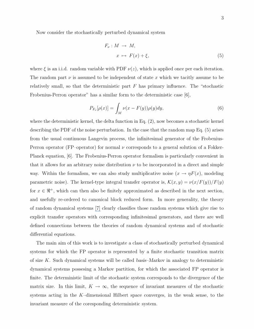
Now consider the stochastically perturbed dynamical system

Fν : M → M,

x 7→ F (x) + ξ, (5)

where ξ is an i.i.d. random variable with PDF ν(z), which is applied once per each iteration.

The random part ν is assumed to be independent of state x which we tacitly assume to be

relatively small, so that the deterministic part F has primary influence. The “stochastic

Frobenius-Perron operator” has a similar form to the deterministic case [6],

PFν[ρ(x)] =

∫

M

ν(x − F (y))ρ(y)dy, (6)

where the deterministic kernel, the delta function in Eq. (2), now becomes a stochastic kernel

describing the PDF of the noise perturbation. In the case that the random map Eq. (5) arises

from the usual continuous Langevin process, the infinitesimal generator of the Frobenius-

Perron operator (FP–operator) for normal ν corresponds to a general solution of a Fokker-

Planck equation, [6]. The Frobenius-Perron operator formalism is particularly convenient in

that it allows for an arbitrary noise distribution ν to be incorporated in a direct and simple

way. Within the formalism, we can also study multiplicative noise (x → ηF (x), modeling

parametric noise). The kernel-type integral transfer operator is, K(x, y) = ν(x/F (y))/F (y)

for x ∈ ℜ+, which can then also be finitely approximated as described in the next section,

and usefully re-ordered to canonical block reduced form. In more generality, the theory

of random dynamical systems [7] clearly classifies those random systems which give rise to

explicit transfer operators with corresponding infinitesimal generators, and there are well

defined connections between the theories of random dynamical systems and of stochastic

differential equations.

The main aim of this work is to investigate a class of stochastically perturbed dynamical

systems for which the FP operator is represented by a finite stochastic transition matrix

of size K. Such dynamical systems will be called basis–Markov in analogy to deterministic

dynamical systems possesing a Markov partition, for which the associated FP operator is

finite. The deterministic limit of the stochastic system corresponds to the divergence of the

matrix size. In this limit, K → ∞, the sequence of invariant measures of the stochastic

systems acting in the K–dimensional Hilbert space converges, in the weak sense, to the

invariant measure of the coresponding deterministic system.

4

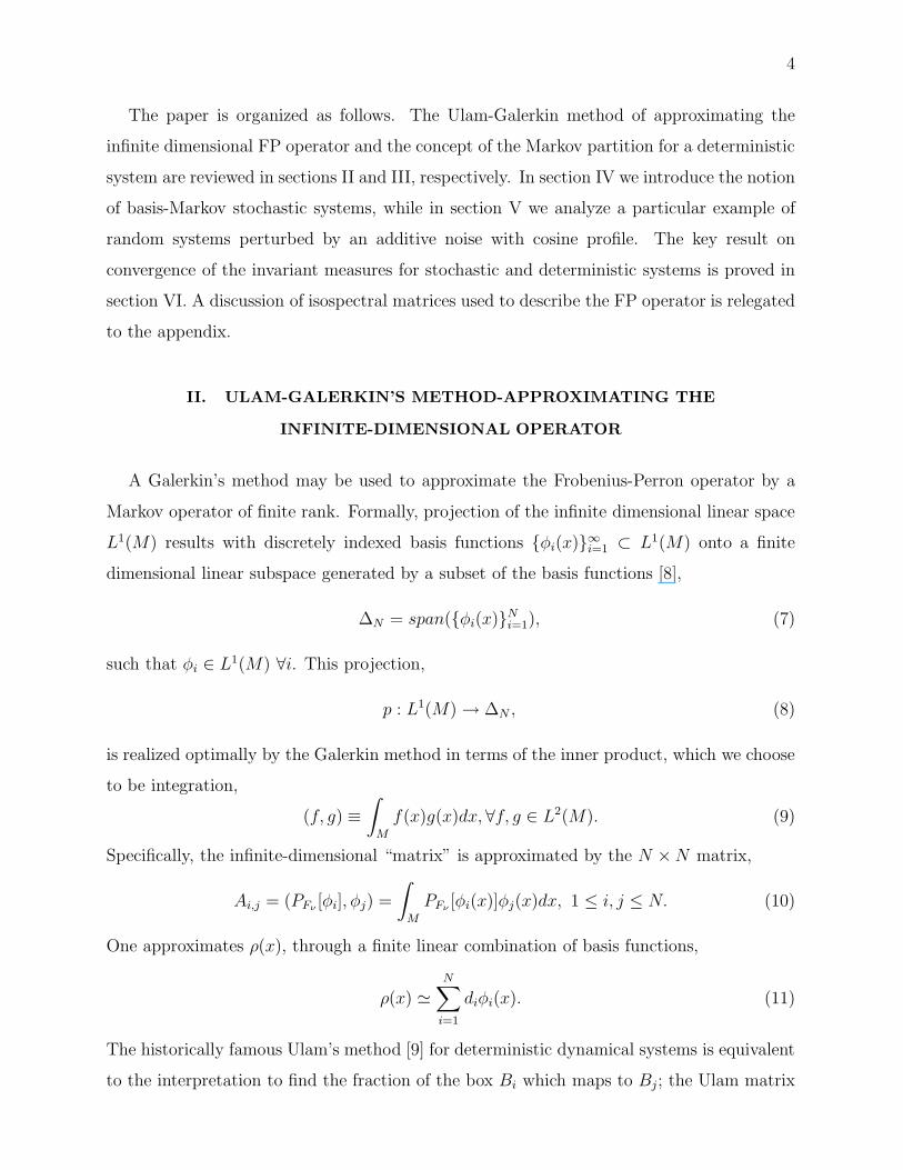
The paper is organized as follows. The Ulam-Galerkin method of approximating the

infinite dimensional FP operator and the concept of the Markov partition for a deterministic

system are reviewed in sections II and III, respectively. In section IV we introduce the notion

of basis-Markov stochastic systems, while in section V we analyze a particular example of

random systems perturbed by an additive noise with cosine profile. The key result on

convergence of the invariant measures for stochastic and deterministic systems is proved in

section VI. A discussion of isospectral matrices used to describe the FP operator is relegated

to the appendix.

II. ULAM-GALERKIN’S METHOD-APPROXIMATING THE

INFINITE-DIMENSIONAL OPERATOR

A Galerkin’s method may be used to approximate the Frobenius-Perron operator by a

Markov operator of finite rank. Formally, projection of the infinite dimensional linear space

L1(M) results with discretely indexed basis functions {φi(x)}∞i=1 ⊂ L1(M) onto a finite

dimensional linear subspace generated by a subset of the basis functions [8],

∆N = span({φi(x)}Ni=1), (7)

such that φi ∈ L1(M) ∀i. This projection,

p : L1(M) → ∆N , (8)

is realized optimally by the Galerkin method in terms of the inner product, which we choose

to be integration,

(f, g) ≡∫

M

f(x)g(x)dx, ∀f, g ∈ L2(M). (9)

Specifically, the infinite-dimensional “matrix” is approximated by the N × N matrix,

Ai,j = (PFν[φi], φj) =

∫

M

PFν[φi(x)]φj(x)dx, 1 ≤ i, j ≤ N. (10)

One approximates ρ(x), through a finite linear combination of basis functions,

ρ(x) ≃N

∑

i=1

diφi(x). (11)

The historically famous Ulam’s method [9] for deterministic dynamical systems is equivalent

to the interpretation to find the fraction of the box Bi which maps to Bj; the Ulam matrix

5

is equivalent to the Galerkin matrix by using Eq. (10) and choosing the basis functions to

be the family of characteristic functions,

φi(x) = 1Bi(x) =

1 if x ∈ Bi

0 else.

(12)

Specifically, we choose the ordered set of basis functions to be in terms of a nested refinement

of boxes {Bi} covering M . Though Galerkin’s and Ulam’s methods are formally equivalent

in the deterministic case, we are of the opinion that the Galerkin description is a more

natural description in the stochastic setting.

III. MARKOV PARTITIONS OF DETERMINISTIC SYSTEMS, AND EXACT

PROJECTION

In this section, we discuss that a Markov partition is special for the Frobenius-Perron

operator of a deterministic dynamical system, in that characteristic functions supported over

those partition elements leads to an exact projection of the FP operator onto an operator

of finite rank - a matrix.

For a one-dimensional transformation of the interval, a Markov partition is defined [2, 3],

Definition: A map of the interval f : [a, b] → [a, b] is Markov if there is a finite partition

{Ij} such that,

1. ∪jIj = [a, b] (covering property),

2. int(Ij) ∩ int(Ik) = ∅ if k 6= k (no overlap property),

3. f(Ij) = ∪kiIki

, (a grid interval maps completely across a union of intervals without

“dangling ends” property).

It is not hard to show that the set of characteristic functions forms a finite basis set of

functions

{φi(x)} = {1Ii(x)}i, (13)

such that Galerkin projection Eq. (10) is exact onto an operator of finite rank, or a matrix

Ai,j. That is, Eq. (10) simplifies,

Ai,j = (PFν[φi], φj) =

∫

M

PFν[φi(x)]φj(x)dx,

6

=

∫

M

∫

M

δ(x − F (y))φi(y)φj(x)dydx

=

∫

Ij

∫

Ii

δ(x − F (y))dydx 1 ≤ i, j ≤ N. (14)

From the definition of the Markov partition, we see that a row of Ai,j accounts that PFν[φi(x)]

is a linear combination of φj(x).

Similarly, there is a well defined notion of an Anosov diffeomorphisms with a Markov

partition [1, 3, 10, 11], and so for such systems, it can be shown that characteristic functions

supported over the corresponding Markov partition creates a basis set such that Eq. (10)

results in an operator of finite rank.

We take these observations as motivation to make the following definition which is meant

to generalize the notion of a Markov partition to stochastic systems:

Definition: Suppose a measure space, {M,B, µ}, and a transformation F : M → M ,

then the transformation is “basis Markov” if there exists a finite set of basis functions

{φi(x)}ni=1 : M → [0, 1] ∈ L1(M) such that the Frobenius-Perron operator is operationally

closed within ∆n, where ∆n = span({φi(x)}ni=1). That is, for any probability measure ρ, its

image PF [ρ(x)] belongs to ∆n.

Remark 1: If a transformation F is basis-set Markov, then if we perform Galerkin’s method,

Ai,j = (PFν[φi], φj)M×M , with that basis set, then it allows that for any initial density which

can be written as a linear combination of these basis functions,

ρ0(x) =n

∑

i=1

ciφi(x), (15)

or stated simply,

ρ0(x) ∈ ∆n, (16)

then the action of the Frobenius-Perron operator on such initial densities, ρ1(x) = PFν[ρ0(x)],

can be exactly represented by the following matrix-vector multiplication:

c′ = A · c, where ρ1(x) =n

∑

i=1

c′iφi(x). (17)

That is, the FP operator projects exactly to an operator of finite rank - a matrix.

Note that for a general finite set of functions, if we take a general linear combination

of those functions and then apply the Frobenius-Perron operator, we do not expect the

resulting density can be written as a (finite) linear combination of basis functions.

7

The following is a direct consequence of our definition of basis Markov in relationship

to the usual definition of a Markov map, stating the sense in which basis Markov is a

generalization:

Remark 2: Given a Markov map, then Eq. (14) implies that any Markov map, together

with the characteristic functions supported over the partition elements, is basis Markov.

IV. BASIS MARKOV STOCHASTIC SYSTEMS: A GENERAL CASE DUE TO

SEPARABLE NOISE

We analyze a dynamical system defined on an interval M = [0, 1] with both ends identified

and subjected to a specific form of the additive noise,

x′ = f(x) + ξ . (18)

To specify the special case of the stochastic dynamical system written in Eq. (5), the stochas-

tic perturbation will be characterized by the probability P(x, y) of a transition form point

x to y induced by noise. Describing the dynamics in terms of a probability density ρ(x) its

one-step evolution is governed by the stochastic Frobenius-Perron (FP) operator,

ρ′(y) = Pf(ρ(y)) =

∫

P(f(x), y)ρ(x)dx. (19)

We will denote this stochastic Frobenius-Perron operator by the symbol Pf , in all that

follows. The operator Pf acts on every probability measure defined on M and in general, it

cannot be represented by a finite matrix. However, in the sequel we shall analyze a certain

class of noise profiles for which such a representation is possible.

We assume that the transition probability P(x, y) satisfies the following properties [12,

13]:

a) P(x, y) ≡ P(x − y) = P(ξ),

b) P(x, y) ≡ P(x mod 1, y mod 1),

c) P(x, y) =

N∑

m,n=0

Amn un(x) vm(y), (20)

for x, y ∈ R and an arbitrary finite N . Property a) assures that the distribution of the

random variable ξ does not depend on the position x, while the periodicity condition is

8

provided in b). A noise profile fulfilling the latter property c) is called separable (decom-

posable), and it allows us to represent the dynamics of an arbitrary the system with such a

noise in a finite dimensional Hilbert space. Here A = (Amn)m,n=0,...,N is a yet undetermined

real matrix of expansion coefficients. Note that A characterizes the noise and does not de-

pend on the deterministic dynamics f . We assume that the functions un; n = 0, . . . , N and

vm; m = 0, . . . , N are continuous in X = [0, 1) and linearly independent, so we can express

f ≡ 1 as their linear combinations. Both sets of functions span bases in an N + 1 Hilbert

space. Their orthogonality is not required.

This name “separable noise” is concocted in an analogy to separable states in quantum

mechanics and separable probability distributions, since such a property was called N + 1-

separability by Tucci [14]. Making use of this crucial feature of the noise profile we may

expand the kernel of the Frobenius–Perron operator (19),

ρ′(y) = Pf(ρ(y)) =

∫ 1

0

N∑

m,n=0

Amnun(f(x))vm(y)ρ(x)dx (21)

=

N∑

m,n=0

Amn

[

∫ 1

0

un(f(x))ρ(x)dx]

vm(y) (22)

=N

∑

n=0

[

∫ 1

0

un(f(x))ρ(x)dx]

vn(y)

for y ∈ X, where,

vn =

N∑

m=0

Amnvm. (23)

Thus, any initial density is projected by the FP–operator Pf into the vector space spanned

by the functions vm; m = 0, . . . , N .

Assuming that a given density ρ(x) belongs to this space, we can be expand it in this

basis,

ρ(x) =

N∑

m=0

qm vm(x) . (24)

Expanding ρ′ in an analogous way we will describe it by the vector ~q′ = {q′0, . . . , q′N}.

Let B denotes a matrix of integrals,

Bnm =

∫ 1

0

un(f(x))vm(x)dx, (25)

where n, m = 0, . . . , N . Observe that B depends directly on the system f and on the noise

via the basis functions u and v. Making use of this matrix, the one–step dynamics (23) may

9

be rewritten in a matrix form

q′n =

N∑

m=0

Dnm qm, where D = BA (26)

and A is implied by (20). In this way we have arrived at a representation of the Frobenious–

Perron operator Pf by a matrix D of size N + 1 × N + 1, the elements of which read,

Dnm =

∫ 1

0

un(f(x))vm(x)dx, n, m = 0, . . . , N. (27)

Although the probability is conserved under the action of Pf , the matrix D need not be

stochastic. This is due to the fact that the functions {vm(x)} forming the expansion basis

in (24) were not normalized. We shall then compute their norms,

τm =

∫ 1

0

vm(y)dy =

N∑

n=0

Amnbn (28)

where,

bn =

∫ 1

0

vn(y)dy. (29)

Let K ≤ N + 1 denote the number of non-zero components of the vector ~τ and let k =

1, . . . , K runs over all indexes n ∈ 0, . . . N + 1, for which τk 6= 0. Then the rescaled vectors,

Vk(y) := vk(y)/τk, (30)

are normalized,∫ 1

0

Vk(y)dy = 1. (31)

The normalization condition∫ 1

0ρ(x)dx = 1 implies

∫ 1

0

N∑

m=0

qlvm(x)dx =

N∑

m=0

qmτm =

K∑

k=1

qkτk = 1 (32)

The same is true for the transformed density,

∑

k

q′kτk = 1. (33)

Hence this scalar product is preserved during the time evolution. Making use of the rescaled

coefficients

ck := qkτk, (34)

10

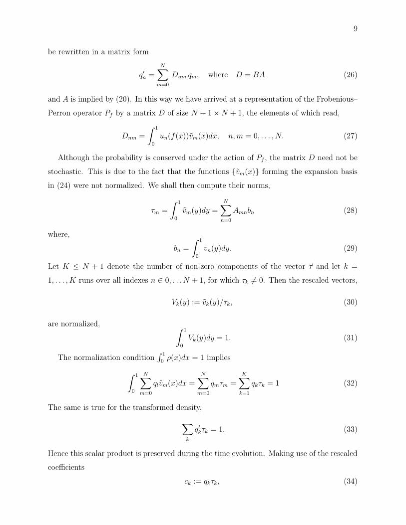
FIG. 1: The cosine noise of Eq. (37) closely resembles a normal noise profile, but with finite support.

Several values of N are shown, with decreasing standard deviation with increasing N .

the dynamics (26) reads

c′k = q′kτk =∑

j

Dkj qjτk =∑

j

Dkjτk

τj

qjτj =:∑

j

Tkj cj . (35)

The coefficients ck sum to unity, so the transition matrix

Tkj ≡ Dkjτk

τj=

∑

ii′

DkjAkiτi

Aji′τi′. (36)

is stochastic. In the above equation, all indices run from 1 to K and the coefficients τk

are non-zero by construction. Hence the dynamics (26) effectively takes place in an K-

dimensional Hilbert space, and the Frobenious–Perron operator Pf is represented by a

stochastic matrix T is of size K × K. The dimensionality K ≤ N + 1 is determined by

the parameter N and the choice of the basis functions {vl(x)} entering (20).

V. A SPECIAL CASE: COSINE NOISE

We will now discuss a particularly simple case of the separable noise described above,

introduced in [12]. Let,

PN (ξ) = CN cosN(πξ) , (37)

11

where N is even (N = 0, 2, . . .) and with the normalization constant,

CN =√

πΓ[N/2 + 1]

Γ[(N + 1)/2]. (38)

See Fig. 1, in which we can see the decreasing standard deviation with respect to increasing

N , and it can be seen that this type of noise reminds of a normal distribution, but of compact

support.

The parameter N controls the strength of the noise measured by its variance

σ2 =1

2π2Ψ′(

N

2+ 1) =

1

12− 1

2π2

N/1∑

m=1

1

m2, (39)

where Ψ′ stands for the derivative of the digamma function.

For the expansion (20) we use basis functions,

um(x) = cosm(πx) sinN−m(πx),

vn(y) = cosn(πy) sinN−n(πy), (40)

where x ∈ X and m, n = 0, . . . , N . Expanding cosine as a sum to the N -th power in (37)

we find that the (N + 1) × (N + 1) matrix A defined by (20) is diagonal,

Amn = amδmn, with am = CN

(

N

m

)

. (41)

Integrating trigonometric functions we find the coefficients,

bm =

∫ 1

0

sinm(πx) cosN−m(πx)dx =2

πN

Γ[(m + 1)/2] Γ[(N − m + 1)/2]

Γ(N/2), (42)

and,

τm = ambm, (43)

which are non-zero only for even values of m. Hence the size K ×K of the transition matrix

reads,

K = N/2 + 1, (44)

and the expression (36) takes the form

Tkj = Dmnambm

anbn

where k, j = 1, . . . , K; m = 2(k − 1), n = 2(j − 1) . (45)

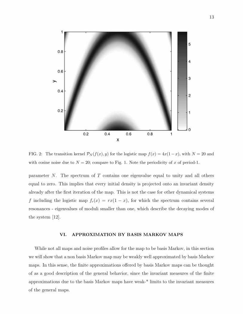
We find in the cosine noise Eq. (37) and with basis Eqs. (40), that the transition kernel

reminds of a fuzzy but periodically repeated version of the map. See Fig. 2. However, the

12

Frobenius-Perron operator embeds to a transition matrix T , which “appears” roughly as a

different form of the original map. See Fig. 3. However, with zero-noise, an Ulam transition

matrix approximating the Frobenius-Perron operator would appear as the deterministic map.

For this reason, we define the limit of T matrices as K → ∞ to be a singular limit of the

Frobenius Perron operators, and associated the associated transformations.

There is an interesting correspondence between the spectrum of eigenvalues of the two

matrices D and T . Since T is stochastic its largest eigenvalue is equal to unity. Moreover, it

is the only eigenvalue with modulus one, which follows from the fact that the kernel P(x, y)

vanish only for x − y = 1/2 (mod 1), and the two–step probability function is everywhere

positive,∫

P(x, z)P(z, y)dy > 0, for x, y ∈ X. (46)

See [6], Th. 5.7.4. A particularly useful consequence and simplification is that the eigenstate

corresponding to the largest eigenvalue of the matrix represents the invariant density of the

system, ρ∗ = Pf(ρ∗); this can be easily found numerically by diagonalizing T .

All of the other eigenvalues are included inside the unit circle and their moduli |λi|characterize the decay rates. It is worth emphasizing that the spectra of both matrix repre-

sentations of the FP-operator - by matrices D of size (N + 1)× (N + 1) used in [12, 13, 15]

and the stochastic T matrices of size (N/2 + 1)× (N/2 + 1), developed here, coincide up to

the additional N/2 eigenvalues which are equal to zero – see the Appendix for details.

For concreteness let us discuss an exemplary 1-D dynamical system, a tent map:

f(x) :=

2x if 0 ≤ x ≤ 1/2

2(1 − x) if 1/2 ≤ x ≤ 1 .(47)

Simple integration allows us to obtain analytic form of the transition matrix T (N) for the

tent map (47) perturbed by additive noise characterized by small values of N ,

T (2) =1

2

1 1

1 1

, T (4) =1

24

11 3 11

6 6 6

7 15 7

, T (6) =1

320

145 25 25 145

69 45 45 69

51 75 75 51

55 175 175 55

. (48)

In the simplest case N = 2 the transition matrix is bistochastic, but it is not so for larger

N . However, for this system, the matrix T (N) is of rank one for arbitrary value of the noise

13

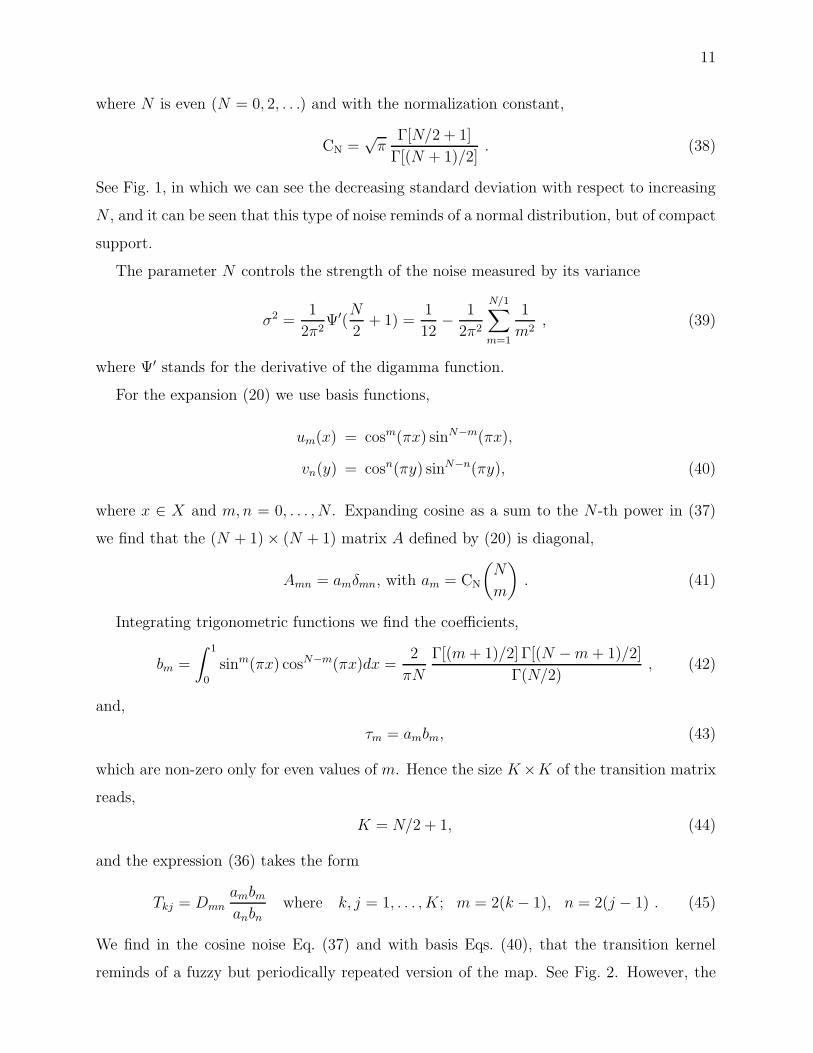
FIG. 2: The transition kernel PN (f(x), y) for the logistic map f(x) = 4x(1−x), with N = 20 and

with cosine noise due to N = 20; compare to Fig. 1. Note the periodicity of x of period-1.

parameter N . The spectrum of T contains one eigenvalue equal to unity and all others

equal to zero. This implies that every initial density is projected onto an invariant density

already after the first iteration of the map. This is not the case for other dynamical systems

f including the logistic map fr(x) = rx(1 − x), for which the spectrum contains several

resonances - eigenvalues of moduli smaller than one, which describe the decaying modes of

the system [12].

VI. APPROXIMATION BY BASIS MARKOV MAPS

While not all maps and noise profiles allow for the map to be basis Markov, in this section

we will show that a non basis Markov map may be weakly well approximated by basis Markov

maps. In this sense, the finite approximations offered by basis Markov maps can be thought

of as a good description of the general behavior, since the invariant measures of the finite

approximations due to the basis Markov maps have weak-* limits to the invariant measures

of the general maps.

14

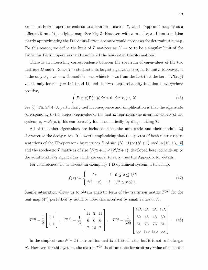
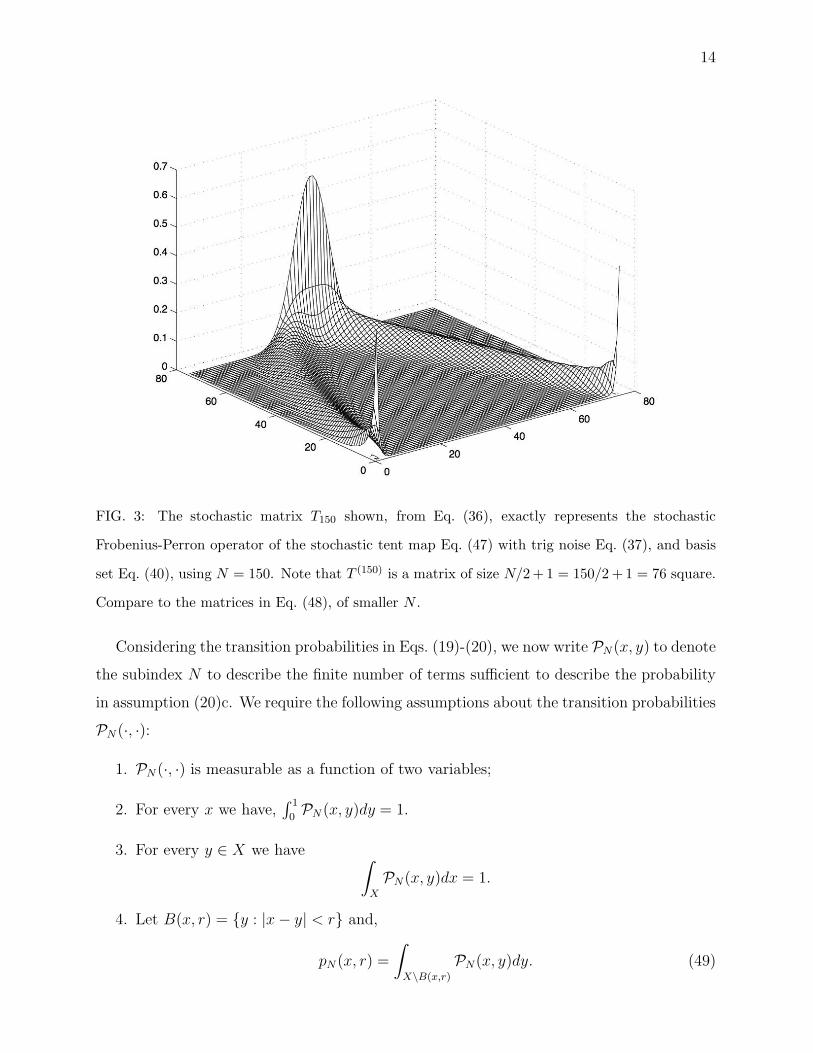
FIG. 3: The stochastic matrix T150 shown, from Eq. (36), exactly represents the stochastic

Frobenius-Perron operator of the stochastic tent map Eq. (47) with trig noise Eq. (37), and basis

set Eq. (40), using N = 150. Note that T (150) is a matrix of size N/2 + 1 = 150/2 + 1 = 76 square.

Compare to the matrices in Eq. (48), of smaller N .

Considering the transition probabilities in Eqs. (19)-(20), we now write PN(x, y) to denote

the subindex N to describe the finite number of terms sufficient to describe the probability

in assumption (20)c. We require the following assumptions about the transition probabilities

PN (·, ·):

1. PN (·, ·) is measurable as a function of two variables;

2. For every x we have,∫ 1

0PN (x, y)dy = 1.

3. For every y ∈ X we have∫

X

PN(x, y)dx = 1.

4. Let B(x, r) = {y : |x − y| < r} and,

pN (x, r) =

∫

X\B(x,r)

PN(x, y)dy. (49)

15

Then, for any r > 0,

pN(r) = supx∈X

pN(x, r) → 0, as N → +∞.

Assumptions 1-3 are typical for probability measures, while assumption 4 is also rather

mild, and it is easy to check that all four assumptions are satisfied by the cosine noise

Eq. (37).

Under these assumptions, the following is true:

Proposition: For any ρ ∈ L1(X) we have

∫

X

ρ(x)PN (x, y)dx → ρ(y), as N → ∞ (50)

in L1(X).

Proof: Let us assume that ρ is uniformly continuous and let us fix an ε > 0. We can find

an r > 0 such that |ρ(x) − ρ(y)| < ε whenever |x − y| < r. We have

∫

X|ρ(y) −

∫

Xρ(x)PN (x, y)dx|dy =

(assumption (3)) =∫

X|∫

Xρ(y)PN(x, y)dx−

∫

Xρ(x)PN (x, y)dx|dy

≤∫

X

∫

X|ρ(y) − ρ(x)|PN (x, y)dxdy

=∫ ∫

{(x,y):|x−y|<r}|ρ(y) − ρ(x)|PN (x, y)dxdy

+∫ ∫

{(x,y):|x−y|≥r}|ρ(y) − ρ(x)|PN (x, y)dxdy

≤ ε · 1 + 2 · (maxX |ρ|) · pN(r). (51)

The last estimate can be made arbitrarily small in view of assumption (4).

Once the convergence is proven for uniformly continuous functions, the proof of conver-

gence for general L1(X) functions is standard:

Since the natural norm of the operator PPN(ρ)(y) =

∫

Xρ(x)PN (x, y)dx in L1(X) is 1, we

have

‖ρ − PPN(ρ)‖ ≤ ‖ρ − ρc‖ + ‖ρc − PPN

(ρc)‖ + ‖PPN(ρc) − PPN

(ρ)‖

≤ ‖ρ − ρc‖ + ‖ρc − PPN(ρc)‖ + ‖PPN

‖‖ρc − ρ‖

≤ 2‖ρ − ρc‖ + ‖ρc − PPN(ρc)‖, (52)

16

where ρc is a uniformly continuous approximation of ρ. �

We will say that the transformation f : [0, 1] → [0, 1] preserves continuity iff for any

continuous function ρ the composition ρ ◦ f is also continuous. Obviously any continuous

transformation f preserves continuity. There are discontinuous maps which also preserve

continuity, e.g., f(x) = kx− Int(kx), for integer k ≥ 2. We now confirm the following result,

stated in the language of our current problem,

Theorem: 1. Let the transformation f be continuity preserving. Under the assumptions

(1), (2), and (4), it follows that if µN is an invariant measure of the stochastic perturbation

of transformation f defined by the transition probability PN , then every weak-∗ limit point

of the set {µN : N ≥ 1} is an f -invariant measure.

Proof: This theorem can be proved following the ideas from, R.Z. Khasminskii, [16]. Let

us assume that µN → µ weakly as N → +∞. We want to show that µ is f -invariant. To

this end it is enough to show that∫

X

ρdµ =

∫

X

ρ(f)dµ,

for any continuous function ρ. The stochastic perturbation of f defined by transition prob-

ability PN acts on continuos functions as a compositions with f followed by application of

the operator P ∗PN

, defined as follows

(P ∗PN

ρ)(x) =

∫

X

ρ(y)PN(x, y)dy.

This operator is conjugated to the operator PPNdefined in the proof of the previous theorem.

P ∗PN

acts on functions, while PPNacts on functions understood as densities. Thus,

∫

X

ρdµN =

∫

P ∗PN

(ρ(f))dµN ,

for any continuous function ρ. Using assumption (4) we obtain

|ρ(x) − (P ∗PN

ρ)(x)|

= |∫

Xρ(x)PN (x, y)dy −

∫

Xρ(y)PN(x, y)dy|

≤∫

{y:|y−x|<r}|ρ(x) − ρ(y)|PN(x, y)dy +

∫

{y:|y−x|≥r}|ρ(x) − ρ(y)|PN(x, y)dy

≤ ε + 2 · (maxX |ρ|) · pN(r),

where ε and r are as in the proof of the previous theorem. This shows that P ∗PN

(ρ) converges

uniformly to ρ for any continuous function ρ as N → +∞.

17

We have

|∫

Xρdµ −

∫

Xρ(f)dµ| ≤ |

∫

Xρdµ −

∫

XρdµN |

+|∫

XρdµN −

∫

P ∗PN

(ρ(f))dµN | + |∫

P ∗PN

(ρ(f))dµN −∫

Xρ(f)dµN |

+|∫

Xρ(f)dµN −

∫

Xρ(f)dµ|

The first and the last differences converge to 0 since µN converge ∗-weakly to µ. The second

difference is 0 by the definition of µN . The third difference converges to 0 by the uniform

convergence established just before. This proves Theorem 1. �

In this way we have established a relation between a sequence of noisy systems fN and

the deterministic dynamical system f . A stochastic system (18) with the noise profile (37)

for a fixed noise parameter N is described by a stochastic matrix T (N) of size K = N/2 + 1

and acts in the Hilbert space HK .

We have shown that the sequence of stochastic matrices T (N), corresponds to the dynam-

ical system f , in a sense that the sequence µN of the invariant measures of T (N) converge

weakly to the f -invariant measure µ in the deterministic limit N → ∞. Furthermore, for

any initial density ρ the sequence of vectors ρ′N transformed by fN converges weakly to the

density transformed by the Frobenious–Perron operator associated with f . Observe that

the above property holds not only for one-dimensional systems, but also dynamical system

f in higher dimensional measure spaces.

VII. CONCLUDING REMARKS

In this work we have introduced the concept of basis–Markov stochastic systems, for

which the associated Frobenius–Perron operator is finite. This property resembles the class

of deterministic systems with a Markov partition. However, the Markov partition is char-

acteristic to a very special class of deterministic systems, while the basis–Markov property

is related to the kind of stochastic perturbation. It holds for any deterministic system f ,

subjected to an additive noise with a profile satisfying the separability condition (20). In

this way such a random dynamical system can be described by a stochastic transition matrix

of a finite size K, which diverges in the deterministic limit.

We have shown an intimate relationship between the sequence of stochastic matrices

which act in the space of K–point probability distributions and the FP operator Pf of

18

the deterministic system, which acts in the infinite dimensional space: In the deterministic

limit K → ∞ the invariant densities of stochastic matrices converge in a weak sense to the

invariant measure of the deterministic system f . Thus constructing the transition matrices T

and decreasing the noise strength (and increasing the dimensionality K) one may construct

arbitrary approximations of the FP operator Pf .

Note that the described method of finding an approximate invariant density of a de-

terministic system by applying a weak noise is not restricted to one dimensional systems.

On the contrary, the entire construction can be directly applied for a general case of multi–

dimensional dynamical systems. In particular, the definition (20)c of separable noise profiles

works for the case of an L–dimensional systems, provided the variables x and y represent

vectors with L components each.

If the dynamical system acts on the L–torus for example, M = [0, 1]L, one can take the

Cartesian product of the cosine noise (37) setting

PN (ξ1, . . . ξL) = CLN cosN(πξ1) cosN(πξ2) · · cosN(πξL) , (53)

where ξk = xk − yk and k = 1, . . . , L. This form of the additive noise was used in [15] to

analyze a 2-dimensional system (a variant of the baker map), and to compare the spectral

properties of the FP operator associated with the classical stochastic system with properties

of the propagator of the corresponding quantum evolution. In such a case the deterministic

limit of the classical noisy system, K → ∞ is related to the classical limit, ~ → 0, of the

corresponding quantum dynamics.

Note that for basis–Markov stochastic systems, the transition matrices T exactly describe

the action of the dynamical system with additive noise on densities. Thus our construction

differs from an approach applied in [17, 18, 19], were a finite dimensional description of

the density dynamics of a deterministic system was achieved by truncation of an infinite

transition operator Pf to the finite dimension K. The effect of such a truncation may also

be regarded as a kind of noise depending on the matrix size K and the base, in which Pf

is represented. On the other hand, in our case a suitable choice of the noise profile added

to the deterministic system distinguishes a relevant basis, in which the FP operator of the

perturbed system is finite.

19

VIII. ACKNOWLEDGMENTS

E. B. was supported by the National Science Foundation under grants DMS-0404778

while K. Z. acknowledges a partial support by the grant number 1 P03B 042 26 of Polish

Ministry of Science and Information Technology.

IX. APPENDIX: ISOSPECTRAL MATRICES

In this appendix we show that the matrix D defined by Eq. (27) and used in [12, 13, 15]

to represent the Frobenius-Perron operator and the stochastic transition matrix T share the

same non-zero part of the spectrum. We make use of a following algebraic result,

Lemma. Let A be a square matrix of size N ×N and ~s a vector of length N containing

only non-zero entries. Then the matrix

Bjk ≡ Ajksj

sk

, (54)

has the same spectrum as A.

(there is no summation over repeating indices).

Proof: To study equation det(B − λ1) = 0 we start analyzing an exemplary term P B

of the determinant. It consists of a product of N elements Bi,σ(j), where σ(i) stands for a

certain permutation of the indeces. The product of N factors of the type si/sσ(i) is equal to

unity, so that

P Bσ =

∏

i

Bi,σ(i) =∏

i

Bi,σ(i)s1s2 · · · sN

s1s2 · · · sN=

∏

i

Ai,σ(i) . (55)

Thus every term contributing to the free coefficient of the characteristic equation will be the

same, P Bσ = P A

σ , hence these coefficients for both matrices A and B are equal. Since the

diagonal elements of both matrices coincide, Bjj = Ajj, all terms forming the coefficients

standing by an arbitrary power of λ are the same for both matrices. Therefore characteristic

equations for both matrices are equal and so are their spectra. �.

Treating all non-zero elements of the vector τk, k = 1, . . . , K as vector ~s we may apply

the lemma to equation (36) and obtain equivalence of the spectrum of T and the non-zero

part of the spectrum of D. Since integrals (25) vanish for odd values of m, every second

20

column of D is equal to zero, and the remaining N/2 eigenvalues of D are equal zero.

[1] R. Bowen, Equilibrium States and the Ergodic Theory of Anosov Diffeomorphisms, Springer-

Verlag, Berlin 1975.

[2] A. Boyarsky and P. Gora, Laws of chaos: invariant measures and dynamical systems in one

dimension, Birkhauser, Boston, 1997.

[3] E. Bollt, J. Skufca, “Markov Partitions,” Encyclopedia of Nonlinear Science, invited

short, Editor, Alwyn Scott, Fitzroy Dearborn Publishers, to appear (2003). Available at

http://www.clarkson.edu/∼bolltem

[4] B.P. Kitchens, Symbolic Dynamics, One-sided, Two-sided and Countable State Markov Shifts,

Springer (New York, 1998).

[5] R. Fischer, Sofic Systems and Graphs, Monatsh. Math. 80 (1975), 179-186.

[6] A. Lasota, M.C. Mackey, Chaos, fractals, and noise, 2nd Ed. (Springer-Verlag, New York,

1994).

[7] L. Arnold, Random Dynamical Systems, Springer-Verlag, New York, 1998.

[8] T.-Y. Li, “Finite Approximation for the Frobenius-Perron Operator. A Solution to Ulam’s

Conjecture,” J. Approx.Th. 17, 177-186 (1976).

[9] S. Ulam, Problems in Modern Mathematics, Interscience Publishers, (New York, NY, 1960).

[10] C. Robinson, Dynamical Systems, Stability, Symbolic Dynamics, and Chaos, 2nd, CRC Press,

(1999).

[11] J. Guckenheimer, P. Holmes, Nonlinear Oscillations, Dynamical Systems, and Bifurcations of

Vector Fields, Springer (1991).

[12] A. Ostruszka, P. Pakonski, W. S lomczynski, and K. Zyczkowski, “Dynamical entropy for

systems with stochastic perturbations”, Phys. Rev. E, 62 2 2018-2029 (2000).

[13] A. Ostruszka, K. Zyczkowski, “Spectrum of Frobenius-Perron operator for systems with

stochastic perturbation,” Phys. Lett. A 289 306-312 (2001).

[14] R. R. Tucci, Entanglement of Formation and Conditional Information Transmission, preprint

quant-ph/0010041 (2000).

[15] A. Ostruszka, Ch. Manderfeld, K. Zyczkowski, and F. Haake, ”Quantization of Classical Maps

with tunable Ruelle-Pollicott Resonances”, Phys. Rev. E 68, 056201 (2003)

21

[16] R.Z. Khasminskii, ”Ergidicheskie svoistva vozvratnykh diffuzionnykh protsessov...”, Teoria

Veroyat. i yeye Prim. 5, No. 2, (1960), 196–214.

[17] M. Khodas, S. Fishman, Relaxation and Diffusion for the Kicked Rotor Phys. Rev. Lett. 84

2837 (2000).

[18] J. Weber, F. Haake, P. A. Braun, C. Manderfeld and P. Seba, Resonances of the Frobenius-

Perron Operator for a Hamiltonian Map with a Mixed Phase Space J. Phys. A 34 7195 (2001).

[19] S. Nonnenmacher, Spectral properties of noisy classical and quantum propagators Nonlinearity

16, 1685-1713 (2003).