redacted_ - DSpace@MIT - Massachusetts Institute of ...

Multi-Echelon Inventory Strategies for a Retail Replenishment Business Modelby

Benjamin M. PolakB.S. Physics, Haverford College, 2007

Submitted to the MIT Sloan School of Management and the Mechanical Engineering Department inPartial Fulfillment of the Requirements for the Degrees of

Master of Business Administrationand

Master of Science in Mechanical Engineering

In conjunction with the Leaders for Global Operations Program at theMassachusetts Institute of Technology

June 2014

MASSACH Ir W1IJEOF TECHNOWGY

JUN 18 201

LIBRARIES@ 2014 Benjamin M. Polak. All right reserved.

The author hereby grants to MIT permission to reproduce and to distribute publicly paper and electroniccopies of this thesis document in whole or in part in any medium now known or hereafter.

Signature of Author Signature redactedMIT Sloan School of Management

MIT Department of Mechanical Engineering

May 9th, 2014Certifed bySignature redacted_Certified by 0 tE a 2 ad

Stephen Graves, Thesis Supervisor

Professor of Management Science, MIT Sloan School of Management

Signature redactedCertified by

Certified by

I David Simchi-Levi, Thesis Supervisor

Professor of Engineering Systems, Engineering Systems Division

Signature redacted-'David E. Hardt, Chair

Mechanical Engineering Committee on Graduate Students

Signature redacted-Accepted by

David E. Hardt, Chair

Mechanical Engineering Committee on Graduate Students

Signature redactedAccepted by

Mau a Herson, Director of MIT Sloan MBA Program

MIT Sloan School of Management

-1"

This page intentionally left blank.

2

Multi-Echelon Inventory Strategies for a Retail Replenishment Business Model

by

Benjamin M. Polak

Submitted to the MIT Sloan School of Management and the MIT Department of MechanicalEngineering on May 9th, 2014 in Partial Fulfillment of the Requirements for the Degrees of

Master of Business Administration and Master of Science in Mechanical Engineering

Abstract

The mission of the Always Available retail replenishment business at NIKE is to ensureconsumer-essential products are in-stock at retailers at all times. To achieve this goal, NIKEhas developed a forecast-driven, make-to-stock supply chain model which allows retailersto place weekly orders to an on-hand inventory position in a distribution center. Thechallenge facing the business is how to design an inventory strategy that achieves a highlevel of service to its customers while minimizing inventory holding cost. Specifically, safetystock holding cost is targeted as it accounts for the majority of on-hand inventory and canbe reduced without significantly impacting the underlying supply chain architecture.

This thesis outlines the application of multi-echelon inventory optimization in a retailreplenishment business model. This technique is used to determine where and how muchsafety stock should be staged throughout the supply chain in order to minimize safety stockholding cost for a fixed service level. Provided a static supply chain network, the ideal safetystock locations and quantities which result in minimal total safety stock holding cost isdetermined. For this business, the optimal solution is to stage lower-cost componentmaterials with long supplier lead times and high commonality across multiple finishedgoods at the manufacturer in addition to finished goods at the distribution centers. Safetystock holding cost reduction from component staging increases significantly when thedistance between manufacturers and the distribution center decreases and for thosefactories producing a variety of finished goods made from the same component materialsdue to inventory pooling. Forecast accuracy drives the quantity of safety stock in thenetwork. The removal of low volume, highly unpredictable products from the portfolioyields significant inventory holding cost savings without a detrimental impact to revenue.By deploying the optimal safety stock staging solution and by removing unpredictableproducts, this analysis shows that finish goods safety stock inventory would be reduced by35% for the modeling period (calendar year 2012) while only decreasing topline revenueby 5%.

Thesis Supervisor: Stephen GravesTitle: Professor of Management Science, MIT Sloan School of Management

Thesis Supervisor: David Simchi-LeviTitle: Professor of Engineering Systems, Engineering Systems Division

3


4

Acknowledgments

I would like to extend my sincerest gratitude to NIKE and the entire Always

Available team for providing me with an incredible experience. Never have I been a

part of an organization so willing to accept new ideas and to challenge the status

quo. I will treasure my time with this team for the rest of my career. I would

especially like to thank my truly incredible project coaches, Silvana Bonello and Brie

Davidge, for their unwavering support and mentorship throughout the project. I

would also like to thank my project sponsor, Susan Brown, for championing this

initiative and ensuring that this work will live in the organization. I would like to

acknowledge Dr. Hugo Mora, Craig Frankland, Lucas DeBrito, Luciano Luiz and Ben

Thomson for their patience and guidance throughout this project. And thank you to

my LGO classmates and fellow NIKE interns, Tacy Napolilo and Jane Guertin, for

sharing your expertise and friendship throughout our internships.

I would also like to thank the Leaders for Global Operations program at MIT for

providing me with absolutely incredible opportunities and experiences these past

two years. The knowledge and skills I have gained from this amazing community

will be with me forever. Additionally, I am gracious for the mentorship and

guidance of my advisors, Dr. Stephen Graves and Dr. David Simchi-Levi.

This thesis is dedicated to my parents, Michael and Barbara Polak. Throughout my

life you set lofty goals for me and provided me with the love and support I needed to

achieve them. I owe all of my successes to you.

5


6

Table of Contents

A bstract ........................................................................................................................................ 3

A cknow ledgm ents.............................................................................................................. 5

Table of Contents ...................................................................................................................... 7

List of Figures............................................................................................................................. 8

1 Introduction.................................................................................................................... 101.1 Overview of NIKE, Inc....................................................................................................... 101.2 Problem Statem ent........................................................................................................... 111.3 Project Goals ....................................................................................................................... 121.4 Project Approach............................................................................................................ 131.5 Thesis Overview ................................................................................................................. 14

2 Supply Chain O perations at NIK E ......................................................................... 152.1 Overview of NIKE Business M odels............................................................................. 17

2.1.1 Futures Business M odel....................................................................................................... 172.1.2 Alw ays Available Business M odel ................................................................................... 192.1.3 Quick Turn and Custom Business M odels.........................................................................20

2.2 Overview of NIKE Supply Chain.................................................................................... 212.3 Distinct Features of the Always Available Supply Chain................................ 23

3 Literature Review ..................................................................................................... 253.1 Safety Stock.......................................................................................................................... 253.2 Multi-Echelon Inventory Optimization Techniques .......................................... 27

4 H ypothesis....................................................................................................................... 28

5 Multi-Echelon Inventory Optimization - Concept Model............................ 295.1 Inventory M odeling ...................................................................................................... 29

5.1.1 Inputs and Assum ptions....................................................................................................... 305.1.2 M ethodology..................................................................................................................................32

5.2 M odel Im plem entation................................................................................................. 355.3 M odel Results...................................................................................................................... 365.4 M odel Lim itations ........................................................................................................ 42

6 Scaled Multi-echelon Inventory Optimization................................................. 426.1 Supply Chain Guru Overview ..................................................................................... 426.2 Supply Chain Guru Im plem entation ...................................................................... 436.3 M odel Results...................................................................................................................... 466.4 M odel Validation ........................................................................................................... 50

7 K ey Results and Recom m endations .................................................................... 517.1 Staging Com ponent M aterials................................................................................... 517.2 Reduction in Forecast Error ...................................................................................... 537.3 Recom m endations ........................................................................................................ 56

7.3.1 Current State Recom m endations................................................................................... 567.3.2 Future State Recom m endations...................................................................................... 56

8 Im plem entation M ethodology............................................................................... 59

7

8.1 Align Product Selection and Sourcing Strategies............................................... 608.2 Broader Applications................................................................................................... 618.3 Additional Areas of Analysis ..................................................................................... 62

9 Sum m ary and Conclusion...................................................................................... 64

10 A ppendices...................................................................................................................... 6610.1 Appendix A: Excel Multi-Echelon Inventory Optimization Model ............... 6610.2 Appendix B: Iterations of Multi-echelon Inventory Optimization Model .... 68

11 R eferen ces ....................................................................................................................... 69

List of FiguresFigure 1: NIKE Inc.'s Total Revenue by Geography .......................................................... 11Figure 2: Percent of NIKE Brand Revenue by Product Engine......................................16Figure 3: Percent of NIKE Brand Revenue by Category................................................. 17Figure 4: Representative Always Available Products.......................................................19Figure 5: NIKE Supply Chain Macro-level Structure for Athletic Training Shorts......21Figure 6: NIKE Always Available Supply Chain Macro-level Structure ..................... 24Figure 7: Node Structure of Standard Always Available Supply Chain......................33Figure 8: Demand and Supply Attributes of Athletic Shorts .......................................... 35Figure 9: Key Inventory Tradeoff Scenarios........................................................................ 38Figure 10: Monthly Safety Stock Holding Cost for North America by Staging Scenario

................. ...... ... ... ........ ......... ... ...... ...... ........ .. ............................................... 4 7Figure 11: Monthly Safety Stock Holding Cost for Europe by Staging Scenario..........47Figure 12: DC Safety Stock Days of Supply for North America by Staging Scenario.. 48Figure 13: DC Safety Stock Days of Supply for Europe by Staging Scenario............. 49Figure 14: Safety Stock Reduction as a Function of Lead Time for North America ... 52Figure 15: Histogram of Forecast Error CoV for Products in North America .......... 55Figure 16: Impact on Revenue and North America DC Safety Stock by Excluding

Products w ith CoV > 1.0..................................................................................................... 55

8


9

1 Introduction

The purpose of this thesis is to describe the application of multi-echelon inventory

optimization methodologies to a global apparel retail replenishment business. This

research was conducted in conjunction with NIKE, Inc. (NIKE), a world leader in

athletic apparel, footwear, equipment and accessories. This introductory chapter

provides the necessary context for the reader to understand subsequent analysis,

findings and recommendations. A synopsis of NIKE and the specific challenge

addressed by this research, an overview of the goals and approach used, and a

summary of the subsequent chapters of the thesis are presented.

1.1 Overview of NIKE, Inc.

Founded originally as Blue Ribbon Sports in January, 1964, NIKE has grown to be

largest seller of athletic footwear and athletic apparel in the world. The firm's

principle business is the design, development and worldwide marketing and sales of

athletic footwear, apparel, equipment, accessories and services.1 Headquartered in

Beaverton, Oregon, NIKE's products are sold in nearly every country in the world

through a combination of NIKE-owned retail stores and websites, third party

retailers and independent distributors. The chart in Figure 1 plots NIKE's topline

revenue from fiscal year 2008 to 2013, segmented by geography. Revenue has

grown at a compounded annual growth rate of 6.3% over the past five years. Recent

annual growth is approximately 10% and is expected to continue at that rate for the

next few years. 2

NIKE, like many of its peers in the footwear and apparel industries, relies nearly

exclusively on contract manufacturers for the production of its products. As of

1 NIKE, Inc. SEC Form 10-K filling, May 31st, 20132 NIKE, Inc. SEC Form 10-K fillings and S&P CapitallQ Estimates Consensus

10

August, 2013, NIKE contracted with 369 factories in 35 countries for apparel

manufacturing and 107 factories in 12 countries for footwear. In total, NIKE's

contract manufacturers employ nearly 900,000 workers on six continents. 3

Figure 1: NIKE Inc.'s Total Revenue by Geography

30,000.0

25,000.0

20,000.0

15,000.0

10,000.0

5,000.0

0FY08 FY09 FY10 FY11 FY12 FY13

Fiscal Year Ending May 31st

a Other Brands*

a Emerging Markets

iJapan

a Greater China

- Central & Eastern Europe

0 Western Europe

a North America

*NIKE separates its subsidiary brands, Converse and Hurley, from its geographic segmentation

NIKE follows the traditional retail cycle of four selling seasons - spring, summer, fall

and winter. Major new product introductions generally occur in the spring and fall

seasons. The lifecycle of a product, as defined by both its style and color, varies

from a single, three-month season up to 24 to 36 months.

1.2 Problem Statement

NIKE primarily offers its products to retailers and consumers using four distinct

business models: Futures, Always Available, Quick-Turn, and Custom. Each of these

3 NIKE, Inc. Manufacturing Map: http://nikeinc.com/pages/manufacturing-map (accessed November2013)

11

models is explained in detail in Section 2.1. This thesis focuses on the Always

Available retail replenishment business model. Always Available allows retailers to

order products weekly from NIKE. Enabling this replenishment capability is a

forecast-driven, make-to-stock supply chain model where demand is fulfilled from

an on-hand inventory position. The target replenishment lead time is one week

from order receipt to delivery. Due to NIKE's primarily off-shore manufacturing

supply base, the company must take an inventory position of its products in a local

distribution center (DC) to facilitate the one-week replenishment lead time. The

target order fill rate service level, set by management, is 95%.

Currently, NIKE faces three key challenges with the Always Available program:

1. The target service level of 95% is not being achieved for all products due to

stock outs.

2. On-hand inventory levels are high for certain products, leading to capacity

constraints in the DCs and decreased profit margins due to product discounts

during seasonal closeouts.

3. NIKE is able to stage inventory at different nodes in the supply chain, which

creates the opportunity to reduce the total inventory cost required to achieve

the target service level. However, the optimal staging strategy is unclear.

To summarize, the problem facing the Always Available business is how best to

design its supply chain and inventory strategy to achieve a high level of service to its

customers while minimizing the inventory holding cost required to do so.

1.3 Project Goals

The purpose of this research is to develop an inventory strategy that ensures a

target level of service is met while minimizing the requisite inventory holding costs.

There are three primary classifications of inventory - cycle stock, pipeline inventory

12

and safety stock. Cycle stock results from batch ordering and depends directly on

how frequently orders are placed. Pipeline or in-transit stock is goods in-transit

between echelons in the supply chain. Safety stock is inventory held to protect

against uncertainty in supply and demand over the short run [1]. Thus, the goal is to

develop an inventory strategy which prescribes at which nodes and with what

quantity safety stock should be staged to reduce the total cost of inventory required

to achieve a target service level.

This thesis targets the minimization of safety stock for two reasons. First, safety

stock constitutes the majority of on-hand inventory for NIKE, which is a result of the

immense challenges in accurately predicting consumer demand behavior for athletic

footwear and apparel and long lead times from off-shore manufacturing. Second,

cycle and pipeline stock are an artifact of the reordering policies and physical supply

chain network, which are both fixed. Safety stock, on the other hand, can be reduced

without modifying these core supply chain attributes.

Safety stock minimization necessarily assumes a static supply chain network and set

of products to assess inventory tradeoffs in the current state. A secondary goal of

this research is to quantify the potential reduction in inventory by relaxing these

constraints. Specifically, what is the benefit, in terms of safety stock reduction, of

improved forecast accuracy through better forecasting techniques or the removal of

difficult-to-predict products from the Always Available portfolio? How could the

underlying supply chain network be modified to reduce the total safety stock cost?

1.4 Project Approach

The scope of the project is Always Available apparel products sold in the North

American and European geographies in calendar year 2012. Apparel products and

these two geographies constitute the majority of the Always Available business. The

first step is to determine the demand-side characteristics needed to develop

13

inventory optimization models, including the specific products, demand forecasts

and actual customer orders. The second step is to define the current-state supply-

side attributes, which include the component material and finished goods source

base, product bill of materials, lead times between nodes and component cost at

each stage in the supply chain. Using these inputs, multi-echelon inventory

optimization models are constructed in the Llamasoft Supply Chain Guru4 software

environment, a tool used by NIKE for supply chain modeling and optimization.

These models and their outputs result in the development of inventory staging

recommendations. Further scenario analysis is performed to quantify the benefit of

relaxing the current-state assumptions surrounding product set, forecast accuracy

and the sourcing network.

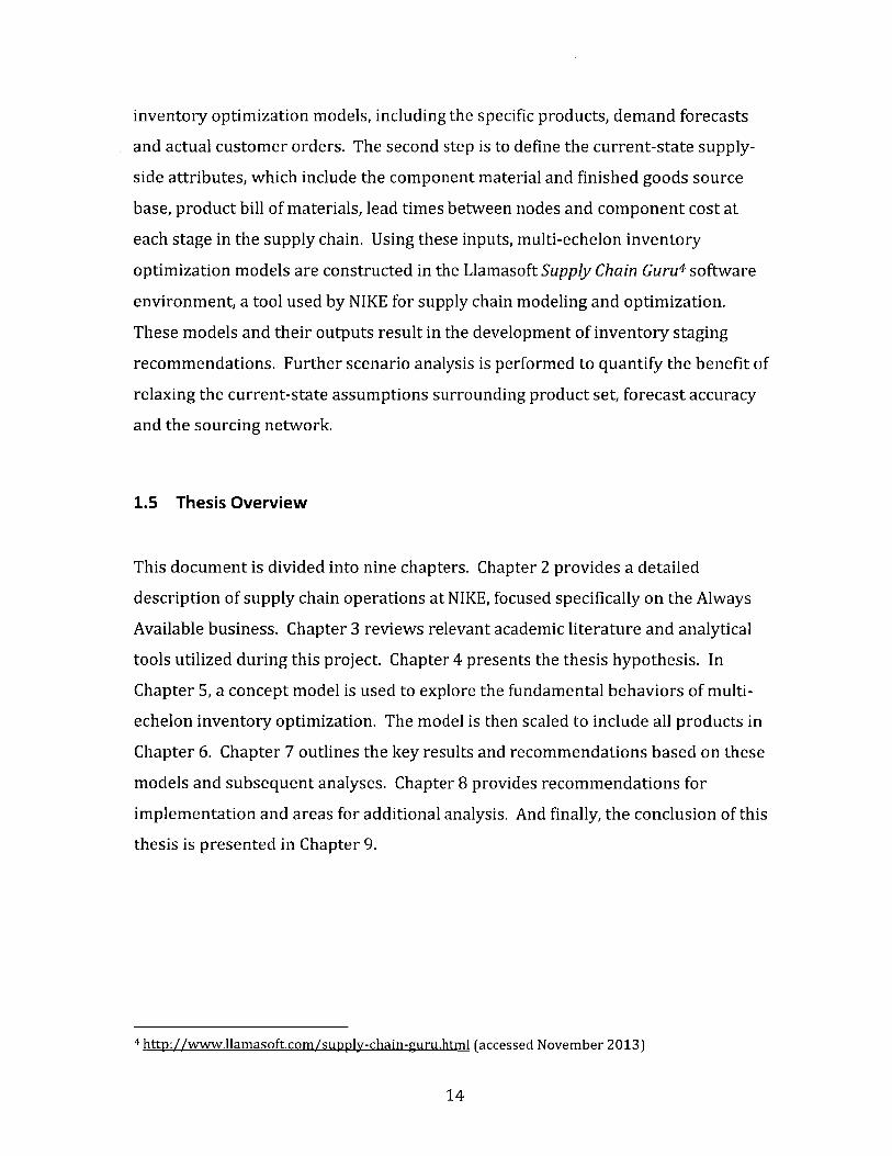
1.5 Thesis Overview

This document is divided into nine chapters. Chapter 2 provides a detailed

description of supply chain operations at NIKE, focused specifically on the Always

Available business. Chapter 3 reviews relevant academic literature and analytical

tools utilized during this project. Chapter 4 presents the thesis hypothesis. In

Chapter 5, a concept model is used to explore the fundamental behaviors of multi-

echelon inventory optimization. The model is then scaled to include all products in

Chapter 6. Chapter 7 outlines the key results and recommendations based on these

models and subsequent analyses. Chapter 8 provides recommendations for

implementation and areas for additional analysis. And finally, the conclusion of this

thesis is presented in Chapter 9.

4 http:://www.llamasoft.com/supply-chain-guru.html (accessed November 2013)

14

2 Supply Chain Operations at NIKE

To understand the supply chain structure of NIKE requires a foundational

knowledge of NIKE's broader organizational structure. The company is organized

into a three-dimensional matrix structure. The primary layer of the matrix is the

geographies. The general managers of these business units have profit and loss

responsibilities and oversee all activities within the region, including supply chain

and distribution operations. The second layer of the matrix is the product engines,

which are divided into footwear, apparel and equipment. These organizations are

responsible for product design and creation, material sourcing, and finished goods

manufacturing. The division into footwear, apparel and equipment is an artifact of

the unique design and manufacturing characteristics of their specific product types.

Figure 2 provides the fiscal year 2013 revenue split between the product engines,

which has held stable at 64% for footwear, 30% for apparel and 6% for equipment.5

For the purpose of this thesis, only footwear and apparel will be explored further.

Historically, the geographies and product engines were the only dimensions of the

matrix. However, in the 2000s, NIKE sought to better tailor its offerings to the

holistic needs of their end consumer. A male runner, for example, will purchase a

pair of running shoes from NIKE but may struggle to find apparel that adequately

compliments the color scheme and overall look of his shoes. Consumers would shop

across brands to assort their wardrobe even though NIKE offered a complete line of

products. Further, the company recognized that, while few firms compete directly

with the full breadth of the NIKE brand, many firms compete for specific consumer

segments such as runners and basketball players. These competitors had gained

market share by focusing their marketing and product creation efforts to the

specific needs of the consumer in their target segment. The third layer of the matrix,

dubbed the categories, was created in response. The purpose of the category

structure is to align the product design, creation and marketing functions within a

s NIKE, Inc. SEC Form 10-K filling, May 31st, 2013

15

particular consumer segment. The major categories, which span geographies and

product engines, are Running, Basketball, Football (Soccer), Men's Training,

Women's Training, Action Sports, and Sportswear. Figure 3 provides a breakdown

of revenue by category for fiscal year 2013.6

Figure 2: Percent of NIKE Brand Revenue by Product Engine

100%

90% -

W 80% -

" 70%

60% -

50% - Equipment

2 40% - Apparel

% Footwear0%

20% --- --

10% ---

0%FY11 FY12 FY13

Fiscal Year Ending May 31, 2013

The architecture of NIKE's organizational structure has a significant impact on

inventory decisions and supply chain operations. Each decision from product

creation through delivery to the end consumer affects each organizational entity

and, as a result, requires alignment. For example, if a product engine wants to move

a product from one factory in a given country to another factory in a different

country, the geography is impacted by changes in lead times, inventory levels and

potentially product cost. Further, the category is keen to ensure the new factory will

not impact the ability of NIKE to deliver to the consumer for this specific segment,

which could risk the competitive position of the firm.

16

6 Ibid.

Figure 3: Percent of NIKE Brand Revenue by Category

100%

90% -.....-.> 80%

70% - Others

60% --- Sportswear

a Action Sports50%-

Z50 Women's Training

40% -a Men's Training

30% Football (Soccer)

10% - -- Running

0%FY11 FY12 FY13

Fiscal Year Ending May 31, 2013

In the following sections, NIKE's four business models are explained and the general

structure of the supply chain is introduced. Then, the Always Available model is

presented in detail, including a key modification of the supply chain architecture.

2.1 Overview of NIKE Business Models

NIKE utilizes four business models to supply retailers and consumers with product:

Futures, Always Available, Quick Turn and Custom. The vast majority of revenue

comes through the Futures and Always Available models. Quick Turn and Custom

are a small but strategically significant source of growth for the firm.

2.1.1 Futures Business Model

The Futures model at NIKE is a classic retail make-to-order business model. It

origin stems from the off-shored nature of the footwear and apparel manufacturing,

17

which inherently results in long product lead times. In the Futures model, NIKE

solicits firm orders from retailers four to six months prior to delivery. NIKE

aggregates these orders and transmits them to its contract manufacturing supply

base. The contract manufacturers then procure raw materials, manufacture the

finished goods and ship the products either to a NIKE DC or directly to retail

customers. The benefits of the Futures model for NIKE and its suppliers are

immense: NIKE has limited inventory risk as orders are firm, it has clear visibility

into its near-term revenue and growth, and its suppliers have sufficient lead times

to optimally procure, produce and deliver the products. Considering these benefits

it is unsurprising that the majority of revenue for NIKE comes from Futures orders.

In fiscal year 2013, 87% of wholesale footwear and 67% of wholesale apparel

revenue came from Futures orders. These percentages have remained fairly stable

over the past three years.7

Despite these benefits, the Futures model has shortcomings. Most notably, nearly all

inventory risk is pushed to the retailer and demand for products must be predicted

well in advance. If actual demand falls below expectations, the retailer is forced to

close out the product at a discount, sacrificing profit margin. In some cases, NIKE

will accept returns for certain types of products. On the other hand, if a product is

selling well, the retailer may stock out, thereby disappointing consumers and

sacrificing upside profit from lost sales. Both instances have a negative impact on

NIKE. High discounts tarnish the brand's image in the marketplace and hurt the

profitability of NIKE's retail partners whom the firm needs for market access. Stock

outs lead to negative consumer sentiments towards the brand and, through lost

sales, limit the revenue and profitability potential of the firm. To respond to these

limitations, NIKE developed the Always Available replenishment model.

18

7 Ibid.

2.1.2 Always Available Business Model

The strategic imperative behind the Always Available business model is to ensure

consumers have the product they want in their desired color and size when and

where they shop. Accomplishing this goal requires a departure from the long lead-

time, make-to-order Futures model. Rather, for the select category essential

products offered in the Always Available portfolio, retailers place weekly orders to

NIKE that are fulfilled from an on-hand inventory position in a DC. These products

are typically long lifecycle, meaning the product design remains unchanged across

multiple seasons, and ideally have low seasonality of demand. The term "category

essential" means these are core, foundational products to a category. Put

differently, in the case of a stock out of a "category essential" product, consumers

are likely to substitute a competitor's product. The Always Available business

currently represents approximately 8-10% of NIKE's total revenue. 8 Figure 4

provides examples of typical Always Available products.

Figure 4: Representative Always Available Products

The Always Available business model provides a variety of benefits for retail

partners. By shifting the inventory risk back to NIKE, retailers hold less inventory

and can respond to fluctuations in demand more quickly. This results in fewer

19

8 Author's estimate.

markdowns and closeouts, leading to higher profit margins. Further, retailers are

able to restock products that are selling quickly reducing lost sales. For NIKE, this

replenishment model ensures its products remain in stock, thereby capturing higher

revenue and serving as a competitor blocking mechanism.

2.1.3 Quick Turn and Custom Business Models

Though the Quick Turn and Custom business models are out of the scope of this

thesis, they represent a strategically important portion of the business. Quick Turn

is NIKE's model for rapid response to marketplace demand, typically driven by key

"sports moments" such as major sports championships, a significant achievement by

a professional athlete, or other unexpected sports culture events. Most of the

products in this business are tee shirts and professional or collegiate jerseys. For

example, consumer demand will spike for a given NFL player's jersey immediately

after he has an outstanding game performance. NIKE would like to capitalize on this

demand and ensure the appropriate product offerings are available in the

marketplace. To enable this rapid response to major spikes in demand, NIKE has

developed various near- and on-shore finishing processes to screen-print tee shirts

or jerseys as a means for delayed differentiation.

The Custom business model allows consumers to design their own footwear and

apparel based on a library of designs, materials, colors and patterns. Dubbed Nike

iD in the marketplace, consumers use a web interface 9 to select the base style and

execute the customization, which NIKE will then manufacture and deliver to the

consumer in a few weeks. This model capitalizes on the growing trend of

individuality and customization in the retail space.

9 See http://www.nike.com/us/en us/c/nikeid for Nike iD footwear customization interface(accessed November 2013)

20

2.2 Overview of NIKE Supply Chain

As referenced in Section 1.1, nearly all of NIKE's products are manufactured by

contract manufacturers located throughout the world. Though the footwear and

apparel supply chains are different in many regards, a single model can be used to

understand the basic supply chain architecture at a macroscopic level. To illustrate

the supply chain design, a pair of athletic training shorts will be used. Figure 5

captures the basic supply chain architecture for these shorts, including processes

ownership within NIKE and inventory ownership for both NIKE and its retail

partners.

Figure 5: NIKE Supply Chain Macro-level Structure for Athletic Training Shorts

NIKE Process Ownership

Product EnginesOrganizatian Geography Organization

Component Retaier A Consume ASappfier A

Retier B Constumer B

Retrier D rCansuner 0

Inventory Ownership

Supplier wned NiKEOwned RetuilerBwn ed

21

In general, there are five echelons or layers in the supply chain - the supplier,

manufacturer, distribution center (DC), retailer and consumer.10 Returning to the

example of the athletic shorts, the supplied components include yarn and / or fabric,

elastic for the waist band, drawstrings, decals, and tag materials. The transit lead

times between nodes and production lead times at each node vary and depend on

the geographic location of each node, the degree of vertical integration of the

manufacturer, process technologies, transportation methods and capacity

constraints. For the Futures business, a planning lead time of four to six months is

used for the complete, end-to-end process.

NIKE divides the organizational responsibility for supply chain operations into two

internal groups. The product engines are responsible for the sourcing of raw

materials through the manufacturing of finished goods. Once the finished good is

made and delivered to a third-party freight consolidator in the origin country for

shipping, the supply chain organization within the geography takes ownership and

is responsible for the product through to delivery to the end customer.

Inventory ownership is a crucial feature of this supply chain and factors heavily into

the development of the multi-echelon inventory strategy. NIKE takes financial

ownership of their products once the finished good is manufactured and sent to the

consolidator. In the short run, the third-party suppliers are financially responsible

for the product in all prior process steps. However, NIKE will take ownership of raw

materials and finished goods work in process (WIP), either through formal transfer

of products or payments made to suppliers, if these materials are not consumed

within a negotiated period of time. For example, if demand falls below expectation

after a season and the supplier has purchased excess raw material, NIKE will

compensate the supplier directly.

10 Not all of NIKE's products flow through a DC or a third party retailer. However, the bulk of NIKE'swholesale business follows this general supply chain structure.

22

Within the finished goods manufacturing node for apparel, there are additional

process steps that could be considered distinct echelons. However, these

intermediary nodes are not crucial for the purpose of understanding the subsequent

analysis in this thesis.'1

2.3 Distinct Features of the Always Available Supply Chain

Recall from Section 2.1.2, the purpose of the Always Available business model is to

ensure core, category essential products are available to consumers in their size,

style, and color preference whenever they shop. To ensure product availability,

NIKE replenishes retailer orders from an on-hand inventory position in a DC.

Retailers can place orders throughout the season and NIKE targets a retailer

replenishment lead time of one week.

NIKE uses the same physical supply chain network for its products, regardless of

whether the product is offered through the Futures or Always Available business

models. Indeed, all Always Available products are also offered through Futures.

Only certain retail accounts have the need and technical sophistication required to

utilize the replenishment benefits of Always Available. In practice, many Always

Available retailers will use Futures orders at the start of a selling season to "load-in"

their retail floors and will use the replenishment offering to "fill-in" products that

are selling well throughout the season.

To enable rapid replenishment, NIKE has modified its standard, five-echelon

structure to include inventory stocking nodes. These inventory positions in the

supply chain reduce the effective replenishment lead time for their respective

downstream echelons. This is the key difference between the Futures and Always

Available supply chains. Figure 6 provides a diagram of a typical Always Available

11 For a more thorough treatment of the intermediary manufacturing nodes in NIKE's apparel supplychain, see Sections 2.3-2.4 of the MIT LGO thesis by Robert Giacomantonio, Multi-Echelon InventoryOptimization in a Rapid-Response Supply Chain, 2013.

23

supply chain network. The network structure is the same as presented in Figure 5

but now explicitly highlights the inventory stocking locations for raw materials and

finished goods. The component material inventory position at the finished goods

factory, called Material Staging in NIKE lexicon, consists of staged input

components. The finished goods inventory position at the factory, dubbed Demand

Pull, are completed products held at the factory. The third inventory node is the

finished goods held at the DCs located in each geography - Memphis, TN for North

America and Laakdal, Belgium for Europe.

Figure 6: NIKE Always Available Supply Chain Macro-level Structure

NNCE Process Ownersiip

Product EnginesOrganization Geography Organization

U*O C

C a

L b Nef~wA O E A

pnd eE ndYOWtaei d

ISuppl ier Owned I NIKE Owned jRetailerOwned

24

3 Literature Review

A significant body of research has been performed to study this problem of how best

to achieve a target service level in a make-to-stock business model while minimizing

the requisite amount of safety stock, and inventory holding cost, through staging

inventory in the supply chain. This chapter is divided into two sections. The first

explains the item fill rate safety stock formula and highlights the key drivers of

safety stock. The second section summarizes techniques for minimizing total safety

stock through multi-echelon staging.

3.1 Safety Stock

As described in Section 1.3, there are three main classifications of inventory:

1. Cycle Stock: on-hand inventory that results from batch ordering. Cycle stock

is driven by the governing inventory policy set by the company, which in turn

dictates the reordering frequency. NIKE uses a modified base-stock policy

with a one-week review period. Each week, the total inventory position (on-

hand in the DC plus in-transit) is compared to forecasted demand. The

magnitude of the order placed is the forecasted demand for the week

following lead time, less any forecasted excess inventory for demand during

lead time. For example, if lead time is three weeks, the order placed would

be expected demand for week four less expected excess inventory during the

prior three weeks. For reasonably stable demand, average cycle stock is 3.5

days of sales.

2. Pipeline Stock: inventory in-transit between supply chain echelons. For

NIKE, this consists of finished goods inventory between the finished goods

factory and the DC. Components in-transit between suppliers and the

finished goods manufacturer are generally not included in inventory

calculations. In steady state, pipeline inventory will be equal to the expected

25

demand during lead time. In terms of days of sales, a lead time of 30 days

results in 30 days of pipeline inventory.

3. Safety Stock: inventory held to account for uncertainty in supply and demand

in the short run.

To determine the required safety stock to achieve a target service level for a

periodic review inventory policy, the following equation can be used

Safety Stock = k * cL

where k is the safety factor and UL is the standard deviation of demand during the

sum of the lead time and review period. Assuming normalcy in forecast error, k can

be derived using the unit normal loss function G[k],

G [k] = E[DLeadTme] (1 - IFR)07L

where E[DLeadTime] is the forecasted demand during the lead time and IFR is the

target item fill rate. The standard deviation of demand over lead time, CL, takes the

form [2]:

UL = IE(L)(rD)2 + (E(D)) 2 0eadTime2

where1 2

E(L) = expectation, or mean, lead time

UD = root mean square error (RMSE) of forecasted demand over a unit time

period (e.g., one week)

E(D) = expectation of demand over a unit time period (e.g., one week)

ULeadTime = standard deviation of lead time.

12 This formula assumes demand and lead time are independent random variables.

26

As evident from these equations, the required inputs for safety stock calculations

are:

" Demand forecast

" RMSE of demand forecast

" Expected supply lead time

* Standard deviation of supply lead time

" Target item fill rate (IFR)

3.2 Multi-Echelon Inventory Optimization Techniques

The question of where to stage safety stock to minimize total inventory cost while

maintaining a fixed service level has been studied at length. Simpson [3] proposes a

methodology for determining where to stage in-process inventory for a serial

supply chain utilizing a base-stock manufacturing processes. In the decades since, a

variety of research has expanded on this foundation. Graves [4] offers a

comprehensive review of the subsequent literature on safety stock in a

manufacturing environment and proposes a new modeling paradigm that removes

the rigid constraints on production flexibility. Masse [5] provides an additional

summary of relevant, more recent literature on the specific question addressed by

this thesis.

Graves and Willems [6] introduce a method for modeling safety stock in a supply

chain that is subject to forecast uncertainty. This framework and related

optimization algorithm are used by a variety of commercially available safety stock

optimization software and form the analytical basis for this thesis. Subsequent

research, including Graves and Willems [7] and Schoenmeyr and Graves [8], expand

this approach to include non-stationary demand and evolving forecasts.

27

4 Hypothesis

The preceding sections provide an overview of NIKE's corporate structure and

supply chain operations and introduce the key literature related to the question

being addressed by this thesis. With this background, a series of hypotheses can be

made.

As introduced in Section 1.3, three key questions drive this research:

1. Given the extant NIKE supply chain architecture and portfolio of products

offered through the Always Available model, what is the best multi-echelon

inventory staging strategy that achieves a target item fill rate while

minimizing total system safety stock cost?

2. What is the value, in terms of safety stock reduction, of reducing systemic

forecast error, either by improving forecast accuracy or removing difficult-

to-predict products from the portfolio?

3. How can the underlying physical supply chain network be modified to reduce

total system safety stock cost?

Based on these questions, three hypotheses will be explored:

1. Multi-echelon safety stock staging will reduce the total finished goods safety

stock in the distribution center and will decrease the total system safety

stock cost. However, the value of staging will depend heavily on the relative

lead times between nodes and component material commonality across

products sourced from the same factory.

2. Decreasing total portfolio forecast error through improved forecast accuracy

or the removal of difficult-to-predict products will significantly reduce safety

stock requirements and, ultimately, decrease total inventory in the system.

28

3. Regardless of staging strategy, producing finished goods closer to the final

destination will reduce total system safety stock. Implementing component

staging at these near-shore factories will amplify the reduction in total

system safety stock cost.

5 Multi-Echelon Inventory Optimization - Concept Model

A simplified supply chain architecture illustrates the core dynamics of multi-echelon

inventory optimization. Specifically, the supply chain model for a pair of athletic

training shorts introduced in Section 2.2 can be used. In this chapter, a

mathematical framework to minimize overall safety stock value given a specific

target item fill rate, based on Graves and Willems [6], is introduced and applied to

this representative supply chain architecture. An Excel implementation is detailed.

The results of this model, including the optimal solution of staging components at

the finished goods manufacturer, are explored. Finally, limitations to this modeling

approach are addressed.

5.1 Inventory Modeling

Graves and Willems [6] propose a methodology that models a supply chain as a

network of nodes. Each node represents a distinct step in the manufacturing and

distribution process. For NIKE, these nodes are stages in the supply chain. The

purpose of the algorithm is to determine the quantity of safety stock to stage at each

node which minimizes total system safety stock cost while achieving a target service

level. The detailed explanation and application of the algorithm in the subsequent

sections is based on their original paper and Masse [5].

29

5.1.1 Inputs and Assumptions

To translate a complex supply chain into a series of mathematical equations

necessary for modeling, a number of key assumptions about supply chain inputs and

dynamics must be made.

Lead time

Both transit lead times between nodes and process lead times within a process step

are assumed to be known and deterministic. In reality, this is rarely the case as

there is variability in shipping, receiving, order processing, and manufacturing.

However, data on lead time variability was unavailable at the time of this research.

For the purpose of this concept model and subsequent full-scale models, the

planned lead times set in the MRP systems at NIKE are used. While these values are

likely to be an upper-bound of true transit and processing lead times, they are

consistent with NIKE's overall planning paradigm and will be leveraged in any large

scale implementation of multi-echelon inventory optimization.

Customer Demand Variability

In the apparel retail industry, customer demand is notoriously difficult to predict.

Both consumer preferences and product designs change frequently. Further, for the

Always Available business, demand manifests as orders placed by retailers to NIKE's

DCs. As is the case in supply chains lacking perfect coordination, these orders are

batched based on the retailers' internal processes and do not necessarily reflect true

consumer demand over time.

NIKE uses a commercially available statistical forecasting and planning software,

Logility's Voyager13 , to develop monthly demand forecasts. This software uses a

variation of the Holt-Winters exponential smoothing method to predict future

demand based on past actual and forecasted demand. The tool then generates seven

13 http:://www.logility.com/solutions/demand-planning-solutions/voyager-demand-planning

(accessed November 2013)

30

forecasted monthly demand values, one for each of the six months leading up to the

target business month and a forecast during the actual business month.

To generate a forecast error value used for safety stock calculations, the six-month-

ahead forecast is selected based on administrative lead times required for securing

materials and factory capacities. The root mean square error (RMSE) based on 12

months of forecast and actual sales data is used. The RMSE has the form

n

0Forecast 1 ~~ t-yt)2t=1

where

Uforecast = forecast standard deviation

n = number of forecasted periods (n = 12)

xt = observed demand for period t

ft-y,t = forecasted demand for period t made in period t-y (y = 6)

This calculation is performed at the SKU level, meaning product style and color but

not size. Forecasts are not generated for specific sizes; rather, a size curve is

applied.

Unconstrained Stocking Nodes and Processing Characteristics

The model makes the broad assumptions that each stocking node has unconstrained

capacity for holding inventory and that processing and transit times are invariant to

the quantity of product in each process step. It also does not account for loss, either

through inventory shrinkage or yield loss in the manufacturing processing. These

assumptions are reasonable for the purpose of the research questions being

addressed.

31

5.1.2 Methodology

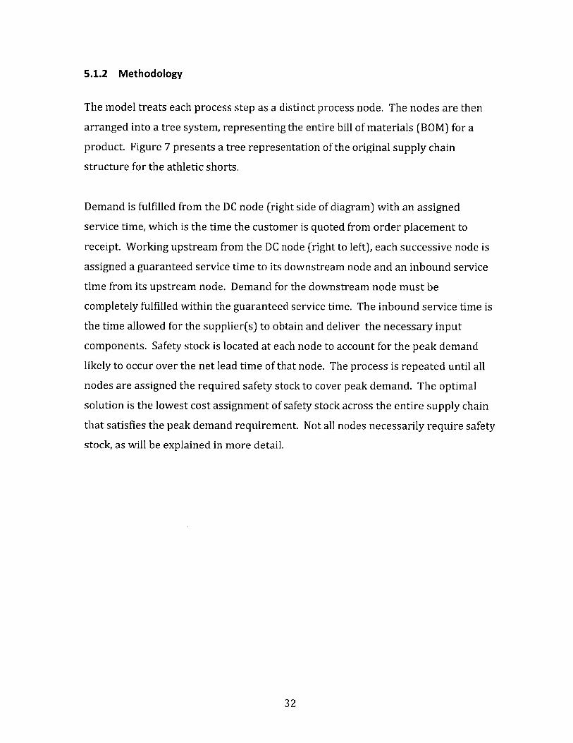
The model treats each process step as a distinct process node. The nodes are then

arranged into a tree system, representing the entire bill of materials (BOM) for a

product. Figure 7 presents a tree representation of the original supply chain

structure for the athletic shorts.

Demand is fulfilled from the DC node (right side of diagram) with an assigned

service time, which is the time the customer is quoted from order placement to

receipt. Working upstream from the DC node (right to left), each successive node is

assigned a guaranteed service time to its downstream node and an inbound service

time from its upstream node. Demand for the downstream node must be

completely fulfilled within the guaranteed service time. The inbound service time is

the time allowed for the supplier(s) to obtain and deliver the necessary input

components. Safety stock is located at each node to account for the peak demand

likely to occur over the net lead time of that node. The process is repeated until all

nodes are assigned the required safety stock to cover peak demand. The optimal

solution is the lowest cost assignment of safety stock across the entire supply chain

that satisfies the peak demand requirement. Not all nodes necessarily require safety

stock, as will be explained in more detail.

32

Figure 7: Node Structure of Standard Always Available Supply Chain

I Component RawI Material InventoryI Staged Prior toI Production

Supplier LeadA Time A

Supplier LeadB

49

I f

ProductionLea Time

Finished GoodInventory Held at

Factory

Supplier LeadC Time C

Supplier LeadD Tirne D

/

Transit LeadTime

/i

Formally, the objective function for the optimization is:

N

min hA{D (SI. + T - Sj) - (SI + T - S )p }1=1

Subject to

1. Sj - SI; T forj= 1, 2,..., N

2. SI - Si 0 for each pair (i,j), where node i directly supplies node j

3. Sj s for all demand nodes j

4. S, SI1 > 0 and integer forj= 1, 2,..., N

Where

hj = unit inventory value at node j

SI = inbound service time to nodej

Sj = guaranteed service time of nodej

Dj(t) = is a function representing the maximum or peak demand over an

interval of length t experienced by node j

33

Finished GoodsInventory Held at

DC

Tj = the planned lead time or processing time of node j

y;= average demand per time period experienced by nodej

s;= maximum service time for demand node]

At each node] in the supply chain, the assigned safety stock is the difference

between peak demand, Dj, and average demand, yu over the net replenishment time

for the node. The net replenishment time for the node is given by SI + T - S. The

optimization minimizes this safety stock quantity multiplied by the holding cost, h;,

across all nodes in the supply chain.

The four constraints restrict the optimization to the feasible solution space given the

design of the supply chain. The first constraint ensures that the net replenishment

time (the summation inside of the parenthesizes in the objective function) for each

node is non-negative. The second constraint requires node] to wait until all supply

nodes i have delivered materials. The third constraint ensures the guaranteed

service time for each node is less than the quoted service time for the end customer.

The fourth simply ensures that all times are positive and integer units.

This formulation is a nonlinear optimization problem. Graves and Willems [6]

provide a dynamic programming approach for solving it on a larger scale, which is

the algorithm used by commercially available software such as Llamasoft's Supply

Chain Guru. However, for simple supply chain architectures, this algorithm can be

implemented in Excel.

34

5.2 Model Implementation

To demonstrate the dynamics of multi-echelon inventory optimization, the athletic

running shorts presented previously will be used. Figure 8 summaries the supply

and demand attributes of this product.14

Figure 8: Demand and Supply Attributes of Athletic Shorts

Demand-side Attributes

Mean Monthly Demand 37,000 units

Monthly Forecast RMSE 7,800 units

Monthly Demand CoV 0.21

Target Service Level 95%

Annual Inventory Holding Cost 20%

Supply-side Attributes

Transit/ Process

Product and Staging Product Value at Monthly Inventory Lead Time of Prior

Node Node Holding Cost Node

Component A at $1.02 $0.01 2 daysMaterial Staging

Component B at $0.45 $0.00 28 daysMaterial StagingComponent C at $0.26 $0.00 28 daysMaterial Staging

Component D at $0.16 $0.00 46 daysMaterial Staging

Finished Good at $4.46 $0.03 25 daysManufacturer

Finished Good at DC $5.80 $0.04 11 days

14 The bill of materials, product value, demand data and lead times have been changed to preserve

confidentiality. However, they are representative of a typical Always Available product.

35

11

Two additional inputs are required to complete the model. First, the guaranteed

demand service time, sj, for customers is set to zero. NIKE targets an order to

receipt lead time from its DC of one week. Because there generally is not enough

time to receive an inbound shipment, process the order and ship to the consumer

within the one-week window, the DC must fill all orders from an on-hand position.

Second, the formula for peak demand per time period, Dj, is the average demand per

time period plus safety stock. Section 3.1 provides an overview of the safety stock

calculation using a target service level. 15 Using this information and the

formulation of the optimization model from Section 5.1.2, an Excel model can be

built to determine the lowest-cost safety stock. This model, including formulas, is

provided in Appendix A.

The Solver optimization engine in Microsoft Excel utilizes the General Reduced

Gradient (GRG2) algorithm for solving non-linear optimization problems. This

algorithm identifies the locally optimal solution for well-scaled, non-convex models.

However, because it only guarantees local optimality, testing multiple initial

conditions is required to ensure the solution space is adequately explored. This is a

limitation of formulating this problem in Excel and large-scale implementation

requires a more sophisticated optimization engine. However, for this simple

concept model, the solution space is easily explored through manual manipulation

of decision variables. This approach is described at length in Section 5.3.

5.3 Model Results

In effect, the optimization algorithm iterates through all possible staging scenarios

to determine the lowest inventory holding cost solution. For this example with four

component materials and finished goods staging at the factory, there are five

15 For the purpose of the Excel concept model, safety stock is calculated using the Type I service levelmethodology, where k is simply the safety factor based on the unit normal distribution functionrather than unit loss function. This simplification is purely for ease of implementation in Excel. TypeII (or fill rate) service level is used in the Supply Chain Guru implementation.

36

possible staging conditions resulting in 32 combinations of staging scenarios. The

table in Appendix B displays the output of these 32 combinations.

Toggling between staging and not staging a given material at a given node impacts

the net replenishment lead time. When a node stages safety stock, its guaranteed

outbound service time goes to zero as it has enough inventory to cover peak

demand. This translates to a zero inbound service time for that component at its

downstream node. The net replenishment time for the downstream node will be the

lead time between the upstream node and the downstream node. If the upstream

node does not stage inventory, the net replenishment time for the downstream node

is the sum of the service time between the downstream node and the upstream node

(as before) and the upstream node's inbound lead time. The amount of safety stock

held at a node is the k safety factor multiplied by the standard deviation of demand

over the net replenishment lead time.

Five specific inventory tradeoff scenarios are worth exploring in more detail to elicit

deeper insights into the optimal staging strategy for NIKE's supply chain. The model

results for these five scenarios - No Upstream Staging, Finished Goods Staging,

Complete Material Staging, Staging at All Nodes, and the Optimal Staging Solution -

are presented in Figure 9.

37

Figure 9: Key Inventory Tradeoff Scenarios

Scenario 1: No Upstreaii StagingOutbound

Lead Time Inbound Guaranteed Net Safety Stock Safety StockProduct and Staging Hold Safety from Prior Service Service Replenishment Quantity Holding CostNode Stock? Node (Days) Time (Days) Time (Days) lime (Days) (Units) (USD)Component A at No 2 0 2 0 0 $ -Material StagingComponent B at No 28 0 28 0 0 $Material StagingComponent C at No 28 0 28 0 0 $ -Material StagingComponent D at No 46 0 46 0 0 $ -Material StagingFinished Good atManufacturer No 25 46 71 0 0 $ -

Finished Good at DC Yes 11 71 0 82 21211 $ 820.17

Total 21211 $ 820.17

Scenario i: Fnitshied GodsStagingOutbound

Lead Time Inbound Guaranteed Net Safety Stock Safety StockProduct and Staging Hold Safety from Prior Service Service Replenishment Quantity Holding CostNode Stock? Node (Days) Time (Days) Time (Days) lime (Days) (Units) (USD)Component A at No 2 0 2 0 0 $ -Material StagingComponent B at No 28 0 28 0 0 $ -Material StagingComponent C at No 28 0 28 0 0 $ -Material StagingComponent D at No 46 0 46 0 0 $ -Material StagingFinished Good at Yes 25 46 0 71 19737 $ 586.86


Total 27506 $ 887.26

Scenario 3: Complete Materia StagingOutbound

Lead Time Inbound Guaranteed Net Safety Stock Safety StockProduct and Staging Hold Safety from Prior Service Service Replenishment Quantity Holding CostNode Stock? Node (Days) Time (Days) Time (Days) Time (Days) (Units) (USD)Component A at Yes 2 0 0 2 3313 $ 22.57Material StagingComponent B at Yes 28 0 0 28 12395 $ 37.18Material StagingComponent C at Yes 28 0 0 28 12395 $ 21.48Material StagingComponent D at Yes 46 0 0 46 15887 $ 16.95Material StagingFinished Good at No 25 0 25 0 0 $ -Manufacturer


I Total 58044 $ 641.62

38

,

Scenario 4: Staging at All NodesOutbound

Lead Time Inbound Guaranteed Net Safety Stock Safety StockProduct and Staging Hold Safety from Prior Service Service Replenishment Quantity Holding CostNode Stock? Node (Days) Time (Days) Time (Days) lime (Days) (Units) (USD)Component A at Yes 2 0 0 2 3313 $ 22.57Material StagingComponent B at Yes 28 0 0 28 12395 $ 37.18Material StagingComponent C at Yes 28 0 0 28 12395 $ 21.48Material StagingComponent D at Yes 46 0 0 46 15887 $ 16.95Material StagingFinished Good at Yes 25 0 0 25 11712 $ 348.24Manufacturer


Total 63470 $ 746.82

Scenario 5: Optimal Staging SolutionOutbound

Lead Time Inbound Guaranteed Net Safety Stock Safety StockProduct and Staging Hold Safety from Prior Service Service Replenishment Quantity Holding CostNode Stock? Node (Days) Time (Days) Time (Days) Time (Days) (Units) (USD)Component A at No 2 0 2 0 0 $ -Material Staging

Component B at Yes 28 0 0 28 12395 $ 37.18Material Staging

Component C at Yes 28 0 0 28 12395 $ 21.48Material Staging

Component D at Yes 46 0 0 46 15887 $ 16.95Material StagingFinished Good at No 25 2 27 0 0 $ -Manufacturer


I Total 55116 $ 633.94

Under the No Upstream Staging scenario, all safety stock inventories are held at the

customer-facing DC. The safety stock quantity at this node must buffer against

expected peak demand over a net replenishment time of 82 days, which is the

critical path lead time for the entire sourcing and production process. The critical

path lead time is the sum of 46 days for the longest lead time component material,

25 days for finished goods production and 11 days of transit to the DC.

In the Finished Goods Staging scenario, the factory must hold sufficient safety stock

to cover expected peak demand across a net replenishment lead time of 71 days,

39

which is the sum of the longest lead time component material (46 days) and

production time (25 days). The DC now only holds enough safety stock to cover the

transit time from the finished goods inventory position at the factory (11 days).

Notably, while the quantity of finished goods safety stock in the DC decreases nearly

63% under this scenario due to the significant decrease in net replenishment time,

the total quantity of finished goods safety stock in the system increases almost 30%

and the total system safety stock cost increases 8.2%. Because safety stock is

proportional to the square root of the lead time, separating the replenishment lead

time across two serial nodes actually increases the total safety stock required in the

system.16

Under the Complete Material Staging scenario, safety stock for all four component

materials is held. This reduces the net replenishment lead time for the DC to the

sum of finished good production lead time and transit lead time, or 36 days. The

inventory holding cost of the safety stock staged in component form is significantly

less than the finished good, as the value of the components is less than the value of

the finished good. Therefore, the total safety stock quantity in the system, in terms

of finished goods equivalent units, increases by nearly 270% compared to the No

Upstream Staging scenario, but the total safety stock holding cost decreases by

nearly 22%. In the Staging at All Nodes scenario, safety stock is held for all products

at all locations. The net replenishment time to the DC is the same as Finished Goods

Staging scenario whereas the time to replenish the finished goods position at the

factory decreases to 25 days, which is the production lead time. The buffer of

component stock staged at the start of production eliminates all additional

component lead times. Again, because there is a net increase in finished goods

safety stock in the system, due to the finished goods staged at the factory, the total

safety stock cost is higher.

16 To clarify this mathematical relationship, consider a simple example: the square of 2 plus thesquare root 2 equals 2.83 which is greater than the square root of 4.

40

The Optimal Staging Solution stages three of the four component materials but no

finished goods at the factory. In this scenario, cost is minimized to $633.23 per

month, a 22.7% decrease from the No Upstream Staging scenario. The net

replenishment time for the DC node is 38 days, which is the sum of the upstream

transit time from the factory (11 days), the production lead time (25 days) and the

lead time for the unstaged component material, Component A (2 days). The key

difference between the Optimal Staging Solution and the Complete Material Staging

solution is that Component A is not being staged. This results in a small difference

of 1.2% in total safety stock cost. In effect, the incremental cost of staging safety

stock for Component A, which results in a decline in the net replenishment lead time

for the DC of two days, is equivalent to the difference in total cost between the two

scenarios. Note that the value of Component A is significantly higher than the other

constituent inputs. This results in a higher inventory holding cost per unit. The cost

savings from the decreased quantity of safety stock at the DC, due to the reduction

in the DC's net replenishment lead time by two days, is less than the increased cost

of holding safety stock for Component A.

This fundamental tradeoff between the incremental cost of staging a component

material and incremental savings from decreasing the quantity of finished goods

safety stock held at the DC that results from this staging is at the core of multi-

echelon inventory optimization. The algorithm determines where this tradeoff is

minimized. Further, in the specific case of NIKE, staging finished goods at the

factory always increases the total system safety stock cost. Splitting the inventory

across two serial nodes increases the total quantity of finished goods safety stock in

the system. The inventory holding cost difference between a finished good at the

factory versus at the DC, assuming a constant percentage of product value, is not

significant and does not justify staging more finished goods at an upstream node.

41

5.4 Model Limitations

Though this concept model of the athletic training shorts is useful for illustrating the

fundamental tradeoff in multi-echelon inventory optimization, it has its

shortcomings. Principally, this model is for a single style-color SKU. A typical

factory will produce a variety of colors of a single product, as well as other products

which share common BOM components. Therefore, the inventory pooling

advantage of staging components used across SKUs is not being captured.

Additionally, most products are made of significantly more than four components.

The example athletic training shorts are actually made from 14 components sourced

from nine different factories around the world. The BOM was simplified to four

components purely for illustrative purposes.

6 Scaled Multi-echelon Inventory Optimization

Commercially available inventory optimization software packages provide a

scalable environment for analysis and allow for more complex supply chain

architectures to be modeled. NIKE has a relationship with the supply chain software

firm, Llamasoft, and utilizes their supply chain network and inventory optimization

software, Supply Chain Guru, to support strategic supply chain decision making.

This chapter provides a brief overview of the software, explains the large-scale

implementation performed for the Always Available business and presents the key

model results.

6.1 Supply Chain Guru Overview

Llamasoft's Supply Chain Guru is an integrated software platform that combines

supply chain network and safety stock optimization. It also offers simulation

42

functionality. The tool has three components that make it attractive for enterprise-

level supply chain modeling. First, it has an intuitive user interface based on the

Microsoft Office environment. Input and output files are can be viewed and

manipulated in Microsoft Excel and Access formats. Second, the software includes a

large supply chain intelligence database, which includes a spectrum of reference

data, including geospatial mapping, transit costs, and emission data. Third, the

solver engine itself contains multiple integrated solvers, operations research

algorithms and simulation engines. The tool also includes a variety of graphical

outputs and easily allows for scenario analyses. For this research, the inventory

optimization package of Supply Chain Guru was used for large scale modeling and

analysis of the Always Available business. This package first solves the network

optimization algorithm to establish the underlying network architecture and

product flows and then uses a variant of the multi-echelon inventory optimization

algorithm developed by Graves and Willems [6] to determine the lowest-cost

staging scenario. The solver algorithm uses dynamic programming approach, which

alleviates the concern surrounding the GRG2 algorithm's ability to find global

maxima and minima presented in Section 5.2.

6.2 Supply Chain Guru Implementation

To assess the opportunity of multi-echelon inventory optimization for the Always

Available business, the entire calendar year 2012 product line for the North

American and European geographies is modeled. Models are built at the finished

goods factory level of aggregation. In NIKE's current supply chain structure,

component material is held at the finished good factory and is not shared across

factories. Further, purchase orders for each geography are administratively

distinct; therefore, though Europe and North America may source an identical

product from the same factory, the orders are treated separately and must be

modeled as unique products. For the North American geography, 27 finished-goods

factories in 12 countries are modeled with 289 finished good products (style-color).

43

For Europe, 19 factories in 8 countries, which supplied 131 finished good products,

are modeled. The time period for the models is one month, meaning the output is

safety stock quantity per month.

Supply Chain Guru uses a series of database tables, which can be constructed in

Microsoft Access or Excel, as input files. For each factory, the following tables are

created:17

" Products table: defines all the products in the system, including finished

goods and components.

" Bill of Materials (BOM) table: establishes the relationship between finished

goods and component products. If, in a single factory, a particular

component is used in multiple finished goods, the BOM table contains a row

for each component-finished good relationship.

* Sites table: contains the name and physical locations of the physical nodes in

the supply chain (e.g., Supplier A, FG Factory B, DC).

* Sourcing Policies table: establishes linkages between the sites in the model

and products that flow between the sites. For example, the DC must source

finished goods from Factory A, which in turn sources component materials

from Suppliers A-E. This table also contains the finished goods production

lead time, which is set to 25 days based on internal planning data.

" Inventory Policies table: determines which products can be held in inventory

at which site. Suppliers cannot hold inventory, Factories can hold

components and finished goods, and DCs can only hold finished goods. This

table also defines the product value at the specific site used in the inventory

holding cost calculation and establishes the inventory reordering policy,

which is seven days for the DC and 30 days for Factories. Suppliers are

assumed to have infinite inventory.

17 For a much more thorough explanation of the attributes of the input tables, see Giacomantonio,Multi-Echelon Inventory Optimization in a Rapid-Response Supply Chain, 2013 or the step-by-stepmanual for building models in the Supply Chain Guru environment provided to NIKE at theculmination of this research.

44

" Transportation Policies table: defines the transit time and days between

replenishment for a given product between nodes. For this implementation,

transit times are static and based on internal planning times. Days between

replenishment are based on NIKE's general inventory policy (seven days for

the DC and 30 days for Factories).

* User-defined Demand table: provides mean quantity demanded and forecast

error for each product for each month. The mean quantity demanded is the

forecasted quantity for that month. The forecast error is the forecast RMSE

described previously.18

Once these input tables are complete, the optimization algorithm is executed and

the following output tables are generated:

* Inventory table: an output of network optimization, this captures two of the

three types of inventory in the system - cycle stock and in-transit inventory.

When lead time variability is present a third field called the safety inventory

is populated to capture the additional safety stock required. Lead time

variability is not used in this research.

* Safety Stock Details table: the key output from safety stock optimization.

This table provides the safety stock quantity, cost and days of sales by

scenario, month, site, and product type. It also provides safety stock cost,

which is simply the inventory holding cost at each node (20% of the value of

inventory at that node).

18 More formally, the forecast RMSE is scaled by the Variance Law to better approximate the valueused in Logility Voyager software. The Variance Law is an empirical relationship that accounts forvariation in error as a function of volume. A full discussion of the Variance Law is outside the scopeof this thesis.

45

6.3 Model Results

Based on the findings from the concept model in Section 5.3, the expected lowest-

cost multi-echelon staging solution is to stage some components at the factory but

no finished goods. Figure 10 plots the total monthly safety stock holding cost for all

289 products in North America during 2012 across three scenarios - No Upstream

Staging, Finished Goods Staging (in the factory and at the DC) and the Optimal

Solution. Staging finished goods at the factory is the most expensive solution due to

the net increase in total quantity of finished goods in the system. This is the same

result found in the concept model. The Optimal Solution results in staging some, but

not all, component materials at the factory and finished goods in the DC. On

average, Finished Goods Staging is 44.8% more expensive than the No Upstream

Staging scenario while the Optimal Solution is 23.9% less expensive. Similarly,

Figure 11 plots the analogous data for the European geography. The average cost

increase for Finished Goods Staging is 46.4% while the savings in the Optimal

Solution is 18.2% compared to the No Upstream Staging solution.

The Optimal Solution minimizes safety stock holding cost across the entire supply

chain network. However, from a NIKE-centric view staging component materials

but not finished goods at the factory is not necessarily optimal in the short-run. As

described in the inventory ownership diagram presented at the bottom of Figure 5,

NIKE does not take immediate financial ownership of inventory held on-site at the

contract manufacturers. Therefore, in the short-run, the optimal solution for NIKE

may be the solution which minimizes the amount of safety stock in the DC.

46

Figure 10: Monthly Safety Stock Holding Cost for North America by Staging Scenario

Total System Safety Stock Holding Cost for the North AmericanGeography

-i-No Upstream Staging-*-Finished Goods Staging-4-Optimal Solution

Icee6 0"' 6

Calendar Year 2012

Figure 11: Monthly Safety Stock Holding Cost for Europe by Staging Scenario

Total System Safety Stock Holding Cost for the European Geography

-r-No Upstream Staging

-U-Finished Goods Staging

---- Optimal Solution

- -.... - -. -

(~ ~

Calendar Year 2012

Z& 6 41

47

0

U

'U0,

904a

$700,000

$600,000

$500,000

$400,000

$300,000

$200,000

$100,000

4-10

0

4a4

E

7i

4-1

10

$600,000

$500,000

$400,000

$300,000

$200,000

$100,000

ell

-

In Figure 12 and Figure 13, safety stock days of supply held in the DC is plotted over

the same time scale by scenario for North America and Europe, respectively. Days of

supply (DOS) is a metric where the safety stock quantity is divided by the forward

forecasted demand. In effect, it conveys the number of days of projected demand

that would be satisfied by the safety stock position. For both geographies, Finished

Goods Staging minimizes this measure of inventory held in the DC. This same result

was found in the prior analysis of the concept model. When finished goods are

staged at the factory, the effective net replenishment time for the DC is decreased to

the transit time between the nodes. Expected demand over this shortened lead time

is lower and, therefore, the safety stock quantity decreases.

Figure 12: DC Safety Stock Days of Supply for North America by Staging Scenario

DC Safety Stock Days of Supply for the North American Geography

70-*-No Upstream StagingC.

0 60 - -U-*Finished Goods Staging - - - - -

-4-Optimal Solution

0

200 30- -- -- - - - - - - - --- - - - --- - ------

1nY0

Calendar Year 2012

48

Figure 13: DC Safety Stock Days of Supply for Europe by Staging Scenario

DC Safety Stock Days of Supply for the European Geography

1 6 0- - - - - - -- - - - - - - - - - -

--*-No Upstream Staging140 -U-Finished Goods Staging

02 --- Optimal Solution120

100

80 -10

-~ 60

00

M )0

0

!4- & e "

Calendar Year 2012

While the Finished Goods Staging solution may be ideal in the short-term, this

strategy has significant flaws over the long term. First, the prior analysis has

illustrated how staging finished goods at the factory actually increases the total

quantity of finished goods in the system and the total holding cost for the system.

Though NIKE does not have immediate financial ownership of this increased

inventory at the factory, it must eventually accept this inventory at the end of the

product's lifecycle. This represents a significant inventory liability for NIKE. Absent

perfect coordination and purchase order tapering, this will result in an increased

quantity of product that must be cleared through retail channels, likely at a discount.

This process erodes profit margin and has other negative impact on the brand.

Second, many factories are not able to commit significant working capital to hold

NIKE's inventory. Third, these factories are not operationally equipped to

warehouse significant inventories and the risk of shrinkage is high. Therefore, the

Optimal Solution, which is the lowest cost across the entire supply chain, should be

considered ideal.

49

Similar criticisms could be made for staging component materials at the factory.

However, in practice, the relationship in this region of the supply chain is different.

NIKE already takes an active role in the procurement of component materials on

behalf of finished goods factories and generally is more financially invested in these

materials earlier in the process. Further, these components have much longer

lifecycles than the finished good products and the risk of needing to closeout

components at the end of a season is lower.

6.4 Model Validation

To validate the outputs of the model, comparisons between inventory levels

predicted by the model and actual performance should be made. However, this

posed a unique challenge for a few reasons. First, about one half of the products

offered through the Always Available replenishment program were staged upstream

from the DC. Second, in the year prior and during this research effort, the Always

Available supply chain did not use a forecast-driven safety stock inventory

methodology for setting inventory positions in the upstream nodes when products

were staged. Third, component staging at the finished goods factory is a relatively

new capability for NIKE and, as such, only a handful of products were being staged.

Instead, a quasi-qualitative approach for validation was made. Comparisons

between the No Upstream Staging scenario and the unstaged actual historical

inventory quantities, the only directly analogous scenarios, were made. The model

output predicted lower finished goods inventory at the DC for most of the products

but much higher inventory positions for others. This discrepancy is primarily

attributable to human interaction with the inventory planning system. Inventory

planners at NIKE have the capability to manually adjust the safety stock positions

and frequently do this based on additional information they receive from other

parts of the business that is not captured in the forecasts. The resulting inventory

position is thus decoupled from the calculated position driven from historical

50

forecast error. This conclusion was validated with a number of subject matter

experts at NIKE and further explains why, in general, the total inventory positions

were believed to be too high while stock outs were still frequent.

7 Key Results and Recommendations

The optimization models presented in the prior section lead to a number of findings

related to the original hypotheses presented in Section 4. In this chapter, staging

component materials is explored in depth to better understand which components

should be staged and why. The role of the underlying supply chain network and the

impact of reducing forecast error are explained. Finally, near- and long-term

recommendations for improving the overall supply chain are made.

7.1 Staging Component Materials

From a total system perspective, staging component materials at the factory and

finished goods at the DC is the lowest-cost multi-echelon solution. However, certain

factories and products receive a greater benefit from component staging than

others. There are three variables which drive the magnitude of the reduction in

safety stock cost from staging component materials - distance from factory to DC,

input component commonality across product families, and component cost.

Figure 14 is a scatter plot of the percent reduction in total system safety stock cost

as a function of finished goods factory distance from the DC for North America in the

Optimal Solution scenario. 19 The general trend is negative, implying factories which

are closer to the DCs have a more significant reduction in system safety stock cost as

compared to those further away. A simple thought experiment illustrates this

19 For this specific dataset, nearly all suppliers for Europe were located in Asia, which led to lessdifferentiation between factory to DC lead times. A similar, though less pronounced relationshipdoes exist in that geography.

51

phenomenon. Consider a factory in Mexico that has a seven-day transit to the North

American DC and a factory in Indonesia with a 23 day transit time. Assume the

input components are both coming from Southeast Asia, where the transit time from

the component supplier to the factory in Mexico is about 20 days versus seven days

for the Indonesian factory. Production time for both is 25 days. Recall that safety

stock at a node is proportional to the square root of the net replenishment lead time

for the node. Staging components at the factory in Mexico reduces the net

replenishment time for the DC from 52 days to 32 days. Staging components at the

Indonesian factory only reduces the net replenishment time from 55 days to 48

days. Eliminating the long component lead times for the near-shore factory yields a

much greater reduction in DC replenishment time and, as a result, finished goods

safety stock quantity and total safety stock cost as compared to off-shore factories.

The value of multi-echelon inventory optimization, or staging components in NIKE's

supply chain, increases significantly as the distance between the DC and finished

goods factory decreases.

Figure 14: Safety Stock Reduction as a Function of Lead Time for North America

Reduction in Safety Stock as a Function of Factory Distance for NorthAmerica

40%

35% --- Upper ..%.C....den.e .nterv..

0 a.

0 3 %j- --- -

302

sG 25%

M Z 20%l

04

M 15%.506CE

0 0.5 10% * Finished Good Factory

-Linear Regression

-Lower 99% Confidence Interval

- Upper 99% Confidence Interval

0 5 10 15 20 25 30 35 1

Distance from Finished Goods Factory to DC (Days)

52

A second driver of value for component staging results from the net inventory

reduction due to pooling of common components. Most components for apparel

products are shared across a variety of finished goods. At a minimum, there is

typically more than one color of a given style, which means all components except

the dyed fabric are common. Assuming independent forecast error for multiple

products, the aggregated pooled safety stock components will be less than the sum

of the individual safety stock quantities for a fixed service level. All else equal, a

factory which supplies a large variety of finished goods composed of the same input

components, such as fleece sweatshirts and sweatpants, will have a greater benefit

from component staging than a factory which produces a more differentiated

selection of products.

The third variable is simply the holding cost, which is a percentage of the product

value at the node. All else equal, low cost components should be staged instead of

high cost components. This is best illustrated by Component A in the concept

model, where the high inventory holding cost negated the benefit of staging the

material and reducing the net replenishment time by two days.

In summary, staging the right components at the finished goods factory minimizes

the total system safety stock holding cost. Factories with shorter finished goods

lead times compared to component lead times will receive the greatest benefit from

staging. Further, large factories producing finished goods from common

components yield even greater benefits. These two results have significant

implications for how to modify the underlying supply chain architecture to take full

advantage of component staging.

7.2 Reduction in Forecast Error

The Supply Chain Guru inventory models provide an environment for a variety of

additional scenario analysis and hypothesis testing. One particular question relates

53

the impact of forecast accuracy on safety stock. At the time of this research, NIKE

was undertaking an initiative to improve the statistical forecasting process in the

Always Available business.

Figure 15 is a histogram of the monthly forecast error coefficient of variation

(CoV) 2 0 for the products in the North America Always Available business. The

majority of products have a forecast error CoV that is less than or equal to one.

However, approximately 14% of products (by product type) have error CoVs higher

than one. A CoV greater than one indicates an error term that is larger, in

magnitude, than the forecasted demand. These are incredibly difficult to predict

products. As a result of this large error, a significant quantity of safety stock must

be held to achieve the target service level.

The output from the inventory models can be used to determine the value of

eliminating these highly unpredictable products from the Always Available portfolio

and, instead, offering them only as Futures products. Figure 16 plots the revenue

and safety stock impact of removing products with a CoV greater than one from the

North America portfolio. The y-axis displays the percent of total Calendar Year

2012 revenue. The x-axis displays the percent of total safety stock held in the DC

node. Under the No Upstream Staging scenario, where all safety stock is held at the

DC, removing the 14% of products with a CoV greater than one leads to a decrease

in total revenue for the Always Available business of 4.7% and a reduction in DC-

held safety stock of 10.4%. Eliminating these products and implementing the

optimal solution of component staging at the finished goods factory magnifies the

reduction in safety stock to 34.4%. The value of excluding products with high

forecast error, achieved either through removing them from the portfolio or

improving statistical forecasting techniques for these products, is significant.

20 Coefficient of Variation (CoV) is normalization metric defined as the forecast error divided by themean forecasted quantity. For this analysis, monthly forecast error and quantities is used.

54

Figure 15: Histogram of Forecast Error CoV for Products in North America

Historgram of Forecast Error CoV for theNorth American Geography

1Af

120

100

80

60

z20 - -I

-

00.0 - 0.5 0.5 - 1.0 1.0 - 1.5 1.5 - 2.0

CY2012 Forecast Error CoV

> 2.0

Figure 16: Impact on Revenue and North America DC Safety Stock by Excluding Products withCoV > 1.0

100%

80%

60%

40%

20%

0%0%

Reduction in North America DC Safety StockInventory from Removing High CoV Products

* No Upstream Staging

M With Component Staging

20% 40% 60% 80%

Percent of No Upstream Staging DC Safety Stock Quantity

100%

55

tn

-J10L-

4-0

.0

a)

V40N

4-04-a

7.3 Recommendations

The findings detailed in the prior two sections result in recommendations for how

best to design a supply chain and inventory strategy for the Always Available

business. These recommendations can be divided into near-term, current state

actions that will yield immediate results and long-term, future state strategic

maneuvers that will significantly improve the entire supply chain system.

7.3.1 Current State Recommendations

The lowest-cost multi-echelon inventory staging solution is to stage select long lead

time, highly common component materials at the finished goods factory in addition

to the necessarily safety stock inventory at the DC to cover customer demand

fluctuations. Initially, component staging should be focused on near-shore factories

or those factories which have the greatest discrepancy between finished goods

transit time and component transit time. Further, these factories should be of large

scale to take advantage of the pooling benefits that result from staging common

components. The specific materials to be staged should be those of comparably low

cost, highly common and with long supplier lead times. Finally, products that are

difficult to forecast, or otherwise have high forecast errors, should be considered for

removal from the portfolio of Always Available products.

7.3.2 Future State Recommendations

In the long-run, a number of actions can be taken which will meaningfully reduce

the total inventory in the Always Available supply chain and improve the financial

performance of the business.

56

Forecast Error

The relatively high forecast error for Always Available products is a key driver of

high safety stock inventory, regardless of staging scenario. A number of actions can

be taken to address this issue. Statistical forecasts should be generated for at least

two seasons prior to adding a product to the Always Available offering. This allows

planners to understand the demand dynamics of the product and adjust their

forecasts accordingly. Based on this "pre-forecast" and the resulting error, a

decision can be made whether the product should be added. For example, a new

forecast error metric based on the forecast CoV could be created. If a product has an

error higher than certain threshold, such as greater than one, during the "pre-

forecast" period, additional management scrutiny would be triggered prior to its

addition to the portfolio. Further, products should be monitored on a continuous

basis. Those that exhibit high forecast errors would be candidates for removal.

Finally, forecasting methodology should be continuously reviewed and improved.

Best in class forecasting is a collaborative exercise which combines analytical

insights and individual expertise from organizations across the business. Not only

should the algorithms be continually refined based on performance, mechanisms

that incentivize collaboration, information sharing, and after-action review within

the business and with retail and supply partners should be created.

"Core" Factory Approach

A second area for significant improvement surrounds the assortment of the product

portfolio and the manufacturing source base. The key differentiator for the Always

Available program is the opportunity for retailers to more flexibly, and more

profitably, react to consumer demand for a set of core product types. The supply

chain design is the primary enabler of this offering. One recommendation would be

to target a core set of finished goods factories which are prime candidates for

component staging - operationally mature, relatively near shore, and high volume,

supplying products with a highly common bill of materials. These factories can be

focused on a specific apparel segment, such as base layer, fleece, t-shirts, or socks.

NIKE would develop a partnership with these factories to establish their operational

57

capabilities for component staging and inventory control. In return for the factory's

investment in these skills, NIKE would enter longer-term contracts to ensure

production is not moved season to season. Committing to a factory for multiple

seasons is also necessary to gain the benefit of component staging, as the value of

material staging is lost if products are moved season to season. Finally, as products

are added and removed from the Always Available portfolio, preference should be

made towards producing these products in the core finished good factory partners.

Once the organizational processes are established and a track record of successful

execution is in place, the model can be replicated at additional factories.

Product Design

The supplier lead time of component materials drives the safety stock quantity to be

staged. Further, component commonality amplifies the cost reduction from

component staging. Both of these factors should be considered during the product

design process for products which may be offered through the Always Available

model. This idea, design with the supply chain in mind, can take many forms. In the

most extreme case, designers could be limited to a pre-set pallet of components and

materials which are ideal for inventory staging. At the other end of the spectrum,

designers could simply be informed of the supply chain impacts of their design

decisions and persuaded to consider alternative components or materials which

may have shorter lead times or are more commonly used in other products. NIKE

provides similar information to designers about the environmental impact of their

material selections through the NIKE MAKING smartphone application.21

Product design and innovation are at the core of NIKE and any action to constrain

the designer's creativity should be heavily scrutinized. However, in the case of

Always Available products, the successful execution of the supply chain is as critical

as the design of the offering. Allowing the supply chain to influence the design

21 http: //nikeinc.com/news/nike-unveils-new-app-to-help-designers-invent-better (accessedNovember 2013)

58

process without placing detrimental limitations on the creativity and innovation

core to the company should be explored.

Integration with the Futures Business

An implicit assumption to the modeling and analysis performed in this research is

that the Always Available business exists in isolation. In reality, every product in the

Always Available portfolio is also offered to retail partners through the traditional

future business. Additional colors of the exact same product offered in Always

Available are through Futures, as well. The majority of components which would

be staged under the ideal multi-echelon solution are used in these more seasonal

products. Integration of component staging with the Futures business achieves

significant benefits for both business models. Inventory pooling, and the reduction

in aggregated safety stock that results, is amplified as more products are produced

from the same set of common components. Lead times for the Futures business

would be reduced, thereby creating the opportunity to respond to spikes in demand

for seasonal products apart from the specific Always Available offerings. While the

execution of this integration is challenging, the potential benefits are substantial and

worth exploring further.

8 Implementation Methodology

This research identifies the lowest-cost inventory staging strategy for achieving a

target service level for the Always Available business. Organizational alignment is

crucial for realizing the benefits of this strategy. Once the benefits are proven in a

pilot setting, the strategy can be expanded to more factories and product types,

ultimately netting benefits across the Always Available and potentially Futures

businesses. This chapter provides a discussion of the critical organizational aspects

required to implement the component staging strategy and an example pilot

59

implementation. Broader applications of the findings from this research are also

explored. Finally, additional areas of analysis are introduced.

8.1 Align Product Selection and Sourcing Strategies

Successful implementation of the inventory strategy outlined in this research relies

on the coordination and alignment of disparate groups within NIKE. Supply chains

are inherently integrated systems which cut across the entire firm. At NIKE, all

stakeholders must have the transparency to quantify tradeoffs, understand the

impact of their decisions, and share information with their partners, both internal

and external. The strategy developed through this research highlights areas that

require specific attention.

Each organizational element - product design, the product engines, and geography

supply chain / demand planning groups - should recognize how their function

impacts the rest of the supply chain. The materials selected by the product

designers directly impact the ability to profitably stage components. The lead time

to the DCs, dictated by the factory selection made by the product engines, has a huge

influence on the quantity of safety stock which must be held. Further, moving

products season to season to minimize FOB cost eliminates the benefits of

component staging and may increase the total inventory in the system, both of

which may ultimately raise the total landed cost of the product for the company.

Demand planning, and the ability to forecast demand accurately, significantly

impacts the quantity of safety stock required. Each piece of the value chain must be

aligned to obtain material benefits from a multi-echelon inventory strategy.

Inherently, models such as the ones developed as part of this research are simplified

approximations of reality. To best test the results of this research, a pilot

implementation is recommended. NIKE should identify a class of products, such as

base layer apparel, which is a strong candidate for component staging. Based on the

models, a factory partner should be identified who has the financial stability and

60

operational maturity to build a robust component staging program. NIKE should

commit to this program with this factory for multiple seasons. Some of the key

lessons to be learned include how best to propagate demand forecasts and safety

stock information to each node in the supply chain, which components can actually

be staged effectively compared to the model's recommendations, and how the

component staging for Always Available impacts the Futures business. Once the

processes have been established and the benefits of staging quantified, the program

can be expanded to other classes of products. The optimization models are useful

for identify which factory and products will yield the greatest benefits from

component staging. However, they do not capture the sourcing organization's

business sense and experience, which is required for successful execution of the

strategy.

8.2 Broader Applications

The findings of this research and the dynamics of multi-echelon inventory

optimization that have been presented are not unique to NIKE's Always Available

business. Rather, the core findings are universally true. Relative lead times

between each echelon and the value of the product at that echelon are the key

drivers for staging decisions. Due to the long transit lead times for off-shored

manufacturing, staging products at the factory will always increase the net quantity

of inventory in the supply chain, despite reducing the quantity held in the local

distribution centers. In the optimal solution, inventory is held upstream from the

major value-added step in the manufacturing process. For textiles and footwear,

this is at the component level immediately prior to finished goods manufacturing.

Finally, the value of multi-echelon inventory staging improves significantly when

the final factory to DC transit time is reduced and multiple products can be made

from the same pool of components.

61

The high markups typical of apparel and footwear products result in a skewed

tradeoff between lost sales and inventory costs. The cost of inventory is

significantly smaller than the lost profit from a stock out. From a theoretical

viewpoint, this implies that the target service level should be close to 100%,

meaning the amount of safety stock and total inventory in the system should be

nearly unconstrained. For other business reasons, NIKE has selected 95% as the

target service level (fill rate) for all products. However, regardless of the methods

used for defining the service level, staging components at the factory will help

reduce the total inventory cost.

8.3 Additional Areas of Analysis

A variety of assumptions were made throughout the modeling of NIKE's supply

chain due to data availability constraints. To develop more accurate models and

implement multi-echelon inventory optimization at an operational level, additional

data and analysis is required:

" Transit lead times: collect and analyze historical data of actual transit times

between all nodes to determine mean and variability.

" Product lead times: collect and analyze historical data of actual production

time and assign the specific mean and variability of production time to each

unique factory.

" Forecasted and actual demand at a more granular aggregation: the current

models use monthly forecasts and actual sales to develop forecast error

values for modeling. For more operationally-focused efforts, forecasts

should be made at the weekly level and actual sales should be based on

specific sales order and purchase order data.

" Temporal impacts on forecasting: the current models assume the six-month-

ahead forecast is the best metric for measuring error and setting safety stock

throughout the supply chain. However, forecast accuracy should improve

62

over time and the error for setting safety stock at each node should capture

this improvement. The analysis should look at forecast evolution over time

and determine which error value should be used for each node.

Inventory holding costs: more accurate values of inventory holding costs at

each node will improve the accuracy of the inventory versus lead time

reduction tradeoff.

Beyond improving the optimization models, this data will also allow for robust

simulation of the potential solutions, allowing for further comparisons and

sensitivity analysis. Under the assumptions used in this inventory optimization, all

possible solutions will achieve a 95% service level when demand is approximately

normal. However, the true demand NIKE experiences is often erratic compared to

the forecast. Some staging solutions, which may not be optimal under the normal

demand assumptions, will react better to erratic demand signals. Moreover, certain

staging solutions such as Finished Goods staging may recover much more quickly in

the instance of a stock out. A model which uses supply-side dynamics with

historical demand forecasts to set an inventory staging policy and then uses actual

demand history to simulate the supply chain performance should result in

additional insights into cost and service tradeoffs between inventory staging

scenarios.

In addition to further data analysis and simulation of supply chain models to

determine the ideal inventory staging solution, exploring the potential value of

flexible production capacity would be useful. Ultimately, the Always Available

business is seeking the lowest-cost method to fulfill stochastic demand for NIKE's

products. The approach used in this research focused on inventory reduction

through multi-echelon staging and implicitly assumed static, pre-planned

production capacity. A complementary means for meeting demand while reducing

cost and inventory would be flexible production capacity. To truly react to changes

in demand requires both staged inventory as well as flexible, unassigned capacity at

the factory to produce the products as they are needed. Additional analysis could be

63

performed to quantify the benefit for reserving capacity early and then deploying

that capacity as needed throughout the year, thereby reducing the production lead

time substantially.

9 Summary and Conclusion

The Always Available business model offers retailers the opportunity to capture

increased revenue and profit by better reacting to customer demand. To achieve

this outcome, NIKE allows retailers to replenish their offerings throughout the

selling season, thereby netting demand upside and reducing the product discounts

needed to clear excess inventory. NIKE uses a forecast-driven, make-to-stock model

to enable this offering. The purpose of this research was to determine the ideal

multi-echelon inventory staging strategy which achieves a target service level while

minimizing the total system safety stock holding costs.

Based on the inventory modeling and optimization techniques outlined in this

thesis, the ideal inventory strategy of staging select component materials at the

finished goods factories is established. By removing the long supplier component

lead times, the total system safety stock holding cost is minimized. The ideal

candidate factories for component staging have relatively short finished goods to DC

lead times compared to supplier lead times and supply a large quantity of finished

goods composed of the same components. The ideal candidate components are

lower-cost and used by a large number of finished goods. Forecast error has a

significant impact on the total quantity of safety stock and efforts to reduce the error

in the portfolio, either by improving forecasting techniques or eliminating

unpredictable products, will result in significant reductions in safety stock.

Implementation of this strategy requires coordination across the entire value chain,

including product design, sourcing and manufacturing, distribution and demand

64

planning. A pilot implementation focused on key factory and product family will

highlight additional challenges and opportunities for cost savings that may be

extended to other parts of the business. Additional data collection and analysis is

necessary to fully operationalize the strategy outlined in this research. However,

the benefits of multi-echelon inventory staging are immense.

65

Targ

et S

ervi

ce L

evel

95

%

Dai

lyM

onth

lyM

onth

ly

Dai

ly C

oV

CoV

Mea

n D

eman

d 12

33

3700

0 1.

155

0.21

1

Sta

ndar

d D

evia

tion

1424

78

00

Imm

edia

te

Pro

duct

M

onth

ly

Inbo

und

Out

boun

dP

rior

Lead

To

tal

Inve

ntor

y H

old

Ser

vice

G

uara

ntee

d N

et

Saf

ety

Saf

ety

Tim

e Tj

V

alue

at

Hol

ding

Cos

t S

afet

y Ti

me

Ser

vice

Tim

e R

eple

nish

men

t S

tock

S

tock

S

afet

yN

ode

(Day

s)

Nod

e at

Nod

e (2

0%)

Sto

ck?

(SIj)

(S

j) Ti

me

(Slj+

Tj-S

j) Q

uant

ity

Val

ue

Sto

ck D

SIC

ompo

nent

A

2 $

1.02

$

0.00

7 0

0 2

0 0

$ -

0C

ompo

nent

B

28

$ 0.

45

$ 0.

003

1 0

0 28

12

395

$ 37

.18

10C

ompo

nent

C

28

$ 0.

26

$ 0.

002

1 0

0 28

12

395

$ 21

.48

10C

ompo

nent

D

46

$ 0.

16

$ 0.

001

1 0

0 46

15

887

$ 16

.95

13Fi

nish

ed G

ood

at F

acto

ry

25

$ 4.

46

$ 0.

030

0 2

27

0 0

$ -

0Fi

nish

ed G

ood

at D

C 11

$

5.80

$

0.03

9 1

27

0 38

14

440

$ 55

8.33

12

I To

tal S

afet

y S

tock

55

116

$ 63

3.94

45

0 CL n n C" 5. 0 3 -I 0 0 CL

(31 C31

0 CD t0 CD

Targ

et S

ervi

ce L

evel

0.

95

Dai

ly

Mon

thly

D

aily

CoV

M

onth

ly C

oV

Mea

n D

eman

d =D

5/30

37

000

=C6/

C5

=D6/

D5

Stan

dard

Dev

iatio

n l=D

6/SQR

T(30

) 17

800

Imm

edia

te

Prod

uct

Mon

thly

In

boun

d N

etIo

de

Pru

t In

vento

ry

Hol

d Sa

fety

S

erv

in

d ou

tbou

nd G

uara

ntee

d Se

rvic

e R

eple

nish

men

t Sa

fety

Sto

ck Q

uant

ity

Saf

ety

Stoc

k Sa

fety

Sto

ckN

ode

Prio

r Lea

d To

tal V

alue

H

oldi

ng C

ont

at

Stoc

k?

Slj)

eTm

ie

(j

Rpe

ihet

Sft

tokQ

att

au

STi

me

Tj (

Days

) at

Nod

e H

od

(2

a)

(Sev

i Ti

me

(SIj+

Tj-S

j)N

ode

(20%

)

Co

mp

on

ent

A 2

1.02

2 =

D11

*(0.

2/30

) 0

0 =I

F(F1

1=1,

0,C

11)

=G11

+C11

-H11

=F

11*N

OR

M.S

.INV

($C

$2)*

$C$6

*SQ

RT(

111)

=J

11*E

11

=J11

/$C

$5

Com

pone

nt B

28

0.

45

=D

12*(

0.2/

30)

1 0

=lF(

F12=

1,0,

C12

) =G

12+C

12-H

12

=F12

*NO

RM

.S.IN

V($

C$2

)*$C

$6*S

QR

T(12

) =J

12*E

12

=J12

/$C

$5

Com

pone

nt C

28

0.

26

=D13

*(0.

2/30

) 1

0 =I

F(F1

3=1,

0,C1

3)

=G13

+C13

-H13

=F

13*N

ORM

.S.IN

V($C

$2)*$

C$6*

SQRT

(113

) =J

13*E

13

=J13

/$C$

5

Com

pone

nt D

46

0.

16

=D14

*(0.

2/30

) 1

0 =I

F(F1

4=1,

0,C1

4)

=G14

+C14

-H14

=F

14*N

ORM

.S.IN

V($C

$2)*$

C$6*

SQRT

(14)

=J

14*E

14

=J14

/$C$

5

Fini

shed

Goo

d at

Fac

tory

25

4.46

=

D15

*(0.

2/30

) 0

=MA

X(H

11:H

14)

=IF

(F15

=1,0

,C15

+MA

X(H

11:H

14)

=G15

+C15

-H15

=F

15*N

OR

M.S

.IN

V($

C$2

)*$C

$6*S

QR

T(1

15)

=J15

*E15

=J

15/$

C$5

Fini

shed

Goo

d at

DC

11

5.8

=D

16*(

0.2/

30)

1 =H

15

0 =G

16+C

16-H

16

=F16

*NO

RM

.S.IN

V($

C$2

)*$C

$6*S

QR

T(11

6)

=J16

*E16

=J

16/$

C$5

To

tal

Safe

ty S

tock

=S

UM

(J11

:J16

) =S

UM

(Kl1

:K16

) =S

UM(L

11:L

16)

(01

10.2 Appendix B: Iterations of Multi-echelon Inventory Optimization Model

Hold Safety Stock? Net Replenishment Time(Yes = 1) (Days)

TotalSafety

Scenario Stock Costco U C CZ CZ

1 0 0 0 0 0 1 0 0 0 0 0 82 $820.172 0 0 0 0 1 1 0 0 0 0 71 11 $887.263 1 0 0 0 0 1 2 0 0 0 0 82 $842.744 0 1 0 0 0 1 0 28 0 0 0 82 $857.365 0 0 1 0 0 1 0 0 28 0 0 82 $841.666 0 0 0 1 0 1 0 0 0 46 0 64 $741.537 1 1 0 0 0 1 2 28 0 0 0 82 $879.938 1 0 1 0 0 1 2 0 28 0 0 82 $864.239 1 0 0 1 0 1 2 0 0 46 0 64 $724.5810 0 1 1 0 0 1 0 2828 0 0 82 $878.8411 0 1 0 1 0 1 0 28 0 46 0 64 $778.7112 0 0 1 1 0 1 0 0 28 46 0 64 $763.0113 1 1 1 0 0 1 2 28 28 0 0 82 $901.4114 1 1 0 1 0 1 2 28 0 46 0 64 $801.2815 1 0 1 1 0 1 2 0 28 46 0 64 $785.5816 0 1 1 1 0 1 0 28 28 46 0 64 $633.9417 1 1 1 1 0 1 2 28 28 46 0 36 $641.6218 1 0 0 0 1 1 2 0 0 0 71 11 $909.8319 0 1 0 0 1 1 0 28 0 0 71 11 $924.4420 0 0 1 0 1 1 0 0 28 0 71 11 $908.7421 0 0 0 1 1 1 0 0 0 46 53 11 $824.3822 1 1 0 0 1 1 2 28 0 0 74 11 $947.0123 1 0 1 0 1 1 2 0 28 0 71 11 $931.3124 1 0 0 1 1 1 2 0 0 46 53 11 $846.9525 0 1 1 0 1 1 0 8 2 8 0 71 11 $945.9226 0 1 0 1 1 1 0 28 0 46 53 11 $861.5727 0 0 1 1 1 1 0 0 28 46 53 11 $845.8728 1 1 1 0 1 1 2 8 2 8 0 71 11 $968.4929 1 1 0 1 1 1 2 28 0 46 53 11 $884.1430 1 0 1 1 1 1 2 0 28 46 53 11 $868.4431 0 1 1 1 1 1 0 6 46 27 11 $737.9132 1 1 1 1 1 1 2 28 46 25 11 $746.82

68

11 References

[1] Silver, Pike, & Peterson, Inventory Management and Production Planning and

Scheduling, Wiley, 3rd Edition, 1988, pp. 31.

[2] G. Hadley & T.M. Whitin, Analysis of Inventory Systems, Prentice Hall, 1963.

[3] Simpson, K. F., "In-process Inventories," Operations Res., 6 (1958), 863-873.

[4] Graves, S.C., "Safety Stocks in Manufacturing Systems," Journal of Manufacturing

and Operations Management, 1988, Vol. 1, No. 1, pp. 67-101.

[5] Masse, B.R., "Inventory Optimization in High Volume Aerospace Supply Chains,"

MIT LGO Thesis, 2011.

[6] Graves, S.C., S.P. Willems, "Optimizing Strategic Safety Stock Placement in Supply

Chains," Manufacturing Service Operations Management, 2000 2(1) pp. 68-83.

[7] Graves, S.C., S.P. Willems, "Strategic Inventory Placement in Supply Chains: Non-

stationary Demand," Manufacturing Service Operations Management, 10(2) 2008

pp. 278-287.

[8] Schoenmeyr, T., Graves, S.C., "Strategic Safety Stocks in Supply Chains with

Evolving Forecasts," Manufacturing Service Operations Management, 11(4) 2009

pp. 657-673.

69

redacted_ - DSpace@MIT - Massachusetts Institute of ...

Documents

Transcript of redacted_ - DSpace@MIT - Massachusetts Institute of ...