Quantitative historical hydrology in the eastern area of the ...
214
Quantitative historical hydrology in the eastern area of the Ebro River basin (NE Iberian Peninsula) Josep Lluís Ruiz Bellet http://hdl.handle.net/10803/386456 Quantitative historical hydrology in the eastern area of the Ebro River basin (NE Iberian Peninsula) està subjecte a una llicència de Reconeixement-NoComercial- SenseObraDerivada 3.0 No adaptada de Creative Commons Les publicacions incloses en la tesi no estan subjectes a aquesta llicència i es mantenen sota les condicions originals. (c) 2016, Josep Lluís Ruiz Bellet Nom/Logotip de la Universitat on s’ha llegit la tesi
-
Upload
khangminh22 -
Category
Documents
-
view
1 -
download
0
Transcript of Quantitative historical hydrology in the eastern area of the ...

Quantitative historical hydrology in the eastern area ofthe Ebro River basin (NE Iberian Peninsula)
Josep Lluís Ruiz Bellet
http://hdl.handle.net/10803/386456
Quantitative historical hydrology in the eastern area of the Ebro River basin (NEIberian Peninsula) està subjecte a una llicència de Reconeixement-NoComercial-SenseObraDerivada 3.0 No adaptada de Creative Commons
Les publicacions incloses en la tesi no estan subjectes a aquesta llicència i es mantenen sotales condicions originals.
(c) 2016, Josep Lluís Ruiz Bellet
Nom/Logotip de la Universitat on s’ha
llegit la tesi

Quantitative historical hydrology in the eastern area of the Ebro River basin
(NE Iberian Peninsula)
DISSERTATION
to obtain the degree of Doctor by the University of Lleida
MEMÒRIA DE TESI
per a optar al grau de Doctor per la Universitat de Lleida
by
per
Josep Lluís Ruiz Bellet
Supervisor: J. Carles Balasch Solanes
Doctorate programme: Gestió multifuncional de superficies forestals
Departament de Medi Ambient i Ciències del Sòl Escola Tècnica Superior d’Enginyeria Agrària
Universitat de Lleida 24th May 2016
Universitat de Lleida Departament de Medi Ambient i Ciències del Sòl


Assessment committee Membres del tribunal
Dr. Ramon J. Batalla Villanueva
Associate professor. Universitat de Lleida
Dr. Gerardo Benito Ferrández
Research professor. CSIC. Madrid
Dr. Michel Lang
Researcher. Irstea. Lyon
Dr. Andrés Díez Herrero
Researcher. IGME. Madrid
Substitute member
Dra. Rosa Maria Poch Claret
Professor. Universitat de Lleida
Substitute member


In theory, there is no difference between
theory and practice. But, in practice, there is.
Yogi Berra Baseball player and coach
Une mesure médiocre vaut mieux qu'un bon calcul. [...] Il est cependant des cas où des mesures directes ne peuvent
être réalisées [...]. L'hydrologue, la mort dans l'âme, se résout alors à appliquer des formules.
Marcel Roche
Hydrologie de surface. Gauthier-Villars, Paris, 430 pp, 1963


i
Title of the thesis: Quantitative historical hydrology in the eastern area of the Ebro River basin (NE Iberian Peninsula)
Abstract: Quantitative historical hydrology is an emerging branch of Earth sciences that is based on the use of historical information (that is, man-made pieces of information: documents, pictures, flood marks) to reconstruct the hydrological and hydraulic characteristics of past floods. This multidisciplinary science (which is very close in concept to paleohydrology) uses methods from historiography, hydraulics, hydrology, meteorology, climatology, statistics, and even social sciences, and is full of possible useful applications, not only in flood risk management but also in basic hydrological research. However, and despite the number of studies lately done in the eastern area of the Ebro River basin, quantitative historical hydrology is not being generally used by end users so far. This thesis develops some of the huge possibilities of quantitative historical hydrology by applying it to several case studies in different catchments in Catalonia and the lower Ebro River. More specifically, this thesis:
− Presents a database of 2711 historical floods occurred in Catalonia since 1500 and discusses the potential of such a database as a tool to estimate the hydrometeorological conditions associated with extreme floods.
− Reconstructs the peak flows of all the known overbank floods in the ungauged catchment of the Ondara River in Tàrrega since 1615, with the ultimate objective of using these peak flows in flood frequency assessment.
− Proposes a new kind of analysis of a historical flood: its complete reconstruction, which includes the quantification of the casualties and damages it caused, its hydraulic and hydrological modelling, and the analysis of the meteorological processes that caused it. The analysed flood (1874 Santa Tecla floods) happened to have some of the highest specific peak flows ever modelled in the Western Mediterranean basin.
− Estimates the total error of the peak flow reconstruction of a major flood, occurred in the Ebro River in 1907, at ±31%. This case study also identifies water height as the most influencing input variable over peak flow results, and recommends focusing on the accuracy and precision of the flood mark more than on those of the roughness coefficients.
− Finds that the benefits of including reconstructed historical peak flows in flood frequency analysis in a large basin depend on the length of the systematic series and on how different the systematic and non-systematic data are.
The final conclusion is that the use of historical hydrology improves flood risk prevention and management, both in gauged and ungauged catchments within the studied area.

ii
Títol de la tesi: Hidrologia històrica quantitativa a la zona oriental de la conca de l’Ebre. Resum: La hidrologia històrica quantitativa és una branca emergent de les ciències de la Terra que es basa en l’ús d’informació històrica (és a dir, informació produïda per les persones: documents, imatges, limnimarques) per a reconstruir les característiques hidrològiques i hidràuliques de riuades antigues. Aquesta ciència multidisciplinària (molt propera, en concepte, a la paleohidrologia) utilitza mètodes d’historiografia, hidràulica, hidrologia, meteorologia, climatologia, estadística i, fins i tot, de les ciències socials, i té moltes aplicacions útils, no només en la planificació del risc d’inundacions, sinó també en la recerca hidrològica bàsica. Malgrat tot plegat i malgrat els nombrosos estudis duts a terme els darrers anys a la zona oriental de la conca de l’Ebre, la hidrologia històrica quantitativa no s’ha convertit, de moment, en una eina d’aplicació general per als usuaris finals. Aquesta tesi desenvolupa algunes de les grans possibilitats de la hidrologia històrica quantitativa tot aplicant-la en diversos casos d’estudi en diferents conques de Catalunya i del tram baix de l’Ebre. Més específicament, aquesta tesi:
− Presenta una base de dades de 2711 riuades històriques ocorregudes a Catalunya des de l’any 1500 i n’analitza el potencial com a eina per a estimar les condicions hidrometeorològiques associades a riuades extremes.
− Reconstrueix els cabals pic de totes les riuades amb desbordament de què es té coneixement a la conca del riu Ondara a Tàrrega des del 1615, amb l’objectiu final d’usar-los en una anàlisi de freqüència.
− Proposa un nou tipus d’anàlisi de riuades històriques: la reconstrucció total, que inclou la quantificació de víctimes i danys amb mètodes historiogràfics, la modelització hidràulica i hidrològica i l’anàlisi meteorològica dels processos que van causar la riuada. La riuada triada per a la reconstrucció total (la de Santa Tecla al 1874) ha resultat tenir alguns dels cabals pic específics més alts mai modelitzats a la Mediterrània occidental.
− Estima en ±31% l’error total del cabal pic reconstruït de la gran riuadade l’Ebre de l’any 1907. Aquest cas d’estudi també identifica l’alçada de l’aigua com la variable d’entrada amb més influència sobre el cabal pic, i recomana centrar els esforços en millorar l’exactitud i la precisió de la limnimarca més que no les dels coeficients de rugositat.
− Troba que els beneficis d’incloure cabals pic històrics reconstruïts en l’anàlisi de freqüència depenen de la llargada de la sèrie sistemàtica i de les diferències entre les sèries sistemàtica i no sistemàtica.
La conclusió final és que l’ús de la hidrologia històrica millora la prevenció i la gestió del risc de riuades, tant en conques aforades com no aforades de la zona estudiada.
iii
Títol dera tèsi: Idrologia istorica quantitativa ena zona orientau dera conca der Ebre Resum: Era idrologia istorica quantitativa ei ua branca emergenta des sciéncies dera Tèrra que se base en emplec d’informacion istorica (ei a díder, informacion produsida pes persones: documents, imatges, limnimarques) entà rebastir es caracteristiques idrologiques e idrauliques d'aiguats ancians. Aguesta sciéncia multidisciplinària (fòrça propèra, en concèpte, ara paleoidrologia) emplegue metòdes d’istoriografia, idraulica, idrologia, meteorologia, climatologia, estadistica e, autaplan, des sciéncies sociaus, e a fòrça aplicacions utiles, non sonque ena planificacion deth risc d’inondacions, mès tanben ena recèrca idrologica basica. Maugrat tot aquerò e maugrat es nombrosi estudis hèts ena zona orientau dera conca der Ebre, era idrologia istorica quantitativa non s’a convertit, de moment, en un utís d’emplec generau entàs usatgers finaus. Aguesta tèsi desvolòpe bères ues des granes possibilitats dera idrologia istorica quantitativa en tot aplicar-la en diuèrsi casi d’estudi en diferentes conques de Catalonha e deth tram baish der Ebre. Mès especificaments, aguesta tèsi:
− Presente ua basa de donades de 2711 inondacions arribades en Catalonha dempús er an 1500 e analise eth sòn potencial coma estrument entà analizar es condicions idrometeorologiques des aigüats extrems.
− Rebastís es cabaus pic de toti es aiguats damb desbordament que se n'a coneishença ena conca der arriu Ondara en Tàrrega dempús eth 1615, damb er objectiu finau d’emplegar-les en ua analisi de frequéncia.
− Prepause un nau tipe d’analisi d’inondacions istoriques: era reconstruccion totau, qu'includís era quantificacion de victimes e damnatges damb metòdes istoriografics, era modelizacion idraulica e idrologica e era analisi meteorologica des procèssi que causèren era inondacion. Er aiguat escuelhut entara reconstruccion totau (Santa Tecla en 1874) a resultat auer quaqu'uns des cabaus pic especifics mès nauti jamès modelizadi ena Mediterranèa occidentau.
− Estime en ±31% er error totau deth cabau pic rebastit dera grana inondacion der Ebre de 1907. Aguest madeish cas d’estudi identifique era nautada dera aigua coma era variabla d’entrada damb mès influéncia sus eth cabau pic, e recomane centrar es esfòrci en melhorar era precision dera limnimarca mès que non es des coeficients de rugositat.
− Trape qu’es beneficis d’includir cabaus pic istorics rebastits ena analisi de freqüéncia en ua conca grana depenen dera longitud dera série sistematica e des diferéncies entre es séries sistematica e non sistematica.
Era conclusion finau ei qu’er emplec dera idrologia istorica melhore era prevencion e era gestion deth risc d’inondacions, tant en conques aforades coma no aforades dera zòna estudiada.

iv
Título de la tesis: Hidrología histórica cuantitativa en la zona oriental de la cuenca del Ebro
Resumen: La hidrología histórica cuantitativa es una rama emergente de las ciencias de la Tierra que se basa en el uso de información histórica (es decir, información producida por las personas: documentos, imágenes, limnimarques) para reconstruir las características hidrológicas e hidráulicas de riadas antiguas. Esta ciencia multidisciplinaria (muy próxima, en concepto, a la paleohidrología) utiliza métodos de historiografía, hidráulica, hidrología, meteorología, climatología, estadística e, incluso, de las ciencias sociales, y tiene muchas aplicaciones útiles, no sólo en la planificación del riesgo de inundaciones, sino también en la investigación hidrológica básica. A pesar de todo ello y a pesar de los numerosos estudios hechos en los últimos años en la zona oriental de la cuenca del Ebro, la hidrología histórica cuantitativa no se ha convertido, de momento, en una herramienta de aplicación general para los usuarios finales. Esta tesis desarrolla algunas de las grandes posibilidades de la hidrología histórica cuantitativa aplicándola en varios casos de estudio en diferentes cuencas de Cataluña y del tramo bajo del Ebro. Más específicamente, esta tesis:
− Presenta una base de datos que de 2711 riadas ocurridas en Cataluña desde el año 1500 y analiza su potencial como herramienta para estimar las condiciones hidrometeorológicas asociadas a inundaciones extremas.
− Reconstruye los caudales pico de todas las riadas con desbordamiento de que se tiene conocimiento en la cuenca del río Ondara en Tàrrega desde el 1615, con el objetivo final de usarlos en un análisis de frecuencia.
− Propone un nuevo tipo de análisis de riadas históricas: la reconstrucción total, que incluye la cuantificación de víctimas y daños con métodos historiográficos, la modelización hidráulica e hidrológica y el análisis meteorológico de los procesos que causaron la riada. La riada elegida para la reconstrucción total (la de Santa Tecla en 1874) ha resultado tener algunos de los caudales pico específicos más altos jamás modelizados en el Mediterráneo occidental.
− Estima en ± 31% el error total del caudal pico reconstruido de la gran inundación del río Ebro de 1907. Este mismo caso de estudio identifica la altura del agua como la variable de entrada con más influencia sobre el caudal pico, y recomienda centrar los esfuerzos en mejorar la exactitud y la precisión de la limnimarca más que las de los coeficientes de rugosidad.
− Encuentra que los beneficios de incluir caudales pico históricos reconstruidos en el análisis de frecuencia en una cuenca grande dependen de la longitud de la serie sistemática y de les diferencias entre les series sistemática y no sistemática.
La conclusión final es que el uso de la hidrología histórica mejora la prevención y la gestión del riesgo de inundaciones, tanto en cuencas aforadas como no aforadas de la zona estudiada.

v
AGRAÏMENTS/ARREGRAÏMENTS/AKNOWLEDGEMENTS A començaments del segle XX, les curses ciclistes eren gestes gairebé romàntiques fetes per individus, sols davant la carretera i les inclemències del temps. Ara, això ha canviat: els ciclistes s’integren en equips altament competitius, amb un cap de files, un lloctinent i gregaris, i els acompanyen un o dos cotxes amb el director de l’equip, el mecànic, el metge i altres assistents. I quan arriben als Camps Elisis, el mallot groc és una mica de tots. Amb la ciència, ha passat una cosa semblant: abans era una tasca individual i ara ja és del tot impensable sense un bon equip. Per això, aquesta tesi no hauria estat possible sense una bona colla de gent:
− J. Carles Balasch, el director de la tesi, que ha estat més un bon company de feina que un cap, i que ha fet que tot sigui fàcil. Segurament, aquesta tesi hauria sigut diferent amb un altre director; per això és també, en part, obra seua.
− Tots els coautors dels diferents articles que componen la tesi, la majoria integrants de l’equip Prediflood: J. Carles Balasch, de nou, Mariano Barriendos, Xavier Castelltort, Adrián Monserrate, Jordi Mazón, David Pino, Alberto Sánchez, Jordi Tuset, i Joan Lluís Ayala.
− Molts dels resultats presentats en aquesta tesi provenen de projectes de fi de carrera o de màster fets per Andreu Abellà, Carlos Astudillo, Albert Garcia, Sandra Guerrero, Joaquín Martín de Oliva, Diego Mérida, Adrián Monserrate, Alberto Sánchez i Jordi Tuset, tots dirigits per J. Carles Balasch i molts co-dirigits per Jordi Tuset.
− Els companys del grup RIUS Ramon J. Batalla, Damià Vericat, José Andrés
López Tarazón, Álvaro Tena i Efrén Muñoz, que ens han ajudat moltes vegades prestant-nos material, acompanyant-nos al camp, dibuixant-nos mapes, trobant-nos dades, aconsellant-nos quin ordinador comprar i moltes altres coses.
− La gent del Departament de Medi Ambient i Ciències del Sòl de l’Escola d’Enginyeria Agrària de la Universitat de Lleida, que han ajudat en incomptables ocasions (sobretot la Clara Llena, la secretària) i que creen un bon ambient que facilita la feina: Diana, Montse, Àngela, Damià, José Antonio, Rosa, i companyia.
− Many reviewers, anonymous and not, and journal editors, who have suggested corrections for the individual papers that make up the thesis; they are acknowledged at the end of each chapter.
− Jordi Suïls (UdL), qu’a revisat e corregit era version occitana deth resum.
− A més, moltes altres persones (tantes que no les sabria enumerar), que m’han ajudat en moltes petites coses, però importants.
D’altra banda, en aquest món nostre, res no es fa sense diners: els ciclistes tenen els patrocinadors i nosaltres tenim les beques i els projectes. He pogut fer la tesi gràcies a la beca predoctoral de la Universitat de Lleida, però sobretot gràcies a l’ajut econòmic dels

vi
meus pares, que em renoven la “beca” cada any sense demanar-me l’expedient acadèmic ni el currículum del meu director. A més, el Departament de Medi Ambient i Ciències del Sòl de la Universitat de Lleida em va concedir un ajut econòmic per a la finalització de la tesi. Finalment, aquesta tesi s’integra dins del projecte Prediflood CGL20102-35071 finançat pel Ministeri d’Economia i Competitivitat d’Espanya. Per últim, la base de tot el que s’explica en les pàgines següents és la informació que persones del passat van decidir recollir, potser amb l’esperança que serien útils a algú del futur, com ara nosaltres. I nosaltres recopilem i analitzem aquesta informació una mica amb el mateix objectiu: que sigui útil per a algú del futur.

vii
CONTENTS Abstract i
Resum en català ii
Resum en occitan iii
Resumen en español iv
Agraïments/Arregraïments/Acknowledgements v
Chapter 1. Introduction 1
1.1. Background 3
1.2. Justification and working hypothesis 8
1.3. Objectives 9
1.4. Overview of the data and methods used 10
1.5. Geographical framework: the eastern area of the Ebro River basin
12
1.5. Structure of the thesis 15
Chapter 2. The “Prediflood” database of historical floods in Catalonia (NE Iberian Peninsula) AD 1035-2013, and its potential applications in flood analysis
19
Abstract 21
Keywords 21
2.1. Introduction 21
2.2. Review of historical floods compilations in Spain 22
2.2.1. Early attempts in floods collection (1850-1980) 22
2.2.2. The involvement of the administration (since 1980) 23
2.2.3. Scientific approaches 24
2.3. Characteristics of the "Prediflood" database 24
2.3.1. General criteria 25
2.3.2. Location and codification system 27
2.3.3. Classification system by assessment of impacts 29
2.3.4. Meteorological and hydrological information 31
2.4. Firsts results of the "Prediflood" database 31
2.5. Historiographical data collection procedures 35
2.5.1. Justification for a historiographical research 35
2.5.2. Proposal of classification of information sources 36
2.5.3. Proposed procedures 37
2.6. Reconstruction methodology 38
2.6.1. Hydraulic reconstruction 39
2.6.2. Hydrological reconstruction 42
2.6.3. Meteorological reconstruction 44
2.7. Concluding remarks 45

viii
Acknowledgements 45
Chapter 3. Historical flash floods retromodelling in the Ondara River in Tàrrega (NE Iberian Peninsula)
47
Abstract 49
3.1. Introduction 49
3.2. Study framework 50
3.2.1. Catchment 50
3.2.2. Evolution of the town’s and the floodplain’s morphology 51
3.2.3. Historical floods 54
3.3. Methods 54
3.3.1. Historically observed maximum water height 56
3.3.2. Channel’s and floodplain’s morphology 59
3.3.3. Channel’s and floodplain’s roughness 59
3.3.4. Uncertainty assessment 60
3.4. Results and discussion 61
3.4.1. Hydraulic modelling 61
3.4.2. Uncertainty assessment of the hydraulic modelling 63
3.4.3. Hydrological analysis of the peak flows 66
3.4.4. Temporal trends 67
3.5. Conclusions 67
Acknowledgements 68
Chapter 4. Historical, hydraulic, hydrological and meteorological reconstruction of 1874 Santa Tecla flash floods in Catalonia (NE Iberian Peninsula)
69
Abstract 71
Keywords 71
4.1. Introduction 71
4.2. Study area 72
4.3. Methods 75
4.3.1. Historiographical research 76
4.3.2. Hydraulic modelling 77
4.3.3. Hydrological modelling 79
4.3.4. Meteorological analysis 81
4.4. Results and discussion 82
4.4.1. Historiographical research 82
4.4.1.1. Meteorological and hydrological information 82
4.4.1.2. Damages 84
4.4.1.3. Casualties 85
4.4.2. Hydraulic modelling 86
4.4.3. Hydrological modelling 89

ix
4.4.4. Meteorological reconstruction 92
4.4.5. General discussion 95
4.5. Conclusions 97
Acknowledgements 97
Chapter 5. Uncertainty of the peak flow reconstruction of the 1907 flood in the Ebro River in Xerta (NE Iberian Peninsula)
99
Abstract 101
Keywords 101
5.1. Introduction 101
5.2. Study area and study flood 104
5.3. Methods 106
5.3.1. Peak flow reconstruction of 1907 flood 107
5.3.1.1. HEC-RAS 107
5.3.1.2. Iber 110
5.3.1.3. Manning’s equation 110
5.3.2. Uncertainty assessment of HEC-RAS results 112
5.4. Results and discussion 116
5.4.1. Manning’s n calibration with the 1961 flood 116
5.4.2.Peak flow reconstruction 117
5.4.2.1. HEC-RAS 117
5.4.2.2. Iber 117
5.4.2.3. Manning’s equation 118
5.4.3. Uncertainty assessment of HEC-RAS results 119
5.4.3.1. Water height 121
5.4.3.2. Manning’s n 122
5.4.3.3. Downstream boundary condition 124
5.4.3.4. Number of cross sections 124
5.4.3.5. Flow paths 124
5.4.3.6. DEM horizontal resolution 124
5.4.3.7. Input variables not analysed 125
a) Channel’s erosion and accretion 125
b) Sediment transport 125
c) Steady and unsteady flow 126
5.5. Conclusions 126
Acknowledgements 128
Chapter 6. Improvement of flood frequency analysis with historical information in different types of catchments and data series within the Ebro River basin (NE Iberian Peninsula)
129
Abstract 131
Keywords 131

x
6.1. Introduction 131
6.2. Study area 133
6.3. Methods 135
6.3.1. Systematic series 136
6.3.2. Non-systematic series 137
6.3.3 Peaks over-threshold series 139
6.3.4. Frequency analysis 139
6.4. Results 142
6.4.1. Systematic series 142
6.4.2. Non-systematic series 142
6.4.3. Peaks over-threshold series 144
6.4.4. Frequency analysis 147
6.5. Discussion 151
6.6. Conclusions 154
Acknowledgements 154
Appendix A. Systematic and non-systematic series used 155
Chapter 7. Conclusions 157
7.1. Main conclusion 159
7.2. Answers to the research questions 159
7.3. Other remarkable results 163
7.4. Other contributions 164
7.5. Limitations and future research 165
7.6. Final remark 166
References 167

xi
LIST OF FIGURES Figure 1.1. Flood scale on the façade of the Assumption Church at 1,
Major Square in Xerta 4
Figure 1.2. The different areas in which historical hydrology is divided and its applications.
6
Figure 1.3. Overview of the data sources and methods used 11
Figure 1.4. Location of the Ebro basin within Europe and the Iberian Peninsula, and map of the Ebro basin with its three main hydrological areas
14
Figure 1.5. Structure of the thesis 15
Figure 2.1. Location of Catalonia within Europe and the Iberian Peninsula, and map of Catalonia
25
Figure 2.2. Bidecadal distribution of flood cases and flood events of the “Prediflood” database information
32
Figure 2.3. Overview of the methodological procedure of historical floods data collection
36
Figure 2.4. Overview of the multidisciplinary reconstruction methodology of historical floods
39
Figure 2.5. Iterative procedure used in the hydraulic reconstruction of peak flows
41
Figure 2.6. Iterative procedure used in the hydrological reconstruction of hyetographs
43
Figure 3.1. Location of the Ondara River’s catchment within the Iberian Peninsula and within Catalonia, and map of the catchment itself with the location of the town of Tàrrega
51
Figure 3.2. Tàrrega’s urbanized area evolution since the 17th century and detail of Sant Agustí Street area
52
Figure 3.3. Two of the three morphology scenarios used in the modelling: scenario A and scenario C including the 53 cross sections and their main morphology features
53
Figure 3.4. Three of the five limnimarks found 57
Figure 3.5. Location of the nine observed maximum water heights of the seven studied floods
58
Figure 3.6. Sant Agustí Street cross section in scenarios A and C as seen from upstream with the six water height historical observations found in Sant Agustí Street
58

xii
Figure 3.7. Modelled and observed maximum water heights of the seven floods
62
Figure 3.8. Results of the sensitivity analyses performed by varying historically observed maximum water height and Manning’s n
65
Figure 3.9. Modelled peak flows of the major floods occurred in the Ondara River in Tàrrega since the 17th century and their uncertainties
66
Figure 4.1. Location of Catalonia and the study area affected by 1874 flood within the Iberian Peninsula
74
Figure 4.2. Diagram of the multidisciplinary procedure for historical floods reconstruction applied to 1874 Santa Tecla floods
75
Figure 4.3. Map of Catalonia highlighting the area most severely affected by the 1874 floods and the sites where information about them was found
83
Figure 4.4. Map of Catalonia with the number of destroyed structural elements by county; this includes dwellings, bridges, canals, mills and all kinds of infrastructures and buildings
84
Figure 4.5. Map of Catalonia with the number of casualties by county 86
Figure 4.6. K index of the reconstructed peak flow of 1874 Santa Tecla flood in Francolí River in Montblanc
87
Figure 4.7. Hydrographs and hyetographs of Sió River at Mont-roig, of Ondara River at Cervera and Tàrrega, and Corb River at Guimerà and Ciutadilla
91
Figure 4.8. Synoptic conditions 48, 24, and 0 h before Santa Tecla storm, occurred around midnight 23 September 1874
93
Figure 4.9. Pressure indexes: WeMo; NAO; and a zonal index between Cádiz and Uppsala
95
Figure 4.10. Synoptic conditions around midnight 18 September 1874, five days before Santa Tecla floods
96
Figure 5.1. Location of the Ebro basin within Europe and the Iberian Peninsula, and of the town of Xerta within the Ebro basin
104
Figure 5.2. The towns of Xerta and Tivenys on either sides of a meander of the Ebro River
105
Figure 5.3. Flood scale on the façade of the Assumption Church at 1, Major Square in Xerta
106
Figure 5.4. Overview of the methodological procedure 107
Figure 5.5. Soil uses determined from aerial photographs of 1957 109

xiii
Figure 5.6. Modelled reach with the cross sections, flow paths and the towns of Xerta and Tivenys
109
Figure 5.7. The flood scale cross section, with the three methods of dividing it
111
Figure 5.8. Two ways of drawing the flow path lines required in the HEC-RAS programme: straight and meandering
115
Figure 5.9. Relative error in the modelled peak flow of 1907 flood in Xerta, caused by the six water height uncertainties tested
121
Figure 6.1. Location of the Ebro River basin within Europe, and within the Iberian Peninsula, and location within the Ebro basin of the outfalls of the three studied catchments
134
Figure 6.2. Methodological procedure, with reference to the subsections that describe each part
135
Figure 6.3. Relationship between annual maximum daily flow (Qc) and annual maximum instantaneous flow (Qci)
143
Figure 6.4. K-index of the highest reconstructed peak flow in Tàrrega 145
Figure 6.5. K index of the highest reconstructed peak flows in Zaragoza and Tortosa
145
Figure 6.6. Stationarity tests for the over-threshold series of Tàrrega, Zaragoza and Tortosa
146
Figure 6.7. Frequency analyses in Zaragoza and Tortosa 149
Figure 6.8. Frequency analyses in Tàrrega, Zaragoza and Tortosa 150
Figure 7.1. Graphical definitions of accuracy and precision 162
Figure 7.2. Graphical example of why accuracy is less important in imprecise results
163


xv
LIST OF TABLES Table 1.1. Area and mean flow of the three great hydrological areas of
the Ebro River 14
Table 1.2. Articles that compose this thesis and associated posters and oral communications
16
Table 1.3. Contribution of the author to the articles contained in the thesis
17
Table 2.1. Examples of flood case and flood event codification 29
Table 2.2. Relation of flood events selected according to severity 34
Table 2.3. Comparative values between the flood compilations of Civil Protection Spain and the “Prediflood” Project
34
Table 3.1. Summary of the information about the seven studied floods 55
Table 3.2. Land uses identified at Sant Agustí Street cross section (number 1147) in scenario C and their related Manning’s n values
60
Table 3.3. Results of the hydraulic modelling at the time of the peak flow
63
Table 3.4. Results of the sensitivity analyses performed by varying historically observed maximum water height and Manning’s n
64
Table 3.5. Peak flow error intervals due to historically observed water height and Manning’s n
65
Table 4.1. Morphological and hydrographical characteristics of the ten catchments
73
Table 4.2. List of the flood marks used in the hydraulic modelling 77
Table 4.3. Changes in the modelled reaches. Own elaboration from historical information
78
Table 4.4. Destroyed and damaged structural elements in Urgell County and in the whole Catalonia
85
Table 4.5. Results of the hydraulic modelling at the ten sites 87
Table 4.6. Series of reconstructed flows of historical floods in Tàrrega 88
Table 4.7. Results of the sensitivity analyses of the hydraulic modelling 88
Table 4.8. Results of the hydrological modelling at five of the ten sites 89
Table 4.9. Hyetographs of total and effective rain in Sió, Ondara and Corb catchments
90

xvi
Table 4.10. Results of the sensitivity analysis of the hydrological modelling
92
Table 4.11. Some convective indexes over the town of Valls during the rainstorm occurred on September 23 1874, at 00 UTC
93
Table 5.1. Previous estimates of peak flows of 1907 flood and descriptions of the damages that it caused in different locations
105
Table 5.2. Values of the input variables used in the peak flow reconstruction of 1907 flood with HEC-RAS
108
Table 5.3. Hydrograph used in the hydraulic modelling with Iber 110
Table 5.4. The five hydraulically homogeneous sectors into which the flood scale cross section was divided
112
Table 5.5. Manning’s n values calibrated with 1961 flood 116
Table 5.6. Results of the hydraulic reconstruction of 1907 flood in Xerta
117
Table 5.7. Results of the use of Manning’s equation at the flood scale cross section
118
Table 5.8. The 14 sensitivity analyses performed and their results 120
Table 5.9. Peak flow total error (relative and absolute) and the relative contribution to it of the five variables with a sensitivity index above zero
120
Table 5.10. Comparison of Manning’s n sensitivity indexes from different studies
123
Table 6.1. Basic characteristics of the three studied catchments and their series of peak flows
134
Table 6.2. List of flood marks used in peak flow reconstruction 138
Table 6.3. Input data used in peak flow reconstruction of historical floods
139
Table 6.4. Threshold value not to be exceeded in the Kolmogorov-Smirnov test for goodness of fit
141
Table 6.5. Non-systematic series of each of the three catchments 144
Table 6.6. Data required to perform the stationarity tests 146
Table 6.7. Parameters of the functions fitted to the three types of series and goodness of fit
148
Table 6.8. Relative difference (in %) in the expected peak flow of 100-year return period
151

xvii
Table 6.9. Relative difference (in %) in the expected peak flow of 500-year return period
152
Table 6.10. Values of the parameters used in Eqs. 5.5, 5.6 and 5.7 152
Table 6.11. Peak flow/threshold ratio of the over threshold flows in Zaragoza and Tortosa
153
Table A.1. Non-systematic series used for frequency analysis in Ondara River in Tàrrega
155
Table A.2: Systematic and non-systematic series used for frequency analysis in Ebro River in Zaragoza
155
Table A.3: Systematic and non-systematic series used for frequency analysis in Ebro River in Tortosa
156


Chapter 1
Introduction


Chapter 1. Introduction
3
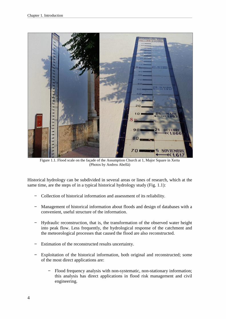
1.1. Background Floods are amongst the most destructive natural hazards in Western Europe. Indeed, in the period 1998-2009, 213 severe floods occurred in Europecausing 1126 people, half a million of displaced people and more than EUR 60 billion in economic losses (EEA, 2010). In Catalonia, between 1950 and 1999, floods produced around 1400 casualties and caused damages for EUR 300 million per year in average (Llasat et al., 2004a). Most of these casualties and damages are caused by flash floods. These floods occur in small, steep catchments and are characterised by their sudden and torrential nature and, therefore, are very destructive and difficult to forecast. The reduction of flood risk is undertaken from different (actually opposing) points of view: either the civil engineering focus, based on the reduction of the danger via concrete defensive structures, or the environmental engineering one, based on the reduction of the exposition and vulnerability, via the renaturalization of river channels and floodplains, soft engineering measures, the relocation of human settlements and activities, and the emergency and evacuation management planning. In any case, a solid knowledge of flood occurrence is needed for planning the defensive strategy. This knowledge can only be found in past floods. Unfortunately, records of measured floods are short and sometimes incomplete. In fact, some of the greatest floods may not be included because they usually destroy gauging stations or are too dangerous for a person to gauge them manually. Therefore, the knowledge that can be drawn from these records is sometimes partial and biased. In small catchments, this problem is even more acute: they are frequently ungauged and, thus, the lack of flow data is total. In historical times, the greatest floods, due to their destructive power and to the impact they caused on people, have usually been recorded, either with the immediate aim of damage survey or with the more farsighted objective of preserving this information as a warning for future generations. These records come in various formats: written (accounts, town council’s minutes, notarial documents), graphical (engravings, paintings, photographs), epigraphic (flood marks, flood scales, plaques, nicks) (Fig. 1.1). Depending on the quantity and quality of the information that they contain, these documents can be used to analyse the floods. Large historical floods have been studied since long, particularly those recorded as epigraphic marks, but the use of written historical documents to reconstruct and quantitatively analyse the floods is relatively recent. In order to differentiate this quantitatively-oriented use from the previous, more qualitative descriptions of floods, Benito et al. (2015) have coined the term “quantitative historical hydrology”; they also give a complete overview of this new branch of Earth sciences and of its rapid evolution in the last 15 years, especially in Europe. Quantitative historical hydrology (hereinafter, just historical hydrology) is very close, in terms of objectives, approach and methods, to paleohydrology, in which floods and other extreme events, such as droughts, are reconstructed, instead of from human-made records, from paleostage indicators: slackwater and lake deposits and flood evidences on trees and lichens (Baker, 1987; Baker, 2008). The simultaneous use of both historical records and paleostage indicators can diminish, where available, the uncertainty of the reconstructed peak flow (Thorndycraft et al., 2005).
Chapter 1. Introduction
4
Figure 1.1. Flood scale on the façade of the Assumption Church at 1, Major Square in Xerta
(Photos by Andreu Abellà) Historical hydrology can be subdivided in several areas or lines of research, which at the same time, are the steps of in a typical historical hydrology study (Fig. 1.1):
− Collection of historical information and assessment of its reliability.
− Management of historical information about floods and design of databases with a convenient, useful structure of the information.
− Hydraulic reconstruction, that is, the transformation of the observed water height into peak flow. Less frequently, the hydrological response of the catchment and the meteorological processes that caused the flood are also reconstructed.
− Estimation of the reconstructed results uncertainty.
− Exploitation of the historical information, both original and reconstructed; some of the most direct applications are:
− Flood frequency analysis with non-systematic, non-stationary information;
this analysis has direct applications in flood risk management and civil engineering.

Chapter 1. Introduction
5
− Use of the long series of rare events to analyse:
− Flood sensitivity to climate variability.
− The hydrological and hydraulic response of the catchment during extreme floods (for example, the different contribution of the subcatchments to the generation and propagation of the flood wave or canyons that may act as dams in the case of high flows) and its evolution as a consequence of changes in soil uses or in the channel’s geometry.
− The evolution of the social perception of risk expressed by floodplain occupation and the consequent damages.
Although, historical hydrology started, along with paleohydrology, in the 1980s (Condie & Lee, 1982; Cohn, 1986; Stedinger & Cohn, 1986; Stedinger & Baker, 1987), it is not until the 21st century that it sees a quick development and that its usefulness is extensively known among scientists. Bayliss and Reed (2001) give early methodological guidelines, which are further completed by Benito & Thorndycraft (2004), who address the practicalities of many of the issues listed above: assessment of the historical information reliability, use of Geographical Information Systems (GIS) to store and manage the data, hydraulic modelling and its uncertainty, or integration of historical floods in an instrumental flow series for frequency analysis. Barriendos & Coeur (2004) also discuss the methodological implications of historical information reliability, as do Barnolas & Llasat (2007), who also focus on the implementation of GIS-based historical floods databases. The formulation of these methodological bases has been accompanied by recent efforts to retrieve and collect historical information, which have resulted in an array of quite detailed chronologies of large floods in the last 500 years in Europe (Camuffo & Enzi, 1996; Brázdil et al. 2006, 2012; Gaume et al., 2009; Glaser et al. 2010; Luterbacher et al., 2012; Lang & Coeur, 2014), in Spain (Barriendos et al., 2003; Barriendos & Rodrigo, 2006), and in Catalonia (Barriendos & Pomés, 1993; Barriendos & Martín-Vide, 1998; Llasat et al., 2005; Barrera et al., 2006). However, not all the flood records contained in these chronologies can be used to reconstruct the floods. Actually, hydraulic modelling requires a certain amount of input information (most notably, the maximum water height reached by the water, and the geometry and roughness of the flooded area at the time of the flood) and a lengthy procedure, which often makes peak flow very difficult to obtain (Herget et al., 2014). Anyhow, the examples of peak flow reconstruction are abundant throughout Europe: (Sheffer et al., 2003, 2008; Brázdil, 2004; Naulet et al., 2005; Herget & Meurs, 2010; Elleder et al., 2013).

Chapter 1. Introduction
6
Figure 1.2. The different areas in which historical hydrology is divided and its applications.
Labelled in red, the areas dealt with in this thesis. In Spain also, large historical floods have been analysed since long, but mainly from the historical and social points of view with qualitative methods: Bentabol (1900), Blasco-Ijazo (1959), Couchoud (1965), Iglésies (1971), López-Gómez (1983), Curto (2007). Nevertheless, quantitative analyses with their focus on hydrological and meteorological aspects have also been attempted, some even including approximate peak flow estimations: García-Faria (1908), Fontseré & Galcerán (1938), López-Bustos (1972, 1981), Novoa (1984), Llasat et al. (2003). In any case, peak flow reconstruction of historical floods with hydraulic models is much more recent (Benito et al., 2003; Ortega & Garzón, 2009) and, with exceptions (Ruiz-Villanueva et al., 2010, for example), generally limited to large basins, such as the Tagus River. In Catalonia, the first attempts at historical floods hydraulic reconstruction are by Fernández-Bono & Grau-Gimeno (2003) and Lang et al. (2004) in the Onyar River in Girona and the Segre River in Lleida. Balasch et al. (2007, 2010a) follow suit, the former with the reconstruction of a river flood in the Segre River and the latter with that of a huge flash flood event in three small catchments. The main problem that hydraulic reconstruction is faced with is the correct determination of the characteristics of the modelled reach at the time of the flood, that is, the geometry of the channel and the floodplain and their roughness, which determines its friction against the flow. These determinations, despite the abundance of information, are always approximate estimations since direct measurement is impossible. Thus, hydraulic

Chapter 1. Introduction
7
reconstruction results have a non-negligible amount of uncertainty. The sources of this uncertainty have been deeply investigated (Pappenberger et al., 2005; Pappenberger et al., 2006; Lang et al., 2010; Neppel et al., 2010); however, no methodology has been developed and widely agreed upon yet. Therefore, only some hydraulic reconstructions give an estimate of their uncertainty, as for example, Naulet et al. (2005), Remo & Pinter (2007), Balasch et al. (2010a) and Herget & Meurs (2010). The hydraulic reconstruction of a historical flood can be part of the thorough hydrometeorological analysis of a particular event, one that can address questions such as the hydrological response of the subcatchments, the floodwave routing across the catchment, and the meteorological situation and the ensuing processes that caused the flood; examples of this kind of study can be found in Gaume et al. (2004), Bürger et al. (2006), Thorndycraft et al. (2006), Brázdil et al. (2010), Blöschl et al. (2013), and Herget et al. (2015). However, the main use of the reconstructed peak flow of a historical flood is to be integrated in a flow series for flood frequency analysis. Flood frequency analysis, which is essential in civil engineering, risk mitigation and land use planning, is based on flow series; unfortunately, measured flow series are usually too short for the usual purposes of flood frequency analysis. Therefore, the possibility of lengthening flow series with historical floods is very much welcomed and that is why this particular aspect of historical hydrology is one of the most investigated since long (Condie, 1982; Cohn, 1986; Hosking & Wallis, 1986a; Macdonald, 2006; Macdonald et al., 2006; Kjeldsen et al., 2014). The two main problems of using historical floods in frequency analysis are, on the one hand, the development of methods to use censored, non-systematic data (historical floods) along with systematic data (gauge measurements) and, on the other hand, the non-stationarity of floods over a long period. The former has been dealt with by Hirsch (1987), Stedinger & Cohn (1986), Francés (2004), among others; the latter, by Cunderlink & Buhn (2003), Westra et al. (2010), Machado et al., (2015). Currently, new techniques are also being developed to improve flood frequency analysis: regional analysis (Gaume et al., 2010), fuzzy-logic-based methods (Salinas et al., 2015), Bayesian analysis (Viglione et al., 2013). Historical hydrology can be especially useful in flood frequency analysis in ungauged catchments, where no flow series are available, and which, since usually small, are frequently affected by flash floods (Payrastre et al., 2005; Nguyen et al., 2014). Aside from an immediate primary use in flood frequency analysis and risk mitigation (Petrucci & Polemio, 2003), long series of historical floods and their reconstructed peak flows can be used to assess the evolution of flood regime (Hall et al., 2014; Blöschl et al., 2015) and to relate that evolution to changes in climate (Brázdil et al., 2005; Gregory et al., 2006; Benito et al., 2008; Kiss, 2009b; Kundzewicz et al., 2010; Szolgayova et al., 2014), in the catchment’s hydrological response (Andréassian, 2014) or even in the social perception of risk (Llasat et al., 2008; Viglione et al., 2014). Moreover, historical hydrology increases the quantity of information, usually, scarce, about extreme floods. This increased information can help to gain insight into the processes that cause this kind of flood and their evolution in the last centuries. For instance, it has enabled studies about the contribution of subcatchments to flood magnitude and frequency in a large basin, such as the Ebro River (Balasch et al., 2014). It has enabled, also, the analysis of meteorological patterns and processes associated with

Chapter 1. Introduction
8
large floods (Bárdossy & Filiz, 2004; Kiss, 2009a; Llasat et al., 2004b; Pino et al., 2015). This meteorological analysis is very much facilitated, for floods since 1871, by the high resolution (both spatial and temporal) data obtained by the 20th Century Reanalysis (Compo et al., 2011). 1.2. Justification and working hypothesis In view of what has been just said, the research possibilities that historical hydrology creates are numerous and promising. Besides, the practical usefulness of historical hydrology has been sanctioned by the European Union Floods Directive on the assessment and management of flood risks (2007/60/EC of the European Parliament and of the Council, 26 November 2007) and its transpositions to the member states’ legislations (such as the Spanish Real Decreto 903/2010, 9 July 2010), which encourage the use of historical information in flood risk assessment. However, historical hydrology is still a recent area of knowledge and much research is yet to be done to develop it and, especially, to make it a useful and widespread tool among end users and decision makers. Unfortunately, historical hydrology is rarely applied in engineering and planning studies nowadays (Benito et al., 2015). The reason is that historical hydrology is a multidisciplinary science that requires a wide expertise including archival research, hydrological and hydraulic modelling, uncertainty assessment, and flood frequency analysis. It must, therefore, be tackled by a task force of experts. Because of that, presently, its general use among engineers and decision-makers, and the benefits that would come with it, are hindered. In Catalonia, historical hydrology is still an underused resource, not only in terms of everyday application by regional and local authorities but also in terms of basic research. Presently, only two teams are specifically studying historical floods in Catalonia: GAMA, led by Maria del Carmen Llasat from the University of Barcelona, focused on social perception of risk and meteorological processes associated with floods; and Prediflood, led by J. Carles Balasch and David Pino from the Universities of Lleida and Politècnica de Catalunya, within which this thesis was done. Two other teams, both of the University of Barcelona, work in related fields: FluVAlps, led by Lothar Schulte, which focus on the use of paleohydrology in Alpine environments with climate change assessment purposes; and RiskNat, led by Joan Manuel Vilaplana and Glòria Furdada, which focus on geological risks in general (floods, landslides, avalanches, earthquakes), both modern and historical, in the Pyrenees. In our opinion, both basic research on floods and applied knowledge for flood risk reduction can benefit much from the development of historical hydrology in these areas. In order to achieve the desirable wide use of historical hydrology, two main actions should be implemented: Firstly, historical information about floods should be gathered and published for everyone to easily access it; otherwise, only historians and archivists would be able to find it. Secondly, techniques and methodologies enabling the use of historical information in hydrological and hydraulic modelling, uncertainty estimation, and flood frequency analysis, should be developed and given general access. Thus, the working hypothesis that this thesis tries to prove is that the use of descriptive, qualitative information about historical floods preserved in documentary sources allows

Chapter 1. Introduction
9
the quantitative reconstruction of those floods and of the meteorological processes that caused them, and that this reconstruction has the required degree of validity to improve the knowledge on which flood hazard assessment and risk management are based, especially in ungauged catchments. 1.3. Objectives The main objective of this thesis is to investigate, by means of case studies, the potential of novel applications of historical hydrology in Catalonia and the Ebro River basin, and, through this investigation, to contribute to the understanding of the meteorological, hydrological and hydraulic contexts associated to the most extreme floods in NE Spain. This investigation was done under an applied approach, since each analysed aspect of historical hydrology was illustrated with a case study. In order to meet the main objective of the thesis, some of the various aspects related with historical hydrology listed in Section 1.1 were analysed. These analyses are the secondary objectives of the thesis:
1) Construction of a database of historical floods occurred in Catalonia since 1500, with an adequate structure to be a useful tool inhistorical flood reconstruction (Chapter 2).
2) Reconstruction with hydraulic modelling from flood marks of a peak flow series of seven floods since 1615 in the town of Tàrrega. (Chapter 3).
3) The complete reconstruction (hydraulic, hydrological and meteorological) of 1874 Santa Tecla flood in Catalonia (Chapter 4).
4) Estimation of the uncertainty of the reconstructed peak flow of 1907 flood in the Ebro River (Chapter 5).
5) Identification of the input variables of hydraulic modelling with greater influence on the peak flow result (Chapter 5).
6) Quantification of the improvement that reconstructed historical information provides to flood frequency analysis? (Chapter 6).
These secondary objectives helped to answer the following research questions in the form of a general discussion of the implications of the results of the thesis (Section 7.2):
1) What characteristics and what kind of information should a database have in order to be successfully used in historical flood reconstruction? (Chapter 2).
2) What can the most immediate applications of hydraulic reconstruction of historical floods be? What is the best method to reconstruct a peak flow? What are the main obstacles for hydraulic reconstruction to become a widespread tool among end users? (Chapter 3).

Chapter 1. Introduction
10
3) What usefulness does a complete reconstruction of a historical flood have? (Chapter 4).
4) How much uncertainty does a historical flood reconstructed peak flow have? Is it acceptable? Does this uncertainty make this reconstructed peak flow useless? (Chapter 5).
5) What input variables influence the most the peak flow result in hydraulic modelling? And what input variables influence the most the peak flow uncertainty? What recommendations could be made with the objective of reducing peak flow uncertainty? (Chapter 5).
6) In what measure does reconstructed historical information improve flood frequency analysis? (Chapter 6).
1.4. Overview of the data and methods used Three main tasks were performed within this thesis: flood reconstruction, uncertainty assessment and flood frequency analysis. Further details of the data sources and methods used in each of these tasks are given in the following chapters. In any case, a short overview is given hereinafter: 1) Data sources: The reconstruction of a historical flood requires a great number of input data. The sources of the data used in this thesis were diverse: on the one hand, epigraphic marks that signalled the maximum water height of the flood, and, on the other hand, written and visual documents. The latter can also pinpointed the maximum height of the flood but primarily gave indications of the geometry of the modelled river reach, of the occupation of the channel and the flood plain by vegetation and constructions, of the soil’s type, use and cover, and of the hydraulic characteristics of the hydrographic network within the catchment. 2) Flood reconstruction (see Section 2.6): In this thesis, the three parts of flood reconstruction were attemted: hydraulic, hydrological and meteorological reconstruction-
− Hydraulic reconstruction: Its objective is the estimation of the peak flow from a flood mark. These estimations were done with a hydraulic model: the one-dimensional HEC-RAS model (USACE, 2008, 2010a), which was fed data about the hydraulic characteristics of the modelled reach: geometry and roughness. In some cases where additional information about the evolution of water stage was available, the whole hydrograph (not only the peak flow) could be estimated. The estimation procedure was an iterative one, since the peak flow is an input data that the model needs.
− Hydrological reconstruction: Its objective is the estimation of the hyetograph of the rain that caused the flood from the previously estimated hydrograph. These estimations were done with the lumped hydrological model HEC-HMS (USACE 2010b; 2013), which was fed data about the hydrological response of the modelled catchment: the soil’s infiltration capacity, given by the soil’s type, use and cover, and the hydraphic network’s reactivity, given by the stream’s length, slope and

Chapter 1. Introduction
11
roughness. The estimation procedure was an iterative one, since the hyetograph is an input data that the model needs.
− Meteorological reconstruction: Its objective is the estimation of the meteorological processes that caused the storm that subsequentially caused the flood. These estimations were only possible with a certain degree of detail for events occurred since 1851 thanks to the charts reconstructed by the 20th Century Reanalysis (Compo et al., 2011). These charts contain data about many meteorological variables on any location on the globe at many different heights with a time resolution of up to six hours and a space resolution of 2º. These data describe the air masses characteristics (temperature and moisture) and their movements that, at their turn, give an explanation of the processes involved in creation of the rain event. According to Compo et al. (2011), the quality of the data is generally high when compared with independent radiosonde data, especially in the extratropical Northern Hemisphere.
3) Uncertainty assessment (see Section 5.3.2): Its objective is the estimation of the error of the peak flow modelling in the hydraulic reconstruction. These estimations were done with local sensitivity analyses, which give the range of variation of the output variable (the modelled peak flow) caused by known variations of the input variables. The quadratic sum of the variations caused by individually-altered input variables gives a good estimation of the peak flow total error. 4) Flood frequency analysis (see Section 6.3): Its objective is the estimation of the annual exceedance probability of a given flow. These estimations were done with the software AFINS (GIMHA, 2014), using peak flow series composed of systematic (measured) and non-systematic data (that is, reconstructed peak flow data of historical floods).
Figure 1.3. Overview of the data sources and methods used

Chapter 1. Introduction
12
1.5. Geographical framework: the eastern area of the Ebro River basin The Ebro is one of the great rivers of the Mediterranean basin, similar in size and mean flow to the Rhône (France and Switzerland) and the Po (Italy), but smaller than the Nile and Danube. Among the rivers in the Iberian Peninsula, it is the second longest (930 km), the second in mean flow (428 m3·s-1) and the most regular in annual discharge volume. The Ebro River drains the north-eastern part of the Iberian Peninsula, which includes most of the southern face of the Pyrenees Range, into the Mediterranean Sea. It has a NW-SE oriented, triangular-shape basin of 85,000 km2, which approximately matches the Cenozoic foreland basin caused by the rising of the Pyrenees Range. This range limits the basin to the NE, whereas the Cantabrian Mountains limit it to the NW, the Iberian System Range to the SW and the Catalan Pre-Coastal Range to the SE. Due to the extension and geographical configuration of the Ebro basin, the climate in the headwaters and in the lowlands is very different,. Mean annual rainfall in the basin was 622 mm during the period 1920-2000; however, rainfall is very unevenly distributed across the basin: there is a high altitudinal gradient: 1000-1500 mm in the Cantabrian Mountains and Pyrenees; 400-700 mm in the Iberian System and Catalan Pre-Coastal Range; and less than 400 mm in the lower area. Evapotranspiration loss has an opposite gradient of that of rainfall: it is higher in lower areas, with a basin average value of 450 mm. This spatial heterogeneity translates into different hydrological regimes; according to them, the Ebro basin can be divided into three great hydrological areas, which can include one or more sub-catchments (Fig. 1.4 and Table 1.1):
− Upper Ebro, in the west, from the source to Zaragoza, approximately in the centre of the medium reach. It includes sub-catchments of the Cantabrian Mountains: Oca, Zadoya, Najerilla and Cidacos; sub-catchments located in the Iberian System Range: Jalón and Juerva; and some western Pyrenean sub-catchments: Ega Arga, Aragón and Gállego. This area is 48% of total Ebro basin surface and contributes 231 m3·s-1 (or 54% of total) to mean runoff. The hydrological regime is driven by rain and snow in winter and spring.
− Segre-Cinca system: these are the two main tributaries of the Ebro, and drain a large sector of the central and eastern Pyrenees. These two rivers join and just six km downstream flow together into the Ebro in Mequinensa. Their catchments are 27% of Ebro’s total area and their mean runoffs (80 m3·s-1 and 78 m3·s-1, respectively) is 37% of total. The hydrological regime is characterised by spring snowmelt and autumn rainfalls.
− Lower Ebro, from Zaragoza to the Mediterranean Sea: it contains the small tributaries of the eastern area of the Iberian System and the Catalan Pre-Coastal Range, as, for example, Martín, Guadalope and Matarranya. Its area is 26% of the total and its mean runoff is 9% of the total. Rainfall is more frequent in autumn. Water budget in this area is negative due to high evapotranspiration and human use.
The result of this diverse basin is high spatial variability, irregularity and seasonality of the flows. For instance, the irregularity factor (that is, the ratio between the highest and lowest monthly mean flows) is 6.3 in Zaragoza and 2.9 in Tortosa, due to the more

Chapter 1. Introduction
13
regular contributions of the Segre-Cinca system (Albentosa, 1989). Seasonality is also quite marked: in Tortosa, near the outfall of the basin, the ratio between the season’s mean flow and the annual mean flow is 1.5 in spring, 1.35 in autumn and 0.35 in summer (July and August). Similarly, annual maximum instantaneous flow (Qci) can occur any time in the year in different places within the catchment, according to the climate of the area (Davy, 1975). Thus, in the Upper Ebro, floods generally happen in autumn and winter; in Segre-Cinca system, in spring; in the upper half of the Lower Ebro, in spring and summer; and in the lower half of the Lower Ebro, in autumn. Floods starting in the headwaters of the Ebro basin take 6-7 days to reach the sea: 2-3 days down to Miranda de Ebro, 1.5-2 days from Miranda to Zaragoza and 2-3 days from Zaragoza to Tortosa and the sea. Floods originating in the Segre-Cinca system have a transit time of 1.5-2 days down to Tortosa. Although, the first non-systematic flow measurements, nowadays unfortunately lost, were done in mid-19th century in Bocal, Tudela (López-Bustos, 1972), systematic flow gauging started in 1912-13 in the towns of Zaragoza and Tortosa (Ebro), and Lleida (Segre). Many of the gauging stations across the basin accumulate from 50 to 75 years of data. However, data about magnitude and frequency of floods in the Ebro basin are scarce: there are no flow measurements of any flood prior the 20th century and, within that century, most of the systematic measurement series lack the greatest floods, such as 1907, 1937 and 1982. Early calculations greatly over-estimated 1907 flood’s peak flow (García-Faria, 1908); however, posterior revisions (López-Bustos 1972, 1981) estimate it at 12000 m3·s-1 in Tortosa, that is, 28 times the annual mean flow. The peak flows in various locations of 1907 and 1982 floods have also been calculated by the Hydraulic Administration (Fontseré i Galcerán, 1938; López-Bustos, 1981; Novoa, 1984). Throughout the 20th century, about 190 dams were built within the Ebro basin, mainly in the main Pyrenean tributaries and in the lower Ebro. The impoundment runoff index (that is the ratio between impounding capacity and annual runoff volume) is presently 57%. The Mequinensa (1534 hm3) and the Riba-roja (210 hm3) reservoirs have altered the flood regime in the lower Ebro: they have reduced by 30% the peak flows with a return period between 2 and 10 years (Batalla et al., 2004) and by 25% the peak flows with a return period between 10 and 25 years (Batalla & Vericat, 2011). Dams have also contributed to the increasing water use, which, coupled with changes in soil use in mountainous regions, have greatly reduced runoff volume in Tortosa, near the outfall: from 18,500 hm3·yr-1 in the 1960s to 13,500 hm3·yr-1 (or 428 m3·s-1) in the 2000s (Gallart & Llorens, 2004). The geographical framework of this thesis is the easternmost area of the Ebro basin, that is, the Segre catchment and the eastern half of the Lower Ebro −although in the last chapter, floods occurred in Zaragoza are also analysed. In any case, each chapter has a slightly different study area since it focuses on particular catchments; therefore, there is a specific section devoted to describe them in each chapter.

Chapter 1. Introduction
14
Table 1.1. Area and mean flow of the three great hydrological areas of the Ebro River
Hydrological area Site
Area Mean flow
Area (km2) Percentage of
total Ebro area (%)
Mean flow (m3 s-1)
Percentage of mean flow at Tortosa (%)
Upper Ebro Zaragoza(1) 40,434 48 231 54
Segre-Cinca system
Cinca Fraga 9,612 11 78 18 Outlet 9,699 11 ND ND
Segre Lleida 11,369 13 80 19 Outlet 12,880 15 ND ND
Lower Ebro Tortosa 21,217 25 428 100(2) Outlet 21,988 26 ND ND
Total Ebro Tortosa 84,230 99 428 100 Outlet 85,001 100 ND ND
ND = No data (1) Zaragoza is the outlet of the Upper Ebro subbasin (2) The mean flow of the Lower Ebro is the mean flow of the total Ebro
Figure 1.4. Location of the Ebro basin within Europe (a) and the Iberian Peninsula (b), and map of the Ebro basin with its three main hydrological areas (c). In (c), blue lines represent rivers and black lines represent sub-basins’ watersheds. Maps (a) and (b) modified from a map Copyright © 2009 National Geographic
Society, Washington, D.C.; map (c) drawn by Damià Vericat (RIUS-University of Lleida).

Chapter 1. Introduction
15
1.6. Structure of the thesis This thesis is composed of seven chapters, five of which are articles either published in or submitted to international research journals (Table 1.2), all of which were in the first quartile of their category at the time of publication, except Zeitschrift für Geomorphologie, which was in the second quartile; the contribution of the author of the thesis to each of these articles is detailed in Table 1.3. More specifically, the thesis has the following structure (Fig. 1.5):
1) Chapter 1 is a general introduction that contains a historical overview of historical hydrology, as well as the justification, the objectives and the structure of this thesis.
2) Chapter 2 presents the “Prediflood” database of floods occurred in Catalonia since 1035 and enunciates the characteristics that such a database should have in order to successfully store and manage historical information for hydrological research purposes.
3) Chapter 3 is the base of any historical hydrology study: hydraulic reconstruction; in this case, the hydraulic reconstruction of seven historical floods in one location, with the objective of creating the peak flow series of an ungauged catchment for frequency analysis purposes.
Figure 1.5. Structure of the thesis

Chapter 1. Introduction
16
4) Chapter 4 is an example of the complete reconstruction of a historical flood: the historical, hydraulic, hydrological and meteorological reconstruction of 1874 Santa Tecla floods, in an area of over 10000 km2.
5) Chapter 5 quantifies the uncertainties of the results of the hydraulic reconstruction of 1907 flood of the Ebro River in the town of Xerta.
6) Chapter 6 uses the flow data series created in Chapter 3 and two other series to assess the benefits of using hydraulically reconstructed peak flows of historical floods in flood frequency analysis.
7) Chapter 7 closes the document with the general conclusions, the answers to the key research questions, the limitations of this study and the future research that should be done.
Table 1.2. Papers that compose this thesis and associated posters and oral communications
Chapter Type of
communication Reference
2
Paper (Published
04/Dec/2014)
Barriendos, M., Ruiz-Bellet, J.L., Tuset, J., Mazón, J., Balasch, J.C., Pino, D., Ayala, J.L. (2014): The “Prediflood” database of historical floods in Catalonia (NE Iberian Peninsula) AD 1035-2013, and its potential applications in flood analysis. Hydrol. Earth Syst. Sci., 18, 4807-4823.
Oral communication
Ruiz-Bellet, J.L., Tuset, J., Balasch, J.C., Barriendos, M., Mazón, J., Pino, D., Ayala, J.L, (2013): Possibilities of the PREDIFLOOD database (Catalonia, AD 1033-2010). Workshop ‘Deciphering river flood change: historical floods’, Technisches Universität Wien, Vienna, Austria, 5-6 September
3
Paper (Published
21/Dec/2011)
Balasch, J.C., Ruiz-Bellet, J.L., Tuset, J. (2011): Historical flash floods retromodelling in the Ondara River in Tàrrega (NE Iberian Peninsula). Nat. Hazards Earth Syst. Sci., 11, 3359-3371.
Poster
Ruiz-Bellet, J.L., Balasch, J.C., Tuset, J., Vericat, D. (2012): Flash floods reconstruction from historical data in the ungauged Ondara River basin at Tàrrega (NE Iberian Peninsula). EGU General Assembly 2012, Vienna, Austria, 22-27 April
4
Paper (Published
16/Feb/2015)
Ruiz-Bellet, J.L., Balasch, J.C., Tuset, J., Barriendos, M., Mazón, J., Pino, D. (2015): Historical, hydraulic, hydrological and meteorological reconstruction of 1874 Santa Tecla flash floods in Catalonia (NE Iberian Peninsula). J. Hydrol., 524, 279-295.
Poster Ruiz-Bellet, J.L., Balasch, J.C., Tuset, J., Barriendos, M., Mazón, J., Pino, D. (2013): Meteorological analysis of 1874 Santa Tecla’s flash floods in NE Iberian Peninsula. EGU General Assembly 2013, Vienna, Austria, 8-12 April
5
Article (Submitted
23/Jan/2016)
Ruiz-Bellet, J.L., Castelltort, X., Balasch, J.C., Tuset, J.: Uncertainty of the peak flow reconstruction of the 1907 flood in the Ebro River in Xerta (NE Iberian Peninsula). Submitted to J. Hydrol. (January 2016).
Poster
Ruiz-Bellet, J.L., Castelltort, X., Balasch, J.C., Tuset, J. (2016): Error of the modelled peak flow of the hydraulically reconstructed 1907 flood of the Ebro River in Xerta (NE Iberian Peninsula). EGU General Assembly 2013, Vienna, Austria, 17-22 April
6
Paper (Published
01/Nov/2015)
Ruiz-Bellet, J.L., Balasch, J.C., Tuset, J., Monserrate, A., Sánchez, A. (2015): Improvement of flood frequency analysis with historical information in different types of catchments and data series within the Ebro River basin (NE Iberian Peninsula). Zeitschrift für Geomorphologie, 59(3), 127-157.
Poster
Balasch, J.C.., Ruiz-Bellet, J.L., Tuset, J., Astudillo, C., Sánchez, A., Castelltort, X., Barriendos, M., Mazón, J., Pino, D. (2014): Improvement of flood frequency analysis from historical floods in different-sized basins. HEX Conference, Bonn, Germany, 9-15 June

Chapter 1. Introduction
17
Table 1.3. Contribution of the author to the articles contained in the thesis Chapter
(see Table 1.2)
Co-authoring position
Contribution
2 Second
− Participation in the definition of hypotheses, objectives and methodology
− Writing of part of the introduction and the concluding remarks − Writing of section 2.6 − Figures 2.1, 2.4, 2.5 and 2.6 − Review of the whole document
3 Second
− Participation in the definition of hypotheses, objectives and methodology
− Compilation of documentary information about the floods − Assistance in hydraulic modelling − Hydrological analysis − Uncertainty assessment − Writing of the whole document (including tables) − Figures 3.3 to 3.9 − Description of the study area − Discussion of the results − Coordination of the co-authors contributions
4 First
− Definition of hypotheses, objectives and methodology
− Bibliographical research − Compilation of documentary information about the floods − Assistance in hydraulic and hydrological modelling − Uncertainty assessment − Writing of the whole document (including tables) − Figures 4.2 and from 4.6 to 4.10 − Description of the study area − Discussion of the results − Coordination of the co-authors contributions
5 First
− Definition of hypotheses, objectives and methodology
− Bibliographical research − Assistance in hydraulic modelling − Uncertainty assessment and sensitivity assessment − Writing of the whole document (including tables) − Figures 5.1, 5.2, 5.4, 5.7 and 5.9 − Compilation of documentary information about the floods − Description of the study area − Discussion of the results − Coordination of the co-authors contributions
6 First
− Definition of hypotheses, objectives and methodology
− Bibliographical research − Compilation of documentary information about the floods − Flood frequency analysis − Writing of the whole document (including tables) − All figures − Description of the study area − Discussion of the results − Coordination of the co-authors contributions

Chapter 2
The “Prediflood” database of historical floods in Catalonia (NE Iberian Peninsula) AD 1035-2013, and its
potential applications in flood analysis
Barriendos, M., Ruiz-Bellet, J.L., Tuset, J., Mazón, J., Balasch, J.C., Pino, D., Ayala, J.L. (2014): The “Prediflood” database of historical floods in Catalonia (NE Iberian Peninsula) AD 1035-2013, and its potential applications in flood analysis. Hydrol. Earth Syst. Sci., 18, 4807-4823. http://www.hydrol-earth-syst-sci.net/18/4807/2014/ doi:10.5194/hess-18-4807-2014 Published 4 December 2014


Chapter 2. The “Prediflood” database of historical floods in Catalonia
21
Abstract “Prediflood” is a database of historical floods that occurred in Catalonia (NE Iberian Peninsula), between the 11th century and the 21st century. More than 2700 flood cases are catalogued, and more than 1100 flood events. This database contains information acquired under modern historiographical criteria and it is, therefore, suitable for use in multidisciplinary flood analysis techniques, such as meteorological or hydraulic reconstructions. Keywords: historical floods, database, historiographical criteria, multidisciplinary flood analysis 2.1. Introduction Floods have always been among the most destructive of natural hazards, in part due to the traditionally high exposure and vulnerability of most human settlements. Indeed, between 1998 and 2009, Europe suffered more than 213 severe floods, which caused 1126 casualties, the displacement of half a million people and more than EUR 60 billion in economic losses (EEA, 2010). Unfortunately, both the frequency and magnitude of floods are likely to increase in the near future due to climate change, thus worsening the effects of floods on the human population. This is especially true for the Mediterranean region, where climatic models foresee an increase of rainfall irregularity: in Catalonia (NE Iberian Peninsula), for the period 2070-2100, models estimate a 15% decrease in total rain depth but, at the same time, a 15-30% increase in the number of days with heavy precipitation (Barrera and Cunillera, 2011). In central Europe, torrential precipitations will also increase in the near future, although this cannot be assured to cause an increase in river flows, due to the short length of the data series (IPCC, 2014; Kovats and Valentini, 2014). The increase of flood hazard will force the undertaking of protection measures, which are going to need information about floods frequency and magnitude. Unfortunately, river flow instrumental series are usually too short (when they exist at all) to analyse low-frequency events, such as flash floods (Gaume et al., 2009). However, these series can be lengthened with historical floods information. In this sense, the European Union Floods Directive on the assessment and management of flood risks (2007/60/EC of the European Parliament and of the Council, 26 November 2007) encourages the use of historical information in flood risk assessment. Regrettably, historical flood compilations in Spain have always had a low quality, due to the lack of proper historiographical methods and, hence, they are useless in flood risk assessment. In fact, in order to ensure a good quality of information, historical floods compilations in Spain should be created anew. The main objective of this article is to present the “Prediflood” database, a new database of historical floods in Catalonia that encompasses the period AD 1035-2013, created from scratch with modern historiographical methods; a secondary objective is to show its potential applications in flood analysis and in flood risk assessment. More specifically,
Chapter 2. The “Prediflood” database of historical floods in Catalonia
22
this paper describes the process of creation of the “Prediflood” database from past events, the issues that can be improved and the potential of the organized information. The initial research project (see acknowledgements), in which this work is framed, analyses the past 500 years but data collection has provided information beyond this limit. This process is an opportunity to reassess previous procedures and to incorporate historiographical criteria regarding the sources of information. PREDIFLOOD is the acronym of a Spanish research project. The general aim of the project is to improve the capacity of Predictivity of Flood events based on a large collection of historical information and modern data for all possible flood events in our study area. With these materials, hydraulic-hydrologic reconstructions and synoptic meteorological reconstructions will improve knowledge enough to produce tools for the improvement of preventive and early warning procedures for risk management situations. Considering the topography and climatology of Catalonia, with a large number of ungauged basins, small dimension of basin but strong torrential rainfall events and high demographic concentration on the littoral as opposed to river mouths, improved knowledge for early warning procedures is strongly positive for management of these situations. 2.2. Review of historical floods compilations in Spain 2.2.1. Early attempts in floods collection (1850-1980) The first attempts to gather information on historical floods in Spain began in the second half of the 19th century, with the prevalence of positivism in historiography. These attempts took advantage of the network of historical archives created and managed by the public administration. However, these first works lack scientific objectives beyond the mere compilation of data. On the other hand, the period's context without technological resources, made the systematic collection and analysis of large quantity of historical information and data impossible. Consequently most of these works do not have minimum conditions, and hence, many of these works do not meet the minimum standards of historiographical rigor. Nevertheless, some Spanish compilators took as a reference the work of the French historian Maurice Champion (Champion, 1858-1864). Of these, two local studies stand out: one in the town of Girona (Chía, 1861) and one in town of Murcia (Hernández, 1885) −this last one including an analysis of the causes and effects of floods. A remarkable synthesis of all the basins in the Iberian Peninsula was also published (Bentabol, 1900). The first half of the 20th century saw a hiatus in flood compilations due to a movement of rejection of historiographical determinism. However, highly destructive floods which occurred in this period reignited the interest in this area of research and several local works of increasing methodological rigour appeared, such as those of the Túria River (Almela, 1957), the Ebro River (Blasco, 1959), the Segura River (Couchoud, 1965), the Llobregat River (Codina, 1971) and the junction of the Ter and the Onyar rivers at Girona (Alberch et al., 1982). At the same time, analytical studies began to appear, focused either on single events (Iglésies, 1971) or on the general characteristics of floods (López-Gómez, 1983).

Chapter 2. The “Prediflood” database of historical floods in Catalonia
23
2.2.2. The involvement of the administration (since 1980) In the last 30 years, the Spanish administration has made several attempts to gather historical floods information and to render it useful. More specifically, two types of organisms have led the way: basin authorities (called in Spanish “Confederaciones Hidrográficas”) and civil protection authorities (“Dirección General de Protección Civil y Emergencias”). On the one hand, basin authorities early began to search and use information about historical floods as a complement of instrumental data, with the objective of better assessing floods’ frequencies, flows, duration and behaviour. To this end, they launched several initiatives of historical floods data collection. Unfortunately, the personnel involved in those projects were civil engineers, with a poor background on historiographical methods; they looked for information in ill-organized compilations of uneven quality, which did not permit a clear identification of the documentary sources. Furthermore, the information thus found was only used in comparing some extreme historical flood to those of the instrumental period and in creating flood chronologies that lacked any methodological criteria of exhaustiveness and, hence, had a mere informative objective. Besides all this, over the years, basin authorities have been placed under different ministries due to their diverse competencies on water (irrigation, drinkable water, waste water, infrastructures, taxes), and this hampered long-term projects, such as historical floods compilations. The civil protection service is relatively new in Spain (Law 2/1985, 21 January 1985). This new concept of emergency prevention and management brings a new challenge to the collection and analysis of historical information. Indeed, this service needs greats amounts of reliable information in order to perform the multidisciplinary analysis required both in emergency planning (prevention, rescue, evacuation, safe and vulnerable areas) and in urban planning. Membership of the European Union also places new demands on the civil protection service. The Water Framework Directive (2000/60/EC of the European Parliament and of the Council, 23 October 2000) defined new work elements on water resources management and their severe manifestations, as droughts and floods. But it was the EU Floods Directive (EU Floods Directive on the assessment and management of flood risks, 2007/60/EC of the European Parliament and of the Council, 26 November 2007), that, for the first time, specifically commanded the EU State members to assess flood hazard and risk. In Spain, this task was already underway with the mapping of flooding areas: “Sistema Nacional de Cartografía de Zonas Inundables” (SNCZI, 2010). Regarding historical floods, the transposition of the EU Floods Directive into Spanish legislation (Real Decreto 903/2010, 9 July 2010), in its articles 6 and 7, define the use of historical information in flood risk assessment. However, the results of the actions ordered by the EU Floods Directive are uneven in Spain. Instrumental information has been successfully catalogued and homogenized. But available historical information has not been thoroughly confirmed by systematic consultation of reliable documentary sources. Indeed, in relation to historical flood information, the work has been reduced to organizing and digitizing the data from the previous flood compilations done by the basin authorities (Catálogo Nacional de

Chapter 2. The “Prediflood” database of historical floods in Catalonia
24
Inundaciones Históricas, 2006-2010). This is a mere accumulation of information, but not an improvement in its quality, quantity or applicability, because the source compilations are fragmentary and they lack both flood selection criteria and references to primary documentary sources. Unfortunately, this has been the usual procedure in the treatment of historical floods information until now. Therefore, although powerful software programmes support these modern compilations, their applicability in flood analysis is very limited and they are seen as mere collections of anecdotes for informational pieces into calendars or yearbooks. 2.2.3. Scientific approaches Apart from the efforts of administration, there have also been scientific approaches to the collection of historical flood information in recent years, with the aim of creating flood compilations of European-homologable quality. The first doctoral thesis on the subject was by Grimalt on the island of Mallorca (Grimalt, 1988), which was later published as a book (Grimalt, 1992). Since then, several research projects acquired historical information with specific criteria in order to produce consistent and reliable data series. However, these projects, which were costly and lasted from 2 to 4 years, were limited to a scarce number of chronologies in small areas −examples are the compilations of Maresme County (Barriendos and Pomés, 1993), of the Spanish Mediterranean coast (Barriendos and Martín-Vide, 1998) and of the basins of the Ter, Llobregat and Segre rivers (SPHERE Project, “Systematic, Palaeoflood and Historical data for the improvEment of flood Risk Estimation”, EU Project EVG1-CT-1999-00010, 2000-2004). Also, the Geological Institute of Catalonia started a campaign of systematic collection of information between 2008 and 2010 in order to map natural risks, but budget limitations stopped the survey and only the Pyrenees area was completed. These compilations done with scientific purposes, although scarce and modest, follow the methods of European research. This has allowed complex analyses such as: the improvement of climate behaviour estimations from multicentennial flood chronologies (Llasat et al., 2005; Barriendos and Rodrigo, 2006); the study of flash floods (Llasat et al., 2003; Barrera et al., 2006; Balasch et al., 2010a ); or the reconstruction of the peak flows and the impacts of one of the worst floods in the Iberian Peninsula, that of November 1617 (Thorndycraft et al., 2006). 2.3. Characteristics of the "Prediflood" database The “Prediflood” database contains information about historical floods occurred in Catalonia (NE Iberian Peninsula) between AD 1035 and 2013. The current state-of-the-art of historical floods in Spain (as previously described) and the potential of our contribution as outlined in this paper are very different. Previous official databases mostly took information only from a selected number of bibliographical references, but not defined by historiographical criteria or any specific order. The obtained database included a large amount of information, but with important

Chapter 2. The “Prediflood” database of historical floods in Catalonia
25
weaknesses. On the other hand, previous research projects in this field have worked from documentary and bibliographical sources, but focused on very specific geographical sites. We suggest and apply systematic approach to bibliographical sources obtaining a complete identification of primary sources (historical documentary sources with full reliability: objectivity, eyewitness in real time, and so forth). A new online database and tools help a lot in this new approach and in the achievement of the reasearch objectives. Our research is focused in long flood-chronologies for specific sites, but we also collect, integrate and analyse information from all existing flooded sites. This new approach changes the focus from "floods occurring in one location" to "all locations recording overflow during one flood event". In our opinion, a flood event is so complex in atmospheric and surface processes that all possible information contributes to a better understanding of it. Catalonia is a relatively mountainous region of 32114 km2 on the east Mediterranean coast of the Iberian Peninsula (Fig. 2.1). Due to both its location and its relief, it is prone to several flood-causing weather phenomena: severe thunderstorms, long frontal rain events, and massive snow thaw. It is also a relatively populous area and has recently undergone a period of massive construction, sometimes in flood-prone areas, a consequence of speculativebuilding construction bubble. Therefore, exposure and vulnerability have increased in the last few decades.
Figure 2.1. Location of Catalonia within Europe (a) and the Iberian Peninsula (b), and map of Catalonia (c).
Own elaboration from a map Copyright © 2009 National Geographic Society, Washington, D.C. 2.3.1. General criteria Due to the state of research in Spain, it is advisable to work with general criteria when managing historical floods information, in order to make it usable for future multidisciplinary studies. Considerations of the modern-day situation:
a) The bibliographical review on which modern databases are based is partial, obsolete, and not acquired with conventional historiographical criteria.

Chapter 2. The “Prediflood” database of historical floods in Catalonia
26
b) The search of historical documents with continuous, objective information of floods (local administration sources) has barely covered 3% of the total documents available in the National Documentary Heritage.
c) The use of primary documentary sources is rare. Thus, uncertainty about reliability and accuracy of data available is very high.
d) The databases have a closed design, with precise structures to organize information, adequate for instrumental data, but frustrating and not operative for historical information and its level of detail.
e) Closed-structure databases deem all their information certain, although research can bring many corrections, enlargements and even detection of serious errors, such as date or location of the flood, repeated flood records, or floods that never occurred.
Aa an example of working without a critical analysis of sources (historiographical procedures), one bibliographical reference with wrong information describes a flood in 1897 in Girona city caused by the overflow of the Güell River. If this reference is taken into account, we introduce wrong information into flood frequency analysis for this sector. Taking different documentary and bibliographical references in a cross-analysis, we concluded that this "flood" it was only a problem on rainfall infiltration on the roof of the City Hall. Proposed criteria (used in the “Prediflood” database)
a) Open structure: with so many documentary and bibliographical sources not yet searched, designing fixed-structure databases is premature. The most operative alternative is having a collection of information entries in their original formats and, in parallel, a list or catalogue of these entries which can be used as a temporary database.
b) Positive error management: an open structure allows a quick detection, correction and substitution of erroneous information. The creation of a new flood case from not contrasted information must be avoided if there already are reviewable elements. New cases are generated from imprecise and doubtful information.
c) Traceability: every flood record should have a complete reference to a primary documentary source, from which the printed sources derive: monographs, articles, reports. A flood record is reliable only when its sources are completely traceable. In addition, this allows the maximum access to generated information.
Because of these previous factors and future needs, the information organization structure has two different parts. On the one hand, all the found materials in documentary and bibliographical sources are stored in their original formats. The minimal transformation and reduction permits the use of the information in successive improvements and corrections that would arise after new material gathering. On the other hand, a spreadsheet records the basic information required for all kinds of queries, at the same time, allowing quick changes in the created categories and items.

Chapter 2. The “Prediflood” database of historical floods in Catalonia
27
To this end, the “Prediflood” database information is organized into three areas:
a) Area 1: Digital Archive. Most of the information already available in official/public databases is contained in digital archives supported by different software, from complex files developed by specific DB software (i.e. Access) to simple scanned materials in pdf format. All these materials are considered "Digital Archive". We also include digital files of publications, technical reports, academic works, as well as instrumental data.
b) Area 2: Factual Archive. This refers to materials in different physical formats
−materials preserved in historical archives, such as old photographs, pictures, painting, cartography; we also include epigraphic flood marks (old buildings, bridges, etc.). In the best case, we can find direct testimonies of oral history preserved on old cassette tapes, etc.
c) Area 3: Textual Archive. This is the core of our research work. We have "reset"
the information available in different databases into text format (Word files) for a better management of such a large and complete amount of information. We are exploring more new bibliographical and documentary sources. New information must be added with detailed insertions case-by-case, date-by-date. All this work is made in descriptive texts (of course, including numeric and instrumental data).
2.3.2. Location and codification system The “Prediflood” project’s research area is the Catalonia administrative unit, which is divided into two group of basins: (1) the final part of the Ebro River basin (including the Segre River basin, a tributary of the Ebro), and (2) the “Catalan Interior Basins”, all the rivers that flow directly into the Mediterranean between the Ebro River and the French frontier. The period studied is the last 500 years, which is the usual length that the law requires to define flooding areas under extreme magnitude events. Nevertheless, strict time limits are unadvisable in historiographical research. Historical events information is not always complete and detailed but sometimes has cross-references to previous events and, therefore, an extension of the studied period contributes to an improvement of the initial information. As an example of the process of collecting all possible references, consider Event 1380, March 7th. Onyar River, Girona city (Level 5, Catastrophic):
− Chía (1861) mentions this flood flowing by Argenteria Street, damaging two monasteries, destroying a city gate and causing 3 casualties. This report is based on a section of correspondence from the City Council Archive of Girona, volume of year 1380.
− Marqués (1979a, b) describes this flood as having a measurement of eight spans of flooding level on "Força" Gate (1.56 m) and destruction of the other gate of the city. This source does not mention primary (documentary) sources.

Chapter 2. The “Prediflood” database of historical floods in Catalonia
28
− Alberch et al. (1982) describes a partial collapse of the city wall, affecting one building in Argenteria Street (with three dead). This source is based on the City Council Minute Books, of year 1381, preserved in City Council Archive of Girona.
The information has been singularized to the locations where a flood is described or documented. For the geographical location, the ACA (Catalan Water Agency) procedure has been used:
a) Basin
b) River
c) Town
d) Element A full identification up to level 3 is the most usual, using the official name of municipalities, the basic local administrative unit in Spain. The use of smaller units has not been envisaged due to the great diversity of the descriptive level of the different flood records. It is preferable to keep this information in a raw state for eventual specific analyses when needed. All details are preserved with original names and descriptions. Most of them will have to be cross-checked with new data sources, if the work proceeds, in the near future. Time location is not excessively complex. The consulted documentation is usually precise with dating. Fortunately, we focus on administrative documentary sources and local newspapers. Dating of this type of documents is exact. Only calendar adjustments are required (i.e. Julian to Gregorian calendar style).Curiously, the worst indeterminations are found in bibliographical sources; this justifies the effort to reach original documentary sources for the historical period events. In contrast, the local press provides rich information, even allowing hour resolutions, very useful in hydrological and meteorological reconstructions. The only issue that deserves attention is the possibility to of recording the duration of some events. In larger rivers, the precise dating of the beginning of floods and of their peak flows can be very helpful. Dates are the key element proposed to identify every flood record, because of their high reliability. Every record will have a code composed of the complete date (YYYYMMDD) and an order number. When only one record is available for a flood event, this order number is "01". When different flood cases have the same date, order number simply shows the order in which records have entered the database. After this identification of "Case Code", when a group of records are suspected, according to hydrological or meteorological evidence, to correspond to a same event, an independent code for the event is also generated (YYYY-MM). For different flood events in the same month, we distinguish with successive letters (a, b, c...). After this provisional coding, when the gathering of quantitative information is sufficient, a definitive

Chapter 2. The “Prediflood” database of historical floods in Catalonia
29
procedure for coding should be applied, considering duration, extension, and severity of flood event (see Table 2.1):
Table 2.1. Examples of flood case and flood event codification
Location River Year Month Day
Order when
entering the
database
Case Code Event Code
Flix Ebro 1787 October 8 3rd 1787100803 1787-10 Xerta Ebro 1787 October 8 4th 1787100804 1787-10
Tortosa Ebro 1787 October 9 1st 1787100901 1787-10 2.3.3. Classification system by assessment of impacts The collected floods require a minimal common characterization in order to be classified. Most of the flood records are still to be completed with more precise and reliable information search, but, for the moment, the most evident traits can be used. The more common elements to an event of any time are those referring to its basic hydrological behaviour and the impacts it caused. The combination of these two criteria has been used in many studies at a European level. In the case of Spain, the first proposal had three levels of classification (Barriendos and Pomés, 1993; Barriendos and Martin-Vide, 1998; Llasat et al., 2005):
1) Non-overbank flood + disturbance: ordinary flood
2) Overbank flood + disturbance + damage: extraordinary flood
3) Overbank flood + damage + destructions: catastrophic flood
The analysis of many and very diverse floods during project SPHERE led to a refining of the classification system, hereby presented with the latest improvements:
ERR Erroneous information: The flood never existed 1) Unnoticeable flood, no damage: No flood 2) Non-overbank flood + disturbance: Ordinary flood 3) Non-overbank flood + disturbance + damages: Ordinary/extraordinary flood 4) Overbank flood + disturbance: Extraordinary flood 5) Overbank flood + disturbance + damage: Extraordinary/catastrophic flood 6) Overbank flood + damage + destruction : Catastrophic flood
In general, the basic criteria are the occurrence of flood and whether it is an overbank flood or not. Then, there are two further levels: first, the capacity to damage non-permanent elements (vehicles, cattle, stored goods) or light structures (catwalks or

Chapter 2. The “Prediflood” database of historical floods in Catalonia
30
temporary wooden structures), and second, the capacity to destroy completely or partially permanent structural elements, either in an urban or in a rural environment: stone bridges, walls and other defensive elements, watermills, buildings, irrigation systems, or roads and railroads. Regarding agriculture, a flood is considered destructive if it has rooted out large fields, or if it has destroyed the harvest or the productive plants (grapevines, fruit trees), removing the productive soil and leaving large fluvial deposits of any kind −in summary, catastrophic situations that will need important economic resources and several years for a full recovery, or that mean the abandonment of the affected elements. The classification system does not take into account human fatalities due to occurrence of this kind of impact being random in relation with the severity of the flood. Regarding human victims, a lot of interesting considerations could be described and analysed. In historical time, the numbers of victims are very low. We suggest that high vulnerability provoked an automatic mechanism of reduction of exposure. However, since the Industrial Revolution, people vulnerability has been greatly reduced by new technical resources. But then exposure increased and fatalities increased. People’s poor prior assessment of risk is also an important factor for explaining victims in flood events in the area under study. Consequently, we considered first that human impacts (displaced, injured, dead victims) are related to inhomogeneous and hazardous factors. They cannot be applied to an initial general floods event analysis. In a second stage of the research, we will introduce vulnerability indices, in the hope that this information will be useful to improve flood event knowledge. To fix the evaluation of impacts on permanent structural elements is a more objective approach and more adequate for this task. The effects on population are recorded but only used in specific studies. A last issue to take into account is the lack of a criterion of severity classification according to the number of affected catchments. Due to the characteristics of the Mediterranean regions, with intense torrential but not always extensive rainstorms, and with a complex orography, this territorial affection criterion would be not very representative of the magnitude of the floods. Nevertheless, the accumulation of information will lead to the application of such a criterion in the near future, which will be useful in identifying and classifying large floods. Firstly, we focus on a physical/natural event. To reduce bias produced by human presence changing with time (new structural elements, population growing, new land uses....), we focus the research on two basic criteria (overflowing and impacts) on the same sites when possible. For example, we generate different levels of classification fixing one group of streets, one bridge or dike (unchanged on time), and observing when these elements are overflooded, when they are damaged and when they are destroyed, but taking into account the same elements, whenever possible. When local changes of the bed river are very important or large hydraulic infrastructures are built upstream, we finish flood chronologies on this site. In a next step to be developed in future research, we want to maintain physical event considerations, but introducing human aspects. We want to collect urbanistic and demographic information by municipalities (demographic evolution, quantity and type of
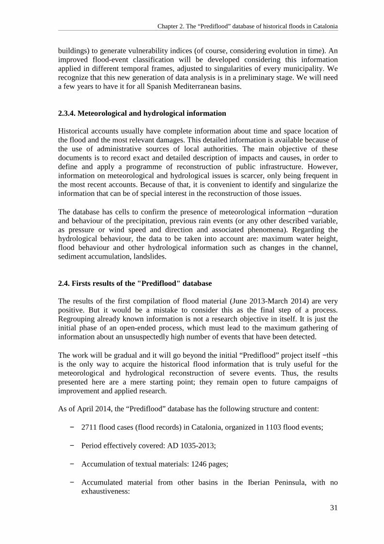
Chapter 2. The “Prediflood” database of historical floods in Catalonia
31
buildings) to generate vulnerability indices (of course, considering evolution in time). An improved flood-event classification will be developed considering this information applied in different temporal frames, adjusted to singularities of every municipality. We recognize that this new generation of data analysis is in a preliminary stage. We will need a few years to have it for all Spanish Mediterranean basins. 2.3.4. Meteorological and hydrological information Historical accounts usually have complete information about time and space location of the flood and the most relevant damages. This detailed information is available because of the use of administrative sources of local authorities. The main objective of these documents is to record exact and detailed description of impacts and causes, in order to define and apply a programme of reconstruction of public infrastructure. However, information on meteorological and hydrological issues is scarcer, only being frequent in the most recent accounts. Because of that, it is convenient to identify and singularize the information that can be of special interest in the reconstruction of those issues. The database has cells to confirm the presence of meteorological information −duration and behaviour of the precipitation, previous rain events (or any other described variable, as pressure or wind speed and direction and associated phenomena). Regarding the hydrological behaviour, the data to be taken into account are: maximum water height, flood behaviour and other hydrological information such as changes in the channel, sediment accumulation, landslides. 2.4. Firsts results of the "Prediflood" database The results of the first compilation of flood material (June 2013-March 2014) are very positive. But it would be a mistake to consider this as the final step of a process. Regrouping already known information is not a research objective in itself. It is just the initial phase of an open-ended process, which must lead to the maximum gathering of information about an unsuspectedly high number of events that have been detected. The work will be gradual and it will go beyond the initial “Prediflood” project itself −this is the only way to acquire the historical flood information that is truly useful for the meteorological and hydrological reconstruction of severe events. Thus, the results presented here are a mere starting point; they remain open to future campaigns of improvement and applied research. As of April 2014, the “Prediflood” database has the following structure and content:
− 2711 flood cases (flood records) in Catalonia, organized in 1103 flood events;
− Period effectively covered: AD 1035-2013;
− Accumulation of textual materials: 1246 pages;
− Accumulated material from other basins in the Iberian Peninsula, with no exhaustiveness:

Chapter 2. The “Prediflood” database of historical floods in Catalonia
32
− Peninsular basins: 873 flood cases,
− Insular basins (Balearic Islands): 111 flood cases,
− Basins in Roussillon (SE France): 250 flood cases,
− Total absolute: 3945 flood cases.
The distribution in time of the flood cases and events (Fig. 2.2a and b) shows a logical concentration in the last 200 years, as a result of the greater availability of information, but also due to an increase in exposure and vulnerability in the face of a result of population growth, the industrialization of river areas in the 19th century, and the intensive urban development along the coast during the second half of the 20th century.
Figure 2.2. Bidecadal distribution of flood cases (a) and flood events (b) of the “Prediflood” database
information (own elaboration). Three flood cases/events are out of the period AD 1035-2013.

Chapter 2. The “Prediflood” database of historical floods in Catalonia
33
For this reason, data analysis in later works will consider internal periodization −every basin has its specific historical context evolution, but general periods could be:
− Years ca. 1000-1500: information poorly detailed and scattered. Population in small location with low exposure to flood events.
− Ca. 1500-1750: qualitative detailed and homogeneous information. Stable locations with important level of exposure to flood events.
− Ca. 1750-1850: highest level of qualitative information. First quantitative data available (meteorological, demographic statistics, tributary reports). Strong demographic growth producing an important increase of vulnerability.
− Since ca. 1850: quantitative information is available and qualitative primary
information is diversified (administrative sources, local newspapers, technical reports). Locations increase exposure but also different preventive structural works reduce vulnerability. Case-by-case analysis is required.
The number of flood cases in relation with the identifiable events reveals some interesting matters:
− one case per event: 756 flood events,
− between two and nine cases per event: 306 flood events,
− ten or more cases per event: 41 flood events. The great number of events with only one documented flood case highlights the typical regime of torrential precipitations, very intense but not large, which cause serious but localized overbank floods. But it also highlights the insufficient historiographical research that has not more completely defined flood events. A single-cased flood event is a stimulus to deepen the research in that area and date. The greatest events, with 10 or more documented cases, are optimal starting points to deepen the research. They occurred in a relatively recent period, thus their study will be more efficient. Besides, their already proved severity can be definitely characterized and brings more information for the meteorological and hydrological reconstruction. A detailed study of these high-impact events is an immediate usage of the “Prediflood” database (see Table 2.2). Finally, the results of the “Prediflood” database can be compared to those of the compilations of the competent institutions: basin authorities and civil protection service. (see Table 2.3). The available databases, organized in hydrographical basins, have uneven time coverage. In some cases, importance has been attached to very ancient events, whereas other basin authorities have preferred to focus their study in a more realistic period, of about 500 years long, to be used in the 500-year return period calculations required in different land planning instruments. However, these databases contain few events: between 150 and 250 events per basin. The Ebro and the Guadalquivir basins stand out with about 500 events, a

Chapter 2. The “Prediflood” database of historical floods in Catalonia
34
number very much due to their large areas. Catalonia, with an average area compared to other basins, reaches 1103 flood events.
Table 2.2. Relation of flood events selected according to severity (10 or more cases per event).
Year Date Number of
cases Year Date
Number of cases
1617 30 Oct-6 Nov 47 1942 27-28 Apr 12 1787 25 sep-9 Oct 13 1943 15 Dec 21 1842 23-26 Aug 29 1944 24-25 Feb 12 1850 15-21 Sep 26 1951 2-12 Oct. 13 1853 23-26 May 19 1962 24-26 Sep 26 1856 8-16 Jun 11 1962 10-17 Oct 19 1863 7-8 Oct 12 1962 4 Nov 17 1866 19-25 Oct 10 1963 3 Aug 11 1874 22-23 Sep 69 1963 11-14 Sep 11 1890 18-19 Sep 15 1965 4-9 Oct 12 1898 15-18 Jan 25 1969 3-5 Apr 17 1901 21 Sep 13 1970 10-12 Oct 31 1907 10-16 Oct 30 1971 20-21 Sep 26 1907 21-25 Oct 89 1973 7-8 Sep 11 1913 29-30 Sep 16 1977 18 Oct 17 1919 6-9 Oct 13 1982 15-16 Feb 17 1921 16-18 Aug 17 1982 6-8 Nov 38 1926 31 Aug-4 Sep 16 1984 29 Sep 11 1932 11-17 Oct 11 1987 3-10 Oct 16 1937 25-28 Oct 43 1994 10-11Oct 29 1940 16-18 Oct 21 --- --- ---
Table 2.3. Comparative values between the flood compilations of Civil Protection Spain and the “Prediflood” Project. Source: "Catálogo Nacional de Inundaciones Históricas" (2006-2010), Ministerio del
Interior, España.
Basin Area (km2)
Period Number of events
Years Coverage1 Density2
Duero 78954 1483-1985 278 503 39.7 7.0 Segura 18869 1482-1982 214 501 9.5 22.5 Júcar 42989 1088-1983 217 896 38.5 5.6 Tajo 55645 849-1979 159 1131 62.9 2.5 Ebro 85399 BC49-1984 554 2034 173.7 3.2
Guadalquivir 63972 1483-1985 474 503 32.2 14.7 Norte+Galicia 40894 1482-1983 141 502 20.5 6.9
Guadiana 59677 620-1985 149 1366 81.5 1.8 Sur 17969 1544-1983 162 440 7.9 20.5
Pirineo Oriental3 16418 1483-1983 162 501 8.2 19.8 Total Spain 493838 --- 2579 838 (av.) 413.8 6.2 Prediflood 32114 1035-2013 1103 979 31.4 35.1
(1) Coverage: (years × surface) / 106 km2 (according to Gaume et al., 2009) (2) Density: Number of events / coverage (according to Gaume et al., 2009) (3) Pirineo Oriental Basin: data provided directly by Catalan Water Agency (ACA)
The use of an objective criterion to compare the general results in Spain with those of the “Prediflood” project in Catalonia (Gaume et al., 2009) shows a space and time coverage obviously greater for the whole of Spain compared to Catalonia (413.8 yr × surface / 106 km2 and 31.4 years × surface / 106 km2, respectively). However, considering the number of events in Spain (2579 events) and Catalonia (1103 events), the density of events in

Chapter 2. The “Prediflood” database of historical floods in Catalonia
35
relation to their space and time coverage reaches a value of 6.2 events/coverage in Spain and 35.1 events/coverage in Catalonia, which is almost six times greater. 2.5. Historiographical data collection procedures 2.5.1. Justification for a historiographical research Historical floods information has specific sources, documentary and bibliographical, the traditional area of research of historians. However, natural events are not, in general, appealing to this collective. Floods simply appear as mere anecdotes in local historiography, and only deserved some systematic effort during the positivist period. The present context of natural risks in their interaction with human activities makes this research field interesting. In a few years, historical climatology has shown its development capacity in the scientific literature from information exclusively collected in historical documentary sources on the issue of floods (among others: Camuffo and Enzi, 1996; Glaser, 1996; Pfister, 1998; Brázdil et al., 1999, 2006; Wetter et al., 2011). The situation in Spain is optimal to this kind of research thanks to the great documentary heritage preserved. However, historiographical research has focused on political and social issues. Up to the present, only 3% of the documentary sources of specific interest to floods have been explored. (In Catalonia, this percentage is 5% approximately). Local historiography has accessed a greater number of documentary sources, but just to generate lists of flood dates. The administrations competent with managing basins and emergency situations have used these bibliographical sources but the results have been scarce and limited despite the potential of the available documentation. The solution to this situation can come from historiographical research itself, and the results can be as positive as those of previous European experiences. The majority of flood events in Spain are based on an insufficient exploitation of historiographical sources. Reaching a complete identification of these sources is, by itself, a study with multiple positive aspects (see Fig. 2.3).

Chapter 2. The “Prediflood” database of historical floods in Catalonia
36
Figure 2.3. Overview of the methodological procedure of historical floods data collection (own elaboration) 2.5.2. Proposal of classification of information sources The development of a study on so large and diverse a range of historical sources requires a good classification of them. The following proposal is based on their reliability levels and content format:
1) Primary sources: Information for flood events generated by contemporary eyewitness authors
a) Documentary sources1
1 Objective sources, quasi-complete data series

Chapter 2. The “Prediflood” database of historical floods in Catalonia
37
b) Local newspapers2
2) Secondary sources: Information obtained from primary sources by not eyewitness authors
a) Scientific literature1
b) Historiographical sources and thematic works2
3) Tertiary sources: Information obtained from secondary sources by not eyewitness
authors
a) Technical reports1
b) Non-specialized works and social networks collections2
Q. Quantitative Data: Information recorded in numeric or quantifiable formats (All sources can contain quantitative data, generated by themselves or copied and transmitted)
a) Instrumental sources
b) Paleolimnimetry: epigraphic and textual flood marks
The source level relate to their proximity to the events. Every source level has some objective sources, with which data gathering is almost complete, and some subjective ones, which offer incomplete information. 2.5.3. Proposed procedures The first analysis of the compiled floods shows the levels of the sources of information. Data exploitation can be immediate, but the classification of sources can highlight the reliability and quality of the sources used and, therefore, of the available information. If required, the origin of the information can be investigated until arriving at the primary level sources. Given the present state of references on flood cases, the research effort should focus on finding the primary sources for most of them ensuring, at least, one reliable and objective source of information. Application of this principle of traceability would have a number of positive aspects:
1) The starting point would be already available information, thus not limiting its availability but consolidating and improving its reliability.
2) By reaching primary sources of a public administrative nature, information endorsed by a public notary would become available. The maximum reliability provided by such testimony would strengthen reconstruction studies based on the information contained in these sources.
2 Subjective sources, incomplete data series

Chapter 2. The “Prediflood” database of historical floods in Catalonia
38
3) New bibliographical and documentary sources would be brought to light. This
would enlarge the available information and new floods cases and events would be detected subsequently, in a sort of chain reaction.
4) A line of research would be defined for historians. In the case of Spain, it would doubtlessly mean many years of work. The possibility would arise to expand the research into poorly explored areas or to deepen it into events that deserve a more detailed study.
5) The accumulation of the maximum available description of impacts and quantifiable information about hydrological and meteorological information, up to an acceptable degree of exhaustiveness, would be reached. It would not be all the desirable information but, at least, all information known to date.
6) Such studies, besides detecting unknown flood information, could also detect information about other infrequent natural risks (earthquakes, landslides and rare meteorological phenomena).
2.6. Reconstruction methodology Our multidisciplinary reconstruction of historical floods consists of three parts:
1) Hydraulic reconstruction, the objective of which is the calculation of the peak flow (or, when possible, the whole hydrograph) of the flood,
2) Hydrological reconstruction, the objective of which is the calculation of the
hyetograph of the rain event that caused the flood,
3) Meteorological reconstruction, the objective of which is to analyse the meteorological processes before and during the rain event that caused the flood.
These three parts are linked −the results of the hydraulic reconstruction (flood’s peak flow or hydrograph) are needed in the hydrological one, and the results of the hydrological reconstruction (hyetograph) should agree with the results of the meteorological one (Fig. 2.4).
Chapter 2. The “Prediflood” database of historical floods in Catalonia
39
Figure 2.4. Overview of the multidisciplinary reconstruction methodology of historical floods (own
elaboration) The three reconstructions occur in very different spatial scales: typically, the hydraulic reconstruction takes place along a river reach (up to a dozen kilometres squared); whereas the hydrological one takes into account the whole catchment (from some dozens to thousands of kilometres squared); and the meteorological reconstruction is done, depending on the meteorological phenomenon causing the event, from a local (hundreds of kilometres squared) to a regional scale (1 million km2). Whatever the case, all of them need historical information in order to feed the models used with the required input data and initial and boundary conditions. 2.6.1. Hydraulic reconstruction The objective of the hydraulic reconstruction is to calculate the flood’s peak flow from the maximum water height observed or flood mark, recorded in a plaque or in a written document.
This calculation can be quickly done (although with a high uncertainty) with Manning’s empirical equation, which relates, in one section of the stream, the flow of water to the geometrical and friction characteristics of the section, summarized in only four values: the section’s area and wet perimeter, the longitudinal slope and a roughness coefficient.

Chapter 2. The “Prediflood” database of historical floods in Catalonia
40
However, the precision of a peak flow calculation is improved with the use of hydraulic models. Typically, these models use physically based equations (e.g. Bernouilli, one-dimensional Saint-Venant) in dozens of sections along a reach of river several hundred metres long. The major drawback is that they need more input data. Simple hydraulic models (e.g. WSPRO, QUICK-2, CAUCES) can only operate in steady flow conditions (that is, no variation in time is allowed: they calculate the situation of a still instant), while others (e.g. HEC-RAS, DAMBRK, SWMM, Mike 11 HD) can calculate in unsteady flow conditions, thus obtaining more accurate results, especially in river reaches with floodplains with a great water-storing capacity. Similarly, some simpler models do their calculations in one dimension only (all flow lines are perpendicular to the cross-section), while more sophisticated and accurate ones (e.g. Iber, Sobek, Mike 21 and FLO-2D) do them in two dimensions (flow lines can be oblique to the cross-section). The difference in accuracy between 1-D and 2-D models increases in winding stretches, in those in which the water velocities in the channel and on the floodplain are very different, and in those were the flow is clearly not unidirectional. However, the gain in accuracy with the use of unsteady flow conditions or 2-D models comes at a higher effort in input data acquisition and, especially, in computation time, which can even make the use of complex models impractical in historical floods reconstruction, because they have to be applied iteratively. Besides, a high standard of accuracy in the calculations is not essential in reconstructing historical flows, because the input data have themselves a high degree of uncertainty. Because of this, and for the sake of homogeneity between data-rich and data-poor sites, we systematically use the 1-D hydraulic model HEC-RAS (version 4.0) in steady flow conditions (USACE, 2008), which gives accurate enough results (Balasch et al., 2010a; Chapter 5 in this thesis). Nevertheless, we also apply the 2-D model Iber (Bladé et al., 2012; Ruiz-Villanueva et al., 2013) in some cases which would otherwise produce excessive inaccuracy: highly urbanized or very sinuous reaches or with large floodplains. It must be noted that models calculate hydraulic parameters (water velocities and depths) from a given peak flow, whereas we need the opposite: to calculate the peak flow from a given water height. Thus, the hydraulic model has to be applied iteratively, feeding it with tentative peak flows until the observed water height is approached (Fig. 2.5).

Chapter 2. The “Prediflood” database of historical floods in Catalonia
41
Figure 2.5. Iterative procedure used in the hydraulic reconstruction of peak flows (modified from Balasch et
al., 2010b) The input data that the model needs, besides the tentative peak flow, are the cross sections geometry and friction against water flow, the former given by the digital elevation model, and the latter given by Manning roughness coefficients, found in tables that relate friction with type of surface, sinuosity, vegetation, obstacles and cross-section contractions or expansions (Chow, 1959). Also, a hydraulic model has to be given boundary conditions, which link what happens inside the modelled river reach with what happens upstream and downstream. All these input data have to be adequately adapted to be as close as possible to their values at the time when the historical flood to be reconstructed took place. Therefore, old maps and documents are essential in reconstructing the channel and floodplain morphology at the time of the flood (obstacles, meanders, islands) and in hypothesizing the roughness coefficients. It must be noted that since they are acquired by estimating and hypothesizing from old documents, the input data have a high degree of uncertainty. Again, this process adds a high degree of uncertainty to the input data. In those rare cases where measured flow data are available, they should be used in calibrating the hydraulic model in that reach, that is, in estimating more accurately roughness coefficients and boundary conditions (Lang et al., 2004). As said above, hydraulic reconstruction involves a great deal of assumptions about input data; therefore, sensitivity analyses should be performed to delimit the effect of a given variation in input data on the results, that is, to estimate the error of the results.

Chapter 2. The “Prediflood” database of historical floods in Catalonia
42
2.6.2. Hydrological reconstruction The objective of the hydrological reconstruction is the hyetograph of the rainfall that caused the flood. A hydrological model summarizes the characteristics of the catchment that conform its hydrological response, that is, the way it transforms rainfall into runoff and, eventually, into river flow. In other words, a model tries to quantify the hydrological processes occurring between the rain precipitation and the water exiting the catchment through its outlet. There are three main types of hydrological models: the stochastic ones, the empirical ones and the physics-based ones. Firstly, the stochastic models use large amounts of paired rainfall-flow data to calculate non-dimensional parameters that describe the catchment’s hydrological response; an example is GR4J (Perrin et al., 2003). Secondly, the empirical models use simplified empirical equations and methods (such as the Curve Number method; NRCS, 2007). Finally, the physics-based models use complex physics equations and need a lot of precise field measurements; an example is InHM (VanderKwaak and Loague, 2001). Hydrological models can also be classified according to their treatment of space as well: lumped models calculate processes at the catchment or subcatchment scale (e.g. HEC-HMS), whereas distributed models do it in smaller areas and afterwards aggregate the results (e.g. r.water.fea, Vieux et al., 2004). Due to the scarcity of data typically found outside heavily instrumented catchments and for the sake of simplicity, we use HEC-HMS (version 3.3), an empirical, lumped hydrological model (USACE, 2010b). HEC-HMS allows the user to choose among a number of different empirical methods for each one of these three hydrological processes: runoff generation, transformation of runoff into river flow, and river flow routing. For each of these processes we chose, systematically and respectively, the SCS Curve Number, the Synthetic Unit Hydrograph and the Muskingum-Cunge methods, because of their simplicity of use, their moderate requirements in input data and their being generally accepted and commonly used (NRCS, 2007). Similarly as in the hydraulic reconstruction, the calculation procedure is iterative, because the result (that is, the hyetograph) is, actually, an input datum required by the model (Fig. 2.6). Therefore, a tentative hyetograph must be built using the available historical information about the rain event, such as, its duration, the affected area (in which subcatchments it rained and in which it did not), or indications that can lead to a rough estimation of the rainfall volume. Besides this tentative hyetograph, the model needs input data describing the catchment (or subcatchments) hydrological characteristics, such as soil type, land use, antecedent soil moisture and the stream’s slope.

Chapter 2. The “Prediflood” database of historical floods in Catalonia
43
Figure 2.6. Iterative procedure used in the hydrological reconstruction of hyetographs (modified from Balasch et al., 2010b)
The result of the hydrological model (the peak flow) is then compared to the one calculated in the hydraulic reconstruction; if the two are similar enough, the tentative hyetograph is provisionally accepted. If this provisional hyetograph agrees with the meteorological processes found in the meteorological reconstruction, it is definitely accepted. The kind of input variables and empirical methods used have a great degree of uncertainty (Willems, 2001), all the more in the case of historical floods, because the data have to be adapted from present-day values to the estimated ones at the time of the studied flood. Thus, a calibration of the model should be made whenever measured data are available. For the same reason, a sensitivity analysis should be performed once the hydrological reconstruction is done in order to estimate the real amount of uncertainty in the results.

Chapter 2. The “Prediflood” database of historical floods in Catalonia
44
2.6.3. Meteorological reconstruction The objective of this reconstruction is the analysis of the meteorological processes before and during the rain event that caused the flood. This analysis has two direct applications: the estimation of the antecedent soil moisture condition (an input required in the hydrological reconstruction) and the classification of floods according to their meteorological causes, which can, eventually, become a useful tool in flood forecasting. The meteorological reconstruction is done in three different levels depending on the data availability or, more specifically, on the horizontal, vertical and temporal resolution of the available data, which decreases as we move back in time. Also, there are three different periods according to the quality of the available data, and a different level of reconstruction is applied to the floods in each one of them:
1. Events that occurred since ca. 1750 (available data: surface temperature, pressure and precipitation recorded at several European locations): since the second half of the 18th century, several observatories in Europe recorded surface temperature and pressure. Some of them additionally recorded accumulated precipitation. Surface temperature and pressure records are used to analyse the synoptic conditions at a regional scale and to calculate zonal pressure indexes (Luterbacher et al., 2002).
2. Events that occurred since 1871 (available data: 20th Century Reanalysis data from NOAA). Surface and upper-level meteorological charts since 1871 from the reanalysis made by the Earth System Research Laboratory of the National Oceanic and Atmospheric Administration (NOAA; Kalnay et al., 1996) are used to estimate the synoptic conditions of each episode: temperature, atmospheric circulation at different vertical levels, and precipitation estimates. Additionally, the reanalysis data allow us to calculate several parameters related to the convection intensity, such as the Vertical, Cross and Total Totals indexes (Miller, 1972), the K index (George, 1960), the Humidity index (Litynska et al., 1976), the Ko index (Andersson et al., 1989), the Lifted Index (LI; Galway, 1956), the Integrated Convective Available Potential Energy (ICAPE; Mapes, 1993; Doswell and Rasmussen, 1994), the Vorticity Generating Parameter (Rassmussen et al., 1998), the difference between the LCL and LFC, the wind shear between surface and 1, 3 and 6 km high, among others. In addition, the reanalysis data can be used to obtain information about wind field, moisture, and column of precipitable water.
3. Events that occurred since ca. 1960 (available data: global models with larger resolution and mesoscale numerical simulations). Finally, for more recent events, version 3.3 of the WRF-ARW mesoscale model (Skamarock et al., 2008) is used at high horizontal resolution (up to approximately 1 km) to analyse synoptic, mesoscale and local conditions during the floods. The initial and boundary conditions to run the model are obtained from the ECMWF model reanalysis up to 0.25º horizontal resolutions.

Chapter 2. The “Prediflood” database of historical floods in Catalonia
45
2.7. Concluding remarks The Prediflood database meets the internationally accepted scientific standards. It is, therefore, a repository of reliable and contrasted information that allows accurate flood analysis. Actually, some of its data have already been successfully used in several flood reconstructions; at the same time, the density of the information in both space and time gives this database a great potential in time series analysis. The Prediflood database is in a permanent state of data incorporation. The present-day information comes from the search of about 5% of documentary sources with interesting information in Catalonia. Consequently, the drawing of any kind of conclusion is premature. First steps are showing that this research with an interdisciplinary framework is possible in the Spanish context and may be fruitful. This effort is focused not only on quantity of flood events detected, but also on qualitative aspects, putting especial effort into increasing the reliability and detail of information collected to be subjected to hydraulic, hydrological, meteorological reconstructions, as is made for climatic reconstruction in recent years. This produces a substantial improvement of quality and quantity of obtainable results: quality because results are more credible; quantity because spatio-temporal scales covered by reconstructions can be enlarged. For the future, the most immediate objectives for the Prediflood database are:
− To enlarge the percentage of primary sources used for flood events reconstruction.
− To explore the archives of presently poorly represented areas or flood events interesting that appear interesting but are not known about well enough.
At present, the Prediflood database is a heterogeneous amount of information well catalogued. Its potentialit can be tested immediately. Large or severe events can be easily identified and classified. Quantified information allows basic reconstruction of hydraulic and hydrological processes involved. Atmospheric conditions producing strong rainfall events and floods would be better analysed with an enlargement of the number of cases for NE Iberian Peninsula. Detection and definition of patterns of the synoptic conditions, and comparison between different flood events will improve understanding of the atmospheric processes producing floods. When long data series becomes available, after the homogenization needed by the different demographic and social contexts existing for different flood events, an improved climatic variability analysis related to flood events will be possible. Application for meteorological forecasting services and flood risk managers will be strongly positive. Acknowledgements Research supported by PREDIFLOOD Project, CGL2012-35071, Programme I+D+i, Spanish Ministry of Economy and Competitiveness. One author has a predoctoral grant supported by University of Lleida. Authors thanks support and data provided by Catalan Geological Institute (IGC) and Catalan Water Agency (ACA).


Chapter 3
Historical flash floods retromodelling in the Ondara River in Tàrrega (NE Iberian Peninsula)
Balasch, J.C., Ruiz-Bellet, J.L., Tuset, J. (2011): Historical flash floods retromodelling in the Ondara River in Tàrrega (NE Iberian Peninsula). Nat. Hazards Earth Syst. Sci., 11, 3359–3371, 2011 http://www.nat-hazards-earth-syst-sci.net/11/3359/2011/ doi: 10.5194/nhess-11-3359-2011 Published 21 December 2011


Chapter 3. Hydraulic reconstruction of seven flash floods
49
Abstract Flash floods in the Ondara River have caused many fatalities and damages in the town of Tàrrega in the last 400 years. Unfortunately, no flow records are available. However, floods can sometimes be reconstructed thanks to available historical information: limnimarks, written accounts and archaeological surveys. Indeed, from these data and using the retromodelling method on three different scenarios to take into account morphology changes, the peak flows of the seven greatest floods occurred in Tàrrega since the 17th century were estimated. The results showed that the heaviest flood’s specific peak flow (10.7 m3·s-1·km-2) ranks among the highest ever modelled or measured in similar-sized catchments in the Western Mediterranean region. The results pointed out, as well, that the changes in channel’s morphology (mainly, the disappearance of a mediaeval bridge under sediment) caused by one of the floods increased the hydraulic capacity of a crucial cross section. All this resulted in modest floods invading less often the town, but with much faster and, thus, more destructive flows. A preliminary estimation of the results’ uncertainty was 4% for great floods and 18% for modest floods. The reconstructed peak flows will be introduced in a database for a future use in climatic and hydrological studies.
3.1. Introduction Flash floods are a common hydrological event in the small and medium-sized catchments located in the Mediterranean coastal fringe of Catalonia, in NE Iberian Peninsula (Llasat et al., 2003; Gaume et al., 2009). Nevertheless, this torrential behaviour is also known to catchments located inland, specifically to those enclosed in the Ebro River basin having their headwaters on the coastal ranges, the water divide between the coastal and the inland catchments. Indeed, in these catchments, flash floods occur frequently −usually caused by autumn convective rainstorms coming from the Mediterranean Sea− and have historically caused fatalities and damages. However, flash floods have not been studied in these catchments so far. Besides, historical floods in the Iberian Peninsula have usually been used to find climate temporal trends (Barriendos and Martín-Vide, 1998; Llasat et al. 2005; Benito et al., 2008) and, except for floods occurred in large basins (Benito et al., 2003; Thorndycraft et al., 2006; Ortega and Garzón, 2009), rarely have they been hydraulically reconstructed. Thus, our research focuses on historical flash floods’ reconstruction in 200-500 km2, westward-flowing catchments located in the eastern-most fringe of the Ebro River basin. Among them, we have chosen the Ondara River’s catchment as the paradigm to study flood reconstruction because a lot of information about historical floods can be found there, both as flood marks, also called limnimarks, and as documents: written accounts

Chapter 3. Hydraulic reconstruction of seven flash floods
50
found in archives (Salvadó, 1875; Iglésies, 1971; Segarra, 1987; Farré, 2008), press chronicles and photographs (Coma, 1990). A reason for this abundance of information might have been the great magnitude of the damages caused by the floods, due to the Ondara’s catchment having historically been a very populated area, with important towns such as Tàrrega and Cervera (16500 and 9300 inhabitants respectively, in 2009). Thus, according to written and epigraphic documents, the Ondara River has flash-flooded the town of Tàrrega at least seven times since early 17th century: in 1615, 1644, 1783, 1842, 1874, 1930 and 1989, sometimes causing a great number of fatalities: more than 300 in 1644 and about 150 in 1874. Besides specific information about the floods, hydraulic modelling requires data about the channel’s and floodplain’s morphology and roughness. Fortunately, a lot of information about the evolution of these features in the Ondara River is available thanks to the efforts of local archaeologists and historians. Despite this abundance of information, it has never been used to hydraulically or hydrologically reconstruct those events; with one exception: 1874 Santa Tecla’s flood has only recently been modelled in order to quantify its peak flow and the rainstorm that caused it (Balasch et al., 2010a, 2010b). Therefore, the objectives of this paper were to find and process all the available information in order to calculate 1615, 1644, 1783, 1842, 1930 and 1989 floods’ peak flows and improve the previously calculated 1874 flood’s peak flow. 3.2. Study framework 3.2.1. Catchment The Ondara River is a left-side tributary of the downstream stretch of the Segre River, which is, at its turn, the main tributary of the Ebro River (Fig. 3.1); however, before reaching the Segre, the Ondara River’s water flows into a large alluvial fan just downstream Tàrrega. When it arrives at Tàrrega, at a height of 362 m above sea level, the Ondara has a length of 28.6 km and an average slope of 1.5%. Its catchment is 150 km2 and has an east-west orientation, its headwaters lying on the Central Catalan Depression’s monoclinal relieves, with the highest point at Coll de la Creu del Vent, in Montmaneu Range (804 m). Unirrigated cereal crops cover 85% of the catchment’s area, whereas forest and uncultured soil cover 13%, and urban soil, 2%. Although there has never been any flow gauging station on the Ondara River, its modest average flow at the end of the alluvial fan could be estimated through water resources modelling (CHE, 1996): 0.5 m3·s-1. However, the alluvial fan’s flow is greatly increased by the seepage from irrigated fields; thus, the share of water coming from the Ondara must be smaller, a good estimation of its average flow in Tàrrega being 0.1 m3·s-1 or less.

Chapter 3. Hydraulic reconstruction of seven flash floods
51
Figure 3.1. Location of the Ondara River’s catchment within the Iberian Peninsula (a) and within Catalonia
(b), and map of the catchment itself with the location of the town of Tàrrega (c) Ondara’s hydrological regime, not regulated by any hydraulic structure, shows a high-water period around May and long low-water periods, a consequence of the continental Mediterranean climate (Köppen Csa) of the catchment, which has an annual mean rainfall of 450 mm with a variation coefficient of 20%. In any case, autumn overflowing flash floods are not rare, occurring about three or four times per century, according to the most complete record compiled by Coma (1990) and Espinagosa et al. (1996). Severe flash floods, caused by great rainstorms, often occur simultaneously in Ondara and its adjoining catchments: Sió and Corb. Certainly, severe rainstorms are common; this can be partially explained by the regional relief, which triggers storms in two ways: stopping weather fronts that come from the Mediterranean Sea and contributing to the development of convective rainstorms during summer and early autumn. All this results in an eastward rainfall gradient, because weather fronts come from the east and because the highest lands, where convective rainstorms are more likely to form, are in the eastern part of the catchment. 3.2.2. Evolution of the town’s and the floodplain’s morphology The knowledge of the channel’s and the floodplain’s morphology is essential in hydraulic modelling (see section 3.3. Methods). However, this morphology can change greatly in 400 years, especially in urban areas (Fig. 3.2).

Chapter 3. Hydraulic reconstruction of seven flash floods
52
Figure 3.2. Tàrrega’s urbanized area evolution since the 17th century (a) and detail of Sant Agust´ı Street
area (b) Thus, in order to reconstruct as faithfully as possible the floodplain’s and channel’s morphology at the time of each studied flood −including the main obstacles to the water flow, ie. houses, walls, bridges, streets–, many sources of historical information were used: archaeological surveys, written accounts (Salvadó, 1875; Segarra, 1987; Farré, 2008), antique town maps (from the local archives: Urgell County Archive), the 1668 artistic drawing by Italian artist Pier Maria Baldi, and photographs. Tàrrega was founded in the 11th century, between the right bank of the Ondara River and the slopes of Sant Eloi’s Hill. Both its population and its urbanized area remained more or less unchanged until the railway opening in 1860 boosted the growth of the town, which rose from 4000 inhabitants up to 8000 inhabitants in 1930. This growth continued throughout the 20th century, but only recently the town has spread onto the river’s left bank and has reached a population of 16500. There is proof of at least one major change in the floodplain’s and channel’s morphology in the last 400 years: a 3-m-deep sediment layer transported by 1874 flood and discovered by recent archaeological surveys. Besides this natural geomorphological change, the presence or absence of several man-made features in the immediate vicinity of the river have greatly modified the floodplain’s and the channel’s morphology in the last 400 years: Sant Agustí‘s Convent and slum on the left bank, Sant Agustí Bridge, two walls alongside the right bank: a mediaeval one and a modern one, and the bridges of roads C-14 and L-2021 (Fig. 3.3). More precisely:

Chapter 3. Hydraulic reconstruction of seven flash floods
53
a) Sant Agustí’s Convent was built on the left bank of the river in 1322, destroyed by the 1644 flood and rebuilt immediately afterwards, and definitely destroyed by the 1874 flood. The stones of the ruined monastery were used to build Sant Agustí slum, which is still in place.
b) Sant Agustí Bridge was built circa 1340 and connected the eponymous street with the eponymous convent on the left bank; it was damaged by floods and afterwards reconstructed in 1615, 1644 and 1842; finally, it was buried in a 3-m-deep sediment layer deposited by 1874 flood.
c) The mediaeval wall was built in 1360-1370, more to protect the town against armed attacks than against floods. It was severely damaged by the 1644 and 1874 floods; finally it was buried in the 3-m-deep sediment layer that covered Sant Agustí Bridge.
d) The modern wall –known as the Carlist Wall– was built in 1875 as a defensive response to the 1874 flood and is still in place, a little bit closer to the river axe than the mediaeval wall and lying on the 3-m-deep sediment layer.
e) C-14 road’s bridge was built in the early 20th century, and is still in place.
f) LV-2021 road’s bridge was built in the early 20th century, and still in place.
Figure 3.3. Two of the three morphology scenarios used in the modelling: scenario A (a) and scenario C (b) including the 53 cross sections and their main morphology features, illustrated by: Pier Maria Baldi’s 1668 drawing (c), a 2007 downstream view from the C-14 road’s bridge (d), and a c. 1910 upstream view of the
Ondara River in Tàrrega and the C-14 road’s bridge (e)
In the 1990s, the Ondara River’s floodplain at Tàrrega was channelled by building a wall along the left bank; this enabled a heavy urbanization of the area behind that new wall. Moreover, in the early 2000s, the floodplain between the two walls was turned into an urban park and a footbridge was built just over the nowadays buried Sant Agustí’s Bridge.

Chapter 3. Hydraulic reconstruction of seven flash floods
54
3.2.3. Historical floods An historical flood is a flooding event not measured by instruments, but recorded in different historical information sources: limnimarks, written accounts, photographs. Sometimes, there is enough information, both in quality and in quantity, to allow a reliable hydraulic reconstruction of the historical floods’ peak flows. The basic piece of information needed in historical floods’ reconstruction is maximum water height. This datum can be obtained from a limnimark (a commemorative plaque or a carving on a wall which points out the maximum height reached by one particular flood), a written account or a photograph; sometimes, the latter two can even inform of the water height at times other than the peak time, thus allowing the estimation of the flood’s evolution over time, that is, of its approximate hydrograph. Moreover, written accounts can provide some details required in the reconstruction of the rainstorm hyetograph –such as rainstorm’s starting and ending times and rain occurrence in previous days. So far, we have found seven historical floods in the Ondara in Tàrrega with enough information to reconstruct their peak flows: three maximum water heights given by limnimarks (1644, 1783, and 1874) and four by written accounts (1615, 1842, 1930, and 1989). Two of them stand out due to their magnitude and the damages they caused: 1644 and 1874, both occurred at night, which explains the great number of casualties (more than 300 and 150 respectively). Besides, there is a lot of information about the 1874 flood, and that is why we chose it as the paradigm to start historical flood reconstruction in the area, having so far successfully estimated its hydrograph and hyetograph (Tuset, 2007; Balasch et al., 2010b). Summarized information about the seven greatest historical floods found in Tàrrega is gathered in Table 3.1, along with the sources of information that report them and the most conspicuous morphology features at the time of each flood. 3.3. Methods Depending on the available information, the hydraulic reconstruction of a historical flood can have different types of results: from just the peak flow value to the entire hydrograph. In this case, hydrological and morphological information of the seven studied floods (the only seven known to us that flooded the town since the 17th century), which was gathered from multiple historical and archaeological sources, only allowed peak flow estimations. We calculated these seven peak flows using the HEC-RAS 4.0 (USACE, 2008) hydraulic modelling software on one-dimensional, gradually varied, steady, sub-critical flow. Actually, this software calculates water height from a flow value; hence, we applied it iteratively, trying tentative peak flows until the difference between the modelled and the historically observed water heights was smaller than 1 cm (Fig. 2.5). This method is known as retromodelling, and its accuracy has been successfully tested by Lang et al. (2004), Naulet et al. (2005) and Remo and Pinter (2007).

Chapter 3. Hydraulic reconstruction of seven flash floods
55
Table 3.1. Summary of the information about the seven studied floods, their nine historically observed water height records with their records, and the major morphology features present at the time of each flood
Year 1615 1644 1783 1842 1874 1930 1989
Date 25th July 17th
September 17th
September 25th
August 23rd September
19th October
28th October
Popular name
Sant Jaume flood
─ ─ Sant
Bartomeu flood
Santa Tecla flood Sant Lluc flood
─
Fatalities 0 > 300 0 0 150 0 1
Historically observed
water height (m a.s.l.)
366.0 368.39 364.91 363.5 367.26 368.30 369.08 363.4 363.3
Location of the
observation (Fig. 3.5)
1 2 3 4 5a 5b 5c 6 7
Observa-tion’s record
ACUR (1621) (1)
Carving in a column at
Sant Antoni Square
Stone plaque at Sant
Agustí Street
Salvadó (1875)
Marble plaque at Sant Agustí Street
Marble plaque at Font Street
Marble plaque at Piques Street
Local press(3)
Local press(4)
Type of record
Written account
Limnimark (Fig. 3.4a)
Limnimark (Fig. 3.4b)
Written account
Limni-mark (Fig. 3.4d)
Limni-mark
Limni-mark
Written account
Written account
Other information
sources ─
Parets (1891) (2) Salvadó (1875)
Salvadó (1875)
─ Salvadó (1875) Iglésies (1971)
─ ─
Morpholo-gy features
Sant Agustí Bridge 3-metre-deep sediment layer
Mediaeval Wall ─ Carlist Wall
Sant Agustí Convent Sant Agustí’s
slum
─ C-14 road’s
bridge
─ LV-2021 road’s
bridge (1) Found in Segarra (1987) and Farré (2008) (2) Found in Vila (1998) (3) Reported by Tàrrega’s Regional Museum’s director (Anonymous, 1930) (4) Castellà and Miranda (1989) We applied the retromodelling method separately for each of the seven studied floods along a 2700 m long reach of the Ondara River by the town of Tàrrega. In order to do
Chapter 3. Hydraulic reconstruction of seven flash floods
56
that, we first measured and estimated the required input data: the historically observed maximum water height and the channel’s and floodplain’s morphology and roughness. 3.3.1. Historically observed maximum water height Historically observed maximum water height above sea level was acquired either directly from limnimarks, or indirectly from written accounts. Whichever the case, this height was measured with topographic equipment and its reliability was assessed with source analysis methods (Bayliss and Reed, 2001) and hermeneutical techniques. When a limnimark was available, the maximum water height reached by the flood was directly marked either by a line carved on a stone column (1644 flood mark) or by the lower edge of a commemorative plaque (1783 and 1874 flood marks), as Fig. 3.4 shows. When no limnimark was found, the maximum water height was estimated from information found in contemporary accounts; more precisely:
a) 1615 flood: An indication of maximum water height was found in Llibre d’Actes i Memòries: 1603-1621 (ACUR, 1621; Farré, 2008). It says that the flood reached the ball playground located in Font Street (approximately 366.0 m a.s.l.).
b) 1842 flood: According to the account written by Salvadó (1875), the water arrived
somewhat further than the main door of the Codina mill, the remains of which are still to be found at Sant Agustí Street. We estimated this maximum water height as 363.5 m a.s.l., that is, the height of the door threshold.
c) 1930 and 1989 floods: Several journalistic accounts are conserved from these
floods. Crònica Targarina (Anonymous, 1930) and La Vanguardia (Castellà and Miranda, 1989) describe how the water overflowed at the end of the Carlist Wall and how it flowed back up to the beginning of Sant Agustí Street. We estimated these heights as 363.4 and 363.3 m a.s.l., respectively.
Since an actual line is usually more precisely placed (and, thus, measured) than a description of that line, the accuracy of the water height estimation is higher when done from a limnimark than from a written account: 5 mm against 5 cm (Table 3.1); this gives an idea of the importance of limnimarks in historical flood reconstruction. In total, we found nine documented maximum water height observations, one for each of the seven floods, except for the 1874 flood, which had three (Fig. 3.5). In that specific case, one observation was used to model the flood and the remaining two, to visually assess the accuracy of the modelled flow. Each historically observed maximum water height was compared to the modelled height at a particular cross section, called the reference cross section, which usually was the closest one to the observation. Actually, four different cross sections had to be used to properly compare the nine observed water heights to the nine modelled ones:

Chapter 3. Hydraulic reconstruction of seven flash floods
57
a) Piques Street cross section, 1333 m upstream of the junction with the Cercavins River, for one of the observations of 1874 flood (observation 5c in Fig. 3.5).
b) Font Street cross section, 1245 m upstream of the junction with the Cercavins
River, for the 1615 flood observation (observation 1 in Fig. 3.5) and for one of 1874 flood (observation 5b in Fig. 3.5).
c) Sant Agustí Street cross section (Fig. 3.6), 1147 m upstream of the junction
with the Cercavins River, for 1644, 1783, 1842 and 1874 floods’ maximum water height observations (observation 2, 3, 4 and 5a in Fig. 3.5).
d) A cross section 1123 m upstream of the junction with the Cercavins River, for
1930 and 1989 floods’ maximum water height observations (observations 6 and 7 in Fig. 3.5). In these cases, the observed maximum water heights do not mark the height of the streamflow at the cross-section where they were placed (Sant Agustí Street’s) but at the spot where the two floods overflowed the right bank and flowed back along the town-side of the Carlist Wall; as explained above, this overflowing spot was the downstream end of the Carlist Wall, i.e. 1123 cross section. Actually, both observed water heights were lower than the Carlist Wall at Sant Agustí Street cross section (Fig. 3.6) and, thus, the right bank was not hydraulically connected with the channel in that spot.
Figure 3.4. Three of the five limnimarks found: (a) carving on a column at Sant Antoni Square marking the 1644 flood’s maximum water height (observation 2 in Fig. 3.5), (b) sandstone plaque at Sant Agustí Street corresponding to the 1783 flood (observation 3 in Fig. 3.5), (c) marble plaque (marked by an arrow) at Sant Agustí Street corresponding to the 1874 flood (observation 5a in Fig. 3.5) and (d) detail of that plaque

Chapter 3. Hydraulic reconstruction of seven flash floods
58
Figure 3.5. Location of the nine observed maximum water heights of the seven studied floods, obtained from historical information (a key can be found in Table 3.1); and the four reference cross-sections used
when comparing observed and modelled water heights
Figure 3.6. Sant Agustí Street cross section in scenarios A and C as seen from upstream with the six water
height historical observations found in Sant Agustí Street. Scenario A includes Sant Agustí Bridge and Convent and Scenario C, the Carlist Wall, which is higher than 1930 and 1989 floods maximum heights, as
explained in section 3.3.1. (Horizontal axis marks the distance from an arbitrary spot on the left bank)

Chapter 3. Hydraulic reconstruction of seven flash floods
59
3.3.2. Channel’s and floodplain’s morphology Present-day channel’s and floodplain’s morphology was defined with 53 cross sections obtained from a 1:1000 map; moreover, Sant Agustí Street section was measured with topographic equipment in order to increase its precision, since it was the reference section in four of the flood reconstructions. Transition between two contiguous cross sections was defined by expansion and contraction coefficients, which were chosen among the HEC-RAS tabulated values. Afterwards, combinations of the corresponding changes explained in section 3.2.2 were added to present-day morphology and we obtained three different morphologies or scenarios, which were used in modelling the corresponding floods:
a) Scenario A (pre-1874 scenario): The river bed was three metres below the present-day one, and its longitudinal slope was 0.95% just upstream of Sant Agustí Street cross section and 0.24% just downstream of it. Sant Agustí Bridge was not buried, the Mediaeval Wall ran along the right bank and Sant Agustí Convent lay on the left floodplain. 1615, 1644, 1783, 1842 and 1874 floods were modelled in this scenario.
b) Scenario B (1874 scenario): The river bed was the present-day one, with a
longitudinal slope of 0.15% just upstream of Sant Agustí Street cross section and 1% just downstream of it. Sant Agustí Bridge and the Mediaeval Wall were completely buried, and Sant Agustí Convent lay on the left floodplain. 1874 flood was modelled in this scenario, as well as in scenario A.
c) Scenario C (post-1874 scenario): The river bed was the present-day one, as in
scenario B. Sant Agustí Bridge and the Mediaeval Wall were completely buried, the Carlist Wall ran along the right bank, Sant Agustí Convent was replaced by Sant Agustí Slum on the left floodplain, and two new bridges were in place: C-14 road’s and LV-2021 road’s. 1930 and 1989 floods were modelled in this scenario.
3.3.3. Channel’s and floodplain’s roughness Channel’s and floodplain’s roughness, which accounts for friction against the flow, is quantified, for use in HEC-RAS software, with Manning’s n, which is estimated from tables that give its value on different river types and land uses (Chow, 1959). Aerial photos and historical maps and documents were used to determine the different land uses around the studied reach of the river at the time of each flood. Obviously, the uncertainty of such a determination increases for older floods. However, we hypothesized (and we found no evidence of the contrary) that no great changes occurred between the 17th and 19th centuries. Actually, each cross section was divided into homogeneous land use segments, which were assigned a Manning’s n value from tabulated values, as in the example shown in Table 3.2. This value varied according to the modelling scenario: for instance, Sant Agustí Street cross section had a composed Manning’s n of 0.089 in scenario A and 0.070 in both scenario B and C.
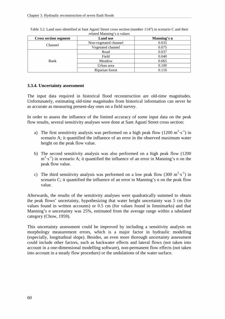
Chapter 3. Hydraulic reconstruction of seven flash floods
60
Table 3.2. Land uses identified at Sant Agustí Street cross section (number 1147) in scenario C and their related Manning’s n values
Cross section segment Land use Manning’s n
Channel Non-vegetated channel 0.035
Vegetated channel 0.075
Bank
Road 0.037 Field 0.040
Meadow 0.065 Urban area 0.100
Riparian forest 0.116 3.3.4. Uncertainty assessment The input data required in historical flood reconstruction are old-time magnitudes. Unfortunately, estimating old-time magnitudes from historical information can never be as accurate as measuring present-day ones on a field survey. In order to assess the influence of the limited accuracy of some input data on the peak flow results, several sensitivity analyses were done at Sant Agustí Street cross section:
a) The first sensitivity analysis was performed on a high peak flow (1200 m3·s-1) in scenario A; it quantified the influence of an error in the observed maximum water height on the peak flow value.
b) The second sensitivity analysis was also performed on a high peak flow (1200
m3·s-1) in scenario A; it quantified the influence of an error in Manning’s n on the peak flow value.
c) The third sensitivity analysis was performed on a low peak flow (300 m3·s-1) in
scenario C; it quantified the influence of an error in Manning’s n on the peak flow value.
Afterwards, the results of the sensitivity analyses were quadratically summed to obtain the peak flows’ uncertainty, hypothesizing that water height uncertainty was 5 cm (for values found in written accounts) or 0.5 cm (for values found in limnimarks) and that Manning’s n uncertainty was 25%, estimated from the average range within a tabulated category (Chow, 1959). This uncertainty assessment could be improved by including a sensitivity analysis on morphology measurement errors, which is a major factor in hydraulic modelling (especially, longitudinal slope). Besides, an even more thorough uncertainty assessment could include other factors, such as backwater effects and lateral flows (not taken into account in a one-dimensional modelling software), non-permanent flow effects (not taken into account in a steady flow procedure) or the undulations of the water surface.

Chapter 3. Hydraulic reconstruction of seven flash floods
61
3.4. Results and discussion 3.4.1. Hydraulic modelling As results in Table 3.3 and Fig. 3.7 show, the morphology scenario strongly determined the hydraulic behaviour of the modelled flows:
a) First, in scenario A, the flows of four different floods’ behave similarly along the modelled river reach regardless of their peak flow magnitude: water longitudinal profiles are parallel (Fig. 3.7.a); indeed, they are horizontal just upstream of Sant Agustí Bridge for about 180 m and they all fall abruptly downstream of that bridge. The reason for this is that Sant Agustí Bridge acts as a dam (because the bridge’s spans cannot convey all the flow) and, thus, the water builds up behind it and eventually jumps over it like over a weir; in other words, the bridge causes a raise of the water level above the one that could have been observed had not the bridge been in place. Actually, Sant Agustí Bridge caused a raise of the water surface of 1 m for 1842 flood’s peak (210 m3·s-1) and of 3.4 m for 1644 flood’s peak (1600 m3·s-1), as can be seen in Fig. 3.7.a. This explains the concentration of historical flood information at Sant Agustí Street: the over-risen flow easily flooded that area, causing much damage and, therefore, a great impact of the floods, which were recorded on limnimarks and written accounts.
b) On the other hand, in scenario B, which only differed from A in the 3-m-deep
sediment layer, the water’s longitudinal profile of the 1874 flood displays an horizontal segment between 180 m and 300 m upstream of Sant Agustí Bridge and then a steep slope between the end of that segment and the bridge (Fig. 3.7.b). The deposition of the 3-m-deep sediment layer explains this behaviour, since it covered the bridge, thus reducing six times the channel’s longitudinal slope just upstream of that structure and increasing it four times just downstream of it. Thus, the hydraulic configuration was no longer that of a dam but that of a succession of a slow segment, a faster one and a waterfall. In any case, 1874 modelled peak flow value was the same in either scenario A and B
c) Finally, in scenario C, in spite of including the same 3-m-deep sediment layer, the
flow behaviour of the 1930 and 1989 floods is different for two reasons: the modest magnitude of these floods’ peak flows compared to that of 1874 and the presence of the LV-2021 road’s bridge, which created a dam effect that reached Sant Agustí Street cross section (Fig. 3.7.c).
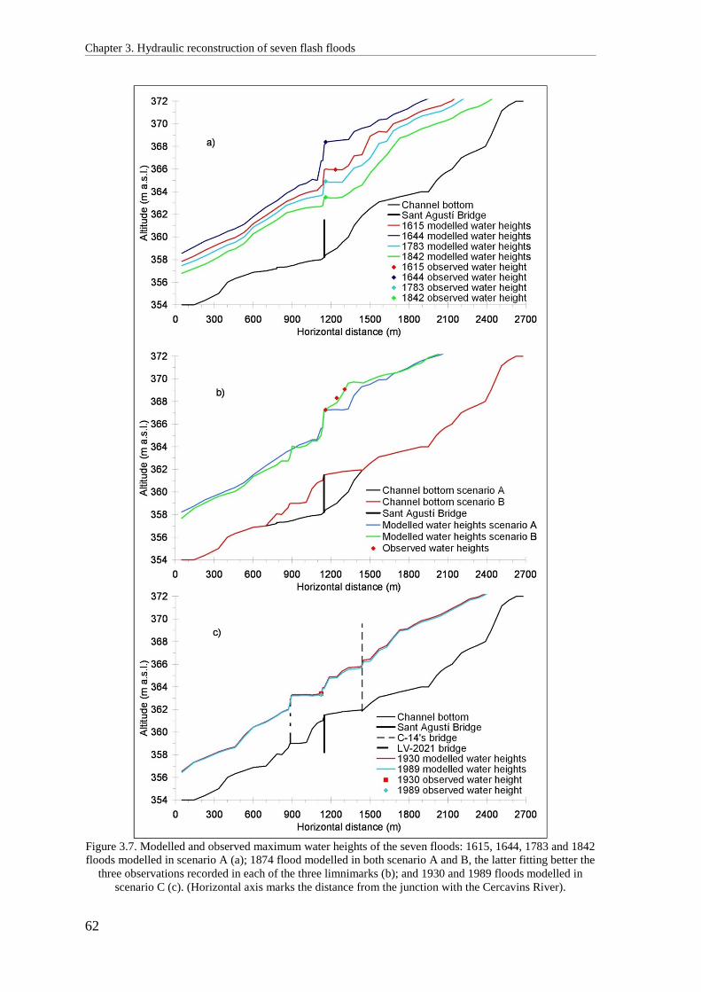
Chapter 3. Hydraulic reconstruction of seven flash floods
62
Figure 3.7. Modelled and observed maximum water heights of the seven floods: 1615, 1644, 1783 and 1842 floods modelled in scenario A (a); 1874 flood modelled in both scenario A and B, the latter fitting better the
three observations recorded in each of the three limnimarks (b); and 1930 and 1989 floods modelled in scenario C (c). (Horizontal axis marks the distance from the junction with the Cercavins River).

Chapter 3. Hydraulic reconstruction of seven flash floods
63
Table 3.3. Results of the hydraulic modelling at the time of the peak flow
Flood Scenario Refer-
ence cross section(1)
Results at reference cross section Results at 1147 cross section Channel’s
bottom height (m
a.s.l.)
Peak flow
(m3·s-1)
Specific peak flow
(m3·s-1·km-2)
Water height (m)
Wetted area (m2)
Mean water
velocity (m·s-1)
Froude’s number
1615
A
1245 359.0 790 5.3 7.7 290 2.7 0.38 1644 1147 358.2 1600 10.7 9.93 520 3.1 0.39 1783 1147 358.2 490 3.3 6.69 240 2.1 0.38 1842 1147 358.2 210 1.4 5.3 125 1.7 0.36
1874 A
1147 358.2 1190 7.9 8.88 428 2.8 0.39
B 361.5 1190 7.9 5.73 325 4.3 0.63 1930
C 1123 361.0 280 1.9 2.5 65 4.2 1.00
1989 1123 361.0 260 1.7 2.4 65 4.1 1.00 (1) The reference cross section is the closest one to the historical water height observation and its number is
the distance (in metres) from the cross section to the downstream extreme of the reach: the junction of the Ondara with the Cercavins River
The comparison of peak flows and water heights at Sant Agustí cross section between the 1842, 1930 and 1989 floods, and between those of the 1874 flood in scenarios A and B points out that, despite the section area reduction caused by the deposition of the 3-m-deep sediment layer and the construction of the Cartlist Wall, Sant Agustí Street cross section is hydraulically more efficient in scenarios B and C than in A; that is, the same peak flow is conveyed with a smaller water height. This effect is more evident in lower peak flows (1842, 1930 and 1989 floods) and results in less flooding due to modest events. This hydraulic efficiency increase is due to the acceleration of the flow caused by, on the one hand, Manning’s n reduction and, on the other hand, the absence of Sant Agustí Bridge, buried by the 1874 flood sediment layer, which acted as a dam in the occurrence of a heavy flood. Indeed, in the new hydraulic conditions, the flow is much faster –its velocity more than doubles– and, thus, has a higher destruction capacity. That sediment layer was deposited during the 1874 flood; not knowing if that happened before or after the peak flow, that flood was modelled in both scenarios A and B. The lucky existence of two additional limnimarks allowed us to decide that scenario B results fitted better the actual flood (Fig. 3.7.b) and, therefore, that the sediment was deposited mainly before the peak flow, that is, during the ascending limb of the hydrograph. Since the 1644 flood’s peak flow was even higher than 1874’s, a similar sediment deposition might as well have occurred at that time. However, 1668 Pier Maria Baldi’s drawing does not show such an accretion and there is no proof of dredging between the flood’s and the drawing’s dates. Therefore, the 1874 flood’s sediment deposition might be related to factors other than the mere peak flow value, such as the hydrograph shape, the flood’s duration or even possible changes in land uses within the catchment. 3.4.2. Uncertainty assessment of the hydraulic modelling The results of the sensitivity analyses displayed in Table 3.4 and Figure 3.8 show that the relationships between the variation of the modified input magnitude and variation of the modelled peak flow are linear within the explored range of input magnitude:
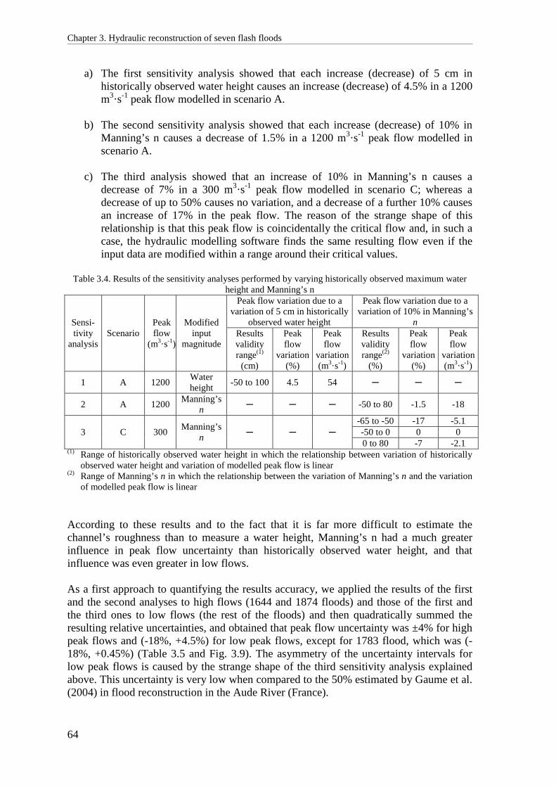
Chapter 3. Hydraulic reconstruction of seven flash floods
64
a) The first sensitivity analysis showed that each increase (decrease) of 5 cm in historically observed water height causes an increase (decrease) of 4.5% in a 1200 m3·s-1 peak flow modelled in scenario A.
b) The second sensitivity analysis showed that each increase (decrease) of 10% in
Manning’s n causes a decrease of 1.5% in a 1200 m3·s-1 peak flow modelled in scenario A.
c) The third analysis showed that an increase of 10% in Manning’s n causes a
decrease of 7% in a 300 m3·s-1 peak flow modelled in scenario C; whereas a decrease of up to 50% causes no variation, and a decrease of a further 10% causes an increase of 17% in the peak flow. The reason of the strange shape of this relationship is that this peak flow is coincidentally the critical flow and, in such a case, the hydraulic modelling software finds the same resulting flow even if the input data are modified within a range around their critical values.
Table 3.4. Results of the sensitivity analyses performed by varying historically observed maximum water
height and Manning’s n
Sensi-tivity
analysis Scenario
Peak flow
(m3·s-1)
Modified input
magnitude
Peak flow variation due to a variation of 5 cm in historically
observed water height
Peak flow variation due to a variation of 10% in Manning’s
n Results validity range(1) (cm)
Peak flow
variation (%)
Peak flow
variation (m3·s-1)
Results validity range(2)
(%)
Peak flow
variation (%)
Peak flow
variation (m3·s-1)
1 A 1200 Water height
-50 to 100 4.5 54 ─ ─ ─
2 A 1200 Manning’s
n ─ ─ ─ -50 to 80 -1.5 -18
3 C 300 Manning’s
n ─ ─ ─
-65 to -50 -17 -5.1 -50 to 0 0 0 0 to 80 -7 -2.1
(1) Range of historically observed water height in which the relationship between variation of historically observed water height and variation of modelled peak flow is linear
(2) Range of Manning’s n in which the relationship between the variation of Manning’s n and the variation of modelled peak flow is linear
According to these results and to the fact that it is far more difficult to estimate the channel’s roughness than to measure a water height, Manning’s n had a much greater influence in peak flow uncertainty than historically observed water height, and that influence was even greater in low flows. As a first approach to quantifying the results accuracy, we applied the results of the first and the second analyses to high flows (1644 and 1874 floods) and those of the first and the third ones to low flows (the rest of the floods) and then quadratically summed the resulting relative uncertainties, and obtained that peak flow uncertainty was ±4% for high peak flows and (-18%, +4.5%) for low peak flows, except for 1783 flood, which was (-18%, +0.45%) (Table 3.5 and Fig. 3.9). The asymmetry of the uncertainty intervals for low peak flows is caused by the strange shape of the third sensitivity analysis explained above. This uncertainty is very low when compared to the 50% estimated by Gaume et al. (2004) in flood reconstruction in the Aude River (France).

Chapter 3. Hydraulic reconstruction of seven flash floods
65
Figure 3.8. Results of the sensitivity analyses performed by varying historically
observed maximum water height (a) and Manning’s n (b) Table 3.5. Peak flow error intervals due to historically observed water height and Manning’s n. (Precision
of the historically observed water height was 0.5 cm when obtained from limnimarks (1640, 1783 and 1874 floods) and 5 cm when obtained from other historical sources (1615, 1842, 1930 and 1989) and Manning’s n precision was estimated as 25% in all cases; accordingly to the sensitivity analyses, the relative error of the peak flow due to a 5 cm error in historically observed water height was 4.5%, and that due to a 10% increase in Manning’s n was -1.5% for high peak flows and -7% for low peak flows and 1.5% and 0%,
respectively, for a 10% decrease in Manning’s n; 1000 m3·s-1 was the limit chosen between high and low peak flows)
Flood Peak flow
(m3·s-1)
Peak flow relative error interval (%)
Peak flow absolute error interval (m3·s-1)
Negative Positive Negative Positive 1615 790 -18 4.5 -140 40 1644 1600 -4 4 -60 60 1783 490 -18 0.45 -90 2 1842 210 -18 4.5 -40 10 1874 1190 -4 4 -50 50 1930 280 -18 4.5 -50 10 1989 260 -18 4.5 -50 10
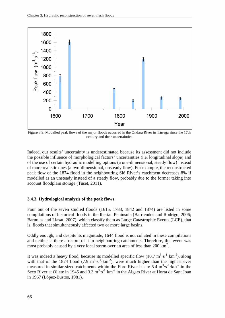
Chapter 3. Hydraulic reconstruction of seven flash floods
66
Figure 3.9. Modelled peak flows of the major floods occurred in the Ondara River in Tàrrega since the 17th
century and their uncertainties Indeed, our results’ uncertainty is underestimated because its assessment did not include the possible influence of morphological factors’ uncertainties (i.e. longitudinal slope) and of the use of certain hydraulic modelling options (a one-dimensional, steady flow) instead of more realistic ones (a two-dimensional, unsteady flow). For example, the reconstructed peak flow of the 1874 flood in the neighbouring Sió River’s catchment decreases 8% if modelled as an unsteady instead of a steady flow, probably due to the former taking into account floodplain storage (Tuset, 2011). 3.4.3. Hydrological analysis of the peak flows Four out of the seven studied floods (1615, 1783, 1842 and 1874) are listed in some compilations of historical floods in the Iberian Peninsula (Barriendos and Rodrigo, 2006; Barnolas and Llasat, 2007), which classify them as Large Catastrophic Events (LCE), that is, floods that simultaneously affected two or more large basins. Oddly enough, and despite its magnitude, 1644 flood is not collated in these compilations and neither is there a record of it in neighbouring catchments. Therefore, this event was most probably caused by a very local storm over an area of less than 200 km2. It was indeed a heavy flood, because its modelled specific flow (10.7 m3·s-1·km-2), along with that of the 1874 flood (7.9 m3·s-1·km-2), were much higher than the highest ever measured in similar-sized catchments within the Ebro River basin: 5.4 m3·s-1·km-2 in the Seco River at Oliete in 1945 and 3.3 m3·s-1·km-2 in the Algars River at Horta de Sant Joan in 1967 (López-Bustos, 1981).

Chapter 3. Hydraulic reconstruction of seven flash floods
67
In any case, these specific flows are congruent with the highest modelled in similar-sized Catalan catchments, which have an enveloping curve value of 10 m3·s-1·km-2 (Gaume et al., 2009). Similarly, Delrieu et al. (2005) and Payrastre et al. (2005) have modelled specific flows of this order in neighbouring Southern France. 3.4.4. Temporal trends The reconstructed peak flows are shown on a time scale in Fig. 3.9. The floods temporal distribution is quite regular; the periods between them are of 30-60 years, except between 1644 and 1783 (139 years). All the studied floods that took place within the Little Ice Age (LIA) –that is, between the 15th and 19th centuries (Pfister et al., 1996)–, except that of 1644, occurred in periods in which catastrophic flash floods were more frequent in Catalonia: 1580-1620, 1760-1800 and 1830-1870 (Barriendos and Martin-Vide, 1998; Llasat et al., 2005). However, this higher frequency does not seem to be related to climate evolution since there are differences between those periods: the first and the last of them were especially cold and wet, whereas the second one, known as Maldà’s anomaly, was very dry (Barriendos and Llasat, 2003). Furthermore, during the coldest period within the LIA in Central and Northern Europe, the Late Maunder Minimum (1675-1715), no floods were recorded in the Ondara’s catchment. Therefore, the extreme weather that caused the five pre-1900 flash floods does not seem to be related to a period’s wetness or coldness. Nevertheless, pre- and post-1900 floods might have had different climatic causes. Indeed, the five pre-1900 floods occurred between late July and late September and all of them –except again the 1644 flood, which was exceptional in more than one way– did not last long, a sign of their convective origin. Conversely, post-1900 floods both took place in the second half of October and were caused by weather fronts. 3.5. Conclusions There is no flow gauging data of the Ondara River; nevertheless, the great availability of historical information about floods and urban evolution of the town of Tàrrega allowed the hydraulic reconstruction of the major floods occurred since the 17th century. This reconstructed information will probably improve flood prediction in Tàrrega, because of the magnitude of the modelled floods: two of the calculated specific peak flows are among the highest ever modelled in similar-sized catchments in the Western Mediterranean basin. Besides, archaeological surveys uncovered a great modification in the channel’s and floodplain’s morphology operated by 1874 flood: a 3-m-deep sediment layer deposition. Afterwards, our reconstruction proved that this deposition occurred before the peak flow and, thus, had an influence on the flood’s characteristics: it accelerated the flow and, therefore, it increased its destruction capacity. At the same time, this morphology change caused the modest flows to be less prone to flooding than previously.

Chapter 3. Hydraulic reconstruction of seven flash floods
68
The sensitivity analyses showed that Manning’s n had more influence in the modelled peak flow error than water height. Furthermore, a preliminary uncertainty assessment taking only estimated the peak flows’ error in 4% for high flows and 18%, for low flows; this uncertainty may be deemed underestimated because it is extremely low when compared to other estimations found in the literature and because the assessment only took into account observed water height and Manning’s n. Acknowledgements We thank the anonymous people who decided to keep records of ancient floods, either in the form of limnimarks or written accounts, which allowed the reconstruction of these events. We thank also Rubén Remacha (University of Lleida) and Francesc Marsà (Catalonia Water Agency), who told us about Tàrrega’s limnimarks; Oriol Saula (Urgell County Museum), who told us a lot about Ondara’s floodplain’s morphology evolution; and Miquel Àngel Farré (Urgell County Archive), who helped us to find some documents. We thank as well the two anonymous referees that reviewed the text and the editor of the volume Aristides Bartzokas for their work in improving the article. One of the authors belongs to the RIUS Fluvial Dynamics Research Group (UdL) and was funded by the Catalonia Water Agency (ACA) (CV08000251).

Chapter 4
Historical, hydraulic, hydrological and meteorological reconstruction of 1874 Santa Tecla flash floods in
Catalonia (NE Iberian Peninsula)
Ruiz-Bellet, J.L., Balasch, J.C., Tuset, J., Barriendos, M., Mazón, J., Pino, D. (2015): Historical, hydraulic, hydrological and meteorological reconstruction of 1874 Santa Tecla flash floods in Catalonia (NE Iberian Peninsula). J. Hydrol., 524, 279-295. http://dx.doi.org/10.1016/j.jhydrol.2015.02.023 doi:10.1016/j.jhydrol.2015.02.023 Published 16 February 2015


Chapter 4. Complete recontruction of 1874 Santa Tecla floods
71
Abstract A multidisciplinary methodology for historical floods reconstruction was applied to the 1874 Santa Tecla floods occurred in Catalonia (NE Spain), using both historical information and meteorological data from 20th Century Reanalysis. The results confirmed the exceptionality of the event: the highest modelled specific peak flow was around 14.6 m3·s-1·km2 in Espluga de Francolí (a 100 km2 catchment) and all the modelled total rainfall values were above 110 mm in about six hours, with maximum intensities around 60 mm·min-1. The peak flows’ return periods were about 260 years and the rainfalls’ periods were between 250 and 500 years. The meteorological cause of the rainstorms was the quick ascent of a mass of humid air at low-levels initiated by the sudden withdrawal of a mass of hot air at mid-levels. A sensitivity analysis on the various sources of error shows that peak flow errors from hydraulic modelling ranged from 5% to 44%, and rainfall errors from hydrological modelling were about 36%. Keywords: Historical flash floods, multidisciplinary reconstruction, peak flow, rainfall, 20th Century Reanalysis, uncertainty 4.1. Introduction Flash floods rank among the most dangerous and destructive natural hazards in southern Europe. Despite this, scientific research about past floods is only recent and mainly focused on modern events. This is a drawback when trying to analyse and classify flash floods in a climatic change context because important information, which old events would provide, is missing. Fortunately, data about long-past floods can be retrieved from sedimentary and dendrogeomorphological evidences and from historical documents. Indeed, historical archives keep raw data −such as maximum water depths, rainfall durations, channel morphologies, atmospheric variables− which, after proper collecting and processing, can enlarge present day records of floods. As said above, the use of this historical information in flood analysis and reconstruction is only very recent and usually restricted to academic research (Bayliss & Reed, 2001; Benito et al., 2004; Gaume et al., 2004; Naulet et al., 2005; Brázdil et al., 2006; Elleder, 2010), but it will most probably become more used because of the EUDirective2007/60/EC (2007) on flood risk assessment. Nevertheless, and excluding investigations that analyse climate and flood frequency, only a few studies so far have tried to thoroughly analyse historical floods by linking hydrological and meteorological information (Petersen et al., 1999; Delrieu et al., 2005; Bürger et al., 2006; Thorndycraft et al., 2006; Flesch & Reuter, 2012). In this same line, this study presents an applied example of the multidisciplinary methodology (historiographical, hydraulic, hydrological and meteorological) of historical floods reconstruction introduced in Chapter 2. This methodology was applied on a case study: the 1874 Santa Tecla floods. The night of 22-23 September 1874 several flash floods occurred in many catchments throughout the

Chapter 4. Complete recontruction of 1874 Santa Tecla floods
72
eastern part of the Ebro River basin, in Catalonia (NE Iberian Peninsula, Fig. 4.1). These floods −known as Santa Tecla floods because this was the saint of that day− caused 575 casualties and ravaged an approximate area of 10000 km2 and are considered, as a whole, one of the heaviest events in the region over the last 500 years. Luckily, there is a lot of information about this event, especially, maximum water depths in many locations. So far, some of this information has already been used to calculate the peak flows of the floods in six sites located in three catchments (Balasch et al., 2010a). Here, we enlarged this list with four more sites and two more catchments. In some cases, it was also possible to calculate the hyetograph of the rainfall. Besides this hydraulic and hydrological information, meteorological data of the days before the floods, available from NOAA's 20th Century Reanalysis (Compo et al., 2011), were used to characterise the meteorological causes of the floods. The objective of this paper is to use a multidisciplinary methodology of hydraulic, hydrological and meteorological reconstruction of historical floods on a case study: the 1874 Santa Tecla floods, occurred in NE Iberian Peninsula. Although in this paper only this one flood was reconstructed, our long-term objective is to use this multidisciplinary methodology to analyse the heaviest floods occurred in NE Iberian Peninsula in the last 500 years. By doing so with such a thorough reconstruction methodology, we will be able to classify the historical floods of the region according to their meteorological causes and, thus, to improve prediction, planning and readiness. 4.2. Study area The study area is composed of ten sites in five catchments located in the southern half of the Catalan Central Depression. The Catalan Central Depression is a succession of high plateaus between 800 and 1000 metres interspersed with eroded river catchments. The height of the plateaus diminishes westward, where the Catalan Central Depression and the Ebro River Depression meet (Fig. 4.1). The geological substrates in these catchments are Cenozoic sediments of the Ebro depression, with some outcrops of Paleozoic and Mesozoic materials of the Pre-coastal ranges in the southernmost of the ten catchments: Francolí. The climate in the Catalan Central Depression is Mediterranean (Köppen Csa), but with continental traits that distinguish it from the nearby coast: a wider temperature range and a lower rainfall: less than 600 mm per year, which decreases as height decreases. However, heavy rainstorms are frequent in the studied area. The complex orography of this region, with a maximum altitude of around 1000 m, plays a main role in uplifting the Mediterranean air flows, thus causing severe storms (Romero et al., 1997; Pascual et al., 2004). Additionally, its location on the western coast of the Mediterranean basin (Fig. 4.1) favours torrential rainfall, especially at the end of summer and autumn (Llasat et al., 2005), when the warm Mediterranean Sea provides large amounts of heat and moisture to the lower layers of the atmosphere. Moreover, regional climate models forecast a decrease in the average yearly precipitation but, at the same time, an increase in the maximum daily precipitation, that is, an increase of torrential downpours frequency, over this region in this next century (Barrera & Cunillera, 2011).

Chapter 4. Complete recontruction of 1874 Santa Tecla floods
73
The complex orography mentioned above, also implies small catchments (80-300 km2 with short, steep streams (15-35 km long and 1-2% of slope) and, therefore, with a very quick hydrological response: their very low average flows, less than 1 m3·s-1, can multiply thousands of times in a matter of hours. The main soil use is dry land cereal farming, whereas the higher areas are covered with Mediterranean forest. These catchments, mostly rural but with some populated towns, were the most damaged by 1874 Santa Tecla flash floods, within the 10000 km2 affected area. The ten sites within the five catchments were the hydraulic and hydrological modelling were performed are located in the northern half of the area affected by 1874 Santa Tecla floods and are, from north to south and from west to east: Sió, Ondara, Corb, Vall Major and Francolí (Fig. 4.1 and Table 4.1). All of them have their headwaters either on the Catalan Central Depression ranges or on the Pre-coastal ranges, between 700 and 900 m (Portella, Tallat, Llena, and Prades ranges). All of them but Francolí flow westwards: Sió and Vall Major into the Segre River, the main tributary of the Ebro River, and Ondara and Corb into large alluvial fans. Francolí flows southwards into the Mediterranean Sea. All of them have scarce flows all year round, with a high-water period around May and long low-water periods, but, due to irrigation, they never dry up, except Vall Major, which is usually dry. In any case, autumn overflowing flash floods are typical, occurring about three or four times per century (Corominas et al., 1985; Novoa, 1987; Coma, 1990). Table 4.1. Morphological and hydrographical characteristics of the ten catchments were the hydraulic and,
in some cases, the hydrological reconstructions were performed. Own elaboration from various sources
Site number in Fig. 4.1
River Site Area (km2) Main stream
length (km)
Main stream
slope (%)
Max/min height (m)
Mean flow
(m3·s-1)
Mean annual rainfall (mm)(5)
1 Sió
Mont-roig 219 24.2 1.4 745-400 <0.8(1) 480
2 Agramunt 341 34.9 1.2 745-335 <0.8(1) 479
3 Ondara
Cervera 86 17.1 1.7 804-460 0.5(2) 464
4 Tàrrega 150 28.6 1.4 804-356 0.5(2) 449
5
Corb
Vallfogona de Riucorb
46 10.4 1.8 890-698 <0.9(3) 509
6 Guimerà 91 15.0 1.7 890-500 <0.9(3) 418
7 Ciutadilla 123 19.6 2.2 890-450 <0.9(3) 459
8 Vall Major Granyena de les Garrigues
50 17.0 2.1 670-309 0 410
9 Francolí
Espluga de Francolí
101 16.3 3.9 1050-404 0.3(4) 537
10 Montblanc 344 25.5 3.0 1050-284 0.3(4) 528 (1) Gauging station: Balaguer (EA182), period: 1965-1992 (2) CHE, Confederación Hidrográfica del Ebro (1996) (3) Gauging station: Vilanova de la Barca (EA183), period: 1965-1992 (4) Gauging station: Montblanc (28), period: 1945-1990 (Junta d’Aigües, 1995) (5) Ninyerola et al. (2005)
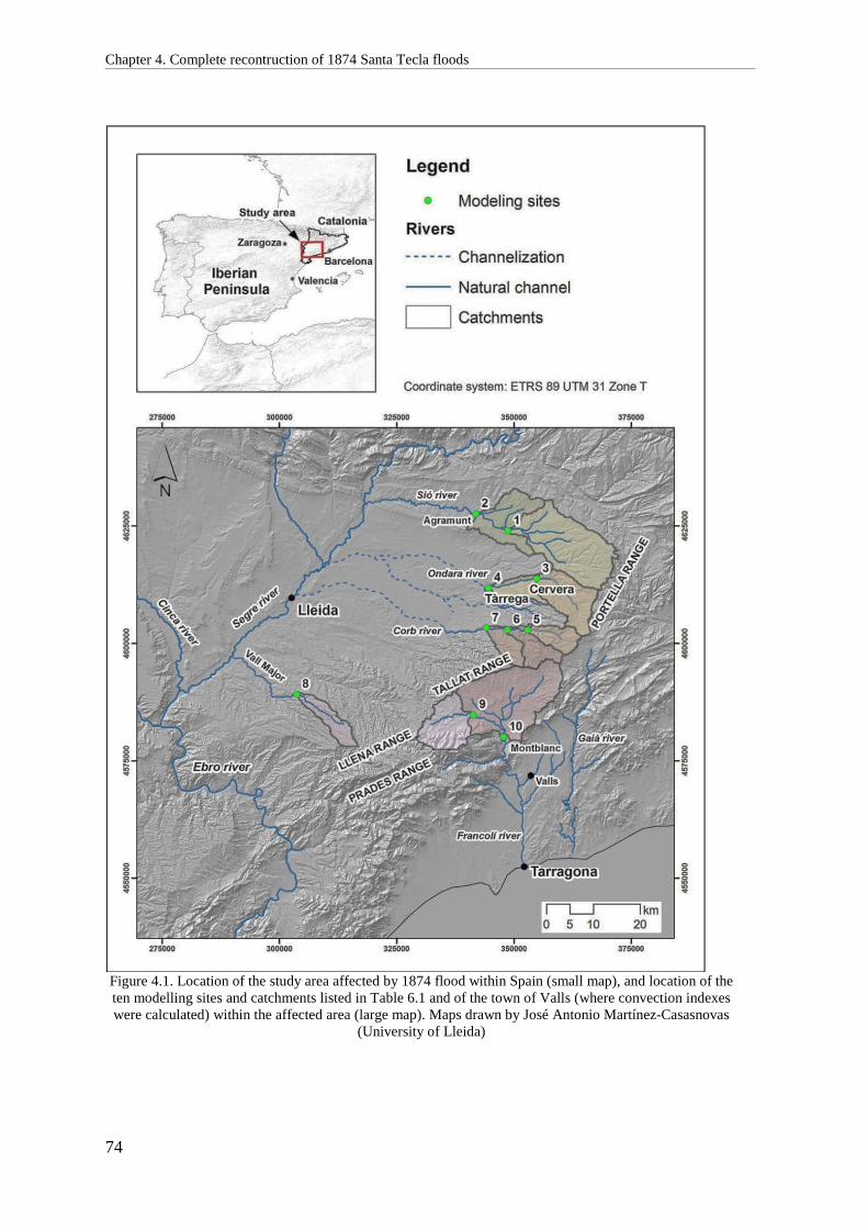
Chapter 4. Complete recontruction of 1874 Santa Tecla floods
74
Figure 4.1. Location of the study area affected by 1874 flood within Spain (small map), and location of the ten modelling sites and catchments listed in Table 6.1 and of the town of Valls (where convection indexes were calculated) within the affected area (large map). Maps drawn by José Antonio Martínez-Casasnovas
(University of Lleida)
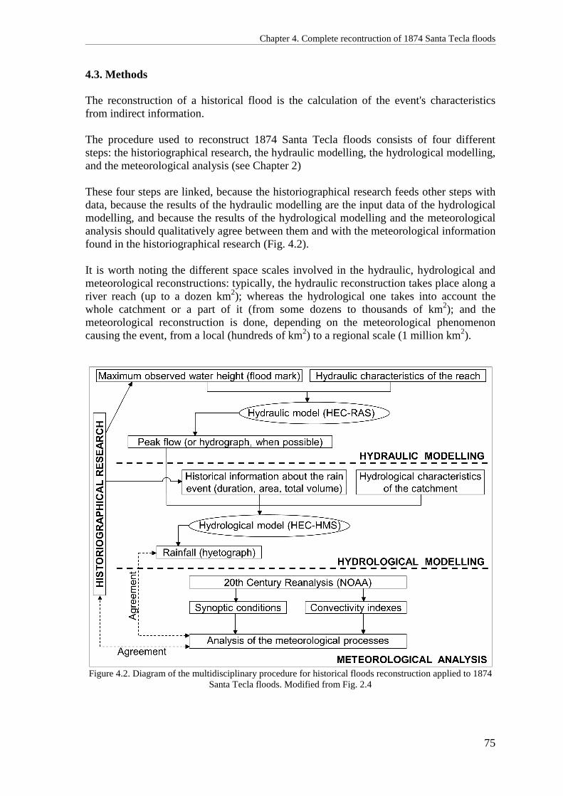
Chapter 4. Complete recontruction of 1874 Santa Tecla floods
75
4.3. Methods The reconstruction of a historical flood is the calculation of the event's characteristics from indirect information. The procedure used to reconstruct 1874 Santa Tecla floods consists of four different steps: the historiographical research, the hydraulic modelling, the hydrological modelling, and the meteorological analysis (see Chapter 2) These four steps are linked, because the historiographical research feeds other steps with data, because the results of the hydraulic modelling are the input data of the hydrological modelling, and because the results of the hydrological modelling and the meteorological analysis should qualitatively agree between them and with the meteorological information found in the historiographical research (Fig. 4.2). It is worth noting the different space scales involved in the hydraulic, hydrological and meteorological reconstructions: typically, the hydraulic reconstruction takes place along a river reach (up to a dozen km2); whereas the hydrological one takes into account the whole catchment or a part of it (from some dozens to thousands of km2); and the meteorological reconstruction is done, depending on the meteorological phenomenon causing the event, from a local (hundreds of km2) to a regional scale (1 million km2).
Figure 4.2. Diagram of the multidisciplinary procedure for historical floods reconstruction applied to 1874
Santa Tecla floods. Modified from Fig. 2.4

Chapter 4. Complete recontruction of 1874 Santa Tecla floods
76
4.3.1. Historiographical research Historiographical research is the key step in the reconstruction of any historical flood: without correct, reliable information, no correct, reliable modelling can be done. Historiographical research is mainly based in archive scanning, that is, in the systematic scrutiny of documents in search of any records related to any flood. These documents can hold all kinds of data about the flood: meteorological (start and end times of the rainfall, weather in the previous days), hydraulic and hydrological (time of the peak flow, time of the overbank flow, maximum height reached by the water, height of the water at various times, state of saturation of the catchment's soils), and human and social (number of victims, economic loss). Some of these data are essential in order to reconstruct the flood, and the nature of these documents is mostly official (town council's minutes, notarized documents, local authorities official reports to higher levels of the administration), but they also include contemporary newspapers (Diario de Barcelona, 1874), personal accounts (Salvadó, 1875) and local historians' research (Pleyán de Porta, 1945; Iglésies, 1971; Xuclà, 1977; Piqué, 1986; Coma, 1990; Vila, 1992; Espinagosa et al., 1996; Còts, 2012). Besides this archive information, flood marks are also very important pieces of information in hydraulic modelling, because they precisely mark the maximum height of the water, which can be equated (with a small, acceptable error) to the height of the water at the peak of the flood. Twelve flood marks were used in the hydraulic modelling of the ten reconstructed peak flows. Some of them are plaques whereas others are simple carvings on the walls and even others are mere notes found in written documents (Table 4.2). The reliability of these twelve flood marks is generally high, since most of them have been confirmed by local historians and experts. There is only a slight suspicion that the Agramunt mark might have been moved. This one scored 2 (moderately reliable) in the three-degreed classification of reliability by (Bayliss and Reed, 2001), whereas the other marks all scored 3 (very reliable). The precision of a flood mark (that is, the maximum expected difference between the flood mark and the actual maximum water height) depends on its reliability and on its nature. Those flood marks with a high reliability and a physical nature (a plaque or an incision) were given a precision of ±10 cm. The one with moderate reliability (Agramunt) and the two of a written nature (Cervera and Vallfogona de Riucorb) were given a precision of ±30 cm (Table 4.2).

Chapter 4. Complete recontruction of 1874 Santa Tecla floods
77
Table 4.2. List of the flood marks used in the hydraulic modelling
Site number in Fig.
4.1
River Site Address UTM Coordinates
(ETRS89, UTM 31T) Type of mark
Relia- bility (3)
Preci- sion (4)
(cm) X (m) Y (m) Z (m)
1
Sió
Mont-roig Molí del
Serra 348,614 4,624,073 373.18
Incision on a column
3 ±10
2 Agramunt
Mediaeval bridge by Plaça del
Torronaire
341,898 4,627,625 330.03 Plaque 2 ±30
3
Ondara
Cervera Molí del
Grau 355,352 4,613,639 462.19 Written
reference(1) 3 ±30
4 Tàrrega
8-10 bis, Piques Street
345,101 4,612,138 369.08 Plaque 3 ±10
6, Font Street 345,056 4,612,077 368.30 Plaque 3 ±10 26, Sant
Agustí Street 345,003 4,611,995 367.26 Plaque 3 ±10
5
Corb
Vallfogona de Riucorb
1, Plaça Major
352,925 4,608,844 563.40 Written
reference(2) 3 ±30
6 Guimerà 7, Piques
Street 348,733 4,602,951 507.57 Plaque 3 ±10
7 Ciutadilla Hostal del
Teuler 344,061 4,603,095 464.01 Plaque 3 ±10
8 Vall
Major Granyena de les Garrigues
Molí de la Societat
303,646 4,589,302 312.08 Incision on the northern
corner 3 ±10
9
Francolí
Espluga de Francolí
Font Major 341,355 4,584,783 408.68 Plaque 3 ±10
10 Montblanc Molí de la
Farga 347,865 4,580,138 295.47
Plaque on the SW corner
3 ±10
(1) Corbella (2003) (2) Xuclà (1977) (3) Reliability according to Bayliss and Reed (2001) scale: 1 = unreliable; 2 = reliable; 3 = very reliable (4) Precision: maximum expected difference in cm between the flood mark and the actual maximum water
height 4.3.2. Hydraulic modelling The objective of the hydraulic modelling was the calculation of the peak flows at the ten sites. It was done from the maximum water heights observed (Table 4.2), because it was considered (accepting a minimum error) that these maximum heights occurred simultaneously with their corresponding peak flows. The hydraulic model used was the one-dimensional HEC-RAS 4.0 (USACE, 2008) under gradually varied, steady, mixed regime. Actually, this model calculates water height from a discharge value. Therefore, we applied it iteratively, trying tentative peak flows until the difference between the modelled water height and the actual flood mark was smaller than 1 cm (Fig. 2.5). The HEC-RAS model needs as input data:

Chapter 4. Complete recontruction of 1874 Santa Tecla floods
78
1) the channel's geometry (cross sections shape and channel's longitudinal slope), given by the cross sections of the digital terrain model,
2) the Manning roughness coefficients (also known as Manning's n), that relate friction with type of surface and are found in tables (Chow, 1959),
3) the boundary and initial conditions, which tell what is happening upstream and downstream the modelled river reach,
4) the aforementioned tentative peak flow. All these input data are limited to a river reach, usually less than 2 km long, upstream and downstream the flood mark site. However, the data had to be adequately adapted to be as close as possible to their values at the time when Santa Tecla floods took place. Old maps, engravings and written descriptions were used to reconstruct the channel and floodplain morphology at the time of the flood (obstacles such as human structures, meanders and islands, and cross sections' contractions or expansions) and to hypothesize the roughness coefficients. Table 4.3 lists the changes in each of the ten modelled sites.
Table 4.3. Changes in the modelled reaches. Own elaboration from historical information Site (Fig. 4.1)
River Site Type of reach
Changes in cross sections geometry
Changes in transversal infrastructures
1 Sió
Mont-roig Rural None None 2 Agramunt Urban Channelization 2 bridges 3
Ondara Cervera Rural None None
4 Tàrrega Urban Deposition of a 3 m deep
layer (see Chapter 3) Carlist Wall and 3
bridges (see Chapter 3) 5
Corb Vallfogona Urban Channelization One bridge
6 Guimerà Urban Channelization One bridge 7 Ciutadilla Rural None One bridge
8 Vall
Major Granyena de les Garrigues
Rural None None
9 Francolí
Espluga de Francolí
Urban None None
10 Montblanc Rural None None Besides, also in Tàrrega, the existence of three flood marks along the river reach, allowed choosing the correct river bed morphology between two possible ones ((see Chapter 3). In this same town, the previous reconstruction of six other historical floods allowed the calculation of Santa Tecla's peak flow return period (see Chapter 3). In Montblanc, the peak flow return period was calculated from a series of measurements in the period 1946-2014 (Junta d’Aigües, 1995). The high degree of uncertainty associated with historical floods input data is inevitably transferred to the results. In order to estimate this uncertainty, a sensitivity analysis of the hydraulic modelling was performed in 5 of the 10 sites. More specifically, the effects of two input variables on the resulting peak flows were assessed: maximum water height and the Manning roughness coefficients (or Manning's

Chapter 4. Complete recontruction of 1874 Santa Tecla floods
79
n). This was done by estimating a value of uncertainty or error for those two variables: the precision values of the flood marks given in Table 4.2, for the maximum water height; and ±30% for the Manning roughness coefficients (Marcus et al., 1992; Johnson, 1996; Wohl, 1998) and then separately calculating the relative error in the peak flow results that each one of these input errors would cause. The two resulting relative errors were then quadratically added as follows: ��,����� = ��,�� �� + ��,������ � (4.1)
where δQ,total = peak flow total relative error δQ,height = peak flow relative error caused by the error in maximum water height δQ,Manning = peak flow relative error caused by the error in Manning's n Relative errors have no units and are given in parts-per-one. In two of the five sites, only the relative error caused by maximum water height was calculated. 4.3.3. Hydrological modelling The objective of the hydrological reconstruction was the calculation of the hyetograph of the rain that caused the flood. To this end, the hydrological modelling software HEC-HMS 3.3 (USACE, 2010b) was used. HEC-HMS is an empirical, lumped rainfall-runoff model, which allows the user to choose among an array of different empirical methods for three hydrological processes: runoff generation, transformation of runoff into river flow, and river flow routing. For each of these processes we chose, respectively, the SCS Curve Number, the SCS Synthetic Unit Hydrograph and the Muskingum-Cunge methods, because of their simplicity of use, their moderate requirements in input data and their being generally accepted and commonly used (NRCS, 2007). Similarly as in the hydraulic reconstruction, the calculation procedure is iterative, because the result (that is, the hyetograph) is, actually, an input datum required by the model (Fig. 2.6). Therefore, a tentative hyetograph must be built using the available historical information about the rain event, such as its duration and other indications that can lead to a rough estimation of the rainfall volume. Hence, only in those cases when all these required data were available, the tentative hyetograph could be built and the hydrological modelling, performed; more specifically, this could be done in five sites: Mont-roig by the Sió River, Cervera and Tàrrega by the Ondara River, and Ciutadilla and Guimerà by the Corb River. Besides this tentative hyetograph, the model needs input data describing the catchment (and subcatchments) hydrological characteristics, such as soil type (and its hydrological characteristics), land use and cover, antecedent soil moisture condition, and the main stream's length, slope, and Manning roughness coefficient.

Chapter 4. Complete recontruction of 1874 Santa Tecla floods
80
These data had to be adapted, when necessary, from present-day values to the estimated ones at the time of the studied flood. Particularly, on the one hand, the antecedent soil moisture condition was estimated from the historiographical research3 and confirmed with the meteorological analysis; condition III (saturated soils) was ultimately chosen. According to SCS Curve Number model, for condition III to be chosen, it must have rained at least 53 mm in the five previous days. On the other hand, regarding soil uses and cover, none of the three modelled catchments suffered major changes since 1874. They all are mostly rural, with non-irrigated cereal crops and small patches of Mediterranean forest. The result of the hydrological modelling (the peak flow) was then compared to the one calculated in the hydraulic modelling; if the two were similar enough (less than 1% apart), the tentative hyetograph was accepted. Then, the approximate return period of the total rainfall was directly obtained from the maps drawn by Casas (2005). As happened in the hydraulic modelling, calibrations of the hydrological models in the five modelled sites were not possible because none of the studied catchments has ever been gauged. However, as said in Section 4.3.2., an event occurred in 1989 allowed to calibrate both the hydraulic and the hydrological models in the town of Tàrrega in the Ondara catchment. However, in order to estimate the real amount of uncertainty in the results, a sensitivity analysis was done by observing the variation in the results caused by variations in the input variables: the influence of Curve Number and Synthetic Unit Hydrograph's lag time on peak flow (which is the actual output of the model), and the influence of antecedent soil moisture condition on total rainfall (which is, as part of the hyetograph, our aimed result). This was done in two of the five sites: Mont-roig and Tàrrega. The Curve Number value summarizes the runoff production of a catchment. Its value is estimated with tables from soil type, land use and land cover (NRCS, 2007) and it is therefore somewhat arbitrary. Thus, we assumed an error of ±10 units in its estimation, slightly more conservative than the ±10% value suggested by Hawkins (1975). Soil moisture also affects the catchment's permeability. The Curve Number method treats this parameter as a qualitative discrete variable called antecedent soil moisture condition, with three possible values: dry (I), intermediate (II), and saturated (III). In practice, a change in antecedent soil moisture condition entails a change in the Curve Number value. In this way, we assessed the influence in total rainfall of a change in antecedent soil moisture condition from III (saturated) to II (intermediate), which equates to a reduction in the Curve Number of around 8 units. However, an error in this parameter seems quite unlikely, given the written accounts that describe a rainy week before the floods (Diario de Barcelona, 1874; Pleyán de Porta, 1945). Synthetic Unit Hydrograph's lag time is the time between the moment when half of the rain has fallen and the moment of the peak flow. Lag time is indirectly calculated with an empirical equation that only requires the main stream's length and slope (NRCS, 2007):
3 For example, Pleyán de Porta (1945) states that the soils in the Sió, Ondara and Corb catchments were at field capacity due to a generous rain on 18th September 1874, just five days before Santa Tecla rainstorm.

Chapter 4. Complete recontruction of 1874 Santa Tecla floods
81
��� = 0.6 · 0.6 · � ���.���.�� (4.2)
where tlag is the lag time (in h), L is the length of the main stream (in km) and J is the mean slope of the main stream (in parts-per-one). This indirect way of calculating lag time results in a high uncertainty. Indeed, Bell and Om Kar (1969) state that lag time may vary from about 70% to 140% of the value found with Eq. 4.2; besides, they also conclude that lag time for extreme floods is 10% shorter. Thus, we decided to assess the influence of a ±40% error in lag time on peak flow. As in the hydraulic modelling (see Eq. 4.1), total relative error in peak flow was calculated quadratically summing the relative errors caused by Curve Number and by lag time. 4.3.4. Meteorological analysis The objective of the meteorological analysis was to determine the meteorological processes that caused the flood. More precisely:
a) To describe the synoptic conditions (atmospheric situation at several levels) during 1874 Santa Tecla floods. This meteorological analysis allowed, on the one hand, determining the cause of the floods and, on the other hand, validating the hyetograph found in the hydrological modelling. If the former could be done with many floods in the region, flood forecasting would be improved.
b) To assess the possibility of rainfall in the weeks before the floods in order to estimate the antecedent soil moisture condition, a piece of information needed in the hydrological modelling.
This analysis was performed by using the data from the 20th Century Reanalysis by the National Oceanic and Atmospheric Administration (NOAA), available from 1 January 1871 onwards. According to Compo et al. (2011), the quality of these data is generally high when compared with independent radiosonde data, especially in the extratropical Northern Hemisphere. This meteorological analysis was done by directly examining the maps and also by calculating several indexes that measure the convection intensity:
a) The Convective Available Potential Energy (CAPE; Mapes, 1993; Doswell and Rasmussen, 1994).
b) The Lifted Index LI (Galway, 1956).
c) The K index (George, 1960).
d) Vertical, Cross and Total Totals indexes (Miller1972).
e) The Humidity index (Litynska et al., 1976).

Chapter 4. Complete recontruction of 1874 Santa Tecla floods
82
f) The difference between the lifted condensation level (LCL) and the level of free convection (LFC).
g) The limit of convection (LOC).
h) The wind shear between surface and 1 km, and between surface and 3 km. These convectivity indexes were calculated approximately over the town of Valls4, located within the Francolí River catchment (Fig. 4.1). Additionally, three pressure indexes, which measure the difference in surface pressure between two distant locations, were also calculated for every day of the month of September 1874 from contemporary daily measurements:
a) The WeMo index, between Cádiz and Padua (Martín-Vide and López-Bustins, 2006).
b) The NAO index, between Cádiz and Reykjavík.
c) A zonal index between Cádiz and Uppsala. 4.4. Results and discussion The results of the reconstruction of 1874 Santa Tecla flood and their discussion are presented in several sections corresponding to the different phases of the reconstruction. 4.4.1. Historiographical research 4.4.1.1. Meteorological and hydrological information The summer of 1874 had been particularly hot and dry, even when compared to the generally hot and dry summers in the area, so the Mediterranean Sea was very warm and, thus, there was a high probability of heavy thunderstorms (Iglésies, 1971). Intense precipitations occurred in Reus, Vilanova i la Geltrú, and Tarragona on 19 September 1874 (Diario de Barcelona, 1874). Indeed, an Atlantic depression crossed NE Spain between 17 and 19 September; there are records of rainfall in Zaragoza on 17 and 18 September, Valencia on 18 (28.6 mm) and Barcelona on 19 (30 mm). This episode of rain left the soil very wet (Pleyán de Porta, 1945) and, thus, with a reduced ability to absorb the precipitation that would fall on the day of Santa Tecla. Indeed, after a few days of calm, the night of 22-23 September 1874, a strong thunderstorm driven by SE, SSE and S strong winds affected the coast and the southern half of Catalonia; these precipitations caused floods in many small catchments throughout an area of around 10000 km2 (Diario de Barcelona, 1874) (Fig. 4.3;). In Barcelona, from
4 UTM coordinates of Valls: X = 335,500 m; Y = 4,572,000 m; Z = 200 m; UTM 31 T / ETRS89

Chapter 4. Complete recontruction of 1874 Santa Tecla floods
83
the only rainfall measurement found, it rained 63 mm on 23 September, almost the average precipitation of the whole month. As an example of the quickness of the events, Iglésies (1971) reports that, in Tàrrega (in the Ondara catchment), the rain, which had started at 09:00 p.m. (local time, UTC) on 22 September, grew more intense at around 01:00 a.m. and lasted two more hours, and that the peak flow of the flood occurred between 03:00 and 03:30 a.m.. Almost the same happened in the Francolí River: the downpour began at 01:00 a.m., and the peak flow reached Tarragona (the outfall of the catchment) at around 03:00 a.m. (Diario de Barcelona, 1874; Iglésies, 1971).
Figure 4.3. Map of Catalonia highlighting the area most severely affected by the 1874 floods and the sites
where information about them was found. Modified from Barriendos et al. (2013) The historiographical sources and the contemporary newspapers consulted (Diario de Barcelona, 1874; Iglésies, 1971; Coma, 1990; Barriendos and Pomés, 1993; Espinagosa et al., 1996; Còts, 2012) list fifty-one locations where the rain caused floods, thirty-one of which, destructive (see Fig. 4.3, a article fig 5) This distribution of floods provides information about the movement of the storm. Indeed, most of the thirty-one destructive floods cluster along the rivers with headwaters on either side of the southern Pre-coastal ranges; that is, along both the leeward ones (like Sió, Ondara, Corb and Vall Major) and the windward ones (like Francolí and Gaià) (Fig. 6.1). Therefore, these windward rivers acted as natural corridors for the southeastern wind, which pushed the stormy air mass up to the top of the Pre-coastal ranges, where it developed and precipitated. This explanation agrees with the meteorological analysis (Section 4.4.4) and with the rainfall distribution, with higher rainfalls in the catchments' headwaters (Section 4.4.3).

Chapter 4. Complete recontruction of 1874 Santa Tecla floods
84
Outside this most severely affected area in the southern half of Catalonia, there were two non-destructive overbank floods along the northeastern coast, which point out that the turbulent activity also affected that area. In contrast, rainfall was scarce on the northern half of inland Catalonia. 4.4.1.2. Damages Santa Tecla floods were catastrophic in terms of both affected area (about 10000 km2) and degree of destruction. Since the rainstorm began past midnight and affected small, quick-response catchments −with lag-times of 4 h or less− the damages along the rivers were huge: about 700 collapsed dwellings, and destroyed crops and infrastructures. In total, 960 structural elements were damaged, 643 of which were completely destroyed or suffered irreparable damage. The most affected county, Urgell, where 452 elements were completely destroyed (Fig. 4.4 and Table 4.4), is crossed by the Sió, Ondara and Corb Rivers.
Figure 4.4. Map of Catalonia with the number of destroyed structural elements by county; this includes
dwellings, bridges, canals, mills and all kinds of infrastructures and buildings. Modified from Barriendos et al. (2013)
Actually, Santa Tecla floods destruction is comparable to that of the floods occurred in 1617, known as "The Year of the Deluge", which destroyed 389 buildings, 22 bridges and 17 mills in Catalonia (Thorndycraft et al., 2006). The cost of the damages of Santa Tecla in only one of the two most damaged provinces has been estimated to be at least 100 million Euros (updated to the year 2014 values) (Lladonosa, 1974).

Chapter 4. Complete recontruction of 1874 Santa Tecla floods
85
Besides destroyed buildings and general structures, damages in agriculture were great and varied: loss of fertile soil and fruit trees, destruction of irrigation structures and mills, and loss of seed, seedlings, and staples (grain, beans, nuts, olive oil, and wine) stored in destroyed warehouses. The economic impact of such damage is difficult to assess, but it was enormous: agriculture was the basis of the economy of the region at the time, and recovering required many years. The floods caused thus a long-lasting impoverishment of the population. In addition to this, the reconstruction tasks were hampered by the Third Carlist War (1872-1876).
Table 4.4. Destroyed and damaged structural elements in Urgell County and in the whole Catalonia. Own elaboration from various sources (Diario de Barcelona, 1874; Salvadó, 1875; Pleyán de Porta, 1945;
Iglésies, 1971; Piqué, 1986; Coma, 1990; Vila, 1992; Espinagosa et al., 1996) Structural element Urgell County Catalonia
Destroyed buildings >406 564
Damaged buildings >290 317
Bridges 1 24
Mills 15 32
Roads No data 5
Railroads 2 5
Factories 4 6
Warehouses Several 4
Irrigation infrastructures All 3
Total destroyed elements 452 643
4.4.1.3. Casualties Adding up the figures found in the historiographical sources and contemporary press, 575 people died because of the floods (Diario de Barcelona, 1874; Iglésies, 1971). The distribution of victims (Fig. 4.5), is almost identical to that of damages, with again the most affected county being Urgell, traversed by the Sió, Ondara and Corb rivers. In this county alone, 293 people died, 205 of them in its capital town Tárrega. The sudden nature of these flash floods and the fact that they occurred past midnight are the main reasons for this large number of fatalities. Santa Tecla floods caused more casualties than the floods occurred in Catalonia in 1907 (29 casualties), 1940 (90 casualties), but less than the highly destructive floods of 1962 (more than 815 casualties).

Chapter 4. Complete recontruction of 1874 Santa Tecla floods
86
Figure 4.5. Map of Catalonia with the number of casualties by county. ‘Fatalities from upstream’ refer to
people who were washed downstream by the flood. Modified from Barriendos et al. (2013) 4.4.2. Hydraulic modelling The results of the hydraulic modelling are shown in Table 4.5). In four of the ten sites (Cervera, Vallfogona de Riucorb, Espluga de Francolí and Montblanc), the specific peak flow is extremely high (≥9.6 m3·s-1·km-2). However, they agree with the highest values in the Mediterranean area (8 and 15 m3·s-1·km-2) of a recent inventory of extreme floods in France from 1770 to 2011 (Lang and Coeur, 2014), and rank among the highest values of the flash floods collected by Gaume et al. (2009) in similar-sized catchments (between 50 and 350 km2) in the Western Mediterranean area. Besides, the highest K index of the ten reconstructed peak flows, that of Francolí River in Montblanc, is 5.5 (Table 4.5), and it is, therefore, higher than the K indexes of the highest measured and reconstructed flows of severe flash floods in Mediterranean catchments of Spain and southern France (Fig. 4.6). The K index, calculated with Eq. 4.3, is used to compare peak flows between catchments of very different area (Francou and Rodier, 1967; Herschy, 2003). � = 10 · �1 6 log$� %8 log$� '� (4.3)
where K = K index (dimensionless) Q = flow (m3·s-1) A = catchment’s area (km2)

Chapter 4. Complete recontruction of 1874 Santa Tecla floods
87
Table 4.5. Results of the hydraulic modelling at the ten sites
Site number in Fig.
4.1
River Site Area (km2)
Peak flow
(m3·s-1)
Specific peak flow
(m3·s-1
·km-2)
K index (Eq. 4.3)
Torrentiality index
(peak flow / mean
flow(1))
Water velocity range(3) (m·s-1)
1 Sió
Mont-roig 219 1080 4,9 4,8 1350 1.6-3.0 2 Agramunt 314 1016 3,2 4,6 1270 1.0-7.4 3
Ondara Cervera 86 852 9.9 4,9 1704 1.2-4.0
4 Tàrrega 150 1190 7.9 5,0 2380 1.6-7.4
5 Corb
Vallfogona de Riucorb
46 546 11.9 4,9 607 2.2-7.3
6 Guimerà 91 410 4.5 4,4 456 0.4-5.6 7 Ciutadilla 123 580 4.7 4,5 644 0.2-4.5
8 Vall
Major Granyena de les Garrigues
50 153 3,1 3,9 Not
applicable(2) 1.9-5.1
9 Francolí
Espluga de Francolí
101 1470 14.6 5.3 4900 4.4-8.3
10 Montblanc 344 3289 9.6 5.5 5482 2.9-9.4 (1) Mean flow found in Table 4.1 (2) Not applicable because mean flow is 0 m3·s-1 (3) Minimum and maximum water velocity in the channel along the modelled reach
Figure 4.6. K index of the reconstructed peak flow of 1874 Santa Tecla flood in Francolí River in
Montblanc compared to those of the major floods in small Mediterranean catchments (10-1000 km2) of the Iberian Peninsula and southern France. Own elaboration with data from López-Bustos (1981), Llasat et al.
(2003), Delrieu et al. (2005), Lang and Coeur (2014) and Nguyen et al. (2014)
The exceptionality of these values is furthermore confirmed by the observed return period of the peak flows in Tàrrega and Montblanc: around 260 years. This return period was calculated, in the case of Tàrrega, with the series of reconstructed flows of historical floods shown in Table 4.6 and, in the case of Montblanc, with a series of measured peak flows for the period 1946-2014 (Junta d’Aigües, 1995).

Chapter 4. Complete recontruction of 1874 Santa Tecla floods
88
Table 4.6. Series of reconstructed flows of historical floods in Tàrrega. Source: Chapter 3
Year Peak flow (m3·s-1) 1615 790 1644 1600 1783 490 1842 210 1874 1190 1930 280 1989 260
Nevertheless, the torrentiality indexes of the floods (i.e. the peak flow divided by the mean flow) are between 500 and 5500 in the ten catchments; these values are not extraordinary if compared to the maximum ones (between 5000 and 10000) calculated by Conacher and Sala (1998) for Mediterranean streams of Spain. However, our torrentiality indexes may be underestimated since some of the mean flows from which they have been calculated might be overestimated due to the seepage of irrigation water. Water velocities in the channels are very varied, with some very high values (>7 m·s-1) at very specific points that explain the magnitude of the damages and casualties. The relative errors of the peak flows calculated in the sensitivity analysis are between ±5% and ±44% (Table 4.7). These error values for peak flow modelling are far better than 50%, the highest value deemed as acceptable in historical floods reconstruction (Barriendos et al., 2003) and, if the two calculated from the least precise flood marks are excluded, they are close to those typical in flow measurement, which should be more precise than flow modelling: ±6-19% (Harmel et al., 2006) and ±10% (Butts et al., 2004).
Table 4.7. Results of the sensitivity analyses of the hydraulic modelling
Site number in Fig. 4.1
River Site Peak flow
(m3·s-1)
Peak flow’s relative error (%)
Peak flow’s relative error
(%) due to water
height(1)
Peak flow’s relative
error (%) due to
Manning’s n’s(2)
Peak flow’s joint
relative error (3) (%)
1 Sió
Mont-roig 1120 ±9 No data ±9 2 Agramunt 1005 ±17 ±11 ±20 3
Ondara Cervera 852 ±44 No data ±44
4 Tàrrega 1190 ±3 ±5 ±5 6
Corb Guimerà 410 ±5 ±11 ±12
7 Ciutadilla 580 ±13 ±11 ±18 (1) Peak flow’s relative error supposing an error in water height of ±30 cm in Agramunt and
Cervera and ±10 cm in the other sites (Table 4.2) (2) Peak flow’s relative error supposing an error of ±30% in Manning’s n (3) Quadratic sum (Eq. 4.1) of the relative errors due to water height and (when calculated)
Manning’s n It must be noted, however, that our values are lower bounds for peak flow error, since they were calculated from water height and roughness coefficients errors and, therefore,

Chapter 4. Complete recontruction of 1874 Santa Tecla floods
89
the error caused by the rest of the input data (such as channel's shape and slope, or boundary and initial conditions) have not been taken into account yet. However, the objective of this simple sensitivity analysis was to obtain an estimation of the order of magnitude of the error. Other reconstruction studies base their sensitivity analyses on the same variables and obtain similar results (Barriendos et al., 2003; Neppel et al., 2010; Herget et al., 2014). The peak flow relative error caused by the uncertainty in maximum water height varies from ±3% to ±13% when flood mark precision is ±10 cm and from ±17% to ±44% when flood mark precision is ±30 cm. These differences are most probably due to the cross sections' shape: in wider sections, a small increase in water height means a greater increase in water flow than in narrower sections. Similarly, one of the peak flow relative errors caused by the uncertainty in Manning's n is also smaller than the rest, that of Tàrrega. This may be caused, again, by differences in the geometry of the reach: reaches with high slopes and high hydraulic radius are less influenced by changes in Manning's n than reaches with the opposite features. It must be kept in mind that these estimations are low boundaries for peak flow error, which could have been larger due to unknown uncertainties linked to the flood marks and to the high difficulty of estimating the hydraulic characteristics of the modelled reach at the time of the flood. The best way to reduce the peak flow error is to use, if possible, more than one flood mark along the modelled reach so that the water profile coincides with as many of these flood marks as possible. 4.4.3. Hydrological modelling The results of the hydrological modelling are shown in Tables 4.8 and 4.9 and in Figure 4.7. Total rainfall values must be deemed quite exceptional, judging from their approximate return periods, which were estimated from regional maps drawn by Casas (2005). Besides, maximum rainfall intensity values qualify as torrential, according to a classification by the Spanish Meteorological Institute (Llasat, 2001).
Table 4.8. Results of the hydrological modelling at five of the ten sites
Site number
in Fig. 1c
River Site
Event’s total
rainfall (mm)
Total rainfall’s estimated
return period(1) (years)
Maximum rainfall intensity (mm h-1)
Storm rainfall /
mean annual
rainfall(2)
Runoff coefficient
(%)
Lag time (h)
1 Sió Mont-roig 112 250 56 0,23 61 4.0 3
Ondara Cervera 155 > 500 70 0,33 77 2.5
4 Tàrrega 147 > 500 67 0,33 72 3.5 6
Corb Guimerà 114 250 61 0,27 57 3.0
7 Ciutadilla 114 250 61 0,25 59 3.5 (1) Approximate return periods from maps by Casas (2005) (2) Mean annual rainfall found in Table 4.1

Chapter 4. Complete recontruction of 1874 Santa Tecla floods
90
Table 4.9. Hyetographs of total and effective rain in Sió, Ondara and Corb catchments, with their mean Curve Number and their antecedent soil moisture condition
Sió River catchment Ondara River catchment Corb River catchment Curve
Number 85 85.5 84.5
Antecedent soil moisture
condition III (saturated) III (saturated) III (saturated)
Local time Total rain
(mm) Effective rain (mm)
Total rain (mm)
Effective rain (mm)
Total rain (mm)
Effective rain (mm)
9:00 pm 2.4 0.0 2.9 0.0 0.0 0.0 10:00 pm 33.1 19.5 26.2 14.6 0.0 0.0 11:00 pm 53.2 49.4 68.5 63.7 0.0 0.0
12 midnight 26.0 25.3 43.7 42.9 11.2 1.9 01:00 am 5.9 5.8 9.5 9.3 56.5 46.4 02:00 am 1.7 1.6 2.5 2.4 23.6 22.5 03:00 am 0.7 0.7 1.0 1.0 9.7 9.3 04:00 am 0.5 0.4 0.0 0.0 7.1 6.9 05:00 am 0.5 0.4 0.0 0.0 5.9 5.7 06:00 am 0.2 0.2 0.0 0.0 0.0 0.0
Similarly, the values of the ratio 'Storm rainfall / mean annual rainfall' were greater than those found for flash-flood-causing rainstorms of the same duration (about 6 h) by Marchi et al. (2010), which are all below 0.2. In the four catchments with more than one studied site, specific peak flows decrease downstream, between 20 and 60% (Table 4.5); this could mean that rainfall was heavier in the catchments' headwaters, which is consistent with the conclusions drawn from the historiographical research and the meteorological analysis. The runoff coefficients are very large, especially in the Ondara catchment, and are higher than the highest but one runoff coefficients of flash flood-causing rainstorms of the same magnitude (between 110 and 150 mm) in the Mediterranean region calculated by Marchi et al. (2010). These high runoff coefficients are a consequence of the selection of the antecedent soil moisture condition III (saturated soils caused, according to the model, by at least 53 mm of rain in the five previous days). This soil moisture condition was selected to agree with the accounts of the event (Diario de Barcelona, 1874; Salvadó, 1875; Pleyán de Porta, 1945). Soil saturation translated in an increased impermeability of the catchments and contributed to the magnitude of the floods. Lag times range between 2.5 and 4 h, which agree with the torrential nature of these streams and the suddenness of the floods; they also agree with the values found by Marchi et al. (2010) in flash-flood-causing rainstorms in similar-sized catchments (between 50 and 350 km2) in the Mediterranean region. The sensitivity analysis shows that the hydrological modelling results are quite sensitive to changes in input data. Indeed, relative errors in peak flow caused by errors in two input data (Curve Number and lag time) calculated in two of the sites are around ±36% (Table 4.10); the Curve Number alone causes an error in peak flow of ±23% to ±28% and the lag time alone, an error of ±23% to ±27%. This agrees with the findings of Ponce and Hawkins (2001) for Curve Number influence on results.

Chapter 4. Complete recontruction of 1874 Santa Tecla floods
91
Figure 4.7. Hydrographs and hyetographs of Sió River at Mont-roig (a), of Ondara River at Cervera and
Tàrrega (b), and Corb River at Guimerà and Ciutadilla (c). Modified from Balasch et al. (2010b)

Chapter 4. Complete recontruction of 1874 Santa Tecla floods
92
Table 4.10. Results of the sensitivity analysis of the hydrological modelling
Site number in Fig.
4.1
River Site
Total rainfall’s
relative error (%) caused
by antecedent
soil moisture condition(1)
Peak flow’s relative error (%) Peak
flow’s relative
error (%) due to Curve
Number(2)
Peak flow’s relative
error (%) due to lag
time(3)
Peak flow’s joint
relative error (4) (%)
1 Sió Mont-roig No data ±28 ±23 ±36 4 Ondara Tàrrega +30 ±23 ±27 ±36
(1) Total rainfall’s relative error if antecedent soil moisture condition had been II (intermediate) instead of III (saturated)
(2) Peak flow’s relative error supposing an error of ±10 units in the Curve Number value (3) Peak flow’s relative error supposing an error of ±40% in lag time (4) Quadratic sum of the relative errors due to Curve Number and lag time
The effect of these variables in total rainfall error is yet to be calculated, but it is probably of the same order of magnitude. Indeed, the error in total rainfall caused by an error in antecedent soil moisture condition (or by the equivalent decrease of 8 units in the Curve Number value) is +30%. Therefore, hydrological modelling results should be seen as merely approximate. 4.4.4. Meteorological reconstruction According to the maps from NOAA's 20th Century Reanalysis (Compo et al., 2011) shown in Fig. 4.8, on 23 September 1874, a very stable and deep depression located in the centre of the Iberian Peninsula had been blowing southerly winds onto Catalonia for at least 10 days. These winds brought warm, moist air that accumulated in the low levels of the troposphere due to the presence over Catalonia of an African ridge (a mass of hot air) at mid-levels (at a height between 850 hPa and 500 hPa or, approximately, between 1500 m and 5500 m), which prevented vertical movements. Indeed, those warm and moist winds had not been able to move to upper levels until 23 September, when the African ridge withdrew. Only then, the warm, moist air mass could rapidly rise forming thick clouds and, eventually, thunderstorms; this rise was furthermore enhanced by the presence of the Pre-coastal mountain ranges, which run parallel to the coast about 30 km inland.

Chapter 4. Complete recontruction of 1874 Santa Tecla floods
93
Figure 4.8. Synoptic conditions 48, 24, and 0 h before Santa Tecla storm, occurred around midnight 23
September 1874. Upper maps: pressure at sea level (in Pa); middle maps: air temperature (in K) at a height of 850 hPa (approx. 1500 m); bottom maps: air temperature (in K) at a height of 500 hPa (approx. 5500 m).
Source: NOAA’s 20th Century Reanalysis This succession of events, which we have named flash triggering effect (Mazón et al., 2014), is the same process that caused the equally destructive 1962 floods in a nearby area (Vallès) (Ruiz-Bellet et al., 2013). Due to its suddenness, this process is very difficult to forecast (Maddox et al., 1979). This interpretation of the synoptic maps is backed by the convectivity indexes calculated from the same NOAA's 20th Century Reanalysis data. Indeed, all these indexes but one (wind shear 1 km) have values related to severe thunderstorm weather around the time of the storm, that is, 23 September 1874 at midnight (Table 4.11). These values are also extreme when compared to the values of the other fourteen heaviest floods in Catalonia since 1871; indeed, Santa Tecla indexes are always in the top three (Mazón et al., 2014).
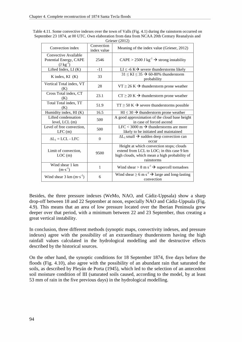
Chapter 4. Complete recontruction of 1874 Santa Tecla floods
94
Table 4.11. Some convective indexes over the town of Valls (Fig. 4.1) during the rainstorm occurred on September 23 1874, at 00 UTC. Own elaboration from data from NCAA 20th Century Reanalysis and
Grieser (2012)
Convection index Convection index value
Meaning of the index value (Grieser, 2012)
Convective Available Potential Energy, CAPE
(J kg-1) 2546 CAPE > 2500 J kg-1 � strong instability
Lifted Index, LI (K) -11 LI ≤ -6 K� severe thunderstorms likely
K index, KI (K) 33 31 ≤ KI ≤ 35 � 60-80% thunderstorm
probability Vertical Total index, VT
(K) 28 VT ≥ 26 K � thunderstorm prone weather
Cross Total index, CT (K)
23.1 CT ≥ 20 K � thunderstorm prone weather
Total Total index, TT (K)
51.9 TT ≥ 50 K � severe thunderstorms possible
Humidity index, HI (K) 16.5 HI ≤ 30 � thunderstorm prone weather Lifted condensation
level, LCL (m) 500
A good approximation of the cloud base height in case of forced ascend
Level of free convection, LFC (m)
500 LFC < 3000 m � thunderstorms are more
likely to be initiated and maintained
ΔL1 = LCL - LFC 0 ΔL1 small � sudden deep convection can
occur
Limit of convection, LOC (m)
9500
Height at which convection stops; clouds extend from LCL to LOC; in this case 9 km
high clouds, which mean a high probability of rainstorms
Wind shear 1 km (m·s-1)
1 Wind shear > 8 m s-1 � supercell tornadoes
Wind shear 3 km (m·s-1) 6 Wind shear ≥ 6 m s-1
� large and long-lasting convection
Besides, the three pressure indexes (WeMo, NAO, and Cádiz-Uppsala) show a sharp drop-off between 18 and 22 September at noon, especially NAO and Cádiz-Uppsala (Fig. 4.9). This means that an area of low pressure located over the Iberian Peninsula grew deeper over that period, with a minimum between 22 and 23 September, thus creating a great vertical instability. In conclusion, three different methods (synoptic maps, convectivity indexes, and pressure indexes) agree with the possibility of an extraordinary thunderstorm having the high rainfall values calculated in the hydrological modelling and the destructive effects described by the historical sources. On the other hand, the synoptic conditions for 18 September 1874, five days before the floods (Fig. 4.10), also agree with the possibility of an abundant rain that saturated the soils, as described by Pleyán de Porta (1945), which led to the selection of an antecedent soil moisture condition of III (saturated soils caused, according to the model, by at least 53 mm of rain in the five previous days) in the hydrological modelling.

Chapter 4. Complete recontruction of 1874 Santa Tecla floods
95
Figure 4.9. Pressure indexes (surface pressure differences between two locations): WeMo (between Cádiz and Padua); NAO (between Cádiz and Reykjavík); and a zonal index (between Cádiz and Uppsala). Note:
measurements taken approximately at noon local time daily 4.4.5. General discussion To the best of our knowledge, this study is one of the first examples of a complete reconstruction of a flash flood from historical information: historiographical, hydraulic, hydrological and meteorological. Indeed, although historical floods reconstructions have increased in number in the last two decades, most of these limit to hydraulic modelling and only a few attempt some sort of hydrometeorological reconstruction (Benito et al., 2003; Delrieu et al., 2005; Bürger et al., 2006; Ducrocq et al., 2008; Millán et al., 2014). Besides, these combined hydraulic, hydrological and meteorological reconstructions of the event was not limited to one single location, but was done in ten different sites located in five catchments, in order to have an idea of the spatial distribution of the event. The 1874 Santa Tecla floods, which previously were a somewhat unknown and ignored set of records in regional historical flood compilations (Llasat et al., 2005; Barriendos and Rodrigo, 2006), reveal as a first order hydrological and meteorological event, with both great peak flows and destruction, which affected an area of 10000 km2.

Chapter 4. Complete recontruction of 1874 Santa Tecla floods
96
Figure 4.10. Synoptic conditions around midnight 18 September 1874, five days before Santa Tecla floods. Upper map: pressure at sea level (in Pa); middle map: air temperature (in K) at a height of 850 hPa (approx.
1500 m); bottom map: air temperature (in K) at a height of 500 hPa (approx. 5500 m). Source: NOAA’s 20th Century Reanalysis

Chapter 4. Complete recontruction of 1874 Santa Tecla floods
97
4.5. Conclusions The innovative interdisciplinary methodology used allowed us to achieve, from the historical information available, a complete reconstruction and, thus, a thorough understanding of 1874 Santa Tecla floods. These floods seem to be exceptional according to the results of the hydraulic and hydrological modeling and were indeed exceptional in terms of destruction. Although the return period is an improper concept for highly non-stationary variables as flood and rainfall frequency over long periods of time, we use it here to give an approximate, imperfect measure of the excepcionality of the 1874 event. Indeed, the peak flows and the rainfalls have all long return periods: around 260 years the former, and between 250 and 500 years the latter. This means that, accepting a 250 year return period, the probability of having an event of the same magnitude at least once in the next 50 years is 18% and in the next 100 years, 33%. Besides, floodplain occupation, and, thus, exposition to floods, has greatly increased since 1874; therefore, damages of Santa Tecla floods could be much greater nowadays. The exceptionality of the floods seems to be more a consequence of a reduction of permeability of the catchment caused by soil saturation due to rainfalls in the five previous days than of the magnitude of the rain the day of the floods. The information generated can be used to calculate return periods in the ungauged catchments to improve the hazard assessment of exceptional flood events. Indeed, since the synoptic situation and the ensuing meteorological processes that caused these floods have been determined, alert protocols could be prepared to early warn civil protection services in the occurrence of similar synoptic and hydrological circumstances. If these prevention measures were to be undertaken, the number of victims could be very much diminished if Santa Tecla floods occurred again. The peak flow estimation obtained in the hydraulic modelling was quite accurate. In contrast, the uncertainty of the hydrological modelling results was somewhat higher. Nevertheless, these results are still useful if taken as approximations. However, in both cases, the error values found were only lower bound estimations and further research must be done to improve error calculation with other sources of error (other input data) and in different types of catchment. Acknowledgements Known and unknown people of the past recorded and preserved valuable information of the floods that made this study possible. Xavier Castelltort, Rubén Remacha, Francesc Marsà (ACA), Mateu Esquerda, Ferran Riba, Adrià Marquilles and Roger Sosa (UdL) informed of ten of the twelve flood marks. Álvaro Tena and Damià Vericat (RIUS-UdL) and Carlos Astudillo (UdL) helped in the topographic survey of the flood marks. Topographic survey equipment was provided by RIUS-UdL Fluvial Dynamics Research Group. Joaquín Martín de Oliva, Sandra Guerrero and Albert Garcia (UdL) calculated four of the ten peak flows. Oriol Saula (Tàrrega County Museum) provided useful archaeological and historical information. José Antonio Martínez-Casasnovas drew the maps in Fig. 3.1. Ramon J. Batalla (RIUS-UdL) and Quim

Chapter 4. Complete recontruction of 1874 Santa Tecla floods
98
Farguell (ACA) helped complete 1946-2014 peak flow series of Francolí River in Montblanc. 20th Century Reanalysis V2 data provided by the NOAA/OAR/ESRL PSD, Boulder, Colorado, USA, from their Web site at http://www.esrl.noaa.gov/psd/. Support for the Twentieth Century Reanalysis Project dataset is provided by the U.S. Department of Energy. The editor Konstantine Georgakakos and two anonymous reviewers made suggestions that improved the text. The authors were financed by Spanish MINECO projects CGL2012-35071 and CGL2012-37416-C04-03, and by the INTERREG EU project FLUXPYR EFA 34/08. One of the authors has a pre--doctoral grant from the University of Lleida.

Chapter 5
Uncertainty of the peak flow reconstruction of the 1907 flood in the Ebro River in Xerta (NE Iberian Peninsula)
Ruiz-Bellet, J.L., Castelltort, X., Balasch, J.C., Tuset, J. (2015): Uncertainty of the peak flow reconstruction of the 1907 flood in the Ebro River in Xerta (NE Iberian Peninsula) Submitted to Journal of Hydrology (23/Jan/2016)


Chapter 5. Uncertainty of the peak flow reconstruction of 1907 flood
101
Abstract There is no clear, unified and accepted method to estimate the uncertainty of hydraulic modelling results. In historical floods reconstruction, due to the lower precision of input data, the magnitude of this uncertainty could reach a high value. With the objectives of giving an estimate of the peak flow error of a typical historical flood reconstruction with the model HEC-RAS and of providing a quick, simple uncertainty assessment that an end user could easily apply, the uncertainty of the reconstructed peak flow of a major flood in the Ebro River (NE Iberian Peninsula) was calculated with a set of local sensitivity analyses on six input variables. The peak flow total error was estimated at ±31% and water height was found to be the most influential variable on peak flow, followed by Manning’s n. However, the latter, due to its large uncertainty, was the greatest contributor to peak flow total error. Besides, the HEC-RAS resulting peak flow was compared to the ones obtained with the 2D model Iber and with Manning’s equation; all three methods gave similar peak flows. Manning’s equation gave almost the same result than HEC-RAS. The main conclusion is that, to ensure the lowest peak flow error, the reliability and precision of the flood mark should be thoroughly assessed. Keywords: error; sensitivity analysis; Manning’s roughness coefficient; DEM resolution; historical hydrology; hydraulic modelling; HEC-RAS; Iber 5.1. Introduction Information about long-past floods, either in the form of paleostage indicators (sedimentary evidence) or historical documents, has in the last few decades begun to be used to reconstruct peak flow values. This approach reveals fruitful because the longer the time period considered, the greater the probability to include floods of extreme magnitude, which greatly enrich the information contained within the flood data series. This relatively new branch of hydrology, subdivided in paleohydrology and historical hydrology (depending on the type of information used: paleostage indicators or historical documents) has suffered a great advance in the last decade (Bayliss and Reed, 2001; Benito et al., 2004; Gaume et al., 2004; Naulet et al., 2005; Brázdil et al., 2006; Elleder, 2010; Benito et al., 2015). Different aspects of paleo- and historical hydrology have been investigated so far: the improvement and systematization of historical information data bases, the use of dendrogeomorphic evidences (Ruiz-Villanueva et al., 2010), the link between meteorological, hydrological and hydraulic processes (Bürger et al., 2006; Pino et al., 2015), or flood frequency analysis (Francés, 2004; Payrastre et al., 2011; Machado et al., 2015). However, although one such important issue as the estimation of the uncertainty of the results of the hydraulic modelling has been deeply analysed (Pappenberger et al., 2005; Pappenberger et al., 2006; Lang et al., 2010; Neppel et al., 2010), no clear methodological procedures as to its determination have been formulated. As a consequence, only a few historical flood reconstructions try to give an estimation of the uncertainty of the results (Naulet et al., 2005; Remo & Pinter, 2007; Herget & Meurs, 2010).
Chapter 5. Uncertainty of the peak flow reconstruction of 1907 flood
102
And yet, uncertainty is an essential part of the result, an attribute of information (Zadeh, 2005). As Johnson (1996) points out, if uncertainties cannot be determined, the results are inaccurate. Similarly, Beven (2006) thinks that not to estimate the uncertainty of a model prediction is “simply indefensible (or unscientific)” because hydrology is a highly uncertain science. Actually, uncertainty in flow data is not negligible (Di Baldassarre & Montanari, 2009). Indeed, flow measurements with a current meter have errors between 5 and 20% (Pelletier, 1987; Léonard et al., 2000; Schmidt, 2002). Pappenberger et al. (2006) find that rating curve uncertainties cause an uncertainty of 18-25% in peak flow. Moreover, Lang et al. (2010) state that extreme flows uncertainties are larger than those of average flows. Thus, one should expect even larger uncertainties in historical hydrology reconstructions, where one has to model long-past extreme floods from a scarce set of data of sometimes unknown reliability, estimated rather than measured. Refsgaard et al. (2006) and Götzinger & Bardossy (2008) identify three main sources of uncertainty in hydraulic modelling results:
− Uncertainties in the observations measurement. Some of them are:
− Accuracy of the flood marks (Wohl, 1998).
− Channel geometry and stream slope (Jarret, 1987; Aronica et al. 1998; Pappenberger et al. 2005; Merwade et al., 2008).
− Viscosity of the fluid, affected by the amount of sediment load (Jarret, 1987).
− Changes in the river bed morphology, either during the flood or between the flood and the date of the study due to erosion and sedimentation (Jarret, 1987; Wohl, 1998; Lang et al., 2010).
− Representation of hydraulic structures such as bridges, culverts, and embankments (Merwade et al., 2008), their hydraulic behaviour and their being frequently blocked by debris and vegetation (Lang et al., 2010).
− Uncertainties in the parameters estimation, for example:
− Accuracy of the Manning’s n roughness coefficients (Jarret, 1987; Wohl,
1998).
− Changes in the downstream boundary condition due to a back-water effect or to a hydraulic jump (Lang et al., 2010).
− Expansion and contraction losses (Jarret, 1987).
− Uncertainty caused by end user’s decisions, the model structure (equations, hypotheses and assumptions), and the numerical methods used. Some of them are:

Chapter 5. Uncertainty of the peak flow reconstruction of 1907 flood
103
− Number of cross sections, that is, spacing between cross sections (Jarret, 1987; Merwade et al., 2008).
− Steady or unsteady flow (Jarret, 1987).
− One-dimensional or two-dimensional modelling (Cea & Bladé, 2008). Montanari (2007) distinguishes four types of techniques for assessing the uncertainty of hydrological modelling results; they can be also used in hydraulic modelling:
− Approximate analytical methods: e.g. first-order reliability method (FORM).
− Techniques based on the statistical analysis of model errors: e.g. Bayesian
Forecasting System (BFS).
− Approximate numerical methods, that is, sensitivity analyses: e.g. the Generalised Likelihood Uncertainty Estimation (GLUE) methodology of (Beven & Binley, 1992).
− Non-probabilistic methods: e.g. fuzzy set theory. In ungauged or scarcely gauged catchments (a frequent circumstance in historical hydrology), sensitivity analysis provides good uncertainty estimations (Montanari, 2007). Sensitivity is defined as a measure of the influence of the input variables on the result (McCuen, 1973). The existing types of sensitivity analysis have been reviewed by Van Griensven et al. (2006): the simplest of them is the local sensitivity analysis, in which each input variable of the model is separately modified at a time; another widely used type is the aforementioned GLUE methodology (Beven and Binley, 1992). Despite this profusion of methods and techniques, there is no unified procedure to guide hydrological and hydraulic modelling end users to easily quantify uncertainty (Pappenberger & Beven, 2006; Montanari, 2007; Merwade et al, 2008). Beven (2006) even wonders if these methods do not overestimate uncertainty. The main objective of this article was to calculate the uncertainty of the resulting peak flow of a typical historical flood reconstruction with a simple and quick procedure of uncertainty estimation, one that an end user could easily apply. The secondary objective was to identify the input variables that influenced the result the most and their contribution to peak flow total error. The ultimate goal behind this secondary objective was to formulate some recommendations as to the degree of accuracy that each input variable should have in order to minimize results’ uncertainty. In order to achieve these objectives, the uncertainty of 1907 flood of the Ebro River in the town of Xerta (NE Iberian Peninsula) was calculated with a series of local sensitivity analyses of the main variables affecting the resulting peak flow; it must be noted that uncertainties stemming from model structure or numerical resolution methods were not analysed in this study. Besides, in order to see to what degree the result depended on the chosen model, the HEC-RAS resulting peak flow was compared to the ones obtained with the 2D model Iber and with Manning’s equation.

Chapter 5. Uncertainty of the peak flow reconstruction of 1907 flood
104
5.2. Study area and study flood
The town of Xerta (1250 inhabitants in 2014) is located about 60 km upstream from the mouth of the Ebro River (Fig. 5.1). The Ebro River is one of the main rivers in the Iberian Peninsula. It drains into the Mediterranean Sea an area of 85,000 km2, including almost completely the southern face of the Pyrenees. Its mean flow in Tortosa (13 km downstream Xerta) is 428 m3·s-1 (Gallart & Llorens, 2004); since the average annual rainfall in the basin is 622 mm (period 1920-2000) and the basin area in Tortosa is 84,230 km2, the runoff coefficient in that location is 25.8%. The climate within the basin is varied, ranging from wet Oceanic (Köppen Cfb) in some Pyrenean valleys to dry Mediterranean (Köppen Csa) in the centre of the basin. Floods in the Ebro River, with peak flows as high as ten times the mean flow in Tortosa, are more frequent in autumn and are usually caused by the two main tributaries Cinca and Segre, with headwaters in the Pyrenees.
Figure 5.1. Location of the Ebro basin within Europe (a) and the Iberian Peninsula (b), and of the town of
Xerta within the Ebro basin (c). In (c), blue lines represent rivers and black lines represent sub-basins’ watersheds. Maps (a) and (b) modified from a map Copyright © 2009 National Geographic Society,
Washington, D.C.; map (c) drawn by Damià Vericat (RIUS-University of Lleida). By Xerta, on the Ebro River has a meandering pattern with an ample floodplain in the inner side; opposite Xerta, lies the town of Tivenys (Fig. 5.2). The Ebro basin in Xerta is 82,972 km2 or 97.6% of its total catchment surface. The nearest gauging station is that of Tortosa, operative since 1952; the highest instantaneous flow measured is 4580 m3·s-1, in

Chapter 5. Uncertainty of the peak flow reconstruction of 1907 flood
105
1961 (MAGRAMA, 2015). Xerta is a remarkable town in historical hydrology terms because it possesses a flood scale containing nine major floods since 1617 (Fig. 5.3), which have been hydraulically reconstructed by Sánchez (2007). The second highest of these floods, that of 21-23 October 1907, was selected to perform the uncertainty calculation for this study. This flood was caused by a rainfall episode that lasted three days and mainly affected the central Pyrenean area. The moderate rain depth fell on already saturated soils, because only ten days before (12-13 October), an almost equally destructive (albeit somewhat smaller) flood had occurred in the Pyrenean tributaries of the Ebro (Balasch et al., 2007). The 21-23 October flood was the largest one in the Ebro basin in the 20th Century and ravaged many towns; previous estimates of peak flows and descriptions of the impacts caused by this flood caused are shown in Table 5.1.
Figure 5.2. The towns of Xerta and Tivenys on either sides of a meander of the Ebro River. Adapted from
an aerial photograph of June 2014 (ICGC, 2015). Table 5.1. Previous estimates of peak flows of 1907 flood and descriptions of the damages that it caused in
different locations (see Fig. 5.1).
Town River Estimated peak flow Casualties and damages
Value (m3·s-1)
Source Count Source
Lleida Segre 5250(1) Balasch et al.,
2007 Bridge, embankment and 300-
400 dwellings destroyed Balasch et al.,
2007 Móra d’Ebre
Ebro 11200(1) Abellà, 2013 More than 50 buildings
destroyed Curto, 2007
Benifallet Ebro 11500(1) 10000(2)
Mérida, 2014 5 buildings destroyed Curto, 2007
Xerta Ebro 10500(1,3) Sánchez, 2007
2 buildings destroyed Curto, 2007
Tivenys Ebro 23 buildings destroyed
Tortosa Ebro 12000(4) López-Bustos,
1972 3 casualties and 7 buildings
destroyed Miravall, 1997;
Curto, 2007 (1) Calculated with the HEC-RAS model (one-dimensional). (2) Calculated with the Iber model (two-dimensional). (3) Recalculated in Section 5.4.1. (4) Estimated with unspecified methods.

Chapter 5. Uncertainty of the peak flow reconstruction of 1907 flood
106
This flood was selected because it is a good case study of a major flood in the Ebro basin on which to explore different types of uncertainties associated to large floods hydraulic modelling. Besides, within the historical period, 1907 is a relatively recent year and, therefore, the input data required can be more accurately estimated. The 1907 flood is one of the floods with more flood marks along the the Lower Ebro; it has been hydraulically modelled in different locations by Balasch et al. (2007), Sánchez (2007), Abellà (2013) and Mérida (2014). Besides, Pino et al. (2015) have included it in a comprehensive hydrometeorological analysis of 23 floods.
Figure 5.3. Flood scale on the façade of the Assumption Church at 1, Major Square in Xerta
(Photo by Alberto Sánchez) 5.3. Methods The process followed in this study had two parts (Fig. 5.4): On the one hand, the peak flow of 1907 flood in Xerta was estimated with three procedures: HEC-RAS (USACE, 2010a), Iber (Bladé et al., 2012), and Manning’s equation. On the other hand, the uncertainty of the peak flow obtained with HEC-RAS was assessed with sensitivity analyses. These analyses allowed us to determine the peak flow total error, the individual contribution of each tested input variable on that error and their individual influence on the peak flow value.
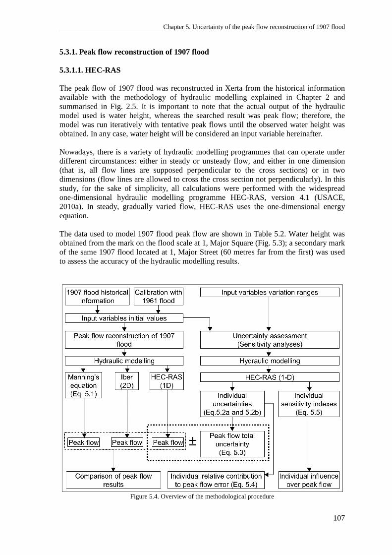
Chapter 5. Uncertainty of the peak flow reconstruction of 1907 flood
107
5.3.1. Peak flow reconstruction of 1907 flood 5.3.1.1. HEC-RAS The peak flow of 1907 flood was reconstructed in Xerta from the historical information available with the methodology of hydraulic modelling explained in Chapter 2 and summarised in Fig. 2.5. It is important to note that the actual output of the hydraulic model used is water height, whereas the searched result was peak flow; therefore, the model was run iteratively with tentative peak flows until the observed water height was obtained. In any case, water height will be considered an input variable hereinafter. Nowadays, there is a variety of hydraulic modelling programmes that can operate under different circumstances: either in steady or unsteady flow, and either in one dimension (that is, all flow lines are supposed perpendicular to the cross sections) or in two dimensions (flow lines are allowed to cross the cross section not perpendicularly). In this study, for the sake of simplicity, all calculations were performed with the widespread one-dimensional hydraulic modelling programme HEC-RAS, version 4.1 (USACE, 2010a). In steady, gradually varied flow, HEC-RAS uses the one-dimensional energy equation. The data used to model 1907 flood peak flow are shown in Table 5.2. Water height was obtained from the mark on the flood scale at 1, Major Square (Fig. 5.3); a secondary mark of the same 1907 flood located at 1, Major Street (60 metres far from the first) was used to assess the accuracy of the hydraulic modelling results.
Figure 5.4. Overview of the methodological procedure

Chapter 5. Uncertainty of the peak flow reconstruction of 1907 flood
108
The roughness coefficients (Manning’s n hereinafter) of nine different soil uses were calibrated with the 1961 (4 January) flood, of which there are a flood mark in Xerta’s flood scale and a peak flow official measurement. This peak flow value was 4580 m3·s-1
in Tortosa (MAGRAMA, 2015) and was accepted for Xerta due to the short distance between both towns (13 km) and to the small difference in catchment area (1.5%). Soil uses were determined from aerial photographs of 1957 (ICGC, 2015) and were considered unchanged between 1907 and 1961 (Fig. 5.6). Indeed, an aerial photograph of 1927 (not used because of its low resolution) showed no changes between that date and 1957. The modelled reach consisted of 45 cross sections along 7690 m, that is, with an average distance between cross sections of 170 m. However, this distance was much smaller around the flood scale cross section (Fig. 5.6). The geometry of the channel and the floodplain was obtained from a Digital Elevation Model (DEM) with a horizontal resolution of 5x5 developed from LiDAR information of 2009 (IGN, 2015). The geometry, thus, was that of 2009; it was not modified to represent those of 1907 and 1961 because it was deemed stable and, therefore, with minimal changes throughout the period. Table 5.2. Values of the input variables used in the peak flow reconstruction of 1907 flood with HEC-RAS
Input variable Value
1907 flood mark from flood scale at 1, Major Square, Xerta
X(1) 288,655 Y(1) 4,531,394
z (m a.s.l.) 15.175
1907 flood mark at 1, Major Street, Xerta X(1) 288,714 Y(1) 4,531,407
z (m a.s.l.) 15.325
1961 flood mark from flood scale at 1, Main Square, Xerta
X(1) 288,655 Y(1) 4,531,394
z (m a.s.l.) 12.171 1961 peak flow (m3·s-1); source MAGRAMA (2015) 4580
Manning’s n Calibrated with 1961 flood (See
Table 5.5) Length of the modelled reach (m) 7690
HEC-RAS specific
parameters
Number of cross sections 45 DEM resolution (m); source IGN (2015) 5x5
Boundary conditions Upstream Critical depth
Downstream Normal depth(2): 0.905 m·km-1 Contraction/expansion coefficients(3) 0.1/0.3
Type of flow Steady mixed (1) UTM coordinates: reference frame ETRS89, zone 31T (2) When “Normal depth” is chosen as the downstream boundary condition in the HEC-RAS, a water surface
slope is asked; for the sake of simplicity, we considered the water surface parallel to the channel’s bottom: 0.0905 m·m-1 is the slope of the channel.
(3) Default values used by HEC-RAS.

Chapter 5. Uncertainty of the peak flow reconstruction of 1907 flood
109
Figure 5.5. Soil uses determined from aerial photographs of 1957. (Source: ICGC,
2015)
Figure 5.6. Modelled reach with the cross sections (green lines), flow paths (blue lines) and the towns (red areas) of Xerta (left) and Tivenys (right), over an orthophotograph of ICGC (2015).

Chapter 5. Uncertainty of the peak flow reconstruction of 1907 flood
110
5.3.1.2. Iber In a one-dimensional model such as HEC-RAS, the flow is always assumed to be perpendicular to each cross section. However, in floods over large floodplains, this assumption is no longer true: eddies, lateral and upstream flows, and backwater areas are common. One way to take this into account is to draw the cross sections with angulated segments (Fig. 5.6) instead of with a single straight line, in order that they be as perpendicular to the flow in each segment as possible. However, this does not completely solve the problem of modelling floodplain flow with one-dimensional models. Thus, in the reconstruction of large floods that inundate wide floodplains with many obstacles such as buildings, 2D models, which allow for the horizontal component of the velocity vector, should provide a better estimation of the flow than 1D models (Paquier & Mignot, 2003; Cea & Bladé, 2008). The 2D model Iber version 2.3.1 (Bladé et al., 2012) was used to obtain an alternative peak flow value, so as to quantify the difference and improvement obtained over a 1D model such as HEC-RAS. In order to enable the comparison between the results, the input data used were the same as for the modelling with HEC-RAS, including the Manning’s n calibrated with HEC-RAS on 1961 flood, but excluding the specific parameters required in the 1D model (Table 5.2), and including others specific to Iber, such as the hydrograph shown in Table 5.3. Iber solves the 2D Saint Venant equations with the finite-volume method in unsteady flow.
Table 5.3. Hydrograph used in the hydraulic modelling with Iber Time (s) Flow (m3·s-1)
0 2000 7200 12500 14400 8000 28800 6000
5.3.1.3. Manning’s equation Hydraulic models, one- or two-dimensional, require some training and many data (namely, a Digital Elevation Model). Conversely, Manning’s equation is a much simpler method to obtain the peak flow from a water height value. Thus, it was considered interesting to compare the results of the two previously presented computer-based hydraulic models with the result of the Manning’s equation (Eq. 5.1) applied at the flood scale cross section. % = ' · $� · (� )* · +$ �* (5.1)
Where Q (m3·s-1): peak flow A (m2): wet area of the cross section at the moment of the peak flow n: Manning’s coefficient, related to the roughness of the cross section R (m): hydraulic ratio of the cross section (wet area divided by wet perimeter) at
the moment of the peak flow S (m·m-1): longitudinal slope of the channel at the cross section

Chapter 5. Uncertainty of the peak flow reconstruction of 1907 flood
111
Actually, the flood scale cross section was divided in three different ways and Manning’s equation was individually applied to each sector of each of the three methods of division; then, the peak flows of the individual sectors were added up. The three different resulting peak flows were averaged and compared to the ones obtained with HEC-RAS and Iber. The three ways in which the cross section was divided were:
− Division according to hydraulically homogeneous sectors: this resulted in five sectors (Fig. 5.7). Their characteristics, required to calculate Manning’s equation, are shown in Table 5.4.
− Division according to soil use, using the same soil use map as in HEC-RAS and Iber modelling: this resulted in 17 sectors (Fig. 5.7). Their individual hydraulic characteristics are not showed.
− Division according to HEC-Geo-RAS, a programme that links a Geographical Information System (GIS) programme with HEC-RAS. HEC-Geo-RAS described the cross section with the coordinates of 277 points, resulting in 276 sectors (Fig. 5.7); their individual hydraulic characteristics are not showed.
Figure 5.7. The flood scale cross section, with the three methods of dividing it: the five hydraulically
homogeneous sectors (labelled near the horizontal axis); the 17 sectors into which it was divided according to the soil use, each one with its Manning’s n value (above the cross section); the 276 sectors into which
HEC-Geo-RAS divided the cross section (limited by the 277 black rectangular dots over the line that outlines the cross section).

Chapter 5. Uncertainty of the peak flow reconstruction of 1907 flood
112
Table 5.4. The five hydraulically homogeneous sectors into which the flood scale cross section was divided in one of the three methods of division in order to apply the Manning’s equation, with their characteristics.
Sector Position in the x axis in Fig.
5.7 (m)
Wetted area (m2)
Wetted perimeter
(m)
Average Manning’s
n(1)
Longitudinal slope (m·km-1)
Left floodplain 4-412 2059 413 0.051 1 Channel 412-545 1386 135 0.041 1
Right floodplain
Not urban
545-707 736 132 0.047 1
Urban 707-1003 913 287 0.092 1 Not
urban 1003-1232
410 218 0.058 1
Total 4-1232 5504 1212 0.060 --- (1) Average Manning’s n weighted by wetted perimeter of each soil use in the flood scale cross section.
Manning’s n values calibrated with 1961 flood (Table 5.5). 5.3.2. Uncertainty assessment of HEC-RAS results The uncertainty assessment of the peak flow obtained with HEC-RAS was done with a set of sensitivity analyses, technically called local sensitivity analyses, because they were performed separately on each selected input variable. In these analyses each input variable was varied within a range that was chosen either because it was considered adequate or because it was found in the literature. In any case, with the objective to obtain an upper boundary of peak flow uncertainty, the ranges of variation were chosen rather large. The hydraulic model was then run with the modified value of the input variable in order to obtain a new peak flow output. This new peak flow value was used to calculate the individual uncertainty of that input variable, that is, the variation of the peak flow caused by the individually modified input variable with Eq. 5.2a when the variation was one-sided (i.e. only x+a or x-a) and with Eq. 5.2b when the variation was symmetrical (i.e. x±a). Then, these individual uncertainties were added with a quadratic sum in order to obtain the peak flow total error (Eq. 5.3). The relative contribution of each variable to the peak flow total error was quantified with Eq. 5.4. �, = -$ -
If variation of the variable is one-sided (only x+a or x-a)
(5.2a)
�, = ± /0-$ -1 + 0- -�12 / = ± 3-$ -�2 3 If variation of the variable is symmetrical (x±a)
(5.2b)
������ = ±4560�,1�7�,8$
(5.3)
9, = �,∑�, · 100 (5.4)

Chapter 5. Uncertainty of the peak flow reconstruction of 1907 flood
113
Where x: modified input variable in each individual sensitivity analysis n: number of modified input variables (or total sensitivity analyses) δx (m
3·s-1): individual uncertainty: variation of the peak flow caused by a variation in input variable x
δtotal (m3·s-1): total uncertainty of the peak flow
F (m3·s-1): peak flow obtained with the initial values of the input variable x F1 (m
3·s-1): peak flow obtained with the modified value of the input variable x: x+a
F2 (m3·s-1): peak flow obtained with the opposite modified value of the input
variable x, when a symmetrical variation (x±a) was done: x-a Cx (%): contribution of variable x to the total uncertainty of the peak flow Besides, the results of the sensitivity analyses were also used to calculate a sensitivity index Ix for each varied input variable in order to determine to what degree each one affected the resulting peak flow (Eq. 5.5; adapted from Lenhart et al. 2002). This dimensionless parameter allows the identification of the most influential variables, regardless of the range within they are varied (Lenhart et al. 2002). According to the value of Ix, Lenhart et al. (2002) arbitrarily classify the influence of the input variable over the results as small or negligible (|Ix|<0.05), medium (0.05≤ |Ix|< 0.02), high (0.02 ≤ |Ix|<1) or very high (|Ix| ≥1).
;, = -$ -�-$�<$ <�<$� (5.5)
Where Ix: sensitivity index of input variable x (dimensionless) F1 (m
3·s-1): resulting peak flow when input variable x equals x1 (x+a) F2 (m
3·s-1): resulting peak flow when input variable x equals x2 (x-a) F12 (m
3·s-1): resulting peak flow when input variable x equals x12 x12: mean of x1 and x2
Note: when the opposite modification of the input variable was not done (i.e. only x+a, instead of x±a), then F2=0, x2=0 and x12 is the initial value of variable x
The input variables upon which the sensitivity analyses were done were chosen from the list of the main factors affecting the uncertainty of hydraulic modelling results given in Section 5.1; these variables were: water height, Manning’s n, downstream boundary condition, number of cross sections, direction of the flow paths, and horizontal resolution of the DEM. In total, 6 input variables were modified resulting in 14 different sensitivity analyses. Details of these 14 analyses, along with their results, can be found in the paragraphs below and in Table 5.8. Other variables that could have had an influence on the peak flow results, such as variations of the channel’s geometry, the model structure or the numerical resolution methods, were not analysed, since the objective of the study was to perform a quick, simple uncertainty assessment. However, it must be noted that Refsgaard et al. (2006) argue that model structure is the main source of uncertainty in model predictions, especially when extrapolating.

Chapter 5. Uncertainty of the peak flow reconstruction of 1907 flood
114
Flood marks provide the maximum height that the water reached during a flood. Many sources of error can contribute to the inaccuracy of the mark: the oscillating nature of the water surface of a flood, the time elapsed between the flood and the making of the mark, or even the capillary ascension of the water along the wall. In this study, water height was subject to three levels of symmetrical modification for the sensitivity analyses: ±10 cm, ±30 cm, ±100 cm, in order to represent three degrees of uncertainty. Uncertainty of the maximum water height obtained from a flood mark can be subdivided into two components: precision and reliability. Precision is the accuracy of the measurement and reliability is the degree of truth that the flood mark has. Lang et al. (2010) estimate a precision of ±5 cm in water height measurements. Reliability can be affected by trivial but not so uncommon events such as inadvertently installing the flood mark plaque at a wrong height, either in a first moment, either after some restoration works (Benito et al., 2015); therefore, reliability must be assessed with historiographical methods that try to ascertain who, when, why and how marked the flood height (Bayliss & Reed, 2001; Barriendos & Coeur, 2004; Barnolas & Llasat, 2007). In other cases, the flood mark has no physical entity: it is not a plaque or a nick on a wall, but a written reference of a water height given in relation to a pre-existing object, such as a distinctive element in a bridge or a windowsill on a building’s façade; in these cases, it is precision that is affected, because it is an indirect measurement and, thus, less accurate than the direct one given by a physical flood mark. In this study, it was decided that uncertainties greater than ±1 m would be related to extremely unreliable or imprecise historical sources and, therefore, not used in flood hydraulic reconstruction. Marcus et al. (1992) found very high uncertainties for Manning’s n: they found that Chow’s (Chow, 1959) and Cowan’s (Cowan, 1956) visual methods underestimated Manning’s n from 28% up to 291% (141% in average) and from 21% up to 170% (100% in average), respectively. However, they tested these methods in conditions of extreme roughness: a steep glacier stream over coarse moraine sediment. Therefore, we chose a smaller range of variation for Manning’s n (±30%), which is in the upper region of the range of typical uncertainty estimated for this variable by Johnson (1996): ±8-35%, and similar to the sensitivity analyses performed by Wohl (1998) and Casas et al. (2004): ±25%, Di Baldassarre & Montanari (2009): +33%, and higher than those of De Roo et al. (1996) and Naulet et al. (2005): ±20%. Besides this modification of Manning’s n (±30%), we also tested the accuracy of a simpler, more straightforward estimation of the roughness coefficients versus the highly elaborate and time consuming calibration done with 1961 flood and a detailed soil use map. Thus, a sensitivity analysis was performed in which the Manning’s n of the channel was 0.045 and that of the floodplain was 0.056 regardless of the soil uses. These values were chosen because they are, in the case of the channel, the half-way point of the range given by Chow (1959) for this kind of river channel. In the case of the floodplain, Maaning’s n is the average of the ranges of the two prevailing soil uses (Fig. 5.5), namely crops and orchards, and vegetated floodplain (shrubs) (Table 5.5). This average was not weighted by area, since it is supposed to be obtained from a perfunctory soil use determination. Lang et al. (2004) suggest testing the influence on the peak flow result of different downstream boundary conditions and different hydrographs (under unsteady flow conditions), but they give no further instructions. This study was conducted with the normal depth chosen as the downstream boundary condition, because it is our usual

Chapter 5. Uncertainty of the peak flow reconstruction of 1907 flood
115
procedure when no water depth and no flow are known downstream the modelled reach. When normal depth is selected, HEC-RAS asks the user a water surface slope. For the sake of simplicity, we considered the water surface parallel to the channel’s bottom; therefore, 0.905 m·km-1, the longitudinal slope of the channel downstream the modelled reach, was introduced as the water surface slope (Table 5.2). The influence of the downstream boundary condition was assessed by varying this slope ±15%. With regards to decisions that depend on the modeller’s expertise, Paquier & Mignot (2003) stress the importance of correctly choosing the flow paths direction. Therefore, the influence of the drawing of the flow paths that HEC-RAS needs to operate, an arbitrary decision that depends on the expertise of the model user, was assessed. An initial, deemed more hydraulically correct, drawing located the flow paths over the floodplain in a more or less straight trajectory (Fig. 5.8a). A second drawing located the flow paths along the banks, following the meanders (Fig. 5.8b). The influence on peak flow of two more input variables was also assessed: the number of cross section (also a decision that depends on the modeller’s expertise) and the horizontal resolution of the Digital Elevation Model (DEM). To do so, the model was run, on the one hand, with half the initial number of cross sections (22) by simply erasing every second cross section upstream and downstream the flood scale cross section, and on the other hand, with a much coarser DEM: with an horizontal resolution of 25x25 m (IGN, 2015) instead of 5x5 m.
Figure 5.8. Two ways of drawing the flow path lines required in the HEC-RAS programme: (a) straight and
(b) meandering

Chapter 5. Uncertainty of the peak flow reconstruction of 1907 flood
116
5.4. Results and discussion 5.4.1. Manning’s n calibration with the 1961 flood The calibrated Manning’s n were within the ranges given by Chow (1959) and, except for two soil uses (vegetated floodplains and urban area), they were quite similar to those calibrated by Sánchez (2007) with the same flood in the same reach (Table 5.5). The greater difference with Sánchez was in the urban area: the high value we used accounts for the zigzagging trajectories that water has to follow when flowing through the town streets, which slow it down. These discrepancies, although important, fall within the range of uncertainties given by Marcus et al. (1992) for Manning’s n determination with Chow’s visual method (28-291%). Nonetheless, they illustrate the difficulty to objectively estimate the roughness coefficients, even when they can be calibrated with the same known flow. In any case, the positive differences in individual soil uses compensated almost completely the negative ones, as shown by the relative difference in the Manning’s n averaged by the area of each soil use within the flooded part of the modelled reach: -20%. The channel’s Manning’s n found is considerably higher than the ones calibrated in the same Ebro River with the same 1961 flood by Mérida (2014) in Benifallet (12 km upstream) and Abellà (2013) in Móra d’Ebre (40 km upstream Xerta): 0.024 and 0.028. Our higher value, as well as the one found by Sánchez (2007), can be explained by the extra roughness provided by the double meander on which Xerta lies (Fig. 8). Table 5.5. Manning’s n values calibrated with 1961 flood for the soil uses identified in Fig. 5.5, compared to those calibrated by Sánchez (2007) with the same flood and to the general values given by Chow (1959)
and Martín-Vide (2002)
Soil use
Area within the flooded part of the modelled reach (km2)
Manning’s n general values (Chow, 1959)
Manning’s n value calibrated with 1961 flood
This study Sánchez (2007)
Relative difference(1)
(%) Channel 1.28 0.031-0.100 0.041 0.038, 0.040 +3, +8 Canals 0.18 0.030 0.030 No data ---
Bare floodplain 0.30 0.030-0.050 0.048 No data --- Vegetated floodplain (shrubs)
0.46 0.045-0.100 0.060 0.100 -50
Riparian forest 0.01 0.080-0.160 0.085 0.100 -16 Crops and orchards
2.60 0.030-0.050 0.050 No data ---
Olive and almond trees
0.05 0.050-0.080 0.065 0.060 +8
Roads 0.06 0.016 0.050 No data --- Urban area 0.12 0.100(2) 0.100 0.030 +108
Total 5.06 --- 0.049(3) 0.060(3,4) -20 (1) Relative difference (Rd) calculated as: (= = �>?�@A>BA@@ · 100, where n1 is the Manning’s n used in this study
and n2 is the one used by Sánchez (2007). (2) Martín-Vide (2002); Chow (1959) provided no value for urban areas (3) Average Manning’s n weighted by area of each soil use within the flooded part of the modelled reach. (4) Urban area (streets) not taken into account because considered hydraulically ineffective.

Chapter 5. Uncertainty of the peak flow reconstruction of 1907 flood
117
5.4.2. Peak flow reconstruction 5.4.2.1. HEC-RAS The reconstructed peak flow of 1907 flood in Xerta was 11500 m3·s-1, which gave a modelled water height only 0.5 cm below the mark in the flood scale (Table 5.6). The goodness of this result is furthermore confirmed by the small difference between modelled water height and observed water height at Major Street’s flood mark: 0.5 cm. Besides, the resulting peak flow is close to (and, thus, coherent with) the ones calculated with HEC-RAS in Móra d’Ebre (40 km upstream) by Abellà (2013) and in Benifallet (12 km upstream) by Mérida (2014): 11200 and 11500 m3·s-1, and to the one estimated by López-Bustos (1972) in Tortosa (13 km downstream): 12000 m3·s-1 (Table 5.1); relative differences with our result are less than 3%, 0% and 4% , respectively. The difference with the peak flow calculated by Sánchez (2007) with HEC-RAS in Xerta (10500 m3·s-1) is a little bit greater: 9%. In any case, this amount of difference is acceptable in historical hydrology and smaller than the peak flow total error presented in Section 5.4.3 (±31%). Probably, the different peak flows are due, on the one hand, to the 20% difference in Manning’s n (Table 5.5) and, on the other hand, to the smaller cross section that Sánchez used in the town, caused by his decision to consider the whole urban area (not only the buildings, but also the streets) hydraulically ineffective, that is, to consider that water did not flow across that part of the section. This decision results in his effective cross section at the flood scale being 16% smaller than ours (4675 m2 and 5504 m2, respectively). These differences illustrate the relative insensitivity of hydraulic modelling results: the combined effect of a 20% increase in Manning’s and a 16% reduction in cross section area was only a 9% reduction in peak flow. Most likely, this insensitivity is caused by the fact that the reduction of cross section area affected a section were the flow was low, due to the low water stage and the high friction.
Table 5.6. Results of the hydraulic reconstruction of 1907 flood in Xerta
Variable Observed Modelled with a
peak flow of 11500 m3·s-1
Difference (cm)
Water height at Major Square’s flood scale (m)
15.175 15.17 -0.5
Water height at Major Street’s flood mark (m)
15.325 15.33 +0.5
5.4.2.2. Iber The value of the peak flow reconstructed with the two-dimensional hydraulic model Iber was 12000 m3·s-1, that is, 4% higher than the one reconstructed with the one-dimensional model HEC-RAS. This small difference, much smaller than the total error presented in Section 5.4.3, confirms the validity of the reconstructed peak flow. This coincidence of results contrasts with what Mérida (2014) finds in a similar comparison of the two models for the same 1907 flood in Benifallet (12 km upstream Xerta): 11300 m3·s-1 with HEC-RAS and 10000 m3·s-1 with Iber, or a difference of 12%. He also finds that Iber is much less sensitive to Manning’s n; however, he suspects that the low sensitivity of Iber’s results is due to the fact that the rating curve, required as a

Chapter 5. Uncertainty of the peak flow reconstruction of 1907 flood
118
boundary condition in Iber, is left unchanged. Our coinciding results also contrast with the accepted fact that 2D are more accurate than 1D models, especially in floods over large floodplains (Paquier & Mignot, 2003; Cea & Bladé, 2008). In any case, two-dimensional models will only yield more accurate results than one-dimensional ones if they are fed very detailed input data (Merwade et al., 2008). Certainly, Lang et al. (2004) obtain a larger peak flow error (40%) with a 2D model than with a 1D model in the Onyar River in Girona because parameter calibration is more difficult. Moreover, under conditions of abundance of data to perform a complete calibration, Horritt & Bates (2002) find that HEC-RAS results are as good as the 2D model TELEMAC-2D in a 60 km reach of the Severn River. Therefore, no clear conclusions about the superiority of 2D models with respect to 1D ones can be drawn. 5.4.2.3. Manning’s equation The three resulting peak flows using Manning’s equation in the three divisions on the flood scale cross section were: 11172, 11534 and 11759 m3·s-1 (Table 5.7). Their average was 11488 m3·s-1 and their standard deviation, ±296 m3·s-1 (±3%). This result coincides with the peak flow we calculated with HEC-RAS: relative differences are, respectively 3%, 0% and 2%.
Table 5.7. Results of the use of Manning’s equation at the flood scale cross section, depending on the number of sectors into which the cross section was divided
Method (Number of sectors into which the cross section was divided)
Sector Peak flow (m3·s-1)
5
Left floodplain 3744 Channel 5056
Right floodplain
Not urban 1353 Urban 677
Not urban 342 Total 11172
17 --- 11534 276 --- 11759
In conclusion, the calculation of the peak flow of 1907 flood in Xerta with Manning’s equation seems to produce acceptable results with an easier method than computer-based hydraulic models. However, the lack of a peak flow error makes it impossible to compare the accuracy of the three methods used: HEC-RAS, Iber and Manning’s equation. Certainly, if the total error of the peak flow calculated with Manning’s equation were too large, there would be no advantage in using that method. In any case, Harmel et al. (2006) report uncertainties in peak flow estimation with Manning’s equation from ±15%, in stable, uniform channels with an accurately estimated n, up to ±35%, in unstable, irregular channels, with poorly estimated n; these are totally acceptable peak flow errors. Herget et al. (2014) have reconstructed 15 peak flows in six locations with Manning’s equation, with results that underestimate the referential gauged values from 4% to 9% in ten cases and from 16% to 28% in the other five. This systematic underestimation of peak flow with Manning’s equation with respect to gauged values in large river floods contrasts with the frequent overestimation that Lumbroso &

Chapter 5. Uncertainty of the peak flow reconstruction of 1907 flood
119
Gaume (2012) observe, although, in their case, in flash floods; they also find much larger peak flow errors in flash floods hydraulic reconstruction (±50%), which they consider caused almost solely by errors in Manning’s n estimation when done by visual methods. Although a sensitivity analysis of Manning’s equation was not done, the three slightly different peak flows obtained with the three methods of dividing the cross section are a sign of the sensitivity of the results using Manning’s equation. For example, Herget & Meurs (2010) and Herget et al. (2015) find sensitivity indexes of the roughness coefficient between -0.9 and -1.1, slightly above the ones found with HEC-RAS in other studies (Table 5.10). 5.4.3. Uncertainty assessment of HEC-RAS results Table 5.8 shows the results of the 14 sensitivity analyses performed. According to the sensitivity indexes obtained, water height is the most influential input variable over peak flow. Manning’s n comes next, followed by the number of cross sections and the dostream boundary condition; the other two variables (flow paths direction and DEM resolution) have much less or no influence on peak flow results. Peak flow total error was calculated with Eq. 5.3. Actually, it was calculated combining different water height uncertainties with the fact of taking or not taking into account the error caused by the reduction of the number of cross sections (Table 5.9). In fact, it is very rare for a modeller to use too few cross sections, since there are clear recommendations about that and the HEC-RAS model displays alerts when this occurs; therefore, and considering that the flood scale is very precise and reliable, the total relative error of the reconstructed peak flow of 1907 flood in Xerta was 31%. But even if the flood mark were a lot less precise, the total error would not increase excessively: ±39%. These errors are comparable to that obtained for extreme floods by Naulet et al. (2005) in the Ardèche River: +40%, and to those that we estimated in Chapter 4 in six flash flood reconstructions: ±5-44%, and totally acceptable in historical hydrology. Indeed, Neppel et al. (2010) estimate that the uncertainty of the peak flows of extreme floods calculated with rating curves lies in the range of 10-100% and Cong and Xu (1987) consider that information about large floods is useful even with errors up to 60%. For comparison, Pelletier (1988) estimates the error of a good flow measurement at 5%.

Chapter 5. Uncertainty of the peak flow reconstruction of 1907 flood
120
Table 5.8. The 14 sensitivity analyses performed and their results Sensitivity analyses Influence on the peak flow
Number Modified input
variable Initial value
Modification of the initial
value
Resulting peak flow (m3·s-1)
Absolute individual
error (m3·s-1)
Relative individual
error (%)
Sensi-tivity index (Ix)
1
Water height 15.175 m a.s.l.
+10 cm 11750 ±275 ±2.4 +3.6
2 -10 cm 11200 3 +30 cm 12325
±838 ±7.3 +3.7 4 -30 cm 10650 5 +100 cm 14430
±2803 ±24.4 +3.7 6 -100 cm 8825 7
Manning’s n
A different one for each cross
section, according to soil uses (see Table
5.5)
+30% 8925 ±3500 ±30.4 -1.0
8 -30% 15925
9
Channel: 0.045 (+9%)
Floodplain: 0.056 (+7%) Average (1):
0.055 (+8%)
10225 -1275 -11 -1.4
10 Downstream
boundary condition:
normal height(2)
0.905 m·km-1 +15% 11880
±455 ±4.0 +0.3
11 -15% 10970
12 Number of cross
sections 45 22 14330 +2830 +25 +0.5
13 Flow paths
direction (Fig. 5.8)
Straight Meandering 11500 0 0 NA(3)
14 DEM resolution 5x5 25x25 11475 -25 -0.2 +0.01 (1) Average Manning’s n weighted by area of each soil use in the flooded part of the modelled reach. (2) When “Normal height” is chosen as the downstream boundary condition in the HEC-RAS, a water
surface slope is asked; for the sake of simplicity, we considered the water surface parallel to the channel’s bottom: 0.0905 m·m-1 is the slope of the channel downstream the modelled reach.
(3) NA: not applicable, because “straight” and “meandering” cannot be expressed in numbers to calculate Eq. 5.5.
Table 5.9. Peak flow total error (relative and absolute) and the relative contribution to it of the five variables
with a sensitivity index above zero, depending on the water height uncertainty considered and on the inclusion in the calculation or not of the error caused by the reduction of the number of cross sections
Error caused by the
reduction of the number of cross sections
Water height uncer-tainty
considered (cm)
Peak flow total
absolute error (1) (m3·s-1)
Peak flow total
relative error (1)
(%)
Relative contribution to the peak flow total error (1) (%)
Water height
Manning’s n
Down-stream
boundary condition
Number of cross sections
DEM reso-lution
Not included ±10 ±3540 ±31 6 82 11 NA(2) <1 ±30 ±3627 ±32 17 73 9 NA(2) <1 ±100 ±4507 ±39 41 52 7 NA(2) <1
Included ±10 ±4532 ±39 4 49 6 40 <1 ±30 ±4601 ±40 11 46 6 37 <1 ±100 ±5322 ±46 29 36 5 29 <1
(1) Calculations do not take into account the error found in sensitivity analysis 9, because it is included in the error found in sensitivity analysis 8 (see Section 5.4.3.2).
(2) NA: Not applicable, because the error caused by the reduction of the number of cross section is not taken into account
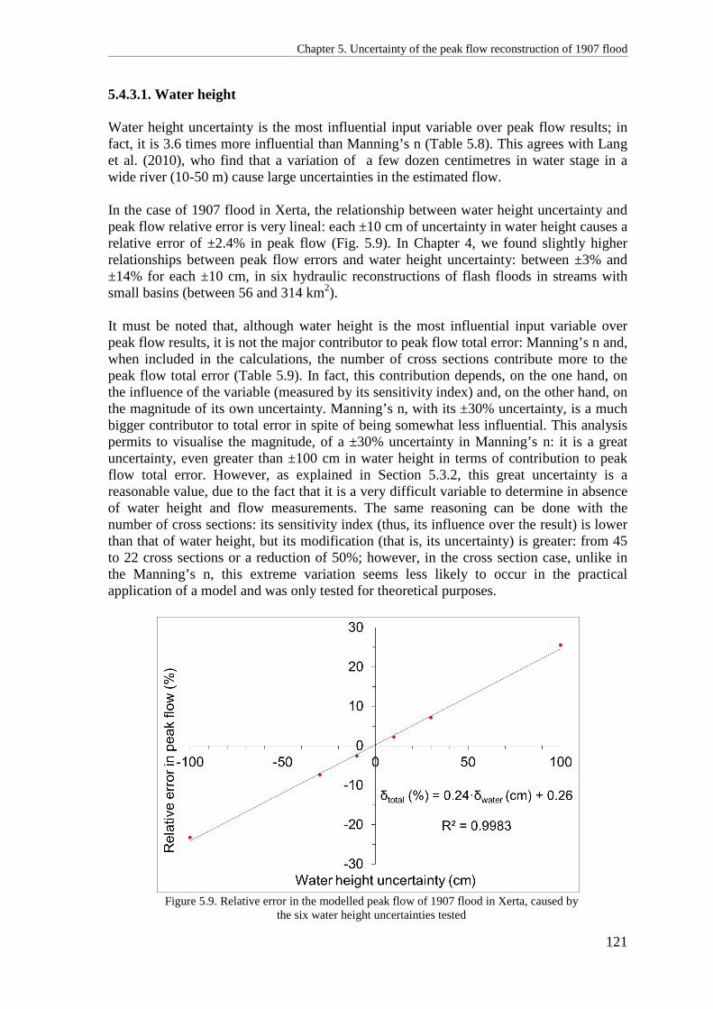
Chapter 5. Uncertainty of the peak flow reconstruction of 1907 flood
121
5.4.3.1. Water height Water height uncertainty is the most influential input variable over peak flow results; in fact, it is 3.6 times more influential than Manning’s n (Table 5.8). This agrees with Lang et al. (2010), who find that a variation of a few dozen centimetres in water stage in a wide river (10-50 m) cause large uncertainties in the estimated flow. In the case of 1907 flood in Xerta, the relationship between water height uncertainty and peak flow relative error is very lineal: each ±10 cm of uncertainty in water height causes a relative error of ±2.4% in peak flow (Fig. 5.9). In Chapter 4, we found slightly higher relationships between peak flow errors and water height uncertainty: between ±3% and ±14% for each ±10 cm, in six hydraulic reconstructions of flash floods in streams with small basins (between 56 and 314 km2). It must be noted that, although water height is the most influential input variable over peak flow results, it is not the major contributor to peak flow total error: Manning’s n and, when included in the calculations, the number of cross sections contribute more to the peak flow total error (Table 5.9). In fact, this contribution depends, on the one hand, on the influence of the variable (measured by its sensitivity index) and, on the other hand, on the magnitude of its own uncertainty. Manning’s n, with its ±30% uncertainty, is a much bigger contributor to total error in spite of being somewhat less influential. This analysis permits to visualise the magnitude, of a ±30% uncertainty in Manning’s n: it is a great uncertainty, even greater than ±100 cm in water height in terms of contribution to peak flow total error. However, as explained in Section 5.3.2, this great uncertainty is a reasonable value, due to the fact that it is a very difficult variable to determine in absence of water height and flow measurements. The same reasoning can be done with the number of cross sections: its sensitivity index (thus, its influence over the result) is lower than that of water height, but its modification (that is, its uncertainty) is greater: from 45 to 22 cross sections or a reduction of 50%; however, in the cross section case, unlike in the Manning’s n, this extreme variation seems less likely to occur in the practical application of a model and was only tested for theoretical purposes.
Figure 5.9. Relative error in the modelled peak flow of 1907 flood in Xerta, caused by
the six water height uncertainties tested

Chapter 5. Uncertainty of the peak flow reconstruction of 1907 flood
122
5.4.3.2. Manning’s n Manning’s n is the second most influential variable over peak flow results, with a sensitivity index of -1.0, classified as very high by Lenhart et al. (2002); in any case, it is similar or slightly higher than others found in the literature (Table 5.10). Manning’s n is, as said in Section 5.4.3.1., a major contributor to peak flow total error due to its high uncertainty. Certainly, an error of ±30% in determining Manning’s n, which is a relatively high but not uncommon value (as specified in Section 5.3.2), caused an error of ±30.4% in 1907 flood’s peak flow in Xerta. In our sensitivity analysis, we modified the Manning’s n of all the soil uses in all the cross sections exactly in the same amount and sign: either +30% or -30%. This kind of systematic error seems quite improbable. Rather, Manning’s n would be underestimated in some cross sections and overestimated in others within the modelled river reach, thus ones compensating others. Therefore, and taking also into account that ±30% is quite a relatively generous uncertainty for Manning’s n, our estimation seems to be an upper boundary of the uncertainty in the resulting peak flow caused by that input variable.
Wohl (1998) concludes that the influence of Manning’s n is greater in steep, narrow, and highly rough channels, than in flatter, wider, smoother ones. Wohl’s conclusion is in contradiction with Dawdy and Motayed (1979) and O’Connor and Webb (1988), who find that the Manning’s n has a small influence on peak flow results when using HEC-2, a precursor of HEC-RAS, in deep, narrow channels. Similarly, Chow (1959) states that Manning’s n influence is greater in low flows than in high flows; this concurs with the findings of Naulet et al. (2005): in their modelled reach of the Ardèche River, a change of ±20% in Manning’s n results in a change of ±20% in the peak flow of medium floods and of ±10% in large floods, this being explained by the reduced effect of roughness in flows with high depths. This conclusion also agrees with what we found in Chapter 3: for low flows, a decrease of 50% in Manning’s n causes no variation in peak flow, but a 10% increase in n causes a 7% decrease in peak flow, which is larger than the 1.5% caused by the same variation of n in high flows. Hall et al. (2005) find that the channel Manning’s n is the factor that influences the most the model’s results in a reach of the River Thames in the United Kingdom, but that floodplain Manning’s n gains importance in the wider parts of their modelled reach, where there is more out-of-bank flow. Similarly, Alemseged & Rientjes (2007) find that channel’s Manning’s n values affect more the resulting peak flow than floodplain values and Schumann et al. (2008) find that floodplain Manning’s n has no influence on hydraulic modelling results when varied between 0.04 and 0.1 in their modelled flood. In this study, the separate effects on the peak flow of the roughness of the channel and the floodplain were not assessed. However, when calibrating the Manning’s n with 1961 flood, channel’s roughness coefficient seemed to be more influential than those of the floodplain. Nevertheless, there was much less overbank flow in 1961 than in 1907 and, therefore, no conclusion can be drawn about which segment’s roughness (channel or floodplain) affects the most the peak flow of an extreme flood such as that of 1907. Casas et al. (2004) find that Manning’s n has a greater influence on the modelling results as the resolution of the DEM increases; in other words, a hydraulic model run on a coarse DEM is less sensible to uncertainties in Manning’s n than when run on a finer one. This
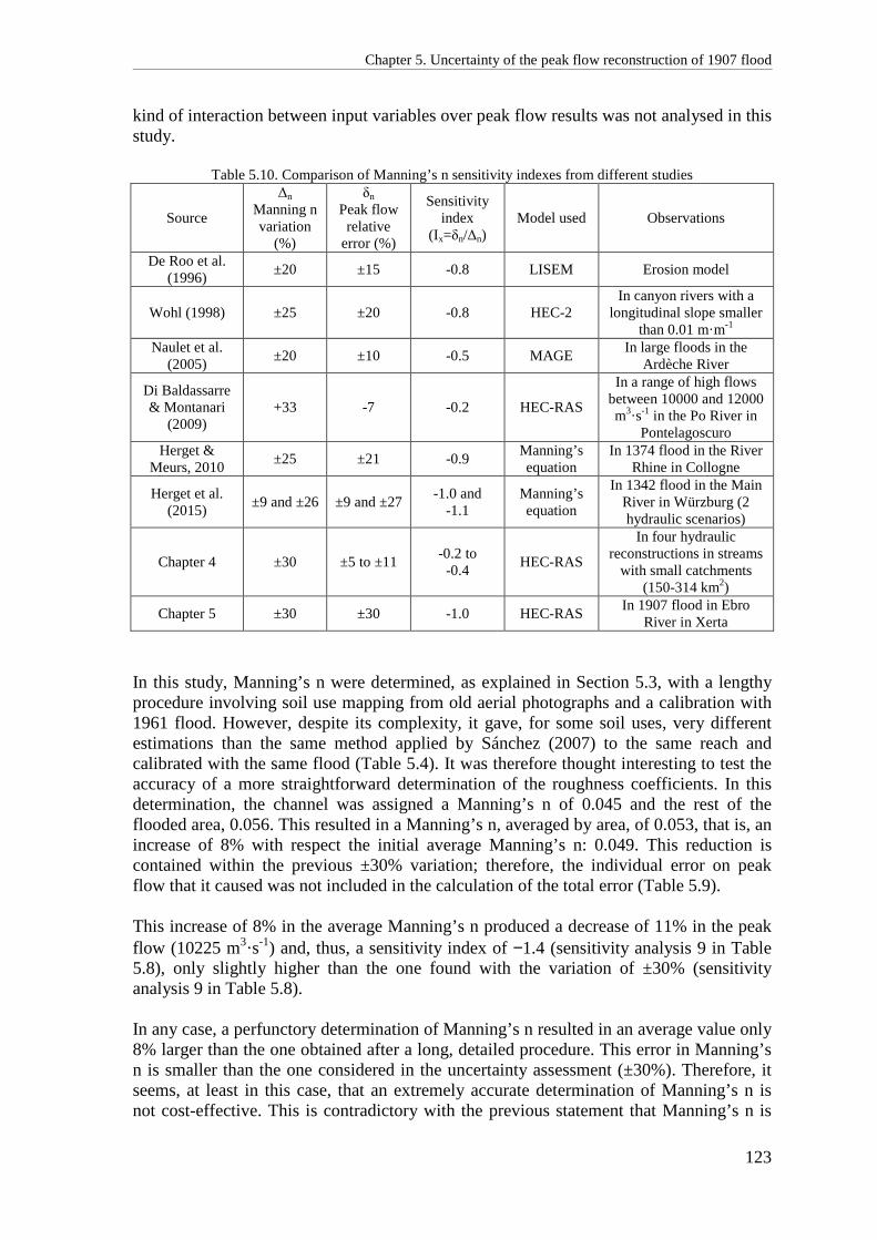
Chapter 5. Uncertainty of the peak flow reconstruction of 1907 flood
123
kind of interaction between input variables over peak flow results was not analysed in this study.
Table 5.10. Comparison of Manning’s n sensitivity indexes from different studies
Source
Δn Manning n variation
(%)
δn Peak flow relative
error (%)
Sensitivity index
(Ix=δn/Δn) Model used Observations
De Roo et al. (1996)
±20 ±15 -0.8 LISEM Erosion model
Wohl (1998) ±25 ±20 -0.8 HEC-2 In canyon rivers with a
longitudinal slope smaller than 0.01 m·m-1
Naulet et al. (2005)
±20 ±10 -0.5 MAGE In large floods in the
Ardèche River
Di Baldassarre & Montanari
(2009) +33 -7 -0.2 HEC-RAS
In a range of high flows between 10000 and 12000 m3·s-1 in the Po River in
Pontelagoscuro Herget &
Meurs, 2010 ±25 ±21 -0.9
Manning’s equation
In 1374 flood in the River Rhine in Collogne
Herget et al. (2015)
±9 and ±26 ±9 and ±27 -1.0 and
-1.1 Manning’s equation
In 1342 flood in the Main River in Würzburg (2 hydraulic scenarios)
Chapter 4 ±30 ±5 to ±11 -0.2 to -0.4
HEC-RAS
In four hydraulic reconstructions in streams
with small catchments (150-314 km2)
Chapter 5 ±30 ±30 -1.0 HEC-RAS In 1907 flood in Ebro
River in Xerta In this study, Manning’s n were determined, as explained in Section 5.3, with a lengthy procedure involving soil use mapping from old aerial photographs and a calibration with 1961 flood. However, despite its complexity, it gave, for some soil uses, very different estimations than the same method applied by Sánchez (2007) to the same reach and calibrated with the same flood (Table 5.4). It was therefore thought interesting to test the accuracy of a more straightforward determination of the roughness coefficients. In this determination, the channel was assigned a Manning’s n of 0.045 and the rest of the flooded area, 0.056. This resulted in a Manning’s n, averaged by area, of 0.053, that is, an increase of 8% with respect the initial average Manning’s n: 0.049. This reduction is contained within the previous ±30% variation; therefore, the individual error on peak flow that it caused was not included in the calculation of the total error (Table 5.9). This increase of 8% in the average Manning’s n produced a decrease of 11% in the peak flow (10225 m3·s-1) and, thus, a sensitivity index of −1.4 (sensitivity analysis 9 in Table 5.8), only slightly higher than the one found with the variation of ±30% (sensitivity analysis 9 in Table 5.8). In any case, a perfunctory determination of Manning’s n resulted in an average value only 8% larger than the one obtained after a long, detailed procedure. This error in Manning’s n is smaller than the one considered in the uncertainty assessment (±30%). Therefore, it seems, at least in this case, that an extremely accurate determination of Manning’s n is not cost-effective. This is contradictory with the previous statement that Manning’s n is
Chapter 5. Uncertainty of the peak flow reconstruction of 1907 flood
124
the second most influential variable over the results: if it is so influential, it should be accurately determined. Actually, if in a peak flow uncertainty assessment, the assigned uncertainty to Manning’s n is large (as it is advisable to do due to the difficulty in determining it), there is no need to accurately estimate it. A parallel with water height can help to explain this idea: to measure an unreliable flood mark to the µm would be a loss of time, because its uncertainty can be up to ±100 cm. 5.4.3.3. Downstream boundary condition Peak flow results are moderately sensitive to variations of the boundary condition set 2700 m downstream (sensitivity index of +0.3; Table 5.8). This contrasts with Alemseged & Rientjes (2007), who conclude that the effects of the boundary conditions are significant only near the downstream end of the river reach. However, Naulet et al. (2005) find, in a reach of the Ardèche River with a slope of less than 2.5 m·km-1 modelled with the MAGE hydraulic model, that a variation of ±1 m in the downstream condition has effects in the peak flow as far as 12 km upstream. 5.4.3.4. Number of cross sections When running the model with half the initial number of cross sections (22), the resulting peak flow was 25% higher than with all 45 cross sections. This variable has a relatively high sensitivity index (0.5). Due to the wide range of variation of its local sensitivity analysis (-50%), the number of cross sections has a high contribution to the peak flow total error (between 29% and 40%) if included in the calculation, which, as said in Section 5.4.3, does not seem necessary, because the HEC-RAS model has an automatic warning system that alerts when too few cross sections are being used. Alemseged & Rientjes (2007) find that different cross section spacing (2 to 20 m) results in different water surface profiles, only near the downstream end of the modelled river stretch. Cea & Bladé (2008) suggest placing the cross sections in representative spots within the modelled reach, spaced between 1 and 5 times the reach’s width. They warn against an excessive number of cross sections, since this could cause errors in the model’s iterative calculation process. The effect of an excessive number of cross sections and of their exact location along the reach has not been analysed in this study. 5.4.3.5. Flow paths The results show that, in the case of 1907 flood in Xerta, the direction and location of the flow paths has no influence on the peak flow results. 5.4.3.6. DEM horizontal resolution To use a lower resolution DEM (25x25 m instead of 5x5 m) resulted in a practically no change of the initially modelled peak flow: a reduction of 0.2%. Certainly, the influence of this variable on peak flow is very small: its sensitivity index is 0.01; and its relative contribution to total peak flow error is also reduced: less than 1%. These results seem to

Chapter 5. Uncertainty of the peak flow reconstruction of 1907 flood
125
agree with Horritt & Bates (2001), who find that, when modelling a flood of the River Severn with the 1D model LISFLOOD-FP and its NCFS version, a resolution of 500x500 m is adequate enough and resolutions finer than 100x100 m do not further improve the results. However, our results are in contradiction with various studies, which have shown that small errors in the topography can have significant effects on model results (Bates et al., 1997; Nicholas and Walling, 1998; Wilson, 2004) and with other studies that even conclude that the representation of the channel geometry seems to be the most influencing aspect of hydraulic modelling (Aronica et al. 1998; Pappenberger et al. 2005; Merwade et al., 2008). Similarly, Casas et al. (2004) conclude that a HEC-RAS model run on coarse-resolution DEM produces lower peak flows than when run on finer DEM, and that this difference is greater for low flows than for high flows. Alemseged & Rientjes (2007) also find, although in a two-dimensional model, that reducing the DEM resolution causes a reduction of water velocity (and, therefore, of peak flow). 5.4.3.7. Input variables not analysed The peak flow total errors shown in Table 5.9 include variables the error of which can be easily reduced, such as the drawing of flow paths, the number of cross sections and the resolution of the DEM. One could think that this gives an upper bound of the total uncertainty of the modelled peak flow. However, the set of sensitivity analyses performed is far from being exhaustive and other input variables not taken into account could increase that total error. The influence of those input variables was not quantified in this study because their analyses were deemed too difficult to be included in a basic uncertainty assessment intended for an end user, which was the main objective of this article. In any case, a short discussion of other studies’ findings is provided below. a) Channel’s erosion and accretion The erosion and accretion of the channel, either during the reconstructed flood or between the date of the flood and that of its reconstruction, can cause significant changes in the geometry than can ultimately translate into errors in the hydraulic modelling results. According to Kirby (1987), erosion is of extreme importance in modelling. Actually, Sauer & Meyer (1992) find that a mobile, unstable bed can cause an error of 10% in water stage measurement. Similarly, Naulet et al. (2005) find, in a modelled reach of the Ardèche River, that variations of -4/+2 m in the river bed height result in a variation of ±7% in peak flow for medium floods and of ±10% for extreme floods. However, in Chapter 3, we obtained the same peak flow when modelling a flash flood with two different channel geometries. b) Sediment transport Sediment transport, a factor rarely taken into account, can alter the hydraulic modelling results. In fact, according to Quick (1991), in floods with an important sediment transport, one third of the hydraulic energy is consumed in conveying the sediment and the other
Chapter 5. Uncertainty of the peak flow reconstruction of 1907 flood
126
two thirds in moving the water. Therefore, not taking into account sediment load tends to overestimate peak flow. But this overestimation can be even greater when hyper-concentrated flows occur, because then the fluid ceases to be Newtonian and the equations used by the model no longer apply. Although this is an infrequent circumstance in river flows such as 1907 in Xerta, it is not uncommon in flash floods in scarcely vegetated catchments: for example, Balasch et al. (2010a), report a sediment volume of 12% in one historical flood, which would qualify as a hyper-concentrated flow. c) Steady and unsteady flow One of these non-analysed input variables is the choice between steady and unsteady flow. In this study, the steady flow was used because it needs less information or, in the lack of it, less assumptions. However, steady flow is thought to overestimate the peak flow, since it does not allow for water storage over the floodplain. Actually, Naulet et al. (2005) find that the steady flow condition overestimates extreme floods’ peak flows by 2%, in a modelled reach of the Ardèche River; similarly, Tuset (2011) finds an overestimation of 8% in the reconstruction of a flash flood in a 220 km2 catchment. Besides, Bales & Wagner (2009) state that the effect on the results of modelling with a steady flow is greater for high flows than for low flows because water storage over the floodplain is greater. Nevertheless, this effect is diminished in floods with a prolonged, stable peak flow (that it, with a flat-summited hydrograph), virtually equivalent to a steady flow. In any case, choosing the unsteady flow option in the HEC-RAS model does not automatically reduce the uncertainty of the results. Indeed, the unsteady flow choice requires a hydrograph and Alemseged & Rientjes (2007) claim that the shape of that hydrograph affects the hydraulic modelling results, although not significantly. 5.5. Conclusions The peak flow of 1907 flood in the Ebro River in Xerta, reconstructed with HEC-RAS, was 11500 m3·s-1 and its total error was ±31-39%. However, actual total error could be greater because the uncertainty assessment did not include other possible sources of error, such as geometry modifications of the channel due to erosion and sedimentation or model structure. Anyway, the assessment procedure used proved to be a quick, simple one that obtained a rough but reliable estimate of peak flow error, similar to the values found in the literature. The most influential input variable over peak flow results was water height; however, the one that contributed the most to peak flow error was Manning’s n, because its uncertainty was far greater than water height’s. The drastic reduction of the number of cross sections resulted in a great variation of peak flow; however, since there are clear recommendations regarding the minimal number of cross sections needed in a modelled reach, such an extreme scenario seems improbable to occur. The other three analysed variables (downstream boundary condition, flow paths direction, DEM resolution) had far less influence on both the peak flow and its uncertainty.

Chapter 5. Uncertainty of the peak flow reconstruction of 1907 flood
127
A simple, straightforward method of determining Manning’s n provided roughness coefficients similar to the ones obtained with a more convoluted method that included a detailed soil uses mapping and a calibration with a known peak flow. In view of all this, it would be advisable, when attempting the hydraulic reconstruction of a historical flood, to soundly verify the reliability of the flood marks and, afterwards, to precisely measure them, since water height is the input variable that most influences the results. Conversely, Manning’s n estimation does not need to be extremely accurate, since the methods to do so are often subject to strong uncertainties; in other words, thorough estimations are not necessarily closer to the actual roughness coefficients values than more cursory ones. The quantification of the other tested variables does not need to be extremely precise either, since they have even less influence over the modelling results. In order to reduce the inherent uncertainty of a hydraulic reconstruction, several sensible steps should also be taken when possible:
1) To use more than one flood mark along the modelled river reach in order to obtain a more accurate water profile.
2) To assess the evolution of the river’s channel and flood plain morphology, in order to reduce the uncertainty contributed by this factor.
3) To calibrate the hydraulic model with measured flows of more modern extreme floods.
4) To reconstruct the flood in several locations throughout the basin in order to validate the results reciprocally through discharge continuity along the river.
As said above, the uncertainty assessment did not include all the variables that could affect the peak flow error. An improved uncertainty assessment with the objective of calculating the upper bound of the actual peak flow total error should include all the possible sources of error, as well as interactions between them (that is, the influence of simultaneous modifications of different variables). These interactions need to be analysed with a global sensitivity analysis instead of with a collection of local ones. In order to do so, and also in order to apply other uncertainty assessment procedures such as the GLUE (Beven & Binley, 1992), the introduction of input variables into the model should be automated, due to the high number of simulations needed. Nonetheless, a totally complete quantification of peak flow uncertainty seems very difficult. Indeed, the use of a hydraulic model implies a great number of small decisions that depend on the modeller’s expertise or, in other words, that convey a small amount of subjectivity. These decisions cannot be all taken into account in an uncertainty assessment, but can cause great differences between the results of two different modellers. Furthermore, a thorough comparison between 1D and 2D models could be done in order to determine if the more complex to operate two-dimensional programmes are actually more accurate while still being cost-effective when calculating peak flow in wide

Chapter 5. Uncertainty of the peak flow reconstruction of 1907 flood
128
floodplains with many obstacles to flow. Besides, more research is needed to ascertain if the channel’s Manning’s n is more influential on peak flow than the floodplain’s. The simple method of applying Manning’s equation at a single cross section seems to yield acceptable results, very similar to the one obtained with the HEC-RAS model. However, an uncertainty assessment is needed in order to compare their accuracy to that of computer-based methods. This study was limited to peak flow uncertainties; however, the uncertainties of other relevant hydraulic modelling results of interest in flood risk management, such as the flooded surface or the floodwave travel time, could also be assessed. Acknowledgements Damià Vericat drew the map in Fig. 5.1c. Alberto Sánchez measured the heights of the three flood marks used in this study and took the photo in Fig. 5.3. This study was funded by Project CGL2012-35071 of the Spanish Ministry of Economy. One of the authors has a pre-doctoral grant from the University of Lleida.

Chapter 6
Improvement of flood frequency analysis with historical information in different types of catchments and data
series within the Ebro River basin (NE Iberian Peninsula)
Ruiz-Bellet, J.L., Balasch, J.C., Tuset, J., Monserrate, A., Sánchez, A. (2015): Improvement of flood frequency analysis with historical information in different types of catchments and data series within the Ebro River basin (NE Iberian Peninsula). Zeitschrift für Geomorphologie, 59(3), 127-157. doi: http://dx.doi.org/10.1127/zfg_suppl/2015/S-59219 Published: 21 October 2015


Chapter 6. Flood frequency analysis with historical information
131
Abstract The use of historical information is acknowledged to improve frequency analysis. However, it is not well known if the degree of this improvement depends on the characteristics of both the catchment and the data series. In order to address this issue, frequency analyses with historical and systematic data were performed in three very different catchments: the Ondara River in Tàrrega, the Ebro River in Zaragoza and the Ebro River in Tortosa. Besides differences in their physical characteristics, these catchments differed also in their data series: their overall lengths and those of the historical and systematic periods. The results show that frequency analysis with historical information is extremely useful in ungauged catchments such as the Ondara River in Tàrrega, because the alternative (rainfall-runoff modelling) gives less accurate estimation of expected peak flows. However, in gauged catchments (Ebro River in Zaragoza and Ebro River in Tortosa), the degree of modification of peak flow estimates due to the use of historical data depends on the length of the historical period relative to the systematic record. Keywords: Systematic data, historical floods, peaks over-threshold, series stationarity 6.1. Introduction Flood frequency analysis is an essential issue in the study of flood hazards and planning as well as in civil engineering. Due to the low frequency of extreme floods and to the high return periods, the flood data sets from gauged records should be long enough to obtain reliable results. Ideally, a series should be much longer than the return periods calculated from it (Klemeš, 1986). Unfortunately, measured data series (also known as instrumental or systematic) are often less than 100 years long and they usually contain information gaps due to discontinuous measurements (e.g. during wars or gauge destruction by floods). In the worst cases, some river catchments may even lack any systematic records and, therefore, flood frequency is estimated by means of rainfall-runoff models which without gauging stations cannot be calibrated and validated leading to great uncertainty in the results. However, flow data series can be lengthened or reconstructed, in the case of ungauged catchments, with historical data. In terms of statistical analysis, Stedinger and Cohn (1986) indicated that 50 years of historical flood data provide as much information for frequency analysis as 10 to 30 years of systematic data. Unlike systematic data, historical flood data are not flow measurements. Actually, there are two types of historical flood information: (1) binomial data describing the occurrence of a flood above a certain threshold or not in a given year, and (2) estimated discharge data based on subsequent calculations with hydraulic models from the maximum water height reached by the flood recorded in documents or in epigraphic marks (Benito et al., 2004; Balasch et al., 2010a; Macdonald and Black, 2010). Due to its non-continuous nature (only the years with flows above a threshold are included) a historical data series is

Chapter 6. Flood frequency analysis with historical information
132
what is known as a non-systematic series, in contrast with a systematic series of measured data. In the last decade, there has been an effort to retrieve pre-instrumental hydrological information, both historical (from documents) and sedimentary evidence. As a result, several special issues have been published about this subject (Benito et al., 2005; Gregory et al., 2006; Brádzil and Kundzewicz, 2006). Indeed, nowadays, long flood chronologies have been restored in Europe (Glaser et al., 2010; Brádzil et al., 2006, 2012; Luterbacher et al., 2012) and in the Iberian Peninsula (Barriendos et al., 2003; Llasat et al., 2005; Barriendos and Rodrigo, 2006). However, the calculation of the peak flows for these chronologies is still scarce due to its complexity and to frequent changes in river channel topography since flood occurrence (Herget et al., 2014). In any case, there are some instances of peak flow reconstruction in long series of historical floods (over 400 years long), either referred to a single location (Thorndycraft et al., 2006; Balasch et al., 2007; Calenda et al., 2009; Elleder et al., 2013, 2010), or to several locations in the same catchment, which allow a spatial analysis of the flood dynamics (Benito et al., 2003; Naulet et al., 2005; Herget and Meurs, 2010; Balasch et al., 2010a; Roggenkamp and Herget, 2014). The use of historical data in flood frequency analysis requires a different treatment than other analyses based only on systematic, instrumental data. In fact, the special characteristics of this kind of information (being binomial or calculated, non-continuous, and sometimes less reliable and accurate) involves a higher number of steps for flood frequency analysis, including a test to check the authenticity and reliability of data, a test of stationarity and outliers, and selection of estimation methods and the distribution functions (Lang et al., 1999; Bayliss and Reed, 2001; Barriendos and Coeur, 2004; Francés, 2004; Renard et al., 2013). Another type of frequency analysis, with or without historical information can be implemented: the regional frequency analysis, which uses data from several locations within the same catchment (Hosking and Wallis, 1997; Wallis et al., 2007). More recently, this technique has been improved with the inclusion in the analysis of extraordinary flash floods reported in ungauged catchments within the same basin (Gaume et al., 2010; Nguyen et al., 2014). Despite the general agreement on the value of historical information for flood frequency analysis (Hosking and Wallis, 1986b; Stedinger and Cohn, 1986; Sutcliffe, 1987; Macdonald, 2004, 2013; Naulet et al., 2005; Payrastre et al., 2011), the gain of using such non-systematic information needs to be analysed in terms of the influence of characteristics of the catchment size and hydrological regime and of the flow data series (length, maximum measured flow). The question to answer is: do catchment and data series characteristics play a role in the degree of benefit obtained with the use of historical floods? Indeed, if the improvement provided by historical information depends on catchment and flood series characteristics, suggestions could be made in terms of where this extra effort would pay off and where it most probably would not be worth it. This paper aims (1) to quantify the improvement obtained in flood frequency estimation with the use of historical information in different catchments found within the Ebro River
Chapter 6. Flood frequency analysis with historical information
133
basin (NE Spain), and (2) to assess if this improvement depends on the catchment characteristics and type of flow series (historical, instrumental or both). 6.2. Study area The Ebro River is 930 km long and drains the north-eastern part of the Iberian Peninsula, which includes most of the southern side of the Pyrenees Range, into the Mediterranean Sea (Figure 1.a and 1.b). The Ebro River basin is a Cenozoic foreland basin with a NW-SE orientation and a triangular shape covering an area of 85,000 km2. The basin is limited by the Pyrenees to the north, the Iberian Range to the south, and the Catalan Pre-coastal Ranges to the south-east. The flood frequency analysis was carried out in three sites within the Ebro River basin: Ondara River in Tàrrega, Ebro River in Zaragoza, and Ebro River in Tortosa (Fig. 6.1.c). The annual average rainfall within the basin is 622 mm (period 1920-2000), with a strong altitudinal gradient: from over 2000 mm in the Pyrenees to less than 350 mm in the centre of the basin. Soil use changes and water use increases have severely reduced the annual runoff volume in Tortosa, near the mouth of the basin: from 18,500 hm3 yr-1 in the 1960s decade, to present values of 13,500 hm3 yr-1 or 428 m3·s-1 (Gallart and Llorens, 2004). During the 20th century, about 190 large reservoirs were constructed, mainly on the Pyrenean tributaries and on the lower Ebro River. The reservoir runoff index (calculated as reservoir capacity divided by mean annual runoff) is presently 57%, which causes a reduction of 25% in the expected peak flows of return period between 10 and 25 years (Batalla and Vericat, 2011). The Ebro River basin can be divided into three main sub-basins (Fig. 6.1.c):
− Upper Ebro: Encompasses the occidental area of the basin, from the headwaters to the city of Zaragoza. Its high flows are caused by spring thaw and winter and spring rainfalls linked to Atlantic fronts (Davy, 1975).
− Segre-Cinca sub-basin: The southern face of the eastern and central Pyrenees is drained by the two main tributaries of the Ebro: the Segre and Cinca Rivers. High flows are caused either by spring thaw or by heavy autumn rainstorms lasting several days.
− Medium and lower Ebro: from Zaragoza to the Mediterranean Sea. With the meagre runoff of streams from the eastern part of the Iberian Range and the southern part of the Catalan Pre-Coastal Ranges, extreme floods in this section of the Ebro River usually originate in the other two sub-basins.
The main characteristics of the three study sites (Zaragoza, Tortosa, and Tàrrega) are shown in Table 6.1. According to the aforementioned Ebro Basin division, Zaragoza is the outfall of the upper Ebro sub-basin, Tortosa is located in the lower Ebro sub-basin, only 40 km upstream the basin’s mouth in the Mediterranean, the area of the basin above this point being 99% of the total Ebro basin area. Zaragoza and Tortosa both have annual maximum instantaneous flow series that cover, respectively, the periods 1946-2012 and 1952-2012.

Chapter 6. Flood frequency analysis with historical information
134
Figure 6.1. Location of the Ebro River basin within Europe (a), and within the Iberian Peninsula (b), and location, within the Ebro basin (c), of the outfalls of the three studied catchments: Tàrrega by the Ondara River, Zaragoza by the Ebro River and Tortosa by the Ebro River. In (c), blue lines represent rivers and black lines represent sub-basins’ watersheds. Maps (a) and (b) modified from a map Copyright © 2009 National Geographic Society, Washington, D.C.; map (c) drawn by Damià Vericat (RIUS-University of
Lleida)
Table 6.1. Basic characteristics of the three studied catchments and their series of peak flows
Catchment Area (km2)
Main stream’s length (km)
Systematic series of peak flows(1) Non-systematic information
Gauging station code
Period
Length (years)
Mean flow
(m3·s-1)
Maximum measured peak flow (m3·s-1) (year of
occurrence)
Period
Length (years)
Number of floods with information
Ondara in Tàrrega
150 28.6 NA(2) NA(2) NA(2) 0.5(3) NA(2) 1615-2012
398 7
Ebro in Zaragoza
40,400 550 9011 1946-2012
67 230 4,150 (1961)
1643-1913
271 9
Ebro in Tortosa
84,200 890 9027 1952-2012
61 428 4,580 (1961)
1617-1951(4)
335(4) 8(4) (1) Available at MAGRAMA (n.d.) (2) NA: not applicable, because Ondara in Tàrrega is an ungauged catchment
(3) Modelled by CHE (1996) downstream Tàrrega
(4) Non-systematic series of Xerta, 13 km upstream Tortosa

Chapter 6. Flood frequency analysis with historical information
135
The third site is Tàrrega, on the Ondara River, a left-side tributary of the lower reach of the Segre River (Figure 1.c). The Ondara River is purely rain-fed and, with a continental Mediterranean and an annual mean rainfall of 450 mm, the mean annual flow estimated is 0.5 m3·s-1 (CHE, 1996), although most of it is seepage from agricultural irrigation. Floods in this catchment are typically flash floods caused by highly convective, autumn rainstorms. Unfortunately, there are no systematic flow measurements at Tàrrega and historical data are the only source of information. For the study sites, systematic data series can be complemented with historical flood information (or non-systematic series). There is information on seven floods since 1615 at Tàrrega, on nine floods since 1643 at Zaragoza, and on eight floods since 1617 at Tortosa. It must be noted that historical floods information at Tortosa is that of the town of Xerta, located 13 km upstream. 6.3. Methods The methodological procedure followed is schematized in Fig. 6.2.
Figure 6.2. Methodological procedure, with reference to the subsections that describe each part
Chapter 6. Flood frequency analysis with historical information
136
Two kinds of peak flow series were used:
1) Systematic series, made up of continuous records of annual maxima of instantaneous flow measurements (Qci).
2) Non-systematic series, with two types of data:
a) Annual maxima of instantaneous flow measurements (Qci) corresponding to isolated years (thus not being part of the continuous systematic series) which exceed a certain threshold (only in the case of Tortosa).
b) Reconstructed peak flows of extreme historical floods, either calculated with a hydraulic model from flood marks as explained in Chapter 3, or found in the literature: 1906 and 1907 floods in Zaragoza, reconstructed by López-Bustos (1972).
The difference between a systematic and a non-systematic series is the kind of data they contain: a systematic series is a continuous list of years, each with the value of the annual maximum instantaneous flow (Qci). A non-systematic series consists of peak flow values that exceeded a certain threshold that made them noticeable enough to be recorded, namely above a censoring threshold. The Ondara River in Tàrrega has only non-systematic data, since it is an ungauged catchment, whereas the sites on the Ebro River in Zaragoza and Tortosa have a systematic and a non-systematic series. The flood frequency analyses were performed on three combinations of the systematic and non-systematic series: (a) systematic series only; (b) combined series of systematic and non-systematic data; and (c) peaks over-threshold series, containing all the data of the combined series that exceeded a certain threshold, which was chosen to match the censoring threshold of the non-systematic series. 6.3.1. Systematic series The systematic series of annual maximum instantaneous flows (Qci) of the Ebro River contain 67 years for the Zaragoza gauge (1946-2012) and 61 years for the Tortosa gauge (1952-2012). However, in the case of Zaragoza, the record was extended between 1914 to 1945 from the series of annual maximum daily flows (Qc). First, a relationship between Qci and Qc was obtained with a linear regression between pairs of data (Qc, Qci) for those years with both kinds of data occurring in the same day. Then, the equation found with the regression was used to calculate the Qci of those years with only Qc available. This method was also applied to the Qc series of Tortosa for the years 1913 to 1935. However, since in this case the Qc series has a huge gap between 1936 and 1951, the obtained Qci, corresponding to the period 1913-1935, could not be added to the systematic series. Nevertheless, the data that exceeded the censoring threshold were added to the non-systematic series.

Chapter 6. Flood frequency analysis with historical information
137
6.3.2. Non-systematic series The non-systematic series consisted of discharges over-threshold data from both measurements done in isolated years (and thus not in continuity with the systematic series; only in the case of Tortosa) and peak flows estimated from flood marks and historical documents. On the one hand, Tortosa’s peak flow measurements of isolated years were obtained by applying the Qc-Qci method described in Section 3.1 on the Qc series for the years 1913 to 1935. The obtained Qci exceeding the censoring threshold were added to the non-systematic series. On the other hand, the reconstructed peak flows were calculated from the list of flood marks shown in Table 6.2. The reliability of all the flood marks is the highest of the three-degree scale by Bayliss and Reed (2001) because all the floods they relate to are well known. The precision of a flood mark (the maximum expected difference between the flood mark and the actual maximum water height) is determined by its nature and its reliability; since in this case all marks are very reliable, precision depends solely on its nature: physical marks (plaques, incisions and flood scales) and accuracy of written documents. These descriptions may be very detailed if they refer to particular elements (such as the iron ring on the first pillar of Bridge “Puente de Piedra” in Zaragoza) or newspaper photographs, or, in other instances, they may be less accurate if they refer to general elements (e.g. streets or buildings, Figs. 3.4 and 5.3). The flood marks were used to reconstruct their associated peak flows with the procedure summarized in Fig. 2.5 and described in detail in Section 2.6.1. The modelling software used was the one-dimensional hydraulic HEC-RAS 4.1 (USACE, 2010a), under gradually varied, steady, mixed flow. The input data used are shown in Table 6.3. The hydraulic model of Tàrrega was calibrated in two ways:
a) By comparing 1989 flood modelled peak flow with the peak flow calculated with a hydrological model (HEC-HMS 4.0; USACE, 2013) from rainfall data.
b) By adjusting the water line to the three different flood marks available for the
1874 flood.
The hydraulic models of Zaragoza and Tortosa were both calibrated by comparing the 1961 flood modelled peak flow with the actual measurement from the systematic series. Reconstructed peak flow uncertainties were calculated with a sensitivity analysis in which flood mark heights were modified within their ranges of precision (Table 6.2); other sources of error, such as roughness coefficients and the geometry of the channel, were not included in the calculation of peak flow uncertainty.

Chapter 6. Flood frequency analysis with historical information
138
Table 6.2. List of flood marks used in peak flow reconstruction
Catchment Flood year
Flood mark characteristics
Location UTM coordinates
(ETRS89) Type of mark
Relia-bility (1)
Preci-sion(2) (cm) Zone X (m) Y (m) Z (m)
Ondara in Tàrrega
1615 3, Font Street
31T
345,044 4,612,091 366.0 Written
reference(3) 3 ±30
1644 5, Sant Antoni
Square 344,978 4,612,055 368.39
Incision on a column
(Fig. 3.4a) 3 ±10
1783 13, Sant
Agustí Street 345,000 4,612,012 364.91
Plaque (Fig. 3.4b)
3 ±10
1842 32, Sant
Agustí Street 345,011 4,611,979 363.5
Written reference(4)
3 ±30
1874
8-10 bis, Piques Street
345,101 4,612,138 369.08 Plaque 3 ±10
6, Font Street 345,056 4,612,077 368.30 Plaque 3 ±10 26, Sant
Agustí Street 345,003 4,611,995 367.26
Plaque (Fig. 3.4d)
3 ±10
1930 25, Sant
Agustí Street 345,018 4,611,973 363.4 Written
reference(5) 3 ±30
1989 25, Sant
Agustí Street 345,023 4,311,963 363.3 Written
reference(6) 3 ±30
Ebro in Zaragoza
1643 Convento de Predicadores
30T
675,764 4,614,022 199.33 Written
reference(7) 3 ±50
1775 Puerta de Sancho
675,521 4,614,008 198.95 Written
reference(8) 3 ±50
1787 198.45 3 ±50
1871 Puente de
Piedra (first pillar from the
right bank)
676,869 4,613,798
195.93 Written
reference(9,10) 3 ±10
1874 195.15 Written
reference(9)
3 ±10 1878 194.59 3 ±10 1888 193.84 3 ±10
1961(11) 195.55 Plan(12) 3 ±10
Ebro in Tortosa
1617
Flood scale in Xerta
(1, Major Square)
31T 288,655 4,531,394
13.83
Flood scale (Fig. 5.3)
3 ±10 1787 16.15 3 ±10 1853 14.23 3 ±10 1866 14.03 3 ±10 1871 12.58 3 ±10 1884 13.41 3 ±10 1907 15.17 3 ±10 1937 14.67 3 ±10
1961(11) 12.17 3 ±10 (1) Reliability according to a scale by Bayliss and Reed (2001): 1 = unreliable, 2 = reliable, 3 = very
reliable (2) Precision: maximum expected difference in cm between the flood mark and the actual maximum water
height. Physical flood marks (plaques, incisions, flood scales) were given a precision of ±10 cm, whereas written references were given a precision of ±10, ±30 or ±50 cm depending on the possibility to precisely pinpoint the described object or place used as a reference of water height
(3) ACUR (1621) (4) Salvadó (1875) (5) Anonymous (1930) (6) Castellà and Miranda (1989) (7) Marcuello and Marcuello (1999) (8) Affidavit found in the City Archive of Zaragoza (9) Blasco-Ijazo (1959) (10) Galván et al. (2013) (11) Flood mark used to calibrate the hydraulic model (12) Plan of the bridge found in the archives of the department of urban planning of Zaragoza City Council

Chapter 6. Flood frequency analysis with historical information
139
Table 6.3. Input data used in peak flow reconstruction of historical floods
Catchment Length of the
modelled reach (km)
Number of cross-sections
Channel’s longitudinal
slope (m km-1)
Mean roughness
coefficients Ondara in Tàrrega
2.7 23 4.5 0.089(1) 0.070(2)
Ebro in Zaragoza
10.5 142 0.5 0.044
Ebro in Tortosa
4.0 65 0.24 0.053 (1) Valid for floods before 1874 (2) Valid for floods since 1874, due to a drastic change in channel morphology caused by
significant deposition of sediments during 1874 flood (see Chapter 3) It must be noted that the non-systematic series of Tortosa was built from flood marks of the near town of Xerta, located 13 km upstream. Peak flow values in Xerta were considered equal to those in Tortosa assuming a minimum error due to the closeness of the two sites (the catchment in Tortosa is only 0.18% larger than in Xerta); in other words, Xerta peak flows were not routed downstream to Tortosa. Two reconstructed peak flows found in López-Bustos (1972) could have been added to complete the non-systematic series in Zaragoza: the 1906 flood (3030 m3·s-1) and 1907 flood (1700 m3·s-1); however, both floods didn’t exceed the censoring thresholds and they weren’t finally added. 6.3.3 Peaks over-threshold series Once the non-systematic series were obtained, one “peaks over-threshold” series per catchment was built. These series contained all the data (whether systematic or non-systematic) with a value above a certain threshold. The thresholds chosen correspond to the overbank flow that produces damage: (1) Tàrrega: 210 m3·s-1; (2) Zaragoza: 3500 m3·s-1; (3) Tortosa: 4500 m3·s-1. These “peaks over-threshold” series were tested for stationarity with the test proposed by Lang et al. (1999). This test plots the confidence interval that marks the frontiers between stationarity and non-stationarity. This confidence interval depends on the Type I error (the risk of not accepting as stationary a stationary flood series), on the length of the tested period of the series, and on the number of floods that exceeded a certain threshold in that period. The Type I error (or alpha) quantifies the percentage of a set of randomly generated stationary flood series that would fall outside the limits of the confidence interval; then, the higher the Type I error, the more strict the test is, and the more sure one can be of the stationarity of a series. In our case, we chose a Type I error of 5%. 6.3.4. Frequency analysis The objective of flood frequency analysis is to estimate the annual exceedance probability of a certain flow, that is, the probability that this flow value be exceeded in a given year; the inverse of this probability is the return period (expressed in years).

Chapter 6. Flood frequency analysis with historical information
140
Different frequency analyses were performed with three types of peak flow series: a) The systematic series (where available, that is, only in Zaragoza and Tortosa).
b) The combined systematic and non-systematic series, with all the data (again, only
in Zaragoza and Tortosa).
c) The peaks over-threshold series, with the systematic and non-systematic data that exceeded a threshold (in Tàrrega, Zaragoza and Tortosa).
The first two types of series were analysed with AFINS 2.0 (GIMHA, 2014), a programme that allows calculations with systematic and combined series. Three probability functions were fitted to these two different kinds of series with the maximum likelihood method; these functions were: Gumbel (Eq. 6.1; Gumbel, 1941), TCEV (Two Component Extreme Value) (Eq. 6.2; Rossi et al., 1984), and SQRT-ETmax (Eq. 6.3; Etoh et al., 1986; Zorraquino 2004)). C0% > %∗1 = 1 FG?H·�0IJ·K∗1L (6.1)
C0% > %∗1 = 1 FG?M>·�0IJ>·K∗1?M@·�0IJ@·K∗1L (6.2)
C0% > %∗1 = 1 FN?O·P$QRH·�∗S·�TIRU·K∗VW (6.3)
where P(Q>Q*) = annual exceedance probability (in parts per one) of a certain peak
flow (Q*) Q* = peak flow (m3·s-1) α, λ, λ1, λ2, θ1, θ2, and κ are parameters to be estimated. These functions were fitted separately to the systematic data only, on the one hand, and to all the data, including the non-systematic, on the other. The censoring thresholds (3500 m3·s-1 and 4500 m3·s-1 for Zaragoza and Tortosa respectively) were introduced in the programme as upper bounds for the non-systematic period. This kind of frequency analysis was not possible for Tàrrega data, because the software used can’t work with only non-systematic data. The third type of series −the peaks over-threshold series− was analysed by fitting (with the least squares method) an exponential equation (Eq. 6.4) to pairs of peak flow data and their observed annual exceedance probabilities.
P(Q>Q*) = b·exp (a·Q*) (6.4) where P(Q>Q*) = annual exceedance probability (in parts per one) of a certain peak
flow (Q*) Q* = peak flow (m3·s-1) a and b are parameters to be estimated.

Chapter 6. Flood frequency analysis with historical information
141
The quality of fit of all functions was assessed in three ways:
a) Visually with a graph, in which the observed annual exceedance probabilities of the data were calculated with Eq. 6.5 for over-threshold data and with Eq. 6.6 for under-threshold data (Bayliss and Reed, 2001).
b) With the Kolmogorov-Smirnov test, which compares the greatest residual
(difference in absolute value between observed exceedance probabilities and those estimated by the function) with a threshold value that marks the acceptance of the fit (Table 6.4). When only the systematic series was used to fit the functions, the observed annual exceedance probabilities to be used in this test were calculated with Eq. 5.7.
c) With the calculation of the mean square residuals.
X = Y Z[ + 1 2Z · [\ (6.5)
X = [\ + \ [\ · Y [ Z+ F + 1 2Z (6.6)
X = ] Z+ + 1 2Z (6.7)
where p = observed annual exceedance probability (in parts per one)
i = position of the flow value in a decreasing rearrangement of the combined series (between 1 and s+e’)
j = position of the flow value in a decreasing rearrangement of the systematic series (between 1 and s)
α = constant: in our case 0.44 (Cunnane, 1978) k = number of over-threshold flows in the series e’ = number of non-systematic data over threshold e = number of systematic data over threshold n = length of the combined series (years) s = length of the systematic series (years)
Finally, the best fitting functions to the three types of series were compared among them in order to assess whether the inclusion of non-systematic data improves the frequency analyses.
Table 6.4. Threshold value not to be exceeded in the Kolmogorov-Smirnov test for goodness of fit, for number of data (n) greater than 35 and several values of Type I error (or alpha); the greater the Type I error,
the more strict the test is. Source: Sachs (1984) Type I error (α) Threshold value
0.20 1.075·n-0.5 0.15 1.138·n-0.5 0.10 1.224·n-0.5 0.05 1.358·n-0.5 0.01 1.628·n-0.5 0.001 1.949·n-0.5

Chapter 6. Flood frequency analysis with historical information
142
6.4. Results 6.4.1. Systematic series The systematic series in Zaragoza was lengthened with the annual maximum instantaneous flow (Qci) of the years 1914-1942, 1944 and 1945, which were calculated from the annual maximum daily flow (Qc) and the Qc-Qci relationship of that gauge. This Qc-Qci relationship was calculated with fifty pairs of data of the period 1946-2012 (Fig. 6.3.a). The discharge of the 1943 flood could not be estimated from this relationship because only one month of Qc measurements was available on the record. In order not to leave a blank year and to obtain a continuous systematic series, an arbitrary annual maximum was assigned to this year. This arbitrary value was the average of the Qci measurements between 1946 and 2012 (1834 m3·s-1). This value is obviously untrue, but it served our purpose to have a continuous systematic series for the frequency analysis with the advantage that it didn’t significantly distort the final results. Both Qc-Qci relationships obtained in Zaragoza and Tortosa had a high correlation coefficient (98% and 97%; Fig. 6.3). 6.4.2. Non-systematic series The reconstructed peak flows of Tàrrega (see Chapter 3); Zaragoza (Monserrate, 2013) and Tortosa (Sánchez, 2007) are shown in Table 6.5. The Qc-Qci relationship was calculated with forty-four pairs of data of the period 1952-2012 (Fig. 6.3.b) and allowed the calculation of 22 Qci values of the period 1914-1935 in Tortosa. Only two (1916 and 1921) of these 22 calculated Qci exceeded the censoring threshold and could therefore be included in the non-systematic series of Tortosa, alongside the reconstructed peak flows of historically documented floods (Table 6.5). The 1617 flood in Tortosa was excluded from the non-systematic series with which to perform the frequency analysis because the inclusion of this flood made the over-threshold series non-stationary (see section 6.4.3). Similarly, two of the seven reconstructed peak flows in Zaragoza were not added to its non-systematic series because they were below the censoring threshold: the floods of years 1878 and 1888. For the same reason, the peak flows reconstructed by López-Bustos (1972) in Zaragoza years 1906 (3030 m3) and 1907 (1700 m3·s-1) were not added either. Thus, of the total nine floods since 1643 in Zaragoza, only five were selected for the non-systematic series to be used in the frequency analysis. The K index is used to compare peak flows between catchments of very different area (Francou and Rodier, 1967; Herschy, 2003; Eq. 3.3). The highest reconstructed peak flow in the Ondara River in Tàrrega has a K index of 5.2, similar to those of the highest measured flows of severe flash floods in Mediterranean catchments of the Iberian Peninsula and southern France (Fig. 6.4). Similarly, the highest peak flow reconstructed for the Ebro River in Tortosa has a K index of 3.9, which is at the same level of the highest measured flows in similar-sized catchments in Europe. Nevertheless, the K index

Chapter 6. Flood frequency analysis with historical information
143
of the highest reconstructed peak flow for the Ebro River in Zaragoza is somewhat lower: 3.3 (Fig. 6.5).
Figure 6.3. Relationship between annual maximum daily flow (Qc) and annual maximum instantaneous
flow (Qci) for fifty data pairs between 1946 and 2012 of the flow gauge 9011 in Zaragoza (a) and for forty-four data pairs between 1952 and 2012 of the flow gauge 9027 in Tortosa (b). Data source: MAGRAMA
(n.d.)

Chapter 6. Flood frequency analysis with historical information
144
Table 6.5. Non-systematic series of each of the three catchments, made up with peak flows reconstructed from flood marks and historical documents and with Qci data calculated with a Qc-Qci relationship from
measured Qc
Peak flow value characteristics
Ondara in Tàrrega (censoring threshold:
210 m3·s-1)
Ebro in Zaragoza (censoring threshold:
3500 m3·s-1)
Ebro in Tortosa (censoring threshold:
4500 m3·s-1) Year of the flood
Peak flow, Qci (m3·s-1)
Relative error(1)
(%)
Year of the flood
Peak flow, Qci (m3·s-1)
Relative error(1) (%)
Year of the flood
Peak flow, Qci (m3·s-1)
Relative error(1)
(%)
Reconstructed from flood marks and historical
documents
Over-threshold
1615 790 ±9 1643 5560 ±5 1617 7500(2) ±4 1644 1600 ±3 1775 5180 ±5 1787 12900 ±5 1783 490 ±3 1787 4600 ±5 1853 8250 ±5 1842 210 ±9 1871 4844 ±4 1866 7750 ±6 1874 1190 ±3 1874 3624 ±6 1871 5000 ±5 1930 280 ±9 --- --- --- 1884 6500 ±7 1989 260 ±9 --- --- --- 1907 10500(3) ±3 --- --- --- --- --- --- 1937 9250 ±4
Under threshold
--- --- --- 1878 2805(2) ±7 --- --- --- --- --- --- 1888 1965(2) ±10 --- --- ---
Calculated from
measured Qc
Over-threshold
--- --- --- --- --- --- 1916 4663 ---
--- --- --- --- --- --- 1921 5686 ---
(1) Peak flow’s relative error caused by flood mark’s uncertainty; it does not include other sources of error (2) Not used in the flood frequency analysis (3) In this chapter we used this peak flow instead of the one calculated in Chapter 5 (11500 m3·s-1), in order
that it be calculated with the same model (geometry, roughness coefficients, boundary conditions) than the other reconstructed peak flows of the historical series. In any case, as said in Chapter 5, this peak flow value is correct, too.
6.4.3. Peaks over-threshold series In Tàrrega, the non-systematic series and the peaks over-threshold series were the same. In Zaragoza, the over-threshold series was composed of five out of the seven reconstructed peak flows plus two systematic data: 1930 (3500 m3·s-1) and 1961 (4130 m3·s-1). In Tortosa, the over-threshold series was made up with all the non-systematic data plus one systematic data: 1961 (4580 m3·s-1). The data needed to perform the stationarity tests on the three over-threshold series are gathered in Table 6.6 and the results are shown in Figure 8. Tàrrega and Zaragoza series can be deemed stationary with a Type I error of 5% and with the thresholds given in Table 6.6, whereas Tortosa series is not stationary. However, it is stationary in the 1787-2012 period (i.e., leaving out 1617 flood): its confidence interval given by the green lines in Fig. 6.6.c.

Chapter 6. Flood frequency analysis with historical information
145
Figure 6.4. K index of the highest reconstructed peak flow in Tàrrega and those of the highest measured
flows of flash floods in Mediterranean catchments of the Iberian Peninsula and southern France between 10 K indexand 1000 km2. (Own elaboration with data from López-Bustos, 1981; Llasat, et al. 2003; Delrieu et
al., 2005; Nguyen et al., 2014)
Figure 6.5. K index of the highest reconstructed peak flows in Zaragoza and Tortosa and those of the
highest measured flows in similar-sized catchments in the Iberian Peninsula and Europe between 30,000 and 110,000 km2. (Own elaboration with data from López-Bustos, 1981 and Herschy, 2003)

Chapter 6. Flood frequency analysis with historical information
146
Table 6.6. Data required to perform the stationarity tests
Catchment Threshold
(m3 s1) Period
Series length (years)
Number of floods over threshold in the period
Total Of the
systematic series
Of the non-systematic
series Ondara in Tàrrega
210 1617-2012 396 7 NA(1) 7
Ebro in Zaragoza
3500 1643-2012 370 7 2 5
Ebro in Tortosa
4500 1617-2012(2) 396 11 1 10 1787-2012(2) 226 10 1 9
(1) NA: not applicable, because Ondara in Tàrrega is an ungauged catchment (2) Two different periods were tested
Figure 6.6. Stationarity tests (Lang et al. 1999) for the over-threshold series of Tàrrega (a), Zaragoza (b)
and Tortosa (c). Solid lines are the number of floods over threshold in the series and dashed lines are the 95% confidence interval (i.e. 5% of randomly generated stationary flood sequences would fall
outside the confidence interval); grey dotted lines in Tortosa are the same confidence interval but for a shorter period: 1787-2012 instead of 1617-2012

Chapter 6. Flood frequency analysis with historical information
147
A reason for the non-stationarity of the Tortosa series may be the fact that the peak flows of the four floods that occurred between 1643 and 1775 could not be reconstructed because they were not recorded as flood marks and, therefore, could not be added to the over-threshold series. If only one flood exceed the 4500 m3·s-1 threshold in that period (1617-1787), the whole series would qualify as stationary. As a result, Tàrrega and Zaragoza over-threshold series were valid for frequency analysis and Tortosa series was valid only if taken from 1787 onwards. 6.4.4. Frequency analysis Flood frequency analyses were performed on different subsets of the data gathered in (Tables A1, A2 and A3, see Appendix A). The results of these frequency analyses are shown in Table 6.7 and Figs. 6.7 and 6.8. In Tàrrega, the absence of systematic data prevented the use of the AFINS software for frequency analysis. In this case, only a simple exponential function could be fitted to the over-threshold non-systematic data. The fit was nonetheless very good, both visually (Fig. 6.8.a) and numerically: R2 = 0.9738 and maximum residual much smaller than the Kolmogorov-Smirnov threshold value for 20% of Type I error. The results obtained with the exponential function are far greater that the ones calculated by the hydraulic administration (ACA, 2007) from rainfall data and a hydrological model (Fig. 6.8.a). In fact, the expected peak flow doubles for the 100-year return period (Table 6.8) and triples for the 500-year return period (Table 6.9). In the case of Zaragoza, the functions which fitted best the systematic and combined series were Gumbel and TCEV, which almost overlapped (Table 6.7 and Fig. 6.8.a). In this case, the inclusion of over-threshold non-systematic data corresponding to historical floods did not improve the results: there was only a 3% decrease in the expected peak flows of 100 and 500-year return periods. These two functions also overlapped with the official calculations (Fig. 6.8.b). Anyhow, the function with the best fit on the highest flow values (over a return period of 50 years) was an exponential equation fitted to over-threshold data only, both visually (Fig. 6.8.b) and numerically (Table 6.7); i.e. smallest maximum residual and smallest mean square error. This equation coincided with the official estimations for the 100-year expected peak flow (Table 6.8); however, its estimate of the 500-year expected peak flow was 8.7% higher than the official one (Table 6.9). In Tortosa, a sharp change occurred in the TCEV function when the non-systematic data were included in the analysis (Fig. 6.7.b). This was the function best fitted to the combined series among Gumbel, TCEV and SQRT-ETmax (Table 6.7 and Fig. 6.7.b). However, the exponential equation was again in this case the best fitted of all to over-threshold data (with return periods from 20 years on): the maximum residual and the mean square error were much smaller than those of the other functions (Table 6.7 and Fig. 6.8.c). In Tortosa, the official calculation overlaps the exponential equation for return periods over 100 years; however, it seems to overestimate the peak flows below a return period of 100 years.

Chapter 6. Flood frequency analysis with historical information
148
Table 6.7. Parameters of the functions fitted to the three types of series and goodness of fit through Kolmogorov-Smirnov test (with Type I error or alpha = 20%) and mean square error
Catchment Series Function Parameters
Kolmogorov-Smirnov test Mean square error
Maximum residual
Threshold value for
α=0.2 Total
Over-threshold
data
Tàrrega Peaks over-threshold
Exponential a = -0.002 b = 0.0206 R2 = 0.9738
0.013 0.247 10-4 10-4
Zaragoza
Systematic
Gumbel α = 14.1125 λ = 0.00166
0.043 0.108 5·10-4 NA(1)
TCEV
θ1 = 10.8762 θ2 = 3.71636 λ1 = 0.00165 λ2 = 0.00182
0.049 0.108 5·10-4 NA(1)
SQRT-ETmax
κ = 61.3994 α = 0.02397
0.067 0.108 1.5·10-3 NA(1)
Combined
Gumbel α = 15.1436 λ = 0.00175
0.081 0.105 1.3·10-3 4·10-4
TCEV
θ1 = 11.1633 θ2 = 3.79247 λ1 = 0.00172 λ2 = 0.00182
0.081 0.105 1.3·10-3 4·10-4
SQRT-ETmax
κ = 76.1622 α = 0.02735
0.134 0.105 5.5·10-3 1.4·10-3
Peaks over-threshold
Exponential a = -0.001 b = 0.8209 R2 = 0.8768
0.007 0.247 10-5 10-5
Tortosa
Systematic
Gumbel α = 7.18641 λ = 0.00135
0.074 0.138 9·10-4 NA(1)
TCEV
θ1 = 7.72230 θ2 = 8.05031 λ1 = 0.00138 λ2 = 5.33320
0.070 0.138 1.1·10-3 NA(1)
SQRT-ETmax
κ = 19.4249 α = 0.01601
0.108 0.138 1.9·10-3 NA(1)
Combined
Gumbel α = 4.81202 λ = 0.00101
0.095 0.128 1.8·10-3 1.2·10-3
TCEV
θ1 = 7.92679 θ2 = 0.10973 λ1 = 0.00147 λ2 = 0.00025
0.087 0.128 1.2·10-3 10-4
SQRT-ETmax
κ = 14.2186 α = 0.01319
0.089 0.128 10-3 8·10-4
Peaks over-threshold
Exponential a = -0.0003 b = 0.1831 R2 = 0.974
0.008 0.215 2·10-5 2·10-5
(1) NA: not applicable

Chapter 6. Flood frequency analysis with historical information
149
Figure 6.7. Frequency analyses in Zaragoza (a) and Tortosa (b). Probability functions (Gumbel, TCEV and
SQRT-ETmax) fitted either to systematic or to all data

Chapter 6. Flood frequency analysis with historical information
150
Figure 6.8. Frequency analyses in Tàrrega (a), Zaragoza (b) and Tortosa (c). Probability functions fitted either to systematic, to all data, or to over-threshold data. Comparison with the hydraulic administration
calculations is provided.

Chapter 6. Flood frequency analysis with historical information
151
Table 6.8. Relative difference (in %) in the expected peak flow of 100-year return period when calculated from the series displayed at the left of the row instead of the series displayed at the top of the column. Over-threshold series used to fit an exponential equation, and systematic and combined series used to fit a TCEV
function
Catchment Tàrrega Zaragoza Tortosa
Series Over-
threshold Official
(1) System-
atic Combined
Over-threshold
Official (2)
System-atic
CombinedOver-
thresholdOfficial
(3)
Expected peak flow (m3·s-1)
461 224 4318 4201 4246 4246 4799 9571 9154 9277
Tàrrega
Non-systematic
461 --- 106 --- --- --- --- --- --- --- ---
Official(1) 224 -51 --- --- --- --- --- --- --- --- ---
Zaragoza
Systematic 4318 --- --- --- 2.8 1.7 1.7 --- --- --- --- Combined 4201 --- --- -2.7 --- -1.1 -1.1 --- --- --- ---
Over-threshold
4246 --- --- -1.7 1.1 --- 0.0 --- --- --- ---
Official(2) 4246 --- --- -1.7 1.1 0.0 --- --- --- --- ---
Tortosa
Systematic 4799 --- --- --- --- --- --- --- -50 -48 -48 Combined 9571 --- --- --- --- --- --- 99 --- 4.6 3.2
Over-threshold
9154 --- --- --- --- --- --- 91 -4.4 --- -1.3
Official(3) 9277 --- --- --- --- --- --- 93 -3.1 1.3 --- (1) Official expected peak flow calculated by the hydraulic administration with rainfall-runoff modelling
(ACA 2007) (2) Official expected peak flow calculated by the hydraulic administration with systematic data
(MAGRAMAn.d.) (3) Official expected peak flow calculated by the hydraulic administration with systematic and non-
systematic data (MAGRAMA n.d.) The observed probabilities of the data plotted in Figs. 6.7 and 6.8 and used in the assessment of the quality of fit of the functions were calculated with Eqs. 6.5, 6.6 and 6.7 and with the data gathered in Table 6.10. 6.5. Discussion In the Iberian Peninsula, the use of historical (non-systematic) information in flood frequency analysis is recommended by the Water Administration (Jiménez-Álvarez et al., 2012). Indeed, the lack of historical information can cause a severe underestimation of the expected peak flows of high return period. In general, the estimates of the 500-year expected peak flow using only systematic data are 5 to 10 times smaller than when historical information is included (Jiménez-Álvarez et al., 2012; Kjieldsen et al., 2014). In this study, the differences were not so great: 2.5 times in Tortosa and no difference in Zaragoza. But even in the case of Zaragoza, the inclusion of historical information may have the beneficial effect of reducing the uncertainty of expected peak flow estimates, as Neppel et al. (2010) point out. In the case of the ungauged catchment of Ondara River in Tàrrega, flood frequency analysis with historical information was very much improved because present-day calculation based on rainfall-runoff modelling seems to underestimate the expected peak flows.

Chapter 6. Flood frequency analysis with historical information
152
Table 6.9. Relative difference (in %) in the expected peak flow of 500-year return period when calculated from the series displayed at the left of the row instead of the series displayed at the top of the column. Over-threshold series used to fit an exponential equation, and systematic and combined series used to fit a TCEV
function
Catchment Tàrrega Zaragoza Tortosa
Series Over-
threshold Official
(1) System-
atic Combined
Over-threshold
Official (2)
System-atic
CombinedOver-
thresholdOfficial
(3)
Expected peak flow (m3·s-1)
1448 461 5281 5130 5596 5148 5964 16026 14115 14359
Tàrrega
Non-systematic
1448 --- 214 --- --- --- --- --- --- --- ---
Official(1) 461 -68 --- --- --- --- --- --- --- --- ---
Zaragoza
Systematic 5281 --- --- --- 2.9 -5.6 2.6 --- --- --- --- Combined 5130 --- --- -2.9 --- -8.3 -0.3 --- --- --- ---
Over-threshold
5596 --- --- 6.0 9.1 --- 8.7 --- --- --- ---
Official(2) 5148 --- --- -2.5 0.4 -8.0 --- --- --- --- ---
Tortosa
Systematic 5964 --- --- --- --- --- --- --- -63 -58 -58 Combined 16026 --- --- --- --- --- --- 169 --- 14 12
Over-threshold
14115 --- --- --- --- --- --- 137 -12 --- -1.7
Official(3) 14359 --- --- --- --- --- --- 141 -10 1.7 --- (1) Official expected peak flow calculated by the hydraulic administration with rainfall-runoff modelling
(ACA 2007) (2) Official expected peak flow calculated by the hydraulic administration with systematic data
(MAGRAMA n.d.) (3) Official expected peak flow calculated by the hydraulic administration with systematic and non-
systematic data (MAGRAMA n.d.)
Table 6.10. Values of the parameters used in Eqs. 5.5, 5.6 and 5.7
k, number of over-threshold
flows in the series
e’, number of non-
systematic data over threshold
e, number of
systematic data over threshold
n, length of the
combined series (years)
s, length of the
systematic series (years)
Tàrrega 7 7 NA(1) 398 NA(1) Zaragoza 7 5 2 370 99 Tortosa 10 9 1 226 61
(1) NA: Not applicable because Tàrrega has no systematic series The Spanish water administration has found that GEV (Generalized Extreme Value), with the probability weighted moments method (PWM), is the function that best fits both systematic and non-systematic series in most of the studied Iberian catchments (Jiménez-Álvarez et al., 2012). However, in small, steep catchments with severe convective rainstorms, such as the Mediterranean ones of eastern Iberian Peninsula, these same authors find that the function that best fits is the TCEV (Two-Component Extreme Value) with the maximum likelihood method (ML). We found that this function also fits to data of a larger, less reactive catchment such as Ebro River in Tortosa, this meaning that the

Chapter 6. Flood frequency analysis with historical information
153
series has two groups of data, each one fitted by one of the two components of the TCEV function. Indeed, in Tortosa, unlike in Zaragoza, it seems that the flow series is divided into two different populations: that of the higher peak flows (over the censoring threshold and over a return period of around 20 years) and that of the lower peak flows. This “dog leg” effect, pointed out by Potter (1958), Matalas (1975) and Francés (1998), leads to the better fit of the TCEV, which was especially designed for this circumstance and is more recommended in the Western Mediterranean area than other functions, traditionally used in frequency analysis, that can’t fit to two-population series, such as Gumbel and Log-Pearson III (Rossi et al., 1984; Francés, 2004). In the western Mediterranean region, the frequent existence of two different populations of peak flows within the same series has been linked to the type of rainstorm causing the flood. The frequent, low peak flows might be caused by rainfall from frontal systems, whereas infrequent, high peak flows might be caused by highly convective summer and autumn storms (Rossi et al., 1984). However, this hypothesis was not analysed in this paper and nothing can be said about it for the time being. Nonetheless, the presence of a “dog leg” effect in Tortosa and its absence in Zaragoza might be explained by differences in the data series. Whereas the Zaragoza series is longer in the overall and in the historical and systematic periods (Table 6.10), both series have the same historical/systematic ratio: 2.7 historical data per 1 systematic datum. On the other hand, they are very different when it comes to peaks over threshold per century (Table 6.6): this variable remains unchanged in Zaragoza (1.9 peaks/century in the historical period and 2.0 peaks/century in the systematic one), but shows a great decrease in Tortosa (5.5 peaks/century in the historical period and 1.6 peaks/century in the systematic one). Besides peaks over threshold frequency, there are differences in peak flow values: indeed, whereas in Zaragoza the highest peak flow is only 1.6 times higher than the threshold, in Tortosa the highest peak flow is 2.9 times higher than the threshold and there are two more peak flows more than double the threshold (Table 6.11). Similarly, in Zaragoza, the highest non-systematic peak flow is 1.3 times larger than the highest systematic peak flow, while in Tortosa, this ratio is 2.8.
Table 6.11. Peak flow/threshold ratio of the over threshold flows in Zaragoza and Tortosa Zaragoza (Threshold: 3500 m3·s-1) Tortosa (Threshold: 4500 m3·s-1)
Year Peak flow (m3·s-1)
Peak flow/threshold
Year Peak flow (m3·s-1)
Peak flow/threshold
1643 5560 1.6 1787 12900 2.9 1775 5180 1.5 1907 10500 2.3 1871 4844 1.4 1937 9250 2.1 1787 4600 1.3 1853 8250 1.8 1961 4130 1.2 1866 7750 1.7 1874 3624 1.0 1884 6500 1.4 1930 3537 1.0 1921 5686 1.3 --- --- --- 1871 5000 1.1 --- --- --- 1916 4663 1.0 --- --- --- 1961 4580 1.0

Chapter 6. Flood frequency analysis with historical information
154
However, the reason for these differences in both frequency and magnitude of over threshold peak flows is still unclear and more research is needed: it could have a climatic reason (if Zaragoza is more affected by floods flowing down from the Atlantic part of the catchment and Tortosa is more affected by floods flowing down the Pyrenees), an anthropogenic cause (changes in the catchment, such as land use or dam construction) or even other reasons uncertain so far. 6.6. Conclusions In the ungauged basins, such as the Ondara River in Tàrrega, flood frequency analysis with historical information was extremely useful because it seemingly gives better expected peak flow estimates than rainfall-runoff modelling. In the case of the Ebro River in Tortosa, the inclusion of historical information into systematic series resulted in a combined series with two populations of data that follow two different probability functions. In these cases, frequency analysis is greatly modified and improved with the use of historical information. Indeed, in Tortosa, the expected peak flow estimates of 100 and 500-year return period were 2 and 2.5 times higher, respectively, when including non-systematic data than when using only systematic data. This difference was not observed in Ebro River in Zaragoza, the series of which being composed of only one population of data. The existence of one population of data in Zaragoza and of two in Tortosa may have different explanations and more research is needed to ascertain which αis the correct one. In any case, this difference causes a difference between Zaragoza and Tortosa in terms of the benefits produced by the inclusion of historical information in frequency analysis. Therefore, although the use of historical information always pays off in terms of uncertainty reduction, the actual change in expected peak flow estimates might depend on the series characteristics, namely, the existence of two populations of peak flows, which ultimately depends on the hydrological and climatic characteristics of the catchment. Finally, although both in Zaragoza and Tortosa, the exponential equation fitted to the over-threshold series showed a better fit for return periods higher than 50 years than the functions fitted to the combined series (made up of all data, systematic and non-systematic), more research is needed to argue that using only over-threshold data can lead to more accurate expected peak flow estimates. For further research, these frequency analyses could be done including other types of data besides exact peak flows: values exceeding a threshold or values within a range. Moreover, peak flow errors, such as the one calculated in Chapter 5, should be included in the analyses. Finally, other probability functions of the GEV and GP families should also be used. Acknowledgements We want to thank Jürgen Herget (editor of the special issue) and the two reviewers (Gerardo Benito and an anonymous one), whose comments improved the text.
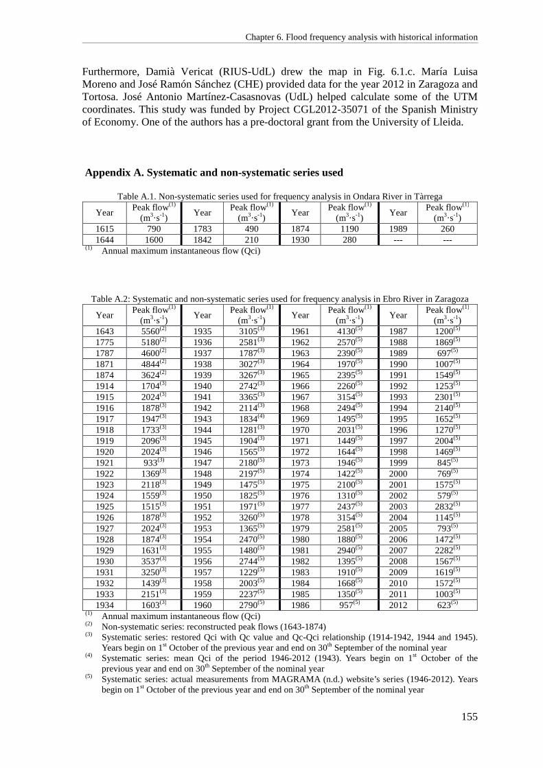
Chapter 6. Flood frequency analysis with historical information
155
Furthermore, Damià Vericat (RIUS-UdL) drew the map in Fig. 6.1.c. María Luisa Moreno and José Ramón Sánchez (CHE) provided data for the year 2012 in Zaragoza and Tortosa. José Antonio Martínez-Casasnovas (UdL) helped calculate some of the UTM coordinates. This study was funded by Project CGL2012-35071 of the Spanish Ministry of Economy. One of the authors has a pre-doctoral grant from the University of Lleida. Appendix A. Systematic and non-systematic series used
Table A.1. Non-systematic series used for frequency analysis in Ondara River in Tàrrega
Year Peak flow(1)
(m3·s-1) Year
Peak flow(1) (m3·s-1)
Year Peak flow(1)
(m3·s-1) Year
Peak flow(1) (m3·s-1)
1615 790 1783 490 1874 1190 1989 260 1644 1600 1842 210 1930 280 --- ---
(1) Annual maximum instantaneous flow (Qci)
Table A.2: Systematic and non-systematic series used for frequency analysis in Ebro River in Zaragoza
Year Peak flow(1)
(m3·s-1) Year
Peak flow(1) (m3·s-1)
Year Peak flow(1)
(m3·s-1) Year
Peak flow(1) (m3·s-1)
1643 5560(2) 1935 3105(3) 1961 4130(5) 1987 1200(5) 1775 5180(2) 1936 2581(3) 1962 2570(5) 1988 1869(5) 1787 4600(2) 1937 1787(3) 1963 2390(5) 1989 697(5) 1871 4844(2) 1938 3027(3) 1964 1970(5) 1990 1007(5) 1874 3624(2) 1939 3267(3) 1965 2395(5) 1991 1549(5) 1914 1704(3) 1940 2742(3) 1966 2260(5) 1992 1253(5) 1915 2024(3) 1941 3365(3) 1967 3154(5) 1993 2301(5) 1916 1878(3) 1942 2114(3) 1968 2494(5) 1994 2140(5) 1917 1947(3) 1943 1834(4) 1969 1495(5) 1995 1652(5) 1918 1733(3) 1944 1281(3) 1970 2031(5) 1996 1270(5) 1919 2096(3) 1945 1904(3) 1971 1449(5) 1997 2004(5) 1920 2024(3) 1946 1565(5) 1972 1644(5) 1998 1469(5) 1921 933(3) 1947 2180(5) 1973 1946(5) 1999 845(5) 1922 1369(3) 1948 2197(5) 1974 1422(5) 2000 769(5) 1923 2118(3) 1949 1475(5) 1975 2100(5) 2001 1575(5) 1924 1559(3) 1950 1825(5) 1976 1310(5) 2002 579(5) 1925 1515(3) 1951 1971(5) 1977 2437(5) 2003 2832(5) 1926 1878(3) 1952 3260(5) 1978 3154(5) 2004 1145(5) 1927 2024(3) 1953 1365(5) 1979 2581(5) 2005 793(5) 1928 1874(3) 1954 2470(5) 1980 1880(5) 2006 1472(5) 1929 1631(3) 1955 1480(5) 1981 2940(5) 2007 2282(5) 1930 3537(3) 1956 2744(5) 1982 1395(5) 2008 1567(5) 1931 3250(3) 1957 1229(5) 1983 1910(5) 2009 1619(5) 1932 1439(3) 1958 2003(5) 1984 1668(5) 2010 1572(5) 1933 2151(3) 1959 2237(5) 1985 1350(5) 2011 1003(5) 1934 1603(3) 1960 2790(5) 1986 957(5) 2012 623(5)
(1) Annual maximum instantaneous flow (Qci) (2) Non-systematic series: reconstructed peak flows (1643-1874) (3) Systematic series: restored Qci with Qc value and Qc-Qci relationship (1914-1942, 1944 and 1945).
Years begin on 1st October of the previous year and end on 30th September of the nominal year (4) Systematic series: mean Qci of the period 1946-2012 (1943). Years begin on 1st October of the
previous year and end on 30th September of the nominal year (5) Systematic series: actual measurements from MAGRAMA (n.d.) website’s series (1946-2012). Years
begin on 1st October of the previous year and end on 30th September of the nominal year

Chapter 6. Flood frequency analysis with historical information
156
Table A.3: Systematic and non-systematic series used for frequency analysis in Ebro River in Tortosa
Year Peak flow(1)
(m3·s-1) Year
Peak flow(1) (m3·s-1)
Year Peak flow(1)
(m3·s-1) Year
Peak flow(1) (m3·s-1)
1787 12900(2) 1961 4580(4) 1979 2990(4) 1997 2704(4) 1853 8250(2) 1962 2950(4) 1980 1191(4) 1998 2422(4) 1866 7750(2) 1963 2151(4) 1981 806(4) 1999 529(4) 1871 5000(2) 1964 1770(4) 1982 897(4) 2000 959(4) 1884 6500(2) 1965 1746(4) 1983 3780(4) 2001 2483(4) 1907 10500(2) 1966 1927(4) 1984 1736(4) 2002 541(4) 1916 4663(3) 1967 1979(4) 1985 1404(4) 2003 2422(4) 1921 5686(3) 1968 2402(4) 1986 990(4) 2004 1203(4) 1937 9250(2) 1969 2609(4) 1987 921(4) 2005 671(4) 1952 3490(4) 1970 2451(4) 1988 1937(4) 2006 1285(4) 1953 2028(4) 1971 3238(4) 1989 460(4) 2007 1716(4) 1954 2600(4) 1972 2281(4) 1990 733(4) 2008 1755(4) 1955 2280(4) 1973 1400(4) 1991 1311(4) 2009 1191(4) 1956 2955(4) 1974 2662(4) 1992 858(4) 2010 1338(4) 1957 1778(4) 1975 2094(4) 1993 1805(4) 2011 1053(4) 1958 2034(4) 1976 929(4) 1994 1399(4) 2012 738(4) 1959 2047(4) 1977 2433(4) 1995 1504(4) --- --- 1960 4100(4) 1978 2810(4) 1996 1572(4) --- ---
(1) Annual maximum instantaneous flow (Qci) (2) Non-systematic series: reconstructed peak flows (1787-1907 and 1937) (3) Non-systematic series: restored Qci with Qc value and Qc-Qci relationship (1916 and 1921) (4) Systematic series: actual measurements from MAGRAMA (n.d.) website’s series (1952-2012). Years
begin on 1st October of the previous year and end on 30th September of the nominal year

Chapter 7
Discussion and conclusions


Chapter 7. Conclusions
159
7.1. Main conclusions and secondary objectives The main objective of this thesis, which was to investigate the huge possibilities of quantitative historical hydrology applying it to case studies in Catalonia and the Ebro River basin, was met; in this thesis different applications of historical hydrology are used with novel approaches. More specifically, the following goals, which were the secondary objectives of the thesis, were achieved:
1) The creation of a database intended to contain the records of all the major floods occurred in Catalonia since 1500.
2) The reconstruction of a 400-year-long peak-over-threshold flow series for the ungauged Ondara River catchment in Tàrrega, by means of hydraulic modelling. This series allowed, afterwards, the flood frequency analysis of this ungauged catchment, with results very much different from the ones of the previous frequency analysis, which was based on rainfall-runoff modelling.
3) The complete reconstruction of 1874 Santa Tecla flash floods: historical (casualties and damages), hydraulic (peak flows and hydrographs), hydrological (hyetographs) and meteorological (synoptic situation and processes that caused the rainstorm).
4) The estimation of the error of a reconstructed peak flow, an estimation that wanted to be as comprehensive as possible. This error was estimated at about ±31%.
5) The identification of the most influential input variables on hydraulic modelling results.
6) The flood frequency analysis in two locations within the Ebro River basin and the different effects that the inclusion of historical information has on them, and a flood frequency analysis in an ungauged catchment using reconstructed historical floods only.
These goals helped obtain the specific conclusions to be found at the end of Chapters 2 to 6 and answer the research questions asked in Section 1.3. In the view of these results, the working hypothesis stated in Section 1.2 has been successfully proved: historical floods information is a useful source of reliable knowledge with direct applications in flood risk management. 7.2. Answers to the research questions 1) What characteristics and what kind of information should a database have in order to
be successfully used in historical flood reconstruction?
An exhaustive database with reliable and detailed information is the solid base on which support quantitative historical hydrology in order to obtain solid, credible results. Therefore, a historical flood database should be as complete and exhaustive as possible in a given territory, so as to ensure that no major floods and only a small

Chapter 7. Conclusions
160
percentage of second and third order floods are missing. In order to do this, it should be public and accessible in the Internet, so as to permit other researchers furnish it with newly found data. Besides, this public access is also essential to facilitate the use of historical hydrology to end users.
A useful database should identify each record so as to easily retrieve it in different types of query: by catchment, by degree of destruction, by event. It should completely identify the source of the information and classify this source into primary, secondary or tertiary, depending on the number of intermediaries between it and the actual flood event. It should, as well, incorporate and clearly identify the clerical errors found in the sources of information, so that this error is not introduced again in the database as a correct record.
2) What can the most immediate applications of hydraulic reconstruction of historical floods be? What is the best method to reconstruct a peak flow? What are the main obstacles for hydraulic reconstruction to become a widespread tool among end users?
Hydraulic reconstruction of historical floods can improve flood frequency analyses in ungauged catchments or in gauged catchments with only a short series of measured flows. This improvement is more dramatic in ungauged catchments, where flood frequency assessments are done with information obtained from rainfall-runoff modelling from a short series of rainfall data and, thus, far less accurate and more subject to uncertainties. Other results of the hydraulic reconstruction, such as water velocity and flooded area, can be used in improving flood protection plans. The hydraulic reconstruction of a historical flood peak flow is usually done by means of a hydraulic model. Nowadays, the use of one-dimensional models is more widespread than the use of the allegedly more accurate two-dimensional ones. However, the latter are more costly in terms of data and modeller training time, because they are more complex. Conversely, the application of the simple Manning’s equation at a single cross section seems to yield equally accurate results. In any case, more research is required before determining the superiority on one method over the others. The main obstacle for an end user to apply historical hydrology, once the water height signalled by flood mark has been measured, is the scarcity of information about the hydraulic characteristics of the modelled reach, namely channel and floodplain geometry and roughness, at the time of the flood. However, these pieces of information can always be approximately estimated, as long as the consequent error in the results is assumed (see answers to Research Questions 4 and 5 below).
3) What usefulness does a complete reconstruction of a historical flood have?
A flood and the damages that it causes are the product of the complex interaction of various processes (meteorological, hydrological, hydraulic and even economic and social) that evolve in different environments (atmosphere, catchment, stream, and town) with different space and time scales. Therefore, in order to fully analyse a flood and to ultimately understand its causes, a complete reconstruction is essential.
Chapter 7. Conclusions
161
This kind of reconstruction, composed of historiographical analysis of casualties and damages, hydraulic and hydrological modelling and meteorological analysis, is a complex, lengthy endeavour that requires the combined skills of a multidisciplinary team of historians, hydraulic modellers, hydrologists and meteorologists. A complete reconstruction is not, therefore, a tool with direct application possibilities for end users. However, it is a very interesting approach in basic research, since it can help gain insight into the different hydrological processes and meteorological patterns that most frequently cause extreme floods. This detailed knowledge can be then used in classifying floods according to their causes, which would be extremely useful in early warnings against floods, since it can improve flood forecasting. It can also be used in climate change research and in studies on the evolution of the hydrological response of a catchment and on the social perception of flood risk.
4) How much uncertainty does a historical flood reconstructed peak flow have? Is it
acceptable? Does this uncertainty make this reconstructed peak flow useless?
Many sources of error affect a hydraulically modelled peak flow, let alone if it is the peak flow of a historical flood, the hydraulic characteristics of which have to be inferred and estimated from present day values. However, our estimation of the peak flow error of the hydraulic reconstruction of one of the greatest floods of the Ebro River in the last 400 years, an estimation that intended to take into account as many error sources as possible, found an uncertainty of around ±35%. This amount of error is perfectly acceptable in a highly uncertain science such as hydrology (Beven, 2006); actually, Cong and Xu (1987) sustain that information about large floods is useful even with errors up to 60%.
5) What input variables influence the most the peak flow result in hydraulic modelling?
And what input variables influence the most the peak flow uncertainty? What recommendations could be made with the objective of reducing peak flow uncertainty?
In the hydraulic reconstruction of 1907 flood of Ebro River in Xerta with the HEC-RAS model presented in Chapter 5, water height was found to be the input variable with the highest influence on the peak flow result. However, the roughness coefficient (or Manning’s n), due to its higher uncertainty, had a greater contribution to the peak flow total error. This is equivalent to say that water height is the input variable that influences the most peak flow accuracy whereas Manning’s n is the input variable that influences the most peak flow precision. Here, we must recall the difference between accuracy and precision: accuracy is the distance between the actual value targeted and the modelled value; precision is the range of dispersion of the modelled value or, in other words, its error, its uncertainty (Fig. 7.1). Ideally, a hydraulic reconstruction should aim for an accurate and precise peak flow; this objective should be normally obtained with accurate and precise determinations of the input variables. Unfortunately, as said above, the precision of the reconstructed peak flow of a historical flood is much limited by the low precision of some input variables, namely Manning’s n, due to their approximate methods of estimation. Oddly enough, when precision is low, accuracy does not need to be extremely high,

Chapter 7. Conclusions
162
because the actual value is more likely to be included in the wide range that a low precision means even when the modelled value is not accurate (Fig. 7.2). Therefore, since precision cannot be improved beyond a certain point, an extreme accuracy of peak flow is not required either. Moreover, accuracy can in some cases be improved by the compensation between different input variables uncertainties.
Figure 7.1. Graphical definitions of accuracy and precision.
Therefore, a first recommendation would be not to put a great effort in an extremely accurate and precise determination of input variables. An exception to this would be extremely influential variables such as water height and Manning’s n. Indeed, a great effort should be put in verifying the flood marks reliability via historiographical research, as well as in precisely measuring the water height signalled by the flood marks. Besides, it is highly recommendable to use as many flood marks as possible of the same event in the same location in order to verify the results. In the case of Manning’s n, precision is always low because the methods to estimate this input variable are approximate; and this precision is even lower when the Manning’s n to be estimated are those of several centuries ago. Therefore, any attempt of an accurate determination of Manning’s n, as for example, with detailed soil use mapping and calibrations with known flows, is usually a futile exercise, because, even if it is an accurate estimation, it will still be imprecise.
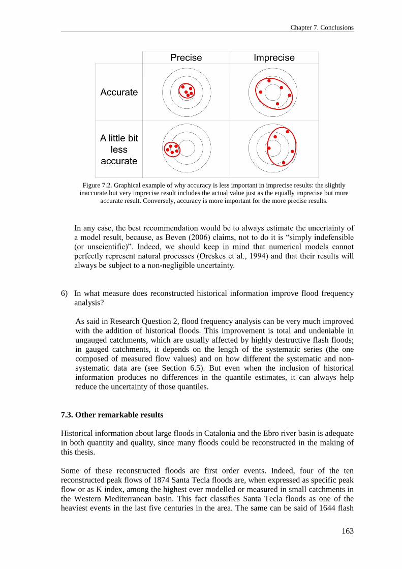
Chapter 7. Conclusions
163
Figure 7.2. Graphical example of why accuracy is less important in imprecise results: the slightly
inaccurate but very imprecise result includes the actual value just as the equally imprecise but more accurate result. Conversely, accuracy is more important for the more precise results.
In any case, the best recommendation would be to always estimate the uncertainty of
a model result, because, as Beven (2006) claims, not to do it is “simply indefensible
(or unscientific)”. Indeed, we should keep in mind that numerical models cannot
perfectly represent natural processes (Oreskes et al., 1994) and that their results will
always be subject to a non-negligible uncertainty. 6) In what measure does reconstructed historical information improve flood frequency
analysis?
As said in Research Question 2, flood frequency analysis can be very much improved with the addition of historical floods. This improvement is total and undeniable in ungauged catchments, which are usually affected by highly destructive flash floods; in gauged catchments, it depends on the length of the systematic series (the one composed of measured flow values) and on how different the systematic and non-systematic data are (see Section 6.5). But even when the inclusion of historical information produces no differences in the quantile estimates, it can always help reduce the uncertainty of those quantiles.
7.3. Other remarkable results Historical information about large floods in Catalonia and the Ebro river basin is adequate in both quantity and quality, since many floods could be reconstructed in the making of this thesis. Some of these reconstructed floods are first order events. Indeed, four of the ten reconstructed peak flows of 1874 Santa Tecla floods are, when expressed as specific peak flow or as K index, among the highest ever modelled or measured in small catchments in the Western Mediterranean basin. This fact classifies Santa Tecla floods as one of the heaviest events in the last five centuries in the area. The same can be said of 1644 flash

Chapter 7. Conclusions
164
flood of the Ondara River in Tàrrega. Similarly, but in another spatial scale, 1787 flood in the Ebro River is of the same order of magnitude than the greatest floods ever measured in the Danube or the Rhône, in spite of lacking the great contribution of snow thaw that the two great Alpine-born rivers have. The peak flows of the reconstructed historical floods in the Ebro River basin are far larger than the measured flows included in the systematic series, opposite to what happens in most countries in Central Europe, where measured floods of the 20th century are greater than the reconstructed historical ones. This means that, in the case of the Ebro River basin, research in historical hydrology can pay off in terms of improvement of flood frequency analysis, especially for the rarest quantiles. Flood frequency analyses in two locations of the Ebro River gave insight into the different hydrological behaviours regarding floods of the two main subcatchments of the basin. The hydrological regime of the western half of the basin is dominated by gentler floods coming from the areas closer to the Atlantic Ocean and the eastern half is affected by more violent floods coming down from the Pyrenees. 7.4. Other contributions This thesis is among the first applications of quantitative historical hydrology (that is, historical hydrology based on hydraulic reconstruction of peak flows) in Catalonia and in the Ebro River basin, as well as in the westernmost part of the Mediterranean basin. It is an innovative thesis because it applies historical hydrology techniques in a creative manner:
− It introduces a novel interdisciplinary methodology to perform a complete reconstruction of a flood and the first application of this methodology to 1874 Santa Tecla floods in an area of around 10000 km2. This methodology includes an original procedure of reconstructing a hyetograph via hydrological modelling. The obtained hyetographs corresponded to perfectly plausible rainstorms and were furthermore confirmed by the meteorological analysis based on the maps reconstructed by the 20th Century Reanalysis project (Compo et al., 2011), which permitted to establish the synoptic situation at the time of the flood and the processes (prevailing winds, air moisture build up, sudden vertical instability) that caused the rainstorm that ultimately caused the floods. The meteorological analysis also provided an insight into the spatial distribution of the event, which could be then compared to the spatial variability of the reconstructed peak flows in ten sites within five different catchments.
− It applies hydraulic reconstruction to both flash floods and river floods, which are processes that occur in different space and time scales.
− It compares three methods of peak flow estimation: the simple Manning’s equation, the one-dimensional model HEC-RAS, and the two-dimensional model Iber.
Chapter 7. Conclusions
165
− It presents the first example known to us of a flood frequency analysis with a flow series composed solely of reconstructed historical peak floods, which, moreover, were flash floods. This flood frequency analysis was also innovative because it fitted, with adequate results, a simple exponential function to the reconstructed data.
7.5. Limitations and future research The major limitations of the research presented in this thesis were:
− The lack of use of two-dimensional hydraulic models, which are thought to give more accurate results.
− Absence of some important input variables (namely, channel and floodplain geometry, and model structure and assumptions) in the uncertainty assessment of the hydraulic reconstruction.
− Absence of uncertainty assessment of the hydrological reconstruction.
− Not having taken into account non-stationarity in flood frequency analysis.
Therefore, the future endeavours of our research group, both in the short- and in the medium-term, are:
− Implementation of a flood marks database, which is essential in order to, on the one hand, guarantees the conservation of this historical heritage and, on the other hand, to facilitate future historical hydrologists work.
− Re-calculation with a two-dimensional hydraulic model of some of the
reconstructed peak flows.
− Improvement and refinement of the procedure of hydrological reconstruction of hyetographs.
− Improvement of the uncertainty assessment of the hydraulic reconstruction, taking into account as many input variables as possible: geometry, model structure. This uncertainty assessment should be extended to other results of the hydraulic reconstruction, such as water velocity or the whole hydrograph.
− Uncertainty assessment of the hydrological reconstruction, that is, the estimation of the error of the reconstructed hyetographs.
− Flood frequency analysis with methods that allow taking into account the non-stationarity of historical floods data.
− Propagation of hydraulic reconstruction uncertainties to flood frequency analysis.

Chapter 7. Conclusions
166
− Classification of major floods depending on the meteorological processes that caused them.
− Exploration of relationships between periods of different flood frequency and climate variables.
− Thorough analysis of the hydrological behaviour of the Ebro River basin and its
subcatchments during the major floods of the last 500 years.
− Analysis of modern flash floods in order to quantify their sediment load and, thus, the viscosity of the flow with the objective to estimate these variables in past flash floods in the same catchments.
7.6. Final remark I would like to end this dissertation with a quote of its supervisor J. Carles Balasch: “In order to understand the hydrology of the future, it is essential to reconstruct and understand the hydrology of the past”.

References


References
169
Abellà, A. (2013): Reconstrucció de les riuades més importants del riu Ebre al seu pas per Móra d’Ebre. Master thesis. University of Lleida, 100 pp.
ACA, Agència Catalana de l’Aigua. (2007): Estudi de tramificació dels principals cursos fluvials de Catalunya. Departament de Medi Ambient i Habitatge, Generalitat de Catalunya, Barcelona, 41 pp.
ACUR, Arxiu Comarcal de l’Urgell. (1621): Nota de la rubina de l’any 1615. Llibre d’Actes i Memòries 1603-1621, p. 1v.
Albentosa (1989): El Clima y las Aguas. Geografia de España, 4. Editorial Síntesis, Madrid, 240 p.
Alberch, R., Freixes, P., Massanas, E., Miró, J. (1982): Girona: Ponts, rius, aiguats. Ajuntament de Girona, Girona.
Alemseged, T.H., Rientjes, T.H.M. (2007): Uncertainty issues in hydrodynamic flood modelling. In: Proceedings of the 5th international symposium on spatial data quality SDQ.
Almela, F. (1957): Las riadas del Turia (1321-1949). Ajuntament de València, València.
Andersson, T., Andersson, M., Jacobsson, C., Nilsson, S. (1989): Thermodynamic indices for forecasting thunderstorms in southern Sweden. Meteorol. Mag. 116, 141-146.
Andréassian, V. (2004): Waters and forests: from historical controversy to scientific debate. J. Hydrol., 291(1), 1-27.
Anonymous (1930): La rubina del dissabte passat. Crònica Targarina, 478, (25 October 1930), Tàrrega, Catalonia.
Aronica, G., Hankin, B., Beven, K.J. (1998): Uncertainty and equifinality in calibrating distributed roughness coefficients in a floods propagation model with limited data. Adv. Water. Resour., 22(4), 349-365.
Baker, V.R. (1987): Paleoflood hydrology and extraordinary flood events. J. Hydrol., 96(1), 79-99.
Baker, V.R. (2008): Paleoflood hydrology: origin, progress, prospects. Geomorphol., 101, 1-13.
Balasch, J.C., Remacha, R., Eritja, X., Sánchez, A. (2007): 1907. La riuada del Segre a Lleida. Pagès Editors, Lleida, 229 pp.
Balasch, J.C., Ruiz-Bellet, J.L., Barriendos, M., Tuset, J., Monserrate, A., Sánchez, A. Casteltort, X., Astudillo, C. (2014): Analysis of the major floods in the Ebro River basin (Iberian Peninsula) since 1600 AD. Poster communication, EGU General Assembly, Vienna, 27 April - 2 May. Available at: http://presentations.copernicus.org/EGU2014-5733_presentation.pdf

References
170
Balasch, J.C., Ruiz-Bellet, J.L., Tuset, J., Martín de Oliva, J. (2010a): Reconstruction of the 1874 Santa Teclas’s rainstorm in Western Catalonia (NE Spain) from flood marks and historical accounts. Nat. Hazards Earth Syst. Sci., 10, 2317-2325.
Balasch, J.C., Tuset, J., Ruiz-Bellet, J.L. (2010b): Reconstructing the 1874 Santa Tecla flash flood in the Ondara River (Ebro Basin, NE Spain). Adv. Geosci., 26, 45-48.
Balasch, J.C., Tuset, J., Ruiz-Bellet, J.L. (2010b): Reconstructing the 1874 Santa Tecla flash flood in the Ondara River (Ebro Basin, NE Spain). Adv. Geosci., 26, 45-48.
Bales, J.D., Wagner, C.R. (2009): Sources of uncertainty in flood inundation maps. Journal of Flood Risk Management, 2(2), 139-147.
Bárdossy, A., Filiz, F. (2004): Analysis of flood producing atmospheric circulation patterns. In: Benito, G., Thorndycraft, V.R. (eds.): Systematic, Palaeoflood and Historical Data for the Improvement of Flood Risk Estimation: Methodological Guidelines. Centro de Ciencias Mediambientales (CSIC), Madrid, 115 pp.
Barnolas, M., Llasat, M.C. (2007): Metodología para el estudio de inundaciones históricas en España e implementación de un SIG en las cuencas del Ter, Segre y Llobregat. CEDEX, Ministerio de Fomento, Monografías M-90, Madrid, 264 pp.
Barrera, A., Cunillera, J. (2011): Primer informe sobre la generació d’escenaris climàtics regionalitzats per a Catalunya durant el segle XXI. Technical report. Servei Meteorològic de Catalunya, Departament de Territori i Sostenibilitat, Generalitat de Catalunya, 95 pp.
Barrera, A., Llasat, M.C., Barriendos, M. (2006): Estimation of extreme flash flood evolution in Barcelona County from 1351 to 2005. Nat. Hazards Earth Syst. Sci., 6, 505-518, doi:10.5194/nhess-6-505-2006.
Barriendos, M., Coeur, D. (2004): Flood data reconstruction in historical times from non-instrumental sources in Spain and France. In: Benito, G., Thorndycraft, V.R. (eds.): Systematic, palaeoflood and historical data for the improvement of flood risk estimation: Methodological guidelines. CSIC, Madrid, 29-42.
Barriendos, M., Coeur, D., Lang, M., Llasat M.C., Naulet, R., Lemaitre, F., Barrera, A. (2003): Stationarity analysis of historical flood series in France and Spain (14th-20th centuries). Nat. Hazards Earth Syst. Sci., 3, 583-592.
Barriendos, M., Llasat, M.C. (2003): The case of the ‘Maldà’ anomaly in the Western Mediterranean basin (AD 1760-1800): an example of a strong climatic variability. Clim. Chang., 61, 191-216.
Barriendos, M., Martín-Vide, J. (1998): Secular climatic oscillations as indicated by catastrophic floods in the Spanish Mediterranean coastal area (14th-19th centuries). Clim. Chang., 38, 473-491.
Barriendos, M., Martin-Vide, J. (1998): Secular climatic oscillations as indicated by catastrophic floods in the Spanish Mediterranean coastal area (14th-19th Centuries). Climatic Change, 38, 473-491.

References
171
Barriendos, M., Pomés, J. (1993): L’aigua a Mataró. Inundacions i recursos hídrics (ss. XVIII-XX). Caixa d’Estalvis Laietana, Mataró, Catalonia.
Barriendos, M., Rodrigo, F. (2006): Study of historical flood events on Spanish rivers using documentary data. Hydrol. Sci. J., 51(5), 765-783.
Barriendos, M., Tuset, J., Mazón, J., Pino, D., Ruiz-Bellet, J.L., Balasch, J.C. (2013): La rubinada de Santa Tecla a Tàrrega (23 de setembre de 1874). Urtx, Revista d’humanitats de l’Urgell, 27, 10-25.
Batalla, R.J.; Gómez, C.M. & Kondolf, G.M. (2004): Reservoir-induced hydrological changes in the Ebro River basin (NE Spain). Journal of Hydrology, 290: 117-136.
Batalla, R.J., Vericat, D. (2011): Hydrology and Sediment Transport. In Barceló, D., Petrovic, M. (eds.): The Ebro River Basin. Springer, Berlín-Heidelberg, 21-46.
Bates, P.D., Anderson, M.G., Hervouet, J.M., Hawkes, J.C. (1997): Investigating the behavior of two-dimensional finite element models of compound channel flow. Earth Surface Processes and Landforms, 22(1), 3-17.
Bayliss, A.C., Reed, D.W. (2001): The use of historical information in flood frequency estimation. Technical report to Ministry of Agriculture, Fisheries and Food. Centre for Ecology and Hydrology, Wallingford, UK, 86 pp.
Bell, F.C., Om Kar,S. (1969): Characteristic response times in design flood estimation. J. Hydrol., 8(2), 173-196. http://dx.doi.org/10.1016/0022-1694(69)90120-6.
Benito, G., Brázdil, R., Herget, J., Machado, M.J. (2015): Quantitative historical hydrology in Europe. Hydrol. Earth Syst. Sci., 19, 3517-3539.
Benito, G., Díez-Herrero, A., Fernández de Villalta, M. (2003): Magnitude and frequency of flooding in the Tagus basin (central Spain) over the last millennium. Climat. Chang., 58, 171-192.
Benito, G., Lang, M., Barriendos, M., Llasat, M.C., Francés, F., Ouarda, T., Thorndycraft, V.R., Enzel, Y., Bardossy, A., Coeur, D., Bobée, B. (2004): Use of systematic, palaeoflood and historical data for the improvement of flood risk estimation. Review of scientific methods. Nat. Hazards, 31(3), 623-643.
Benito, G., Ouarda, T.B.M.J., Bárdossy, A. (2005): Applications of paleoflood and historical data in flood risk analysis. J. Hydrol., 313, 1-2.
Benito, G., Thorndycraft, V.R. (2004): Systematic, palaeoflood and historical data for the improvement of flood risk estimation. Centro de Ciencias Medioambientales (CSIC), Madrid, 115 pp.
Benito, G., Thorndycraft, V.R., Rico, M., Sánchez-Moya Y., Sopeña, A. (2008): Palaeoflood and floodplain records from Spain: evidence for long-term climate variability and environmental changes. Geomorphol., 101, 68-77.

References
172
Bentabol, H. (1900): Las aguas de España y Portugal. Vda. e Hijos de M. Tello, Madrid, 2nd ed.
Beven, K.J. (2006): On undermining the science? Hydrol. Process. (HPToday), 20, 3141-3146.
Beven, K.J., Binley, A.M. (1992): The future of distributed models: Model calibration and uncertainty in prediction. Hydrol. Process. 6, 279-298.
Bladé, E., Cea, L., Corestein, G., Escolano, E., Puertas, J., Vázquez-Cendón, E., Dolz, J., Coll, A. (2012): Iber: herramienta de simulación numérica del flujo en ríos. Revista Internacional de Métodos Numéricos para Cálculo y Diseño en Ingeniería, 30(1), 1-10.
Blasco-Ijazo, J. (1959): Las avenidas del Ebro. Crecidas verdaderamente extraordinarias 1261-1959. Librería General, Col. La Cadiera, 139, Zaragoza,Spain, 14 pp.
Blöschl, G., Gaál, L., Hall, J., Kiss, A., Komma, J., Nester, T., Parajka, J., Perdigão, R.A.P., Plavcová, L., Rogger, M., Salinas, J.L., Viglione, A. (2015): Increasing river floods: fiction or reality? Wiley Interdisciplinary Reviews: Water, 2(4), 329-344. doi: 10.1002/wat2.1079
Blöschl, G., Nester, T., Komma, J., Parajka, J., Perdigão, R. A. P. (2013): The June 2013 flood in the Upper Danube basin, and comparisons with the 2002, 1954 and 1899 floods. Hydrology and Earth System Sciences, 17, 5197-5212.
Brázdil, R., Demarée, G.R., Deutsch, M., Garnier, E., Kiss, A., Luterbacher, J., Macdonald, N., Rohr, C., Dobrovolný, P., Kolář, P., Chromá, K. (2010). European floods during the winter 1783/1784: scenarios of an extreme event during the ‘Little Ice Age’. Theoretical and applied climatology, 100(1-2), 163-189.
Brázdil, R., Dobrovolný, P., Kotyza, O. (2004): Floods in the Czech Republic during the past millennium. La Houille Blanche, 5, 50-55.
Brázdil, R., Glaser, R., Pfister, C., Antoine, J.M., Barriendos, M., Camuffo, D., Deutsch, M., Enzi, S., Guidoboni, E., Rodrigo, F.S. (1999): Flood events of selected rivers of Europe in the Sixteenth Century. Climatic Change, 43, 239-285.
Brázdil, R., Kundzewicz, Z.W. (2006): Historical hydrology – Editorial. Hydrol. Sci. J., 51(5), 733-738.
Brázdil, R., Kundzewicz, Z.W., Benito, G. (2006): Historical hydrology for studying flood risk in Europe. Hydrol Sci. J., 51(5), 739-764.
Brázdil, R., Kundzewicz, Z.W., Benito, G. (2006): Historical hydrology for studying flood risk in Europe. Hydrol. Sci. J., 51(5), 739-764.
Brázdil, R., Kundzewicz, Z.W., Benito, G., Demarée, G., Macdonald, N., Roald, L.A. (2012): Historical floods in Europe in the past millennium. In: Kundzewicz, Z.W. (ed.): Changes in Flood Risk in Europe. IAHS Special Publication, 10, Wallingford, 121-166.

References
173
Brázdil, R., Pfister, C., Wanner, H., von Storch, H., Luterbacher, J. (2005): Historical climatology in Europe – the state of the art. Climatic Change, 70, 363-430.
Bürger, K., Dostal, P., Seidel, J., Imbery, F., Barriendos, M., Mayer, H., Glaser, R. (2006): Hydrometeorological reconstruction of the 1824 flood event in the Neckar River basin (southwest Germany). Hydrol. Sci. J., 51(5), 864-877.
Butts, M.B., Payne, J.T., Kristensen, M., Madsen, H. (2004): An evaluation of the impact of model structure on hydrological modelling uncertainty for streamflow simulation. J. Hydrol., 298(1), 242-266.
Calenda, G., Mancini, C.P., Volpi, E. (2009): Selection of the probabilistic model of extreme floods: The case of the River Tiber in Rome. J. Hydrol., 371, 1-11.
Camuffo, D., Enzi, S. (1996): The analysis of two bi-millennial series: Tiber and Po river floods. In: Jones, P.D., Bradley, R.S., Jouzel, J. (eds.): Climatic Variations and Forcing Mechanisms of the Last 2000 Years. Springer Verlag, NATO ASI Series, Vol. 141, 433-450.
Casas, A., Benito, G., Thorndycraft, V.R., Rico, M. (2004): La importancia del modelo digital del terreno en modelos hidráulicos de crecidas. In: Benito, G., Díez-Herrero, A. (eds.): Riesgos naturales y antrópicos en Geomorfología. (Actas de la VIII Reunión Nacional de Geomorfología, Toledo, 22-25 de septiembre de 2004). SEG y CSIC, Madrid, 47-57.
Casas, M.C., 2005. Análisis espacial y temporal de las lluvias extremas en Catalunya. Modelización y clasificación objetiva. Ph.D. thesis, University of Barcelona, 198 pp.
Castellà, J., Miranda, C. (1989): Fuertes riadas en varias comarcas de Cataluña. Un desaparecido en Tàrrega. La Vanguardia [newspaper], 38.751 (29 October 1989), 44, Barcelona.
Catálogo Nacional de Inundaciones Históricas (2006–2010): Digitized format: 5 CDs, vol. 1 (2006, Duero and Segura Basins), vol. 2 (2007, Júcar and Tajo Basins), vol. 3 (2008, Ebro and Guadalquivir Basins), vol. 4 (2009, Norte and Galicia Basins), vol. 5 (2010, Guadiana and Sur Basins). Dirección General de Protección Civil y Emergencias, Ministerio del Interior, Madrid.
Cea, L., Bladé, E. (2008): Modelización matemática en lecho fijo del flujo en ríos. Modelos 1D y 2D en régimen permanente y variable. Jornadas Técnicas sobre Hidráulica Fluvial. Madrid, 3-7 March 2008.
Champion, M. (1858-1864): Les Inondations en France depuis le VIe siècle jusqu'à nos jours, recherches et documents contenant les relations contemporaines, les actes administratifs, les pièces officielles, etc. de toutes les époques, avec détails historiques sur les quais, ponts, digues, chaussées, levées, etc., publiés, annotés et mis en ordre par M. Maurice Champion. V. Dalmont, Paris, 6 volumes.
CHE, Confederación Hidrográfica del Ebro (1996): Propuesta de Plan Hidrológico de la Cuenca del Ebro. Anexo 2: Aportaciones de las estaciones de aforo. Ministerio de Medio Ambiente, Medio Rural y Marino, Madrid, 10 pp.

References
174
Chía, J. (1861): Inundaciones de Gerona. Relación histórica de las más notables inundaciones que han causado en esta ciudad las avenidas de los ríos Ter, Oñar, Güell y Galligans desde la ocurrida en 28 de diciembre de 1367 hasta las que tuvieron lugar en 8 y 11 de octubre del corriente año de 1861. Paciano Torres, Girona.
Chow, V.T. (1959): Open-channel hydraulics. McGraw-Hill, New York, 680 pp.
Codina, J. (1971): Inundacions al Delta del Llobregat. R. Dalmau, Col. "Episodis de la Història", 147-148, Barcelona.
Cohn, T.A. (1986): Flood frequency analysis with historical flood information. Ph.D. Dissertation, Cornell Univ., Ithaca, New York, 144pp.
Coma, M.T. (1990): Les inundacions en el terme municipal de Tàrrega. Urtx Revista Cultural de l’Urgell, 2, 249-259.
Coma, M.T. (1990): Les inundacions en el terme municipal de Tàrrega. Urtx, Revista cultural de l’Urgell, 2, 249-259.
Compo, G.P., Whitaker, J.S., Sardeshmukh, P.D., Matsui, N., Allan, R.J., Yin, X., Gleason, B.E., Vose, R.S., Rutledge, G., Bessemoulin, P., Brönnimann, S., Brunet, M., Crouthamel, R.I., Grant, A.N., Groisman, P.Y., Jones, P.D., Kruk, M., Kruger, A.C., Marshall, G.J., Maugeri, M., Mok, H.Y., Nordli, ∅, Ross, T.F., Trigo, R.M., Wang, X.L., Woodruff, S.D., Worley, S.J. (2011): The Twentieth Century Reanalysis Project. Quart. J. Roy. Meteorol. Soc., 137, 1-28.
Conacher, A., Sala, M. (1998). Land degradation in Mediterranean environments of the World: nature and extent, causes and solutions. Wiley, Chichester, New York, 491 pp.
Condie, R., Lee, K.A. (1982): Flood frequency analysis with historic information. J. Hydrol., 58, 47-61.
Cong, A., Xu, Y. (1987): Effect of discharge measurement errors on flood frequency analysis. In: Singh, V.P. (ed.): Application of Frequency and Risk in Water Resources. Reidel Publishing Company, 175-190.
Corbella, D. (2003): Vallfogona de Riucorb. Imatge i memòria. Farrell Editors, Sant Vicenç de Castellet, Catalonia, 135 pp.
Corominas, J. (1985): L'acció catastròfica de les avingudes, in: Història Natural dels Països Catalans. Recursos Geològics i Sòl. Volum 3. Fundació Enciclòpedia Catalana, Barcelona, pp. 253-267.
Còts, P. (2012): El pont baixmedieval sobre el riu Ondara de Tàrrega: Resultats de l’actuació arqueològica duta a terme l’any 2007. Urtx, Revista Cultural de l’Urgell, 26, 116-131.
Couchoud, R. (1965): Hidrología histórica del Segura. Efemérides hidrológica y fervorosa recopilada y escrita por el Dr. R. Couchoud. Centro de Estudios Hidrográficos, Madrid.
References
175
Cowan, W.L. (1956): Estimating hydraulic roughness coefficients. Agricultural Engineering, 37, 473-475
Cunderlik, J. M., Burn, D. H. (2003). Non-stationary pooled flood frequency analysis. Journal of Hydrology, 276(1), 210-223.
Cunnane, C. (1978): Unbiased plotting positions − a review. J. Hydrol., 37(3), 205-222.
Curto, A. (2007): La riuada de 1907. La riuada, 29, 4-8.
Davy, L. (1975): L’Ebre. Étude Hydrologique. PhD thesis. University Paul Valéry, Montpellier, France, 800 pp.
Dawdy, D.R., Motayed, A.K. (1979): Uncertainties in determination of flood profiles. In: McBean, E.A, Hipel, K.W., Unny, T.E. (eds.): Inputs for risk analysis in water systems.Water Resources Publications, Ft. Collins (USA), 193-208.
De Roo, A.P.J., Offermans, R.J.E, Cremers, N.H.D.T. (1996): LISEM: A single-event, physically based hydrological and soil erosion model for drainage basins. II: Sensitivity analysis, validation and application. Hydrol. Process., 10, 1119-1126.
Delrieu, G., Ducrocq, N., Gaume, E., Nicol, J., Payrastre, O., Yates, E., Kirstetter, P.E., Andrieu, H., Ayral, P.A., Bouvier, C., Creutin, J.D., Livet, M., Anquetin, S., Lang, M., Neppel, L., Obled, C., Parent-du-Châtelet, J., Saulnier, G.M., Walpersdorf, A., Wobrock, W. (2005): The catastrophic flash-flood event of 8-9 September 2002 in the Gard region, France: a first case study for the Cévennes-Vivarais Mediterranean Hydrometeorological Observatory. J. Hydrometeorol., 6(1), 34-52.
Di Baldassarre, G., Montanari, A. (2009): Uncertainty in river discharge observations: a quantitative analysis. Hydrol. Earth Syst. Sci., 13, 913-921. www.hydrol-earth-syst-sci.net/13/913/2009/
Diari de Barcelona (1874). Newspaper; issues published between September 22nd and October 3rd 1874, no. 258-269, pp. 9121-9568.
Doswell, C.A. III, Rasmussen, E.N. (1994): The effect of the neglecting the Virtual temperature correction on CAPE calculations. Weather Forecast., 9(4), 625-629.
Ducrocq, V., Nuisier, O., Ricard, D, Lebeaupin, C, Thovenin T. (2008): A numerical study of three catastrophic precipitating events over southern Frances. II: Mesoscale triggering and stationarity factors. Quart. J. Roy. Meteorol. Soc., 134, 131-145.
EEA, European Environment Agency (2010): Mapping the impacts of natural hazards and technological accidents in Europe. An overview of the last decade. EEA Technical report, no. 13/2010, 146 pp.
Elleder, L. (2010): Reconstruction of the 1784 flood hydrograph for the Vltava River in Prague, Czech Republic. Global Planet. Change, 70(1), 117-124.

References
176
Elleder, L., Herget, J., Roggenkamp, T., Nießen, A. (2013): Historic floods in the city of Prague – reconstruction of peak discharges for 1481-1825 based on documentary sources. Hydrol. Res., 44, 202-214.
Espinagosa, J., Gonzalvo, G., Coma, T. (1996). La rubinada de Santa Tecla de 1874 a Tàrrega. Natan Estudis, Ajuntament de Tàrrega, Tàrrega. 86 pp.
Etoh T., Murota, A., Nakanishi, M. (1986): SQRT – Exponential Type Distribution of Maximum. In: Singh, V.P. (ed.): Hydrologic frequency modeling. Proceedings of the International Symposium on Flood Frequency and Risk Analyses, 14-17 May 1986, Louisiana State University, Baton Rouge. D. Reidel Publishing, Dordrecht (Holland), 253-265.
EU Directive 2007/60/EC (2007). Directive 2007/60/EC of the European Parliament and of the Council of 23 October 2007 on the assessment and management of flood risks.
Farré, M.A. (2008): Fenòmens naturals i religiositat a la Tàrrega dels segles XVI-XIX. Urtx Revista Cultural de l’Urgell, 22, 151-164.
Fernandez-Bono, J.F., Grau-Gimeno, P. (2003: Peak discharge estimation for historical flood events. In: Thorndycraft, V.R. (ed.): Palaeofloods, Historical Data and Climatic Variability: Applications in Flood Risk Assessment. CSIC, Madrid.
Flesch, T.K., Reuter, G.W. (2012): WRF model simulation of two Alberta flooding events and the impact of topography. J. Hydrometeorol., 13(2), 695-708.
Fontseré, E., Galcerán, F. (1938): Les inundacions d’octubre del 1937 a l’Alt Pirineu. Memòries (Servei Meteorològic de Catalunya), 1,3, Generalitat de Catalunya, Barcelona, 15 pp.
Francés, F. (1998): Using the TCEV distribution function with systematic and non-systematic data in a regional flood frequency analysis. Stoch. Hydrol. Hydraul., 12, 267-283.
Francés, F. (2004): Flood frequency analysis using systematic and non-systematic information. In: Benito, G., Thorndycraft, V.R. (eds.): Systematic, palaeoflood and historical data for the improvement of flood risk estimation. Methodologica guidelines. CSIC, Madrid, 55-70.
Francou, J., Rodier, J. (1967): Essai de classification des crues maximales observées dans le monde. Cahiers ORSTOM, Série Hydrologie IV(3), 19-46.
Gallart, F., Llorens, P. (2004): Observation on land cover changes and water resources in the headwaters of the Ebro catchment, Iberian Peninsula. Phys. Chem. Earth, 29(11-12), 769-773.
Galván, R., del Valle, J., Losada, J.A., Arnal, M. (2013): La inundación del Ebro de 1871 en Zaragoza. Boletín de la Real Sociedad de Geografia, 149, 139-169.

References
177
Galway, J. G. (1956): The lifted index as a predictor of latent instability. B. Am. Meteorol. Soc., 43, 528-529.
García-Faria, P. (1908): Las inundaciones de octubre de 1907 en Catalunya. Revista de Obras Públicas, I, 56.
Gaume, E., Bain, V., Bernardara, P., Newinger, O., Barbuc, M., Bateman, A., Blaskovicova, L., Blöschi, G., Borga, M., Dumitrescu, A., Daliakopoulos, I., Garcia, J., Irimescu, A., Kohnova, S., Koutroulis, A., Marchi, L., Matreata, S., Medina, V., Preciso, E., Sempere-Torres, D., Stancalie, G., Szolgay, J., Tsanis, I., Velasco, D., Viglione, A. (2009): A compilation of data on European flash floods. J. Hydrol., 367(1), 70-78.
Gaume, E., Gaal, L., Viglione, A., Szolgay, J., Kohnova, S., Blöschl, G. (2010): Bayesian MCMC approach to regional flood frequency analyses involving extraordinary flood events at ungauged sites. J. Hydrol., 394, 101-117.
Gaume, E., Livet, M., Desbordes, M., Villeneuve, J.P. (2004) : Hydrological analysis of the river Aude, France, flash flood on 12 and 13 November 1999. J. Hydrol., 286(1), 135-154.
George, J.J. (1960): Weather Forecasting for Aeronautics. Academic Press, 673 pp.
GIMHA, Grupo de Investigación de Modelización Hidrológica y Ambiental. (2014): Software. Last accessed on 12/Dec/2014 at http://lluvia.dihma.upv.es/ES/software/software.html
Glaser, R. (1996): Data and Methods of Climatological Evaluation in Historical Climatology. Hist. Soc. Res., 21, 56-88.
Glaser, R., Riemann, D., Schönbein, J., Barriendos, M., Brázdil, R., Bertolin, C., Camuffo, D., Deutsch, M., Dobrovolný, P., van Engelen, A., Enzi, S.,, Halíèková, M., Koenig, S.J., Kotyza, O., Limanówka, D., Macková, J., Sghedoni, M., Martin, B., Himmelsbach, I. (2010): The variability of European floods since AD 1500. Climat. Chang., 101, 235-256.
Götzinger, J., Bárdossy, A. (2008): Generic error model for calibration and uncertainty estimation of hydrological models. Water Resour. Res., 44, W00B07, doi:10.1029/2007WR006691
Gregory, K.J., Benito, G., Dikau, R., Golosov, V., Jones, A.J.J., Macklin, M.G., Parsons, A.J., Passmore, D.G., Poesen, J., Starkel, L., Walling, D.E. (2006): Past hydrological events related to understanding global change: An ICSU research project. Catena, 66, 2-13.
Grieser, J. (2012): Convection Parameters. Last accessed on 5 August 2015 at http://www.juergen-grieser.de/CovectionParameters/ConvectionParameters.pdf
Grimalt, M. (1988): Aproximació a una geografia del risc a Mallorca. Les inundacions. Ph.D. thesis. Departament de Ciències de la Terra, Universitat de les Illes Balears, Palma, 3 volumes.
References
178
Grimalt, M. (1992): Geografia del risc a Mallorca. Les Inundacions. Institut d'Estudis Baleàrics, Palma.
Gumbel, E.J. (1941): The return period of flood flows. The Annals of Mathematical Statistics, 12, 163-190
Hall, J., Arheimer, B., Borga, M., Brázdil, R., Claps, P., Kiss, A., Kjeldsen, T.R., Kriauciuniene, J., Kundzewicz, Z.W., Lang, M., Llasat, M.C., Macdonald, N., McIntyre, N., Mediero, L., Merz, B., Merz, R., Molnar, P., Montanari, A., Neuhold, C., Parajka, J., Perdigão, R.A.P., Plavcová, L., Rogger, M., Salinas, J.L., Sauquet, E., Schär, C., Szolgay, J., Viglione, A., Blöschl, G. (2014): Understanding Flood Regime Changes in Europe: A state of the art assessment. Hydrology and Earth System Sciences, 18, 2735-2772, doi:10.5194/hess-18-2735-2014.
Hall, J.W., Tarantola, S., Bates, P.D., Horritt, M.S. (2005): Distributed sensitivity analysis of flood inundation model calibration. J. Hydraul. Eng., 131(2), 117-126.
Harmel, R.D., Cooper, R.J., Slade, R.M., Haney, R.L., Arnold J.G. (2011): Cumulative uncertainty in measured streamflow and water quality data for small watersheds. Trans. Am. Soc. Agric. Biol. Eng., 49(3), 689-701.
Hawkins, R.H. (1975): The importance of accurate Curve Numbers in the estimation of storm runoff. Water Resour. Bull., 11(5), 887-891.
Herget, J., Kapala, A., Krell, M., Rustemeier, E., Simmer, C., Wyss, A. (2015): The millennium flood of July 1342 revisited. Catena, 130, 82-94.
Herget, J., Meurs, H. (2010): Reconstructing peak discharges for historic flood levels in the city of Cologne – Germany. Global Planet. Change ,70, 108-116.
Herget, J., Roggenkamp, T., Krell, M. (2014): Estimation of peak discharges of historical floods. Hydrology and Earth System Sciences, 18(10), 4029-4037.
Hernández, A. (1885): Inundaciones de la Huerta de Murcia. Juicio sobre su frecuente repetición de pocos años a esta parte, sus terribles desastres, sus causas y remedios. El Diario, Murcia.
Herschy, R. (2003): World Catalogue of Maximum Observed Floods. IAHS Publ. no. 284. Wallingford, UK, 285 pp.
Hirsch, R.M. (1987): Probability plotting position formulas for flood records with historical information. J. Hydrol., 96(1), 185-199.
Horritt, M.S., Bates, P.D. (2001): Effects of spatial resolution on a raster based model of flood flow. J. Hydrol., 223, 239-249.
Horritt, M.S., Bates, P.D. (2002): Evaluation of 1D and 2D numerical models for predicting river flood inundation. J. Hydrol., 268, 87-99.
Hosking, J.R.M., Wallis, J.R. (1986a): Paleoflood hydrology and flood frequency analysis. Water Resour. Res., 22(4), 543-550.

References
179
Hosking, J.R.M., Wallis, J.R. (1986b): The value of historical data in flood frequency analysis. Water Resour. Res., 22(11), 1606-1612.
Hosking, J.R.M., Wallis, J.R. (1997): Regional frequency analysis: An approach based on L-Moments. Cambridge University Press, London, 224 pp.
ICGC, Institut Cartogràfic i Geològic de Catalunya. (2015): Aerial Photograph. Available at http://www.icc.cat/vissir3/. Last accessed: 27/10/2015.
Iglésies, J. (1971): L’aiguat de Santa Tecla (23 de setembre de 1874). Rafael Dalmau, Barcelona. 62 pp.
Iglésies, J. (1971): L'aiguat de Santa Tecla (23 de setembre de 1874). Col. "Episodis de la Història" 156, 64 pp., Dalmau, Barcelona.
IGN, Instituto Geográfico Nacional (2015): MDT05/MDT05-LiDAR and MDT25. http://www.ign.es/ign/main/index.do. Last accessed: 12/11/2015.
IPCC (2014): Summary for policymakers. In: Field, C. B., Barros, V. R., Dokken, D. J.,Mach, K. J., Mastrandrea, M. D., Bilir, T. E., Chatterjee, M., Ebi, K. L., Estrada, Y. O., Genova, R. C., Girma, B., Kissel, E. S., Levy, A. N., MacCracken, S., Mastrandrea, P. R., L. L., White (eds.): Climate Change 2014: Impacts, Adaptation, and Vulnerability. Part A: Global and Sectoral Aspects. Contribution of Working Group II to the Fifth Assessment Report of the Intergovernmental Panel on Climate Change. Cambridge University Press, Cambridge, UK and New York, NY, USA, 1–32.
Jarrett, R.D. (1987): Errors in slope-area computations of peak discharges in mountain streams. J. Hydrol., 96, 53-67.
Jiménez-Álvarez, A., García-Montañés, C., Mediero, L., Incio, L., Garrote, J. (2012): El mapa de caudales máximos de las cuencas intercomunitarias. Revista de Obras Públicas, 3533(159), 7-32.
Johnson, P.A. (1996): Uncertainty of hydraulic parameters. J. Hydraul. Eng., 122(2), 112-114.
Junta d’Aigües (1995): Anuari de dades hidrològiques. Technical Report, Generalitat de Catalunya, Barcelona, 470 pp.
Kalnay, E., Kanamitsu, M., Kistler, R., Collins, W., Deaven, D., Gandin, L, Iredell, M., Saha, S., White, G., Woollen, J., Zhu, Y., Leetmaa, A., Reynolds, R., Chelliah, M., Ebisuzaki, W., Higgins, W., Janowiak, J., Mo, K. C., Ropelewski, C., Wang, J., Jenne, R., Joseph, D. (1996): The NCEP/NCAR Reanalysis 40-year Project. B. Am. Meteorol. Soc., 77, 437-471.
Kirby, W.H. (1987): Linear error analysis of slope-area discharge determinations. J. Hydrol., 96, 125-138.
Kiss, A. (2009a): Floods and weather in 1342 and 1343 in the Carpathian basin. J. Environ. Geogr, 2, 37-47.

References
180
Kiss, A. (2009b): Historical climatology in Hungary: role of documentary evidence in the study of past climates and hydrometeorological extremes. Idöjárás, 113, 315-339.
Kjeldsen, T.R., Macdonald, N., Lang, M., Mediero, L., Albuquerque, T., Bogdanowicz, E., Brazdil, R., Castellarin, A., David, V., Fleig, A., Gul, G.O., Kriauciuniene, J., Kohnova, S., Merz, B., Nicholson, O., Roald, L.A., Salinas, J.L., Sarauskiene, D., Sraj, M., Strupczewski, W., Szolgay, J., Toumazis, A., Vanneuville, W., Veijalainen, N., Wilson, D. (2014): Documentary evidence of past floods in Europe and their utility in flood frequency estimation. J. Hydrol., 517, 963-973.
Klemeš, V. (1986): Dilettantism in hydrology: Transition or destiny? Water Resour. Res.,22(9S), 177S-188S, doi:10.1029/WR022i09Sp0177S
Kovats, S., Valentini, R. (2014): IPCC WGII AR5, IPCC Working Group II, Technical Support Unit, Stanford, USA, Chapter 23. Europe, 93 pp.
Kundzewicz, Z.W., Hirabayashi, Y., Kanae, S. (2010): River floods in the changing climate—observations and projections. Water Resources Management, 24(11), 2633-2646.
Lang M, Coeur D. (2014): Les inondations remarquables en France. Inventaire 2011 pour la directive Inondation. Quae, Versailles, France, 640pp.
Lang, M., Fernández-Bono, J.F., Recking, A., Naulet, R., Grau-Gimeno, P. (2004): Methodological guide for palaeoflood and historical peak discharge estimation. In: Benito, G., Thorndycraft, V.R. (eds.): Systematic, paleoflood and historical data for the improvement of flood risk estimation. Methodological guidelines. CSIC, Madrid, 43-53.
Lang, M., Ouarda, T.B.M.J., Bobée, B. (1999): Towards operational guidelines for over-threshold modeling. J. Hydrol., 225, 103-117.
Lang, M., Pobanz, K., Renard, B., Renouf, E., Sauquet, E. (2010): Extrapolation of rating curves by hydraulic modelling, with application to flood frequency analysis. Hydrol. Sci. J., 55(6), 883-898, doi: 10.1080/02626667.2010.504186
Lenhart, T., Eckhardt, K., Fohrer, N., Frede, H.-G. (2002): Comparison of two different approaches of sensitivity analysis. Phys. Chem. Earth, 27, 645-654.
Léonard, J., Mietton, M., Najib, H., Gourbesville, P. (2000): Rating curve modelling with Manning’s equation to manage instability and improve extrapolation. Hydrol. Sci. J., 45(5), 739-750.
Litynska, Z., Parniewicz, J., Pinkowski, H. (1976): The prediction of air mass thunderstorms and hails. Technical Report, 200(R), World Meteorological Organization, 450, 128-130.
Lladonosa, J. (1974): Historia de la Diputación Provincial de Lérida. Volumen 1. Artis Estudios Gráficos, Lleida, Catalonia, 501 pp.
References
181
Llasat, M. C., López, L., Barnolas, M., Llasat-Botija, M. (2008). Flash-floods in Catalonia: the social perception in a context of changing vulnerability. Advances in Geosciences, 17(17), 63-70.
Llasat, M.C. (2001): An objective classification of rainfall events on the basis of their convective features: application to rainfall intensity in the northeast of Spain. Int. J. Climatol., 21(11), 1385-1400.
Llasat, M.C., Barnolas, M., Ceperuelo, M., Llasat, M., Prat, M.Á. (2004a): Algunos aspectos del impacto social de las inundaciones en Cataluña. Revista del aficionado a la meteorologia, 20, 1-11. Available at: www.tiempo.com/ram/
Llasat, M.C., Barrera, A., Barriendos, M. (2004b): Analysis of climàtic conditions associated with historical floods. In Benito, G., Thorndycraft, V.R. (eds.): Systematic, Palaeoflood and Historical Data for the Improvement of Flood Risk Estimation: Methodological Guidelines. Centro de Ciencias Mediambientales (CSIC), Madrid, 85-94.
Llasat, M.C., Barriendos, M., Barrera, A., Rigo, T. (2005): Floods in Catalonia (NE Spain) since the 14th century. Climatological and meteorological aspects from historical documentary sources and old instrumental records. J. Hydrol., 313(1), 32-47.
Llasat, M.C., Rigo, T., Barriendos, M. (2003): The “Montserrat-2000” flash-flood event: a comparison with the floods that have occurred in the Northeastern Iberian Peninsula since the 14th Century. Int. J. Climatol., 23, 453-469.
López-Bustos, A. (1972): Antecedentes para una historia de avenidas del río Ebro. Revista de Obras Públicas, 3083, 191-204.
López-Bustos, A. (1981): Tomando el pulso a las grandes crecidas de los ríos peninsulares. Revista de Obras Públicas, 3190, 179-192.
López-Gómez, A. (1983): Las lluvias catastróficas mediterráneas. Estudios Geográficos, 44(170), 11-30.
Lumbroso, D., Gaume E. (2012): Reducing the uncertainty in indirect estimates of extreme flash flood discharges. J. Hydrol., 414, 16-30.
Luterbacher, J., García-Herrera, R., Allan, A.R., Álvarez-Castro, B.G.., Benito, G., Booth, J., Büntgen, U., Colombaroli, D., Davis, B., Esper, J., Felis, T., Fleitmann, D., Frank, D., Gallego, D., González-Rouco, J.F., Goosse, H., Kiefer, T., Macklin, M.G., Montagna, P., Newman, L., Power, M.J., Rath, V., Roberts, N., Sicre, M., Silenzi, S., Tinner, W., Valero-Garcés, B., van der Schrier, G., Vannière, B., Vogt, S., Wanner, H., Werner, J.P., Willett, G., Xoplaki, E., Zerefos, C.S., Zorita, E. (2012): A review of 2000 years of paleoclimatic evidence in the Mediterranean. In: Lionello, P. (ed.): The Climate of the Mediterranean region: from the past to the future. Elsevier, Amsterdam, The Netherlands, 87-185.
Luterbacher, J., Xoplaki, E., Dietrich, D., Rickli, R., Jacobeit, J., Beck, C., Gyalistras, D., Schmutz, C., Wanner, H. (2002): Reconstruction of sea-level pressure fields over the eastern North Atlantic and Europe back to 1500. Clim. Dynam., 18, 545-561.
References
182
Macdonald, N. (2004): The application of historical flood information in reassessing flood frequency in Britain. PhD thesis. University of Dundee, UK, 255 pp.
Macdonald, N. (2006): An underutilized resource: historical flood chronologies a valuable resource in determining periods of hydro-geomorphic change. In: Rowan, J.S., Duck, R.W., Werritty, A. (eds.): Sediment Dynamics and the Hydromorphology of Fluvial Systems. IAHS Press, Wallingford, UK, 120-126.
Macdonald, N. (2013): Reassessing flood frequency for the River Trent through the inclusion of historical flood information since AD 1320. Hydrol. Res., 44(2), 215-233.
Macdonald, N., Black, A.R. (2010): Reassessment of flood frequency using historical information for the River Ouse at York, UK (1200-2000). Hydrol. Sci. J., 55(7), 1152-1162.
Macdonald, N., Werritty, A., Black, A.R., McEwen, L.J. (2006): Historical and pooled flood frequency analysis for the River Tay at Perth, Scotland. Area, 38(1), 34-46.
Machado, M.J., Botero, B.A., López, J., Francés, F., Díez-Herrero, A., Benito, G. (2015): Flood frequency analysis of historical flood data under stationary and non-stationary modelling. Hydrol. Earth Syst. Sci., 19, 2561-2576.
Maddox, R.A., Chappell, C.F., Hoxit, L.R. (1979): Synoptic and Meso-alpha Scale Aspects of Flash Flood Events1. Bull. Am. Meteorol. Soc., 60, 115-123.
MAGRAMA, Ministerio de Agricultura, Alimentacion y Medio Ambiente (2015): Anuario de aforos. Available at http://sig.magrama.es/aforos/visor.html. Last accessed: 18/11/2014.
Mapes, B.E. (1993): Gregarious tropical convection. J. Atmos. Sci., 50, 2026-2037.
Marchi, L., Borga, M., Preciso, E., Gaume, E. (2010): Characterisation of selected extreme flash floods in Europe and implications for flood risk management. J. Hydrol., 394(1), 118-133.
Marcuello, A.- Marcuello, J.R. (1999): El Ebro. Caja de Ahorros de la Immaculada, Zaragoza, Spain, 128 pp.
Marcus, W.A., Roberts, K., Harvey, L., Tackman, G. (1992): An evaluation of methods for estimating Manning's n in small mountain streams. Mountain Research and Development, 12(3), 227-239.
Marqués, J. (1979a): Girona Vella/1. Ajuntament de Girona, Girona.
Marqués, J. (1979b): Girona Vella/2. Ajuntament de Girona, Girona.
Martín-Vide, J., López-Bustins, J.A. (2006): The Western Mediterranean Oscillation and rainfall in the Iberian Peninsula. Int. J. Climatol., 26, 11, 1455-1475.
Martín-Vide, J.P. (2002): Ingeniería de ríos. Edicions UPC, Barcelona, 404 pp.

References
183
Matalas, N.C., Slack, J.R, Wallis, J.R. (1975): Regional Skew in search of a parent. Water Resour. Res., 11, 815-826.
Mazón, J., Balasch, J.C., Barriendos, M., Ruiz-Bellet, J.L., Tuset, J., Pino, D. (2014): Meteorological reconstruction of major floods from early instrumental period in Catalonia (NE Iberian Peninsula). In: EMS Annual Meeting, 14th EMS/10th ECAC. Last accessed on 5 August 2015 at http://presentations.copernicus.org/EMS2014-141_presentation.pdf
McCuen, R.H. (1973): The role of sensitivity analysis in hydrologic modelling. J. Hydrol., 18, 37-53.
Mérida, D. (2014): Estudi comparatiu del model Iber amb el model HEC-RAS per a l’avinguda histórica de 1907 al riu Ebre en Benifallet (Baix Ebre). Master’s degree thesis, University of Lleida, 87 pp.
Merwade, V., Olivera, F., Arabi, M., Edleman, S. (2008): Uncertainty in Flood Inundation Mapping: Current Issues and Future Directions. J. Hydrol. Eng., 13(7), 608-620.
Millán, M.M. (2014): Extreme hydrometeorological events and climate change predictions in Europe. J. Hydrol., 518, 206-234.
Miller, R.C. (1972): Notes on analysis and severe storm forecasting procedures of the Air Force Global Weather Central. Tech. Report 200(R), Headquarters, Air Weather Service, Scott Air Force Base, IL 62225, 190 pp.
Miravall, R. (1997): Flagells naturals sobre Tortosa. Riuades, gelades, aiguats i sequeres, ventades i terratrèmols. Columna, Barcelona, 191 pp.
Monserrate, A. (2013): Reconstrucción de avenidas de finales del siglo XIX en Zaragoza. Master’s degree thesis. University of Lleida, Catalonia,79 pp.
Montanari, A. (2007): What do we mean by “uncertainty”? The need for a consistent wording about uncertainty assessment in hydrology. Hydrol. Proc., 21, 841-845.
Naulet, R., Lang, M., Ouarda, T.B.M.J., Coeur, D., Bobée, B., Recking, A., Moussay, D. (2005): Flood frequency analysis on the Ardèche river using French documentary sources from the last two centuries. J. Hydrol., 313, 58-78.
Neppel, L. Renard, B., Lang, M., Ayrat P-A., Cœur, D., Gaume, E, Jacob, N., Payrastre, O., Pobanz, K., Vinet, F. (2010): Flood frequency analysis using historical data: accounting for random and systematic errors. Hydrol. Sci. J. 55(2): 192-208
Nguyen, C.C., Gaume, E., Payrastre, O. (2014): Regional flood frequency analyses involving extraordinary flood events at ungauged sites: further developments and validations. J. Hydrol., 508, 385-396.
Nicholas, A.P., Walling, D.E. (1998): Numerical modelling of floodplain hydraulics and suspended sediment transport and deposition. Hydrol. Process., 12(8), 1339-1355.
References
184
Ninyerola, M., Pons, X., Roure, J. M. (2005): Atlas Climático Digital de la Península Ibérica. Metodología y aplicaciones en bioclimatología y geobotánica. Universitat Autònoma de Barcelona, Bellaterra, Catalonia. Last accessed on 5 August 2015 at http://www.opengis.uab.es/wms/iberia/mms/index.htm
Novoa, M. (1984): Precipitaciones y avenidas extraordinarias en Catalunya. Ponencias y Comunicaciones de las Jornadas de Trabajo sobre Inestabilidad de Laderas en el Pirineo, 1: 1-15, Barcelona.
Novoa, M. (1987). Inundaciones en la cuenca del Pirineo Oriental. In: Berga, L., Dolz, J. (eds.): Avenidas. Sistemas de previsión y alarma. Colegio de Ingenieros de Caminos, Canales y Puertos, Madrid, pp. 375-397.
NRCS, Natural Resources Conservation Service (2007): National Engineering Handbook. Technical Report. US Department of Agriculture.
O’Connor, J.E., Webb, R.H. (1988): Hydraulic modelling for paleoflood analysis. In: Baker, V.R., Patton, P.C. (eds.): Flood geomorphology. John Miley & Sons, New York, 393-402.
Oreskes, N., Shrader-Frechette, K., Belitz, K. (1994): Verification, validation and confirmation of numerical models in the Earth sciences. Science, New Series, 263(5147), 641-646.
Ortega, J.A., Garzón, G. (2009): A contribution to improved flood magnitude estimation in base of paleoflood record and climatic implications - Guadiana River (Iberian Peninsula). Nat. Hazards Earth Syst. Sci., 9, 229-239.
Pappenberger, F., Beven, K.J. (2006): Ignorance is bliss: Or seven reasons not to use uncertainty analysis. Water Resour. Res., 42, W05302, doi:10.1029/2005WR004820
Pappenberger, F., Beven, K.J., Horritt, M., Blazkova, S. (2005): Uncertainty in the calibration of effective parameters in HEC-RAS using inundation and downstream level observations. J. Hydrol., 302, 46-69.
Pappenberger, F., Matgen, P., Beven, K.J., Henry, J.B., Pfister, L., de Fraipont, P. (2006): Influence of uncertain boundary conditions and model structure on flood inudation predictions. Adv. Water Resour., 29, 1430-1449.
Paquier, A., Mignot, E. (2003): Use of 2D models to calculate flood water levels: calibration and sensitivity analysis. In: Ganoulis, J., Prinos, P. (eds.): XXX IAHR Congress, Thessaloniki, 24-29.
Parets, M. (1891): De los muchos sucesos dignos de memoria que han ocurrido en Barcelona y en otros lugares de Cataluña (1626-1660). In: Pujol, C. (ed.): Memorial Histórico Español, XXIII, Madrid.
Pascual, R., Callado, A., Berenguer, M. (2004): Convective storm initiation in central Catalonia. In: Proceedings of ERAD04, 464-468.
References
185
Payrastre, O., Gaume, E., Andrieu, H. (2005): Use of historical data to assess the occurrence of floods in small watersheds in the French Mediterranean area. Adv. Geosci., 2, 313-320.
Payrastre, O., Gaume, E., Andrieu, H. (2011): Usefulness of historical information for flood frequency analyses: Developments based on a case study. Water Resour. Res., 47, W08511, doi:10.1029/2010WR009812.
Pelletier, M.P. (1988): Uncertainties in the determination of river discharge: a literature review. Can. J. Civ. Eng., 15, 834-850.
Perrin, C., Michel, C., Andréassian, V. (2003): Improvement of a parsimonious model for streamflow simulation. J. Hydrol., 279, 275-289.
Petersen, W.A., Carey, L.D., Rutledge, S.A., Knievel, J.C., Doesken, N.J., Johnson, R.H., McKee, T.B., Haar, T.V., Weaver, J.F. (1999): Mesoscale and radar observations of the Fort Collins flash flood of 28 July 1997. Bull. Am. Meteorol. Soc., 80(2), 191-216.
Petrucci, O., Polemio, M. (2003): The use of historical data for the characterisation of multiple damaging hydrogeological events. Natural Hazards and Earth System Science, 3(1/2), 17-30.
Pfister, C. (1998): Wetternachhersage: 500 Jahre Klimavariationen und Naturkatastrophen. Verlag Paul Haupt, Bern.
Pfister, C., Swartz-Zanetti, G., Wegmann, M. (1996): Winter severity in Europe: The Fourteenth Century. Clim. Chang., 34, 91-108.
Pino, D., Ruiz-Bellet, J.L., Balasch, J.C., Romero-León, L., Tuset, J., Barriendos, M., Mazón, J., Castelltort, X. (2015): Meteorological and hydrological analysis of major floods in NE Iberian Peninsula. Submitted to Journal of Hydrology.
Piqué, J.J. (1986): Història i cultura de la vall del Corb. In: Boleda, R., Duch, J., Gelabert, D., Vallverdú, J. (eds.): La vall del riu Corb. Institut d’Estudis Ilerdencs, Lleida, Catalonia, pp. 78-136
Pleyán de Porta, J. (1945): Efemérides leridanas recogidas y ordenadas. Institut d’Estudis Ilerdencs, Lleida, Catalonia.
Ponce, V.M., Hawkins, R.H. (1996): Runoff curve number: Has it reached maturity? J. Hydrol. Eng., 1(1), 11-19.
Potter, W.D. (1958): Upper and lower frequency curves for peak rates of runoff. American Geophysical Union Transactions, 39, 100-105.
Quick, M.C. (1991): Reliability of flood discharge estimates. Can. J. Civ. Eng., 18(4), 624-630.
Rasmussen, E.N., Blanchard, D.O. (1998): A baseline climatology of sounding derived supercell and tornado forecast parameters. Weather Forecast., 13, 1148-1164.

References
186
Real Decreto 903/2010, 9 July 2010, de evaluación y gestión de riesgos de inundación.Ministerio de la Presidencia. BOE núm. 171 de 15 de Julio de 2010
Refsgaard, J.C., van der Sluijs, J.P., Brown, J., van der Keur, P. (2006). A framework for dealing with uncertainty due to model structure error. Adv. Water Resour., 29, 1586-1597
Remo, J.W.F., Pinter, N. (2007): Retro-modeling the Middle Mississipi River. J. Hydrol.,.337, 421-435.
Renard, B., Kochanek K., Lang, M., Garavaglia, F., Paquet, E., Neppel, L., Najib, K., Carreau, J., Arnaud, P., Aubert, Y., Borchi, F., Soubeyroux, J.-M., Jourdain, S., Veysserie, J.-M., Sauquet, E., Cipriani, T., Auffray, A. (2013): Data-based comparison of frequency analysis methods: A general framework. Water Resour. Res., 49, 825-843.
Roggenkamp, T., Herget, J. (2014): Reconstructing peak discharges of historic floods of the River Ahr - Germany. Erdkunde, 68, 49-59.
Romero, R., Ramis, C., Alonso, S. (1997): Numerical simulation of an extreme rainfall event in Catalonia: role of orography and evaporation from the sea. Quart. J. Roy. Meteorol. Soc., 123(539), 537-559.
Rossi, F., Fiorentino, M., Versace, P. (1984): Two-Component Extreme Value distribution for flood frequency analysis. Water Resour. Res., 20(7), 847-856.
Ruiz-Bellet, J.L., Balasch, J.C., Tuset, J., Barriendos, M., Mazón, J., Pino, D. (2013): Meteorological analysis of 1874 Santa Tecla’s flash floods in NE Iberian Peninsula. EGU General Assembly 2013. Poster communication. Last accessed on 5 August 2014 at: http://presentations.copernicus.org/EGU2013-11180_presentation.pdf
Ruiz-Villanueva, V., Bladé, E., Díez-Herrero, A., Bodoque, J.M., Sánchez-Juny, M. (2013): Two-dimensional modelling of large wood transport during flash floods. Earth Surf. Proc. Land., 39, 438-449.
Ruiz-Villanueva, V., Díez-Herrero, A., Stoffel, M., Bollschweiler, M., Bodoque, J.M., Ballesteros, J.A. (2010): Dendrogeomorphic analysis of flash floods in a small ungauged mountain catchment (Central Spain). Geomorphol., 118, 383-392.
Sachs, L. (1984): Applied statistics. A handbook of techniques. Springer, New York, 706 pp.
Salinas, J., Viglione, A., Kiss, A., Blöschl, G. (2015): Use of indexed historical floods in flood frequency estimation with Fuzzy Bayesian methods. EGU General Assembly Conference Abstracts, 17, 14898.
Salvadó, J. (1875): Memoria de la inundación acaecida en la villa de Tárrega en la madrugada del dia 23 de Setiembre del año 1874 con una reseña histórico-crítica de las que tuvieron lugar en la misma villa en 17 de Setiembre de 1644, en 17 de Setiembre de 1783 y en 25 de Agosto de 1842. Establecimiento Tipográfico de Ramírez y Comp., Barcelona, 86 pp. In: Espinagosa, J., Gonzalvo, G., Coma, T. (1996). La rubinada de Santa Tecla de 1874 a Tàrrega. Natan Estudis, Ajuntament de Tàrrega, Tàrrega, 110 pp.

References
187
Sánchez, A. (2007): Modelización hidráulica y análisis de magnitud-frecuencia de avenidas históricas en el curso bajo del Rio Ebro. Master’s degree thesis, University of Lleida, 77 pp.
Sauer, V.B., Meyer, R.W. (1992): Determination of error in individual discharge measurements. USGS Open File Report 92-144. Washington, D.C.
Schmidt, A.R. (2002): Analysis of stage-discharge relations for open channel flow and their associated uncertainties. PhD thesis. University of Illinois, Urbana, 328 pp.
Schumann, G., Cutler, M., Black, A., Matgen, P., Pfister, L., Hoffmann, L., Pappenberger, F. (2008): Evaluating uncertain flood inundation predictions with uncertain remotely sensed water stages. International Journal of River Basin Management, 6(3), 187-199, DOI: 10.1080/15715124.2008.9635347
Segarra, J.M. (1987): Història de Tàrrega amb els seus costums i tradicions. Vol. II (Segle XVI-XVIII). Museu Comarcal de Tàrrega, Tàrrega, España, 1987.
Sheffer, N.A., Enzel, Y., Benito, G., Grodek, T., Poart, N., Lang, M., ... & Coeur, D. (2003): Paleofloods and historical floods of the Ardeche River, France. Water Resources Research, 39(12).
Sheffer, N.A., Rico, M., Enzel, Y., Benito, G., Grodek, T. (2008): The Palaeoflood record of the Gardon River, France: A comparison with the extreme 2002 flood event. Geomorphology, 98(1), 71-83.
Skamarock, W., Klemp, J.B., Dudhia, J., Gill, D.O., Barker, D., Duda, M.G., Huang, X.-Y., Wang, W. (2008): A description of the advanced research WRF version 3, NCAR, Boulder, USA, Tech. Rep. NCAR/TN475+STR, NCAR.
SNCZI, Sistema Nacional de Cartografía de Zonas Inundables (2010): Sistema Nacional de Cartografía de Zonas Inundables. Ministerio de Agricultura, Alimentación y Medio Ambiente, Madrid. Available at: http://www.magrama.gob.es/ca/agua/temas/gestion-de-los-riesgos-de-inundacion/snczi/, last access: 3 August 2015.
Stedinger, J.R., Baker, V.R. (1987): Surface water hydrology: historical and paleoflood information. Reviews of Geophysics, 25(2), 119-124.
Stedinger, J.R., Cohn, T.A. (1986): Flood frequency analysis with historical and paleoflood information. Water Resour. Res., 22, 785-793.
Sutcliffe, J.V. (1987): The use of historical records in flood frequency analysis. J. Hydrol., 96, 159-171.
Szolgayova, E., Parajka, J., Blöschl, G., Bucher, C. (2014): Long term variability of the Danube River flow and its relation to precipitation and air temperature. J. Hydrol., 519, 871-880.
Thorndycraft, V., Barriendos, M., Benito, G., Rico, M., Casas, A. (2006): The catastrophic floods of AD 1617 in Catalonia (northeast Spain) and their climatic context. Hydrol. Sci. J., 51(5), 899-912.

References
188
Thorndycraft, V.R., Benito, G., Rico, M., Sopena, A., Sánchez-Moya, Y., Casas, A. (2005): A longterm flood discharge record derived from slackwater flood deposits of the Llobregat River, NE Spain. J. Hydrol., 313, 16-31.
Tuset, J. (2007): Reconstrucció de l’aiguat de Santa Tecla en el riu Ondara a Tàrrega a partir de limnimarques i restes de dipòsits decantats. Master's degree thesis, ETSEA, University of Lleida, 224 pp.
Tuset, J. (2011): Reconstrucció de l’aiguat de Santa Tecla (23 de setembre de 1874) en el riu Sió a Mont-Roig a partir de documentació histórica. Master’s degree thesis, University of Lleida, 40 pp.
USACE, US Army Corps of Engineers (2008): HEC-RAS River Analysis System: Hydraulic Reference Manual. US Army Corps of Engineers, Hydrologic Engineering Center, Davis, CA, USA.
USACE, US Army Corps of Engineers (2010a): HEC-RAS River Analysis System Version 4.1. User’s Manual. US Army Corps of Engineers, Hydrologic Engineering Center, Davis, CA, USA, 790 pp.
USACE, US Army Corps of Engineers (2010b): Hydrology Modeling System HEC-HMS User’s Manual. US Army Corps of Engineers, Hydrologic Engineering Center, Davis, CA, USA.
USACE, US Army Corps of Engineers (2013): Hydrology Modeling System HEC-HMS User’s Manual. US Army Corps of Engineers, Hydrologic Engineering Center, Davis, CA, 426 pp.
Van Griensven, A., Meixner, T., Grunwald, S., Bishop, T., Diluzio, M., Srinivasan, R. (2006): A global sensitivity analysis tool for the parameters of multi-variable catchment models. J. Hydrol., 324, 10-23.
VanderKwaak, J.E., Loague, K. (2011): Hydrologic-response simulations for the R-5 catchment with a comprehensive physics-based model. Water Resour. Res., 37, 999-1013.
Vieux, B.E., Cui, Z., Gaur, A. (2004): Evaluation of a physics-based distributed hydrologic model for flood forecasting. J. Hydrol., 298, 155-177.
Viglione, A., Di Baldassarre, G., Brandimarte, L., Kuil, L., Carr, G., Salinas, J.L., Scolobig, A., Blöschl, G. (2014): Insights from socio-hydrology modelling on dealing with flood risk - roles of collective memory, risk-taking attitude and trust. Journal of Hydrology, 518, 71-82, doi: dx.doi.org/10.1016/j.jhydrol.2014.01.018.
Viglione, A., Merz, R., Salinas, J.L., Blöschl, G. (2013): Flood frequency hydrology: 3. A Bayesian analysis, Water Resources Research, 49, 675-692. doi:10.1029/2011WR010782
Vila, J. (1992): Els canals d’Urgell i la seva història. Diputació de Lleida, Lleida, Catalonia. 636 pp.

References
189
Vila, M.A. (1998): Catalunya: rius i poblament. Col. Cavall Bernat, 30, Publicacions de l’Abadia de Montserrat, Barcelona, 223 pp.
Wallis, J.R., Schaefer, M., Barker, B., Taylor, G. (2007): Regional precipitation-frequency analysis and spatial mapping for 24-hour and 2-hour durations for Washington State. Hydrol. Earth Syst. Sci., 11, 415-442.
Westra, S., Varley, I., Jordan, P., Nathan, R., Ladson, A., Sharma, A., Hill, P. (2010): Addressing climatic non-stationarity in the assessment of flood risk. Aust. J. Water Resour., 14(1), 1-16.
Wetter, O., Pfister, C., Weingartner, R., Luterbacher, J., Reist, T., Trösch, J. (2011): The largest floods in the High Rhine basin since 1268 assessed from documentary and instrumental evidence. Hydrolog. Sci. J., 56, 733-758.
Willems, P. (2011): Stochastic description of the rainfall input errors in lumped hydrological models. Stoch. Env. Res. and Risk A., 15, 132-152.
Wilson, M.D. (2004): Evaluating the Effect of Data and Data Uncertainty on Predictions of Flood Inundation. University of Southampton, Southampton, 276 pp.
Wohl, E.E. (1998): Uncertainty in flood estimates associated with roughness coefficient. J. Hydraul. Eng., 124(2), 219-223.
Xuclà, R.M. (1977): Sopar al molí d’en Grau. Segarra, 773, 1-3.
Zadeh, L.A. (2005): Toward a generalized theory of uncertainty (GTU)—an outline. Inform. Sciences, 172, 1-40.
Zorraquino, C. (2004): La función SQRT-ET max. Revista de Obras Públicas, 3447, 33-37