energies

Article

Proposal of a New Technique to Obtain Some Fuel Cell InternalParameters Using Polarization Curve Tests and EIS Results

Guillermo Gómez * , Pilar Argumosa, Adrian Correro and Jesús Maellas

Citation: Gómez, G.; Argumosa, P.;

Correro, A.; Maellas, J. Proposal of a

New Technique to Obtain Some Fuel

Cell Internal Parameters Using

Polarization Curve Tests and EIS

Results. Energies 2021, 14, 7161.

https://doi.org/10.3390/en14217161

Academic Editor: Stefano Ubertini

Received: 21 September 2021

Accepted: 25 October 2021

Published: 1 November 2021

Publisher’s Note: MDPI stays neutral

with regard to jurisdictional claims in

published maps and institutional affil-

iations.

Copyright: © 2021 by the authors.

Licensee MDPI, Basel, Switzerland.

This article is an open access article

distributed under the terms and

conditions of the Creative Commons

Attribution (CC BY) license (https://

creativecommons.org/licenses/by/

4.0/).

Energy and Environment Department, National Institute of Aerospace Technology (INTA), Ctra Ajalvir km 4,E-28850 Madrid, Spain; argumosa@inta.es (P.A.); acorreroricard@gmail.com (A.C.); maellasbj@inta.es (J.M.)* Correspondence: ggomez@isdefe.es

Abstract: Nowadays, fuel cells are becoming a real alternative to power several applications, fromportable electronic devices to cars, buses, or stationary facilities. Usually, a basic analysis of a fuelcell includes polarization curve test, as this method is excellent to characterize the behavior of a fuelcell as a whole, because it integrates all the different physical process that happens inside in currentand voltage signals. On the other hand, it does not provide accurate information of these physicalprocesses as individual. In this research, we relate the results of polarization curve test and EIS(Electrochemical Impedance Spectroscopy) test through two mathematical expressions. Then, usingequivalent electrical circuit elements to model EIS curves, and applying the developed expressions,we correlate the EIS and polarization curve results, allowing us to interpret the physical meaning ofthese circuit elements and obtain a deeper vision of the internal processes that happen.

Keywords: fuel cell; EIS; polarization curve

1. Introduction

There exists a general acceptance that climate change represents one of the mostserious challenges humanity currently has to face. And according to [1–3] there is aconsensus between the scientific community that climate change driven by global warmingis caused by anthropogenic activities.

To diminish the effects of these activities, and taking into consideration that transportrepresents 24% of global CO2 emissions from energy [4], and the use of renewable energysources implies also the deployment of energy storage solutions capable to address variablegeneration profile, the use of clean energy carries, where the hydrogen technologies areincluded, should play a central role in the global decarbonization too.

The FLHYSAFE project [5], which provided the experimental results that we usein this research, is a research project supported by the Fuel Cells and Hydrogen 2 JointUndertaking under the European Horizon 2020 framework program for Research andInnovation (GA No 779576). Its principal goal is to show that a fuel cell based modularsystem can substitute a current Ram Air Turbine of a commercial aircraft, improving safety,capabilities, and reducing costs. Additionally, demonstrating that fuel cell technologyfulfills all mass, volume, and maintenance requirements to be installed into a currentaircraft design.

Then, in order to ease the use of fuel cell technologies in transport means, the creationof procedures that allow us to know the state of health of the fuel cells and characterizetheir performance are becoming mandatory. Currently there are several studies, whichpropose different diagnostic tools to study ageing processes and failure causes in fuelcells [6–9]. However, the necessary equipment to implement these procedures could beeasily embarked in transport means to obtain in-situ measurements, this should not becomplex and expensive and the number of sensors should not be enormous, but theopposite, they have to be easy to install and robust. Thus, we deduce that they shouldbasically consist of current, voltage, temperature, humidity, and flow-meter sensors, to

Energies 2021, 14, 7161. https://doi.org/10.3390/en14217161 https://www.mdpi.com/journal/energies

Energies 2021, 14, 7161 2 of 17

obtain the energy production of the stack and temperature, humidity, and mass-flow tocharacterize the intake gases.

Additionally, if we analyze the fuel cell characterization tests that could fit with theprevious premises of using the defined list of sensors, they do not need big and/or complexequipment in the way that it can be installed in a vehicle, and they only cause negligibleeffects during measurements. We decided to reduce the list to polarization curve test andElectrochemical Impedance Spectroscopy (EIS) test.

Polarization curve test [10–12] would probably be the most basic fuel cell characteriza-tion test. This test can be thought of as a non-continuous succession of equilibrium states,where the fuel cell goes from one state to another varying the working current value. Inother words, it is a semi-stationary test. This test is very useful to synthesize the generalperformance of a fuel cell, so it treats the cell as a whole, integrating all the effects andphysical phenomena in a response of voltage and current, from there we can obtain thegeneral health state of the stack, but from this data it is not easy to deduce what kind ofevents are happening inside the stack.

The Electrochemical Impedance Spectroscopy test [13–16] basically consists of apply-ing an electrical stimulus (a known tiny periodic voltage or current signal) to electrodesat different frequencies and obtaining a response (a resulting current or voltage). Thisresponse can be transformed into an equivalent electric circuit, in other words, into a combi-nation of serial-parallel collection of resistances, capacitors, Warburg diffusion elements . . .where any of these electric components tries to represent any physical process that happensinside the stack, so this technique allows to obtain a deeper insight of what is happeningin stack than the polarization curve test. EIS is considered to play an important role inelectrochemistry and materials science, and it is expected that this role will be enhanced incoming years.

Commonly, the polarization curve test is used to study the effects that the operatingconditions and their variations have on the fuel cell performance and in the degradationprocesses [17–20] and EIS test are applied to study the evolution of the fuel cell internalresistance in function of operating conditions, detect hydrogen crossover flow, and assessthe hydric conditions of fuel cells [21–27]. However, another possibility would be to studythe state of health of a fuel cell combining V-I curve and EIS results tests, and through aparametric analysis of a model obtain extra information about the physical processes thatcan cause fuel cell degradation [28,29].

In this article, we present two mathematical expressions that can establish a linkbetween these two techniques, and we describe how to use them to obtain the internalinformation of a fuel cell. Preliminary results of the first equation were presented at theEuropean Hydrogen Energy Conference 2018 [30], but in this article, we present a new andmore robust mathematical expression that solves some issues of the first equation, thisis simpler but does not present a physical solution at I = 0 A. Previously, we applied thePolarization Curve and EIS techniques on the short fuel cell stack of FLHYSAFE project toobtain experimental results that we used to validate the mathematical models.

2. Equipment and Methods Description

This section is divided in two points. In the first one, we describe the used equipmentand test methodology to carry out the tests and the main characteristics of the tested fuelcell, and in the second point, we derive the two mathematical expressions that allow us tolink the results of the polarization curve and EIS tests.

2.1. Equipment and Test Methodology Descriptions

In this work, we tested the nearest single cell to inlet gases of a short stack, which iscomposed of six LT PEM cells with an active area of 170 cm2 each cell, and platinum basedcatalytic layer.

To obtain the experimental results, we performed a polarization curve test, carryingout an EIS test at every current step, once the voltage values will be steady. The experiments

Energies 2021, 14, 7161 3 of 17

were conducted at constant stoichiometry of 1.5 in anode and 2.0 in cathode and relativehumidity of 50%, the working pressure and temperature 1.3 bara and 65 C respectively.

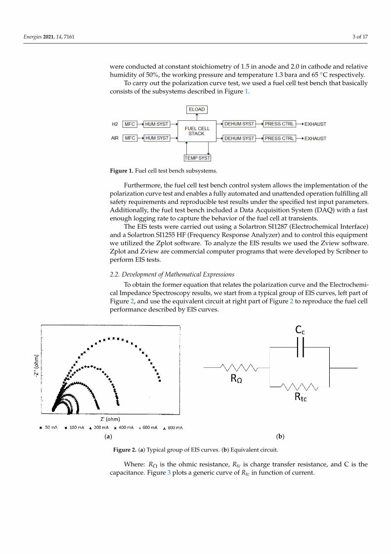
To carry out the polarization curve test, we used a fuel cell test bench that basicallyconsists of the subsystems described in Figure 1.

Energies 2021, 14, x FOR PEER REVIEW 3 of 17

2.1. Equipment and Test Methodology Descriptions In this work, we tested the nearest single cell to inlet gases of a short stack, which is

composed of six LT PEM cells with an active area of 170 cm2 each cell, and platinum based catalytic layer.

To obtain the experimental results, we performed a polarization curve test, carrying out an EIS test at every current step, once the voltage values will be steady. The experi-ments were conducted at constant stoichiometry of 1.5 in anode and 2.0 in cathode and relative humidity of 50%, the working pressure and temperature 1.3 bara and 65 °C re-spectively.

To carry out the polarization curve test, we used a fuel cell test bench that basically consists of the subsystems described in Figure 1.

Figure 1. Fuel cell test bench subsystems.

Furthermore, the fuel cell test bench control system allows the implementation of the polarization curve test and enables a fully automated and unattended operation fulfilling all safety requirements and reproducible test results under the specified test input param-eters. Additionally, the fuel test bench included a Data Acquisition System (DAQ) with a fast enough logging rate to capture the behavior of the fuel cell at transients.

The EIS tests were carried out using a Solartron SI1287 (Electrochemical Interface) and a Solartron SI1255 HF (Frequency Response Analyzer) and to control this equipment we utilized the Zplot software. To analyze the EIS results we used the Zview software. Zplot and Zview are commercial computer programs that were developed by Scribner to perform EIS tests.

2.2. Development of Mathematical Expressions To obtain the former equation that relates the polarization curve and the Electro-

chemical Impedance Spectroscopy results, we start from a typical group of EIS curves, left part of Figure 2, and use the equivalent circuit at right part of Figure 2 to reproduce the fuel cell performance described by EIS curves.

(a) (b)

Figure 2. (a) Typical group of EIS curves. (b) Equivalent circuit.

Figure 1. Fuel cell test bench subsystems.

Furthermore, the fuel cell test bench control system allows the implementation of thepolarization curve test and enables a fully automated and unattended operation fulfilling allsafety requirements and reproducible test results under the specified test input parameters.Additionally, the fuel test bench included a Data Acquisition System (DAQ) with a fastenough logging rate to capture the behavior of the fuel cell at transients.

The EIS tests were carried out using a Solartron SI1287 (Electrochemical Interface)and a Solartron SI1255 HF (Frequency Response Analyzer) and to control this equipmentwe utilized the Zplot software. To analyze the EIS results we used the Zview software.Zplot and Zview are commercial computer programs that were developed by Scribner toperform EIS tests.

2.2. Development of Mathematical Expressions

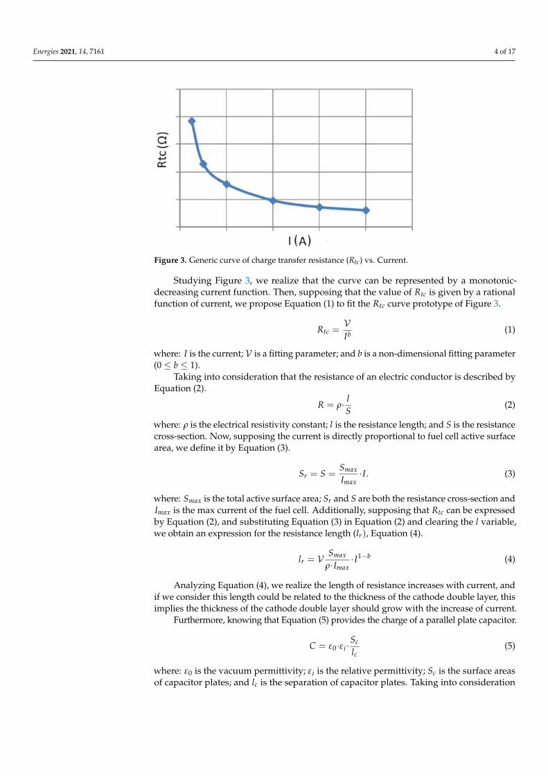
To obtain the former equation that relates the polarization curve and the Electrochemi-cal Impedance Spectroscopy results, we start from a typical group of EIS curves, left part ofFigure 2, and use the equivalent circuit at right part of Figure 2 to reproduce the fuel cellperformance described by EIS curves.

Energies 2021, 14, x FOR PEER REVIEW 3 of 17

2.1. Equipment and Test Methodology Descriptions In this work, we tested the nearest single cell to inlet gases of a short stack, which is

composed of six LT PEM cells with an active area of 170 cm2 each cell, and platinum based catalytic layer.

To obtain the experimental results, we performed a polarization curve test, carrying out an EIS test at every current step, once the voltage values will be steady. The experi-ments were conducted at constant stoichiometry of 1.5 in anode and 2.0 in cathode and relative humidity of 50%, the working pressure and temperature 1.3 bara and 65 °C re-spectively.

To carry out the polarization curve test, we used a fuel cell test bench that basically consists of the subsystems described in Figure 1.

Figure 1. Fuel cell test bench subsystems.

Furthermore, the fuel cell test bench control system allows the implementation of the polarization curve test and enables a fully automated and unattended operation fulfilling all safety requirements and reproducible test results under the specified test input param-eters. Additionally, the fuel test bench included a Data Acquisition System (DAQ) with a fast enough logging rate to capture the behavior of the fuel cell at transients.

The EIS tests were carried out using a Solartron SI1287 (Electrochemical Interface) and a Solartron SI1255 HF (Frequency Response Analyzer) and to control this equipment we utilized the Zplot software. To analyze the EIS results we used the Zview software. Zplot and Zview are commercial computer programs that were developed by Scribner to perform EIS tests.

2.2. Development of Mathematical Expressions To obtain the former equation that relates the polarization curve and the Electro-

chemical Impedance Spectroscopy results, we start from a typical group of EIS curves, left part of Figure 2, and use the equivalent circuit at right part of Figure 2 to reproduce the fuel cell performance described by EIS curves.

(a) (b)

Figure 2. (a) Typical group of EIS curves. (b) Equivalent circuit. Figure 2. (a) Typical group of EIS curves. (b) Equivalent circuit.

Where: RΩ is the ohmic resistance, Rtc is charge transfer resistance, and C is thecapacitance. Figure 3 plots a generic curve of Rtc in function of current.

Energies 2021, 14, 7161 4 of 17

Energies 2021, 14, x FOR PEER REVIEW 4 of 17

Where: RΩ is the ohmic resistance, Rtc is charge transfer resistance, and C is the capac-itance. Figure 3 plots a generic curve of Rtc in function of current.

Figure 3. Generic curve of charge transfer resistance (Rtc) vs Current.

Studying Figure 3, we realize that the curve can be represented by a monotonic-de-creasing current function. Then, supposing that the value of 𝑅 is given by a rational function of current, we propose Equation (1) to fit the 𝑅 curve prototype of Figure 3.

𝑅 =𝒱

𝐼 (1)

where: 𝐼 is the current; 𝒱 is a fitting parameter; and 𝑏 is a non-dimensional fitting pa-rameter (0 ≤ b ≤ 1).

Taking into consideration that the resistance of an electric conductor is described by Equation (2).

𝑅 = 𝜌 ·𝑙

𝑆 (2)

where: 𝜌 is the electrical resistivity constant; 𝑙 is the resistance length; and 𝑆 is the re-sistance cross-section. Now, supposing the current is directly proportional to fuel cell ac-tive surface area, we define it by Equation (3).

𝑆 = 𝑆 =𝑆

𝐼· 𝐼 (3)

where: 𝑆 is the total active surface area; 𝑆 and 𝑆 are both the resistance cross-sec-tion and 𝐼 is the max current of the fuel cell. Additionally, supposing that 𝑅 can be expressed by Equation (2), and substituting Equation (3) in Equation (2) and clearing the 𝑙 variable, we obtain an expression for the resistance length (𝑙 ), Equation (4).

𝑙 = 𝒱𝑆

𝜌 · 𝐼· 𝐼 (4)

Analyzing Equation (4), we realize the length of resistance increases with current, and if we consider this length could be related to the thickness of the cathode double layer, this implies the thickness of the cathode double layer should grow with the increase of current.

Furthermore, knowing that Equation (5) provides the charge of a parallel plate ca-pacitor.

𝐶 = 𝜀 · 𝜀 ·𝑆

𝑙 (5)

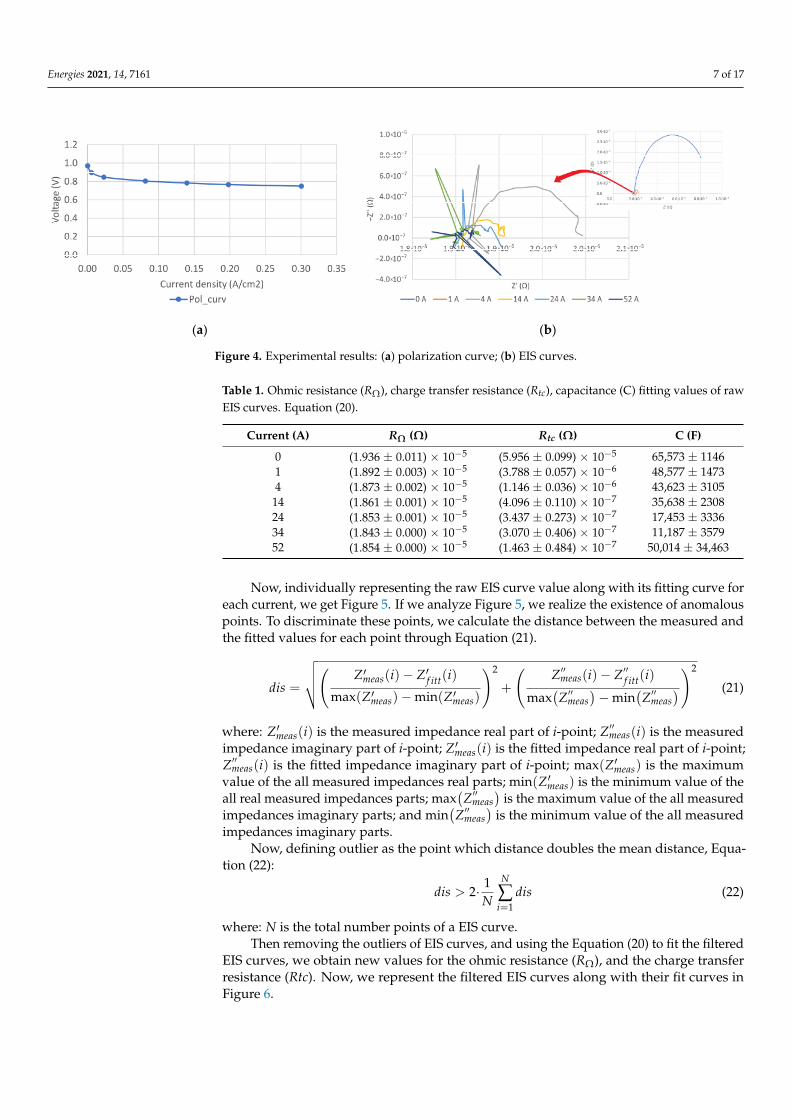
Figure 3. Generic curve of charge transfer resistance (Rtc) vs. Current.

Studying Figure 3, we realize that the curve can be represented by a monotonic-decreasing current function. Then, supposing that the value of Rtc is given by a rationalfunction of current, we propose Equation (1) to fit the Rtc curve prototype of Figure 3.

Rtc =VIb (1)

where: I is the current; V is a fitting parameter; and b is a non-dimensional fitting parameter(0 ≤ b ≤ 1).

Taking into consideration that the resistance of an electric conductor is described byEquation (2).

R = ρ· lS

(2)

where: ρ is the electrical resistivity constant; l is the resistance length; and S is the resistancecross-section. Now, supposing the current is directly proportional to fuel cell active surfacearea, we define it by Equation (3).

Sr = S =Smax

Imax·I. (3)

where: Smax is the total active surface area; Sr and S are both the resistance cross-section andImax is the max current of the fuel cell. Additionally, supposing that Rtc can be expressedby Equation (2), and substituting Equation (3) in Equation (2) and clearing the l variable,we obtain an expression for the resistance length (lr), Equation (4).

lr = VSmax

ρ·Imax·I1−b (4)

Analyzing Equation (4), we realize the length of resistance increases with current, andif we consider this length could be related to the thickness of the cathode double layer, thisimplies the thickness of the cathode double layer should grow with the increase of current.

Furthermore, knowing that Equation (5) provides the charge of a parallel plate capacitor.

C = ε0·εi·Sc

lc(5)

where: ε0 is the vacuum permittivity; εi is the relative permittivity; Sc is the surface areasof capacitor plates; and lc is the separation of capacitor plates. Taking into consideration

Energies 2021, 14, 7161 5 of 17

that the resistor (Rtc) and the capacitor (C) are in parallel, we make the hypothesis that lcand lr, and Sc and Sr are related by Equation (6).

lr = lcSc = Smax − Sr = Smax −Smax

Imax·I (6)

Therefore, combining Equations (4)–(6), we obtain an expression that describes thecapacitance behavior with current, Equation (7). This expression implies the capacitance iszero when I = Imax.

C = ε0·εiρ

V

(Imax

I− 1)·Ib (7)

Additionally, we know that Equation (8) gives the charge of a capacitor.

Q = Vcap·C (8)

where: Q is the charge; Vcap is the voltage; and C is the capacitance. Now, supposing thatthe charge of a capacitor should be proportional to its plate area, we can write Equation (9).

Q = K·(

Smax −Smax

Imax·I)

(9)

where: K is a constant of proportionality. Then, combining Equations (7)–(9), we obtain theEquation (10).

Vcap =K·Smax

ε0·εiV ρ

I1−b

Imax(10)

This voltage should correspond to the voltage drop caused by cathode activationoverpotential. In other words, the energy of activation overpotential is used to charge thecapacitor and this voltage loss grows with current.

Additionally, if we perform a dimensional analysis on Equation (10), we obtain that theexpression is dimensionally correct. As the units of parameters and variables are: K

(A·sm2

);

ε0( s

Ω·m); εi(dimensionless); ρ(Ω·m); Smax

(m2); V(Ω·Ab

); I(A); Imax(A); and Vcap(V).

Finally, supposing that Vcap corresponds to cathode activation overpotential, wepropose the Equation (11) as candidate to describe a fuel cell polarization curve.

V = V0 −CteImax·I1−b − r·I (11)

where: V is the voltage of fuel cell; V0 is the Open Circuit Voltage; and Cte = K·Smaxε0 ·εiV ρ

.

Using the Equation (11) to fit polarization curve test results, we get good results, butif we analyze the Equation (1), we realize that is not defined at I = 0 A, then to solve thisissue we propose to use Equation (12) to fit the Rtc curve prototype of Figure 3 instead ofEquation (1).

Rtc =V

Ib + d(12)

where: d is a fitting parameter. Then, using Equation (12) and operating as we did to obtainthe First Mathematical Expression, we get the Equation (13).

lr =V·Smax

ρ·Imax· IIb + d

(13)

Furthermore, if in this case we define lc as the addition of two magnitudes in order toavoid C tends to infinite, as lr → 0 when I → 0 .

lc = lr + ·l0 =V·Smax

ρ·Imax· IIb + d

+ l0 (14)

Energies 2021, 14, 7161 6 of 17

where: l0 is the separation of capacitor plates when I = 0; and the other magnitudes aredefined as usual. Then, combining Equations (5), (6), and (14), we obtain a new expressionto capacitance.

C = ε0·εi·SmaxImax

(Imax − I)V·Smaxρ·Imax

· IIb+d + l0

(15)

Now, solving the equation system (6), (8), and (15), we get a new expression tocapacitor voltage.

Vcap =QC

=K·Smax·V

ε0·εi·ρ·Imax

IIb + d

+K

ε0·εil0 (16)

If we analyze Equation (16), we can see l0 is an unknown variable, to obtain anexpression for l0 we substitute I = 0 in Equation (15) and clear l0. After that, replacing l0by this expression in Equation (15) and taking into consideration that Qmax = K·Smax, weobtain a new equation for Vcap where all variables and parameters are defined.

Vcap =K·Smax·V

ε0·εi·ρ·Imax

IIb + d

+K·Smax

C0=

K·Smax·Vε0·εi·ρ·Imax

IIb + d

+Qmax

C0(17)

where: Qmax is the maximum charge of the capacitor, C0 is the capacitance at I = 0, andthe other magnitudes are defined as usual. Furthermore, if we compare Equations (10) and(17), we can identify the first addend of the Equation (17) with Equation (10), or in otherwords, the first addend would correspond to the cathode activation overpotential, whilethe second addend is the values of Vcap when I = 0. Then, taking into consideration this,and operating as we did to derive Equation (11), we obtain a new equation to model a fuelcell polarization curve, and in this case, the new equation is defined in the whole range ofcurrents.

V = VNERNST −Qmax

C0− K·Smax·V

ε0·εi·ρ·Imax

IIb + d

− r·I (18)

where: VNERST is the Nernst equation voltage. Additionally, if we group terms, we willobtain Equation (19), which is equal to Equation (11) except for the parameter d.

V = V0 −CteImax

IIb + d

− r·I (19)

3. Results

At this point, we apply polarization curve and EIS tests on a single cell of the Short-Stack of FLHYSAFE project. This cell was located at the extreme of the Short-Stack next tothe entrance of gases. Using the presented methodology we explain in detail how to relatethe results of both tests and extract internal information from the tested cell.

Firstly, we performed a polarization curve test and for each current step we carriedout an EIS test, once the standard deviation of the last 10 voltage measurement was lessthan 1%, this is the criteria that we used to establish the fuel cell behavior was steady andstable. The results of these tests appear in Figure 4.

As can be seen, all EIS curves are represented in in (b) Figure 4, but as the EIS curveat Open Circuit Value (OCV) is much bigger in comparison to the rest, we zoom the EIScurves from I = 4 A to I = 52 A. Now, using the Zwiev software we fit each one of theEIS curves with the Equation (20) in order to extract the ohmic resistance (RΩ), and thecharge transfer resistance (Rtc), these values are collected in Table 1. The Equation (20) isthe mathematical transposition of the equivalent circuit of Figure 2b.

ZT = RΩ +Rtc

1 + ω2·R2tc·C2

− ω·R2tc·C

1 + ω2·R2tc·C2

·i (20)

where: ω = 2·π· f and f is the frequency of EIS stimulus.

Energies 2021, 14, 7161 7 of 17Energies 2021, 14, x FOR PEER REVIEW 7 of 17

(a) (b)

Figure 4. Experimental results: (a) polarization curve; (b) EIS curves.

As can be seen, all EIS curves are represented in in (b) Figure 4, but as the EIS curve at Open Circuit Value (OCV) is much bigger in comparison to the rest, we zoom the EIS curves from I = 4 A to I = 52 A. Now, using the Zwiev software we fit each one of the EIS curves with the Equation (20) in order to extract the ohmic resistance (RΩ), and the charge transfer resistance (Rtc), these values are collected in Table 1. The Equation (20) is the math-ematical transposition of the equivalent circuit of Figure 2b.

𝑍 = 𝑅 +𝑅

1 + 𝜔 · 𝑅 · 𝐶−

𝜔 · 𝑅 · 𝐶

1 + 𝜔 · 𝑅 · 𝐶· 𝑖 (20)

where: 𝜔 = 2 · 𝜋 · 𝑓 and 𝑓 is the frequency of EIS stimulus.

Table 1. Ohmic resistance (RΩ), charge transfer resistance (Rtc), capacitance (C) fitting values of raw EIS curves. Equation (20).

Current (A) RΩ (Ω) Rtc (Ω) C (F) 0 (1.936 ± 0.011) × 10−5 (5.956 ± 0.099) × 10−5 65,573 ± 1146 1 (1.892 ± 0.003) × 10−5 (3.788 ± 0.057) × 10−6 48,577 ± 1473 4 (1.873 ± 0.002) × 10−5 (1.146 ± 0.036) × 10−6 43,623 ± 3105

14 (1.861 ± 0.001) × 10−5 (4.096 ± 0.110) × 10−7 35,638 ± 2308 24 (1.853 ± 0.001) × 10−5 (3.437 ± 0.273) × 10−7 17,453 ± 3336 34 (1.843 ± 0.000) × 10−5 (3.070 ± 0.406) × 10−7 11,187 ± 3579 52 (1.854 ± 0.000) × 10−5 (1.463 ± 0.484) × 10−7 50,014 ± 34,463

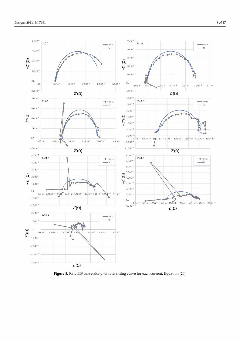
Now, individually representing the raw EIS curve value along with its fitting curve for each current, we get Figure 5. If we analyze Figure 5, we realize the existence of anom-alous points. To discriminate these points, we calculate the distance between the meas-ured and the fitted values for each point through Equation (21).

𝑑𝑖𝑠 =𝑍 (𝑖) − 𝑍 (𝑖)

max(𝑍 ) − min(𝑍 )+

𝑍 (𝑖) − 𝑍 (𝑖)

max(𝑍 ) − min(𝑍 ) (21)

where: 𝑍 (𝑖) is the measured impedance real part of i-point; 𝑍 (𝑖) is the measured impedance imaginary part of i-point; 𝑍 (𝑖) is the fitted impedance real part of i-point; 𝑍 (𝑖) is the fitted impedance imaginary part of i-point; max(𝑍 ) is the maximum value of the all measured impedances real parts; min(𝑍 ) is the minimum value of the all real measured impedances parts; max(𝑍 ) is the maximum value of the all meas-ured impedances imaginary parts; and min(𝑍 ) is the minimum value of the all meas-ured impedances imaginary parts.

Figure 4. Experimental results: (a) polarization curve; (b) EIS curves.

Table 1. Ohmic resistance (RΩ), charge transfer resistance (Rtc), capacitance (C) fitting values of rawEIS curves. Equation (20).

Current (A) RΩ (Ω) Rtc (Ω) C (F)

0 (1.936 ± 0.011) × 10−5 (5.956 ± 0.099) × 10−5 65,573 ± 11461 (1.892 ± 0.003) × 10−5 (3.788 ± 0.057) × 10−6 48,577 ± 14734 (1.873 ± 0.002) × 10−5 (1.146 ± 0.036) × 10−6 43,623 ± 310514 (1.861 ± 0.001) × 10−5 (4.096 ± 0.110) × 10−7 35,638 ± 230824 (1.853 ± 0.001) × 10−5 (3.437 ± 0.273) × 10−7 17,453 ± 333634 (1.843 ± 0.000) × 10−5 (3.070 ± 0.406) × 10−7 11,187 ± 357952 (1.854 ± 0.000) × 10−5 (1.463 ± 0.484) × 10−7 50,014 ± 34,463

Now, individually representing the raw EIS curve value along with its fitting curve foreach current, we get Figure 5. If we analyze Figure 5, we realize the existence of anomalouspoints. To discriminate these points, we calculate the distance between the measured andthe fitted values for each point through Equation (21).

dis =

√√√√( Z′meas(i)− Z′f itt(i)

max(Z′meas)−min(Z′meas)

)2

+

(Z′′meas(i)− Z′′f itt(i)

max(Z′′meas

)−min

(Z′′meas

))2

(21)

where: Z′meas(i) is the measured impedance real part of i-point; Z′′meas(i) is the measuredimpedance imaginary part of i-point; Z′meas(i) is the fitted impedance real part of i-point;Z′′meas(i) is the fitted impedance imaginary part of i-point; max(Z′meas) is the maximumvalue of the all measured impedances real parts; min(Z′meas) is the minimum value of theall real measured impedances parts; max

(Z′′meas

)is the maximum value of the all measured

impedances imaginary parts; and min(Z′′meas

)is the minimum value of the all measured

impedances imaginary parts.Now, defining outlier as the point which distance doubles the mean distance, Equa-

tion (22):

dis > 2· 1N

N

∑i=1

dis (22)

where: N is the total number points of a EIS curve.Then removing the outliers of EIS curves, and using the Equation (20) to fit the filtered

EIS curves, we obtain new values for the ohmic resistance (RΩ), and the charge transferresistance (Rtc). Now, we represent the filtered EIS curves along with their fit curves inFigure 6.

Energies 2021, 14, 7161 8 of 17

Energies 2021, 14, x FOR PEER REVIEW 8 of 17

Now, defining outlier as the point which distance doubles the mean distance, Equa-tion (22):

𝑑𝑖𝑠 > 2 ·1

𝑁𝑑𝑖𝑠 (22)

where: N is the total number points of a EIS curve.

Figure 5. Raw EIS curve along with its fitting curve for each current. Equation (20). Figure 5. Raw EIS curve along with its fitting curve for each current. Equation (20).

Energies 2021, 14, 7161 9 of 17

Energies 2021, 14, x FOR PEER REVIEW 9 of 17

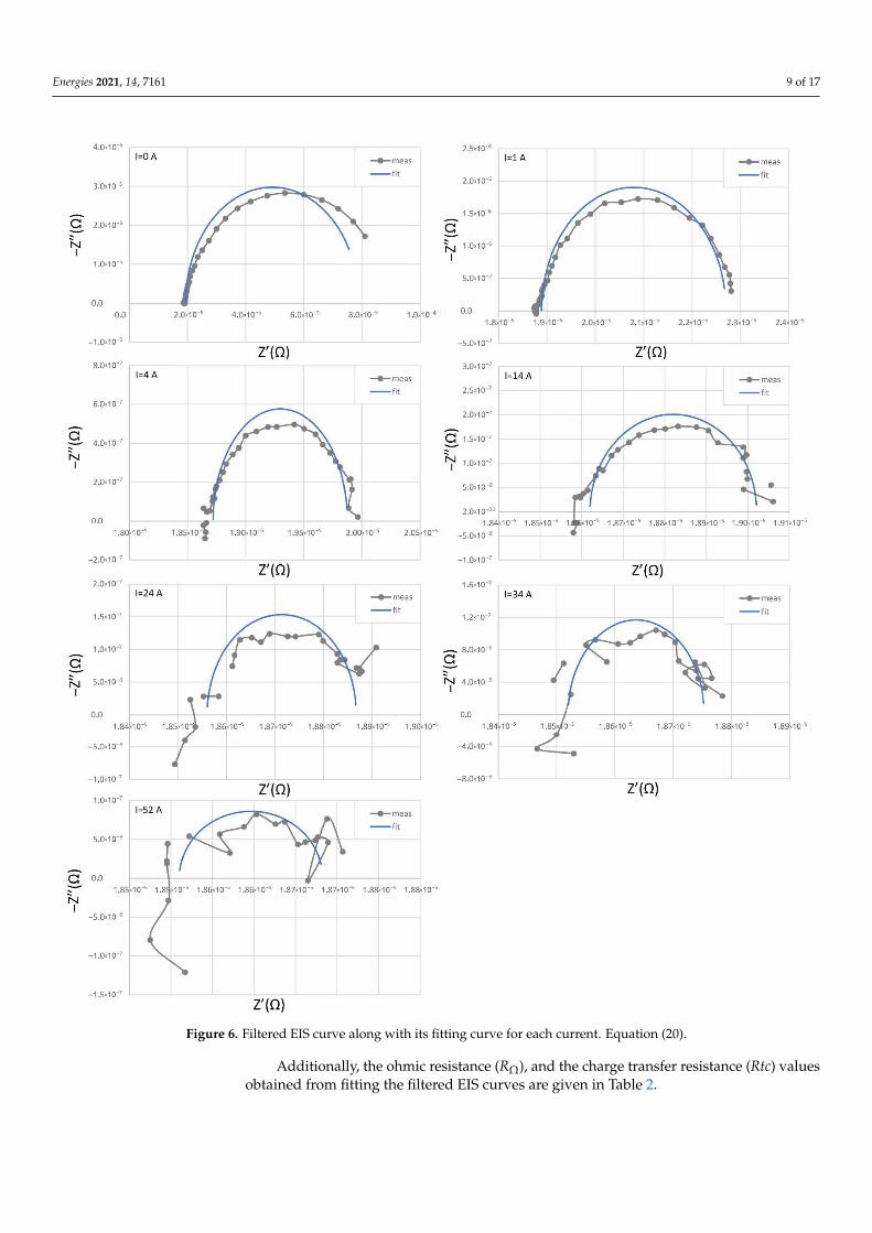
Then removing the outliers of EIS curves, and using the Equation (20) to fit the fil-tered EIS curves, we obtain new values for the ohmic resistance (RΩ), and the charge trans-fer resistance (Rtc). Now, we represent the filtered EIS curves along with their fit curves in Figure 6.

Figure 6. Filtered EIS curve along with its fitting curve for each current. Equation (20). Figure 6. Filtered EIS curve along with its fitting curve for each current. Equation (20).

Additionally, the ohmic resistance (RΩ), and the charge transfer resistance (Rtc) valuesobtained from fitting the filtered EIS curves are given in Table 2.

Energies 2021, 14, 7161 10 of 17

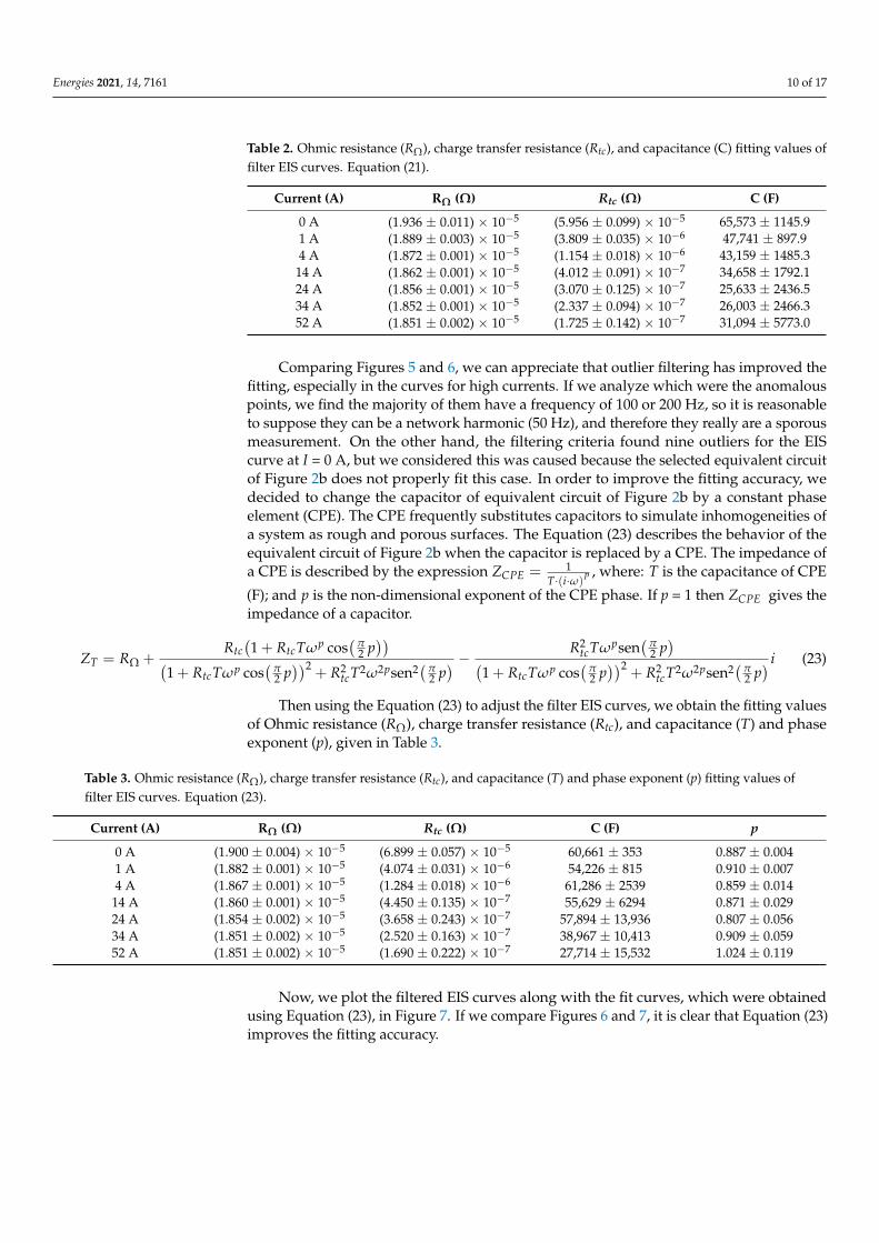
Table 2. Ohmic resistance (RΩ), charge transfer resistance (Rtc), and capacitance (C) fitting values offilter EIS curves. Equation (21).

Current (A) RΩ (Ω) Rtc (Ω) C (F)

0 A (1.936 ± 0.011) × 10−5 (5.956 ± 0.099) × 10−5 65,573 ± 1145.91 A (1.889 ± 0.003) × 10−5 (3.809 ± 0.035) × 10−6 47,741 ± 897.94 A (1.872 ± 0.001) × 10−5 (1.154 ± 0.018) × 10−6 43,159 ± 1485.3

14 A (1.862 ± 0.001) × 10−5 (4.012 ± 0.091) × 10−7 34,658 ± 1792.124 A (1.856 ± 0.001) × 10−5 (3.070 ± 0.125) × 10−7 25,633 ± 2436.534 A (1.852 ± 0.001) × 10−5 (2.337 ± 0.094) × 10−7 26,003 ± 2466.352 A (1.851 ± 0.002) × 10−5 (1.725 ± 0.142) × 10−7 31,094 ± 5773.0

Comparing Figures 5 and 6, we can appreciate that outlier filtering has improved thefitting, especially in the curves for high currents. If we analyze which were the anomalouspoints, we find the majority of them have a frequency of 100 or 200 Hz, so it is reasonableto suppose they can be a network harmonic (50 Hz), and therefore they really are a sporousmeasurement. On the other hand, the filtering criteria found nine outliers for the EIScurve at I = 0 A, but we considered this was caused because the selected equivalent circuitof Figure 2b does not properly fit this case. In order to improve the fitting accuracy, wedecided to change the capacitor of equivalent circuit of Figure 2b by a constant phaseelement (CPE). The CPE frequently substitutes capacitors to simulate inhomogeneities ofa system as rough and porous surfaces. The Equation (23) describes the behavior of theequivalent circuit of Figure 2b when the capacitor is replaced by a CPE. The impedance ofa CPE is described by the expression ZCPE = 1

T·(i·ω)P , where: T is the capacitance of CPE

(F); and p is the non-dimensional exponent of the CPE phase. If p = 1 then ZCPE gives theimpedance of a capacitor.

ZT = RΩ +Rtc(1 + RtcTωp cos

(π2 p))(

1 + RtcTωp cos(

π2 p))2

+ R2tcT2ω2psen2

(π2 p) − R2

tcTωpsen(

π2 p)(

1 + RtcTωp cos(

π2 p))2

+ R2tcT2ω2psen2

(π2 p) i (23)

Then using the Equation (23) to adjust the filter EIS curves, we obtain the fitting valuesof Ohmic resistance (RΩ), charge transfer resistance (Rtc), and capacitance (T) and phaseexponent (p), given in Table 3.

Table 3. Ohmic resistance (RΩ), charge transfer resistance (Rtc), and capacitance (T) and phase exponent (p) fitting values offilter EIS curves. Equation (23).

Current (A) RΩ (Ω) Rtc (Ω) C (F) p

0 A (1.900 ± 0.004) × 10−5 (6.899 ± 0.057) × 10−5 60,661 ± 353 0.887 ± 0.0041 A (1.882 ± 0.001) × 10−5 (4.074 ± 0.031) × 10−6 54,226 ± 815 0.910 ± 0.0074 A (1.867 ± 0.001) × 10−5 (1.284 ± 0.018) × 10−6 61,286 ± 2539 0.859 ± 0.014

14 A (1.860 ± 0.001) × 10−5 (4.450 ± 0.135) × 10−7 55,629 ± 6294 0.871 ± 0.02924 A (1.854 ± 0.002) × 10−5 (3.658 ± 0.243) × 10−7 57,894 ± 13,936 0.807 ± 0.05634 A (1.851 ± 0.002) × 10−5 (2.520 ± 0.163) × 10−7 38,967 ± 10,413 0.909 ± 0.05952 A (1.851 ± 0.002) × 10−5 (1.690 ± 0.222) × 10−7 27,714 ± 15,532 1.024 ± 0.119

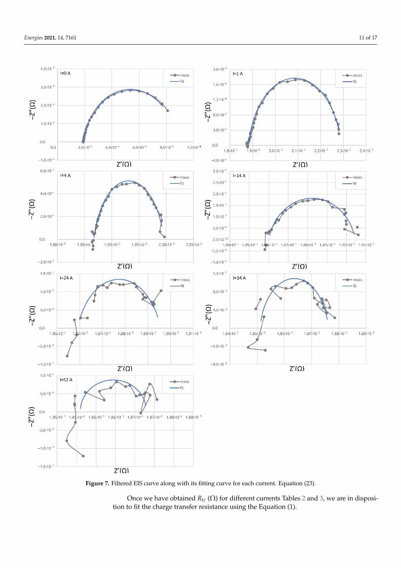
Now, we plot the filtered EIS curves along with the fit curves, which were obtainedusing Equation (23), in Figure 7. If we compare Figures 6 and 7, it is clear that Equation (23)improves the fitting accuracy.

Energies 2021, 14, 7161 11 of 17Energies 2021, 14, x FOR PEER REVIEW 11 of 17

Figure 7. Filtered EIS curve along with its fitting curve for each current. Equation (23).

Once we have obtained Rtc (Ω) for different currents Tables 2 and 3, we are in dispo-sition to fit the charge transfer resistance using the Equation (1).

Equivalent circuit with capacitor:

Figure 7. Filtered EIS curve along with its fitting curve for each current. Equation (23).

Once we have obtained Rtc (Ω) for different currents Tables 2 and 3, we are in disposi-tion to fit the charge transfer resistance using the Equation (1).

Energies 2021, 14, 7161 12 of 17

Equivalent circuit with capacitor:

Rtc(I) = 3.89876·10−6·I−0.83986 ; 〈errrel〉 = 10% (24)

Equivalent circuit with CPE:

Rtc(I) = 4.16959·10−6·I−0.81909 ; 〈errrel〉 = 7% (25)

〈errrel〉 is the mean relative error, defined by Equation (26).

〈errrel〉 =∑N

i=1|xi_meass−xi_ f itt|

xi_meass

N(26)

where xi_meass are measured values, and xi_ f itt are fitting values. To calculate the mean rela-tive error for Equations (25) and (26) the value of Rtc at 0 A was not taken in consideration,as Equation (1) is not defined for this current.

Now, substituting the values of the charge transfer resistance fitted parameters inEquation (11) and adjusting this expression to polarization curve of Figure 4a, we obtainthe following fitted Equations (27) and (28).

Equivalent circuit with capacitor:

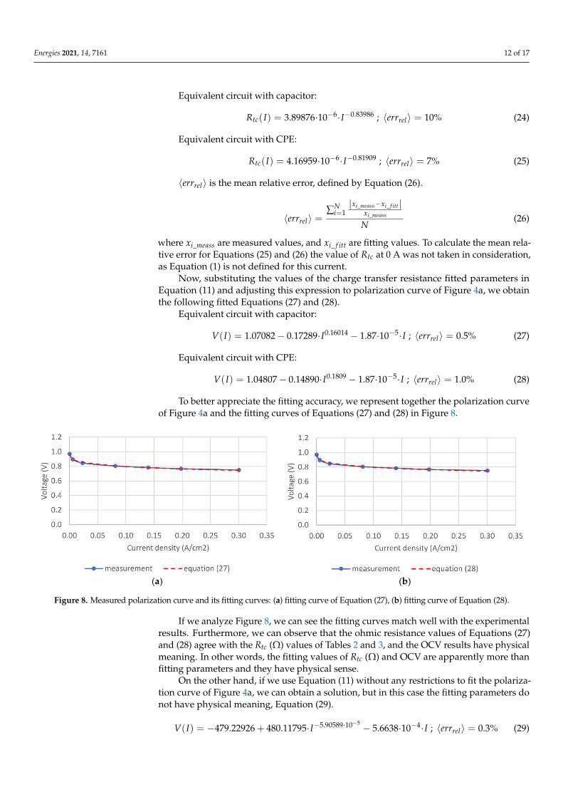
V(I) = 1.07082− 0.17289·I0.16014 − 1.87·10−5·I ; 〈errrel〉 = 0.5% (27)

Equivalent circuit with CPE:

V(I) = 1.04807− 0.14890·I0.1809 − 1.87·10−5·I ; 〈errrel〉 = 1.0% (28)

To better appreciate the fitting accuracy, we represent together the polarization curveof Figure 4a and the fitting curves of Equations (27) and (28) in Figure 8.

Energies 2021, 14, x FOR PEER REVIEW 12 of 17

𝑅 (𝐼) = 3.89876 · 10 · 𝐼 . ; < 𝑒𝑟𝑟 >= 10% (24)

Equivalent circuit with CPE:

𝑅 (𝐼) = 4.16959 · 10 · 𝐼 . ; < 𝑒𝑟𝑟 >= 7% (25)

< 𝑒𝑟𝑟 > is the mean relative error, defined by Equation (26).

< 𝑒𝑟𝑟 >=

∑𝑥 _ − 𝑥 _

𝑥 _

𝑁

(26)

where 𝑥 _ are measured values, and 𝑥 _ are fitting values. To calculate the mean relative error for Equations (25) and (26) the value of 𝑅 at 0A was not taken in consid-eration, as Equation (1) is not defined for this current.

Now, substituting the values of the charge transfer resistance fitted parameters in Equation (11) and adjusting this expression to polarization curve of Figure 4a, we obtain the following fitted Equations (27) and (28).

Equivalent circuit with capacitor:

𝑉(𝐼) = 1.07082 − 0.17289 · 𝐼 . − 1.87 · 10 · 𝐼 ; < 𝑒𝑟𝑟 >= 0.5% (27)

Equivalent circuit with CPE:

𝑉(𝐼) = 1.04807 − 0.14890 · 𝐼 . − 1.87 · 10 · 𝐼 ; < 𝑒𝑟𝑟 >= 1.0% (28)

To better appreciate the fitting accuracy, we represent together the polarization curve of Figure 4a and the fitting curves of Equations (27) and (28) in Figure 8.

(a) (b)

Figure 8. Measured polarization curve and its fitting curves: (a) fitting curve of Equation (27), (b) fitting curve of Equation (28).

If we analyze Figure 8, we can see the fitting curves match well with the experimental results. Furthermore, we can observe that the ohmic resistance values of Equations (27) and (28) agree with the Rtc (Ω) values of Tables 2 and 3, and the OCV results have physical meaning. In other words, the fitting values of Rtc (Ω) and OCV are apparently more than fitting parameters and they have physical sense.

On the other hand, if we use Equation (11) without any restrictions to fit the polari-zation curve of Figure 4a, we can obtain a solution, but in this case the fitting parameters do not have physical meaning, Equation (29).

𝑉(𝐼) = −479.22926 + 480.11795 · 𝐼 . · − 5.6638 · 10 · 𝐼 ; < 𝑒𝑟𝑟 >= 0.3% (29)

Now, repeating the previous process, but using Equation (12) to fit the charge trans-fer resistance of Tables 2 and 3, we obtain the following expressions.

Equivalent circuit with capacitor:

Figure 8. Measured polarization curve and its fitting curves: (a) fitting curve of Equation (27), (b) fitting curve of Equation (28).

If we analyze Figure 8, we can see the fitting curves match well with the experimentalresults. Furthermore, we can observe that the ohmic resistance values of Equations (27)and (28) agree with the Rtc (Ω) values of Tables 2 and 3, and the OCV results have physicalmeaning. In other words, the fitting values of Rtc (Ω) and OCV are apparently more thanfitting parameters and they have physical sense.

On the other hand, if we use Equation (11) without any restrictions to fit the polariza-tion curve of Figure 4a, we can obtain a solution, but in this case the fitting parameters donot have physical meaning, Equation (29).

V(I) = −479.22926 + 480.11795·I−5.90589·10−5 − 5.6638·10−4·I ; 〈errrel〉 = 0.3% (29)

Energies 2021, 14, 7161 13 of 17

Now, repeating the previous process, but using Equation (12) to fit the charge transferresistance of Tables 2 and 3, we obtain the following expressions.

Equivalent circuit with capacitor:

Rtc(I) =4.05848·10−6·

I0.86405 + 0.06814; 〈errrel〉 = 9% (30)

Equivalent circuit with CPE:

Rtc(I) =4.32066·10−6·

I0.84039 + 0.06263; 〈errrel〉 = 8% (31)

Then, using the Rtc parameterization, and fitting the polarization curve of Figure 4awith Equation (18), we get two expressions for fuel cell voltage.

Equivalent circuit with capacitor:

V(I) = 1.03676− 0.16459· II0.86405 + 0.06814

− 1.87·10−5·I 〈errrel〉 = 0.6% (32)

Equivalent circuit with CPE:

V(I) = 1.02569− 0.14626· II0.84039 + 0.06263

− 1.87·10−5·I 〈errrel〉 = 0.3% (33)

Carrying on as before, we plot together the polarization curve of Figure 4a and thefitting curves of Equations (32) and (33) in Figure 9.

Energies 2021, 14, x FOR PEER REVIEW 13 of 17

𝑅 (𝐼) =. · ·

. . ; < 𝑒𝑟𝑟 >= 9% (30)

Equivalent circuit with CPE:

𝑅 (𝐼) =. · ·

. . ; < 𝑒𝑟𝑟 >= 8% (31)

Then, using the 𝑅 parameterization, and fitting the polarization curve of Figure 4a with Equation (18), we get two expressions for fuel cell voltage.

Equivalent circuit with capacitor:

𝑉(𝐼) = 1.03676 − 0.16459 · . .− 1.87 · 10 · 𝐼 ; < 𝑒𝑟𝑟 >= 0.6% (32)

Equivalent circuit with CPE:

𝑉(𝐼) = 1.02569 − 0.14626 · . .− 1.87 · 10 · 𝐼 ; < 𝑒𝑟𝑟 >= 0.3% (33)

Carrying on as before, we plot together the polarization curve of Figure 4a and the fitting curves of Equations (32) and (33) in Figure 9.

(a) (b)

Figure 9. Measured polarization curve and its fitting curves: (a) fitting curve of Equation (31); (b) fitting curve of Equation (32).

Now, assessing the fitting accuracy of Equations (11) and (18) to adjust a polarization curve of a fuel cell, we can see that both of them match well, and none of them does sig-nificantly better than the other. However, Equation (18) is defined in all ranges of current and provides extra information.

Then, the results of the equivalent circuit with CPE are selected arbitrarily, as repeti-tion of the analysis process with the results of the equivalent circuit with capacitor does not provide any extra information. We can see that Equation (18) predicts the existence of a kind of current value when the load demand is zero. The parameter 𝑑 can be written as 𝑑 = 𝐼 , , then clearing 𝐼 we obtain, 𝐼 = 0 .037 A. The experimental equipment measured 0.05 A when there was no power demand.

4. Discussion In this article, we present a new methodology that allows us to relate the results of

polarization curve tests with the EIS tests. Each test provides different information of the same reality, so it is expected that the correct combination of them could provide a more complete vision of the physical phenomena that occurs inside the fuel cell.

This methodology is based on Equation (11) or Equation (18), the second one is an evolution of the first. Once they have been partially parametrized using the EIS results, they fit well with the experimental results of polarization curve tests, and the fitting pa-rameters have physical meaning. Conversely, when the selected equation does not have restrictions, we can obtain a good fitting curve too, but in this case, the fitting parameter

Figure 9. Measured polarization curve and its fitting curves: (a) fitting curve of Equation (31); (b) fitting curve of Equation (32).

Now, assessing the fitting accuracy of Equations (11) and (18) to adjust a polarizationcurve of a fuel cell, we can see that both of them match well, and none of them doessignificantly better than the other. However, Equation (18) is defined in all ranges ofcurrent and provides extra information.

Then, the results of the equivalent circuit with CPE are selected arbitrarily, as repetitionof the analysis process with the results of the equivalent circuit with capacitor does notprovide any extra information. We can see that Equation (18) predicts the existence ofa kind of current value when the load demand is zero. The parameter d can be writtenas d = I0

0,84039, then clearing I0 we obtain, I0 = 0.037 A. The experimental equipmentmeasured 0.05 A when there was no power demand.

4. Discussion

In this article, we present a new methodology that allows us to relate the results ofpolarization curve tests with the EIS tests. Each test provides different information of the

Energies 2021, 14, 7161 14 of 17

same reality, so it is expected that the correct combination of them could provide a morecomplete vision of the physical phenomena that occurs inside the fuel cell.

This methodology is based on Equation (11) or Equation (18), the second one is anevolution of the first. Once they have been partially parametrized using the EIS results, theyfit well with the experimental results of polarization curve tests, and the fitting parametershave physical meaning. Conversely, when the selected equation does not have restrictions,we can obtain a good fitting curve too, but in this case, the fitting parameter has no physicalmeaning. Therefore the hypothesis that we established to derive the equations could becorrect, and they can capture the physical processes that happen inside the fuel cell. If thisis right, we have developed a model that pretends to describe the dynamic of the doublelayer, establishing a link between the elements of Figure 4b. In other words, the variationsof the resistance affects the capacitance and vice versa.

According to this model, Equation (6) describes the coupling laws between capacitorand resistor, if Equation (11) is selected to describe the fuel cell voltage dependence withcurrent. If not, the relation between the length of resistance and the distance of capacitorparallel plates is defined by Equation (14). In any case, these coupling laws say that thevariations of lengths are equal ∆lr = ∆lc and the variations of surface areas are the opposite∆Sr = −∆Sc.

Now, taking into consideration Equation (4), the lengths are related to the thickness ofthe double layer, the model says this grows with current.

Concerning surface areas, we know that Equations (1) and (12) are rational functionsand both indicate the resistance decreases with current but lr increases—this implies thatactive surface area or in other words the resistance surface area Sr grows fast enough tocompensate the lr increase. This could point out that total charge transfer resistance is thesum of parallel resistances of the ionic current paths that go through the double layer, andthe number grows with the increase of current. This is expressed by Equations (34) and (35):

1RT

=1

R1+

1R2

+ · · ·+ 1Rn→ 1

RT=

R2·R3 · · · Rn + R1·R3···Rn + · · ·+ R1·R2···Rn−1

R1·R2 · · · Rn(34)

where: RT is the total charge transfer resistance, and Ri is the resistance of i-th ioniccurrent path. Now, considering that R1 = R2 = · · · = Rn without loss of generality, weobtain a rational function for total charge transfer resistance that decreases with current:

1RT

=n·Rn−1

Rn → RT =Rn→ RT =

Rn(I)

(35)

Additionally, the model expresses that the double layer surface should be equalto Smax = Sr + Sc and Smax is constant, so if Sr increases with current, this means thatSc decreases. Then, taking into consideration this, and that lc grows with current, weobtain that capacitance should decrease with current, as it usually does according to theexperimental results of Tables 2 and 3, but not always. The discrepancy between resultsand this conclusion must be studied in detail, to determine its causes.

On the other hand, it is necessary to note the novelty of the research, and that it wasnot supported by a large number of results. Nowadays, this methodology has been appliedin nine cases, obtaining positive results in all cases. We continue checking the methodologyand improving the models.

5. Conclusions

In this section, we pretend to summarize the most important findings. Basically, inthis research, we have obtained two prototypes of Equations (11) and (18), that can describethe behavior of an experimental polarization curve with a mean relative error inferior to1%, and when the parameter b is obtained from using one of the previously described

Energies 2021, 14, 7161 15 of 17

methodologies, the values of other fitting parameters have physical meaning, allowing usto write:

V0 = VNERST −Qmax

C0(36)

where V0 is the Open Circuit Voltage, VNERST is the Nernst Voltage and C0 is the capacitanceat I = 0 A. Equation (36) implies the loss of voltage at I = 0 A is mainly caused by theformation of the double layer in cathode interface region and provides an easy way toquantify the charge of the double layer when the load is zero.

Additionally, Equation (18) provides an expression for the cathode overpotential ηcathtoo, Equation (37).

ηcath =K·Smax·V

ε0·εi·ρ·Imax

IIb + d

(37)

Equation (37) shows the cathode overpotential presents dependence with the permit-tivity and the resistivity of the cathode interface, and this expression can be used to obtainhow the variation of the permittivity and the resistivity affects the cathode overpotential,and maybe this could be used to improve fuel cell technology.

Author Contributions: Conceptualization, G.G.; methodology, G.G.; validation, G.G.; formal analy-sis, G.G.; investigation, G.G. and A.C.; resources, J.M.; data curation, G.G.; writing—original draftpreparation, G.G.; writing—review and editing, G.G., P.A., A.C. and J.M.; visualization, G.G.; super-vision, J.M. and P.A.; project administration, P.A.; funding acquisition, P.A. and J.M. All authors haveread and agreed to the published version of the manuscript.

Funding: This research received no external funding.

Institutional Review Board Statement: Not applicable. This study does not involve humans oranimals.

Informed Consent Statement: Not applicable. This study does not involve humans.

Acknowledgments: This research was developed at INTA using the experimental results of FL-HYSAFE Project. Funded by the Fuel Cells and Hydrogen 2 Joint Undertaking under the EuropeanHorizon2020 Framework Programme for Research and Innovation (GANo779576).

Conflicts of Interest: The authors declare no conflict of interest.

Abbreviations

EU European UnionFLHYSAFE Fuel celL HYdrogen System for AircraFt EmergencyEIS Electrochemical Impedance SpectroscopyMFC Mass Flow ControllerHUM SYST Humidification SystemDEHUM SYST Dehumidification SystemPRESS CTRL Pressure Control SystemTEMP SYST Working Temperature Control SystemELOAD Electric LoadDAQ Data Acquisition SystemRtc Charge transfer resistance (Ω)I Current (A)V Fitting parameter (ΩAb)b Fitting parameter (0 ≤ b ≤ 1).ρ Electrical resistivity (Ωm)Sr Resistance cross-section (m2)lr Resistance length (m)Smax Total active surface area (m2)Imax Maximum current of fuel cell (A)ε0 Vacuum permittivity (Fm−1)

Energies 2021, 14, 7161 16 of 17

εi Relative permittivitySc Surface area of capacitor plates (m2)lc Separation of capacitor plates (m)Q Charge of capacitor (C)C Capacitance (F)Vcap Voltage of capacitor (V)K Constant of proportionality (Asm−2)V Fuel cell voltage (V)V0 Open Circuit Voltage (V)d Fitting parameter (Ab)l0 Separation of capacitor plates at I = 0 A (m)C0 Capacitance at I = 0 A (F)VNERST Nernst equation voltage (V)ηcath Cathode overpotential (V)

References1. Powell, J. Scientists Reach 100% Consensus on Anthropogenic Global Warming. Bull. Sci. Technol. Soc. 2017, 37, 183–184.

[CrossRef]2. Cook, J.; Nuccitelli, D.; Green, S.A.; Richardson, M.; Winkler, B.; Painting, R.; Way, R.; Jacobs, P.; Skuce, A. Quantifying the

consensus on anthropogenic global warming in the scientific literature. Environ. Res. Lett. 2013, 8, 024024. [CrossRef]3. Anderegg, W.R.L.; Prall, J.W.; Harold, J.; Schneider, S.H. Expert credibility in climate change. Proc. Natl. Acad. Sci. USA 2010, 107,

12107–12109. [CrossRef]4. Cars, Planes, Trains: Where do CO2 Emissions from Transport Come from? Available online: https://ourworldindata.org/co2

-emissions-from-transport (accessed on 1 August 2021).5. Fuel celL HYdrogen System for AircraFt Emergency Operation. Available online: https://www.flhysafe.eu/ (accessed on 1

August 2021).6. de Moor, G.; Bas, C.; Chavin, N.; Moukheiber, E.; Niepceron, F.; Breilly, N.; André, J.; Rossinot, E.; Claude, E.; Albérola, N.D.; et al.

Understanding Membrane Failure in PEMFC: Comparison of Diagnostic Tools at Different Observation Scales. Fuel Cells 2012, 12,356–364. [CrossRef]

7. Zheng, Z.; Petrone, R.; Péra, M.C.; Hissel, D.; Becherif, M.; Pianese, C.; Steiner, N.Y.; Sorrentino, M. A review on non-model baseddiagnosis methodologies for PEM fuel cell stacks and systems. Int. J. Hydrogen Energy 2013, 38, 8914–8926. [CrossRef]

8. Lin, R.H.; Xi, X.N.; Wang, P.N.; Wu, B.D.; Tian, S.M. Review on hydrogen fuel cell condition monitoring and prediction methods.Int. J. Hydrogen Energy 2019, 44, 5488–5498. [CrossRef]

9. Priya, K.; Sathishkumar, K.; Rajasekar, N. A comprehensive review on parameter estimation techniques for Proton ExchangeMembrane fuel cell modeling. Renew. Sust. Energ. Rev. 2018, 93, 121–144. [CrossRef]

10. Malkov, T.; Pilenga, A.; Tsotridis, G.; de Marco, G. EU Harmonised Polarization Curve Test Method for Low Temperature WaterElectrolysis. European Commission, Joint Research Centre, Directorate C: Energy, Transport and Climate. © European Union 2018.Available online: https://publications.jrc.ec.europa.eu/repository/bitstream/JRC104045/kjna29182enn_online.pdf (accessed on1 August 2021).

11. Mitzel, J.; Kabza, A.; Hunger, J.; Malkow, T.; Piela, P.; Laforet, H. Test Module P-08: Polarization Curve. Development of PEM FuelCell Stack Reference Test Procedures for Industry. STACK-TEST Project no. 303445. Fuel Cells and Hydrogen Joint Undertaking(FCH). 2015. Available online: http://stacktest.zsw-bw.de/fileadmin/stacktest/docs/Information_Material/Performance/TMs/TM_P-08_Polarisation_Curve.pdf (accessed on 1 August 2021).

12. Mohsin, M.; Raza, R.; Mohsin-ul-Mulk, M.; Yousaf, A.; Hacker, V. Electrochemical characterization of polymer electrolytemembrane fuel cells and polarization curve analysis. Int. J. Hydrogen Energy 2020, 45, 24093–24107. [CrossRef]

13. Yuan, X.-Z.; Song, C.; Wang, H.; Zhang, J. Electrochemical Impedance Spectroscopy in PEM Fuel Cells Fundamentals and Applications;Springer: London, UK, 2010. [CrossRef]

14. Piela, P.; Malkow, T.; de Marco, G. Test Module P-10c: H2-PEMFC and DMFC Stack Electrochemical Impedance Spectroscopy.Development of PEM Fuel Cell Stack Reference Test Procedures for Industry. STACK-TEST Project no. 303445. Fuel Cells andHydrogen Joint Undertaking (FCH). 2015. Available online: http://stacktest.zsw-bw.de/fileadmin/stacktest/docs/Information_Material/Performance/TMs/TM_P-10c_Electrochemical_Method_Impedance_Spectroscopy.pdf (accessed on 1 August 2021).

15. Macdonald, J.R.; Johnson, W.B. CHAPTER 1. Fundamentals of Impedance Spectroscopy. In Theory, Experiment, and Aplications,3rd ed.; Barsoukov, E., Macdonald, J.R., Eds.; John Wiley & Sons, Inc.: Hoboken, NJ, USA, 2018; pp. 1–20. ISBN 9781119333173.

16. Lasia, A. Electrochemical Impedance Spectroscopy and Its Applications; Springer Science & Business Media: New York, NY, USA, 2014.[CrossRef]

17. Hu, Z.; Xu, L.; Li, J.; Gan, Q.; Xu, X.; Song, Z.; Shao, Y.; Ouyang, M. A novel diagnostic methodology for fuel cell stack health:Performance, consistency and uniformity. Energy Convers. Manag. 2019, 185, 611–621. [CrossRef]

18. Xia, L.; Zhang, C.; Hu, M.; Jiang, S.; Chin, C.S.; Gao, Z.; Liao, Q. Investigation of parameter effects on the performance ofhigh-temperature PEM fuel cell. Int. J. Hydrogen Energy 2018, 43, 23441–23449. [CrossRef]

Energies 2021, 14, 7161 17 of 17

19. Pessot, A.; Turpin, C.; Jaafar, A.; Soyez, E.; Rallières, O.; Gager, G.; d’Arbigny, J. Contribution to the modelling of low temperaturePEM fuel cell in aeronautical conditions by design of experiments. Math. Comput. Simul. 2019, 158, 179–198. [CrossRef]

20. Labach, I.; Rallières, O.; Turpin, C. Steady-state Semi-empirical Model of a Single Proton Exchange Membrane Fuel Cell (PEMFC)at Varying Operating Conditions. Fuel Cells 2017, 17, 166–177. [CrossRef]

21. Yan, X.; Hou, M.; Sun, L.; Liang, D.; Shen, Q.; Xu, H.; Ming, P.; Yi, B. AC impedance characteristics of a 2 kW PEM fuel cell stackunder different operating conditions and load changes. Int. J. Hydrogen Energy 2007, 38, 8914–8926.

22. le Canut, J.M.; Abouatallah, R.M.; Harrington, D.A. Detection of Membrane Drying, Fuel Cell Flooding, and Anode CatalystPoisoning on PEMFC Stacks by Electrochemical Impedance Spectroscopy. J. Electrochem. Soc. 2006, 153, A857–A864. [CrossRef]

23. Mérida, W.; Harrington, D.A.; le Canut, J.M.; McLean, G. Characterization of proton exchange membrane fuel cell (PEMFC)failures via electrochemical impedance spectroscopy. J. Power Sources 2006, 161, 264–274. [CrossRef]

24. Mousa, G.; Golnaraghi, F.; DeVaal, J.; Young, A. Detecting proton exchange membrane fuel cell hydrogen leak using electrochemi-cal impedance spectroscopy method. J. Power Sources 2014, 246, 110–116. [CrossRef]

25. Manzo, S.C.; Castillo, U.C.; Greenwood, P. Impedance Study on Estimating Electrochemical Mechanisms in a Polymer ElectrolyteFuel Cell During Gradual Water Accumulation. Fuel Cells 2019, 19, 71–83. [CrossRef]

26. Tang, Z.; Huang, Q.A.; Wang, Y.J.; Zhang, F.; Li, W.; Li, A.; Zhang, L.; Zhang, J. Recent progress in the use of electrochemicalimpedance spectroscopy for the measurement, monitoring, diagnosis and optimization of proton exchange membrane fuel cellperformance. J. Power Sources 2020, 468, 228361. [CrossRef]

27. Génevé, T.; Régnier, J.; Turpin, C. Fuel cell flooding diagnosis based on time-constant spectrum analysis. Int. J. Hydrogen Energy2016, 38, 516–523. [CrossRef]

28. El Aabid, S.; Regnier, J.; Turpin, C.; Rallières, O.; Soyez, E.; Chdourne, N.; Arbigny, J.D.; Hordé, T.; Foch, E. A global approachfor consistent identification of static and dynamic phenomena in a PEM Fuel Cell. Math. Comput. Simul. 2019, 158, 432–452.[CrossRef]

29. Aabid, S.E.; Turpin, C.; Regnier, J.; D’Arbigny, J.; Horde, T.; Pessot, A. Monitoring of Ageing Campaigns of PEM Fuel Cell StacksUsing a Model-Based Method. Int. J. Renew. Energy Res. 2021, 11, 92–100.

30. Gómez, G.; Maellas, J.; García, C.; López, E. Proposal of an equation to measure the degradation of a PEM fuel cell, using EISresults. In Proceedings of the European Hydrogen Energy Conference 2018 (EHEC 2018), Malaga, Spain, 14–16 March 2018.