Production Optimization of Pump Jacks

by

HASSAN KHAN

Submitted

in partial fulfillment of the requirements

for the degree of

MASTER OF ENGINEERING

Major Subject: Petroleum Engineering

at

DALHOUSIE UNIVERSITY

Halifax, Nova Scotia July, 2009

© Copyright by Hassan Khan, 2009

1*1 Library and Archives Canada

Published Heritage Branch

395 Wellington Street Ottawa ON K1A 0N4 Canada

Bibliotheque et Archives Canada

Direction du Patrimoine de I'edition

395, rue Wellington OttawaONK1A0N4 Canada

Your file Votre reference ISBN: 978-0-494-55456-2 Our file Notre reference ISBN: 978-0-494-55456-2

NOTICE: AVIS:

The author has granted a non­exclusive license allowing Library and Archives Canada to reproduce, publish, archive, preserve, conserve, communicate to the public by telecommunication or on the Internet, loan, distribute and sell theses worldwide, for commercial or non­commercial purposes, in microform, paper, electronic and/or any other formats.

L'auteur a accorde une licence non exclusive permettant a la Bibliotheque et Archives Canada de reproduire, publier, archiver, sauvegarder, conserver, transmettre au public par telecommunication ou par I'lnternet, preter, distribuer et vendre des theses partout dans le monde, a des fins commerciales ou autres, sur support microforme, papier, electronique et/ou autres formats.

The author retains copyright ownership and moral rights in this thesis. Neither the thesis nor substantial extracts from it may be printed or otherwise reproduced without the author's permission.

L'auteur conserve la propriete du droit d'auteur et des droits moraux qui protege cette these. Ni la these ni des extraits substantiels de celle-ci ne doivent etre imprimes ou autrement reproduits sans son autorisation.

In compliance with the Canadian Privacy Act some supporting forms may have been removed from this thesis.

Conformement a la loi canadienne sur la protection de la vie privee, quelques formulaires secondaires ont ete enleves de cette these.

While these forms may be included in the document page count, their removal does not represent any loss of content from the thesis.

Bien que ces formulaires aient inclus dans la pagination, il n'y aura aucun contenu manquant.

• • •

Canada

DALHOUSIE UNIVERSITY

To comply with the Canadian Privacy Act the National Library of Canada has requested that the following pages be removed from this copy of the thesis :

Preliminary Pages Examiners Signature Page - . Dalhousie Library Copyright Agreement

Appendices Copyright Releases (if applicable)

IV

LIST OF TABLES

Table 2.1: API rod specifications [7] 14

Table 2.2: Pump Constants and Plunger Areas for Commonly Used API Pumps [10] 28

Table 4.1: Data required for Acoustic method [14] 48

Table 6.1: IPR calculations data 62

V

LIST OF FIGURES

Figure 2.1: Pump Jack Configuration [1] 6

Figure 2.2: Conventional pumping unit [2] 7

Figure 2.3: Mark II pumping unit [4] 8

Figure 2.4: Air Balanced pumping unit [5] 9

Figure 2.5: Dynamometer Card [3] 12

Figure 2.6: Sucker rod and Coupling [7] 13

Figure 2.7: Goodman Diagram for API rods and Service Factor of One [3] 15

Figure 2.8: Sucker rod pump valve operation [1] 18

Figure 2.9: Bottomhole pump operation [3] 20

Figure 2.10: Standard bottomhole pumps [9] 22

Figure 2.11: Standard bottomhole pumps [9] 23

Figure 2.12: Specialty bottomhole pumps [9] 26

Figure 3.1: Acoustic Well Sounder System [11] 31

Figure 3.2: Manual Gas Gun [12] 32

Figure 3.3: Microphone [7] 33

Figure 3.4: Fluid Level Measurement Showing Induced Wave and Echo Off of Fluid Top [13] 34

Figure 4.1: Wellbore [14] 37

Figure 5.1: Fluid Flow to the Wellbore [ 14] 49

Figure 5.2: Constant Productivity Index IPR 52

Figure 5.3: Vogel's IPR Curve [13] 54

Figure 5.4: Flow efficiency curves [17] 55

Figure 5.5: Composite IPR Curve (Courtesy Penn west energy) 56

Figure 6.1: Well Production Graph (GEOSCOUT) 57

Figure 6.2: Well Production graph (GEOSCOUT) 58

Figure 6.3: Fluid Level Gradient (Prime Pump Industries Inc.) 61

Figure 6.4: Composite IPR Graph (Courtesy Penn West Energy) 63

Figure 6.5: Well information data input (RODSTAR) 65

Figure 6.6: Pressure and Production data input (RODSTAR) 66

Figure 6.7: IPR Calculation (RODSTAR) 67

vi

Figure 6.8: Pump & Tubing data input (RODSTAR) 68

Figure 6.9: Rod String data input (RODSTAR) 69

Figure 6.10: Pumping Unit data input (RODSTAR) 70

Figure 6.11: Prime mover data input (RODSTAR) 71

Figure 6.12: IPR result (RODSTAR) 72

Figure 6.13: Dynamometer Result (RODSTAR) 72

Figure 6.14: IPR Result sheet (RODSTAR) 73

Figure 6.15: Well data result (RODSTAR) 73

Figure 6.16: Tubing result (RODSTAR) 74

Figure 6.17: Rod string result (RODSTAR) 74

Figure 6.18: Gearbox loading result (RODSTAR) 75

Figure 6.19: Rod string data input II (RODSTAR) 76

Figure 6.20: Rod string result II (RODSTAR) 76

LIST OF SYMBOLS AND ABBREVIATIONS

AQL = Change in liquid production rate

APwf - Change in flowing bottomhole pressure

D = Fluid level depth, ft

Dpcrfs = Distance between the MPP and pump, ft

F0 = Oil gradient correction factor

G0 = Corrected oil gradient, psi/ft

Gw = Corrected water gradient, psi/ft

L = Oil column height above the pump, ft

L) = Fluid height (before depression), ft

L2 = Fluid height (after depression), ft

Pwf - Flowing bottomhole pressure, psi

Pc = Casing pressure, psi

Pci = Casing pressure at L\, psi

Pc2 = Casing pressure at L2, psi

Pgc = Gas column pressure, psi

P0 = Oil column pressure, psi

PL = Oil-water column pressure, psi

Ps = Static reservoir pressure, psi

Q0 = Oil production rate, BPD

QL = Total liquid production rate, BPD

QLmax = Maximum production rate, BPD

Qw = Water production rate, BPD

viii

T = Tensile strength, psi

Tr = Round trip time of transient wave, sec

V = Acoustic velocity, ft/sec

BPD = Barrels per day

BHP = Bottomhole pump

GOR = Gas/Oil ratio

IPR = Inflow Performance Relationship

MPP = Midpoint of perforations

PI = Productivity Index

SPM = Strokes per minute

SV = Standing valve

TV = Travelling valve

IX

ACKNOWLEDGEMENTS

The author would like to acknowledge all these people whose help, support and guidance was

indispensable in preparation of this report:

First and foremost to Dr. Michael Pegg for supervising this work and being patient enough to

allow me to work through correspondence from Alberta where I work full time as a Petroleum

Engineer for Penn West Energy. Thanks are due to Dr. Pak Yeut and Dr. M. Satish for

examining this work. Thanks are also due to Mr. Stephen Urselescu, P.E. (Ex- Operations

Manager, Penn West Energy, Calgary, AB), to Mr. Gord Wichert, P.E. (Manager, North

Development Team, Penn West Energy, Calgary, AB), to Mr. Kenny wheat (Director Technical

Services, GPSA, Tulsa, OK) and to all Penn West Energy Staff on the Swan Hills team.

X

ABSTRACT

Optimization in the oil and gas world means the practice of obtaining the maximum amount of production from oil and gas wells for the least operating and transportation costs. In other words the lifting, transportation and facility operation costs should be kept at a minimum to maximize the economics of production. If we are successful at increasing the production from a well, but at the same time create a drastic increase in operating costs, we have failed at optimizing.

In many cases, we may be very successful at optimization without any increase in production by optimizing our pipelines and facilities. The focus of this report is restricted to the optimization process of a pump jack which will help us in reducing our lifting costs per barrel of oil equivalent (BOE). In that case, if we can eliminate one failed pump jack gear box or increase the run life of a downhole pump etc., we have been just as successful at optimizing as if we had achieved a significant increase in production.

The basic configuration of a pump jack consists of a beam jack driven by an electric or gas engine which moves a rod string in a reciprocating motion to operate a downhole positive displacement pump consisting of a barrel and plunger assembly.

The process of rod pump optimization is not very complicated but requires regular monitoring of things like daily production, Gas/Oil ratio (GOR), the amount of fluid in the well, tubing and casing pressures etc. In order to optimize production, it is very important to know what the well is currently producing compared to what it is capable of producing and hence the project will focus on the questions and the data required to successfully optimize a pump jack.

xi

TABLE OF CONTENTS

Page

LIST OF TABLES iv

LIST OF FIGURES v

LIST OF SYMBOLS AND ABBREVIATIONS vii

ACKNOWLEDGEMENTS ix

ABSTRACT x

1 INTRODUCTION 1

1.1 Background 1

1.2 Objectives 2

1.3 Introduction to Topics of the Report 3

2 PUMP JACK CONFIGURATION AND OPERATION 5

2.1 Pumping Units 5

2.1.1 Conventional Units 6

2.1.2 Mark II Units 7

2.1.3 Air Balanced Units 8

2.2 Beam Pump Classification 9

2.3 Prime Movers 11

2.3.1 Gas Engines 11

2.3.2 Electric Motors 11

2.4 Sucker Rods 12

2.4.1 API Rods 13

2.4.2 Analysis of Rod Loading 14

2.4.3 Non API Rods 16

2.5 Reciprocating Rod Pump 17

2.5.1 API Pumps 20

3 GATHERING FLUID LEVEL DATA 29

3.1 Optimizing Wells 29

3.2 Considerations 29

xii

3.3 Pumping Fluid Level 30

3.4 Acoustic Well Sounder (Fluid Level) 30

3.5 Fluid Level Equipment 30

3.5.1 Wellhead Attachment (Gun) 31

3.5.2 Recorder 32

3.6 Gathering Good Fluid Level Data 34

4: FLOWING BOTTOMHOLE PRESSURE & IPR 36

4.1 Flowing Bottomhole Pressure 36

4.2 Acoustic Method 37

4.2.1 Scenario 1 41

4.2.2 Scenario 2 41

4.2.3 Scenario 3 42

4.3 Pump above or below the Producing Interval 43

4.3.1 Pump above the Producing Interval 43

4.3.2 Pump below the Producing Interval 45

4.4 Annular Fluid Gradients 45

4.4.1 Depression Method 45

5 INFLOW PERFORMANCE RELATIONSHIP (IPR) 49

5.1 Introduction 49

5.2 Constant PI 50

5.2.1 Graphical Analysis 51

5.2.2 Non Graphical Analysis 53

5.3 Vogel's Curve 53

5.3.1 Vogel's limitations: 54

5.4 Combination Constant PI and Vogel's Curve 56

6 CASE STUDY OF BHP DESIGN AND PUMP JACK OPTIMIZATION 57

6.1 Data Analysis 57

6.2 Bottomhole Pump Design 59

6.3 Fluid Level Data 59

6.4 IPR Calculations 62

6.5 Pump Jack Selection 63

xiii

6.6 Results 77

7 CONCLUSIONS AND RECOMMENDATIONS 78

7.1 Conclusions 78

7.1.1 Recommendations 78

8 REFERENCES 80

APPENDIX A 82

APPENDIX B 84

1 INTRODUCTION

1.1 Background

In the context of oil and gas well production engineering, optimization means the practice of

obtaining the maximum amount of production from oil and gas wells for the least operating

costs. In other words the lifting cost per barrel of oil equivalent (BOE) should be kept at a

minimum to maximize the economics of production. If we are successful at increasing the

production from a well, but at the same time create a drastic increase in operating costs, we have

failed at optimizing.

In many cases, we may be very successful at optimization without any increase in production

whatsoever. This occurs with depleted oil fields like here in Alberta that are on artificial lift for

the most part or shallow gas fields where the wells are not capable of more production, and all

optimization efforts are directed towards reducing operating costs. In that case, if we can

eliminate one failed pump jack gear box or increase the run life of a downhole pump etc., we

have been just as successful at optimizing as if we had achieved a significant increase in

production.

The town of Swan Hills Alberta had its first well drilled in 1959 by Amoco Canada together with

British American (Gulf) and has been producing 41 degree API oil ever since but the daily

production has gone down quite substantially. The south Swan Hills unit now operated by Penn

West Petroleum is using artificial lift systems to recover whatever oil and gas is left in the

reservoir. My job as a production engineer is to make sure that production costs are kept low

while seeking incremental volumes from the current producing oil wells. There are close to 200

wells in the south Swan Hills unit with over 50 pump jacks. The basic configuration of a pump

jack consists of a beam jack driven by an electric or gas engine which moves a rod string in a

reciprocating motion to operate a downhole positive displacement pump consisting of a barrel

and plunger assembly.

The process of rod pump optimization is not very complicated but requires regular monitoring of

things like daily production, GOR, the amount of fluid in the well, tubing and casing pressures

1

2

etc. To optimize production, it is very important to know what the well is currently producing

compared to what it is capable of producing and hence the following are some of the questions

that need to be answered.

• Is there a high fluid level in the well?

• Is the fluid liquid oil or a column of foam?

• What is the maximum production rate you can expect from this well?

Based on these questions the following points need to be considered before attempting to

increase production from a well.

1. Reservoir Consideration: Will the GOR or water production increase excessively?

2. Equipment Limitations: Will the existing rod and pump unit be over-stressed if the

pumping rate, pump size, or stroke length is increased?

3. Economic Consideration: If new equipment must be purchased in order to pump more

fluid, will the increase in production be large enough to pay for the equipment and its

cost of installation?

4. Surface Facility Considerations: Are existing treatment and storage facilities adequate or

will expansions or upgrading being required? Expansions to existing facilities can be

required due to EOR (Enhanced Oil Recovery) initiatives resulting in higher total fluid

production from the producing wells.

Based on these considerations we start the process of optimization and try to either increase

production, reduce operating costs or both if possible. There are various software (Rodstar,

Perform, Echometer well performance etc.) to help a production engineer with the optimization

process, although, it is more desirable for an engineer to apply his knowledge, skills, experience

and engineering judgment to perform the calculations manually or through spread sheets or at

least carry out manual verification of the results provided by these software.

1.2 Objectives

The objectives of this report are:

i. To describe the basics of Pump Jacks, its components and operation.

3

ii. To describe the operation of a downhole sucker rod pump and its components,

iii. To describe the steps and processes involved in rod pump optimization from a

production/optimization engineering point of view,

iv. To introduce the process of finding out the level of fluid in a wellbore which would help

to calculate the flowing bottomhole pressure (BHP) at the midpoint of perforations. This

flowing bottomhole pressure coupled with the static reservoir pressure will help in

finding out the inflow performance relationship of the well,

v. This whole process would give an engineer the data required to make an informed

decision whether to upsize or downsize the pump to optimize its operation and reduce

costs or increase production.

1.3 Introduction to Topics of the Report

This report will describe the above mentioned in different chapters and the chapters included are

as follows:

2: Pump Jack Configuration and Operation

This chapter contains a detailed description of a pump jack, the different types and components

that make and run a pump jack. The chapter also describes downhole pump that consists of a

barrel and plunger assembly - its different types and sizes and how it operates. Sucker rods,

which provides a link between the surface unit and the downhole pump, its different types and

how to calculate rod loading based on the API modified Goodman diagram.

3: Gathering Fluid Level Data

This chapter describes the considerations and steps involved in rod pump optimization. It

includes a brief description of the equipment used to conduct fluid level measurements and the

basic theory behind it. It includes the steps involved in gathering accurate and dependable fluid

level data which is the key to any rod pump optimization.

4: Bottomhole Pressure (BHP)

This chapter describes in detail how to calculate the flowing bottomhole pressure in the wellbore

at the midpoint of perforations. Different scenarios could significantly change the flowing

4

bottomhole pressure and the difference between pump intake pressure and flowing bottomhole

pressure. This bottomhole pressure once determined along with the static reservoir pressure is

used to determine the inflow performance relationship (IPR) of a particular well.

5: Inflow Performance Relationship (IPR)

Fluid flow in a reservoir is caused by the fluid moving from an area of high pressure to an area of

low pressure. As fluid is removed from the producing interval, the pressure is reduced. A

pressure drop is created between the producing interval and the reservoir pressure. The greater

the pressure drop, the higher the fluid flow. This relationship is called the inflow performance

relationship (IPR) and is discussed in detail in this chapter. It includes both the constant

productivity index IPR and the Vogel's curve which accounts for the solution gas contained in

the oil.

6: A case study of bottomhole pumps design and pump jack optimization.

2 PUMP JACK CONFIGURATION AND OPERATION

2.1 Pumping Units

Sucker rod pumps are an important asset in the way oil is produced today. The pump jack, also

known as a beam unit is by far the most widely used surface unit. Operating costs are fairly low

and they offer the least amount of operating problems. Over 85% of all wells that require

artificial lift are using this method, which is pictured in the schematic below. The schematic

includes a conventional pumping unit, as well as a standard oil well configuration.

These units can be divided into three classes:

1. Conventional class I lever system

2. Mark II class III lever system

3. Air balanced class III lever system

The operating principle is the same for all API beam units. A walking beam is moved by a crank

that is connected to an electric drive or a gas engine with a belt as shown in Figure 2.1.

Alternative names for pump jacks are horse-head pumps, grasshopper pumps, sucker-rod pumps,

nodding donkeys, beam pumps, thirsty bird pumps and jack pumps. Pump jacks drive the

reciprocating pumps in the well to raise fluids out. These are mostly used onshore and on wells

with lower pressure. The lower pressure could either be because of the lower initial pressure or

when the higher initial pressure has been exhausted to the level that natural flow is no more

feasible or possible.

5

6

D ) T'~""

r..-. i H - t'

1J r.ii-'r- 3 r :•:••:

Figure 2.1: Pump Jack Configuration [1]

2.1.1 Conventional Units

Conventional units are the most commonly used and have the advantage of being the least

expensive to manufacture. These units are mostly crank counter balanced but smaller units that

are beam counter balanced are also available.

7

Figure 2.2: Conventional pumping unit [2]

A crank and beam counter balance combination is often used. Conventional pumps come in gear

box sizes between 25,000 in-lbs to 912,000 in-lbs and stroke lengths of 12 to 168 inches [3]. A

typical conventional pumping unit is shown in Figure 2.2.

2.1.2 Mark II Units

The Mark II unit structure is generally capable of producing more fluid without equipment

overloads when compared with either conventional or air balanced units. They are very

expensive because of their extra counterbalance weight requirement to offset the structural

unbalance and also due to their complex geometry. They are seldom used in Alberta. A typical

Mark II unit is shown in Figure 2.3.

SAMSON POST BEARING ASSEMBLY WALKING BEAM

NiA-'-'-ss.

? 1 * ><

: \\

V-

POST" •'••*•.*.•

CROSS YOKE BEABlfiG

* * ' ^ s — ^ ^ w . . ••- ' - - ^ - ^ - ^ c ^ t ^ ;;»»r r#?wa

ANGLE BRACE

COUNTERWEIGHT

X 1 FITMAfl —*• f

>1.

HORSE HEAD

;*'

CROSS ̂ % ! r ^ " : / YOKE V £ 3 :' ' . ,,'.

V I

WIRELINE

LAOOCfi

PRIME MOVES

'\V 'v'X CRfiflK

• \

"••—t& BRAKE '• • K CABLE

XV#;T; ^ ^ T V.( %S

' • » .

;•» X . 8EA*1I;G

" /T?M- CRANK

l „ f i * — — GUARD

" •,....- "*!•;• •f---H-.;-'*''.V'..'}'- * v.ff 1

ia: Figure 2.3: Mark II pumping unit [4]

Mark II pump jacks require crank counter balance by necessity. The improved structure

geometry and phased counter balance torque are the main advantages derived from this type of

unit. Gearbox sizes range from 114,000 in-lbs and stroke lengths range from 64 inches to 216

inches [3].

2.1.3 Air Balanced Units

An air balanced unit as shown in Figure 2.4 is lighter in weight due to no counter balance

requirement. They are favorite offshore pumping units due to being light weight. The air cylinder

9

Figure 2.4: Air Balanced pumping unit [5]

and piston arrangement can provide large counter balance without overloading the equipment.

They are costlier to maintain than a conventional unit due to pneumatic controls and compressed

air requirement. Air balanced units are available with gear box sizes ranging from 114,000 in-lbs

to 256,000 in-lbs and with stroke lengths ranging from 64 inches to 240 inches [3].

2.2 Beam Pump Classification

Pumping units are described by the API as follows [6]:

Type: C - conventional, M - Mark II, A - air-balanced

Reducer rating: thousand inch - pounds

10

Structure rating: hundred pounds

Maximum stroke: inches

Structural Unbalance (SUB): pounds

Example:

C - 9 1 2 - 3 6 5 - 1 6 8 SUB:-1500 lbs

Where;

C = Type of Pumping Unit (Conventional)

912 = Gear reducer peak torque rating (thousand of inch lbs)

365 = Polish rod/structure load rating (hundred lbs)

168 = Maximum stroke length (inches)

The negative structural unbalance of -1500 lbs. is an indication of the unit being horse head

heavy [3].

The most common way to counter balance a pumping unit is by adding adjustable weights to the

crank. It can be approximately calculated by adding the buoyed sucker rod weight to half of the

expected fluid load. Counter balance can also be roughly calculated using the equation 2.1.

Max. C'balance Torque (in-lbs) = [C'balance at PR (lbs) - Str. Unbalance] x 0.5 SL (Eq. 2.1)

These approximations are used only for design purposes. Actual counterbalance requirement for

a given well is determined by many variables in a pumping system (pumping speed, pump

fillage, downhole friction etc.). Therefore, proper balancing can only be done on a well by well

basis, and under stabilized pumping conditions.

Beam units are the most common rod pumping units available. However, other types are being

used with varying degrees of success. These types include winch, hydraulic and pneumatic.

Although these units may have advantages over beam units, they usually require more

maintenance and hence seldom used in the oil industry.

11

2.3 Prime Movers

Prime movers can be broken down into two broad categories, gas engines and electric motors.

2.3.1 Gas Engines

Engines are of two basic types: high speed and low speed engines.

High speed engines usually have 6 cylinders and operate between 800 - 1400 RPM. Low speed

engines are normally single cylinder and operate between 200 - 600 RPM. High speed engines

have a smaller flywheel effect compared to low speed engines. Thus slow speed engines behave

similarly to the standard NEMA D type electric motor where high speed engines behave more

like the ultra high slip electric motor [3].

When compared to electric motors, energy costs were usually less for gas engines but with

increasing gas prices there isn't much of a difference anymore. The initial and maintenance costs

are also normally higher for gas engines. Electric motors also have an advantage over gas

engines when it comes to well automation such as using pump off controllers for remotely

monitoring wells [3].

2.3.2 Electric Motors

Electric motors can also be classified into two types:

1. Standard NEMA D

2. Ultra high slip

Speed variation for NEMA D motor is small due to lower slips (8 - 12%). Speed variation is

expressed in equation 2.2.

Speed variation (%) = (Max - Min) / (Max) x 100 (Eq. 2.2)

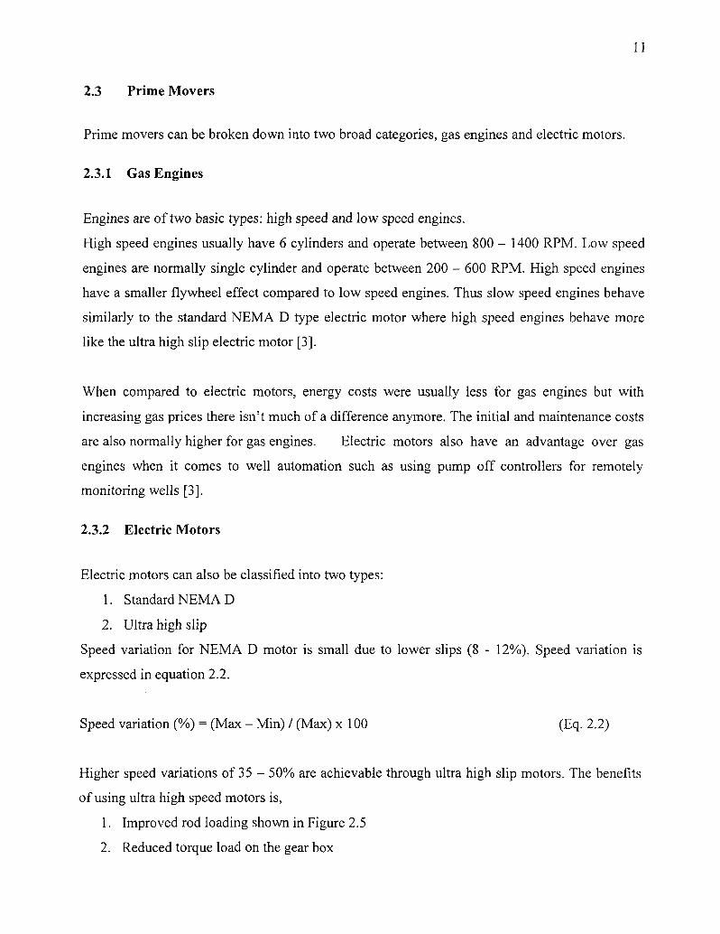
Higher speed variations of 35 - 50% are achievable through ultra high slip motors. The benefits

of using ultra high speed motors is,

1. Improved rod loading shown in Figure 2.5

2. Reduced torque load on the gear box

12

NEMA D Ultra High Slip

Figure 2.5: Dynamometer Card [3]

Ultra high slip motors are offered in several sizes ranging from about 10 HP to about 200 HP.

Each size is equipped with power modes. Higher modes have higher horse power rating but

lower speed variations [3].

Speed variations can be increased by "minimizing the upstream rotary inertia to the reducer. This

includes the unit sheave, motor sheave and motor rotor. For example, more speed variation can

be expected with a 32 inch sheave and 8 inch motor sheave than with a 44 inch sheave and 11

inch motor sheave.

Inertia effects can be enhanced by locating the leading weights at ends of cranks and by moving

the trailing or lagging weights inward the required amount for proper balance"[3].

2.4 Sucker Rods

Sucker rods provide the link between the surface unit and the downhole pump. Because of size

restraints, an adverse environment and strength limitation, the sucker rod is normally considered

the weak link in a pumping system. For this reason surface equipment performance is often

judged by how good the equipment is on the rods.

13

l-l'SET HEM J

/ /

KOIJ UOHY

i",s snocu:.>/:/{ r.tc /; / /

(W1N1Y nfl

/ W W

TilKEALV:

H'fiKM:// i'l.AV SHOVLDEH

COUEL.WT; /io/>y

COUPUXO FACE

Figure 2.6: Sucker rod and Coupling [7]

Longer unit strokes are normally preferred to maximize production with fewer rod reversals.

Longer stokes also help in reducing peak loads and the resulting stress ranges which increase the

life of the sucker rods [3].

2.4.1 API Rods

There are three API classes of sucker rods. These are class C, D and K. API rod specifications

are shown in Table 2.1.

14

Table 2.1: API rod specifications [7]

API Class

Min. tensile strength, psi

Hardness, Brinell

Metallurgy

C

90,000

185-235

AISI 1036 (Carbon)

D

115,000

235-285

Carbon or Alloy

K

85,000

175-235

AISI 46xx (Alloy)

A steel rod has a modulus of elasticity of around 3,050,000 lbs/in that includes a small correction

for the coupling and a stress wave propagation velocity of about 14,400 feet per second. There is

KD rod (not API recognized) also manufactured that has K rod metallurgy but a higher strength

equal to that of D rod [3]. API rods are 25 feet (± 2 inches) long in length.

2.4.2 Analysis of Rod Loading

The most meaningful method for evaluating rod loading is based on the API Modified Goodman

Diagram. This allows consideration of both maximum stress and stress range. A graphical

evaluation is shown in Figure 2.7. This procedure in Figure 2.7 evaluates rod loads for a service

factor of one (Ideal conditions such as no corrosion, fluid pound etc.)

15

in Vi -+—»

t/5

75000

60000

45000

30000

15000

Maximum Allowable Stres,

Figure 2.7: Goodman Diagram for API rods and Service Factor of One [3]

1. /Find out the tensile strength (T) of the rod in use. Table 2.1 can be used for API rods

2. Lay the maximum stress on the Y-axis and the minimum stress on the X-axis. Draw a 45

degree line through it which establishes the minimum allowable stress.

3. Calculate T/1.75 and lay it on the 45 degree line.

4. Calculate T/4 and mark it on the Y-axis. Connect this point to point laid off on the 45

degree line in step 3. This line establishes the maximum allowable stress for a service

factor of one.

5. Find out the peak polish rod load and lay it off on the graph. Find out the stress range for

rod type from the graph. If the peak load determined is greater than the maximum

allowable stress for those rods, they are overloaded.

The Goodman method is an easy way to determine the stress range for a particular rod type. It

helps in deciding to lower the allowable peak stress by replacing with a higher strength rod when

the stress range is high and vice versa.

16

The Goodman diagram calculations are applicable to ideal conditions as mentioned - i.e.

flawless handling practices, no manufacturing defects, and totally non corrosive well fluids. If

any of these conditions are present, particularly corrosive well fluids, the allowable stress range

should be de-rated from the ideal situation.

Most studies concerning rod failures show that over half of the failures are connector breaks. It

usually happens due to inappropriate joint make up and can be avoided using power tongs. In

wells deeper than 2000 feet, the rod sizes are normally tapered which provides a stronger yet

lighter rod design [3].

2.4.3 Non API Rods

The Electric rod from Oilwell is an extra high strength steel rod. They are very expensive but can

be a good substitute in wells experiencing higher rod failures.

It's the heat treating process that gives the electric rod its ultra high strength. The rod's core is

pre stressed and hence does not have a stress range like the other API steel rods. The Goodman

diagram cannot be used to evaluate stress loading in this rod type [3].

Continuous rod or Corod is a single piece of rod with no connectors. They come in 1/6 inch

tapers rather than the standard 1/8 inch seen in API rods. Since they have the same metallurgy as

the API steel rod, the Goodman diagram can be applied to evaluate stress loading in these rods.

The rod is wound on a large spool, and thus requires special equipment for running and pulling

operations [3].

Fiberglass sucker rod has certain advantages over steel rods.

1. They are lighter than steel rods, which reduce equipment loading and energy usage

2. They are corrosion resistant

3. They are four times more stretchable than the standard API steel rods

They also have their disadvantages such as,

17

1. They wear more quickly in deviated wells

2. Their maximum temperature rating is 200 degree Fahrenheit

3. The maximum torque is 100 ft-lbs for 1 inch rod

4. They are extremely difficult to fish in case of rod breaks

5. It is very difficult to space out the pump with fiberglass rods only. Smaller steel rods

called "Ponies" are used on top to compensate for that.

Fiberglass rods have a lower modulus of elasticity than steel rods and hence can stretch four

times more than the standard API steel rods. Their modulus of elasticity ranges from 6,300,000

to 8,100,000 lbs/in and have a stress wave propagation velocity of approximately 14,400 fps [3].

Fiberglass rods have a stress range and so stress range diagrams like the Goodman's have been

developed for these types of rods.

2.5 Reciprocating Rod Pump

When crude oil was found to have increasing values, the method of getting it to the top was

simple mechanical application of already developed positive displacement pump. In the early

days everyone in the oil business had their own idea as to designing a pump, material to use in its

construction and specifications required in lifting oil. This led to many pump designs which were

similar in operation and had one thing in common, that they were all positive displacement

plunger type sub surface pumps. A growing petroleum industry saw the need of working out

some sort of uniformity in bottomhole pump design, nomenclature and its specifications. Hence

American Petroleum Institute (API) was born and developed a standard set of prints and

specifications which controls or standardizes the manufacture of over 90% of all sucker rod

pump parts used today.

Bottomhole oil well pumps are actuated from the surface by a string of sucker rods working from

a mechanical pumping unit, usually the pump jack. The surface or pumping unit as discussed is a

machine that converts rotational power (Prime mover) into vertical reciprocating motion. The

motion is transmitted to the bottom of the oil well through the connecting string of sucker rods

which the pump into action. As the working parts of the bottomhole pump are moved up and

18

down, a positive displacement takes place within the pump action, and this starts fluid from the

bottom of the hole to move towards the surface through the tubing string shown in Figure 2.8.

+ ^

* i

4,

\

Up St*cke J o w n i. t r o •<-.£•

Figure 2.8: Sucker rod pump valve operation [1]

19

The standard oil pump is a machine known as the force pump. During the upstroke, the standing

valve (SV) is open which allows the fluid to enter the barrel of the pump. The fluid continues to

enter the barrel of the pump till it reaches the top of the stroke. At this point the fluid load is

transferred to the standing valve at the start of the downward stroke. This closes the standing

valve and opens the travelling valve (TV) which allows the fluid to pass through it and enter the

tubing string. On the next upward stroke, the travelling valve closes again and the standing valve

reopens [8]. The fluid again starts to enter the barrel of the pump while is simultaneously forced

up the inside of the tubing string and down the flow line. This illustration of the bottomhole

pump is shown in Figure 2.9. It is important to mention that two strokes (upward and downward)

combined, makes a full stroke length and should be kept in mind when determining the pumping

unit speed referred to as strokes per minute or SPM.

Figure 2.9: Bottomhole pump operation [3]

This principle of operation described above is true for all API pumps both insert and the tubing

types.

2.5.1 API Pumps

API type pumps can be divided into two classes:

1. Rod pumps &

2. Tubing pumps

21

Insert pumps are run and pulled with sucker rods. Pumps are usually set in a "seating nipple or

shoe which is an integral part of the tubing string. However, a retrievable seating device can also

be used which allows the pump to be set at any depth within the tubing. The retrievable pump

seat does not have the fluid sealing reliability of the more commonly used seating nipples. In

principle, the retrievable seat operates similarly to a hook wall packer. API type seating devices

are of two types; cup type and mechanical type. The cup type seats use the composition type

seals on the pump hold down to seal and anchor the pump by the tight friction fit. In contrast, the

mechanical pump seat has a metal to metal tapered fit for a fluid seal and a collets type latch to

anchor the pump. Typical API assemblies and designations are shown below.

The abbreviations used in the following Figures are explained here:

RHA: Rod, Stationary Heavy Wall Barrel, Top Anchor Pump

RHB: Rod, Stationary Heavy Wall Barrel, Bottom Anchor Pump

RWA: Rod, Stationary Thin Wall Barrel, Top Anchor Pump

RWB: Rod, Stationary Thin Wall Barrel, Bottom Anchor Pump

THC: Tubing, Heavy wall Barrel Pump

22

i j i i

J

""Jl

_"t

ZJ ' • !

"J

'J

V

11

KHAC

if RHP;

1

RWAC R;VB(

Figure 2.10: Standard bottomhole pumps [9]

pi

T*Ti

23

,;-i

L.'

% I

"J

if :HC :

V

ry ; ' •

; '-, » < 0

—.; i _ .

; • • > i

,

.- nt

•

THM;

r r , •

- '

~J N 1 "\ J p

-"*

F

: -"' r*

"f :"!

*""./

4~~.: - \"-Z 3

>ull Tube RWAC

_: : ;* -

• r t ,

.*» *

— ;

^ i " r ' a - 1 J*.

7V~5~5 —....._ Pull Tube R'.VBC

Figure 2.11: Standard bottomhole pumps [9]

As shown, rod pumps can be seated at the top (top anchor) or bottom (bottom anchor). Bottom

anchor pumps can be either traveling plunger or traveling barrel, while top anchor pumps must

be of traveling plunger type. The most commonly used pump is the bottom anchor traveling

plunger type. The top anchor and bottom anchor traveling barrel type are used primarily in dirty

24

wells where it is necessary to have continuous cleaning or flushing above the pump seat to

prevent sediment (sand, scale and debris) from sticking the pump in the seat.

Pump plungers can be either metal-to-metal (most common) or soft packed. Soft packed plungers

are of three types; cup, composition ring and Flexite ring or a combination of these. The cup-type

plunger (oldest) consists of composition or plastic valve cups spaced equally on a metal plunger

mandrel. The cup lips are forced out against the pump barrel on the upstroke by the fluid load to

obtain an effective seal. Cup-type plungers are normally limited to shallow lift, generally less

than 2500 feet. Composition ring and Flexite ring plungers are capable of greater lift but

normally are limited to less than 7000 feet.

Composition ring plungers are of two types; split ring (Martin ring) and the flange ring (non

split). These rings are constructed of rubber and cotton duck especially formulated for oil well

environments. Before installing the plunger, pre-swelling (dipping in kerosene or diesel for about

a minute) the composition ring is necessary to obtain the proper plunger to barrel fit.

Flexite ring plungers use a special hard plastic ring impregnated with graphite for lubrication.

The rings are precision made to fit the pump barrel much the same as piston rings in a gas

engine. The Flexite ring material has good wear resistance and is inert to the oil well

environment. Since the rings are self lubricating, Flexite ring plungers are used in high water cut

wells.

Advantages of soft-packed plungers are lower initial pump cost and lower repair costs. Also soft

packed pumps are often more tolerant to dirty or scaly well condition. Metal to metal pumps are

normally recommended in deep wells with net lifts of 7000 feet or more and in most cases tend

to have longer run life when compared to pumps with soft packed plungers.

Pump barrels are of two basic types, thin wall and heavy wall. Liner type barrels consisting of 12

inch long precision honed sections aligned and clamped inside a jacket have been replaced by

one piece heavy wall barrels. Problems with liner alignment, higher costs and the ability to

precision hone one piece barrels have discouraged the use of liner type barrels.

25

Thin wall barrels (1/8 inch wall thickness) are for shallow to medium depth walls while heavy

wall barrels (3/16 inch or greater wall thickness) are used for deep wells and for the bigger bore

tubing type pumps.

With metal to metal fits, the pump can be designed for stroke through operation where part of the

plunger passes out of the barrel at the top and bottom of each stroke. Stroke through pumps are

often used in scaly conditions where there is an advantage to sweeping or cleaning the entire

pump barrel to prevent pump sticking. Soft packed plungers should only be run in full barrel type

pumps.

Metal to metal plunger to barrel fits are typically 0.003 to 0.004 inch, but depends on bottomhole

temperature, well depth, plunger diameter, plunger length and fluid characteristics, i.e. solid

content and viscosity. Plungers are normally 6 to 12 inches in length per thousand feet of lift up

to a maximum of 6 feet. Again, plunger length requirement depends on the fit, well depth and

fluid viscosity.

With tubing type pumps, as the name implies, the pump barrel is an integral part of the tubing

string. Thus, plungers can be made larger to increase pump displacement above that possible

with common API insert pumps where the pump barrel must fit inside the tubing. Disadvantages

of tubing pumps are higher repair costs and poor gas handling ability. In order to replace the

pump barrel, both the tubing and the rods must be pulled. Poor gas handling results because of

the necessity of high spacing (added clearance) to avoid hitting down and damaging the plunger

and valve assemblies.

26

a fl' 1-J ry

• - N l i l

-r? Ml

frf L-;.i

i "J

* /

74 I.:'- --! IJ 2RSIZ5 TUB'NG1

Figure 2.12: Specialty bottomhole pumps [9]

Spacing the pump high results in a low compression ratio and causes poorer volumetric

efficiency under gassy conditions.

The barrel of a tubing pump can be much larger than the tubing ID to further increase pump

displacement. With this type of installation the plunger and standing valve cannot be retrieved by

pulling the rods; therefore, an on-off tool must be used to release the rods from the pump.

Although large bore tubing pumps equipped with on-off tools have the advantages of higher

displacement, they also have the disadvantages of high repair costs (tubing must be pulled to

repair pump) and fluid acceleration and friction effects add substantially to equipment loading.

27

Casing type pumps can be used to eliminate the use of on-off tools and tubing and to lower

equipment loads caused by fluid acceleration and friction. Since fluid is produced up the casing

(no tubing), an anchor pack off device is used as part of the pump assembly. Casing pumps are

normally large bore pumps for producing high volume shallow wells; however, slim-hole tubing

less completions is smaller versions of casing pumps. Casing type pump arrangements have

serious disadvantages including rod wear on the casing, harder fishing of parted rods, and

inability to vent free gas.

Also there is more risk where sand, scale and corrosion are present. Another version of casing

pump installation is to run tubing with a perforated tubing sub directly above the pump. This

requires the use of a tension packer and an on-off tool but has the advantages of reducing the

load from fluid acceleration and friction effects. This is because fluid is produced both up casing

and tubing. Rod wear on the casing is also eliminated, and parted rods can be more easily fished

inside tubing.

Pump valves are of the ball and seat type. The ball is confined in a cage which is designed to

allow free fluid flow while maintaining ball alignment with the seat. Wear of the guiding ribs of

the cage results in off-center fall of the ball on the seat and short valve life. To reduce or

diminish cage and valve wear, cages are available with resilient inserts and hard facing metal on

the ribs. Valves can be installed in tandem, often referred to as double valves to help insure

longer valve life. However these increases pump costs and therefore not usually recommended.

Balls and seats are available in many materials.

The selection of pump type and the materials for the various pump parts depend on factors such

as depth, corrosion, abrasion and gas liquid ratio" [3].

Pumps are manufactured in various bore sizes. Table 2.2 can be used to calculate the pump size

using the plunger diameter, speed (SPM) and the pump constant (C).

28

Table 2.2: Pump Constants and Plunger Areas for Commonly Used API Pumps [10]

Formula: BPD = Pump Stroke (inches) x SPM x C C = (Pump Diameter/x 0.1166

Plunger diameter (Inches)

7/8 (0.875)

1-1/16(1.0625)

1-1/4(1.250)

1-1/2(1.5)

1-5/8(1.625)

1-3/4(1.750)

1-25/32(1.781)

2 (2.000)

2-1/4 (2.250)

2-1/2 (2.500)

2-3/4 (2.750)

3-1/4(3.250)

3-3/4 (3.750)

4.3/4 (4.750)

Gross plunger area (square inches)

0.6013

0.8866

1.2272

1.7671

2.0739

2.4053

2.49

3.1416

3.9761

4.9087

5.9396

8.2958

11.045

17.721

Pump constant, C (BPD/SPM/inch of pump stroke)

0.0892

0.1316

0.1821

0.2622

0.3078

0.3569

0.3699

0.4662

0.5901

0.7285

0.8814

1.231

1.639

2.6297

3 GATHERING FLUID LEVEL DATA

3.1 Optimizing Wells

Optimization of producing wells is a growing concern within the petroleum industry. Economic

and conservation concerns have forced the issue of production efficiency to the forefront of

operations. It is now a question of getting the most return for the least expenditure.

In order to optimize production, it is vitally important to know what the well is currently

producing compared to what it is capable of producing. Therefore, the actual production should

be regularly monitored. Several tests can be conducted to determine the amount of available

production and whether the production can be increased.

The following are some of the questions that need to be answered.

• Is there a high fluid level in the well?

• Is the fluid level oil or a column of foam?

• What is the maximum production rate you can expect from this well?

3.2 Considerations

The following points need to be considered before attempting to increase production from a well.

1. Reservoir Consideration: Will the GOR or water production increase excessively?

2. Equipment Limitations: Will the existing rod and pump unit be over-stressed if the

pumping rate, pump size, or stroke length is increased?

3. Economic Consideration: If new equipment must be purchased in order to pump more

fluid, will the increase in production be large enough to pay for the equipment and its

cost of installation?

4. Surface Facility Considerations: Are existing treatment and storage facilities adequate or

will expansions or upgrading being required?

29

30

3.3 Pumping Fluid Level

The fluid level in a producing well can be determined using acoustics. A pressure wave is

introduced into the tubing-casing annulus and the reflected pressure waves are recorded upon

their return to the surface.

An accurate fluid level is often used to:

• Determine bottomhole pressure.

• Help evaluate pump performance.

• Determine additional production potential.

• Assess operating changes.

A fluid level reading under Table conditions is perhaps the best single indicator of whether or not

a pumping well is producing at its maximum capacity.

3.4 Acoustic Well Sounder (Fluid Level)

An acoustic well sounder is used to conduct fluid level measurements under both producing and

shut in conditions.

The basic instrument consists of a well head attachment connected by a cable to an electric

recording instrument. The well head instrument also called the gun is attached to the well head

casing valve leading into the casing-tubing annulus. The well head attachment contains a device

to provide the source for creating a pressure wave, and a microphone (Pressure Transducer) to

sense pressure waves reflected through the casing-tubing annulus. An energy pulse is generated

down the annulus. This disturbance is created with a black powder blank cartridge, high pressure

inert gas (CO2 or N2) or using the well pressure itself.

3.5 Fluid Level Equipment

A typical acoustic well sounder system consists of a recorder and a gun/well head attachment as

shown in Figure 3.1.

31

Figure 3.1: Acoustic Well Sounder System [11]

3.5.1 Wellhead Attachment (Gun)

• Is the source of pressure waves

• Has blank shells or gas charges discharged by a firing head.

• Contains a microphone that picks up reflected pressure waves and relays them to the

recorder as an electric signal.

A well head attachment (Gun) is shown in Figure 3.2.

3.5.2 Recorder

f! I ^ i i

' og« r CABJNO R U f » BLEED

t BLEED

32

Figure 3.2: Manual Gas Gun [12]

Picks up signal via a cable connected to the wellhead attachment

Filters and amplifies the signal and then records it on a strip chart or digital recorder

33

Figure 3.3: Microphone [7]

The pressure wave generated travels through the gas in the annulus from the surface to the fluid

top and then returns to the surface. A recorder is shown in Figure 3.3. The computer measures

the round trip time of the wave and then computes the fluid level using the formula

D = (VxT r ) /2 (Eq. 3.1)

Where:

D - Fluid level depth, ft

V = Acoustic velocity, ft/sec

Tr = Round trip time of transient wave, sec

A pictorial view of the wave generated and the fluid level echo is shown in Figure 3.4.

34

Travel time (sec): 7.388

Velocity (JVsec): 1215

— 0

— 1000

— 2000

— 3000 Casing Pressure (psi); 88.

Fluid level (ftfrom surf): 4490

Fluid submergence (ft): 3230

Pump depth (ft): 7720

Vent Method, Manual Valve

j | — 4000

~*V — 5000

f — 6000

1 - 7000

1 — 8000

Figure 3.4: Fluid Level Measurement Showing Induced Wave and Echo Off of Fluid Top

[13]

3.6 Gathering Good Fluid Level Data

It is critical that accurate and dependable fluid level data be obtained. Inaccurate or incorrect

information can lead to invalid analysis which may result incorrect upsizing or downsizing of

equipment. We should make sure that,

1. Reduce background noise:

• Close onside valve to reduce noise.

• Slow down the gas engine

• Shut down lift system (if necessary)

2. If pressure is too low (to get a fluid level response) shut casing in to increase pressure.

35

3. Obtain fluid levels soon after wax treatments for waxy wells. This will reduce

unnecessary noise.

4: FLOWING BOTTOMHOLE PRESSURE & IPR

4.1 Flowing Bottomhole Pressure

The flowing bottomhole pressure is the pressure in the wellbore at the midpoint of the producing

interval.

As fluid is removed from the wellbore, the pressure is reduced. The pressure drop that is created

between the wellbore and the static reservoir pressure is often called drawdown. Drawdown is

directly related to production. A generally rule is the greater the drawdown, the greater the

production. If the flowing bottomhole pressure is decreased, the drawdown will be increased,

thus there will be higher production. This relationship is called the inflow performance

relationship and will be discussed in Chapter 5.

Since flowing bottomhole pressure is directly related to the well inflow and, therefore, the

production knowledge of a well, knowledge of the flowing bottomhole pressure is essential for

rod pump optimization. It also helps in determining the right type of artificial lift for the amount

of dynamic fluid level in the wellbore.

Flowing bottomhole pressure can change due to reservoir effects or changes in the pumping

system; thus, it is important to estimate flowing bottomhole pressure on a regular basis.

Generally, it should be monitored on a quarterly basis during the well review process in order to

make or suggest changes to the pumping unit. Well automation has really changed things these

days as it constantly monitors things like peak loads, pump tillage, down time etc. This

information is stored in the automation device called a pump off controller and can be

transmitted to a central location through SCADA (supervisory control and data acquisition).

There are several ways of determining flowing bottomhole pressure in rod pumped wells but we

will only discuss the acoustic well sounding (AWS) method for the purpose of our project.

Acoustic well sounding is by far the most widely used method for calculating the bottomhole

pressure due to the following:

36

37

• It is accurate enough on most wells for all practical purposes except for deep, unstable

and wells with repaired or damaged casings

• The process is quick to complete

• AWS equipment is straight forward to handle and easily available

4.2 Acoustic Method

r—; Pc

pgc ^ ! _ i-i

L

Pwf

Df

Figure 4.1: Wellbore [14]

It is calculated through the acoustic method by:

FBHP = Casing Pressure + Gas Column Pressure + Fluid Column Pressure

or,

Pwf=Pc + Pgc + Po + PL (Eq.4.1)

Where:

Pwf = Flowing bottomhole pressure

Pc = Casing pressure

P = Gas column pressure gc

P0 = Oil column pressure, given by Eq. 4.2

38

P ° = L x F o x G ° (Eq.4.2)

Where:

L = Oil column height above the pump

G0 = Corrected oil gradient

F0 = Oil gradient correction factor due to the produced gas

PL = The oil-water column pressure from MPP (midpoint of perforations) to the pump

intake and can be estimated using equation 4.3.

(G xQ +G xQ ) P = i * v w o v 0 ; (Eq. 4.3)

(Qw+Q0)xDperfs

Where:

Gw = Corrected water gradient

Qw = Water production rate

G0 = Corrected oil gradient

Q0 = Oil production rate

Dperfs = Distance between the MPP (midpoint of perforations) and pump

The casing pressure, Pc is measured at the wellsite directly from the pressure gauge.

The pressure exerted by the gas column is ignored for all practical purposes when it is less than

5% of the total bottomhole pressure or for wells up to 6,000 feet deep. It can be easily obtained

using Figure 4.2.

Note

If sufficient gas is breaking out of solution that affects the oil gradient between the midpoint of

perforations and the pump, equation 4.3 is not valid. A multiphase correlation is required in that

case. A program like NODAL/PC can be used which is outside the scope of this project.

39

PRESSURE EXERTED BY GAS COLUMN [PS.I)

200 300 400 500 600

Ml" 1000

0.™ 0.80 0.90

GAS GRAVITY (AIR= 1.0)

Figure 4.2: Gas Column Pressure [7]

40

Generally, there are three stable producing scenarios that exist in the field. For a well to be stable

there should not have been any recent shutdowns longer than 15 min.

1. Scenario 1: The liquid level is at the midpoint of perforations (MPP) and no significant

gas is produced up the annulus [14] [15].

2. Scenario 2: The liquid level is above the midpoint of perforations and no significant gas

is produced up the annulus [14]. Significant gas production affects the oil gradient that

can result in erroneous fluid level calculations if not accounted for. Gas break out or

production is significant if, under stable producing conditions, the casing pressure will

build up more than 200 kPa in two hours or less [15].

3. Scenario 3: The liquid level is above the midpoint of perforations and significant gas

breaks out of the solution [14] [15].

These three scenarios are shown in Figure 4.3 below.

Figure 4.3: Stable Producing Conditions in a Normally Completed Rod-Pump Well [15]

In each of the scenarios, the gas column pressure (Pgc) will be ignored for simplicity.

4.2.1 Scenario 1

41

Figure 4.4: Scenario 1 [14]

The liquid level in this case is at the MPP and no significant gas breaks out of the solution. The

casing pressure in this scenario is approximately equal to the flowing bottomhole pressure and so

equation 4.1 becomes,

Pwf = P c (Eq. 4.4)

4.2.2 Scenario 2

Figure 4.5: Scenario 2 [14]

42

The liquid level in this case is above the MPP and no significant gas breaks out of solution. The

pump is landed at the MPP.

In this situation, casing pressure and the liquid column both contribute to the flowing bottomhole

pressure. The gas column pressure is neglected for simplicity. The liquid column in this case is

all oil if the well is producing under stable conditions. The oil gradient is determined by

correcting the stock tank oil gradient to the annulus pressure and temperature. Equation 4.1 can

then be rewritten as,

Pwf = P c + ( L x F 0 x Q 0 ) (Eq.4.5)

Where:

L = Oil column above the pump

G0 = Corrected oil gradient (1 in this case)

And thus equation 4.5 becomes,

Pwf = P c + ( L x F J (Eq.4.6)

4.2.3 Scenario 3

Figure 4.6: Scenario 3 [14]

In this scenario, the liquid level is above the MPP and significant gas breaks out of the solution.

43

This situation occurs in one out of every ten wells in the field [15]. The flowing bottomhole

pressure is made up of the casing pressure and the gaseous oil column above the pump. The

dissolved gas in the oil not only makes the oil lighter but also increases its volume in the

annulus. This must be corrected for gas produced up the annulus to calculate an accurate flowing

bottomhole pressure.

Using equation 4.4,

Pw f=Pc + (LxF 0 xG 0 ) (Eq. 4.7)

Where,

F0 = Corrected oil gradient and can be calculated using the depression method or the

Podio and McCoy's method

4.3 Pump above or below the Producing Interval

s.

kU :tr

W

Figure 4.7: Pump Landed Above or Below the Producing Interval [14]

4.3.1 Pump above the Producing Interval

In Figure 4.7, one of the pumps is landed above the MPP and so an estimate of pressure between

the pump and the producing interval is required. A multiphase flow correlation may be required

in case of gas breaking out of solution.

44

Incase where no gas breaks out of solution, a multiphase correlations is not required. "Industry

practice is to make the assumption that the liquid between the pump and the formation is oil and

water in approximately the same ratio as produced by the well. For example, a well produces

60% water and 40% oil and the pump is 100 meters above the formation. For calculations

purposes only, the height of the liquid above the formation will be 60 meters of water and 40

meters of oil" [14]. This is shown in Figure 4.8.

Production

gas

oil

60% wafer

40% ait

1

- 60% water

-40*/

\

> oil

i [

t L

1

rfs

V

Figure 4.8: Pump above the Producing Interval [14]

The water oil ratio is Figure 4.8 is the same as that produced from the well and so we can calculate the liquid column pressure (PL) using equation 4.3.

PL = ( G w x Q w + G 0 x Q o )

( Q w + Q o ) > < D p e r f s (Eq. 4.3)

Hence PL must be added to the pump intake pressure to calculate the flowing bottomhole

pressure.

45

4.3.2 Pump below the Producing Interval

If the pump is below the producing interval, assume that the pump is landed at the producing

interval and calculate the flowing bottomhole pressure accordingly using equations 4.1, 4.2, 4.3,

4.4, 4.5 and 4.6 accordingly for their respective scenarios.

4.4 Annular Fluid Gradients

Annular liquid columns must be corrected for gas break out to calculate an accurate flowing

bottomhole pressure.

Fluid columns not corrected for dissolved gas production will indicate higher fluid levels in the

wellbore. This will result in erroneous IPR calculations and improper bottomhole pump (BHP)

design. A lot of time and money can be wasted due to inaccurate bottomhole pressure

calculation.

Gaseous liquid columns can be determined using;

1. Depression method

2. Podio and McCoy's method

The Podio and McCoy's method, also known as dp/dt method, uses the casing pressure build up

rate and Gilbert's curve to calculate the corrected gradient. This is an iterative process and can be

used to check the accuracy of the depression method.

4.4.1 Depression Method

The depression method which is also called the Walker's method has been an industry standard

for a long time for calculating fluid gradients in rod pump wells.

The first step is to get a fluid level reading for a stable producing rod pump well and record the

casing pressure directly from the gauge attached to the casing. The second step is to close the

casing valve a little which acts as a back pressure valve to increase the casing pressure in the

annulus. This depresses or lowers the liquid column due to increased casing pressure. The well

46

needs to be stabilized before getting a second fluid level reading at the corresponding casing

pressure [15]. This is shown in Figure 4.9.

Pel Pc2

Figure 4.9: The Depression Method for Gradient Determination [14]

The gradient can be calculated from the depression method as illustrated below.

Final - Initial GasLiquid Interface Pressure Average Gradient = •

Final - Initial Fluid Level

or,

F0G0 = P - P

L>-L2

(Eq. 4.8)

Where:

F0G0 = corrected oil gradient

G0 = oil gradient

F0 = correction factor

L, = fluid height (before depression)

Pc, = casing pressure at L,

L2 •= fluid level (after depression)

PC2 = casing pressure at L2

47

The first step in what actually occurs in the field is to record the casing pressure and fluid level

on a stable producing rod pump well. At this point the casing valve is closed and the fluid is

lowered to a new level. The well is not given time to stabilize. Another fluid level is taken

usually after 30 minutes and the casing pressure recorded. Remember that equation 4.7 is based

on the assumption that the flowing bottomhole pressure is the same at both fluid levels. If the

well is not given time to stabilize as mostly done in the field, fluid level depression causes liquid

to be pushed out of the annulus into the pump intake, which reduces flow from the reservoir.

Thus the flowing bottomhole pressure would not be the same at both fluid levels. If this

difference were significant, equation 4.7 would not be valid and the calculated gradient may not

be acceptable.

To ensure that an accurate gradient is obtained with the depression method, several checks are

recommended:

First of all, it is important to check that the inflow into the wellbore has not changed

significantly, which would imply a considerable change in flowing bottomhole pressure. Inflow

could be affected in two ways:

1. The fluid depression into the pump intake from the annulus will reduce inflow

2. A change in pumping system so that total liquid flow changes

Inflow is checked by putting the well on test during the depression method. If the ratio of the

volume of the annulus fluid that was depressed to the total liquid production during the

depression method is small (Approximately 10%), fluid depression has not affected flowing

bottomhole pressure significantly. For example, if the total liquid production during a depression

is 100 m3/day and the volume of annulus fluid depressed into the pump is only 5m3/day, then

5/100x100-5%

Since, the ratio is less than 10%, inflow was not significantly affected. A second recommended

check for accuracy of the depression method is to obtain four to five fluid levels thus providing

48

enough gradients. If all gradients agree within a reasonable range, it is likely accuracy has been

achieved.

Third, since a buildup is required to do the depression method, it is also recommended to

calculate the gradient using Podio's method if possible to confirm accuracy.

Table 4.1 shows all data required to calculate the flowing bottomhole pressure when the well is

stable.

Table 4.1: Data required for Acoustic method [14]

ITEM

Oil production

Water production

Oil gradient at annulus pressure and temperature, not corrected for free gas Water gradient

Casing pressure

Distance from surface casing bowl to midpoint of perforations (mpp)

Pump setting depth

Joints to fluid

SYMBOLS

Q0(mJorBPD)

Qw(mJorBPD)

G0 (kPa/m or psi/ft)

Gw(kPa/morpsi/ft)

Pc (kPa or psi)

Df (m or ft)

Dp (m or ft)

SOURCE

Well test

Well test

PVT data

Measure with hydrometer or estimate

Measure at wellhead

Well file

Well file

Fluid level

5 INFLOW PERFORMANCE RELATIONSHIP (IPR)

5.1 Introduction

Fluid always flows from an area of high pressure to that of a lower pressure and this is true for

reservoirs as well. Reducing the flowing bottomhole pressure increases the fluid flow from the

reservoir and is known as drawdown in reservoir engineering terms. The higher the drawdown,

the greater the production from that well will be. A typical wellbore at static conditions is

illustrated in Figure 5.1.

FLUID PRODUCTION

RESERVOIR PRESSURE

FLUID FLOW

RESERVOIR PRESSURE

FLUID FLOW

PRODUCING INTERVAL

Figure 5.1: Fluid Flow to the Wellbore [14]

Inflow performance relationship (IPR) of a well is simply a measure of the relationship between

the bottomhole pressure and the producing rate. The equations used to calculate the inflow

performance of the reservoir is a simplified form of the complex reservoir geometry downhole.

An IPR indicates the production rate that can be expected from a given well under stabilized

conditions [8]. This potential of the well is very essential for any artificial lift design and in our

case for proper sizing and optimization of a rod pump.

49

50

The data required to calculate IPR's for different wells consists of the static reservoir pressure,

the flowing bottomhole pressure and the production rate at those pressures. For all practical

purposes in the field, inflow performance relationship is a good indication of the reservoir

deliverability.

The static reservoir pressure for a particular zone is obtained by shutting all wells in that zone

and giving it time to stabilize. Since this is practically impossible for an operating company to

shut down production completely, it can be calculated using the static bottomhole pressure.

Static bottomhole pressure is obtained by shutting in one well and either waiting for it to stabilize

or estimating the stable pressure from the bottomhole pressure build-up. According to ERCB

(Energy Resource and Conservation Board of Alberta) a well must be shut in for at least fourteen

days or the pressure build-up should not be greater than 2 kPa/m in two hours before running a

static gradient for reporting purposes.

If the well is producing, the pressure at the midpoint of producing interval is called the flowing

bottomhole pressure. The pressure drop that is created between the static reservoir pressure and

the flowing bottomhole pressure is often called the drawdown.

IPRs are almost always analyzed graphically for all practical purposes in the field. The

production rate is plotted on the horizontal axis against the bottomhole pressure on the vertical

axis as shown in Figure 5.2. We will evaluate three types of inflow relationships:

1. Constant productivity index

2. Vogel's equation

3. Combined Vogel's and constant PI

5.2 Constant PI

This method is usually used for single phase flow or oil reservoirs flowing above the bubble

point pressure. It can also be used for reservoirs with extremely low pressures e.g. 1000 kPa or

less since minimal gas breaks out from the oil at those pressures. The constant PI graph results in

51

a straight line as shown in Figure 5.2. It was assumed for many years that the IPR was a straight

line but it became apparent that this almost always produced overly optimistic predictions of

productivity when changes were made to increase production from a well.

5.2.1 Graphical Analysis

The productivity index is an indication of the incremental production for each unit of pressure

drop. If the IPR of any well is a straight line, the productivity index is constant regardless of the

production rate. It is defined as the production rate divided by the draw down as shown in

equation 5.1.

PI = QL/(Ps-Pwf) (Eq.5.1)

Where,

PI = Productivity index

QL = Total liquid production rate

Pwf - Flowing bottomhole pressure at QL

Ps = Static reservoir pressure

Using equation 5.1 would result in a straight line. It can also be defined as an inverse of the slope

for that IPR line [14].

52

7000

6000

5000

S. 4000

1 3000 Q.

2000

1000

0

S Static Reservoir Pressure

^ s . Operating point at ^ - ^ A /Pwf = 3700kPa

^ \

1 1 — •

/Operating point at

< F W f = 2300 kPa

1 1 - ^

• Series 1

20 40 60 80 100 120

Liquid Production Rate (m3/day)

Figure 5.2: Constant Productivity Index IPR

Figure 5.2 has been created by plotting two points on the graph: the static reservoir pressure

(6000 kPa, 0 m3/day) and the operating point (3700 kPa, 43 m3/day). A straight line is drawn

through these two points. This operating line or inflow performance relationship can now be

used to estimate the production at any flowing bottomhole pressure.

In theory, the maximum production is the production where the flowing bottomhole pressure is

equal to zero, shown in Figure 5.2 as 120 m /day. However the practical maximum production

occurs where the operating line intercepts the tubing pressure, shown in Figure 5.2 at

approximately 800 kPa, 105 m3/day. The reason for the practical maximum limit is that the

casing pressure is usually controlled near tubing pressure, and the flowing bottomhole pressure

consists of the casing pressure as well as the pressure due to the liquid and gas columns in the

annulus. If the annulus fluid level was at pump and the pump was landed at the perforations, the

flowing bottomhole pressure could only be lowered if the casing pressure were lowered. Since

the casing pressure is controlled near tubing pressure, the tubing pressure becomes the lowest

practical pressure or maximum production that the well could be produced at. An exception to

this scenario may occur if a casing gas compressor is used to reduce casing pressure.

53

5.2.2 Non Graphical Analysis

Once we calculate the productivity index of a well, we can derive the incremental production for

every drop in pressure. Since the static reservoir pressure remains the same, reducing the flowing

bottomhole pressure results in increased production. This is done using equation 5.2.

AQL = APw fxPI (Eq. 5.2)

Where,

AQL = Change in liquid production rate

APwf = Change in flowing bottomhole pressure

PI = Productivity index

5.3 Vogel's Curve

In 1968, J.V. Vogel conducted computer simulation studies on solution drive reservoirs under a

variety of conditions to identify the shape of the inflow performance curve. Although Vogel's

study was conducted for solution drive reservoirs, his correlations are valid for other types of

reservoirs as well. The declining productivity index as shown in Figure 5.3 is caused by reduced

relative permeability to oil due to gas breakout near the wellbore. Also, the viscosity of oil

increases as its solution gas content decreases. This combination of relative permeability effect

and increased viscosity makes the IPR curve deviate from the linear trend. As long as some

dissolved gas is present, this phenomenon will occur. So, reservoirs below bubble point pressure

will follow a curved decline compared to a straight line as seen in constant productivity index

IPR [16]. It is important to mention that reservoirs with pressures below 1000 kPa can be plotted

on the constant productivity index IPR for all practical purposes since there is minimal dissolved

gas to break out at those pressures.

Vogel's equation is an empirical fit of the curve given by;

QL/ Qunax = 1 - 0.2 x (Pwf / Ps) - 0.8 x (Pwf/Ps)2 (Eq. 5.3)

54

Where,

QL = Liquid production rate

QLmax = Maximum production rate and is an empirical constant

Pwf = Flowing bottomhole pressure

Ps = Static reservoir pressure

a. £L

11

<u i _ 3 in v\ «> k .

OL D) C (J 3

• u

o k .

a. _a> <> X

E o

«> L . 3 OT 10 <0

0. k .

o > fc-<t> Sfl 0>

(0

OT o m

1 0

K

.6

.4

_ .2

i i

" T ' ' "

! .2 .4 .6

Current Production Rate Maximum Producing Rate

.8 1.0

= «*U

Figure 5.3: Vogel's IPR Curve [13]

5.3.1 Vogel's limitations:

Vogel's simulations did not include cases including viscous crudes and flow restrictions due to

skin effect. Vogel's work only accounted for zero skin effect which was later modified by M.B.

55

Standing to account for both positive and negative skin effects. Standing's work showed that for

damaged wells, the inflow performance relationship has less curvature than predicted by Vogel,

and a stimulated wellbore has greater curvature than predicted by Vogel [17]. It is shown in

Figure 5.4

Producing rate / Max. producing rate without damage

Figure 5.4: Flow efficiency curves [17]

Water inflow performance is not affected by gas breakout near the wellbore to the same extent as

oil, and it is common practice to approximate the water inflow performance using a straight line

Productivity index.

Also, 20% error was seen during the later production years of the reservoirs with lower

producing rates and correspondingly low draw downs. Since the volumes produced are low, the

56

magnitude of error would be less than 0.5 BPD [16]. Hence for all practical purposes in the field,

this can be ignored.

5.4 Combination Constant PI and Vogel's Curve

Combination IPR is the most widely used IPR curve in the industry. This curve will have a

constant productivity index IPR for water and a Vogel IPR for the solution oil. Combined, the

IPR curve will have a straight line for the single phase fluids and a curved portion towards the

end for the two phase fluids. Also for solution oil wells with no water cuts, if the producing

bottomhole pressure remains above the bubble point, gas break out will not occur, and the IPR

would be a straight line for all practical purposes. Once the bottomhole pressure is reduced

below the bubble point for greater draw downs, gas breaks out and Vogel's IPR correlation is

applied. The resulting IPR would be a composite IPR curve illustrated in Figure 5.4 (Courtesy

Perm west energy Trust).

5000

4500

4000

o 3000 Q. ^ °>2Z500

• - J*

o ~2000

1500

1000

500

0.00

PWP Boundary Lake 16-16-84-12 W6

^*' i ^-

1 i

1 1 I 1 i

"̂"-̂ x̂

^ ^ * ^ ^ ^ - v

* ^ >*^-^

" ~ ~^3 >c. ^SN*~

^

\ x \ \

\ \ : 5.00

-•— Oil Prod

10.00 15.00

Production, q (m3/day)

20.00

-*— WProd _ x ~ Total Prod

25.00

Figure 5.5: Composite IPR Curve (Courtesy Penn west energy)

6 CASE STUDY OF BHP DESIGN AND PUMP JACK OPTIMIZATION

6.1 Data Analysis

The whole process of optimization starts with the scrutiny of production data from well

databases such as Geo-Scout or PVR (Production Volume Reporting) on a well by well basis.

This is usually done quarterly to make sure that all running equipment is optimized and take

notice of any sudden changes in production. Different companies could use different software

e.g. SROD, RODSTAR, Perform etc. to design and optimize pumping units but the results

should all be the same in all cases. What is usually looked for is the following.

1. A sudden drop in production as shown in Figure 6.1 would indicate a downhole problem

or pump failure.

§ § 8

2 2 o

o o g

31

>,l

• ' • » IV.. M f 1 1 V \ 1'

I V \ ' '

i I

1

1 1

1 i: ' I ,1 ll 1 .. !', I..'!,]

1. ! ' . l l I n H

* ' l | l i

I I I 1

!l ! i!

i1'

3 3

, " , A ,

r ,m is iV p i

! ''' V 1 lv

r, M i i ' i 'n- . i i

i i I ' M 1

i i j i i

I I I !) i i i i

1 j '

i'

' rmlTi

1

[J

* * " ~ If i i i

}k Jl, 1

A

f i r

~r\./..,

f

ill,

:

;J&~2.foA.-i,.„ li.i'jj 1]^ '|

11

| V V Y A

I

fc . A/ y^

A

v/iw>,

c

T r w p h ^ y TIK^U

' " ^ i i '

D

n

j 3

v u [puj

*2i J •*>. \ nr'V V1./ 1/

h

Mril 1! 1 I1' j •I J 1 1 «li

Jjlf

i V 1 i

[

t l

,

-1. i\-\H "\

/Mil i' I Mil 1 ,' • e i f il ;

u',;.>. ! i ' ' &.I

1 I

! ' I

' ' •{ il

IWt " ' M

1

3

TTOTT4!

^ j

r i

! 1 i

< ! !

nr

i. ii

ii

H ii

i\

, .

•!> ! ' •

J\

i

', °

£h£

D a

<,•>

cc

91 Time 'years)

> Cai-DayAvg GAS Mcf/<1ay 3 Cal-Day Avg WTR BN/day 1 Cal-Day Avg OIL Bbl/day

Cum GAS 1,280,013. Cum OIL 438,818. Cum WTR 39,023.

4 MCI I 1 Bbl |

7 ea

00 03 2004

Monthly Hours lirs r—

Figure 6.1: Well Production Graph (GEOSCOUT)

57

58

2. An increase in GOR or GLR as shown in Figure 6.2 below would indicate the need to use

gas separation in the downhole assembly to stop the pump from getting gas locked.

Figure 6.2: Well Production graph (GEOSCOUT)

3. Any downhole issues such as wax or scale that could be restricting the fluid flow into the

pump might need a chemical program to solve the issue. Once determined that it is a wax

or scale issue, a suitable chemical is pumped down the casing annulus on a continuous

basis that dissolves the wax and scale and is then pumped with the well fluid down the

flow line.

4. Pump Jack speed: A fast moving pump jack operating at 80 % pump efficiency would

indicate the need to increase the stroke length or design a larger bottomhole pump or

similarly, 40% pump efficiency would require us to look at installing a new BHP.

59

6.2 Bottomhole Pump Design

This pump jack that was shortlisted during normal quarterly field review process was running at

10 SPM and only making about 8 m3/d (50 BPD) of fluid with a 1.5 inch bottomhole pump and a

64 inch stroke length. Based on these numbers using Table 2.2, the production should be;

BPD = Pump Stroke (inches) x SPM x C (Eq. 6.1)

= 64x10x0.2622

= 167.8 BPD

This indicates that the bottomhole pump is only running at approximately 29 % efficiency. Now

before it is decided to do any modifications or changes to the existing configuration, it is

important to find out the life of the BHP from the well file. The file in this case indicated that the

BHP was three years old and probably worn out. If it was replaced recently, then there could be

other reasons for the pump inefficiency some of which are;

1. Scale or wax issues

2. Gas Interference

3. Not enough fluid in the wellbore which would require us to actually downsize the pump,

its stroke length or reduce the speed

6.3 Fluid Level Data

After it is determined that the well is capable of higher production, the first thing that needs to be

confirmed is the fluid level in the wellbore. The whole process of how to acquire the length of

fluid column in the wellbore is explained in Chapter 3. A fluid level reading under stable

conditions is perhaps the best single indicator of whether or not a pumping well is producing at

its maximum capacity.

It is critical that accurate and dependable fluid level data be obtained. Inaccurate or incorrect

information can lead to invalid analysis which may result incorrect upsizing or downsizing of

equipment. It has been my experience that we should make sure that,

4. Reduce background noise:

60

• Close onside valve to reduce noise

• Slow down the gas engine

• Shut down lift system (if necessary)

5. If pressure is too low (to get a fluid level response) shut casing in to increase pressure

6. Determine fluid levels soon after wax treatments for waxy wells. This will reduce

unnecessary noise

Note

It is very important to close the onside casing valve to get a good fluid level. Most people will

just skip this step and could get a false reading as a result.

For this particular well, the fluid level data and the results are shown in Figure 6.3. All the

wellbore information has to be provided to the person doing the fluid level reading prior to the

acquisition of the fluid level data. All this data is entered in the fluid level equipment before

rigging the equipment in. Looking at the data in Figure 6.3, the fluid level is at 35 joints of

tubing from surface which is equivalent to a length of 332 meters. To verify that the level

reflected a true reading of the fluid and not foam in the tubing-casing annulus, it is required to do

a depression test as discussed in section 4.4.1 of the report.

By looking at Figure 6.3, it can be seen that the gradient in part 3 is different from part 1. Part 2

shows a gradient of 2.485 KPa/m, which is indicative of foam in the annular space. Based on the

numbers from the Table in Figure 6.3, we can apply equation 4.4 namely;

_ ,. Final - Initial GasLiquid Interface Pressure Average Gradient =

Final - Initial Fluid Level

61

R FVATIONS

KELLY BUSHING (X.B.)

CASING FLANGE (C.F.)

K.B. TO C.F.

7JS7.03 m

741.67 m

5.38 ro

TUBING

TOTAL JOsHTS

"USiNG BOTTOM

PUMP CE?TH

PRODUCING INTERVAL

TOP OF INTERVAL

BOTTOM OF INTERVAL

MID-POINT

FLUID PROPERTIES

GAS GRAVITY

OIL GRAVITY

WATER GRAVITY

PRODUCTION

OIL RATE

WATER SATE

GAS RATS

G.O.R.

SURFACE UNIT

TUBiMG PRESSURE

PUMPiNG SPEED

STROKE LENGTH

= = =

= = =

= = =

= = = -

= = =

118.000

1147.6

1137.7

1130.00

1135-00

1132.50

0.700

35.000

1.050

2.70

5.00

1.80

665.67

335.0

9.4

BC.O

m KB

n-, KB

rr.X3

mXB

m KB

•-API

rr,Va

m'/e

E'm'/d

m'fci'

kPaa

3PM

cm

COLUMN

1 2

3

Gas Column

Caleulasd

Kabir

AVERAGE GRADIENT

fkPa'ro) 0.061

2.485

4.234

COLUMN

LENGTH

mt - 4S.0

7*2. t

COLUMN

PRESSURE

(kPa) 17.4

119.3. JS5TT1

950 1900 2850 3800 4750

520

ACOUSTIC TESTING COMMENCED OK 20O6-APR-27 AT 10:50:00

TEST TIME

(hours |

JOINTS TO

FLUID

FLUID LP.'EL |mCF)

CASING INTERFACE PRESSURE PRESSURE

HPas| (KPaa)

0.300 267.5 76.0 6314

u

10C0-

P3HP = 4161

1500

\

\ Q \ F V

\

5 kPaa @ MPP (1127.1 mCF). -4UBWG-iNS-:

Interface Pressure (kPaal

Figure 6.3: Fluid Level Gradient (Prime Pump Industries Inc.)

62

6.4 IPR Calculations

Once the fluid level data is obtained and it is confirmed that there is fluid in the wellbore annulus

that the pump was not producing, an IPR (Inflow Performance Relationship) calculation is run as

discussed in Chapter 5 of the report. It is required to make sure that by reducing the producing

bottomhole pressure resulting mainly from the fluid column in the annulus, will result in

incremental production. All IPR calculations can be done either by hand or using available

industry software like RODSTAR, SROD or Perform etc. It is highly recommended and

encouraged to calculate the results with spreadsheets using equation 5.3 as illustrated in Table

6.1.

Table 6.1: IPR calculations data

Date of Test (YY-MM-DD)

Oil Test Rate (nrVday)

Water Test Rate (mJ/day)

Reservoir Pressure (kPa)

Bubble Point Pressure (kPa)

Test Bottomhole Pressure (kPa)

Pumping F/L: (Joints from surface)

Top Perf: (mKB)

Casing Pres. (kPa)

09/06/2008

2.5

5.5

5500

3000

4166

35

1130

700

63

PWP Boundary Lake 6-35-85-15w6

6000

•r 5000

4000 -

^Sooo — .*:

t 2000

E 2 1000

0.00

'W y\ - ^

- - ^

"N̂ V

\

\

" " • \

\

X "*-*/

"V.

• s .

5.00 10.00 15.00 20.00

Production, q (m3/day)

25.00 30.00 35.00

-•— Oil Prod -*— WProd —X— Total Prod

Figure 6.4: Composite IPR Graph (Courtesy Penn West Energy)

The result from the spread sheet illustrates that an incremental 5 m Id of oil can be obtained by

lowering the flowing bottomhole pressure to zero kPa. In actual life, it is quite difficult to

eliminate all back pressure on the formation but one should be able to reduce the flowing

bottomhole pressure in this case to 1000 kPa. The reason to choose a 1000 kPa is because the

casing pressure in this case is 700 kPa and that is usually the line pressure. The only way one can

eliminate the casing pressure is by putting a small compressor on the well head tied directly into

the casing.

As described in section 5.3, the accuracy of Vogel's curve is reduced for water cuts above 50%.

6.5 Pump Jack Selection

Based on all the information gathered so far, it is very clear that the bottomhole pump is not

functioning properly to lift the amount of fluid coming from the formation. The BHP would also

64

need to be upsized for the total available production of 188 BPD. The problem in this case is

that if the barrel length is increased, it would still be limited by the stroke length on the pump

jack and the maximum stroke length available is, 64 inches on the current pump jack. Also the

pumping unit is currently running at approximately 10 SPM and increasing the speed any further

to get some incremental production would not be recommended.

It is highly recommended to run pump jacks at speeds ranging between 5-6 SPM. This increases

the life of the bottomhole assembly and minimizes the wear and tear on the jack itself.

Looking at the data, a Pump jack with a maximum stroke length of at least 120 inches to get the

desired production would be required. The jack could run at 6 SPM, set at 120 inches stroke

length and produce approximately 190 BPD of fluid. This is an iterative process and one needs to

keep on changing the SPM, SL and pump diameter until the desired result is obtained. Using

Table 2.2 and equation 6.1:

BPD = Pump Stroke (inches) x SPM x C (Eq. 6.1)

= 120x6x0.2622

= 188.8 BPD

In order to design the BHP assembly it is required that;

1. The pumping unit is not over loaded

2. The rod stresses stay within the allowable limits as shown in the Goodman diagram in

Figure 2.8

3. Most importantly, the project economics support the optimization work

To evaluate the rod string and Pump Jack structural loadings, a design software, RODSTAR is

run.

The Snapshots below is a step by step process of sizing the right pump jack and bottomhole

pump.

65

Stepl

Enter the raw data into the software as shown below. One can tell the software how efficient the

BHP needs to be. Pump depth, tubing and casing pressure and water cut are the most important

data points that need to be entered into Figure 6.5.

Note

Field experience shows that one should design the pump to be 80% efficient at the most. This is

because of solution gas entering the pump and any wax, scale or paraffin issues that usually

hampers the pump performance.

ril<j D lit Runi -Jnj2<

i-iols Window rtelp

^ W T H I W\ \W[mW\7]&\®\-+\ \W\m\mW] ft «Visual Input

lnjjx] Company name:

Well name:

Usei name:

Comment:

Pennwest

B-35-85-15wG

Hassan

Date: l l -Jun-09

Pump depth (ft): 4232.283

Run time (hrs/day): |24

Stuffing box friction (lbs): pOfT

Pump load adjustment (lbs): 0

Pump condition:

O Full pump

C Fluid pound

<?: Gas interference

G Calculate pump condition and Milage

Pump efficiency {%)-).

Pump Milage (%):|80

Tubing pressure (psi): |90

Casing pressure (psi): [100

Water cut [Z): .[65

Water specific gravity:

Oil gravity (API •): (41

Fluid specific gravity: 10-9

Right-click in the area whose data you want to change:

Figure 6.5: Well information data input (RODSTAR)

The stuffing box value is the friction between the stuffing box and polish rod. The default value

is 100 and is a good estimate under normal producing conditions. We calculate our water cut

ratio from the average daily production. It is calculated by dividing the water produced by the

total fluid production.

66

Step 2

Shown in the Figure 6.6, the next step involves entering the Pump Jack speed and the well

production data. The software will then calculate the maximum fluid production based on the

inflow performance of the reservoir with minimal bottomhole pressure. This calculation is

described in Chapter 5 in detail. Vogel's method is selected because of solution gas breaking out

of the oil in this case. If the reservoir pressure is above the bubble point pressure, gas does not

break out from the oil produced and constant PI method as described in section 5.2 can be used.

R i R O D S T A R f ° r Windows - 6 -35 -85 - .RST

File Edit Run! Tools Window Help iBixl

nW[a\ \M fWTMllZTM F̂R m m s <<Visual Input

9 Production I n f o r m a t i o n

O Enter fluid leve

O E hter pump intake pressure

m - Jn l x l Pump intake pressure (psi): calculated |

O Ca l cu la te pump i n t a k e p r e x s u i e f rom fo rge t p r o d u c t i o n a n d IPR data

<§> Cnter p u m p i n g s p e e d

O Cnter lar<jet p r o d u c t i o n

O Ca lcu la te p r o d u c t i o n (rom in f l ow p e i f o r m . i n c c dat<-i

Pumping speed (spm): J6

« I P R Data |

Voge l IPR calculation method:

Va lue of "n" (Fetkovich corr.}:

Mid-perf. depth [ f t ) : f3715.551

Stat ic b'hole pressure (psi):

Bubble point pressure (psi):

Number Production test points: of test points:

zl TPR prst:

797 .707G

["" Ca lcu la te "n"

Calc. max. production (BPD) Oil: Water: Fluid:

43.39 117.67 161.06

I - Producing below b. point

Update calc. max. production

zl 1

Pres. test point Pwf | "

Pressure fpsil G05.0

Fluid production fbfpd) 5 0 . 0 0

J±.

I

Right-click in the area whose data you want to change:

Figure 6.6: Pressure and Production data input (RODSTAR)

67

Inflow Performance

Correlation: Vogel 800

700-

600

500-

400-

300

200

100

0 I ' ' ' I

60 80 I • ' ' I ' • ' I • ' ' I ' '

100 120 140 160 180

Production (BPD)

J*!

Legend Oil

— Water

Total fluid

D Test point

Producing bottomhole pressure | 760 psi Oil production

Pump intake pressure [ 760 J psi Water production ] 6

Total fluid production 10

BPD

BPD

BPD

Print

Close

Figure 6.7: IPR Calculation (RODSTAR)

This is a good way of making sure that the results from the software match that of the spread

sheet calculations done earlier. In this case RODSTAR indicates the same incremental

production as shown in Figure 6.7 that was obtained from the spread sheet calculations. One

thing to note from Figure 6.7 is that RODSTAR will only lower the flowing bottomhole pressure

to the casing pressure as shown. To get a full drawdown on the well, the casing pressure would

need to be lowered to zero.

So, looking at Figure 6.7, up-to 161 BPD of fluid from the given well can be obtained at the

current casing pressure of 100 psig. A BHP should be designed for maximum drawdown in case

it is decided to put a compressor on the well head to reduce the casing pressure.

Step 3

The next step requires the tubing size, plunger size, the tubing anchor depth and pump friction.

The pump friction value measures the amount of resistance the plunger is subjected to while

travelling downward. The value affects the bottom minimum stress at the bottom of the rod

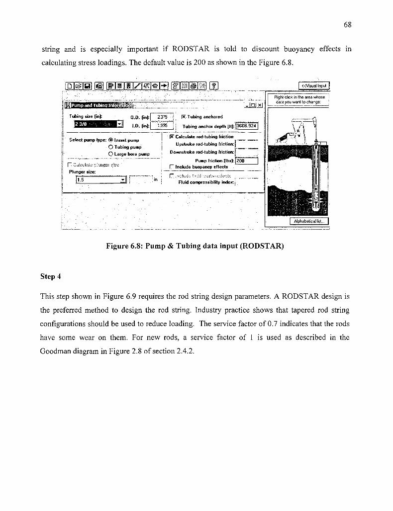
68

string and is especially important if RODSTAR is told to discount buoyancy effects in

calculating stress loadings. The default value is 200 as shown in the Figure 6.8.

QMM \M ffHTITZigteliH gMMUjB

|8|Pump and Tubing ihformatip

Tubing size (in): O.D. (in):

I.D. (in):

2.375

1.995

ix" Tubing anchored

Tubing anchoi depth (»):J3608 924 |

Select pump type: (a) Insert pump

O Tubing pump

O Large bore pump

Plunger size:

1.5 Mi

pT Calculate rod-tubing friction

Upstroke rod-tubing friction: |

Downstroke rod-tubing friction:!

Pump friction (lbs):]200

f Include buoyancy effects

f~ S?<ife«fe feM :n&*j'aw eii&Jit

Fluid compressibility index:]

«Visual Input

Right-click in the area whose data you want to change:

Figure 6.8: Pump & Tubing data input (RODSTAR)

Step 4

This step shown in Figure 6.9 requires the rod string design parameters. A RODSTAR design is

the preferred method to design the rod string. Industry practice shows that tapered rod string

configurations should be used to reduce loading. The service factor of 0.7 indicates that the rods

have some wear on them. For new rods, a service factor of 1 is used as described in the

Goodman diagram in Figure 2.8 of section 2.4.2.

69

Step 5

In this next step shown in Figure 6.10, the type and make of pumping unit from the drop down

list are selected. Also the stroke length that is set in the field is selected from the drop down list.

In this case, a Pump Jack with a maximum available stroke length of 120 inches is selected.

Since Penn west has a Lufkin C320-256-120 available in the inventory, it was selected from the

drop down list to avoid any extra capital expenditures.

The structure unbalance is defined in API 11E as "The force you need at the polished rod to hold

the walking beam horizontal with the pitman arms disconnected from the crank pins". This force

is positive when acting downward and negative when acting upward.

70

PMjal \m [fMITTTMM^] [ i M M H f «Visual Input

I i

Igjg Pumping Unit Informa'tidj^j

; ] © Manufacturer:

1 Pumping unit: i '.

0 Unit ID: i

; ' API designation:

) j Unit name: ! Other information:

1 :""

| Structural unbalan

Existing maximum

,...,..::„r.r'-^—-~~^

Lufkin Conventional - New

C-320D-256-120

CL45 D Use custom

C-320-25G-120" .

C-320D-25S-120

ce (lbs): 55

counterbalance moment (M in-lbs): • • • ( ' . . . . — • r — —

! Use CBALANCE data... 1 Unknown |x ' 1 1 l

._-

zJ ~z\

; " - |P | :X l

Recommended unit size:

No recommepidatiof |

pumping unit list

—

Crank rotation:

0 Clockwise

® Counterclockwise

Crank hole:

:0KHIHHSIjizJ^ Calculated stroke length:

121.0" |

Right-click in the area whose data you want to change:

Step 6

Figure 6.10: Pumping Unit data input (RODSTAR)

This step requires entering the energy costs per unit, the motor type from the drop down list and

the motor size as shown in Figure 6.11. It is recommended to use RODSTAR recommendation

for motor size.

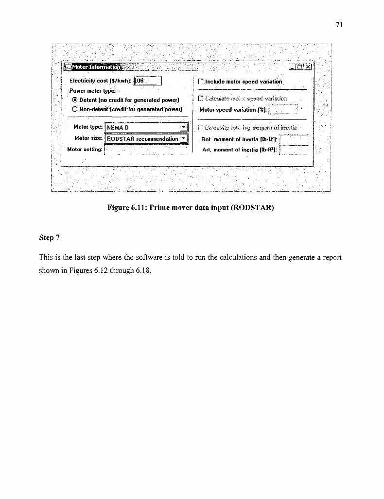
71

1-iuiMamuMF I • ™™ ;

Electricity cos

^13 mTtk t

t ( s / k w h j : LOG n Include motor speed variation

Power meter type:

® Detent [no credit for generated power)

0 N on-detent (credit for generated power)

Motor type:

Motoi size:

Motor setting: 1 t

NEMA D :z\

RODSTAR recommendation '_jj

.•• O CaScuEaJs RMKH tpssd ymmimm

Motor speed variation (%): j

• r i 'Gaiculeie reliving MomesiH of inertia •'••

x |

i

•

Rot. moment of inertia (Ib-fP):

Art. moment of inertia (Ib-fP): }

Step 7

Figure 6.11: Prime mover data input (RODSTAR)

This is the last step where the software is told to run the calculations and then generate a report

shown in Figures 6.12 through 6.18.

72

pMTal \M WMW\7\M^W\jM Till Visual lnput>>

FjfOutput Results 2<j

3

o

©

o

800-i

700-

600-

500

100

300-

200-

100

0

Inflow Performance Relationship (Correlat ion: Voge l )

- on - Water - Fluid - Current Design D Test Points

r — > -0 20

—I—r-40 60

- i — r —

80 i—I—r 100 120 1-40 160 180

P r o d u c t i o n (BPD)

I rjynamometer X o r Q u e Plot I PR Plot Report I Animate Dyno: E t I » ; Close

Figure 6.12: IPR result (RODSTAR)

£ H Output Result ^S lS lS

</> II)

5 O

_ l

Predicted Dynamometer Plots

16000-

14000 -_

12000-f

10000-f

8000-

6000 {

4000-j

2000-j

-2000 J

v̂__ ——— Predicted surface dyna. card

Dowinhole dynamometer card Permissible load diagram

y " ^ V jr

^^^ "\ I I 1 1 1 1 1 1 1 1 1 1 ' 1 ' 1

D 20 40 60

Position

i | • i

80

(inches)

; , , ' •

i i > i i i i i i i 100 120 140

f Dynamometer"]" Xorque Plot j IPR Plot Report j Animate Dyno: ^JJJJ > J j ^ CJosi

Figure 6.13: Dynamometer Result (RODSTAR)

73

MlOutput Results

INFLOW PERFORMANCE RELATIONSHIP INFORMATION

Correlation: Vogel Mid-perf depth (ft): 3716

Pressure test points: Flowing b.h. press, (psi)

605.0

Fl.Prod (BFPD)

50.00

Pressure vs. Pump intake press.(psi)

275.0 250.0 225.0 200.0 175.0 150.0 125.0 100.0

Static b h. pressure (psi): 798 Bubble point pressure (ps

production: Flowing b.h. press, (psi)

275.0 250.0 225.0 200.0 175.0 150.0 125.0 100.0

Oil (BOPD)

37.69 38.72 39.67 40.56 41.37 42.11 42 .79 43 .39

Water (BWPD)

88. 15 92 .37 96.59 100.80 105.02 109.24 113.45 117.67

L) : 3000

Fluid (BFPD)

125.84 131.09 136.26 141.36 146.39 151.35 156.24 161.06

I Dynamometer j Jorque Plot j ]PR Plot I Report | Animate Dyno: | i | • | •• | CJosi

Figure 6.14: IPR Result sheet (RODSTAR)

FSlOutput Results

Company: Pennwest Well: 6-35-85-15w6 Comment:

User: Hassan Disk file: 6-35-85-.RST Date: ll-Jun-09

Production rate (BFPD): 150 Strokes per minute: 6.0 Run time (hrs/day): 24.0 Surface stroke (in): 121.0 Water specific gravity: 1.0 Water cut: 65% Oil API gravity: 41.0 Fluid specific gravity: 0.9

Pump intake pressure (psi) : 157 Fl. lev. (ft over pump): 120 (calc.) Tubing pressure (psi): 90.0 Casing pressure (psi): 100.0 Buoyant weight of rods (lbs): 6851

Peak polished rod load (lbs): 11786 Hin. polished rod load (lbs) : 5183 Polished rod horsepower: 6.6 PLHP: 25.1 PRHP/PLHP =0.26 N/No1: 0.097 Fo/SKr: 0.08 System efficiency (Hotor->Pump): 42% Balanced elect, cost (?/bf): .069 Balanced elect, cost (S/bo): .198

Balanced min. req. motor HP: 12 Unit structure loading: 46% Balanced gearbox loading: 69% •Maximum rod loading: 112% Fluid load on pump (lbs) : 2822

j Dynamometer Tpique Plot IPR Plot Report Animate Dyno: M • •• Close

Figure 6.15: Well data result (RODSTAR)

74

CT^THI figl (MWTITZIM^I^I CTlTaTWI IT Visual lnput»

F»| Output Results ms- *J TUB ING PUMP

Tubing O.D. (in): 2.375 Tubing I.D. (in): 1.995 Tubing anchor depth (ft): 3 609 Tubing stretch (in): 0.5 Upstr. rod-tub. frict: 0.53 (calc. Downs, rod-tub. frict: 0.53 (calc. Stuffing box friction (lbs): 100 Pump load adjustment (lbs): 0

Pump depth (ft): 4232 Pump condition: Full pump Pump type: Insert Pump friction (lbs): 200 Plunger size (in): 1.5 Gross pump stroke (in): 113 Assumed pump volum. efficiency: 85% Pump spacing (in. from botm.): 12.7 Minimum pump length (ft): 15.0 Recom. plunger length (ft): 3.0

fF vnamorneter I Toraue Plot T~ IPR Plot "1 ~ Reooit 1 Animate Dvno: I BI J » I Close

Figure 6.16: Tubing result (RODSTAR)

Fsl Output Results 2<j

ROD STRING

Diam.

(in)

+ 0.875 0.75

+ Requires

STRESS ANALYSIS (rod tapers calculated) Service factor: 0.7

Rod

Grade

K (API) K (API)

Len.

(ft)

1382 2850

Tensile

St. (psi)

85000 85000

Stress

Load %

112% 112%

Top Hax.

Str.(psi)

19524 18924

Top Min.

Str.(psi)

8875 6931

Bot. Min

Str. (psi

5259 -453

slimhole couplings. NOTE: Stress calculations do not include buoyancy effects.

i

I

t t

1

f

i i

I—

1 j i i

i

Dynamometer X«"Que Plot IPR Plot Report Animate Dyno: m\ • •• Close

Figure 6.17: Rod string result (RODSTAR)

75

'(Output Results

PUMPING UNIT: Lufkin C o n v e n t i o n a l Uni t name: C-320D-256-120

New n API size: C-320-256-120 Calc. stroke length (in): 121.0 Structural unbalance (lbs): 55 Rotation with well to right: CCW

TORQUE ANALYSIS

Unit ID: CL45 Crank hole # 1 (out of 4) Crank offset angle (deg): 0.0 Maximum CB moment: Unknown

Peak gearbox torque (M in-lbs): Gearbox loading: Cyclic load factor: Maximum counterbalance moment (H in-lbs) Counterbalance effect (lbs):

BALANCED (Min Ener)

2 3 7 74% 1 . 5 6 4 8 5 . 8 2 8572

BALANCED (Min T o r q )

222 69% 1 . 5 7 5 0 8 . 2 0 8 9 6 4

Dynamometer X°rQ.ue Plot IPR Plot Report ] Animate Djino: Close

Figure 6.18: Gearbox loading result (RODSTAR)

The report generated will include the IPR curves, rod and gear box stresses and also if they are

within the allowable stress range percentage, the calculated horse power for the motor size and

the downhole pump card.

Based on the report generated, necessary adjustments are done to make sure that all equipment is

operating optimally within the allowable stress ranges. It is always recommended for an engineer

to apply his knowledge, skills, experience and engineering judgment to perform the calculations

manually or through spread sheets or at least carry out manual verification of the results provided

by these software.

The first report shows that the rod string loading is in excess of 100 %, so a different rod string

grade from "K" to "D" would need to be selected as shown in Figure 6.19, which has a higher

tensile strength and this effectively resolved the loading problem as shown in Figure 6.20.

76

DT^TB] fill [ITWTlTZT^riTO [MBTa

Rod grade or manufacturer:

Maximum rod diameter to consider:

Minimum rod diameter to consider:

f " Include sinker bars/sinker rods ®. K » A «

Sinker bar grade/manufacturer:'<

Sinker bar diameter:!

O S an'̂ sc jcas

17 Sinker bar length (ft): •

Service factor:

Additional rod costs:

Cost description:

«Visual Input

Right-click in the area whose data you want to change:

Figure 6.19: Rod string data input II (RODSTAR)

QMMWMMMJMZJMK FTM •GPlmlmiz*

~ O u t p u t Results %.? jm&u-a-:-^-

Visual lnput>>

-*j

ROD STRING

Diam.

(in)

+ 0.875 0.7S

STRESS ANALYSIS (rod tapers calculated) Service factor: 0.7

Rod

Grade

D (API) D (AP I)

Len.

(ft)

1532 2700

Tensile

St. (psi)

115000

115000

Stress

Load %

73% 73%

Top Max.

Str. (psi)

19660 18270

Top Hin.

Str. (psi)

8956 6461

Bot. Hin

Str. (psi

4929 -453

+ Requires slircihole couplings.

NOTE: Stress calculations do not include buoyancy effects.

j

il

'i

:i i

! 1

1

Dynamometer torque Plot JPR Plot Report Animate Dyno: • I • I • • Dose

Figure 6.20: Rod string result II (RODSTAR)

77

6.6 Results

Based on the results from the RODSTAR report, it shows that by installing the pump jack, C320-

256-120 with the current grade "K" rod string, having a tensile strength of 85000 psi, the rod

string would be over stressed as seen from the stress load section in Figure 6.17. In-order to

mitigate the problem, a higher strength rod would have to be selected. In this case by selecting a

grade "D" rod string, with a tensile strength of 115,000 psi effectively resolved the issue as

shown in Figure 6.20.

For the downhole pump, a longer pump barrel was designed to fully utilize the 120 inch stroke

length with the same 1.5 inch plunger diameter. A bigger pump jack could have been avoided

provided there was 2.875 inch diameter tubing in the wellbore. In that case by landing a 2 inch

diameter plunger would have resulted in the incremental volumes as shown in the IPR curve in

Figure 6.7.

After upsizing the pump jack, the production rose to 120 BPD of total fluid that resulted in some

of our expected incremental production. Since the well has wax and scale issues, it was put on a

more stringent chemical program to effectively resolve the issue and increase the pump

efficiency. It is important to mention that any work done might not result in instant change as

expected and could take a while before the desired results are noticed or observed.

This describes the process of optimizing a pump jack in the field. There are other things like

pump off controllers, dynamometers etc. that can be included in the optimization process but that

is beyond the scope of this project and anyone interested in carrying forward the optimization

work can actually write a full report on it.

7 CONCLUSIONS AND RECOMMENDATIONS

7.1 Conclusions

This report can be very beneficial for students and graduate engineers interested in the field of

pump jack optimization. It is written in the context of actual practices involved in pump jack

optimization in the petroleum industry.

The description of the overall optimization process of pump jacks in this report serves the

purpose of building an understanding of the technical challenges involved in this process and a

step by step process to address those challenges. The learning and skills provided in this report

will give a person the ability to:

i. Understand the importance of flowing bottomhole pressure in rod pump optimization

ii. Understand the behavior of a producing rod pump well

iii. Calculate the flowing bottomhole pressure of a rod pump well by using the acoustic

method

iv. Calculate the oil gradient in the casing annulus

v. And the ability to use the following methods to estimate producing potential

a. Constant PI method

b. Vogel's method

c. Combined constant PI and Vogel's method

7.1.1 Recommendations

1. The ideal means to verify the exact nature of the inflow performance relationship is to

conduct a multi point test also known as a flow after flow test. This involves simply

testing the well at different draw downs to determine the resulting production rates. Since

it is very costly and time consuming as the well needs to be stabilized before every

successive flow after flow test, it is not done until it requires a more expensive artificial

lift type like an ESP (electrical submersible pump). For most land based application in

western Canada, there is very little multi point testing conducted on oil wells and the

current practice involves just a single point test and applying Vogel's correlation. For

78

79

most artificial lift design using beam pumping, this approach is accurate enough due to

the flexibility of pump jacks to adjust pump displacement to match well capacity.

Also well stimulation to achieve a flow efficiency of one or greater than one could be

very costly in case of damaged formations if it involves fracturing, and hence for the

most part, until very high incremental volumes are expected it is very difficult to justify

the costs for the job.

2. It is recommended to use sinker bars on the bottom of the rod string particularly with

large diameter pumps, viscous fluid wells and highly deviated wells. This helps to

eliminate the bending and buckling of rod string that usually occurs during the pumping

cycle. Since RODSTAR does not have any design consideration for sinker bars, it is

advised based on field experience to use them when designing the rod string. Graphs for

recommended lengths of sinker bars for a variety of depths and pump sizes are published

by the USS oil well division of the United States steel.

3. It is also very important to know the specific gravity of the gas when calculating the fluid

level by the acoustic method. This is done on a regular basis by sending gas samples to

the laboratory. It has been experienced in the field that by entering an incorrect value for

the specific gravity of the annular gas in the acoustic equipment will result in an incorrect

fluid level. This happens due to the improper calculation of velocity of the sound wave

propagated down the annular space.

8 REFERENCES

[ 1 ] Quinn Pumps Training Manual

[2] Lufkin, Conventional & Reverse Mark Pumping Units, Installation manual CU-96, Texas, U.S.A.

[3] Penn West Petroleum, Production Engineering Training Manual Volume 1

[4] Lufkin, Mark II Pumping Units, Installation Manual M-96, Texas, U.S.A.

[5] Lufkin Pumping Units, Lufkin Industries, Inc. Texas, U.S.A.

[6] API Specification for Subsurface Pumps and Fittings, API Std 11 AX (Sixth Edition), American Petroleum Institute, Washington, D.C., March 1971

[7] Artificial Lift Systems, ENFORM, 2006

[8] Boyun Gou, William C. Lyons, and Ali Ghalambor, Petroleum Production Engineering, Elsevier Science & Technology Books, 2007

[9] CE Franklin LTD., Artificial Lift systems, Bottomhole Pump School Manual

[ 10] Production Optimization, ENFORM, 2006

[11] Echometer Co., http://www.echometer.com/images/product photos/lg/wa_lg.jpg, accessed date: 10-08-2008

[12] Echometer Co., http://www.echometer.com/images/product photos/1 g/compact gas gun lg.jpg, accessed date: 10-08-2008

[13] Fluid Level Analysis System, User Manual, Ventawave (Lufkin Automation) Houston, TX, 2001

[14] Penn West Petroleum, Production Engineering Training Manual Volume 2

[15] A.L.Podio, J.N. McCoy and K.L. Huddleston, Acoustic Producing Bottomhole Pressures, SPE 1425

[16] Vogel, J.V.: "Inflow Performance Relationships for Solution- Gas Drive Wells", JPT, (Jan. 1968)83-92

[17] Standing, M.B.: "Inflow Performance Relationships for Damaged Wells Producing by Solutions-Gas Drive", JPT (Nov. 1970) 1399-1400

[18] Engineering Data Book, S.I. Version, Volume I, GPSA, Tulsa, OK, 2004

80

81

4, Las Vegas, NV, 1985

[19] Engineering Data Book, S.I. Version, Volume II, GPS A, Tulsa, OK, 2004

[20] Nind, T.E.W.: Principles of Oil Well Production, McGraw-Hill, New York, 1964

APPENDIX A

Authorization from Penn West Petroleum to reproduce Parts from Proprietary Production Engineering Training Manuals, Volume 1 & 2

From: Gordon Wichert Sent: Fri 1/30/2009 3:13 PM

To: Hassan Khan

Cc: Gregg Gegunde <-, , . RE: Permission to Use excerpts from Pennwest Training

' manuals for production Engineers Attachments:

View As Web Page

Hassan:-

Penn West has no objections to the use of information from the Training Manuals as per the conditions of use that you have described below.

regards,

GordonWichert,M.Sc, P.Eng. Manager, North Production Penn West Energy office:(403)777-2542

From: Hassan Khan Sent: Thursday, January 22, 2009 4:28 PM To: Gordon Wichert Subject: Permission to Use excerpts from Pennwest Training manuals for production Engineers

Gord,

As discussed, I am working on my M.eng project and would like permission to produce some material in my project work from the Penn west Training Manuals for Production engineers with proper reference stating that "Excerpts from the Penn west training manuals are reproduced with the permission of Penn west. All rights reserved". Reference to proprietary data and locations will be removed.

82

83

I had discussed this with Steve Urselescu and he had no objections as long as it was properly referenced. Since he is no longer with the company, I request you to kindly grant me permission to do so. Just to let you know this is purely for educational purposes and I think the university students at Dalhousie, Halifax will benefit a lot from this kind of information.

These training manuals became the property south swan hills unit from Gulf oil. Awaiting

Thanking you.

; Hassan Khan PENN WEST ENERGY Tel: (403)777-2590 Cell: (403) 510-1820

of Penn West Energy /our kind response.

after the acquisition of the

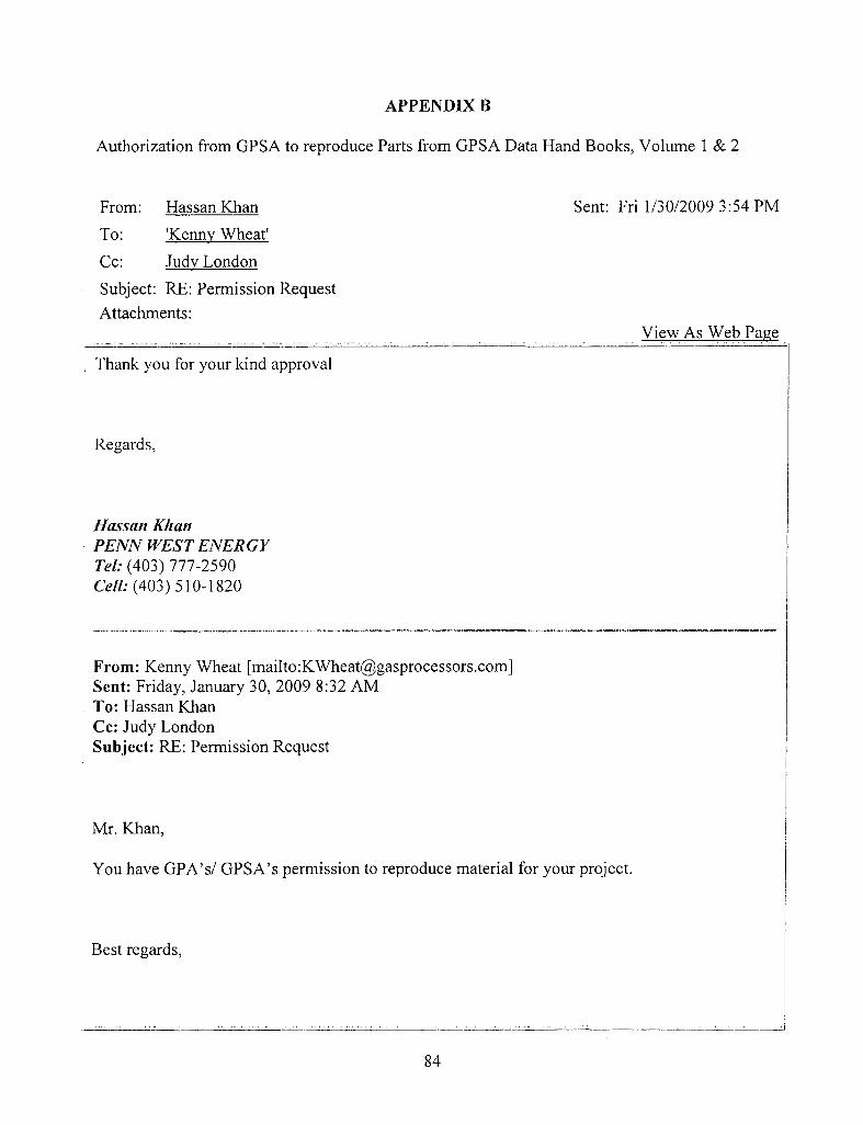
APPENDIX B

Authorization from GPSA to reproduce Parts from GPSA Data Hand Books, Volume 1 & 2

From: Hassan Khan Sent: Fri 1/30/2009 3:54 PM

To: 'Kenny Wheat'

Cc: Judy London

Subject: RE: Permission Request Attachments:

View As Web Page

Thank you for your kind approval

Regards,

Hassan Khan PENN WEST ENERGY Tel: (403) 777-2590 Cell: (403) 510-1820

From: Kenny Wheat [mailto:KWheat@gasprocessors.com] Sent: Friday, January 30, 2009 8:32 AM To: Hassan Khan Cc: Judy London Subject: RE: Permission Request

Mr. Khan,

You have GPA's/ GPSA's permission to reproduce material for your project.

Best regards,

84

Kenny Wheat

Director Technical Services

Gas Processors Association

6526 E 60th St, Tulsa, OK 74145

Ph 918-493-3872; Fx 918-493-3875

kwheat@gasprocessors. com

From: Judy London Sent: Thursday, January 29, 2009 8:31 PM To: Kenny Wheat Subject: Permission Request

See below .. please respond.

Judy London

Publications Administrator

Gas Processors Association

Tulsa, Oklahoma USA

918-493-3872

ilondon@GPAglobal.org

www.GPAglobal.org

86

From: Hassan Khan [mailto:Hassan.Khan@pennwest.com] Sent: Monday, January 26, 2009 4:41 PM To: Judy London Subject: GPSA Data handbooks reference permission

Hello

I am working on my Masters of engineering project Titled "Production optimization of Pump Jacks" and would like permission to produce some material in my project work from the GPSA data handbooks with proper reference stating that "Excerpts from the GPSA Data hand books are reproduced with the permission of GPSA. All rights reserved".

I request you to kindly grant me permission to do so. Just to let you know this is purely for educational purposes and I think the university students at Dalhousie, Halifax will benefit a lot from this kind of information.

Awaiting your kind response.

Thanking you.

Hassan Khan PENN WEST ENERGY Tel: (403) 777-2590 Cell: (403) 510-1820