Production Inventory System with Different Rates of ...

International Conference on Mechanical, Industrial and Materials Engineering2015(ICMIME2015),

11-13 December,2015 RUET Rajshahi, Bangladesh

1

Production Inventory System with Different Rates of Production

Considering Poisson Demand Arrivals

Mohammad Ekramol Islam1, K.M. Safiqul Islam2 and Md. Sharif Uddin2

1Northern University, Bangladesh 2Jahangirnagar University, Bangladesh

Email: [email protected]

Abstract

This paper represents a single product stochastic production inventory model with two different

rates of production where demand arrives according to Poisson process. The model is built up

based on matrix approach. In this current model, backlogs are permitted and assumed that the

production will start from the inventory level where there are some predetermined backlogs. It is

also assumed that the production rate is higher during the backlogs situation than the situation

where there is no backlog. Some measures of the system performance in the steady state case are

derived, some numerical illustrations are given and sensitivity analyses are provided.

Key words: Backlogs, Production Inventory, Stochastic Inventory system.

1. Introduction During the last 40 years there has been a rapid growth of interest in scientific inventory

control. Scientific inventory control is generally understood to be the use of mathematical

model to obtain rules for operating inventory system. The subject has attracted such a wide

interest that today every serious student in Mathematics. Management science and industrial

Engineering areas are expected to have some experienced working with inventory Model.

Originally, the development of Inventory models had practical application as an immediate

objective to the large extent this is still true, but as the subject becomes older, better developed

and more thoroughly explored, an increasing number of individuals are working with

inventory models because they present interesting theoretical problems in Mathematics. For

such individuals, practical application is not a major objective; although there is the possibility

that their theoretical work may be helpful in practice at some future time.

2. Background of the Study

Many researchers have considered inventory model with the finite and infinite production

rates. Dave and Choudhuri [5] considered finite rate of production. Bhonia and Maiti [1] have

examined two models, in one model they considered production rate as a function of the on

hand inventory and in another as a function of demand rate. Chaho-Ton Su. Change-Wang Lin &

Chih-Hung Tsai [3] A deterministic Production Inventory model for deteriorating items with an

exponential Declining Demand. Rein Nobel and Headen [13] have considered production

inventory model with two discrete production modes. Perumal and Arivarignan [14] have

considered a deterministic inventory model with two different production rates. A

Krishnamoorthy andMohammad Ekramol Islam[7] considered (s,S) inventory system with

postponed demands. Mohammad Ekramol Islam et.al [8] considered stochastic inventory

system with different rates of production where backlogs were permitted. They also consider

in that paper shelf-life of the inventoried items are infinity. Mohammad Ekramol Islam et.al

[9] farther extended the result for perishable inventoried items.

Paper ID: IE-01

mailto:[email protected]



2

In that paper switching time also considered and that has taken as a random phenomena. In

both of their papers, they built up the models by using the concept of Kolmogorov differtial-

difference equations. B. Sivakumar and G. Arivarignan [2] have considered an inventory

system with postponed demands. Mohammad Ekramol Islam, K M Safiqul Islam and

Shahansha Khan[10] have considered Inventory system with postponed demands considering

reneging pool customers. Mohammad Ekramol Islam and Shahansha khan [11] have

considered a perishable inventory model at service facilities for systems with postponed

demands. Mohammad Ekramol Islam and Shahansha khan [12] further considered a

perishable inventory systems with postponed demands considering reneging pool customers

In this paper, we have considered a stochastic production inventory system with two different

rates of production with the possible slippage of production rate from one rate to another rate

over time. For the stage (-N to 0) we have considered production rate 1 and that of the stage

(0 to S) 2, where 1>2. Such a situation is desirable since our production starts from a

backlog situation and the model is built up by matrix approach.

3. Notations Arrival rate

1 Production rate when inventory levels vary from –N to 0.

2 Production rate when inventory levels vary from 0 to S.

N Pre-determined backlogs quantity.

S Maximum Inventory level.

I(t) Inventory level at time t.

4. Assumptions (1) Two different rates of production 1 and 2 are considered where 1 2.

(2) The process will continue producing at the rate 1 until the backlog vanishes and then will

start producing at the rate 2 and will continue producing at the same rate up to order

level (S) following exponential distribution.

(3) Production process will start when the inventory level reaches –N unit of items as a

backlogs.

(4) When inventory level will reach the order level, production will be switched off

5. Methodology In this model, the inventory system starts with a backlog and reaches in off mode at the

inventory level S. Demand arrives at a rate following Poisson process. Inventory level will be

depleted when customers demand will be satisfied. When inventory level reaches in the state

0,1 N the very next demand converts the system on mode from off mode i.e, 1,N .

In that stage, if further demand arrives that will be lost forever. The inventory level I (t) take the

values in the set SNNA ,......,0,......,1,

By our assumptions I(t), t0} does not follow Markov Process. To get a two dimensional Markov

process, we incorporate the process δ(t), t0 into I(t), t0 process where δ(t) is defined by,

δ(t)=

Otherwise 0

ON is process productionn Whe1

Now, I(t), δ(t), t0is a two dimensional continuous Markov Chain defined on the state space

21 EEE where, SNNiiE ,...,2,1:0,1 and

1,...,1,:1,2 SNNiiE

The infinitesimal generator matrix of the process Ā= )),(,,);,:,(( Elkjilkjia



3

22

22

2

22

11

~

..00..000..00..00

..00..000..00..000

................................

00....00..00..000

00....000..00..000

................................

00..00..0..00..000

00..00..0..00..000

00..00..0..00..000

................................

00..00..000..0..000

00..00..000....000

................................

00..00..000..00..00

00..00..000..00..0

00..00..000..00..0

1,1

1,2

..

1,1

1,0

..

1,1

1,

0,1

..

0,0

0,1

..

0,2

0,1

0,

S

S

N

N

N

S

S

S

A

The above matrix can be obtained using the following arguments;-

A. The arrival of demand makes a transition from

1....1 if )1,1(),(

.2....1, if )0,0,1(),(

NSijlikji

NSSijlikji

B. Production of an item makes a transition

2.... if)1,1(),( SNijlikji

C. A demand can convert the system from off mode to on mode and can make a

transition from.

1 if ,1,1()0,( Nijlikji

D. One unit of production can convert the system from one mode to off mode and can

make a transition

1Si if );,1()1,( ojlikji

Inventory level which represents negative sign indicates intangible items (i,e backlogs,)

6. Steady State Analysis

It can be seen from the structure of matrix A

that the state space E is irreducible. Let the

limiting distribution be denoted by jip , :

ElkjittILtpt

ji

, ,,,Pr ,

The limiting distribution exists and satisfies the following equations-

1 and 0~ S

1,0-Ni

1-S

1,j

, N

jipAp

The first equation of the above yields the following set of equations:-

In off Mode

(i) 01,120, SS pp

(ii) 1....,1;00,10, NSipp ii

(iii) 01,10,11,1 NNN ppp

In On Mode

(i) 0)( 1,221,12 SS pp

(ii) 1,...,3,2; 0)( 1,121,11,2 SSippp iii



4

(iii) 0)( 1,111,11,02 ppp

(iv) 1,...,2,1; 0)( 1,111,11,1 Nippp iii

The solutions are as follows When the system is in off mode

1,...,1,;1

)1,1(

2

0, NSSipp Si

When the system is in on mode

)1,1(11,2 1 SS pp

Sippp iSiSiS ,....,4,3; 1 )1),2((2)1),1((21,

1; )1),2((1)1),1((1)1,( Sippp iSiSiS

1

2

2

2

1

1

)1),2((1)1),1((11,

,,,

,....,2; 1

where

NSSippp iSiSiS

Where, )1,1( Sp can be obtained by using the following normalizing condition i.e.,

11

1,

1

0,

S

Ni

i

S

Ni

i pp

7. System Performance Measures

(a) Mean Inventory holds in the system

Let 1 denote the average inventory level in the steady state. Then

1

1

1,

1

0,1

S

i

i

S

i

i ipip

(b) Expected backlogs hold in the system:

Let 2 be the expected backlogs in the system in steady state. Then 2 can be defined as:

1

1

1

1,0,2

Ni Ni

ii pipi

(c) Average number of Customer’s lost to the system:

Let 3 is the average number of customers lost to the system. Then 3 can be defined as:

1,3 Np

(d) The probability that a demand will be satisfied just after its arrival is,

1

1

1,

0

0,4

S

i

i

S

i

i pp

(e) Expected waiting time of a customer

3

0

)1,(

1

)0,(

1

2

0

1]

1[)(

n

nn

n

qn

qnnN

TE



5

8. Steady State Cost Analysis of the model

Let us consider costs under steady state as given below: -

L = the initial set-up cost of the system.

C1 = inventory carrying cost per unit per unit time.

C2 = Backlog cost per unit time.

C3 = Cost due to customer lost to the system

So, the expected total cost to the system is,

E (TC) = L + C1 1 + C2 2 + C3 3

= L + C1 (

1

1

1,

1

0,

S

i

i

S

i

i ipip )+ C2 (

1

1

1

1,0,

Ni Ni

ii pipi )+ C3 1,Np

Since the computation of the s' are recursive, it is very difficult to show the convexity of

the total expected costs. However, it may possible for many cases to demonstrate the

computability of the result and to illustrate the existence of local optima when the cost

function is treated as function of only two variable which obviously a restricted case and

hence avoided. Of course, it may possible to explore some of the very important

characteristics of the system and also possible to do sensitivity analysis of the system.

9. Results

The results we have obtained in steady state case may be illustrated through the following

numerical example:

Steady state probabilities in the system for the parameters of S = 10, N = 3, = 3, 1 = 5, 2 =

4, L = 100, C1 = 6, C2 = 4 and C3 = 3 are as follows:

Table 1: Different system performances by using a given set of parameters

10. Sensitivity Analysis

Table 2: Production rate 1 Vs Total cost

Mean inventory holds in the system 2.38591

Expected backlogs holds in the system 0.48549

Average customers lost to the system 0.21051

Probability that a demand will be satisfied just after arrival 0.47661

Total cost to the system 116.88895

1 value 1 2 3 Total Cost

5 2.38591 0.48549 0.21051 116.88895

6 2.37760 0.49503 0.21909 116.90299

7 2.65555 0.32571 0.12054 117.59776

8 2.54998 0.37984 0.15588 117.28688

9 2.75436 0.24349 0.08040 117.74132

10 2.96740 0.10266 0.00375 118.22629



6

Fig. 1: Production rate Vs Waiting time

11. References

[1] A. K. Bhunia and M. Maiti, Ò Deterministic inventory model for variable production Journal of

Operations Research Society",Vol.48, pp.221-224, (1997).

[2] B. Sivakumar and G. Arivarignan , Ò An inventory system with postponed demands; Stochastic

Analysis and Applications",Vol.26, pp.84-97, (2008).

[3] Chaho-Ton Su. Change-Wang Lin & Chih-Hung Tsai (1999): A deterministic Production Inventory

model for deteriorating items with an exponential Declining Demand; Opsearch; V. 36, No. 2, 1999, p-

95-105.

[4] Krishnamoorthy A. and Mohammad Ekramol Islam, Ò (s, S) inventory system with postponed

demands;Stochastic Analysis and Applications", Vol.22, No.3, pp.827-2004,(2004).

[5] L.Y. Ouyang, C.K. Chen and H.C, Ò Chang, Lead time and ordering cost reduction in continuous

review inventory system with partial backorders. Journal of Operations Research Society", pp.1272-

1279,(1999).

[6] M. Deb and K. S. Chaudhury, Ò An EOQ model for items with finite rate of production and variable

rate of deteriorations", Opsearch, Vol. 23, pp.175-181, (1986).

[7] Mohammad Ekramol Islam, Abul Kalam Azad and A.B.M. Abdus Subhan Miah, Ò Stochastic

inventory models with different rates of production with backlogs", Jahangirnagar University Journal of

Science. Vol. 28, pp.209-218, (2005).

[8] Mohammad Ekramol Islam , Mohammad Shahjahan Miah and A.B.M.Abdus Subhan Miah,, Ò A

perishable stochasticinventory models with different rates of production with backlogs and random

switching time",Journal of National Academy of Science. Vol.31, No. 2, 231-238,(2007).

[9] Mohammad Ekramol Islam, K M Safiqul Islam and Shahansha Khan, ÒInventory system with

postponed demands considering reneging pool customers", Proceeding of the International Conference

on Stochastic Modelling and simulation (ICSMS) VelTech Dr.RR and Dr.SR Technical University,

Chennai. Tamilnadu(Pp(203-208), Allid Publishers Pvt Ltd. (2011).

[10] Mohammad Ekramol Islam and Shahansha khan , Ò A perishable inventory model at service

facilities for systems with postponed demands",Computational and Mathematical Modeling; Narosa

Publishing House,New Delhipg, pp-214-226, (2012)

[11] Mohammad Ekramol Islam and Shahansha khan, Ò A perishable inventory systems with

postponed demands considering reneging pool customers", International Conference on Engineering

Research, Innovation and Education (ICERIE), Sylhet, Bangladesh, (2013).

[12] Mohammad Ekramol Islam, K M Safiqul Islam and Md.Sharif Uddin, Ò Inventory system with

postponed demands considering reneging pool and rejecting Buffer customers", Proceeding of the

International Conference on Mechanical, Industrial and Material Engineering (ICMIME), RUET,

Rajshahi, Bangladesh.pp(1-3),November 2013.

0

0.05

0.1

0.15

0.2

0.25

0 2 4 6 8 10 12

Mea

n w

ait

ing

tim

e o

f

the

cust

om

er

Production rate 1

International Conference on Mechanical, Industrial and Materials Engineering 2015 (ICMIME2015)

11-13 December, 2015, RUET, Rajshahi, Bangladesh.

Paper ID: IE-04

Study of Process Parameters and Optimization of Process Variables for the

Production of Urea by Using Aspen HYSYS

Sadia Sikder[1] , Sadiya Afrose[2], Md. Ruhul Amin[3]

[1],[2],[3] Department of Chemical Engineering, Bangladesh University of Engineering and Technology

BUET

E-mail addresses: [email protected], [email protected], [email protected]

Abstract

Being easily acceptable in the soil, owning availability of raw materials and easy transportation made urea a

unique fertilizer. Two main reasons are involved in urea fertilizer to be the best of all fertilizers. Firstly, about

46 percent nitrogen is contained in it. Secondly, it is a white crystalline organic chemical compound. Urea is

formed naturally as a waste product by metabolizing protein in humans as well as other mammals, amphibians

and some fish. Urea is widely used in the agriculture sector both as a fertilizer and animal feed additive having

the chemical CO(NH2)2. In this paper, production of urea by the reaction of ammonia and carbon dioxide is

simulated by the Simulator software Aspen HYSYS v.7.1. It is performed to investigate effect of few important

parameters like temperature of carbon dioxide, temperature of HP (high pressure) steam and LP(low pressure)

steam on the composition of urea. When temperature of HP steam varies from 3570C to 3650C, composition of

urea varies from 0.055 to 0.08. When temperature of LP (low pressure) steam varies from 2870C to 3160C,

composition of urea varies from 0.055 to 0.782. Being a typical Stamicarbon process, different process

parameters are studied to understand the whole plant properly which are related with one another and the

relation with several graphical representations are shown. By analyzing the process variables, the profit is

optimized by using HYSYS Optimizer and found that $790.8.

Keywords: Biuret, Simulation, Stripping, Prilling, Granulation

1. Introduction Maintenance of high temperature and pressure is needed for the production of urea [1]. Urea is formed through

the heterogeneous reaction of carbon monoxide and ammonia [2]. Urea prills are produced in the prilling towers

where a solidification-cooling process takes place and the ambient air is used as the cooling air stream for this

process [3]. The temperature of produced prills and caking tendency of the prilled urea can be reduced by the

increase in heat transfer from the particles by using installation of induced fans [4]. Granulation being the most

fundamental operations in particulate processing, insight into the complex dynamic state behavior of these units

is still needed [5]. Having similar chemical properties of both prills and granules and also distinguishable

physical and mechanical properties, urea has been made suitable for different application either as fertilizer or

raw materials for chemical industry [6]. Urea granulation is favored over prilling due to the problems associated

with prilling [7]. In this paper, modeling and simulation of high-pressure and low urea synthesis loop has been

studied [8] Due to well established global warming concerns, technological attempts have been made to

decrease reactive nitrogen (N) species emitted from the application of urea fertilizer to agricultural soils [9].

HYSYS is applied to model the most significant aspects of the urea production processes by the availability of

modern flow sheeting tools [10].

2

2. Process Description The raw material composition used for this simulation is: CO2 gas 20% and liquid NH3 80% in mole fraction

The block diagram of Urea production according to Stamicarbon stripping processs from CO2 gas and Liquid

NH3 is shown in Fig. 1.

2.1 Reactions Involved 2 NH3 + CO2 ↔ H2N-COONH4

Ammonium Carbamate

H2N-COONH4 ↔ (NH2)2CO + H2O

Urea

2NH2CONH2 ↔ NH2CONHCONH2 + NH3

Biuret

2.2 Industrial Production Process Urea is synthesized from ammonia and carbon dioxide. The urea plant has 5 sections excluding utility system:

1. Synthesis section

2. Purification section

3. Concentration and prilling system

4. Recovery system

5. Process and condensate treatment system

Fig. 1. Process block diagram of urea production.

3

Fig. 2. Process flow diagram of urea production from ammonia and carbon dioxide.

2.3 Optimization

Table 1. Assumptions and data imported from HYSYS

Assumptions Data imported from HYSYS

Selling Price of cooler Out product, Pcool = $0.471/kg Mass of cooler out = M1= 3225 lb/hr Selling Price of Urea solution, PU = $0.6/kg Mass of urea solution out=M2= 200 lb/hr Cost of HP steam Inlet, PHP = $ 0.20/kg Mass of fresh CO2 = M3= 120 lb/hr Cost of LP steam Inlet, PLP= $0.30/kg Mass of NH3 = M4= 190 lb/hr Cost of fresh CO2, Pco2 =$0.05/kg Mass of HP steam= M5= 1250 lb/hr Cost of fresh NH3, PNH3 = $ 0.06/kg Mass of LP steam = M6= 1936 lb/hr Cost of pump duty, Cp= $0.03/kg Pump duty =Q1= 184.4 Btu/hr Cost of Compressor duty, Cc = $0.02/kg Compressor duty = Q2= -13.33 Btu/hr

Profit= (M1*Pcool) + (M2*PU)-(M3*Pco2)-(M4*PNH3)-(M5*PHP)-(M6*PLP) - (((Q1*Cp)+(Q2*Cc))/3600)

=790.8

3. Results and Analysis By comparing the process parameters and calculating the profit of this typical Stamicarbon process, more profit

can be made from the real plant. From optimization it was found that maximum profit was $790.8.The whole

process can be understood very clearly.

4

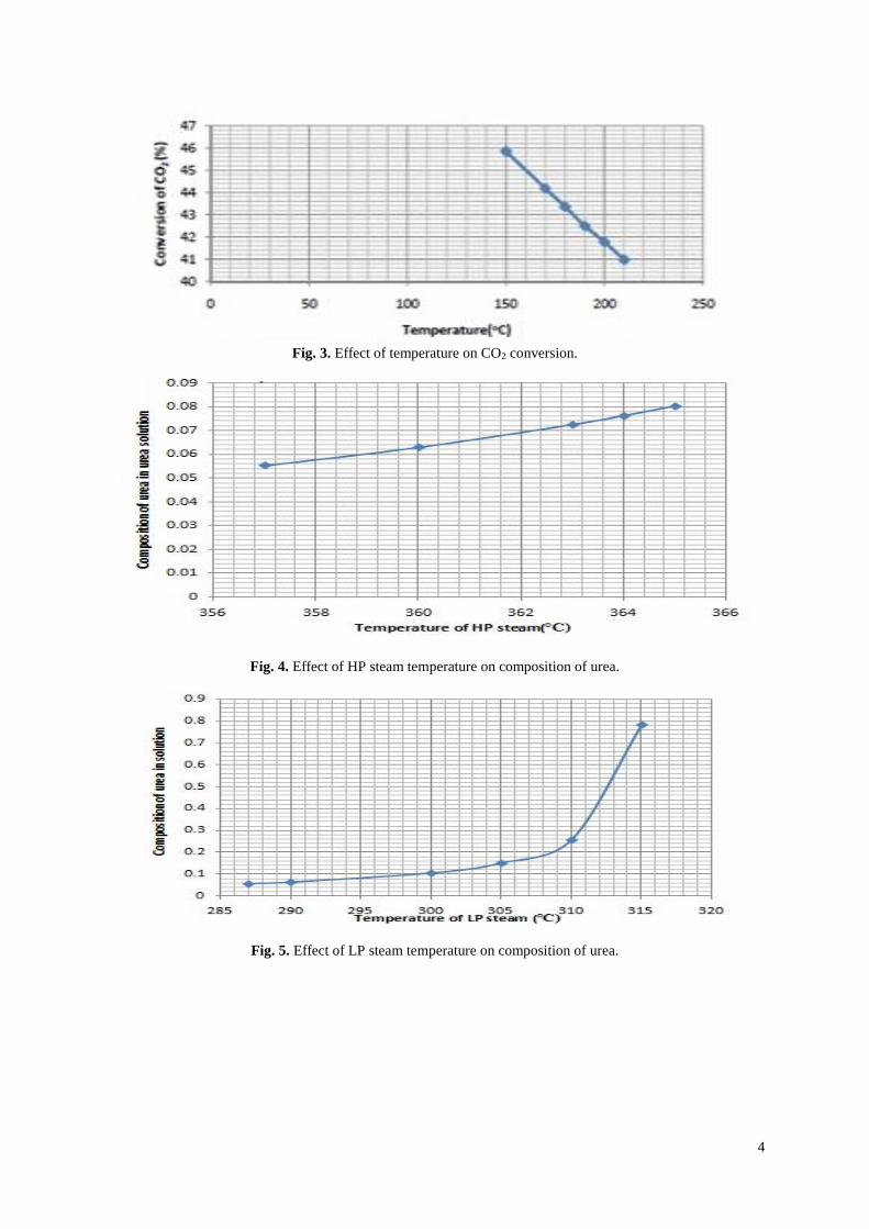
Fig. 3. Effect of temperature on CO2 conversion.

Fig. 4. Effect of HP steam temperature on composition of urea.

Fig. 5. Effect of LP steam temperature on composition of urea.

5

Fig. 6. Effect of CO2 temperature on heat generated in urea solution.

Fig. 7. Effect of pressure of CO2 on heat generated in urea solution.

Fig. 8. Effect of pressure on CO2 conversion.

Fig. 9. Relation between rate of ammonia to carbon dioxide flow rate and conversion of carbon dioxide.

6

Fig. 3 shows the effect of temperature on the percentage conversion of CO2 in the reactor (at 200 atm). As the

temperature increases, the conversion of CO2 decreases. Fig. 4 shows the effect of HP steam temperature on

composition of urea (at 170 atm). As the HP steam temperature increases, the composition of urea also

increases. Fig. 5 shows the effect of LP steam temperature on composition of urea. When the LP steam

temperature reaches 3100C, the composition of urea suddenly increases from 0.25 to 0.8. Fig. 6, shows the effect

of temperature of CO2 on heat generated in urea. Heat generated in urea solution decreases with the increase in

temperature. Fig. 7, shows the effect of pressure of CO2 on heat generated in urea solution. Generation of heat in

urea solution is increased with the increase of CO2 pressure. Fig. 8 shows the effect of pressure on the

percentage conversion of CO2 in the reactor. The conversion of CO2 is seen constant after the pressure reaches

210 atm. Fig. 9 shows the effect of ammonia flowrate on composition of urea. Conversion of CO2 at 210 atm is

seen constant when the ratio of NH3 to CO2 is made 15.

4. Discussion The reactor temperature and pressure are kept in the range 1800C-1900C and 120-150 bars respectively. So the

fresh ammonia temperature and pressure should be chosen carefully. Similar process should also be maintained

for fresh carbon dioxide. Production of urea and optimization is depended on the feed temperature and pressure.

So feed temperature and pressure should be chosen cautiously.

5. Conclusion Being an inexpensive and most concentrated nitrogenous fertilizer, urea is incorporated in mixed fertilizers as

well as also used alone to the soil. Over 90% of the world’s production of the substance is done for fertilizer

related product. About 350 MMSCFD natural gas is required for the yearly production of about 3 million metric

ton urea. A very competitive market has taken place due to the excessive use of urea. In order to produce urea at

a low cost, Simulation analysis can be proved very handy in the optimization of urea production without

conducting any real reactions or experiments. This job can be done pretty efficiently by optimizing several

operating conditions.

6. Acknowledgement Authors are grateful to the HYSYS course instructors of HYSYS Laboratory for their support and patience. The

technical assistance given by the Department of Chemical Engineering, Bangladesh University of Engineering

and Technology was very appreciable.

7. References [1] Kroschwitz, I. and Howe-Grant, M. Kirk-Othmer. Encyclopedia of Chemical Technology, Fourth edition, Volume2:638-

691. New York, Chichester, Bristbane, Toronto, Singapore : John Wiley and Sons Inc., 1995.

[2] M. Hamidipour, N. Mostou, R. Sotudeh, Modeling the synthesis section of an industrial urea plant, 25 July 2004.

[3] A. Mehrez, A. Hamza H. Ali, W. K. Zahra, S. Ookawara, and M. Suzuki,Study, “Heat and Mass Transfer During Urea

Prilling Process”, International Journal of Chemical Engineering and Applications, Vol. 3, No. 5, October 2012.

[4] N. Rahmaniana*, M. Homayoonfarda &A .Alamdari, Simulation of urea prilling process: an industrial case study,

doi:10.1080/00986445.2012.722147.

[5] Diego E. Bertín *, Juliana Piña and Verónica Bucalá Dynamics of an Industrial Fluidized-Bed Granulator for Urea

Production, DOI: 10.1021/ie901155a.

[6] Rahmanian, Nejat, Naderi, Sina, Šupuk, Enes, Abbas, Rafid and Hassanpour, Ali. Urea Finishing Process: Prilling

versus Granulation. Procedia Engineering,(2014), ISSN 1877-7058.

[7] U. Irshad, M. N. Sharif, R.U.Khan & Z.H. Rizvi, Granulation of Urea in a Pan Granulator, 2010.

[8] Xiangping Zhanga, Suojiang Zhanga, Pingjing Yaob, Yi Yuanb Modeling and simulation of high-pressure urea synthesis

loop, 28 October 2003.

[9] M. I. Khalil .Physical and Chemical Manipulation of Urea Fertilizer To Limit the Emission of Reactive Nitrogen Species,

Vol. 1072, ISBN13: 9780841226548, October11, 2011].

[10] , M.; Pierucci, S.; Sogaro, A.; Carloni, G. and Rigolli, E, Simulation Program for Urea Plants, Vol. 21, No. 5, 389-400,

1988.

International Conference on mechanical, Industrial and Materials Engineering 2015 (ICMIME2015)


Paper ID: IE-05

Inventory system at service-facility with N-policy consider reneging

and rejection of pool customers

Dr.Mohammad Ekramol Islam1, Dr. Shahansha khan2 1School of Business Administration, Northern University of Bangladesh 2School of Science and Engineering of Mathematics Uttara University, Bangladesh.

E-mail: [email protected]

Abstract

In this paper, we consider (S,s)inventory system. We assume that customer arrive to the system

according a Poisson process with parameter 0 . When inventory level depletes to s due to demands or

service to a buffer customer, an order for replenishment is taken placed. The lead time is exponentially

distributed with parameter .Any demand that takes place when the pool is full and inventory level is

zero, is assumed to be lost forever. During the time of waiting in the pool customers can get impatience

and leave the system with rate 1 can stay in the pool with rate Due to some reasons like to fail

to show the proper documents, customer can get the rejection from the server during the time of taking

the service with rate )1( or can get service with rate . The server will be on mode when the

number of pool customer is N , otherwise it is off mode. When inventory level is zero then arrival

customer may enter the pool with 1 rate and with rate will lost forever. Customers directly go

to the pool (waiting room) that has finite capacity 𝑀 < ∞.When number of customers reach to N , server

becomes on mode to provide the service provided that the items are available in the stock. When number

of waiting customers reach to 1N again server becomes idle Customers are served as the basis of

FIFS. In the present model, it is considered that during the time of waiting, customers can get impatient

and can leave the system. Moreover the server has the authorization to reject the customers due to lack

of eligibility or fail to show the proper documents to get services. The steady state probabilities are

determined, some system characteristics are derived, numerical illustrationsare provided and sensitivity

analysis is also made.

Key words: Reneging, Rejection, pooled customer and Inventory.

Introduction: In inventory models the major objective consists of minimizing the total inventory cost and to balance

the economics of large orders or large production runs against the cost of holding inventory and the cost

of going short. Staring from a simple lot size formula a huge amount of research is done in inventory

modeling. At the earlier research inventory control was treated as a separate identity from the service

providing system. But the dimension is changed over the last three decades. Our model is on continuous-

review inventory system with lost sales of customer that arrives during stock out. The lost sales situation

arises in many cases, where the intense competition allows customer to choose another service point.

This can be considered as a typical situation for being described by pure inventory Model. Lost sale are

usually known as losses of customers. There is a huge amount of literature on loss system, especially in

connection with telegraphic and communication system, where losses usually occur due to limited server

capacity. But there is another occurrence of loses due to balking or reneging of impatient customers.

Inventory system with service facilities was firstly considered by Sigman and simchi Levi[1]. Inthatpaer

they considered M\G\1 queue with limited inventory system. An approximation procedures are use to

find performance descriptions models, in which the interaction of queuing for service and inventory

control in integrated. In a sequence of papers Berman and his coworkers [2-6] investigated the behavior

of service systems with related to inventory system. Schwarz et al[7] characterized the earlier approaches

in the following manner: They defined a Markovian system process and then used classical optimization

methods to find the optimal control strategy of the inventory system. All those models assumed that the

demand which arrives during time the inventory is zero is backlogged. The model varied with respect to

lead-time distribution, the service time distribution, waiting room size, order size and reorder policy.


Islam and his co-workers [9-10] built some inventory models related to postponed demand, reneging

pool customers and rejection of customers from the system in service facilities. In this paper we

introduce Inventory system at service facility with N-policy. Consider reneging and rejection of pool

customers. Customers direct go to the pool region and get service. The strategy of our investigation in

this paper is as follows; we start the observation of Islam etal that paper the inventory system is started

when the inventory levels is When the number of customers reach to N server becomes on mode to

provide the service provided that the items are available in the stock. When number of waiting customers

reach to 1N again the server becomes idle. From the pool customers can get impatience and can leave

the system with rate 1 and can stay in the pool with rate Due to the same reasons like to fail

to show the proper documents customer can get the rejection from the server.

Assumption: 1. Initially the inventory level is S

2. Interarrival times of demands are exponentially

distributed with parameter .

3. Lead time is exponentially distributed with

parameter .

4. Maximum pool capacity is M.

5. Demand that arrives when the pool is full,

demand will be lost forever.

6. During the time of waiting in the pool;

customers can get impatience and can leave the

system with rate )1( can stay in the pool

with rate .

7. Due to some reasons like to fail to show the

proper documents, customers can get the

rejection from the server at service epoch with

rate )1( or can get service with rate .

8. The server will be on mode for the pool size if

MNNj ,.....,1, and in off mode if

1 Nj .

9. When inventory level is zero then arrival

customer may enter the pool with rate

and with rate )1( will lost forever.

Notation:

)(tI = Inventory level at time t . ; = Arrival rate of customers to the system. = Lead time

parameter. ; )(tN = Number of customers in the pool. )(tX = Represents the server’smode. ;

= service rate of the system.

1-1

; 1-1

;

1-1

; 1

Model and Analysis; In this model, the inventory system is stared when the inventory levels is S and the system is in OFF

mode. Demands follows Poisson Process with rate Inventory level will be deplete due to items

provided to the customers from the pool customers can get impatience and can leave the system with

rate )1( can stay in the pool with rate and Due to some reasons like to fail to show the proper

documents, customers can get the rejection from the server during the time of taking the service with rate

)1( or can get service with rate .When inventory level reaches in the state 0,1 N the

very next demand converts the system on mode from off mode i.e., 1,N . In that stage, if further

demand arrives that will be lost forever. The inventory level tI take the values in the set

SNNA ,......,0,......,1, By our assumptions I(t), t0} does not follow Markov Process. To get

a two dimensional Markov process, we incorporate the process δ(t), t0 into I(t), t0 process where δ(t)

is defined by,

Now, I(t), δ(t), t0is a two dimensional continuous Markov Process defined on the state space

21 EEE where, SNNiiE ,...,2,1:0,1 and

1,...,1,:1,2 SNNiiE

Where

1mod ,1

.....1,mod ,0)(

Njeonisserverwhen

MNNjeoffisserverwhentX

}0 ; )(),(),({ ttXtNtI is a three dimensional Markov process with state space

SE .......,.........3,2,1,01 ; MNNE ,.......,1,......,.........3,2,1,0

2 ; 1,0

3E ;

321EEEE

The infinitesimal generator can be obtained using the following arguments.

A) Arrival of customer makes a transition from 1,0,,2,......0,.....00,1,,, jmilkNJSinjmilkji

B) A demand can convert the system off mode to on mode makes a transition

0,,1,.....01,1,,, kNjSinjmilkji

C) A customer demand can satisfied convert the system from on mode to off mode

1,,........,.....00,0,.....1,,,, kMNJSinNNmilkji

D) Due to the replenishment inventory , the system makes a transitions

1,,......,.....0,,,, kMNjSiknjmQilkji

E) Due to the inventory, the system makes transitions.

0,,1......0,.....00,,,, kNJSiknjmQilkji

On Mode: QilSi ,.,.........2,1,0

j=N,..........M, m=j

K=1………, n=k 1 ,........2,1 ilSi

1 ..........1 jmMNj

1 1 knk

1 ,........2,1 ilSi

1 jmNj

0 1 knk

1 ilSi ,.........2,0

1 ......1 jmMNj

knk 1

1 ilSi ,........2,0

1 jmNj

0 1 knk

1 ilSi ,........2,1

1 ........1 jmMNj

knk 1

1 ilSi ,.......1,0

1 jmNj

0 1 knk

ilSi .,.........1

1 1-,...M jmNj

knk 1

ili 0

1 1-,...M jmNj

knk 1

1 ilsi ,...,1

jmMNj ,,...

knk ,1

1 ilSsi ,...1

jmMNj ,1,...

knk ,1

11 ili 0

jmMNj ,1,...

knk ,1

11 ili 0

jmMj

knk 1

11 ilsi ,...,1

jmMj

knk 1

11 ilSsi ,...,1

jmMj

knk 1 1 ilSi ,,...2,1

jmMj ,

knk ,1

Off Mode: Qilsi .......,.........1,0

jmj 1-...N0,1.......

0 0 knk

ilSi .......,.........1

1 2-...N0,1....... jmj

0 0 knk

ilSi .......,.........1

1 1-N jmj

1 0 knk

1 ilSi .......,.........1,0

1 1-...N0,1....... jmj

ili 0

1 2-...N0,1....... jmj

0 0 knk

1 ilsi ,...,1

jmNj ,...,0

knk 0

1 ili 0

jmNj 1,...,0

knk 0

1 ili S1,...,s

jmNj 1,...,0

knk 0

0 0 knk

Let us assumed S0 I and 00 X

consider the transition probabilities:

0,0,0,0,00,,,,,,0,0,

SXNIjitXtNtIptkjiS

P

From now onwards we can write tkjiP ,,

for tkjiSP ,,0,0,

. The kolmogorve forward difference

differential equation are given below.

When the system is OFF mode

0j, 1.....sS.........i;

0,1,0,0,

0,0,-

0,0,

iP

QiP

iP

iP

0j, .....1s.........i;

0,1,

0,,-

0,,

jiP

jiP

jiP

0j, 0i; 0,1,

0,,

- 0,,

ji

Pji

Pji

P

1j, 1S......si;

0,,0,1,0,,

0,,

0,,

jiP

jiP

jQiP

ijiP

jiP

1-..N1.........j1,........s.....i ;

0,,0,1,0,,

0,,1,1,1

0,,

jiP

jiP

jQiP

ijiP

jiP

jiP

1-..N1.........j1,........s.....i;

0,,0,1,0,,

0,,

0,,

jiP

jiP

jQiP

ijiP

jiP

..N1.........j, 0i ;

0,,0,1,

0,,

0,,

jiP

jiP

ijiP

jiP

When the system is on mode

1-2........Mj, 1S......si;

1,,1,1,1,,

1,,

1,,

jiP

miP

jQiP

ijiP

jiP

1-2........Mj, 11......s-Si ;

1,,11,,1,1,1,,

1,,

1,,

iMiP

jiP

miP

jQiP

ijiP

jiP

Mj , Si ;

1,,1,,1,,

1,,

1,,

jiP

miP

jQiP

ijiP

jiP

1-2........Mj, 1S......si;

1,,1,1,1,,

1,,

1,,

jiP

miP

jQiP

ijiP

jiP

1-3........Mj , 11......s-Si ;

1,,11,,1,,1,,

1,,

1,,

MiP

jiP

miP

jQiP

ijiP

jiP

Mj, Si ;

1,,1,,

1,,

1,,

jiP

jQiP

ijiP

jiP

Nj, 1.s....i ; 1,1,11,,1,1,

1,1,

1,,

ji

Pji

Pji

Pji

Pji

P

Mj , 1.......s.....i ;

1,,11,,1,,

1,1,

1,,

jiP

jiP

jiP

jiP

jiP

1-M...........1j, 0i;

1,,1,1,

1,1,

1,,

N

jiP

jiP

jiP

jiP

Mj, 0i ;

1,,1,1,

1,,

jiP

jiP

jiP

Limiting Distribution:

The steady state probabilities for E ji, of the system size are obtained by taking the limit at t

on both sides of the above equations and solving them respectively .Note that under steady state

condition

01,,

lim;00,,

lim

jiP

tji

Pt

And 1,,1,,

lim;0,,0,,

limji

qji

Pt

jiq

jiP

t

The limiting distribution exists and satisfies the normalize condition

1S

-1i

M

j1,,

10,,

1

0

Nji

PS

iji

PN

j

The balancing equation can be written as

When the is in off mode:

0j, 1.....sS.........i ;

0,1,0,0,

0,0,

iq

Qiq

iq

0j, .....1s.........i;

0,1,

0,,

jiq

jiq

0j, 0i;

0,1,

0,,

jiq

jiq

1j, 1S......si ;

0,1,0,,

0,,

0,,

jiq

jQiq

ijiq

jiq

1-1........Nj, s......1i ;

1,1,1,1,1

0,1,

0,,

jiq

jiq

jiq

jiq

1-1........Nj; s......1i;

1,1,

0,1,

0,,

jiq

jiq

jiq

1-1........Nj , s......1i ;

1,1,

0,1,

0,,

jiq

jiq

jiq

When the syatem is on mode

1-2........Mj, 1S......si;

1,1,1,,

1,,

1,,

miq

jQiq

ijiq

jiq

1-2........Mj, 11......s-Si ;

1,1,1,1,11,,

1,,

1,,

miq

Miq

jQiq

ijiq

jiq

Mj, Si ;

1,1,1,,

1,,

1,,

miq

XjQiq

ijiq

jiq

1-3........Mj, 11......s-Si ;

1,,1,,11,,

1,,

1,,

miq

Miq

jQiq

ijiq

jiq

Mj, Si;

1,,

1,,

1,,

jQiq

ijiq

jiq

Nj , s......1i ;

1,1,1,1,1

1,,

1,,

jiq

jiq

ijiq

jiq

Mj , s......1i;

1,,1,,1

1,,

1,,

ji

qji

qiji

qji

q

Mj, s......1i;

1,,

1,,

ijiq

jiq

1-1........MNj , 0i ;

1,1,

1,,

1,,

jiq

ijiq

jiq

Mj, 0i;

1,,

1,,

ijiq

jiq

System Performance Measures (a) Mean Inventory holds in the system

S

iji

iPM

Nj

S

iji

iPN

j 11,,

10,,

1

01

b) Expected number of customers

reneging to the system

S

i

S

iji

PiM

Njji

PiN

j0 01,,

10,,

11

12

c) Expected number of customers

rejection to the system: 1,,

0

13 ji

PS

i

M

Nj

d) The probability that a demand will

be satisfied just after its arrival is,

S

iJi

PM

Nj

S

iji

PN

j 11,,

10,

1

04

Steady State Cost Analysis of the mode: Let us consider the costs under steady state as given below: -

L = the initial set-up cost of the system. C1 = inventory carrying cost per unit per unit time.

C2= Cost due to reneging per unit time. C3=Cost due to rejection per unit time.

C4 = Cost due to customer lost to the system So, the expected total cost to the system is,

TCE =44332211

CCCCL

Numerical Illustrations: The results we have obtained in steady state case may be illustrated through the following numerical

example: Let Then we can get the following system performances by using the given set of parameters

which is shown in table-1. 5S , 2N , 4 , 8.0 , 5 , , 100L , 61C , 4

2C , 3

3C and

24C .Then we can get the following system performance by using the given set of parameters which

is shown in table-1.

Table 1: Different system performances by using a given set of parameters

Mean inventory holds in the system 0.72398146

Expected number of reneging customers in the system 0.1227514428

Expected number of rejectionscustomers in the system 0.11349607

Average customers lost to the system 0.11349607

Total cost to the system 105.175368

References: [1] K.Sigman and D.Simchi-Levi; Light traffic heuristic for an M/G/1 queue with limited inventory: Annals of

Operations Research; 371-380, (1992).

[2] O.Berman and E.Kim; Stochastic Models for inventory management at service facilities, Stochastic models,

15,695-718, (1999).

[3] O.Berman and E.Kim; Stochastic inventory management at service facilities with non-instantaneous order

replenishment; Working paper, Joseph L.Rotman School of management, University of Toronto, (1999).

[4] O.Berman and E.Kim; Dynamic order replenishment policy in internet based supply chain, Mathematical

model of operation Research 53, 371-390, (1999).

[5] O.Berman and K.P.Sapna; Inventory management at service facilities for system with arbitrarily Distributed

Service Times, Stochastic Models, 16(384)343-360, (2000).

[6] O.Berman and K.P.Sapna; Optimal control of service for facility holding inventory. Computer and Operations

Research, 28,429-441, (2001).

[7] MaikeSchwaz, CorneliaSauer, HansDaduna, Rafatkulik and Ryszard Sgekli; M/M/1, (2006).

[8] Queuing system with inventory; Queing System 54,55-78.

[9] Mohammad Ekramol Islam, K M Safiqul Islam and Shahansha Khan Inventory system with postponed

demands considering reneging pool customers,Proceeding of the International Conference on Stochastic

Modelling and simulation (ICSMS) Vel Tech Dr. RR and Dr.SR Technical University,

Chennai.Tamilnadu,(15-17) December 2011.

[10] Mohammad EkramolIslam, K M Safiqul Islam and Md.Sharif Uddin; Inventory system with postponed

demands considering reneging pool and rejecting Buffer customers. Proceeding of the International

Conference on Mechanical, Industrial and Meterial Engeering(ICMIME) (1-3)November, RUET, Rajshahi,

Bangladesh, (2013).

Appendix

∏(5,0,0)

0.0

026

762

0

∏(4,0,0)

0.0

100

089

∏(3,0,0)

0.0

641

753

4

∏(2,0,0)

0.0

024

546

∏(1,0,0)

0.0

012

776

∏(0,0,0)

0.0

001

088

∏(5,1,0)

0.0

066

905

∏(4,1,0)

0.0

250

224

∏(3,1,0)

0.1

666

008

∏(2,1,0)

0.0

153

415

∏(1,1,0)

0.0

079

860

5

∏(0,1,0)

0.0

023

128

∏(5,2,1)

0.0

167

262

6

∏(4,2,1)

0.0

049

493

1

∏(3,2,1)

0.0

040

477

5

∏(2,2,1)

0.0

021

160

7

∏(1,2,1)

0.0

200

447

3

∏(0,2,1)

0.0

005

132

1

∏(5.3.1)

0.0

836

320

∏(4,3,1)

0.0

091

659

∏(3,1,1)

0.0

046

709

0

∏(2,3,1)

0.0

067

681

1

∏(1,3,1)

0.0

069

871

6

∏(0,3,1)

0.0

289

502

∏(5,4,1)

0.4

599

589

∏(4,4,1)

0.0

036

663

∏(3,4,1)

0.0

033

364

∏(2,4,1)

0.0

023

344

3

∏(1,4,1)

0.0

017

91

∏(0,4,1)

0.3

534

654



Paper ID: IE-06

A Production Inventory Model for Different Classes of Demands with

Constant Production Rate Considering the Product’s Shelf-Life Finite

Mohammad Ekramol Islam1, Shirajul Islam Ukil2and Md Sharif Uddin2

1Department of Business Administration, Northern University Bangladesh, Dhaka, Bangladesh and 2Department of Mathematics, Jahangirnagar University, Savar, Bangladesh

E-mail: [email protected] , Phone: + 88-01914 402 372, + 88-01769193626

Abstract

This paper unfolds how a model is developed on the basis of market demands and company’s

production pattern. It advances in quest of optimum cost considering the product’s shelf-life

finite. The paper discusses about a production inventory model where company produces items

with a constant rate, but demands vary due to the customers’ needs. Without having any sort of

backlogs, production starts. Reaching at the desired level of inventories, it stops production.

After that due to demands along with the deterioration of the items it initiates its depletion and

after certain periods the inventory gets zero. It is assumed that the decay of the products is level

dependent. The objective of this paper is to find out the optimum cost and time.

Key words:Production inventory, Shelf-life time, Demand class, Production rate.

1. Introduction In minimizing inventory cost this paper develops an Inventory Model of Deterministic Demand of materials which

have the definite shelf-life. The Model advances by considering the constant production rate, small amount of decay,

varying demand pattern, while reaching in certain amount of inventory level the production stops. Harries [1]

presented the famous economic order quantity (EOQ) formulae. Whitin [2] was the first researcher who develops the

inventory model with decay for fashion goods. Ghare and Schrader [3] first pointed out the effect of decay and

discovered EOQ model. Rosenblatt and Lee [4] assumed the time as important factor for stock. Jamal, Sarker and

Mondal [5] used single and Ekramol [6,7] used various production stages. Abdullah and Chaudhuri [8] and Jia-Tzer

and Lie-Fern [9] included the defective items with imperfect process and backorders in the model. Teng, Chern and

Yang [10] considered fluctuating demand and Skouri and Papachristos [11] discussed continuous review model.

Vinod [12] described time dependent deteriorating items and Brojeswar, Shib and Chaudhuri [13] discussed with

rework able items and supply distribution. The important formulae from Naddor [14] and Whitin [15] has been

introduced to develop this paper. Subsequently, the model is formulated by proving that the total variable is convex,

which shows that the optimum inventory cost is minimal.

2. Assumptions a. Production rate is constant which starts when inventory is zero and decay is vary small.

b. Inventory level is highest at tT 3 . From this point, the old items must be delivered early to avoid its

decay. Since, the production stops while inventory is highest, inventory depletes quickly due to demand.




3. Notations

= Production rate and ia = demand rate at time xtiT )1( to ixt , where i= 1 to 3.

= Very small amount of constant decay rate for unit inventory. After the production stops is ‘zero’.

)(I = Inventory level at instant and 4I = average inventory while no production occurs in the lemma.

21,,0 QQQ and 3Q which depicts the inventory level respectively at ttT 2,,0 and t3 .

)(TQ = Inventory at timeT , nQ = inventory considering the demand pattern index n and m = An integer.

x = Demand size during time t , n = demand pattern index, 0K = Set up cost and h = average holding cost.

q = Inventory level while production stops and S = inventory after production stops at the beginning.

dT = Small portion ofT , aW demand, while no production occurs and V small time segment.

)( 1QTC = Total cost in terms of 1Q and

*

1Q = optimum order quantity.

4. Development of the model

At the beginning, while time 0T , the production starts with zero inventory with the rate which remains

constant for entire production cycle. But demands will vary time to time which is shown in the figure 1.

From the above figure we get the value of t in different time segments and those are,

)1(3

23

2

12

1

1

a

QQ

a

QQ

a

Qt

Therefore we get, )2()(

1

2112

a

aQQQ

)3()()(

1

31

1

2113

a

aQ

a

aQQQ

During 0T to t , inventory increases at the rate of )(1 Ia and we get the differential equation as:

Fig. 1. Inventory level at various stages

T1

a

Q3

Q2

Q1

Q =0

λ - a3

λ – a2

λ – a1

t 2t 3t



1)()( aIId

d

Applying the boundary condition 0 and 0)( I we get the solution as,

)1()( 1

e

aI

Considering up to second degree of and using equation (1), total un-decayed inventory during 0 to t ,

)4()(2

)()(1

2

1

0

1

0

1a

QeadII

tt

During tT to t2 , applying the boundary condition at t , we consider, 1)( QI .Then we get,

)5()()( 21

2

eea

Qa

I t

Being as a small quantity neglecting its higher power, the total un-decayed inventory during t to t2 is,

)2

)(()()(2

21

2

2

2

tt

aQ

atdII

t

t

)6()(2

)23(2

1

21

2

1

a

aaQ

During tT 2 to t3 , similar approach and boundary condition at t2 , 2)( QI (say) being used, and

being very small neglecting its higher power, we get the total un-decayed inventory as,

})(

}{)(2-

{)()-

( 3

1

2112

1

2

1

1

13

1

13

a

a

aQQ

a

Q

a

Qa

a

QI

)7()(2

22275(3

1

113121

2

1321

22

1

a

aQaaaaaaaaQ

After reaching the desired level of inventories, the production stops and in this stage inventory reaches zero due to

constant demand and negligible amount of decay.

Lemma: If the maximum inventory level is 3Q and demand occurs in a uniform way, the amount of inventory

will be as,

)8()(2

3

1

31211114

a

aQaQaQQI

Proof: We know from Naddor [14], that the demand pattern can be generally represented as

)9()( n

tTxSTQ

And on the basis of above equation from Naddor [9], we can express the average amount of inventory by



)10()(1

20

14

V

n dTQQmt

qI

where, nn V

TWWQ which can be compared with equation no (9). In our case we use the last time segment

tT 31 , the demand occurs uniformly and as we neglected decay i.e. 0 and comparing as 41 II ,

3Qq , tTt 31 , V , tT , aW , maQ 3 , i.e. a

Qm 3 , and demand pattern index

1n .

Putting these values in the equation no (10), we get the following result,

)11()(2

3

2 1

312111134

a

aQaQaQQQI

Hence, from the equation number (8) and (11) we get the proof.

Total time cycle

Now, total time cycle can be expressed as,

)12()(

)23()(

-

33)3(3

1

3213

1

111

aa

aaaQ

a

a

a

Q

a

QmttTtT

Total cost function

We use the equation no (6), (8), (9)and (10) to get the total cost, ))(

)(1

432101

T

IIIIhKQTC

2

1

21

2

1

1

2

1

321

1

321

101

)(2

)23(

)(2{

)23(

)(

)23(

)()(

a

aaQ

a

Q

aaaQ

aha

aaaQ

aaKQTC

V or θ

a+μ

Fig. 2. Inventory level while no production occurs

W

a

t1-3T=mθ

t=mV

q=m

v

Q3=

ma



})(2

3

)(2

22275(

1

3121111

3

1

113121

2

1321

22

1

a

aQaQaQQ

a

aQaaaaaaaaQ

)13()23()(2

)3149(

)23(

)(

32

2

1

3121

2

1321

2

1

321

10

aaaa

aaaaaaaahaQ

aaaQ

aaK

To determine the optimum order quantity*

1Q and to verify that the equation no (13) is convex in 1Q , we must show

that the first and second derivative of the equation (13) with respect to*

1Q is zero and positive respectively. Hence,

the convex properties imply that the first derivative 0)( 1

1

QTCdQ

dand the second derivative,

)23(

)(2)(

32

3

1

1012

1

2

aaaQ

aaKQTC

dQ

d

)}2()(){(

)(2

32

3

1

10

aaaQ

aaK

which is always positive as the quantity 32110 ,,,,, aaaQaK are positive.

Therefore, total cost is convex in 1Q . Hence, for optimum value of 1Q the total cost function will be minimum and

by Hadley and Whitin [15], we get the optimum order quantity *

1Q as below,

)14()3149(

)(2

3121

2

1321

2

3

10*

1aaaaaaaaha

aaKQ

5. Numerical illustration with sensitivity analysis

Let, the parameters, 01.0,6,2,3,2,1,2,100 3210 aaaahK . Then from (13) and (14)

we get the optimum order quantity *

1Q = 8.07 units and total optimum cost )(*

1QTC = 14.58 units. Total cost

decreases if demand a1, a and λ increases; total cost increases if the demand a2and a3 increases.

Order quantity ( 1Q ) verses total cost (TC )

14.576

14.578

14.58

14.582

14.584

14.586

14.588

14.59

7.83 7.86 7.89 7.92 7.95 7.98 8.01 8.04 8.07 8.1 8.13 8.16 8.19 8.22 8.25 8.28 8.31 8.34

Tota

l Co

st (

TC)

Order Quantity (Q1)Fig. 3. Quantity Verses Total Cost



6. Conclusion

Total cost decreases in the first stage as it has sufficient inventory with respect to its demand increases. This cost

increases during the second and third stages due to its reduced inventory level as the production stops at the end of

this stages having increasing demand. Total cost increases in the fourth stage, while demand increases after no

production. The Model could establish that with a particular order level (i.e.*

1Q = 8.07 units) total cost is minimum

(i.e. TC = 14.58 units). Before and after this point Total Cost increases sharply. This paper discussed that, in a

varying demand pattern how a model is developed by receiving appropriate amount of order considering the market

demands, product’s shelf-life and company’s production rate, which has ultimately ensured the optimum inventory

cost.

7. References [1] F. W. Harris, “How Many Parts to Make Once”, The Magazine of Management, Vol. 10, No. 2, pp. 135-136, 1913. [2] T. Whitin, Theory of Inventory Management, Princeton University Press, Princeton, NJ, pp. 62-72, 1963. [3] P. M. Ghare and G. P. Schrader, “A Model for and Exponentially Decaying Inventory”, Journal of Industrial Engineering,

Vol. 14, No. 5, 1963.

[4] M. J. Rosenblatt and H. L. Lee, “Economic Production Cycles with Imperfect Production Processes”, IIE Transactions, Vol.

18, No. 1, pp. 48-55, 1986. [5] A. M. M. Jamal, B. R. Sarker and S. Mondal, “Optimal Manufacturing Batch Size with Rework Process at Single-Stage

Production System”, Computers and Industrial Engineering, Vol. 47, pp. 77-89, 2004.

[6] M. Ekramol Islam, “A Production Inventory with Three Production Rates and Constant Demands”, Bangladesh Islami

University Journal, Vol. 01. Issue. 01, pp. 14-20.

[7] M. Ekramol Islam, “A Production Inventory Model for Detetiorating Items with Various Production Rates and Constant

Demand”, Proc. of the Annual Conference of KMA and National Seminar on Fuzzy Mathematics and Applications, Payyannur,

Kerala, pp. 15-23, 2004.

[8] E. Abdullah and O. Gultekin, “An Economic Order Quantity Model with Defective Items and Shortages,”, International

Journal of Production Economics, Vol. 106, 18 pp. 544-549, 2007.

[9] H. Jia-Tzer and H. Lie-Fern, “Integrated Vendor-Buyer Cooperative Model in an Imperfect Production Process with Shortage

Backordering”, International Journal of Advance Manufacturing Technology, Vol. 65, Issue. 1-4, pp. 493-505. 2013.

[10] J. T. Teng, M. S. Chern and H. L. Yang, “Deterministic Lot-Size Inventory Models with Shortages and Deteriorating for

Fluctuating Demand”, Operation Research Letters, Vol. 24, 18 pp. 65-72, 1999.

[11] K. Skouri and S. Papachristos, “A Continuous Review Inventory Model with Deteriorating Items, Time-Varying Demand,

Linear Replenishment Cost, Partially Time-Varying Backlogging”, Applied Mathematical Modeling, Vol. 26, pp. 603-617, 2002.

[12] K. M. Vinod and S. S. Lal, “Production Inventory Model for Time Dependent Deteriorating Items with Production

Disruptions”, International Journal of Management Science and Engineering Management, Vol. 6, No. 4, pp. 256-259, 2011.

[13] P. Brojeswar, S. S. Shib and K. Chaudhuri, “A Multi-Echelon Supply Chain Model for Rework able Items in Multiple-

Markets with Supply Disruption”, Economic Modeling, Vol. 29, pp. 1891-1898, 2012.

[14] E. Naddor, Inventory Control System, pp. 24-55, 1965.

[15] G. Hadley and T. Whitin, Analysis of Inventory Systems, Prentice Hall, Engle-wood Cliffs, pp. 169-174, 1963.



Paper ID: IE-08

Analyzing and Developing the Quality Control System of a Renowned

Battery Industry, Bangladesh: A Case Study

Subrata Talapatra1,Md. Naziat Hossain2 *,Md. Rashedul Haque3 1,2,3Department of Industrial Engineering and Management

Khulna University of Engineering & Technology, Khulna-9203, Bangladesh 2E-mail: [email protected] 3E-mail: [email protected]

Abstract

This paper intends to combine Hourly Data System (HDS) and quality control charts to improve process

capability and sigma values of a renowned batteries industry, Bangladesh. The main focus of this work is to find

𝐶𝑝 , 𝐶𝑝𝑘 and Sigma values of the process. ‘Minitab 17’ software were applied to calculate X bar and S chart.

Then number of hourly defective product was taken. Attribute control chart (U chart) for defect was applied

through the same software. Overall, it was found that few causes were responsible for lowering process

capability.. However, implementation of some recommendations have been given in this paper which can

significantly improve the 𝐶𝑝 , 𝐶𝑝𝑘 and Sigma values of the process.

Keywords: 𝐶𝑝,𝐶𝑝𝑘, X bar and S chart,U Chart.

1. Introduction Statistical process control is a technique used to monitor the process stability which ensures the predictability of

the process. In 1920’s Shewart introduced the control chart techniques that are one of the most important

techniques of quality control to detect if assignable causes exist. [7] The widely used control chart techniques

are X bar S chart for variable and U chart for non-conformities. A control chart, consists of three lines namely

centre line, upper and lower control limit. These limits are represented by the numerical values. The process is

either “in-control” or “out of control” depending on numerical observations.

A process capability index is another one used to indicate the performance of the process relative to

requirements. 𝐶𝑝 Is one of the most commonly used capability index. The natural tolerance of the process is

computed as 6σ. The index simply makes a direct comparison of the process natural tolerance to the engineering

requirements. [3] Assuring the process distribution is normal and process average is exactly centered between

engineering requirements.

There are so many statistical software that enables an inspector to control the quality of a product in industry.

This type of in process quality inspection not only makes the entire process fast and less costly but also

determine and analyse whether or not the lot of production is acceptable, provide that the company is willing to

allow up to a certain known number of defective parts. Among the statistical software, ‘Minitab 17’ is the best

and most widely used in industry, because it has built-in capacity to analyse the control chart and process

capability with different graphical window.[11]

Lead-acid batteries which are mainly applied to store energy and to get uninterruptible power supply in human

demand such as telecommunication, traffic, industry and medical system.[9] This paper presents the experiences

in practice of quality assurance in the battery plant production and emphasizes the integration of statistical

quality control (SQC) software with the process and production control methods. Quality improvements were

achieved by careful security of manufacturing process details. This quality improvements resulted in more

consistent battery life at lower cost.

2. Methodology The control chart may be classified into two types namely variable and attribute control chart. In monitoring the

production process, the control of process averages or quality level is usually done by X bar charts. The process

variability or dispersion can be controlled by either a control chart for the range or a control chart for standard

deviation. So, Variable control chart is further classified into X bar R chart and X bar S chart. X bar S chart is

used when sample size n >5 [8]. In this case, sample size is six.

2

Lead grids for positive and negative plates are cast in mold. The grid must be rigid, free from discontinuities and

have specified weight and thickness. If the grids heavier than the specified weight are functionally accepted but

increase the battery cost. On the other hand, if grids less than the specified weight are functionally not

acceptable and reduce the quality of the battery. [10]

In order to investigate the manner of variation of quality of gird, a specific control chart X bar S chart was

introduced because quality characteristics(weight of grid) is measurable and expressed in number. [5] Weight

were measured six times a day per hour from 8.00am to 6.00 pm for eight days. [6] In an X bar S chart, X bar

chart shows a change in subgroup mean and S chart shows a change in the variation within the subgroup. When

all points plotted in a control chart are between control limits, the process is considered to be in control stage.

When an X bar S chart shows the statistically control state, process capability was grasp by a histogram of raw

data.

In this paper, U chart was used to count of non-conformities per unit in an inspected battery. A non-conforming

unit is one which contains at least one nonconformity. Major non-conformities were found in the battery were

[10]

A. Short Molding

B. Lead Tear

C. Grid Cracking

D. Grid Lugs misshaped

The some of the factors are,

a. Spray Vanishes

b. Mold Temperatures

c. Mold Physical condition

d. Machine Physical Condition

Sample size of the U chart may be either variable or constant. Normally a constant subgroup size is preferred.

This chart would help to reduce the number of nonconformities per unit. The control chart for attributes are

quite similar to the control chart for variables, that is, the Centre line and control limits are set in the same

manner.[4] However, it is important to note that the purpose of using these two types of control chart are quite

distinct.

3. Data Analysis and Result Table 1. The detail data of grid weight measured

Sample

No

Observations

TX1.4

Grid

weight(grams)

1 122.4 122.6 122.8 122.6 122.6 123.2

2 122.2 122.8 122.6 122.8 122.8 122.8

3 122.6 122.8 122.4 122.6 122.6 122.8

4 122.6 122.6 122.2 122.6 122.6 122.4

5 122.8 123.2 122.6 122.8 122.8 122.6

6 122.6 122.6 122.6 123.2 122.8 122.8

7 122.4 122.4 122.8 122.8 122.6 122.8

8 122.8 122.8 123.2 122.6 122.8 123.4

3

Fig. 1. X bar S chart for Grid Casting

Solid line in the centre of the chart for the X bar S chart, as shown in the figure 1, are obtained by

�� =𝛴𝑥

𝑛 And 𝑆 =

𝛴𝑆

𝑛 (1)

Assuming normal distribution for data, control limits for the charts are established at ±3σ from the central value,

as follows [2]

For X bar chart,

Upper Control Limit (UCL) = 𝑥 + A3S (2)

Lower Control Limit (LCL)= 𝑥 + A3𝑆 (3)

For S chart,

Upper Control Limit (UCL) = B4S (4)

Lower Control Limit (LCL)= B3𝑆

Where the constant A3, B3, B4 are obtained from the standard statistical table. [1]

X bar chart is in control limit. S chart as well. No points is outside the control limits. The data was grouped into

lots on each days with n=6.Thus the within-subgroup variation is composed of the daily variation including the

variation both within and between lots. The variation between subgroup is the variation between days.

Table 1. The detail data for non-conformities

Sample

Number

Sample

Size

Defects

1 2 7

2 5 2

3 3 4

4 4 1

5 7 3

4

Fig. 2. U chart for defects of in grid casting

The central line is determined by,

�� =𝐶

𝑛

(5)

Where, C=number of nonconformities in grid casting.

The figure shows approximately a normal distribution and all the point except one lies within the specified grid

casting range. However, cracks, lead tear, short molding were found in samples even though most of them were

in the specification limit. The standard deviation of the samples were found.

Fig. 3. Process capability of Grid Casting.

1 0987654321

4

3

2

1

0

Sample

Sam

ple

Co

un

t P

er U

nit

_U=0.902

UCL=2.066

LCL=0

1

U Chart of Defects

Tests performed with unequal sample sizes

5

The histogram lies within the upper and lower limit of specification with margin. The process can be controlled

by control lines calculated by process data. The control state is a state in which assignable causes are removed

and process variation is only due to chance causes. The process is in control state and satisfying the

specification. For preventing the occurrence of defectives the effort to improve the process capability. This will

happen when the process has sufficient capability for the specification.

4. Conclusion When the relation between a quality characteristics has been grasped sufficiently, next step is to control these

process factors at certain level so that the target value of quality characteristics is kept in a desirable range. This

step is called process control. The control chart serve as a helpful means to identify abnormal conditions of

process and maintain process at a stable condition. The control chart cannot determine, if the process meets the

specification or not process capability index gives a measure of it. In case of variable control X bar S chart, the

limits are symmetrical about the central line and all point fall inside the ±3σ limit. So process is in control. This

control chart is used to improve process quality by determining the process capability index, which is

found1.00 .It means that process is capable to meet the specification. In case of attribute chart, one point is way

outside the specification limit. The main cause of it is temperature controlling system. Because of rough cooling

in grid cracking occurs. So, proper cooling system has to be maintained to avoid the non-conformities. In case of

𝐶𝑝𝑘 which is 0.96, lower than 1, which indicates most of nonconforming units produced by the process are

falling within the specification limit.

5. References

[1] A. Gupta, & S. Kant, “Development of Quality Control Systems for A Machine Tool Industry (Tractor Division)

In Northern India: A Case Study”, Vol-4, No-1, 2014.

[2] M.T. Chao and S.W. Cheng, “Semicircle control chart for variables data”, Quality Engineering Vol-8, No-3, pp-

441-446, 1996.

[3] R.S. Leavenworth & E.L. Grant, “Statistical quality control”, Tata McGraw-Hill Education, 2000.

[4] R. Srinivasu, G.S. Reddy & S.R. Rikkula, “Utility of quality control tools and statistical process control to improve

the productivity and quality in an industry”, International Journal of Reviews in Computing, Vol-5, pp-15-20,

2011.

[5] M. Jafri & K.T. Chan, “Improving quality with basic statistical process control (SPC) tools: A case study”.

Journal of Teknologi, pp-21-34, 2001.

[6] U. Heider, R. Oesten & M. Jungnitz, “Challenge in manufacturing electrolyte solutions for lithium and lithium ion

batteries quality control and minimizing contamination level”, Journal of power sources, pp-119-122, 1999.

[7] D.C. Montgomery, “Introduction to statistical quality control. John Wiley & Sons,2007

[8] Montgomery, D. C., & W.H. Woodall, “Research issues and ideas in statistical process control”, Journal of Quality

Technology, Vol-3, No-4, pp-376-387, 1999.

[9] D. Pavlov, “Lead-acid batteries: science and technology: science and technology. Elsevier, 2011.

[10] T.C. Hsiao, T.L. Chen, C.H. Liu, C.M. Lee, H.C. Yu & T.S. Chen, “Quality Control of Lead-Acid Battery

according to Its Condition Test for UPS Supplier and Manufacturers”, Mathematical Problems in Engineering,

2014.

[11] A. Mitra, “Foundation of Quality Control”, Pearson Education, 2012.



Paper ID: IE-09

Technical study of the effect of CO2 Laser surface engraving on the

physical properties of denim fabric

Joy Sarkar1, Elias Khalil2, Md. Arifur Rahman3

1Lecturer, Department of Textile Engineering, Khulna University of Engineering

& Technology, Khulna 9203, Bangladesh. 2Lecturer, Department of Textile Engineering, World University of Bangladesh,

Dhanmondi, Dhaka. 3Department of Textile Engineering, World University of Bangladesh,

Dhanmondi, Dhaka. E-mail: [email protected]

Abstract

Laser engraving is a technology used to design various patterns on fabric surface within a very short time.

Laser engraving has successfully replaced some conventional dry processes which were used to make the fabric

look faded and worn out. These dry processes were time consuming, health hazardous for both the worker and

the end user and with a high rejection rate whereas the laser engraving technology is fast and very much

accurate. But controlling the process parameters in laser engraving is very important. If the process parameters

are not set and controlled correctly, the physical properties of the fabric can be changed drastically and can

result in rejection of the fabric. Present study aims to study the effect of CO2 laser parameters on 100% cotton

denim fabric. Leg panels were formed from the fabric pieces and then the leg panels were exposed to different

DPI (Dots per Inch) and Pixel time. The leg panels were treated using 20 DPI and 100 µS, 20 DPI and 150 µS,

20 DPI and 200 µS, 25 DPI and 100 µS, 25 DPI and 150 µS, 25 DPI and 200 µS. The treated panels were then

washed with detergent and softener by following standard recipe. The physical properties of the treated denim

leg panels were analyzed using standard test methods. The properties that were analyzed are hand feel, tearing

strength, fabric weight, EPI (Ends per Inch), PPI (Picks per Inch) and crease recovery angle. The laser

intensity has a great effect on the physical properties especially on the strength of the denim. The treated leg

panels exhibits a significant difference in the properties than the untreated samples.

Keywords: CO2 Laser, Laser intensity, Denim, Physical property of denim.

1. Introduction In Bangladesh ready-made garments are the top export item and among which the share of woven item is

maximum [1]. Among woven items, the denim garments possess a significant share. This denim is processed

with several of wet washes [2] and dry processes [3]. Some of the dry processes are used to make the denim

look like faded and worn out. But these conventional processes of dry processing are time consuming. Health

hazardous for both the worker and the end user and their rejection rate is notably high [4]. The laser engraving is

the best suited solution of this problem in terms of speed of the production and accuracy [4]. Apart from this,

laser systems are also used in fashion design, pleating, cutting, modification of fabric surface [5] and to impart

some special finish like antimicrobial finish [6]. The application of laser engraving technique can create unique

appearances of textiles without chemical applications and is environmentally friendly compared to other

conventional methods employed for creating the same effect [7]. Different types of laser treatments can be

achieved by using different machines such as carbon dioxide laser (CO2 laser), neodymium-doped yttrium

2

aluminium garnet laser (Nd: YAG) and diodes lasers [8]. Laser engraving is a subtractive method and can

engrave simple or complex patterns and designs through laser beam scanning. CO2 laser is the most efficient

and suitable for engraving materials that are not good conductors of heat and electricity because its wavelength

can easily be absorbed by textiles [7]. A laser system generates monochromatic, coherent photons in a low-

divergent beam. The beam is focused on the desired area of the fabric and within the focused region, the

material is subject to a very intensive heating within a very small region. Laser energy is absorbed as heat and

the material rapidly heats leading to melting as a phase change from solid to liquid takes place. Some of the

molten liquid tries to move, driven by surface tension of the liquid. The remaining liquid heats very rapidly,

boiling and releasing vapors another phase change takes place from liquid to gas [9]. Despite of having some

safety issues [10] in laser processing, the process is very useful in textile cutting [11] and engraving [12].

2. Materials and methods

Materials 100% cotton denim leg panels were used. These comprised sized indigo dip-dyed denim fabric, GSM (Grams

per Square Meter) 481, 3/1 warp faced twill, construction 76 x 57 / 12 x 11, fabric width 57 inch. The leg panels

were treated in a laser system (VAV Technology) according to the intended DPI (Dots Per Inch) and Pixel Time

(µs). Then the samples were washed with detergent (Hostapur WCTH, Germany) and softener (Resil AOEC,

Resil, India) following standard recipe.

Methods At first, the samples (leg panels) were treated in a laser system (VAV Technology) for 100 µs, 150 µs and 200

µs in 20 DPI and for 100 µs, 150 µs and 200 µs in 25 DPI. The design was developed with Photoshop software

and then the leg panels were treated in the laser machine in the above mentioned conditions. After laser

treatment, a normal washing was performed to remove size particles and other dirt and dusts from the leg

panels. At first twill leg panels were desized using desizing agent. This pretreatment was conducted in liquor

containing desizing agent, Luzyme (1 g/l). Material to liquor ratio was 1:10 and the process was performed in a

small scale front loading industrial washing machine (Sutlick, Singapore). This treatment was carried out at

temperature 60°C for 10 min and the pH of the bath was 7. Then the panels were washed using detergent,

Hostapur WCTH (1 g/l) in the same machine for 5 minutes at 30o C. Then the panels were rinsed twice with

cold water. After treating with detergent, the panels were softened with a softener. This treatment was conducted

in a bath with a liquor ration of 1:10, containing Resil AOEC (2 g/l), acetic acid (40 gm.) to maintain pH 5.5 in

room temperature for 7 minutes.

Washed and softened denim leg panels were squeezed to a wet pick-up of 70% at 200 rpm for 3- 4 min in

laboratory scale hydro-extractor machine (Zanussi, Roaches International Limited, England), then dried at 70-74

°C for 18 min. in a steam dryer (fabcare, India). Treated denim leg panels were then analyzed to determine and

compare their physical properties.

Testing and analysis Treated denim leg panels were conditioned in 65% RH and 20°C for 24 hour before testing according to BS EN

20139 and ASTM D1776. Hand feel of the fabric was determined by holding the fabric between the thumbs and

compared with the untreated sample. Tearing strength was determined according to ASTM D1424 - 09(2013).

Fabric weight (GSM) was determined according to ASTM D 3776 and the weight change (%) was calculated

from the difference in fabric weight before and after the treatment. Crease recovery angle of the treated fabric

has been determined according to AATCC Test Method 66- 2014.

3. Results and discussion

Effect of laser treatment on feel of fabric The handle of the fabric improves a lot after performing the laser engraving and normal washing process. But it

is notable that, the hand feeling improves significantly with the increment in the DPI or pixel time of laser. For

25 DPI and 100 µs, the best feeling is achieved.

Effect of laser treatment on general fabric property Effects of laser engraving treatment on EPI, PPI, Warp count, Weft count and GSM (Grams per square meter)

are presented in the table below-

3

Table 1. Effect of laser treatment on the general specification of denim fabric

Treating

Conditions

EPI

(Ends/Inch)

PPI

(Picks/ Inch)

Warp Count

(Ne)

Weft Count

(Ne)

Fabric Weight

(GSM)

Control 76 57 12 11 481

20 DPIX100 µs 77 57 13 11 391 (-18.7%)

20 DPIX150 µs 78 58 14 12 368 (-23.5%)

20 DPIX200 µs 77 57 14 11 364 (-24.3%)

25 DPIX100 µs 77 57 14 12 350 (-27.2%)

25 DPIX150 µs 78 57 15 12 336 (-30.1%)

25 DPIX200 µs 77 58 15 12 318 (-33.9%)

Here (-) means decrement and (+) means increment in fabric weight

It is clear from table 1 that, the laser engraving imparts significant change in the fabric properties. The fabric

weight (GSM) has been found reduced up to 33.9% as the laser melts and evaporates the surface materials and a

part of the fiber from the denim fabric. The effect of decreasing of GSM is more prominent in case of increased

DPI than increased pixel time. High DPI damages the higher portion of denim surface and that causes rapid

decrement in the GSM of the fabric. But a very long pixel time may cause severe damage to the fabric which

can result the burning of the fabric.

The changes in EPI, PPI, Warp count and Weft count are not so prominent. The weft count remains either same

or increases a little as the laser ray burns a part away from the yarn and their weight per unit length reduces.

This change of count is more prominent in warp way as the fabric is warp faced twill and the laser acts direct

upon the warp yarns and thus the count of warp yarns are found increasing with the increment of laser intensity

(DPI and pixel time).

Fig. 1. Change in fabric GSM (Grams per Square Meter) in different process conditions

Effect of laser treatment on tearing strength of the fabric Effects of laser engraving treatment on the tearing strength of the denim fabric are presented in the table below-

0

100

200

300

400

500

600

Con

trol

20 D

PIX

10

0 µ

s

20 D

PIX

15

0 µ

s

20 D

PIX

20

0 µ

s

25 D

PIX

10

0 µ

s

25 D

PIX

15

0 µ

s

GSM

4

Table 2. Effect of laser treatment on the tearing strength of denim fabric

Treating

Conditions

Tearing Strength (lb)

Warp Weft

Control 8.78 9.16

20 DPIX100 µs 5.19 5.54

20 DPIX150 µs 5.15 5.36

20 DPIX200 µs 4.75 4.94

25 DPIX100 µs 3.55 3.80

25 DPIX150 µs 3.14 3.38

25 DPIX200 µs 2.99 3.07

Gradual increment in laser intensity (DPI and pixel time) causes gradual decrement in tearing strength of denim

fabric. Increased pixel time and DPI causes damage to the fabric and thus the strength of the fabric falls. In 25

DPI and 150 µs the strength of the denim fabric is found minimum and which is 65.94% less than control in

warp way and 66.48 % less than control in weft way. In case of 20 DPI and 100 µs the tearing strength

experiences a huge decrement (40.89% in warp way and 39.48% in weft way) compared to the control sample.

Then the tearing strength falls gradually in increasing laser intensity.

Fig. 2. Changes in warp way and weft way tearing strength of denim fabric in different process conditions

Effect of laser treatment on crease recovery angle of the fabric Effects of laser engraving treatment on the crease recovery angle of the denim fabric are presented in the table

below-

Table 3. Effect of laser treatment on the crease recovery angle of denim fabric

Treating Conditions Crease recovery angle (Degree)

Warp Weft

Control 70 65

20 DPIX100 µs 69 62

20 DPIX150 µs 67 61

20 DPIX200 µs 65 60

25 DPIX100 µs 60 57

25 DPIX150 µs 55 50

25 DPIX200 µs 52 48

In both warp and weft way, the crease recovery angle is found decreasing with the increasing laser intensity. A

reduced crease recovery angle means the fabric becomes softer and more prone to crease. Thus in case of 25

DPI and 150 µs the crease recovery angle is minimum in both warp and weft way.

0

1

2

3

4

5

6

7

8

9

10

Con

trol

20 D

PIX

10

0 µ

s

20 D

PIX

15

0 µ

s

20 D

PIX

20

0 µ

s

25 D

PIX

10

0 µ

s

25 D

PIX

15

0 µ

s

Warp

Weft

5

Fig. 3. Changes in warp way and weft way crease recovery angle of denim fabric in different process condition

4. Conclusion The laser engraving treatment has a distinct effect on the physical properties of the denim fabric. Fabric

appearance, crease resistance and more importantly, the strength of the fabric are significantly changed as a

result of the treatment. The weight (GSM) of the fabric also changed in a notable extent. The decrement in GSM

of the fabric makes the fabric light, comparatively dimensionally unstable as well as the strength of the fabric

falls. We can see that, the tearing strength of the fabric is 65.94% and 66.48% less than the raw sample in warp

and weft way respectively in the highest laser intensity. This also affects the crease recovery angle of the fabric.

Of course the increasing intensity of the laser makes the fabric soft but, it makes the fabric weak and more prone

to crease. So, it is eminent that, the increased laser intensity is required for a more prominent design on the

surface of the fabric but, the increasing laser intensity makes the fabric weak, dimensionally unstable and more

prone to crease. So a balance needs to be drawn. An optimum condition should be chosen to engrave the denim

with laser without hampering the strength, GSM, crease recovery angle in large extent. The best condition

should be chosen depending on the required performance of the end product.

Considering all the requirements and serviceability of the end product it can be said that, 20 DPI with 100, 150

and 200 µs can be used for this particular fabric. But increasing laser intensity than these conditions will reduce

the serviceability of the end product in a large extent which is not acceptable.

5. References [1] Retrieved September 10, 2015 from http://www.bgmea.com.bd/chart_test/exportOfWovenAndKnit/2015.

[2] M.A. Kashem, Garments Merchandising, Lucky-One Traders, 1, pp. 214-232, 2008.

[3] R. Paul, Denim, Woodhead Publishing, 1, pp. 426-431, 2015.

[4] J. Sarkar and M. Rashaduzzaman, “Laser fading technology: facts and opportunities”, Bangladesh textile Today, Vol.7,

2014 .

[5] G.Yuan, S. Jiang, E. Newton, J. Fan and W. Au, “Fashion Design Using Laser Engraving Technoloy”, 8ISS Symposium

Panel on Transformation, pp. 65-69, 2011.

[6] S. Nourbakhsh and A. Ashjaran, “Laser Treatment of Cotton Fabric for Durable Antibacterial Properties of Silver

Nanoparticles”, Materials, Vol.5, pp. 1247-1257, 2012.

[7] M. Ortiz-Morales, M. Poterasu, S. E. Acosta-Ortiz, I. Compean and M. R. Hernandez-Alvarado,“A comparison between

characteristics of various laser based denim fading processes”, Optics and Laser in Engineering, Vol.39, pp.15-24,

2003.

[8] K. Thyagarajan and A. Ghatak, Lasers, Springer,2, pp. 277-288, 2010.

[9] I. Viļumsone-Nemes, Industrial Cutting of Textile Materials, Woodhead Publishing, 1, pp. 118-119, 2012.

[10] J. A. S. Carruth, A. L. McKenzie and A. C. Wainwright, “The carbon dioxide laser: safety aspects”, The Journal of

Laryngology & Otology, Vol.94, pp. 411-417, 1980.

[11] H. Carr and B. Latham, Technology of clothing manufacture, Blackwell Publishing, 4, pp. 44-45, 2008.

[12] C.W. Kan, C.W.M. Yuen and C.W. Cheng, “Technical study of the effect of CO2 laser surface engraving on the colour

properties of denim fabric”, Coloration Technology, Vol.126, pp. 365-371, 2010.

0

20

40

60

80

100

120

140

160

Control 20

DPIX100 µs

20

DPIX150 µs

20

DPIX200 µs

25

DPIX100 µs

25

DPIX150 µs

Weft

Warp



Paper ID: IE-10

Demand Forecasting of Power Thresher in a Selected Company

Syed Misbah Uddin1, Kawsar Ahmed2, Gulam Saniath Subhane2 1Associate Professor, Industrial and Production Engineering Department

2 Graduate, Industrial and Production Engineering Department

ShahJalal University of Science and Technology, Sylhet, Bangladesh. E-mail:[email protected]

Abstract

The purpose of this study is to assess the present status of demand forecasting used by the manufacturer of

agricultural machineries and to identify the best suitable method for forecasting. For this a renowned

manufacturer of agricultural machineries has been selected to explore the current situation. At present their

forecasting technique for particular month is on the basis of 10% allowance of previous year’s corresponding

month sale. We collected four years secondary sales data of Power Thresher to evaluate the performance of

different forecasting techniques. For the verification, various established time series smoothing methods such as

moving average, exponential smoothing, multiplicative and additive models are applied. The mean absolute

deviation (MAD) is the comparative parameter here. Multiplicative model is best suited for forecasting demand

since it gives lowest value of MAD. Establishment of selected method can reduce the deviation of demand and

forecast the demand of products more precisely.

Keywords: Time series, Smoothing technique, Decomposition, MAD, Accuracy.

1. Introduction

Bangladesh Agro Machinery sector is on a significant growth path. This sector is packed with good tidings,

both in terms of domestic market penetration and in terms of its contribution to the world agro equipment scenario.

In fact, trends already point to an exponential rise in Bangladesh share in the global farm equipment market in

years ahead. The performance of that sector is a result of efforts put in by both the government and the private

sector towards promotion and adoption of mechanization in Bangladesh agricultural systems.

Forecasting product demand is crucial to any supplier, manufacturer, or retailer. Forecasts of future demand

will determine the quantities that should be purchased, produced, and shipped. Demand forecasts are necessary

since the basic operations process, moving from the suppliers' raw materials to finished goods in the customers'

hands, takes time. In the competitive market environment manufacturers have to maintain finished goods

inventories at a good standard to deliver their products to customers on time. That’s why almost every organization

involved needs to manufacture or at least order parts based on a forecast of future demand. The accuracy achieved

in the forecasts has consequences for companies at all levels of the supply chain, from the retailer to the raw

materials supplier [1]. In general practice, accurate demand forecasts lead to efficient operations and high levels

of customer service, while inaccurate forecasts will inevitably lead to inefficient, high cost operations and/or poor

levels of customer service. In many supply chains, the most important action we can take to improve the efficiency

and effectiveness of the logistics process is to improve the quality of the demand forecasts [2].

Forecasting is used by companies to determine how to allocate their budgets for an upcoming period of time.

This is typically based on demand for the goods and services it offers, compared to the cost of producing them.

Forecasting is important because it contributes to better accountability, cost containment, productivity, profit,

maximization, and customer and employee satisfaction [3]. Forecasting is important in operations management

and in other functions within an organization [4]. Forecasts are vital to every business organization and for every

significant management decision. Forecasting is the basis of corporate long run planning [5]. Forecasting is a

planning tool that helps management in its attempts to cope with the uncertainty of the future, depend mainly on

past data and analysis of trends. Forecasting uses historic data to determine the direction of future trends [6]. Time

series modeling is widely used statistical methods of forecasting. A study is conducted by Andrew et al.[7] to

develop a forecasting model for hotel occupancy rates. The results of the study indicated that time-series models

did give accurate forecasts.

2

In this paper various forecasting methods such as simple moving average, three months moving average,

weighted moving average, single exponential smoothing, double exponential smoothing, multiplicative and

additive model are applied to evaluate the most suitable techniques for forecasting the demand that will give

lowest value of mean absolute deviation (MAD).

2. Methodology

There are two main methods of forecasting [4] such as Subjective or qualitative methods and Quantitative

methods. Quantitative forecasting methods use a mathematical expression or model to show the relationship

between demand and some independent variable(s). There are two major types of quantitative forecasting methods

for example Time series methods and Causal or explanatory methods. Time series models use time as the

independent variable and project the “demand pattern” (that is the past relationship between demand and time) to

estimate demand in the future [8]. There are two types of time series method. They are Smoothing method and

Decomposition method.

Smoothing methods such as simple moving average, weighted moving average, exponential smoothing

attempt to forecast by removing extreme changes in past data. This method, when properly applied, reveals more

clearly the underlying pattern to the data series from randomness [9]. The underlying pattern can also be broken

down into the sub pattern to identify the component factors that influence each of the values in a series. This

procedure is called decomposition [9].

Mathematical representation of the decomposition approach is Yt = f (St,Tt,Et) where Yt is the time series

value (actual data) at period t, St is the time seasonal component (index) at period t, Tt is the trend cycle

components at period t and Et is the irregular (remainder) component at period t. The exact functional form

depends on the decomposition model actually used. The major advantage of multiplicative model is that the end

user has an appreciation of how the forecast was developed; he or she may have more confidence in its use for

decision making [10].

A case study research has been performed in Alim Industries Ltd. which was established in 1990 at the

BISCIC Industrial Estate, Gutatikar, Sylhet. Since then the company is engaged in production, assembly, import

and marketing of agricultural machineries. Power thresher is chosen from a variety of products in order to conduct

a study of demand forecasting. The information as well as data have been gathered through questionnaire,

interview, and past sales record from sales manager. Data have been analyzed by using various time series model

such as simple moving average, three months moving average, weighted moving average, single exponential

smoothing, double exponential smoothing, multiplicative model and additive model. The estimated forecasts were

then compared with the actual sales to calculate the MADs. The MAD is the mean of the error made by the

forecast model over a series of time periods, without regard to whether an error was an overestimate or an

underestimate [4]. Mathematically

MAD = ∑ |𝐴𝑡−𝐹𝑡|𝑛𝑡=1

𝑛 (1)

Where, At= actual demand in period t, Ft=forecast demand in period t, n=number of period being used,

Maximize accuracy and minimize bias are the two major criteria for selecting forecasting method. Here best suited

forecasting technique has been selected on the basis of lowest mean absolute deviation (MAD).

3. Data collection and analysis

The case study deals with the demand forecasting of Power thresher. The company determines their products’

demand from previous year’s sales data. They forecast for a particular month on the basis of 10% allowance of

previous year’s corresponding month sale. The company maintains a high level of inventory to avoid demand

Table 1. Sales data of power thresher

Months 2009 2010 2011 2012

January 87 108 84 112 February 373 238 325 298

March 975 885 798 890

April 860 758 832 820

May 202 347 364 307 June 103 119 96 118

July 145 128 125 119

August 155 136 122 172

September 57 23 47 36 October 87 113 105 98

3

November 345 243 317 321

December 44 107 79 86

uncertainties. The sales data of power thresher for the year 2009, 2010, 2011, and 2012 are given in table 1.

After collecting sales data different forecasting techniques are used to calculate mean absolute deviation (MAD)

for each year.

3.1 Calculation of MAD using time series smoothing Different smoothing methods such as simple moving average, three months moving average, three months

weighted moving average, single exponential smoothing, double exponential smoothing, and 36-months moving

average have been used to forecast the demand of power thresher. Absolute deviations have also been calculated

for the corresponding months of the year. The mean absolute deviations (MADs) found from these calculations

are listed in table 2.

Table 2. Values of MAD using smoothing methods for power thresher

In smoothing method seasonal effects have not been considered, that’s why the values of MAD found are

very high. But there is a seasonal variation in demand of agricultural machinery. Figure-1 shows the variation of

sales of power thresher in 2009, 2010, and 2011. Sales rise mainly in March, April and November. To reflect the

seasonal variations in demand forecasting, decomposition analysis is crucial.

Fig. 1. Trend of sale for power thresher

3.2 Decomposition analysis for forecasting demand The two common approaches of decomposition method are multiplicative model and additive model.

3.2.1 Multiplicative model

This model requires baseline demand and seasonal factors to get the forecast [13]. Baseline demand is

calculated by taking average of each year demand. Baseline averages are used to forecast the baseline for next

year by applying trend. This is shown in table 3.

Table 3. Calculation of baseline demand for Power thresher

Average demand of the year Trend/year Baseline demand for the

year 2012 2009 2010 2011

286.08 267.08 274.5 -5.79 269

Type of smoothing MAD for the year

2009 2010 2011 36 months

Simple moving average 248 198 220 222

Three months moving average 246 201 227 237

Three months weighted moving average 218 177 205 216

Single exponential smoothing 256 214 236 224

Double exponential smoothing 494 425 439 298

0

200

400

600

800

1000

1200

Sa

les

Vo

lum

e

Months

Sale data 2009

Sale data 2010

Sale data 2011

4

Seasonal factor for each month is calculated by taking the ratio of actual data to baseline average for three

different years. Average seasonal factor is calculated for each month which is shown in table 4. Forecast for each

month of the year 2012 is predicted by multiplying baseline demand with the average seasonal factor that is shown

in result and discussion section.

Table 4. Calculation of seasonal factors for Power thresher

Months Seasonal factor for the year Average seasonal

factor 2009 2010 2011

January 0.30 0.40 0.31 0.34

February 1.30 0.89 1.18 1.13

March 3.41 3.31 2.91 3.21

April 3.01 2.84 3.03 2.96

May 0.71 1.30 1.33 1.11

June 0.36 0.45 0.35 0.39

July 0.51 0.48 0.46 0.48

August 0.54 0.51 0.44 0.50

September 0.20 0.09 0.17 0.15

October 0.30 0.42 0.38 0.37

November 1.21 0.91 1.15 1.09

December 0.15 0.40 0.29 0.28

3.2.2 Additive model

An additive seasonal variation simply assumes that the seasonal amount is a constant no matter what the trend

or average amount is [13]. At first centered moving average of order 4 is calculated. Trend-cycle component is

calculated by taking average of two consecutive centered moving average. The seasonal factors are computed by

subtracting the trend-cycle components from the data (S= Y - T) that are shown in table 5. It is assumed that the

time series is additive. So, forecasts are calculated by adding seasonal factor with the baseline demand that is

shown in result and discussion section.

Table 5. Average seasonal factors calculation for power thresher

Months Seasonal factor for the year Average

seasonal factor 2009 2010 2011

January 0.00 -143.25 -175.13 -159.19

February 0.00 -170.00 -94.13 -132.06

March 386.88 357.88 253.25 332.67

April 291.25 215.88 280.88 262.67

May -229.25 -85.63 -74.38 -129.75

June -136.38 -141.25 -169.50 -149.04

July 11.88 -14.00 -12.13 -4.75

August 42.00 35.25 23.38 33.54

September -79.00 -91.38 -76.75 -82.38

October -60.13 -12.13 -37.38 -36.54

November 205.38 113.88 0.00 159.62

December -120.88 -56.25 0.00 -88.56

4. Result and discussion

The calculated Mean absolute deviations (MADs) of forecasted data by different forecasting techniques are

plotted in figure 2. It is seen that three months weighted moving average gives lowest value of MAD for the year

2009, 2010, 2011 and 36-months average.

5

Fig. 2. Values of MAD using time series smoothing methods for power thresher

The forecast for each month of the year 2012 by multiplicative model along with actual sale is shown in figure

3. Forecast exceeds the actual sale in February and July. In October forecast is very close to actual sale. In rest of

the month actual sales surplus the forecast due to conservative estimate. The maximum absolute deviation is

occurred on August and its value is 38.

Fig. 3. Actual sales and forecast for the year 2012 by multiplicative model.

Figure 4 shows the comparison between actual sale and forecast for the year 2012 by additive model. In the

month of February, March, April and May actual sales cross the forecast in a great amount. The absolute deviation

between actual and forecast for at least five months is over 50. It indicates seasonal amount is not constant.

Fig. 4. Comparison between actual sale and forecast for the year 2012 by additive model

0

200

400

600

Simple

moving

average

Three

months

moving

average

Three

months

weighted

moving

average

Single

exponential

smoothing

Double

exponential

smoothing

Sa

les

Vo

lum

e

M onths

MAD for 2009

MAD for 2010

MAD for 2011

MAD for 36 months

0

200

400

600

800

1000

Sale

s vo

lum

e

Months

Actual sale

Forecast

0

200

400

600

800

1000

Sale

s vo

lum

e

Months

Actual sale

Forecast

Absolute deviation

6

Mean absolute deviations (MADs) by multiplicative and additive model are calculated and found as 16 and

139 respectively. MAD of additive model is eight times more than multiplicative model. This is because constant

nature of seasonal factor is not justified for those sales data. From the analysis it is said that multiplicative model

is the best suited method for power thresher since it gives lowest MAD.

5. Conclusion

Forecasting plays a major role in decision making. In this study four years secondary sales data of power

thresher have been collected from Alim Industries Ltd. Time series smoothing methods are used to forecast the

sales of that product. Mean absolute deviations (MAD) are also calculated for each forecasting technique. The

calculated MADs are found very high because of seasonal variation in their sales. To offset the seasonal effect,

time series decomposition methods namely multiplicative and additive model have been used for forecasting

demand for the year 2012. By comparing the actual sales data of the year 2012 with the forecasted data, it is found

that multiplicative model shows the lowest mean absolute deviation. From the analysis it can be concluded that

Multiplicative model is best suited to forecast the sales of the product since it gives lowest value of mean absolute

deviation (MAD). With the help of proper forecasting technique, underproduction and overproduction of product

can be avoided. It can also help in inventory management and thus reduces the cost of warehousing.

6. References

[1] P.M. Yelland, “Stable seasonal pattern models for forecast revision: A comparative study”, International Journal of

Forecasting, Vol.22, No.4, pp. 799-818, 2006.

[2] R. Fildes and C. Beard, “Forecasting systems for production and inventory control”, International Journal of Production

and Operations Management, Vol.12, No.5, pp. 4-27, 1992.

[3] M. A. Moon, J. T. Mentzer and C. D. Smith, “Conducting a sales forecasting audit”, International Journal of Forecasting,

Vol.19, pp. 5-25, 2003.

[4] J. B. Dilworth, Production and Operation Management, McGraw-Hill Publishing Company Limited, Fifth Edition, pp.

128-166, 1993.

[5] L. J. Krajeski and L. Ritzman, Operations Management Strategy and Analysis, McGraw-Hill Publishing Company

Limited, 11th Edition, pp. 536-573, 2006.

[6] J. G. De Gooijer, and R. J. Hyndman, “25 years of time series forecasting”, International Journal of Forecasting, Vol.22,

No.3, pp. 443-473, 2006.

[7] W. P. Andrew, D.A. Cranage, and C.K. Lee, “Forecasting hotel occupancy rates with time series models: An empirical

analysis”, Journal of Hospitality and Tourism Research, Vol.14, No.2, pp. 173-181, 1990.

[8] R.K. Jain, Planning Process and Management, Khanna publishers, 16th Edition, pp. 110-111, 2001.

[9] R. B. Chase, N. J. Aquilano and F. R. Jacobs, Production and Operations Management, McGraw-Hill Publishing

Company Limited, Eighth Edition, pp. 521-523, 1999.

[10] J. S. Armstrong, Principle of forecasting, McGraw-Hill Publishing Company Limited, Third Edition, pp. 25-69, 1997.



Paper ID: IE-11

An Approach to Enhance the Sigma Level in Cable Industry by Using QC

Tools and DMAIC Methodology: A Case Study

Pritom Kumar Mondal1, Md.Ferdaus Hasan2, Md. Zamiul Islam3

1,2.3Department of Industrial Engineering and Management,

Khulna University of Engineering & Technology, Khulna-9203, BANGLADESH E-mail: [email protected], [email protected], [email protected]

Abstract

The Six Sigma approach has been increasingly adopted worldwide in the manufacturing sector for enhancing

quality performance, making the process robust to quality variations and reducing defects level to less than 3.4

per million process, product or service opportunities (DPMO). This paper deals with analyzing and improving

the quality level of Bangladesh Cable Shilpa Limited (BCSL), a renowned cable industry of Bangladesh by

employing a six sigma-DMAIC (Define–Measure-Analyze-Improve-Control) based methodology where different

quality improvement tools viz. Control chart, Pareto chart, FMEA (Failure Mode and Effect Analysis) Chart,

cause and effect diagram have been used. The existing sigma level of this industry is 2.7 has been calculated by

using Minitab software which is not satisfactory at all. Here a six sigma based framework has been provided to

identify, quantify and eliminate sources of variation in different operational processes and improve the

performance by establishing sustainable quality control plans to enhance the existing sigma level.

Keywords: DMAIC, Control Chart, DPMO, Six Sigma, QC tools.

1. Introduction Bangladesh Cable Shilpa Limited (BCSL), is one of the most successful optical fiber and telecommunication

cable manufacturing industries of this country. BCSL maintains its own Standard Operating Procedures (SOP)

for providing a better quality product. Bangladesh Cable Shilpa Ltd. usually produces four types of

telecommunication wire according to the customer requirements. BCSL started its commercial production in

1971-72, now produces all types of telecommunication copper cables and satisfies a major portion of the annual

demand of cables in Bangladesh and also exports in abroad [2].

Quality is specifically measured in terms of defect rates and is assessed in terms of customer’s perspective. Six

Sigma is a set of techniques and tools for process improvement. It was developed by Motorola in 1986 [11].

Jack Welch introduced the concept of quality in General Electric in 1995 for the first time ever [11]. Today, it is

used in almost all kinds of industries. Six Sigma simply means a quality ensuring measure that strives for near

perfection. Six Sigma is a disciplined, data-driven approach and methodology for eliminating defects. A Six

Sigma defect is defined as anything outside of customer specifications. Process sigma means the quality level of

any particular process, can easily be calculated using a Six Sigma calculator. The term Six Sigma originated

from the terminology associated with the statistical modeling of manufacturing processes. The real power of Six

Sigma is simple because it combines people power with process power. If an organization is concern about

quality and want to enhance the sigma level must have a well established quality plan which includes both

quality measuring and controlling tools [1]. Six Sigma concepts helps measure the level of excellence in

performance of any activity. This also measures the capability of the activity to perform defect free work. In

fact, Six Sigma relies on normal distribution theory to predict defect rates of any activity being predicted. The

level of sigma can be analyzed by two ways which are known as defected parts per million opportunities or

defects per million opportunities (PPMO or DPMO). Six Sigma only can be achieved when it is possible to

reduce the defect rate to 3.4 parts per million opportunities [4]. Over the years, Six Sigma has been evolved

interestingly and become a customer-driven approach. The Six Sigma is a unique means of quality

measurement, which can be applied irrespectively of the type, complexity and diversity of the processes and

products. The attention is focused on the processes, as the final results depend on what happens during the

processes [3]. Dr. Hurbert K. Rampersad and Brutu Madalina introduced Total Performance Scorecard (TPS)

and also its application in the sales management [6][7].

The first job of implementing Six Sigma is to measure the current sigma level, so in our case we also had

measured the current sigma level of BCSL and it was around 3 which is not satisfactory at all. The major issue




2

of implementing six-sigma in any organization is the need of diagnosis of the critical causes responsible for the

occurrence of the defects. Reducing those defects is the only way to increase the sigma level. Checking and

eliminating defects is a continuous process and can be easily maintained by following DMAIC methodology

which has been shown in the later portion of this paper.

2. Literature Review

The fundamental objective of the Six Sigma methodology is the implementation of a measurement-based

strategy that focuses on process improvement and the reduction of the variations in the process, through the

application of Six Sigma improvement projects. Six Sigma can be accomplished by implementing either

DMAIC (Define, Measure, Analyze, Improve and Control or DMADV (Define, Measure, Analyze, and Design

and verify).

Six- Sigma is a statistical measurement which is 3.4 defects per million and regarded as a management

philosophy focused on eliminating mistakes, waste and rework. In addition to this, Six Sigma uses several

statistical measures to analyze and interpret the data on processes and products. Historically a process was

considered to be capable if specifications were +/− 3 standard deviations from the mean, which would result in

about 3 defects per thousand opportunities if the process remained centered. Six Sigma follows a much more

stringent approach to define process capabilities, and provides tools for mathematical computation of that

capability. If a process is capable at six standard deviations, only 3.4 defects per million opportunities can be

occurred (assuming a 1.5 standard deviation shift in the process mean) [5]. Six Sigma is a highly disciplined

approach of decision making that helps people to focus on the improvement of the processes to make them as

near perfect close to “zero defects” as possible [6]. More formally, Six Sigma can be described as an organized and systematic method for strategic process

improvement and new product and service development that relies on statistical methods and the scientific

methods to make dramatic reductions in customer defined defect rates [1].

There are countless benefits of having employees trained on the Six-Sigma related processes. Some of the

benefits include the followings: cost savings, increased productivity, lower frequency of defects, shorter cycle

time, and improved customer satisfaction. One of the earliest success stories of Six Sigma had been begun with

Motorola, the founders of Six-Sigma. At the Schaumburg, Illinois facility, ten years after implanting Six-Sigma,

great successes had been seen. Like this two there are a plenty of stories of the success of the Six Sigma.

Though Fredrick Taylor, Walter Stewart and Henry Ford played a great role in the evolution of Six-Sigma in the

early twentieth century, it is Bill Smith, Vice President of Motorola Corporation, who is considered as the

Father of Six sigma [7].

DPMO (Defects per Million Opportunities) is a measure of process performance. DPMO is the actual and

observed number of defects which have been extrapolated to every 1,000,000 opportunities. Opportunities are

actually the quality parameters against which the defects are identified. DPMO is not same as the defective Parts

per Million (PPM) since it is possible that each unit (part) being appraised, may be found to have multiple

defects of the same type or may have multiple types of defects. A part is defective if it has one or more defects.

The number of defectives can never exceed the number of defects. If each part has only one characteristic that

can be a defect, then DPMO and PPM will be the same. DPMO will always exceed or equal to PPM for a given

yield or sigma level of performance.

Six-Sigma is composition of five steps which are represented shortly by DMAIC. Sequentially Define, Measure,

Analysis, Improve and control are the steps which are mainly followed in six-sigma methodologies

The objective of this paper is to identify the problems that cause defects in various steps of production processes

in a cable manufacturing industry and to improve the quality level of each manufacturing steps by reducing

defects. This paper is mainly discussed with the six sigma based DMAIC cycle.

3. Methodology

The preface of implementing Six-sigma is very complicated job with several sequential steps which are related

to observe carefully and concentrate deeply in all of the processes. These sequential steps have been discussed

in the later portion of this study.

3

Data Analysis Data has been collected from the factory of BCSL to pinpoint the problem. For the inspection of the quality

level in the major four manufacturing stages of cable production (maintaining wall thickness, producing loose

tube, inner sheet and outer sheet), data of the 15 consecutive days have been collected from the quality

management department. Control chart has been used for assessing the ongoing quality of the cable industry.

For BCSL, it has been plotted the X bar S chart in fig. 1,2,3,4 to illustrate the fluctuation of amperage for 15

consecutive days.

Fig. 1: X bar-S chart of wall thickness.

Fig. 2: X bar-S chart of loose tube.

X bar control chart has been used for the analysis of the quality data to examine the quality level of the major

four manufacturing stages of cable production to know that whether the quality of those mentioned department

is in under control or not. On the other hand S Charts have been employed to determine the process deviation

from the mean (standard) or Target value.

An X bar Control Chart of maintaining wall thickness has been constructed as shown in Fig. 1, where UCL is

0.3407, Centre line is 0.3091 and the LCL is 0.2774. The wall thickness data of day 10 and 12 has been placed

beyond the upper specification limit. The control limit has been fixed according to the customer satisfaction.

The S-control chart has been selected to reduce the deviation of process at the same time. An X bar Control

Chart of the production of loose tube has also been constructed as shown in Fig.2, in where UCL is 2.4, Centre

line is 2.2107 and the LCL is 2.2. From X bar chart it is clear that all the loose tube data are within specification

limit but in S Chart it can be shown that the loose tube data of day 14 is not in specification limit due to the

process variability.

Fig. 3: X bar-S chart of inner sheet.

Fig. 4: X bar-S Chart of outer sheet.

X bar and S Control Chart of producing inner sheet has been constructed as shown in Fig. 3, where UCL is

7.4, Centre line is 7.22 and the LCL is 7.2 of the X bar control chart where all the data remains within the

control limit. From S Chart it is clear that there is no process variation in this process as all the data remains in

4

control limit. X bar and S Control Chart of producing outer sheet has also been constructed as shown in Fig. 4,

where UCL is 13.8, Centre line is 13.3413 and the LCL is 13.3 of the X bar chart. Here two points are out of

control in X bar Chart, but in S-chart there is one point plotted outside of the control limit.

DMAIC to implement six-sigma it is needed to follow DMAIC approach step-by step. The DMAIC is a basic component

of Six-Sigma methodology- a better way to improve process by eliminating the defect rate in the final product.

The DMAIC methodology has five phases: define, measure, analysis, improvement, and control. These five

phases of DMAIC have been followed as the solution maker in this study.

PROCESS DEFINATION

Define is the first phase of the DMAIC methodology of Six Sigma. The purpose of this phase is to define the

problem, goals of the project and the process that needs to be improved to get higher sigma level. In this stage,

the process which is needed to be improved is identified by proper investigation. Flowchart has become a key

tool in the development of information systems, quality management systems, and employee handbooks. Here in

this stage the processes are clearly identified and the critical processes for improvement are recognized.

PROCESS MEASUREMENT

In this measurement stage, different variables are identified for the accurate measurement of the Sigma Level

and defects. As it has been tried to improve the sigma level of the organization, initially the present sigma level

has been measured by using an Excel based sigma calculator and it was found that the present sigma level of the

studied organization not satisfactory and it was 2.7 only. Hence, to improve this level, different quality

improvement tools have to be employed and the organization should be needed to set a milestone to achieve.

Table 1: Sigma calculation

Total Checked 470

No. of Defectives 49

% Defectives 10.43%

DPO 0.10425532

DPMO 104255.32

Sigma level 2.7

. Fig. 5: Pareto Chart

Pareto Chart which is a bar graph has been used to graphically summarize and display the relative importance of

the differences between groups of data. The lengths of the bars represent frequency and have been arranged with

longest bars on the left and the shortest to the right. In this way the chart visually depicts which areas are more

significant. In this research, the major causes or types of defects were identified through Pareto Chart. The chart

was constructed by the Minitab Software. Fig. 5 shows a pareto chart in which major sweing defects and their

severity have been displayed.

PROCESS ANALYSIS

The purpose of this phase is to target the improvement opportunities by taking a closer look on the different

processes. Process problems and inefficiencies have been identified by root cause analysis. At the measurement

phase eight major types of defects have been identified and the target of this phase is to find out all the potential

causes of those defects. It is a very important stage to consider because lack of proper analysis may lead the

process in a wrong way which will cause deviation from the main functions of improvement. In this stage,

different basic tools of quality are preferably used to analyze the real condition of the processes.

A cause - effect diagram is drawn to analyze the potential root causes of different problems occurred in different

stages of the production process. Cause - Effect diagram is a chart that identifies potential causes for particular

5

quality problems as shown in Fig 6. They are often called fishbone diagram. These causes could be related to the

machines, workers, measurement, suppliers, materials, and many other aspects of the production process.

Fig. 6: Cause – Effect Diagram

Cause - Effect diagrams is constructed based on the root causes identified by the online inspection. Total 470

pieces were inspected directly and 49 defects were found. The causes behind the defects were also identified

immediately. There are some vital causes shown in Table 2, which have the highest frequency of occurrence and

are mainly responsible for the defects.

Table 2: Root Cause analysis

Sl

No.

Root Causes Suggested Solution

1. Carelessness Improve Supervision

2. Lack of skills Adequate training

3. Poor team work Proper interaction

4. Maintenance Make sure the

machine work

properly

5. Old equipment Change the old

equipment over new

ones

6. Repairing delay Repair as early as

possible

7. Insufficient Make sure the cables

are sufficient

8. Devices Check every devices

before working

9. Lighting Provide adequate

lighting

10. Cleanness All devices should be

clean

11. Low quality Change into high

quality materials

12. Inspection Proper inspection

must be done

13 Low speed Starts with low speed

then gradually

increase

PROCESS IMPROVEMENT

In this stage, improvement strategies are developed for achieving the desired goal. According to the analysis,

perfect measures should be taken to progress the current situation. As the major concern is to implement six-

sigma approach in the BCSL to improve current sigma level, it is highly needed to diagnose the critical issues

responsible for this defect. For this reason, Pareto analysis is performed for different stages of production viz.

maintaining wall thickness and producing loose tube, inner sheet and outer sheet to precisely identify the

responsible factor of high defect and this is shown by Pareto charts in fig. 5.

PROCESS CONTROL

After taking appropriate actions for improving the process, it has been checked again whether it is under control

or not, through checklist. On the basis of the results of this assessment, previous steps may be repeated several

times to achieve the desired level. It is not possible always to get success at the first time, so recurring of all the

steps will lead the process gradually at the preferred point. Here the major defects have been identified and

partially reduced in amount. Now the real challenge is to sustain the improvements and improve the process

6

continuously. So, this research made a sustainable control plan to sustain the improvements and make the

process improving continuously.

4. Discussion

Minimizing defect is very important for ensuring the quality of products. The main purpose of this study is to

increase quality level by decreasing the defects which will in turn raise the sigma level. As the minimization of

defects is a continuous process further implementation of this methodology will help the company enjoying

more reduction on defect rate and improvement on productivity. Though this case study has been conducted in

a cable manufacturing organization, the procedures will be suitable for any manufacturing organization. During

the study not all the information had been collected instantly, but some previous records have been also used for

better understanding. Here in this paper, the direct implications of using six-sigma are not shown practically, but

the pathways to implement them are discussed well. Due to time constraint, management could not be able to

implement all of our suggestions. But they implemented some of our suggestions in short time-frame as a pilot

run and found some improvement. All the charts and diagrams used here are drawn carefully to show the real

scenario of the case organization. The organization is trying itself to improve its quality by reducing defects, but

without using appropriate tools and techniques, it is almost impossible to make that happen. The management of

BCSL has been satisfied with the Six Sigma – DMAIC based methodology discussed in this paper and ensured

us that they will implement this procedure in large scale in recent future.

5. Conclusion The six-sigma framework provides an impetus for establishing best quality practices in the organization. The

primary reason for the success of Six Sigma is that it is not just a collection of tools, but it provides a systematic

approach for quality and process improvement. This paper had identified the present sigma level and quality

positions of the BCSl and compared it with the standard value. Future performance enhancement programs are

based on a performance benchmark which has also been provided by this study.

6. References [1]. Linderman, K., Schroeder, R., Zaheer, S., & Choo, A., (2003). Six sigma: a goal-theoretic perspective. Journal of

Operations Management, 21(2), 193-203.

[2]. www.bcsl.gov.bd

[3]. Galabova, L., & Nenkova, B. (2003). Possibilities for the organization and enterprise management continuous

improvement by the six sigma approach. 14th International Conference on Quality for Better Life 2003, Quality in the

Workplace: Make it Happen (pp. 133-141). Sofia, Bulgaria.

[4]. Ravichandran, J. (2012). A review of preliminary test-based statistical methods for the benefit of six sigma quality

practitioners, Statistical Papers, 53(3), 531-547.

[5]. Langabeer, J. R., DelliFraine, J. L., Heineke, J., & Abbass, I., (2009). Implementation of lean and six sigma quality

initiatives in hospitals: a goal theoretic perspective. Operations Management Research, 2 (1-4), 13-27.

[6]. Stevenson, J. W. (2009). Operations management (10th ed.). New York: McGraw-Hill Companies.

[7]. McFadden, F. R. (1993). Six-sigma quality programs, Quality Progress, 26(6), 37-42.

[8]. Montgomery, C. D. (2009). Introduction to statistical quality con

[9] Rampersad, H. K., Total Performance Scorecard; a new blueprint for sustained organizational performance with integrity,

President of TPS International Inc. California and Vice-president TPS Middle East, Cairo, Riyadh, UAE.

[10] M_d_lina, B., The Application Of The Total Performance Scorecard (TPS) Process in the Sales Management,

University of Pitesti, Faculty of Economic Scienes, Pitesti, Aleea Lacului, Str. Argedava, Nr. 3, Bl. A3, Ap20, pp 129-

134.trol (6th ed.). USA, John Wiley & Sons Inc.

[11].Tennant, Geoff (2001). SIX SIGMA: SPC and TQM in Manufacturing and Services, Gower Publishing, Ltd. p 6. ISBN

0-566-08374-4.



Paper ID: IE-16

Android Application Based MIS to Monitor and Manage Students

Attendance

Md. Badiuzzaman1 1Department of IEM, Khulna University of Engineering and Technology, Khulna, Bangladesh

Md. Shahinur Alam2 2Department of CSE, Jessor University of Science and Technology, Jessor, Bangladesh


Abstract

Management information system or MIS broadly refers to a computer-based system that provides managers with

the tools to organize evaluate and efficiently manage departments within an organization. In order to provide

past, present and prediction information, a management information system can include software that helps in

decision making, data resources such as databases, the hardware resources of a system, decision support systems,

people management and project management applications, and any computerized processes that enable the

department to run efficiently. In this paper we mentioned about an android application based MIS to manage

attendance of students of any educational institute. Now a day’s people using android smart phone vastly. Lots of

android application making us dependable on android based system and that is logical due to a small computing

device, we focused on this matter and developed an android based MIS. Typically people use “RF-Tag” ID card

or finger print scanner for time-attendance management system. There have some common difficulties in existing

system that the “RF-Tag” reader and finger print scanner need high price and strong technical efficiency to setup.

As we are thinking about educational institute, we see some times students can punch their friend’s ID card for

fake attendance. To reduce this common difficulties we work on a new attendance monitoring system. Most of

people using smart phone so there have no such initial cost because, that device will be a vital part of our

developed system. Using a software any android [1]

mobile phone will replace “RF-Tag” reader. Also the

attendance will be submitted directly by teachers so here have no option of miss management. The new system

will make a virtual management link between students, teachers, and administration using some common used

device. Also our developed MIS will send SMS notification to parents about their child progress. Our work will

results an effective management system with help of familiar device and technology in reasonable automation

cost.

Keywords: MIS, Android, E-Management, Automation.

1. Introduction We can find many existing computerized student attendance management system, but it requires some costly

hardware like RF tag card reader, finger print scanner to input attendance data or recording attendance at a register

book then input it manually to MIS software. In our work we converted a commonly used android [1-3]

smart

phone as an attendance register and many things more. This will make the total system paperless. We made android

mobile software and PC (Personal Computer) based online software that can collect daily attendance of an

educational institute and produce some desired report of percent of attend/absent students. Teacher will use the

android application at class room to input attendance of his class and simultaneously the data will be uploaded at

online server using internet connectivity, he does not need to carry an attendance register book or any related

papers. From the online database, higher authority will be able to monitor attendance details, generate various

reports like daily attendance, class wise attendance, and statistics of attendance. The android application has some

features like, teacher can find absent students name list from his previous submitted data and with students &

guardian’s contact number and teacher can call directly by a simple click. Also has a progress reporting option

where the call duration with absent students list will be saved and uploaded at online with status of students.

Similarly management can evaluate effort of teacher and observe his conversation details (Calling time, number,

duration, etc.), there could be call record and remark writing option. The MIS is flexible according to requirements.

Another useful option that any time authority will be able to send SMS notification to guardian to inform them

about student’s status. Our system will replace the current costly attendance management system and a daily used

android mobile phone can brings MIS in palm. This system will be an enhancement of MIS.

2

2. Limitation of Existing Systems

From our observation we find out that the existing common attendance management system is use of “RF” tag ID

card. In this system sometimes students punch another’s card which is a common deception in the system and it

become difficult to monitor that where has large number of student transaction. Another problem is technical

difficulties due to maintenance and pricing. To overcome this limitation and making a low cost management

system using the available resources of an institute we designed this management system.

3. Android Based MIS system design

Basically our designed system has three parts, an android application [1]

, and online database and a web

application. This three component will work together and we are calling consist of this android based MIS. The

technological support and resources that required in our system, those are mostly available at any institute.

Personal computer is commonly used at any educational institute. Now a day most of people using android smart

phones so we need only an internet online database server. Our implemented system has following components

shown in “Fig:1”

Fig. 1. Basic System Configuration

4. Required skill, tools for development and technique From technical sense it required some skills on programming, data structure, web design, android app

development and debates management system. In development process of this system we used common web

programming techniques to develop online database and web application to handle database from personal

computer. To develop android app we can use “Android Studio” or “Eclips”. This two development studio mostly

used for android programming. First of all it needs to design the database schema, flow chart and data structure

of probable software. After doing this we developed the logic of android app and web site. Here also need to

design a web site, it depends on user what will be the design and whatever user want. Android app development

growing very fast and many programmer switched their skill in this sector. Despite it is new but in future android

application will replace current pc based application. We used a bridge between data entry and data processor

which is an android operating system powered smart phone. The smart phone access the online database using

internet connection and transects data over there. So the processing online software get data which came from

“RF-Tag” reader in traditional system. To setup SMS notification system we used bulk SMS service of mobile

network operator. We connected their SMS sending API with our web application.

5. Working Procedure We made this system user friendly as possible. First all information of students will be stored at online database

which is only hard work needs to operate this system. After that the authorized person will be able to access web

application and get all required report, attendance statistics, progress repost etc. Teachers will use our developed

android app as replacement of traditional attendance register book. He will get all students data according to his

selection and assigned subject at classroom by using internet connection. From his application he will check the

name list of attend students. From this simple task the system will process a lot of report which mandatory for an

educational institute. Teacher also can call the absent students from using android app and that data also will

3

upload simultaneously to online server. Managing authority will access the web application and observe all those

desired report.

Fig. 2. System Architecture

6. Inputs of the system Input at online database: (1) Student’s basic information form PC. (2) Students and parents contact number. (From

PC) (3) Teacher’s authentication data to get access from android app. (4) Daily attendance from android apps. (5)

Progress and communication report from android app. (6) Notice board data. (General notice, news, event) (7)

Basic information of college Like: department information, teachers list and their contact, others contact

information.

7. Output of the System (Web Application) Output/Reports from Online Data using web application: (1) Department wise daily attendance and absent report.

(2) Date to date or Monthly & Weekly attendance report with statistical curve. (3) Progress and phone call

communication report submitted by teachers. (4) Printable various reports from online data that often need for

various official purpose. (5) Semester migration. (6) Teachers routine, assigned subject list. Fig.-2 showing the

real view of our developed online web application software which could be access from anywhere in the world.

It needs only any web browser and internet connection.

8. Functionality of Android Application All students will be able to access (Notice board, contact numbers of teachers and others, basic information of

college) and they don’t need any authentication. Teacher will be able using authentication (Password/

IMIE/Mobile Number) or any other method but very much secure. He can select and input daily attendance. He

will be able to search date wise absent and attend students name list with their contact list. From that list he call

make call by a click. When teacher will select progress report option and start calling students from absent list the

app will record call time number and duration and save it to database have a remark field if teacher fail to reach

those number.

Fig. 3. GUI (Graphical User Interface) of Android Application

9. Technical Requirements and Costing

Online

Database

Android Application

On Mobile Device

PC based App

Website

Teachers

Management

Class

Room

Student

Various

Report

Parents will get notification

4

This android based attendance automation and management system has a few technical requirements like some

personal computers, smart/android OS based mobile phone, internet connectivity, online database hosting. In this

requirements list PCs and mobile phone almost on hand so we need only purchase a online hosting and have

internet connectivity. Spreading of internet facility is a growing sector in Bangladesh so in very low cost it is

possible to manage internet connection. Rather than “RF” tag, finger friend scanner our system is very low cost

and has less maintenance requirements. We calculated that our android based MIS can reduce 50% of cost than a

typical automated management system.

10. Advantages As we mentioned previously that our projected cost and user friendly system will replace a large time attendance

related problem and also the following advantages

No extra device needed, a personally used phone will be a part of this system.

User friendly software to use.

Using of a familiar device in management will make users mind, less pressurized than a new hardware.

After installing once, no further maintenance required.

Very low operational cost.

Easy to configure and training of users.

Teachers, Parents, Management will be able to monitor student’s status by a single click.

Faster management and increase decision making capability.

Stop corruption and less working tendency of staff.

11. Limitation and Recommendation Despite some good features and low cost user friendly system it has some limitation like, to run this system we

need all time internet connectivity and better Wi-Fi coverage else everything is perfect according to cost analysis.

We also recommend and planed to include integrate this system with mobile messaging alert service to guardian.

12. Application & Implementation One of a reputed private engineering college agreed with our system and they have already started using our

“Android Based MIS for students attendance management” That college has 2000 students and 50 faculty

members. They have already inputted their data and using the currently developed system as test user. We are

getting very positive feedback from them.

13. Conclusion We can strongly say that once people will be depended on small computing devices. From that sense we developed

this management, based on android mobile and also based on electronic management. We can call that it is a

futuristic management thinking that will today or tomorrow implemented all over the world. We integrated e-

management and mobile computing together which is the future computing system for any management.

14. References [1] Donn Felker, “Androide Application development”, Wiley Publishing, PP. 1-56, 2011.

[2] Yvette E. Gelogo & Haeng-Kon Kim, Development of Mobile Enterprise Inventory Management System Application

with CBD, International Journal of Software Engineering and Its Applications, Vol.8, No.1 (2014), pp.385-396.

[3] Shubhada Bhalerao , Bhagyashree Bhosale, Gayatri Bhangale, Komal Nigade, Pooja Nitturkar, Cloud Based Sales and

CRM Application for Builders A Web Enabled and Android CRM Tool, International Journal of Computer Science and

Information Technologies, Vol. 5 (1) , 2014, 490-491.

[4] Robert J Burtz, “Mobile Computing Development and management”, SYBEX, 1st, pp. 441-461, 2015.

[5] Ian Gouge, Information System E-management, Springer, 1st, pp. 1-44, 2003.

[6] Angela Burth, E-mangement Market, 1st, pp.1-6, 2006.

[7] Arthur Tatnall, Javier Osorio, Adrie Visscher, “Educational management and IT”, Springer, 1st, pp.5-20, 2005.



1

Paper ID: IE-19

Defects Reduction in Casting Process by

Applying Six Sigma Principles and DMAIC Problem Solving Methodology

(A Case Study)

Md. Abdur Rahman1 1Student, Dept. of IEM, KUET.

Subrata Talapatra2 2Assistant Professor, Dept. of IEM, KUET.

E-Mail: [email protected]

Mobile: 01720660422

Abstract

DMAIC one of the Six Sigma methodologies used to improve quality by reducing defects through its several

techniques. In this paper Six Sigma and DMAIC used as a defect reduction technique to reduce defects

happening during the casting process. For this different type defects are identified, root causes are found and

provide a way for minimizing the defects according to the DMAIC phases. Through DMAIC phases from many

defects surface roughness is found as main defect and its root causes are found as pouring temperature too high

and too coarse the molding sand grain size. For improving the condition, combination of design of experiments

(DOE), and two way analysis of variance (ANOVA) are accomplished by Vassar Stats online two way ANOVA

solver to find the significance of pouring temperature and grain size on surface roughness. With the help of IBM

SPSS Software, boxplot is performed and through trial and error process an optimum solution is gained. At

about 50% surface roughness defects are concentrated after performing DMAIC methodology which helped to

reduce its defects per million opportunities (DPMO) from 609,302 to 304,651 and improve its Sigma level from

1.2 to 2.

Keywords: Six sigma, DMAIC, Casting process, Defects reduction, ANOVA

“1. Introduction”

In today’s world Competition has become much harder. TO be profitable and survive, well performance is

required for every industries and organizations. As well as for different shapes and sizes products, making

through the casting process, has to uphold the class of the products so that customers get delighted and

excellently compete in market place. In general, one of the most vital concerns of the production which is based

on casting process is the reduction of common quality defects such as surface roughness, gas porosity, shrinkage

defects etc. in casting. From this theme, an organization not only wastes its means and times to rework the

products, but also customer’s gratification and dependence is also reduced. This paper investigates quality issues

of casting and provides a solution so that the common defects can be diminished. In order to complete it, most

effective quality management and improvement methodology, Six Sigma used in this paper. In precise, the

DMAIC (Define-Measure-Analyze-Improve-Control) problem-solving and improvement model of Six Sigma is

followed. With the help of this model, several statistical and quality improvement tools such as fishbone

diagram, Pareto chart, Design of Experiments (DOE) and two-way analysis of variance (ANOVA) have been

used. As an early step, some of the relevant theories are briefly reviewed about Six Sigma and DMAIC, giving

precise attention to the supports and the positive impact on performance that these approaches bring to

organizations, and the manufacturing process studied.

“2. Literature Review on Six Sigma”

Six sigma was proposed by Motorola, in the mid-1980s, as an approach to improve production, productivity and

quality, as well as reducing operational costs [1]. The Sigma’s name originates from the Greek alphabet and in

quality control terms, Sigma (σ) has been traditionally used to measure the variation in a process or its output

[2]. In the Six Sigma’s terminology, the “Sigma level” is denoted as a company’s performance [3]. Particularly,

a Six Sigma level refers to 3.4 defects per million opportunities (DPMO) [4], or in other words, to have a

process which only produces 3.4 defects per every one million products produced. Besides being a measure of

variability and organization’s quality performance, Brue and Howes [5] mention that Six Sigma is also a

management philosophy and strategy as well as a problem-solving and improvement methodology that can be


2

applied to every type of process to eliminate the root cause of defects. In particular, some authors argue that the

main benefits that an organization can gain from applying Six Sigma are: cost reduction, cycle time

improvements, defects elimination, an increase in customer satisfaction and a significant raise in profits [3, 4, 6,

and 7]. Markarian [8] suggests that not only can the process improvement generated by Six Sigma be used in

manufacturing operations, as it is the case for the project presented in this paper, but it can also be expanded to

improve business sectors such as logistics, purchasing, legal and human resources. In addition, Kumar et al. [9]

state that although Six Sigma is normally used in defects reduction (industrial applications), it can also be

applied in business processes and to develop new business models. Banuelas et al. [10] claim that other benefits

such as (1) an increase in process knowledge, (2) participation of employees in Six Sigma projects and (3)

problem solving by using the concept of statistical thinking can also be gained from the application of Six

Sigma. To illustrate this point, during the utilization of Six Sigma in this research project, several tools and

techniques were employed. One of the Six Sigma’s distinctive approaches to process and quality improvement

is DMAIC [11]. The DMAIC model refers to five interconnected stages (i.e. define, measure, analyze, improve

and control) that systematically help organizations to solve problems and improve their processes. Dale et al. [6]

briefly defines the DMAIC phases as follows:

• Define – this stage within the DMAIC process involves defining the team’s role, project scope and boundary,

customer requirements and expectations and the goals of selected projects [12].

• Measure – this stage includes selecting the measurement factors to be improved [2] and providing a structure

to evaluate current performance as well as assessing, comparing and monitoring subsequent improvements and

their capability [4].

• Analyze – this stage centres in determining the root cause of problems (defects) [2], understanding why

defects have taken place as well as comparing and prioritizing opportunities for advance betterment.

• Improve – this step focuses on the use of experimentation and statistical techniques to generate possible

improvements to reduce the amount of quality problems and/or defects [2].

• Control – finally, this last stage within the DMAIC process ensures that the improvements are sustained [2]

and that ongoing performance is monitored. Process improvements are also documented and institutionalized

[4].

DMAIC resembles the Deming’s continuous learning and process improvement model PDCA (plan-do-check-

act) [14]. Within the Six Sigma’s approach, DMAIC assures the correct and effective execution of the project by

providing a structured method for solving business problems [15]. Pyzdek [16] considers DMAIC as a learning

model that although focused on “doing” (i.e. executing improvement activities), also emphasizes the collection

and analysis of data, previously to the execution of any improvement initiative. This provides the DMAIC’s

users with a platform to take decisions and courses of action based on real and scientific facts rather than on

experience and knowledge, as it is the case in many organizations, especially small and medium side enterprises

(SMEs) [11].

“3. Casting process”

Casting process which is studied and investigated in this paper, are generally comprised of six main steps,

namely: (1) mold-making, (2) clamping, (3) pouring, (4) cooling, (5) removal, and (6) trimming.

The process cycle for casting consists of six main stages, which are explained below.

“3.1 Mold-making”

The first step in the sand casting process is to create the mold for the casting. In an expendable mold process,

this step must be performed for each casting. A sand mold is formed by packing sand into each half of the mold.

The mold-making time includes positioning the pattern, packing the sand, and removing the pattern.

“3.2 Clamping”

Once the mold has been made, it must be prepared for the molten metal to be poured. The surface of the mold

cavity is first lubricated to facilitate the removal of the casting. Then, the cores are positioned and the mold

halves are closed and securely clamped together. It is essential that the mold halves remain securely closed to

prevent the loss of any material.

“3.3 Pouring” The molten metal is maintained at a set temperature in a furnace. After the mold has been clamped, the molten

metal can be ladled from its holding container in the furnace and poured into the mold. Enough molten metal

must be poured to fill the entire cavity and all channels in the mold. The filling time is very short in order to

prevent early solidification of any one part of the metal.

“3.4 Cooling” The molten metal that is poured into the mold will begin to cool and solidify once it enters the cavity. When the

entire cavity is filled and the molten metal solidifies, the final shape of the casting is formed. The desired

cooling time can be estimated based upon the wall thickness of the casting and the temperature of the metal.

Most of the possible defects that can occur are a result of the solidification process.

3

“3.5 Removal”

After the predetermined solidification time has passed, the sand mold can simply be broken, and the casting

removed. This step, sometimes called shakeout, is typically performed by a vibrating machine that shakes the

sand and casting out of the flask.

“3.6 Trimming” During cooling, the material from the channels in the mold solidifies attached to the part. This excess material

must be trimmed from the casting either manually via cutting or sawing, or using a trimming press.

“4. Six Sigma and DMAIC Application”

“4.1 Define”

Casting is one of the most versatile forms of mechanical process for producing components because there is no

limit to the size, shape and intricacy of the articles that can be produced by casting. But during casting process

different types of defects are happened. Those defects are responsible for high machining cost, low product

quality. So, identifying the most happening defects and reduce as many defects as possible will be the goal of

these project. Numbers of casting defects were identified. The casting defects are as below. Among these the

most happening casting defects were surface roughness, gas porosity and shrinkage defect.

Fig. 1. Defects of casting

“4.2 Measure” The “measure” phase of the DMAIC problem solving methodology consists of establishing reliable metrics to

help monitoring progress towards the goals, which in this research consisted of reducing the number of defects

in the casting process. Particularly, in this project the “measure” phase meant the definition and selection of

effective metrics in order to clarify the major defects which needed to be reduced [2]. Also, a collection plan

was adopted for the data to be gathered efficiently. One of the metrics defined was simply number of defects per

type. In addition, two other metrics were used to compare the “before and after” states of the casting process

when conducting the Six Sigma’s project. These factors were quality level, which was measured through

DPMO, and the Sigma level of the process. After defining the total number of defects, the DPMO and Sigma

level of the casting process were calculated.

Table 1. Defect summary before the improvement

As a next step, a Pareto analysis was carried out to identify the utmost occurring defects and priorities the most

critical problem which was required to be tackled. The collected data was generated in the form of a Pareto

chart, which is illustrated in Figure 2. The Pareto chart shown in Figure 2 indicated that the highest rate of

defects was caused by Surface roughness. In particular, this type of defect contributed to over 60 percent of the

overall amount of defects. Therefore, the improvement team and organization decided to initially focus on the

reduction of the Surface roughness. The Surface roughness rate was then translated into the quality and Sigma

levels as “Quality level 609302 DPMO” and “Sigma level 1.2 Sigma”. The calculation of the DPMO and Sigma

metrics allowed the improvement team and organization to have a more detail and operational definition of the

current state of the casting process as well as the Six Sigma’s goal in terms of the casting process improvement.

These are shown in Table 2. The next stage in the Six Sigma project, and following the DMAIC methodology,

consisted in analyzing the root causes of this particular problem, as well as identifying an appropriate solution.

Types of defects Number of defects Percentage of defects

Surface roughness 1310 60.93

Gas porosity 385 17.90

Shrinkage defect 365 16.98

Others 90 4.19

Total 2150 100

4

Fig. 2. Casting defects Pareto chart

Table 2. Casting process current and expected states

Major type of

defects

Number of the major defect (units) Quality levels (DPMO) Sigma levels

C* E* C* E* C* E*

Surface roughness 1310 655 6,09302 3,04651 1.2 2

C*= Current process performance;

E*= Expected process performance after the completion of the Six Sigma project

“4.3 Analyze” This phase in the DMAIC improvement methodology involves the analysis of the system, in this case the

casting process that produces product, in order to identify ways to reduce the gap between the current

performance and the desired goals [11]. To do this, an analysis of the data is performed in this phase, followed

by an investigation to determine and understand the root cause of the problem [7]. In order to gain an enhanced

comprehension and understanding of the casting process an analysis was done through the whole process. Once

that the inputs, outputs and sequence of the process were understood with the help of the flow chart, an analysis

was carried out to identify the root cause of the Surface roughness. Several brainstorming sessions were

conducted to identify based on the improvement team member’s experience, possible causes as to why the

Surface roughness problem in casting occurred. In order to illustrate and categorized the possible causes of the

problem, a cause-and-effect diagram was constructed. The possible root causes brainstormed are illustrated in

the cause and effect diagram shown in Figure 3.

Fig. 3. Cause and effect diagram related to the surface roughness problem

In particular, it was determined that two process factors (i.e. pouring temperature and grain size of molding

sand) had a direct effect on the number of Surface roughness. Therefore, the pouring temperature of molten

metal and grain size of molding sand and their impact on the number of surface roughness produced was

inspected in the following DMAIC’s “improve” phase.

“4.4 Improve” After the root cause(s) has/have been determined, the DMAIC’s “improve” phase aims at identifying solutions

to reduce and tackle them [2]. Stamatis [4] suggests the use of design of experiments (DOE), which is defined as

a statistical technique to investigate effects of multiple factors, in the “improve” phase. According to

Montgomery [17], benefits of DOE can be seen as enhancing process yields, decreasing variability and lowering

the overall expenses. The DOE technique was used to investigate whether the assumed problem was statistically

significant. In particular, an experiment was designed to investigate whether the parameters of both high

temperature and too coarse grain size had a negative effect on the process, causing surface roughness. To do this

and in order to analyze the experiment’s results, two-way analysis of variance (ANOVA) was used. ANOVA is

a statistical model for comparing differences among means of more than two populations [18]. However, if there

are two sources of data (like in this case) that need to be investigated, two way ANOVA, which is a statistical

5

methodology for analyzing the effect of two factors, is required [18]. The two factors which were mentioned

earlier (i.e. pouring temperature and molding sand grain size) were investigated with four different ranges of

temperatures; 700°c, 725°c, 750°c and 775°c respectively based on aluminum melting temperature which is

660°c and three distinct grain size; .030in, .015in and .0075in respectively. These parameters were defined

based on the process knowledge. From this point, the experiment was conducted with two parameters (i.e.

pouring temperature and grain size) at four levels. Pyzdek and Keller [3] suggest the two-way ANOVA with

replication as the most effective tool to be used for this type of analysis. As the statistical test aimed at

investigating whether the two factors (i.e. pouring temperature and grain size) resulted in surface roughness, a

hypothesis that indicated that a variation in the number of defects would occur if the pouring temperature and

grain size of molding sand were varied was formulated. The two way ANOVA with replication are shown in

table-3.

Table 3. Two way ANOVA with replication

ANOVA Summary

Source SS df MS F P

grain size 1040.22 2 520.11 456.74 <.0001

temperature 12404.31 3 4134.77 3630.97 <.0001

grain size x temperature 2.45 6 0.41 0.36 0.8969

Error 27.33 24 1.14

Total 13474.31 35

The results presented in ANOVA summary table indicated that the molding sand grain size and pouring

temperature both has the effect significantly, based on its significance level which is above 0.05. Therefore, the

analysis helped to statistically conclude that both pouring temperature and grain size influenced for the amount

of surface roughness. The next step was to determine the finest grain size based on temperature that would result

in the lowest amount of defects. The numbers of defects from the experiment replications are summarized in the

form of column chart in figure-4 and boxplots in figure-5. These figures denoted that 700°C temperature and

grain size of .0075in provided the lowest amount of surface roughness. After the optimum parameters were

defined, a trial was performed in order to test whether the optimum parameters (i.e. 700°C and .0075in) defined

by the experiment were the best options to provide an improvement for the casting process and reduce defects.

Table-4 presents the results of the trial and a comparison between the “before and after” setting the new

parameters. The results indicate that the optimum parameters identified in the experiment improved the casting

process by reducing the amount of surface roughness by about 50%. This resulted in a reduction of DPMO from

609,302 to 304,651 and a Sigma level improvement from 1.2 to 2. Consequently, the initial targets set for

DPMO and Sigma level, see Table3, were fulfilled.

Table 4. Percentage of defects between before and after the improvement

Types of defects % of defects before the improvement % of defects after the improvement

Surface roughness 60.93 29.465

Gas porosity 17.90 10.57

Shrinkage defect 16.98 9.75

Others 4.19 3.4

Total 100 53.185

It can be concluded that, by setting up the pouring temperate at 700°c and grain size at .0075in., not only

reduced the amount of surface roughness defect but also reduced the other types of defects. The improvement

also demonstrated that the utilization of Six Sigma and DMAIC problem solving methodology was effective and

Fig. 5. Box plot of Surface roughness

defects

Fig. 4. Surface roughness defects by

varying grain size and temperature

6

efficient to minimize the number of defects. A comparison between the “before and after” the Six Sigma

improvement project presented in this paper is illustrated in Figure 6.

Fig. 6. “Before and after” states of conducting the Six Sigma project in the casting process

“4.5 Control” The aim of the “control” phase is to sustain the gains from processes which have been improved by the six

sigma process and controlling ongoing operations. So to keep going with this improved process the

organization should concern about their pouring temperature of the molten metal so that it will not become too

high and also about the grain size of molding sand that it will not become too coarse. By controlling these two

things it can keep going through better surface finish.

“5. Results, Discussion and Conclusions” This paper presented a successful study of defects reduction in casting process by applying Six Sigma principles

and the DMAIC problem solving methodology. Therefore, the paper can be used as a reference for

Manufacturing Industrialists to guide specific process improvement projects, in their organizations, similar to

the one presented in this paper. After the analyses carried out in the “analyze” and “improve” phases of

DMAIC, the improvement project presented in this paper found that the pouring temperature and grain size of

molding sand had a statistically significant impact on the surface roughness defect. By considering this, a

reduction in the amount of defects was obtained by determining the optimum pouring temperature and grain

size, which were defined as 700°c and .0075in. respectively. This demonstrates that as long as the organization

continues embracing Six Sigma within its continuous improvement culture and applies its concepts and

principles to systematically solve quality problems, it is believed that benefits such as cost savings, increase in

products’ quality and customer satisfactions will be enhanced. The suggested methodology can be used for any

type of selection problem involving any number of selection criteria. Application of this method in a wider

range of selection problems in real-time manufacturing environment remains as a future research scope of this

paper.

“6. References” [1] Bhote, K.R. and Bhote, A.K., 1991, World-class quality: using design of experiments to make it happen, 2nd Edition,

American Management Association, New York.

[2] Omachonu, V. K. and Ross, J. E., 2004, Principles of total quality, 3rd Edition, CRC Press LLC, Florida.

[3] Pyzdek, T. and Keller, P. A., 2010, The Six Sigma handbook: a complete guide for greenbelts, black belts, and managers

at all levels, 3rd Edition, McGraw-Hill Companies Inc., New York.

[4] Stamatis, D.H., 2004, Six Sigma fundamentals: a complete guide to the system, methods and tools, Productivity Press,

New York.

[5] Brue, G. and Howes, R. 2005, Six Sigma: the MacGraw-Hill 36 hour’s course, MacGraw-Hill, New York.

[6] Dale, B.G., Wiele, T. and Iwaarden, J., 2007, Managing Quality, 5th Edition, Blackwell Publishing Ltd., Oxford.

[7] Breyfogle III, F. W., Cupello, J. M. and Meadows, B., 2001, Managing Six Sigma, John Wiley & Sons Inc., New York.

[8] Markarian, J., 2004, “Six Sigma: quality processing through statistical analysis”, Plastics, Additives and Compounding,

9(4), 28-31.

[9] Kumar, U.D., Nowicki, D., Ramirez-Marquez, J.E. and Verma, D., 2008, “On the optimal selection of process

alternatives in a Six Sigma implementation”, International Journal of Production Economics, 111 (2), pp. 456467.

[10] Banuelas, R., Antony, J. and Brace, M., 2005, “An application of Six Sigma to reduce waste”, Quality and Reliability

Engineering International, 21(6), 553-570.

[11] Garza-Reyes, J.A., Oraifige, I., Soriano-Meier, H., Harmanto D. and Rocha-Lona, L., 2010, “An empirical application

of Six Sigma and DMAIC methodology for business process improvement”, Proceedings of the 20th International

Conference on Flexible Automation and Intelligent Manufacturing (FAIM), July 12-14, California, US, 92-100.

[12] Gijo, E.V., Scaria, J. and Antony, J., 2011, “Application of Six Sigma methodology to reduce defects of a grinding

process”, Quality and Reliability Engineering International, [Online] (3 May 2011).

[14] Hammer, M. and Goding, J., 2001, “Putting Six Sigma in perspective”, Quality, 40(10), 58-63.

[15] Ishikawa, K., 1982, Guide to quality control, Asian Productivity Organization, Japan.

[16] Pyzdek, T., 2003, The Six Sigma handbook: a complete guide for green belts, black belts, and managers at all levels,

McGraw-Hill Companies Inc., New York, NY.

[17] Montgomery, D.C., 2009, Design and analysis of experiments, 7th Edition, John Wiley (Asia), Hoboken.

[18] Iversen, G.R. and Gergen, M., 1997, Statistics: the conceptual approach, Springer-Verlag New York Inc., NY.



Paper ID: IE-20

Optimization of Cutting force in Turning AISI 1040 Steel: Using Taguchi

Orthogonal Array and Genetic Algorithm

Md. Ariful Islam, Mahbubur Rahaman and Porag Kumar Sharma

Department of Industrial & Production Engineering

Rajshahi University of Engineering & Technology; Rajshahi 6204, Bangladesh


Abstract

Turning is the well-known material removal process that removes the unwanted material from the outer

diameter of the rotating cylindrical work piece. The cutting tool is moved parallel to the axis of rotation. In the

turning process, a cutting force is generated by the cutting tool as it machines the work piece and it has the

great effect on the machinability. The objective of this paper is to select an optimal combination of process

parameters (Spindle Speed, Feed rate and Depth of cut) turning operation, resulting is an optimal value of

cutting force. Taguchi orthogonal array and genetic algorithm is used for designing a high quality system.

Taguchi method stresses the importance of studying the response variation using the signal–to–noise (S/N)

ratio, resulting in minimization of quality characteristic variation due to uncontrollable parameter. In this

paper Taguchi orthogonal array method and genetic algorithm is used to find the best combination of the

machining parameters which gives optimal cutting force. Taguchi orthogonal array has been designed with

three levels of these cutting parameters by using Minitab 16 software. Analysis of variance (ANOVA) is also

conducted to determine the performance of experimental measurements and the effects of different parameters.

For optimal value of cutting force, a correlation is established between cutting speed, Feed and depth of cut by

regression analysis. Finally compare these results with the experimental result.

Keywords: Turning, Taguchi orthogonal array, ANOVA, Linear Regression, Genetic Algorithm.

1. Introduction Turning is a form of machining or a material removal process which is used to create rotational parts by cutting

away unwanted material. Turning is the most widely used among all the cutting processes. The increasing

importance of turning operations is gaining new dimensions in the present industrial age, in which the growing

competition calls for all the efforts to be directed towards the economical manufacture of machined parts , The

cost of machining amounts to more than 20% of the value of manufactured products in industrialized countries.

Cutting force of turned components has greater influence on the quality of the product. Cutting force in turning

has been found to be influenced in varying amounts by a number of factors such as feed rate, work material

characteristics, work hardness, unstable built-up edge, cutting speed, depth of cut, cutting time and tool nose

radius. Many studies have been made using Taguchi Method to optimize the turning parameter. Tarng. Y.S ,

S.C. Juang and C.H. Chang [1] proposes the use of grey-based Taguchi methods for the optimization of the

Submerged Arc Welding (SAW) process parameters in hard facing with considerations of multiple weld

qualities. They found that a grey relational analysis of the S/N ratios can convert the optimization of the multiple

performance characteristics into the optimization of a single performance characteristic called the grey relational

grade. Vijayan. P and V. P. Arunachalam [2] reported research in their work Taguchi‘s off-line quality

control method applied for determines the optimal process parameters which maximize the mechanical

properties of squeeze cast LM24 aluminum alloy. For this purpose, concepts like orthogonal array, S/N ratio and

ANOVA were employed. Nihat Tosun Cogun and Gul Tosun [3] investigated the effect and optimization

of machining parameters on the kerf (cutting width) and material removal rate (MRR) in wire electrical

discharge machining (WEDM) operations. The experimental studies were conducted under varying pulse

duration, open circuit voltage, wire speed and dielectric flushing pressure. The settings of machining

parameters were determined by using Taguchi experimental design method. The level of importance of the

machining parameters on the cutting kerf and MRR was determined by using analysis of variance (ANOVA).

The optimum machining parameter combination was obtained by using the analysis of signal-to-noise (S/N)

ratio. The variation of kerf and MRR with machining parameters is mathematically modeled by using

regression analysis method. Sahoo. P. [4] used Response Surface Methodology (RSM) to develop a predictive

2

model of surface roughness in terms of machining parameters in turning based on experimental results and then

used Genetic algorithm (GA) to optimize the machining parameter that results minimum surface roughness.

Saha [5] used genetic algorithm (GA) to obtain the optimum cutting parameters by minimizing the unit

production cost for a given amount of material removal for the multi-pass face milling process. The cutting

parameters optimized were: cutting speed, feed and depth of cut. Hasan Oktem ,Tuncay Erzurumlu and Mustafa

C [6] developed a Taguchi optimization method for low surface roughness in terms of process parameters

when milling the mold surfaces of 7075-T6 aluminum. Considering the process parameters of feed, cutting

speed, axial and radial depth of cut, and machining tolerance, they performed a series of milling experiments to

measure the roughness data. Regression analysis was performed to identify whether the experimental

measurements represent a fitness characteristic for the optimization process. It is therefore imperative to

investigate the machinability behavior of different materials by changing the machining parameters to obtain

optimal results. The machinability of a material provides an indication of its adaptability to manufacturing by a

machining process. Good machinability is defined as an optimal combination of factors such as low cutting

force, good surface finish, low tool tip temperature, and low power consumption. Process modeling and

optimization are the two important issues in manufacturing products. S/N ratio analysis is performed to find the

optimum level of the optimum machining parameters from the experimentation is obtained. ANOVA is used to

find the percentage of contribution of each parameter. Linear Regression model is used to find the relationship

between their control and response parameters and correlations between them. Optimization algorithm is the

process that is executed iteratively by comparing various solutions until the optimum or satisfactory

solution. Accepting the best solution after comparing a few design solutions is the way of achieving

optimization in many industrial design activities. Taguchi parameter design approach and Genetic Algorithm

(GA) is used here to optimize the machining parameters. The selection of optimal cutting parameters, like depth

of cut, feed and speed is a very important issue for every machining process, hence, the objectives of this paper

is to find the best combinations of cutting parameters like speed (N), feed (f), depth of cut (d) to get the optimal

cutting force and finally compare these results with the experimental results.

2. Experimental setup and conditions For the measuring cutting force the experiments are carried out on a lathe machine which is origin in Sweden

and the motor power of lathe is 3500 watt. A Photographic and schematic view of experimental setup shown in

Fig.1 (a) and (b) respectively. In this experiment three different types of the force are measured with a Cutting

force measurement device which is called Dynamometer, produce by Gunt Humburg Co. (Model no. FT-102).

(a)

(b)

Fig. 1 (a) Photographic and (b) Schematic view of Experimental Setup.

Cutting condition for the experimental setup is given below:

Cutting Environment : Dry

Work piece dimension : Diameter 50 mm and Length 400mm

Cutting tool : v type carbide insets

Cutting tool geometry : Side cutting edge angle-65 degree; End cutting edge angle-65 degree;

Nose radius-50 degree; Side relief angle-4 degree; End relief angle-4 degree

3. Taguchi orthogonal arrays of 3r rows for r = 2 There is an experiment having 3 factors which have three levels, then total number of experiment is (3^3)

= 27. Then results of all experiments will give 100 accurate results. In Taguchi orthogonal array make list of

nine experiments in a particular order which cover all factors. Those nine experiments will give 99.96%

accurate result. By using this method number of experiments reduced to 9 instead of 27 with almost same

3

accuracy. A complete three-element orthogonal array with 3r rows has (3r-1)/(3-1) columns and it is constructed

in three steps:

Step 1: Write in the r columns specified by column numbers 1,2,5,14,..., (3r-1)/(3-1)+1 a complete factorial plan

in r factors each having three test levels represented by 0,1, and 2, respectively. In order to match Taguchi's

display format, write this plan in such a way that the entries of the left-most columns change less frequently than

do the entries of the right-most columns. Mark these columns as x1, x2, x3,……., xr respectively.

Step 2: As before the generators of the remaining columns are of the form a1x1+a2x2+………+a3x3 where x1, x2,

x3, …………xr denote the r basic columns and the coefficients a a1, a2, a3………, ar for a particular column are

given in the appropriate row of table . List the generators in the order of column numbers.

Step 3: Compute the entries of the remaining columns by using the entries of the r basic columns and the

appropriate generators. All calculations are done in module 3 arithmetic. All these steps are shown in the Table

1, Table 2 ,Table 3 and Table 4.

Table 1: Coefficients of the generators of two-element orthogonal arrays of 2' rows for r = 2

Column no a1 a2 Column no a1 a2

1 1 0 7 2 0 First(3r-1)/(3-l) entries are 0

Next (3r-1) entries are 1




2 0 1 8 0 1

3 1 1 9 1 1

4 2 1 10 2 1

5 0 0 11 0 2

6 1 0

Construction of an OA9 (3^3) Here N = 9= 32 so r =2.

Step 1: Write the r = 2 basic columns

Table 2: Basic column

Column No.

Row No.

1 2 3

1 0 0 -

2 0 1 -

3 0 2 -

4 1 0 -

5 1 1 -

6 1 2 -

7 2 0 -

8 2 1 -

9 2 2 -

Step 2: List the generators (see rows 1 to 3 )

Table 3: Generators

Column

no

Generator

1 x1

2 x2

3 x1+x2

Step 3: Complete the array (Column No. 3) using the

generators identified in step 2.

Table 4: Complete Array

Column No.

Row No.

1 2 3

1 0 0 0

2 0 1 1

3 0 2 2

4 1 0 1

5 1 1 2

6 1 2 0

7 2 0 2

8 2 1 0

9 2 2 1

4. Experimental data analysis In the experiment, three cutting parameters (Speed, Feed and Depth of cut) are considered with three different

levels. All these cutting parameters with different level is shown in the Table 5.

Table 5: Cutting Parameters

Level Speed in rpm Feed in mm/rev Depth of cut in mm

1 395 0.12 0.4

2 490 0.14 0.7

3 650 0.16 1

Taguchi method stresses the importance of studying the response variation using the signal-to-noise (S/N) ratio,

resulting in minimization of quality characteristic variation due to uncontrollable parameter. The Cutting force

was considered as the quality characteristic with the concept of "the smaller-the-better". That is, it will be better

4

if there is produced lower cutting force for turning operation. The S/N ratio for the smaller-the-better is given

by the equation (i).

)/(log10/1

2

10 nyNSn

i i (i)

Where, n is the number of measurements in a trial and y is the measured value in a run. The S/N ratio values are

calculated by taking into consideration the above equation and with the help of software Minitab 16. Three

different types of cutting force (Feed force, Thrust force and Axial force) at different level with S/N ratio are

shown in Table 6.

Table 6. Experimental data and S/N ratios for Cutting Force

Experiment

No.

Speed, V

in rpm

Feed,

f in

mm/rev

Depth of

cut, D in

mm

Cutting Force S/N ratio

F1 in KN F2 in KN F3 in KN Mean F in

KN

1 395 0.12 0.4 0.10 0.09 0.10 0.096667 20.2841

2 395 0.14 0.7 0.17 0.19 0.17 0.176667 15.0446

3 395 0.16 1.0 0.19 0.19 0.18 0.186667 14.5759

4 490 0.12 0.7 0.15 0.13 0.11 0.13 17.6531

5 490 0.14 1.0 0.20 0.19 0.18 0.19 14.4169

6 490 0.16 0.4 0.11 0.14 0.13 0.126667 17.9048

7 650 0.12 1.0 0.14 0.13 0.15 0.14 17.0627

8 650 0.14 0.4 0.10 0.09 0.12 0.103333 19.6524

9 650 0.16 0.7 0.17 0.15 0.14 0.153333 16.2586

5. Result analysis and discussion Regardless of the category of the performance characteristics, a greater S/N value corresponds to a better

performance. Therefore the optimal level of the machining parameters is the level with the greatest value.

Using Minitab-16 Table 7 and Table 8 are found.

Table 7. Response for S/Noise Ratios of Cutting Force

Level Speed Feed Depth of cut

1 16.63 18.33 19.28

2 16.66 16.37 16.32

3 17.66 16.25 15.35

Delta 1.03 2.08 3.93

Rank 3 2 1

Table 8. Response for Means of Cutting Force

Level Speed Feed Depth of cut

1 0.1533 0.1222 0.1089

2 0.1489 0.1567 0.1533

3 0.1322 0.1556 0.1722

Delta 0.0211 0.0344 0.0633

Rank 3 2 1

Fig. 2. Mean of cutting force form Data

Fig. 3. S/N ratio of cutting force form Data

5

From Fig. 2. & Fig. 3. it is clear that cutting force is minimum at the 3rd level of cutting parameter speed (V),

1st level of parameter feed (f) and 1st level of cutting parameter depth of cut (D). The effect of cutting

parameters are shown that when the speed is increased from 395 rpm to 650rpm, cutting force is decreased from

0.1533 KN to 0.1322 KN, when the feed rate is increased from 0.12 mm/rev to 0.16 mm/rev, cutting force is

increased from 0.1222 KN to 0.1556 KN, when the depth of cut is increased from 0.4 mm to 1 mm, cutting

force is also increased from 0.1089 KN to 0.1722 KN. So the best combinations of cutting parameters feed,

speed and depth of cut to get the optimal cutting force are given below:

Spindle Speed: The effect of parameters spindle speed on cutting force values is shown above figure for S/N

ratio. Its effect is increasing with increase in spindle speed. So optimum spindle the speed is level 3 i.e. 650 rpm.

Feed Rate: The effect of parameters feed rate on cutting force values is shown above figure S/N ratio. Its effect

is decreasing with increase in feed rate. So the optimum feed rate is level 1 i.e. 0.12 mm/rev.

Depth of Cut: The effect of parameters depth of cut on cutting force values is shown above figure for S/N ratio.

Its effect is decreasing with increase in depth of cut. So the optimum depth of cut is level 1 i.e. 0.4 mm.

From the above, the best combination of cutting parameters (speed, feed and depth of cut) is (650,.12,.4).

Analysis of variance (ANOVA) is the application of a statistical method to identify the effect of individual

cutting parameter. Results from ANOVA can determine very clearly the impact of each cutting parameter on the

process results. Table 9 shows the analysis of variance with arithmetic average of cutting force. This analysis is

carried out for a 5% significance level i.e. for a 95% confidence level.

Table 9. ANOVA data table for Cutting Force

Source DOF SS MS F ratio P Contribution %

Speed 2 0.0007432 0.0003716 7.00 0.125 7.83

Feed 2 0.0022988 0.0011494 21.65 0.044 24.22

Depth of cut 2 0.0063432 0.0031716 59.74 0.016 66.83

Error 2 0.0001062 0.0000531 1.12

Total 8 0.0094914

From the ANOVA Table 9 of Cutting Force with the suitable F values and contributions of the Factors for 95%

confidence level show that the Depth of cut (F = 59.74 and 66.83%) and Feed (F=21.65 and 24.22%) are the two

significant factors and other factor Speed (F = 7.00 and 7.83%) is the factor found to be insignificant.

5.1 Predicted cutting force for Taguchi method The predicted cutting force at the optimal levels are calculated by using the following equation:

1

expexp )(n

impredicted YYYY (ii)

Where, Ypredicted - Predicted response value after optimization, Yexp-Total mean value of quality

characteristics, Yim - Mean value of quality characteristic at optimal level of each parameter and i - Number of

main machining parameters that affect the response parameter.

So, Ypredicted (Cutting force) = 0.1448 + (0.1322 – 0.1448) + (0.1222 – 0.1448) + (0.1089 – 0.1448)

= 0.0737 KN

5.2 Regression model The experimental results are used to obtain the mathematical relationship between process parameters

(Speed, Feed and Depth of cut) and machine outputs(Cutting Force). The co-efficient of mathematical models

is computed using method of general linear regression. For the linear regression equation minitab-16 software is

used.

Table 10. Co-efficient of Linear Regression

Predictor Co-efficient

Constant -0.0022

Speed -0.000085

Feed 0.833

Depth of cut 0.106

So the regression equation of Cutting Force, F = - 0.0022 - 0.000085 V + 0.833 f + 0.106 D

5.3 Predicted cutting force for regression model For the optimal level of machining parameters V=650 rpm, f=0.12 mm/rev and D=0.4 mm. So the Cutting Force

of the regression model is-

F = (- 0.0022 - 0.000085 *650 + 0.833 * 0.12 + 0.106 *0.4) = 0.08491 KN

6

5.4 Cutting force for genetic algorithm based optimization GA-based approaches are used for optimization of machining parameters. From the observed data for Cutting

Force, the response function has been determined using Regression Model and fitness function is defined as

Minimizing, Cutting force (F) = - 0.0022 - 0.000085 V + 0.833 f + 0.106 D

Subject to:

395 rpm ≤ V ≤ 650 rpm;

0.12 mm/rev ≤ f ≤ 0.16 mm/rev; and

0.4 mm ≤ D ≤ 1 mm;

xil ≤ xi ≤ xiu

where xil and xiu are the upper and lower bounds of process variables xi, x1, x2, x3 are the cutting speed,

feed, depth of cut respectively. Form this formulation and using MATLAB, the result of the fitness function and

the variables is shown below in Table 11.

Table 11. Output value of the Genetic Algorithm

Machining Parameters Output of Genetic Algorithm Method

Speed , V in rpm 647.0841

Feed , f in mm/rev 0.12

Depth of cut , D in mm 0.4

Minimum Cutting force , F in KN 0.08516

5.5 Comparisons of the results The outcome of the calculations and formulation for the optimization of cutting force by the methods i.e.

Prediction by Taguchi Method, Regression model and Genetic Algorithm is shown in Table 12. By using the

optimal factor level combination suggested by Taguchi Methodology the experiments are conducted. It is

found that the optimum experimental cutting force is 0.08333 (KN)

Table 12. Comparison of the Results of Cutting Forces by different methods

Taguchi Method Linear Regression Model Genetic Algorithm Experimental

Cutting Force 0.0737 (KN) 0.08491(KN) 0.08516(KN) 0.08333(KN)

Best Combination

(V , f , D)

650 , 0.12 , 0.4 650 , 0.12 , 0.4 647.084, 0.12, 0.4 650 , 0.12 , 0.4

6. Conclusion

Several conventional techniques are used in the turning process for machining optimization problems. Taguchi

L9 orthogonal array GA method is used in this paper for optimizing cutting parameters. In the Orthogonal array,

the best combination of cutting parameters is obtained and the result is spindle speed, feed rate and depth of cut

respectively 650 rpm, 0.12mm/rev and 0.4mm. From ANOVA it is also found that the Depth of cut has 66.83%

and feed has24.22% contribution on cutting force. Optimum cutting force using Regression analysis model and

GA is found 0.08491 KN and 0.085682 KN respectively. The experimental cutting force for the best

combination of cutting parameters is 0.08333 KN.

References [1] Tarng.Y.S , S.C. Juang and C.H. Chang, The use of grey-based Taguchi methods to determine submerged arc

welding process parameters in hard facing. Journal of Materials Processing Technology Vol 128, Issues 1-3, 2002,

pp 1-6.

[2] Vijayan. P and V. P. Arunachalam, Optimization of squeeze casting process parameters using Taguchi analysis

.The International Journal of Advanced Manufacturing Technology Vol 33, Numbers 11-12, 2007, pp.1122-1127

[3] Nihat Tosun ,Can Cogun and Gul Tosun A study on kerf and material removal rate in wire electrical discharge

machining based on Taguchi method.Journal of Materials Processing Technology,Vol. 152, Issue 3,2004, pp 316-

322.

[4] Sahoo, P., (2011), æOptimization of turning parameters for surface roughness using RSM and GA”, Advances in

Production Engineering and Management, Vol. 6, No. 3, pp. 197-208.

[5] Saha, S.K., (2009), æGenetic Algorithm based optimization and post optimality analysis of multipass face milling”, hal-

00355828, version 1-25.

[6] Hasan Oktem ,Tuncay Erzurumlu and Mustafa.C, A study of the Taguchi optimization method for surface

roughness in finish milling of mold surfaces.The International Journal of Advanced Manufacturing

Technology,Vol.28,No.7-8,2008,pp. 694-700.



Paper ID: IE-21

Performance Evaluation of a Supply Chain Network Distinctly by Some

New Flexibility Indexes with the Real-World Applicability: A Case Study

Md. Al-Mamun* and Md. Tajmiruzzaman

Department of Industrial & Production Engineering, Rajshahi University of Engineering &

Technology, Rajshahi-6204, Bangladesh *E-mail: [email protected]

Abstract

Supply chain management, analysis, and improvement are becoming increasingly important. To develop and

improve a supply chain network, the evaluation of its quantitative performance is a prerequisite that has to be

consistent with the real-world situations. In this paper, we propose flexibility measures: demand flexibility, lead

time flexibility, and product type flexibility as new indices to evaluate the quantitative performance of a specific

type of supply chain network. To describe these measures some assumptions are made. Finally, numerical

analysis is adopted to illustrate the performance of the supply chain by means of flexibility indexes distinctly in

favor of searching an optimal supply chain network with respect to industrial case.

Keywords: Supply Chain Network, Flexibility Index, Performance Evaluation, Industrial Case.

1. Introduction A supply chain network (SCN) is an integration of facilities, supplies, customer, information, communication,

transportation, manufacturing, distribution, purchasing, and method of controlling inventory etc. In recent years,

the importance of designing an optimal supply chain network is becoming necessary because of competitive

business due to globalized market. Nevertheless, designing an optimal supply chain is a difficult and critical task

because supply chain network design covers a wide range of areas including multiple layers, members, periods,

products, and inventory decision [1]. Designing obviously includes the task of performance evaluation. Three

types of performance measures are: resource measures (generally cost), output measures (generally customer

responsiveness), and flexibility (how well the system reacts to uncertainty) measures [2]. Among these three we

present the flexibility measure. The measurements of flexibility that are existent are: volume flexibility, delivery

flexibility, mix flexibility, new product flexibility [2]. But in this paper we propose three new measurements of

flexibility these are: demand flexibility, product type flexibility, and lead time flexibility to evaluate supply

chain performance in favor of designing an optimal supply chain network. Firstly the formulation of these

flexibility measurements is done and secondly the numerical analysis is adopted by taking the necessary data

from two case companies named 1) Lafarge Surma Bangladesh Lt, and 2) Bangladesh Master Pack Limited.

2. Literature Review The literature on the quantitative performance evaluation considering the real-world situation of the system is

limited. Tinggui Chen et al. [1] present a new method for evaluating the performance of a supply chain network.

The main index is cost factors, which include four categories: production costs, disruption costs, co-ordination

costs, and vulnerability costs. Benita M. Beamon [2] presents an overview and evaluation of the performance

measures used in supply chain models and also presents a framework for the selection of performance

measurement systems for manufacturing supply chains. He presents four flexibility indices to evaluate the

performance of a supply chain. Zuo-Jun Max Shen [3] presents a profit-maximizing supply chain design model

in which a company has flexibility in determining which customers to serve. The company may lose a customer

to competition if the price it charges is too high. Benita M. Beamon [4] presents a focused review of literature in

multi-stage supply chain modeling and defines a research agenda for future research in this area. He also

presents that, for years, researchers and practitioners have primarily investigated the various processes within

manufacturing supply chains individually. Recently, however, there has been increasing attention placed on the

performance, design, and analysis of the supply chain as a whole. This attention is largely a result of the rising

costs of manufacturing, the shrinking resources of manufacturing bases, shortened product life cycles, the

leveling of the playing field within manufacturing, and the globalization of market economies. Jayaraman and

Pirkul [5] had considered total cost of supply chain as an objective function in their studies. However, there are

2

no design tasks that are single objective problems. The design, planning, scheduling projects are usually

involving trade-offs among different incompatible goals. Recently, multi objective optimization of SCNs has

been considered by different researchers in literature. Altiparmak et al. [6] Leaving aside the procurement

function (purchasing of raw materials), the SC network becomes a multi-echelon production/distribution

system. Santoso et al. [7] the design of SC networks is a difficult task because of the intrinsic complexity of the

major subsystems of these networks and the many interactions among these subsystems, as well as external

factors such as the considerable uncertainty in product demands. Tsiakys et al. [8] in the past, this complexity

has forced much of the research in this area to focus on individual components of supply chain networks.

Recently, however, attention has increasingly been placed on the performance, design, and analysis of the

supply chain as a whole. In the last decades, several optimization procedures have been developed to solve NP-

hard problems. In the last decades, several optimization procedures have been developed to solve these

problems. Recently, Amiri [9] presented a heuristic method based on the Lagrange relaxation technique to

minimize the total cost of a two stages, un-capacitated SCN distribution network. Ilkka Sillanpää [14] presents

an empirical study of measuring supply chain performance. The purpose of this paper is to create a supply chain

measurement framework for manufacturing industry. The key elements for the measurement framework were

defined as time, profitability, order book analysis and managerial analysis. The measurement framework is

tested by measuring case SC performance. Suggestions for future research are multiple case studies in different

manufacturing industry areas and positivistic-based SC performance research. The remaining of this paper is

organized as follows. Section 3 describes the illustration of supply chain network and formulation of different

measurements of flexibility. In section 4, numerical analyses are adopted with respect to industrial cases. The

conclusion and future work are shown in section 5. Section 6 represents references.

3. The Method for Evaluating Supply Chain Network Performance

3.1 Illustration of a Supply Chain Network

Fig. 1. Existing supply chain network of Lafarge Surma Bangladesh Lt

The topological structure of a supply chain is shown in figure 1. We all know that, purchasing, distribution,

planning, marketing, and manufacturing organizations along the supply chain operated independently. But every

organization has its own objective so these are often conflicting [1]. Therefore, an optimal, stable, and efficient

supply chain is always necessary. Illustration of a supply chain is shown in figure 1. In figure 1, we can see that

if we want to deliver a product directly from plant to the market then a direct connection between the plants to

the market is needed. Furthermore, as depicted in figure 1, there, distribution centers, and transportations in the

supply chain network.

3

3.2 Supply Chain Performance Evaluation

3.2.1 Demand flexibility ( )

The generalization of demand flexibility is to measure of the range of demand of product that will be demanded

by customer at a certain time period. For any manufacturing system demand fluctuation incurs generally cost to

the business. Demand could be greater or less than the volume that the manufacturer produces. But we consider

here that the market demand is always equal to the volume that is transferred to the market stage from the

manufacturing stage through the supply chain. For the establishment of supply chain demand flexibility measure

we are interested in how much the market demand can be met considering the range of product that are

produced profitably by the manufacturer. Here we also assume that the production of product is approximately

equal to the demand. So that inventory does not affect the profit of the manufacturer when the demand is in a

profitable range.

Demand flexibility measure, measures the proportion of demand that can be met by the existing supply chain.

Let us consider that demand volume (D) is a random variable of an approximate normal distribution. Again

consider that the maximum and minimum market demand is and respectively. If the demand volume

data are available then we can consider mean demand and demand variance as and , respectively, where

= (1)

And

= (2)

Where the demand during time period t and T is the number of periods we assume.

Demand flexibility can be written as

=P ( ) (3)

Or

= Ф ( ) – Ф ( ) (4)

Where 0 1, and represents the long-run proportion of demand which can be met by the supply chain.

The demand flexibility above represents the performance of supply chain the manufacturer uses.

3.2.2 Lead Time Flexibility ( )

The scope of delivering a product considering extended lead time and reduced lead time are important in supply

chain management. This ability facilitates supply chain to accurate orders and special orders etc. Lead time

flexibility can be expressed as the percentage of lead time that can be either extended or reduced. Although

reduction of lead time is at most a rare case in the real world situation, it might be considered as a favorable case

for the manufacturer. If there are p= 1, 2, 3, ….., P products in the system then the total lead time that is deviated

from the actual lead time can be given by the quantity

+ + - ) – ( + - for the case of extension of lead time

And

+ + - ) – ( + - for the case of reduction of lead time

Where,

= time when order is placed, = exact delivery time of product, = normal lead time, = extended lead

time, = reduced lead time.

The lead time flexibility can be expressed in percentage form as

= (for the extension of lead time) (5)

This simplifies to

4

= (6)

= (for the reduction of lead time) (7)

This simplifies to

= (8)

3.2.3 Product Type Flexibility ( )

Conceptually the product type flexibility is same as the process and job flexibility of a system. This can be

expressed as the percentage of number of additional products type that can be produced at a certain time period.

Additional products mean the extra products that have to be produced with the initial or existing product type.

Here assumption should be made that an additional product will take the same labor and time as the previous

product one. Let is the initial number of product type, isthe additional number of product type, and there

are j= 1, 2, 3,..…, J types of initial product and k= 1, 2, 3,…., K types of additional product. Then the product

type flexibility can be calculated as

= (9)

This simplifies to

= (10)

4. Numerical Analysis

4.1 Demand flexibility ( )

We collect some data from Cement Company named Laferge Surma Bangladesh Lt in where Market wise

Demand Volume in Metric ton is like as in table 1. The manufacturer supplies product using its supply chain at

eleven markets:

Table 1. Market wise Demand Volume in Metric ton (Source: Lafarge Surma Bangladesh Lt)

Market

Demand 4100 3600 3300 2800 3600 3100 3500 3300 3400 3400 3700

So, for this system

= 3436.36 (11)

And

= = 335.48 (12)

The system has the maximum and minimum profitable demand is 4100 and 2800 metric ton respectively per

unit time period so the demand flexibility can be determined by:

= Ф ( ) – Ф ( )

(1.98) – Ф (-1.90)

0.9474 (13)

5

4.2 Lead Time Flexibility ( )

Laferge Surma Bangladesh Lt is able to deliver its product approximately within two days after ordering by its

customer that means lead time is two days. The company has single type of product so p=1. Letting the ordering

dates by the customer are: 1, 8, 15, and 22 in a certain month (ordering dates are the first day of consecutive

weeks of a certain month) and both the extension and reduction of lead time is one day then we can show these

data at a glance as in table 2.

Table 2. Ordering time, delivery time, and lead time (Source: Lafarge Surma Bangladesh Lt)

So the lead time flexibility is

= (when lead time extended) (14)

= 20%

And

= (when lead time reduced) (15)

= 20%

4.3 Product Type Flexibility ( )

Bangladesh Master Pack Lt Produces five types of Bag: FIBC, WPP Bag, Jumbo Bag, Bulk container, and

Builder Bag initially but now wants to produce other tree types of Bag so if it has a supply chain like figure 1

then that supply chain will have a performance.

Table 3. Initial and additional number of product and product type (Source: Bangladesh Master Pack Limited)

Initial number of product type Additional number of product type

FIBC

350

WPP

bag

300

Jumbo bag

200

Bulk

container

350

Builder

bag

300

250

350

400

So, we get

= 0.4 (16)

So the product type flexibility of supply chain of Bangladesh Master Pack Limited is approximately 40% when

the approximate number of monthly production of FIBC, WPP Bag, Jumbo Bag, Bulk container, and Builder

Bag are: 350, 300, 200, 350, 300 respectively with the additional number of products = 250, = 350, =

400.

5. Conclusion

In this paper, we present some new measures for evaluating the performance of a supply chain network. The

main index is flexibility measures, which includes some categories among these, we propose three categories:

demand flexibility, lead time flexibility, and product type flexibility. Additionally, to describe these flexibility

Ordering time Time to deliver Normal Lead time

(day)

Extended lead time

(day)

Reduced lead

time (day)

1

8

15

22

3

10

17

24

2

2

2

2

1

1

1

1

1

1

1

1

6

indices some assumptions are made. Finally, numerical analysis is adopted to illustrate its efficiency and

effectiveness in searching for an optimal scheme in supply chain network design.

The future work may be focus on the following two aspects: (1) how to find out other flexibility indices need

further study; (2) other influence factors such as customer satisfactory may also affect the decision making of a

supply chain network design. As a result, how to quantify these indices is another direction that may be explored

in future.

6. References [1] Tinggui Chen, Xiaoqing Gong, “Performance evaluation of a supply chain network”, Procedia Computer Science, Vol.

17, pp. 1003-1009, 2013.

[2] Benita M. Beamon, “Measuring supply chain performance”, International Journal of Operations & Production

Management, Vol. 19, No. 3, pp. 275-292, 1999.

[3] Zuo-Jun Max Shen, “A profit-maximizing supply chain network design model with demand choice flexibility”,

Operations Research Letters, Vol. 34, pp. 673- 682, 2006.

[4] Benita M. Beamon, “Supply chain design and analysis: models and methods”, International Journal of Production

Economics, Vol. 55, No. 3, pp. 281-294, 1998.

[5] Jayaraman, V., And Prkul, H., “Planning and coordination of production and distribution facilities for multiple

commodities”, European Journal of Operational Research, Vol. 133, pp. 394-408, 2001.

[6] Altiparmak, F., Gen, M., Lin, L., and Karaogla., I., “A steady-state genetic algorithm for multi-product supply chain

network design”, Computers and Industrial Engineering, Vol. 56, No. 2, pp. 521-537, 2009.

[7] T. Santoso, S. Ahmed, M. Geotchalskx, A. Shapiro, “A stochastic programming approach for supply chain network

design under uncertainty”, European Journal of Operational Research, Vol. 167, pp. 96-115, 2005.

[8] P. Tsiakys, L. G. Papageorgiou , “Optimal production allocation and distribution supply chain networks”, International

Journal of Production Economics, Vol. 111, pp. 468-483, 2008.

[9] A. Amiri, “Designing a distribution network in a supply chain system: Formulation and efficient solution procedure”,

European Journal of Operational Research, Vol. 171, No. 2, pp. 567-576, 2006.

[10] Deniel Kitaw et al., “Supply chain network design-opportunities for cost reduction as applied to east Africa bottling

share company in Ethiopia”, Journal of EEA, Vol. 28, pp. 67- 82, 2011.

[11] Suhong, Li., Nathan, B., Nathan, T.S., and Rao, S., “The impact of supply chain management practices on competitive

advantage and organizational performance”, The International Journal of Management Science, Omega, vol. 34, pp.

107-124, 2006.

[12] Peter, T. and Aleš, G., “Measurement of supply chain integration benefits”, Interdisciplinary Journal of Information,

Knowledge, and Management, vol. 1, 2006.

[13] Handfield, R.B. and Nichols, E.L., “Introduction to supply chain management”, Prentice-Hall, 2006.

[14] Ilkka Sillanpää, “Empirical study of measuring supply chain performance”, Benchmarking: An International Journal,

Vol. 22 No. 2, pp. 290- 308, 2015.

[15] Shaw, S. Grant, D.B. and Mangan, J., “Develo[ping environmental supply chain performance measures”,

Benchmarking, Vol. 17, No. 3, pp. 290- 339, 2010.

[16] Bhagwat, R. and Sharma, M.K., An application of the integrated AHP-PGP model for performance measurement of

supply chain management”, Production Planning and Control, Vol. 20, No. 8, pp. 678-690, 2009.

[17] Bigliardi, B. and Bottani, E. “Performance measurement in the food supply chain: a balanced scorecard approach”,

Facilities, Vol. 28, Nos. 5-6, pp. 249-260, 2010.

[18] Caridi, M., Crippa, L., Perego, A., Sianesi, A. and Tumino, A., “Measuring visibility to improve supply chain

performance: a quantative approach”, Benchmarking, Vol. 17, No. 4, 593-615, 2010,

[19] Chia, A., Goh, M. and Hum, S.-H., “Performance measurement in supply chain entities: balanced scorecard

perspective”, Benchmarking, Vol. 16, No. 5, pp. 605-620, 2009.

[20] Lin, L.-. and Li, T.-., “An integrated framework for supply chain performance measurement using six-sigma metrics”,

Software Quality Journal, Vol. 18, No. 3, pp. 387-406, 2010.

[21] Olsen, E.O., Zhou, H., Lee, D.M.S., Ng, Y., Chong, C.C. and Padunchwit, P., Performance measurement system and

relationship with performance results: a case study analysis of a continuous improvement approach to PMS design”,

International Journal of Productivity and Performance Management, Vol. 56, No. 7, pp. 559-582, 2007.

[22] Ramanathan, U., Gunasekaran, A. and Subramanian, N., Supply chain collaboration performance metrics: a conceptual

Framework”, Benchmarking, Vol. 18, No. 6, pp. 856-872, 2011.

[23] Thakkar, J., Kandar, A. and Deshmukh, S.G., Supply chain performance measurement framework for small and

medium scale enterprises”, Benchmarking, Vol. 16, No. 5, pp. 702-723, 2009.



Paper ID: IE-23

Best Supplier Selection Using Analytical Hierarchy Process (AHP) of a

Furniture Industry in Bangladesh

Md. Golam Rabbani1, Md. Rasel Sarkar2 Department of Industrial & Production Engineering

Rajshahi University of Engineering & Technology, Rajshahi-6204, Bangladesh. E-mail: [email protected], [email protected]

Abstract

Supplier selection is one of the most important functions of Supply Chain Management. In this competitive

global world markets, companies are under pressure to find ways to minimize production and material costs in

order to survive and sustain their competitive position in their respective markets. Since a qualified supplier is a

main element and a good resource for a buyer in reducing such costs, evaluation and selection of the potential

suppliers has become an important function of supply chain management. Supplier should be compared based

on their impact on the supply chain surplus and total cost. Supplier selection decision should not be driven

based solely on the price. Many other characteristics such as lead time, reliability, quality also affect the total

cost of doing business with a supplier. In such a case, multi criteria decision making tool may be used. In this

study, a multi criteria decision making tool known as Analytical Hierarchy Process (AHP) has been used for

solving such a multi criteria supplier selection problem. In this paper we apply Analytical Hierarchy Process

(AHP) to select the best supplier of a furniture industry in Bangladesh.

Keywords: Supply chain management, Analytical Hierarchy Process (AHP), Multi criteria decision.

1. Introduction In modern supply chain management suppliers are considered not only a supplier of raw materials rather they

are considered as a part of that organization. The supplier evaluation process not only helps defending the

shortage of materials for production but also helps in maintaining the buyer-seller relationship and many other

business aspects. In early times cost was the prime priority. Minimizing cost and maximizing revenue through

value addition of suppliers and other management aspects such as, quality management, distributions,

competitive pricing etc. are to be incorporated as the criteria of supplier selection [1] But now a days supply

quality, supply lead time, supplier reliability, supplier flexibility etc. are considered as important along with cost.

Selecting the right supplier significantly reduces purchasing costs, improves competitiveness in the market and

enhances end user satisfaction [2]. Thus supplier selection is the evaluation of different criteria and various

supplier attributes, it can be considered as a multiple criteria decision making (MCDM) problem. Since these are

qualitative terms a quantitative conversion is needed for comparison among alternatives. Different approaches

are available for these purposes. Analytical Hierarchy Process (AHP) is a multi-criteria decision-making tool

that has been used in almost all the applications related with decision-making [3]. AHP, developed by Saaty,

addresses how to determine the relative importance of a set of activities in a multi-criteria decision problem. It

uses a multi-level hierarchical structure of objectives, criteria, sub-criteria, and alternatives. The relevant data

are derived by using a set of pairwise comparisons. These comparisons are used to obtain the weights of

importance of the decision criteria, and the relative performance measures of the alternatives in terms of each

individual decision criterion [4]. In our study we incorporate eight criteria-Quality, Pricing, Lead Time, Supply

Capability, Payment Term, Country of Origin, Uncertain Demand Capability and Conduct Media. We compare

among four alternative suppliers with respect to these eight criteria.

2. Literature review Analytical hierarchy process (AHP) is a mathematical tool for taking decisions in case of multiple constraint

function. It is a mathematical approach for converting qualitative terms into quantitative measure. This tool is

used by business organizations and researchers for such type of decisions. This tool is also extensively used for

supplier selection in business organizations. Özkan et al. [5] used the AHP to choose the best supplier for

computer and printer purchasing for General Directorate of Land Registry with respect to 4 main criteria and 16

sub criteria. They compare between the alternatives and the criteria and select best supplier by rating them. Dain

2

et al. [6] proposed a five step AHP model to the supplier selection decision for strategic development of lean

suppliers at a large German industrial company. They established a pre-filter based on Spekman (1989) in order

to reduce the number of detailed supplier evaluations if suppliers meet the minimum requirements for supplier

development. Tanmoy et al. [7] proposed a novel heuristic approach as an optimization technique to solve the

multi criteria decision making problem for supplier selection. The initial solution of the problem had been

achieved using AHP and thereafter the quality of the solution is improved using the proposed heuristic

technique. Damle et al. [8] used a pair wise comparison among three alternative suppliers based on three criteria.

They used four pair of quality for their comparison. Mustafa [9] used fuzzy AHP for supplier selection problem.

The Fuzzy AHP model had been utilized to solve the supplier selection problem of a manufacturing company, to

determine the best supplier among 3 alternatives. These alternative suppliers had been inspected with respect to

5 criteria namely; quality, origin of the raw material, cost, delivery time, and after sales services. In Fuzzy AHP

model, the pair wise comparisons of both criteria and the alternatives were performed through the linguistic

variables, which were represented by triangular numbers. Shahroodi et al. [10] used six criteria for supplier

selection for a manufacturing firm. Narendra et al. [11] had used Analytical Hierarchy Process (AHP) and

Weighted Sum Model (WSM) for supplier selection of Coke Energy Ltd. India. Firstly, the weights of criteria

had been calculated by using AHP, and then by implementing Weighted Sum Model (WSM), assessment of

suppliers had been done. In our model we use eight criteria as mentioned above for selection of supplier for a

furniture company-Hatil Complex Ltd. of Bangladesh. These criteria’s are very important for a firm. We then

compare among the alternative suppliers with respect to these criteria.

3. Methodology Analytic Hierarchy Process (AHP), since its invention, has been a tool at the hands of decision makers and

researchers; and it is one of the most widely used multiple criteria decision-making tools. This is an Eigen value

approach to the pair-wise comparisons. It provides a means of measure the quantitative as well as qualitative

performances. The AHP method is based on three principles:

a) Identifying problem and structure of the model

b) Comparative judgment of the alternatives and the criteria

c) Relative weight evaluation

In the first step, a complex decision problem is structured as a hierarchy. AHP initially breaks down a complex

multi-criteria decision-making problem into a hierarchy of interrelated decision criteria, decision alternatives.

The second step is the comparison of the alternatives and the criteria. The pairwise judgment starts from the

second level and finishes in the lowest level, alternatives. In each level, the criteria are compared pairwise

according to their levels of influence and based on the specified criteria in the higher level. In AHP, multiple

pairwise comparisons are based on a standardized comparison scale of nine levels.

It should be noted that the quality of the output of the AHP is strictly related to the consistency of the pairwise

comparison judgments. First the consistency index (CI) needs to be estimated. This is done by adding the

columns in the judgment matrix and multiply the resulting vector by the vector of priorities (i.e., the

approximated eigenvector) obtained earlier. This yields an approximation of the maximum eigenvalue, denoted

by max . The consistency ratio CR is obtained as the ratio of the CI and the random index (RI) [12].

RICICR / (1)

Table 1. Random index (RI) for the factors used in the decision making process

n 1 2 3 4 5 6 7 8 9 10

RI 0 0 0.58 0.9 1.12 1.24 1.32 1.41 1.45 1.49

If C.R. ≤ 0.10, the calculation of relative criteria importance (alternative priority) is considered acceptable. In

the opposite case, the decision maker has to analyze the reasons for unacceptably high evaluation inconsistency.

(Saaty, 1980).

4. Supplier Selection with AHP In this study, we consider eight criteria for four suppliers. The eight criteria are marked in the following way:

C1 - Quality

C2 - Pricing

C3 - Lead Time

C4 - Supply Capability

C5 - Payment Term

3

C6 - Country of Origin

C7 - Uncertain Demand Capability

C8 - Conduct Media

Now, the importance of attributes could be assigned as presented in the table 2.

Table 2. The criteria attribute comparison

C1 C2 C3 C4 C5 C6 C7 C8 weight

C1 1 2 3 4 4 5 5 7 0.3384

C2 0.5 1 2 2 2 3 3 4 0.1910

C3 0.33 0.5 1 1 1 2 2 3 0.1182

C4 0.25 0.5 1 1 1 1 1 2 0.0846

C5 0.25 0.5 1 1 1 1 1 2 0.0846

C6 0.20 0.33 0.5 1 1 1 1 1 0.0658

C7 0.20 0.33 0.5 1 1 1 1 1 0.0658

C8 0.14 0.25 0.33 0.5 0.5 1 1 1 0.0515

108.8max 0154.01

max

n

nCI

)(10.0011.0 acceptable

RI

CICR

The alternative suppliers could be marked in the following way:

A1 - Supplier no. 1

A2 - Supplier no. 2

A3 - Supplier no. 3

A4 - Supplier no. 4

The corresponding alternatives comparison matrices for each attribute and their respective priorities are

presented in tables 3-10.

Table 3. Matrix of alternative relative importance compared to C1 (Quality) attribute

A1 A2 A3 A4 Weight

A1 1 2 3 0.5 0.2575

A2 0.5 1 2 0.25 0.1486

A3 0.33 0.5 1 0.16 0.0788

A4 2 4 6 1 0.5151

0301.4max 01.01

max

n

nCI


RI

CICR

Table 4. Matrix of alternative relative importance compared to C2 (Pricing) attribute

A1 A2 A3 A4 Weight

A1 1 0.5 2 0.33 0.1517

A2 2 1 4 0.5 0.2971

A3 0.5 0.25 1 0.16 0.0757

A4 3 2 6 1 0.4754

0303.4max 0101.01

max

n

nCI


RI

CICR

Table 5. Matrix of alternative relative importance compared to C3 (Lead Time) attribute

A1 A2 A3 A4 Weight

A1 1 0.33 2 0.5 0.1517

A2 3 1 6 2 0.4754

A3 0.5 0.16 1 0.25 0.0757

A4 2 0.5 4 1 0.2971

0303.4max 0101.01

max

n

nCI


RI

CICR

4

Table 6. Matrix of alternative relative importance compared to C4 (Supply Capability) attribute

A1 A2 A3 A4 Weight

A1 1 2 0.33 1 0.1818

A2 0.5 1 0.16 0.5 0.0906

A3 3 6 1 3 0.5458

A4 1 2 0.33 1 0.1818

4max 01

max

n

nCI

)(10.00 acceptable

RI

CICR

Table 7. Matrix of alternative relative importance compared to C5 (Payment Term) attribute

A1 A2 A3 A4 Weight

A1 1 3 2 1 0.3472

A2 0.33 1 0.5 0.33 0.1071

A3 0.5 2 1 0.5 0.1984

A4 1 3 2 1 0.3472

0203.4max 0068.01

max

n

nCI


RI

CICR

Table 8. Matrix of alternative relative importance compared to C6 (Country of Origin) attribute

A1 A2 A3 A4 Weight

A1 1 0.5 0.33 2 0.1517

A2 2 1 0.5 4 0.2971

A3 3 2 1 6 0.4754

A4 0.5 0.25 0.16 1 0.0757

0303.4max 0101.01

max

n

nCI


RI

CICR

Table 9. Matrix of alternative relative importance compared to C7 (Uncertain Demand Capability) attribute

A1 A2 A3 A4 Weight

A1 1 0.5 0.5 0.33 0.1205

A2 2 1 1 0.5 0.2328

A3 2 1 1 0.5 0.2328

A4 3 2 2 1 0.4139

0236.4max 0079.01

max

n

nCI


RI

CICR

Table 10. Matrix of alternative relative importance compared to C8 (Conduct Media) attribute

A1 A2 A3 A4 Weight

A1 1 2 3 3 0.4464

A2 0.5 1 2 2 0.2728

A3 0.33 0.5 1 1 0.1404

A4 0.33 0.5 1 1 0.1404

021.4max 007.01

max

n

nCI


RI

CICR

Now, all alternatives are multiplied by the weight of the single decision criteria and then the obtained results are

summarized in the following table. The alternative with the highest value obtained is A4 (Supplier no. 4) that is

the optimal alternative.

5

Table 11. Synthesized data of supplier selection

Criteria C1 C2 C3 C4 C5 C6 C7 C8 Total

Weight 0.3384 0.1910 0.1182 0.0846 0.0846 0.0658 0.0658 0.0515

A1 0.2575 0.1517 0.1517 0.1818 0.3472 0.1517 0.1205 0.4464

Weight * A1 0.0871 0.0290 0.0179 0.0154 0.0294 0.0100 0.0079 0.0230 0.2197

A2 0.1486 0.2971 0.4754 0.0906 0.1071 0.2971 0.2328 0.2728

Weight *A2 0.0503 0.0567 0.0562 0.0077 0.0091 0.0195 0.0153 0.0140 0.2288

A3 0.0788 0.0757 0.0757 0.5458 0.1984 0.4754 0.2328 0.1404

Weight *A3 0.0267 0.0145 0.0089 0.0462 0.0168 0.0313 0.0153 0.0072 0.1669

A4 0.5151 0.4754 0.2971 0.1818 0.3472 0.0757 0.4139 0.1404

Weight *A4 0.1743 0.091 0.0351 0.0154 0.0294 0.0050 0.0272 0.0072 0.3846

From the above table it can be concluded that supplier no. 4(A4) gives a fair result than the other 3 suppliers.

So supplier no. 4 (A4) is the best supplier. Comparatively supplier no. 3(A3) gives the worst result. So the worst

supplier is supplier no. 3 (A3).

9. Conclusion The AHP process incorporates both intangible qualitative criteria along with tangible quantitative criteria. In this

paper, AHP process is used to determine the best supplier for purchasing raw materials in a Furniture Industry.

Using AHP technique, we find that the alternative A4 is determined as the best supplier alternative, while A2 is

determined as second best alternative and A3 is the worst alternative. The AHP technique can further be applied

in more critical vendor selection problem by involving more conflicting criteria and sub-criteria such as risk

management, supplier profile, supplier reputation etc. However, in this paper, AHP technique is used for

supplier selection problems, other multi criteria decision making techniques such as fuzzy AHP, Technique for

Order Preference by Similarly to Ideal Solution (TOPSIS), Fuzzy Analytic Network Process (ANP) etc. can also

be used and compared with the obtained results.

11. References

[1] P. M. Simpson, J. A. Siguaw, and S. C. White, “Measuring the Performance of Suppliers: An Analysis of Evaluation

Processes”, Journal Supply Chain Management, Vol.38, No.1, pp. 29-41, 2002.

[2] S. Önüt, S. S. Kara, and E. Isik, “Long Term Supplier Selection Using a Combined Fuzzy MCDM Approach: A Case

Study for a Telecommunication Company”, Journal of Expert Systems with Applications, Vol.36, No.2, pp. 3887–3895,

2009.

[3] O. S. Vaidya, and S. Kumar, “Analytic hierarchy process: An overview of applications”, European Journal of

Operational Research, Vol.169, pp. 1-29, 2004.

[4] E. Triantaphyllou, and S. H. Mann, “Using the analytic hierarchy process for decision making in engineering applications:

some challenges”, International Journal of Industrial Engineering, Vol.2, No.1, pp. 35-44, 1995.

[5] B. Özkan, H. Basligil, and N. Sahin, “Supplier Selection Using Analytic Hierarchy Process: An Application From

Turkey”, Proc. of the World Congress on Engineering, Vol.2, 2011.

[6] T. Chakraborty, T. Ghosh, and P. K Dan, “Application of Analytical Hierarchy Process (AHP) technique to evaluate and

selecting suppliers in an effective supply chain”, Business Intelligence Journal, pp. 167-177, 2011.

[7] N. Dudhe, S. S. Chauhan, and A. Yadav, “Selection of Supply Chain Partner for Coke Energy Ltd. India using Combined

AHP (analytical hierarchy process)-WSM (weighted sum model) Approach”, International Journal of Engineering

Sciences & Research Technology, Vol.2, No.7, pp. 1918-1926, 2013.

[8] A. M. Damle, and I. P. Keswani, “Selection of Best Supplier in Furniture Manufacturing Company by Using Analytic

Hierarchy Process”, International Journal of Engineering Research and Applications, Vol.4, No.8, pp. 41-45, 2014.

[9] M. B. Ayhan, “A fuzzy AHP approach for supplier selection problem: a case study in a gear motor company”,

International Journal of Managing Value and Supply Chains, Vol.4, No.3, pp. 11-23, 2013.

[10] R. Calvi, M. Dain, T. C. Fendt, and C. J. Herrmann, “Strategic supplier selection for lean supplier development with the

analytic hierarchy process”, Proc. of the IPSERA, 2010.

[11] T. Chakraborty, T. Ghosh, and P. K Dan, “Application of analytic hierarchy process and heuristic algorithm in solving

vendor selection problem”, Journal of Business Intelligence, Vol.4, No.1, pp. 167-177, 2011.

[12] M. P. Amiri, “Project selection for oil-fields development by using the AHP and fuzzy TOPSIS methods’’, Journal of

Expert Systems with Applications, Vol.37, No.9, pp. 6218–6224, 2010.



Paper ID: IE-25

Renovation of Automation with Human Resources in Industrial Sector in

Bangladesh

A. S. M. Shamsuzzaman1, P. K. Halder1, *, A.S.M. Mojahidul Hoque1, M. T. Islam2, M. E.

Hoque3

1Department of Industrial and Production Engineering, Jessore University of Science and Technology,

Jessore-7408, Bangladesh 2Department of Industrial Engineering and Management, Khulna University of Engineering and

Technology, Khulna-9203, Bangladesh 3Department of Mechanical Engineering, Rajshahi University of Engineering and Technology,

Rajshahi -6204, Bangladesh E-mail: [email protected]

Abstract

The world of micro computing known as automation is an ocean of innovation that has been broaden rapidly in

the last 15 years. In recent days, many new technologies have been using in industrial and home automation.

Almost 90% of industries are using automation in developed countries while this percentage in under developed

countries is only 30-45%. The industries are becoming more computerized for ensuring more safety, low labor

cost, better product quality with improved efficiency. The sole motto of this paper is to demonstrate the

accomplishment of automation and the possibilities of combination of human resources and automation in

industrial and home automation in Bangladesh. This study also shows a comparison of country’s present

situation of automation with the developed countries in the world. In Bangladesh, about 46% of industries are

automated however, the safety is not monitored, and quality is not maintained properly.

Keywords: Automation, man power, industry, high-technology, Bangladesh.

1. Introduction Automation is the sovereign monitoring of a task by a device or system and is considered as the prime mover of

industrial success in this modern era. [1] Automation and robotics are the two sector of micro computing. Micro

computing is such a technology where the device contains a processor or a microcontroller supported with

multiple types of sensor and it is controlled through a program. Technological development directly affects the

living standard of human being. Human life is now more comfortable than the old ages. During the last 15 years,

technology has reached in a position that people did not think even in their dream however, some people make it

possible.

In the 19th century, HG Wells first gave the concept of automation through his writing of science-fiction

cartoons magazine named Jetsons. After that, Westinghouse Electric developed the first computer based

automation system in 1966 named ECHO IV. [2] They are also the pioneer of AC electrical system. The

revolutionary innovation in this sector came in 1971 when, Intel Corporation lunched 4 bit microprocessor

called Intel-4004. [3] At the same time Texas instrument engineer Gary Boone and Michael Cochran created the

first microcontroller named TMS1000. [4] In 1975, Pico Electronics developed X10 protocol for communication

among with electronic devices used for home automation. [5] In addition to these, Microchip Corporation

commercially introduced PICXXXX series Microcontrollers with their EEPROM technology in 1993. [6] The

dot.com boom created a great step for communicating Pc to Pc through using FTP and HTTP protocol in 1993.

During the Last few years, many automation technologies has been developed based on Microcontroller and

Microprocessor such as Programmable Logic Controller (PLC), Remote Terminal Unit (RTU), Artificial neural

network (ANN), Programmable automation controller (PAC), Raspberry Pi, and Arduino. This paper presents

the prospect of integration of automation with human resources towards a massive industrial development in

Bangladesh.

2

2. Present condition of automation and economic growth corresponding to the world Almost every developed country in the world is following the policy of less labor, high production and better

efficiency. High production rate with better efficiency and low labor cast is possible through only using

industrial robot. Therefore, the application of industrial robot is increasing rapidly. Japan is the highest

industrial robot user and has been using over 300 robots per 1000 manufacturing employees where, the global

average is approximately 50 as illustrated in Figure 1 [7]. The developed countries in the world are using almost

149 robots against 1000 employee and contributing about 50% global manufacturing outputs as depicted in

Figure 2 [7]. On the other hand, total emerging sectors holds only about 11 robots against 1000 employee with

50% of world’s output. For cope space with increasing product demand, we are expecting about 1.5 million

Robots driven job including the new industrial activity and expanding the existing industries in next two years.

Fig. 1. Robot density of some selected countries [7] Fig. 2. Global output and robots per employee [7]

The market of automation is increasing very fast has reached to approximately 62%. Robotics demand with

respect to the market in Japan has increased to 18%, in China to 17%, in Western Europe to 17%, in Noth

America to 15%, in Other Asia to 24% and in other to 8%. The Market of Industrial Automation is about USD

152 billion globally while, the market of Factory Automation and Process Automation are USD 72 billion and

USD 83 billion respectively as presented in Figure 3 [7]. The yearly shipment of multipurpose industrial robots

in Japan, China, USA, Korea and Germany are 25110 units, 36560 units, 23679 units, 21307 units, and 18297

units respectively. Recently, PLM, DSC, SCADA, and ERP contribute the most of the revenue in automation

market.

Fig. 3. Automation markets by revenue [7]

3

3. Present condition of industry in Bangladesh Bangladesh is developing country and the economy is dominated by a diversified private sector, alongside state-

owned enterprises. However, over the last 15 years the country has made a revolutionary change in its industrial

sector. The contribution of manufacturing sector in GDP growth has increased to USD 28.4904 Billion in year

2014 from USD 7.4906 Billion in year 2000. On the other hand, in case of industrial sector, the amount of

contribution in GDP has increased to USD 46.1249 Billion in year 2014 from USD 11.8905 Billion in year

2000. Table 1 [8] shows that, the share of industry in percentage of GDP growth increased over the past years

and expected to increase to a value 37% in year 2021.

It is very difficult to exact time period when the use of automation had been started in Bangladesh. After the

British period, the East Pakistan had almost 1930 industries comprising 660 small scale industries and 1270

large scale industries until 1971. The modernization of these industries had been started probably at the end of

19th centuries. Although most of the largest industries in Bangladesh are using industrial robot for

manufacturing and production, it is a very little amount.

Table 1. Projection of growth and shares of different sectors in GDP [8]

4. Human resources in Bangladesh Bangladesh is a densely populated country in South Asia. The population density in the country increased to

1217.74 in the year 2014 with a growth rate of 1.22%. Up to July 1, 2015, total population is estimated about

160411249 of which about 56.8% is young and energetic and expected to increase 201947716 in year 2050.

Therefore, we have a great opportunity to make use of these huge human resources.

However, it is not easy to use these resources appropriately with a handsome salary. Although the workers of

Bangladesh engage with hard and dangerous work yet they get the lowest wage among the world. A worker

working in garment sectors gets about BDT 17000 in China, about BDT 8000 in Cambodia, whereas BDT 5300

in Bangladesh. In addition, the minimum wage for a 19 years old worker is BDT 2596. Still the owners of the

garment sectors in Bangladesh are not willing to increase the wages of worker in an excuse of loss. This

problem can be solved through industrial automation. At the same time it will secure the valuable lives of

people.

Labor force is of a country is considered as similar to the paddle of cycle. The economic development of a

country fully depends on its labor force. Bangladesh has a large population and comparatively less skill labor

force as estimated about 77.6097 Million of which 41.8 million between 29 to 15 ages. The demographic

statistics of the worker is presented in Figure 4 [9]. The most interesting fact is that industrial labor is increasing

and agriculture labor is decreasing. As of World Bank report, industrial labor has increased by 4.2% and

agriculture labor has decreased by 14% in the year 2005. In recent days, developed countries are using

automation for production. Therefore, have to install automation as well as we have to be skilled our human

resource. In Bangladeshi least number of worker are high skilled and professional. Therefore, this affects the

product quality as well as the production rate. It can be possible to increase the product quality and production

with a less risk by simulating the labor force with automation. Through the vision of 2021, Government of

Bangladesh is focusing on education sector for making a skilled man power but the benefit of the program will

start a few years later. The solution of this problem can be industrial automation.

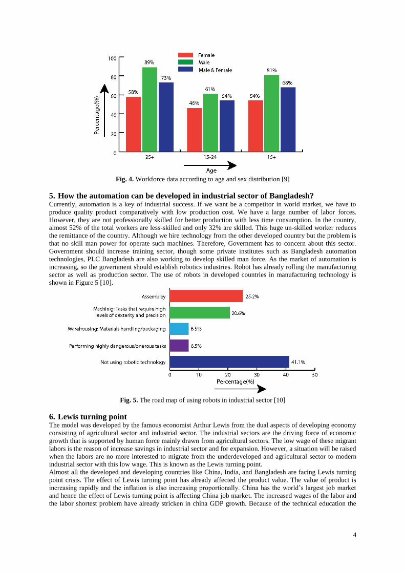
4

Fig. 4. Workforce data according to age and sex distribution [9]

5. How the automation can be developed in industrial sector of Bangladesh? Currently, automation is a key of industrial success. If we want be a competitor in world market, we have to

produce quality product comparatively with low production cost. We have a large number of labor forces.

However, they are not professionally skilled for better production with less time consumption. In the country,

almost 52% of the total workers are less-skilled and only 32% are skilled. This huge un-skilled worker reduces

the remittance of the country. Although we hire technology from the other developed country but the problem is

that no skill man power for operate such machines. Therefore, Government has to concern about this sector.

Government should increase training sector, though some private institutes such as Bangladesh automation

technologies, PLC Bangladesh are also working to develop skilled man force. As the market of automation is

increasing, so the government should establish robotics industries. Robot has already rolling the manufacturing

sector as well as production sector. The use of robots in developed countries in manufacturing technology is

shown in Figure 5 [10].

Fig. 5. The road map of using robots in industrial sector [10]

6. Lewis turning point The model was developed by the famous economist Arthur Lewis from the dual aspects of developing economy

consisting of agricultural sector and industrial sector. The industrial sectors are the driving force of economic

growth that is supported by human force mainly drawn from agricultural sectors. The low wage of these migrant

labors is the reason of increase savings in industrial sector and for expansion. However, a situation will be raised

when the labors are no more interested to migrate from the underdeveloped and agricultural sector to modern

industrial sector with this low wage. This is known as the Lewis turning point.

Almost all the developed and developing countries like China, India, and Bangladesh are facing Lewis turning

point crisis. The effect of Lewis turning point has already affected the product value. The value of product is

increasing rapidly and the inflation is also increasing proportionally. China has the world’s largest job market

and hence the effect of Lewis turning point is affecting China job market. The increased wages of the labor and

the labor shortest problem have already stricken in china GDP growth. Because of the technical education the

5

labor are becoming more skilled and they are demanding high salary which affect the country’s job market. The

recent industrial occupation category and their hourly wage are illustrated in Figure 6 [10].

Fig. 6. Employment, robotics and wages [10]

7. Possible solution and effects of Lewis turning point in Bangladesh The solutions will be come through the increasing use of industrial robots. Developed countries are starting to

walk with the theory of installing industrial robot for keeping their market value of product comparing to the

developing country. Industrial robots give better efficiency, better product quality with less of wages

comparative to the human resources.

We have to consider the following factors that affect the Lewis turning point effects on Bangladesh.

The population growth rate is decreasing in the country. It has been estimated that over the last 15

years the rate decreased from 1.84% to 1.22%.

The poverty headcount ratio is decreasing. It decreased from 48.9 % in year 2000 to 31.51 % in year

2010 as shown in Figure 7.

The GDP per capita based on purchasing power parity (PPP) is increasing. The amount increased from

USD 1293.58 in year 2000 to USD 3135.5 in year 2014.

The most important thing is that education growth has increased dramatically. It has increased 63.62%

in year 2001 to 79.94% in year 2012.

Fig. 7. Per capita GDP in Bangladesh

6

8. How to ensure sustainable industrial growth? Due to the decrease of the poverty headcount ratio and the increase of GDP per capita based on purchasing

power parity (PPP), people has obtained medium range of purchasing ability. As far the wages of the labor is

increasing, after a short period Bangladesh will face Lewis turning point crisis as like as China. Therefore, we

need to create an environment where the labor will robot and the driver will be human. So, we must think that

how could we do this?

It can be perceived through making skill labor force with high technical knowledge. Without this Bangladesh

will not able to be a part of world economy. We need to establish more and more technical institutions and must

ensure proper training. Government should make an industrial guide line as well as a proper wages system and

should care about the natural resource considering its significant effect on industrial sector. The next age will be

the age of robotics; therefore we have to give much emphasis on industrial automation in Bangladesh.

9. Conclusion The economic success and the internal development of a nation depend upon the development of industrial

sector. The industrial sector of Bangladesh is upgrading rapidly. However, the industrial work is largely

dependent on human workers, hence the product quality and quantity are low than expectation. The industrial

robots can replace the human worker to improve the output of the industry. However, fully industrial automation

in Bangladesh is quite impossible due to technical and financial barrier. The country has a massive man power

and almost 60% of them are young. Therefore, the successful deployment of the combination of automation and

human resource would bring a milestone result in country’s industrial sector as well as textile and high-

technology.

10. References [1] R. Parasuraman, and V. Riley, “Humans and automation: Use, misuse, disuse, abuse”, Human Factors, Vol.39, pp. 230–

253, 1997.

[2] G. Sankar, K.N. Sreekumar, M. Kumaresan, “Resistive Touch Screen Based Home Automation System Design”, Journal

of Nano Science and Nano Technology, Vol.2, No.2, pp. 140-143, 2014.

[3] The Story of the Intel® 4004. ⟨http://www.intel.com/content/www/us/en/history/museum-story-of-intel-4004.html⟩

[accessed June 2015].

[4] S. Augarten, State of the art: A photographic history of the integrated circuit. New Haven and New York 1983. ISBN 0-

89919-195-9.

[5] Edward B. Driscoll Jr. The History of X10. ⟨www.eddriscoll.com⟩ [accessed June 2015].

[6] Microchip unveils PIC®16C84, a reprogrammable EEPROM-based 8-bit microcontroller, and PICMASTER™-16C, a

new supporting development tool. ⟨http://ww1.microchip.com/downloads/en/DeviceDoc/031693.doc⟩ [accessed June

2015].

[7] Credit Suisse. Global Industrial Automation-Research and Analytics. ⟨https://www.credit suisse.com/global/en.html⟩

[accessed June 2015].

[8] Perspective Plan of Bangladesh 2010-2021. ⟨http://www.plancomm.gov.bd/wp-content/uploads/2013/09/Perspective-

Plan-of-Bangladesh.pdf⟩ [accessed June 2015].

[9] Country Profile, “Bangladesh”, Policies ami Programmes for Utilizing Health and Auxiliary Personnel in the Delivery of

Family Planning Services (ed. J Paxman), pp. 24-33, 1979.

[10] PricewaterhouseCoopers (PwC). The new hire: How a new generation of robots is transforming manufacturing.

⟨http://www.pwc.com/us/en/industrial-products/assets/industrial-robot-trends-in-manufacturing-report.pdf⟩ [accessed

June 2015].



Paper ID: IE-28

Ready-Made Garment (RMG) Industry in Bangladesh: Economic

Contribution and Potentiality

Md. Al-Mamun*, Md. Tajmiruzzaman and Md. Asadujjaman


Technology, Rajshahi-6204, Bangladesh *E-mail: [email protected]

Abstract

The Ready-Made Garment (RMG) industry of Bangladesh has a lion share in foreign exchange and became a

potential financial player in the national Economy. Bangladesh is now the second largest apparel exporting

country after China in the world. Although after the tragic collapse of Rana Plaza, Bangladesh’s RMG sectors

have lost their fame slightly to the buyers, trade unions and other garments related organizations temporarily,

a more glittering future is waiting for the RMG garment industry of Bangladesh as hinted by facts and

international surveys. This sector accounts for about 81% of the total export income and employs 4.4 million

people directly and 20 million indirectly. Undoubtedly, RMG sector has a potentiality to play as a key driving

force of Bangladesh’s economy in future. The intention of this paper is to prepare a statistical database with

these RMG related information to enhance the bright future of this sector and to forecast the total RMG export

for FY 2020-2021.

Keywords: Ready-Made Garments, Economic Potentiality, Forecasting, Semi-Average Method.

1. Introduction The Ready-Made Garment (RMG) sector has been the largest exporting industry in Bangladesh, which acts as

the backbone of the national economy. The tremendous success of readymade garment exports from

Bangladesh over the last two decades has surpassed the most optimistic expectations which have been expanded

almost uninterruptedly since the late 1970s [7]. The percentage of RMG to total exports has increased

considerably over last two decades in Bangladesh [2]. It increased from 12% in 1985 to over 80% in 2014,

making it the most important sector for the Bangladesh economy. Its contribution to the economy of

Bangladesh, and in providing employment, is indeed remarkable. As may be expected, the industry has faced

numerous challenges in the growth process, which averaged more than 15% per year. Despite all the adverse

publicity, RMG exports growth during the last fiscal year 2013-2014, was 13.8% [9]. The apparel exports of

Bangladesh has been concentrated to two major destinations- EU and North America [8, 15]. It is encouraging

to note that over the last five years, remarkable progress has been achieved in diversifying the RMG exports ton

on- traditional markets [8]. This diversification of exports destination, with growing exports, is a healthy sign for

RMG sectors. The simplification of GSP rules of origin are positive signs for this sector. That is why the RMG

sector of Bangladesh is optimistic that the new wave of opportunities and the growth momentum will energize

the RMG industry to add new success stories in the coming years [7]. The literature on the RMG industry is

limited. Mohammad Ekramul Islam et al. [1] present the economic recession and its impact on the Bangladesh’s

economy with special references of RMG and remittance sectors. In this paper, they exploited the ways, concept

and techniques which help them a lot to overcome the difficulties and able to stabilize their economic

improvement. Ahsan Firoz [4] has carried out a research on the design of readymade garments industry for fire

safety and explores the ways that how workplace can be taken free from any unexpected occurrences of Ready-

Made Garments sectors. Ahmed et al. [5] presented that the workplace safety is not sufficient in RMG sectors

in developing countries. Akhter et al. [6] showed that most of worker of garments industries in Bangladesh are

female and there need more improvement for health and safety. In Dhaka apparel summit [7], it is estimated that

Bangladesh RMG will reach to 2021- $ 50 Billion on the 50th Anniversary of Bangladesh. With the estimation

of the RMG export in FY 2020-2021 the present RMG export, present number of worker, the number of RMG

industries, the present contribution and potentiality of RMG sector are explored in this apparel summit. The

apparel story [8] explores the budget for FY 2014-15 and how this can be met. The objective of this paper is to

explore the economic roles that the RMG sector has on the national economy of Bangladesh and finally

forecasting the future of the Ready-Made Garments (RMG) sector in Bangladesh.

2

2. Methodology This paper has basically used the data from Bangladesh Garments Manufacturer and Export Association

(BGMEA) and Export Promotion Bureau (EPB). As an initial input, it has been prepared a detailed structure of

the relevant areas in which export-oriented RMG sector of Bangladesh was contributing. Different Books,

Journals, Newspapers, Magazines, Internet etc. has also been used for supporting this work. Personal interview

may also be conducted with the important personalities of these sectors. Finally, semi-average method is used to

forecast the total RMG export. The rest of this is organized as follows. Section 3 describes the growth of RMG

sector in Bangladesh. In section 4, we analyze the statistical data and forecast the total RMG export up to fiscal

year 2020-2021. Section 6 concludes the paper.

3. Growth of the RMG Industry Could one have predicted the growth of the RMG industry in Bangladesh? After the liberation of Bangladesh it

inherited a devastated economy with industrial production close to nil. The jute sector, which was the major

foreign exchange earner, saw no further growth in the immediate aftermath of independence [7]. Following

tables show that how the RMG sector gradually established a firm base from which to grow.

Table 1. Export of RMG sector in million US $ contrasting the total export of Bangladesh

(Source: BGMEA Website, 2014)

The export of RMG increased exponentially from 1984 to 2014. This exponential increase can be accounted for

by increase in demand in the Bangladeshi exports in EU and USA markets. Moreover, Bangladesh is also

exporting RMG in the non-traditional markets in an attempt to increase its revenue and stance in the global

market. The percentage of the contribution of RMG to total exports has increased considerably over the last two

decades. It increased from 12% in 1985 to over 80% in 2014, making it the most important sector for the

Bangladesh economy. It also provides employment to around 4.2 million Bangladeshis, mainly women from

low income families which affect their social status [1]. It has by now become a huge industry, earning the

lion’s share of the country foreign exchange and created the largest job opportunities for our countrymen

specially provided the largest formal employment for the women [7]. Of the estimated 4.2 million people

employed in this sector, about 50 percent of them are women from rural areas [1]. In 2000, the industry

consisting of some 3000 factories employed directly more than 1.5 million workers of whom almost 80% were

female [1, 11, 12]. The number of workers in garments sectors is increased day by day. In 1985-86 the total

workers were 20 million [1]. In 2007-08 the number of garments workers in Bangladesh is 2.50 million [1]. The

number of garment factories increased almost 11 times from 1992 to 2014.Though the number of factories

increased consistently from 1992 to 2013, the number of garments factories is decreased 19% from 2013 to

2014 which is shown in bracket in table 3. This percentage of decrement is resulted after the Tazreen fire and

Rana Plaza incident. Despite all the potential on the demand side, the question remains that, will Bangladesh be

able to take advantage of the increased opportunities? The ability of Bangladesh to supply is an equally

important issue in the changed global sourcing scenario. A comparison of the infrastructure in selected countries

is presented in table 4 for comparison.

Fiscal Year (FY) Total Export of

RMG (Knitwear

& Woven)

Total Export of

Bangladesh

% of RMG’s to Total

Export

2004-2005 6417.67 8654.52 74.15

2005-2006 7900.80 10526.16 75.06

2006-2007 9211.23 12177.86 75.64

2007-2008 10699.80 14110.80 75.83

2008-2009 12347.77 15565.19 79.33

2009-2010 12496.72 16204.65 77.12

2010-2011 17914.46 22924.38 78.15

2011-2012 19089.73 24287.66 78.60

2012-2013 21515.73 27018.26 79.63

2013-2014 24491.88 30176.80 81.16

3

Table 2. Cumulative Value of % growth of RMG Export in Bangladesh

(Source: BGMEA Website, 2014)

Table 3. Year wise Number of Workers Employed in RMG Sectors (In Million) in Bangladesh and number of

Garment Factories

(Source: BGMEA website, 2014)

Table 4. Comparison of infrastructure quality 2014-2015

(Source: The global competitiveness report 2014-2015 (2014 world economic forum); Ranking among 144 countries. The

rankings are in descending order with ‘’1’’ as the best performer)

4. Analysis of Statistical Data and Findings

There are in total 5615 units in the RMG sector of Bangladesh [7]. Out of them, 2723 are woven factories, 1383

knit, 629 W/K, and 880 sweater factories. Consequently, woven factories make up 48%, knit 25%, W/K 11%,

and sweater 16% of the factories in the industries [7]. Therefore, it can be seen that woven comprises of the

highest unit with sweater the least producing unit. The main components of RMG are the woven and knit which

comprises approximately the three-fourths of the total in terms of the factories.

Fiscal Year (FY) Total Export of

RMG (Knitwear &

Woven) in million

US $

% Growth of Export

of RMG

Cumulative Value of %

growth of RMG Export

2004-2005 6417.67 11.40 11.40

2005-2006 7900.80 18.77 30.17

2006-2007 9211.23 14.27 44.44

2007-2008 10699.80 13.91 58.35

2008-2009 12347.77 13.35 71.7

2009-2010 12496.72 1.19 72.89

2010-2011 17914.46 30.24 103.13

2011-2012 19089.73 6.16 109.29

2012-2013 21515.73 11.28 120.57

2013-2014 24491.88 12.15 132.72

Fiscal Year Number of

Garment

Factories

% of growth Employment

In million

Workers

% of growth

2004-2005 4107 3.65 2.00 0

2005-2006 4220 2.68 2.20 9.09

2006-2007 4490 6.01 2.40 8.33

2007-2008 4743 5.33 2.80 14.29

2008-2009 4925 3.70 3.50 20

2009-2010 5063 2.76 3.60 2.78

2010-2011 5150 1.69 3.60 0

2011-2012 5400 4.63 4.00 10

2012-2013 5600 3.57 4.00 0

2013-2014 4536 (19) 4.00 0

Country/Region Country

Ranking

Overall

Infrastructure

Score

Electricity Roads Railroads Port

Bangladesh 109 2.8 2.5 2.9 2.4 3.7

India 71 3.7 3.4 3.8 4.2 4.0

China 28 4.4 5.2 4.6 4.8 4.6

Cambodia 95 3.4 3.0 3.4 1.6 3.6

Myanmar 134 2.3 2.8 2.4 1.8 2.6

Pakistan 129 3.3 2.1 3.8 2.5 4.4

Sri Lanka 73 5.0 4.8 5.1 3.7 4.2

Thailand 31 4.1 5.1 4.5 2.4 4.5

4

Fig. 1. Percentage of the different kinds of factories (Source: BGMEA website, 2014)

Figure 2 shows that the growth of the total export of RMG in FY 2013-2014 is comparatively smaller than the

other fiscal years and this is may be because of the Tazreen fire and Rana Plaza Tragedy but growth could be

fallen tremendously although that had not happened which indicates that the RMG sector of Bangladesh has a

bright future.

Fig. 2. Total export of RMG (Knitwear& Woven) in million US $ (Source: BGMEA website, 2014)

Fig. 3. Employment of RMG in Million Workers (Source: BGMEA website, 2014)

The number of RMG industries has been increasing dramatically since the late 1970s causing the tremendous

growth of RMG employment [13]. Up to FY 2011-2012 the number of employment has increased but through

last three FY RMG employments is approximately constant.

5

The total RMG export in FY 2004-2005 was 6417.67 million USD which increased to 24491.88 million USD in

FY 2013-2014, shown in table 5. So the percentage increase is 73.8%. The total RMG export for the FY 2020-

2021 can be calculated by the Semi-average forecasting method as-

= (1)

Or

= (2)

Total RMG export can be calculated by-

= + ( ) (3)

Where,

and = Semi-average trend value, (E) =RMG export , = Fiscal year, f = Number of fiscal year

Table 5. RMG export data from 2004-2014

(Source: BGMEA website, 2014)

Analyzing the total export data from table 5 by using the semi-average method it has been forecasted that the

total export of RMG might be about 24815.36 million USD in Fiscal Year 2020-2021 as shown in table 6 if the

trend of increasing the RMG exports remains as like as the export shown in table 1

Table 6. Forecasted RMG export in million USD up to FY 2020-2021

The RMG industries can achieve better result than the forecasted export if it can be ensured the workplace

safety, realistic solution of child labor issue with ILO, UNICEF & US Embassy, successfully faced global

recession, and after all creating the opportunity using the strengths of RMG industries.

No of

FY ‘f’

Fiscal year

f=1,2,…,10

RMG export in million

USD

Semi-total Semi-average trend

value

or *

1

2

3

4

5

6

7

8

9

10

2004-2005

2005-2006

2006-2007

2007-2008

2008-2009

2009-2010

2010-2011

2011-2012

2012-2013

2013-2014

6417.67

7900.80

9211.23

10699.80

12347.77

12496.72

17914.46

19089.73

21515.73

24491.88

46577.27

95508.52

9315.45

*19101.70

No.

of FY

‘f’

Fiscal year

f=11,12,…,17

Semi-average

trend value

Semi-average

trend value

RMG export

in million

USD

11 2014-2015 9315.45 19101.70 1398.04 21897.78

12 2015-2016 9315.45 20981.92 1166.65 20981.92

13 2016-2017 9845.67 20981.92 1237.36 23456.63

14 2017-2018 9845.67 21905.61 1139.56 23520.39

15 2018-2019 10998.35 22136.29 1012.54 24161.38

16 2019-2020 10998.35 22860.82 988.54 24837.89

17 2020-2021 12009.77 23107.95 853.71 24815.36

6

5. Conclusion From the illustration above we can say that Bangladesh has repeatedly demonstrated its flexibility and ability to

overcome all odds. Truly speaking, Ready-Made Garment sector is an excellent example of what the country

can achieve. Despite all challenges, with accompanying global ups and down, the country has positioned itself

as the second largest apparel exporter within just three decades and about one-fourth of the national earning is

from the RMG sector. Therefore, we can evidently say that the vision 2021 for Bangladesh’s RMG is attainable

if the RMG sector can ensure the workplace safety, realistic solution of child labor issue with ILO, UNICEF &

US Embassy, successfully faced global recession, and after all creating the opportunity using the strengths of

RMG industries. After all, the RMG is a confidential sector that can exploit its potential in terms of the foreign

exchange while overcoming the challenges it faces in upcoming years.

6. References [1] Mohammad Ekramol Islam, Mahbuba Sultana, ASM Mahbubul Kamal, “Economic recession and its impact on the

[2] Bangladesh’s economy with a special references of RMG and remittance sectors”, International Journal of Science

and Research, Vol. 2 (Issue 12), pp. 2319-7064, 2013.

[3] Naiem Jalal Uddin Ahmed, “ Socio-Business consideration of garment workers in Bangladesh: a statistical review”, ABC

Journal of Advanced Research, Vol. 2, No. 2, pp. 2304-2621, 2013.

[4] Ahsan Firoz, “Design of readymade garments industry for fire safety”, Master dissertation, Postgraduate Programs in

Disaster Management, BRAC University, 2011.

[5] Ahmed et al., “Industrial safety in the readymade garment sector: a developing country perspective”, Sri Lankan Journal

of Management, Vol. 14, No. 1, pp. 1-13, 2009.

[6] S Akhter, AFM Salauddin, M. Iqbal, ABMA Malek and N Jahan , “Health and occupational safety for female workforce

of garment industries in Bangladesh”, Journal of Mechanical Engineering, Vol. ME 41, No. 1, pp. 65-70, 2010.

[7] Bangladesh RMG 2021- $ 50 Billion on the 50th Anniversary of Bangladesh: Dhaka Apparel Summit, pp. 1-105, 2014.

[8] Md Shahidullah Azim, Mamun Rashid, Nur Mohammad Amin Rasel, Omar Gias, and Nasim Uddin, “The apparel

story”, Bangladesh Magazine, pp. 1-39, April 2014.

[9] Omar Gias, “Budget for FY 2014-15: RMG perspective”, Md Shahidullah Azim, Mamun Rashid, Nur Mohammad

Amin Rasel, Omar Gias, and Nasim Uddin, “The apparel story”, Bangladesh magazine, pp. 1-51, May-June 2014.

[10] Md. Rizwan Hassan, Md. Maruf Ullah, Md. Shahnur Azad Chowdhury, “Impact of tourism in Bangladesh economy”,

World Journal of Social Sciences, Vol. 3, No. 6, pp. 45-57, 2013.

[11] Md. Salim Uddin, Mohammed Abu Jahed, “Garments industry: a prime mover of the socio economic development of

Bangladesh”, The Cost and Management, Vol. 35, No. 1, pp. 59-70, 2007.

[12] Md. Mehedi Hasan Sikdar, Md. Sujahangir Kabir Sarkar, Sumaiya Sadeka, “Socio-economic conditions of the female

garment workers in the capital city of Bangladesh”, International Journal of Humanities and Social Science, Vol. 4 No.

3, 2014.

[13] Redwan Ahmed, Md. Tawhidul Islam, Md. Al-Amin, “The effects of market diversification activities on Bangladesh

RMG export”, International Journal of Economics and Financial Issues, Vol. 3, No. 4, pp.938-948, 2013.

[14] Ferdous Ahamed, “Could monitoring and surveillance be useful to establish social compliance in the ready-made

garment (RMG) industry of Bangladesh?”, International Journal of Management and Business Studies, Vol. 3, pp. 088-

100, 2013.

[15] Razzaque, A., “The small country assumption, econometric estimates and policy making: a resentment with

Bangladesh’s RMG exports to the European Union”, The Bangladesh Development Studies, No. 1&2, 2004.

[16] Mst. Nurnahar Begum, Rama Rani Sutradhar,” Behavior of remittance inflows and its determinants in Bangladesh”.

Working paper Series: WP 1202Nur, M., Wijeweera, A. and Dollery, B., “Estimation of the export demand function

using bilateral trade data: The case of Bangladesh”, South Asia Economic Journal, Vol. 8, No. 2, pp. 249-264, 2007.

[17] http://www.assignmentpoint.com/science/textile/rmg-bangladesh.html, viewed on: Jan 4, 2015.

[18] http://bdnews24.com/bangladesh/2011/04/16/guard-against-mishaps-rmg-industry-told, viewed on: Jan 4, 2015.

[19] Bangladeshi RMG sector: http://en.wikipedia.org/wiki/Bangladeshi_RMG_Sector#cite_note-reuters, viewed on: Jan

4, 2015.

[20] EPB (2014): Export Promotion Bureau, Website: http://www.epb.gov.bd/, viewed on: Jan 4, 2015.

[21] Bangladesh Bank (2014): Economic Trends, Various Issues, viewed on: Feb 9, 2015.

[22] BGMEA (2014): BGMEA Website http://bgmea.com.bd/, viewed on: Feb 9, 2015.

http://www.assignmentpoint.com/science/textile/rmg-bangladesh.html

http://bdnews24.com/bangladesh/2011/04/16/guard-against-mishaps-rmg-industry-told

http://en.wikipedia.org/wiki/Bangladeshi_RMG_Sector#cite_note-reuters

http://www.epb.gov.bd/

http://bgmea.com.bd/



Paper ID: IE-29

Flow Sheet Development and Simulation with Optimization of Industrial

Scale Natural Gas Processing Plant by Using Aspen-Hysys

Md.Nurus Sakib[1], Noor Mohammad[2], Niloy Barua[3], Dr. Md Ruhul Amin [4], [1], [2], [3] Department of Chemical Engineering, Bangladesh University of Engineering University,

BUET [4] Associate Professor, Department of Chemical Engineering, Bangladesh University of Engineering

University, BUET Email addresses: [email protected], [email protected], [email protected],

[email protected]

Abstract

Bangladesh has a gas field discovery success ratio 3.1:1 of which two of the gas fields are located in offshore

area. Bibiyana gas field has been selected for the study of flow sheet development and simulation with

optimization of industrial scale natural gas processing plant by using Aspen-Hysys as it is a world class gas

reservoir. Flow sheet development and simulation of 150 MMSCFD natural gas producing Bibiyana gas plant

was done by means of Aspen-Hysys. The steady state simulation was performed based on both the design and

physical property data of the plant. The main purpose of optimization was cost minimization by regulating the

process stream flows and heat duty and hence profit maximization. The objective function, Profit, was

calculated from the difference of sales gas, LPG and condensate selling revenue and condenser or reboiler duty

costs. Hysys Optimizer has been used to optimize the present process which resulted in more than 8.5% increase

in profit with negligible change in optimized methane composition (around 99.46 %). In addition, LPG was also

recovered with a production rate of around 1746 barrel/day.

Keywords: Natural Gas; Aspen-Hysys; Gas Processing; Separation; Simulation; Optimization.

1. Introduction Natural Gas is among the top most used energy sources in the world. Since natural gas can be processed and

distributed easily, the demand is growing rapidly [Rahman and Tamim, 2012]. Hence, fast and efficient gas

processing and optimization are needed. Natural gas processing plants are used to purify the raw natural gas

extracted from underground gas fields and brought up to the surface by gas wells.

Natural gas processing consists of separating all of the various hydrocarbons and fluids from the pure natural

gas, to produce what is known as ‘pipeline quality’ dry natural gas. Many removal processes can be adopted, for

example, amine base process for the removal of carbon di oxide [Kinigoma and Osharode, 2013] or by Benfield

process [Chowdhury and Chowdhury, 2013]. Furthermore, Dehydration of Natural Gas which is another

important step in gas processing. Deethanization and also depropanization can be enhanced by using dividing

wall column [Long and Lee, 2012]. Nitrogen-removal processes using liquid solvents, adsorption, and cryogenic

processing are currently available, but all of these methods require recompression of the methane product, which

penalizes their economics. However, the Use of three column system requires less compression and higher

methane recovery (around 98%) than other methods available [MacKenzie et al. 2012].

Analysis of industrial scale Natural Gas plant includes many complicated aspects which are mainly assessed by

simulation programs. Aspen HYSYS is an easy-to-use process modeling environment that enables optimization

of conceptual design and operations and removes process bottlenecks. Simulation of plant model and

optimization of natural gas processing plant that reduces process loss and maximizes profit can be developed

though Aspen-Hysys [Roy and Amin, 2011]. The role of Hysys is to provide a capable and accurate design.

Aspen Hysys introduced the novel approach of steady state and dynamic simulations in the same platform. It has

become the defacto standard in industry, and today enjoys universal acceptance [Amber et al. 2012]. Simulator

response modeling relates key process variables to plant performance satisfying the remaining unknown

information from the material balance equations [Bullin and Hall, 2000]. In a gas simulation process, the inlet

conditions (Composition, pressure and temperature) affect the throughput and quality of products. However, to

counter such problems, about 80 % of the bumps can be reduced by using Hysys [ Ramzan et al. ]. Owing to

such performance, Hysys simulation has been used to optimize process condition for maximum profit.

2. Simulation of gas process unit For the Bibiyana plant simulation, there are five major units which processes the raw natural gas. These are:

separation unit, dehydration unit, heat exchanger, de-ethanizer and final purification & CO2 removal

units. The simulation process is based on Bibiyana gas production process and following are the description of

units of the process:

2.1 Separation unit: Gas is drawn from three wells: Well-1, Well-2, Well-3 respectively in simulation of the

processing plant. The feed Composition can be found in datasheet. Then the feed gas is passed through the

pressure control valve to relief some pressure & then fed into 3 ‘three phase separators’ (H-110A, H-110B, H-

110C) to separate each valve out stream in heavy liquid, light liquid & vapor streams. Most of the liquids are

separated at this separation unit. The 3 heavy liquid streams(mostly H2O) is removed & the 3 light liquid

streams are mixed together in a mixer & then entered into a distillation column(D-320) through an expansion

valve, the bottom liquid product is liquefied petroleum gas(LPG) & is stored in a tank(F-210). The overhead

product of D-320 is mixed with refined gas stream to prepare the very final product.

2.2 De-hydration unit & heat-exchanger unit: There are three vapor streams of the separators(H-110A,

H-110B, H-110C) which are mixed in a mixer and passed through the dehydration unit for water removal. The

dehydration unit consists of an absorption tower (D-310) where Tri Ethylene Glycol is used to absorb water.

The overhead vapor product of (D-310) contains dehydrated hydrocarbons which is passed through two heat

exchangers (E-230) & (E-250) so that temperature is decreased. The tube out of E-250 heat exchanger is then

entered into a separator (H-140). Then expander (G-152) lowers streams temperature using Joule-Thomson

principle of pressure relief & then three phase separator separates the remaining water in the mixed inlet more

precisely. Heavy liquid is removed & light liquid (H-150 liq out) and vapor(H-150 vap out) is used for further

processing.

On the other hand, bottom product of the absorption tower(D-310) is passed through an expansion valve (K-

131) & a two phase separator(H-130) ,bottom product of which is used as a tube side inlet of heat exchanger (E-

240). The tube side outlet is then entered into a column(D-330) whose bottom product is make-up Glycol

solution & is entered into the shell side of the heat-exchanger(E-240) & heat-exchanger(E-230). Between the

heat-exchangers a pump is used to increase the pressure. The shell outlet of E-230 is mixed with TEGlycol feed

to use in the absorption tower (D-310)

2.3 De-ethanizer unit: The liquid stream of the three phase separator(H-150) is then used in the de-ethanizer

which is a distillation column (D-340). Bottom product of the column(D-340) is LPG which is passed through

the heat-exchanger(E-101) to prepare ‘Final LPG’ at low temperature. Stream(H-150 vap out) is mixed with the

over-head vapor product of (D-340). Mixed stream out (M-231) is entered into the shell side of the heat

exchanger (E-250) to increase the temperature.

2.4 Purification & CO2 removal unit: Stream (M-251 shell out) is then undergone through CO2 removal

process. In this stage, we used principles of liquefaction to separate CO2. Using cooler (E-100) we cooled shell

out stream and this cool gas stream is passed to a separator (V-100) preceded by a valve (VLV-100). Then the

final product stream enters compressor & then again thorough consecutive separations and thus CO2 from

natural gas has been decreased significantly (less than 0.03%). CO2 can also be removed using absorption

process where MEAmine solution is used to absorb CO2.

3. Optimization of gas processing plant simulation After performing the whole simulation process, profit optimization was done. Optimization was done by

controlling two main prospect. One is the flow of the revenue earning stream and the other is the duty

corresponding to cost of the process. The main purpose of optimization was cost minimization. The objective

function, Profit, was calculated from the difference of sales gas, LPG and crude gasoline (a stream having many

of the properties of gasoline) selling revenue and condenser or reboiler duty costs. . Some energy was also

extracted from an expander (G152) that was included with the revenue too. In the process, the profit is a

function of both cost of heat duty and the revenue of flow rates of products i.e. sales gas, LPG and crude

gasoline. The objective function is given as :

Profit=Total revenue –Total cost

Several user defined variables were considered as primary variables; i.e.: outlet stream pressures of absorption,

de-methanization and de –ethanizaion units, compressors and valves to name a few.

3.1 Optimization effect: This part illustrates on the optimization function and optimized condition of the

final simulation. Here, the optimizer spread sheet (Fig 3.1) lists all the variables relating with price. This spread

sheet was formed by opening the spreadsheet of Hysys Optimizer® tool. Then functions were listed in the

functions tab of the tool. By means of Hysys Optimizer® which uses both static and dynamic simulation

modeling tool, optimization is achieved. Hysys uses the dynamic analysis of a process system that provides

understanding of process system which is not possible with steady state modeling. Following is the

mathematical formulation:

Table3.1: Market Value of Products and utilities: (Prices estimated from the year book of Petrobangla and

Bangladesh Energy Regulatory Commission)

Natural Gas 9.580 taka/m3

LPG 56 taka/kg

Crude Gasoline 42470taka /m3

Heating or Cooling Duty 0.737 taka/KWh

Revenue Calculation:

Sales gas volume = B1 Sales gas price per unit volume, B2=9.580 tk/m3

LPG sales volume= B3 Sales LPG price per unit volume, B4 = 56 taka/kg

Crude Gasoline sales volume= B5 Crude Gasoline sales price per unit volume, B6= 42470 taka/m3

Revenue, B7 = B1×B2+B3×B4+B5×B6

Cost Calculation:

Expander Duty = D1 , D320 Re-boiler Duty= D2 ,D330 Re-boiler Duty= D3, D330 Condenser Duty = D4

D340 Re-boiler Duty = D5 , D340 Condenser Duty = D6, L231 Pump Duty = D7, Cooling Duty = D8

Heating Duty = D9, E100 Heat Duty = D10, Compressor Duty = D11, E104 Duty = D12, Price per KWh, D13 =

0.737 $, Total Cost,

D14 = (D1+D2+D3+D4+D5+D6+D7+D8+D9+D10+D11+D12) × D13, Profit = B7-D13

Before Optimization After Optimization

Figure 3.1: Spread Sheet Values of the simulation after optimization

4. Results and discussions After the optimization, both flow rates of LPG and Sales Gas were increased. Consequently, theoretical increase

in revenue and total profit was about 8 percent as shown in the spread sheet of Figure 3.1. Following tables

shows the before and after condition of the process which shows the variability in composition due to

optimization. Comparing these tables shows the efficacy of optimization since the desired components

compositions varies in a positive way. Even though the methane fraction lowered but the sales flow increased

hence the revenue.

Table 4.1: Composition of significant components of sales gas before optimization*

Name of Components Composition Name of Components Composition

Water(H2O) 5.95E-06 Methane(CH4) 0.995707

N2 2.11E-03 Ethane 9.29E-04

CO2 2.70E-04

Table 4.2: Composition of significant components of LPG(Liquified Petroleum Gas)*

Name of Components Composition in LPG Name of

Components

Composition in

LPG

Propane 0.236602 n-Heptane 0.144678

i-Butane 0.154207

n-Butane 0.15947

Table 4.3: Optimized composition of significant components of sales gas

Name of

Components

Composition Name of

Components

Composition

N2 2.11E-03 Propane 2.61E-04

CO2 5.41E-04 i-Butane 1.21E-04

Methane(CH4) 0.994594 n-Butane 1.61E-04

Ethane 1.78E-03 i-Pentane 1.71E-04

Table 4.4: Optimized composition of significant components LPG(Liquified Petroleum Gas)

Name of Components Composition in LPG Name of

Components

Composition in

LPG

Propane 0.241527 n-Hexane 9.74E-02

i-Butane 0.153288 n-Heptane 0.143707

n-Butane 0.158469 n-Pentane 5.73E-02

i-Pentane 9.15E-02

Figure 4.1: Graphical representation of LNG components

* Tablular Data were taken from Bibiyana Gas Fields of Bangladesh

0

0.05

0.1

0.15

0.2

0.25

Co

mp

osi

tio

n

Components

5. Process flow diagram

Following is a depiction of part of the simulated process on Hysys.

.

Figure 5.1: PFD of a part of the simulation process

6. Conclusion At present time natural gas is a major source of energy. Most of the industries are run by energy using natural

gas as their main source. Near about 95% of the natural gas is used as fuel gas. So, it is a major prospect to focus

on and develop for the betterment of energy utilization. The model for natural gas processing plant is developed

in this paper. Different process can be used to meet the specification required for processing of natural gas.

Environmental constraints and the need to reduce cost require innovative processes. The process used here

derived from earlier processes, but tend to offer significant reductions in investment and operating costs. In the

longer term, new concepts such as gas permeation can be expected to play a growing role and the natural gas

processing will keep changing. In this plan, the composition of sales gas is satisfactory. The percentage

removals of unwanted elements are good enough to run the process. Furthermore, profit was maximized by

means of optimization. Optimization provides a better process with higher benefits.

7. Acknowledgment We are very thankful to BUET Chemical Engineering Forum (BCEF) for their support. The technical and

administrative backup given by the Department of Chemical Engineering, BUET is highly appreciated.

Nomenclature Symbol Meaning

HC

H

E

M

LPG

Hydrocarbon

Two and three phase separator

Heat Exchanger

Mixer

Liquefied petroleum gas

References

[1] Amber, T., Chavan, T., Manali, K., Walke, S., M., “ Simulation of Process Equipment by Using Hysys” International

Journal of Engineering Research and Applications (IJERA) ISSN: 2248-9622 .National Conference on Emerging Trends in

Engineering & Technology (VNCET-30 Mar’12)

[2] Bullin, K.,A., Hall, K., R., “ Optimization of Natural Gas Processing Plants Including Bussiness Aspects”, Bryan

Research and Engineering, Inc. Preceedings of the seventy ninth convention, 2000.

[3] Chowdhury N. B., Chowdhury N. B., “ChemCAD Simulation of Benfield Process to Remove CO2 from Natural Gas and

Inspection of Temperature Profile of Key Units”, Advances in Mechanical Engineering and its Application (AMEA) Vol.

3,No. 2. 2013, ISSN 2167-6380

[4] Kinigoma, B., S., Osharode, D., I., “Optimization of Amine Base Process in the Removal of Carbon Dioxide from

Natural Gas for LNG Production”, Journal of Energy Technologies and Policy, ISSN 2224-3232, Vol. 3, No.3, 2013

[5] Long,N.,V.,D., Lee, M., “ Improvement of the Deethenizing and Depropanizing Fractionation Steps in NGL Recovery

Process Using Dividing Wall Column”, JCEJ, Vol.45. No.4, April 2012

[6] MacKenzie, D., Cheta, I., Burns, D., “Removing Nitrogen”, Gas Liquids Engineering, Canada, Hydrocarbon Engineering

November 2002.

[7] Roy,S., Amin, R.,:”Aspen-HYSYS Simulation of Natural Gas Processing Plant. Journal of Chemical Engineering”, IEB,

2011. Vol. ChE. 26(1): p. 4.

[8] Ramzan,N.m Naveed, S.m Muneeb, R., Tahir, F.,M., “Simulation of Natural Gas Processing Plant for Bump less Shift”

NFC-IEFR Journal of Engineering and Scientific Research.

[9] Rahman M., Tamim M., Rahman L., “Analysis of Natural Gas Consumption by the Industrial Sector of Bangladesh”,

Journal of Chemical Engineering, IEB Vol. ChE. 27. No. 1, June 2012

[10] Vago, A., Rippel- Petho, D., Horvath, G., Toth, I., Olah, K. “Removal of Hydrogen Sulfide From Natural Gas, A Motor

Vehicle Fuel”, Hungarian Journal of Industrial Chemistry, Veszprem, Vol. 39(2) pp. 283-287 (2011)

[11] Haring, H.W. (2008) Industrial Gas Processing. Weinheim, Germany: WILEY-VCH Verlag Gmbh & CO. KGaA

[12] Kohl, A., & Nielsen, R. (1997) Gas Purification. 5TH Edition. Houston, Texas: Gulf Publishing Company

[13] "Gas Processes 2002", Hydrocarbon Processing, pages 84-86, May 2002 (schematic flow diagrams and descriptions of

nitrogen rejection and nitrogen removal processes)



Paper ID: IE-30

Modeling and Optimization of Aggregate Production Planning by Time-

varying Acceleration Coefficients PSO

Md. Sahab Uddin1*, Sayed Rezwanul Islam2, Md. Mahmudul Hasan3

1,2Department of Industrial & Production Engineering,

Rajshahi University of Engineering & Technology, Rajshahi- 6204, BANGLADESH 3Department of Computer Science & Engineering,

Rajshahi University of Engineering & Technology, Rajshahi- 6204, BANGLADESH 1*E-mail: [email protected]

Abstract

The aim of this paper is to apply Time-varying Acceleration Coefficients PSO (TVACPSO) for modeling and

optimization of aggregate production planning problem. TVACPSO is a modified and updated form of Particle

Swarm Optimization (PSO). Most practical decisions made to solve APP problems usually consider total costs; we

have eliminated other objective functions of APP in this case. There was several variables problem with constraints

which was solved in MATLAB. The proposed approach attempts to minimize total costs with reference to inventory

levels, labor levels, and overtime, subcontracting and backordering levels. An industrial case is presented to

demonstrate the feasibility of applying the proposed method to real APP problems. Consequently, the proposed

TVACPSO approach yields an efficient APP compromise solution.

Keywords: Aggregate production planning (APP), Time-varying Acceleration Coefficients PSO (TVACPSO), cost

minimization.

1. Introduction Aggregate production planning is a process by which a company determines ideal levels of capacity, production,

subcontracting, inventory, stock out & even pricing over a specified time horizon. It uses intermediate-range

capacity planning that typically covers a time horizon (2 to 12 months), although some companies it may extend to

as much as 18 months. The planning horizon is often divided into periods. For example, a one year planning horizon

may be composed of six one-month periods plus two or three month periods. In other words, It is concerned with

planning overall production of all products combined over a planning horizon for a given (forecast) demand

schedule. The goal of aggregate is to achieve a production plan that will effectively utilize the organization’s

resources to satisfy expected demand. Planner must make decisions on output rates, employment levels and changes,

inventory levels and changes, back orders, and subcontracting in or out. Aggregate planning might seek to influence

demand as well as supply. If this is the case, variables such as price, advertising, and product mix might be used. If

changes in demand are considered, then marketing, along with operations, will be intimately involved in

aggregate planning. Aggregate planning is essentially a big-picture approach to planning. The purpose of aggregate

production planning is to achieve a production plan that will effectively utilize the organizations resource to satisfy

expected demand. There are many solving procedure for APP problem but in this paper we have used a new

algorithm Time-varying Acceleration Coefficients PSO (TVACPSO). TVACPSO is a modified and updated form

of Particle Swarm Optimization (PSO). The algorithm of PSO emulates from behavior of animals societies that

don’t have any leader in their group or swarm, such as bird flocking and fish schooling. PSO algorithm is a multi-

agent parallel search technique which maintains a swarm of particles and each particle represents a potential

solution in the swarm. All particles fly through a multidimensional search space where each particle is adjusting its

position according to its own experience and that of neighbors. In a PSO method, all particles are initiated randomly

and evaluated to compute fitness together with finding the personal best (best value of each particle) and

global best (best value of particle in the entire swarm). In this study, TVACPSO is a relatively new approach for

solving optimization problem is employed to solve the proposed APP problem due to its simplicity, speed,

and robustness.




2. Literature Review Aggregate production planning is the problem to determine the resource capacity needed to meet demand in the

production line. Shorten product life cycle in market & fickle customer perceptions push the researchers to

choose this broad area to research. Wang and Fang (2001) [1] modeled an APP with fuzzy variables and in this

study the decision variables, the demands and subcontracting cost are accepted as triangular fuzzy numbers. Tang et

al (2000) [2] formulated a multi-product APP problem as a fuzzy quadratic programming with both fuzzy demand

and fuzzy constraint appears in the same model. A fuzzy multi-product APP problem was solved Fung et al. (2003)

[3] and the APP problem has only one objective (minimizing the total cost) and only the demands and the capacities

are defined as fuzzy. For solving the multi-product APP problem in a fuzzy environment a fuzzy multi-objective

linear programming model was developed by Wang and Liang (2004) [4]. Wang and Liang (2005) [5] handled a

fuzzy multi-product APP problem and is modeled as a multi-objective linear programming problem and all of the

objectives are defined as fuzzy with imprecise aspiration levels. Ning et aI. (2006) [6] established a multiproduct

aggregate production planning (APP) decision making model in fuzzy random environments. Baykasoglu and

Gocken (2006) [7] proposed a multi-objective tabu search (TS) based solution method to solve fuzzy goal programs.

Tavakkoli-Moghaddam et al. (2007) [8] presented a fuzzy APP model for make-to-stock environments. Ling (2008)

[9] developed a fuzzy multi objective linear programming (FMOLP) model with piecewise linear membership

function to solve integrated multi product and multi time period production/ distribution planning decisions (PDPD)

problems. Torabi et al (2009) [10] presented a fuzzy hierarchical production planning comprised of two decision-

making levels. Chen and Huang (2010) [11] proposed a solution procedure that is able to find the fuzzy objective

value of the fuzzy APP model. Based on ranking methods of fuzzy numbers and tabu search Baykasoglu and

Gocken (2010) [12] proposed a direct solution method to solve fuzzy multi-objective aggregate production planning

problem. Ramezanian et al (2012) [13] presented a mixed integer linear programming (MILP) model for general

two-phase aggregate production planning systems. Zhang et al (2012) [14] built a mixed integer linear programming

(MILP) model to characterize mathematically the problem of APP with capacity expansion in a manufacturing

system including multiple activity centers. Some meta-heuristic algorithms were also employed to solve APP

problems. Raa et al (2013) [15] presented a mixed integer linear programming formulations for the planning

problem and a metaheuristic solution approach based on the models. Chakrabortty and Hasin (2013) [16] used three

distinct scenarios simultaneously with different genetic algorithm options for solving multiple objectives of fuzzy

linear programming models including escalating factors. Chen and Huang (2014) [17] investigated multiproduct,

multi-period APP problems with several distinct types of fuzzy uncertainties. Particle Swarm Optimization (PSO) is

another relatively new bio-inspired algorithm that may be used to find optimal or near-optimal solutions to

numerical and quantitative problems. It was originally developed by a social psychologist, James Kennedy and

Russel Eberhart (1995) [18]. El Mounayri et al. (2003) [19] used PSO to predict parameters of surface roughness in

end milling. Prakasvudhisarn (2004) [20] used PSO to determine minimum tolerance zones of all basic form

features for discrete parts inspection. Some researchers applied PSO to solve optimization problems with

constraints. Hu et al. (2003) [21] modified the PSO to solve constrained nonlinear problems by preserving

only feasible solutions. In 2002, A. Salman [22] published a paper on the use of particle swarm optimization for

task assignment problem. Again H. J. Escalante et al [23] worked on particle swarm model design. In 2007, M. F.

Tasgetiren et al [24] researched on the use of PSO algorithm for make span and total flow time minimization in flow

shop sequencing problem.

3. Algorithm

3.1. Time-varying Acceleration Coefficients PSO PSO has multiple particles, and every particle consists of its current objective value, its position, its velocity, its

personal best value, that is the best objective value the particle ever experienced, and its personal best position, that

is the position at which the personal best value has been found. Time-varying Acceleration Coefficients PSO

(TVACPSO) does not only change the inertia weight w, but also the acceleration coefficients, i.e., the personal c1

and global best weight c2, over time. The idea is to have a high diversity for early iterations and a high convergence

for late iterations. TVACPSO uses the following iteration to determine the velocities:

Step1: Assume the number of particles.

Step2: Initialize the position of the particles.

Step3: Evaluate the objective function for each particle.

Step4: Set the initial velocities of each particle.



Step5: Find the personal best and global best position

Step6: New velocities calculation for each particle by using the following equation,

v(i)(n + 1) = w(n)v(i)(n) + c1r1(i)(n)[xp

(i)(n) – x(i)(n)] + c2r2(i)(n)[xg(n) – x(i)(n)],

n = 0, 1, 2,..., N − 1,

Where the personal best weight c1 and the global best weight c2at every iteration n are calculated using the following

equations:

w (n) = ws − (ws – we) n

N

c1 (n) = c1s − (c1s – c1e)

c2 (n) = c2s − (c2s – c2e) n

N

where c1 (n) is the personal best weight at iteration n, c2(n) is the global best weight at iteration n, c1s is the personal

best weight designated for the first iteration, c1e is the personal best weight designated for the last iteration N , c2s is

the global best weight designated for the first iteration, and c2e is the global best weight designated for the last

iteration N .

Step7: Find updates position for each particle by using the following equation

x (i)(n + 1) = x(i)(n) + v(i)(n + 1), n = 0, 1, 2, ..., N − 1,

Step8: Continue this process from step 3 to step 8.

4. Problem Formulation

4.1. Problem Description & Notation

The following notations were employed for formulating the APP problem:

N Types of products

T Planning horizon

z Total production cost

Dnt Forecasted demand for nth product in period t (units)

ant Regular time production cost per unit for the nth product in period t (Tk./unit)

Qnt Regular time production for nth period in period t (units)

bnt Overtime production cost per unit for the nth product in period t (Tk./unit)

Ont Overtime production for nth period in period t (units)

cnt Subcontracting cost per unit for the nth product in period t(Tk./unit)

Snt Subcontracting volume for nth period in period t (units)

dnt Inventory carrying cost per unit for the nth product in period t(Tk./unit)

Int Inventory level in period t for nth product (units)

ent Backorder cost per unit for the nth product in period t (Tk./unit)

Bnt Backorder level for nth period in period t (units)

gt Regular-time wages in period t (Tk./man-day)

Wt Workforce level in period t (man-days)

kt Cost to hire one worker in period t (Tk./man-days)

Ht The number of workers hired in period t (man-days)

mt Cost to layoff one worker in period t (Tk./man-days)

Ft The number of worker laid off in period t (man-days)

int Hours of labor per unit of nth product in period t (man-hour/unit)

rnt Hours of machine usage per unit of nth product in period t (machine-hour/unit)

δ Regular time per worker (man-hour/man-day)

αt The fraction of regular-time workforce available for use in overtime in period t



Vnt Warehouse spaces per unit of nth product in period t (ft2/unit)

Wtmax Maximum labor level available in period t (man-days)

Mtmax Maximum machine capacity available in period t (machine-hours)

Vtmax Maximum warehouse available in period t (ft2)

4.2. Objective Function

Min z = ∑ ∑ (ant Qnt+ bnt Ont+ cnt Snt+ dnt Int+ ent Bnt)Tt=1

Nn=1 + ∑ (kt

Tt=1 Ht+ mt Ft+ gt Wt )

4.3. Constraints Constraint on carrying inventory,

In(t-1 )- Bn(t-1) + Qnt + Ont + Snt - Int +Bnt = Dnt for ∀n, ∀t

Constraint on labor level,

Wt= Wt-1+ Ht -Ft for ∀t

∑ int Qnt𝑁𝑛=1 ≤ δWt for ∀t

∑ int Ont𝑁𝑛=1 ≤ αt δWt for ∀t

Wt ≤ Wtmax for ∀t Constraint on Machine capacity and Warehouse space,

∑ 𝑟nt(𝑂nt + 𝑄nt)𝑁𝑛=1 ≤ Mtmax for ∀t

∑ Vnt Int𝑁𝑛=1 ≤ Vtmax for ∀t

Non-negativity constraints on decision variables,

Qnt, Ont, Snt, Int, Bnt, Wt, Ht, Ft ≥ 0

5. Case Description In this study required data was taken from CCKL, one the leading company in RMG sector in

Bangladesh.Tables1and 2 summarize the forecast demand, related operating cost, and capacity data. Other relevant

data are as follows:

1. Initially there is no backorder (Bn0=0) and initial inventory (In0) of product 1 is 500 units and product 2 is 200

units.

2. Regular time per worker (δ) is 8 hours. Beginning workforce level (W0) is 1,000 man-days.

3. The cost associated with regular, hiring and layoffs are Tk.195, Tk.205, Tk.115, per worker per day,

respectively.

4. Setup cost for period 1 is 220 and period 2 is 210.

5. Hours of labor per unit of any periods are fixed to 0.033 man-hours for product 1 and 0.05 man hours for

product 2.Hours of machine usage per unit for each of the two planning periods is 0.1 machine hours for

product 1 and 0.08 machine hours for product 2. Warehouse spaces required per unit are 1 square feet for

product 1 and 1.5 square feet for product 2. Setup time for product 1 is 0.6 machine-hours and product 2 is 0.5

machine-hours.

6. Faction of regular workforce level available for overtime for both periods is 0.4.

Table1: Forecasted demand, maximum labor and machine and warehouse capacity data

Item (Units) Periods

1 2

D1t (pieces) 1400-1500 3000-3100

D2t (pieces) 1600-1700 800-900

Wt max 225 225

Mt max 400 500

Vt max 1000 1000



Table2: Related operating cost data

Product ant (Tk./Unit) bnt (Tk./Unit) cnt (Tk./Unit) dnt (Tk./Unit) ent (Tk./Unit)

1 22 40 27 3.5 42

2 20 40 30 4 47

6. Results and Findings The APP decision problem presented here was solved by Time Varying Acceleration Coefficient PSO (TVACPSO).

It was run in MATLAB 2010a by a PC with configuration Intel (R) Core(TM) i3-2310M CPU @ 2.10 GHz, 2 GB

RAM. We have used ws =0.9, we =0.4, c1s =2.5, c2s =0.5, c1e =0.5 and c2e = 2.5. The optimal value when applying

TVACPSO to minimize the total costs was Tk. 2, 82, 249. In this problem TVACPSO excelled in all criterion. It

had the better objective function value in shortest time. In this case, only one objective function which is cost related

is considered. But in practice, the firms may be operating under competing criteria and the primary objective may

not necessarily be only minimizing cost. Finally, the TVACPSO approach is useful for solving APP decision

problems and can generate better decisions within very short time.

7. Conclusion & Future Works The results show that TVACPSO is much more effective in this type of case. Besides, fewer parameters selection

has made it much easier to work with TVACPSO. In future we can work with total uncertain condition. Besides

some modifications regarding velocity upgrade or velocity clamping can be made which will result in even faster

performance. And obviously there’s an option that we can perform some comparative study of TVACPSO with

standard PSO and different modified form of PSO. Also TVACPSO may compare with other optimization

algorithms and find suitable options for solving engineering optimization problems.

8. References [1] R.C. Wang, H.H. Fang, “Aggregate production planning with multiple objectives in a fuzzy environment”, European Journal

of operational Research, vol.133, pp.521-536, 2001.

[2] R.Y.K. Fung, J. Tang, D. Wang, “Fuzzy formulation for multi-product aggregate production planning”. Production planning

& control: The Management of Operations, 11(7): 670-676, 2000.

[3] R.Y.K. Fung, J. Tang, D. Wang, “Multiproduct aggregate production planning with fuzzy demands and fuzzy capacities”,

IEEE Transactions on Systems, Man, and Cybernetics- Part A: Systems and Human, vol. 33, No.3, pp. 302-313, 2003.

[4] R.C. Wang, T.F. Liang, “Application of fuzzy multi-objective linear programming to aggregate production planning”,

Computers and Industrial Engineering. Vol. 46, No. 1, pp. 17-41, 2004.

[5] R.C. Wang, T.F. Liang, “Aggregate production planning with multiple fuzzy goals”. International Journal of Advance

Manufacturing Technology; vol. 25, pp. 589-97, 2005.

[6] Y. Ning, W. Tang, R. Zhao. “Multiproduct aggregate production planning in fuzzy random environments”. World Journal of

Model Simulation. Vol. 2(5): pp. 312-32, 2006.

[7] A. Baykasoglu, T. Gocken, “A tabu search approach to fuzzy goal programs and an application to aggregate production

planning”. Eng Optim; Vol. 38: pp. 155-177, 2006.

[8] R. Tavakkoli- Moghaddam, M. Rabbani, A.H. Gharehgozli, N. Zaerpour, “A fuzzy aggregate production planning model for

make-to-stock environments”. IEEE International Conference on Industrial Engineering and Engineering Management; 2-4

December 2007. P. 1609-13, 2007.

[9] T. Liang, “Fuzzy multi-objective production/distribution planning decisions with multiproduct multi-time period in supply

chain”, Computer and industrial Engineering, 55(2008), 676-694, 2008.

[10] S.A. Torabi, M. Ebadian, R. Tanha, “Fuzzy hierarchical production planning (with a case study)”. Journal of fuzzy sets and

systems; 161(2010), 1511-1529, 2009.



[11] S.P. Chen, W.L. Huang, “A membership function approach for aggregate production planning problems in fuzzy

environments,” International Journal of Production Research, vol.48, no. 23, pp.7003-7023, 2010.

[12] A. Baykasoglu, T. Gocken, “Multi-objective aggregate production planning with fuzzy parameters”. Adv Eng Softw; vol.

41(9):pp.1124-1131, 2010.

[13] R. Ramezanian, D. Rahmani, F. Barzinpour, “an aggregate production planning model for two phase production systems:

Solving with genetic algorithm and tabu search”, Expert Systems with Applications, vol.39, pp.1256-1263, 2012.

[14] R. Zhang, L. Zhang, Y. Xiao, I. Kaku, “The activity-based aggregate production planning with capacity expansion in

manufacturing systems”, Computers & Industrial Engineering, 62 (2) 491-503, 2012.

[15] B. Raa, W. Dullaert, E.H. Aghezzaf, “A metaheuristic for aggregate production-distribution planning with mould sharing”

Int. J. Production Economics, 145 (1) 29-37, 2013.

[16] R.K. Chakrabortty, M.A.A. Hasin, “Solving Fuzzy Multiproduct Aggregate Production Planning Problem by Fuzzy Based

Genetic Algorithm (FBGA) Approach”, International Journal of Fuzzy Logic Systems (IJFLS) Vol. 3, No.1, 2013.

[17] S.P. Chen, W.L. Huang, “Solving Fuzzy Multiproduct Aggregate Production Planning Problems Based on Extension

Principle”, International Journal of Mathematics and Mathematical Sciences; Vol. 2014, Article ID 207839, 2014.

[18] R. Eberhart, and J. Kennedy, “A new optimizer using particle swarm theory”, Proceeding of the 6thInternational

Symposium on Micro Machine and Human Science, pp. 39-43, 1995.

[19] H. El-Mounayri, Z. Dugla, and H. Deng, “Prediction of surface roughness in end milling using swarm intelligence” ,

Proceedings of IEEE Swarm Intelligence Symposium, pp. 220-227, 2003.

[20] C. Prakasvudhisarn, “A particle swarm search for determination of minimum zone”, proceeding of the Seventh

International Conference on Industrial Management, pp. 109-115, 2004.

[21] X. Hu, R.C. Eberhart, and Y. Shi, “Engineering optimization with particle swarm”, Proceedings of the 2003 IEEE on Swarm

Intelligence Symposium, pp. 53-57, 2003.

[22] A. Salman, “Particle swarm optimization for task assignment problem”, Microprocessors and Microsystems, 26(8):363–371,

2002.

[23] H. J. Escalante, M. Monte, and L.E. Sucar, “Particle Swarm Model Selection”, Journal of Machine Learning Research, 10

(2009) 405-440, 2009.

[24] M. F. Tasgetiren, Y.C. Liang, M. Sevkli, and G. Gencyilmaz, “A particle swarm optimization algorithm for make span and

total flow time minimization in the permutation flow shop sequencing problem”. European Journal of Operational Research,

177(3):1930–1947, 2007.



Paper ID: IE-31

The Implementation of Different Forecasting Techniques for Demand

Forecasting in Jute Product Section in Bangladesh

P. K. Halder1, *, S. K. Biswas1, M. T. Islam1, M. R. A. Beg2

1Department of Industrial and Production Engineering, Jessore University of Science and Technology,

Jessore-7408, Bangladesh 2Department of Mechanical Engineering, Rajshahi University of Engineering and Technology,

Rajshahi-6204, Bangladesh E-mail: [email protected]

Abstract

This paper illustrates a case study of forecasting method selection based on its error determinants for a jute

products manufacturing industry in Bangladesh. The historical demand data of jute yarn for the year 2010,

2011, 2012, and 2013 from Akij Jute Mills, Akij Group Ltd. in Noapara, Jessore were used to forecast for the

upcoming periods. The analysis shows that, the Mean absolute percent error (MAPE) value of the Naïve

forecast is 26.55, simple moving average varies between 27-35 for the 1 year, 6 month and 3 month, the

exponential smoothing value ranging from 28-30 with smoothing constant α =0.1 to 0.9 and the least square

linear regression is 25.83. In summary, the weighted moving average gives the best performance of forecast

with the minimum MAPE value of 16.29. This study will provide an outline for the Bangladeshi manufacturers

to select the best forecasting method for their industry.

Keywords: Forecasting, forecasting error, jute industry.

1. Introduction The forecasting is a technique that is used to predict future event and occurrences. It is one of the key tools for

the management decision making. Therefore, every organization typically contains a forecasting function for

planning and controlling their operations. Availability of future value makes easy for future planning and

decision making activities [1]. Different methods are developed to forecast and the selection of the best

technique is based on various measures of performance. In general, accuracy of the forecasting is measured in

each case using different criteria such as MSE, MAD and MAPE etc.

Time series forecasting have passed much precise experiment for the last quarter century. Hooker (1921)

first introduced moving-averages which consider several period averages to predict the future event [2]. On the

other hand, Roberts (1959) first developed the exponentially weighted moving average for identifying small

modifications in the mean of a process [3]. Brown (1950) expanded simple exponential smoothing to detached

data and promoted methods for trends and seasonality [4]. Pegels (1969) presented a simple and suitable

taxonomy of the trend and the seasonal patterns depending on their linearity and nonlinearity [5].

Business firms prepare sales forecasts using method that provides accuracy of their predictions. Business firms

commonly use subjective, extrapolation and naive techniques in various forecasting situations [3]. As

forecasting errors are the main concern, business firms are using computers and seasonal adjustments in more

for reducing these errors [6]. Kolmogorov (1941), Levinson (1947) and Wiener (1949) were the pioneers in the

field of linear prediction who described the methodology of using in multivariate processes [7-9]. The least-

squares method was expressed by Legendre (1805) while, Gauss (1809) provided such type of prediction which

is used in forecasting [10]. The short-term and long-term study shows that, daily seasonality differences

accounted for a large portion of the variance which makes urgent the consideration of seasonality when

forecasting [11]. The foremost purpose of this study is to validate the feasibility of forecasting methods namely

Naïve Approach, Simple Moving Average, Weighted moving average, Exponential Smoothing, and Linear

Least Square Regression for choosing the most suitable one.

2

2. Importance of forecasting in industries in Bangladesh: In general, every industry in Bangladesh uses forecasting technique for various purposes. Forecasting is needed

to predict future sells and inventory management. Some industries may work on the order basis but they need to

ensure the availability of all raw materials just in time. Most of the manufacturing industries in Bangladesh do

not produce all the raw materials what they need. In this case, to acquire these materials they need proper

method in order to avoid the excess cost. Forecasting certainly is a way to solve this problem. On the other hand,

supplier type industries supply their materials to various industries. So they need to maintain proper inventory

management system which is impossible without following forecasting technique. Industries which do not

operate in order basis, forecast market demand of their products. In Bangladesh all the industries, suppliers or

manufacturers either operate or do not operate in order basis, need to follow forecasting technique.

3. Methodology This paper involves comparing five different forecasting methods and selecting the one based on various

measures of forecasting accuracy namely Mean absolute deviation (MAD), Mean square error (MSE) and Mean

absolute percent error (MAPE). The sample demand data for forecasting were collected from Akij Jute Mills,

Akij Group Ltd. in Noapara, Jessore. Quantitative techniques are used here as they are based on the idea that

past demand data can be used to predict future demand. Among the quantitative techniques Naïve Approach,

Simple Moving Average, Weighted moving average, Exponential smoothing and Linear Least Square

Regression are used. Trends, seasonal and random components of demand are incorporated to calculate the

seasonality index which is used in each technique. Required calculations are performed to analyze relevant data

and make the forecast. Various equations used for our research purpose are listed below.

Naive Forecasts:

Forecast next period, (1)

Where, Previous actual value

Simple moving average:

(2)

Where, Forecast for time period i

Moving average with n periods

Actual value with age i

Age of the data ( 1, 2, 3…….)

Number of periods in moving average

Weighted Moving Average:

(3)

Where,

The current period

The forecast for next period

The forecasting horizon (how far back we look),

The actual sales figure from each period.

The importance (weight) we give to each period

Exponential smoothing:

(4)

Where, Forecast for period t

Forecast for the previous period

Smoothing constant

Actual demand

Least square Linear Regression Analysis:

(5)

3

Addressing Seasonality in the Model:

(6)

(7)

(8)

(9)

Addressing both Trend and Seasonality in the Model:

(10)

Error, Actual – forecast (11)

Mean Absolute Deviation, (12)

Mean Squared Error, (13)

Mean Absolute Percent Error, (14)

4. Result and Discussion From demand data of Jute Yarn in the year 2010, demand was steady 1-4 weeks, than it sharply increased to a

value 726 ton at week 5, it continued steady till week 8 and suddenly it decreased to a value 503 ton as

presented in Table 1.

.

Table 1. The demand data of Jute yarn of Akij Jute Mill (2010-2013)

Year Week

1 2 3 4 5 6 7 8 9 10 11 12 13

2010 403 405 427 420 726 729 745 757 503 505 507 509 510

2011 680 695 670 685 940 970 992 995 770 725 750 765 710

2012 711 723 727 730 1056 1065 1077 1099 844 833 827 824 820

2013 990 995 993 991 1577 1586 1589 1598 1250 1245 1237 1230 1225

Year Week

14 15 16 17 18 19 20 21 22 23 24 25 26

2010 480 470 460 455 565 569 575 579 585 587 592 578 560

2011 650 664 633 620 700 705 712 727 732 750 755 767 778

2012 775 767 765 760 990 992 994 995 993 975 977 976 978

2013 1187 1180 1178 1175 1319 1329 1327 1337 1345 1365 1367 1375 1377

Year Week

27 28 29 30 31 32 33 34 35 36 37 38 39

2010 498 490 487 485 478 990 992 997 999 427 419 415 412

2011 787 745 737 732 706 702 1001 1050 1080 1097 600 604 607

2012 979 960 962 963 967 1275 1285 1287 1290 1295 895 890 845

2013 1380 1282 1283 1287 1290 1790 1793 1795 1797 1799 1097 1060 1050

Year Week

40 41 42 43 44 45 46 47 48 49 50 51 52

2010 522 517 505 500 530 533 537 545 567 520 546 555 569

2011 609 703 702 705 715 635 681 603 607 627 617 615 621

2012 820 982 984 987 989 991 993 995 994 985 983 981 979

2013 1036 1240 1252 1265 1243 1340 1342 1343 1347 1133 1123 1120 1128

4

It was quite steady from week 9-17 and in week 18 a medium increased in demand was found then it was quite

same till week 31. The trend of demand found in weeks 32-35 was highest and here the seasonality found. After

that it sharply decreased and continued with slight fluctuations. The trend of demand in 2011 was quite same as

2010 with little variations. Here demand in each week was above 600 ton, seasonality trends were found in

weeks 5-8 and 33-36 and in both cases that was increasing trends. In week 18-32, 37-40, 41-44 and 47-52 the

demands were steady and the demands in the remaining weeks fluctuated slightly. Demand data 2012 showed

that the trend was quite same like year 2010 and 2011 however, here the average demand increased and both the

lowest and highest demands were greater than the previous years. Seasonality trends were found in weeks 5-9

and 32-36. In week 37-40 demands fluctuated and in case of other trend demands were very steady.

Demand data 2013 showed great change in demand at every week and these values were greater than the

previous years. The lowest value of demand was above 1000 ton. The trends of data were similar to the previous

years but it varied slightly from the demand data 2012. Here demand data from week 41-53 fluctuated heavily.

Table 2 shows the various measure of forecasting accuracy using different approaches. MAD value in different

methods varies 209.94 to 487.63, MSE value varies 52047.65 to 294600.20 and MAPE value varies 16.29 to

35.70. Among these methods weighted moving average displays the minimum value in each case which is an

indication of greater accuracy and implies the suitability of this method.

Table 2. Accuracy measurements of different forecasting methods

Forecasting Model MAD Value MSE Value MAPE Value

Naïve Approach 363.5962 156659.2 26.55625

Simple Moving Average

1 Year moving Average 487.6331 294600.2 35.70618

6 month moving average 391.1026 195637.3 28.77705

3 month moving average 374.3141 173320.3 27.78583

Weighted moving average 209.9423 52047.65 16.2936

Exponential smoothing

α=0.1 422.67 244408.34 30.64

α=0.2 403.05 213711.98 29.50

α=0.3 394.87 201738.28 29.00

α=0.4 387.99 194513.50 28.55

α=0.5 386.68 190005.67 28.55

α=0.6 383.71 186271.45 28.38

α=0.7 382.27 183335.37 28.34

α=0.8 381.16 181028.22 28.31

α=0.9 380.23 179250.41 28.29

Linear Least Square Regression 361.2609 182250.7 25.8384

5. Conclusions Forecasting is the best renowned method used in various firms to predict the future event. To select a suitable

method among various methods is very essential for a firm. This paper selects weighted moving average as the

best method which yields a MAPE value 16.29. As the firm does not apply any particular method for forecasting

their demand, this method can be useful for them to predict their actual demand. The analysis of various

techniques for demand forecasting in this paper can be a guide for other firms to select their appropriate

forecasting method.

6. Acknowledgement The authors would like to thank the Department of Industrial and Production Engineering, Jessore University of

Science and Technology for the necessary support to conduct this survey. The authors also would like to thank

Akij Jute Mills, Akij Group Ltd., Noapara, Jessore for providing necessary data for analysis.

5

7. References [1] M. A. A. Rahman, “Stochastic demand forecast and inventory management of a seasonal product in a supply chain

system”, Doctoral dissertation, Louisiana State University, 2008.

[2] R. H. Hooker, “Forecasting the crops from the weather”, Quarterly Journal of the Royal Meteorological Society, Vol.47,

No.198, pp. 75-100, 1921.

[3] S. W. Roberts, “Control chart tests based on geometric moving averages”, Technometrics, Vol.1, No.3, pp. 239-250,

1959.

[4] R. J. Hyndman, A. B. Koehler, J. K. Ord, and R. D. Snyder, “Forecasting with Exponential Smoothing: The State Space

Approach”, Springer-Verlag Berlin Heidelberg. ISBN 978-3-540-71916-8, pp. 5, 2008.

[5] J. G. De Gooijer, and R. J. Hyndman, “25 years of time series forecasting” International journal of forecasting, Vol.22,

No.3, pp. 443-473, 2006.

[6] D. J. Dalrymple, “Sales forecasting practices: Results from a United States survey”, International Journal of Forecasting,

Vol.3, No.3, pp. 379-391, 1987.

[7] A. N. Kolmogorov, “Interpolation and extrapolation of stationary random sequences” Izvestiya Rossiiskoi Academy of

Sciences Seriya Matematicheskaya, Vol.5, pp. 3-14, 1941.

[8] N. Levinson, “The Wiener rms error criterion in filter design and prediction”, Journal of Mathematical Physics, Vol.25,

pp. 261-278, 1947.

[9] N. Weiner, “Extrapolation, interpolation and smoothing of stationary time series”, John Wiley & Sons, New York, 1949.

[10] A. Björck, “Numerical Methods for Least Squares Problems”, The Society of Industrial and Applied Mathematics,

ISBN: 978-0-898713-60-2, pp. 2, 1996.

[11] J. L. Miller, C. S. McCahon, and B. K. Bloss, “Food production forecasting with simple time series models”,

Hospitality Research Journal, Vol.14, pp.9–21, 1991.



Paper ID: IE-34

Optimization of Turning Parameters for Cutting Force and Chip

Thickness Ratio in Dry Turning Process: An Experimental Investigation

Shahed Mahmud*, Khan Mohaimanul Islam, Md. Ahasan Habib, Md. Sanowar Hossain and

Md. Mosharraf Hossain Department of Industrial & Production Engineering

Rajshahi University of Engineering & Technology (RUET), Rajshahi-6204, Bangladesh *Corresponding Author: E-mail:[email protected]

Abstract

The aim of this paper is to determine the best turning process parameters that give the optimal magnitude of

chip thickness ratio and cutting forces of cylindrical mild steel bar under turning operation. There were total 27

experimental combinations for the three machining parameters i.e. Spindle speed, Feed rate and Depth of cut in

three levels. From the obtained experimental data, two separate general equations were developed for both chip

thickness ratio and generated force, where chip thickness ratio and force are the responses of the three

considered cutting parameters. In developing equations, the theory of multiple regression analysis was used.

The Analysis of Variance Approach (ANOVA) was employed to verify the significance of the equations in

practical implementation and the developed equations were found to be significant physically and statistically.

Finally Genetic Algorithm (GA) was adopted to determine the best level of the parameters.

Keywords: Turning process parameters, optimization, cutting force, ANOVA, GA.

1. Introduction

Turning, Milling, and Drilling is the most common secondary metal shaping technology [1]. Turning is a form

of machining or a material removal process, which is used to create rotational parts by cutting away unwanted

material. The turning process requires a turning machine or lathe, work piece, fixture, and cutting tool. The

work piece is a piece of re-shaped material that is attached to the fixture, which itself is attached to the turning

machine, and allowed to rotate at high speed. The cutter is typically a single-point cutting tool that is also

attached in the machine. The cutting tool feeds into the rotating work piece and cuts away material in the form

of small chips to create the desired shape. In turning process, the speed and motion of the cutting tool and

rotating work piece are specified through several parameters. These parameters are selected for each operation

based upon the workpiece material, tool material, tool size and more. The most important turning parameters

that can affect the process are cutting speed, depth of cut, feed rate etc.

The forces acting on a single point cutting tool are of fundamental importance in the design and of cutting and

machine tools. The resultant cutting force P acting on the tool is considered to be as vector sum of three

components of forces mutually at right angles. Feed force (Fx) acts in a horizontal plane but in the direction

opposite to the feed. Thrust force (Fy) acting in the direction perpendicular to the generated surface. Cutting

forces (Fz) is in the direction of the main cutting motion. The relationships among these forces depend upon

cutting variables. Resultant force, P =√(𝐹𝑥2 + 𝐹𝑦

2 + 𝐹𝑧2). Power consumption is directly proportional to the

resultant force generated. During the turning process, when force is applied by cutting tool against the workpiece, the uncut layer deforms

first elastically followed by plastic deformation due to the shearing action near the cutting edge of the tool.

Shearing takes place along a shear zone and shear is highest at the shear plane. After passing out the shear plane,

the deformed material slides along the tool face as chip as cutting progresses. Chip thickness ratio, r = t1/t2;

where t1= chip thickness before cutting and t2= chip thickness after cutting. The value of chip thickness ratio is

always less than 1. If the ratio r is larger i.e. close to 1, the cutting action is good defined by good surface finish.

The ratio is affected by process parameters.

The high tech industries require, generally, high dimensional accuracy and good surface integrity of the

fabricated parts, being the machining an essential manufacturing process for reaching these requirements [2].

There are several strategies which have been used with some success in the development of machinability of

different materials, namely the optimization of cutting parameters [3, 4], chip breaking [5, 6], tool vibration [7,

2

8], cryogenic cooling [9], high pressure coolant [10], and others for meeting the demand of high tech industries.

Chip thickness ratio is the important index of machinability [11] which is usually judged by cutting temperature;

pattern and mode of chip formation; surface finish; tool wear and tool life [12]. Another researcher also said that

Machinability of both materials and tools can be evaluated in terms of roughness, flank wear, cutting force, chip

thickness ratio, and shear angle [13]. During the turning of the hard martensitic stainless steel it was found that it

produced saw tooth chips in all operating parameters which increased the cutting forces [14] which is another

great important machinability index. During the conduction of study on cutting AISI 420 steel using PCBN

tool, it was observed that the tool wear was found due to abrasion and cutting temperature [15].

Environment awareness and the cost pressure on business organization have led to a rethinking of conventional

flood cooling [16]. The last few decades, different cooling systems during machining process have been

developed such as cryogenic cooling, solid lubricants, minimum quantity lubrication, high pressure coolant and

also dry cooling [17]. After handsome amount of literature review, authors have selected two machinability

indices which are the cutting force and the chip thickness ratio. These two machinability indices then have been

optimized by selecting appropriate level of the turning process parameters such as depth of cut, feed rate, and

spindle speed in dry condition.

When the chip thickness ratio is large, the cutting condition defined by surface finish is good and when the

generated force is less, energy consumption is less. The chip thickness ratio depends on the turning parameters

like depth of cut, spindle speed, feed rate etc. For obtaining good cutting conditions, the important affecting

parameters need to be designed optimally. An investigation is made for searching the optimum and efficient

combination of the affecting parameters of chip thickness ratio and force generated.

2. Experimental design

The experimental investigations were conducted to determine the optimal combination of the turning process

parameters (Depth of cut, feed rate and spindle speed) on basis of the two response parameters (generated force

and Chip thickness ratio). All the experimental tests were performed in a lathe machine whose specifications are

demonstrated in table1. HSS single point cutting tool, widely used for machining carbon steel alloy, whose

specifications are tabulated in the table 2 were used to perform the experiment in dry condition on the work

piece whose specifications are demonstrated in the table 3. The most prominent turning process parameters

which are depth of cut, feed rate and spindle speed were selected as control parameters, and each parameter was

designed to have three levels, denoted as level 1, 2, and 3, mentioned in table 4. The experiments were designed

by considering three control parameters and its levels. By this experimental design total 27 experimental runs

were obtained and those are shown in table 5.

Table 1.Machine specifications

Characteristics Size Characteristics Size

Bed Length 8.5 ft. Spindle hollow 90 mm

Width of Bed 450 mm Metric threads 1-14 mm

Height of center 400 mm Number of feed rate 30

Swing over Bed 800 mm Range of feed rate 0.033-0.5 mm

Swing over cross slide 530 mm Number of spindle speed 9

Swing in gap 1200 mm Spindle speed range 30-720 RPM

Admit between centers 1500 mm Electric motor 5 Hp, 1440 RPM

Table 2.Cutting tool specifications

Characteristics Size Characteristics Size

Tool material High Speed Steel (HSS) Side relief angle 6 degree

Tool type Single point cutting tool End cutting edge angle 8 degree

Back rack angle 10 degree Side cutting edge angle 8 degree

Side rack angle 10 degree Nose radius 2 mm

End relief angle 6 degree Major cutting edge angle 71 degree

Table 3.Work piece specifications

Characteristics Type Characteristics Size

Material Mild Steel (MS) Diameter 40 mm

Shape Cylindrical Length 1.5 ft.

3

Table 4.Parameters and its levels

Parameters Level 1 Level 2 Level 3

Depth of cut (mm) 0.415 0.56 0.68

Feed Rate (mm/rev.) 0.08 0.14 0.28

Spindle speed (RPM) 245 490 650

3. Experimental results and decisions

The turning tests in dry condition were performed on a lathe machine according to the experimental design.

During the turning process, the generated force and the chip thickness were measured with digital dynamometer

and digital slide calipers respectively for each experimental run and those were also recorded for the further

analysis. All data were recorded in the table 5.

Table 5.Experimental data table

No. of

experiment

Depth of

Cut (mm)

xai

Feed rate

(mm/revolution)

xbi

Spindle speed

(rpm)

xci

Force Generated

(KN)

yai

Chip thickness

Ratio

ybi

01

0.415

0.08

245 0.16 0.860

02 490 0.15 0.880

03 650 0.13 0.915

04

0.14

245 0.19 0.875

05 490 0.18 0.900

06 650 0.17 0.930

07

0.28

245 0.24 0.880

08 490 0.22 0.905

09 650 0.21 0.910

10

0.56

0.08

245 0.29 0.790

11 490 0.27 0.813

12 650 0.25 0.821

13

0.14

245 0.28 0.844

14 490 0.27 0.861

15 650 0.25 0.870

16

0.28

245 0.30 0.820

17 490 0.29 0.830

18 650 0.28 0.850

19

0.68

0.08

245 0.34 0.653

20 490 0.32 0.671

21 650 0.31 0.690

22

0.14

245 0.43 0.674

23 490 0.41 0.692

24 650 0.38 0.710

25

0.28

245 0.52 0.722

26 490 0.49 0.740

27 650 0.44 0.763

Multiple regression analysis

The complexity of most scientific mechanics is such that in order to be able to predict an important response, a

multiple regression model is needed. When this model is linear in the coefficient, it is called a multiple linear

regression model. The depth of cut (mm), feed rate (mm/rev), and spindle speed (rpm) as turning process

parameters were considered in the development of the mathematical models for the responses i.e. chip thickness

ratio and the generated force. The coefficients of determination between the turning process parameters and the

responses for the mild steel bar turning process performed by the lathe machine were also obtained by the

multiple linear regression analysis.

The estimated response is obtained from the equation, �� = 𝑏0 + 𝑏𝑎𝑥𝑎 + 𝑏𝑏𝑥𝑏 + 𝑏𝑐𝑥𝑐 + … … … … . + 𝑏𝑘𝑥𝑘;

where,�� is the estimate of the response variable, 𝑥𝑎 , 𝑥𝑏 , 𝑥𝑐 … … . 𝑥𝑘are the explanatory variables

4

and𝑏0, 𝑏𝑎, 𝑏𝑏 … …. 𝑏𝑘 are estimates of the explanatory variables. The mathematical model for the generated

force during turning process is as follows:𝑦�� = 𝑏0 + 𝑏𝑎𝑥𝑎 + 𝑏𝑏𝑥𝑏 + 𝑏𝑐𝑥𝑐; where, 𝑦�� is the estimate of the

generated force, 𝑥𝑎 , 𝑥𝑏,𝑥𝑐 are the explanatory variables i.e. depth of cut (mm), feed rate (mm/rev), and spindle

speed (rpm) respectively and 𝑏0, 𝑏𝑎 , 𝑏𝑏 , 𝑏𝑐 are estimates of the explanatory variables.The mathematical model

for the chip thickness ratio during turning process is as follows: 𝑦�� = 𝑏0 + 𝑏𝑎𝑥𝑎 + 𝑏𝑏𝑥𝑏 + 𝑏𝑐𝑥𝑐; where, 𝑦�� is

the estimate of the chip thickness ratio and all other terms are same as the previous definition.

By using the most popularly used statistical analysis software package MINITAB, the following equations were

obtained on the basis of the data table 5:

𝑦�� = −0.1071776379595 + 0.79320020501288𝑥𝑎 + 0.16164457721730𝑥𝑏 − 0.00014941495564𝑥𝑐..(1)

𝑦�� = 1.10907107499039 − 0.62732429036086𝑥𝑎 + 0.01444122008191𝑥𝑏 + 0.00009551097505𝑥𝑐…(2)

Sum square regression, SSR = ∑ (𝑦�� − ��)27𝑖=1

2

Sum square error, SSE = ∑ (𝑦𝑖 − 𝑦��)27𝑖=1

2

Sum square total, SST = SSR + SSE

Mean square regression, MSR = SSR/k

Mean square error, MSE = SSE/n-(k+1)

n = total number of experiments, k = number of parameters considered.

Coefficient of multiple determinations,

In response to generated force i.e. equation 1,𝑅2 = SSR/SST = 80.053%

In response to chip thickness ratio i.e. equation 2,𝑅2 = SSR/SST = 82.9898%

The quantity of 𝑅2 indicates the measure of the proportion of variability explained by the fitted model. Both the

fitted model in response of force generated and chip thickness ratio is acceptable, since 𝑅2>80% for both the

cases respectively.

Analysis of variance approach (ANOVA)

The problem of analyzing the quality of the estimated regression line is handled by an analysis of variance

(ANOVA) approach. In this approach, the total variation in the dependent variable is subdivided into

meaningful components that are then observed and treated in a systematic fashion. The general table of the

different parameters of ANOVA is given in table 6.

Table 6. General parameters of ANOVA

Source Sum of Squares Degree of freedom Mean Squares F-value

Regression SSR k MSR=SSR/k MSR/MSE

Error SSE n-(k+1) MSE=SSE/n-(k+1)

Total SST n-1

Table 7.Analysis of variance in response of force

Source Sum of Squares Degrees of freedom Mean Squares F- value

Regression 0.209688437 k=3 0.069896 30.76

Error 0.052247 n-(k+1) = 27-4 0.00227161

Total 0.261935437 n-1 = 27-1

Table 8.Analysis of variance in response of chip thickness ratio

Source Sum of Squares Degree of freedom Mean Squares F-value

Regression 0.13226 k=3 0.053123 7.66

Error 0.027109 n-(k+1)=27-4 0.0069291

Total 0.159369 n-1=27-1

For degrees of freedom n-(k+1) = 23 and k = 3, the critical value of the F-Distribution is 3.03 at 95% confidence

interval. In above models, both the obtained F-values from experimental data in response of force generated and

chip thickness ratio are greater than the critical value obtained from F-Distribution. Therefore the models

present statistical and physical significance for the turning parameters of generated force and chip thickness

ratio respectively.

The relationship of the process parameters on the response are demonstrated in the fig 1. Some parameters have

the strong relationship with the response and it is indicated by the rate of change of curve. From the fig 1, it is

clear that depth of cut has the strong relationship with the generated force and the chip thickness ratio. The mean

generated force is increased with increase of the depth of cut. On the other hand, the chip thickness ratio is

decreased with increase of depth of cut. All other factors have the moderate relationship with the generated

force and the chip thickness ratio.

5

Fig 1: Main effects of process parameters

Genetic algorithm

Genetic algorithm (GA) is a method for solving both constrained and unconstrained optimization problems

based on a natural selection process that mimics biological evolution. GA is a very effective way of quickly

finding a reasonable solution to a complex problem. The GA repeatedly modifies a population of individual

solutions. At each step, the GA selects individuals at random from the current population to be parents and uses

the parents to generate the children for the next generation. Over successive generations, the population evolves

toward an optimal solution.

In above modeled equations, the number of decision variable is three at each equation and each variable has the

defined upper and lower limit i.e. level 1 and level 3. So the search space is known but very large and complex.

In this situation, the GA can be used to find out the optimal solutions for the above models.

The less the force generated the less is the power consumption, so equation of 𝑦�� is a minimization problem.

Solving with Genetic Algorithm (GA), the following results are obtained,𝑦��= 0.13781427538676855 KN, xa=

0.415 mm, xb= 0.08 mm/rev., xc = 650 RPM.

The more the chip thickness ratio the better the surface finish, so equation of 𝑦�� is a maximization problem.

Solving with Genetic Algorithm (GA), the following results are obtained, 𝑦��= 0.9148564934304552, xa= 0.415

mm, xb= 0.28 mm/rev., xc = 650 RPM.

4. Conclusion and recommendation

The chip thickness ratio and the cutting force are the important index of machinability measure. How are these

indices of machinability measure influenced by the turning process parameters and what is the optimal

combination of the turning process parameters for getting desired machinability were the main objectives in this

research. It has been observed that the chip thickness ratio and the cutting force are strongly correlated with the

turning process parameters, depth of cut, feed rate and spindle speed. From the experimental data, it has been

also observed that (i) the generated force is increasing with the increase in depth of cut and this change is

strongly significant whereas the chip thickness ratio is decreasing with the increase in depth of cut and this

change is also strongly significant;(ii) the generated force is increasing with the increase in feed rate and this

change is moderately significant whereas the chip thickness ratio is increasing with the increase in feed rate and

this change is weakly significant; (iii) the generated force is decreasing with the increase of spindle speed and

this change is moderately significant whereas the chip thickness ratio is increasing with the increase in spindle

speed and this change is weakly significant.

To know about the effect of turning process parameters on the machinability indices is vital important for the

manufacturing engineers to set the optimal level of process parameters in order to get the desired quality of the

machined products along with lower power consumption. Finally, optimal combination of the process

parameters has been also determined for both generated force and chip thickness ratio by adopting genetic

algorithm. The optimal combination for low generated force is depth of cut (0.415 mm), feed rate (0.08 mm/rev)

and spindle speed (650 RPM) and for high chip thickness ratio is depth of cut (0.415 mm), feed rate (0.28

mm/rev) and spindle speed (650 RPM).

The obtained equation 1 and equation 2 can be used to predict the turning process parameters to generate desired

surface finish and energy consumption, since fitness (R2) and physical significance (F-value) of both equations

are acceptable. This methodology is very simple and systematic for identifying the optimal combination of

process parameters and the output of the research can be used in practical purpose for better performance of the

manufacturing process.

6

5. References [1] T. Childs, K. Maekawa, T. Obikawa, Y. Yamane, “Metal machining: theory and applications”, John Wiley & Sons Inc.,

605,Third Avenue, New York, NY 10158-0012, 2000.

[2] L. C. Zhang, “Precision Machining of Advanced Materials”,Key Engineering Materials, 2001.

[3] M.V. Ribeiro, M.R.V. Moreira, J.R. Ferreira, “Optimization of titanium alloy (6Al–4 V) machining”,Journal of

Materials Processing Technology, Vol.143-144, pp. 458-463,2003.

[4] J.P. Davim, A. Conceicao, “Optimization of Cutting Conditions in Machining of Aluminium Matrix composites Using

a Numerical and Experimental Model”,Journal of Materials Processing Technology, Vol.112( 1), pp. 78-82,2001.

[5] J. Rotberg, A. Ber, R. Wertheim, “Chip Control in Cut-off Tools”,CIRP Annals Manufacturing Technology, Vol.40 (1),

pp. 73-77,1991.

[6] S. Smith, B. Woody, W. Barkman, D. Tursky, “Temperature control and machine dynamics in chip breaking using

CNC tool paths”, CIRP Annals- Manufacturing Technology, Vol. 58(1), pp. 97-100, 2009.

[7] N.J. Churi, Z.J. Pei, C. Treadwell, “Rotary ultrasonic machining of titanium alloy (Ti−6Al−4V): Effects of tool

variables [J]”,International Journal of Precision Technology, Vol.1(1), pp. 85−96, 2007.

[8] D. Brehl, T. Dow,“Review of vibration-assisted machining”, Precision Engineering, Vol. 32 (3), pp. 153 – 172, 2008.

[9] Y. Yildiz, M. Nalbant,“A review of cryogenic cooling in machining processes”,International Journal of Machine Tools

and Manufacture, Vol.48, pp.947-964, 2008.

[10] A.K. Nandy, G. C. Gowrishankar, S. Paul,“Some studies in high pressure cooling in turning Ti-6Al-4V”,International

Journal of Machine Tool and Manufacture, Vol.49(2), pp.182-198, 2009.

[11] A.K.Sahoo, T.Mohanty, “Optimization of multiple performance characteristics in turning using Taguchi’s quality loss

function: An experimental investigation”, International Journal of Industrial Engineering Computations, Vol. 4, pp.

325–336, 2013.

[12] N. R. Dhar, M. Kamruzzaman, A. Mahiuddin, “Effect of minimum quantity lubrication (MQL) on tool wear and

surface roughness in turning AISI-4340 steel”, Journal of materials processing technology, Vol. 172, pp. 299-304,

2006.

[13] S.Thamizhmanii,S.Hasan, “Machinability Study using Chip Thickness Ratio on Difficult to Cut Metals by CBN Cutting

Tool”,Key Engineering Materials, Vol. 504-506, pp. 1317-1322, 2012.

[14] A. Senthikumar, A.Rajadurai, T.Sornakumar, “The effect of tool wear on tool life of alumina based ceramic cutting

tools while machining hardened stainless steel”, Journal of Materials Processing Technology, Vo.173, pp.151-1 56,

2006.

[15] W.Y.H.Liew, B.K.A.Ngoi, Y.G. Ln,“Wear characteristics of PCBN tools in the ultra precision machining of stainless

steel at low cutting speeds”, Wear, 254, pp. 265-277,2003.

[16] K. Weinert, I.Inasaki, J.W. Sutherland, T. Wakabayashi, “Dry machining and minimum quantity lubrication”,CIRP

Annals Manufacturing Technology, Vol. 53(2), pp. 511– 537, 2004.

[17] V.S. Sharma, M. Dogra, N.M. Suri, “Cooling techniques for improved productivity in turning”, International Journal of

Machine Tools and Manufacture, Vol. 49, pp. 435 – 453, 2009.

http://www.sciencedirect.com/science/article/pii/S0890695508000242

International Conference on Mechanical Industrial and Materials Engineering (ICMIME),

11-13 December 2015.

Corresponding author: Md. Mohibul Islam, Department of Industrial & Production Engineering , Rajshahi

University of Engineering & Technology, E-mail Address: [email protected]

Paper ID: IE-35

Solving a Transportation Problem of a Typical Dairy Firm Considering

Fuzzy Environment

Nadia Tanzeem1, Md. Mohibul Islam2 and Nusrat Jahan3


Technology E-mail address: [email protected], [email protected], [email protected]

Abstract

Generally material supplying quantity, product demand, conveyance capacity, transportation cost and others

transportation related parameters are hardly specified. But in real life practice, it is found that they may be

varied from one period to another period. So this variation should be considered for taking appropriate

decision.In this paper a new approach has been proposed for special type of perishable product for the

minimization of transportation cost considering an additional restriction on time. Primarily triangular fuzzy

numbers are considered for each of the parameters then precise ranges valuesare also considered for each of

the parameter. Based on second assumption randomly random value is generated from the range and evaluate

the model. Then obtained results are compared with each other for taking feasible decision regarding on

transportation problem.

Keywords: Perishable items, Triangular fuzzy number, Random number and Precise range value.

1. Introduction Transportation has contributed much to the development of economic, social, political and other fields for

uplifting their condition. So now-a-days transportation cost is a sector of extreme interest for business persons

and researchers to get a more improved and efficient system. Actually, in real problems approximated number

instead of crisp one are used for input parameters because it is impossible to use fixed value to describe

complicated transportation problems. Empirical surveys reveal that Linear Programming (LP) is one of the most

frequently applied OR technique in real world transportation problems. The idea of Linear Programming was

introduced byLilien and Tingley(1987).The idea offuzzy set was first proposed byZadeh L.A. (1965).

Introducing a concept ‘Approximate Reasoning’ Zadeh successfully showed that vague logical statements

enable the formation of algorithms that can be use vague data to derive vague inferences. Recently, Gaurav

Sharma, S.H. Abbas and Vijay Kumar Gupta (2012) represented the transportation problem for a company

to reduce transportation cost and solved the transportation problem with the help of dual simplex and two phase

method.S. Narayanamoorthy, S.Saranya and S. Maheswari (2013) proposed a new algorithm of Russell’s

method for the initial basic feasible solution to a transportation problem. And we have solved the transportation

cost minimization problem with an additional restriction and mixed constraints in which coefficients of

objective functions, additional restriction function, and demand, supply and conveyance capacity are expressed

as TFNs. Then it has been solved by MATLAB(R2011a) considering five cases of data format and made a

comparison among them.

2. Mathematical Statement Here, all the parameters that is needed to be considered and which have effect on the transportation cost have

been considered as Triangular Fuzzy Number (TFN) to cope up with the uncertain behavior of parameters and

get a result which is more realistic. We have tried to optimize the total cost of transportation of total products of

an industry within a certain time considering uncertainty by this following way using LP model. There are one

source, seven destinations and three type of convenience as shown in the figure 4. As illustrated in the figure,

the entity labeled S1 denotes only one supplier, those labeled D1-D7 denote the destination zones and entities

labeled E1-E3 denote three types of conveyance.






Figure 1: Transportation Model

Presented below is the formulation of the transportation problem. A short description of the data of values,

constraints and parameters are presented in this section. The principal set of indices used to denote the entities

and the interactions between entities in the supply chain is given in Table 1

Table 1: Indices Used in the Formulation

Index Meaning Total

M Supplier 1

N Destination zone 7

K convenience 3

Parameters Oi = Origins/sources (i=1, 2, 3,……. m)

Dj = Destinations (j=1, 2, 3,……. n)

ai= Amount of homogeneous product which we want to transport to destinations Dj.

bj = Demands for units of product to be satisfied at n destinations Dj

ek = Units of product which can be carried by K different modes of transportation (k =1,2,3,….,K)

Cijk = Cost associated with transportation of a unit of the product from source i to destination j by means of k-th

conveyance

tijk = Delivery time of unit item of transportation from i-th zone to j-th zone by means of k-th conveyance

T = Total delivery time

Decision variables xijk = The unknown quantity to be transported from origin Oi to destination Dj by means of the k-th

conveyance.

A general single objective transportation model with mixed constraints, written as follows-

MinimumZ = ∑ ∑ ∑ cijkxijk

k∈Kj∈Ji∈I

Subject to

∑ ∑ xijk

k∈Kj∈J

= ai i = 1,2,3 … … … . m






∑ ∑ xijk

k∈Ki∈I

= bj j = 1,2,3 … … … . n

∑ ∑ xijk = ek

j∈Ji∈I

k = 1,2,3 … … … . k

xijk ≥ 0

As we want to transport perishable goods for which restriction on total delivery time is necessary. We are now

adding an additional restriction to the above model that the total delivery time (∑ ∑ ∑ tijkkji xijk) is not more

than T units. As delivery time, demand and supply amount are somewhat uncertain, imprecise and vague in

nature. So in real life situation, to depict this nature, all the parameters in the above model may be taken as

fuzzy numbers.Then the above model in fuzzy environment for perishable product may be rewritten as-

Minimum Z = ∑ ∑ ∑ cijkxijk

k∈Kj∈Ji∈I

Subject to

∑ ∑ ∑ tijk

kji

xijk ≤ T … … … … … … … … .. . … … … … … … … … … (1)

∑ ∑ xijk

k∈Ki∈I

= ai ( i = 1,2,3 … … … . m) … . … … … … … … … … (2)

∑ ∑ xijk

k∈Ki∈I

= bj ( j = 1,2,3 … … … . n) … . … … … … … … … (3)

∑ ∑ xijk

j∈Ji∈I

= ek (k = 1,2,3 … … … . k) . . … . … … … … … … … . (4)

xijk ≥ 0 … … … … … … … … … … … … … … … … … … ….(5)

Here, �� denotes Triangular Fuzzy Number (TFN) value of any variable A.TFN �� is parameterized by a

triplet(𝑎1,𝑎2, 𝑎3) where

𝑎1 = pessimistic value and the lower limit of the variable A

𝑎2 = most likely value of the variable A

𝑎3 = optimistic value and the upper limit of the variable A

3. Solution Technique To solve the transportation problem MATLAB(R2011a) is used based on linear programming method. Equation

are mentioned as follows:-

Minimize,

Z=c111𝑥111+c112𝑥112+c113𝑥113+c121𝑥121+c122𝑥122+c123𝑥123+c131𝑥131+c132𝑥132+c133𝑥133+c141𝑥141+c142𝑥142+

c143𝑥143+c151𝑥151+c152𝑥1522+c153𝑥153+c161𝑥161+c162𝑥162+c163𝑥163+c171𝑥171+c172𝑥172+c173𝑥173

Subject to,

t111x111+t112x112+t113x113+t121x121+t122x122+t123x123+t131x131+t132x132+t133x133+t141x141+t142x142+

t143x143+t151x151+t152x152+t153x153+t161x161+t162x162+t163x163+t171x171+t172x172+t173x173 ≤ T

……………… (1)

𝑥111+𝑥112+𝑥113+𝑥121+𝑥122+𝑥123+𝑥131+𝑥132+𝑥133+x141+x142+x143+x151+x152+x153+x161+x162+x163+x171+

x172+x173=��1……………. (2)

x111+x112+x113 = b1 ……………. (3)

x121+x122+x123 = b2 …………… (4)

x131+x132+x133 = b3……………. (5)

x141+x142+x143 = b4 ……………. (6)

x151+x152+x153 = b5 ……………. (7)

x161+x162+x163 = b6 ……………. (8)

x171+x172+x173 = b7 ……………. (9)






𝑥111+𝑥121+𝑥131+x141+x151+x161+x171 = e1 ……………. (10)

𝑥112+𝑥122+x132+x142+x152+x162+x172 = e2 ……………. (11)

𝑥113+𝑥123+x133+x143+x153+x163+x173 = e3 ……………. (12)

4. Data Collection and Analysis To keep pace with the criterions of selection of data source, data needed for the transportation problem have

been collected from nationally and internationally renowned PRAN DAIRY LIMITED for the specific dairy

item ‘Processed Pasteurized Milk’ of 500ml packet because it has a restricted life time, specific customers

demand

Table 2: Data of quantity of demand of 7 destination zones

SL Destination zone Quantity of products transported from Narsingdi, Liter

1 Dhaka 18000-21500

2 Chittagong 10000-12000

3 Sylhet 4000-5000

4 Rajshahi 3000-3600

5 Khulna 3000-3650

6 Rangpur 4500-5500

7 Barisal 5000-6000

Table 3: Data of time required to transport product by 3 types of conveyance from Narsingdi to 7 destination

zones

SL Destination Zone Time required to transport from Narsingdi, Hour

Conveyance 1 Conveyance 2 Conveyance 3

1 Dhaka 2-3 2-3 1.5-2

2 Chittagong 8-9 8-9 7.5-8

3 Sylhet 4.5-5 4.5-5 4-5

4 Rajshahi 7.5-8 7.5-8 7-8

5 Khulna 8-9 8-9 7.5-8

6 Rangpur 9-10 9-10 8.5-9

7 Barisal 8-9 8-9 7.5-8

Table 4: Data of costof transporting product by 3 types of conveyance from Narsingdi to 7 destination zones

Table 5: Data of daily production capacity of the plant

Table 6: Data of capacity range of the conveyance

SL Destination

zone

Cost incurred to transport from Narsingdi, Taka

Conveyance 1 Conveyance 2 Conveyance 3

1 Dhaka 4000-5000 3900-4900 3800-4800

2 Chittagong 16000-17000 15900-16900 15800-16800

3 Sylhet 9000-10000 8900-9900 8800-9800

4 Rajshahi 15000-16000 14900-15900 14800-15800

5 Khulna 16000-17000 15900-16900 15800-16800

6 Rangpur 18000-19000 17900-18900 17800-18800

7 Barisal 16000-17000 15900-16900 15800-16800

Source Production capacity per day, Liter

Narsingdi 50000-60000






5.Results Now, to find the optimum value of transportation cost and the optimum quantity (liter) of products (processed

pasteurized milk) transported to 7 destinations from 1 source after fulfilling the given constraints, we use

MATLAB(R2011a) software. Here, we have considered 5 formats of the data. To show the differences of the

result that means optimum transportation cost and optimum quantities of product transported to 7 destinations

by 3 types of conveyance, we have solved transportation problem firstly considering three values taken from the

triangular membership function of the parameters (Optimistic, Most likely, Pessimistic) separately which are at

last used as fixed values. Then at the 4th case, we have multiplied the 3 values of triangular membership function

by their weight and then take a single value to use in the programming. Last the 5th case is our main

consideration where we have taken a range of possible values for each of the parameters and solved the problem

by taking into account possible uncertainty in the source supply, destinations demand, conveyances capacity,

and unit cost of product, unit time for delivery and restricted delivery time. By doing this we have got a result

more practical than other considerations which is shown in the Table 7.

Table 7:Comparison among the Results

6. Conclusion The main objective of the paper is to present a solving technic for transportation problem in fuzzy environment

which has considered uncertainty visible in the total transportation process from source to destination.

Moreover, the special feature is to optimum the cost of transportation of a time sensitive product. By

considering all needed factors we have collected our data from PRAN DAIRY LIMITED for Processed

Pasteurized Milk and then solve the linear programming model to find the optimum cost of transportation and

optimum quantities transported to each destination by conveyances of different capacities. But the limitation is

hereonly fixed operating cost and trip related cost have been included in transportation cost but vehicle related

cost, quantity related cost and overhead cost haven’t been concluded. More work can be done on this model that

can be on the time restriction function to get a more acceptable result from the transportation problem solving.

Additionally, amulti-objective linear transportation problem which minimizes not only the transportation cost

but also it includes other factors such as optimization of transportation time or minimization of deterioration

amount can be solved using the proposed technic of solving the transportation considering the pattern of

collected data concerning of transportation problem. Moreover, optimized result in uncertain environment of the

transportation problem can be gained by any fuzzy solver such as Fuzzy Programming Technique, Fuzzy

Decisive Method etc.

REFERENCES [1]Haley K.B.,“The Solid Transportation Problem”, Operational Research, 11, 448-446, 1962.

[2]Zadeh L. A. , “ Fuzzy Sets“, Information andControl, 8, 338-353, 1965.

Conveyance No. Capacity, Liter

Conveyance 1 3000-3050



Cases

Optimum

transportat

ion cost,

Taka

Case

considering

randomly

generated value

within the range

Optimum

transportation

cost, Taka

Difference between

Cases considering

precise value and

randomly generated

value, Taka

Decreased

Percentage of

TC of random

case compare to

precise cases

%

Optimistic 109230 Randomly

Generated

Values within

the Range

107210

2020 1.85

Most Likely 118220 11010 9.31

Pessimistic 140900 33690 23.91

Weighted

Average 120520 13310 11.04






[3]Bellman R.E. and Zadeh L.A., “Decision making in a fuzzy environment”, Management science, 17, 141 164, 1970.

[4]Klingman D. and Russell D.,”The transportation problems with mixed constraints”, Research Gate, London, 1974.

[5]Tong S., 1994, ‘Interval number and fuzzy number linear programming”, Fuzzy Setsand System, 66, 301-306.

[6]Rommel anger H., SlowinskiR.,“Fuzzy Linear Programming with single or multiple objective functions”, Kluwer

Academic Publisher, 1998.

[7]Das S.K.,Goswami A., and Alam S.S.,” Multi objective transportation problem with interval; cost, source and destination

parameters”, European Journal of Operational Research, 117, 100-112, 1999.

[8]Lushu L. and Lai K.K., 2000, “A fuzzy approach to the multi objective transportation problem”, Elsevier, 27, 43-57.

[9]Saad, Omar M.,”A Parametric Study on Transportation Problem under Fuzzy Environment”, Engineering Journal of

Qatar University, 15, 165-176, 2002.

[10]WaielF.A., El-Wahed, Sang M.L., “Interactive fuzzy goal programming for multi-objective transportation problems”,

Elsevier, Omega 34, 158 – 166, 2006.

[11]Gani N. and RazakA.K.,”Two Stage Fuzzy Transportation Problem”, Journal of Physical Sciences, 10, 63 – 69, 2006.

[12]Shiang-Tai L., and Chiang K.,”Solving fuzzy transportation problem based on extension principle”, Journal of Physical

Science, 10, 63-69, 2006.

[13]Jana B. and Roy T.K.,“Multi objective intuitionistic fuzzy linear programming and its application in transportation

model”, Notes on IFS, 13, 34—51, 2007.

[14]LiU B., 2007,”Uncertainty Theory”,Springer-Verlag, Berlin,

[15]Lingyun L., “A New Method Based on Goal Programming for Solving Transportation Problem with Fuzzy Cost”,IEEE,

3-8, Moscow, 2008.

[16]Wuttinan and Phruksaphanrat, “A Multi objective Programming for Transportation Problem with the Consideration of

both Depot to Customer and Customer to Customer Relationships”,Proceedings of the International Multi

Conference of Engineers and Computer Scientists, Hong Kong, 2009.

[17]Sheng Y., and Yao K., “Transportation Model with Uncertain Costs and Demands”, An International Interdisciplinary

Journal, 15, 3179-3186, 2012.

[18]ShuganiP.,“Unbalanced Fuzzy Transportation Problem with Robust Ranking Technique”, Asian Journal of Current

Engineering and Math, 1 (3), 94 – 97, 2012.

[19]Kundu P., Kar S. and MaitiM,“Multi-objective multi-item solid transportation problem in fuzzy environment”, 37,

2028–2038., 2013.

[20]Narayanamoorthy S., Saranya S. and Maheswari S., “A Method for Solving Fuzzy Transportation Problem (FTP) using

Fuzzy Russell's Method”,IJISA, 5(2),2013.

[21]Durga S., Dash P., Dash R.B.,“Solving Fuzzy Multi Objective Non-linear Programming Problem Using Fuzzy

Programming Technique”, International Journal of Engineering Science and Innovative Technology (IJESIT),

Odisha, 2013.


http://www.ifigenia.org/wiki/Notes_on_Intuitionistic_Fuzzy_Sets/13/1



Paper ID: IE-36

The Importance of the Information Technology Application on Supply

Chain Management

Sudipta Kumar Saha1, Bikram Dey2

1Student, Department of Mechanical Engineering, Khulna University of Engineering &

Technology E-mail: [email protected]

2Student, Department of Industrial Engineering and Management, Khulna University of

Engineering & Technology E-mail: [email protected]

Abstract

Information technology draws a huge impact and advantages which has already taken place and brought a

great change and development in the field of supply chain management in each types of factories and industries.

Now a days with the comparison of rapid technological changes and high competitiveness the success factor of

the companies are depend on the collecting the consumer needs and regarding their existing opportunities in

order to satisfy their customer demands in time so information technology plays a key role factor in this purpose.

Collection of certain amount of information it is necessary for the companies to control or maintain operational

and the strategic issues of supply chain management in a tactical level. By using those data and the help of

better information technology can helps the companies to improve their existing supply chain management

which directly positively impact on increasing the production, qualities of the products and brings out the better

serviceability and helps to build up better relationship between customers and the manufactures. The purpose of

this research paper is mainly focus on the importance of the information technology application on supply chain

management, assigning different problems related with supply chain management and try to find out the

competitive solutions of that identified problems by the help of the application of information technology in

order to make the total supply chain management system more sophisticated and more modest in the respect of

current international trade market and improves the internal collaboration between the different stages of the

supply chain management and increase the overall efficiency of the service level of the company.

Keywords: Supply chain management, Information technology, Inter-organizational systems, E-commerce,

Supply chain collaboration, Information sharing, Case study

1. Introduction Supply Chain Management is a foremost concern in many industries as Companies comprehend the importance

of building an integrated relationship with their suppliers and customers. According to the Global Supply Chain

Forum (GSFC), Supply Chain Management is defined as “the integration of key business processes from end

user through original suppliers that provide products, services, and information that add value for customer and

other stakeholders.”(Chan & Qi, 2003)Information technology is a crucial segment of any business or

organization, and under goes constant change.

Supply chain management is a growing and rapidly evolving area of employment being shaped by international

competition. If resources - people, money, machinery, facilities, material and information - are to be used wisely,

supply chain management personnel must be familiar with computer technology, quantitative methods, and

planning and problem-solving technique useful in analyzing business systems. For the better control and make

the supply chain system more flexible information technology plays an important role in this purpose and also

information technology helps to better sinking among the different stages of supply chain management system

which helps the organization to cope up with their full filling the issues of customer demand and be able to

sustain or maintain equilibrium balance in their productions or services. IT gives information flow which makes

the supply chain stronger and more flexible without reducing its efficiency. The following figure demonstrates

the process of full filling the customers demand in supply chain management systems. This flow diagram is also

partially demonstrates the flows of information between the different stages of supply chain management and

provides a potential realization to the applications of the importance of information technology in supply chain

management system.

2

Suppliers

Process

Product Distribution

Customers

Fig. 1. The process flow diagram of satisfying the customer demand in supply chain management.

Information systems to organizational performance is changed effectively and nowadays information systems

for organizations, are the creator of value information systems play the role of integration and coordination

between different parts of the supply chain and the performance of this system has a direct impact on the

efficiency of supply chain performance.

As for IT systems, when discussing the use of IT in SCM, we refer to the use of inter organizational systems

that are used for information sharing and processing across organizational boundaries. Thus, besides

internal IT systems such as Enterprise Resource Planning systems we also consider identification technologies

such as RFID from the scope of this study

IT and SCM: Recently with development of IT, the concepts of supply chain design and management have

become a popular operations paradigm. The complexity of SCM has also forced companies to go for online

communication systems. For example, the Internet increases the richness of communications through greater

interactivity between the firm and the customer. This illustrates an evolution in supply chain towards online

business communities.

Supply chain management emphasizes the long-term benefit of all parties on the chain through cooperation and

information sharing. This confirms the importance of IT in SCM which is largely caused by variability of

ordering.

Fig. 2. Information sharing and the role of information technology in supply chain

2. Theoretical framework Over the last 100 plus years of the history of supply chain management has evolved from an initial focus on

improving relatively simple, but very labor-intensive processes to the present day engineering and managing of

Information Sharing

Supply Chain Responsiveness

Supply Chain Performance

Supply Chain Efficiency

3

extraordinarily complex global networks. Information technology, industrial engineering and operations

research have their roots in logistics. Supply chain management, is result of logical progression in logistics

management. Logistics management has been created by adding construction, manufacturing, supplies and

orders into distribution management (Droodchi & Nikmehr, 2007). Karbassian in a survey performed in 2003

concluded that supply chain management were studied as a serious discussion in the scientific community, from

the early 1980s and many researchers, provides framework and model for that.

An effective supply chain are considered as the key to creating network of sustainable competitive by improving

relations inside and outside the organization. Wu and others have shown, using resource-based view that supply

chain capabilities by using information technology (IT) cause distinctions in companies compared to

competitors and inimitable to competitors ,in this study the impact of IT development and IT to theoretical

convergence on supply chain capabilities marketing and financial performance were assessed.

The Study of Mishra, (2012) thoroughly focused on the role of Information technology (IT) in supply chain

management. It also highlights the contribution of IT in helping to restructure the entire distribution set

up to achieve higher service levels and lower inventory and lower supply chain costs. The broad strategic

directions which need to be supported by the IT strategy are increasing of frequency of receipts/dispatch,

holding materials further up the supply chain and crashing the various lead times. Critical IT contributions and

implementations are discussed. Fundamental changes have occurred in today's economy.

The Study of (Dong et al., 2009) in this study, the researchers aimed to better understand the value of

information technology (IT) in supply chain contexts. Grounded in the resource-based theory in conjunction

with transaction cost economics, they developed a conceptual model that links three IT-related resources

(backend integration, managerial skills, and partner support) to firm performance improvement. The model

differs from previous studies by proposing a moderating effect of competition on the resource-

performance relationships.

The technological resource alone, however, does not hold the answer to IT value creation. In fact, managerial

skills, which enable adaptations on supply chain processes and corporate strategy to accommodate the use

of IT, are shown to play the strongest role in IT value creation. Furthermore, backend integration and

managerial skills are found to be more valuable in more competitive environments.

While commodity-like resources have diminishing value under competition, interactional and managerial

resources become even stronger. Overall, their results shed light on the key drivers of IT-enabled supply chains,

and provide insights into how competition shapes IT value.

The research of (Olugbode et al., 2008) aimed to study the effect of information systems on firm performance

and profitability using a case-study approach on Beale and Cole Company that was experiencing

significant levels of growth in its business. The researches realized that it’s existing operational practices

and ICT infrastructure were incapable of efficiently sustaining their level of growth. A thorough analysis

of the operational systems was carried out covering both the manual systems and those supported by its

computerized accounting system.

The study of (David et al., 2004) indicated that the supply chain management is critical since firms

always confront the competition on their supply chain efficiency. This article discusses the trend in supply

chain management by examining Web technologies that transform and streamline the supply chain management.

3. Problems of supply chain and application of IT: As the development of the industry is continuously evolves, several trends are becoming apparent. Businesses in

touch with these trends and prepared to address them, will likely be better positioned to succeed.

3.1. Risk management of Supply chain

In the field of production the supply chain is a very crucial sector for the better combinations among the

different stages of production and provides the better feedback of the customer demands. For this reason the

matter of risk management of supply chain are eagerly considered by the companies. The risks are too high.

Information technology and the techleaders build collaborative, agile supply chains, capable of rapid yet cost-

effective adaptation. They achieve this agility through practices that include: a variable vs. fixed supply chain

network; collaboration and risk sharing across supply chain partners; extended supply chain information

visibility and sharing; sense-and-respond mechanisms for spotting anomalies and changes; segmented supply

chain management risk mechanisms tied to value at risk; orchestrated supply chains, with partners aligned on

key value dimensions. The more mature a company’s supply chain and risk management processes are, the

better the company fares when disruption occurs, the experiment shows that: 44percent of companies with

mature processes are directly suffered at a 3 percent or more decline in their revenue, compared to 57percent

with immature processes.

3.2. Bullwhip Effect and the application of IT

4

Bullwhip effect in the field of supply chain creates a great problem. It generally occurs for the lacking of

information between the different stages of the supply chain. Consumers demand in the market will to be

influenced by the entering of the new products or by the satisfactions of using the current products and the value

of the incumbent competitor products and so on. This type of fluctuation of demands of the customers greatly

affected not only the proper satisfaction or the supply of the products but also to the production of the product or

services. This type of problem occurs for the lack of information among the different stages of supply chain

which creates the bullwhip effect. In this regard if the proper information systems will to be adopted by using

the flexible information systems and technology the better conformity between the information of different

stages of supply chain and provide the organizations to avoiding the bullwhip effect. In this regard they use

different types of supply chain software like SAP, ERP, MRP software etc.

3.3. Transaction processing Transaction processing of IT use for increasing the efficiency of repetitive information exchanges between

supply chain partners. In this type of IT use the exchanged information is typically related to such tasks as order

processing, billing, delivery verification, generating and sending dispatch advices, and producing order quotes.

The second type of IT use, supply chain planning and collaboration, represents the use of IT for sharing

planning-related information such as demand forecasts and other demand information, inventory information,

and production capacity information, with the intention of increasing the effectiveness of the supply chain.

3.4. Data collection The data about the customer demand and about the production is one of the major concern in the field of supply

chain management. For maintaining good and balanced relation between the customer demand and production

proper data and the better collection of these data should be confirmed by the production or service

organizations. Because proper and updated data provides better flexibility and helps to boosts up the eminence

and service ability of the organizations. On the other hand lack of proper data collection is so much deleterious

for the organization in order to maintain harmony of the organization. In this respect the information technology

provides a support to maintain or collection of proper data among all the stages of the supply chain management

by using different types of data assortment software (JDA software, DOYELI etc.) and using computer and

different varieties of information technological system.

3.5. Data analysis and information sharing The success of the organization and also the service ability not only depends on the data collection but also

proper analysis of the collecting data and also the proper information sharing. Because the proper data analysis

helps the organization to understand the fluctuation s of their customer demand, their production rate, their

service condition, their current market situation and so on. In this regard information of these analyzed data

should be shared among different stages of the supply chain management. Because it helps the company to

rescheduling or scheduling their production plan, aggregate planning, better forecasting, resource scheduling

and better flexibility among different stages of supply chain management. The modern information technology

plays an important role in this purpose. Such as using the MATLAB software the FUZZY LOGIC is more

appropriate for analyzing and calculating most critical and more amount of data within a short time and helps to

maintain the record of this analyzed data.

3.6 Scheduling and planning problem for effective supply chain management: Scheduling and planning is one of the most valuable parts in the supply chain management system. Better

planning and scheduling system helps the organization to control their supply policy in the more sophisticated

way and also helps to reduce to the chance of risk occurring event and helps to up to date their information. The

better scheduling and planning technique help the company for the better utilization of their scare resources and

also helps the company to lessen the extra manpower and transportation cost.

We survey a local company in order to utilize how the information technology plays an important role in the

field of better planning and scheduling in order to effective supply chain management.

The name of the company is “Brothers Beverage Company Limited”. They have total 68 sub point in Khulna

city where they supply their beverage items.

Table1. Sub point category, their numbers and company routing policy in a month

Sub point category Number of sub point Company policy

5

High Value

8 Monthly travel 5 times

Medium value 41 Monthly travel 4 times

Low value 18 Monthly travel 2 times

Total 68

Total travel 199 times in a

month

In this routing policy in each month the company use 5 rickshaw van and 4 mini pickup and they were 10

workers for delivery the products in different shops. Including all the fixed cost(office rent, employee salaries,

furniture etc.) and also the transportation cost the total expenses of the company is approximately 1 corer 20

lakhs monthly. It seems too much expensive for the company. The routing policy of the company is not

sophisticated. The table shows that the company emphasizes mostly the high value sub points. In this respect we

found that the medium value and the low value sub point is not get so much routine observation than the high

value sub points. The survey find out that there is a distinguish and for the lacking of proper synchronizing

causes great expenses each month for the company. This problem can be solved by using better information

technology and adopting the updated technological facilities and also by using different types of information

software. For collecting the order from the retailer shop easily and quickly and up-to-date the data time to time

we suggested to use a server based ordering system instead of classical system. This helps the company to

gather their demand from the retailer shop quickly and reduce the time to record them by the classical manner

and helps the company to response of their customer more quickly than the current system. The “DOYELY” is

one of the most effective software in this purpose which is server based software and helps to collect the data in

a more sophisticated way.

For better synchronization between the different sub points we use the “ARC GIS” software. This software

helps to better synchronizing between different sub points and create an optimum route by synchronizing closest

sub points on each individual route. This software is generated 11 routes by combining 68 sub points. It helps to

emphasize the sub points of all categories almost equally (to cover all routes 5 times in a month) which helps the

better distribution and increasing the sales. The “OPTRAK” is more sophisticated tool. This creates an optimum

travel schedule of the vehicles on the basis of the data and the optimum route plan which is generated by Arc

Gis software. These optimum vehicles routing schedule helps the company to reduce the total number of

vehicles. And it shows that only 3 Rickshaw van and 3 mini Pickup are able to covering all the optimum routes

equally in a month instead of 5 rickshaw van and 4 mini pickup. So it is able to reduce 2 Rickshaw van and 1

mini Pickup. This optimum routing schedule of the vehicles not only helps to increase the serviceability but also

help to reduce the total routing in each month as well as the transportation cost and also the manpower.

The following table giving the overall comparison between the existing and optimal network.

Table 2. Comparison between Existing & Optimal Distribution Network Analysis

Criteria

Existing

Optimal

Difference

Manpower

10 Delivery Man

6 Delivery Man

4 Reduced

Vehicle

5 Rickshaw van+4

mini Pickup

3 Rickshaw van+3

mini Pickup

2 Rickshaw van and 1

mini Pickup Reduced

Transportation cost 2,40000 1,51000 89000 Taka Reduced

Other fixed cost 372000

320000

52000 Taka

Total Cost Reduced= 89000+52,000= 1, 41,000 taka Per Month. This practical example shows that the

information technology and the modern technologies are plays an important role in the field of supply chain

management for better planning and scheduling and helps to improves its service ability as well as sustainability

in the competitive market place and helps to extended the network and reduce the chance of risk.

6

Table 3.The following table shows the fields of supply chain management where the IT is frequently use.

Supply Chain Problem IT Solution

Linear sequence of processing is too slow. Parallel processing, using workflow software.

Waiting times between chain segments are excessive Identify reason (using decision support software) and

expedite communication and collaboration (intranets,

groupware)

Existence of non-value-added activities. Value analysis (SCM software) , simulation software

Slow delivery of paper documents. Electronic documents and communication system

(e.g., EDI, e-mail).

Repeat process activities due to wrong shipments,

poor quality, etc.

Electronic verifications (software agents),

automation, eliminating human errors, electronic

control systems.

Learn about delays after they occur, or learn too late. Tracking systems, anticipate delays, trend analysis,

early detection (intelligent systems).

Excessive administrative controls such as approvals

(Signatures). Approvers are in different locations.

Parallel approvals (workflow), electronic approval

system, and analysis of need.

Lack of information, or too slow flow. Internet/intranet, software agents for monitoring and

alert, barcodes, direct flow from POS terminals.

Lack of synchronization of moving materials. Workflow and tracking systems, synchronization by

software agents.

Poor coordination, cooperation, and communication. Groupware products, constant monitoring, alerts,

collaboration tools.

Delays in shipments from warehouses. Use robots in warehouses, use warehouse

management software.

Redundancies in the supply chain. Too many

purchasing orders, too much handling and packaging.

Information sharing via the Web, creating teams of

collaborative partners supported by IT.

Scheduling problems, manufacturing lack of control. Intelligent agents for B2B modeling.

4. Conclusions The outcomes of this analytical study contribute support to the interrelationships between supply chain and the

use of IT. So the contribution was also essential to found to the expected influence of the use of IT for supply

chain management. The main focus was to use of IT for supply chain planning and collaboration, conversely,

discuss about some further possibilities and findings and more through research and findings. Also now a days

the information technology has greatly influenced the supply chain management by adopting E-commerce. By

using information technology (IT) the will be more systematic and more electric mode of control over the

supply chain and thus more complex and critical procedure will see the light of success.

5. References [1] S. Dong, S. X. Xu, K. X. Zhu, “Information Technology in Supply Chains: The Value of IT-Enabled Resources Under

Competition”, Vol. 20, No. 1, pp. 18–32, March 2009.

[2] Auramo, J., J. Kauremaa and K. Tanskanen, “Benefits of IT in supply chain management – an explorative study of

iprogressive companies International Journal of Physical Distribution and Logistics Management”, 35(2): 82-100, 2005.

[3] M. Al-Fawaeer, S. Alhunity, H. Al-Onizat, “The Impact of Information Technology in Enhancing Supply Chain

Performance: An Applied Study on the Textile Companies”, ISSN 2222-1697 (Paper) ISSN 2222-2847 (Online),Vol.4, No.8,

2013.

[4] M. A. Harsini, S. R. Hassani, “The Study of Effect and Application of Information Technology In Supply Chain

Management In Compititive Situations(A Case Study: Comparing Of Turkish And Iran Air Airlines In Kermanshah City In

2013)”, ISSN: 2231 – 6345, Vol. 4 (S4), pp. 1079-1089,2014.

[5] Prof. H. S. Moharana, Dr. J.S. Murty, Dr. S. K. Senapati, Prof. K. Khuntia, “IMPORTANCE OF INFORMATION

TECHNOLOGY FOR EFFECTIVE SUPPLY CHAIN MANAGEMENT”, IJMER, ISSN: 2249-6645, Vol.1, Issue.2, pp-

747-751.

[6] Hanfield R. B.,Nichols E. L. (1999), “Introduction to Supply Chain Management”,Prentice Hall Press, 143-156.

[7] S. J. Mousavian, F. Tayebi, M. P. Panah, S. Ashouri, R. Touhidi, R. Nobahar, N. Azizi, F. Z. Seighalani , “The Impact of

Information Technology Application on Supply Chain Performance”, IJCRB, VOL 3, NO 8, 2011.

[8] M. Fasanghari, F. H. Roudsari and S. K. Chaharsooghi “Assessing the Impact of Information Technology on Supply

Chain Management” World Applied Sciences Journal 4 (1): 87-93, 2008 ISSN 1818-4952.

[9] J. Kauremaa and K. Tanskanen, 2005, “Benefits of IT in supply chain management - an explorative study of progressive

companies” International Journal of Physical Distribution and Logistics Management, 35(2): 82-100.

[10] Cheng, C.H. and Y. Lin, 2002, “Evaluating the best main battle tank using fuzzy decision theory with linguistic criteria

evaluation”, European journal of operation research, 142(2): 174-176.

International Conference on Mechanical, Industrial and Materials Engineering 2015

11-13 December, 2015, Rajshahi, BANGLADESH

Paper ID: IE-38

Study on the effects of back rest roller height of warp yarn breakages with

asymmetric sheds.

Kazi Sowrov 1, Prof. Mashud Ahmed 2 , Prof. Dr.Mahbubul Hauque 3 1 Department of Fabric Engineering,

Bangladesh University of Textiles, Dhaka-1208. BANGLADESH

2 Department of Fabric Engineering,

Bangladesh University of Textiles, Dhaka-1208. BANGLADESH.

3 Department of Textile Engineering,

Daffodil International University, Dhaka-1208. BANGLADESH.

Abstract

Maintaining fabric quality and conformity of the fabric parameters as per buyer’s requirement are very

challenging job in the weaving industries. During weaving, there are various factors that affect weaving

performance leading poor quality of the fabric as well as nonconformance in the constructional parameters.

Warp breakage during weaving is an important aspect that can deteriorate fabric quality. Improper backrest

height is an important weaving parameter that affects warp breakage leading to loss of fabric quality. The work

reported here in this paper demonstrates this aspect of weaving process e.g. study on the effect of back rest

roller height on the warp breakages for using finer yarns while asymmetric sheds. In this regard fabrics were

woven using 40s ,50s and 60s yarns (both warp and weft) at several back rest height position (0 to +10cm) and

warp breakages was studied. To produce the fabrics Picanol OptiMax rapier loom was used with asymmetric

cam shedding mechanism. The results show that the back rest height has significant effect on the warp

breakages during weaving. Least breakages were found when the back rest roller was at 6cm to 10cm positions

upper from the reference line. The results are then represented in tabulated and graphical forms with the

analysis.

Key-words: Weaving, warp yarn, breakage, back rest roller, asymmetric shed

“1. Introduction” Woven fabrics are the ancient and most aristocratic mean of weaving. The woven fabrics are produced the

machine called “loom”. Loom has different setting areas which are needed to be changed when the fabric

designs and constructions are changed.

On a weaving loom, warp yarn are divided into two half to make up a shed. This division makes up a specific

geometry of divided warp yarns, called "Shed Geometry". Shed Geometry plays vital role in controlling warp

yarns & tension, elongation and friction between them resultantly this helps in controlling weft density of fabric

by controlling pick penetration, warp and weft yarn breakages and loom stoppages, hence machine Efficiency.

Components that may part of the shed geometry of may contribute to it are: frame height, frame depth, cloth

support (front rest) height, back rest (and deflecting roller) height and depth, virtual shed dividing line, dropper

box adjustment and droppers movement, top shed line, bottom shed line, front shed, rare/back shed.

Most of the high speed modern looms are operated with cam shedding motion- either symmetric or asymmetric.

But the later one is preferred because of the higher scope of design variety. In our country, almost all the looms

are running with asymmetric cam systems. The most disadvantageous feature of the asymmetric cam system is

the higher tension in the top warp shed. This higher tension occur higher breakages. While dealing with finer

yarns and plain weave in such asymmetric cam motions, the setting in the warp shed geometry is needed to be

changed so that minimum warp breakages occur. The easiest mean of changing the warp shed geometry is to

change the position of the back rest roller.

The main purpose of this work is to show the optimized setting of the backrest roller to minimize the warp

breakage thus stable weaving.



“2. Literature Cited” The vertical and horizontal position of the back rest influences the shed geometry. As known, the raised back

rest gives better spreading of warp ends on the face of the fabric. If the back rest is horizontally away from the

heald, the tension per unit length of the warp ends is reduced. That is why for silk and filament weaving the

back rests are away from the healds as compared to their positions for cotton weaving.

• BTRA studies [1] have shown the scope for improving productivity and quality by varying the vertical and

horizontal positions of the back rest. For non-automat looms weaving plain cotton fabric, the back rest is given

an oscillating movement by means of a cam on crank shaft through a lever to ease the warp threads during

shedding. The effect of loom parameters on properties of fabrics has been studied by a number of research

workers. Joshi [2] has made the following observations unless otherwise stated while weaving a plain cotton

fabric with 32 epc, 33 ppc, 2/60 Ne warp and 2/60 Ne weft on Northrop Vicker Stafford Loom.He found the

following observations:

• Raising the back rest to 25 - 50 mm above the normal height reduces the warp crimp, increasing the welt

crimp. Lowering of the back rest below the normal height increases the warp crimp decreasing the weft crimp

,Positioning of back rest does not have any effect on breaking strength of fabric, The fabric elongation at break,

both warp and weft is affected by a change in the back rest position. Similar observations have been made by

Salem and Natarajan [3].

• Lyer [4] has found that the back rest position has greater influence on thread crimps than shed timing.

According to Agarwal [5] both earlier shedding and raised back rest give higher limit of weft packing density

however, the former is more effective than the later, when used alone. Joshi, Salam and Natarajan have observed

that the warp way fabric strength is not effected by change in shed timings.

During the process of weaving , the warp yarn is subjected to a complex action consisting of extension, abrasion

and bending [6,7,8]. Maximum abrasion takes place in the heald eyes whilst the deflection of the yarn and its

movement in a plane at right angles to the plane of the heald eye intensify the abrading action. Lord [9] found

that early shedding gives a low warp tension but the amount of abrasion is maximum. The race board rubs the

threads on the bottom shed line and the shuttle abrades the warp yarns in the longitudinal and transverse

direction. Wear of the warp yarn by abrasion increases with the increase in warp and weft density of the cloth.

The mechanical condition of loom parts which directly come in contact with the warp and settings of loom

motions and mechanisms have a great influences on the warp breakages. Some important factors as

recommended by BTRA [10]are as follows: depth of the shed & shed timing: More depth of shed than necessary

and too early shed timing lead to a high number of warp breaks.

Effect of cam asymmetry on fabric formation was further explained by Stubli [11],a famous shedding cam

manufacturer. Some of their results are mentioned below-

Symmetrical cam

Ft = Fb

Asymmetrical cam

AL 20 Ft = 1,17 x Fb

AL 40 Ft = 1,3 x Fb

Figure 1: Distribution of warp tension for both symmetrical and asymmetrical sheds

“3. Methodology” To conduct this work, fabrics were prepared fabric with same yarn density but yarn count was different. The

fabric parameters are shown as tabulated below:



Fabric parameters: The fabric particulars are tabulated below.

Table 1: Fabric parameters used in the experiment

Sl No EPI PPI Warp Count

(Ne)

Weft Count

(Ne)

Fabric Width

(inch)

Weave

Type

1 100 90 40 40 36 1/1

2 100 90 50 50 36 1/1

3 100 90 60 60 36 1/1

Yarn parameters: The yarns have the following criterion which are shown in a tabulated form.

Table 2: Yarn parameters used to produce the fabrics

Specification 40 Ne 50 Ne 60 Ne

Actual count 40.56 50.44 60.61

CV% 0.66 .69 0.77

IPI 74 86 97

CSP 2975 2910 2842

E% 8.93 8.67 8.77

TPI 26.56 29.69 32.53

Fiber MIC Value 4.4 4.4 4.4

Fiber Staple Length(mm) 30 30 30

Type Comb Comb Comb

The warping was done by Karl Mayer High Speed warping machine. Sizing was done by Karl Mayer Slasher

sizing machine which is originated from Germany. The size take-up percentage was 11% to all of the warp

yarns and to weave the fabric Picanol Optimax which is one of the latest weaving machine was used.

“4. Results & Analysis”

Table 3: Breakage of different yarns when shed angle is 26°

Sl

No.

Back Rest

Position

Shed

angle in °

Time Yarn

count

Breakage

number

Yarn

count

Breakage

number

Yarn

count

Breakage

number

1 0

26

1 hr

40 Ne

11

50 Ne

14

60 Ne

17

2 1 8 11 14

3 2 6 10 9

4 3 5 7 8

5 4 3 4 5

6 5 3 4 5

7 6 1 4 3

8 7 0 3 3

9 8 0 3 4

10 9 1 4 4

11 10 2 4 4



Figure 2: Graphical representation of warp breakages when shed angle is 26°

Table 4: Breakage of different yarns when shed angle is 28°

Sl

No.

Back Rest

Position

(cm)

Shed

angle in

°

Time Yarn

count

Breakage

number

Yarn

count

Breakage

number

Yarn

count

Breakage

number

1 0

28

1 hr

40 Ne

12

50 Ne

14

60 Ne

18

2 1 10 11 14

3 2 9 11 9

4 3 6 7 7

5 4 5 5 6

6 5 5 5 4

7 6 3 4 4

8 7 1 4 4

9 8 0 3 3

10 9 0 4 3

11 10 2 4 4

Figure 3: Graphical representation of warp breakages when shed angle is 28°

0

5

10

15

20

0 1 2 3 4 5 6 7 8 9 10

No

. of

war

p B

reak

age

s

Back Rest Roller Position (cm)

Back Rest Roller Position Vs Number of Warp Breakages

40 Ne

50 Ne

60 Ne

0

5

10

15

20

0 1 2 3 4 5 6 7 8 9 10

No

. of

war

p B

reak

age

s

Back Rest Roller Position (cm)

Back Rest Roller Position Vs Number of Warp Breakages

40 Ne

50 Ne

60 Ne



Graph 1,2,3 is showing the comparative breakage status of 40 Ne,50Ne,60,Ne warp yarn at shed angle 26° and

28° respectively. From the graph it is clear that when the shed angle is 28° the warp breakages are more. This

may be due to the greater stroke length of the heald frames for 28° shed angle. From these graphs it is clear that

minimum warp breakages were found at the back rest roller position 7cm,8cm,9cm above the centre line (8cm &

9cm for 40ne & 60ne yarns respectively whereas 7cm & 8cm for 50ne yarns). To explain this phenomena,

amathamatical model calculation was done result of which is shown as table below.

Table 5: Percentages of warp strain for different sheds.

Shed Type Strain on Top Shed Strain on Bottom Shed

Symmetric Shed 0.725% 0.725%

Asymmetric Shed with back rest roller position at 0 1.81% 0.11%

Asymmetric Shed with back rest roller position at +5 1.52% 0.339%

From the table 5.8, 5.9 and graph 5.11, 5.12 it is clear that as the yarn is becoming more finer the number of

warp breakages are more. This may be due to the yarn strength.40 Ne yarn has more strength than to 50 Ne and

50 Ne has greater than 60 Ne warps. So the warp yarn with 40 Ne yarn count have least breakages and 60 Ne

having the maximum.

“5. Conclusion” In this work it was tried to show the effect of the position of back rest roller on warp breakage while using the

asymmetric cams. From this work it was found that position of the back rest roller has significant effect on the

warp breakages. While the back rest roller was at the bottom position i.e at 0 line the shed was strongly

asymmetric and strain on the top shed was maximum. So the number of warp breakage was also maximum.

With the back rest roller moving upwards the effect of shed asymmetry reduces so as the warp breakage. So it

can be recommended that while using asymmetric cams, the back rest roller should be in higher position i.e.

back rest height should be greater so that the yarns in the top shed have least tension so as least warp breakage.

References [1].Mocaye S.S. &Bhide P.H., Effect of Loom Setting on Warp Breakages, BTRA Research Project Report No. 28 July,

1978.

[2] Joshi SM.M.Text. Thesis University of Bombay,1970.

[3] Salam E.A. and Natarajan, 6th Jt. Technological Conference of ATIRA, BTRA. SITRA, 1965.

[4] Iyer, B.V. Ph. D. Thesis, University of Leeds. 1960.

[5] Agarwal P, M.Sc. Thesis, University of Leeds. 1964.

[6] AggarwalS.k. and Hari P.K, I.T.J,99,5,1989

[7] Zototarevski,L.T.,Tech.ofText.Ind.U.S.S.R. No.6, 1963

[8] Kolhass O.,Int.Text. Bulletin (Weaving), No.1,1981,69

[9] Lord,P.R., Text. Rec.,no.98,May, 1966

[10] BTRA silver Jubilee Monograph- Warping and Sizing, December 1986.

[11] DHRA / StäubliFaverges / WAS Meeting September 2007.



Paper ID: IE-44

Optimal procurement strategy for uncertain demand situation and

imperfect quality by genetic algorithm

Md. Sanowar Hossain*, Nur-E-Zannat*, Umme Aftahaune Mohana* and Md. Mosharraf

Hossain* *Department of Industrial and Production Engineering

Rajshahi University of Engineering and Technology, Rajshahi 6204, Bangladesh E-mail: [email protected]

Abstract

This paper determines an optimal procurement strategy as the demand over a finite planning horizon is known.

This study considers the scenario of supply chain with multiple products and multiple suppliers, all of which

have limited capacity. It is assumed that the received items from suppliers are not of perfect quality. Items of

imperfect quality, not necessarily defective, could be used in another inventory situation. Imperfect items are

sold as a single batch, prior to receiving the next shipment, at a discounted price. Some critical parameters for

determining optimal procurement strategies like maximum storage space for the buyer, standard deviation of

demand during lead time the corresponding product dependent compensation cost are also considered here. The

whole mathematical model is structured and represented as linear programming model and was solved by an

efficient meta-heuristic algorithm (Genetic Algorithm). Some computational studies were also carried on to

prove its acceptance in the real world.

Keywords: Supply Chain Management, Inventory control, Genetic algorithm, Integer linear programming,

optimal procurement strategy, Supplier selection.

1. Introduction For a multi-objective optimization problem, a complete optimal solution seldom exists, and a Pareto-optimal

solution is usually used. A number of methods, such as the weighting method, assigning priorities to the

objectives and setting aspiration levels for the objectives are used to derive a compromised solution. In general,

an inventory model involves ‘‘fuzziness” since shortage constraint and demands are not always known exactly.

Furthermore a DM often has vague goals such as ‘‘This profit and ROII objective functions should be larger

than or equal to a certain value.” For such cases, fuzzy set theory and fuzzy mathematical programming methods

should be used [16]. Again some researcher proposed an interactive fuzzy method for multi-objective non-

convex programming problems using genetic algorithms.

Classical inventory models generally deal with a single-item. But in real world situations, a single-item

inventory seldom occurs and multi-item inventory is common. In a multi-item inventory system, the companies

or the retailers are required to maximize/minimize two or more objectives simultaneously over a given set of

decision variables. This leads to the idea of a multi-objective mathematical programming problem. Toroslu and

Arslanoglu [14] researched a genetic algorithm for the personnel assignment problem with multiple objectives.

While modeling an inventory problem, inventory costs, purchasing and selling prices in the objectives and

constraints are defined to be confirmed. However, it is seldom so in the real-life. For example, holding cost for

an item is supposed to be dependent on the amount put in the storage. Similarly, set-up cost also depends upon

the total quantity to be produced in a scheduling period.

During the last two decades, many researchers have given considerable attention to the area of inventory of

deteriorating/defective/perishable items, since the life time of an item is not infinite while it is in storage and/or

all units can’t be produced exactly as per the prescribed specifications. Recently, Goyal and Giri [7] have

presented a review article on the recent trends in modeling with deteriorating items listing all important

publications in this area. The application of control theory in production inventory control analysis is now-a-

days gradually increasing due to its dynamic behavior. Many research papers [Bounkel et al. [4] Kleber et al. [9]

etc.] have been published in this regard. Later many researchers utilized optimal control theory to obtain

optimal production policy for production inventory systems where items are deteriorating at a constant rate.

Optimal control problems usually deal with both objective function and the constraints. The objective function


2

is the cost function that needs to be minimized with respect to time, fuel, energy, etc. The constraints are usually

the system dynamics, the limits of the system states and the control effort.

The traditional economic order quantity (EOQ) models cannot be applied to solve these types of production

problems. Wang et al. [13] discussed an economic production plan under chaotic demands to minimize overall

cost. There have been numerous publications on EOQ models with fixed cost per unit. Recently, however,

several papers relaxed the assumption of the fixed cost per unit for the EOQ models. Supplier selection problem

has gained great attention in the business management literature and Under the business environment of global

sourcing, core-competence outsourcing strategy, supply base reduction, strategic buyer–supplier relationship,

cross functional purchasing program, Internet and e-commerce and so forth, the supplier selection decision is

becoming ever important and complicated decision.

Basnet and Leung [2] presented a model for optimal procurement lot-sizing with supplier selection. Multi-period

models also offer the opportunity to change suppliers for a product from one period to the next. Many supplier

selection models are single period models. Benson [3] by introducing capacities for the suppliers, considered a

supply chain with multiple suppliers, all of which have limited capacity and determined an optimal procurement

strategy for this multi-period horizon. Rezaei & Davoodi [11] provided a deterministic multi-item inventory

model with supplier selection and imperfect quality. O. Jadidi et al [10] propose models the problem of

supplier selection as a multi-objective optimization problem (MOOP) where minimization of price, rejects and

lead-time are considered as three objectives.

In this paper, a multi-item inventory model is discussed having demand uncertainty/lumpiness as well as

imperfect quality items. The demand uncertainty is expressed in terms of the demand variation in the lead time

which eventually causes the cost of compensation for the organization concerned. Later, a way for determining

optimal procuring quantities from supplier along with the selection of suppliers in a particular period is

formulated as an integer programming model. Then the model is solved with Genetic Algorithm.

2. Problem formulation

The model which is considered here consists of multiple products and multiple suppliers having capacity

limitation (fig.1). It is assumed that the products or materials that would be purchased from the supplier are all

not of perfect quality. That means some of them may be of imperfect quality, not necessarily defective and

would be used in another inventory situation. These imperfect quality products will be sold as single batch at a

discounted price prior to receiving the next shipment. In fig.1, it is shown that each of the suppliers is providing

each of the products. After receiving the products, screening takes place to sort out the imperfect quality items.

Then production is carried out and demand is fulfilled with the inventories of currently produced ones along

with the inventories from the previous period. Imperfect quality items are also sold prior to the next shipment.

Eventually, the unsold products remain in the inventory for use in next period. The demand over a finite

planning horizon is considered to be known and what needs to be determined is the optimal procurement

strategy for this multi period horizon. A supplier-dependent transaction cost applies for each period in which an

order is placed on a supplier. A product-dependent holding cost per period applies for each product in the

inventory that is carried across a period in the planning horizon. A product-dependent compensation cost applies

for each type of product due to the variation of demand during lead time.

Also a maximum storage space for the buyer in each period is considered. In order to maximize the total profit,

the decision maker, the buyer, needs to decide what products to order, in what quantities, with which suppliers,

and in which periods (xijt). Since multiple products, multiple suppliers, multiple periods are considered; solving

such a large optimal problem using conventional methods is quite impossible. In order to obtain a population of

solutions a GA approach is proposed to solve the problem.

Assumptions & notations Some assumptions & notations are adopted to develop the model-

Oj Transaction cost for supplier j does not depend on the variety and quantity of products involved

Hi Holding cost of product i per period is product-dependent

Dit Demand of product i in period t is known over a planning horizon

Pij Each lot of product i received from supplier j contains an average percentage of defective items

bij Purchasing price of product i from supplier j

Sgi Good-quality items i have a selling price per unit

Sdi Discounted price of defective items i are sold as a single batch

vi screening cost of product I,

W Available total storage space

wi Product i needs a storage space

L Standard deviation of demand during lead time

Ci Corresponding compensation cost for this variation is considered to be of product i

3

Fig. 1: Behavior of the model in period t

The assumptions are

100% screening process of the lot is conducted.

Items received, are not of perfect quality, not necessarily defective, kept in stock and sold prior to the next

period as a single batch.

Each supplier has a limited capacity.

All requirements must be fulfilled in the period in which they occur: shortage or backordering is not

allowed.

Also Sgi>Sdi

Now, the revenue & cost terms of the model can be stated as below-

Total revenue (TR) = revenue of selling good quality products + revenue of selling imperfect quality products.

TR = i j t

giijijt SPX )1( )1........(....................i j t

diijijt SPX

Total cost (TC) = purchase cost of products + transaction cost for the suppliers + screening costs of the

products + holding cost for remaining inventory in each period + compensation cost

TC=i j t

ijijtbX + j t

jtjYO i j t

iijtVX +

)2.....(....................)1((1 1

i j t

iLijt

i t

t

k

t

k

ikijijti CXDPXH

So, Profit, (π) = TR – TC

= i j t

giijijt SPX )1( i j t

diijijt SPX {i j t

ijijtbX + j t

jtjYO

i j t

iijtVX + i j t

iLijt

i t

t

k

t

k

ikijijti CXDPXH 1 1

))1(( }…………...(3)

The problem is to find the number of product i ordered from supplier j in period t so as to maximize the total

profit function subject to restrictions and boundary conditions.

Objective function:

Max(π)=Max[ i j t

giijijt SPX )1( i j t

diijijt SPX {i j t

ijijtbX + j t

jtjYO i j t

iijtVX

+ )4........(..........].........}))1((1 1

i j t

iLijt

i t

t

k

t

k

ikijijti CXDPXH

New

Global

Tex

Zhejiang

Zhonghai Suzhou

Tianyuan

Tex

Marianne

Jackets Honey

Trousers

Helsinki

Shirts

Good

items

from

Period t-1

Sale

Good

items

Sale

imperfect

items

Good

items to

Period

t+1

4

Subject to:

t

k

ik

t

k

ijijk DPX1

\

1

0)1( for all i, t ………………………………(5)

t

k

ijijtjtik PXYD1

\ 0)1( for all i, j, t………………………………..... (6)

t

k

t

k

ik

j

ijijk

i

i WDPXw1 1

)1( for all t………………………… (7)

0 Xijt for all i, j, t……………………………………………………………..(8)

The constraints (5) indicate that all requirements must be fulfilled in the period in which they occur and shortage

or backordering is not allowed. The constraints (6) represents that each Suppliers have limited capacities. The

constraint (7) represents that the available total storage space is limited.

3. Results and discussions To solve the model and to observe how profit is maximized, data are collected from one of the reputed garment

industries in Bangladesh namely Talisman Ltd. which is a sub-company of FCI group and it’s a UK-based

company. Garments of different styles are usually produced by Talisman Ltd. each year. But considering all the

styles will make the maximization problem more cumbersome and also the collection of such a huge data is

quite arduous. Thus three particular styles namely Marianne jackets, Honey trousers and Helsinki shirts are

taken into consideration. These products are supplied from each of the three suppliers i.e. New Global Tex,

Zhejiang Zhonghai Printing & Dyeing Co. Ltd. and Suzhou Tianyuan.

In this paper, result is actually representing what products to order, in what quantities, with which suppliers and

in which periods. That means the result is associated with the variables Xijt and Yjt. Thus for the two variables a

nearly optimal outcome is reached such that it maximizes the profit. The MATLAB R2012a is used with genetic

algorithm being the solver to solve the maximization problem. The options and codes that are used for running

the problem are mentioned in appendix along with the other used & required details.

Table 1: Demand in pieces of three products over four periods

Products Planning horizon (periods in four quarters of a year)

1st 2nd 3rd 4th

Marianne jackets 330 1594 357 1461

Honey trousers 320 1977 1886 426

Helsinki shirts 405 1925 2712 653

For that, the required data include demand, purchase price, transaction cost, average percentage of defective

items, selling price of both the good & defective items, holding cost, screening cost, compensation cost for a

variation in demand during lead time and warehouse space. Data of three products i.e. jackets, trousers, shirts

are collected over a planning horizon of four periods. In this paper, data for only fabrics are considered since it

incurs 95 % of the total cost. Demand in pieces of three products over four periods (Table 1).

Table 2: Sgi, Sdi, Ci, Hi, Vi, L, wi for three products

parameter Products

1 2 3

Sgi $ 16.15 $ 12.5 $ 10

Sdi $ 9.5 $ 6.8 $ 5.75

Ci $ 0.80 $ 0.30 $ 0.10

Hi $ 2.75 $ 2 $ 2.5

Vi $ 0.20 $ .15 $ .18

L 5 pcs 5 pcs 5 pcs

wi 28.14 m2 16 m2 20.6 m2

There are three suppliers and their prices and transaction cost and average percentage of the defective items are

shown in Tables 2 and 3, respectively. In Table 4, selling price of good product i (Sgi), selling price of defective

product i(Sdi), storage space of product i (Wi), holding cost of product i per period (Hi) and screening cost of

product i(vi) are shown.

5

Table 3: Average percentage of defective items for three suppliers

Products Average percentage of defective items

1 2 3

Marianne jackets 13 15 16

Honey trousers 12 11 14

Helsinki shirts 14 13 10

Total storage space, W = 3521.03 m2

In this section the numerical example of the above model is solved by using a Real Parameter Genetic

Algorithm. So, after running the problem in MATLAB software, the magnitudes of the variables X ijt & Yjt are

obtained. The nearly optimal values of ordering frequency (Xijt) of the three products i.e. jackets (Table 4),

trousers (Table 5) & shirts (Table6) from each of the three suppliers at each quarter of a year is summarized. As

the model has been formulated with vague parameters, the decision maker may choose that solution which suits

him best with respect to resources. At the same time the standard deviation of lead time demand and the

percentage of defective item supplied by supplier is considered.

Table 4: Ordering quantities for Marianne jackets

Jackets

(i=1)

Periods (t)

1 2 3 4

Su

pp

lie

rs (

j) 1 9688 55 9 55

2 13 151 29 20

3 9935 181 8 23

Table 5: Ordering quantities for Honey trousers

Trousers

(i=2)

Periods (t)

1 2 3 4

Su

pp

li

ers

(j) 1 27 108 100 70

2 323 1576 25 9597

3 21 6498 337 9930

Table 6: Ordering quantities for Helsinki shirts

Shirts

(i=3)

Periods (t)

1 2 3 4

Su

pp

lier

s

(j)

1 93 10001 139 9516

2 122 9848 50 8169

3 145 171 9963 24

Here uncertainty is incorporate to the analysis by the standard deviation of demand during lead time i.e. L. For

5% standard deviation of demand during lead time i.e. L the corresponding result is obtained the genetic

algorithm. Since the suppliers have limited capacities, thus the quantities that the supplier can provide are also

restrained. Depending on that restriction, the decision of which supplier is selected (Yjt) in which quarter of a

year that summarized in (Table 7). Also imperfect quality and compensation cost incorporated to the model to

find the actual scenario of inventory control system.

In the table, the binary values represent yes/no decisions. 1 for yes and 0 for no i.e. 1 means to select the

supplier where 0 indicates those suppliers that should not be selected for particular period of a year. Thus order

should be received from supplier 1 in periods 2 and 4, from supplier 2 in periods 1 and 3, from supplier 3 in

periods 1 and 2. The objective function value for the concerned problem is 282518.85, which actually indicates

the magnitude of annual profit of the concerned company. Thus the profit is determined to be $ 282518.85.

Table 7: Decision for the selection of suppliers

Periods

supplier

1 2 3 4

1 0 1 0 1

2 1 0 1 0

3 1 1 0 0

6

For sensitivity analysis, the main parameter to be considered in this paper is the standard deviation of demand

during lead time i.e. L which is the indicator of uncertain demand. So, by both increasing and decreasing the

values of L will show how it has affected the result. For increased value of L (L=10 pcs) it is seen that the

ordering quantities of each product has changed a lot. Not only that but also the supplier selection situation has

also changed. The profit has decreased tremendously. For decreased value of L (L=1 pcs) it is seen that the

ordering quantities of each product remain the same so do the supplier selection situation. The profit here has

increased approximately by 42%. So, comparing the profit indicates that a little larger value of L can cause a

great loss to the concerned organization while keeping it as lower as possible can enlarge the profit.

4. Conclusions A multiple-production-inventory model with multiple suppliers is considered in this paper. The current paper

aims at providing a basis of planning and controlling the inventory in supply chain and unifying the selection of

supplier for multi-products, period, and suppliers Backlogging compensation is one of the major considerations

of this paper. They also face a great problem to decide appropriate suppliers from multiple suppliers what

products to order, in what quantities, and in which periods. But it can be possible for the decision maker (DM)

to apply this process to come to an overall verdict with fewer hurdles. Genetic Algorithm is used to solve the

problem but Fuzzy Logic solver or other heuristic approaches can also be used to solve the problem. This study

considers fabric cost of three products. So in future one may also consider accessories cost for as high number

of products as possible.

References [1] A.B. Smith, C.D. Jones, and E.F. Roberts, “Article Title”, Journal, Vol.1, No.2, pp. 1-10, 2012.

[2] Basnet, C 2005, ‘Inventory lot-sizing with supplier selection’, Computer Operation Research, vol.32, pp.1–14.

[3] Benson, HY 2005, ‘Optimal pricing and procurement strategies in a supply chain with multiple capacitated suppliers’,

Computer Operation Research, vol.32, no.1, pp.1–14.

[4] Bounkel, M. 2004, ‘Optimal control of a production system with inventory-level-dependent demand’, Applied Math E-

Notes, vol.5, pp.36– 43.

[5] Degraeve, EL 2001, ‘The evaluation of vendor selection models from a total cost of ownership perspective’, European

Journal of Operational Research, vol-125, pp.34–58.

[6] G Kiesmuller, S.M, R.K. 2000, ‘Optimal control of a one product recovery system with backlogging’, IMA Journal of

Mathematics Applied in Business and Industry, vol.11, pp.189–207.

[7] Goyal, S.K. 2001, ‘Recent trends modeling of deteriorating inventory’, European Journal of Operational Research,

vol.134, pp.1–16.

[8] Jolai,F.,Yazdian,S.A.,Shahanaghi,K.,Khojasteh,M.A.,2011.Integrating fuzzy TOPSIS and multi-period goal

programming for purchasing multiple products from multiple suppliers .J. Purchasing Supply Manage.17(1),42–53.

[9] Kleber, R. 2002, ‘A continuous time inventory model for a product recovery system with multiple options’,

International Journal of Production Economy, vol.79, pp. 121–141.

[10] O. Jadidi a, S.Zolfaghari b,n, S.Cavalieri (2014). A new normalized goal programming model for multi-objective

problems: A case of supplier selection and order allocation. Int. J.ProductionEconomics148(2014)158–165

[11] Rezaei, Jafar & Davoodi, Mansoor 2008, ‘A deterministic multi-item inventory model with supplier selection and

imperfect quality’, Applied Mathematical Modelling, vol.32, pp.2106-2116.

[12] S. Blanchini, S.M, R.P, P.R. 2001, ‘Control policies for multi-inventory systems with uncertain demand’, IEEE

Conference on Decision and Control, Orlando, FL, USA.

[13] Wang, K-J, Wee, H-M, Gao, S-F & Chung, S-L 2005, ‘Production and inventory control with chaotic demands’ The

International Journal of Management Science, vol.33, pp.97-106.

[14] Toroslu, Y.A. 2007, ‘Genetic Algorithm for the personnel Assignment problem with multiple objectives’, Information

Science, vol.177, pp. 786-803.

[15] T.Y. Wang, Y.H. Yang, A fuzzy model for supplier selection in quantity discount environments, Expert Syst. Appl. 36

(10) (2009) 12179–12187.

[16] Zimmermann, H.J. 1978, ‘Fuzzy programming and linear programming with several objective functions’, Fuzzy Sets

and Systems, vol. 1, pp.45–5



1

Paper ID: IE-45

Analysis of the effects of shed crossing timing angle on the pick density of

woven fabrics.

Kazi Sowrov 1, Prof. Mashud Ahmed 2 , Prof. Dr.Mahbubul Hauque 3


Bangladesh University of Textiles, Dhaka-1208. BANGLADESH


Bangladesh University of Textiles, Dhaka-1208. BANGLADESH.

3 Department of Textile Engineering,

Daffodil International University, Dhaka, BANGLADESH.

Abstract

It is always difficult to weave cloths specially with finer yarns controlled by asymmetric cam motion. During

weaving, there are various factors that affect weaving performance leading poor quality of the fabric as well as

nonconformance in the constructional parameters. Consistency in uniform pick spacing is an essential

requirement for good quality woven fabrics. There are many factors that can hamper this consistency and

timing of the shed crossing angle was found to affect the consistency in picks spacing. The paper reported here

demonstrates this aspect of weaving process e.g. the effect of timing of shed crossing angle on the consistency

in pick spacing. In this regard fabrics were woven using 40s ,50s and 60s yarns (both warp and weft) as well as

shed crossing timing was also changed to different angles. To produce the fabrics Picanol OptiMax rapier loom

was used with asymmetric cam shedding mechanism. It was found that the shed crossing angle timing affect the

consistency in pick spacing to a significant extent. The optimum pick density was found when the timing was

298° or 300° with minimum CV%. The results are shown as both in tabulated and graphical forms.

Key-words: Woven fabric, pick density, sheds crossing, loom timing, asymmetric cams.

“1. Introduction” Woven fabrics are the ancient and most aristocratic mean of weaving. The woven fabrics are produced the

machine called “loom”. Loom has different setting areas which are needed to be changed when the fabric

designs and constructions are changed. Most of the high speed modern looms are operated with cam shedding

motion- either symmetric or asymmetric. But the later one is preferred because of the higher scope of design

variety. Problem with asymmetric cams is the variation in the pick density. This occurs due to the changes in the

shed crossing timing angle. So an optimized timing angle is to be set up to find out the best pick density. Shed

crossing angle is the angular measurement of loom shafts when the top and bottom sheds are crossing each

other. Every loom has an standard range of angle of this crossing time. When this crossing is done either earlier

or later the standard timing angle it results pick space variation. Generally early shed results higher pick density

and late shedding causes less pick density. But with early shedding it causes bumping which is harmful for both

the machine and cloth. So an optimized setting is needed to find out maximum pick density with no harm. The

main purpose of this work is to find out the optimized shed crossing angle to find out the best pick density of the

fabric.

Early Shedding The weft carrier enters and leaves the shed at around 1100 and 2400 respectively. The shed is leveled (closed) at

2700. Then it starts to open as the two healds starts to move in opposite directions. The shed is fully open at 300.

Two healds are at two extreme positions at this moment (One heald is at its topmost position and another is at its

bottommost position). From 300 to 1500, the healds are stationary. Therefore, the shed is fully open and at dwell

during this period. After 1500, the healds start to move in opposite direction as compared to the movement they

had between 300 and 1500. This means that the heald which was at its topmost position starts to descend and

vice versa. The shed is again leveled at 2700.



2

Figure 1: Early Shedding

It is understood that when the rapier enters the shed (110), more than half of the dwell period is over. When the

weft carrier leaves the shed (240), the shed is about to close. Therefore, there is high probability that the rapier

will abrade the warp sheet which is not desirable especially for the delicate warp yarns. However, this type of

timing is advantageous for weaving heavy cotton cloth. Because during beat up (0), the shed is fully crossed.

Therefore, the newly inserted pick will be trapped by the crossed warp yarns. As a result, the pick will not be

able to move away from the cloth fell ever after the reed recedes. This facilitates attaining higher picks per inch

which is required for heavy fabric.

Late Shedding

The problem of abrasion between warp sheets and weft carrier can be minimized by adopting late shedding. In

this case, the timing of shedding is delayed is such a way that it is almost coinciding with the timing of carrier

flight. The shed is leveled (closed) at 00. Then it starts to open as the two healds move in opposite directions.

The shed is fully open at 1200. From 120 0 to 240 0, the healds are stationary. Therefore, the shed is fully open

and at dwell during this period. The timing of weft carrier flight almost coincides with the dwell time. After

2400, the healds start to move in opposite direction and the shed is again leveled at 0 0/3600.

Figure 2: Late Shedding

The beat up occurs when the shed is leveled and healds are yet to cross each other. Therefore, this timing is not

favorable for weaving heavy fabrics. However, this kind of timing is favorable for weaving delicate warp yarns

and the possibility of abrasion with the carrier is very low.

“2. Literature Cited” Early shed timing has a significant effect on fabric properties, whereas late shed timing has limited effects.

When shed timing is changed from normal to early Joshi [11] found that the warp crimp decreases and weft

crimp increases, but the fabric thickness decreases. Lyer [13] has found that the back rest position has greater

influence on thread crimps than shed timing. According to Agarwal [14] both earlier shedding and raised back

rest give higher limit of weft packing density however, the former is more effective than the later, when used

alone. Joshi, Salam and Natarajan have observed that the warp way fabric strength is not effected by change in

shed timings. Lord [18] found that early shedding gives a low warp tension but the amount of abrasion is

maximum.



3

“3. Methodology” To conduct this work, fabrics were prepared fabric with same yarn density but yarn count was different. The

fabric parameters are shown as tabulated below:

Fabric parameters: The fabric particulars are tabulated below.

Table 1: Fabric parameters used in the experiment

Sl No EPI PPI Warp Count

(Ne)

Weft Count

(Ne)

Fabric Width

(inch)

Weave

Type

1 100 90 40 40 36 1/1

2 100 90 50 50 36 1/1

3 100 90 60 60 36 1/1

Yarn parameters: The yarns have the following criterion which are shown in a tabulated form.

Table 2: Yarn parameters used to produce the fabrics

Specification 40 Ne 50 Ne 60 Ne

Actual count 40.56 50.44 60.61

CV% 0.66 .69 0.77

IPI 74 86 97

CSP 2975 2910 2842

E% 8.93 8.67 8.77

TPI 26.56 29.69 32.53

Fiber MIC Value 4.4 4.4 4.4

Fiber Staple Length(mm) 30 30 30

Type Comb Comb Comb

The warping was done by Karl Mayer High Speed warping machine. Sizing was done by Karl Mayer Slasher

sizing machine which is originated from Germany. The size take-up percentage was 11% to all of the warp

yarns and to weave the fabric Picanol Optimax which is one of the latest weaving machine was used.

Data Collection: The pick density was measured by looking glass and needle by physical observation manually following ASTM

standard.

“4. Results & Analysis”

Table 3: Showing comparison of pick density and its CV% on different timing of shed crossing when warp

yarn count is 40 Ne, 50 Ne and 60 Ne.

Sl

no

Shed crossing

timing in º

Averages for pick density in inch CV% of Pick density

40 Ne 50 Ne 60 Ne 40 Ne 50 Ne 60 Ne

1 290 90.6 90.2 90.4 0.020051 0.026469 0.022939

2 292 89.6 90 89.6 0.016926 0.017568 0.020274

3 294 90.4 90.4 89.6 0.012613 0.01851 0.020274

4 296 88.4 88.4 88.4 0.006196 0.012898 0.010118

5 298 88 87.8 88.2 0.0 0.005094 0.00507

6 300 88 87.2 88 0.0 0.005129 0

7 302 88.2 86.2 87.4 0.00507 0.009706 0.006267

8 304 86.2 86.2 86.4 0.005188 0.005188 0.010352

9 306 85.8 85.8 86.2 0.005212 0.005212 0.005188

10 308 86 86.2 86.2 0.0 0.005188 0.005188

11 310 85.4 85.4 84.4 0.006414 0.006414 0.013509



4

Figure 3: Showing the variation in the average pick density in inch for different count of warp yarn with the

variable timing of shed crossing.

Figure 4: Showing the CV% pick density for different count of warp yarn with the variable timing of shed

crossing. Analysis

From the table 5.12 it can be stated that, earlier timing of shed crossing gives much higher pick density than to

the later timing. But both earlier and late timing has higher CV%. The optimum pick density found with

minimum variation at timing 298° to 300°.

It can also be noted that, shed crossing timing does not necessarily have any influence on the pick density for

different count of yarn but have some on the variation of the density. More finer the yarn more the variation on

the pick density.[Graph 5.18 & 5.19]

“5. Conclusion” It was assumed that the shed timing has great influence on pick density and going with this work the assumption

was found true. For earlier shed crossing the pick density was found much higher than the late shedding. At

crossing angle 290° the pick density was found the highest and at 310° it was found lowest. But with earlier

shed crossing the CV% of pick density was also very much high. This variation of the pick density was also

found at the late shedding at an significant mark. The CV% of pick density was lowest when the shed crossing

84

85

86

87

88

89

90

91

92

290 292 294 296 298 300 302 304 306 308 310

Ave

rage

Pic

k d

en

sity

in in

ch

Timing of Shed crossing in °

Average Pick Density Vs Timing of Shed Crossing

40 Ne

50 Ne

60 Ne

-0.005

0

0.005

0.01

0.015

0.02

0.025

0.03

290 292 294 296 298 300 302 304 306 308 310

CV

% o

f P

ick

de

nsi

ty

Timing of Shed Crossing in °

CV% of Pick Density Vs Timing of Shed Crossing

40 Ne

50 Ne

60 Ne



5

angle was 298°-300°.At this crossing angle range the pick density was 88 which is very much acceptable. It was

also found that yarn count variation has almost no effect on pick density. So it can be recommended that for

getting an optimum pick density the shed crossing angle should be kept on the range of 298°- 300°.

References [1] Joshi SM.M.Text. Thesis University of Bombay,1970.

[2] Iyer, B.V. Ph. D. Thesis, University of Leeds. 1960.

[3] AggarwalS.k. and Hari P.K, I.T.J,99,5,1989

[4] Lord,P.R., Text. Rec.,no.98,May, 1966

[5] DHRA / StäubliFaverges / WAS Meeting September 2007.

[6].Picanol/Omni/TTC info/version 1.01/09-2000.

[7].Giovanni Castelli,Salvatore Maietta,Giuseppe Sigrisi,Ivo Matteo Slaviero - Weaving: Reference Books of Textile

Technologies. Published in October 2000

[8] Operation Manual of Picanol Optimax (Rapier)



Paper ID: IE-46

A Comparative Analysis of

Heuristics for Optimizing the Makespan in Flow Shop Scheduling

Dewan Sabbir Ahammed RAYHAN1 and Samiran CHAKMA2 1, 2 Student, Department of Industrial and Production Engineering, Rajshahi University of Engineering

and Technology, Rajshahi-6204, BANGLADESH E-mail: 1 [email protected] (Corresponding Author) & 2 [email protected]

Abstract

Scheduling is the allocation of launch and finish time to each particular order. Therefore scheduling can bring

about a revolutionary change in productivity in shop floor by providing a calendar for processing a set of jobs.

The single machine scheduling problem consists of n jobs with the same single operation on each of the jobs,

while the flow shop scheduling problem consists of n jobs with m operations on each of the jobs. The main

objective of this investigation is to find out the optimal makespan for a 5 jobs and 5 machines flow shop

scheduling problem. Then the makespan that have been determined by Palmer’s heuristic, CDS heuristic

(Campbell Dudek Smith), Insertion algorithm (Nawaz Enscore Ham) and Gupta’s algorithm are compared and

which is better technique among these four techniques also have been shown in this paper. From the

comparative analysis, it has been found that Insertion algorithm (NEH) up to 4 machines problem provides

better results as compared to Palmer’s heuristic, CDS heuristic, Insertion algorithm and Gupta’s algorithm.

Gant chart is provided for confirming the effectiveness of heuristics. The practice of these four techniques makes

it conceivable to generate a schedule that minimizes the makespan.

Keywords: Flow Shop Scheduling, Palmer’s Heuristic, CDS heuristic, Insertion algorithm, Gupta’s Heuristic,

Makespan, Comparison of Makespan.

1. Introduction and Literature Review Flow Shop Scheduling is one kind of decision making procedure and its intention is to optimize the allocation of

resources over time to perform a collection of tasks. In a production process system a job is operated by a series

of machines. In the case of multiple job operation, jobs must go through each machine in a sequence or a series

so that a machine can operate every job effectively. But problems arise when scheduling and sequencing of

these jobs, if the amount of Job and Machine is quit high. The order of processing of the required jobs with

different processing times over different machines is included by a typical permutation flow shop scheduling

problem [8]. A variety of objectives to be minimized for flow shop scheduling are total job completion time, total Flow time,

Makespan, Tardiness based objectives etc. The flow shop scheduling was first introduced by Johnson in which a

given set of machines are used to process a set of n jobs with an identical order [1]. Different heuristics and

Meta heuristics are developed to solve the complex type of flow shop scheduling problems. The most well-

known methods are Palmer Heuristics [4], Campbell Dudek Heuristics [5], Insertion algorithm (NEH) [6] and

Gupta’s Heuristic algorithm [7] for solving flow shop problems having machine greater than 3.

Literature shows that most of the heuristics developed over the last half century for minimizing makespan in

flow shop scheduling. A K Sahu (2009) compared RA, Gupta’s, CDS and Palmer’s Heuristics in Flow Shop

Scheduling on 8 jobs & 3 machines, 10 jobs & 8 machines & 10 jobs & 10 machines. He determined that RA

heuristic performs well when compared to other heuristics. Malik A. & A. K. Dhingra (2013) had made a

Comparative Analysis of Heuristics for Makespan Minimizing in Flow Shop Scheduling [13]. They concluded

that NEH heuristic shows the minimum value of makespan when compared to other heuristics.

2. Problem Statement The minimization of the makespan by four different heuristics and selection of the best heuristics that gives the

optimal makespan of a flow shop scheduling problem is our main objective in this study. As the primary data of

a flow shop is not available, a secondary data of a flow shop industry is used in this paper [9]. By using this

secondary data, the minimum makespan and optimum job sequence have computed for four Heuristics. The


[email protected]%20

2

makespan of these four methods are compared and the minimum (optimal) makespan is selected for this flow

shop scheduling problem. This flow shop problem has the processing times for 5 jobs and 5 machines which are

tabulated below;

Table 1: Processing times for 5 jobs and 5 machines in a flow shop [9]

Processing time

Job Machine-1

(M1)

Machine-2

(M2)

Machine-3

(M3)

Machine-4

(M4)

Machine-5

(M5)

Job-1(J1) 5 9 8 10 1

Job-2(J2) 9 3 10 1 8

Job-3(J3) 9 4 5 8 6

Job-4(J4) 4 8 8 7 2

Job-5(J5) 3 5 6 3 7

3. Methodology In order to minimize the makespan and to obtain the optimum job sequence palmers heuristics, CDS algorithm,

Insertion algorithm and Gupta’s heuristic algorithm are used in this paper. These methods consist of a series of

steps which are given below;

3.1 Palmer Heuristics To minimize the makespan in static flow shop, palmer has developed a heuristic which is known as the Palmer

Heuristics. This algorithm sometimes gives optimal solution (Makespan) but not guarantee to give optimal

solution for all the time. Palmer has developed a concept of slope to compute the optimum makespan and job

sequence in flow shop. Based on this slope (Aj), this heuristic can evaluate only one optimal sequence of job.

Palmer heuristics comprises two following steps [4, 3];

Step1: If the number of job is n and machine is m, then the slope Aj for jth job is computed as follows;

Where, Pij denotes the processing time of the job.

Step 2: Jobs are arranged in the sequence according to their descending (decreasing) order of slope Aj value.

Table 2: Determination of job’s slope

Job M1 M2 M3 M4 M5 Slope Aj

J1 5 9 8 10 1 -14

J2 9 3 10 1 8 -8

J3 9 4 5 8 6 -4

J4 4 8 8 7 2 -10

J5 3 5 6 3 7 +10

m-(2i-1) -4 -2 0 +2 +4

Arranging slope values in decreasing order; the job sequence J5-J3 -J2-J4-J1 is obtained.

Table 3: Makespan calculation of Palmer’s heuristic for job sequence J5-J3 -J2-J4-J1

Job M1 M2 M3 M4 M5 Makespan

J5 3 8 14 17 24

61

J3 12 16 21 29 35

J2 21 24 34 35 43

J4 25 33 42 49 51

J1 30 42 50 60 61

3

Figure 1: Gantt chart for sequence J5-J3 -J2-J4-J1 (Palmer’s Heuristic)

3.2 CDS Algorithm

An unostentatious heuristic algorithm was proposed by Campbell et al based on extension of Johnson's rule

which is known as the Campbell, Dudek, and Smith (CDS) heuristic [5]. This method constructs (m-1) different

sequences of jobs in which each sequence assembles to the engagement of Johnson's rule on a new 2-machines

problem [10]. After computing the sequences, the best sequence is picked. This heuristic is better than the

Palmer heuristics because it can evaluate (m-1) sequences. CDS heuristic comprises following steps;

Step 1: Taking machine M1 & M5 and using Johnson’s rule, sequence J5-J2-J3-J4-J1 is obtained;

Table 4: Makespan calculation of M1 & M2 for job sequence J5-J2-J3-J4-J1


J5 3 8 14 17 24

61

J2 12 15 25 26 34

J3 21 25 30 38 44

J4 25 33 41 48 50

J1 30 42 50 60 61

Step 2: Taking M1+M2 and M4+M5, the following sequence is obtained that is shown in Table 5;

Table 5: Makespan calculation for M1+M2 & M4+M5

Sequence Makespan

J5-J3-J1-J4-J2 61

J5-J3-J1-J2-J4 61

Step 3: Taking M1+M2+M3 and M3+M4+M5, the following sequence is obtained that is shown in Table 6;

Table 6: Makespan calculation for M1+M2+M3 & M3+M4+M5

Sequence Makespan

J5-J3-J2-J1-J4 62

J5-J3-J1-J2-J4 61

Among the two sequences, J5-J3-J1-J2-J4 sequence is selected because of minimum makespan 61.

Step 4: Taking M1+M2+M3+M4 and M2+M3+M4+M5, the sequence J5-J1-J4-J3-J2 is obtained and the

makespan is calculated which is shown in Table 7 below;

Table 7: Makespan calculation for M1+M2+M3+M4 and M2+M3+M4+M5


J5 3 8 14 17 24

64

J1 8 17 25 35 36

J4 12 25 33 42 44

J3 21 29 38 50 56

J2 30 33 48 51 64

Step 5: From the step 1, step 2, step 3and step 4; job sequences J5-J2-J3-J4-J1, J5-J3-J1-J2-J4, J5-J3-J1-J4-

J2 are selected for optimum makespan 61.

4

Figure 2: Gantt chart for sequence J5-J2-J3-J4-J1 (CDS Heuristics)

3.3 Insertion (NEH) Algorithm

Newaz, Enscor and Ham (NEH) algorithm concept creates job sequence in iterative manner [6]. It evaluates n-

sequences and results better than Palmer and CDS heuristics. It comprises following steps [6];

Step 1: The total work content (Tj) for each job is calculated using expression;

Step 2: The jobs are arranged in a work content list according to decreasing values of Tj.

Step 3: First two jobs are selected from the list and from two partial sequences by inter changing the place of

two jobs. The value of partial sequences is computed. Of the two sequences, the sequence having larger value of

Makespan is discarded. The lower value of Makespan is called as incumbent sequence.

Step 4: The next job is picked and put in incumbent sequence. The value of Makespan of all sequences is

calculated.

Step 5: If there is no job left in work content list to be added to Incumbent sequence then STOP otherwise go to

step 4.

Table 8: Makespan and job sequence for Insertion algorithm

Sequence Makespan Optimal Makespan & Sequence

J5-J4-J3-J1-J2 58 Optimal



J4-J3-J1-J5-J2 63 Not optimal


Figure 3: Gantt chart for sequence J5-J4 –J3-J1-J2 (Insertion Algorithm)

5

Figure 4: Makespan versus job sequence curve for Insertion (NEH) Algorithm

3.4 Gupta’s Heuristic Algorithm

Gupta developed a heuristic to achieve a nearly minimum makespan in which all the jobs are allocated into two

groups by comparing the dispensation times of the first machine and the last machine in each job [7]. For each

group, the sum of processing times of any two adjoining job are calculated and the minimum processing time is

quested, and then the jobs are arranged according to the ascending order of summed processing times [2, 7].

Step 1: Form the group of jobs U less time is taken on the first machine than on the last machine.

Step 2: Form the group of jobs V less time is taken on the last machine than on the first machine.

Step 3: For each job Ji in U, the minimum of (tkj + t(k+1)j) is calculated for k = 1 to m-1.

Step 4: For each job Jj in V, the minimum of (tkj + t(k+1)j) is calculated for k = 1 to m-1.

Step 5: The jobs in U in ascending order of πi's are sorted; if two or more jobs have the same value of πi then

the jobs are sorted in an arbitrary order.

Step 6: The jobs in V in descending order of πj's are sorted; if two or more jobs have the same value of πj then

the jobs are sorted in an arbitrary order.

Step 7: The jobs on the machines in the sorted order of U are scheduled, then in the sorted order of V [2].

Table 9: Makespan and job sequence for Gupta’s Heuristic Algorithm

Sequence Makespan Optimal Makespan & Sequence

J2-J3-J4-J5-J1 63 Not Optimal

J3-J2-J4-J5-J1 64 Not Optimal



Figure 5: Makespan versus job sequence curve for Gupta’s Heuristic

6

4. Results

Table 10: Makespan Comparison of Palmer Heuristics, CDS Heuristics,

Insertion Algorithm and Gupta’s Heuristics

Method No. Method Name Optimal sequence Optimal Makespan

1 Palmer’s Heuristic J5-J3 -J2-J4-J1 61

2 CDS Heuristics J5-J2-J3-J4-J1; J5-J3-J1-J2-J4;

J5-J3-J1-J4-J2 61

3 Insertion (NEH)

Algorithm J5-J4-J3-J1-J2; J4-J5-J3-J1-J2;

J4-J3-J5-J1-J2 58

4 Gupta’s Heuristic J4-J2-J3-J5-J1 60

The Makespan of the Palmer Heuristics, CDS Heuristics, Insertion Algorithm and Gupta’s Heuristic are

compared. From the comparison table 10, it is clear that Insertion Algorithm (NEH) results the best optimal

Makespan (58) and gives the best optimal job sequence. So to achieve best optimal makespan, job sequences J5-

J4-J3-J1-J2; J4-J5-J3-J1-J2; J4-J3-J5-J1-J2 can be employed in the flow shop.

5. Conclusion and Summary

Scheduling plays an important role in several flow shop industries. Without proper scheduling productivity

decreases that may reduce the profit of the organization and cause an increased price of the product. This paper

mainly shows how the makespan are minimized by using the Palmer’s Heuristic, CDS Heuristic, Insertion

Algorithm and Gupta’s heuristic of a 5 job and 5 machine flow shop problem and their differences. Finally, this

analysis proves that the Insertion (NEH) algorithm is the best among these four heuristics because it results most

optimum makespan 58 for the given problem. In future, this work can help the flow shop industries and

researches to identify the effective and efficient heuristic techniques for resolving the flow shop scheduling

problems. By elaborating the size of the problems and adding any assumptions this analysis can be extended. If

the hybrid methods of these heuristics are developed in future, larger type of flow shop scheduling problem can

be mitigated.

6. References [1] S. M. Johnson, “Optimal two-and three-stage production schedules with setup times included,” Naval Research Logistics

Quarterly, vol. 1, no. 1, pp. 61–68, 1954.

[2] Sandeep Kumar, Pooja Jadon, “A Novel Hybrid Algorithm for Permutation Flow Shop Scheduling”, International

Journal of Computer Science and Information Technologies, vol. 5, no. 4, pp. 5057-5061, 2014.

[3] R. Paneerselvam, Production and Operations management, Asoke K. Ghosh publisher, Third Edition, pp. 276-291, 2013.

[4] D. Palmer, “Sequencing jobs through a multi-stage process in the minimum total time – a quick method of obtaining a

near optimum”, Operation Research, vol. 16, pp. 101-107, 1965.

[5] H. G. CAMPBELL, R. A. DUDEK and M. L. SMITH, “A heuristic algorithm for the n-job, m-machine sequencing

problem”, Management Science, vol. 16, pp. 630 – 637, 1970.

[6] M. Nawaz, Jr. E. Enscore and I. Ham, A Heuristic Algorithm for the m-Machine, n-job flow-shop sequencing problem,

OMEGA - Elsevier, vol. 11, pp. 91 – 95, 1983.

[7] J. N. D. Gupta, “Heuristic algorithm for multistage flow shop problem”, AIIE Transactions, vol. 4, pp. 11-18, 1972.

[8] Baskar A , Anthony Xavior M , “Analyzing a few Heuristic Algorithms Considering Machine Idle Time and Processing

Time in Permutation Flow Shop Scheduling Problems”, International Journal of Applied Information Systems

Foundation of Computer Science FCS, New York, USA, vol. 6 , no. 4, 2013.

[9] Ekta Singhal, Shalu Singh, Aneesh Dayma, “An Improved Heuristic for Permutation Flow Shop Scheduling (NEH

ALGORITHM)”, International Journal of Computational Engineering Research, vol. 2, 2012.

[10] Vladimír Modrák, R. Sudhakara Pandian, “Flow Shop Scheduling Algorithm To Minimize Completion Time For N-

Jobs M-Machines Problem”, Technical Gazette 17, vol. 3, pp. 273-278, 2010.

[11] Md. Sanowar Hossain, Md. Asadujjaman, Md. Ashraful Alam Nayon, Priyanka Bhattacharya, “Minimization of

Makespan in Flow Shop Scheduling Using Heuristics”, International Conference on Mechanical, Industrial and Energy

Engineering, no. PI-140163, 2014.

[12] Chia, Lee, “Minimizing the total completion Time in permutation flow shop”, Computers and operations research,

vol.6, pp. 2111-2121, 2009.

[13] Malik A. & A. K. Dhingra, “ Comparative Analysis of Heuristics for Makespan Minimizing in Flow Shop Scheduling”,

International Journal of Innovations in Engineering and Technology, vol. 2, issue 4, pp. 263-269, 2013.



Paper ID: IE-47

Present Scenario and Possible Scope of Film Industry: a Case Study on

Bangladeshi Film (Dhallywood)

Shahed Mahmud*, Md. Golam Rakib, Md. Imran Rahman, Md. Mosharraf Hossain Department of Industrial & Production Engineering

Rajshahi University of Engineering & Technology (RUET), Rajshahi-6204, Bangladesh *Corresponding Author: E-mail: [email protected]

Abstract

The present condition of the Bangladeshi film industry is not as good as compared to other countries’ film

industry like Hollywood, Bollywood, Chinese, etc. This industry is plunging day by day as though it reflects not

only one country’s people, their customs, society, etc., just like a window of a society but also a huge amount of

profit can be earned through it. If it can be improved anyway the country of that film industry can be easily

highlighted all over the world and can bring the benefit in multi-dimensional way. This research is conducted to

identify the ins and outs of Bangladeshi film industry namely Dhallywood in order to bring out the possible

scopes that can be improved for making film more attractive and interesting along with getting financial benefit.

A customer survey of different ages is taken to know about their attitude towards the contemporary commercial

Bangladeshi cinema, environment of cinema hall, etc. According to their opinions and suggestions regarding to

this subject, a comprehensive analysis is conducted by adopting Quality Function Deployment (QFD) and Fuzzy

TOSPIS group decision making techniques. Finally a list of scopes with their priority is mentioned.

Keywords: Film, Dhallywood, Survey, QFD, Fuzzy TOPSIS

1. Introduction Cinema of a country is nothing but a reflection of the culture, customs, society and all other things having the

nation of its own. Therefore it can portray the pros and cons of a society and it can also introduce the nation to

the world as doing different big film industries such as Hollywood, Bollywood etc. The first Bangladesh based

full length film is Mukh O Mukhosh produced in 1956 after the release of Pather Pachali by Satyajit Roy. In

1957, Bangladesh Film Development Corporation (BFDC) was established and Suryo Dighal Bari was the first

internationally recognized film. Before it, Bangla cinema means the production of Kolkata. But now the

scenario is different, Bangladesh is producing huge number of films in a year. Among them very few number of

films are successful and one or two film is world standard. Therefore it has been demanded that there are some

actors, actresses, directors and others who have sufficient potentialities to gift the world standard films. If the

problems of the Bangladeshi Film industry (namely Dhallywood) can be found out and possible to solve, then it

will be the most profitable sector of the government and one day it will lead with the world famous film

industries such as Hollywood and Bollywood [1].

The successive comparison among the different film industries such as Hollywood, Bollywood, Kolkata,

Korean, Telegu, and Dhallywood in the year of 2013 with respect to the gross income for the top five movies in

the box office are as follows:

Fig. 1. Fraction of net gross Fig. 2. Fraction of the net gross

0

0.2

0.4

0.6

0.8

1

Fra

ctio

n o

f net

gro

ss

Box office

0.00

0.10

0.20

0.30

0.40

0.50

0.60

Telegu Kolkata Dallywood

Fra

ctio

n o

f net

gro

ss

Box office

2

In the fig. 1 there is no sign of the fraction of net gross of Dallywood with respect to other big film industries in

the world. Excluding the first three, the Fig.1 is redrawn as follows. In fig.2 the bar of the Dallywood is

appeared as though it is little hope. If the problems of the Bangladeshi film industry can be identified by any

means and these problems can be overcome then it will be world standard film industry. This study will

accommodate different views of different people from different classes of society having a variety of age range.

According to their views the existing laggings of our film industry will be identified. Possible ways of

improvement according to the requirements of people to make a higher standard films will be recommendated.

Suitable tasks are to be performed and to be prioritize to wipe out the existing laggings.

2. Research methodology A questionnaire consisting of 34 questions is distributed among 150 people and their opinions are taken. The

age of those people is ranging from 18 to 50 years.According to their viewpoint the existing problems, probable

solutions and their expectations are indicated. Interview and some propositions are collected of a renowned

Bangladeshi Film director. The principal factor which is a crying need for the improvement of our films is

determined by using QFD tool. Other factors are also sort out by applying the same process. Fuzzy TOPSIS is

also used for determining what technical specification is getting first priority to solve and finally a comparison

between QFD and Fuzzy TOPSIS are made.

3. Data collection and analysis

Quality function deployment QFD is a way to assure the design quality while the product is still in the design stage [2]. QFD consists of two

components which are deployed into the design process: quality and function. The “quality deployment"

component brings the costumer’s voice into the design process. The "function deployment" component links

different organizational functions and units into to the design-to-manufacturing transition via the formation of

design teams [3].

Fig. 3. Description of the house of quality (HOQ)

The following steps are taken to implement the QFD in the film industry domain.

Step 1: List the customer requirement (WHATs): QFD starts with list of customer requirements. 150 voices of

customers in the age of 18 to 50 are collected and the key customer requirements are listed into the QFD

diagram shown its location in fig. 3.

Step 2: List the corporate language (HOWs): it is then required to breakdown general customer requirements

into more specific technical requirements which here is called corporate language by probing what is needed.

Step 3: Develop a relation matrix between WHATs and HOWs: it is very important to develop relationship

between customer requirements and the corporate languages. It should be taken extra care because each

customer requirement may relate with more than one corporate language. It is completed by breakdown the

relation into three categories such as strong, medium, and low.

Step 4: Develop an interrelationship matrix between HOWs: A comprehensive relationship is represented at the

roof of the house of quality in between the corporate languages. Blank block represents no relationship.

3

Step 5: Customer rating of the competition: understanding the customers’ rating to the competitors and how they

rating our film provide the tremendous advantages for the improvement of the target. At most right of the house

of quality diagram represents it.

Step 6: Develop prioritized customer requirements: the prioritized customer requirements consists of we today,

target value and improvement ratio.

Step7: Prioritization of design requirement: the QFD team identifies technical descriptors that are most needed

to fulfill customers’ requirements and need to further improvement.

The final house of quality diagram is shown in fig. 4.

Fig. 4. The house of quality diagram

Fuzzy TOPSIS Fuzzy TOPSIS (Technique for Order Preference by Similarity to Ideal Situation) is widely used approach to

evaluate potential alternatives against the selected criteria [4]. Fuzzy TOPSIS has been applied to facility

location problems by researchers in [5-9]. The following steps are generally followed for this approach.

Step 1: Define the customer requirements those they want to see in the Bangladeshi film. It is defined in the

WHATs part of HOQ.

Step 2: define the customer requirements into the engineering term denoted as corporate language in this study.

Corporate language is presented in the HOWs part of the HOQ.

4

Step 3: Build relationship between the customer requirements and the corporate language and finally select the

potential corporate language for incorporating into the Bangladeshi film as priority basis Fuzzy TOPSIS is

adopted. According to [4], the following steps required for the completion of Fuzzy TOPSIS:

Assignment of ratings to the customer requirements and the corporate language: Let consider the customer

requirements weight are denoted by wi = {w1 , w2 ,…, wi }. The performance ratings of each decision maker Dk

= {D1 , D2 ,…,Dk} for each corporate language Aj = {A1, A2, …,Aj} with respect to customer requirements Cm =

{ C1 , C2 , …,Cm } are denoted by Rk = xijk with membership function μRk (x).

Assignment of ratings to the customer requirements and the corporate language: If the fuzzy rating and the imp-

ortance weight of the kth decision maker are xijk = ( aijk, bijk, cijk) and weight wijk = { wij1 , wij2 , wij3}, then the

aggregated fuzzy ratings of alternatives with respect to each criterion are given by xij = ( aijk, bij, cij) where,

aij = {aijk}kmin ; bij =

1

k∑ bijkk1 ; cij = {cijk}k

max

The aggregated fuzzy weights of each criteria are calculated as wj = ( wj1 , wj2 , wj3), where,

wj1 = {wjk1}kmin ; wj2 =

1

k∑ wjk2k1 ; wj3 = {cjk3}k

max

Compute the fuzzy decision matrix: the fuzzy decision matrix and the criteria are constructed as follows:

W = (w1,w2… ,wn)

Normalized the fuzzy decision matrix: The normalized fuzzy decision matrix R is given by R = [rij]m ∗ n where i= 1,2…,m and j= 1,2…,n;

𝑟𝑖𝑗 = (𝑎𝑖𝑗

𝑐𝑗∗ ,

𝑏𝑖𝑗

𝑐𝑗∗ ,

𝑐𝑖𝑗

𝑐𝑗∗) and 𝑐𝑗

∗ = 𝑐𝑖𝑗𝑖𝑚𝑎𝑥 (benefit criteria)

rij = (aj−

cij,aj−

bij,aj−

aij) and aj

− = aijimin (cost criteria)

Compute the weighted normalized matrix: it is the multiplication of the weight of evaluation criteria and the

normalized fuzzy decision matrix as follows: V = [vij]m ∗ nwhere vij = rij(. )wj

Compute the fuzzy Ideal solution (FPIS) and Negative Ideal Solution (FNIS): it is computed as follows:

A∗ = (v1∗, v2

∗ , … , vn∗), where vj

∗ = {vij3}i

max, i=1,2,...,m; j=1,2,…,n

A− = (v1∗, v2

∗ , … , vn∗), where vj

− = {vij1}i

min, i=1,2…,m; j=1,2,…,n

Compute the distance of each alternative from FPIS and FNIS: it is computed as follows:

di∗ = ∑ dv(vij, vj

∗)nj=1 ; di

− = ∑ dv(vij, vj−)n

j=1

Where, j= 1,2,…,n, dv is the distance measure between two fuzzy number (a, b).

Compute the closeness coefficient (CCi) of each alternative: it represents the distance to FPIS and FNIS

simultaneous. It is calculated as follows:

CCi =di−

di−+di

∗ , where i=1,2,…,m

Rank the corporate language (alternatives): select the alternative with the highest closeness coefficient for final

implementation. The best alternative is the closest to the FPIS and farthest from FNIS. Table 1. Customer requirements and corporate languages

Customer Requirements(C) Definition Corporate Language (Alternative A)

Reflect real culture (C1) the more the better Handsome Budget (A1)

Realistic Theme (C2) the more the better Expert directors (A2)

Good quality film (C3) the more the better Technical support & filming devices (A3)

Digital print (C4) the more the better Young talents and new comers (A4)

Copying (C5) the less the better Modified sensor board (A5)

Good location (C6) the more the better Good story (A6)

Good camera work (C7) the more the better Trained technician and stuffs (A7)

Creativity (C8) the more the better Qualified screen play writers (A8)

Active sensor board (C9) the more the better

Film for only targeted people (C10) the less the better

Independency to hero or heroine (C11) the more the better

Smart title (C12) the more the better

5

Table 2. Linguistic terms for customer requirements rating as well as corporate language rating

For customer requirements rating For corporate language rating

Linguistic term Membership function Linguistic term Membership function

Very Low (1,1,3) Very Poor (1,1,3)

Low (1,3,5) Poor (1,3,5)

Medium (3,5,7) Fair (3,5,7)

High (5,7,9) Good (5,7,9)

Very High (7,9,9) Very Good (7,9,9)

Table 3. Linguistic Assessment of the criterion

Criteria Decision Maker

D1 D2 D3 D4

Reflect real culture (C1) VH VH H VH

Realistic Theme (C2) VH H VH VH

Good quality film (C3) VH H H VH

Digital print (C4) VH H M H

Copying (C5) H H M VH

Good location (C6) H M M VH

Good camera work (C7) VH VH H VH

Creativity (C8) M H H M

Active sensor board (C9) M M M H

Film for only targeted people (C10) M M M M

Independency to hero or heroine (C11) M M L M

Smart title (C12) M M H M

Table 4. Linguistic assessment of the corporate languages based on customer requirements

Decision Maker (D)

C A D1 D2 D3 D4 C A D1 D2 D3 D4 C A D1 D2 D3 D4

C1

A1 F G G F

C5

A1 VP VP VP VP

C9

A1 VP VP VP VP

A2 VG VG VG G A2 F G F F A2 VP VP VP VP

A3 VP VP P P A3 VP VP VP VP A3 VP VP VP VP

A4 VP P P VP A4 VP P P VP A4 VP VP VP VP

A5 F F F G A5 VP VP VP VP A5 VG G G VG

A6 VG VG G VG A6 VG VG VG G A6 F G G F

A7 F G F F A7 VP VP VP VP A7 VP VP VP VP

A8 VG G VG VG A8 VG VG VG G A8 VP VP VP VP

C2

A1 VP VP VP P

C6

A1 VG VG VG G

C10

A1 VP P P VP

A2 VG VG VG G A2 VP VP VP P A2 VG G G VG

A3 VP P VP VP A3 VP VP VP VP A3 VP VP VP VP

A4 VP VP VP VP A4 VP VP VP VP A4 VP P P VP

A5 F F G G A5 VP VP VP VP A5 F F F F

A6 VG G G G A6 VP P VP P A6 F G G G

A7 VP VP VP P A7 F F F F A7 VP VP VP VP

A8 VG VG VG VG A8 VP P P P A8 VG G G VG

C3

A1 F F F G

C7

A1 F G F G

C11

A1 F F F F

A2 VG G VG VG A2 VG G G G A2 F G F G

A3 F G G G A3 VP P P VP A3 VP VP VP VP

A4 F G F G A4 VP VP VP P A4 VG G VG VG

A5 VG G G G A5 VP VP VP VP A5 VP VP VP VP

A6 F G F G A6 F F F F A6 VP VP VP VP

A7 VG G G VG A7 VG VG G G A7 VP VP VP VP

A8 F F F F A8 VP P P P A8 F G F G

C4

A1 VG G G VG

C8

A1 F F F F

C12

A1 VP VP VP VP

A2 VP G G F A2 VG VG VG G A2 F G F F

A3 VG G VG VG A3 VP VP P P A3 VP VP VP VP

A4 VP VP VP VP A4 F VG G G A4 VP VP VP VP

A5 VP P P P A5 F F F F A5 VP P P P

A6 F F F G A6 VG G G VG A6 VP VP VP P

A7 VP VP VP VP A7 VP VP VP VP A7 VP VP VP VP

A8 F G G F A8 VG G G G A8 F G F G

6

Table 5. Closeness coefficient (CC) of alternatives

A1 A2 A3 A4 A5 A6 A7 A8

d+ 65.516 64.032 74.455 76.661 69.712 67.113 70.388 67.397

d- 51.963 52.543 38.800 37.302 43.904 47.716 42.842 46.778

CCi 0.442 0.451 0.343 0.327 0.386 0.416 0.378 0.410

Rank 2 1 7 8 5 3 6 4

4. Results and Findings The importance of the corporate languages those are strongly related to the customer requirements is obtained

from the house of quality diagram. According to the rank, if those can be incorporated into the Bangladeshi film

then it will be world standard and can keep pace with the market leader film industries. Another analysis is also

adopted called Fuzzy TOPSIS that also ranks the corporate language on the basis of customer requirements. The

results of both methods are summarized as follows:

Quality Function Deployment Fuzzy TOPSIS

A2>A8>A6>A1>A5>A7>A3 A2>A1>A6>A8>A5>A7>A3>A4

5. Conclusion and Recommendation Bangladeshi films have lot of opportunities to achieve the world standard. Because it has lot of talents and

creative faces who are able to direct the international level film. It has been already proved. But numbers of such

level film are directed and produced very few. Therefore, Bangladesh Film Development Corporation with the

help of Bangladesh government should take steps for patronizing the expert film directors and should welcome

the young talents in the domain. Most of the people of Bangladesh want to go to cinema hall for expending their

leisure period with family watching cinema. But nowadays it is very difficult to go into cinema hall with family

due to unsecured environment and absence of art, culture, qualified story etc in the cinema. If these can be

improved the arrival rate of audience of the viewers will increase tremendously. Therefore the Bangladeshi

commercial films will not flop. In the mean time the new producers dare not to invest in this sector. Both

Educated and uneducated film viewers always want to watch clean, morally sound, cultured films according to

statistics. Actually none want to watch vulgar, unsocial, or illogical film. The film which is good quality is liked

to all. From few decades past to present, the parents whatever they are upper class or lower class do not feel free

to allow their children to go into cinema hall for entertainment. Even they do not like Bangladeshi cinema to be

watched of their children at home. If the aforesaid problems along with modified sensor board; trained

technician and stuffs; qualified screen play writers can be improved it will not take no longer time to become

world standard film to lead with the big film industries.

11. References

[1] S. Yasmin, “Contemporary Bangladeshi commercial cinema: A perspective from young generation of Bangladesh”,

ASA University Review, Vol. 5, No. 1, 2011.

[2] Y. Akao, Quality Function Deployment, Productivity Press, Cambridge MA, 1990.

[3] A. Lockamy, A. Khurana, “ATotal quality management for new product design”, International Journal Quality and

Reliability Management, Universal Press Ltd. (UK), 1995.

[4] A. Awasthi, S.S. Chauhan, S.K. Goyal, “A multi-criteria decision making approach for location planning for urban

distribution centers under uncertainty”, Mathematical and Computer Modelling, Vol. 53, pp. 98-109, 2011.

[5] T.C. Chu, “Facility location selection using Fuzzy TOPSIS under groups”, International Journal of Uncertainty,

Fuzziness and Knowledge-Based Systems, Vol. 10, No. 6, pp. 687-701, 2002.

[6] D. Yong, “Plant location selection based on fuzzy TOPSIS”, International Journal of Advanced Manufacturing

Technology, Vol. 53, pp. 1762-1772, 2007.

[7] G.R. Jahanshahloo, L.F. Hosseinzadeh, M. Izadikhah, “Extension of the TOPSIS method for decision-making problem

problems with fuzzy data”, Applied Mathematics and Computation, Vol. 181, pp. 1544-1551, 2006.

[8] Y.J. Wang, H.S. Lee, “Generalizing TOPSIS for fuzzy multi-criteria group decision making”, Computers and

Mathematics with Applications, Vol. 53, pp. 1762-1772, 2007.

[9] S. Saghafian, S.R. Hejazi, “Multi-criteria group decision making using a modified fuzzy TOPSIS procedure”, Control

and Automation, and International Conference on Intelligent Agents, Web Technologies and Internet Commerce, IEEE,

2005.



Paper ID: IE-48

Minimizing Make span for Flow Shop Scheduling using Matrix

Manipulation and Heuristic methods under processing uncertainty

Md. Asaduzzaman1, Aninda Saha2, Md. Sanowar Hossain3 and Shahed Mahmud4

1,2,3,4 Department of Industrial & Production Engineering,

Rajshahi University of Engineering & Technology, Rajshahi-6204, BANGLADESH Email: [email protected]

Abstract

Scheduling has to consider operations sequences, machine load and availability of machines. Its aim is to

optimize the objectives with the allocation of resources to tasks within the given time periods. A typical flow

shop scheduling problem involves the determination of the order of processing of jobs with different processing

times over different machines. In reality, any inaccuracy in scheduling can cause long lead-time, production

cost increase, and lateness. This inaccuracy may occur due the inaccurate information, uncertainties in demand

and uncertainties production facilities. In this paper, matrix manipulation method with MATLAB is proposed to

solve flow shop scheduling problem of n jobs on m machines under uncertain processing time. The problems

have been considered for comparative analysis with Palmer’s heuristic, CDS heuristic & NEH heuristic. The

preliminary result indicates that the proposed code is very efficient and time saving in comparison with other

methods to find out the minimum makes span through an optimal sequence for flow shop scheduling problem of

n jobs on m machines.

Keywords: Scheduling, Flow shop, Uncertainty, Make span, MATLAB, Heuristic.

1. Introduction Scheduling plays an important role in most manufacturing and service systems. Scheduling is a decision making

practice that is used on a regular basis in many manufacturing and services industries. Its aim is to optimize one

or more objectives with the allocation of machines to tasks over given time periods. Flow shop Scheduling is

used to determine the optimal sequence of n jobs to be processed on m machines in the same order. In this

paper, the problem considered in which processing times of jobs are uncertain. The uncertain parameters are

represented by triangular fuzzy number. We have used Liou and Wang [1] approach for ranking fuzzy numbers

to precisely determine the total integral value of triangular fuzzy number with respect to the degree of

achievement. In this paper an attempt was made to apply matrix manipulation method in MATLAB for finding

out the best optimal result for the flow shop scheduling problem without performing any manual calculation at

very minimum effort compared to other heuristic methods.

2. Literature Review Most research works for minimizing make span in flow shop scheduling have been being done over the last half

centuries. From then many methods have developed. One of them was Johnson [2] who proposed an algorithm

to solve general flow shop problem for two machines and n jobs to find out the optimum sequence. After that

Johnson’s algorithm was extended for three machines and n jobs. Palmer [3] proposed an algorithm which is a

slope indexing method to solve n jobs and m machines for finding optimal sequence. Campbell et al. [4]

proposed an algorithm which was an extension of Johnson’s algorithm for solving flow shop scheduling

problems to find optimal sequence with minimum make span. Gupta [5] developed an algorithm which was

similar to Palmer’s algorithm in which the slope index was defined in a different way by considering some

interesting facts of Johnson’s algorithm for three machines. Dannenbring [6] developed a ‘Rapid Access’

procedure which combined the advantages of Palmer’s and CDS algorithm to provide a better solution in which

it solves only one artificial problem using Johnson’s algorithm instead of solving m-1 artificial two machine

problems. Nawaz et al. (NEH) [7] proposed an algorithm which is based on the assumption of assigning the

highest priority of job with higher total processing time on all machines. It is a constructive algorithm in which

sequences are built by adding a new job at each step and finding the optimal solution. Rajendran [8] proposed a

method for solving flow shop scheduling problem with multiple objectives of optimizing make span, total flow

time and idle time for machines in which the first sequence was taken from CDS algorithm. Tejpal & Jayant


2

[9] proposed a method which is an extension of Palmer's heuristic for the flow shop scheduling problem.

Tang and Zhao [10] developed a model for scheduling a single semi continuous batching machine for

scheduling jobs on the machine to minimize make span. Eren and Guner [11] developed a bi-criteria flow shop

scheduling problem with a learning effect in a two-machine flow shop for finding a sequence that minimizes a

weighted sum of total completion time and make span. Fuzzy sets are often used to describe the processing time

when the processing time is uncertain. A number of fuzzy approaches to flow shop scheduling problems have

been established. The job sequencing with fuzzy processing time was addressed by MacCahon and Lee [12].

Hong and Chuang [13] proposed a new triangular fuzzy Johnson algorithm. Seyed Reza Hejari [14] etc

introduced an improved version of Mc Cahon and Lee algorithm. Yager [15], Shukla and Chen [16], Marin and

Roberto [17] have contributed remarkably in the field of flow shop scheduling problems. Ishibuchi and Lee [18]

formulated the fuzzy flow shop scheduling problem with fuzzy processing time.

3. Treatment of the fuzzy variables This work assumes that the decision maker (DM) has already adopted the pattern of triangular possibility

distribution to represent the crashing cost, variable indirect costs per unit time and Available total budget in the

original fuzzy linear programming problem. In the process of defuzzification, this work applies Liou and Wang

(1992) approach for ranking fuzzy method to convert fuzzy number into a crisp number.

If the minimum acceptable membership level α, then corresponding auxiliary crisp of triangular fuzzy number

t = [to , tm , tp] is:

tα = ½{αto + tm + (1-α)tp}…………(1)

The primary advantages of the triangular fuzzy number are the simplicity and flexibility of the fuzzy arithmetic

operations. For instance, Figure 1 shows the distribution of the triangular fuzzy number of t. In practical

situations, the triangular distribution of t may: (1) the most pessimistic value ( ) that has a very low likelihood

of belonging to the set of available values (possibility degree 0 if normalized); (2) the most likely value ( ) that

definitely belongs to the set of available values (membership degree = 1 if normalized); and (3) the most

optimistic value ( ) that has a very low likelihood of belonging to the set of available values (membership

degree = 0 if normalized).

4. Data collection & case description

We have collected data of 4 Jobs, 10 Machines flow shop problem with processing times in second described by

triangular fuzzy numbers as given in table 1. The given data is collected from RFL Plastics Ltd, 105 Pragati

Sarani, Middle Badda, Dhaka 1212, which is a leading manufacturing company in Bangladesh. They produce

Premium/Elegant/Fancy Towel Hanger (J1), Premium Tissue Holder (J2), Premium/Fancy Soap case(J3),

Elegant Corner Rack (J4) and for making these they need six machines namely Sealing (M2), lock setting (M3),

Body setting (M4), Royal Plug packing (M5) and Finished Good Packing machines (M6).They produce these

products as J1-J2-J3-J4 sequence to M1-M2-M3-M4-M5-M6 order machine sequence.

Table 1: Fuzzy processing times

JOB M1 M2 M3 M4 M5 M6

J1 (21.5,22,23) (23,24,25.5) (15.5,16,17.5) (15,16,16.5)

J2 (23.5,24,25) (24,25,26.5) (27,28,29.25) (34.20,35,36.75)

J3 (9.6,10,11.1) (11.2,12,12.9) (14.3,15,16.2) (11.35,12,12.9)

J4 (20.95,22,23.5) (31.2,32,33.4) (20.95,22,23.5) (20.4,21,22.10)

3

In that company all the jobs need to have same operation for meeting customer demand as product. So as the

position of machines can always be fixed. And that is why this is flow shop scheduling and will be fruitful to

our selected methodologies. By this way, they usually face high time to the get the final products. Here we find

the problem and take challenge to reduce the total completion time. In the process of defuzzification, this work

applies Liou and Wang (1992) approach for ranking fuzzy method to convert fuzzy number into a crisp number.

If the minimum acceptable membership level α = 0.5, then corresponding auxiliary crisp of triangular fuzzy

number using equation (1) is given in the table 2 and table 3.

Table 2: Crisp value of Fuzzy processing times when α = 0.5


J1 22.125 24.125 0 0 16.25 15.875

J2 0 24.125 25.125 28.0625 35.2375 0

J3 10.175 0 12.025 0 15.125 12.0625

J4 0 22.025 0 32.15 22.1125 21.125

Table 3: Crisp value of Fuzzy processing times when α = 0.6


J1 22.2 24.25 0 0 16.35 15.95

J2 0 24.2 25.25 28.175 35.365 0

J3 10.25 0 12.11 0 15.22 12.14

J4 0 22.16 0 32.26 22.24 21.21

5. The solving approaches and procedures

The matrix manipulation method using MATLAB, Palmer’s heuristic, CDS heuristic and NEH algorithm are

used and compared for finding out the optimal result for the collected flow shop problem. Palmer’s heuristic

have the calculation of slop of the completion times of each job respected to the machines and with decreasing

order of it makespan is being determined. It has limitation of much number products and machines production

scheduling problem. CDS heuristic and NEH algorithm are good compared to Palmer’s heuristic because of in

there the makespan are to calculate for more than one job sequence. And in MATLAB manipulation, the

makespan for the jobs of every possible job sequences. Since the problem is of flow shop production scheduling,

the heuristic algorithms and our proposed MATLAB coding are assembled here to find out optimal makespan.

Matrix Manipulation in MATLAB MATLAB (matrix laboratory) is a multi-paradigm numerical computing environment and fourth-generation

programming language. A MATLAB code has been developed using matrix manipulation method to find out

the optimal result for the given problem. In our MATLAB code, permutation system has been used where every

possible permutation of the jobs is being included as well their makespans and it will also find out what the

minimum completion time is and also its job sequence. With increasing but a certain risk factor α, it has been

seen that the completion time is also increased. That’s why the company gets more chances to cope up with

uncertain time and to get their final product within lead time. The outputs derived from the code are given

below.

Table 4: Final result for matrix manipulation in MATLAB

Type of Processing Times OUTPUT

Processing times when 𝛂=0.5 Optimal Time=158.80s, Optimal Sequence= J4-J1-J3-J2

Processing times when 𝛂=0.6 Optimal Time=159.44s, Optimal Sequence= J4-J1-J3-J2

Palmer’s Heuristic

In flow shop scheduling, Palmer proposed a heuristic to minimize the make-span measure. He mainly proposed

a slope index S j for each job. The formula for the slope index S j is shown below.

S j = (m -1) t j. m + (m-3) tj.m-1 + (m-5) t j. m -2 +…-(m-3) tj.2 – (m-1) tj.1

Where m is the total number of machines.

Procedure:

Step 1.Compute slope for each job.

Step 2.Arrange the jobs as per the decreasing order of slope.

4

When 𝛂=0.5 then the company gets more time than previous one and for considering the value of risk factor a

little bit uncertainty of time can be minimized easily. And for 0.5 value of the risk factor Palmer’s heuristic give

the J4-J3-J2-J1 job sequence. This job sequence shows total job completion time 166.7 seconds which is less

than traditional completion time of the company.

Table 5: Solution of Palmer’s heuristic with J4-J3-J2-J1 when 𝛂=0.5

Job M1 M2 M3 M4 M5 M6

J4 0 22.025 22.025 54.175 76.2875 97.4125

J3 10.175 22.025 34.05 54.175 91.4125 109.475

J2 10.175 46.15 71.275 99.375 134.575 134.575

J1 32.3 70.275 71.275 99.375 150.825 166.7

And in second case, for 0.6 value of the risk factor, Palmer’s heuristic gives a higher completion time than

𝛂=0.5 with job sequence J4-J3-J2-J1 and the total completion time is 167.45 seconds. In this sense, the company

gets good opportunity to cope up with uncertain processing times of each job.

Table 6: Solution of Palmer’s heuristic with J4-J3-J2-J1 when 𝛂=0.6


J4 0 22.16 22.16 54.42 76.66 97.87

J3 10.25 22.16 34.27 54.42 91.88 110.01

J2 10.25 46.36 71.61 99.785 135.15 135.15

J1 32.45 70.61 71.61 99.785 151.5 167.45

CDS Heuristic CDS heuristics is basically an extension of the Johnson's algorithm. The main objectives of the heuristic are

the minimization of make-span for n jobs and m machines in a deterministic flow shop scheduling

problem. The CDS heuristic forms in a simple manner a set of an m-1 artificial 2-machine sub problem for

the original m machine problem by adding the processing times in such a manner that combines M1,

M2,...,Mm-1 to pseudo machine 1 and M2, M3,... Mm to pseudo machine 2. Finally, by using the

Johnson's 2-machines algorithm each of the 2-machine sub-problems is then solved. The best of the

sequence is selected as the solution to the original m-machine problem. For the given flow shop problem

as stated in table 1 of size 6×4 using this heuristic the following sequences and make span has been established.

Table 7: Solution of CDS heuristic with J4-J3-J2-J1 when 𝛂=0.5


J4 0 22.025 22.025 54.175 76.2875 97.4125

J3 10.175 32.15 44.175 54.175 91.4125 109.475

J1 20.3 56.275 56.275 56.275 107.6625 125.35

J2 20.23 80.4 105.525 133.5875 168.825 168.825

When 𝛂=0.5 applying CDS heuristic it is observed that the sequence J4-J3-J1-J2 will have minimum make span

and the total completion time is 168.825 seconds. The makespan from CDS heuristic is higher than Palmer’s

heuristic with same uncertain processing times of the jobs. For this the result given by the CDS heuristic is

obsolete by the Palmer’s heuristic. The minimized makespan given by this heuristic is as follows.

Table 8: Solution of CDS heuristic with J4-J3-J2-J1 when 𝛂=0.6


J4 0 22.16 22.16 54.42 76.66 97.87

J3 10.25 32.41 44.52 54.42 91.88 110.01

J1 32.45 56.7 56.7 56.7 108.23 125.96

J2 32.45 80.9 106.15 134.325 169.69 169.69

Again when the value of the risk factor is being increased, the makspan by the CDS heuristic also be increased

for the uncertain processing time of the jobs. When 𝛂=0.6, then the total completion time is 169.69 seconds

which is shown in the above mentioned tableau.

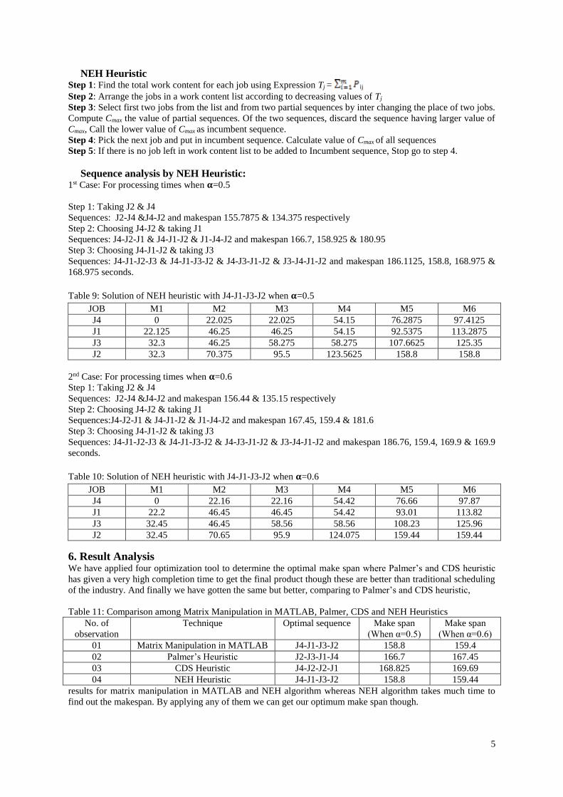
5

NEH Heuristic

Step 1: Find the total work content for each job using Expression Tj = ij

Step 2: Arrange the jobs in a work content list according to decreasing values of Tj

Step 3: Select first two jobs from the list and from two partial sequences by inter changing the place of two jobs.

Compute Cmax the value of partial sequences. Of the two sequences, discard the sequence having larger value of

Cmax, Call the lower value of Cmax as incumbent sequence.

Step 4: Pick the next job and put in incumbent sequence. Calculate value of Cmax of all sequences

Step 5: If there is no job left in work content list to be added to Incumbent sequence, Stop go to step 4.

Sequence analysis by NEH Heuristic: 1st Case: For processing times when 𝛂=0.5

Step 1: Taking J2 & J4

Sequences: J2-J4 &J4-J2 and makespan 155.7875 & 134.375 respectively

Step 2: Choosing J4-J2 & taking J1

Sequences: J4-J2-J1 & J4-J1-J2 & J1-J4-J2 and makespan 166.7, 158.925 & 180.95

Step 3: Choosing J4-J1-J2 & taking J3

Sequences: J4-J1-J2-J3 & J4-J1-J3-J2 & J4-J3-J1-J2 & J3-J4-J1-J2 and makespan 186.1125, 158.8, 168.975 &

168.975 seconds.

Table 9: Solution of NEH heuristic with J4-J1-J3-J2 when 𝛂=0.5


J4 0 22.025 22.025 54.15 76.2875 97.4125

J1 22.125 46.25 46.25 54.15 92.5375 113.2875

J3 32.3 46.25 58.275 58.275 107.6625 125.35

J2 32.3 70.375 95.5 123.5625 158.8 158.8

2nd Case: For processing times when 𝛂=0.6

Step 1: Taking J2 & J4

Sequences: J2-J4 &J4-J2 and makespan 156.44 & 135.15 respectively

Step 2: Choosing J4-J2 & taking J1

Sequences:J4-J2-J1 & J4-J1-J2 & J1-J4-J2 and makespan 167.45, 159.4 & 181.6

Step 3: Choosing J4-J1-J2 & taking J3

Sequences: J4-J1-J2-J3 & J4-J1-J3-J2 & J4-J3-J1-J2 & J3-J4-J1-J2 and makespan 186.76, 159.4, 169.9 & 169.9

seconds.

Table 10: Solution of NEH heuristic with J4-J1-J3-J2 when 𝛂=0.6


J4 0 22.16 22.16 54.42 76.66 97.87

J1 22.2 46.45 46.45 54.42 93.01 113.82

J3 32.45 46.45 58.56 58.56 108.23 125.96

J2 32.45 70.65 95.9 124.075 159.44 159.44

6. Result Analysis We have applied four optimization tool to determine the optimal make span where Palmer’s and CDS heuristic

has given a very high completion time to get the final product though these are better than traditional scheduling

of the industry. And finally we have gotten the same but better, comparing to Palmer’s and CDS heuristic,

Table 11: Comparison among Matrix Manipulation in MATLAB, Palmer, CDS and NEH Heuristics

No. of

observation

Technique Optimal sequence Make span

(When α=0.5)

Make span

(When α=0.6)

01 Matrix Manipulation in MATLAB J4-J1-J3-J2 158.8 159.4

02 Palmer’s Heuristic J2-J3-J1-J4 166.7 167.45

03 CDS Heuristic J4-J2-J2-J1 168.825 169.69

04 NEH Heuristic J4-J1-J3-J2 158.8 159.44

results for matrix manipulation in MATLAB and NEH algorithm whereas NEH algorithm takes much time to

find out the makespan. By applying any of them we can get our optimum make span though.

6

7. Conclusion In this paper it has been proposed that matrix manipulation method in MATLAB to solve flow shop scheduling

problems for minimizing make span. The problem up to 4 jobs and 6 machines under uncertain processing

times have been considered for comparative analysis among our proposed matrix manipulation method in

MATLAB and Palmer’s heuristic, CDS heuristic & NEH heuristic. From the analysis, it has been found that our

used matrix manipulation method in MATLAB and NEH heuristic show the minimum value of make span

time when compared to other heuristics. But NEH and other heuristics take long time for the calculation and it

will be very difficult to solve if the size of the problem is very large. In this regard our proposed matrix

manipulation method in MATLAB is able to solve any problem of any size such as n jobs and m machines

without any manual calculation and gives the output at a very short time. Moreover if you wish to see the

completion time required for any of the sequences of very large size problem then our proposed system will help

you must and very firstly. But it is not at all possible in NEH or other heuristic because of they do not find all

the job sequences and their respective make span. In our MATLAB coding, you will just have to put the

processing times for every jobs for corresponding machines .The work can be extended by making a comparison

of the effectiveness of the coding for the proposed matrix manipulation method with other coding.

8. References [1] Liou, T. S. and Wang, M.T., “Ranking fuzzy numbers with integral value,” Fuzzy Sets and Systems, 50, pp.247–255,

(1992)

[2] Johnson SM,” Optimal two and three stage production schedules with setup times included” Naval Research Logist

Quarterly, Vol. 1, Issue 1, pp.61-68,(1954)

[3] Palmer D,” Sequencing jobs through a multi-stage process in the minimum total time – a quick method of obtaining a

near optimum” Operation Research Vol. 16, pp.101-107, (1965)

[4] Campbell HR and Smith DM , “A heuristic algorithm for n-jobs m-machines sequencing problem”, Manage

Science, Vol.16B, pp. 630−637,(1970)

[5] Gupta J,” A functional heuristic algorithm for the flow shop scheduling problem” Operation Research Vol. 22, pp.39-47,

(1971)

[6] Dannenbring D, “An evolution of flow shop scheduling heuristics. Manage Science”Vol. 23, Issue 11, pp.1174-1182,

(1977)

[7] Nawaz, M., Enscore Jr, E. and Ham, I., “A heuristic algorithm for the machine, n-jobs flow shop scheduling problem”

OmegaVol. II, pp.91-95, (1983)

[8] Rajendran C, “Theory and methodology heuristics for scheduling in flow shop with multiple objectives”,

European Journal Operation Research, Vol. 82, pp.540 −555,(1995)

[9] Tejpal S. Hundal & Jayant Rajgopal, “An extension of Palmer's heuristic for the flow shop scheduling problem”,

International Journal of Production Research,Vol. 26, Issue 6, pp.1119-1124,(2007)

[10] Tang and Zhao, “Scheduling a single semi-continous batching machine” Omega Volume 36, No. 6, pp. 992-1004,

(2008)

[11] Eren and Guner, “A bicriteria flow shop scheduling”Applied Mathematical Modeling, Volume 32, Issue 9, pp. 1719-

1733, (2008)

[12] McCahon .S and Lee. E.S., “Job sequencing with fuzzy processing times,” Computer and mathematics applications,

19(7), pp.294-301. (1990)

[13] Hong .T and Chuang .T, “New triangular fuzzy Johnsons algorithm,” Computer and Industrial engineering, 36(1),

pp.179 - 200. (1999)

[14] Seyed Reza Hejari, Saeed Emami, Ali Arkan , “A Heuristic algorithm for minimizing the expected make span

in two machine flow shops with fuzzy processing time,” Journal of uncertain systems, 3(2), pp.114-122. (2009)

[15] Yager. R.R, “A procedure for ordering fuzzy subsets of the unit interval,” Information Sciences, 24, pp.143-

161. (1981)

[16] Shukla .C.S. and Chen, “The state of in intelligent real time FMS control –a comprehensive study,” Journal of

intelligent Manufacturing, 4, pp.441-455, (1996)

[17] Martin .L and Roberto .T, “Fuzzy scheduling with application to real time system,” Fuzzy sets and Systems, 121(3), pp.

523-535, (2001)

[18] Ishibuchi. H and Lee. K. H., “Formulation of fuzzy flow shop scheduling problem with fuzzy processing time”,

Proceeding of IEEE international conference on Fuzzy system, pp.199-205, (1996)

International Conference on Mechanical, Industrial and Materials Engineering 2015 (ICMIME2015) 11-13 December, 2015, RUET, Rajshahi, Bangladesh.

1

Paper ID: IE-49

An evaluation of failure modes and effect analysis for a battery

manufacturing industry Md. Abdus Salam1, Md Mashum Billal2, Md. Moshiur Rahman3 and Md. Ariful Islam4

2,4Department of Industrial and Production Engineering, Rajshahi University of Engineering and

Technology, Rajshahi-6204, Bangladesh. E-mail:[email protected], Cell.01741238070 (Corresponding author),

E-mail:[email protected] 1Department of Process Engineering, Gildan Activewear, Ashulia, Saver, Dhaka, Bangladesh.

E-mail:[email protected] 3Department of Quality Engineering, Dutch-Bangla pack Ltd, Dhaka, Bangladesh.

E-mail:[email protected]

Abstract Failure mode and effects analysis (FMEA) is one of the well-known analysis methods where the potential

failure modes usually are known and the task is to analyze their effects on system behavior. This thesis paper

aim to identifies and eliminate current and potential problems from assembly lines in a battery industry.

Feasibility test using control chart aim to find out the error and process performance. This thesis provides

work sheets for problems identification and guide lines for recommending corrective actions. This thesis

paper also analyzes Risk Priority Number (RPN). The different types of information are very difficult to

incorporate into the FMEA by the traditional risk priority number (RPN) model. In this thesis paper we

present an FMEA using the evidential reasoning (ER) approach, a newly developed methodology for multiple

attribute decision analysis. The proposed FMEA is then illustrated with an application to a fishing vessel. As

is illustrated by the numerical example, the proposed FMEA can well capture FMEA team members' diversity

opinions and prioritize failure modes under different types of uncertainties.

Keywords: Failure mode and effects analysis, evidential reasoning (ER) approach, risk priority number.

1. Introduction In the present era, there has been tremendous pressure on manufacturing and service organizations to remain

competitive and provide timely delivery of quality products. The managers and engineers have been forced to

optimize the performance of all systems involved in their organizations. The deterioration and failure of these

systems might incur high costs due to production losses and delays, unplanned intervention on the system and

safety hazards. In order to avoid such situations, an appropriate maintenance policy strategy is necessary in

order to repair or replace the deteriorated system before failure. Deciding on the best policy is not an easy

matter, as the maintenance program must combine technical requirements with the management strategy. A

good quality program must define maintenance strategies for different facilities. The failure mode of every

component must be studied in order to assess the best maintenance solution, in accordance with its failure

pattern, impact and cost on the whole system. The management of large number of tangible and intangible

attributes that must be taken into account represents the complexity of the problem. Several techniques have

been discussed in the literature for planning maintenance activities of industrial plants. The most commonly

used technique to evaluate the maintenance significance of the items failure modes and categorizing these in

several groups of risk is based on using Failure Mode Effect and Analysis FMEA. This methodology has been

proposed in different possible variants, in terms of relevant criteria considered and/or risk priority number

formulation. Using this approach, the selection of a maintenance policy is performed through the analysis of

the obtained priority risk number. The FMEA discipline was originally developed in the United States

Military. The generic nature of the method assisted the rapid broadening off MEA to different application

areas and various practices fundamentally using the same analysis method were created. The rest of this

paper is organized as follows; section 2 represents literature review, section 3 represents problem statement &

methodology, Section 4 represents data collection and result analysis. Section five represents the discussion

and conclusion and finally references are mentioned after the conclusion portion.

2. Literature Review Procedures for conducting FMEA were described in US Armed Forces Military Procedures document MIL-P-

1629(1949); revised in 1980 as MIL-STD-1629A). During the 1970s, use of FMEA and related techniques

spread to other industries. The automotive industry began to use FMEA by the mid-1970s.Although initially

developed by the military, FMEA methodology is now extensively used in a variety of industries including

semiconductor processing, battery industry, food service, plastics, software, and healthcare. There is relatively


2

little information published on the use of FMEA for battery manufacturing systems. Documenting and

analyzing potential risks proactively are essential for improved patient safety. Accomplishing this goal

requires an effective method to identify risks and an easily understood approach to manage risks [3]. In situ

simulation occurs in a patient unit at the microsystem level and involves inter disciplinary teams and

organizational processes. Unlike simulations that occur in a laboratory setting, in situ simulation is a strategy

that takes place on a patient care unit [5]. The authors [9] proposed a method to combine multiple failure

modes into a single one, which opens the possibility for us to analyze a system considering multiple failure

modes at the same time. Unfortunately, although they proposed such method, the detailed procedure such as

which multiple failures need to be combined was not given. This paper aims to develop a new FMEA method

that enables us to combine multiple failure modes into single one, considering importance of failures and

assessing their impact on system reliability. FMEA is a tool for identifying, analyzing and prioritizing

failures. It is a design technique which systematically identifies and investigates potential system weakness.

It consists of a methodology for examining all the ways in which a system failure can occur, potential effects

of failure on system performance and safety, and all seriousness of these [12]. effects A safety system used

to monitor a nuclear power plant may have a logic error that allows a failure to dampen an overloaded

reactor to go undetected. Risk prioritization produces a ranked ordering of risk items that are identified and

analyzed. [4] Collected and analyzed a number of key risk factor and their impact on the system. An error in

a spacecraft program for controlling re-entry angle could cause skip-out and loss of mission. The authors [8]

proposed that this study was carried out considering the specific processes implemented at CNAO,

therefore, the detailed definition of failure modes and the assignment of RPN scores, strongly depend on

the specific process under investigation and on the current strategies/solutions locally applied. However,

the process and fault trees here delineated can be easily adapted by other users to their local scenario or, at

least, be useful as a starting reference point, thus minimizing the workload impact of the FMEA analysis on

the involved team. P. C. [11] proposed a method for FMEA generation for a generic application using

minimum information during the conceptual design stage. Prototype software has been created for the

proposed method. It has been evaluated using case studies from the design and manufacture of two way

radios. The evaluation revealed the feasibility of the proposal, as well as some weaknesses that need further

improvement. Generally, the capability of the method to generate FMEA report with minimum information is

demonstrated. According to BS 5760 FMEA is a method of reliability analysis intended to identify

failures, which have consequences affecting the functioning of a system within the limits of a given

application, thus enabling priorities for action to be set. In the paper [1] draw attention a new technique

based on modified FMECA along with TOPSIS is proposed to determine the Maintenance Criticality Index

(MCI) and to overcome the limits of the conventional RPN, as cited above. This technique permits to

take into consideration the several possible aspects concerning the maintenance selection problem (failure

chances, detect-ability, etc.).

3. Problem statement In case of process improvement, at first one should know about the process whether the existing process is

capable or not. Incapable process produces large number of defective items. In these case manufacturers

should justify the process capabilities. In Rahimafrooz Globatt Ltd. the production of defective items in

different stages of assembles line is well enough. But the failure in Open circuit voltage is serious. If this

failure is occurred there is no way to rework except scrap. So this paper concentrates on the reasons of OCV

failures and develops worksheet for individual reasons of failure. RPN is also important for ranking of

seriousness of those failures. The objectives of this thesis work are (i) Find out the failure rate. (ii) Find out

the failure reason. (iii) Proposed corrective action.

3.1 Methodology Statistical data collection methods for checking the quality percentage of errors and determining

Process Capacity Ratio (PCR) of the process. Production process flow and Standard operation

procedure is reviewed. We collect data from production engineer and Quality Assurance department

of Rahimafrooz Globatt Limited.

Identify potential design and process related failure modes. Ideally, the process is changed to remove

potential problems in the early stages of development.

Find the effects of the failure modes for each failure on system operation.

Find the root causes of the failure modes. Barkai (1999) stated that an FMEA is designed to find the

sources of the failures of a system.


3

Identify, implement, and document the recommended actions. Pries noted that FMEA documents

should be under formal document control. Kennedy stated that the recommended actions are to

address failure modes with rankings that are considered unacceptable.

4. Data Collection and Results analysis 4.1 Control Chart: X bar R chart

From a day’s a production, a sample of 4 batteries is selected randomly from the production line and their

voltage are recorded. The average voltage of this sample are computed and recorder in a table. We collected

this data in 20 days in the month of December. Thus, X bar and R values of 20 samples are recorded in the

table.

Table 4.1: Voltages of battery in volt from four observations

SL

Voltages of battery for four observations ��

R

i ii iii iv

1 12.63 12.55 12.59 12.60 12.59 0.08

2 12.63 12.66 12.67 12.64 12.65 0.04

3 12.69 12.65 12.63 12.58 12.64 0.11

4 12.58 12.54 12.67 12.69 12.62 0.15

5 12.70 12.64 12.69 12.60 12.66 0.10

6 12.63 12.66 12.67 12.64 12.65 0.04

7 12.55 12.56 12.60 12.56 12.57 0.05

8 12.69 12.64 12.65 12.69 12.67 0.05

9 12.69 12.62 12.63 12.58 12.63 0.11

10 12.67 12.60 12.73 12.60 12.65 0.13

11 12.70 12.64 12.69 12.63 12.67 0.07

12 12.68 12.61 12.63 12.69 12.65 0.08

13 12.62 12.69 12.69 12.62 12.66 0.07

14 12.68 12.63 12.60 12.69 12.65 0.09

15 12.59 12.57 12.68 12.69 12.63 0.12

16 12.73 12.78 11.50 12.51 12.38 1.28

17 12.65 12.68 12.70 12.63 12.67 0.07

18 12.51 12.65 12.68 12.69 12.63 0.18

19 12.63 12.66 12.67 12.58 12.64 0.09

20 12.60 12.66 12.56 12.65 12.62 0.10

Average 12.63 0.151

4.1.1 R Chart development: First, the R chart is developed.

𝑅 =∑ 𝑅𝑖

𝑚𝑖=1

𝑚=

3.02

20= 0.151

For samples of size n=4, from appendix: D3=0&D4=2.282

We know, the control limits Range (R) chart are found

UCLR=𝑅D4 = (0.151) * (2.282) = 0.343 CLR =𝑅 = 0.151 LCLR = (0.151) * (0) = 0

Hence, the R chart is constructed as below.

0.00

0.50

1.00

1.50

1 2 3 4 5 6 7 8 9 10 11 12 13 14 15 16 17 18 19 20

Ran

ge v

alu

e, R

Sample number

R Chart

UCLCL

LCL

Out of range

Fig 1: the R chart


4

We observed that one of the sample values go outside of the limits. They are not pretty random around the

mean as well. Thus, the range chart can be considered as “out of control”.

4.1.2 �� Chart development The �� chart is constructed below

�� =∑ ��20

𝑖=1

20=

∑ 252.520𝑖=1

20=12.625

For samples size n=4 then form appendix Table D, A2=0.729

UCLX =�� + A2𝑅 = 12.625+ (0.729)*(0.151) = 12.735 CLX= 𝑅 = 12.625

LCLX= �� - A2𝑅 = 12.625- (0.729)*(0.151) = 12.516

Sample standard deviation:

σ =𝑅

𝑑2 =

0.151

2.059 =0.073

Suppose that the stated speciation limits are: 12.50 V and 10.78 V, the centre line or the mean of the process

has been found equal to 12.625.

Probability of the Voltages greater than the USL and less than LSL

P(X>USL) =1 - φ[12.78−12.625

.073] =1 – φ (2.123) = 1-0.9831 = 0.0168= 1.68% & P(X<LSL) = 4.34%

Process Capability Ratio (PCR) is

PCR =𝑈𝑆𝐿−𝐿𝑆𝐿

6𝜎 =

12.78−12.50

6∗0.073 =0.639 < 1

This shows that the PCR value is less than 1, which indicates that a large number of products are

nonconforming.

4.2 Pareto analysis for OCV failure Table 4.2.1: Cumulative sum for various complaints

S. No. Complaints Event Cumulative count Percentage

1 Bent negative plate 8 8 40

2 Separator problem 6 14 30

3 Positive & negative plate contact 2 16 10

4 Molten lead 2 18 10

5 Short molding of container 1 19 5

6 Lead splash at inter cell welding 1 20 5

Total 20 100

4.2.2 Graphical view:

Fig 4.2.2.1: Pareto analysis for battery defect

4.3 Worksheet for failure Sub system name: OCV test, Model year: 2013

P=probability of occurrence, S=seriousness of failure

D=likelihood the defect will reach the customer, RPN= risk priority number

0

5

10

15

20

25

Bent

negative

plate

Separator

problem

Positive &

negative

plate contact

Molten lead Short

molding of

container

Lead splash

at intercell

welding

Even

t, P

erce

nt

complaints

Pareto analysis

Event

Cumulativecount


5

4.3

.1 F

ME

A w

ork

shee

t fo

r O

CV

fa

ilu

re: Tab

le 4

. 3.1

: F

un

ctio

n o

f O

CV

tes

ter

Act

ion

tak

en

Wir

e

chan

ged

Reg

ula

rly

insp

ect

par

amet

er

Rec

om

men

d

ed

corr

ecti

ve

acti

on

Rep

lace

th

e

wir

e

chec

k t

he

char

gin

g

tim

e

&p

aram

eter

RP

N

40

Cu

rren

t

con

tro

ller

Ref

ill

acid

lev

el t

hen

char

gin

g

pro

per

ly

Eff

ect

of

Fai

lure

Th

e

bat

tery

is

scra

ped

Mec

han

ism

& c

ause

of

fail

ure

Les

s ch

arg

ing

tim

e &

par

amet

er

Inte

r ce

ll

sho

rten

ing

Fai

lure

Mo

de

Lo

w

ou

tpu

t

vo

ltag

e

Fu

nct

ion

Ch

eck

th

e

op

en

circ

uit

vo

ltag

e

Par

t

Nam

e

OC

V

test

er

SL

1

4.3

.1.1

FM

EA

wo

rksh

eet

for

Neg

ati

ve

pla

te b

end

ing

:

Tab

le 4

. 3.1

.1:

Fun

ctio

n o

f N

egat

ive

pla

te b

end

ing

Act

ion

tak

en

Imp

rov

e g

rid

cast

ing

m/c

per

form

ance

Tra

in u

p

lab

or

Rec

om

men

d

ed

corr

ecti

ve

acti

on

Mai

nta

in

spec

ific

thic

kn

ess

Car

efu

lly

in

sert

cell

RP

N

42

Cu

rren

t

con

tro

ll

er

N/A

Eff

ect

of

Fai

lure

Th

e b

atte

ry

is s

crap

ed

Mec

han

ism

& c

ause

of

fail

ure

Th

in g

rid

th

an

spec

ific

atio

n

Lo

w p

asti

ng

Fai

lure

Mo

de

Lo

w

ou

tpu

t

vo

ltag

e

Fu

nct

ion

Dro

p 2

.1

vo

ltag

e

Par

t

Nam

e

Neg

ativ

e

pla

te

ben

din

g

SL

1

4.4 Potential failure cause with RPN for 20 defects Battery For different potential failure the value of probability severity and detection are given bellow.

Table 4.4.1: Calculation of Risk Priority

Failure

no.

Potential failure cause Frequency Probability

(p)

Severity

(S)

Detection

(D)

RPN

1 Bent negative plate 8 7 3 2 42

2 Separator problem 6 6 3 3 36

3 Positive & negative plate contact 2 4 5 2 40

4 Molten lead 2 4 2 2 16

5 Short molding of container 1 3 5 2 30

6 Lead splash at inter cell welding 1 3 4 1 12


6

From the Table 4.4.1 it can be concluded that failure (1and 3) i.e. Bent negative plate and Positive & negative

plate contact failures are of high risk, is catastrophic failure. The failures (2 and 5) i.e. Separator problem and Short

molding of container failure, are classified as critical. The failures (4 and 6) i.e. Molten lead and Lead splash at inter

cell welding failure are categorized as marginal failures. According to Table 4.4.1 Bent Negative plate failures and

Positive & negative plate must be inspected when the failure occurs again and again.

5 Discussions and Conclusion 5.1 Discussion By calculation the process capability Ration (PCR) is 0.639. This shows that the PCR value is less than 1, which

indicates that the process is inappropriate. So the process is not good at all. This is due to a few products were taken

as a sample. This paper finds out the products nonconforming or failures area to develop a worksheet or document

to reduce products failure and smooth assemble line. FMEA worksheet is our main work which is very effective to

increase product Quality and Productivity. Most of the machines are software based and automated so the

implementation of recommended corrective action is hard enough.

5.2 Conclusion EMEA is a team-oriented development tool used to analyze and evaluate potential failure modes and their causes in

manufacturing process. It prioritizes potential failures according to their risk and drives actions to eliminate or

reduce their likelihood of occurrence. FMEA provides a methodology for documenting this analysis for future use

and continuous process improvement. It is structured approach to the analysis, definition, estimation and evolution

of risks. This study shows that in battery production the process of manufacturing is very important which

demonstrate the OCV (Open Circuit Voltage) failures. This paper checks the process capability and prioritizes

reasons of failures using pareto analysis. This study tries to develop a FMEA documentation/worksheet for taking

future action. This paper also calculated RPN for failure causes. The data was collected only from Rahimafrooz

Globatt Ltd. Therefore, many possible future research works can be defined in this context. For example it is better

to involve customers and suppliers in the preparation of FMEA. Involvment of customers and suppliers is a

recommended part of TQM and FMEA for a battery industries is more cost effective at the earlier stage of design

than at later stage when a design is almost at the final one.

6. REFERENCES

[1] Anish Sachdeva*, Dinesh Kumar (January 2009), Multi-factor failure mode critically analysis using TOPSIS. Journal of

Industrial Engineering International, Vol. 5, No. 8, 1-9.

[2] Denny Stephens, Battelle Phillip Gorney, Barbara Hennessey (January26, 2012) ,Failure Modes & Effects Criticality

Analysis of Lithium-Ion Battery Electric and Plug-in Hybrid Vehicles NHTSA SAE 2012 Government/Industry

Meeting.

[3] Welborn C. Using FMEA to assess outsourcing risk. Qual Prog 2007; 40: 17-21.

[4] Aloni D.Dulmin R.& Mininno V.(2007) Risk management in ERP project introduction:Review of the the literature.

Information and management. 44(6),547-567.

[5] Hamman W, Rutherford W, Liang BA, et al. In situ simulations: Moving simulation to new levels of realism within

healthcare organizations. Third Conference on Safety Across High-Consequence Industries; 2007 Mar 13-15; St.

Louis, MO.

[7] Kwai-Sang China,∗, Ying-Ming Wangb, Gary KaKwai Poona, Jian-Bo Yangc(2009), Failure mode and effects analysis using

a group-based evidential reasoning approach. Computers & Operations Research 36 (2009) 1768 – 1779.

[8] Marie Claire Cantone1, Mario Ciocca,(2013). Application of failure mode and effects analysis to treatment planning in

scanned proton beam radiotherapy, Cantone et al. Radiation Oncology 2013, 8:127.

[9] Ningcong Xiao a, Hong-Zhong Huang a*, Yanfeng Li a, Liping He a, Tongdan Jin b(2011), Multiple failure modes analysis

and weighted risk priority number evaluation in FMEA

.

[10] NL Narayana, Dr. NVS Raju, Chaithanya. K & Dr. P. Ram Reddy(2013), Failure Mode, Effects and Criticality Analysis

of Load Haul Dump Vehicles (100t) in Open Cast Mines. Global Journals Inc. (USA).

[11] P. C. TEOH* and KEITH CASE (4, June 2005). An evaluation of failure modes and effects analysis generation method for

conceptual design. Int. J. Computer Integrated Manufacturing, Vol. 18, No. 4, 279 – 293.

[12] Segismundu A. & Miguel P.A.C (2008). failure modes and effect analysis (FMEA) in the context of the risk management in

new product development. International journal of Quality & reliability management. 25(9),811-912.



Paper ID: IE-50

Statistical Process Control (SPC) Tools for Minimizing the Moulding

Defects in Spun Pre-stressed Concrete Electric Pole Production

Md. Asadujjaman*, Md. Safiul Kabir, Md. Arifuzzaman and Md. Mosharraf Hossain Department of Industrial and Production Engineering, Rajshahi University of Engineering and

Technology, Rajshahi, Bangladesh *E-mail: [email protected]

Abstract

Statistical process control tools are used to monitor production process over time to detect changes and to

decrease mistakes for better capture and conversion of customer’s needs. The aim of this paper is to identify and

minimize various types of defects in spun pre-stressed concrete pole manufacturing. SPC tools like check sheet,

histogram, Pareto chart, process flow chart, cause-effect diagram, control chart (p-chart and np-chart) are

used and it is found that the thickness uniformity problem is the vital few problem and responsible for 90% of

the total results of the problems. Operating characteristics curve is drawn to find out type-I error and type-II

error. It is found that the average run length is 319 when the process is in control. Finally, the major causes of

nonconformities of the quality problem are specified and possible remedies are proposed.

Keywords: Check Sheet, Histogram, Pareto Chart, Cause-Effect Diagram, Operating Characteristics Curve.

1. Introduction Statistical process control tools are basic quantitative techniques for total quality management (TQM) and have

widely been used to monitor process performance and to detect abnormal situations of the process behavior. The

role of statistical process control (SPC) is to make a process stable by reducing process variability [1]. TQM

tools are check sheet, Pareto chart, process flow chart, stratification analysis, scatter diagram, histogram, cause-

effect diagram and control charts. Enormous steel rod manufacturing companies and some other manufacturing

companies are using various methods to optimize their production and process failures. Paul and Azeem [2]

used Pareto chart and cause-effect analysis for identifying and analyzing the defects of a pharmaceutical

product. Joshi and Kadam [3] have also used Pareto chart and cause-effect analysis in manual casting process to

know correct cause and remedial factors in order to increase productivity and to improve customer satisfaction.

Sultana, Razive and Azeem [4] used statistical process control tools to increase total output and for identifying

major loss times from various machine breakdowns using hourly data system. Mohana Rao et al. [5] used

univariate control chart for monitoring hot metal making process in a blast furnace of a steel industry for

continuous quality improvement. They also concluded that large number of process parameters combined with

lower penetration of manufacturing automation and shortage of skilled workers are the main causes for which

foundry industry suffers from poor quality and productivity. Kumar, Mantha and Kumar [6] analyzed the

reasons for increasing scrap in manufacturing industries by using quality management tools. Fouad and

Mukattash [7] used statistical process control tools in order to identify the major and root causes of quality

problem and possible remedies of them. Applying the tools they have found that the steel tensile strength is the

vital few problem and account for 72% of the total results of the problems. Raghavendra et al. [8] used

statistical process control technique on liners manufacturing industry that improve process capabilities by

reducing rejection rate from 6.52% to 4.62%. Cause effect diagrams, design of experiments, if-then rules (expert

systems) and artificial neural networks are used to identify, analyze and rectify casting defects by Mane, Sata

and Khire [9]. A comparison of the univariate out-of-control signals with the multivariate out-of-control signals

was done by El-Din, Rashed and El-Khabeery [10]. They conduct a case study on steel making where average

run length was used to analyze performance for charting method. Samanta and Bhattacherjee [11] used Shewart

control chart in order to analyze quality characteristics for mining applications. Statistical process control tools

may be used in any industry and service center in order to find out the main causes and sub-causes of any

problem of the system. In this paper, statistical process control tools are used in spun pre-stressed concrete

(SPC) pole manufacturing industry for identifying and minimizing defects and finally some remedies are

proposed to increase productivity and customer satisfaction.

2

2. Methodology At first, process flow chart is used to examine various processes for the production of SPC electric pole. A

check sheet is used to record data of various types of defects for further processing. A histogram is used that

represents the frequencies of defects by classes of data that helps to access the current production situation.

Then Pareto chart is used to rank the causes from most significant to least significant. To broken down the main

causes to sub-causes; cause-effect diagram is used where the causes are broken down into the main categories of

man, machine, material, method, management and environment. To monitor the proportion of nonconforming in

a sample p-chart is used and np-chart is used to monitor the number of nonconforming units in a sample. Then

the operating characteristic (OC) curve has drawn for displaying and investigating probability of accepting the

lot with fraction of nonconforming. Finally, recommendations are given based on the findings.

3. Analysis To examine potential sources of moulding defects of spun pre-stress concrete pole production and to identify

steps for improving, process flow chart is done.

Fig. 1. Process flow chart for spun pre-stressed concrete production

Fig. 2. Process flow chart of cage making and inserting the cage into the mould

Fig. 3. Process flow chart of concrete mixing and pouring the mixture into the mould

Fig. 4. Process flow chart of pretension, spinning and pin removing

Fig. 5. Process flow chart of de-moulding

Cage making and

inserting cage into

the mould

Concrete mixing

and pouring

Pretension,

spinning and pin

removing

De-moulding

Fetching mould from

spinning section to steam

curing section

Loosening of I-bolt and

keeping pole in steam

curing chamber

Raising temperature (30-

75)0C within two hours

Decreasing temperature

from 750C to normal

temperature within two

hours

Keeping temperature

constant (750C) for four

hours

Collection of raw materials Mixing the raw materials in

correct ratio Pouring the mixture

manually with the help of

vibrator

Elongation of HT wire by

applying pressure

I-bolt tightening Sending the mould for

spinning process

Cutting and straightening

HT wire

Inserting end and reaction

plate

Head forming at the both

ends

Cleaning and lubricating the

mould

Inserting pins into the

mould

Inserting pipes and mud into

the pins

Winding spiral wires around

the cage

Inserting disks into the cage

Setting de-bonding pipes

3

After analyzing the process, check sheet is used to collect and organized data of moulding defects. The check

sheet, also called a ‘defect concentration diagram’, is a simple tool used to record data for further processing.

Table 1. Check sheet for various defects of spun pre-stressed concrete poll production

Type of defects Talley Frequency Frequency (%) Cumulative frequency (%)

Thickness problem llll llll llll llll llll

llll llll llll llll llll

llll llll llll llll ll

72 90.00 90.00

Honey comb problem llll 5 6.25 96.25

Collar distance problem ll 2 2.50 98.75

Minor crack at the top l 1 1.25 100

Total 80 100

Histogram determines the statistical nature of the collected data sets and the frequency distribution shows how

often each different value in a set of data occurs. Fig. 6. Shows the histogram of the defects found in moulding

of SPC pole production. The Pareto chart ranks the causes from most significant to least significant. It depicts a

series of vertical bars lined up in a descending order– from high to low– to reflect frequency, importance or

priority. In Pareto chart the number indicated sequentially as: (i) thickness uniformity problem, (ii) honey comb

problem, (iii) collar distance problem and (iv) minor crack at the top. It is seen that the thickness uniformity

problem is the vital few and responsible for 90% of total defects.

Fig. 6. Histogram for various defects of spun pre-

stressed concrete poll production

Fig. 7. Pareto chart for various defects of spun pre-

stressed concrete poll production

Figure 8: Cause-effect diagram for thickness uniformity problem

4

Since, the thickness uniformity problem is the major problem; therefore, the cause-effect diagram is used to

identify possible causes for thickness uniformity problem by broken down the main causes into sub-causes. It is

also known as ‘fishbone diagram’ which combines brainstorming that helps to consider all possible causes of

thickness uniformity problem for spun pre-stressed concrete electric pole production. Control chart have used to

monitor quality and to see how the process chances over time.

p-chart for fraction non-conforming of average sample size

d = Non-conforming (defective) poles, n = average sample size =180 and m = number of periods =27

= = 0.0105

Therefore, Control limit,CL = =.0105

Upper control limit, UCL = zα/2 (1 and Lower control limit, LCL = zα/2 (1

For 3 quality, zα/2= 3

Here, UCL = 0.0333 and LCL = - 0.0115. As the fraction non-conforming can’t be negative. So, LCL = 0

np-chart for fraction non-conforming of average sample size

UCLnp = np +3√{np(1-p)} = 5.99, CLnp= np = 1.89, LCLnp= np - 3√{np(1-p)} = -2.2.

As the fraction non-conforming can’t be negative. LCL = 0

252219161310741

0.035

0.030

0.025

0.020

0.015

0.010

0.005

0.000

Sample

Pro

po

rtio

n

_P=0.01049

UCL=0.03328

LCL=0

P Chart of no. of defects

Fig. 9. p-chart for average Sample Size

252219161310741

6

5

4

3

2

1

0

Sample

Sa

mp

le C

ou

nt

__NP=1.889

UCL=5.990

LCL=0

NP Chart of defects

Fig. 10. np-chart for average Sample Size

5

The control chart shows that the process is in control. Therefore, operating characteristics curve has used to

investigate the probability of accepting the lot with fraction of nonconforming.

The Operating Characteristics Function and Average Run Length

Let,α = Type-I error = Producer’s risk, and, β = Type-II error = Customer’s risk.

β = P(D < n.UCL) P(D ≤ n.LCL)

Here, UCL = 0.03310, = 0.01044 and LCL = 0.

β = P(D<181*0.03310) – P(D≤0*0.3310) = P(D<6) – P(D≤0) = 0.996

α = 1 – β = 1 – 0.996 = 0.004

If we vary the value of p ,then the value of also changes which is shown below:

Table 2: Sensitivity analysis of

P(D<6) P(D =P(D<6) P(D

0.005 0.999 0 0.999

0.010 0.997 0 0.997

0.01044 0.996 0 0.996

0.015 0.979 0 0.979

0.020 0.927 0 0.927

0.025 0.830 0 0.830

0.030 0.698 0 0.698

0.035 0.552 0 0.552

0.040 0.411 0 0.411

0.045 0.290 0 0.290

0.050 0.195 0 0.195

0.055 0.125 0 0.125

0.060 0.078 0 0.078

Fig. 11. Operating characteristics curve

ARL = , as the process is in control. Thus ARL is 319. This indicates that we have to take the sample size as

large as 319 to detect a non-conforming product when process is in control.

4. Discussion and Recommendation We have recognized that the main cause of quality problem is thickness uniformity problem. So, here are some

remedies of this problem:

1. Changing the design or one of the designing parameters of the mould, such that introducing an extra

sheet metal section in the joining sections of the mould or changing the edge parts of the mould for

leakage control of concrete mixture into the mould during spinning may minimize the defects. This

research proposes a new edge design of the mould.

6

Figure 12: Existing mould Figure 13: Proposed design mould

2. Check center pins and tightening the bolt before starting the operation of molding.

3. Optimize the r.p.m. of existing spinning machine.

4. Create groups for Fixed Area Network (GFAN) to minimize problems of scheduling and inter-

relationship between the quality control team, junior engineers and workers.

5. The diameter of the spinning machine and the mould should check regularly to ensure the peripheral

uniformity of both mould and spinner to avoid the mould hammering.

6. Check the wet of the raw materials before stating the production and keep checking the wet after a

certain interval as the quality largely depends on the raw materials.

7. Change the metals used for manufacturing the mould. Metals of light weight and of high tensile and

compressive strength should be chosen for manufacturing the mould.

8. Improved I-bolts should be attached with the mould for tightening the mould properly. Moreover,

existing I-bolts should be re-grinded regularly for effective use of the threads of the bolt.

5. Conclusions

Statistical process control tools detect the major problems for manufacturing spun pre-stress concrete poles. The

thickness uniformity problem is the major problem and it should be minimized at first. Operating characteristics

curve and calculations of type-I error and type-II error helps to identify customer and consumer risks. The

average run length is 319 for this in control process. This research and proposed recommendations is helpful for

any spun pre-stressed concrete electric pole production company to minimize the problems and to increase

productivity and customer satisfaction.

6. References [1] P. A. Marques, C. B. Cardeira, P. Paranhos, S. Ribeiro, H. Gouveia, “Selection of the most suitable statistical process

control approach for short production runs: s decision model”, International Journal of Information and Education

Technology, Vol. 5, No. 4, 2015.

[2] S. K. Paul, A. Azeem, “Defects identification and analysis of a pharmaceutical product using Pareto and cause-effect

analysis”, Proceedings of the International Conference on Mechanical Engineering, ICME09-RT-23, 2009.

[3] A. Joshi, P. kadam, “An application of Pareto analysis and cause-effect diagram for minimization of defects in manual

casting process”, Proceedings of Annual International Conference IRAJ, pp. 31-35, 2014.

[4] F. Sultana, N. I. Razive, A. Azeem, “Implementation of statistical process control (SPC) for manufacturing performance

improvement”, Journal of Mechanical Engineering, Vol. 40, No. 1, 15-21, 2009.

[5] S. Kumar, S. S. Mantha, A. Kumar, “Scrap reduction by using total quality management tools”, International Journal of

Industrial Engineering, Vol. 16, No. 4, 364-369, 2009.

[6] O. R. MohanaRao, K. Venkatab Subbaiah, K. NarayanaRao, T. SrinivasaRao, “Application of univariate statistical

process control charts for improvement of hot metal quality- a case study”. Journal of Engineering Research and

Applications, Vol. 3, No. 3, 2013, 635-641.

[7] R. H. Fouad, A. Mukattash, “Statistical process control tools: a practical guide for Jordinian industrial organizations”,

Jordan Journal of Mechanical and Industrial Engineering, Vol. 4, No. 6, 693-700, 2010.

[8] S. T. V. S. Raghavendra, B. Manideep, R. P. Sai, Y. A. S. K. Reddy, “A case study on total quality control of

manufacturing of liners by applying SPC technique”, International Journal of Engineering Research and Applications,

Vol. 3, No. 4, 357-368, 2013.

[9] V. V. Mane, A. Sata, M. Y. Khire, “New approach to casting defects classification and analysis supported by

simulation”, Technical paper for 59th Indian Foundry Congress, 2011.

[10] M. A. S. El-Din, H. I. Rashed, M. M. El-Khabeery, “Statistical process control charts applied to steelmaking quality

improvement”, Quality Technology & Quantitative Management, Vol. 3, No. 4, 473-491, 2006.

[11] B. Samanta, A. Bhattacherjee, “Problem of non-normality in statistical quality control- a case study in surface mine,

The Journal of the South African Institute of Minining and Metallurgy, Vol. 104, 257-264, 2004.



Paper ID: IE-51

CONSTRUCTING A VIRTUAL FACTORY USING 3D STUDIO MAX

H.A. Zafor, J.C. Dhar, Santa Saha, Syeda Kamrun Nahar and M. Iqbal

Department of Industrial and Production Engineering

Shahjalal University of Science & Technology, Sylhet-3114, Bangladesh

Email: [email protected]

Abstract

The interactive visualization of 3D objects has revolutionized such fields as engineering, medicine,

entertainment and education. In fact there are a broad range of applications which are used to give virtual

world more realistic detail. It is important to design a layout of any factory before physical construction which

gives us the ideas about the machine set up, production process, material handling and inventory management

of that factory. To consider design alternatives creation of a 3D virtual factory using 3D modeling software and

animation based simulation system can provide a fast, effective method of visualizing and experiencing new

designs which can be easily modified. In this paper the construction and visualization of a 3D factory of flanges

has been described. 3D Studio Max software has been used for this purpose. The objective of the research paper

is to create a 3D factory showing a general layout of a flange factory and providing basic concept on the

building techniques of 3D virtual world for the new students and trainee. Conversion process of a 3D studio

virtual model to an AutoCAD model and Conversion process of an AutoCAD model, applications of factory

planning and advantages of virtual reality have also been described in the paper.

Key words: Factory, Modeling, Software, Visualization and Manufacturing.

1. Introduction Making virtual environment or virtual reality is modern technology to realize the condition of actual model or

any future model. A 3D factory as a well-designed and integrated environment is essential for success

applications of new technology. In this paper the construction and visualization of a factory of flanges has been

described. It is expected that this method is very much useful for construction of a factory and helps to manage

diverse information and re-use 3D models. At the design stage of a production system at a factory, designer can

evaluate the feasibility design environment, detect the factory and it can be used for factory management. The

development of virtual engineering factory is expected to be valuable by means of a 3-dimentional modeling

system and animation based simulation package by taking into account the real data of a factory. A 3D model of

a factory has been modeled by using 3D Studio Max software. Participant can navigate through virtual factory

and examine the virtual factory from different points. Thus 3D modeling and animation based simulation

technique provides a fast, effective method of visualizing and experiencing new designs which can be easily

modified. Designer can design and see different types of layout of factory before making final decision to

choose the best one. The animations of different machines may also successfully be done.

Virtual reality (VR) started from an unknown science and progressed into a highly exclusive, yet known

science. The technology was born from the merging of many disciplines including psychology, cybernetics,

computer graphics, database design, electronics, robotics and telepresence. Any representation that emulates

reality (i.e. a drawing, a photograph, a movie, an audio recording) is, in a sense, a virtual reality. The term

Virtual Reality (VR) is used by different people with many meanings. Virtual Reality (VR) is the computer

aided simulation of a 3D model that one can interact with in order to get a better sense of object [2]. Virtual

reality can also be defined as a synthetic computer generated (and hence virtual) environment within which a

person can navigate and interact with the virtual objects as the person would in the real world (reality) [2].

2. Literature Review Virtual environments are made up of 3D graphical images that are generated with the intention between the user

and the objects in that environment. The term virtual environment (VE) describes a computer-based generation

of an intuitive perceivable and experience able scene of a natural or abstract environment [2]. VE application

will contribute to enhancing the qualities of human-computer interaction, the importance of which, in view of



2

increasing complex information and communication applications, is constantly rising. Several types of problems

can be solved with better visualization support, e.g. issues concerning workshop-layout, production flow,

workplace design, etc. Users will get better perspectives if 3D models are used in the planning process instead

of traditional 2D models [1]. There are several additional benefits from using detailed visualization in those

virtual models. E.g. increase in planning speed, decrease in planning costs, and increase in planning quality are

some of the benefits that have been discussed.

Virtual reality originated in 1960’s, the person accredited with pioneering the concept of VR is Dr. Ivan

Sutherland, who made ground breaking contribution to the computer graphics and immersive interaction at

Harvard and University of Utah [3]. He showed that, a person with the aid a light pen could interact with the

computer via a display surface. Engineering based applications within all areas of academic, commercial and

industrial life are increasing. It is generally acknowledged that most of the growth in the VR industry has been

due to the demands for VR in the entertainment sector. In the 1917’s, Hollywood started to realize the power of

VR in the film industry due to its potential to create extra ordinary visual scenarios. Films such as ‘Star Wars’,

followed by ‘Terminator’ and ‘Jurassic Park’ are just some of the films that benefited immensely from VR and

computer graphics. Recently Pentagon has conducted a Virtual Nuclear War Game to predict its consequence.

3D digital models can be freely constructed in this virtual environment [4]. From a great deal of digital

modeling research in color, material, lighting by Sasada [5], Liu[ 6] and etc., it can be realize that the simulation

is nearly real. This not only enables to receive more feedbacks in the designing process, but also helps non-

professionals to fully understand the designing content.

N. Shariatzadeh, G. Sivard, D. Chen I in their paper titled “Software Evaluation Criteria for Rapid Factory

Layout Planning Design and Simulation” described the functionalities of software tools which can support the

factory layout design process to shorten design time and to identify errors in early stages of design [7]. Tullio

Tolio, Marco Sacco, Walter Terkaj, Marcello Urgo in their research paper titled “Virtual Factory: an Integrated

Framework for Manufacturing Systems Design and Analysis” addresses the concept of a integrated Factory

Design framework providing the capacity of using different and heterogeneous analysis and design tools on the

same manufacturing system model in a concurrent and coherent way. This framework is highlighted s a

prerequisite condition to tack the co-evolution problem, i.e the integrated management of product, process and

production system and their evolution over the time [8]. Sangsu and Sang Do Noh in their study tried to describe

the virtual factory implementation strategy (method) of manufacturing companies and the method of

diagnosing/evaluating the virtual factory establishment level of a manufacturing company. In addition, a case

study of a manufacturing company in Korea was analyzed using the developed diagnosis/evaluation method [9].

.

3. Construction of a 3 Dimensional Factory A factory is integrated infra-structure for digital manufacturing including CAD, 3ds Max and simulation models

of machines, equipment, work cells, lines and plants. Fig.1 has shown a general procedure to construct a factory.

It takes much time, cost and resources, so effective action plans and objectives are essential. To construct a

factory in CAD, 3ds Max and simulation model must be implemented. Both modeling works need considerable

time, cost and efforts. So technologies developments for an effective measuring and geometric modeling, a

knowledge based CAD, 3ds Max and simulation and reuse models are essential. In addition to this technologies,

systematic planning, determinations of detailed scopes and model maintenance are also very important.

Figure 1: Procedure to construct a 3D factory.



3

Areas and effects of manufacturing for flange factories are as below:

Environments for 3D engineering design, Design and operation of a factory, Validation and evaluation of

products and processes, Line simulations, inspections and quality managements, Visualization of products,

processes and resources.

Geometric Modeling 3D geometry modeling CAD system such as AutoCAD is widely used in engineering design. AutoCAD is

very suitable as a graphics editor for geometric modeling, especially for 3D geometric modeling. Although

AutoCAD is powerful for geometry modeling, it can’t be used as the tool for complex system motion

verification. AutoCAD do not have the dynamic simulation capabilities. AutoCAD provides some primary 3D

objects, such as box, cone, wedge ball etc., which are often used in 3D modeling. In order to create a realistic

virtual model of the studio as a 3DS file .Similarly virtual model for modification, the virtual model was

imported into AutoCAD as a DXF (Data Interchange Format) file. A DXF file is an ASCH (American Standard

Code for Information Interchange) coded file, of an AutoCAD drawing for importing and exporting to and from

other software packages [3]. Fig 2 illustrates the process of converting a realistic AutoCAD model into 3D

Studio virtual model.

Create 3D studio model(object)

Figure 2(a): Conversion process of a 3D studio virtual model to an AutoCAD model.

Export as a AutoCAD (3DS) file Model(object)

Import AutoCAD (DXF) file Model(object)

Create AutoCAD model (object)

Figure 2(b): Conversion process of an AutoCAD model.

Application of Virtual Engineering Factory Planning The typical applications of virtual factory planning are:

i. Planning and verification of machine setup.

ii. Determination of production sequence of factory machines.

iii. Analysis of different alternatives of layout of the factory.

iv. Planning and verification of material logistics.

v. Agile planning.

Advantages of Virtual Factory Planning The typical advantages of virtual factory planning are as follows:

a. More precise planning results compared to conventional tools.

b. Exchange of knowledge among different experts in the planning team.

c. Taking into account various influential factor such as workplace safety, accessibility and production tools.

d. Reduction of planning time and errors.

e. Planning results can be used for the purpose of training and education.

f. Documentation of company know-how.

g. Planning results can be used for the purpose of training and education.

4. Requirements for 3D Factory Modeling

Import AutoCAD (DXF) file Model(object)

Export as a AutoCAD (DXF) file Model(object)



4

In order to build the virtual factory, which is similar to a real factory, there might be many requirements in

modeling the elements of manufacturing system. Among a number of requirements, the authors emphasize that

the following three ones are most important to develop a modeling system for virtual factories [10]:

Visualization: The most important requisite is that a virtual factory should be visualized with reality. With good

visualization, one can easily and observes how each system elements work in the manufacturing systems.

Detailed descriptions: Each elements needs its detailed description, not only for its visualization, but also for

calculating a number of its attributes for example when you want to put a work piece into a box, you have to

know the shapes and dimensions of the work piece and the box in order to check whether the box can contain

the work piece or not. Flexibility: The modeling system should present a flexible way of modifying a virtual

factory in order to cope with the change of machines, layout and other facilities. Any facility to create computer-

generated models of virtual objects and environments that can be interactively explored in 3D and modified and

recreated in offers enormous potential for concurrent engineering and for integration of manufacturing activities

generally [11]. The designer would be able to quickly visualize the product concept and represent alternative

design solution.

The basic requirement for virtual 3D factory facilities planning is, first of all, the availability of all objects in

virtual environment. If this requirement is fulfilled simple production facilities planning are possible. The

system development was divided into two main parts [12]: Construction of a virtual environment: This part

provides experience of creating virtual object and placing them in the virtual environment with associated real

world. Properties in order to illustrate how models are created. Use of virtual environment: This part

encourages exploring different attributes of the virtual environment within two broad categories which are

factory walk through and visualization of different sections of the factory.

5. Simulation - Using 3D Studio Max Modeling and editing panel: The cornerstone of 3D Studio MAX is an advanced 3D modeling and animation

environment. One can perform 2D drawing, 3D modeling, and spline based animation within the unified

workspace. Modeling, editing and animation tools are always available in the command panels and toolbar.

Lights & Camera: Designer can create light objects using the light category of creating a panel. Ambient light

is found in the Environment dialog by choosing Rendering/Environment. The lights can cast shadows, project

images, and create volumetric effects for atmospheric lighting. 3D Studio Max also supports real-world camera

controls for lens length, field of view, and motion control such as truck, and pan. Materials: 3D Studio Max

contains a sophisticated Material Editor that floats in its own window above the scene. One can use the Material

Editor to create highly realistic materials by defining hierarchies of surface characteristics. Animation: The user

can begin animating his scene at any time by clicking the animation button. This button can be clicked again to

move back and forth between modeling and animation. The users can extensive control over his animation with

the 3D Studio Max Track View. This is a window into time where one can edit animation keys, set up

parametric animation controllers or display and adjust motion curves for all of your animated effects.

Rendering: The 3D Studio Max render includes advanced features such as analytical, motion, volumetric,

lighting, and environmental effects [11]. A research was done on Design and Development of workshop in 3D

environment using 3D studio MAX by Syeda Nusrat Jahan, Muhammad Bayazid Bustami, Ranjan Kumar Das,

Dept. of Industrial and production Engineering, Shahjalal University of Science and Technology, Sylhet,

Bangladesh in the year of 2006 [13].

Modeling objects in 3D Studio Max: The latest technology in modeling is utilized in this project by combining

3D Studio Max software and AutoCAD with Supers cape VRT for object drawing. 3D Studio Max is a three-

dimensional modeling and animation based package. It has the facilities to add, subtract, combine, and can add

material to object, to perform 2D drawing, 3D modeling based animation within the unified workspace.

Modeling, editing and animation tools are always available in the command panels and toolbars. The designer

can draw 2D and convert it to 3D by using tool bars and can view in front view, top view, and in perspective

view. This software helps the designer to change an initial profile of a model, thus updating the previous model

and its current drawing. Moreover it helps viewing the model at the same time in different ways. Figure 3 shows

the overall factory layout and figure 4 shows the office layout. Figure 5, 6, 7 shows the machines used in the

manufacturing of flanges and figure 8 shows the warehouse of the factory.



5

Fig. 3: Factory area. Figure 4: Office layout.

Fig. 5: Drilling Machine. Fig. 6: Engine Lathe machine.

Fig. 7: Milling Machine. Fig. 8: Factory Warehouse.

6. Conclusion The initial studies presented in this paper have shown that a realistic virtual model of the factory with high level

of details and accuracy. Here a 3D virtual environment and modeling software (3ds Max) is used for effective

construction and visualization of flange manufacturing factory. The basic construction method using virtual 3D

modeling software has been described here. Also some types of 3D flanges have been cited using 3D Studio

Max Software. Presently product are conceptually designed and then modified before making it in real life. So

this technology is becoming important in every sector of human needs. This makes important for future

designers to design effective 3D factories

7. References [1] Jonata Berglunda, Johan Vallhagenb, Björn Johansson, Erik Lindskoga, Forty Sixth CIRP Conference on

Manufacturing Systems Visualization support for virtual redesign of manufacturing systems, 2013

[2] Tusher H. Dani, Marwan Fathallah, and Rajit Gadh, “COVIRDS: An Architecture for a conceptual virtual

design system”, in proceeding of the 1994 Design for Manufacturability Conference, Chicago, IL, USA, pp



6

19-26, 1994,

[3] Gavriel, “Handbook of Human Factors and Ergonomics”, published by John Wily, New York, pp.1726

1997.

[4] Mitchel W., McCullough M., Digital Design Media, New York1997.

[5] Sasada, T., Computer Graphics and Design: Presentation Taiwan, 2000.

[6] Liu, Y.T., Eisenman, P, “Emergence of Digital Architecture”, Hu’s, Taipei, 2001.

[7] N. Shariatzadeh, G. Sivard, D. Chen “Software Evaluation Criteria for Rapid Factory Layout Planning Design and Simulation” published in the SciVerse ScienceDirect, Procedia CIRP 3 of 45th CIRP Conference on Manufacturing Systems, PP. 299-304, 2012.

[8] Tullio Tolio, Marco Sacco, Walter Terkaj, Marcello Urgo, “Virtual Factory: an Integrated Framework for

Manufacturing Systems Design and Analysis”, published in the SciVerse ScienceDirect, Procedia CIRP 7

Of 46th CIRP Conference on Manufacturing Systems, PP. 25-30, 2013.

[9] Sangsu and Sang Do Noh, “A Diogonal and Evolution Method for Strategic Planning and Systematic

Design of a Virtual Factory in Smart Manufacturing Systems” published in the International Journal of

Precision Engineering and Manufacturing Vol. 16, No. 6, pp. 1107-1115, ISSN 2234-7593(PRINT)/ ISSN

2005-4602 (online), June 2015.

[10] Onosanto and K. Iwata, “Virtual Works: Buildings Virtual Factory with 3D Modelling and Object

Oriented Programming Technique”, proceeding of the 1992 IFAC-INCOM, Toronto, Canada, pp.281-286,

1992.

[11] Tompkins A. James, “Facilities Planning”, published by John Wily & Sons Inc. New York, pp.103, 1996,

[12] D. Fan, Felger, W.G. and Global, M., “Applying Virtual Reality to Electronic Prototyping-Concepts and

First Results”, proceeding of the IFIP WG 5.10 Workshop on Virtual Environment and Their Applications

And Virtual Prototyping Stuttgart, Germany, pp.326-336, 1994.

[13] Syeda Nusrat Jahan, Muhammad Bayazid Bustami, and Ranjan Kumar Das, “Design and Development of

workshop in 3D environment using 3D studio MAX”; Department of Industrial and Production

Engineering, Shahjalal University of Science and Technology, Sylhet, Bangladesh, 2006.



Paper ID: IE-52

Automatic Whiteboard Cleaner Using Microcontroller Based Rack and

Pinion Mechanism

Sonia Akhter*, Anindo Saha, Md. Rayhan Parvez Koushik, Md. Asaduzzaman, Razoana

Islam Shorna, Md. Moudud Ahmed

Department of Industrial & Production Engineering

Rajshahi University of Engineering & Technology (RUET), Rajshahi-6204, Bangladesh

*Corresponding Author: E-mail: [email protected]

Abstract

At recent years whiteboard has become a crucial element at almost every educational institute. They are large

in size, for that reason it is very time consuming and tedious process to erase the writings from the board

with duster manually. It breaks concentration of both lecturers and listeners. Automatic Whiteboard Cleaner

can solve these problems. Automatic whiteboard cleaner will reduce the time and also the effort. It takes around

6secs to clear the board smoothly. This paper represents the design and construction of automatic whiteboard

cleaner. The system consists of Arduino microcontroller, driver module, dc gear motor, rack and pinion

mechanism, sonar sensor, supports, and a cleaner bar to give that an automation figure. When the switch is on,

it moves across the full width of the board and its direction is reversed automatically in order to clean the

board. So, this “Automatic Whiteboard Cleaner” is a great replacement of “duster” and it can be suggested to

use this to reduce the effort of the board user as well as to introduce the classroom with an automation system.

Key words: Automation, whiteboard cleaner, arduino, rack and pinion mechanism, sonar sensor.

1. Introduction

Education is the back bone of a nation. Education comprises of teaching and learning. The resources and

materials used in teaching becoming updated along with the teaching and learning techniques. Writing was

earlier done on sand, walls, slates made out of wood, chalkboards and in recent times on white boards and

electronic boards [1]. Chalk dust scatter causes serious health problems. Because of these reasons white board

has been widely implemented into many other sectors of human endeavor besides teaching [2].

Many researches and testing had been done on white board from a long time. Many variations had been done on

cleaning of whiteboard surfaces. Remote control motorized cleaners are made in which the dusters are operated

with the help of remote control [1]. This type of cleaner moves horizontally by means of motor mechanism

and erase the board with the help of dusters attached to it but it could not create sufficient pressure on

board . This limitation was solved by using rolling whiteboard surface and fixed dusters [3]. Instead of moving

the dusters the whiteboard surface is moved around the rollers. The friction produced between fixed dusters and

rolling surface creates sufficient pressure to erase the written data on it but this process is too time consuming to

clean the board. This drawback was overcome by using microcontroller and sensors but the longevity of board

surface is short because it acts as flat belt [4]. Remote control motorized cleaners makes use of belts which have

low wear and tear resistance and with the frequent operation of cleaning process, the belt is likely to cut and

hence makes the device or the cleaner less useful [3], [4]. Instead of belt, chain had been used to improve

the cleaning procedure but it creates too much noise [5]. Using cord and pulley arrangement the wiper bar

connected to the motors can erase writings on the board which creates less noise but it requires four motors and

two motor drivers causing too much cost [6]. These limitations have been overcome by the proposed design in

this paper. Only one motor and one motor driver with rack and pinion mechanism is used instead of belts and

large amount of pressure has provided by rack and pinion mechanism with necessary supports.

2. System components

This system is designed considering the present scenario of white boards. It consists of seven main components.

They are dc gear motors, arduino UNO, motor driver, wooden block, duster holders, dusters, rack & pinion

mechanism, AC to DC converter and whiteboard surface.

3. Design of system components

The whole system is based upon two individual units. One is the cleaning unit which ensures to erase writings

and other is the controlling unit which controls the cleaning system. The cleaning unit consists of the

necessary arrangement which enable the cleaner slide over the board and the controlling unit consists of

micro-controller which controls the motor, rpm, and the time of rotation.

Design of controlling unit

At controlling unit Arduino Uno is used which is a microcontroller board based on the ATmega328 .It has 14

digital input/output pins (of which 6 can be used as PWM outputs), 6 analog inputs, a 16 MHz ceramic

resonator, a USB connection, a power jack, an ICSP header, and a reset button. One of its most

important features is its ease of programmability. Motor Driver of L293D IC model is used which is a

monolithic integrated, high voltage, high current, 4-channel driver. Using chip it is possible to use DC motors

and power supplies of up to 36 Volts and maximum current of 600mA per channel.

Fig.1. Arduino UNO Microcontroller Fig.2. Motor driver

A dc gear motor is used at this project which can be operated within the range of 4V - 24V and has a speed of

100 RPM. The shaft length of motor is 25-30 mm and shaft diameter is 8 mm. This type of gear motors has high

torque and produces very less vibration effect so that the pinion can rotate smoothly. AC to DC adapter is used

to convert AC supply into DC supply. In this system the converter is used to step down the 240V AC to 18V, 3

amp DC supply. The converter is required for functioning of DC gear motors because these motors work only

on dc supply. Sonar Sensor or Ultrasonic Range Sensor (HC-SR04) is used to calculate the distance between the

sensor and the reflecting object mounted at brush. Pin connection of both motor driver and arduino UNO has

shown at fig. 3.

Fig.3. Pin connection of Arduino UNO and Motor Driver

As shown in the figure above, it's possible to drive 2 motors with a single L293D but only 1 motor is used at this

project. Table 1 shows how to make the motor turn clockwise and anti-clockwise. For example, if the pins 1 and

7 are in HIGH state, and the pin 2 in the LOW, the motor will rotate clockwise. On the other hand, if the pins 1

and 2 are in HIGH, and the pin 7 in the LOW, the motor will turn to the other way. Signal from sonar sensor

will change the state of pin 2 and pin 7.

http://api.ning.com/files/2JurkTHbQdyEJc0Us*C9I5BgklPg596Okj8IKIsIa8WQR3T3KTnIIyLYDn9llE4Hao3cvc2vNy2S8ytKUmseZB*S5uMsuuwT/l293dpin.jpeg

Table 1. Combination of pin status to make the motor run clockwise and anti-clockwise

If the distance between the sonar sensor and brush is less than 1 inch then motor will rotate clockwise and if this

distance is greater than 1 inch then motor will rotate anticlockwise which is programmed into the

microcontroller. The flow chart of motor rotation has shown below.

Fig.4. Flow chart of motor rotation

Main circuit diagram of automatic whiteboard cleaner has shown below which comprises of arduino, motor

driver, 9v dc gear motor and sonar sensor. 18v dc gear motor has used in the final project instead of 9v dc gear

motor.

Fig.5. Design of main circuit of Automatic whiteboard cleaner

http://api.ning.com/files/jFhR10F2nKDm5cJ0p2jcpgHpKd4hNPz01QgMS8OF6QUh82aIgvr-dp1uzQSopb*PQgSlhFEgj5ALhek3X56Zq6xDZuw-9vwD/l293dmontagem.jpeg

Design of cleaning unit

Cleaning unit consists of rack and pinion, brush, whiteboard, supportive board etc. Rack and pinion mechanism

consists of a circular pinion of a diameter of 1.5 inches and long rectangular rack of a length of 18 inches. The

pinion is coupled with the motor that means the pinion rotates with the shaft of the motor. The rotary motion of

the motor is transferred to the rack & the rack moves in translatory direction. The brush is an important part for

this project. To clean the white board smoothly a brush of better quality has been used. It has attached to the

brush holder with the help of glue & the brush holder is attached to the end of the rack with a nut & bolt. Foam

has been used as the cleaner. An amonyte sheet of 10 inches × 6 inches size has been used as a white board. The

whiteboard is enclosed within two reels. A wooden block is used as a supporting base for the whole system and

is made up of plywood. It is of length 50cm, breadth 5cm and height 40cm. It is used to support the whiteboard

sheet at the time of writing. The motor and rack & pinion mechanisms are also fitted on wooden block. The

reels are fixed with this supportive board by the help of angle plate.

Fig.6. Complete design of an automatic whiteboard cleaner

4. Construction of main structure

The system is assembled by using all the components as mentioned above. The duster holders with the dusters

fixed in it are attached on backside of the wooden block. A DC gear motor (18V) is fixed on the upper side of

the wooden block with clamp. The pinion is coupled with the motor that means the pinion rotates with the shaft

of the motor.

Fig.7. Constructed Automatic whiteboard cleaner

The rotary motion of the motor is transferred to the rack & the rack moves in translatory direction. A brush has

been attached to the brush holder with the help of glue & the brush holder is attached to the end of the rack with

a nut & bolt. The flexible white board surface is fixed on the wooden block enclosed with reels. The sonar

sensor is fixed on the lower portion of whiteboard attached with angle plate.

5. Working procedure

Now, considering the system is in use and the teacher wants to rub the board. When the teacher switch on the

supply, current is passed to the 18V adapter and then it passes through Arduino. This ARDUINO provides

signal to the driver module at a specific time interval. To drive the motor a DRIVER MODULE (L293D) has

been used. It receives the signal coming from the ARDUINO & change the polarity of the motor for which the

direction of the motor changes. To sense the distance and time specified by ARDUINO, a sonar sensor is used,

hence the motor rotates in both clock-wise & anti-clockwise direction. Due to the rotation of the shaft of the

motor, the pinion connected to it also rotates which in turn the rack moves in translatory direction along the

whiteboard. A brush holder is attached to the end of the rack with a nut & bolt. To clean the white board

smoothly a brush of better quality has been used which is attached to the brush holder. The brush moves from

the upper portion to the lower portion of the board and get rubbed due to the friction between board surface and

brush.

Fig.8. Flow diagram of power transmission of whiteboard cleaner

6. Time analysis

Prototype board of 10 inch wide and 6 inch long has been used in this project. Using manual duster it takes

about 25 secs for whole board cleaning. Proposed automatic whiteboard cleaner reduces the time requirement.

When switch is on, firstly brush moves downward and then moves upward direction thus completes one full

cycle of movement. Proposed automatic brush needs 5 full cycles for cleaning the board completely which takes

only 6 secs. Several data had taken to determine the time requirement for completing the wiping process.

Table-1 shows the time for ten observations.

Table 2: Time requires for complete cleaning

Trial No

n

Downward

Motion Time

(Sec),

D

Upward

Motion Time

(Sec),

U

Total Time

of 1 cycle

(sec),

T

Average

Time (sec),

A=T/n

Total average time for

complete cleaning

(Sec),

T.A.T= A * no. of

cycles

1 0.57 0.59 1.16

1.195

1.195× No of

cycles=1.195×5=5.975

2 0.58 0.61 1.19

3 0.55 0.60 1.15

4 0.64 0.62 1.26

5 0.56 0.63 1.19

6 0.57 0.59 1.16

7 0.63 0.61 1.24

8 0.60 0.60 1.20

9 0.59 0.62 1.21

10 0.58 0.61 1.19

7. Result and discussion

It is observed that the time of complete cleaning of the board using this system is average 5.975 sec. On the

other hand while using the manual process the time of cleaning is about 25 sec which is about four times of the

machine time. So proposed whiteboard cleaner takes less time than other previous models. It creates less noise

than other motorized cleaners. Sufficient pressure has been induced during the operation due to the attachment

of brush to the side reels of whiteboard which helps to clean the board very effectively and efficiently. Change

of brush is very easy and it does not affect any other parts while changing. This system is only applicable to

whole board cleaning. Partial cleaning of the board is not possible through this system. Though there is some

lagging in to start the motor, but averagely it is optimum.

8. Conclusions

It is concluded that automatic whiteboard cleaner has successfully designed. The system has designed with

innovative features which reduces human efforts and makes teaching efficient. This type of whiteboard

could be very effectively used in schools, colleges and universities as it increases the interest of the students to

study with different technology. The machine has reduced both time and human effort. The construction of

automatic whiteboard cleaner consists of arduino microcontroller which is very user friendly in programming.

On the other hand to construct the main structure, very simple tool work is needed, and the materials used

in this project is cheap and easily available in market. So it is not complicated to construct this machine and it

will help to introduce an automation system. The system can be further developed by integrating a bluetooth

remote for controlling the switch. Infrared sensors can be used to convert this system to a smart white board.

Aesthetic looks of the whiteboard can also be improved.

8. References [1] Tsado Jacob, “A Remote Controlled Motorized White Board Cleaner”, AU Journal of Technology, Vol.15, No.4,

pp. 273-280, 2012.

[2] Praveen. G, “Microcontroller Based Automatic Electronic Duster”, Proceedings Of International Academic

Conference On Electrical, Electronics And Computer Engineering, pp. 10-13, 2013.

[3] Puneet Mathur et. al., “Automated Motorized Whiteboard”, International Journal Of Engineering, Business And

Enterprise Applications (IJEBEA), Vol.6, No.1, pp. 01-04, 2013.

[4] Bhushan Tukaram Chougule and Puneet Mathur, “Automated Motorized Sensing Whiteboard”, International Journal

Of Advanced Research In Engineering And Technology (IJARET), Vol. 5, No. 3, pp. 155-163, 2014.

[5] Simolowo and O. E., “Preliminary Design of an Automated White Board Cleaner”, International Multidisciplinary

Journal, Vol. 8 (2), No. 33, pp. 68-82, 2014.

[6] Imam-Ul-Ferdous and A.H.M Fazle Elahi, “Development of an Automatic Board Cleaning system using

Microcontroller”, International Conference on Mechanical, Industrial and Energy Engineering 2014 (ICMIEE: PI-140307),

Khulna, Bangladesh.

[7] Chris Betcher and Mal lee, “The Interactive Whiteboard Revolution”, Aust Council for Ed Research, pp. 10-12, 2009.

[8] Shmuylovich and Salcman, “Whiteboard Presentation of Interactive and Expandable Modular Content,” U.S.Patent

057106 A2, Sept. 07, 2012.



Paper ID: IE-053

Safety Audit in a Milk Industry of Bangladesh

Md Mamunur Rashid1*, M. Iqbal2, Md. Mossarrof Hossain3, Mokbul Hossain3 and Md Mostafizur Rahman3 1* Bangladesh Institute of Management, Dhaka, Bangladesh; 2 Shahjalal Universities of Science and Technology,

Sylhet, Bangladesh; 3 BMCUL, Mirpur, Dhaka, Bangladesh; 1*Email: [email protected]

Abstract

For the safety of the Milk industry and specially Milkvita Bangladesh took the initiative to investigate/identify

the areas of improvement on safety through Audit/Observation. The research study includes analyzing the

safety awareness and safety condition of a Milkvita Factory resulting in finding non-compliance issues and

recommendations for correcting those issues to elevate or upgrade the safety scenario in working and operating

the said Milkvita Factory. Parameters are taken in this study are: Equipment based analysis; Job based

analysis; Location based analysis; Identifying the presence of resources including PPE(Personal Protective

Equipment) etc; Checking on factory premises including factory access, weigh bridge area, roads, lanes and

cleanliness related to Health Hazard; Preparing Accident record register in MS Excel; Factory Building design

review & recommendation; Electrical Safety assessment & recommendation; Machine Safety assessment &

recommendation; Identification and recommendation for occupational health; Evaluation of Fire fighting

training & Drill. No secondary data was used. Research results shows that the mean fire risk index (FRI) is 3 on

a scale of 5.0, which indicates an alarming condition. Locked exit doors, lack of emergency announcement

system and lack of fire drills are the three worst performers among the 24 investigated parameters used in the

study. Those parameters require immediate attention from the regulators and stakeholders. It is also observed

that a U-shaped relationship between FRI and factory size has been developed. Factories that are members of

the industry’s trade lobby generally have better fire safety practices than the non-members. FRI for the industry

can be very useful to understand the immediate concerns and thus to curb fatalities and injuries from fire

accidents in this sector. Given the importance of the Milk industry may be supply quality and hygienic and

quality milk to the customers. It is found from the findings that there is lack of training to the entire employee of

the Milkvita Company.

Keywords: Safety; Audit, Training; Fire Risk Index and Factory

1. Introduction

Milk production of Bangladesh is gradually increasing day by day due to proper nourishment of milk and milk

industry. Milk industry in Bangladesh is increasing. But it is to be mention that Milkvita is one of the largest and

pioneer of this sector. Milk is very much essential for the country people to meet up the nutritional

requirements. Among all industries Milkvita is one of the industries where safety measures are taken. In factory

cases electrical wiring, mechanical measures are taken for the safety of the employee and staffs. It can promote

the production line and keep the factory free from hazards. To remove accidental facts it is very much need to

improve safety measures. Milkvita has a variety of products such as Pasteurized Liquid Milk ,Flavored Milk

,Butter ,Full Cream Milk Powder, Skimmed Milk Powder, Ice-Creams, Ghee, Sweet Curd , Cream , Lollies

,Rasa Malai (sweet meat) , Condense Milk ,UHT Flavor Milk ,UHT Pasteurized ,Liquid Milk Chocolaté etc. All

these products are from health hazards by the unique & systematic tools, engineering and technical helps of our

resources personnel. By this way, the Milk industry is a highly competitive industry and cost-saving is highly

valued, but, given the lack of a safety culture in the country in general, cost-cutting measures often affect the

health and safety of the workers. Clothing is easily flammable and as such fire is one of the most sometimes and

damage inducing accidents in these factories in Bangladesh. Cold and fire cause most of the injuries of milk

industry, if industry can minimize that by providing suitable environment may get a good result. Cause of on-

the-job injuries and fatalities in this sector. Each new incident of fire and related damage adversely affects the

reputation of the industry. The Milk industry is a highly competitive industry and cost-saving is highly valued,

but, given the lack of a safety culture in the country in general, cost-cutting measures often affect the health and

safety of the workers. Clothing is easily flammable and as such fire is one of the most sometimes and damage

inducing accidents in these factories in Bangladesh. Cold and fire cause most of the injuries of milk industry, if

industry can minimize that by providing suitable environment may get a good result. Cause of on-the-job

injuries and fatalities in this sector. Each new incident of fire and related damage adversely affects the

2

reputation of the industry. Despite a number of initiatives to curb fire accidents in the Milk factory, there are still

a significant number of fire occurrences in this industry. Unfortunately, there is no comprehensive statistics on

the current status of fire provisions and management practices in the Milk industry. Though Milkvita is one of

the largest organizations in Bangladesh its safety audit was not done before. This kind of audit can be very much

innovative for milk industry, if any milk industry can perform all the safety measure. For this perspective, a

safety audit can be done in Milk industry like Bangladesh Milk Producers' Co-operative Union Ltd (BMCUL)

for achievement of better performance.

2. Brief History of BMCUL

Dhaka Dairy Plant is a milk processing factory under the organizational trade name MILKVITA and the

authoritative of LGRD ministry in Mirpur region, Dhaka. In terms of machineries, it is the largest milk industry

of the country. Bangladesh Milk Producers' Co-operative Union Ltd (BMCUL) popularly known by its brand

name Milk Vita, was established by the Bangladesh Government in 1973, immediately after the liberation war,

based upon the recommendation by UNDP/FAO in the pattern of AMUL, India. The project was set up

primarily at the four milk shed areas of the country. It was initiated as a development project of the Government

titled "Co-operative Dairy Complex" with the objective of ensuring fair price for the poor, landless and marginal

milk producing farmers of the rural Bangladesh and on the other hand to provide the city dwellers with a regular

supply of fresh and hygienic milk and milk products at a reasonable price. The total project cost was Tk. 155.61

million comprising of a foreign exchange component of Tk. 61.07 million. Under the starting stage of the

project 5 (Five) plants were set up followed by 7 (seven) more plants with self-financing. During the period of

its activities, the organization has succeeded in bringing together over 160,000 farmer-members into the fold of

2068 village milk producers' co-operative societies who deliver milk to this organization twice a day, in the

morning and in the evening. Thus, around 7, 00,000 farmer family members are being benefited by this

organization. Moreover, the activities of Milk Vita have created about 4,000 job opportunities in the urban areas

in addition to 1000 at its plant-levels. The co-operatives members get reasonable price of milk produced by their

cattle with a guaranteed market. The project infrastructure further could drive away the traditional ghoses, the

middle men, who used to exploit the farmers paying low price for their produces from centuries. The co-

operative farmers are also given incentive bonus/price difference against their milk supply annually. Through

its activities for the last 3 decades, BMPCUL has made a significant impact on the national economy &

especially in the milk production sector benefiting the farmers. At the outset of production, Dhaka City was ear-

marked as the target market. Gradually the marketing activities have been increased and expansion has been

made to big city areas like Chittagong, Comilla, Feni, Rangpur, Brahmanbaria, Sreemangal, Moulvibazar and

Sylhet etc. with the expansion of market and diversification of product range as per market demand.

3. OBJECTIVES:

Broad Objective: In broad sense the safety audit is to make a report that where the factory needs to improve and what to do for a

reputed milk industry.

Specific Objective:

In some specific cases following objectives is need to observe for a large milk industry:

Risk/Hazard Assessment and analysis

Equipment based analysis

Job based analysis

Location based analysis

Identifying the presence of resources including PPE (Personal Protective Equipment) etc.

Checking on factory premises including factory access, weigh bridge area, roads, lanes and

cleanliness related to Health Hazard.

Preparing Accident record register in MS Excel

Factory Building design review & recommendation

Electrical Safety assessment & recommendation

Machine Safety assessment & recommendation

Identification and recommendation for occupational health

Evaluation of Fire fighting training & Drill

4. Methodology This safety audit can be conducted on Milkvita, Mirpur. Section -7, Milkvita road, Mirpur, Dhaka, Bangladesh.

The Data Collection process can be done through primary sources (Face to Face interviews, Department wise

Team meeting, and random sampling of the factory staffs) and physical observations of the factory premise and

3

finally all the activity are practice regularly in a large milk industry to produce quality ,hygienic and safety milk

and milk products .

5. DATA ANALYSIS AND FINDINGS

5.1 Paraphernalia/Equipment

SL Non Compliance Action Plan Comment/Recommendations

1. Absent Sprinkler System Installment of Sprinkler System covering the

Pharma, binding and end product storage areas.

Only Firefighting equipment

present fire extinguish

2. Absent Smoke or Heat

Detector

Installment of inter-zone smoke detector in all

areas including raw material storage specially

paint and lubricant storage.

NA

3. Cold room Equipment

The entire employee use jacket with musk and

gum boot to protect them.

World class equipment is

available.

4. Laboratory safety For the safety of laboratory there is used high

quality mask, apron and cap.

Sometimes may be mistakes

but it’s acceptable.

5.

No high quantity fire

prevention instrument

present(i.e. Water hydrant

or water hose coil)

Installment of water hose for emergency fire

fighting. Already there is a water hose of small

quantity which is not sufficient for full coverage.

Even though it can be

inconvenient for raw materials

.It is recommended that at least

two point to be installed as

front and back point for water

output.

6.

Secondary Equipment for

chemical fire or chemical

hazard which is not

sufficient as per standard

bench mark.

-Installment of Sand bucket( Minimum

requirement)

- Already have sufficient storage of Rubber Boot

and gloves for chemical handling(As a safety

measure)

Acceptable.

5. About fire alarm Installment of Fire Alarm for each zone

including emergency lights. NA

5.2. Job based Analysis


1.

Availability of Dedicated

employee role &

responsibility for

emergency fire fighting.

Training and assigning dedicated employee for

rescue, medical & fire fighting awareness among

employees.

Regular Drill can be

conducted.

2.

The employee role and

responsibility for

emergency escape

assignment or schedule.



employees.


conducted.

3.

Not presence of rescue

and medical detail among

employees in case of

emergency.



employees.


conducted.

4. About emergency

prevention plan

Should implement emergency prevention plan

including:

Major work place hazards

Personnel responsible for various

emergency procedures

Regular training & Drill on emergency.

Implementation of Health &

Safety committee can be

formed.

5. Emergency response

procedure

Should implement emergency response plan

including: i. Personnel responsible for various

emergency procedures.

ii. Regular training & drill on emergency

procedures.

Application of Emergency

response committee can be

formed.

6. Absences of proper First

aid training

Conducting regular first aid training and

designation of primary responsible for First Aid.

Highly experienced Training

Manager (First Aid) can be

appointed as contact basis,

ASAP.

4

5.3. Location based Analysis:

Sl Non Compliance Action Plan Comment/Recommendations

1. Exit: gate are open always

Installation of “Outward Opening Door” will be

optimum even though the gates are always open

while operation goes on.

Three gate with shutters: One

front, One back, One middle

can be introduced.

2. Kill paste Modern equipment are available NA

3.

Ventilation: there are big

ventilation fan for proper

air flow.

Need more cool places for quality products. More or less upto the mark.

4. Space: Placement of raw

and output material. Lots of modern cold room is present NA

5.

Proper space for planning:

Space is used way over the

limit of optimal use,

resulting congested space

because of machineries.

Thinning out the machines and acquiring

additional space for more spacious storage place.

It will reduce accident, free up

space for emergency pathways

and reduce heat.

6. About separate place for

chemicals. There is a separate chemical place NA

7.

Building integrity: about

approval by concerned

authority for building

construction for this

particular production

facility. About occupancy

certificate either.

All the programmed is more or less approved

from authority.

High quality engineer are

available there. .

8. About environment

clearance certificate.

Acquisition of environmental clearance

certificate.

Day to day ETP monitoring

and compliance with DoE.

5.4. PPE and Others:


1.

No accident/incident

report is maintained, very

Few found(only)

Maintenance of chronological

accident/incident register NA

2. Deviation report found

but none consistently. Should maintain as daily routine basis. NA

3.

Insufficient of

PPE(Personal protective

equipment) not maintain

up to the Mark

Implementation of regulation on all times

usage of Rubber Gloves while handling

chemicals and wearing Rubber boots while

handling large quantities of it. Even though the

sound level is not above tolerance, usage of

noise reducing ear plug is preferable.

Similarly, usage of metal gloves in cutting

machine is advisable.

Employees should be made aware

of the necessity of the personal

protective equipment through

regular training and implemented

standard operating procedure

(SOP).

4. No sufficient backup

light Installment of More Backup light.

Several charge lights are used as

instant back up light, backup

generator line comes from outside

supplier which supplies power for

several lights only (No Generator

for machines).

5.

No Safety

cell/Committee or

awareness activity

Formation of safety committee and

conducting regular safety awareness

campaign.

Regular training and drills will

work greatly in this aspect.

5.5. Electrical Wiring: Electrical connection, quality & placement of switch boards are barely satisfactory. Each machine has separate

line & switch. Most lines are jacketed with plastic pipes and placed above head on the wall. There are some new

electrical lines added outside of the jacketed lines which increases the fire risk even though they are bound the

jacketed lines with twines or tape. There are no crises-crossing below the roof & no lines on the ground. Only

placement of several pedestal revolving fan encroach on unsafe placement.

5

5.6. Machine Safety: Machines are mostly safe with regular maintenance. The Heat producing machines has separate exhaust pipe to

outside. Additionally some wall mounted revolving fans circulate the excess heat produced while in production.

The possibility of work hazard includes cutting machine and various motors running in the press.

Provision of Safety:

Identifying the “Areas of Improvement” on Safety through Audit/Observation:

Risk/Hazard Assessment & Analysis on

Equipment based analysis.

Job based analysis.

Location based analysis.

Identifying the presence of the resources including “PPE” (Personal Protective Equipment) etc. &

developing a useable PPE Matrix and recommending for immediate arrangement of the equipment to

implement the Safety Management Program.

Factory Premises including Factory Access, Weigh bridge area, roads, lanes & cleanliness related

health hazard.

Preparing Accident Record Register in MS Excel: Must Provide an Excel Sheet and Online

Information….

Factory Building Design Review & recommendation(subject to availability of the original building

architectural layout plan in soft copy in AutoCAD only)

Electrical “Safety Assessment & Correction” where possible as per recommendation of our Electrical

Engineer.

Machine Safety Assessment & recommendation

Identification & recommendation for “Occupational Health”

Working “Uniform/Dress”, Safe for work_ awareness campaign among the first line workers.

Recommendations for “Awareness Campaign Materials”.

Formation of “Safety Cell” (Safety Committee) for self Inspection & carrying out safety events at a

regular/scheduled interval.

Giving Complete Guideline to establish an “Emergency Safety Clinic”.

Formation of “First Aid Team”, One day “First Aid Training” by Qualified Medical Professional (On

Additional Payment).

Fire protection Equipment & PPE :

Fire Fighting Training & Drill

Formation of “Fire Safety Cell (Team)” & Preparing Yearly Fire Safety Drill Schedule(FSDS) :

6. List of Observation Documents

SL Category Observation

1. Documentation Boiler license

2. Documentation Boiler Operator license

3. Documentation Fire License

4. Documentation HVAC System permission

5. Documentation Previous Assessment Report

6. Fire Protection Construction Generator Room & Generator control room is not fire

rated

7. Fire Protection Construction Uncovered light in the stored area

8. Fire Protection Construction Fire barriers are provided to separate boiler rooms.

9 Fire Protection Construction Fire rated separations between Diesel tank and

Generator are not found

10. Electrical Substation

establishment Permission from Power Development Board.

11. Means of Egress Some of the Exit signs have no illumination system

12 Means of Egress Insufficient emergency light

13. Means of Egress Day Care location

6

14. Fire protection systems Fire pumps accessibility

15. Fire protection systems Fire department connections are not provided

16. Fire protection systems Inspection, maintenance and testing records for hose

pipe system not found.

7. Conclusion Milkvita is a branded dairy industry in Bangladesh, no another one as like as Milkvita. The key idea is only a

quality and safety products are produced by applying engineering technological assessment and systematic

system safety management. As safety precaution equipment it has fire extinguishers, cold room protector which

acts as the moderate fire and cold fighting unit. The chemical handling & storage situation is upto the mark.

Ventilation scenario is acceptable. Electrical wiring is sufficient in terms of safety protocol with jacketed wiring

and separate switch boards for the machines. Usages of space are available and meet up the requirement of milk

industry. Moreover the findings and recommendations in section 5 can be introduced in the factory for better

performance of the company.

8. Recommendations Recommendations of safety issues have been mentioned in the section 5 of data analysis and findings.

According to observation, the company can try to maintain up to the mark fire safety but one of the major

problems there is lack of training to the entire employee. Employees are always doing to break the rules of

safety about fire and others. It can be needed proper care from authority.

11. References [1] Md Mamunur Rashid and M. Iqbal “Industrial Health and Welfare” ISBN 978-984-33-8162-0, Publisher- New Book

Centre, Nilkhet, Dhaka, 2015.

[2] Mohammad Hafizur Rahman “Management of Occupational Safety Health & Environment” Adorn Publications, Dhaka,

ISBN-978-984-20-0057-7; 2009.

[3] Shibbir Ahmad, M. Iqbal, Md. Mamunur Rashid, Salma A. Iqbal and M. Roomi (2013) , Productivity improvement

focusing on investigation of injuries, accidents and hazards occurred in a garments investigation of injuries,

accidents and hazards occurred in a garments investigation of injuries, manufacturing organization, Bangladesh

Research Publications Journal, ISSN: 1998- 2003,Vol.8(4), 256-264, July- August,2013 (Bangladesh); Retrieve

from http://www.bdresearchpublications.com/admin/journal/upload/

[4] Shibbir Ahmad, Md. Mamunur Rashid, M. Iqbal and M.A. Rashid Sarkar, ERGONOMICS FOR TABLOID CHAIR

MANUFACTURING, International Journal of Business, Social and Scientific Research ISSN: 2309-7892 Volume 01,

Issue 01,July-December 2013pp 30-36; http://www.ijbssr.com/paperview/13090106

http://www.bdresearchpublications.com/admin/journal/upload/

http://www.ijbssr.com/paperview/13090106

Production Inventory System with Different Rates of ...

Documents

Transcript of Production Inventory System with Different Rates of ...