
PROCEEDINGS OF THE ROMANIAN ACADEMY
218
PROCEEDINGS OF THE ROMANIAN ACADEMY Series A: Mathematics, Physics, Technical Sciences, Information Science SPECIAL ISSUE THE X TH CONSTRUCTAL LAW AND SECOND LAW CONFERENCE AT THE ROMANIAN ACADEMY 15–16 MAY, 2017, IN BUCHAREST CONTENTS *** Forward ................................................................................................................................................. 97 Jack CHUN, The genesis of the constructal law as a scientific revolution ............................................... 99 André Luis RAZERA, Marcelo Risso ERRERA, Elizaldo Domingues DOS SANTOS, Liércio André ISOLDI, Luiz Alberto Oliveira ROCHA, Constructal network of scientific publications, co- authorship and citations ................................................................................................................... 105 Marcelo Risso ERRERA, Constructal Law in light of philosophy of science ........................................... 111 Sylvie LORENTE, The Constructal Law as an approach to address energy efficiency in the urban fabric ................................................................................................................................................ 117 Alexandru M. MOREGA, Alin A. DOBRE, Mihaela MOREGA, Alina SĂNDOIU, Constructal optimization of magnetic field source in magnetic drug targeting therapy ........................................ 123 Ahmed WAHEED, Ansam ADIL, Ali RAZZAQ, The optimal spacing between diamond-shaped tubes cooled by free convection using constructal theory ......................................................................... 129 María SANTOS BLANCO, Flow is pleasing and reminds us how nature works .................................... 135 Rafał SIEDLECKI, Daniel PAPLA, Agnieszka BEM, A logistic law of growth as a base for methods of company’s life cycle phases forecasting ...................................................................................... 141 Huijun FENG, Lingen CHEN, Zhihui XIE, Constructal optimizations for line-to-line fluid networks in a triangular area by releasing the tube angle constraint ................................................................. 147 Olayinka O. ADEWUMI, Tunde BELLO-OCHENDE, Josua P. MEYER, Analysis of the thermal performance of single and multi-layered microchannels with fixed volume constraint ............................ 154 Tanimu JATAU, Tunde BELLO-OCHENDE, Constructal design of flat plate solar collector.......................... 160 Wei FU, Hua LIN, Xinzhi LIU, Houlei ZHANG, Constructal design of molten salt flow and heat transfer in horizontal hollow disc-shaped heaters................................................................................................. 166 James A. WILLS, Tunde BELLO-OCHENDE, Second law analysis and constructal design of Stirling engine heat exchanger (regenerator) for medium temperature difference (MDT) ................................................... 172 Mark HEYER, The Constructal theory of information ............................................................................................. 178 Alex J. FOWLER, Geometric optimization of a tube bank heat exchanger in a slow moving free stream ............................................................................................................................................... 183 Olayinka O. ADEWUMI, Andrew ADEBUSOYE, Adetunji ADENIYAN, Nkem OGBONNA, Ayowole A. OYEDIRAN, Scale analysis and asymptotic solution for natural convection over a heated flat plate at high Prandtl numbers.................................................................................................................... 189
-
Upload
khangminh22 -
Category
Documents
-
view
2 -
download
0
Transcript of PROCEEDINGS OF THE ROMANIAN ACADEMY
PROCEEDINGS OF THE ROMANIAN ACADEMY
Series A:
Mathematics, Physics, Technical Sciences, Information Science
SPECIAL ISSUE
THE XTH CONSTRUCTAL LAW AND SECOND LAW CONFERENCE AT THE ROMANIAN ACADEMY
15–16 MAY, 2017, IN BUCHAREST
CONTENTS
***Forward ................................................................................................................................................. 97 Jack CHUN, The genesis of the constructal law as a scientific revolution ............................................... 99 André Luis RAZERA, Marcelo Risso ERRERA, Elizaldo Domingues DOS SANTOS, Liércio André
ISOLDI, Luiz Alberto Oliveira ROCHA, Constructal network of scientific publications, co-authorship and citations................................................................................................................... 105
Marcelo Risso ERRERA, Constructal Law in light of philosophy of science........................................... 111 Sylvie LORENTE, The Constructal Law as an approach to address energy efficiency in the urban
fabric ................................................................................................................................................ 117 Alexandru M. MOREGA, Alin A. DOBRE, Mihaela MOREGA, Alina SĂNDOIU, Constructal
optimization of magnetic field source in magnetic drug targeting therapy ........................................ 123 Ahmed WAHEED, Ansam ADIL, Ali RAZZAQ, The optimal spacing between diamond-shaped tubes
cooled by free convection using constructal theory ......................................................................... 129 María SANTOS BLANCO, Flow is pleasing and reminds us how nature works .................................... 135 Rafał SIEDLECKI, Daniel PAPLA, Agnieszka BEM, A logistic law of growth as a base for methods
of company’s life cycle phases forecasting ...................................................................................... 141 Huijun FENG, Lingen CHEN, Zhihui XIE, Constructal optimizations for line-to-line fluid networks in
a triangular area by releasing the tube angle constraint................................................................. 147 Olayinka O. ADEWUMI, Tunde BELLO-OCHENDE, Josua P. MEYER, Analysis of the thermal
performance of single and multi-layered microchannels with fixed volume constraint............................ 154 Tanimu JATAU, Tunde BELLO-OCHENDE, Constructal design of flat plate solar collector.......................... 160 Wei FU, Hua LIN, Xinzhi LIU, Houlei ZHANG, Constructal design of molten salt flow and heat transfer in
horizontal hollow disc-shaped heaters................................................................................................. 166 James A. WILLS, Tunde BELLO-OCHENDE, Second law analysis and constructal design of Stirling engine
heat exchanger (regenerator) for medium temperature difference (MDT) ................................................... 172 Mark HEYER, The Constructal theory of information ............................................................................................. 178 Alex J. FOWLER, Geometric optimization of a tube bank heat exchanger in a slow moving free
stream ............................................................................................................................................... 183 Olayinka O. ADEWUMI, Andrew ADEBUSOYE, Adetunji ADENIYAN, Nkem OGBONNA, Ayowole
A. OYEDIRAN, Scale analysis and asymptotic solution for natural convection over a heated flat plate at high Prandtl numbers.................................................................................................................... 189

João Paulo Silva LIMA, Luiz Alberto Oliveira ROCHA, Elizaldo Domingues dos SANTOS, Mauro de Vasconcellos REAL, Liércio André ISOLDI, Constructal design and numerical modeling applied to stiffened steel plates submitted to elasto-plastic buckling......................................................................... 195
George STANESCU, Ene BARBU, Valeriu VILAG, Theodora ANDREESCU, Constructal approach on the feasibility of compressed air temperature control by evaporative cooling in gas turbine power plants ..................................................................................................................................... 201
Cătălina IORDAN, Daniel-Georgel PREDA, From constructal theory up to fundamental principles of helical geometrodynamics................................................................................................................ 207
Umberto LUCIA, Giulia GRISOLIA, Constructal Law and ion transfer in normal and cancer cells ................. 213 Stephen PÉRIN, Bimodal IT: Beyond the hype with the Constructal Law?............................................................ 219 Patrick KALASON, Mariem ESSAIDI, Touria ABOUSSAOUIRA, Constructal interdisciplinary and the
concomitance of the dynamic variations of the living to cogito-dynamics .................................................... 225 Masoud ASADI, Mohamed M. AWAD, Geometrical optimization of louver-fin arrays by using Constructal
Law at low Reynolds number regime ............................................................................................................... 231 Emad M.S. EL-SAID, Mohamed ABDULAZIZ, Mohamed M. AWAD, Thermodynamic performance
evaluation for helical plate heat exchanger based on second law analysis................................................... 237 Vinicius R. PEPE, Luiz A. O. ROCHA, Antonio F. MIGUEL, Optimality to flow and design of branching
ducts .................................................................................................................................................................... 243 Stoian PETRESCU, Monica COSTEA, Bogdan BORCILA, Valeria PETRESCU, Romi BOLOHAN, Silvia
DANES, Florin DANES, Michel FEIDT, Georgeta BOTEZ, George STANESCU, What is quantum biological thermodynamics with finite speed of the cardio-pulmonary system: a discovery or an invention? ........................................................................................................................................................... 249
Alexandru M. MOREGA, Juan ORDONEZ, Mihaela MOREGA, Lucian Pîslaru-Dănescu, Alin A. DOBRE, Compact, interdigitated constructal design applied to supercapacitor systems ........................................... 255
Laurentiu OANCEA, Timur MAMUT, Camelia BACU, Eden MAMUT, Ioan STAMATIN, Optimal fluid flow channel architectures in bipolar plates dedicated to the operation of fuel cells in microgravity conditions............................................................................................................................................................ 261
Antonio HEITOR REIS, Constructal Law, and the albedo and global warming conundrum............................... 267 Viorel BADESCU, Tudor BARACU, Rita AVRAM, Roxana GRIGORE, Monica PATRASCU, On the
design and optimization of constructal networks of heat exchangers by considering entropy generation minimization and thermoeconomics ................................................................................................................. 273
Kassiana RIBEIRO, Juan C. ORDONEZ, José V.C. VARGAS, André B. MARIANO, Constructal design of a non-invasive temperature based mass flow rate sensor for algae photobioreactors................................. 279
Allen E. REAM, John C. SLATTERY, Paul G.A. CIZMAS, A reduced-order methane-air combustion mechanism that satisfies the differential entropy inequality ........................................................................... 285
Helene CARA CHESTER, Immigrant entrepreneurship: a process illustrating Constructal Law ...................... 291 Tadeu Mendonca FAGUNDES, Neda YAGHOOBIAN, Luiz Alberto Oliveira ROCHA, Juan Carlos
ORDONEZ, Constructal design of branched conductivity pathways inserted in a trapezoidal body: A numerical investigation of the effect of body shape on optimal pathway structure....................................... 297
Adrian S. Petrescu, Ovidiu PANEA, Natural flows: e-Commerce, cyber-, bitcoin, blockchain............................ 303 Adrian BEJAN, Constructal Law, twenty years after................................................................................................ 309
Special Issue 97
Forward
The Constructal law is the law of physics that broadens thermodynamics to cover all phenomena of design, organization and evolution in nature. It accounts for the natural tendency of evolution toward flow configurations that provide easier access to what flows. The word “access” means the opportunity to enter and move through a confined space such as the rain plain and the crowded room. This mental viewing covers all the flow design and evolution phenomena, animate and inanimate.
The systems that we discern in nature have flow, shape, structure and rhythm. They are macroscopic, finite size, and recognizable as images – sharp lines on a diffuse background. They are simple: their complexity is modest, because if it were not modest we would not be able to discern them and to question their existence. The fact that they have names (river basins, blood vessels, trees) indicates that they have appearances that the observer recognizes.
The Constructal law is about the direction of evolution in time, and the fact that the design phenomenon is not static: it is dynamic, ever changing, like the images in a movie at the cinema. Evolution never ends. The Constructal law is not a statement of optimization, maximization, minimization, or any other mental image of end design or destiny. This is important to keep in mind, because there is a growing list of ad hoc proposals of optimality (end-design), but each addresses a narrow domain, and, as a consequence, the body of optimality statements that have emerged is self-contradictory, and the claim that each is a general principle is easy to refute.
In the two decades since its first publication in June1996, we have seen an accelerated activity of using the Constructal law to predict design and evolution in nature, from biology and geophysis to technology and social organization. This volume presents selected articles from the 10th Constructal Law & Second Law Conference, which was held on 15 and 16 May 2017 at Romanian Academy, in Bucharest.
The previous nine Constructal Law meetings were at Duke (2006, 2007), Evora (2008), Florence (2008), Paris (2009), Pisa (2010), Porto Alegre, Brazil (2011), Nanjing (2013) and Parma (2015). The 11th meeting is a workshop sponsored by the U.S. National Science Foundation on 17 and 18 April 2018 at Villanova University, on “Constructal Theory: 20 Years of Exploration and What the Future Holds.”

98

THE PUBLISHING HOUSE PROCEEDINGS OF THE ROMANIAN ACADEMY, Series A, OF THE ROMANIAN ACADEMY Special Issue/2018, pp. 99–104
THE GENESIS OF THE CONSTRUCTAL LAW AS A SCIENTIFIC REVOLUTION
Jack CHUN
The Hong Kong Polytechnic University, Hung Hom, Kowloon, Hong Kong
E-mail: [email protected]
Abstract. This paper uncovers the genesis of a scientist’s discovery of the constructal law as a scientific revolution from its fermentation to the official formulation. Exploring different models of creative discovery, I reconstruct Bejan’s discovery process, documented in his two books [1, 2], as a case study. I conclude that it is illuminative to decipher the subjective dimension that underlies the objective formulation of the law, where something crucial, called the chance-constraint, can be identified, which has been activated in Bejan’s personal history long before the scientific law was officially formulated by him.
Key words: Adrian Bejan, Constructal law, Psychology of science, Scientific revolution, Thomas Kuhn, Dean Simonton
1. INTRODUCTION
The emergence of a physics law is often a fascinating story to tell. This is particularly true when the physics law goes beyond existing scientific paradigms in such a way that it demands a re-conceptualization of the nature of the physical world. The constructal law is a case in point, which reads, “For a finite system to persist in time (to live) it must evolve in such a way that it provides easier access to the imposed currents that flow through it” (Bejan [1, 3]). This law applies mathematically without distinction to the objects (or currents), insofar as they are moving. It predicts the patterns of movement of both animate and inanimate objects in terms of their design architectures naturally generated by the flow for their easier access, such as the S-type curve or the hierarchical order of the arrangement of objects. Examples of the “currents” include river currents, vehicles, animals, technologies, humans and anything acquired by them when they move, like knowledge and wealth. The trajectory of human movement, which is typically considered as “free” (including the flow of human knowledge), is now considered as predictable under a physics law. This unification of the predictive power over animate and inanimate objects in one physics law demands one to massively reconceptualise the relationship between physics and the evolutionary movement of everything in the universe. It revolutionizes our conception of the scope of applications of a physics law. In short, a scientific revolution has been emerging. How did this happen?
2. FROM EUREKA TO A PHYSICS LAW
The interesting story about the discovery of the constructal law started with the conference Bejan attended on 24 September 1995, which was his birthday [1, 14]. At the age of 47 as a mechanical engineering professor, he had brought his own seventh engineering book [4] to the international conference on thermodynamics where the Belgian Nobel laureate Ilya Prigogine delivered a pre-banquet talk. In the talk, Prigogine “asserted that the tree-shaped structures that abound in nature – including river basins and deltas, the air passages in our lungs, and lightning bolts – were aléatoires (the result of throwing the dice). That is, there is nothing underlying their similar design. It’s just a cosmic coincidence.” Bejan claims that his “work took a fateful turn” when he listened to Prigogine’s talk. “When he made that statement, something clicked, the penny dropped. I knew that Prigogine, and everyone else, was wrong . . . In a flash, I realized that the world was not formed by random accidents, chance, and fate but that behind the dizzying diversity is a seamless stream of predictable patterns.”

Jack CHUN 2
100
This interesting recollection raises two questions. First, why did Adrian Bejan, and nobody else, have this sort of discovery at that point. What special experience might have happened to him that it would be he, not anybody else, to discover the law at that historic moment? Second, Bejan’s insight came up as a flash, a click in a split second. It was unprepared and unpremeditated, at least at his conscious level. But how could that happen?
3. THE ANSWER SEEKS THE QUESTION
To begin with, Bejan’s case might be compared with Archimedes’ discovery, as the legend goes, of the principle of buoyance. In De Architectura (Book IX, Chapter 3), Vitruvius writes of Archimedes that he was ordered by the king to figure out whether an allegedly golden crown is made of pure gold. After a long deliberation period, one day Archimedes jumped out of the bathing tub after seeing the watering overflowing from it as the result of his sitting down in the bathtub. And he yelled in Greek, heureka, heureka. [5, 43–44]
Now, if we compare Archimedes’ experience with Bejan, we see that both got some eureka experience, though it seems that only Archimedes also got euphoria on the spot. The point to note here, however, is the difference at the level of conscious attention that had been paid to the problem prior to the discovery of the solution. Archimedes was ordered by the king to check the purity of the golden crown. He had been totally absorbed in the reflection on the targeted puzzle for a span of time, including his favourite bathtime for deliberating on mathematical problems [6, p. 45]. The facts suggest that the problem was clearly identified before Archimedes started to look for the solution.
Bejan’s case is different. The constructal law was not conceived as a solution to any identified puzzle before the eureka occurred, because the question had not yet been explicitly posed by anyone yet, not even by Bejan until then. In response to Prigogine’s talk, Bejan was literally hit by the idea of the law when he was for the first time to hear Prigogine’s talk.
This account, however sketchy, is philosophically important because it does not fit in with the influential theory of Thomas Kuhn [7], who tries to account for the paradigm shift as a scientific revolution due to the awareness of the accumulation of irresolvable anomalies of the old paradigm in the scientific community. In Bejan’s case, no anomaly has been detected in the scientific community as such. To the contrary, the scientific community was complacent about the conventional assumptions. Instead of being proposed as a solution to an identified problem (or what Kuhn calls “anomalies”), Bejan’s idea is more akin to a research programme self-generated (unconsciously from his personal history, as we will see below) that would eventually precipitate a radical conceptual change in physics.
The difference between Archimedes’ and Bejan’s discoveries can be further explained in terms of the distinction between pseudo- and genuine serendipity [8]. Pseudo-serendipity happens when the solution is “accidentally” found in response to a problem identified by the scientist who has already consciously focused on it in reflection. Archimedes is a case in point. On the other hand, genuine serendipity happens when the scientist bumps into a solution to something which has never been consciously identified as a problem at all, until the discovery of the answer and the question are made almost simultaneously. At this point, B. Nalebuff and I. Ayers’ analysis [9] of creative thinking in general is highly relevant. They argue that the creative answer might precede the question as if the solution were seeking out the problem. Bejan’s discovery belongs to the category of genuine serendipity. I will explore this question in the next two sections.
4. SIMONTON’S DARWINIAN PERSPECTIVE OF CREATIVITY
Dean Simonton [10] advances a Darwinian theory of creative discoveries. According to this model, successful scientists with impactful discoveries typically go through the so-called variation-selection process. By this, he means that eminent scientists typically generate a huge number of offspring (publications) with ideational variation for their entrance to the hall of fame in history. Simonton’s model is Darwinian because, as nature always blindly lets the fittest survive, the creative scientist would also succeed “blindly” by chancing on the “fittest” publications for the reception of the scientific community from his/her large pool of publications. The more offspring the higher the chance for the scientist to adapt to the varying conditions of the selection process. Yet, what is considered as the fittest offspring/output is something, on
3 The genesis of the constructal law as a scientific revolution
101
this model, quite unpredictable to the scientist and is highly contingent on the intellectual climate and standards adopted at that time. There are just so many variables for the development of the intellectual standards that the factor of randomness, Simonton argues, would dominate the scene all the time.
Simonton further holds that for scientists to be successfully impactful they have to be prolific and productive. Nature, or the scientific community, will do the rest for “blindly” admitting the best at the time. In addition, what is really needed for the fittest to survive would not (and need not) be all (not even the majority) of the publications of the creative scientist for him/her to be recognized as eminent. A few “fittest” publications would keep the scientist’s name shining in history. For example, Einstein in his lifetime published around 300 pieces of scientific works (based on Schilpp [11] and Calaprice et al. [12]) out of 80,000 existing records of his manuscripts and correspondence (see Einstein Papers Project [13]). Only a handful of his academic publications were considered epoch-making while others were hardly read by the general scientific community. But this is already more than adequate to single Einstein out in the history of science as exceptionally creative and successfully epoch-making.
Let’s go back to the conference in 1995 when the idea of constructal law first flashed across Bejan’s mind. By that time, Bejan already published 7 books and 228 peer-reviewed journal papers [14, 15]. This prolific productivity continues as a regular pattern in his career. By 2017, he has published 30 books and over 600 peer-reviewed papers, and already been rated as one of the top 100 highly cited in all engineering research in 2001. This outstanding output record clearly satisfies one of Simonton’s Darwinian requisite conditions for the recognition of the scientist’s successful creativity in science.
But there are limitations of this Darwinian model. Simonton admits that this model could not predict or explain what exactly would be produced or the exact time when the epoch-making product will come out from the history of the prolific scientist. Much would depend on chance. He claims, “The broad outlines of genius and its products can be explained and predicted with commendable confidence, but the minuscule names, dates, and places are left in the whimsical hands of historical chance” [10, p. 189]. But the qualifications he then makes on the same page seem to cause some tension within his theory: “Of course, to note that chance participates so conspicuously in the making of the creative product is not tantamount to asserting that genius is random. The effects of chance are constrained”. So, apart from chance-elements, there should be chance-constraints. It is the interplay of these two that could fully account for what has really happened in any of the creative discoveries in science. In his later work [16], Simonton basically delves into the possible constraints of chance, specifically in science. One of such chance-constraints is the scientist’s character trait. Another is the personal history. In the next section, I will explore these chance-constraints in Bejan’s case.
5. THE GENESIS: WHAT HAPPENED ON 24 SEPTEMBER 1995 (AND BEFORE)
What sorts of personality traits, abilities and experiences did Bejan possess, as documented by himself, that might help explain (by imposing the constraints on chance) that it was more likely for him than any other scientist to discover the law at that point, assuming other candidates under consideration also sharing the same prowess in engineering knowledge and mathematical skills?
I want to single out two interesting aspects of his life experience [1]. First, he was a member of the Romanian national basketball team before he became an engineering professor. This indicates his top capabilities in the sport that implicate a certain type of intelligence in physical movement. Howard Gardner [17] calls it the bodily-kinesthetic intelligence, and Robert and Michele Root-Bernstein [18] name it the ability of bodily thinking. At the same time, Bejan displayed an early interest and talent in drawing and his parents had sent him to an art school in Romania. This interest in drawing has never ended. In fact, some of the pictures in his books were drawn by him. In his discussion of the constructal law, he keeps referring to his previous experience of drawing at different stages. In [1], he uses the term “drawing(s)” for 56 times. He even claims, “The constructal law is also a way of seeing” [1, 7]. That is quite a remarkable statement. For the type of artistic intelligence displayed by Bejan, Gardner would identify it as the spatial intelligence, and Root-Bernsteins as the imaging abilities.
What can one make from these two types of additional talents for one who is good at mathematics? First, let’s begin at the general level. It is illuminating to look to Csikszentmihalyi’s account [19] of the psychology of creative individuals. He notes that creative people, different from the non-creative, tend not to
Jack CHUN 4
102
be dominated by unitary dimensions of personality (or a group of dimensions that the tradition would estimate as of the same conglomeration) but “seem to harbour opposite tendencies” as integral to their personality: they would have both opposite personalities integrated as one in the same person. The ten pairs of opposite personalities or personal styles of creative individuals, as noted by him, are: (1) energetic/quiet; (2) convergent/divergent in thinking; (3) playful/disciplinary; (4) imaginative/with a strong sense of reality; (5) extrovert/introvert; (6) humble/proud; (7) masculine/feminine; (8) traditional/conservative; (9) passionate/ objective; (10) with the opposite tendencies to expose themselves to pain and enjoyment.
The possession of these opposite personality traits reveals that the successful, creative individual enjoys a special perspective and thinking style that other people seldom do. Such a dynamic personality would favour adaptability and flexibility in thinking by attacking the problem from different combinations of angles, and the readiness to think out of the box, whatever box (discipline) is in question. If Bejan’s sophisticated interests in artistic drawing and sport display the energetic and quiet personalities respectively (or even the extrovert and introvert personalities for that matter), he clearly fits in with some of the crucial traits of creative personality. And, based on my personal acquaintance with him, I suspect that he would possess more, if not all, of such polar pairs of personalities as unified in the same person. There is a reason why he observes of himself that he is “able to see what others had missed.” This is the general point I want to make about the especially advantageous position Bejan occupies with his dynamic personality.
Now, it would be oversimplification to conjoin the formulation of the constructal law and Bejan’s life-long, cultivated interests in artistic drawing as the same type of spatial intelligence and simply from this to conclude that it was Bejan to discover the law in 1995. For one thing, the formulation of the law requires, as Gardner [17] would claim, the logico-mathematical intelligence and it is not yet clear how this figures in the explanatory account of his discovery of the law. For another, it remains to see in more detail how the possession of these diverse abilities (of the visual art and mathematics) can exactly better explain the scientific discovery.
A better way of examining the case would first start with an important feature of creative thinking, be it called associative basis by Mednick [20], bisociative thinking by Arthur Koestler [21], alchemy by Annette Moser-Wellman [22] or combinatorial processes by Simonton [10]. The function of this type of associative thinking is that the creative scientist would combine or relate two remote or unrelated disciplines or skills in the problem-solving process. In history, this combination of unrelated skills or disciplinary knowledge happened quite often for creative geniuses, in science and arts. A famous example is Albert Einstein. When asked how he conducted scientific thinking, he answered, as cited by Brewster Ghiselin [23], that it was essential for him first to have a “combinatory play” of images, of which some are muscularly felt, in seeing and confirming any important ideas. The logical construction in words, which became secondary and ad hoc in importance for Einstein, would come at a later stage. The associative combination of visual images is a signature thinking style of Einstein. His visualizations of thought-experiments famously abounded. Other physicists also have similarly interesting experience. Richard Feynman reported that when he was solving a mathematical equation, he would see individual mathematical variables literally flying around in different colours. What is more, when Feynman studied Euclidean geometry problems, he reported that he “manipulated the diagrams in his mind; he anchored some points and let others float, imagined some lines as stiff rods and others as stretchable bands, and let the shapes slide until he could see what the result must be,” as noted by Moser-Wellman [22]. Outside science, even Wolfgang Amadeus Mozart noted that he would visualize the entire musical composition as a static physical statue and see it all at one glance, so that he would not hear the musical piece in his imagination successively in parts (as all of us might do), but hearing them all at once, comparable to seeing an object at one glance. He thought that this was the best gift given to him by the Divine Maker [Ghiselin 23].
There is no doubt that Bejan would easily conduct this type of visualization in scientific thinking. In fact, to reiterate, for him “The constructal law is also a way of seeing.” Bejan has consistently brought drawing into mathematics, converting drawing as part of mathematics. “I began with pencil and paper. I drew a rectangle filled with circuits in the system.” “I called my first drawing the elemental construct” [1, 2]. He has a chapter [1] on this vision of oneness of objects (animate and inanimate) as the implication for adopting the constructal law. He saw the tree-like patterns generated by the inanimate and animate objects not as a coincidence in the conference in 1995. It is about the structure of the universe. In retrospect, the gap between the two types of objects is closed and they are seen as of the same category, united in oneness under the constructal law.

5 The genesis of the constructal law as a scientific revolution
103
Now, and this is the important point and the conjecture I want to make in this paper, isn’t it the case that in drawing there is no need to drive the (ontological) wedge between inanimate and animate objects? Both realms of objects could be portraited in lines and colours just as beautifully as one another. They are on a par, artistically speaking. The distinction between the inanimate and animate objects as two disparate ontological categories foreign to each other would be artificial and arbitrary, from an artistic viewpoint. This is exactly one of the embedded points made in Bejan’s recollection [1, p. 75] of an interesting anecdote in his heartfelt observation of his father’s ingenious solution to the lack of meat in Romania in the 1960’s by hatching eggs. Bejan says (with my emphasis added) that, as a teenager, “I started in awe and wonder at the growth that unrolled before my eyes each day, as the vasculature grew and spread tightly on the inside surface of the shell. I also noticed that the design I was seeing was the same as that of the river basins on the colored maps I was drawing in school. Where the chicken embryo was evolving on the inside of the sphere, the Danube basin had evolved on the outside of the spherical Earth. . . Back then, I considered these similarities cool correspondences, nice ideas.”
On the surface, the intended point Bejan makes above is that, back then as a teenager, he did not see the seamless connection between the inanimate and animate objects from a physics point of view. This for sure is true. How could he know the underlying mathematics at that time? But pace Bejan, he is wrong to imply that he has no inkling of whatever that might eventually contribute to the discovery of the constructal law. From the artistic point of view he learnt from the drawing school, he should not draw only animate or only inanimate objects. Skill-wise, he need not make such a distinction between the inanimate and the animate objects as if they belonged to different disciplines. What he missed out was not, again in retrospect, the revolutionary picture about the oneness of the animate and inanimate objects in nature but the mathematical skills that he was about to acquire in the USA one decade later. This overriding, unconscious, artistic, unified conception of the world that has stayed with him for as long as he ever got his never-ceasing interests in drawing, I hold, has penetrated his thinking and conception, including the scientific, of the objects, at the unconscious if not conscious level. This should unmistakably have laid the very special foundation for the unique discovery of the epoch-making constructal law: the gap between inanimate and animate objects, which has long been bridged in his artistic heart, should somehow be merged once again mathematically in his engineering profession, whereby the ontology of oneness be materialized seamlessly. For this reason, Bejan belongs to the modern renaissance scholars who openly rejects the artificial wedge between the art and science disciplines in the modern university curriculum.
In passing, it is interesting to note that a similar motivation had been shared by another artist-engineer, who was less fortunate than Bejan as he did not have the chance to acquaint himself with the laws of thermodynamics or sophisticated mathematical skills, thereby lacking the requisite conceptual apparatus to complete the mathematical task. And this unfortunate soul was Leonardo da Vinci. According to Wojciehowski [24], Leonardo da Vinci also had in his lifetime “begun to look for the constant mechanical laws and models that applied to all things – organic or inorganic, animate or inanimate. This unity based on motion that he sought to theorize encompassed machines, buildings, the Earth, animals and man.” Something more than a chance, which in Simonton’s words is the “chance-constraint,” is indeed required for the completion of the story of the discovery of the constructal law.
By the completion of his seventh engineering book, coupled with his prior artistic experience and creative personality fostered since the Romania days, Bejan was already in the position of leaping from “the scientific community’s conventional wisdom” in grasping the type of answer that would seek out the question simultaneously. The answer could not be fully articulated at the conscious level until the question prompted it. Thanks to Prigogine, his talk has directly precipitated the question in Bejan’s mind, to which he should have had the answer ready-made unconsciously at the back of his mind long ago. The constraints on chance nicely met with the chance event of the conference, where, unbeknownst to him, Bejan would almost be destined to be the one who would “suddenly” proclaim the discovery of the constructal law.
6. CONCLUSION
History never repeats itself. It is difficult to evaluate the conjectures I have made. So, what conclusion can one draw from all this? I hold that, given the constraints on chance as delineated above, one could at least say that it was very likely that Bejan (and nobody else at that time, on the assumption that his personal experience and talents were unique) would be the one who discovered the constructal law. A still better way

Jack CHUN 6
104
of putting this is this: it is very unlikely that, when everything had fallen into place in just the way they had (that is, at the right time in the right place), Bejan did not consciously discover (his unconscious discovery of) the constructal law. It is not that it is necessary that he did that at that historic moment. It is only that it is very unlikely that he did not (or would not). The double negation of the last sentence, I trust, reveals something important (the interplay between chance events and chance constraints) that is worth pondering and articulating from the history of scientific discoveries and, above all, scientific revolutions.
ACKNOWLEDGMENTS
This paper originated from numerous pre-writing discussion with Adrian Bejan in person and in email. I am very grateful for all the help he has given me, though he will probably disagree with many of my conjectures made here. For any infelicities remaining, I am solely responsible.
REFERENCES
1. A. BEJAN, Z. J. PEDER, Design in Nature, New York, Anchor Books, 2012. 2. A. BEJAN, The Physics of Life: the Evolution of Everything, New York, St Martin’s Press, 2016. 3. A. BEJAN, Constructal-theory network of conducting paths for cooling a heat generating volume, Int J. Heat Mass Transfer, 40,
pp. 799-816, 1997. 4. A BEJAN, Entropy Generation Minimization: The Method of Thermodynamic Optimization of Finite-Size Systems and Finite-
Time Processes (Mechanical and Aerospace Engineering Series), CRC Press, 1995. 5. W. GRATZER, Eurekas and Euphorias: The Oxford Book of the Scientific Anecdotes, Oxford University Press, 2000. 6. C. A. PICKOVER, Archimedes to Hawking: Laws of Science and the Great Minds Behind Them, Oxford University Press, 2008. 7. T. KUHN, The Structure of Scientific Revolutions, 2nd edition (enlarged), Chicago University Press, 1970. 8. C. L. DÍAZ DE CHUMACEIRO, Serendipity or pseudoserendipity? Unexpected versus desired results, Journal of Creative
Behavior, 29, pp. 143-47, 1995. 9. B. NALEBUFF, I. AYRES, Why not? How to use Everyday Ingenuity to Solve Problems Big and Small, Harvard Business School
Press, 2003. 10. D. K. SIMONTON, Origins of Genius: Darwinian Perspectives on Creativity, Oxford University Press, 1999. 11. A. SCHLIPP, Albert Einstein: Philosopher-Scientist, La Salle, Illinois, Open Court, 1970. 12. A. CALAPRICE, D. KENNEFICK and R. SCHULMANN, An Einstein Encyclopedia, Princeton University Press, 2015. 13. EINSTEIN papers project, retrieved from http://www.einstein.caltech.edu/ on 24 August 2017. 14. A. BEJAN, email correspondence on 30 April 2017. 15. WIKIPEDIA, “Adrian Bejan,” retrieved on 30 April 2017. 16. D. K. SIMONTON, Creativity in Science: Chance, Logic, Genius and Zeitgeist, Cambridge University Press, 2004. 17. H. GARDNER, Frames of Mind: The Theory of Multiple Intelligences, 10th anniversary edition, New York, Basic Books, 1993. 18. R. ROOT-BERNSTEIN, M. ROOT-BERNSTEIN, Sparks of Genius: the 13 thinking tools of the World’s Most Creative People,
Boston and New York, Mariner Books, 2001. 19. M. CSIKSZENTMIHALYI, Creativity: Flow and the Psychology of Discovery and Invention, New York, HarperPerennial, 1999. 20. S. A. MEDNICK, The associative basis of the creative process, Psychological Review, 69, pp. 220-232, 1962. 21. A. KOESTLER, The Act of Creation, Arkana, Penguin Books, 1964. 22. A. MOSER-WELLMAN, The Five Faces of Genius: Creative Thinking Styles to Succeed at Work, Penguin Books, 2001. 23. B. GHISELIN, ed., The Creative Process: A Symposium, University of California Press, 1985. 24. H. WOJCIEHOWSKI, Group Identity in the Renaissance World, Cambridge University Press, 2013.

THE PUBLISHING HOUSE PROCEEDINGS OF THE ROMANIAN ACADEMY, Series A, OF THE ROMANIAN ACADEMY Special Issue/2018, pp. 105–110
CONSTRUCTAL NETWORK OF SCIENTIFIC PUBLICATIONS, CO-AUTHORSHIP AND CITATIONS
André Luis RAZERA*, Marcelo Risso ERRERA**, Elizaldo Domingues DOS SANTOS***, Liércio André ISOLDI****, Luiz Alberto Oliveira ROCHA*****
* Universidade Federal do Rio Grande do Sul (UFRGS), Programa de Pós-Graduação em Engenharia Mecânica (PROMEC), Sarmento Leite St. nº 425, Porto Alegre, 90050-170, Brazil, [email protected]
** Universidade Federal do Paraná (UFPR), Environmental Engineering Department, Rua Cel. Francisco H. Dos Santos, 210, Curitiba, Paraná, 81531-980, Brazil, [email protected]
*** Universidade Federal do Rio Grande (FURG), Programa de Pós-Graduação em Engenharia Oceânica (PPGEO), Itália Ave. km 8, Rio Grande, 96203-900, Brazil, [email protected]
**** Universidade Federal do Rio Grande (FURG), Programa de Pós-Graduação em Modelagem Computacional (PPGMC) Itália Ave. km 8, Rio Grande, 96203-900, Brazil, [email protected]
***** Universidade do Vale do Rio dos Sinos – UNISINOS, Mechanical Engineering Graduate Program, São Leopoldo, 93.022-750, Brazil, [email protected]
Corresponding author: Luiz Alberto Oliveira ROCHA, E-mail: [email protected]
Abstract. This paper presents a network analysis of the scientific publications, co-authorship and citations associated to the word “constructal” that appears in Journals between the years 1996 to 2016 using search engine recognized in the international academic community. The constructed networks consider the existing relationships between authors and the number of publications and citations in the studied range of years. The results show that constructal field has been growing and spreading. The papers have been published so far in all continents except Oceania. The subjects of the papers also cover diverse areas from Engineering, Thermodynamics and Mechanics to Physics, Biomedicine and Biophysics. The number of publications and citations is still in the exponential stage of the growth of the S-curve and it has reached the amount of 108 publications and approximately 2,300 citations in 2016. A characteristic exhibited by natural networks, hierarchy, also emerges from constructal network: few authors with large number of publications/citations, and many authors with small number of publications/citations.
Key words: Constructal networks, Number of publications, Co-authorship, Citations.
1. INTRODUCTION
The Constructal law – “For a finite-size system to persist in time (to live), it must evolve freely in such a way that it provides easier access to the imposed (global) currents that flow through it” – has been stated by Prof. Adrian Bejan in 1996 [1]. Growing literature emerged supporting Constructal law and its validity by determining the shape and structure of natural and engineered flow systems [2–6]. Bejan [7–9] showed that this law of physics can also account for the phenomenon of evolution and proposed a new concept of life in Physics [10–13]: “life is movement that evolves freely, in both animate and inanimate spheres”. All the flow systems animate and inanimate are alive; if the flow stops, they die. Was this message heard? How many researchers are taking into account Constructal theory in their researches and how they are connected among themselves? A possible answer to these questions can be found studying scientific collaboration [14–17] among researchers in the academy, which use or apply constructal theory in their works. According to Bejan [12] “we work with colleagues to create new things that facilitate movement for everybody; collaboration itself is movement, as well as another word for organization, a flow configuration with purpose and the freedom to change, which together mean life”.
The main objective of this work is to build and analyze the constructal network based on the possible relationships between authors who published on constructal realm in journals, from 1996 to 2016, using a
André L. RAZERA, Marcelo R. ERRERA, Elizaldo D. DOS SANTOS, Liércio A. ISOLDI, Luiz A. O. ROCHA 2 106
digital search engine recognized in the academic community, namely Web of Science. This analysis makes possible to infer the importance of co-authoring Constructal network, how is it spreading around the world, the main researchers, where they live and the evolution of the constructal network in time.
2. CO-AUTHORING NETWORKS
In a co-authoring network all authors of the same work are connected to each other, each author is a vertex of the network and an edge exists if these authors are coauthor of a same work. According to Newman [17] the majority of authors have few coauthors however there are few authors that have hundreds, even thousands of coauthors. Each publication that is inserted in the network represents a group of coauthors connected together. Authors belonging to different groups connect these groups. This modeling is known as the Click Network.
A Network of Clicks is one in which its dynamics of formation and evolution involves the addition of mutually connected vertices. This set of connected vertices is called a click and the merging of clicks generates the Clicks Network. Pereira et al. [18] used a network of scientific journals in which each title is modeled as a click: words from the same title are connected and clicks link by overlapping the common word.
The structure of a social network can be modeled by a graph G = (V, E), where V is a non-empty set of objects called vertices and finite and E is a set of unordered pairs of V, called edges. The topological characterization of the network and the comparison between communities can be done through statistical indices, which depend only on information contained in the two sets cited above. The social network presented here, contains authors who have published on constructal field from 1996 to 2016. With them, it was possible to build the constructal network and see how this network has evolved in time. It was also possible to identify the main contributors, how they are connected to their collaborators and where they are located over the globe.
3. METHODOLOGY
The data were obtained in the published works on the constructal field from the year 1996 to 2016. Four steps were established to investigate the constructal networks:
Step 01 – Establish the main digital search engines that would be used. Web of Science was selected as the digital search engine.
Step 02 – Determine the keywords for search in digital search engines. Constructal was the keyword to determine the scientific works and its corresponding authors which were selected to be included in the constructal network.
Step 03 – Establish criteria for exclusion and inclusion of papers that will be used for the construction of co-authoring networks. The authors of the constructal network were selected if they publish at least seven works. If they met this requirement their main collaborators were also included in the contructal network, even they have published only a few works.
Step 04 – Build the co-authoring constructal network. In this stage, 885 journal publications were selected from the database Web of Science [19] to build the co-authoring constructal network, using the authors of each article selected in the previous stage reaching the total amount of 842 authors. The data corresponding to the name of the authors were modeled as a click network. The authors are the nodes of the constructal network and two authors are connected, if they are co-authors of the same work. Figure 1 shows a more simplified network which was elaborated with the criterion of highlighting the authors with seven or more publications, and their main working partners that have more than three publications. The size of the circles is according to the Degree of each author (see Table 1), i. e. the number of edges that are adjacent to the node. A significative measure of node importance in a network based on a node’s connections is named eigenvector centrality. Table 1 presents the eigenvector centrality of some actives authors working on the Constructal network. It is also important to notice that the research groups shown in Fig. 1 have different gradient colors, which represent the strength of the connections with the main author of the research group (e.g. in the main group the strongest colors are from the closest connections with Bejan). This collaboration network takes into account only the networking among the authors not taking into account the number of journal publications or citations. The network was generated graphically using the Gephi 0.9.1 software [20].

3 Constructal network of scientific publications, co-authorship and citations 107
Fig. 1 – Co-authoring Constructal network.
Table 1 Degree and Eingenvector Centrality of the authors
Autors Degree Autors Eingenvector Centrality
Bejan, A. 45 Bejan, A. 1,0000 Lorente, S. 26 Lorente, S. 0,6942
Lorenzini, G. 15 Rocha, L.A.O 0,5416 Rocha, L.A.O. 15 Lorenzini, G. 0,4678
Sun, F.R. 11 Biserni, C. 0,3930 Dos Santos, E.D. 11 Dos Santos, E.D. 0,3343
Isoldi, L.A. 11 Isoldi, L.A. 0,3343 Chen, L.G. 10 Anderson, R. 0,3044 Biserni, C. 10 Bello-Ochende, T. 0,2965
Hajmohammadi, M.R. 10 Meyer, J.P. 0,2807
4. METHODOLOGY
Figure 1 has shown that the constructal network is spreading and growing. Many research groups are embracing the constructal law and applying it to their works. This observation is corroborated by Fig. 2a that presents the evolution of number of publications which are related to constructal field. This number has increased from the first journal paper published in 1996 to around the rate of 10 publications per year from 1997 to 2003, and it continued to rise until reached the rate 100 publications per year in 2013–2016. This growing can also be noticed when it is observed the number of citations in the literature. Figure 2a also shows that the rate of number of citations per year has increased from 10 citations per year in 1997 to 100 citations per year in 2004, and reached 1,000 citations per year around 2010. The rate of the number of citations continued increasing steadily until reaching around 2,300 citations in 2016.
An important question that emerges, when it is investigated the number of publications and citations, is the role of the Prof. Bejan’s in these indicators. Figure 2b indicates that as time passes, in spite the enormous production and number of citations (approximately 330 in 2016) of Prof. Bejan, the percentage of works produced by him in the constructal field has diminished from 100 % of all constructal paper journals published in the range 1996–2000 to around only 10% in 2016. In the other side, Prof. Bejan’s citations have also decreased from 100 % in the range 1996–2003 to 30 % of all citations in the constructal domain in 2016.
The total number of authors that are publishing in the Constructal domain is spreading and growing. This evidence is shown in Fig. 2c, which also presents another characteristic of the constructal network which is also observed in natural networks: hierarchy. This figure clearly elucidates that hierarchy also rules

André L. RAZERA, Marcelo R. ERRERA, Elizaldo D. DOS SANTOS, Liércio A. ISOLDI, Luiz A. O. ROCHA 4 108
this network presenting a few researchers with a larger amount of journal publications and many authors with small number of publications.
Fig. 2 – a) Total number of publications and citations where the word “constructal” appears in the text; b) percentage of Prof. Bejan’s
participation in the total number of publications and citations; c) number of authors as function of the Number of Publications.
Another interesting finding is the participation of some actives researchers in the constructal field. Figure 3a shows the percentage of these authors in the total number of publications in the period 1996 – 2016. This figure indicates the names of 19 actives researchers where each one is responsible for at least 2% of of all the publications. It is also important to know the countries where live most of the active authors in the constructal field. Figure 3b shows that they are distributed on 14 countries around the globe corroborating the information of Fig. 2b that constructal theory has been adopted and spreaded around the world. Constructal theory has emerged while Prof. Bejan was solving a thermal engineering problem [1]. This fact could suggest to someone that Constructal theory has been embraced only for researchers that work on this area. Figure 3c elucidates that this is not true. Constructal law has been used in several areas of knowledge: from Engineering/Thermodynamics to Materials Science, Biomedice, and Biophysics, among others [2–13].
Fig. 3 – a) Percentage of participation of some actives authors in the total number of publications; b) percentage of the participation of author’s nationality in the total number of publications in the constructal field; c) percentage of participation of knowledge areas
as function of the total number of publications.
Another way to see the Co-authoring Constructal Network is shown in Fig. 4. This figure was built by selecting the authors with more than 11 published works (authorship + co-authorship) and their main research partners. These authors have their name highlighted on the network. The lines of partnership aim to show the strength of connection between the authors, so that each color represents a certain amount of collaborated works. The size of the circles, representing each author, highlights the amount of published works. These aspects are described in the caption presented at the top of the collaboration network. The purpose of this network is to highlight the main research groups and their main collaborators, showing the strength of connection that each group has. In addition, one can visualize the main connections between different research groups and which authors are responsible for expanding the Constructal theory for new researchers.
a) b) c)
a) b) c)

5 Constructal network of scientific publications, co-authorship and citations 109
It is also interesting to know how the international connection among the authors of the Constructal Network works. Figure 5 shows the geographical distribution of some actives authors of the Constructal network and their international cooperation with the colleagues in the area. The size of the circles represents the number of journal papers published as described in the caption of the figure. The criterion for the elaboration of this map was to insert all authors with more than 11 published works (authorship + co-authorship), and to show the international connections among them. This figure also makes possible to see the emergence of the main development sites and propagation paths of the Constructal theory around the world and how it is going with the flow.
Fig. 4 – Co-authoring Constructal Network.
Fig. 5 – Lines of International Collaboration.
André L. RAZERA, Marcelo R. ERRERA, Elizaldo D. DOS SANTOS, Liércio A. ISOLDI, Luiz A. O. ROCHA 6 110
5. CONCLUSIONS
This paper presented a collaboration network connecting the researchers that have been publishing in the Constructal domain called Co-authoring Constructal Network. The used database was Web of Science; 885 papers journals and 842 authors/coauthors were collected from 1996 to 2016. The authors of the constructal network were selected if they have published at least seven works in this domain. The results indicated that this network is spreading and growing steadily. The results also showed that 90% of the journal papers published in 2016 in the Constructal field were published without Prof. Bejan as a coauthor indicating that the field is already well established, i.e. there are many constructal research groups working independently. It also showed that researchers that have been publishing in the Constructal realm are located all around the world and they have connections among them, i.e. most of them collaborate with each other. The constructal network presented a characteristic that is also noticed in natural networks – hierarchy – a few authors publishing larger number of paper journals and many authors with small amount of publications. Future works can explore the behavior of the constructal network using other databases as Scopus and Google Scholar.
ACKNOWLEDGEMENTS
The authors acknowledge FURG, UFRGS, UFPR, and UNISINOS for the support. E. D. dos Santos, L. A. Isoldi, and L. A. O. Rocha, thank to CNPq for research grant. The authors are also grateful to Prof. Sylvie Lorente for the idea and suggestions for drawing Fig. 5.
REFERENCES
1. BEJAN, A. Constructal-theory network of conducting paths for cooling a heat generating body, Int. J. Heat and Mass Transfer, 40, 4, pp. 799–810, 1997.
2. BEJAN, A. Shape and structure: from engineering to nature, Cambridge University Press (Cambridge), 2000. 3. BEJAN, A., LORENTE, S. Constructal Theory of generation of configuration in nature and engineering, Journal of Applied
Physics, 100, p. 041301, 2006. 4. REIS, A.H. Constructal theory: from engineering to physics, and how flow systems develop shape and structure, Applied
Mechanics Reviews, 59, pp. 269–281, 2006. 5. BEJAN, A., LORENTE, S. Constructal theory of generation of configuration in nature and engineering, Journal of Applied
Physics, 100, 041301, 2006. 6. BEJAN, A., LORENTE, S. Design with Constructal Theory, Wiley, Hoboken, 2008. 7. BEJAN, A., Science and technology as evolving flow architectures, International Journal of Energy Research, 33, pp. 112–125,
2009. 8. CHARLES J.D, BEJAN, A., The evolution of speed, size and shape in modern athletics, The Journal of Experimental Biology,
212, pp. 2419-2425, 2009. 9. BEJAN, A., LORENTE, S., The constructal law of design and evolution in nature, Philosophical Transactions Royal Society B,
365, ppl. 1335–1347, 2010. 10. BEJAN A., ZANE J.P., Design in Nature: How the Constructal Law Governs Evolution in Biology, Physics, Technology, and
Social Organization, Random House LLC, New York, 2012. 11. BEJAN A., LORENTE S., Constructal law of design and evolution: Physics, biology, technology, and society, Journal of Applied
Physics, 113, 15, pp. 151301–20, 2013. 12. BEJAN, A., The Physics of Life: The evolution of everything, St. Martin’s Press, New York, 2016. 13. BEJAN, A., Evolution in thermodynamics, Applied Physics Reviews, 4, 011305, 2017. 14. SANTOS, C.C.R., PEREIRA, H.B.B., CUNHA, M.V., Análise de Redes de Coautoria e Colaboração Científica a Partir das
Publicações sobre Redes Marítimas em Periódicos entre os anos de 1957 a 2015, Encontro Nacional de Modelagem Computacional, João Pessoa, PB, Brazil, 2016.
15. KATZ, J.S., MARTIN, B.R., What is research collaboration?, Research Policy, 26, 1, pp. 18, 1997. 16. SONNENWALD, D.H., Scientific Collaboration, Annual Review of Information Science and Technology (New York), 42, 1,
pp. 643–681, 2008. 17. NEWMAN, M.E.J., Scientific collaboration networks construction and fundamental results, Physical Review E, 64, 2001. 18. PEREIRA, H.B.B., FADIGAS, I.S., SENNA, V., MORET, M. Semantic networks based on titles of scientific papers, Physica A:
Statistical Mechanics and its Applications, 390, 6, pp. 1192–1197, 2011. 19. WEB OF SCIENCE, https://webofknowledge.com 20. GEPHI 0.9.1 software, https://gephi.org
THE PUBLISHING HOUSE PROCEEDINGS OF THE ROMANIAN ACADEMY, Series A, OF THE ROMANIAN ACADEMY Special Issue/2018, pp. 111–116
CONSTRUCTAL LAW IN LIGHT OF PHILOSOPHY OF SCIENCE
Marcelo Risso ERRERA
Universidade Federal do Paraná (UFPR), Environmental Engineering Department, Rua Cel. Francisco H. Dos Santos, 210, Curitiba, Paraná, 81531-980, Brazil
E-mail: [email protected]
Abstract. Since it was first submitted in 1996 and later published in an early 1997 issue of the International Journal of Heat and Mass Transfer (Bejan, 1997), the Constructal Law (CL) statement “For a finite-size system to persist in time (to live), it must evolve in such way that it provides easier access to the imposed (global) currents that flow through it.” has invited the scientific community and the general public to take a new outlook on the phenomenon of origin and evolution of shapes, forms, rhythms and organization. The original statement has been revised along the years. As new paradigm and language were introduced, questions arose from the scientific community. One of the issues concerns whether the theory was stated according to today’s consensual scientific method. In this paper, the Constructal Law is discussed in light of philosophy of science and its adherence to the current consensual scientific method. The falsifiability and testability of CL are addressed. The original statement is rewritten in two complementary hypotheses in order to turn its testability explicit. It is shown that CL and its derivative theories meet the epistemological criteria either in the strict sense of Karl Popper’s positivism or Thomas Kuhn postulates of scientific revolutions (paradigm transitions). In addition the origin of the name “constructal” and its contrast to fractal is revisited.
Key words: Constructal law, Epistemology, Falsifiability, Scientific method, Fractals.
1. INTRODUCTION
Constructal Law (CL) was first submitted in 1996 and later published in a 1997 issue of the International Journal of Heat and Mass Transfer [1, 2] with the statement “For a finite-size flow system to persist in time (to live), its configuration must change in time such that it provides easier and easier access to its currents.”.
The new idea was that shapes, forms, rhythms and organization are all outcome of one single physics principle that applies indistinctively in the animate, the non-animate and in the human made realms. CL is necessary for it addresses the reasons why design and organization evolve while other theories mostly rely on ad-hoc principles or just focus on the mechanisms of how specific designs and organizations occur and evolve [2–7, 23]. CL is meant to be an alternative to plain empirical modeling.
Along twenty years CL has been adopted in many branches of Science (e.g., [8–12]). The Constructal theories provided new outlooks, interpretations and more importantly explanations rather than description to many observed phenomena. In fact CL proposed a paradigm shift [3–5, 7, 8]. Today there are more than 13,000 qualified citations with the entry “constructal” [13]. The field has been reviewed periodically [4, 5, 7, 9, 12, 14, 15]. This paper provides a brief epistemological outlook of the Constructal law. In this brief essay I rely my arguments on the works and visions of those who are concerned with the scientific method and the progress of scientific knowledge, e.g., refs. [16–20]. Kremer-Marietti, Brachta and Dhombres [21] have previously opened that line of debate. They pointed out the virtue of CL being a theory, not a model, and a candidate to be a “law of physics”. The discussion presented in this paper covers from the extreme demarcation principle of Popper’s critical rationalism to Feyerabend’s methodological anarchism.
The paper addresses the logic of the CL statement, the embodied conjectures and its testability. I revisit the original CL statement and present it in two direct falsifiable hypotheses in order to enhance its testability and meet the most orthodox demarcation criteria. CL can be verified or refuted by anyone who can properly test it. I also explain how this natural law was named “constructal”. The paper ultimately shows the Constructal Law statement meets the requirements of contemporary views of the scientific method.
Marcelo Risso ERRERA 2 112
2. ON THE PHILOSOPHIC METHOD BEHIND THE CONSTRUCTAL THEORY
First let us acknowledge that Bejan’s statement of the constructal law was a just a hypothesis within a theory, the constructal theory (a hypothesis itself), namely [1-7]:
i. The generation and evolution of shapes, forms, structures, rhythms, i.e., design and organization in nature is a physics phenomenon;
ii. Such phenomenon is the outcome of a principle: the constructal law; With these two hypotheses and the CL statement comes an embodied set of premises [1–7]: Flow System: It refers to anything that functions, biotic, abiotic or anthropic, separated from its
surroundings through which any kind of flow associated to the system’s purposes takes place. “A flow represents the movement of one entity relative to another (the background)” [2]. It however refers to a category of system with same features not to an individual specimen;
Finite-size: The system size is measurable (not infinitesimal, nor infinity) in way the system becomes macroscopic. It has discernible and measurable features;
Imposed currents: Anything that flows, as stated in the “Flow system”, that is related to the functions of the system and that can be observed and measured in proper units;
Persist in time (to live): It means that specimens of such flow systems are not “dead” in the sense they are still observable through time and currents still flow through it. Ref. [7] states that “a live system is one that has two universal characteristics: It flows (i.e., it is a nonequilibrium system in thermodynamics), and it morphs freely toward configurations that allow all its currents to flow more easily over time.” In the CT paradigm to be alive is more than being in nonequilibrium with the surroundings;
Configuration: A set of discernible and measurable attributes that establish an arrangement of elements, shapes, forms in a particular form, figure, or combination of those and affects the access of the currents by the flow system;
Evolve: Something that undergoes the process of evolution. “Evolution means changes that occur in a discernible direction in time” and it is related to the purposes of the flow system [9];
Greater (easier) access: Easier access to the currents that matters for the flow system to be alive (to be functioning) either within the system or outside the system;
Design: Ref. [9] states design “…is a plan, a scheme, a project with purpose or intention (aim) for an outcome. Design is the arrangement of parts, details, form, and color, so as to produce a complete unit that has purpose”;
Time scale: There is implicitly the premise that the changes in configuration are discernible in a compatible time scale in which design evolution can be accounted for.
The two claims of the CT resulted from observations under the spirit of inductivism in the sense that inductive reasoning is the process by which a small set of observations is used to infer a larger theory without necessarily proving it at the moment it is stated. It is a leap, a risk, a scientist takes in the direction to explain phenomena that the prevailing paradigms of science seem to fail to do so.
In his 1996 paper Bejan [1] made use of design of electronics cooling to introduce his theory. He went beyond the technological problem addressed in the paper and took the risk of registering his insights in the old question of the origins of observable “design” in nature and in the human civilizations. Bejan did that instead of playing the so-called Popper’s “game of science” which Thomas Kuhn also referred to as “normal science” [18, p. 35]. Kuhn stated it is often unwittingly adopted and it does not question the established paradigms.
Bejan and collaborators have since applied the ideas and the CL hypotheses to a variety of problems (e.g., [1–5, 8–10, 23]). To say the least it has be proven to be an effective method of design [2] – it became indeed a useful paradigm in almost 1900 qualified papers [13].
In order to provide a more conventional framework for CT, Bejan and collaborators also introduced more elements of the established body of knowledge such as Classical Thermodynamics [22], Irreversible Thermodynamics [23] and the accompany mathematics. Bejan argues thermodynamics is the appropriate field to study design evolution as physics (e.g., ref. [15]). By the same token, he also claims CL is a complementary law of thermodynamics (e.g., [15]). In the recent years, the constructal theory has been taken to a higher level of generalization. Now it claims to be a broader paradigm. It is a new way of thinking at everything that “lives” and what “life” itself is [2, 5].

3 Constructal Law in light of philosophy of science 113
Today constructal theory (and constructal law) is undoubtedly an established field. There is now a network of collaborations with published results [13]. Perhaps is fair to say in the last twenty years CT has climbed the steps of transitional paradigms [18], when it is already adopted by some and still refuted by others. One then should question of what is a fair framework to accept or refute CT?
Initially one ought to make sure the CT belongs in science. There are four main schools of thoughts in philosophy of science that deal with demarcation, namely, inductivism (Bacon), falsificationism (Popper) transitional paradigms (Kuhn) and methodological anarchy (Feyerabend), e.g., [16, 17].
The most rigorous school of demarcation is provided by Popper’s critical reasoning or falsificationism. Essentially he proposed all scientific hypothesis, proposition or theory must be falsifiable, which is the inherent possibility of a theory of being logically tested (testability) or the possibility to prove a theory to be false. In sum, a true scientific theory must provide the opportunity to be refuted in the theory’s statement. Most of today’s “good” scientific experiments adopt the paradigm of falsificationism (e.g., [16, 17, 20]).
The two main statements of the Second Law of thermodynamics are good examples of falsified statements (e.g., [6, 9]):
Clausius: No process is possible whose sole results is the transfer of heat from a body of lower temperature to a body of higher temperature.
Kelvin: Spontaneously, heat cannot flow from cold regions to hot regions without external work being performed on the system.
They were stated in XIX century. The negative tense of those statements helps design experiments to test the validity of the claims. However unlikely, it is possible that one day a test will show Second Law to be false or not universally true. All that it takes is one single false outcome of test.
Falsificationism has been criticized for being too limiting and also that there were instances in history when scientific breakthroughs took place without following the good science consensus of its time [18, 19]. The excessive positivist and dogmatic nature of falsificationism has been highly questioned (e.g., [16–19]). Is there scientific truth? And if there is, is falsificationism the only proper method to find them? Can theories be truly verified? What is a proper test?
Perhalps all scientists can do is to propose and test theories hoping to make contributions. In any case, proper testing would require verification or confirmation. Verification would be the ultimate test of a claim. It is a rigorous way to classify a theory valid or invalid. Nevertheless, Rudolf Carnap proposed confirmation instead of the plain and absolute verification of claims. As long as a theory passes proper testing it goes confirmed (e.g., [16, 18]). In confirmation theory there still remains to establish what counts as evidence, how well evidence supports a claim and how much evidence is needed to support a claim [16, 17, 19, 20].
I argued that Bejan made use of inductivism to propose his theory in ref. [1] and created a transition of paradigms as opposing to following the normal science [18]. Constructal theory is so general it is hard to conceive tests in short time. Bejan took the leap of faith out of the orthodox Popper’s critical reasoning. He probably just realized that normal science or the game of science would not allow the investigation to go further.
There is a school of demarcation that proposes full freedom. The so-called methodological anarchy was set forth by Paul Feyerabend in his book “Against Method” [19]. According to Feyerabend there should not be a “scientific method” as a doctrine or as a rule. The continuous quest for answers will filter what works and what does not. Strict rules will only inhibit the progress of science. Furthermore excessive weight on evidence may be flawed because evidence may be contaminated. One should not discard theories because it is hard to be tested or verified. Good examples of theories that otherwise would have been discarded at the first moment are the statements of the second law of thermodynamics. Those verbal propositions turned out be one of the foundations of classical thermodynamics.
Bejan and Lorente consider science a construct of human civilization that itself follows the constructal law: “Science is an evolutionary design in which what we know – what is true, what works – becomes simpler, more accessible, and easier to teach.” Perhaps it was not accidentally Bejan closed his last review paper [15] saying, “Science is self-correcting”.
The present arguments do not claim “anything goes” but the understanding that CL and CT were not intended – and probably should not have – to meet the orthodoxy of restraining doctrines.
It seems there is not, perhaps there must not be, a strict rule for a fair framework of testability and confirmation for CT, CL or any other theory that presents itself as candidate to explain the observations of forms, shapes, design, rhythms and organization that are ubiquitous in nature.
Still, in the next section I show how CT and CL fit in the school of thoughts of scientific method.

Marcelo Risso ERRERA 4 114
3. HOW CONSTRUCTAL THEORY AND CONSTRUCTAL LAW MEET THE REQUIREMENTS
By now it is fair to say the statement of the constructal law as well as the constructal theory are in conformity with inductivism, with Kuhn’s paradigms transition and with methodological anarchy in science. There remains to address how CL and CT fit in Popper’s critical rationalism or falsicationism.
Published criticism on CL and CT have been based on arguments comparing the performance of specific designs, that the law is not precise neither mathematically sound, and that it does not follow the most accepted doctrines of the scientific method in physics. Some of those arguments have been addressed (e.g., [4, 6, 7]). Some of that criticism came from advocates of competing theories for particular fields. Most criticisms have also been made in websites never in the scientific literature. The legitimacy of those critics, most often anonymous, is highly questionable.
Many of the theories based on the constructal law use deductive reasoning (e.g., [1, 2, 9, 10, 15]). Constructal Theory is not modeling even though one can build models from it. It is the conjecture that
supports the idea that any occurrence of organization and design is the result of a sole natural principle. And being so, it is fair to say it is part of physics as we know today. CL was proposed as law from the start [1] and later argued as such by Kremer-Marietti [21] because it could not be deduced from any other known first principles. Therefore it remains to be shown whether CL and CT can be tested as a scientific theory following the prevailing practices or if it is just taking the long path of paradigm shift.
The first part of the constructal theory is: (i) The generation and evolution of shapes, forms, structures, rhythms, i.e., design and organization in nature is a physics phenomenon. The validity of this conjecture will depend more on the meaning of the terms design, organization, nature and physics. The two additional embodied premises are the following (e.g., [5, 7, 9]):
Nature: comprises of the so called natural world in the ordinary sense and the world built by human civilization;
Physics: it means the knowledge of nature. The branch of science that studies the observed natural world. Alternatively the field which goal is to analyze and understand the natural phenomena of the universe.
One can agree or disagree with a statement only in view of its premises. If one takes the conventionally and often excessive positivist mindset of physics, at first one tends to disagree with CT statement (i) since there is no formula with physical quantities in conventional physical units.
The CL statement (ii) [1, 2, 5, 7, 15] can be rewritten to meet falsifiability requirements as Popper proposed. Two distinct logical parts can be identified and will be treated separately. First, that design changes over time (H1), and second, on the direction and conditions those changes take place over time (H2). It thus follows that a sequence of falsifiable hypotheses can be set forth. And if both of them are falsifiable, hence the main CL statement can be false. CL is thus falsifiable.
The first hypothesis (H1) considers the established premises of finite-size system, flow system, freedom to morph, life, imposed currents, changes over time and design in physics:
H1: It is impossible for the design of a living finite-size flow system with freedom to morph to stay unchanged over time when currents are imposed through it.
One credible evidence of the possibility that a system design remains unchanged under such conditions will disprove H1, then H1 will be false and ultimately CL will be false. CL is thus falsifiable. A proper test condition requires a reasonable time scale.
Confirmation, sensus Carnap, tells us H1 will be considered valid whenever the observed data matches the theoretical predictions of prescribed properties. In this case, they are the discernible and measurable geometric features, rhythm, etc. If the claim is confirmed extensively and long enough, the scientific community adopts H1 as a paradigm and universal as seen in other historical instances (e.g., Second Law).
H1 is in “negative” tense as the classic statements of the second law of thermodynamics. Worth noting Clausius and Kelvin took the risk of not testing all possible imaginable and feasible situations that second law covered. That so because it covers everything and it would be infeasible. Nonetheless both statements are falsifiable. It suffices to find one single observation that contradicts their claims to turn their statement of the second law false. The second law has been tested exhaustively, always confirmed and it has become one of the pillars of physics. The hypothesis H1 can now follow the same course.
The second part of the CL statement deals with the direction design changes take place:

5 Constructal Law in light of philosophy of science 115
H2: It is impossible to a living finite-size flow system persist in time when the designed changes that occurred progressively impede the access to the imposed currents that flow through it.
The falsifiability of this statement relies on the fact that it is conceivable to measure how easy is the access to the imposed currents (e.g., a measurable property such as flow resistance). The observations will then quantitatively show greater access in time, or not. If not, H2 is false thus making H2 falsifiable. Hence CL is falsifiable. Noteworthy is that the possibility of no design changes is covered by H1.
With the two parts of CL, H1 and H2, being falsifiable, by straight logic CL is falsifiable. They are falsifiable to fulfill the expectations of Popper unconditional followers (critical reasoning). The complexity that arises to test both hypotheses is mere consequence that they are in the verge of a new paradigm as Kuhn [18], Kordig [2] and Feyerabend [19] pointed out.
The last argument will be whether CL can be derived from another first principle. So far it has not [7, 15, 21].
And there is another challenge for the skeptic scientific community: to show why, not how, design emerges by any other means other than invoking the CL or a logically equivalent statement.
All the theories built by invoking the CL are subject of their own requirements of falsifiability.
4. THE NAME “CONSTRUCTAL”
“Constructal” was a coined in 1996. A theory’s name carries its own meaning. The very first phenomenon addressed by CT was the occurrence of dendron structures. The first tree-shaped network ever predicted, not modeled, was the heat-conducting tree for cooling electronics [1]. By the time CL was being stated, fractals were still novelty and a hot topic. The resemblance of fractals illustrations to natural designs [25] stunned the public and overshadowed theories that sought the physics of the nature forms and structures. It seemed that it was the final word: “nature is fractal”.
Indeed fractals are a powerful mathematical resource for many things. Since our earlier studies we knew no one was predicting theoretically any of those forms and drawings. They were all descriptive computational artistic rendering based on empirical observations. Prof. Bejan said those renderings could as well be made by a hand drawing with a paintbrush since they did not embody any physics deductive reasoning [1, 4, 6].
We then found a ten-years old editorial calling for the physics behind fractals in agreement with our impressions [26]. It is worth quoting Kadanoff: “(…) However, further progress in this field depends upon establishing a more substantial theoretical base in which geometrical form is deduced from the mechanisms that produce it.” The editorial ended with “(…) Despite the beauty and elegance of the phenomenological observations upon which the field is based, the physics of fractals is, in many ways, a subject waiting to be born.”
It so happens that Constructal Theory showed fractals alone do not deduce natural forms. One can make fractals resemble natural forms as one pleases, but not deduce those forms. Furthermore CT showed natural forms and structures can and must be fully described in classic Euclidian space. Fractals work from large to small until an arbitrary inner cut-off scale in order to be represented in paper or screen, while constructal theories showed that forms and structures could be deduced by physical principles if they are seen in the opposite direction of fractals. Branching was replaced by confluence [1, 6]. CT also predicted there would be a smallest scale where the confluence of diffusive slow flow regime would meet the advective fast flow regime. Tree-shaped structures were fully deduced in a progressively growing direction until an area or volume constraint was met [1, 6]. Parts were put together instead of broken apart (fracture). Bejan’s training in Latin came in hand to find the word “construere”.
5. CLOSURE
In this brief essay, I reviewed how constructal law and constructal theory fit in the main schools of thoughts of scientific methods. Constructal law and constructal theory formed a new useful and explanatory paradigm. The new paradigm is facing the expected resistance from the establishment, which is mostly adept to the positivist approach set by Popper’s critical reasoning or fasificationism. I showed that with little adaptation of the original statement, constructal law and constructal theory meet the strictest contemporary paradigm of the scientific method: constructal law and constructal theory are falsifiable and testable.

Marcelo Risso ERRERA 6 116
Constructal theory belongs to physics because it aids us to understand the world around us and to make predictions as well. While the constructal theory paradigm goes confirmed, it will progressively expands its acceptance. If in any fair test constructal law or constructal theory fails to be observed, the constructal paradigm will not be discarded but amended to explain why in many instances it applies and in others not.
ACKNOWLEDGEMENTS
This work was partially funded by Duke University and by the Federal University of Paraná. My gratitude to Prof. Bejan for encouraging me to write an account of origins of the name constructal.
REFERENCES
1. A., BEJAN, Constructal-theory network of conducting paths for cooling a heat generating body, Int. J. Heat and Mass Transfer, 40, 4, pp 799-810, 1997.
2. A., BEJAN, S., LORENTE, Design with Constructal Theory. Wiley, Hoboken, 2008. 3. A., BEJAN, The Physics of Life: The evolution of everything, St. Martin’s Press, New York, 2016. 4. A., BEJAN, Shape and structure: from engineering to nature, Cambridge University Press (Cambridge), 2000. 5. A., BEJAN, J.P., ZANE, Design in Nature: How the Constructal Law Governs Evolution in Biology, Physics, Technology, and
Social Organization, Random House LLC, New York, 2012. 6. A., BEJAN, Advanced Engineering Thermodynamics, 3rd ed., Wiley, Hoboken, 2006. 7. A., BEJAN, S. LORENTE, Constructal law of design and evolution: Physics, biology, technology, and society, Journal of Applied
Physics, 113, 15, pp. 151301–20, 2013. 8. A., BEJAN, G.A., MERKX, eds., Constructal Theory of Social Dynamics, New York, Springer, 2007. 9. A., BEJAN, M.R., ERRERA, Complexity, organization, evolution, and constructal law. Journal of Applied Physics, 119,
pp. 074901, 2016. 10. A., BEJAN, M.R., ERRERA, Wealth inequality: The physics basis, Journal of Applied Physics, 121, 124903, 2017. 11. T., BASAK, The law of life: The bridge between physics and biology, Phys. Life Rev., 8, pp. 249–252, 2011. 12. A.H., REIS, Design in nature, and the laws of physics, Phys. Life Rev., 8, pp. 255–256, 2011. 13. A.L., RAZERA, M.R., ERRERA, E.D., DOS SANTOS, L.A., ISOLDI, L.A., ROCHA, O., Constructal Network of Scientific
Publications, Co-authorship and Citations, Proceedings of Constructal Law & Second Law Conference 2017 (CLC 2017), Bucharest, 14–16 May, 2017.
14. A., BEJAN, S., LORENTE, The constructal law of design and evolution in nature, Philosophical Transactions Royal Society B, 365, pp. 1335–1347, 2010.
15. A., BEJAN, Evolution in thermodynamics, Applied Physics Reviews, 4, 011305, 2017. 16. A., ZUCKER, Introduction of Philosophy of Science, Upper-Saddle, NJ, Prentice-Hall, 1996. 17. R., NOLA, R,. STANLEY, Theories of Scientific Method, Acumen, Durham, GBR, ProQuest Library, Web, 6 July 2015, 2007. 18. T. S., KUHN, The Structure of Scientific Revolutions, 4th ed., University of Chicago Press, 2012. 19. P., FEYERABEND, Against Method, New Left Books, London, 1975. 20. G., ELLIS, J., SILK. Scientific method: Defend the integrity of physics, Nature, 516, pp. 321–323, 2014. 21. J.D., BACHTA, J., DHOMBRES, A., KREMER-MARIETTI, Trois Etudes sur la Loi Constructale d’Adrian Bejan, L’Harmattan,
Paris, 2008. 22. A., BEJAN, S., LORENTE, The constructal law and the thermodynamics of flow systems with configuration, Int. J. of Heat and
Mass Transfer, 47, 14–16, pp. 3203–3214, 2004. 23. A.H., REIS, Use and validity of principles of extremum of entropy production in the study of complex systems, Ann. Phys., 346,
pp. 22–27, 2014. 24. C.R., KORDIG, Discussion: Observational Invariance, Philosophy of Science, 40, pp. 558–569, 1973. 25. B.B., MANDELBROT, The Fractal Geometry of Nature, W.H. Freeman, New York, 1982. 26. L.P., KADANOFF, Fractals: Where's the Physics, Reference Frame, Physics Today, 39, pp. 6–7, 1986.
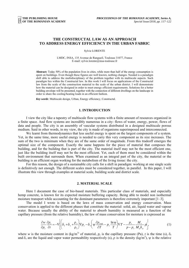
THE PUBLISHING HOUSE PROCEEDINGS OF THE ROMANIAN ACADEMY, Series A, OF THE ROMANIAN ACADEMY Special Issue/2018, pp. 117–122
THE CONSTRUCTAL LAW AS AN APPROACH TO ADDRESS ENERGY EFFICIENCY IN THE URBAN FABRIC
Sylvie LORENTE
LMDC, INSA, 135 Avenue de Rangueil, Toulouse 31077, France E-mail: [email protected]
Abstract: Today 50% of the population lives in cities, while more than half of the energy consumption is spent on buildings. Even though these figures are well known, nothing changes. Needed is a paradigm shift able to address the multidisciplinary of the problem together with its multiscale aspects. Such paradigm lies within the Constructal law. In this work I will focus on applications of the Constructal law from the scale of the construction material to the scale of the urban district. I will demonstrate how the material can be designed in order to meet energy efficient requirements. Solutions for a better building envelope will be presented, together with the connection of different dwellings on the landscape in order to share the cooling/heating loads in an efficient fashion.
Key words: Multiscale design, Urban, Energy efficiency, Constructal.
1. INTRODUCTION
I view the city like a tapestry of multiscale flow systems with a finite amount of resources organized in a finite space. And flow systems are incredibly numerous in a city: flows of water, energy, power, flows of data and people. The city is an assembly of vascular systems distributed in a designed multiscale porous medium. Said in other words, in my view, the city is made of organisms superimposed and interconnected.
We learnt from thermodynamics that less useful energy is spent on the largest components of a system. Yet, in the same time, more useful energy is needed to carry this very component as its size increases. The sum of the two is minimum when they are of the same order of magnitude. From this tradeoff emerges the optimal size of the component. Exactly the same happens for the piece of material that composes the building, and for the building that is part of the city. The material itself may not be the most efficient one, just like the building itself may not be the most efficient. Yet, each of them must be considered within the built environment that surrounds them. When examined as an integral part of the city, the material or the building is an efficient organ working for the metabolism of the living tissue: the city.
For this reason, the design of a sustainable city calls for a shift in paradigm: working at one single scale is definitively not enough. The different scales must be considered together, in parallel. In this paper, I will illustrate this view through examples at material scale, building scale and district scale.
2. MATERIAL SCALE
Here I document the case of bio-based materials. This particular class of materials, and especially hemp concrete, is known for its expected moisture buffering capacity. Being able to model non isothermal moisture transport while accounting for the dominant parameters is therefore extremely important [1–3].
The model I wrote is based on the laws of mass conservation and energy conservation. Mass conservation is applied to the different phases that constitute the material: solid, air, liquid water and vapour water. Because usually the ability of the material to absorb humidity is measured as a function of the capillary pressure (from the relative humidity), the law of mass conservation for moisture is expressed as
∂w
∂pc
∂pc
∂t= −∇ δl +δv + ρv
ρl
⎛
⎝ ⎜
⎞
⎠ ⎟ ∇pc − δv ψ ∂pvsat
∂T− pv
ln ψT
⎛ ⎝ ⎜
⎞ ⎠ ⎟ ∇T − pv
p − pv
Mv
Maδa
p⎡
⎣ ⎢
⎤
⎦ ⎥ , (1)
where w is the moisture content in (kg/m3) of material, pc is the capillary pressure (Pa), t is the time (s), δl and δv are the liquid and vapor water permeability respectively (s), ρ is the density (kg/m3), ψ is the relative

Sylvie LORENTE 2 118
humidity, T is the temperature, ρv (T) is the vapor pressure, ρvsat (T) is the vapor saturation pressure, Mv and Ma are respectively the molar mass (kg/mol) of vapor and air, δa is the air permeability of the material (s), and p is the total pressure (Pa).
The energy conservation reads
ρscs + wicp,i
i
∑⎛
⎝ ⎜ ⎜
⎞
⎠ ⎟ ⎟
∂T
∂t= kmat∇
2T − cp,l − cp,v( )T − Lv[ ]Sl − wiVicp,i∇Ti
∑ , (2)
where the subscript i = 1 for air, i = 2 for vapor and i = 3 for liquid, ρs is the solid density (kg/m3), cs is the solid specific heat capacity (J/kg K), cp,i is the specific heat capacity at constant pressure of the different fluids (J/kg K), kmat is the apparent thermal conductivity of the porous material, Lv is the latent heat of vaporisation (J/kg), and Sl is the water source (or sink) term (kg/(m3s)), and V is the velocity vector (m/s). The source term Sl is obtained from the mass balance applied to liquid water only, combined to mass conservation for the solid ( / 0w t∂ ∂ = )
( )11 l c l
v l
w p St
⎛ ⎞ ∂= −∇ δ ∇⎜ ⎟− ρ ρ ∂⎝ ⎠
∓ . (3)
The boundary conditions consist in the external (and internal) ambiance conditions, namely temperature and relative humidity, heat transfer and mass transfer coefficients.
The objective is to design a porous construction material able to store moisture and release it later; this is the so-called moisture buffering capacity. In view of the Constructal law [4], the challenge consists in discovering the set of material characteristics that allows the highest moisture transfer performances. Those parameters are the material porosity, which will impact the capillary pressure, the absorption isotherm (∂w ⁄ ∂pc), the liquid permeability and the vapour permeability. Starting from the most classical construction material, concrete, we search for the material characteristics allowing to predict a moisture buffering capacity as high as possible. As an example, assume the material is wide enough to consider it as semi-infinite. The material is submitted to the following boundary conditions: Constant temperature T = 22.6°C, relative humidity: 1 day at RH = 50% (initial conditions), followed by 9 days at RH = 75%, and 9 days at RH = 33%.
The system of equations together with the boundary and initial conditions are solved with a FEM package [5]. Plotted in Fig. 1 are the evolutions in time of the temperature and relative humidity at 50 mm from the surface. In addition to the imposed boundary conditions presented in the figures, we show the results obtained for the classical material (concrete), and for the designed material which transfer properties were improved. The temperature peak due to the phase change (water condensation) is noticed for the 2 materials although in a much weaker extend for concrete. The concrete is insensitive to the changes in relative humidity on its surface, unlike the designed material. It takes the latter 9 days to absorb almost entirely the increase in moisture due the sudden change in RH after day 1. Then the material slowly releases moisture in time, a behaviour accentuated within the depth of the material.
21.5
22
22.5
23
23.5
0 5 10 15 20
Tem
pera
ture
(°C
)
Time (days)
Bio-based material
Concrete
Boundary Condition
0.2
0.4
0.6
0.8
1
0 5 10 15 20
Rel
ativ
e H
umid
ity (%
)
Time (days)
Bio-based material
Concrete
Boundary Condition
Fig. 1 – Temperature and relative humidity at 50 mm from the material surface.
3. BUILDING ENVELOPE SCALE
Ventilated cavities can be used for reducing the solar heat gains passing through the roof assembly. When an open ended air gap is placed below the tiles in a house or a building, then a current is formed due to buoyancy forces and part of the heat is removed by natural convection [6–8]. I view here an opportunity to introduce a
3 The Constructal law as an approach to address energy efficiency in the urban fabric 119
fundamental approach to the problem of naturally ventilated roof. By considering both the radiation and the convection heat exchanges, the theoretical analysis will help to determine the optimal air strip geometry.
The flow between two parallel vertical or quasi-vertical walls, with one wall receiving a constant heat flux q'' is driven by natural convection. This is also the case for a ventilated roof if we consider that the air slot is located between two walls inclined of an angle θ with the vertical. The two walls are made of panels of heights H, and width W. At first approximation we do not consider the walls thickness in the analysis that follows. The distance between the two walls is D (Fig. 2). We are looking for the optimal spacing D such that the ventilated air layer extracts as much heat as possible. The air outside the ventilated slot is at T∞. T∞ is also the temperature at which air enters the bottom of the roof. The upper wall receives q". Heat is then transferred by natural convection along the wall and by radiation. Because D W and D H, we consider that the radiation heat exchange is between the 2 walls of surface W×H separated by the distance D.
Fig. 2 – Inclined air layer.
We have
( )4 4_1 1 1rad H C
H cq T Tσ′′ =
ε + ε −, (4)
where ′ ′ q rad is the radiation heat flux, σ is the Boltzmann constant, εH and εC are respectively the emissivity along the hot wall (upper plate of the channel) at the average temperature TH, and the cold wall at TH. According to [9] the ratio between the convection heat flux and the radiation heat flux in such a configuration is such that ′ ′ q conv represents 1/2 of ′ ′ q .
We invoke now scale analysis and write that, in an order of magnitude sense, the thermal boundary layer thickness along a wall of height H is
δT ~ H Ra H *−1 5 , (5)
Ra H * = gcosθβ ′ ′ q conv
ναkH 4 , (6)
where Ra H * is the Rayleigh number β is the volumetric expansion coefficient, ν is the kinematic viscosity, α is the thermal diffusivity, k is the air thermal conductivity. When the spacing between the two walls is greater than 2δT, the air does not take advantage of the flow induced by natural convection, while a spacing between the two walls smaller than 2δT would not use entirely the boundary layers development. In accord with the method of the intersection of asymptotes [10] we consider now 2 extreme cases. In the large spacing D limit, boundary layers develop independently along the 2 walls. Note that without radiation the temperature of the downer wall would be quasi identical to the inlet temperature T∞. The average Nusselt number along the hot wall is given by Vliet and Liu’s correlation [11], and assuming that the convective heat transfer is quasi identical along the 2 walls, we obtain
( )1/ 5large ~ 1.5 Ra .HD Hq k W T T∗ ∞− (7)

Sylvie LORENTE 4 120
If the spacing between the walls is small enough, the boundary layers merge to create a chimney effect. Assume that Texit is the air temperature at the exit of the slot. Because the external wall is heated, Texit > T∞ and the air density at Texit is lower than the air density at the channel inlet, ρ(T∞). We write that, Texit = T∞ + ΔT, with ΔT the temperature increase along the air slot of height H. At the exit of the slot, the pressure difference is ΔP = ρgβΔT H cosθ. Considering the friction losses along the walls and combining them with energy conservation, we have
qsamll D ~ρ2gβcosθ
fcp
′ ′ q conv
⎡
⎣ ⎢ ⎢
⎤
⎦ ⎥ ⎥
1 3
DWcpΔT . (8)
The intersection of the 2 asymptotes represented by Eqs. (7) and (8) leads to the optimal spacing between walls D.
( ) 1 32 15* 2~ 1.5 RaH
opt Hp
T T k fD HT c
∞ −− ⎛ ⎞ ⎛ ⎞
⎜ ⎟ ⎜ ⎟⎜ ⎟Δ ρ να⎝ ⎠⎝ ⎠. (9)
4. DISTRICT SCALE
Ground Source Heat Pumps are part of the green buildings design strategies [12]. Typically, the building heat pump is coupled with an underground pipe network, which acts as a heat exchanger with the soil. At the scale of the district, connecting the building heat pumps to one single horizontal water loop is an interesting opportunity [13–16]. The heat exchanges through the loop can provide the base loads needs, while a conventional heating/cooling system in each connected building may supply the supplement peak demand.
Data centers house hundreds of computer servers, storage servers, etc. The corresponding heating gains are such that the internal load is higher than the heat losses through the buildings envelop, and the data centers need cooling all year round. Here we propose a methodology to design the underground loop network connecting a data center to several buildings in winter conditions [12]. Quantitatively, we assume that the buildings are classical office buildings without any specific energy efficient system. The heating needs are evaluated at 200 kWh/(m2 year) with a total surface of 1 000 m2 per building. This makes each office building heating need at about 23kW. The data center is assumed to have a small size with a heat pump rejecting 50 kW. The temperature of the fluid at the exit of each heat pump is known. Unknown is the flow system configuration such that the overall performance of the system is increased. The underground heat exchanger is a horizontal loop connecting the data center to the buildings. To illustrate the methodology we conduct the analysis in the case of two buildings, yet it can be expanded easily to more buildings. We developed the basis of the analytical part in [17]. As shown in Fig. 3, the data center heat pump connected to the loop rejects heat at a fluid temperature TDa and with a mass flow rate mDa. The cold fluid comes from the two building heat pumps reject at respectively TB1 and TB2 with a mass flow rate B1m and B2m . On an axis attached to the loop, x = 0 is the location where the hot fluid from the data center is injected to the loop, noted A in Fig. 3. The first building is connected at a distance on the loop x = L, while the second building is connected at x = 2L. The way the 2 buildings are connected to the horizontal loop relatively to the data center is a degree of freedom: in Case 1, the first building heat pump extracts heat at a temperature TB1, out at x = L, while the second building does the same at a temperature TB2,out at the distance x = 2L (Fig. 3a). In Case 2, the cold fluid is injected from the first building heat pump at TB1 and x = L. So does the second building heat pump at x = 2L and T = TB2 (Fig. 3b). In both cases LCD (= LFA) is a constant.
A baseline mass flow rate 0m circulates along the horizontal heat exchanger thanks to an auxiliary pump. According to the nomenclature in Fig. 3, we assume that the mass flow rate in the U-turn FA is 0m . The system of equations, based on the laws of mass and energy conservation, was solved in a non-dimensional form based on data listed in [12]. Note that we chose realistic values, which make the soil temperature between the exit temperatures of the datacenter and the buildings heat pumps.
5 The Constructal law as an approach to address energy efficiency in the urban fabric 121
(a)
(b)
,
A
F E D
C B
,
,
,
A
F E D
C B
, ,
Fig. 3 – Two buildings heat pumps connected to a datacenter heat pump on the same loop [12].
0.1 0.2 0.3 0.4 0.50
0.2
0.4
0.6
0.8
1
rDa / rBi
q*
25
a)
0.1 0.3 0.5 0.7 0.90
0.2
0.4
0.6
0.8
1
rDa / rBi
q*= 0.001= 0.167
= 0.25
= 0.167
= 0.001
= 0.25
b)
Fig. 4 – Non dimensional enthalpies q* as a function of the mass flow rate ratio rDa ⁄ rBi in: a) case 1; and b) case 2 [12].
Plotted in Fig. 4 are the non-dimensional enthalpies as a function of the ratio γDA γBi (here γB1 = γB 2 ) for different values of the length ratio ( )* 4 2 FAL L L L= + . The two extreme cases correspond to * 0L ≈ with buildings infinitely close to the datacenter, and L* ≈ 0.25 when L >> LFA. In the first case, the enthalpy provided by the datacenter is entirely given to the buildings, while the second extreme case corresponds to the maximum heat exchanges with the soil. The effect of the configuration on the results can be seen by comparing Fig. 4a to Fig. 4b, the latter corresponding to Case 2. The only difference between the two cases is the way the office buildings are connected to the loop. The network cannot provide the needed enthalpy exchanges in Case 2 whatever the loop length and whatever the mass flow rate ratio γDA γBi even though there is no ratio limitation in this case.
5. CONCLUSION
I believe that the solution to the design of sustainable living is to develop a holistic multi-scale and transdisciplinary approach to the city as a live flow system. Why multi-scale? We demonstrated in the past
Sylvie LORENTE 6 122
that the sum of efficient elements – efficient in the sense of needing minimum power to operate – does not lead to the most efficient whole. The lesson taught by the examples developed in this paper is that each component must be envisaged hand-in-glove with its environment. From the constitutive material to the building envelope and the district/city scale, each object of study is like an organ working for the metabolism of the living body: the city.
ACKNOWLEDGEMENTS
I would like to thank the current and former students who contributed to this work: Billy Seng for the material scale section, Sylvia Slobodova for the envelope scale section, and Delphine Paludetto for the district scale section.
REFERENCES
1. JANSSEN H., BLOCKEN B., CARMELIET J., Conservative modelling of the moisture and heat transfer in building components under atmospheric excitation, International Journal of Heat and Mass Transfer, 50, pp. 1128–1140, 2007.
2. OSANYINTOLA O.F., TALUKDAR P., SIMONSON C.J., Effect of initial conditions, boundary conditions and thickness on the moisture buffering capacity of spruce plywood, Energy and Buildings, 38, pp. 1283–1292, 2006.
3. VAN BELLEGGHEM M., STEEMAN M., JANSSEN H., JANSSENS A., DE PAEPE M., Validation of a coupled heat, vapour and liquid moisture transport model for porous materials implemented in CFD, Building and Environment, 81, pp. 340–353, 2014.
4. BEJAN A., LORENTE S., Design with Constructal theory, Wiley, 2008. 5. www.comsol.com 6. SUAREZ C., JOUBERT P., MOLINA J.L., SANCHEZ F.J., Heat transfer and mass flow correlations for ventilated facades,
Energy and Buildings, 43, pp. 3696-3703, 2011. 7. LEE S., PARK S.H., YEO M.S., KIM K.W., An experimental study on airflow in the cavity of a ventilated roof, Building and
Environment, 44, pp. 1431–1439, 2009. 8. BRANGEON B., JOUBERT P., BASTIDE A., Influence of the dynamic boundary conditions on natural convection in an
asymmetrically heated channel, International Journal of Thermal Sciences, 95, pp. 64–72, 2015. 9. KRISHNAN, PREMACHANDRAN B., BALAJI C., VENKATESHAN S.P., Combined experimental and numerical approaches
to multi-mode heat transfer between vertical parallel plates, Experimental Thermal and Fluid Sciences, 29, pp. 75–86, 2004. 10. BEJAN A., Convection Heat Transfer, 4th Ed., Wiley, 2013. 11. VLIET G.C., LIU C.K., An experimental study of turbulent natural convection boundary layers, Journal of Heat Transfer, 91,
pp. 517–531, 1969. 12. PALUDETTO D., LORENTE S., Modeling the heat exchanges between a datacenter and neighboring buildings through an
underground loop, Renewable Energy, 93, pp. 502–509, 2016. 13. G. FLORIDES, S. KALOGIROU, Ground heat exchangers – a review of systems, models and applications, Renewable Energy,
32, pp. 2461–2478, 2007. 14. HUA Q., YUNGANG W., Modeling the interactions between the performance of ground source heat pumps and soil
temperature variations, Energy for Sustainable Development, 23, pp. 115–131, 2014. 15. SONI S.K., PANDEY M., BARTARIA V.N., Ground coupled heat exchangers: a review and applications, Renewable
Sustainable Reviews, 47, pp. 83–92, 2015. 16. ALAVY M., DWORKIN S.B., LEONG W.H., A design methodology and analysis of combining multiple buildings onto a single
district hybrid ground source heat pump system, Renewable Energy, 66, pp. 515–522, 2014. 17. ALMERBATI A., LORENTE S., ANDERSON R., BEJAN A., Energy design for dense neighborhoods: one heat pump rejects
heat, the other absorbs heat from the same loop, International Journal of Thermal Sciences, 96, pp. 227–235, 2015.

THE PUBLISHING HOUSE PROCEEDINGS OF THE ROMANIAN ACADEMY, Series A, OF THE ROMANIAN ACADEMY Special Issue/2018, pp. 123–128
CONSTRUCTAL OPTIMIZATION OF MAGNETIC FIELD SOURCE IN MAGNETIC DRUG TARGETING THERAPY
Alexandru M. MOREGA*,**, Alin A. DOBRE*, Mihaela MOREGA*, Alina SĂNDOIU* * “Politehnica” University of Bucharest, 313 Splaiul Independentei, Bucharest, 060042, Romania
** “Gheorghe Mihoc – Caius Iacob” Institute of Mathematical Statistic and Applied Mathematics, Romanian Academy, 125 Calea Victoriei, Bucharest, 010071, Romania
Corresponding author: Alexandru M. MOREGA, E-mail: [email protected]
Abstract. Magnetic drug targeting (MDT) is a promising, developing, non-intrusive therapy used to treat malfunctions in organism such as tumoral entities, stenoses, and thrombosis. Body forces are produced by external magnetic fields of high gradient to precisely guide the medication towards regions of interest, aiming to destroy the affected tissues and avoid the healthy cells. The MDT medication, deposited super-paramagnetic nanoparticles (SPN), is entrained by the hemodynamics of the arterial tree to the region of interest (ROI). Key to the success of MDT is the high gradient magnetic field, hence its source, here a permanent magnet. This study presents a constructal optimized array of permanent magnets for high gradient magnetic field.
Key words: Constructal law, Optimization, Magnetic drug targeting, Permanent magnet, Numerical simulation.
1. INTRODUCTION
Magnetic drug targeting is a noninvasive modern technique to reduce the side effects related to the excessive distribution of powerful medication and improve its efficiency. In this therapy, the medication carried by superparamagnetic nanoparticles and injected in the blood stream interacts with an external magnetic field aimed at targeting the drug and fixing it mostly in the region of interest (ROI) for optimal delivery [1–6].
For example, tumor formations excision may be improved by destroying more of the affected tissue rather than healthy tissue through magnetic drug targeted therapies. Worth noting, magnetic targeting has also industrial applications (e.g., micro stirring devices) [7].
The constructal optimization is related to the magnetic drug targeting therapy, one of the many applications that require high gradients and intense magnetic fields, in order to retain and guide the SPION medication [8] into the region of interest, such as tumors, with the aim to maximizing the efficiency of the therapy.
In this paper we focus on the analysis and optimization of a static magnetic field source (e.g., a permanent magnet), able to generate a high gradient magnetic field, to obtain a localized and an as high as possible fluid flow – magnetic field interaction that may prolong the time of residence of the medication in the region of interest (ROI). To this aim, we investigated the interaction of the aggregate fluid (blood and magnetic drug) with the magnetic field.
The magnetic field source is permanent magnet as magnet field source that is divided into an array of slot magnets. The numerical simulations were performed in the finite element method (FEM) technique. The main purpose is to generate a high gradient and powerful magnetic field, using an array of permanent magnets, following a simple criterion – each setup has the same amount of magnetic energy, and the same footprint on the skin.
2. THE MATHEMATICAL MODEL
In this study we neglect the flow-vessel walls structural interactions. Previous studies [6] revealed that, although a problem of concern in many circumstances, it is less so in magnetic drug targeting. The magnetic drug transport and fixation problem is analyzed by coupling the magnetic field model to the fluid flow. The

Alexandru M. MOREGA, Alin A. DOBRE, Mihaela MOREGA, Alina SĂNDOIU 2 124
aggregate fluid – blood and medication – has the magnetic properties of the drug carrier (a superparamagnetic material). First, the static magnetic field problem of the permanent magnet is solved for to find the (magnetization) body forces. Next, the fluid-flow interaction is studied. In this two-step approach we neglect the reaction of the flow upon the external magnetic field. The reason is the relatively low velocity field in hemodynamic.
The magnetic field model is governed by: Ampère’s law
∇ ×H = 0 ; (1)
Magnetic flux law
∇ ⋅B = 0 ; (2)
Constitutive law
permanent magnet B =μ0μr,magH +Brem ,
aggregate fluid (blood and medication) B =μ0 H +M ff H( )[ ],
elsewhere B =μ0H ,
(3)
where μ0 [H/m] is the magnetic permeability of free space, μr,mag the relative magnetic permeability of the permanent magnet, H [A/m] the magnetic field strength, B [T] the magnetic flux density, Brem [T] the remanent magnetic flux density, and Mff [A/m] the magnetization of the aggregate fluid, a function of H.
Using the magnetic vector potential A [Wb/m] (and the divergence free gauge condition)
B =∇ ×A , ∇ ⋅A = 0 , (4)
the mathematical model for the magnetic field problem is
( )1 10 0r− −∇× μ μ ∇× =A . (5)
Magnetic insulation (n×A = 0) boundary conditions close the magnetic field problem. The mathematical model (1)–(5) is solved using FEM [9]. The magnetic body forces (MBF), fmg [N/m3], that occur in a magnetisable medium, such as the blood and magnetic medication aggregate, may be obtained using the energy, i.e., the theorem of the generalized forces
( ) .mg = ⋅∇f M H (6)
It is assumed that the fixation process is “non-thermal”, which means that the system is in thermal equilibrium both internally and with its surrounding environment (at 37ºC).
Concerning the hemodynamic problem of the medication transportation, it is assumed that the flow of the aggregate, magnetisable medium (blood and medication) does not modify the magnetic field produced by the permanent magnet, i.e., the magnet may influence the flow whereas the flow does not modify the magnetic field. Furthermore, all media except for the permanent magnet and the aggregate magnetizable medium (blood and medication) have no magnetic properties therefore their structure, positions, and shapes are not accounted for.
3. THE CONSTRUCTAL OPTIMZATION
The particular positioning of the magnet – along the blood vessel trajectory – suggest its shape: a parallelepiped with a longer side parallel to the blood vessel, and two smaller, equal sides, defining a face orthogonal to the vessel. Figure 1a displays a qualitative sketch of the computational domain.

3 Constructal optimization of magnetic field source in magnetic drug targeting therapy 125
a) the 2D computational domain and boundary conditions for ns = 2 magnetic slots
b) optimization parameters: AR = H/L, and GS = D. The permanent magnet has the per unit length volume
Vol ( 1) const.s sH n L n L= ⋅ ⋅ + − ⋅ =⎡ ⎤⎣ ⎦
Here the number of slots ns = 2.
Fig. 1 – The boundary conditions and the geometric optimization parameters.
In this study, we present the optimization principle using a 2D computational domain, along a crosscut plane through the magnet and the vessel. The full 3D analysis and the effect of the pulsatile flow make the object of a future work.
The constructal optimization refers to a permanent magnet of fixed volume, Vol [m3], with the total magnetic energy, ( ) ( ),
Vol
2d Vol 2p mag rem cW v B H= ⋅ ≅ ⋅∫ B H , where Hc [A/m] is its coercive field. As
suggested by eq. (6), the more non-uniform the magnetic field is the larger the body forces are. In particular, if the magnetic field is uniform then the magnetization forces are null.
In view this assertion, the optimization strategy in this study relies on dividing the magnet, successively, in several identical parts – called “slots” –, while keeping the total volume of the initial, undivided magnet. We introduce the slot aspect ratio, AR (height/length). Assuming that the slots are equally spaced, we define a second parameter, the gap size, GS, where “gap” is the spacing between the slots (Fig. 1b). The optimum design is decided in terms of the horizontal and vertical components of the MBFs, evaluated at a distance that corresponds, roughly, to the distance from the magnet basis to the wall of the blood vessel that conveys the medication.
4. NUMERICAL SIMULATION RESULTS
Figure 2 shows the magnetic field for several cases: the undivided permanent magnet, the magnet divided into ns = 2 slots with a GS = 0.9, and the permanent magnet divided into ns = 5 slots, with GS = 0.5. The magnetic field is highly non-uniform at the margins of the magnet, where the highest gradients occur. The division of the permanent magnet into slots introduces local gaps that increase, locally, the magnetic field gradient. However, qualitatively, the gap size should be as large as the distances from the magnet basis to the vessel. On the other hand, increasing GS produces slots with too large ARs, which would result in too weak magnetic energy in the region of the blood vessel. It turns that GS upper margin is related to the upper limit of the slot AR. Another factor that impacts on the spatial variation of the magnetic field produced by the permanent magnet is the distance to the source – the magnetic flux density decreases with the inverse of the distance, and the magnetic energy with the square of it. These two factors, GS and the distance to the source are interplaying and an optimal design of the magnet should account for both.
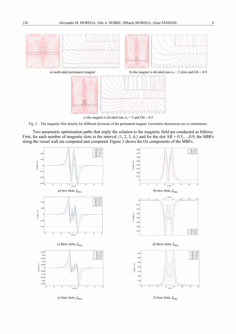
Alexandru M. MOREGA, Alin A. DOBRE, Mihaela MOREGA, Alina SĂNDOIU 4 126
a) undivided permanent magnet b) the magnet is divided into ns = 2 slots and GS = 0.9
c) the magnet is divided into ns = 5 and GS = 0.5
Fig. 2 – The magnetic flux density for different divisions of the permanent magnet. Geometric dimensions are in centimeters.
Two parametric optimisation paths that imply the solution to the magnetic field are conducted as follows. First, for each number of magnetic slots in the interval {1, 2, 3, 4,} and for the slot AR = 0.5,…,0.9, the MBFs along the vessel wall are computed and compared. Figure 3 shows the Ox components of the MBFs.
a) two slots, fmg,x b) two slots, fmg,y
c) three slots, fmg,x d) three slots, fmg,y
e) four slots, fmg,x f) four slots, fmg,y

5 Constructal optimization of magnetic field source in magnetic drug targeting therapy 127
g) five slots, fmg,x h) five slots, fmg,y
Fig. 3 – The magnetic body forces for different slot aspect ratios, at different slots number.
The Ox component, fmg,x, may perturb the aggregate flow, but this would happen during the low flow rate interval of the pulsatile flow. Its effect may be important and worth discussing for pulsatile flow. Therefore we turn our attention on the Oy component, which acts into attracting the medication towards the magnet. It is worth noting the ROI for medication targeting has to be situated between the magnet and the blood vessel or the effect of the magnetic field is detrimental.
a) GS = 0.6, fmg,x b) GS = 0.6, fmg,y
c) GS = 0.8, fmg,x d) GS = 0.8, fmg,y
e) GS = 0.95, fmg,x f) GS = 0.95, fmg,y
Fig. 4 – The magnetic body forces for different slot aspect ratios, at different gap sizes.
The amplitude of fmg,y decreases slightly with the number of slots, and more significantly with the GS size. On the other hand, larger GSs lead to smaller oscillations in amplitude (for ns = 2 and Gs = 0.9, fmg,y shows off also negative values, i.e., the magnetic field acts repulsively). We may conjecture that the design with
Alexandru M. MOREGA, Alin A. DOBRE, Mihaela MOREGA, Alina SĂNDOIU 6 128
GS = 0.7 and ns = 5 (Fig. 3h) seems to optimal. Next, the parameter of interest is for GS. For GS = 0.6,…,0.95, the magnet is divided into ns = 1,..,8 slots, and the MBFs along the vessel wall are computed and compared. Figure 4 shows the MBF along the top part of the vessel wall. The same observation on fmg,x stands here too. In what concerns fmg,y, for smaller GSs, the larger ns is the more uniform but smaller is the amplitude. For larger GSs, the same is true but the maximum peaks are invariant. Also, for small GSs and reduced ns the Oy component may register negative value, which is undesirable. Finally, the decision on the best design is to be taken according to the size, shape, and relative position with respect to the magnet of the ROI.
5. CONCLUSIONS
The constructal optimization presented in this study is related to the magnetic drug targeting therapy, one of the many applications that require high gradients and intense magnetic fields. The constructal optimization refers to a permanent magnet of fixed volume hence total magnetic energy, as the magnetic field source. The particular positioning of the magnet – along the blood vessel trajectory – suggest its shape: a parallelepiped with a longer side parallel to the blood vessel, and two smaller, equal sides, defining a face orthogonal to the vessel. It was assumed that the flow of the aggregate, magnetic medium (blood and medication) does not modify the magnetic field produced by the permanent magnet, i.e., the magnet may influence the flow whereas the flow does not modify the magnetic field.
The optimization strategy relies on dividing the magnet, successively, in several identical parts – “slots” – while keeping the total volume of the initial, undivided magnet. The slot aspect ratio, AR (height/length) and the gap size, GS, where “gap” is the spacing between the slots, are the two design parameters. The optimum design is decided in terms of the horizontal and vertical components of the MBFs, evaluated at a distance that corresponds, roughly, to the distance from the magnet basis to the wall of the blood vessel that conveys the medication.
The Ox component, fmg,x, may perturb the aggregate flow, but this would happen during the low flow rate interval of the pulsatile flow. Its effect may be important and worth discussing for pulsatile flow. Therefore, the attention here is devoted to the Oy component, which acts into attracting the medication towards the magnet. It is worth noting the ROI for medication targeting has to be situated between the magnet and the blood vessel or the effect of the magnetic field is detrimental. The decision on the best design is to be taken according to the size, shape, and relative position with respect to the magnet of the ROI.
ACKNOWLEDGEMENTS
The work was conducted in the Laboratory for Electrical Engineering in Medicine, affiliated with the BIONGTEH platform at UPB.
REFERENCES
1. ALEXIOU, C., JURGONS, R., SCHMID, R.J., BERGEMANN, C., HENKE, J., ERHARDT, W., HUENGES, E., PARAK, F., Magnetic drug targeting-biodistribution of the magnetic carrier and the chemotherapeutic agent mitoxantrone after locoregional cancer treatment, J. Drug Target., 11, pp. 139–149, 2003.
2. VOLTAIRAS, P.A., FOTIADIS, D.I., MICHALIS, L.K., Hydrodynamics of Magnetic Drug Targeting, J. Biomech., 35, pp. 813–821, 2002.
3. PLAVINS, J., Lauva, M., Study of Colloidal Magnetite Binding Erythrocytes: Prospects for Cell Separation, J. of Magnetism and Magnetic Materials, 122, pp. 349–353, 1993.
4. SUZUKI, H., Development of a Chaotic Micro-Mixer Using Magnetic Beads, PhD Thesis, UCLA, USA, 2003. 5. MOREGA, A.M., DOBRE, A., MOREGA, M., MOCANU, D., Computational modeling of arterial blood flow, Proc. Second
MediTech Conference, 23–26 September 2009, Cluj-Napoca, Romania. 6. MOREGA, A.M., DOBRE, A.A., MOREGA, M., Numerical simulation of magnetic drug targeting with flow – structural
interaction in an arterial branching region of interest, 17–19 Nov. 2010, Comsol Conference, Versailles, France. 7. PLAVINS, J., LAUVA, M., Study of Colloidal Magnetite Binding Erythrocytes: Prospects for Cell Separation, J. of Magnetism
and Magnetic Materials, 122, pp. 349–353, 1993. 8. MANEA, L., MOREGA, A.M., MOREGA, M., Numerical simulation of magnetic drug localization in the knee joint medication,
International Symposium on Fundamentals of Electrical Engineering (ISFEE), 28–29 Nov., 2014, 10.1109/ISFEE.2014.7050615.
9. COMSOL MULTIPHYSICS, v.3.5a,…5.3., received August 21, 2017.
THE PUBLISHING HOUSE PROCEEDINGS OF THE ROMANIAN ACADEMY, Series A, OF THE ROMANIAN ACADEMY Swpecial Issue/2018, pp. 129–134
THE OPTIMAL SPACING BETWEEN DIAMOND-SHAPED TUBES COOLED BY FREE CONVECTION USING CONSTRUCTAL THEORY
Ahmed WAHEED*, Ansam ADIL**, Ali RAZZAQ** * Al-Nahrain University, College of Engineering, Mechanical Engineering Department, Baghdad, Iraq
** Al-Nahrain University, College of Engineering, Mechanical Engineering Department, Baghdad, Iraq Corresponding author: Ahmed WAHEED, E-mail: [email protected]
Abstract. The optimal spacing between diamond-shaped tubes cooled by free convection is studied numerically. A row of isothermal diamond-shaped tubes is installed in a fixed volume and the spacing between them is selected according to the constructal theory (Bejan's theory). In this theory, the spacing between the tubes is chosen such that the heat transfer density is maximized. A finite volume method is employed to solve the governing equations; SIMPLE algorithm with collocated grid is utilized for coupling between velocity and pressure. The range of Rayleigh number is (103 ≤ Ra ≤ 105), the range of the axis ratio of the tubes is (0 ≤ e ≤ 0.5), and the working fluid is air (Pr = 0.71). The results show that the optimal spacing decreases as Rayleigh number increases for all axis ratios, and the maximum density of heat transfer increases as the Raleigh number increases for all axis ratios and the highest value occurs at axis ratio (e = 0, flat plate) while the lowest value occurs at (e =0.5) (rhombic tube). The results also show that the optimal spacing is unchanged with the axis ratio at constant Rayleigh number.
Key words: Diamond Tubes, Constructal Theory, Free Convection.
1. INTRODUCTION
According to the constructal theory, the optimal spacing between a heat generating devices (plates, fins, cylinders, etc.) is defined as the spacing that provides easier access of heat flow from these devices to the coolant streams. The quest of easier heat flow motivates the designers to find the optimal spacing between parallel plates in forced, free, and mixed convection [1–3], the optimal spacing between circular cylinders in forced and free convection [4–5], and the optimal spacing between circular rotating cylinders in forced and free convection [6–7]. Free convection from square cylinders can be found in many devices, heat exchangers, and heat sinks with square pin fins [8]. Free convection from a single square cylinder was studied previously, for example [9–11]. The optimal spacing between horizontal square cylinders (rotated with 45o, diamond-shaped) is not addressed yet. In this paper, evolutionary design is employed to find the optimal spacing between square cylinders installed in a fixed volume and cooled by free convection.
2. MATHEMATICAL MODEL
Consider a row of diamond-shaped tubes installed in a fixed volume per unit depth (h L) as shown in Fig. 1. The major axis of the diamond tube is (h/2) and the minor axis of the tube is (b). The axis ratio is defined as (e = b/h). The tubes are maintained at constant wall (hot) temperature of (Tw), the ambient fluid is maintained at constant temperature of (T∞). The objective is to find the number of tubes or the tube – to – tube spacing (s) for different axis ratio (e) in order to maximize the heat transfer density. In this geometry there are two degrees of freedom, the first is the spacing (s) and the second is the axis ratio (e). The dimensionless governing equations for steady, laminar, and incompressible flow with Boussinesq approximation for the density in the buoyancy term can be written as [12]

Ahmed WAHEED, Ansam ADIL, Ali RAZZAQ 2 130
∂U∂X
+ ∂V∂Y
= 0 , (1)
1/ 2 2 2
2 2PrRa
U U P U UU VX Y X X Y
⎛ ⎞∂ ∂ ∂ ∂ ∂⎛ ⎞+ = − + +⎜ ⎟⎜ ⎟∂ ∂ ∂ ∂ ∂⎝ ⎠ ⎝ ⎠, (2)
1/ 2 2 2
2 2PrRa
V V P V VU V TX Y Y X Y
⎛ ⎞∂ ∂ ∂ ∂ ∂⎛ ⎞+ = − + + +⎜ ⎟⎜ ⎟∂ ∂ ∂ ∂ ∂⎝ ⎠ ⎝ ⎠, (3)
( )
2 2
1/ 2 2 21
Ra PrT T T TU VX Y X Y
⎛ ⎞∂ ∂ ∂ ∂+ = +⎜ ⎟
∂ ∂ ∂ ∂⎝ ⎠. (4)
The non-dimensionalised variables and groups used are
( ) ( )1/ 2 1/ 2 2 2
3
/ , / , / Ra Pr , / Ra Pr , / Ra Pr,.
/ , Pr / , Ra ( ) /W W
X x h Y y h U uh V vh P ph
T t T T T g T T h∞ ∞ ∞
⎫= = = α = α = α ρ ⎪⎬
= − − = ν α = β − αν ⎪⎭ (5)
Since the flow is symmetrical between the tubes, only half of the flow channel between two tubes can
be used to find the spacing in the numerical solution. Half of the flow channel is shown in Fig. 2. The total dimensionless height of the channel is (Hu + H + Hd), the dimensionless upstream height (Hu) and the dimensionless downstream (Hd) are added to avoid the applying of incorrect velocity and temperature at the inlet and outlet of the channel. The flow and thermal dimensionless boundary conditions on the channel are shown in Fig. 2.
Fig. 1 – Physical geometry. Fig. 2 – Dimensionless boundary conditions.
The right side of the downstream boundary condition is applied to permit fluid to enter the domain horizontally in order to avoid the vertical acceleration, which generated by chimney effects.
The spacing between the tubes is to be chosen such that the heat transfer density (objective function) is maximized. The heat transfer density is the heat transfer rate per unit volume and given as
′ ′ ′ q = ′ q
(s +2b)h, (6)
where q′ is the total heat transfer rate from one tube per unit width. The heat transfer density can be written in non-dimensional form as
3 The optimal spacing between diamond-shaped tubes cooled by free convection using constructal theory 131
( ) ( )
12 0 0
d d
( 2 ) ( 2 ) ( 2 )
h
w w
t Tk y h Yq h x XQk T T s b h k T T s b h S e∞ ∞
∂⎛ ⎞ ∂− −⎜ ⎟′ ∂⎝ ⎠ ∂= = =− + − + +
∫ ∫.
(7)
3. NUMERICAL PROCEDURE, GRID INDEPENDENCE TEST, AND VALIDATION
A FORTRAN program is written to solve the algebraic equations, which obtained from the finite volume discretization. The general transport equation is firstly transformed to curvilinear coordinates and the convective term is discretized by hybrid scheme while the diffusion term is discretized by second order central scheme. For coupling between the pressure and velocity SIMPLE algorithm is employed. To prevent the oscillation in the pressure field the interpolation method of Rhie and Chow [13] is used. The convergence criterion of iteration is that the total imbalance in the source term in the pressure correction equation becomes less than 10-4. Further computational details can be found in Rhie and Chow [13]. The grid independence test is performed for three grids for configuration at which (Ra = 104, e = 0.1, and S = 0.3). The grid independence test showed that the increasing of the grid size reduces the error percentage in the heat transfer density, and the minimum error is at (50×50) control volumes in the region ((e+S/2)×H). So this grid size is used and adopted in all results, gird independence test is illustrated in table (1). The upstream extension of (Hu = 0.5) and downstream extension of (Hd = 2) are used in the computational domain because it is observed that after double these extensions the variation in transfer density is less than 2.5%. The numerical results are validated by comparing the result of the optimal spacing with the result from the intersection of asymptotes of Bejan [14] for natural convection between vertical isothermal plates (e = 0) and (Ra =105). For this case, the optimal spacing in this study is (Sopt = 0.13) and the optimal spacing found in Bejan [14] was (Sopt = 0.129).
Table 1
Grid Independence Test for the Case (Ra = 104, e =0.1, and S =0.3)
Number of control volumes in the region ((e +S/2)xH) Q Error% 30×30 30.629 – 40×40 31.244 2 50×50 31.713 1.5
4. RESULTS AND DISSCUSION
The numerical results are presented in this section for, temperature contours, optimal spacing, and density of heat transfer for different values of tube axis ratio (0 ≤ e ≤ 0.5). The range of Rayleigh number is (103 ≤ Ra ≤ 105) and the working fluid is air with (Pr = 0.71). Figure 3 shows the temperature contour as a function of the dimensionless spacing between the tubes (S) for (Ra = 103) and axis ratio (e = 0.1). For small spacing (S ≤ 0.3) the downstream region is occupied by hot fluid at temperature same as the wall temperature (red region), this is due to that the small spacing between the tubes prevents the cold air to flow downstream and the air there still hot (overworked fluid). As the spacing between the tubes increases (S ≥ 0.3) the downstream temperature begins to decrease and become less than the wall temperature and this is clear from the appearance of the (orange, yellow and green) regions. At some spacing the thermal boundary layers from both sides are merged at the downstream region (the channel is fitted with the convective flow body), at this spacing the heat transfer density becomes maximum, and the spacing represents the optimal spacing, in this case (Sopt = 0.35). Further increasing in spacing between the tubes leads to a cold fluid region to appear in the downstream as seen in the blue region near the centerline (underworked fluid) for (S ≥ 1), this large spacing permits the ambient (cold) fluid to flow downstream and leads to reduce the thermal conductance between the tubes and the surrounding fluid. Figure 4 illustrates the temperature contour for (Ra = 105) and (e = 0.1). The behavior of the temperature contour is similar to that of (Ra = 103) except that the spacing between the tubes here becomes smaller, note that at (Ra = 103) the hot (red) downstream region can be observed for (S ≤ 0.3)

Ahmed WAHEED, Ansam ADIL, Ali RAZZAQ 4 132
while this region can be observed for (S ≤ 0.05) at Ra = 105, the spacing decreases because the thermal boundary layer thickness decreases as Rayleigh number increases.
Fig. 3 – Temperature contour with various spacing between the
tube for (Ra = 103, Pr = 0.7, and axis ratio e = 0.1). Fig. 4 – Temperature contour with various spacing between
the tube for (Ra = 105, Pr = 0.7, and axis ratio e = 0.1).
As the axis ratio of the tube increases to (e = 0.5) (rhombic tube) for (Ra = 103), the thermal boundary layer on the upper surface becomes thicker than the thermal boundary layer on the upper surface of the tube of (e = 0.1) as shown in Fig. 5 for (S ≥ 0.3). This thick thermal boundary layer reduces the heat transfer rate from the upper surface. For (Ra = 105) and as the axis ratio of the tube increases to (e = 0.5), a plume-like appears in temperature contours on the upper surface of the tube as shown in Fig. 6 for (S ≤ 0.06). This plume-like region reduces the temperature gradient (i.e., heat transfer rate) on the upper surface of the tube. Figure 7 shows the dimensionless heat transfer density as a function of the spacing at different Rayleigh numbers for (e = 0.1). This figure shows that there is an optimal spacing for each Rayleigh number. At this spacing the heat transfer density reaches its maximum value (tops of the curves). It is interesting to note that the optimal spacing decreases as Rayleigh number increases due to the decreasing of thermal boundary layer thickness.
Fig. 5 – Temperature contour with various spacing
between the tube for Ra = 103, Pr = 0.7, and axis ratio e = 0.5. Fig. 6 – Temperature contour with various spacing
between the tube for (Ra = 105, Pr = 0.7, and axis ratio e = 0.5.
Fig. 7 – Heat transfer density with spacing at different Rayleigh numbers for axis ratio (e = 0.1).

5 The optimal spacing between diamond-shaped tubes cooled by free convection using constructal theory 133
Figure 8 shows the optimal spacing (Sopt) versus Rayleigh number for various axis ratios (e = 0, 0.1, 0.25, and 0.5), it is noted that the optimal spacing decreases as Rayleigh number increases for all values of (e). At constant Rayleigh number, the optimal spacing is almost unchanged for the range axis ratio (0.1 ≤ e ≤ 0.5). Since the optimal spacing is nearly unchanged with the axis ratio in the range (0.1 ≤ e ≤ 0.5), the number of tubes that installed in the same volume must be reduced as the axis ratio increases. Figure (9) shows the maximum heat transfer density versus Rayleigh number at various axis ratio (e), it can be noted that the maximum heat transfer density increases as Rayleigh number increases for all values of (e), the increasing of Rayleigh number leads to increase the buoyancy force and thus increase the maximum heat transfer density. It also can be seen that at each Rayleigh number the highest value of the maximum heat transfer density occurs at (e = 0, flat plate) and the lowest value occurs at (e = 0.5, rhombic tube). This can be explained as the geometry changes from flat plate to diamond-shaped tube, a plume-like is formed on the upper surface of the tube and the temperature gradient on the upper surface deceases and thus the maximum heat transfer density decreases.
Fig. 8 – Maximum heat transfer density
with Rayleigh number for different axis ratios. Fig. 9 – Maximum heat transfer density
with Rayleigh number for different axis ratios.
5. CONCLUSIONS
The conclusions for optimal spacing between diamond-shaped tubes cooled by free convection can be summarized as:
1 – The optimal spacing decreases as Rayleigh number increases for all axis ratios. 2 – The maximum heat transfer increases as Rayleigh number increases for all axis ratios. 3 – The highest value of the maximum heat transfer density occurs at axis ratio (e = 0, flat plate) and
lowest value occurs at axis ratio (e = 0.5, rhombic tube) for all Rayleigh numbers. 4 – The optimal spacing remains almost constant in the range (0.1 ≤ e ≤ 0.5) at constant Rayleigh
number. 5 – The number of tubes installed in the same volume must be reduced as the axis ratio increases.
REFERENCES
1. BEJAN, A., SCIUBBA, E., The optimal spacing for parallel plates cooled by forced convection, International Journal of Heat and Mass Transfer 35, pp. 3259–3264, 1992.
2. DA SILVA, A.K., BEJAN, A., LORENTE, S., Maximal heat transfer density in vertical morphing channels with natural convection, Numerical Heat Transfer Part A Applications 45, pp. 135–152, 2004.
3. BELLO-OCHENDE, T., BEJAN, A., Optimal spacings for mixed convection, Journal of Heat Transfer, 126, 6, pp. 956–962, 2004. 4 STANESCU, G., FOWLER, A.J., BEJAN, A., The optimal spacing of cylinders in free-stream cross-flow forced convection,
International Journal of Heat and Mass Transfer, 39, pp. 311–317, 1996. 5. BEJAN, A., FOWLER, J., STANESCU, G., The optimal spacing between horizontal cylinders in a fixed volume cooled by natural
convection, Journal of Heat and Mass Transfer, 38, pp. 2047–2055, 1995. 6. PAGE, L.G., BELLO-OCHENDE, T., MEYER, J.P., Maximum heat transfer density rate enhancement from cylinders rotating in
natural convection, International Communications in Heat and Mass Transfer, 38, pp. 1354–1359, 2011.

Ahmed WAHEED, Ansam ADIL, Ali RAZZAQ 6 134
7. JOUCAVIEL, M., GOSSELIN, L., BELLO-OCHENDE, T., Maximum heat transfer density with rotating cylinders aligned in cross-flow, International Communications in Heat and Mass Transfer, 35, pp. 557–564, 2008.
8. LEDEZMA, G., MOREGA, A.M., BEJAN, A. Optimal spacing between pin fins with impinging flow, 118, pp. 570–577, 1996. 9. CHANG, K., CHOI, C., Separated laminar natural convection above a horizontal isothermal square cylinder, International
Communications in Heat and Mass Transfer, 13, pp. 201–208, 1986. 10. S. MAHMUD, D.P. KUMAR, N. HYDER, Laminar natural convection around an isothermal square cylinder at different
orientations, International Communications in Heat and Mass Transfer, 29, 7, pp. 993–1003, 2002. 11. SASMAL, C., CHHABRA, R.P., Effect of orientation on laminar natural convection from a heated square cylinder in power-law
liquids, International Journal of Thermal Sciences, 57, pp. 112–125, 2012. 12. ZHANG Z., BEJAN A., LAGE J.L., Natural convection in a vertical enclosure with internal permeable screen, Journal of Heat
Transfer, 113, pp. 377–383, 1991. 13. RHIE, C. M., CHOW, W. L., Numerical study of the turbulent flow past an airfoil with trailing edge separation, AIAA Journal,
21, pp. 1525–1532, 1983. 14. BEJAN A., Convection Heat Transfer, Wiley, New York, 1984.
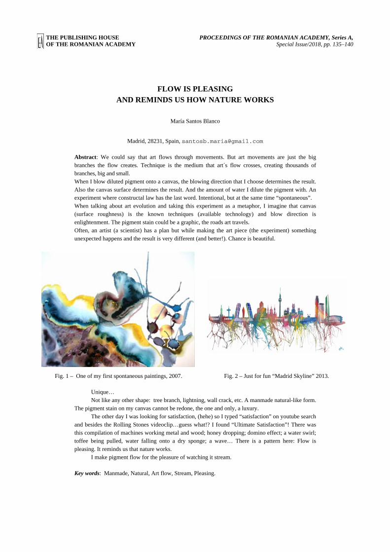
THE PUBLISHING HOUSE PROCEEDINGS OF THE ROMANIAN ACADEMY, Series A, OF THE ROMANIAN ACADEMY Special Issue/2018, pp. 135–140
FLOW IS PLEASING AND REMINDS US HOW NATURE WORKS
María Santos Blanco
Madrid, 28231, Spain, [email protected]
Abstract: We could say that art flows through movements. But art movements are just the big branches the flow creates. Technique is the medium that art´s flow crosses, creating thousands of branches, big and small. When I blow diluted pigment onto a canvas, the blowing direction that I choose determines the result. Also the canvas surface determines the result. And the amount of water I dilute the pigment with. An experiment where constructal law has the last word. Intentional, but at the same time “spontaneous”. When talking about art evolution and taking this experiment as a metaphor, I imagine that canvas (surface roughness) is the known techniques (available technology) and blow direction is enlightenment. The pigment stain could be a graphic, the roads art travels. Often, an artist (a scientist) has a plan but while making the art piece (the experiment) something unexpected happens and the result is very different (and better!). Chance is beautiful.
Fig. 1 – One of my first spontaneous paintings, 2007. Fig. 2 – Just for fun “Madrid Skyline” 2013.
Unique… Not like any other shape: tree branch, lightning, wall crack, etc. A manmade natural-like form.
The pigment stain on my canvas cannot be redone, the one and only, a luxury. The other day I was looking for satisfaction, (hehe) so I typed “satisfaction” on youtube search
and besides the Rolling Stones videoclip…guess what!? I found “Ultimate Satisfaction”! There was this compilation of machines working metal and wood; honey dropping; domino effect; a water swirl; toffee being pulled, water falling onto a dry sponge; a wave… There is a pattern here: Flow is pleasing. It reminds us that nature works.
I make pigment flow for the pleasure of watching it stream.
Key words: Manmade, Natural, Art flow, Stream, Pleasing.

María SANTOS BLANCO 2 136
1. FOR ART TO BE UNIVERSAL, FIRST IT HAS TO BE PERSONAL
1.1. Blowing pigment
Forever young, playing with pigment has been a constant in my life. When I was 11, a pen broke and I poured the ink on a blank paper and blew onto it ... it made me very happy while the ink was flowing in unexpected directions and ramifications.
Fig. 3 – Blown acrylic ramifications and bead embroidery.
Okapi is the closest living relative to the giraffe. There is a war in Congo due to coltan exploitation, an ore containing tantalum, an essential component of very compact electronic devices: smartphones, laptops, computers, guided weapons, etc. Therefore, the okapi is currently in danger. Coelacanths have not changed their design for 400 million years. First the fossil was discovered, and later the animal that still lives in the sea.
Malachite Sunbird, forming an exclusive relationship with the flower with which he feeds, the disappearance of the bird involves the same destination for the plant and vice versa. This is the same with some human relationships.
This is what I call oxymoron: intentional random. The meanings that this concept has for me are numerous. It explains why though I was raised catholic I always stayed away from religion and preferred philosophy and it´s links with science.
Fig. 6 – Title: “The fine line distinguishing characteristic from tare”. Measures: Round Canvas 50 cm in diameter.
Materials: Acrylic and beads collage. Year: 2015.
Fig. 7 – Title: “Mutant” (detail). Measures: Round Canvas 50 cm in diameter. Materials: Acrylic and beads collage.
Year: 2015.

3 For art to be universal, first it has to be personal 137
Fig. 8 – Title: “Codependent”. Measures:
Round Canvas 50 cm in diameter. Materials: Acrylic and beads collage. Year: 2015.
Fig. 9 – Title: “Oxymoron: Insignificant necessary.” Measures: Round Canvas 50 cm in diameter. Materials:
Acrylic and beads collage. Year: 2015.
Oxymoron makes me think of life as a complex arrangement of events we try to control and understand. The best feeling is to be out of control (like in a rollercoaster or watching a horror movie), but still people avoid it…another oxymoron. I am out of control when I make art: is a mixture of joy, fear, care, know-how…What makes the “out of control” feeling a good feeling is the combination with a safe feeling, a happily ever after feeling. To “live to tell” is better than to not live and have nothing to tell.
1.2. Constructal Art
Constructal law on life evolution reminds me of the many, many events that lead us to civilization and even understanding where we come from, how life works. I consider Constructal law discovery a big step for humankind and it´s the main reason why I make art about it, a beautiful memory of this achievement.
Fig. 4 – Title: “Veteran”. Measures: Round Canvas 50 cm in diameter. Materials: Acrylic, beads embroidery. Year: 2015.
Fig. 5 – Title: “Obsolete”. Measures: Round Canvas 50 cm in diameter. Materials: Acrylic, beads embroidery. Year: 2015.

María SANTOS BLANCO 4 138
Fig. 10 – How to make ink flow (17 seconds). Same technique with diluted acrylic and watercolour.

5 For art to be universal, first it has to be personal 139
2. ART FLOWS
2.1. What is Art
Art’s flow. High to low. Hot to cold. High pressure to low pressure. We could say that art is one of those “useless” things that humans do in order to show off. Just like
athletes. Frustration drives these people’s will. High pressure perceived by their mind is turned into low pressure through manual, intellectual, physical work and finally public recognition. Wait, did I say that art is useless? Let’s analyse that:
If art is a warning for society, it reaches most minds with delay. Way too much delay. If art is sensuality, why sunbathe isn’t art? If art is a memory (for example, so that the future generation avoids repeating a mistake from the past)
why people don’t remember?
Fig. 11 – Andreas Gursky, 99 Cent, 1999. Fig. 12 – Shooting on 3rd of may, Goya, 1814.
If art is a craft, why is my grandma not an artist? Art is a warning for the illiterate, a manmade sun, a beautiful memory you want to protect, a craft that
takes a workshop’s lifetime, a new way of thinking.
Fig. 13 – Olafur Eliasson – The weather Project,
2003. Fig. 14 – Ai Weiwei crafting porcelain sunflower seeds.
We go to the moon because we can. We make art because we can. Art calls for technology. Art is about pushing the limits, being harder, better, faster, stronger. Art is acknowledgement, representing what we interpret from what´s new, an opinion to be discussed.
Science fiction is art´s friend. Science fiction is a self-fulfilled prophecy and so is art.
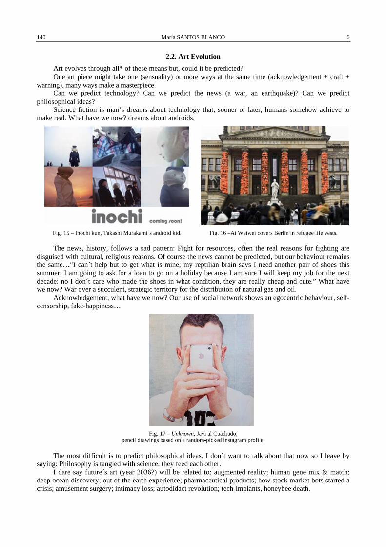
María SANTOS BLANCO 6 140
2.2. Art Evolution
Art evolves through all* of these means but, could it be predicted? One art piece might take one (sensuality) or more ways at the same time (acknowledgement + craft +
warning), many ways make a masterpiece. Can we predict technology? Can we predict the news (a war, an earthquake)? Can we predict
philosophical ideas? Science fiction is man’s dreams about technology that, sooner or later, humans somehow achieve to
make real. What have we now? dreams about androids.
Fig. 15 – Inochi kun, Takashi Murakami´s android kid. Fig. 16 –Ai Weiwei covers Berlin in refugee life vests.
The news, history, follows a sad pattern: Fight for resources, often the real reasons for fighting are disguised with cultural, religious reasons. Of course the news cannot be predicted, but our behaviour remains the same…”I can´t help but to get what is mine; my reptilian brain says I need another pair of shoes this summer; I am going to ask for a loan to go on a holiday because I am sure I will keep my job for the next decade; no I don´t care who made the shoes in what condition, they are really cheap and cute.” What have we now? War over a succulent, strategic territory for the distribution of natural gas and oil.
Acknowledgement, what have we now? Our use of social network shows an egocentric behaviour, self-censorship, fake-happiness…
Fig. 17 – Unknown, Javi al Cuadrado,
pencil drawings based on a random-picked instagram profile.
The most difficult is to predict philosophical ideas. I don´t want to talk about that now so I leave by saying: Philosophy is tangled with science, they feed each other.
I dare say future´s art (year 2036?) will be related to: augmented reality; human gene mix & match; deep ocean discovery; out of the earth experience; pharmaceutical products; how stock market bots started a crisis; amusement surgery; intimacy loss; autodidact revolution; tech-implants, honeybee death.

THE PUBLISHING HOUSE PROCEEDINGS OF THE ROMANIAN ACADEMY, Series A, OF THE ROMANIAN ACADEMY Special Issue/2018, pp. 141–146
A LOGISTIC LAW OF GROWTH AS A BASE FOR METHODS OF COMPANY’S LIFE CYCLE PHASES FORECASTING
Rafał SIEDLECKI1, Daniel PAPLA2, Agnieszka BEM1
1Wroclaw University of Economics, Department of Corporate Finance and Public Finance, Poland
2Wroclaw University of Economics, Department of Insurance, Poland Corresponding author: Rafał SIEDLECKI, E-mail: [email protected]
Abstract. A logistic law of growth can be easily identified in natural sciences, social sciences, physics or technology. In economy, the logistic law of growth, expressed by a logistic law function (S-curve) can be employed to describe the processes of economic growth or a company’s cycle of life. However, according to the fact, that in almost all economic phenomena values cannot be limited, the logistic function often doesn’t fully work, mainly due to the problem of “limited growth” (expressed by an asymptote). This inconvenience can be avoided by employing the modified S-curve (loglogistic function). In this paper we present the application of the S-curve, as well as the modified S-curve in company’s life cycle forecasting. We have also proposed our own method of iterative estimation, which can be used to estimate all functions’ parameters, especially those, which cannot be converted to linear form.
Keywords: Constructal law, Law of growth, Forecasting, Business cycle, Time series analysis, S-curve, Modified S-curve.
1. INTRODUCTION
The every system, including economic ones, can be described as a flow system enable to generate and evolve structures, which can increase flow access [1, 2]. It also emphasise the time direction of the analysed phenomenon, which can take several forms – one of them is manifested through a logistic law of growth. The logistic law of growth, initially proposed by Verhulst, from the beginning, is employed to analyse natural processes in biology, demography or physics [3–8], where the phenomena are described using statistical and econometric models – basing on an assumption, that some phenomena have a very similar tenor. The logistic law of growth might be applied also in economy. There are, generally, two important factors which influence economic activity – there are technological and sociological progress. Both those factors are caused by human needs, activity, creativity, which, in turn, are the result of political, economic and technical decisions. This activity submits to the logistic growth law, which can take a form of varied economic laws: the law of diminishing returns from the land, or the law of relatively decreasing efficiency of inputs. These laws base not only on experience, but also on empirical research; we can observe, that, in the case of almost every economic process, after a beginning stage, characterized by slow growth, further increase of inputs initiate the dynamic growth of effects, up to certain maximum level. From that moment, the growth of effects is getting smaller, until it reach some stable level, or even, in some cases, a dramatic reduction of results.
The S-curve is a mathematic expression of logistic growth law, and becomes a popular tool for forecasting and analysing of economic processes, which follow the rule of the logistic growth, like GDP growth [8–14] or company’s valuation [17]. Despite undeniable advantages, S-curve is characterized by several disadvantages, from which the most important is a problem of limited growth – S-curve has an asymptote, what, in practice, means, that after reaching some level, further growth cannot be achieved. We should be aware, that in many economy, and finance, this limited growth cannot be accepted because those data, cannot be limited in values. This important disadvantage can be avoided by employing the modified S-curve, which is both elastic, and offers the unlimited growth.
The S-curve, as well as the modified S-curve, can be also employed primarily in the analyses of company’s cycle of life [16]. It is widely confirmed, that enterprise’s development has a cyclical form. Companies, depending
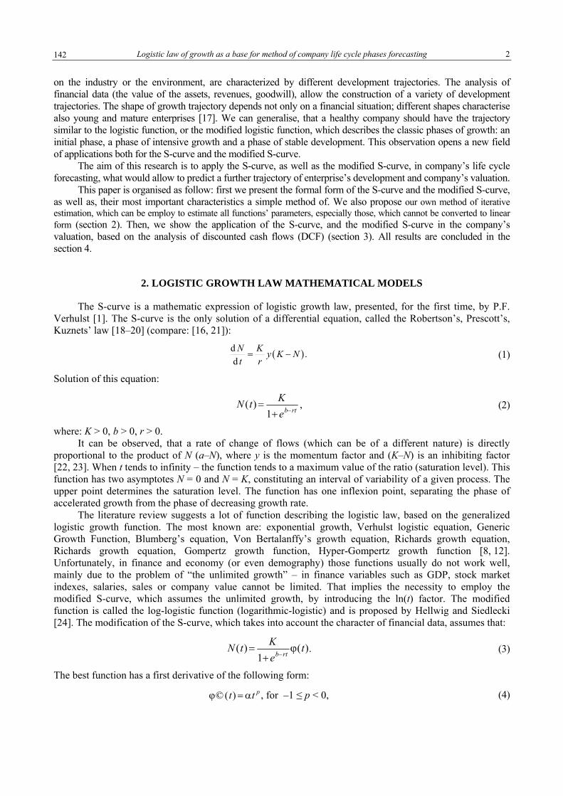
Logistic law of growth as a base for method of company life cycle phases forecasting 2
142
on the industry or the environment, are characterized by different development trajectories. The analysis of financial data (the value of the assets, revenues, goodwill), allow the construction of a variety of development trajectories. The shape of growth trajectory depends not only on a financial situation; different shapes characterise also young and mature enterprises [17]. We can generalise, that a healthy company should have the trajectory similar to the logistic function, or the modified logistic function, which describes the classic phases of growth: an initial phase, a phase of intensive growth and a phase of stable development. This observation opens a new field of applications both for the S-curve and the modified S-curve.
The aim of this research is to apply the S-curve, as well as the modified S-curve, in company’s life cycle forecasting, what would allow to predict a further trajectory of enterprise’s development and company’s valuation.
This paper is organised as follow: first we present the formal form of the S-curve and the modified S-curve, as well as, their most important characteristics a simple method of. We also propose our own method of iterative estimation, which can be employ to estimate all functions’ parameters, especially those, which cannot be converted to linear form (section 2). Then, we show the application of the S-curve, and the modified S-curve in the company’s valuation, based on the analysis of discounted cash flows (DCF) (section 3). All results are concluded in the section 4.
2. LOGISTIC GROWTH LAW MATHEMATICAL MODELS
The S-curve is a mathematic expression of logistic growth law, presented, for the first time, by P.F. Verhulst [1]. The S-curve is the only solution of a differential equation, called the Robertson’s, Prescott’s, Kuznets’ law [18–20] (compare: [16, 21]):
( )d .dN K y K Nt r= − (1)
Solution of this equation:
N (t)= K
1+eb−rt, (2)
where: K > 0, b > 0, r > 0. It can be observed, that a rate of change of flows (which can be of a different nature) is directly
proportional to the product of N (a–N), where y is the momentum factor and (K–N) is an inhibiting factor [22, 23]. When t tends to infinity – the function tends to a maximum value of the ratio (saturation level). This function has two asymptotes N = 0 and N = K, constituting an interval of variability of a given process. The upper point determines the saturation level. The function has one inflexion point, separating the phase of accelerated growth from the phase of decreasing growth rate.
The literature review suggests a lot of function describing the logistic law, based on the generalized logistic growth function. The most known are: exponential growth, Verhulst logistic equation, Generic Growth Function, Blumberg’s equation, Von Bertalanffy’s growth equation, Richards growth equation, Richards growth equation, Gompertz growth function, Hyper-Gompertz growth function [8, 12]. Unfortunately, in finance and economy (or even demography) those functions usually do not work well, mainly due to the problem of “the unlimited growth” – in finance variables such as GDP, stock market indexes, salaries, sales or company value cannot be limited. That implies the necessity to employ the modified S-curve, which assumes the unlimited growth, by introducing the ln(t) factor. The modified function is called the log-logistic function (logarithmic-logistic) and is proposed by Hellwig and Siedlecki [24]. The modification of the S-curve, which takes into account the character of financial data, assumes that:
N (t)= K
1+eb−rtϕ(t). (3)
The best function has a first derivative of the following form:
ϕ© (t) = αt p , for –1 ≤ p < 0, (4)

3 Rafał SIEDLECKI, Daniel PAPLA, Agnieszka BEM
143
Assuming, that p = –1, and omitting α, we get:
φ(t) = ln(t). (5)
This modified, log logistic function (modified S-curve) is expressed by the following formula [24-25]:
N (t) = K ln( t)
1+ eb− rt, (6)
where K > 0, b > 0, c > 0. First derivative:
d
d t= K
1+eb−rt + rteb−rt ln t
t 1+eb−rt( )2. (7)
Second derivative:
d2
d t 2= K
r 2t 2eb − rt eb − rt −1( )ln t − 2rte b − rt 1+eb − rt( )− 1+eb − rt( )2
t 2 1+eb − rt( )3. (8)
When examining the function variability graph, its basic properties can be analysed: it is monotonic (for t1 < t2, N(t2) > N(t1)) and characterised by the unlimited growth – it doesn’t have the extreme points and its first derivative is always positive.
When forecasting and determining the phases of economic cycles using the modified S-curve, the special attention should be paid to the determination of characteristic points – points of inflection and points
indicating changes: from the early stage into the intensive growth stage, and from the intensive growth stage into the stable stage. The modified S-curve phase has usually two points of inflection, where the first point is of less importance from the point of view of the growth cycle. The second point of inflection, which usually indicates a centre of the intensive growth phase. Points of inflection, for both functions, indicate the change of function convexity (from convex into concave) what signalises the change of a growth rate.
It can be concluded, that both the first and the second derivative of the modified S-curve are very complex, and it is impossible to estimate its parameters using analitical methods. It is also very difficult to convert this function into a linear form. According to that, we propose the method of parameters’ estimation for functions with three or more parameters, e.g.,
( )0
0 0
ln( )( ) ,rtKN tN t
K N e N−=− +
where N0 =
K1+ eb
, ( ) ( )ln .2 3K b rN t = t + +t t t
⎛ ⎞⎜ ⎟⎝ ⎠
This is relatively simple, iterative, numerical method (see [14]). The procedure is presented on Fig. 1.
Our proposal is based on a random searching of “the parameters space”. In each step, the search is narrowed due to the use of α, β and η. Values of
parameters α, β and η are chosen carefully, after several trials, using an experimental method and an empirical constant. This method can be successfully employed not only in the case of the modified S-curve, but also for other functions which cannot be presented in a linear form. The proposed algorithm is not only
Fig. 1 – Flowchart of numerical estimation of function
parameters, where α > β > η are parameters of algorithm,N is number of observations, NI is number of iterations
and Rnd is random number (source: own study).

Logistic law of growth as a base for method of company life cycle phases forecasting 4
144
simple, but, in the same time, efficient and reliable, and can be implemented using popular software tools, like Excel, Matlab, Gretl, etc. This algorithm can be also extended to include an intercept (d). For example, as a starting value of d we can choose x1.
3. FORECASTING OF A COMPANY LIFE CYCLE’ PHASE. A VALUATION PROBLEM
The S-curve, as well as the modified S-curve, allows the extrapolation of long time series, among all the determining of the phases of company’s development, revenues and future cash flows, by estimating a moment of transition from one phase of development to another, and, finally, to the saturation level or the slow growth rate. The identification of “turning points” in economic cycle’s phases, can be achieved using the analytical or expert methods. Usually, in order to determine those points of transition, historical data, as well as the analysis of a sector, must be employed. The moments of transition into the phase of intensive growth, or into the stagnation period, is detected based on the analysis of I and II derivatives [12]. The moment of transition into the phase of intensive growth, or the moment of transition into the phase of stagnation, is determined by the first derivative, while the second derivative determines the change of a function’s bulge. After solving the equation of II derivative, we can observe the following characteristic: the function is convex for 0 ≤ t < b/r and concave for t > b/r (Fig. 2).
Fig. 2 – Phases of company life cycle based on the S-curve (source: [14]).
Fig. 3 – Revenue and earnings analysis.
Using financial data (EAT, EBIT), we can conclude, that the S-curve shows a successful start, then grows rapidly, and peaks while transforming to the maturity and decreasing phase. After this moment, we can usually observe “a jump” to the new S-curve – again and again [26]. This “jump” can be achieved by investments in fixed and current assets, tax management or a human capital development, according to the fact, the fact, companies must maximizing owners’ wealth (see Fig. 3).
The most popular, both in practice and theory, method of the company’s valuation, is discounted cash flow (DCF) method, where the enterprise’s value is equal to the sum of all implemented investment projects represented by the sum of the discounted cash flows. The effectiveness of DCF depends on the possibility of identifying value drivers, and thus, is determined by the phases of the company’s development (see [15, 27]). In the early stages of development, namely the creation of intense growth, when there is too little information and the valuation is mainly based on the financial planning and analysis, the use of this method is not easy - in the initial period, it is very difficult to determine the company’s condition, because companies often have relatively low sales revenues or losses – due to a large scale of investments or a small market share. When a company grows dynamically, different financial variables, such as revenues, profits, assets or working capital, allow the easier analysis and forecasting of cash flows and a cost of capital.
In order to valuate or forecast a cash flows growth, S-curve and modified S-curve can be successfully employed. In this approach, it can be assumed, that the differential equation [18, 23] can be used to describe the formation of a company's cash flow (FCFF):
dFCFF
d t= r
FCFFmax
FCFF FCFFmax −FCFF( ) , (9)
for S-curve, but it is not known for modified S-curve, where: FCFFmax – free cash flow during saturation period

5 Rafał SIEDLECKI, Daniel PAPLA, Agnieszka BEM
145
(maximum level); t – time Cash flows can be described as the S-curve, or the modified S-curve:
FCFF(t) = FCFFmax
1+eb−rt , or ln( )FCFF( )
1 b rtt Ate −=
+, (10)
where FCFFmax > 0, b > 0, r > 0, A > 0. Assuming that the initial cash flows are negative, we need to modify this function by the inclusion of
the intercept. In this case, the intercept (d) represents the value of a minimum flow (negative) and the saturation level reach a level FCFFmax = a + d. Accordingly to those assumptions, the goodwill can be described as:
( ) WACCFCFF dt
tV t e t
∞ − ⋅= ⋅∫ . (11)
The main problem of this method is a little undervaluation, due to the unlimited growth’s assumption. Using data for CCC company, which is one of the biggest footwear distributors and one of the biggest shoe manufacturers in Poland, we can present the application of the presented method (ex post valuation). Three years cash flows, in the beginning of the company’s activity, are: 27.075 mln PLN (in 2001), 3.903 mln PLN (in 2002), 10.065 mln PLN (in 2003) and 13.834 mln PLN (in 2004).
Assuming that cash flow growth is shaped by the logistic law of growth, with the assumption of a level market saturation at the level of 227.075 million PLN, the transition from the phase of rapid growth takes place after four years, and after seven years – into the stabilization phase (the moment of change of the convexity of the function – five years). Results of the company’s valuation, at the beginning of 2005, is presented in Table 1.
Table 1
Result of valuation
WACC DCF basic models DCF based on S-curve DCF based on modified S-curve Firm value (in millions PLN)
10% 9057.660151 1218.03091 ? 12% 2759.104054 921.2325028 ?
Stock price 10% 235.16 31.62 ? 12% 75.58 23.85 ?
Big differences can be observed in then company’s value using both models (we compare the DCF model and the S-curve model). DCF model significantly overvalues company’s valuation. On the other hand, DCF based on S-curve also bring some undervaluation, because the stock price was, in 2005, between 39-50 PLN. Unfortunately, it is impossible to estimate analysed values based on modified S-curve, because we can’t calculate the integral’s value.
4. CONCLUSION
In this paper we, successfully, show the procedure, which allows to use the modified S-curve, based on the logistic law, in order to determine the shape of company life cycle. This procedure can be also employed in the company’s valuation. Based on presented empirical examples, we can form some concluding remarks:
• the modified S-curve is a very good tool, which allow smoothing of time series, because it is monotonic and flexible,
• the modified S-curve allows far extrapolation of economic and financial time series, • it can be employed in forecasting, or modelling, of economic processes, which follow the logistic
growth law. The paper presents also the concept of valuation methods, using logistic law of growth. That tool can
be presented in the functional form, can be effective, especially form the point of view of investors and managers, who analyse company’s condition in order to determine a market price or a moment of the exit

Logistic law of growth as a base for method of company life cycle phases forecasting 6
146
from the investment, but also for owners, who want to determine a value of its operations for informational purposes, planning the development or transformation into a commercial company.
We still lack: • a differential equation which help us to describe unlimited growth law, • possibilities to use the modified S-curve for the company’s valuation, • a calculation of significance of estimated parameters of the S-curve and the modified S-curve, • a building of interval forecasts based on the modified S-curve (we use RMSE but we think it is not
sufficient).
REFERENCES
1. BEJAN A., LORENTE S., Constructal law of design and evolution: Physics, biology, technology, and society, Journal of Applied Physics, 113, 15, p. 5, 2013.
2. BEJAN A., LORENTE S., The constructal law and the evolution of design in nature, Physics of life Reviews, 8, 3, pp. 209–240, 2011. 3. VERHULST P.F., Notice sur la loi que la population suit dans son accroissement, Corr. Math. Physics, 10, 113, 1838. 4. CARLSON T., Über geschwindigkeit und grösse der hefevermehrung in würze, Biochem. Z., 57, pp. 313–334, 1913. 5. PEARL R., The growth of populations, Quarterly Review of Biology, 2, pp. 532–548, 1927. 6. RICKER W.E., Handbook of Computations for Biological Statistics of Fish Populations, Fisheries Research Board of Canada, 1958. 7. LOTKA A.J., Elements of Physical Biology, William & Wilkins Co., Baltimore, 1925. 8. TSOULARIS A., Analysis of Logistic Growth Models, Res. Lett. Inf. Math. Sci., 2, pp. 23–46, 2001. 9. MODIS T., Long-term GDP forecasts and the prospects for growth, Technological Forecasting and Social Change, 80, pp. 1557–1562,
2013. 10. KWASNICKI W., Logistic growth of the global economy and competitiveness of nations, Technological Forecasting and Social Change,
80, pp. 50–76, 2013. 11. BORETOS G.P., The future of the global economy, Technological Forecasting and Social Change, 76, 3, pp. 316–326, 2009. 12. SIEDLECKI R., PAPLA D., Forecasting economic crisis using gradient measurement of development and log-logistic function,
Business and Economic Horizons, 9, 3, pp. 28–40, 2013. 13. GRODINSKY J., Investments. Part II, The Roland Press, New York, 1953. 14. SIEDLECKI R., PAPLA D., BEM A., S-curve and modified S-curve in economy forecasting. New method of parameters estimation,
Working paper, 2017. 15. SIEDLECKI R., PAPLA D., KWIEDOROWICZ M., Valuation of Companies in an Early Stage of Development Using S-curve,
European Financial Systems, 514, 2015. 16. SIEDLECKI R., Financial warning signals in company’s cycle of life (in Polish), Warszawa, C.H. Beck, 2006. 17. RUTKOWSKA J., Wykorzystanie szeregów czasowych miernika syntetycznego we wczesnym rozpoznaniu zagrożenia kryzysem,
Materiały konferencyjne, Katowice, 2002. 18. ROBERTSON T.B., The Chemical Basis of Growth and Senescence, J.B. Lippincot Co., Philadelphia, 1923. 19. PRESCOTT R., Laws of Growth in Forecasting Demand, Journal of the American Statistical Society, 18, pp. 471–479, 1922. 20. KUZNETS S., Economic Growth of Nations, Belknap, Harvard, 1971. 21. SIEDLECKI R., PAPLA D., Log-logistic function estimation and forecasting phases of economic growth, Conference Proceedings the
5th International Conference Economic Challenges in Enlarged Europe: Conference CD/Hazak A. (red.), Tallinn University of Technology, 2013.
22. STANISZ T., Funkcje jednej zmiennej w badaniach ekonomicznych, PWN, Warszawa, 1986. 23. SIEDLECKI R., Forecasting Company Financial Distress Using the Gradient Measurement of Development and S-curve, Procedia
Economics and Finance, Elsevier, 2014. 24. HELLWIG Z., SIEDLECKI J., Loglogistic curve, properties and use for forecast of socioeconomic development (in Polish), Prace
Naukoznawcze i Prognostyczne, 4, 1989. 25. SIEDLECKI R., PAPLA D., Conditional Correlation Coefficient as a Tool for Analysis of Contagion in Financial Markets and Real
Economy Indexes Based on the Synthetic Ratio, Economic Computation and Economic Cybernetics Studies and Research, 50, 4, 2016.
26. NUNES P., BREENE T., Reinvent Your Business Before It’s Too Late, Harvard Business Review, January-February, 2011. 27. DAMODARAN A., VALUING Y., Start-up and Growth Companies: Estimation Issues and Valuation Challenges, SSRN, 2009.
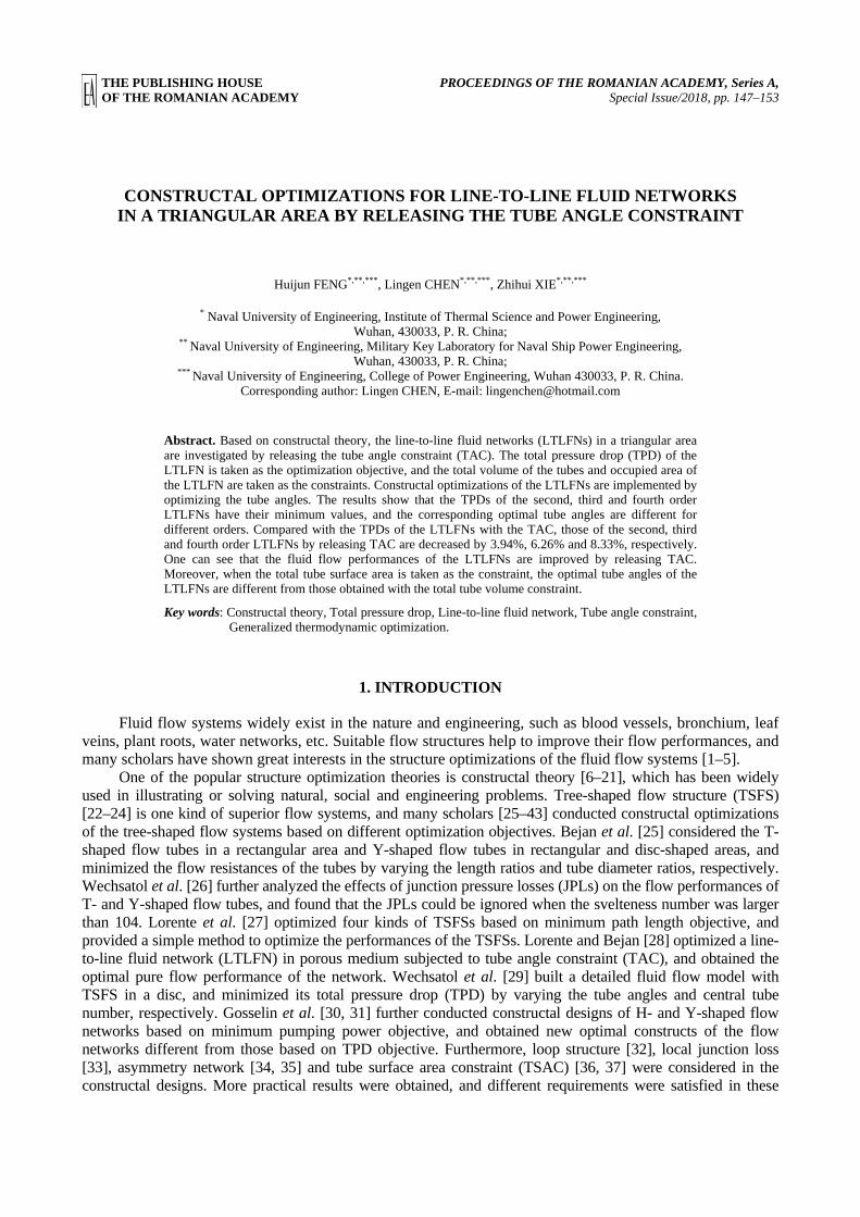
THE PUBLISHING HOUSE PROCEEDINGS OF THE ROMANIAN ACADEMY, Series A, OF THE ROMANIAN ACADEMY Special Issue/2018, pp. 147–153
CONSTRUCTAL OPTIMIZATIONS FOR LINE-TO-LINE FLUID NETWORKS IN A TRIANGULAR AREA BY RELEASING THE TUBE ANGLE CONSTRAINT
Huijun FENG*,**,***, Lingen CHEN*,**,***, Zhihui XIE*,**,*** * Naval University of Engineering, Institute of Thermal Science and Power Engineering,
Wuhan, 430033, P. R. China; ** Naval University of Engineering, Military Key Laboratory for Naval Ship Power Engineering,
Wuhan, 430033, P. R. China; *** Naval University of Engineering, College of Power Engineering, Wuhan 430033, P. R. China.
Corresponding author: Lingen CHEN, E-mail: [email protected]
Abstract. Based on constructal theory, the line-to-line fluid networks (LTLFNs) in a triangular area are investigated by releasing the tube angle constraint (TAC). The total pressure drop (TPD) of the LTLFN is taken as the optimization objective, and the total volume of the tubes and occupied area of the LTLFN are taken as the constraints. Constructal optimizations of the LTLFNs are implemented by optimizing the tube angles. The results show that the TPDs of the second, third and fourth order LTLFNs have their minimum values, and the corresponding optimal tube angles are different for different orders. Compared with the TPDs of the LTLFNs with the TAC, those of the second, third and fourth order LTLFNs by releasing TAC are decreased by 3.94%, 6.26% and 8.33%, respectively. One can see that the fluid flow performances of the LTLFNs are improved by releasing TAC. Moreover, when the total tube surface area is taken as the constraint, the optimal tube angles of the LTLFNs are different from those obtained with the total tube volume constraint.
Key words: Constructal theory, Total pressure drop, Line-to-line fluid network, Tube angle constraint, Generalized thermodynamic optimization.
1. INTRODUCTION
Fluid flow systems widely exist in the nature and engineering, such as blood vessels, bronchium, leaf veins, plant roots, water networks, etc. Suitable flow structures help to improve their flow performances, and many scholars have shown great interests in the structure optimizations of the fluid flow systems [1–5].
One of the popular structure optimization theories is constructal theory [6–21], which has been widely used in illustrating or solving natural, social and engineering problems. Tree-shaped flow structure (TSFS) [22–24] is one kind of superior flow systems, and many scholars [25–43] conducted constructal optimizations of the tree-shaped flow systems based on different optimization objectives. Bejan et al. [25] considered the T-shaped flow tubes in a rectangular area and Y-shaped flow tubes in rectangular and disc-shaped areas, and minimized the flow resistances of the tubes by varying the length ratios and tube diameter ratios, respectively. Wechsatol et al. [26] further analyzed the effects of junction pressure losses (JPLs) on the flow performances of T- and Y-shaped flow tubes, and found that the JPLs could be ignored when the svelteness number was larger than 104. Lorente et al. [27] optimized four kinds of TSFSs based on minimum path length objective, and provided a simple method to optimize the performances of the TSFSs. Lorente and Bejan [28] optimized a line-to-line fluid network (LTLFN) in porous medium subjected to tube angle constraint (TAC), and obtained the optimal pure flow performance of the network. Wechsatol et al. [29] built a detailed fluid flow model with TSFS in a disc, and minimized its total pressure drop (TPD) by varying the tube angles and central tube number, respectively. Gosselin et al. [30, 31] further conducted constructal designs of H- and Y-shaped flow networks based on minimum pumping power objective, and obtained new optimal constructs of the flow networks different from those based on TPD objective. Furthermore, loop structure [32], local junction loss [33], asymmetry network [34, 35] and tube surface area constraint (TSAC) [36, 37] were considered in the constructal designs. More practical results were obtained, and different requirements were satisfied in these
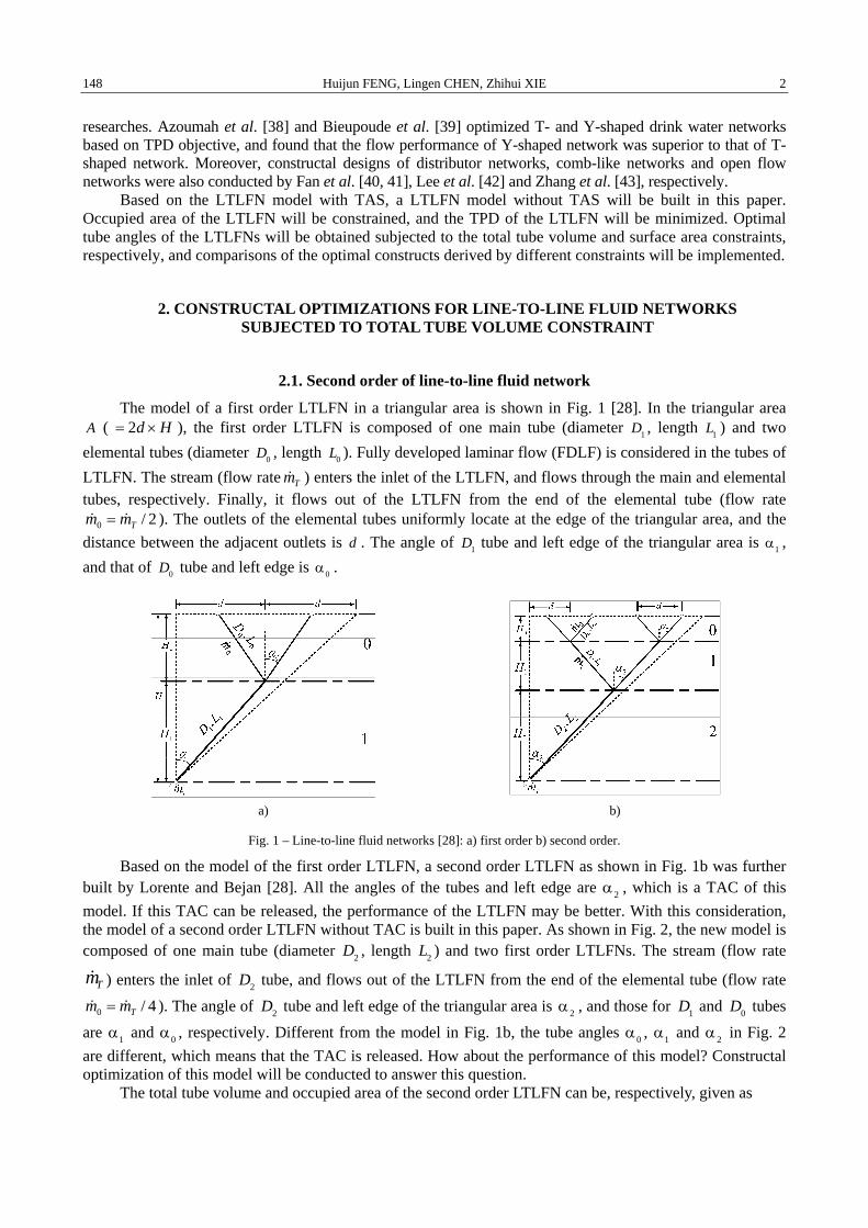
Huijun FENG, Lingen CHEN, Zhihui XIE 2 148
researches. Azoumah et al. [38] and Bieupoude et al. [39] optimized T- and Y-shaped drink water networks based on TPD objective, and found that the flow performance of Y-shaped network was superior to that of T-shaped network. Moreover, constructal designs of distributor networks, comb-like networks and open flow networks were also conducted by Fan et al. [40, 41], Lee et al. [42] and Zhang et al. [43], respectively.
Based on the LTLFN model with TAS, a LTLFN model without TAS will be built in this paper. Occupied area of the LTLFN will be constrained, and the TPD of the LTLFN will be minimized. Optimal tube angles of the LTLFNs will be obtained subjected to the total tube volume and surface area constraints, respectively, and comparisons of the optimal constructs derived by different constraints will be implemented.
2. CONSTRUCTAL OPTIMIZATIONS FOR LINE-TO-LINE FLUID NETWORKS SUBJECTED TO TOTAL TUBE VOLUME CONSTRAINT
2.1. Second order of line-to-line fluid network
The model of a first order LTLFN in a triangular area is shown in Fig. 1 [28]. In the triangular area A ( 2d H= × ), the first order LTLFN is composed of one main tube (diameter D1 , length L1 ) and two elemental tubes (diameter D0 , length L0 ). Fully developed laminar flow (FDLF) is considered in the tubes of LTLFN. The stream (flow rate Tm ) enters the inlet of the LTLFN, and flows through the main and elemental tubes, respectively. Finally, it flows out of the LTLFN from the end of the elemental tube (flow rate
0 / 2Tm m= ). The outlets of the elemental tubes uniformly locate at the edge of the triangular area, and the distance between the adjacent outlets is d . The angle of D1 tube and left edge of the triangular area is α1 , and that of D0 tube and left edge is α0 .
a) b)
Fig. 1 – Line-to-line fluid networks [28]: a) first order b) second order.
Based on the model of the first order LTLFN, a second order LTLFN as shown in Fig. 1b was further built by Lorente and Bejan [28]. All the angles of the tubes and left edge are α2 , which is a TAC of this model. If this TAC can be released, the performance of the LTLFN may be better. With this consideration, the model of a second order LTLFN without TAC is built in this paper. As shown in Fig. 2, the new model is composed of one main tube (diameter D2 , length L2 ) and two first order LTLFNs. The stream (flow rate
Tm ) enters the inlet of D2 tube, and flows out of the LTLFN from the end of the elemental tube (flow rate
0 / 4Tm m= ). The angle of D2 tube and left edge of the triangular area is α2 , and those for D1 and D0 tubes are α1 and α0 , respectively. Different from the model in Fig. 1b, the tube angles α0 , α1 and α2 in Fig. 2 are different, which means that the TAC is released. How about the performance of this model? Constructal optimization of this model will be conducted to answer this question.
The total tube volume and occupied area of the second order LTLFN can be, respectively, given as

3 Constructal optimizations for line-to-line fluid networks in a triangular area by releasing the tube angle constraint 149
V = π(4D02L0 + 2D1
2L1 + D22L2 ) / 4,
(1)
A = 4d(H0 + H1 + H2 ) / 2.
(2)
When the tube diameter ratios of the LTLFN obey Murry law, the relationships of the diameters are:
D2 = 21/3 D1 = 22/3 D0.
(3)
For the fixed total volume of the tubes, the diameter of the elemental tube can be obtained by substituting the diameter relationships into Eq. (1), i.e.,
D0 =V 1/2 ⋅[π(L0 + 2−1/3 L1 + 2−2/3 L2 )]−1/2.
(4)
According to the structure of the second order LTLFN, the lengths and vertical distances of the tubes are, respectively, given as
0 0 1 1 2 2/[2sin( )], / sin( ), 2 / sin( ),L d L d L d= α = α = α
(5)
0 0 0 1 1 1 2 2 2cos( ), cos( ), cos( ).H L H L H L= α = α = α
(6)
For the fixed area A , substituting Eqs. (5) and (6) into Eq. (2) yields the distance between the adjacent outlets
d = A1/2 ⋅[cot(α0 )+ 2cot(α1)+ 4cot(α2 )]−1/2.
(7)
According to Refs. [29, 37], the TPD of the second order LTLFN for FDLF is 4 4 4
2 0 0 0 1 1 1 2 2 2128 /( ) 128 /( ) 128 /( ).P m vL D m vL D m vL DΔ = π + π + π
(8)
From Eq. (8), the dimensionless total pressure drop (DTPD) can be expressed as 2 3/ 2 2 / 3 1/ 3 3
2 2 0 1 24(/ 2( ) ,2 2 )TP PV A L L LmΔ = Δ π ν = + +
(9)
where 1/ 20 1 2 0 1 2( , , ) ( , , ) /L L L L L L A= . From Eq. (9), the DTPD 2PΔ of the second order LTLFN is a function of
the tube angles 0α , 1α and 2α , and constructal optimization of the second order LTLFN can be conducted by taking these parameters as optimization variables.
Fig. 2 – Second order line-to-line fluid network by releasing TAC. Fig. 3 – Characteristics of 2PΔ versus α0 and α1 .
Figure 3 shows the three-dimensional relationship of the DTPD 2PΔ versus the tube angles 0α and 1α with 2 40α = ° . From Fig. 3, there exist optimal tube angles ( 0,optα and 1,optα ) which leads to double minimum value of the DTPD. Numerical calculation shows that the tube angle 2α can be further optimized, the optimal tube angles of the second order LTLFN by releasing the TAC are 0, 60.16optα = ° , 1, 51.18optα = ° and
2, 37.83optα = ° . Compared with the DTPD of the LTLFN with the TAC, that of the LTLFN without the TAC is reduced by 3.94%. Therefore, the flow performance of the LTLFN is improved by releasing the TAC.

Huijun FENG, Lingen CHEN, Zhihui XIE 4 150
2.2. Third and fourth orders of line-to-line fluid networks
The model of a third order LTLFN without the TAC is shown in Fig. 4. It is composed of one main tube (diameter 3D , length 3L ) and two second order LTLFNs. One can see that the models of the higher order LTLFNs can be further built by adopting this method. The stream (flow rate Tm ) enters the inlet of 3D tube, then flows along iD tubes (flow rate 3/ 2 , 3, 2,1,0i
i Tm m i−= = ), and finally flows out of triangular area from the outlet of 0D tube. The angle of 3D tube and triangular left edge is 3α .
The total tube volume and occupied area of the third order LTLFN can be, respectively, given as
V = π(8D02L0 + 4D1
2L1 + 2D22L2 + D3
2L3) / 4,
(10)
A = 8d(H0 + H1 + H2 + H3) / 2.
(11)
According to the structure of the LTLFN shown in Fig. 4, the length and vertical distance of each order tube are, respectively, expressed as
L0 = d / [2sin(α0 )], L1 = d / sin(α1), L2 = 2d / sin(α2 ), L3 = 4d / sin(α3),
(12)
H0 = L0 cos(α0 ), H1 = L1 cos(α1), H2 = L2 cos(α2 ), H3 = L3 cos(α3).
(13)
Similar to the method adopted in section 2.1, the DTPD of the third order LTLFN can be obtained by combining Eqs. (10)–(13)
2 3/ 2 2 / 3 1/ 3 33 3 0 1 2 38(2 2 2 )/( ) ,TP PV A L L L LmΔ = Δ π ν = + + +
(14)
where the dimensionless tube lengths are defined as 1/ 20 1 2 3 0 1 2 3( , , , ) ( , , , ) /L L L L L L L L A= . From Eq. (14), the
DTPD 3PΔ of the third order LTLFN is a function of the tube angles 0α , 1α , 2α and 3α , and constructal optimization of the third order LTLFN can be conducted by taking these parameters as optimization variables.
Fig. 4 – Third order line-to-line fluid network
by releasing TAC. Fig. 5 – Comparison of the optimal constructs of the third order line-to-line fluid
networks: (a) releasing TAC (b) preserving TAC.
Figure 5 shows the comparison of the third order LTLFN with and without the TACs. From Fig. 5, one can see that the optimal tube angles of the third order LTLFN without the TAC are 0, 66.06optα = ° , 1, 59.25optα = ° ,
2, 49.89optα = ° and 3, 35.74optα = ° , and the optimal length ratios of the tubes are 3 2 2.6( / ) 2optL L = ,
2 1 2.2( / ) 5optL L = and 1 0 2.1( / ) 3optL L = , respectively. All the tube angles of the third order LTLFN with the TAC are 0 1 2 3 42.94α α α α= = = = ° , and all length ratios of the tubes are 2 [28]. One can see that the optimal constructs of the third order LTLFN with and without the TACs are different. Numerical calculations show that compared with the DTPDs of the third and fourth order LTLFNs with the TAC, those of the LTLFNs without the TAC are reduced by 6.26% and 8.33%, respectively. Therefore, the flow performance of the LTLFN can be further improved by releasing the TAC and adopting higher order network simultaneously.
5 Constructal optimizations for line-to-line fluid networks in a triangular area by releasing the tube angle constraint 151
3. CONSTRUCTAL OPTIMIZATIONS FOR LINE-TO-LINE FLUID NETWORKS SUBJECTED TO TOTAL TUBE SURFACE AREA CONSTRAINT
The LTLFNs subjected to the tube volume constraint (TVC) are optimized in Section 2. The cost of a network is always associated with its total tube surface area [4, 25, 36, 37]. In the design of the network with finite cost, the total surface area is an important constraint in the optimizations. Due to this reason, constructal designs of the second and third orders of LTLFNs subjected to the TSAC will be conducted as examples.
The models of the second and third order LTLFNs without the TAC are shown in Figs. 2 and 4, respectively. The total tube surfaces of the second and third order LTLFNs can be, respectively, given as
AT = π(4D0L0 + 2D1L1 + D2L2 ),
(15)
AT = π(8D0L0 + 4D1L1 + 2D2L2 + D3L3).
(16)
For the total TSACs in Eqs. (15) and (16), constructal optimizations of the second and third order LTLFNs can be conducted by releasing the TAC similar to the method adopted in section 2.
Numerical calculations show that for the fixed total TSAC, the optimal tube angles of the second order LTLFN by releasing the TAC are 0, 68.43optα = ° , 1, 56.14optα = ° and 2, 32.38optα = ° ; those of the third order LTLFN are 0, 75.39optα = ° , 1, 67.52optα = ° , 2, 54.58optα = ° and 3, 28.54optα = ° ; those of the fourth order LTLFN are 0, 80.19optα = ° , 1, 75.03optα = ° , 2, 66.95optα = ° , 3, 53.59optα = ° and 4, 25.89optα = ° , respectively. One can see that the optimal constructs of the second and higher order of LTLFNs with TSAC are different from those with TVC. Compared with the DTPDs of the second, third and fourth order LTLFNs with the TAC, those of the LTLFNs without the TAC are reduced by 20.05%, 31.36% and 40.98%, respectively. Therefore, releasing TAC exhibits obvious advantages in flow performance improvements of the second and higher order LTLFNs when total tube surface is taken as the constraint.
4. CONCLUSIONS
A LTLFN model in a triangular area without the TAC is built in this paper. The total volume of the tubes and occupied area of the LTLFN are taken as the constraints. Constructal optimizations of the LTLFNs are implemented by optimizing the tube angles, and the TPDs of the LTLFNs are minimized. The results show that when the total TVC is considered and the TAC is released, the optimal tube angles of the third order LTLFN are 0, 66.06optα = ° , 1, 59.25optα = ° , 2, 49.89optα = ° and 3, 35.74optα = ° , and the corresponding optimal length ratios of the tubes are 3 2 2.6( / ) 2optL L = , 2 1 2.2( / ) 5optL L = and 1 0 2.1( / ) 3optL L = , respectively. All the tube angles of the third order LTLFN with the TAC are 0 1 2 3 42.94α α α α= = = = ° , and all length ratios of the tubes are 2. The optimal constructs of the third order LTLFN with and without the TACs are different. Compared with the DTPDs of the third and fourth order LTLFNs with the TAC, those of the LTLFNs without the TAC are reduced by 6.26% and 8.33%, respectively. Therefore, the flow performance of the LTLFN can be further improved by releasing the TAC and adopting higher order network simultaneously. Moreover, the optimal constructs of the LTLFNs subjected to TVC and TSAC are different, which can provide different guidelines for the designs of the fluid flow systems.
Actually, the LTLFN model built in this paper is an ideal one. The local pressure losses exist and turbulent flow may occur in the tubes. The mass flow rates in the tubes may not equal to each other, and different design requirements should be satisfied. Therefore, one can built more practical LTLFN models by considering local resistance losses, different flow regimes and nonuniform flow rate distributions, respectively, and further conduct constructal designs of the LTLFNs based on multi-objectives.
ACKNOWLEDGEMENTS
This work was supported by the National Natural Science Foundation of China (Grant Nos. 51506220 and 51579244) and the Natural Science Foundation of Hubei Province (Grant No. 2016CFB504).
Huijun FENG, Lingen CHEN, Zhihui XIE 6 152
REFERENCES
1. C.D. MURRAY, The physiological principle of minimal work, in the vascular system, and the cost of blood-volume, Acad. Nat. Sci., 12, 3, pp. 207–214, 1926.
2. T.A. WILSON, Design of the bronchial tree, Natrue, 213, 5077, p. 668–669, 1967. 3. B. MAUROY, M. FILOCHE, E.R. WEIBEL, B. SAPOVAL, An optimal bronchial tree may be dangerous, Nature, 427, 6975,
pp. 633–636, 2004. 4. M. DURAND, Structure of optimal transport networks subject to a global constraint, Phys. Rev. Lett., 98, 8, p. 088701, 2007. 5. A.F. MIGUEL, Fluid flow in a porous tree-shaped network: Optimal design and extension of Hess-Murray’s law, Phys. A: Stat.
Mech. Appl., 423, pp. 61–71, 2015. 6. A. BEJAN, Shape and Structure, from Engineering to Nature, Cambridge University Press, Cambridge, 2000. 7. A. REIS, Constructal theory: From engineering to physics, and how flow systems develop shape and structure, Appl. Mech. Rev.,
59, 5, pp. 269–282, 2006. 8. A. BEJAN, S. LORENTE, Design with Constructal Theory, Wiley, New Jersey, 2008. 9. G. LORENZINI, S. MORETTI, A. CONTI, Fin Shape Thermal Optimization Using Bejan’s Constructal Theory, Morgan &
Claypool Publishers, USA, 2011, pp. 1–219. 10. L.G. CHEN, Progress in study on constructal theory and its application, Sci. China: Tech. Sci., 55, 3, p. 802–820, 2012. 11. A. BEJAN, S. LORENTE, Constructal law of design and evolution: Physics, biology, technology, and society, J. Appl. Phys., 113,
15, p. 151301, 2013. 12. A. BEJAN, Constructal law: Optimization as design evolution, Trans. ASME, J. Heat Transfer, 137, 6, p. 061003, 2015. 13. G.N. Xie, Y.D. Song, M. Asadi , G. Lorenzini, Optimization of pin-fins for a heat exchanger by entropy generation minimization
and constructal law, Trans. ASME, J. Heat Transfer, 137, 6, p. 061901, 2015. 14. M.R. HAJMOHAMMADI, G. LORENZINI, O. JONEYDI SHARIATZADEH, C. BISERNI, Evolution in the design of V-shaped
highly conductive pathways embedded in a heat-generating piece, Trans. ASME, J. Heat Transfer, 137, 6, p. 061001, 2015. 15. L.G. CHEN, H.J. FENG, Multi-objective Constructal Optimizations for Fluid Flow, Heat and Mass Transfer Processes (in
Chinese), Science Press, Beijing, 2016. 16. A. BEJAN, M.R. ERRERA, Complexity, organization, evolution, and constructal law, J. Appl. Phys., 119, 7, p. 074901, 2016. 17. L.G. CHEN, H.J. FENG, Z.H. XIE, Generalized thermodynamic optimization for iron and steel production processes: A
theoretical exploration and application cases, Entropy, 18, 10, p. 353, 2016. 18. P. XU, A.P. SASMITO, B.M. YU, A.S. MUJUMDAR, Transport phenomena and properties in treelike networks, Trans. ASME,
Appl. Mech. Rev., 68, 4, p. 040802, 2016. 19. A. BEJAN, A. ALMERBATI, S. LORENTE, Economies of scale: The physics basis, J. Appl. Phys., 121, 4, p. 044907, 2017. 20. A. BEJAN, Evolution in thermodynamics, Appl. Phys. Rev., 4, 1, p. 011305, 2017. 21. A. BEJAN, Wealth inequality: The physics basis, J. Appl. Phys., 121, p. 124903, 2017. 22. S. LORENTE, W. WECHSATOL, A. BEJAN, Optimization of tree-shaped flow distribution structure over a disc-shaped area,
Int. J. Energy Res., 27, 8, p. 715–723, 2003. 23. W. WECHSATOL, A. BEJAN, S. LORENTE, Tree-shaped flow architectures: Strategies for increasing optimization speed and
accuracy, Numer. Heat Transfer: Part A: Appl., 48, 8, p. 731–744, 2005. 24. A. BEJAN, S. LORENTE, Constructal tree-shaped flow structures, Appl. Thermal Eng., 27, 4, pp. 755–761, 2007. 25. A. BEJAN, L.A.O. ROCHA, S. LORENTE, Thermodynamic optimization of geometry: T- and Y- shaped constructs of fluid
streams, Int. J. Thermal Sci., 39, pp. 949–960, 2000. 26. W. WECHSATOL, S. LORENTE, A. BEJAN, J.C. ORDONEZ, Elemental T and Y shapes of tree networks of ducts with various
cross-sections, J. Hydraul. Eng., 135, 2, pp. 132–139, 2009. 27. S. LORENTE, W. WECHSATOL, A. BEJAN, Tree-shaped flow structures designed by minimizing path lengths, Int. J. Heat Mass
Transfer, 45, 16, pp. 3299–3312, 2002. 28. S. LORENTE, A. BEJAN, Heterogeneous porous media as multiscale structures for maximum flow access, J. Appl. Phys., 100,
11, p. 114909, 2006. 29. W. WECHSATOL, S. LORENTE, A. BEJAN, Optimal tree-shaped networks for fluid flow in a disc-shaped body, Int. J. Heat
Mass Transfer, 45, 25, pp. 4911–4263, 2002. 30. L. GOSSELIN, A. BEJAN, Tree network for minimal pumping power, Int. J. Thermal Sci., 44, 1, pp. 53–63, 2005. 31. L. GOSSELIN, Minimum pumping power fluid tree networks without a priori flow regime assumption, Int. J. Heat Mass Transfer,
48, 11, pp. 2159–2171, 2005. 32. W. WECHSATOL, S. LORENTE, A. BEJAN, Tree-shaped networks with loops, Int. J. Heat Mass Transfer, 48, 3, p. 573–583,
2005. 33. W. WECHSATOL, S. LORENTE, A. BEJAN, Tree-shaped flow structures with local junction losses, Int. J. Heat Mass Transfer,
49, 17–18, pp. 2957–2964, 2006. 34. L. GOSSELIN, A. BEJAN, Emergence of asymmetry in constructal tree flow networks, J. Appl. Phys., 98, 10, p. 104903, 2005. 35. W. WECHSATOL, J.C. ORDONEZ, U.S. KOSARAJ, Constructal dendritic geometry and the existence of asymmetric
bifurcation, J. Appl. Phys., 100, 11, p. 113514, 2006. 36. L. GOSSELIN, Optimization of tree-shaped fluid networks with size limitations, Int. J. Thermal Sci., 46, 5, pp. 434–443, 2007. 37. H.J. FENG, L.G. CHEN, Z.H. XIE, F.R. SUN, Constructal optimization for tree-shaped fluid networks in a disc-shaped area
subjected to the surface area constraint, Arab. J. Sci. Eng., 39, 2, pp. 1381–1391, 2014. 38. Y. AZOUMAH, P. BIEUPOUDE, P. NEVEU, Optimal design of tree-shaped water distribution network using constructal
approach: T-shaped and Y-shaped architectures optimization and comparison, Int. Comm. Heat Mass Transfer, 39, 2, pp. 182–189, 2012.

7 Constructal optimizations for line-to-line fluid networks in a triangular area by releasing the tube angle constraint 153
39. P. BIEUPOUDE, Y. AZOUMAH, P. NEVEU, Constructal tree-shaped water distribution networks by an environmental approach, Int. J. Design & Nature Ecodyn., 7, 1, pp. 74–92, 2012.
40. Z. FAN, X. ZHOU, L. LUO, W. YUAN, Experimental investigation of the flow distribution of a 2-dimensional constructal distributor, Exp. Thermal Fluid Sci., 33, 1, pp. 77–83, 2008.
41. Z. FAN, X. ZHOU, L. LUO, W. YUAN, Evaluation of the performance of a constructal mixer with the iodide-iodate reaction system, Chem. Eng. Process.: Process Intensification, 49, 6, pp. 628–632, 2010.
42. J. LEE, Y. KIM, S. LORENTE, A. BEJAN, Constructal design of a comb-like channel network for self-healing and self-cooling, Int. J. Heat Mass Transfer, 66, pp. 898–905, 2013.
43. J. ZHANG, X.D. LOU, L.Z. GUO, Universal patterns and constructal law in open flow networks, Int. J. Heat Tech., 34, S1, pp. 75–82, 2016.
THE PUBLISHING HOUSE PROCEEDINGS OF THE ROMANIAN ACADEMY, Series A, OF THE ROMANIAN ACADEMY Special Issue/2018, pp. 154–159
ANALYSIS OF THE THERMAL PERFORMANCE OF SINGLE AND MULTI-LAYERED MICROCHANNELS WITH FIXED VOLUME CONSTRAINT
OLAYINKA O. ADEWUMI1, TUNDE BELLO-OCHENDE2, JOSUA P. MEYER1 1 University of Pretoria, Department of Mechanical and Aeronautical Engineering, South Africa
2 University of Cape Town, Department of Mechanical Engineering, South Africa Corresponding author: Olayinka O. ADEWUMI, E-mail: [email protected]
Abstract. This study presents a numerical analysis of forced convection heat transfer and steady, laminar, incompressible fluid flow through single-, two- and three-layered microchannels with different flow arrangements and fixed total volume constraint. Previous studies on multi-layered microchannel heat sinks have shown that these types of heat sinks perform better than single-layered microchannel in terms of reducing thermal resistance and pressure drop, but this is obtained with increased total volume of the solid substrate because equal volumes of the single-layered microchannel are stacked to obtain the number of desired layers. In this paper, the total volume of the solid substrate for all the microchannels considered was fixed at 0.9 mm3 and the geometries of the different microchannels were optimised based on the objective of maximising the thermal conductance using a computational fluid dynamics package with a goal-driven optimisation tool. The results show that for a fixed total volume and fixed inlet fluid velocity, the pumping power of the two-layered microchannel with the different flow arrangements was 10% less than that required for the single-layered microchannel but was increased by about 12% when the number of layers was increased to three. The results obtained from this study show that the multi-layered microchannels give very good results without increasing the total volume of the solid substrate as presented in previous investigations.
Key words: Forced convection, Maximised thermal conductance, Pumping power, Pressure drop, Temperature rise, Fluid velocity.
1. INTRODUCTION
In recent times, stacked microchannel heat sinks, which integrate many layers of microchannels, have been developed to provide efficient thermal management at relatively low pressures while maintaining uniform chip temperature [1–4]. The design of stacked microchannel heat sinks found in literature provide larger flow passages with the aim of reducing pressure drop significantly for a constant heat flux. The larger flow passages are a result of the increase in total volume, as equal volumes of single-layered microchannels are stacked to achieve the desired number of layers. The multi-layered microchannel heat sink geometries in the outlined studies had increased total volume ( ≥ 100%) more than the single-layered microchannel because the total volume of the solid substrate had to be doubled, tripled and so on, depending on the number of layers in the stack. With microelectronics devices becoming smaller, increasing the volume of the solid substrate is a disadvantage because of space constraints in these devices. Aside from the increase in volume, there is also increase in weight which is often discouraged in recent electronic device designs. This is why it is crucial to investigate how the multi-layered microchannel performs under a volume constraint. The optimisation of the multi-layered microchannel heat sink will be based on minimising the peak temperature of the solid substrate, which results in maximising the thermal conductance of the highly conductive silicon substrate [5]. Comparison between the pumping power and pressure drops for the different microchannels is also investigated.
2. MODEL DESCRIPTION AND MATHEMATICAL FORMULATION
Figure 1 shows the elemental volume used as computational domain for the single-, two- and three-layered microchannel while Fig. 2 shows the different flow configurations considered in this study.
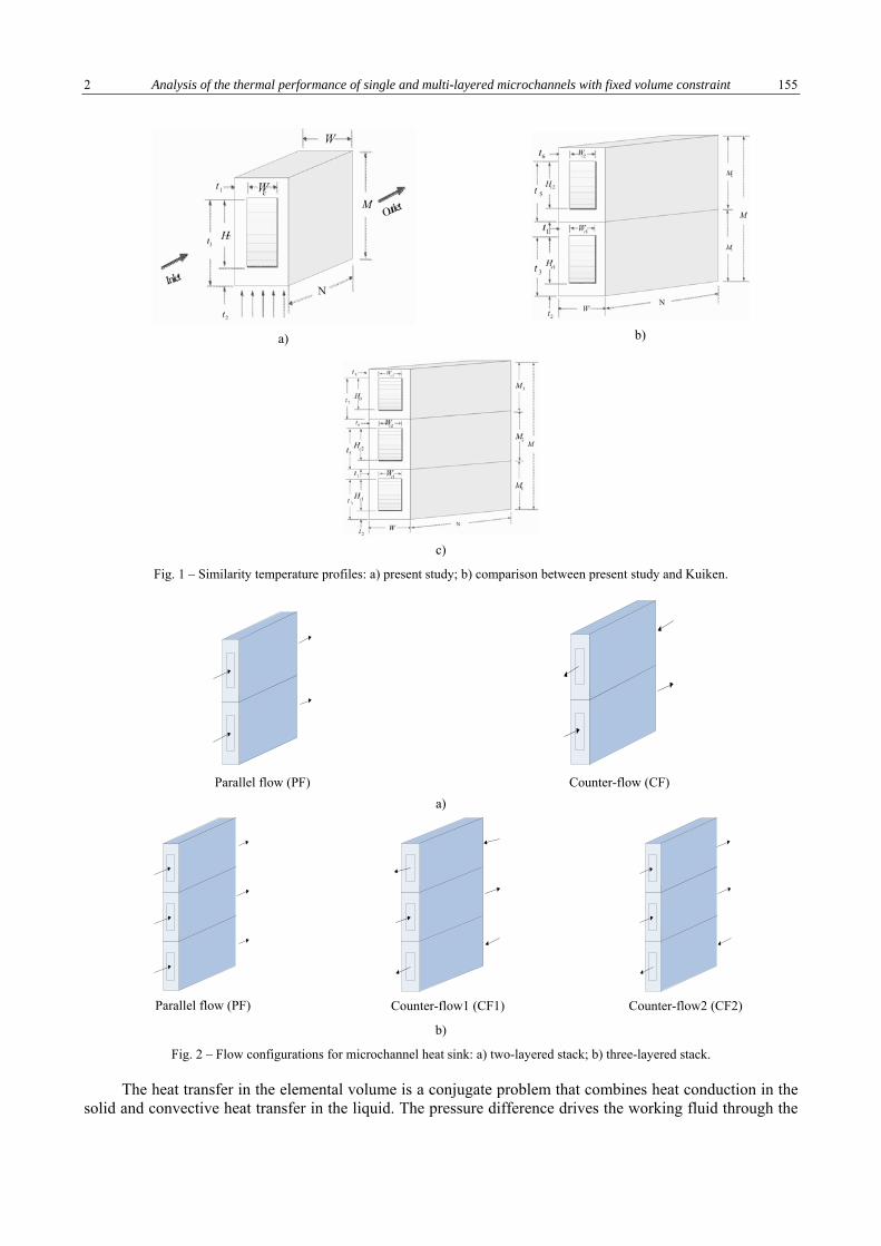
2 Analysis of the thermal performance of single and multi-layered microchannels with fixed volume constraint 155
a)
b)
c)
Fig. 1 – Similarity temperature profiles: a) present study; b) comparison between present study and Kuiken.
Parallel flow (PF)
Counter-flow (CF)
a)
Parallel flow (PF)
Counter-flow1 (CF1)
Counter-flow2 (CF2)
b)
Fig. 2 – Flow configurations for microchannel heat sink: a) two-layered stack; b) three-layered stack.
The heat transfer in the elemental volume is a conjugate problem that combines heat conduction in the solid and convective heat transfer in the liquid. The pressure difference drives the working fluid through the

Olayinka O. ADEWUMI, Tunde BELLO-OCHENDE, Josua P. MEYER 3 156
microchannels as a result of pumping power that is applied at the channel inlet. The flow and heat transfer are assumed to in steady-state conditions, incompressible flow, constant thermophysical properties with negligible radiation heat transfer.
2.1. Governing equations, boundary conditions and numerical procedure
The continuity, momentum and energy equations (equations 1 to 4) along with the specified boundary conditions were solved numerically using ANSYS Fluent computational fluid dynamic package, which employs a finite volume method. The solution is assumed to converge when the normalised residuals of the continuity and momentum equation fall below 10-5, while that of the energy equation falls below 10-7
0∇ ⋅ =v , (1)
ρv∇ ⋅ v = −∇p +μ∇ 2v , (2)
ρ f Cp, f v ⋅∇T = k f ∇2T , (3)
ks∇2T = 0 . (4)
The heat flux between the interface of the fluid and the solid walls is coupled and its continuity between the interface of the solid and the liquid and the dimensionless global thermal conductance, which is the measure of performance is stated in equation (5). Equation (6) shows the expressions for the temperature rise on the heated wall and pumping power respectively. The flow boundary conditions are: no slip and no penetration at the wall surfaces, u = uin, v = w = 0 m/s at the inlet and zero stress at the outlet. The thermal boundary conditions are specified as T = Tin at the inlet, while symmetry boundary conditions are specified at the left and right side of the computational domain. A constant uniform heat flux q '' is applied at the bottom wall, while no heat flux is applied at the top wall.
ks∂T
∂n Ω
= −k f∂T
∂n Ω
ks∂T
∂n Ω
= −k f∂T
∂n Ω
, C = ′ ′ q Nkf ΔT , ΔT = Tmax − Tmin ΔT = Tmax − Tmin , (5)
ΔTbase = Tmax − Tmin, base , (6)
PP = uin AcΔP PP = uin AcΔP . (7)
2.2. Numerical optimization procedure
The length N, height M and width W of the solid is fixed, which makes the total volume of the single-, two- and three-layered microchannel V fixed as shown in equation (8), while t1, t2, t3, t5, t6, t7, t8, Hc, Hc1, Hc2, Hc3, Wc, Wc1, Wc2 and Wc3 are varied, but also subject to manufacturing constraints shown in equations (9) to (11).
V = MWN = const., (8)
Hc1-c3/Wc1-c3 ≤ 20, t2 ≥ 50 µm, (9)
M – t3 ≥ 50 µm, M2 – t5 ≥ 50 µm, M3 – t7 ≥ 50 µm, (10)
1 2 .nM M M M+ + + =… (11)
Goal driven optimisation tool (GDO) is an optimisation technique that finds design candidates from the response surfaces. The accuracy of the response surface for the design candidates is checked by converting it to a design point and, thereafter, a full simulation is carried out for that point to check the validity of the output parameters. Numerical simulations and optimisation were carried out for a fixed total volume V of 0.9 mm3

4 Analysis of the thermal performance of single and multi-layered microchannels with fixed volume constraint 157
with fixed axial length N of 10 mm, total height M of 900 µm and width W of 100 µm. The temperature of water pumped across the microchannel was 20°C and heat flux applied to the bottom wall was 106 W/m2. The design space for the response surface for the fixed total volume was defined as 54 ≤ Wc1, Wc2, Wc3 ≤ 66 µm, 50 ≤ M – t3 ≤ 60 µm, 25 µm ≤ M1 – t3, M2–t5 ≤ 30 µm and 240 µm ≤ Hc1, Hc2, Hc3 ≤ 375 µm. The optimised design point chosen was required to meet the manufacturing constraints.
3. RESULTS AND DISCUSSION
The results obtained for the two- and three-layered microchannel heat sinks in the present study were compared with those obtained for the single-layered microchannel in our previous study [5]. The corresponding inlet fluid velocity was between 0.329 m/s to 1.865 m/s for pressure drop of 10 kPa to 60 kPa considered. The range of Reynolds number (ReDh) for these velocities is 36 < ReDh < 210. Therefore, in this study, the inlet velocity of fluid flow into each channel of the two- and three-layered microchannels were exactly the same as those of the single-layered microchannel.
3.1. Comparison between maximised thermal conductance of single and multi-layered microchannels with the same total volume
Figure 3 shows the comparison between the maximised thermal conductance of the single and multi-layered microchannels with different flow arrangements. Results obtained show that for the same total volume of solid substrate, increasing the microchannel layers to three improves the thermal performance of the microchannel for inlet velocities greater than 0.648 m/s.
500
1000
1500
2000
2500
0 0.5 1 1.5 2
Single-layeredTwo-layered PFTwo-layered CFThree-layered PFThree-layered CF1Three-layered CF2
Cm
ax
uin
(m/s) Fig. 3 – Comparison between the maximised thermal conductance
of the single-, two- and three-layered microchannels at different velocities.
3.2. Comparison between pumping power in single- and multi-layered microchannel with the same total volume
Figure 4 shows the comparison between the pumping power requirements for the different fluid inlet velocities in the single- and two-layered microchannels. It was observed that, as the velocity of the fluid increased, the required pumping power increased, which is the expected trend. However, the results presented in Fig. 4a show that the bottom channel required 40% to 50% more pumping power for fluid flow than the top channel. This was because the bottom channel is in direct contact with the heated base. Consequently, more cooling was needed at the bottom layer than at the top layer. Figure 4b shows that the total pumping power required for the two-layered microchannel was reduced by about 10% for both the parallel and counter-flow

Olayinka O. ADEWUMI, Tunde BELLO-OCHENDE, Josua P. MEYER 5 158
arrangement when compared with the single-layered microchannel. These results show that reduced pumping power can be achieved without increasing the total volume of the two-layered microchannel.
0
0.002
0.004
0.006
0.5 1 1.5 2
Single-layeredTwo-layered PF (1st layer)Two-layered PF (2nd layer)Two-layered CF (1st layer)Two-layered CF (2nd layer)
PP (W
)
uin
(m/s)
a)
0
0.003
0.006
0 0.5 1 1.5 2
Single-layeredTwo-layered PF(1st layer+2nd layer)Two-layered CF (1st layer+2nd layer)
PPT (W
)
uin
(m/s)
b)
Fig. 4 – Comparison between the pumping powers in the single and two-layered microchannels: a) each layer; b) total.
Figure 5 shows a comparison between the pumping power required for fluid flow through the single- and three-layered microchannels with the three different flow arrangements. In Fig. 5a, it was observed that the average pumping power required for the single-layered microchannels is 150% more than that required for each layer of the three-layered microchannels PF, CF1 and CF2. It was also shown that, for the three-layered PF, CF1 and CF2 the second layer required up to about 13% more pumping power than that of the first layer and about 15% more than the third layer. In Fig. 5b, the results show that when the total pumping power required for the three-layered microchannel was compared with the requirement for the single-microchannel, the three-layered PF, CF1, and CF2 requirements exceeded the requirement of the single-layered microchannel by an average of about 12%. These results show that, even though less pumping power was required in the two-layered microchannel, when the layers were increased to three with the same total volume, the total pumping power requirement for the same inlet fluid velocity range increased.
-0.002
0
0.002
0.004
0.006
0 0.5 1 1.5 2
Single-layeredThree-layered PF (1st layer)Three-layered PF (2nd layer)Three-layered PF (3rd layer)Three-layered CF1 (1st layer)Three-layered CF1 (2nd layer)Three-layered CF1 (3rd layer)Three-layered CF2 (1st layer)Three-layered CF2 (2nd layer)Three-layered CF2 (3rd layer)
PP (W
)
uin
(m/s)
a)
-0.002
0
0.002
0.004
0.006
0.008
0 0.5 1 1.5 2
Single-layeredThree-layered PF (1st layer+2nd layer+3rd layer)Three-layered CF1 (1st layer+2nd layer+3rd layer)Three-layered CF2 (1st layer+2nd layer+3rd layer)
PPT (W
)
uin
(m/s)
b) Fig. 5 – Comparison between the pumping powers in the single and three-layered microchannels: a) each layer; b) total.

6 Analysis of the thermal performance of single and multi-layered microchannels with fixed volume constraint 159
4. CONCLUSION
This paper presented three-dimensional numerical studies that investigated the heat transfer and fluid flow within different multi-layered microchannel heat sinks with different flow arrangements for a fixed total volume. Results from the multi-layered design were compared with those from single-layered microchannels with the same total volume and axial length. When results of pumping power requirement within the microchannels were compared, the two-layered microchannel with the different flow arrangements gave the least pumping power requirement for the range of fluid inlet velocity considered in this study.
REFERENCES
1. X. WEI, Y. JOSHI, M.K. PATTERSON, Experimental and numerical study of stacked micro-channel heat sink for liquid cooling of microelectronic devices, Journal of Heat Transfer, 129, pp. 1432–1444, 2007.
2. M.K. PATTERSON, X. WEI, Y. JOSHI, R. PRASHER, Numerical study of conjugate heat transfer in stacked micro-channels, Inter Society Conference on Thermal Phenomena, 2004, pp. 372–380.
3. K. JEEVAN, I.A. AZID, K.N. SEETHARAMU, Optimization of double layer counter flow (DLCF) micro-channel heat sink used for cooling chips directly, Electronics Packaging Technology Conference, 2004, pp. 553–558.
4. S.H. CHONG, K.T. OOI, T.N. WONG, Optimization of single and double layer counter flow micro-channel heat sinks, Applied Thermal Engineering, 22, pp. 1569–1585, 2002.
5. O.O. ADEWUMI, T. BELLO-OCHENDE, J.P. MEYER, Constructal design of combined microchannel and micro pin fins for electronic cooling, International Journal of Heat and Mass Transfer, 66, pp. 315–323, 2013.

THE PUBLISHING HOUSE PROCEEDINGS OF THE ROMANIAN ACADEMY, Series A, OF THE ROMANIAN ACADEMY Special Issue/2018, pp. 160–165
CONSTRUCTAL DESIGN OF FLAT PLATE SOLAR COLLECTOR
Tanimu JATAU, Tunde BELLO-OCHENDE
University of Cape Town, Department of Mechanical Engineering Private Bag X3 Private Bag X3, Rondebosch, 7701, South Africa
Corresponding author: [email protected]
Abstract. This paper presents a geometric optimization of flat plate solar collector for water heating using constructal design method. In this case, the objective is to identify an optimized geometric configuration of flat plate collector with the minimum entropy generation subject to global constraints (fixed area of the collector surface and fixed volume of the riser tube). The length of the absorber plate equivalent to the length of the riser tubes (L), the spacing between the risers (W) and the diameter of the riser (D) are free to morph with respect to the degree of freedom provided by the area of the collector surface and the volume of the riser tube until an optimal geometric configuration is obtained at minimum entropy generation or maximum conductance. The heat flux (equivalent to solar radiation) applied on the top surface area of absorber plate; the inlet velocity and the inlet temperature of water were all considered constant. With the simulation results obtained a modified Reynolds number was computed and some useful correlations of the modified Reynolds number with the optimal geometrical parameters (Lopt, Wopt and Dopt), minimum entropy generation and maximum conductance were established. The effect of the volume of fluid in the riser tube with respect to optimal geometrical parameters was also studied at constant modified Reynolds. It was observed that the optimal length increases with increase in the volume of the fluid while the optimal riser tube diameter and riser tube spacing slightly decrease with increase in the volume of the fluid. The minimum entropy generation also slightly decreases as the volume of fluid in the riser tubes increases. The numerical results obtained using computational fluid dynamics (CFD) code were verified with the experimental data reported in the open literatures and there was a good agreement with the experimental data.
Key words: Geometric, Constructal method, Entropy generation, Flat plate collector, Modified Reynolds number.
1. INTRODUCTION
Flat plate collector (FPC) is one the solar collectors developed to harness solar energy. It is a special type of exchanger that transforms solar radiation into heat unlike the convectional heat exchangers which usually accomplish a fluid-to-fluid exchange with high heat transfer rate [1, 2]. It is simple and inexpensive to fabricate, install, and require little maintenance [3].
In an attempt to improve the thermal performance of FPC, various researches have been conducted, some of the works done are as follows: Bejan et al. [4] conducted an exergy analysis of a solar collector using second law of thermodynamic and found that the amount of exergy delivered by solar collector system is affected by heat transfer irreversibility occurring between the sun and the collector, between the collector and the ambient air and inside the collector. The effect of irreversibility on the performance of FPC was studied by Saha and Mahanta [5]. Luminosu and Fara [6] analysed the optimal operation mode of FPSC by mean of exergy analysis using numerical solution under the assumption that the fluid inlet temperature is equal to the ambient temperature. In the exergetic optimization of FPC carried out by Farahat et al. [7] of which the optimum values of parameters such as mass flow rate, the absorber plate area and the maximum exergy efficiency were obtained. The design method of FPC based on minimum entropy generation was carried out by Torre-Reyes et al. [8]. Maha et al. [9] examined the effect of geometrical design parameters of FPC on energy and exergy efficiencies. The used converging lenses mounted at the glass cover of FPC was carried out by Alkhair et al. [10] and found out that the temperature of the water increases as the number of

2 Constructal design of flat plate collector 161
lenses increase. In a similar vein, different geometry configurations of FPC has been used to improve its performance as shown by Sivakumar et al. [11], Sanke et al. [12], Kumar [13]. The work on fluid flow and heat transfer in FPC has been investigated by Fan et al., [14] and Marroquin-De et al. [15].
It is apparent that much study has done to improve the thermal performance of the flat plate solar collector ranging from energy and exergy optimization to the use of various geometric configurations of the collector. However, based on available literatures there is lack of information on the geometric optimization of FPC where optimal parameters such as length of the absorber plate, spacing between the risers and the diameter of riser tubes are simultaneously obtained.
In this paper, a geometric optimization of the unglazed flat plate collector using constructal design method with the global objective function of minimization of entropy generation which is equivalent to the maximization of exergy is carried out. In this case, the external irreversibilities due to temperature difference between the sun and the collector and between the collector and environment are fixed. The focus is to minimize the internal irreversibility which is due to fluid flow friction and heat transfer as result of temperature difference between the collector and the fluid. The global objective is to determine the optimal size of the collector which destroys least exergy.
2. PHYSICAL MODELLING
Figure 1 is 3D geometric of unglazed flat plate collector (FPC) which consists of three basic parameters which includes: the length of the absorber plate equivalent to the length of the riser (L), spacing between the riser tubes and diameter of the riser (D). The riser tubes bonded below the absorber plate are usually connected to the header tube which conveys and distributes water into the riser tubes. The water enters from one end of the riser tubes through the header pipe and gets heated in the collector area and the hot water is given out at the other end. But for the simplicity of the geometric, the header tube connected to the riser tubes is not considered.
The riser tubes bonded to absorber plate are of equal diameter and are uniformly spaced. Hence, it can be assumed that the flow rate in all riser tubes is constant and fluid is uniformly distributed in all the riser tubes from the header tube. Therefore, it is only a symmetric of the collector that is modelled for simplicity of the analysis as seen in the computational domain in Fig. 2. The fluid (water) used was assumed to be a continuous medium and incompressible which possesses laminar flow characteristics. Thermo-physical properties of the material (copper) for both absorber plate and riser tube are constant with respect to the operating temperature. The bottom side of the absorber tube and the absorber plate as well as sides of the absorber plate was assumed to be adiabatic. In order to eliminate the drawbacks arising from the random variation of inlet temperature, it was also assumed that the inlet temperature is equal to environment temperature.
a) 3D view b) front view
Fig. 1 – The FPC with five (risers) tubes bonded below the absorber plate. Fig. 2 – The 3D view of FPC with five (risers) tubes bonded below the absorber plate
3. GOVERNING EQUATIONS
The three dimensional, laminar, incompressible and steady viscous Newtonian flow in the collector is governed by the continuity, momentum and energy equations as follows [16]
∇ ⋅U = 0 , (1)
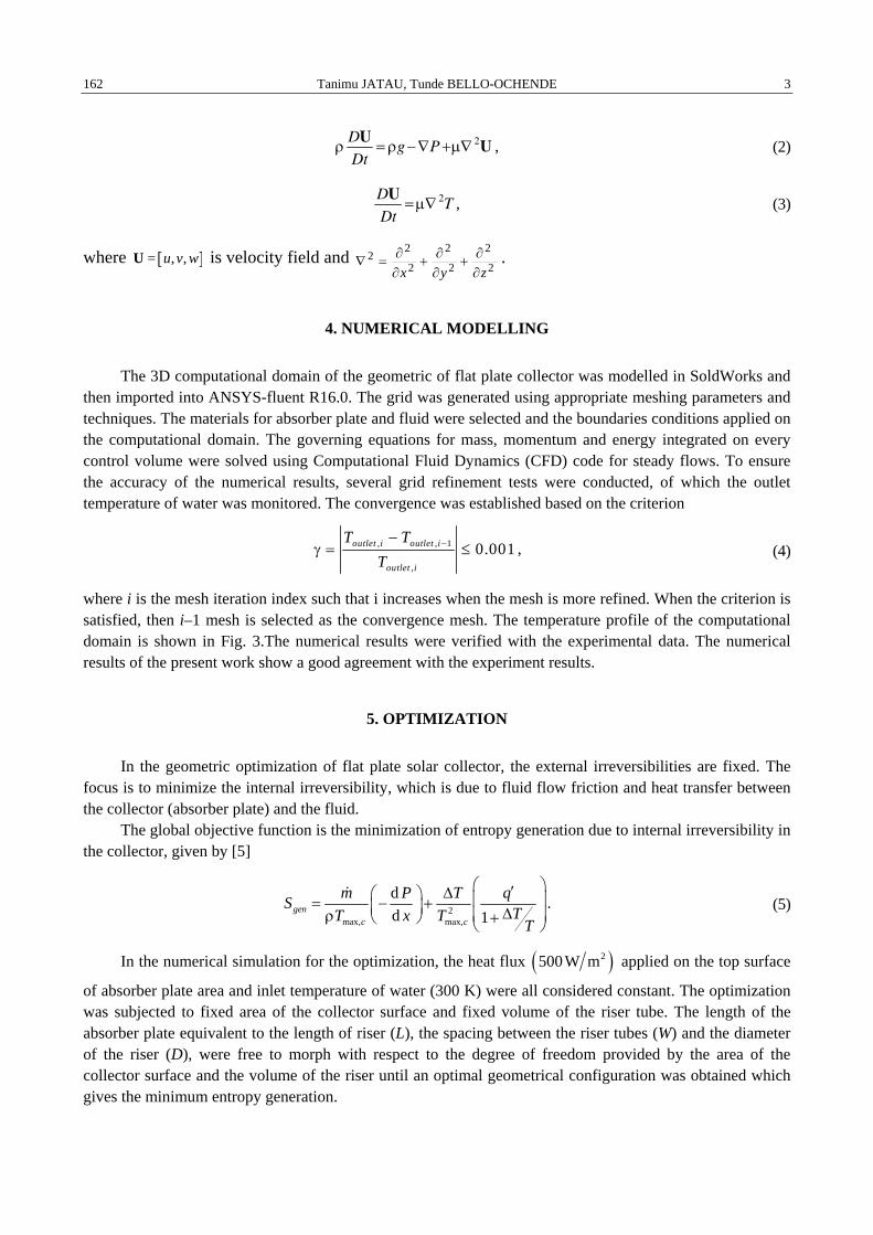
Tanimu JATAU, Tunde BELLO-OCHENDE 3 162
ρ DUDt
= ρg−∇P+μ∇ 2U , (2)
DUDt
=μ∇ 2T , (3)
where [ ]= , ,u v wU is velocity field and 2 2 22
2 2 2x y z∂ ∂ ∂∇ = + +∂ ∂ ∂
.
4. NUMERICAL MODELLING
The 3D computational domain of the geometric of flat plate collector was modelled in SoldWorks and then imported into ANSYS-fluent R16.0. The grid was generated using appropriate meshing parameters and techniques. The materials for absorber plate and fluid were selected and the boundaries conditions applied on the computational domain. The governing equations for mass, momentum and energy integrated on every control volume were solved using Computational Fluid Dynamics (CFD) code for steady flows. To ensure the accuracy of the numerical results, several grid refinement tests were conducted, of which the outlet temperature of water was monitored. The convergence was established based on the criterion
, , 1
,
0.001outlet i outlet i
outlet i
T TT
−−γ = ≤ , (4)
where i is the mesh iteration index such that i increases when the mesh is more refined. When the criterion is satisfied, then i–1 mesh is selected as the convergence mesh. The temperature profile of the computational domain is shown in Fig. 3.The numerical results were verified with the experimental data. The numerical results of the present work show a good agreement with the experiment results.
5. OPTIMIZATION
In the geometric optimization of flat plate solar collector, the external irreversibilities are fixed. The focus is to minimize the internal irreversibility, which is due to fluid flow friction and heat transfer between the collector (absorber plate) and the fluid.
The global objective function is the minimization of entropy generation due to internal irreversibility in the collector, given by [5]
2max, max,
dd 1gen
c c
m P T qS TT x T T
⎛ ⎞′Δ⎛ ⎞ ⎜ ⎟= − +⎜ ⎟ Δ⎜ ⎟ρ +⎝ ⎠ ⎝ ⎠. (5)
In the numerical simulation for the optimization, the heat flux ( )2500W m applied on the top surface
of absorber plate area and inlet temperature of water (300 K) were all considered constant. The optimization was subjected to fixed area of the collector surface and fixed volume of the riser tube. The length of the absorber plate equivalent to the length of riser (L), the spacing between the riser tubes (W) and the diameter of the riser (D), were free to morph with respect to the degree of freedom provided by the area of the collector surface and the volume of the riser until an optimal geometrical configuration was obtained which gives the minimum entropy generation.

4 Constructal design of flat plate collector 163
6. NUMERICAL RESULTS AND DISCUSSION
The simulation results obtained are presented in the graphical form as shown in Figs. 3–11. The basic geometric parameters for FPC considered are the length of the absorber plate/length of riser tubes, the spacing between the riser tubes and the diameter of the riser tube. Figures 4–6, show entropy generation as the function of the length of the absorber plate/length of riser tubes, spacing between the riser tubes and the diameter of the riser tube for different modified Reynolds number (Rem). The entropy generation is highest at the minimum value of length of the absorber plate/riser tubes and at the maximum value of spacing between the riser tubes and at maximum value of the diameter of the riser tube. It reduces as the length, the spacing between the riser and the diameter of the riser increase from left to right hand side of the graph, this is due to improvement in heat transfer between the collector and the fluid and consequently the entropy generation attain the minimum value and start increasing again as the length, the spacing between the riser and diameter keep increasing, as a result of increase of irreversibility due to fluid flow. This indicates that the collector gives the best performance at the minimum value of entropy generation.
Figure 7 shows the variation of the three geometric optimal parameters with the modified Reynolds number of which the optimal length of the absorber plate/riser tubes increase with increase in modified Reynolds number while the other parameters; the optimal spacing between the riser tubes and the optimal diameter of the riser tube decrease as the modified Reynolds number increase. Figure 8 shows the minimum entropy generation as a function of modified Reynolds number of which increase in modified Reynolds number give rise to decrease in the minimum entropy generation. In terms of maximum conductance, the modified Reynolds number increases with increase in the maximum conductance as shown in Figure 9.
The numerical result was used to develop some correlations for the three geometric parameters; optimal length of the absorber plate/riser tubes, optimal spacing between the riser tubes and the optimal diameter of the riser tube as well as the minimum entropy generation and the maximum conductance with respect to the modified Reynolds number as follows:
130.1294Reopt mL = ,
131.5456Reopt mW −
= , 1
60.0392Reopt mD −= ,
23
.min 0.2155Regen mS −= ,
12
max 0.0021RemC = .
Figure 10 shows the effect of volume of the fluid on the optimal parameters of the collector at constant modified Reynolds number. The optimal length increases with increase in the volume of the fluid while the optimal riser tube diameter and riser tube spacing slightly decrease with increase in the volume of the fluid. The minimum entropy generation also slightly decreases as the volume of fluid in the riser tubes increases as shown in Fig. 11.
Fig. 3 – Converged solution; temperature profile of the computational domain.
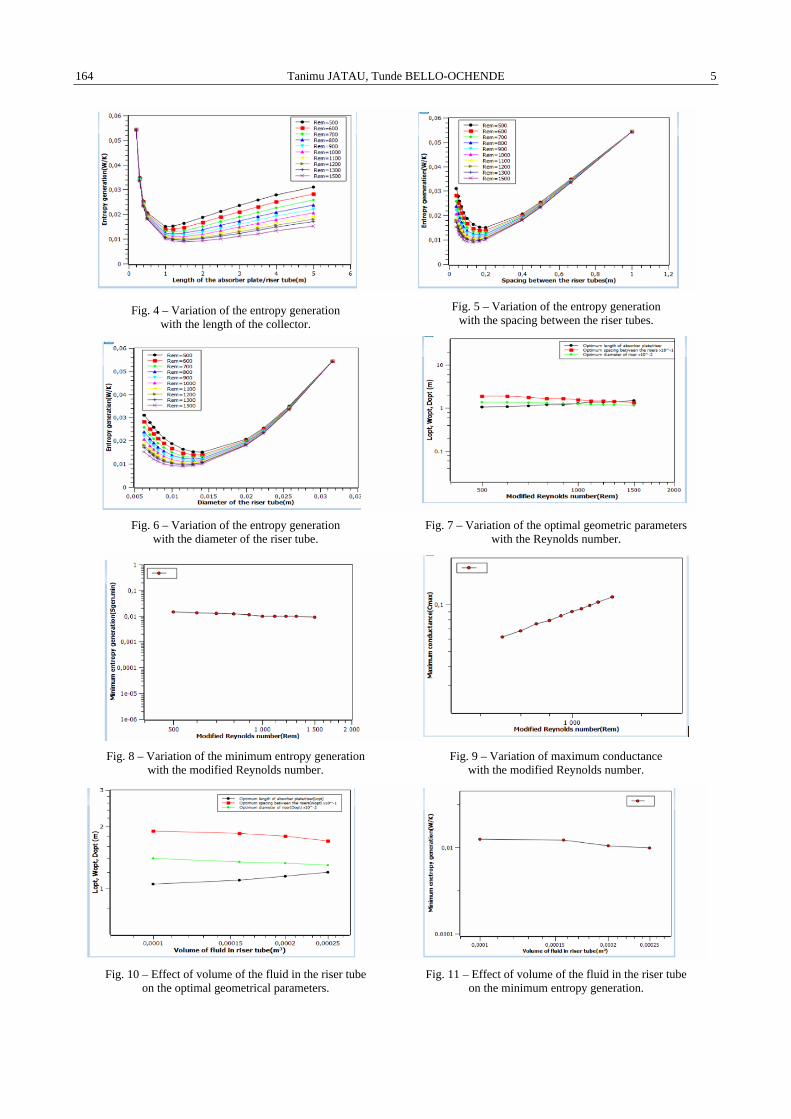
Tanimu JATAU, Tunde BELLO-OCHENDE 5 164
Fig. 4 – Variation of the entropy generation with the length of the collector.
Fig. 5 – Variation of the entropy generation with the spacing between the riser tubes.
Fig. 6 – Variation of the entropy generation
with the diameter of the riser tube. Fig. 7 – Variation of the optimal geometric parameters
with the Reynolds number.
Fig. 8 – Variation of the minimum entropy generation
with the modified Reynolds number. Fig. 9 – Variation of maximum conductance
with the modified Reynolds number.
Fig. 10 – Effect of volume of the fluid in the riser tube
on the optimal geometrical parameters. Fig. 11 – Effect of volume of the fluid in the riser tube
on the minimum entropy generation.

6 Constructal design of flat plate collector 165
6. CONCLUSION
The optimal geometric parameters such as the length of the absorber plate/riser tubes, the spacing between the riser tubes and the diameter of the riser tube were achieved at the minimum value of entropy generation.
The performance of optimal geometric parameters as the function of modified Reynolds number was investigated and it was shown that the optimal length of the absorber plate increases with increase in modified Reynolds number while the optimal spacing between the riser tubes and the diameter of the riser tube decrease with the increase of the modified Reynolds number. It was also observed that the modified Reynolds number increased as the maximum conductance increased while the minimum entropy generation decreased. This means that internal irreversibilities are minimized at the higher modified Reynolds number thereby resulting to better performance of the collector.
Also, the performance of optimal geometry parameters with respect to the volume of fluid in the riser tube was investigated and it was observed that the optimum length of absorber plate/riser tube increases as the volume of the fluid increase. For the optimal riser tube spacing and the diameter as well as the minimum entropy generation slightly decreases with increase in the volume of the fluid.
Some useful correlations were developed to help predict the performance of the collector with respect to modified Reynolds number for the optimal geometric parameters. The correlations could be very useful in the design of the flat plate collector and also to predict the performance of the collector for different modified Reynolds number.
REFERENCES
1. DUFFIE, J.A. BECKMAN, W., Solar Engineering of Thermal Process, John Wiley and Sons, Inc., 4th edition, 2013. 2. KALOGIROU, S.A., Solar thermal collectors and applications, Progress in Energy and Combustion Science, 30, pp. 231–295,
2004. 3. SUKHATME, S.P., NAYAK, J.K., Solar Energy: Principles of Thermal Collection and Storage, New Delhi, Tata Mc Graw-Hill
Publishing Company Limited, 2008. 4. BEJAN, A., KEARNEY, D.W., KREITH F., Second Law Analysis and Synthesis of Solar Collector Systems, Journal of Solar
Energy Engineering, 103, pp. 23–28, 1981. 5. SAHA, S.K., MAHANTA, D.K., Thermodynamic Optimization of Solar Flat-Plate Collector, Renewable Energy, 23, pp. 181–193,
2001. 6. LUMINOSUA, I., FARA L., Exergetic optimization of flat plate solar collectors, Energy, 30, pp. 731–747, 2005. 7. FARAHAT, S., SARHADD, I F., AJAM, H., Exergetic Optimization of Flat Plate Solar Collectors, Renewable Energy, 34,
pp. 1169–1174, 2009. 8. TORRES-REYES, E., CERVANTES-DE GORTARI, J.G., IBARRA-SALAZAR, B.A, PICON-NUÑEZ, M., A Design Method of
Flat-Plate Solar Collectors Based on Minimum Entropy Generation, Exergy International Journal, 1, pp. 46–52, 2001. 9. MAHA, B., ALI, S., AMMAR, B.B., Thermodynamic Optimization of Flat Plate Solar Collectors, The Fifth International
Renewable Energy Congress IREC, 2014. 10. ALKHAIR, M.A., SULAIMAN, M.Y., SOPIAN, K., LIM, C.H., ELIAS, S., MAT, S., Thermal Analysis of Concentrating Flat
Plate Solar Water Heater Absorber using “ANSYS” Simulation, International Conference on Engineering and Built Environment (ICEBE), 2012.
11. SIVAKUMAR P., CHRISTRA W., SRIDHARAN M., JAYAMALATHI N., Performance Improvement Study of Solar Water Heating System, ARPN Journal of Engineering and Applied Sciences, 7, 2012.
12. SANKE, N., SHKHAIR, M.M., Heat Transfer Analysis of a Riser Tube in a Flat Plate Collector with Fins, International Journal & Magazine of Engineering, Technology, Management and Research, 2, pp. 163–167, 2015.
13. KUMAR, A., Performance of Solar Flat plate by using Semi-Circular Cross Sectional Tube, International Journal of Engineering Research and General Science, 2, pp. 33–37, 2014.
14. FAN J., SHAH L. J., FURBO S., Flow distribution in a solar collector panel with horizontally inclined absorber strips, Solar Energy, 81, pp. 1501–1511, 2007.
15. MARROQUÍN-DE, J.Á., OLIVARES-RAMÍREZ, J.M., JIMÉNEZ-SANDOVAL, O., ZAMORA-ANTUÑANO, M.A., ENCINAS-OROPESA, A., Analysis of Flow and Heat Transfer in a Flat Solar Collector with Rectangular and Cylindrical Geometry Using CFD, Ingeniería Investigación y Tecnología, XIV, 4, pp. 553–561, 2013.
16. TANNECHILL, J.C., ANDERSON, D.A., PLETCHER, R.H., Computational Fluid Mechanics and Heat Transfer, 2nd edition, Taylor & Francis, 1997.
THE PUBLISHING HOUSE PROCEEDINGS OF THE ROMANIAN ACADEMY, Series A, OF THE ROMANIAN ACADEMY Special Issue/2018, pp. 166–171
CONSTRUCTAL DESIGN OF MOLTEN SALT FLOW AND HEAT TRANSFER IN HORIZONTAL HOLLOW DISC-SHAPED HEATERS
Wei FU *, Hua LIN**, Xinzhi LIU*, Houlei ZHANG* * Nanjing University of Science and Technology, Xiaolingwei 200, Nanjing 210094, China
** Xishuangbanna Tropical Botanical Garden, Chinese Academy of Sciences, Mengla 666303, China Corresponding author: Houlei ZHANG, E-mail: [email protected]
Abstract. Molten salt-based horizontal hollow disc-shaped heaters important in material heating fields were studied. By invoking constructal design method, we investigated the effects of inlet/outlet structures, internal circumferential fins and guiding plates on molten salt flow and heat transfer. The hot air pre-heating time in cold-start process was also documented. The results show that bottom surface-positioned inlet/outlet structures provide better heat transfer performance and less entropy generation rate than side surface-positioned designs. Inlet/outlet structures with larger volumes generate smaller pressure drop. Increasing fin number can improve flow and heat transfer performance simultaneously for specified cases. Guiding plates increase both the heat transfer coefficient and the pressure drop. Better heat transfer design also shortens the pre-heating time that is good for dynamic process control.
Key words: Molten salt, disc-shaped heater, constructal design, heat transfer, entropy generation.
1. INTRODUCTION
Disc-shaped heater (Fig. 1) is a kind of indirect heating equipment that is widely used in material drying [1]. It is composed of some static hollow discs with central holes. In the hollow discs, the hot working fluid (heat transfer oil or steam) flows from inlet to outlet and transfers heat to the outside material via the top surfaces of the discs. In many material thermal processing applications (e.g., biomass pyrolysis), where the temperature is in the range 300℃–600℃, molten salt becomes favourable. Recently, Vignarooban et al. [2] reviewed heat transfer fluids (including molten salts) thoroughly for concentrating solar power systems and Du et al. [3] reviewed high temperature molten salt heat exchangers and their applications in both conventional industrial heating and renewable energy fields. When the material-side convective heat transfer coefficient is in the same scale as that of the working fluid-side, it is important to enhance the heat transfer of both sides. For disc-shaped dryers with radial fin design, Zhang et al. [4] presented numerical and experimental results using hot water as the working fluid. Pin fins were also developed to enhance heat transfer in hollow discs [1]. Since the Constructal Law was proposed by Bejan [5], constructal design method (CDM) has been extensively utilized in flow and heat transfer design and optimization [6–7]. Recently, Zhang [8] investigated the molten salt flow and heat transfer characteristics in hollow paddle-shaft structures based on CDM. They revealed the design evolving direction of the paddles and heat transfer effect of internal guiding plates.
According to the Constructal Law, with specified material-side constraints, one way to enhance the molten salt-side heat transfer is to distribute the fluid and bathe the internal space of the hollow discs as uniformly as possible. Along this way, in this paper, we will study the steady and dynamic heat transfer processes of molten salt in hollow disc-shaped heaters and search better designs for potential applications.
2. NUMERICAL MODEL
Consider one hollow disc with Hitec salt (53% KNO3 – 40% NaNO2 – 7% NaNO3 based on mass fraction) as the working fluid, shown in Fig. 2. There are two common types of inlet/outlet structures to be

2 Constructal Degisn of Molten Salt Flow and Heat Transfer in Horizontal Hollow Disc-shaped Heaters 167
selected. One is side surface-positioned (Fig. 2 right half) and another is bottom surface-positioned (Fig. 2 left half). The effects of guiding plates and circumferential fins in the hollow disc are to be further discussed. As molten salt will solidify when its temperature is lower than its melting temperature, the dynamic behaviour (e.g., cold-start process) will be investigated. We will simulate the molten salt flow and heat transfer processes by using CFD model for three-dimensional conjugated heat transfer. Assume that the molten salt flow is incompressible and turbulent, the properties of fluids and stainless steel are constant except the air density in natural convection in dynamic simulations, and the influence of gravity is negligible.
Fig. 1 – Configuration of disc-shaped heater [1]. Fig. 2 – Computational domain of hollow disc-shaped heater: D1 = 500 mm, D2 = 2500 mm, L = 1300 mm, d = 41 mm,
H – variable, W - variable, thickness of walls and fins = 8mm.
For steady analysis, standard k-ε turbulence model is used to simulate molten salt flow and heat transfer and transient heat conduction equation without heat generation is used to calculate the heat transfer in solid. All equations can be easily found from standard textbooks, e.g., [9]. Effective convective heat transfer coefficient heff is defined as ,eff aveh QA T= Δ where Q is heat transfer rate, A is the top surface area of the hollow disc and ΔTave is average temperature difference. In the dynamic simulations, we only consider the cold-start process in which hot air on the outside of the disc is used to heat the device with trapped air in the hollow disc. The objective is to determine the pre-heating time that prevents liquid salt solidification. The trapped air is simulated with standard natural convection k-ε turbulence model [9]. The radiation between solid surfaces is included in the model. Based on simulation results, the entropy generation rate Sg is given as follows [10]
( ) 0 0lng out in p out inS m s s Q T mc T T V P Q T= − + = + α Δ ρ + . (1)
In Eq. (1), m is mass flow rate, sin and sout are inlet entropy and outlet entropy respectively, To is material temperature, cp is specific heat, Tin and Tout are inlet temperature and outlet temperature respectively, αV is thermal expansion coefficient, ΔP is pressure drop and ρ is density. The boundary conditions for steady simulations are given as follows: Tin = 550°C, specified pressure at molten salt outlet, To = 400°C and material-side convective heat transfer coefficient ho = 200 W/(m2·K). The boundary conditions and initial conditions for dynamic simulations are given as follows: adiabatic wall at inlet and outlet, radiation heat transfer coupled internal walls with emissivity 0.8, air temperature 400°C, external air convective heat transfer coefficient 50 W/(m2·K) and external solid surface emissivity 0.8. The properties of Hitec salt are obtained based on [11]. The density, specific heat and thermal conductivity of stainless steel are 7 980 kg/m3, 485 J/(kg·K) and 21 W/(m·K) respectively. The inlet and outlet arrangements are symmetrical and listed in Table 1.
To solve the flow and temperature fields a finite-volume computational package ANSYS Fluent with pressure-based solver SIMPLE algorithm was used [12]. Second-order upwind scheme was used for convection terms in spatial discretization. The residuals for continuity, momentum are 10-3 and the residual for energy is 10-6. The space and time mesh independence was checked before each simulation was performed. Less than 1% changes in pressure drop, heat transfer rate and pre-heating time between successive meshes are considered acceptable results. The number of space grids used in the simulations varies from case to case, from a few million to more than twenty million. Dimensionless mass flow rate M, pressure drop Be, effective heat transfer coefficient heff and entropy generation rate Sg are used to summarize the simulating results: ( )( )2
0 2 0 0 0/ ,Be / , / , / / ,p eff eff g g inM mh A c PD h h D S S h A T T T= = Δ μα = λ = − where μ is dynamic viscosity and a is thermal diffusivity [11].
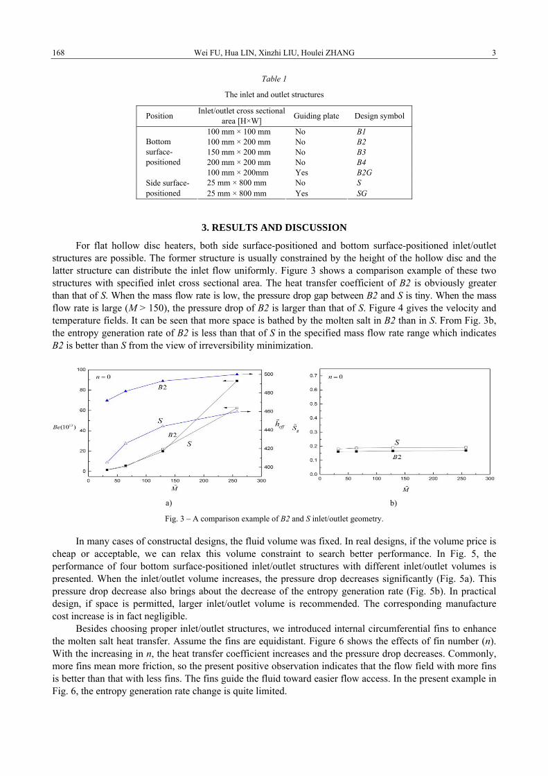
Wei FU, Hua LIN, Xinzhi LIU, Houlei ZHANG 3 168
Table 1
The inlet and outlet structures
Position Inlet/outlet cross sectional area [H×W] Guiding plate Design symbol
100 mm × 100 mm No B1 100 mm × 200 mm No B2 150 mm × 200 mm No B3 200 mm × 200 mm No B4
Bottom surface-positioned
100 mm × 200mm Yes B2G 25 mm × 800 mm No S Side surface-
positioned 25 mm × 800 mm Yes SG
3. RESULTS AND DISCUSSION
For flat hollow disc heaters, both side surface-positioned and bottom surface-positioned inlet/outlet structures are possible. The former structure is usually constrained by the height of the hollow disc and the latter structure can distribute the inlet flow uniformly. Figure 3 shows a comparison example of these two structures with specified inlet cross sectional area. The heat transfer coefficient of B2 is obviously greater than that of S. When the mass flow rate is low, the pressure drop gap between B2 and S is tiny. When the mass flow rate is large (M > 150), the pressure drop of B2 is larger than that of S. Figure 4 gives the velocity and temperature fields. It can be seen that more space is bathed by the molten salt in B2 than in S. From Fig. 3b, the entropy generation rate of B2 is less than that of S in the specified mass flow rate range which indicates B2 is better than S from the view of irreversibility minimization.
a) b)
Fig. 3 – A comparison example of B2 and S inlet/outlet geometry.
In many cases of constructal designs, the fluid volume was fixed. In real designs, if the volume price is cheap or acceptable, we can relax this volume constraint to search better performance. In Fig. 5, the performance of four bottom surface-positioned inlet/outlet structures with different inlet/outlet volumes is presented. When the inlet/outlet volume increases, the pressure drop decreases significantly (Fig. 5a). This pressure drop decrease also brings about the decrease of the entropy generation rate (Fig. 5b). In practical design, if space is permitted, larger inlet/outlet volume is recommended. The corresponding manufacture cost increase is in fact negligible.
Besides choosing proper inlet/outlet structures, we introduced internal circumferential fins to enhance the molten salt heat transfer. Assume the fins are equidistant. Figure 6 shows the effects of fin number (n). With the increasing in n, the heat transfer coefficient increases and the pressure drop decreases. Commonly, more fins mean more friction, so the present positive observation indicates that the flow field with more fins is better than that with less fins. The fins guide the fluid toward easier flow access. In the present example in Fig. 6, the entropy generation rate change is quite limited.

4 Constructal Degisn of Molten Salt Flow and Heat Transfer in Horizontal Hollow Disc-shaped Heaters 169
a)
b)
c)
d)
Fig. 4 – The velocity field (the central cross section in the thickness direction) and the temperature field (top surface) of B2 and S with n = 0 (M = 128.77): a) B2, velocity field; b) B2, temperature field; c) S, velocity field; d) S, temperature field.
a) b)
Fig. 5 – The effects of inlet/outlet volume.
Figure 7 presents the effects of fin pitch (represented by diameter D) for B2 with n = 1, where r = (D–D1)/(D2–D1). The effects of r on both flow and heat transfer are not obvious for the specified mass flow rate. When r = 0.125, the heat transfer coefficient and the entropy generation rate are a little bit higher. The effects of more fins with other flow rates can be analyzed similarly.
For both side surface-positioned and bottom surface-positioned inlet/outlet designs, the flow and heat transfer in the hollow disc can be further modified by introducing guiding plates. Figure 8 illustrates the effects of guiding plates. Both the heat transfer coefficient and pressure drop of B2G with guiding plates are greater than that of B2. This indicates that better heat transfer in the hollow disc is accompanied by the significantly enlarged inlet/outlet pressure drop due to smaller cross sectional area of the inlet/outlet structures induced by guiding plates. The performance of SG is also presented in Fig. 8. Seen in Fig. 8b, the entropy generation rates of B2G and B2 are nearly the same but larger than that of SG.

Wei FU, Hua LIN, Xinzhi LIU, Houlei ZHANG 5 170
a) b)
Fig. 6 – The effects of fin number.
a) b)
Fig. 7 – The effects of fin pitch.
a) b)
Fig. 8 – The effects of guiding plates.
In order to prevent salt solidification in the cold-start process, the pre-heating process with hot air as
the pre-heating medium should sustain until the minimum solid temperature Tmin is higher than the melting temperature (142°C or 415K for Hitec salt). After that, molten salt is pumped into the hollow discs of the heater. Figure 9 documents temperature rising curves of two designs in the cold-start process. The pre-heating time is about 390s for the design B2G with n = 3 and 720s for the design B2 with n = 0 respectively. The result shows that the enhanced heat transfer design also shortens the cold-start time efficiently. Based on the relationship between the air temperature Tair and the minimum solid temperature Tmin, the air temperature can be monitored for cold-start process control which is more convenient.
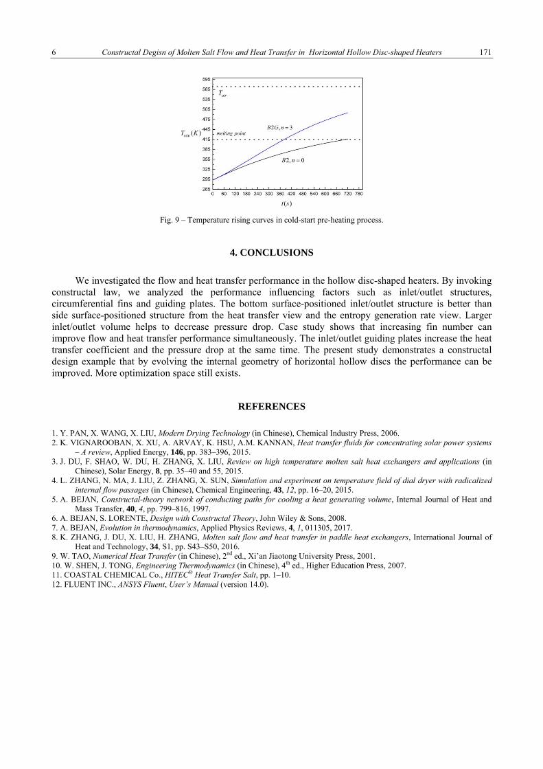
6 Constructal Degisn of Molten Salt Flow and Heat Transfer in Horizontal Hollow Disc-shaped Heaters 171
Fig. 9 – Temperature rising curves in cold-start pre-heating process.
4. CONCLUSIONS
We investigated the flow and heat transfer performance in the hollow disc-shaped heaters. By invoking constructal law, we analyzed the performance influencing factors such as inlet/outlet structures, circumferential fins and guiding plates. The bottom surface-positioned inlet/outlet structure is better than side surface-positioned structure from the heat transfer view and the entropy generation rate view. Larger inlet/outlet volume helps to decrease pressure drop. Case study shows that increasing fin number can improve flow and heat transfer performance simultaneously. The inlet/outlet guiding plates increase the heat transfer coefficient and the pressure drop at the same time. The present study demonstrates a constructal design example that by evolving the internal geometry of horizontal hollow discs the performance can be improved. More optimization space still exists.
REFERENCES
1. Y. PAN, X. WANG, X. LIU, Modern Drying Technology (in Chinese), Chemical Industry Press, 2006. 2. K. VIGNAROOBAN, X. XU, A. ARVAY, K. HSU, A.M. KANNAN, Heat transfer fluids for concentrating solar power systems
– A review, Applied Energy, 146, pp. 383–396, 2015. 3. J. DU, F. SHAO, W. DU, H. ZHANG, X. LIU, Review on high temperature molten salt heat exchangers and applications (in
Chinese), Solar Energy, 8, pp. 35–40 and 55, 2015. 4. L. ZHANG, N. MA, J. LIU, Z. ZHANG, X. SUN, Simulation and experiment on temperature field of dial dryer with radicalized
internal flow passages (in Chinese), Chemical Engineering, 43, 12, pp. 16–20, 2015. 5. A. BEJAN, Constructal-theory network of conducting paths for cooling a heat generating volume, Internal Journal of Heat and
Mass Transfer, 40, 4, pp. 799–816, 1997. 6. A. BEJAN, S. LORENTE, Design with Constructal Theory, John Wiley & Sons, 2008. 7. A. BEJAN, Evolution in thermodynamics, Applied Physics Reviews, 4, 1, 011305, 2017. 8. K. ZHANG, J. DU, X. LIU, H. ZHANG, Molten salt flow and heat transfer in paddle heat exchangers, International Journal of
Heat and Technology, 34, S1, pp. S43–S50, 2016. 9. W. TAO, Numerical Heat Transfer (in Chinese), 2nd ed., Xi’an Jiaotong University Press, 2001. 10. W. SHEN, J. TONG, Engineering Thermodynamics (in Chinese), 4th ed., Higher Education Press, 2007. 11. COASTAL CHEMICAL Co., HITEC® Heat Transfer Salt, pp. 1–10. 12. FLUENT INC., ANSYS Fluent, User’s Manual (version 14.0).
THE PUBLISHING HOUSE PROCEEDINGS OF THE ROMANIAN ACADEMY, Series A, OF THE ROMANIAN ACADEMY Special Issue/2018, pp. 172–177
SECOND LAW ANALYSIS AND CONSTRUCTAL DESIGN OF STIRLING ENGINE HEAT EXCHANGER (REGENERATOR)
FOR MEDIUM TEMPERATURE DIFFERENCE (MTD)
James A. Wills, Tunde Bello-Ochende** University of Cape Town, Department of Mechanical Engineering
Corresponding author: Tunde Bello-Ochende, E-mail: [email protected]*
Abstract. This paper presents an analysis into the effects that the regenerator length, regenerator matrix choice and dead-volume ratio have on medium temperature difference (MTD) Stirling engine performance. The Stirling engine has potential for use in the renewable energy industry and is suitable for use with low grade heat sources. The aim of the investigation is to give insight into the effects that the choice of regenerator properties and dead-volume ratio have on engine performance. The higher the effectiveness of the regenerator, the higher the thermal efficiency of the Stirling engine. Increasing the length of the regenerator increases the effectiveness, but results in an increased pressure drop. Decreasing the length results in a decreased pressure drop, but the heater and cooler loads increase decreasing engine performance. Therefore, there is an optimal regenerator length that gives optimal engine performance. In this paper, an engine of volume 1 000 cm3 is analyzed at four different MTD heater inlet temperatures, namely 150°C, 200°C, 250°C and 300°C. Quasi-steady flow conditions and finite source and sink heat capacity rates are assumed and the exergy analysis approach is used to optimize the configuration. Results show that for each source temperature and mesh type there is a regenerator length and dead-volume ratio that give optimal engine work output.
Key words: Stirling engine, Regenerator, Ideal adiabatic, Entropy generation, Optimization.
1. INTRODUCTION
Currently there is major concern over the future availability of fossil fuels and the effect that these fuels have on the environment. Renewable energy sources are currently considered the most effective solution to these problems [1]. The Stirling engine is suitable for use with renewable energy sources, has multi-fuel capabilities, is quiet, and efficient [2]. There are different orders of Stirling engine mathematical models used in the analysis of Stirling cycle machines [3], these approached vary widely in complexity and accuracy. Stirling engines are often categorized in terms of their heater wall temperature. Low temperature difference engines having a heater wall temperature of between 80 °C and 150 °C and medium temperature difference engines having a wall temperature of 150 °C to 400 °C [4].
There have been several efforts to optimize LTD and MTD engines, as these types of engines are of economic interest for use with cheaper non-concentrating solar collectors [5]. An analysis was presented in [6], which looked to analyze and optimize the performance of an LTD engine [7] using a new three component second order model. In [8], an exergetic, energetic and entropic analysis of the Stirling cycle was presented. The cycle was then optimized per these criteria. The same authors conducted a thermodynamic analysis of an LTD Stirling engine at steady state operation [9]. The result of the analysis was the optimal conditions for operation which is the minimum amount of exergy destruction or production of entropy and thus, minimization of operating cost. In [10], the effect of changing the heat transfer coefficients and temperature difference in the engine was investigated. The analysis in [11], looked at the effect of pressure loss and irreversible heat transfer and found that the maximum attainable efficiency is half of Carnot efficiency. The analysis presented in [12], optimized a mean temperature deferential solar Stirling engine with several loss mechanisms incorporated. Several investigations have been conducted into the effect of the regenerator on Stirling engine performance. The analysis presented by de Boer utilizes a first order model to

2 Second Law Optimisation of an MTD Stirling Engine Regenerator 173
optimize the regenerator, showing that the maximum attainable efficiency is half of the Carnot efficiency [13]. Another analysis looked at a 2-dimensional model of the regenerator, analyzing the different modes of temperature oscillation [14]. Additionally, the constructal law has been applied to regenerators to optimize flow architecture [15], and could be used to minimize temperature oscillations. Furthermore, there have also been several investigations into the effects of dead-volume on Stirling engine performance. The analysis conducted in [16], looked at the effect of dead-volume on the ideal isothermal model. This analysis found that dead-volume decreases the power output and efficiency of the engine, with the optimal dead-volume ratio being zero. However, as established in [17] the dead-volume ratio is an important design parameter that greatly affects the performance of real machines. There have been several authors who have emphasized the great importance of optimizing the global performance of a system by spreading the irreversibility between components [18].
This paper presents a dynamic model with finite source and sink heat capacity rates, pressure drops, irreversible heat transfer, and thermal conduction between the hot and cold components. The exergy analysis methodology is used to optimize the different variables. A 1 000 cm3 engine is optimized for maximum power output at 4 different MTD heater inlet temperatures with four different regenerator mesh types.
2. ANALYSIS
The following section briefly discusses the mathematical model of the irreversible Stirling engine which was used in the analysis, and the formulation of the objective function.
2.1. Stirling engine model The Stirling engine model used is the ideal-adiabatic model, developed by Urieli and Berchowitz [19].
The quasi-steady flow assumption is made and empirical relations are used to calculate the heat transfer and flow losses in the different heat exchangers. The relations proposed by [20] are used to calculate the regenerator effectiveness and pressure drop and the standard steady turbulent flow relations are used to calculate the heat transfer coefficients and frictions factors in the heater and cooler. These values are then used to calculate the rate of entropy generation which is an input into the objective function.
2.2. Objective function
The objective function was formulated using the exergy analysis approach, where exergy is defined the maximum amount of energy available to be converted to work. Combining the mathematical expressions for the first and second laws of thermodynamics gives equation 1, the exergy equation
geninout
i
n
i iSTSThmSThmQ
TTSTVPE
dtdW 00
00
0
1
000 )()(1)( −−−−+⎟⎟
⎠
⎞⎜⎜⎝
⎛−+−+−= ∑∑∑
=
. (1)
Rewriting equation 1 to describe the maximum net-work output of the Stirling engine yields equation 2, this equation incorporates the entropy generation rate in each component in the Stirling engine which is calculated using the empirical relations describing heat transfer and fluid flow in the engine. This equation is the objective function used to optimize the geometry, volume ratios and speed of the engine.
cooler
lossk
cb
kbk
rregeneratokb
hbrr
hk
hbkbp
heater
lossh
hb
ebhnetnet
TQ
dPPmRT
dPPmRdm
TTTTC
T
TQ
dPPmRTQW
⎥⎥⎦
⎤
⎢⎢⎣
⎡+⎟⎟
⎠
⎞⎜⎜⎝
⎛−
⎥⎥⎦
⎤
⎢⎢⎣
⎡⎟⎟⎠
⎞⎜⎜⎝
⎛+⎟⎟
⎠
⎞⎜⎜⎝
⎛−
⎥⎥⎦
⎤
⎢⎢⎣
⎡+⎟⎟
⎠
⎞⎜⎜⎝
⎛−=
∫
∫∫
∫
0
,0
0
0
,0
)()(ln)(
2
)()(ln)(
2)(ln
4
)()(ln)(
2
θθθθ
π
θθθθ
πθθ
π
θθθθ
π
. (2)

James A. WILLS, Tunde BELLO-OCHENDE 3 174
2.3. Method of solution
In the case of the ideal adiabatic model no closed form solution exists and it is therefore necessary to find the solution using an iterative method. To quickly and effectively find the solution, the 4th order Runge-Kutta method is used for the first 4 steps, following this the 4th order Adams-Bashforth method is used. The iterative scheme is run until convergence is reached between the start and end temperatures in the expansion and compression spaces. The heat transfer rates are then obtained, and using the empirical relations the effectiveness’s of the heat exchangers are calculated and used to calculate new heater and cooler temperatures. This is run continuously until convergence between the previous and current temperature is achieved.
3. NUMERICAL OPTIMISATION
3.1. Model parameters
The working fluid in the engine is assumed to be air and model parameters that are assumed to be constant are seen in table 1.
Table 1
Table of assumed model values
Symbol Description Value Vtot Total engine volume (cm3) 1000 α Phase difference (°) 90 Nh Number of heater and cooler tubes (-) 250 Nk Number of cooler tubes (-) 250 Ch Heat capacity rate of source (kJ/K) 0.25 Ck Heat capacity rate of sink (kJ/K) 0.25 Pmean Mean engine pressure (bar) 25
Four different regenerator mesh types are used and their respective properties are seen in Table 2.
Table 2
Table of regenerator wire netting dimensions [20]
Symbol Diameter (mm) Porosity (-) WN50 0.23 0.645 WN100 0.1 0.711 WN150 0.06 0.754 WN200 0.05 0.729
3.2. Optimization procedure
The model has five variables that are optimized at each specified dead-volume ratio. These variables are the length of regenerator to total heat exchanger length (Lr/L), the cooler and heater tube diameter (D), the ratio of heater length to cooler length (Lh/Lk), the swept volume ratio (Vc/Ve), and the engine speed. The objective function, which is the maximum net-work output is optimized in terms of the input variables at different dead-volume ratios using the Nelder-Mead algorithm.
4. RESULTS AND DISCUSSION
The following section presents the results of the numerical optimization: the maximum net-work output, optimal thermal efficiency, regenerator length and regenerator effectiveness are all plotted versus dead-volume ratio. Each figure has four plots, each plot representing a different heater inlet temperature which is in the range of medium temperature difference (MTD) source temperatures.
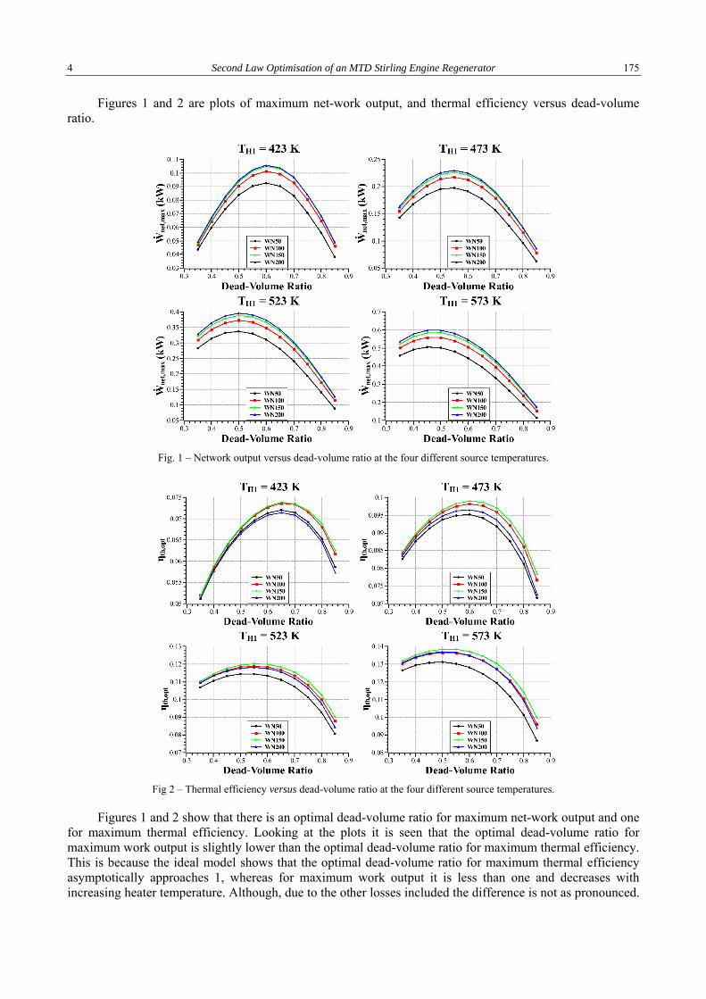
4 Second Law Optimisation of an MTD Stirling Engine Regenerator 175
Figures 1 and 2 are plots of maximum net-work output, and thermal efficiency versus dead-volume ratio.
Fig. 1 – Network output versus dead-volume ratio at the four different source temperatures.
Fig 2 – Thermal efficiency versus dead-volume ratio at the four different source temperatures.
Figures 1 and 2 show that there is an optimal dead-volume ratio for maximum net-work output and one for maximum thermal efficiency. Looking at the plots it is seen that the optimal dead-volume ratio for maximum work output is slightly lower than the optimal dead-volume ratio for maximum thermal efficiency. This is because the ideal model shows that the optimal dead-volume ratio for maximum thermal efficiency asymptotically approaches 1, whereas for maximum work output it is less than one and decreases with increasing heater temperature. Although, due to the other losses included the difference is not as pronounced.
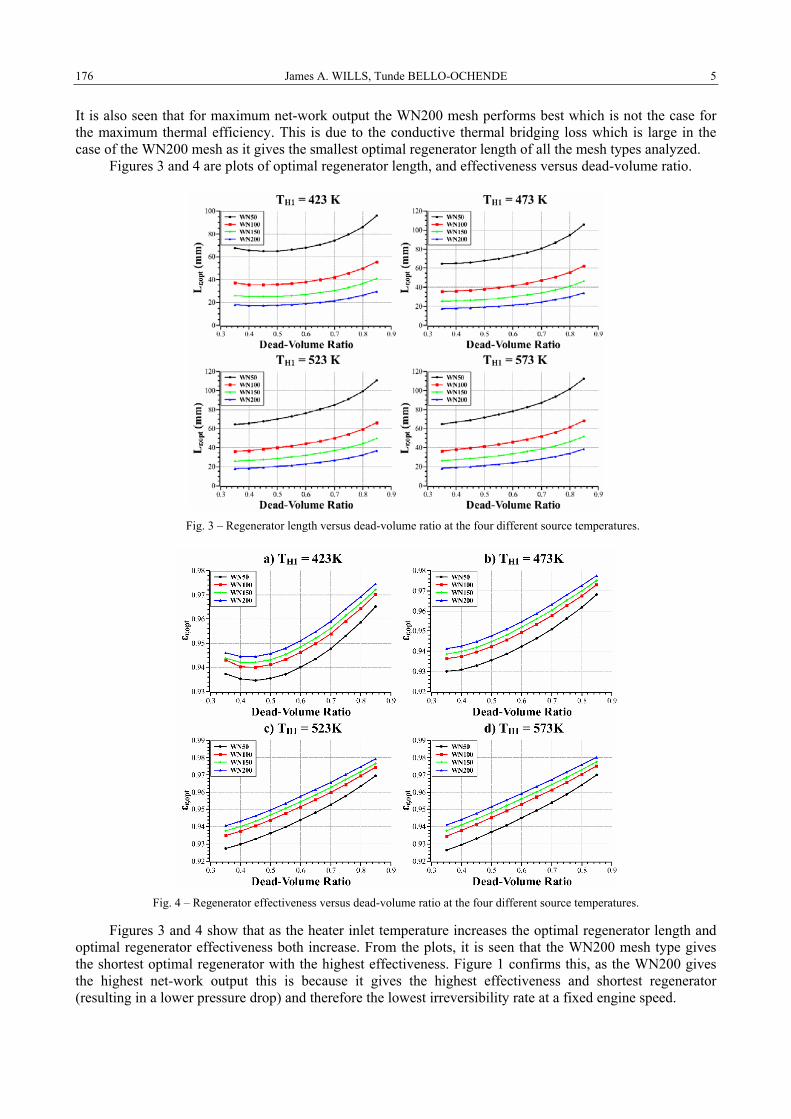
James A. WILLS, Tunde BELLO-OCHENDE 5 176
It is also seen that for maximum net-work output the WN200 mesh performs best which is not the case for the maximum thermal efficiency. This is due to the conductive thermal bridging loss which is large in the case of the WN200 mesh as it gives the smallest optimal regenerator length of all the mesh types analyzed.
Figures 3 and 4 are plots of optimal regenerator length, and effectiveness versus dead-volume ratio.
Fig. 3 – Regenerator length versus dead-volume ratio at the four different source temperatures.
Fig. 4 – Regenerator effectiveness versus dead-volume ratio at the four different source temperatures.
Figures 3 and 4 show that as the heater inlet temperature increases the optimal regenerator length and optimal regenerator effectiveness both increase. From the plots, it is seen that the WN200 mesh type gives the shortest optimal regenerator with the highest effectiveness. Figure 1 confirms this, as the WN200 gives the highest net-work output this is because it gives the highest effectiveness and shortest regenerator (resulting in a lower pressure drop) and therefore the lowest irreversibility rate at a fixed engine speed.
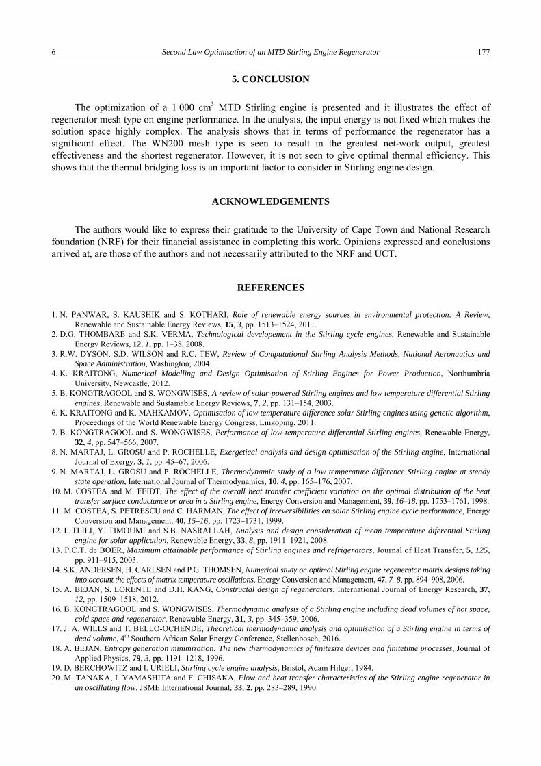
6 Second Law Optimisation of an MTD Stirling Engine Regenerator 177
5. CONCLUSION
The optimization of a 1 000 cm3 MTD Stirling engine is presented and it illustrates the effect of regenerator mesh type on engine performance. In the analysis, the input energy is not fixed which makes the solution space highly complex. The analysis shows that in terms of performance the regenerator has a significant effect. The WN200 mesh type is seen to result in the greatest net-work output, greatest effectiveness and the shortest regenerator. However, it is not seen to give optimal thermal efficiency. This shows that the thermal bridging loss is an important factor to consider in Stirling engine design.
ACKNOWLEDGEMENTS
The authors would like to express their gratitude to the University of Cape Town and National Research foundation (NRF) for their financial assistance in completing this work. Opinions expressed and conclusions arrived at, are those of the authors and not necessarily attributed to the NRF and UCT.
REFERENCES
1. N. PANWAR, S. KAUSHIK and S. KOTHARI, Role of renewable energy sources in environmental protection: A Review, Renewable and Sustainable Energy Reviews, 15, 3, pp. 1513–1524, 2011.
2. D.G. THOMBARE and S.K. VERMA, Technological developement in the Stirling cycle engines, Renewable and Sustainable Energy Reviews, 12, 1, pp. 1–38, 2008.
3. R.W. DYSON, S.D. WILSON and R.C. TEW, Review of Computational Stirling Analysis Methods, National Aeronautics and Space Administration, Washington, 2004.
4. K. KRAITONG, Numerical Modelling and Design Optimisation of Stirling Engines for Power Production, Northumbria University, Newcastle, 2012.
5. B. KONGTRAGOOL and S. WONGWISES, A review of solar-powered Stirling engines and low temperature differential Stirling engines, Renewable and Sustainable Energy Reviews, 7, 2, pp. 131–154, 2003.
6. K. KRAITONG and K. MAHKAMOV, Optimisation of low temperature difference solar Stirling engines using genetic algorithm, Proceedings of the World Renewable Energy Congress, Linkoping, 2011.
7. B. KONGTRAGOOL and S. WONGWISES, Performance of low-temperature differential Stirling engines, Renewable Energy, 32, 4, pp. 547–566, 2007.
8. N. MARTAJ, L. GROSU and P. ROCHELLE, Exergetical analysis and design optimisation of the Stirling engine, International Journal of Exergy, 3, 1, pp. 45–67, 2006.
9. N. MARTAJ, L. GROSU and P. ROCHELLE, Thermodynamic study of a low temperature difference Stirling engine at steady state operation, International Journal of Thermodynamics, 10, 4, pp. 165–176, 2007.
10. M. COSTEA and M. FEIDT, The effect of the overall heat transfer coefficient variation on the optimal distribution of the heat transfer surface conductance or area in a Stirling engine, Energy Conversion and Management, 39, 16–18, pp. 1753–1761, 1998.
11. M. COSTEA, S. PETRESCU and C. HARMAN, The effect of irreversibilities on solar Stirling engine cycle performance, Energy Conversion and Management, 40, 15–16, pp. 1723–1731, 1999.
12. I. TLILI, Y. TIMOUMI and S.B. NASRALLAH, Analysis and design consideration of mean temperature diferential Stirling engine for solar application, Renewable Energy, 33, 8, pp. 1911–1921, 2008.
13. P.C.T. de BOER, Maximum attainable performance of Stirling engines and refrigerators, Journal of Heat Transfer, 5, 125, pp. 911–915, 2003.
14. S.K. ANDERSEN, H. CARLSEN and P.G. THOMSEN, Numerical study on optimal Stirling engine regenerator matrix designs taking into account the effects of matrix temperature oscillations, Energy Conversion and Management, 47, 7–8, pp. 894–908, 2006.
15. A. BEJAN, S. LORENTE and D.H. KANG, Constructal design of regenerators, International Journal of Energy Research, 37, 12, pp. 1509–1518, 2012.
16. B. KONGTRAGOOL and S. WONGWISES, Thermodynamic analysis of a Stirling engine including dead volumes of hot space, cold space and regenerator, Renewable Energy, 31, 3, pp. 345–359, 2006.
17. J. A. WILLS and T. BELLO-OCHENDE, Theoretical thermodynamic analysis and optimisation of a Stirling engine in terms of dead volume, 4th Southern African Solar Energy Conference, Stellenbosch, 2016.
18. A. BEJAN, Entropy generation minimization: The new thermodynamics of finitesize devices and finitetime processes, Journal of Applied Physics, 79, 3, pp. 1191–1218, 1996.
19. D. BERCHOWITZ and I. URIELI, Stirling cycle engine analysis, Bristol, Adam Hilger, 1984. 20. M. TANAKA, I. YAMASHITA and F. CHISAKA, Flow and heat transfer characteristics of the Stirling engine regenerator in
an oscillating flow, JSME International Journal, 33, 2, pp. 283–289, 1990.
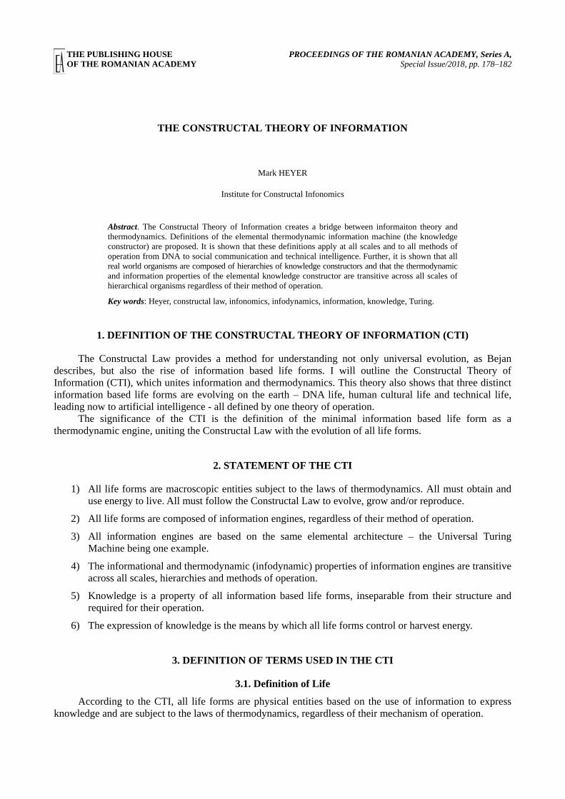
THE PUBLISHING HOUSE PROCEEDINGS OF THE ROMANIAN ACADEMY, Series A, OF THE ROMANIAN ACADEMY Special Issue/2018, pp. 178–182
THE CONSTRUCTAL THEORY OF INFORMATION
Mark HEYER
Institute for Constructal Infonomics
Abstract. The Constructal Theory of Information creates a bridge between informaiton theory and thermodynamics. Definitions of the elemental thermodynamic information machine (the knowledge constructor) are proposed. It is shown that these definitions apply at all scales and to all methods of operation from DNA to social communication and technical intelligence. Further, it is shown that all real world organisms are composed of hierarchies of knowledge constructors and that the thermodynamic and information properties of the elemental knowledge constructor are transitive across all scales of hierarchical organisms regardless of their method of operation.
Key words: Heyer, constructal law, infonomics, infodynamics, information, knowledge, Turing.
1. DEFINITION OF THE CONSTRUCTAL THEORY OF INFORMATION (CTI)
The Constructal Law provides a method for understanding not only universal evolution, as Bejan describes, but also the rise of information based life forms. I will outline the Constructal Theory of Information (CTI), which unites information and thermodynamics. This theory also shows that three distinct information based life forms are evolving on the earth – DNA life, human cultural life and technical life, leading now to artificial intelligence - all defined by one theory of operation.
The significance of the CTI is the definition of the minimal information based life form as a thermodynamic engine, uniting the Constructal Law with the evolution of all life forms.
2. STATEMENT OF THE CTI
1) All life forms are macroscopic entities subject to the laws of thermodynamics. All must obtain and use energy to live. All must follow the Constructal Law to evolve, grow and/or reproduce.
2) All life forms are composed of information engines, regardless of their method of operation.
3) All information engines are based on the same elemental architecture – the Universal Turing Machine being one example.
4) The informational and thermodynamic (infodynamic) properties of information engines are transitive across all scales, hierarchies and methods of operation.
5) Knowledge is a property of all information based life forms, inseparable from their structure and required for their operation.
6) The expression of knowledge is the means by which all life forms control or harvest energy.
3. DEFINITION OF TERMS USED IN THE CTI
3.1. Definition of Life
According to the CTI, all life forms are physical entities based on the use of information to express knowledge and are subject to the laws of thermodynamics, regardless of their mechanism of operation.

2 The Constructal Theory of Information 179
With this postulate, we can make a universal definition of life that integrates both information and thermodynamics:
1. A life form is any macroscopic, finite machine (knowledge constructor, as defined below) that can receive information from the environment, integrate it logically with memory (stored information) to synthesize knowledge to perform an action (express knowledge), to control or harvest energy in the environment and use that energy to perpetuate its survival.
2. The question of how a life form originates, operates or replicates is secondary. Size, complexity and method of operation are arbitrary. A life form can be DNA based, an object fabricated by humans, or may be a hybrid of life forms as with humans and their tools, cars and computers.
3. To continue living, any organism must increase exergy collected to greater than the exergy needed for equilibrium operation. In order to grow, evolve or reproduce – to morph – it must obtain additional exergy, as shown by the Constructal Law.
4. The communication of information (knowledge) between and among organisms is a common feature of life forms. Communication can be intimate, as among the cells in a body, or extended, as in a flock of birds, or a human family or organization. With communication, the enclosing hierarchical organism becomes a knowledge constructor itself, inheriting the energetic drives of its members.
3.2. The three information families of life
All life forms are based on the same information and thermodynamic (infodynamic) principles. From this perspective, we can identify three great families of life. For brevity, these are provided without comment:
1. DNA Life
2. Human Social Life Forms (families, tribes, religions, companies, states, etc)
3. Machine Life (machines with embedded knowledge or intelligence).
3.3. Definition of information
Information is energy received by a sensor and passed to the processor of a sentient receiver (knowledge constructor).
Information is relevant only if the receiver already possesses stored information establishing a context for recognition of the received energy as information to be incorporated into knowledge.
Obviously, information can be stored in various ways, but it only becomes information if it can be received and understood by a sentient receiver. For example, a USB storage device may hold considerable information – if you have a computer to read it. A person without a computer could never prove that the device did or did not contain information.
The term information is often confused with the more accurate term “configuration” when used to describe processes in nature. Matter itself does not “contain” information.
3.4. Definition of knowledge
Knowledge is a physical and operational property of all life forms. Knowledge is an integral part of any knowledge constructor. Knowledge is created by the "processor" that receives information from an input (sensor), integrates it logically with memory, creates knowledge, and potentiates an action at the output (actuator). Knowledge can only be proven by observing its expression.
Knowledge is inseparable from the knowledge constructor that possesses it. This is a statement of the Completeness Theorem, described elsewhere.
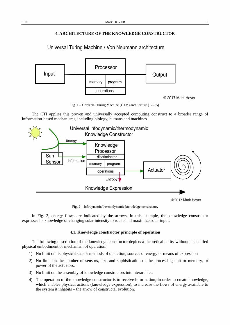
Mark HEYER 3 180
4. ARCHITECTURE OF THE KNOWLEDGE CONSTRUCTOR
Fig. 1 – Universal Turing Machine (UTM) architecture [12–15].
The CTI applies this proven and universally accepted computing construct to a broader range of information-based mechanisms, including biology, humans and machines.
Fig. 2 – Infodynamic/thermodynamic knowledge constructor.
In Fig. 2, energy flows are indicated by the arrows. In this example, the knowledge constructor expresses its knowledge of changing solar intensity to rotate and maximize solar input.
4.1. Knowledge constructor principle of operation
The following description of the knowledge constructor depicts a theoretical entity without a specified physical embodiment or mechanism of operation:
1) No limit on its physical size or methods of operation, sources of energy or means of expression
2) No limit on the number of sensors, size and sophistication of the processing unit or memory, or power of the actuators.
3) No limit on the assembly of knowledge constructors into hierarchies.
4) The operation of the knowledge constructor is to receive information, in order to create knowledge, which enables physical actions (knowledge expression), to increase the flows of energy available to the system it inhabits – the arrow of constructal evolution.
4 The Constructal Theory of Information 181
• Sensor – Mechanism for receiving energy from the environment.
• Discriminator – Input to the knowledge processor. A method to “recognize” the sensor’s energy input. This generally requires that the input be compared to a value in memory. ed.
• Memory – A means by which to recognize new (or unknown) inputs and to create knowledge about what action is to be taken in response to an input.
• Processor – At minimum, a logic unit to compare input with memory and decide on the action to be taken. The processor can have unlimited complexity, manage multiple sensors and actuators and subordinate knowledge constructors.
• Actuator – A physical mechanism used to control energy in the environment under the direction of the processor, e.g., a propeller, valve, switch, pump, etc.
4.2. Operation of the knowledge constructor
The operation of all knowledge constructors (as infodynamic/thermodynamic engines) is dissipative. Therefore they need a source of energy in excess of the exergy required for operation, to account for entropy production, per the second law.
In order to grow, evolve and reproduce, the knowledge constructor must achieve access to exergy above what is required for survival. It must use this extra exergy to morph and evolve its channels (sensors, processor and actuators), to increase the flow of energy through it, or the organism it is part of, in accordance with the Constructal Law.
There is no limit on the size or complexity of a single knowledge constructor. It may be microscopic, as in intracellular mechanisms, or the size of a house or the entire earth itself. It can have any number of sensors and/or actuators.
4.3. Knowledge constructor hierarchies
Hierarchies of knowledge constructors may form to maximize their shared capabilities to increase exergy access for the benefit of the group.
There is no limit to the size or function of knowledge constructor hierarchies. Communication allows the formation of virtual knowledge constructors even though the individuals may be distant, e.g., a flock of birds or a company.
The infodynamic and thermodynamic principles of the elemental knowledge constructor are transitive across all hierarchies, scales or methods of operation.
5. PROOF OF THE CTI
5.1. Proof of the knowledge constructor
1. The Turing proof of computability (Universal Turing machine) establishes the definition of the universal information machine.
2. All information-based life forms are composed of information machines, defined here as knowledge constructors.
3. All knowledge constructors are physical entities and thus governed by the laws of thermodynamics The complete proof is provided in the full text of this paper, available on request.
5.2. Proof of knowledge constructors in biology
A key part of the proof of the CTI is demonstrating that the Turing architecture operates in biological settings. This has been amply demonstrated in the literature. This proof is available in the full paper.

Mark HEYER 5 182
6. CONCLUSION
In this paper, I have shown that all forms of life share a common information and knowledge principle of operation, exemplified by the Turing proof of computability and the architecture of the Universal Turing Machine. Further, I have shown that all existential life forms are governed by the second law and the Constructal Law.
Therefore, I have defined the “knowledge constructor” as a physical entity that incorporates the Turing architecture and is governed by the laws of thermodynamics. This definition can be shown to be the fundamental basis of all life forms, regardless of their mechanism of operation.
Life forms can therefore be defined within the realms of DNA, human social life forms and machines. It provides a foundation for understanding and predicting the evolution of composite, or hybrid life forms.
The CTI also demonstrates that knowledge constructors can and do form hierarchies, and that their method of operation is transitive across all scales of hierarchy. Thus, a human being is a hierarchy of trillions of cells, bacteria, yeast and fungi, yet the human is driven by the same principle of operation as each of its parts.
This paper has not dealt explicitly with the issue of dependence, which is operational in all hierarchies. Dependence is the root of cooperation and specialization among the members of a hierarchical organization and gives rise to behaviors and advanced social behavior.
The author can be reached at: [email protected]. The complete paper is available on request.
REFERENCES*
1. https://en.wikipedia.org/wiki/Constructal_law 2. https://en.wikipedia.org/wiki/Von_Neumann_universal_constructor 3. WALKER, Sara Imari, Top-Down Causation and the Rise of Information in the Emergence of Life, Information, 5, pp. 424–439,
2015. 4. https://www.nasa.gov/vision/universe/starsgalaxies/life%27s_working_definition.html 5. CLELAND, C.E. & CHYBA, C.F. Orig Life Evol Biosph, 32, 387, doi:10.1023/A:1020503324273, 2002. 6. http://www.dictionary.com/browse/life 7. https://plato.stanford.edu/entries/knowledge-analysis/ 8. https://en.wikipedia.org/wiki/Von_Neumann_universal_constructor 9. https://www.youtube.com/watch?v=GMYr-H70VYo&feature=youtu.be, 2013. 10. Through the Wormhole – Did God Create Evolution? – Constructal theory. 11. BEJAN, Adrian, ERREREA, Marcelo, Wealth Inequality: The physics basis, J. of Applied Physics 121, 2017. 12. http://constructalinfonomics.org/infonomics-thermodynamics-and-trump/ 13. https://en.wikipedia.org/wiki/Universal_Turing_machine 14. http://people.cs.uchicago.edu/~odonnell/Teacher/Courses/UChicago/CMSC31100/UTM.pdf 15. http://www.alanturing.net/turing_archive/pages/Reference%20Articles/What%20is%20a%20Turing%20Machine.html 16. http://blog.wolfram.com/2007/10/24/the-prize-is-won-the-simplest-universal-turing-machine-is-proved/ 17. https://en.wikipedia.org/wiki/DNA_computing 18. https://www.newscientist.com/article/2124907-recoded-organism-paves-way-to-new-genetic-language-of-life/ 19. K. XIE, G. FOX E., J. LIU, C. LYU, J.C. LEE C., H. KUANG, S. JACOBS, M. LI, T. LIU, S. SONG, J.Z. TSIEN, Brain
Computation is Organized via Power-of-Two-Based Permutation Logic, Frontiers in Systems Neuroscience, 10.3389/ fnsys.2016.00095, 2016.
20. http://journal.frontiersin.org/article/10.3389/fnsys.2016.00095
* Many of the references below are included in the original paper and do not appear in this abbreviated version. They are included here for completeness.
THE PUBLISHING HOUSE PROCEEDINGS OF THE ROMANIAN ACADEMY, Series A, OF THE ROMANIAN ACADEMY Special Issue/2018, pp. 183–188
GEOMETRIC OPTIMIZATION OF A TUBE BANK HEAT EXCHANGER IN A SLOW MOVING FREE STREAM
Alex J. FOWLER University of Massachusetts Dartmouth
Mechanical Engineering Department North Dartmouth, MA, USA
Corresponding author: Alex FOWLER, E-mail: [email protected]
Abstract. This paper reports the results of a computational optimization study performed on a tube bank heat exchanger that is immersed in a low velocity free stream. The stream in this work is unconstrained such that the fluid flow that is intended to provide cooling or heating to the tube bank may be diverted away from the heat exchanger by the presence of the tube bank itself – that is the fluid may pass around the outside of the tube bank rather than through it due to pressure increases that may occur at the entry region of the tube bank. In the low Reynolds number flow regime it is shown that this effect can be significant. Optimization is performed using finite element simulations of incompressible flow through tube banks subject to a maximum volume constraint. Optimization parameters include tube diameter, tube number and the geometric position of the tubes within the specified volume. It is shown that geometric optimization in this regime leads to heat exchanger geometries in which the positioning of the tubes in the entrance region results in increased flow capture within the heat exchanger volume. Such geometric arrangements are shown to lead to increases in heat transfer rates of 20% or more relative to traditional geometric arrangements.
Key words: Heat exchanger, Optimization, Computational heat transfer.
1. INTRODUCTION
This paper presents preliminary studies aimed at determining the optimum geometry for a heat exchanger such that it maximizes heat transfer to the surrounding fluid when subject to a volume constraint. The new aspect of the current work relative to earlier studies is that in this work the heat exchanger is assumed to occupy a space in which the fluid flow that bathes the heat exchanger is free to bypass the heat exchanger as a result of pressure increases caused by the presence of the heat exchanger itself.
Optimization of heat exchangers became of increased interest in the 1990’s with the advent of high performance computer chips that needed to be cooled within tight volume constraints. The demand for increased cooling density has led to the exploration and development of many new cooling technologies such as micro-heat sinks, heat pipes and micro-channel cooling [1], but an interest also developed in determining the optimal geometries for classic heat exchanger designs.
Extensive studies aimed at the geometric optimization of shell and tube, plate and counterflow heat exchangers have been undertaken in which up to seven different geometric design variables have been used to optimize heat exchangers for minimum operating cost, minimum entropy generation, minimum exergy destruction, minimum volumes and other criteria [2–16]. In all of these studies, however, the fluid in the flow field is forced through the heat exchanger. Pressure drop in the fluid is often included either indirectly as it affects operating costs or directly as a parameter, but the flow in these systems is not free to avoid the heat exchanger entirely as inlet pressure increases.
The current study follows more closely a series of optimization studies that focused on optimizing the geometry of single channels to maximize heat transfer for a specified pressure drop within each channel. Numerous geometric parameters have been optimized in studies of this type including channel width, fin shape (tube, plate, elliptical, etc.) and arrangement of fins within the channel [17–22]. Single channel optimization is a valid surrogate for optimization of an entire heat exchanger when the width of the heat
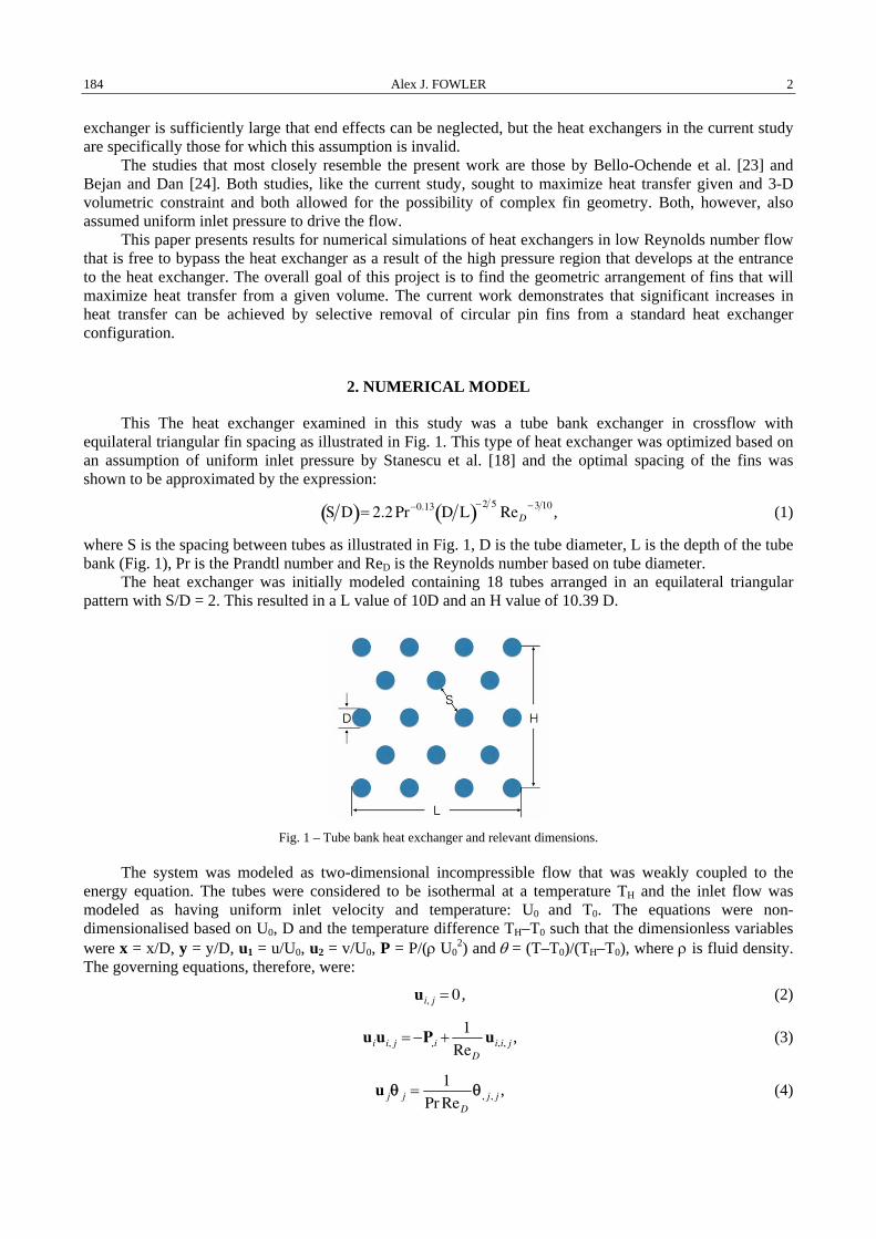
Alex J. FOWLER 2 184
exchanger is sufficiently large that end effects can be neglected, but the heat exchangers in the current study are specifically those for which this assumption is invalid.
The studies that most closely resemble the present work are those by Bello-Ochende et al. [23] and Bejan and Dan [24]. Both studies, like the current study, sought to maximize heat transfer given and 3-D volumetric constraint and both allowed for the possibility of complex fin geometry. Both, however, also assumed uniform inlet pressure to drive the flow.
This paper presents results for numerical simulations of heat exchangers in low Reynolds number flow that is free to bypass the heat exchanger as a result of the high pressure region that develops at the entrance to the heat exchanger. The overall goal of this project is to find the geometric arrangement of fins that will maximize heat transfer from a given volume. The current work demonstrates that significant increases in heat transfer can be achieved by selective removal of circular pin fins from a standard heat exchanger configuration.
2. NUMERICAL MODEL
This The heat exchanger examined in this study was a tube bank exchanger in crossflow with equilateral triangular fin spacing as illustrated in Fig. 1. This type of heat exchanger was optimized based on an assumption of uniform inlet pressure by Stanescu et al. [18] and the optimal spacing of the fins was shown to be approximated by the expression:
S D( )= 2.2 Pr−0.13 D L( )−2 5ReD
−3 10 , (1)
where S is the spacing between tubes as illustrated in Fig. 1, D is the tube diameter, L is the depth of the tube bank (Fig. 1), Pr is the Prandtl number and ReD is the Reynolds number based on tube diameter.
The heat exchanger was initially modeled containing 18 tubes arranged in an equilateral triangular pattern with S/D = 2. This resulted in a L value of 10D and an H value of 10.39 D.
Fig. 1 – Tube bank heat exchanger and relevant dimensions.
The system was modeled as two-dimensional incompressible flow that was weakly coupled to the energy equation. The tubes were considered to be isothermal at a temperature TH and the inlet flow was modeled as having uniform inlet velocity and temperature: U0 and T0. The equations were non-dimensionalised based on U0, D and the temperature difference TH–T0 such that the dimensionless variables were x = x/D, y = y/D, u1 = u/U0, u2 = v/U0, P = P/(ρ U0
2) and θ = (T–T0)/(TH–T0), where ρ is fluid density. The governing equations, therefore, were:
ui, j = 0 , (2)
uiui, j = −P,i + 1
ReD
ui,i, j , (3)
u jθ j = 1
Pr ReD
θ, j, j , (4)
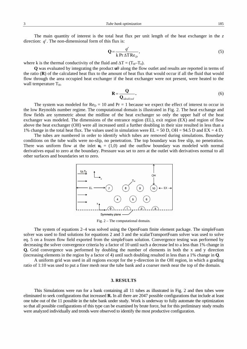
3 Tube bank optimization 185
The main quantity of interest is the total heat flux per unit length of the heat exchanger in the z direction: ′ q . The non-dimensional form of this flux is:
Q = ′ q
k Pr ΔTReD
, (5)
where k is the thermal conductivity of the fluid and ΔT = (TH–T0). Q was evaluated by integrating the product uθ along the flow outlet and results are reported in terms of
the ratio (R) of the calculated heat flux to the amount of heat flux that would occur if all the fluid that would flow through the area occupied heat exchanger if the heat exchanger were not present, were heated to the wall temperature TH.
R = QQidealized
. (6)
The system was modeled for ReD = 10 and Pr = 1 because we expect the effect of interest to occur in the low Reynolds number regime. The computational domain is illustrated in Fig. 2. The heat exchange and flow fields are symmetric about the midline of the heat exchanger so only the upper half of the heat exchanger was modeled. The dimensions of the entrance region (EL), exit region (EX) and region of flow above the heat exchanger (OH) were all increased until a further doubling in their size resulted in less than a 1% change in the total heat flux. The values used in simulation were EL = 50 D, OH = 94.5 D and EX = 4 D.
The tubes are numbered in order to identify which tubes are removed during simulations. Boundary conditions on the tube walls were no-slip, no penetration. The top boundary was free slip, no penetration. There was uniform flow at the inlet ui = (1,0) and the outflow boundary was modeled with normal derivatives equal to zero at the boundary. Pressure was set to zero at the outlet with derivatives normal to all other surfaces and boundaries set to zero.
Fig. 2 – The computational domain.
The system of equations 2–4 was solved using the OpenFoam finite element package. The simpleFoam solver was used to find solutions for equations 2 and 3 and the scalarTransportFoam solver was used to solve eq. 5 on a frozen flow field exported from the simpleFoam solution. Convergence testing was performed by decreasing the solver convergence criteria by a factor of 10 until such a decrease led to a less than 1% change in Q. Grid convergence was performed by doubling the number of elements in both the x and y direction (increasing elements in the region by a factor of 4) until such doubling resulted in less than a 1% change in Q.
A uniform grid was used in all regions except for the y-direction in the OH region, in which a grading ratio of 1:10 was used to put a finer mesh near the tube bank and a coarser mesh near the top of the domain.
3. RESULTS
This Simulations were run for a bank containing all 11 tubes as illustrated in Fig. 2 and then tubes were eliminated to seek configurations that increased R. In all there are 2047 possible configurations that include at least one tube out of the 11 possible in the tube bank under study. Work is underway to fully automate the optimization so that all possible configurations of this type can be examined by brute force, but for this preliminary study results were analyzed individually and trends were observed to identify the most productive configuration.
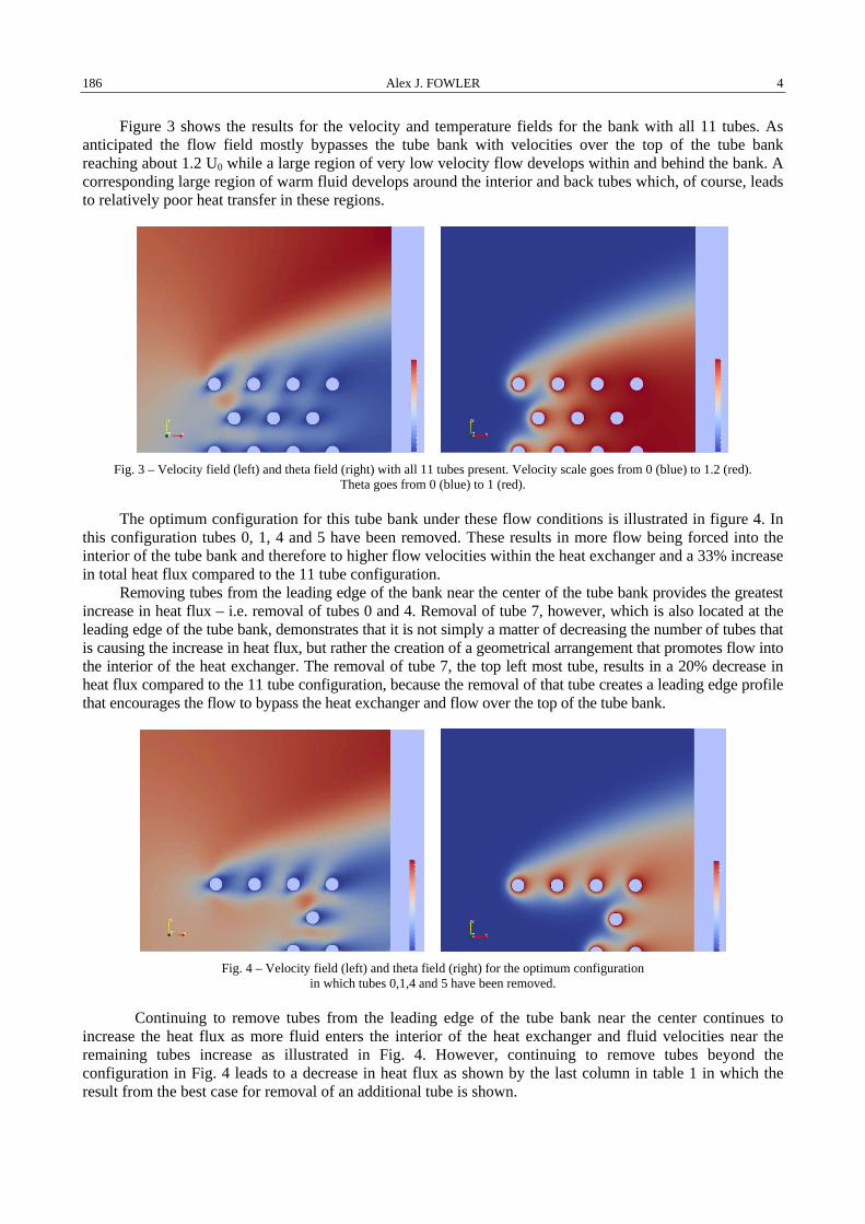
Alex J. FOWLER 4 186
Figure 3 shows the results for the velocity and temperature fields for the bank with all 11 tubes. As anticipated the flow field mostly bypasses the tube bank with velocities over the top of the tube bank reaching about 1.2 U0 while a large region of very low velocity flow develops within and behind the bank. A corresponding large region of warm fluid develops around the interior and back tubes which, of course, leads to relatively poor heat transfer in these regions.
Fig. 3 – Velocity field (left) and theta field (right) with all 11 tubes present. Velocity scale goes from 0 (blue) to 1.2 (red).
Theta goes from 0 (blue) to 1 (red).
The optimum configuration for this tube bank under these flow conditions is illustrated in figure 4. In this configuration tubes 0, 1, 4 and 5 have been removed. These results in more flow being forced into the interior of the tube bank and therefore to higher flow velocities within the heat exchanger and a 33% increase in total heat flux compared to the 11 tube configuration.
Removing tubes from the leading edge of the bank near the center of the tube bank provides the greatest increase in heat flux – i.e. removal of tubes 0 and 4. Removal of tube 7, however, which is also located at the leading edge of the tube bank, demonstrates that it is not simply a matter of decreasing the number of tubes that is causing the increase in heat flux, but rather the creation of a geometrical arrangement that promotes flow into the interior of the heat exchanger. The removal of tube 7, the top left most tube, results in a 20% decrease in heat flux compared to the 11 tube configuration, because the removal of that tube creates a leading edge profile that encourages the flow to bypass the heat exchanger and flow over the top of the tube bank.
Fig. 4 – Velocity field (left) and theta field (right) for the optimum configuration
in which tubes 0,1,4 and 5 have been removed.
Continuing to remove tubes from the leading edge of the tube bank near the center continues to increase the heat flux as more fluid enters the interior of the heat exchanger and fluid velocities near the remaining tubes increase as illustrated in Fig. 4. However, continuing to remove tubes beyond the configuration in Fig. 4 leads to a decrease in heat flux as shown by the last column in table 1 in which the result from the best case for removal of an additional tube is shown.
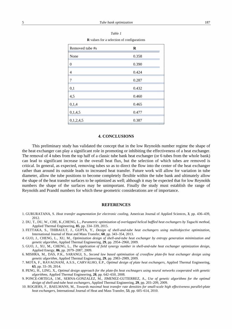
5 Tube bank optimization 187
Table 1
R values for a selection of configurations
Removed tube #s R
None 0.358
0 0.390
4 0.424
7 0.287
0,1 0.432
4,5 0.460
0,1,4 0.465
0,1,4,5 0.477
0,1,2,4,5 0.387
4. CONCLUSIONS
This preliminary study has validated the concept that in the low Reynolds number regime the shape of the heat exchanger can play a significant role in promoting or inhibiting the effectiveness of a heat exchanger. The removal of 4 tubes from the top half of a classic tube bank heat exchanger (or 6 tubes from the whole bank) can lead to significant increase in the overall heat flux, but the selection of which tubes are removed is critical. In general, as expected, removing tubes so as to direct the flow into the center of the heat exchanger rather than around its outside leads to increased heat transfer. Future work will allow for variation in tube diameter, allow the tube positions to become completely flexible within the tube bank and ultimately allow the shape of the heat transfer surfaces to be optimized as well; although it may be expected that for low Reynolds numbers the shape of the surfaces may be unimportant. Finally the study must establish the range of Reynolds and Prandtl numbers for which these geometric considerations are of importance.
REFERENCES
1. GURURATANA, S. Heat transfer augmentation for electronic cooling, American Journal of Applied Sciences, 3, pp. 436–439, 2012.
2. DU, T., DU, W., CHE, K.,CHENG, L., Parametric optimization of overlapped helical baffled heat exchangers by Taguchi method, Applied Thermal Engineering, 85, pp. 334–339, 2015.
3. FETTAKA, S., THIBAULT, J., GUPTA, Y., Design of shell-and-tube heat exchangers using multiobjective optimization, International Journal of Heat and Mass Transfer, 60, pp. 343–354, 2013.
4. GUO, J., CHENG, L., XU, M., Optimization design of shell-and-tube heat exchanger by entropy generation minimization and genetic algorithm, Applied Thermal Engineering, 29, pp. 2954–2960, 2009.
5. GUO, J., XU, M., CHENG, L., The application of field synergy number in shell-and-tube heat exchanger optimization design, Applied Energy, 86, pp. 2079–2087, 2009.
6. MISHRA, M., DAS, P.K., SARANGI, S., Second law based optimisation of crossflow plate-fin heat exchanger design using genetic algorithm, Applied Thermal Engineering, 29, pp. 2983–2989, 2009.
7. MOTA, F., RAVAGNANI, A.S.S., CARVALHO, E.P., Optimal design of plate heat exchangers, Applied Thermal Engineering, 63, pp. 33–39, 2014.
8. PENG, H., LING, X., Optimal design approach for the plate-fin heat exchnagers using neural networks cooperated with genetic algorithms, Applied Thermal Engineering, 28, pp. 642–650, 2008.
9. PONCE-ORTEGA, J.M., SERNA-GONZALEZ, M., JIMENEZ-GUTIERREZ, A., Use of genetic algorithms for the optimal design of shell-and-tube heat exchangers, Applied Thermal Engineering, 29, pp. 203–209, 2009.
10. ROGIERS, F., BAELMANS, M., Towards maximal heat transfer rate densities for small-scale high effectiveness parallel-plate heat exchangers, International Journal of Heat and Mass Transfer, 53, pp. 605–614, 2010.

Alex J. FOWLER 6 188
11. VARGAS, J.V.C., BEJAN, A., Integrative thermodynamic optimization of the environmental control system of an aircraft, International Journal of Heat and Mass Transfer, 44, pp. 3907–3917, 2001.
12. VARGAS, J.V.C., BEJAN, A., Thermodynamic optimization of finned crossflow heat exchangers for aircraft environmental control systems, International Journal of Heat and Fluid Flow, 22, pp. 657–665, 2001.
13. VARGAS, J.V.C., BEJAN, A., SIEMS, D.L., Integrative thermodynamic optimization of the crossflow heat exchanger for an aircraft environmental control system, Journal of Heat Transfer, 123, pp. 760–769, 2001.
14. XIE, G.N., SUNDEN, B., WANG, Q.W., Optimization of compact heat exchangers by a genetic algorithm, Applied Thermal Engineering, 28, pp. 895–906, 2008.
15. ZAREA, H., KASHKOOLI, M., MEHRYAN, A.M., SAFFARIAN, R., BEHEGHANI, E.N., Optimal design of plate-fin heat exchangers by a Bees algorithm, Applied Thermal Engineering, 69, pp. 267–277, 2014.
16. ZHOU, Y., ZHU, L., YU, J, LI, Y., Optimization of plate-fin heat exchangers by minimizing specific entropy generation rate, International Journal of Heat and Mass Transfer, 78, pp. 942–946, 2014.
17. BEJAN, A., MOREGA, A., Optimal array of pin fins and plate fins in laminar forced convection, Journal of Heat Transfer, 115, pp. 75–83, 1993.
18. STANESCU, G., FOWLER, A.J., BEJAN, A., The optimal spacing of cylinders in free-stream cross flow forced convection, International Journal of Heat and Mass Transfer, 39, pp. 311–317, 1996.
19. FOWLER, A.J., LEDEZMA, G.A., BEJAN, A., Optimal geometric arrangement of staggered plates in forced convection, International Journal of Heat and Mass Transfer, 40, pp. 1795–1805, 1997.
20. MATOS, R.S., VARGAS, J.V.C., LAURSEN, T.A., BEJAN, A., Optimally staggered finned circular and elliptic tubes in forced convection, International Journal of Heat and Mass Transfer, 47, pp. 1347–1359, 2004.
21. MATOS, R.S., LAURSEN, T.A., VARGAS, J.V.C., BEJAN, A., Three-dimensional optimization of staggered finned circular and elliptic tubes in forced convection, International journal of Thermal Sciences, 43, pp. 477–487, 2004.
22. WANG, H., LIU, Y., YANG, P., WU, R., HE, Y., Parametric study and optimization of H-type finned tube heat exchangers using Taguchi method, Applied Thermal Engineerimg, 103, pp. 128–138, 2016.
23. BELLO-OCHENDE, T., MEYER, J.P., DIRKER, J., Three-dimensional multi-scale plate assembly for maximum heat transfer rate density, International Journal of Heat and Mass Transfer, 53, pp. 586–593, 2010.
24. BEJAN, A., DAN, N., Constructal trees of convective fins, Journal of Heat Transfer, 121, pp. 675–682, 1999.
THE PUBLISHING HOUSE PROCEEDINGS OF THE ROMANIAN ACADEMY, Series A, OF THE ROMANIAN ACADEMY Special Issue/2018, pp. 189–194
SCALE ANALYSIS AND ASYMPTOTIC SOLUTION FOR NATURAL CONVECTION OVER A HEATED FLAT PLATE AT HIGH PRANDTL NUMBERS
Olayinka O. ADEWUMI1, Andrew ADEBUSOYE1, Adetunji ADENIYAN2, Nkem OGBONNA3, Ayowole A. OYEDIRAN1
1 University of Lagos, Department of Mechanical Engineering, Nigeria
2 University of Lagos, Department of Mathematics, Nigeria
3 Michael Okpara University of Agriculture, Umudike, Department of Mathematics, Nigeria Corresponding author: Olayinka O. ADEWUMI, E-mail: [email protected]
Abstract. This study presents a free convection flow over a heated flat plate using Bejan’s method of scale analysis for balancing forces. For Newtonian fluids of large Prandtl numbers, two different layers which are the thermal and velocity boundary layers exist. The thermal boundary layer is thinner than the velocity boundary layer. The method of matched asymptotic expansion is used to obtain the velocity and temperature within the two layers and these quantities are then matched at the interface. A 5–5 matching is used to obtain both inner and outer solutions for velocity and temperature. A natural small parameter in this problem is the inverse of the square root of the Prandtl number multiplying the highest derivative. In the Bejan formulation for large Prandtl number flows, the two dimensionless quantities that emerge are the Rayleigh and Prandtl numbers as opposed to the Grashof and Prandtl numbers obtained in previous works. The results of velocities, temperature, shear stress and Nusselt number presented in this study are for fluids that have Prandtl numbers ranging 10 to 100,000. The Nusselt number predicted as Prandtl number goes to infinity, approaches the same asymptote as in previous works, while there's about 30% difference in the skin friction predicted when the differences in scaling used are not taken into consideration.
Key words: Large Prandtl number, Scale analysis, Asymptotic expansion, Boundary layer, Free convection.
1. INTRODUCTION
Considerable efforts have been expended on the solution of free convection flows of a steady, viscous, heat conducting, and incompressible fluid near a heated vertical surface. This type of flow has application in many industrial and engineering processes, such as shutdown of high temperature high pressure flows in the oil and gas industry, cooling of reactor walls, condensation processes, heat exchangers and other electronics components. On account of its technological implications, accurate prediction of the skin friction on the heated wall as well as heat transfer rates near and far from the wall is highly desirable. Starting with the work of Ostrach [1], boundary layer flows due to free convection have been studied both theoretically and experimentally by many researchers [1–7]. Most of these works considered moderate Prandtl numbers or moderate Grashof numbers. The boundary layer solutions considered flows only in a narrow zone, by using similarity solution to reduce the partial differential equations to a set of nonlinear ordinary differential equations, and were solved numerically. Some contributors used the method of matched asymptotic expansions to solve the similarity equations, some considered the inverse of Grashof’s number as the small parameter while other investigators used inverse of square root of Prandtl number as the small parameter or the Prandtl number for small Prandtl number flows. Bejan [4] was able to compare the dominant forces for both low and high Prandtl number flows. Naturally, two dimensionless parameters arose and these are the Prandtl and the Rayleigh numbers. In this study, high Prandtl number flows are considered using the scaling laws of Bejan. Results obtained for Prandtl numbers as high as 100,000 are compared with the work of Kuiken [5], who rescaled Ostrach’s equations, and also with the analytical investigation by Bachiri & Bouabdallah [6, 7] who used Bejan’s scale analysis with a different solution method.
Olayinka O. ADEWUMI, Andrew ADEBUSOYE, Adetunji ADENIYAN, Nkem OGBONNA, Ayowole A. OYEDIRAN 2 190
2. PHYSICAL MODEL
Consider a hot, semi-infinite vertical plate of temperature Tw immersed in a cold fluid of temperature T∞, with the vertical plate aligned along the y-axis in a Cartesian coordinate system. The fluid is assumed to be heat conducting Newtonian, steady, viscous, and incompressible with constant thermo-physical properties. With the assumption of Boussinesq approximation, the two-dimensional governing continuity, momentum and energy equations for boundary layer fluid flow and heat transfer are equations (1) to (3), where u and v are the velocities of the fluid along the x- and y- axis, respectively, ϑ is the kinematic viscosity of the fluid, β is the volume expansion coefficient and b is the acceleration due to gravity. The boundary conditions at the wall (x = 0) are u = v = 0, T = Tw while the boundary condition far away from the wall (x → ∞), are v = 0 and T = T∞.
2.1. Inner layer equations and boundary conditions
The inner layer which is also the thermal boundary layer (δT), is ruled by friction-buoyancy at large Pr which can be expressed as,
u v+ = 0,x y
∂ ∂∂ ∂
(1)
( )2
2
u v vu +v = +b T Tx y x ∞
∂ ∂ ∂ϑ β −
∂ ∂ ∂, (2)
u∂T
∂x+ v
∂T
∂y=α ∂ 2T
∂x 2, (3)
δT ~ Ra H Pr( )−1
4
. (4)
Introducing a similarity variable η =x
δT
,and stream function ψinner =αRa y
1
4
g η,Pr( ) which satisfies the
continuity equation and dimensionless temperature expressed as θ η( )=T − T∞
Tw − T∞
, the partial differential
boundary layer equations (1) to (3) are transformed to dimensionless ordinary differential equations (5) and (6) for similarity solutions g(θ) and η(θ) subject to boundary conditions in equation (7) as shown below [1],
34
gθ' =θ'' , (5)
ε 2 1
2g' 2 − 3
4gg''⎛
⎝ ⎜
⎞ ⎠ ⎟ = −g''' +θ , (6)
g(0) = 0, g’(0) = 0, θ(0) = 1, (7)
where ε =1
Pr
⎛
⎝ ⎜
⎞
⎠ ⎟ is the ratio of the thicknesses of the two layers. From equations (5) to (7), it is seen that the
energy equation is a second-order equation and the momentum equation is a third-order equation but there are only three boundary conditions. The missing boundary conditions will be obtained using the method of matched asymptotic expansion (MMAE) by equating the velocities at the interface of the two layers.

3 Scale analysis and asymptotic solution for natural convection 191
2.2. Outer layer equations and boundary conditions
The outer layer is ruled by inertia-friction balance and the thickness is expressed as equation (8),
δ ~ H Pr1
2Ra H
−1
4, (8)
34
Gθ' = ε 2Θ'' , (9)
12
G' 2 − 34
GG'' = −G''' +ε −2Θ, (10)
G' δ → ∞( )= 0, Θ ε → ∞( )= 0 . (11)Equations (8) to (10) are equivalent to a fifth-order equation, with only two boundary conditions (11).
The matched asymptotic expansion method will be used to obtain the missing initial conditions. The velocity of flow and temperature at the edge of inner layer are same as the corresponding quantities at the beginning of the outer layer. The procedure outlined by Kuiken [5], where G is expanded in Taylors series near ξ = 0 while g is expanded algebraically as η → ∞,is used to obtain equations (12) to (14) as follows:
αRa y
1
2
g =ϑ Pr−1
2Ra y
1
2
G , (12)
ξ 0= lim
limη
εg G→
→∞
becomes
( ) ( ) ( ) ( ) ( )2 3 2 3 40 1 2 3 0 1 2 3 4
00 + + + + + + + +lim lim
→∞ ξ→
⎡ ⎤ = ξ ξ ξ ξ ξ⎣ ⎦g εg g g G G G G G
ηε ε ε ε ε ε ε (13)
[ ]
2 2 2 3 2 300 01 02 10 11 12 20 21 22 23
4 2 3 4 2 230 31 32 33 34 00 01 10 02 11 20
3 3 2 4 4 3 203 12 21 30 04 13 22 31 40
0 + + + + + + + g + g + g + g
+ + + + + + + + + + +
+ + + + + + + + + .
g g g g g g
g g g g g G G G G G G
G G G G G G G G G
⎡ ⎤ ⎡ ⎤ ⎡ ⎤ε η η η +⎣ ⎦ ⎣ ⎦ ⎣ ⎦⎡ ⎤ ⎡ ⎤=⎣ ⎦ ⎣ ⎦⎡ ⎤ ⎡ ⎤⎣ ⎦ ⎣ ⎦
ε η η ε η η
ε η η η η ε η ε η η
ε η η η ε η η η η
(14)
Matching gives the quantities that will serve as boundary conditions for the g equations to various orders and initial conditions for G equations as stated below,
O (1): G00 = 0 ⋁ G0(0) = 0
O (ε ): 02 01 01 00 100, ,g g G g G= = =
O (ε 2 ): g12 = G02 , g11 = G11, g10 = G20 .
3. RESULTS AND DISCUSSION
The scaling used for the previous work by Kuiken and results obtained were compared with the results of this study using Bejan’s method of scale analysis. Table 1 presents the different scales used, and results obtained, for temperature and velocity in the inner and outer layer as well as the shear stress.

Olayinka O. ADEWUMI, Andrew ADEBUSOYE, Adetunji ADENIYAN, Nkem OGBONNA, Ayowole A. OYEDIRAN 4 192
Table 1
Comparison of scales used in previous and present studies Dimensionless quantities Kuiken [5] Present study
eta (η) (inner layer) Ra y
4
⎛
⎝ ⎜
⎞
⎠ ⎟
1
4
x
y Ra y( )
1
4 x
y
psi (ξ) (outer layer) Ra y
4
⎛
⎝ ⎜
⎞
⎠ ⎟
1
4
Pr
−1
2 x
y Ra y( )
1
4
Pr
−1
2 x
y
vertical velocity (g´)(inner layer)
vy
2αRa y
1
2
vy
αRa y
1
2
Nusselt number −2
−1
2θ '0| η =0
+ε θ '1| η =0+ε 2 θ ' '2| η =0
⎛ ⎝ ⎜ ⎞
⎠ ⎟ − θ '0| η =0
+ε θ '1| η =0+ε 2 θ ' '2| η =0
⎛ ⎝ ⎜ ⎞
⎠ ⎟
Shear stress (g´´(0))
τ 0y 2
2μ0αRa y
3
4
τ 0y2
μ0αRa y
3
4
Vertical velocity (G´)(outer layer)
vyPr
2ϑRa y
1
2
vyPr
ϑRa y
1
2
3.1. Temperature profiles and Nusselt number
Table 2 shows a comparison between the results obtained with MMAE and those of Bachiri & Bouabdallah. The results obtained using MMAE were more accurate than those obtained by Bachiri & Bouabdallah when compared with the theoretic work by Le Fevre. Results in Fig. 1 show that, as Prandtl number increases, the temperature approaches an asymptote. These results are similar to those of Kuiken. It is also shown that, as the Prandtl number increases, the Nusselt number increases but approaches an asymptotic value of about 0.502. This confirms the large Prandtl number limit stated by Bejan as Pr →∞.
Table 2 Comparison of Nusselt numbers obtained in this present study and previous works
Prandtl number Present study Kuiken [5] Le Fevre Bachiri & Bouabdallah
[6, 7]
10 0.46581 0.46581 0.4650 0.4600 100 0.49004 0.49004 0.4900 0.4830 1000 0.49862 0.49863 0.4990 0.495
10 000 0.50143 0.50144 - 0.508 40 000 0.502095 - - - 100 000 0.502336 - - -
a) b)
Fig. 1 – Similarity temperature profiles: a) present study; b) comparison between present study and Kuiken [5].

5 Scale analysis and asymptotic solution for natural convection 193
3.2. Velocity profiles and shear stress
Figure 2 shows results for dimensionless velocity and the dimensionless shear stress for the inner layer. The trend in the plots show that as the Prandtl number increases, the velocity increases but approaches an asymptote. The shear stress predicted by Kuiken is about 30% greater than those obtained using Bejan’s method of scale analysis when Kuiken’s scale as shown in Table 1 but with the use of the different scales, the results are similar. Results in Fig. 3 shows that in the outer viscous layer, the velocity decreases as Prandtl number increases. This is because as the Prandtl number increases, there is more resistance to flow as a result of increase in the viscosity of the fluid. Also, the outer viscous layer thickness is about 4.6 times thicker than the inner thermal layer. The results obtained showed that if the scales used by Kuiken is not taken into consideration, the results obtained for outer layer velocities in this present study will be 50% larger than those of Kuiken’s.
a)
b)
Fig. 2 – Inner layer: a) velocity profiles; b) dimensionless shear stress.
a)
b)
Fig. 3 – Comparison of velocity profiles of present study with Kuiken [5]: a) using same scales; b) using different scales.
4. CONCLUSION
In this study, Bejan’s method of scale analysis and the method of matched asymptotic expansion were used to determine the inner layer velocity, temperature, shear stress and outer layer velocity profiles for free convection flow over a heated plate at high Prandtl numbers of 10 to 100,000. Results obtained showed that the method of matched asymptotic expansion gave accurate predictions of large Prandtl number limits when combined with Bejan’s method of scale analysis. It was also shown that for accurate comparison of results with previous works cited in literature, the scaling method used needs to be taken into consideration.

Olayinka O. ADEWUMI, Andrew ADEBUSOYE, Adetunji ADENIYAN, Nkem OGBONNA, Ayowole A. OYEDIRAN 6 194
REFERENCES
1. OSTRACH, S., An Analysis of Laminar free-convection flow and Heat Transfer about a flat plate parallel to the direction of the generating body force, NACA IIII, 1953.
2. SURIANO, F.J., KWANG-TZU, Y., DONLON, J.A., Laminar free convection along a vertical plate at extremely small Grashof Numbers, Int. J. Heat Mass Transfer, 8, pp. 815–831, 1965.
3. POP, I.I., INGHAM, D.B., Convective Heat Transfer: Mathematical and computational modelling of viscous fluids and porous media, Elsevier Science & Technology Books, 2001.
4. BEJAN, A., Convective Heat Transfer, John Wiley & Sons, 1984. 5. KUIKEN, H.K., An Asymptotic solution for large Prandtl number free convection, J. Engr. Math., II, 4, 1968. 6. BACHIRI, M., BOUABDALLAH, A., Natural Convection study by the direct integration of the momentum and energy Equations,
Int. J. Heat and Technology, 34, 2, pp. 181–185, 2016. 7. BACHIRI, M., BOUABDALLAH, A., An analytic investigation of the steady-state natural convection boundary layer flow on a
vertical plate for a wide range of Prandtl Numbers, Heat Transfer Engineering, 31, 7, pp. 608–616, 2010.

THE PUBLISHING HOUSE PROCEEDINGS OF THE ROMANIAN ACADEMY, Series A, OF THE ROMANIAN ACADEMY Special Issue/2018, pp. 195–200
CONSTRUCTAL DESIGN AND NUMERICAL MODELING APPLIED TO STIFFENED STEEL PLATES
SUBMITTED TO ELASTO-PLASTIC BUCKLING
João Paulo Silva LIMA*, Luiz Alberto Oliveira ROCHA**, Elizaldo Domingues dos SANTOS*, Mauro de Vasconcellos REAL*, Liércio André ISOLDI*
* Universidade Federal do Rio Grande (FURG), Itália Ave. km 8, Rio Grande, 96203-900, Brazil ** Universidade Federal do Rio Grande do Sul (UFRGS), Sarmento Leite St. nº 425, Porto Alegre, 90050-170, Brazil
Corresponding author: Luiz Alberto Oliveira Rocha , E-mail: [email protected]
Abstract. Stiffened steel plates are components widely used in structural engineering, being especially indispensable in ship and aerospace structures. The stiffeners are beams fixed to the plates with the purpose to increase its mechanical strength. It is well known that if an axial compressive load is imposed to these components the undesired instability phenomenon of buckling can occur. For a specific load value, the limit stress is achieved and the plate suffers out-of-plane displacements indicating the buckling occurrence. Therefore, in the present work, allying the Constructal Design method, the exhaustive search technique and the computational modelling, the influence of rectangular stiffeners in the elasto-plastic plate buckling behaviour was analysed aiming its geometric optimization. To do so, a reference steel plate without stiffeners was adopted. Its total volume (V), length (a) and width (b) were preserved, but some portion of its material was transformed in stiffeners which leads a reduction in its thickness (t). The volume fraction (φ) parameter defines this steel portion by the ratio between the stiffeners volume (Vs) and V. In addition, as degree of freedoms the number of longitudinal and transversal stiffeners as well as the ratio hs/ts between height (hs) and thickness (ts) of the stiffeners were considered. The maximization buckling limit stress is adopted as objective function. The results indicate that significant improvements in the ultimate buckling stress value can be obtained when a stiffened plate is adopted in relation to a reference plate with the same in-plane dimensions and the same material volume. It was also possible to define the optimized geometric configuration for the stiffened plate that maximizes its ultimate buckling stress, hence conducting to a superior structural performance.
Key words: Stiffened plates, Elasto-plastic buckling, Numerical simulation, Constructal design, Geometric optimization.
1. INTRODUCTION
Plates and panels are structural components widely employed in several engineering applications. One way to increase the mechanical strength of these elements is by insertion of stiffeners, that can be arranged longitudinally and/or transversely [1].
Among the different loads that can be applied to a plate structure, the compressive longitudinal load needs a special attention due to the possibility of the buckling phenomenon occurrence. Unlike columns the plates are capable to resist an increment of load after to suffer the elastic buckling [2]. Besides, the addition of stiffeners in a plate promotes an increase in its buckling limit stress with a small or even null increment in the structure weight. However, the presence of stiffeners also increases its geometric configuration complexity, being the computational modeling by means the finite element method (FEM) an effective approach for the analysis of these components.
2. BUCKLING PLATES
The critical stress that defines the elastic buckling in a thin uniaxial compressed plate is given by [3]
σcr = K qπ2E
12 1− υ2( )tb
⎛
⎝ ⎜
⎞
⎠ ⎟
2
, (1)

João P.S. LIMA, Luiz A.O. ROCHA, Elizaldo D. dos SANTOS, Mauro de V. REAL, Liércio A. ISOLDI 2 196
where t is the plate thickness, b is the plate width and Kq = 4 for a simply supported plate [2, 4]. The determination of elastic critical stress is important to understand the different buckling modes of
thin plates [5]. However, it does not represent its real behavior because geometric and material nonlinearities must be taken into account. Therefore when the material yielding happens before the elastic critical stress is reached it is said that an inelastic buckling occurs; if it is achieved a stress level higher than critical stress the post-buckling stage is developed. Finally, the ultimate stress is defined by the maximum stress that the plate can resist before its collapse. In addition, these structural components can resist a significant additional compressive loading beyond the critical load allowing its maximum capacity be the sum of critical buckling load and the post-buckling load [2].
3. COMPUTATIONAL MODELING
It is well known that the finite element method (FEM) can be used to obtain approximate solutions for the mechanical behavior of plates with reasonable accuracy [6]. In the field of structural analysis it is usually adopted in its displacement formulation. For this, the structure continuum is divided into a number of small regions, the so-called finite elements that are assumed to be interconnected at a discrete number of nodal points located on their boundaries [7, 8]. More information about the FEM can be obtained in references [9, 10]. The ANSYS software is based on the FEM, being used for the numerical simulations of the present work by means the SHELL93 finite element.
3.1. Numerical analysis of elasto-plastic buckling
Because of the complexity of the stress-strain relation beyond the elastic buckling state [11] the determination of the buckling ultimate stress of a plate is a complex nonlinear analysis. Hence, numerical methods are widely recommended and employed for the analysis of the plates post buckling behavior.
To do so, in the present work a computational model was developed considering linear elastic perfectly plastic material behavior, i.e. with no strain hardening, being this assumption the most critical situation for the steel. Besides, as an initial condition for the nonlinear elasto-plastic buckling simulation, it is necessary that the plate has an imperfect geometric configuration. This initial imperfect geometry is obtained from the first elastic buckling mode with maximum lateral deflection defined as b/2000, being b the plate width [12].
A computational model based on the eigenvalue approach was employed to the first elastic buckling mode determination. More detailed information about the elastic buckling computational model, as well as about the elasto-plastic buckling computational model can be encountered in reference [13].
3.2. Verification and validation of computational model
A verification and validation of the elasto-plastic buckling computational model were performed considering a plate with longitudinal and transversal stiffeners, called SP1 in reference [14]. Fig. 1 shows the geometric configuration of this simply supported steel plate, being a = 1.16 m, b = 0.96 m, tp = 0.01 m, c1 = 0.28 m, c2 = 0.32 m, a1 = 0,1 m, b1 = 0.06 m, hs = 0.05 m and ts = 0.005 m. Moreover the mechanical properties of the steel are σy = 218 MPa, E = 180 GPa and ν = 0.3.
Reference [14] presents experimental and numerical results for the ultimate buckling load of Pu = 983.00 kN and Pu = 1036.20 kN, respectively, while in the present work a value of Pu = 1075.55 kN was numerically obtained. An error of 9.41% and a difference of 3.79% were found when our numerical solution is compared respectively with experimental and numerical results of [14], validating and verifying the computational model used.
4. CONSTRUCTAL DESIGN METHOD
The Constructal Theory is based on a physics principle, which is the constructal law: “For a finite-size flow system to persist in time (to survive) its configuration must evolve freely in such a way that it provides

3 Constructal Design and numerical modeling applied to stiffened steel plates submitted to elasto-plastic buckling 197
an easier access to the currents that flow through it” [15,16]. The Constructal Law requests for configurations with successively smaller global flow resistances in time. Resistances (imperfection) cannot be eliminated. They can be matched neighbor to neighbor, and distributed so that their global effect is minimal, and the whole basin is the least imperfect that it can be [17].
Fig. 1 – Steel plate with longitudinal and transversal stiffeners.
In turn, the Constructal Design method allows the use of the Constructal Law to improve engineering performances, seeking better strategies for generating the system geometry. Therefore, it guides the designer (in time) toward flow architectures that have greater global performance for the specific flow access conditions (fluid flow, heat flow, flow of stresses, etc.) pursuing the optimal distribution of imperfections [15, 16]. The proposal of the present work is to treat the mechanic of materials as the flow configurations are treated in fluid mechanics or heat transfer: mechanical structures are networks through which stresses flow from components to their neighbors [17].
It is well known in structural engineering that concentrations of maximum stresses are not good for mechanical performance. The best use of a mechanical resistant material is reached when the limit stresses are distributed uniformly through the available material, being this design principle in agreement with the principle of the optimal distribution of imperfections [13, 17].
Therefore, aiming to apply the Constructal Design method for the evaluation of the geometry influence in the elasto-plastic buckling of a stiffened plate, a reference plate without stiffeners (Fig. 2a) was adopted. The total material volume of the reference plate is a constraint, being kept constant in all studied cases. To transform part of the total volume in stiffeners, it was defined the volume fraction (φ) parameter:
φ = Vs
V=
Nls ahsts( )+ Nts b − Nlsts( )hsts[ ]abt
, (2)
where: Vs is the material volume of reference plate transformed in stiffeners, V is the total material volume, Nls and Nts are, respectively, the number of stiffeners in longitudinal and transversal directions (see Fig. 2b), hs and ts are, respectively, the height and thickness of the stiffeners.
The reference plate (Fig. 2a) with a = 2 000 mm, b = 1 000 mm, t = 14 mm and V = 28 × 106 mm3 was considered. Moreover volume fractions of φ = 0.1 and 0.4 were adopted for the stiffened plates (Fig. 2b), with combinations of Nls = 2, 3, 4 and 5 and Nts = 2, 3, 4 and 5 for several values of hs/ts. In addition, Fig. 2a presents a stiffened plate with Nls = 2 and Nts = 3, called P(2, 3). Steel AH-36 was adopted for these plates, having the follow mechanical properties: σy = 355 MPa, E = 210 Gpa, and ν = 0.3.
It is important to highlight that as the plate dimensions a and b are kept constant, the tp value is dependent of the φ parameter with the purpose of guaranteeing no variation in the total material volume.
5. RESULTS AND DISCUSSIONS
Considering a simply supported condition, the reference plate was numerically simulated and the elasto-plastic buckling ultimate stress obtained is σuR = 187.61 MPa. This value was adopted to normalize the buckling ultimate stress value of stiffened plates.

João P.S. LIMA, Luiz A.O. ROCHA, Elizaldo D. dos SANTOS, Mauro de V. REAL, Liércio A. ISOLDI 4 198
Fig. 2 – Illustration of: a) reference plate; b) a stiffened plate with Nls = 2 and Nts = 3, called P(2, 3).
For each studied φ value (φ = 0.1 and 0.4) and each stiffeners arrangement (P(2, 2), P(2, 3), P(2, 4), P(2, 5), P(3, 2), P(3, 3), P(3, 4), P(3, 5), P(4, 2), P(4, 3), P(4, 4), P(4, 5), P(5, 2), P(5, 3), P(5, 4) and P(5, 5)), the hs/ts variation allowed to identify an optimal plate geometry (hs/ts)o leading to a maximized normalized ultimate buckling stress (σuN)m. It is worth to emphasize that in each arrangement the hs/ts variation always conduct to the same mechanical behavior trend: from the lowest hs/ts value its increase promotes an augmentation of σuN until be reached (hs/ts)o and (σuN)m, thenceforth the σuN value decrease as hs/ts increase. In other words, the optimized geometric configuration was always obtained with an intermediate hs/ts ratio. This fact indicates that it is not possible to define the superior mechanical behavior without to perform a geometry evaluation. In this context, the geometric configuration variation proposed by the Constructal Design method allows to find the one that leads to the best performance, keeping constant the total material volume.
Then, for φ = 0.1 and 0.4, with the values of (hs/ts)o and (σuN)m for each above mentioned arrangement it was possible to elaborate graphs relating (σuN)m and (hs/ts)o as function of Nts, respectively, in Figs. 3a and 3b.
Fig. 3 – Influence of Nts, for φ = 0.1 and φ = 0.4, over: a) (σuN)m; b) (hs/ts)o.
It is possible to note in Fig. 3a for φ = 0.1 a reduction in (σuN)m with the increase of Nts. Considering that longitudinal and transversal stiffeners have the same ratio hs/ts, the increase of Nts causes a reduction of material used in longitudinal stiffeners. As explained in [11], the longitudinal stiffeners are the main responsible to resist unixial buckling. So, when a little amount of material from reference plate is transformed in stiffeners, φ = 0.1 in in this case, as the Nts increases it is expected a diminution in ultimate buckling stress. In addition, until Nts = 4 the presence of stiffeners improved the mechanical capacity of plates in comparison with reference plate, i.e. for these cases it was obtained (σuN)m > 1. However, in Fig. 3a for φ = 0.4 there is a stabilization of (σuN)m around 1.8 indicating that due the greatest material amount used as stiffeners a superior mechanical behavior can be achieved.
Regarding Fig. 3b, in a general way the increase of Nts promotes a decrease in (hs/ts)0 value, being this trend more evident for φ = 0.4.

5 Constructal Design and numerical modeling applied to stiffened steel plates submitted to elasto-plastic buckling 199
After that, for each Nls value it was defined an optimized value for Nts, named (Nts)o. Hence, it was also defined the ultimate buckling stress twice maximized, (σuN)mm, and hs/ts twice optimized, (hs/ts)oo. These results are plotted in Fig. 4.
Fig. 4 – Variation of (Nts)o, (hs/ts)oo and (σuN)mm as a Nls function: a) φ = 0.1; b) φ = 0.4.
Figures 4a and 4b indicate that (Nts)o = 2 and (Nts)o = 5 leads to superior structural performances independent of Nls, respectively, for φ = 0.1 and φ = 0.4. However, in Fig. 4b, when Nls = 2 the geometric configuration with (Nts)o = 2 also leads to an optimized geometry. Besides, it is possible to note in Fig. 4a that 2.10 ≥ (hs/ts)oo ≥ 4.04 for φ = 0.1, while in Fig. 4b one can observe that 7.59 ≥ (hs/ts)oo ≥ 9.41 for φ = 0.4. Therefore, there are specific values for hs/ts around which the best geometry is defined. An exception occurs for plate P(2, 2), that has (hs/ts)oo = 18.92 (Fig. 4b). Finally, regarding (σuN)mm, for φ = 0.1 (Fig. 4a) the increase of Nls causes a reduction in (σuN)mm, while for φ = 0.4 (Fig. 4b) it is possible to note a stabilization of the (σuN)mm value around 1.81, i.e. there is no significant influence of Nls in ultimate buckling stress.
A last analysis was performed comparing the effect of volume fraction over the mechanical behavior of stiffened plates submitted to uniaxial buckling. To do so, the geometric configuration that maximizes the ultimate stress for each φ value was defined from Fig. 4, as can be seen in Tab. 1.
Table 1
Geometric configuration with (Nls)o, (Nts)oo, (hs/ts)ooo and (σuN)mmm
φ Plate (Nls)o (Nts)oo (hs/ts)ooo (σuN)mmm 0.1 P(2,2) 2 2 2.10 1.37 0.4 P(4,5) 4 5 8.12 1.82
The results of Tab. 1 indicate that between the two volume fractions value considered and among several geometries numerically simulated there is a geometry that conduct to the global best performance, being this the plate P(4, 5) with φ = 0.4, (hs/ts)ooo = 8.12 and (σuN)mmm = 1.82. It has an ultimate buckling stress 82% and 33% superior than the reference plate and the best geometry for φ = 0.1 (P(2,2) with (hs/ts)ooo = 2.10 and (σuN)mmm = 1.37. The von Mises stress distributions for stiffened plates of Tab. 1 are depicted in Fig. 5.
It is evident from Fig. 5 that the plate P(4,5) with φ = 0.4 (Fig. 5b) can promote a better distribution of the limit stress (in red color) than the plate P(2, 2) with φ = 0.1 (Fig. 5a). While the plate with the best global performance is almost all submitted to the limit stress (Fig. 5b), the other one has only few regions in this situation. This fact can be explained by the Constructal principle of optimal distribution of imperfection. Moreover, in Fig. 5 it is possible to prove that the transversal stiffeners are submitted to low stresses, as already mentioned.
6. CONCLUSIONS
In this work, numerical models for elastic and elasto-plastic buckling of plates allied to the Constructal Design and the Exhaustive Search were employed to perform a geometric optimization of stiffened plates.
A reference plate with no stiffeners was used. From it and taking into account the volume fraction (φ) parameter, plates with longitudinal and transversal stiffeners were defined but always keeping constant the total material volume. Two φ values were studied, having as degrees of freedom the ratio between the height
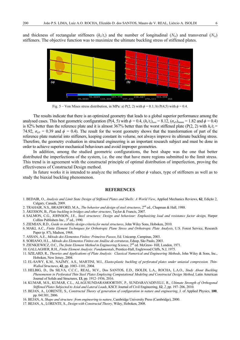
João P.S. LIMA, Luiz A.O. ROCHA, Elizaldo D. dos SANTOS, Mauro de V. REAL, Liércio A. ISOLDI 6 200
and thickness of rectangular stiffeners (hs/ts) and the number of longitudinal (Nls) and transversal (Nts) stiffeners. The objective function was to maximize the ultimate buckling stress of stiffened plates.
Fig. 5 – Von Mises stress distribution, in MPa: a) P(2, 2) with φ = 0.1; b) P(4,5) with φ = 0.4.
The results indicate that there is an optimized geometry that leads to a global superior performance among the analysed cases. This best geometric configuration (P(4, 5) with φ = 0.4, (hs/ts)ooo = 8.12, (σuN)mmm = 1.82 and φ = 0.4) is 82% better than the reference plate and it is almost 367% better than the worst stiffened plate (P(2, 2) with hs/ts = 74.92, σuN = 0.39 and φ = 0.4). The result for the worst geometry shows that the transformation of part of the reference plate material into stiffeners, keeping constant its volume, not always improve its ultimate buckling stress. Therefore, the geometry evaluation in structural engineering is an important research subject and must be done in order to achieve superior mechanical behaviours and avoid improper geometries.
In addition, among the studied geometric configurations, the best shape was the one that better distributed the imperfections of the system, i.e. the one that have more regions submitted to the limit stress. This trend is in agreement with the constructal principle of optimal distribution of imperfection, proving the effectiveness of Constructal Design method.
In future works it is intended to analyze the influence of other φ values, type of stiffeners as well as to study the biaxial buckling phenomenon.
REFERENCES
1. BEDAIR, O., Analysis and Limit State Design of Stiffened Plates and Shells: A World View, Applied Mechanics Reviews, 62, Edição 2, Calgary, Canadá, 2009.
2. TRAHAIR, N.S., BRADFORD, M.A., The behavior and design of steel structures, 2nd ed., Chapman & Hall, 1988. 3. ÅKESSON, B., Plate buckling in bridges and other structure, Taylor & Francis, 2007. 4. SALMON, C.G., JOHNSON, J.E., Steel structures: Design and behaviour: Emphasizing load and resistance factor design, Harper
Collins Publishers Inc., 3d ed., 1990. 5. ZIEMIAN, R.D., Guide to stability design criteria for metal structures, John Wiley Sons, Hoboken, 2010. 6. MAKI, A.C., Finite Element Techniques for Orthotropic Plane Stress and Orthotropic Plate Analysis, U.S. Forest Service, Research
Paper (p. 87), Madson, 1968. 7. ASSAN, A.E., Método dos Elementos Finitos: Primeiros Passos, Ed. Unicamp, Campinas, 2003. 8. SORIANO, H.L., Método dos Elementos Finitos em Análise de estruturas, Edusp, São Paulo, 2003. 9. ZIENKIEWICZ, O.C., The finite Element Method in Engineering Science, 2nd ed. McGraw- Hill, London, 1971. 10. GALLAGHER, R.H., Finite Element Analysis: Fundamentals, Prentice-Hall, Englewood Cliffs, N.J, 1975. 11. SZILARD, R., Theories and Applications of Plate Analysis: Classical Numerical and Engineering Methods, John Wiley & Sons, Inc.,
Hoboken, New Jersey, 2004. 12. EL-SAWY, K.M., NAZMY, A.S., MARTINI, M.I., Elasto-plastic buckling of perforated plates under uniaxial compression. Thin-
Walled Structures, 42, pp. 1083–1101, 2004. 13. HELBIG, D., Da SILVA, C.C.C., REAL, M.V., Dos SANTOS, E.D., ISOLDI, L.A., ROCHA, L.A.O., Study About Buckling
Phenomenon in Perforated Thin Steel Plates Employing Computational Modeling and Constructal Design Method, Latin American Journal of Solids and Structures, 13, pp. 1912–1936, 2016.
14. KUMAR, M.S., KUMAR, C.L., ALAGUSUNDARAMOORTHY, P., SUNDARAVADIVELU, R., Ultimate Strength of Orthogonal Stiffened Plates Subjected to Axial and Lateral Loads, KSCE Journal of Civil Engineering, 12, 2, pp. 197–206, 2010.
15. BEJAN, A., LORENTE, S., Constructal Theory of generation of configuration in nature and engineering, J. of Applied Physics, 100, pp. 041301, 2006.
16. BEJAN, A. Shape and structure: from engineering to nature, Cambridge University Press (Cambridge), 2000. 17. BEJAN, A., LORENTE, S., Design with Constructal Theory, Wiley, Hoboken, 2008.

THE PUBLISHING HOUSE PROCEEDINGS OF THE ROMANIAN ACADEMY, Series A, OF THE ROMANIAN ACADEMY Special Issue/2018, pp. 201–206
CONSTRUCTAL APPROACH ON THE FEASIBILITY OF COMPRESSED AIR TEMPERATURE CONTROL
BY EVAPORATIVE COOLING IN GAS TURBINE POWER PLANTS
George STANESCU*, Ene BARBU**, Valeriu VILAG**, Theodora ANDREESCU** * Federal University of Parana, Mechanical Engineering Department, Centro Politecnico,
Caixa Postal 19100, 81531-990 Curitiba PR, Brazil ** INCD Turbomotoare COMOTI, Iuliu Maniu 220D, Bucharest, 061126, Romania
Corresponding author: George STANESCU, E-mail: [email protected]
Abstract. Summer higher atmospheric air temperatures affect the performance of gas turbine power plants. To prevent in such conditions diminishing of the produced mechanical power there are already available two technologies based on water injection. The first, known as “fog cooling”, is a simple technology to reduce the intake air temperature by direct evaporative cooling based on spraying liquid water at the axial compressor entrance. The “inter-stage water spraying” technology is the second one, where the liquid water is gradually injected along the axial compressor. This paper aims to evaluate the potential of these two technologies for improving the overall performance of the gas turbine power plants. To investigate the limits and conditions in which the real axial compressor's design may evolve, the numerical results are calculated based on the Constructal Theory by modeling the compressor as an ensemble of adjacent elemental isothermal compressors that ”...provides easier access to the imposed currents that flow through it”. Compressed moist air temperature control within each of the elemental compressor is done based on the evaporative cooling principle. Numerical results, for the first technology, agree well with test bench values obtained for the TV2-117A version of a gas turbine converted by COMOTI from kerosene to gaseous fuel.
Key words: Evaporative cooling, Isothermal compression, Gas turbines, Constructal Law.
1. INTRODUCTION
Performances and the long lifetime of the modern gas turbine power plants (GTPPs) make them well suited for cogeneration groups. The International Standards Organization (ISO) considers the following characteristics of the atmospheric air for the gas turbines design: T* = 150C, P* = 101.3 kPa and φ* = 60%. During the summer time the atmospheric air temperature increases while the air density decreases, resulting in the GTPP's produced power reduction. Depending on the gas turbine type employed, the atmospheric air temperature may change the operating point of both the compressor and the turbine, such that 100C increases in the ambient temperature reduces the power of the GTTP with 5–13% and the efficiency with 1.5–4% respectively [1]. Together, these particularities of the gas turbines operation, the requirements for competitiveness in the field of electricity and the obligation to comply with the EU Directive 2010/75 provisions, result in a great challenge for finding technical solutions for compensating for power losses during the summer without building additional power plants.
To avoid shortcomings of the GTPP’s performance during the summer time, there are already available some technologies for cooling down the intake air such as: (1) the evaporative cooling systems that mixture atmospheric air with liquid water that evaporates producing lower temperature moist air, and (2) indirect cooling systems continuously cooling upstream of the compressor the intake air by thermal interaction within a heat exchanger [2].
The evaporative cooling of the intake air is done in several ways: (i) traditional system forcing the flow of the atmospheric air through a soaked porous media; (ii) evaporative cooling spraying liquid water directly into the atmospheric air stream entering the axial compressor (“inlet fogging”), with overspray variant (or wet compression); (iii) inter-stage evaporative cooling, when the liquid water is gradually injected along the

George STANESCU, Ene BARBU, Valeriu VILAG, Theodora ANDREESCU 2 202
axial compressor, allowing thus for the optimization of the compressor functioning since in this way it can be injected the desired quantity of liquid water at the exact position for better controlling the compressed gas temperature.
In the indirect cooling systems case, the intake air cooling occurs upstream of the compressor, within heat exchangers that may use low temperature water or some refrigerant fluid as cooling fluid. Detailed analysis of the intake air cooling technologies was presented by Melino [2], while various other studies were developed for specific locations with high summer temperature in Brazil by Celis et al. [3], in Saudi Arabia by Ibrahim and Vamham [4], and in Oman by Dawoud et al. [5].
Accounting the complexity of the two-phase flow process and the polydisperse spraying, Bhargava et al. [6] consider that there is a poor understanding of the phenomenology of wet compression in the compressor stages of the gas turbine. Thus, the authors state that the efficiency of wet compression is influenced by a variety of factors such as the droplets diameter, gas pressure and temperature, and the mass flow rate of injected liquid water. When inter-stages water spraying is used, the injection position along the compressor becomes also an important parameter. Anurov [7] studied the dynamics of the evaporation process of water droplets along the 13 stages compressor of the GT-009 gas turbine installation, by considering various parameters such as the injected water flow rate, water injection position towards the airstream and the diameters of water droplets.
To contribute with the decision-making on directions for developing the existing air cooling technologies in GTPPs, and for better understanding the fundamentals and its maximum potential for increasing the efficiency, this paper presents a constructal approach on the evaporative cooling process employed to control the temperature of the compressed air in GTPPs.
2. FUNDAMENTALS OF EVAPORATIVE COOLING IN THE GTPPs
Evaporative cooling is one of the most simple and cheap intake air cooling technologies applied on gas turbine industry, compared with nowadays sophisticated techniques (mechanical chiller or absorption ones, thermal storage etc.). Temperature rise attenuation of intake air mass flow is achieved due to contact with water which vaporizes. Theoretically, the minimum temperature that can be achieved is the wet bulb temperature. Practically, this temperature is difficult to be achieved and the temperature drop is dependent on both the equipment and the environmental conditions.
2.1. “Fog cooling” technology
Intake air cooling technology by spraying water mist form was applied to a gas turbine since 1980 [8]. Normally, fine water droplets (with a diameter of less than 30 µm) sprayed into the intake air stream (Fig.1) evaporates until entering the compressor. Depending on the ambient conditions, the water mass flow rate injected towards the airstream is about 1–2% of the air flow rate.
Fig. 1 – Physical configuration of a GTPP employing the "fog cooling" technology with complete vaporization
before the admission into the compressor of the liquid water sprayed into the intake.

3 Constructal approach on the feasibility of compressed air temperature control by evaporative cooling in GTPPs 203
Advantages of this type of method for gas turbine performance improvement are: low installation costs; reduced pressure drop on compressor intake; high efficiency; inexpensive technological reconfiguration; can be located either upstream or downstream of the air filter.
2.2. “Inter-stage water spraying” technology
Technology that involve water injection between the axial compressor stages (Fig. 2) presents special nozzles to ensure a homogeneous jet with droplets having a diameter below 10 µm and a very short compressor residence time, in the range of 15...30 ms. This technology can provide a higher power increase than the water injection technique into the compressor intake. Also, this method could remove compressor working away from stall limit, ensuring a more stable operation of the entire gas turbine engine.
Fig. 2 – Physical configuration of a GTPP employing the “inter-stage water spraying” technology.
It should be outlined the idea that the compressor characteristic will be changed for the wet compression evolution, compared to dry compression; moreover the wet compression depends on the compressor overall geometry and the size of the water droplets.
3. CONSTRUCTAL APPROACH OF COMPRESSED AIR TEMPERATURE CONTROL
To provide “greater and greater access to the currents that flow through” the internal volume of a gas turbine power plant’s (GTPP’s) axial compressor, the existing configurations shown in Figs. 1 and 2 are replaced by a “globally easier flowing configuration” as shown in Fig. 3, where the liquid water injection is considered to develop along the compressor. Then, in order to quantitatively address the problem, the internal configuration of the air compressors in Figs. 1 and 2 is replaced by a repetitive pattern of many adjacent elemental compression stages.
Fig. 3 – Adjacent elemental compression stages within the internal volume of the GTPP’s axial compressor.

George STANESCU, Ene BARBU, Valeriu VILAG, Theodora ANDREESCU 4 204
4. MATHEMATICAL MODEL
The mathematical model is based on the equations of mass and energy conservation and on the second law of thermodynamics applied to the control volumes representing the elemental compression stages in Fig. 3. The combustion chamber (CC) and the turbine (T) are modeled based on their global characteristics, as usual for gas turbine Brayton thermodynamic cycle. The model employed in this study determines the characteristic parameters by focusing firstly on the reversible functioning and then on irreversible operation. The dimensionless ODE system to approach the reversible operation is written down as follows in the equations (1), (2), (3) and (4):
d ˜ ′ T
d ˜ P = 0.622 ˜ P
˜ P − ˜ P sat( )2Δ˜ s fg + ka −1
ka
1˜ P
⎡
⎣
⎢ ⎢ ⎢
⎤
⎦
⎥ ⎥ ⎥
1
T+ω d ′ s w
vap
d ˜ ′ T + 0.622 ˜ P
˜ P − ˜ P sat( )2Δ˜ s fg
d ˜ P sat
d ˜ ′ T
⎡
⎣
⎢ ⎢ ⎢
⎤
⎦
⎥ ⎥ ⎥ , (1)
d ′ ω d ˜ P
= 0.622εφ ˜ P
˜ P − ˜ P sat( )2
d ˜ P sat
d ˜ ′ T
d ˜ ′ T
d ˜ P −1
⎛
⎝ ⎜
⎞
⎠ ⎟ , (2)
δ ˜ ′ W Comp ˜ m a( )d ˜ P
= − 1+ ′ ω d ˜ h wvap
d ˜ ′ T
⎛
⎝ ⎜
⎞
⎠ ⎟
d ˜ ′ T
d ˜ P + Δ ˜ h fg
d ′ ω d ˜ P
⎡
⎣ ⎢ ⎢
⎤
⎦⎥⎥, (3)
δ ˜ ′ W p ˜ m a( )d ˜ P
= − P*
ρwliqcpaT *
⎛
⎝ ⎜ ⎜
⎞
⎠ ⎟ ⎟
˜ P − ˜ P 0( )d ′ ω d ˜ P
, (4)
while for the irreversible case the dimensionless ODE system is given by equations (5), (6), (7) and (8):
d ˜ ′ ′ T
d ˜ P = 0.622 ˜ P
˜ P − ˜ P sat( )2Δ ˜ h fg − 1
ηs,C
δ ˜ ′ W Comp ˜ m a( )d ˜ P
⎡
⎣
⎢ ⎢ ⎢
⎤
⎦
⎥ ⎥ ⎥
1+ ′ ′ ω d ˜ h wvap
d ˜ ′ ′ T + 0.622 ˜ P
˜ P − ˜ P sat( )2Δ ˜ h fg
d ˜ P sat
d ˜ ′ ′ T
⎡
⎣
⎢ ⎢ ⎢
⎤
⎦
⎥ ⎥ ⎥ , (5)
d ′ ′ ω d ˜ P
= 0.622ε ′ ′ φ ˜ P
˜ P − ˜ P sat( )2
d ˜ P sat
d ˜ ′ ′ T
d ˜ ′ ′ T
d ˜ P −1
⎛
⎝ ⎜
⎞
⎠ ⎟ , (6)
δ ˜ ′ ′ S gen,Comp ˜ m a( )d ˜ P
= 1˜ ′ ′ T
+ ′ ′ ω d˜ s wvap
d ˜ ′ ′ T
⎛
⎝ ⎜
⎞
⎠ ⎟
d ˜ ′ ′ T
d ˜ P + Δ˜ s fg
d ′ ′ ω d ˜ P
− ka −1
ka
1˜ P
⎡
⎣ ⎢ ⎢
⎤
⎦ ⎥ ⎥ , (7)
δ ˜ ′ ′ W p ˜ m a( )d ˜ P
= − P*
ρwliqcpaT *
⎛
⎝ ⎜ ⎜
⎞
⎠ ⎟ ⎟
˜ P − ˜ P 0( )d ′ ′ ω d ˜ P
, (8)
where ka , ρwliq , cpa and ηs,C = ˜ ′ W Comp
˜ ′ ′ W Comp are the ratio of specific heats of dry air, the liquid water density, the dry air’s specific heat at constant pressure and the compressor isentropic efficiency, respectively. Δ ˜ h fg
and Δ˜ s fg represent the dimensionless specific enthalpy and entropy of vaporization for water, while ˜ h wvap and
˜ s wvap the dimensionless specific enthalpy and entropy of the water vapor.
Dimensionless temperature, pressure, mass flow rate, specific enthalpy and entropy and mechanical power are given by: ( ) ( )* * * * * *, , , , , anda pa pa a paT T T P P P m m m h h c T s s c W W m c T= = = = = = . (*) superscript refers to the ISO characteristics of the atmospheric air for the gas turbines design, while the
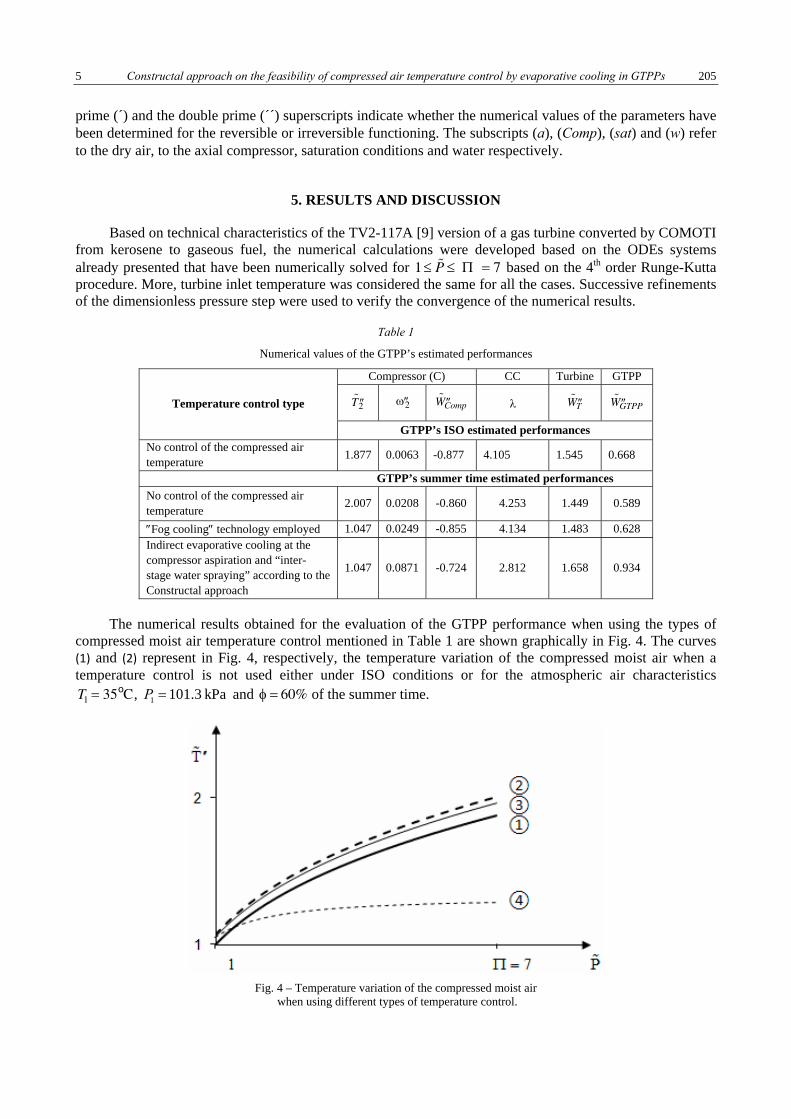
5 Constructal approach on the feasibility of compressed air temperature control by evaporative cooling in GTPPs 205
prime (´) and the double prime (´´) superscripts indicate whether the numerical values of the parameters have been determined for the reversible or irreversible functioning. The subscripts (a), (Comp), (sat) and (w) refer to the dry air, to the axial compressor, saturation conditions and water respectively.
5. RESULTS AND DISCUSSION
Based on technical characteristics of the TV2-117A [9] version of a gas turbine converted by COMOTI from kerosene to gaseous fuel, the numerical calculations were developed based on the ODEs systems already presented that have been numerically solved for 1 ≤ ˜ P ≤ Π = 7 based on the 4th order Runge-Kutta procedure. More, turbine inlet temperature was considered the same for all the cases. Successive refinements of the dimensionless pressure step were used to verify the convergence of the numerical results.
Table 1
Numerical values of the GTPP’s estimated performances
Compressor (C) CC Turbine GTPP
′ ′ ˜ T 2 ′ ′ ω 2 ′ ′ ˜ W Comp λ ′ ′ ˜ W T ′ ′ ˜ W GTPP Temperature control type
GTPP’s ISO estimated performances No control of the compressed air temperature 1.877 0.0063 -0.877 4.105 1.545 0.668
GTPP’s summer time estimated performances No control of the compressed air temperature 2.007 0.0208 -0.860 4.253 1.449 0.589
″Fog cooling″ technology employed 1.047 0.0249 -0.855 4.134 1.483 0.628 Indirect evaporative cooling at the compressor aspiration and “inter-stage water spraying” according to the Constructal approach
1.047 0.0871 -0.724 2.812 1.658 0.934
The numerical results obtained for the evaluation of the GTPP performance when using the types of compressed moist air temperature control mentioned in Table 1 are shown graphically in Fig. 4. The curves (1) and (2) represent in Fig. 4, respectively, the temperature variation of the compressed moist air when a temperature control is not used either under ISO conditions or for the atmospheric air characteristics
T1 = 35oC, 1 101.3 kPaP = and φ = 60% of the summer time.
Fig. 4 – Temperature variation of the compressed moist air
when using different types of temperature control.

George STANESCU, Ene BARBU, Valeriu VILAG, Theodora ANDREESCU 6 206
When the “fog cooling” technology is considered for improving the summer time GTPP performance, the compressed moist air temperature variation is represented in Fig. 4 by the curve (3). Graphically represented by the curve (4) in Fig. 4 are also the numerical results obtained when approaching based on the Constructal Law the GTPP’s summer time performance with indirect evaporative cooling at the compressor aspiration and “inter-stage water spraying”.
6. CONCLUSIONS
The numerical results obtained in this work show, at least from a fundamental point of view, the effectiveness of compressed air temperature control by evaporative cooling in gas turbine plants.
There is a continuous compressed moist air temperature increase tendency when a temperature control is not used either under ISO conditions or for the summer time air characteristics, nor when the "fog cooling" technology is employed to improve the summer time GTPP performance. Meanwhile, the results obtained based on the Constructal approach, with indirect evaporative cooling at the compressor aspiration and “inter-stage water spraying”, show comparatively that during most of the compression process a temperature of the compressed moist air 45% lower.
Providing a “globally easier flowing configuration”, the Constructal approach with indirect evaporative cooling at the compressor aspiration and “inter-stage water spraying”, shed some light on the potential of growth in the mechanical power delivered by the GTPP of 45.81% and a simultaneous reduction of 2.26% in the fuel specific consumption.
Numerical results on the entropy generation due to the compressor functioning confirm the realism of the adopted assumptions and the adequacy of the mathematical formulation of the proposed model for numerical simulation purposes.
Application of water injection in each compressor stages involves miniature holes drilled on stators and a sophisticated water injection system. The experiments regarding water injection through TV2-117A intake, reconfigured from kerosene to methane showed not only a power augmentation but also NOx emissions reduction similar to the work presented in [10]. Thus the introduction of water into the gas turbine intake at idle generates a reduction of averaged turbine inlet temperature of about 5 0C and also NOx emissions fall by approximately 4 ppm. Idle regime becomes important for “stand-by GTTP” that is used only when energy peaks occur since they can work as little as one hour but the pollutant emissions should be low all the time.
REFERENCES
1. BARIGOZZI, G. et al., Techno-economic analysis of gas turbine inlet air cooling for combined cycle power plant for different climatic conditions, Applied Thermal Engineering, 82, pp. 57–67, 2015.
2. MELINO, F., A parametric evaluation of fogging technology for gas turbine performance enhancement, Alma Mater Studiorum Universita’ Degli Studi di Bologna, 2004.
3. CELIS, C. et al., Power augmentation technologies for gas turbines: A review and a study on their influence on the performance of simple cycle power plants, 19th International Congress of Mechanical Engineering November 5–9, 2007, Brasília, DF.
4. IBRAHIM, M.A., VARNHAM, A., A review of inlet air-cooling technologies for enhancing the performance of combustion turbines in Saudi Arabia, Applied Thermal Engineering, 30, pp. 1879–1888, 2010.
5. DAWOUD, B. et al., Thermodynamic assessment of power requirements and impact of different gas-turbine inlet air cooling techniques at two different locations in Oman, Applied Thermal Engineering, 25, pp. 1579–1598, 2005.
6. BHARGAVa et al., Gas turbine compressor performance characteristics during wet compression – influence of polydisperse spray, Proceedings of ASME Turbo Expo 2009: Power for Land, Sea and Air (GT2009) June 8–12, 2009, Orlando, FL USA.
7. ANUROV, M.Yu. et al., Calculation study of water injection on compressor characteristics of a GT-009 gas-turbine installation, Thermal Engineering, 53, 12, pp. 964–969, 2006.
8. JONES, C., JACOBS, A.J., Economic and technical considerations for combined-cycle performance-enhancement options, GE Power Systems Schenectady, NY, GER-4200.
9. *** Motorul de aviaţie turbopropulsor TV2 117-A şi reductorul VR-8. Descriere tehnică şi instrucţiuni pentru exploatare, Klimov Corporation, Russia.
10. BARBU, E. et al., The influence of inlet air cooling and afterburning on gas turbine cogeneration groups performance, Gas Turbines – Materials, Modeling and Performance, Dr. Gurrappa Injeti (Ed.), InTech, 2015.
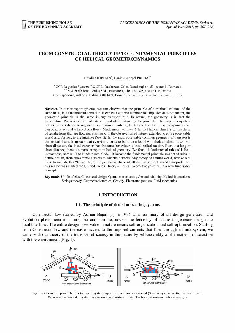
THE PUBLISHING HOUSE PROCEEDINGS OF THE ROMANIAN ACADEMY, Series A, OF THE ROMANIAN ACADEMY Special Issue/2018, pp. 207–212
FROM CONSTRUCTAL THEORY UP TO FUNDAMENTAL PRINCIPLES OF HELICAL GEOMETRODYNAMICS
Cătălina IORDAN*, Daniel-Georgel PREDA** * CCR Logistics Systems RO SRL, Bucharest, Calea Dorobanţi no. 53, sector 1, Romania
** MG Profesionall Sales SRL, Bucharest, Ticus no. 8A, sector 1, Romania Corresponding author: Cătălina IORDAN, E-mail: [email protected]
Abstract. In our transport systems, we can observe that the principle of a minimal volume, of the same mass, is a fundamental condition. It can be a car or a commercial ship, size does not matter, the geometric principle is the same in any transport rule. In nature, the geometry is in fact the information. We observe it, understand it and after, extracting the principle. The Kepler conjecture optimizes the spheres arrangement in a minimum volume, the tetrahedron. In a dynamic geometry we can observe several tetrahedrons flows. Much more, we have 2 distinct helical chirality of this chain of tetrahedrons that are flowing. Starting with the observation of nature, extended to entire observable world and, further, to the intuitive flow fields, the most observable common geometry of transport is the helical shape. It appears that everything tends to build up a lot of wormholes, helical flows. For short distances, the local transport has the same behaviour, a local helical motion. Even is a long or short distance, there is a mass transport in helical geometry. We found 4 fundamental rules of helical interactions, named “The Fundamental Code”. It became the fundamental principle as a set of rules in nature design, from sub-atomic clusters to galactic clusters. Any theory of natural world, new or old, must to include this “helical key”, the geometric shape of all natural self-optimized transports. For this reason was started the Unified Fields Theory – Helical Geometrodynamics, in a new time-space concept.
Key words: Unified fields, Constructal design, Quantum mechanics, General relativity, Helical interactions, Strings theory, Geometrodynamics, Gravity, Electromagnetism, Fluid mechanics.
1. INTRODUCTION
1.1. The principle of three interacting systems
Constructal law started by Adrian Bejan [1] in 1996 as a summary of all design generation and evolution phenomena in nature, bio and non-bio, covers the tendency of nature to generate designs to facilitate flow. The entire design observable in nature means self-organization and self-optimization. Starting from Constructal law and the easier access to the imposed currents that flow through a finite system, we came with our theory of the transport efficiency in the nature by self-assembly of the matter in interaction with the environment (Fig. 1).
Fig. 1 – Geometric principle of a transport system, optimized and non-optimized (S – our system, matter transport zone, W, w – environmental system, wave zone, our system limits, T – traction system, outside energy).

Cătălina IORDAN, Daniel-Georgel PREDA 2 208
As a general principle, for any optimal transport research, we have always three different subsystems interacting: luggage, vehicle and environment. The luggage is the matter, our system during its time evolution. The matter flows, from any “A” zone to any “B” zone. That means it is not a static geometry and it have a sense of flow. Any matter transport contains subsystems, forced to construct specific flow geometry, in accord with tractor and environmental systems. That means interactions.
We understood that the environmental interactions, as pressure or any sort of forces, put borders and limits to our self-assembled luggage. We assumed that the smallest particles of universe, our luggage, are like a fluid and tend to be spherical.
1.2. Chirality, the principle of positive or negative flow
The first close packing spheres was made in the 17th century by Johannes Kepler. Further, in 1994 Fejes Tóth mathematically proved that the hexagonal lattice is the densest of all possible bi-dimensional packing, as mentioned by Conway and Sloan. [2].
The Boerdijk-Coxeter helix [3], which is obtained as a linear packing of regular (or not) tetrahedron, could be the most efficient solution to some close-packing problems in matter transport. There are two chiral forms, with either clockwise or counterclockwise windings and they are not rotationally repetitive [3] (Fig. 2).
Fig. 2 – Kepler conjecture, in a dynamic packing arrangement, became a tetrahelix,
a dynamic geometry with sense and chirality.
We made some predictions: – Every transport line may be, in fact, a three-dimensional line, a tornado. – Every line (tornado) has a sense and a chirality of transport. – Every line may be surrounded by other lines, in opposite chirality, creating layers (any line may be our system, the luggage, and surrounded lines are environmental system).
Langmuir lines [4], Ekman layers [5], Maxwell vortex tubes [6] and many others use the same geometric transport rules. We can extract and predict the first geometric transport rule, an efficient chiral flow is surrounded by anti-chiral flows. The alternating chirality appears to be very important in matter transport, detectable or not detectable (theory). It was an interesting idea to correlate the natural chirality, left and right, with charged particles, positive or negative. We made a new and one of the most important prediction; in all natural world do not exists” charged systems”, it exists only chiral systems of transport. Fluids are not charged systems; they are a turbulent “lines”, parallel” lines” and “layers”! Planets, from our solar system, are not „charged” systems. They are our luggage in a self-assembled position, with spin motion, with chiral rotations to the galactic center. The solar system planets may be the witnesses of the flow to „B” zone from one of the chiral galactic arms.
2. “THE FUNDAMENTAL CODE”
2.1. Helical interaction rules between transport lines-“The Fundamental Code”
We predict, in nature, a set of fundamental interaction rules between any two neighboring helical flows. As a result of all interactions it is a geometric principle. Even if the flow is heat transport or fluid transport, magnetic or electric transport, gravitational transport or galactic flows, all nature obeys the first constructal rule, a geometric key (Fig. 3).

3 From constructal theory up to fundamental principles of helical geometrodynamics 209
Fig. 3 – “The Fundamental Code”, a set of interactions rules between any adjacent helical flows.
We found 4 fundamental rules of helical interactions, named “The Fundamental Code” (Fig. 3). In a general relativity, “The Fundamental Code” has four situations. Two of them are simple, named total rejection. When two adjacent tornadoes have same sense (parallel) and same chirality are repulsive, between their axes and ands. It is a simple and intuitive friction situation. The same for opposite directions (anti-parallel) land opposite chirality means total rejection (Fig. 3). Next case is the same chirality and opposite senses, that means peripheral attraction and axial rejection (A). The forth case is different chirality and same senses that means peripheral rejection and axial attraction (B).
For a better understanding „The Fundamental Code” included three different symbols: II, ( ) and X. The symbol “II” is used to exemplify total rejection. The symbol “( )“ means axial rejection and peripheral attraction, anti-parallel tornadoes or one after another, in a chain shape, A-case (Fig. 3). The symbol “X” is used to exemplify axial attraction and peripheral rejection, B-case (Fig. 3). This is the foundation, the basic principle in any sort of matter transport. The fluidity of universe, as a detectable or not detectable matter transport, is essential for our understanding.
We observe, in natural flows, that a strong flow can induce other local flows, and can disturb the local transport. As wind induces helical motions in ocean water [4] we understood the motion inductive mechanism. Much more, we predicted that inductive mechanism is generalized.
We predicted two inductive principles, cylinder-cylinder (C–C) and cylinder-torus (C–T) (Fig. 3), not detailed in this paper. The principle “C–C” induces parallel flows in opposite chirality and the principle “C–T” induces perpendicular flows in same chirality.
The tornado transport in vertical directions, as helical shape, can move horizontally in the same time. This is a drift motion, the matter as wave. The “C–C” principle can form chains as layers of tornados. It means a geometric mechanism in wave propagation.
The two inductive principles and the local transport (waves as drift motions), for a better understanding need a new space-time concept and are not detailed here. Both of them use “The Fundamental Code”. This code and “the two inductions principles” are, in fact, helical interactions rules between any transport lines, localized (waves) or not localized.
The geometry in dynamics, meaning the geometrodynamics [7] acting in the same way for each tractor system and for any medium, flowing from IN-A zone to B-OUT zone.
2.2. The three flow classes in Universe
A dimensional class of particles can have a natural flow rotation in left handed and right handed, this is the fermion class. These motions can be conjugated or not. Both of them are present in nature and play the
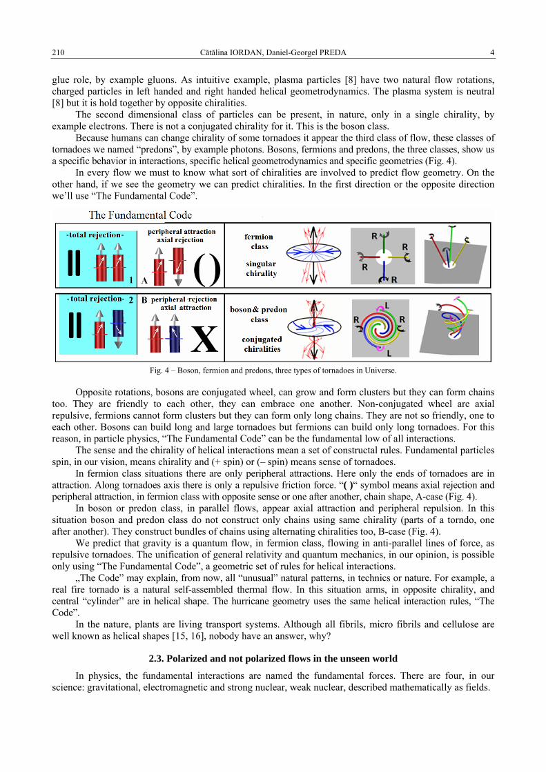
Cătălina IORDAN, Daniel-Georgel PREDA 4 210
glue role, by example gluons. As intuitive example, plasma particles [8] have two natural flow rotations, charged particles in left handed and right handed helical geometrodynamics. The plasma system is neutral [8] but it is hold together by opposite chiralities.
The second dimensional class of particles can be present, in nature, only in a single chirality, by example electrons. There is not a conjugated chirality for it. This is the boson class.
Because humans can change chirality of some tornadoes it appear the third class of flow, these classes of tornadoes we named “predons”, by example photons. Bosons, fermions and predons, the three classes, show us a specific behavior in interactions, specific helical geometrodynamics and specific geometries (Fig. 4).
In every flow we must to know what sort of chiralities are involved to predict flow geometry. On the other hand, if we see the geometry we can predict chiralities. In the first direction or the opposite direction we’ll use “The Fundamental Code”.
Fig. 4 – Boson, fermion and predons, three types of tornadoes in Universe.
Opposite rotations, bosons are conjugated wheel, can grow and form clusters but they can form chains too. They are friendly to each other, they can embrace one another. Non-conjugated wheel are axial repulsive, fermions cannot form clusters but they can form only long chains. They are not so friendly, one to each other. Bosons can build long and large tornadoes but fermions can build only long tornadoes. For this reason, in particle physics, “The Fundamental Code” can be the fundamental low of all interactions.
The sense and the chirality of helical interactions mean a set of constructal rules. Fundamental particles spin, in our vision, means chirality and (+ spin) or (– spin) means sense of tornadoes.
In fermion class situations there are only peripheral attractions. Here only the ends of tornadoes are in attraction. Along tornadoes axis there is only a repulsive friction force. “( )“ symbol means axial rejection and peripheral attraction, in fermion class with opposite sense or one after another, chain shape, A-case (Fig. 4).
In boson or predon class, in parallel flows, appear axial attraction and peripheral repulsion. In this situation boson and predon class do not construct only chains using same chirality (parts of a torndo, one after another). They construct bundles of chains using alternating chiralities too, B-case (Fig. 4).
We predict that gravity is a quantum flow, in fermion class, flowing in anti-parallel lines of force, as repulsive tornadoes. The unification of general relativity and quantum mechanics, in our opinion, is possible only using “The Fundamental Code”, a geometric set of rules for helical interactions.
„The Code” may explain, from now, all “unusual” natural patterns, in technics or nature. For example, a real fire tornado is a natural self-assembled thermal flow. In this situation arms, in opposite chirality, and central “cylinder” are in helical shape. The hurricane geometry uses the same helical interaction rules, “The Code”.
In the nature, plants are living transport systems. Although all fibrils, micro fibrils and cellulose are well known as helical shapes [15, 16], nobody have an answer, why?
2.3. Polarized and not polarized flows in the unseen world
In physics, the fundamental interactions are named the fundamental forces. There are four, in our science: gravitational, electromagnetic and strong nuclear, weak nuclear, described mathematically as fields.
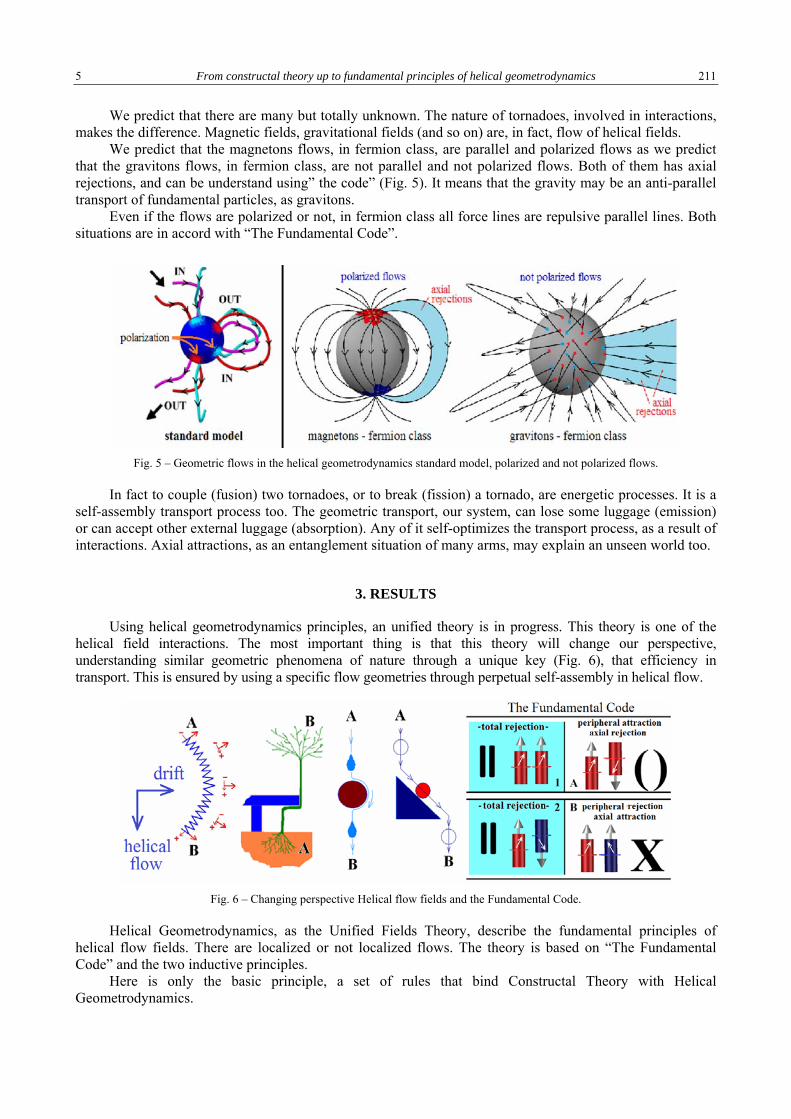
5 From constructal theory up to fundamental principles of helical geometrodynamics 211
We predict that there are many but totally unknown. The nature of tornadoes, involved in interactions, makes the difference. Magnetic fields, gravitational fields (and so on) are, in fact, flow of helical fields.
We predict that the magnetons flows, in fermion class, are parallel and polarized flows as we predict that the gravitons flows, in fermion class, are not parallel and not polarized flows. Both of them has axial rejections, and can be understand using” the code” (Fig. 5). It means that the gravity may be an anti-parallel transport of fundamental particles, as gravitons.
Even if the flows are polarized or not, in fermion class all force lines are repulsive parallel lines. Both situations are in accord with “The Fundamental Code”.
Fig. 5 – Geometric flows in the helical geometrodynamics standard model, polarized and not polarized flows.
In fact to couple (fusion) two tornadoes, or to break (fission) a tornado, are energetic processes. It is a self-assembly transport process too. The geometric transport, our system, can lose some luggage (emission) or can accept other external luggage (absorption). Any of it self-optimizes the transport process, as a result of interactions. Axial attractions, as an entanglement situation of many arms, may explain an unseen world too.
3. RESULTS
Using helical geometrodynamics principles, an unified theory is in progress. This theory is one of the helical field interactions. The most important thing is that this theory will change our perspective, understanding similar geometric phenomena of nature through a unique key (Fig. 6), that efficiency in transport. This is ensured by using a specific flow geometries through perpetual self-assembly in helical flow.
Fig. 6 – Changing perspective Helical flow fields and the Fundamental Code.
Helical Geometrodynamics, as the Unified Fields Theory, describe the fundamental principles of helical flow fields. There are localized or not localized flows. The theory is based on “The Fundamental Code” and the two inductive principles.
Here is only the basic principle, a set of rules that bind Constructal Theory with Helical Geometrodynamics.
Cătălina IORDAN, Daniel-Georgel PREDA 6 212
4. CONCLUSIONS
All transports mean patterns, means the most efficient geometry in transport. We try to understand principled patterns of natural transport, most common, in many branches of science. As a scientific method, we made many qualitative observations. We supposed that a general and constructal principle must exist and it must refer to this perpetual transport. So we followed a helical geometry key, we searched if helical transport is the most efficient transport and especially why. For this reason, compared to our commercial transport, we brought forth basic principles, fundamental ones.
The interactions of these helical systems of transport, as tornado shape, seem to obey strict rules, which can be identified in the natural environment, at any scale. Furthermore, this interaction strict set of rules, called “The Fundamental Code”, can be extrapolated to the undetectable universes, to the minimum or maximum ones.
From now, the laws of the Universe [9] can be explained using “The Fundamental Code”. There is a geometric key in any natural fiber for every plant [15, 16]. Hair grow [17, 18], skin grow [19] or any life form growth using the same geometric key, a helical one. The twistor theory [10], quantum gravity [11], string theory [12, 13] or any theory about an intelligent design of Universe are clarified and substantiated by “The Code”. More of those issues were presented at the 10th Constructal Law & Second Law Conference (CLC2017), hosted by the Romanian Academy on the 15 and 16 May 2017.
For further research any scientific field can use the helical geometrodynamics to explain the fundamental design of everything. The Universe is hiding indeed the geometric key in a Nutshell [14].
REFERENCES
1. BEJAN, A., LORENTE, S., Design with Constructal Theory, International Journal of Engineering Education, 22, 1, pp. 140–147, 2006.
2. CONWAY, J.H., SLOANE N.J.A., Sphere Packings, Lattices, and Groups, 2nd ed., Springer, New York, 1993, pp. 8–9. 3. LORD, E.A., RANGANATHAN, S., The c-brass structure and the Boerdijk–Coxeter helix, Journal of Non-Crystalline Solids,
334–335, pp. 121–125, 2004. 4. LANGMUIR, I., Surface Motion of Water Induced by Wind, Science, 87, 1938. 5. EKMAN, V.W., On the influence of the Earth’s rotation on ocean currents, Arch. Math. Astron. Phys., 2, pp. 1–52, 1905. 6. MAXWELL, J.C., On Physical Lines of Force, Philosophical Magazine, 1861. 7. WHEELER, J.A., Geometrodynamics, Academic Press, New York, 1962. 8. SHKAROVSKY, I.P., JOHNSTON, T.W., BACHYNSKY, M.P., The Particle Kinetics of Plasma, Addison-Wesley, London,
1966. 9. PENROSE, R., The Road to Reality – A Complete Guide to the Laws of the Universe, Jonathan Cape, London, 2004. 10. PENROSE, R., Twistor Algebra, J. Math. Phys., 1967. 11. SMOLIN, L., Space, Time, Universe: Three Roads to Quantum Gravity, Humanitas, 2008. 12. SUSSKIND, L., The Cosmic Landscape: String Theory and the Illusion of Intelligent Design, Humanitas, 2012. 13. KAKU, M., Parallel Worlds: A journey Through Creation, Higher Dimensions, and Future of the Cosmos, Edit. Trei, 2015. 14. HAWKING, S., The Universe in a Nutshell, Humanitas, 2006. 15. ABRAHAM, Y., TAMBURU, C., KLEIN, E., DUNLOP, J.W.C., FRATZL, P., RAVIV, U., ELBAUM, R., Tilted cellulose
arrangement as a novel mechanism for hygroscopic coiling in the stork’s bill awn, R. Soc. Interface, 2012. 16. MIGLIACCIO, F., TASSONE, P., FORTUNATI, A., Circumnutation as an autonomous root movement in plants, American
Journal of Botany, 2013. 17. WANG, Y., HAO, Q., FATEHPURIA, A., LAU, D.L., HASSEBROOK, L.G., Data Acquisition and Quality Analysis of 3-Dimensional
Fingerprints, IEEE Conference on Biometrics, Identity and Security, Florida, 2009. 18. KÜCKEN, M., NEWELL, A.C., Fingerprint formation, Journal of Theoretical Biology, 235, pp. 71–83, 2005. 19. YANG F.C., ZHANG Y., RHEINSTADTER M.C, The structure of people’s hair, PeerJ 2:e619, DOI10.7717 /peerj.619, 2014.

THE PUBLISHING HOUSE PROCEEDINGS OF THE ROMANIAN ACADEMY, Series A, OF THE ROMANIAN ACADEMY Special Issue/2018, pp. 213–218
CONSTRUCTAL LAW AND ION TRANSFER IN NORMAL AND CANCER CELLS
Umberto LUCIA*, Giulia GRISOLIA** * Politecnico di Torino, Dipartimento Energetica, Corso Duca degli Abruzzi 24, 10129 Torino, Italy, [email protected] ** Politecnico di Torino, Dipartimento Energetica, Corso Duca degli Abruzzi 24, 10129 Torino, Italy, [email protected]
Corresponding author: Umberto LUCIA, Dipartimento Energetica, Politecnico di Torino, Corso Duca degli Abruzzi 24, 10129
Torino, Italy, E-mail: [email protected]
Abstract. All the living systems waste heat into environment. It is no more than the result of their internal irreversibility. The Constructal law analysis of the irreversibility related to this wasted heat represents a new useful approach to the study of the cells behaviour. This approach allows us to consider the living systems as black boxes and analyze only the inflows and outflows of energy and mass, and their changes in relation to any environmental modification. The consequence is the analysis of the effect of the ions transport through the membrane, and the related cell-environment pH changes, with consideration on the Krebs or Warburg cycle, used for energy conversion, by the normal and cancer cells respectively. Consequently, the entropy generation related to the pH changes can be obtained, and related to mitosis/apoptosis ratio, fundamental to evaluate the probability of evolution of cancer.
Key words: Constructal law, Cancer, Living cell analysis, Membrane transport.
1. INTRODUCTION
Life involves organisational and thermodynamic processes, which tend towards the maximum conversion of available energy [1–8]. The biochemical reactions produce or consume external metabolites, and connect internal metabolites, at constant concentrations in the cells at their steady states. In order to do so, the cell must exchange energy and matter through its membrane. The fundamental phenomena used by cells to reach their optimality consist of a redistributing of the flow patterns through their metabolic network. Many processes such as replication, transcription and translation, require fluxes of ions and molecules which are driven by the endogenous electric fields and accumulate in the nm-thin layer of water [6, 9, 10]. Electrophoresis of positive ions generates hydrodynamic forces, which draw negative ions in the opposite direction [6]. This transportation of ions induces biochemical reactions, so that appropriate external electromagnetic fields are able to facilitate or oppose these spontaneous fluxes, with the consequent possible control of chemical reactions within cells and tissues. Recently, a correlation between the presence of electric gradients and cellular reactions was highlighted in relation to cell migration, adhesion and differentiation [6]. Direct cell migration is fundamental in tissue formation. But, when proliferation and invasion is out of control, a new behaviour occurs: cancer emerges through a series of steps thought to be sequential, as a disease of abnormal growth [11–14] driven by local cellular expansion, adjacent tissue infiltration, and distant metastases. Consequently, one of the fundamental approaches to carcinogenesis consists of investigating the derangement of mitosis and, perhaps more so, of the mitosis/apoptosis ratio, which will lead to such an abnormal large mass [15, 16]. But, all these processes are driven by fluxes of energy and mass, and geometry results fundamental in their analysis [17–20]; indeed, the spatial and the temporal structures in nature are no more than the results of a global process of optimization of fluxes in relation to the local and global constraints [21–24]. So, the evolution of the shape of finite-size systems is determined by the natural principle of providing the easiest access to their internal currents. The consequence of this principle is the allometric law, which is a power-law relation between geometric and functional parameters (flows for us) of living systems.
Here we develop the thermodynamic analysis of cancer, based on these considerations.
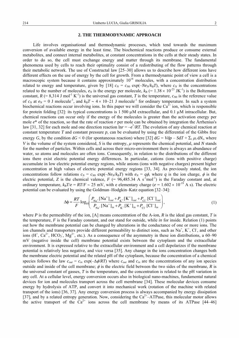
Umberto LUCIA, Giulia GRISOLIA 2 214
2. THE THERMODYNAMIC APPROACH
Life involves organisational and thermodynamic processes, which tend towards the maximum conversion of available energy in the least time. The biochemical reactions produce or consume external metabolites, and connect internal metabolites, at constant concentrations in the cells at their steady states. In order to do so, the cell must exchange energy and matter through its membrane. The fundamental phenomena used by cells to reach their optimality consist of a redistributing of the flow patterns through their metabolic network. The use of Constructal law [25–30] allows us to describe how different ions have different effects on the use of energy by the cell for growth. From a thermodynamic point of view a cell is a macroscopic system because it contains approximately 1014 molecules, with a concentration distribution related to energy and temperature, given by [18] cN = cN0 exp(–NeN/kBT), where cN is the concentrations related to the number of molecules, eN is the energy per molecule, kB (= 1.38 × 10⁻²³ JK-1) is the Boltzmann constant, R (= 8,314 J mol-1 K-1) is the universal gas constant, T is the temperature, cN0 is the reference value of cN at eN = 0 J molecule-1, and kBT ∼ 4 × 10–21 J molecule-1 for ordinary temperature. In such a system biochemical reactions occur involving ions. In this paper we will consider the Ca2+ ion, which is responsible for protein folding [32]: its typical concentrations is 1 500 μM extracellular, and 0.1 μM intracellular. But, chemical reactions can occur only if the energy of the molecules is greater than the activation energy per mole e* of the reaction, so that the rate of reaction r per mole can be obtained by integration the Årrhenius's law [31, 32] for each mole and one direction reaction lnr = –e*/RT. The evolution of any chemical reaction at constant temperature T and constant pressure p, can be evaluated by using the differential of the Gibbs free energy G, by the condition dG < 0 (for spontaneous reaction) where [32] dG = Vdp – SdT + Σi μi dNi, where V is the volume of the system considered, S is the entropy, μ represents the chemical potential, and N stands for the number of particles. Within cells and across their micro-environment there is always an abundance of water, so atoms and molecules are often ions. Consequently, in relation to the distributions of the different ions there exist electric potential energy differences. In particular, cations (ions with positive charge) accumulate in low electric potential energy regions, while anions (ions with negative charges) present higher concentration at high values of electric potential energy regions [33, 34]. As previously stated, the ion concentrations follow relations cN = cN0 exp(–NeN/kBT) with eN = qφ, where q is the ion charge, φ is the electric potential, Z is the chemical valence, F (= 96,485.34 A s-1mol-1) is the Faraday constant and, at ordinary temperature, kBT/e = RT/F ∼ 25 mV, with e elementary charge (e = 1.602 × 10⁻¹⁹ A s). The electric potential can be evaluated by using the Goldman–Hodgkin–Katz equation [32–34]:
Δφ = RT
Flog10
PNa+ [Na+]out +P
K + [K+]out +PCl− [Cl−]out
PNa+ [Na+]in +P
K + [K+]in +PCl− [Cl−]in
⎛
⎝ ⎜ ⎜
⎞
⎠ ⎟ ⎟ , (1)
where P is the permeability of the ion, [A] means concentration of the A-ion, R is the ideal gas constant, T is the temperature, F is the Faraday constant, and out stand for outside, while in for inside. Relation (1) points out how the membrane potential can be changed by alterations in the conductance of one or more ions. The ion channels and transporters provide different permeability to distinct ions, such as Na+, K+, Cl-, and other ions (H+, Ca2+, HCO3
-, Mg2+, etc.). As a consequence of the asymmetry in these ion distributions, a 60–90 mV (negative inside the cell) membrane potential exists between the cytoplasm and the extracellular environment. It is expressed relative to the extracellular environment and a cell depolarizes if the membrane potential is relatively less negative, and vice versa [35]. Any change in the ions concentration changes both the membrane electric potential and the related pH of the cytoplasm, because the concentration of a chemical species follows the law cout = cin exp(–Δφ/RT) where cout and cin are the concentrations of any ion species outside and inside of the cell membrane; φ is the electric field between the two sides of the membrane, R is the universal constant of gasses, T is the temperature, and the concentration is related to the pH variation in any cell. At a cellular level, energy conversion occurs also in biological nano-machines, fundamental natural devices for ion and molecules transport across the cell membrane [34]. These molecular devices consume energy by hydrolysis of ATP, and convert it into mechanical work (rotation of the machine with related transport of the ions) [36, 37]. Any energy conversion process is always accompanied by energy dissipation [37], and by a related entropy generation. Now, considering the Ca2+–ATPase, this molecular motor allows the active transport of the Ca2+ ions across the cell membrane by means of its ATPase [44–46]
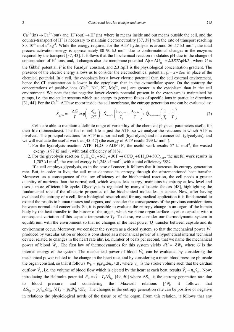
3 Constructal law, ion transfer and cancer 215
Ca2+(in) → Ca2+(out) and H+(out) → H+(in) where in means inside and out means outside the cell, and the counter-transport of H+ is necessary to maintain electroneutrality [37, 38] with the rate of transport reaching 8 × 10⁻⁵ mol s-1kg-1. While the energy required for the ATP hydrolysis is around 56–57 kJ mol-1, the total process activation energy is approximately 80–90 kJ mol-1 due to conformational changes in the enzymes required by the transport [37, 43]. It follows that the biochemical reaction modulates pH due to the change of concentration of H+ ions, and, it changes also the membrane potential Δφ = ΔG
H + +2.3RTΔpH/F , where G is the Gibbs’ potential, F is the Faradys’ constant, and 2.3 ΔpH is the physiological concentration gradient. The presence of the electric energy allows us to consider the electrochemical potential, ˜ μ = μ + Zeφ in place of the chemical potential. In a cell, the cytoplasm has a lower electric potential than the cell external environment, hence the Cl- concentration is lower in the cytoplasm than in the extracellular space. On the contrary the concentrations of positive ions (Ca2+, Na+, K+, Mg2+, etc.) are greater in the cytoplasm than in the cell environment. We note that the negative lower electric potential present in the cytoplasm is maintained by pumps, i.e. the molecular systems which use energy to generate fluxes of specific ions in particular directions [31, 44]. For the Ca2+–ATPase motor inside the cell membrane, the entropy generation rate can be evaluated as:
*
, ,, , ,
0 0
1 1exp Ca out Ca inCag Ca out Ca Ca in out
G eS N QT RT T T T T→
μ μΔ ⎛ ⎞ ⎛ ⎞⎛ ⎞= − − − − + −⎜ ⎟ ⎜ ⎟ ⎜ ⎟⎝ ⎠ ⎝ ⎠ ⎝ ⎠. (2)
Cells are able to maintain a definite range of variability of the chemical-physical parameters useful for their life (homeostasis). The fuel of cell life is just the ATP, so we analyse the reactions in which ATP is involved. The principal reactions for ATP in a normal cell (hydrolysis) and in a cancer cell (glycolysis), and we will evaluate the useful work as [45–47] (the exergy of ATP results 299 kJ mol-1):
1. For the hydrolysis reaction ATP +H2O → ADP+P , the useful work results 57 kJ mol-1, the wasted exergy is 97 kJ mol-1, with total efficiency of 81%;
2. For the glycolysis reaction C6H12O6 +6O2 + 30 P → 6CO2 +6 H2O + 30 PATP , the useful work results in 1,707 kJ mol-1, the wasted exergy is 1,248 kJ mol-1, with a total efficiency 58%.
If a cell employs glycolysis, as in the case of cancer, it follows that it increases its entropy generation rate. But, in order to live, the cell must decrease its entropy through the aforementioned heat transfer. Moreover, as a consequence of the low efficiency of the biochemical reaction, the cell needs a greater quantity of nutrients than the normal cell, which wastes less exergy, maintains its entropy at low level and uses a more efficient life cycle. Glycolysis is regulated by many allosteric factors [48], highlighting the fundamental role of the allosteric properties of the biochemical molecules in cancer. Now, after having evaluated the entropy of a cell, for a biological research and for any medical application it is fundamental to extend the results to human tissues and organs, and consider the consequences of the previous considerations between normal and cancer cells. So, it is possible to evaluate the entropy change in an organ of the human body by the heat transfer to the border of the organ, which we name organ surface layer or capsule, with a consequent variation of this capsule temperature TS. To do so, we consider our thermodynamic system in equilibrium with the environment so that no changes in the heat power Q transfer between capsule and its environment occur. Moreover, we consider the system as a closed system, so that the mechanical power W produced by vascularisation or blood is considered as a mechanical power of a hypothetical internal technical device, related to changes in the heart rate nhr, i.e. number of beats per second, that we name the mechanical power of blood bW . The first law of thermodynamics for this system yields dU = −δWb where U is the internal energy of the system. The mechanical power of blood bW can be evaluated by considering the mechanical power related to the change in the heart rate, and by considering a mean blood pressure pb inside the organ constant, so that it follows d / d=b b sv hrW p v n t , where svv is the stroke volume such that the cardiac outflow bV , i.e. the volume of blood flow which is ejected by the heart at each beat, results b hr svV n v= . Now, introducing the Helmoltz potential H S bpF U T S= − Δ [49, 50] where bpSΔ is the entropy generation rate due to blood pressure, and considering the Maxwell relations [49], it follows that
d /d d /dΔ = =bp b sv hr S b b SS p v n T p V T . The changes in the entropy generation rate can be positive or negative in relationo the physiological needs of the tissue or of the organ. From this relation, it follows that any
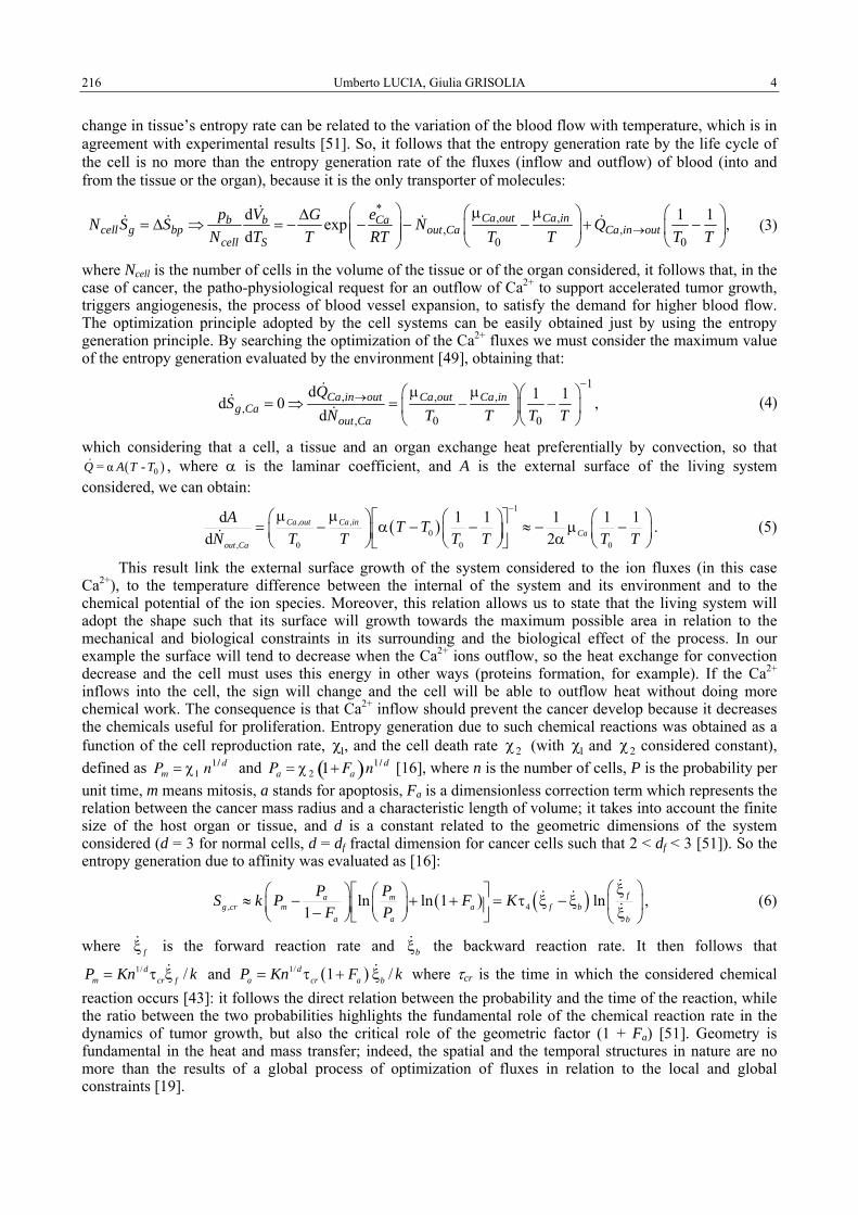
Umberto LUCIA, Giulia GRISOLIA 4 216
change in tissue’s entropy rate can be related to the variation of the blood flow with temperature, which is in agreement with experimental results [51]. So, it follows that the entropy generation rate by the life cycle of the cell is no more than the entropy generation rate of the fluxes (inflow and outflow) of blood (into and from the tissue or the organ), because it is the only transporter of molecules:
*, ,
, ,0 0
d 1 1exp ,d →
⎛ ⎞ μ μ⎛ ⎞ ⎛ ⎞Δ= Δ ⇒ = − − − − + −⎜ ⎟ ⎜ ⎟ ⎜ ⎟⎜ ⎟ ⎝ ⎠ ⎝ ⎠⎝ ⎠
Ca out Ca inb b Cacell g bp out Ca Ca in out
cell S
p V eGN S S N QN T T RT T T T T
(3)
where Ncell is the number of cells in the volume of the tissue or of the organ considered, it follows that, in the case of cancer, the patho-physiological request for an outflow of Ca2+ to support accelerated tumor growth, triggers angiogenesis, the process of blood vessel expansion, to satisfy the demand for higher blood flow. The optimization principle adopted by the cell systems can be easily obtained just by using the entropy generation principle. By searching the optimization of the Ca2+ fluxes we must consider the maximum value of the entropy generation evaluated by the environment [49], obtaining that:
1, , ,
,, 0 0
d 1 1d 0 ,d
−→ μ μ⎛ ⎞⎛ ⎞
= ⇒ = − −⎜ ⎟⎜ ⎟⎝ ⎠⎝ ⎠
Ca in out Ca out Ca ing Ca
out Ca
QS
N T T T T (4)
which considering that a cell, a tissue and an organ exchange heat preferentially by convection, so that ( )0= αQ A T - T , where α is the laminar coefficient, and A is the external surface of the living system
considered, we can obtain:
( )1
, ,0
, 0 0 0
d 1 1 1 1 1d 2
Ca out Ca inCa
out Ca
A T TN T T T T T T
−μ μ ⎡ ⎤⎛ ⎞ ⎛ ⎞ ⎛ ⎞= − α − − ≈ − μ −⎜ ⎟ ⎜ ⎟ ⎜ ⎟⎢ ⎥ α⎝ ⎠ ⎝ ⎠ ⎝ ⎠⎣ ⎦
. (5)
This result link the external surface growth of the system considered to the ion fluxes (in this case Ca2+), to the temperature difference between the internal of the system and its environment and to the chemical potential of the ion species. Moreover, this relation allows us to state that the living system will adopt the shape such that its surface will growth towards the maximum possible area in relation to the mechanical and biological constraints in its surrounding and the biological effect of the process. In our example the surface will tend to decrease when the Ca2+ ions outflow, so the heat exchange for convection decrease and the cell must uses this energy in other ways (proteins formation, for example). If the Ca2+ inflows into the cell, the sign will change and the cell will be able to outflow heat without doing more chemical work. The consequence is that Ca2+ inflow should prevent the cancer develop because it decreases the chemicals useful for proliferation. Entropy generation due to such chemical reactions was obtained as a function of the cell reproduction rate, χ1, and the cell death rate χ2 (with χ1 and χ2 considered constant), defined as Pm = χ1 n1/ d and Pa = χ 2 1+ Fa( )n1/ d [16], where n is the number of cells, P is the probability per unit time, m means mitosis, a stands for apoptosis, Fa is a dimensionless correction term which represents the relation between the cancer mass radius and a characteristic length of volume; it takes into account the finite size of the host organ or tissue, and d is a constant related to the geometric dimensions of the system considered (d = 3 for normal cells, d = df fractal dimension for cancer cells such that 2 < df < 3 [51]). So the entropy generation due to affinity was evaluated as [16]:
( ) ( ), 4ln ln 1 ln1
fa mg cr m a f b
a a b
P PS k P F KF P
⎛ ⎞ξ⎡ ⎤⎛ ⎞ ⎛ ⎞≈ − + + = τ ξ − ξ ⎜ ⎟⎜ ⎟ ⎜ ⎟⎢ ⎥− ξ⎝ ⎠ ⎝ ⎠⎣ ⎦ ⎝ ⎠, (6)
where fξ is the forward reaction rate and bξ the backward reaction rate. It then follows that 1/ /d
m cr fP Kn k= τ ξ and ( )1/ 1 /da cr a bP Kn F k= τ + ξ where τcr is the time in which the considered chemical
reaction occurs [43]: it follows the direct relation between the probability and the time of the reaction, while the ratio between the two probabilities highlights the fundamental role of the chemical reaction rate in the dynamics of tumor growth, but also the critical role of the geometric factor (1 + Fa) [51]. Geometry is fundamental in the heat and mass transfer; indeed, the spatial and the temporal structures in nature are no more than the results of a global process of optimization of fluxes in relation to the local and global constraints [19].
5 Constructal law, ion transfer and cancer 217
3. CONCLUSIONS
The analysis of the Ca2+ flux has been developed in order to point out the role of this ion in the decreasing of the cancer growth. We can highlight that it requires energy in relation to its electric charge and the membrane electric field; indeed, the positive charge of the Ca2+ ion decrease the cell energy. It is due to the electrochemical work required by the ions to cross the membrane cell. Cancer growth is related to the energy management of cells, and the process of malignant transformation is no more than a difference in energy lost to the microenvironment. Cancer must increase its energy dissipation to reduce its entropy [4–6, 43]. So, the cancer cell must increase the coefficient of convection, through exchange with blood and fluids, so it is poised to induce blood vessel growth towards the tumor, i.e. angiogenesis, because it needs to increase this convection coefficient, and the aforementioned metabolite flows, and to sustain the nourishment demands of on-site growth. Moreover, such sprouting vessels should lead to a deterioration of tissue consistency, thus reduce mechanical confinement which consequently supports continued on-site expansion, and serves migrating cells as a path to move along. But, even if dissipation is improved by an increase of convection, it occurs with body fluids at 37°C, insufficient to provide the required relief through facilitated energy outflow. As a consequence, cancer cells attempt to increase the flow of H+ and other ions to consume ATP and to increase energy dissipation; this induces both a pH variation and a change in membrane potential. Any variation in pH generates a variation in the behavior of the cell; if the environment turns acidic, further carcinogenesis towards more aggressive phenotypes becomes more likely. From these analytical results, it is possible to argue that cell functions are regulated by membrane proteins that are sensitive to the electric field. Changes in the membrane’s electric field are then transduced into a conformational change of the biological molecules, and in turn, this allosteric effect triggers the function of membrane proteins, with consequences for the regulation of cell functions or even entire phenotypes. We argue that based on the role of the electrostatic potential in regulating normal cell differentiation, conceivably its control, or rather loss of control, is fundamental for the development of cancer: the voltage-responsive transduction mechanisms on the cell membrane allow bioelectric signals to regulate the polarization of cell molecules. The biochemical reactions that enable cell life produce or consume external metabolites, and connect with internal metabolites. Cancer needs to dissipate energy, which leads to heat storage in the environment, and pH acidification, in a vicious cycle.
REFERENCES
1. Y. DEMIREL, S.I. SANDLER, Thermodynamics and bioenergetics, Biophysical Chemistry, 97, pp. 87–111, 2002. 2. O. TOUSSAINT, E.D. SCHNEIDER, The thermodynamic and evolution of complexity in biological systems, Comparative
Biochemical Physiology A, 120, pp. 3–9, 1998. 3. S.R. CAPLAN, A. ESSIG, Bioenergetics and Linear Nonequilibrium Thermodynamics, The Steady State, Harvard University
Press, Cambridge, 1983. 4. U. LUCIA, Entropy generation approach to cell systems, Physica A, 406, pp. 1–11, 2014. 5. U. LUCIA, Bioengineering thermodynamics: an engineering science for thermodynamics of biosystems, I. Jo.T., 18, pp. 254–265,
2015. 6. U. LUCIA, Bioengineering thermodynamics of biological cells, Theor. Biol. Med. Model., 12, p. 29, 2015. 7. A. KATCHALSKY, P.F. CURRAN, Nonequilibrium Thermodynamics in Biophysics, Harvard University Press, Cambridge, 1967. 8. U. LUCIA, Irreversibility in biophysical and biochemical engineering, Physica A, 391, pp. 5997–6007, 2012. 9. C. BUSTAMANTE, Y.R. CHEMLA, N.R. FORDE, D. IZHAKY, Mechanical Processes in Biochemistry, Annual Review of
Biochemistry, 73, pp. 705–748, 2004. 10. U. LUCIA, Thermodynamics and cancer stationary states, Physica A, 392, pp. 3648–3653, 2013. 11. J. HARRIS, M. MORROW, L. NORTON, Malignant tumors of the breast, In De Vita, V.T. Jr, HELLMAN, S., ROSENBERG,
S.A., Eds., Cancer: Principles and Practice of Oncology, Fifth Edition, Lippincott-Raven, Philadelphia, 1997. 12. L. NORTON, Conceptual and Practical Implications of Breast Tissue Geometry: Toward a More Effective, Less Toxic Therapy,
The Oncologist, 10, pp. 370–381, 2005. 13. E. IZQUIERDO-KULICH, E. ALONSO-BECERRA, J.M. NIETO-VILLAR, Entropy Production Rate for Avascular Tumor
Growth, Journal of Modern Physics, 2, pp. 615–620, 2011. 14. J.D. RUPA, A.P. de BRUINE, A.J. GERBERS, M.P. LEERS, M. NAP, A.G. KESSELS, B. SCHUTTE, J.W. ARENDS,
Simultaneous detection of apoptosis and proliferation in colorectal carcinoma by multiparameter flow cytometry allows separation of high and low-turnover tumors with distinct clinical outcome, Cancer, 97, pp. 2404–2411, 2003.
15. E.A. COMEN, L. NORTON, J. MASSAGUE, Breast Cancer Tumor Size, Nodal Status, and Prognosis: Biology Trumps Anatomy, Journal of Clinical Oncology, 29, pp. 1–3, 2011.
Umberto LUCIA, Giulia GRISOLIA 6 218
16. U. LUCIA, A. PONZETTO, T.S. DEISBOECK, A thermodynamic approach to the ‘mitosis/apoptosis’ ratio in cancer, Physica A, 436, pp. 246–255, 2015.
17. A. BEJAN, Heat Transfer, John Wiley & Sons, Hoboken, 1993. 18. A. BEJAN, Convection Heat Transfer, John Wiley & Sons, Hoboken, 2013. 19. A. BEJAN, Shape and Structure, from Engineering to Nature, Cambridge University Press, Cambridge, 2000. 20. A. BEJAN, S. LORENTE, Design with Constructal Theory, John Wiley & Sons, Hoboken, 2008. 21. A. BEJAN, S. LORENTE, The constructal law and the evolution of design in nature, Phil. Trans. B, 365, p. 1545, 2010. 22. A.H. REIS, Constructal theory: from engineering to physics, and how flow systems develop shape and structure, Appl. Mech.
Rev., 59, pp. 269–282, 2006. 23. A.F. MIGUEL, The physics principle of the generation of flow configuration, Phys. Life Rev., 8, pp. 243–244, 2011. 24. A.F. MIGUEL, A. BEJAN, The principle that generates dissimilar patterns inside aggregates of organisms, Physica A, 388, pp.
727–731, 2009. 25. A.H. REIS, Design in nature, and the laws of physics, Phys. Life Rev., 8, pp. 255–256, 2011. 26. A. BEJAN, The Constructal Law of Organization in Nature: Tree-shaped flows and body size, J. Exp. Biol. 208, pp. 1677–1686,
2005. 27. A. BEJAN, S. LORENTE, Design with Constructal Theory, Wiley, Hoboken, 2008. 28. A. BEJAN, Theory of Organization in Nature: Pulsating Physiological Processes, Int. J. Heat Mass Trans., 40, pp. 2097–2104,
1997. 29. A. BEJAN, The Physics of Life: The Evolution of Everything, St. Martin's Press, New York, 2016. 30. A.H. REIS, Use and validity of principles of extremum of entropy production in the study of complex systems, Ann. Phys. 346,
pp. 22–27, 2014. 31. J. WOLFE, Cellular thermodynamics: the molecular and macroscopic point of views, eLS-John Wiley & Sons, Chichester, 2015. 32. P. ATKINS, J. De PAULA, Physical Chemistry for Life Sciences, Oxford University Press, New York, 2006. 33. M. ASHRAFUZZAMAN, J.A. TUSZYNSKI, Membrane Biophysics, Springer, Berlin, 2013. 34. S. KJELSRUP, J.M. RUBI, D. BEDEAUX, A Thermodynamic Description of Active Transport, in Franzese, G., Rubi, J.M.
(Eds.), Aspects of Physical Biology: Biological Water, Protein, Solutions, Transport and Replication, Springer, Berlin, 2008. 35. D.E. GOLDMAN, Potential, impedance, and rectification in membranes, J. Gen. Physiol., 27, pp. 37–60, 1943. 36. P. MITCHELL, Coupling of phosphorylation to electron and hydrogen transfer by a chemi-osmotic type mechanism, Nature,
191, p. 144, 1961. 37. J.M. RUBI, M. NASPREDA, S. KJELSTRUP, D. BEDEAUX, Energy transduction in biological systems: a mesoscopic non-
equilibrium thermodynamics perspective, J. Non-Equil. Thermodyn., 32, pp. 351–378, 2007. 38. M.C. BERMAN, Slippage and uncoupling in P-type cation pumps; implication for energy transduction mechanism and
regulation of metabolism, Biochem. Biophys. Acta, 1513, pp. 95–121, 2001. 39. L. de MEIS, Energy Interconversion in Transport ATPase, in Franzese, G., Rubi, J.M. (Eds.), Aspects of Physical Biology:
Biological Water, Protein, Solutions, Transport and Replication, Springer, Berlin, 2008. 40. U. LUCIA, Electromagnetic waves and living cells: A kinetic thermodynamic approach, Physica A, 461, pp. 577–585, 2016. 41. U. LUCIA, Thermodynamic approach to nano-properties of cell membrane, Physica A, 407, pp. 185–191, 2014. 42. U. LUCIA, Entropy generation and cell growth with comments for a thermodynamic anticancer approach, Physica A, 406, pp.
107–118, 2014. 43. U. LUCIA, Different chemical reaction times between normal and solid cancer cells, Medical Hypotheses, 81, pp. 58–61, 2013. 44. R.K. HOBBIE, Intermediate Physics for Medicine and Biology, Springer-Verlag, New York, 1997. 45. J. SZARGUT, D.R. MORRIS, F.R. STEWARD, Exergy analysis of thermal, chemical, and metallurgical processes, Hemisphere
Publishing Co., London, 1988. 46. S. LEMS, H.J. van der KOOI, J. de SWAAN ARONS, Thermodynamic analysis of the living cell: design of an exergy-based
method, Int. J. Exergy, 4, pp. 339–356, 2007. 47. S. LEMS, H.J. van der KOOI, J. de SWAAN ARONS, The second-law implications of biochemical energy conversion: exergy
analysis of glucose and fatty-acid breakdown in the living cell, Int. J. Exergy, 6, pp. 228–248, 2009. 48. E. RACKER, Warburg effect revisited, Science, 213, pp. 1313, 2008. 49. A. BEJAN, Advanced Engineering Thermodynamics, John Wiley, New York, 2006. 50. S. BOREGOWDA, R. HANDY, D. SLEETH, A. MERRYWEATHER, Measuring Entropy Change in a Human Physiological
System, J. Thermodyn., 2016, pp. 1–6, 2016. 51. L. NORTON, Conceptual and Practical Implications of Breast Tissue Geometry: Toward a More Effective, Less Toxic Therapy,
The Oncologist, 10, pp. 370–381, 2005.
THE PUBLISHING HOUSE PROCEEDINGS OF THE ROMANIAN ACADEMY, Series A, OF THE ROMANIAN ACADEMY Special Issue/2018, pp. 219–224
BIMODAL IT: BEYOND THE HYPE WITH THE CONSTRUCTAL LAW?
Stephen PÉRIN
MiST – Management of Information Systems and Technologies, OCTO Technology, 34, Avenue des Champs-Élysées, Paris 75002, France
Corresponding author: Stephen PÉRIN, E-mail: [email protected]
Abstract. Several models of Information Technology (IT) and digital products delivery organization have waxed and waned during the last five years: Two Speed IT, Bimodal IT, Multi-speed IT, Right-Speed IT, etc. In this article, we review and briefly compare some of the main models proposed, mainly by large IT research or consulting firms. In a second part, and since IT and Information Systems (IS) can be viewed as complex flow systems, we will show how the constructal theory can help to discriminate between these, often competing, IT organizational models. More particularly, we will show how the constructal theory of the origin of S-curve fits with Wardley’s PST triple-modes model, which is rooted in the analysis of a generic IT product lifecycle logistic curve. We thus illustrate here a first approach to integrate the principles of the constructal theory into the domain of corporate and IT organization and processes.
Key words: Bimodal IT, Constructal law, Digitization, S-curve, Two-speed IT, Wardley’s PST model.
1. CONTEXT: A WHOLE LANDSCAPE OF IT DELIVERY MODELS
1.1. The need for speed in the Digital economy
The evolution of information systems is becoming a strategic and competitive activity for many companies, more particularly due to the rise of e-commerce, mobile computing, and online social networks –in a word, due to the digitization of business [1–2]. For this reason, the delivery of digital products and services – for instance based on mobile apps, web sites, or connected devices–needs a faster delivery model than the traditional IT waterfall model, generally leading to long tunnels of software developments [1]. In brief, the interest to go faster is not just to be quicker than the competitors, but also, among other advantages, to be able to quickly validate the product-market fit, before injecting more substantial budget into it [3].
1.2. Gartner’s Bimodal IT enters the scene
To cope with this challenge, several IT delivery models have been proposed during the last five years [1–8]. The more famous and discussed of these models probably being the so-called Gartner’s “Bimodal IT” [1, 6]. Gartner is a famous IT research and consulting company. It is also widely known for its thematic technology forecasts called the “hype cycle”, hence the title of this article–and the private joke: “Bimodal IT, beyond the hype”, i.e. beyond the hype cycle [9].
“Bimodal IT”, or more simply “Bimodal” is one the many concepts forged, by Gartner, whose job is also to identify-and name-new technological trends in the industries markets and in the IT industry especially. Based on a research on its documentary corpus, searchable online, the first Gartner’s publication on Bimodal IT was released in February 2014 [1, 10]. This concept is defined, as follows, by Gartner:
“Bimodal is the practice of managing two separate but coherent styles of work: one focused on predictability; the other on exploration. Mode 1 is optimized for areas that are more predictable and well-understood. It focuses on exploiting what is known, while renovating the legacy environment into a state that is fit for a digital world. Mode 2 is exploratory, experimenting to solve new problems and optimized for

Stephen PÉRIN 2 220
areas of uncertainty. […] Marrying a more predictable evolution of products and technologies (Mode 1) with the new and innovative (Mode 2) is the essence of an enterprise bimodal capability. Both play an essential role in the digital transformation” [11].
To summarize, the “Bimodal” model defines two main flow modes for the “Digital Era” company, one focused on “running the business” (mode 1, traditional), and a more exploratory mode focused on “transforming business” (mode 2, digital) thanks to a more exploratory, breaking innovation, approach. These two modes are sometimes compared by Gartner to the two different performance of a marathon runner (mode 1), and a sprinter (mode 2), as in [12, p. 16]. The adoption of this model within corporate organizations is of course very largely promoted by Gartner. For example, among many other frequent (and self-accomplishing?) predictions, Gartner announced in 2014 that “by 2017, 75% of IT organizations will have a bimodal capability” [13, p. 19].
Fig. 1 – Number of occurrence of “Bimodal IT” in Gartner’s
online research corpus, for all content type. Fig. 2 – Cumulated Google Trends search interest rate for
“Bimodal IT”, in percent, since August, 2012.
On Fig. 1 is displayed the number of occurrence of the term “Bimodal IT” in Gartner’s online research corpus (available at https://www.gartner.com/search/all/simple), for all content type, since January, the 1st, 2012. The data have been corrected only for 2012 and 2013, the search engine having provided one non-relevant occurrence for each year (ex. “[…] bimodal, it […]”. It seems that the Bimodal hype reached its peak in 2016 for Gartner, but also for the general public, since its interest is now slowly decreasing, as can be seen in the inflexion of the cumulated search interested rate provided by Google Trends (trends.google.com), and showed on Figs. 2 and 3 – Clearly, Bimodal IT trend has already gone… beyond the hype.
1.3. A clash of models
In the wake of the publication of Gartner’s Bimodal IT model, in February 2014, several models have been proposed by other consulting firms, and competitors [4–8]. These models are listed here below in table 1. They include, for instance, McKinsey’s vision of “Two speed IT” [8], Accenture proposition on a “Multi-speed IT” model [4], or Deloitte’s “Right-Speed IT” view on this topic [7].
Usually, the proposed models are a more or less customized two-modes “copycat” model (e.g. McKinsey’s [8]). Deloitte, on its side, doesn’t exactly propose a model, but explain that each project must have his own pace, to meet its own constraint, hence the lack of a more generalized view, i.e. a model [7]. But several other kinds of models or other cases are worth considering [14–16]. First, it must be noticed that Gartner’s Bimodal was not the first two-modes-IT delivery models ever proposed. More particularly, four years before, in August 2012, The Boston Consulting Group (BCG) was advocating for the adoption of a “Two Speed IT” model, in order to face the challenge of Digitization [14]. The two speeds were called “Industrial Speed” and “Digital Speed”. Interestingly enough, in 2016, the BCG changed its position and recommended to abandon this previous two speed model–
Fig. 3 – Google Trends’ search interest rate for “Two speed IT”
and “Bimodal IT”, in percent, since January, 2012.

3 Bimodal IT: beyond the hype with the constructal law? 221
allegedly due to the rapid evolution of the market under the Digitization pressure–, and advised to adopt now a single delivery mode model, inspired by Agile software delivery methods, and thus called “All-Agile” [15]. As can be seen on figure 3, the BCG’s two-speed IT model had a very smaller impact on the market than the Bimodal IT. Effectively, the search interest provided by Google Trends for the “two speed IT” model hardly reach 20% of the interest triggered by “Bimodal IT”. Finally, Gartner itself used the term two speed in at least of the its two seminal publication: “bimodal or two-speed approach to managing IT” [10, p. 2], § Recommendation.
Forrester, a very virulent competitor of Gartner [16], also promoted its own IT delivery model very early before the release of Bimodal IT. In a publication dating from July 2008, Forrester already describe its approach towards “Business Technology”, as opposed to “IT Technology” [16]. This is the very same model Forrester has been opposing to Gartner’s views, into several polemic publications directly attacking the Bimodal IT approach, and strongly advising against it. For instance see the following publication title: “the false promise of Bimodal IT” [16], “Bimodal Is Out Of Sync With Faster Change Bimodal Dinosaurs Won't Be Able To Lead Their Companies To Success” [18].
Regarding the impact of the models reviewed, other than the BCG’s or Gartner’s, not enough search data were available on Google Trends to enable a comparison or analysis. By itself, this negative result is obviously a strong signal of the very lesser interest from the market, hence very lesser impact on it, of these alternatives models.
Table 1
IT delivery models reviewed
Source IT Delivery Model
Number of IT delivery modes
IT delivery modes Publication date (dd/mm/yyyy)
Simon Wardley PST 3 Pioneering, Settling, Town Planning 27/03/2008
Forrester Research, Inc.
[IT to] Business Technology (BT)
2 IT Technology, Business Technology 09/07/2008
The Boston Consulting Group Two speed IT 2 Industrial Speed, Digital Speed 01/08/2012
Gartner, Inc Bimodal IT 2 Mode 1, Mode 2 14/02/2014 McKinsey & Company Two speed IT 2 Slow-speed, Fast-speed 12/2015
Accenture Multi-speed IT 2 Legacy IT, Agile IT (Fast Lane
IT) 11/11/2015
Deloitte Development LLC
Right-speed IT N N/A (project-specific speed) 24/02/2016
The Boston Consulting Group All-Agile 1 Agile 12/08/2016
Beyond the “small world” of IT research and consulting firms and competitors, the Bimodal IT model has also generated a lot of discussions, and polemics online in the, larger, IT world, the debate being facilitated by the easy access to many kinds of blogs or social media: “Saying Goodbye to Bimodal IT” [19], “Why BiModal IT Won’t Work” [20], “Bimodal IT: A Buzzword, a Solution, or a Smokescreen?” [21], “Bimodal IT - the new old hotness” [22]. In favor of Gartner, it appears that the understanding of its model is often reduced to the caricature, e.g. “Agile” vs. “Waterfall”: “Bimodal is widely misinterpreted by many as simply the introduction of agile tools and methodologies such as Scrum or the introduction of DevOps practices” [23, p. 4], § “BECS Defined: Five Integrated Services”. This is of course the case for every concept when it diffuses into a larger public: the meaning dilutes, it is wrongly interpreted, or misunderstood–a phenomenon well known, unfortunately unavoidable, and sometimes called “semantic diffusion”: “One of the problems with building a jargon is that terms are vulnerable to losing their meaning, in a process of semantic diffusion” [24].
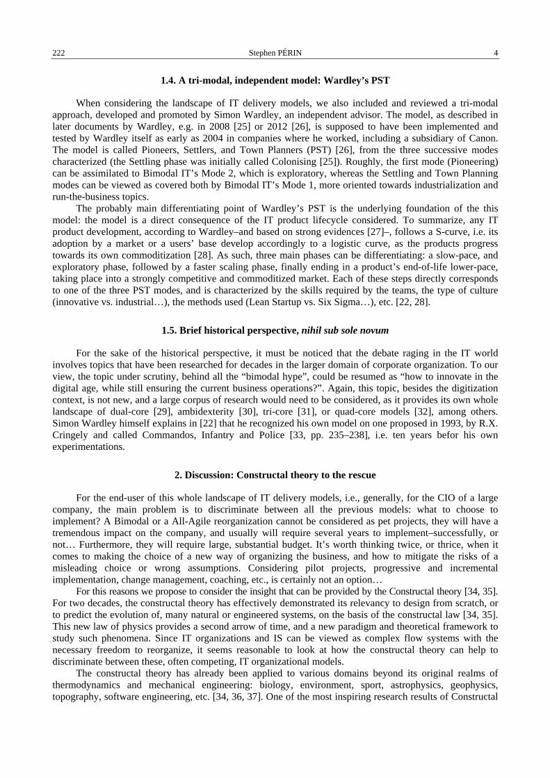
Stephen PÉRIN 4 222
1.4. A tri-modal, independent model: Wardley’s PST
When considering the landscape of IT delivery models, we also included and reviewed a tri-modal approach, developed and promoted by Simon Wardley, an independent advisor. The model, as described in later documents by Wardley, e.g. in 2008 [25] or 2012 [26], is supposed to have been implemented and tested by Wardley itself as early as 2004 in companies where he worked, including a subsidiary of Canon. The model is called Pioneers, Settlers, and Town Planners (PST) [26], from the three successive modes characterized (the Settling phase was initially called Colonising [25]). Roughly, the first mode (Pioneering) can be assimilated to Bimodal IT’s Mode 2, which is exploratory, whereas the Settling and Town Planning modes can be viewed as covered both by Bimodal IT’s Mode 1, more oriented towards industrialization and run-the-business topics.
The probably main differentiating point of Wardley’s PST is the underlying foundation of the this model: the model is a direct consequence of the IT product lifecycle considered. To summarize, any IT product development, according to Wardley–and based on strong evidences [27]–, follows a S-curve, i.e. its adoption by a market or a users’ base develop accordingly to a logistic curve, as the products progress towards its own commoditization [28]. As such, three main phases can be differentiating: a slow-pace, and exploratory phase, followed by a faster scaling phase, finally ending in a product’s end-of-life lower-pace, taking place into a strongly competitive and commoditized market. Each of these steps directly corresponds to one of the three PST modes, and is characterized by the skills required by the teams, the type of culture (innovative vs. industrial…), the methods used (Lean Startup vs. Six Sigma…), etc. [22, 28].
1.5. Brief historical perspective, nihil sub sole novum
For the sake of the historical perspective, it must be noticed that the debate raging in the IT world involves topics that have been researched for decades in the larger domain of corporate organization. To our view, the topic under scrutiny, behind all the “bimodal hype”, could be resumed as “how to innovate in the digital age, while still ensuring the current business operations?”. Again, this topic, besides the digitization context, is not new, and a large corpus of research would need to be considered, as it provides its own whole landscape of dual-core [29], ambidexterity [30], tri-core [31], or quad-core models [32], among others. Simon Wardley himself explains in [22] that he recognized his own model on one proposed in 1993, by R.X. Cringely and called Commandos, Infantry and Police [33, pp. 235–238], i.e. ten years befor his own experimentations.
2. Discussion: Constructal theory to the rescue
For the end-user of this whole landscape of IT delivery models, i.e., generally, for the CIO of a large company, the main problem is to discriminate between all the previous models: what to choose to implement? A Bimodal or a All-Agile reorganization cannot be considered as pet projects, they will have a tremendous impact on the company, and usually will require several years to implement–successfully, or not… Furthermore, they will require large, substantial budget. It’s worth thinking twice, or thrice, when it comes to making the choice of a new way of organizing the business, and how to mitigate the risks of a misleading choice or wrong assumptions. Considering pilot projects, progressive and incremental implementation, change management, coaching, etc., is certainly not an option…
For this reasons we propose to consider the insight that can be provided by the Constructal theory [34, 35]. For two decades, the constructal theory has effectively demonstrated its relevancy to design from scratch, or to predict the evolution of, many natural or engineered systems, on the basis of the constructal law [34, 35]. This new law of physics provides a second arrow of time, and a new paradigm and theoretical framework to study such phenomena. Since IT organizations and IS can be viewed as complex flow systems with the necessary freedom to reorganize, it seems reasonable to look at how the constructal theory can help to discriminate between these, often competing, IT organizational models.
The constructal theory has already been applied to various domains beyond its original realms of thermodynamics and mechanical engineering: biology, environment, sport, astrophysics, geophysics, topography, software engineering, etc. [34, 36, 37]. One of the most inspiring research results of Constructal
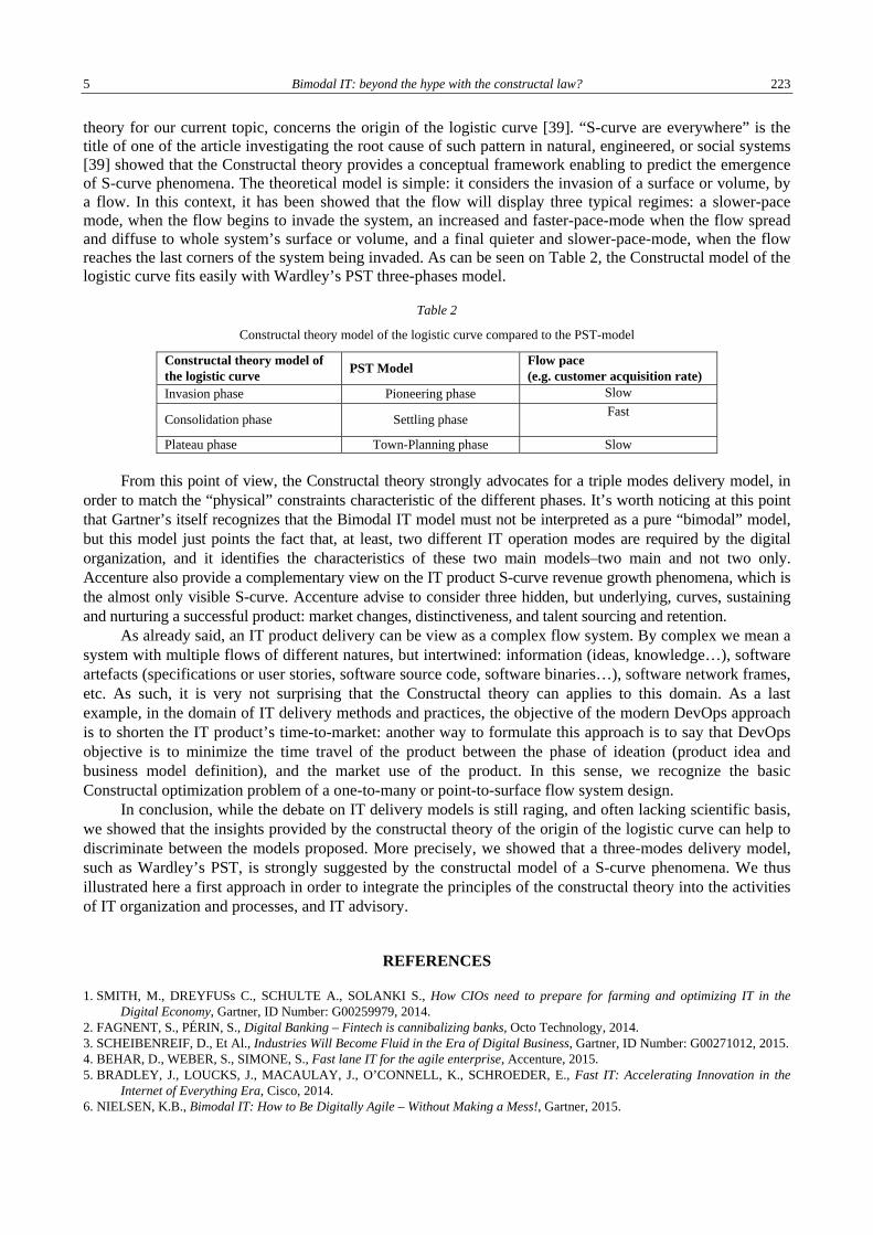
5 Bimodal IT: beyond the hype with the constructal law? 223
theory for our current topic, concerns the origin of the logistic curve [39]. “S-curve are everywhere” is the title of one of the article investigating the root cause of such pattern in natural, engineered, or social systems [39] showed that the Constructal theory provides a conceptual framework enabling to predict the emergence of S-curve phenomena. The theoretical model is simple: it considers the invasion of a surface or volume, by a flow. In this context, it has been showed that the flow will display three typical regimes: a slower-pace mode, when the flow begins to invade the system, an increased and faster-pace-mode when the flow spread and diffuse to whole system’s surface or volume, and a final quieter and slower-pace-mode, when the flow reaches the last corners of the system being invaded. As can be seen on Table 2, the Constructal model of the logistic curve fits easily with Wardley’s PST three-phases model.
Table 2
Constructal theory model of the logistic curve compared to the PST-model
Constructal theory model of the logistic curve PST Model Flow pace
(e.g. customer acquisition rate) Invasion phase Pioneering phase Slow
Consolidation phase Settling phase Fast
Plateau phase Town-Planning phase Slow
From this point of view, the Constructal theory strongly advocates for a triple modes delivery model, in order to match the “physical” constraints characteristic of the different phases. It’s worth noticing at this point that Gartner’s itself recognizes that the Bimodal IT model must not be interpreted as a pure “bimodal” model, but this model just points the fact that, at least, two different IT operation modes are required by the digital organization, and it identifies the characteristics of these two main models–two main and not two only. Accenture also provide a complementary view on the IT product S-curve revenue growth phenomena, which is the almost only visible S-curve. Accenture advise to consider three hidden, but underlying, curves, sustaining and nurturing a successful product: market changes, distinctiveness, and talent sourcing and retention.
As already said, an IT product delivery can be view as a complex flow system. By complex we mean a system with multiple flows of different natures, but intertwined: information (ideas, knowledge…), software artefacts (specifications or user stories, software source code, software binaries…), software network frames, etc. As such, it is very not surprising that the Constructal theory can applies to this domain. As a last example, in the domain of IT delivery methods and practices, the objective of the modern DevOps approach is to shorten the IT product’s time-to-market: another way to formulate this approach is to say that DevOps objective is to minimize the time travel of the product between the phase of ideation (product idea and business model definition), and the market use of the product. In this sense, we recognize the basic Constructal optimization problem of a one-to-many or point-to-surface flow system design.
In conclusion, while the debate on IT delivery models is still raging, and often lacking scientific basis, we showed that the insights provided by the constructal theory of the origin of the logistic curve can help to discriminate between the models proposed. More precisely, we showed that a three-modes delivery model, such as Wardley’s PST, is strongly suggested by the constructal model of a S-curve phenomena. We thus illustrated here a first approach in order to integrate the principles of the constructal theory into the activities of IT organization and processes, and IT advisory.
REFERENCES
1. SMITH, M., DREYFUSs C., SCHULTE A., SOLANKI S., How CIOs need to prepare for farming and optimizing IT in the Digital Economy, Gartner, ID Number: G00259979, 2014.
2. FAGNENT, S., PÉRIN, S., Digital Banking – Fintech is cannibalizing banks, Octo Technology, 2014. 3. SCHEIBENREIF, D., Et Al., Industries Will Become Fluid in the Era of Digital Business, Gartner, ID Number: G00271012, 2015. 4. BEHAR, D., WEBER, S., SIMONE, S., Fast lane IT for the agile enterprise, Accenture, 2015. 5. BRADLEY, J., LOUCKS, J., MACAULAY, J., O’CONNELL, K., SCHROEDER, E., Fast IT: Accelerating Innovation in the
Internet of Everything Era, Cisco, 2014. 6. NIELSEN, K.B., Bimodal IT: How to Be Digitally Agile – Without Making a Mess!, Gartner, 2015.

Stephen PÉRIN 6 224
7. WHITE, M., PENNINGTON, J., GALIZIA, T., HABECK, M., Right-Speed IT, Tech Trends 2016, Innovating in the digital era, Deloitte University Press, pp. 5-19, 2016.
8. AVEDILLO, J.G., BEGONHA, D., PEYRACCHIA, A., Two ways to modernize IT systems for the digital era, Business Technology Office, McKinsey & Company, 2015.
9. WITTY, R.J., MORENCY, J.P., Hype Cycle for Business Continuity Management and IT Disaster Recovery Management, 2010, Gartner, ID Number: G00206424, 2010.
10. MINGAY, S., IYENGAR, P., POTTER, K., How CIOs Need to Prepare for Industrializing and Mutualizing IT in the Digital Economy, Gartner, ID Number: G00259981, 2014.
11. GARTNER, From the Gartner IT Glossary: What is Bimodal?, https://research.gartner.com/definition-whatis-bimodal, Consulted: 2 May 2017, Gartner, 2017.
12. HUNTER, R., Digital Humanism: Swinging the Pendulum of Digital Business, Gartner Symposium ITxpo 2014, Gartner, 2014. 13. MELLO, A., Negócios Digitais na Era da Inovação, CASE, 2014, Gartner, 2014. 14. GOURÉVITCH, A., REHBERG, B., BOBIER, J.-F., Two-Speed IT: A Linchpin for Success in a Digitized World,
bcgperspectives.com, The Boston Consulting Group, 2012. 15. KETTERER, H., REHBERG, B., SCHMID, C.N., KLEINE, D., The End of Two-Speed IT, bcgperspectives.com, The Boston
Consulting Group, 2016. 16. MCCARTHY, J.C., LEAVER, S., SCHADLER, T., GIRON, F., MATZKE, P., MINES, C., WASHBURN, D., EASTON L.,
BIRRELL, R., The false promise of Bimodal IT, BT provides a customer-led, insights-driven, fast, and connected alternative, Forrester, 2016.
17. PETERS, A., SAYER, P., CULLEN, A., PELINO, M., SHANAHAN, A., WORTHINGTON, B., The IT to Business Technology Transformation — Learning From Telcos, The Telecom Industry is A Case Study for Other Industries to Learn From, Forrester, 2008.
18. SHEEDY, T., GUARINI, M., MATZKE, P., ESA, E., NAGEL, B., Speed and innovation drive CIO success, Bimodal dinosaurs won't be able to lead their companies to success, Forrester, 2017.
19. CAMPBELL, M.A., Saying Goodbye to Bimodal IT, cioinsight.com, CIO Insight, QuinStreet Inc., 2016. 20. UKELSON, J., Why BiModal IT Won’t Work, linkedin.com, LinkedIn, 2015. 21. LANE, S., Bimodal IT: A Buzzword, a Solution, or a Smokescreen?, Soliant Consulting, Inc, 2017. 22. WARDLEY, S., Bimodal IT - the new old hotness, http://blog.gardeviance.org/2014/11/bimodal-it-is-long-hand-for-snafu.html,
2014. 23. SHORT, J., YOUNG, A., Competitive Landscape: Bimodal Enablement Consulting Services, Gartner, ID Number: G00314747,
2016. 24. FOWLER, M., SemanticDiffusion, https://martinfowler.com/bliki/SemanticDiffusion.html, 2006. 25. WARDLEY, S., Anyone feeling cold?, http://blog.gardeviance.org/2008/03/anyone-feeling-cold.html, 2008. 26. WARDLEY, S., Pioneers, Settlers and Town Planners, http://blog.gardeviance.org/2012/06/pioneers-settlers-and-town-
planners.html, 2012. 27. ASTHANA, P., Jumping the technology s-curve, IEEE Spectrum, 32, 6, pp. 49-54, 1995. 28. WARDLEY, S., MOSCHELLA, D., The Future is More Predictable than You Think – A Workbook for Value Chain Mapping,
Leading Edge Forum, CSC, 2013 29. DAFT, R.L., A Dual-Core Model of Organizational Innovation, Academy of Management Journal, 21, 2, pp. 193-210, 1978. 30. O’REILLY, C.A., III, TUSHMAN, M.L., Organizational Ambidexterity: Past, Present and Future, Academy of Management
Perspectives, The Academy of Management Perspectives, 27, 4, pp. 324–338. 31. GROVER, V., FIEDLER, K.D., Empirical Evidence on Swanson's Tri-Core Model of Information Systems Innovation,
Information Systems Research, 8, 3, pp. 273–287, 1997. 32. ROSE, G. M., LYYTINEN, K., The Quad-Core Model of Information Systems Innovation: Identifying and Confirming the Role
of Novel Technological Frames as a Supra-Innovation Core – The Case of Internet Induced IT Innovation (ICIS 2001), pp. 419–424, 2001.
33. CRINGELY, R.X., Accidental Empires, Addison-Wesley, 1996. 34. BEJAN, A., ZANE, J.P., Design in Nature: How the Constructal Law Governs Evolution in Biology, Physics, Technology and
Social Organization, Doubleday, New York, 2012. 35. BEJAN, A., Science and technology as evolving flow architectures, International Journal of Energy Research, 33, pp. 112–125,
2009. 36. BEJAN, A., Life and evolution as physics, Communicative & Integrative Biology, 9, 3, 2016. 37. BEJAN, A., ERRERA, M.R., Complexity, organization, evolution, and constructal law, J. of Applied Physics, 119 (074901),
2016. 38. BEJAN, A., LORENTE, S., The physics of spreading ideas, International Journal of Heat and Mass Transfer, 55, pp. 802–807,
2012. 39. BEJAN, A., LORENTE, S., SAHIN, Y.A.Z., Why solidification has an S-shaped history, Scientific Reports, 3, Article Number:
1711, 2013.

THE PUBLISHING HOUSE PROCEEDINGS OF THE ROMANIAN ACADEMY, Series A, OF THE ROMANIAN ACADEMY Special Issue/2018, pp. 225–230
CONSTRUCTAL INTERDISCIPLINARY AND THE CONCOMITANCE OF THE DYNAMIC VARIATIONS OF THE LIVING TO COGITO-DYNAMICS
Patrick KALASON*, Mariem ESSAIDI**, Touria ABOUSSAOUIRA*** * Information and Communication Sciences, Constructalis Free Lab, Morocco
** ENCG National School of Business and Management of Casablanca, Morocco: Laboratoire Universitaire de Recherches Prospectives en Finance et Gestion
*** University Hassan II, Faculty of Medicine and Pharmacy, Casablanca, Morocco
Corresponding author: Patrick KALASON, E-mail: [email protected]; [email protected]
Abstract. Currently, the search for “meaning” in Human Sciences is of primary importance. This research is based on many strategies whose diversity leads the multiplication of models. Modeling is empiricism, the opposite of theory. Models are not theory.” Allergic to the possibilities offered by the possible unifying theories, these academies cannot progress effectively. Thus, since the Constructal Theory is of a phenomenological nature, applicable from the tiniest to the largest, there is no obstacle for it to be applied to the benefit of the research fields of the “Sciences of Information and Communication”. The objective of our work over these past thirty years has been to demonstrate, that based on a trifunctional approach of communications, the Constructal Theory of Human Communications is able to offer relevant answers to many questions put forward in a binary fashion by The Mental Research Institute of Palo Alto since the 1950’s in psychology, psycho-sociology, linguistic, cognitive process and also in the Sciences of Information and Communication, in relation to the concepts of cybernetics. The cogitodynamics process begins with the bacteria and develops with the cell.
Key words: Communication’s Constructal law, Sciences of Communication and Information, Trifunctional Construction, Cogitodynamics, Systemic, Trikãla, Dynamic variations, Movement, Development, Evolution, Biofilm, Aggression, Inhibition, Escape, Unifying power, Economics, Exchange value, Cytoskeleton, Extra-cell matrix, Elastine organization in arteriole.
1. CONSTRUCTAL THEORY: A SINGLE LAW FROM THERMODYNAMICS TO THE COGITO-DYNAMICS
The structuralist and anthropologist, Claude Lévi-Strauss thought that it would be possible to arrive at “a sort of periodic table [ ...] where all real or simply possible customs would appear grouped into families and where we would no longer than to recognize those which societies have in fact adopted” (Tristes Tropiques, Paris, Plon, 1955, p.183).
The famous linguist Edward Sapir considered, in communication, the existence of “a secret and complicated code that is written nowhere that nobody knows, but heard by all”. He thought possible, by logic, to update the operating rules and deduce the program, cf. Y. Walls, Anthropology of the Communication, Bruxelles, De Boeck, back cover, 1996.
Πάντα χωρε⎥ κα℘ οὲδὲν μένειEverything flows and nothing stays.
Everything flows and nothing abides.Everything gives way and nothing stays fixed.
Everything flows; nothing remains.All is flux, nothing is stationary.
All is flux, nothing stays still.All flows, nothing stays.
Fig. 1 – Design in nature from Wikipedia & brain.

Patrick KALASON, Mariem ESSAIDI, Touria ABOUSSAOUIRA 2
226
Now it is time to present an overview of the unifying power of the constructality in communications. This article is intended to bring to your attention the existence of the constructal constant structure in cogito-dynamics at the service of evolution.
The broadcast point, where the physics of life gives birth to the cogito-dynamics by the bio living evolution (bio in Greek meaning “evolution”), invites us to abandon the matrix approaches at the profit of a triadic approach at the instant where the S-curve escapes and falls within the field of the cogitodynamics whose object is to create the evolution by this way.
2. FROM TRANSFORMATION TO INFORMATION
For Descartes the thinking substance opposes rationalism to empiricism. It includes intuition, conjecture and deduction. In this, the thinking substance internalizes its physical, thermodynamic substratum in order to take power and to produce not only new materials at the heart of time but to produce new knowledge capable of shortening time and optimizing matter. We can then speak of cogito-dynamics which, inserted within its thermodynamic substrate of a quantitative type, will, through the systemic constructal law, allow the qualitative evolution by the exchange and processing of information to the profit of the evolution as well as to slow down ravages of time by optimization.
Fig. 2 – The third principle makes a constructal spin between exogenous and endogenous.
3. THE CONSTRUCTAL LAW OF LIFE’S COMMUNICATION IS OF RARE TRIADIC SUBTLETY
This would simplify things by declaring the constructal law would be merely the third law, since it is also the law of the whole, including that of the cogito-dynamics. The cogito-dynamics is the direct immaterial consequence of the telescoping of the first two laws of thermodynamics and the raison to be of the constructal law.
We arrived, as Sanders Peirce, at the system of three categories after a thoroughgoing study of many predecessors, with special reference to the categories of Aristotle, Kant, Hegel, Dumézil. The names that they used for categories varied with context and occasion. Peirce's distinctive claim is that a type approach of three levels is generative of all that we need in logic. According to Peirce's Reduction Thesis:
• Triads are necessary because genuinely triadic relations cannot be completely analyzed in terms of monadic and dyadic predicates,
• Triads are sufficient because there are no genuinely tetradic or larger polyadic relations all higher-arity, n-adic relations can be analyzed in terms of triadic and lower-arity relations and are reducible to them.
• Others, notably Robert Burch (1991) and Joachim Hereth Correia and Reinhard Pöschel (2011), have offered proofs of the Reduction Thesis.
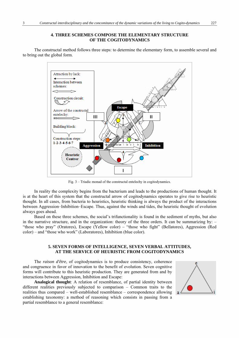
3 Constructal interdisciplinary and the concomitance of the dynamic variations of the living to Cogito-dynamics
227
4. THREE SCHEMES COMPOSE THE ELEMENTARY STRUCTURE OF THE COGITODYNAMICS
The constructal method follows three steps: to determine the elementary form, to assemble several and to bring out the global form.
Fig. 3 – Triadic monad of the constructal entelechy in cogitodynamics.
In reality the complexity begins from the bacterium and leads to the productions of human thought. It is at the heart of this system that the constructal arrow of cogitodynamics operates to give rise to heuristic thought. In all cases, from bacteria to heuristics, heuristic thinking is always the product of the interactions between Aggression–Inhibition–Escape. Thus, against the winds and tides, the heuristic thought of evolution always goes ahead.
Based on these three schemes, the social’s trifunctionality is found in the sediment of myths, but also in the narrative structure, and in the organization: theory of the three orders. It can be summarizing by: – “those who pray” (Oratores), Escape (Yellow color) – “those who fight” (Bellatores), Aggression (Red color) – and “those who work” (Laboratores), Inhibition (blue color).
5. SEVEN FORMS OF INTELLIGENCE, SEVEN VERBAL ATTITUDES, AT THE SERVICE OF HEURISTIC FROM COGITODYNAMICS
The raison d'être, of cogitodynamics is to produce consistency, coherence and congruence in favor of innovation to the benefit of evolution. Seven cognitive forms will contribute to this heuristic production. They are generated from and by interactions between Aggression, Inhibition and Escape:
Analogical thought: A relation of resemblance, of partial identity between different realities previously subjected to comparison – Common traits to the realities thus compared – well-established resemblance – correspondence allowing establishing taxonomy: a method of reasoning which consists in passing from a partial resemblance to a general resemblance:
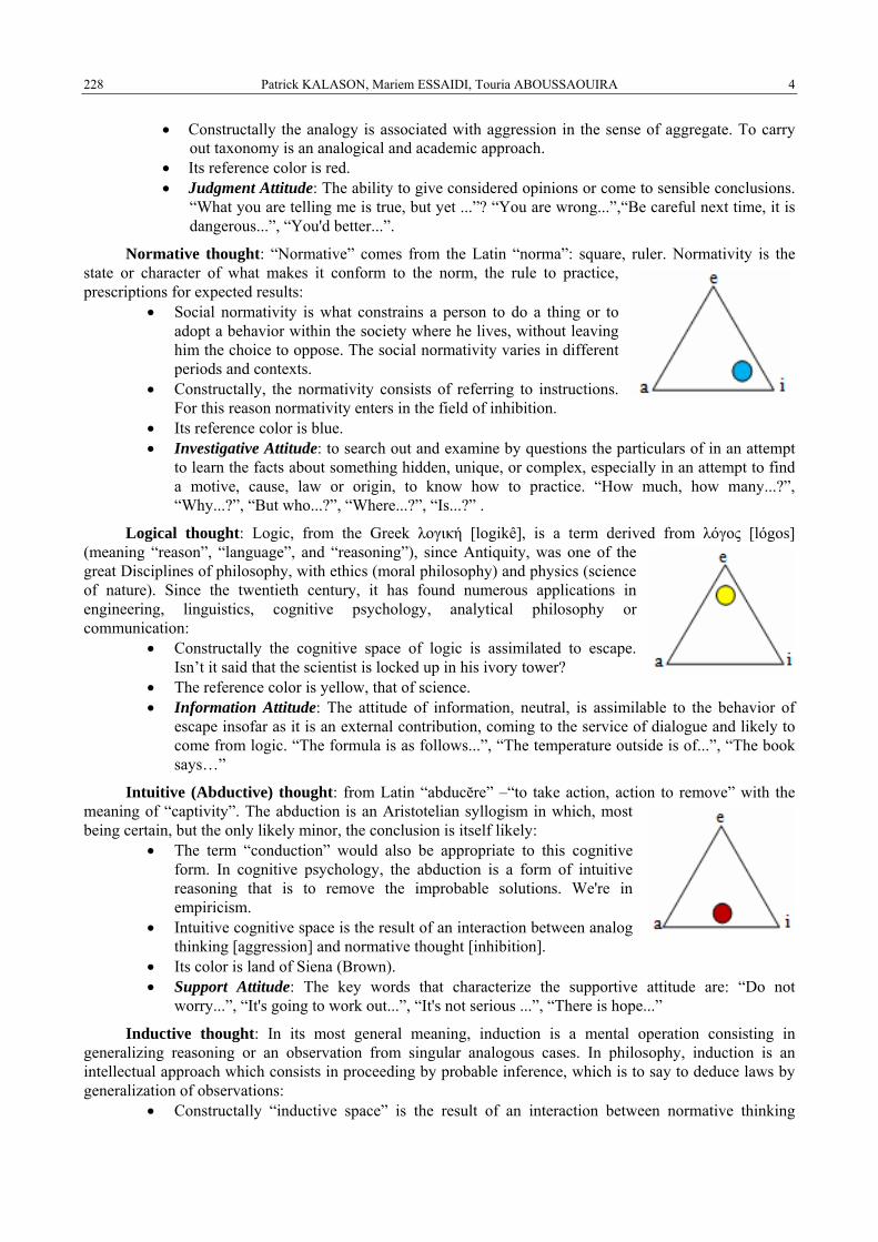
Patrick KALASON, Mariem ESSAIDI, Touria ABOUSSAOUIRA 4
228
• Constructally the analogy is associated with aggression in the sense of aggregate. To carry out taxonomy is an analogical and academic approach.
• Its reference color is red. • Judgment Attitude: The ability to give considered opinions or come to sensible conclusions.
“What you are telling me is true, but yet ...”? “You are wrong...”,“Be careful next time, it is dangerous...”, “You'd better...”.
Normative thought: “Normative” comes from the Latin “norma”: square, ruler. Normativity is the state or character of what makes it conform to the norm, the rule to practice, prescriptions for expected results:
• Social normativity is what constrains a person to do a thing or to adopt a behavior within the society where he lives, without leaving him the choice to oppose. The social normativity varies in different periods and contexts.
• Constructally, the normativity consists of referring to instructions. For this reason normativity enters in the field of inhibition.
• Its reference color is blue. • Investigative Attitude: to search out and examine by questions the particulars of in an attempt
to learn the facts about something hidden, unique, or complex, especially in an attempt to find a motive, cause, law or origin, to know how to practice. “How much, how many...?”, “Why...?”, “But who...?”, “Where...?”, “Is...?” .
Logical thought: Logic, from the Greek λογική [logikê], is a term derived from λόγος [lógos] (meaning “reason”, “language”, and “reasoning”), since Antiquity, was one of the great Disciplines of philosophy, with ethics (moral philosophy) and physics (science of nature). Since the twentieth century, it has found numerous applications in engineering, linguistics, cognitive psychology, analytical philosophy or communication:
• Constructally the cognitive space of logic is assimilated to escape. Isn’t it said that the scientist is locked up in his ivory tower?
• The reference color is yellow, that of science. • Information Attitude: The attitude of information, neutral, is assimilable to the behavior of
escape insofar as it is an external contribution, coming to the service of dialogue and likely to come from logic. “The formula is as follows...”, “The temperature outside is of...”, “The book says…”
Intuitive (Abductive) thought: from Latin “abducĕre” –“to take action, action to remove” with the meaning of “captivity”. The abduction is an Aristotelian syllogism in which, most being certain, but the only likely minor, the conclusion is itself likely:
• The term “conduction” would also be appropriate to this cognitive form. In cognitive psychology, the abduction is a form of intuitive reasoning that is to remove the improbable solutions. We're in empiricism.
• Intuitive cognitive space is the result of an interaction between analog thinking [aggression] and normative thought [inhibition].
• Its color is land of Siena (Brown). • Support Attitude: The key words that characterize the supportive attitude are: “Do not
worry...”, “It's going to work out...”, “It's not serious ...”, “There is hope...”
Inductive thought: In its most general meaning, induction is a mental operation consisting in generalizing reasoning or an observation from singular analogous cases. In philosophy, induction is an intellectual approach which consists in proceeding by probable inference, which is to say to deduce laws by generalization of observations:
• Constructally “inductive space” is the result of an interaction between normative thinking
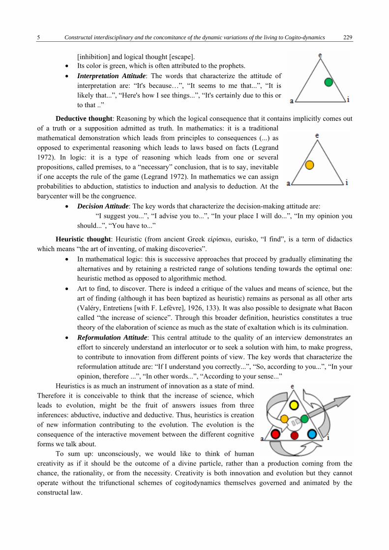
5 Constructal interdisciplinary and the concomitance of the dynamic variations of the living to Cogito-dynamics
229
[inhibition] and logical thought [escape]. • Its color is green, which is often attributed to the prophets. • Interpretation Attitude: The words that characterize the attitude of
interpretation are: “It's because…”, “It seems to me that...”, “It is likely that...”, “Here's how I see things...”, “It's certainly due to this or to that ..”
Deductive thought: Reasoning by which the logical consequence that it contains implicitly comes out of a truth or a supposition admitted as truth. In mathematics: it is a traditional mathematical demonstration which leads from principles to consequences (...) as opposed to experimental reasoning which leads to laws based on facts (Legrand 1972). In logic: it is a type of reasoning which leads from one or several propositions, called premises, to a “necessary” conclusion, that is to say, inevitable if one accepts the rule of the game (Legrand 1972). In mathematics we can assign probabilities to abduction, statistics to induction and analysis to deduction. At the barycenter will be the congruence.
• Decision Attitude: The key words that characterize the decision-making attitude are: “I suggest you...”, “I advise you to...”, “In your place I will do...”, “In my opinion you
should...”, “You have to...”
Heuristic thought: Heuristic (from ancient Greek είρίσκω, eurisko, “I find”, is a term of didactics which means “the art of inventing, of making discoveries”.
• In mathematical logic: this is successive approaches that proceed by gradually eliminating the alternatives and by retaining a restricted range of solutions tending towards the optimal one: heuristic method as opposed to algorithmic method.
• Art to find, to discover. There is indeed a critique of the values and means of science, but the art of finding (although it has been baptized as heuristic) remains as personal as all other arts (Valéry, Entretiens [with F. Lefèvre], 1926, 133). It was also possible to designate what Bacon called “the increase of science”. Through this broader definition, heuristics constitutes a true theory of the elaboration of science as much as the state of exaltation which is its culmination.
• Reformulation Attitude: This central attitude to the quality of an interview demonstrates an effort to sincerely understand an interlocutor or to seek a solution with him, to make progress, to contribute to innovation from different points of view. The key words that characterize the reformulation attitude are: “If I understand you correctly...”, “So, according to you...”, “In your opinion, therefore ...”, “In other words...”, “According to your sense...”
Heuristics is as much an instrument of innovation as a state of mind. Therefore it is conceivable to think that the increase of science, which leads to evolution, might be the fruit of answers issues from three inferences: abductive, inductive and deductive. Thus, heuristics is creation of new information contributing to the evolution. The evolution is the consequence of the interactive movement between the different cognitive forms we talk about.
To sum up: unconsciously, we would like to think of human creativity as if it should be the outcome of a divine particle, rather than a production coming from the chance, the rationality, or from the necessity. Creativity is both innovation and evolution but they cannot operate without the trifunctional schemes of cogitodynamics themselves governed and animated by the constructal law.
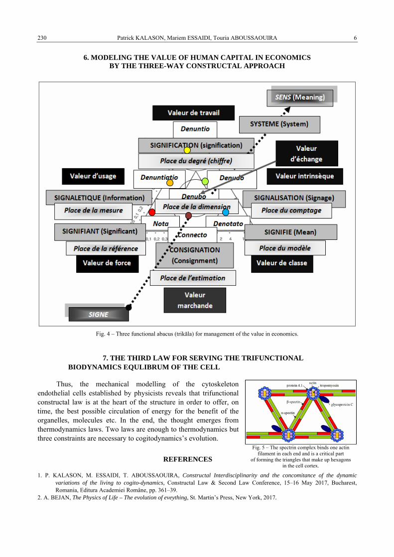
Patrick KALASON, Mariem ESSAIDI, Touria ABOUSSAOUIRA 6
230
6. MODELING THE VALUE OF HUMAN CAPITAL IN ECONOMICS BY THE THREE-WAY CONSTRUCTAL APPROACH
Fig. 4 – Three functional abacus (trikãla) for management of the value in economics.
7. THE THIRD LAW FOR SERVING THE TRIFUNCTIONAL BIODYNAMICS EQULIBRUM OF THE CELL
Thus, the mechanical modelling of the cytoskeleton endothelial cells established by physicists reveals that trifunctional constructal law is at the heart of the structure in order to offer, on time, the best possible circulation of energy for the benefit of the organelles, molecules etc. In the end, the thought emerges from thermodynamics laws. Two laws are enough to thermodynamics but three constraints are necessary to cogitodynamics’s evolution.
REFERENCES
1. P. KALASON, M. ESSAIDI, T. ABOUSSAOUIRA, Constructal Interdisciplinarity and the concomitance of the dynamic variations of the living to cogito-dynamics, Constructal Law & Second Law Conference, 15–16 May 2017, Bucharest, Romania, Editura Academiei Române, pp. 361–39.
2. A. BEJAN, The Physics of Life – The evolution of eveything, St. Martin’s Press, New York, 2017.
Fig. 5 – The spectrin complex binds one actin filament in each end and is a critical part
of forming the triangles that make up hexagons in the cell cortex.
THE PUBLISHING HOUSE PROCEEDINGS OF THE ROMANIAN ACADEMY, Series A, OF THE ROMANIAN ACADEMY Special Issue/2018, pp. 231–236
GEOMETRICAL OPTIMIZATION OF LOUVER-FIN ARRAYS BY USING CONSTRUCTAL LAW AT LOW REYNOLDS NUMBER REGIME
Masoud ASADI*, Mohamed M. AWAD**
* Azad Islamic University Science and Research Branch,Department of Mechanical Engineering, Tehran, Iran ** Mansoura University, Mansoura, Mechanical Power Engineering Department, Faculty of Engineering, Egypt 35516
Corresponding author: Mohamed M. AWAD, E-mail: [email protected]
Abstract. With recent advancements in the computing technology, electronic devices have become smaller and more powerful, which leads to generation of more and more heat. This can be an important challenge when thousands of transistors work at high frequency, and the temperature reaches a critical value where typical cooling techniques are not sufficient. Louver fins are regarded as one of the best extended surfaces that can be employed for enhancing heat transfer without considerably increasing the pressure drop. In this paper, Constructal theory has been used to optimize louver fin arrays. The selected domain has three degrees of freedom; the louver angle ratio, the louver pitch ratio, and the inlet louver length to outlet louver length ratio. The results show that the Constructal variables are insensitive to changes in Reynolds number. The flow structure in the low Reynolds number regime is a function of the louver angle ratio, the louver pitch ratio and the Reynolds number, but above a critical Reynolds number it depends on the louver pitch ratio value alone. The results showed that the Constructal law can increase the total heat transfer rate more than 6% compared with a typical geometry.
Key words: Constructal theory, Louvered-fins, Louver angle, Louver pitch ratio, Optimal design.
1. INTRODUCTION
Since the birth of electronic technology, the heat flux generation from electronic devices has increased dramatically, and it seems this trend will continue. According to the International Technology Roadmap for Semiconductors, the allowable maximum junction temperature must be less than 85oC for a reliable operation. Therefore, various types of cooling systems and techniques have been developed in recent years. Passive cooling technologies, like the microchannel sink with a liquid as the working fluid, fin surfaces, and jet impingement are some of the solutions to provide high heat flux dissipation. Louvered fins are popular for removing heat because they can increase the total heat transfer rate at a reasonable increase of pressure drop. However, maintaining the junction temperature lower than a safe value is a challenging problem at the low Reynolds numbers. One of the most recent technologies to overcome this problem is constructal design, which is now a growing field in thermal science.
Constructal Theory and constructal Law are terms that are appearing more and more frequently in the scientific world. Mainly this is because an increasing number of people are using the constructal paradigm to optimize the performance of Thermofluid flow systems by generating geometry and flow structure. Adrian Bejan originates of the constructal law, in 1996. He tells that the idea came to him when he was trying to figure out the problem of minimizing the thermal resistance between an entire heat generating volume and one point. The constructal law states that for every finite-size system to persist in time, it must search for a configuration that provides easier access to the current that flow throw it. A basic result of the constructal law is that a system’s shape and internal flow configuration do not develop by chance, but are obtained from the permanent struggle for better performance and therefore have to be evolved in time. From a geometric point of view, natural systems are far from being perfect, because geometric perfection means symmetry. However, in the real (physical) world the higher the internal symmetry the closer to equilibrium is. In animate systems, it is possible to find the perfect geometric configuration, because they are physically and geometrically asymmetries.

Masoud ASADI, Mohamed M. AWAD 2 232
A major field of applied search for constructal design architectures is the development of compact architectures for increasing the heat transfer rate. This activity began with the discovery of optimal spacing for channels with natural [1] and forced [2] convection, and the development of T-shaped assemblies for cooling [3]. In the heat transfer framework, the study of cavities and fin arrays has deserved close attention, mainly because of its adequate representation of several engineering problems, such as heat exchangers, microelectronics, and thermal energy storage systems [4–6].
Concerning the employment of constructal law for an arrangement of fins, Bejan and Almogbel [7] conducted a study on geometric optimization of a T-shaped fin with the purpose to maximize the total heat transfer rate. Then, other geometries were investigated, such as Y-shaped [8], T-Y shaped [9], I-Y shaped [10], and X-shaped [11].
Feng et al. [12] used the constructal theory for optimization of a solidification heat transfer process of a slab under continuous casting with a complex function as the optimization objective. The complex function was composed of the function of the heat loss rate and surface temperature gradient of the slab. The results showed that the functions of the heat loss rate and the surface temperature gradient after optimization were decreased by 35.04% and 21.4%, respectively. Therefore, the scheme of the optimal construction of the water distribution could reduce the heat loss rate and surface temperature gradient of the slab simultaneously.
Rubbe and Sciubba [13] and Kuddusi and Denton [14] optimized a slab by using the constructal law. Lorenzini and Biserni [15] tried to develop the application of the constructal theory to other fields like biology, geophysics, social dynamics and economics. They concluded that this theory can remove the distinction between physics and engineering. Afterwards, Lorente and co-authors [16], based on the concept of the constructal law, explained why swimmers must spread their fingers and toes. Bejan and Lorente [17] studied about the evolution of the biosphere from prehistory to today. They stated that animal flow has been spreading vertically in space and towards higher speeds, longer ranges and better vision. Then these authors focused on Constructal thermodynamics where it could place the concepts of life, design and evolution in physics [18]. This new vision to design can open the doors to new advances especially in areas where design evolution is key to performance.
Recently, Asadi and coworkers used the constructal law for optimization of different shapes such as wavy channels in the low Reynolds number regime [19], shell-and-tube heat exchangers [20], wavy-fin channels of a compact heat exchanger with heat transfer rate maximization and pressure losses minimization [21], pin-fins [22], channel with louvered-fins with heat transfer rate maximization and pressure losses minimization [23].
Moreover, many researchers employed the constructal law for optimization of several various shapes like shell-and-tube heat exchangers conforming to TEMA standards [24], discrete heat sources flush mounted on a laminar flow cooled flat plate [25].
With these observations as a motivation, the goal of the present work is to employ the constructal law for improving the performance of a channel with louvered-fins. In 2013, Asadi and Mehrabani [26] used the entropy generation minimization (EGM) method to optimize louvered fins in a plate-fin compact heat exchanger. In the current study, the domain has three degrees of freedom, and six variables. The best configurations have been found by using the constructal law. From the Data Bank that have been provided (from geometric optimization) and with employing the Nonlinear Regression method, a correlation is developed for the total heat transfer rate versus constructal variables.
2. NUMERICAL MODEL
Figure 1a shows the mesh schematics of the louvered-fins. The configuration is two dimensional as shown in Fig. 1b with the third dimension D perpendicular to the plane of the domain. On the left side of the turnaround, L1 is the louver pitch, and L2 is the louver pitch on the right side.α1 and α2 are the louver angle on the left and right side of the turnaround louver, respectively. The inlet louver length is given by P1, and the outlet louver length by P2. In general, the configuration has six Constructal variables, and three degrees of freedom; the louver angle ratio, the inlet louver length to outlet louver length ratio, and the louver pitch ratio (α1/α2, L1/L2, P1/P2). These three degrees of freedom were also used in the study of Asadi et al. [23]. In that study, Asadi et al. [23] found that the louver angle effect was stronger for larger louver pitch ratios. The maximum heat transfer coefficient was dependent on the louver pitch ratio and the inlet louver length to outlet louver length ratio (P1/P2, L1/L2). For the louver pitch ratio, there was a minimum value and below this value the vortices upstream of the turnaround louver blocked the distance between louvers and so decreased the flow efficiency. The researchers

3 Geometrical optimization of louver-fin arrays by using constructal law at low Reynolds number regime
233
compared their results with previous experimental studies presented by DeJong and Jacobi [27] and Malapure et al. [28] and showed that the channel optimized by constructal law was considerably superior compared to the standard channel in low Reynolds number regime. In the present study, the swept length is L, and it is assumed that the flow assembly is bathed by a uniform and isothermal free-stream.
Fig. 1 – b) Two-dimensional louvered-fins. Fig. 1 – a) Mesh schematics of louvered-fins.
The domain has three constraints as follows,
L1P1 = const, (1)
L2P2 = const, (2)
L1 + P1 + L2 + P2 = const. (3)
The flow is considered incompressible, steady and laminar. Effects on heat transfer by radiation and natural convection are negligible and all thermo-physical properties are assumed as constant. Considering these assumptions, the continuity, momentum and energy equations are:
∂ ˜ u
∂˜ x + ∂ ˜ v
∂˜ y = 0 , (4)
Re ˜ u ∂ ˜ u
∂ ˜ x + ˜ v
∂ ˜ u
∂ ˜ y
⎛
⎝ ⎜
⎞
⎠ ⎟ = − ∂˜ p
∂ ˜ x +∇ 2 ˜ u , (5)
Re ˜ u ∂ ˜ v
∂˜ x + ˜ v
∂ ˜ v
∂ ˜ y
⎛
⎝ ⎜
⎞
⎠ ⎟ = − ∂˜ p
∂ ˜ y +∇ 2 ˜ v , (6)
Re⋅ Pr ˜ u ∂ ˜ T
∂˜ x + ˜ v
∂ ˜ T
∂ ˜ y
⎛
⎝ ⎜
⎞
⎠ ⎟ = ∇ 2 ˜ T . (7)
For the channel with louvered-fins, the energy equation is reduced to:
∇ 2 ˜ T = 0 , (8)
where ∇ 2 = ∂∂x 2
+ ∂∂y 2
. The hydrodynamic boundary condition is the condition of no-slip at the walls of
channel, i.e. u = v = 0, where u and v are the components of the velocity vector ( ˜ U ). Equations (4) to (7) are non-dimensionalized by using the below variables:
(x, y) = ( ˜ x , ˜ y )
L, (9)
(u, v) = ( ˜ u , ˜ v )
U∞
, (10)

Masoud ASADI, Mohamed M. AWAD 4 234
˜ T = T − T∞
Tw − T∞
, (11)
˜ p = p
μU∞ / L, (12)
where Re and Pr, in Equations (5–7), are Reynolds and Prandtl numbers, respectively
Pr = μν
, (13)
Re = U∞L
ν, (14)
Tw, T∞, and U∞ are wall temperature, free-stream temperature, and free-stream velocity, respectively.
Furthermore, ˜ u = 1, ˜ p = 1 and ∂ ˜ u
∂˜ x = 0 prevail at the inlet of the domain; ˜ p = 0, and ∂ ˜ u
∂˜ x = ∂ ˜ v
∂˜ y = 0 at the exit.
For the thermal boundary conditions; ˜ T = 1 on the louvered-fin surfaces, and ˜ T = 0 at the inlet plane of the domain. The other planes are considered as adiabatic. The geometric arrangement of main interest is that maximizing the total heat transfer rate between the louvered-fins and the surrounding fluid. The total heat transfer rate is determined as follows:
˜ q = q / D
k (Tw − T∞). (15)
In this formula, q is integrated over the surface of the louvered-fins.
3. NUMERICAL VALIDATION
The numerical model is solved by using the commercial code FLUENT [29]. The domain is discretized using polyhedral elements. The solver is pressure based, and the velocity-pressure coupling is handled by the SIMPLE algorithm. Second order schemes are invoked to discretize the momentum and energy equations. The convergence is obtained when the residuals of mass, momentum and energy equations are less than 10-6, 10-6 and 10-8, respectively.
4. RESULTS AND DISCUSSIONS
The numerical work consisted of determining the total heat transfer rate in a large number of configurations. Figure 2 clearly shows that there is an optimal P1/P2 value that maximizes the heat transfer rate when the parameters of α1/α2 and L1/L2 are fixed. This optimal value is P1/P2 = 1.2 for the all L1/L2 values. It is worthwhile to mention that the performance of L1/L2 = 1.2 is slightly superior compared to other L1/L2 values. Figures 3 and 4 also show the total heat transfer rate when the louver angle ratio is 1.0 and 1.2, respectively. From these figures, it can be found that the total heat transfer rate is almost insensitive to changes in the louver angle ratio. However, it seems that it has a significant effect on the optimal L1/L2 value, because when α1/α2 = 0.8 the optimum L1/L2 value is 1.2, but by increasing the louver angle ratio the optimal L1/L2 value decreases from 1.2 to 1.0.
It can be found that for all the configurations, the optimal P1/P2 value is 1.2, and this shows that the length of the inlet louver must be larger than the exit louver in order to shed vortices. Overall, the optimal configuration lies in the design domain of P1/P2 = 1.2, 1.0 ≤ L1/L2 ≤ 1.2, 1.0 ≤ α1/α2 ≤ 1.2. Figure 5 shows the behavior of the Constructal variables as well as the total heat transfer rate for changing Reynolds number. It appears that all Constructal variables are insensitive to the Reynolds number, and only the dimensisonless heat transfer rate increases linearly with growing Re.
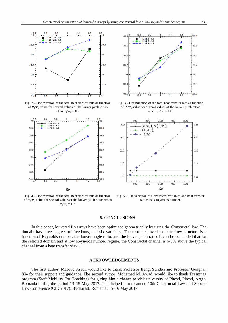
5 Geometrical optimization of louver-fin arrays by using constructal law at low Reynolds number regime
235
Fig. 3 – Optimization of the total heat transfer rate as function
of P1/P2 value for several values of the louver pitch ratios when α1/α2 = 1.0.
Fig. 2 – Optimization of the total heat transfer rate as function of P1/P2 value for several values of the louver pitch ratios
when α1/α2 = 0.8.
Re
Re
Fig. 5 – The variation of Constructal variables and heat transfer rate versus Reynolds number.
Fig. 4 – Optimization of the total heat transfer rate as function of P1/P2 value for several values of the louver pitch ratios when
α1/α2 = 1.2.
5. CONCLUSIONS
In this paper, louvered fin arrays have been optimized geometrically by using the Constructal law. The domain has three degrees of freedoms, and six variables. The results showed that the flow structure is a function of Reynolds number, the louver angle ratio, and the louver pitch ratio. It can be concluded that for the selected domain and at low Reynolds number regime, the Constructal channel is 6-8% above the typical channel from a heat transfer view.
ACKNOWLEDGEMENTS
The first author, Masoud Asadi, would like to thank Professor Bengt Sunden and Professor Gongnan Xie for their support and guidance. The second author, Mohamed M. Awad, would like to thank Erasmus+ program (Staff Mobility For Teaching) for giving him a chance to visit university of Pitesti, Pitesti, Arges, Romania during the period 13–19 May 2017. This helped him to attend 10th Constructal Law and Second Law Conference (CLC2017), Bucharest, Romania, 15–16 May 2017.
Masoud ASADI, Mohamed M. AWAD 6 236
REFERENCES
1. BEJAN, A., Convection Heat Transfer, Wiley, New York, 1984. 2. BEJAN, A., SCIUBBA, E., The optimal spacing of parallel plates cooled by forced convection, International Journal of Heat and
Mass Transfer, 35, 12, pp. 3259–3264, 1992. 3. LORENZINI, G., BISERNI, C., CORREA, R.L., dos SANTOS, E.D., ISOLDI, L.A., ROCHA, L.A.O., Constructal design of
T-shaped assemblies of fins cooling a cylindrical solid body, International Journal of Thermal Sciences, 83, pp. 96–103, 2014. 4. AZAD, A.V., AMIDPOUR, M., Economic optimization of shell and tube heat exchanger based on constructal theory, Energy, 36,
2, pp. 1087–1096, 2011. 5. SALIMPOUR, M.R., MENBARI, A., Constructal design of cooling channels embedded in a ring-shaped heat-generating body,
Energy, 73, pp. 302–310, 2014. 6. HAJMOHAMMADI, M.R., RAHMANI, M., CAMPO, A., SHARIATZADEH, O.J., Optimal design of unequal heat flux elements
for optimized heat transfer inside a rectangular duct, Energy, 68, pp. 609–616, 2014. 7. BEJAN, A., ALMOGBEL, M., Constructal T-shaped fins, conducting body, International Journal of Heat and Mass Transfer, 43,
pp. 2101–2115, 2000. 8. LORENZINI, G., ROCHA, L.A.O., Constructal design of Y-shaped assembly of fins, International Journal of Heat and Mass
Transfer, 49, pp. 4552–4557, 2006. 9. LORENZINI, G., ROCHA, L.A.O., Constructal design of T-Y assembly of fins for an optimized heat removal, International
Journal of Heat and Mass Transfer, 52, pp. 1458–1463, 2009. 10. LORENZINI, G., S. MORETTI, Numerical performance analysis of constructal I and Y finned heat exchanging modules, ASME
Journal of Electronic Packaging, 13, 3, Paper No. 031012, 2009. 11. FENG, H., CHEN, L., XIE, Z., DING, Z., SUN, F., Constructal entropy generation rate minimization for X-shaped vascular
networks, International Journal of Thermal Sciences, 92, pp. 129–137, 2015. 12. FENG, H., CHEN, L., XIE, Z., DING, Z., SUN, F. Generalized constructal optimization for solidification heat transfer process
of slab continuous casting based on heat loss rate, Energy, 66, pp. 991–998, 2014. 13. ROBBE, M., SCIUBBA, E., Derivation of the optimal internal cooling geometry of a prismatic slab: Comparison of constructal
and non-constructal geometries, Energy, 34, pp. 2167–2174, 2009. 14. KUDDUSI, L., DENTON, J.C., Analytical solution for heat conduction problem in composite slab and its implementation in
constructal solution for cooling of electronics, Energy Conversion and Management, 48, 4, pp. 1089–1105, 2007. 15. LORENZINI, G., BISERNI, C., The Constructal law: From design in nature to social dynamics and wealth as physics Comment
on “The Constructal law and the evolution of design in nature” by Professor Adrian Bejan and Professor Sylvie Lorente, Physics of Life Reviews, 8, 3, pp. 259–260, 2011.
16. LORENTE, S., CETKIN, E., BELLO-OCHENDE, T., MEYER, J.P., BEJAN, A., The constructal-law physics of why swimmers must spread their fingers and toes, Journal of Theoretical Biology, 308, pp.141–146, 2012.
17. BEJAN, A., LORENTE, S., The constructal law and the evolution of design in nature, Physics of Life Reviews, 8, 3, pp. 209–240, 2011.
18. BEJAN, A., LORENTE, S., Constructal law of design and evolution: Physics, biology, technology, and society, Journal of Applied Physics, 113, Paper No. 151301, 2013.
19. XIE, G., ASADI, M., SUNDEN, B., ZHENG, S., Constructal theory based geometric optimization of wavy channels in the low Reynolds number regime, ASME Journal of Electronic Packaging, 136, 3, Article No. 31013, 2014.
20. ASADI, M., SONG, Y., SUNDEN, B., XIE, G., Economic optimization design of shell-and-tube heat exchangers by a cuckoo-search-algorithm, Applied Thermal Engineering, 73, pp. 1032–1040, 2014.
21. SONG, Y., ASADI, M., XIE, G., ROCHA, L.A.O., Constructal wavy-fin channels of a compact heat exchanger with heat transfer rate maximization and pressure losses minimization, Applied Thermal Engineering, 75, pp. 24–32, 2015.
22. XIE, G., SONG, Y., ASADI, M., LORENZINI, G., Optimization of pin-fins for a heat exchanger by entropy generation minimization and constructal law, ASME Journal of Heat Transfer, 137, 6, Article No. (061901), 2015.
23. ASADI, M., SUNDEN, B., XIE, G., Constructal optimization of louver fin channels subjected to heat transfer rate maximization and pressure loss minimization, Heat Transfer Engineering, DOI: 10.1080/01457632.2017.1312881, 2017.
24. YANG, J., FAN, A., LIU, W., JACOBI, A.M., Optimization of shell-and-tube heat exchangers conforming to TEMA standards with designs motivated by constructal theory, Energy Conversion and Management, 78, pp. 468-476, 2014.
25. SHI, Z., DONG, T., A synthetic layout optimization of discrete heat sources flush mounted on a laminar flow cooled flat plate based on the constructal law, Energy Conversion and Management, 106, pp. 300–307, 2015.
26. ASADI, M, MEHRABANI, N.D., Minimizing entropy generation for louvered fins in a plate-fin compact heat exchanger, Journal of Petroleum and Gas Engineering, 4, pp. 35–45, 2013.
27. DEJONG, N.C., JACOBI, A.M., Localized flow and heat transfer interactions in louvered-fin arrays, International Journal of Heat and Mass Transfer, 46, pp. 443–455, 2003.
28. MALAPURE, V.P., MITRA, S.K., BHATTACHARYA, A., Numerical investigation of fluid flow and heat transfer over louvered fins in compact heat exchanger, International Journal of Thermal Sciences, 46, pp. 199–211, 2007.
29. FLUENT Documentation, http://www.fluent.com
THE PUBLISHING HOUSE PROCEEDINGS OF THE ROMANIAN ACADEMY, Series A, OF THE ROMANIAN ACADEMY Special Issue/2018, pp. 237–242
THERMODYNAMIC PERFORMANCE EVALUATION FOR HELICAL PLATE HEAT EXCHANGER BASED ON SECOND LAW ANALYSIS
Emad M.S. EL-SAID*, Mohamed ABDULAZIZ**, Mohamed M. AWAD***
* Fayoum University, Faculty of Engineering, Mechanical Engineering Department, Fayoum, Egypt ** SIMTRAN, Eningen unter Achalm, Reutlingen, Baden-Württemberg, Germany
*** Mansoura University, Mechanical Power Engineering Department, Faculty of Engineering, Mansoura, Egypt 35516 Corresponding author: Mohamed M. AWAD, E-mail: [email protected]
Abstract. Second-law analysis has affected the design methodology of different heat and mass transfer systems to minimize the entropy generation rate, and so to maximize system available work. In this paper, thermodynamic performance evaluation for helical plate heat exchanger (HPHE) based on second law analysis is studied. The entropy generated per unit amount of heat transferred and by friction are investigated in the entropy generation analysis. A three-dimensional numerical simulation of a whole plate heat exchanger with is carried out by using computational fluid dynamics (CFD) code of Ansys 16.2 for modeling and computational calculations. Helical plate with different pitch ratios and different flow channel cross section aspect ratio were studied for variation of Reynolds numbers. The results showed that the maximum total entropy generation is 0.074 in case of pitch ratio and aspect ratio 1.31 and 0.67 respectively.
Key words: Helical plate, CFD, Heat exchanger, Second law analysis.
1. INTRODUCTION
Heat exchangers performance plays vital role in many industrial applications. Because of high energy costs and low energy sources, there are many efforts to enhance heat exchangers’ efficiency. As a result, it is very important to determine the performance of heat exchange devices on both heat transfer and thermodynamic considerations. Heat exchangers are the equipments that provide the flow of thermal energy between two or more fluids at different temperatures. The second law of thermodynamics has proved to be a very powerful tool in the optimization of complex thermodynamic systems such as heat exchangers and is required to establish the difference in quality between mechanical and thermal energy in it [1]. Yilmaz et al. [2] presented second-law based performance evaluation criteria in order to evaluate the heat exchangers performance. Firstly, they recalled and discussed the need for the systematic design of heat exchangers using a second law-based procedure. After that, the researchers classified the evaluation techniques for heat exchangers based on the second law of thermodynamics into two categories: the evaluation techniques using exergy as an evaluation parameter, and the evaluation techniques using entropy as an evaluation parameter. They presented and reviewed collectively both categories, and gave their respective characteristics and constraints. It was shown how some of these criteria were related to every other. In addition, emphasis was placed on the importance of second law-based thermoeconomic analysis of heat exchangers, and these methods were discussed briefly. Etghani and Baboli [3] investigated numerical model of shell and helical tube heat exchanger in order to assess heat transfer coefficient and exergy loss. The researchers took to consideration four design parameters including tube diameter, pitch coil, cold and hot flow rate that were more significant for the performance of heat exchanger. Then, they applied Taguchi approach to figure out the optimum levels of the design factors. They modeled and analyzed numerically sixteen cases with diverse design parameters. They found that tube diameter and cold flow rate were the most significant design parameters of heat transfer and exergy loss, respectively. In addition, the highest Nusselt number was achieved by more both cold and hot flow rates and also, heat transfer coefficient was reduced by pitch coil increasing as well as by hot flow rate increasing, the exergy loss increased. The optimum levels for heat

Emad M.S. EL-SAID, Mohamed ABDULAZIZ, Mohamed M. AWAD 2 238
transfer coefficient were: tube diameter 12 mm, pitch 13 mm, cold and hot flow rate 4 LPM. Moreover, the optimum level for exergy loss are: tube diameter 12 mm, pitch 13 mm, cold and hot flow rate 1 LPM. İpek et al. [4] investigated experimentally exergy loss analysis of newly designed compact heat exchanger (CHE). The researchers designed and constructed experimental system used for experimental analysis of the newly designed CHE and brazed plate heat exchanger (BPHE). Also, they investigated thermodynamic analysis of newly designed CHE and BPHE. They compared the experimental results of the CHE and BPHE. They calculated exergy loss values for every type of heat exchanger. Their experimental results showed that similar exergy loss values were obtained. The least exergy loss value for newly designed CHE has been obtained as about 4.65 kW, while the highest exergy loss value has been obtained as about 7.6 kW for the same heat exchanger. The compared and presented graphically the experiments results. Dizaji et al. [5] studied experimentally exergy analysis for shell and tube heat exchanger made of corrugated shell and corrugated tube. The researchers evaluated said parameters for various arrangements of corrugated tubes. They produced corrugated tubes using a special machine that was developed for this purpose. They found that corrugations caused increment of both exergy loss and NTU. If both tube and shell were corrugated, the exergy loss and NTU increased about 17–81% and 34–60% respectively. They observed maximum exergy loss for heat exchanger made of convex corrugated tube and concave corrugated shell. The present paper presents an evaluation of the thermodynamic performance of a promising type of heat exchanger with helical plate (HPHE) based on second law analysis with different helical plate pitch ratios and flow channel cross section aspect ratio.
2. HPHE GEOMETRY AND PROBLEM FORMULATION
The Helical plate heat exchanger with nine helix turns is shown in Figs. 1 and 2. The hot fluid flows in the helical channel with the series arrangement in counter with cold fluid. The heat transfer process occurs through a Helical copper plate with thickness 1 mm. These plates are repeated in the x-direction, with a pitch P, and height h. Here, the dimensionless geometric parameter; pitch ratio = P/h and aspect ratio =w/h were used in the numerical study. The hydraulic diameter Dh was used as the characteristic flow channel diameter.
50 A
A Section view A-A
Plat
e w
ith th
ickn
ess
= 1
mm
h =30
w =
P=20
b) front view a) isometric view
Hot fluid in
Hot fluid out Cold fluid in
Cold fluid out
z
y x
Outer surface Inner surface
Fig. 2 – Helical plate heat exchanger with pitch ratio = 0.67.
Fig. 1 – Counter flow arrangement .
2.1. Numerical domain and grid generation
The whole HPHE with 9 helix turns was modeled as the numerical domain. Commercial software (ANSYS CFX 16.2) was used with a structural hexahedral grid of a total number of nodes in the range of 197,324 to 237,888 using the multi-zone meshing approach. The grid spacing is non-uniform, being concentrated near the interfaces because of the heat transfer and frictions in that region.
3 Thermodynamic performance evaluation for helical plate heat exchanger based on second law analysis
239
2.2. Governing equations and solution assumptions
The problem investigated is a three-dimensional steady state turbulent flow through a helical flow channel fitted with plain tube using the governing equations for the mass, momentum, and energy conservations, and for k and ε turbulence model. The following assumptions were employed: 1. The heat transfer and fluid flow are time-independent (steady-state), three-dimensional, and incompressible, 2. Phase changes and heat transfer by radiation and natural convection are neglected, 3. All the thermo-physical properties of the solid are assumed to be constants.
Mass conservation equation ∇ ⋅ (ρ
v V ) = 0 . (1)
Momentum conservation equation
( ) ( ) ( ) ( )2 .3
⎡ ⎤⎡ ⎤ ⎡ ⎤ ⎡ ⎤∇ ⋅ ρ = −∇ − ∇ μ ∇⋅ +∇⋅ μ ∇⋅ +∇⋅ μ ∇⋅⎣ ⎦ ⎣ ⎦ ⎣ ⎦⎢ ⎥⎣ ⎦TV V p V V V (2)
Energy conservation equation
( )ρ × = × + + × +φ.∂⎡ ⎤∇ ∇ ∇ ∇⎡ ⎤⎣ ⎦ ⎢ ⎥∂⎣ ⎦p
pc V T k T V pt
(3)
Turbulence model
( )( ) .tk
k
ukV k G⎡ ⎤⎛ ⎞∇• ρ = ∇⋅ μ + ∇⋅ + −ρε⎜ ⎟⎢ ⎥σ⎝ ⎠⎣ ⎦ (4)
Entropy generation. In order to evaluate irreversibility loss in heat exchanger, the modified number of entropy generation units (Ns) is defined as [6].
( )h,i c,i .g
sS T T
NQ−
= (5)
The entropy balance for an open system such as the heat exchanger is defined as Eq. (6). In a steady-flow process, sysSΔ is zero. In addition, the heat exchanger is often seen as an adiabatic system; therefore, sysSΔ is also zero.
sys .i 0 gfS S S +S +SΔ = − (6)
Then the entropy balance equation can be reduced to:
.g o iS = S S− (7)
From Eq. (7), the total rate of entropy production ,g totalS in the heat exchanger can be expressed as follows [7]:
.
Entroy generation due to frictionEntropy gneration due to heat transfer
= ln + ln + β Δ +β Δc p,c c,o c c cc,ig,total h p,h h,o h,i h h hS m c T T m c T T V p V p (8)
Then, according to Eqs. (5), (7) and (8), the total number of entropy generation units (totalsN ), Ns due to heat
transfer (TsN
Δ), and Ns due to friction (
PsNΔ
) are defined as follows:
,T PtotalNs Ns NsΔ Δ= + (9)
( )( )
( )( )min min
min min
1 1.ln 1 . 1 .ln 1 . 1 ,T
p ph p,h c p,cc,i h,is
h p,h h,i c p,c c,ip p
m c mcm c m cT TN
m c T m c Tm c mcΔ
⎡ ⎤ ⎡ ⎤⎛ ⎞ ⎛ ⎞⎢ ⎥ ⎢ ⎥= + ε − + + ε −⎜ ⎟ ⎜ ⎟⎜ ⎟ ⎜ ⎟ε ε⎢ ⎥ ⎢ ⎥⎝ ⎠ ⎝ ⎠⎣ ⎦ ⎣ ⎦
(10)

Emad M.S. EL-SAID, Mohamed ABDULAZIZ, Mohamed M. AWAD 4 240
( ) ( ).
min
1 V Vps c c ch h h
pN P p
mcΔ= β Δ +β Δε
(11)
2.3. Numerical method
The above mentioned equations were solved with the commercial software ANSYS CFX 16.2. The renormalization group (RNG) k–ε model is adopted because it can provide improved predictions of near-wall flows and flows with high streamline curvature [8]. Solution sequential algorithm (segregated solver algorithm) with settings including implicit formulation, steady (time-independent) calculation, SIMPLE as the pressure-velocity coupling method, and first-order upwind scheme for energy and momentum equations was selected for simulation.
2.4. Boundary and initial conditions
The inlet boundary and initial conditions of hot and cold fluid are axial velocity and outlet boundary condition is fixed average static pressure equal to the standard atmohpheric pressure. The inner and outer surface of the HPHE is adiabatic (isolated). All blocks are starting with water. The hot and cold fluids have inlet temperatures of 400 and 300 K for all simulations. The numerical values of velocities and pitch ratios, which were used in a number of the simulations are given in Table 1.
Table 1
Numerical values of the parameters used for simulations
Velocity, m/s Pitch ratio
Hot fluid Cold fluid 0.24 0.67 1.31
0.1 0.2 0.3 0.4 0.5 0.07 0.13 0.20 0.27 0.33
0.24 0.93 0.75 0.56 0.37 0.19 0.65 0.52 0.39 0.26 0.13 0.67 0.67 0.53 0.40 0.27 0.13 0.47 0.37 0.28 0.19 0.09 1.31 0.59 0.47 0.35 0.24 0.12 0.41 0.33 0.25 0.17 0.08
3. RESULTS AND DISCUSSIONS
Figures 3–5 show the variations in number of entropy generation units due to friction ( NsΔp ), heat
transfer ( NsΔT ) and total entropy generation as a function of Reynolds number, pitch ratio and aspect ratio. For constant pitch and aspect ratios, it is shown that the increasing of Reynolds number for both fluids; the number of entropy generation units will decrease. Maximum entropy generation due to friction is 0.003 in case of pitch ratio and aspect ratio 0.24 and 0.12 respectively. Maximum entropy generation due to heat transfer and total entropy generation are 0.073 and 0.074 in case of pitch ratio and aspect ratio 1.31 and 0.67 respectively.
In this section a comparison of helical plate with flat plate heat exchangers is presented according to thermal, hydraulic and thermodynamic parameters. Figures 6–8 show the variations in number of entropy generation units due to friction ( NsΔp ), heat transfer ( NsΔT ) and total entropy generation for helical plate and
flat plate heat exchangers as a function of Reynolds number at constant aspect ratio. For constant aspect ratio, it is shown that an increasing in the number of entropy generation units for flat plate heat exchanger over helical plate heat exchanger by about 1.24 to 1.65 on average.

5 Thermodynamic performance evaluation for helical plate heat exchanger based on second law analysis
241
Pitch ratio = 0.24 and aspect ratio = 0.12
num
ber o
f ent
ropy
gen
erat
ion
units
(Ns Δ
T)
Reynolds number of hot flow channel, Reh
Reynolds number of cold flow channel, Rec
Pitch ratio = 1.31 and aspect ratio = 0.65 Pitch ratio = 0.67 and aspect ratio = 0.33
Pitch ratio = 0.24 and aspect ratio = 0.12
num
ber o
f ent
ropy
gen
erat
ion
units
(Ns Δ
p)
Reynolds number of hot flow channel, Reh
Reynolds number of cold flow channel, Rec
Pitch ratio = 1.31 and aspect ratio = 0.65Pitch ratio = 0.67 and aspect ratio = 0.33
Fig. 4 – Variations in number of entropy generation units due to heat transfer ( NsΔT ) as a function of Reynolds number, pitch
ratio and aspect ratio.
Fig. 3 – Variations in number of entropy generation units due to friction ( NsΔp ) as a function of Reynolds number, pitch ratio
and aspect ratio.
Num
ber o
f ent
ropy
gen
erat
ion
units
(Ns Δ
p)
Reynolds number in cold flow channel, Rec 1400 2800 4200 5600 7000
Reynolds number in hot flow channel, Reh
10000 8000 6000 4000 2000
Straight channelHelical channel
Pitch ratio = 0.24 and aspect ratio = 0.12
num
ber o
f ent
ropy
gen
erat
ion
units
(Ns to
tal)
Reynolds number of hot flow channel, Reh
Reynolds number of cold flow channel, Rec
Pitch ratio = 1.31 and aspect ratio = 0.65Pitch ratio = 0.67 and aspect ratio = 0.33
Fig. 6 – Number of entropy generation units due to friction ( NsΔp ) for helical and straight flow channel as a function of
Reynolds number at aspect ratio = 0.12.
Fig. 5 – Variations in number of total entropy generation units ( Nstotal ) as a function of Reynolds number, pitch ratio and aspect
ratio.
4. CONCLUSIONS
In this paper a three dimensional simulation model of flow and heat transfer in the fluids channels of a whole HPHE were established numerically to evaluate the thermodynamic performance based on second law analysis with different helical plate pitch ratios and flow channel cross section aspect ratio. The main conclusions are summarized:
1. Maximum total entropy generation is 0.074 in case of pitch ratio and aspect ratio 1.31 and 0.67 respectively.
2. The present numerical simulation had been compared and a good agreement with experimental data trend had been obtained from another published work.
Emad M.S. EL-SAID, Mohamed ABDULAZIZ, Mohamed M. AWAD 6 242
ACKNOWLEDGEMENTS
The third author, Mohamed M. Awad, would like to thank Erasmus+ program (Staff Mobility For Teaching) for giving him a chance to visit university of Pitesti, Pitesti, Arges, Romania during the period 13–19 May 2017. This helped him to attend 10th Constructal Law and Second Law Conference (CLC2017), Bucharest, Romania, 15–16 May 2017.
REFERENCES
1. Y.A. CENGEL, M.A. BOLES, Thermodynamics – An Engineering Approach, New Delhi, Tata McGraw Hill, 2002. 2. M. YILMAZ, O.N. SARA, S. KARSLI, Performance evaluation criteria for heat exchangers based on second law analysis,
Exergy Int. J., 1, 4, pp. 278–294, 2001. 3. M.M. ETGHANI, S.A.H. BABOLI, Numerical investigation and optimization of heat transfer and exergy loss in shell and helical
tube heat exchanger, Applied Thermal Engineering, 121, pp. 294–301, 2017. 4. O. İPEK. B. KILIÇ, B. GÜREL, Experimental investigation of exergy loss analysis in newly designed compact heat exchangers,
Energy, 124, pp. 330–335, 2017. 5. H.S DIZAJI, S. JAFARMADAR, S. ASAADIA, Experimental exergy analysis for shell and tube heat exchanger made of
corrugated shell and corrugated tube, Experimental Thermal and Fluid Science, 81, pp. 475–481, 2017. 6. Z.M. XU, S.R. YANG, Z.Q. CHEN, A modified entropy generation number for heat exchangers, J. Therm. Sci., 5, pp. 257–263,
1996. 7. H. YIN and R. OOKA, Shape optimization of water-to-water plate-fin heat exchanger using computational fluid dynamics and
genetic algorithm, Applied Thermal Engineering, 80, pp. 310–318, 2015. 8. J.L. YIN, D.Z. WANG, H. CHENG, W.G. GU, Assessment of RANS to predict flows with large streamline curvature, Materials
Science and Engineering, 52, pp. 144–158, 2013.
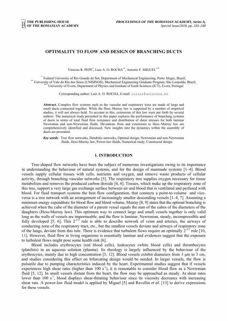
THE PUBLISHING HOUSE PROCEEDINGS OF THE ROMANIAN ACADEMY, Series A, OF THE ROMANIAN ACADEMY Special Issue/2018, pp. 243–248
OPTIMALITY TO FLOW AND DESIGN OF BRANCHING DUCTS
Vinicius R. PEPE*, Luiz A. O. ROCHA**, Antonio F. MIGUEL*** * Federal University of Rio Grande do Sul, Department of Mechanical Engineering, Porto Alegre, Brazil,
** University of Vale do Rio dos Sinos (UNISINOS), Mechanical Engineering Graduate Program, São Leopoldo, Brazil. *** University of Evora, Department of Physics and Institute of Earth Sciences (ICT), Evora, Portugal
Corresponding author: Luiz A. O. ROCHA, E-mail: [email protected]
Abstract. Complex flow systems such as the vascular and respiratory trees are made of large and small ducts connected together. While the Hess–Murray law is supported by a number of empirical studies, it will not always hold. To account to this, extensions of this law were put forth by several authors. The numerical study presented in this paper explores the performance of branching systems of ducts in terms of total fluid flow resistance and distribution of shear stresses for both laminar Newtonian and non-Newtonian fluids. Deviations from and extensions to Hess–Murray law are comprehensively identified and discussed. New insights into the dynamics within the assembly of ducts are presented.
Key words: Tree flow networks, Dendritic networks, Optimal design, Newtonian and non-Newtonian fluids, Hess-Murray law, Power-law fluids, Numerical study, Constructal design.
1. INTRODUCTION
Tree-shaped flow networks have been the subject of numerous investigations owing to its importance in understanding the behaviour of natural systems, and for the design of manmade systems [1–4]. Blood vessels supply cellular tissues with cells, nutrients and oxygen, and remove waste products of cellular activity, through branching vascular networks [5]. The respiratory tree supplies oxygen necessary for tissue metabolism and removes the produced carbon dioxide [4, 6]. Tissues, which make up the respiratory zone of this tree, support a very large gas exchange surface between air and blood that is ventilated and perfused with blood. For fluid transport systems the best flow configuration, that connects a point-to-volume and vice-versa is a tree network with an arrangement of increasingly smaller descending vessels [1–4, 7]. Assuming a minimum energy expenditure for blood flow and blood volume, Murray [8, 9] states that the optimal branching is achieved when the cube of the diameter of a parent vessel equals the sum of the cubes of the diameters of the daughters (Hess-Murray law). This optimum way to connect large and small vessels together is only valid long as the walls of vessels are impermeable, and the flow is laminar, Newtonian, steady, incompressible and fully developed [5, 6]. This 2-1/3 rule is able to describe network of veins and arteries, the airways of conducting zone of the respiratory tract, etc., but the smallest vessels deviate and airways of respiratory zone of the lungs, deviate from this rule. There is evidence that turbulent flows require an optimally 2-3/7 rule [10, 11]. However, fluid flow in living organisms is essentially laminar and evidences suggest that the exposure to turbulent flows might pose some health risk [6].
Blood includes erythrocytes (red blood cells), leukocytes (white blood cells) and thrombocytes (platelets) in an aqueous solution (plasma). Its rheology is largely influenced by the behaviour of the erythrocytes, mainly due to high concentration [5, 12]. Blood vessels exhibit diameters from 3 μm to 3 cm, and studies considering this effect on bifurcating design would be needed. In larger vessels, the flow is pulsatile due to pumping characteristics induced by the heart. Experimental studies suggest that if vessels experiences high shear rates (higher than 100 s-1), it is reasonable to consider blood flow as a Newtonian fluid [5, 12]. In small vessels distant from the heart, the flow may be approached as steady. At shear rates lower than 100 s-1, blood displays shear-thinning behaviour since its viscosity decreases with increasing shear rate. A power-law fluid model is applied by Miguel [5] and Revellin et al. [13] to derive expressions for these vessels.

Vinicius R. PEPE, Luiz A. O. ROCHA, Antonio F. MIGUEL 2 244
It is observed a significant decrease of apparent blood viscosity in ducts with diameters in the range of 50–500 μm (Fåhræus-Lindqvist effect) [12]. The reason behind this effect is the formation of a cell-free layer near the wall of the duct, which has a reduced local viscosity (the core of the duct has a higher local viscosity). Miguel [12] investigated how the optimal branching of parent to daughter vessels is affected by occurrence of Fåhræus-Lindqvist effect.
Although first derived from the principle of minimum work, Hess-Murray law can be also obtained in the light of the constructal law [1–3]. For minimum resistance under global size constraints of a Newtonian fluid under laminar flow, Bejan et al. [11] showed that both diameter and length of the offspring vessels can be predicted conform a 2-1/3 rule. Other studies used the constructal law to propose the rules of design for flows of non-Newtonian fluids through bifurcating vessels, and for porous-walled vessels were also predicted [5, 6]. These rules were reported to depend on fluid behaviour index and on wall permeability. It is important to note that, the rules of design obtained based both on principle of minimum work and on constructal law are based on one-dimensional (1D) and two-dimensional (2D) analytical approaches, and involve many assumptions and simplifications listed in [14]. This study aims to obtain new insights into the dynamics of Newtonian and non-Newtonian flows in bifurcating vessels. A three-dimensional (3D) numerical analysis is performed to study fluid flow through T-shaped structures. The results are compared with analytical expressions presented by Murray [8, 9], Bejan et al. [11], Miguel [5] and Revellin et al. [13]. We chart the similitudes and differences, to provide a comprehensive view of the flow process.
2. MATHEMATICAL FORMULATION
2.1. Constructal law of design and extremum principles of entropy production
The emergence of configuration, defined by the constructal law, requires that the entropy changes, rather than staying the same [1–4, 15]. Consider that the fluid flow, Q, raised to the power of n is proportional to the pressure difference, ΔP. The rate of entropy generated, Sg, at absolute temperature, T, is given by
d.
dΔ
=n
gS Q Pt T
(1)
Here n is the power-law index (n < 1 fluid with shear-thinning properties, n > 1 fluid with shear-thickening properties, n = 1 Newtonian fluid). As Qn = R-1ΔP, in terms of flow resistance R, Eq. (1) may be rewritten as
( )( )2
2
d / d, or .
d / dg
ng
T S tPR RS t QΔ
= = (2)
Minimum R for a specified potential (ΔP = constant) means maximizing of the entropy generation rate, but minimum R for a constant current (Q = constant), means minimizing the entropy generation rate.
2.2. Problem description
Consider a symmetric T-shaped flow system composed by cylindrical ducts designed according to
D2
D1
= aD , and L2
L1
= aL , (3)
where D is the diameter, L is the length, the subscripts 1 and 2 mean parent and daughter ducts, and the scale factors aD and aL may vary between 0.1 to 1.0. The geometric constraints are [11]
( )2 21 1 2 22 ,
4totalV D L D Lπ= + and 1 22 const,= =planarA L L
which means the total volume occupied by the ducts and the total space occupied by the planar assembly of ducts are fixed.
3 Optimality to flow and design of branching ducts 245
2.3. Governing equations
Consider a laminar, steady and incompressible flow. Continuity and the momentum equations are
∇r v = 0 , (5)
( ) ( ) ( )v v Pϕ ∇ = ∇ − ∇τ . (6)
Here v is the velocity, φ is the density, τ is stress and
τ ij = μZij , (7)
μ = kγn −1 expT0
T, (8)
where Z is the rate of deformation tensor, μ is the viscosity, T0 is the reference temperature, k is the consistency index, and n is the power-law index. The Reynolds number for power-law fluid flows is [15]
ReD = 44 −3n φϕ2−n
π2−nKD14 −3n 3n +1
4n
⎛ ⎝ ⎜
⎞ ⎠ ⎟
n,
(9)
where ReDn is the generalized Metzner-Reed Reynolds number.
2.4. Numerical procedure
The governing Eqs. 5–7 are solved using a finite volume method and employing the segregated method with implicit formulation. A constant mass flow rate and an outflow boundary condition are used at the inlet and at the outlet, respectively. No-slip boundary conditions are applied at walls. Relaxation factors for momentum and pressure were set to 0.70 and 0.30, respectively. The residual values of the governing Eqs. 5 and 6 were all set to 10-4 and 10-6, respectively. Details can be found in [14].
3. RESULTS AND CONCLUSIONS
Here we present a comprehensive set of results for laminar flow (ReDn=100) and for power-law indices n < 1 (shear-thinning fluid) and n = 1 (Newtonian fluid). The numerical study was carried out using the following fluids with the following properties: n = 0.66: ρ = 1041 kg/m3 and k = 0.2 Pa·sn (tomato paste 5.8% solid); n = 0.776: ρ = 1060 kg/m3 and k = 1.47×10⁻⁴ Pa·sn (blood); n = 1: ρ = 1.1405 kg/m3 and μ = 1.9043×10⁻⁵ Pa·s (air), ρ = 998 kg/m3, μ = 8.91×10⁻⁴ Pa·s (water), and ρ = 1259.9 kg/m3, μ = 7.99×10⁻¹ Pa·s (glycerine).
Fig. 1 – Velocity contours (middle plane) in a 3D T-structure (D2/D1 = L2/L1= 2-1/3): air, water and glycerine, respectively.

Vinicius R. PEPE, Luiz A. O. ROCHA, Antonio F. MIGUEL 4 246
Fig. 2 – Shear stress contours (top plane) in a 3D T-structure (D2/D1 = L2/L1= 2-1/3): air, water and glycerine, respectively.
Fig. 3 – Velocity contours (middle plane) in a 3D T-structure (D2/D1 = L2/L1= 2-1/3): n = 0.66 (tomato paste 5.8% solid),
n = 0.776 (blood), respectively.
Fig. 4 – Shear stress contours (top plane) in a 3D T-structure (D2/D1 = L2/L1= 2-1/3): n = 0.66 (tomato paste 5.8% solid),
n = 0.776 (blood), respectively.
Figures 1 and 2 show the velocity and shear stress contours for the Newtonian fluids. Although air, water and glycerine have different properties, the velocity and the shear stress profiles are similar. It is interesting to note that, although the geometry of the bifurcation is symmetric, velocity and shear stress are slightly asymmetric. This agrees with the findings of Andrade Jr et al. [16], and Pepe et al. [14] that also reported asymmetric velocities profiles. It has also been found a dependence of velocity asymmetric on Reynolds number [14]. As for Newtonian fluids, shear-thinning flows also show asymmetric velocity and shear stress distributions (Figs. 3 and 4). This means that these asymmetric distributions in symmetric geometries are common fingerprints to both shear-thinning and Newtonian fluids.
Fig. 5 – Dimensionless total flow resistance, R*, of a T-flow structure (n = 1): air, water and glycerine, respectively.

5 Optimality to flow and design of branching ducts 247
Fig. 6 – Dimensionless total flow resistance, R*, of a T-flow structure: n = 0.66 (tomato paste 5.8% solid), n = 0.776 (blood), respectively.
According to Eq. 2, minimizing the entropy generation rate means minimizing the flow resistance under a constant fluid flow. Figures 5 and 6 show the total dimensionless flow resistance, R*, for flows of Newtonian and shear-thinning fluids through T-shaped structures. The dimensionless resistance R* is defined by the ratio of total flow resistance to the total flow resistance in a T-shaped assembly of ducts designed according to D2/D1 = L2/L1=2-1/3. The scale factors aD and aL that allows a T-configuration with a minimum system-resistance are obtained and compared with those predicted analytically by [5] and [13] (Table 1). For Newtonian fluids the optimal aD and aL is independent of fluid properties. This may be explained by the similar velocity and shear stress contours depicted in Figs. 1 and 2. For shear-thinning fluid, the optimal scale factors aD and aL depend on power-law index n. These numerical results agree very well with the prediction of analytical models presented by [5, 8, 11, 13]. In an attempt to provide additional information, we also calculated the total flow resistance for each optimal T-shaped configuration (Table 2).
Table 1
Optimal branching scale factor for minimum flow resistance of a T-shaped assembly of ducts
Optimal assembly of ducts basedon Figs. 5 and 6
Optimal assembly of ducts based on the analytical model of references [5, 8, 11, 13] power-law index
n aD aL aD aL 0.660 (tomato concentrate ) 0.76 0.87 0.76 0.87 0.776 (Blood) 0.77 0.83 0.77 0.84
1.000(air
water glycerine)
0.79 0.79 0.79 0.79
Table 2
Flow resistance in each duct of an optimal T-shaped assembly of ducts
Power-law index n 0.660 (tomato paste) 0.776 (blood) 1.000 (water) Total Flow Resistance
(Pa.sn/kgn) aD = 0.76, aL = 0.87 aD = 0.77, aL = 0.83 aD = 0.79, aL = 0.79
Parent duct 2.36E-01 4.65E-04 4.26E-04 Daughter duct 1 7.25E-02 1.48E-04 1.62E-04 Daughter duct 2 7.35E-02 1.49E-04 1.63E-04
Junction parent-daughter ducts 4.70E-02 6.86E-05 1.72E-04 Total 3.32E-01 6.48E-04 6.75E-04
Table 2 shows that the flow resistance at parent duct is higher than in any other duct. It is remarkable to notice that the flow resistance in each daughter duct is not the same. This may be a direct consequence of the heterogeneous velocity and shear stress distributions shown at Figs. 1 to 4. It is remarkable to notice that the flow resistance at the junction of parent-daughter ducts is of same order of magnitude than the flow resistance at each daughter duct, exception for n = 0.776. This means that the flow resistance at the junction between parent and daughter ducts is not small enough to be negligible. In fact, Wechsatol et al. [17] suggested that the junction losses have a sizeable effect on optimized geometry when the svelteness factor defined by the ratio of the external to the internal length scales is lower than the square root of 10 (~3.2). In our study, the svelteness factor of T-configurations varies between 2.108 and 2.236. Notice that the
Vinicius R. PEPE, Luiz A. O. ROCHA, Antonio F. MIGUEL 6 248
analytical models in the literature (see for example [6–11, 13]) assume that the flow resistance at parent-daughter junction is negligible, but even so they predict very well the optimal scale factor aD and aL..
To obtain further insights into the results depicted in Table 2, it is quite intuitive to consider the fluid flow like the flow of electric charges (electric current). For any system (fluid or electric charges), the total flowrate must be the same (principle of continuity). In our flow system, we assume that parent duct and the duct that connects parent-daughter ducts are resistors connected in series, and the daughter ducts are resistors connected in parallel. The total equivalent resistance of the resistors is
Rt ~ Rp + Rc + Rd1Rd 2
Rd1 + Rd 2
, (10)
where R is the resistance and the subscripts t, p, c, d1 and d2 mean total equivalent, parent duct, junction parent-daughter ducts, d1 daughter duct 1 and d2 daughter duct 2, respectively. Eq. 10 reproduces rather well the numerical results depicted in Table 2, which means that is a good assumption to consider the parent duct and the junction of parent-daughter ducts as flow resistances connected in series. It is also important to note that the contribution of the flow resistances of daughter ducts to Rt is less than the smallest of the daughter resistances.
ACKNOWLEDGEMENTS
L.A.O. Rocha work is supported by CNPq, Brasília, DF, Brazil. A.F. Miguel acknowledge the funding provided by ICT, under contract with FCT (the Portuguese Science and Technology Foundation), Pest/OE/CTE/UI0078/2014.
REFERENCES
1. BEJAN, A., Shape and Structure, from Engineering to Nature, Cambridge University Press Cambridge, 2000 2. BEJAN, A., LORENTE, S., Design with Constructal Theory, Wiley, New Jersey, 2008. 3. BEJAN, A., Evolution in thermodynamics, Applied Physics Reviews, 4, 011305, 2017. 4. MIGUEL, A.F., Penetration of inhaled aerosols in the bronchial tree, Medical Engineering and Physics, 44, pp. 25–31, 2017. 5. MIGUEL, A.F., Toward an optimal design principle in symmetric and asymmetric tree flow networks, J. Theor. Biol., 389,
pp. 101–109, 2016. 6. MIGUEL, A.F., Fluid flow in a porous tree-shaped network: Optimal design and extension of Hess–Murray’s law, Physica A,
423, pp. 61–71, 2015. 7. MIGUEL, A.F., Quantitative unifying theory of natural design of flow systems: emergence and evolution, Constructal Law and the
Unifying Principle of Design, Springer, 2013, pp. 21–38. 8. MURRAY, C.D., The physiological principle of minimum work: I. The vascular system and the cost of blood volume, Proceedings
of the National Academy of Sciences of the United States of America, 12, pp. 207–214, 1926. 9. MURRAY, C.D., The physiological principle of minimum work applied to the angle of branching of arteries, J. Gen. Physiol., 9,
pp. 835–841, 1926. 10. UYLINGS, H.B.M., Optimization of diameters and bifurcation angles in lung and vascular tree structures, Bull. Math. Biol., 39,
pp. 509–520, 1977. 11. BEJAN, A., ROCHA, L.A.O., LORENTE, S., Thermodynamic optimization of geometry: T and Y-shaped constructs of fluid
streams, Int. J. Therm. Sci., 39, pp. 949–960, 2000. 12. MIGUEL, A.F., Scaling laws and thermodynamic analysis for vascular branching of microvessels, Int. J. Fluid Mech. Res., 43,
pp. 390–403, 2016. 13. REVELLIN, R., ROUSSET, F., BAUD, D., BONJOUR, J., Extension of Murray's law using a non-Newtonian model of blood
flow, Theor. Biol. Med. Model, 6, 7, 2009. 14. PEPE, V.R., ROCHA, L.A. O., MIGUEL, A. F., Optimal branching structure of fluidic networks with permeable walls, BioMed
Research International, 5284816, 2017. 15. MIGUEL, A.F., A study of entropy generation in tree-shaped flow structures, Int. J. Heat Mass Trans., 92, pp. 349–359, 2016. 16. ANDRADE Jr., J.S., ALENCAR, A.M., ALMEIDA, M.P., MENDES FILHO, J., BULDYREV, S.V., ZAPPERI, S., STANLEY,
H.E., SUKI, B., Asymmetric flow in symmetric branched structures, Phys. Rev. Let., 81, p. 926, 1998. 17. WECHSATOL, W., LORENTE, S., BEJAN, A., Tree-shaped flow structures with local junction losses, Int. J. Heat Mass Trans.,
49, pp. 2957–2964, 2006.
THE PUBLISHING HOUSE PROCEEDINGS OF THE ROMANIAN ACADEMY, Series A, OF THE ROMANIAN ACADEMY Special Issue/2018, pp. 249–254
WHAT IS QUANTUM BIOLOGICAL THERMODYNAMICS WITH FINITE SPEED OF THE CARDIO-PULMONARY SYSTEM:
A DISCOVERY OR AN INVENTION?
Stoian PETRESCU1, Monica COSTEA1, Bogdan BORCILA1, Valeria PETRESCU1, Romi BOLOHAN2, Silvia DANES3, Florin DANES3, Michel FEIDT4, Georgeta BOTEZ5, George STANESCU6
1 “Politehnica” University of Bucharest, Dept. of Engineering Thermodynamics, 313 Splaiul Independentei, 060042 Bucharest, Romania
2 Emergency Clinical Center for Cardiovascular Diseases Dr. Constantin Zamfir, Clinic of Cardiology, Electrophysiology and Arrythmology, Calea Plevnei no. 134, Bucharest, Romania
3 University of Lorraine, LEMTA, 2 avenue de la Forêt de Haye, 54518 Vandoeuvre-les-Nancy, France 4 University of Nantes, Thermokinetics Lab, 44 035 Nantes Cedex, France
5 Sindan Pharma, 11 Bd. Ion Mihalache, 011171 Bucharest, Romania 6 Federal University of Paraná, Dept. of Mechanical Engineering, Rua XV de Novembro,
1299 – Centro, Curitiba, Paraná, Brazil Corresponding author: Monica COSTEA, E-mail: [email protected]
Abstract. The successful development, applications and validation of Thermodynamics with Finite Speed (TFS) for Thermal Machines (TM) has prompted us to try to extend it to Biological Systems. As the most important Validation of TFS was achieved for Stirling Machines where basically two pistons are in continuous motion, the Cardio-Pulmonary System appeared as an appropriate candidate for study. It can be seen as an ensemble of two biological machines: a liquid pump with valves (the Heart) and an air compressor (the Lung), similarly to a two pistons machine (as in Stirling one). This association allowed us to invent a new pV/px diagram for this Biological System, similar to the one previously introduced for Stirling Machines. By using these new concepts and tools, experimental studies on more than 50 peoples (children, yang, adults, old) were done. Thousands of stationary states and processes with and without quantum jump (new concept) in the Cardio-Pulmonary System were analyzed and 5 new diagrams were invented, where this system can now be described qualitatively and quantitatively in similar way to the TFS approach. Thus, the equations of the 4 fundamental processes in the Cardio-Pulmonary System were discovered, creating what we call Quantum Biological Thermodynamics with Finite Speed, as an extension of TFS from Thermal Machines to one of the most important Biological System in humans and animals.
Key words: Thermodynamics with Finite Speed, Quantum Biological Thermodynamics with Finite Speed, Stationary States in Cardio-Pulmonary System, Processes with Quantum Jump in Cardio-Pulmonary System.
1. INTRODUCTION
The wide range of domains where the Constructal Theory of Prof. Adrian Bejan applies [1-4] encouraged us to try to extend the Thermodynamics with Finite Speed (TFS) to Biological and Social Systems [5–11]. Like in Bejan’s Constructal Theory [1–4], we do consider that the speed of any process is a very important parameter in Thermodynamics with Finite Speed, applied to any kind of process, either in Thermal Machines [12–15], Electrochemical Apparatus [11, 15–17], Biological Systems [5, 6, 8–11], or in Society Processes [7].
From all biological systems, our attention focused on the Cardio-Pulmonary System which is extremely important for sustaining life of animals and human beings. The Heart is just a “naturally designed” liquid (blood) pump, and the Lungs are just similar “naturally designed” air compressors. Certainly, like in the Constructal Theory vision, the Nature designed and optimized these Biological Machines, as mechanical engineers also do in their job, namely a continuous Optimization of Thermal Machines (engines, compressors, pumps etc.). Seeking for Thermal Machines having some similarities with the Cardio-

Stoian PETRESCU, Monica COSTEA, Bogdan BORCILA, Valeria PETRESCU, Romi BOLOHAN et al. 2 250
Pulmonary System, we discovered that Stirling Machines and Cardio-Respiratory Systems have something in common, namely, both have “two pistons”, working together in a certain “ordered interaction”. For Stirling Machines, we have already developed a very successful Computation Scheme of Performances (Efficiency and Power) by using Thermodynamics with Finite Speed and the Direct Method [12–15] that was validated for 15 Stirling Machines. This success of TFS made us confident in its extension also to Cardio-Pulmonary System study.
The present paper presents the main achievements of this extension in terms of a new diagram pV/px for heart and lung operation, the new specific processes in Cardio-Pulmonary System and the equations describing them, and the five diagrams for the study of stationary states and processes with and without quantum jump that have been introduced in what we called Quantum Biological Thermodynamics with Finite Speed (QBTFS).
2. THE pV/pX DIAGRAM FOR CARDIO-RESPIRATORY SYSTEM
The new diagram introduced for Stirling machines and called “pV/px” [15, 18] was adapted for Cardio-Pulmonary System. Presented for the first time in [5, 11], this diagram helped us to extend the concepts and the Direct Method from Thermal Machines to an extremely important Biological System, namely the Cardio-Pulmonary System. Figure 1 shows the Heart operation as a liquid pump having actually “two corps” (working simultaneously), each of them having two stages (atriums and ventricles). As in TFS, the diagrams contain the losses in the valves, that are responsible of very important “irreversibility losses”, especially in many illnesses (atrial/ventricular fibrillation, fluttering etc.).
Fig. 1 – The pV/px Diagram for Cardio-Pulmonary System [5, 11].
This diagram (Fig. 1) is essential for the computation of Irreversible Work per Cycle of each Biological Machine (Heart and Lungs), Power consumed by each, (and together), of Entropy Source for each (and together). Also, it helps to analyze the normal and the abnormal (in the case of illness) functioning of Heart and Lungs based on 5 diagrams invented by us using equation (1) and the new concepts that we have introduced [8, 11], namely Stationary States in Cardio-Respiratory System, and Processes (simple or complex) between successive Stationary States.
3. EQUATIONS FOR CARDIO-RESPIRATORY SYSTEM PROCESSES
Based on experiments analysis we have done on thousands measurements of Heart (FH) and Lung (FL) Frequencies in Stationary States on different persons and after plotting the diagram FH = f(FL) [6], we discovered a very simple equation correlating these two oscillation frequencies:

3 What is quantum biological thermodynamics with finite speed of the cardio-pulmonary system 251
FH = FL 2 + N
4
⎛ ⎝ ⎜
⎞ ⎠ ⎟ , (1)
where N is an integer number that we called quantum number of the interaction between the Heart and Lung in a stationary state, in a healthy person. We believe that if a person does not achieve easy and quite fast (1-2 minutes) such a state, Eq. (1) is not validated for she or he, which means this person may have already illness or will have it in the future.
The two previously mentioned frequencies (FH or/and FL) may be constant (for minutes, tens of minutes or even hours) in what we called stationary quantum states (SQS), associated to different positions (laying, sitting on a chair, walking, or doing repetitive physical work, etc).
By connecting two successive stationary states we have got a process line similar with the lines illustrating Reversible Processes in Classical Thermodynamics (CT) diagrams, such as p-V, T-S, h-s etc., generally used in Thermal Machines study and design.
Equation (1) applied to the successive quantum stationary states 1 and 2, representing the initial and final states of a quantum process, can be written as:
FH ,1 = FL,1 2 + N1
4
⎛ ⎝ ⎜
⎞ ⎠ ⎟ , FH ,2 = FL,2 2 + N2
4
⎛ ⎝ ⎜
⎞ ⎠ ⎟ . (2)-(3)
As in CT, three equations of the human Cardio-Pulmonary System will result from Eqs. (2) and (3), when a state parameter is kept constant during each corresponding process:
FL,2
FL,1
= 8 + N1
8 + N2
, at FH = constant, Iso-Pulse process (4)
FH ,2
FH ,1
= 8 + N2
8 + N1
, at FL = constant, Iso-Rhythm process (5)
FH ,2
FH ,1
=FL,2
FL,1
, at N = constant, Iso-Quantum process. (6)
The general process corresponding to the polytropic one in Classical Thermodynamics is introduced by the polytropic coefficient given by the slope of the process line:
μ = ΔN
ΔFL
. (7)
By discovering with experimental measurements of FH and FL the connection between the slope of polytropic process and change of position or other processes generated by activities (eating, walking, running, climbing), one can express the polytropic equation as:
FH , 2 = FL, 2 ⋅ 2 + N1
4+μ
FL, 2 − FL,1
4
⎛
⎝ ⎜
⎞
⎠ ⎟ . (8)
Processes governed by the above equations are illustrated in Figs. 2–4.
4. THE FIVE DIAGRAMS FOR STUDY OF THE STATIONARY STATES AND PROCESSES WITH AND WITHOUT “QUANTUM JUMP”
IN THE CARDIO-PULMONARY SYSTEM
We invented 4 diagrams inspired from Classical Reversible Thermodynamics similarly to p-V, T-V ones, where we replaced the 3 parameters of equilibrium state: p, V, T, by other 3 parameters of State corresponding to Cardio-Pulmonary Systems, namely: FH – frequency of Heart (rhythm of Heart oscillations), FL – frequency of Lung (rhythm of Lungs oscillations), and N – quantum number which
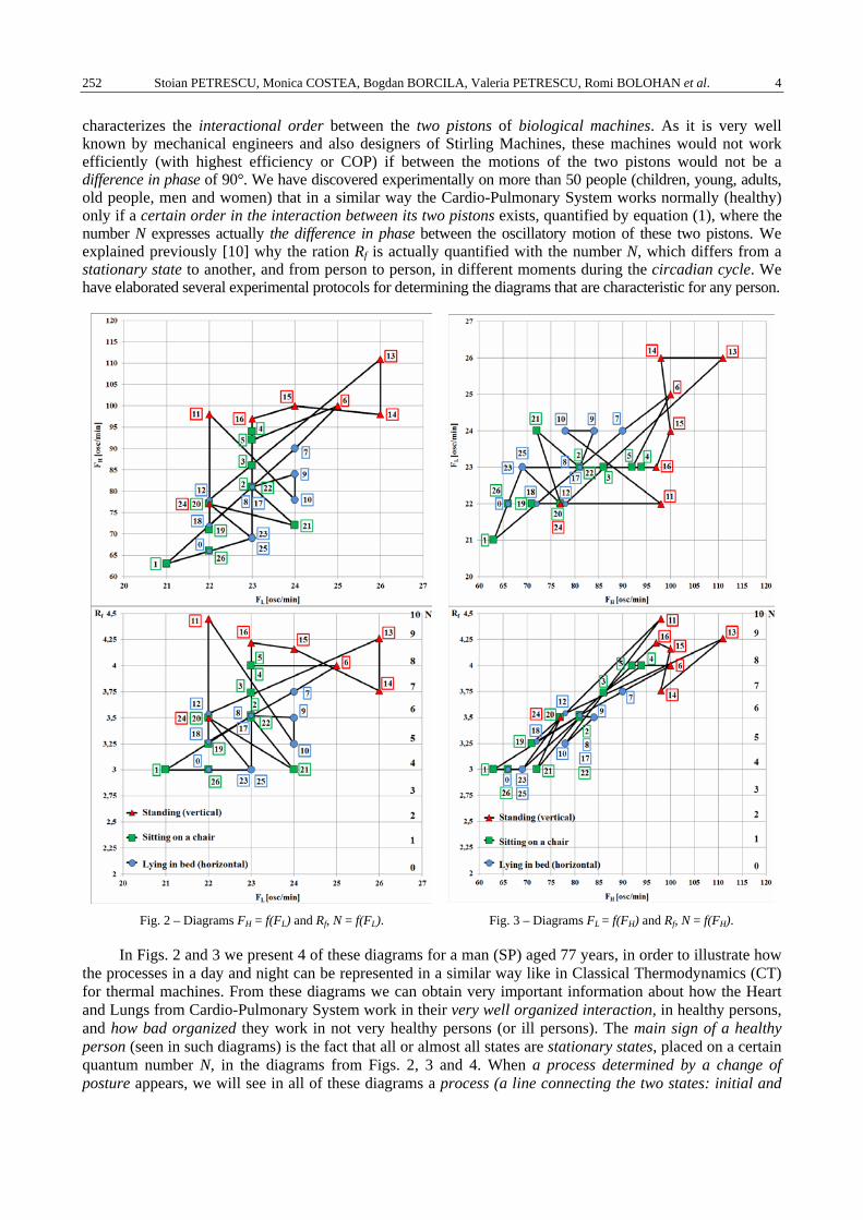
Stoian PETRESCU, Monica COSTEA, Bogdan BORCILA, Valeria PETRESCU, Romi BOLOHAN et al. 4 252
characterizes the interactional order between the two pistons of biological machines. As it is very well known by mechanical engineers and also designers of Stirling Machines, these machines would not work efficiently (with highest efficiency or COP) if between the motions of the two pistons would not be a difference in phase of 90°. We have discovered experimentally on more than 50 people (children, young, adults, old people, men and women) that in a similar way the Cardio-Pulmonary System works normally (healthy) only if a certain order in the interaction between its two pistons exists, quantified by equation (1), where the number N expresses actually the difference in phase between the oscillatory motion of these two pistons. We explained previously [10] why the ration Rf is actually quantified with the number N, which differs from a stationary state to another, and from person to person, in different moments during the circadian cycle. We have elaborated several experimental protocols for determining the diagrams that are characteristic for any person.
Fig. 2 – Diagrams FH = f(FL) and Rf, N = f(FL). Fig. 3 – Diagrams FL = f(FH) and Rf, N = f(FH).
In Figs. 2 and 3 we present 4 of these diagrams for a man (SP) aged 77 years, in order to illustrate how the processes in a day and night can be represented in a similar way like in Classical Thermodynamics (CT) for thermal machines. From these diagrams we can obtain very important information about how the Heart and Lungs from Cardio-Pulmonary System work in their very well organized interaction, in healthy persons, and how bad organized they work in not very healthy persons (or ill persons). The main sign of a healthy person (seen in such diagrams) is the fact that all or almost all states are stationary states, placed on a certain quantum number N, in the diagrams from Figs. 2, 3 and 4. When a process determined by a change of posture appears, we will see in all of these diagrams a process (a line connecting the two states: initial and

5 What is quantum biological thermodynamics with finite speed of the cardio-pulmonary system 253
final) with or without a quantum jump, corresponding to a change of, or a constant N. A constant N process (iso-quantum number) corresponds to equation (6) and is represented by processes 0–1, 8–9, 5–6. We also see processes described by equation (5) with constant FL (processes 11–12, 16–17, 9–10, 2–3, 4–4, 13–14). There are also processes with constant or quasi-constant FH (process 14–15, eq. (4)).
The stationary states corresponding to the horizontal position and sitting on the chair are usually in the bottom and medium domain of all diagrams (circles and quadrates points), but standing on the feet and walking positions correspond (triangles) to the upper side domain of the diagrams. This is caused by the increase of FH, because more Oxygen is needed for more effort consumed in the muscles. Also when eating (for example the breakfast, process 1–2), the stationary state is changed, with increasing the quantum number N (quantum jump up from 4 to 6), because of the effort of the muscles during eating, and the beginning of the metabolism process involving the muscles of the stomach.
If the position changes appear, from standing to siting or laying in the bed, the state (point on diagram) is moving usually to lower quantum number with a quantum jump down (process 16–17 where N changes from 9 to 6, and process 11–12 where N goes from 10 to 6).
In the opposite situation, changing the position from horizontal (in bed) to vertical (on the feet), the quantum number N is increasing with a quantum jump up (process 12–13 where N is increasing from 6 to 9, and process 10–11, where N is increasing from 5 to 10).
In the fifth diagram presented in Fig. 4 we see the correlations between the change of Oxygen percent in the blood O2, the change of frequency of the heart FH, the change of the frequency of the lung FL and the change in the Frequency ratio Rf = FH/FL (corresponding also to the change of the quantum number N)
over a day in which different activities were carried out. There are very obvious correlations between the changing of the 4 parameters of state: O2, FH, FL, Rf (respectively N).
The main correlation is based on the discovered formula (Eq. 1) which led us to express quantitatively “the very well organized” interaction between Heart and Lung.
Based on these diagrams combined with the diagram from Fig. 1, and using the Direct Method from TFS we can compute now the Power, Entropy Source and Efficiency of this wonderful and extremely efficient Biological Machines that compose the Cardio-Pulmonary Systems in humans and animals.
Fig. 4 – Diagrams O2 = f(Number of the state); FH = f(Number of the state); FL = f(Number of the state) and Rf, N = f(Number of the state).

Stoian PETRESCU, Monica COSTEA, Bogdan BORCILA, Valeria PETRESCU, Romi BOLOHAN et al. 6 254
5. CONCLUSIONS AND PERSPECTIVES
The answer to the title question is that Quantum Biological Thermodynamics with Finite Speed of Cardio-Pulmonary System (QBTFSCPS) is both a discovery based on Equation (1) and also an invention based on the 5 diagrams, built in a similar way to those from Classical Thermodynamics, but using new fundamental concepts such as stationary quantum states, processes between stationary quantum states, with or without quantum jump.
This discovery is in agreement with the Bejan’s Constructal Law in the sense that “the natural Process which designed human being has Optimized the functioning of this essential System, the Cardio - Pulmonary System” (in healthy people). Unfortunately, in not very healthy people the interaction is not any better organized and the consequences could be dramatically.
This new branch of Irreversible Thermodynamics, called Quantum Biological Thermodynamics with Finite Speed that we applied here to Cardio-Pulmonary System can help the designer teams of Doctors, Physiologists, Mechanical Engineers, Electronic and Electrical Engineers, Chemist and Electrochemist, to design Optimized and Personalized Artificial Hearts that will suit better for different types of patients in the near future.
REFERENCES
1. BEJAN A., Shape and Structure from Engineering to Nature, Cambridge University Press, Cambridge, UK, 2000. 2. BEJAN A., LORENTE S., Design with Constructal Theory, Wiley, Hoboken, 2008. 3. BEJAN A., ZANE J.P., Design in Nature. How the Constructal Law Governs Evolution in Biology, Physics, Technology, and
Social Organization, Doubleday, New York, 2012. 4. BEJAN A., The Physics of Life: The Evolution of Everything, St. Martin’s Press, New York, 2016. 5. PETRESCU S., COSTEA M., TIMOFAN L., PETRESCU V., Means for Qualitative and Quantitative Description of the Cardio-
Pulmonary System Operation within Irreversible Thermodynamics with Finite Speed, Proceedings of ASTR Conference, Sibiu, Romania, 2014.
6. PETRESCU S., PETRESCU V., COSTEA M., TIMOFAN L., DANES S., BOTEZ G., Discovery of “Quantum Numbers” in the Cardio-Pulmonary Interaction Studied in Thermodynamics with Finite Speed, Proceedings of ASTR Conference, Sibiu, Romania, 2014.
7. GANEA I., PETRESCU S.A., TIMOFAN L., PETRESCU S., COSTEA M., A socio-economic regularity established based on an analogy with Thermodynamic Processes with Finite Speed – An Equation for Standard of Living, Proceedings of ASTR Conference, Sibiu, Romania, 2014.
8. PETRESCU S., COSTEA M., PETRESCU V., BOLOHAN R., BORIARU N., PETRESCU A.S., BORCILA B., Stationary Quantum States in Cardio-Pulmonary System, Proceedings of ASTR Conference, Galati, Romania, 2015.
9. PETRESCU, S., COSTEA, M., PETRESCU, A.S., PETRESCU, V., BORIARU, N., BOLOHAN, R., BORCILA B., Processes with Quantum Jumps in the Cardio-Pulmonary System, Proceedings of ASTR Conference, Galati, Romania, 2015.
10. PETRESCU S., BOLOHAN R., PETRESCU V., BORCILA B., COSTEA M., Diagrams Describing Stationary States and Processes in Cardio- Pulmonary System, Proceedings of ASTR Conference, Targu-Mures, Romania, 2016.
11. PETRESCU S., COSTEA M., FEIDT M., GANEA I., BORIARU N., Advanced Thermodynamics of Irreversible Processes with Finite Speed and Finite Dimensions, AGIR, Bucharest, Romania, 2015.
12. PETRESCU S., COSTEA M., HARMAN C., FLOREA T., Application of the Direct Method to Irreversible Stirling Cycles with Finite Speed, International Journal of Energy Research, 26, pp. 589–609, 2002.
13. PETRESCU S., ZAISER J., HARMAN C., PETRESCU V., COSTEA M., FLOREA T., PETRE C., FLOREA T.V., FLOREA E., Advanced Energy Conversion – Vol. I–II, Bucknell University, Lewisburg, PA, USA, 2006.
14. PETRESCU S., PETRE C., COSTEA M., BORIARU N., DOBROVICESCU A., FEIDT M., HARMAN C., A Methodology of Computation, Design and Optimization of Solar Stirling Power Plant using Hydrogen/Oxygen Fuel Cells, Energy, 35, pp. 729–739. 2010.
15. PETRESCU S., COSTEA M., et al., Development of Thermodynamics with Finite Speed and Direct Method, AGIR, Bucharest, 2011.
16. PETRESCU S., PETRESCU V., STANESCU G., COSTEA M., A Comparison between Optimization of Thermal Machines and Fuel Cells based on New Expression of the First Law of Thermodynamics for Processes with Finite Speed, Proceedings of the First International Thermal Energy Congress (ITEC–93), Marrakech, Morocco, 1993.
17. PETRESCU S., Lectures on New Sources of Energy, Helsinki University of Technology, Otaniemi, Finland, 1991. 18. PETRESCU S., Harman C., COSTEA M., FLOREA T., Determination of the Pressure Losses in a Stirling Cycle through Use of
a PV/Px Diagram, ISI Proceedings of the International Symposion on Efficiency, Costs, Optimization Simulation and Environmental Aspects of Energy Systems (ECOS’2000), edited by G.G. Hirs, Enschede, Netherlands, 2000, pp. 659–670.
THE PUBLISHING HOUSE PROCEEDINGS OF THE ROMANIAN ACADEMY, Series A, OF THE ROMANIAN ACADEMY Special Issue/2018, pp. 255–260
COMPACT, INTERDIGITATED CONSTRUCTAL DESIGN APPLIED TO SUPERCAPACITOR SYSTEMS
Alexandru M. MOREGA1,2, Juan ORDONEZ3, Mihaela MOREGA1, Lucian Pîslaru-Dănescu4, Alin A. DOBRE1 1 “Politehnica” University of Bucharest, 313 Splaiul Independentei, Bucharest, 060042, Romania
2 “Gheorghe Mihoc – Caius Iacob” Institute of Mathematical Statistic and Applied Mathematics, Romanian Academy, 125 Calea Victoriei, Bucharest, 010071, Romania
3 Florida State University, Tallahassee, FL 32310, USA 4National Institute for Research and Development in Electrical Engineering ICPE-CA, Bucharest, Romania
Corresponding author: Alexandru M. MOREGA, E-mail: [email protected]
Abstract. Interdigitated grid topology may provide for higher quality electrical devices, which are sieges of electric and magnetic fields, in terms of capacity, reconfiguration capability, and compactness. It is then important to provide design solutions that add to these the architectural scalability required to produce readily available solutions for designers. This paper aims to propose a constructal solution for interdigitated grid topologies based on an optimal scalable, minimum-redundant, reconfigurable interdigitated topology for planar electric devices. Although the interdigitated constructal design (ICD) may be of interest in the optimization of numerous planar structures, here we envisage two applications. In this paper, ICD is applied to optimize a planar micro supercapacitor that utilizes vertically grown carbon nanotube forests electrodes. This study relies on numerical solutions to boundary value problems that are solved using the finite element method.
Key words: Constructal law, Optimization, Supercapacitor, Carbon nanotubes forests, Interdigitated electrodes, Numerical simulation.
1. INTRODUCTION
Supercapacitors (SCs) are electrolytic capacitors with enhanced electrical charge storage capacity [1]. As their dielectric is an ion-conducting electrolyte, under a biased voltage, positive and negative ions separate and accumulate by the electrodes surfaces, producing the nm-thin electro-chemical double layer (EDL). The EDL ionic segregation and migration produce two capacitors connected in series [2].
The SCs with carbon nanotubes electrodes (SCNTs), unlike regular electrolytic capacitors, use extremely porous electrode materials to enhance the interfacial capacitance. The electrolyte/porous electrodes interface enhance the EDL phenomenon to astonishingly high value of specific capacitance (capacitance per unit area) [3]. When compared to fuel cells and Li-ion batteries, the charging/discharging process of the SC, which imply no chemical reaction, their stable performance (~106 cycles vs. ~103 cycles of Li-ion batteries [1]) and less temperature dependency, are of particular importance in medium and small power applications like vehicle regenerative braking and as the main power sources for short-term, high power-density usages in many applications. SCs are envisaged also as reversible power sources in pulse-power applications such as MEMS solid-state sensors, and for temporarily energy storage from energy harvester and power the system for sensing and wireless communication needs.
Enhanced electrodes structures were investigated, e.g., conducting polymer-coated metal layer [4] electrodes, KOH etching to increase the electrodes surface area [5], carbon nanotubes (CNT) with high surface area-to-volume ratio and good conductivity deposited on the electrodes [6], CNT arrays transferring to a conductive substrate after the synthesis process [7]. Recently, planar architectures with nanotube (CNT) forests are utilized as electrodes in SCs.
Here we apply the Constructal Law (CL) method [8] to enhance the performances of planar SCs with interdigitated finger electrodes configuration: systems of finite volume with internal fluxes (currents) that may cross their boundaries and which are subject to internal and external constraints morph such that their shape and
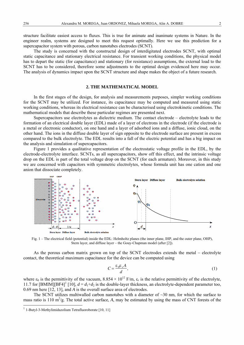
Alexandru M. MOREGA, Juan ORDONEZ, Mihaela MOREGA, Alin A. DOBRE 2 256
structure facilitate easiest access to fluxes. This is true for animate and inanimate systems in Nature. In the engineer realm, systems are designed to meet this request optimally. Here we use this prediction for a supercapacitor system with porous, carbon nanotubes electrodes (SCNT).
The study is concerned with the constructal design of interdigitated electrodes SCNT, with optimal static capacitance and stationary electrical resistance. For transient working conditions, the physical model has to depart the static (for capacitance) and stationary (for resistance) assumptions, the external load to the SCNT has to be considered, therefore some adjustments to the optimal design evidenced here may occur. The analysis of dynamics impact upon the SCNT structure and shape makes the object of a future research.
2. THE MATHEMATICAL MODEL
In the first stages of the design, for analysis and measurements purposes, simpler working conditions for the SCNT may be utilized. For instance, its capacitance may be computed and measured using static working conditions, whereas its electrical resistance can be characterised using electrokinetic conditions. The mathematical models that describe these particular regimes are presented next.
Supercapacitors use electrolytes as dielectric medium. The contact electrode – electrolyte leads to the formation of an electrical double layer (EDL) made of a layer of electrons in the electrode (if the electrode is a metal or electronic conductor), on one hand and a layer of adsorbed ions and a diffuse, ionic cloud, on the other hand. The ions in the diffuse double layer of sign opposite to the electrode surface are present in excess compared to the bulk electrolyte. The EDL results into a fall of the electric potential and has a big impact on the analysis and simulation of supercapacitors.
Figure 1 provides a qualitative representation of the electrostatic voltage profile in the EDL, by the electrode-electrolyte interface. SCNTs, as all supercapacitors, show off this effect, and the intrinsic voltage drop on the EDL is part of the total voltage drop on the SCNT (for each armature). Moreover, in this study we are concerned with capacitors with symmetric electrolytes, whose formula unit has one cation and one anion that dissociate completely.
Fig. 1 – The electrical field (potential) inside the EDL: Helmholtz planes (the inner plane, IHP, and the outer plane, OHP), Stern layer, and diffuse layer – the Gouy-Chapman model (after [2]).
As the porous carbon matrix grown on top of the SCNT electrodes extends the metal – electrolyte contact, the theoretical maximum capacitance for the device can be computed using
C =ε 0ε r A
d, (1)
where ε0 is the permittivity of the vacuum, 8.854 × 10¹² F/m, εr is the relative permittivity of the electrolyte, 11.7 for [BMIM][BF4]1 [10], d = d1+d2 is the double-layer thickness, an electrolyte-dependent parameter too, 0.69 nm here [12, 13], and A is the overall surface area of electrodes.
The SCNT utilizes multiwalled carbon nanotubes with a diameter of ~30 nm, for which the surface to mass ratio is 110 m2/g. The total active surface, A, may be estimated by using the mass of CNT forests of the 1 1-Butyl-3-Methylimidazolium Tetrafluoroborate [10, 11]

3 Compact, interdigitated constructal design applied to supercapacitor systems 257
device. For instance, a mass of 3×10⁻⁵ g yields an area of 3.3×10⁻³ m2. Moreover, the equivalent electrical circuit of a SCNT may be thought of as made of two capacitances connected in series, one for each of its armatures. Then, the theoretical value of A has to be divided by two, which yields 1.65×10⁻³ m2. Using these derivations, eq. (1) may provide for the theoretical peak capacitance (e.g., 248 μF), which is an upper limit [10].
Figure 2 shows a qualitative view of an electrode with CNT grown on top and filled with electrolyte, and its equivalent model proposed in this study.
Fig. 2 – Qualitative sketch of carbon nanotubes electrodes. The electrolyte separates in positive and negative ions
that build electrical charges layers by the electrodes.
We assume that the CNT forest and the filling electrolyte are replaced with a homogeneous block with anisotropic relative permittivity
–parallel to the CNT ε || = εCNT + ε e , (2)
–perpendicular to the CNT
ε⊥ =εCNTε e
εCNT + ε e
, (3)
where εCNT is the sheet CNT relative permittivity, and εe is the electrolyte relative permittivity. Here εCNT = 1.3 and εe = 11.7 [12].
The electrostatic field inside the SCNT, outside the EDLs that exist by the electrodes, is described by
ΔV = 0 , (4)
where V [V] is the electrostatic potential. The boundary conditions that close the mathematical model are electrical insulation (zero charge)
everywhere, except for the electrodes, where Dirichlet (potential) conditions are assumed. Here V+ = 100 mV and V– = –100 mV.
2.1. The electrokinetic field
In stationary working conditions, the electrical field is described by
ΔVk = 0 , (5)
where Vk [V] is the electrokinetic potential. Here too, it is convenient to approximate the carbon forest and the electrolyte inside it with a homogeneous block with anisotropic electrical conductivity that yields
– parallel to the CNT
σ|| =σCNTσe
σCNT +σe
, (6)
– perpendicular to the CNT
σ⊥=σCNT +σe , (7)
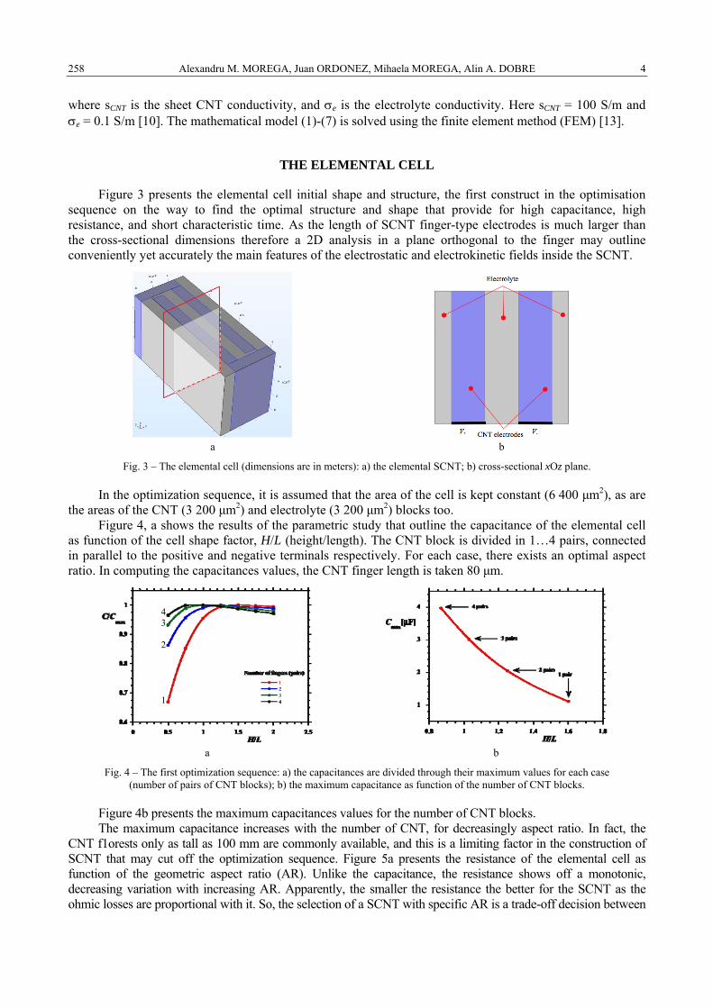
Alexandru M. MOREGA, Juan ORDONEZ, Mihaela MOREGA, Alin A. DOBRE 4 258
where sCNT is the sheet CNT conductivity, and σe is the electrolyte conductivity. Here sCNT = 100 S/m and σe = 0.1 S/m [10]. The mathematical model (1)-(7) is solved using the finite element method (FEM) [13].
THE ELEMENTAL CELL
Figure 3 presents the elemental cell initial shape and structure, the first construct in the optimisation sequence on the way to find the optimal structure and shape that provide for high capacitance, high resistance, and short characteristic time. As the length of SCNT finger-type electrodes is much larger than the cross-sectional dimensions therefore a 2D analysis in a plane orthogonal to the finger may outline conveniently yet accurately the main features of the electrostatic and electrokinetic fields inside the SCNT.
a b
Fig. 3 – The elemental cell (dimensions are in meters): a) the elemental SCNT; b) cross-sectional xOz plane.
In the optimization sequence, it is assumed that the area of the cell is kept constant (6 400 μm2), as are the areas of the CNT (3 200 μm2) and electrolyte (3 200 μm2) blocks too.
Figure 4, a shows the results of the parametric study that outline the capacitance of the elemental cell as function of the cell shape factor, H/L (height/length). The CNT block is divided in 1…4 pairs, connected in parallel to the positive and negative terminals respectively. For each case, there exists an optimal aspect ratio. In computing the capacitances values, the CNT finger length is taken 80 μm.
a b
Fig. 4 – The first optimization sequence: a) the capacitances are divided through their maximum values for each case (number of pairs of CNT blocks); b) the maximum capacitance as function of the number of CNT blocks.
Figure 4b presents the maximum capacitances values for the number of CNT blocks. The maximum capacitance increases with the number of CNT, for decreasingly aspect ratio. In fact, the
CNT f1orests only as tall as 100 mm are commonly available, and this is a limiting factor in the construction of SCNT that may cut off the optimization sequence. Figure 5a presents the resistance of the elemental cell as function of the geometric aspect ratio (AR). Unlike the capacitance, the resistance shows off a monotonic, decreasing variation with increasing AR. Apparently, the smaller the resistance the better for the SCNT as the ohmic losses are proportional with it. So, the selection of a SCNT with specific AR is a trade-off decision between
4 3 2 1
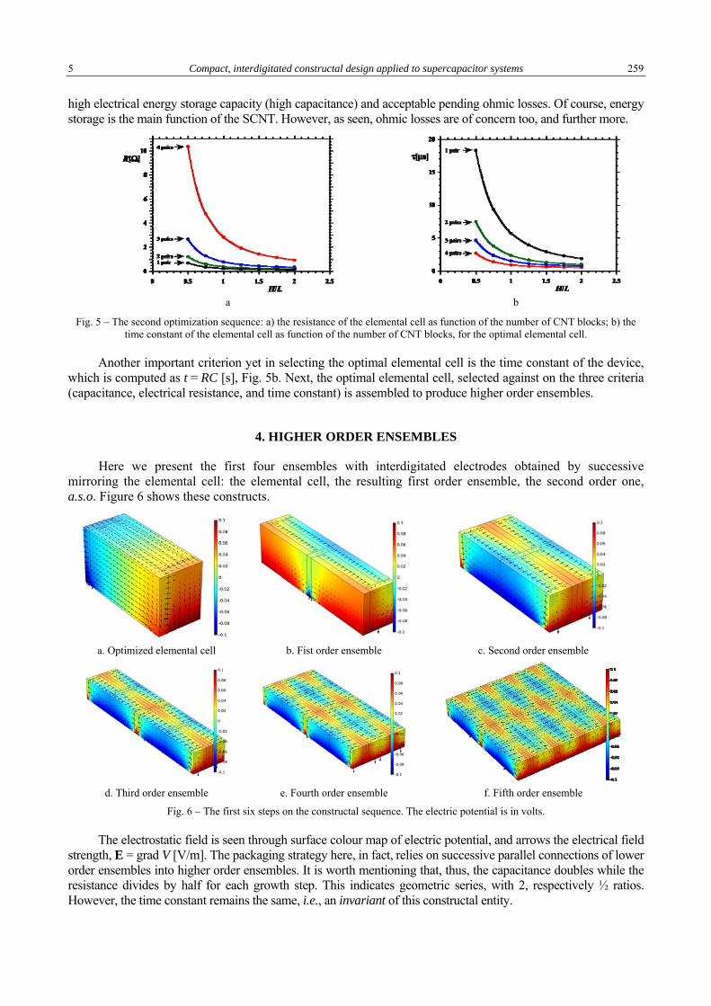
5 Compact, interdigitated constructal design applied to supercapacitor systems 259
high electrical energy storage capacity (high capacitance) and acceptable pending ohmic losses. Of course, energy storage is the main function of the SCNT. However, as seen, ohmic losses are of concern too, and further more.
a b
Fig. 5 – The second optimization sequence: a) the resistance of the elemental cell as function of the number of CNT blocks; b) the time constant of the elemental cell as function of the number of CNT blocks, for the optimal elemental cell.
Another important criterion yet in selecting the optimal elemental cell is the time constant of the device, which is computed as t = RC [s], Fig. 5b. Next, the optimal elemental cell, selected against on the three criteria (capacitance, electrical resistance, and time constant) is assembled to produce higher order ensembles.
4. HIGHER ORDER ENSEMBLES
Here we present the first four ensembles with interdigitated electrodes obtained by successive mirroring the elemental cell: the elemental cell, the resulting first order ensemble, the second order one, a.s.o. Figure 6 shows these constructs.
a. Optimized elemental cell b. Fist order ensemble c. Second order ensemble
d. Third order ensemble e. Fourth order ensemble f. Fifth order ensemble
Fig. 6 – The first six steps on the constructal sequence. The electric potential is in volts.
The electrostatic field is seen through surface colour map of electric potential, and arrows the electrical field strength, E = grad V [V/m]. The packaging strategy here, in fact, relies on successive parallel connections of lower order ensembles into higher order ensembles. It is worth mentioning that, thus, the capacitance doubles while the resistance divides by half for each growth step. This indicates geometric series, with 2, respectively ½ ratios. However, the time constant remains the same, i.e., an invariant of this constructal entity.
Alexandru M. MOREGA, Juan ORDONEZ, Mihaela MOREGA, Alin A. DOBRE 6 260
5. CONCLUSIONS
The Constructal Law (CL) method is applied to improve the performances of planar supercapacitors with carbon nanotubes forest electrodes (SCNTs) and interdigitated finger electrodes configurations. The results of this study are useful in the first stages of the SCNT design, for analysis and measurements purposes, and it relies on modelling simpler working conditions.
Assuming that the CNT forest and the filling electrolyte are replaced with homogeneous blocks with anisotropic relative permittivity and electrical resistivity, a 2D analysis in a plane orthogonal to the finger outlines conveniently yet accurately the main features of the electrostatic and electrokinetic fields inside the SCNT. In the CL optimization sequence conducted on the 2D model it was assumed that the area of the SCNT cell, the area of the CNT, and that of the electrolyte blocks are constant, and that the cell geometric aspect ratio (AR) (height/length) is the single optimization variable. The capacitance as AR-function shows off a maximum, which singles out the optimal cell geometry. The maximum capacitance increases with the number of CNT, for decreasingly AR. The resistance varies monotonically (decreases) with AR, therefore the optimal cell shape should be a trade-off decision between a high storage capacity and conveniently high ohmic losses cell.Another important criterion yet in selecting the optimal elemental cell is the time constant of the device, which may be computed using the values of capacitances and resistances. Summing up, three criteria (capacitance, electrical resistance, and time constant) may be considered in selecting the optimal cell.
The packaging strategy presented here, in fact, relies on successive parallel connections of lower order ensembles into higher order ensembles. It is worth mentioning that, thus, the capacitance doubles while the resistance divides by half for each growth step. This indicates geometric series convergences with 2, respectively ½ ratios. However, the time constant remains the same, i.e., an invariant of this constructal entity.
ACKNOWLEDGEMENTS
The research was performed with the support offered by UEFISCDI, PNCDI II Programme – Joint Applied Research Projects, Romania, research grant no. 63/2014, Environment energy harvesting hybrid system by photovoltaic and piezoelectric conversion, DC/DC transformation with MEMS integration and adaptive storage.
REFERENCES
1. CONWAY B.E., Electrochemical Supercapacitors: Scientific Fundamentals and Technological Applications, Kluwer Academic/Plenum Publishers, New York, 1999.
2. GHOSH P., Electrostatic Double Layer Force: Part II, NPTEL Chemical Engineering Interfacial Engineering, Department of Chemical Engineering, IIT Guwahati, Guwahati –781039, India, 2017
3. SHENA C., WANGA X., ZHANGA W., KANG F., A high-performance three-dimensional micro supercapacitor based on self-supporting composite materials, J. of Power Sources, 196, pp. 10465–10471, 2011.
4. SUNG J.H., KIM S.J., LEE K.H., Fabrication of microcapacitors using conducting polymer microelectrodes, J. Power Sources, 124, pp. 343–350, 2003.
5. In H.J., KUMAR S., SHAO-HORN Y., BARBASTATHIS G., Nanostructured Origami™ 3D Fabrication and Assembly of Electrochemical Energy Storage Devices, Proc 2005 IEEE on Nanotechnology, Nagoya, Japan, July 2005, pp. 374–377.
6. An K.H., KIM W.S., PARK Y.S., CHOI Y.C., LEE S.M., CHUNG D.C., BAE D.J., LIM S.C., LEE Y.H., Supercapacitors Using Single-Walled Carbon Nanotube Electrodes, Adv. Mater., 13, pp. 497–500, 2001.
7. PUSHPARAJ V.L., SHAIJUMON M.M., KUMAR A., MURUGESAN S., CI L.J., VAJTAI R., LINHARDT R.J., NALAMASU O., AJAYAN P.M., Flexible energy storage devices based on nanocomposite paper, PNAS, 104, pp. 13574–13577, 2007.
8. BEJAN A., Design and Structure from Engineering to Nature, Cambridge Univ. Press, 2000. 9. WAKAI C., OLEINIKOVA A., OTT M., WEINGARTNER H., How polar are ionic liquids? Determination of the static
dielectric constant of an imidazolium-based ionic liquid by Microwave Dielectric Spectroscopy, J. Phys. Chem. B, 109, pp. 17028–17030, 2005.
10. JIANG Y.Q., ZHOU Q., LIN L., Planar MEMS supercapacitor using carbon nanotube forests, IEEE 22nd International Conference on Micro Electro Mechanical Systems, 2009. MEMS 2009, 10.1109/MEMSYS.2009.4805450.
11. http://www.sigmaaldrich.com/catalog/product/aldrich/91508?lang=en®ion=RO 12. JIANG Y.Q., Carbon Nanotube-based MEMS Energy Storage Devices, PhD Thesis, Univ. of California, Berkeley, Fall 2011. 13. Comsol Multiphysics, v. 3.5a–5.2a.
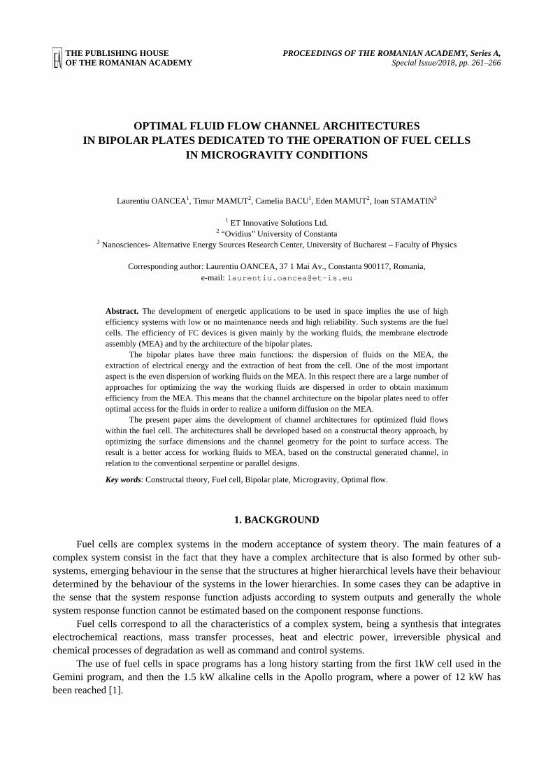
THE PUBLISHING HOUSE PROCEEDINGS OF THE ROMANIAN ACADEMY, Series A, OF THE ROMANIAN ACADEMY Special Issue/2018, pp. 261–266
OPTIMAL FLUID FLOW CHANNEL ARCHITECTURES IN BIPOLAR PLATES DEDICATED TO THE OPERATION OF FUEL CELLS
IN MICROGRAVITY CONDITIONS
Laurentiu OANCEA1, Timur MAMUT2, Camelia BACU1, Eden MAMUT2, Ioan STAMATIN3 1 ET Innovative Solutions Ltd.
2 “Ovidius” University of Constanta 3 Nanosciences- Alternative Energy Sources Research Center, University of Bucharest – Faculty of Physics
Corresponding author: Laurentiu OANCEA, 37 1 Mai Av., Constanta 900117, Romania,
e-mail: [email protected]
Abstract. The development of energetic applications to be used in space implies the use of high efficiency systems with low or no maintenance needs and high reliability. Such systems are the fuel cells. The efficiency of FC devices is given mainly by the working fluids, the membrane electrode assembly (MEA) and by the architecture of the bipolar plates.
The bipolar plates have three main functions: the dispersion of fluids on the MEA, the extraction of electrical energy and the extraction of heat from the cell. One of the most important aspect is the even dispersion of working fluids on the MEA. In this respect there are a large number of approaches for optimizing the way the working fluids are dispersed in order to obtain maximum efficiency from the MEA. This means that the channel architecture on the bipolar plates need to offer optimal access for the fluids in order to realize a uniform diffusion on the MEA.
The present paper aims the development of channel architectures for optimized fluid flows within the fuel cell. The architectures shall be developed based on a constructal theory approach, by optimizing the surface dimensions and the channel geometry for the point to surface access. The result is a better access for working fluids to MEA, based on the constructal generated channel, in relation to the conventional serpentine or parallel designs.
Key words: Constructal theory, Fuel cell, Bipolar plate, Microgravity, Optimal flow.
1. BACKGROUND
Fuel cells are complex systems in the modern acceptance of system theory. The main features of a complex system consist in the fact that they have a complex architecture that is also formed by other sub-systems, emerging behaviour in the sense that the structures at higher hierarchical levels have their behaviour determined by the behaviour of the systems in the lower hierarchies. In some cases they can be adaptive in the sense that the system response function adjusts according to system outputs and generally the whole system response function cannot be estimated based on the component response functions.
Fuel cells correspond to all the characteristics of a complex system, being a synthesis that integrates electrochemical reactions, mass transfer processes, heat and electric power, irreversible physical and chemical processes of degradation as well as command and control systems.
The use of fuel cells in space programs has a long history starting from the first 1kW cell used in the Gemini program, and then the 1.5 kW alkaline cells in the Apollo program, where a power of 12 kW has been reached [1].

Laurentiu OANCEA, Timur MAMUT, Camelia BACU, Eden MAMUT, Ioan STAMATIN 2 262
Fig. 1 – Microgravity fuel cell feeding schematics [2].
In recent years, researches have been concentrated in replacing mechanical components in fuel cell systems in order to reduce mass and power consumption and improve system reliability as a whole [3]. Concerns in the direction of thermofluid modelling of fuel cells have been related to overall problems with the administration of thermal fluxes and improvement of cell reliability [4, 5].
A synthesis of the present state of the art for fluid feeding schemes for fuel cells operating under microgravity conditions is shown in Fig. 1. Thus, it can be noticed that the hydraulic circuits are pressurized and impose a specific architecture to ensure fluid circulation both at the cell anode and cathode and through the cooling sections.
In order to optimize thermofluid flow structures there is a wide range of approaches reported in the literature. A multiscale analysis approach has been proposed in [6]. There were also developed models based on Thermoeconomics, placing a special focus on the conservation of energy resources, both in the design phase and in the operating phase of the systems through a multidisciplinary approach, combining engineering techniques with economic methods cost analysis to minimize energy consumption, emissions, and resulting waste/slurry.
Fig. 2 – The complexity of the design space for stationary energy intensive systems.
In Fig. 2 it is proposed a graph based on the adaptation of thermoeconomic optimisation principles [7] and it presents a three-dimensional coordinate system to visualize the methodology. Thus, for a given objective function (minimum cost, minimum maintenance, etc.), an optimal design solution is characterized by an optimal structure (consisting of the components of the installation and the connections between them) and an optimal set of process parameters. From this perspective the result is that in such a complex space there can be no single optimal point. In this approach there may be several optimal solutions that can be identified at a preliminary stage and then analysed in detail.

3 Optimal fluid flow channel architectures in bipolar plates dedicated to the operation of fuel cells 263
Further developments in this direction focused more on expanding the exergy approach by introducing the concepts of cumulative exergy content and developing a common exergy reporting space for both the system (structure) and process components, respectively the exergy contained in various thermodynamic agents evolving in system components through various physical or chemical transformation processes with the constant destruction of the exergy contained. In this context, a chapter in thermodynamics called Exergoeconomy has emerged.
A development of optimization theories of thermofluid systems based on the principle of minimal entropy generated by a particular flow or heat transfer process has led to a new theory that allows a unitary approach to the relationship between process and structure called Constructal Theory [8].
Being a consecrated theory, a direction has also emerged in engineering design based on the constructional principle, called Constructal Design. One of these designs was developed also for a PEM fuel cell by Senn SM and Poulikakos D in 2004 [9].
2. THE DESIGN
The approach is based on the Constructal Law in general and on the applications for the optimization of fluid flows in particular. The full algorithm for the optimization is presented in the Shape and Structure, From Engineering to Nature [8], but for the development of the present case, there are necessary the optimization formulas for the elemental volume and for the first construct:
21
00~
0
0 2−
⎟⎠⎞
⎜⎝⎛= φK
lh
, 4
1
00
~2
10
~2 ⎟
⎠⎞
⎜⎝⎛=
−φKl ,
41
00
~2
10
~2
−
⎟⎠⎞
⎜⎝⎛= φKh ,
21
00
~
0
~
21
−
⎟⎠⎞
⎜⎝⎛=Δ φKP .
(1)
For the first construct, the formulas are presented in Table 1:
Table 1
Formulas for the first construct
hi li h_
i l_
i ni = Ai Ai−1 Δ P_
i (2C0 C1)1 2 21 2C0
1 4 C0−1 4C1
1 2 (2C1)1 2 (2C0C1)−1 2
For the development of the bipolar fuel cell design, it was considered a minimum width of the central pipe of one millimetre, which generated the shape having a length of 12.5 mm and height of 9 mm.
The first construct contained twelve elemental volumes, as it is presented in Fig. 4:
Fig. 3 – Elemental volume. Fig. 4 – First order construct.

Laurentiu OANCEA, Timur MAMUT, Camelia BACU, Eden MAMUT, Ioan STAMATIN 4 264
In Fig. 4 above, the first level construct is shaped as a rectangle. In order to cover the expected square shape of a fuel cell, there were used two identical constructs, placed next to each other.
3. THE ANALYSIS
The fluid flow analysis was developed by means of CFD. The obtained shape was enclosed buy a 2 mm wall, in order to contain the fluid (outer boundary).
As it can be noticed, the resulting shape has two inlets and two outlets, positioned in such a way as to allow the fluid to access the elemental volumes Fig. 5.
Fig. 5 – Enclosed constructs.
In order to simplify the analysis, it was extracted from the shape only the flowing channel and it was imported into the CFD analysis Fig. 6.
Fig. 6 – 3D flow channel.
For the analysis, it was considered a laminar flow, with two velocity inlets (bottom) and two outlets (top). The velocity flow inlet was set to 0.1 m/s and the working fluid was set to liquid urea. The exterior of the channel was set to a wall boundary condition. Gravity was set to zero.
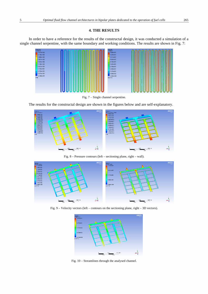
5 Optimal fluid flow channel architectures in bipolar plates dedicated to the operation of fuel cells 265
4. THE RESULTS
In order to have a reference for the results of the constructal design, it was conducted a simulation of a single channel serpentine, with the same boundary and working conditions. The results are shown in Fig. 7:
Fig. 7 – Single channel serpentine.
The results for the constructal design are shown in the figures below and are self-explanatory.
Fig. 8 – Pressure contours (left – sectioning plane, right – wall).
Fig. 9 – Velocity vectors (left – contours on the sectioning plane, right – 3D vectors).
Fig. 10 – Streamlines through the analysed channel.

Laurentiu OANCEA, Timur MAMUT, Camelia BACU, Eden MAMUT, Ioan STAMATIN 6 266
The most important aspect, which can be noticed from the analysis of the single channel serpentine and the constructal design, is the profile of the pressure inside the two volumes. In the single channel, the pressure builds up along the length of the channel, as in the constructal design, the pressure is distributed along the system. This leads to the possibility to increase the pressure of the system or the pressure drop, up to the maximum allowed working pressure.
5. CONCLUSIONS
By identifying the local and global constraints for the design, the constructal theory offers the opportunity to create a design for the flowing structures in a simple way, by considering only a basic set of parameters with the highest impact on the structure-process system.
The emerging structure in this case is rectangular, as the shape of the membrane-electrode assembly of the fuel cell is rectangular. At the moment, this form is easier and cheaper to produce, and at the same time it can be used to allow the fluid to exit the volume without major modifications. However, the next steps need to be in the development of non-rectangular shapes (e.g. the dendritic shape) for a reduction in the material raw used.
As it can be seen from the design and the analysis of the structure, in order to use the shape as an inlet and an outlet to the surface, there were considered two first constructs placed in parallel, in order to cover the envisaged area. At the same time, this conducted to a shape which presented for the outlet structure a similar optimal shape: the shape in the middle is the same first construct and the two shapes from the extremities are two halves of one construct. This translates in an optimal inlet for the fluid and an also an optimal outflow for the same fluid.
For the optimization of the flow, it can be noticed that there is a better access of fluids to the area, taking into consideration the conventional single channel serpentine. While the single channel builds up pressure as the length increases, the constructal shape distributes the pressure on the entire area or volume, producing a lower maximum pressure in the system.
The possibility to use the constructal design has a superior advantage over the classical approach of trial and error when developing new systems, as the constructal principles can be applied from the sketching phases of flow architectures, in a simple manner and with astonishing results for structure-process system optimization.
REFERENCES
1. H. GUO, X. LIU, J.F. ZHAO, F. YE, C.F. MA, Experimental study of two-phase flow in a proton exchange membrane fuel cell in short-term microgravity condition, Applied Energy, 136, pp. 509–518, 2014.
2. Mark HOBERECHT, NASA’s First Year Progress with Fuel Cell Advanced Development in Support of the Exploration Vision, Advanced Power and Propulsion Technologies and Systems, February 14th, 2007.
3. M. NAJJARI, F. KHEMILI, S.B. NASRALLAH, The effects of the gravity on transient responses and cathode flooding in a proton exchange membrane fuel cell, Int. J. Hydrogen Energy, 38, pp. 3330–3337, 2013.
4. H. GUO, X. LIU, J.F. ZHAO, F. YE, C.F. MA, Effect of low gravity on water removal inside proton exchange membrane fuel cells (PEMFCs) with different flow channel configurations, Energy, 112, pp. 926–934, 2016.
5. R. BANERJEE, S.G. KANDLIKAR, Two-phase flow and thermal transients in proton exchange membrane fuel cells – A critical review, Int. J. Hydrogen Energy, 40, pp. 3990–4010, 2015.
6. MAMUT E., Modelling Single Phase Flows in Micro Heat Exchangers – A Multiple Scales Analysis Approach, in Ed. Ingham D.B. et al., Emerging Technologies and Techniques in Porous Media, Kluwer Academic Publishers, 2004, pp. 351–366.
7. EL-SAYED Y., A short Course in Thermo-Economics, Summer School, “Ovidius” University of Constanta, Constanta, Romania, July 1999.
8. BEJAN A., Shape and Structure, from Engineering to Nature, Cambridge University, 2000. 9. SENN SM, POULIKAKOS D., Tree network channels as fluid distributors constructing double-staircase polymer electrolyte fuel
cells, J. A. Phys., 96, pp. 842–852, 2004.

THE PUBLISHING HOUSE PROCEEDINGS OF THE ROMANIAN ACADEMY, Series A, OF THE ROMANIAN ACADEMY Special Issue/2018, pp. 267–272
CONSTRUCTAL LAW, AND THE ALBEDO AND GLOBAL WARMING CONUNDRUM
A. HEITOR REIS
University of Évora, Department of Physics and Institute of Earth Sciences (ICT), R. Romão Ramalho, 59, 7002–554 Évora, Portugal, Email: [email protected]
Abstract. In the current debate on global warming is under analysis whether the albedo will increase with temperature, and may thus constitute a negative feedback mechanism by increasing the amount of solar radiation reflected into space. This issue is analyzed in this paper in the light of the Constructal Law. In fact, by maximizing the overall conductivity of the processes that lead to the thermalization of the solar energy absorbed on Earth and its subsequent radiation into space at the global average temperature, it is possible to conclude that the albedo should increase with the global temperature, thus constituting a negative feedback mechanism that will help to restrain the increase of global temperature. Additionally, the value found for the rate of variation of the albedo with global surface temperature is very close to the values published in the literature, which were obtained both through satellite data and ground-based observations. Although they result from a preliminary analysis, these results are encouraging towards the implementation of the Constructal Law in the analysis of the climate system.
Key words: Earth’s albedo, Global warming, Constructal Law.
1. INTRODUCTION
Earth’s albedo is defined as the ratio of radiation reflected by the entire planetary surface to the radiation incident on it. Because the Earth’s surface also emits thermal radiation, it is not easy to separate this fraction from that corresponding to the radiation received from the Sun. Currently, two method are used based on data from: (i) Earth Radiation Budget Experiment (ERBE, a set of satellite instruments designed to measure the Earth’s energetic balance), and (ii) Earthshine (ES, ground based measurements of reflectance based on the dayside earthlight reflected from the Moon back to the night-time observer [1–3]. Anomalies in the terrestrial albedo are detected through the photometric ratio of the dark (earthshine) to the bright (moonshine) sides of the Moon [1].
The main contributors to the Earth’s albedo are clouds, polar ice caps, and desert belts in the two hemispheres. Albedo is a chief modulator of the Earth’s climate, because it controls the global energy budget through the amount of radiation reaching the Earth’s surface.
The direction of the variation of the Earth's albedo in the last decades, in which an increase in the global temperature has been observed, is currently in dispute. By the beginning of the century, Pallé and co-workers [4] found that albedo anomalies although positive show “a steady decrease in Earth’s reflectance from 1984 to 2000, with a strong climatologically significant drop after 1995. From 2001 to 2003, only earthshine data are available, and they indicate a complete reversal of the decline.” However, in a later paper [5] they reported an incorrect treatment of outlier data points, which caused an overly large decreasing trend of positive anomalies in the period 1998–2003. Recently, Pallé and co-workers published the results of the analysis of an extended period (1998–2014) in which they sigma-clipped data to remove outlier values lying more than 3σ and 1σ away from the fit to the data (σ stands for standard deviation) [5]. As they explained, clipping was done by fitting all the data and eliminating all data more than 3σ and 1σ away from the fit, respectively. The result is shown in Figs. 1 and 2.
We can observe in both cases the same trend: the albedo (or earthshine) increases with Earth global temperature. In the case of 3σ clipping this trend is more noticeable and of order of 0.5Wm-2 in the period (1998–2014), while the value corresponding to 1σ clipping is smaller and of order 0.25 Wm-2. Moreover, as

A. Heitor REIS 2 268
noted by Pallé and co-workers [5], contrarily to the 3σ clipping case, in the plot corresponding to 1σ clipping both the satellite and ground based data sets from of albedo anomalies are in good agreement over the 14 years they have in common. Therefore, in the following we will use the value of 0.25 Wm-2 (1σ clipping) as the earthshine variation with Earth’ temperature in the period (1998–2014).
The global Earth temperature anomaly evolution in the period 1998–2014, with respect to the base (averaged) values of the period (1951–1980), is shown in Fig. 3. Data of global temperature anomalies were taken from the GISS Surface Temperature Analysis (GISTEMP) that uses data files from NOAA GHCN v3 (meteorological stations), ERSST v4 (ocean areas), and SCAR (Antarctic stations) [6]. Yearly anomalies represented by the points in Fig. 3 are averages of the values of the respective year, the values of the precedent and subsequent years. The best fit provides 0.0124K/year, as the rate of increase of the global temperature anomaly in the period 1998–2014.
Year
W/m
2
3σ clipping, ΔES= 0.5W/m2
Fig. 1 – Earthshine/albedo anomalies (ΔES), calculated over the mean of the full period (1998–2014)
with 3σ clipping expressed as reflected flux in W/m2. Ground based (black), satellite data (blue), adapted from [5].
ΔT= 0,0124/yearR² = 0,7678
0,3
0,35
0,4
0,45
0,5
0,55
0,6
0,65
0,7
0,75
0,8
1998 2000 2002 2004 2006 2008 2010 2012 2014
Tem
pera
ture
ano
mal
y (K
)
Year Fig. 2 – Earthshine/albedo anomalies (ΔES), calculated over the mean of the full period (1998–2014)
with 1σ clipping expressed as reflected flux in W/m2. Ground based (black), satellite data (blue), adapted from [5].
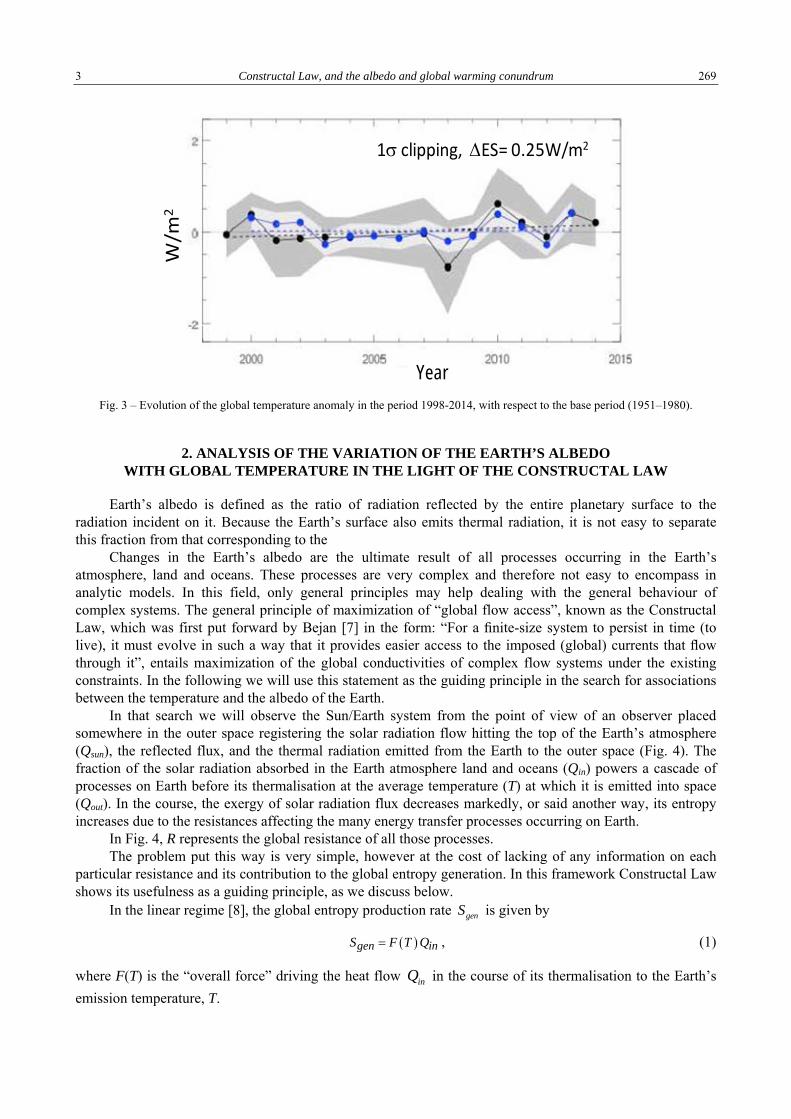
3 Constructal Law, and the albedo and global warming conundrum 269
W/m
2
Year
1σ clipping, ΔES= 0.25W/m2
Fig. 3 – Evolution of the global temperature anomaly in the period 1998-2014, with respect to the base period (1951–1980).
2. ANALYSIS OF THE VARIATION OF THE EARTH’S ALBEDO WITH GLOBAL TEMPERATURE IN THE LIGHT OF THE CONSTRUCTAL LAW
Earth’s albedo is defined as the ratio of radiation reflected by the entire planetary surface to the radiation incident on it. Because the Earth’s surface also emits thermal radiation, it is not easy to separate this fraction from that corresponding to the
Changes in the Earth’s albedo are the ultimate result of all processes occurring in the Earth’s atmosphere, land and oceans. These processes are very complex and therefore not easy to encompass in analytic models. In this field, only general principles may help dealing with the general behaviour of complex systems. The general principle of maximization of “global flow access”, known as the Constructal Law, which was first put forward by Bejan [7] in the form: “For a finite-size system to persist in time (to live), it must evolve in such a way that it provides easier access to the imposed (global) currents that flow through it”, entails maximization of the global conductivities of complex flow systems under the existing constraints. In the following we will use this statement as the guiding principle in the search for associations between the temperature and the albedo of the Earth.
In that search we will observe the Sun/Earth system from the point of view of an observer placed somewhere in the outer space registering the solar radiation flow hitting the top of the Earth’s atmosphere (Qsun), the reflected flux, and the thermal radiation emitted from the Earth to the outer space (Fig. 4). The fraction of the solar radiation absorbed in the Earth atmosphere land and oceans (Qin) powers a cascade of processes on Earth before its thermalisation at the average temperature (T) at which it is emitted into space (Qout). In the course, the exergy of solar radiation flux decreases markedly, or said another way, its entropy increases due to the resistances affecting the many energy transfer processes occurring on Earth.
In Fig. 4, R represents the global resistance of all those processes. The problem put this way is very simple, however at the cost of lacking of any information on each
particular resistance and its contribution to the global entropy generation. In this framework Constructal Law shows its usefulness as a guiding principle, as we discuss below.
In the linear regime [8], the global entropy production rate genS is given by
( )gen inS F T Q= , (1)
where F(T) is the “overall force” driving the heat flow inQ in the course of its thermalisation to the Earth’s emission temperature, T.
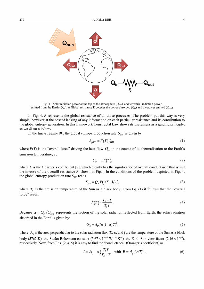
A. Heitor REIS 4 270
Qsun
Qin Qout
Qout
QoutQout
Qout
Fig. 4 – Solar radiation power at the top of the atmosphere (Qsun), and terrestrial radiation power
emitted from the Earth (Qout). A Global resistance R couples the power absorbed (Qin) and the power emitted (Qout).
In Fig. 4, R represents the global resistance of all those processes. The problem put this way is very simple, however at the cost of lacking of any information on each particular resistance and its contribution to the global entropy generation. In this framework Constructal Law shows its usefulness as a guiding principle, as we discuss below.
In the linear regime [8], the global entropy production rate genS is given by
( )gen inS F T Q= , (1)
where F(T) is the “overall force” driving the heat flow inQ in the course of its thermalisation to the Earth’s emission temperature, T, Qin = LF T( ), (2)
where L is the Onsager’s coefficient [8], which clearly has the significance of overall conductance that is just the inverse of the overalll resistance R, shown in Fig.4. In the conditions of the problem depicted in Fig. 4, the global entropy production rate Sgen reads Sgen = QinF 1 T −1 S( ), (3)
where sT is the emission temperature of the Sun as a black body. From Eq. (1) it follows that the “overall force” reads:
F T( )= TS − T
TST. (4)
Because in sunQ Qα = represents the faction of the solar radiation reflected from Earth, the solar radiation absorbed in the Earth is given by:
( ) 41in p SQ A f T= σ − α , (5)
where pA is the area perpendicular to the solar radiation flux, Ts, σ, and f are the temperature of the Sun as a black body (5762 K), the Stefan-Boltzmann constant (5.67 × 10⁻⁸ Wm–2K–4), the Earth-Sun view factor (2.16 × 10⁻⁵), respectively. Now, from Eqs. (2, 4, 5) it is easy to find the “conductance” (Onsager’s coefficient) as
L = B 1−α( ) TST
TS − T, with 4
p sB A f Tσ= . (6)

5 Constructal Law, and the albedo and global warming conundrum 271
We note that L represents the global conductance associated with the flow inQ under the global driving force F(T) acting between its absorption in Earth and its emission from Earth.
By letting the Earth’s emission temperature (T) free, Constructal Law requires the overall “conductance”, L, to be maximal (Ts and B fixed). From Eq. (6) that condition is expressed as:
( ) ( )d 11d 1T T T
α= − α
−, with T = ˜ T TS . (7)
The dimensionless Eq. 7 shows that albedo and Earth’s emission temperature have the same sense of variation, therefore increase in the albedo must be expected as the planetary global temperature increases. In order to test Eq. 7 in the case of the Earth first we will translate earthshine anomalies ( ESΔ ) into albedo anomalies according to
4ΔES SC( )= Δα , (8)
where SC is the Solar Constant, 1367 Wm–2, and the factor 4 accounts for the fact that solar radiation is reflected/diffused by the entire spherical Earth surface (therefore the anomaly 0.25 Wm-2 stands for the average value on the Earth’s surface), while the amount of incoming solar radiation is given for the product of the Solar Constant and the area of the Earth perpendicular to the solar radiation flux. Additionally, we take Ts = 5,762 K, the Earth’s emission temperature T = 255 K, and α = 0.7, as the value of the albedo currently accepted. We will also consider the observed earthshine anomalies 20.25ES Wm−Δ = in the 17 years period (1998–2014) corresponding to 1σ clipping [5] (see also Fig. 3), together with an increase in the global temperature of ΔT = 0.211 K in the same period (see Fig. 3.)
Therefore the observations [5, 6] provide the following rate of variation of albedo with temperature:
dαdT
⎛ ⎝ ⎜
⎞ ⎠ ⎟
obs
= 3.5 ×10⁻³ K−1 . (9)
On the other hand, the value calculated from Eq. (7) is
dαdT
⎛ ⎝ ⎜
⎞ ⎠ ⎟
CLaw
= 2.9 ×10⁻³ K−1. (10)
Both results are close and of same order. Given the uncertainty that affects the observed data and, hence the slope of the linear fittings in Figs. 2 and 3, the result anticipated under the Constructal Law is really remarkable as it grounds only on a basic principle applied to a simple model of global solar and terrestrial radiation.
3. CONCLUSIONS
By applying the Constructal Law to a simple model of Earth’s incoming solar radiation, reflected radiation and emitted thermal radiation, it is possible to anticipate that the Earth’s albedo should increase with the global temperature, thus constituting a negative feedback mechanism that will help to restrain the increase in global temperature by increasing the amount of reflected solar radiation into space. It was found that this theoretical result finds support in recent observations corresponding to the period (1998–2014). The value found for the rate of variation of the albedo with global temperature (2.9 × 10⁻³K–1) is very close to the value obtained from data published in the literature (3.5 × 10⁻³K–1), which were obtained through both satellite data and ground-based observations. Although they result from a preliminary analysis, these results Together previous ones are encouraging towards the generalized use of the Constructal Law in the analysis of the climate system.

A. Heitor REIS 6 272
ACKNOWLEDGEMENTS
The author acknowledges the funding provided by the Institute of Earth Sciences (ICT), under contracts UID/GEO/04683/2013 with FCT (the Portuguese Science and Technology Foundation), and COMPETE POCI-01-0145-FEDER-007690
REFERENCES
1. E., PALLÉ, P.R., GOODE, V., YURCHYSHYN, J., QIU, J., HICKEY, P., MONTAÑÉS-RODRIGUEZ, M.-C. CHU, M.C., KOLBE, E., BROWN, C.T., KOONIN, S.E., Earthshine and the Earth’s albedo: 2. Observations and simulations over 3 years, J. Geophys. Res., 108, D22, p. 4710, 2003.
2. E., PALLÉ, P.R., GOODE, P., MONTAÑÉS-RODRÍGUEZ, S.E., KOONIN, Changes in Earth’s Reflectance over the Past Two Decades, Science, 304, pp. 1299–1301, 2004.
3. E., PALLÉ, P.R, GOODE, P., MONTAÑÉS –RODRÍGUEZ, Interannual variations in Earth’s reflectance 1999–2007, J. Geophys. Res., 114, D00-D03, 2009.
4. E. PALLÉ, P.R., GOODE, P., MONTAÑÉS-RODRIGUEZ, S.E., KOONIN, Can Earth's Albedo and Surface Temperatures Increase Together?, Eos, Transactions American Geophysical Union, 87, 4, pp. 37–43, 2006.
5. E., PALLÉ, P.R., GOODE, P., MONTAÑÉS-RODRIGUEZ, A., SHUMKO, B., GONZALES-MERINO, C., MARINEZ-LONBILLA, F., JIMENEZ-IBERRA, S., SHUMKO, E., SANROMA, A., HULIS, P., MILES-PAEZ, F. MURGAS, G., NOWAK, S.E., KOONIN, Earth’s Albedo Variations 1998–2014 as Measured from Ground-based Earthshine Observations, Geophysical Research Letters, 43, pp. 4531–4538, 2016.
6. GISTEMP Team (2017), GISS Surface Temperature Analysis (GISTEMP), NASA Goddard Institute for Space Studies. Dataset accessed 2017-04-25 at https://data.giss.nasa.gov/gistemp/.
7. A., BEJAN, Advanced Engineering Thermodynamics (Ch. 3), 2nd ed. Wiley, New York, 1997. 8. A.H., REIS, Use and validity of principles of extremum of entropy production in the study of complex systems, Annals of Physics
346, pp. 22–27, 2014.
THE PUBLISHING HOUSE PROCEEDINGS OF THE ROMANIAN ACADEMY, Series A, OF THE ROMANIAN ACADEMY Special Issue/2018, pp. 273–278
ON THE DESIGN AND OPTIMIZATION OF CONSTRUCTAL NETWORKS OF HEAT EXCHANGERS BY CONSIDERING ENTROPY GENERATION
MINIMIZATION AND THERMOECONOMICS
Viorel BADESCU1,2, Tudor BARACU2, Rita AVRAM3, Roxana GRIGORE4, Monica PATRASCU1 1 “Politehnica” University of Bucharest, Romania
2 Romanian Academy, Romania 3 “Ovidius” University of Constanta, Romania
4 “Vasile Alecsandri” University of Bacau, Romania Corresponding author: Tudor Baracu, E-mail: [email protected]
Abstract. This study aims to integrate in constructal networks of heat exchangers (HEXs) two ways of optimization: entropy generation minimization and thermoeconomics. We obtained a complete (non-simplified) analytic solution of the entropy generation along of the HEX that allows exact evaluation of the irreversible processes in smooth or augmented tubes. By using this analytic solution, we proposed an adapted augmentation entropy generation number and compared it with Bejan’s original formulation. We developed a thermoeconomic model of a HEX for periods of operation of 1 to 10 years, for which we obtained specific optimum points of cost. Representing the cost versus entropy generation opens the path for future advanced comparisons of complementary objectives that may conduct to balanced designs: thermal process optimum vs economical optimum. We outlined a new methodology of analysis of the constructal tree networks based on the network laws and thermo-hydro-electric analogy. The proposed methodology is characterized by compactness, a higher degree of abstraction of the problem and allows further generalizations, making it suitable for advanced objectives like optimization, irreversibility analysis, sensitivity analysis or inverse problems.
Key words: Entropy generation, Thermoeconomics, Constructal theory, Heat exchangers with corrugated tubes optimization, Network analogy.
1. INTRODUCTION
Problems of heat transfer are present in most of the designs of energy systems. While for all thermal systems the first level of analysis consists in finding the solutions for the equations of process that condition the operation of the system, a second level of analysis is often concerned with optimization (Fig. 1). The common design of a system may suffer a qualitative evolution when objectives of thermal or/and economic efficiency are concerned (Fig. 1).
Constructal theory integrates such instruments considering that the design evolution is one of its bases. Bejan’s approach [1, 2] introduced the concepts of analysis based on the criterion of entropy generation of
the design variation towards an augmented one. In this regard, in this article we propose an adapted augmentation entropy generation number which, as a consequence of a new analytical solution for entropy generation, will complete Bejan’s original formulation. Additionally, a thermoeconomic model of a HEX developed through the constraint equations of process will reveal
how the cost function varies versus entropy generation.
Fig. 1 – Criteria of optimization for the design of the thermal systems.
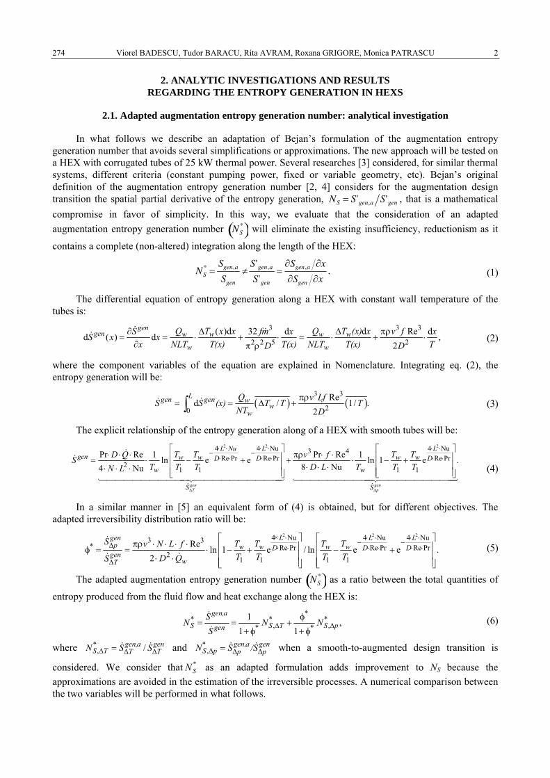
Viorel BADESCU, Tudor BARACU, Rita AVRAM, Roxana GRIGORE, Monica PATRASCU 2 274
2. ANALYTIC INVESTIGATIONS AND RESULTS REGARDING THE ENTROPY GENERATION IN HEXS
2.1. Adapted augmentation entropy generation number: analytical investigation
In what follows we describe an adaptation of Bejan’s formulation of the augmentation entropy generation number that avoids several simplifications or approximations. The new approach will be tested on a HEX with corrugated tubes of 25 kW thermal power. Several researches [3] considered, for similar thermal systems, different criteria (constant pumping power, fixed or variable geometry, etc). Bejan’s original definition of the augmentation entropy generation number [2, 4] considers for the augmentation design transition the spatial partial derivative of the entropy generation, NS = S'gen,a S'gen , that is a mathematical compromise in favor of simplicity. In this way, we evaluate that the consideration of an adapted augmentation entropy generation number NS
*( ) will eliminate the existing insufficiency, reductionism as it
contains a complete (non-altered) integration along the length of the HEX:
NS* =
Sgen,a
Sgen
≠S'gen,a
S'gen
=∂Sgen,a ∂x
∂Sgen ∂x. (1)
The differential equation of entropy generation along a HEX with constant wall temperature of the tubes is:
3 3 3
2 2 5 2( )d d32 d Re dd ( ) d ,
2Δ Δ∂ πρ
= = ⋅ + ⋅ = ⋅ + ⋅∂ π ρ
gengen w w w w
w w
Q T x x Q T (x) xS fm x v f xS x xx NLT T(x) T(x) NLT T(x) TD D
(2)
where the component variables of the equation are explained in Nomenclature. Integrating eq. (2), the entropy generation will be:
( ) ( )3 3
20
Red / 1/ .2
Lgen gen ww
w
Q v LfS S (x) T T TNT D
πρ= = Δ +∫ (3)
The explicit relationship of the entropy generation along of a HEX with smooth tubes will be: 2 2 24 4 Nu 4 Nu3 4
Re Pr Re Pr Re Pr2
1 1 1 1
Pr Re 1 Pr Re 1ln e e ln 1 e .8 Nu4 Nu
gen genT p
L Nu L Lgen w w w wD D D
w w
S S
T T T TD Q v fST T T D L T T TN L
Δ Δ
⋅ ⋅ ⋅ ⋅ ⋅ ⋅− −
⋅ ⋅ ⋅ ⋅ ⋅ ⋅⎡ ⎤ ⎡ ⎤
⋅ ⋅ ⋅ πρ ⋅ ⋅⎢ ⎥ ⎢ ⎥= ⋅ − + + ⋅ − +⎢ ⎥ ⎢ ⎥⋅ ⋅ ⋅⋅ ⋅ ⋅ ⎢ ⎥ ⎢ ⎥⎣ ⎦ ⎣ ⎦
(4)
In a similar manner in [5] an equivalent form of (4) is obtained, but for different objectives. The adapted irreversibility distribution ratio will be:
2 2 24 Nu 4 Nu 4 Nu3 3* Re Pr Re Pr Re Pr
21 1 1 1
Re ln 1 e / ln e e .2
×L L Lgenp w w w wD D D
genwT
S T T T Tv N L fT T T TD QS
⋅ ⋅ ⋅ ⋅ ⋅− −Δ ⋅ ⋅ ⋅ ⋅ ⋅ ⋅
Δ
⎡ ⎤ ⎡ ⎤πρ ⋅ ⋅ ⋅ ⋅ ⎢ ⎥ ⎢ ⎥φ = = ⋅ − + − +
⎢ ⎥ ⎢ ⎥⋅ ⋅ ⎢ ⎥ ⎢ ⎥⎣ ⎦ ⎣ ⎦
(5)
The adapted augmentation entropy generation number NS*( ) as a ratio between the total quantities of
entropy produced from the fluid flow and heat exchange along the HEX is: *
* * *, ,* *
1 ,1 1
Δ Δφ
= = ++ φ + φ
gen,a
S S T S pgenSN N NS
(6)
where *, Δ Δ/Δ = gen,a gen
S T T TN S S and ,Δ Δ Δ= gen,a gen*S p p pN S /S when a smooth-to-augmented design transition is
considered. We consider that *SN as an adapted formulation adds improvement to NS because the
approximations are avoided in the estimation of the irreversible processes. A numerical comparison between the two variables will be performed in what follows.

3 On the design and optimization of constructal networks of heat exchangers 275
2.2. Adapted augmentation entropy generation number: numerical evaluation
In this section we surveyed the efficiency of a HEX with corrugated tubes and we identified the better augmentation solution. Thus, we used the aforementioned analytical advancements and we performed a comparison between Bejan’s original formulation and an adapted formulation of the augmentation entropy generation number. Figure 2 illustrates the effect of the augmentation techniques from two perspectives: Bejan’s original formulation and the adapted Bejan formulation. A sensible difference of the results of the two formulations can be observed. At high Reynolds numbers of the flow regime Bejan’s original formulation shows a slight increase of the NS number while the *
SN number appears relatively constant. It is also noticeable that Bejan’s original formulation of the entropy generation number tends to overestimate the irreversibility effect of the augmentation (corrugation), most probably due to its simplifications.
a) b)
Fig. 2 – Augmentation entropy generation number characterizing the design transition: a) Bejan’s original formulation; b) adapted formulation.
2.3. Optimization using the thermoeconomic approach
While the thermoeconomic optimization is focused on cost function, some connections with the entropy generation that is strictly linked to the thermal process can be made. The economic optimum will recommend different solutions than the second law optimum, yet a direct comparison between those independent criteria can be done in a common diagram and a balanced design can be obtained. In several works [7–11] various ways of performing cost optimization are described, and often the cost is related to exergy destruction [7, 8]. We developed the criteria of cost optimization of a heat exchanger with smooth tubes (the thermal power is 25 KW) by considering different periods of operation (1…10 years). The total cost function of the investment cost and operation cost is:
ρ δ PP τ ,inv op M S e e OTinvestment operation
C = C +C = c × × × S +c × × (7)
where OTτ is the operation time (of 1…10 years). The constraints of the process of flow and heat transfer are used. The thermoeconomic model of the HEX (Fig. 3) represents a field of design options that satisfy the phenomenological constraints of the process of flow and heat exchange.
Unlike the optimum of the thermal process, the optimum of cost acknowledges a relative status as the extremum point can widely vary with the unit costs afferent to the HEX. An economic scheme guarantees that the design is opportune in an economic environment and the second law optimization satisfies the preoccupation for conservation of useful energy. Both paths are complementary and recommend in most cases a balanced decision of design. We observed that the increase of period of operation coincides with the deviation of the point of optimum cost towards a higher entropy generation. At this stage the conditions for the implementation description of both optimization tools in a constructal network of heat exchangers can be prepared.
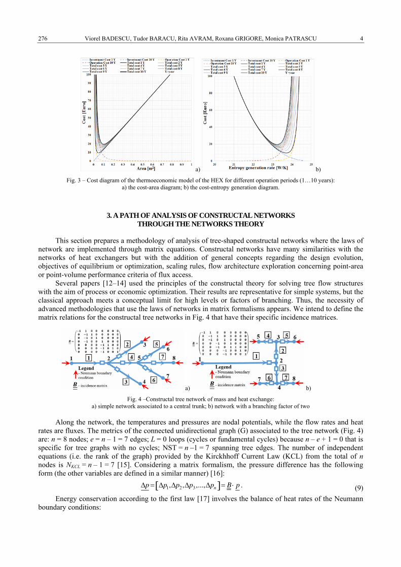
Viorel BADESCU, Tudor BARACU, Rita AVRAM, Roxana GRIGORE, Monica PATRASCU 4 276
a) b)
Fig. 3 – Cost diagram of the thermoeconomic model of the HEX for different operation periods (1…10 years): a) the cost-area diagram; b) the cost-entropy generation diagram.
3. A PATH OF ANALYSIS OF CONSTRUCTAL NETWORKS THROUGH THE NETWORKS THEORY
This section prepares a methodology of analysis of tree-shaped constructal networks where the laws of network are implemented through matrix equations. Constructal networks have many similarities with the networks of heat exchangers but with the addition of general concepts regarding the design evolution, objectives of equilibrium or optimization, scaling rules, flow architecture exploration concerning point-area or point-volume performance criteria of flux access.
Several papers [12–14] used the principles of the constructal theory for solving tree flow structures with the aim of process or economic optimization. Their results are representative for simple systems, but the classical approach meets a conceptual limit for high levels or factors of branching. Thus, the necessity of advanced methodologies that use the laws of networks in matrix formalisms appears. We intend to define the matrix relations for the constructal tree networks in Fig. 4 that have their specific incidence matrices.
a) b)
Fig. 4 –Constructal tree network of mass and heat exchange: a) simple network associated to a central trunk; b) network with a branching factor of two
Along the network, the temperatures and pressures are nodal potentials, while the flow rates and heat rates are fluxes. The metrics of the connected unidirectional graph (G) associated to the tree network (Fig. 4) are: n = 8 nodes; e = n – 1 = 7 edges; L = 0 loops (cycles or fundamental cycles) because n – e + 1 = 0 that is specific for tree graphs with no cycles; NST = n –1 = 7 spanning tree edges. The number of independent equations (i.e. the rank of the graph) provided by the Kirckhhoff Current Law (KCL) from the total of n nodes is NKCL = n – 1 = 7 [15]. Considering a matrix formalism, the pressure difference has the following form (the other variables are defined in a similar manner) [16]:
Δp = Δp1,Δp2,Δp3,...,Δpn[ ]= B ⋅ p . (9)Energy conservation according to the first law [17] involves the balance of heat rates of the Neumann
boundary conditions:

5 On the design and optimization of constructal networks of heat exchangers 277
0
d .d
N,outN,in
i N,in N,in N,out N,out i p N,in N,in p N,out N,out=0i in out i j k
E Q +W m h + m h = Q c m T +c m Tτ− − − −∑ ∑ ∑ ∑ ∑ ∑
(10)
According to the second law, the entropy generation [17] on the entire network will be:
0
d .d
igen,tot N,in N,in N,out N,out
ii in out=
QSS = m S + m S ³0τ T− −∑ ∑ ∑ (11)
The exergy balance of the system by considering the Neumann boundary conditions is:
0
0
dd
d 0.d
Q W D N,in in N,out outin out=0=
0 0 0i D N,in N,out
i N,in N,outi j k=
e E + E + E m e + m e =τ
T T Te= Q 1- + E Q 1 + Q 1 =τ T T T
− −
⎛ ⎞ ⎛ ⎞⎛ ⎞− − − −⎜ ⎟ ⎜ ⎟⎜ ⎟ ⎜ ⎟ ⎜ ⎟⎝ ⎠ ⎝ ⎠ ⎝ ⎠
∑ ∑
∑ ∑ ∑ (12)
When the system is determined after considering the previous equations, strategies of optimization can be applied, regarding the entropy generation, cost, flow path, flow resistance, surface-to-point or volume-to-point resistance [18], etc. Sensitivity analysis and inverse boundary value problems can be also explored in specific conditions. The process optimization will consist in minimizing the total entropy generation:
1 11Re Re ; minimum.gen gen,i gen n n nS = S = S ( ... D ...D ; A ...A ) =∑ (13)
At the same time, the thermoeconomic optimization of the network will involve the minimization of the cost function of economic operation:
1 1Re Re minimum.tot tot n 1 n nC = C ( ... ;D ...D ; A ...A ) = (14)
We presented a methodology of analysis for tree-shaped constructal networks that can be further developed for complex cases. Its advantage consists in compactness of the algorithm and it is applicable for networks with multiple nodes and branches.
4. CONCLUSIONS
In this paper we defined new methodologies of performance evaluation and optimization of heat exchangers (HEX) by considering entropy generation minimization and thermoeconomics. We illustrated the method of implementation for such objectives in constructal networks using matrix equations.
We used the analytic solution of integration of the entropy generation on the domain of a HEX to define the adapted augmentation entropy generation number ( *
SN ). This approach does not fundamentally change the original augmentation entropy generation number (NS) defined by Bejan, yet it offers the possibility of exact evaluation of the impact of augmentation techniques. A comparison of the two suggested a difference of evaluation that ranges between 7% and up to 55% when the level of corrugation of the surface of the tubes is ample. Bejan’s original formulation still remains more practical due to its simplicity, but we recommend the adapted formulation for important design objectives. We identified the most efficient design for different sizes of augmentation of the corrugated tubes and the different recommendations justify the necessity of using the adapted formulation as an alternative to the original one.
The thermoeconomic analysis of HEXs offers different perspectives regarding the interpretation of efficiency, as the quantified thermal processes are combined with cost objectives. A comparison of the cost function versus entropy generation suggests that the increase of operation period corresponds to the deviation of the position of the optimum point towards higher entropy generation of the process associated to a higher irreversibility. The second law and thermoeconomic optimizations offer the instrumental conditions to approach the objectives of a constructal network. We obtained meaningful matrix relations associated to the hydraulic and thermal phenomena in order to model and solve the contructal tree networks. Through this holistic and compact

Viorel BADESCU, Tudor BARACU, Rita AVRAM, Roxana GRIGORE, Monica PATRASCU 6 278
methodology we provided a full determination of the system. Furthermore, the methodology allows for advanced objectives of optimization, sensitivity analysis or inverse problems to be pursued.
The main advantage of this approach is the level of generalization that allows an overall description of the evolution of the system. It opens possibilities to multidisciplinary surveys and further developments.
Nomenclature
Q – heat rate e – exergy (corrugation) height N – no. of tubes; no. of nodes δ – wall thickness
S – entropy generation rate E – exergy, number of edges Nu – Nusselt number D – (exergy) destruction m – mass flow rate f – fanning factor Re – Reynolds number e – electrical
B – incidence matrix L – length T – temperature w – wall
c – unit cost p – (corrugation) pitch; pressure W – mechanical power gen, generation C – total cost Pr – Prandtl number φ – irrev. distribution ratio tot, total D – diameter PP – pumping power ρ – density s – steel
REFERENCES
1. A., BEJAN, General criterion for rating heat-exchanger performance, Journal of Heat and Mass Tranfer, 21, 5, pp. 655–658, 1978. 2. A., BEJAN, Entropy Generation Through Heat and Fluid Flow, John Wiley & Sons, New York, 1982. 3. V., ZIMPAROV, Enhancement of heat transfer by a combination of three-start spirally corrugated tubes with a twisted tape,
International Journal of Heat and Mass Transfer, 44, pp. 551–574, 2001. 4. A., BEJAN, Advanced Engineering Thermodynamics, 3rd Ed., John Wiley & Sons, New York, 2006. 5. A.Z., SAHIN, Entropy generation in turbulent liquid flow through a smooth duct subjected to constant wall temperature, International
Journal of Heat and Mass Transfer, 43, pp. 1469–1478, 2000. 6. T.S., RAVIGURURAJAN, General correlations for pressure drop and heat transfer for single-phase turbulent flows in ribbed tubes,
PhD Thesis, Iowa State University, 1986. 7. A., BEJAN, G., TSATSARONIS, M., MORAN, Thermal Design and Optimization, John Wiley&Sons, 1996. 8. W., FRATZSCHER, Exergy and possible applications, Rev. Gen. Therm. (Paris), 36, pp. 690–696, 1997. 9. T., SAJIN, Thermoeconomics (in Romanian), Alma Mater, Bacau, Romania, 2002. 10. R.E., AVRAM, T., BARACU, E., SCIUBBA, E., MAMUT, Thermoeconomic Analysis of the Environmental Impact of Condensing
Boilers, MEET MARIND, Varna, 2002. 11. T., BARACU, Optimization of the heat exchangers with corrugated tubes (in Romanian), MSc Thesis, “Ovidius” University of
Constanta, Romania, 2002. 12. A., BEJAN, V., BADESCU, A., DE VOS, Constructal theory of economics structure generation in space and time, Energy
Conversion and Management, 41, 13, pp. 1429–1451, 2000. 13. A., BEJAN, V., BADESCU, A., VOS DE, Constructal theory of economics, Energy Conversion and Management, 41, 13,
pp. 1429–1451, 2000. 14. V. D., ZIMPAROV, A.K., DA SILVA, A., BEJAN, Thermodynamic optimization of tree-shaped flow geometries with constant
channel wall temperature, International Journal of Heat and Mass Transfer, 49, 25–26, pp. 4839–4849, 2006. 15. T., BARACU, S., COSTINAS, C., GHIAUS, A., BADEA, R., AVRAM, F., VLADULESCU, D., JUGRAVESCU, New analytical
methodologies for radiative heat transfer in enclosures based on matrix formalism and network analogy, Applied Thermal Engineering, 107, pp. 1269–1286, 2016.
16. V., BADESCU, T., BARACU, R., AVRAM, R., GRIGORE, M., PATRASCU, On the design and optimization of constructal networks of heat exchangers by considering entropy generation minimization and thermoeconomics, Proceedings of the Constructal Law & Second Law Conference (CLC 2017), 15-16 May, 2017, Bucharest (Romania), Edit. Academiei Române, pp. 539–547.
17. A., BEJAN, The Method of Entropy Generation Minimization, Energy and the Environment, 1999, pp. 11–22. 18. A., BEJAN, Constructal design: Optimal flow-system geometry deduced from thermodynamic optimization and constraints,
Termotehnica, 2, 2001.

THE PUBLISHING HOUSE PROCEEDINGS OF THE ROMANIAN ACADEMY, Series A, OF THE ROMANIAN ACADEMY Special Issue/2018, pp. 279–284
CONSTRUCTAL DESIGN OF A NON-INVASIVE TEMPERATURE BASED MASS FLOW RATE SENSOR FOR ALGAE PHOTOBIOREACTORS
Kassiana RIBEIRO1,2, Juan C. ORDONEZ1,2, José V.C. VARGAS1,2, and André B. MARIANO2
1 Florida State University, Department of Mechanical Engineering, Energy and Sustainability Center and Center for Advanced Power Systems, Tallahassee, Florida, 32310, USA
2 Federal University of Paraná, Sustainable Energy Research and Development Center (NPDEAS), Curitiba, Brazil Corresponding author: Juan ORDONEZ, E-mail: [email protected]
Abstract. Microalgae are among the best-established life forms on earth and have been identified as likely sources of biofuels [1]. Controlled cultivation of microalgae in photobioreactors, PBR, requires the ability of monitoring and sensing key process variables (e.g., CO2 levels, mass flow rates, irradiance). The current work is aimed at improving the use of compact transparent pipes photobioreactors for continuous microalgae growth through the development of a non-invasive mass flow rate sensor that can be used as an alternative to more expensive commercially available ones. The paper presents a Volume Element Model (VEM) for a temperature based mass flow rate sensor, that combines principles of thermodynamics, heat transfer, and fluid mechanics and discretizes the system in space, resulting in a system of ordinary differential equations with respect to time that allows for the exploration of design parameters following a constructal approach. A sensor total volume constraint is identified, and the sensor shape is optimized for minimum entropy generation, which results in maximum temperature difference measurements, which are proportional to pipe mass flow rate, thus increasing sensitivity and reducing cost. Sharp maxima were obtained for the sensor flow temperature difference, depicting a 97% variation for ΔT in the range 0.01 ≤ R1/R4 ≤ 0.3, for
10 W=genQ and 10.1 kg s−=m . The results illustrate how following a constructal design approach,
it is possible to tune the system resistances to heat transfer in order to achieve a functional design.
Key words: Second Law of Thermodynamics, Constructal Design, Flow sensor, Shape optimization.
1. INTRODUCTION
Batch cultivation is a typical form of chemical reactors operation that is used to grow microalgae in large scale compact tubular photobioreactors [1–3], such as the type shown in Fig. 1. An alternative to this mode of operation is a continuous cultivation, in which the photobioreactor continues to operate with the highest cell concentration for a longer time. In this system dilution and biomass harvesting are done in a continuous way, therefore integrated mass flow and concentration sensors are needed to properly
monitor the process. An extensive review of microalgae growth kinetics mathematical models was recently conducted [4]. The study pointed out the need for the development of non-invasive sensors [5–7] in order to avoid cultivation disturbances, and therefore imprecisions in the determination of required model constants. The present study establishes two objectives to address this need: i) to propose a new non-invasive thermal mass flow rate sensor design, and ii) to introduce a dynamic mathematical model for the proposed sensor in order to produce a system constructal design [8] based on the entropy generation minimization method. To achieve that, the model is based on the physical laws, i.e., mass and energy conservation principles, so that reliability is assured for possible future use in design, control and optimization of photobioreactors or any other system.
Fig. 1 – Left: compact tubular photobioreactor at Federal
University of Parana, Curitiba, Brazil, and right: branching used for the proposed mass flow rate sensor.

K. RIBEIRO, J.C. ORDONEZ, J.V.C. VARGAS, A. MARIANO 2 280
2. MATHEMATICAL MODEL
In order to reduce the flow rate going through the sensor, the configuration illustrated in Fig. 1 (right) is proposed. Accordingly, the main photobioreactor pipe is branched into a section of reduced diameter to which the heating element is attached, the rotameter is used only to calibrate the sensor. With this configuration, the relationship between the flow rate in the main pipe and the mass flow rate going through the heater derivation pipe is dictated by the difference in flow resistance in branches 1 and 2, and is obtained from the solution of the simple flow network. Using mass conservation, ṁ = ṁ1 + ṁ2, where ṁ, ṁ1 and ṁ2 are the mass flow rates in the main pipe, branch 1, and branch 2, respectively, kg s-1, and ensuring that the pressure drop (due to major and minor losses) along branches 1 and 2 must be equal, therefore
K1
2+2 f1
L1
D1
ρ ,
K1 = KT (bf ),1 + Ksc + Kval ,1 + K90,1 + K90,2 + Kval ,2 + Kse + KT (bf ),2 , (1)
K 2 = KT ( tf ),1 + KT ( tf ),2 ,
where ρ is the fluid density; L1 and L2 the total length of branches 1 and 2 ducts, respectively; D1 and D2 the hydraulic diameters in branches 1 and 2 respectively; K1 the sum of the minor loss coefficients in branch 1 due to the two tees (branching flow), a sudden contraction, two valves, two 90-degree turns and a sudden expansion, as it is shown in Table 1.
K2 is the sum of minor loss coefficients in branch 2: two tees (through flow). In eq. (1) f1 and f2 are the Fanning friction factors, which are obtained [9] as f =16 /ReDk
for ReDk< 2,300 and
f = 0.079 ReDk
−1/ 4 for ReDk> 2,300 (k = 1, 2),
where ReDk= VkDk
ν is the Reynolds number,
=ρ
kk
c,k
mVA
is the fluid velocity [ms-1]; ν – the
fluid kinematic viscosity branch k pipe, and Ac,k – the cross sectional area of the branch k pipe [m2].
To calculate the sensor temperature differential it is necessary to compute the temperature distribution in the sensor branch (branch 1). For that, a Volume Element Model (VEM) [11, 12] is developed. The solution
domain is discretized in small Volume Elements (VE) in the z direction as illustrated in Fig. 2. Each VE is comprised by 3 systems: S1 – algae/water (medium); S2 – pipe wall, and S3 – heater. The first law of thermodynamics is applied to each system in the VE. Constitutive and heat transfer equations are used to evaluate the physical properties and heat transfer rates between the VE, respectively. A similar approach has been employed previously in the modelling and optimization of energy systems engineering (e.g. [11–14]).
2.1. System 1 (algae/water medium)
The first law of thermodynamics applied to the S1 in VE i shown in Fig. 2 states that:
( ) ( ) ( )111 1 12 1 1 1 1 12 2 112
d ,d
− − −i
ii i i i i i i i icv cv
Tm c = Q +Q ; Q = m c T T ; Q = UA T Tt
(3)
in which superscript i refers to VE i, for 1 ≤ i ≤ n , with n being the total number of VE that discretizes the
Fig. 2 – Top: schematic representation of the sensor cross sectional,
and bottom: volume elements and systems within the VE.

3 Constructal design of a non-invasive temperature based mass flow rate sensor for algae photobioreactors 281
sensor as shown in Fig. 2 (bottom); [ ]WQ is the heat transfer rate; m ji = ρV( )j
i [kg] – the mass of the
material (medium, pipe, or heater) within Sj (j = 1, 2 or 3, as shown in Fig. 2) in VE i; ρ [kg m-3] – the density; V [m3] – the volume; T [K] – the temperature; t [s] – the time, and c [J kg-1 K-1] – the specific heat.
Table 1
Loss coefficients expressions and values used in the simulation [10]
Component Loss coefficient
Sudden expansion; Sudden contraction; Tee (branching flow) Kse = 1−
D2
D1
⎛
⎝ ⎜
⎞
⎠ ⎟
2⎧ ⎨ ⎪
⎩ ⎪
⎫ ⎬ ⎪
⎭ ⎪
2
; Ksc =
0.5 1− D2
D1
⎛
⎝ ⎜
⎞
⎠ ⎟
2⎧ ⎨ ⎪
⎩ ⎪
⎫ ⎬ ⎪
⎭ ⎪
D2
D1
⎛
⎝ ⎜
⎞
⎠ ⎟
4; KT (bf ),1 = KT (bf ),2 = 1.62
Tee (through flow); Ball valve; 90o elbow
KT (tf ),1 = KT (tf ),2 = 0.54 ; K val ,1 = K val ,2 = 9.2 ; K 90,1 = K 90,2 = 0.8
The thermal conductance and the Nusselt number correlations for both laminar and transient regimes [9, 10] are calculated by
(UA)12i =
lnR1 + R2
2R1
⎛
⎝ ⎜
⎞
⎠ ⎟
2πk2Δz i+ 1
2πR1Δz ih
⎧
⎨ ⎪ ⎪
⎩ ⎪ ⎪
⎫
⎬ ⎪ ⎪
⎭ ⎪ ⎪
−1
, ReD1
< 2,300 : NuD1= 4.36 (uniform heat flux)
ReD1> 2,300 : NuD1
=( f1 /2)(ReD1
−1000) Pr
1+12.7( f1 /2)1/ 2(Pr2 / 3−1)
⎧
⎨ ⎪
⎩ ⎪
, (4)
where U is the overall heat transfer coefficient; A [m2] is the heat transfer area; R [m] is the system radius as shown in Fig. 2; k is [W m-1 K-1] the thermal conductivity; Δz i [m] is the VE i length; ReD1
> 2,300
(turbulent regime), the Gnielinski correlation is valid for 0.5 Pr 2,000≤ ≤ , and Re D1≤ 5 ×10 6 , and Pr is the
fluid Prandtl number. For the aqueous microalgae medium in this work, Pr ≅ 7 . The convective heat transfer coefficient, h, is then calculated via h = k1 NuD1
/D1.
2.2. System 2 (pipe)
12
22 2 23 2 2
d ;d
ii i i i i
,c,in ,c,outTm c = Q +Q +Q Qt
− −
12 2 2 2
2 1
12 2 2 2
2
,Δ Δ 2
.Δ Δ 2
i i-c,i
,c,in i i
i i+c,i
,c,out i i+1
k A (T T )Q =
( z + z )/
k A (T T )Q =
( z + z )/
−
⎧ −−⎪
⎪⎨
−⎪−⎪
⎩
(5)
Equation (5) relies upon the first law of thermodynamics applied S2, so that the second system represents the pipe walls, in which m2
i is the medium mass within S2 in VE i [kg]; the subscripts c, in and out indicate conduction heat transfer, inlet and outlet, respectively. Equation (5) also accounts for the convective heat transfer rate absorbed by the algae stream,
12
iQ , and the conduction heat transfer rate through
the pipe walls between VE i and its two neighbors, 2i,c,inQ and 2
i,c,outQ . Note that when i =1 and n,
2 0=1,c,inQ and 2 0n
,c,outQ = , respectively, assuming the negligible heat leak rate to the ambient in the axial direction at the sensor left and right sides. The conduction heat transfer rate between S2 and S3 is calculated by 23 23 2 1(UA) ( )= −i i i iQ T T with (UA)23
i ={ln(2R2/(R1+R2)) / ( 2πk2Δz i ) + ln (( R2 + R3)/ ( 2R2))/( 2πk3Δz i )}-1.

K. RIBEIRO, J.C. ORDONEZ, J.V.C. VARGAS, A. MARIANO 4 282
2.2.3. System 3 (heater)
For the heater system, the first law requires that:
3 3 23 3 3d ,d
ii i i i i i3
gen ,c,in ,c,outTm c = Q +Q +Q Q Qt ∞− − − , (8)
where the conduction heat transfer rates 3 3andi i,c,in ,c,outQ Q for the heater are calculated similarly to what was
done for system 2; igenQ is the heat rate generated by the heater, so that taking h∞ [W m-2 K-1] as the
convection heat transfer coefficient between the insulation external surface and the environment; i3 3(UA) ( )i i iQ T T∞ ∞ ∞= − is the heat leak rate through the insulation to the ambient; (UA)3∞
i = {ln(R4/R3)⋅(2πkinsΔzi)-1+ +ln(2R3/(R2+R3))⋅(2πk3Δzi)-1 +(2πR4Δzi h∞)-1}-1; h∞ [W m-2 K-1] is the convection heat transfer coefficient between the insulation external surface and the environment, and subscripts ins and 3∞ for the insulation, and the interaction between system 3 and the ambient, respectively.
2.3. Physical properties
The thermo-physical properties of the algae/water were evaluated at atmospheric pressure (101,325 Pa) and 20oC, the dimensions and additional physical properties used in a base case simulation are (c1, c2, c3) = = (4180, 385, 450) J kg-1 K-1; (k1, k2, k3, kins) = (0.591, 401, 11.3, 1) W m-1 K-1; (D2, L1, L2) = (0.0508, 0.3, 1) m; (R1, R2, R3, R4) = (0.0067, 0.00795, 0.0125, 0.0245) m; h∞ = 5 W m-2 K-1; ṁ = 0.1 kg s–1 , genQ = 10 W, Tin = T∞ = 293.15 K, (ρ = ρ1, ρ2, ρ3) = (1,000, 8,933, 8,400) kg m–3, and the initial conditions are
1,0 2,0 3,0 293.15 KT T T= = = .
3. THE CONSTRUCTAL DESIGN
One objective function is selected to evaluate the sensor system total entropy generation rate, genS , which should be minimized. Considering a control volume involving the sensor shown in Fig. 2, from the inlet to the outlet and limited by the insulation external surface, for an incompressible liquid, the second law of thermodynamics states that:
134
3 2 3i1 1 3i
3 3
2ln lnln 0; ; (UA) ,
(UA) 2 2
n i ii iout
gen ins 3 insi i iinins insi=1
RRR R RTQ QS = +m c ³ T = T
TT k z k z
−
∞ ∞
∞
⎧ ⎫⎛ ⎞ ⎛ ⎞⎪ ⎪⎜ ⎟ ⎜ ⎟+⎪ ⎪⎝ ⎠ ⎝ ⎠− ≥ + = +⎨ ⎬
π Δ π Δ⎪ ⎪⎪ ⎪⎩ ⎭
∑ (10)
where Tin = T11, Tout = T1
n , and Tinsi is the temperature at the insulation external surface in VE 1; the subscript
3ins refers to the thermal conductance between system 3 and the insulation external surface. The second objective function is the total sensor fluid temperature difference, which is evaluated with ΔT = T1
n −T11.
Since the sensor hardware, i.e., pipe, heater and insulation, shown in branch 1 of Fig.1, are commodities in short supply, it makes sense to recognize the total sensor volume as a physical constraint for the optimization problem. For a fixed length L1, and circular cross section, the sensor total volume constraint is represented by a fixed outer radius, R4, as it is defined in Fig. 5, so that R1 + tp + th + tins = R4 .
There are 3 geometric parameters to optimize, and the fourth results from them. Therefore, assuming fixed pipe and heater thicknesses, tp = 0.00125 m and th = 0.00455 m, as additional constraints, the optimization problem is reduced to find the optimal pipe inner radius, R1,opt, that maximizes ΔT and minimizes Ṡgen, and the optimal insulation thickness, tins,opt, that results from R1,opt.

5 Constructal design of a non-invasive temperature based mass flow rate sensor for algae photobioreactors 283
4. RESULTS AND DISCUSSION
Figure 5 illustrates the system temperature transient response toward steady state in the last volume element. The time to reach steady state is approximately 1 hour. The sensor temperature distribution at steady state is shown in Fig. 6. Both figures are for for 10 W=genQ and ṁ = 0.1 kgs–1.
Fig. 5 – The temperature transient evolution in VE n (z = 0.2925m). Fig. 6 – The steady state temperature distribution.
The pipe and heater systems are almost in thermal equilibrium, the fluid at a lower temperature, and the insulation external surface at a significantly lower temperature as expected. All temperatures increase as z increases as the fluid accumulates heat that is driven from the heater. This effect creates the temperature differential that is proportional to the pipe mass flow rate, i.e., the ultimate sensor measurement. Note that, in spite of the low heat input rate, the sensor design herein proposed is capable of producing an easily measurable ΔT . Next, the study proceeds in pursuit of the sensor constructal design. For that, the optimization procedure described in section 3 is conducted. The existence of an optimal pipe inner radius to outer insulation radius, R1 / R4( )opt
, is physically explained by analyzing two extremes: i) when R1 / R4 → 0 , 1 0→m , and the heat generated by the heater is uniformly distributed in the sensor by conduction, so that ΔT → 0, and ii) when R1 / R4 is large, 1m increases so that for fixed genQ , ΔT → 0 as well. Hence, there must be an intermediate and optimal value for R1 / R4 so that ΔT is maximum. Such system tradeoffs apply similarly to the system total entropy generation rate. Fig. 7 shows the optimization results. Even for such low heater power input, a sharp maximum is found with respect to R1 / R4 , depicting ΔTmax = 27.5 K for R1 / R4( )opt
= 0.071. Regarding the entropy generation rate, it is
found that R1 / R4( )opt= 0.1 with -1
,min = 0.022 W KgenS and ΔT =18.2 K whereas for R1 / R4 = 0.071, -1= 0.0245 W KgenS and ΔTmax = 27.5 K , i.e., approximately a 10% and 50% increase in genS and ΔT ,
respectively. Fig. 8 demonstrates the robustness of the optima with respect to the variation of genQ .
Fig. 7 – The maximization of ΔT and minimization of genS
for
10 W=genQ and -10.1 kg sm = .
Fig. 8 – The variation of genQ on the maximization of ΔT
and minimization of genS for -1= 0.1 kg sm .

K. RIBEIRO, J.C. ORDONEZ, J.V.C. VARGAS, A. MARIANO 6 284
5. CONCLUSIONS
A novel constant current noninvasive thermal mass flow rate sensor has been proposed. The temperature measurement based sensor is placed in a derivation branch of the main pipe, where only a small fraction of the flow is routed. The temperature difference across the sensor is later correlated to the total mass flow rate. A mathematical model was also developed for sizing and thermodynamically optimizing the sensor for maximum flow temperature difference and minimum entropy generation, therefore finding the sensor constructal design. Sharp maxima were obtained for the sensor flow temperature difference, depicting a 97% variation for ΔT in the range 0.01 ≤ R1 / R4 ≤ 0.3, for = 10 WgenQ and 1= 0.1 kg sm − . This aspect stresses the importance of finding the sensor constructal design so that high performance is obtained.
ACKNOWLEDGEMENTS
The authors acknowledge support ONR grant N00014-16-1-2956, CNPq, Brazil, projects 407198/2013-0, 403560/2013-6, 407204/2013-0, and 302938/2015-0; contracts 41-2013/UFPR/PSA, and 111-2014/UFPR/NILKO Tecnologia Ltd.
REFERENCES
1. SATYANARAYANA, K.G., MARIANO, A.B., VARGAS, J.V.C., A review on microalgae, a versatile source for sustainable energy and materials, International Journal of Energy Research, 35, pp. 291–311, 2011.
2. VARGAS, J.V.C., BALMANT, W., STALL, A., MARIANO, A.B., ORDONEZ, J.C., HOVSAPIAN, R., DILAY, E., Patent Number US2012088296-A1 and WO2012050608-A1 – US Patent and Trademark Office, 2012.
3. VARGAS, J.V.C., MARIANO, A.B., CORRÊA, DO., ORDONEZ, J. C., The microalgae derived hydrogen process in compact photobioreactors, International Journal of Hydrogen Energy, 39, pp. 9588–9598, 2014.
4. LEE, E., JALALIZADEH, M., ZHANG, Q., Growth kinetic models for microalgae cultivation: A review, Algal Research, 12, pp. 497–512, 2015.
5. DIGIACOMO, R., Review of industrial processing flowmeters, White paper, ABB Flowmeters, ABB Measurement Products, 2012. 6. WILSON, J.S., Sensor Technology Handbook (Chapter 10), Elsevier, Saint Louis, US, 2004. 7. FINGERSON, L.M., Thermal anemometry, current state, and future directions, Rev. Sci. Instrum., 65, 2, pp. 285–300, 1994. 8. BEJAN, A., Shape and Structure, from Engineering to Nature, Cambridge University Press, 2000. 9. INCROPERA, F.P., DEWITT, D.P., BERGMAN, T.L., LAVINE, A.S., Fundamentals of Heat and Mass Transfer, 6th ed., Wiley,
2007. 10. SHAMES, I. H., Mechanics of Fluids, London, McGraw-Hill, 2003. 11. VARGAS, J.V.C., STANESCU, G., FLOREA, R., CAMPOS, M.C., A numerical model to predict the thermal and psychrometric
response of electronic packages, ASME Journal of Electronic Packaging, 123, 3, pp. 200–210, 2001. 12. DILAY, E., VARGAS, J.V.C., SOUZA, J.A., ORDONEZ, J.C., YANG, S., MARIANO, A.B., A volume element model (VEM)
for energy systems engineering, Int. J. Energy Res., 39, pp. 46–74, 2015. 13. ORDONEZ, J.C., VARGAS, J.V.C., HOVSAPIAN, R., Modeling and simulation of the thermal and psychrometric transient
response of all-electric ships, internal compartments and cabinets, Simulation, 84, 8–9, pp. 427–439, 2008. 14. ORDONEZ, J.C., SOUZA, J.A., SHAH, D.R., VARGAS, J.V.C., HOVSAPIAN, R., Temperature and pressure drop model for
gaseous helium cooled superconducting DC cables, IEEE Transactions on Applied Superconductivity, 23, 3, pp. 5402005, 2013, doi:10.1109/TASC.2013.2241380.

THE PUBLISHING HOUSE PROCEEDINGS OF THE ROMANIAN ACADEMY, Series A, OF THE ROMANIAN ACADEMY Special Issue/2018, pp. 285–290
A REDUCED-ORDER METHANE-AIR COMBUSTION MECHANISM THAT SATISFIES THE DIFFERENTIAL ENTROPY INEQUALITY
Allen E. REAM, John C. SLATTERY, Paul G.A. CIZMAS
Texas A&M University, Department of Aerospace Engineering, College Station, Texas 77843–3141, USA
Corresponding author: Paul G.A. CIZMAS, E-mail: [email protected]
Abstract. This paper presents a new method for determining the Arrhenius parameters of a reduced chemical mechanism such that it satisfies the second law of thermodynamics. The strategy is to approximate the progress of each reaction in the reduced mechanism from the species production rates of a detailed mechanism by using a linear least squares method. A series of non-linear least squares curve fittings are then carried out to find the optimal Arrhenius parameters for each reaction. At this step, the molar rates of production are written such that they comply with a theorem that provides the sufficient conditions for satisfying the second law of thermodynamics. This methodology was used to modify the Arrhenius parameters for the Westbrook and Dryer two-step mechanism for methane combustion. The optimized mechanism showed good agreement with the detailed mechanism for species mole fractions and production rates of most major species. The optimized mechanisms produced no violations of the second law of thermodynamics.
Key words: Second law of thermodynamics, Methane combustion, Differential entropy inequality, Laminar flame, Chemically reacting flows.
1. INTRODUCTION
The differential entropy inequality, while not entirely unknown, is always ignored in simulating chemically reacting flows. In addition to satisfying the differential mass, momentum, and energy balances, simulations of chemically/biochemically reacting systems must satisfy the entropy inequality (the second law of thermodynamics). Common types of material behavior (Newton’s law of viscosity, Fourier’s law, Fick’s first law) satisfy the differential entropy inequality automatically, but common empirical descriptions of chemical/biochemical reactions do not.
To simulate methane flame combustion, or any reacting fluid flow, it is necessary to incorporate a reaction mechanism that describes the incremental steps and associated rates leading from reactant species to products. Detailed mechanisms include all possible species and elementary reactions so as to provide accurate solutions in a wide range of simulation conditions. Unfortunately, there is a large computational cost associated with the complexity of detailed mechanisms. Therefore, reduced mechanisms are created for specific conditions where simplifying assumptions can be made to decrease the complexity of detailed mechanisms. It has been shown, however, that common reduced mechanisms produce violations of the differential entropy inequality (DEI)
− tr T+ PI( )⋅ D[ ]+ 1
Tε ⋅∇T +cRT j n( )⋅
d n( )ρ n( )n =1
NS
∑ + μ n( )R n( ) r( )n =1
NS
∑r=1
Nr
∑ ≤ 0 , (1)
a local form of the second law of thermodynamics [1]. Here T is the stress tensor, P the thermodynamic pressure, I the identity tensor, D the rate of deformation tensor, c the total molar density, R the gas law constant, T the temperature, Ns the number of species, j(n) the mass flux of species n relative to ν, ρ(n) the mass density of species n, Nr the number of reactions, μ(n) the chemical potential for species n on a molar
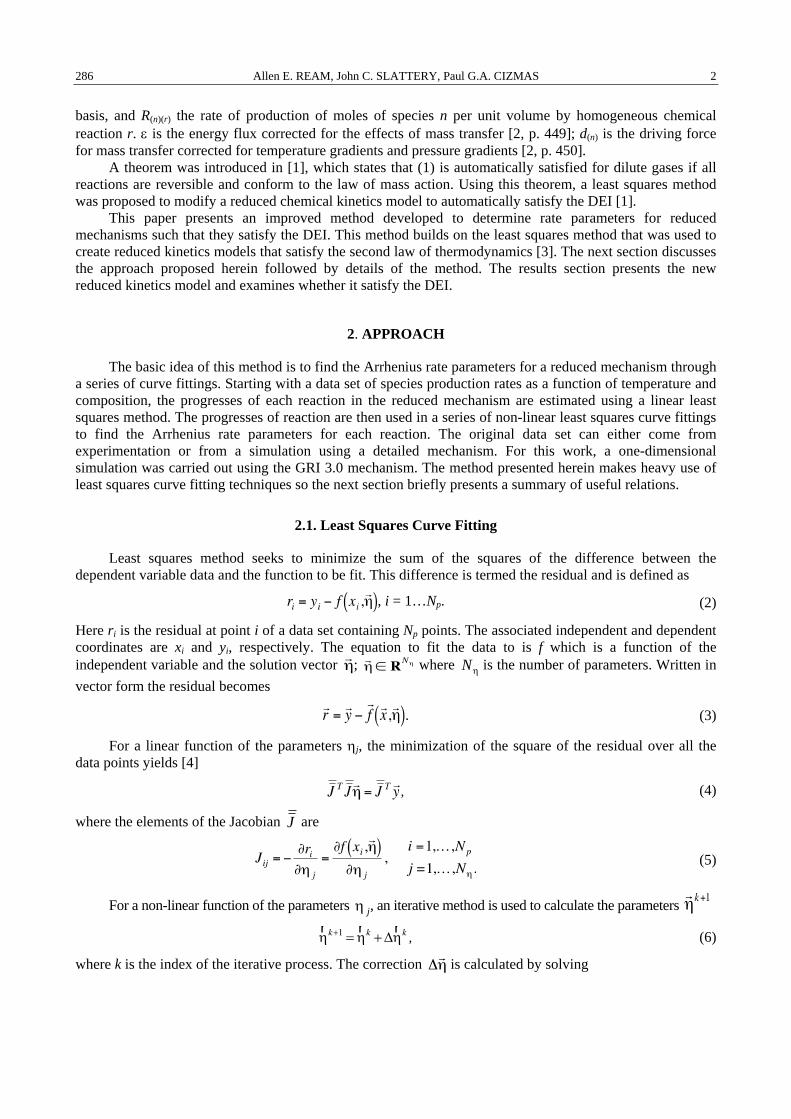
Allen E. REAM, John C. SLATTERY, Paul G.A. CIZMAS 2 286
basis, and R(n)(r) the rate of production of moles of species n per unit volume by homogeneous chemical reaction r. ε is the energy flux corrected for the effects of mass transfer [2, p. 449]; d(n) is the driving force for mass transfer corrected for temperature gradients and pressure gradients [2, p. 450].
A theorem was introduced in [1], which states that (1) is automatically satisfied for dilute gases if all reactions are reversible and conform to the law of mass action. Using this theorem, a least squares method was proposed to modify a reduced chemical kinetics model to automatically satisfy the DEI [1].
This paper presents an improved method developed to determine rate parameters for reduced mechanisms such that they satisfy the DEI. This method builds on the least squares method that was used to create reduced kinetics models that satisfy the second law of thermodynamics [3]. The next section discusses the approach proposed herein followed by details of the method. The results section presents the new reduced kinetics model and examines whether it satisfy the DEI.
2. APPROACH
The basic idea of this method is to find the Arrhenius rate parameters for a reduced mechanism through a series of curve fittings. Starting with a data set of species production rates as a function of temperature and composition, the progresses of each reaction in the reduced mechanism are estimated using a linear least squares method. The progresses of reaction are then used in a series of non-linear least squares curve fittings to find the Arrhenius rate parameters for each reaction. The original data set can either come from experimentation or from a simulation using a detailed mechanism. For this work, a one-dimensional simulation was carried out using the GRI 3.0 mechanism. The method presented herein makes heavy use of least squares curve fitting techniques so the next section briefly presents a summary of useful relations.
2.1. Least Squares Curve Fitting
Least squares method seeks to minimize the sum of the squares of the difference between the dependent variable data and the function to be fit. This difference is termed the residual and is defined as
, i = 1…Np. (2)
Here ri is the residual at point i of a data set containing Np points. The associated independent and dependent coordinates are xi and yi, respectively. The equation to fit the data to is f which is a function of the independent variable and the solution vector ; where Nη is the number of parameters. Written in vector form the residual becomes
. (3)
For a linear function of the parameters ηj, the minimization of the square of the residual over all the data points yields [4]
, (4)
where the elements of the Jacobian J are
(5)
For a non-linear function of the parameters η j, an iterative method is used to calculate the parameters
r η k+1 =
r η k + Δ
r η k , (6)
where k is the index of the iterative process. The correction is calculated by solving
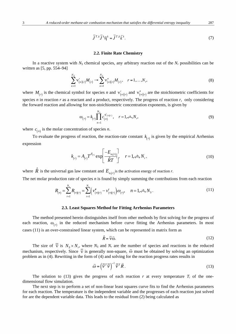
3 A reduced-order methane-air combustion mechanism that satisfies the differential entropy inequality 287
. (7)
2.2. Finite Rate Chemistry
In a reactive system with NS chemical species, any arbitrary reaction out of the Nr possibilities can be written as [5, pp. 554–94]
, (8)
where M r( ) is the chemical symbol for species n and and are the stoichiometric coefficients for
species n in reaction r as a reactant and a product, respectively. The progress of reaction r, only considering the forward reaction and allowing for non-stoichiometric concentration exponents, is given by
ω r( ) = k r( ) c n( )q' n( ) r( )
n =1
NS
∏ , r =1, ,Nr, (9)
where c n( ) is the molar concentration of species n.
To evaluate the progress of reaction, the reaction-rate constant k r( ) is given by the empirical Arrhenius
expression
k r( ) = A r( )Tβ r( ) exp
−Ea, r( )
R̂T
⎡
⎣⎢
⎤
⎦⎥, r =1, , Nr , (10)
where R̂ is the universal gas law constant and Ea, r( ) is the activation energy of reaction r.
The net molar production rate of species n is found by simply summing the contributions from each reaction
R n( ) = R n( ) r( )r=1
Nr
∑ = ′′ν n( ) r( ) − ′ν n( ) r( )( )ω r( )r=1
Nr
∑ , n =1, , NS . (11)
2.3. Least Squares Method for Fitting Arrhenius Parameters
The method presented herein distinguishes itself from other methods by first solving for the progress of each reaction, ω r( ) in the reduced mechanism before curve fitting the Arrhenius parameters. In most
cases (11) is an over-constrained linear system, which can be represented in matrix form as
. (12)
The size of ν is NS × Nr, where NS and Nr are the number of species and reactions in the reduced mechanism, respectively. Since ν is generally non-square, must be obtained by solving an optimization problem as in (4). Rewriting in the form of (4) and solving for the reaction progress rates results in
. (13)
The solution to (13) gives the progress of each reaction r at every temperature Ti of the one-dimensional flow simulation.
The next step is to perform a set of non-linear least squares curve fits to find the Arrhenius parameters for each reaction. The temperature is the independent variable and the progresses of each reaction just solved for are the dependent variable data. This leads to the residual from (2) being calculated as
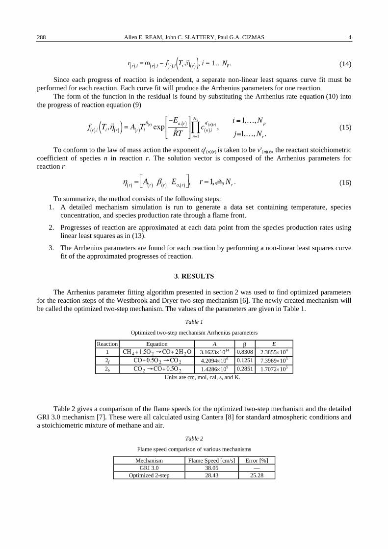
Allen E. REAM, John C. SLATTERY, Paul G.A. CIZMAS 4 288
, i = 1…Np. (14)
Since each progress of reaction is independent, a separate non-linear least squares curve fit must be performed for each reaction. Each curve fit will produce the Arrhenius parameters for one reaction.
The form of the function in the residual is found by substituting the Arrhenius rate equation (10) into the progress of reaction equation (9)
(15)
To conform to the law of mass action the exponent q'(n)(r) is taken to be v'(n)(r), the reactant stoichiometric coefficient of species n in reaction r. The solution vector is composed of the Arrhenius parameters for reaction r
η r( ) = A r( ) β r( ) Ea, r( )⎡⎣
⎤⎦, r =1, , Nr . (16)
To summarize, the method consists of the following steps: 1. A detailed mechanism simulation is run to generate a data set containing temperature, species
concentration, and species production rate through a flame front.
2. Progresses of reaction are approximated at each data point from the species production rates using linear least squares as in (13).
3. The Arrhenius parameters are found for each reaction by performing a non-linear least squares curve fit of the approximated progresses of reaction.
3. RESULTS
The Arrhenius parameter fitting algorithm presented in section 2 was used to find optimized parameters for the reaction steps of the Westbrook and Dryer two-step mechanism [6]. The newly created mechanism will be called the optimized two-step mechanism. The values of the parameters are given in Table 1.
Table 1
Optimized two-step mechanism Arrhenius parameters
Reaction Equation A β E 1 3.1623×10¹⁴ 0.8308 2.3855×10⁴ 2f 4.2094×10⁶ 0.1251 7.3969×10³ 2b 1.4286×10⁹ 0.2851 1.7072×10⁵
Units are cm, mol, cal, s, and K.
Table 2 gives a comparison of the flame speeds for the optimized two-step mechanism and the detailed GRI 3.0 mechanism [7]. These were all calculated using Cantera [8] for standard atmospheric conditions and a stoichiometric mixture of methane and air.
Table 2
Flame speed comparison of various mechanisms
Mechanism Flame Speed [cm/s] Error [%] GRI 3.0 38.05 —
Optimized 2-step 28.43 25.28
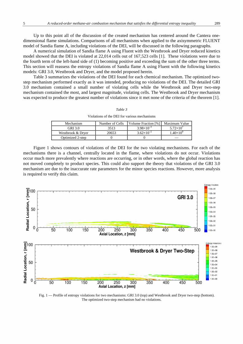
5 A reduced-order methane-air combustion mechanism that satisfies the differential entropy inequality 289
Up to this point all of the discussion of the created mechanism has centered around the Cantera one-dimensional flame simulations. Comparisons of all mechanisms when applied to the axisymmetric FLUENT model of Sandia flame A, including violations of the DEI, will be discussed in the following paragraphs.
A numerical simulation of Sandia flame A using Fluent with the Westbrook and Dryer reduced kinetics model showed that the DEI is violated at 22,014 cells out of 167,523 cells [1]. These violations were due to the fourth term of the left-hand side of (1) becoming positive and exceeding the sum of the other three terms. This section will reassess the entropy violations of Sandia flame A using Fluent with the following kinetics models: GRI 3.0, Westbrook and Dryer, and the model proposed herein.
Table 3 summarizes the violations of the DEI found for each chemical mechanism. The optimized two-step mechanism performed exactly as it was intended, producing no violations of the DEI. The detailed GRI 3.0 mechanism contained a small number of violating cells while the Westbrook and Dryer two-step mechanism contained the most, and largest magnitude, violating cells. The Westbrook and Dryer mechanism was expected to produce the greatest number of violations since it met none of the criteria of the theorem [1].
Table 3
Violations of the DEI for various mechanisms
Mechanism Number of Cells Volume Fraction [%] Maximum Value GRI 3.0 3513 3.98×10⁻³ 5.72×10⁷
Westbrook & Dryer 20653 3.62×10⁻² 1.40×10⁹ Optimized 2-step 0 0 —
Figure 1 shows contours of violations of the DEI for the two violating mechanisms. For each of the mechanisms there is a channel, centrally located in the flame, where violations do not occur. Violations occur much more prevalently where reactions are occurring, or in other words, where the global reaction has not moved completely to product species. This could also support the theory that violations of the GRI 3.0 mechanism are due to the inaccurate rate parameters for the minor species reactions. However, more analysis is required to verify this claim.
Fig. 1 — Profile of entropy violations for two mechanisms: GRI 3.0 (top) and Westbrook and Dryer two-step (bottom). The optimized two-step mechanism had no violations.
Allen E. REAM, John C. SLATTERY, Paul G.A. CIZMAS 6 290
4. CONCLUSIONS
A new method for determining the Arrhenius parameters of a reduced chemical mechanism was developed herein. This method seeks to find an optimal set of parameters for a specific operating condition. The basic strategy is to approximate the progress of each reaction in a reduced mechanism from the species production rates of a detailed mechanism. A series of non-linear least squares curve fittings are then carried out to find the optimal Arrhenius parameters for each reaction. This process was used to find parameters for the reaction steps of the Westbrook and Dryer two-step mechanism. The optimized mechanism showed good agreement with the detailed mechanism for species mole fractions and production rates of most major species. The optimized mechanisms produced no violations of the DEI.
ACKNOWLEDGEMENTS
The authors gratefully acknowledge the computational resources provided by the Texas A&M Supercomputing Facility.
REFERENCES
1. J.C. Slattery, P.G.A. Cizmas, A.N. Karpetis, S.B. Chambers, Role of Differential Entropy Inequality in Chemically Reacting Flows, Chemical Engineering Science, 66, pp. 5236–5243, 2011.
2. J.C. Slattery, Advanced Transport Phenomena, Cambridge University Press, 1999. 3. N.H. Jones, P.G.A. Cizmas, J.C. Slattery, Creating Reduced Kinetics Models that Satisfy the Entropy Inequality, Journal of
Engineering for Gas Turbines and Power, 137, 7, 2015. 4. A.E. Ream, Creating reduced order methane-air combustion mechanisms that satisfy the differential entropy inequality, Master’s
thesis, Texas A & M University, College Station, Texas, December 2015. 5. F.A. Williams, Combustion Theory, The Benjamin/Cummings Publishing Company, 1985. 6. C.K. Westbrook, F.L. Dryer, Simplified Reaction Mechanisms for the Oxidation of Hydrocarbon Fuels in Flames, Combustion
Science and Technology, 27, pp. 31–43, 1981. 7. G.P. Smith, D.M. Golden, M. Frenklach, B. Eiteener, M. Goldenberg, C.T. Bowman, R.K. Hanson, W.C. Gardiner, V.V. Lissianski,
Z.W. Qin, GRI-Mech 3.0, 2000. http://combustion.berkeley.edu/gri-mech/ 8. D. Goodwin, Cantera: An object-oriented software toolkit for chemical kinetics, thermodynamics, and transport processes, 2013,
http://www.cantera.org/docs/sphinx/html/index.html
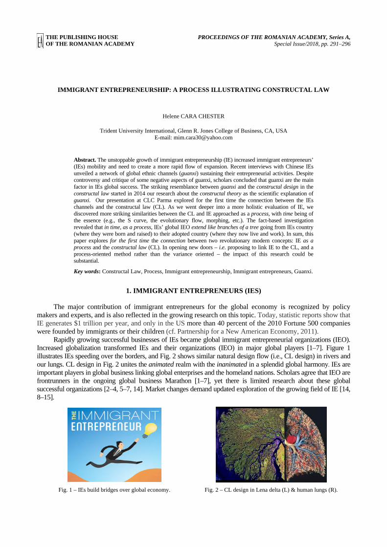
THE PUBLISHING HOUSE PROCEEDINGS OF THE ROMANIAN ACADEMY, Series A, OF THE ROMANIAN ACADEMY Special Issue/2018, pp. 291–296
IMMIGRANT ENTREPRENEURSHIP: A PROCESS ILLUSTRATING CONSTRUCTAL LAW
Helene CARA CHESTER
Trident University International, Glenn R. Jones College of Business, CA, USA E-mail: [email protected]
Abstract. The unstoppable growth of immigrant entrepreneurship (IE) increased immigrant entrepreneurs’ (IEs) mobility and need to create a more rapid flow of expansion. Recent interviews with Chinese IEs unveiled a network of global ethnic channels (guanxi) sustaining their entrepreneurial activities. Despite controversy and critique of some negative aspects of guanxi, scholars concluded that guanxi are the main factor in IEs global success. The striking resemblance between guanxi and the constructal design in the constructal law started in 2014 our research about the constructal theory as the scientific explanation of guanxi. Our presentation at CLC Parma explored for the first time the connection between the IEs channels and the constructal law (CL). As we went deeper into a more holistic evaluation of IE, we discovered more striking similarities between the CL and IE approached as a process, with time being of the essence (e.g., the S curve, the evolutionary flow, morphing, etc.). The fact-based investigation revealed that in time, as a process, IEs’ global IEO extend like branches of a tree going from IEs country (where they were born and raised) to their adopted country (where they now live and work). In sum, this paper explores for the first time the connection between two revolutionary modern concepts: IE as a process and the constructal law (CL). In opening new doors – i.e. proposing to link IE to the CL, and a process-oriented method rather than the variance oriented – the impact of this research could be substantial.
Key words: Constructal Law, Process, Immigrant entrepreneurship, Immigrant entrepreneurs, Guanxi.
1. IMMIGRANT ENTREPRENEURS (IES)
The major contribution of immigrant entrepreneurs for the global economy is recognized by policy makers and experts, and is also reflected in the growing research on this topic. Today, statistic reports show that IE generates $1 trillion per year, and only in the US more than 40 percent of the 2010 Fortune 500 companies were founded by immigrants or their children (cf. Partnership for a New American Economy, 2011).
Rapidly growing successful businesses of IEs became global immigrant entrepreneurial organizations (IEO). Increased globalization transformed IEs and their organizations (IEO) in major global players [1–7]. Figure 1 illustrates IEs speeding over the borders, and Fig. 2 shows similar natural design flow (i.e., CL design) in rivers and our lungs. CL design in Fig. 2 unites the animated realm with the inanimated in a splendid global harmony. IEs are important players in global business linking global enterprises and the homeland nations. Scholars agree that IEO are frontrunners in the ongoing global business Marathon [1–7], yet there is limited research about these global successful organizations [2–4, 5–7, 14]. Market changes demand updated exploration of the growing field of IE [14, 8–15].
Fig. 1 – IEs build bridges over global economy. Fig. 2 – CL design in Lena delta (L) & human lungs (R).

Helene CARA CHESTER 2 292
This study is focusing on a process-oriented research, explaining IE as a process rather than a one-time act of creativity (product, service, new concept). Thus, the paper brings a holistic view of the IE as a multi-level process, considering time as a salient factor influencing this process. This study also explains how IE illustrates the Constructal Law (CL) as a natural design phenomenon through a network of channels called guanxi.
2. GLOBAL FLOW OF GUANXI
Multiple interviews with successful Chinese IEs unveiled a network of global channels (guanxi) sustaining their entrepreneurial activities [3–4], [7–8]. Despite the critique of negative aspects of guanxi, scholars concluded that guanxi are the main factor in IEO’s rapid global success [1, 3, 5–7, 12–15]. Guanxi – an old Confucian concept preserved as a main philosophy in Chinese society – is functioning today in China as a personalized network of influence based on trust, friendship, loyalty, respect, and mutual favors [7, 8, 14].
Fig. 3 – Flow of GN illustrates CL design (Google CL). Fig. 4 – CL hierarchy design (Web guanxi).
The global collaboration of IE is represented by the guanxi network (GN), a top professional networking group for IE in Asian Pacific area, is producing spectacular events (Linkedin GN). The complexity and diversity of guanxi channels, their free morphing determined scholars to consider IE more of a process than a one-time act.
3. GUANXI & THE CONSTRUCTAL LAW (CL)
The striking resemblance between guanxi and the constructal design (Figs. 3, 4) started in 2014 our research about the CL as a scientific explanation of guanxi. The fact-based investigation revealed that guanxi are extending like branches of a tree going from immigrant entrepreneurs’ country (where IE were born and raised) to their adopted country (where IE now live and work). Today, guanxi are constantly morphing and expanding in new countries, where other IE – sharing the same culture and language – conduct business. The morphing flow of guanxi includes diverse people, from suppliers and distributors to bankers and partners. Although past research praised guanxi as unique marketing, provided no explanation of being based on a scientific concept [7–9, 14–15].
Our 2015 Parma presentation explained for the first time the connection between the guanxi network and the constructal law [14]. Increased interest of scientific community in the CL produced studies demonstrating that the flow of guanxi is real, that the process of IE is illustrating the CL evolutionary flow, and that the successful outcomes are based on science rather than on ingenuity [14, 17, 21, 25–27].
4. ENTREPRENEURIAL JOURNEY: IE AS A PROCESS
A new venture is the integration of information in the old system, by an individual or an organization [7–12]. Past research is rich in exploring the novelty of creation of new ventures, and the unique, exceptional qualities of entrepreneurs [3–9, 17], and what differentiate entrepreneurs from small business owners:

3 Immigrant entrepreneurship: a process illustrating Constructal Law 293
creativity, reject of status-quo, innovation, dealing with risk and uncertainty [2–7]. However, only a few recent studies started asking questions about what happens afterwards, when the startup develops quickly into a global organization, when a factor called time begins to play a salient role in the development of venture [8–10].
Our study explores the influence of time on IE, and demonstrates that entrepreneurship is a long, complex process rather than a one-time act [25]. In today’s shifting global economy, IE became a complex process, in a sequence of events, initially triggered by IEs desire for profit. In time, the desire for profit interacts with coming information, and based on presence of other factors (motive, means, and opportunity), a new idea emerges. Based on the same factors (motive, means, opportunity), the idea becomes a product, which product in turn, if conditions permit, can generate a positive cash flow [25]. Figure 5 illustrates IE as a process.
Fig. 5 – IE as a process: from desire for profit to goal, to idea, to product, to positive cash flow
(adapted from McMullen & Dimov 2013).
The sequence of events in IE process is important for IE’s process-oriented research--not only because it illustrates similar design as in the CL – but also because it is an essential element for a complete, holistic, systemic demonstration [25, 21–30]. Table1 summarizes this systemic process [25].
Table 1
IE – A horizontal systemic process supported by the CL
IE: Variance vs. Process, the latter supported by the
CL (IE as a process)
Variance-oriented: fixed in- time relationship between partitioned
variables
Process-oriented: the sequence of events in time brings a holistic view to IE
process
5. IE: A HORIZONTAL SYSTEMIC PROCESS
The process approach to entrepreneurship research may reveal predictable patterns and events that variance-oriented studies would otherwise miss. Few studies traced this journey from start to finish, making existing empirical research limited and merely dated [25, 36–37]. The IE multi-level process is a horizontal research unlike the vertically oriented variance research which is separating creativity from strategy [25]. In sum, our findings show an interdependent relationship between diverse, separate actions, which warrants further investigation, offering a framework for further empirical studies [25, 8, 21, 25, 31].
6. THE CONSTRUCTAL LAW (CL)
Constructal is a word coined by professor Adrian Bejan (1996), when he described that everything around us is a flow system [11], and all these “flow systems evolve over time, being connected to and shaped by other systems in a global tapestry of flow” [12]. Bejan’s CL is based on a fundamental principle of physics about the evolution of flow systems as they change their design over time to increase flow access (in the IE field this increasing flow translates in success, i.e. a positive outcome).
Bejan & Lorente (2011) claim that CL is about the fact that “design in nature is not static: it is dynamic, ever changing, like the images in a movie at the cinema. This is what design and evolution are in nature, and the constructal law captures them completely.” [44, p. 211]. The authors argue that branching tree-shaped flow patterns that govern the design of everything that moves in nature, animate or inanimate— “generate in time shapes that facilitate this movement” [12]. Examples of treelike architectural design are: plants and tree roots, leaves, river basins, our cardiovascular system, human lungs, the corporate structure,

Helene CARA CHESTER 4 294
politics, and lastly, the IE process. In sum, based on physics, the CL unites for the first time in oneness the animate with the inanimate realm [14–21, 23–24].
Fig. 6 – CL unites everything, L to R: the water circuit, deltas, animal movements (swim, run, fly),
machines, wind,trees (Bejan et al. 2008).
Recent scientific studies demonstrate that the CL governs the phenomena of design and evolution in many diverse areas: medicine, biology, social sciences, distribution of wealth [21], politics, architecture, sports, arts, economy, academics, business, technology, IE as a process [8-12, 14, 16–25].
7. THE ‘S’ CURVE
As our study progressed, aspects of the resemblance between the CL and IE reached a deeper level of investigation. The findings showed that EI illustrates diverse CL manifestations e.g. the “S” curve (Fig. 7).
Fig. 7 – The ‘S Curve’ demonstrates IE as a Process (Adapted from Mc Mullen & Dimov, 2013).
The curve shape design in the CL (Fig. 7) was clearly noticed and widely accepted by scientists in the evolutionary flow of IEO: slow and short at the start, then fast and long – invasion, followed finally by another slow and short in the end – consolidation [21, 23–25, 33–37]. Another aspect of similarity between CL & IE is the Golden Ratio design, evident in existing studies as form follows flow [26].
8. GOLDEN RATIO & HIERARCHY
GR is an old concept that unites arts and science through aesthetic beauty norms. Recognized as an expression of perfection – the GR is related to numbers, proportions, and repeating patterns of fractal geometry [14–17]. The CL design shows nature generating spatial fractal geometry. Based on the CL complementing the golden ratio, studies argue that both CL and the IE process flow are aligned with GR [21 – 27].
Among the most interesting demonstrations based on CL is the natural design of hierarchy (few large and many small) that unifies river basins and rivulets, politics, social science and distribution of wealth [21, 24]. CL hierarchy is created out of necessity – the large (river basins or well-doing people), and small (rivulets or poor people left behind) need each other for evolving and morphing together [24].
Consolidation: Short & slow
Invasion: Fast & long
IEO
TIME Startup: Short & slow

5 Immigrant entrepreneurship: a process illustrating Constructal Law 295
9. CONCLUSION
Our presentation links for the first time two revolutionary concepts: the CL [11–14, 17–24], and IE as a multi-level process [25, 32–33]. Entrepreneurship researchers have long called for a process-oriented approach. The approach of IE as a process with sequential events explanation is an important predictability tool, bringing a holistic view of this multi-level process [25, 33]. Regardless of salient pragmatic implications for IEO, the switch from ‘act’ to ‘journey’ for sure helps advance scholarly understanding of IE phenomenon, a transformational process in which time cannot be ignored [25, 33]. In opening new doors and asking new questions, the impact of this research might prove to be substantial.
REFERENCES
1. MUSTAFA, M., CHEN, S., The strength of family networks in transnational immigrant entrepreneurship, Thunderbird International Business Review, 52, 2, pp. 97–106, 2010.
2. ACS, Z., AUDRETSCH, D., BRAUNERHJELM, P., CARLSSON, B., Growth and entrepreneurship, Small Biz. Econ., 39, 2, pp. 289–300, 2012.
3. XIE, Y., AMINE, L.S., Social networks and the internationalization of Chinese entrepreneurs, Global Business & Organizational Excellence, 29, 1, pp. 61–78, 2009.
4. IYER, G.R., & SHAPIRO, J.M., Ethnic entrepreneurial and marketing systems, Journal of International Marketing, 7, 4, pp. 83–110, 1999.
5. ZOLIN, R., SCHLOSSER, F., Characteristics of immigrant entrepreneurs, Thunderbird International, 55, 3, pp. 271–284, 2013. 6. KLOOSTERMAN, R., RATH, J., Entrepreneurship among migrants and returnees, J. of Ethnic and Migration Studies, 27, 2, 2001. 7. BASU, A., From 'break out' to 'breakthrough’: Immigrant entrepreneurs in UK, Intl. J. of Entrepreneurship, pp. 151–123, 2011. 8. ASSUDANI, R.H,. Ethnic entrepreneurship: The distinct role of ties, J. of Small Business, 22, 2, pp. 197–205, 2009. 9. LING, H., New sources and perspectives on southern Chinese emigration, Frontiers of History in China, 6, 3, pp. 370–406, 2011. 10. BRZOZOWSKI, J., CUCCULELLI, M., SURDEJ, A., Transnational ties and performance of immigrant entrepreneurs: the role of
home-country conditions, Entrepreneurship & Regional Development, 26, 7/8, pp. 546–573, 2014. 11. KARIV, D., MENZIES, T.V., BRENNER, G.A., FILION, L., Transnational networking and business performance: Ethnic
entrepreneurs in Canada, Entrepreneurship & Regional Development, 21, 3, pp. 239–264, 2009. 12. WEIDENBAUM, M.L., The bamboo network, Martin Kessler Books, Free Press. p. 23-28, 1996 13. LIU, A.H., GAO, H., Examining relational risk typologies for guanxi boundary spanners, Journal of Marketing Theory & Practice, 22, 3,
pp. 271–284, 2014. 14. CARA CHESTER, H., Global channels of successful immigrant entrepreneurs illustrate the constructal law, Intl. J. of Heat and
Technology, 34, 1, S, pp. 29–36, 2016. 15. AI, J., Guanxi networks in China: Importance and future trends, China &World Economy, 14, 5, pp. 105–118, 2006. 16. BEJAN, A., Advanced Engineering Thermodynamics, 2nd ed., New York, Wiley, 1997. 17. BEJAN, A., ZANE, P.J., Design in nature: How the constructal law governs evolution in biology, physics, technology, and social
organizations, New York, Doubleday a division of Random House, 2012. 18. BEJAN, A., The constructal law origin of the wheel, size, and skeleton in animal design, American J. of Physics, 78, 7, pp. 692–699,
2010. 19. BEJAN, A., LORENTE, S., Constructal law of design and evolution: Physics, biology, technology, and society, J. of Applied Physics, 1,
13, pp. 151–301, 2013. 20. BEJAN, A., The constructal law of “designdness” in nature, AIP Conference Proceedings, 1033, 1, pp. 207–212, 2008. 21. BEJAN, A., The Physics of Life: The Evolution of Everything, New York, St. Martin’s Press, 2016. 22. REIS, A.H. Design in nature and the laws of physics, Phys Life Rev., 8, pp. 255–256, 2011. 23. BEJAN, A., LORENTE, S., The constructal law origin of the logistics S curve, J. of Applied Physics, 110, 2, 2011. 24. LORENTE, S. BEJAN, A., Few large and many small: Hierarchy in movement on earth, Intl. J. of Design & Nature and Ecodynamics,
5, 3, pp. 1–14, 2010. 25. MCMULLEN, J. S., DIMOV, D., Time and the Entrepreneurial Journey: The Problems and Promise of Studying Entrepreneurship as a
Process, J. of Management Studies, 50, 8, pp. 1481–1512, 2013. 26. JASKIEWICZ, P., COMBS, J.G., KETCHEN, D.J. Jr., IRELAND, R.D., Enduring entrepreneurship: antecedents, triggering
mechanisms, outcomes, Strategic Entrepreneurship Journal, 10, pp. 337–345, 2016.

Helene CARA CHESTER 6 296
27. GOMPERS, P., KOVNER, A., LERNER, J., Performance persistence in entrepreneurship, J. of Financial Economics, 96, 1, 2010. 28. ARORA, V.K., Dynamic entrepreneurship in static pipeline, Asia Pacific Journal of Management, 2, 1, 2013. 29. GORDON, I.D., Design in nature: How the constructal law governs evolution, Library Journal, 137, 3, pp. 123–124, 2012. 30. BEJAN, A., LORENTE, S., The constructal law and thermodynamics of flow systems with configuration, Intl. J. of Heat and Mass
Transfer, 47, pp. 3203–3214, 2004. 31. VAN DE VEN, A. H., ENGLEMAN, R.M., Event- and outcome-driven explanations of entrepreneurship, J. of Business Venturing, 19,
pp. 343–58, 2004. 32. RASMUSSEN, E., MOSEY, S., WRIGHT, M., The evolution of entrepreneurial competencies: a longitudinal study of university spin-
off venture emergence, J. of Management Studies, 48, pp. 1314–1345, 2011. 33. PRASHANTHAM, S., DHANARAJ, C., The dynamic influence of social capital on the international growth of new ventures, J. of
Management Studies, 47, 6, pp. 967–994, 2010. 34. GARTNER, W.B., What are we talking about when we talk about entrepreneurship?, J. of Business Venturing, 5, pp. 15–28, 1990. 35. GUPTA, V.K., CHILES. T.H., MCMULLEN J.S., Theory evaluation, entrepreneurial processes, and performativity, The Academy of
Management Review, 41, 3, pp. 544–49, 2016. 36. BEJAN, A. LORENTE, S., The constructal law and the evolution of design in nature, Physics of Life Reviews, 8, pp. 209–240, 2011.
THE PUBLISHING HOUSE PROCEEDINGS OF THE ROMANIAN ACADEMY, Series A, OF THE ROMANIAN ACADEMY Special Issue/2018, pp. 297–302
CONSTRUCTAL DESIGN OF BRANCHED CONDUCTIVITY PATHWAYS INSERTED IN A TRAPEZOIDAL BODY: A NUMERICAL INVESTIGATION
OF THE EFFECT OF BODY SHAPE ON OPTIMAL PATHWAY STRUCTURE
Tadeu Mendonca FAGUNDES*, Neda YAGHOOBIAN*, Luiz Alberto Oliveira ROCHA**, Juan Carlos ORDONEZ* * Florida State University, Department of Mechanical Engineering, Tallahassee, FL, 32310, United States
** Universidade Federal do Rio Grande do Sul,Department of Mechanical Engineering, Rua Sarmento Leite, 425, Porto Alegre, RS, 90.050–170, Brazil
Corresponding author: Tadeu Mendonca FAGUNDES E-mail: [email protected]
Abstract. This paper presents the application of constructal design to the geometry of a morphing branched conductivity pathway inserted in a trapezoidal body with a constant heat transfer rate at the base. The objective is to study the effect of conductivity ratio of the materials, and the strength of the convective cooling on the structure of the embedded pathway, whose geometrical features are deduced through constructal design. It is shown that the body global thermal resistance, represented by the maximum dimensionless temperature can be minimized by means of a constrained geometric optimization, in which the total area of the body remains constant. Five degrees of freedom were identified along the lines of constructal theory; three related to the pathway geometry and two related to the body geometry. The exploration of the search space was conducted via optimization by a genetic algorithm. The results indicate that when the conductivity pathway shape is free to morph, the thermal performance is improved according to the constructal principle of optimal distribution of imperfection. In addition, two different behaviours in the heat transfer process are identified: one for small values of heat transfer coefficient and other for high values. It is reported that the optimal pathway geometry changes under different conditions, with the combined system always aiming for the configuration that allows more ease for the currents within it.
Key words: Conductivity pathways, Constructal design, Genetic algorithm, Heat transfer, Trapezoidal body.
1. INTRODUCTION
The Constructal law dictates the universal phenomenon of design evolution for both animate and inanimate systems. Along with the first and second laws, the Constructal law elevates thermodynamics to a science of systems configuration [1–3] that finds application in the search for shapes and structures that facilitate flow [4–7], applicable to engineering systems.
Fins with relatively simple shapes (e.g., T-shape [8], Y-shape [9], and TY-shape [10]) have been widely studied in the context of Constructal theory. Moreover, recent studies show the importance of the basement body shape on the optimal fin configuration [11, 12]. There have also been significant studies on conduction pathways [13] with some notable being the X-shaped [14], phi and psi shaped [15] and V-shaped pathways [16]. In counterpart, for fluid flow distribution, similar geometries have been explored [17, 18].
In the present work, heat flow in a branched conductivity pathway inserted in a trapezoidal body is numerically investigated. The objective is to minimize the global thermal resistance of the system by allowing changes in the geometry of the inserted pathway in response to different conductivity ratios of the materials and the strength of the convective cooling. The mathematical and numerical models used in this study are presented in Sections 2 and 3, respectively, followed by results and conclusion in Sections 4 and 5.
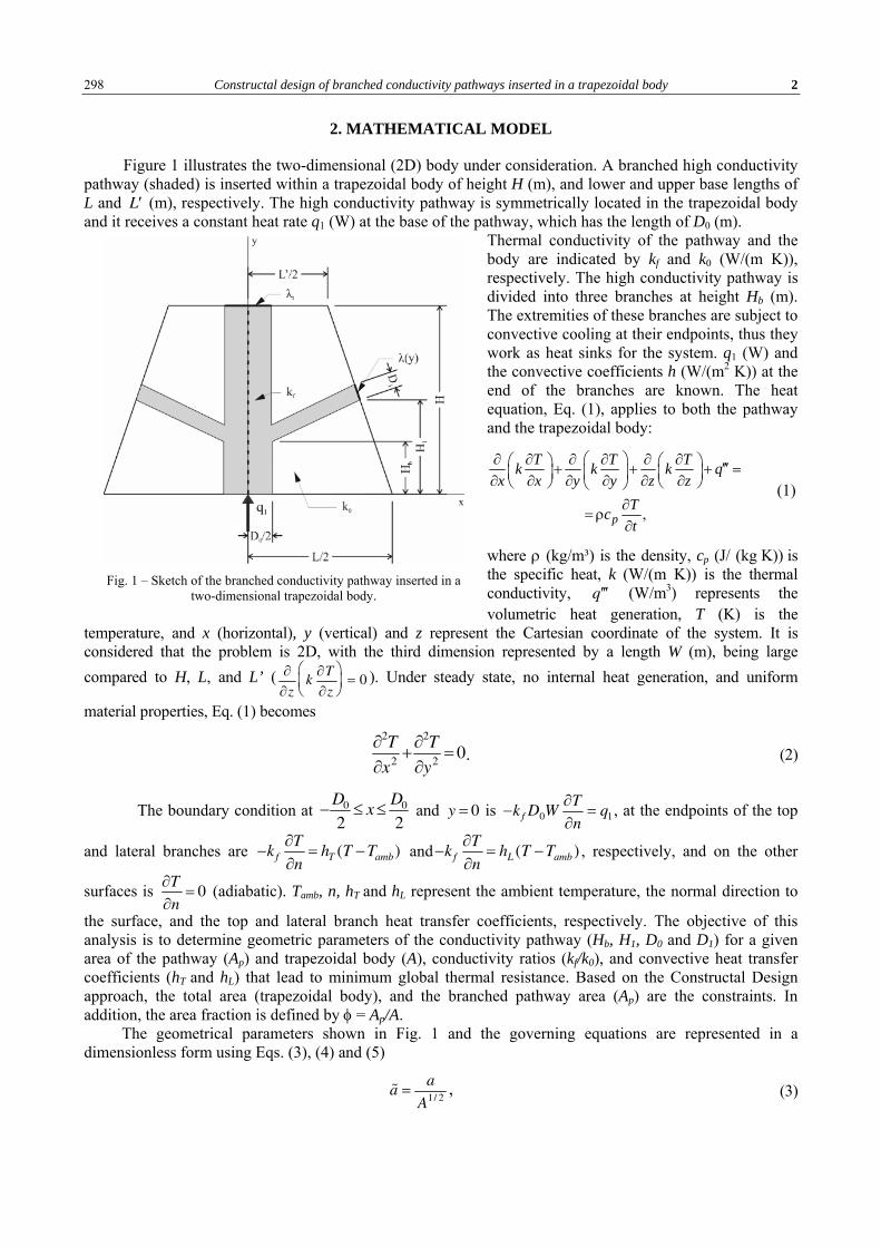
Constructal design of branched conductivity pathways inserted in a trapezoidal body 2 298
2. MATHEMATICAL MODEL
Figure 1 illustrates the two-dimensional (2D) body under consideration. A branched high conductivity pathway (shaded) is inserted within a trapezoidal body of height H (m), and lower and upper base lengths of L and ′ L (m), respectively. The high conductivity pathway is symmetrically located in the trapezoidal body and it receives a constant heat rate q1 (W) at the base of the pathway, which has the length of D0 (m).
Thermal conductivity of the pathway and the body are indicated by kf and k0 (W/(m K)), respectively. The high conductivity pathway is divided into three branches at height Hb (m). The extremities of these branches are subject to convective cooling at their endpoints, thus they work as heat sinks for the system. q1 (W) and the convective coefficients h (W/(m2 K)) at the end of the branches are known. The heat equation, Eq. (1), applies to both the pathway and the trapezoidal body:
,
⎛ ⎞∂ ∂ ∂ ∂ ∂ ∂⎛ ⎞ ⎛ ⎞ ′′′+ + + =⎜ ⎟ ⎜ ⎟⎜ ⎟∂ ∂ ∂ ∂ ∂ ∂⎝ ⎠ ⎝ ⎠⎝ ⎠∂
= ρ∂p
T T Tk k k qx x y y z z
Tct
(1)
where ρ (kg/m³) is the density, cp (J/ (kg K)) is the specific heat, k (W/(m K)) is the thermal conductivity, ′ ′ ′ q (W/m3) represents the volumetric heat generation, T (K) is the
temperature, and x (horizontal), y (vertical) and z represent the Cartesian coordinate of the system. It is considered that the problem is 2D, with the third dimension represented by a length W (m), being large compared to H, L, and L’ ( ∂
∂zk
∂T
∂z
⎛ ⎝ ⎜
⎞ ⎠ ⎟ = 0 ). Under steady state, no internal heat generation, and uniform
material properties, Eq. (1) becomes
∂2T
∂x2+ ∂2T
∂y2= 0. (2)
The boundary condition at − D0
2≤ x ≤ D0
2 and y = 0 is −k f D0W
∂T
∂n= q1 , at the endpoints of the top
and lateral branches are −kf∂T
∂n= hT (T −Tamb) and −kf
∂T
∂n= hL (T −Tamb) , respectively, and on the other
surfaces is ∂T
∂n= 0 (adiabatic). Tamb, n, hT
and hL represent the ambient temperature, the normal direction to
the surface, and the top and lateral branch heat transfer coefficients, respectively. The objective of this analysis is to determine geometric parameters of the conductivity pathway (Hb, H1, D0
and D1) for a given area of the pathway (Ap) and trapezoidal body (A), conductivity ratios (kf/k0), and convective heat transfer coefficients (hT
and hL) that lead to minimum global thermal resistance. Based on the Constructal Design approach, the total area (trapezoidal body), and the branched pathway area (Ap) are the constraints. In addition, the area fraction is defined by φ = Ap/A.
The geometrical parameters shown in Fig. 1 and the governing equations are represented in a dimensionless form using Eqs. (3), (4) and (5)
˜ a = a
A1/ 2, (3)
Fig. 1 – Sketch of the branched conductivity pathway inserted in a
two-dimensional trapezoidal body.

3 Tadeu Mendonca FAGUNDES, Neda YAGHOOBIAN, Luiz Alberto Oliveira ROCHA, Juan Carlos ORDONEZ 299
θ = T −T0
q1(kf W )
, (4)
˜ k =kf
k0
, (5)
where a represents any geometric parameter given in (m). Thus, Eq. (2) can be rewritten in its dimensionless form as shown in Eq. (6) with its normalized boundary
conditions as − ∂θ∂˜ y
= 1˜ D 0
at −˜ D 02
≤ ˜ x ≤˜ D 02
and ˜ y = 0, ∂θ∂ ˜ n
= −λT θ at the endpoint of the top branch,
∂θ∂ ˜ n
= −λ Lθ at the endpoint of the lateral branches, and ∂θ∂ ˜ n
= 0 on the other surfaces (adiabatic), where ˜ n is
the dimensionless direction normal to the boundary surface, and λN is defined by Eq. (7), similar to [2].
∂2θ∂˜ x 2
+ ∂2θ∂˜ y 2
=0, (6)
λN = hN A1/ 2
kf
. (7)
Equation (6) with the provided boundary conditions can be solved numerically to obtain the temperature field.
In this work, the endpoints of the lateral branches are subject to convective cooling that is achieved by linking the lateral heat transfer coefficients to the top heat transfer coefficient through a linear approximation:
λL (y) = λT (y / H) . (8)
The maximum dimensionless temperature, θmax¸ also represents the global thermal resistance of the configuration
θmax = Tmax −T0
q1kf W
. (9)
For the purposes of this work, five non-dimensional degrees of freedom were chosen: H/L, L’/L, Hb/H, H1/H and D1/D0. For a given φ and these degrees of freedom the system geometry can be fully defined.
3. NUMERICAL PROCEDURES
The solution was obtained using a finite element approach with non-uniform, triangular elements in both x and y directions, implemented in MATLAB using the PDETool toolbox. This method has been verified in previous studies of cavities and fins [12, 16]. The appropriate mesh size was determined using successive refinements. In each refinement, the number of elements were increased four times until the criterion |(θj
max – θj+1max)/θj
max| < 1×10⁻⁴ was satisfied. Here, θjmax and θj+1
max represent the maximum dimensionless temperatures calculated using the current and the next mesh sizes, respectively. The results presented in the following section were obtained using a mesh composed of approximately 28,000 triangular elements, in which the previous criterion was fulfilled. For the geometric optimization presented in this paper, a binary, single-objective, elitist genetic algorithm was employed, with a mutation rate of 10% and a crossover probability of 80%. The application of genetic algorithm in heat transfer problems has been extensively reviewed [19] and, for the sake of brevity, will not be detailed here.
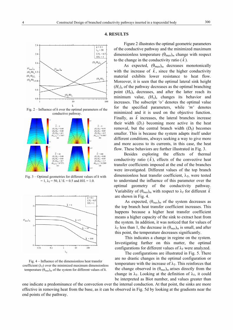
4 Constructal Design of branched conductivity pathways inserted in a trapezoidal body
4. RESULTS
Figure 2 illustrates the optimal geometric parameters of the conductive pathway and the minimized maximum dimensionless temperature (θmax)m change with respect to the change in the conductivity ratio ( ˜ k ).
As expected, (θmax)m decreases monotonically with the increase of ˜ k , since the higher conductivity material exhibits lower resistance to heat flow. Moreover, it is seen that the optimal lateral sink height (H1)o of the pathway decreases as the optimal branching point (Hb)o decreases, and after the latter reach its minimum value, (H1)o changes its behavior and increases. The subscript ‘o’ denotes the optimal value for the specified parameters, while ‘m’ denotes minimized and it is used on the objective function. Finally, as ˜ k increases, the lateral branches increase their width (D1) becoming more active in the heat removal, but the central branch width (D0) becomes smaller. This is because the system adapts itself under different conditions, always seeking a way to give more and more access to its currents, in this case, the heat flow. These behaviors are further illustrated in Fig. 3.
Besides exploring the effects of thermal conductivity ratio ( ˜ k ), effects of the convective heat transfer coefficients imposed at the end of the branches were investigated. Different values of the top branch dimensionless heat transfer coefficient, λT, were tested to understand the influence of this parameter over the optimal geometry of the conductivity pathway. Variability of (θmax)m with respect to λT for different ˜ k are shown in Fig. 4.
As expected, (θmax)m of the system decreases as the top branch heat transfer coefficient increases. This happens because a higher heat transfer coefficient means a higher capacity of the sink to extract heat from the system. In addition, it was noticed that for values of λT less than 1, the decrease in (θmax)m is small, and after this point, the temperature decreases significantly.
This indicates a change in regime on the system. Investigating further on this matter, the optimal configurations for different values of λT were analyzed.
The configurations are illustrated in Fig. 5. There are no drastic changes in the optimal configuration or temperature with the increase of λT. This reinforces that the change observed in (θmax)m arises directly from the change in λT. Looking at the definition of λT, it could be interpreted as Biot number, and values greater than
one indicate a predominance of the convection over the internal conduction. At that point, the sinks are more effective in removing heat from the base, as it can be observed in Fig. 5d by looking at the gradients near the end points of the pathway.
Fig. 2 – Influence of k over the optimal parameters of the conductive pathway.
Fig. 3 – Optimal geometries for different values of k with
� = 1, λT = 50, L’/L = 0.5 and H/L = 1.0.
Fig. 4 – Influence of the dimensionless heat transfer coefficient (λT) over the minimized maximum dimensionless
temperature (θmax)m of the system for different values of k.
300

5 Tadeu Mendonca FAGUNDES, Neda YAGHOOBIAN, Luiz Alberto Oliveira ROCHA, Juan Carlos ORDONEZ 301
The influence of λT on the optimal values of D1/D0 for different values of k~ was also analyzed. The results are shown in Fig. 6.
Fig. 5 – Optimal configurations of the system for different values of
λT, with φ = 0.1, H/L = 1, L’/L = 0.5 and k = 10. Fig. 6 – Influence of λT over the optimal lateral and central
branches ratio (D1/D0)o for different values of k.
Fig. 6 illustrates that the optimal width (D1) value of the lateral branch increases around the same λT, (≈ 1), in which the faster decrease of (θmax)m starts. With a low value of λT, the system opts for a wider central pathway and lateral sinks as low as possible. Beyond λT = 1, this behavior changes, and the lateral sinks can remove heat effectively even on a relatively lower height, and then they become more important to the heat removal process, thus becoming wider and conducting a higher portion of heat throughout the system.
5. CONCLUSIONS
After exploring the configuration design space of a high conductivity pathway inserted within a trapezoidal body of lower conductivity it is observed that Constructal Design reveals configurations that allows more access to the flows within it. This phenomenon, predicted by the Constructal Law, is clearly seen in action in the system studied in this work. For this case, the balance between transporting the heat through the conductivity pathway or the background body led to structures that minimize the maximum dimensionless temperature. This minimization of the maximum dimensionless temperature is also the minimization of the thermal global resistance of the system.
By imposing a function for the lateral heat transfer coefficient dependent on the height, the system displays two distinct methods for dissipating the heat. For a small heat transfer coefficient, the system aims to dissipate the heat through the main channel of the pathway, while minimizing the area of the lateral branches and keeping them relatively low in the system, since they do not have a great influence in the heat transfer process. On the other hand, for a higher heat transfer coefficient, the system starts to increase the lateral branches and transport more heat through them. This is due to a balance involving the pathway conductivity, the heat transfer coefficient and the ratio between the lateral and main branches lengths.
ACKNOWLEDGEMENTS
J.C. Ordonez acknowledges partial support from ONR-ESRDC under grant N00014-16-1-2956.
REFERENCES
1. BEJAN, A., Advanced Engineering Thermodynamics, John Wiley & Sons, Hoboken, NJ, 2006. 2. BEJAN, A., Evolution in Thermodynamics, Applied Physics Reviews, 4, 1, p. 011305, 2017. 3. BEJAN, A., Shape and Structure, From Engineering to Nature, Cambridge University Press, Cambridge, UK, 2000.

6 Constructal Design of branched conductivity pathways inserted in a trapezoidal body
4. BEJAN, A., LORENTE, S., LEE, J., Unifying Constructal Theory of Tree Roots, Canopies and Forests, J. Theor. Biol., 254, 3, pp. 529–540, 2008.
5. REIS, A. H., BEJAN, A., Constructal Theory of Global Circulation and Climate, Intl. J. of Heat and Mass Transfer, 49, 11–12, pp. 1857–1875, 2006.
6. MIGUEL, A.F., The emergence of design in pedestrian dynamics: locomotion, self-organization, Walking Paths and Constructal Law, Phys. Life Rev., 10, 2, pp. 168–190, 2013.
7. ORDONEZ, J.C., BEJAN, A., CHERRY, R.S., Designed Porous Media: Optimally Nonuniform Flow Structures Connecting One Point with more Points. Intl. J. of Thermal Sciences, 42, 9, pp. 857–870, 2003.
8. BEJAN, A., ALMOGBEL, M., Constructal T-shaped fins, Intl. J. of Heat and Mass Transfer, 43, 12, pp. 2101–2115, 2000. 9. LORENZINI, G., ROCHA, L.A.O., Constructal design of Y-shaped assembly of fins, Intl. J. of Heat and Mass Transfer, 49, 23,
pp. 4552–4557, 2006. 10. LORENZINI, G., ROCHA, L.A.O., Constructal design of T–Y assembly of fins for an optimized heat removal, Intl. J. of Heat and
Mass Transfer, 52, 5, pp. 1458–1463, 2009. 11. BISERNI, C., DALPIAZ, F.L., FAGUNDES, T.M., ROCHA, L.A.O., Constructal design of T-shaped morphing fins coupled with a
trapezoidal basement: A numerical investigation by means of exhaustive search and genetic algorithm, Intl. J. of Heat and Mass Transfer, 109, pp. 73-81, 2017.
12. BISERNI, C., DALPIAZ, F.L., FAGUNDES, T.M., GARAI, M., ROCHA, L.A.O., Geometric optimization of morphing fins coupled with a semicircular heat generating body: A numerical investigation on the basis of Bejan's theory, Intl. Communications in Heat and Mass Transfer, 81, pp. 81–91, 2017.
13. SOUZA, J.A., ORDONEZ, J.C., Constructal Design of High-Conductivity Inserts, Constructal Law and the Unifying Principle of Design, 91–111. Understanding Complex Systems, Springer, New York, NY, 2013, Doi:10.1007/978-1-4614-5049-8_6.
14. LORENZINI, G., BISERNi, C., ROCHA, L.A.O., Constructal design of X-shaped conductive pathways for cooling a heat-generating body, International Journal of Heat and Mass Transfer, 58, 1, pp. 513–520, 2013.
15. HAJMOHAMMADI, M.R., ABIANEH, V.A., Moezzinajafabadi, M. Daneshi, M., Fork-shaped highly conductive pathways for maximum cooling in a heat generating piece, Applied Thermal Engineering, 61, 2, pp. 228–235, 2013.
16. Da Sd ESTRADA, E., FAGUNDES, T.M., ISOLDI, L.A., Dos SANTOS, E.D., XIE, G., ROCHA, L.A.O., Constructal Design Associated to Genetic Algorithm of Asymmetric V-Shaped Pathways, J. of Heat Transfer, 137, 6, pp. 061010, 2015.
17. WECHSATOL, W., J.C. ORDONEZ, and S. KOSARAJU, Constructal dendritic geometry and the existence of asymmetric bifurcation, Journal of Applied Physics, 100, 11, 2006.
18. WECHSATOL, W., LORENTE, S., BEJAN, A., ORDONEZ, J.C., Elemental T and Y Shapes of Tree Networks of Ducts with Various Cross-Sectional Shapes, J. of Hydraulic Engineering, 13, 52, pp. 132–139, 2009.
19. GOSSELIN, L., TYE-GINGRAS, M., MATHIEU-POTVIN, F., Review of utilization of genetic algorithms in heat transfer problems, International Journal of Heat and Mass Transfer, 52, 9, pp. 2169–2188, 2009.
302
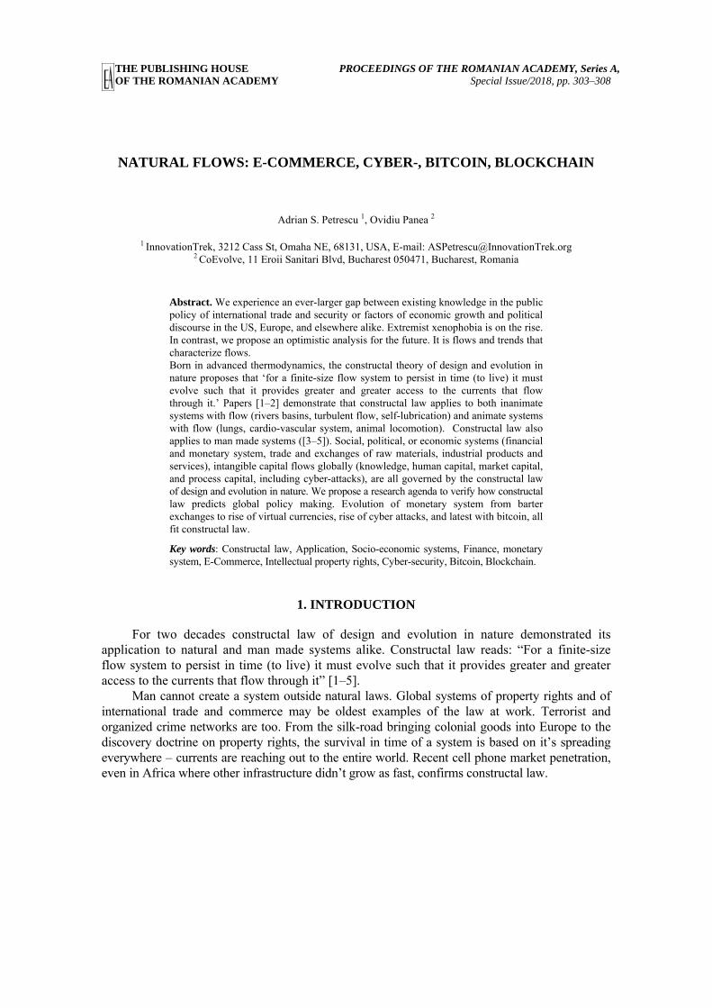
THE PUBLISHING HOUSE PROCEEDINGS OF THE ROMANIAN ACADEMY, Series A, OF THE ROMANIAN ACADEMY Special Issue/2018, pp. 303–308
NATURAL FLOWS: E-COMMERCE, CYBER-, BITCOIN, BLOCKCHAIN
Adrian S. Petrescu 1, Ovidiu Panea 2
1 InnovationTrek, 3212 Cass St, Omaha NE, 68131, USA, E-mail: [email protected]
2 CoEvolve, 11 Eroii Sanitari Blvd, Bucharest 050471, Bucharest, Romania
Abstract. We experience an ever-larger gap between existing knowledge in the public policy of international trade and security or factors of economic growth and political discourse in the US, Europe, and elsewhere alike. Extremist xenophobia is on the rise. In contrast, we propose an optimistic analysis for the future. It is flows and trends that characterize flows. Born in advanced thermodynamics, the constructal theory of design and evolution in nature proposes that ‘for a finite-size flow system to persist in time (to live) it must evolve such that it provides greater and greater access to the currents that flow through it.’ Papers [1–2] demonstrate that constructal law applies to both inanimate systems with flow (rivers basins, turbulent flow, self-lubrication) and animate systems with flow (lungs, cardio-vascular system, animal locomotion). Constructal law also applies to man made systems ([3–5]). Social, political, or economic systems (financial and monetary system, trade and exchanges of raw materials, industrial products and services), intangible capital flows globally (knowledge, human capital, market capital, and process capital, including cyber-attacks), are all governed by the constructal law of design and evolution in nature. We propose a research agenda to verify how constructal law predicts global policy making. Evolution of monetary system from barter exchanges to rise of virtual currencies, rise of cyber attacks, and latest with bitcoin, all fit constructal law.
Key words: Constructal law, Application, Socio-economic systems, Finance, monetary system, E-Commerce, Intellectual property rights, Cyber-security, Bitcoin, Blockchain.
1. INTRODUCTION
For two decades constructal law of design and evolution in nature demonstrated its application to natural and man made systems alike. Constructal law reads: “For a finite-size flow system to persist in time (to live) it must evolve such that it provides greater and greater access to the currents that flow through it” [1–5].
Man cannot create a system outside natural laws. Global systems of property rights and of international trade and commerce may be oldest examples of the law at work. Terrorist and organized crime networks are too. From the silk-road bringing colonial goods into Europe to the discovery doctrine on property rights, the survival in time of a system is based on it’s spreading everywhere – currents are reaching out to the entire world. Recent cell phone market penetration, even in Africa where other infrastructure didn’t grow as fast, confirms constructal law.
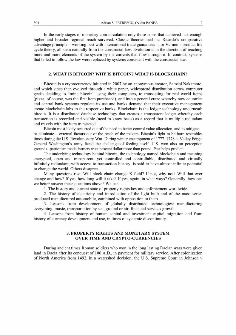
Adrian S. PETRESCU, Ovidiu PANEA 2 304
In the early stages of monetary coin circulation only those coins that achieved fast enough higher and broader regional reach survived. Classic theories such as Ricardo’s comparative advantage principle – working best with international trade guarantees –, or Vernon’s product life cycle theory, all stem naturally from the constructal law. Evolution is in the direction of reaching more and more elements of the system by the currents that flow through it. In contrast, systems that failed to follow the law were replaced by systems consistent with the constructal law.
2. WHAT IS BITCOIN? WHY IS BITCOIN? WHAT IS BLOCKCHAIN?
Bitcoin is a cryptocurrency initiated in 2007 by an anonymous creator, Satoshi Nakamoto, and which since then evolved through a white paper, widespread distribution across computer geeks deciding to “mine bitcoin” using their computers, to transacting for real world items (pizza, of course, was the first item purchased), and into a general craze whereby now countries and central bank systems regulate its use and banks demand that their executive management create blockchain labs in the respective banks. Blockchain is the ledger technology underneath bitcoin. It is a distributed database technology that creates a transparent ledger whereby each transaction is recorded and visible (need to know basis) as a record that is multiple redundant and travels with the item transacted.
Bitcoin most likely occurred out of the need to better control value allocation, and to mitigate – or eliminate – external factors out of the reach of the makers. Bitcoin’s fight to be born resembles times during the U.S. Revolutionary War. During winter encampment of 1777–1778 at Valley Forge, General Washington’s army faced the challenge of feeding itself. U.S. won also on perception grounds--patriotism made farmers trust nascent dollar more than pound. Past helps predict.
The underlying technology behind bitcoin, the technology named blockchain and meaning encrypted, open and transparent, yet controlled and controllable, distributed and virtually infinitely redundant, with access to transaction history, is said to have almost infinite potential to change the world. Others disagree.
Many questions rise. Will block chain change X field? If not, why not? Will that ever change and how? If yes, how long will it take? If yes, again, in what ways? Generally, how can we better answer these questions above? We use:
1. The history and current state of property rights law and enforcement worldwide. 2. The history of electricity and introduction of the light bulb and of the mass series
produced manufactured automobile, combined with opposition to them. 3. Lessons from development of globally distributed technologies: manufacturing
everything, music, transportation by sea, ground or air, financial services growth. 4. Lessons from history of human capital and investment capital migration and from
history of currency development and use, in times of systemic discontinuity.
3. PROPERTY RIGHTS AND MONETARY SYSTEM OVER TIME AND CRYPTO-CURRENCIES
During ancient times Roman soldiers who won in the long lasting Dacian wars were given land in Dacia after its conquest of 106 A.D., in payment for military service. After colonization of North America from 1492, in a watershed decision, the U.S. Supreme Court in Johnson v

3 Natural flows: e-Commerce, cyber-, bitcoin, blockchain
305
M’Intosh (1823) took property ownership of U.S. land for federal government from First Nations so that Virginia could pay its militia that fought the Revolutionary War. About 1700 years apart the same pattern creates property rights where none existed. Discovery doctrine, used in both cases, spreads as property rights are needed [6]. A system based on rule of law that guarantees property rights, in order to survive, needs to have its currents reach every element that the flow may reach. Constructal law predicts a global property rights regime. Before, constructal law predicted free roaming bison over prairie lands of First Nations. What happens when two systems meet, or compete?
The monetary system evolved from transactional money-less exchanges, through the middle ages, Bretton Woods, US Exit from the gold standard (or the Nixon shock), Bretton Woods II, to the current post Euro-zone creation of the late 1990’s, and the aftermath of the 2008 crisis. We now live the competitive and cooperative nature of a system with multiple currencies of last resort. It is no surprise that many actors may have felt a disconnect between their perceptions about their own net worth and their direct access to the controls and levels of the financial system. Young professionals with technical skills who sell those skills to highest bidder investors must have felt frustrated with a system out of their control. Why not make a start-up making monetary instruments directly, without the intermediation of any product or service? Hence the rise of “alternative virtual currencies.”
Bitcoin and blockchain are neither unique nor new. All the way back to US army at Valley Forge, competing currencies, real or virtual, existed before. Gaming virtual dollars are ubiquitous in past three decades. Real currency buys gaming dollars, not the other way around. Creator(s) or adopters of bitcoin argue that a crypto-currency (virtual) never existed before. Monopoly games come to mind. Developments in monetary systems serve as model when predicting future of bitcoin and blockchain. They justify applying constructal law to socio-economic systems. US dollar “conquered the world” even at a time when governments in the East (1950’s–1989) were trying hardest to stop it. Western currencies won trust. Traditional and non-traditional currencies will thus cooperate and compete alike.
4. COMPARING E-COMMERCE, CYBER-THREATS, BITCOIN AND BLOCKCHAIN
The core question in our research agenda: how will current monetary and financial systems, and the systems of property rights, including traditional (such as real estate) and modern newly created (mineral rights, air rights, IP rights and their evolution) all on the one hand, and bitcoin and blockchain and other future virtual currencies on the other interact into the future, and what system will evolve from their interaction? Bitcoin and particularly blockchain have the potential to make business transactions more transparent, equitable and efficient, and much less based on information asymmetry than today. As with the joining of two rivers, a new river forms from the original two. Bitcoin and blockchain will likely increase participation in monetary and financial systems. Constructal law predicts so. We drive manufactured automobiles. Almost everyone everywhere owns a cell phone.
Figure 1 suggests an interdisciplinary approach to solving the puzzle. Economics, finance, mathematics, physics – in particular thermodynamics –, law – traditional and newly created property rights –, biology, as well as political science, national and international security, and advanced methods in epistemology of science help predict e-Commerce, cyber-threats, bitcoin and blockchain evolution.
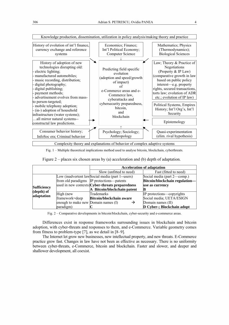
Adrian S. PETRESCU, Ovidiu PANEA 4 306
Knowledge production, dissemination, utilization in policy analysis/making theory and practice
History of evolution of int’l finance, currency exchange and reference
systems
Economics; Finance; Int’l Political Economy;
Computer Science
Mathematics; Physics (Thermodynamics); Biological Sciences
↓
Law; Theory & Practice of Negotiations
(Property & IP Law) (comparative growth in law
based on public policy interest—e.g. property
rights, secured transactions, torts law; evolution of ADR
etc.; evolution of IP law)
Political Systems, Empires History; Int’l Org’s, Int’l
Security
History of adoption of new technologies disrupting old:
- electric lighting; - manufactured automobiles; - music recording, distribution; - digital photography; - digital publishing; - payment methods; - advertisement evolves from mass- to person-targeted; - mobile telephony adoption; - (in-) adoption of household infrastructure (water systems); …all mirror natural systems-- constructal law predictions.
Predicting field specific
evolution (adoption and speed/growth
of impact) of
e-Commerce areas and e-Commerce law, cyberattacks and
cybersecurity preparedness,bitcoin,
and blockchain
Epistemology ↑
Consumer behavior history;
InfoSoc era; Criminal behavior Psychology; Sociology;
Anthropology Quasi-experimentation
(elim. rival hypothesis)
Complexity theory and explanations of behavior of complex adaptive systems
Fig. 1 – Multiple theoretical implications method used to analyse bitcoin, blockchain, cyberthreats.
Figure 2 – places six chosen areas by (a) acceleration and (b) depth of adaptation.
Acceleration of adaptation Slow (unfitted to need) Fast (fitted to need)
Low (inadvertent lawfrom old paradigms used in new contexts)
Social media (part 1--users) IP protections—patents Cyber-threats preparedness A Bitcoin/blockchain patent
Social media (part 2—comp.) Bitcoin/blockchain regulation—use as currency B Sufficiency
(depth) of adaptation High (new
framework=deep enough to make new paradigm)
Trademarks Bitcoin/blockchain aware Domain names (I) C
IP protections—copyrights Social media; UETA/ESIGN Domain names (II) D Cyber-; Blockchain adopt
Fig. 2 – Comparative developments in bitcoin/blockchain, cyber-security and e-commerce areas.
Differences exist in response frameworks surrounding issues in blockchain and bitcoin adoption, with cyber-threats and responses to them, and e-Commerce. Variable geometry comes from fitness to problem-type [7], as we detail in [8–9].
The Internet let grow new businesses, new intellectual property, and new threats. E-Commerce practice grew fast. Changes in law have not been as effective as necessary. There is no uniformity between cyber-threats, e-Commerce, bitcoin and blockchain. Faster and slower, and deeper and shallower development, all coexist.
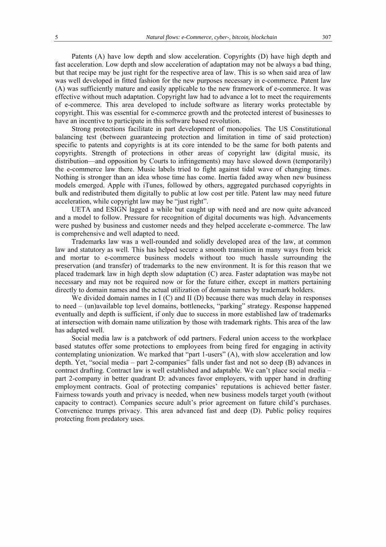
5 Natural flows: e-Commerce, cyber-, bitcoin, blockchain
307
Patents (A) have low depth and slow acceleration. Copyrights (D) have high depth and fast acceleration. Low depth and slow acceleration of adaptation may not be always a bad thing, but that recipe may be just right for the respective area of law. This is so when said area of law was well developed in fitted fashion for the new purposes necessary in e-commerce. Patent law (A) was sufficiently mature and easily applicable to the new framework of e-commerce. It was effective without much adaptation. Copyright law had to advance a lot to meet the requirements of e-commerce. This area developed to include software as literary works protectable by copyright. This was essential for e-commerce growth and the protected interest of businesses to have an incentive to participate in this software based revolution.
Strong protections facilitate in part development of monopolies. The US Constitutional balancing test (between guaranteeing protection and limitation in time of said protection) specific to patents and copyrights is at its core intended to be the same for both patents and copyrights. Strength of protections in other areas of copyright law (digital music, its distribution—and opposition by Courts to infringements) may have slowed down (temporarily) the e-commerce law there. Music labels tried to fight against tidal wave of changing times. Nothing is stronger than an idea whose time has come. Inertia faded away when new business models emerged. Apple with iTunes, followed by others, aggregated purchased copyrights in bulk and redistributed them digitally to public at low cost per title. Patent law may need future acceleration, while copyright law may be “just right”.
UETA and ESIGN lagged a while but caught up with need and are now quite advanced and a model to follow. Pressure for recognition of digital documents was high. Advancements were pushed by business and customer needs and they helped accelerate e-commerce. The law is comprehensive and well adapted to need.
Trademarks law was a well-rounded and solidly developed area of the law, at common law and statutory as well. This has helped secure a smooth transition in many ways from brick and mortar to e-commerce business models without too much hassle surrounding the preservation (and transfer) of trademarks to the new environment. It is for this reason that we placed trademark law in high depth slow adaptation (C) area. Faster adaptation was maybe not necessary and may not be required now or for the future either, except in matters pertaining directly to domain names and the actual utilization of domain names by trademark holders.
We divided domain names in I (C) and II (D) because there was much delay in responses to need – (un)available top level domains, bottlenecks, “parking” strategy. Response happened eventually and depth is sufficient, if only due to success in more established law of trademarks at intersection with domain name utilization by those with trademark rights. This area of the law has adapted well.
Social media law is a patchwork of odd partners. Federal union access to the workplace based statutes offer some protections to employees from being fired for engaging in activity contemplating unionization. We marked that “part 1-users” (A), with slow acceleration and low depth. Yet, “social media – part 2-companies” falls under fast and not so deep (B) advances in contract drafting. Contract law is well established and adaptable. We can’t place social media – part 2-company in better quadrant D: advances favor employers, with upper hand in drafting employment contracts. Goal of protecting companies’ reputations is achieved better faster. Fairness towards youth and privacy is needed, when new business models target youth (without capacity to contract). Companies secure adult’s prior agreement on future child’s purchases. Convenience trumps privacy. This area advanced fast and deep (D). Public policy requires protecting from predatory uses.

Adrian S. PETRESCU, Ovidiu PANEA 6 308
Cyber-threats and responses validate framework too. Organized criminal networks and sole attackers adapted fast (D) to new information society conditions and took advantage early of vulnerabilities in global cyber-systems, from early bank attacks to ubiquity of digital targets, political or financial. Responses and preparedness to cyber-threats lag behind (A) because open inertial government systems are less nimble than organized criminal networks. Gaps may even widen over time [10].
5. CONCLUSIONS
Bitcoin and blockchain will evolve and will be adopted widely. Blockchain may facilitate better more accurate property rights recordation. Financial institutions and government regulatory agencies will own technology and will channel it to existing systems. Flows will grow to reach more of systems’ elements. Consumers and banks too will adopt. Competition among payment systems (fully centralized or not, i.e. device-to-device based) will be fought between blockchain and legacy systems, with flows reaching customers globally. Hopefully cyber- gap threats-answers will close. Constructal law can predict quantitatively growth of systems.
REFERENCES
1. A., BEJAN, J.H., MARDEN, The constructal unification of biological and geophysical design, Phys. Life Rev. Jun., 6 2, pp. 85–102, 2009.
2. A., BEJAN, S., LORENTE, The Constructal Law of Design and Evolution in Nature, Philosophical Transactions of the Royal Society B, pp. 1335–48, 2010.
3. A., BEJAN, Advanced Engineering Thermodynamics, Wiley, New York, 1997. 4. A., BEJAN, The Physics of Life: The Evolution of Everything, St. Martin's Press, New York, 2016. 5. A., BEJAN, M.R., ERRERA, Wealth inequality: The physics basis, J. of Applied Physics, 121, 124903 (2017);
doi: 10.1063/1.4977962. 6. L.G., ROBERTSON, Conquest by Law: How Discovery of America Dispossessed Indigenous Peoples of Their
Lands, 1st ed., Oxford Univ Press, 2007. 7. J.D., THOMPSON, A., TUDEN, Strategies, Structure, and Processes of Organizational Decision, in Thompson,
J.D. et al. (Eds.), Comparative Administration Studies, University of Pittsburgh Press, 1959. 8. A.S., PETRESCU, O., PANEA, Equilibrium: Natural Laws in Society, 4th ed., 2018. 9. A.S., PETRESCU, O., PANEA, A research agenda: facilitating global socio-economic equilibrium through
enabling and accelerating natural flows – the case of e-commerce law, bitcoin, and blockchain, MPSA 75th Annual Conf., Chicago IL, April 6–8, 2017.
10. R.A., GRIMES, Hacking the hacker. Learn from the experts who take down hackers, Wiley, 2017.

THE PUBLISHING HOUSE PROCEEDINGS OF THE ROMANIAN ACADEMY, Series A, OF THE ROMANIAN ACADEMY Special Issue/2018, pp. 309–311
CONSTRUCTAL LAW, TWENTY YEARS AFTER
Adrian BEJAN
Duke University, Department of Mechanical Engineering and Materials Science, Durham, NC 27708-0300, USA
The Constructal law has come a long way since its enunciation in two 1996 papers [1, 2], which were followed by a book [3] and five more papers in 1997 [4–8]. In Bucharest on 15–16 May 2017, we celebrated the 10th international conference dedicated to the emerging Constructal law field. The preceding conferences were held in the USA (2006, 2007), Portugal (2008), Italy (2008), France (2009), Italy (2010), Brazil (2011), China (2013) and Italy (2015).
As shown in Ref. [9], a law of physics is a concise statement that summarizes a phenomenon that occurs in nature. The Constructal-law field started from the realization that design is a universal physics phenomenon. It unites the animate with the inanimate over an extremely broad range of scales, from the tree design of the snowflake, to animal design and the tree design of the Amazon river basin. The river delta and the human lung are just two examples of the same volume-point flow architecture, one inanimate and the other animate, to which one could add many more relatives (e.g., lightning, vascularized living tissues, city traffic, the spreading of new ideas on the globe). Nature has evolution (Fig. 1).
Fig. 1 – The evolution and spreading of thermodynamics during the past two centuries.
The concepts of life, design and future (evolution) were placed firmly in physics by the Constructal Law, stated in 1996 [1, 2]:
“For a finite-size flow system to persist in time (to live), its configuration must evolve freely in such a way that provides greater and greater access to the currents that flow through it.”
According to the Constructal Law, a live system is one that has two universal characteristics: it flows (i.e., it is a nonequilibrium system in thermodynamics), and it morphs freely toward configurations that allow all its currents to flow more easily over time. Life and evolution are a self-standing physics phenomenon, and they belong in physics [10].
The Constructal Law is a field that is expanding rapidly in physics, biology, technology and social sciences. The field is expanding rapidly. Books on the Constructal Law appear regularly [11–23]. Today, on Google Scholar the word constructal yields 5,700 articles and books.
To see the position of design in nature as a universal phenomenon of physics, it is necessary to recall that thermodynamics rests mainly on two laws, which are both first principles. The first law commands the conservation of energy in any system. The second law commands the presence of irreversibility (i.e. the generation of entropy) in any system: Irreversibility means that, by itself, any stream flows naturally one way,
Adrian BEJAN 2 310
from high to low. The permanence and extreme generality of the two laws are consequences of the fact that in thermodynamics the any system is a black box. It is a region of space, or a collection of matter without specified shape and structure. The two laws are global statements about the balance or imbalance of the flows (mass, heat, work, entropy) that flow into and out of the black box.
Nature is not made of boxes without configuration. The systems that we discern in nature have shape and structure. They are macroscopic, finite size, and recognizable as images-sharp lines on a diffuse background. They have configurations, maps, rhythms and sounds. They are simple: their complexity is modest, because if it were not modest we would not be able to discern them and to question their existence. The very fact that they have names (river basins, blood vessels, trees) indicates that they have appearances that the observer recognizes.
The constructal-law literature draws attention to the fact that the laws of thermodynamics do not account completely for the systems of nature, even though scientists have built thermodynamics into thick books in which the two laws are just the introduction. The body of thermodynamics is devoted to describing, designing and optimizing things that seem to correspond to flow systems found in nature, or to devices that can be used by humans to make life easier. Nowhere is this more evident than in engineering, where the method of Entropy Generation Minimization [24–26] is recognized as thermodynamics even though neither of the two laws accounts for the natural occurrence of design or optimization phenomena.
The Constructal law is not a statement of optimization, maximization, minimization, or any other mental image of end design or destiny. The Constructal law is about the direction of evolution in time, and the fact that the design phenomenon is not static: it is dynamic, ever changing, like the images in a movie at the cinema. Evolution never ends. This is important to keep in mind, because there is a growing list of ad hoc proposals of optimality (end-design), but each addresses a narrow domain, and, as a consequence, the body of optimality statements that have emerged is self-contradictory, and the claim that each is a general principle is easy to refute [9, 27]:
(i) Minimum entropy generation (production) and maximum efficiency are used commonly in engineering and biology.
(ii) Maximum entropy production (MEP) is being invoked in geophysics. (iii) Maximum fitness and adaptability (robustness, resilience) are used in biology. (iv) Minimum flow resistance (fluid flow, heat transfer, mass transfer) is invoked in engineering, river
mechanics and physiology. (v) Maximum flow resistance is used regularly in physiology and engineering, e.g. maximum resistance
to loss of body heat through animal hair and fur, or through the insulation of power and refrigeration plants, the minimization of fluid leaks through the walls of ducts, etc.
(vi) Minimum travel time is used in urban design, traffic, transportation. (vii) Minimum effort and cost is a core idea in social dynamics and animal design. (viii) Maximum profit and utility is used in economics. (ix) Maximum territory is used for rationalizing the spreading of living species, deltas in the desert, and empires. (x) Uniform distribution of maximum stresses is used as an axiom in rationalizing the design of
botanical trees and animal bones. (xi) Maximum growth rate of flow disturbances (deformations) is invoked in the study of fluid flow
disturbances and turbulence. (xii) Maximum power was proposed in biology, physics and engineering.
The optimality statements are contradictory and disunited, yet they demonstrate that the time for placing the ‘evolution’ phenomena in science is now. The progress made with the Constructal law [9, 27–29] shows that the diversity of phenomena addressed with the ad hoc statements (i) – (xii) are manifestations of the single natural tendency that is expressed by this law of physics. For example, the contradiction between (i) minimum and (ii) maximum entropy production (MEP) was resolved based on the Constructal law: both (i) and (ii) are covered by the Constructal law.
The Constructal law can be used to fast-forward design in engineering and social organization. This is useful, but the imagined end design (min, max) is neither reachable in nature, nor is it to be confused with

3 Constructal Law, twenty years after 311
the phenomenon and the law of physics, which is the natural tendency (the direction in time) that points to it. The time direction is the natural phenomenon, and the law of physics that governs this natural phenomenon is the Constructal law.
Science is an evolutionary design [30] in which what we know – what is true, what works – becomes simpler, more accessible, and easier to teach. The Constructal law is a new law of physics that broadens significantly the reach of thermodynamics (Fig. 1).
REFERENCES
1. A. BEJAN, Street Network Theory of Organization in Nature, Journal of Advanced Transportation, 30, 2, pp. 85–107, 1996. 2. A. BEJAN, Constructal-Theory Network of Conducting Paths for Cooling a Heat Generating Volume, International Journal of
Heat and Mass Transfer, 40, pp. 799–816, 1997. 3. A. BEJAN, Advanced Engineering Thermodynamics, 2nd ed., Wiley, New York, 1997. 4. A. BEJAN, Theory of Organization in Nature: Pulsating Physiological Processes, International Journal of Heat and Mass
Transfer, 40, pp. 2097–2104, 1997. 5. G.A. LEDEZMA, A. BEJAN, M.R. ERRERA, Constructal Tree Networks for Heat Transfer, Journal of Applied Physics, 82, 1,
pp. 89–100, 1997. 6. A. BEJAN, How Nature Takes Shape, Mechanical Engineering, 119, 10, pp. 90–92, 1997. 7. A. BEJAN, Constructal Tree Network for Fluid Flow between a Finite-Size Volume and One Source or Sink, Revue Générale de
Thermique, 36, pp. 592–604, 1997. 8. A. BEJAN, M.R. ERRERA, Deterministic Tree Networks for Fluid Flow: Geometry for Minimal Flow Resistance between a
Volume and One Point, Fractals, 5, 4, pp. 685–695, 1997. 9. A. BEJAN, S. LORENTE, Constructal law of design and evolution: Physics, biology, technology, and society, Journal of Applied
Physics, 113, p. 151301, 2013. 10. T. BASAK, The law of life: the bridge between Physics and Biology, Phys Life Rev., 8, pp. 249–252, 2011. 11. A. KREMER-MARIETTI, J. DHOMBRES, L’Épistemologie, Ellipses, Paris, 2006. 12. A. BEJAN, G.W. MERKX (Eds.), Constructal Theory of Social Dynamics, Springer, New York, 2007. 13. P. KALASON, Le Grimoire des Rois: Théorie Constructale du Changement, L’Harmattan, Paris, 2007. 14. P. KALASON, Épistémologie Constructale du Lien Cultuel, L’Harmattan, Paris, 2007. 15. A. BEJAN, S. LORENTE, Design with Constructal Theory, Wiley, Hoboken, 2008. 16. D. QUEIROS-CONDE, M. FEIDT (Eds.), Constructal Theory and Multi-scale Geometries: Theory and Applications in
Energetics, Chemical Engineering and Materials, Les Presses de L’ENSTA, Paris, 2009. 17. L. ROCHA, Convection in Channels and Porous Media. Analysis, Optimization, and Constructal Design, VDM Verlag,
Saarbrücken, 2009. 18. A. BEJAN, S. LORENTE, A.F. MIGUEL, A.H. REIS (Eds.), Constructal Human Dynamics, Security and Sustainability, IOS
Press, Amsterdam, 2009. 19. G. LORENZINI, S. MORETTI, A. CONTI, Fin Shape Optimization Using Bejan’s Constructal Theory, Morgan & Claypool
Publishers, San Francisco, 2011. 20. A. BACHTA, J. DHOMBRES, A. KREMER-MARIETTI, Trois Etudes sur la Loi Constructale d’Adrian Bejan, L’Harmattan,
Paris, 2008. 21. A. BEJAN, J.P. ZANE, Design in Nature. How the Constructal Law Governs Evolution in Biology, Physics, Technology, and
Social Organization, Doubleday, New York, 2012. 22. L.A.O. ROCHA, S. LORENTE, A. BEJAN, Constructal Law and the Unifying Principle of Design, Springer, New York, 2012. 23. A. BEJAN, The Physics of Life: The Evolution of Everything, St. Martin’s Press, New York, 2016. 24. A. BEJAN, Entropy Generation through Heat and Fluid Flow, Wiley, New York, 1982. 25. A. BEJAN, Entropy Generation Minimization, CRC Press, Boca Raton, 1996. 26. A. BEJAN, Advanced Engineering Thermodynamics, 4th ed., Wiley, Hoboken, 2016. 27. A. BEJAN, S. LORENTE, The constructal law and the evolution of design in nature, Phys. Life Rev., 8, pp. 209–240, 2011. 28. A.H. REIS, Constructal theory: from engineering to physics, and how flow systems develop shape and structure, Appl. Mech.
Rev., 59, pp. 269–282, 2006. 29. L. CHEN, Progress in study on constructal theory and its applications, Science China, Technological Sciences, 55, 3, pp. 802–820,
2012. 30. A. BEJAN, Evolution in thermodynamics, Applied Physics Reviews, 4, p. 011305, 2017.