Proceedings of the International Academy of Ecology and Environmental Sciences, 2015, Vol. 5, Iss. 1

Proceedings of the International Academy of

Ecology and Environmental Sciences

Vol. 5, No. 1, 1 March 2014

International Academy of Ecology and Environmental Sciences

Proceedings of the International Academy of Ecology and Environmental Sciences ISSN 2220-8860 ∣ CODEN PIAEBW Volume 5, Number 1, 1 March 2015

Editor-in-Chief WenJun Zhang Sun Yat-sen University, China International Academy of Ecology and Environmental Sciences, Hong Kong E-mail: [email protected], [email protected] Editorial Board Taicheng An (Guangzhou Institute of Geochemistry, Chinese Academy of Sciences, China) Jayanath Ananda (La Trobe University, Australia) Ronaldo Angelini (The Federal University of Rio Grande do Norte, Brazil) Nabin Baral (Virginia Polytechnic Institute and State University, USA) Andre Bianconi (Sao Paulo State University (Unesp), Brazil) Iris Bohnet (CSIRO, James Cook University, Australia) Goutam Chandra (Burdwan University, India) Daniela Cianelli (University of Naples Parthenope, Italy) Alessandro Ferrarini (University of Parma, Italy) Marcello Iriti (Milan State University, Italy) Vladimir Krivtsov (Heriot-Watt University, UK) Suyash Kumar (Govt. PG Science College, India) Frank Lemckert (Industry and Investment NSW, Australia) Xin Li (Northwest A&F University, China) Bryan F. J. Manly (Western EcoSystems Technology Inc. and University of Wyoming, USA) T.N. Manohara (Rain Forest Research Institute, India) Ioannis M. Meliadis (Forest Research Institute, Greece) Lev V. Nedorezov (University of Nova Gorica, Slovenia) George P. Petropoulos (Institute of Applied and Computational Mathematics, Greece) Edoardo Puglisi (Università Cattolica del Sacro Cuore, Italy) Zeyuan Qiu (New Jersey Institute of Technology, USA) Mohammad Hossein Sayadi Anari (University of Birjand, Iran) Mohammed Rafi G. Sayyed (Poona College, India) R.N. Tiwari (Govt. P.G.Science College, India) Editorial Office: [email protected]

Publisher: International Academy of Ecology and Environmental Sciences

Address: Unit 3, 6/F., Kam Hon Industrial Building, 8 Wang Kwun Road, Kowloon Bay, Hong Kong

Tel: 00852-2138 6086; Fax: 00852-3069 1955 Website: http://www.iaees.org/ E-mail: [email protected]

Proceedings of the International Academy of Ecology and Environmental Sciences, 2015, 5(1): 1-6

IAEES www.iaees.org

Article

The dynamic response of Kolohai Glacier to climate change

Asifa Rashid1, M. R. G. Sayyed2, Fayaz. A. Bhat3

1Department of Geology, Savitribai Phule Pune University, Pune 411007, India 2Department of Geology, Poona College (Savitribai Phule Pune University), Camp, Pune 411001, India 3Department of Environmental Sciences, Savitribai Phule Pune University, Pune 411007, India

E-mail: [email protected]

Received 19 September 2014; Accepted 28 October 2014; Published online 1 March 2015

Abstract

Glaciers are one of the important components of local, regional and continental water resource and are also key

indicators of climate change. Glaciers provide a wealth of information about how climatic components of the

earth have changed in the past. Changes in weather condition year after year cause variations in the amount of

snow deposited on the glacier and in the amount of ice lost by melting of glacier. Interest in worldwide

monitoring of glaciers has grown as rapid glacier recessions in many regions of the world have been evidenced.

This further recognized need for a comprehensive assessment of the world’s glaciers in driving efforts to

devise and refine methods of extracting glacier information from satellite data. Due to adverse weather

conditions, limited time is available in summer for detailed glacier studies. Remote sensing is of immense

value as a mapping tool for measuring the spatial extent, mass balance and variations in the terminus of the

glacier. Present study was carried out for Kolohai glacier of Lidder valley concentrated near Kolohai Mountain.

This study is an attempt to reconstruct glacier fluctuations in response to climate changes through time series.

A series of multidate imageries since 1992 to 2006 was used for mapping the changes in geometry and

dynamics of glacier. Topographic maps, Landsat ETM, LISS-III imageries and high resolution DEM were

used to conduct this study. The core of the methodology is to calculate the changes in areal extent and ELA

variations of the glacier over the referenced time period and to determine the AAR of glacier. This was done

by manual delineation, segment ratio of images to delineate changes. The study revealed that the Kolohai

Glacier shows recession in terms of spatial extent, and variations in the terminus of the glacier in response to

climate change.

Keywords glacier; ELA; AAR; sblation; retreat.

Proceedings of the International Academy of Ecology and Environmental Sciences ISSN 22208860 URL: http://www.iaees.org/publications/journals/piaees/onlineversion.asp RSS: http://www.iaees.org/publications/journals/piaees/rss.xml Email: [email protected] EditorinChief: WenJun Zhang Publisher: International Academy of Ecology and Environmental Sciences


IAEES www.iaees.org

1 Introduction

A glacier (Latin glacies meaning ice) is a large, slow moving mass of ice, formed from compacted layers of

snow that slowly deforms and flows in response to gravity. Glacier is formed from precipitation in the form of

snow and ice crystals. The upper part of a glacier that receives most of the snowfall is called the accumulation

zone. In general, the accumulation zone accounts for 60-70% of the glacier's surface area. On the opposite end

of the glacier, at its foot or terminal, is the deposition or ablation zone, where more ice is lost through melting

than gained from snowfall and sediments are deposited. The altitude where the two zones meet is called the

equilibrium line (also called the snow line). At this altitude, the amount of new snow gained by accumulation

is equal to the amount of ice lost through ablation. Glaciers are one of the important components of local,

regional and continental water resource. Changes in weather condition year after year (Zhang and Liu, 2012),

cause variations in the amount of snow deposited on the glacier (accumulation) and the amount of ice lost by

melting of glacier (ablation). Due to adverse weather conditions, limited time is available in summer for

detailed glacier studies and hence Remote Sensing (Tahir et al., 2013) is of immense value as a mapping tool

for glacier studies. Present study was carried out for Kolohai Glacier of Lidder valley concentrated near

Kolohai Mountain. This study is an attempt to reconstruct the fluctuations in the glacier geometry as a

response to climate changes through time series. A series of multi-date imageries was used for mapping the

changes in geometry and dynamics of glacier. Methodology carried out for this includes manual delineation,

segment ratio of images to delineate changes in its areal extent, determination of Equilibrium Line Altitude

(ELA) in time for Kolohai glacier

2 Aims and Objectives

The main aim of this study was to find out the geometry of the Kolohai glacier like its area, width, shape and

the glacier dynamics like ablation, Equilibrium line altitude (ELA), Area accumulation ratio (AAR) etc. In

order to unveil the role of glaciers in the earth system it is necessary to understand the way in which their

properties are organized in the modern time plane and also how they changed through the passage of time.

Thus the glaciers are major players which help in unfolding the phenomenon of changing environment by

providing a wealth of information about how climatic and other components of the earth system have changed

in the past. In remote areas of rugged terrain the glaciers become inaccessible which restricts data collection in

the normal course. Approaching glaciers becomes difficult in winter due to blocking of high passes, leading to

these areas and hence limited time is available in summer which is not sufficient for detailed studies of all the

glaciers in that particular region. Therefore for glaciological studies the glacier field surveys coupled with the

remote sensing data are necessary to optimize the benefits. The easy availability of satellite remote sensing

data of far-flung areas is of immense value for identifying various features of glaciers as glacier features show

different spectral reflectance helping in characterizing and mapping them. This present study of the Kolohai

glacier will prove to be of immense significance in understanding and assessing the changes in its extent,

geometry change and re-constructing its last glacial maximum. Thorough monitoring of glacier geometry

changes is helpful in global climate models and understands them to forecast future trend of water availability

(Rignot et al., 2003). This study will enable us to understand glacier dynamics like ablation, equilibrium line

altitude (ELA), accumulation area ratio (AAR) which is valuable parameters to monitor the state of glacier

health.

3 Study Area

The present study deals with the reconstruction of Last Glacial Maximum (LGM) of Kolohai Glacier of Lidder

Valley in Kashmir Himalaya (Fig. 1). The Lidder valley opens into southeastern corner of Kashmir valley

2


IAEES www.iaees.org

giving passage to a river of same name and is situated between geographical co-ordinates of 33o43′ - 34o15′ N

latitude and 750 05′ - 750 32′ E longitude. The Glaciers in the Lidder valley are presently confined along the

northern ridge of the east and west Lidder valley. Kolohai Glacier, located at an altitude of 3690 m, is the

largest glacier among west Lidder valley glaciers which are concentrated near Kolohai Mountain. Lidder is one

of important tributaries of river Jhelum, formed by two mountain torrents (east and west Lidder). The first

mountain torrents rise from Sheshnag and carving a deep gorge round Pisu hills, flows past Chandanwari to

Pahalgam. Near Pahalgam, a second torrent rising from the south of Kolohai glacier receives a tributary from

the Sanasar lake near Kolohai valley enters it, the whole volume of water swelling and flowing with rapidly to

join first torrent at Pahalgam. It plays an important role in hydrological and socioeconomic system of local

communities. Lidder (yellow river) is known for its scenic value and plays very important role in promoting

tourism in Jammu and Kashmir.

Fig. 1 The location of the Kolohai Glacier in the Lidder valley of Kashmir Himalaya, India.

4 Methodology

The data sets used were topographic maps, Landsat – ETM (1999), Landsat – ETM (2001), LISS III (2006)

and DEM (90 m) The topographic maps were used in the rectifying and entailing the determination of

locations of the features that are easily recognized in both a satellite image and corresponding cartographic

coordinate system. First, extensive pre-processing has been performed to enhance comparability of multi-date

images which includes the topographic corrections, mosaic creation and multi-date radiance normalization.

Since visual analysis of multi-date images has the capacity to overcome the complexity of land cover change

the multi-date images and the topographic maps were visually analyzed (visual interpretation) by incorporating

key elements such as texture, shape, size and patterns.

KOLOHAI

3


IAEES www.iaees.org

5 Results and Discussion

The study revealed that the Kolohai glacier shows recession in terms of spatial extent and variations in the

terminus of the glacier in response to climate change (Fig. 2). From the comparison of the calculated glacier

area from the multi-series data it was observed that the glacier extent has drastically decreased with the

passage of time. Further the glacier has retreated from 13.87 km2 to 11.24 km2 during time series between1976

to 2006 (Table 1 and Fig. 3) while the terminus position has also changed from 3522 m to 3655m from 1976 to

2006 respectively. The snout has also narrowed from 560.76m to 116.86m leaving behind end and lateral

moraines (Fig. 3). In 2006 the ELA of Kolohai glacier lies within 4594m altitude while AAR is 0.59 (Table 2).

The occurrence of glacier is related to climatic conditions and they form in those parts of the world where

the rate of accumulation is greater than melting of snow under lower temperature. In mountainous areas

glaciers are located above the snowline and they can be found virtually at any altitude where solid precipitation

is sufficiently large to promote permanent ice cover wherein topographic and climatic factors are favourable

for deposition and survival of snow. Globally it has been found that the permanent snowline lies at sea level at

poles, 1200 m for Scandinavia, 2500-3000 m for Alps and 5000-6000 m for Equatorial locations (Upadhyay

and Bahadur, 1982). In Himalayan regions glaciers are generally found at altitude of above 4000m. Although

remote sensing has served as an efficient method of gathering data about glaciers since its emergence the

recent advent of Geographic Information Systems (GIS) and Global Positioning Systems (GPS) has been

found most useful to analyze the acquired data in the effective monitoring and mapping of temporal dynamics

of the glaciers. The glacial features, identifiable from aerial photographs and satellite imageries, include spatial

extent, transient snowline, equilibrium line elevation, accumulation and ablation zones and differentiation of

ice/snow. Digital image processing (e.g., image enhancement, spectral ratioing and automatic classification)

improves the ease and accuracy of mapping these parameters. The traditional visible light and infrared remote

sensing of two-dimensional glacier distribution has been extended to three-dimensional volume estimation and

dynamic monitoring using radar imageries and GPS. The emergence of new satellite images will make remote

sensing of glaciology more predictive, more global and towards longer terms.

Table 1 Recession of Kolohai glacier area.

Year Area (km2) 1976 13.87 1999 12.98 2001 11.79 2006 11.24 Average Recession 0.65 km2/year

Table 2 ELA and AAR values.

Year ELA AAR 2001 4205 0.57 2006 4594 0.59

4


IAEES www.iaees.org

Fig. 2 Recession of the Kolohai glacier and the changes in the snout position since 1976 to 2006.

5


IAEES www.iaees.org

0

4

8

12

16

1976 1999 2001 2006

Year

Are

a (k

m2 )

Fig. 3 Recession of Kolohai glacier area in terms of area.

6 Conclusions

Mass balance for non-calving glaciers is the difference between snow accumulation on a glacier and snow and

ice loss from the glacier. Monitoring glacier mass balance is important for understanding and predicting the

response of glaciers to climate change and resulting impacts on sea level change, watershed hydrology, and

glacier-related hazards. However, direct measurements are scarce (Dyurgerov, 2002) since traditional mass

balance measurements are highly time- and labour-consuming, and glaciers tend to be located in remote areas.

Hence ELA and AAR have been used to understand the glacier mass Dyurgerov (1996). The mass balance

studies carried out for the Kolohai glacier by using the remote sensing data between years 1976 and 2006

revealed considerable recession in its spatial extent. The retreat is from 13.87 km2 in 1976 to 11.24 km2 in

2006. The values of ELA and AAR indicate negative mass balance of the Kolohai glacier.

References

Dyurgerov M. 1996. Substitution of long term mass balance data by measurements of one summer. Z.

Gletscherkd. Glazialgeol., 32: 177-184

Dyurgerov MB. 2002. Glacier mass balance and regime: data of measurements and analysis. In: INSTAAR

Occasional Paper No. 55. (Meier M, Armstrong R, eds). Institute of Arctic and Alpine Research,

University of Colorado, Boulder, USA

Rignot E, Rivera A, Casassa G. 2003. Contribution of the Patagonian ice fields of South America to sea level

rise. Science, 302 (5644): 434-437

Tahir M, Imam E, Hussain T. 2013. Evaluation of land use/land cover changes in Mekelle City, Ethiopia using

Remote Sensing and GIS. Computational Ecology and Software, 3(1): 9-16

Upadhyay DS, Bahadur J. 1982. On some hydrometeorological aspects of precipitation in Himalayas. In:

Proceedings of the International Symposium on Hydrological Aspects of Mountainous Watersheds. I: 58-

I:65, University of Roorkee, India

Zhang WJ, Liu CH. 2012. Some thoughts on global climate change: will it get warmer and warmer?

Environmental Skeptics and Critics, 1(1): 1-7

6


Article

Reproductive biology of Cinnamomum sulphuratum Nees. from wet

evergreen forest of Western Ghats in Karnataka

D. Shivaprasad, C. N. Prasannakumar, R. K. Somashekar, B. C. Nagaraja Department of Environmental Science, Bangalore University, Bangalore -560056, Karnataka, India


Received 1 July 2014; Accepted 8 August 2014; Published online 1 March 2015

Abstract

In Cinnamomum sulphuratum the initiation of the buds occurred after the leaf initiation during October and

initiation of buds started during November last week. Inflorescence is an axillary panicle with 62.48±7.01

floral buds that took 13±1.41 days to bloom. Flower offer both pollen and nectar as a floral reward to the

pollinators. Foragers include honeybees, butterflies, wasps, flies and ants. The flowers are self-compatible,

pollinate both by self and cross pollination. In Allogamy (Hand cross pollination), highest mean percentage of

fruit set was observed as 71 and 75% respectively for the period 2012-13 and 2013-14.

Keywords Cinnamomum sulphuratum; phenology; pollination; breeding system.

1 Introduction

The genus Cinnamomum belongs to the family Lauraceae, comprising of many commercial spices. Leaves of

different species of Cinnamomum are used as a substitute to tamalapatra (Baruah et al., 2000; Sunil Kumar,

2006; Sunil Kumar et al., 2012a,b) on account of its easy availability and similarity in flavor, different parts of

Cinnamomum sulphuratum are used as a substitute for commercial Cinnamomum derived spices.

Cinnamomum sulphuratum is a medium size tree, distributed in the southern Western Ghats of India. It is

one of the 12 endemic south Indian species of Cinnamomum (Kostermans, 1983). It is also reported from

North Cachar Hills of Assam and Northeast India (Nath and Barua, 1994; Ravindran et al., 2004). In South

India it is distributed in Western Ghats regions of Tamilnadu viz., including Nilgiris and Annamalai and

Thiruvananthapuram and Wynad in Kerala. In Karnataka it is found in Coorg, Dakashina Kannada, Hassan,

Mysore, Shimoga and Uttara Kannada districts (FRLHT, 2006; Sunil Kumar et al., 2013). The leaves and bark

of the tree are aromatic (Baruah et al., 1999a, b) leaves are used as a spice and has vernacular name tejpat by

the North-East Indian people (Baruah and Nath, 1998; Baruah et al., 2000). Medicinal uses of C. sulphuratum



IAEES www.iaees.org

is similar to C. zeylanicum which includes use for treating wounds, fever, intestinal worms, headache and

menstrual problems.

Although many important investigations on reproductive ecology of tropical tree species have been

undertaken (Whitmore, 1990; Richards, 1996), yet many species remain uninvestigated. Contrary to the

situation in other countries, interest in the field of reproductive biology is rather dwindling in India. This trend

is disheartening to the research community across India, harboring two biodiversity hotspots of the world.

Many of these species are threatened and require developing of an effective conservation strategy. The study

of phenology of tree species gives information on the time of appearance of floral buds, anthesis, fruit

development and fruit fall during the reproductive phase of a tree (Morales et al., 2005). Besides these, it also

provides essential input for many relevant ecological, most importantly concerned with the global carbon and

water cycles (Menzel, 2002; Sparks and Menzel, 2002). In generally the information on phenological patterns

of endemic tree species in tropical forests of the Western Ghats is limited. Bhat (1992), Murali and Sukumar

(1994), Joseph (1981), Kubitzki and Kurz (1984) and Mohanakumar et al. (1985) studied the floral biology of

Cinnamomum species, but information is still incomplete (Ravindran et al., 2004). Current threat status of C.

sulphuratum is vulnerable at the global scale (FRLHT, 2013). Keeping this in view, the present study was

conducted to study the vegetative and reproductive phenology, pollination biology and breeding systems of

this important species.

2 Study Area

The study was carried out in the Agumbe region of Someshwara Wildlife Sanctuary, situated in Udupi-

Shimoga districts within the central Western Ghats of Karnataka. Agumbe region falls within 13o30’9.64”N

and 75o5’25.15”E with an elevation ranges 400-600 meters above mean sea level (MSL).These forests are

composed of rich endemic flora (Pascal et al., 1988). Agumbe is one of the wettest regions in Karnataka, with

a mean annual rainfall between 5000 to 8000 mm.

3 Material and Methods

3.1 Vegetative and reproductive phenology

The phenological events were studied by selecting 25 mother trees, marked randomly from the study location.

The observations were made on phenophases such as, (1) leaf sprouting and maturation (2) flowering and

anthesis, (3) Fruiting and (4) leaf and fruit drop, for a period of three consecutive years from January 2011 to

January 2014. The phenological records were made every week during the high activity period of flowering

season from October to March, till fruit maturation. The observations were continued on other phenophases

with three week intervals during the rest of the year (Prasannakumar et al., 2013). 3.2 Floral biology

The studies pertaining to floral biology started from the very beginning of floral bud initiation. The

inflorescences were selected and marked on matured mother trees to observe the flowering period and different

stages of floral development. The observations continued until fruit formation. The time of anthesis was noted.

To observe the dehiscence of anther and stigma receptivity hand lens (10x) was used before and after the

opening of flowers (Tidke and Thorat, 2011).

3.3 Pollen production, germination, viability, and pollen-ovule ratio

Pollen production was determined from randomly selected matured anthers taken from flower buds (Nair and

Rastogi, 1963; Nanda et al., 2006), for the three consequent flowering seasons between November 2011 and

December 2013. The number of ovules were counted by taking a cross section of ovary (Cruden, 1977).

8


IAEES www.iaees.org

In-vitro pollen germination studies were carried out using Breawbaker media. Freshly dehisced pollen

grains were placed in requisite concentration of sugar following “Hanging Drop Technique” (Brewbaker and

Kwack, 1963). Also, various concentrations of sucrose solution such as 5, 10, 15, 20, 30, 40 and 50% and,

distilled water was used as control media maintained at room temperature. A pinch of boric acid was added to

each concentration to facilitate initiation of germination. The pollen viability was assessed by aniline blue

fluorescence microscopy and by 0.5% acetocarmine solution; the stainability was taken as an index of viability

as described by Shivanna and Rangaswamy (1992).

3.4 Flower visitor’s dynamics and behavior

Pollinators were observed over 24 hours during the flowering period for three consecutive years and

particularly between 0600-1800 hrs. and the duration of time spent by each pollinator and floral visitors was

noted (Fenster et al., 2004).

The behavior of insect visitors during flowering period was observed at different hours of the day, at each

study site. The observations were also made on their mode of approach, the type of forage they collect, contact

established with the essential organs of the flowers and the activities of the forager during the visits. Number

of flowers visited per bout by floral visitors and the time spent on each flower were noted (Tidke and Thorat,

2011).

3.5 Breeding studies

Breeding experiments were carried out manually by hand pollination of the flowers as briefed here under

I. Apomixis: mature flowers were selected from the inflorescence before anthesis and emasculation was

carried out followed by bagging.

II. Autogamy: matured flowers were selected from the tagged inflorescences and bagged.

III. Allogamy: matured flowers were selected from the tagged inflorescences emasculated before anthesis and

pollen grains from a mature flower of another plant as deposited on the receptive stigma.

IV. Natural pollination: Mature flowers from the inflorescence were marked and observed for the pollination.

V. One time insect pollination: matured flowers were selected from the inflorescences before anthesis and

observed for insect visit. In all the cases visited flowers were bagged and observed.


4.1 Vegetative and reproductive phenology

The leaf initiation in C. sulphuratum started during the first week of October in 2011, second and third week of

October during 2012 and 2013. Flowering started by first week of December in 2011 and 2012 and during

2013, the flowering started in the last week of November. Fruit initiation started during the third week of

March during 2012 and 2013. The three year phenological observations showed insignificant difference

between the occurrence of vegetative and floral phenological events. Phenological events were on par within a

week difference during the three consequent years from 2011 to 2013. Similar phenological observation has

been recorded by Chauhan et al. (2008) in Terminalia arjuna; Dhillon et al. (2009) in Pongamia pinnata;

Prasannakumar et al. (2013) in Madhuca neriifolia.

9


IAEES www.iaees.org

Fig. 1 Phenological events for the period of 2011 to 2013.

4.2 Floral biology

Flowers of C. sulphuratum is hermaphroditic, occur in axillary panicles, Average length of the inflorescence

is 12.37±2.40 cm, average number of flowers per inflorescence is 62.48±7.01 and the average number of

anthers per flower is 12 arranged in two whorls. Flowers of C. sulphuratum have greenish white colour

peduncles, bracteate, actinomorphic, bisexual flowers, trimerous, perigynous, perianth six in two whorls of

three each, free, stamens. Stamens and staminode filaments are provided with minute hairs. Ovary superior,

unilocular with a single pendulous anatropous ovule.

Opening of the flowers occurred in two stages. On an average flower takes 13±1.41 days for development

from the day of initiation. In the first stage after the flower opened stigma appeared to be receptive and there

was no anther dehiscence. After five hours, the flowers closed and opened again the next day i.e., second stage

when anther dehisces before second time opening of the flower, after five hours flowers again got closed and

opened again. Similar observations are recorded in C. verum and C. camphora (Kubitzki and Kurz, 1984;

Mohanakumar et al., 1985).

4.3 Pollen production, germination, viability and pollen-ovule ratio

Average number of anther per flower is 12. Pollen production was 7536, 7753 and 8470 during 2011, 2012 and

2013 respectively. Percentage pollen germination is observed to be 60.97±13.91 in Brew baker media. The

average percentage of pollen viability is 82.60, 80.69 and 87.73% during 2011, 2012 and 2013 respectively.

4.3.1 Pollen-ovule ratio

The pollen: ovule ratio is 1256 during 2011; 1292 during 2012 and 1411 during 2013. The average nectar

volume is 0.9±0.51, 1.02±0.56 and 1.09±0.68. Whereas, nectar concentration is 4.59±1.89, 5.79±1.68 and

6.16±1.70 during 2011, 2012 and 2013 (Fig. 3). Nectar production in C. sulphuratum is very meagre due to the

10


IAEES www.iaees.org

small size of the flower. Nectar glands are produced regularly at the base of the stamens in Lauraceae

(Weberling, 1989). Nectar secretion is strongly influenced by floral type, plant age, position of inflorescence

on the stem and light etc. as observed by Cawoy et al. (2008).(

Table 1 Pollen – ovule ratio for the period 2011 to 2013.

Year Total pollen production No. of ovule Pollen-Ovule ratio 2011 7536.00 6 1256.00 2012 7753.20 6 1292.20 2013 8470.80 6 1411.80

Table 2 Pollen production in Cinnamomum sulphuratum during 2011-2013.

Year Sample size (Flower No.)

Mean no. of pollen per flower

S.D S.E Range Total pollen

production per flower

2011 10 7536.00 2208.00 698.23 3840-10800 7536±2208.00

2012 10 7753.20 2140.76 676.97 5664-11760 7753.2±2140.76

2013 10 8470.80 2346.51 742.03 4608-11772 8470.8±2346.51

Table 3 Floral visitors of Cinnamomum sulphuratum.

Pollinators Forage

type Time of visit

(hrs) Length of visit (sec)

Flowers visited per bout

Visit frequency

Apis dorsata P 09.00 - 13.00 8-25 3-8 VF Apis indica P 09.00 - 16.00 5-12 4-8 VF Apis florae P 09.00 - 16.00 3-10 4-6 VF Butterfly P 09.00 - 12.00 2-5 1-3 VR Trigona sp. P 13.00 - 16.00 10-40 5-9 VF Vespa sp. P 12.00 - 17.00 5-25 2-6 VF Formicidae sp N 07.00 - 18.00 Long period - VF

Note: VF – Very frequently and VR – Very rarely

11


IAEES www.iaees.org

a

b c d

e f g

h ij

Fig. 2 a) Floral stages b) Matured flower c) Longitudinal section of flower d) Inflorescence e) Butterfly f) Hoverfly g) Bee h) Trigona sp. i) Vespa sp. j) Pollen viability test.

4.4 Pollinator observation and breeding systems

Flowers of C. sulphuratum are pollinated by insects such as honey bees (Apis indica, A. dorsata and A. florae),

Hoverfly (Episyrphus balteatus), Wasps (Vespa spp.), bee (Trigona iridipennis), Butterfly (Cupha erymanthis)

and Ants (Formicidae sp) (Fig. 2). They forage daily during day hours from 0600-1800h collecting pollen and

nectar.

The average duration of visit made by wasps is 5-25 sec; Trigona with 10-40 sec between 1400 and 1800h,

Apis dorsata visits for 8-25 sec between 09.00 to 13.00h. Apis indica (5-12 sec) and A. florae (3-10 sec) during

09.00 to 16:00h, Butterfly visit for 2 to 5 sec during 09.00 to 12.00h and the duration of Ants visit is highest

between 07.00 to 18:00h. The bees and trigona are the dominant pollinators. Apart from their regular

12


IAEES www.iaees.org

pollinators, C. sulphuratum is also reported to be pollinated by Thrips (Devy and Davidar, 2003). The floral

colour of C. sulphuratum attracts a few pollinators, as observed by Sharma et al. (1999) in Boswellia serrate.

Fig. 3 Nectar production and concentration during 2011 to 2013.

Table 4 Breeding data of C. sulphuratum during 2012 to 2014.

Treatments Sample size (Flowers)

2012-2013 2013-2014

No. of Fruits set Fruit set (%) No. of Fruits set Fruit set (%)Apomixis

100

00.00 00 00.00 00 Allogamy (HC) 71.00 71 75.00 75 Autogamy (HS) 63.00 63 70.00 70 Natural pollination 58.00 58 63.00 63 One time insect pollination 51.00 51 55.00 55

From the breeding studies it is observed that this species is both cross and self-compatible as fruit setting

was observed are both controlled self and cross pollinated flowers. However, apomixis is absent and

percentage of fruit set in apomixis is zero; allogamy (71.00%), autogamy (63.00%), natural pollination

(58.00%) and one time insect pollination (51.00%) during 2012 and 2013, whereas during 2013. While in the

year 2014, it was 75% in allogamy, 70% in autogamy, 63% due to natural pollination and one time insect

pollination accounted for 55%. No significant difference between autogamy and allogamy is observed. Also

the naturally pollinated and one time insect pollinated flowers showed significant fruit set. Joseph (1981)

observed that the flowers of Cinnamomum are highly adapted for cross-pollination. A similar observation was

made in Madhuca neriifolia an endangered species from Western Ghats of Karnataka (Prasannakumar et al.,

2013). In insect pollinated species the pollen and nectar are the major rewards and a pollen vector having

visited one flower is most likely to find the next attractive flower in the same or a neighboring tree

contributing to both self and cross pollination as opined by (Bawa, 1974).

13


IAEES www.iaees.org

Acknowledgement

The authors thank the Ministry of Environment and forest, Government of India (MoEF, GOI) for providing

the necessary funds to undertake the present research work. We are also thankful to the Karnataka Forest

Department (KFD) for providing necessary permission and cooperation for undertaking the field survey. We

are also thankful to Meteorological Center, Bangalore for providing the necessary information

References

Baruah A, Nath SC. 1998. Diversity of Cinnamomum species in North-East India: A micromorphological

study with emphasis to venation patterns. In: Modern Trends in Biodiversity (Goel AK, Jain VK, Nayak

AK, eds). Jaishree Prakashan, Muzaffarnagar, U.P., India

Baruah A, Nath SC, Boissya CL. 1999a. Taxonomic discrimination amongst certain chemotypes of

Cinnamomum sulphuratum Nees, with emphasis to foliar micromorphology. Journal of Swamy Botanical

Club, 16: 3-7

Baruah A, Nath SC, Boissya CL. 2000. Systematics and diversities of Cinnamomum species used as “tejpat”

in Northeast India. Journal of Economic and Taxonomic Botany, 41: 361-374

Baruah A, Nath SC, Leclercq PA. 1999b. Leaf and stem bark oils of Cinnamomum sulphuratum Nees from

North-East India. Journal of Essential Oil Research, 11: 194–196

Bawa KS. 1974. Breeding systems of tree species of a lowland tropical community. Evolution, 28: 85-92

Bhat DM. 1992. Phenology of tree species of tropical moist forest of Uttarakannada district, Karnataka, India.

Journal of Biosciences, 17: 325-352

Brewbaker JL, Kwack BH. 1963. The essential role of calcium ion in pollen germination and pollen tube

growth. American Journal of Botany, 50: 859-865

Cawoy V, kinet JM, Jacquemart AL. 2008. Morphology of nectaries and biology of nectar production in the

distylous species Fagopyrum esculentum. Annasls of Botany, 102: 675-684

Chauhan S, Sharma SB, Chauhan SVS. 2008. Reproductive biology of Terminalia arjuna (ROXB.) WT. &

ARN. Indian Forester, 134: 1468-1478

Cruden RW. 1977. Pollen-Ovule Ratios: A conservative indicator of breeding systems in flowering plants.

Evolution, 31: 32-46

Devy MS, Davidar P. 2003. Pollination systems of trees in Kakachi, a mid-elevation wet evergreen forest of

Western Ghats, India. American Journal of Botany, 90: 650-657

Dhillon RS, Hooda MS, Ahlawat KS, et al. 2009. Floaral biology and breeding behaviour in Karanj (Pongamia

pinnata L. PIERRE). Indian Forester, 135: 618-628

Fenster CB, Armbruster WS, Wilson P, et al. 2004. Pollination syndromes and floral specialization. Annual

Review of Ecology, Evolution and Systematics, 35: 375-403

FRLHT. 2006. Fact-Sheet No.1 Adaptive Management for Sustainable Harvesting of NTFPS/Medicinal Plants

Cinnamomum malabatrum (Burm.f.) Blume, C. sulphuratum Nees.

Joseph J. 1981. Floral biology and variation in cinnamon. In: PLACROSYM IV, ISPC, CPCRI (Vishveshwara

S, ed). Kasaragod, India

Kostermans AJGH. 1983. The South Indian Species of Cinnamomum Schaeffer. (Lauraceae). Bulletin of the

Botanical Survey of India, 25: 90-133

Kubitzki K, Kurz H. 1984. Synchronised dichogamy and dioecy in neotropical Lauraceae. Plant Systematics

and Evolution, 147: 253-266

14


IAEES www.iaees.org

Menzel A. 2002. Phenology: its importance to the global change community. Climate Change, 54: 379-385

Mohanakumar GN, Mokashi AN, Narayana Swamy P, et al. 1985. Studies on the floral biology of Cinnamon.

Indian Cocoa, Arecanut & Spices Journal, 8: 100-102

Morales MA, Gray JD, Inouye DW. 2005. A phenological mid-domain effect in flowering diversity. Oecologia,

142: 83-89

Murali KS, Sukumar R. 1994. Reproductive phenology of tropical dry forest in Mudumalai, Southern India.

Journal of Ecology, 82: 759-767

Nair PKKK, Rastogi K. 1963. Pollen production in some allergenic plants. Current science, 32: 566-567

Nanda V, Bera MB, Bakhshi AK. 2006. Optimization of the process parameters to establish the quality

attributes of hydromethylfurfual content and diastatic activity of sunflower (Helianthus annus) honey

using response surface methodology. European Food Research and Technology, 222: 64-70

Nath SC, Barua IC. 1994. A rare Cinnamomum (C. sulphuratum Nees) discovered in Assam. Journal of

Economic and Taxonomic Botany, 18: 211-12.

Pascal JP, Ramesh BR, Bourgeon G. 1988. The 'Kan Forests' of the Karnataka Plateau (India): Structure and

Floristic Composition, Trends in the Changes due to their Exploitation. Tropical Ecology, 29(2): 9-23

Prasannakumar CN, Shivaprasad D, Somashekar RK, et al. 2013. Reproductive Phenology and Pollination

Biology of Madhuca neriifolia in wet evergreen forest of Western Ghats, South India. International Journal

of Advanced Research, 1: 296-306

Ravindran PN, Nirmal Babu K, Shylaja M. 2004. The genus Cinnamomum- Cinnamon and Cassia. CRC Press,

USA

Richards PW. 1996. The Tropical Rain Forest (2nd ed). Cambridge University Press, Cambridge, USA

Sharma MK, Kshetrapal S, Ahuja K. 1999. Studies on the effect of different colour attractants on cross-

pollination in Boswellia serrate Roxb. Ex Colebr. Indian Forester, 125: 1244-1247

Shivanna KR, Rangaswamy NS. 1992. Pollen Biology: A Laboratory Manual. Narosa Publishing House, New

Delhi, India

Sparks TH, Menzel A. 2002. Observed changes in seasons: an overview. International Journal of Climatology,

22: 1715-1725

Sunil Kumar KN. 2006. Pharmacognosical evaluation of Cinnamomum tamala (Buch. - Ham.) Nees and

Eberm. (Tamalapatra) and few of its allied species, M.Sc. Thesis, Gujarat Ayurved University, Jamnagar,

Gujarat, India

Sunil Kumar KN, Rajalekshmi M, Sangeetha B, et al. 2012a. Chemical examination of leaves of Cinnamomum

malabatrum (Burm. f.) Blume sold as Tamalapatra. Pharmacognosy Journal, 31: 11-15

Sunil Kumar KN, Rajalekshmi M, Sangeetha B, et al. 2013. Chemical fingerprint of leaves of Cinnamomum

sulphuratum Nees growing in Kodagu, Karnataka. JPP, 2: 164-169

Sunil Kumar KN, Sangeetha B, Rajalekshmi M, et al. 2012b. Chemoprofile of tvakpatra; leaves of

Cinnamomum verum. J.S. Presl,. Pharmacognosy Journal, 4: 26-30

Tidke JA, Thorat SB. 2011. Observations on reproductive biology of Madhuca longifolia (Koen) Maccbr. The

International Journal of Reproductive Biology, 3: 1-8

Weberling F. 1989. Morphology of Flowers and Inflorescences. Cambridge University Press, USA

Whitmore TC. 1990. An Introduction to Tropical Rain Forests. Claredon Press, Oxford, UK

15


IAEES www.iaees.org

Article

Experimental effects of sand-dust storm on tolerance index, percentage

phototoxicity and chlorophyll a fluorescence of Vigna radiata L.

M. Alavi1,2, Mozafar Sharifi1 1Razi University Centre for Environmental Studies, Department of Biology, Baghabrisham 67149, Kermanshah, Iran 2Laboratory of plant physiology, Department of Biology, Faculty of Science, Razi University, Kermanshah, Iran


Received 23 October 2014; Accepted 2 December 2014; Published online 1 March 2015

Abstract

In arid and semi-arid parts of the world excessive mineral aerosol carried by air parcels is a common climatic

incident with well-known environmental side effects. In this way, we studied the role of sand-dust

accumulation on various aspects of productivity of Vigna radiata L. including dry mass (DM), chlorophyll

(Chl) a, b, Chlorophyll a fluorescence (effective quantum yield of PSII photochemistry (ФPSII), maximal

quantum yield of PSII photochemistry (Fv/Fm) and electron transport rate (ETR)). V. radiata was exposed to a

gradient of dust concentrations in a dust chamber (0.5 (T1), 1(T2) and 1.5 g/m3 (T3)) simulated by a dust

generator for a period of 60 days. Results of this experiment indicate that DM and Chl content of shoot are

negatively correlated with the intensity of the dust exposure. Exposure of V. radiata to dust compared with the

control was caused 5% (T1), 14% (T2) and 27% (T3) reduction in leaf DM (p≤0.05, ANOVA). Also, exposure

to the dust induced a significant (p≤0.05) reduction in the Total Chl content in (T3) 25%. Also, we showed that

ФPSII, ETR and Fv/Fm were affected by increasing of the dust concentrations. Exposure to the dust resulted in

a significant reduction in ETR of 15%, 22%, and 43%.

Keywords sand and dust storm; Vigna radiata L; effective quantum yield of PSII photochemistry (ФPSII).

1 Introduction

1 Introduction

In arid and semi-arid parts of the world, excessive mineral aerosols which are carried by air parcels is a

common climatic incident with well-known environmental side effects. Both dust and sand storms are known

to have profound effects on human health and on the environment. Chemical and physical properties of dust

could produce a number of plant responses due to the direct effects on plant shoots or through indirect effects

on the soil. Chemically inert dust particles can physically affect photosynthesis and transpiration when dusts

accumulate on leaf surfaces (Naidoo and Chirkoot, 2004). In extreme cases leaf stomata can be plugged by



IAEES www.iaees.org

mineral particles (Paling et al., 2001). Such cementing effects of dust accumulation on aerial shoots can affect

temperature balance by increasing leaf temperature (Borka, 1984) or some times by shading (Paling et al.,

2001). Increasing leaf temperature by dust coverage and a corresponding increase in the rate of transpiration

and photosynthesis have been documented for several plant species (Hirano et al., 1995). Increase in dust

deposition or accumulation on leaves is known to increase absorbance of solar radiation, which in turn may

cause increase in leaf temperature by up to 3ºC (Sharifi et al., 1997).

Unlike climatic provision through increased rainfall and temperature, there are reports on a sudden

increase in frequencies and intensities of dust storm in Iran which is thought to be associated with the land use

practices in North Africa and Middle East (Gerivan et al., 2011). Recent dust storms have affected human

health and the environment in the western and southern provinces of Iran such as Kermanshah, Illam and

Khuzestan Provinces up to southeastern in Sistan and Baluchistan Provinces (Misconi and Navi, 2010). Until

recently the downwind impacts of dust had received little attention compared with the impacts at source. This

may be because the visible evidence of long distance transported dusts, called dust plumes, is often subtle, in

contrast to dust storms which are visually more impressive. Therefore, we hypothesized that with increasing

exposure to sand and dust various aspects of plant productivity would decrease.

2 Materials and Methods

2.1 Plant medium

We used 12 PVC (80 × 30 × 25cm) containers for planting Mung Bean (V. raditat) at ecology laboratory,

Department of Biology, Razi University, Kermanshah, Iran. Soil of a mixture of fine sand and compost (50:50)

was used over a 15 cm layer of cobles. Two hundred seeds of V. radiata were planted in three replicate

containers. Following plantation, every container was covered by a black plastic sheet for 48 h. The seedlings

grow in control condition at average daily temperature of 27° C. Light was supplied by 12 metal halide lamps

(3 for three containers), attached to wooden sheets and placed over PVC containers at the height of 50cm over

the plants. These lamps provided a broad spectrum of photosynthetically available irradiance. Quantum flux

density (QFD) was (90µm m-2 s-1) when measured at the soil surface in the containers. Plants have been

irrigated by tap water every other day up to the wilting point acknowledged by finger touch.

2.2 Dust generator

The dust used in this experiment was a typical heavy eutric combisol formed by alluvial process and collected

at the bank of River Gharasou in Kermanshah Province. This heavy textured soil was grinded and passed

through sieve (200 opening/inches) in order to provide a fine texture dust. For simulation and calibration of

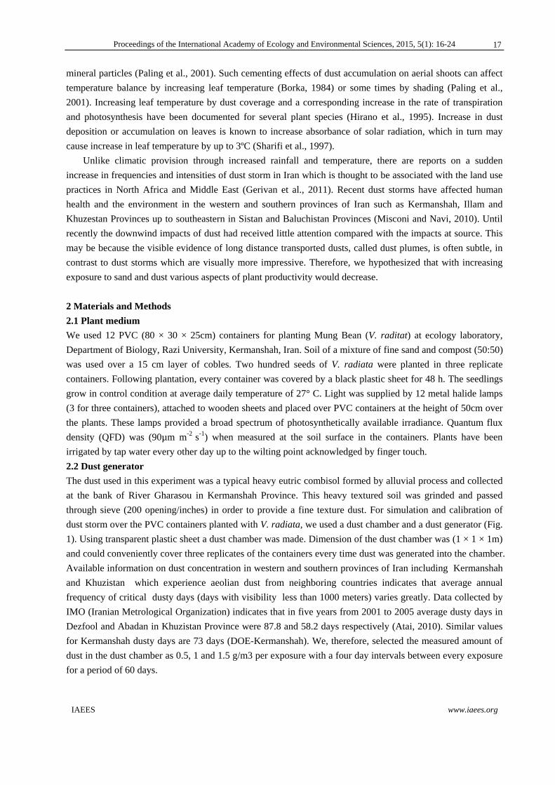
dust storm over the PVC containers planted with V. radiata, we used a dust chamber and a dust generator (Fig.

1). Using transparent plastic sheet a dust chamber was made. Dimension of the dust chamber was (1 × 1 × 1m)

and could conveniently cover three replicates of the containers every time dust was generated into the chamber.

Available information on dust concentration in western and southern provinces of Iran including Kermanshah

and Khuzistan which experience aeolian dust from neighboring countries indicates that average annual

frequency of critical dusty days (days with visibility less than 1000 meters) varies greatly. Data collected by

IMO (Iranian Metrological Organization) indicates that in five years from 2001 to 2005 average dusty days in

Dezfool and Abadan in Khuzistan Province were 87.8 and 58.2 days respectively (Atai, 2010). Similar values

for Kermanshah dusty days are 73 days (DOE-Kermanshah). We, therefore, selected the measured amount of

dust in the dust chamber as 0.5, 1 and 1.5 g/m3 per exposure with a four day intervals between every exposure

for a period of 60 days.

17


IAEES www.iaees.org

Fig. 1 Schematic presentation of the dust generator and dust chamber has used in present study.

2.3 Biomass

In order to assess productivity of planted V. radiata under exposure of varying amounts of dust, dry and wet

mass of leaf and roots were measured. At every sampling (every four day intervals), four plants unearth

completely from each vessel and cleaned thoroughly by tap water for removing debris. In order to obtain the

DM, fresh root and leaf of the plant have been incubated at 60º C for 48 h and weighted to get DM.

2.4 Chlorophyll content

Content of Chl a, b and total obtained using Arnon (1949) method. At end of experiment, four individual leaf

were collected from each container and cleaned thoroughly by water, then 0.2g fresh leaf from each sample

was separated, grinded in a mortar with 5ml of (80%) acetone (acetone: water 80:20 v:v) and 15ml of (100%)

acetone. After, the absorbance at A645 and A663 was read in the spectrophotometer instrument. For

calculation, Arnon’s equation “Eq. (1)” was used to convert absorbance measurements to mg Ch/g1 leaf tissue:

Chl a (mg/g1) = [(12.7 × A663) - (2.6 × A645)] × ml acetone/mg1 leaf tissue

Chl b (mg/g1) = [(22.9 × A645) - (4.68 × A663)] × ml acetone/mg1 leaf tissue

Chl T= Chl a + Chl b

Growth parameters like vigor index (VI), tolerance index and percentage of phototoxicity (Bewly and

Black, 1982) were evaluated. Also, biochemical parameters such as total sugar (Nelson, 1944) were measured

and recorded.

2.5 Chlorophyll a fluorescence

Chl a fluorescence was determined with portable, pulse amplitude, modulated fluorometer (MINI-PAM, S/N:

PYAA0421). ФPSII were calculated as (Fm´-F)/ Fm´ (Genty et al., 1989). Measurements of Chl a

fluorescence was made under laboratory conditions at saturating on the same leaves. ETR through PSII was

calculated as ФPSII × PFDa × 0.5 assuming that (84%) of incidental light is absorbed by leaves (PFDa) and

those photons are equally distributed between PSII and PSI (Schreiber et al., 1995). Fv/Fm of electron

transport through photosystem II (PS II) was specified from Chl a fluorescence induction kinetic. It was

measured after 30 min dark period in black room.


3.1 Biomass

3.1.1 Leaf dry mass

18


IAEES www.iaees.org

The effect of different amounts of dust exposure on leaf DM after the course of the experiment (60 days) is

illustrated in Fig. 2a. At this stage, leaf DM showed a significant difference in T3 at 0.05 confidence level

using single factor analysis of variance (ANOVA). Average reductions in the amount of leaf DM at the end of

experiment for the three treatments (0.5, 1 and 1.5 g/m3) were 5%, 14% and 27%. However, the degree of leaf

DM reduction varies between the treatments. Average reduction in DM at the end of the experiment in T1

compare to T2 was not significant at 0.05 level, but T1 compare with T3 was significant (p≤ 0.05). Also, the

amount of DM in T2 compare to T3 did not show a significant difference.

Fig. 2 Effect of dust on leaf DM (a) and root DM (b) in V. radiata exposed to 0.5, 1 and 1.5 g/m3 of dust in the dust chamber. Error bars indicate one standard error of the mean. T1, T2, T3 and C represent treatment 1, 2, 3 and control.

3.1.2 Root dry mass

In spite of the impact of sand-dust concentrations on plant leaf, plant root performed a slow and random

reaction to the sand-dust exposure. After the end of the experiment, plant exposure to the highest concentration

of dust (1.5 g/m3), the amounts of root DM illustrated a reduction compared to the control. In total, while

plants in control perform 0.89% growth in root DM, exposure to 0.5, 1 and 1.5 g/m3causes about 39%

reduction in root DM (Fig. 2b).

3.2 Chlorophyll a, b

The impact of sand-dust amounts at 0.5, 1 and 1.5 g/m3 on Chl a content in V. radiata is presented in Fig. 3a. It

is clear that the exposure to sand-dust amounts has caused a reduction in Chl a content as shown in T1, T2 and

T3 compared to control. Statistical analysis illustrates no significant difference (p≤0.001) for all treatments.

These reductions were 4% (T1), 8% (T2) and 17% (T3). Differences among treatments were not considerable

as the reduction in Chl a content in T1 compare to T2 was not significantly different. Also, T2 compare with

T3 had not a significant difference (p≤0.05).

19


IAEES www.iaees.org

Fig. 3 The impact of simulated sand-dust storm on Chl a (a), Chl b (b), Total chl (c), Total sugar (d), Vigour index (e), Tolerence index (f) and Percentage phototoxicity (g) in V. radiata exposed to concentration of 0.5 (T1), 1 (T2) and 1.5 g/m3 (T3) of dust in a dust chamber. Error bars indicate one standard error of the mean. Significant difference are shown by (*), (**) and (***) at 0.05 and 0.01 and less probability levels using single factor analysis of variance.

20


IAEES www.iaees.org

In Fig. 3b, the reduction in Chl b content of the plant exposed to 0.5 g/m3 dust per cubic meter was

significant, As, higher concentration of dust amounts (1.5 g/m3) has caused significant differences in Chl b

content of the leaf (Fig. 3b). Also, similar to Chl b, Chl T, Growth parameters like vigor index, tolerance

index and percentage of phototoxicity and total sugar illustrated reclined respond to sand-dust exposure in

third treatment (Fig. 3c, d, e, f and g). This reduction for Chl T was significant in (T3) 25%.

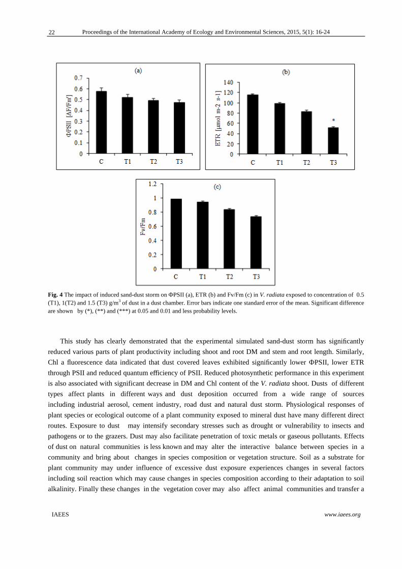
3.3 Chlorophyll fluorescence

Fig. 4 provides changes in the amount of ФPSII, ETR and Fv/Fm compare to control sample. Despite of

decline in all treatment, ФPSII of Control samples compared to treatments had not the significant difference at

the 0.05 level (p≤0.05). Exposure to dust resulted in a reduction in ETR of 15%, 22%, and 43%. However,

control samples than to third treatment had the significant difference at 0.05 levels. Also, there was not the

significant difference at 0.05 level within three treatments. Similarity, Fv/Fm was reduced by increasing of the

exposure of sand-dust concentration but, control compare to T1, T2 and T3 has no significance difference at

0.05 level (p≤0.05). Also, T1 compare to T2 and T3 had no significant difference at 0.05 level.

4 Conclusions

Present study provides information indicating that both Chl content and chlorophyll a fluorescence are affected

by exposure to sand-dust. Anthropogenic dust pollution result in the decrease in physiological characteristics

of seed progeny, germinability, and root length (Prokopiev et al., 2012). The reduction in Chl content of the

shoot exposed to dust compared to that of the control leaf may be attributed to the alkaline condition

developed by solubilization of chemicals present in the dust particulates in cell sap which is believed to be

responsible for Chl degradation (Prusty et al., 2005). Another factor that may cause a reduction in the synthesis

of Chl a is dust deposition on leaf surfaces (Chaurasia et al., 2013). Inhibition of enzymes essential for Chl

biosynthesis might be caused by the interference of dust particles which, it is a potential factor in leading to a

reduction in Chl content (Vijaywargiya and Pandey, 1996). Similar reduction in the total Chl content of leaves

exposed to polluted air was reported by various authors (Anthony, 2001). The extent of reduction of Chl

pigments under the influence of dust deposition in present study is similar to several studies. Chl a and b

contents in the leaf samples of Ficus religiosa under the influence of industrial dust have shown 38.13% and

42.73% reductions respectively (Prusty et al., 2005). In a similar study Rao (1971) has reported 20.13 and

19.70% decreasing in Chl a and b for Mangifera indica. The reduction decrease of 38.13% in Chl a was

recorded at polluted site in comparisons to control site, whereas a decrease of 42.73% in Chl b was recorded at

polluted site in comparison to control site (Chauhan, 2010).

21


IAEES www.iaees.org

Fig. 4 The impact of induced sand-dust storm on ФPSII (a), ETR (b) and Fv/Fm (c) in V. radiata exposed to concentration of 0.5 (T1), 1(T2) and 1.5 (T3) g/m3 of dust in a dust chamber. Error bars indicate one standard error of the mean. Significant difference are shown by (*), (**) and (***) at 0.05 and 0.01 and less probability levels.

This study has clearly demonstrated that the experimental simulated sand-dust storm has significantly

reduced various parts of plant productivity including shoot and root DM and stem and root length. Similarly,

Chl a fluorescence data indicated that dust covered leaves exhibited significantly lower ФPSII, lower ETR

through PSII and reduced quantum efficiency of PSII. Reduced photosynthetic performance in this experiment

is also associated with significant decrease in DM and Chl content of the V. radiata shoot. Dusts of different

types affect plants in different ways and dust deposition occurred from a wide range of sources

including industrial aerosol, cement industry, road dust and natural dust storm. Physiological responses of

plant species or ecological outcome of a plant community exposed to mineral dust have many different direct

routes. Exposure to dust may intensify secondary stresses such as drought or vulnerability to insects and

pathogens or to the grazers. Dust may also facilitate penetration of toxic metals or gaseous pollutants. Effects

of dust on natural communities is less known and may alter the interactive balance between species in a

community and bring about changes in species composition or vegetation structure. Soil as a substrate for

plant community may under influence of excessive dust exposure experiences changes in several factors

including soil reaction which may cause changes in species composition according to their adaptation to soil

alkalinity. Finally these changes in the vegetation cover may also affect animal communities and transfer a

22


IAEES www.iaees.org

community of mainly vertebrate grazers to a community of mainly soil invertebrates or microbial consumers

(McTainsh and Strong, 2006).

V. radiata is a major legume crop in western Iran. Seeds of V. radiata are rich in amino acids and protein

and serve as a valuable protein source for human consumption. Also, sprouts of this plant are eaten as a

vegetable and are a source of mineral elements and vitamins (Somta et al., 2008). It is not easy to extrapolate

the results of present study to agricultural products in the general study area. However, this study provides

several major impacts upon agricultural products. Most direct impact of sand-dust storm is the loss of crop and

possibly on the livestock resulted from tissue damage. There is a direct loss of plant productivity resulted from

damaged caused to plant tissue as a result of sandblasting. With this loss of plant leaves, there is a reduction in

photosynthetic activity and therefore reduced energy for the plant to utilize for growth, reproduction.

Additionally, the loss of energy for plant growth would also delay plant development and in regions with short

growing seasons. If the sand and dust storms occur later in the season, the plant damage will reduce yield

during grain development and if it occurs at maturity but before harvest, there will be a direct harvest loss.

Acknowledgement

The author is thankful to the Razi University for financial assistance and necessary facilities to accomplish the

present work.

References

Anthony P. 2001. Dust from walking tracks: Impacts on rain forest leaves and epiphylls, Cooperative Research

Centre for Tropical Rain forest Ecology and Management, Australia. Available at www.rainforest-

crc.jcu.edu.au

Arnon DI. 1949. Copper enzymes in isolation chloroplasts, poly-phenoloxidase in Beta vulgaris. Plant

Physiology, 24: 1-15

Atai H. 2010. Dust one of the environmental problems in Islamic world case study: Khozestan province,

ICIWG

Bewly JD, Black BM, 1982. Germination of seeds, In: Physiology and Biochemistry of Seed Germination

(Khan AA, ed), Springer-Verlag, USA

Borka G. 1984. Effect of metalliferous dust from dressing works on the growth, development, main metabolic

processes and yield of winter wheat in situ and under controlled conditions. Environmental Pollution, 35:

67-73

Chauhan A. 2010. Photosynthetic pigment changes in some selected trees induced by automobile exhaust in

Dehradun, Uttarakhand. New York Science Journal, 3: 45-51

Chaurasia S, Karwariya A, Gupta AD. 2013. Effect of cement industry pollution on chlorophyll content of

some crops at Kodinar, Gujarat, India. Proceedings of the International Academy of Ecology and

Environemental Sciences, 3(4): 288-295

Genty B, Briantais JM, Baker NR. 1989. The relationship between the quantum yield of photosynthetic

electron transport and quenching of chlorophyll fluorescence. Biochemica et Biophysica Acta, 990: 87-92

Gerivan H, Lashkaripour GR, Ghafoori M, et al. 2011. The source of dust storm in Iran: a case study based on

geological information and rainfall data. Carpathian Journal of Earth Environmental sciences, 6: 297-308

Hirano T, Kiyota M, Aiga I. 1995. Physical effects of dust on leaf physiology of cucumber and kidney bean

plants. Environmental Pollution, 89: 255-261

23


IAEES www.iaees.org

McTainsh G, Strong C. 2006. The role of Aeolian dust in ecosystems. Geomorphology, 89: 39-54

Misconi H, Navi M. 2010. Medical Geology in the Middle East. 135-174, Springer, Netherlands

Nelson N. 1944. A photometric adaptation of the somogyis method for the determination of reducing sugar,

Liebigs Annalen der Chemie, 3: 426-428

Naidoo G, Chirkoot D. 2004. The effects of coal dust on photosynthetic performance of the mangrove,

Avicennia marina in Richards Bay, South Africa. Environmental pollution, 127: 359-366

Paling EI, Humphries G, McCardle I, et al. 2001. The effects of iron ore dust on mangroves in Western

Australia: lack of evidence for stomatal damage. Wetlands, 9: 363-370

Prokopiev IA, Filippova FV, Shein AA. 2012. Effect of anthropogenic pollution with dust containing heavy

metals on seed progeny of spear saltbush. Russian Journal of Plant Physiology, 59: 238-243

Prusty BAK, Mishra PC, Azeez PA. 2005. Dust accumulation and leaf pigment content in vegetation near the

national highway at Sambalpur, Orissa, India. Ecotoxicology and Environmental Safety journal, 60: 228-

235

Rao DN. 1971. A study of the air pollution problem due to coal unloading in Varanasi, India. In Proceedings

of the Second International Clean Air Congress(Englund HM, Beery WT, eds). 273-276, Academic Press,

New York, USA

Schreiber U, Bilger W, Neubauer C. 1995. Chlorophyll fluorescence as a non-intrusive indicator for rapid

assessment of in vivo photosynthesis, In: Ecophysiology of Photosynthesis. 49-70, Springer-Verlag,

Berlin/Heidelberg, Germany

Sharifi MR, Gibson AC, Rundel PW. 1997. Surface dust impacts on gas exchange in Mojave Desert shrubs.

Applied Ecology, 34: 837-846

Somta C, Somta P, Tomooka N, et al. 2008. Characterization of new sources of Mung bean (Vigna radiata L.

Wilczek) resistance to bruchids, Callosobruchus spp. Journal of Stored Products Research, 44: 316-321

Vijaywargiya A, Pandey GP. 1996. Effect of cement dust pollution on soybean physiological and biochemical.

Ecology Environment and Conservation, 2: 143-145

24


IAEES www.iaees.org

Article

Interactive effects of arsenic and phosphorus on their uptake by

wheat varieties with different arsenic and phosphorus soil treatments

N. Karimi 1, M. Pormehr1, H. R. Ghasempour2 1Laboratory of plant physiology and Biotechnology, Department of Biology, Faculty of Science, Razi University, Kermanshah,

Iran 2Department of Biotechnology-Chemical engineering, Science and Research Branch, Islamic Azad University, Kermanshah, Iran

E-mail: [email protected], [email protected]

Received 17 July 2014; Accepted 25 August 2014; Published online 1 March 2015

Abstract

In this research we have investigated relationship between arsenate and phosphate uptake and its distribution in

root, shoot, and seed of wheat varieties. Three wheat varieties were selected and grown in 7 Kg pots under

controlled conditions among which, Sardari variety were collected from Iranian arsenic contaminated area and

tested along with two other varieties Parsi and Pishtaz. The aim was to select a variety with low arsenate

uptake ability with the aim of improving food safety and human health. Arsenic was applied with following

concentrations of 0, 5, 25, 125 and 625 mg l−1

in the presence or absence of P. With increasing As

concentration in irrigation water, As levels of roots, shoots and seeds increased. Also, measurements indicated

that As uptake rates decreased in the presence of P. Also, at 125 and 625 mg l−1 As concentration levels, the

measured As concentrations of seed and shoot exceeded the tolerance limit, regardless of P presence. Among

wheat varieties, Sardari (of contaminated area) had significantly less uptake of As compared with two other

varieties. Besides, P concentrations in all wheat varieties followed the following order: seed > root > shoot.

Keywords arsenate; contaminated area; food safety; phosphate; wheat.

1 Introduction

1 Introduction

Agricultural soils in many parts of the world are slightly to moderately contaminated by heavy toxic metal

such as Cd, Cu, Zn, Ni, Co, Cr, Pb, and As (Yadav, 2009). Arsenic (As) is a ubiquitous trace element with

mean lithosphere concentration of 5 mg kg-1. In soils, As level is generally around 5-10 mg kg-1 and

concentration above 20 mg kg-1 soil is considered high (Smedley and Kinniburgh, 2002). Also, its

environmental inputs can be through either natural (geogenic) or anthropogenic processes. Natural processes

including volcanic eruption, weathering of rocks and minerals, fossil fuel, and forest fire can release huge

amounts of As into the environment that may be transported over long distances as suspended particulates



IAEES www.iaees.org

through both water and air. Anthropogenic activities are the main source of As in the environment, exceeding

natural sources by 3:1 (Woolson, 1983). Among the anthropogenic sources, industrial effluents constitute the

largest contribution. Industrial sources generally include coal-fired power plants, smelting, incinerations of

wastes, wood preservation, and agriculture fertilizers (Mahimairaja et al., 2005). The present free style way of

disposing agricultural, industrial and domestic effluents into natural water-bodies results in serious surface and

groundwater contamination (Zandsalimi et al., 2011; karimi et al., 2010). During the last three decades, high

concentrations of As in ground water have been reported in different regions of the world such as the USA,

China, Chile, Bangladesh, Taiwan, Mexico, Argentina, Poland, Canada, Hungary, Japan, India, Vietnam,

Nepal (Jack et al., 2003) and recently from Iran (Mosaferi et al., 2003; Karimi et al., 2009; Karimi et al., 2013).

As contaminated ground water is not only used as a source of drinking water, but also extensively used for

irrigation in some regions (Kazia et al., 2009). Long term use of As contaminated water for irrigation has

resulted in elevated As levels in agricultural soils (Meharg and Rahman, 2003).

As is typically considered a non-essential element for plants and its bioavailability depends on plant

species and soil properties (Tao et al., 2006). The absorption of As by plants is influenced by the concentration

of As in soil (National Research Council of Canada, 1977). In general, As availability to plants is highest in

coarse-textured soils having little colloidal material and little ion exchange capacity, and lowest in fine-

textured soils high in clay, organic material, iron, calcium and phosphate (National Research Council of

Canada, 1978). Crop and vegetable production can benefit from knowledge of habitats and external conditions

which might promote a higher accumulation of As in edible parts of the plants (Wolterbeek and van der Meer,

2002; Karimi et al., 2013). For example, Rice may take up As from the surrounding soil and the concentration

of As in rice grains can reach elevated levels (Williams et al., 2007). The concentration of As in rice is usually

below 0.5 mg kg-1 (DW), but since it is common to eat approximately 200 g (DW) of rice per day in Asian

diets (Zhu et al., 2008), the total amount of ingested As can reach levels 5-10 times higher than the daily limit

set compared to drinking water (Sun et al., 2009). Beside, this conclusion is also true in the case of wheat. Rice

and wheat are the main cereal cultivated in world. Grain is largely used in human food and also as feed for

poultry. Also, straw may be used as fodder for cattle. To evaluate the possible health risk to humans

consuming crops irrigated with As contaminated water, information is needed regarding the soil-to-plant

transfer of As and to minimize the accumulation of As in plants consumed directly by humans, farm animals or

wildlife (Meharg and Hartley-Whitaker, 2002). In addition, pesticides and fertilizers are the major sources of

As in agricultural soils (Jiang and Singh, 1994). Numerous cases of As contamination of agricultural soils due

to arsenic containing pesticides have been reported (Woolson et al., 1971; Peterson et al., 1981; Merry et al.,

1986).

Arsenic can be found in both organic and inorganic compounds with variable oxidation states.

Understanding the difference between inorganic and organic arsenic is important because some of the organic

forms are less harmful than the inorganic forms. EPA has classified inorganic arsenic as a known human

carcinogen (ATSDR, 2005). Arsenate, the dominant inorganic species of arsenic in aerobic/oxic environments,

while arsenite species dominates under anoxic conditions (Sadiq, 1997). Arsenate, which is chemically very

similar to orthophosphate, is thought to enter the root cell by the same uptake mechanism as phosphate in a

variety of organisms (Asher and Reay, 1979; Meharg and Macnair, 1994). Kinetic studies suggest that at least

two phosphate uptake systems exist, a low and a high affinity system (Meharg and Macnair, 1990; Ullrich-

Eberius et al., 1984). The understanding of the general patterns of accumulation and speciation of As in plants

could help to elucidate the implications for dietary uptake of As from crops and vegetables cultivated in As

contaminated soils.

26


IAEES www.iaees.org

The aim of this study was to evaluate the accumulation rate of As in the presence and absence of P and also

its effects on phyto toxicity, uptake and partitioning between different parts (seed, shoot, root) of three wheat

varieties that grown in contaminated and uncontaminated soil. Also, to select a variety with a low arsenate

uptake rate in order to improve food quality and safety.

2 Material and Methods

2.1 Growth conditions and treatments

The present experiments were conducted from September 2011 to June 2012 in a controlled condition

greenhouse of Razi University. The greenhouse temperature was 14°C at night and 30 °C days, with an

average photon flux of 825 mmolm_2 s_1. Three varieties of wheat (Triticum aestivum cv. Sardari, Parsi and

Pishtaz) were selected for the study by the Sub-Center of Cereal Quality Control, Ministry of Agriculture of

Iran. Seeds of contaminated Sardari were collected from populations growing in six contaminated villages of

Bijar County, in the Northeast Kurdistan province, West of Iran, grid reference 34° 442 to 36° 302 North, and,

45° 312 to 48° 162 East. These villages were selected on the basis of the high arsenic contamination and the

inadequate supply of safe drinking water (Mosaferi et al., 2009). Control population of Sardari variety was

sourced from fields of Kermanshah province, grid reference 34°1815N 47°0354E. Wheat plants were

grown in pots filled with 7 kg of the soil planted at a density of 10 seeds per pot sown directly in the pots, and

irrigated during the first 2 weeks with water. After this period the seedlings were thinned to four per pot. A

solution of As (Na3AsO4.12H2O) was mixed thoroughly with the soil at a rate of 0 (control), 5, 25, 125 and

625 mg l-1 soil. The four As treatments used in this study represent either moderate or serious contamination

dose levels in Iran. Each treatment was replicated 3 times. Furthermore, in half of the pots 5.6 mM P as

K2HPO4 was added to the nutrient solution in order to evaluate the influence of P on As uptake by plants. Thus,

there were two sets of treatments one supplemented with Pi (P−) and the other without Pi (P+).

2.2 Soil preparation and characteristics

Pots were filled with a coarse-silt loam Soil, collected from a local farm at 0-15 cm depth. It was crushed,

mixed thoroughly and sieved through a 2 mm mesh. A composed sample from this soil was collected for

physico-chemical analysis. Some soil properties are presented in (Table 1). Soil properties were determined as

follows: pH was determined by potentiometer in a soil paste saturated with water and organic matter was

determined by dichromate oxidation using the Turin method (Soon and Abboud, 1991). For determination of

CEC the soil was extracted with 1 M NH4OAc at pH 7.0. Total phosphorus concentration was determined by

colorimetric method using 0.5 M NaHCO3 as the extract ant Olsen method (Olsen et al., 1954). The particle

size distribution (sand, silt and clay) was analyzed by the hydrometer method (Ashworth et al., 2001). The

arsenic concentration in soil was determined by inductively coupled plasma atomic emission spectroscopy

(ICP-AES, Shimadzu, 6200) (Meharg and Jardin, 2003).

Table 1 Physical and chemical properties of soil.

Soil characteristics Value Clay (%) 50.60 Silt (%) 20.98 Sand (%) 26.74 pH (1:2.5 H2O) 7.51 CEC (mequiv/100 g) 11.7 Organic matter (%) 1.38 Total phosphorus (mg/kg) 78.6 Total As (mg/kg) 5.53

27


IAEES www.iaees.org

2.3 Sampling and harvest procedure

When the wheat plants were harvested, they were thoroughly washed with tap water, and then with distilled

de-ionized water, adhering water was then removed with filter paper. Root, shoot and seeds of each plant was

separated and oven-dried at 70°C for 48 hrs, and dry weight was determined.

2.4 Total As analysis

Oven-dried plant materials were digested in nitric acid on a heating block, and the temperature was at 100°C

for 1 h, then at 120°C for 2 h. Reagent blank and standard reference were used to verify the precision of

analytical procedures. The concentrations of As were measured by a hydride generation–atomic absorption

spectrometer (Shimadzu, 6200). Hydride generation was used for samples due to their lower detection limits of

detection (0.5 μg l−1) (Meharg and Jardin, 2003).

2.5 Statistical analysis

All data were expressed as an average of three replicates. Treatment effects were determined by analysis of

variance according to the General Linear Model procedure of the SPSS program. Duncan test at a 5%

probability was used for post harvest comparisons in order to separate treatment differences.

3 Results

3.1 Concentration of As in root, shoot and seed

The results showed that root As concentration in wheat varieties increased significantly with increasing As

levels in irrigation water, particularly in pots without P treatments (P-) (Table 2). So, by increasing As level in

irrigation water from 5 to 625 mg l−1, the measured As concentration levels of roots ranged from 7.31 to 75.9

and 3.4 to 74.9 mg kg−1 in pots without P- and with P+ treatments (Table 2). Also, in pots without P-

treatments, root As concentration was at the highest As level (625 mg l-1) which were 7, 4.7, 4.5 and 4.5 times

higher than the lowest As level (5 mg l-1) in contaminated area of which Sardari seeds were collected and

uncontaminated area of Sardari, Parsi and Pishtaz wheat varieties, respectively. The reduction of arsenic in

different treatments followed the same pattern in three wheat varieties. So that, root As concentration in the

presence of phosphate showed a significant reduction from 5 to 25 mg l-1 treatments of As, But at 125 to 625

mg l-1 treatments of As didn’t show a significant reduction (Table 2). Though, the Parsi and Pishtaz from

uncontaminated area, and Sardari from contaminated area had the highest and lowest As concentration in plant

roots (Table 3). Also, addition of phosphate to pots caused a significant reduction of As concentration in roots

of Sardari variety (Table 3).

Then, total arsenic uptake due to the different implemented levels of As treatments in shoot of wheat

varieties were determined. Thus, Table 2 presents the results of arsenic uptake by plant shoots in pots without

P- and with P+. Shoot As concentration of wheat varieties showed a significant increase in all treatments. Also,

Pi application significantly decreased shoot As concentration in 5 to 25 mg l-1 treatments of As. But, no

significant differences were found at 125 to 625 mg l-1 treatments of As (In all wheat varieties). In the absence

of P, shoot As concentration was at the lowest As level (5 mg l-1) and were in the ranged of 3.7, 7.5, 7.9 and 8

mg kg−1, when irrigated with the highest As level (625 mg l−1) increased to 24.6, 54.9, 57.6 and 56.3 mg kg −1

in contaminated Sardari as well in uncontaminated Sardari, Parsi and Pishtaz varieties. Furthermore, in the

presence of P, shoot As concentration increased slightly from 1.7, 3.5, 3.8 and 3.9 to 24.5, 54.5, 57.8 and 56.7

mg kg−1 in all wheat varieties (Table 2). Both root and shoot As concentration increased as As levels increased

in both with or without P treatments, even though in pots without P- these ratios were much higher (Table 2).

Our results demonstrate that root As concentrations increased more rapidly than shoot and that roots were

more sensitive to As than shoots.

28


IAEES www.iaees.org

In spite of, the maximum As concentration allowed in fodder plants by the law is 4 mg kg-1 on a dry weight

basis (Zhang et al., 2009), the wheat varieties investigated in this study accumulated relatively higher

concentration of As in their edible parts; which this might represent a risk for animal and human health when

this crop are grown on As contaminated soils and consumed. Except, Sardari variety of the one which was

collected from contaminated area, that showed the lowest amounts of As in shoot at 5 mg l-1 treatment of As,

but the other wheat varieties showed higher As amounts in shoot than the standard limit in all pots without P-

treatments. Although, in pots treated with phosphate at 5 mg As l-1 treatment it did reduce the arsenic levels

below the standard limit in all three wheat varieties (Table 2). The Parsi and Pishtaz varieties from

uncontaminated area, and Sardari from contaminated area had the highest and lowest As concentration in plant

shoots (Table 3). Also, addition of phosphate to pots caused a significant reduction of As concentration in

shoots of Sardari variety (Table 3). But, shoot As concentration in the presence of phosphate did not show a

significant reduction in Parsi and Pishtaz varieties (Table 3).

Table 2 describes changes in accumulation levels As by wheat seeds under different As and As × P As

treatments. In pots without P- treatments, As concentrations in pots treated with 5 mg l-1 of As the measured

data were 0.3, 0.4. 0.6 and 0.7 mg kg−1 Sardari seeds collected from contaminated lands verses Sardari, Parsi

and Pishtaz from uncontaminated lands. But, at As level of 625 mg l-1, As levels increased to 3.4, 4.3, 5.4 and

5.7 mg kg −1. Also, in pots with P+ treatments, as As levels in irrigation water augmented from 5 to 625 mg l−1,

As concentrations from 0.1, 0.2, 0.3 and 0.4 increased to 3.1, 4.2, 5.4 and 5.7. Our study showed that As

concentrations of grains exceeded the tolerance limit described by Zhang et al., (2009) up to 0.5 mg kg-1. Even

though, the Sardari variety which seeds were collected from contaminated area significantly showed the lowest

levels of As in grain. Also, among the pots which were fertilized with P only at As levels of 5 mg l-1 treatment

of As levels reduced below the tolerance limit. Furthermore, as mentioned, Sardari variety (seeds collected

from contaminated and uncontaminated lands) reduced As levels below the tolerance limit in both 5 and 25 mg

l-1 of As (Table 2). The Parsi and Pishtaz varieties from uncontaminated area and Sardari from contaminated

area had the highest and lowest As concentration in plant seeds (Table 3). Also, addition of phosphate to pots

caused a significant reduction of As concentration in seeds of wheat varieties (Table 3).

Table 2 Root, shoot and seed arsenic accumulation (mg/kg) in wheat varieties (Triticum aestivum cv. Sardari, Parsi and Pishtaz) exposed to four arsenic treatments (5, 25, 125 and 625 mg l−1).

Seed As content Shoot As content Root As content Treatments (mg l−1)

Variety (mg kg−1)

0.08±0.005 e 1.3±0.1 e 2.8±0.21 ef Control(P-) Sardari (C) 0.3±0.05 d 3.7±0.13 d 7.3±0.48 d As 5 0.5±0.04 c 7±0.16 c 14.6±0.35 c As 25 2.4±0.08 b 16.3±0.53 b 21.8±0.35 b As 125 3.4±0.1 a 0.008±0.003 e 0.1±0.008 e 0.3±0.01 d 2.4±0.03 b 3.1±0.04 a

24.6±0.31 a 0.91±0.03 e 1.7±0.14 e 3.3±0.21 d 16.1±0.93 b 24.5±1.37 a

51.1±0.75 a 1.4±0.15 f 3.4±0.19 e 7.2±0.31 d 21.3±0.77 b 49.9±0.35 a

As 625 Control(P+) As 5 + P As 25 + P As 125 + P As 625 + P

0.08±0.003 f 1.5±0.11 ef 3.1±0.12 f Control(P-) Sardari (UC) 0.4±0.01 d 7.5±0.11 d 15.3±0.28 d As 5 0.6±0.03 c 15.4±0.26 c 34±1.52 c As 25 3.2±0.06 b 34.2±0.51 b 47.2±0.44 b As 125 4.3±0.1 a 54.9±0.87 a 73.2±1.3 a As 625

29


IAEES www.iaees.org

0.03±0.01 f 0.2±0.001 e 0.5±0.01 d 3.1±0.06 b 4.2±0.09 a

0.96±0.01 f 3.5±0.12 e 3.9±0.18 e 34.2±1.2 b 54.5±1.6 a

1.8±0.13 f 7.4±0.23 e 16.6±0.25 d 46.6±0.83 b 72.8±1.73 a

Control(P+) As 5 + P As 25 + P As 125 + P As 625 + P

0.06±0.003 e 1.3±0.1 f 2.7±0.2 f Control(P-) Parsi 0.6±0.005 d 7.9±0.1 d 16.7±0.1 d As 5 0.9±0.01 c 17.3±0.2 c 35.8±0.2 c As 25 4.3±0.06 b 37±0.2 b 50.6±0.3 b As 125 5.4±0.1 a 0.03±0.003 e 0.3±0.005 e 0.6±0.01 d 4.2±0.04 b 5.4±0.008 a

57.6±0.4 a 0.91±0.03 f 3.8±0.1 e 7.9±0.1 d 37.3±1.05 b 57.8±0.9 a

75.9±0.6 a 1.6±0.1 f 8.4±0.3 e 17.2±0.1 d 50.4±0.6 b 74.9±0.4 a


0.07±0.003 f 1.4±0.15 e 3.2±0.14 f Control(P-) Pishtaz 0.7±0.04 d 8±0.04 d 16.7±0.48 d As 5 1.1±0.03 c 17.8±0.14 c 36.3±0.17 c As 25 4.8±0.04 b 37.4±0.18 b 50.2±0.19 b As 125 5.7±0.08 a 0.04±0.002 f 0.4±0.002 e 0.7±0.004 d 4.8±0.05 b 5.7±0.06 a

56.3±1.4 a 0.97±0.005 e 3.9±0.05 e 8.4±0.16 d 37.4±1.3 b 56.7±2.3 a

75.9±0.41 a 1.6±0.09 f 8.3±0.32 e 17.9±0.06 d 49.8±1.26 b 74.3±1.71 a


The data are expressed as mean ± S.E. C= Sardari of contaminated area and UC= Sardari of

uncontaminated area. P+ and P- = with (P+) and without (P−) P fertilization. Data are expressed as mean

values of n=3 and have been analyzed by two-way analysis of variance. Means followed by the same letter

within columns are not significantly different by Duncan test at the 5% level.

Table 3 mean comparison of root, shoot and seed As accumulation in wheat varieties.

Variety Root arsenic Shoot arsenic Seed arsenic (mg kg-1)

Sardari P- (C) 19.55±4.5 e 10.59±2.3 e 2.06±0.4 e Sardari P- (UC) 34.46±6.5 b 22.74±5.2 b 3.4±0.6 bc

Parsi P- 36.20±6.7 a 24.21±5.4 a 3.5±0.7 ab

Pishtaz P- 35.51±6.8 a 24.26±5.3 a 3.6±0.7 a

Sardari P+ (C) 16.7±4.8 f 9.34±2.5 f 1.67±0.5 f

Sardari P+ (UC) 29.2±7.1 d 20.17±5.6 d 3.03±0.7 d

Parsi P+ 30.75±7.5 c 21.58±5.9 c 3.11±0.8 d

Pishtaz P+ 30.74±7.4 c 21.52±5.8 c 3.25±0.8 cd



30


IAEES www.iaees.org



3.2 Concentration of P in root, shoot and seed

The total phosphorus levels in root plants are shown in Table 4. There was not a broad variation of mean P

concentrations among wheat varieties, ranging from 12.7 to 33.7 mg kg−1 and 12.8 to 42.6 mg kg-1 in pots

without P- and with P+. Also, root phosphorus concentrations increased as the level of As increased. So, this

increase was proportional to the increase of As concentrations in treatments. Furthermore, by adding

Phosphate to the pots it did increase the concentration of P in the roots. Although, by escalating the As

concentrations in treatments, the amount of phosphorus in roots increased from 48% to 68%. Moreover, most

of the root P concentration was reported in Sardari variety collected from contaminated area (Table 5). On

contrary, the results showed that P concentration in shoot significantly decreased as As levels increased (Table

4). Although, over all Pi application increased shoot P concentration in pots with P+ as compared with the one

without P-. Also, at highest As level, Shoot P concentration levels decreased by 83.7% in Sardari variety of

contaminated area, 66.9% in uncontaminated Sardari, 74.2% in Parsi and 64.2% in Pishtaz compared with the

control. Although, this reduction was less severe in the treatments with P+, 66.6%, 58.4%, 61.6%, and 58%

(Table 4). So, this study confirmed the higher ability of roots, to accumulate P, than shoot in As treatments

(Similar behavior to arsenate resistant plants). Also, most of the shoot P accumulation was reported in Sardari

variety collected from contaminated area (Table 5). Seed P concentrations of wheat varieties treated with

different levels of As are summarized in Table 4. Grain P concentrations decreased with increasing level of As

in all wheat varieties. However, it showed no significant differences at 125 and 625 mg l-1 levels of As in pots

treated with or without phosphorus (Table 4). Generally, the phosphorus concentration of grains in pots treated

with P+ was higher than pots without P- treatments (Table 5). Thus, P concentrations in all wheat varieties

followed the following order: seed > root > shoot (Table 5).

Table 4 Root, shoot and seed phosphorus content (mg/kg) in wheat varieties (Triticum aestivum cv. Sardari, Parsi and Pishtaz) exposed to four arsenic treatments (5, 25, 125 and 625 mg l−1).

Seed P content Shoot P content Root P content Treatments (mg l−1)

Variety (mg kg−1)

73.5±0.76 b 25.3±0.51 b 12.7±0.24 e Control(P-) Sardari (C) 66.3±0.42 c 22.8±0.43 d 14.7±0.65 de As 5 49.2±0.82 e 15.2±0.41 f 19.2±0.7 d As 25 42±0.24 f 7.2±0.25 i 27.3±0.48 c As 125 38.2±0.59 g 82±1.31 a 72.4±0.74 b 63.8±0.73 d 42.3±0.38 f 38.7±0.71 g

4.1±0.20 j 26.1±0.55 a 23.5±0.48 c 19.8±0.33 e 11.2±0.4 g 8.7±0.26 h

33.7±0.77 b 13.1±1.1 e 14.9±0.86 de 25±1.2 c 35.9±2.1 b 42.6±3.1 a


70.6±0.51 b 25.1±0.58 a 13.5±0.41 g Control(P-) Sardari (UC) 64.8±0.34 c 23.6±0.43 c 15.1±0.73 f As 5 55.9±0.65 e 16.4±0.35 f 18.5±0.32 e As 25 31.5±0.31 f 10.6±0.36 h 22.2±0.64 d As 125 29.4±0.47 g 77.7±0.62 a 71.7±0.37 b 61.7±0.59 d 31.5±0.27 f

8.3±0.25 j 24.8±0.52 b 23.1±0.31 d 19.5±0.33 e 12.1±0.35 g

28.4±0.84 b 13.5±0.33 g 15.4±0.51 f 20.2±0.42 d 26.3±0.41 c

As 625 Control(P+) As 5 + P As 25 + P As 125 + P

31


IAEES www.iaees.org

29.3 ±0.64 g 10.3±0.23 i 34.4±0.71 a As 625 + P

57.2±0.65 b 24.1±0.58 b 12.9±0.47 f Control(P-) Parsi 49.3±0.51 d 22.2±0.44 d 15.8±0.31 e As 5 40.7±1.3 e 14.9±0.46 f 18.3±0.62 d As 25 28.6±0.41 f 9.3±0.35 i 20.8±0.41 c As 125 20.4±1.07 g 62.5±1.7 a 53.05±0.45 c 42.9±0.66 e 28.7±0.55 f 20.51±0.97 g

6.2±0.41 j 24.8±0.29 a 22.9±0.48 c 18.3±0.37 e 13±0.34 g 9.5±0.31 h

26.2±0.45 b 12.8±0.62 f 15.5±1.03 e 20.7±0.51 c 25.3±0.83 b 30.6±0.65 a


51.6±0.41 b 23.8±0.61 b 12.7±0.25 g Control(P-) Pishtaz 47.3±0.45 c 22.5±0.48 d 14.3±0.43 f As 5 37.7±0.53 e 16.1±0.35 f 19.2±0.35 e As 25 22.9±0.51 f 11±0.41 h 22.1±0.38 d As 125 17.5±1.11 g 57.3±1.15 a 50.2±0.46 b 41.2±1.01 d 23.2±0.72 f 17.5±1.03 g

8.5±0.29 j 24.1±0.55 a 23.3±0.57 c 18.7±0.34 e 12.5±0.31 g 10.1±0.33 i

24.6±0.41 c 12.8±0.82 g 15.7±0.54 f 22±0.35 d 26.5±0.71 b 30.5±0.39 a






Table 5 Mean comparison of root, shoot and seed phosphorus content in wheat varieties.

Variety Root phosphorus Shoot phosphorus Seed phosphorus (mg kg-1)

Sardari P- (C) 21.5±2.03 b 16.80±1.38 d 53.95±3.67 b Sardari P- (UC) 19.64±1.43 c 14.84±1.18 g 50.46±4.54 c

Parsi P- 18.84±1.22 c 15.40±1.26 f 39.29±3.58 e

Pishtaz P- 18.62±1.21 c 16.38±1.32 e 35.46±3.57 g

Sardari P+ (C) 26.27±3.18 a 18.02±1.77 a 59.96±4.57 a

Sardari P+ (UC) 22.09±2.04 b 17.86±1.59 b 54.46±5.41 b

Parsi P+ 21.02±1.75 b 17.70±1.72 c 41.53±4.13 d

Pishtaz P+ 21.53±1.76 b 17.75±1.66 c 37.92±4.15 f





32


IAEES www.iaees.org

4 Discussion

4.1 As concentrations in plant tissues

The four As treatments used in this study represent either moderate or high contamination levels in Iran

(Zandsalimi et al., 2011). Although varieties tested in this study differed in their response to As addition in soil,

but, they all followed the same pattern. Further experiments showed that As uptake by seedlings, which

followed Michaeli-Menten kinetics, increased with increasing As concentrations in the irrigation solution. So

that, there is a relationship between As concentrations of wheat roots, shoots, seeds and As treatments by

uncontaminated three wheat varieties. Arsenic concentration followed the order: root > shoot > seed in all

wheat varieties (Table 3). The ranking of plant parts according to As accumulation is regularly used as

“evidence” that aboveground edible parts are no risk to human health. It is, however, the absolute

concentration of inorganic As in the edible parts that should be evaluated, regardless of As concentrations in

other parts of the plant. The most As accumulation levels were in roots than any other plant parts which were

also reported in rice (Marin et al., 1992; 1993), maize, English ryegrass, rape and sunflower (Gulz et al., 2005)

their findings were similar to results reported in this experiments. For example, in pot experiments with rice

plants exposed to As added via As in irrigation water, Abedin et al. (2002a,b) ranked plant parts according to

the As concentrations as follows: root > straw > husk > grain (Bleeker et al., 2003; Carbonell et al., 1998;

Carbonell-Barrachina et al., 1997, 1998; Hartley-Whitaker et al., 2001; Sneller et al., 1999).

Also, there was a decrease in the shoot As concentration level than the root of wheat plants grown without

P (P−) and As levels reduced gradually from 46% to 34%, 33% and 34% in plants grown from collected seeds

of contaminated lands Sardari compared to Sardari, Parsi and Pishtaz varieties of uncontaminated area. Also,

there were a reduction of As accumulation in wheat seeds both in varieties irrigated with or without P. The

roots to shoot and shoot to seed transfer factor of As (TF) were in the range of 0.5–0.6, and 0.07 to 0.1 in all

varieties. Also, the results indicated that regardless of P treatment, most of the As accumulated in root and the

smallest amount in the seed, although this behavior was more pronounced in pots with P+. The results matches

with the studies in rice reported by Williams et al., (2007) and their data indicated that export of arsenic from

the shoot to the seed was under tight physiological control and the seed arsenic concentration level were much

lower than the shoot. Also, findings were similar to results reported for wheat by both Pigna et al. (2009) and

Zhang et al., (2009).

4.2 P concentrations in plant tissues

Also, Table 5 compares the changes of P accumulation levels in roots, shoots and seeds. as well, results

showed significant different accumulation rates of phosphorus in roots, shoots and seeds among the pots

treated with or without phosphorous. Moreover, the highest phosphorus concentration was observed in Sardari

roots of contaminated area. Also, Parsi, Pishtaz and uncontaminated Sardari varieties didn’t show a significant

difference in root P accumulation. In contrast, phosphorus accumulation of shoots decreased. Besides, the

lowest P concentration within the shoots found in Sardari variety collected from uncontaminated area. In

addition, the highest P accumulation rates in seeds belonged to Sardari variety of contaminated lands.

Furthermore, Phosphorus has the most important role in bioaccumulation potential of As in different parts

of plants. Considering the fact that P and As belong to the same chemical group, they stand for similar

geochemical behavior in soils (Adriano, 2001). Also, P is frequently the most restrictive element for plant

growth and the crop yield on 30%–40% of the world’s arable land is limited by P availability (Runge-Metzger,

1995). Phosphate in plants is important for energy transfer and protein metabolism (Marschner, 1995). In view

of the fact that, As is a chemical analogue to Phosphorus, As may exert toxicity to plants by interfering with

many physiological functions performed by P. Therefore, P should play a critical role in a plant’s protection

against As phytotoxicity (Meharg and Hartley-Whitaker, 2002). Meharg et al. (1994) postulated that Pi and

33


IAEES www.iaees.org

arsenate are accumulated by plant roots via the same uptake system, and that the Pi–arsenate uptake system is

much more efficient in accumulating Pi compared with arsenate. Geng et al., (2006) indicated that fertilization

by P may reduce the effects of As toxicity by restricting As accumulation in the above-ground parts of plants.

This has practical importance in agricultural systems, since may reduce yield losses and improve yield quality.

Also, P could decrease the reactive oxygen species and non-protein thiols production, formed during exposure

to As that cause tissue damage and lipid peroxidation (Hartley-Whitaker et al., 2001). Fitz and Wenzel (2002)

have reported that the effects of P on the uptake and toxicity of As in plants depends on plant species, chemical

speciation of As, growth medium and the experimental conditions. Our results were in agreement with these

findings, which reported P restricted the transfer of As from the soil to the above-ground plant organs.

Overall, Sardari variety collected from contaminated area showed a better tolerance to As for which several

explanations may be possible. This tolerance to arsenic could be related to some physiological and biochemical

adaptation strategies (Meharg, 1994). Also, some plants appear to have an exclusion mechanism which allows

them to bioaccumulate heavy metals at different levels, thus avoiding the uptake of too much of a toxic

element. Meharg and Macnair (1991) commented on the fact that internal tolerance mechanisms are

considered to play a more significant role than avoidance mechanisms in the adaptation of plants to

contaminated habitat. The definition of tolerance mechanisms which has been used by Meharg and Macnair

(1991) refers to biochemical detoxification and limited movement of the metal ion once absorbed in the plant,

or isolation of the ion within a cell.

In general, the tolerance to arsenic involves (1) complication of arsenic by such as peptides with SH-

groups (Karimi et al., 2009), (2) reduction of As influx by suppressing phosphate/arsenate uptake systems

(Meharg and Macnair, 1992; Meharg, 1994), and (3) enhanced production of antioxidants that detoxify free

reactive oxygen species (ROS) produced in response to As (Hartley-Whitaker, 2001). In Meharg and Macnair's

(1991) study on arsenate tolerance in certain grasses, they concluded that the evolved tolerance was due to an

adaptation of the arsenate uptake system. Porter and Peterson (1975) found that grasses growing on mine

wastes which contained high arsenic concentrations, tested plants developed a tolerance to the elevated levels

compared to the grasses found on a site with low standard levels. In conclusion, the long contamination history

of the surveyed areas in Iran, there was an evident exclusion mechanism of effective pressure toward As

tolerance by the crops species. To summarize, based on the current available information, risks to food safety

and yield are likely to increase with the buildup of As in the soil and irrigation water. Although the risks

cannot be quantified for the time being, it is proposed to focus on preventing and minimizing input via

irrigation and uptake by crops (Brammer, 2005; Duxbury et al., 2003; Karimi et al., 2009; Karimi et al., 2013).

For example, P fertilization may reduce the effects of As toxicity without increase As concentrations in the

above-ground parts of plants. This has practical importance in agriculture, since may reduce yield losses and

improve yield quality. Furthermore, breeding crops tolerant to As with a low accumulation of As in seeds may

reduce potential risks as well.

5 Conclusion

This study monitored the correlation between the arsenic content in different parts of tested wheat varieties and

also the arsenic concentration of irrigation water in the presence or in the absence of P fertilization. Although,

As concentrations which were used in this experiment could exist in areas with As contamination in

groundwater and soil deposited by mining activities. Moreover, Arsenic concentrations in root shoot and seed

increased with increasing As concentration in irrigation water. When Pi was added (P+), As concentration of

root, shoot and seed decreased compared to plants without Pi (P-) treatments. So, the arsenic content in

different parts of plants were found to be in the order of roots > shoots > seeds parts. Also, in 125 and 625 mg

34


IAEES www.iaees.org

l-1 of As treatment levels, shoot and seed parts of all varieties showed arsenic concentrations higher than the

Chinese food hygiene limit. Additionally, Sardari variety of contaminated area was found to be more resistant

to arsenic contamination than the other studied wheat varieties. Also, our results have shown that there were

considerable differences in arsenic transport rates into different plant organs. Besides, when P was applied it

did reduce the arsenic uptake into the plant organs. Thus, based on the results of the present study, phosphorus

application in rate according to the plant demands, leads to lower As accumulation in root, shoot and seed of

wheat. This has practical importance in agricultural performance.

References

Abedin MJ, Cotter-Howells J, Meharg AA. 2002a. Arsenic uptake and accumulation in rice (Oriza sativa L.)

irrigated with contaminated water. Plant and Soil, 240: 311-319

Abedin MJ, Cressner MS, Meharg AA, et al. 2002b. Arsenic accumulation and metabolism in rice (Oryza

sativa L.). Environ Science Technology, 36: 962-968

Adriano DC. 2001. Trace Elements in the Terrestrial Environment. Springer, New York, USA

Asher CJ, Reay PF. 1979. Arsenic uptake by barley seedlings. Australian Journal of Plant Physiology, 6: 459-

466

Ashworth J, Keyes D, Kirk R, Lessard R. 2001. Standard procedure in the hydrometer method for particle size

analysis. Communications in Soil Science and Plant Analysis. 32: 633-642

ATSDR. 2005. Draft Toxicological Profile for Arsenic. Agency for Toxic Substances and Disease Registry,

USA

Bleeker PM, Schat H, Vooijs R, Verkleij JAC, Ernst WHO. 2003. Mechanisms of arsenate tolerance in Cytisus

striatus. The New Phytologist, 157: 33-38

Brammer H. 2005. The Arsenic Problem in Bangladesh. Tropical Agriculture Association Newsletter.

Carbonell AA, Aarabi MA, Delaune RD, et al. 1998. Arsenic in wetland vegetation: availability, phytotoxicity,

uptake and effects on plant growth and nutrition. The Science of the Total Environment, 217: 189-199

Carbonell-Barrachina AA, Burlo F, Burgos-Hernandez A, et al. 1997. The influence of arsenite concentrations

on arsenic accumulation in tomato and bean plants. Scientia Horticulturae. 71: 167-176

Duxbury JM, Mayer AB, Lauren JG, Hassan N. 2003. Food chain aspects of arsenic contamination in

Bangladesh: effects on quality and productivity of rice. Journal of Environmental Science and Health, 38:

61-69

Fitz WJ, Wenzel WW. 2002. Arsenic transformations in the soil-rhizosphereplant system: fundamentals and

potential application to phytoremediation. Journal of Biotechnology. 99: 259-278

Geng CN, Zhu YG, Hu Y, et al. 2006. Arsenate causes differential acute toxicity to two P-deprived genotypes

of rice seedlings. Plant and Soil, 279: 297-306

Gulz PA, Gupta S, Schulin R. 2005. Arsenic accumulation of common plants from contaminated soils. Plant

and Soil, 272: 337-347

Hartley-Whitaker J, Ainsworth G, Vooijs R, et al. 2001. Phytochelatins are involved in differential arsenate

tolerance in Holcus lanatus. Plant Physiology, 126: 299-306

Jack CN, Wang J, Shraim AA. 2003. Global health problem caused by arsenic from natural sources.

Chemosphere, 52: 1353-1359

Jiang QQ, Singh BR. 1994. Effect of different forms and sources of arsenic on crop yield and arsenic

concentration. Water, Air, and Soil Pollution, 74: 321-343

35


IAEES www.iaees.org

Karimi N, Ghaderian SM, Raab A, et al. 2009. An Arsenic accumulating, Hypertolerant Brassica, Isatis

cappadocica. The New Phytologist, 184: 41-47

Karimi N, Ghaderian SM, Maroofi H, Schat H. 2010. Analysis of arsenic in soil and vegetation of a

contaminated area in Zarshuran, Iran. International Journal of Phytoremediation, 12: 159-173

Karimi N, Siyahat Shayesteh L, Ghasempour H, Alavi M. 2013. Effects of Arsenic on growth, photosynthetic

activity, and accumulation in two new hyperaccumulating populations of Isatis cappadococa Desv.

Journal of Plant Growth Regulation (DOI 10.1007/s00344-013-9350-8)

Kazia TG, Araina MB, Baig JA, et al. 2009. The correlation of arsenic levels in drinking water with the

biological samples of skin disorders. The Science of the Total Environment, 407: 1019-1026

Mahimairaja S, Bolan NS, Adriano DC, et al. 2005. Arsenic contamination and its risk management in

complex environmental settings. Advances in Agronomy, 86: 1-82

Marin AR, Masscheleyn PH, Patrick WH. 1992. The influence of chemical form and concentration of arsenic

on rice growth and tissue arsenic concentration. Plant and Soil, 139: 175-183

Marin AR, Pezashki SR, Masschelen PH, et al. 1993. Effect of dimethylarsenic acid (DMAA) on growth,

tissue arsenic, and photosynthesis of rice plants. Journal of Plant Nutrition, 16: 865-880

Marschner H. 1995. Mineral Nutrition of Higher Plants. Academic Press, UK

Meharg AA. 1994. Integrated tolerance mechanisms constitutive and adaptive plant responses to elevated

metal concentrations in the environment. Plant, Cell and Environment, 17: 989-993

Meharg AA, Hartley-Whitaker J. 2002. Arsenic uptake and metebolism in arsenic resistant and nonresistant

plant species. The New Phytologist, 154: 29-1879

Meharg AA, Jardine L. 2003. Arsenite transport into paddy rice (Oryza sativa) roots. The New Phytologist,

157: 39-44

Meharg AA, Macnair MR. 1990. An altered phosphate uptake system in arsenate-tolerant Holcus lanatus L.

The New Phytologist, 116: 29-35

Meharg AA, Macnair MR. 1991. The mechanisms of arsenate tolerance in Deschampsia cespitosa (L.) Beauv

and Agrostis capillaris L. The New Phytologist, 119: 291-297

Meharg AA, Macnair MR. 1992. Suppression of the high affinity phosphate uptake system a mechanism of

arsenate tolerance in Holcus lanatus L. Journal of Experimental Botany, 43: 519-524

Meharg AA, Macnair MR. 1994. Relationship between plant phosphorus status and the kinetics of arsenate

influx in clones of Deschampsia cespitosa (L.) Beauv that differ in their tolerance to arsenate. Plant and

Soil, 162: 99-106

Meharg AA, Rahman M. 2003. Arsenic contamination of Bangladesh paddy field soils: implications for rice

contribution to arsenic consumption. Environmental Science and Technology, 37: 229-234

Merry RH, Tiller KG, Alston AM. 1986. The effects of contamination of soil with copper, lead, and arsenic on

the growth and composition of plants. I. Effects of season, genotype, soil temperature, and fertilizers.

Plant and Soil, 91:115-128

Mosaferi M, Yunesian M, Mesdaghinia AR, et al. 2003. Occurrence of arsenic in Kurdistan Province of Iran.

In: BUET-UNU International Symposium. International Training Network Center, Dhaka, Bangladesh

Mosaferi M, Yunesian M, Dastgiri S, et al. 2009. Prevalence of skin lesions and exposure to arsenic in

drinking water in Iran. Science of The Total Environment, 390 : 69-76

National Research Council of Canada (NRCC). 1977. Committee on Medical and Biologic Effects of

Environmental Pollutants, Arsenic. 16-79. National Academy of Sciences, Washington DC, USA

National Research Council of Canada (NRCC). 1978. National Research Council of Canada Publications

NRCC 15391, 1-349, Canada

36


IAEES www.iaees.org

Olsen SR, Cole CV, Watanabe FS, Dean LA. 1954. Estimation of Available Phosphorus in Soils By Extraction

with Sodium Bicarbonate. Department of Agriculture, USA

Peterson PJ, Girling CA, Benson LM, et al. 1981. Effects of Trace Metals on Plant Function. Applied Science

Publisher, London, UK

Pigna M, Cozzolino V, Violante A, Meharg AA. 2009. Influence of phosphate on the arsenic uptake by wheat

(Triticum durum L.) irrigated with arsenic solutions at three different concentrations. Water, Air and Soil

Pollution, 197: 371-380

Porter EK, Peterson PJ. 1975. Arsenic accumulation by plants on mine waste (United Kingdom). Sei. Total

Environment, 4: 356-371

Runge-Metzger A. 1995. Closing the cycle: obstacles to efficient P management for improved global security.

In: Phosphorus in the Global Environment (Tiessen H, ed). 27-42, Wiley, Chichester, UK

Sadiq M. 1997. Arsenic chemistry in soils: an overview of thermodynamic predictions and field observations.

Water, Air and Soil Pollution, 93: 117-136

Smedley PL, Kinniburgh DG. 2002. A review of the source, behavior, and distribution of arsenic in natural

waters. Applied Geochemistry, 17: 517-568

Sneller EFC, Van Heerwaarden LM, Kraaijeveld-Smit FJL, et al. 1999. Toxicity of arsenate in Silene vulgaris,

accumulation and degradation of arsenate induced phytochelatins. The New Phytologist, 144: 223-232

Soon YK, Abboud S. 1991. A comparison of some methods for soil organic carbon determination.

Communications in Soil Science and Plant Analysis, 22: 943-954

Sun GX, Williams PN, Zhu YG, et al. 2009. Survey of arsenic and its speciation in rice products such as

breakfast cereals, ricecrackers and Japanese rice condiments. Environment International, 35: 473-475

Tao Y, Zhang Sh, Jian W, Yuan Ch, et al. 2006. Effects of oxalate and phosphate on the release of arsenic

from contaminated soils and arsenic accumulation in wheat. Chemosphere, 65: 1281-1287

Ullrich-Eberius CI, Novacky A, Van Bel AJE. 1984. Phosphate uptake in Lemna gibba Gr: energetics and

kinetics. Planta, 161:46-52

Williams PN, Villana A, Deacon C, et al. 2007. Greatly enhanced arsenic shoot assimilation in rice leads to

elevated grain levels compared to wheat and barley. Environmental Science and Technology, 41: 6854-

6859

Woolson EA. 1983. Emission, cycling and effects of arsenic in soil ecosystems, In: Biological and

Environmental Effects of Arsenic (Fowler BA, ed). Elsevier, Netherlands

Woolson EA, Axley JH. Kearney PC. 1971. The chemistry and phytotoxicity of arsenic in soils: I.

contaminated field soils. Soil Science Society of America Proceedings, 35(6): 938-943

Wolterbeek H, van der Meer A. 2002. Transport rate of arsenic, cadmium, copper and zinc in Potamogeton

pectinatus L.: radiotracer experiments with 76As, 109, 115Cd, 64Cu and 65/69Zn. The Science of the

Total Environment, 287: 13-30

Yadav SK. 2009. Heavy metals toxicity in plants: An overview on the role of glutathione and phytochelatins in

heavy metal stress tolerance of plants. South African Journal of Botany, 76: 167-179

Zandsalimi S, Karimei N, Kohandel A. 2011. Arsenic in soil, vegetation and water of a contaminated region.

International Journal of Environmental Science and Technology, 8: 331-338

Zhang WD, Tian JC, He FL. 2009. Toxicity and accumulation of arsenic in wheat (Triticum aestivum L.)

varieties of China. FYTON, 78: 147-154

Zhu YG, Williams PN, Meharg AA. 2008. Exposure to inorganic arsenic from rice: A global health issue?

Environmental Pollution, 154: 169-171

37


IAEES www.iaees.org

Article

Application of generalized discrete logistic model for fitting of pine

looper moth time series: Feasible sets and estimations of model

parameters

L.V. Nedorezov

Research Center for Interdisciplinary Environmental Cooperation RAS, Saint-Petersburg, Russia


Received 23 October 2014; Accepted 30 November 2014; Published online 1 March 2015

Abstract

New approach to estimation of ecological model parameters is considered and applied to analysis of well-

known pine looper moth time series (Klomp, 1966). Within the framework of approach it is assumed that

before constructing and minimizing of loss-function basic requirements to model and to deviations between

empirical and theoretical (model) datasets must be formulated. After that respective statistical criterions must

be determined, and with the help of these criterions structure of feasible set in space of model parameters

(where these criterions are satisfied) must be obtained. Structures of feasible sets were determined for

generalized discrete logistic model with known datasets of pine looper moth population dynamics. Results

were compared with estimations obtained with Least Square Method.

Key words: pine looper moth; time series; discrete logistic model; statistical criterions.

1 Introduction

1 Introduction

Let’s consider the following discrete model of population dynamics:

),(1

kk xFx . (1)

In (1) kx is population size (or population density) at time moment k , ...2,1,0k ;

is vector of model

parameters. Additionally we’ll assume that at initial time moment 0k population size 0x is unknown

model parameter too. Let }{ *kx , Nk ,...,1,0 , be a sample, empirical time series of changing of size of

(certain) population; 1N is sample size. Using this sample }{ *kx we have to find estimations of model (1)

parameters

and 0x .



IAEES www.iaees.org

For this reason we can use various approaches. In particular, we can use Least Square Method (LSM)

(Bard, 1974; Bolshev and Smirnov, 1983; Draper and Smith, 1998). In this occasion we have to choose loss-

function, and, for example, we can choose it in the following form:

N

kkk xxxxQ

0

2*00 ),(),(

. (2)

In (2) ),( 0xxk

is solution of equation (1) which is determined for parameters

and initial value 0x . It is

assumed that best estimations of parameters can be obtained minimizing functional (2). After determination of

values of parameters we have to check properties of set of deviations *

0 ),( kkk xxxe

.

Basic (traditional) ideas about deviations are following (Draper, Smith, 1998): ke must be values of

independent normally distributed stochastic variables with zero averages. Correspondence of deviations to

Normal distribution can be checked with Kolmogorov – Smirnov, Lilliefors, Shapiro – Wilk and other tests

(Shapiro et al., 1968; Lilliefors, 1967; Bolshev and Smirnov, 1983; Bard, 1974). Checking of

absence/existence of serial correlation in sequence of residuals can be provided with Durbin – Watson test and

non-parametric Swed – Eisenhart test (Draper and Smith, 1998).

If serial correlation is observed in a sequence of residuals we have a background for conclusion that model

isn’t suitable for fitting of considering time series. The same conclusion we can get in a situation when

distribution of residuals isn’t Normal (for fixed significance level). It means that final conclusion about

suitability of model for fitting of time series we make using one point from the space of model parameters.

Best parameters give minimum for minimizing functional (2). But what is a background for assumption

that estimations of model parameters must give minimum for (any) functional form? The answer is rather

obvious: this assumption has no background. Moreover, it has no relation to biological object and biological

problem we have to solve (to determine of law of population size changing). It is possible to point out the only

explanation: we want to find one point and we don’t want to operate with sets.

One more assumption about Normality of deviations has no background too. Moreover, in real situations

this assumption doesn’t correspond to reality. For example, if we estimate weights of insects, obtained dataset

cannot correspond to Normal distribution: we’ll never have insect with negative weight, we cannot have error

in several tons of kilograms. But if we postulate that errors of measurements correspond to Normal distribution

it means that a’priori we assume that we may have insects with negative weight with positive probability. With

positive probability we may also have insects with weight of several tons.

Counter-evidences on these remarks are following: probabilities of these events (to obtain negative weights

and very big weights) are very small and we can ignore such events… Of course, distribution of residuals isn’t

Normal but it is very close to Normal distribution etc… But we have to note that two expressions “to have

Normal distribution” and “to be close to Normal distribution” are qualitatively different. And it isn’t obligatory

that properties which were proved for Normal distribution must be observed for distribution which is close to

Normal.

Finally, summarizing presented above about LSM we can conclude that there is a lot of problems in

application of this method to solution of real problems. It is a problem of selection of loss-function which has

no relation to biological problem (but it has strong influence on final results). This is a problem with

assumption about normality of deviations, and this is a problem with creation of final conclusion about

suitability of model for fitting of time series which is based on one point from a space of model parameters.

These problems appeared in a result of logic mistake in order of providing analysis. Before all calculations,

39


IAEES www.iaees.org

before estimation of model parameters we have to formulate basic requirements to model and to deviations

between theoretical and empirical values.

Below we compare results which were obtained for pine looper moth time series with traditional approach

(LSM) and non-traditional approach. In all considering situations we got different estimations (in quantitative

and qualitative sense).

2 Basic Requirements to Model

All requirements to model can be conditionally divided onto three groups:

1. Deviations between theoretical (model) and empirical time series must have symmetric distribution

(symmetric density function) with respect to origin; branches of density function must have monotonic

behavior (in positive part of straight line density function must decrease monotonously, and it must increase in

negative part). This requirement is not strong as requirement for deviations to have Normal distribution. It is

possible to point out a lot of distributions which satisfy to considering conditions (see, for example, Korn and

Korn, 1973).

Let }{ ke be a set of positive deviations, and }{ ke be a set of negative deviations with sign “minus” (i.e.

}{ ke is a set of positive values). Symmetry of density function with respect to origin means that for selected

significance level there are no reasons for rejecting hypothesis about equivalence of distributions of two

samples }{ ke and }{ ke . For checking of symmetry of distributions Kolmogorov – Smirnov test, Lehmann –

Rosenblatt test, and Mann – Whitney U-test were used (Bolshev and Smirnov, 1983; Hollander and Wolfe,

1973; Likesh and Laga, 1985).

Monotonic behavior of branches of density function was tested using Spearmen rank correlation coefficient

(Bolshev, Smirnov, 1983). Let }{ *ke be ordered sample }{

ke : ...*2

*1 ee . In the case of monotonic

decreasing of right branch of density function in ideal situation lengths of intervals ],0[ *1e , ],[ *

2*1

ee , …

must be ordered too and in the same manner. In ideal case intervals can be ranked 1, 2,… (from smallest to

biggest interval). This ideal variant must be compared with sequence of ranks determined by the sample. Let

be a Spearmen rank correlation coefficient. It is obvious that Null hypothesis :0H 0 (with

alternative hypothesis :1H 0 and fixed significance level) must be rejected. If we have to reject Null

hypothesis we have a guarantee that branch of density function has a monotonic behavior. If we cannot reject

this hypothesis we haven’t a guarantee.

2. In a sequence of residuals serial correlation cannot be observed. If we have to reject hypothesis about

absence of serial correlation it means that some important mechanisms were not taken into account in model.

Thus, we have to conclude that model cannot be used for fitting of time series. For testing of absence/existence

of serial correlation Swed – Eisenhart test (Draper, Smith, 1998) and “jumps up – jumps down” (Likesh and

Laga, 1985) were used.

3. Application for analysis of deviations all pointed out above tests cannot give us cogent argument for

conclusion about suitability of model for fitting of empirical time series. We have no reasons to say that

considering model is good if for every increasing intervals in time series model demonstrates decreasing and

vice versa. Thus, we have to check hypothesis about quota q of successive variants “increasing in time series

– increasing in model” and “decreasing in time series – decreasing in model” among all observed situations. It

is obvious, if model demonstrates good correspondence with empirical dataset, we have to reject Null

hypothesis :0H 5.0q with alternative hypothesis :1H 5.0q .

40


IAEES www.iaees.org

Checking of properties of points of space of parameters (with finite steps of changing of values of

parameters) will allow obtaining of feasible set for model where we can and/or have to find minimum of any

minimizing functional.

Finally, the following statistical criterions and characteristics were used for testing of properties of points

of model parameter space (in pointed out order):

1. Kolmogorov – Smirnov test (used for testing of symmetry of distribution),

2. Lehmann – Rosenblatt test (used for testing of symmetry of distribution),

3. Mann – Whitney U-test (used for testing of symmetry of distribution),

4. Spearmen rank correlation coefficient (used for testing of monotonic behavior of branches of density

function),

5. Swed – Eisenhart test (used for testing of absence/existence of serial correlation),

6. “jumps up – jumps down” test (used for testing of absence/existence of serial correlation),

7. test for correspondence of changing in time series and model.

If one of pointed out statistical tests showed negative result respective point of space of model parameters

was marked with green color; if all statistical tests demonstrated required results respective point of space of

model parameters was marked with red color. Results of calculations are presented as projections of feasible

sets on the plane ),( ba . If for fixed values a and b it is possible to find any initial value 0x when point

),,( 0 bax was marked in red color, respective point on plane ),( ba was marked with red color too. Partly

this plan of estimation of model parameters was realized in our publication (Sadykova and Nedorezov, 2013).

3 Generalized Discrete Logistic Model

For fitting of datasets on pine looper moth dynamics generalized discrete logistic model (Nedorezov, 2012)

was used:

.,0

,0),(1

k

kkkk xb

bxxbaxx , 0, constba . (3)

In (3) ab is maximal birth rate; b is carrying capacity. This model has rich set of dynamic regimes, and its

application for fitting of various time series allowed obtaining good results (Nedorezov, 2011; Nedorezov,

Sadykova, 2010; Nedorezov, Utyupin, 2011). Model (3) has following basic properties: if 1ab population

eliminates for all initial values of population size; if 21 ab regime of monotonic stabilization of

population size is observed in model (3); if 32 ab there is a regime of fading fluctuations near non-zero

stationary state; if 43 ab cyclic regimes of various lengths and chaotic regimes can be observed in phase

space; if 4ab trajectories of model (3) can intersect level b , and after that trajectory becomes equal to

zero identically. In last case model (3) cannot be used for forecasting of population size dynamics. These

bifurcation curves 1ab , 2ab , 3ab , and 4ab are presented on pictures.

4 Datasets

In current publication time series on pine looper moth were used (Klomp, 1966). In numerical format datasets

can be found and free downloaded in Internet (NERC Centre for Population Biology, Imperial College (1999)

The Global Population Dynamics Database, № 2727, 2728 and 2729). In first time series (№ 2727) values are

presented in units «average number of eggs per square meter»; in second time series (№ 2728) values are

presented in units «average number of larvae per square meter»; in third case (time series № 2729) values are

41


IAEES www.iaees.org

presented in units «average density of pupae per square meter». In first case sample size is equal to 15 (initial

value was obtained in 1950); in the second case sample size is equal to 14 (initial value was also obtained in

1950 but information about density of larvae in 1962 is absent); in the third case we have 14 values (initial

value was obtained in 1951).

Data were collected in Netherlands in national park De Hoge Veluwe. It was demonstrated in our previous

publications (Nedorezov, 2011, 2012) that discrete logistic model is unique which allowed obtaining sufficient

approximation for all time series (with the framework of traditional approach to estimation of model

parameters). In current publication we compare results which can be obtained for pine looper moth dynamics

time series within the framework of traditional approach (LSM) and within the framework of non-traditional

approach described above.

5 Time Series № 2727

For time series № 2727 following LSM-estimations for model (3) parameters were obtained: 23.380 x ,

0437.0a , 158.92b , 8.7290min Q where minQ is minimal value of functional (2).

Fig. 1 Empirical dataset (2727, solid line) and model trajectory (broken line) calculated with LSM-estimations of model parameters.

For pointed out parameters behavior of empirical time series and model (3) trajectory are presented on

figure 1. For these estimations of model parameters probability of event that distribution of deviations is

Normal is greater than 0.2, 2.0p (Kolmogorov – Smirnov test and Lilliefors’ test); Shapiro – Wilk test

showed that this probability is rather big, 99816.0p . Thus, hypothesis about Normality of distribution

cannot be rejected even with 10% significance level (Bolshev and Smirnov, 1983; Shapiro et al., 1968;

Lilliefors, 1967; Hollander and Wolfe, 1973). For deviations average plus/minus standard error is equal to

716.5345.5 . Hypothesis about equivalence of average to zero cannot be rejected.

Durbin – Watson test showed that 628.1d ; critical value for 5% significance level 36.1Ud ,

ddU . Swed – Eisenhart test showed that 063.0p . Consequently, both tests showed that serial

correlation is absent in sequence of residuals (there are no reasons for rejecting of the respective hypotheses

with fixed significance level) (Draper, Smith, 1998). It means that within the framework of traditional

42


IAEES www.iaees.org

approach to model parameter estimations (LSM) we have to conclude that generalized discrete logistic model

(3) is suitable for fitting of considering time series 2727.

Fig. 2 Projection of feasible set (for 2727) onto the plane ),( ba . Crest corresponds to point of minimum of functional (2). Functions 1ab , 2ab , 3ab , and 4ab are basic bifurcation curves for model (3).

On Fig. 2 projection of feasible set on plane ),( ba is presented. As we can see on this picture, minimum

of functional (2) doesn’t belong to any set of maximum concentration of red points. It belongs to domain

}4:),{( abba , and as it was pointed out above with these estimations of model parameters equation (3)

cannot be used for forecast.

It is interesting to note that rather small number of red points belongs to domain }31:),{( abba (Fig.

2). It means that with 5% significance level we can conclude that observed time series corresponds to dynamic

regime of asymptotic stabilization of population density on non-zero level. If it is true, model (3) can be used

for forecast of population density changing. We have also to note that there are no red points in the domain

}1:),{( abba (observed dynamics doesn’t correspond to the regime of asymptotic elimination of

population). And no points were found in the domain }43:),{( abba : there are no reasons for

conclusion that observed regime is cyclic or chaotic.


For time series № 2727 following LSM-estimations for model (3) parameters were obtained: 5.60 x ,

227.0a , 33.19b , 6.152min Q where minQ is minimal value of functional (2). For pointed out

parameters behavior of empirical time series and model (3) trajectory are presented on figure 3 (two last years

values of elements of sample and model trajectory are very close).

43


IAEES www.iaees.org


For these estimations of model parameters probability of event that distribution of deviations is Normal is

greater than 0.2, 2.0p (Kolmogorov – Smirnov test and Lilliefors’ test); Shapiro – Wilk test showed that

this probability is rather big, 13045.0p . Thus, hypothesis about Normality of distribution cannot be

rejected even with 10% significance level. For deviations average plus/minus standard error is equal to

981.01152.0 . Consequently, hypothesis about equivalence of average to zero cannot be rejected.

Durbin – Watson test showed that 319.1d ; critical value for 2.5% significance level and one predictor

variable is 18319.1Ud , ddU (for determination of value of Durbin – Watson test first 12 values of

sample were used only). Swed – Eisenhart test showed that probability of sequence of signs of residuals is

rather big, 762.0p . Thus, both statistical tests showed that serial correlation is absent in sequence of

residuals. It means that within the framework of traditional approach to model parameter estimations we have

to conclude that generalized discrete logistic (3) is suitable for fitting of time series 2728.

On Fig. 4 projection of feasible set onto the plane ),( ba is presented. As we can see on this picture,

minimum of functional (2) belongs to zone of maximum concentration of marked red points. Additionally,

minimum belongs to zone }4:),{( abba , and it means that in this case model (3) cannot be used for

prediction of population density dynamics.

As we can see on fig. 4, big number of red points belongs to zone }21:),{( abba . It allows

concluding that there are no reasons for rejecting hypothesis that population dynamics corresponds to regime

of monotonic stabilization at non-zero level. Like in previous case there are no points in the domain

}1:),{( abba . Thus, observed dynamics doesn’t correspond to the regime of population elimination.

Big number of red points belongs to the domain }43:),{( abba . It allows concluding that observed

dynamic regime may have cyclic or chaotic nature. Thus, for both first variants (time series 2727 and 2728) we

can point out similar dynamic regimes.

44


IAEES www.iaees.org

Fig. 4 Projection of feasible set (for 2728) on plane ),( ba . Crest corresponds to point of minimum of functional (2). Functions

1ab , 2ab , 3ab , and 4ab are basic bifurcation curves for model (3).


For time series 2729 the following LSM-estimations were obtained:: 33.30 x , 64.1a , 05.4b ,

4.15min Q .


45


IAEES www.iaees.org

For pointed out parameters behavior of empirical time series and model (3) trajectory are presented on

figure 5. As we can see on this picture, model demonstrates similar behavior like initial sample. For these

estimations of model parameters probability of event that distribution of deviations is Normal is greater than

0.2, 2.0p (Kolmogorov – Smirnov test and Lilliefors’ test); Shapiro – Wilk test showed that this

probability is rather big, 68609.0p . Thus, hypothesis about Normality of distribution cannot be rejected

even with 10% significance level. For deviations average plus/minus standard error is equal to

282.0254.0 . Consequently, hypothesis about equivalence of average to zero cannot be rejected (with

fixed 5% significance level).

Durbin – Watson test showed that 967.1d . It allows concluding that there are no serial correlations in

the sequence of residuals. Swed – Eisenhart test showed that 413.0p : hypothesis about existence of serial

correlation in the sequence of residuals must be rejected. Finally, within the framework of traditional approach

to model parameter estimations we have to conclude that generalized discrete logistic model (3) is suitable for

fitting of time series 2729.

Fig. 6 Projection of feasible set (for 2729) on plane ),( ba . Crest corresponds to point of minimum of functional (2). Functions

1ab , 2ab , 3ab , and 4ab are basic bifurcation curves for model (3).

On figure 6 projection of feasible set onto the plane ),( ba is presented. As we can see on this picture,

minimum of functional (2) doesn’t belong to zone of maximum concentration of marked red points. And,

additionally, this minimum belongs to zone }4:),{( abba . Like in both previous cases red points can be

found in the domain }43:),{( abba : it gives a possibility to find common dynamic regime for all

46


IAEES www.iaees.org

considering time series (taking into account that all time series correspond to dynamics of one and the same

pine looper moth and in one and the same place, these samples must correspond to one and the same dynamic

regime).

In considering case there are no red points in the domain }3:),{( abba . It allows concluding that

regime of asymptotic stabilization at non-zero level doesn’t correspond to analyzing time series.

8 Conclusion

In current publication we compared two various approaches to estimation of non-linear model parameters on

an example of generalized discrete logistic model (3) and time series on pine looper moth population dynamics

(Klomp, 1966) in Netherlands. First of all, least square method (LSM) was used as traditional, widely used,

and well-known method. Together with LSM standard statistical methods were used for analyses of properties

of sets of deviations between theoretical and empirical datasets (tests for Normality of deviations, tests for

absence/existence of serial correlation etc.).

Alternative approach to considering problem is inverse way to LSM. Within the framework of LSM we

have to have any loss-function which depends on model parameters. Minimizing of loss-function can be

considered as a first step of process, and it gives best estimations for model parameters. In other words, it gives

one point from a space of model parameters, and final conclusion about suitability of model for fitting of

empirical time series we make after application of pointed above statistical criterions to set of deviations

obtained for model with these best estimations.

It is very important to note that loss-function has no relation to considering biological object or process, no

relation to data collection etc. And it is not obligatory to use loss-function as a sum of squared deviations: we

can use various modifications of this function. For example, we can summarize absolute values of deviations

in any power; we can multiply squared deviations on any positive or non-negative weights etc. In every case

we’ll get different values of best estimations of model parameters.

It allows concluding that LSM is based on logic mistake. Before creation of loss-function, before

minimizing of this loss-function we have to determine basic requirements to model and sets of deviations. In

Chapter 2 the list of possible basic requirements is presented. These requirements are rather obvious and don’t

need in special explanations. For example, density function of deviations must be symmetric with respect to

origin, and left and right branches of density function must be monotonic and so on. These obvious

requirements allow obtaining (after application of respective statistical criterions) feasible sets of points in

space of model parameters (red points on fig. 2, 4, and 6). Feasible sets contain points when we can observe

correspondence (from standpoint of selected requirements to model) between theoretical (model) and empirical

datasets.

In all three cases LSM led to results which belong to feasible sets but far from centers of subsets of highest

concentration of red points of these feasible sets. Moreover, obtained LSM-estimations belong to feasible sets

which correspond to situations when model cannot be used for forecast of population density dynamics. At the

same time in all considered situations it is possible to point out red points which can be used for long-term

forecast and belong to zone when discrete logistic model (non-generalized model) can be used for fitting of

empirical time series.

47


IAEES www.iaees.org

References

Bard Y. 1974. Nonlinear Parameter Estimation. Academic Press, New York, USA

Bolshev LN, Smirnov NV, 1983. Tables of Mathematical Statistics. Nauka, Moscow, Russia

Draper NR, Smith H, 1998. Applied Regression Analysis. John Wiley and Sons Inc., New York, USA

Hollander M, Wolfe DA, 1973. Nonparametric Statistical Methods. John Wiley and Sons, New York, USA

Klomp H, 1966. The dynamics of a field population of the pine looper, Bupalus piniarius L. (Lep., Geom.).

Advances in Ecological Research, 3: 207-305

Korn GA, Korn TM, 1973. Mathematical Handbook for scientists and engineers. Nauka, Moscow, Russia

Likesh J, Laga J, 1985. Basic Tables Of Mathematical Statistics. Finance and Statistics, Moscow, Russia

Lilliefors HW, 1967. On the Kolmogorov–Smirnov test for normality with mean and variance unknown.

Journal of the American Statististcal Association, 64: 399-402

Nedorezov LV, 2011. Analysis of cyclic fluctuations in larch bud moth populations with discrete-time

dynamic models. Biology Bulletin Reviews 72(2): 407-414.

Nedorezov LV, 2012. Chaos and Order in Population Dynamics: Modeling, Analysis, Forecast. LAP Lambert

Academic Publishing, Saarbrucken, USA

Nedorezov LV, Sadykova DL, 2010. Analysis of population time series using discrete dynamic models (on an

example of green oak leaf roller). Lesovedenie, 2: 14-26

Nedorezov LV, Utyupin YuV, 2011. Continuous-Discrete Models of Population Dynamics: An Analytical

Overview. State Public Scientific-Technical Library, Russian Academy of Sciences, Novosibirsk, Russia

Sadykova DL, Nedorezov LV, 2013. Larch bud moth dynamics: can we explain periodicity of population

fluctuations by the time lag-dependence in birth rate? Population Dynamics: Analysis, Modelling, Forecast

2(4): 154-181

Shapiro SS, Wilk MB, Chen HJ, 1968. A comparative study of various tests of normality. Journal of the

American Statistical Association, 63: 1343-1372.

48


IAEES www.iaees.org

Article

Imposing early stability to ecological and biological networks through

Evolutionary Network Control Alessandro Ferrarini Department of Evolutionary and Functional Biology, University of Parma, Via G. Saragat 4, I-43100 Parma, Italy

E-mail: [email protected], [email protected]

Received 27 October 2014; Accepted 3 December 2014; Published 1 March 2015

Abstract

The stability analysis of the dynamical networks is a well-studied topic, both in ecology and in biology. In this

work, I adopt a different perspective: instead of analysing the stability of an arbitrary ecological network, I

seek here to impose such stability as soon as possible (or, contrariwise, as late as possible) during network

dynamics. Evolutionary Network Control (ENC) is a theoretical and methodological framework aimed to the

control of ecological and biological networks by coupling network dynamics and evolutionary modelling.

ENC covers several topics of network control, for instance a) the global control from inside and b) from

outside, c) the local (step-by-step) control, and the computation of: d) control success, e) feasibility, and f)

degree of uncertainty. In this work, I demonstrate that ENC can also be employed to impose early (but, also,

late) stability to arbitrary ecological and biological networks, and provide an applicative example based on the

nonlinear, widely-used, Lotka-Volterra model.

Keywords Evolutionary Network Control; genetic algorithms; Lotka-Volterra system; network stability;

predator-prey model.

1 Introduction

Evolutionary Network Control (ENC; Ferrarini, 2013a; Ferrarini, 2013b) has been introduced with the goal to

control ecological and biological networks (Ferrarini, 2011a; Ferrarini, 2011b) both from the outside (Ferrarini,

2013a) and from inside (Ferrarini, 2013b) by coupling network dynamics, stochastic simulations and

evolutionary modelling (Holland, 1975; Goldberg, 1989).

ENC also estimates the reliability of the achieved solutions (Ferrarini, 2013c). This is an important topic

because it’s not sure that, while managing a network-like system, we are able to impose to nodes and edges

exactly the optimized values required to achieve the desired control. In addition, ENC has solved the issue of



IAEES www.iaees.org

seeking the most feasible solution to network control by introducing the concepts of control success and

feasibility (Ferrarini, 2013d). ENC also has shown its ability to locally (step-by-step) drive ecological and

biological networks so that also intermediate steps (and not only the final state) are under control by using an

ad hoc intermediate control functions (Ferrarini, 2014).

The study of the stability of dynamical networks is a common topic, both in ecology and in biology. In this

paper, I adopt a different perspective: instead of analysing the stability of an arbitrary ecological network, I

search to impose such stability as soon as possible (or, contrariwise, as late as possible) during network

dynamics, and provide an applicative example based on the nonlinear, widely-used, Lotka-Volterra model

(Lotka, 1925; Volterra, 1926).

I show here that Evolutionary Network Control is on top of this task. It’s not purpose of this work to

discuss the ecological implications of these results, but it’s evident that they are not irrelevant.

2 Imposing Early Stability to Ecological and Biological Networks: Mathematical Formulation

Given a generic ecological (or biological) dynamical system with n interacting actors

( , )dS

S tdt

(1)

where Si is the amount (e.g., number of individuals, total biomass, density, covered surface etc…) of the

generic i-th actor, if we also consider inputs (e.g. species reintroductions) and outputs (e.g. hunting) from-to

the outside, we must write

( , ) ( ) ( )dS

S t I t O tdt

(2)

with initial values

0 1 2 nS =<S (0), S (0)...S (0)>

(3)

and co-domain limits

1min 1 1max

nmin nmax

S ( ) S

...

S ( ) Sn

S t

t

S t

(4)

and stability happening at time T= tequilibrium when

1 0

...

0n

dS

dt

dS

dt

(5)

Now, in order to impose early stability to the arbitrary network above, ENC acts as follows

minimize tequilibrium (6)

by ruling the network parameters and initial values as in Ferrarini (2013a, 2013b).

50


IAEES www.iaees.org

As an example, let’s consider the widely used Lotka-Volterra predator-prey model (Lotka, 1925; Volterra,

1926). The Lotka-Volterra equations (Lotka, 1925; Volterra, 1926), otherwise known as the predator-prey

equations, are a combination of first-order, non-linear, differential equations widely used to describe the

dynamics of biological systems with two species interacting (one as a prey and the other as a predator). The

Lotka-Volterra model makes five assumptions about the environment and the dynamics of the two interacting

species: 1) the prey population finds food at any times; 2) the food supply for the predator depends completely

on the size of the prey population; 3) the rate of change of each population is proportional to its size; 4) during

the interaction, the environment remains unvarying; 5) predators have unbounded appetency. Since differential

equations are used, the solution is deterministic and continuous; this means that the generations of both the

predator and prey continually overlap. The nonlinear Lotka-Volterra model with logistic grow of the prey S1 is

a particular case of (1), and it reads as follows

1 11 1 2

21 2 2

(1 )dS S

S S SdtdS

S S Sdt

(7)

with initial values

0 1 2S =<S (0), S (0)>

(8)

and co-domain limits

1min 1 1max

2min 2 2max

S ( ) S

S ( ) S

S tt

S t

(9)

In order to get global control of such model, Evolutionary Network Control acts upon the previous Lotka-

Volterra model as follows

1 11 1 2

21 2 2

0 1 2

(1 )

S =<S (0), S (0)>

dS SS S S

dt

dSS S S

dt

(10)

where the tilde symbol means that the ENC is active over such actors by controlling equation parameters and

initial values, in order to determine as soon as possible (or, also, as late as possible)

1

2

with 0

dS

dtdS

dt

(11)

The control equations in (10) are able to drive the nonlinear Lotka-Volterra model to the desired final state

with an uncertainty degree that can be calculated as proposed in Ferrarini (2013c).

51


IAEES www.iaees.org

1 11 1 2

21 2 2

0 1 2

(1 )

S =<S (0), S (0)>

dS SS S S

dt

dSS S S

dt

(12)

where the underscores represent 1%, 5% or 10% uncertainties about the optimized parameters. Thus for

example:

0.99* 1.01*

0.95* 1.05*

0.90* 1.10

*

or

or

(13)

If we stochastically vary n times (e.g. 10,000 times) the parameters that have been optimized via ENC, we can

compute how many times such uncertainty makes the optimization procedure useless. Hence, uncertainty

about network control can be computed as in Ferrarini (2013c)

% 100*k

Un

(14)

where k is the number of stochastic simulations acting upon the optimized parameters that make the

optimization procedure useless (i.e. the goal of the optimization procedure is not reached).

3 An Applicative Example

Let’s consider the Lotka-Volterra system of eq. (7) with the following parameters and constants:

(15)

Fig. 1 shows its dynamical behaviour.

52


IAEES www.iaees.org

Fig. 1 Time plot of the nonlinear Lotka-Volterra dynamical system described by eq. (15).

The previous nonlinear system goes at the steady state at t= 61.75 with S1= 80.00 and S2= 67.20.

Now let’s suppose that we seek to stabilize the system earlier than t= 61.75 by optimizing via ENC the

parameters in (15) of no more than 10% with respect to their initial values (slight changes to the Lotka-

Volterra model). Fig. 2 and Table 2 show the optimal solution detected via ENC. The system becomes

stabilized at tequilibrium = 27.15 with final values S1= 108.11 and S2= 74.11. Thus, the initial tequilibrium has been

lowered by 40.05, passing from 67.20 to 27.15.

0

50

100

150

200

250

300

0 10 20 30 40

S1 S2

Fig. 2 The Lotka-Volterra model of Fig. 1 has been stabilized at tequilibrium= 27.15 using Evolutionary Network Control. The solution has been found through the software Control-Lab (Ferrarini, 2013e).

53


IAEES www.iaees.org

Table 1 The optimized parameters detected via ENC in order to stabilize as early as possible the

Lotka-Volterra system of Fig. 1 by changing the initial parameters of no more than 10%.

S1(0) 109.4208223

S2(0) 10.95093103

a 4.397088922

b 0.045137919

k 451.0657846

c 0.900567487

d 4.394835934

Now let’s suppose that we want to stabilize the system earlier than t= 61.75 by optimizing via ENC the

parameters in (15) of no more than 20% (average changes to the initial Lotka-Volterra model).

Fig. 3 and Table 2 show the solution detected via ENC. The optimized system becomes stabilized at

tequilibrium = 16.06 with final values S1= 136.41 and S2= 73.01. Thus the initial tequilibrium has been lowered by

51.14, passing from 67.20 to 16.06.

0

50

100

150

200

250

300

0 10 20 30 40

S1 S2

Fig. 3 The Lotka-Volterra model of Fig. 1 has been stabilized at t= 16.06 using Evolutionary Network Control. The solution has been found through the software Control-Lab (Ferrarini, 2013e).

54


IAEES www.iaees.org

Table 2 The optimized parameters detected via ENC in order to stabilize as early as possible the

Lotka-Volterra system of Fig. 1 by changing the initial parameters of no more than 20%.

S1(0) 116.9693275

S2(0) 10.67240538

a 4.580402248

b 0.041595202

k 404.8463846

c 0.833454426

d 4.729172808

In addition, ENC can also impose more complex kinds of control, for instance by ruling not only the

equilibrium time, but also the final values for S1 and S2 (Ferrarini, 2015). It’s clear that ENC can also do

opposite, i.e. imposing a late stability to the dynamics of any kind of network.

4 Conclusions

The analysis of the stability of dynamical networks is a well-studied topic both in ecology and in biology. In

this paper, I have adopted a different perspective: instead of analysing the stability of an arbitrary ecological

network, I have searched to impose such stability as soon as possible (or, contrariwise, as late as possible)

during network dynamics.

I have showed that Evolutionary Network Control is on top of this task. What’s more, ENC can also tame

the final values of network’s actors, thus assuming a forceful position over the network control. While it’s not

purpose of this work to discuss the implications of these results in ecology and biology, it’s evident that they

are not irrelevant.

References

Ferrarini A. 2011a. Some thoughts on the controllability of network systems. Network Biology, 1(3-4): 186-

188

Ferrarini A. 2011b. Some steps forward in semi-quantitative network modelling. Network Biology, 1(1): 72-78

Ferrarini A. 2013a. Exogenous control of biological and ecological systems through evolutionary modelling.

Proceedings of the International Academy of Ecology and Environmental Sciences, 3(3): 257-265

Ferrarini A. 2013b. Controlling ecological and biological networks via evolutionary modelling. Network

Biology, 3(3): 97-105

Ferrarini A. 2013c. Computing the uncertainty associated with the control of ecological and biological systems.

Computational Ecology and Software, 3(3): 74-80

Ferrarini A. 2013d. Networks control: introducing the degree of success and feasibility. Network Biology,

3(4): 115-120

Ferrarini A. 2013e. Control-Lab 5.0: a software for ruling Quantitative Ecological Networks using Ecological

Network Control. Manual

55


IAEES www.iaees.org

Ferrarini A. 2014. Local and global control of ecological and biological networks. Network Biology, 4(1): 21-

30

Ferrarini A. 2015. Evolutionary network control also holds for nonlinear networks: Ruling the Lotka-Volterra

model. Network Biology (in press)

Goldberg D.E. 1989. Genetic Algorithms in Search Optimization and Machine Learning. Addison-Wesley,

Reading, USA

Holland J.H. 1975. Adaptation in natural and artificial systems: an introductory analysis with applications to

biology, control and artificial intelligence. University of Michigan Press, Ann Arbor, USA

Lotka A.J. 1925. Elements of physical biology. Baltimore: Williams & Wilkins Co., USA

Volterra V. 1926. Variazioni e fluttuazioni del numero d'individui in specie animali conviventi. Mem. R.

Accad. Naz. dei Lincei. Ser. VI, Vol. 2.

56

Proceedings of the International Academy of Ecology and

Environmental Sciences

The Proceedings of the International Academy of Ecology and Environmental Sciences (ISSN 2220-8860) is an open access, peer/open reviewed online journal that considers scientific articles in all different areas of ecology and environmental sciences. It is the flagship journal of the International Academy of Ecology and Environmental Sciences. It dedicates to the latest advances in ecology and environmental sciences. The goal of this journal is to keep a record of the state-of-the-art research and promote the research work in these fast moving areas. All manuscripts submitted to Proceedings of the International Academy of Ecology and Environmental Sciences must be previously unpublished and may not be considered for publication elsewhere at any time during review period of this journal. The topics to be covered by this journal include, but are not limited to theory, methodology, technology, innovation, activity, and project in the following areas:

Animal ecology, plant/microbe ecology, wetland ecology, farmland ecology, forest/grassland ecology, marine ecology, pollution ecology, etc.

Biological conservation & preservation, ecosystem restoration, environmental policy, environmental toxicology, environmental pollution and control, natural resource, bioenergy research, environmental technology, waste management, environmental economics, environmental management & planning, environmental education, environmental engineering, global climate change, oceanography, etc.

Authors can submit their works to the email box of this journal, [email protected].

In addition to free submissions from authors around the world, special issues are also accepted.

The organizer of a special issue can collect submissions (yielded from a research project, a

research group, etc.) on a specific topic, or submissions of a conference for publication of special

issue.

Editorial Office: [email protected]

Publisher: International Academy of Ecology and Environmental Sciences

Address: Unit 3, 6/F., Kam Hon Industrial Building, 8 Wang Kwun Road, Kowloon Bay, Hong Kong

Tel: 00852-2138 6086

Fax: 00852-3069 1955


Proceedings of the International Academy of Ecology and Environmental Sciences ISSN 2220-8860 ∣ CODEN PIAEBW Volume 5, Number 1, 1 March 2015 Articles The dynamic response of Kolohai Glacier to climate change Asifa Rashid, M. R. G. Sayyed, Fayaz. A. Bhat 1-6 Reproductive biology of Cinnamomum sulphuratum Nees. from wet evergreen forest of Western Ghats in Karnataka D. Shivaprasad, C. N. Prasannakumar, R. K. Somashekar, B. C. Nagaraja 7-15

Experimental effects of sand-dust storm on tolerance index, percentage phototoxicity and chlorophyll a fluorescence of Vigna radiata L. M. Alavi, Mozafar Sharifi 16-24

Interactive effects of arsenic and phosphorus on their uptake by wheat varieties with different arsenic and phosphorus soil treatments N. Karimi, M. Pormehr, H. R. Ghasempour 25-37 Application of generalized discrete logistic model for fitting of pine looper moth time series: Feasible sets and estimations of model parameters L.V. Nedorezov 38-48 Imposing early stability to ecological and biological networks through Evolutionary Network Control Alessandro Ferrarini 49-56

IAEES http://www.iaees.org/

Proceedings of the International Academy of Ecology and Environmental Sciences, 2015, Vol. 5, Iss. 1

Documents

Transcript of Proceedings of the International Academy of Ecology and Environmental Sciences, 2015, Vol. 5, Iss. 1