C M Y K

WYDAWNICTWOPOLITECHNIKIKRAKOWSKIEJ

TECHNICALTRANSACTIONS

TECH

NIC

AL TR

AN

SA

CTIO

NS

1-M

/2

01

5C

ZA

SO

PIS

MO

TECH

NIC

ZN

E

MECHANICS

ISSUE1-M (6)

YEAR2015 (112)

CZASOPISMOTECHNICZNEMECHANIKA

ZESZYT1-M (6)ROK2015 (112)

ISSN 0011-4561ISSN 1897-6328

TECHNICALTRANSACTIONS

MECHANICS

CZASOPISMOTECHNICZNEMECHANIKA

ISSUE 1-M (6)YEAR 2015 (112)

ZESZYT 1-M (6)ROK 2015 (112)

Chairman of the Cracow University of Technology Press

Editorial BoardJan Kazior

Przewodniczący Kolegium Redakcyjnego Wydawnictwa Politechniki Krakowskiej

Chairman of the Editorial Board Józef GawlikPrzewodniczący Kolegium Redakcyjnego Wydawnictw Naukowych

Basic version of each Technical Transactions magazine is its online versionPierwotną wersją każdego zeszytu Czasopisma Technicznego jest jego wersja online

www.ejournals.eu/Czasopismo-Techniczne www.technicaltransactions.com www.czasopismotechniczne.pl

© Cracow University of Technology/Politechnika Krakowska, 2015

Mechanics Series Editor Andrzej Sobczyk Redaktor Serii Mechanika

Scientific Council

Jan BłachutTadeusz BurczyńskiLeszek Demkowicz

Joseph El HayekZbigniew Florjańczyk

Józef GawlikMarian Giżejowski

Sławomir GzellAllan N. HayhurstMaria Kušnierova

Krzysztof MagnuckiHerbert Mang

Arthur E. McGarityAntonio Monestiroli

Günter WoznyRoman Zarzycki

Rada Naukowa

Section Editor Dorota Sapek Sekretarz SekcjiEditorial Compilation Aleksandra Urzędowska Opracowanie redakcyjne

Typesetting Anna Pawlik Skład i łamanieNative speaker Tim Churcher Weryfikacja językowa

Cover Design Michał Graffstein Projekt okładki

Editorial Board Mechanics1-M/2015

Editor-in-Chief:Andrzej Sobczyk, Cracow University of Technology, Poland

Editorial Board:Ali Cemal Benim, Duesseldorf University of Applied Sciences, Germany

Finn Conrad, Technical University of Denmark, DenmarkJan Czerwiński, Fachhochschule Biel-Bienne, Switzerland

Heikki Handroos, Lappeenranta University of Technology, FinlandRichard Hetnarski, Rochester Institute of Technology, USA

Monika Ivantysynova, Purdue University, USADaniel Kalinčák, University of Žilina, Slovakia

Rajesh Kanna, Velammal College of Engineering and Technology, India Janusz Kowal, AGH University of Science and Technology, Poland

Janoš Kundrak, University of Miškolc, HungaryRathin Maiti, Indian Institute of Technology, India

Massimo Milani, University of Modena & Reggio Emilia, ItalyMoghtada Mobedi, Izmir Institute of Technology, Turkey

Abdulmajeed A. Mohamad, University of Calgary, CanadaTakao Nishiumi, National Defence Academy, Japan

Petr Noskievic, VSB - Technical University of Ostrava, Czech RepublicLeszek Osiecki, Gdańsk University of Technology, Poland

Zygmunt Paszota, Gdańsk University of Technology, PolandZbigniew Pawelski, Lodz University of Technology

Pieter Rousseau, University of Cape Town, South AfricaKazimierz Rup, Cracow University of Technology, Poland

Rudolf Scheidl, Johannes Kepler University, AustriaSerhii V. Sokhan, National Academy of Science, Ukraine

Mirosław Skibniewski, University of Maryland, USAJacek Stecki, Monash University, Australia

Kim A. Stelson, University of Minnesota, USAJarosław Stryczek, Wrocław University of Technology, PolandEdward Tomasiak, Silesian University of Technology, Poland

Andrzej Typiak, Military University of Technology, PolandEdward Walicki, University of Zielona Góra, Poland

Shen Yu, Chinese Academy of Sciences, ChinaMaciej Zgorzelski, Kettering University, USA

Tadeusz Złoto, Czestochowa University of Technology, Poland

Executive Editor:Kazimierz Rup, Cracow University of Technology, Poland

* Prof. Ph.D. D.Sc. Eng. Piotr Cyklis, Faculty of Mechanical Engineering, Cracow University of Technology.

TECHNICAL TRANSACTIONSMECHANICS

1-M/2015

CZASOPISMO TECHNICZNEMECHANIKA

PIOTR CYKLIS*

SELECTED ISSUES OF THE MULTISTAGE EVAPORATOR THERMODYNAMICS

WYBRANE ELEMENTY TERMODYNAMIKI WYPARKI WIELOSTOPNIOWEJ

A b s t r a c t

The well known multi-stage evaporation is an energy efficient process applied for concentrate juice production. There are however, some important issues concerning its thermodynamics which are not commonly revealed by the producers. The multi-stage design requires a properly designed control system to achieve maximum efficiency and capacity of the evaporator. In this paper, results of the author’s practical experience concerning the thermodynamics of the operation of the multi-stage evaporator in the industrial environment are presented. The report describes problems concerning the steady-state evaporator operation, choice of control parameters, and thermodynamics of the transient states.

Keywords: multi-stage evaporation, thermodynamics of the industrial evaporation processes

S t r e s z c z e n i e

Wielostopniowe odparowanie jest powszechnie znanym, energetycznie wydajnym procesem, który jest stosowany przy produkcji koncentratu soku owocowego. Jest jednak szereg proble-mów dotyczących termodynamiki procesu, które nie są chętnie pokazywane przez wytwór-ców. Wielostopniowy proces odparowania wymaga zastosowania odpowiedniego sterowania do osiągnięcia maksymalnej sprawności energetycznej i wydajności wyparki. W publikacji po-kazane zostały wyniki praktycznego doświadczenia autora dotyczące termodynamiki projek-towania i pracy wyparki w zakładzie przetwórczym. Opisane problemy dotyczą pracy wyparki w warunkach ustalonych, doboru parametrów sterowania i termodynamiki stanów nieustalo-nych.

Słowa kluczowe: wyparka wielostopniowa, termodynamika przemysłowych procesów wyparnych

4

Notation

m – mass flow rate,i – specific enthalpy,cw – specific heat, t – temperature,Qstri – heat loss on the i-th stage,

subscriptsp ‒ steam,k – condensate,s – juice,i ‒ the parameters and function values at the entrance to the i-th stage, i+1 the outlet

from the i-th stage.

1. Introduction

The multi-stage evaporation process is widely known[1, 2]. It is applied in sea water desalination, condensed milk production, sugar production, waste drying, paper production etc. [3, 7, 8]. The most important cost of the process is the energy consumption of the evaporator. The first stage of the evaporator is usually powered by fresh steam from steam boiler. The amount of fresh steam from the boiler is dependent upon: the evaporator design; the number of stages (most important factor); the requirements for cleaning periods and ambient conditions. The number of stages for juice concentrate production is limited due to process requirements. There are two design types of multi-stage evaporator ‒ plate heat exchangers, and tube heat exchangers. Plate heat exchangers require less space and are less expensive in production [7, 8]. Tube heat exchangers with falling liquid film are more expensive, but are less affected by the possibility of clogging by particles in juice. Currently, the development of evaporators is concentrated mostly on the control and automation process [3, 5, 9]. The control system, when properly applied, has to implement ambient conditions into the algorithm and consider time delay reactions for each parameter. A properly designed control system results in lower energy consumption and better product quality.

2. Steady state operation of the evaporator

Juice concentrate production has specific temperature requirements. The maximum temperature is limited specific to the fruit type (about 98°C for apple juice, 85°C for so called “soft”, “coloured” fruits). These limits are due to the quality requirement regarding colour and taste. The theoretical low temperature limit of the condenser is the ambient wet thermometer temperature value. The actual produced evaporator capacities in Poland are mostly within 10‒30t/h. It is usually the requirement of the user to control the evaporator capacity within 30‒100% of the nominal value, because at the beginning and at the end of the season the available amount of fruits is much lower. Fortunately, at the season beginning also the

5

requirement for fresh steam temperature is lower because of the nature of coloured fruit processing (strawberries, cherries, blackcurrant).

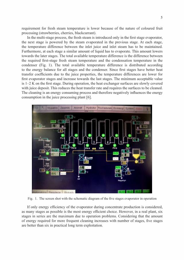
In the multi-stage process, the fresh steam is introduced only in the first stage evaporator, the next stage is powered by the steam evaporated in the previous stage. At each stage, the temperature difference between the inlet juice and inlet steam has to be maintained. Furthermore, at each stage a similar amount of liquid has to evaporate. This amount lowers towards the later stages. The total available temperature difference is the difference between the required first-stage fresh steam temperature and the condensation temperature in the condenser (Fig. 1). The total available temperature difference is distributed according to the energy balance for all stages and the condenser. Since first stages have better heat transfer coefficients due to the juice properties, the temperature differences are lower for first evaporator stages and increase towards the last stages. The minimum acceptable value is 1‒2 K on the first stage. During operation, the heat exchanger surfaces are slowly covered with juice deposit. This reduces the heat transfer rate and requires the surfaces to be cleaned. The cleaning is an energy consuming process and therefore negatively influences the energy consumption in the juice processing plant [6].

If only energy efficiency of the evaporator during concentrate production is considered, as many stages as possible is the most energy efficient choice. However, in a real plant, six stages in series are the maximum due to operation problems. Considering that the amount of energy required for more frequent cleaning increases with number of stages, five stages are better than six in practical long term exploitation.

Fig. 1. The screen shot with the schematic diagram of the five stages evaporator in operation

6

The designer of the evaporator has to consider the overall heat transfer coefficients shown in Table 1. Theoretical values differ substantially from ‘industrial experiments’. Measurements undertaken during evaporator operation are both easily obtained and accurate: the amount of evaporated steam is measured on the basis of sugar content [brix] after each stage, and temperatures are measured before and after the stage on both sides of heat exchanger. On this basis, the averaged overall heat transfer coefficient for the whole heat exchanger can be calculated using equations 1 and 2. Results show that this coefficient is also a function of the heat exchanger height [1, 3, 12, 13].

T a b l e 1The overall heat transfer coefficients according to different sources and industrial experiment

Evaporator stage

k (W·m‒2·K‒1)

VDI formula

Chemical resources formula

WIEGAND formula

[www.sugartech.co.za] software

Authors experiment tubes: 6m

Authors experiment tubes: 9m

I 1932 2056 3991 3994 2646 2200II 1703 1700 3574 2934 2460 2000III 1580 1471 3050 1950 2175 1300IV 1284 1364 2401 1225 1709 1000V 1064 704 1451 601 1215 800

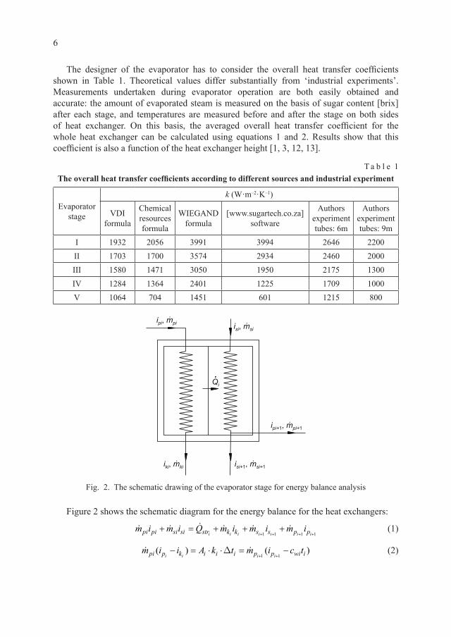
Figure 2 shows the schematic diagram for the energy balance for the heat exchangers:

m i m i Q m i m i m ipi pi si si str k k s s p pi i i i i i i+ = + + +

+ + + +1 1 1 1 (1)

m i i A k t m i c tpi p k i i i p p wi ii i i i( ) ( )− = ⋅ ⋅ = −

+ +D

1 1 (2)

Fig. 2. The schematic drawing of the evaporator stage for energy balance analysis

7

Equations (1) and (2) are used during the design process of the evaporator, for each stage and the condenser.

3. Transient operation states

During every-day operation the system also has to control transient states of evaporator operation. The transient processes occur during start-up, shut-down, load change, juice properties change, and change of the ambient conditions. The issue of non-stationary evaporator process has been considered by [3, 4, 9]. There are two main approaches for transient processes in the evaporator: first one based upon the full mathematical description of the process; the second upon using expert system analysing where a “black box” system is characterised only by its response to excitation [11].

As an example, let‘s consider ∆tsri as the average temperature difference on a heat exchanger. There are several parameters having an influence on its value, of which the most important is the evaporation temperature – tsi, The evaporation temperature is a function of the saturation temperature t” for the pressure psi and boiling point elevation ∆t (b, ti) due to the sugar content in the solution. t t p t b tsi si i= ′′ +( ) ( , )D (3)

Differentiating this equation with respect to time τ results in the following equation:

dtd

tp

dpp

tb

dbd

tt

dtd

si

si

si

si si

i

τ τ τ=∂ ′′∂

⋅ +∂∂

⋅ +∂∂

⋅( ) ( )D D (4)

The functions

∂ ′′∂

=∂∂

=∂∂

=tp

a tb

a tt

asi

p bsi

t, ( ) , ( )D D (5)

are given for small parameter disturbances and can be calculated from the saturation curve, or derived from the experimental results.

The same mathematical algorithm can be applied for other linear elements of the balance equations, where the ordinary differential equation system is derived after the settlement of the coefficients resulting from partial derivatives.

A practical approach, which in fact is commonly used by the evaporator operators, is the analysis of the recorded experimental parameter changes. In this case, the evaporator is treated as a black-box. This allows for the inclusion of not only liquid and gas parameters, but also the thermal capacity of the heat exchangers and manifold. The model is elaborated to assess the influence of the following factors on the amount of mass evaporated: the steam mass flow rate mpi; raw juice inflow msi; pressure after heat exchanger; the inlet juice sugar mass fraction; the cooling water mass flow rate and temperature of the condenser. An example of such a function is displayed in Fig. 3. Similar relationships can be found also in the literature [5].

The function shape is heavily dampened however, the oscillatory character at the beginning of the curve is clearly visible. This function can be described by mathematical formulae of the first or second order Laplace transformation:

8

G s K es

G s K es s

s s( ) , ( )=

+ ⋅=

⋅+ +

− −D Dτ τ

ζω

ζω ω1 2

2

2 2 (6)

where:K ‒ coefficient of the linearised response,∆τ ‒ time delay,ζ ‒ damping coefficient,ω ‒ free frequency.

On the basis of the analysis of the registered functions, the dynamic model of the evaporator can be formulated. The graphical method for the determination of the coefficient using registered function in time is presented in Fig. 4. Additional definitions are needed:

ζπ

ω π=−

+= +

log

(log ), (log )M

M TM

2 22 22 (7)

Fig. 3. Registered by the author, influence of the steam supply reduction on the outlet vacuum level in [%] with respect to time [min]

Fig. 4. Determination of the basic transform parameters using graphical approach

9

4. Evaporator control design

The evaporator control system has to meet the following conditions:– assuring long and steady state evaporator work including consideration to the fact that

during operation, external weather conditions (humidity and temperature) may change. Other problems, for example the possible fouling of the heat exchangers surfaces, also have to be considered;

– possibility of controlled operation within the range between nominal and minimal desired evaporator load;

– all non-desired states of the evaporator have to be reported to the operators;– ease of operation for evaporator crew has to be ensured.

The vacuum control within the condenser is one of the issues because it depends on the ambient conditions. Over the course of a season the cooling water temperature for the condenser may vary within 5‒30°C. In consequence, the condenser temperature may change within the range 20‒55°C. This results in a condensing pressure change within the range 3‒17 kPa (97‒83% vacuum). For apple juice concentration, the available temperature difference on the evaporator is within the range 43 K‒78 K. This means 60 K ± 18 K. The vacuum pump control is important because its main role is the removal of the non-condensing gases. If the assumed pressure resulting from condensing temperature is too low, then the total heat transfer process in the evaporator may collapse. Fig. 5 shows the distribution of the total available temperature difference of five evaporator stages. The incorrect temperature distribution is close to normal operation. In this specific case incorrect operation has been as of a result of heat exchanger fouling on stage I. The same result may be due to a non- -condensing gases film forming on the surface.

Fig. 5. Temperature differences during normal and incorrect operation

10

5. Conclusions

Evaporator design and operation requires solution to the following issues:a) Heat transfer rates for each evaporator stage are determined with no more than 20%

accuracy. The design has to take into consideration the minimum juice flow needed to cover internal tube surface;

b) It is necessary to implement ambient condition compensation into the evaporator control algorithm;

c) The control algorithm also has to consider dynamic conditions which occur during evaporator start up, shut down and parameter changes. In the algorithm, a time delay has to be introduced based on experimental tests. The oscillations of temperature functions have to be used for delay coefficient determination;

d) The control system has to consider the fact that the evaporation is always determined by the worst stage.

R e f e r e n c e s

[1] Kubasiewicz P., Wyparki. Konstrukcja i obliczanie, WNT, Warszawa 1997.[2] Lewicki P. i in., Inżynieria procesowa i aparatura przemysłu spożywczego, WNT, Warszawa

2005.[3] Aly N.H., Marwan M.A., Dynamic response of multi-effect evaporators, Desalination 114, 1997,

189-196.[4] Aprea C., Renno C., Experimental analysis of a transfer function for an air cooled evaporator,

Applied Thermal Engineering, 21, 2001, 481-493.[5] Cyklis P., Żelasko J., Optymalne sterowanie procesami wymiany ciepła i masy w wielostop-

niowej wyparce cienkowarstwowej, XIII Sympozjum Wymiany Ciepła i Masy, 2007, 379-386.[6] Cyklis P., Dynamika pracy wielostopniowej wyparki cienkowarstwowej z opadającym filmem

cieczy, Materiały konferencyjne IV Warsztatów „Modelowanie przepływów wielofazowych w układach termochemicznych, Stawiska 2007.

[7] Hoffman P., Plate evaporators in food industry – theory and practice, Journal of Food Engineering, 61, 2004, 515-520.

[8] Jariel O., Reynes M., Courel M., Durand N., Dornier M., Comparison de quelques techniques de concentration des jus de fruits, Fruits, vol. 51 (6), 2007, 437-450.

[9] Stefanov Z., Hoo K.A., Control of a Multiple-Effect Falling-Film Evaporator Plant, Ind. Eng. Chem. Res., 44, 2004, 3146-3158.

[10] VDI – Wärmeatlas Berechnungsblatter fur den Wärmeübertragung, VDI-Verlag, GmbH, Dusseldorf 1977.

[11] Lovett D.J., Mackay M.E., Improving Quality and Profitability with Evaporators and Dryers using Advanced Control Technology (www.cidip.com).

[12] www.sugartech.co.za/rapiddesign/juiceheater/index.php.[13] www.cheresources.com.

* Prof. Ph.D. D.Sc. Eng. Piotr Cyklis, M.Sc. Eng. Roman Duda, Faculty of Mechanical Engineering, Cracow University of Technology

TECHNICAL TRANSACTIONSMECHANICS

1-M/2015

CZASOPISMO TECHNICZNEMECHANIKA

PIOTR CYKLIS*, ROMAN DUDA*

THE HYBRID SORPTION-COMPRESSION REFRIGERATION CYCLE CONTROL SYSTEM

AUTOMATYKA I STEROWANIE HYBRYDOWEGO SORPCYJNO-SPRĘŻARKOWEGO

SYSTEMU ZIĘBNICZEGO

A b s t r a c tThe requirements for environmentally friendly refrigerants promote the application of both CO2 and water as working fluids. Both solutions have disadvantages resulting from the high temperature limit for CO2 and the low temperature limit for water. This can be avoided by the application of the hybrid adsorption-compression system, where water is the working fluid in the adsorption cycle which is used to cool down the CO2 compression cycle condenser. The adsorption process is powered with a low- -temperature renewable heat source such as solar collectors or waste heat sources. This solution has been developed by the authors of this paper and has not been reported in any other literature source. The different ambient conditions over the course of the year require specially designed control procedures and the automation system. The algorithm has to control positive and negative heat sources operation, valve actions, pumps, fans and compressor operation. In the control algorithm, the ambient temperature and solar conditions or other waste heat sources have to be introduced as control parameters, optimised to achieve maximum efficiency of the whole system. The refrigeration effect as a parameter has to be considered both for the refrigeration capacity as well as the CO2 evaporation temperature.

Keywords: hybrid adsorption-compression refrigeration, control

S t r e s z c z e n i eWymagania dotyczące użycia przyjaznych dla środowiska czynników chłodniczych promują zastosowanie CO2 i wody jako czyn-ników roboczych. Oba rozwiązania posiadają wady będące wynikiem ograniczeń maksymalnej temperatury CO2 i dolnej grani-cy temperatury wody. Można tego uniknąć przez zastosowanie hybrydowego adsorpcyjno-sprężarkowego systemu chłodniczego, w którym woda jest cieczą roboczą w cyklu adsorpcyjnym, który zaś stosuje się w celu ochłodzenia skraplacza CO2 w cyklu sprę-żarkowym. Adsorber jest zasilany energią z niskotemperaturowego odnawialnego źródła ciepła, takiego jak kolektory słoneczne lub źródła ciepła odpadowego. Takie rozwiązanie to nasz własny pomysł i nie odnotowano go w żadnym innym źródle literatury. Nato-miast różne warunki otoczenia przez cały rok wymagają specjalnie zaprojektowanych procedur sterowania i rozwiązań automatyki. Algorytm sterujący musi kontrolować działanie dodatnich i ujemnych źródeł ciepła, zawory, pompy, wentylatory i pracę układu sprężarkowego. W tym algorytmie temperatura otoczenia i warunki słoneczne lub z innego źródła ciepła na przykład odpadowego muszą być wprowadzone jako jego parametry, biorąc pod uwagę działanie obiegów w celu osiągnięcia maksymalnej wydajności całego systemu. Zapotrzebowanie na efekt chłodniczy jest parametrem zarówno pod względem mocy chłodniczej, jak i tempera-tury odparowania CO2.

Słowa kluczowe: hybrydowy adsorpcyjno-sprężarkowy system chłodniczy, sterowanie

12

1. Introduction

Compression and sorption systems are usually applied alternatively in refrigeration and air conditioning systems for refrigeration and heat pump cycles.

In two stage cascade refrigeration compression cycles, with the same refrigerants on both stages the temperature of about ‒60°C can be achieved [1]. Cascade compressor applications, with two independent cycles and two different refrigerants, are also frequently used. In this case, two refrigeration compressor cycles are connected by a heat exchanger (evaporator-condenser). The temperature of the LT (low temperature) cycle evaporator may fall below ‒80°C [2, 3].

The application of carbon dioxide in compression refrigeration system is well known, but due to its low critical temperature, CO2 requires a high discharge pressure, since the transcritical cycle has to be applied under normal ambient condition. In this case, a gas cooler is applied instead of the condenser. The carbon dioxide cycle is frequently used in the LT stage at the two stage compression refrigerating cycle [4‒6].

The sorption systems like LiBr/H2O absorption or silica gel adsorption cycles where H2O is a working fluid, are limited for refrigeration purposes by H2O condensing temperature not lower than 4‒8°C [7, 8].

There are also some papers covering new idea of hybrid cycle where low temperature cycle (LT) is compression refrigeration and high temperature cycle (HT) is thermal compression. The examples are for such a hybrid cycles are: sorption (CO2‒NH3 cascade) [9], (N2O‒CO2 cascade) [10], adsorption [11, 12] or thermoelectric cooling. Adsorption zeolite air conditioning and heat pump have already been developed [13].

Coupling two systems (adsorption at the HT stage and CO2 compression at the LT stage) is a new idea, combines the possibility of utilising waste heat or solar heat as an energy source for the HT stage [14].

The advantages of the proposed system are: the application of only natural refrigerants and low energy consumption when utilising the solar or waste energy. The TEWI coefficient is significantly lower for the proposed system than for other solutions.

2. The hybrid system design

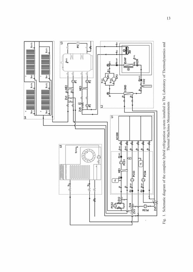
In the Laboratory of Thermodynamics and Measurements of Thermal Machines at the Cracow University of Technology a test stand with a hybrid refrigeration adsorption- -compression system has been designed and constructed [15].

HT stage of the system is the adsorption cycle based on ACS08 adsorber (SorTech AG). This adsorber is coupled with tube solar collectors with heat storage and a sprayed cooling tower for MT (medium temperature) glycol for re-cooling. Solar system is composed of 17 vacuum tube solar collectors HEWALEX KSR-10 and a heat storage tank with a capacity of 2000 litres. An evaporative (sprayed) cooling tower DECSA REF-C-005 with a maximum cooling power about 75 kW is used for cooling the adsorption unit.

The low temperature compression cycle is equipped with two CO2 compressors Dorin CD300H ph3; one of them is equipped with frequency inverter ABB ACS355-03-08A8-4.

13

Fig.

1.

Sche

mat

ic d

iagr

am o

f the

com

plet

e hy

brid

refr

iger

atio

n sy

stem

inst

alle

d in

The

Lab

orat

ory

of T

herm

odyn

amic

s an

d Th

erm

al M

achi

nes M

easu

rem

ents

14

A refrigeration compartment with internal dimensions 1960 mm × 1920 mm × 2690 mm and with a wall thickness of 200 mm is cooled using evaporator Gunter CXGHF 040.2H/17- -ENW50.E with fan VT0398U and high pressure expansion valve CX4 CO2 PCN 801990. The lamellar heat exchanger SWEP B16DWHx64/1P-SC-U is working as a CO2 condenser. Ethylene glycol is used as secondary liquid for the cooling tower and solar collectors. The air heater Flowair Leo FB 9 has been installed in the cooling chamber to simulate the thermal load.

The complete system is shown in Fig 1. Table 1 presents the measurement devices.

T a b l e 1Measurement devices mounted in test stand

measurement count Sensor class used range

ti 36 Introl IT-CF-1 Pt100 B ‒25~200; ‒50~150; 0~150 [°C]

ti/curent loop 36 Introl 0.03% 4~20 [mA]

m4liq 1 SIEMENS MASSFLO 2100 0.01% 0~1000 [kg/h]

m4liq 1 SIEMENS MASS 6000 0.01% 0,0002~0,2786 [kg/s]

m4vap 1 Hoffer Flow Controls ACEII 0.05% 10~110 [l/min]

m1; m1AD; m2, m3 4 Hoffer Flow Controls 0.05% 4,73~35,96; 6,62~60.57; 9,46~109.78 [l/min]

m1; m1AD; m2, m3 4 KEP BATRTM2AC 0.05% 0~36; 0~60; 0~110 [l/min]

p7; p10 2 Vegabar 17 0.05% 0~100 [bar]

pAKU 1 Vegabar 17 0.05% 0~25 [bar]

Pii 9 LUMEL 0.01% 0~200; 0~700; 0~3000; 0~8000; 0~10000; 0~15000 [W]

current loop 8 ICP DAS M-7017RC 0.01% 4~20 [mA]

3. Control system design

The main problem of the proposed system, which has to be solved by automatic control, is the continuous: 12 months, 24 hours, working time for refrigeration system.

This is the reason why the cooling tower applied in our laboratory stand has more power than required only for adsorption cooling. The adsorption cooling of the CO2 condenser is possible only in periods when waste heat or solar heat is available. In case of the the solar heat, during the night, only part of the time the adsorption cycle work may it be powered from the storage tank. Then, the cooling tower has to cool down the condenser directly. During

15

the night, temperature achievable with the wet cooling tower is low enough to cool down the CO2 condenser to below the critical point. In the case of extremely high air humidity, the electric heater may be used as a backup for adsorption Also, any other kind of waste heat may be used to heat up the desorber. The advantage of the adsorption system is that it may work with 60‒65°C driving temperature, depending on the adsorber design.

There are several work regimes for each subsystem.

For subsystem L1, the adsorber work shall have four main regimes:1. A summer day working (SDW) regime is when the input temperature from heat source

exceeds 65°C, and the ambient air temperature is higher than 13°C. Under such conditions the adsorption subsystem works in the cooling mode. Since the outlet cooling temperature from the adsorber is a function of cooling load, it is sufficient to leave the system at lowest possible cooling temperature as possible. This self-adjustment function of the adsorption unit allows achieving the lowest possible condensing temperature, reducing total energy consumption. This regime occurs until two above mentioned temperatures used as control functions will not be crossed;

2. Summer night work (SNW). The adsorber work is no longer possible when heat source temperature decreases below 65°C, then the adsorption system has to be stopped, and then, only the wet tower is used to cool down the CO2 condenser;

3. Heat pump work (HPW). This option is used when the ambient air temperature goes below 13°C. Then, the adsorber may be used separately as a heat pump collecting all waste heat and ambient heat and using the heat collector as HT source, while the MT (medium temperature heat) is used for domestic/company heating. In this case, the CO2 cycle condenser is cooled down directly from the cooling tower;

4. Additional Heater Work (AHW). The temperature of the heat source is below 65°C and the requirements for condenser cooling are higher than the cooling tower can provide. This may be the case only in special ambient conditions with a very high relative air humidity and high temperature when no waste or solar heat source is available.

Subsystem L2 – compression cycle CO2

Commonly known CO2 compression refrigerating cycle control system will not be discussed here in details. However, there are two important differences:1. The cooling requirements for CO2 condenser may in some cases be limited, and additional

cooling power may be required. In this case the control signal is released to run AHW program in the L1 subsystem, reducing the compressor power at the same time;

2. One of the compressors is equipped with the frequency inverter. This makes it possible to change refrigeration capacity according to the current chamber load, instead of conventional on/off system.

Subsystem L3, L4, L5 – heat storage, solar collectors, wet cooling towerThe heat storage subsystem is simple in operation. It has an electric heater with an on/

off system only for L1 AHW mode. Not mentioned earlier ZV valves and pumps have to work accordingly to other subsystem modes, opening flow path accordingly to the system needs:

16

1. Mode SAC – the solar heat accumulation is controlled using temperature readings. Once the temperature reading is higher than required, the PCS2 pump starts working and continues until the outlet temperature from the solar collectors exceeds the temperature in the heat storage container for 15 K. Then the P1 pump starts and the heat storage container load starts. This accumulation goes on until the glycol temperature in the solar circuit falls below the container temperature by 2‒3 K. In case of fast solar collectors temperature decrease the PCS2 pump is switched off. When heat container temperature limit is reached (95°C achieved), the mode SAC is switched to mode SWS;

2. Mode SW solar work– the heat storage container is fully loaded to 95°C, P1 pump then switches off, if the L1 subsystem is on SDW mode, the glycol directly heats the adsorber. In case of to high solar temperature or subsystem L1 not operating, the mode SW switches into SWS mode;

3. SWS mode – solar waste mode. This is the case when no heat source is needed (L1 is not operating, accumulator is full) and there is considerable amount of solar radiation and the temperature readings in solar subsystem exceeds the set point (about 100°C). Then pump PCS2 then has to be put into operation and all heat is removed in the cooling tower.In Table 2, the control system setup for each mode is shown.

T a b l e 2Regimes Modes and working Systems

COMMON EQUIPMENT

MODE ZV1 ZV2 ZV3 ZV4 ZV5 PCS2 PCS4’

SDW/SAC POS-1-2 POS-1-3 POS-1-2 POS-1-2 POS-1-3 T-CTL OFF

SDW/SW POS-1-2 POS-1-2 POS-1-2 POS-1-2 POS-1-3 T-CTL OFF

SDW/SWS POS-1-3 POS-1-3 POS-2-3 POS-1-2 POS-1-3 T-CTL OFF

SNW POS-1-2 POS-1-3 POS-1-2 POS-1-3 POS-1-2 OFF ON

HPW POS-1-2 POS-1-3 POS-1-2 POS-1-3 POS-1-2 ON ON

AHW POS-1-2 POS-1-2 POS-1-2 POS-1-2 POS-1-3 ON OFF

L1

MODE ACS PCS1 PCS3 PCS4

SDW/SAC OFF ACS-CTL ACS-CTL ACS-CTL

SDW/SW ON ACS-CTL ACS-CTL ACS-CTL

SDW/SWS ON OFF OFF OFF

SNW OFF ACS-CTL ACS-CTL ACS-CTL

HPW ON ACS-CTL ACS-CTL ACS-CTL

AHW ON ACS-CTL ACS-CTL ACS-CTL

17

L2

MODE AKC ECX SP1 SP2 EZR MEVAP MAH

SDW/SAC ON ON AKC-CTL AKC-CTL ECX-CTL AKC-CTL MAN-CTL

SDW/SW ON ON AKC-CTL AKC-CTL ECX-CTL AKC-CTL MAN-CTL

SDW/SWS OFF OFF OFF OFF OFF OFF MAN-CTL

SNW ON ON AKC-CTL AKC-CTL ECX-CTL AKC-CTL MAN-CTL

HPW ON ON AKC-CTL AKC-CTL ECX-CTL AKC-CTL MAN-CTL

AHW ON ON AKC-CTL AKC-CTL ECX-CTL AKC-CTL MAN-CTL

L3

MODE P1 P2 P3 P5 ZV6 EH1 EH2

SDW/SAC T-CTL MAN-CTL MAN-CTL ON MAN-CTL OFF OFF

SDW/SW OFF MAN-CTL MAN-CTL OFF MAN-CTL OFF OFF

SDW/SWS OFF MAN-CTL MAN-CTL OFF MAN-CTL OFF OFF

SNW ON MAN-CTL MAN-CTL ON MAN-CTL OFF OFF

HPW ON MAN-CTL MAN-CTL ON MAN-CTL OFF OFF

AHW ON MAN-CTL MAN-CTL ON MAN-CTL ON ON

L5

MODE PTWR MTWR

SDW/SAC ACS-CTL ACS-CTL

SDW/SW ACS-CTL ACS-CTL

SDW/SWS T-CTL T-CTL

SNW T-CTL T-CTL

HPW ON ON

AHW ACS-CTL ACS-CTL

4. Hybrid system advantages

The hybrid system presented in the paper has been put into operation in the Laboratory of Thermodynamics and Thermal Machines Measurements at Cracow University of Technology (Politechnika Krakowska). Several tests have been done with a different system setup. This allowed for the calculation of real values for energy consumption shown in Fig. 2.

18

The results of investigation of the new hybrid system (CO2 + adsorption) have been compared to the calculated and experimental results of four other systems: CO2 only one and two stages transcritical cycles, CO2 + cooling tower only, double stage compression cycle with R410 as HT stage and CO2 as LT stage. In most cases, the results of the new hybrid cycle have been better than others in terms of energy. The TEWI coefficient of a new cycle has been significantly better than other investigated cases.

The results of this investigation and the control system set up for the determined working modes are the basis for system work optimization during the whole year, 24 hours a day cycle.

5. Conclusions

The new hybrid system shown in this paper has been designed, constructed and investigated in the Laboratory of Thermodynamics and Thermal Machines Measurements at the Cracow University of Technology.

The system assumptions, as a new ecological idea with lower energy consumption and a low TEWI coefficient have been checked and validated. The achieved experimental efficiency is significantly better than conventional systems.

The system control design allowing for optimisation of the hybrid system operation for different ambient conditions and required refrigeration temperatures has been shown.

Fig. 2. Results of the experimental investigations of the cycle shown in Fig. 1

19

This publication has been written as a part of the project financed from the funds of the Polish National Centre of Research and Development (agreement no. N R06 0002 10 0936/R/T02/2010/10)

R e f e r e n c e s

[1] Cecchinato L., Corradi M., Transcritical carbon dioxide small commercial cooling applications analysis, Elsevier International Journal of Refrigeration, No. 34, 2012, pp. 50-62.

[2] da Silva A., Pedone Bandarra Filho E., Heleno Pontes Antunes A., Comparison of a R744 cascade refrigeration system with R404A and R22 conventional systems for supermarkets, Elsevier Applied Thermal Engineering, No. 41, 2012, pp. 30-35.

[3] Getu H.M., Bansal P.K., Thermodynamic analysis of an R744-R717 cascade refrigeration system, Elsevier International Journal of Refrigeration, No. 31, 2008, pp. 45-54.

[4] Pearson A., Carbon dioxide-new uses for an old refrigerant, Elsevier International Journal of Refrigeration, No. 28, 2005, pp. 1140-1148.

[5] Ge Y.T., Tassou S.A., Control optimisation of CO2 cycles for medium temperature retail food refrigeration systems, Elsevier International Journal of Refrigeration, No. 32, 2009, pp. 1376-1388.

[6] Girottoa S., Minettoa S., Neksa P., Commercial refrigeration system using CO2 as the refrigerant, Elsevier International Journal of Refrigeration, No. 27, 2004, pp. 717-723.

[7] Desideri U., Proietti S., Sdringola P., Solar-powered cooling systems: Technical and economic analysis on industrial refrigeration and air-conditioning applications, Elsevier Applied Energy, No. 86, 2009, pp. 1376-1386.

[8] Cimsit C., Ozturk I.T., Analysis of compressioneabsorption cascade refrigeration cycles, Elsevier Applied Thermal Engineering, No. 40, 2012, pp. 311-317.

[9] Fernandez-Seara J., Sieres J., Vazquez M., Compression-absorption cascade refrigeration system, Elsevier Applied Thermal Engineering, No. 26, 2006, pp. 502-512.

[10] Bhattacharyya S., Garai A., Sarkar J., Thermodynamic analysis and optimization of a novel N2O‒CO2 cascade system for refrigeration and heating, Elsevier International Journal of Refrigeration, No. 32, 2009, pp. 1077-1084.

[11] Wang L., Ma A., Tan Y., Cui X., Cui H., Study on Solar-Assisted Cascade Refrigeration System, Elsevier Energy Procedia, No.16, pp. 1503-1509.

[12] Labus J., Bruno J.C., Coronas A., Performance analysis of small capacity absorption chillers by using different modeling methods, Elsevier Applied Thermal Engineering, No. 58, 2013, pp. 305-313.

[13] Sekret R., Turski M., Research on an adsorption cooling system supplied by solar energy, Elsevier Energy and Buildings, No. 51, 2012, pp. 15-20.

[14] Cyklis P., Kantor R., Concept of hybrid adsorption-compression refrigeration system, Zeszyty Naukowe Politechniki Poznanskiej, 2011.

[15] Cyklis P., Kantor R., Górski B., Ryncarz T., Hybrydowe sorpcyjno-sprężarkowe systemy ziębnicze. Część III – Wyniki badań systemu, Technika Chłodnicza i Klimatyzacyjna, No. 1, 2013, p. 203.

* Prof. Ph.D. D.Sc. Eng. Piotr Cyklis, M.Sc. Eng. Przemysław Młynarczyk, Faculty of Mechanical Engineering, Cracow University of Technology.

TECHNICAL TRANSACTIONSMECHANICS

1-M/2015

CZASOPISMO TECHNICZNEMECHANIKA

PIOTR CYKLIS*, PRZEMYSŁAW MŁYNARCZYK*

NOZZLE SUPPRESSED PULSATING FLOW CFD SIMULATION ISSUES

PROBLEMY SYMULACJI CFD PULSUJĄCEGO PRZEPŁYWU TŁUMIONEGO PRZEZ DYSZĘ

A b s t r a c tPressure pulsations in volumetric compressor manifolds are one of the most important problems in compressor operation. These problems occur not only in huge compressor systems such as those used in natural gas piping in gas mines or national transport systems, but also in small refrigeration compressors found in domestic applications. Nowadays, systems require a new approach since in all applications, variable revolution speed compressors are introduced. Mufflers designed in a conventional way on the basis of the Helmholtz theory only have good pressure pulsation damping action within the designed frequency range. In the case of revolution speed change, the reaction of the damper designed according to the Helmholtz theory may be insufficient. Therefore, any innovative ideas for pressure attenuation is welcomed by the compressor industry. One of the possibilities to attenuate pressure pulsations over a wide range of frequencies is the introduction of specially shaped nozzles in the gas duct flow directly after the compressor outlet chamber. It is obvious that the nozzle attenuates pressure and flow pulsations due to energy dissipation, but at the same time, it also raises the requirement for the pumping power of the compressor. The estimation of nozzle pulsation attenuation may be assessed using CFD simulation. In the paper, the influence of the time step and viscous models choices have been shown. The differences between viscous and inviscid gas models have been shown.

Keywords: CFD simulations, Pressure pulsations damping, nozzle gas flow

S t r e s z c z e n i ePulsacje ciśnienia w instalacjach sprężarek wyporowych są jednym z najważniejszych problemów w eksploatacji sprężarek. Pro-blem ten pojawia się nie tylko w dużych systemach sprężarkowych, jak na przykład w sprężarkach gazu ziemnego w kopalniach i rurociągach transportowych, ale również w małych sprężarkach chłodniczych w zastosowaniach domowych. Aktualnie te systemy wymagają nowego podejścia, jako że we wszystkich zastosowaniach wprowadzane są sprężarki o zmiennych prędkościach obro-towych. Tłumiki projektowane zgodnie z teorią Helmholtza mają dobre wskaźniki tłumienia pulsacji tylko w projektowym zakre-sie częstotliwości. W przypadku zmian prędkości obrotowej sprężarki działanie tłumika opartego na teorii Helmholtza może być niewystarczające. Dlatego każda innowacyjna technika tłumienia pulsacji ciśnienia jest oczekiwana przez przemysł sprężarkowy. Jedną z możliwości tłumienia pulsacji w szerokim zakresie jest zastosowanie zwężek kształtowych wprowadzonych bezpośrednio na tłoczeniu sprężarki. Oczywiście zwężka taka ogranicza pulsacje, powodując jednak równocześnie zwiększenie mocy potrzebnej do sprężania czynnika. Ocena efektywności tłumienia pulsacji ciśnienia może być oceniona na podstawie wyników symulacji CFD. W pracy pokazano wpływ modelu gazu lepkiego i doboru kroku czasowego na wyniki symulacji. Przedstawiono także różnice w wynikach dla gazu ściśliwego i nieściśliwego

Słowa kluczowe: symulacje CFD, pulsacje ciśnienia, przepływ gazu w dyszy

22

Nomenclature

ξ ‒ dampingcoefficient

1. Introduction

Pressurepulsationattenuationinvolumetriccompressormanifoldsisstilloneofthemostdifficultproblemstosolveinvolumetriccompressormanifolds.

Thepulsatingflowcausesthefollowingproblems:– systemvibrationwhichcausesystemdamage,– noisewhichisveryunwelcomeinsmallrefrigerantcompressorsystems,– interactionbetween the frequencyof valve oscillations andpulsation frequencywhich

affectsthedynamicperformanceofvalvescausingdynamicleaksorprematurewear,– dynamicboostorweakeningwhichcausesaproblemwitchdirectlyimpactonthepower

ofcompression.Standardpressureattenuatorshavemanydisadvantagesasvolumedampers,especially

inthecaseofvariablerevolutionspeed,therefore,findingothersolutionsisverydesirableforthecompressorindustry.Themodellingofpressurepulsationattenuationiswidelyanalysedinmanypapers dealingwith problems in periodicallyworkingmachine installations likecompressors,pumpsorengines.Variousnumericalmethodsusedforcalculatingtransmissionlossinpipelines,mufflersandsilencersystemsaredescribedindifferentstudies.In[1,5],comparison of experimental results and Helmholtz model results of pressure pulsationsinexistinginstallationsarediscussed.Theauthor[1]showsthattheerroroftheconventionalHelmholtzmethodmayinsomecasesreach90%andafterintroducinganewtransmittancematrix method, significant improvements have been achieved. The Helmholtz modelmethod has been applied by the authors [2, 4, 9, 10] to simulate and analyse differentacousticsystems.

Therearemanypublishedinvestigationsconcerningcarmufflers.Thetheoryissimilarto the volumetric compressormufflers theory. In [4] the transfermatrix of themuffler iscalculated and compared to the CFD simulations and test rig experiments. In paper [8],analgorithm for theefficient acoustic analysisof silencersof anygeneralgeometrywithatransfermatrixisshown.In[7],athree-dimensionalfiniteelementapproachforpredictingthe transmission loss in mufflers and silencers is presented. In paper [11], the effectof roughness and the distribution of holes in the long concentric perforated resonatorwere studied. The main difference between car and compressor mufflers is their size.Thecarmuffleralwayshasafreeoutletandthecompressormufflerworksinthemanifoldthereforethemanifoldreactionhastobeconsidered.

Paper[6]describesaCFDsimulationofasinglepipeexcitedwithasingledisturbance.The response, which is periodicwith a constant frequency, is characterized by a certaindegree of damping.The paper shows that the analysis of pressure pulsation damping bydifferent elements is important.However there is still an issue how theCFD simulationresultscanbeappliedforHelmholtzzerodimensionalmodel.

23

2. Investigated muffling elements

In this paper, passive choking elements mounted in the compressor manifold are investigated as pulsation attenuators. The possibility of passive damping of the pressure pulsations using specially shaped nozzles placed in the gas duct flow directly after the compressor outlet chamber has been analysed. Arbitrary chosen nozzle shapes have been prepared for experimental analysis of pressure pulsation damping. In Fig. 1, examples of nozzle geometries are shown. Three main nozzle profiles in different configurations and size(Venturi orifice, Venturi nozzle and hyperboloidal nozzle)were chosen as most promising for pressure attenuation with low flow restriction.

The key element of this investigation is the assessment of the influence of the nozzle on pulsation on the basis of computer simulation. This method was proposed in [2]. In our method, each manifold element may be characterised by its transmittance. Transmittance describes the response of the element to flow excitation for upward and downward flow.

In the case of a manifold element, there are two physical phenomena − pressure and flow pulsations which may be used in calculation as excitation or response. There are two ways to calculate transmittances − experimental [1] or theoretical based on the CFD simulation [2]. The concept of the method is as follows: for a considered element of a manifold, a full multi-dimensional CFD non-linear simulation is carried out, solving the Navier-Stokes set of equations numerically together with the necessary closing models, i.e. gas state model, turbulence model, boundary conditions. The obtained results are

Fig. 1. Shape and main dimensions of the a) Venturinozzle, b) Hiperboloidal nozzle, c) Venturi orifice

24

averaged at the inlet and outlet of the element in question, then a complex transformation of the results is performed so that the transmittances consistent with the generalized form of matrices are calculated. In this way, the advantages of both methods can be combined ‒ the Helmholtz model possibility of analysis of geometrically complex installations and the possibility of introducing real geometry of any element, without priori simplifications.

Using CFD, it is convenient to put the closed end with the closing impedance Zk = ∝ and M2 = 0 or an open end with Zk = 0 and P2 = 0 as a boundary condition. Therefore, the CFD simulation with impulse flow excitation using CFD methods is critical to assessing the nozzle element influence on pressure pulsations.

3. Simulation results

Several simulation problems were studied in order to find out the best possible simulation method. The FULENT software package was used with several simulation parameters. First, the inviscid model was applied, then the Spalart-Allmaras (S-A) and finally, the Reynolds stress model (RSM). For inviscid simulation,a1mmdefault mesh was used, for SA and RSM, three boundary layers were introduced as shown in Fig. 2.

Boundary conditions:– At the inlet impulse excitation of the 0.1 [kg/s] peak mass inflow is introduced.

The impulse excitation means in numerical application that its duration is equal to one time step. The mass flow in all other time steps is zero.

– Pressure outlet where the pressure at the outlet is defined as the arithmetical average between the pressure outside the domain and the last cell inside the domain.

– Wall (also for closed end elements) where tangential stresses are included in the momentum conservation equation. Velocity at the wall is equal to zero.

Fig. 2. Mesh with three boundary layers for S-A and RSM models

25

The ideal gas isentropic flow model has been applied. The flow is turbulent due to unsteady excitation and high peak velocity. Mach number approximately 0.46.

Results have been obtained in 2D mode using axial symmetry.The results were spatially averaged at the inlet and outlet to obtain one dimensional

flow and pressure pulsations. For closed elements for both direction flows, the pressure pulsation is the response and for open elements mass flow rate for impulse inflow excitation. Examples of this flow are shown in Fig. 3.

It is clearly visible that the inviscid flow model application results in the highest amplitudes of pressure and flow pulsations. The RSM and S-A model gave similar results.

Fig. 3. Outlet pulsations at the outlet of open and closed element with the hyperboloidal nozzle fi = 20 [mm]

26

In Fig. 4, the comparison of the time step influence on the results has been presented. As can be seen, there is nearly no influence of the time step on the pulsation simulation results. The fixed time step was applied. As a result from this investigation, a fixed time step of 2e-6 sec was selected for future simulation.

4. Comparison of different viscosity approaches

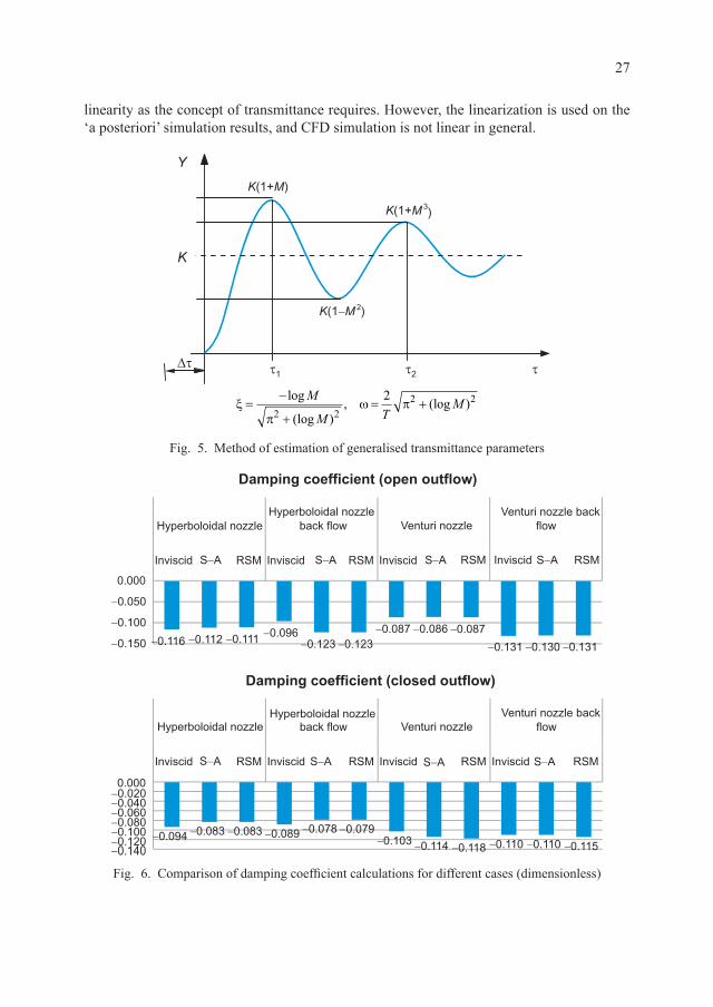
The method for the parameter estimation of generalised transmittances is shown in Fig. 5. The damping coefficient ξ, free frequency ω, delay time ∆τ, and amplification coefficient K can be estimated by analysing pulsation curves shown in Fig 4. The problem requires the decomposition of the function for each free frequency. The method assumes

Fig. 4. Comparison of the pressure pulsation simulation for different time steps

27

linearity as the concept of transmittance requires. However, the linearization is used on the ‘a posteriori’ simulation results, and CFD simulation is not linear in general.

Fig. 5. Method of estimation of generalised transmittance parameters

ξπ

ω π=−

+= +

log

(log ), (log )M

M TM

2 22 22

Fig. 6. Comparison of damping coefficient calculations for different cases (dimensionless)

28

In Fig. 6 and 7, only damping and amplification coefficients have been shown. All other parameters have been calculated, but due to the lack of space, they will not be shown here. However, the comparison is significant and may be used for all transmittance parameters. The comparison made for onward and backward flows, for three viscosity approaches (inviscid, RSM and S-A), for the open and closed ends of the pipe containing the investigated nozzle. Only two shapes have been shown (the Venuri and hyperboloidal nozzle)as in our experiments, those two showed the most promising results. Other shapes and dimensions have also been investigated. As may be expected, for most cases inviscid simulation gave a higher K value (amplification coefficient). It has been expected that the damping coefficient for inviscid simulation (absolute value) will be much lower than for viscous flow, but this is true only in some cases. For the hyperboloidal nozzle, it is even higher than for the viscous flow simulation. This is as a result of a high K coefficient, which causes a high output for the first pulsation wave.

5. Conclusions

The concept of introducing shaped nozzles for pressure pulsation attenuation is presented in this paper. The main problem is to estimate which nozzle shape is more effective for pressure pulsation damping with the lowest gas flow chocking. This can be

Fig. 7. Comparison of amplification coefficient K calculations for different cases (dimensionless)

29

assessed experimentally, but using this approach, shape and dimension optimisation is strongly limited. That is why the CFD simulation can be applied. The application of the CFD code leads to the generalised transmittances for a shaped nozzle, however, important questions arise, concerning simulation models and parameters. In this paper, the influence of the time step and viscous models is demonstrated. The proper time step choice is shown. The viscous gas model showed significant difference when comparing with the inviscid model. The viscosity models RSM or S-A give similar results. The choice for turbulence model depends upon simulation time.

R e f e r e n c e s

[1] Cyklis P., Experimental identification of the transmittance matrix for any element of the pulsating gas manifold, Journal of Sound and Vibration, 244, 2001, 859-870.

[2] Cyklis P., Transmittance estimation for any element of volumetric compressor manifold using CFD simulation, The Archive of Mechanical Engineering, No. 2, Vol. LVI, 2009.

[3] Georges S.N.Y., Jordan R., Thieme F.A., Bento Coelho J.L., Arenas J.P., Muffler Modelling by Transfer Matrix Method and Experimental Verification, ABCM, Vol. XXVII, No. 2, 132-140.

[4] Andersen K.S., Analysing Muffler Performance Using the Transfer Matrix Method, COMSOL Conference, Hannover 2008.

[5] Ma Y.-C., Min O.-K., Pressure calculation in a compressor cylinder by a modified new Helmholtz modelling, Journal of Sound and Vibration, 243, 2001, 775-796.

[6] Sekavcnik M., Ogorevc T., Skerget L., CFD analysis of the dynamic behaviour of a pipe system, Forsh Ingenieurwes, 70, 2006, 139-144.

[7] Mehidizadeh O.Z., Paraschivoiu M., A three-dimensional finite element approach for predicting the transmission loss in mufflers and silencers with no mean flow, Applied Acoustics, 66, 2005, 902-918.

[8] Dowling J.F., Peat K.S., An algorithm for the efficient acoustic analysis of silencers of any general geometry, Applied Acoustics, 65, 2003, 211-227.

[9] Liu G., Li S., Li Y., Chen H., Vibration analysis of pipelines with arbitrary branches by absorbing transfer matrix method, Journal of Sound and Vibration, 332, 2013, 6519-6536.

[10] Huang Z., Jiang W., Analysis of source models for two-dimensional acoustic systems using the transfer matrix method, Journal of Sound and Vibration, 306, 2007, 215-226.

[11] Lee S.-H., Ih J.-G., Effect of non-uniform perforation in the long concentric resonator on transmission loss and back pressure, Journal of Sound and Vibration, 311, 2008, 208-296.

* M.Sc. Eng. Piotr Kopeć, Institute of Thermal and Process Engineering, Faculty of Mechanics, Cracow University of Technology.

TECHNICAL TRANSACTIONSMECHANICS

1-M/2015

CZASOPISMO TECHNICZNEMECHANIKA

PIOTR KOPEĆ*

INFLUENCE OF REFRIGERANT R1234YF AS A SUBSTITUTE FOR R134A

ON A PERFECT REFRIGERATION CYCLE AND EXCHANGER EFFICIENCY

WPŁYW CZYNNIKA CHŁODNICZEGO R1234YF JAKO ZAMIENNIKA R134A NA

PRACĘ IDEALNEGO OBIEGU CHŁODNICZEGO ORAZ WYDAJNOŚĆ WYMIENNIKA

A b s t r a c t

This paper analyses the R1234yf refrigerant as a substitute of R134a with respect to its thermodynamic properties. For the assumed calculation parameters, identical evaporation and condensation temperature, ideal refrigeration cycles with R1234yf and R134a were compared. Moreover, for an actual car evaporator, thermal calculations were performed for the exchanger and the theoretical efficiency parameters of both refrigerants were provided.

Keywords: refrigerant R134a, refrigerant R1234yf

S t r e s z c z e n i e

W artykule dokonano analizy czynnika chłodniczego R1234yf jako zamiennika R134a pod względem termodynamicznym. Dla założonych parametrów obliczeniowych, identycznej tem-peratury odparowania i skraplania, porównano pracę idealnego obiegu, który współpracuje z czynnikiem R1234yf oraz R134a. Ponadto dla rzeczywistego parownika samochodowego wykonano obliczenia cieplne wymiennika i podano teoretyczne charakterystyki wydajnościo-we obu czynników.

Słowa kluczowe: czynnik chłodniczy R134a, czynnik chłodniczy R1234yf

32

Nomenclature

A – heat transfer surface area [m2]COP – coefficient of performance [‒]dz – outer tube diameter [m]i1 – refrigerant enthalpy at the outlet from the evaporator, inlet of the compressor

[kJ/kg]i2 – refrigerant enthalpy at the outlet from the compressor, inlet of the condenser [kJ/kg]i3 – refrigerant enthalpy at the outlet from the condenser, inlet of the expansion valve

[kJ/kg]i4 – refrigerant enthalpy at the outlet from the expansion valve, inlet of the evaporator

[kJ/kg]kA – heat transfer coefficient referring to surface area A [W/(m2·K)]m – mass flow rate of refrigerant [kg/s]N – power of compressor [kW]

NTU – number of heat transfer units [‒]Qo – capacity of evaporator [kW]Qk – capacity of condenser [kW]

RCJ – degree of process openness, calculated as 1/(Sensible Heat Ratio) [‒]Tp1 – outside air temperature at the exchanger inlet [°C]To – evaporation air temperature [°C]Wp – air flux thermal capacity [W/K]αp – air-side heat transfer coefficient [W/(m2·K)]αo – refrigerant-side heat transfer coefficient [W/(m2·K)]αkon – heat transfer coefficient for single-phase vapour flow [W/(m2·K)]αos – heat transfer coefficient for large-volume boiling [W/(m2·K)]ε – heat exchanger efficiency [‒]

1. Introduction

The introduction of refrigerant R1234yf to the market raised certain concerns in the refrigeration and air-conditioning sector. The refrigerant was launched on the market as a substitute for R134a, which was widely used in small refrigeration and air-conditioning devices, its main use being within the automobile industry. The change resulted from legislation adopted for environmental protection reasons.

When comparing two substances, besides examining their physical and chemical properties, it is necessary to look at environmental indicators which help to assess the refrigerant’s impact on the Earth’s atmosphere – the GWP (Global Warming Potential) is one such coefficient. It describes the greenhouse effect potential of a particular refrigerant. Another important indicator is the ODP (Ozone Depletion Potential), which identifies the impact of a particular substance on the depletion of the ozone layer of the Earth’s atmosphere.

33

In 2006, the European Union adopted Directive 2006/40/CE relating to emissions from air-conditioning systems of fluorinated gases. Pursuant to the aforementioned legal act, since 1 January 2011 it has been necessary to use refrigerants with a GWP value lower than 150 in automobiles. Due to technical problems related to the manufacturing of the new refrigerant, the directive has applied since 1 January 2013. From 1 January 2017, no new vehicles will be registered if their air-conditioning systems use refrigerants with a GWP value of > 150 [1]. Two global companies (Honeywell and DuPont) established a joint venture company and introduced R1234yf to the market in order to help the automobile industry to meet the stringent requirements of the EU directive. The parameters of the proposed refrigerant are similar to those of R134a and are coupled with low GWP coefficient values.

2. Comparison of refrigerants R134a and R1234yf

When introducing a new refrigerant as a substitute for an existing one, it needs to be ensured that it has better physical, chemical and thermo-dynamic properties, is safe to use, easily accessible, affordable and meets relevant legislative requirements [2].

Table 1 shows some properties of refrigerants R134a and R1234yf. When the data is compared, it becomes clear that the refrigerants are quite similar. The only major difference concerns the GWP indicator. For R1234yf, the GWP value is 357 times lower than that of R134a and significantly below the requirements set forth in the EU Directive. Another key unfavorable factor is the low self-ignition temperature and low flammability threshold of R1234yf when compared to R134a, which is non-flammable.

T a b l e 1Selected properties of refrigerants R134a and R1234yf [2, 4, 5, 6]

Name 1,1,1,2-Tetrafluoroethane (R134a) or HFC 134a

2,3,3,3-Tetrafluoropropane or HFO 1234yf

Molar mass 102.03 [kg/kmol] 114.04 [kg/kmol]

Density (for t = 25°C) 1206 [kg/m3] 1100 [kg/m3]

Boiling point ‒26.07 [°C] ‒29.45 [°C]

Critical temperature 101.06 [°C] 94.70 [°C]

Critical pressure 40.59 [bar] 33.82 [bar]

Self-ignition temperature non-flammable 405 [°C]

Flammability limits non-flammable 6.2% (vol) to 12.3% (vol)

GWP 1430 4

ODP 0 0

34

3. Comparison of theoretical refrigeration cycles fed with refrigerants R134a and R1234yf

The following parameters, listed in Table 2, have been adopted for the purposes of conducting a comparison of ideal refrigeration cycles with refrigerants R134a and R1234yf. The relevant points of the compared refrigeration cycles were then plotted on log p ‒ i graphs for the compared refrigerants. The graph was then used to identify the values of enthalpy at particular points and the efficiency of other elements of the installation was calculated along with the COP value using equations (1)−(4).

T a b l e 2Parameters of the air-conditioning installation

Evaporator capa city

[W]

Overheating of refrigerant vapour

[K]

Subcooling of refrigerant liquid

[K]

Evaporation temperature

[°C]

Condensation temperature

[°C]4000 5 5 0 50

mQi i

o=−1 4

(1)

Q m i ik = ⋅ −( )2 3 (2)

N m i i= ⋅ −( )2 1 (3)

COP =

QNo (4)

Figure 1 shows the comparison cycles for the examined refrigerants with the assumed operating parameters of the installation.

Fig. 1. Refrigeration cycles for refrigerants R134a and R1234yf

35

Table 3 shows a comparison of the mass flux of the refrigerant m, the capacity of the

condenser Qk , the compressor engine power N and the COP calculated on the basis of equations (1)−(4).

T a b l e 3Results of calculations

Refrigerant m [kg/s] Qk [kW] N [kW] COP

R134a 0.0287 4.93 0.93 4.31R1234yf 0.0378 4.91 0.91 4.39

% 31.67 ‒0.36 ‒1.93 1.97

An analysis of the obtained results clearly indicates that the parameters of installations operating with both refrigerants are similar. Refrigerant R1234yf and R134a have almost identical condensation pressures, while the evaporation pressure is slightly higher in the former compared to the latter. As regards the other parameters included in Table 3, when using a new refrigerant in the air-conditioning installation, it is necessary to account for a greater mass flux of the refrigerant, which increases by almost 32%. This results from the fact that the refrigerant vapours leaving the evaporator are less dense and therefore they have lower volumetric efficiency and, as shown in Fig. 1, lower values of latent heat.

4. Comparison of the efficiency of an actual automobile evaporator fed with refrigerants R134a and R1234yf

Besides comparing the performance of a theoretical refrigeration cycle, the study also looked at how the efficiency of an actual automobile evaporator changed when fed with each of the analysed refrigerants. The refrigerant evaporation temperature, the surrounding temperature and various air flow velocities in the exchanger were assumed for calculation purposes. A passenger car evaporator made of brass tubes and aluminum lamellas was used as a sample exchanger for the purposes of performing the calculations. The geometrical parameters are included in Table 4.

T a b l e 4Geometrical parameters of the evaporator

width G = 357 mm transversal pitch Sq = 25 mmheight H = 202 mm longitudinal pitch Sl = 12 mmdepth L = 89 mm lamella pitch t = 1,5 mm

number of tubes nr = 8 lamella thickness g = 0,1 mmnumber of tube rows nrr = 8 number of lamellas 230

number of feeds nz = 6 tube arrangement staggeredouter tube diameter dz = 8mm

36

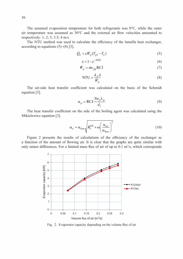
The assumed evaporation temperature for both refrigerants was 0°C, while the outer air temperature was assumed as 30°C and the external air flow velocities amounted to respectively: 1; 2; 3; 3.5; 4 m/s.

The NTU method was used to calculate the efficiency of the lamella heat exchanger, according to equations (5)−(8) [3].

Q W T To p p o= −ε ( )1 (5)

ε = − −1 e NTU (6)

W mcp pp= RCJ (7)

NTU =k AWA

p

(8)

The air-side heat transfer coefficient was calculated on the basis of the Schmidt equation [3].

αλ

pp p

z

Nud

= RCJ (9)

The heat transfer coefficient on the side of the boiling agent was calculated using the Mikielewicz equation [3].

α α ωααo konos

konR= +

1

0 82

. (10)

Figure 2 presents the results of calculations of the efficiency of the exchanger as a function of the amount of flowing air. It is clear that the graphs are quite similar with only minor differences. For a limited mass flux of air of up to 0.1 m3/s, which corresponds

Fig. 2. Evaporator capacity depending on the volume flux of air

37

to the airflow velocity through the exchanger of ca. 1.5 m/s, the graphs virtually overlap. In the case of a larger mass flux, the graphs are similar, but the efficiencies differ. The capacity of the exchanger fed with R1234yf is slightly higher than the capacity of that fed with R134a at airflow velocities inside the exchanger between 2 m/s and 4 m/s. The increase amounts to ca. 4% for an exchanger operating with R1234yf.

5. Conclusions

A cooling installation operating with R1234yf has a 2% higher COP coefficient than an installation filled with R134a. The evaporation and condensation pressures are at similar levels for the same operating conditions. Depending on the operating conditions, the capacity of a heat exchanger with R1234yf is almost identical or slightly higher (by 4%) than the capacity achieved when R134a is being evaporated.

Just as R134a was introduced as a substitute for R12 in the early 1990s, the time has come for R1234yf to be introduced as a substitute for R134a. When the advantages and disadvantages of R1234yf are analysed, it becomes clear that as far as cooling installations are concerned, the refrigerant seems to be an appropriate substitute for R134a. It slightly improves the efficiency and COP of the cooling installation and operates with similar parameters. Flammability and explosiveness are a concern among car users, but it needs to be stressed that other flammable substances besides the refrigerant are commonly found in automobiles. They may also cause a threat to the user and the environment. As far as environmental protection is concerned, the refrigerant is a desirable substitute and should be used in air-conditioning installations. Currently, studies on the application of natural refrigerants in air cooling and air-conditioning installations are becoming readily available. Let us hope that a natural refrigerant, such as CO2, can be used in cars in the near future. It would be both safe for the user and environmentally neutral.

R e f e r e n c e s

[1] Directive 2006/40/EC of the European Parliament and of the Council of 17 May 2006, Official Journal of the European Union, L161 Vol. 49, 14 June 2006.

[2] Wesołowski A., Kontrowersje związane z R1234yf jako czynnikiem chłodniczym, Chłodnictwo & Klimatyzacja, Euro-Media Sp. z o. o., No. 10(146)/2010.

[3] Niezgoda-Żelasko B., Zalewski W., Chłodnicze i klimatyzacyjne wymienniki ciepła – Obliczenia cieplne, Wyd. PK, Kraków 2012.

[4] Andrzejczyk R., Alternatywne do R134a czynniki proponowane jako płyny robocze w klimatyzacji samochodowej i innych instalacjach chłodniczych o małej wydajności, część 1, Technika Chłod-nicza i Klimatyzacyjna, Wydawnictwo Masta, 5/2012.

[5] Andrzejczyk R., Alternatywne do R134a czynniki proponowane jako płyny robocze w klimatyzacji samochodowej i innych instalacjach chłodniczych o małej wydajności, część 2, Technika Chłod-nicza i Klimatyzacyjna, Wydawnictwo Masta, 6‒7/2012.

[6] Bonca Z., Butrymowicz D., Dambek D., Targański W., Poradnik Czynniki chłodnicze i nośniki ciepła – własności cieplne, chemiczne i eksploatacyjne, IPPU Masta, 1998.

* Prof. Ph.D. D.Sc. Eng. Zbigniew Matras, Division of Fluid Mechanics, Cracow University of Technology.

TECHNICAL TRANSACTIONSMECHANICS

1-M/2015

CZASOPISMO TECHNICZNEMECHANIKA

ZBIGNIEW MATRAS*

FRICTION CURVES TRANSFORMATION OF NON-NEWTONIAN FLUIDS IN COILS

TRANSFORMACJA KRZYWYCH OPORÓW PRZEPŁYWU PŁYNÓW NIENEWTONOWSKI W WĘŻOWNICACH

A b s t r a c t

The transformation of pseudo-Newtonian dimensionless numbers: Re and fs, describing flow of power-law non-Newtonian fluids in circularly curved tubes, has been done. It has been shown that the multi-parameter friction curves of power-law non-Newtonian fluid can be described, in new dimensionless coordinate system, with the help of single curve in the laminar as well as turbulent flow region. Moreover, the criterion of transition from laminar to turbulent region was clearly determined.

Keywords: coil, non-Newtonian fluid, inner resistance

S t r e s z c z e n i e

Przeprowadzono transformację pseudonewtonowskich liczb bezwymiarowych opisujących przepływ płynów nienewtonowskich, spełniających prawo potęgowe, w rurach zwiniętych kołowo. Wykazano, że wieloparametrowe krzywe oporów potęgowych cieczy nienewtonow-skich mogą być opisane w nowym układzie bezwymiarowych współrzędnych za pomocą poje-dynczej krzywej zarówno w zakresie laminarnym, jak i turbulentnym. Ponadto jednoznacznie określono kryterium przejścia od ruchu laminarnego do turbulentnego.

Słowa kluczowe: wężownica, płyn nienewtonowski, tarcie wewnętrzne

40

Symbols

D ‒ curvature diameter [m]d ‒ inner pipe diameter [m]De ‒ Dean number (De = Re [d/D]0.5) [‒]Det ‒ characteristic Dean number (Det = Re [d/D]2) [‒]De ‒ pseudo-Newtonian Dean number (De = Re [d/D]0.5) [‒]Dem ‒ modified Dean number (eq. (26)) [‒]Fc ‒ pseudo-Newtonian friction factor (Fc = fc⋅[D/d]0.5) [‒]Fcm ‒ modified friction factor (eq. (12)) [‒]fc ‒ Fanning factor (eq. (14)) [‒]fc ‒ pseudo-Newtonian Fanning factor of curved pipes (eq. (13)) [m/s]K ‒ consistency constant of a power-law fluid [kg⋅sn‒2⋅m‒1]L ‒ length of a curved pipe measurement section [m]n ‒ power-law index [‒]∆p ‒ pressure loss [N⋅m‒2]Re ‒ pseudo-Newtonian Reynolds number (eq. (11)) [‒]Re′ ‒ generalized Reynolds number (eq. (12)) [‒]v ‒ mean velocity [m/s]ρ ‒ density of a fluid [kg⋅m‒3]

REMARK: all bolted symbols relate to the pseudo-Newtonian fluid flow

1. Introduction

In recent years, developments in process engineering has caused liquids of various kinds to be used extensively within industry. Since many such fluids exhibit non-Newtonian flow properties, it has become increasingly important to determine the flow characteristics of non-Newtonian fluids. Curved tubes are widely used for the passage of fluids, heat exchangers and many industrial applications. For this reason, many theoretical and experimental studies on the flow of Newtonian fluids through coiled pipes have been published.

Dean [1] analytically solved the Navier-Stokes equations for the flow of a Newtonian fluid in a round curved tube under the assumption that the radius of curvature is large. He showed that a single dimensionless expression

De =

Re.D

d

0 5 (1)

later called the Dean number, is the essential dynamic parameter that has an influence upon pressure losses in the flow through curved pipes in the laminar as well as turbulent region and – especially in cases where the ratio of radii D/d is small. It causes the friction

41

factor curve of the fluid flow in the straight pipe (described in the laminar region by the Fanning formula and in the turbulent region by the Blasius formula) to be changed into a one or two-parameter cluster of curves [2‒6].

The momentum integral method was used by Ito [7] to analyse the flow of Newtonian fluid in a curved tube. He showed that the relationship between the Dean number and the dimensionless number Fc, called the friction index, can be described in the laminar flow region by the empirical formula

FDec =

+344

1 56 5 73( . log ) . (2)

where

F fc cDd

=

0 5.

(3)

and

fcd pL v

=D

2 2ρ (4)

In the turbulent flow region, the relationship between the non-dimensional variable,

DetdD

=

Re2

(5)

first introduced by Ito, and the friction index is depicted by Ito’s formula

FDec

t=0 079

0 2.. (6)

On the other hand, the flow of non-Newtonian fluids within coiled pipes has not been analysed to the same extend. The first analysis of laminar and turbulent flows of a purely viscous power-law fluid in the curved tubes was carried out by Mashelkar and Devarajan [8‒10]. They assumed that in the region of high Dean numbers (De > 100), which is of practical importance, the secondary field consists of an inviscid core and a thin boundary layer adjacent to the wall. The central part of the fluid is driven towards the outer wall by the centrifugal force. Thus the fluid entering the boundary layer region is pushed back along the wall towards the inner side by a pressure gradient. It then returns to the core region and this pattern leads to the vertical motion in the cross-section of the pipe. On the whole, the axial velocity dominates the flow in the coiled tube, but it becomes comparable to the angular velocity in the boundary layer.

Despite the fact that Mashelkar and Devarajan applied the momentum integral method, they had to solve the governing equations numerically and present the numerical results in a form that was suitable for engineering design. The final correlations for the laminar and the turbulent flow regions are given as formulas (7) and (8) respectively:

fcn

n

n n dD

nn

d= − +

+

′−( . . . ) Re

.( )9 069 9 438 4 37 8 3 1

42

0 51

DD

n

−0 5 0 122 0 768. ( . . )

(7)

42

fcn

n

dD

nn

dD

=

+

′

∗

−

α

β

0 5

11 2

8 3 14

.

( )/( )

Re

+β β/( )n 1 (8)

where α* and β are functions of flow behaviour index.Although Mashelkar and Devarajan stated that their results were in excellent agreement

with Ito’s solution for Newtonian fluids, their correlations are not equivalent to Ito’s equations for n = 1. Similar approaches hold true for the other empirical correlations reported in the literature [11‒15].

The present investigation was undertaken to study a fully developed curved pipe flow of purely viscous non-Newtonian liquids over an extensive range of Reynolds numbers.

The main objective of this work is to present a new method for predicting a pressure drop along the centre-line of a coiled pipe. A special transformation method [12] was extended and adopted to construct a pseudo-Newtonian model for the non-Newtonian flow within a curved tube.

2. Pressure losses in curved tubes

The prediction of pressure losses in the flow of non-Newtonian fluids in curved pipes is much more complicated. The reason for this is that Ito’s equations (2) and (6), describing the flow of even simple Ostwald-de Waele rheological formula fluid, generate additional curves in the laminar as well as the turbulent region of the [De, Fc] co-ordinate system.

The inconvenience can be partially eliminated by the generalization of the transformation method describing flow of non-Newtonian fluids in straight pipe [16].

Consider a pseudo-Newtonian model of non-Newtonian fluid flow in the pipe. Matras and Nowak [16] defined the following dimensionless variables and expressions as follows:

fc =16Re

(9)

It was also shown [16] that the turbulent dimensionless resistance law for smooth pipes takes a form analogous to Blasius’ formula

f Rec =−0 079 0 25. . (10)

The modified Reynolds number Re is related to the generalized Metzner and Reed’s Reynolds number Re′ by the equation

Re = ′ ++

−

Re ( ) .2 13 1

2 5nn

(11)

43

where

Re( )

′ =+

−

−

d v

K nn

n n

nn

2

13 14

8

ρ (12)

Similarly, the modified friction factor is related to the classical Fanning factor by the equation

fc cnn

=++

f 2 13 1

2 5( ) .

(13)

where

fcd pL v

=D

2 2ρ (14)

This finding encouraged the author to take the modified friction factor and the modified Reynolds number, resulting from the transformation method, and use them in Ito’s pseudo- -Newtonian formulas to describe the pressure drops in the laminar flow

FDec

AB

=+( log )α

(15)

and the turbulent flow of non-Newtonian fluids through curved pipes

FDec

taC

= (16)

In both equations (1) and (16), Fc, De and Det are modified pseudo-Newtonian dimensionless numbers defined as follows:

De Re=

dD

0 5.

(17)

De RetdD

=

2

(18)

F fc cDd

=

0 5.

(19)

3. Experimental methods and coordidate system transformation

Experimental apparatus, in the form of a standard pipe flow facility was used to verify the utility of the proposed, generalized Ito’s equations (15) and (16). Working fluids flowed into a straight or coiled pipe from a head tank. The fluid discharged through a pipe made of polyamide was recirculated or discarded. Pressure drop measurements were performed on two coils with ratio of radii d/D equal to 0.0232 and 0.0323.The geometrical details of coiled

44

tubes are given in Figs 1 and 2. The pitch of the coiled pipe was equal to its outer diameter. Two pressure taps with a 1mm in diameter were bored in the outer wall of each pipe.

The axial pressure difference was measured by using differential pressure transducers PD1 (HBM) suitably placed to avoid the entrance and exit effects. The volumetric flow rates were measured by an electromagnetic flow meter. Experiments were conducted on aqueous solutions of low molecular methylcellulose (MC) with concentrations in the range of 0.1% to 0.4% (by wt.) and mixture of 0.3% aqueous solution of hydroxyethyl cellulose (HEC) and 0.1% water chalk suspension. Special care was taken in the preparation of the solutions. Possible effects of viscoelasticity on the rheological properties were eliminated by first preheating and then recirculating each of the studied solutions through the system for a few hours. Shear stress/shear rate data were taken by means of non-corrective capillary rheometer URK-1, [17]. All the solutions were determined to be power-law, non-Newtonian liquids in the shear rate range of 150‒35,000 s‒1 and in the flow index n range of 0.769–1.0. Shear stress/shear rate data taken for each solution just before and just after each series of runs showed no further degradation of polymer solutions, i.e., no changes in consistency K and flow-behaviour index n were observed.

A preliminary experiment was carried out to test the adequacy of the flow system. Friction indices of curved pipes for water were obtained from this experiment and these results were plotted in the form suggested by Ito’s Equations. Very strong agreement was found between Ito’s equation (16) and the turbulent flow data with C = 0.079 and a = 0.2. On the other hand, the data points within the laminar flow range indicate that the Newtonian friction index is slightly small in the comparison to its theoretical value calculated from Ito’s original equation (2). Nevertheless, it can be well described by Ito’s equation (15) with A = 321 and unchanged values of B = 1.56 and α = 5.73

Now, the generalized Ito’s equation describing the pseudo-Newtonian analogue of purely viscous non-Newtonian fluid under laminar flow conditions

FDec =

+321

1 56 5 73( . log ) . (20)

and equation

FDec

t=0 079

0 2.. (21)

within the turbulent flow region can be tested.The experimental values of the friction indices obtained in this work have been

compared with these relationships in Fig. 1 for polymer solutions of different concentrations. The different data symbols refer to different values of curvature ratios d/D. The data tested in this work correspond to the modified Dean number’s Det range of approximately 0.01 to 80. A statistical analysis performed to test the strength of the fit indicated that all the data on purely viscous fluids were correlated with a standard deviation of approximately 3%. Such a strong agreement between the theory and the experimental results confirms the validity of the hypothetical pseudo-Newtonian model for the laminar curved pipe flow.

The non-Newtonian power-law index n does not have an influence on the shape and location of the curve (20) in the laminar flow region. However, the curve described by the

45

mentioned equation is no longer valid above some critical values of Dean number De*. The value of De* depends on d/D ratio.

The turbulent flow data reported in Fig. 1 was plotted in the form suggested by the generalized Ito’s equation (21). The scattering of data about the curve (21) in the turbulent flow range does not exceed ±2% and does not depend on either the curvature ratio d/D or the flow-behaviour index n.

Representative experimental data of the aqueous solutions flow of MC and HEC in curved pipes presented in the [Det, Fc] co-ordinate system (Fig. 1) overlap each other, according to expression (21), along a single curve in the turbulent region. On the other hand, the one-parameter series of curves is observed within the laminar flow region. There is no knowledge of the upper limit of the validity of expression (21). De* is unknown function of the ratio (d/D).

It is desirable that co-ordinates should be transformed in that way to make experimental data in Fig. 1 lie on a single modified curve in a new co-ordinate system.

Assume that there is a non-dimensional co-ordinate system to address the problem. Then, the critical value of the adequately transformed Dean number Det*

should statistically meet a constant value regardless of the pipe curvature and power-law index value ‒ n.

Transform the equation (20) into the following form

F

De

c

tdD

=

+

−

321

1 561 5 5 73

. log[ ]. . (22)

Fig. 1. Fc vs. Det for aqueous polymer solutions

46

Making the problem somewhat easier one can assume that the intersection of the curve (21) and any other, followed by the expression (20), obtain the point (Det*

, Fc*) as

a place of transition from the laminar flow region to the turbulent one. Such an assumption is quite justified by the experimental data analysis shown in Fig. 1, which proves the violent nature of the mentioned transition. If we eliminate the friction index Fc* out of equations (21) and (22), we obtain

1

1 56

0 2

1 5 5 73=

+

∗

∗

−

De

De

t

tdD

.

. .

. log[ ]

(23)

The embroiled form of expression (23) causes it to be of little use in predicting the lower validity limit of equation (21). However, it can be approximated with a high degree of accuracy by the expression

DetdD

dD∗ = +

114 245681 5.

(24)

The corresponding value of the critical friction index is as follows

FDec

t∗

∗

=0 079

0 2.. (25)

Transform the [Det, Fc] dimensionless co-ordinate system to the new one [Detm, Fcm] in the way, that one moves each point laying on the curve (21) (adequate to the critical value of Dean number (24)), to the point of the (Det0, Fc0) co-ordinates laying also on the curve (21). All the points which create the curve described by the equation (22) then move to the single constant curve Fcm = f (Detm) that crosses the curve (21) at the point of (Det0, Fc0) co-ordinates.

Consider the new modified criterion numbers Detm and Fcm defined as follows

De DeDeDetm t

t

t=

∗

0 (26)

and

F FFFcm cc

c=

∗

0 (27)

where Det* is defined by means of equation (24) and Fcm* as follows in (24) and (25), i.e.

FcdD

dD

∗ =

+

0 079

114 245681 5 0 2

.. . (28)

47

Let the critical value of Dean number Det0 =1. Then, the equations

FDecm

tm=

+321

4 26 5 73( . log ) . (29)

and

FDecm

tm=0 079

0 2.. (30)

should respectively describe the single curve of hydraulic losses in the laminar as well as the turbulent flow region.

This proposal was confirmed by the experimental data shown in Fig. 2. Marked points represent the same experimental data as shown in Fig. 1, but they had been transformed according to formula (26) and (27). The generalized hydraulic loses curve was drawn as a solid line described by equations (29) and (30).

A strong agreement between equations (20) and (21) with experimental data fully confirm the hydrodynamic analogy of the laminar and turbulent flow of the non-Newtonian fluid in curved pipes to the Newtonian fluid.

Regardless of the power-law index n, the single curve correlations (29) and (30), can be applied in ranges 0.01 < d/D < 0.1 and 0.01 < Detm = 1 < 100.

Fig. 2. Modified resistance curve of the non-Newtonian fluids flow in curved pipes

48

R e f e r e n c e s

[1] Dean W.R., Phil. Mag., 4, 1927, 208.[2] White C.M., Proc. Roy. Soc. Lond., A 123, 1929, 645.[3] Barua S.N., Quart. J. Mech. Appl. Math., 16, 1, 1963, 61.[4] Schmidt E.F., Chemie-Ing.-Techn., 13, 139, 1967, 768.[5] Topakoglu H.C., J. Math. Mech., 12, 16, 1967, 1321.[6] Baurmeister U., Brauer H., VDI-Forsch.-Heft., 1979, 593.[7] Ito H., Inst. High Speed Mech., Japan, 22, 1970, 161.[8] Mashelkar R.A., Devarajan G.V., Trans. Inst. Chem. Engrs, 54, 1976, 100.[9] Mashelkar R.A., Devarajan G.V., Trans. Inst. Chem. Engrs, 54, 1976, 108.

[10] Mashelkar R.A., Devarajan G.V., Trans. Inst. Chem. Engrs, 55, 1976, 29.[11] Kawase Y., Moo-Young M., Ind. Eng. Chem. Res., 6, 26, 1987, 1248.[12] Mishra P., Gupta S.N., Ind. Eng. Chem. Process Des. Dev., 18, 1, 1979, 130.[13] Mc Cann P.C., Islas C.G., Frictional Pressure Loss during Turbulent Flow in Coiled Tubing,

paper SPE 36345 presented at the SPE/ICoTA North American Coiled Tubing Roundtable held in Montgomery, Texas, 26–28 February 1996.

[14] Zhou, Y., Shah, S.N., AIChE J.,53, 9, 2007, 2210.[15] Gupta R., Wanchoo R.K., Jafar Al i T.R.M., Ind. Eng. Chem. Res., 50, 2, 2011, 1150.[16] Matras Z., Nowak Z., Inż. Chem. i Proces., IX, 3, 1979, 711.[17] Matras Z., Inż. Chem. i Proces., 24, 2003, 139.

* Prof. Ph.D. D.Sc. Eng. Zbigniew Matras, M.Sc. Eng. Bartosz Kopiczak, Faculty of Mechanical Engineering, Cracow University of Technology.

TECHNICAL TRANSACTIONSMECHANICS

1-M/2015

CZASOPISMO TECHNICZNEMECHANIKA

ZBIGNIEW MATRAS*, BARTOSZ KOPICZAK*

COMPARATIVE ANALYSIS OF DRAG REDUCTION FLOW EFFICIENCY THROUGH THE USE OF SURFACTANTS

AND HIGH MOLECULAR POLYMER ADDITIVES

ANALIZA PORÓWNAWCZA EFEKTYWNOŚCI REDUKCJI OPORÓW PRZEPŁYWU ZA POMOCĄ

DODATKÓW WIELKOCZĄSTECZKOWYCH POLIMERÓW I SUBSTANCJI POWIERZCHNIOWO CZYNNYCH

A b s t r a c t

A comparative analysis of drag reduction efficiency through the use of surfactants and high molecular polymer additives has been performed. Results document that for polymer micellar solutions, the stable transitional zone between the laminar flow and the turbulent flow becomes extended towards higher Reynolds number values. The existence of a third extended drag reduction zone in the turbulent range of flow is also observed. It follows that the analysed polymer-micellar solutions combine and intensify positive features of their purely polymer and micellar analogues providing a more efficient drag reduction effect in wider range of flow.

Keywords: drag reduction, polymer, surfactant, aggregate, PEO, CTAB

S t r e s z c z e n i e

Zbadano efektywność redukcji oporów przepływu za pomocą jednoczesnego wprowadzenia do rozpusz-czalnika polimeru i substancji powierzchniowo czynnej. Wykazano, że dla roztworów polimerowo-mice-larnych stabilna strefa przejściowa pomiędzy ruchem laminarnym i turbulentnym zostaje wydłużona w kie-runku większych wartości liczb Re. Zaobserwowano wystąpienie trzeciej, rozszerzonej strefy redukcji w zakresie turbulentnym. Wynika z tego, że analizowane roztwory, łącząc i potęgując pozytywne cechy ich czysto polimerowych i micelarnych odpowiedników, zapewniają efektywniejszą redukcję oporów w szer-szym przedziale przepływowym.

Słowa kluczowe: redukcja oporów przepływu, polimer, SPC, agregat, PEO, CTAB

50

Notation

cf – Fanning friction coefficient [‒]cfM – modified, pseudorheostable Fanning friction coefficient (5) [‒]d – pipe diameter [m]K – fluid consistency constant [kg⋅sn‒2/m]L – length of pipes measurement distance[m]n – flow behaviour index of power law fluid model [‒]∆P – pressure loss [Pa]ReM – modified pseudorheostable Reynolds number (5) [‒]ReS – Reynolds number referenced to the pure solvent [‒]vm – mean velocity of pipe flow [m/s]ρ – solution density [kg/m3]ρS – solvent density [kg/m3]ηS – solvent dynamic viscosity [kg/(m⋅s)]

1. Introduction

Abnormal flow drag reduction through the use of surfactants or polymer additives is an effect which has been intensely examined and described in literature [1‒6]. This phenomenon allows for increasing the flow rate without increasing power the demand, or vice-versa – reducing power demand while maintaining a constant flow rate. It provides potentially high possibilities for the application of this effect in different industry branches, particularly within the oil industry, heat engineering, fire fighting, and the transportation of slurries, sludge and brines [2, 7‒9].The causes of the described drag reduction have been associated with the existence of the new internal solution structure which formulates when special additives are mixed with the solution. The addition of high molecular weight polymer agents into the solvent results in a macromolecule structure formation [1, 6]. In cases where there has been the application of surfactants as drag reducing additives, the formation of micelle structures is observed [2, 5]. In the static condition, when the fluid is at rest, the above mentioned structures are chaotic. It is only during fluid flow shearing that both macromolecules and micelles start to arrange in characteristic orientation, in accordance with the principle of minimum resistance.

In order to improve the effectiveness of the micellarisation process, small amounts of electrolytes are added into the solution (e.g. sodium salicylate or sodium bromide). The effect of flow drag reduction through the use of high molecular polymer or surfactants has also some limitations. The main disadvantage of high molecular polymers is their susceptibility to mechanical and thermal degradation. In the case of surfactant solutions, it is the exceeding of a certain critical Reynolds number which results in the loss of micelles orientation and the collapse of the drag reduction effect.

The effect of the drag reduction induced by simultaneous addition of the high molecular polymer and the surfactant with salt into the solvent is still recent and poorly recognized. It is mainly internal structure formations and chemical reaction processes

51

in polymer-micellar solutions that are highlighted in a few published works related to this subject [11‒14]. The first attempts of drag reduction effect experimental examination have been performed. Experimental results confirmed that the simultaneous addition of polymer and surfactant with salt into the solvent, combine and intensify positive features of their purely polymer or purely micellar solutions behaviour, providing extension of drag reduction zones [13, 14]. Nevertheless, the research pieces indicate that this new effect requires comprehensive experimental study in order to gain a deeper knowledge of this phenomenon.

The existence of polymer macromolecules in the surfactant solution enhances the ability of the surfactant to form micelles structures at a much lower concentration. The newly formed macromolecules are called aggregates [12, 13]. The addition of a small amount of salt (e.g. NaCl or NaSal) into the high molecular polymer and surfactant solution causes an increase in the size of micelles. It also increases the amount of micelles linked to the polymer chain. Furthermore, the addition of the salt can raise the solution viscosity.

The aim of this paper is to perform an analysis of drag reduction efficiency through the simultaneous addition of both surfactants and high molecular polymer into the solvent and compare with the drag reduction effect obtained by the application of the pure polymer or pure surfactant agents.

2. Internal structure characteristic of a polymer-micellar solution

The simultaneous addition of small amounts of polymer and surfactant into the solvent provides the initiation of micellarisation process at a much lower concentration in comparison with the critical micelle concentration (CMC). The concentration at which the initiation of micelle formation occurs in the presence of polymer macromolecules is called the critical aggregation concentration (CAC). The mechanism of the aggregates formation process can be illustrated in Fig. 1. The polymer chain structure is indicated with solid lines in the Figure. Remaining elements correspond to particles of the

Fig. 1. Mechanism of polymer micelle aggregate formation [14]: a) Concentration of both polymer and surfactant additives is too low to induce interaction between additives molecules, b) Increase in concentration leads to micelles and aggregates structure formation, c) Polymer saturation point (PSP) – maximum viscosity value of mixture is reached, d) Further increase in solution concentration leads to the phenomenon of electrostatic screen;

separate micelles are insulated

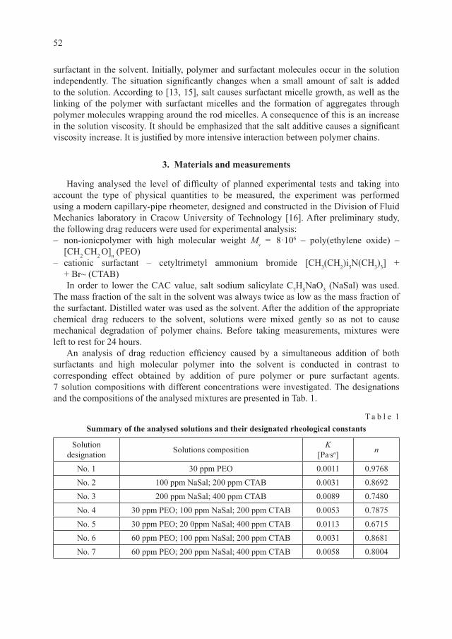
52

surfactant in the solvent. Initially, polymer and surfactant molecules occur in the solution independently. The situation significantly changes when a small amount of salt is added to the solution. According to [13, 15], salt causes surfactant micelle growth, as well as the linking of the polymer with surfactant micelles and the formation of aggregates through polymer molecules wrapping around the rod micelles. A consequence of this is an increase in the solution viscosity. It should be emphasized that the salt additive causes a significant viscosity increase. It is justified by more intensive interaction between polymer chains.

3. Materials and measurements

Having analysed the level of difficulty of planned experimental tests and taking into account the type of physical quantities to be measured, the experiment was performed using a modern capillary-pipe rheometer, designed and constructed in the Division of Fluid Mechanics laboratory in Cracow University of Technology [16]. After preliminary study, the following drag reducers were used for experimental analysis:– non-ionicpolymer with high molecular weight Mv = 8·106 – poly(ethylene oxide) –

[CH2 CH2 O]n (PEO)– cationic surfactant – cetyltrimetyl ammonium bromide [CH3(CH2)i5N(CH3)3] +

+ Br~ (CTAB)In order to lower the CAC value, salt sodium salicylate C7H5NaO3 (NaSal) was used.

The mass fraction of the salt in the solvent was always twice as low as the mass fraction of the surfactant. Distilled water was used as the solvent. After the addition of the appropriate chemical drag reducers to the solvent, solutions were mixed gently so as not to cause mechanical degradation of polymer chains. Before taking measurements, mixtures were left to rest for 24 hours.

An analysis of drag reduction efficiency caused by a simultaneous addition of both surfactants and high molecular polymer into the solvent is conducted in contrast to corresponding effect obtained by addition of pure polymer or pure surfactant agents. 7 solution compositions with different concentrations were investigated. The designations and the compositions of the analysed mixtures are presented in Tab. 1.

T a b l e 1Summary of the analysed solutions and their designated rheological constants

Solution designation Solutions composition K

[Pa.sn] n

No. 1 30 ppm PEO 0.0011 0.9768No. 2 100 ppm NaSal; 200 ppm CTAB 0.0031 0.8692No. 3 200 ppm NaSal; 400 ppm CTAB 0.0089 0.7480No. 4 30 ppm PEO; 100 ppm NaSal; 200 ppm CTAB 0.0053 0.7875No. 5 30 ppm PEO; 20 0ppm NaSal; 400 ppm CTAB 0.0113 0.6715No. 6 60 ppm PEO; 100 ppm NaSal; 200 ppm CTAB 0.0031 0.8681No. 7 60 ppm PEO; 200 ppm NaSal; 400 ppm CTAB 0.0058 0.8004

53

Adiabatic steady flow of homogenous solutions were examined in the temperature equal to 27°C. Fluid flow was performed in 8 different straight pipes having diameters ranging between 1.8 [mm] and 21 [mm].

4. Rheological characteristics and flow resistance measurements results

In order to identify rheological characteristics of the analysed solution, experimental/pipe-flow curves of analysed solutions were drawn in the form of the functional relationship described by the equation (1): τw f= ( )Γ (1)

where:

τwd PL

=D4

– shear stress at the pipe wall,

Γ =8vdm – pipe shear rate (value of shear rate on pipe wall).

Interpretation of experimental results presented in the form of relationship (1) indicates that analysed solutions can be successfully approximated with the Ostwald – de Waele power law fluid model. Rheological parameters K (the fluid consistency constant) and n (the flow behavior index) for each of the analysed solutions are summarized in Tab. 1. Representative rheological characteristics in form of pipe flow curves are illustrated in Fig. 2.

Fig. 2. Representative experimental flow curves for polymer, surfactant and polymer-surfactant solutions

54

The experimental results of the flow resistance are presented in the classical system of dimensionless numbers [ReS, cfS] described by formulas (2) and (3):

ReSm S

S

v d=

ρη

(2)

c d Pv Lfm

=D

2 2ρ (3)

and additionally in the form of the drag reduction coefficient DR defined as a function of the Reynolds number (2), and prescribed in percentage terms:

DR = −

⋅1 100

ccf

fS% (4)

The analysis of the flow resistance curves reveals that none of the analysed flow range measurement points correspond to the theoretical functions which describe Newtonian fluid flow (Fig. 3). The simultaneous addition of even small amounts of high molecular polymers and surfactants causes an increase in flow resistance in the laminar range of flow. In the case of turbulent flow, the simultaneous application of the analysed chemical additives produces a drag reduction effect (Fig. 4).

Furthermore, the value of the critical Reynolds number, for which transition from the laminar flow to the turbulent flow is observed, takes various values depending on pipe diameters, and the type and concentration of chemical additives introduced to the solvent.

Fig 3. The flow resistance curves of polymer-surfactant water solutions defined in the system of cardinal numbers (2) and (3)

55

Better interpretation of the drag reduction phenomena can be achieved by presentation of the same measurement data in modified system of “pseud-Newtonian” [6] dimensionless numbers [ReM, cfM], where:

Re ( ) .

M

nmn

nn

d v

K nn

nn

=+

++

−

−

−2

1

2 5

3 14

8

2 13 1

ρ (5)

c d Pv L

nnfM

m=

++

D

22 13 12

2 5

ρ( ) .

(6)

Obviously [6], in so defined dimensionless number system, the flow resistance curves of purely viscous non-Newtonian fluids are transformed to the single curve – in the whole range of modified Reynolds number (5). Additionally, relationship (6) becomes identical to the classical Newtonian curves both in the laminar and turbulent flow ranges. The selection of such a coordinate system was dictated by the fact that it facilitated the identification and description of the characteristic drag reduction flow zones. In this modified system of pseudorheostable numbers [ReM, cfM], each deviation of the experimental flow resistance curve that indicates abnormal drag reduction from pseudorheostable Blasius curve, allows the identification of the influence of specific additives (polymers or/and surfactants with salt) on the range of the analysed drag reduction effect. Fig. 5 presents the comparison of flow resistance curves in the modified number system (5) and (6) for the three analysed types of solutions with different internal structures. The results of the experimental data analysis indicate that polymer additives cause significant drag reduction in the turbulent range of

Fig. 4. The drag reduction coefficient curves DR = f (Re)

56

flow. Surfactant and salt additives (micellar solution) induce the appearance of a stable transitional zone in which a spectacular reduction of flow resistance is observed – usually greater in comparison with the same effect achieved with polymer additives. In this zone, the loss of stability of the laminar flow increases very softly, whereas the Reynolds number values grow ‒ relative drag reduction is at its greatest within this range. After exceeding a certain second critical Reynolds number value (ReM > ReM2), the occurrence of an unstable transitional zone is observed. Within this range of flow, a rapid loss of the drag reduction effect occurs. Beyond certain third critical Reynolds number values (ReM > ReM3), the solution starts to behave like classical rheostable non-Newtonian fluid. The simultaneous use of polymer and surfactant with salt additives causes extension of a stable transitional zone in comparison with the same effect obtain with pure surfactant and salt additives. Additional abnormal drag reduction zone is observed in the turbulent range above ReM3.

The results of the drag reduction measurement analysis indicate the effect of pipe diameter change on drag reduction efficiency. Decreases in pipe diameter value d result in increases in the drag reduction effect in the turbulent range of flow.

5. Conclusions

Analysis of drag reduction efficiency by pure high molecular polymers, pure surfactants and mixed additives of polymer, surfactant and salt has been carried out. It indicates that multi-component solution of polymer, surfactant and salt causes increase of flow resistance in comparison with the pure solvent flow in the laminar range.

Fig. 5. The flow resistance curves of polymer, surfactant and polymer-surfactant water solutions, defined in the system of cardinal numbers (5) and (6)

57

In the case of turbulent flow, the simultaneous application of the examined chemical additives produces a drag reduction effect. Significant extension of the stable transitional zone is observed between the laminar flow and the turbulent flow ranges. Surfactant with salt additives have the major influence on efficiency of drag reduction in this zone.

Experimental results prove that a simultaneous addition of surfactants and high molecular polymers into the solvent leads to the occurrence of a third significantly extended drag reduction zone in the turbulent range of flow. The viscoelastic characteristics of solution caused by the presence of polymer macromolecules play a crucial role in this zone. Increase in mass fraction of polymer additive result in increase in the efficiency of drag reduction effect only in the turbulent range of flow.

The performed comparative study indicates that the analysed polymer-micellar solutions combine and intensify the positive features of their purely polymer or purely micellar analogues providing a more efficient drag reduction effect across a wider range of flows.

R e f e r e n c e s

[1] White C.M., Mungal M.G., Mechanics and Predictions of Turbulent Drag Reduction with Polymer Additives, Annular Review of Fluid Mechanics, no. 40, 2008, pp. 235-256.

[2] Wang Y., Yu B., Zakin J.L., Shi H., Review on Drag reduction and Its Heat Transfer by Additives, Advances in Mechanical Engineering, no. 10, 2011, 17 pages.

[3] Borostow W., Drag reduction in flow: Review of applications, mechanism and prediction, Journal of Industrial and Engineiring Chemistry, vol. 14, July 2008, 409-416.

[4] Shu-Peng C., Drag reduction of a cationic surfactant solution and its shear stress relaxation, Jurnal of Hydrodynamics, 24(2), 2012, 202-206.

[5] Tamano S., Ito M., Kato K., Yokota K., Turbulent drag reduction in nonionic surfactant solutions, Physics of Fluids, 22(5), 2010, 055102.

[6] Matras Z., Przepływ cieczu Tomsa w przewodach kołowych, Politechnikia Krakowska, Monografia, 29, 1984.

[7] Motier J.F., Chou L.C., Kommareddi N.S., Commercial drag reduction: past, present, and future, Proceedings of the ASME Fluids Engineering Division Summer Meeting, San Diego, Calif, USA 1996.

[8] Dujmovich T., Gallegos A., Drag reducers improve throughput, cut costs, Offshore, vol. 65, no. 12, 2005, pp. 1-4.

[9] Figueredo R.C.R., Sabadini E., Firefighting foam stability: the effect of the drag reducer poly(ethylene) oxide, Colloids and Surfaces A, vol. 215, no. 1‒3, 2003, pp. 77-86.

[10] Jung T.K., Chul A.K., Ke Z., Chun H.J., Hyoung J.C., Effect of polymer–surfactant interaction on its turbulent drag reduction, Colloids and Surfaces A: Physicochemical and Engineering Aspects, Volume 391, Issues 1‒3, 5 November 2011, pp. 125-129.

[11] Suksamranchit S., Sirivat A., Jamieson A.M., Polymer–surfactant complex formation and its effect on turbulent wall shear stress, Journal of Colloid and Interface Science, Volume 294, Issue 1, 1 February 2006, pp. 212-221.

[12] Mohsenipour A.A., Pal R., Prajapati K., Effect of cationic surfactant addition on the drag reduction behaviour of anionic polymer solutions, The Canadian Journal of Chemical Engineering, Vol. 91, Issue 1, January 2013, pp. 181-189.

[13] Matras Z., Malcher T., Gzyl-Malcher B., The influence of polymer-surfactant aggregates on drag reduction, Thin Solids Films, vol. 516, 2008, pp. 8848–8851.

58

[14] Hou Z., Li Z., Wang H., Interaction between poly(ethylene oxide) and sodium dodecyl sulfonate as studied by surface tension, conductivity, viscosity, electron spin resonance and nuclear magnetic resonance, Colloid Polym. Sci., 277, 1999, pp.1011-1018.

[15] Minatti E., Zanette D., Colloids Surfaces A: Phisicochem Eng Aspects, 1996, pp. 113-237.[16] Matras Z., Walczak S., Reometr kapilarno-rurowy, Czasopismo Techniczne 5-M/2003,

pp. 359-370.

* Ph.D. D.Sc. Eng. Łukasz Mika, Ph.D. Eng. Ryszard Kantor, Institute of Thermal and Process Engineering, Faculty of Mechanical Engineering, Cracow University of Technology.

** Ph.D. Eng. Bogusław Górski, ProBiotics Polska.

TECHNICAL TRANSACTIONSMECHANICS

1-M/2015

CZASOPISMO TECHNICZNEMECHANIKA

ŁUKASZ MIKA*, BOGUSŁAW GÓRSKI**, RYSZARD KANTOR*

FLOW MODELLING OF SLURRY ICE IN A CONTROL VALVE

MODELOWANIE PRZEPŁYWU ZAWIESINY LODOWEJ W ZAWORZE REGULACYJNYM

A b s t r a c t

The paper presents the results of simulations of the flow of slurry ice through a control valve. The study focused on a HERZ Strömax-M DN20 control valve. The mass share of ice crystals in the studied slurry ice ranged from 5% to 20%. The results of experimental studies confirmed that the simulations were correct.

Keywords: slurry ice flow, control valve, simulation calculating

S t r e s z c z e n i e

W artykule przedstawiono wyniki badań symulacyjnych przepływu zawiesiny lodowej w za-worze regulacyjnym. W badaniach wykorzystano przelotowy zawór regulacyjny DN20 firmy HERZ typu Strömax-M. Udziały masowe drobinek lodu w zawiesinie w badaniach wynosiły od 5 do 20%. Wyniki badań doświadczalnych potwierdziły poprawność wyników badań symu-lacyjnych.

Słowa kluczowe: przepływ zawiesiny lodowej, zawór regulacyjny, obliczenia symulacyjne

60

1. Introduction

Slurry ice is most often produced from carrier liquids other than pure water. Such liquids may include: aquatic solutions of ethanol; propylene glycol; ethylene glycol; even aquatic solutions of table salt (or other salts). In particular devices and applications, the initial concentration of such solutions varies. Depending on the production method, the size of the ice crystals in the slurry may also vary, in industrial installations these typically range from 0.1 mm to 0.5 mm.

As slurry ice contains ice crystals, its flow through a partially closed valve is highly unstable. Due to the ice particles in the slurry, it is quite likely that the valve may temporarily become partially or fully clogged. In light of the above, the practical use of these kind of valves to control the flow of slurry ice with a significant content of ice is highly limited.

CFD (Computational Fluid Dynamics) based modelling was used with the aim of applying a numerical model to the simulation of the flow of slurry ice through a poppet valve. Therefore, the model was expected to ensure sufficient consistency of the results of calculations with the results of experimental studies of slurry ice flow.

In the Ansys Fluent software chosen for the modelling, two approaches to the multi- -phase flow problem are offered: a discrete model ‒ i.e. an Euler-Lagrange model and an Euler-Euler model. Lagrange’s method is used to describe the movement of particles, while Euler’s method is applied to describe the continuous phase. An Euler-Euler model can be used for adiabatic multi-phase flow, in which Euler’s approach is used for each phase of the mixture. Euler multi-phase mixture models include the volumetric model (VOF), the mixture model and the Euler model. The volumetric VOF model may be used in simulations of the flow of mixtures where a 10% dispersed fraction in the carrier liquid is not exceeded, as well as in cases of stratified or plug flow. The other two models allows for an analysis of the impact of the physical properties of the components of the mixture, the size of solid particles and their mass share. Those models also can take into consideration the creation of flow structures or phase segregation. The Mixture model and the Euler model are therefore dedicated to modelling the flow of the mixture in elbows, bends, collector tubes and valves.

When the relationships used in the models are analysed, it becomes clear that the Euler model is the most complex multi-phase model and the Mixture model is a simplification of the Euler model. The simplification is due to fact that in the Euler model, the mass and momentum conservation equations are solved for each phase of the mixture, while in the Mixture model, the continuity and motion equations are solved for the entire mixture. Nevertheless, the Mixture model for ‘granular’ flow makes it possible to take into consideration the physical properties of the dispersed phase, where the share of the dispersed phase in the carrier liquid may range from 0% to 100%. The model also makes it possible to take into account various velocities of particular phases or, if the velocity of the phases is identical, the model is reduced to a homogenous multi-phase flow.

The choice between the Mixture and Euler models is not completely straightforward. The Euler model, being the more complex one, requires more time-consuming calculations but allows for a greater accuracy of the results. The Mixture model also makes it possible

61

to obtain the same level of accuracy in some cases but in a shorter time. Considering the presented objective of performing the numerical simulations of slurry ice flow, the authors decided to use the Mixture model.

2. Equations describing slurry ice flow

Slurry ice is a mixture of two phases: the carrier (liquid) phase, i.e. an aquatic solution of ethyl alcohol and ice particles (the dispersed phase) with a particular mass (volumetric) share. In the Mixture model, for an adiabatic two-phase flow, the mass conservation and momentum equations are used for the mixture and may be complemented with equations specifying the mass and momentum transfer processes between the phases [2]. In the mass conservation equation for the mixture (m), the mean mass velocity of the mixture is described by the equation:

ν

α ρ ν

ρm

k k kk

n

m=

⋅=∑

1 (1)

In equation (1) k is the subsequent phase of the mixture, and ρm is the density of the mixture described as:

ρ α ρm k kk

n

==∑

1

(2)

The equation of motion for the mixture is the sum of two equations of motion for particular phases of the mixture:

∂∂

+ ⋅ = − + ⋅ + +

+ ⋅ + +

tp T

g F

m m m m m m m m

m

( ) ( ) [ ( )]ρ ν ρ ν ν µ ν ν

ρ

Ñ Ñ Ñ Ñ Ñ

Ñ ⋅⋅

=∑α ρ ν νk k dr k dr kk

n

, ,1

(3)

where:n ‒ describes the number of phases of the mixture,

F – body force,µm ‒ viscosity of the mixture, defined as:

µ α µm k kk

n

==∑

1

(4)

νdr k, ‒ rubbing speed of the dispersed phases of the mixture:

ν ν νdr k k m, = − (5)

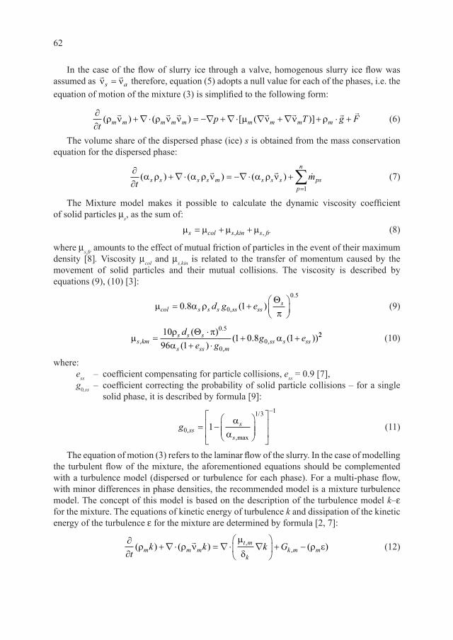
62

In the case of the flow of slurry ice through a valve, homogenous slurry ice flow was assumed as

ν νs a= therefore, equation (5) adopts a null value for each of the phases, i.e. the equation of motion of the mixture (3) is simplified to the following form:

∂∂

+ ⋅ = − + ⋅ + + ⋅ +t

p T g Fm m m m m m m m m( ) ( ) [ ( )]ρ ν ρ ν ν µ ν ν ρ

Ñ Ñ Ñ Ñ Ñ (6)

The volume share of the dispersed phase (ice) s is obtained from the mass conservation equation for the dispersed phase:

∂∂

+ ⋅ = − ⋅ +=∑tms s s s m s s s ps

p

n

( ) ( ) ( )α ρ α ρ ν α ρ νÑ Ñ� � �

1

(7)

The Mixture model makes it possible to calculate the dynamic viscosity coefficient of solid particles µs, as the sum of: µ µ µ µs col s kin s fr= + +, , (8)

where µs,fr amounts to the effect of mutual friction of particles in the event of their maximum density [8]. Viscosity µcol and µs,kin is related to the transfer of momentum caused by the movement of solid particles and their mutual collisions. The viscosity is described by equations (9), (10) [3]:

µ α ρπcol s s s ss sssd g e= +

0 8 10

0 5

. ( ),

.Θ (9)

µρ πα

αs kms s s

s ss mss s ss

de g

g e,

.

,,

( )( )

( . ( ))=⋅

+ ⋅+ +

1096 1

1 0 8 10 5

00

Θ 22 (10)

where:ess – coefficient compensating for particle collisions, ess = 0.9 [7],g0,ss – coefficient correcting the probability of solid particle collisions ‒ for a single

solid phase, it is described by formula [9]:

g sss

s0

1 3 1

1,,max

/

= −

−

αα

(11)

The equation of motion (3) refers to the laminar flow of the slurry. In the case of modelling the turbulent flow of the mixture, the aforementioned equations should be complemented with a turbulence model (dispersed or turbulence for each phase). For a multi-phase flow, with minor differences in phase densities, the recommended model is a mixture turbulence model. The concept of this model is based on the description of the turbulence model k‒ε for the mixture. The equations of kinetic energy of turbulence k and dissipation of the kinetic energy of the turbulence ε for the mixture are determined by formula [2, 7]:

∂∂

+ ⋅ = ⋅

+ −

tk k k Gm m m

t m

kk m m( ) ( ) ( ),,ρ ρ ν

µ

δρ εÑ Ñ Ñ

(12)

63

∂∂

+ ⋅ = ⋅

+ −

t kC G Cm m m

t mk m m( ) ( ) ( ),,ρ ε ρ ν ε

µ

δε

ερ ε

εε εÑ Ñ Ñ

1 2 (13)

In the simulation calculations, the adopted turbulence model was RNG k‒ε [1, 4, 10]. A full description of Euler’s model in reference to the flow of slurry ice is included in [7].

The modelling of flow processes required the physical properties of the mixture to be determined. The adopted method of specifying the physical properties of an aquatic solution of ethyl alcohol and slurry ice is shown in [6].

A HERZ Strömax-M DN20 straight-run control valve was chosen for numerical studies of the slurry ice flow in valves. For the purposes of simulation calculations, a geometrical model of the valve was constructed on the basis of the valve previously used in experimental studies. This allowed for the elimination of the possible impact of workmanship accuracy of particular valves on the numerical calculations. The results obtained from the simulation numerical calculations were compared with the results obtained from experimental studies.

3. Simulation of the flow of slurry ice through a control valve

The simulation of slurry ice flow through a control valve was presented within the largest range of the revolution angle of the valve stem for slurries with ice contents of: 5%; 10%; 15%; 20%.

The grid of the geometrical model adopted in the calculations is shown in Fig. 1.Various values of the mass flux of the liquid were assumed at the valve inlet, depending

on the rotation angle of the valve stem. In the calculations the atmospheric pressure at the outlet of the valve was assumed. The valve inlet and outlet were extended by a section equal to double the diameter of the tube on which the valve was installed. At the remaining outer walls of the model, a constant temperature value was assumed as a boundary condition (adiabatic flow of the slurry ice through the valve).

Fig. 1. Geometric model grid for slurry ice flow through a valve, multi-phase model, 3D [5]

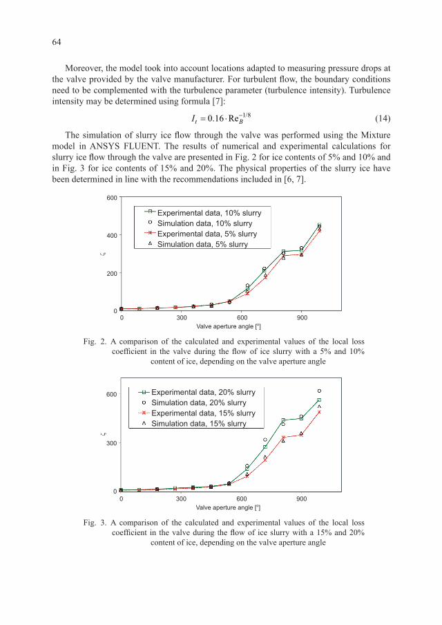
64

Moreover, the model took into account locations adapted to measuring pressure drops at the valve provided by the valve manufacturer. For turbulent flow, the boundary conditions need to be complemented with the turbulence parameter (turbulence intensity). Turbulence intensity may be determined using formula [7]:

It B= ⋅ −0 16 1 8. Re / (14)

The simulation of slurry ice flow through the valve was performed using the Mixture model in ANSYS FLUENT. The results of numerical and experimental calculations for slurry ice flow through the valve are presented in Fig. 2 for ice contents of 5% and 10% and in Fig. 3 for ice contents of 15% and 20%. The physical properties of the slurry ice have been determined in line with the recommendations included in [6, 7].

Fig. 2. A comparison of the calculated and experimental values of the local loss coefficient in the valve during the flow of ice slurry with a 5% and 10%

content of ice, depending on the valve aperture angle

Fig. 3. A comparison of the calculated and experimental values of the local loss coefficient in the valve during the flow of ice slurry with a 15% and 20%

content of ice, depending on the valve aperture angle

65

During comparative experimental studies of the flow of ice slurry through a control valve, flow resistances at the valve ∆pmeas were measured. It was measured simultaneously as a sum of local resistances at the valve together with friction resistances in straight-line sections with the distance L1 and L2, as well as friction resistances ∆pL within a straight- -line section with the length of L. Later, local resistances at the valve were determined on the basis of formula (15) [6]:

D D Dp p p L LLz L= −+

meas1 2 (15)

The studies relied on pressure measurement stubs installed at a distance of 80D and 50D upstream of the valve and 95D and 65D downstream of the valve.

The results of simulation calculations and experimental studies indicated a point of inflection in the characteristics of the local loss coefficient (ζ) at the valve aperture angle of ca. 800° (the moment when the poppet enters the valve socket).

4. Conclusions

On the basis of the results of experimental studies and simulation calculations, it was determined that the existing CFD modelling software can effectively be used to optimise the structure of a valve in terms of controlling ice slurry flow. Up to the aperture angle of ca. 500º there are no differences in the values of the local loss coefficients for slurry ice with various proportions of ice flowing through the valve. After that limit value of the valve aperture angle, the values of local resistance coefficients are heavily dependent on the content of ice particles in the slurry (the higher the ice content, the higher their values). The higher the content of ice particles in the slurry, the steeper the characteristics of the valve through which the slurry ice flows. The point of inflection of the characteristics of the local loss coefficient at the valve aperture angle of ca. 800° represents the moment when the poppet enters the valve socket (within a certain range, the free cross-section area in the valve through which the slurry ice flows is constant).

R e f e r e n c e s

[1] Choudhury D., Introduction to the renormalization group method and turbulence modeling, Fluent Inc, Technical Memorandum TM-107, 1993.

[2] Fluent, Ansys Fluent, Theory Guide 13.0, Ansys Incorporated USA, 2010.[3] Gidaspow D. Bezburuah R., Hydrodynamics of circulating fluidized beds, kinetic theory approach,

Proceedings of 7th Engineering Foundation Conference on Fluidization, 1992, pp. 75-82.[4] Launder B.E., Second-moment closure and its use in modeling turbulent industrial flows,

International Journal for Numerical Methods in Fluids, 9, 1989, 963-985.[5] Mika Ł., Ice slurry flow in a poppet-type flow control valve, Experimental Thermal and Fluid

Science, Volume 45, 2013, pp.128-135.[6] Mika Ł., Opory przepływu zawiesiny lodowej w elementach instalacji chłodniczej, Monograph

No. 399, Wydawnictwo Politechniki Krakowskiej, Kraków 2011.

66

[7] Mika Ł., Opory przepływu zawiesiny lodowej w elementach instalacji chłodniczej, Monograph No. 334, Wydawnictwo Politechniki Krakowskiej, Kraków 2011.

[8] Schaeffer D.G., Instability in the Evolution Equations Describing Incompressible Granular Flow, Journal of Differential Equations, 66, 1987, 19-50.

[9] Ogawa S., Umemura A., On equation of fully fluidized granular materials, Journal of Applied Mathematics and Physics, 31, 1980, 483-493.

[10] YakhotV., Orszag S.A., Renormalization Group Analysis of Turbulence: I. Basic Theory, Journal of Scientific Computing, 1, 1986, 1-51.

* Ph.D. Eng. Łukasz Mika, Prof. Ph.D. D.Sc. Eng. Wojciech Zalewski, Institute of Thermal and Process Engineering, Faculty of Mechanical Engineering, Cracow University of Technology.

TECHNICAL TRANSACTIONSMECHANICS

1-M/2015

CZASOPISMO TECHNICZNEMECHANIKA

ŁUKASZ MIKA*, WOJCIECH ZALEWSKI*

LOCAL PRESSURE LOSS COEFFICIENT DURING THE FLOW OF SLURRY ICE TROUGH

SUDDEN PIPE EXPANSIONS

WSPÓŁCZYNNIK MIEJSCOWYCH STRAT CIŚNIENIA PRZY PRZEPŁYWIE ZAWIESINY LODOWEJ PRZEZ NAGŁE ROZSZERZENIA PRZEWODU

A b s t r a c t

The paper presents the results of experimental studies on ice slurry flow resistance in sudden pipe expansions. In the experimental studies, the mass fraction of solid particles in the slurry ranged from 5 to 30%. The pressure loss coefficients identified as a result of the experimental studies of the turbulent flow of the ice slurry are the same as the coefficients calculated for Newtonian liquids.

Keywords: slurry ice, loss coefficient, pressure loss coefficient, sudden pipe expansion

S t r e s z c z e n i e

W artykule przedstawiono wyniki badań współczynnika miejscowych strat ciśnienia przy prze-pływie zawiesiny lodowej przewodem o nagle zwiększającym się przekroju przepływu. Bada-nia przeprowadzono dla zawiesiny lodowej o udziale masowym lodu od 5 do 30%. Otrzymane z badań wartości współczynników strat miejscowych w turbulentnym zakresie przepływu są zgodne z wartościami tych współczynników obliczonymi jak dla przepływu cieczy newtonow-skiej.

Słowa kluczowe: zawiesina lodowa, współczynnik miejscowych strat ciśnienia, nagłe roz- szerzenie przekroju przepływu

68

1. Introduction

Ice slurry is a mixture of a base fluid and ice particles whose dimensions range from 1.0 ⋅  10‒4 to 0.5 mm. Water or aquatic solutions of glycols, alcohols or salts are most often used as base fluids. The key properties of ice slurry include its high specific thermal efficiency, its high heat transfer coefficient values, and its environmental neutrality. Those properties make it possible for ice slurry to be used not only as a refrigerant, but also as a heat-accumulating agent.

Currently, ice slurry is used in air-conditioning installations for large buildings and mines. It is the chosen refrigerant for air-conditioning systems in supermarkets used to cool reach-in refrigerators, cold plate freezers and cold rooms where food is stored. Ice slurry is also used in the petrochemical and dairy industries, as well as in breweries, medicines and fire-fighting. The first ice slurry-fed systems were created in the early 1980s. They are now widespread in many countries of the world, including Japan, South Africa, South Korea, Germany, France, Colombia and Singapore. In Poland, this cooling technology is not used yet. A significant barrier to its application is the price of the ice slurry generators and the resulting investment costs, which exceed those necessary in the case of traditional refrigeration systems, as well as a lack of knowledge on the part of the investors and designers with respect to the specific properties of ice slurry and refrigeration systems based on heat accumulation in ice.

The specific properties of the ice slurry make it necessary to take account of them in design calculations performed for the planned installations. Besides thermal calculations, flow calculations are equally important, as they enable the determination of the flow resistance of the slurry in pipes and cooling installation fittings. The body of relevant literature includes publications on friction resistances during the flow of ice slurry through straight-line pipe sections, as well as bends and elbows. However, there is no data on local flow resistances in various pipe fittings such as ball valves, globe valves, control valves, pipe reducers, T-connectors and distributors. The results of the study of local flow resistances of ice slurry in sudden pipe expansions presented in this paper should contribute to a better understanding of the topic.

2. Experimental setup description

The experimental studies were carried out with an experimental stand, the setup of which is presented in Figure 1. Ice slurry with the required content of ice made in the ice generator (2) was collected in the accumulation tank (4). The measurement section consisted of the analysed fitting (1) installed between straight-axis pipe sections, each with a length of 4.9 m ‒ this fulfilled the role of run-up sections. The mass flux of the slurry (flow velocity) in the measurement section was adjustable using either the by-pass (12) located directly downstream of the pump package, or the inverter (6) of the pump drive (5). The mass stream could be additionally adjusted using another by-pass, which may extend or reduce the flow path of the slurry.

Ice slurry temperature was measured using precise HART SCIENTIFIC Pt 100 resistance sensors located in thermometric sleeves (11).

69

FUJI ELECTRIC meters with various measurement ranges were used to measure pressure and pressure differences. Due to the properties of the slurry ice, it was decided that pressure in the installation would be measured using 4mm impulse stub pipes (13) with non-insulated transparent impulse piping.

The mass flux of the ice slurry was measured using Danfoss (Siemens) MASSFLO mass flow meters (7), which also performed continuous measurements of the density of the flowing medium. Table 1 shows the key measurement devices used in the study.

The experimental study was conducted for ice slurries with a mass fraction of ice of 30%, 25%, 20%, 15%, 10% and 5%, made on the basis of a 10.6% aquatic solution of ethyl alcohol. In order to avoid heterogenic flow, it was necessary to ensure a minimum flow velocity of ice slurry in the measurement section between 0.15 m/s and 0.25 m/s, depending on pipe diameter and ice content [1, 3, 5, 7].

The mass flux of the ice slurry, its density and the mass fraction of ice were controlled both upstream and downstream of the investigated fitting in order to prevent ice crystals from remaining or melting in the measurement section of the stand. The measurement was

Fig. 1. Schematic diagram of the experimental test stand: 1 – expansion; 2 – ice slurry generator; 3 – mixer; 4 – storage tank; 5 – main pump; 6 – main pump inverter; 7 ‒ mass flow-meter; 8 – data collecting; 9 – multipoint measurement of pressure; 10 – control of ice fraction; 11 − measurement of temperature and pressure; 12 – bypass; 13 – pressure measurement stub; 14 – removable

section of the test stand

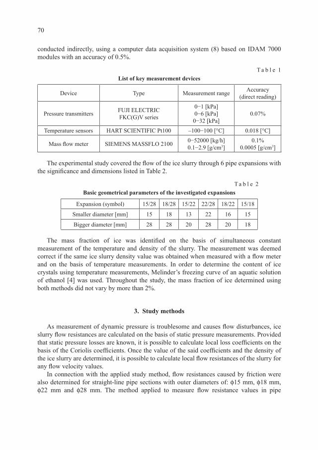
70

conducted indirectly, using a computer data acquisition system (8) based on IDAM 7000 modules with an accuracy of 0.5%.

T a b l e 1List of key measurement devices

Device Type Measurement range Accuracy(direct reading)

Pressure transmitters FUJI ELECTRICFKC(G)V series

0−1 [kPa]0−6 [kPa]0−32 [kPa]

0.07%

Temperature sensors HART SCIENTIFIC Pt100 –100−100 [°C] 0.018 [°C]

Mass flow meter SIEMENS MASSFLO 2100 0−52000 [kg/h]0.1−2.9 [g/cm3]

0.1%0.0005 [g/cm3]

The experimental study covered the flow of the ice slurry through 6 pipe expansions with the significance and dimensions listed in Table 2.

T a b l e 2Basic geometrical parameters of the investigated expansions

Expansion (symbol) 15/28 18/28 15/22 22/28 18/22 15/18

Smaller diameter [mm] 15 18 13 22 16 15

Bigger diameter [mm] 28 28 20 28 20 18

The mass fraction of ice was identified on the basis of simultaneous constant measurement of the temperature and density of the slurry. The measurement was deemed correct if the same ice slurry density value was obtained when measured with a flow meter and on the basis of temperature measurements. In order to determine the content of ice crystals using temperature measurements, Melinder’s freezing curve of an aquatic solution of ethanol [4] was used. Throughout the study, the mass fraction of ice determined using both methods did not vary by more than 2%.

3. Study methods

As measurement of dynamic pressure is troublesome and causes flow disturbances, ice slurry flow resistances are calculated on the basis of static pressure measurements. Provided that static pressure losses are known, it is possible to calculate local loss coefficients on the basis of the Coriolis coefficients. Once the value of the said coefficients and the density of the ice slurry are determined, it is possible to calculate local flow resistances of the slurry for any flow velocity values.

In connection with the applied study method, flow resistances caused by friction were also determined for straight-line pipe sections with outer diameters of: φ15 mm, φ18 mm, φ22 mm and φ28 mm. The method applied to measure flow resistance values in pipe

71

expansions involved measuring static pressure (and as a control measurement also the differences in static pressure at selected measurement points) along the flow of the ice slurry through the entire measurement section [2]. The measurement section consisted of the analysed fitting and run-up sections, this made it possible to obtain a fully developed velocity profile.

The method applied in the study consisted of extrapolating a fully developed pressure gradient to the place of installation of a particular fitting, on both its sides separately.

On the basis of the information collected in the trial measurement series, the static pressure measurement stubs were installed within the measurement section at distances of: 80D, 65D, 50D and 35D upstream of the studied fitting, and 95D, 80D, 65D and 50D downstream of the studied fitting.

The value of the local pressure loss coefficient was calculated using equation:

k pV

VV

= + −2

12 1 2

22

12

D

ρα α (1)

where ∆p – pressure drop,V – flow velocity,α ‒ Coriolis coefficient,ρ – ice slurry density.

Indices 1 and 2 refer to the state of the ice slurry upstream and downstream of the expansion.

In order to determine the local loss coefficient in the fittings in which flow velocity changes, it is necessary to know the Coriolis coefficient for the laminar and turbulent flow range on both sides of the studied fitting.

In reference works, it is difficult to find verified equations for determining the Coriolis coefficient in the turbulent flow range for non-Newtonian fluids. However, papers by other authors indicate that in the said range, both the values of local loss coefficients and the velocity profiles of both non-Newtonian and Newtonian fluids are quite similar [2, 8]. Therefore, in order to calculate the value of the Coriolis coefficient for the turbulent flow of ice slurry in a tube, an empirical relationship may be used as for a Newtonian fluid.

The Strzelecka and Jeżowiecka-Kabsch equation [5] was used for Reynolds numbers within the range of Re = 2800 ‒ 100000:

α = + ⋅

− ⋅

+ ⋅1 105 10 11 88 10 1 208 10

2

3

2

2

2ln Re.

ln Re.

ln Re

(2)

The value of the Coriolis coefficient in the laminar flow range for a Bingham fluid was determined in the paper using equation [6]:

αε ε

ε ε=

⋅ ⋅ + ⋅ +

⋅ + ⋅ +

54 47 58 3535 2 3

2

2 3( )( )

B B

B B (3)

whereεB ‒ Bingham’s fluid active shear stress ratio.

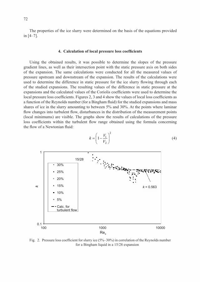
72

The properties of the ice slurry were determined on the basis of the equations provided in [4‒7].

4. Calculation of local pressure loss coefficients

Using the obtained results, it was possible to determine the slopes of the pressure gradient lines, as well as their intersection point with the static pressure axis on both sides of the expansion. The same calculations were conducted for all the measured values of pressure upstream and downstream of the expansion. The results of the calculations were used to determine the difference in static pressure for the ice slurry flowing through each of the studied expansions. The resulting values of the difference in static pressure at the expansions and the calculated values of the Coriolis coefficients were used to determine the local pressure loss coefficients. Figures 2, 3 and 4 show the values of local loss coefficients as a function of the Reynolds number (for a Bingham fluid) for the studied expansions and mass shares of ice in the slurry amounting to between 5% and 30%. At the points where laminar flow changes into turbulent flow, disturbances in the distribution of the measurement points (local minimums) are visible. The graphs show the results of calculations of the pressure loss coefficients within the turbulent flow range obtained using the formula concerning the flow of a Newtonian fluid:

k VV

= −

1 1

2

2

(4)

Fig. 2. Pressure loss coefficient for slurry ice (5%‒30%) in correlation of the Reynolds number for a Bingham liquid in a 15/28 expansion

73

Fig. 3. Pressure loss coefficient for slurry ice (5%‒30%) in correlation of the Reynolds number for a Bingham liquid in a 18/28 expansion and a 15/22 expansion

Fig. 4. Pressure loss coefficient for slurry ice (5%‒30%) in correlation of the Reynolds number for a Bingham liquid in expansions 22/28, 18/22 and 15/18

74

5. Conclusions

As can be inferred from the graphs presented in Figures 2, 3 and 4, in the laminar flow range there exists a clear correlation between the values of the local loss coefficient and the Reynolds number of the slurry (Bingham fluid). As the value of the Reynolds number increases, the value of the said coefficient decreases. In the turbulent range, the value of the local loss coefficient is constant, independent of the Reynolds number, and close to the values calculated as for a Newtonian fluid. This is consistent with results obtained by other authors [1, 2, 8].

In both flow ranges, it is possible to observe the influence of the content of ice and the expansion’s diameters ratio on the value of the local pressure loss coefficient. The higher the ice content of the slurry, the higher its viscosity, which directly translates into an increase of the value of the local loss coefficient and local flow resistances in the expansion. An increase of the ratio of the diameters of the pipe upstream and downstream of the expansion causes a decrease in the value of the local loss coefficient.

R e f e r e n c e s

[1] Ayel V., Lottin O., Peerhossaini H., Rhelogy flow behaviour and heat transfer of ice slurries: a review of the state of the art, International Journal of Refrigeration, 26, 2003, 95-107.

[2] Fester V., Mbiya B., Slatter P., Energy losses of non-Newtonian fluids in sudden pipe contractions, The Chemical Engineering Journal, 145, 2008, 57-63.

[3] Kitanovski A., Vuarnoz A., Ata-Caesar D., Egolf P.W., Hansen T.M., Doetsch Ch., The fluid dynamics of ice slurry, International Journal of Refrigeration, 28, 2005, 37-55.

[4] Melinder A., Thermophysical properties of liquid secondary refrigerants. Tables and diagrams for the refrigerants industry, IIF/IIR, Paris 1997.

[5] Mika L., Energy losses of ice slurry in pipe sudden contractions, Experimental Thermal and Fluid Science, 35, 2011, 939-947.

[6] Mika Ł., Opory przepływu zawiesiny lodowej w elementach instalacji chłodniczej, Wydawnictwo Politechniki Krakowskiej, Kraków 2011.

[7] Niezgoda-Żelasko B., Wymiana ciepła i opory przepływu zawiesiny lodowej w przewodach, Wydawnictwo Politechniki Krakowskiej, Kraków 2006.

[8] Turian R.M., Ma T.W., Hsu F.L.G., Sung M.D.J., Plackmann G.W., Flow of concentrated non- -Newtonian slurries: 2 Friction losses in bends, fittings, valves and venturi meters, International Journal Multiphase Flow, 24, 1998, 243-269.

* Ph.D. D.Sc. Eng. Beata Niezgoda-Żelasko, Ph.D. Eng. Jerzy Żelasko, Faculty of Mechanical Engineering, Cracow University of Technology.

TECHNICAL TRANSACTIONSMECHANICS

1-M/2015

CZASOPISMO TECHNICZNEMECHANIKA

BEATA NIEZGODA-ŻELASKO*, JERZY ŻELASKO*

FREE CONVECTION ON THE OUTER SURFACE OF VERTICAL LONGITUDINALLY FINNED TUBES

KONWEKCJA SWOBODNA NA ZEWNĘTRZNEJ POWIERZCHNI RUR OŻEBROWANYCH WZDŁUŻNIE

A b s t r a c t

The paper presents methods of determination and the results of experimental studies of heat transfer coefficients on the outer surface of longitudinally finned tubes under free convection conditions.

Keywords: free convection, vertical finned tubes, heat transfer coefficients, measuring methods

S t r e s z c z e n i e

Artykuł przedstawia metody wyznaczania współczynników przejmowania ciepła w warun-kach konwekcji swobodnej na zewnętrznej powierzchni rur ożebrowanych wzdłużnie.

Słowa kluczowe: konwekcja swobodna, pionowe rury ożebrowane, współczynnik przejmo- wania ciepła, metody pomiarowe

76

Nomenclature

Afin1 – surface area of the cross-section of a fin Afin1 = s · L [m2]Ao1 – surface area of a smooth tube at the base of the fin in relation to a single fin [m2]d – diameter [m]g – gravitational acceleration [m/s2]h – specific enthalpy [J/kg]hfin – fin height [m]k – thermal conduction coefficient [W/(mK)]L – tube length [m]

m – parameter in equations (14‒16), m k sa= ⋅ ⋅ ⋅( ) / ( )2 RCJ Alαnfin – number of fins [‒]Nu – Nusselt number Nu = α · do1/k [‒]Pr – Prandtl number, Pr = µ · cp/k [‒]

Ra – Raylegh number, Ra Gr= ⋅ = ⋅ ⋅ ⋅ ⋅ ⋅ ⋅ −Pr ( / ) ( / ) [ ]β ρ µ µg d T c ko p13 2 2D

Q – heat capacity [W]s – fin thickness [‒]Ta ‒ mean air temperature [°C]Tab, Tat – air temperature at the bottom, top of the tube [°C]Tf – end of fin temperature [°C]Twalloi – temperature of the outer wall of the tube, temperature at the base of the fin at the

‘I’ sensor installation point (Twalloi =Twoi) [°C]U – overall heat transfer coefficient [W/(m2K)]∆T – temperature difference ( )DT T Ta wallo= − in the definition of Grasshof

number [K]α – heat transfer coefficient [W/(m2K)]β – volumetric expansion coefficient [1/K]εfin – fin efficiency, εfin = tanh (mhfin)/(mhfin) [‒]

1. Introduction

This paper analyses the heat transfer process on the external surface of a vertical bi- -metallic tube with eight longitudinal aluminum fins situated central-symmetrically along the perimeter of the tube, with an inner core in the form of a copper pipe (Fig. 1a). Such tubes are frequently used in heat pump evaporators which are not fitted with fans. As evaporators operate under normal external conditions and the tubes are freely arranged, the tubes of the evaporator are not grouped into banks, but are located loosely. Null and low velocities of external air flowing from variable directions require the surface of the heat exchanger to be considerably enhanced ‒ this is achieved thanks to fins being the correct length and them having a ‘wavy’ shape as well as their axisymmetric arrangement [1].

77

In the case of longitudinally finned tubes, it is necessary to differentiate between tubes fitted with single ribs or membrane tubes, and tubes where ribs are situated centrally and symmetrically along the circumference of the entire tube. For both types, various reference works propose equations for transverse air flow around a bank of tubes [2‒4].

The influence of a single longitudinal straight fin located on the outer surface of a horizontal cylinder on the natural convection heat transfer process was analysed in [5]. Tolpadi and Kuehn [5] found a slight influence of the fin on the averaged value of the heat transfer coefficient with respect to a smooth tube. The results of their studies indicated differences in the measured local and mean heat transfer coefficients for fins other than vertical fins.

Problems relating to the numerical analysis of heat transfer processes under free convection on the surface of longitudinal fins are often examined for flow inside longitudinally-finned tubes [6, 7]. Paper [8] presents a numerical analysis of the impact of the thickness, height and number of fins in the free convection process on the distribution of velocities, temperatures and heat flux outside a horizontal cylindrical surface with longitudinal fins. The authors note that the maximum heat flux released by the finned surface can be achieved for fins thinner than 0.01 m (within the considered range of between 0.01‒0.05) and for heights not greater than 0.2 m. The maximum heat fluxes released by the finned surface were recorded for between 6 and 12 fins.

Publication [9] includes a numerical analysis of the influence of free convection on the increase of flow resistances and the heat transfer process occurring during laminar flow in a vertical ring pipe with longitudinal fins located on the outer tube. The authors analysed the influence of the number of fins and the relationship between the diameters of the channel’s tubes on an increase of flow resistances and heat transfer coefficients. The authors pointed critical values of the Rayleigh number, at which there was clear influence of free convection on an increase of heat transfer coefficients. Among other things, it was indicated that the fewer fins there are, the closer the relationship between the outer tube diameter and the inner tube diameter; and the shorter the fin, the lower the value of the critical Rayleigh number and the greater the influence of free convection on the increase of heat transfer coefficients in the forced convection process. The critical Rayleigh numbers identified in [9] fitted within the range of 20 to 104.

2. Description of the measurement stand and methods

The experimental studies were conducted for a system including two 2 m-tall vertical tubes, whose axes were set apart at a distance of Sq = 0.2306 [m] (Fig. 1b). Measurements for airflow around the tubes were performed after the tubes were fed with ice water or R407C and R507 refrigerants. When air was cooled using the cooling fluids, the tubes made part of an evaporator system of a cooling device (Fig. 1b). Two shell heat exchangers fitted with electric heaters were an additional component of the evaporator of the cooling system. Eighteen NiCr-NiAl thermocouples were located on the external surface of the finned tubes in order to enable the measurement of temperature at the external surface of the pipe and at the tips of the fins (Fig. 1a). All the thermocouples were calibrated using a Quartz-35

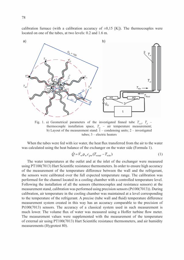
78

calibration furnace (with a calibration accuracy of ±0,15 [K]). The thermocouples were located on one of the tubes, at two levels: 0.2 and 1.6 m.

When the tubes were fed with ice water, the heat flux transferred from the air to the water was calculated using the heat balance of the exchanger on the water side (Formula 1).

Q V c T Tw w pw wout win= −ρ ( ) (1)

The water temperatures at the outlet and at the inlet of the exchanger were measured using PT100(7013) Hart Scientific resistance thermometers. In order to ensure high accuracy of the measurement of the temperature difference between the wall and the refrigerant, the sensors were calibrated over the full expected temperature range. The calibration was performed for the channel located in a cooling chamber with a controlled temperature level. Following the installation of all the sensors (thermocouples and resistance sensors) at the measurement stand, calibration was performed using precision sensors (Pt100(7013)). During calibration, air temperature in the cooling chamber was maintained at a level corresponding to the temperature of the refrigerant. A precise (tube wall and fluid) temperature difference measurement system created in this way has an accuracy comparable to the precision of Pt100(7013) sensors. The accuracy of a classical system used in such measurement is much lower. The volume flux of water was measured using a Hoffer turbine flow meter. The measurement values were supplemented with the measurement of the temperature of external air using PT100(7013) Hart Scientific resistance thermometers, and air humidity measurements (Hygrotest 80).

Fig. 1. a) Geometrical parameters of the investigated finned tube Twoi, Tfi ‒ thermocouple installation space, Tai ‒ air temperature measurement; b) Layout of the measurement stand: 1 ‒ condensing units; 2 ‒ investigated

tubes; 3 ‒ electric heaters

79

When the investigated tubes were fed with the cooling fluid, the heat flux transferred from the air was calculated using the heat balance equation on the side of the boiling refrigerant:

Q m h h Q QR= − − +( ) ( )Rout Rin HEAT HEAT1 2 (2)

In this case, the mass flux of the refrigerant was measured using a Mass 6000 Coriolis mass flow meter installed on the liquid line of the cooling circuit. The enthalpy of the refrigerant at the inlet and outlet from the evaporator of the cooling system were determined using RefproP.exe software, following earlier measurement of the temperatures (PT100 Hart Scientific resistance thermometers) and pressures (Vegabar17 pressure transmitter) of the refrigerant.

2.1. Determination of the mean values of heat transfer coefficient

The heat transfer coefficients of the air were obtained using two methods. The first method involved the calculation of the mean experimental values of the overall heat transfer coefficient UAw (3) and the mean heat transfer coefficients αR for the cooling medium (4‒5):

U QA TAww m

=⋅

D, (3)

αRw walli R

QA T T

=⋅ −

( ), (4)

T T QAd

kdd k

ddwalli wallo

w

i o

o cu

o

i= −

+

21 11

Alln ln

, (5)

The mean temperature of the outer wall Twallo was calculated as the arithmetical mean of the temperature of the outer wall along the circumference of the investigated tubes. Using formulas (2‒5) and solving equation (6) concerning the heat transfer coefficient (finned surface) for αa for each measurement point, the heat transfer coefficient for air was calculated:

Ud

kdd k

dd

AAw

R

i o

o cu

o

i

w

a

=

+

+

+ ⋅

11

21 11

α αAlln ln

RRCJ fin fin⋅ ⋅ +( )

,

ε A At

(6)

In the case under consideration, the fin is treated as a prismatic straight fin with a height resulting from its heat transfer surface area. Hence, according to [10], fin efficiency is calculated using Schmidt’s equation . The height of the fin hfin corresponds to the substitute height of a straight fin with a length of L and the actual fin surface area of:

h An Lfinfin

fin=

⋅ (7)

The openness of the RCJ process [11] applied to formulas (6) makes it possible to take into consideration the impact of condensation of water vapour from the air on the increase in the heat flux transferred by air to ice water. The RCJ coefficient determines the ratio

80

of the heat flux related to the change in air enthalpy (change in temperature and degree of air humidity) and the visible heat flux related to the change in air temperature.

The openness of the RCJ process [11, 12] applied to formulas (8) and (10) makes it possible to take into consideration the impact of the condensation of water vapour from the air on the increase in the heat flux transferred by air to ice water. If the temperature of the cooler ( )Twallo is above the dew point, then the cooling process takes place without any change in air humidity, Xa = const, and the condition line coefficient of the transformation

tends to infinity η = → −∆∆

∞hX

[13]). Otherwise, humidity is condensed on the heat

transfer surface. The air cooling process on the surface of the cooler may be treated as the mixing of two air streams: an air stream with the parameters, temperature and relative humidity corresponding to those of the cooler’s surface (Ta = Twallo, φa = 100%); an air stream with inlet parameters. The total heat flux transferred by the air to the heat transfer surface is the sum of the visible heat flux Qv ‒ relating to a change in air temperature and the

sensible heat flux Qs relating to the condensation of water vapour. The balance of the heat transferred by the air to the surface of the exchanger may be expressed by the following equation:

Q Q Q A A T T A A X Xv s t a wallo a t a= + = ⋅ + − + ⋅ + −( )( ) ( )(ε α εfin fin fin fin wwall a gh)β (8)

Equation (8) may be transformed to form (10) using Lewis’s psychometric relationship for humid air (Chilton–Colburn heat and mass exchange analogy) describing the relationship between the heat transfer coefficient αa and the mass transfer coefficient βa (9) [14]:

αβa

apa pac c= Le2 3/ » (9)

Q A A T TX X hT Tt a wallo aa wall a a g

a wallo= ⋅ + − +

−

−( )( )

( )( )

ε αβ

fin fin 1αα

ε α

a

t a wallo aa wall g

aA A T T

X X hT T

= ⋅ + − +−

−( )( )

( )(fin fin 1

wwallo pac)

(10)

For humid air, it is assumed that Le2/3 ≈ 1 [14]. The expression in the rectangular brackets in equation (10) describes the RCJ coefficient used in equation (6):

RCJ = +−−

1hc

X XT T

g

pa

a wall

a wallo

( )( )

, (11)

where Xwall is the degree of humidity of saturated air at temperature Twallo

Xp Tp Twallw wallo

w wallo=

⋅

−

0 622105. ( )

( ). (12)

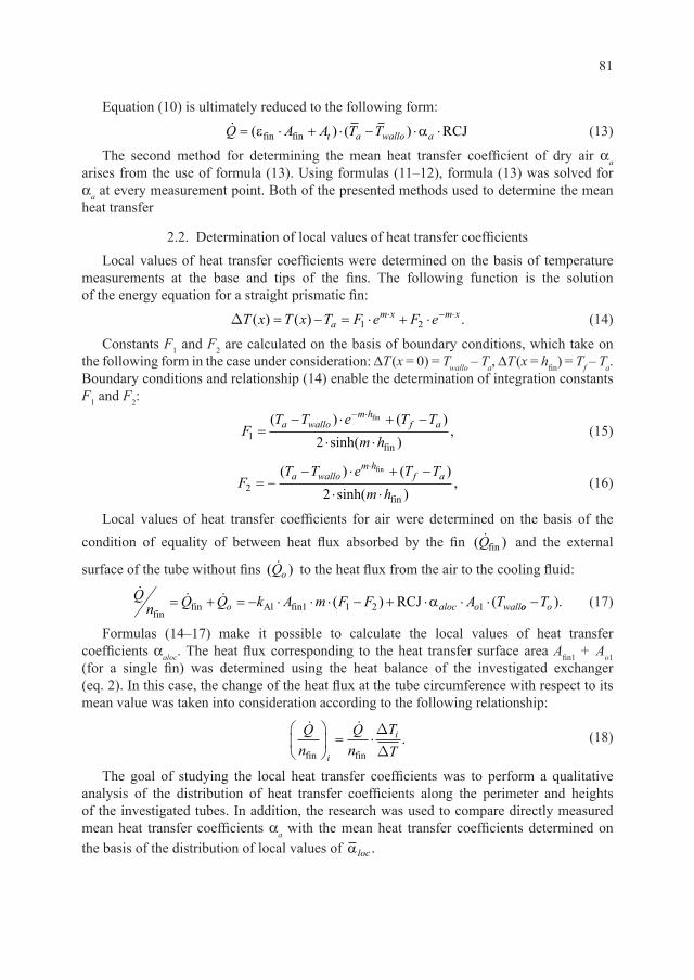
81

Equation (10) is ultimately reduced to the following form:

Q A A T Tt a wallo a= ⋅ + ⋅ − ⋅ ⋅( ) ( )ε αfin fin RCJ (13)

The second method for determining the mean heat transfer coefficient of dry air αa arises from the use of formula (13). Using formulas (11‒12), formula (13) was solved for αa at every measurement point. Both of the presented methods used to determine the mean heat transfer

2.2. Determination of local values of heat transfer coefficientsLocal values of heat transfer coefficients were determined on the basis of temperature

measurements at the base and tips of the fins. The following function is the solution of the energy equation for a straight prismatic fin:

DT x T x T F e F eam x m x( ) ( ) .= − = ⋅ + ⋅⋅ − ⋅

1 2 (14)

Constants F1 and F2 are calculated on the basis of boundary conditions, which take on the following form in the case under consideration: ∆T (x = 0) = Twallo ‒ Ta, ∆T (x = hfin) = Tf ‒ Ta. Boundary conditions and relationship (14) enable the determination of integration constants F1 and F2:

FT T e T T

m ha wallo

m hf a

1 2=

− ⋅ + −

⋅ ⋅

− ⋅( ) ( )sinh( )

,fin

fin (15)

FT T e T T

m ha wallo

m hf a

2 2= −

− ⋅ + −

⋅ ⋅

⋅( ) ( )sinh( )

,fin

fin (16)

Local values of heat transfer coefficients for air were determined on the basis of the condition of equality of between heat flux absorbed by the fin ( )Qfin and the external

surface of the tube without fins ( )Qo to the heat flux from the air to the cooling fluid:

Qn Q Q k A m F F A To aloc o wallfin

fin Al fin RCJ= + = − ⋅ ⋅ ⋅ − + ⋅ ⋅ ⋅1 1 2 1( ) (α oo oT− ). (17)

Formulas (14‒17) make it possible to calculate the local values of heat transfer coefficients αaloc. The heat flux corresponding to the heat transfer surface area Afin1 + Ao1 (for a single fin) was determined using the heat balance of the investigated exchanger (eq. 2). In this case, the change of the heat flux at the tube circumference with respect to its mean value was taken into consideration according to the following relationship:

Qn

Qn

TTi

i

fin fin

= ⋅

D

D. (18)

The goal of studying the local heat transfer coefficients was to perform a qualitative analysis of the distribution of heat transfer coefficients along the perimeter and heights of the investigated tubes. In addition, the research was used to compare directly measured mean heat transfer coefficients αa with the mean heat transfer coefficients determined on the basis of the distribution of local values of αloc .

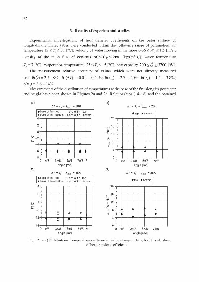
82

3. Results of experimental studies

Experimental investigations of heat transfer coefficients on the outer surface of longitudinally finned tubes were conducted within the following range of parameters: air temperature 12 ≤ Ta ≤ 25 [°C]; velocity of water flowing in the tubes 0.06 ≤ Ww ≤ 1.5 [m/s]; density of the mass flux of coolants 90 260£ £GR [kg/(m2·s)]; water temperature

TR = 7 [°C]; evaporation temperature ‒25 ≤ TR ≤ ‒5 [°C]; heat capacity 200 3700£ £Q [W].The measurement relative accuracy of values which were not directly measured

are: δ( ) . %;Q = −2 5 8 δ  (∆T) = 0.01 ‒ 0.24%; δ(kAw) = 2.7 ‒ 10%; δ(αR) = 1.7 ‒ 3.8%; δ(αa) = 8.6 ‒ 14%.

Measurements of the distribution of temperatures at the base of the fin, along its perimeter and height have been shown in Figures 2a and 2c. Relationships (14‒18) and the obtained

Fig. 2. a, c) Distribution of temperatures on the outer heat exchange surface; b, d) Local values of heat transfer coefficients

83

measurements have been used to determine the local values of heat transfer coefficients along the perimeter of the tube (Fig. 2b and 2d).

Slightly higher values of heat transfer coefficients for the air have been recorded in the bottom part of the investigated tubes. In general, greater temperature differences Ta ‒ Twallo correspond to higher values of coefficients αaloc. In the upper part of the investigated tube, water temperature was higher than at the tube inlet. Under free convection, the buoyancy force is proportional to the difference in air density caused by differences in temperatures at the wall and at a large distance from the wall. A greater buoyancy force corresponds to higher airflow velocities and therefore, more intensive mixing of the fluid and an increased

Fig. 3. a) Relationship αa (Ta ‒ Twallo); b) Relationship Nu(Ra)

84

heat transfer coefficient. It also needs to be noted that the values of heat transfer coefficients obtained with the use of the two measurement methods (point 2.1) did not differ by more than 1.5%). In addition, the figure also shows the mean values of the heat transfer coefficients ( ),αloc obtained on the basis of the local values of heat transfer coefficients (αaloc). The obtained results indicate that the adopted measurement methods are correct and make it possible for the results to be described using a single dimensionless relationship.

Figure 3b shows the relationship between the Nusselt number and the Rayleigh number, determined both for cooling with ice water and coolants. The data included in Figure 3b provided the basis for determining the following dimensionless relationship:

Nu Ra Ra

fin fin= ⋅ ⋅

⋅⋅ ⋅ + ⋅

+

Bd

n h d

B Bo

o1

100001

110000

22 3

( / )(

ππ −− ⋅

n sfin 1

0 15.

, (19)

Ra Gr= ⋅ =⋅ ⋅ ⋅ ⋅

⋅⋅

Pr ,β ρ

µ

µg d T ck

o a

a

a pa

a

13 2

2D

(20)

where the characteristic dimension in the definition of Nu and Ra numbers is the outer diameter of the tube. The final element of equation (19) describes the influence of the heat transfer surface enhancement on the value of the heat transfer coefficient [10]. The obtained values of coefficients A, B and C in equation (19) are: B1 = 5.55 · 10‒5, B2 = 21.24; B3 = 3,151. Figure 3b) shows a comparison of measured and calculated values of Nu numbers.

4. Conclusions

The paper presents methods and the results of experimental research on heat transfer coefficients for airflow around vertical finned tubes with centrally-symmetrical longitudinal wavy fins. The research was carried out under free convection conditions. The mean values of heat transfer coefficients obtained during the study amounted to 2‒8.5 [W/(m2K)].

Studies of local values of heat transfer coefficients have confirmed the increasingly stronger relationship between those values and the difference between the temperature of the wall and of the air. The mean values of heat transfer coefficients obtained on the basis of the distribution of local values αaloc corresponded to mean values calculated from the balance equation and measurements of heat transfer coefficients.

As a result of the experimental studies, dimensionless relationships were determined to calculate the heat transfer coefficients for the cases under consideration. For free convection, for 85% of the measurement points, the differences between the measured heat transfer coefficients and those calculated on the basis of the dimensionless relationship were lower than 20%.

The results of the experimental research discussed in the paper, as well as the proposed dimensionless relationships, can be of great practical importance in designing air coolers and heaters working with natural airflow. The results presented in the paper will be especially useful in the design of heat pumps with evaporators without a fan.

85

R e f e r e n c e s

[1] Niezgoda-Żelasko B., Zalewski W., Żelasko J., Experimental research of the air-water heat pump with evaporator operating under free convection conditions, Proceedings from the 44th Science and Technology Conference − Refrigerations Days, Poznań 2012, 237-244.

[2] Taler J., Sobota T., Cebula A., Determining local heat transfer coefficients on the circumference of smooth and longitudinally finned tubes, Archives of Thermodynamics, vol. 26(1), 2005, 35-52.

[3] Pronobis M., Kalisz S., Wejkowski R., Model investigations of convective heat transfer and pressure loss in diagonal membrane heating surfaces, Heat and Mass Transfer vol. 38, 2002, 343-350.

[4] Sparrow E.M., Kang S.S., Longitudinally-finned cross-flow tube banks and their heat transfer and pressure drop characteristics, International Journal Heat Mass Transfer, vol. 28(2), 1985, 339-350.

[5] Tolpadi A.K., Kuehn T.H., Experimental investigation of conjugate natural convection heat transfer from horizontal isothermal cylinder with a nonisothermal longitudinal plate fin at various angles, International Journal Heat Mass Transfer, vol. 28, 1985, 155-163.

[6] Rustum I.M., Soliman H.M., Numerical analysis of laminar mixed convection in horizontal internally finned tubes, International Journal Heat Mass Transfer, vol. 33(7), 1990, 1485-1496.

[7] Chai J.C., Patankar S.V., Natural laminar convection in internally finned horizontal annuli, Numerical Heat Transfer, Part A, vol. 24, 1993, 67-87.

[8] Haldar S.C., Kochhar G.S., Manohar K., Sahoo R.K., Numerical study of laminar free convection about a horizontal cylinder with longitudinal fins of finite thickness, International Journal of Thermal Sciences, vol. 46, 2007, 692-698.

[9] Prakash C., Renzoni R., Effect of buoyancy on laminar fully developed flow in a vertical annular passage with radial internal fins, International Journal Heat Mass Transfer, vol. 28, 1985, 995-1003.

[10] Schmidt K.G., Wärmeübergang an berippten Oberflächen, VDI-Wärmeatlas, Düsseldorf 2002, Mb 9.

[11] Kołodziejczyk L., Rubik M., Cooling Technology in Air-Conditioning, Arkady, 1976 (in Polish).[12] Niezgoda-Żelasko B., Zalewski W., Cooling and air-conditioning heat exchangers: thermal

calculations, Wydawnictwo Politechniki Krakowskiej, Kraków 2012 (in Polish).[13] ASHRAE, Fundamentals Handbook (SI), Psychrometrics, 1993, 6.1-6.17.[14] Cengel Y.A., Ghajar A.J., Heat and Mass Transfer: Fundamentals and Applications, Mc Graw

Hill Education, 2011.

* Ph.D. D.Sc. Eng. Beata Niezgoda-Żelasko, Ph.D. Eng. Jerzy Żelasko, Faculty of Mechanic Engineering, Cracow University of Technology.

TECHNICAL TRANSACTIONSMECHANICS

1-M/2015

CZASOPISMO TECHNICZNEMECHANIKA

BEATA NIEZGODA-ŻELASKO*, JERZY ŻELASKO*

HEAT TRANSFER OF ICE SLURRY FLOWING IN RECTANGULAR AND SLIT CHANELS

WYMIANA CIEPŁA ZAWIESINY LODOWEJ PODCZAS PRZEPŁYWU W KANAŁACH PROSTOKĄTNYCH I SZCZELINOWYCH

A b s t r a c t

This paper presents the results of experimental investigations into heat transfer between the wall and ice slurry during its flow through channels of rectangular and slit cross-sections. Ice slurry flow is treated as a generalized flow of a non-Newtonian fluid. The influence of solid particles, the flow character, as well as the cross-section of the channel on the heat transfer coefficient are discussed. As the final result, the dimensionless dependences for the calculation of the Nusselt number value in the range of laminar and turbulent flows are presented.

Keywords: ice slurry, heat transfer, melting, generalized non-Newtonian fluid flow

S t r e s z c z e n i e

W artykule przedstawiono wyniki badań eksperymentalnych wymiany ciepła ścianka-zawie-sina lodowa podczas przepływu w kanałach o przekrojach prostokątnym oraz szczelinowym. Przepływ zawiesiny lodowej traktowany jest jako uogólniony przepływ cieczy nienewtonow-skiej. Omówiono wpływ udziału cząstek stałych, charakteru ruchu, przekroju poprzecznego na zmiany współczynnika przejmowania ciepła. Końcowym efektem pracy są zależności kryte-rialne służące do wyznaczania liczb Nusselta w obszarze przepływu laminarnego i burzliwego.

Słowa kluczowe: zawiesina lodowa, wymiana ciepła, topnienie, uogólniony przepływ cieczy nie-Newtonowskiej

88

Nomenclature

cpB – mean value of specific heat of ice slurry [(J/(kg⋅K)]d – diameter [m]dh – hydraulic diameter [m]KF – phase change number KF = r/(cpB · ∆T )K* – consistency index, [Nsn/m2]L – tube length [m]LHeat – length of heat measurement section [m]n* – characteristic flow-behaviour index n = d (lnτw) ∕d (lnΓ)qm – mean heat flux density [W/m2]

r – ice melting capacity [J/kg]T – temperature [K]Tf – mass mean temperature [K]Tw – wall temperature [K]w – flow velocity [m/s]xa – carrying fluid concentration [%]xs – mass fraction of ice [%]α – heat transfer coefficient [W/(m2⋅K)]∆xs – change of mass fraction of ice [%]λ – heat conductivity [W/(m⋅K)]µp – plastic viscosity [Pa⋅s]λB,w – heat conductivity of ice slurry at flow velocity w ≠ 0 [W/(m⋅K)]λB,w=0 – heat conductivity of ice slurry at flow velocity w = 0 [W/(m⋅K)]ρ – density [kg/m3]GzK – Graetz number, GzK = PrB ReK dh /LHeatNu – Nusselt number, Nu = αdh /λB,w=0PeK – Peclet number for ice slurry, PeK = ReK · PrBPrB – Prandtl number for ice slurry, PrB = µp cpB /λB,w=0ReB – Reynolds number for ice slurry, ReB =wdh ρB /µp

ReK – Reynolds number according to Kozicki, Re / ( )* * * *K B m

nhn nw d K= − −ρ 2 18

1. Introduction

Ice slurry is a mixture of either water ice crystals and water, or water with a content of a substance which lowers the freezing point (salt, glycol, alcohol). Ice slurry is a non-Newtonian fluid. This medium is treated as a rheologically stable liquid. Rheological models most frequently assigned to this fluid are: the Ostwald de Waele power law model [5]; the Bingham model [1, 4, 6, 11]; the Casson model [7].

Experimental studies regarding the heat transfer processes in ice slurry flows refer to various flow geometries. The largest number of all published works concerns ice slurry flows through tubes [6, 7, 9, 13]. Paper [12] includes a thermal study of ice slurry in a plate

89

heat exchanger. Stamatiou and Kawaii [14] present the results of thermal studies of ice slurry made up of a 6.2% water salt solution in vertical tubes of a rectangular cross-section. A detailed list of references concerning heat transfer processes with ice slurry is available in paper [1].

The objective of this paper is to present the phenomena accompanying the heat transfer process in ice slurry during its flow through horizontal straight tubes of rectangular and slit cross-sections

2. Experimental studies

The test program included measurements of flow and thermal parameters of ice slurry flow through:– a rectangular tube with the following dimensions: 0.0078 × 0.0265 × 3.0 [m];– a tube of a rectangular (slit) cross-section, with the following dimensions:

0.03 × 0.0358 × 2.0 [m].Tests concerning ice slurry heat transfer were conducted at a constant heat flux density.

The selected thermal measurement lengths guaranteed a hydrodynamically and thermally formed ice slurry flow in turbulent regions. For laminar flow inside tubes, the measurements were taken in the take-off run length, in which the flow was hydrodynamically formed and practically thermally formed. The values of Lheat/dh included in the present study are significantly higher than the ones commonly found in thermal studies of ice slurry flow in pipes (Lheat/dh < 80) [2, 4]. In the case of thermal studies of ice slurry flow through rectangular tubes, Stamatiou and Kawaji [14] conducted research for tubes with hydraulic diameters of dh = 0.023 and 0.047 m and with the values of Lheat/dh = 11 and 22.

Paper [10] describes in detail the measurement stand and the adopted heat transfer measurement method.

Thermal studies included measurements for:– mean flow velocities 0,1 ≤ wm ≤ 4.5 [m/s];– heat flux density of qm = 2000 5000 8000; ; [W/m ];2

– mass fraction of ice 0 ≤ xs ≤ 30%;– average size of ice crystals (width/length) ds = 0.1/0.15 [m] [10].

Figure 1 presents experimental values of heat transfer coefficients determined for the cross-sections: rectangular (a×b = 0.0078 × 0.0265 [m]); slit (a×b = 0.003 × 0.0358 [m]). A detailed description of the results of the experimental research on heat transfer during flow through the pipes is presented in [10]. In the case of the flow through the rectangular tubes, similar to flow in the pipes, it is possible to observe an increase in the heat transfer coefficient of the ice slurry in comparison to the heat transfer coefficient of the carrying liquid. The influence of solid particles on the increase of the ice slurry’s heat transfer coefficient depends of the hydraulic diameter of the channel. The smaller hydraulic diameter causes the smaller increase of the heat transfer coefficient of the ice slurry in comparison to the heat transfer coefficient of ethanol. In laminar flow regions, this ratio equals 3.2‒4.8 for a cross- -section of a/b = 0.29; dh = 0.012 [m], as well as 1.9‒3.4 for the cross-section of a/b = 0.084; dh = 0.0055 [m]. A similar trend could be observed in the case of the pipe flow [11].

90

The above mentioned relationships show that the values of the heat transfer coefficients of ice slurry are influenced by two opposing phenomena. One of these is the microconvection effect of solid particles, which causes increases in the effective value of the slurry’s thermal conductivity. The smaller the hydraulic diameter of the channel, the greater the shear rate and the value of the effective thermal conductivity. Hence, the greater value of the heat transfer coefficient of the slurry. On the other hand, however, the smaller the pipe diameter, the lower the values of the Reynolds numbers corresponding to the same mean velocities and the greater the thickness of the near-wall layer. In addition, in the case of slurry, the shift of the critical Reynolds number towards greater values for greater ice fractions results in the fact that for various pipe diameters, the disruption of the laminar sub-layer caused by flow turbulization will occur later (for greater velocities) in the case of pipes with smaller diameters. In turbulent flow regions, the heat transfer coefficient of the ice slurry is much less dependent on the content of solid particles. The observable increase in the heat transfer coefficient of the slurry in comparison to ethanol amounted to 20‒30%.

3. Calculating the heat transfer coefficient for ice slurry

In study analyzed the effect of generalised Reynolds number according to Kozicki ReK [8], the phase-change number KF, the influence of solid particles and the temperatur gradient in the transversal cross-section of the flow on the Nusselt number. This enabled the formulation of the dimensionless form of the equation used to determine heat transfer coefficients for rectangular and slit channels. Figure 2 shows the dependence of the Nusselt number (Nu = α dh /λB) on the generalized Reynolds number according to Kozicki for the flow through a slit and a rectangular channel, respectively.

Figure 3 presents the influence of phase change, which accompanies the heat transfer process, on the Nusselt number values, in the form of a relationship of the Nusselt number and the expression ∆xsKF/100. Figures 2 and 3 show that for different flow cross-sections, the change tendencies of the Nusselt numbers are similar.

The influence of solid particles on the Nusselt number (which occurs due to the microconvection effect and the reaction with the near-wall layer) has been taken into

Fig. 1. Experimental values of heat transfer coefficients for different cross- -sections: a) Rectangular channel a × b = 0.0078 × 0.0265 [m]; b) Slit channel

a × b = 0.003 × 0.0358 [m]

91

account by introducing an additional factor to Formula (1): (ds/dh)p. Figure 4 presents

the general tendency of changes in the Nusselt number from the expression ds/dh.

Heat transfer between the fluid and the tube wall depend on the thickness of the near- -wall layer and on the heat transfer coefficient of the liquid. In moving slurry, it is possible to observe an increase in heat conductivity (λBw) in comparison to the heat conductivity of static slurry (λBw=0).

Quantitatively, the result of the increase in the heat conductivity of a moving slurry is described by the Charunyakorn formula [3]. According to this equation, larger solid particles

Fig. 2. The Nusselt number as a function of a generalized Reynolds number: a) rectangular channel a × b = 0.0078 × 0.0265 [m], b) slit channel a × b = 0.003 × 0.0358 [m]

Fig. 3. A relationship of the Nusselt number and the expression ∆xsKF/100

Fig. 4. Tendency of the changes in the Nusselt number from expression ds/dh: a) Laminar flow, b) Turbulent flow

92

lead to greater heat conductivity. This is the cause of the increase in heat transfer coefficients of the slurry in comparison to the heat transfer coefficient of the carrying liquids. The above presented remarks concern types of slurry in which neither the melting process nor any related changes in the solid particle fraction take place. In laminar regimes, small mass fluxes make the amount of received heat sufficient to completely melt the ice particles within the near-wall layer. As a consequence, a structure with properties corresponding to the features of the carrying liquid was created near the wall. In this case, the heat transfer from the wall to the core of the fluid, where solid particles were present, was hindered. It should be kept in mind that in the analyzed case, the intensity of the heat transfer process also depends on the heat transfer process which takes place between the carrying liquid and the solid particles. The greater the contact surface between the solid particles and the carrying liquid (more particles with a smaller diameter ds), the greater the intensity of heat transfer between the wall, the carrying liquid and the solid particles. As far as turbulent flow is concerned, greater mass fluxes and an intensive mixing process impede the complete melting of ice near the walls, and the influence of solid particles on the heat transfer process of ice slurry resembles a corresponding process in the case of the types of slurry which do not undergo phase change. Thus, graphs included in Figure 4 demonstrate a slightly different influence of the ds/dh parameter on the heat transfer process in the laminar and turbulent regimes.

Greater temperature gradients (∆T = Tw ‒ Tf ) in transversal cross-section and a more intensive melting process of solid particles (which accompany laminar flow) near the tube wall cause a visible change in the rheological properties of the liquid in a transversal cross- -section. The influence on the heat transfer process of the heterogeneity of the rheological properties of slurry in a transversal flow cross-section has been taken into account.

The following element was introduced to formula (1): ( / ) .K KTf Twy∗ ∗ In turbulent flow

regimes, this effect is not so visible and the accuracy of calculating the ( / )K KTf Twy∗ ∗ quotient

is outweighed by the measurement accuracy of the temperature difference ∆T.

Formulas (1) and (2) express the equations finally adopted for calculating the Nusselt number in laminar and turbulent regimes.

Fig. 5. Comparision of the measured and calculated Nusselt numbers for laminar flow (expression 1), and turbulent flow (expression 2)

93

Nu Gz= ⋅ ⋅⋅

− − ∗

3 66100

0 160 28 0 12

. ( ) .. .

Ks F s

h

Tfx K dd

K

KD

TTw∗

0 16.

, (1)

Nu = ⋅0 0032 0 86. (Pe ) ..K (2)

Formula (2) takes into account the fact that in turbulent flow regimes, the temperature profile of the fluid was thermally developed and the influence of the thermal entry length on the heat transfer process was overlooked.

Figure 5 presents a comparison of the measured and calculated Nusselt numbers by means of formulas (1) and (2) for all analyzed cross-sections.

4. Conclusions

An analysis of the experimental studies allows for the following conclusions to be drawn:– for ice slurry with a mass fraction of ice of xs > 20%, there are velocities at which the

ice slurry heat transfer coefficients are smaller than the heat transfer coefficients of the carrying liquid. The phenomenon of intersecting the heat transfer coefficient curve of the carrying liquid by the curves of heat transfer coefficients of ice slurry can be explained by the fact that the physical properties of slurry change along with the mass fraction of ice, which causes a change in the type of movement of the ice slurry. For greater mass fractions of ice, the change in the type of motion occurs at higher Reynolds numbers. The presence of solid particles in a homogenous slurry flow makes ice crystals absorb a part of the kinetic energy of the turbulence from the carrying liquid. The slurry flow laminarization process starts and the loss of laminar flow stability is ‘delayed’,

– irrespective of the transversal cross-section of the flow, it was possible to observe a stronger influence of the mass fraction of solid particles on the heat transfer coefficients in the laminar rather than in the turbulent range. This phenomenon might be explained by the significant influence of heat conduction in the near-wall region on the heat transfer process for laminar flow. On the other hand, the presence of ice crystals causes the heat conductivity coefficient to increase, by bringing on an additional microconvection effect. In the case of a turbulent flow, the microconvection process caused by solid particles is outweighed by the turbulence of the carrying liquid,

– in laminar flow regimes for over 80%, and in turbulent regime for over 88% of measurement points, the divergence between the heat transfer coefficient values calculated on the basis of their own criterial relations and those obtained through measurement is smaller than 15%. According to Kozicki, making the Nusselt number dependent on the generalized Reynolds number, as long as other similarity conditions are fulfilled, allows for the application of the suggested formula to non-Bingham fluids.

94

R e f e r e n c e s

[1] Niezgoda-Żelasko B., Heat transfer and pressure drop of ice slurries flow in tube, Monografia 334, Wyd. PK, Kraków 2006.

[2] Ayel V., Lottin O., Peerhossaini H., Rheology, flow behaviour and heat transfer of ice slurrues: a review of the state of the art, International Journal of Refrigeration, 26, 2003, 95-107.

[3] Charunkyakorn P., Sengupta S., Roy S.K., Forced convective heat transfer in microencapsulated phase change material slurries: flow in circular ducts, International Journal of Heat Mass Transfer, 34, 1991, 819-833.

[4] Egolf P.W., Kitanovski A., Ata-Caesar D., Stamatiou E., Kawaji M., Bedecarrats J.P., Strub F., Thermodynamics and heat transfer of ice slurries, International Journal of Refrigeration, 28, 2005, p. 51-59.

[5] Guilpart J., Experimental study and calculation method of transport characteristics of ice slurries, First Workshop on Ice Slurries of the International Institute of Refrigeration, Yverdon- -Les-Bains, Schwitzerland 1999, p. 74-82.

[6] Jensen E., Christensen K., Hansen T., Schneider P., Kauffeld M., Pressure drop and heat transfer with ice slurry, Purdue University, IIF/IIR 2000, p. 521-529.

[7] Kitanovski A., Vuarnoz A., Ata-Caesar D., Egolf P.W., Hansen T.M., Doetsch T.M., The fluid dynamics of ice slurry, International Journal of Refrigeration, 28, 2005, 37-55.

[8] Kozicki W., Chou C.H., Tiu C., Non-Newtonian flow in ducts of arbitrary cross-sectional shape, Chemical Engineering Science, 21, 1966, 665-679.

[9] Meewisse J.W., Infante Ferreira C.A., Optimal properties of ice slurries in secondary cooling systems, Purdue University IIR-IIF, 2000, 513-520.

[10] Niezgoda-Żelasko B., Heat transfer of ice slurries flows in tubes, International Journal of Refrigeration, 29, 2006, 437-450.

[11] Niezgoda-Żelasko B., Żelasko J., Generalized non-Newtonian flow of ice-slurry, Chemical Engineering and Processing, 46, 2007, p. 895-904.

[12] Nørgaard E., Sørensen T.A., Hansen T.M., Kauffeld M., Perfomance of components of ice slurry systems: pumps, plate heat exchangers and fittings, International Journal of Refrigeration, 28, 2005, 83-91.

[13] Snoek C., Bellamy J., Heat transfer measurements of ice slurry in tube flow, Exp. Heat Transfer Fluid Mech. Thermo, 1997, 1993-1997.

[14] Stamatiou E., Kawaji M., Thermal and flow behavior of ice slurries in a vertical rectangular channel. Part I: Local distribution measurements in adiabatic flow, International Journal of Heat and Mass Transfer 48, 2005, 3527-3543.

* Ph.D. Eng. Ryszard Wójtowicz, M.Sc. Eng. Sara Paszkowska, Institute of Thermal and Process Engineering, Faculty of Mechanical Engineering, Cracow University of Technology.

TECHNICAL TRANSACTIONSMECHANICS

1-M/2015

CZASOPISMO TECHNICZNEMECHANIKA

RYSZARD WÓJTOWICZ*, SARA PASZKOWSKA*

INVESTIGATIONS OF LIQUID FLOW VELOCITY IN A VIBROMIXER USING STEREO PIV ANEMOMETRY

BADANIA PRĘDKOŚCI PRZEPŁYWU CIECZY W MIESZALNIKU WIBRACYJNYM METODĄ ANEMOMETRII OBRAZOWEJ STEREO PIV

A b s t r a c t

This paper presents the results of investigations of liquid flow in a vibromixer with a single, reciprocating disc. Measurements were conducted using Particle Image Velocimetry (Stereo PIV). Liquid circulation was analysed for two cases: in a whole mixing vessel; in selected zones of intensive flow, e.g. in a gap between the disc and the tank wall. Results of measurements are presented as vector and contour maps of flow velocity distribution. Also, curves illustrating changes of flow for various instantaneous disc positions are shown. Results presented in this work can be used in practice during designing and design optimization of vibromixers applied in the production of multiphase systems and also for the creation of theoretical foundations for the dispersing of phases using mixing equipment of this kind.

Keywords: mixing, liquid flow, vibromixer, reciprocating agitator, Stereo PIV anemometry

S t r e s z c z e n i e

W artykule przedstawiono wyniki badań przepływu cieczy w mieszalniku wibracyjnym z pojedynczym, tarczowym mieszadłem, wykonującym ruch posuwisto-zwrotny. Pomiary prowadzono z wykorzysta-niem metody anemometrii obrazowej Stereo PIV. Analizowano ruch cieczy w dwóch przypadkach: w skali całego aparatu i w wybranych obszarach intensywnego przepływu, np. w szczelinie pomiędzy ścianką zbiornika a mieszadłem. Wyniki pomiarów przedstawiono w postaci wektorowych i konturowych map rozkładu prędkości cieczy oraz krzywych obrazujących zmiany parametrów przepływu przy różnych chwi-lowych położeniach mieszadła. Efekty pracy mogą być praktycznie wykorzystane podczas projektowania i optymalizacji konstrukcji mieszalników wibracyjnych stosowanych do wytwarzania układów wielofazo-wych oraz do tworzenia podstaw teoretycznych procesów dyspergowania faz w tego typu aparatach.

Słowa kluczowe: mieszanie, przepływ cieczy, mieszalnik wibracyjny, mieszadło wykonujące ruch posuwi-sto-zwrotny, anemometria obrazowa Stereo PIV

96

1. Introduction

Vibromixers equipped with solid or perforated reciprocating agitators have been gaining popularity in recent years. Their advantages, such as their simple design, their ability to be used for various applications and their ability to generate a specific circulation in a vessel (without rotational liquid motion, central vortex or unfavourable liquid aeration) make vibromixers an interesting alternative to classical stirred tanks [1, 2]. So far, research on vibromixers has focused upon determining their suitability for multiphase systems production. Interesting results were obtained for the application of reciprocating discs during emulsion formation [3,4], drawdown of solids [5] or in mass transfer processes [6]. In some cases, for the proper selection of geometric and operating parameters, a vibromixer is characterized by a greater efficiency than stirred tanks equipped with turbine impellers. Also, great shear stresses that conventionally appear at the tip of blades of fast moving rotational impellers can be avoided. The mixing of liquids by reciprocating discs should therefore be preferred in a popular biotechnology, where great shear stresses lead to bio-cell damage [7].

In spite of all these advantages, mixing vessels with reciprocating agitators have thus far been seldom tested and investigated. The literature lacks comprehensive review papers, which would characterise the hydrodynamics of liquid flow in a vibromixer, e.g. values and distribution of velocity and turbulence parameters in a flow stream generated by a reciprocating disc. It significantly complicates the comparison of a vibromixer performance to classical stirred tanks with rotational impellers which is presented in the literature.

The first publications on this problem [8, 9] were based on CFD simulations, and they required experimental validation and verification. The current state-of-the-art shows a need for further research work, especially using modern anemometry methods, e.g. Particle Image Velocimetry (PIV) [10] or Laser Doppler Anemometry (LDA) [11]. Our results will enable the creation of comprehensive hydrodynamic models of flow for mixing vessels with reciprocating agitator(s). They will also make it possible to precisely analyse multiphase system formation and calculate the power consumption in vibromixers.

2. Experimental Methodology

The vibromixer used in the tests and details of the experimental set-up are shown in Fig. 1. The experimental system consisted of a cylindrical vessel (1) (internal diameter D = 2R = 0.286 m) and a single, reciprocating agitator (2). The circular flat disc (d = 0.220 m) without perforations was used as an agitator. It was selected that D/d = 1.3. The thickness of the disc gd = 0.003 m. The agitator clearance (measured from the bottom of the vessel) was set at h = 0.5H. The liquid height H = D. The reciprocating movement of the disc was provided from the top of the vessel by a driving system (4) (variable speed motor, flywheel, connecting-rod and vibrating-rod). The vibration amplitude was set at A = 0.04 m and the frequency was set at f = 1 Hz. Distilled water (ρ = 998 kg/m3, η = 0.001 Pa·s (at 20°C)) was used in the experiments as the model liquid, and polyamide solids (PSP-50) of 50 µm in diameter were applied as tracer particles.

97

The Stereo PIV measuring system consisted of a dual-impulse laser Dantec DualPower 50-200 (5) (impulse energy > 50 mJ, repetition rate 200 Hz, light wave length 532 nm), two optical systems ‒ laser beam (6) and ‘light sheet’ (7) and two Dantec Speed Sense 9040 high-speed cameras (9) (recording frequency 1016 FPS). The use of two cameras at the same time (Stereo 3D) enabled the determination of all three components of flow velocity, according to the X, Y and Z axes (see Fig. 1).

The cameras and ‘light sheet’ optical system were located on movable sections of the traversing system. They could be moved synchronically during the measurements and the calibration process.

Fig. 1. Details of experimental set-up: 1 ‒ tank; 2 ‒ reciprocating agitator; 3 ‒ cuboid jacked; 4 ‒ driving system; 5 ‒ dual-impulse laser; 6 ‒ laser beam optical system, 7 ‒ ‘light sheet’ optical system; 8 – ‘light sheet’, 9 ‒ high-speed

cameras; 10 ‒ traversing system; 11 ‒ computer with software

98

Images recorded by cameras were analysed using the advanced computer software, Dynamic Studio 3.20 [12]. Consequently, liquid flow velocity values for three perpendicular directions were determined. Stereo PIV Processing was applied, whereas Adaptive Correlation and Average Filter modes were used to obtain vector maps.

3. Results and discussion

Figure 2 presents example 3-D maps of liquid flow obtained during a complete, upward disc motion. Vectors exemplify components of a radial (ux) and axial (uy) velocity, whereas the contours illustrate values of a tangential one (uz). For a more precise analysis of flow in the vibromixer, 3-D maps were created for three basic disc positions (the lowest, the middle and the highest) and for two intermediate positions located in between the basic ones. All measurements were carried out in a vertical-section plane, located along a central, vertical tank axis.

It can be seen that the most intensive flow occurs in the region of vortex generation (below and above the disc) and in the gap between the disc and the tank wall. For the lowest disc position ring (Fig. 2a), axial-symmetric, large-scale vortices are observed below as well as above the disc. However, the upper vortex is larger in diameter and takes up more space (the whole region between the wall and the disc shaft).

The successive upward disc movement induces an intensive liquid flow through the gap between the disc and the wall. A vortex in the bottom part of the vessel yields to gradual deformation, becoming increasingly larger (Fig. 2b). At the middle disc position (Fig. 2c), we can see fully-developed, large-scale vortices in the bottom and upper part of the vessel with comparable diameters. Furthermore, a successive upward motion of the disc (Fig. 2d) causes gradual disappearance of the upper vortex and inhibits the flow through the gap. When the agitator takes the highest position (Fig. 2e), liquid motion in the top part of the vibromixer is very weak and flow through the gap does not occur. When we analyse the liquid flow in the scale of the whole mixing vessel, velocity values are diverse. Vortex cores can be located in various vessel zones, their scale and shape change essentially not only owing to disc action and also as a result of both bottom and wall.

For these operating conditions, values of radial (ux) and axial (uy) velocity components (vectors) are not greater than 0.75 m/s. In comparison to classical stirred vessels with turbine impellers, the tangential (rotational) liquid flow in the vibromixer is significantly weaker. Values of a tangential velocity (uz) for the majority of a measuring plane do not exceed 0.2 m/s. It is noteworthy that in the same regions we can see a few, irregular located zones of high tangential velocities (uz >1.2 m/s). These results can show a strong, unstable flow for this direction. As previously stressed, these zones are relatively uncommon and have a small surface compared to the whole measuring area (Fig. 2).

An intensive liquid flow during disc movement was observed in a ring-shaped gap between the disc tip and the tank wall. Precise 3D-maps of this region are shown in Figure 3, and a quantitative analysis is presented in Figure 4.

The upward disc movement does not only initiate vortex generation, but also an intensive axial flow in the opposite direction to the disc movement. Vectors also illustrate a strong radial

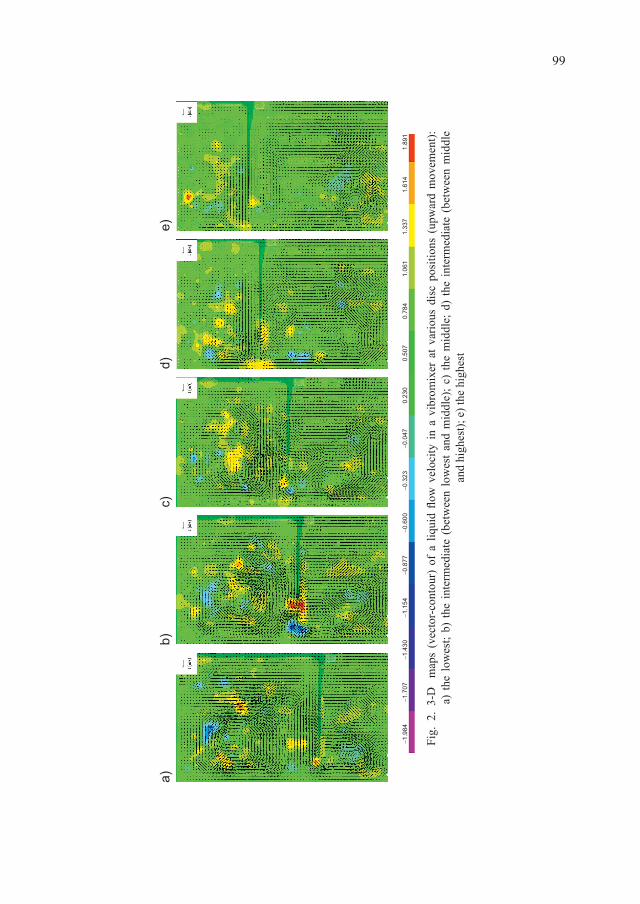
99

Fig.

2.

3-D

m

aps

(vec

tor-c

onto

ur)

of a

liq

uid

flow

vel

ocity

in

a vi

brom

ixer

at

vario

us d

isc

posi

tions

(up

war

d m

ovem

ent):

a)

the

low

est;

b) th

e in

term

edia

te (

betw

een

low

est a

nd m

iddl

e); c

) th

e m

iddl

e; d

) th

e in

term

edia

te (

betw

een

mid

dle

and

high

est);

e) t

he h

ighe

st

100

Fig. 3. 3-D maps (vector-contour) of liquid flow in the ring-shaped gap between the disc and tank wall at various disc positions (upward movement): a) the lowest; b) the intermediate (between lowest and middle); c) the middle;

d) the intermediate (between middle and highest); e) the highest

101

flow along the disc surface, which in the region of the disc tip changes direction and axial velocity components start to dominate. 3-D maps present distinct regions of liquid stream separation into lower (under the disc) and upper (above the disc) zones of vortex interaction. Instability of tangential flow can also be seen, determined practically for both (along z-axis and opposite) directions, coloured red and blue, respectively. A significant obstruction of radial-axial flow through the gap is visible for the highest disc position (Fig. 3e).

Additionally, to facilitate quantitative flow analysis, graphs illustrating values of velocity components were drawn. Curves represent values of individual velocity components (radial, axial and tangential) at the examined disc positions as a function of the relative vessel radius (r* = 2r/D) including the gap.

Changes of radial velocity (Fig. 4a) have a similar course regardless of disc position. The radial liquid flow is generated from the disc to the tank wall. Along the gap width, the

Fig. 4. Changes of flow velocity components as a function of a relative vessel radius (r* = 2r/D): a) radial velocity (ux); b) axial velocity (uy); c) tangential velocity (uz)

102

values of this velocity component increase, reach a distinct extremum near half of the gap width. Next, they decrease as the distance to the wall decreases. With a successive upward disc movement, extreme values of a radial velocity component increase with the maximum (ux = 0.6 m/s) for the intermediate (middle/highest) disc position. A very low radial flow for the highest disc position following change of disc movement (upward to downward) and a relatively weak flow circulation in the whole volume of the mixing vessel at this stage is but an isolated case. A similar tendency with extreme values in the region of half of the gap width is also observed for axial velocity (Fig. 4b). However, in this case the values are lower (uy = 0.4 ‒ 0.5 m/s) in comparison with the radial velocities. The curves representing the axial velocities for the lowest, intermediate (lowest/middle) and middle disc positions have very close maximum values, and, in the near wall zone, they overlap. The flow at the tip and under the disc also has an interesting structure. For most investigated disc positions (Fig. 3), we can see vortices with reversed flow (axially consistent with disc movement) which is also confirmed by data in Fig. 4 (positive values of velocity).

As is mentioned above, the third (tangential) component of velocity is characterised by a large irregularity and high velocities of flow. This interesting problem will be analysed in our further investigations. Also, results obtained in the present study will be used for the validation and verification of numerical CFD simulations.

These investigations were conducted with financial support from the Statutory Activities I don’t think that capitalisation here is appropriate of Cracow University of Technology (M5/194/DS/2013).

R e f e r e n c e s

[1] Paul E.L., Atiemo-Obeng W.A., Kresta S.M., Handbook of Industrial Mixing, Wiley & Sons Inc., New Jersey 2004.

[2] Kamieński J., Agitation of multiphase systems, WNT, Warsaw 2004 (in Polish).[3] Kamieński J., Wójtowicz R., Dispersion of liquid-liquid systems in a mixer with a reciprocating

agitator, Chemical Engineering and Processing, 42, 2003, 1007-1017.[4] Lo M.Y.A., Gierczycki A.T., Titchener-Hooker N.J., Ayazi Shamlou P., Newtonian power curve

and drop size distributions for vibromixers, Canadian Journal Chemical Engineering, 76, 1998, 471-478.

[5] Wójtowicz R., Choice of an optimal agitated vessel for the drawdown of floating solids, Industrial & Engineering Chemistry Research, 53, 2014, 13989-14001.

[6] Masiuk S., Rakoczy R., Power consumption, mixing time, heat and mass transfer measurements for a liquid vessel that is mixed using a reciprocating multiplates agitator, Chemical Engineering and Processing, 46, 2007, 89-98.

[7] Brauer H., Annachhrate A.P., Nitrification and denitrification in a system of reciprocating jet bioreactor, Bioprocess Engineering, 7, 1992, 269-275.

[8] Komoda Y., Inoue Y., Hirata Y., Characteristics of turbulent flow inducted by reciprocating disk in cylindrical vessel, Journal of Chemical Engineering of Japan, 34, 2001, 929-935.

[9] Wójtowicz R., The vibromixers – a current state of research and trends of further investigations, [In:] Process Engineering and Chemical Plant Design (G. Wozny, Ł. Hady, eds.), Universitätsverlag der TU Berlin, Berlin 2011.

103

[10] Raffel M., Willert C.E., Wereley S.T., Particle Image Velocimetry – A practical guide, Springer, Berlin Heidelberg 2007.

[11] Albrecht H.-E., Borys M., Damaschke N., Tropea C., Laser Doppler and Phase Doppler Measurement Techniques, Springer, Berlin-Heidelberg 2003.

[12] Dantec Dynamics, DynamicStudio 3.2 User’s Guide, Dantec Dynamics, Skovlunde 2011.

CONTENTS

Cyklis P.: Selected issues of the multistage evaporator thermodynamics ........................................ 3Cyklis P., Duda R.: The hybrid sorption-compression refrigeration cycle control system ............... 11Cyklis P., Młynarczyk P.: Nozzle suppressed pulsating flow CFD simulation issues ...................... 21Kopeć P.: Influence of refrigerant R1234yf as a substitute for R134a on a perfect refrigeration

cycle and exchanger efficiency ................................................................................................... 31Matras Z.: Friction curves transformation of non-Newtonian fluids in coils ................................... 39Matras Z., Kopiczak B.: Ccomparative analysis of drag reduction flow efficiency through the use

of surfactants and high molecular polymer additives ................................................................. 49Mika Ł., Górski B., Kantor R.: Flow modelling of slurry ice in a control valve .............................. 59Mika Ł., Zalewski W.: Local pressure loss coefficient during the flow of slurry ice trough

sudden pipe expansions .............................................................................................................. 67Niezgoda-Żelasko B., Żelasko J.: Free convection on the outer surface of vertical longitudinally

finned tubes ................................................................................................................................. 75Niezgoda-Żelasko B., Żelasko J.: Heat transfer of ice slurry flowing in rectangular and slit

chanels ........................................................................................................................................ 87Wójtowicz R., Paszkowska S.: Investigations of liquid flow velocity in a vibromixer using stereo

PIV anemometry ......................................................................................................................... 95

TREŚĆ

Cyklis P.: Wybrane elementy termodynamiki wyparki wielostopniowej ......................................... 3Cyklis P., Duda R.: Automatyka i sterowanie hybrydowego sorpcyjno-sprężarkowego systemu

ziębniczego ................................................................................................................................. 11Cyklis P., Młynarczyk P.: Problemy symulacji CFD pulsującego przepływu tłumionego przez

dyszę ........................................................................................................................................... 21Kopeć P.: Wpływ czynnika chłodniczego R1234yf jako zamiennika R134a na pracę

idealnego obiegu chłodniczego oraz wydajność wymiennika .................................................... 31Matras Z.: Transformacja krzywych oporów przepływu płynów nienewtonowski w wężownicach 39Matras Z., Kopiczak B.: Analiza porównawcza efektywności redukcji oporów przepływu

za pomocą dodatków wielkocząsteczkowych polimerów i substancji powierzchniowo czynnych ..................................................................................................................................... 49

Mika Ł., Górski B., Kantor R.: Modelowanie przepływu zawiesiny lodowej w zaworze regulacyjnym .............................................................................................................................. 59

Mika Ł., Zalewski W.: Współczynnik miejscowych strat ciśnienia przy przepływie zawiesiny lodowej przez nagłe rozszerzenia przewodu .............................................................................. 67

Niezgoda-Żelasko B., Żelasko J.: Konwekcja swobodna na zewnętrznej powierzchni rur ożebrowanych wzdłużnie ........................................................................................................... 75

Niezgoda-Żelasko B., Żelasko J.: Wymiana ciepła zawiesiny lodowej podczas przepływu w kanałach prostokątnych i szczelinowych ................................................................................ 87

Wójtowicz R., Paszkowska S.: Badania prędkości przepływu cieczy w mieszalniku wibracyjnym metodą anemometrii obrazowej stereo PIV ................................................................................ 95