Forest Ecology and Conservation

Techniques in Ecology and Conservation Series

Series Editor: William J. Sutherland

Bird Ecology and Conservation: A Handbook of Techniques

William J. Sutherland, Ian Newton, and Rhys E. Green

Conservation Education and Outreach Techniques

Susan K. Jacobson, Mallory D. McDuff, and Martha C. Monroe

Forest Ecology and Conservation

Adrian C. Newton

Forest Ecology andConservation

A Handbook of Techniques

Adrian C. Newton

1

3Great Clarendon Street, Oxford OX2 6DP

Oxford University Press is a department of the University of Oxford.It furthers the University’s objective of excellence in research, scholarship,and education by publishing worldwide in

Oxford New York

Auckland Cape Town Dar es Salaam Hong Kong KarachiKuala Lumpur Madrid Melbourne Mexico City NairobiNew Delhi Shanghai Taipei Toronto

With offices in

Argentina Austria Brazil Chile Czech Republic France GreeceGuatemala Hungary Italy Japan Poland Portugal SingaporeSouth Korea Switzerland Thailand Turkey Ukraine Vietnam

Oxford is a registered trade mark of Oxford University Pressin the UK and in certain other countries

Published in the United Statesby Oxford University Press Inc., New York

© Oxford University Press 2007

The moral rights of the author have been assertedDatabase right Oxford University Press (maker)

First published 2007

All rights reserved. No part of this publication may be reproduced,stored in a retrieval system, or transmitted, in any form or by any means,without the prior permission in writing of Oxford University Press,or as expressly permitted by law, or under terms agreed with the appropriatereprographics rights organization. Enquiries concerning reproductionoutside the scope of the above should be sent to the Rights Department,Oxford University Press, at the address above

You must not circulate this book in any other binding or coverand you must impose the same condition on any acquirer

British Library Cataloguing in Publication Data

Data available

Library of Congress Cataloging in Publication Data

Data available

Typeset by Newgen Imaging Systems (P) Ltd., Chennai, IndiaPrinted in Great Britainon acid-free paper byBiddles Ltd., King’s Lynn

ISBN 978–0–19–856744–8 (Hbk)ISBN 978–0–19–856745–5 (Pbk)

10 9 8 7 6 5 4 3 2 1

To my father, Alan Newton, for all his support and encouragement over the years.

This page intentionally left blank

Preface

For the past 25 years, forests have been the focus of international conservationconcern. High rates of deforestation and forest degradation are common in manyparts of the world, but it was the rapid loss of tropical rain forests that particularlycaptured the attention of the world’s media from the early 1980s onwards. Morerecently, it has been increasingly recognized that many other ecologically impor-tant forest types, such as temperate rain forests and tropical dry forests, are alsobeing lost at an alarming rate. In response, particularly following the UnitedNations Conference on Environment and Development in 1992, major interna-tional efforts have been devoted to forest protection and sustainable management.There have been some notable successes during this time, yet still the widespreadloss of forests continues.

Despite the growth in the number of forest conservation and developmentprojects, as well as in the scientific discipline of forest ecology, practitioners areoften unsure how best to tackle the problems that they face. A lack of access toinformation about appropriate techniques is hindering both the development ofthe science and its application to forest conservation. This book was written inresponse to this need, and is part of a series providing information on methods inecology and conservation, focusing on different species and habitats. The targetaudience is ecologists involved in forest research or conservation projects, includ-ing both established professionals and those just starting out on their careers. It ishoped that the book will also be of value to practising foresters. Although forestershave traditionally been trained primarily in management of forests for timber, theprofession has undergone something of a revolution in recent years. The individ-ual forest manager is now often expected to be familiar with social, economic, andecological aspects of forests, as well as timber production. Hopefully this book willbe of value to those practitioners aiming at the elusive goal of truly sustainableforest management.

Forest ecology and conservation is an enormous subject. I have therefore had tobe highly selective in selecting material for this book. Inevitably, this choice hasbeen influenced by my own interests and experience, and for this bias, I apologize.Although it is recognized that different forest types differ substantially in theirecology and composition, the book is designed to be relevant to all kinds of forests.This is undoubtedly an ambitious goal, but I am comforted by the fact that in myown experience I have been more struck by the similarities between differentforests than by their differences, particularly regarding the conservation problemsthat they face. Many of the techniques described here have been applied to forestsgrowing in very different parts of the world, although perhaps with some adapta-tion. These methods should therefore be applied flexibly, not as rigid protocols.There is no substitute for common sense!

It is important to remember that techniques are not fossils. This is a livingdiscipline, in every sense. This means that there is scope to improve on all of themethods described here. Refining a method, or developing a new approach, is aworthwhile focus of research in its own right. Users of this book are thereforeencouraged not to consider the techniques presented as a finished article, butrather as a starting point for further experimentation and innovation. I havedeliberately provided extensive references, to provide examples of these methodsbeing used in practice, and to encourage readers to investigate their chosentechniques in greater depth. Citing these examples illustrates the fact that differentworkers use techniques in different ways, and in many cases the best way of doingsomething is an issue still open to both critical appraisal and debate.

In preparing this book, I particularly thank the many wonderful postgraduatestudents and research assistants with whom I have had the privilege of working,and who have grappled with many of the methods described: Theo Allnutt,Claudia Alvarez Aquino, Siddhartha Bajracharya, Sarah Bekessy, Niels Brouwers,Philip Bubb, Elena Cantarello, Cristian Echeverría, Duncan Golicher, JamieGordon, Carrie Hauxwell, Gus Hellier, Valerie Kapos, Tracey Konstant, FabiolaLópez Barrera, Rizana Mahroof, Elaine Marshall, John Mayhew, Francisco Mesén,Lera Miles, Khaled Misbuhazaman, Gill Myers, Simoneta Negrete, TheresaNketiah, Daniel Ofori, Tanya Ogilvy, Ashley Robertson, Patrick Shiembo, TonnySoehartono, Kerrie Wilson.

While writing the text I became increasingly aware of how much I owe thepeople that taught me as a student. It was surprising to discover how many of thetechniques described here were introduced to me when studying at Cambridgemore than 20 years ago. It is easy to take a good education for granted. I was veryfortunate to be taught by some eminent plant ecologists, and I here record a debtof gratitude to all of those who so generously shared their knowledge and expertise,particularly David Briggs, David Coombe, Peter Grubb, Bill Hadfield, DonaldPigott, Oliver Rackham, Edmund Tanner, Max Walters, and Ian Woodward.

Many thanks also to everyone who responded positively to a request forphotographs, and to my wife Lynn for checking the text.

Forests are magnificent places. I deeply respect those individuals who dedicatetheir lives to forest conservation, and I very much hope that this book will be ofsome value in supporting their efforts. Please let me know if the book proves to beof use, and more importantly, how it could be improved.

Adrian C. NewtonSchool of Conservation Sciences

Bournemouth Universityanewton@bournemouth.ac.uk

May 2006

viii | Preface

Contents

Abbreviations xiv

1. Introduction 1

1.1 Defining objectives 2

1.2 Adopting an investigative framework 5

1.3 Experimental design 8

1.4 Achieving scientific value 9

1.5 Achieving conservation relevance 12

1.6 Achieving policy relevance 16

1.7 Defining terminology 21

1.8 Achieving precision and accuracy 26

1.9 Linking forests with people 27

2. Forest extent and condition 32

2.1 Introduction 32

2.2 Aerial photography 33

2.2.1 Image acquisition 34

2.2.2 Image processing 36

2.2.3 Image interpretation 38

2.3 Satellite remote sensing 39

2.3.1 Image acquisition 42

2.3.2 Image processing 47

2.3.3 Image classification 49

2.4 Other sensors 54

2.5 Applying remote sensing to forest ecology and conservation 55

2.5.1 Analysing changes in forest cover 55

2.5.2 Mapping different forest types 60

2.5.3 Mapping forest structure 62

2.5.4 Mapping height, biomass, volume, and growth 63

2.5.5 Mapping threats to forests 66

2.5.6 Biodiversity and habitat mapping 66

2.6 Geographical information systems (GIS) 68

2.6.1 Selecting GIS software 71

2.6.2 Selecting data types 73

2.6.3 Selecting a map projection 74

2.6.4 Analytical methods in GIS 75

2.7 Describing landscape pattern 76

2.7.1 Choosing appropriate metrics 78

2.7.2 Estimating landscape metrics 82

3. Forest structure and composition 85

3.1 Introduction 85

3.2 Types of forest inventory 85

3.3 Choosing a sampling design 87

3.3.1 Simple random sampling 88

3.3.2 Stratified random sampling 89

3.3.3 Systematic sampling 90

3.3.4 Cluster sampling 90

3.3.5 Choosing sampling intensity 91

3.4 Locating sampling units 91

3.4.1 Using a compass and measuring distance 91

3.4.2 Using a GPS device 92

3.5 Sampling approaches 93

3.5.1 Fixed-area methods 94

3.5.2 Line intercept method 95

3.5.3 Distance-based sampling 95

3.5.4 Selecting an appropriate sampling unit 98

3.5.5 Sampling material for taxonomic determination 102

3.6 Measuring individual trees 104

3.6.1 Age 104

3.6.2 Stem diameter 107

3.6.3 Height 109

3.6.4 Canopy cover 111

3.7 Characterizing stand structure 113

3.7.1 Age and size structure 113

3.7.2 Height and vertical structure 115

3.7.3 Leaf area 116

3.7.4 Stand volume 118

3.7.5 Stand density 120

3.8 Spatial structure of tree populations 121

3.9 Species richness and diversity 125

3.9.1 Species richness 125

3.9.2 Species diversity 131

3.9.3 Beta diversity and similarity 133

3.10 Analysis of floristic composition 135

3.10.1 Cluster analysis 136

3.10.2 TWINSPAN 138

3.10.3 Ordination 139

3.10.4 Importance values 142

3.11 Assessing the presence of threatened or endangered species 142

3.12 Vegetation classification 144

x | Contents

4. Understanding forest dynamics 147

4.1 Introduction 147

4.2 Characterizing forest disturbance regimes 148

4.2.1 Wind 149

4.2.2 Fire 151

4.2.3 Herbivory 153

4.2.4 Harvesting 159

4.3 Analysis of forest disturbance history 161

4.4 Characterizing forest gaps 164

4.5 Measuring light environments 167

4.5.1 Light sensors 167

4.5.2 Hemispherical photography 170

4.5.3 Light-sensitive paper 174

4.5.4 Measuring canopy closure 174

4.6 Measuring other aspects of microclimate 178

4.7 Assessing the dynamics of tree populations 181

4.7.1 Permanent sample plots 181

4.7.2 Assessing natural regeneration 182

4.7.3 Measuring height and stem diameter growth 184

4.7.4 Measuring survival and mortality 185

4.7.5 Plant growth analysis 189

4.7.6 Factors influencing tree growth and survival 191

4.8 Seed bank studies 195

4.9 Defining functional groups of species 198

5. Modelling forest dynamics 203

5.1 Introduction 203

5.2 Modelling population dynamics 204

5.2.1 The equation of population flux 204

5.2.2 Life tables 205

5.2.3 Transition matrix models 205

5.3 Population viability analysis 213

5.4 Growth and yield models 220

5.5 Ecological models 221

5.5.1 Gap models 222

5.5.2 Transition models 226

5.5.3 Other modelling approaches 228

5.5.4 Using models in practice 230

6. Reproductive ecology and genetic variation 235

6.1 Introduction 235

6.2 Pollination ecology 235

6.2.1 Tagging or marking flowers 236

6.2.2 Pollen viability 236

Contents | xi

6.2.3 Pollen dispersal 237

6.2.4 Mating system 239

6.2.5 Hand pollination 243

6.2.6 Pollinator foraging behaviour and visitation rates 244

6.3 Flowering and fruiting phenology 245

6.4 Seed ecology 250

6.4.1 Seed production 250

6.4.2 Seed dispersal and predation 252

6.5 Assessment of genetic variation 262

6.5.1 Molecular markers 262

6.5.2 Quantitative variation 279

7. Forest as habitat 285

7.1 Introduction 285

7.2 Coarse woody debris 285

7.2.1 Assessing the volume of a single log or snag 286

7.2.2 Survey methods for forest stands 287

7.2.3 Assessing decay class and wood density 294

7.2.4 Estimating decay rate 296

7.3 Vertical stand structure 297

7.4 Forest fragmentation 300

7.5 Edge characteristics and effects 302

7.6 Habitat trees 307

7.7 Understorey vegetation 312

7.8 Habitat models 316

7.8.1 Conceptual models based on expert opinion 317

7.8.2 Geographic envelopes and spaces 320

7.8.3 Climatic envelopes 321

7.8.4 Multivariate association methods 321

7.8.5 Regression analysis 322

7.8.6 Tree-based methods 323

7.8.7 Machine learning methods 323

7.8.8 Choosing and using a modelling method 324

7.9 Assessing forest biodiversity 326

8. Towards effective forest conservation 332

8.1 Introduction 332

8.2 Approaches to forest conservation 333

8.2.1 Protected areas 334

8.2.2 Sustainable forest management 338

8.2.3 Sustainable use of tree species 344

8.2.4 Forest restoration 347

8.3 Adaptive management 354

8.4 Assessing threats and vulnerability 357

xii | Contents

8.5 Monitoring 363

8.6 Indicators 367

8.6.1 Indicator frameworks 368

8.6.2 Selection and implementation of indicators 369

8.7 Scenarios 374

8.8 Evidence-based conservation 377

8.9 Postscript: making a difference 377

References 379

Index of Authors and Names 431

Subject Index 437

Contents | xiii

Abbreviations

AAC allowable annual cutACE abundance-based coverage estimatorAFLP amplified fragment length polymorphismsANOVA analysis of varianceATBI all taxa biodiversity inventoryATFS American Tree Farm SystemAVHRR advanced very high resolution radiometerC&I criteria and indicatorsCBD Convention on Biological DiversityCCA canonical correspondence analysisCI cover indexCIFOR Centre for International Forestry ResearchCSA Canadian Standards AssociationCWD coarse woody debrisdbh diameter at breast heightDCA or DECORANA detrended correspondence analysisDEI depth of edge influenceDEMs digital elevation modelsDIFN diffuse non-interceptanceDN digital numberDPSIR drivers, pressure, state, impact, and responseDSS decision support systemENFA ecological niche-factor analysisESUs evolutionarily significant unitsFAO Food and Agriculture Organization of the United

NationsFCR fluorochromatic reactionFCS favourable conservation statusFHD foliage height diversityFLDM forest landscape dynamics modelFLEG forest law enforcement and governanceFLR forest landscape restorationFMU forest management unitFPA formalin/propionic acid/alcoholFRIS Forest Restoration Information ServiceFSC Forest Stewardship CouncilGAM generalized additive modelGCP ground control pointGFRA Global Forest Resources Assessment

GIS geographical information systemGLCF Global Land Cover FacilityGLM generalized linear modelGPS global positioning systemGRMU gene resource management unitHBLC height to base of live crownHCVF high conservation value forestHPS horizontal point samplingHSI habitat suitability indexIALE International Association for Landscape EcologyICE incidence-based coverage estimatorIFF International Forum on ForestsIPF Intergovernmental Panel on ForestsISI self-incompatibility indexITTO International Tropical Timber OrganizationIUCN World Conservation UnionIUFRO International Union of Forest Research

OrganizationskNN k nearest neighbourLAI leaf area indexLAR leaf area ratioLMR leaf mass ratioMBR Maya Biosphere ReserveMU management unitMWP modified-Whittaker plotNDVI normalized difference vegetative indexNFI national forest inventoryNGOs non-governmental environmental organizationsNTFP non-timber forest productOECD Organisation for Economic Co-operation and

DevelopmentOTU operational taxonomic unitPAR photosynthetically active radiationPCA principal components analysisPCO principal coordinates analysisPEFC Programme for the Endorsement of Forest

CertificationPIT passive integrated transponderPPFD photosynthetic photon flux densityPRA participatory rural appraisalPRC population recruitment curvePSP permanent sample plotPSR pressure–state–responsePVA population viability analysis

Abbreviations | xv

QTL quantitative trait lociRAP rapid assessment programmeRAPD random amplified polymorphic DNARAPPAM rapid assessment and prioritization of protected areas

managementRFLP restriction fragment length polymorphismRGR relative growth rateRGRH relative growth rate of heightROC receiver–operator characteristicRPVA relative population viability assessmentRRA rapid rural appraisalRTU recognizable taxonomic unitSFI sustainable forestry initiativeSFM sustainable forest managementSI suitability indexSLA specific leaf areaSLA sustainable livelihoods approachSSR microsatelliteUNCED United Nations Conference on Environment and

DevelopmentUNEP United Nations Environment ProgrammeUNFCCC United Nations Framework Convention on Climate

ChangeUNFF United Nations Forum on ForestsUTM Universal Transverse Mercator (projection)WCPA World Commission on Protected AreasWDPA World Database of Protected AreasWSSD World Summit on Sustainable DevelopmentWWF World Wide Fund for Nature

xvi | Abbreviations

1Introduction

This book describes techniques that may be used in ecological research, surveyor monitoring work in support of forest conservation and management. Yet con-servation is much more than simply a research endeavour. Rather, conservationmanagement depends on understanding the interplay between social, economic,and political issues relating to a particular forest, and on appreciating the values heldby different people with an interest in it. In practice, the scientific understanding ofthe ecology of a forest often plays a relatively minor role in determining how it isconserved or managed. In many cases, management decisions are based on politicalor economic expediency rather than the results of the latest ecological research. Yeteven though ecological understanding alone never conserved a forest, such anunderstanding can play a crucial role in ensuring that conservation management iseffective. The aim of this introductory chapter is to help achieve this objective, byplacing the application of ecological techniques in a broader context.

The science of forest ecology has progressed enormously over the past twodecades, assisted by rapid technological developments in areas such as remotesensing, GIS, and molecular ecology. Such techniques have transformed our under-standing of forest distribution and ecological condition, and have afforded pro-found insights into how forests respond to environmental change at a variety ofscales. Yet our understanding of forest ecology has its roots far deeper, havinggrown out of more than two centuries of forestry practice. While some of themethods described here are still evolving rapidly, others have proved themselvesover many years of practical application. Ecological researchers often have much tolearn from forestry professionals with respect to methods of forest mensurationand inventory, and any technique that has stood the test of time is worthy ofconsideration. New technology is no guarantee of improved measurements.

Deciding which technique is appropriate for use in a particular situationdepends critically on the objectives of the research or survey work to be under-taken. Defining these objectives clearly at the outset is of paramount importanceto any research or conservation programme. The objectives of a research ecologistmay differ substantially, however, from those of a conservation practitioner or aforest manager. Many forest conservation projects are designed to help implementsome policy objective, whether this be a policy statement developed by theorganization responsible for developing the project, or some national or inter-national policy goal. Even in the case of relatively ‘pure’ ecological research, fundingorganizations are increasingly inclined to direct their support towards research that

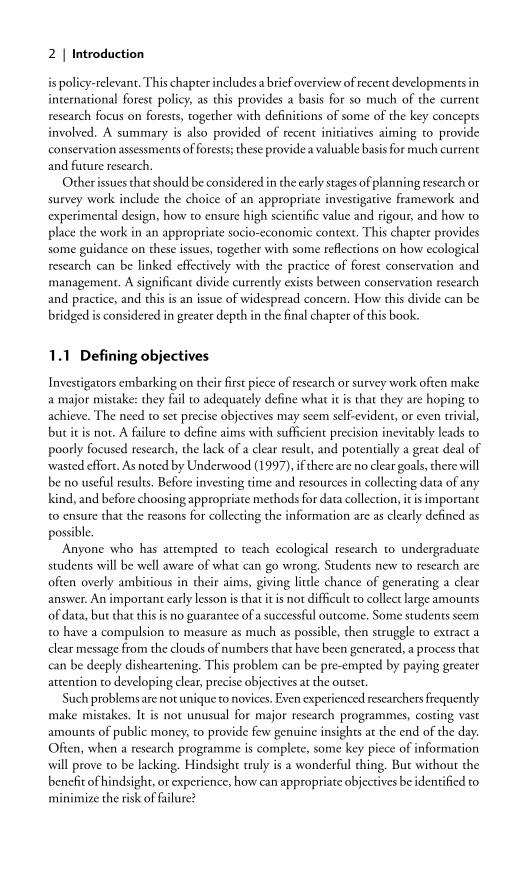
is policy-relevant. This chapter includes a brief overview of recent developments ininternational forest policy, as this provides a basis for so much of the currentresearch focus on forests, together with definitions of some of the key conceptsinvolved. A summary is also provided of recent initiatives aiming to provideconservation assessments of forests; these provide a valuable basis for much currentand future research.

Other issues that should be considered in the early stages of planning research orsurvey work include the choice of an appropriate investigative framework andexperimental design, how to ensure high scientific value and rigour, and how toplace the work in an appropriate socio-economic context. This chapter providessome guidance on these issues, together with some reflections on how ecologicalresearch can be linked effectively with the practice of forest conservation andmanagement. A significant divide currently exists between conservation researchand practice, and this is an issue of widespread concern. How this divide can bebridged is considered in greater depth in the final chapter of this book.

1.1 Defining objectives

Investigators embarking on their first piece of research or survey work often makea major mistake: they fail to adequately define what it is that they are hoping toachieve. The need to set precise objectives may seem self-evident, or even trivial,but it is not. A failure to define aims with sufficient precision inevitably leads topoorly focused research, the lack of a clear result, and potentially a great deal ofwasted effort. As noted by Underwood (1997), if there are no clear goals, there willbe no useful results. Before investing time and resources in collecting data of anykind, and before choosing appropriate methods for data collection, it is importantto ensure that the reasons for collecting the information are as clearly defined aspossible.

Anyone who has attempted to teach ecological research to undergraduatestudents will be well aware of what can go wrong. Students new to research areoften overly ambitious in their aims, giving little chance of generating a clearanswer. An important early lesson is that it is not difficult to collect large amountsof data, but that this is no guarantee of a successful outcome. Some students seemto have a compulsion to measure as much as possible, then struggle to extract aclear message from the clouds of numbers that have been generated, a process thatcan be deeply disheartening. This problem can be pre-empted by paying greaterattention to developing clear, precise objectives at the outset.

Such problems are not unique to novices. Even experienced researchers frequentlymake mistakes. It is not unusual for major research programmes, costing vastamounts of public money, to provide few genuine insights at the end of the day.Often, when a research programme is complete, some key piece of informationwill prove to be lacking. Hindsight truly is a wonderful thing. But without thebenefit of hindsight, or experience, how can appropriate objectives be identified tominimize the risk of failure?

2 | Introduction

Choosing an appropriate question to ask can be a daunting process. The range ofpossible objectives, even for a relatively simple forest system, is potentially infinite.An important first step is to define the kind of study that is being attempted. It isuseful to differentiate between ecological research, survey, and monitoring (some-times the word surveillance is also used for the latter):

● Research is generally undertaken to answer a specific question, or to test ahypothesis.

● A survey is typically a descriptive piece of work, which might be more open-ended in nature than a research project, and might not have such a clearoutcome.

● Monitoring is a form of survey that is designed to be repeated over time,enabling trends in some variable of interest to be determined.

Many of the techniques described in this book are equally relevant to each ofthese different approaches. However, the nature of the study will have implicationsfor how the methods are implemented, and above all for the design of the datacollection process.

The international scientific community tends to place greater emphasis onresearch rather than survey and monitoring work, and this is reflected in thecontent of scientific journals. According to Peters (1991), because of its lack ofrelationship to relevant theory, survey work does not qualify as science, but mightbe better referred to as natural history. Yet the importance of natural history shouldnot be underestimated. Much of our current ecological theory was developed onthe basis of painstaking field observations made by generations of naturalists.Furthermore, survey and monitoring methods are of fundamental importance tothe practice of conservation, providing information of value to priority setting andmanagement. There is great merit in simply observing how species behave in theirnatural habitats, and such observations can contribute directly to defining appro-priate management interventions (Marren 2002). It is striking how little is knownabout even our most important forest-dwelling ‘flagship’ species. As an example, itis salutary to note that we do not know precisely how many individuals remain ofany of the great ape species, nor what their precise habitat requirements are(Caldecott and Miles 2005).

There are situations where some form of survey will be preferred to a researchprogramme. In forest areas for which no prior information is available, a descriptivesurvey is the logical first step, perhaps with the simple aim of describing forestcomposition and structure. A survey might be undertaken to assess the conservationstatus or condition of a particular forest or associated species, or to determine theoccurrence of some potential threat. Many conservation organizations are currentlyinvesting heavily in survey work of this nature, with the aim of identifying prioritiesfor conservation. An initial survey can provide a basis for developing more tightlydefined questions relating to ecological processes or functions, which could beaddressed by subsequent research. Yet even in the case of a preliminary, descriptivesurvey, clear objectives should be defined at the outset.

Defining objectives | 3

A brief checklist is provided here to help guide the definition of objectives fora research, survey or monitoring programme:

● Is it original? Has the information already been collected by somebody else? Thiscan be most readily determined by conducting a review of relevant literature, forexample by using an appropriate search engine (such as �www.google.com�) orcitation database (such as the ISI Web of Science, �www.thomsonisi.com�).However, most information relating to forests has never been formallypublished, but resides in internal reports, data archives, newsletters and otherso-called ‘grey’ literature. Accessing such information can present an enormouschallenge. There may be no substitute for personally contacting relevant insti-tutions and individuals to ascertain what work has been carried out previously,and to find out what happened to the results. Although tracking down suchinformation can take a great deal of time and effort, the rewards may be signifi-cant. There is a fine tradition of meticulous survey work among many forestryinstitutions, which can still be a source of valuable information.

● Is it tractable? In other words, is it possible to deliver an answer to the questionset, given available time and resources? If not, then the objectives need to bemore tightly focused, for example by limiting the spatial or temporal scope ofthe project more narrowly. It is important to remember that some ecologicalquestions are impossible to answer.

● Is it interesting? Interest can be increased by choosing an issue that is topical ornovel. For example, has there been recent media interest in the chosen subject?Might the results of the research generate media interest? Many newresearchers are unaware of the extent to which different scientific themes go inand out of fashion, yet an awareness of current trends can be of great importancein successfully publishing results or securing funding for further research.

● Can the objectives be phrased as a question? Presenting the objectives in this waycan be a great help in focusing the design of the research, and in obtaining aclear answer from the results. It can be helpful to define a set of sub-questionsunder a general aim, to help break the problem down into more manageable,clearly defined units.

● Is it of practical value? Although this criterion may not be of paramount impor-tance to a ‘pure’ researcher, much ecological information is collected with aspecific end use in mind. To ensure that appropriate data are collected in a suit-able form, the objectives should be developed in consultation with the intendedusers of the information, such as conservation practitioners or forest managers.

Time spent refining objectives is never wasted. Remember that not everythingthat can be measured, should be (Krebs 1999). In practice, this means consideringalternatives, attempting to rephrase and refine the wording, always with the goal ofincreasing precision (see Box 1.1 for an example). Consult textbooks (for exampleBegon et al. 1996) or monographs (for example Hubbell 2001) to identify theoriesworth testing. Seek advice from your peers, colleagues, and supervisors beforeembarking on the project. Observe and analyse how the objectives are described in

4 | Introduction

published scientific papers. Avoid questions such as ‘why’ and ‘how come’, andfocus instead on developing questions that begin with ‘how much’, ‘how many’,‘when’ and ‘where’ (Peters 1991). Critically consider the possible answers to theobjectives that you have set.

Adopting an investigative framework | 5

Box 1.1 Defining research objectives

Research should be both tractable and interesting. In order to ensure that researchis manageable, objectives should be tightly focused, for example by limiting theirtemporal and spatial scope. In the example below, this has been achieved byexplicitly stating the area of forest to be considered, avoiding broad statementsabout forests in general that would be impossible to evaluate in a field survey. Toensure that the research is interesting, it should be topical, something that can beascertained by reference to the international media, as well as to recent issues ofscientific journals. In this example, whereas measuring forest biomass was anactive area of research during the boom in systems ecology in the 1960s, todayestimation of carbon sequestration is arguably a much more topical issue—evenif the basic techniques have not changed.

Not interesting Interesting

Not tractable Do forests have high Do forests sequester a lot of biomass? carbon?

Tractable What is the above-ground How much carbon does this biomass of this 0.01 ha forest 0.01 ha of forest sequester inplot? a year?

Many researchers set great store by the need to state hypotheses clearly at theoutset. Referees of manuscripts submitted to international scientific journals oftenexpect to see the objectives of a piece of research stated in this form. Yet not every-one agrees with this approach. The role of hypothesis testing continues to be thesubject of intense philosophical debate regarding how science should be done. Thisis a debate in which anyone embarking on a research project can usefully engage,perhaps involving some lively discussion with colleagues. This book cannot pre-tend to be a philosophical treatise, but researchers should be aware that opinionsvary regarding how science should be carried out. It is worth noting, however, thatstatistical tests are explicitly designed to test hypotheses, and if there is an intentionto employ such tests in the analysis of the results, then the hypotheses to be testedin this way should be made explicit at the outset.

1.2 Adopting an investigative framework

Regardless of what the precise objectives actually are, any piece of research or surveywork should be carefully planned and implemented according to an appropriateinvestigative framework. Adopting a clear logical procedure is important for

communicating the results to others, and to ensure that the information collectedachieves the objectives set.

A framework is presented here based on that described by Underwood (1997)(Figure 1.1). Versions of this procedure are widely practised in ecologicalinvestigations. The framework comprises a series of logical steps, beginning withobservations that are typically made in the field. Such observations can vary inspatial or temporal scale, and might be purely casual observations made during avisit to a particular forest, or the results of systematic survey work undertaken overa prolonged period. Usually some feature or pattern of potential interest will bedetected, which might be worthy of further study. For example, it might be noticedthat a particular species of tree appears only to occur in certain areas, perhaps alongriver banks or at particular altitudes.

The next step is to attempt to explain the phenomenon observed. Forest standsmight be dominated by large, old trees, with little evidence of recent recruitment.

6 | Introduction

OBSERVATIONSPatterns in space or time

MODELSExplanations or theories

HYPOTHESISPredictions based on model

NULL HYPOTHESISLogical opposite to hypothesis

EXPERIMENTCritical test of hypothesis

INTERPRETATION

START HERE

Retain H0Refute hypothesis

and model

Reject H0 Support hypothesis

and model

DON'T END HERE

Fig. 1.1 Generalized scheme of logical components of a research programme. Ho

represents the null hypothesis. (From Underwood (1997). Experiments in

Ecology: their logical design and interpretation using analysis of variance.

Cambridge University Press.)

Why might this be? There might be several alternative explanations to an observationsuch as this: for example, failure of seed production or dispersal, destruction ofjuvenile trees as a result of fire or the activities of herbivores, or the lack of appro-priate environmental conditions for seedling establishment. Typically there will bemany possible explanations for the observations made, and research will berequired to differentiate between them.

When undertaking any form of ecological investigation, it is helpful to differ-entiate between pattern and process. Patterns or phenomena are those things thatwe observe. Many ecological patterns are subtle and are difficult to detect, perhapsbecause they occur at a temporal or spatial scale that is difficult for us to perceive.Others might be more obvious but more difficult to explain. Such patterns arecaused by ecological processes. Alex Watt, one of the founding fathers of forestecology, was the first to explicitly separate pattern from process in considering thedynamics of vegetation in relation to its structure. His work on regeneration cyclesin beech woodland in southern England laid the foundations of our current under-standing of gap dynamics in forests, which has become such a powerful researchparadigm in forest ecology. His classic paper (Watt 1947) is still worth consultingtoday, despite the fact that it is based purely on observation. A focus on ecologicalprocesses is a central feature of much modern ecological research.

Having detected and described an ecological pattern, how can we identify themany different processes that might have been responsible for its formation? How canwe determine which of the many potential explanations for the pattern is correct?The formation of different logical hypotheses can help differentiate among explan-ations (Underwood 1997). A hypothesis can be defined as a prediction based on someexplanation of the observations made. Once a hypothesis has been formulated, it canpotentially be tested (Figure 1.1). This process of predicting an outcome by deducingwhat is logically consistent with a hypothesis, followed by its testing against obser-vations made, is known as the hypothetico-deductive scientific method.

Often, objectives of research are expressed as a null hypothesis, which is theopposite of a hypothesis. This reflects the fact that it is easier to disprove somethingthan to prove it (Underwood 1997). For example, it might be hypothesized that theabundance of an Acacia species is low in a particular area of savannah because it ispreferentially browsed by giraffes. This would be difficult to prove, because therecould always be some situation—another savannah, perhaps—that would provide anexception. So as an alternative, this could be expressed as a null hypothesis: theincidence of giraffe browsing has no effect on the abundance of the Acacia species. Thenull hypothesis could then be tested (or falsified), for example by experimentally alter-ing the incidence of giraffe browsing and observing its effects on Acacia abundance.

An experiment is the only way of adequately testing a hypothesis. If the outcomeof an experiment is to reject the null hypothesis, then the explanation or theorythat it was designed to test is supported. If the experiment fails to falsify the nullhypothesis, then the hypothesis is shown to be wrong, as its predictions were notcorrect. What happens next? If the explanation was supported, then it could betested again—through an additional experiment—to see whether it applies to

Adopting an investigative framework | 7

other situations, and if so, could then be considered as a general theory. If thehypothesis was not correct, then it needs to be revised in the light of the experi-mental results. There may be a need to collect additional observations. In eithercase, the process is a cyclic one (see Figure 1.1), and as Underwood (1997) pointsout, research can therefore be seen as a never-ending process—which might becomforting in terms of ensuring long-term job security!

Are there alternatives to this investigative framework? There is no doubt thatit has its flaws, and is not supported by all ecological researchers. As an illustration,it can sometimes be difficult to determine whether or not the hypothesis should beretained or rejected, as a result of type I or type II errors (Underwood 1990).

An alternative way of approaching research is offered by the use of Bayesianmethods. Bayesian inference involves the representation of beliefs or information inthe form of probabilities. The knowledge or beliefs available before research isundertaken are represented as a likelihood distribution, known as the ‘prior’. Thiscan then be revised in the light of new information generated by research, througha process of statistical inference using Bayes’ theorem. The revised probabilitydistribution is known as the ‘posterior’ (Dennis 1996). The use of Bayesian methodsin ecology was greatly stimulated by a series of papers published in the journalEcological Applications in 1996. As noted by Dennis (1996), the application ofBayesian approaches in ecology is controversial, as it implies abandoning thescientific method based on testing hypotheses and the investigative frameworkdescribed above. Protagonists of the Bayesian approach suggest that it makes betteruse of available data, allows stronger conclusions to be drawn from uncertain data,and is more relevant to environmental decision-making (Ellison 1996).

The application of Bayesian methods to conservation management is examinedby Wade (2000), who highlights the value of presenting information in a form thatdecision-makers can readily understand, in a way that incorporates uncertaintydirectly into the analysis. Ghazoul and McAllister (2003) reached similar con-clusions when considering the application of Bayesian methods to forest research.Whether or not Bayesian methods of analysis are adopted, it is helpful to makeunderlying models, paradigms, world views, and beliefs explicit, so that it ispossible to determine their influences on what and how measurements were taken(Underwood 1997).

1.3 Experimental design

Any ecological technique must be applied according to an appropriate experimentalor sampling design if the information generated is to be useful. A comprehensivetreatment of the principles of experimental design is beyond the scope of this book.There are now a number of texts that provide a valuable introduction to theprinciples of designing surveys and experiments. I particularly recommend thoseby Ford (2000), Krebs (1999), Peters (1991), Southwood and Henderson (2000),and Underwood (1997). Dytham (2003) provides a highly practical guide to theprinciples of sampling and statistical analysis.

8 | Introduction

The design of the research or survey will depend on the objectives set, and thecharacteristics of the forest to be studied. Some general principles to remember arelisted below:

● Randomize. Randomization is essential in order to avoid sample bias, and toensure that samples are representative. Most statistical tests assume that samplesare independent and free from bias, and this can most readily be achieved bysampling randomly. Stratified random sampling approaches are commonlyadopted in forest ecology, where random samples are taken within a forest areadivided into relatively homogeneous subareas classified on the basis of someenvironmental variable or forest composition. The number of samples takenshould be proportional to the size of each subarea (Southwood and Henderson2000). Remember that random samples should be truly random: use a randomnumber generator provided by a pocket calculator or appropriate computersoftware (many statistical or spreadsheet packages have this feature).

● Replicate. Replication is essential in order to determine patterns of variation, sothat the results obtained can be attributed to the experimental treatments orfactors of interest. Replicate samples should be taken within each area of study,and should be genuinely independent, to avoid the risk of pseudoreplication(Hurlbert 1984).

● Use appropriate controls. Many experimental investigations fail because of inadequate selection of controls, which are characterized by the absence of theexperimental factor or treatment of interest. By providing a basis for comparison,controls are of fundamental importance to effective experimentation. Manysurveys and monitoring approaches fail to collect baseline information beforethe experimental treatments (or management interventions) are applied, andfail to include untreated controls. Only by including such controls can any effectsdetected be attributed to directly to the treatment of interest.

● Perform a power analysis before starting the main investigation. Before investingtime and effort in intensive data collection, it is recommended that a pilotstudy be undertaken to test the methods and protocols. The data obtainedduring such a pilot study can then be used to perform a power analysis, whichwill enable estimates to be made of the number of samples required to detecteffects of a given magnitude. Statistical power is influenced by the sample size,the variability of the population being sampled, and the magnitude of theeffect of the experimental treatment or factor. Methods of power analysis arepresented by Krebs (1999) (see also Chapter 8); software programs that per-from such analyses are reviewed by Thomas and Krebs (1997).

1.4 Achieving scientific value

Once the objectives of a research or survey project have been defined, an investigativeframework adopted, and an appropriate design put in place, then success in terms ofdelivering some valuable results might seem assured. However, failure to deliver resultsof genuine scientific value is more common than many researchers might care to

Experimental design | 9

admit. Most researchers have at least one file drawer full of results that have failed tosee the light of day in terms of a scientific publication. Entire doctoral theses, repre-senting years of honest endeavour, have been consigned to this form of oblivion. Howcan this failure be avoided, and results of real scientific value be achieved?

This raises the question of what constitutes scientific value. Although scientificperformance is often assessed in terms of the number and quality of publicationsproduced, this may be a poor measure of its real value. Most scientific papers arecited rarely, some not at all. Few have real impact in terms of influencing forestconservation policy or practice. But the problems may go deeper than how theresults are disseminated: to the nature of ecological science itself.

Peters (1991) provides a comprehensive critique of the science of ecology andhow it is currently practised. In many ways, this is an extraordinary book, and it isrecommended reading for anyone interested in engaging in any form of ecologicalresearch. He concludes that:

The weakness of the central constructs of contemporary ecology results because ecology com-pounds its single failings. Operational impossibilities spawn tautological discussions that replacepredictive theories with historical explanations, testable hypotheses with the infinite research ofmechanistic analysis, and clear goals for prediction with vague models of reality. The resultingmélange obscures appropriate research and attainable goals with sloppy, ineffective activity. As aresult, the central constructs in ecology yield predictions with difficulty and these are often soqualitative, imprecise and specific that they are of little interest and less utility (Peters 1991).

Peters’ book does not make comfortable reading for most ecologists. There ishardly a single area of ecological method that escapes some degree of censure.Needless to say, the conclusions are controversial, but at the very least the pointsraised are worthy of serious consideration and debate. But what are the practicalimplications of this critique? Some of these are summarized briefly below, but thereader is encouraged to consult the original text for a comprehensive considerationof these and many other issues.

● Pluralism. A single approach or technique will not be successful in all systems;rather, different approaches may be needed for different systems and differentquestions. This applies as much to the methods used in building theory as tothose used to test it. Multiple working hypotheses should be encouraged.

● Practicality. Many ecological theories, it is argued, have little relevance to thereal world. They are often based on abstract mathematical representations ofphenomena rather than on empirical measurements. Researchers should focuson making practical observations, and on addressing little questions that canbe answered rather than big questions that cannot. Theory should always berelevant, and inspired by pressing problems about nature rather than the searchfor scholasticism. Seek the simplest way of making testable predictions.

● Sound variables. Much ecological research suffers from use of concepts that aredifficult or even impossible to measure. Even concepts as widely used as ‘niche’,‘ecosystem’, and ‘habitat’ have been defined variously by different authors and aredifficult to operationalize in practice. Variables should be simple, measurable,

10 | Introduction

and operationally defined, such as diversity, nitrogen concentration, biomass,population density, etc. Poorly defined variables should be avoided.

● Empiricism. Theories must be supported by data, or directly based ondata. Patterns in these data should be identifiable by using simple statisticalmanipulations, such as regression. Focus on prediction rather than explan-ation. All predictive models are probabilistic; uncertainty should always beestimated or represented in such models.

Above all, Peters (1991) emphasizes the importance of testing predictions madeon the basis of relevant theory, as an essential ingredient of high-quality ecologicalscience. Investigators embarking on a new programme of research should thereforeseek to identify relevant theory at the outset, and on the basis of such theory,develop hypotheses incorporating specific predictions that can readily be tested.Peters (1991) also notes that ecological research often encourages the constructionof irrelevant theories and the collection of irrelevant data by proposing and testingunderlying mechanisms that might contribute to an observed pattern, althoughthey are neither necessary nor sufficient for that pattern. Theories that arescientifically relevant are those that can help resolve questions posed by the scien-tific community. Scientifically relevant data are those that can test the predictionsfrom such theories (Peters 1991).

How can relevant theory be identified? Ecological science is not short of theor-etical ideas, and a search of relevant textbooks or journal papers will soon uneartha variety of candidates. Selection of an appropriate theory will depend upon thecharacteristics of the problem that has been identified. Many problems relating toforest dynamics, for example, can be addressed by using theories relating tosuccessional processes. In the conservation biology literature, island biogeographytheory and metapopulation theory never seem to be very far away. New ideas arealways worth seeking out and critically examining.

Problems relating to forest ecology have fortunately attracted the interest ofsome outstanding researchers, who have produced some highly original andstimulating works. To cite just two examples: the recent book by Stephen Hubbell,although it has implications far beyond the boundaries of forest ecology, wasinspired by detailed analysis of community composition in tropical forests. Hissynthesis of island biogeography theory and theories of relative abundance is, inmy view, the most important contribution to ecological science in the past threedecades, and an outstanding intellectual achievement (Hubbell 2001). Read it andsee whether you agree with me. Whether right or wrong, there are enough ideas inthis book to keep generations of postgraduate students busy for decades. Withrespect to the forests of northern Europe, Vera (2000) has produced a remarkablebook that seeks to overturn traditional views of forest succession, by criticallyexamining almost a century’s worth of accumulated empirical evidence. This bookprovides a salutary reminder that no theory in ecology is so well established thatit could not be overturned by some appropriate research. As an aside, Vera hasmanaged what many researchers aspire to but few achieve: a radical reappraisal ofconservation practice, among practitioners themselves.

Achieving scientific value | 11

1.5 Achieving conservation relevance

Although scientific journals are bursting with research results that often appear tohave important implications for forest conservation, most research seems to havelittle impact on how conservation is actually practised. This can be a source of greatfrustration to those who have worked so hard to obtain the results concerned. Whatis going wrong? Is it because practitioners do not read scientific papers? Or hasthe wrong research been done? Or does the problem go deeper—do practitionersfully understand the implications of research? Do researchers fully appreciate theproblems faced by practitioners?

This divide between conservation research and practice is currently the focus ofmuch concern, particularly among researchers. At the same time, policy-makers areincreasingly requiring that management action be based on an ‘evidence-based’approach—in other words, on the best scientific information available. How can thisbe achieved? The techniques that can be used to strengthen the links between conser-vation research and practice are described in Chapter 8. Here, I focus on more generalissues that should be considered when planning any research or survey programme.

If research is to be relevant to conservation practice, then there is no substitute foreffective communication between researchers and practitioners. A researcher mayhave a theory of how forests respond to environmental change, and be keen to testit. The practitioner’s priorities may be very different: perhaps there is uncertaintyabout the potential impacts of a proposed management intervention, or how aforest is being affected by some newly emerging threat. Only a process of dialoguebetween both parties will ensure that the practitioner’s needs are properly met by theproposed research. This dialogue can be great fun and enormously educational forboth parties, if based on mutual respect.

Many conservation organizations appear to spend most of their time organizingworkshops. Forest managers often feel as if they are spending more time attendingmeetings, discussing how things ought to be done, rather than getting outand doing it. There is now great emphasis on engaging in a process of ‘stakeholderconsultation’ before implementing any conservation action. This reflects thegrowing recognition that for conservation to be effective, those people that have aninterest or stake in the outcome need to be involved in the decision-making processfrom the outset. Ecological research or survey work often seems to play little role inthis consultation process, and the idea of attending interminable meetings can bevery off-putting to many researchers (as well as some practitioners). Discussionsaround a table can seem very remote from real-life conservation action. Yet,engagement in this process is often essential if research is to play its proper role ininfluencing conservation outcomes.

If you are a researcher who wants to make a difference, it is worth learningabout how conservation decisions are made. Often the technical issues surroundinghow a particular forest should be managed are relatively easy to solve. Yet the transla-tion of research results into conservation practice can be a long and arduous process.It should be remembered that conservation is a highly political endeavour. It can beviewed as a struggle for competing values. Sometimes it even erupts into conflict.

12 | Introduction

One of the most striking trends in conservation over the past three decades hasbeen the growth in size and influence of non-governmental environmental organ-izations (often referred to as NGOs). Collectively, these organizations have playeda hugely significant role in placing forest conservation on the international agenda.Each NGO has its own particular objectives and mode of operation. Some, such asGreenpeace, focus exclusively on campaigning and direct action. Others, such as theWorld Wide Fund for Nature (WWF), actively develop and implement conserva-tion projects on the ground. Some environmental NGOs are now large, influentialorganizations that work in partnership with government agencies and (sometimescontroversially) the private sector in their conservation projects. Some NGOs,notably Conservation International and WWF, have invested heavily in developingtheir own research and assessment programmes, to provide a scientific basis to theircampaigning and priority setting (Figure 1.2).

Achieving conservation relevance | 13

Fig. 1.2 The ultimate conservation priority? The island of New Caledonia is widely

recognized as being of outstanding conservation importance, particularly because of

the high diversity and endemicity of its flora. The island is home to many evolutionary

primitive species as a result of being a remnant of Gondwanaland that has been

isolated for a very long time. It is both a ‘priority ecoregion’ and a ‘biodiversity

hotspot’, as defined by WWF and Conservation International respectively. The site

pictured is the Chute de la Madelaine on the Plaine des Lacs, an exceptionally

important site for endemic and extremely rare tree species, with six different conifer

genera occurring within an area of about 10ha. Two conifer species, Dacrydium

guillauminii and Retrophyllum minor, are known only from this area. Although protected,

the site is suffering from increasing visitor pressure. (Photo by Adrian Newton.)

14

|In

trod

uctio

n

Table 1.1 Some of the major assessments and campaigns relating to forests currently being undertaken by leading non-governmental

conservation organizations.

Organization Assessment or Comments URLcampaign

Conservation Biodiversity Hotspots are areas characterized by high www.conservation.org/xp/CIWEB/homeInternational (CI) hotspots endemism and high rates of habitat loss. To www.biodiversityhotspots.org/xp/Hotspots

qualify as a hotspot, a region must contain at least 1500 species of vascular plant as endemics, and have lost at least 70% of its original habitat. A global assessment of biodiversity hotspots is available (Mittermeier et al. 2004). CI are also active in conserving high-biodiversity wilderness areas, many of which are forested

Fauna and Flora International/ Global Tree A collaborative programme involving www.globaltrees.org/UNEP World Conservation Campaign campaigning and conservation action Monitoring Centre focusing on threatened tree species in

different parts of the world

Greenpeace Ancient A conservation campaign focusing on www.greenpeace.org/international/Forests ‘the world’s remaining forests which campaigns/forests

have been shaped largely by natural

Ach

ieving co

nse

rvatio

n re

levan

ce|

15

events and which are little impacted byhuman activities’ (Greenpeace International 2002)

IUCN Red List The most comprehensive assessments of the /www.redlist.org/world’s threatened species, undertaken andregularly updated by IUCN through its Species Survival Commission (SSC)

World Resources Institute / Frontier An assessment of the world’s ‘remaining large http://forests.wri.org/Global Forest Watch forests intact natural forest ecosystems’ (Bryant et al. www.globalforestwatch.org/

1997), equivalent to the Ancient Forests english/index.htmfeaturing in the Greenpeace campaign

WWF Ecoregions An ecoregion is a large area of land or www.worldwildlife.org/water that contains a geographically distinct assemblage of natural communities. WWF has identified825 terrestrial ecoregions worldwide, and is targeting some 200 of them forconservation action (Olson and Dinerstein 1998, Olson et al. 2000, 2001).Thorough assessments are beingundertaken of the biodiversity of these areas

NGOs can be powerful allies in disseminating research results and putting theminto practice. Many have close links with the media and produce their own pub-licity material or technical publications. An awareness of their current prioritiesand activities is therefore useful. Conservation campaigns can also provide a con-text or justification for research. However, researchers should never forget theirown capacity to set the agenda. Novel information about some conservation issueor problem might well be seized upon and become a focus of campaigning andeventual conservation action. The biodiversity hotspot concept developed byNorman Myers (Myers 1988, 1990, 2003), for example, has become the centralfocus of campaigning and action by Conservation International (Myers et al.2000).

In recent years, some international NGOs have devoted substantial resources toundertaking biodiversity assessments, with a view to defining conservation prioritiesat the global scale. A summary of some of the key initiatives is presented inTable 1.1, together with some of the main campaigns relating to forests implementedby international NGOs. The ecoregion assessments produced by WWF provide aparticularly informative account of the ecological characteristics of different forestareas, and the conservation issues affecting them, providing a very valuable sourceof reference (Burgess et al. 2005, Dinerstein et al. 1995, Ricketts et al. 1999,Wikramanayake et al. 2002). A valuable overview of current assessments and theconservation approaches of leading NGOs is provided by Redford et al. (2003).Although such assessments can provide useful context for research, they are notbeyond criticism. In an important paper, Mace et al. (2000) point out the highdegree of duplication between the conservation assessments that have recentlybeen completed, and highlight the need for greater collaboration between conser-vation organizations. Whitten et al. (2001) go further and question the value ofthe conservation assessments that are currently being undertaken, as well as therelevance of scientific research to conservation practice.

Researchers should therefore be aware of the social, political, and institutionalenvironment within which conservation action takes place. Recognize that allorganizations have their own agenda and approach and, even if they appear to beworking to a common goal of conservation, may have very different priorities ormeans of achieving it. It is important to keep abreast of developments and emergingissues, as illustrated by NGO campaigns. Consult websites, publications, andother media; attend conferences and meetings focusing on conservation practice aswell as research. Remember that your research results may be of interest to a largecommunity of conservation activists as well as practitioners, but be prepared topromote your findings if you believe them to be important. Conservation is notjust a struggle about values, but a battle for ideas. And for resources.

1.6 Achieving policy relevance

Forest policy is something of a mystery to many researchers. They may dimly beaware of its presence, yet consider it of little relevance to their work. Cynics

16 | Introduction

perceive international policy development fora as endless talking shops, whichachieve little in terms of practical conservation action. The process by whichpolicies are developed at national and subnational scales can similarly appearopaque and somehow divorced from the situation in the field. Yet, in reality, policydecisions and agreements made at a high level underpin many research and man-agement actions, and have a major bearing on the availability of research fundingto address specific problems. Does policy matter? Even if a research project is notdesigned to be policy-relevant, its results may be used in that way. It therefore paysto be aware of what is happening in the policy arena.

This is not the place for a comprehensive account of forest policy. The issue iscovered in detail by other texts such as Mayers and Bass (2004) and Sample andCheng (2004). Rather, the aim here is to encourage researchers to be aware of thepolicy context in which they are working. Some guidance is given regarding howto keep abreast of policy developments, and how to make the link between policyand research.

Some key recent developments in international forest policy are listed inTable 1.2. It is important to remember that policy-makers are just as subject tofashion as are many other elements of our increasingly globalized society. Newissues can suddenly emerge and within a relatively short time come to dominatedebate. Interest then gradually subsides as some other issue comes to the fore.Keeping abreast of policy developments presents a significant challenge to theaverage forest practitioner or researcher; after all, attending the internationalcircuit of policy meetings is a full-time job for professionals dedicated to the (ratherthankless) task. Fortunately, access to information has improved enormously withthe development of the Internet, and most international forest policy processesnow provide ready access to the many documents that they generate via theirwebsites. Some relevant URLs are provided in Table 1.2. The Forest Policy Experts(POLEX) electronic list server �www.cifor.cgiar.org/docs/_ref/polex/index.htm� is aparticularly useful way of keeping up to date on developments in forest policy.Another effective way to stay in touch is to monitor the websites of the leadingenvironmental NGOs active in forest conservation. Many of these engage closelyin policy processes and have teams of staff dedicated to the task, who report regu-larly via their own organization’s websites.

Since the United Nations Conference on Environment and Development(UNCED) in 1992, the issue of sustainable forest management has been at thecentre of the international policy debate relating to forests, and underpins manynational policy initiatives. Much of this discussion has focused on how sustainableforest management can be defined and assessed. Considerable effort has beendevoted to the development of criteria and indicators (C&I) that might assist inthis process. These developments have primarily occurred under the auspices ofinternational ‘C&I processes’ (see Table 1.2). It was recognized early on that forestsin different parts of the world have very different characteristics, and thereforedifferent sets of C&I would need to be developed. Although the idea of harmonizingor standardizing between these different indicator sets has been discussed from

Achieving policy relevance | 17

time to time, this is something that is no longer actively being pursued. The C&Iprocesses like to keep their independence.

Many of the international C&I processes have developed indicators that areappropriate for use at the national scale, rather than at the local scale, and are usedfor the development and updating of national and international policy instruments(Castañeda 2001). However, these processes are increasingly driving the collection ofinformation about forests at local scales, which can then be aggregated for reportingat higher scales. The Global Forest Resources Assessment (GFRA), coordinated bythe FAO, has now structured the reports that it solicits from individual countriesaround C&I. These C&I therefore provide an important context for much of thedata collection relating to forests.

At the scale of forest management units, the development of indicators forsustainable forest management has primarily been driven by the growth of interest inforest certification. Forest certification is essentially a tool for promoting responsibleforestry practices, and involves certification of forest management operations byan independent third party against a set of standards. Typically, forest products

18 | Introduction

Table 1.2 A summary of key international policy processes relating to forest

conservation.

The Convention on Biological Diversity (CBD), agreed at the 1992 Earth Summit inRio, is the main international convention focusing on biodiversity conservation andsustainable use. The CBD has developed a thematic programme specifically focusingon forest biodiversity (�www.biodiv.org/programmes/areas/forest/ �) with an associatedprogramme of work, which details what Parties to the Convention should actually bedoing in this area.

The ‘Forest Principles’ and Chapter 11 of Agenda 21 are a set of non-legally bindingprinciples relating to the conservation and sustainable development of forests that wereagreed at the 1992 Earth Summit (UNCED) (�www.un.org/esa/sustdev/documents/agenda21/ �).The United Nations Forum on Forests (UNFF) was established in 2000 to ‘promotethe management, conservation and sustainable development of all types of forests andto strengthen long-term political commitment to this end’ (�www.un.org/esa/ forests/ �).The UNFF provides an important forum for international dialogue about forests. Itis the successor to two prior initiatives, the Intergovernmental Panel on Forests (IPF)and the International Forum on Forests (IFF), which together recommended morethan 270 proposals for action to be adopted by the international community, specific-ally relating to implementation of the Forest Principles and Chapter 11 of Agenda 21.Implementation of these proposals is currently being assessed by the UNFF.

International C&I processes include ITTO, the Pan-European (or ‘Helsinki’) Process,the Montreal Process, and the Tarapoto, Lepaterique, Near East, Dry Zone Asia, andDry Zone Africa processes, which have each generated sets of C&I (Castañeda 2001).Currently, around 150 countries are participating in these processes.

(generally timber but also non-timber forest products) from certified forests arelabelled so that consumers can identify them as having been derived from well-managed sources. There are now many different organizations certifying forestsagainst a variety of different standards. Examples include the Sustainable ForestryInitiative (SFI) Program and the Forest Stewardship Council (FSC). At least at ageneral level, the standards developed by certification bodies can be viewed assupporting sustainable forest management, although not all certifying organizationsuse this precise terminology.

More recently, other key policy developments have come to dominate inter-national discussion. Increased concern about widespread illegal logging has led tothe development of regional Forest Law Enforcement and Governance (FLEG)processes, as well as action by the G8 group of countries and the World Summit onSustainable Development (WSSD) �www.illegal-logging.info�. Forests are also ofconcern to the United Nations Framework Convention on Climate Change(UNFCCC), particularly as the Kyoto Protocol potentially provides a mechanismfor financing forest establishment and conservation. Under the Protocol, industri-alized countries that lack options for expanding forests may partly compensate fortheir greenhouse-gas emissions by paying for the establishment and maintenanceof forests in other countries �http://unfccc.int/ �. Forests do not feature so prom-inently in other recent international policy initiatives, such as the United NationsMillennium Development Goals and the WSSD held in 2002 �www.un.org/esa/sustdev/�. However, the 2010 biodiversity target adopted by the Convention onBiological Diversity (CBD) and endorsed by the WSSD has become a centralpolicy objective in conservation, aiming to achieve a ‘significant reduction of thecurrent rate of biodiversity loss at the global, regional and national level’. Thispotentially offers a significant opportunity to further conservation efforts world-wide, and its implementation is already taxing the scientific community (Balmfordet al. 2005).

How can research be linked with policy? Many funding organizations nowrequire that research be ‘policy-relevant’. What does this actually mean? Simplyput, research should strive to assist the process of policy implementation, withoutnecessarily being policy-prescriptive. Put another way, policy-makers often do notlike being told what to do, but recognize that research can play a role in helping toachieve policy goals. Researchers should not forget, however, that they have thecapacity to significantly influence, or even lead, the policy agenda. Issues such asclimate change, invasive species, and deforestation have all become the focus ofinternational attention from policy-makers, partly as a result of the research thathas been carried out on their actual or potential impacts.

How can research help implement policy? A key area is in helping to oper-ationalize policy concepts. If many concepts in ecological science are difficult todefine and measure precisely, as pointed out by Peters (1991), then the problemwith forest policy is even more acute. Policy-makers seem to delight in coiningterms whose meaning is difficult to pin down. Sustainable forest management isa case in point: what does this mean, exactly? Biodiversity is another term that

Achieving policy relevance | 19

means different things to different people. Of course, this obfuscation is partlydeliberate: the use of vague terminology is designed to help provide politicianswith room for manoeuvre, as they rarely enjoy being held to account. The use ofpoorly defined concepts is rightly an anathema to many ecological researchers,and this perhaps helps explain the antipathy that many researchers feel towardsthe area of policy.

It is practitioners who are typically at the sharp end of having to implementforest policy, and who often struggle with translating policy goals into practice.Forest managers are often assailed by poorly defined terminology: conceivably theymight be asked to achieve sustainable forest management by using an ecosystemapproach, by implementing multi-purpose forestry while adopting the precau-tionary principle, while not forgetting to consult stakeholders throughout theprocess. This kind of jargon is enough to task even the most hardened forestryprofessional. It is hardly surprising if these lofty policy goals sometimes fail to affectforest management on the ground.

Researchers can assist in the operationalization of policy concepts, by interpret-ing policy terms in the form of environmental variables that can be accurately andprecisely measured. Researchers can also help determine whether policy goals arebeing achieved. There is a real concern that despite all of the policy interest insustainable forest management, little is actually changing on the ground. Whetheror not policy implementation is being successful is a worthy area of research itself,yet this is something that has been neglected by researchers. Available informationsuggests that the effects of certification and application of C&I have been limitedto date (Rametsteiner and Simula 2003); many organizations that have certifiedforests are often those that were managing forests responsibly in any case (Leslie2004). Why has application of C&I not been more successful in producingchanges in forest management? Perhaps it requires the research community toengage more closely with the process, to help inform policy-makers and practi-tioners how best to define, measure and achieve progress towards policy goals; thisis an important role that is often overlooked. Many of the indicators that have beenproposed to date are difficult to implement in practice; often they are stated invague or imprecise terms (Stork et al. 1997).

Forest ecologists who really want to make a difference to conservation may seekto see their results reflected in policy. How can this be achieved? Some suggestions:

● By engaging in a dialogue with policy makers, and by disseminatingresearch results through policy fora such as the CBD. There are oftenmechanisms for researchers to present their results in this way, for example through preparation of an information note for delegates to theConvention’s meetings.

● By presenting their results in a form that can be readily assimilated by policy-makers, for example by publishing a policy brief.

● By collaborating with NGOs who are continually campaigning for policychange.

20 | Introduction

● By publicizing their results in popular media, an approach of proveneffectiveness in bringing issues to the attention of politicians, and an approachcontinually being adopted by campaigning NGOs, and even UN agencies.

● By publishing their results in scientific journals with a high impact factor, whichcan be remarkably successful in attracting media attention and increasingawareness among politicians.

1.7 Defining terminology

As mentioned above, one of the principal challenges to interpreting policy con-cepts relates to defining the terms used. Many terms used in forest conservation areopen to a variety of different interpretations, and this can present a significantobstacle to clear communication. It is therefore important to define terms preciselyat the outset of any investigation. In addition, make sure that your collaboratorsand partners share the same definition and understanding of the terms involvedthat you do.

The problems that can arise are usefully illustrated by reference to that mostfundamental of definitions: what is a forest? Simply put, a forest is a type of vegeta-tion dominated by trees. This might seem self-evident, and the problem of defininga forest might seem trivial, but the issue has been the subject of serious debate at theinternational level. Problems arise because of variation in the use of different terms,such as forest, woodland, savannah, and parkland, in different areas and amongdifferent communities of people. In some areas, the word ‘forest’ has specific legalconnotations, defining rights of access and use. An example is provided by the royalhunting forests of northern Europe, which were traditionally used by the monarchyfor exploiting populations of large vertebrates, and which often include extensiveareas with low tree cover. Another aspect of the problem centres around how manytrees are required within a given area in order for the vegetation to qualify as forestrather than some other vegetation type, such as savannah.

This issue has direct implications for conservation, most notably in the case ofestimating deforestation rates and assessing the conservation status of particularforest types. If we cannot agree on what a forest is, how can we meaningfullyanalyse how much forest is being lost? This point was illustrated by Matthews(2001), who pointed out that the definition of forest adopted by the FAO haschanged over time, and this has had a major impact on estimation of deforestationrates. For example, in the 1990 GFRA produced by the FAO, developed countryforests were defined as land with tree crowns covering more than 20% of land area.In the FRA 2000, the definition was standardized to 10% for all countries.Matthews (2001) notes that a threshold of 10% is low enough to include land thatmight otherwise be described as tundra, wooded grassland, savannah, or scrublandrather than forest. In Australia, this change in definition led to an increase in esti-mated forest area from 40 million ha in the 1990 assessment to 158 million ha inthe FRA 2000—enough to significantly influence estimates of change in global

Defining terminology | 21

forest area (Matthews 2001). Another vexed question is whether plantationsshould be considered together with natural forests in estimations of global forestcover. Most forest ecologists recognize that plantation forests have characteristicssubstantially different from those of natural forests, and that expansion in area ofthe former does not adequately offset losses of the latter. This did not stop FAOconsidering both together when developing estimates of change in global forestcover (Matthews 2001). The lesson is: state your definitions clearly. They may bechallenged, and you may be required to justify them.

Forest ecologists, managers and conservationists seem to delight in inventingconcepts that are difficult to define exactly, or to apply in practice. For example,forests characterized by a relatively low level of human influence have been variouslydescribed as pristine, old-growth, primary, antique, climax, and ancient. Suchterms should not be used uncritically, but should be exposed to rigorous scrutinyand defined precisely before being invoked. It is worth continually asking thequestion: can this variable be measured? And if so, how?

An example is provided by the concept of naturalness. This is considered to bevery important by many conservationists, and reflects belief in a rather intan-gible property of ‘natural’ or ‘wild’ forests that plantations patently do not possess.But the issue is not clear-cut. Forests that were originally planted but have beenleft to regenerate naturally over a prolonged period of time can be very difficultto differentiate (in terms of structure and composition) from forests that havenever been felled. Similarly, ‘natural’ forests that have been ‘enriched’ throughlocalized planting of particular tree species can also retain most, if not all, of thecharacteristics of truly ‘natural’ forest. Naturalness therefore has a lot to do withthe history of a particular forest, which can have a profound influence on itsecological characteristics. Unfortunately, information on the history of how asite has developed is often lacking, and consequently attempts are often made toinfer the degree of naturalness from measurements of the current ecologicalcharacteristics of a forest, a process fraught with difficulty. A thoughtful consid-eration of how different types of naturalness might be defined is provided byPeterken (1996).

The problem of adopting poorly defined terminology can be further illustratedby the example of ‘authenticity’. This is a term that has been used by the WorldConservation Union (IUCN) and WWF as a way of describing the ‘quality’ offorest habitat. The term is defined as ‘the extent to which an existing forest has abalanced ecology and a full range of species . . . a fully authentic forest is a forestin which all the expected ecosystem functions can continue to operate indefin-itely’ (IUCN/WWF International 1999). Measuring authenticity presents aconsiderable, perhaps insurmountable challenge. For example, what is meant by‘a balanced ecology’ and ‘a full range of species’? How might the indefinite oper-ation of ecosystem functions be assessed? An inability to operationalize a conceptsuch as this fatally undermines its value to ecological science and conservationmanagement.

22 | Introduction

In response to this terminological confusion, the FAO has coordinated a processto harmonize forest-related definitions through an ongoing series of internationalmeetings, for which proceedings are available (FAO 2005). These provide a usefulreference point in terms of selecting definitions for use in any particular investiga-tion (Table 1.3), and provide some valuable background with respect to the usageof different terms. However, even these definitions should not be applied uncritic-ally. For example, many of them employ the word ‘natural’, which as noted above,has itself been subject to a variety of interpretations.

Some of the terms commonly used by forest conservation organizations aredefined in Table 1.3. To these should be added the concept of high conservationvalue forest (HCVF), which was first defined by the FSC as part of their principlesrelating to forest certification, and is increasingly being used in conservation andnatural resource planning and advocacy, most notably by WWF (Jennings et al.2003). The concept focuses on the values that make a forest particularly importantin conservation terms, rather than the definition of particular forest types (primary, old growth, for example) or methods of forest management. HCVF maytherefore have widespread value as a tool for forest conservation planning andmanagement, but this again depends on how the concept is operationalized. Thevalues by which HCVF is defined include measures of biodiversity value (such asendemism, endangered species, refugia), the occurrence of ‘naturally occurringspecies . . . in natural patterns of distribution and abundance’ and presence of ‘rare,threatened or endangered ecosystems’, as well as provision of environmentalservices to people (such as watershed protection, erosion control, subsistence,health) (Jennings et al. 2003). Some practical guidance is now available for forestmanagers and conservation practitioners to support implementation of the concept(Jennings et al. 2003).

The aim of this section is to encourage increased precision in the use of termsrelating to forest conservation, and not to provide a comprehensive survey of theterms in current use. However, there are four further concepts that merit furtherelaboration, given their widespread inclusion in policy documents and theircurrent importance to those involved in practical forest conservation. These arethe ecosystem approach, ecosystem management, the precautionary principle,and adaptive management. Definitions of these concepts are provided inBox 1.2.

Development of these concepts reflects growing recognition of the manyecological services provided by forests, and a shift away from managing forestspurely for timber. To a degree, they could all be viewed as different perspectives onthe same theme, but their overlapping and uncertain definitions can be the sourceof great confusion. IUCN et al. (2004) provide a comparison of some of theseterms, noting some linkages between them: for example, the ecosystem approachadvocates use of the precautionary principle. Perhaps the main difference betweenthe ecosystem approach and sustainable forest management is that the formerplaces greater emphasis on negotiation to solve problems, whereas the concept of

Defining terminology | 23

24 | Introduction

Table 1.3 Proposed definitions for some key concepts relating to forests (Carle

and Holmgren 2003, FAO 2005). (Note that not all of the definitions listed below

have been formally ‘harmonized’ or agreed by the FAO process).

Natural forest Forest stands composed predominantly of native treespecies established naturally. This can include assisted natural regeneration, excluding stands that are visibly offspring/descendants of planted trees.

Semi-natural forest A managed natural forest which, over time, has taken on anumber of natural characteristics (such as layered canopy,enriched species diversity, random spacing, etc.) orplanted forests which acquire more natural characteristicsover time.

Planted forest Forest stand in which trees have predominantly beenestablished by planting, deliberate seeding or coppicing,where the coppicing is of previously planted trees.

Primary forest A forest that has never been logged and has developedfollowing natural disturbances and under natural processes,regardless of its age.

Secondary forest A forest that has been logged and has recovered naturally orartificially.

Old-growth forest Stands distinguished by old trees and related structuralattributes that may include tree size, accumulations of largedead woody material, number of canopy layers, speciescomposition, and ecosystem function.

Forest management The formal or informal process of planning and implement-ing practices aimed at fulfilling relevant environmental, economic, social, and/or cultural functionsof the forest and meeting defined objectives.

Sustainable forest The stewardship and use of forests and forest lands in amanagement way, and at a rate, that maintains their biodiversity,

productivity, regeneration capacity, vitality, and theirpotential to fulfil, now and in the future, relevant ecological,economic, and social functions, at local, national, andglobal levels, and that does not cause damage to otherecosystems (definition from the Ministerial Conferenceon the Protection of Forests in Europe, now adoptedby FAO).

sustainable forest management tends more towards the application of professionaljudgement (IUCN et al. 2004). Practitioners should certainly be aware of theseconcepts, and are encouraged to consider critically how they might be put intopractice.

Defining terminology | 25

Box 1.2 The ecosystem approach, ecosystem management, the

precautionary principle, and adaptive management.

● The ecosystem approach has been adopted by the CBD as a central strategy inthe implementation its goals. It can be described as ‘a strategy for the inte-grated management of land, water and living resources that promotes conser-vation and sustainable use in an equitable way’. It is described by the CBD�www.biodiv.org� as being ‘based on the application of appropriate scientificmethodologies focused on levels of biological organization which encompassthe essential processes, functions and interactions among organisms and theirenvironment. It recognizes that humans, with their cultural diversity, are anintegral component of ecosystems’. With respect to forests, the CBD statesthat ‘the ecosystem approach requires adaptive management to deal with thecomplex and dynamic nature of forest ecosystems and the absence of com-plete knowledge or understanding of their functioning . . . the conservation oftheir structure and functioning should be a priority target’.

● The goal of ecosystem management is the simultaneous use of biologicalresources and the maintenance of the integrity of the ecosystems that pro-duce the resources. It can be considered as the basis of sustainable forest man-agement and the ecosystem approach, and focuses on managing ecologicalunits in an integrated and holistic way (IUCN et al. 2004). The term hasbeen particularly used in the USA, where it is was adopted by the US ForestService in the 1990s. A useful overview of the application of the concept toforests is provided by Johnson et al. (1999).

● The precautionary principle, or precautionary approach, is increasingly beingemployed in environmental policy and management. The principle hasbeen interpreted differently by various workers, and a number of differentdefinitions exist, leading to some confusion about what it actually means.Cooney (2004) provides a comprehensive account of the development ofthe principle, and how it has been applied to conservation, together with thedifferent definitions that have been used. As a minimum, the precautionaryprinciple requires that scientific certainty of environmental harm is notrequired as a prerequisite for taking action to avert it (Cooney 2004). Whenapplied according to a relatively ‘strong’ definition, the principle may lead toprohibition of any activities that pose an environmental threat, and for thisreason application of the principle is often controversial. Application of theconcept to forest management and conservation is considered in depth byNewton and Oldfield (2005).

● Adaptive management approaches focus on acquiring knowledge fromexperience, monitoring and research, and integrating this information intomore effective management practices (Lindenmayer and Franklin 2002).Further information and resources on adaptive management approaches areprovided in section 8.3.

1.8 Achieving precision and accuracy

This book provides information about techniques that can be used to makemeasurements of ecological phenomena. If the measurements are to be useful, andan appropriate degree of scientific rigour is to be achieved, then they need to beas effective, precise, and accurate as possible. How can this be achieved? Somesuggestions are given below (Ford 2000):

● Choose an effective technique. Make sure that the chosen technique actuallymeasures the thing that you are interested in. Simply because an instrumentis available that generates numbers does not mean that these numbers arerelevant to the problem that you have identified.

● Practice. Making measurements is a skill that can be developed with practice,which can increase the degree of familiarity with the instruments or tech-niques being applied. Always perform pilot experiments or take preliminarymeasurements before applying a new technique.

● Avoid bias. Accuracy refers to how closely the measurements made representreality. In order to be accurate, the methods used must be free from bias. Thiscan be assessed by comparing the results obtained by different methods indifferent situations. To improve accuracy, use multiple techniques to measurethe variable of interest. Ensure that instruments are properly calibrated bothbefore and during use.

● Repeat measurements. Precision relates to the repeatability of values measuredunder the same conditions and using the same technique. This is influencedby sampling intensity and design, and by the performance of the instrumentor method used. Repetition of measurements improves precision and enablesthe degree of precision to be estimated, which has an important bearing on theinterpretation of results. Results should be presented to a level of precisionthat is consistent with the method used. Simply reporting a high degree ofprecision in the results does not ensure that the information is accurate, andcould potentially be misleading.

● Measure variability. Many ecological phenomena are highly variable, and as aresult, making accurate measurements is often difficult. Variation can bedue to intrinsic properties of the ecological system being investigated, orcan be introduced as a result of the technique employed. Measurements ofphotosynthesis, for example, might be highly variable over short timescalesbecause of variation in sunlight, and the response time of the instrumentbeing used. Adequately assessing variability is fundamental to ecologicalscience. Observations can best be portrayed as frequency distributions of thevariable being measured (Underwood 1997).

It is important to make sure that results obtained are reported with an appro-priate degree of precision. It is incorrect to report results with more significantdigits than were observed during measurement. For example, if a tree height wasmeasured with a precision to the nearest metre, then the result should not be

26 | Introduction

presented as 36.0 m, as this suggests that the measurement is more precise thanit actually is. It is important to consider the number of significant digits to takeand record during original measurements, and care should be taken in presentingresults. If numbers are multiplied or divided, the number with the fewestsignificant figures limits the number of significant digits in the result. For example,if measurements 756.83 and 42.1 are multiplied, the product is 31862.543.However, only the first three figures in the product (3, 1, and 8) are significant,because the number 42.1 was presented to only three significant digits. The firstthree figures in the product are the only ones that are reliable (Husch et al. 2003).Similarly, in the addition of 253.026 � 1.4 � 254.426, the result has only foursignificant digits and should therefore be expressed to only one decimal place,i.e. 254.4.

Using greater precision than is needed is a waste of time, effort and money. Somesuggestions (Husch et al. 2003):

● Do not try to make measurements to a greater precision (more significantdigits) than can reliably be indicated by the measuring process or instrument.For example, it would not be appropriate to attempt to measure the height ofa tree to within a few centimetres with an Abney level.

● The precision needed in original data may be influenced by how large adifference is important in comparing results. For example, if the objective isto compare different approaches to forest management in terms of how muchbiomass is produced, and estimates are to be compared to the nearest tenth ofa cubic metre, there is no need to estimate biomass with any greater degree ofprecision than this.

● The degree of precision chosen is influenced by the variation in the populationsampled and the size of the sample. If variation within the population is high,or if the sample size is not large, then high measurement precision is worthwhile.

1.9 Linking forests with people

One of the main developments in forestry practice over the last three decades hasbeen its evolution from a practical discipline with a primary, or even exclusive,focus on management of forests for timber, to a more holistic approach recogniz-ing that forests provide a wide range of environmental and social services and thatprovision of these should form an objective of management. The development ofconcepts such as forest ecosystem management and multi-purpose forestry aresymptomatic of this process. The importance of forests to people has been increas-ingly recognized, as illustrated by the widespread implementation of forestmanagement approaches explicitly aimed at or involving local communities, suchas community forestry and social forestry. The importance of actively involvinglocal communities and other stakeholders is consistently an element of approachesto sustainable forest management.

Achieving precision and accuracy | 27

In a similar way, the practice of conservation has shifted from a primary focus onthe conservation of individual species, to a broader approach in which the importanceof meeting the needs of local people is explicitly recognized. Many conservationprojects now integrate conservation actions with rural development approaches.

What has this meant for forest managers and conservation practitioners? Often,they are now expected to fulfil roles that they were not trained for. For example,many foresters who were trained primarily in practical silviculture and the prin-ciples of forest management now find themselves responsible for managing a widerange of habitats, and having to justify their management decisions to a wide rangeof individuals and organizations. Multi-purpose forests require multitaskingmanagers. Similarly, many conservation professionals, who might have trained asbiologists or ecologists, now find themselves spending more time dealing withpeople than with the habitats and species that they were trained to manage.

As a result, it is now rare for ecological techniques to be applied in a conser-vation context that does not involve some link with people. Concepts such as theecosystem approach and sustainable forest management place great emphasis onthe need to involve the public, consult stakeholders, develop partnerships withlocal communities, and understand the role of forests in supporting livelihoods.These are all laudable aims, but there is no doubt that this shift in focus representsan enormous challenge to those involved in practical forest management andconservation.

Ideally, the social components of projects should be carried out by specialistprofessional staff who have received appropriate training and possess the requiredskills. The number of people working in forest conservation with a background insocial science or rural development training is, however, very small. Oftenmanagers with a technical training in forestry, environmental management, orsome other biophysical subject are required to extend their activities to includesocial elements. However, it is also worth noting that many young peopleentering into a career in conservation today recognize the importance of socialissues and are keen to develop skills in this area to complement their biophysicaltraining. Perhaps the new generation of conservation managers will overcome thetraditional barriers between subjects and employ whichever techniques andmethods seem appropriate to the task in hand, whether they be social or biophys-ical in origin. In my experience, I have seen many students take on integratedprojects of this nature and do them with alacrity and success, and in my mind, thisform of integration is definitely to be encouraged. On the other hand, someonetrained in ecological science may find their first meeting with a social scientistextremely challenging: the world views of these schools of thought can beprofoundly different.

Techniques for social science are often a crucially important part of the toolkit ofpractitioners involved in forest conservation. A wide variety of methods are available,and a considerable body of experience has now been accumulated regarding theirapplication in situations relevant to forest management and sustainable use.Widely used methods include participatory rural appraisal (PRA), rapid rural

28 | Introduction

appraisal (RRA), and the sustainable livelihoods approach (SLA). Tools that arecommonly used as part of these methods include:

● structured or semi-structured interviews with key informants, groupinterviews, workshops

● focus group discussions● preference ranking and scoring● mapping and modelling● seasonal and historical diagramming, use of timelines● direct observation, foot transects, familiarization, participation in activities● biographies, local histories, case studies● ranking and scoring.

Detailed description of social survey techniques is beyond the scope of thisbook. Some excellent guides are now available that provide an overview of themethods. Particularly recommended are those by Chambers (1992, 2002),Holland and Campbell (2005), McCracken et al. (1988), Pretty et al. (1995), andTheis and Grady (1991). An example of how these methods can be applied inpractice, and integrated with biophysical research methods, is provided by theCEPFOR Project (Box 1.3).

One approach that has proved particularly valuable for understanding thecomplex issues surrounding the role of forests in rural development (see Box 1.3)is the sustainable rural livelihoods framework (Ashley and Carney 1999, Carney2002). This approach views the livelihoods of people as depending on the avail-ability of certain assets, namely:

● Natural capital. This includes the natural resource stocks (forest resources)from which products and services useful for livelihoods are derived.

● Physical capital. This comprises the basic infrastructure and producer goodsneeded to support livelihoods (shelter and buildings; tools and equipmentused for farming or forest management; transportation, energy, and commu-nications; etc.).

Linking forests with people | 29

Box 1.3 Example of an integrated forest conservation and development

research programme: the CEPFOR Project.

CEPFOR was an international collaborative research project that examined thecommercialization of non-timber forest products (NTFPs) in Mexico and Bolivia(Marshall et al. 2006). NTFPs have recently been the focus of a great deal of inter-est among forest conservation and development organizations, as they seem tooffer a ‘win–win’ solution by enabling local communities to benefit financiallyfrom the sale of forest products, thereby increasing the economic value of forestsand acting as an incentive for their conservation. However, in practice attempts atcommercializing NTFPs have often failed to deliver the expected benefits. TheCEPFOR Project was designed to find out why.

30 | Introduction

The commercial development of forest resources is a complex issue. Clearly, suc-cess has a lot to do with economics: there must be demand for the product and amarket within easy reach. There are many social factors that can also influence suc-cess, such as the way a community is organized and how it collects, processes, andtrades the product. Ecologically, the main issue is how the forest resource is man-aged and whether extraction of the product is sustainable. To address these differentissues, CEPFOR employed a multidisciplinary team of specialists, with expertise ineconomics, social science, and forest ecology. Social scientists employed a variety ofparticipatory methods, including structured and semi-structured interviews, groupinterviews, workshops, ranking and scoring, and development of narratives basedon personal experience. Interviews were used to collect much of the economicinformation, which was analysed by using traditional econometric approaches.

One of the biggest challenges to an interdisciplinary project such as this is howto integrate the different types of data that are generated, including both quanti-tative and qualitative information. Unlike some purely social research projects,CEPFOR explicitly aimed to test a series of hypotheses identified at the outset ofthe project on the basis of a thorough literature review, and this provided a valu-able focus for analysing the many different forms of data collected. In addition,CEPFOR found that the SLA provided a very valuable analytical framework,which successfully enabled research findings to be integrated and related directlyto the livelihoods of poor people. Bayesian approaches were also used to integratethe research results, and to present them in the form of a decision-support tool,designed to support practical decision-making (Marshall et al. 2006).

Fig. 1.3 Interviewing mushroom collectors in Cuajimoloyas, Mexico. An

example of one of the social survey techniques used in the CEPFOR project

investigating the use of non-timber forest products by local communities.

(Photo by Elaine Marshall.)

● Human capital. This includes the skills, knowledge, ability to work, andhealth that people need to pursue different livelihood strategies and achievetheir objectives.

● Financial capital. This includes the financial resources that people use toachieve their livelihood objectives, including savings in various forms, accessto credit, earnings, remittances, and any debt burdens.

● Social capital. This refers to the social resources that people draw upon to helpmeet their livelihood objectives, including networks and connectionsbetween people, memberships; relationships of trust; and the rules, norms,and sanctions associated with different institutions.

The ‘livelihoods framework’ concept considers the impact of different environ-mental, socio-economic and political factors on the availability of these differentassets that are required for living. A livelihood is considered sustainable when it cancope with and recover from stresses and shocks and maintain or enhance its assetsinto the future, while not undermining the natural resource base (Chambers andConway 1992). The ways in which people combine and use their assets to achievetheir goals are referred to as their livelihood strategies, which might includeharvesting particular forest products (Box 1.3). The livelihoods framework thereforeprovides a useful way of considering how different environmental, socio-economic,and political factors might affect the livelihoods of people, and their livelihood strat-egies, by influencing the availability of different assets. Further details of thisapproach are available at �www.livelihoods.org/�.

Linking forests with people | 31

2Forest extent and condition

2.1 Introduction

Tools for mapping the extent of forest cover are of central importance to forestconservation and management planning. This chapter describes the use of remotesensing technologies and geographical information systems (GIS), which togetherhave revolutionized our ability to map patterns of forest distribution and estimaterates of forest loss and recovery. Increasingly, remote sensing and GIS methods arealso being used to assess forest condition and the environmental services providedby forests. This can include assessment of forest composition, the degree of canopycover, tree density, the pattern and intensity of natural and anthropogenic disturb-ance, and forest fragmentation, among many other variables. Many of thesevariables can be measured by using techniques other than remote sensing and GIS,as described in subsequent chapters.

The application of remote sensing and GIS technologies to forest assessment isthe focus of ongoing research, and the techniques continue to develop rapidly. Inorder to keep abreast of developments, the reader is encouraged to monitor rele-vant scientific journals such as the International Journal of Remote Sensing, RemoteSensing of the Environment, and Forest Ecology and Management. Other textbooksthat provide a useful introduction to remote sensing include Campbell (1996) andLillesand and Kiefer (1994). Recent books that explicitly focus on applying remotesensing methods to forests include Corona et al. (2003), Franklin (2001, 2006),and Wulder and Franklin (2003). Horning (2004) has provided an exceptionallyuseful online resource that provides practical guidance to the use of remote sensingmethods in biodiversity conservation, with a particular focus on the use of Landsatimagery �http://cbc.rs-gis.amnh.org/guides/�. Cohen and Goward (2004) provide amore general review of the role of Landsat imagery in ecology.

Remote sensing data can be collected from a wide variety of ground-based,airborne, or satellite sensors, which vary markedly in their spectral characteristics,resolution, and scale. Rather than provide a comprehensive survey of these differ-ent methods, this chapter focuses on those techniques that are most likely to be ofuse to forest ecologists and conservationists. First, the use of aerial photography isdescribed, then the most widely used forms of satellite remote sensing are consid-ered. Most other ground-based and airborne sensors have a relatively limited,specialist use, and are not considered here in depth, although mention is made oflidar, which is increasingly proving of value to ecologists (Lefsky et al. 2002).

The application of these methods to forest ecology and conservation is described,with reference to practical examples. An introduction to GIS methods is thenprovided, followed by a description of the methods used to assess the spatialcharacteristics of forest landscapes.

2.2 Aerial photography

Aerial photography has been widely used for assessment of forests for more than50 years; it therefore has the benefit of being a tried and tested technique(Lachowski et al. 2000). Black-and-white, colour, and infrared aerial photographsare routinely collected over many forest areas, and are used for forest mapping,assessment of forest condition, forest management planning, and conservationassessments (Figure 2.1).

Despite the development of satellite technologies, aerial photographs are stillthe most common form of remote sensing used to assess and map forests, primar-ily because they can provide high-resolution images at relatively low cost, and arerelatively easy to use. They are also flexible: photographs are available at a rangeof scales, and can be produced by using a variety of different films, lenses, andcameras (Franklin 2001). The most significant advantage of aerial photographs

Aerial photography | 33

Fig. 2.1 Aerial photograph of part of the New Forest National Park in southern

England. Such photographs are an extremely useful tool for assessing forest extent

and distribution. On this image, the boundaries of forest fragments and even the

location of individual trees can readily be determined. Comparison of such images

taken at different times enables vegetation change to be assessed. (Courtesy of

Getmapping plc, with permission.)

over satellite images is that they can be interpreted with little or no processing,which greatly increases their practical value and reduces their cost. With relativelylittle practice or training, most people are able to readily interpret many of the fea-tures illustrated in a typical aerial photograph. Useful introductions to the use ofaerial photography in forest assessment are provided by Franklin (2001) and Hall(2003). Details of the methods used for estimating stand variables from aerialphotography, including appropriate algorithms, are provided by Stellingwerf andHussin (1997). Wolf and Dewitt (2000) provide a detailed account of the prin-ciples of photogrammetry (or the methods by which information can be derivedfrom remote sensing imagery, including photographs) and its links with GIS.

2.2.1 Image acquisition

If financial resources are available, it may be possible to commission an organiza-tion or company to provide the photographs required. Specialist companies arenow available in many areas that will acquire specific imagery on request. However,it is often the case that aerial photographs are already available for the area ofinterest. National forest services or conservation agencies may possess extensivearchives of air photo imagery, although it is important to remember that interest insuch photographs goes well beyond the forestry and conservation sectors. Landplanning and rural development agencies, local or regional governmentadministrations, hydrological surveys, and agricultural departments may all havecommissioned aerial surveys at various times. Failing that, national military ordefence organizations can usually be relied upon to possess comprehensive airphoto coverage, which in some cases is made available to the public sector.Some companies, such as those involved in mining or the construction of oil, gas,or water pipelines, also invest in developing extensive archives of air photos.Increasingly, comprehensive coverage is offered by specialist companies who canprovide specific images to order, from archives that they have already developed.The Internet resource Google Earth �www.earth.google.com� is a particularly usefulsource of such imagery.

Whatever the source of the imagery, a key consideration is scale, which deter-mines the area on the ground that the photograph can detect. The spatial resolutionor resolving power of a photograph describes the degree of detail on the groundthat can be observed, and is influenced by the properties of the camera lens andfilm used in taking the photograph, as well as the characteristics of the object itself,such as its degree of contrast with its surroundings. The resolution of the image isoften expressed in the form of line pairs per millimetre, values of which can becalculated based on the finest set of parallel lines that can be clearly resolved whenthe image is examined (Wolf and Dewitt 2000). These values can be converted intoan effective spatial resolution at a given scale, giving an indication of the size ofobjects on the ground that can be differentiated. Resolution values that areobtained for photography systems used to assess forests generally fall within therange 0.25–0.8 m at a scale of 1 : 20 000 (Hall 2003), although higher-resolutionimagery can sometimes be obtained.

34 | Forest extent and condition

The spectral sensitivity of an aerial photograph refers to the sensitivity of the filmto different parts of the electromagnetic spectrum, which depends on the type offilm used. The main types of film used are black-and-white, black-and-whiteinfrared, colour, and colour infrared (Lillesand and Kiefer 1994). Radiometricresolution refers to the image contrast or density on the film, and is influenced bythe dyes and metallic silver used in the manufacture of the film, and its degree ofexposure. Films also differ in terms of their types of emulsion and how they areprocessed, which can affect the graininess of the image, and therefore its spatialresolution. The characteristics of films used in aerial photography can most readilybe obtained by reference to the websites of the relevant manufacturers (Hall 2003).The quality of the image produced can also be influenced by the type of paper usedin printing the image from the negative.

Often, aerial photographs are digitized by using a scanner, to create digitalimages that can be viewed on a computer and incorporated within a GIS. It isimportant that the scanner used has sufficient geometric and radiometric reso-lution, as well as high geometric accuracy, as otherwise the scanning process canintroduce artefacts into the image. A number of scanners specially designed forphotogrammetry are commercially available (Wolf and Dewitt 2000). Althoughrelatively low-cost desktop scanners can also be used, they are generally less accur-ate and may distort the image. The minimum radiometric resolution of thescanner should be 8-bit (256 levels), although most modern scanners are able tocapture images at 10-bit (1024 levels) or higher. Minimum pixel sizes should be ofthe order of 5–15 mm, and the positional accuracy should be around 2–3 mm(Wolf and Dewitt 2000). Scan resolution is often given in the form of dots per inch(dpi). The size of a single pixel on the ground can be calculated by expressing thescale as 1 cm � x m, then using the following simple formula (Hall 2003):

As a general rule, images should be scanned so that the pixel size is no larger than20–25% of the size of the object to be resolved. For example, at a map scale of1 : 20 000, 1 mm on the map is equivalent to a distance of 20 m on the ground. Inorder to be able to map this level of precision with a scanned image, the pixel sizeshould be no larger than 4–5 m (Hall 2003).

It is important to check the date when the photograph was taken. The time ofyear influences the solar angle and therefore affects how objects within the photo-graph are illuminated by the sun, and the size of shadows that are cast. The phen-ology of the vegetation changes through the growing season, even in evergreenforests, and this influences the characteristics of the vegetation on the photograph.Details of the flightpath may also be useful as an aid to interpretation.

It is also important to note that aerial photographs vary in terms of the angleabove the ground at which they are taken. Whereas vertical photographs are takenwith the axis of the camera arranged vertically, oblique photographs will result ifthe camera axis is tilted. In forest ecological work, vertical air photographs are

pixel size (m) �2.54 � scale (m)

dpi

Aerial photography | 35

almost always preferred. If obliques are available, they may be of some value interms of interpreting the characteristics of a forest area, but are likely to be of lim-ited value with respect to development of forest maps unless they can be adequatelyconverted through some form of digital processing (orthorectification).

2.2.2 Image processing

Much useful information can be gained by examining aerial photographs visually,for example by using a hand lens or binocular microscope. Stereoscopes can beused to view stereo pairs of photographs, enabling a three-dimensional image to beviewed. This is an important technique for photogrammetry, and is described indetail by Wolf and Dewitt (2000). However, at least for most ecological applica-tions, photographs are generally viewed on a computer screen following digitiza-tion (it should be noted that instruments for on-screen stereoscopic examinationof digitized images are now available; Hall 2003).

Once in the digital domain, the photograph will often need to be rectified if it isto be used as a basis for spatial analysis or mapping. Image rectification refers to theprocess of producing an image that is geometrically corrected, removing any dis-tortions introduced during the photographic process. The process of correcting fordistortion caused by variation in topography is called orthorectification, and photo-graphs that have been processed in this way are often referred to as orthophotos.Orthorectification is almost always necessary, unless photographs are obtainedthat have already been processed in this way.

There are two main methods by which an aerial photograph can be orthorecti-fied. First, ground control points (GCPs) are taken at selected locations within a land-scape; these may be obtained from field surveys, perhaps by using a globalpositioning system (GPS), or directly from a published map. These points are thenlocated on the image and their coordinates entered. At least 3–5 GCPs must beestablished in this way, but this is a minimum, and more accurate results areobtained if a larger number of GCPs is used. An alternative method is to use digitalelevation models (DEMs), which may be derived from digital maps, some remotesensing data (such as lidar) or from stereoscopic models by photogrammetricmethods. As with GCPs, a relationship is determined between the map coordinatesin the real world and locations on the digitized aerial photograph, and the digitalimage is then resampled to create the rectified image. This resampling involveswarping the image so that distance and area measurements made on the image areclosely related to those in the real world. Orthorectification is generally done byusing specialist software; some widely used software packages are listed in Table 2.1.

Whether or not a photograph is rectified, it will certainly need to be referencedif it is to be used as a basis for producing maps. The process of georeferencing (some-times called ground registration) involves processing an image so that it is alignedaccording to a ground coordinate system (Wolf and Dewitt 2000). Although theprocess shares some similarities with orthorectification, it is important not toconfuse the two processes: whereas orthorectification corrects for distortion in theimage, georeferencing enables the image to be related to existing map coordinate

36 | Forest extent and condition

Aeria

l ph

oto

gra

ph

y|

37

Table 2.1 Selected computer software packages appropriate for processing aerial photographs.

Product Comments URL

Aerial Image A relatively cheap product that enables aerial images to be rectified, www.tatukgis.com/Corrector (AIC) referenced and mosaiced.ArcView Image An extension to the widely used ArcView GIS software that enables www.esri.com/software/arcview/extensions/imageanalysis/Analysis imagery to be manipulated and viewed. Can be used for data

visualization, data extraction/creation, and analysis.ER Mapper Very powerful, relatively expensive, high-specification software www.ermapper.com/

package, enabling a wide range of digital image analyses includingorthorectification.

ERDAS Another powerful, and relatively expensive, but widely used http://gis.leica-geosystems.com/IMAGINE software package. The same company also markets simpler

versions of IMAGINE software, and other sophisticated products such as the Leica Photogrammetry Suite.

Orthoengine A flexible software package specifically designed for www.pcigeomatics.com/product_ind/orthoengine.htmlorthorectification; can also be used to produce digital elevationmodels (DEMs).

SmartImage An application that provides integrated spatial analysis and www.mappingandbeyond.com/visualization, including rectification, aimed at MapInfo or ArcView users.

3D Mapper A fully featured, desktop soft photogrammetry package solution www.3dmapper.com/3dmapper.htmthat enables users to capture 3D vector data and orthophotos from(scanned) digital photography.

systems. Again, GCPs are selected in the image for which coordinates on theground are available. These are then entered, usually by clicking on the appropri-ate points on a computer screen using a mouse. Most GIS software packages havethe capability to georeference images in this way, although it should be noted thattheir ability to warp images (as required during orthorectification) is often limited.As a result, a GIS package cannot be relied upon to provide all of the tools that maybe required to process a photograph to the degree necessary for its use in mappingactivities; additional image-processing software (Table 2.1) may also be needed.

Once an image has been georeferenced it can be combined with other spatialdata in a GIS with the same coordinate system. Measurements of variables such asdistance and area can now be made, enabling different forms of spatial analysis tobe carried out. The accuracy of these measurements depends on the accuracy of thegeoreferencing process, as well as the characteristics (such as spatial resolution) ofthe image, so care should be taken throughout the processing procedure, andattention paid to the levels of accuracy achieved.

2.2.3 Image interpretation

Aerial photographs are usually interpreted visually, a skill that can be developedthrough training and practice. Guidance on the interpretation of air photographsis provided by Avery (1968, 1978) and Avery and Berlin (1992). Areas or objectscan be differentiated by inspection of characteristics such as tone, texture, pattern,size, shadows, shapes or associations (Lillesand and Kiefer 1994). These may bedefined as:

● Image tone or colour. Many objects have a characteristic colour or tone,depending on the specific signatures of electromagnetic radiation that arereflected or emitted. Different types of vegetation may therefore vary in howthey appear on either black-and-white or colour images, according to theirspecies composition, phenological state and canopy characteristics.Coniferous tree canopies, for example, often appear darker than those ofbroadleaved tree species. Usually, similar objects emit or reflect similar wave-lengths of radiation. The types of camera and film used can also influence howobjects appear on an image. For example, on colour infrared images forestcanopies tend to appear pink or red rather than the usual tones of green.

● Texture. Vegetation canopies differ in their surface texture, or whether theyappear rough or smooth. Texture can readily be used to differentiate betweendifferent types of land cover, such as forest and cropland; for example, agri-cultural crops often appear to have a smoother, more homogeneous texturethan most natural forest canopies. Forest canopies with many strata or canopygaps can appear rougher than even-aged stands. Texture, as with the size of theobjects being observed, is related to the scale of the image.

● Pattern. How objects are arranged within an image can help aid their identifi-cation. Plantation forests or orchards, for example, tend to be characterized bya more regular pattern of tree distribution than natural forests.

38 | Forest extent and condition

● Size. It is important to note the scale of the image during visual inspection, asthis has a major bearing on how objects are interpreted. Both the relative andabsolute sizes of objects are important in their identification. The absolute sizeof an object is determined by reference to the scale of the image.

● Shadow. The presence of shadows can greatly complicate image interpreta-tion, as shaded features generally appear to be dark and difficult to discern.On the other hand, shadows can be used to help interpret features: for example,the length of a shadow cast by an individual tree can give an indication of itsheight relative to other objects on the image. Shadows can also display theshape of an object on the ground.

● Shape. The shape of objects can be highly diagnostic. Roads, rivers, and urbandevelopment can readily be identified because of their characteristic shapes,but it is also possible to differentiate some individual tree species on the basisof crown shape, as well as different kinds of disturbance to which a forest hasbeen subjected—a fire or logging coup may produce a canopy gap with a verydifferent shape to one caused by a natural windthrow.

Visual interpretation of aerial photographs can be used to map a wide variety offorest features, including variation in species composition, degree of crown clos-ure, height class and density, and pattern of disturbance. Typically, forests aremapped as stands, which may be defined as areas with relatively homogeneouscharacteristics. Determining the boundaries between forest stands can, however,be difficult in practice. As with all other aspects of visual interpretation, decisionsmade by the analyst are subjective and may therefore be subject to a degree of errorthat can be difficult to quantify. However, experienced practitioners are able todiscern features with a very high degree of accuracy, which can potentially bevalidated by reference to field surveys, and for this reason aerial photography is stillthe main technique of choice for producing maps in support of forest manage-ment. For example, in Finland, data for forest management planning are generallygathered by field surveys of forest stands that are first delineated by reference to airphotos (Pekkarinen and Tuominen 2003). Many studies have shown that digitizedaerial photographs can do better than satellite remote sensing data for a variety offorest mapping applications (Franklin 2001, Hyyppä et al. 2000, Poso et al. 1999).

2.3 Satellite remote sensing

There is no doubt that satellite remote sensing techniques have revolutionized themapping, assessment and monitoring of forests, enabling precise estimates of for-est extent and condition to be made at a range of scales, from local to global.However, there are two main challenges to the effective use of these methods. First,the analysis of satellite imagery is a highly technical field, with its own specialistmethods and associated literature. Use of such imagery at anything other than asuperficial level has generally required access to high-specification computingfacilities and specialist software, which typically requires a high level of technical

Satellite remote sensing | 39

expertise to be used effectively. Second, the development of satellite remote sens-ing methods has been driven largely by rapid technological advancement sup-ported by a great deal of scientific research. It can be argued that thesedevelopments have been led by producers of the imagery and the research com-munity, rather than by its potential users. In reality, only a tiny proportion of avail-able imagery has been put to any practical use; much of it resides in very extensivedata archives, some of which are only rarely accessed. These problems have some-times been compounded by a lack of understanding among practitioners of thestrengths and weaknesses of satellite imagery, leading to unrealistic expectations ofwhat such imagery can deliver. There are many examples of forest projects thathave made substantial investment in satellite imagery, only for the results to be dis-appointing and of little practical value (Franklin 2001).

The barriers to effective use of satellite imagery in forest assessment are increas-ingly being overcome. Software tools are now available that enable images to beprocessed and classified relatively easily, and combined with other spatial data toproduce highly visual outputs that can easily be understood by forest managers.Dialogue between the developers and potential users of this technology has helpedimprove the practical application of remote sensing methods in ways that cangenuinely support decision-making. Experience of applying different methods toparticular problems has enabled ready identification of the situations where use ofsatellite imagery is most likely to be valuable, and those where results are less likelyto be satisfactory. As a result, it is now feasible for someone with no prior experienceof the methods (such as a postgraduate research student, perhaps) to be producinghighly accurate analyses of satellite remote sensing data with just a few weeks ofappropriate training.

On the other hand, even though satellite imagery and the requisite analyticalsoftware are increasingly becoming available at little or no cost, use of thesemethods still requires substantial investment of time and effort, as well as capitalexpenditure. Careful consideration should be given to whether satellite imageryoffers the most cost-effective way of addressing the issue at hand, or whether somecheaper, alternative method might be available. A valuable critique of the use ofremote sensing in forest planning is provided by Holmgren and Thuresson (1998),which highlights a series of limitations in the technique, such as the difficulty ofdifferentiating more than a small number of different forest types, and the highlevels of inaccuracy that are often associated with vegetation classifications basedon remote sensing imagery. Satellite sensors are only able to detect the canopy fromabove, and cannot directly measure the age, structure, height, or volume of foreststands, particularly when crown cover is complete. These methods should not beviewed as a quick technical fix; they can require a great deal of technical expertiseand resources to be used effectively. It is worth remembering that better and lessexpensive ways of obtaining the necessary information might often be available(Holmgren and Thuresson 1998). Just because aerial photographs are a relativelymature technology does not mean they are no longer of value: they may often bethe most cost-effective method available. Yet there may be no realistic alternative

40 | Forest extent and condition

to the use of satellite data, particularly where the forest areas to be assessed are largeand inaccessible (Figure 2.2).

As noted by Franklin (2001), satellite remote sensing should not be viewed as apanacea, and cannot be expected to meet all needs relating to forest monitoringand assessment. However, it can be considered as one of the most importantsources of information available to those involved in forest conservation and man-agement, and has the potential to be of even greater value in the future. A key chal-lenge is to integrate remote sensing information with field observations, and toidentify the appropriate role for remote sensing methods. Perhaps the most usefulapproach is to consider how field observations, aerial photography and satellitedata can be used in a complementary way (Franklin 2001).

Satellite remote sensing | 41

Fig. 2.2 A map of forest cover produced using satellite remote sensing (raster)

data. The image is the island of Borneo and was created using MODIS data at a

spatial resolution of 500 m. The depth of shading on the image relates to the

density of tree cover; areas in white are largely absent of trees. These MODIS data

have been used in a variety of different forest conservation assessments (e.g.

Miles et al. 2006, DeFries et al. 2005). (Data from Hansen et al. 2003.)

How can the risk of failure be minimized? The following sections are designedto help identify some of the pitfalls and limitations in use of satellite imagery. Aclear definition of the problem or objective in question is very important. Considerthe level of accuracy and precision that is actually required in the analysis; it maybe that relatively low-resolution data will be adequate, which could save muchtime and resources. Above all, discuss your intended approach with experiencedpractitioners if you possibly can, or better still, collaborate with someone who hasexperience of using these methods.

In which situations might satellite remote sensing be preferable? Commonsituations where this method is used include (Franklin 2001):

● mapping spatial distribution of forest cover and different types of forest● assessing forest condition and forest health● monitoring changes in forest extent and structure, for example in response to

some management intervention or another form of environmental change;some believe that the greatest strength of remote sensing techniques lies intheir use for environmental monitoring

● assessing forests at multiple scales and resolutions, enabling plot-based data tobe scaled up to landscapes and regions

● assessing landscape pattern and structure by using quantitative methods● assessing forest growth and biomass, which can be of value for estimating the

environmental services provided by forests, such as carbon sequestration● monitoring threats to forests (such as fire, flooding, or deforestation).

Remote sensing data derived from satellite-borne sensors first need to beacquired, then subjected to various forms of image processing. Typically, the imageis then classified by using additional data, such as information derived from a fieldsurvey or forest inventory. Each of these steps in the use of satellite imagery isconsidered in separately in the following sections. The limitations and commonproblems associated with using satellite imagery for forest assessment are thenprofiled. Examples of applying satellite remote sensing to practical problems relat-ing to forest ecology and conservation are considered in a subsequent section (2.5).

2.3.1 Image acquisition

The provision of satellite remote sensing data is highly dynamic, with new datasources continually becoming available as new satellites are placed in orbit.Traditionally, the main source of such data has been the national and internationalspace agencies involved in developing and launching earth observation satellites,such as NASA, the European Space Agency, and the space agencies of countriessuch as Russia and India. Data can be purchased directly from these sources, butincreasing amounts of data are now being made available for free downloadover the Internet. Researchers in academic institutions are particularly well placedto take advantage of educational discounts and academic agreements whenaccessing data, and much information is now available to researchers free ofcharge. Increasingly, however, remote sensing data are being provided by private

42 | Forest extent and condition

corporations. For example, the very high-resolution data provided by Ikonos andQuickbird are available from Space Imaging and Digital Globe, respectively,typically at relatively high cost. Such high-resolution imagery is now so detailedthat it can compete effectively with aerial photography, and can be used to mapindividual trees (see, for example, Koukal and Schneider 2003). The cost ofobtaining remote sensing imagery is typically a major factor influencing purchas-ing decisions. Although an increasing number of archives are offering free access tosatellite imagery, much of it is at low (less than 250 m) resolution and therefore oflimited value for application at the scale of forest stands or landscapes. Beforepurchasing imagery, it is worth checking whether anyone else (perhaps a researcherin an institute or university, the forest service or other government agency) hasalready analysed imagery for the area in which you are interested—they may beprepared to share their data.

Some widely used sources of satellite imagery are listed in Table 2.2. The choiceof which satellite data are most appropriate for a particular task depends on thenature of the problem being addressed, and the characteristics of available data.Different sources of satellite data vary in their resolution, which refers to the abil-ity of the sensor to acquire data with specific characteristics and comprises thefollowing components (Franklin 2001):

Satellite remote sensing | 43

Table 2.2 Selected sources of satellite imagery.

Product Comments URL

EOMOnline Sells a variety of imagery, www.eomonline.com/such as Landsat 5, IRSImagery and Landsat 7

Terraserver www.terraserver.com/ResMap Provides free online access www.resmap.com

to satellite data, includingover 10 terabytesof Landsat imagery

Ikonos www.spaceimaging.com/SPOT www.spotimage.fr/Landsat 7 Available from USGS http://landsat.usgs.gov/Orbimage www.orbimage.com/AVHRR Available from USGS http://edc.usgs.gov/products/satellite/

avhrr.htmlQuickbird www.digitalglobe.com/Global Land Cover Provides access to Landsat http://landcover.org/Facility TM images for much of (GLCF) the world for download

● Spectral resolution. The number and dimension of specific wavelength intervalsin the electromagnetic spectrum to which a sensor is sensitive. Particular wave-length intervals are selected for specific applications; for example, the redregion of the spectrum can be related to the chlorophyll content of leaves.Hyperspectral sensors detect very many narrow (2–4 nm) intervals (Figure 2.3).

● Spatial resolution. A measure of the smallest separation between objects that canbe distinguished by the sensor. A system with higher spatial resolution can detectsmaller objects. Spatial resolution can best be understood as the size of a pixel interms of dimensions on the ground, and is usually presented as a single value rep-resenting the length of one side of a square (for example, a spatial resolution of30m indicates that one pixel represents an area of 30�30m on the ground).

● Temporal resolution. The image frequency of a particular area recorded by thesensor. Satellite sensors vary in the time interval between visits to a particulararea.

● Radiometric resolution. The sensitivity of the detector to differences in theenergy received at different wavelengths. Greater resolution enables smallerdifferences in radiation signals to be discriminated.

Some of the most important sources of satellite remote sensing data are listed inTable 2.3, together with an indication of their spatial resolution. There are oftentrade-offs between different forms of resolution; for example, an increase in thenumber of bands that the sensor is able to detect increases spectral resolution, butoften decreases spatial resolution. There may also be trade-offs in the design of sen-sors between spectral and spatial resolution (Franklin 2001). Imagery should be

44 | Forest extent and condition

Hyperspectral sensors

Multispectral sensors

Photographic sensors

300 14000 Radar and passive microwave sensors

300 700 900

0.3�m

Wavelength

Frequency

1 mm 1 m

InfraredColour

300 2400

Fig. 2.3 Electromagnetic spectrum with regions of interest for remote sensing

of forests. The main regions of interest are the optical/ infrared and microwave

portions of the spectrum. (Copyright 2001, From Remote sensing for sustainable

forest management, by S. E. Franklin. Reproduced by permission of Taylor and

Francis, a division of Informa plc.)

selected with a spatial resolution (pixel size) that is appropriate to the scale of thepattern being assessed. Collection of an unnecessary degree of detail can hinderinterpretation of the imagery and slow the analytical process. Imagery should alsobe selected with a spectral resolution that is appropriate to measurement of thephenomenon of interest.

Variation between sources of remote sensing imagery in their resolution influ-ences the scale to which they can be usefully applied. Scale refers to the area overwhich a pattern or process is mapped or assessed. According to cartographic con-vention, ‘small-scale’ refers to a large area of coverage, whereas ‘large-scale’ refers toa small area of coverage and consequently greater detail. The scale on a map orimage refers to the difference in size between features represented in the image and

Satellite remote sensing | 45

Table 2.3 Characteristics of selected sources of satellite remote sensing data

that are of value for forest assessment and monitoring (adapted from Franklin

2001).

Satellite name Sensor Number of bands Spatial resolution (m)

Landsat-5 TM 7 30–120MSS 4 82

Landsat-7 ETM� 7 15–30SPOT-2 HRV 4 10–20SPOT-4 HRV 5 10–20

VI 4 1150SPOT-5 HRG 4 2.5

HRS 4 10VEGETATION 2 4 1150–1700

IRS-1B LISS 4 36–72IRS-1C, -1D LISS 4 23–70

PAN 1 5.8ERS-1, -2 AMI (SAR) 1 26

ATSR 4 1000Space Imaging Ikonos-2 5 1–4NOAA-15 AVHRR 5 1100NOAA-14 AVHRR 5 1100NOAA-L AVHRR 5 1100Terra (EOS AM-1) ASTER 14 15, 30, 90

MODIS 36 250, 500, 1000MISR 4 275

DigitalGlobe Quickbird2 5 0.61–2.44Orbview-3 Orbview 4 1–4IRS P6 LISS 3 4 23

AWiFS 3 56

on the ground, and is usually expressed as a ratio of image distance over grounddistance. For example, a scale of 1 : 100 000 indicates that a distance of 1 cm on themap represents a distance of 100 000 cm (1 km) on the ground. On an image ofthis scale, an area of 5 � 5 cm would represent an area of 2500 ha on the ground.

The relation between the resolution of imagery and the scale of phenomena thatcan be detected can be summarized as follows (following Franklin 2001):

● Low spatial resolution (for example NOAA, AVHRR, MODIS, SPOT VEG-ETATION, Landsat data). Usual applications are the study of patterns vary-ing over hundreds or thousands of metres and for mapping at the small scale,for example the distribution of forest types within a region.

● Medium spatial resolution (for example Landsat, SPOT, IRS). Most relevantfor assessing patterns that vary over tens of metres and for mapping at themedium scale, such as tree density, size of forest stands, and the characteristicsof forest patches.

● High spatial resolution (for example Ikonos, Quickbird). Applicable to theassessment of phenomena that vary over distances of centimetres to metresand for large-scale mapping, such as mapping individual trees, detailedassessment of forest structure, or mapping the distribution of individualspecies within forest stands.

Other issues that might be considered when selecting imagery include(Franklin 2001, Horning 2004):

● Spectral bands (channels), characterized by the bandwidth (the range of wave-lengths detected), the placement of the bands (the portion of the electromag-netic spectrum that is used), and the number of bands: sensors with more thanone band are multispectral and images with very many bands (more than 100)are called hyperspectral.

● The history of the satellite sensor. Analysis of deforestation, for example,requires a time series of images for comparison. Landsat imagery is availablefrom the early 1970s, but most other imagery is only available from muchmore recent dates, particularly in the case of very high-resolution imagery.

● The surface area covered by an image, which varies between different satellitesensors, and influences the number of scenes that you will need to obtain. Ifpossible, it is preferable to use just a single image to cover the entire study area,as tiling together different images to cover a particular area can pose problems(for example, if the images differ in quality).

How can the most appropriate source of imagery best be selected? The mosteffective way of making an informed decision is to discuss the alternatives withexperienced practitioners, who can help identify successful approaches and poten-tial pitfalls (Horning 2004). There are many relevant discussion fora accessible viathe Internet, and specialists within university departments, research institutions,and government agencies might also be able to offer advice. It is also worth con-sulting research publications providing examples of the kind of investigation that

46 | Forest extent and condition

you want to undertake. For example, Corona et al. (2003) provide a large numberof recent examples involving application of different remote sensing data to forestmanagement and biodiversity assessment. Most satellite data can be inspectedbefore purchase, enabling appropriate images to be selected. A common problemin selecting imagery for forest assessment is that clouds may obscure the areas ofinterest; being able to browse the imagery before purchase enables cloud-freeimages to be selected. Sensors such as Terra MODIS that revisit areas relativelyfrequently (every 1–2 days) increase the chances of locating imagery that iscloud-free.

How can an appropriate spatial resolution be selected? There may be no substi-tute for trial and error. As a rule of thumb, try to select imagery that has a resolutiona factor of 10 higher than the area of the features you are identifying (Horning2004). For example, in order to differentiate forest patches with a minimum size of1 ha (100 � 100 m), imagery with a spatial resolution of 30 m or finer would bepreferred. In order to map tree crowns of around 3 m diameter, imagery with a resolution of at least 1 m should be used.

2.3.2 Image processing

Satellite remote sensing data need to be subjected to at least two forms of imageprocessing in order to be of use: radiometric processing, which seeks to ensure thatthe measured data accurately represent the spectral properties of the targetfeature, and geometric processing, which aims to relate the locations of pixels tocoordinates on the Earth’s surface according to a chosen map projection(Franklin 2001). Radiometric processing removes the effects of sensor errorsand/or environmental factors such as atmospheric interference, often usingadditional data collected when the image was obtained. Geometric processingcorrects any errors caused by the curvature of the Earth and movement of thesatellite, and involves registering an image to points on a map that has alreadybeen rectified.

After radiometric and geometric processing, the image may be further processedin a variety of ways. Unprocessed satellite imagery is generally stored in a grey-scaleformat, in which the numerical values of each pixel (known as the digital number,DN) are stored as numbers representing shades of grey from black to white, whichrepresent the variation in energy detected. Image-processing techniques can beused to increase the degree of contrast between shades of grey, enabling differentobjects to be differentiated more readily. Usually, the image is converted from grey-scale to colour, which is achieved by assigning specific DN values to differentcolours. Colours chosen may be ‘true colour’, representing the spectral bands thatwere detected, or ‘false colour’, where colours are chosen that are different from thespectral bands detected (Horning 2004).

Many satellites produce multispectral data, or data collected from a number ofdifferent spectral bands. Use of multiple spectral bands enables land-cover types tobe differentiated more easily, and therefore images from different sensors are often

Satellite remote sensing | 47

combined into what is known as a composite image. Different spectral bandscan be mapped with different colours to help visualize the data. For example, acomposite image can be produced from Landsat ETM� data by selecting threespectral bands and assigning one to each of the three primary colours used in anRGB display—red, green, and blue (Horning 2004). The level of each colour ineach pixel represents the measured value of each appropriate spectral band. Thefinal composite image could potentially include thousands of different coloursproduced by different combinations of red, green, and blue, illustrating variationin the different spectral bands detected. The choice of colours used in producingan image can have a major influence on which patterns and objects are visuallydetectable.

Satellite remote sensing data are often used to map forest cover by using thenormalized difference vegetative index (NDVI), which is calculated from the ratiobetween measured reflectivity in the red and near infrared parts of the electromag-netic spectrum (Franklin 2001). These bands are particularly sensitive to thedensity of green vegetation and the absorption of chlorophyll, and provide a highdegree of contrast between vegetation cover and the soil surface. The NDVI isproduced by using mathematical algorithms to transform raw data produced bythe satellite sensor. The transformed data are used to produce a new image usingthe calculated colour values of each pixel. NDVI is calculated according to thefollowing formula, where R � red and NIR � near infrared:

The advanced very high resolution radiometer (AVHRR) sensor, mounted onNOAA meteorological satellites, is a widely used source of data for calculation ofNDVI and has been widely used in forest mapping over large areas. Landsat TMand ETM data can also be used to produce images based on calculation of NDVI,at substantially higher resolution than images derived from AVHRR data (i.e.30 m rather than 1 km).

Some form of computer software is needed to process satellite remote sensingimagery. Although images can be manipulated to a basic degree by using standardgraphics software, such as Adobe Photoshop (Horning 2004), typically specialistsoftware is required that includes the algorithms needed for radiometric correctionand geometric processing and for producing transformed or composite images.Some of the software packages listed in Table 2.1 can be used for this purpose; forexample, ERDAS IMAGINE (Leica Geosystems) is popular software for this task.Increasingly, however, GIS software packages are offering at least some of the func-tionality that is required to process remote sensing imagery (see section 2.6). Somefreely available software that can be used to process remote sensing imagery is listedin Table 2.4.

It is important to note that image processing is demanding in terms of comput-ing resources; as the data files tend to be very large, high-speed processors, large

NDVI �(NIR�R)(NIR�R)

48 | Forest extent and condition

Satellite remote sensing | 49

Table 2.4 Selected freely available software suitable for image processing of

satellite remote sensing data (adapted from Horning 2004).

Product Comments URL

OpenEV An Open Source project available for http://openev.sourceforge.net/a range of platforms to display and analyse vector and raster geospatial data.

MultiSpec Developed at Purdue University, www.ece.purdue.edu/~MultiSpec was originally designed biehl/MultiSpec/as a teaching tool but is now widely used by remote sensing practitioners, and has some sophisticated features.

OSSIM An integrated, Open Source tool for www.ossim.org/image processing and GIS. A graphical user interface is available,called ImageLinker.

IDV An Open Source Java-based program http://my.unidata.ucar.edu/for visualizing and analysing content/software/metapps/geoscience data, developed by index.htmlUnidata.

SPRING Developed by Brazil’s National www.dpi.inpe.br/spring/Institute for Space Research (INPE), combining GIS and imageprocessing capabilities. Documentation available in Spanish and Portuguese.

amounts of RAM, and substantial hard disk space are required. Furthermore,specialist software is often technically demanding, and it can take a long time tolearn how to use it effectively. The choice of an appropriate software packagedepends primarily on the objectives of the investigation and the financial andcomputing resources available, although the technical skills available amongproject staff is also an important determinant.

2.3.3 Image classification

Forest managers and ecologists generally want to know about the distribution offorest within a particular area. In order to obtain this information from satelliteremote sensing data, some form of image classification is needed. How this classi-fication is done depends largely on the types of land-cover class that need to bemapped and on the particular definition of forest adopted (see Chapter 1), as well

as on how different forest types are defined. Ideally, the classes used should bedefined by their characteristics visible during field survey, for the images and mapsto be of practical value (Franklin 2001).

Images derived from satellite data can be classified visually, in much the sameway as an aerial photograph, using characteristics of the image such as tone, colour,contrast, and shape of different objects. For this kind of classification, a true-colourimage would generally be used. More usually, images are classified by using appro-priate computer software that classifies each pixel on the basis of its spectral char-acteristics. As with image processing, the process of image classification mayrequire specialist software, although increasingly many GIS software packages pro-vide tools for this purpose. The key objective of image classification is to relate thespectral characteristics of individual pixels to the classes of interest, such as differ-ent forest stand types or communities. In general, multispectral images are used forthis purpose.

Classifications are of two principal types: supervised and unsupervised. A super-vised classification is one where some knowledge about the distribution of theclasses within an image is used to assist the classification process. Locations forwhich some information is available, perhaps obtained from field survey or forestinventory, are used as ‘training sites’ to help identify the spectral characteristics ofeach class of interest, a task carried out by appropriate software. Once these spec-tral ‘signatures’ have been identified for each class, the software can be used to pro-duce a map of different forest classes by relating the information available for eachpixel to the signatures that have been determined. Each pixel is assigned to the for-est class that it resembles most closely. An unsupervised classification does notmake use of any external information, but involves classification of the pixelspurely on their spectral characteristics by using some form of statistical procedure.Once groups of pixels have been identified by this approach, they can be related toclasses of interest.

The choice of whether to use a supervised or unsupervised approach to imageclassification depends on whether or not appropriate information is available withwhich to train the data. Either approach can have advantages in different situations.A supervised approach might be preferred if there are classes that need to be mapped(for example, some forest type of particular conservation importance), regardless ofhow well the data actually represent them. The accuracy of the map will depend onhow closely the remote sensing data are related to the classes of interest (Franklin2001). In contrast, an unsupervised approach might be preferred if few field surveydata are available, or if there is a need to identify variation in forest characteristicswithin an area where there are few preconceptions about the kinds of forest thatmight be present. The main risk of this approach is that the classes identified as aresult of the classification process can sometimes be difficult to relate to the forestcharacteristics observable in a field survey. It should be remembered that remotelysensed imagery detects variation in forests from above the canopy, whereas forestclassifications used in ecology or management are instead developed from below thecanopy. For this reason, they sometimes do not coincide.

50 | Forest extent and condition

If a supervised approach is employed, a decision needs to be made regardingwhich types of forest are to be mapped. Many different ecological classifications ofdifferent forest types are available, some applicable only at local or national scales,others designed for application at regional or global scales (see section 3.12).Decisions also need to be made regarding whether various non-forest land-covertypes should be included, such as agricultural land, urban development, or wet-land areas. Consideration should therefore be given to how the maps produced willbe applied in practice, while choosing an appropriate classification. The defin-itions used in the classification should be clearly documented.

It is also important to note the difference between the terms ‘land cover’ and‘land use’. Although they are sometimes used interchangeably, they refer to differ-ent things: whereas land cover is a description of what covers the Earth’s surface,land use refers to how this land surface is being used by people. This is a particularissue in relation to forests, where different forest types (such as coniferous orbroadleaved forest) might be differentiated as land-cover types. Each of these for-est types might be used in different ways, such as a protected area, a recreationalarea, or a forest concession from which timber is being extracted. Whereas differ-ent ecological communities of forest trees can be considered as different land-covertypes, forestry can be considered as a form of land use, and this has led to some con-fusion in the classifications adopted in forest mapping. Land use or land-covertypes can usefully be differentiated by using different colours, patterns, or symbols.Most importantly, each class included on any map should be clearly defined andthe distinctions clearly drawn between classes.

Many different methods can be used to classify remote sensing imagery, andnew methods are continually being developed. Some of the principal methods thathave been used in support of forest mapping and assessment are listed in Table 2.5.The choice of which classification method to use will largely be determined by theobjectives of the study, the available software, and the skills and experience of theperson undertaking the task. Typically, classification is undertaken by using someform of automated method, in which an algorithm is used to assign individualpixels or groups of pixels to an appropriate category. The algorithm can be appliedto the entire image by using data from multiple satellite bands, in some casestogether with other spatial data such as elevation, slope, and aspect. A variety ofdifferent algorithms are available, particularly for supervised classifications, whichdiffer in how a particular pixel is assigned to a land-cover category.

Supervised image classifications may result in a pixel being unequivocallyassigned to a particular land-cover class. Such ‘hard’ classifications are suitablewhen the signature data are gathered from training sites that are homogeneous,and where pixels with mixed land-cover classes are rare. However, many forests arespatially complex, characterized by the occurrence of mixed stands and high spatialheterogeneity. In this situation, an area represented by an individual pixel cancontain more than one land-cover class, and a ‘hard’ classification method may beinappropriate. As an alternative, some form of ‘soft classification’ approach mightbe adopted, such as Bayesian or fuzzy methods (Chirici et al. 2003, Foody 1996).

Satellite remote sensing | 51

52

|Fo

rest exte

nt a

nd

con

ditio

n

Table 2.5 Classification methods used to classify satellite remote sensing data for use in forest mapping and assessment (adapted from

Horning 2004, Franklin 2001, and Franklin et al. 2003).

Unsupervised One of the most commonly used unsupervised classification algorithms is ISODATA, which is used to identify clusters classification of pixels or classes that are then labelled to produce a forest cover map. Before ISODATA is run, several variables need to

be defined, such as the number of clusters that will be produced, the number of iterations, and how the clusters will be combined and divided.

Supervised A number of statistical algorithms are available, including linear discriminant analysis, minimum distance, and maximumstatistical likelihood. These algorithms differ in how the similarity between pixels is determined. The maximum likelihood methodclassification has been particularly widely used in forest classification, in which classes are defined on the basis of their mean and

covariance matrix. However, if the data are not normally distributed, then non-parametric methods should be used instead, such as a parallelepiped classifier, neural networks, or decision trees.

Bayesian and fuzzy Fuzzy classification methods assign pixels to multiple classes, but based on different degrees of membership, expressed as approaches a likelihood. Fuzzy approaches are becoming increasingly popular as many ecological classifications of forests do not have

sharp boundaries between classes, and because many forest stands are heterogeneous in composition. Bayesian methods, and modifications such as Dempster–Shafer theory, similarly establish probabilistic relationships between pixels and the classes used.

Artificial neural net Neural networks have developed from the field of artificial intelligence, and can be used to classify images through a processclassification of machine learning. This method is more technically challenging than statistical approaches, and can require a degree of

experience in order to be performed effectively. Extensive training data are required, but the results can be very accurate.

Decision tree Another machine learning tool based on a set of rules governing how land cover classes should be assigned to pixels. This classification method involves defining nodes in a decision tree by using a set of rules, generally implemented by means of specialist

software. Useful for combining remote sensing and other variables.

Image A method that enables contiguous pixels to be grouped into relatively homogeneous areas (segments). This can be done segmentation before classifying an image. The method employs algorithms that analyse the value of a pixel in relation to the values of

neighbouring pixels, to determine whether or not they should be grouped together. After being ‘segmented’ in this way, an image can be classified at the level of segments rather than pixels, reducing the amount of time required. This method is increasingly being implemented in remote sensing applications relating to forests, particularly with high-resolution imagery.

Such methods provide an estimate of the degree to which individual pixelsbelong to different land-cover classes, which may be illustrated on separate maps.This method of mapping each class as a separate layer indicating the percentagecoverage of that particular cover type in each pixel is referred to as continuous fieldsmapping.

However a map is produced, it will contain errors. There are two main types oferror in forest maps derived from satellite imagery: position error and thematic error.Position error refers to inaccurate placement of a feature or object on a map, evenif its size and shape are correct. Thematic error refers to a situation when an objector feature on a map is identified incorrectly. For example, if an area labelled as man-grove forest on a particular map is in fact shrubland or some other vegetation type,then this would be classified as a thematic error. If it were correctly classified asshrubland, but was located incorrectly, then this would be a position error. Thesedifferent types of error are often difficult to separate in practice. However, estima-tion of these errors is an essential part of quality control and should form part ofany mapping project using such data.

Accuracy can be influenced by the characteristics of the area being mapped, onthe quality of the data used to assist in the classification, and the classificationmethod used. Accuracy estimates of 80% or less are common. The accuracy of aland-cover map can be assessed by selecting sites of different cover type on theimage, then doing a field survey to determine whether or not the forest has beenclassified correctly. The accuracy of the classification can be assessed with respect toeach land-cover class. The data can be compared statistically, typically by usingcontingency tables, sometimes known as a classification confusion matrix(Lillesand and Kiefer 1994). Care must be taken to ensure that a representativesample of locations is selected for comparison. A comprehensive description of theanalysis of accuracy, including the use of contingency tables, is provided byCzaplewski (2003). Such analyses can be used to estimate the errors of omission(the probability of excluding a pixel that should have been included in a particularclass) and commission (including a pixel in a class when it should have beenexcluded) (Franklin 2001, Horning 2004). Accuracy estimates may be based eitheron the pixels used for training during the (supervised) classification process, or ona set of pixels that were not used during this training. Usually, the latter approachis adopted, as the former tends to give an artificially high estimate of accuracy.Another widely used statistic is kappa (�), which enables two or more contingencytables to be statistically compared (Horning 2004). The accuracy of a classificationcan often be significantly increased by inclusion of ancillary information, suchas a DEM.

One of the problems inherent in all maps is that boundaries between areasappear to be discrete and well defined, whereas in reality different types of landcover may vary continuously and merge into each other. As a result, the boundarieson maps produced from remote sensing data may be something of an abstraction,and be difficult to relate to patterns observable on the ground. Although imagesproduced from satellite data can look impressive, they may give a very misleading

Satellite remote sensing | 53

impression of how different forest types are actually distributed within an area, andtherefore they should always be interpreted with caution. Interpreting an imagevisually, rather than making some form of quantitative classification, can save agreat deal of time and resources, and may even produce a more useful result at theend of the day (Horning 2004).

2.4 Other sensors

Although a variety of other sensors are currently being used for assessing forests,principally from airborne platforms, most of these have narrow, specialist uses andhave not been widely applied to questions relating to ecology and conservation.However, it is likely that the importance of such techniques to conservation appli-cations will increase in future. For example, thermal imagery can be used in recon-struction of surface temperature patterns that can be related to the incidence ofwater stress in forests, and has been used to provide an indicator of biodiversity(Bass et al. 1998).

Ground-based and airborne radar sensors have been applied to forest assess-ment, primarily for estimates of biomass or timber volume extraction (Franklin2001). Radar has particular value in areas of persistent cloud cover, where its abil-ity to produce imagery despite the presence of clouds may offer an advantage overother remote sensing techniques. Airborne digital multispectral scanners, framecameras, and videography are other technologies at a relatively early stage of devel-opment that are increasingly being used to assess forests (Franklin 2001, Wulderand Franklin 2003).

Lidar (light detection and ranging) devices use lasers to scan terrain to producehigh-resolution topographic data, which are being increasingly used for the devel-opment of DEMs. Lidar can be used to measure the three-dimensional structure ofvegetation, unlike conventional optical sensors. Application of this technique toforest assessment has been relatively limited to date, but recent technologicaldevelopments are leading to a growth in interest (Dubayah and Drake 2000). Lidarhas now been used to estimate forest stand characteristics such as tree height, tim-ber volume, tree density, and canopy structure (Lefsky et al. 2002, Naesset 1997,Naesset and Bjerknes 2001). For example, Hirata et al. (2003) describe the use ofa helicopter-borne lidar instrument for high-resolution measurement of canopystructure in a mixed deciduous forest, including assessment of the verticalstructure of the different canopy layers. Similarly, Lefsky et al. (1999a) describe useof lidar to assess the canopy structure of conifer forests, and Hinsley et al. (2002)used the same method to characterize woodland structure and habitat quality forbirds. Lidar systems applied to forest assessment vary in the size of their ‘footprint’or spatial resolution, a large-footprint system with a diameter of 10–25 m coveringa group of standing trees, and a small-footprint system with a diameter of less thana metre enabling the canopy surface of an individual tree to be surveyed in detail(Hirata et al. 2003).

54 | Forest extent and condition

Lidar has a substantial advantage over other remote sensing techniques inenabling three-dimensional images to be produced. It is possible to envisage anumber of potential applications to forest ecology and conservation; for example,the recent growth in interest in the ecology of forest canopies might benefit fromhigh-resolution mapping of canopy surfaces. Lidar data generally require less pro-cessing than satellite data, although filtering may be required to determine thestructures of interest (Hirata et al. 2003). The main challenge to the use of lidar isthe large amount of data involved, requiring a lot of computer memory capacityand processing power.

2.5 Applying remote sensing to forest ecology

and conservation

As described in the previous sections, a wide variety of methods are available foranalysing remote sensing data. Choosing an appropriate method for a particulartask can be a daunting exercise. The best way of making an appropriate choice is tolearn from the experience of others, particularly in a rapidly developing field suchas this. This section describes the approaches that have been adopted in a range ofpublished studies, to illustrate how remote sensing methods have been applied toaddress specific questions relating to forest ecology and conservation. Problemsthat may be encountered when using particular techniques and general limitationsof these methods are also highlighted.

The selection of an appropriate method is governed by the overall objectives ofthe investigation, and how the data are to be used. Once a map has been producedfrom remote sensing data, it can be used as simply as a visual aid for forest planningpurposes or to inform a stakeholder consultation process. Alternatively, a range ofdifferent quantitative analyses can be carried out, including species habitat model-ling, deforestation modelling, landscape pattern and forest fragmentation analysis,and conservation priority-setting. Some of these methods are considered in subse-quent chapters of this book. In the current chapter, methods are presented that areuseful for assessing changes in forest area and in forest condition.

2.5.1 Analysing changes in forest cover

The use of remote sensing imagery to assess changes in forest cover is of great inter-est to forest conservationists. Such analyses can be used to estimate deforestationrates and patterns, which can be of value in identifying conservation priorities andpotential sites for forest restoration. In addition, analysis of changes in forest covercan be used to infer changes over time in the availability of habitat for forest-dwelling species.

Aerial photography can be used for very detailed assessment of rates and patternsof change in forest area (Price 1986); as photographs are often obtained relativelyeasily, this is frequently the method of choice. Aerial photographs have the addedadvantage of being potentially available over longer time periods than other types of

Applying remote sensing | 55

imagery, enabling forest changes over longer timescales to be evaluated. The mainproblem with this method is the difficulty in mapping the boundaries of vegetationtypes, which do not always coincide with those observed during field surveys(Franklin 2001). Despite this problem, aerial photography continues to be verywidely used for assessments of forest change (see, for example, Lowell et al. 1996).

Typically, satellite imagery is used to evaluate changes in forest cover by produ-cing classified maps that illustrate the distribution of different change classes, suchas forest to non-forest, forest unchanged, non-forest to forest, and non-forestunchanged (Horning 2004). The commonest way of producing a map of changesin forest cover is to compare two classified images produced for different dates. Ifthe amount of change is large then this approach can be highly effective (Franklin2001). A variety of different algorithms can be used to calculate the differencebetween two images, ranging from simple subtraction to more complex statisticalmanipulations, which are available in image-processing software. Details of thesealgorithms are provided by Gong and Xu (2003).

The main problem with this post-classification approach is the fact that errorsassociated with each of the individual land cover maps are accumulated into thefinal map illustrating forest cover change, which therefore tends to be less accuratethan either of the individual land-cover maps (Horning 2004). As an alternative,the images from the two different dates can be combined into a single image,which can then be classified by using the approaches described earlier. This methodcan potentially enable classes of land-cover change to be mapped directly, produ-cing lower errors than the post-classification method. The main problem with thisapproach is the potential difficulty of identifying changes in forest cover if there isvariation within the images that is not directly related to changes in forest cover(Horning 2004).

Other methods that can be used include (Horning 2004):

● Image difference or ratio. This involves the analysis of individual bands or sin-gle-band image products, such as vegetation indices (such as NDVI). Imagesfrom different dates can be compared by subtracting them, and the valuesanalysed to determine changes in forest cover. Although rapid, this methoddoes enable changes between specific land-cover types (for example, conver-sion of forest cover to different non-forest land-cover types) to be determined.

● Spectral change vector analysis. This involves assessing changes in spectralcomposition and intensity of pixels between different dates. For example,conversion of forest cover to bare ground is likely to result in an increase in thebrightness of an image as well as a change in colour. This method is typicallyemployed with multispectral imagery.

● Manual methods. Visual interpretation, supported by on-screen digitizing,can be used to manually produce maps of changes in forest cover. Forexample, polygons can be drawn on screen by using suitable GIS software rep-resenting different classes of land-cover change. Although relatively simple,the work can be arduous, and is subject to biases introduced by the analyst.

56 | Forest extent and condition

● Hybrid approaches. These incorporate elements of both the automated andmanual methods described above. For example, an image might first beproduced by using an automated method, then edited visually to produce thefinal map.

One of the biggest challenges to the analysis of changes in forest cover is the factthat the characteristics of the imagery often differ over time. Satellite remote sens-ing data are only available from the early 1970s onwards, and therefore detectionof change that has occurred over longer timespans than the past 30 years requiresother imagery, such as aerial photographs. Even in this case, earlier photographs arelikely to be black-and-white rather than colour images, which can complicateinterpretation and comparative analysis. Comparison between aerial photographsand satellite data can be achieved by using visual methods; this is most readilyachieved by digitizing (scanning) and georeferencing the photograph and display-ing it together with the satellite image in a GIS.

In the case of satellite imagery, a common problem is encountered when com-paring Landsat images from different dates. Earlier images obtained from theLandsat MSS sensor are at a coarser resolution than more recent Landsat TMimagery, and the number of spectral bands is fewer. To overcome this problem, thelower-resolution data set can be resampled to match the resolution of the otherdata set so that the pixel sizes for the two data sets are equal, making automatedanalysis possible (Horning 2004). Some software packages now enable imagerywith different resolutions to be combined, avoiding the need for resampling.

Another key problem relates to validating the results obtained. Whereas currentmaps of forest cover can be validated relatively easily by comparing the results withrecent field surveys or forest inventories, validating images from the past can pre-sent significant difficulties. Determining the pattern and distribution of differentforest types even just a few decades previously can be highly problematic, particu-larly in areas undergoing rapid deforestation. A range of different sources of infor-mation might be used to help validate the maps produced, such as aerialphotographs, interviews with local people familiar with the area, evidence from cutstumps or logging records, and information from field plots or forest inventoriesthat originate from the time in question. Sometimes it is possible to infer the kindof forest a particular site is likely to have supported given the current environmen-tal characteristics of the site, such as soil type, altitude, aspect, and drainage. Noneof these methods is without problems, and inferring historical patterns of forestcover is always likely to be subject to a high degree of error. This uncertainty shouldobviously be taken into account when applying the results of the analyses.

Any assessment of forest cover change must carefully consider the type of changeclasses that are to be mapped. For example, what are the possible land-cover typesthat might have replaced forest? Is it possible that some land-cover types havereverted to forest through a process of succession, and if so, how might successionalvegetation types be classified? Have natural forests been replaced by plantationforests, and if so, are their spectral characteristics likely to differ? It is important to

Applying remote sensing | 57

select images that adequately cover the period of interest, and that provideinformation at an appropriate spatial and spectral resolution to allow the detectionof significant changes in forest cover. Often, investigations are significantly limitedby the available imagery, and the quality of the analyses depends primarily on mak-ing the best of what can be obtained. Some of the issues that should be consideredwhen selecting imagery for analysing changes in forest cover are listed in Table 2.6.

It should be noted that remote sensing imagery can be used to assess forestrecovery as well as loss. Regeneration surveys based on field survey, supported byaerial photography, are a routine approach in many forest areas, for example todetermine the density of young trees and the success of planting initiatives.Ground-based and airborne sensors have been used for direct estimation of cover,seedling, and stem counts. However, satellite remote sensing of forest regenerationassessment is much less common. One approach is to consider the changes inreflectance characteristics as the forest stand develops over time. For example, inTanzania, Prins and Kikula (1996) reported that detection of coppicing from rootsand stumps in miombo woodland (Brachystegia and Julbernardia) was possible byusing Landsat MSS data acquired during the dry season.

Here are some examples of the use of satellite remote sensing methods to detectchanges in forest area:

● Alves et al. (1999) used Landsat imagery to assess tropical deforestation bycomparing separately classified images from 1977, 1985, and 1999.

● Cushman and Wallin (2000) used Landsat imagery to assess landscape changein the central Sikhote-alin mountains of the Russian Far East. Maximumlikelihood classification of the satellite imagery identified four broad covertypes (hardwood, conifer, mixed, and non-forest); multitemporal principalcomponents analysis was used to describe the magnitude and direction oflandscape change in six watersheds.

● Parmenter et al. (2003) analysed land-cover change in the GreaterYellowstone Ecosystem in the USA. Classification tree regression analysis wasused to define land use and land-cover classes in the landscape, and to producemaps from Landsat TM scenes.

● Hayes and Sader (2001) used three dates of Landsat TM imagery to assessland-cover change in Guatemala’s Maya Biosphere Reserve (MBR). Threechange-detection methods were evaluated: NDVI image differencing, princi-pal components analysis, and RGB–NDVI change detection. A technique togenerate reference points by visual interpretation of colour composite Landsatimages, for kappa-optimizing thresholding and accuracy assessment, wasemployed. The highest overall accuracy was achieved with the RGB–NDVImethod (85%).

● Zhang et al. (2005) used Landsat TM and MSS to assess deforestation in cen-tral Africa.

● Mayaux et al. (2005) provide an overview of the results of recent research thathas employed satellite remote sensing data to assess tropical deforestation.

58 | Forest extent and condition

Ap

plyin

g re

mo

te se

nsin

g|

59

Table 2.6 Some of the variables that should be considered when selecting imagery for assessing changes in forest cover (adaptedfrom Horning 2004 and Franklin 2001).

Sensor Ideally, images from different dates that are selected for comparison should be obtained from the same sensor, so that characteristics sensor characteristics are consistent between the images. However, even if imagery from the same sensor is used, this is (spatial and no guarantee that sensor characteristics will be directly comparable, as sensors change over time. Such changes may need spectral resolution) to be corrected by applying published radiometric correction factors or by procuring radiometrically corrected imagery.

Solar illumination Images should be selected that are similar in terms of solar illumination angles, to ensure that areas under shadow are similar in all images that are to be compared. This can be achieved by selecting images acquired at the same season and time of day. It is also possible to use a DEM to correct for the influence of different illumination angles.

Atmospheric Images to be compared should ideally have been acquired under similar atmospheric conditions, although this is oftenconditions hard to achieve. Selecting images acquired at the same season and time of day can help, but again there may be a need

to use some form of correction algorithm.

Soil moisture Variation in soil moisture can greatly complicate comparison of different images, particularly when image bands sensitive to water (such as Landsat TM band 5) are used in the analysis. Variation in soil moisture availability can also influence the spectral characteristics of vegetation.

Acquisition date Select imagery acquired at a time of year when the features of greatest interest can be accurately differentiated from and frequency other features. For example, if there is a need to map areas of deciduous forest, it might be preferable to use images

obtained when the forests are leafless, enabling them to be differentiated from evergreen vegetation types. However, images acquired during seasons when refoliation or leaf senescence occurs can be difficult to compare over time, because the forest type of interest is changing rapidly. Usually, images obtained at the same time of year are used as the basis of comparison. Lambin (1999) emphasizes the need for long-term data sets for monitoring forest degradation in tropical regions.

2.5.2 Mapping different forest types

A forest ecologist is typically interested in mapping the distribution of different forestcommunities or ecosystems, and perhaps different types of forest stand. Assessmentof the distribution or status of particular forest types often forms an important partof any forest conservation project. Some forest types, such as tropical montane cloudforests or tropical dry forests, are considered as globally threatened and a high priorityfor conservation. Determination of where such forests occur within a particular areamay therefore be a high priority. Alternatively, particular species of conservationconcern may be associated with particular types of forest, and estimation of theextent and distribution of potential habitat for such species may therefore form animportant part of conservation planning. Can analysis of remote sensing data enabledifferent types of forest community to be resolved?

Remote sensing methods can be used to map different forest types according toa range of different classification methods, based on consideration of differentattributes. However, some forest attributes of particular interest to forest ecologistsand conservationists are poorly differentiated by remote sensing methods, andtherefore the potential use of these methods should be critically considered beforeimplementation. It should also be noted that the classifications typically used inassessments of land cover may have limited value in terms of illustrating the distri-bution of ecological communities. A land-cover type is not necessarily equivalentto an ecological community. Many existing forest maps were not developed withecological objectives in mind, and may therefore be of limited use for applicationsrelating to forest ecology or conservation.

Mapping the distribution of different ecological communities, defined in termsof species composition, is generally done by field survey, which can often usefullybe supported by interpretation of aerial photographs (Avery 1968). Forest stands,or areas with relatively homogeneous species composition, can often be differenti-ated on photographs through differences in colour and texture. In forests with arelatively high diversity of tree species, this method is less reliable. Although esti-mates of accuracy are rarely provided, the use of aerial photographs to assist in theprocess of identifying tree species and mapping forest communities is wellaccepted. Experienced human practitioners can be very effective at interpretingphotographic images, in a way that is difficult to duplicate with automated proced-ures (Franklin 2001). In some areas, keys have been developed to assist in theidentification of tree species from air photos. For example, in the DominicanRepublic, Hudson (1991) described how tree species can be identified from suchphotographs by using criteria such as crown shape, crown margin (smooth orserrate), tone (light or dark grey), and texture (rough or smooth).

Identification of individual tree species can also be achieved by the use of otherremote sensing methods, such as field spectroradiometric techniques and airbornedigital imagery, by examining illuminated tree crowns at different times to detectphenological differences between species. Satellite imagery has proved to be less usefulfor mapping the distribution of individual tree species; in low- to medium-resolution

60 | Forest extent and condition

imagery, such as Landsat, the pixel size is too large to differentiate the characteristics ofindividual trees. However, the increasing availability of high-resolution satellite data,such as Ikonos and Quickbird, should facilitate mapping individual tree species andforest communities in future. Analytical methods for analysing such imagery are stillat a relatively early stage of development, but it can be amenable to the visual inter-pretation methods used with aerial photographs.

Potentially, if appropriate field data are available, a satellite image could beclassified according to the communities of tree species present in the canopy. A keypoint made by Horning (2004) is that the accuracy of any classification tends todecline as the number of classes increases. In other words, the higher the precisionfor the class definitions, the lower the accuracy for the individual classes. Horning(2004) provides a useful general guideline of how classification accuracy varieswith the number of classes used, based on experience with Landsat imagery:

● With a simple classification, such as forest/non-forest, water/no water, soil/vegetated, accuracies of over 90% can be achieved.

● If conifer and hardwood forest types are differentiated, accuracies decline to80–90%.

● Classifications based on presence of different tree genera give accuracies of60–70%.

● If individual species are included in the classification, accuracies are likely tofall in the range 40–60%. Landsat imagery is limited to detecting the dom-inant tree species in forest canopies.

● Classification accuracies can be improved if a DEM is used in the classification(Franklin 2001, Horning 2004). This can help define ecological communitiesassociated with different topographical characteristics, such as slope or aspect.

One method that appears to offer particular promise for mapping forest compo-sition by using satellite imagery is spectral mixture analysis. Many forest ecosystemsshow small-scale heterogeneity, which results in many individual pixels representingforest areas that are mixed in terms of their species composition. Mixture modellingapproaches assume that the reflectance of a pixel is a combination of the spectralreflectance of different cover-type objects (or endmembers). The resulting spectraare thus a composite of the endmembers of pure spectra of objects in a pixel,weighted by their area proportion (Corona et al. 2003). Methods of spectral mix-ture analysis are described in detail by Asner et al. (2003). As an example, Köhl andLautner (2001) found that for a test site in the Ore mountains, Germany, spectralmixture analysis provided accurate results for the assessment of mixture proportionsof deciduous and coniferous trees, enabling classification of stand types and differ-entiation of tree species groups by using a maximum likelihood algorithm.

Examples of studies that have used satellite remote sensing data to map differentforest types include:

● Ramirez-Garcia et al. (1998) mapped 10 land-cover classes in Mexico, includ-ing two mangrove communities, with over 90% accuracy by using a Landsat

Applying remote sensing | 61

TM image, a supervised maximum likelihood classifier, and approximately 80field plots.

● Lobo (1997) accurately differentiated four forest types (non-flooded alluvialplains forest, lowland seasonally flooded forest, palm forest, and swampforest) in the Bolivian Amazon (Chimanes) from Landsat TM imagery, byusing a segmentation algorithm that works in a similar way to the visualinterpretation of aerial photographs, by identifying areas with similar toneand texture.

● Adams et al. (1995) used spectral mixture analysis to classify Landsat TMimagery into broad categories of land cover in Amazonian Brazil, includingprimary forest and different communities of regrowth vegetation. Theclassification considered the amount of shade cast by different vegetationtypes to improve accuracy, which was over 90%.

● Foody et al. (1996) analysed tropical forest using Landsat TM imagery. Theywere able to separate six types of forest according to age class and speciescomposition with an accuracy above 80%. The method used was a segmentedimage classification approach based on spectral and textural similarities.A number of other examples are available of studies that have successfullydifferentiated tropical forest types, including Hill (1999), Hill and Foody(1994), Tuomisto et al. (1994, 1995).

● Cayuela et al. (2006) classified the spatially heterogeneous montane forests ofMexico by using the Dempster–Shafer method of ‘soft’ classification appliedto Landsat data. The use of such ‘soft’ approaches is likely to increase in future,now that analytical tools are more readily available (in software packages suchas IDRISI, for example).

The classification of forest stands according to their successional stage can alsobe of great ecological and conservation value. For example, mapping the locationof old-growth forest stands is often a conservation priority. In practice, old-growthforest can be difficult to differentiate with satellite imagery, particularly from othersuccessional stages with large trees and high basal areas. Fiorella and Ripple (1993)found that old-growth stands appeared slightly darker in some Landsat TM bands,probably as a result of the higher number of large canopy gaps in old-growthforests. Cohen et al. (1995) were able to relate variation in satellite spectralresponse to broad age classes (�80, 80–200, and � 200 years) of coniferous forestsin Oregon, again as a result of differences in illumination, absorption and shadowsbetween different age classes.

2.5.3 Mapping forest structure

Variables of potential interest relating to forest structure include the degree offorest crown closure, diameter at breast height (dbh) or basal area of forest stands,timber volume, tree height, stem density, stand age, and stage of development.These structural characteristics have a major influence on the value of a forest standin terms of provision of habitat for different species. Again, such measurements are

62 | Forest extent and condition

generally obtained through field survey, but aerial photography has been widelyapplied to assessing variables such as tree height, canopy cover, and crown density(Löfstrand et al. 2003).

Satellite imagery has also been used to estimate structural variables, but in a different way from image classification. Generally, some form of empiricalmodel estimation has been used, which follows this general procedure (Franklin2001):

● Collect information on structural variables through a field survey at a numberof sites.

● Acquire and process imagery for the area, and locate the sites where the fieldsurveys were undertaken on the image.

● Extract the remote sensing data for these sites from the image.● Develop a model relating the field and spectral data (for example, by using

regression techniques).● Use the model to predict the structural variables for all of the pixels classified

as forest within the area of interest, based on the spectral data.

Generally, statistical regression procedures are used in this form of analysis, inwhich the remote sensing data are the dependent variables and the structural meas-ures (such as stand volume or density) are the independent variable. The remotesensing data are then used as predictors of the structural variables so that they canbe mapped across the landscape (Franklin 2001). Attempts have also been to esti-mate forest structure from remote sensing imagery by using structural indices thatintegrate a number of variables (Cohen and Spies 1992, Danson and Curran1993). Details of these methods are given by Asner et al. (2003). Ingram et al.(2005) describe the use of NDVI derived from Landsat ETM� for assessing thestructure of littoral forests in south-eastern Madagascar. Strong relationships wereidentified among individual bands and field-based measurements of basal area, butnot stem density measurements. An artificial neural network was used to predictbasal area from radiance values in four bands and to produce a predictive map ofbasal area for the entire forest landscape.

2.5.4 Mapping height, biomass, volume, and growth

It is possible to estimate tree height from aerial photographs, for example by usingparallax or shadows; details of these methods are given by Stellingwerf and Hussin(1997). With respect to other sensors, lidar measurements have greatest potentialfor measurement of tree height. In general, satellite remote sensing has not beensuccessfully used for this purpose, with a few exceptions (see, for example,Shettigara and Sumerling 1998).

Estimation of forest biomass (or total organic matter content) is currently ofgreat interest with respect to measurement of the carbon sequestration potential offorests. Traditionally, estimates of stand biomass have been derived from stemvolume estimates obtained from forest inventories or other forms of field survey(Aldred and Alemdag 1988). Relatively few attempts have been made to estimate

Applying remote sensing | 63

biomass from satellite remote sensing data, reflecting the difficulty of relatingbiomass estimates to spectral response. Here are some examples:

● Brown et al. (1999) mapped biomass for forests in the eastern USA by com-bining estimates of biomass derived from an inventory with AVHRR satellitedata based on 4 �4 km grid cells.

● Kesteven et al. (2003) produced biomass estimates by integrating remotesensing data with process-based models of forest development.

● Sader et al. (1989) estimated biomass accumulation in regenerating tropicalareas by using Landsat data.

● Foody et al. (2003) showed that the use of vegetation indices, multiple regres-sion and feedforward neural networks with Landsat TM data can be used forbiomass estimation in tropical forests, although the relations defined had lim-ited predictive power.

Ground-based and airborne sensors, such as radar and lidar, have also success-fully been used to estimate forest biomass (Lefsky et al. 1999b, Patenaude et al.2005).

Estimation of timber volume can be achieved by using the same method as forestimating biomass. Volume and dbh can be estimated from aerial photography,usually by using regression equations relating these variables to tree height andcrown diameters, which can be measured from the photograph directly (Hall et al.1989b, Stellingwerf and Hussin 1997). Use of satellite data for this purposerequires a relation to be established between the spectral characteristics of theimagery and variables such as crown size and closure, which may be related tovolume or dbh estimates. In general, such relations are relatively weak, althoughsome attempts have been made at using remote sensing for this purpose (see, forexample, Trotter et al. 1997 in New Zealand).

Although forest managers are very interested in mapping and measuring forestgrowth, this is not something that is readily obtained directly from remote sensingimagery. However, it may be inferred from other structural variables that can bemeasured. Most commonly leaf area index (LAI) is used for this purpose; this isthe leaf area per unit ground area, usually defined in units of m2 m–2. LAI can bemeasured in the field by using a range of different methods (see section 3.7.3) andcan be used as input to process-based models that estimate growth and productivityacross the landscape (see Chapter 5). LAI can be estimated from remote sensingimagery by using an empirical modelling approach, involving correlation ofspectral indices such as NDVI with field estimates (Curran et al. 1992). Estimatescan be derived for areas for which no field data are available, by means of regressionapproaches. Guidance on how remote sensing data can be used to estimate LAI isprovided by Asner et al. (2003), Fassnacht et al. (1997), Fournier et al. (2003), andFranklin (2001).

There is increasing research interest in the integration of remote sensing data withforest inventories to provide estimates of forest cover, volume, biomass, and condi-tion over large areas, which cannot readily be met by remote sensing data alone

64 | Forest extent and condition

(Corona et al. 2003). An example of this approach is provided by experience inSweden, involving integration of Landsat TM and AVHRR data with informationfrom the Swedish National Forest Inventory (NFI) (Fazakas and Nilsson 1996).Landsat TM imagery and NFI field plots were analysed by using regressionmethods, enabling timber volume at the stand level to be predicted. AVHRR data(NDVI values) were then used to produce additional regression models, enablingmaps to be generated for all of southern Sweden and associated estimates of timbervolumes and biomass to be estimated at the regional scale (Fazakas et al. 1999).This provides a useful illustration of how relatively coarse satellite imagery, such asAVHRR, can be used to scale up from analyses carried out at a higher spatialresolution, for example by using Landsat TM data. A similar approach was used byDeFries et al. (2005) in their analysis of rates of deforestation in the vicinity ofprotected areas in tropical forests.

Nilsson et al. (2003) provide a detailed consideration of how remote sensing andforest inventory data can usefully be combined, and highlight a number of issuesthat should be considered, including the following:

● The presence of geometric errors in an image, together with errors in the posi-tioning of field plots, affects how accurately field data and satellite images canbe matched, which in turn affects the estimation or classification accuracy.Issues relating to the accuracy of field plots are considered by Curran andWilliamson (1985).

● Attempts to relate relatively small field plots to data from medium-resolutionsensors such as Landsat TM are subject to a high degree of error, particularlyif local variation in the forest landscape is high.

● Accuracy is also influenced by the fact that the correlation of satellite spectraldata with variables such as stem volume or basal area is stronger in youngstands than in old ones (Horler and Ahern 1986).

● Care must be taken to ensure that the data from different inventories that arecombined in this way are comparable, for example in terms of the definitionsof variables measured.

● Some forest types are spectrally very similar to other land-cover classes, mak-ing them difficult to differentiate and map; problems related to mixed pixelsalso negatively affect the classification accuracy.

One method that has attracted particular attention in this context is the k nearestneighbour (kNN) method, which is a technique designed to help relate spectralinformation to data collected in the field (Kilkki and Päivinen 1987, Tomppo1993). Field survey data are related to corresponding pixel values provided by theimagery. For those pixels for which field data are lacking, the k closest field sampleplots are selected (in terms of spectral distance rather than physical distance). Theunknown variables are then estimated by calculating a weighted average of thevalues of the k sample plots (a decaying exponential weight is usually used)(Holmgren et al. 1999). This enables maps to be produced by interpolating valuesfor which no field information is available.

Applying remote sensing | 65

2.5.5 Mapping threats to forests

Assessing the factors responsible for changes in forest extent and condition is offundamental importance to conservation planning, as well as to forest manage-ment. Forests are subject to a wide variety of different causes of environmentalchange, of both natural and anthropogenic origin, which may threaten the viabil-ity of forest ecosystems and the species that reside within them. The methods bywhich such threatening processes can be analysed are considered in more detail insection 8.4. Here it is sufficient to note that remote sensing imagery can be animportant source of information about such threats and their impacts on forests.Examples of relevant studies include:

● floods (Michener and Houhoulis 1997)● winds (Mukai and Hasegawa 2000, Ramsay et al. 1998)● wildfires (Eva and Lambin 2002, Koutsias and Karteris 2000, Salvador et al.

2000)● insect attack (Franklin and Raske 1994, Leckie et al. 1992)● defoliation, for example that caused by aerial pollution (Brockhaus et al.

1992, Olthof and King 2000).

Detection of fires continues to be one of the most important applications ofremote sensing to forests. Global observations of fire occurrence are available on adaily basis from AVHRR, SPOT VEGETATION, or EOS MODIS sensors, andremote sensing is also being used to provide rapid assessments of fire outbreaks at aregional level, such as in Amazonian Brazil. Remote sensing imagery can also be usedto map fire history in forest areas, and to ascertain its impact on spatial variation inforest composition and structure (see, for example, Kushla and Ripple 1998).

A number of studies have used remote sensing methods to assess the impact offorest harvesting on forests, particularly in relation to mapping clearcuts. Forexample, Cohen et al. (1998) mapped cutovers between 1972 and 1993 in 1.2 mil-lion ha of forest in central Oregon by using Landsat images, with an accuracy ofover 90%, illustrating the value of this method for surveying very extensive forestareas. Other examples are provided by Fransson et al. (1999) and Hall et al. (1989a,1991). Few studies have assessed silvicultural interventions other than clearcuts. Asthe degree of canopy disturbance declines, the potential for using satellite imageryfor its detection is reduced. However, the advent of high-resolution imagery mayincrease the potential role of satellite imagery in assessing harvesting impacts. Forexample, Furusawa et al. (2004) used Ikonos data to successfully assess impacts ofselective logging in the Solomon Islands.

The use of remote sensing imagery to assess the degree of forest fragmentation,which can itself be considered a threatening process, is considered in section 2.7.

2.5.6 Biodiversity and habitat mapping

There is currently great interest among conservationists and ecologists in the use ofremote sensing methods to detect and map biodiversity. However, progress has been

66 | Forest extent and condition

relatively limited to date (Foody 2003, Kerr and Ostrovsky 2003, Nagendra 2001,Turner et al. 2003). Although remote sensing imagery can be used to map thecomposition of tree species within a forest, as noted above, mapping the distribu-tion of other forest-dwelling species is more problematic. The integration of fieldsurvey data and remote sensing imagery to assess the status distribution of species isat a relatively early stage. Nagendra (2001) outlines three main approaches that havebeen used to date:

● direct mapping of individual plants or associations of single species in rela-tively large, spatially contiguous units

● habitat mapping by means of remotely sensed data, and predictions of speciesdistribution based on habitat requirements

● establishment of direct relations between spectral radiance values recordedfrom remote sensors and species distribution patterns.

To these may be added the correlation of spectral imagery with maps of speciesrichness (see, for example, Jorgensen and Nohr 1996). A number of studies havesuccessfully related field-based estimates of species richness to NDVI. Forexample, Fairbanks and McGwire (2004) identified relations between NDVI andspecies richness in vegetation communities of California, and Gould (2000)described similar results in the Canadian Arctic.

Methods of habitat mapping are considered in section 7.8. In this approach,environmental data are incorporated in a GIS to produce ecological land classifi-cations that can be used for mapping and modelling the distribution of habitatsand the potential distribution of associated species. Models may include variablesin addition to forest cover, including topography, hydrology, climate, and fielddata on the presence of target organisms (Dettmers and Bart 1999). Issues relatingto the use of remote sensing data for habitat mapping include (Franklin 2001) thefollowing:

● Spectrally distinct land-cover classes may differ from interpreted habitatclasses.

● Ancillary data such as DEMs and biophysical land classifications can be ofgreat value in producing habitat maps from remote sensing imagery.

● Field verification of the maps produced is often very difficult, because of theneed for intensive surveys of the species of interest.

● There is a need to ensure consistency in mapping approaches adopted acrossmanagement units.

Here are some examples of other recent approaches using satellite imagery tomap biodiversity:

● Amarnath et al. (2003) used remote sensing data (IRS LISS III) together withfield survey data to do a GIS-based analysis of the evergreen forests of theWestern Ghats, India. Spatial analysis was used to delineate homogeneouslarge patches of evergreen forest, and to identify the relationship betweenspecies richness and forest fragmentation, to assist in the prioritization of sites

Applying remote sensing | 67

for restoration and conservation. Similar work is described for elsewhere inIndia by Roy et al. (2005) and Roy and Tomar (2000).

● Behera et al. (2005) used satellite image interpretation with field survey andspatial analysis in the eastern Himalayas to assess patterns of speciesendemism and disturbance to natural forests.

● Foody and Cutler (2003) analysed data from field plots and Landsat TMimagery by using feedforward neural networks, to derive predictions ofbiodiversity indices from the imagery, when comparing logged and unloggedforest in Borneo.

2.6 Geographical information systems (GIS)

During the past two decades, GIS has grown from a specialist technique with onlya small number of practitioners to become one of the most important tools in envir-onmental science and management. Use of GIS in forest ecology and conserva-tion is now very widespread. Forest managers use GIS to manage and displayinventory data, and as a basis for management planning and monitoring.Ecological researchers use GIS to visualize and analyse spatial patterns in ecologicalcommunities, and increasingly to investigate the spatial processes responsible forgenerating such patterns (Figure 2.4). The increased ability to collate and processspatial data afforded by GIS has led to the development of landscape ecology as asubdiscipline in its own right, with its own specialist journals (Landscape Ecology),organizations (the International Association for Landscape Ecology (IALE),�www.landscape-ecology.org/ � and textbooks (Gutzwiller 2002, Turner et al. 2001).GIS is also widely used to support conservation planning and priority setting, and formapping biodiversity.

GIS can be defined most simply as a tool for the collection, integration, process-ing, and analysis of spatial data (DeMers 2005). A common feature of GIS is theability to present data in different layers, which can be overlaid on top of each other(I once heard GIS described, by no less than a professor of geography, as ‘glorifiedtracing paper’). Most importantly, GIS can be used to produce maps, whichdifferentiates it from most computer-aided drafting (CAD) systems that otherwiseshare some features with GIS. The technologies associated with GIS, both hardwareand software, continue to develop rapidly. For a thorough introduction to GIS,specialist textbooks should be consulted. Many such books are now available(Borrough and McDonnell 1998, DeMers 2005, Longley et al. 2005). Johnston(1998) provides a useful introduction to the use of GIS in ecology. Informativeresources are also available via the Internet �http://gislounge.com�.

Although GIS software is becoming more accessible and user-friendly, it is alsobecoming more powerful, which can increase the length of the learning curve. Asnoted by Johnston (1998), ecologists should not assume that mastering GIS soft-ware will be as rapid as learning word processing or spreadsheet software. Problemsthat arise can be difficult to solve without access to an experienced practitioner.Such people can be difficult to find, even in academic environments, because they

68 | Forest extent and condition

can usually earn a lot more in the private sector (Johnston 1998). Extensiveresources are available via the Internet that can help solve specific problems, butthere is no substitute to discussing a technical issue with a colleague, so beforeembarking on a GIS project it is worth spending time searching for people whomight be able to help. Johnston (1998) provides some further advice for thoseabout to start using GIS (Table 2.7).

Implementation of GIS requires appropriate software and computer hardwareon which to run it. As spatial data sets can be very large and require a lot ofprocessing power, the computer should be equipped with large amounts of RAMand hard disk memory, as well as a reasonably fast processor. Most commercially

Geographical information systems (GIS) | 69

Fig. 2.4 Example of application of GIS to support a forest conservation project in

the Isle of Wight, southern England. In this example, a map of woodland cover has

been produced by creating a separate polygon (vector data) for each individual

woodland (coloured black on the figure) in the landscape. This was achieved by

digitizing woodland boundaries identified on an aerial photograph. To achieve

this, the photograph was georeferenced and included as a separate data layer in

the GIS database. The white points were created as an additional data layer, and

represent the locations of a threatened insect species determined in a field survey

using a GPS device. (Courtesy of Niels Brouwers.)

70

|Fo

rest exte

nt a

nd

con

ditio

n

Table 2.7 Advice that should be heeded before embarking on a GIS project (adapted from Johnston 1998).

Keep it simple Begin with relatively simple data and software. Although high-specification GIS software may appear attractive, a simpler package may be adequate for the task at hand, and is likely to be easier to learn.

Read the Manuals provided with the software should be carefully consulted. Extensive online help is now available, for documentation example on the websites of the companies producing the software, via user groups for particular software packages,

and from online teaching resources developed by educational establishments.

Use existing data Much spatial data can now be accessed online, and downloaded free of charge in many cases. Develop collaborative partnerships with others investigating the same study area so that data can be shared, duplication of effort avoided, and considerable time saved.

Plan ahead GIS analysis usually requires a series of steps to be undertaken, which should be planned beforehand

Keep good records This is a crucial and often neglected aspect of GIS work. Each data set used should be carefully described anddocumented, and the source noted. (Such information about data is often referred to as metadata.) Keep detailed notes of each step undertaken in the compilation and analysis of the data.

Check results It is important to apply quality control throughout the process; inspect the data and compare different data sets against each other to check on their accuracy. Check that simple operations, such as distance and area operations, are giving correct results.

Consult with experts Before starting any GIS project, consult experienced practitioners for advice on database management and GISprocedures. If no experts are readily available, form a user group with interested colleagues to share tips and techniques.

Geographical information systems (GIS) | 71

available GIS software will perform well on most modern desktop personalcomputers. Facilities for data storage and backup are an important part of any GIScomputer system; writable CD and DVD drives and additional hard disks are allpotential options that should be explored. Once appropriate hardware is available,the main choices that need to be made concern selection of appropriate software,types of data, map projection, and the analytical procedures to be used. Theseare each considered in the following sections.

2.6.1 Selecting GIS software

Several different GIS software programs are available (Table 2.8), which vary intheir specifications and ease of use. How to choose which is most appropriate?This will depend on the precise objectives of the task set, and also the previousexperience of the user. The best approach is to try using demonstration copies ofdifferent software packages, which are often available as a free download via theInternet. Information about the products provided by the manufacturers shouldalso be consulted. Most GIS software programs provide the same basic facilities,for example the ability to enter geographic objects such as lines, polygons, andpoints, together with their attributes, and to overlay different data layers. Wheresoftware programs differ most markedly is in their ability to process and analysespatial data, rather than basic mapping. Also, some are much easier to use thanothers: pay careful attention to the documentation, tutorials and help facilitiesprovided.

Some points to consider when selecting GIS software include the following:

● Will the software run on the hardware that is available? Is it compatible withthe computer’s operating system? Does the hardware have sufficient capacity(in terms of RAM, hard disk memory, and processor speed) to run thesoftware adequately?

● Which file types are supported? Digital data are available in a very wide varietyof formats, which are changing all the time. If there are specific data that youwish to use, check which format they are available in, and ensure that youchoose software that can import data in this format. Although some softwareproducts provide facilities to convert from one file type to another, these donot always work entirely satisfactorily.

● Which type of software is being used by others with whom you wish to col-laborate or share data? Given that tools for converting between file types arewidely available, it may not necessarily present a problem if you wish to sharedata with others using a different type of software. However, a lot of potentialproblems can be avoided if a common type of software is used.

● Do you wish to carry out image-processing operations, such as orthorectifica-tion of aerial photographs, or classification of satellite remote sensingimagery? Although some GIS packages provide these facilities, many do not.Although most provide tools for georeferencing images, the ability to warpimages is often very restricted.

72

|Fo

rest exte

nt a

nd

con

ditio

nTable 2.8 Selected GIS software programs that are widely used for mapping and analysis of forests. Further GIS resources are available at

�http://gislounge.com�

Product Comments URL

AGISMap A simple, easy-to-use GIS package that is distributed as shareware via the internet ESRI www.agismap.com/

ArcGIS, ArcView, ESRI (Environmental Systems Research Incorporated) is the market leader in GIS software, www.esri.com/ArcInfo and is widely used to support practical forest management and planning. The main products

provided by ESRI are ArcView and ArcInfo, which are now combined in a single software package called ArcGIS. Additional functionality is provided by a suite of extensions and additional tools; see website for further details. A free version of the software (ArcExplorer)is also available, which allows basic mapping and spatial querying.

GRASS A well-known and widely used program that can be downloaded free of charge. Can be used www.geog.uni-hannover.de/ for analysis and presentation of both vector and raster data, and for image processing. Not grass/index.phpeasy to use at first.

Idrisi32 Another popular GIS package, with a large community of users interested in forests. www.clarklabs.org/Although it can be used to analyse both vector and raster imagery, it is particularly designed for the latter, and is widely used by the remote sensing and modelling community for this reason. Possesses many powerful analytical features. For example, Idrisi Kilimanjaro includes tools for spatial modelling of forest cover change, such as GEOMOD.

MapInfo A leading GIS software package, with a wide range of basic functions. Although marketed www.mapinfo.com/towards the business sector, and lacking some of the more sophisticated analytical functions of IDRISI or ArcGIS, this package is widely used by land managers and planners.

Map Maker A low-cost and easy to use programme, yet powerful enough to produce sophisticated maps. www.mapmaker.comAn excellent option for those new to GIS, wanting to learn the basic techniques quickly. A basic version is available for free download, and a more powerful version (Map Maker Pro) is available free of charge to non-profit organizations, educational establishments, and African students.

● How do you wish to analyse your data? Does the GIS software offer appropriatetools for the analysis method that you have in mind? Most GIS programs allowdifferent data layers to be integrated and simple analytical procedures to beperformed, such as buffering around objects, calculation of areas and distances,or querying of the data. However, some offer much more sophisticated analyt-ical tools, including tools for geostatistics, spatial analysis, and modelling. Insome cases, these tools are available as additional software modules or extensionsthat can be purchased separately. An alternative approach is to export the datafrom the GIS software to a statistical program (such as SPSS, Statistica, SAS, orS Plus), which can be used to further analyse and process the data.

2.6.2 Selecting data types

A key principle relating to the use of GIS is that digital data are generally availablein one of two forms: raster and vector.

● Raster data represent an area as a grid of (usually square) cells. Various proper-ties or attributes may be assigned to these cells to produce maps. These cellsare equivalent to the pixels that form a digital image, such as those generatedfrom satellite remote sensing data or digitized air photos. It is important tonote that when features are represented in this way, information about vari-ation within the pixel is lost. Selection of a particular grid or pixel size thereforehas an important bearing on how information on some object of interest isrepresented within the GIS.

● Vector data focuses on mapping objects as points (or vertices), lines, or poly-gons, which are areas bounded by points that are joined by lines. The termpolyline, which is widely used, refers to a curved line represented by a series ofstraight lines joined together.

With respect to mapping forests, both types of data have their uses. Forest standscan usefully be mapped as polygons, perhaps derived from an aerial photograph,enabling precise estimates of distances and area to be obtained. Such measure-ments are less reliable if derived from raster data, because of reduced spatialaccuracy. A vector-based map of forest stands might also look more presentable, ormore accurate, than a map of forest stands based on raster data. Yet in practice theboundaries of forest stands are often not sharp, and may in fact be more accuratelyrepresented as raster data (for example, if there is a gradient in species compositionof a forest across an area). The main advantage of raster data is that many analyticalfunctions, including overlay operations, spatial analysis, and modelling are farmore easily done with raster than with vector data. The fact that satellite remotesensing data are provided in raster format is another main reason why raster dataare widely used in forest mapping. In general, file sizes tend to be significantlylarger for raster data than for vector data, and this has implications for data storageand the time required for analytical procedures.

Many GIS software packages now provide tools for the display and analysis ofboth types of data, and even enable data to be converted from one type to another.

Geographical information systems (GIS) | 73

However, most software programs are biased towards one or other data type, interms of the functionality provided. Consideration should therefore be given towhether data are to be represented as raster or as vector data layers within the GIS,and the ability of the software to process the selected data type should be checked.If satellite remote sensing data are to be used as a basis for forest mapping, forexample, it would make sense to choose GIS software that is explicitly designed toanalyse and present raster data.

2.6.3 Selecting a map projection

Given that the Earth’s surface is curved, any representation of features on theEarth’s surface as a two-dimensional map inevitably results in some form of distor-tion. A wide variety of different map projections are available that differ in how theEarth’s surface is represented on a flat surface. These projections distort features indifferent ways, and therefore the choice of map projection has a major influence onthe results of any calculations or analysis performed on the mapped data. A funda-mental issue is that areas and angles cannot be preserved at the same time: if a pro-jection is selected that accurately represents angles, then measurements of area willbe inaccurate. Conversely, if a projection is used that preserves area, then measure-ments of angles will be inaccurate.

Many GIS software packages enable data to be mapped according to a range ofdifferent projections. Choice of an appropriate map projection therefore dependson the type of calculation that is to be made, and can be summarized as follows(DeMers 2005):

● If the objective is to make measurements of area, for example when analysingchanges in forest area over time, then some form of equal area projectionshould be selected. Examples include Alber’s equal area and Lambert’s equalarea projections. The size of the area to be mapped will influence how muchangular distortion occurs; small areas display less angular distortion than largeones when equal area projections are used. This is important if both the areaand shape of forest areas are of interest. The Universal Transverse Mercator(UTM) projection is widely used in the production of large-scale maps; itpreserves the shape of mapped features (Johnston 1998) and providesaccurate estimation of distances.

● If the objective is to analyse motion or the changing direction of objects, forexample when the movements of animals are detected by using radiotelemetry, then a conformal projection is most appropriate. This type ofprojection is preferred whenever angular information is important, such as innavigational maps and with topographic data. Examples of this type ofprojection include the Mercator, Lambert’s conformal conic, and conformalstereographic projections.

● Azimuthal projections are used are used when the determination of shortestroutes is required, particularly over long distances. Examples includeLambert’s equal area, azimuthal equidistant, and gnomonic projections.

74 | Forest extent and condition

2.6.4 Analytical methods in GIS

Typically, spatial data incorporated in a GIS will be georeferenced, enabling mapsto be produced according to an appropriate coordinate system. GIS software pack-ages usually provide georeferencing tools that enable coordinates to be entered foran image or any data that have been collected, as described in section 2.2.2.However, an appropriate coordinate system must be selected. Cartesian coordinatesystems are widely used, which represent coordinates as pairs of x, y values thatindicate the position on a grid. For example, the UTM projection uses a Cartesiancoordinate system, in which easting (x) and northing (y) distances are measured inmetres relative to the origin of the coordinate system, which lies at the intersectionof the equator and the central meridian of each 6 zone of the Earth’s surface(Johnston 1998). Although Cartesian coordinates are appropriate for relativelysmall areas of the Earth’s surface, they cannot be used for the entire planet, becauseof its (approximately) spherical shape. The latitude–longitude system providesEarth coordinates according to a spherical system, with lines of longitude definedas circles that pass through both poles, and lines of latitude defined as concentriccircles around the poles (DeMers 2005). Longitude and latitude coordinatesaccording to this system are presented as degrees from the prime meridian andequator, respectively.

Generally, a coordinate system will be selected that is typically used on pub-lished maps available for a particular area. Individual countries use different coord-inate systems based on different datums, which are ways of describing the shapeof the Earth. Awareness of different datums and their associated coordinate sys-tems is particularly important with respect to the use of GPS (see section 3.4.2),which typically provide options for location data according to a large number ofdifferent datums. It is therefore essential to know which datum is used for georef-erencing a map. The same datum and associated coordinate system must be usedfor each map included in a GIS if they are all to be located at precisely the sameplaces on the Earth’s surface (DeMers 2005). A widely used datum is the worldgeodetic system, WGS84.

Once data have been incorporated within a GIS, a wide range of analyticalprocedures can be carried out. The methods available depend on the softwarebeing used, but a number of basic procedures that are common to most GISpackages are listed below. Many of these operations can be carried out on eitherraster or vector data.

● Querying. The data incorporated in a GIS are generally organized in a database,which permits a variety of operations to be performed on the data, includingfiltering and sorting. Querying refers to the process of selecting specific data-base entries according to their characteristics, and this may be done by using avariety of approaches: interactively, by using a look-up table, by specifyingnumerical thresholds, or through Boolean logic (Johnston 1998). For example,different forest areas could be classified according to the tree species present byusing these different approaches. An interactive query might select those areas

Geographical information systems (GIS) | 75

where a particular species tree is present; a look-up table might relate thepresence of particular species to ecological community types; numericalthresholds could be used to classify forest areas on the basis of relativeabundance of different species; rules based on Boolean logic could be used toclassify forests on the basis of specific combinations of the species present.

● Overlaying. One of the characteristic features of GIS is the ability to superim-pose different layers of spatial data over one another, to visualize how differ-ent features coincide. This is a very useful feature for producing customizedmaps incorporating specific features of interest. For example, a map of a forestarea could be produced that illustrated the distribution of features such asprotected areas, logging concessions, roads, and urban development, eachfeature having been derived from an individual data layer.

● Combining data layers. In addition to the simple graphical overlay of datalayers, it is also possible to combine them in different ways to generate newdata layers. This can be achieved by a variety of processes. Clipping involvescutting one data layer according to the features on another layer; intersectingcreates a new feature from the area where features from different layers over-lap; a union creates a new layer combining the features of other layers.

● Buffering. Most GIS software enables buffer zones to be generated aroundobjects such as points, lines, or polygons. The radius of the buffer can bespecified. This could be used, for example, to define the potential area ofenvironmental impact associated with construction of a feature such as a newroad, or to define areas of potential tree colonization around forest patches.

Although most GIS software can do these basic tasks, the ability to do so withdifferent data types varies between software programs, and this is something to beconsidered when selecting software.

Many GIS software programs also offer a variety of other, more sophisticated, ana-lytical tools, including various spatial analysis and modelling methods. The ability tocarry out such advanced tasks is one of the main distinguishing features separatingcommercially available GIS software programs. Some of these methods are describedin subsequent chapters of this book. The remainder of this chapter focuses on onespecific issue, the description and analysis of the spatial characteristics of forest areas.

2.7 Describing landscape pattern

Forest fragmentation refers to the division of large, continuous expanses of forestinto smaller discrete patches, which are separated by some other type of landcover (such as agricultural land) commonly referred to as the landscape matrix(Forman and Godron 1986). Fragmentation can be caused by natural forms ofdisturbance, and some forests are naturally fragmented because they are associatedwith particular edaphic conditions (such as soil type or climate) that are patchilydistributed. However, it is the widespread forest fragmentation caused by humanactivities that is currently of such concern to conservationists, given that many

76 | Forest extent and condition

species appear to be negatively affected by fragmentation of their habitat. Forestfragmentation is widely considered to be one of the major causes of biodiversityloss, and consequently the development of methods to estimate forest fragmenta-tion has been the focus of much research interest. The issue is considered further insection 7.4.

Descriptions of the pattern of forest landscapes can be produced from maps ofland cover derived from field survey, aerial photography, or satellite remote sensingimagery. Few attempts have been made to describe landscape pattern by usingfield-based approaches. Kleinn and Traub (2003) indicate that plot-based designsused in ecological surveys and forest inventories can be used to produce unbiasedestimates of some spatial attributes, such as total forest area or total perimeterlength. However, other attributes of interest, such as mean patch area or meanpatch perimeter, cannot be directly derived. Typically, analyses are done in GIS,although other software tools such as statistical analysis packages can also be usedfor estimating some spatial patterns. A number of specialized software tools havebeen developed specifically for assessment of landscape pattern, and this has greatlyencouraged use of these methods among the research community.

Turner et al. (2001) provide a valuable overview of how to describe landscapepattern, and highlight the following important caveats that should be borne inmind before using these methods:

● Objectives. A clear statement of objectives of the analysis, or an explicithypothesis, can avoid misleading or confusing results. As many different met-rics are available, it is important to select those most appropriate for address-ing the objectives set.

● Classification scheme. The choice of the land-cover categories, or classes, usedin the pattern analysis has a major influence on the results obtained. Theclasses selected, for example during the classification of remote sensingimagery, should be appropriate to the objectives set and must be rigorouslyapplied across all the landscapes being compared.

● Scale. The spatial resolution and extent of the data will also have a majorinfluence on the results obtained. Comparison of analyses done at differentscales may be invalid because of scale-related artefacts. As the size of the studyarea declines, the risk of the map boundary truncating patches increases,producing additional artefacts. On the basis of an analysis of Landsat imagery,O’Neill et al. (1996) presented the following rule of thumb: the spatialresolution of the map should be 2–5 times smaller than the size of the featuresbeing analysed, and map extent should be 2–5 times larger than the size of thelargest patches.

● Patch identification. Many of the available metrics are based on the concept ofa forest patch. It is important to consider how this concept relates to reality,and how a patch should be defined. Methods used for analysis of rasterimagery, for example, usually define a patch as a contiguous group of cells ofthe same mapped land cover category. But what does contiguous mean in this

Describing landscape pattern | 77

context? Should only the four nearest cells be considered, as is often used inpractice (the ‘four-neighbour rule’), or should diagonal neighbours beincluded also? Also, different species have different perceptions of whatconstitutes a habitat patch, which may differ markedly from those per-ceived by people. Careful consideration should therefore be given to howpatches are mapped and defined, as this will have a major bearing on theresults obtained.

2.7.1 Choosing appropriate metrics

Many metrics have been developed that can be used to describe the spatial patternand characteristics of forest landscapes (Franklin 2001, Jorge and Garcia 1997,McGarigal 2002, Trani and Giles 1999) (Table 2.9). These may be divided intotwo general categories: those that assess composition, or the variety and abundanceof different types of land-cover patches within a landscape, and those that quantifytheir spatial configuration (McGarigal 2002, Wolter and White 2002).

Importantly, composition metrics are only applicable at the landscape level, asthey are integrated over all patch types within a landscape (McGarigal 2002).Measures of landscape composition include (Turner et al. 2001):

● the proportion of the landscape that is occupied by a given land-cover type● the number of land-cover types present, as a percentage of the total possible

number of cover types● diversity, or relative evenness, which refers to how evenly the proportions of

cover types are distributed● dominance, which is the deviation from maximum possible diversity.

Note that either dominance or diversity could be reported, but not both, as theyare correlated. However, as similar values can be reported for these metrics forlandscapes that are very different in character, the usefulness of these measures islimited.

Spatial configuration refers to the spatial characteristics and arrangement ororientation of land-cover patches within a landscape (McGarigal 2002).Configuration metrics are spatially explicit at the scale of individual patches, ratherthan the landscape, although measures of the spatial relationships between patchesand patch types can also be derived.

The metrics that have been developed can be divided into the followingprincipal groups (Echeverría 2005, Franklin 2001, McGarigal 2002):

● Area metrics. Metrics describing the area of patches, such as mean patch size,can be summarized for different patch types and for entire landscapes.

● Edge metrics. These measures of patch geometry represent the length ofedge between land-cover types, and are useful for assessing the extent of edgehabitats.

● Shape metrics. These refer to the shape of land-cover patches and are mostcommonly represented as the relative amount of patch perimeter per unit

78 | Forest extent and condition

area, or as a fractal dimension. The edge-to-area ratio indicates whetherpatches are compact and simple or elongated and complex in shape.

● Core metrics. These refer to the interior of patches, after a user-specified degreeof edge buffer has been subtracted. This represents the part of the patch thatis unaffected by edge effects. Core area metrics effectively integrate patch size,shape and distance from the edge into a single measure, which has been usedto assess the extent of large forest patches in a landscape (Wolter and White2002).

● Isolation/dispersion/proximity metrics. These describe whether patches are reg-ularly distributed or are clumped, and also describe how isolated patches arefrom each other. Calculation of these metrics is based on nearest-neighbourdistance, which is defined as the distance from a patch to a neighbouringpatch.

● Contagion and interspersion. Contagion refers to the tendency of patches to bespatially aggregated, and measures the extent to which cells (in a raster grid) ofa similar type are aggregated. Interspersion refers to the extent to which dif-ferent types of patch are spatially intermixed, and is calculated on patch adja-cencies.

● Connectivity. This generally refers to the connections between patches, whichcan be based on strict adjacency (i.e. patches that are touching), a thresholddistance, a decreasing function of distance that reflects the probability ofconnection at a given distance, or a resistance-weighted distance function.

As no single metric captures all aspects of fragmentation, a suite of selected met-rics tends to be used to characterize landscapes (Baskent and Jordan 1995, Hansenet al. 2001, Staus et al. 2002, Wolter and White 2002). The metrics should beselected carefully, attempting to avoid redundancy (Armenteras et al. 2003) andconsidering the characteristics of both the patches and the matrix (Lambin et al.2001). Area metrics, particularly mean patch size, patch size distribution, andnumber of patches, have been used most widely in forest fragmentation studies.For example, the size of largest patch was used to analyse forest fragmentation inrelation to representativeness of protected areas in Colombian montane forest(Armenteras et al. 2003). Although this metric is simple, it is restricted to assessingforest fragmentation in areas where large patches occur. In landscapes dominatedby patches of a wide range of sizes, metrics such as mean patch size or number ofpatches may be more suitable (Echeverría 2005). Largest patch size, edge density,and mean core area have been shown to be useful descriptors in the context offorest interior-dependent species (Riitters et al. 1995). In contrast, some studieshave found patch density, number of patches, and perimeter-to-ratio metrics tobehave erratically over time (Hargis et al. 1998, Millington et al. 2003, Trani andGiles 1999).

Edge density has been used to analyse patch edges in several landscapes (Hansenet al. 2001, Staus et al. 2002), and fractal dimension and perimeter-to-area ratiometrics to examine patch shape have been widely used (Imbernon and

Describing landscape pattern | 79

80

|Fo

rest exte

nt a

nd

con

ditio

n

Table 2.9 Selected metrics used for assessing the spatial characteristics of forest landscapes (adapted from Baskent 1999, Echeverría

2005, Franklin 2001, McGarigal 2002).

Category of metric Metric Description

Area Total landscape area Percentage of area accounted for by the largest patch.Largest patch Number of patches per unit area.Number of patchesPatch densityNumber of patch typesMean patch size

Edge Total edge Total length of all patch edges.Edge density Length of patch edge per unit area.Total edge contrast index The degree of contrast between a patch and its immediate neighbourhood.Mean edge contrast index The average contrast for patches of a particular type.

Shape Mean shape Mean patch perimeter/area ratio for a patch type.Fractal dimension The complexity of patch shape in a landscape.Mean patch fractal dimension Length of diagonal of smallest enclosing box divided by the mean width.Elongation Measures of landscape compared to a standard.Landscape shape

Core Core area Area of interior habitat of patches defined by specified edge buffer width.Number of core areas Number of core areas per unit area.Core area densityMean core per patch

Describ

ing la

nd

scap

e p

atte

rn|

81

Isolation/dispersion/proximity Similarity The size and proximity distance of all patches, regardless of type, whoseedges are within a specified search radius of the focal patch.

Proximity The size and proximity distance over all patches of the corresponding patchtype, whose edges are within a specified radius of the focal patch.

Mean proximity For a class or for the landscape as a whole.Mean nearest-neighbour distance For a class or for the landscape as a whole.Spatial autocorrelation Patch type spatial correlation; patch type distribution.Dispersion Degree of fragmentation/complexity of patch boundaries.

Contagion and interspersion Clumpiness The frequency with which different pairs of patch types (including pairs ofthe same patch type) appear side-by-side on the map.

Aggregation The number of like adjacencies in a landscape, in which each class isweighted by its proportional area in the landscape.

Splitting The number of patches obtained by dividing the total landscape intopatches of equal size in such a way that this new configuration leads to thesame degree of landscape division as obtained for the observed cumulativearea distribution.

Contagion The tendency of land cover types to clump within a landscape.Interspersion The number of pixels in a square that are of a land cover type different

from that of the central pixel.

Connectivity Patch cohesion The physical connectedness of the patch type.Connectance The number of functional joinings between patches of the same type,

where each pair of patches is either connected or not, based on a user-specified distance criterion.

Traversability Degree of resistance to movement of organisms.

Branthomme 2001, Jorge and Garcia 1997), as have isolation metrics (Cummingand Vernier 2002, Ranta et al. 1998). In contrast, metrics of connectivity are rela-tively uncommon in forest fragmentation analyses despite the emphasis given tohabitat connectivity in the conservation literature. Connectivity is difficult toquantify (McGarigal 2002), and some confusion exists regarding the most appro-priate way to measure it (Tischendorf and Fahrig 2000b). Different conclusionsabout the connectivity of forest patches may be obtained when using differentmetrics (Tischendorf and Fahrig 2000a).

2.7.2 Estimating landscape metrics

Ideally, the choice of metrics should reflect some hypothesis about the observedlandscape pattern and what processes might be responsible for generating it. Also,metric selection should include consideration of the initial pattern of a landscape.If a landscape contains forest patches, or if the potential for patch formation exists,then the use of patch-level metrics is warranted (McGarigal 2002). Conversely, ifthe landscape comprises extensive areas of contiguous forest cover, then other met-rics (forest interior, percentage forest cover, or contiguity, for example) may be pre-ferred (Trani and Giles 1999). It is also important that the choice of metrics shouldbe informed by an understanding of the ecological processes relevant to the inves-tigation. The size and degree of isolation of forest patches, for example, might mostusefully be analysed in relation to the specific habitat needs of selected species ofconservation concern. Many landscapes have been described by using the metricsavailable with little reference to the needs of individual species, and this has limitedthe value of such studies.

Although some analyses can be done using appropriate GIS software, severalsoftware tools have been developed by researchers explicitly for generating land-scape spatial metrics (Table 2.10). The most widely used of these is FRAGSTATS(McGarigal and Marks 1995). Note that some of these tools require specific GISsoftware in order to run, and some are limited to analysis of specific types of data.

There are two important issues regarding the interpretation of metrics. Firstly,as noted earlier, they are sensitive to scale. Consequently, landscape metricscalculated by using different types of satellite imagery might not be comparablebecause of differences in pixel size, which can influence the computation ofindividual metrics (McGarigal 2002). However, it has been shown that patch size,some edge metrics, and a patch diversity metric appear to be relatively insensitiveto variation in spatial resolution between 30 and 1100 m (Millington et al. 2003).To minimize the risk of erroneous interpretation, it is recommended that imagerywith the same scale and spatial resolution be used for analysis (Franklin 2001).This may be difficult to achieve when comparing images obtained from differentdates. To address this problem, some researchers have converted the pixel size reso-lution in all images to a common standard (Imbernon and Branthomme 2001).

The second constraint is that many landscape metrics are highly correlated. Thisreflects the fact that only a few primary measurements can be made on land-coverpatches; most metrics are then derived from these primary measures. Several

82 | Forest extent and condition

Describ

ing la

nd

scap

e p

atte

rn|

83

Table 2.10 Software tools for generating spatial metrics for forest landscapes (adapted from Echeverría 2003 and Turner et al. 2001).

Product Comments URL

Spatial Analyst An ArcView extension that provides tools to create, query, analyse, and www.esri.com/software/arcview/extensions/map cell-based raster data and to perform integrated vector–raster analysis. spatialanalyst/

Patch analyst v3.1 An ArcView extension software that facilitates the spatial analysis of http://flash.lakehead.ca/~rrempel/patch/landscape patches and modelling of attributes associated with patches. Patch Analyst (Grid) extends these capabilities to gridded data. Both require the ESRI Spatial Analyst extension to ArcView, and neither works with ArcGIS software. Available as a free download.

FRAGSTATS Has been widely used to assess landscape structure, offering a comprehensive www.umass.edu/landeco/research/fragstats/choice of landscape metrics including area metrics, patch density, edge, core fragstats.htmlmetrics, etc. (McGarigal and Marks 1995). Version 3 includes a graphical user interface and the addition of several new landscape metrics, and analysis capabilities (McGarigal et al. 2002). Works with raster data. Available as a free download.

LEAPII (Landscape Designed to explore, monitor, and assess a landscape for its ecological www.ai-geostats.org/software/ecological analysis status. Both raster and vector data can be imported. Freeware. Geostats_software/leap.htmv 2.0)

ATTILA v2.0 An ArcView extension designed to generate common landscape indicators. http://epamap1.epa.gov/emap/ca/pages/Does not calculate landscape metrics per se, but allows the user to combine nca_at_frame.htmclasses and obtain class areas and neighbours relatively easily. Requires the Spatial Analyst extension to ArcView.

APACK A stand-alone analysis package for rapid calculation of landscape metrics http://landscape.forest.wisc.edu/projects/on large-scale data sets, developed at the University of Wisconsin-Madison. apackWorks with raster data. Freeware.

r.le A suite of programs that interface with GRASS GIS software. http://grass.itc.it/gdp/terrain/r_le_22.html

investigators have attempted to identify a parsimonious suite of independentmetrics (Li and Reynolds 1993, Riitters et al. 1995, Trani and Giles 1999) byusing correlation matrices along with factor or variance analysis, which should beconsidered for any forest area under investigation. Some studies have evaluatedlarge numbers of metrics: 55 and 61 metrics were used to explain landscapepattern change by Riitters et al. (1995) and Imbernon and Branthomme (2001),respectively. By means of statistical analysis, it was demonstrated that only 5 and6 metrics, respectively, were needed to capture most of the information. An alter-native is to use metrics that display similar behaviour through time and acrossdifferent sites (Millington et al. 2003). Some studies have selected those metricsmost related to the ecological questions being addressed (Armenteras et al. 2003,Hansen et al. 2001, Wolter and White 2002), and this is surely the best approach(Tischendorf 2001).

84 | Forest extent and condition

3Forest structure and composition

3.1 Introduction

Assessments of forest structure are of fundamental importance to forest manage-ment, providing information on the size distribution of trees on which harvestingplans can be developed. Measurements of forest stands also provide much infor-mation relevant to forest ecology and conservation, enabling the regenerationcharacteristics of different tree species to be identified, providing insights into theprocesses of forest dynamics (Chapter 4), and indicating the potential value of thestands as habitat for other organisms (Chapter 7). If there is one thing that forestersknow about, it is how to measure trees. The sections presented here on forest men-suration techniques therefore draw heavily on the forestry literature.

Assessments of the species composition of forest stands are also of crucialimportance to effective conservation planning, enabling different communities oftree species to be differentiated, sites with high species richness to be identified,and the presence of rare or threatened species to be determined. The classificationof forest communities has a long history in ecological science, and a wide range ofdifferent classification systems are currently in use. Rather than attempting toprovide a comprehensive overview of these systems, this chapter describes methodsthat can be used to characterize communities of tree species based on a field survey,with a focus on those methods that are most commonly used today. Information isalso provided on techniques for estimating the species richness and diversity offorest communities, which has received increasing attention in the wake of theConvention on Biological Diversity.

3.2 Types of forest inventory

Forest inventory refers to the process of collecting information about the extent andcondition of forest resources within a specified area. Traditionally, forest inventor-ies were primarily carried out to determine the quantity of available timber, butincreasingly the scope of such inventories has been expanded to include ecologicalvariables such as measures of the quality of habitat provided for different species.A forest inventory may therefore be carried out to obtain a range of differentinformation. For estimating potential timber supplies, the key variable to esti-mate is timber volume, which requires forest area to be measured together with asample of some or all of the trees in the area. Other information relevant to the

development of forest management plans includes descriptions of forest owner-ship, access and transport infrastructure, topography, hydrology, and soils.

Inventory methods used by forestry professionals have been refined over manyyears of use in a wide range of forest types. They are therefore ‘tried and tested’methods. Recent books describing inventory techniques used by foresters includeAvery and Burkhart (2002), Husch et al. (2003), Philip (1994), Reed and Mroz(1997), and West (2004). The design of the inventory or forest survey (sometimesreferred to as a cruise or enumeration) will vary according to the specific informa-tion needs. For example, ecologists may be interested in variables such as the struc-ture and composition of the stand, the extent and pattern of natural regeneration,and those variables that describe the quality of the forest as habitat for wildlife,such as the amount of deadwood (Section 7.2).

National forest inventories (NFIs) have been implemented in many countries,particularly those with extensive forest resources, to provide information on forestsat the national scale in support of forest planning and policy development. NFIsare usually established according to a systematic grid or network of plots across thewhole country, with field plots arranged in clusters to make the process of data col-lection more efficient. Examples are provided by Brändli et al. (1995) forSwitzerland and Ranneby et al. (1987) for Sweden (Figure 3.1). Typically the fielddata are supported by remote sensing data (Chapter 2). The use of these and othernew technologies in NFIs is described by Kleinn (2003).

Many developing countries still lack comprehensive NFIs. This is somethingcurrently being addressed by the FAO through provision of capacity-building andsupport. According to the methods developed by FAO, the country is first strati-fied into relatively homogeneous regions, then tracts are established within whichfield sample plots are located (FAO 2003). The number of tracts may vary between50 and 500, depending on country size and homogeneity. Four field plots are

86 | Forest structure and composition

Permanent cluster

600 m

1200 m 1500 m

500 m

Temporary cluster

10 m

7 m

Fig. 3.1 Design of cluster plots as implemented in the NFI in Sweden. (From

Ranneby et al. 1987.)

established per tract, which are marked permanently on the ground. For example,in Guatemala, the country was divided into three strata according to national eco-logical zones, namely lowland, southern coastal plain, and central high mountainareas. One hundred and eight tracts (1 � 1 km) were systematically distributedthroughout the country, at higher density in the heterogeneous central stratumand at lower density in the relatively homogeneous northern and southern strata.In each tract four sample plots (25 � 20 m2) were established, orientedsouth–north, west–east, north–south, and east–west. Some variables were mea-sured in subplots located within these plots, to save effort (FAO 2003).

It is unlikely that any of the readers of this book will ever be in the position ofneeding to design an NFI—if so, useful guidance is provided by de Vries (1986)and Shiver and Borders (1996). However, NFIs can be of great value as a source ofinformation for forest ecology and conservation. For example, Soehartono andNewton (2000, 2001) used the Indonesian NFI to estimate the population size ofAquilaria spp. (gaharu), threatened tree species of great commercial importancefor which limited information on conservation status was previously available.Field visits were undertaken to check the accuracy of the NFI data used in theseanalyses, and a number of sources of error were discovered, including inaccuratedescriptions of plot locations and taxonomic confusion caused by the use of local,rather than scientific, names of tree species. Despite such problems, this studydemonstrated that NFIs can provide information of value to conservation that isdifficult to obtain in any other way, particularly when the species concerned arewidespread and occur in inaccessible areas. Another example is provided by terSteege (1998), who used NFI data in Guyana for development of a national pro-tected area strategy. However, the limitations of NFIs should also be noted: theyoften lack information of great interest to conservationists, such as production ofnon-timber forest products. Suggestions regarding the use of NFIs for generatingbiodiversity information are provided by Newton and Kapos (2002).

Most inventories are implemented at the scale at which forest management deci-sions are typically taken, the forest management unit (FMU) or stand level.Regardless of which scale the inventory is designed to address, and which variablesare selected for measurement, an appropriate sampling design needs to be imple-mented, and a choice must be made regarding which type of sampling unit to use.These issues are addressed in the following sections. The methods described hereare those used for field survey; typically these will be supported by use of aerialphotographs or other remote sensing data (see Chapter 2).

3.3 Choosing a sampling design

It is rarely possible to measure all of the trees in a particular forest. Therefore, asample must be taken from the complete population of all sample units. The mostimportant basic principle is to ensure that the sample is representative. Otherwise,the information obtained will be biased in some way, and the inferences drawnfrom the data are likely to be invalid. The first step is to divide the forest area to be

Choosing a sampling design | 87

surveyed into sampling units, for example by dividing it into grid squares or foreststands or patches. The next step is to decide which sample units to include in thesurvey, according to an appropriate design. Four basic sampling designs are used inforest surveys: simple random, stratified random, systematic sampling and cluster sam-pling (Figure 3.2). Each of these is considered below.

Whichever method is used, it is important that the survey is as accurate as pos-sible. If a sample is taken from a population, the values of measurements obtainedfrom the sample may differ from those of the population. This difference is referredto as the sampling error, and is expressed as the standard error of the mean.Sampling error can be reduced by increasing the sample size. Other (non-sampling) errors may arise as a result of mistakes or inaccuracies in data collection,bias in the estimates because of a lack of independence in the sample units,inaccurate production of maps and calculation of areas, and poor data processingor management (Husch et al. 2003). Attempts should be made to document andminimize such sources of error.

3.3.1 Simple random sampling

This method requires that there be an equal chance of selecting every possible com-bination of sampling units. It is important to note that this is not the same as eachsampling unit having an equal chance of being selected (Avery and Burkhart2002). The method involves ensuring that the selection of any unit is completely

88 | Forest structure and composition

1:1 systematic grid

Simple random sample Stratified random sample

1:4 systematic grid

A: 7 plots

B: 5 plots

A: 7 plots

B: 5 plots

C: 4 plotsC: 4 plots

Fig. 3.2 Different sampling designs, based on four possible arrangements of

16 samples in a population composed of 256 square plots. (From Avery and

Burkhart 2002. Forest Measurements, 5th ed. with permission of McGraw-Hill.)

independent of selection of any other unit. This can be achieved by assigning everyunit in the population a number, then selecting a sample of these according to ran-domly generated numbers. Alternatively, random numbers can be used to selectintersection points on a sample grid. Random numbers can be obtained from stati-stical tables, or can be generated by some pocket calculators as well as somespreadsheets or statistical analysis software. It is important to use numbers thatgenuinely are randomly generated in this way, and not simply plucked from the airin some arbitrary fashion.

The main problem with this approach is that it may be difficult to accuratelylocate the selected sample points, and it may be difficult to define the most suitableroute between two points, making the process of collecting information less effi-cient than some other methods (Reed and Mroz 1997). It is also important to notethat randomly distributed locations will tend to be clustered. As a result, someparts of the surveyed area will not be included in the sample.

3.3.2 Stratified random sampling

In this approach, the forest to be surveyed is first divided into relatively homoge-neous areas (or strata). Sample units are then randomly selected from each stratum(usually at least two from each), using the same approach as for simple randomsampling. There are a number of key advantages to this approach. Forests are usu-ally spatially heterogeneous, as a result of variation in environmental variables suchas topography, soils, aspect, and altitude, as well as in patterns of natural disturb-ance and previous management. This variation can often be detected on aerialphotographs or during preliminary field surveys. Strata can therefore be defined onthe basis of such information, in a way that is relevant to the objectives of the sur-vey. For example, it may be known that in different parts of the forest the stands aredominated by different tree species because of variation in soil conditions anddrainage. In this case, if the objective is to assess stand structure in each of the dif-ferent kinds of forest stand present, stratified approaches offer an advantage byenabling each type of forest stand to be adequately represented within the sample.

How should the number of sample units in each stratum be determined? Thereare two main options. Samples can be allocated among strata in proportion to theirrelative areas (proportional allocation); in other words, more samples are allocatedto larger strata than smaller strata. Alternatively, sample units can be allocated tostrata taking into account both the size and expected variance of the strata (optimalor Neyman allocation). In other words, more variable strata are sampled moreintensively than less variable strata of the same size (Reed and Mroz 1997). The lat-ter method results in a more precise estimate of the population mean, but requiresprior estimates of the sample variance within the individual strata. However, opti-mal allocation is generally preferred if stratum areas and variances can be reliablydetermined (Avery and Burkhart 2002). Both of these methods provide separateestimates of mean values for each of the strata, which might be different foresttypes or administrative units.

Choosing a sampling design | 89

3.3.3 Systematic sampling

In this method, the first sampling unit is selected randomly or arbitrarily locatedon the ground, and locations to be sampled are thereafter spaced at uniform inter-vals throughout the area to be surveyed. For example, if 10% of the area were to besampled, every tenth sampling unit would be selected. Typically, sample units areestablished on a grid.

This method has been widely used in forest survey because the sampling unitsare easy to locate on the ground, and because the samples are distributed over theentire area, giving the impression that a representative sample has been obtained.The main problem is that it is less statistically powerful than random samplingmethods. Specifically, it is not possible to obtain a genuinely valid estimate of thesample variance, because the sample units are not truly independent. This makes itdifficult to estimate the precision of the measurements taken. This is particularlythe case when there is a regular spatial pattern in the forest being surveyed, whichmay be caused by regular variation in soils, topography, or hydrology. The effectsof topography can be minimized by referring to soil maps or by orientating gridlines to be surveyed up and down slope, rather than along the contours (Reed andMroz 1997). However, in situations where estimations of precision are notrequired, systematic sampling may be preferred, primarily because it may be moreefficient (in terms of information gained per unit effort expended) than randomsampling approaches (Avery and Burkhart 2002).

3.3.4 Cluster sampling

A cluster is a group of smaller units (subplots) that taken together make up the sam-pling unit. Clusters can be arranged in many different ways, depending on the num-ber of subplots included, the distance between them, and their spatial relations. Asnoted earlier, clusters are often used in NFIs, particularly in areas that are remote ordifficult to access. This is because time and resources can be saved if information iscollected from a number of locations within a particular area. However, cluster sam-pling is also sometimes used in regeneration surveys at a local scale.

Clusters are randomly selected from the population. However, they are notstratified, as in stratified random sampling. Cluster sampling may also be dividedinto a number of stages. For example, in two-stage clustering, clusters are ran-domly sampled and then, instead of each subplot within the cluster being sur-veyed, a subsample of these is randomly selected for survey (Reed and Mroz 1997).When implementing cluster sampling, the first step is to specify appropriate clus-ters. Ideally, the number of subplots within a cluster should be relatively smallrelative to population size, and the number of clusters should be relatively large.Cluster sampling will be more precise than simple random sampling if variation atthe local scale is high relative to variation at the scale of the entire population(Avery and Burkhart 2002). It should be remembered, though, that the subplotswithin a cluster are not independent of each other, and therefore the independentsample unit is the cluster rather than the subplot.

90 | Forest structure and composition

3.3.5 Choosing sampling intensity

How many samples should be taken? Enough to obtain the level of precisionrequired. It is therefore important to specify an acceptable level of precision beforethe survey is initiated. For example, in a survey designed to estimate the basal area ofa forest stand, the forest manager might require an estimate within 5 m2 ha–1 witha 95% confidence level. This corresponds to achieving estimated mean basal areathat is within 5 m2 ha–1 of the actual value 95% of the time (Reed and Mroz 1997).

There is a trade-off between precision and cost, because both increase as thenumber of sample locations increases. An index of efficiency can be calculated asthe product of the squared standard error, which is a useful measure of precision,and the survey time (or expenditure) required (Avery and Burkhart 2002). This isbased on the fact that to halve standard error four times as many sampling units arerequired. The required sampling intensity for a specified level of precision is givenby the following formula:

n �(ts/E )2

where n is the number, t is the t value (which can be obtained from statistical tables),s is standard deviation, and E is the desired half-width of the 95% confidence inter-val (Avery and Burkhart 2002). In order to apply this equation, an estimate isrequired of the expected variance that is likely to be achieved, as indicated by theconfidence interval. This can best be obtained by carrying out a preliminary surveybefore the main investigation. Equations for calculating means, standard devi-ations, and confidence intervals for these different sampling approaches are given byAvery and Burkhart (2002), Cochran (1977), and Reed and Mroz (1997).

3.4 Locating sampling units

3.4.1 Using a compass and measuring distance

Sample location can be determined by using a hand compass to identify directionand by pacing to estimate distance. If using this method, it is helpful to calibratethe length of your stride over different terrain, by measuring the number of pacesrequired to cover a set distance marked out with a measuring tape or marker poles.When performed by experienced practitioners, this method can be astonishinglyaccurate. I once accompanied a forest manager in Belize who managed to preciselyrelocate a sample plot, abandoned more than 50 years previously, after a couple ofhours’ walking through dense rainforest with only a compass and his carefully cal-ibrated paces by which to navigate. Instruments such as pedometers are also avail-able that can be used to measure distance. A sketch map, or better still an accuratemap of forest stands, can be of great help in relocating sample locations in thefuture. Photographs can also help in this respect. Field notes on the location andorientation of the camera when the photograph is taken can assist interpretation ofsuch photographs.

Locating sampling units | 91

In ecological surveys, distances are often measured by using 30 m or 50 m tapes,which are usually made of steel, fibreglass cloth, or plastic. Other instruments thatcan be used to measure distances include optical rangefinders, which work on asimilar principle to focusing a camera. A split image is created in the viewfinder byusing mirrors or prisms, and a focusing knob is turned until the two images arecoincident (Husch et al. 2003). Two types of optical rangefinder are available,fixed-based and fixed-angle, which differ with respect to whether the distance orthe angle between the mirrors is altered. Electronic rangefinders are also availablethat measure the time taken for a laser pulse to travel to the target and return to thereceiver. The range over which such rangefinders operate is influenced by the char-acteristics of the forest understorey and whether or not reflectors are used; effectiverange can vary from 20 to 100 m, with larger ranges obtained with the use ofreflectors. Accuracy is also increased through the use of reflectors; accuracies of0.4–0.5% can be achieved with handheld units (Husch et al. 2003). Alternatively,electronic rangefinders can be used that are based on the use of ultrasound, whichhave a maximum range of 20–30 m.

3.4.2 Using a GPS device

The development of satellite navigation systems has proved to be of enormousvalue to forest surveys (Kleinn 2003), enabling sampling locations to be locatedand relocated relatively easily. Most GPS units use the NAVSTAR-GPS systemoperated by the United States Ministry of Defense. The Russian government alsooperates a satellite navigation system called GLONASS. In Europe, a new pro-gramme called Galileo is currently being deployed and is expected to significantlyimprove coverage and precision when it becomes operational in 2008.

GPS receivers can now be obtained relatively cheaply, and are reasonably user-friendly. Although models made by different manufacturers vary in the details oftheir operation, typically they can be used to determine a location, to navigatefrom one location to another, and to store both individual locations and tracks.GPS is particularly useful where available maps are of poor quality, or where thereare few features that can be identified from a map. As different models vary in theiraccuracy, the type of GPS unit used in collecting a set of information should bereported (Johnston 1998).

One of the main problems with use of GPS in forest survey is that it can some-times be difficult to obtain an accurate location fix from underneath a forestcanopy, which can prevent communication between the GPS unit and the satel-lites. To solve this problem, it may be necessary to locate the nearest canopy gap inorder to obtain a measurement. The second main problem is the degree of accuracyobtained with a typical hand-held GPS unit, which is typically 5–10 m at best(Longley et al. 2005), especially under forest canopies (Figure 3.3). This may notbe of sufficient accuracy to relocate a sampling unit. Sometimes a more accurate fixcan be obtained if the GPS unit is left for several minutes, to increase the chancesof detecting a relatively large number of satellites. Taking averages of repeated

92 | Forest structure and composition

readings can also increase accuracy (Johnston 1998). More expensive differentialGPS systems are available that can provide a degree of accuracy of 1 m or better, butthese still function less well under a forest canopy. Measurements of altitude madeby GPS units are often prone to a high degree of error, and it may be preferable touse a conventional altimeter instead.

3.5 Sampling approaches

There are two main types of sampling unit that might be selected. The common-est approach is to use a fixed area method, which involves establishment of a fieldplot that may be square, rectangular, or circular in shape. Alternatively, a distance-based sampling approach might be adopted, where the area sampled varies but thenumber of individuals sampled is fixed. These two approaches are considered inthe following sections, followed by an evaluation of their relative merits. In add-ition, line transects are briefly considered. Examples of the application of different

Sampling approaches | 93

Fig. 3.3 A differential GPS system. The antenna and GPS receiver are illustrated

here. A reference station is also required (not illustrated), which consists of an

additional GPS receiver and antenna. Such systems can provide location data with

an accuracy of a few centimetres. However, accurate measurements may be

difficult to obtain under a forest canopy. This instrument is manufactured by Leica

Geosystems AG of Switzerland. (Photo by Harry Manley.)

sampling units to the assessment of tropical forest are provided by Dallmeier andComiskey (1998a,b).

3.5.1 Fixed-area methods

● Circular plots are widely used because a single dimension (the radius) can beused to define the perimeter (Husch et al. 2003). They can be establishedrelatively easily, and are readily marked through use of a single post, stake, orother form of marker (although they may be more difficult to relocate infuture, for the same reason). Plots may range from 10 to 10 000 m2 in area. Ingeneral, smaller circular plots are more efficient than larger ones (Husch et al.2003). The main problem with this shape of plot is the accurate determin-ation of the plot boundary. The best approach is to extend a tape measurefrom the centre of the circle, or use an electronic measuring device. Beers(1969) describes a method for establishing circular plots on a slope (which areelliptical in horizontal projection).

● Square plots offer an advantage over circular plots as the boundaries arestraight lines, making it easier to determine whether or not an individual treefalls within the plot. To ensure that the corners of the plots are right angles, acompass or right-angle prism should be used. Plot limits can be established bymeasuring diagonals from the centre of the plot. As with circular plots, areasmay vary from 10 to 10 000 m2; for ecological surveys, plots of 1 ha in area orless are typically used.

● Rectangular plots are usually established by measuring distances from the cen-tral axis. Rectangular plots may be preferable in forests with difficult topog-raphy and large altitudinal variation (Husch et al. 2003). The word strip issometimes used to refer to long rectangular plots. Although a strip may bedivided into smaller subplots, the entire strip is equivalent to a single samplingunit, and for this reason separate smaller plots are generally preferred to stripsas they provide greater statistical power for the same amount of effort.

Within fixed-area plots, different size classes of trees are sampled in proportionto their frequency. In natural forests, the number of smaller trees is often muchlarger than the number of large ones, and can take a great deal of time to measure.Generally some form of subplot is used to sample the smaller trees, which is typ-ically nested within the larger plot. In circular plots, subplots can be established asconcentric circles. For example, a plot design with concentric circles of 16, 64,255, and 1018 m2 can be used to measure seedlings, shrubs, small trees, and largetrees, respectively (Husch et al. 2003). Similarly, in square plots, nested square sub-plots tend to be used. For example, within a 1 ha plot (100 � 100 m) all large treesmight be measured, whereas young trees could be surveyed in a subplot 20 � 20 m,and seedlings within a subplot of 10 � 10 m or 5 � 5 m, typically located in thecorner of the main plot. Subplots do not necessarily have to be the same shape asthe larger plot, and can be arranged according to a variety of fixed designs (Huschet al. 2003).

94 | Forest structure and composition

Krebs (1999) points out that the ratio of the length of edge of a plot to the areaenclosed inside it varies with shape, as follows:

circle � square � rectangle

The edge effect is important because it can lead to counting errors, which can arisebecause it is sometimes difficult to determine whether an individual tree is inside aplot or not. Such errors are fewer in circular plots. However, in some studies longer,thinner (rectangular) plots may be preferred because they include greater habitatheterogeneity.

3.5.2 Line intercept method

This method has been widely used by ecologists for measuring the cover of plantsalong line transects (Krebs 1999). A line transect can be established by pegging ameasuring tape or cord across the area of interest. Estimates of cover are simplycalculated as the fraction of the line length that is covered by the canopy of a par-ticular species. Density or abundance estimates are obtained by measuring thelongest perpendicular width w for each plant or sample unit intercepted. Thiswidth determines the probability that any individual plant will be bisected by thesampling line (Krebs 1999). Following Eberhardt (1978), population size can beestimated as:

where N is an estimate of population size, W is the width of the baseline fromwhich transects begin, n is the number of transects sampled, w is the perpendicu-lar width of plants intersected, and k is the total number of plants intercepted onall lines (i � 1, 2, 3, . . ., k). To estimate the density of organisms for any shape ofarea, simply divide this estimate of numbers by the area studied (Krebs 1999). If aseries of line intercepts are measured, each can be used to generate an estimate ofpopulation size, enabling confidence limits to be calculated, providing an estimateof variability.

3.5.3 Distance-based sampling

Distance sampling methods are used primarily for estimation of population dens-ities and abundances (i.e. the number of individuals of a particular species occur-ring in an area), although these methods can also be used for estimating othervariables such as tree heights, basal area, and canopy cover. The methods focus onsampling a certain number of individuals, rather than a fixed area or plot. A com-prehensive description of different distance sampling methods is provided byBuckland et al. (2001) and Krebs (1999), although it should be noted that manyof the methods described are more widely used for investigations of animalpopulations than for plants. A comparative analysis of the performance of variousdistance-based sampling approaches is provided by Engeman et al. (1994). Use of

N � �Wn��

k

i�1�1

w�

Sampling approaches | 95

these methods in forestry is described by Payandeh and Ek (1986). In each of thesemethods, the sampling locations should be selected by using a random or stratifiedrandom design, although Hall (1991) used a systematic design, with sample pointsarranged on a grid.

Distance methods most commonly used by forest ecologists include:

● The point-centred quarter method, in which a sample is taken of four trees ateach sample point by selecting the nearest tree within each of four 90 quad-rants around the sample point (usually defined using compass bearings)(Morisita 1954). An example is provided by Haridasan and de Araújo (1988).Data for each sample point are pooled before analysis, by calculating the meanof the four distances from each sample point.

● The nearest individual method, where the nearest tree to the sample point islocated and the distance between it and the sample point is measured. Densityof trees can be calculated according to the equation

density � 1/(2 D2)2

where D2 is the mean of the distances over all of the samples (Bullock 1996).

● The multiple-nearest-tree technique, which is characterized by sampling multi-ple nearest neighbours to each sample point, rather than just one or four(Williams et al. 1969). Application of this method is described by Hall (1991)in montane forest in Tanzania. In this case, a sample was taken of the nearest20 trees � 20 cm dbh occurring around each sample point, although resultsindicated that a sample of 15 trees would have provided sufficient precision.Sample points were located 200 m apart to avoid any chance of overlapbetween the samples. Distances from the sample points to the trees were esti-mated by extending 50 m measuring tapes from each point.

● The T-square sampling method, in which the distance is measured from thesample point to the nearest tree. A line is then drawn at right angles to the linefrom the sample point to the tree, and the nearest tree to the sample pointpositioned on the other side of this line is then measured (Figure 3.3)(Greenwood 1996).

● The variable-area transect approach involves extending a single rectangular plotuntil it includes the specified number of stems (Parker 1979). This method isconsidered by Engeman et al. (1994) to be the simplest and most practicable ofthe distance methods that they considered. Further refinements to the methodare presented by Engeman and Sugihara (1998). Sheil et al. (2003) highlightsome of the problems with this approach, such as the fact that transects mayextend over large areas, complicating the analysis of relations between densitymeasurements and site characteristics such as soil and topography. Sheil et al.(2003) present a refinement of the variable-area transect method developed forrapid assessment of diversity in tropical forests, in which the sample unit is acluster of cells, each of which is a modified variable-area transect; a set of deci-sions is used to define the sampling effort on the transects.

96 | Forest structure and composition

The following formula is used to estimate population density from datacollected by the point-quarter method (Krebs 1999):

where N is the estimate of population density, n is the number of sample pointsfrom which observations are made,and rij is the distance from random point i tothe nearest organism in quadrant j ( j � 1, 2, 3, 4; i � 1, . . ., n).

In methods where distances are measured between an organism and a fixedpoint, the following formula can be used to estimate density (Krebs 1999):

where N is the estimate of population density, n is sample size, and xi is the distancefrom a random point i to the nearest organism.

For methods that calculate distances between the organism and nearestneighbours, the following formula can be used to measure density (Morisita 1957,Krebs 1999):

where ri is the distance from an organism to its nearest neighbour.For T-square sampling, the following formula can be used (Krebs 1999):

where zi is the T-square distance associated with a random point i.Other equations for estimating densities for use with distance measures and

corresponding estimates of variation are presented by Buckland et al. (2001),Husch et al. (2003) and Krebs (1999).

The use of distance (or plotless) methods to assess tree density is described byBullock (1996), who recommends a minimum of at least 50 sample points for eachestimate. He also points out one of the problems with distance measures: the sam-ple may be biased, because more isolated trees are more likely to be sampled. TheT-square method can overcome this problem, and may therefore be preferred(Greenwood 1996) (Figure 3.4). Bullock (1996) also notes that it takes longer toobtain samples by using the point-centred quarter method than for the nearest-individual method, but the latter gives a more variable estimate and therefore thesample size needs to be higher for the same degree of accuracy. The techniques alsowork less well when rare species, which occur at very low densities, are being sur-veyed. In such cases, it can take an enormous amount of effort to locate individualsand measure distances from sample points.

N �2n

��(zi2)

N �n

��(ri2)

N �n

��(xi2)

N �4(4n�1)

��(rij2)

Sampling approaches | 97

3.5.4 Selecting an appropriate sampling unit

Many factors influence the choice of sampling unit, including cost-effectiveness,required accuracy and precision, resource availability, and ease of data analysis andpresentation (Sheil et al. 2003). Kenkel et al. (1989) provide an overview of suchfactors. Most importantly, the choice of sampling unit varies with the objectivesof the investigation and the characteristics of the forest being surveyed.Establishment of field plots in forests that are dense, inaccessible, or located onsteep topography can be physically very challenging; in such situations, either asmall plot size or a distance-based method may often be preferred. Overall,distance-based methods tend to be faster and more efficient than establishmentof fixed-area plots, but despite these advantages, the use of fixed-area plots is farcommoner in forest ecology research.

Phillips et al. (2003) describe two standard plot-based methods that are widelyused in tropical forest ecology, particularly for assessment of floristic diversity:

● The 1 ha method. This involves a one-time census of all stems � 10 cm indiameter in a 1 ha plot, which is usually square in shape.

● The 0.1 ha method. This involves sampling all stems � 2.5 cm diameter in10 0.01 ha transects each of 2 � 50 m (as developed by Gentry 1982, 1988).This method has been applied mostly, but not exclusively, in the neotropics.

Phillips notes that more than 650 0.1 ha inventories have been established intropical forests to date, which compares with more than 700 1 ha plots surveyedthroughout the tropics.

Another standard plot design particularly used for assessing plant diversity andcover is the modified-Whittaker plot (MWP). This approach employs subplots

98 | Forest structure and composition

N

z

x OP

Fig. 3.4 The T-square method. The black circles represent individuals of the

study species. O is the nearest individual to a random point P; N is O’s nearest

neighbour on the opposite side of the dashed line (which is perpendicular to the

line OP). (From Greenwood 1996.)

with a variety of different uses nested within each other, and can provide accurateestimation of mean species cover and analysis of plant diversity patterns at multiplespatial scales (Stohlgren et al. 1995). Examples of this approach being used inforests are provided by Campbell et al. (2002) and Keeley and Fotheringham(2005). In the former study, which was done in lowland tropical forest, 0.1 haMWPs were found to record species composition and abundance similar to that of1 ha plots, and were equally effective at detecting rare species. In addition, MWPswere more effective at detecting changes in the mean number of species oftrees � 10 cm dbh and of herbaceous plants.

A key aspect that should be considered is the relative efficiency of differentmethods—in other words, the amount of information gained per unit effortexpended. This issue has received surprisingly little attention from ecologicalresearchers, although foresters have long been aware of its importance (Avery andBurkhart 2002). Phillips et al. (2003) repeatedly sampled forests in two regions ofAmazonia by 1 ha and 0.1 ha plot-based methods, and compared their perform-ance against the amount of effort required. Results indicated that the 0.1 hamethod is more efficient for floristic assessment, but the authors also note that1 ha plots still may be preferred in some situations, such as for ground-truthingremotely sensed measurements; they are also widely used in studies of forestdynamics (Condit 1998, Dallmeier and Comiskey 1998a, b). A key advantage ofboth of these methods is that their widespread use enables comparisons to bemade with a range of other studies. On the other hand, the fact that they havebeen widely used by other ecologists does not in itself provide a strong justifica-tion for their use in a particular study. It may be that for the characteristics of aparticular forest, or a specific set of objectives, some other approach might bemore efficient.

This point is further illustrated by the work of Gordon (2005), who comparedfixed area, distance-based, and ad hoc methods for the rapid inventory of tropicalforest tree and shrub diversity in eight seasonally dry tropical forests sites in south-ern Mexico, with the aim of identifying priority sites for conservation. Resultsindicated that the 2 � 50 m protocol with 10 repetitions popularized by Gentry(1982) was relatively inefficient and lacking in statistical power. A 6 � 50 mprotocol and fixed-count circular plots (equivalent to the variable area transectapproach) were found to be more efficient, in terms of results obtained perunit effort. Preliminary surveys testing different methods are therefore to berecommended before committing substantial time and resources to a particularapproach.

Hall et al. (1998) provide a detailed consideration of different samplingapproaches for tropical forests. For determining stand density, many small plots aremore efficient in terms of time required to establish and enumerate, and can providesimilar precision to larger plots. There is a trade-off between total area to be surveyedand number and size of plots, which depends on the extent of variation betweenplots in comparison to the variation between sites that are to be compared. Thistrade-off point can best be estimated by doing a preliminary survey with different

Sampling approaches | 99

plot sizes (Hall et al. 1998). In Amazonian Peru, Stern (1998) compared fixed-areaplots following the strip transect design of Gentry (1982) with variable-area tran-sects; she used a total sample size of 50 stems for each of three size categories. Herconclusions were that the fixed-count plots were more flexible, particularly whendifferent vegetation structures were encountered, but that strip transects had theadvantage of being comparable to assessments from many other sites worldwide.Kint et al. (2004) also found that equal or higher sample sizes are needed for plotsampling than for distance sampling to obtain the same degree of accuracy, and thatdistance methods were generally more efficient. However, plot-based sampling wasmore efficient for estimating stand structure at low to medium accuracy. Kint et al.(2004) also demonstrated that, at least in the low-diversity forests in which theyworked, minimum sample size is negatively correlated with tree density and is gen-erally lower in large stands than in small ones.

Choice of plot size and shape can have a major influence on the results obtainedfrom the survey (Laurance et al. 1998a). For example, Condit et al. (1996) foundthat in tropical forests 5–27% more species were found in rectangular plots than insquare plots of the same area, with longer and narrower plots increasingly diverse.This result reflects the aggregated distributions of individual species, and indicatesthe importance of sampling the same number of stems if the objective is to makecomparisons of diversity. In Mediterranean vegetation, however, Keeley andFotheringham (2005) found no such difference between square versus rectangularplots. The size of the trees being measured can also have implications for plotdesign. For example, Gray (2003) found that in mature Douglas-fir forests, sam-ples of at least 40% of a stand (4 subplots of radius 18 m) were required to reduceerrors for estimated density of large trees (� 122 cm dbh) below 25% of truedensity at least 66% of the time. However, for trees � 75 cm dbh, the standardinventory sample of 0.07 ha with 4 subplots of radius 7.3 m met this degree ofaccuracy for estimates of density and mortality.

It is also worth noting that there is an alternative to the use of either fixed-areaor distance methods: a systematic or ad hoc search of habitat. Searches are typicallydone by the surveyor walking around a site, looking for the target species or record-ing all of the species encountered. Usually, the search is timed so that the informa-tion gained can be corrected for the amount of survey effort expended. Timedsearches can be further standardized by restricting the search to a specific area; anarea might be subdivided into units and a sample of these selected randomly forsurveying. This method is generally used to determine whether a particular speciesis present in a specific area (the absence of the species from the area, however, canbe difficult to demonstrate conclusively) or to produce a checklist of the speciespresent in an area. The approach is widely used in support of conservation plan-ning, particularly where information is needed on the distribution of rare orthreatened species, or where a rapid assessment of floristic composition is required(see, for example, Schulenberg et al. 1999).

Searches suffer from the problems of bias (Nelson et al. 1990) because surveyeffort will not be equally distributed over the forest area, regardless of how carefully

100 | Forest structure and composition

the search is done. As a result, the data obtained in this way cannot be consideredtruly representative of the area that has been surveyed, and are not thereforeamenable to statistical analyses based on the assumption of unbiased data.Comparisons between the information gathered from different areas are thereforedifficult to make, and the method cannot readily be used to provide accurateestimates of abundance. However, searches require much less effort than theestablishment of a field plot and can provide valuable information (Droege et al.1998), particularly where information is needed on the presence of specific species,which can be difficult to gather by means of any other approach. Searches havebeen used to assess tree diversity by Gordon et al. (2004) and Hawthorne (1996),and checklisting was also recommended for this purpose by Gray (2003).

Given the range of different sampling units that are available, how can an appro-priate method be selected? Husch et al. (2003) suggest that the following pointsshould be considered:

● The overall aim should be to sample a large enough number of trees so thatresults of sufficient accuracy are obtained, but a small enough number so thatthe time required for measurement is not excessive.

● In general, the most efficient sampling unit is the one that samples propor-tionally to the variance of the variables being measured.

● Smaller sampling units are often more efficient than larger ones. In a relativelyhomogeneous forest, the precision obtained for a given sampling intensitytends to be higher for relatively small sampling units than for larger ones,because the number of independent sampling units is greater. However, inheterogeneous forests, high variation will be obtained with small samplingunits, and therefore larger sampling units will be preferred.

● In general the cost of sampling, in terms of time and effort expended, isgenerally greater for a large number of small sampling units than for fewerplots of larger size.

● Each sampling unit should be large enough so that it adequately represents thecomposition and structure of the forest. As plot size is reduced, the probabil-ity that it is not representative of the forest increases.

● For dense stands of small trees, plots should be relatively small, but for widelyspaced stands of large trees, plots should be relatively large.

Selection of an appropriate plot size therefore depends on the characteristicsof the forest, and can usefully be determined by doing a preliminary surveytesting a range of designs. Two methods are available for choosing the best plotsize statistically (Krebs 1999). Wiegert (1962) suggested that the most appropri-ate plot size was one that minimizes the product of relative cost and relativevariability. When comparing different plot sizes, relative cost for each plot size canbe defined as:

time to measure a plot of a given sizerelative cost � ———————————————

minimum time to measure a plot

Sampling approaches | 101

Here, the minimum time refers to the least time taken to measure a plot, of all theplot sizes considered. Relative variance can be defined as:

(standard deviation)2

relative variance � —————————————(minimum standard deviation)2

In this case, the standard deviation of a variable measured (such as biomass) iscalculated, and divided by the minimum standard deviation of the same variablefor all of the plot sizes considered. The two values, relative cost and relative vari-ance, are multiplied together to determine the plot size that produces the lowestvalue, which can be considered the most efficient.

Hendricks’ method (Hendricks 1956) proposes that the optimal plot size isdetermined as follows:

where  is an estimate of optimal plot size, a is the absolute value of the slope ofthe regression of log variance on log (plot size), assumed to be between 0 and 1, C0

is the cost of locating one additional plot, and Cx is the cost of measuring oneunit area of sample. This method cannot be applied as generally as Wiegert’smethod, because it is based on a series of assumptions: that the absolute value of theslope of the regression between log of the variance and log of the plot size isbetween 0 and 1, and that the amount of time taken to survey a plot is directlyproportional to plot size. It is important to note that a sampling strategy that isadequate but not optimal for all species or habitats may still save time and money(Krebs 1999).

3.5.5 Sampling material for taxonomic determination

One of the biggest challenges in working with trees is that the parts of the plantmost useful for identification—the flowers, fruits, and leaves—are often out ofreach. This can make taxonomic determination very difficult. It is good practice toretain voucher specimens of taxonomically critical species, or any specimen forwhich identification is uncertain, and deposit them as a reference collection in asuitable herbarium (Stern 1998) (Figure 3.5). Often trees may have to be climbedto collect samples for identification, although this should only be attempted bypeople who have received appropriate training and have access to adequate climb-ing equipment and a safety harness (Figure 3.6). Pruning poles provide a saferalternative, but their reach is limited to a few metres. Other methods that havebeen used to obtain samples for identification include catapults, shotguns, andeven trained monkeys but, as noted by Richards (1996), these are not methods thathave been used extensively. Vegetative characters, such as fallen leaves, bark, andwood characteristics, can often be used to identify species. It is important to avoidover-collecting. A simple rule of thumb is not to collect any specimen unless there

 � � a1�a��C0

Cx�

102 | Forest structure and composition

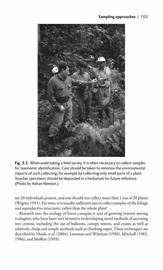
are 20 individuals present, and one should not collect more than 1 out of 20 plants(Wagner 1991). For trees, it is usually sufficient just to collect samples of the foliageand reproductive structures, rather than the whole plant!

Research into the ecology of forest canopies is area of growing interest amongecologists, who have been very inventive in developing novel methods of accessingtree crowns, including the use of balloons, canopy towers, and cranes as well asrelatively cheap and simple methods such as climbing ropes. These techniques aredescribed by Houle et al. (2004), Lowman and Wittman (1996), Mitchell (1982,1986), and Moffett (1993).

Sampling approaches | 103

Fig. 3.5 When undertaking a field survey, it is often necessary to collect samples

for taxonomic identification. Care should be taken to minimize the environmental

impacts of such collecting, for example by collecting only small parts of a plant.

Voucher specimens should be deposited in a herbarium for future reference.

(Photo by Adrian Newton.)

3.6 Measuring individual trees

3.6.1 Age

For some conifers, age estimates can be obtained by counting the number ofbranch whorls, although this method is less accurate in older trees because it can bedifficult to determine where branches have been abscised. In some broadleavedtrees and tree ferns it is possible to estimate ages by counting the number of leafscars on the terminal shoot, although again this method is only useful withyounger trees and branches.

104 | Forest structure and composition

Fig. 3.6 Researchers are often tempted to climb trees to collect samples of

leaves, flowers, or seeds for analysis, but tree climbing should only be attempted

by people who have received appropriate training. Use of safety equipment, such

as the harness and head protection pictured here, is essential. (Photo by Adrian

Newton.)

Age estimates are generally obtained by counting the number of annual rings ina stem cross-section. Annual ring formation depends on the fact that wood formedearlier in the year tends to be more porous and lighter in colour than that formedlater in the year. Total tree age is obtained by counting rings at ground level; ifmeasurements are made higher up the stem, then the number of years that the treetakes to grow to this height should be added to the total (Avery and Burkhart2003). Although this method works well in most temperate forests, it can also beused in some tropical forests, particularly where there is a pronounced dry seasonor where the trees are seasonally deciduous (Schweingruber 1988).

Ring counts are often taken on sawn sections of a tree trunk, which should besmoothed with a plane or knife and viewed with a hand lens or dissecting micro-scope in order for accurate counts to be obtained. If sawn sections are not available,an increment borer can be used (Figure 3.7), which consists of a hollow tube with acutting bit that is screwed into the tree (Husch et al. 2003) and is obtainable fromforestry suppliers. A reverse turn snaps the core of wood inside the tube, which is

Measuring individual trees | 105

Fig. 3.7 Using an increment borer on a Larix decidua tree during a

dendroecological study of mixed woodlands at the upper timberline of the central

Italian Alps. (Photo by John Healey.)

removed with an extractor (Figure 3.8). Accurate determination of tree age by thismethod requires coring through the centre or pith of the tree, which can be diffi-cult to locate. This process can be assisted by employing two people, one of whomtakes the core and the other of whom indicates the perpendicular axis of the treefrom a distance of 2–3 m (Schweingruber 1988). Alternatively, a holding devicecan be used, which can be adjusted in the axial direction by a peg and screw.

The maximum length of an increment borer is around 50 cm, which determinesthe upper limit to the size of tree that can be aged using this method. Cores instanding trees are typically taken at breast height (1.3 m above ground level). Thebore holes should be sealed with grafting wax (available from garden centres andforestry suppliers) to minimize the risk of introducing disease as a result of coring(Schweingruber 1988). Tree species with dense wood can be very difficult to core,and the wood cores or the borer itself can be difficult to extract intact. Extractedcores are fragile and should be stored in a plastic tube, drinking straw, or otherappropriate container. They can be labelled with soft pencil when freshly collected.The cores can be glued into a groove in a block of wood with water-soluble glue, toassist preparation and inspection.

The visibility of tree rings in trunk disks or cored samples can be increased bycutting transverse radial strips with a sharp blade, such as a multiple-snap-off bladeknife, or by polishing the sample with sandpaper of different grades. Samples

106 | Forest structure and composition

Fig. 3.8 Extracting the stem-core from an increment borer for

dendrochronological analysis of growth rings. Great care is needed when

extracting and transporting the cores, as they can be very fragile. (Photo by

John Healey.)

displaying little contrast between tree ring boundaries can be mounted between twoblocks and cut to a thickness of 0.25 mm, then examined in transmitted light undera microscope. Staining of tree rings with paper dye can also be used to improvevisibility, but this is generally not successful (Schweingruber 1988). The surface ofprepared samples can best be examined under a stereomicroscope with a spotlight,or a hand lens. A calibrated eye-piece is useful for making measurement of ringwidths. Dedicated instruments are also available for detailed analysis of tree ringwidths, linked to custom-designed computer software (such as WinDENDRO,�www.regeninstruments.com/�).

Analysis of tree rings has been widely used in archaeology as a means of datingwood fragments, and has also been widely used to analyse past climate change.Details of the methods used in dendrochronology are described by Cook andKairiukstis (1990) and Schweingruber (1988).

A number of problems may be encountered when obtaining ring counts (Huschet al. 2003), namely:

● In slow-growing trees, rings may be very close together and consequentlydifficult to count.

● In some species rings are indistinct, because there is little difference betweenwood formed in the spring and in the summer.

● Some species may form more than one ring in a growing season, for exampleduring a period of dry weather or as a result of defoliation caused by insectattack. False rings often do not extend around the entire circumference of thetree, however.

● Tree ring counts are generally very difficult to obtain from tropical trees,except in areas with a pronounced annual dry season.

Where ring counts are not possible, radiocarbon dating can potentially be used,although this technique is limited to trees of great age (� 500 years old) (Martínez-Ramos and Alvarez-Buylla 1999). It is also possible to estimate tree age usingmodels of growth increment, for those species where reliable long-term growthdata are available (Chambers and Trumbore 1999).

3.6.2 Stem diameter

Measurements of stem diameter are widely used in both forest ecology andmanagement to characterize the size distribution of forest stands and to estimatetimber volumes. Diameter measurements are usually taken at a standard height,the diameter at breast height (dbh), which is defined as 1.3 m above ground level(or 4.5 ft in the USA). Measurements are complicated by the fact that tree stemsare often not circular in cross-section, and may be leaning or surrounded byprominent buttresses, making them difficult to measure. The following standardprocedure is recommended by Husch et al. (2003):

● When the tree is on a slope, measure dbh on the uphill side of the tree.● When a tree is leaning, measure dbh on the high side of the tree, in a way that

is perpendicular to the longitudinal axis of the stem.

Measuring individual trees | 107

● When the tree has a bulge, limb or some other abnormality at breast height,measure dbh above the abnormality; attempt to measure the dbh that the treewould have had if the abnormality were not present.

● When a tree is multistemmed at breast height, measure each stem separately;when a tree forks above breast height, measure it as a single stem. If the forkoccurs at breast height, measure the dbh below the enlargement of the stemcaused by the fork.

● When a tree has a buttress than extends higher than 1 m, measure the stem ata fixed distance (30 cm) above the top of the buttress.

● When the breast height point has been marked on the tree with paint, assumethe point of measurement to be the top of the paint mark. Use of such paintmarks can greatly improve accuracy when repeated measurements are made.

● If the tree stem is elliptical in cross-section, then measure the major and minordiameters separately, and produce an overall figure by calculating the mean ofthe two values.

The two most commonly used instruments for measuring tree stem diametersare calipers and diameter tapes. Calipers are usually used when the trees are lessthan 60 cm dbh; although larger calipers are available, they can be difficult orunwieldy to use in the field. Calipers are usually constructed out of metal, wood,or plastic, and enable the diameter to be read directly off a scale when the arms ofthe caliper are placed around the tree stem. The caliper arms should be pressedfirmly against the tree stem with the main beam of the caliper placed perpendicu-lar to the axis of the tree stem, and the arms parallel and perpendicular to the beam(Husch et al. 2003).

Standard measurement tapes can be used to measure stem diameter by placingthe tape around the circumference of the tree at breast height (Figure 3.9).Measurements of circumference taken in this way can be converted to diameters(assuming a circular cross-section) by dividing the values by �. Diameter tapes canbe obtained, however, that are graduated at intervals of � units (in cm or inches)enabling diameter to be measured directly. Care should be taken to ensure that thetape is positioned correctly: it should be in a plane perpendicular to the trunk ofthe tree, and pulled taut around the trunk so that accurate measurements areobtained (Husch et al. 2003). Although more accurate results can be obtained withcalipers, measurements with tape tend to be more consistent if repeated measure-ments are made, because caliper measurements are more sensitive to the position-ing of the instrument (Husch et al. 2003). A review of different methods formeasuring tree diameters is provided by Clark et al. (2000).

Bark thickness can be determined by using a bark gauge, which consists of asteel shaft that is pushed through the bark. The thickness of the bark can be readdirectly off a scale with the instrument in place. A minimum of two readingsshould be taken (Avery and Burkhart 2003). When measurements of diameter aremade, whether or not the bark was included in the measurement should berecorded.

108 | Forest structure and composition

A number of instruments are available for obtaining measurements of upperstem diameters, which can be useful for assessing the form of the tree or extent ofstem taper. Options include optical forks, optical calipers, and fixed-based or fixed-angle rangefinders (Clark et al. 2000). Many of these instruments are expensiveand are prone to inaccuracy (Avery and Burkhart 2003). Most commonly, a relas-cope is used, which is a form of optical rangefinder (Husch et al. 2003) (see alsoSection 7.2). However, calipers or diameter tapes provide more accurate measure-ments of upper stem diameters, if the upper parts of the tree can be accessedthrough use of climbing ropes or ladders.

3.6.3 Height

Total tree height can be defined as the distance along the axis of the tree stem fromground level to the top of the canopy. Other terms commonly used by foresters

Measuring individual trees | 109

Fig. 3.9 Measuring stand structure in the New Forest National Park, southern

England. The student in the centre is measuring diameter at breast height of an

oak tree (Quercus robur) using a diameter tape. The others are carrying a laser

rangefinder (left) and a hypsometer (right). (Photo by Adrian Newton.)

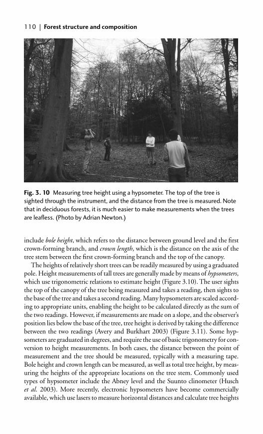
include bole height, which refers to the distance between ground level and the firstcrown-forming branch, and crown length, which is the distance on the axis of thetree stem between the first crown-forming branch and the top of the canopy.

The heights of relatively short trees can be readily measured by using a graduatedpole. Height measurements of tall trees are generally made by means of hypsometers,which use trigonometric relations to estimate height (Figure 3.10). The user sightsthe top of the canopy of the tree being measured and takes a reading, then sights tothe base of the tree and takes a second reading. Many hypsometers are scaled accord-ing to appropriate units, enabling the height to be calculated directly as the sum ofthe two readings. However, if measurements are made on a slope, and the observer’sposition lies below the base of the tree, tree height is derived by taking the differencebetween the two readings (Avery and Burkhart 2003) (Figure 3.11). Some hyp-someters are graduated in degrees, and require the use of basic trigonometry for con-version to height measurements. In both cases, the distance between the point ofmeasurement and the tree should be measured, typically with a measuring tape.Bole height and crown length can be measured, as well as total tree height, by meas-uring the heights of the appropriate locations on the tree stem. Commonly usedtypes of hypsometer include the Abney level and the Suunto clinometer (Huschet al. 2003). More recently, electronic hypsometers have become commerciallyavailable, which use lasers to measure horizontal distances and calculate tree heights

110 | Forest structure and composition

Fig. 3. 10 Measuring tree height using a hypsometer. The top of the tree is

sighted through the instrument, and the distance from the tree is measured. Note

that in deciduous forests, it is much easier to make measurements when the trees

are leafless. (Photo by Adrian Newton.)

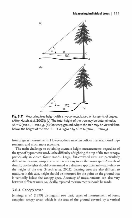
from angular measurements. However, these are often bulkier than traditional hyp-someters, and much more expensive.

The main challenge to obtaining accurate height measurements, regardless ofthe type of hypsometer used, is the difficulty of sighting the top of the tree canopy,particularly in closed forest stands. Large, flat-crowned trees are particularlydifficult to measure, simply because it is not easy to see the crown apex. As a rule ofthumb, tree heights should be measured at a distance approximately equivalent tothe height of the tree (Husch et al. 2003). Leaning trees are also difficult tomeasure; in this case, height should be measured for the point on the ground thatis vertically below the canopy apex. Accuracy of measurements can also varybetween different users, so, ideally, repeated measurements should be made.

3.6.4 Canopy cover

Jennings et al. (1999) distinguish two basic types of measurement of forestcanopies: canopy cover, which is the area of the ground covered by a vertical

Measuring individual trees | 111

α1

α1α2

α2

D

DC

A

B

A

B

C

(a)

(b)

Fig. 3.11 Measuring tree height with a hypsometer, based on tangents of angles.

(After Husch et al. 2003): (a) The total height of the tree may be determined as

AB � D(tan �1 � tan �2). (b) On steep ground, where the tree may be viewed from

below, the height of the tree BC � CA is given by AB � D(tan �1 � tan �2).

projection of the canopy, and canopy closure (or canopy density), which is the pro-portion of the sky hemisphere obscured by vegetation when viewed from a singlepoint. These two terms are often confused in the literature. Canopy cover is animportant variable for estimating stand variables from remote sensing data (seesection 2.5), and in young forest stands may correlate closely with basal area; how-ever, the relation between these variables is often less pronounced in more matureforest stands (Jennings et al. 1999). Canopy closure is likely to be more closelyrelated to light regime and microclimate, as well as plant growth and survival, atthe point of measurement (Jennings et al. 1999).

As noted in Chapter 2, crown diameters can be measured from high-resolution aer-ial photographs. Field measurements of tree crowns are complicated by theirinaccessibility and irregularity. The commonest method to measure the size and shapeof a tree crown is to project the perimeter of the crown vertically down, then measureit at ground level. Estimates of crown area are typically obtained by measuring thecrown diameter at its widest point, then again at right angles to this measurement(Husch et al. 2003). Hand-held or pole-mounted mirrors, prisms, or pentaprismsmay be used to achieve the vertical projection. Appropriate instruments and associ-ated methods for this purpose have been described by Cailliez (1980) and Tallent-Halsell (1994). Crown area is estimated from these measurements by using theformula for calculating the area of a circle, from either the mean value of the two meas-urements made or the mean value of minimum and maximum crown diameters.

The method for estimating crown cover of a forest stand is described byJennings et al. (1999). At each point of measurement, the observer looks verticallyupwards and records whether or not the forest canopy obscures the sky. Anestimate of forest canopy cover can be produced by calculating the proportion ofpoints where the sky is obscured. Observations can be made without use of anyinstrumentation, although both accuracy and repeatability can be improved bydoing so. Examples of instruments designed to ensure that sightings are trulyvertical include the gimbal balance (Walter and Soos 1962) or the sighting tube,which often has an internal crosshair (Johansson 1985). Commercial versions ofthe latter incorporate bubble levels to ensure that the tube is positioned vertically,and 45 mirrors to ensure that the head posture is horizontal during use. Randomor stratified random sampling approaches should be used when taking suchmeasurements according to Jennings et al. (1999), who present formulae for cal-culating the confidence limits of such measurements by using a binomial distribu-tion. Accurate estimates require large sample sizes; these authors suggest that atleast 100 observations should be made in any forest area being surveyed.

Measures of canopy closure, rather than canopy cover, are generally to bepreferred in ecological studies. This requires estimation of the light received at aparticular point, including both direct solar radiation and the indirect radiationthat arrives from all parts of the sky. The entire hemisphere surrounding the samplepoint should therefore be assessed, rather than just the sky immediately above thesample point (Jennings et al. 1999). Methods for assessing canopy closure arepresented in section 4.5.4.

112 | Forest structure and composition

3.7 Characterizing stand structure

A forest stand may be defined as a group of trees that occupy a given area, whichshare some characteristics such as species composition, size, or age. Stand structurerefers to the distribution of species or tree sizes within the stand. Canopy charac-teristics and leaf area can also be considered as structural variables.

3.7.1 Age and size structure

Stands are commonly differentiated into those that are even-aged, where all treesare of approximately the same age, and those that are uneven-aged, where treesdisplay a variety of different ages. The age distribution of trees within a stand canprovide some insights into the history of tree recruitment and patterns of previousdisturbance. The age structure of a stand is generally characterized by sampling asubset of trees from the stand and determining their ages, as described in section3.6.1. In even-aged stands, the age of the stand is usually determined as the meanage of those trees that dominate the canopy (i.e. the largest individuals), andsampling may be restricted to these. Age distributions are typically illustrated byplotting a frequency distribution or histogram of the number of trees within eachage class.

The diameter (dbh) of a stand can be expressed a mean of the diameters of thetrees present. Often, basal area is calculated to provide a measure of stand densityand to provide a basis for calculating stand volume. Basal area can be calculatedfrom measurements of stem diameter by using the following equation (assumingthat trees are circular in cross-sectional area):

where g is cross-sectional area of the tree and d is the diameter of the cross-section.When measured using metric units, tree diameter is usually expressed in

centimetres, and cross-sectional area in square metres. In this case, the equation isas follows (Husch et al. 2003):

Stand basal areas can be calculated by summing values obtained from dbhmeasurements of individual trees.

Stand structure is most commonly described by using measurements of treediameters (section 3.6.2). These data may be illustrated as a stand table, whichindicates the number of trees of each species per unit area belonging to each diam-eter class. Such data can also be illustrated as a frequency distribution or histogramof the number of trees within each size class. This method of illustrating standstructure is very widely used by forest ecologists, and can be used to infer thedynamics of the stands under investigation and their phase of development.

g (m2) ��d 2

4(10 000)� 0.00007854 d 2

g ��d 2

4

Characterizing stand structure | 113

For example, dominance of a stand by many small-diameter trees would suggestthat the stand has only recently been established, perhaps following some form ofdisturbance event. Alternatively, presence of some very large diameter trees withrepresentation of trees in smaller diameter classes might be interpreted as matureor ‘old-growth’ forest, within which continuous recruitment is taking place (Spies1997, Spies and Turner 1999). However, it should be noted that the size and age oftrees are not necessarily closely related. Trees growing on adverse sites or subjectedto a high intensity of browsing can grow very slowly, leading to much greatervariation in age than in size. Stands that appear to be even-aged on the basis of theirdiameter distributions may in fact have been recruited over a prolonged period.For this reason, caution should always be exercised when interpreting diametermeasurements in terms of ages; ideally both age and size should be measured.

Uneven-aged stands are typically characterized by the presence of a large num-ber of trees in smaller-diameter size classes with decreasing frequency as the sizeclass increased. This form of size–frequency relationship is often referred to as an‘inverse-J’ shape (Figure 3.12) and is often an objective of approaches to sustain-able forest management. If a particular tree species displays such a size distribution,then continuous recruitment can generally be inferred, suggesting that the popu-lation is viable as sufficient regeneration it taking place for the population to bemaintained. Techniques for studying forest dynamics and the population viabilityof tree species are described in detail in Chapters 4 and 5.

Stand diameter distributions can be represented mathematically by probabilitydensity functions. A number of different functions have been used, includingnormal, exponential, binomial, Poisson, Pearl, Reed, Schiffel, and Fourier series(Husch et al. 2003). Details of the use of these functions are provided by Johnson

114 | Forest structure and composition

100

80

60

40

20

01 2 3 4 5 6 7 8 9 10 11 12

Size class

No

. ind

ivid

uals

Fig. 3.12 Inverse-J structure of a forest stand, illustrated by plotting the number

of individuals in each size class. The inverse-J structure is characterized by larger

numbers of smaller individuals than of larger individuals. (After Peters 1994,

http://www.panda.org.)

(2001) and Schreuder et al. (1993). The most widely used function in relation toanalysis of forest stand data is the Weibull function (see, for example, Soehartonoand Newton 2001), which can be expressed as follows (Husch et al. 2003):

where f(D) is the probability density, a is a location parameter (theoretical mini-mum population value), b is a scale parameter, c is a shape parameter, and D is thediameter.

The Weibull function can exhibit a variety of different shapes depending on thevalue of c (Husch et al. 2003):

● c � 1, inverse J-shape● c � 1, exponential decreasing● 1 � c � 3.6, positive asymmetry● c � 3.6, symmetric● c � 3.6, negative asymmetry.

The parameters of the Weibull distribution can be derived directly from diam-eter measurements. Parameter a is usually set to the smallest value of diameterobserved. An algorithm for recovering the other two parameters of the function isprovided by Burk and Newberry (1984).

3.7.2 Height and vertical structure

The vertical structure of a forest stand refers to its structural complexity, which isinfluenced by the presence of different plant life forms (such as vines and epi-phytes), the arrangement of leaves on branches, and the amount and distributionof leaves, branches, and twigs, at different heights (Brokaw and Lent 1999).Vertical structure has a major influence on the provision of habitat for wildlife.Quantitative methods for assessing vertical structure in this context are describedin Section 7.3.

Foresters traditionally classify the crown position of trees according to the fol-lowing simple scheme (Oliver and Larson 1996):

● dominant, where tree crowns extend above the general canopy level and arenot physically restricted from above

● co-dominant, where crowns form the general level of a forest canopy and aresomewhat crowded by other adjacent trees

● intermediate, where trees are shorter, but their crowns extend into the generalcanopy that is primarily composed of the crowns of dominant and co-dominanttrees

● suppressed (overtopped), where crowns lie entirely below the general level of thecanopy and are physically restricted from above.

This classification is subjective, and can be difficult to apply in practice, but iswidely used.

f (D) �cb �D�a

b �1/c

e�[(D�a)/b]c

Characterizing stand structure | 115

Ecologists have traditionally described the vertical structure of forest standsthrough profile diagrams. Some excellent examples are provided in Richards’ classicwork on tropical rain forests (Richards 1996). The method involves marking out arectangular strip of forest, typically at least 60 m long with a width of 10 or 20 m.The positions of all trees above 5 m height are then mapped and their diametersrecorded. Height and crown width are then recorded by using the methodsdescribed above. These measurements are used to produce a diagram of a verticalsection through the forest. Richards (1996), who was one of the people responsiblefor developing the method, was well aware of its limitations: it is difficult to selecta site that is truly representative of a particular forest, and it is of limited valueas a source of quantitative information. However, profile diagrams do capturesomething of the vertical structure of forest stands, and are an effective way ofillustrating its complexity.

Average canopy height can be obtained by calculating a mean value of all trees,or a sample of trees in the stand. Mean values can be weighted according to theposition of trees in the canopy, for example whether they are classified as dominantor co-dominant, or according to their basal area (Husch et al. 2003).

3.7.3 Leaf area

Measurements of leaf area may be expressed as a quantity (m2), or more typically,as leaf area index (LAI), which is the leaf area per unit ground area, usually definedin units of m2 m–2. LAI is an important structural attribute of forest ecosystemsbecause of its role in influencing exchanges of energy, gas, and water and physio-logical processes such as photosynthesis, transpiration, and evapotranspiration. Itis therefore very widely used in ecophysiological investigations. As noted inChapter 2, LAI can be estimated from remote sensing data, and is also an import-ant component of many process-based models of forest dynamics (Chapter 4)(Running et al. 1989, Chen and Cihlar 1995).

In the field, LAI can be estimated by using a wide variety of different instru-ments and techniques. These have been reviewed by a number of authors (Chasonet al. 1991, Larsen and Kershaw 1990), and most recently by Bréda (2003), whonoted that LAI is difficult to quantify because of large spatial and temporal vari-ability. Methods developed for estimating LAI may be grouped into direct andindirect methods.

Direct or semi-direct methods described by Bréda (2003) include:

● Direct measurement of leaf area, using either a commercially available leaf areameter or a defined relation between leaf area and some other measuredvariable. In the latter approach, leaf area is typically measured on a subsampleof leaves and related to dry mass—via specific leaf area (SLA, cm2 g–1), forexample—then the total dry mass of leaves collected within a known ground-surface area is converted into LAI by multiplying it by the SLA.

● Relation between foliage area and sapwood area. This is based on the hypothe-sis that leaf area is in balance with the amount of conducting tissues, and

116 | Forest structure and composition

therefore allometric relations can be developed. Because of the difficulties ofmeasuring conducting area, sapwood area is often replaced by more readilymeasured variables, such as dbh. Estimating allometric relations throughdestructive sampling is generally a reliable method of deriving LAI for a givenexperimental site, but different relations may need to be established fordifferent years. Examples of this approach are provided by Medhurst andBeadle (2002) and Pereira et al. (1997).

● Collection of leaf litter. In deciduous stands, leaves can be collected in traps ofknown collecting area distributed below the canopy during leaf fall. Littershould be removed from the traps at least every second week to avoid lossesand decomposition. Collected litter is dried (at 60–80 C for 48 h) andweighed, and the dry mass of litter calculated as g m–2. Leaf dry mass at eachcollection date is converted into leaf area by multiplying the collected biomassby the SLA. LAI is the leaf area accumulated over the period of leaf fall. Asleaves can be sorted, litter collection enables the contribution of each speciesto total leaf area index to be assessed. The depth of fresh leaf litter can also beassessed by using a point quadrat method, by inserting a needle into the litterlayer and counting the number of leaves that it touches.

Indirect methods infer LAI from measurements of the transmission of irradiancethrough the forest canopy, and are based on statistical descriptions of the arrange-ment of leaves. Two main approaches may be differentiated: radiation measure-ment methods, which assume that leaves are randomly distributed within thecanopy, and ‘gap fraction’-based methods that are dependent on estimating leafangle distributions (Bréda 2003). Radiation measurement methods require meas-urement of irradiance both incident on the canopy and below the canopy; LAI iscalculated from an extinction coefficient which is influenced by the total leaf areapresent within the canopy, as well as by canopy architecture and stand structure.Further details of these methods, including the analytical equations used in LAIestimation, are presented by Bréda (2003). A number of commercial sensors areavailable that use gap fraction-based methods of estimating LAI (Table 3.1).Although it should be noted that these sensors were primarily developed for usewith crop plants, they may also be adapted for use with forest canopies.

A further indirect method involves the use of hemispherical photographs, withsupporting digital analysis. The use of hemispherical photographs to characterizeforest light environments is considered further in section 4.5.2.

Comparisons between direct and indirect methods indicate a significant under-estimation of LAI by the latter techniques in forest stands, mainly because ofclumping of leaves and the contribution of stem and branches. Reports indicatethat the degree of underestimation varies from 25% to 50% depending on thecharacteristics of the stands. The sampling strategy adopted also has a major influ-ence on the accuracy of the results, as the spatial heterogeneity of forest canopies isoften very large (Bréda 2003). However, direct methods are all very labour-inten-sive (Fassnacht et al. 1997) and require many replicates to produce a precise result;they are therefore costly in terms of time and money.

Characterizing stand structure | 117

3.7.4 Stand volume

Measurement of the volume of wood produced by a forest stand is of fundamentalimportance to forestry, and consequently foresters have developed a variety ofmethods for estimating it. Particular efforts have been directed towards developingfunctions for stem volume and taper that allow estimates to be made from rela-tively simple measurements. Details of these functions are provided by Avery andBurkhart (2003), Husch et al. (2003), and West (2004). Stem volume is lessimportant to forest ecologists, but as it is used for estimation of stem biomass andcarbon content, a brief overview of the principal methods used in volume estima-tion is presented here (see also section 7.2).

The main method used to measure tree stem volume is the sectional method, whichinvolves measuring the stem in relatively short sections, determining the volume,and each then summing these values to produce an estimate of total volume (West2004). The volume of a stem section is determined by measuring its length, and thestem diameter at the lower end of the section (‘large end diameter’), the upper end(‘small end diameter’) and/or at the midpoint of the section. These measurements areused to estimated volume by using one of three formulae (West 2004):

● Smalian’s formula:

VS � �l(dL2�dU

2)/8

118 | Forest structure and composition

Table 3.1 Characteristics of four commercially available sensors that can be used for

indirect estimation of LAI (adapted from Bréda 2003).

Principle Sensor Company URL

AccuPAR Gap fraction 80 PAR sensors Decagon www.decagon.comor sunflecks distributed Devices,

along a Pullman, USA0.90 m rod

DEMON Gap fraction Detector CSIRO, www.cbr.clw.csiro.au/zenith angles sighted at Canberra, pyelab/tour/demon.htmfrom the sun the sun Australiaat different angles to the vertical

LAI-2000 Gap fraction Fish-eye Li-Cor, www.licor.comfor each sensors with Lincoln, zenith angle five concentric Nebraska, acquired rings of sensors USAsimultaneously

SunScan Gap fraction 64 PAR sensors Delta-T www.delta-t.co.ukor sunflecks distributed Devices Ltd.,

along a 1 m rod Cambridge, UK

● Huber’s formula:

● Newton’s formula:

where VS is the volume of a section of a stem, l is the length of the section, dL is thestem diameter at the lower end of the section, dU is the diameter at the upper endof the section, and dM is the diameter midway along the section.

These formulae provide accurate estimates of stem volume so long as the stem iscircular in section or the stem is shaped in the form of a quadratic paraboloid.A variety of stem taper functions have been developed to accurately describe stemshape, but for most tree species the quadratic paraboloid is a reasonable approxi-mation to the actual shape of tree stems, and for this reason these three functionsare still in widespread use (West 2004). Of the three, Newton’s is generally themost accurate because it uses the most information in the calculation.

Most measurements of tree stem volume use section lengths of 0.5–1 m for largetrees; shorter lengths are used for smaller trees. Stem diameters can be measured bythe methods described in section 3.6.2.

‘Importance sampling’ or ‘centroid sampling’ methods offer an alternative tothe sectional method. These methods require the stem dbh to be measured (D0)together with total height (H ). A further measurement of stem diameter isrequired high on the stem (D1). The location of this measurement point can beselected by either importance sampling or centroid sampling approaches. Theseinvolve application of the following formulae.

First, the value K is determined as:

where HL is the lower height and HU is the upper height of the stem section forwhich the volume estimate is required. The height at which the required upperstem diameter is to be measured (HS) is then determined as:

If importance sampling is used, then N is a randomly selected value in the range0–1. If the centroid method is used, then N � 0.5 (the centroid being the positionalong the stem section above which half of the section volume lies) (West 2004).

Once HS has been determined, the diameter at that height must be measured(DS), by using one of the methods in section 3.6.2 (such as an optical dendrome-ter). The stem volume (VLU) between HL and HU can then be determined as:

This method is relatively simple, as it requires few diameter measurements to bemade. The entire stem can be treated as a single section, or it can be divided into a

VLU � �K (DSDI /DO)2/[8(H�HS)]

HS �H��(H�HL)2�NK

K � 2H (HU�HL)�HL2�HU

2

VS � �/(d L2�4d M

2�d U

2 )/24

VS � �l dM2 /4

Characterizing stand structure | 119

series of sections and estimates obtained for each. Care should be taken to measureupper diameters accurately, and measurements should be made above any but-tresses or stem swelling present near the base of the tree.

3.7.5 Stand density

Stand density refers to the number of trees within a given area. This can bemost simply obtained by counting the number of trees present within a stand andmeasuring its area, then dividing the former by the latter. However, basal area andthe extent of crown cover can also be used as measures of stand density. Standdensity is of great importance to forest management, primarily because of itsimportance in determining the volume of timber likely to be obtained from aparticular stand. Consequently foresters have developed a range of metrics fordescribing it, including various measures of relative spacing, stand density indices,crown competition factors, and stocking diagrams. Details are provided by forestmensuration textbooks such as Avery and Burkhart (2003) and Husch et al.(2003).

As noted earlier (section 3.5), distance measures are often used to estimate standdensity. For example, Patil et al. (1979) proposed a plant density estimator basedon point-to-plant distances that produces consistent results. Barabesi and Fattorini(1995) showed for various spatial plant patterns that an improvement over simplerandom sampling can be achieved by estimating plant density by a ranked setsampling of point-to-plant distances.

Two main issues should be borne in mind when measuring plant density(Bullock 1996). First, it may be difficult to differentiate individuals of clonalplants; in such cases, the number of ramets (i.e. shoots or stems) tends to becounted, rather than the number of genets (i.e. distinct genotypes, which usuallycan only be differentiated if information from molecular markers is available; seesection 6.5.1). Second, measures of density that fail to take into account differ-ences in the size of individual plants may give ecologically misleading results. Forexample, if a herbaceous species were to be compared with a tree species, it mightdemonstrate a much higher density in terms of number of individuals, but bemuch less important in terms of its contribution to the structure of the foreststand. For this reason, combined measures of density and plant size are often pre-ferred. The commonest of these is cover, which is a measure of the above-groundparts of the plant (such as the tree canopy) when seen from above (for methods ofestimating canopy cover, see section 3.6.4; methods for assessing the cover ofunderstorey vegetation are described in section 7.7).

The 3/2 law of self-thinning has attracted a great deal of interest from bothforesters and ecologists, because it is one of those rare things in ecology—a straightline. Usually, the logarithm of mean tree volume or mass is plotted against thelogarithm of the number of trees per unit area. For stands undergoing density-dependent mortality (‘self-thinning’), the slope of the line is approximately �3/2(Kershaw and Looney 1985).

120 | Forest structure and composition

3.8 Spatial structure of tree populations

In recent years, substantial progress has been made in developing methods foranalysing the spatial pattern of plant populations. These techniques can be used todescribe the spatial distribution of individuals within populations, and to developtestable hypotheses about the underlying processes responsible for generatingthese patterns (such as seed dispersal, competition, and herbivory) and theirrelationship to environmental heterogeneity. Dale (1999) and Fortin and Dale(2005) provide detailed accounts of methods of spatial pattern analysis used inplant ecology.

Often, spatial patterns are analysed by mapping the positions of individualplants within a study area or sample plot (see Figure 4.4). A number of methodsare available that are explicitly used with the kind of data produced by thisapproach, which consist of points. Many of these methods focus on determiningwhether the individuals are randomly dispersed, clumped or overdispersed.Random dispersion refers to the situation where points occur independently of oneanother; when clumped, the presence of one point increases the probability offinding another nearby; when overdispersed, the presence of one point decreasesthe probability of finding another nearby (Dale 1999). Often, a key objective is todetermine the scale of the spatial pattern—the size of any clumps present, andtheir spacing.

Many methods are based on analysis of the distance of each plant to its nearestneighbour. For example, the test described by Clark and Evans (1954) enablesrandom, clumped, and overdispersed patterns to be differentiated by analysis ofnearest-neighbour distances. However, such methods provide no information onthe size or spacing of the clumps, and therefore have limited usefulness (Dale1999). Alternatively, it is possible to analyse the distances between all possible pairsof plants, in what is termed plant-to-all-plants distance analysis (Galiano 1982).This method examines the frequency distribution of the distances between all pairsof plants in the area surveyed, but again the method does not always give a fullpicture of the characteristics of spatial pattern (Dale 1999).

More commonly, second-order statistics are used for the analysis of point pat-terns. These methods are based on the distribution of distances of pairs of points,and count the number of points located within a certain specified distance of eachpoint. The methods are described in detail by Ripley (1981, 1988), who first devel-oped them. Two commonly used second-order statistics are Ripley’s K-functionand the pair-correlation function g, which use the information on all interpointdistances within the data set being analysed (Ripley 1981, Diggle 1983). Thesestatistics provide more information than those that use nearest-neighbourdistances only, such as Diggle’s nearest-neighbour functions G or F (Diggle 1983),which are also commonly used. These three statistics have different sensitivities todifferent types of spatial distributions: for example, K has a slightly lower powerthan F for aggregated patterns and a higher power than G for regular patterns

Spatial structure of tree populations | 121

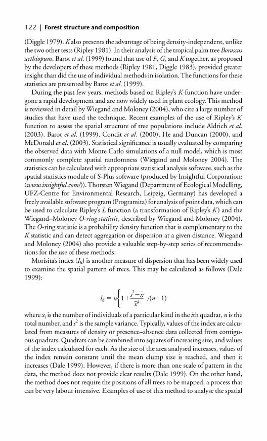
(Diggle 1979). K also presents the advantage of being density-independent, unlikethe two other tests (Ripley 1981). In their analysis of the tropical palm tree Borassusaethiopum, Barot et al. (1999) found that use of F, G, and K together, as proposedby the developers of these methods (Ripley 1981, Diggle 1983), provided greaterinsight than did the use of individual methods in isolation. The functions for thesestatistics are presented by Barot et al. (1999).

During the past few years, methods based on Ripley’s K-function have under-gone a rapid development and are now widely used in plant ecology. This methodis reviewed in detail by Wiegand and Moloney (2004), who cite a large number ofstudies that have used the technique. Recent examples of the use of Ripley’s Kfunction to assess the spatial structure of tree populations include Aldrich et al.(2003), Barot et al. (1999), Condit et al. (2000), He and Duncan (2000), andMcDonald et al. (2003). Statistical significance is usually evaluated by comparingthe observed data with Monte Carlo simulations of a null model, which is mostcommonly complete spatial randomness (Wiegand and Moloney 2004). Thestatistics can be calculated with appropriate statistical analysis software, such as thespatial statistics module of S-Plus software (produced by Insightful Corporation;�www.insightful.com/�). Thorsten Wiegand (Department of Ecological Modelling,UFZ-Centre for Environmental Research, Leipzig, Germany) has developed afreely available software program (Programita) for analysis of point data, which canbe used to calculate Ripley’s L function (a transformation of Ripley’s K ) and theWiegand–Moloney O-ring statistic, described by Wiegand and Moloney (2004).The O-ring statistic is a probability density function that is complementary to theK statistic and can detect aggregation or dispersion at a given distance. Wiegandand Moloney (2004) also provide a valuable step-by-step series of recommenda-tions for the use of these methods.

Morisita’s index (I�) is another measure of dispersion that has been widely usedto examine the spatial pattern of trees. This may be calculated as follows (Dale1999):

where xi is the number of individuals of a particular kind in the ith quadrat, n is thetotal number, and s2 is the sample variance. Typically, values of the index are calcu-lated from measures of density or presence–absence data collected from contigu-ous quadrats. Quadrats can be combined into squares of increasing size, and valuesof the index calculated for each. As the size of the area analysed increases, values ofthe index remain constant until the mean clump size is reached, and then itincreases (Dale 1999). However, if there is more than one scale of pattern in thedata, the method does not provide clear results (Dale 1999). On the other hand,the method does not require the positions of all trees to be mapped, a process thatcan be very labour intensive. Examples of use of this method to analyse the spatial

I� � n1�s2�x

x2 (n�1)

122 | Forest structure and composition

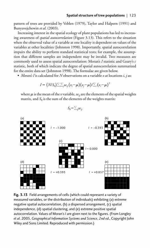
pattern of trees are provided by Veblen (1979), Taylor and Halpern (1991) andBunyavejchewin et al. (2003).

Increasing interest in the spatial ecology of plant populations has led to increas-ing awareness of spatial autocorrelation (Figure 3.13). This refers to the situationwhen the observed value of a variable at one locality is dependent on values of thevariables at other localities (Johnston 1998). Importantly, spatial autocorrelationimpairs the ability to perform standard statistical tests; for example, the assump-tion that different samples are independent may be invalid. Two measures arecommonly used to assess spatial autocorrelation: Moran’s I statistic and Geary’s cstatistic, both of which indicate the degree of spatial autocorrelation summarizedfor the entire data set (Johnston 1998). The formulae are given below.

● Moran’s I is calculated for N observations on a variable x at locations i, j as:

where � is the mean of the x variable, wij are the elements of the spatial weightsmatrix, and S0 is the sum of the elements of the weights matrix:

S0��ijwij

I � (N/S0)�i�jwij (xi��)(xj��)/�i (xi��)2

Spatial structure of tree populations | 123

(a)

l = –0.393 l = –1.000

l = +0.393 l = +0.857

l = 0.000

(c)

(b)

(e)(d)

Fig. 3.13 Field arrangements of cells (which could represent a variety of

measured variables, or the distribution of individuals) exhibiting (a) extreme

negative spatial autocorrelation, (b) a dispersed arrangement, (c) spatial

independence, (d) spatial clustering, and (e) extreme positive spatial

autocorrelation. Values of Moran’s I are given next to the figures. (From Longley

et al. 2005, Geographical Information Systems and Science, 2nd ed., Copyright John

Wiley and Sons Limited. Reproduced with permission.)

● Geary’s c statistic is expressed in the same notation as:

Positive spatial autocorrelation is indicated by a value of Moran’s I that is largerthan its theoretical mean of �1/(N � 1), or a value of Geary’s c less than its meanof 1 (Johnston 1998).

Another statistical approach that can be used for analysis of spatial data isgeostatistics. This provides a set of techniques that can be used for the analysisand prediction of spatially distributed phenomena. The approach was originallydeveloped for use in geology, but is increasingly being used by ecologists. Its use islikely to become more widespread among ecologists in future with the increasingavailability and power of software tools. As noted in section 2.6, some GIS softwareprograms are now able to do geostatistical analysis, either as part of the programitself (for example IDRISI) or as additional software modules or extensions(for example Geostatistical Analyst, which is an ArcGIS extension producedby ESRI; see section 2.5.1 for URLs). Some statistical software programs (suchas the spatial statistics module of S PLUS, see above) can also be used to dogeostatistics.

Geostatistical methods measure the similarity or dissimilarity between variablesbased on the spatial dependence of measurements taken at different locations, andthen use this information for interpolation, extrapolation, or simulation.Geostatistics is based on the assumption that data values located closely together inspace are likely to be more related than locations that are further apart (Johnston1998). Spatial dependence decreases with increasing distances among samplepoints. Analyses are usually done by producing a semivariogram (or variogram forshort), which illustrates the degree of dissimilarity between values at differentintervals of distance and direction.

Once a variogram has been produced, interpolation methods can be used to esti-mate values at unsampled locations (Johnston 1998). The most commonly usedgeostatistical method of interpolation is kriging, which uses weighted average ofsample measurements to estimate the value at non-sampled points. The weightsare calculated from expected spatial dependence between estimated points andsampled points. In practice, kriging is done by selecting a mathematical functionfrom a variety of alternatives, and fitting the function to the observed data pointsto obtain the best possible fit. The fitted variogram is then used to estimate valuesat locations of interest (Longley et al. 2005). A number of different options areavailable regarding the choice of mathematical function for the variogram; anappropriate option has to be determined by the analyst (Longley et al. 2005).Introductions to kriging are provided by DeMers (2005), Longley et al. (2005) andJohnston (1998).

Textbooks describing geostatistical techniques include those by Goovaerts(1997), Isaaks and Srivastava (1989), Wackernagel (2003), and Webster andOliver (2000). Use of geostatistics in ecology is described by Johnston (1998),

c � (N�1)/2S0[�i �j wij (xi�xj)2/�i (xi��)2]

124 | Forest structure and composition

Robertson (1987), and Wagner (2003). Examples of the use of geostatistics inforest ecology include:

● Köhl and Gertner (1997), who used these methods in forest damage surveys● Bebber et al. (2002), who used geostatistics to determine the spatial relation-

ships between canopy openness and seedling performance in secondary low-land forest in Borneo

● Hohn et al. (1993), who used three-dimensional kriging in space and time topredict defoliation caused by gypsy moth in Massachusetts

● Nanos et al. (2004), who used geostatistics to analyse the stand characteristicsof a pine forest in Spain

● Schume et al. (2003), who carried out a spatiotemporal analysis of soil watercontent in a mixed Norway spruce–European beech stand in Austria.

3.9 Species richness and diversity

Species richness refers to the number of species in a particular area, whereas speciesdiversity refers to a combination of richness and relative abundance. A comprehen-sive review of the methods used for estimating both of these variables is providedby Magurran (2004).

3.9.1 Species richness

The main problem with measuring species richness is that the result depends onthe number of individuals recorded. Two main sampling methods are used inforest ecology. One approach is to sample individual trees selected at randomwithin a field plot, and record sequentially the species identity of one tree afteranother. This is referred to as individual-based sampling. Alternatively, a series ofsubplots can be established in each plot, and the number and taxonomic identityof all of the trees within each subplot can be recorded, noting the increase inthe number of species as additional subplots are surveyed. This is referred to assample-based assessment (Gotelli and Colwell 2001). The key difference betweenthese approaches is that the unit of replication is different between the twomethods, being an individual tree in the former case and a sample of individuals inthe latter. The choice of method has a major influence on the estimate obtained(Gotelli and Colwell 2001, Longino et al. 2002). Magurran (2004) mentionsanother method of assessing species richness: the use of incidence or occurrencedata, representing the number of sampling units in which a species is present.Sample units that could potentially be used in this way include grid squares,quadrats, or point samples.

There are three main methods of estimating species richness from samples:extrapolation of species accumulation or species–area curves, use of the shape ofthe species abundance distribution, or use of a non-parametric estimator. Each ofthese is considered below. Further information on these methods is provided byChazdon et al. (1998) and Colwell and Coddington (1994). Recent progress in

Species richness and diversity | 125

interpolating and extracting species accumulation curves is described by Colwellet al. (2004) (see also Golicher et al. 2006).

Species accumulation curves plot the cumulative number of species recorded as afunction of sampling effort, and illustrate the increase in the total number ofspecies encountered during the process of data collection. Species–area curves canbe considered as one form of species accumulation curve, in which species richnessis related to an increase in the area sampled. Smooth curves can be produced ifsamples are added randomly and the process repeated a number of times (at least100 is recommended). Species accumulation curves are often plotted on a linearscale on both axes, although Longino et al. (2002) suggest that the x-axis should belog-transformed to enable easier differentiation between asymptotic and logarith-mic curves.

The total species richness within a particular area can be estimated byextrapolating from species accumulation curves. The best method of making thisextrapolation has been the subject of some debate, as has the most appropriate wayof obtaining samples (Magurran 2004). According to Colwell and Coddington(1994), random samples should be taken from areas of relatively homogeneoushabitat. Rosenzweig (1995) states that a nested design should be used; in otherwords, subplots that are used to sample individuals for production of aspecies–area curve should be contiguous. However, in this case subplots are notstatistically independent of one another; this could lead to the results being biasedand statistical inferences being invalid (Crawley 1993).

Functions fitted to species accumulation curves may be either asymptotic ornon-asymptotic. The equation most commonly used for fitting an asymptoticcurve is the Michaelis–Menten equation (Magurran 2004):

where S(n) is the number of species observed in n samples, Smax is the total numberof species in the assemblage, and B is the sampling effort required to detect 50% ofSmax.

Non-asymptotic curves that have been used include logarithmic transform-ations of the x-axis (a log–linear model) and of both axes (a log–log relation).However, Colwell and Coddington (1994) suggest that non-parametric methods(see below) are preferable to either of these.

If information on the species abundance distribution is available, namely the rela-tion between the number of species and the number of individuals in those species,this can also be used to estimate species richness. A wide variety of different modelshave been used to characterize species abundance distributions, and these areconsidered in detail by Hubbell (2001) and Magurran (2004). Those with thegreatest potential for estimating species richness are the log series and log normaldistributions, which are evaluated by Colwell and Coddington (1994). Again,however, the use of non-parametric estimators is generally preferred to thesemethods (Magurran 2004).

S(n) �SmaxnB�n

126 | Forest structure and composition

A range of different non-parametric estimators are described by Chazdon et al.(1998) and Colwell and Coddington (1994). These include Chao 1, Chao 2, theabundance-based coverage estimator (ACE), the partner incidence-based coverageestimator (ICE), two methods based on the use of jackknife statistics (Jackknife 1and 2), and a bootstrap estimator (see Box 3.1). These can all be calculated easilyby using EstimateS software, which can be downloaded free of charge from�http://viceroy.eeb.uconn.edu/EstimateS� (Colwell 2004a, b). A detailed manual isprovided with this software, which should be consulted carefully before use.Although this program is now widely used, it should be employed with cautionbecause of potential errors (Golicher et al. 2006). Selection of which estimator ismost appropriate depends on the characteristics of the forest being studied, includ-ing the sample size, the patchiness of the vegetation, and the total number of indi-viduals in the sample (Magurran 2004). Relatively few comparative studies of

Species richness and diversity | 127

Box 3.1 Formulae for selected non-parametric estimators of species

richness (after Magurran 2004)

● Chao 1, an abundance-based estimator of species richness

● Chao 2, an incidence-based estimator of species richness

● Jackknife 1; first-order jackknife estimator of species richness (incidence-based)

● Jackknife 2; second-order jackknife estimator of species richness (incidence-based)

● Boostrap estimator of species richness (incidence-based)

● Abundance-based coverage estimator (ACE) of species richness

Sace � Scomm�Srare

Cace�

F1

Cace�ace

2

Sboot � Sobs��Sobs

k�1(1�pk)m

SJack2 � Sobs��Q1(2m�3)m �

Q2(m�2)2

m(m�1) �

SJack1�Sobs�Q1�m�1m �

SChao2�Sobs�Q1

2

2Q 2

SChao1�Sobs�F1

2

2F2

these estimators have been made to date; examples include Chazdon et al. (1998),Colwell and Coddington (1994), Condit et al. (1996b), and Longino et al. (2002).

When estimating species richness, Gotelli and Colwell (2001) emphasize theimportance of standardizing data sets that are to be compared to a common num-ber of individuals. This can be achieved by using species accumulation curves andrarefaction curves, which are produced by repeatedly resampling the pool of indi-viduals or samples at random and plotting the average number of species repre-sented as the sample size increases (Figure 3.14) (Gotelli and Colwell 2001).Gotelli and Colwell (2001) make the following recommendations with respect tothis approach:

● It is essential that a species accumulation curve or rarefaction curve is plottedwhen estimating species richness. Raw species richness counts can only bevalidly compared when such accumulation curves have reached a clear

128 | Forest structure and composition

● Incidence-based coverage estimator (ICE) of species richness

where:

Sest � estimated species richness, where est is replaced in the formula by thename of the estimator

Sobs � total number of species observed in all quadrats pooled

Srare � number of rare species (each with 10 or fewer individuals) when allquadrats are pooled

Scomm � number of common species (each with more than 10 individuals) whenall quadrats are pooled

Sifreq � the number of infrequent species (each found in 10 or fewer quadrats)

Sfreq � number of frequent species (each found in more than 10 quadrats)

m � total number of quadrats

Fi � number of species that have exactly i individuals when all quadrats arepooled (F1 is the frequency of singletons, F2 is the frequency of doubletons)

Qj � the number of species that occur in exactly j quadrats (Q1 is the frequency of uniques, Q2 is the frequency of duplicates)

Pk � the proportion of quadrats that contain species k

Cace � sample abundance coverage estimator

Cice � sample incidence coverage indicator

� estimated coefficient of variation of the Fi for rare species

� estimated coefficient of variation of the Qi for infrequent species�ice2

�ace2

Sice � Sfreq �Sifreq

Cice�

Q1

Cice�ice

2

asymptote. Estimates of species richness should be reported together withinformation about the sampling effort involved.

● When sample-based approaches are used, the number of species should beplotted as a function of the accumulated number of individuals, not the accu-mulated number of samples, because data sets may differ in the mean numberof individuals per sample.

● Individual-based rarefaction analysis is based on the assumption that the spa-tial distribution of individuals in the environment is random, that samplesizes are sufficient, and that assemblages being compared have been sampledin the same way. If these assumptions are not met, misleading results may beobtained.

● It is invalid to simply divide the number of species encountered by the numberof individuals included in the sample to correct for unequal numbers of indi-viduals between samples. This is because such a correction assumes that richnessincreases linearly with abundance, which is rarely the case (Figure 3.15).

Rarefaction curves can be plotted by EstimateS software, as well as by othercommercially available software packages such as Species diversity and richness(Pisces Software, �www.pisces-conservation.com�). Kindt and Coe (2005) have

Species richness and diversity | 129

250

10

20

30S

pec

ies

50 75 100 125

Individuals

Samples

900600300

Individuals: rarefactionIndividuals: accumulation

Samples: accumulationSamples: rarefaction

Fig. 3.14 Sample- and individual-based rarefaction and accumulation curves.

Accumulation curves (jagged curves) represent a single ordering of individuals

(solid-line, jagged curve) or samples (open-line, jagged curve), as they are

successively pooled. Rarefaction curves (smooth curves) represent the means of

repeated re-sampling of all pooled individuals (solid-line, smooth curve) or all

pooled samples (open-line, smooth curve). The smoothed rarefaction curves

therefore represent the statistical expectation for the corresponding

accumulation curves. The sample-based curves lie below the individual-based

curves because of the spatial aggregation of species. Curves were produced by

using EstimateS (see text). (From Gotelli and Colwell 2001. Quantifying

biodiversity: procedures and pitfalls in the measurement and comparison of

species richness. Ecology Letters, Blackwell Publishing.)

produced a useful software program and accompanying manual that can also beused to calculations a number of measures relating to tree diversity, includingrarefaction. These can be downloaded from �www.worldagroforestry.org/treesand-markets/tree_diversity_analysis.asp�.

Many ecological studies assess the number of species present in a particular area,or the species density, which depends both on species richness and on the meandensity of individuals. To compare species density estimates from differentlocations, the x-axis of individual-based rarefaction curves can be rescaled from thenumber of individuals to area, by using a measure of average density (Gotelli andColwell 2001). However, when comparing species density data for two unequalareas it is invalid to divide the number of species by the area measured, because the

130 | Forest structure and composition

Second growth

Old growth

(a)

(b)

Slope = Spp/individual

Slope = Spp/individual

Individuals

Sp

ecie

sS

pec

ies

Individuals

Gaps

Non-gaps

Fig. 3.15 Pitfalls of using species : individual ratios to compare data sets. In (a),

an old-growth and a second-growth forest stand are compared. The two stands

have identical individual-scaled rarefaction curves and thus do not differ in species

richness. The second-growth curve extends farther simply because stem density is

greater, so that more individuals have been examined for the same number of

samples. However, when the species : individual ratio is computed for each, the

ratio is much higher for the old-growth stand. In (b), species richness in treefall

gap quadrats is compared with richness in non-gap (forest matrix) quadrats. In

this case, species : individual ratios are identical, yet the true species richness is

higher in gaps. (From Gotelli and Colwell 2001. Quantifying biodiversity:

procedures and pitfalls in the measurement and comparison of species richness.

Ecology Letters, Blackwell Publishing.)

number of species increases non-linearly with area (Gotelli and Colwell 2001).Again, species accumulation curves should be used to compare samples.

Which measure should be used, species richness or species density? For mostconservation assessments, species density is more likely to be of value. Speciesrichness may be preferred when testing ecological theories or models (Gotelli andColwell 2001).

3.9.2 Species diversity

Species diversity is generally assessed by using some type of diversity index, whichincorporates information on species richness and evenness. The term evennessrefers to the variability in the relative abundance of species. A wide variety of dif-ferent indices are available, which are comprehensively described by Magurran(2004). Measures of evenness (or heterogeneity) can be divided into two groups:those that are based on the parameter of a species abundance model, and non-parametric methods that make no assumptions about the underlying species abun-dance distribution. Examples of parametric measures of diversity include log seriesa, log normal l, and the Q statistic. Examples of non-parametric measures includethe Shannon evenness measure, Heip’s index of evenness, Simpson’s index,Simpson’s measure of evenness and the Berger–Parker index (Magurran 2004).Some of these are given in Box 3.2.

How should an appropriate diversity index be selected? The following advice isprovided by Magurran (2004):

● Rather than simply calculating a range of diversity measures, it is preferable todefine in advance which measure is most appropriate to the objective of theinvestigation; do not simply select the measure that provides the most appeal-ing answer.

● Sample size must be adequate for the method selected.● Replication is always recommended. Many small samples are generally prefer-

able to a single large one. Replication permits statistical analyses, such as thecalculation of confidence limits.

● Consider whether a diversity index is really necessary. A robust estimate of thenumber of species present, without any consideration of their relative abun-dance, may be sufficient to meet the objectives set.

● If some measure of evenness is required, consider using either Fisher’s � orSimpson’s index (Box 3.2). These measures are relatively well understood andare relatively easy to interpret. Fisher’s � is relatively unaffected by samplesize once the sample size is greater than 1000. Simpson’s index provides anaccurate estimate of diversity for relatively small sample sizes.

● The Shannon index is not recommended, despite its popularity, because of itssensitivity to sample size. Interpretation can also be difficult.

● The Berger–Parker index and the Simpson’s evenness measure provide rela-tively simple and easily interpretable measures of dominance (i.e. weighted bythe abundance of the commonest species).

Species richness and diversity | 131

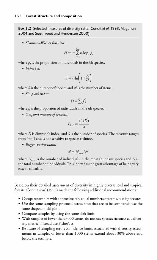
Based on their detailed assessment of diversity in highly diverse lowland tropicalforests, Condit et al. (1998) made the following additional recommendations:

● Compare samples with approximately equal numbers of stems, but ignore area.● Use the same sampling protocol across sites that are to be compared; use the

same shape of field plot.● Compare samples by using the same dbh limit.● With samples of fewer than 3000 stems, do not use species richness as a diver-

sity metric; instead use Fisher’s �.● Be aware of sampling error; confidence limits associated with diversity assess-

ments in samples of fewer than 1000 stems extend about 30% above andbelow the estimate.

132 | Forest structure and composition

Box 3.2 Selected measures of diversity (after Condit et al. 1998, Magurran

2004 and Southwood and Henderson 2000).

● Shannon–Wiener function:

where pi is the proportion of individuals in the ith species.● Fisher’s �:

where S is the number of species and N is the number of stems.● Simpson’s index:

where fi is the proportion of individuals in the ith species.● Simpson’s measure of evenness:

where D is Simpson’s index, and S is the number of species. The measure rangesfrom 0 to 1 and is not sensitive to species richness.

● Berger–Parker index:

where Nmax is the number of individuals in the most abundant species and N isthe total number of individuals. This index has the great advantage of being veryeasy to calculate.

d � Nmax /N

E1/D �(1/D)

S

D �� f i2

S � �ln�1�N��

H � ��Sobs

i�1pi loge pi

Condit et al. (1998) place particular emphasis on the importance of stem numberin influencing diversity estimates in tropical forests, suggesting the followingspecific rules:

● Never use samples of fewer than 50 stems, and in very diverse forests use100 stems or more. These are absolute minimum values; larger samples arepreferable.

● In samples of more than 2000 stems, Fisher’s � can be used to comparesamples, even if they differ substantially in size.

● For samples between 50 and 20 000 stems, either subsample stems to providea common number of stems for all sites to be compared, or apply a correctionfactor to Fisher’s � to adjust for sample size (for details of this approach seeCondit et al. 1998).

Magurran (2004) further emphasizes the importance of sampling approach fordetermining the outcome of diversity measures. Most importantly, the sample sizemust be adequate. However, this can be difficult to determine in practice.Assessment of the rate at which new samples are being encountered is one usefulguide; the experience of knowledgeable field ecologists is another (Magurran2004). In high-diversity sites, Sørensen et al. (2002) recommended the followingrule of thumb: 30–50 individuals should be sampled per species. When usingsample-based approaches, it is necessary to determine an appropriate number ofreplicates. A number of different studies have found 10 replicates to be adequate,but the optimum number varies with the scale of the sampling unit in relation tothe size of the assemblage being surveyed (Magurran 2004). As additional samplesare included in the analysis, their effects on the precision of diversity estimates canbe measured. Unequal sample sizes should be avoided; rather, a consistentapproach to sampling should be used across the entire investigation. It is alsoimportant to remember that samples should be independent; repeated samples ofthe same plot are not true replicates, and replicates should be located randomly andnot grouped together (Crawley 1993).

3.9.3 Beta diversity and similarity

Beta diversity is a measure of the extent to which the diversity of two or morespatial units differs (Magurran 2004) and is generally used to characterize thedegree of spatial heterogeneity in diversity at the landscape scale, or to measure thechange in diversity along transects or environmental gradients. A variety of indicesare available for describing beta diversity, most of which are based on the use ofpresence–absence data, although quantitative abundance data can also be used.One of the most widely used indices is Whittaker’s measure ( �W), which iscalculated as:

�W �S / �

Species richness and diversity | 133

134 | Forest structure and composition

Box 3.3 Measures of similarity and complementarity

(from Magurran 2004)

● Jaccard similarity index (CJ):

where a is the total number of species present in both quadrats or samples beingcompared, b is the number of species present only in quadrat 1, and c is the num-ber of species present only in quadrat 2.

The statistic can be adapted to give a single measure of complementarity acrossa set of samples or along a transect:

where Ujk � Sj � Sk � 2Vjk and is summed across all pairs of samples; Vjk is thenumber of species common to the two lists j and k (the same value as a in the for-mula above); Sj and Sk are the number of species in samples j and k, respectively;and n is the number of samples.

● Sørenson’s similarity index (CS):

(see above for definitions of a, b, and c).● Sørenson’s quantitative index (CN ):

This is a modified version of Sørenson’s index that takes into account the relativeabundance of species, introduced by Bray and Curtis in 1957:

where Na is the total number of individuals in site a, Nb � the total number ofindividuals in site b, and 2jN is the sum of the lower of the two abundances forspecies found in both sites.

● Morisita–Horn index:

This is recommended because it is not strongly influenced by sample size andspecies richness (Henderson 2003):

where Na is the total number of individuals in site a, Nb is the total number ofindividuals in site b, ai is the number of individuals in the ith species in a, bi � the

CMH �2�(aibi)

(da�db)(NaNb)

CN �2jN

Na�Nb

CS �2a

2a�b�c

CT ��Ujk

n

CJ �a

a�b�c

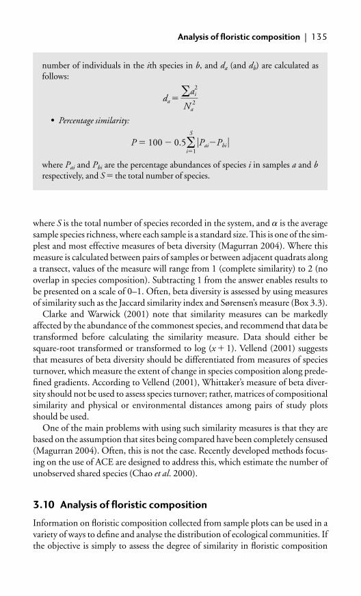
where S is the total number of species recorded in the system, and � is the averagesample species richness, where each sample is a standard size. This is one of the sim-plest and most effective measures of beta diversity (Magurran 2004). Where thismeasure is calculated between pairs of samples or between adjacent quadrats alonga transect, values of the measure will range from 1 (complete similarity) to 2 (nooverlap in species composition). Subtracting 1 from the answer enables results tobe presented on a scale of 0–1. Often, beta diversity is assessed by using measuresof similarity such as the Jaccard similarity index and Sørensen’s measure (Box 3.3).

Clarke and Warwick (2001) note that similarity measures can be markedlyaffected by the abundance of the commonest species, and recommend that data betransformed before calculating the similarity measure. Data should either besquare-root transformed or transformed to log (x � 1). Vellend (2001) suggeststhat measures of beta diversity should be differentiated from measures of speciesturnover, which measure the extent of change in species composition along prede-fined gradients. According to Vellend (2001), Whittaker’s measure of beta diver-sity should not be used to assess species turnover; rather, matrices of compositionalsimilarity and physical or environmental distances among pairs of study plotsshould be used.

One of the main problems with using such similarity measures is that they arebased on the assumption that sites being compared have been completely censused(Magurran 2004). Often, this is not the case. Recently developed methods focus-ing on the use of ACE are designed to address this, which estimate the number ofunobserved shared species (Chao et al. 2000).

3.10 Analysis of floristic composition

Information on floristic composition collected from sample plots can be used in avariety of ways to define and analyse the distribution of ecological communities. Ifthe objective is simply to assess the degree of similarity in floristic composition

Analysis of floristic composition | 135

number of individuals in the ith species in b, and da (and db) are calculated asfollows:

● Percentage similarity:

where Pai and Pbi are the percentage abundances of species i in samples a and brespectively, and S � the total number of species.

P � 100 � 0.5�S

i�1�Pai�Pbi �

da � �ai2

Na2

between samples collected from different locations, then a similarity measure suchas those described in section 3.9 could be used. If the objective is to analyse the rela-tionship between sites or samples in terms of the species present, or to relate speciescomposition to environmental variables, then some form of multivariate analysiswill need to be used. An extensive literature is available relating to multivariatetechniques. Textbooks describing the methods in detail include those by Digbyand Kempton (1987), Jongman et al. (1995), Kent and Coker (1992), andLegendre and Legendre (1998). Shaw (2003) provides a useful and accessibleintroductory account.

For multivariate analyses, specialist statistical or ecological analysis softwaregenerally needs to be used (Table 3.2). Typically, data sets describing species com-position are arranged as a two-dimensional matrix with the different samples form-ing the columns and the species forming the rows. The cells of the matrix canrepresent the observed abundance of each species, an abundance score, or pres-ence–absence information, represented by a 1 if the species was found in the sam-ple and 0 if it was not (Henderson 2003). Such data can readily be entered by usinga spreadsheet program such as Microsoft Excel, or directly into the software pack-age that is to be used for analysis.

3.10.1 Cluster analysis

Cluster analysis can be used to identify groups of sites or samples that are similar interms of their species composition. There are two main types: hierarchical, wheresamples are assigned to groups that are themselves arranged into groups, and non-hierarchical, where the samples are simply assigned to groups (Henderson 2003).Hierarchical methods are most commonly used. The results are usually illustratedby means of a dendrogram (Figure 3.16), in which sites or samples that are moresimilar in terms of species composition group more closely together. A wide varietyof different algorithms can be used to produce dendrograms, which may producedifferent results (Shaw 2003). Cluster analysis can be done by many standardstatistical analysis software packages, including SAS, SPSS, and GENSTAT, as wellas specialist ecological software.

Two key decisions need to be made in cluster analysis: which measure of simi-larity (or distance) to employ, and which rules for cluster formation to adopt (Shaw2003). The similarity measures described in section 3.9, such as the Jaccard andSørensen indices, which are suitable for use with presence–absence data, can beused as a basis of cluster analysis. For continuous variables, Euclidean distance istypically used. With respect to the rules for cluster formation, the simplest methodis to use single-link or nearest-neighbour clustering, in which clusters are joinedbased on the smallest distance between any pair of their component individuals(Shaw 2003). However, dendrograms produced by this method can sometimes bedifficult to interpret. A number of alternative methods are described by Digby andKempton (1987) and Shaw (2003). UPGMA is a widely used alternative methodthat allows clusters to be joined on the basis of the lowest value of the average dis-tance between clusters.

136 | Forest structure and composition

The main problem with cluster analysis, as with other classification techniques,is that the results can easily be misinterpreted. Definition of groups does not nec-essarily reflect genuine ecological differences. Cluster analysis will always dividethe data into groups; even randomly generated data can produce a dendrogram(Henderson 2003). Another problem is that different clustering techniques canprovide very different answers, and as no statistical significance is obtainable forthis form of analysis, it can be difficult to decide which output is ‘correct’. Carefulconsideration of the results is therefore required, to examine whether they make

Analysis of floristic composition | 137

Table 3.2 Software packages suitable for multivariate analysis of ecological data.

Product Comments URL

Canoco for A powerful, high-specification www.plant.dlo.nl/Windows 4.5 package able to perform a wide

variety of multivariate analyses, but particularly suitable for CCA, as the software is designed by the developers of this method. Detailed supporting materials are available (ter Braak and Smilauer 1998).Takes time to learn, but is the software of choice for many researchers.

Community A reasonably powerful Package that is www.pisces-conservation.com.Analysis relatively easy to use. Developed and Package (CAP) marketed by Pisces Software.

DECORANA Available as a free download from the http://science.ceh.ac.uk/and Centre for Ecology and Hydrology in products_services/software/TWINSPAN the UK, who originally developed corn.html

them.

PC-ORD A set of Windows programs for http://oregonstate.multivariate analysis of ecological edu/~mccuneb/data, developed by Bruce McCune pcord.htmat Oregon State University. Widely used.

Primer 5 Developed by Plymouth Marine www.primer-e.com/Laboratory (UK), capable ofperforming a wide range of multivariate analyses. Although developed by marine ecologists, the software is applicable to analysis of forest communities. Well supported.

sense and have some genuine ecological meaning. Cluster analysis should beviewed as a tool for data exploration and hypothesis generation, and not as an endin itself (Shaw 2003).

3.10.2 TWINSPAN

TWINSPAN (Two-Way INdicator SPecies ANalysis procedure) has been verywidely used by plant ecologists since its development more than 30 years ago (Hillet al. 1975). This method can be used with presence–absence, percentage cover, orabundance data. TWINSPAN progressively divides a data set into groups based onall of the information content of the data, rather than merging individuals intogroups as is done in cluster analysis (Shaw 2003). Results are presented in the formof a dendrogram, but the reciprocal averaging ordination method is used to orderthe samples or sites. As a result, the outputs of TWINSPAN analysis are less proneto misinterpretation than dendrograms produced by standard cluster analysis(Shaw 2003). A particularly valuable feature of TWINSPAN is that it allowsindicator species that are characteristic of each group to be identified, and thereforethe method is especially useful when there is a need to identify species that can beused to characterize particular communities (Henderson 2003). In addition, boththe samples and species are ordered along a gradient in the TWINSPAN outputtables, which can greatly help data interpretation (Shaw 2003). An unusual featureof the method is the use of artificial constructs called ‘pseudospecies’, which areused to convert continuous data (such as percentage cover of different species) intocategorical variables. Full details of the method are provided by Hill (1979).Although TWINSPAN output can be rather complicated, the method has been

138 | Forest structure and composition

0.565 0.424 0.283Dissimilarity

0.141 0

Site 1Site 2Site 5Site 6Site 7Site 10

Site 12Site 13Site 11Site 18Site 14Site 15Site 20Site 16Site 19Site 17

Site 3Site 4Site 8Site 9

Fig. 3.16 A dendrogram showing the results of a cluster analysis. The dendrogram

illustrates the degree of similarity between sites according to their species

composition. The diagram was produced by using CAP (Table 3.2). (From

Henderson 2003.)

very widely used and is recognized as a standard technique, with few criticismslevied against it. Its main limitation is that it only considers one axis of variation(Shaw 2003).

3.10.3 Ordination

A wide variety of different ordination methods are available that can be used toanalyse the relationships between sites or samples in terms of their species com-position. The best method is arguably the one that gives the clearest and most easilyinterpreted results, and therefore it may be worth trying a variety of different meth-ods and comparing the results (Henderson 2003). Ordination methods that arecommonly used in forest ecology are considered below. A word of caution is appro-priate, regardless of which method is preferred. These techniques provide little use-ful information unless there is some genuine pattern to be detected and differencesexist between individual samples of vegetation. A great deal of time can be wastedexploring multivariate analyses that produce little of value in the way of clearresults. Ordination outputs can be dominated by outliers and swamped by noise.One solution to this problem is to use sample plots that are large enough to includesufficient stems in the sample, even in sites with low stem densities. Also, do not betoo disheartened if no clear pattern emerges in the results: ecological data can justbe like that.

Principal components analysis (PCA)

PCA is most appropriate for use with abundance data. The method enables therelationship between samples to be illustrated in a two- or three-dimensionalspace by producing a plot of the results (Figure 3.17). This can then be interpretedvisually. The analysis is usually done on a correlation matrix that includes all of thecorrelation coefficients between the variables included in the analysis. If the speciesvary greatly in abundance between samples the data will probably need to betransformed before analysis, using either a square-root or logarithmic transform-ation. The latter procedure cannot handle zeros, and therefore 1 is often added toall of the observations before the transformation (Henderson 2003). However, asthis can distort the output, it is generally preferable to use the square-roottransformation.

Often it is necessary to normalize the data before analysis. This is becausemultivariate datasets often consist of very different variables: for example, thecover of different tree species might be measured on a scale of 0–100%, whereassoil potassium concentration might vary between 5 and 20 mg 100 g–1. To analysesuch data, they should be normalized to ensure that they are comparable. This isusually achieved by converting them to Z scores. Each observation (Xi) can beconverted to a Z score (Zi) as follows (Shaw 2003):

Zi �Xi��

s

Analysis of floristic composition | 139

where � is the mean of a sample and s is the standard deviation. The Z score has nounits (it is the number of standard deviations each observation is from the mean ofthe sample), and therefore data that have been normalized in this way can be read-ily compared in the same analysis.

Outputs of PCA are usually visualized by plotting the sites or samples to be com-pared on the two or three main axes of variation detected by the analysis. Samplesthat are grouped more closely together are more similar in terms of their speciescomposition. Attention should be paid to the proportion of the variability in thedata set that is explained by these axes; the higher the proportion, the more robustthe results. For data sets with more than 20 species, the first three main axes shouldaccount for more than 30% of the variance for the results to be of reasonable value(Henderson 2003).

PCA is very popular among plant ecologists because it is relatively easy to do.The outputs are relatively easy to interpret, but the patterns produced can some-times be difficult to relate to environmental variables of interest. It is important tonote that no test of significance is provided with the analysis: therefore it can onlybe used to explore data and generate hypotheses, rather than test them. However,the axis scores (which are generated during the analysis and describe the positionof each sample along the principal axes) can be used as data themselves and sub-jected to further analysis, such as regression or analysis of variance (ANOVA)(Shaw 2003). For example, by using ANOVA it would be possible to test whetherthe axis scores associated with different forest communities were significantly dif-ferent from one another (assuming that the scores are normally distributed). PCAcannot cope with missing values in the data and may be inappropriate where com-munities develop along environmental or temporal gradients (when DCA may bepreferred; see below) (Shaw 2003).

140 | Forest structure and composition

Site 2

Site 5Site 7

Site 10

Site 11Site 18

Site 17

Principal axis 1

Pri

nci

pal

axi

s 2 Site 3

Site 4Site 9

Site 1 Site 12Site 14

Site 15

Site 16

Site 20

Site 13

Site 8

Site 6

–6

–4 –3 –2 –1 0 1 2 3 4

–5

–4

–3

–2

–1

0

1

2

3

4

5

6

Fig. 3.17 The results of a principal components analysis to illustrate differences

between sites according to their species composition. (Graphical output

produced by using CAP; see Table 3.2). (From Henderson 2003.)

Principal coordinates analysis (PCO) is sometimes confused with PCA, becauseof its similar abbreviation, but is in fact is a very different technique (sometimesreferred to as multidimensional scaling). PCO uses a square matrix of distancesbetween individuals and produces a map from the distances measured. This mapcan be used as a form of ordination to show the relative position of individualssampled; usually Euclidean distance is used (Shaw 2003). The method is relativelylittle used by plant ecologists.

Detrended correspondence analysis (DCA or DECORANA)

DCA is an ordination technique designed specifically to assist with the explorationof ecological data (especially abundance data) and is very widely used by plantecologists. It is particularly appropriate for use in situations where the sites that aresampled can be arranged along an environmental gradient, such as successionalstages in vegetation. In such cases, use of PCA can lead to an artefact in the output(the so-called ‘arch effect’), which DCA was designed to overcome. Ordinations ofboth species and sites can be plotted on the same figure, which enables the influ-ence of different species on the ordination of the sites to be evaluated visually. Theoutput of DCA is otherwise similar to that of PCA.

Canonical correspondence analysis (CCA)

This method was developed by ter Braak (1986), and is widely used by researchersinterested in exploring the relations between community composition and envir-onmental variables. CCA is based on a similar analytical technique to DCA andTWINSPAN, but differs in its inclusion of environmental data within the ordin-ation itself so as to maximize their importance in the output. CCA thereforerequires data on the environmental conditions at each site. These may be repre-sented in the form of classificatory variables (such as ‘high’ or ‘low’ altitude) or con-tinuous variables (such as temperature measured in degrees Celsius). The datamatrix including the environmental variables measured must have the same num-ber of rows (observations) as the species data, but need not have the same numberof columns (variables) (Shaw 2003).

The outputs of the analysis enable the relation between environmental variablesand the observed species communities to be evaluated. The method is sensitive todata quality; poor or incomplete data will produce results of little value. It isimportant that environmental and species data are collected at the same place andat the same time (Shaw 2003). As outputs can be complex, they can be difficult tointerpret. As with other ordination methods, it is not possible to statistically testthe association between species composition and environmental variables.

Biplot

Often, a main objective of ordination is to explore the relations between floristiccomposition and environmental variables (such as soil characteristics, aspect or alti-tude). This can usefully be achieved by producing a biplot. Biplots can be produced

Analysis of floristic composition | 141

by using different ordination techniques (such as PCA, DCA, and CCA), althoughthe methods used differ according the ordination technique adopted. Biplots enablethe properties of the variables measured (such as environmental variables) to beoverlaid on top of the main ordination diagram. Usually the former are illustratedas arrows that run from the 0,0 point to the coordinate in question (Shaw 2003).This can help with data interpretation: for example, if an arrow points to a cluster ofpoints, then this suggests a relation between the variable in question and the sam-ples illustrated by the points in the cluster. For example, an arrow representing soilnitrogen concentration might be associated with a cluster of points representing thecomposition of a particular forest type. However, it should be remembered that abiplot provides no statistical analysis of the strength of this relation, and illustrates acorrelative association rather than any causal relation.

3.10.4 Importance values

Importance values have been widely used as a measure of species composition thatcombines frequency, abundance and dominance importance values (Grieg-Smith1957). This can be calculated according to the following equation (Husch et al.2003):

where Ij is the importance value of the jth species, nj is the number of samplingunits where the jth species is present, N is the total number of sampling units, dj isthe number of individuals of the jth species present in sample population, D is thetotal number of individuals in sample population (D � Σdj ), xj is the sum of sizeparameter (generally basal area or volume) for the jth species, and X is the total sizeparameter across all species X � Σxj .

3.11 Assessing the presence of threatened or

endangered species

Conservation assessments typically depend on knowing not only which species arepresent at a particular location, but also the relative conservation importance ofthese species. At the global level, species at risk of extinction are listed on theIUCN Red List of Threatened Species; these species have been evaluated accord-ing to the IUCN Red List categories and criteria. Details of the listing process,including freely downloadable copies of the categories and criteria, are availableat �www.redlist.org/�. A list of taxa that are considered threatened is maintained ina searchable database, which can be accessed online from the same Internetsite. The only taxonomic groups that have been comprehensively assessed are theamphibians, birds, mammals, conifers, and cycads. The vast majority of plant taxaare not yet included. To find out the conservation status of plant species, the

Ij � 100�nj

N�

dj

D�

xj

X�

142 | Forest structure and composition

UNEP–WCMC Threatened Plants database should be consulted �www.wcmc.org.uk/species/plants/red_list.htm�. For tree species, a separate database is available,the UNEP–WCMC Trees Database �www.unep-wcmc.org/�, which containsinformation on threatened trees and other trees of conservation concern. Thisincludes information published in the World List of Threatened Trees (Oldfieldet al. 1998).

Two points are of particular concern when using the Red List and these data-bases.

● First, they are very incomplete. Application of the Red List criteria requiresinformation on the current (and ideally historical) patterns of occurrence ofindividual species, which is often lacking. Most listing is undertaken on avoluntary basis by specialists familiar with a particular group of species.Although the Red List is continually being revised, it is certain that manyspecies (particularly of plants) that are threatened with extinction are notcurrently listed. Indeed, assessing the conservation status of species is animportant research endeavour in its own right, and readers are encouraged tobecome involved in this process.

● Second, it is important to note that the IUCN Red List includes only taxa thatare globally threatened, in other words when the entire geographic range ofthe taxon is considered. In many cases, it is important to ascertain whetherregionally or nationally scarce or threatened taxa are present at a particularsite. For this purpose, it is necessary to refer to lists of threatened taxa devel-oped at the national scale. Many national governments have developed suchlists, some of which are available online. In some cases, such national lists haveadopted IUCN national Red List criteria and categories (details of which arealso available at �www.redlist.org/�), and may be published in the form ofnational Red Lists. However, in many cases countries or individuals havedeveloped their own categories and criteria by which species may be consid-ered endangered or threatened. For example, a ‘star’ system for scoringdifferent tree species in Ghana according to their rarity was developed byHawthorne (1996) and Hawthorne and Abu-Juam (1995). It is thereforeimportant to distinguish between globally and nationally threatened specieswhen carrying out an assessment, and to consider the criteria by which specieshave been classified, as well as the definition of the classes adopted.

At the international level, another group of species that are considered as prior-ities for conservation are those listed on CITES �www.cites.org/�. Species listed inthe CITES Appendices are those that are considered threatened with extinctionbecause of international trade. For a species to be listed, agreement must bereached between the Parties to the Convention. For this reason, species listed onCITES form only a small subset of those that are threatened with extinction. Theirpresence is useful to record, however, particularly in areas where forests are beingsubjected to some form of management, as CITES listing has significant implica-tions for how resources of these species are traded and managed. Some 38 species

Threatened or endangered species | 143

of tree have now been listed in Appendices I and II of CITES, including econom-ically important timber species such as mahogany (Swietenia spp.). The mainresearch challenge for such species is to determine how they may be harvestedsustainably in accordance with CITES requirements (see section 8.2.3).

At the national scale, species of conservation concern may also be listed in avariety of different forms of legislation or government policies, such as BiodiversityAction Plans or laws governing the protection of particular species. In some cases,species may be accorded conservation importance because of their high social,cultural, or economic value, rather than their rarity or extinction risk. Poorter et al.(2004), in their atlas of woody plant species of West African forests, provide anoutstanding example of how ecological information on tree species, collated at theregional scale, can be analysed and presented in a way designed to support conser-vation efforts.

3.12 Vegetation classification

The classification of forests into different communities or types provides an impor-tant basis for basis for forest management and conservation planning. Numerousdifferent classification systems have been developed and implemented in differentparts of the world. Details of these different approaches are described by Mueller-Dombois and Ellenberg (1974) and Whittaker (1975). Recent examples ofapproaches to classifying forests are provided by McNab et al. (1999) and Carteret al. (1999). Kimmins (1997) presents a useful overview of the differentapproaches that have been used to classify forests in the past, which can be sum-marized as follows:

● Climatic classifications are based on the fact that climate is one of the majorfactors influencing vegetation distribution. Climate types can be defined interms of temperature and precipitation, which are associated with particulartypes of vegetation—for example, tropical rainy and warm temperate climatesare associated with tropical rain forest and temperate rain forest, respectively.It is important to note, however, that climatic classifications represent poten-tial, rather than actual, vegetation distributions.

● Landform or physiographic classifications are based on soil characteristics andlandform features such as topography and altitude. These are often employedwhen classifying vegetation using remote sensing data. Although they have afirm ecological basis, as with climatic classification, this approach is an indir-ect method of classifying vegetation as floristic composition is not taken intoaccount.

● Biophysical or ecosystemic approaches are based on climate, soils, and landformtogether with information about vegetation composition. This approach iswidely used to classify areas at the regional scale.

● Physiognomic classifications are based on the growth form of dominant plantsand the environments in which they grow; for example, vegetation dominated

144 | Forest structure and composition

by coniferous trees, deciduous trees, or shrubs might be differentiated asdifferent vegetation types.

● Floristic composition can also be used to define vegetation types. This is themain method used by ecologists, but different approaches have been adoptedin different regions. For example, the Braun–Blanquet approach has beenused widely in Europe, and the method developed by Daubenmire has beenwidely used in the USA.

This diversity of approaches greatly complicates the integration or comparison ofmaps of forest types produced in different areas, and inhibits the development ofgeneralizations about the patterns of distribution of different forest types and theirrelative conservation status. If the objective is some form of conservation assess-ment, it is very important to note the classification methods used in producing anythat are drawn upon. For example, a map representing potential forest distribution(as produced by climatic or physiographic approaches) would be of little use forassessing the actual current extent of a particular forest type.

The problems of using applying available forest classifications to conservationissues are illustrated by Miles et al. (2006) in their global assessment of the con-servation status of tropical dry forests. A first glance at available maps of foresttypes, such as that presented by FAO (2001b), suggests that extensive areas oftropical dry forest remain. However, the FAO map of ecofloristic zones is basedon a climatic classification of potential vegetation, which gives a very misleadingimpression of current vegetation cover. Miles et al. (2006) therefore used a globalmap of current forest cover derived from remote sensing imagery (MODIS) toexamine the actual current extent of tropical dry forest. The next step was to over-lay this map with ecological classifications of forest types. Blasco et al. (2000) pro-vide a comparison of 10 regional classification schemes developed for tropicalwoody vegetation, and present a common framework based on ‘bioclimatic types’to help make comparisons between them. However, this has proved to be of littleuse for mapping tropical dry forests, as forest types (or formations sensu Blascoet al., 2000) labelled as ‘dry forest’ in available regional classifications are groupedunder no fewer than four of the six bioclimatic types considered. This suggestseither that tropical dry forests have a very broad edaphic tolerance range, or thatthe concept of what constitutes a tropical dry forest is interpreted variously bydifferent authors.

To produce their assessment, Miles et al. (2006) used the global biogeographicclassification presented by Olson et al. (2001). This has the great merit that it wasexplicitly developed to support global conservation assessments. Importantly, theclassification was based primarily on biogeographic information rather thanclimate, and included information regarding distributions of animal species as wellas plants, unlike most alternative classifications that are available. This classifica-tion is applicable for use at global and regional scales, but has also been used byWWF for conservation assessments at subregional (ecoregion) scales (Olson et al.2000).

Vegetation classification | 145

When choosing an appropriate classification scheme, it is necessary to decidewhether compatibility with existing schemes is necessary or desirable. Suchcompatibility can be of great help in enabling communication between peopleworking on a particular forest type. Selection of forest types used in a map willdepend on the map’s purpose, and whether the classes can be accurately and effi-ciently delimited. When a classification system has been selected, it is important todocument the details of each class and apply these definitions in an objective andconsistent manner.

Many vegetation classification systems use a hierarchical approach in whichclasses are nested; major classes are divided into subclasses, which themselves canbe divided into further subclasses. Such systems can be easily adapted to differentscales. Non-hierarchical approaches tend to be used at a specific scale, when theymight be preferred because they can be more readily customized to the particularneeds of the investigation in question.

146 | Forest structure and composition

4Understanding forest dynamics

4.1 Introduction

Research into forest dynamics over the past three decades has transformed ourunderstanding of forest communities and has had a major influence on thedevelopment of ecological science. Increasing recognition of the role of naturaldisturbance in shaping the forest composition and structure, through researchsuch as that of Tom Veblen in south temperate forests (Veblen 1979, 1985, Veblenet al. 1981), has caused a paradigm shift in ecology that has major implications forforest conservation and management (Pickett and White 1985). Investigations offorest disturbance and its impacts on the population dynamics of trees havebecome widespread, and have generated a voluminous literature.

Forest dynamics can be studied in three main ways:

● by inferring dynamics from one-off assessments of stand structure● by monitoring forests over time, for example through repeated surveys of

permanent sample plots (PSP)● through the use of models of forest dynamics.

Each of these approaches has its limitations. A key problem is that most trees arelong-lived. Forests often change slowly, and such changes can be difficult to detecton a scale of a few years or decades, or even over a human lifetime. Inferences ofdynamics from assessments of stand structure can be highly misleading. Forexample, some tree species only produce seed very infrequently. If a field visit doesnot coincide with a ‘masting’ year, when large amounts of seed are produced, anentirely erroneous impression might be gained about the reproductive capacity orregeneration potential of the species present. Modelling approaches have a greatdeal to offer the study of forest dynamics, enabling dynamics over long timescalesto be simulated, but even here there are many problems to be overcome, such as theneed for detailed parameterization and the high degree of uncertainty associatedwith ecological processes and their outcomes.

This chapter describes methods relevant to two of these three approaches, witha particular focus on field techniques. Modelling techniques are considered inChapter 5. Remote sensing methods can also be used to monitor forest change, asdescribed in Chapter 2. The impacts of human activities on forest dynamics arefurther considered in Chapter 8.

4.2 Characterizing forest disturbance regimes

Disturbances can be defined as relatively discrete events that disrupt ecosystem,community or population structure, and change the availability of resources or thephysical environment (Pickett and White 1985). Analysis of the disturbanceregime of a forest can be of great value for understanding patterns of structure andcomposition, as well as being important for defining appropriate managementinterventions. Detailed treatments of forest disturbance are provided by Attiwill(1994), Barnes et al. (1998), Oliver and Larson (1996), Peterken (1996), and Pickettand White (1985).

Characterizing the disturbance regime typically involves assessing the severity,timing, and spatial distribution of the different types of disturbance affecting theforest. It is useful to note the difference between the intensity and severity ofdisturbance. Intensity refers to its physical force, or the amount of energy released,whereas severity refers to the amount of living biomass that is either killed orremoved as a result of the disturbance (Spies and Turner 1999). Timing refers to theseasonality (time of year), duration, frequency, and the return interval or rotationtime of disturbance (Spies and Turner 1999).

Spatial distribution may include assessments of the extent and shape ofdisturbances, and can be characterized at different scales, for example at local,landscape, and regional scales (Barnes et al. 1998).

In order to characterize the disturbance regime of a particular forest, thefollowing variables should therefore be measured (Gibson 2002):

● extent and spatial pattern of the disturbed area● intensity, or the strength of the disturbance (for example, fire temperature or

wind speed)● severity, or the amount of damage that occurred to the forest (for example,

number of individual trees killed or stems damaged)● timing, including the frequency (the number of disturbances per unit time),

the turnover rate or rotation period (the mean time taken for the entire forestarea to be disturbed) and the turnover time or return interval (the mean timebetween disturbances)

● interactions between different types of disturbance (for example, droughtincreases fire intensity).

For each of these variables, the central tendency (mean, mode, or median) andvariation (standard deviation or range, for example) should be calculated, andpresented together with frequency distributions in order to fully characterize adisturbance regime (Gibson 2002).

The main types of natural disturbance affecting forests are fire, weather (includingwind, ice, temperature, and precipitation), soil disturbance (erosion, deposition,flooding, and movement) and herbivory (Gibson 2002). Anthropogenic disturb-ances include logging, fuelwood cutting, road building, drainage, fire, forestclearing for agriculture and urban development, livestock husbandry, application

148 | Understanding forest dynamics

of chemical fertilizers and pesticides, aerial pollution, and many others.Assessment of the impact of human activities on forests is of fundamental import-ance for conservation planning and management. Often, a key objective is todetermine whether a given forest is able to withstand or tolerate a particularanthropogenic disturbance regime. Such analyses lie at the heart of definingapproaches to sustainable forest management, and depend not only on character-izing the disturbance regime, but on understanding how the forest responds todifferent types and patterns of disturbance. An important principle is the idea oflimiting human impacts to the frequency, size, and severity of disturbance to whichspecies are adapted, leading to the development of forest management plans basedon natural disturbance regimes (Spies and Turner 1999). However, this is oftendifficult because of a lack of understanding about past disturbance regimes, andthe ecological impacts of current human activities.

The following sections describe methods for characterizing some of the mostimportant types of forest disturbance. The methods described here are fieldtechniques; remote sensing methods and GIS are also very widely used for assessingforest disturbance and are described in Chapter 2. Although the methodsdescribed here may be useful for characterizing the current disturbance regime of aparticular forest, it can also be helpful to consider the likelihood (White 1979) orrisk of disturbance occurring in the future. This is central to assessment of vulner-ability, an important consideration in conservation planning, which is described insection 8.4. Types of disturbance not considered here in detail include aerialpollution and insect attack, both of which are of major concern to foresters, whohave consequently developed a range of techniques for their assessment (see Horn1988, Innes 1993, Knight and Heikkenen 1980).

4.2.1 Wind

It is helpful to differentiate the typical (‘chronic’) wind disturbance of a site fromthe effects of relatively rare wind events, such as hurricanes or storms (Ennos1997). Rare events can have a major impact on forest ecology by destroying trees.The breakage or uprooting of trees by wind is referred to as windthrow orblowdown. This form of natural disturbance results from the interaction betweenclimate, topography, stand structure, soil characteristics and the growth and formcharacteristics of individual trees. Damage can be in the form of stem failure, rootfailure or uprooting (Mergen 1954). Windthrow can be termed endemic orcatastrophic. The latter results from winds with relatively long return periods and isinfluenced primarily by local wind speed and wind direction, whereas endemicwindthrow results from peak winds with return intervals of less than 5 years and isinfluenced more strongly by site conditions (Lanquaye-Opoku and Mitchell2005). Endemic windthrow is generally more predictable than catastrophicwindthrow, and therefore most assessments of windthrow risk focus on the formerrather than the latter (see section 8.4).

The impacts of wind disturbance on a forest can be assessed through a fieldsurvey, involving measures of the structure and species composition of the area

Forest disturbance regimes | 149

affected (see Chapter 3) and the canopy gaps created (see section 4.4). Windthrowalso results in production of woody debris (see section 7.2 for techniques for assess-ing deadwood volume). Treefalls not only create gaps in the canopy but also causedisturbance to the soil and influence the micro-environmental heterogeneity ofthe forest by creating pit-and-mound micro-relief with exposed root mats, baremineral soil, and humus, as well as fallen logs. These features may provide suitablesites for seedling colonization in many forests, and are therefore often included infield surveys. For example, Ulanova (2000) mapped the distribution of pits andmounds caused by treefalls, as potential sites of seedling establishment. Someauthors have used a decay scale for logs, with between five and nine divisions, todetermine gap age or the time since a windthrow event (see, for example, Liu andHytteborn 1991). However, the degree of decay of a log depends not only on thedate of the windthrow but also on log size and species, its position (i.e. whether itrests directly on the ground or on broken branches), and its status at the time of thewindthrow event (i.e. dead or alive) (Ulanova 2000).

Surveys may also be designed to assess tree condition, by recording differentkinds of damage such as broken or bent stems, branch loss, snapped or uprootedtrees, and root damage. The extent of canopy loss can be estimated visually byusing methods for estimating canopy cover (see section 3.6.4) (Brommit et al.2004). Wounding is often common in wind storms, caused by falling trees andbranches, twisting, etc., and may also be recorded. Different tree species vary in theamount of crown damage caused by storms, reflecting differences in green woodstrength and crown shape (Zimmermann et al. 1994). The capacity for recoveryfollowing wind damage, by resprouting of stumps or branches, also varies betweenspecies (Del Tredici 2001) and can usefully be recorded in a survey (Bellinghamet al. 1994, Paciorek et al. 2000).

The amount of damage caused by wind is a function of wind speed, duration,and the direction from which the winds originate. Wind speed is usually measuredby using a cup anemometer, consisting of three hemispherical or conical cupsmounted on arms and attached to a spindle so that they can rotate in the wind(Coombs et al. 1985). An alternative design, the vane anemometer, consists of anumber of light vanes radially mounted on a horizontal spindle. The main sourcesof error for such mechanical anemometers is that they have a threshold belowwhich the friction of the system prevents rotation, and their inertia causes anoverestimation of wind speed when the latter suddenly drops (Coombs et al.1985). Continuous measurements from anemometers can be recorded by usingdata loggers (see section 4.6). If such instruments are not available, records may beobtained from national weather centres or meteorological surveys. Further detailsof devices for wind measurement are provided by Grace (1977).

Tatter flags offer a relatively simple alternative method of measuring exposure towind. Described by Lines and Howell (1963) and Rutter (1966, 1968a, b), themethod employs flags made out of cotton mounted on poles or wires. It is import-ant that material is used that degrades with time—not the material usually used tomake flags! The material should slowly degrade to lose 50–75% of its initial mass.

150 | Understanding forest dynamics

Tatter flags are also commercially available. The loss in mass or area of the flagmeasured over time can be attributed to attrition caused by wind. Studies of thetattering of flags in both controlled and field conditions have shown that the rateof tatter is closely correlated with wind exposure, but is also influenced by factorssuch as rainfall and atmospheric moisture (Jack and Saville 1973). Another possiblesource of error is freezing of flags in winter. As wind varies seasonally and from yearto year, flags should be flown for 2–3 years and should be distributed throughoutthe area to be surveyed. Use of tatter flags in the UK has been described by Quineand White (1994).

Susceptibility of areas to wind damage can be assessed in several ways (Reed andMroz 1997). It may be possible to identify soil types susceptible to wind damagebecause of shallow rooting depth. The incidence of wind damage in the past canpotentially be ascertained from forest survey notes or weather records, and used toassess relative risks of different areas in the future. Climatic atlases often indicatesevere storm frequencies. For example, Boose et al. (2001) describe methods forreconstructing hurricane disturbance in New England by using a combination ofhistorical research and computer modelling. Wind disturbance history can also beinferred by means of dendrochronological techniques (see section 4.3). The pres-ence of physical evidence such as broken trees, fallen trees, and tip-up mounds canalso be used to infer the previous occurrence of wind damage.

Examples of studies that have assessed the damage caused by windstormson forests include Bellingham et al. (1994, 1995), Brommit et al. (2004),Burslem et al. (2000), Peterson (2000), Peterson and Rebertus (1997), andZimmermann et al. (1994). Further information on the effects of wind on forestsis provided by Coutts and Grace (1995), Ennos (1997), and a special issue of thejournal Forest Ecology and Management (2000), vol. 135. Approaches to modellingwind risk are briefly considered in section 8.4.

4.2.2 Fire

Fire temperatures can be measured by using thermocouples or temperature-sensitive paints. Thermocouples can be used to measure temperature by monitoringthe voltage produced by the difference in temperature between two dissimilarmetals, which are used in construction of the thermocouple. The temperatureresponse of a thermocouple should be calibrated against a reference measurement.Ideally a thermocouple with a small bead (or tip) and small wire diameter shouldbe used; sheathed thermocouples are also preferred because they protect thethermocouple junction from soot, which can influence the measurements made(Saito 2001). However, useful information can also be gained from thicker wirethermocouples (Iverson et al. 2004). Thermocouples need to be connected to adata logger for measurements to be recorded (see section 4.6). Arrays of thermo-couples can be arranged in a grid and at different heights in a vegetation canopy, inorder to characterize spatial variation in fire intensity (Jacoby et al. 1992).

Alternatively, pyrometers can be constructed by painting spots of temperature-indicating paint (such as Temiplaq), which melt at different temperatures, on to

Forest disturbance regimes | 151

the unglazed side of ceramic tiles or metal tags, which are placed in the forest beforethe fire then collected afterwards for inspection (Gibson 2002). The minimumtemperature attained in the fire around each tile is determined as the highest-temperature paint spot that melted in the fire (Hobbs et al. 1984). Maximum firetemperatures can also be estimated through the use of Tempil tablets, which meltat different temperatures (Grace and Platt 1995). The tablets should be wrappedin aluminium foil before they are placed in the forest, to facilitate relocating themafter the fire, and their melting points should be calibrated in the laboratory(Gibson 2002).

Iverson et al. (2004) compared thermocouples and temperature-sensitivepaints to measure fire intensity (Figure 4.1) and found that maximum tempera-tures recorded by the two measuring systems were highly correlated. Theseauthors recommended the use of temperature-sensitive paints if only maximumtemperature is required, because of their substantially lower cost involved.However, additional information can be collected by using thermocouples. Forexample, positioning of the thermocouples in a grid enables information on therate of fire spread to be collected.

A further technique for measuring fire temperature involves use of an infraredcamera and an image recording and analysis system, which is capable of obtaining atwo-dimensional thermal image from a remote location (Saito 2001). This methodhas been used to produce temperature profiles in forest fires (Clark et al. 1999c).

Fire velocity can be measured by using a pitot tube, which can measure velocitiesin the range from a few metres per second to above 100 m s–1, covering most ofthe wind velocity range in forest fires (Saito 2001). The technique is relativelysimple and can measure a one-dimensional velocity component, although three-dimensional measurements can be obtained by changing the direction of the pitottube head when the flow is at a steady state (Saito 2001). The method is describedby Sabersky et al. (1989).

152 | Understanding forest dynamics

Partially buried,capped 15 cm PVCcanister containing

data logger

Aluminium tag withtemperature-sensitive

paints

Temperatureprobe

25 cm

Buried cable

Approximately 2 m

Fig. 4.1 Arrangement of thermocouple temperature probes and temperature-

sensitive paints, used in a comparative trial to measure fire intensity. (From Iverson

et al. 2004. International Journal of Wildland Fire, CSIRO Publishing.

http://www.publish.csiro.au/nid/115/issue/871.htm.)

Trees may survive a fire but be damaged by it. Death of the cambium can lead toproduction of a fire scar, which is visible as a gap in the bark that is usuallytriangular in shape, becoming narrower with height, found on the leeward side oftrees. Fire scars have been widely used to date fires, particularly in conifer forests,but also with some hardwood tree species. Such scars can be detected as blackenedareas or damaged rings in increment cores (see following section), or in discsobtained from the trunks of felled trees (Schweingruber 1988). However, errorscan be caused by missing, false, or indistinct rings, which should be corrected bycross-dating (Fritts 1976). This can be achieved by sampling trees that wereundamaged by the fire, or sampling both sides of the trees affected. Further detailsof these methods are provided by Arno and Sneck (1977), Madany et al. (1982),and Schweingruber (1988).

Byram (1959) provided a simple index of fire intensity:

I � HwV

where H is the heat of combustion of fuel, w is the mass of fuel consumed perunit area, and V is the heading rate of spread of the fire. This index is thought tocorrelate closely with tissue necrosis and possible tree mortality. Iverson et al.(2004) indicate that measurements from thermocouples can be used to estimate I.Fire intensity is usually measured as the rate of heat energy released per unit lengthof fire line per unit time (W m–1 s–1) or sometimes per unit area and time(W m–2 s–1).

An ability to predict the spread of fires is something of great value to forestmanagers, and consequently this has received much attention from researchers.However, fire spread is influenced by a complex set of phenomena occurring overa range of scales, involving turbulent flow influenced by wind and topography, andthe spatial distribution and amount of fuel available. A range of models have beendeveloped in different parts of the world, which are reviewed by Weber (2001).Further information about the ecology of forest fires is provided by Agee (1993),Johnson (1992), Johnson and Myanishi (2001), and Whelan (1995). Methods forevaluating fire risk are considered further in Chapter 8.4.

4.2.3 Herbivory

In order to clearly demonstrate the effects of herbivory on plant populations, prop-erly designed, replicated field experiments are required. Below-ground herbivory isgenerally assessed by applying some form of either physical or chemical exclusionas treatments in a field experiment. Chemical treatments range from the non-specific killing of most soil organisms through the use of chloroform fumigation(see, for example, Sarathchandra et al. 1995), to the use of biocides that are targetedto the control of specific organisms. Organophosphates such as isofenphos andethoprop can be used to reduce populations of soil invertebrates, includingcoleopteran and lepidopteran larvae (Gibson 2002). Freezing of soil to -20 C canbe used to reduce the activity of soil nematodes (Sarathchandra et al. 1995).Experimental control of above-ground herbivory by invertebrates is often achieved

Forest disturbance regimes | 153

through spraying insecticides such as carbaryl, chlorpyrifos, dimethoate, andmalathion (Brown and Gange 1989, Gibson 2002). However, great care should beemployed in the use of any chemical treatments; many can have unforeseen andpotentially deleterious effects on components of the ecological communities otherthan those being investigated, and can have undesirable effects of the physical andchemical properties of soils. Some can alter plant growth, either positively or neg-atively, and this should be evaluated as part of the experiment (Gibson 2002).Insecticides that might be of use in ecological research are listed by appropriateguidebooks such as Page and Thompson (1997), which should be consulted care-fully to ensure that the chemicals are selected, handled, and applied correctly(Gibson 2002) in a way that minimizes impact on the environment.

An important method of assessing herbivory impacts in forests is through theuse of fenced exclosures, designed to exclude browsing mammals such as deer.Comparison of areas within and outside such exclosures can provide insightsinto the impacts that the animals are having on variables such as the extent andcomposition of ground flora and the seedling establishment of trees. Theeffectiveness of the exclosure in excluding the animals should be evaluated; thepresence of a fence is no guarantee that it will be effective. Some species of deerare capable of jumping fences of at least 2 m in height, and can prove remark-ably persistent in attempting to gain access to fenced areas. An appropriatedesign and size of fence should be used for the type of animal to be excluded,and animal populations should be monitored both within and outside theexclosures (see Sutherland (1996) for methods appropriate for censusinganimal populations).

Fences should be regularly checked for damage and repaired, and fence supportsneed to be strong enough to withstand damage from any large animals that arepresent (Gibson 2002). For smaller mammals, an appropriate mesh size for thefencing material must be selected (i.e. 3–4 cm for rabbits, 0.5 cm for voles andmice; Gibson 2002). To exclude burrowing animals (such as rabbits), the fencemust be partly buried in the soil. Care should also be taken to ensure that the fencesdo not have any negative effects on wildlife; for example, in Scotland, collisionswith deer fences were found to be a significant cause of mortality in woodlandgrouse (Summers 1998).

The potential impact of herbivory on individual plants can be examined experi-mentally by introducing herbivores in appropriate cages, or by simulating theeffects of herbivory by clipping leaves or other plant parts with scissors (Canhamet al. 1994b). However, removal of plant material in this way may fail to mimic theeffects of herbivory precisely (Gibson 2002). Generally, the effects of herbivory onindividual plants are assessed by measuring damage to the plant parts consumed,although it should be noted that patterns of dry mass allocation within the plantmay change in response to herbivory, and therefore this may need to be measuredfor a comprehensive assessment of impacts. Plant damage as a result of herbivorycan be most simply assessed as the proportion of damaged leaves or shoots per plant(Gibson 2002). Alternatively, individual leaves can be assessed on a scoring system

154 | Understanding forest dynamics

describing the proportion of leaf area removed. For example, Brown et al. (1987)used the following scoring system on a sample of 20–100 leaves per plant:

Damage rating Estimated leaf area removed (%)0 01 1–52 6–253 26–504 51–755 76–996 Total removal of leaf

Reimoser et al. (1999) provide a useful review of methods for measuring forestdisturbance by ungulates. These authors note that impacts of ungulate herbivoryare usually assessed by analysing variables such as density of tree regeneration,species composition, and growth rate of young trees. These variables can be mea-sured in a field survey using quantitative methods (see Chapter 3 and elsewhere inthis chapter). Surveys can also usefully assess the occurrence of variables such as:

● trampling (includes pawing, scraping, burrowing and rooting); ● browsing (includes ‘unseen’ browsing, i.e. feeding on seeds and seedlings, and

‘visible’ browsing, such as tree twig browsing)● fraying● peeling (of bark or surface roots, for example).

In situations where quantitative approaches are not possible, qualitative surveyscan be considered. For example, Table 4.1 illustrates a classification scheme forforest stands developed in the UK, which can be used to characterize the intensityof grazing based on a series of indicators that can be rapidly assessed by observation.

A further technique widely used in studies of herbivory is the analysis of faecesand gut contents. The technique involves identifying plant fragments that havebeen ingested by herbivores, with the aim of identifying the dietary preferences ofdifferent species. The main advantage of faecal analysis is that the same populationof herbivores can be continuously sampled, without direct interference. Themethod is described in detail by Bhadresa (1986), on which this account is based.The technique depends on development of a reference collection of the cuticles ofplant species found in a study area. This can be achieved by peeling or scraping offthe epidermis of a leaf of the chosen plant species, then mounting it in glycerol jellyon microscope slides. Permanent stained mounts can be produced by dehydratingslowly with alcohol and replacing by xylol, then mounting in Canada balsamor Euparal. The cuticle can then be stained with safranin, acid fuchsin, or gentianviolet, conducted at the 70% alcohol stage.

Faeces can be collected from the field plots, after first clearing an area of existingfaeces to ensure that any material sampled is fresh. The size of the plot varieswith the animal concerned; Bhadresa (1986) recommends 4 � 4 m squares forrabbits, but larger areas are needed for larger mammals. Faeces may be collected at

Forest disturbance regimes | 155

15

6|

Un

dersta

nd

ing fo

rest d

ynam

icsTable 4.1 Indicators of different grazing or browsing pressures in north temperate forest (adapted from Reimoser et al. 1999).

Intensity Indicator

Very heavy No shrub layer; obvious browse line on mature trees; ground vegetation �3 cm tall with grasses, mosses or bracken(Pteridium aquilinum) predominating, and trampling down of ground flora; extensive patches of bare soil; surviving herbspecies usually dominated by unpalatable species; suppression of growth, and killing, of seedlings and saplings by browsingsoon after germination and, therefore, virtually absent; very abundant dung from grazing animals; bark stripped fromyoung and mature trees and from branches on the ground; mosses scarce or absent; possible invasion of weed species; themore palatable, grazing-sensitive shrubs and herbs confined to inaccessible areas or, at least, noticeably more abundant there.

Heavy Shrubs absent or moribund; ‘topiary’ effects on remaining shrubs; a browse line on mature trees; ground vegetation�20 cm tall with grasses, mosses or bracken (P. aquilinum) dominating; few patches of bare soil; surviving herb speciesusually dominated by unpalatable species; tree seedlings not projecting above ground vegetation height; abundant dungfrom grazing animals; bark stripping occasionally occurring; bulky, common mosses favoured at the expense of the rarerspecies requiring deeper shade and cover; the more palatable, grazing-sensitive shrubs and herbs confined to inaccessibleareas or, at least, noticeably more abundant there.

Moderate Patchy shrubs showing evidence of pruning or a browse line; ground vegetation variable in height up to 30 cm, comprisinga mixture of grasses, herbs, or dwarf-shrubs, including some of the more grazing-sensitive species of herb and showingdirect evidence of browsing/grazing; localized close-cropped lawns where there is a concentration of grazing; patches ofbare soil small and rare; tree saplings projecting above ground vegetation in a few areas; some dung from grazing animals;no bark stripping; wide range of moss species.

Light Well-developed shrub layer, with no obvious browse line; a lush ground vegetation in places where the shrub layer coversnot more than ~30–50% of the ground, dominated by grazing-sensitive species; tree saplings common in gaps; dung andtracks of grazing animals difficult to find; no bark stripping; browsed shoots scarce and localized, or totally absent; deeplitter layer; ground mosses uncommon and consisting of few species.

None As for Light but with no browse line on the shrub layer; no, or very few, saplings where there has been no grazing for manyyears; no herbivore dung or tracks present; no browsed shoots; no, or very few seedlings; extensive monospecific mats ofvigorous ground-layer species may also occur on some sites.

regular intervals and stored after drying until required for analysis. Alternativelythey may be stored in a mixture of formalin–acetic acid–alcohol–water in theratio 10 : 5 : 50 : 35. To separate epidermal fragments for analysis, faeces may bedispersed in water, then after subsampling the epidermal fragments can be identi-fied and counted under a microscope (Croker 1959). Alternatively the faeces maybe soaked in 10% sodium hydroxide, or nitric acid and potassium hydroxide, tohelp disperse the epidermal fragments (see Box 4.1 below).

Once cuticular fragments have been extracted, they can be identified bycomparison with a reference collection, following examination with a microscopeunder � 100 magnification. Estimates of the relative abundance of different speciesin the sample can be obtained by one of the following methods (Bhadresa 1986):

● counting the number of fragments in the entire subsample● frequency counts in microscope fields at a particular magnification● direct estimation of surface areas of fragments● estimation of surface areas of fragments using the principle of point quadrats.

Similar methods may be used to analyse gut contents. For example, Ericksonet al. (2003) analysed the feeding preferences of mangrove crabs based on analysisof leaf stomata in gut contents.

One problem to consider during studies of herbivory is the possibility thatobservations made by the researcher may affect the behaviour of animals andconsequently the amount of herbivory taking place. This has been termed the‘herbivore uncertainty principle’ by Cahill et al. (2001). Although Schnitzer et al.(2002) failed to find evidence of this effect, its possible occurrence should be bornein mind when designing studies of herbivory.

Crawley (1997) gives an overview of plant–herbivore interactions (see Figure 4.2),including analytical methods for analysing the effect of herbivores on plant

Forest disturbance regimes | 157

Box 4.1 Method for extracting epidermal fragments from faecal samples

(from Bhadresa 1986).

The method refers to small (0.1 g) droppings; vary the amounts of reagentsproportionately for larger or smaller samples.

Insert the dried faecal sample into a 50 ml conical flask and soak in 2 mldistilled water, followed after 5 minutes by 2 ml concentrated nitric acid. Warmthe flask in a water bath at 50–60 C for 5 minutes; tease with a glass rod. Add10 ml of 1 mol/l potassium hydroxide. While shaking the flask on a flask shaker,take a 1 ml sample with a Pasteur pipette; place in a crucible and remove thesupernatant with a Pasteur pipette after allowing to settle for about 5 minutes.The fragments can then be washed with distilled water, leaving 2–3 drops withthe sample while pipetting off the rest. Scrape the fragments on to a labelledmicroscope slide and allow to dry. If the density of fragments is very high, it maybe necessary to dilute the sample for analysis.

population dynamics. One important issue is the amount of plant materialconsumed per herbivore per unit time as a function of the availability of the plantmaterial. Four different functional responses have been described (Crawley 1997):

● Linear, reflecting the fact that some plant species are eaten whenever they areencountered because they are so attractive; referred to as ‘ice-cream plants’.

● Saturating, where the proportion of plant biomass eaten by herbivoresdeclines as plant abundance increases, because of some upper limit at whichthe herbivores can depress plant abundance.

● Sigmoid, where herbivores only consume a particular plant species after itexceeds a particular threshold of abundance.

● Ratio dependence, where the functional response operates in terms of theamount of plant food available per herbivore, rather than the absolute densityof plant food per unit area.

Changes in plant abundance in response to herbivory can usefully be modelledby using differential equations, such as the following formula (Noy-Meir 1975):

where V is plant abundance, H is a constant herbivore density, and c(V) is theherbivore functional response. G(V)�rV(1� (V/K)), the logistic growth functionwhere r is the intrinsic rate of increase, and K is the carrying capacity. Predictionsdepend on the herbivore’s response to plant availability, c(V) (Frelich 2002).

Crawley (1997) highlights the importance of both field observations and experi-ments for identifying not only which relationship best describes the situation being

dVdt

�G(V )�c(V )H

158 | Understanding forest dynamics

100

80

60

40

20

Plant availabilty

Her

biv

ore

fee

din

g ra

teH

erb

ivo

re f

eed

ing

rate

0

100

(d)

80

60

40

20

Plant availabilty0

100

80

60

40

20

0 20 40 60 80 100 0 20 40 60 80 100

Plant availabilty

0

100

80

60

40

20

Plant availabilty

0

(b)

(c)

(a)

Fig. 4.2 Different herbivore functional responses relating the feeding of an

individual to the amount of food available. (a) linear, (b) saturating, (c) sigmoid,

(d) ratio-dependent. (After Crawley 1997.)

studied, but also the mechanisms underpinning the relationship observed. As theimportance of herbivory in plant ecology is still the subject of active debate,Crawley (1997) highlights the need for more well-designed, replicated, long-termfield studies in which herbivore species are excluded in combination with seed-sowing and soil-disturbance treatments. These observations certainly apply toforests, where discussion regarding the role of herbivores has been greatlystimulated by the recent monograph by Vera (2000). Further information aboutthe impact of browsing by vertebrates on forests is presented by Gill (1992) andPutman (1986, 1996).

4.2.4 Harvesting

Timber harvesting, or logging, can be a major cause of anthropogenic disturbanceto forests. However, it is important to note that harvesting of non-timber products,such as fruits, nuts, and extractives, can also result in significant ecological impacts(Peters 1996, Ticktin 2004). Generally the effects of harvesting are assessed bycomparing field plots established in areas both within and outside areas subjectedto harvesting, although some studies have compared a range of different forestmanagement interventions varying in harvest intensity.

The impacts of harvesting are clearly most direct on the tree species beingharvested. Harvesting for timber may be indiscriminate, but is more likely to targetindividuals above a particular stem diameter threshold. Harvesting of non-timberproducts might involve collection of some plant part other than the stem, such asroots, leaves, flowers, fruit, bark, or latex. In either case it is possible that theharvesting will not be lethal for the individual, as stumps may be able to resproutvegetatively, and other plant parts such as bark or roots may be able to recover afterharvesting. A key objective is therefore to determine the impact of harvesting onthe survival of individuals, requiring monitoring of individuals ideally before andafter harvesting, and on the size or age structure of populations of the species ofinterest within the study area. Many of the techniques described in this chapter arerelevant in this context. Population modelling using transition matrix models (seesection 5.2.3) have been widely used to assess the impact of harvesting on individualspecies and to define whether or not current harvesting approaches are sustainable(Boot and Gullison 1995, Hall and Bawa 1993).

Harvesting may also result in impacts on other species. If trees are felled, this cancause significant damage to other trees and the understorey. Until recently, suchimpacts have not received much attention from researchers. An example is providedby Soehartono and Newton (2001), who assessed the impact of harvestingAquilaria trees (gaharu) in Indonesia by accompanying teams of collectors onharvesting expeditions, and measuring not only the size of trees that were felled,but the number of seedlings, saplings, or adult trees of other species damaged orkilled during the harvesting process (Figure 4.3).

A range of other environmental impacts can result from logging operations, themost significant of which is frequently the construction of access roads, which maybe accompanied by clearing 20–30 m strips through the forest to assist the dryingout of the road surface after rain (Johns 1992). Such roads, strips, timber loading

Forest disturbance regimes | 159

and landing areas, extraction tracks, and skidding trails all represent differentforms of forest damage, which can best be estimated through field survey orthrough aerial photographs. Trees may also die some time after harvestingoperations have taken place, as a result of insolation, drought, or increased risk ofwindthrow (Johns 1992), and therefore post-harvest surveys may need to be repeatedfor some time after harvesting to obtain a complete assessment of the damage thathas occurred.

Harvesting can affect animal species living within the forest, and alsobiophysical variables such as soil fertility. In particular, use of heavy machinerycan cause soil compaction, increasing surface run-off, erosion, and nutrient loss.Recent examples of research investigations that have assessed harvesting impactsinclude:

● Bertault and Sist (1997), who compared conventional and reduced impactlogging techniques on the basis of pre- and post-harvesting stand inventories.This investigation is unusual in having collected data before harvesting,providing a design more powerful than those of many other studies.

● Feldpausch et al. (2005), who surveyed roads and log decks, canopy damage,and ground disturbance in skid trails and treefall gaps in southern Amazonia.

● Laffan et al. (2001), who investigated the impact of cable-logging on forestsoils in Tasmania.

160 | Understanding forest dynamics

Fig. 4.3 Collection of gaharu (Aquilaria spp.) in Indonesia. This resinous wood is

often collected by felling the tree, which can damage seedlings and mature trees

located nearby. Such impacts should be considered when assessing the

sustainability of harvesting forest products. (Photo by Tonny Soehartono.)

● Whitman et al. (1997), who mapped skid roads and tree-felling sites, andassessed soil compaction loss of canopy cover, damage to saplings and trees,and seedling survival after mahogany harvesting in northern Belize.

● Verissimo et al. (1995), who assessed damage caused by harvesting of mahoganyin Amazonia by carrying out a field survey of recently harvested sites.

Further details of the environmental impacts of timber harvesting, with aparticular focus on soil properties, are provided by Dyck et al. (1994).

4.3 Analysis of forest disturbance history

The material in this section is based largely on information provided by Frelich(2002), who notes that it is possible to infer historical patterns of forest disturbanceby using information from a variety of sources, including:

● Fossil evidence. Fossil pollen and other durable plant parts such as seeds,needles, and wood fragments can be preserved in sediments, and provide ameans of reconstructing forest composition in the past. Small forest hollowshave proved to be particularly useful for assessing changes in forest compositionat the local scale (Calcote 1995). The presence of charcoal in forest soil profilescan be used to infer historical fire frequency (see Clark and Royall 1995), andcan be subjected to carbon-14 analysis to provide dating of fire events.

● Historical records. Forest managers often routinely collect information onspecific disturbance events such as storms or fires, as well as records of timberextraction. Alternative historical sources include newspapers and othermedia, records made by surveyors or naturalists, and weather records.

● Physical evidence. The most common form of physical evidence is the presenceof tip-up mounds, produced as a result of treefalls. The date of formation ofthe mound can sometimes be determined by excavating it, and ageing thetrees growing nearby (Henry and Swan 1974). In northern temperate forests,tip-up mounds can remain visible for 200 years or more. Another form ofphysical evidence is the presence of cut stumps, which can be used to inferprevious logging events.

Historical information can also be gathered from ancient documentary evidence,such as legal records, charters, and historical maps; archaeological artifacts; earth-works and surface features; iconography; and oral tradition (Rackham 2003). Useof such evidence has given rise to the discipline of historical ecology, which aims toidentify the historical factors that have influenced the development of vegetationto its current state. The methods arguably lie closer to historical than to ecologicalresearch, and are therefore not considered in detail here. However, their potentialvalue should not be underestimated. In the UK, the historical research of OliverRackham (Rackham 1986, 2003) has not only transformed our understanding ofwoodland ecology, but has led to a major shift in conservation policy. So-called‘ancient woods’, which have a history of management stretching back over many

Forest disturbance history | 161

centuries, are now rightly recognized as of exceptional conservation importance(Rackham 2003).

Most commonly, forest disturbance history is inferred from measurements ofstand size and age structure. The frequency distribution of tree diameters canusefully be plotted to assess whether or not the stand is even-aged, indicated by aunimodal diameter distribution. However, without measurements of the age of thetrees, interpretation of diameter-frequency distributions is subject to a great deal ofpotential error. To reduce such errors, diameter distributions should ideally beplotted separately for the dominant species in a single homogeneous stand, or foronly those trees receiving direct sunlight on the top of the crown. Another struc-tural measure that can be used is the diameter-exposed crown-area distribution,which is obtained by estimating the cross-sectional area of the portion of the crownof each tree exposed to the sun. These areas are then summed for all trees withineach size class. The resulting measure represents the proportion of the totalexposed crown area of the stand occupied by each size class, and has the benefit ofequalizing for the different densities that can occur in various size classes.

Tree ages can be determined most readily by increment corers, at least in temperateforests (see section 3.6.1). Although the age distribution of trees can be very helpfulfor inferring stand disturbance history, the results may often be open to a variety ofdifferent interpretations. For example, the same type or intensity of disturbancecan result in stands with different age structures, simply because of variation in thepattern of recolonization following the disturbance. Stands with even-aged struc-tures can be produced by a series of disturbances, rather than just a single stand-levelling disturbance event, such as when seedling recruitment is interrupted bydeer browsing or ground fires. Trees within a stand can display a wide varietyof ages, reflecting the survival of individual trees following a range of differentdisturbance events.

Patterns of growth increment can also be obtained from increment cores and canprovide a valuable source of information about disturbance history. If a large tree isblown down, then neighbouring trees that were formerly suppressed are likely todisplay a period of significantly higher radial growth. Analysis of such growthpatterns can enable disturbance chronologies to be obtained for entire stands oftrees, and enable those trees that were already in the canopy at the time of disturb-ance to be identified. However, care must be taken when inferring disturbancehistory from increment cores. A tree that has been released may subsequently beovertopped again by a competitor, making the original disturbance more difficult todetect. Trees some distance from a newly created gap can respond to increased lightavailability, and as a result, estimates of disturbance intensity may be inflated.

Details of the techniques of radial increment pattern analysis are presented byFrelich (2002), who provides the following guidance based on detailed analysis ofnorthern temperate forests in the USA:

● Criteria of � 100% and � 50% increases in ring width after disturbance aretypically used to indicate ‘major release’ and ‘moderate release’ for shade-tolerant

162 | Understanding forest dynamics

species, the former indicating transition from an understorey to a canopyposition.

● For the release to be considered abrupt, indicating a sudden disturbanceevent, the � 50% or � 100% release in ring width should occur within aperiod of 1–5 years.

● Criteria of at least 15 years slow growth before release and at least 15 years ofrapid growth after release are used to screen out growth patterns that are notrelated to the disturbance events of interest.

Use of this method, by applying these criteria, can enable disturbance chronologiesto be produced that indicate the proportion of trees that entered the canopy in eachdecade.

Attention also needs to be paid to sampling approaches when taking cores forincrement analysis. Typically, individual trees are selected by using a random orsystematic method; for example, the trees closest to randomly located samplepoints may be selected for coring. Age structure may be represented either as theproportion of individuals in each age class, or as the proportion of area of a plot orlandscape occupied by each age class, based on measurements of crown area. Area-based samples are commonly used in studies of disturbance, where disturb-ance rate is expressed as a percentage of forest area disturbed per unit time.

In some cases it is not possible to obtain complete increment cores, because thetrees are hollow or are too large to core. The dbh and crown area of such treesshould be measured, so that they can be taken into account in area-based calcula-tions of disturbance. Small trees (�5 cm dbh) also tend not to be sampled by usingincrement borers; instead, a proportion of them may be felled to procure ringmeasurements.

How many trees should be sampled for increment analysis? The sample sizedetermines the precision of the estimates obtained, and the chance of missing acohort of trees in the sample. The probability of failure to detect an age class of treescan be calculated from the following equation (Frelich 2002):

Pf � (1�Py)x

where Pf is the probability of failure to detect age class y, Py is the proportional areaoccupied by age class y, and x is the number of independent sample points.Precision can be estimated by calculating the confidence limits for proportions(Frelich 2002):

where p is the sample estimate of the proportion of points belonging to a givencohort, and N is the number of sample points. As a rule of thumb, 5–10 cores maybe enough to characterize the disturbance history of even-aged stands; 30 or morecores may be needed in complex multi-aged stands (Frelich 2002).

Fitting functions to stand age distributions (see section 3.7.1) can also provideinsights into disturbance history. It is also useful to consider the hazard function,

1.96 (p(1�p)/N)

Forest disturbance history | 163

which expresses the chance of disturbance with stand age. For example, an equalhazard function (or equal probability of disturbance across all stand ages) results in thenegative exponential age distribution. The formula for the negative exponential is:

A(t) � exp( � (t/b))

where A is age, t is time in years, and b is the mean stand age. If the cumulativefrequency of stand ages is plotted on a semi-log graph, a straight line is obtained ifa negative exponential distribution fits (Frelich 2002). Changes in the slope of thisgraph indicate changes in the rate of disturbance (1/b).

In the case of the Weibull function (see section 3.7.1), when the shape parameter(c) is 1, the distribution is the same as the negative exponential, with a constanthazard function. When c �1, disturbance hazard increases with age.

Rubino and McCarthy (2004) provide a recent review of the use of den-drochronological techniques to assess forest disturbance history, and highlight twolimitations of radial-growth methods for the assessment of disturbance regimes:

● The length of time used for determining the mean growth rate must be longenough to take account of climatic anomalies (such as extended periods ofincreased or decreased precipitation), yet permit identification of short-termdynamics.

● Release identification methods may not be able to detect a disturbance eventif two release events occur in rapid succession.

Despite such problems, the authors conclude that radial growth analysis is a usefultechnique for characterizing forest disturbance history, particularly where destruc-tive and invasive sampling is undesirable or prohibited, such as in protected areas(Lorimer 1985).

4.4 Characterizing forest gaps

The concept of a forest gap or gap phase dates back to Watt (1947), who used theterm to refer to a patch in a forest created by the death of a canopy tree. Thecomposition and structure of many forest communities can be seen as the result ofthe responses of different species to the size, frequency, and distribution of suchgaps. Investigations of forest gap dynamics became a central theme in ecologicalresearch in the 1980s (Brokaw 1985, Denslow 1980, Runkle 1981; see also thespecial issue of Ecology 70 (3), 1989), and despite criticisms (Brown and Jennings1998), the concept remains important today (see, for example, Cumming et al.2000, Wright et al. 2003). The concept is also used in some approaches to modellingforest dynamics (see Chapter 5).

The definition of what constitutes a gap has been variously interpreted in theliterature, leading to some confusion. For example, a substantial proportion of treemortality can fail to produce any break in the upper forest canopy; it is not alwaysclear whether gaps include or exclude such tree deaths (Lieberman et al. 1985,Swaine et al. 1987). It has been argued that structural definitions are superficial and

164 | Understanding forest dynamics

difficult to apply; rather, Swaine et al. (1987) suggest that a gap incorporatesstructural, microclimatic, edaphic, and biotic changes, and its size should beconsidered relative to the organism of interest. It is important to remember thatalthough a gap in the canopy may often be most noticeable to human observers, agap may also occur in the rooting zone.

One of the main problems of the gap concept is the difficulty of measuring acanopy gap. This is illustrated by one of the most beautifully titled forest ecologypapers ever published: ‘Forests are not just Swiss cheese’ (Lieberman et al. 1989). Inother words, gaps can be difficult to map and measure because their boundaries areoften imprecise. The dichotomy between ‘gap’ and ‘understorey’ can be a grossoversimplification, failing to recognize the pronounced spatial and temporalvariation in light availability that is typically encountered in a forest. The issue ofcharacterizing a gap or non-gap environment is therefore relevant to the broaderproblem of characterizing the light environment within a forest. Most commonly,gaps are characterized by measuring the light environment or degree of canopyclosure (see following sections for appropriate methods). Alternatively, remotesensing methods may be used to produce maps of canopy gaps (see Chapter 2) (see,for example, Fujita et al. 2003a, b).

Gaps can be sampled by surveying transects and measuring length, width, dateof formation, and composition of the gap-making trees and replacement trees in allgaps that are encountered (Runkle 1981, 1982). A protocol for characterizing gapsis presented by Runkle (1992), which is summarized in Box 4.2. This will have tobe amended depending on the objectives of the particular study: it is important tomeasure only those variables that are relevant to the research question beingaddressed. The protocol will not work well in those forests, such as many old-growth forest stands, that are not characterized by the presence of discrete gapsor well-defined gap edges.

Characterizing forest gaps | 165

Box 4.2 A protocol for characterizing forest gaps, abridged from Runkle

(1992).

● Gap definition. A gap is formed by the death (absence from the canopy) of atleast one-half of a tree. The largest gap is created by the death of 10 canopytrees or has a ratio of canopy height to gap diameter equal to 1.0, whicheveris larger for the forest studied. Gaps close when replacement stems reach aheight indistinguishable from that of the surrounding closed forest. Theedges of the gap are defined by a vertical projection of the canopy leaves oftrees adjacent to the gap.

● Sampling for gaps. Line transects should be located randomly in a forest areawith relatively homogeneous site conditions. The location on transects ofthe start and stop of each intersected gap are recorded. The start pointand compass direction of the transect should be recorded. Location of

166 | Understanding forest dynamics

point-centred quarter-points can also be recorded, to characterize canopycomposition and to aid in relocating the transect. Distance along the transectshould be measured by using metre tapes. Gap orientation may beinfluenced by topography; it may be necessary to run transects both acrossand up and down slopes.

● Recording gap makers. Gap makers are those trees that formed the gap by theirdeath. The species, dbh, original height, direction of fall if any (base to top),agent of death, and type of damage (uprooting, partial uprooting, breakagewith stump height, standing dead, partial death) can be measured or estimated.

● Gap size. Many gaps can be approximated by ellipsoidal shapes. These gapsare measured by first locating a pair of perpendicular lines in the gap suchthat the first is the longest straight line that will fit in the gap, and the secondis the longest straight line that will fit in the gap with the constraint that theline is perpendicular to the first. Gap area may often be calculated directlyfrom the lengths of these two lines, fitted into the formula for an ellipse(area � �LW/4, where L is the length of the longer line and W is the lengthof the shorter line). Where the gap shape is more irregular, the length of eachline segment from the intersection to the gap edge is recorded starting withthe longest and moving in a clockwise direction. Gap size is calculated as thesum of the four quarter ellipses determined by the line segments. The orien-tation of each gap can be determined by recording the compass direction ofthe longest line segment. Where gap shape is too irregular to be characterizedas an ellipse, distances from gap centre to edge are measured in at least theeight main compass directions, and the area of the resultant polygon iscalculated. An optional addition is to determine the area of the ‘expanded gap’(Runkle 1982). This is the area within a polygon constructed by drawing aline connecting the boles of all the trees whose crowns border the gap(canopy opening). Field procedure consists of selecting a point near thecentre of the gap (preferably the intersection point previously used forestimating area) and measuring the distance and compass angle for a vectorfrom the point to the bole of each marginal tree. Use of an opticalrangefinder (see section 3.4.1) may facilitate this procedure.

● Gap microhabitats. Gaps consist of several identifiable microhabitats: pit,mound, log, branch pile, bark pile, and remainder. The length and width ofrepresentatives of these microhabitats can be recorded. Previously fallen logscan also be recorded.

● Gap age. The ability to age gaps helps determine which gaps are used incalculating gap-formation rates and forest turnover times. Several differentfeatures can be used to determine gap age: (1) the leaf and bud condition offallen trees; (2) release dates of saplings from bud scar counts or radial incre-ments; (3) ages of rings on scar regrowth, sprout age, and changes in branchgrowth direction; (4) release dates of adjacent trees; (5) dendrochronology ofthe dead tree; (6) ages of seedlings in the gap; and (7) decay state of the gap

4.5 Measuring light environments

4.5.1 Light sensors

A range of different types of sensor are available for measuring light. Quantumsensors can be constructed from photodiodes. Use of appropriate filters enablesthe sensor to measure photosynthetically active radiation (PAR); in other words, thecomponent of solar radiation used in photosynthesis (400–700 nm) (Coombs et al.1985). A white Perspex diffuser is typically used on top of the sensor, in order toobtain accurate measurements at all solar angles (cosine correction). The design ofsuch a PAR quantum sensor is described by Woodward and Yaqub (1979). Thesesensors can be constructed reasonably cheaply, enabling large arrays to be produced,but each sensor must be carefully calibrated in order for accurate measurements tobe made. They may also be obtained from a range of commercial suppliers.

PAR quantum sensors are probably the type of sensor most widely used by forestecologists, providing measurements of the number of quanta incident on a particular

Measuring light environments | 167

maker. Some gaps are formed by several different episodes of tree mortality.In such cases, it may be necessary to subdivide the gap into sections ofdifferent ages.

● Gap aperture. This variable is measured from gap centre (the intersection ofthe major and minor axes) as the average of arcs of sky visible along bothaxes. It thus measures gap canopy openness scaling the size of the gap bythe heights of the surrounding canopy trees. Measurements are taken at1.5 m high.

● Calculating gap properties. The data collected by using the methods outlinedabove can be used to calculate a variety of different measures, including:

percentage of total land area in gaps of specific size or age classes

where n is the number of years for which a complete sample of gaps isobtained, and alsoturnover time (turnover rate) � (gap formation rate)–1

For gap size frequency distributions as a percentage of the number of gapsrather than the area occupied by gaps, correction factors may need to beapplied, depending on the sampling procedure used.

gap formation rate �percentage of total land area in gaps � n years old

n

�transect distance in gaps in of specified class

total transect distance� 100

percentage of total land area in gaps �transect distance in gaps

total transect distance� 100

area (in units of �molm–2 s–1), referred to as the photosynthetic photon flux density(PPFD). Alternatively, sensors may be used that measure solar energy, in units ofwatts per square metre (W m–2). Such sensors (referred to as solarimeters orpyranometers) may either measure total solar energy, or energy within the photo-synthetically active 400–700 nm waveband, depending on the use of filters. Thistype of sensor is preferred if information is needed on the energy relations of plants(relation between solar radiation and leaf temperature, for example). Note that it isnot possible to convert from radiometric measures of solar energy to quantummeasures without knowledge of the spectral composition of the vegetation(Jennings et al. 1999).

Other types of light sensor include:

● Tube solarimeters, which consist of a glass tube enclosing a strip thermophileof alternating black and white surfaces. Such solarimeters have been usedvery widely in crop science; they provide a measure of solar energy flux, andmust be used with filters if measurements of the photosynthetically active part ofthe spectrum is required. As a result of their glass construction, solarimeters arerelatively fragile.

● Ceptometers, such as the LP80 device manufactured by Decagon �www.decagon.com/lp80/ �, which consists of a linear probe 86.5 cm long thatcontains 80 quantum sensors sensitive to the PAR waveband. The instrumentis particularly used for measurements of LAI (see section 3.7.3).

● Plant canopy analysers such as the LAI-2000 manufactured by LI-COR Inc.�www.licor.com�, which is similarly used widely for measuring LAI (see section3.7.3). The instrument consists of a near-hemispherical lens (148 field of view)held in front of five concentric silicon ring detectors, which enable canopy lightinterception at five angles to be measured. Radiation intercepted by the canopyis computed by dividing the above-canopy detector outputs by the below-canopy detector outputs (LI-COR Inc., 1992). The diffuse non-interceptance(DIFN) calculated by this instrument is similar to the instantaneous diffuselight transmission obtained on overcast days and has been found to be closelyrelated to daily temporal variation of light (Hanan and Bégué 1995).

A further type of sensor is used to analyse the spectral composition of solarradiation. Options include spectral radiometers or the Red/Far-Red sensor marketedby Skye Instruments �www.skyeinstruments.com�. This has a basic design similar toa quantum sensor, but with filters enabling ratio of red to far-red light (R : FR, 660:730 nm) to be measured, a ratio that has a major influence on the development andgrowth of some plant species. It is important to calibrate such sensors regularly, astheir performance can change over time.

Such sensors can be used with handheld meters for spot readings. Some areequipped with memory storage (‘integrators’) enabling measurements to berecorded over time. Alternatively, sensors may be attached to programmable dataloggers, which enable readings from multiple sensors to be stored over prolongedperiods. Note that luxmeters should not be used in ecological investigations, as

168 | Understanding forest dynamics

the measurements that they provide (illuminance or brightness as perceived by thehuman eye, given in units of lumens, lux, or foot candles) are not relevant to treegrowth and survival (Jennings et al. 1999).

Estimation of the light environment beneath a forest canopy canopies is verychallenging because of the high spatial and temporal variability typically encoun-tered. Underneath a forest canopy, a single point receives both direct and diffuselight. Direct light comes from the solar disc, and varies according to the time of dayand year as the solar altitude changes. Diffuse light comes from all parts of the skyand is much more uniform, both spatially and temporally, than direct light undera forest canopy (Anderson 1964).

Although PAR sensors can provide accurate measurements, large numbers ofsensors are needed to adequately characterize the light environment within a foreststand. For example, Baldocchi and Collineau (1994) estimated that sample plotsin many tropical forests would require over 270 sensors for a representativedescription. It is important that the sensors are maintained in a level position, at afixed height above ground level, and careful consideration is given to where theyare located. Typically, if multiple sensors are available, they are located by usingstratified random approaches or on points of a grid. Ideally, light should bemeasured continuously for several days in order to take account of temporalvariation. The sensors should be kept clean and horizontal, or else significant errorscan be introduced (Jennings et al. 1999).

Characterizing the light environment via instantaneous measurement of lighttransmission on clear, sunny days around noon has been very popular amongresearchers (Gendron et al. 1998). It is possible to take measurements at numerouslocations in the understorey during such a period, assuming that irradiance abovethe canopy is similar for all measurements. Often, the amount of light recorded isexpressed as a percentage of radiation incident at the top of the canopy (%PPFD,usually measured in an open area such as a large forest clearing) (Gendron et al.1998). Messier and Puttonen (1995) proposed a new method to estimate lightenvironments in the understorey, by measuring instantaneous diffuse light trans-mission on overcast days. This is based on the fact that under an overcast sky,%PPFD at any particular microsite tends to be very stable throughout the day(Messier and Puttonen 1995). Evidence presented by these researchers suggeststhat instantaneous percent above-canopy PPFD ((PPFD in understorey/PPFDabove canopy) �100) under completely overcast conditions, measured with PARquantum sensors, can provide an accurate estimate of the mean daily percentageabove-canopy PPFD over the course of a day and under all sky conditions (Messierand Puttonen 1995, Parent and Messier 1996). This result was supported byGendron et al. (1998), who found that 10 minute averages taken on overcast daysprovided a more accurate assessment of %PPFD over a growing season thaninstantaneous measurements taken on sunny days around noon.

Given their relatively high cost and long cable lengths, quantum sensors areexpensive and cumbersome for multiple-point sampling. For this reason, a numberof simpler indirect methods are widely used, some of which are considered below.

Measuring light environments | 169

4.5.2 Hemispherical photography

Hemispherical or ‘fish-eye’ photography has a long history of use in plant ecology,dating back to the pioneering efforts of Anderson (1964), Becker (1971), andEvans and Coombe (1959). As a result of the development of high-resolutiondigital cameras and advances in image-processing software, there has been a recentrenewal of interest in this method (Bréda 2003). The technique is described indetail by Cannell and Grace (1993) and Rich (1989, 1990), and examples of itsapplication are provided by Rich et al. (1993) and Whitmore et al. (1993).

The technique involves taking a photograph of a forest canopy by using aconventional camera with an unconventional lens, which has a very widefield of view (180, hence the common name ‘fish-eye’). It is important to notethat a true ‘fish-eye’ lens should have a 180 field of view for accurate measure-ment of light environments; some hemispherical lenses do not have such awide field of view and therefore do not capture the full range of incident light.The camera should be mounted so that it is level (Figure 4.4), and it is important

170 | Understanding forest dynamics

Fig. 4.4 The HemiView system used for taking hemispherical photographs of

forest canopies. The system comprises a 180 fisheye lens with a high resolution

digital camera, mounted in a self-levelling camera mount to ensure that it is held

horizontally. (Photo courtesy of Delta-T Devices Ltd.)

Measuring light environments | 171

Fig. 4.5 A hemispherical photograph on to which solar paths have been

superimposed, using HemiView software. This enables the occurrence of sunflecks

and associated solar irradiance to be calculated on any day of the year. (Photo

courtesy of Delta-T Devices Ltd.)

Fig. 4.6 An example of a hemispherical photograph of a forest canopy, taken

using the Hemiview system. (Photo courtesy of Delta-T Devices Ltd.)

that orientation of the camera (due north, for example) is indicated on theimage, to facilitate subsequent analysis. Photographs can be analysed manuallyor with computer software to determine the geometry and position of canopyopenings and the path of the sun at various times, and to indirectly estimatethe characteristics of light environments beneath plant canopies as well asproperties of the canopies themselves (Roxburgh and Kelly 1995) (Figures 4.5,4.6). This enables light transmission to be estimated for any specified period (daily, growing season etc.). Also, both diffuse and direct light componentstransmitted through the canopy can be estimated (often presented as ‘sitefactors’).

A number of commercial instruments are now available (Table 4.2) that enablehemispherical photographs to be analysed. In addition, a number of individualresearchers have developed software for analysing hemispherical photographs,including Solarcalc (Chazdon and Field 1987), HEMIPHOT/WINPHOT (terSteege 1994) �www.bio.uu.nl/~boev/staff/personal/htsteege/htsteege.htm� and GapLight Analyser (GLA) (Frazer et al. 1999) �www.rem.sfu.ca/forestry/index.htm�;�www.ecostudies.org/�. Whichever analysis system is used, hemispherical photographswith both digital and film cameras must be taken under uniform sky conditions,such as those encountered just before sunrise or sunset or when the sky is evenlyovercast.

During analysis, the different parts of the digitized image are classified as eitherblack (completely blocked by foliage) or white (clear sky). The most critical step inimage processing is determining the threshold between the sky and canopyelements (Bréda 2003). Small changes in the threshold value selected can result inrelatively large changes in estimates of canopy closure, particularly beneath densecanopies; yet a consistent threshold value can be difficult to find (Jennings et al.1999). Other shortcomings of the method are that the canopy is assumed to be asingle layer of leaves; the presence of any leaves is assumed to completely block thepassage of light. Furthermore, hemispherical analysis systems currently do nothave the ability to assess reflection from leaves, or layers of leaves; reflection andtransmission may be affected by leaf orientation relative to sun angle, which is notconsidered by the technique (Roxburgh and Kelly 1995). The method alsoassumes that there are no significant seasonal changes in the canopy throughoutthe growing season. However a number of authors have found close correspondencebetween direct measurements of PPFD using quantum sensors and estimatesderived from hemispherical photography (Easter and Spies 1994, Rich et al.1993), although the technique appears to be less reliable in shaded sites (Chazdonand Field 1987, Roxburgh and Kelly 1995).

One of the main drawbacks of hemispherical photography is the high cost, notonly of complete analytical systems but also of the lens required. This has stimu-lated interest in using relatively low-cost, ‘consumer’ digital cameras, some ofwhich offer the capacity to take ‘fish eye’ photographs. Following a comparison ofsuch cameras with conventional systems, Frazer et al. (2001) caution against usingconsumer cameras for scientific applications, because of distortion detected in the

172 | Understanding forest dynamics

Measu

ring lig

ht e

nviro

nm

en

ts|

17

3Table 4.2 Comparison of three commercial systems for analysis of hemispherical photographs, used for characterizing forest light

environments (updated from Bréda 2003).

Measurements Field Resolution Company Websiteof view

WinSCANOPY LAI, leaf-angle distribution, 180 Depends on choice Regent Instruments Inc., www.regent.qc.caand mean leaf angle, of camera; typically Quebec, Canadaangular distribution of gap 6–12 megapixelsfrequencies, sunfleckdistribution, total radiation and site factors (direct, diffuse, and global)

HemiView LAI, leaf-angle distribution 180 2592 � 1944 pixels Delta-T Devices Ltd., www.delta-t.co.ukand mean leaf angle, angular Cambridge, UKdistribution of gap frequencies, sunfleck distribution, total radiation and site factors (direct, diffuse, and global)

CI-110 Imager LAI, sky view factor, mean 150 768 � 494 pixels CID Inc., Vancouver, www.cid-inc.comfoliage inclination angle, USAfoliage distribution and extinction coefficient of the canopy

Note: The WinSCANOPY and HemiView devices are canopy analysis systems based on analysis of colour hemispherical images; the standard systems include a digital camera, acalibrated fish-eye lens, and a self-levelling system. Images are taken in the field and processed externally using specific software. Outputs are available by sky sector or aggregated intoa single overall whole-sky value. The digital plant canopy imager CI-110 is different, because it is designed to capture and processes colour hemispherical images that can be analysedeither in real-time in the field, or subsequently in the laboratory. The hemispherical lens is mounted on an auto-levelling design on the tip of a handle connected to a portablecomputer dedicated to the equipment. Note that the latter system has a relatively low field of view (150).

imagery. However it is probable that this will become less of a problem as thequality of consumer cameras continues to improve, and acceptable results havebeen obtained by other authors (Englund et al. 2000).

4.5.3 Light-sensitive paper

Friend (1961) described a simple technique for measuring light based on the use oflight-sensitive diazo paper, which was recently re-evaluated by Bardon et al.(1995), on which this account is based. Stacks of diazo (ozalid) paper areconstructed into booklets of 20 sheets. These are then placed in Petri dishes forprotection, maintained in position against the inner surface of the lid by a piece ofsponge. A piece of black paper with a central hole of approx 0.95 cm2 is placedinside the lid, allowing light to reach the surface of the booklet of paper. The holeis kept covered and the Petri dishes stored in the dark until the commencement ofmeasurements. Once exposed, the amount of light received is estimated from thenumber of layers of paper that are bleached after dry development with ammoniavapour, with a development time of 20–25 min.

The assumption made by this technique is that the number of diazo sheetsexposed is related to the total quantity of radiation received (i.e., duration �intensity). Bardon et al. (1995) tested whether PPFD measured with a quantumsensor correlates with the number of exposed sheets of diazo paper under avariety of conditions. A stronger linear relationship was found between thenumber of layers of exposed diazo paper and maximum instantaneous PPFDthan the number of layers of exposed diazo paper and accumulated PPFD orlog10 accumulated PPFD. Under field conditions, full sunlight resulted in exposureof no additional layers of diazo paper after about noon. The authors concluded thatdiazo paper seems to record irradiance at a low rate, giving the impression that itis recording accumulated PPFD, whereas in fact it is not. Bardon et al. (1995)therefore recommend that diazo paper should not be used to measure accumulatedPPFD under field conditions, especially for periods that include a significantamount of time after noon or under conditions with light flecks or varyingirradiance. However the method can provide an indication of the maximumintensity of solar radiation received during the period of observation. Accordingto Jennings et al. (1999), however, this method can only provide an approximateestimate of PAR.

4.5.4 Measuring canopy closure

Canopy closure is the proportion of the sky hemisphere obscured by vegetationwhen viewed from a single point (Jennings et al. 1999). Note the differencebetween this term and canopy cover, which refers to the proportion of the forestfloor covered by the vertical projection of the tree crowns (Figure 4.7) (Jenningset al. 1999). Methods for estimating the latter are presented in section 3.6.4.Canopy closure can be measured by using hemispherical photography, or by anumber of other techniques detailed below.

174 | Understanding forest dynamics

Measuring light environments | 175

(a)

(b)

Fig. 4.7 The difference between canopy closure (a) and canopy cover (b). (From

Jennings et al. 1999.)

Table 4.3 Crown position indices presented by Clark and Clark (1992).

Class Description

1.0 No direct light (crown not lit directly either vertically or laterally)1.5 Low lateral light (crown lit only from the site; no large or medium

openings)2.0 Medium lateral light (crown lit only from side: several small or one medium

opening)2.5 High lateral light (crown lit only from side: exposed to at least one major or

several medium openings)3.0 Some overhead light (10–90% of the vertical projection of the crown

exposed to vertical illumination)4.0 Full overhead light (�90% of the vertical projection of the crown exposed

to vertical light, lateral light blocked within some or all of the 90 invertedcone encompassing the crown)

5.0 Crown fully exposed to vertical and lateral illumination within the 90inverted cone encompassing the crown)

Simple visual assessment

It is possible to produce a rapid, visual estimate of canopy closure by comparing thearea of canopy with a standard scale. For example, Clark and Clark (1992) presenteda simple index based on the crown illumination of individual trees (Table 4.3), which

was found to be significantly correlated with measures derived from hemisphericalphotographs. The main limitation of this method is the potential for lack ofrepeatability, particularly between different observers. The magnitude of this errorcan be estimated by taking repeat measurements. Brown et al. (2000) found thatrepeatability could be improved by assessing the size of a hole in the canopy bycomparing it with a series of ellipses of different size (ranging from 10.3 to41.0 cm2 in area) printed on a transparent Perspex screen, which is held at a fixeddistance from the eye by attaching a cord 20 cm long. The score is determined bythe size of the ellipse that fits entirely into the largest canopy opening visible in thecanopy, whilst standing at the point of measurement (Brown et al. 2000).

An alternative approach was described by Lieberman et al. (1989), to provide aquantitative index of canopy closure based on the three-dimensional stereogeometryof trees at a specific point. The index is based on the following measures: (1) thehorizontal distance between the focal tree and each taller neighbour within somegiven radius, (2) the height difference between the two trees, and (3) the distancefrom the top of the focal tree to the top of its neighbour, calculated from the heightdifference and the horizontal distance between the focal tree and the neighbour.The ratio of (2) to (3) is the sine of the included angle �. The index of canopyclosure, G, is defined as the sum of these ratios for all i taller neighbours withinsome specified radius:

The index is lowest for large trees with the fewest crowns above their own. Theindex can be calculated for any point within the forest volume, and therefore canbe used to capture the three-dimensional characteristics of a forest canopy.

Spherical densiometer

A spherical crown densiometer is a relatively simple instrument for estimating crownclosure. The instrument is described by Lemmon (1956), and consists of a convexor concave hemispherical mirror etched with a grid of 24 squares. The observerscores canopy cover by assessing whether sky or foliage is visible at four equallyspaced points within each square. Strickler (1959) suggested that four readings betaken at each point, one for each of the cardinal directions. Potential problemswith the technique are systematic differences between observers (Vales and Bunnell1988), although this can potentially be estimated by taking repeat measurements bydifferent observers. Bunnell and Vales (1990) and Cook et al. (1995) both reportedthat instruments that measure wide sky angles, such as the densiometer, underesti-mate canopy cover compared with methods that measure narrow angles such as theMoosehorn (Garrison 1949) considered below. Although the instrument isportable and robust, Jennings et al. (1999) conclude that spherical densiometersdo not give a highly accurate measure of canopy closure; as the reflection of thecanopy is small, they suffer from poor resolution. A further problem is that obser-vations have to be made by viewing the instrument from the side rather than from

G � �n

i�1sin �i

176 | Understanding forest dynamics

above (to avoid an image of the person making the observations being reflected onthe instrument), which interferes with making an accurate measurement.However, Englund et al. (2000) found in a comparison with hemisphericalphotography that spherical densiometers effectively characterized forest lightenvironments, noting also that densiometer measurements significantly increasedin consistency with user practice. These authors also note that the densiometerdoes not measure the entire sky angle; very little radiation enters beyond zenithangles greater than 58.

Canopy-scope

Brown et al. (2000) describe a simple instrument that can be used for simple andrapid assessment of forest understorey light environments (Figure 4.8). The designis based on an earlier instrument, the Moosehorn (Garrison 1949), but is lesscumbersome and less fragile. The canopy-scope consists of a transparent Perspexscreen that has a 20 cm cord attached to one corner, which is used to maintain aconsistent distance between the screen and the eye. The screen is engraved with25 dots, approximately 1 mm in diameter, that are arranged in a 5 � 5 array, spaced3 cm apart (centre to centre). The observer looks through the screen, placed 20 cmfrom the eye, and counts the number of dots that coincide with the sky rather thanwith the canopy. This ability to observe the canopy directly, through the instru-ment, represents a significant advantage over the densiometer. Whereas theoriginal Moosehorn design required the observer to point the instrument vertically

Measuring light environments | 177

Fig. 4.8 The canopy-scope, a simple instrument that can be used for rapid

assessment of forest understorey light environments (Brown et al. 2000). (Photo

by Nick Brown.)

and make a measurement of canopy openness centred on the zenith, Brown et al.(2000) suggest taking readings centred on the largest canopy gap above the pointof measurement. These authors found that measurements of canopy closure madewith the canopy-scope were significantly correlated with measurements derivedfrom hemispherical photographs, for sites with canopy openness in the range0–30%. Hale and Brown (2005) found that 8–10 canopy-scope measurements in0.25 ha were sufficient to estimate canopy closure in a plantation forest site.

Which method for measuring light or canopy closure?

The choice of which method is most appropriate for light measurement depends onthe objectives of the investigation, and the resources available. The preferred solu-tion is to use an array of PAR quantum sensors, attached to a data logger. However,this is a time-consuming and expensive approach. Hemispherical photography hasattracted a great deal of interest because obtaining and analysing an image is rela-tively rapid, and from a single photograph it is possible (with appropriate software)to estimate light transmission throughout the year—something difficult to achievewith quantum sensors. The main problem of hemispherical photography is the highcost involved. For this reason, a number attempts have been made to determinewhether simpler and cheaper methods give acceptable results.

Machado and Reich (1999) found that in a deeply shaded conifer-dominatedforest understorey, measurements made from hemispherical canopy photographyand hemispherical sensors (LAI-2000) were positively and linearly related to themean daily %PPFD measured with quantum sensors. However, the strength of therelation and closeness to a 1 : 1 fit was weaker for the hemispherical photographtechnique (Gendron et al. 1998). Comeau et al. (1998), working in deciduousforests, found that similar results were obtained with hemispherical photographs,arrays of PAR quantum sensors and the LAI-2000. Ferment et al. (2001) comparedfive different methods in tropical forest, including photosensitive paper, adensiometer, hemispherical photographs, and light sensors. Results indicated thatrelatively simple, cheap, and portable methods, such as photographic papers, canprovide similar information to more cumbersome or expensive methods such asquantum sensors or hemispherical photographs. Brown et al. (2000) noted that insituations where canopy openness exceeds 30%, such as in savannah woodland,methods such as the canopy-scope and crown index are unlikely to be of value.However, these authors suggested that for relatively dense forests, the canopy-scope is the best option available, taking its very low cost of construction intoaccount. Jennings et al. (1999) recommended that details of the angle of viewmeasured, the height to base of live crown, slope, and area of the forest assessedshould be reported when canopy closure is measured.

4.6 Measuring other aspects of microclimate

Disturbance can influence aspects of forest microclimate other than light.Characterization of such changes can be of value in interpreting the potentialimpact of disturbance not only on the growth and survival of tree species, but on

178 | Understanding forest dynamics

the availability of habitat for other species. In montane forests, for example,disturbance to the forest canopy may reduce air humidity in the understorey,which can have negative impacts on epiphytic mosses and lichens. The techniquesand instrumentation required for measurements of microclimate in the field aredescribed by Coombs et al. (1985), Hall et al. (1992), and Pearcy et al. (1990), onwhich this brief summary is based.

Temperature can be readily measured by using a mercury-in-glass thermometer,as used in meteorological stations (Figure 4.9). If recordings are required, eitherthermocouples or thermistors are generally used. Thermocouples are relatively cheapand easy to construct, typically out of copper–constantan or chromel–alumel,taking care to ensure a good junction between the two metals by soldering witheither tin or silver. After soldering, the junctions should be cut with a blade under abinocular microscope to ensure that they are as small as possible (Coombs et al.1985). All thermocouples should be individually calibrated, for example byimmersing them in a water bath whose temperature can be controlled. Thermistorsare semiconductors, composed of sintered mixtures of metallic oxides, and as forthermocouples, can either be constructed or purchased from a commercial supplier.Although more expensive than thermocouples, they are relatively robust. Whenmeasuring air temperature, the instrument should be shaded by a suitable screen.Surface temperatures (of leaves, for example) require contact between the sensorand the surface being measured, often achieved by using clips, springs, or tapes.

Humidity can be measured with a variety of different instruments, includingpsychrometers, dewpoint meters and electronic capacitance and resistance sensors.Although the latter are most convenient, they require frequent calibration.Psychrometers consist of a pair of thermometers, one of which is covered by a wetsleeve. Evaporation from the wetted sensor cools the thermometer, enabling vapourpressure to be calculated. Small ventilated psychrometers are available for use withinor above plant canopies; for example, Delta-T devices �www.delta-t.co.uk�.Available electronic sensors include capacitance hygrometers, which measure thechange in electrical capacitance caused by water-absorption into a dielectric.Infrared gas analysers can also be used to measure water vapour concentration;although very expensive, these instruments are accurate and respond quickly toenvironmental changes. As for air temperature, instruments for measuring airhumidity should be shaded when used in the field, and whichever instrument isused, it should be carefully calibrated.

Soil moisture can be described in two ways: in terms of the quantity of waterpresent or in terms of the energy status of the water. The gravimetric water contentis the mass of water in unit mass of dry soil (kg water/kg soil). Typically the wetmass of the soil sample is determined, then the sample is dried at 100–110 C toconstant mass and reweighed. The volumetric water content is expressed in terms ofthe volume of water per volume of soil (litres of water per litre of soil). This can bemeasured by multiplying the gravimetric water content by the soil bulk density (kgof dry soil/litre of soil). The energy status of water in soil can be expressed as thetotal soil water potential (MPa), which can be divided into the matric, solute andpressure potentials (Rundel and Jarrell 1989). Instruments used for measurement

Other aspects of microclimate | 179

of soil moisture include tensiometers, gypsum resistance blocks, soil psychrometers, andneutron probes. Of these, resistance blocks and tensiometers are the cheapest andeasiest to use, the former being more suitable for drier soils and the latter for wet-ter soils (Rundel and Jarrell 1989).

Measurements of microclimate made over time can be recorded by using a datalogger. A variety of different models are available from commercial suppliers suchas Delta-T Devices, �www.delta-t.co.uk�; Campbell Scientific, �www.campbellsci.com�;or LI-COR, �www.licor.com�. Data loggers can be programmed to collect and storeinformation at a variety of different intervals, and for different lengths of time.Those designed for field use are available with weatherproof cabinets. Key featuresthat differ between models include the number of inputs to which sensors can beattached, memory storage capacity, and battery life. Such data loggers are also

180 | Understanding forest dynamics

Fig. 4.9 A micrometerological station for measuring light availability (using a PAR

sensor) and wind speed (using an anemometer), to which a data-logger has been

attached to record the measurements made. The instrument has been positioned

in an experimental gap created at Harvard Forest, USA. (Photo by John Healey.)

used as the basis of automatic weather stations, which can be used to providedetailed measurements of meteorological variables such as wind speed, wind direc-tion, and rainfall (Figure 4.9). Other sensors that can be attached to data loggersthat are used in plant ecology include those used for measuring surface wetness andsoil moisture content, as well as the PAR sensors described above.

4.7 Assessing the dynamics of tree populations

4.7.1 Permanent sample plots

Permanent sample plots (PSPs) are commonly employed to evaluate forest changesover time, enabling repeated measures to be made on the same individual trees.The locations of PSPs can be determined with a GPS (see section 3.4.2).Topographic maps and aerial photographs are also a useful aid to relocating sampleplots. Information useful to relocating the plot should be recorded, including thedistances and bearings of approach lines (determined using a compass) and referencepoints or landmarks. It is very important to collect and properly archive detailedinformation that will enable the plot to be relocated in the future, as it may be thatattempts will be made to resurvey the plot many years hence.

Permanent markers should be positioned at the centre or corners of the plots,and referenced to a nearby permanent landmark. Plots may either be markedconspicuously, so that they can be relocated easily, or inconspicuously, to reducethe risk of interference from visitors. Small metal rods can be inserted as cornerposts, inserted at depth into the soil, and projecting slightly above it (Avery andBurkhart 2002). Alternatively, galvanized metal posts may be used (Hill et al.2005), which can be inserted entirely into the ground if they need to be entirelyinconspicuous. Metal posts can potentially be relocated with a metal detector or amagnetic detection device (if iron posts are used).

Trees in PSPs are often marked to ensure that consistent measurements are takenduring re-enumeration. For mature trees, the commonest method is to nailnumbered metal tags into the trunks near ground level (Avery and Burkhart 2003).A variety of sizes and shapes of tag are available commercially, made fromaluminium, copper, brass, plastic, or stainless steel. These can be purchased pre-numbered or blank. Alternatively, tags can readily be constructed from aluminiumdrink cans (steel cans tend to rust), by cutting off the top and bottom of the can toform a sheet, which can then be flattened and cut into the size of tag desired. Suchtags can be labelled by pressing hard with a ballpoint pen, and can remain readablefor many years (Kearns and Inouye 1993). Trees can also be marked with vinyl orpolyethylene flagging, which can be wrapped around branches, stems, or trunksand labelled with a permanent marker (Kearns and Inouye 1993). However, suchflags become brittle following exposure to sunlight, and may also be blown off inwindy conditions, and as a result they tend not to last for more than a few months.In the case of younger trees, tags can be tied on with wire or twine, leaving enoughspace for the stem to grow. Plastic tags can also be used, on which numbers can be

Dynamics of tree populations | 181

written on waterproof ink (Moore and Chapman 1986). As an alternative totagging, individual trees can each be accurately mapped and numbered, althoughthis is more labour-intensive than tagging.

A valuable, critical evaluation of the use of long-term PSP data to address a rangeof ecological questions is provided by the work of Douglas Sheil in Uganda (Sheil1995, 1996, 1999, 2001a, b, Sheil et al. 2000, Sheil and Ducey 2002). Results ofthis detailed work have indicated the importance of taking into account sitehistory when interpreting PSP data, the importance of large trees in determiningforest dynamics and the value of collecting data over prolonged periods. A furtheruseful illustration of the use of PSP data is provided by Oliver Phillips and co-workers, who have analysed a compilation of different data sets to examinechanging patterns of turnover in tropical forests over time (Phillips and Gentry1994, Phillips et al. 1994, 1998, 2002a, b). Details of methods for establishing PSPsin tropical forest are given by Alder and Synnott (1992) (see also Condit 1998).

4.7.2 Assessing natural regeneration

Surveys of natural regeneration are often carried out to support the developmentof forest management plans, and can also provide valuable insights into the ecologyof individual tree species. Natural regeneration consists of seedlings, vegetativeresprouts, and saplings. Definitions and size characteristics of these componentsvaries between different studies, although generally seedlings are defined as smallplants of tree species originating from seed, sprouts are stems that have originatedfrom a dead or cut tree stem or from roots, and saplings are young trees that havenot attained a given dbh or height (Husch et al. 2003). The origin of sprouts,whether from cut stumps or roots should be noted, but may be difficult to deter-mine without excavation. Typically, adult trees are defined as �10 cm dbh, andsaplings as �10 cm dbh but height �1.3 m, with any plant under this heightthreshold being referred to as a seedling (or young resprout). However, these defin-itions are arbitrary and may need to be adapted to the specific characteristics of theforest under investigation (for example in shrublands or thickets where the trees donot reach large girths). Some authors restrict use of the word ‘seedling’ to plantsstill bearing cotyledons or to plants �1 m in height (Turner 2001).

Typically, regeneration is assessed by using relatively small fixed-area plots,which are either circular or square in shape. Tree counts in each plot are made byspecies and type of regeneration, and often assessments of health or condition arealso made. Distance-sampling methods can also be used to evaluate forest treeregeneration (see section 3.5.3).

The distribution of seedlings around parent plants is referred to as the popula-tion recruitment curve (PRC), which is plotted as seedling density against distance(Gibson 2002). Although seeds tend to be distributed away from the parent treeaccording to a negative exponential curve (see section 6.4.2), the same is not alwaystrue for seedlings, an issue that has received a great deal of attention from forestecologists (see, for example, Augspurger 1983, and the ‘Janzen–Connell escapehypothesis’; Janzen 1970, Connell 1971).

182 | Understanding forest dynamics

If the aim is to assess change in population numbers through time then repeatedmeasurements are necessary, requiring individuals to be tagged (see above) ormapped (Gibson 2002). The frequency of sampling depends on the life-history ofthe species and the rate at which changes are occurring. Care should be taken whentaking repeated measurements to reduce the risk of damaging the plant and affect-ing future measurements; interference with growing plants should be kept to a min-imum. Techniques for recording the locations of plants in small field plots (�1 m2)include the use of pantographs, mapping tables, bar plotters, and photographs(Hutchings 1986). For the larger plots typically used in forest investigations, a use-ful technique is to attach measuring tapes to adjacent corner posts of the samplingplot and to measure the distances from the corners to each plant in turn. Themeasurements can be converted to rectangular coordinates within the plot byusing the cosine rule (Hutchings 1986) (Figure 4.10). Differential GPS units (seesection 3.4.2) can also be used to map the location of trees to within a fewcentimetres, although this method is more useful in open areas than under a forestcanopy, where obtaining a satellite fix can be difficult.

Rulers, tape measures, or calipers can be used to measure stem height, internodelength, and leaf length and width. Leaf area can be measured by harvesting theleaves, then using a leaf area meter or planimeter. Care needs to be taken to keepthe leaves fresh because if they dry out, leaf curl, roll, and shrinkage can occur,which will affect the accuracy of the measurement. Portable units suitable for fielduse are also available. Such machines can be accurate to within 1% if carefullymaintained and calibrated (Norman and Campbell 1989). Alternatively, leaf areacan be estimated non-destructively from measurements of leaf length and width,according to a simple formula (Norman and Campbell 1989):

area�k (length � maximum width)

Dynamics of tree populations | 183

P

ba

A� B�

BA

y

xz

Fig. 4.10 Calculation of the rectangular coordinates, x and y, of plant P from

measurements a and b, taken respectively from corners A and B of a study plot.

(From Hutchings 1986): cos A' � (z2 � a2�b2/2za); x�a cosA'; .y��a2�x2

where k is 0.5 for a triangle, 1 for a rectangle, and around 0.6 for many broadleavedtrees. The value of k can be derived from a sample of leaves harvested for thepurpose. Methods for measuring leaf area index are presented in section 3.7.3.

4.7.3 Measuring height and stem diameter growth

Height growth of a tree can be obtained by measuring the height at the beginningand end of a time interval, and subtracting the former measurement from thelatter. Height measurements of mature trees can be made with hypsometers (section 3.6.3). Repeated measurements with mechanical handheld hypsometersgenerally do not provide sufficiently precise measurements for accurate incrementsto be determined. However, more recently developed electronic hypsometers doproduce height estimates that are very precise and repeatable (Husch et al. 2003).Even these methods may underestimate height, if the top of the tree crown is notreadily visible. Tree seedlings and saplings are measured by using measuring poles,tapes, or rulers. Seedlings should be measured at consistent points on the stem, typ-ically from the root collar where the roots join the stem to the shoot tip. If there is aterminal bud at the shoot tip, then measurements will need to be made consistentlyto either the base or the tip of the bud.

Annual diameter increments of mature trees are generally small, and thereforeinstruments such as calipers and diameter tapes tend to be used only after intervalsof several years when measurements of diameter growth are required. Precisemeasurement of very small-diameter increments can be obtained by usingdendrometer bands, dial-gauge micrometers, recording dendrographs, and transducers(Husch et al. 2003). Dendrometer bands are probably the most widely used ofthese techniques, and consist of aluminium or zinc bands with vernier scales,enabling diameter measurements to be read directly from the instrument. Theband is placed around the tree stem and held in place by a spring (Figure 4.11).Changes in diameter of less than 0.03 mm can be detected by this method (Bowerand Blocker 1966). Sheil (2003) describes the use of dendrometer bands forgrowth assessment in tropical trees, and highlights the fact that stems contract andexpand as stem water is depleted and replaced. Such daily changes are generallysmall (� 0.2 mm diameter) and are ignored in most growth measurements;however, Sheil (2003) notes that larger changes have sometimes been recorded (even�1 cm diameter), suggesting that significant measurement biases are possible.Comparison of dendrometer bands with multiple precision measurements foundthat the former instrument detected daily changes in stem diameter, but revealedless than a tenth of their magnitude (Sheil 2003).

Dial-gauge micrometers measure the distance of a hook screwed into the xylemto a metal contact glued to the bark; a degree of precision similar to that of adendrometer band can be achieved. Precision dendrographs consist of a pen on anarm bearing on a fixed point on the tree stem; the pen records diameter changes(again to a precision of 0.03 mm) on a chart mounted on a drum. The method isdescribed by Fritts and Fritts (1955). Growth of mature trees can also be assessedby using increment borers (see section 3.6.1). Diameter increment of seedlings andyoung saplings can best be measured with appropriate calipers, at a consistent

184 | Understanding forest dynamics

point on the stem. Generally, measurements of tree seedlings are made at the rootcollar at the base of the stem.

4.7.4 Measuring survival and mortality

If information is required on rates of survival and mortality, then individual plantsmust be permanently tagged, as described above. Mortality can only be assessed byfollowing a cohort of known individuals. Recruitment can only be assessed by re-enumerating the same area at different times (Hall et al. 1998). The finitesurvival rate is defined as the number of individuals alive at the end of the censusperiod, divided by the number of individuals alive at the beginning. Finite mortal-ity rate is defined as 1.0–finite survival rate. Values of both survival and mortalityrate always relate to some specific time period (Krebs 1999).

The survival of plants in populations can be analysed by using either depletioncurves or survivorship curves. In each case, the logarithm of the proportion of

Dynamics of tree populations | 185

Fig. 4.11 Dendrometer band, affixed to a stem of the threatened conifer Fitzroya

cuppressoides. Dendrometer bands can be used to obtain very precise

measurements of stem diameter increment in trees. (Photo by Cristian Echeverría.)

individual plants surviving is plotted against time, on an arithmetic scale (Gibson2002). Depletion curves are produced by plotting the survival of all the plants pre-sent on a given census date through time (Hutchings 1986). Such curves illustratethe survival of plants with a wide range of ages, and are therefore used when thepopulation has an unknown age structure. Depletion curves can also be used tocalculate half-life, or the time taken for a population to decline in size by 50%(Figure 4.12). Survivorship curves involve plotting the survival of a particular

186 | Understanding forest dynamics

75% survival rate

75% survival rate

50% survival rate

50% survival rate

1.0

0.8

0.6

0.4

1

0.1

0.01

0.001

0.0001

0.2

0.00 2 4 6 8 10 12 14 16

0 2 4 6 8 10 12 14 16

(a)

(b)

Pro

po

rtio

n s

urvi

ving

Pro

po

rtio

n s

urvi

ving

Time

Time

Fig. 4.12 Geometric population decline. Many survival analyses assume that a

cohort of plants decreases at a constant survival rate. (a) Geometric declines at

50% and 75% per time period. (b) On a semi-logarithmic plot, in which the

proportion surviving is expressed on a logarithmic scale, the same declines are

linear. (From Ecological Methodology, 2nd ed. by Charles J. Krebs. Copyright ©

1999 by Addison-Wesley Educational publishers, Inc. Reprinted by permission of

Pearson Education, Inc.)

cohort of plants, which are uniform in terms of age. These curves may be used toexamine age-specific mortality risks (Hutchings 1986), which can be of particularvalue for identifying which part of the lifespan conservation or managementefforts should be focused on (Gibson 2002).

Three fundamental types of survivorship curve have been differentiated (Figure4.13); much research has been devoted to determining which type best describesthe survival of particular species. The types are (Gibson 2002, Hutchings 1986):

● type I: mortality increases as the maximum life span is approached.● type II: mortality risk is constant throughout the life of the cohort.● type III: mortality risk is highest for young plants and declines with age.

Most tree species display type III survivorship. Often the relation is defined byfitting a power function equation to the data (Hutchings 1986):

Yt � Y0x–b

or

logeYt � logeY0 � b logex

where Yt is the number of survivors at time t, Y0 is the initial population size, andb represents mortality rate.

When it is possible to age individual trees, survival rates can be estimateddirectly from the ratio of numbers in each successive age group (Krebs 1999):

where St is the finite annual survival rate of individuals in age class t, Nt�1 is thenumber of individuals in age class t�1, and Nt is the number of individuals in ageclass t. However, this simple approach is only applicable when the survival rate isconstant for each age group, all year-classes are recruited at the same abundance,and all ages are sampled equally (Krebs 1999), assumptions that are rarely met inpractice.

St �Nt � 1

Nt

Dynamics of tree populations | 187

100

10

0.1

Age

Type III

Type II

Type I

Sur

vivo

ursh

ip (

%)

1

Fig. 4.13 Three types of survivorship curve. (From Gibson 2002.)

Sheil et al. (1995) critically examine different measures of mortality rate, andhighlight some flaws in methods used previously. These authors recommend thefollowing formula for estimating mortality per year, m:

N1 � N0(1�m)t

which gives

m � 1�(N1/N0)1/t

where N0 and N1 are population counts at the beginning and end of the measure-ment interval t. If counts of stems lost is more convenient to use, then the equationbecomes:

m � 1�[1�(N0�N1)/N0]1/t

Analysing the survival of tree species presents many challenges. Sheil and May(1996) point out that estimated rates of mortality in heterogeneous forests areinfluenced by the length of the census period, emphasizing the need for care whencomparing data collected with different census intervals. Survivorship of seedlingsis difficult to measure accurately; the most intense mortality may occur with verysmall seedlings that are difficult to detect and identify (Turner 2001). Frequentobservations are required early in the life cycle. Conversely, survivorship of maturetrees may be difficult to measure accurately because of their longevity and the lowrates of mortality occurring within any given census interval. Following thesurvival of cohorts throughout their entire lifespan is impossible for most treespecies. Information on age-specific survival of mature trees therefore often has tobe collected by using indirect means, such as annual growth rings, from which theage structure can be determined. A description of age structure can be used to esti-mate the probability of survival from one age class to the next, based on theassumption that age-specific survival rates and recruitment into the populationhave remained the same from year to year (Watkinson 1997). However, it is likelythat these assumptions are rarely met, and therefore considerable care is neededwhen inferring survival from age structures. This is one of the reasons why plantpopulation biologists frequently characterize tree populations by life cycle stagerather than by age (Watkinson 1997), enabling models to be produced describingtheir dynamics (see section 5.2.3).

Another issue is that estimation of survival or mortality rates is influenced bythe length of time between assessments (census interval). This is because mortal-ity rate estimates are often based on models that assume that a population ishomogeneous. Sheil and May (1996) have shown that this can lead to an artefactin estimation of mortality rates, because higher-mortality stems die faster, leavingincreasing proportions of the original cohort represented by lower-mortalitystems. This has the effect that the lower-mortality stems dominate over time,leading to lower estimates of population mortality rates as the census intervalincreases. This hinders comparison between results of different investigations,which has led to suggestions that a standard census interval of 5 years be used for

188 | Understanding forest dynamics

permanent plots established to assess trends in forest turnover (Lewis et al. 2004).However, as noted by these authors, the frequency of measurement and plot sizeneeded for any field study will clearly depend upon the questions being asked andresources available. The most accurate stand level rates for comparisons withother plots always come from monitoring many trees for many years, and trendsover time are probably most accurately elucidated by annual measurements(Lewis et al. 2004).

Causes of tree death in natural forests have rarely been investigated in detail.Uprooting or snapping of trees is generally attributed to the effects of wind.However, trees often die standing as a result of natural senescence, attack by fungalpathogens or insect pests, herbivory, drought, or fire, or a combination of these fac-tors (Swaine et al. 1987). Attributing tree death to one or more of these causes canoften be very difficult, and frequently requires close observation of the individualtree over a period of time. The spatial pattern of tree death merits attention; wheregroups of standing dead trees are encountered, pathogen attack is often assumed(Swaine et al. 1987).

A number of different statistical tests are available for comparing survivorshipcurves or differences in survival between populations. Examples include the log-rank chi-squared test (a non-parametric test) and the likelihood ratio test(a parametric equivalent). Further details of these and other tests are provided byHutchings et al. (1991), Lee (1992), and Krebs (1999).

4.7.5 Plant growth analysis

A number of different metrics can be used to describe plant growth rates; fulldetails are provided by Chiariello et al. (1989), Evans (1972), and Hunt (1978).The ecological importance of these measures is reviewed by Lambers andPoorter (1992), and examples of their application to tree species are providedby Poorter (1999, 2001).

● The relative growth rate (RGR) is the rate of relative growth in dry mass, andis expressed as:

where M1 and M2 are the total plant dry mass at the beginning (T1) and theend (T2) of the growth period, respectively. The units usually used areg kg–1 d–1 (or week–1).

● Leaf area ratio (LAR) is an index of the leaf area (LA) per unit dry mass of thewhole plant (M), and may be calculated as an instantaneous value,LAR � LA/M. Over time, LAR is calculated as:

LAR is usually presented using the units m2 kg–1.

LAR �L2A�L1A

M2�M1�

loge M2�loge M1

loge L2A� loge L1A

RGR �loge M2� loge M1

T2�T1

Dynamics of tree populations | 189

● Specific leaf area (SLA) is the average leaf area per unit dry mass of leaves (LM)and is expressed in the units m2 kg–1. Instantaneously, SLA � LA/LM, andover time

● Leaf mass ratio (LMR; g g–1) is the average proportion of the total dry massallocated to leaves. Instantaneously LMR � LM/M, and over time it is calcu-lated as:

A similar ratio can be calculated independently for roots and stems, toevaluate changes in the allocation of dry mass between different plant partsduring growth.

Many of these plant growth variables require destructive harvests, and thereforethey tend to be used most commonly in laboratory, glasshouse, or nursery experi-ments. However, it is perfectly possible to apply these measures to field experimentsif planned appropriately; typically, a sample of seedlings is taken immediately beforethe application of experimental treatments, and again at the end of the experiment.Sample sizes may need to be larger in field experiments, because variation in plantgrowth tends to be higher. If non-destructive measurements of growth are required,often relative growth rate of height (RGRH) is calculated by substituting measure-ments of height for measurements of dry mass in the equation for RGR. Indirectestimates of plant biomass can be obtained by using linear dimensions (such asshoot height or leaf length) and relating them to biomass by using regressionanalysis with data obtained from calibration harvests. However, the height of treeseedlings is often poorly correlated with growth in dry mass, and therefore directmeasures of dry mass increment are preferred as a measure of growth.

Fresh mass refers to biomass measured at time of sampling (Gibson 2002). Toobtain fresh mass plants should either be weighted immediately after harvesting orstored at � 8 C in watertight and sealed plastic bags. Storage time should be keptto a minimum to avoid decomposition and growth of fungi on plant tissues. Drymass can be obtained after drying plant material to a constant mass (at least 24 h)at 80–105 C in a forced draught oven. Often a two-phase drying process is used,with 60–90 min at 100 C followed by drying to constant mass at 70 C, to min-imize respiratory losses (Chiariello et al. 1989). Samples should be weighed imme-diately after removal from the oven to avoid uptake of moisture from theatmosphere, or stored with a desiccant such as silica gel.

As an alternative to these ‘classical’ growth analysis techniques, growth param-eters can be obtained by fitting functions to time trends of biomass and leaf area(Chiariello et al. 1989). A variety of different functions can be used, includingexponential or logistic equations or polynomial expressions of different orders.The functions can be fitted to raw data or logarithmic transformations. Many ofthe functions that have been used are listed by Hunt and Parsons (1974).

LMR � [(L1M/M1) � (L2M/M2)]/2

SLA � [(L1A/L1M) � (L2A/L2M)]/2

190 | Understanding forest dynamics

4.7.6 Factors influencing tree growth and survival

In order to understand the population dynamics of tree species, it is necessary toexamine the influence of environmental factors such as light availability, competi-tion, herbivory, pathogen attack, weather, soil conditions, and different types offorest disturbance on the processes of tree growth and survival (Watkinson 1997).Although monitoring the performance of individuals growing in different loca-tions can provide some insight into these processes, the amount of informationthat can be gained is always limited unless some form of experimental approachcan be implemented. Experiments should be designed according to the principlesmentioned in Chapter 1; in other words, experimental treatments should beapplied randomly, and replicated, with adequate controls. Typically, the environ-mental factor of interest is manipulated as an experimental treatment and itsimpact on the growth and survival of individual trees is measured.

A large number of experiments investigating tree growth and survival have beenconducted, employing a variety of different experimental approaches. Examples ofenvironmental factors investigated experimentally include fungal pathogens(Augspurger and Kelly 1984), water availability (Fisher et al. 1991), root competi-tion (Coomes and Grubb 1998), and herbivory (Molofsky and Fisher 1993). Themajority of such experiments have investigated the effects of light availability ongrowth. As noted by Turner (2001), a range of different experimental methodshave been adopted, including creation of artificial gaps above naturally occurringseedlings, and artificial establishment of seedlings under canopy gaps of differentsize, either by planting them in the soil or placing them in pots. Examples of theseapproaches are provided by Ashton et al. (1995), Kobe (1999), Osunkoya et al.(1994), Poorter (1999), and Whitmore and Brown (1996).

Field experiments pose a number of challenging problems. No two canopy gapsare exactly the same. Environmental heterogeneity can create differences betweenreplicate treatments, and in addition many of the factors that can influence treegrowth are impossible to control (Brown and Jennings 1998). Typically, attemptsare made to measure as many of the factors influencing growth and survival aspracticable, so that their influence may be taken into account during analysis, byusing either covariance analysis or multivariate statistical techniques. However, theresults of experiments where many factors are simultaneously explored can be verydifficult to interpret.

As a consequence of such difficulties, many experiments have been conductedunder more controlled conditions, for example in nurseries, shadehouses,glasshouses, or laboratory growth chambers. Care is needed in such investigationsto avoid pseudoreplication (Hurlbert 1984): strictly, individual glasshouses,growth chambers, or shadehouses should be considered as single independentunits that require replication. Different groups of plants grown in the sameglasshouse or shadehouse should not be considered as independent replicates inany statistical analysis performed. This is a common error even in many publishedstudies. Even in situations where the growth environment is controlled or

Dynamics of tree populations | 191

regulated, variables such as light availability, temperature, and humidity should beregularly measured, so that the growth conditions can be accurately described andthe experiment easily repeated by someone else.

Shadehouses are often used to examine the effects of different irradiance treat-ments on the growth and survival of tree seedlings (Turner 2001). Typically, shade-houses are constructed by covering a wooden frame with nylon or plastic netting; thesides of the frame should be covered as well as the roof (Figure 4.14). Variation inlight availability can be achieved by using different thicknesses or mesh sizes of theshade material. Although a reduction in PAR may readily be achieved through theuse of such materials, plastic netting generally has little effect on the spectral qualityof the light. In natural forests, the ratio of red to far red light (R : FR) generally dimin-ishes below a forest canopy, and this has a major influence on the development ofsome plant species, influencing growth variables such as leaf thickness and specificleaf area, internode elongation, and plant height. Investigations of the effects of shadeshould therefore seek to mimic natural regimes as far as possible, by varying the R : FR ratio along with total PAR. This can be achieved by using plastic filters orpaints (sourced, for example, from theatrical lighting companies or horticulturalsuppliers). Alternatively, cut foliage, or even the shade provided by living plantsgrown in the nursery, can be used to create different light environments that mimicthose found in natural forests. Ashton (1995) provides an example of an investiga-tion where both the amount and the spectral quality of light were examined.

192 | Understanding forest dynamics

Fig. 4.14 A shadehouse constructed for examining the influence of light

availability on seedling growth. Nylon netting has been used as shading material,

attached to a wooden frame. Note that the sides of the shadehouse are also

covered. Access is provided by a removable lid. (Photo by Adrian Newton.)

However, shadehouses often fail to reproduce the temporal pattern of light asexperienced under a forest canopy, where brief sunflecks of relatively high intensitymay be important for overall carbon balance. Also, use of fluctuating light byseedlings differs from that of uniform irradiance. The relative humidity and tem-perature (both of the soil and of the air) may be very different in a nursery orglasshouse than in a natural forest (Brown and Jennings 1998). As a result, the rele-vance of results obtained under controlled conditions to the field situation isalways open to question. One potential solution is to do parallel experiments bothin the nursery and in the field (see, for example, Newton and Pigott 1991),although this obviously involves substantial additional effort.

Growing seedlings in pots creates its own problems. As potted seedlings are freeof root competition, the results may be substantially different from those obtainedin the field, and may be difficult to interpret (Burslem et al. 1994, Newton andPigott 1991). Plastic pots or containers are preferred to plastic bags, because of thepotential for root spiralling in the latter. The base of the pot should be perforatedso that water is able to drain freely. Pots should ideally be sunk in the substrate sothat their surface is at ground level; otherwise, there is a tendency for them to reachhigher temperatures than the soil, further affecting plant growth and develop-ment. Care must be taken to ensure that pots are neither overwatered or left instanding water, nor allowed to drain so freely that the plants are droughted (unlessthis is one of the experimental treatments being applied). Typically plants in con-trolled experiments are watered daily to field capacity (the point at which waterceases to drain from the soil surrounding the plant). Another criticism that is oftenlevied at pot experiments is that the plants may not be colonized by the mycor-rhizal fungi that are typically found in association with them in the wild.Incorporation of soil collected from around plants of the same species growing inthe wild should help ensure that the appropriate mycorrhizal inoculum is present;disturbance to the soil should be minimized to ensure that mycelial systems areintact. The different growth media used in studies of plant mineral nutrition aredescribed by Rorison and Robinson (1986).

Bhadresa (1986) describes the use of exclosures to protect plants from the effectsof herbivory. Comparison of plants inside and outside fenced exclosures has longbeen used by plant ecologists as a technique to study the effects of herbivory onplant performance (see section 4.2.3). Such exclosures should be sited in areas thatare homogeneous, in terms of vegetation, soil characteristics and topography, sothat the differences detected can be attributed to the effects of herbivory. Fencedexclosures may also be required to protect field experiments from animals.

My own introduction to postgraduate research in forest ecology provides apowerful example of what can go wrong. The 3000 oak tree seedlings that I hadcarefully established in an experimental array to investigate mineral nutrition, sit-uated within a fenced enclosure to prevent herbivory by deer, were all eaten bysquirrels within a week. Such disasters are by no means rare in field-based research,and may be impossible to prevent—as in the case of an experiment established bya colleague of mine, which was de-replicated by a herd of elephants. As a result of

Dynamics of tree populations | 193

this kind of experience, field researchers quickly learn the importance of contin-gency planning, and of maintaining a flexible approach to their research, so thatsetbacks can even be converted into opportunities. Long-term field experimentsdestroyed by hurricanes, for example, can be reinvented as investigations of stormdamage. My personal oak tree disaster was eventually published as an investigationof squirrel predation—the observation of mass mortality turned out to be novel(Pigott et al. 1991).

A further problem with most experimental investigations of tree species is thatthey only examine responses in seedlings; mature trees have received very littleattention from researchers by comparison. The relevance of seedling experimentsto the ecological behaviour of mature trees is open to considerable doubt (Turner2001). As noted by Clark and Clark (1992), studies are required on all size classesof trees, not just seedlings. Our current knowledge of the growth responses ofmature trees, particularly with respect to variables such as stem density and soilcharacteristics, is primarily based on the forestry literature. Although experimentswith mature trees present considerable logistical challenges, foresters have longadopted an experimental approach to silviculture, and a considerable body of valu-able information has been collected for many economically important timbertrees. Much of this information lies in the archives of national forest services, andcan be difficult to locate. To cite just one example: a comprehensive review of thesilviculture of mahogany (Swietenia macrophylla) identified a series of large-scaleexperimental trials investigating seedling regeneration and growth of mature trees,conducted in Belize in the 1920s and 1930s (Mayhew and Newton 1998). Thesetrials produced useful information for understanding the ecology of the species,and have arguably never been bettered.

In some situations it is difficult to manipulate the environmental factor of inter-est, or to adequately control all of the many variables that can influence plantgrowth and survival. For example, the effects of major disturbance such as a hurri-cane or forest fire are difficult to simulate experimentally. A common solution is touse what has been termed the comparative method or a natural experiment; in otherwords, to compare situations occurring naturally that differ with respect to thevariable of interest. An example is provided by the study of forest succession inPuerto Rico resulting from disturbance caused by a plane crash (Weaver 2000). Asthe forest in this area is currently protected, there was no possibility of creatingexperimental tree-fall gaps, and therefore the researcher made use of the only majordisturbance event that was available (although suffering from the obvious problemof a lack of replication!).

The relative strengths and weaknesses of ‘natural experiments’ compared withrandomized, controlled experiments are discussed in detail by Diamond (1986).The main limitation of the ‘natural experiment’ approach is that it is impossible toattribute any differences observed solely to the factor of interest; as a result, thismethod cannot be used to adequately test specific hypotheses (Underwood 1997).As pointed out by Diamond (1986), however, there may sometimes be no alterna-tive. For this reason, purely observational studies that examine the distribution of

194 | Understanding forest dynamics

individuals of a species in relation to patterns of environmental variation (often bymeans of multivariate statistics) are often carried out by forest ecologists (Clarkand Clark 1992, Hubbell and Foster 1986, Newbery et al. 1988).

4.8 Seed bank studies

The soil seed bank refers to the reserve of persistent seeds in the soil and is usuallyassessed as the number of seed in a given volume of soil or for a given ground area(Gibson 2002). A review of soil seed banks is provided by Leck et al. (1989).Investigations of the seed bank occurring within forest soils are often undertakenin the context of understanding forest dynamics, for example when analysing thepotential impact of disturbance on forest composition (see for example Alvarez-Aquino et al. 2005). The density of viable seeds in the seed bank often decreaseswith increasing age since disturbance (Hutchings 1986). Further details of themethods used for seed bank studies are provided by Hutchings (1986), Roberts(1981), and Thompson et al. (1997). Techniques for assessing seed dispersal andseed rain are considered in section 6.4.

The bank of seeds lying on the soil surface can be sampled by using vacuumpumps, although this method has the disadvantage of also collecting unwantedmaterial (such as leaf litter) that subsequently has to be separated from the seeds(Hutchings 1986). Most investigations focus on the buried seed bank, which isusually sampled with a soil corer (or auger). Corers consist of a hollow cylinder thatis twisted into the ground, enabling a cylindrical core of soil to be removed. Simplecorers can be readily constructed from a length of metal pipe, the length anddiameter of which determine the volume of soil sampled. A pair of holes drilled atone end of the pipe enable a handle to be fitted, which is helpful for twisting andextracting the corer (Figure 4.15). The rim at the other end should be sharpened,to assist penetration. Typically, the size of such corers lies in the range 2–20 cm indiameter and 5–20 cm in length (Bullock 1996). The size of the corer, and thevolumes of soil extracted, should be reported with the results.

Seed bank studies | 195

Removable cross-bar

Metal cylinder

Sharpened rim

Fig. 4.15 A soil corer. (After Bullock 1996.)

Seed banks are spatially heterogeneous, both vertically and horizontally withinthe soil profile, and this should be taken into account when designing the samplingregime. It may be useful to separate the surface layers of the soil (for example0–5 cm), where most seeds are generally found, from the deeper layers. Often,layers between 0–2 cm, 2–5 cm, and �5 cm are separated (Bullock 1996). Theratio of seed in the surface and deeper layers provides information about thelongevity of seeds (Thompson et al. 1997). Roberts (1981) recommends that alarge number of small samples should be taken, rather than the converse. Often,five or ten relatively small cores are pooled to form a single sample (Thompson et al.1997). A preliminary sampling study can be of great help in determining the num-ber of soil samples necessary to provide stable mean values of the variables beingmeasured, with standard errors that are acceptably small (Hutchings 1986). It isimportant to remember that the larger the number of replicate samples taken on aparticular site, the lower the variance is likely to be, increasing the chances ofdetecting differences between sites by statistical analysis. A minimum number of50 samples should be taken in order to fully characterize the number of speciespresent in a seed bank, although fewer samples may be sufficient to detect thepresence of most species (Thompson 1993). The time of year at which the samplesare taken also influences the composition of the seed bank recorded. Ideally, samplesshould be taken after the germination season is over and before new seeds aredispersed, if the objective is to estimate the persistent seed bank (Baskin and Baskin1998). Alternatively, repeated samples may be taken at different times of year.

The total volume of soil that should be sampled varies with the objectives of thestudy and the characteristics of the community being sampled. Hutchings (1986)indicates that if the objective is to determine the species composition of the seedbank, the volume of soil needed to reveal the majority of species present increasesas seed density declines. Suggested values are 0.8 l of soil for early successionalvegetation, and 8–12 l for relatively undisturbed woodland. However, as noted byThompson et al. (1997), these values would be inadequate for estimation of seeddensity, because of the high spatial heterogeneity of seed distribution. The volumeof soil sampled has a major influence on the accuracy of values obtained, althoughprecision is determined by the number of independent, replicate samples(Thompson et al. 1997). Accurate and precise estimates of the soil seed bankrequire a great deal of sampling effort; in the case of rare species, the numberof samples required for such estimates may often be unfeasibly large (Thompsonet al. 1997).

An estimate of the total number of all seeds in the soil (the total seed bank) canbe obtained by extracting the seeds through sieving and flotation, then countingthem. Soil samples can be washed on a coarse sieve to remove roots, pebbles, andstones, then on a fine sieve (i.e. 2 mm) to remove clay and silt. This is most easilydone under running water (Bullock 1996). Seeds may be floated in water or indenser solutions, which allow more seeds to float. For example, Price and Reichman(1987) used a saturated solution of potassium carbonate for this purpose. Seeds maybe divided into those that are dead or empty, versus those that are alive but

196 | Understanding forest dynamics

dormant. Dormant seeds may be further divided into those that germinate underlaboratory conditions, and those that do not. Whether or not seeds are alive can bedetermined by using the tetrazolium test (see below).

The germinable (or viable) seed bank, or the seed that can germinate if condi-tions are favourable, is generally assessed by thinly spreading a soil sample on ashallow tray kept in a laboratory or glasshouse environment, or sheltered condi-tions outdoors. The sample should be spread as thinly as possible (�5 mm), ideallyon a sterilized medium (Thompson et al. 1997). The number of seedlings thatsubsequently emerge is then counted. The tray should be kept free of otherdispersing seeds. Trays of sterilized growth medium should be included among thegermination trials to act as controls, by indicating the presence of any contam-inants. If any species appear in these controls, then their appearance in samplesfrom forest soils should be viewed with caution (Gibson 2002). There may be aneed to include a cold stratification period, if some species require this treatmentin order to break seed dormancy. The trays should be kept moist through regularwatering. Environmental conditions, particularly temperature and humidity,should be recorded regularly and reported. Once the rate of seedling appearancedeclines, the soil can be disturbed or stirred to stimulate germination of any buriedseed that remains within the samples. Thompson (1993) recommend continuingto monitor seedling emergence for a period not longer than 6 months, and stirringthe soil only once, although Baskin and Baskin (1998) recommend that a longerperiod be adopted.

The trays should be assessed regularly, and seedlings identified and removed assoon as possible thereafter. Identification can often prove difficult, particularlyif the flora of the area is inadequately known. If some seedlings are difficult toidentify, they can be preserved as voucher specimens, or transferred to individualpots to be grown on until they reach a large enough size to be identified morereadily.

Problems encountered with the approaches described here include (Hutchings1986):

● Viable seeds might die without germinating, and thus be omitted from theestimation of the viable seed bank.

● Some seedlings might germinate and die between survey dates.● Some seeds may have very prolonged dormancy that is very difficult to break.

For these reasons, seed banks are always likely to be underestimated, and thisshould be borne in mind when interpreting results.

Germination test

In order to define the germination requirements of a particular species, some formof germination test is required. An example of an experimental protocol isdescribed by Bradbeer (1988), and involves sowing air-dried samples of 100 seedson moist filter paper placed in Petri dishes, which are then allowed to germinate for28 days. Germination is indicated by the presence of a radicle, assessed every

Seed bank studies | 197

24 hours, and results are expressed as the cumulative percentage of seed germinating.The following experimental treatments are suggested by Bradbeer (1988):

● Compare the effects of pretreatments such as storing air-dry seed in anunsealed container at laboratory temperature for three months, or chill at 5 Cin moist sand for 3 months.

● Examine germination under different combinations of illumination andtemperature, such as 5, 10, 15, or 20 C with or without illumination.

● Apply different physical or chemical treatments, such as removal of the fruit,scarification (rupturing the seed coat with a scalpel or concentrated sulfuricacid), leaching with water, application of gases such as carbon dioxide orethylene, or chemicals such as 10–4 mol/l gallium arsenide, 10–4 mol/l kinetin,0.1 mol/l thiourea, or 0.2% potassium nitrate.

● Such treatments should be applied in fully replicated, randomized designs.Results can be analysed by using chi-squared tests or ANOVA (if the data arearcsin transformed first) (Gibson 2002).

The effects of temperature on seed germination can be analysed in detail byusing thermo-gradient bars. These provide gradients of temperature, along whichseeds can be placed. Details of how to do such experiments are provided by Baskinand Baskin (1998), and further details of the method are provided by Larson(1971) and Thompson and Fox (1971).

Seed viability can also be tested by excising the embryo from fully imbibed seed,then placing it in a 0.1% aqueous solution of 2,3,5-triphenyl-tetrazoliumchloride, pH 7 (Grabe 1970). If uncut seeds are tested, a 1.0% solution is recom-mended. After being placed in the dark for 24 h, living cells develop a red or purplecolour, indicating that the seed was alive and germinable. Care is needed wheninterpreting the results of this test, because the presence of microorganisms cansometimes give a false-positive result (Gibson 2002). Also, the tissues of seeds ofdifferent species display different staining patterns, and in some cases, even non-viable seeds may exhibit tetrazolium staining (Hutchings 1986). Care shouldtherefore be taken in interpreting the results of the test.

Alternatively, a 0.05% indigocarmine solution can be prepared in hot distilledwater, then filtered and allowed to cool. Seed tissue is submerged in the stain for 2 hin the dark, then the stain is washed off with distilled water. A blue colour indicatesdead tissue, whereas living tissue is colourless. As with tetrazolium, this stain ismildly poisonous, so should be handled with care; and the results may not alwaysbe completely reliable (Bullock 1996).

4.9 Defining functional groups of species

The classification of species into functional groups (or types) has received muchattention from ecological researchers, partly as a way of simplifying the hightaxonomic diversity encountered in many communities, and partly as a way ofdescribing the ecological roles or ‘functions’ of different species. The concept is

198 | Understanding forest dynamics

particularly important for modelling approaches that focus on understanding thebehaviour of ecological systems, and many models of forest dynamics considerfunctional groups of species rather than all of the species present (see Chapter 5;Vanclay et al. 1997 provide an example).

There are three main methods of identifying functional groups (Gitay andNoble 1997):

● Subjective approaches, based simply on observations of ecosystems withinwhich it is assumed that functional types exist. For example, a forest ecosystemmight be divided subjectively into trees, shrubs and lianas.

● Deductive approaches, in which a functional classification is derived from an apriori statement or model of the importance of particular processes or proper-ties in the functioning of an ecosystem. The concept of keystone species (Paine1980) is an example of such an approach.

● Data-defined approaches use multivariate statistical techniques to identify clus-ters of species based on a set of characters. In most cases the analyses are based onmorphological or growth characteristics. There are many examples of thisapproach in the scientific literature, with a wide variety of organisms. Leishmanand Westoby (1992) provide an example for woodland plants in Australia.

The basis of any classification of functional groups depends on its purpose: in otherwords, different plant attributes are relevant depending on the purpose of the classifi-cation (Westoby and Leishman 1997). Functional classifications could potentially beused to address questions such as (Westoby and Leishman 1997, Bond 1997):

● Which species are most capable of dispersing in long jumps?● Which species are most capable of establishing as seedlings?● Which species are most capable of growth and competitive persistence as

established plants?● How are the diversity and distribution of vegetation influenced by climate

change?

Characteristics of tree species that have been used for classification of functionaltypes include life span, pollination, seed dispersal, tolerance of fire, tolerance ofdrought, tolerance of low nutrient availability, tolerance of shade, and dependenceon a canopy gap for regeneration (Shugart 1997). For example, Condit et al.(1996) propose and test a classification of plant functional types for tropical treesbased on demography, growth form, phenology, and moisture requirements, usingdata from a 50 ha forest dynamics plot in Panama. The classification presented byNoble and Slatyer (1980) has been widely used for predicting successional changesin vegetation, and is based on consideration of a set of three (sometimes four) ‘vital’attributes that are critical in determining the continuing survival of a species on asite subjected to disturbance. The attributes are:

● Method of persistence on a site after disturbance, by dispersal from exteriorpopulations, by persistence of seeds in a seed bank, by persistence of seeds

Functional groups of species | 199

with protective measures in the canopy, or by vegetative regrowth followingsurvival by some part of the individual.

● Conditions for establishment, based of division of species into tolerant species,which may regenerate at any time irrespective of whether other species alreadyoccupy the site; intolerant species, which are only able to regenerate afterdisturbance when competition is low; and species that require the presence ofmature individuals of their own species or some other species to regenerate.

● Life history, based on the timing of critical events following disturbance,namely (1) the point at which propagules are plentiful enough to allowregeneration following disturbance, (2) the point at which individualsreach reproductive age, (3) the point at which the species is lost from the standas reproducing individuals, (4) local extinction of the species when no viablepropagules remain. If some measure of the relative abundance of species in thestand is required a fifth ‘attribute’ may be added, consisting of maximum size,growth rate, and mortality.

As an illustration of the application of this method to a conservation problem,Bradstock and Kenny (2003) used the ‘vital attributes’ approach to estimateoptimal fire regimes for biodiversity planning in a national park. This was used todefine groups of species that are likely to undergo a significant decline or extinctionin response to particular fire regimes, by grouping species according to theirjuvenile periods, life span and the seed bank longevity.

Although characterization of functional groups has attracted increasingattention as a result of growing interest in the relationship between biodiversityand ecosystem function, it is not always obvious how such groups should bedelineated or how species should be assigned to them (Magurran 2004). Somerecently developed approaches include the following:

● Petchey and Gaston (2002a, b) have recently proposed a new method forquantifying functional diversity based on analysing a dendrogram constructedfrom species trait values. A trait matrix, consisting of a list of species and theirtraits, is assembled and then converted into a distance matrix. Only thosetraits linked to the ecosystem process of interest are used. Clustering methodsare used to produce a dendrogram, then branch length of the dendrogram isused to define functional diversity.

● Gillison (2002) describes an alternative method for classifying plantfunctional types, based on assessment of a standard ‘rule set’ that can be scoredin the field, and provides freely downloadable software (VegClass) to assist inthe process.

● Pillar and Sosinski (2003) describe a new algorithm to numerically search fortraits and identify optimal plant functional types. The algorithm uses threedata matrices: describing populations by traits, communities by thesepopulations and community sites by environmental factors or effects.Functional types are identified by cluster analysis, revealing types whoseperformance in communities is maximally associated to the specified

200 | Understanding forest dynamics

environmental variables. A free software program (SYNCSA Minor) canbe downloaded from �www.opuluspress.se/pub/archives/index.htm� or �http://ecoqua. ecologia.ufrgs.br�.

● Software tools are also freely available to assist in classifying species accordingto the widely used C–S–R functional classification (Hodgson et al. 1999),from �www.people.ex.ac.uk/rh203/allocating_csr.html�.

● A practical handbook of methods for defining plant functional groups isprovided by Cornelissen et al. (2003).

In the case of tropical trees, a number of different functional classifications havebeen proposed. For example, Swaine and Whitmore (1988) defined ‘pioneer’ and‘non-pioneer’ groups of trees on the basis of seed germination requirements, theformer species being found only in canopy gaps because their seed do not germin-ate elsewhere. Turner (2001) identified maximum height and regeneration classas factors that differentiate tropical tree species, the latter referring to the lightrequirements for regeneration, shade-intolerant (‘pioneer’) species being separatedfrom species that are able to establish under canopy shade (‘non-pioneers’) (Swaineand Whitmore 1988). Baker et al. (2003) proposed that functional groups fortropical trees should be defined on the basis of species’ associations with particularedaphic and climatic conditions, as well as regeneration requirements and maximumsize. However, statistically robust comparative studies including large numbers ofspecies are few in number. Sheil et al. (2006) examined the relations between rela-tive crown exposure, ontogeny and phylogeny for 109 canopy species by using ageneralized linear model (GLM) and found the interesting result that speciesachieving large mature sizes are generally shade-intolerant when small, suggestinga trade-off between these two variables.

The concept of shade tolerance is familiar to foresters as well as ecologists andcan readily be inferred from observations of the survival and growth of seedlings oryoung trees under a forest canopy. For example, Augspurger (1984) used the slopeof the logarithmic decay for seedling populations grown in deep shade as an indexof shade tolerance. Alternatively, shade tolerance can be determined by comparingthe growth of seedlings under different light availabilities in shadehouses or growthcabinets (see section 4.7.6) (see, for example, Agyeman et al. 1999, Veenendaalet al. 1996). However, it is important to consider that the degree of shade tolerancemay vary with the age of the tree (Sheil et al. 2006). Hawthorne (1995, 1996)classified species according to their shade tolerance by simply observing crownexposure patterns of young trees (stems �5 cm dbh) and larger trees (�20 cmdbh), shade-intolerant species being defined as those that were consistently wellexposed to light, shade-tolerant species being those consistently found primarily inshade. Similarly, Sheil et al. (2006) used crown exposure records (see section 4.5.4)collected during a forest inventory to classify species according to their apparentshade tolerance.

Kobe et al. (1995) characterized the juvenile survivorship of 10 dominant treespecies in northern hardwood forests in the USA, and by using species-specific

Functional groups of species | 201

mathematical models were able to predict the probability of a sapling dying as afunction of its recent growth history. Combined growth and mortality modelswere found to characterize a species’ shade tolerance, by expressing a sapling’sprobability of mortality as a function of light availability. This was achieved bydetermining the numbers of live and recently dead saplings at each of a series ofstudy sites, and randomly sampling a subset of them. Stem cross-sections werethen removed at 10 cm height for every selected sapling, and the widths of at leastthe 10 most recent annual rings were measured. Mean radial growth over thefive most recent years was used to predict mortality. The relations between growthand mortality were established by using maximum likelihood methods. Relationshipswith light availability were examined by using data from hemispherical photographs.This investigation provides a rare example of a quantitative analysis of shadetolerance under field conditions, and enabled shade tolerance to be specified alonga continuum rather than as a few discrete categories. Species with relatively shade-tolerant saplings were able to better withstand periods of suppressed growth. Animportant finding from this research was that shade tolerance involves a trade-offbetween high-light growth and low-light survivorship. Therefore, both of thesevariables should be assessed when characterizing shade tolerance of tree species.

202 | Understanding forest dynamics

5Modelling forest dynamics

5.1 Introduction

One of the biggest challenges to forest ecologists working on forest dynamics is thelong timescale involved. Many significant disturbance events are very infrequent,but can influence ecological patterns for decades or centuries afterwards. Manyindividual trees are very long-lived, making observations of the entire life cycleimpossible to achieve within a single human lifetime. For this reason, models are avery important tool for forest ecologists, providing a tool for predicting how foreststructure and composition might be affected by disturbance events, potentiallyover very long timescales.

There are many different approaches to ecological modelling, so it is first helpfulto consider what is meant by the term. Ford (2000) describes models as analogiesrepresenting important features of a system, with the principal aim being toexplore ideas rather than to provide an exact description of how the systemoperates. Models provide a very useful tool for making predictions based onrelevant theory, which can be tested through experimentation and observation. Inthis way, they can also provide a valuable framework for fieldwork, by focusingattention on those variables that need to be assessed.

If the objective is to understand the population dynamics of a single species, thenmatrix modelling approaches are often the method of choice. However, in situationswhere the management or conservation of entire forest communities is of interest,other modelling approaches are required that enable the interactions betweenspecies to be examined. The development of such models has been a central activityin forest ecology research over the past three decades, although application of thesemodels to practical management situations has been fairly limited to date. At thesame time, forestry researchers have devoted substantial efforts do developingmodels that enable forest growth and yield to be predicted, with the primary aim ofexploring the impacts of different forest management options on timber produc-tion. Each of these approaches to forest modelling is considered in this chapter.

Recent reviews of forest modelling techniques are provided by Bugmann(2001), Johnsen et al. (2001), Landsberg (2003), Liu and Ashton (1995), Makelaet al. (2000), Porte and Bartelink (2002), and Shugart and Smith (1996). Usefulsource texts include Amaro et al. (2003), Botkin (1993), Canham et al. (2003),Shugart (1984, 1998), Vanclay (1994), and West et al. (1981). General referenceworks about ecological modelling include Ford (2000) and Hilborn and Mangel

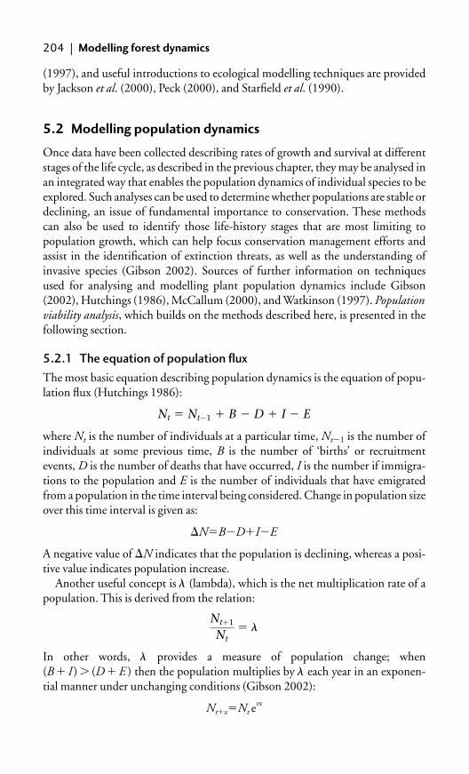
(1997), and useful introductions to ecological modelling techniques are providedby Jackson et al. (2000), Peck (2000), and Starfield et al. (1990).

5.2 Modelling population dynamics

Once data have been collected describing rates of growth and survival at differentstages of the life cycle, as described in the previous chapter, they may be analysed inan integrated way that enables the population dynamics of individual species to beexplored. Such analyses can be used to determine whether populations are stable ordeclining, an issue of fundamental importance to conservation. These methodscan also be used to identify those life-history stages that are most limiting topopulation growth, which can help focus conservation management efforts andassist in the identification of extinction threats, as well as the understanding ofinvasive species (Gibson 2002). Sources of further information on techniquesused for analysing and modelling plant population dynamics include Gibson(2002), Hutchings (1986), McCallum (2000), and Watkinson (1997). Populationviability analysis, which builds on the methods described here, is presented in thefollowing section.

5.2.1 The equation of population flux

The most basic equation describing population dynamics is the equation of popu-lation flux (Hutchings 1986):

where Nt is the number of individuals at a particular time, Nt�1 is the number ofindividuals at some previous time, B is the number of ‘births’ or recruitmentevents, D is the number of deaths that have occurred, I is the number if immigra-tions to the population and E is the number of individuals that have emigratedfrom a population in the time interval being considered. Change in population sizeover this time interval is given as:

A negative value of �N indicates that the population is declining, whereas a posi-tive value indicates population increase.

Another useful concept is � (lambda), which is the net multiplication rate of apopulation. This is derived from the relation:

In other words, � provides a measure of population change; when(B � I ) � (D � E ) then the population multiplies by � each year in an exponen-tial manner under unchanging conditions (Gibson 2002):

Nt�x�Nt erx

Nt�1

Nt� �

�N�B�D�I�E

Nt � Nt�1 � B � D � I � E

204 | Modelling forest dynamics

where x indicates some time interval (in years) after the initial time t, e is the baseof natural logarithms, and r is the intrinsic rate of natural increase of the popula-tion. The latter is related to � by the equation

which can also be written as

In discrete time the value of r can be found from the Euler equation, as follows(Crawley 1997):

where lx is survivorship and mx is fecundity. The value of r can be found numer-ically by using a computer (i.e. an initial value is adjusted until the right-hand sideis equal to 1; Crawley 1997). These equations can be used to develop a simplemodel of population growth from demographic data collected by using the tech-niques described in the previous chapter. However, such a model would be highlysimplistic, failing to consider density-dependence, life-history components such asthe presence of a seed bank, or changing survivorship or mortality over time. Moreelaborate models that consider such issues are presented by Watkinson (1997).

5.2.2 Life tables

A life table can be used to summarize information on mortality risks and repro-duction associated with different categories of plant within a population.Categories can be defined in terms of age, size, or state. Although widely producedfor animals, life tables are rarely produced for plants; most of the examples that areavailable refer to annual plants (Hutchings 1986). Life tables can be presented inthe form of either tables or diagrams; details are provided by Begon and Mortimer(1981) and Ebert (1999). The standard form is the cohort life table in which a groupof organisms born at the same time are followed throughout their life cycle. This isvery difficult to achieve for long-lived plants such as trees. An alternative formderives information from the population at a particular time, and then determinesthe survival over one time period for each age or stage class in the population(McCallum 2000). However, such static life tables do not allow for age-specificchanges in birth and death rates (Gibson 2002).

5.2.3 Transition matrix models

Matrix models provide a relatively simple means of modelling the populationdynamics of individual species. The method has been used with a range of treespecies, and has proved useful for exploring the impacts of different disturbanceintensities, management interventions, or harvesting regimes on population sizeof selected species (and therefore for evaluating the sustainability of different

1��x�0

e�rxlxmx

r�ln(�)

� � er

Modelling population dynamics | 205

harvesting approaches), and for examining the impact of potential threats onextinction risk (Fieberg and Ellner 2001). Matrix models have therefore become astandard method for researching the conservation biology and management ofthreatened plants (Silvertown et al. 1996). The method has been particularlywidely used with palms (Freckleton et al. 2003, Olmsted and Alvarez-Buylla 1995,Pinard 1993); examples of other tree species investigated with this approachinclude Araucaria araucana (Bekessy et al. 2004), Banksia spp. (Drechsler et al.1999), Bertholletia excelsa (Peres et al. 2003), Fagus grandifolia (Batista et al. 1998),Nothofagus fusca (Enright and Ogden 1979), and Vochysia ferruginea (Boucher andMallona 1997).

In this approach, populations are divided into discrete classes based on age or life-history stage, and transitions from one stage to another are used to model survival,growth, and reproduction, enabling population dynamics to be forecast (Caswell1989). Analysis is based on the use of matrix algebra. Matrix models can be used toassess the rate of population increase (�), and through elasticity analysis the effects ofdifferent matrix elements on this parameter can also be evaluated (Caswell 1989).This approach has proved to be a particularly useful tool for examining demographicprocesses in plants, facilitating comparison between species and the development ofgeneralizations regarding their population dynamics (Silvertown and Lovett Doust1993, Silvertown et al. 1996). The following description of the method is based onthat presented by Caswell (1989, 2001), Ebert (1999), and Gibson (2002).

The approach is based on multiplication of a matrix of demographic parameterswith a column vector representing the age or stage structure of a population at aparticular time. The column vector can be represented as follows:

where nt is the age or stage structure of the population at time t, and n1, n2,. . ., ni arethe numbers of individuals in each age/stage class. The matrix of demographicparameters (referred to as the projection matrix) represents the probabilities (ortransitions) of moving from one age/stage to another. There are two main types ofprojection matrix: a Leslie matrix, which is used for models structured by age, and aLefkovitch matrix, which is used for models structure by life-cycle stage or plant size.

The Leslie projection matrix (A) takes the following form:

A � �f1p1

000

f20p2

00

f300p3

0

fn�1

000

pn�1

fn0000�

nt � �n1

n2

n3

n4

�

ni

�

206 | Modelling forest dynamics

where pi is the probability that an individual will survive (values in the range 0 to1), and fi is the rate of reproduction (or fecundity) for an individual in age class i(values of any magnitude). This type of matrix only has non-zero elements in thetop row (indicating the number of offspring produced), and in the subdiagonal(values representing annual survival; pi). The other values are zero because plantscannot remain in the same age from one time step to the next.

The Lefkovitch projection matrix (A) takes the following form:

where si is the probability that an individual will survive and remain in the samestage class (values in the range 0 to 1), gi is the probability that an individual willsurvive and transfer to the next stage class (values in the range 0 to 1), and fi is therate of reproduction (or fecundity) for an individual in stage class i (values of anymagnitude). In this type of matrix, elements in the leading diagonal (si) cannot bezeros, because there is always a possibility that a plant will remain in the same stageof the life cycle the following time step. The elements below the leading diagonalrefer to the probability of growth to the next stage class, and elements above theleading diagonal refer to fecundity, with information presented relating to eachsize class.

The exact form of a Lefkovitch matrix differs between species, depending on thenumber of life-cycle stages that are defined. Multiple stages can be defined forlife-cycle stages such as vegetative reproduction, the seed bank, and either juvenileor mature stages with different reproductive potential. It may be possible for plantsto regress from one stage to another (for example if a tree is felled and subsequentlyresprouts vegetatively). An example of a Lefkovitch matrix for a threatened treespecies is presented in Table 5.1.

To provide an estimate of population in the next time step, the projection matrixis multiplied by the column vector. Repeated iterations can be carried out to deter-mine the age/stage structure in subsequent time steps. The same projection matrix(A) is generally used throughout such calculations, based on the assumption thatdemographic rates do not change over time. Multiplication of matrices can readilybe done using spreadsheet software programs, such as the MMULT worksheetfunction in Microsoft Excel. Some mathematical or modelling software packages(such as Analytica; Lumina Decision Systems, �www.lumina.com�) can also beused to do matrix calculations. Alternatively, dedicated software for modellingpopulation viability can be used (see section 5.3).

If repeated iterations are performed, a point will be reached where the values inthe vector cease to change with further multiplications by the projection matrix.This vector is referred to as the right eigenvector and represents a stable age/sizestructure. At this point, � can be calculated as the dominant eigenvalue of A, which

A � �s1g1

0:0

f2s2g2

:0

f30s3:

…

………

:gn�1

fn00:sn�

Modelling population dynamics | 207

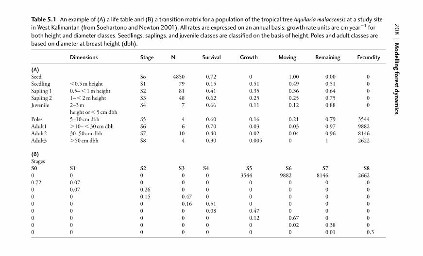
20

8|

Mo

dellin

g fo

rest d

ynam

icsTable 5.1 An example of (A) a life table and (B) a transition matrix for a population of the tropical tree Aquilaria malaccensis at a study site

in West Kalimantan (from Soehartono and Newton 2001). All rates are expressed on an annual basis; growth rate units are cm year�1 for

both height and diameter classes. Seedlings, saplings, and juvenile classes are classified on the basis of height. Poles and adult classes are

based on diameter at breast height (dbh).

Dimensions Stage N Survival Growth Moving Remaining Fecundity

(A)Seed So 4850 0.72 0 1.00 0.00 0Seedling �0.5 m height S1 79 0.15 0.51 0.49 0.51 0Sapling 1 0.5– � 1 m height S2 81 0.41 0.35 0.36 0.64 0Sapling 2 1– � 2 m height S3 48 0.62 0.25 0.25 0.75 0Juvenile 2–3 m S4 7 0.66 0.11 0.12 0.88 0

height or � 5 cm dbhPoles 5–10 cm dbh S5 4 0.60 0.16 0.21 0.79 3544Adult1 �10– � 30 cm dbh S6 6 0.70 0.03 0.03 0.97 9882Adult2 30–50 cm dbh S7 10 0.40 0.02 0.04 0.96 8146Adult3 �50 cm dbh S8 4 0.30 0.005 0 1 2622

(B)StagesS0 S1 S2 S3 S4 S5 S6 S7 S80 0 0 0 0 3544 9882 8146 26620.72 0.07 0 0 0 0 0 0 00 0.07 0.26 0 0 0 0 0 00 0 0.15 0.47 0 0 0 0 00 0 0 0.16 0.51 0 0 0 00 0 0 0 0.08 0.47 0 0 00 0 0 0 0 0.12 0.67 0 00 0 0 0 0 0 0.02 0.38 00 0 0 0 0 0 0 0.01 0.3

Modelling population dynamics | 209

is equivalent to the asymptotic population growth rate (Caswell 1989). Thisparameter is routinely calculated in studies employing transition matrix modellingtechniques, and is often used to evaluate whether harvesting approaches aresustainable or not (indicated by whether � is greater or less than 1, respectively).Other parameters often reported are elasticities, which indicate the sensitivity of�to small changes in matrix elements. These values can be used to assess theimportance of different components of the life cycle to �, and also to fitness (DeKroon et al. 1986). The use of sensitivity analysis to explore the effects of differentmanagement strategies on population size is one of the most important practicalapplications of matrix modelling techniques to conservation. However, it shouldbe noted that values of � may sometimes be misleading as a measure of a popula-tion’s short-term prospects for survival (Bierzychudek 1999).

One of the key decisions to be faced in any matrix modelling exercise is the def-inition of the age or stage categories to be included in the model. Categories maybe defined on the basis of biological criteria, such as size, age, gender, reproductivestate, development, or some combination of these. Alternatively, analyticalmethods are available for defining categories, which maximize within-classsample sizes and minimize error of estimates (Moloney 1986, Vandermeer 1978).However, these analytical methods also have their shortcomings (Caswell 2001)and for this reason many investigators choose categories that subdivide their plantsinto a number of well-represented groups, i.e. small, medium, and large reproduc-tive plants (Gibson 2002). Many studies define categories that seem biologicallyreasonable based on regressions of survivorship and fecundity against size(Brigham and Thomson 2003). For a fixed number of trees for which data are col-lected, the sample size within each category decreases as the number of categoriesincreases. The definition of categories therefore influences model output, and careshould be taken to ensure that the sample size within each category is sufficientlylarge to ensure that estimates of transition probabilities are robust. However, if thecategories are too large, the assumption that individuals falling within the samecategory have the same transition probabilities may be violated (Zuidema 2000).

Complete parameterization of a matrix model requires substantial effort.Ideally, data should be collected for a group of tagged individuals over a period ofyears. Data need to be collected on growth, mortality and fecundity for each of theage/stage categories defined. These data can be collected by the methods describedelsewhere in this chapter (methods for assessing fecundity are described in section6.4.1). The lack of sufficient data (either in terms of number of individualsincluded in the survey, or too few years of data collected) is one of the main short-comings of investigations employing matrix modelling techniques. The fact thatso many tree species are very long-lived presents a particular challenge, as accurateestimates of the very low rates of mortality typical among mature trees can be verydifficult to obtain within the timescales generally available to researchers. As aresult, mature individuals of long-lived tree species may essentially behave as if theyare immortal (Drechsler et al. 1999). Often, in practice, transition values areguessed or a value of 1 is used, which may be unrealistic.

Two other important issues must also be considered when using this technique.First, the demographic parameters incorporated in the projection matrix maychange over time in response to fluctuating environmental conditions. Such sto-chasticity can be incorporated in the model by estimating transition probabilitiesover several years or seasons. Monte Carlo simulations and resampling methodsmay also be used to provide a statistically rigorous method of estimating demo-graphic rates in changing environments (Gibson 2002). Monte Carlo simulationsassume particular statistical distributions (often normal) for vital rates, and themean and variance for � is calculated following several runs of the analysis by draw-ing vital rates from the assumed distribution. Resampling methods do not requiresuch assumptions about the distribution, but resample individuals multiple timeswith replacement (bootstrapping) or random omission of inviduals (jackknifing)to obtain pseudovalues of � (Gibson 2002). Estimates of the mean and variance of� can then be derived from these pseudovalues (Alvarez-Buylla and Slatkin 1991,McPeek and Kalisz 1993). Methods for incorporating stochasticity in matrixmodels are reviewed by Fieberg and Ellner (2001).

A second key issue is density dependence. It is important to include densitydependence because without it, population size in any model will tend rapidlytowards either extinction or infinity, unless the parameters of the model arecarefully adjusted so that net mortality exactly balances net fecundity. Failure toconsider density dependence can lead to relatively high estimates of extinctionrisks (Ginzburg et al. 1990). Although methods are available for incorporatingdensity dependence into matrix models (Caswell 2001, De Kroon et al. 2000),their use is relatively uncommon, reflecting the additional difficulties that thispresents in terms of parameterization. One relatively simple approach is to definea population ceiling, limiting the maximum population size; this is provided asan option in some PVA software such as RAMAS Metapop (see next section).Alternatively, values of survival and growth may be varied in response to variationin density. An example of this approach is provided by Freckleton et al. (2003), intheir investigation of the effects of harvesting of adults on population dynamics ofthe edible palm Euterpe edulis.

Assessing density dependence in field situations can be very challenging.Methods that have been used include analysis of time series data (an approach thatis often criticized on statistical grounds), or experimental manipulation of popula-tion density, involving increasing or decreasing density (for example, by thinninga forest stand) and observing the consequences (see section 3.6.5). He and Duncan(2000) note that the importance of density dependence in tree population dynam-ics is most often inferred from field studies that investigate correlations or regres-sions between a measure of plant performance (such as growth or survival) and thedensity of neighbouring plants. A potential problem with such approaches is thatpatterns resulting from density dependence can be masked by variation in otherenvironmental factors that influence the spatial distribution or performance ofplants. Most field studies have failed to consider variation in such factors, althoughsome have attempted to do so by selecting environmentally homogeneous sites or

210 | Modelling forest dynamics

Modelling population dynamics | 211

by controlling for such variation in statistical analyses. An example of the latterapproach is provided by He and Duncan (2000) in a study of three conifer speciesin British Columbia, Canada. These authors tested for intra- and interspecificdensity-dependent effects on tree survival by analysing both the spatial patterningof trees in a field plot and the relations between neighbourhood density and treesurvival, treating the effects of additional variables (such as elevation) by includingthem as covariates in the neighbourhood analyses. Furthermore, they were able totake advantage of the low decomposition rate of dead stems of these species toreconstruct the spatial patterning of live and dead individuals in the study plot.

Results from previous research indicate that the way in which the matrix modelis constructed and parameterized has a major influence on the results obtained.Zuidema and Zagt (2000) provide a valuable review of the application of matrixmodelling techniques to tree species and, on the basis of previous experience, makethe following recommendations:

● The use of size-dependent relations to parameterize transition matrices yieldsmore reliable model output than observed transition frequencies (Figure 5.1).In the latter case, the transition matrix depends strongly on the distribution ofindividuals among and within categories, especially when sample sizes aresmall. A number of different statistical methods can be used to analyse size-dependent relations in growth (linear regressions, non-linear regression) (see,for example, Zeide 1993) (Figure 5.2), survival (logistic or double-logisticregressions; Gompertz or Weibull distributions) and reproduction (logisticregression and/or linear regression). Data describing demographic rates canalso be pooled between categories, if no significant differences are detected.

● It is important to ensure that the number of adults sampled in demographicfield studies is sufficiently large. Producing accurate assessments of adult

Related to demography Related to methodology

Species life history

• size-dependent growth survival and fecundity• life strategy• total lifespan

• environmental conditions• successional status

Population ‘condition’

• population growth rate• sensitivity, elasticity• age estimates

Model output• number of categories • type of classification• type of parameterisation

Model construction

• data availability• coping with data gaps

Model parameterization

Fig. 5.1 Schematic diagram of factors influencing the output of size-structured

population matrix models. Factors are grouped into four categories: the life history

of the species, the environmental conditions experienced by the study

population, factors related to the construction of the model, and those related to

the parameterization of the model. Each of the four categories may influence the

model output. (From Zuidema 2000.)

survival rates is one of the most significant challenges when modellingpopulation dynamics of trees, and one of the main weaknesses of previousstudies. Model outputs are particularly sensitive to adult survival, and there-fore intense sampling, potentially over long periods of time, may be required.The population viability of many tree species appears to depend particularlystrongly on the presence of long-lived individuals (Bond 1998, Kwit et al.2004), further emphasizing the importance of evaluating the survival of suchindividuals.

● Care should be taken when using uncertain estimates or substituting missingvalues. The values of neighbouring categories can often be adopted. Theimpact of uncertain values on model output can be explored by varying thevalues and observing the outcome.

● It is often useful to pool demographic information from different sites orobservation periods, when no statistically significant differences are foundbetween such data sets. Differences in vital rates (survivorship and fecundity)can be determined by using standard statistical tests such as the t-test or thechi-squared test. When no significant differences are found, data from variousyears or populations can be pooled to produce a more reliable matrix model.

● Estimates of elasticities for vital rates provide a useful tool for demographicanalysis, being relatively insensitive to matrix dimension, and providing a moredirect indication of the dependency of � on changes in measured parameters.

● It is important not to base conclusions (about the sustainability of harvestingregimes, for example) solely on the value of �. As � indicates the populationgrowth rate when time goes to infinity (assuming conditions remain

212 | Modelling forest dynamics

2.0(a) El Tigre

(b) El Sena

1.5

1.0

0.5

0.0

2.5

2.0

1.5

1.0

0.5

0.00 25 50 100 200150

dbh (cm)

db

h g

row

th (

cm y

r–1)

125 17575

Fig. 5.2 Size-dependent pattern in dbh growth in Bertholletia excelsa in two sites

in the Bolivian Amazon; El Tigre (a) and El Sena (b). Shown are fitted Hossfeld IV

equations (lines), observed average (1 SD) growth rate (open dots), and

observed maximum growth rate (closed dots). (From Zuidema 2000 and Zuidema

and Boot 2002, in Journal of Tropical Ecology.)

Population viability analysis | 213

unchanged), this may not always be the most appropriate parameter to assesspopulation status with respect to population management. Estimates of � arealso often prone to a high degree of error.

Further advice regarding transition matrix modelling is provided in the followingsection.

5.3 Population viability analysis

Population viability analysis (PVA) is an important tool in conservation researchand management that focuses on assessing the likelihood of population persistenceover a given timespan (Brigham and Schwartz 2003, Menges 2000). PVA has beenwidely used to assess trends in population size, the risk of extinction, and thepotential impacts of different management interventions on population viability,and has become a central component of many management and recovery plans forthreatened plant species (Caswell 2000, Fieberg and Ellner 2001, Lindenmayeret al. 1995, Menges 1990, 2000, Silvertown et al. 1996). A useful overview ofPVA is provided by Akçakaya and Sjögren-Gulve (2000) (Boxes 5.1 and 5.2), andBrigham and Schwartz (2003) provide an excellent recent source text for PVAspecifically relating to plants.

In recent years there has been some debate about the usefulness and reliability ofPVA (Brook et al. 2000, Coulson et al. 2001, Ellner et al. 2002). For example,

Box 5.1 Uses of PVA.

Akçakaya and Sjögren-Gulve (2000) provide a valuable overview of PVA, andhighlight the fact that PVA can be used to address the following aspects of man-agement for threatened species or other focal species:

● Planning research and data collection. PVA may reveal that population viabil-ity is especially sensitive to particular parameters, enabling research prioritiesto be identified, for example by targeting factors that have an importanteffect on probabilities of extinction or recovery.

● Assessing vulnerability. PVA may be used to estimate the relative vulnerabil-ity of populations to extinction. These results may be used to identify prior-ities for conservation action.

● Impact assessment. PVA may be used to assess the impact of human activities(such as timber harvesting or deforestation) by comparing results of modelswith and without the human activity.

● Ranking management options. PVA may be used to predict the likelyresponses of species to management interventions such as harvesting,reintroduction or habitat rehabilitation, or different designs for protectedarea networks.

Ludwig (1999) highlighted three potential limitations of PVA: the lack of preci-sion regarding estimates of extinction probability, the sensitivity of such estimatesto model assumptions, and the lack of attention to important factors influencingthe extinction of populations. These findings were supported by further analysesbased on diffusion approximations, indicating that reliable predictions of extinc-tion probabilities can only be made for very short-term time horizons (Fieberg andEllner 2000). In contrast, Brook et al. (2000) reported a high degree of correspond-ence between PVA predictions and field data from 21 long-term ecological studies,in the first such replicated evaluation of PVA. These conclusions were criticized byEllner et al. (2002), who highlighted the lack of measures of statistical precisionand power in this analysis (but see Brook et al. 2002 for a response). Despite theshortcomings of PVA, the method is described by Brook et al. (2002) as ‘by far thebest conservation management tool that we have’. Following a thorough review ofthe application of PVA specifically to plant species, Brigham and Schwartz (2003)concluded that PVA has been demonstrated to be most useful for assessing therelative extinction risks of different populations and the potential impacts ofdifferent management options, particularly for species with complex interactionsbetween the factors influencing population dynamics.

Transition matrix models are most often used as the basis of PVA of plants (seeprevious section). Brigham and Thomson (2003) provide a valuable overview ofPVA methods using this approach. A number of specialist software programs havebeen developed for PVA (Table 5.2), which incorporate a number of powerfulfeatures, such as the ability to explore the influence of stochasticity and densitydependence, as well as different management regimes, on population viability.These programs differ in their approach; for example, VORTEX tracks the life ofeach individual in the population, whereas the RAMAS packages are matrix-basedprograms that track the number of individuals. The manuals and tutorials

214 | Modelling forest dynamics

Box 5.2 Approaches to PVA.

The following should be considered when developing a PVA (from Akçakaya andSjögren-Gulve 2000):

● Model structure should be detailed enough to use all the relevant data, but nomore detailed than this.

● Model results should address the question being addressed.● The model should include parameters related directly to the question (for

example, if the question involves the effect of timber harvest on populationviability, then the model should include parameters that reflect such an effectrealistically).

● Model assumptions should be realistic with respect to the ecology of thespecies and the observed spatial structure (for example, if there is populationsubdivision, a metapopulation model should be considered).

Population viability analysis | 215

available with these programs are another valuable source of guidance. Cautionshould always be exercised when using these tools, however. For example, Millset al. (1999) demonstrated that different results can be obtained with the same dataset by using different software programs (although Brook et al. (2002) reported ahigh degree of correspondence in results obtained for a range of species with dif-ferent programs). An alternative approach to using an off-the-shelf software pack-age is to develop a customized program written for a particular species (Frankhamet al. 2002). A valuable online resource is available at �www.ramas.com/�, designedto help avoid mistakes when population modelling (Box 5.3). Methods for testingthe accuracy of PVA are reviewed by McCarthy et al. (2001). An example of a PVAdeveloped for a threatened tree species is given in Box 5.4.

One of the main ways in which PVA programs differ from each other relates tohow they model density dependence. This can have a major influence on modeloutput. As noted in the previous section, density dependence can be difficult toevaluate under field conditions, and this lack of field data is one of the most import-ant shortcomings of many PVA studies. The different methods that have been usedto incorporate density dependence in PVA models are reviewed by Henle et al.(2004), who suggest that spatially explicit models hold particular promise foranalysing the effects of density dependence on population viability. However, suchapproaches are labour-intensive and require a thorough knowledge of the biologyof the species under consideration.

Increasingly, spatially structured models are being used for PVA. For example,matrices can be constructed for different populations and linked by using a

Table 5.2 Selected specialist software programs available for population viability

analysis (PVA).

Product Reference Website

ALEX Possingham and www.rsbs.anu.edu.au/ResearchGroups/ Davies (1995) EDG/Products/Alex/index.asp

META-X Frank et al. (2003), www.ufz.de/oesa/meta-xGrimm et al. (2004)

RAMAS Metapop Akçakaya and www.ramas.com/and RAMAS GIS Root (2002)

VORTEX Lacy (1993) www.vortex9.org/vortex.html

VORTEX is probably the most widely used of these. It should be noted that all of these programs were devel-oped primarily for animals, and have been relatively little used with plants. Whereas ALEX and VORTEXcan be downloaded free of charge, META-X is provided with a book (Frank et al. 2003) and the variousRAMAS programs are available as commercial products. In a rare comparative study, Brook et al. (2000)obtained similar results from different software programs, although other authors (e.g. Lindenmayer et al.1995) have reported contrasting results from different programs. As noted by Lindenmayer et al. (1995), thechoice of which program to use will depend on a range of criteria, including the objectives of the study, andthe strengths, limitations, and assumptions that underpin the program and how these match the attributes,life-history parameters and available data for the target species.

216 | Modelling forest dynamics

Box 5.3 Avoiding mistakes when population modelling.

A very useful online information resource is provided by H. Resit Akçakaya, oneof the designers of the RAMAS Metapop software, at the RAMAS website�www.ramas.com/mistakes.htm�. The resource is designed to help identify andavoid common mistakes when modelling population viability. The list of poten-tial mistakes includes the following:

● invalid model assumptions● model too complex; or conversely model too simple● internal inconsistency in the model● bias in estimation of fecundity or survival, and uncertainty in estimates of

these parameters● too many (or too few) age classes or stages● using the wrong type of density dependence, or failing to consider density

dependence● over- or underestimating maximum growth rate of the population● not considering demographic stochasticity● duration (simulation time horizon) too long or too short● ignoring spatial structure● considering too many (or too few) populations● dispersal rates incorrect or uncertain● estimating risk of extinction rather than decline.

Box 5.4 An example of a population viability model developed for a

threatened tree species: the case of Araucaria araucana.

Araucaria araucana (monkey puzzle, pehuén) is a large and long-lived conifer,endemic to the southern Andes and a restricted area of the coastal region of south-ern Chile (Figure 5.3). The historical range of the species has been much reducedas a result of logging, human-set fires, and clearance of land for agriculture fol-lowing European colonization of the region. The species is of exceptional evolu-tionary as well as conservation interest, with similar fossils known from 200 Maago. The species is listed in Appendix I of CITES.

Bekessy et al. (2004) describe a PVA developed for this species by usingRAMAS Metapop software, based on extensive field observations and glasshouseexperiments. Development of the model presented a number of significant chal-lenges. First, adult trees can be very long-lived (�1000 years), and growth ratesare often very low (�1 mm radial increment per year). This made it difficult tocreate a model that is meaningful in terms of the typical timescales used in con-servation management. Second, modelling density dependence was difficult toincorporate, although field observations suggested that self-thinning is commonin pole-stage stands. Third, the species occurs in different forest associations and

Population viability analysis | 217

displays different ecological characteristics in each. This may be related to thehigh degree of genetic differentiation recorded between populations and thebroad edaphic range of the species, spanning a rainfall gradient (Bekessy et al.2002a).

A model was constructed with 50 stages, including seeds, seedlings, saplings,juveniles, adults, and dominants (Figure 5.4). These were considered to reflect

S1–2,d1, v1

S3, d2,v2

f4–8

f1–3

S4, d3,v3

S5, d4,v4

S5, d5,v5

Sapling(stages i =9–15 and37–43)

Adult(stages i =21–23 and 49)

Dominant(stages i =24–28 and 50)

Juvenile(stages i =16–20 and44–48)

Seedling(stages i =2–8 and30–36)

Seed(stage i =1)

g

Fig. 5.4 Life cycle of Araucaria araucana and its population parameters:

g, germination rate; s, survival; d, fire survival; v, survival following volcanic

activity; t, transition; f, fecundity. (From Bekessy et al. 2004.)

Fig. 5.3 Wild population of Araucaria araucana in the southern Andes. Many

populations of this species are located on active volcanoes. (Photo by

Cristian Echeverría.)

218 | Modelling forest dynamics

important biological stages in the life history of the species, with distinct growthrates, survivorship, fecundity, and sensitivity to disturbance. It was necessary toinclude many stages in the model to delay transitions, which otherwise wouldhave led to unrealistic times for individuals to move through the various stages.Because of their extreme longevity, adult and dominant stages were assumed tobe immortal. The model included both environmental and demographicstochasticity.

Simulations examined the impact of fire, volcanic activity, seed harvest, andtimber harvest on population viability (Figure 5.5). Results indicated that thespecies has very limited ability to recover after disturbance, although seedharvesting appeared to be having relatively little effect on population viabilitycompared with the other forms of disturbance assessed. Most importantly, theviability of the entire species appeared to be particularly sensitive to the fate of anindividual population, which is located in an area of active volcanism.

Fig. 5.5 A set of extinction risk curves for Araucaria araucana, derived from a

meta-population model run for 100 years. (From Bekessy et al. 2004.)

1.2

1

0.8

0.6

Pro

bab

ility

of

qua

si-e

xtin

ctio

n

0.4

0.2

00

500 000

1 000 0

00

1 500 0

00

2 000 0

00

2 500 0

00

3 000 0

00

3 500 0

00

4 000 0

00

Base model Worst case Volcanic eruptions

Pop408 volcanic High seed harvest Low vital rates

dispersal function to produce a form of metapopulation model (for exampleRAMAS Metapop; see Table 5.2). Other approaches to modelling metapopula-tions predict the occupancy of discrete habitat patches through time by using avariety of analytical methods, such as the incidence function model and logisticregression models (for details see Hanski 1994, 1999; Sjögren-Gulve and Hanski2000). A range of software tools to help perform such analyses can be freely down-loaded from the University of Helsinki website; an example is SPOMSIM 1.0,which is a stochastic patch occupancy model �www.helsinki.fi/science/metapop/english/Software.htm�.

Growth and yield models | 219

The recent development of metapopulation theory, by Ilkka Hanski and others,undoubtedly represents one of the most important theoretical contributions toconservation science, and is beginning to have a significant influence on conserva-tion policy and management practice. However, the relevance of the theory topractical conservation problems is open to debate (see, for example, Baguette2004, and Hanski 2004 for a response). The application of metapopulation models to plants has been the subject of particular controversy; it has been arguedthat single population approaches rather than metapopulation approaches may beappropriate for most plant species (Harrison and Ray 2002).

Other spatially explicit modelling approaches examine the locations and dens-ities of individuals across a landscape (see section 5.5.3), rather than the occupancy

Box 5.5 An example score sheet for a relative population viability

assessment (RPVA).

This qualitative approach, based on expert judgement, may be used to provide apreliminary assessment of the vulnerability of species to extinction, where moreformal quantitative information is lacking. Assessors evaluate each criterion foreach species and score them from no degradation (0 points) to degradationsufficient to render the population inviable (20 points). These points are thensummed to provide an assessment of relative risk of extinction for differentspecies (after Schwartz 2003). The scoring system illustrated in Table 5.3 couldpotentially be adapted or further elaborated for any particular group of treespecies under consideration.

Table 5.3 Criteria and point-scoring system.

Criteria Examples Score

Habitat loss Multiple protected populations 0 pointsFew protected populations 5 pointsModerate loss, little protected habitat 10 pointsSevere loss, no protected habitat 15 pointsNearly complete habitat loss 20 points

Disturbance regime Natural disturbance regime maintained 0 pointsdisruption Severe disruption of disturbance regime 20 points

(e.g. fire suppression with obvious indicationof community change)

Habitat degradation Habitat intact 0 pointsSevere habitat degradation 20 points(e.g. invasive weed colonizing habitat)

Population Apparently normal 0 pointsperformance Poor performance 20 points

(e.g. disease killing all seedlings)

of habitat patches. One of the main problems with spatial modelling approaches isthat they require estimates of dispersal distances and probabilities that can be dif-ficult to acquire (see section 6.4.2), yet are of critical importance to the predictionsof the model. However, the incorporation of spatial pattern into populationmodels can undoubtedly provide valuable insights into the processes influencingforest dynamics (Wiegand et al. 2003).

Although the vast majority of PVAs performed with plant species haveemployed stage- or age-structured models, there are alternative approaches.Schwartz (2003) notes that community-level models of forest dynamics (seesection 5.5.1) could be used to assess population viability of tree species, but thishas apparently not an approach that has been used to date. Analysis of populationage or size structure (see section 3.7.1) can be used to identify recruitment failure,which may indicate that the population is not viable (although it should be notedthat many tree species are naturally characterized by episodic recruitment)(Schwartz 2003). Another approach uses a time series of population counts toestimate the mean and variance of the stochastic population growth rate, whichcan then be used to predict extinction probabilities and time to extinction(Brigham and Thomson 2003). The method requires far fewer data than struc-tured approaches to PVA, and is analytically relatively simple. However, observa-tions made over a large number of years (perhaps at least 10) may be required toestimate extinction probabilities accurately. Although the technique has rarelybeen applied to plants, it clearly has potential (Elderd et al. 2003). Alternatively,relative extinction vulnerability can be qualitatively assessed (Box 5.5) bysurveying expert opinion (Schwartz 2003).

5.4 Growth and yield models

Mathematical approaches to predicting growth and yield of timber trees have along tradition in forestry, and are widely used as a tool for forest management.A very large number of simulation models have now been developed for forests inmany parts of the world (see, for example, Vanclay 1995). Most yield models sharethe same basic approach, aiming to predict timber yield over time for a specific site.Models are generally species-specific and aim to explore the relation between standdensity and tree growth, measured in terms of both stem diameter (dbh) and treeheight. In some models, growth is also related to measures of crown size. Growthand yield models are generally produced by empirically deriving equations thatdescribe relations between these growth variables by using standard statisticalprocedures such as regression.

Typically, regressions are carried out on multiple measurements of individualtrees, although growth–yield models differ with respect to the regression functionsused and the variables included. Analyses are generally performed on forest inven-tory data, perhaps employing measurements of forest stands growing on differentsites that have been subjected to different silvicultural treatments or management

220 | Modelling forest dynamics

Ecological models | 221

regimes (Vanclay et al. 1995). The data are usually derived from individual treesthat have been marked within permanent sample plots. These data may be used toproduce yield tables, which give estimates of the changes in stand variables (such asheight, basal area, and volume) with age. In general, models are produce for a rangeof different yield classes, reflecting the variation in growth rate on sites with differ-ent environmental characteristics. Often, a large number of plots (hundreds oreven thousands) are used as a source of data. Details of the methods are providedby Munro (1974) and Ek et al. (1988); uneven-aged stands are considered by Peng(2000). Some examples are provided by Amaro et al. (2003) and Vanclay (1994).

Burkhart (2003) provides some suggestions for using this approach, including:

● Keep the model as simple as possible● Ensure that the model is as accurate as possible, or by increasing the size of the

data set, improving the quality of the data obtained● When planning data collection, include a wide range of site and stand

conditions in the sample

The main value of forest yield models is their ability to make detailed predictionsof tree and stand dynamics, particularly stem-size distribution predictions thataggregate accurately to the stand level (Monserud 2003). In addition, tree mortal-ity is often modelled in some detail, incorporating both competitive interactionsbetween individual trees and stand-level responses such as the �3/2 power law(section 3.7.5). The main disadvantage of this type of forest model is that it doesnot explicitly consider the underlying ecological processes responsible for variationin growth and yield, such as uptake of moisture and mineral nutrients and theprocess of carbon fixation. These models therefore have limited value for under-standing how forest ecosystems function. Most growth–yield models are designedfor a certain forest type or region and the range of species considered is usuallyrestricted to a few that are commercially important. As ecological processes are notincorporated in the models, they are restricted to the range of environmentalconditions under which the data were originally collected, and have limited valuefor predicting how a forest might respond to changing environmental conditions.They therefore have limited applicability to forest conservation. However, theyoffer a useful technique for assessing forest biomass, which is important forconsideration of environmental services such as carbon sequestration and nutrientcycling.

5.5 Ecological models

The term ecological models is used here to refer to all forest dynamics modelsoriginating from an ecological perspective or simulating ecological processes orcharacteristics of forests (following Hope 2003). These may be classified in avariety of different ways; see, for example, Liu and Ashton (1995), Porte andBartelink (2002), and Shugart (1998). Here, following Hope (2003), two maintypes of ecological model are differentiated.

● Process models focus on modelling physiological processes such as photosyn-thesis and respiration (Vanclay 1994). Process models generally do not depictchanges in species composition or stand structure, and therefore have rela-tively little relevance to forest conservation or ecological dynamics. However,some models of this type are of value for exploring the provision of ecologicalservices.

● The other main group of models may be described as succession models (Hope2003), as they focus on simulating the ecological dynamics of forest commu-nities; it is these models that are considered below. This type of model may befurther subdivided into gap and transition models (Figure 5.6).

5.5.1 Gap models

Forest ecologists have devoted substantial efforts to the development of modelsthat simulate the process of forest succession that follows the creation of a canopygap. During the past 30 years, a large number of such models have been developed,all of which are linked to the first such model, JABOWA (Botkin et al. 1972a, b),and its direct descendent FORET (Shugart and West 1977). Gap models simulatethe establishment, growth and mortality of each individual tree within a specifiedarea (often about 0.1 ha, or the size of a typical canopy gap). Typical model outputsinclude species composition, age structure, size distribution of trees and verticalstratification. Gap models have also been applied to other components of forestcommunities, such as the ground vegetation (Kellomäki and Väisänen 1991).

It is useful to differentiate between deterministic models, for which the predictedvalues may be computed exactly, and stochastic models, for which the predictedvalues depend on probability distributions. Many gap models are composed of amixture of deterministic and stochastic sub-models; they are generally described asstochastic if they contain any stochastic elements (see, for example, Liu and Ashton

222 | Modelling forest dynamics

Forest models

Transition

Forest landscape dynamics models

Gap

Individual Stand

Process

Growth-yield Ecological

Succession

Fig. 5.6 A simple hierarchical classification of forest dynamics models. (From

Hope 2003). Whereas growth–yield models have primarily been developed by

foresters for estimating timber yield, those developed by ecologists tend to

focus on forest succession.

Ecological models | 223

1998, He and Mladenoff 1999). Use of stochastic models raises the need to deter-mine the appropriate probability distributions of the stochastic elements, and themodels may need to be run multiple times in order to yield meaningful results(Hope 2003).

Gap models generally have six components (Hope 2003):

● site variables (including gap size, soil fertility, soil moisture, accumulatedtemperature)

● species variables (such as maximum age, maximum diameter, maximumheight, growth rate, shade tolerance, tolerance of low nitrogen availability,tolerance of extreme wet and drought conditions, etc.)

● growth sub-model (deterministic, in which growth of individual trees is oftenexpressed in terms of dbh, height, leaf area, and stem volume)

● resource sub-model (deterministic, in which trees interact with each other byinfluencing the gap neighbourhood)

● recruitment sub-model (stochastic; often the individuals that colonize a gap aredefined by selecting of individuals from the species list at random)

● mortality sub-model (stochastic, often modelled as a function of age andgrowth environment, although harvesting regimes may be included as a causeof mortality).

Gap models calculate annual change within the specific area by calculating thegrowth increment of each tree, the addition of new young trees (both from seedsand by sprouting) and mortality (Shugart 1984). Growth increment is describedby equations that relate growth to current diameter and the maximum diameterobserved for the species, based on the assumption that tree growth is directlyproportional to the abundance of leaves and inversely proportional to the amountof respiring, non-photosynthetic tissue (Hinckley et al. 1996). The variables leafarea, tree height, and species maximum height are defined in the basic diametergrowth equation as a function of current stem diameter. Species-specific regener-ation within the gap is generally defined as a function of light reaching the forestfloor. Interactions between individual trees are described by relatively simple rules,mostly relating to competition for resources, especially light.

Different gap models have been developed for forests with different characteris-tics, and vary with respect to how many species are considered, and how differentforest structures are treated. Some models consider the explicit location of eachindividual tree whereas others do not (referred to as spatial or non-spatial models,respectively). Whereas the processes of recruitment, growth, competition, andmortality are considered by all gap models, the relative emphasis on these differentprocesses varies between models. Parameterization of gap models is often achievedby referring to published information on the characteristics of the tree species ofinterest, for example their establishment requirements, growth rates, andheight–diameter relations. If these data are not available from previous work, thenthey will need to be collected via an appropriate field survey. Data describingenvironmental conditions (for example soil moisture, light, temperature, frost,

elevation, elevation, aspects, altitude, nutrients) should be collected for the sites tobe modelled (Shugart 1984).

It is important to note that the aim of gap models, to explore and test ecologicaltheory, is very different from the objective of the growth and yield modelsdescribed in the previous section. These two modelling approaches have largelydeveloped in isolation from each other. Liu and Ashton (1995) comparegrowth–yield and gap models, and highlight the following differences:

● Although the two types of model share some similar features, they differ inmodel structure and data requirements.

● Growth–yield models tend to be used by foresters to assist timber productionand evaluate growth and yield of timber species in managed forests, whereasgap models are generally used by ecologists to explore ecological processes anddynamics in natural forest ecosystems.

● Site-specific environmental and species information is necessary for con-structing growth–yield models, whereas gap models require species-specificbiological information on individual trees and site-specific environmentaldata.

● Growth–yield models are more diverse in terms of model structure, whereasmost gap models are derived from the original antecedent (JABOWA),although they differ in detail.

One of the attributes of gap models is that gap size strongly influences the predictedpopulation dynamics (Shugart 1984). In contrast, forest yield models are generallyunaffected by a change in plot size (Monserud 2003). Typically, gap models are notdesigned to make direct use of forest inventory data, and do not provide estimatesof timber yield required by foresters. However, some researchers have sought toachieve greater realism by incorporating physiological processes within the models(Friend et al. 1993), as in the case of HYBRID (Friend et al. 1997).

Gap models have recently been criticized by a number of researchers. For exam-ple, Lindner et al. (1997) compared output of a second-generation gap model,FORSKA, with long-term data from Bavaria, and found a poor correspondencewith individual tree dimensions and stand structures. Changing stand density overtime influenced the height–diameter relations of trees and rates of mortality, andthese were found to be inadequately represented in the model. Yaussy (2000)similarly found that projections made by using the gap model ZELIG failed toproduce accurate estimates of biomass or volume, when compared with 30 years’inventory data from Kentucky. These experiences highlight the importance ofcarefully calibrating the underlying growth model if this type of modellingapproach is to be used for guiding management decisions.

Despite these problems, gap models continue to be the focus of active research,and new versions continue to be developed. Details of some of the modelscurrently used are listed in Table 5.4. It is notable that few attempts have beenmade to model dynamics of relatively species-rich forests, such as lowland tropicalforests. Also, although gap models have undoubtedly proved to be of value for

224 | Modelling forest dynamics

Eco

logica

l mo

dels

|2

25

Table 5.4 Selected models used for exploration of forest dynamics.

Name Comments Reference URL

JABOWA The ancestor of most forest gap models Botkin et al. (1972a, b); Botkin (1993) www.naturestudy.org/services/jabowa.htm

FORET An early descendent of JABOWA Shugart (1984); Shugart and West (1977)

SORTIE Individually based and spatially explicit Pacala et al. (1993, 1996), Canham et al. www.sortie-nd.org/SORTIE-ND model developed for mixed temperate (1994a)

forests

LANDIS Uses an object-oriented modelling He and Mladenoff (1999), Mladenoff www.snr.missouri.edu/LANDIS/landisLANDIS II approach operating on raster GIS maps, and He (1999), Mladenoff (2004) Also available commercially from

enabling modelling of forest dynamics Applied Biomathematics at the landscape scale (�www.ramas.com�)

ZELIG Based on FORET, but unlike earlier Urban (1990), Urban et al. (1991)gap models, incorporated spatial interactions

MOSAIC A semi-Markov derivative of the Acevedo et al. (1995) http://emod.unt.edu/ZELIG gap model

FORMIX Simulates the dynamics of tropical Huth et al. (1998), Huth and DitzerFORMINd rainforests based on a few plant (2000), Köhler and Huth (1998)

functional types, but with a relatively detailed treatment of physiological processes

exploring hypotheses about forest dynamics, they have rarely been used to addressforest conservation issues directly. On the other hand, as noted by Bugmann(2001) in his review of forest gap models, no alternative approach offers such anintuitive and elegant means of exploring the effects of competitive interactions ontree population dynamics. He also notes that gap models have evolved consider-ably from the original versions and contain far greater detail than is sometimesrecognized; there is currently a wide variety of approaches that are being used toincorporate the various ecological processes relevant to tree population dynamics.A further advantage of gap models is that the output gives detailed representationsof species composition and physical structure, which could potentially be used todevelop models of habitat attributes (Hope 2003) (see Chapter 7).

5.5.2 Transition models

Other modelling approaches that can be used to explore forest dynamics at thelandscape scale include Markov and semi-Markov models. These are constructedby determining the probability that the vegetation in a specific area will havedeveloped or been converted into some other vegetation type within a given timeinterval. The probabilities for this change or conversion are referred to as transitionprobabilities. The vegetation must therefore be classified into identifiable cat-egories in order to apply this approach. Markov models have two importantcharacteristics (Shugart 1998):

● The transition probabilities at time tn depend only on the immediate pastvalue at time tn–1 and are independent of the state of the system at any timeearlier than tn–1. Sometimes this condition is referred to as a first-orderMarkov process.

● The system is stable if the transition processes do not change over time.

Vegetation categories may be defined in a number of different ways, in terms ofspecies of canopy tree present (Horn 1975), the most abundant species of tree inthe forest canopy, or the number of individuals of different species present.Analysis of Markov models is very similar to the transition matrix modelsdescribed earlier (section 5.2.3), depending upon the multiplication of the transi-tion probabilities by a vector representing the proportions of each vegetationcategory present within an area at a particular time. Markov modelling can there-fore be carried out with any appropriate software that supports matrix algebra(see section 5.2.3). Model outputs describe the projected composition of thevegetation, in terms of the proportional cover of different vegetation categories, atdifferent times into the future.

Markov models have the attraction of being analytically relatively simple andeasy to interpret. The main challenge in using them relates to deriving accurate tran-sition probabilities. These can be obtained either by monitoring vegetation overprolonged periods in permanent sample plots (see section 4.7.1), or by using remotesensing imagery to identify vegetation changes that have occurred in the past (seeChapter 2). The probability of transition from any vegetation category to any other

226 | Modelling forest dynamics

Ecological models | 227

category (or state) must be determined; as a consequence, the number of modelparameters is a function of the square of the number of categories in the model(Shugart 1998). There is therefore a trade-off between the increased resolutionoffered by incorporating a larger number of vegetation categories (or states), and theincreased difficulty of accurately parameterizing a model with a larger numberof transition probabilities. This is particularly problematic given that relativelyrare transitions need to be estimated with equivalent precision to relatively commontransitions (Shugart 1998). One potential way round this problem is to estimatemodel parameters on the basis of some theory (Horn 1975). However, Markovmodels tend to be highly specific to the forest type (and even the particular studyarea) for which they were created, limiting their practical value (Hope 2003).

Examples of applying Markov models to forest dynamics are provided by Horn(1975, 1976) and Waggoner and Stephens (1970). One of the main drawbacks ofthis type of model is that the transition probabilities remain the same through time(Moore and Noble 1990). As an alternative, semi-Markov models have been devel-oped (Acevedo et al. 1996a,b) in which the transition probabilities are not fixedbut instead vary depending on the time that the vegetation unit entered the currentstate. Transitions representing successional change are considered to have holdingtimes associated with them, whereby the transition cannot occur until the vegeta-tion unit has occupied a successional stage for a fixed time period (Hope 2003).Various hybrid approaches have also been developed. For example, Acevedo et al.(1995) linked a semi-Markov model to output from the gap model ZELIG,enabling the behaviour of the gap model to be explored at a much larger spatialscale than would have been possible with the gap model alone. This semi-Markovapproach can be used to assess forest dynamics at the landscape level by making theparameters (probabilities and holding times) depend on environmental variablessuch as elevation, slope, aspect, and soils, and visualizing the output in GIS(Acevedo et al. 1995, 1996a).

Another related approach is the use of cellular automata, in which the area ofinterest is divided into cells, the states of which are defined by rules regarding thestates of neighbouring cells. Interactions between cells are more likely to occurbetween close neighbours than cells far apart, and can relate to spatial processessuch as dispersal or the spread of fire, enabling vegetation change to be modelled atthe landscape scale. Cells are considered to be identical or of a relatively smallnumber of types, so that even though the number of cells is large the number ofparameters needed may be relatively low. Analysis is done by multiplying each cellby the probabilities of plants going from one state to another, for example by usinga transition matrix. The results of the multiplications, however, are weighted bya set of constraints, reflecting interactions with neighbours (Gibson 2002).Environmental constraints and disturbances can be included; for example,Hochberg et al. (1994) included the constraint that tree seedlings were susceptibleto fire-induced mortality following burning, if not surrounded by and protectedby a certain number of adult trees. Cellular automata are particularly useful formaking qualitative predictions regarding spatial pattern formation and have been

applied to the study of tropical rain forests (Alonso and Sole 2000), as well as forsimulating the long-term population dynamics of threatened tree species, such asFitzroya cupressoides (Cannas et al. 1999). A review of the use of cellular automatonmodels in ecology is provided by Balzter et al. (1998), and further guidance isprovided by Durrett and Levin (1994).

5.5.3 Other modelling approaches

Attempts have been made to address the limitations of traditional gap modelsthrough the development of alternative approaches. SORTIE is an empirically basedmodel of forest dynamics, developed for mixed temperate forests, that realisticallysimulates the spatial interactions between individual trees (Pacala et al. 1996). SOR-TIE tracks the exact location of each tree and determines its performance based on itslocal neighbourhood. The model incorporates a sophisticated means of calculatingthe transmission of light through the forest canopy, and simulates the responses ofindividual trees to the light conditions occurring locally. Another key feature of thismodel is the much larger areas of land that can be considered compared with con-ventional gap models. SORTIE is a powerful model that has been used successfullyto investigate forest dynamics over a variety of scales. The main obstacle to usingSORTIE is the substantial amount of field data required to parameterize it. It is alsodemanding in terms of processing power (Bugmann 2001).

Kohyama (1993) and Kohyama and Shigesada (1995) describe a fundamentallydifferent approach to modelling forest dynamics, based on the use of partial differ-ential equations to approximate the shifting-patch mosaic of forest landscapesaccording to the age distribution of patches with different tree-size structures. Thecreation of a treefall gap corresponds with the ‘death’ of a patch of particular age,resetting patch age to zero. Tree size structure is developed in relation to patch age,and the demography of trees in each patch is regulated by patch-scale tree-sizestructure (Kohyama 2005). This approach has recently been extended to largerspatial scales and longer timescales (Kohyama 2005).

As noted earlier, process-based models that simulate physiological processesunder changing environmental conditions offer another approach to forestmodelling (Landsberg and Gower 1997). Although not considered in detail here,increasingly such models are being used to address questions relating to forestmanagement. An example is provided by FORMIX and its successor FORMIND,which includes more information relating to forest dynamics. The latter has beenused to analyse the growth and yield of logged-over forest in Venezuela underdifferent logging scenarios (Kammesheidt et al. 2001).

One of the main developments in recent years is the growth in interest in mod-elling forest dynamics at the landscape scale. Hope (2003) uses the term forestlandscape dynamics model (FLDM) to refer to a spatially explicit forest dynamicsmodel acting at landscape scales (see Figure 5.6). This approach to modelling hasbeen greatly supported by recent developments in GIS technologies (see section2.6), which now enable GIS to be linked to models of forest dynamics, either forpreprocessing data for use in a non-spatial modelling, or for displaying model

228 | Modelling forest dynamics

Ecological models | 229

output. Closer linkages between the model and GIS can be achieved if they sharethe same data structures. Some models are now implemented entirely within a GISenvironment, sometimes using custom-designed GIS modelling packages such asPCRASTER (Wesseling et al. 1996). Examples of models that have been devel-oped specifically to operate at landscape scales are provided by Frelich et al. (1998),Frelich and Lorimer (1991), and Liu and Ashton (1998).

An example of this approach is provided by the model LANDIS (Figure 5.7),which is based on an object-oriented modelling approach operating on raster GISmaps (He et al. 1999, Mladenoff and He 1999). The principal modules of LANDISrelate to forest succession, seed dispersal, wind disturbance, fire, and timber

Establishmentprobability(and type) Shade tolerance

Seed dispersalprobability

Windthrowprobability

Fireprobability

Stand ageSpecies and age classsusceptibility(bottom up)

Species size classsusceptibility(top down)

Land type

Longevity

Sproutingability

Competitivesuccession

Fire mortality Fuel accumulation Windthrowmortality

Tree speciesestablishmentand growth

(a)

Fig. 5.7 Structure of the LANDIS model: (a) original conceptual diagram of the

model, and (b) computer operational design—note the use of raster data

organized in layers. (Reprinted from Ecological Modelling, 180, Mlandenoff,

LANDIS and Forest Landscape Modelling, pp 7–19, (2004), with permission

from Elsevier.)

Model input Processes

Probability, size, ignition,spread, serverity

Probability, size, ignition,spread, serverity

Stands, management units

Fire return intervals: speciesestablishment coefficients:fuel accumulation

Cell object = site species info,disturbance history, succession,seeding, and disturbance interaction

Climate zone

Multiple species andage input maps

Output singlespecies maps

Output speciesclassification

Outputdisturbances

Output agedistribution

Soil map

DEM

Model simulation

FIRE

WIND

HARVEST

LANDTYPE

year 0

year n

(b)

harvesting. In LANDIS, each cell is a spatial object containing species, environment,disturbance, and harvesting information (Mladenoff and He 1999). Tree species aresimulated as the presence or absence of 10 year age cohorts in each cell, rather than asindividual trees, greatly reducing the processing power required to carry out simula-tions over large areas. The integration of LANDIS with GIS provides a powerful setof tools with which to explore the potential impacts of management interventions atthe landscape scale, in relation to the principles of landscape ecology (Mladenoff2004). The model is considered further in section 5.5.4 below.

One of the main limitations of LANDIS, and other landscape-level models suchas LANDSIM (Roberts 1996), is that they cannot be used to address detailedspatial dynamics of forest structure within stands. Recent progress in incorporat-ing spatial processes within individual-based models, such as gap models andSORTIE, is reviewed by Busing and Mailly (2004). Further information regardingspatial modelling of forest dynamics using statistical approaches and GIS isprovided in sections 7.8 and 8.4.

5.5.4 Using models in practice

How can forest models be used in practice? It is important to note that mostavailable models of forest dynamics were developed as research tools, rather than aspractical tools to support decision-making. They may therefore be poorly designedto address the specific question of interest, and have rarely been used to addressissues relating to practical forest management or conservation. Many modelsrequire a great deal of data in order to provide useful outputs. For this reason,Gibson (2002) suggests that models of forest dynamics are of value only to a smallminority of specialist researchers. However, there is no doubt that modellingapproaches have proved to be of great value in understanding the processes offorest dynamics, and their popularity is likely to increase in future as increasedcomputing power becomes more widely available. Forest models offer a uniquelypowerful method for exploring how forest structure and composition mightchange in response to human activities. They also provide a very useful analyticalframework for underpinning field-based investigations. For these reasons,increased use of forest models in both forest research and management is some-thing to be encouraged.

How, then, can forest modelling methods best be employed? A starting point isto use one of the forest models that already been developed (see Table 5.4). Manyof these have been adapted by individual researchers to their own individualcircumstances, and as a result, there is now a wide variety of different modelsavailable. In particular, the JABOWA/FORET/ZELIG family of ‘gap’ models havebeen widely used by researchers, and as a result a wide variety of different versionshave been developed for specific forests and applications. A useful compendium ofavailable models, and associated information, is provided by the WWW-Serverfor Ecological Modelling �http://eco.wiz.uni-kassel.de/ecobas.html�. It may be that aversion of one of these models is available that can be applied directly to theproblem of interest. More typically, researchers use them as a starting point for

230 | Modelling forest dynamics

Ecological models | 231

developing their own models. This can be a significant undertaking, and generallyrequires skills in both computer programming and mathematics. Many individualPhD projects, each of several years’ duration, have been devoted to this form ofmodel development and application. On the other hand, some models (such asLANDIS and SORTIE-ND) are now used by communities of researchers, whomay welcome new collaborators and provide a valuable source of support. Sometextbooks are now available, such as Botkin (1993) and Shugart (1998), whichprovide a helpful introduction to forest modelling methods.

Which type of model is most likely to be of value to forest conservation? Thiswill depend upon the objectives of the investigation. It is therefore very importantto be clear at the outset precisely what the objectives are. To date, relatively littleforest modelling research has been undertaken that is directly relevant to forestconservation. LANDIS is one of the few models that has been designed with thiskind of objective in mind, and has much to recommend it. First, its close linkagewith GIS and its ability to both input and output spatial data, as well as to explorespatial processes such as dispersal, make it particularly suitable for exploration ofdynamics at the landscape scale. The model has partly been inspired by theemerging discipline of landscape ecology, and is consistent with the widespreadgrowth of interest in developing conservation management approaches at the land-scape scale. Second, LANDIS has also been developed as a commercial product (asRAMAS Landscape), available from Applied Biomathematics, �www.ramas.com�,as part of an integrated system that combines LANDIS with one of the leadingsoftware programs for examining metapopulation dynamics of individualspecies, RAMAS GIS. This system provides the first integrated tool that enablesexplorations of forest dynamics to be linked directly with a species metapopulationmodel (Akçakaya et al., 2004). The LANDIS model itself is freely available, andhas been used in an increasing number of forest communities in different partsof the world (Mladenoff 2004). For example, Pennanen and Kuuluvainen (2002)present a modification of LANDIS designed to allow simulation of fire-pronelandscapes in Fennoscandinavia. The main limitation of LANDIS is perhaps itsrelatively simplistic representation of cohorts (Hope 2003).

Whether an existing model is used or adapted, or a new model constructed, anumber of key decisions have to be made (following Hope 2003), regarding:

● Organizational resolution, for example whether the model needs to beindividual-based (where each tree is modelled as an individual entity), orstand-based (where tree attributes are aggregated over the whole stand).

● Operating scale, referring to whether the model should operate at the stand orlandscape scale; in general a landscape is heterogeneous in terms of climate, soiltype and vegetation cover, whereas stands are generally considered to behomogeneous in terms of these variables. Typically, stand scales refer to areasless than a few hectares whereas landscape scales range from hundreds tomillion of hectares.

● Spatiality; typically, a spatial model is composed of non-spatial sub-modelslinked by spatial processes. Alternatively (or additionally), it may be

parameterized by spatial data. Recently, models have tended to become morespatially explicit, reflecting developments in GIS technologies and theincreasing availability of computing power.

● Management objectives: where models are aimed at informing managementdecisions, a distinction may be made between strategic and tactical decision-making processes, the former involving the development of broad strategiesfor dealing with problems whereas tactical management focuses on actions atthe site level.

Similarly, Botkin (1993) suggests the following stepwise approach when develop-ing a model (see also Table 5.5):

● Choose variables of interest. (What are the variables that you want to projectfor the forest—biomass, timber production, diversity, stand structure or someother variable?)

● Determine the conceptual level at which the model should operate. It can beuseful to consider the hierarchical level of the desired output, to help definethe level of detail required. For example, in many applications the desired levelof output refers to populations of trees; to produce output at this level, it maybe necessary to model at the individual level.

● Determine the range of phenomena that the model is required to reproduce.

232 | Modelling forest dynamics

Table 5.5 Key stages in model development, testing, and application (adapted

from Gardner and Urban 2003).

Stage of development Tools for analysis Information derived

1. Conceptualization Mathematical and Class of dynamics definedand selection. graphical analysis

2. Parameter estimation Calibration Adequacy of model representation quantified

3. Parameter refinement Sensitivity analysis, Important parameters and uncertainty analysis processes identified

4. Model evaluation Preliminary exploration Alternative hypotheses, of model (‘experiments’), scenarios may be testedevaluation of uncertainties

5. Validation Statistical comparison of Reliability of model model projections with projections establishedindependent data

6. Application Simulation of relevant Understanding of system management and/or policy dynamicsscenarios, synthesis of results

Note that these stages may be performed iteratively rather than sequentially. Calibration refers to curve-fitting exercises or other statistical procedures designed to help identify the most appropriate modelformulations and parameter values; sensitivity analysis refers to the examination of model response tochanges in parameter values.

Ecological models | 233

● Determine whether the goal is realism (for example, the qualitative shape of anoutput curve) or accuracy (the quantitative difference between observed andprojected values). If the goal is realism, then some rules should be adoptedregarding what level of correspondence between an output curve and actualobservations is acceptable. It is important to remember that a model is anabstraction of nature, and will therefore always represent a simplification; akey decision therefore is to decide the degree of simplification that isacceptable. There are many reasons to keep a model as simple as possible(Canham et al. 2003).

● Define the level of accuracy required. Botkin (1993) suggests that for foreststand models 10–20% accuracy is reasonable.

Whatever model is used, there is value in conducting a sensitivity analysis in whichthe model is run with a range of parameter estimates, and the effect of changingthese values on the model outputs is observed to evaluate how robust the conclu-sions are (Gibson 2002). Often it is impossible to measure ecological parametersaccurately, and therefore there will be a degree of uncertainty about many of thevalues included in the model. The potential influence of this uncertainty can beexplored through sensitivity analysis, typically by varying each of the uncertainparameters in turn, recording the response of the model, while holding allother parameters constant at their most likely values. Further details of sensitivityanalysis methods are presented by Swartzman and Kaluzny (1987).

As noted by Shugart (1984), whichever modelling approach is adopted, a keyquestion is: ‘how well does it work?’. Models can be viewed as hypotheses, whichneed to be tested. This may involve two main types of procedure (Shugart andWest 1980):

● Verification procedures, in which a model is tested to determine whether it canbe made consistent with some set of observations. Usually, forest models areverified by comparing model structures and parameters with what is knownabout the ecological system being modelled.

● Validation procedures, in which a model is tested for its agreement with a set ofobservations that are independent of those observations used to structure themodel and to estimate its parameters. It is important that the data used to testa model in this way are genuinely independent from the data used to param-eterize it.

One of the challenges of modelling forest dynamics is that validation can often bedifficult, because of the lack of long-term data describing the ecological behaviourof forests. As long-term data sets describing forest dynamics are so scarce, mostefforts at model evaluation have focused on comparing model simulations againstmeasured data that refer to a single point in time (Bugmann 2001). Statisticalprocedures used to test ecological models, such as the kappa statistic, contingencytables (or the ‘confusion’ matrix), and receiver–operator characteristic (ROC)curves, are described by Gardner and Urban (2003). Although predictions may bedifficult to test, every effort should be made to validate models as thoroughly as

possible. Bugmann (2001) suggests that model behaviour should be evaluatedthrough a combination of sensitivity analyses, qualitative examinations of processformulations, and quantitative tests of model outputs against various kinds ofempirical data. However, models may also be judged on their usefulness for pro-viding insights into theoretical or practical problems (Shugart 1984). According toBugmann (2001), the value of forest models does not lie in their ability to ‘predict’the future, but rather in their ability to help understanding of processes andpatterns by allowing exploration of the consequences of a set of explicitly statedassumptions that are too complex to explore by other methods.

A further important point relates to the outputs of a model, and how these aredescribed. Many of the terms used by modellers are interpreted variously by differentauthors. Often, model outputs are described as predictions, a word that implies a highdegree of certainty. As uncertainties are inevitably involved in any attempt at eco-logical modelling, Bugmann (2003) argues that the word ‘prediction’ is not appro-priate in this context, and suggests use of the words ‘forecast’ or ‘projection’ instead(see Table 5.6). Models might also be used to support development of scenarios, atechnique that is considered in section 8.7. The word ‘prediction’ is perhaps best usedwhen referring to formal derivations from the logical structure of a theory, whichserve as a means of testing and evaluating that theory (Pickett et al. 1994).

Finally it is pertinent to remember one of the axioms of modelling: GIGO; or‘garbage in, garbage out’. In other words, the quality and value of any model out-put ultimately depend on the quality of the data that are used as input. Carefulattention to ensuring that accurate and precise measurements are obtained duringfield surveys is therefore of paramount importance. Botkin (1993) highlights theimportance of understanding the assumptions on which a model is built, and ofquestioning and testing these assumptions rather than simply applying existingmodels uncritically. It can also be helpful to remember another axiom: all modelsare wrong, but some models are useful (G. E. P. Box, cited in Ryan 1997). A usefuloutcome of modelling might be an increased understanding of the consequencesof the assumptions made, or a demonstration of areas of ignorance (Botkin 1993).

234 | Modelling forest dynamics

Table 5.6 Definition of terms used in modelling forest dynamics (adapted from

Bugmann 2003).

Term Definition

Prediction Commonly denotes inference from facts or accepted laws of nature, implying certainty.

Forecast Differs from prediction in being concerned with probabilities; implies the anticipation of outcomes.

Projection An estimate of future possibilities.

Scenario An account or synopsis of a possible course of action or events.

6Reproductive ecology and

genetic variation

6.1 Introduction

Reproductive ecology tends to receive relatively little attention from researchers; asa consequence, remarkably little is known about even many relatively widespreadtree species. Yet a firm understanding of the processes underpinning reproductivesuccess is of paramount importance to forest conservation and management. Theviability of a population depends critically on the process of reproduction, andmay be influenced by factors such as the availability and behaviour of pollinators,the breeding system of the plant, and the processes of fruit development and dis-persal. The Brazil nut (Bertholletia excelsa, Lecythidaceae) provides a strikingexample. Brazil nuts are one of the most economically important forest productsof the Amazon, but the nuts are not produced without successful cross-pollination.Initial attempts at producing Brazil nuts in cultivation failed because the main pol-linators, euglossine bees, also need epiphytic orchids to complete their life cycle(Smith et al. 1992).

This chapter first considers the process of flowering phenology and pollination,and techniques for measuring fruit production, dispersal, and predation. Methodsfor analysing the mating systems of plants and the genetic structure of populationsare then presented. The recent development of molecular markers has revolution-ized our understanding of the processes influencing genetic variation, and thesetechniques are now being widely applied to address conservation problems, such asestimating rates of gene flow and identifying conservation units. However, themore traditional methods of assessing quantitative genetic variation still have avaluable contribution to make, and are therefore also considered here. Overviewsof plant reproductive ecology are provided by Willson (1983) and Bawa andHadley (1990).

6.2 Pollination ecology

Techniques for pollination ecology are described in detail by Dafni (1992) andKearns and Inouye (1993), on which this account is based. Pollination biology is abroad discipline embracing evolutionary ecology and taxonomy, as well as animalbehaviour. Here, only a small selection of methods is presented, focusing on those

field-based techniques relevant to in situ forest conservation. The significance ofpollination ecology for conservation lies in understanding the processes influen-cing gene flow and reproductive success, and therefore the evolutionary viability ofpopulations. Practical conservation challenges include low production of viableseed by populations of threatened species, perhaps caused by loss of nativepollinators, and the problem of reestablishing populations of species in areas wherespecialist pollinators are absent. Where threatened species are dependent on spe-cific pollinators for reproduction, conservation action must obviously address thepollinators as well as the plant species of concern.

6.2.1 Tagging or marking flowers

In many pollination studies, flowers need to be marked or tagged. It is importantnot to use a method that might alter the attractiveness of the flower to the pollin-ator (for example, the use of red tags may attract hummingbirds). Inconspicuoustags can be made by tying sewing or embroidery thread on to individual flowers; itis also possible to write on the flowers themselves with felt-tip markers, indelibleink, or paint. Jewellery tags (made out of small rectangles of stiff paper), orgummed labels wrapped around the stem or pedicel, can also be used to label flowers. Alternative methods of marking flowers include thin copper wire, lengthsof plastic drinking straws slit lengthwise, and coloured waterproof tape. Techniquesfor marking entire plants are described in section 4.7.1.

6.2.2 Pollen viability

One potential cause of reproductive failure is that the pollen is not viable. Directtests of pollen viability involve depositing pollen on receptive stigmas and observ-ing whether seeds are produced. Although it gives an unequivocal answer, themethod is time-consuming. Indirect methods focus on correlating the ability tofertilize an ovule with some physiological or physical characteristic that can bedetermined relatively rapidly.

The most widely used and reliable indirect method for assessing pollen viabilityis the fluorochromatic reaction (FCR) test (Dafni 1992). The reagent is prepared byplacing 10 ml of freshly made 15% sucrose solution in a transparent vial. A solutionof 20 mg fluorescein diacetate in 10 ml acetone is prepared, and added drop by drop(1–3 drops in total) to the sucrose solution until it turns a light milky or greyishcolour. Dehydrated pollen grains should be stored for 10–30 min under high rela-tive humidity before the test, to enable membrane recovery. The pollen sample isdispersed in a drop of the fluorescein diacetate solution; the microscope slide isplaced in a Petri dish lined with wet filter paper for 10 min and then the drop is cov-ered with a coverslip. The drop can then be examined under a fluorescent micro-scope, through a violet exciter filter. Pollen grains with bright golden-yellowfluorescence can be scored as viable; undeveloped or empty grains will not fluoresce.To record percentage viability, first count the grains under white light then assesshow many grains remain visible after switching to fluorescent light. Observationsshould be completed within 10 min after placing the coverslip over the sample.

236 | Reproductive ecology and genetic variation

Alternatively, pollen grains can be stained with a vital dye such as methyleneblue (1%), neutral red (1%), or aniline blue (1%). A sample of the pollen grains isplaced in a droplet of the dye and covered with a coverslip; the dye is replaced withwater or glycerol after 5 min. The percentage of dyed pollen grains can be counted.This method should be used with caution or only as a preliminary assessment,because values obtained may depart significantly from the actual value of pollenviability.

Pollen germination ability for many species can be examined in aqueoussolutions of sucrose. Germination can be compared in solutions of differentsucrose concentration (0–60%) as percentage by mass (g sucrose/100 g solution)to determine the optimum concentration for pollen germination, and the max-imal germination rate as an indicator of pollen viability. Pollen grains are left in thesucrose solution for 24 h at room temperature, then examined under a microscopewith a small drop of methylene blue. Germination of some species will be lowunless they are kept under high humidity (95%) for a period beforehand (forexample 30 min).

Pollen viability can also be assessed by examining the germination of pollengrains on the stigma, which also provides an indication of the stigma’s receptivity.Pollen tubes can be detected in the style by using the following method (Dafni1992). A solution of FPA is prepared (formalin 40%, concentrated propionic acid,50% ethanol 5 : 5 : 90 by volume). The excised stigma and style is washed in FPAfor 24 h, then stored in 70% ethanol. The style is then washed in tap water,softened for approximately 5 h in sodium hydroxide, then rinsed again in tap waterfor 1–3 h. Stain with 0.1% aniline blue in potassium acetate for 4 h, then squashthe stained style under a coverslip and observe under a fluorescent microscopeequipped with a filter set (maximum transmission 365 nm). Pollen tube wallsand callose plugs should display bright yellow to yellow-green fluorescence.Alternatively, germinating pollen and pollen tubes can be stained with a hotsolution of dye, composed of 150 mg of safranin O and 20 mg aniline blue in 25 mlhot (60 C) glacial acetic acid, which should be filtered before use. The styles arefirst hydrolysed in 45% acetic acid at 60 C for 10–60 min (until the style becomessoft enough to be squashed), then split longitudinally before staining. Pollen grainsare stained blue, but the ends of pollen tubes stain red.

6.2.3 Pollen dispersal

Understanding patterns of pollen dispersal is important for studies of gene flow.However, direct measurements of pollen movement are difficult to obtain. Oneoption is to measure foraging distances travelled by pollinators, although it shouldbe noted that not all pollen is transferred to the next flower visited, and carryoverto a sequence of flowers can be extensive. Studies of the direct measurement ofpollinator movements have recently been transformed by the development ofradio tracking methods suitable for use with small birds and insects (Naef-Daenzeret al. 2005), providing some remarkable new insights into pollination ecology.Techniques include the use of miniaturized VHF radio-transmitters, harmonic

Pollination ecology | 237

radar transponders (Cant et al. 2005), and passive integrated transponders (PIT tags).Further technological developments are likely in this area with continuing progressin the miniaturization of transmitters.

Indirect methods of measuring pollen dispersal include the following (Dafni1992, Kearns and Inouye 1993):

● Pollen stains. Histochemical stains can be used to label pollen, includingbrilliant green (1% w/v), Bismarck brown (1%), methylene aniline blue(1%), orange G (10%), rhodamine (0.2%), and trypan red (2%). The stainmay be injected into anthers with a 10 �l syringe, or applied to the pollenexposure surface of a freshly dehisced anther by means of a toothpick or finebrush. Dispersal can be assessed by examining flowers in the target populationto assess whether stained pollen are present. Collected stigmas can be stored in70% ethanol before analysis. The stigmas are examined by squashing andexamining through a microscope. The ratio of stained to non-stained pollengrains can be calculated as a function of the distance from the dyed pollensource and the time since marking.

● Fluorescent powdered dyes. Such dyes are used to make fluorescent paints andare commercially available from companies supplying these paints. Dyes canbe applied with an atomizer or to individual anthers by using toothpicks. Dyemovement is tracked on the assumption that the dye mimics pollen. An insectthat visits a marked flower is followed to successive flowers; these flowers aretagged, and then their stigmas are examined for dye particles (Figure 6.1). Thefluorescent dyes can readily be detected under ultraviolet light, as they glowbrightly; an ultraviolet light source is therefore required to assess the flowers.

238 | Reproductive ecology and genetic variation

Fig. 6.1 Flowers of the tropical tree Cordia alliodora covered with pollen treated

with fluorescent dye, photographed under ultraviolet light. The technique can be

used to determine pollinator visits to flowers. (Photo by David Boshier.)

Portable ultraviolet light sources enable this to be done in the field at night,but recipient flowers can also be harvested and examined under a dissectingmicroscope in the laboratory (using an epifluorescent microscope, forexample). It should be noted that, although such dyes have often been foundto mimic pollen effectively, this is not always the case. An example of thetechnique is provided by Campbell and Waser (1989).

● Molecular markers. See section 6.5.1.

Pollen can also be extracted from pollinators, to provide measures of the quan-tity of pollen transported or deposited during visits. The most widely used methodfor collecting pollen from insects consists of using glycerine jelly containing a stain(pararosaniline or fuchsin) to make a semi-permanent microscope slide. A smallcube of hardened jelly is placed on the point of a dissecting needle or held withinforceps, and used to pick the pollen off a captured insect. The pollen can then betransferred to a clean microscope slide for examination and counting. In the caseof birds and other vertebrates, pollen can be brushed off captured animals andcollected in a folded piece of paper, or lengths of adhesive tape can be pressed on tothe surface of the animal and then removed and examined microscopically for thepresence of pollen (Kearns and Inouye 1993).

6.2.4 Mating system

Plant mating systems have a major influence on patterns of genetic variationwithin populations, by affecting the extent of gene flow. There are five main typesof mating system (Brown 1990), although these are best considered as points alonga continuum rather than discrete categories:

● predominantly selfing● predominantly outcrossing● mixed mating● partial apomixis● partial selfing of gametophytes (in ferns).

The mating system can vary between populations of the same species, and evenwithin a population there may be differences between individuals in the amount ofselfing or outcrossing that occurs. Within individual trees, variation in the amountof selfing has been recorded in different parts of the crown. These sources ofvariation should be borne in mind when sampling populations or individuals foranalysis.

Excluding flower visitors is a useful method of determining whether the plant isself-pollinating or not. This is usually achieved by enclosing the flower in bagsmade from fine-mesh cloth, gauze, cheesecloth, or nylon mesh (such as mosquitonetting). Synthetic fabrics such as nylon are often preferred because they shedwater more easily. Paper and cellophane have also been used to construct pollin-ation bags, but are not very durable. The bags can be tied on to the plant with stringor wire ties. Birds or bats can be excluded from flowers by using chicken-wire cages.

Pollination ecology | 239

It is important to be aware that the use of bags or cages can alter the microclimatearound the flower, which may alter patterns of flowering phenology. If there is apossibility that thrips are acting as pollinators, and there is a need to remove them,they can potentially be treated by regular applications of an insecticide such asmalathion. Toothpaste has also been successfully used to exclude insects but nothummingbirds from tropical passionflowers (Gill et al. 1982).

To test for wind pollination (anemophily), airborne pollen can be excluded byusing bags with a very fine mesh, made out of nylon stockings or cotton fabric, oreven plastic bottles (Figures 6.2, 6.3). To determine whether pollen is being carriedby the wind, microscope slides coated with silicone grease or glycerine jelly can beused as pollen traps. These may be placed both inside and outside bags placed aroundflowers, to test whether the bag is effective at excluding wind-borne pollen. If there isa possibility of both wind-borne and animal-borne pollen entering a flower, therelative importance of each pollination mechanism can be observed by comparingfertilization and seed-set with a variety of different bags designed to exclude differentpollen sources. Bags with a mesh of 0.25�0.25 mm up to 1�1 mm are regarded asgenerally suitable for enabling airborne pollen to penetrate, but dense enough toexclude pollinators (Dafni 1992)—with the possible exception of thrips.

Exclusion of pollinators before anthesis, by using bagging or caging techniques,can be used in combination with hand pollination methods (see below) to identifywhether flowers are able to self-pollinate and self-fertilize. Open-pollinatedemasculation treatments (involving removing the anthers before anthesis) should

240 | Reproductive ecology and genetic variation

Fig. 6.2 Pollination bag being used to exclude pollinators from flowers of the

tropical tree Cordia alliodora. (Photo by David Boshier.)

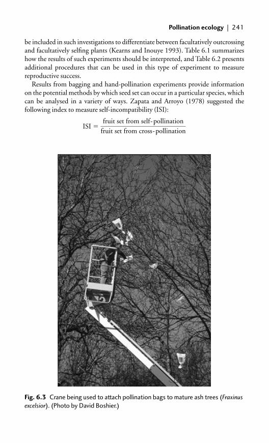
be included in such investigations to differentiate between facultatively outcrossingand facultatively selfing plants (Kearns and Inouye 1993). Table 6.1 summarizeshow the results of such experiments should be interpreted, and Table 6.2 presentsadditional procedures that can be used in this type of experiment to measurereproductive success.

Results from bagging and hand-pollination experiments provide informationon the potential methods by which seed set can occur in a particular species, whichcan be analysed in a variety of ways. Zapata and Arroyo (1978) suggested thefollowing index to measure self-incompatibility (ISI):

ISI �fruit set from self-pollination

fruit set from cross-pollination

Pollination ecology | 241

Fig. 6.3 Crane being used to attach pollination bags to mature ash trees (Fraxinus

excelsior). (Photo by David Boshier.)

Values of ISI can be interpreted as follows:

● �1 � self-compatible● �0.2�1 � partly self-incompatible● �0.2 � mostly self-incompatible● 0 � completely self-incompatible.

The frequency of self-pollination (S ) can be estimated by comparison of seedsfrom naturally pollinated flowers (P0) with those of hand self-pollination (Ps) andhand cross-pollination (Px), as follows (Dafni 1992):

The selfing rate (S) can also be defined as 1–t, where t is the outcrossing rate.Charlesworth (1988) presented a mathematical method of estimating outcrossingrates in populations of self-compatible plants, based on differences in the viabilityof zygotes produced by open pollination, hand-outcrossing and hand-selfing.Alternatively, appropriate molecular markers can be used to determine outcrossingrate (see section 6.5.1).

S �Px�P0

Px�Ps

242 | Reproductive ecology and genetic variation

Table 6.1 Field tests for the determining the ability to self-pollinate (adapted

from Kearns and Inouye 1993).

Treatment Breeding system Facultatively Outcrossingselfing outcrossing

Bagged/caged � �Bagged/caged and emasculated � � �Bagged/ aged and self-pollinated � � �Emasculated and open-pollinated � � �Open-pollinated � � �

�, seed set recorded; �, no seed set.

Table 6.2 Variables used to measure reproductive success (after Dafni 1992).

Variable Procedure

Pollen germination on Examined (or fixed) several hours after natural or artificialthe stigma pollination

Growth of pollen tubes Examined (or fixed) several hours after pollination

Fruit set Counting fruit number as a result of the treatment (% of the test flowers) at the end of the reproduction cycle

Number or mass of Weighing and counting seeds per fruitseeds per fruit

Seed viability Germination or tetrazolium test (see Section 4.8)

6.2.5 Hand pollination

Flowers can be artificially pollinated by hand (Figure 6.4), which is a usefulmethod to test the viability of pollen (see next section), or to test whether theabsence of pollinators is a cause of reproductive failure. In the latter case, hand-pollination offers a practical conservation technique, enabling plants with nopollinators to reproduce. It is important to remember that more than one pollengrain is usually required to initiate seed production. Methods of collecting andtransferring pollen include the following (Kearns and Inouye 1993):

● Collect pollen from dehiscing anthers with toothpicks, needles, small paint-brushes, or forceps, or on small pieces of tissue paper wrapped around forceps.Sometimes fabric has been used attached to wooden sticks, to simulate beehairs. Pencil tips have also been used to scoop anthers out of a flower andtransfer them to a recipient stigma.

● Collect pollen by tapping dehiscing anthers over a Petri dish.● To transport pollen collected on toothpicks or needles, poke the clean end of

a toothpick through the lid of a plastic vial and then close the vial around theend with the pollen (Price and Waser 1979).

● Rub an entire male-phase flower or anther over the recipient stigma.● Mimic pollen application by birds or insects by using dead animals to transfer

pollen, for example introduce the beak of a bird or the head of a bee into the

Pollination ecology | 243

Fig. 6.4 Artificial pollination of the night-flowering, bat-pollinated tropical tree

Bombacopsis quinata. A small brush is being used to transfer pollen to a receptive

stigma. (Photo by David Boshier.)

flower of a pollen donor and then the receptive flower. Construct ‘bee sticks’from dead bees and cocktail sticks, by using glue to attach the bee thorax tothe stick.

● Larger amounts of pollen can be transferred by using hypodermic syringesequipped with rubber bulbs.

6.2.6 Pollinator foraging behaviour and visitation rates

In order to determine which species are responsible for pollination, it is not suffi-cient simply to make observations of animals visiting a flower (flower visitors), assome flower visitors may rob the nectar without transferring pollen. To identify thepollinator of a species, it should be determined whether:

● pollen is transferred from the visitor to the stigma● pollen is transferred between flowers on a plant or among plants● fertilization or seed production has occurred as a result of the pollination.

Methods described in the previous sections can be used to make thisdetermination.

The behaviour of pollinators can affect the success of pollination and patterns ofgene flow. Foraging behaviour can be examined experimentally, for example byusing techniques such as artificial flowers or by manipulating flowers. It is evensometimes possible to train pollinators as part of experimental investigations, as inthe case of hummingbirds studied by Feinsinger and Busby (1987).

When assessing animal foraging behaviour, careful consideration should begiven to sampling design. Ideally, a sampling unit should be reproducible to enablecomparison of the activities of foragers in different times or places. Transectmethods are widely used for this purpose, in which an observer walks at a constantpace along a line while recording the presence of visitors on the flowers in thesample. Typical lengths of transects are 100–200 m3 m broad (Dafni 1992).Remember that points along the transect are not statistically independent; it is thetransect itself that is the sample unit, and the entire transect that must be repli-cated. Alternatively observations may be carried out from fixed points, for the samenumber of flowers or inflorescences, over a standard period of time (10–30 min istypical). Video recording offers a method for recording animal behaviour that canthen be analysed in detail back in the laboratory. Some of the variables commonlymeasured in field studies are listed in Table 6.3.

Visitation rates (number of visits to a flower per unit time) can be measuredfrom the perspective of either the flower or the visitor, by timed field observations(timed with stopwatches). From the perspective of the visitor, it may be helpful torecord the time expended to visit a single flower (which can be further subdividedinto the time taken to land on and manipulate the flower, and the time taken toextract nectar), the spatial distribution of flowers, and how rapidly the visitor canmove within and between inflorescences. Visitation can sometimes be inferredindirectly; for example, some nectar and pollen robbers leave a hole in the flowerthat can be recorded. Some flowers may be scarred or otherwise damaged by

244 | Reproductive ecology and genetic variation

visitors, or may display a morphological response to pollination (such as changesin petal colour, wilting, or flower abscission). However, in most cases visitation canonly be quantified by direct observation, which can be very time-consuming.Automated photography techniques have sometimes been used to reduce thelabour required for such studies (see, for example, Goldingay et al. 1991). Visitationdata can be summarized as the number of visits per flower per minute.

Patterns of movement of pollinators can be described by measuring flightdistance, or the linear distance between two flowers visited in succession, andchange in direction, or the difference in angular direction from one flower to thenext in relation to the direction of approach to the first flower. Such patterns canvary with the density and spatial distribution of flower resources, and can be animportant determinant of pollen flow (Kearns and Inouye 1993). Movementpatterns may be determined by following an individual flower visitor as it forages,with a compass to measure the direction of each flight and a voice recorder tomeasure the direction, time, and distance of each flight. Alternatively, all of theplants within a study area can be mapped and the movements of animals as they visitthe plants recorded. Such observations can be made in three dimensions as well astwo, for example by labelling branches or flowers in a volume of forest canopy.

6.3 Flowering and fruiting phenology

Phenology refers to the seasonal timing of flowering and fruiting. Describing pat-terns of phenology can be important for understanding the relative potential forgene flow at different times of the year, and the reproductive isolation of individ-uals or populations. Seasonal variation in flower and fruit availability will alsoaffect populations of animals dependent on these structures as a source of food.

Flowering and fruiting phenology | 245

Table 6.3 Variables commonly measured in assessments of forager activity in

pollination studies (after Dafni 1992).

Variable Procedure

Index of visitation rate No. of total visits at the observation period / no. of available flowers at this period.

Visitation rate No of visits / flower�hours.

Effective visitation rate per V � (A�N)/C, where A is the no. of visitors per plant flower per time unit (V) per time unit, N is the no. of visited flowers per visitor,

and C is the no. of flowers per plant.

Visitation rate (VR) VR � FT/(HT�FN), where FT is the foraging time per hour, HT is the species-specific handling time of the flower, and FN is the no. of flowers observed.

Attractiveness index No. of visitors/available flowers per time unit.

Foraging rate No. of flowers visited/time unit.

Phenology may be studied at the level of individual flowers, plants, populations, orcommunities.

At the simplest level, records of the first date of flowering and fruiting can beobtained from regular field surveys. Quantitative studies of phenology can beconducted by counting the numbers of flowers or fruit, from which a number ofdifferent variables can be derived (see Table 6.4). Such data can be used to produceflowering curves (the number of flowers or inflorescences open plotted againstcensus date) or fruiting curves (similarly, the number of fruits available over time).Decisions must be made regarding how frequently counts should be done: someflowers may last only days or even hours, and therefore observations may need tobe made hourly, whereas at the other extreme weekly or even monthly observations

246 | Reproductive ecology and genetic variation

Table 6.4 Selected variables commonly recorded in phenological studies (follow-

ing Dafni 1992). Although the variables described here refer to flowering, similar

approaches can be applied to assessment of fruiting phenology.

Variable Definition

Flowering commencement The date (or day number in the year) of the firstflowering.

Rate of flowering The cumulative numbers of flowers versus time.

Course of flowering The number of flowering units versus time.

Peak of flowering The date of maximum number of flowers, flowering plants, flowering species.

Relative flowering intensity The number of flowers at the individual plant peak as a percentage of the highest number of flowers of its conspecific individual.

Index of flowering The number of simultaneous open flowers in a given magnitude time as the percentage of the total number of flowers.

Mean flowering duration The mean flowering duration of the sample in days.

Midpoint flowering time The midpoint of extreme record dates of flowering.

Dispersion of the flowering The observed variance of the distance betweencurves during the flowering mean flowering dates is compared with the expectedseason variance based on randomly dispersed means and a

uniform distribution. If the ratio of the expected variance is much greater than 1, then the dispersion is aggregated; if much less than 1, then the dispersion is even.

Flowering overlaps At the community level, the observed overlaps in flowering between each two species may be compared with those overlaps generated by a series of randomizations.

Flowering termination Last date of flowering.

may be more appropriate, depending on the characteristics of the species beingstudied. Attention must also be paid to the sampling design adopted. Many studiesinvolve sampling individual plants within (randomly located) permanent plots,which are then repeatedly visited over time. Alternatively, individual trees orbranches may be selected for study.

Phenological studies of mature trees are complicated by the difficulty ofobserving reproductive structures in the forest canopy, and of producing reliableestimates for large trees. Binoculars can be used to count inflorescences or fruits.Rather than attempting to sample the entire canopy, a sample of branches (typ-ically 10–20) can be marked at different locations in the canopy, and subsequentlyused to make extrapolations to the whole plant. Another approach is to collectflowers or fruits in traps (see next section). For example, House (1989) measuredthe rate and duration of flower production in rain forest trees by collecting flowersin traps as they fell from the canopy, in units of numbers of flowers trapped persquare metre of crown shadow per unit time. From such data, a number of statisticscan be readily calculated, such as length of flowering or fruiting period, maximumnumber of flowers in bloom, number of species flowering at a particular date, etc.Long-term data can be of great value in determining annual patterns of variationin flower or fruit production, and are essential to detect the masting behaviourdemonstrated by many tree species.

D’eca-Neves and Morellato (2004) highlight the fact that many differentmethods of sampling and describing plant phenology have been used during thelast 30 years, making it difficult to compare the results of different studies. Amongthe 60 studies analysed, these authors recorded the following distribution of sam-pling methods: trails (20%), transects (18%), field plots (15%), and traps (10%).Furthermore, Hemingway and Overdorff (1999) found that the method used tocollect phenology data can affect the results obtained, transect methods detectinga higher number of food resources used by primates than selected tree methods.

A variety of different methods have been used to analyse and present pheno-logical information. Simple graphs or calendars can be produced illustrating thechange in phenological state of an individual plant or community throughout agrowing season. However, as pointed out by Newstrom et al. (1994), the choice ofgraphical style has a major influence on the detection of phenological patterns andthe interpretation of results. Newstrom et al. (1994) present three different typesof graph: time series graphs, which show the frequency and regularity of pheno-logical cycles; matrix graphs, showing the duration and date; and bar graphs, toillustrate seasonality of flowering frequency and amplitude (Figures 6.5 and 6.6).

Patterns of staggered flowering described for tropical forests illustrate theproblem of presenting and analysing phenological data. For example, Stiles (1977,1978) described sequential flowering in a group of 10 different plant species, whichwere pollinated by different hummingbird species. Similar results have beenobtained with pollination by insects (Figure 6.7). This pattern could be interpretedas evidence for competitive interactions or co-evolution between species. However,differences in the seasonal overlap of flowering are difficult to test statistically.

Flowering and fruiting phenology | 247

Estabrook et al. (1982) describe a simple non-parametric statistical procedure toaddress this issue. Phenological observations, such as the day on which a particularflower bud opened, can be compared between two groups of plants by testingwhether the probability that a bud will open on any given day is the same for budsin both groups of plants. This can be achieved by using the formula:

where m is the number of buds that eventually flowered in one group, n is the num-ber of buds that eventually flowered in the other group, and D is the difference incumulative frequency. The larger the value of D, the stronger is the evidence thatthe two phenological patterns are different. The formula enables the thresholdvalue of D to be determined, at P � 0.05. The value of D can be determineddirectly from the data, as the difference in cumulative frequency (for example inbud break) between the two groups, and if this is larger than the threshold value,then the two groups of plants are statistically different at P � 0.05.

A variety of other methods have been used to analyse phenological data. Forexample, Osawa et al. (1983) developed a stochastic model of bud phenology byusing a maximum likelihood technique for parameter estimation, which was fitted

P(D) � 1.36�[(m�n)/mn] � 0.05

248 | Reproductive ecology and genetic variation

Continual Tree 1043210

12 24 36

Guatteria aeruginosa

48 60 72 84 96 108 120 132

Sub-annual Tree 1102210

12 24 36

Protium pittieri

48 60 72 84 96 108 120 132

Annual Tree 1004210

12 24 36

Lonchocarpus oliganthus

48 60 72 84 96 108 120 132

Supra-annual Tree 2173210

12 24 36

Sapranthus campechianus

48 60 72

Time in months: Jan 1969–Dec 1980

Flo

wer

ing

amp

litud

e fo

r o

ne

tree

84 96 108 120 132

Fig. 6.5 Time series graphs showing the frequency and regularity in four basic

flowering patterns. Each graph shows monthly flowering from 1969 to 1980 for

one tree of each of four species. Amplitude categories are 1, light flowering; 2,

heavy flowering; dots on the x-axis, no flowering. (From Newstrom et al. 1994).

to balsam fir (Abies balsamea) data collected in Quebec. The model was furtherextended by Normand et al. (2002), then tested by using experimental data forpopulations of strawberry guava (Psidium cattleianum) on the island of Réunion.Schirone et al. (1990) describe a different approach, based on definition of

Flowering and fruiting phenology | 249

1.0

0.5

0.0

6970717273747576Y

ear

7778798081

J FMAMJ J ASOND

CONTINUALGuatteriaaeruginosaTree 1043

(a)

(b)

SUB-ANNUALProtiumpittieri

Tree 1102

ANNUALLonchocarpus

oliganthusTree 1004

SUPRA-ANNUALSapranthus

campechianusTree 2173

J FMAMJ J ASOND J FMAMJ J ASOND

J FMAMJ J ASOND J FMAMJ J ASOND

Month

J FMAMJ J ASOND

J FMAMJ J ASOND

J FMAMJ J ASOND

Pro

po

rtio

n o

f ye

ars

Fig. 6.6 (a) Bar graphs showing seasonality in four basic flowering patterns as

proportion of years in which heavy (dark bars) or light flowering (light bars)

occurred for each month of the year. (b) Matrix graphs showing duration and date

in four basic flowering patterns. Dark shaded circles, heavy flowering; light shaded

circles, light flowering; blanks, no flowering. (From Newstrom et al. 1994.)

Fig. 6.7 Sequential flowering of 10 species of tropical plant all pollinated by the

same carpenter bees (Xylocopa spp.). (From Whitmore 1990.)

Xanthophyllum discolorXanthophyllum rufum

Connarus sp.Sindora velutinaSindora coriaceaMesua ferreaCallicarpa maingayiMillettia atropurpureaConnarus sp.

JuneMayAprilMarch

?

different phenological stages for leaf development and abscission. A quantitativeestimation of each of these ‘phenophases’ is obtained by using a seven-point scale forpercentage representation, with the unit of assessment being an individual tree orall the branches in a tree crown. Graphs describing the change in phenophase overtime, either for individual trees or for a forest stand, can be produced by fittingcurves to the data, by using logistic, Gompertz, or Richards functions (Schironeet al. 1990). In contrast, Chapman et al. (1999) used spectral analysis (Fourieranalysis) to analyse phenological patterns. This is a type of analysis of variance usedto detect cycles of various frequencies in time series data, and involves comparingthe variation in the time series about the mean to sine functions of differentfrequencies. The result is a periodogram that displays the least-squares fit of eachfrequency to the time series, and was used by Chapman et al. (1999) to identifypeaks in flowering and fruiting.

6.4 Seed ecology

Units of dispersal can include fruit and vegetative reproductive fragments, butthese are referred to here collectively as seed. Further information about seedecology is provided by Baskin and Baskin (1998), Bradbeer (1988), and Fenner(2000).

6.4.1 Seed production

Measures of seed production are required in order to estimate the fecundity oftrees, an important variable when modelling population dynamics and viability(see Chapter 5). Seed production is also often of relevance to studies of those ani-mals that use them as a food source. The simplest method of estimating seed pro-duction is by direct observation, for example by counting fruit or cones on anindividual tree. For example, Koenig et al. (1994a) described a method wherebyobservers count acorns in the tree canopy within a given period of time (30 s).Other visual surveys have employed simple categorical measures to evaluate pro-duction, for example by estimating the percentage of a tree’s canopy containingseed, the percentage of twigs containing seed, and the average number of seeds pertwig to derive an overall score (Whitehead 1969).

The main problem with observational approaches is that fruits may be difficultto count because they are small, inconspicuous, or obscured by foliage. Such meas-ures are therefore likely to be underestimates, particularly in closed forests. Countscan sometimes obtained from open-grown trees (see, for example, Koenig et al.1994b), but such values are often likely to be biased, because seed production bymany tree species is higher in open-grown conditions than in a forest stand.Alternatively, observations can be made from above the forest canopy by usingcranes or towers (LaDeau and Clark 2001).

More commonly, some form of seed trap is used (see also section 6.4.2), a tech-nique that is most appropriate for use when trees are isolated from conspecifics and

250 | Reproductive ecology and genetic variation

dispersal distances are low. Traps used for seed production studies are usually con-structed out of a square wooden frame (typically of 50�50 cm) supported on shortlegs, with a base of nylon cloth of small mesh size (1 mm). A large number of trapsare typically needed for accurate estimates of seed production (Zhang and Wang1995); published studies have surveyed 0.000 03–0.017% of the forest area beinginvestigated (Chapman et al. 1992). Traps should be visited every few days to avoiddecomposition, removal, and damage of fruits and seeds by insects and terrestrialvertebrates. Seed numbers can be counted or their mass measured, and values canbe extrapolated to provide estimates per unit forest area (Parrado-Rosselli et al.2006).

Relatively few studies have compared different methods for assessing seed pro-duction (Chapman et al. 1992, Stevenson et al. 1998, Zhang and Wang 1995). InFrench Guiana, Zhang and Wang (1995) compared three fruit census methods:fruit-traps, observation from platforms situated in the canopy, and a raked-groundsurvey. The last method involved surveying fallen fruits along a fixed route at regu-lar time intervals, removing the checked fruit after each census. While recognizingthe main limitation of fruit-traps (that some of the fruit may be consumed beforefruit fall), these authors note one of the key advantages of this method, in beingable to sample a relatively large area of forest. However, the number of traps neededmay be high, with at least 80 traps needed for accurate assessments of fruitingspecies richness in diverse forests such as this. The main cause of loss from fruittraps was decomposition, although the risk of terrestrial mammals or insects eatingthe fruits while in the trap was also noted. Although the raked-ground survey wasfound to be simple to do, it was found to be inaccurate for determining the quan-tity of fruit falling from tree crowns, because of rapid consumption by terrestrialanimals. Platform observations were found to give the most accurate measure-ments of the quantity of fruit in tree crowns, the main problem being the logisticaldifficulty of creating and accessing the platforms, and the limited proportion of theforest sampled.

Parrado-Rosselli et al. (2006) recently compared fruiting data derived fromfruit-traps placed on the ground with data from canopy-surveyed plots in a terrafirme rain forest, in Colombian Amazonia. Results indicated that estimatesobtained by using the two methods were not correlated: values derived from thecanopy-surveyed plots tended to be higher than fruit-trap estimates, suggestingthat the latter method tends to underestimate seed production. Consequently,these authors suggest that the use of traps should be restricted to particular types ofstudy such as estimates of fruit available for terrestrial frugivores, scatter hoardingrates, and for long-distance dispersal estimates. In contrast, traps should especiallybe avoided in studies aimed at measuring fruit availability for arboreal and flyingfrugivores, because a residual quantity of fruits is sampled.

Chapman et al. (1992) compared three methods to estimate fruit abundance oftropical trees: visual estimation, and relations with tree stem diameter (dbh) andcrown volume. Estimations from measures of dbh were found to be consistentlythe most accurate and precise. Allometric models are often used to estimate

Seed ecology | 251

fecundity of trees, usually as a function of stem diameter (dbh), by using equationssuch as:

where yi is the annual log seed production by the ith tree having log diameter di, and

where �0 and �1 are regression parameters, and i is a zero-mean error process,i �N(0, 2) (Clark et al. 2004). If fecundity is proportional to basal area (diam-eter squared), then �1 � 2. Clark et al. (2004) provide a more sophisticated model,employing a hierarchical Bayes modelling structure and Markov-chain MonteCarlo techniques, to estimate fecundity from the two types of data that ecologiststypically collect, including seed-trap counts and observations of trees. Therelations between tree size, seed mass, and seed production are reviewed by Greeneand Johnson (1994), who showed that tree size (basal area) is related to seedproduction, and that seed production is highly negatively correlated with meanseed mass according to a power law relation.

6.4.2 Seed dispersal and predation

It is useful to differentiate between primary dispersal, which is the movement ofseeds from the inflorescence on the parent plant to its first settling point, and sec-ondary dispersal, which is any subsequent movement prior to germination(Gibson 2002). Zoochory refers to dispersal by animal vectors, anemochory bywind, and hydrochory by water. A complete assessment of seed dispersal in a par-ticular species should involve consideration of all possible vectors. A detailedreview of different dispersal mechanisms is provided by Van der Pijl (1982).Methods for measuring and modelling seed dispersal are reviewed by Greene andCalogeropoulos (2002).

Seed traps

Measurements of the density of seed falling on a particular area, or the seed rain, aregenerally made by using a seed trap (Figures 6.8 and 6.9). The following attributesof a seed trap are important (Kollmann and Goetze 1998):

● It should be designed to allow ready separation of seed from litter, soilparticles and insects.

● There should be some protection against seed predation.● The seeds must not be allowed to rot or decay before examination.

The seed rain is likely to display pronounced spatial variation, and this needs tobe taken into account in designing an appropriate sampling approach. The mostdifficult part to measure of the seed dispersal curve is the tail of the distribution.Ideally, trap area should be increased so that the same proportional area is sampled

�i � �0��1di

yi � �i��i

252 | Reproductive ecology and genetic variation

at increasing distances from the parent plants (Bullock and Clarke 2000).All methods for assessing seed rain are labour-intensive; a large sample size isneeded and it may be necessary to sample in different seasons or even all year round(Bullock 1996).

The following types of seed trap have been used (Gibson 2002, Kollmann andGoetze 1998):

● Flat traps. This involves spreading tissue paper or aluminium foil on theground in order to catch seed. This method is generally very inaccuratebecause of high seed losses due to the effects of rain, wind, or predation.However, the method was successfully applied by Greene and Johnson (1997)in their assessment of birch seed dispersal across snow.

● Soil traps. Pots or trays of sterilized soil or other growth medium are placed inthe field. The trays can then be taken to the laboratory or greenhouse for

Seed ecology | 253

Fig. 6.8 Seed traps manufactured from wire and plastic netting, used in seasonal

tropical montane forest in northern Thailand. (Photo by Kate Hardwick.)

germination trials; the number of seedlings that subsequently appear aretaken to indicate the density of seeds deposited on the site. The accuracy ofthis method is not high because of variation in germination rates, mortality ofseed and seedlings, seed predation, and secondary dispersal.

● Sticky traps. Trays, boards, or filter paper 10–30 cm in diameter can be coveredwith non-drying glue or grease, then exposed either vertically or horizontally.Once seeds land on the glue, they become fixed, enabling the trap to be exam-ined in detail in the laboratory. An example is provided by Werner (1975),who used ‘Tanglefoot’ glue, a bird repellent available in many countries.

254 | Reproductive ecology and genetic variation

Fig. 6.9 Another design of trap used to collect fruit, to measure production. In

this case fruit production by a single tree of Aquilaria malaccensis is being

measured. The trap is constructed from nylon netting on a wooden frame, which

extends beyond the limit of the tree canopy. The man pictured is the proud

creator of the trap, Tonny Soehartono. (Photo by Adrian Newton.)

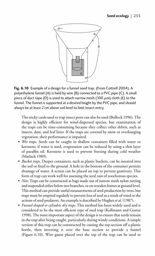
The sticky cards used to trap insect pests can also be used (Bullock 1996). Thedesign is highly efficient for wind-dispersed species, but examination ofthe traps can be time-consuming because they collect other debris, such asinsects, dust, and leaf litter. If the traps are covered by snow or overhangingvegetation, their performance is impaired.

● Wet traps. Seeds can be caught in shallow containers filled with water orkerosene; if water is used, evaporation can be reduced by using a thin layerof paraffin oil. Kerosene is used to prevent freezing during cold weather(Matlack 1989).

● Bucket traps. Deeper containers, such as plastic buckets, can be inserted intothe soil or fixed to the ground. A hole in the bottom of the container permitsdrainage of water. A screen can be placed on top to prevent granivory. Thisform of trap can work well for assessing the seed rain of zoochorous species.

● Nets. Traps can be constructed as bags made out of narrow mesh nylon nettingand suspended either below tree branches, or on wooden frames at ground level.This method can provide useful measurements of seed production by trees, buttraps must be emptied regularly to prevent loss of seed as a result of wind or theactions of seed predators. An example is described by Hughes et al. (1987).

● Funnel-shaped or cylindric dry traps. This method has been widely used and isconsidered to be the most efficient type of seed trap (Kollmann and Goetze1998). The most important aspect of the design is to ensure that seeds remainin the trap after being caught, particularly during windy conditions. A simpleversion of this trap can be constructed by cutting the top section off a plasticbottle, then inverting it over the base section to provide a funnel(Figure 6.10). Wire gauze placed over the top of the trap can be used to

Seed ecology | 255

E

D

A

B

C

Fig. 6.10 Example of a design for a funnel seed trap. (From Cottrell 2004). A

polyethylene funnel (A) is held by wire (B) connected to a PVC pipe (C). A small

piece of duct tape (D) is used to attach narrow mesh (100 �m) cloth (E) to the

funnel. The funnel is supported at a desired height by the PVC pipe, and should

always be at least 2 cm above soil level to limit insect entry.

exclude larger seed predators. The traps can be inserted in the soil, or placedon the soil surface, and should be inspected regularly to minimize seed losses(further details are provided by Cottrell 2004). Hydrochorous seed can becaptured by using floating funnel-traps that remain on the water surfaceduring fluctuating water levels (Middleton 1995).

● Natural traps. Zoochorous seed can be sampled from animal faeces, hair, fur,and feathers. Examples are provided by Izhaki et al. (1991), who counted thedensity of seeds in ‘droppings traps’ constructed out of nylon sheets that wereplaced under trees; Campbell and Gibson (2001), who counted seedlingsemerging from samples of horse dung; and Voysey et al. (1999), who assessedtree seed dispersal by gorillas by using this method.

Once seed have been trapped, their viability can be tested by using the methodsdescribed in section 4.8.

Trapless methods: examining seeds, germinants, and seedlings

In some cases it is possible to sample seeds directly on the ground surface, for exampleby counting the number of seeds present in quadrats located randomly or alongtransects. This approach is particularly useful with large seeds (see, for example,Augspurger and Hogan 1983), but is very time-consuming with small seeds, whichmay be difficult to detect among leaf litter. Examination of germinated seeds (germi-nants) and seedlings can also be used to infer dispersal patterns. For example, Ribbenset al. (1994) used the relationship between seedlings and conspecific trees to estimateseedling production and dispersal. These authors present a model that predictsseedling density as the summed contribution of seedlings from all trees in a sampleplot, estimating fecundity and dispersal distance of seedlings based on the summedcontributions of potential parent trees. The main problem with inferring dispersalfrom seedling distribution is that other factors than purely dispersal may accountfor the distribution of seedlings, including the availability of seedbeds or micrositessuitable for seed germination, herbivore density, the availability of light, or competitionwith other plants. Such factors may vary with increasing distance from the parentplant.

Both traps and examination of seeds or seedlings share the problem that thesource cannot be known with certainty except in situations where a single plant orgroup of plants is isolated from other conspecifics. Therefore, when using thesemethods, isolated trees should be selected for analysis. The following methodsprovide an alternative way of overcoming this problem.

Observations of seed movement

In the field, the usual approach is to place or release seeds on or close to the mater-nal plant, or to mark seeds still attached to the plant before their natural release,and then to track their movement (Gibson 2002). Often, isolated individuals areused to facilitate tracking. Although it is possible to follow seed from the source tothe landing site by visual observation, this method is time-consuming and often

256 | Reproductive ecology and genetic variation

difficult. A more efficient approach is to mark the seed in a way that allows subse-quent identification. Care is needed to ensure that the method of marking does notin itself alter the pattern of dispersal, particularly in the case of small seeds (Gibson2002).

One of the most commonly used methods of marking seed is spray painting(Greene and Johnson 1997), including the use of fluorescent paint, which enablesseeds to be identified during subsequent searching by using a ultraviolet lamp(Bossard 1990). Other methods include the use of radioactive tagging (Winn1989), which involves injecting the parent plants with a radionuclide (often scan-dium-46) in solution while the seeds are developing, then using a counter to detectthe seeds after dispersal. In the case of large seeds, small pieces of metal can beinserted in the seed, which can then be relocated by using a metal detector (Sork1984, Mack 1995). This method was recently tested by López-Barrera et al.(2006a) with oaks in Mexico. The acorns were drilled with a hand drill and a smallnail (15�3 mm) was inserted inside each acorn (following Sork 1984). The headof the nail in each acorn was exposed above the surface and painted with fluores-cent spray paint to facilitate relocation. A number of different models of metaldetector were tried before finding an instrument that successfully detected the tagsunder field conditions. However, in a trial of more than 4000 tagged acorns, only2.2% of the dispersed acorns were recovered, the others presumably having beencached by the small mammals responsible for dispersing them. This highlights oneof the key problems with tagging seeds: often the proportion recovered is very low,and it is impossible to know whether this results from insufficient sampling or thata fraction of the seeds has passed beyond the maximum sampling distance (Greeneand Calogeropoulos 2002).

Alternatively, individual seeds may be followed during transit (the Lagrangianmethod), an approach that has been used with wind-dispersed seeds as well as withthose dispersed by birds, insects, and mammals. For example, an animal can befollowed, and its caches or dung piles examined. However, this approach onlyworks for those seeds travelling short distances, because those travelling further canbe difficult to follow (Greene and Calogeropoulos 2002).

Forget and Wenny (2005) review the methods used to study seed removal andsecondary seed dispersal, and make the following points:

● Although seed dispersal behaviour can be observed directly in open habitats,with small animals that travel short distances, few observational studiesinclude data on final post-dispersal seed fate. In closed forests, visual observa-tion of animals removing seeds is more difficult, although remote cameras andvideo surveillance systems have successfully been used. Marking seeds isessential in the wild when seeds are taken by vertebrates and transported outof sight.

● As an alternative to direct observation of animals moving seeds, indirectmethods of recording animal movements can be used. For example, trappedrodents can be marked with a fluorescent powder and their travel route

Seed ecology | 257

retraced with an ultraviolet lamp. The method works best under dry condi-tions and is therefore not suitable in rain forests.

● Attaching seeds with a nylon thread to a fixed point such as a small tree or twigis useful for distinguishing between biotic and abiotic causes of seed move-ment, and for determining which types of animals remove seeds. The methodalso enables seed fate to be determined. The seed can be glued to the line orpassed through the seed after drilling a small hole. Line lengths of 30–200 cmhave often been used; shorter lengths are less likely to get tangled. Often, insuch experiments, the location of seed is marked by using coloured stakes,flagging tape, or toothpicks. If so, care should be taken to ensure that themethod of labelling the locations does not attract seed predators and thereforebias the results.

● The spool-and-line protocol consists of a thread-filled bobbin from whichthe line is dispensed as the seed attached to the end of the line is carriedaway. The travel route and final location of the seed can be determined byfollowing the line. The main problem is that the line can often be broken, andtracing the line can be difficult. The method works best when studyingground-dwelling animals, but preparing spools can be time-consuming.

● Most studies of seed fate use a free marking method to relocate the removedseeds, and to discriminate between seed predation and hoarding. In additionto radioisotopes or metal objects mentioned above, miniature radio trans-mitters or magnets can be used. If the seeds are large enough it is useful tonumber and mark them individually, allowing individual fates to bedetermined. This can be achieved by using indelible ink.

Overall, Forget and Wenny (2005) suggested that, although the use of magnetsor radiotransmitters is efficient in retrieving seeds, especially over long distances,they are relatively expensive, and therefore free-line methods tend to be more com-monly used in practice. Although radioisotopes have proved very effective, con-cerns about the environmental impacts of radioactivity have deterred researchersfrom using them. Most methods work best with larger seeds, and therefore as aresult relatively little is known about smaller seeds. Most studies focus on com-mon, short-distance events, even though rare, long-distance events may well bemore important to plant community dynamics. Studies that combine techniquesare therefore recommended.

Seed predation

Many studies of post-dispersal seed fate use seed removal as an indicator of seed pre-dation. Commonly, a population of seeds is placed on the ground, either singly or inclumps, and their removal is monitored over time. From such observations, rates ofseed loss can be calculated. However, it may be more appropriate to analyse such seedloss data as a categorical variable. For example, in a seed predation experiment inMexico, López-Barrera et al. (2005) transformed the proportion of seeds removedinto a categorical variable with three levels (low: 0–33%, medium: 33–66% and high

258 | Reproductive ecology and genetic variation

removal: 66–100%). In a second experiment, data appeared to be bimodal (all ormost of the seeds were either present or missing), therefore acorn removal wasassigned to two removal categories (low: 0–50% and high: 50–100%). Such data canbe analysed by using categorical modelling (such as Proc CATMOD in SAS; see SAS2002), a procedure analogous to ANOVA but with categorical data represented incontingency tables (López-Barrera et al. 2005).

Investigations that interpret removal of seed purely as seed predation overlookthe possible occurrence of secondary dispersal, and therefore overestimate themagnitude of predation. Vander Wall et al. (2005) examine the recent literature onseed removal studies, and indicate how the results of some of these investigationsmay have been misinterpreted, highlighting the importance of detailed studies ofseed fates in order to assess predation. Methods used to assess seed fates by trackingare described in the previous section. Following seeds can be very challenging but isthe only sure way of gaining knowledge about seed fates (Vander Wall et al. 2005).

Fitting a dispersal curve

Measurements of seed density or the seed rain can be used to produce a seeddispersal curve, which describes the frequency distribution of dispersal distances,and the seed shadow, which is the post-dispersal spatial distribution of seeds aroundthe maternal plant (Gibson 2002). The seed dispersal curve for wind-dispersedseed is usually described by fitting a negative exponential curve to the data, ofthe form:

where SD is the density of seeds at distance D from the source, and a1 and b1 areconstants indicating the density of seeds falling at the source and the slope of thedecline in seed density with distance, respectively (Bullock and Clarke 2000). Thisgives a linear relation between ln(SD) and D; the slope of the line provides ameasure of the rate of decline in seed density with distance (Gibson 2002). Someauthors (for example Willson 1993) have suggested that logging both axes gives amore realistic relation, which accords with the inverse power model (Bullock andClarke 2000):

These authors found that an empirical mixed model based on the negativeexponential and power models provided a better fit than either individualfunction. This is described by:

where SN and TA are the total number of seeds trapped and the total area of traps asdistance D from the centre of the plant; a, b, and c are constants; and p is the inversepower parameter (Bullock and Clarke 2000). The length of the tail of the fitteddistribution can be reported as the distance within which 84% of the seeds fall(equivalent to one standard deviation of the mean trajectory) (Greene and Johnson

SN � TA(a3 exp(�b3D)�c3D�p3)

SD � a2D�b2

SD � a1exp(�b1D)

Seed ecology | 259

1989). The range and mean of the measured dispersal distances should also bereported (Gibson 2002). Bullock and Clarke (2000) suggest that researchersshould measure the tail of dispersal curves and examine carefully whether thewidely used exponential and power models are, in fact, valid.

Recruitment limitation

As a result of the difficulties of measuring seed production and dispersal in forests,the influence of these processes on the population dynamics of tree species has beenlargely overlooked. Recently, there has been growing awareness that seed may oftenbe in short supply and can limit seedling recruitment. The phenomenon of recruit-ment limitation (Figure 6.11) has attracted increasing attention from researchersworking in a variety of different forests (Hubbell et al. 1999). Clark et al. (1999a)review the concept, and highlight the fact that most studies of seed rain, seed banks,and seedlings are undertaken for relatively short periods (usually 1 year, and veryrarely as much as 5 years). These authors highlight the inadequacy of such samplingapproaches, and indicate the need for data to be collected across multiple years andmultiple forest stands, something rarely achieved to date. In addition, most effortsto quantify seed production and dispersal (such as observations of seedling distri-bution) are highly indirect. Clark et al. (1998b) illustrate how recruitment limitationcan be analysed by using a combination of modelling approaches and in intensiveanalysis of fecundity, seed dispersal, and establishment, by using data from an array

260 | Reproductive ecology and genetic variation

Seed densityand dispersion

Seedling density

D. Establishment

C. Dispersal

B. Source strengthMean

Variance

Total seed production per adult

Spatial variability

Fraction of seeds thatbecome seedlings

A. Source densityand dispersion

Fig. 6.11 Processes responsible for recruitment limitation in forests. (From Clark

et al. 1999b). Seed arrival depends on: (A) density and dispersion of adults, (B)

adult fecundities, and (C) dispersal distances of seed. Seed arrival can be

constrained by source-density (A), source-strength (B), and dispersal limitation

(C). A fourth limitation on recruitment, establishment limitation (D), depends on

seed survival and germination and seedling survival, which depends on physical

(e.g. light, water and nutrients) and biotic (e.g. litter depth, seed and seedling

predators, pathogens, and competitors) factors that vary at several spatial scales,

both within and among forest stands.

of 100 seed traps, and surveys of several thousand mapped trees and seedlings in fivesouthern Appalachian forest stands undertaken over 5 years. Another usefultechnique for studying recruitment limitation is to perform seed-sowing experi-ments, an approach receiving increasing interest from researchers, although rela-tively few such studies have been carried out with woody plants to date (Flinn andVellend 2005, McEuen and Curran 2005).

Long-distance dispersal

Although it is widely recognized that dispersal over long distances is ecologicallyvery important, it is very difficult to measure. Nathan et al. (2003) review methodsfor estimating long-distance dispersal and identify a variety of alternatives:

● Drawing inference from biogeographical distribution patterns; however, dis-persal rate and method of dispersal cannot readily be estimated by using thisapproach.

● Observation of movement (for example by the Lagrangian method, see above);this can give accurate estimates (by feeding labelled seeds to animals, forexample; Yumoto 1999), but is difficult over long distances.

● Short-term and long-term genetic analyses (see next section).● Modelling, including both empirical and mechanistic models.

Greene and Calogeropoulos (2002) further review methods for assessing long-distance seed dispersal, and conclude that there is no single preferred method.Trapping methods are particularly inefficient when used over the large areasneeded to estimated long-distance dispersal. These authors also highlight the needto test models with empirical data describing the far tail of the distribution, whereseed densities are relatively low—something rarely achieved to date.

A range of complex mechanistic models are available, taking into accountwindspeed and height of release (Andersen 1991, Greene and Johnson 1989, Katulet al. 2005, Okubo and Levin 1989). However, the applicability of these modelshas rarely been tested (Bullock and Clarke 2000). Horn et al. (2001) highlightthe fact that dispersal of forest tree seeds by wind is biphasic: seeds that fallwithin the canopy have no chance of long-distance dispersal, but seeds that riseabove the canopy do. For this reason, mixed models such as those presented byBullock and Clarke (2000) and Clark et al. (1999b) are appropriate, as theyprovide an opportunity to estimate separately the partitioning of seeds betweenthose that are dispersed over long distances and those that fall locally. However,zoochorous species can display dispersal curves very different from those of wind-dispersed species, and tend to be highly clumped (for example, high densities ofbird-dispersed species may be found under perching sites). The ecology of seeddispersal is reviewed in detail by Levin et al. (2003).

Trakhtenbrot et al. (2005) review the importance of estimating long-distancedispersal for conservation planning, and highlight two separate issues: the dispersalof alien or exotic species, which may invade ecological communities, and reductionin dispersal of native species through processes such as habitat fragmentation. The

Seed ecology | 261

authors highlight the fact that quantitative assessment of long-distance dispersalis highly informative but also very costly in terms of data collection, and there-fore recommend that such analyses be restricted to addressing the most crucialthreats (such as invasive species). Qualitative assessments can provide a usefulfirst step, for example by enabling potentially invasive species to be identifiedthrough a consideration of dispersal vectors. Where quantitative analysis isneeded, the use of mechanistic models is recommended, ideally supported byempirical tests.

Molecular methods are useful for estimating both short- and long-distancedispersal, especially when used in conjunction with studies of germinants (Cainet al. 2000) or trapping methods. For example, Jones et al. (2005) used microsatel-lites to identify the parent trees of seed collected in a large array of traps, for theneotropical tree species Jacaranda copaia (Bignoniaceae). Use of molecular markervariation to analyse dispersal is considered below (see section 6.5.1).

6.5 Assessment of genetic variation

Information about the extent of genetic variation within species is usually obtainedeither by using molecular markers, or by assessing variation in quantitative traits.Both of these approaches are considered below.

6.5.1 Molecular markers

Most often, molecular markers are used to assess patterns of genetic variationwithin and between populations, but they can also be used to provide informationabout plant breeding systems, clonal structure, the evolutionary history of popula-tions, and estimates of gene flow. Such measures have direct relevance to forest con-servation and management (Haig 1998). Molecular methods are also widely usedfor addressing questions relating to evolutionary relationships and taxonomy,which are not considered further here. Further details regarding application ofmolecular methods in ecology are provided by Baker (2000), McRoberts et al.(1999), Ouborg et al. (1999), and Parker et al. (1998). Two recent introductorytexts on ecological and conservation genetics are by Frankham et al. (2002) andLowe et al. (2004). Young et al. (2000) present a valuable compilation of methodsrelating explicitly to forest genetics, and an overview of approaches to managingand conserving forest genetic resources is provided by the National ResearchCouncil (1991). The application of molecular methods to conservation of treespecies is considered by Newton et al. (1999a).

Practical details of molecular methods are not presented here in depth; thereader is referred to specific texts such as Lowe et al. (2004) and Young et al. (2000).The subject will also be addressed by another book in this series (P. Taberlet, inpreparation). Here, the relative strengths and weaknesses of the main differenttypes of marker are considered in relation to different questions of interest, to helpidentify which method is most appropriate for a particular situation. Some

262 | Reproductive ecology and genetic variation

guidance on use of molecular marker methods for addressing different questions isalso provided.

Collection of material

Careful attention should be paid to sampling when collecting material for geneticanalysis. Typically, samples are collected from populations in the absence of anyinformation about the patterns of genetic variation that exist, or about the size ofthe breeding populations of the species. As a result, there is a high risk that anysampling design adopted will provide an inaccurate assessment of patterns ofvariation within the species. Sampling decisions will obviously depend on theobjectives of the investigation, which should be stated clearly at the outset. Forexample, for an assessment of genetic variation across the entire geographic rangeof a species, populations must be sampled throughout the entire range, perhapssampling a relatively small number of individuals (typically in the range 5–30)within each individual population.

Ideally, for this kind of investigation, individuals should be selected for sam-pling by using random or stratified random procedures. In practice, sampling forgenetic studies is often rather haphazard or opportunistic, being governed bywhich populations and individuals are relatively accessible (Lowe et al. 2004). It isimportant to be aware that any departure from random sampling may introducebias into the results obtained, which should be borne in mind when interpretingresults. If an assessment of genetic variation within a population is required, it isalso important to ensure that clonal individuals are not being repeatedly sampled.This can be achieved by stipulating a minimum distance (typically � 100 m)between individuals to be sampled. Investigations at a more local scale, such asstudies of gene flow across landscapes, may require all individuals within a givenarea to be sampled and mapped. In this case, such studies should ideally bereplicated at different sites. It may also be necessary to sample a large number ofprogeny (� 200) for accurate assessments of gene flow (Lowe et al. 2004) (seesection on p. 270).

Samples of leaf tissue are generally used for DNA analysis, although other plantparts such as roots, seeds, or the cambium layer can also be used (see, for example,Colpaert et al. 2005). Leaf samples collected in the field for DNA analysis can bedried by using silica gel following the method described by Chase and Hills (1991),on which the following account is based:

● Fresh young leaf material should be selected, free from any fungal attack ordirt. Remove any surface water from the leaves before sampling. Torn leafpieces (�2 cm2) should be removed and placed into a small (12�8 cm)sealable plastic bags, or 50 ml tubes with screw caps (for example plasticcentrifuge tubes).

● Add 50–60 g of 20–200 mesh size, grade 12 silica gel (if the gel is to bereused, a smaller mesh grade should be used: for example, 6–16 mesh size,grade 42). Generous amounts of silica gel should be used; a minimum ratio of

Assessment of genetic variation | 263

10 : 1 silica gel : leaf mass is required for effective preservation of leaf samples.A small amount (5%) of indicator silica gel can usefully be added. Never reusegel without first making sure that no contamination from previous specimensis present (by baking or using ultraviolet light to sterilize it, for example).Shake the bag to distribute the gel between the layers of leaves.

● The leaf tissue should be dry after 12–24 hours, by which point the leaffragments should snap and break cleanly. The sample bags should be keptsealed and ideally stored in a refrigerator before analysis.

For isozyme studies either fresh or rapidly frozen material is required. Seedtissues, or seedlings that have recently germinated, are often preferred for isozymestudies because of the relatively high number of loci that can generally be resolvedwhen using such tissues. However, other plant parts such as buds or root tips canalso be used (Soltis and Soltis 1990).

Types of molecular marker

A wide range of different molecular markers are available. Some of those mostwidely used to assess genetic variation in tree species are briefly described below:

● Isozymes. This method involves the separation of different molecular forms ofenzymes by using gel electrophoresis. A variety of specific stains are used todistinguish particular enzymes in a tissue extract. When the polypeptide con-stituents of enzymes are coded by more than one gene, then they are referredto as isozymes, but when coded for by a single gene, they are referred to asallozymes (Gibson 2002). Different banding patterns between individualsobtained on a starch or polyacrylamide gel are interpreted as indicating thepresence of alternate alleles at a given locus. Isozymes can underestimategenetic variation because only a very small part of the plant genome is beingconsidered, even if a large number of loci are screened. Another problem isthat the amount of variation detected may sometimes be small; more than halfof all loci may often be monomorphic (Parker et al. 1998). Details of themethod are described by Soltis and Soltis (1990).

● Restriction fragment length polymorphism analysis (RFLP). DNA is digestedwith restriction enzymes (usually 4–6 bp cutters), then the fragments pro-duced are separated by gel electrophoresis and blotted on to a filter (Gibson2002). The Southern blot procedure is used to hybridize labelled probes to thebound DNA, to allow discrimination of target fragments homologous to theprobe. Fragments that have the same restriction sites (i.e. similar DNAsequence variation) migrate to the same location on the gel. A modification ofthe method (PCR–RFLP) is widely used, based on the restriction digestion ofPCR-amplified products, with the use of primers designed from universalcpDNA, mtDNA, or nuclear DNA sequences.

● Random amplified polymorphic DNA (RAPD). A PCR-based method based on the amplification of arbitrarily derived (‘random’) DNA segments.PCR-amplified products are separated on agarose gels in the presence of

264 | Reproductive ecology and genetic variation

ethidium bromide and visualized under ultraviolet light. Co-migratingbands are assumed to represent identical genome segments for that particularprimer pair.

● Amplified fragment length polymorphisms (AFLP). Genomic DNA is digested,then the cleaved fragments undergo several rounds of selective amplification.The amplified products are radioactively or fluorescently labelled andseparated on sequencing gels.

● Microsatellites (SSR) are short (10–15 copies) tandem repeats that are assumedto be randomly distributed throughout the genome. Primers are designedfor the conserved regions flanking the variable SSR. Polymorphism of theSSR is detected by using PCR and separation of products on agarose, poly-acrylamide, or DNA sequencing gels.

Choice of marker system

Marker systems differ in a range of characteristics, such as the amount of variationdetected, their ease of use, and the costs of development and implementation (seeTable 6.5). The choice of a marker is therefore based on the objectives of the inves-tigation, the properties of the marker system, and the resources available (Loweet al. 2004). To some extent, there are trade-offs to be made between cost, ease ofuse, and information obtained. For example, SSRs are preferred in many investi-gations because of the high level of polymorphism detected and the high repro-ducibility. However, this method is relatively expensive, and requires DNAsequence information for the species of interest. As a result, relatively cheap andeasy methods such as RAPD and AFLP, which do not require any DNA sequenceinformation, have been widely used with tree species. These methods are particu-larly useful for an initial examination of the partitioning of genetic variation withina species or for locating centres of genetic diversity. However, the reliability ofRAPD has been called into question, and investigations by this method are becom-ing increasingly difficult to publish in the scientific literature. The technique iseffectively being replaced by AFLP, which is a somewhat less straightforwardtechnique.

Marker systems are classified as either dominant or co-dominant according totheir mode of inheritance. This difference has major implications for the type ofinformation obtained, how the data can be analysed, and the kind of question thatcan be addressed. Dominant markers provide much less genetic information thanco-dominant markers, resulting in estimates of population genetic statistics thatare much less precise than those obtained from co-dominant markers. The dom-inance of RAPD and AFLP markers is one of their main limitations; as a result,many more loci need to be assayed to obtain sufficient statistical power to answer aparticular question (Glaubitz and Moran 2000).

As isozymes are relatively cheap and easy to do, and are co-dominant, they are auseful starting point for any ecological investigation. They also have the advantagethat a substantial body of isozyme data has been collected previously for a widerange of tree species, providing a basis for comparison (Hamrick and Godt 1990,

Assessment of genetic variation | 265

26

6|

Rep

rod

uctive

eco

logy a

nd

gen

etic va

riatio

n

Table 6.5 Comparison of some of the molecular techniques most commonly used in forest ecology (adapted from Lowe et al. 2004,

Newton et al. 1999, and Young et al. 2000). Note that this is not a comprehensive list.

Isozymes RFLP SSR RAPD AFLP

Details of method Gel electrophoresis Total genomic Specific PCR primers Short sequence primers Total genomic DNAand histochemical DNA digested used to amplify (usually 10-mers) used digested with twostaining of cellular with restriction previously to PCR amplify random restriction enzymes,enzymes and endonucleases characterized loci throughout the DNA adaptors fitted toproteins then probed with hypervariable repeat entire genome cut sites, and products

specific DNA motifs in nuclear or selectively amplified byfragments by organelle genomes using PCR primersSouthern blottingand hybridization

Advantages/ Well-documented Same probes / Unequivocal single Coding and non-coding AFLPs are moredisadvantages enzyme systems can methods locus alleles can be DNA of potentially all reproducible than

provide unequivocal applicable to scored. Microsatellite- three plant genomes, RAPDs, but moremeasures of allele different taxa. Most containing regions randomly analysed. Can expensive. Automationfrequencies. Fresh commonly requires differ between taxa give low reproducibility of marker scoringand often specific use of radiolabelled therefore expensive and artefactual markers available. Radioactivetissues required, e.g. probes. Requires and laborious (owing to competition labels may be requiredbuds, germinated relatively large development required and/or heteroduplexes).seeds amounts of sample for each new species Genomic location

DNA unknown withoutcontrolled crosses

Asse

ssmen

t of g

en

etic va

riatio

n|

26

7Number of loci 30–50 100s 10s 1000s 1000stypically obtained

Degree of Low Moderate High Moderate Moderate polymorphism

Dominance Codominant Codominant Codominant Dominant Dominant (usually)(usually)

Reliability High Very high High Low to medium Medium to high(reproducibility)

Amount of Milligrams of tissue 2–10 �g DNA 25–50 ng DNA 5–10 ng DNA 25 ng DNAsample required per laneper assay

Ease of assay Easy Difficult Easy to moderately Easy Moderately difficultdifficult

DNA sequence No No Yes No Noinformationneeded

Cost of Low Moderate/high High to very high Low / moderate Moderate / highequipment

Cost of Low Moderate/high Very high Low / moderate Moderatedevelopment

Cost of assay Low, although in High Moderate to high Moderate Moderatesome countries, thereagents can bedifficult orexpensive to obtain

Hamrick et al. 1991, 1992, Loveless 1992). (A similar review of use of RAPD withplant species was presented by Nybom and Bartish 2000.) The main limitations ofisozymes are the need for fresh or rapidly frozen material for analysis, which can bedifficult to obtain when sampling in remote areas, and the relatively low numberof loci often obtained. DNA methods might be preferred in such situations, orused as a complement to studies of isozyme variation.

Glaubitz and Moran (2000) suggest that for applications requiring a largenumber of loci, AFLPs or RFLPs might be the DNA marker of choice. Suchapplications include:

● measuring genetic variation and differentiation● estimating rates of gene flow or migration between populations● genetic linkage mapping, or localization of quantitative trait loci (see follow-

ing section).

As noted above, for applications requiring a high discrimination power,microsatellites are the preferred marker, because of the very high degree ofpolymorphism obtained. As few as 5–6 microsatellite markers can often answerconservation genetic questions (such as paternity and pollen flow) that cannot beanswered with 30 or more isozyme loci (Glaubitz and Moran 2000). Relevantapplications for microsatellites include:

● characterizing mating systems● analysing paternity or parentage● characterizing patterns of gene flow or migration within populations.

Some of these various applications are considered in more detail in the followingsections.

Measuring genetic diversity and differentiation

Ideally, for any investigation employing molecular markers, information would beobtained on how the putative loci being investigated are inherited. This should bedetermined by crossing experiments, but this is very difficult to achieve with mosttree species because of the long time taken to reach reproductive maturity. Gilletand Gregorius (2000) describe a method for indentifying marker inheritance fromthe analysis of progeny arrays. However, in most studies, such detailed geneticanalyses are not carried out and loci and alleles are interpreted based on expectedpatterns of segregation (Lowe et al. 2004).

Many statistics describing genetic diversity and differentiation have beendeveloped for use with isozyme data. The use of such statistics with dominantmarkers, such as RAPD and AFLP, is problematic because of the unknownproportion of heterozygotes within the population, although analytical methodshave been proposed to circumvent this problem (Lynch and Milligan 1994).Kremer et al. (2005) provide guidance for estimating diversity by using dominantmarker data, emphasizing the importance of using a large number of loci. Simple

268 | Reproductive ecology and genetic variation

measures of genetic diversity include estimates of allelic diversity (the number ofalleles per locus or the number of polymorphic loci), the percentage of poly-morphic loci, and the mean observed heterozygosity (the mean number ofheterozygotes recorded at a particular locus expressed as a proportion of the totalnumber of loci surveyed) (Lowe et al. 2004).

Nei’s (1973) measure of gene diversity is a very widely used measure, and usesthe expected heterozygosity across the total species (HT) calculated as:

where p is the mean frequency of the ith of K alleles across all populations surveyed.Shannon’s index of diversity (H) is another diversity measure widely used in

ecological genetics (Lewontin 1972):

where pi is the proportion of the ith allele in the population. This method has theadvantage of being appropriate for use with dominant markers such as RAPD (see,for example, Allnutt et al. 1999).

Genetic differentiation is often assessed by using Nei’s GST (Nei 1973), which isthe gene diversity between populations relative to the combined populations.GSTis calculated by using the equation:

where DST is the proportion of gene diversity of the species that is present withinpopulations, and HT is total gene diversity, measured in terms of the total expectedheterozygosity. DST can be calculated as HT – HS, where HS is the mean of expectedheterozygosities within each population (assuming Hardy–Weinberg equilib-rium). GST varies between 0 and 1, with 0 indicating no differentiation betweenpopulations, and 1 indicating that all of the variation detected is attributable todifferences between populations.

Wright’s F-statistics are also very widely used in genetic studies (Wright 1951).Wright described HT and HS as the total expected heterozygosity in the totalpopulation and the mean expected heterozygosity within populations, respectively(assuming Hardy–Weinberg equilibrium). Note that these definitions differ fromthose of Nei (1973), although they have the same mathematical basis (Lowe et al.2004). Wright (1951) also defined HI as the mean observed heterozygosity perindividual. Three main statistics are commonly used (Lowe et al. 2004):

where FIS is the inbreeding coefficient (describing the divergence of observedheterozygosity from expected heterozygosity within populations assumingpanmixia);

FST � (HT�HS)/HT

FIS � (HS�HI)/HS

GST � DST/HT

H ���pi ln( pi)

HT � 1��i�K

i�1P 2

i

Assessment of genetic variation | 269

where FST is the fixation index (describing the reduction in heterozygosity withinpopulations relative to the total population owing to selection or genetic drift); and

where FIT is the overall inbreeding coefficient (describing the reduction ofheterozygosity within individuals relative to the total population owing to non-random mating within subpopulations (FIS) and population subdivision (FST)).

These statistics are usually produced by using specialist software programssuch as:

● FSTAT (developed by J. Goudet, freely available from �www.unil.ch/izea/softwares/fstat.html�)

● POPGENE �www.ualberta.ca/�; also provided by Young et al. (2000)● GENEPOP �http://wbiomed.curtin.edu.au/genepop/�.

Analysing gene flow and mating system

Gene flow refers to the movement of genes between populations and is a keyprocess influencing the pattern of genetic variation within species. As a result ofwidespread concern about the occurrence of habitat fragmentation, molecularmarkers are increasingly being used to provide estimates of gene flow, so that thegenetic impacts of fragmentation can be elucidated (Young and Clarke 2000).Gene flow estimates can be made by using molecular markers and either indirectmethods (in which gene flow is inferred from analysis of the genetic structure ofpopulations) or direct methods (in which gametes or progeny arrays are analysed).

Indirect estimates of gene flow can be obtained from F-statistics (see above),which provide an indication of historical dispersal between populations. Forexample, the effective number of immigrants to a population (Nem) can beestimated as described by Hamrick and Nason (2000):

By using markers with different inheritance patterns it is possible to comparerates of gene flow by seed and by pollen (see, for example, Bacles et al. 2004, 2006).Ennos (1994) describes a method for achieving this based on comparison of dif-ferentiation in the maternally inherited chloroplast genome and the biparentallyinherited nuclear genome. However, such indirect methods have a number of limi-tations: they can only provide relative estimates, rather than absolute distances andfrequencies of gene flow; and they illustrate cumulative gene flow over time, ratherthan current patterns. Indirect methods are also often based on a number ofassumptions (such as an equilibrium having been met between gene flow and drift,and random mating) that are often not met in reality (Lowe et al. 2004). As aconsequence, direct methods are generally preferred.

Direct estimates of gene flow can be obtained by genetically identifying theparents of gametes and/or progeny (parentage analysis; see Box 6.1). The method

Nem �1�FST

4FST

FIT � (HT�HI)/HT

270 | Reproductive ecology and genetic variation

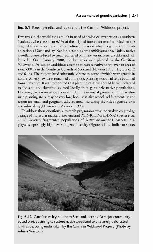
Assessment of genetic variation | 271

Box 6.1 Forest genetics and restoration: the Carrifran Wildwood project.

Few areas in the world are as much in need of ecological restoration as southernScotland, where less than 0.1% of the original forest area remains. Much of theoriginal forest was cleared for agriculture, a process which began with the col-onization of Scotland by Neolithic people some 6000 years ago. Today, nativewoodlands are reduced to small, scattered remnants on inaccessible cliffs and val-ley sides. On 1 January 2000, the first trees were planted by the CarrifranWildwood Project, an ambitious attempt to restore native forest over an area ofsome 600 ha in the Southern Uplands of Scotland (Newton 1998) (Figures 6.12and 6.13). The project faced substantial obstacles, some of which were genetic innature. As very few trees remained on the site, planting stock had to be obtainedfrom elsewhere. It was recognized that planting material should be well adaptedto the site, and therefore sourced locally from genuinely native populations.However, there were serious concerns that the extent of genetic variation withinsuch planting stock may be very low, because native woodland fragments in theregion are small and geographically isolated, increasing the risk of genetic driftand inbreeding (Newton and Ashmole 1998).

To address these questions, a research programme was undertaken employinga range of molecular markers (isozyme and PCR–RFLP of cpDNA) (Bacles et al.2004). Severely fragmented populations of Sorbus aucuparia (Rosaceae) dis-played surprisingly high levels of gene diversity (Figure 6.14), similar to values

Fig. 6.12 Carrifran valley, southern Scotland, scene of a major community-

based project aiming to restore native woodland to a severely deforested

landscape, being undertaken by the Carrifran Wildwood Project. (Photo by

Adrian Newton.)

272 | Reproductive ecology and genetic variation

Fig. 6.13 The first tree planting at Carrifran, on 1 January 2000. The

author and his young son are pictured at the centre of the photograph,

planting a hazel (Corylus avellana) seedling. (Photo by Lynn Davy.)

A

B

C

D

Fig. 6.14 Map of the distribution of four cpDNA haplotypes in sampled

populations of Sorbus aucuparia in the vicinity of the Carrifran Wildwood

Project. Pie chart diameter reflects relative sampling effort in each

population. (From Bacles et al. (2004). Genetic effects of chronic habitat

fragmentation on tree species. Molecular Ecology, 13, 573–584, Blackwell

Publishing.)

from non-fragmented populations in continental Europe, even though the latterwere sampled over a much larger spatial scale. No genetic bottleneck or depar-tures from random mating were detected. The ratio of pollen flow to seed flowbetween fragments was estimated by using these markers, and was found to beclose to 1. Results indicated that reduced gene flow by pollen movement is a likely

Assessment of genetic variation | 273

55

24

20

16

12

8

4

00 10 20 30

Local dispersal within remnants (m)

40 50 60 70 80 90

50

45

Distance (m)

Ob

serv

ed s

eed

dis

per

sal e

vents

(%

)

40

35

30

25

20

15

Foreign dispersal among remnants(m)10

5

00

200400

600800

1000

1200

1400

1600

1800

2000

2200

2400

2600

2800

unkn

own

(a)

(b)

Fig. 6.15 Seed dispersal within and among Fraxinus excelsior remnants in the

area surrounding Carrifran, southern Scotland. (a) Frequency distribution of

effective seed dispersal events within (�3000 m) and outside of the study

area. (b) Close-up on local seed dispersal (�100 m). Effective seed dispersal

events were estimated by means of maximum likelihood parentage analysis.

When a single parent was identified, it was assumed to be the maternal

parent. When a parent pair was identified, the nearest parent was assumed to

be the maternal parent. (From Bacles, C. F. E., Lowe, A. J., and Ennos, R. A.

(2006). Effective seed dispersal across a fragmented landscape. Science, 311,

628. Reprinted with permission from AAAS.)

consequence of habitat fragmentation, but effective seed dispersal by birdsappears to be maintaining high levels of genetic diversity within forest fragments.In a further investigation with the wind-dispersed tree Fraxinus excelsior(Oleaceae), seed dispersal was found to be up to six times more effective thanpollen dispersal at maintaining genetic connectivity among forest remnants(Bacles et al. 2006) (Figure 6.15).

A second concern related to how far away from a site seed may be safely col-lected, to avoid the risk of poorly adapted planting stock. To answer this ques-tion, provenance trials would need to be established for native species, toidentify patterns of adaptive variation. Few such trials have been establishedto date. Although seed transfer zones have been proposed, these may be diffi-cult to implement in practice and are based on very inadequate information(Ennos et al. 1998). As an alternative, Ennos (1998) suggested that compar-isons should be made between the ecological characteristics of the plantingsite and those of the planting sources. The planting source most nearly match-ing the planting site should then be chosen.

requires a co-dominant, highly polymorphic marker, such as microsatellites. In thecase of tree species, seed can be collected from a mother tree and analysed, along withthe mother tree itself. Once the genotype of both the mother and progeny have beenestablished, the identity of the father can be determined by comparing the genotypeof the progeny with potential males in the population, once the maternal genotypehas been subtracted. This can be most simply be achieved by locating an individualor cluster of individuals with a unique allele, then examining the distribution of thisallele within progeny arrays from other individuals or in seedling cohorts within thepopulation (Hamrick and Nason 2000). Alternatively information from all availableloci may be used to exclude particular males (Lowe et al. 2004).

If tree seedlings are analysed, rather than seed, then the problem is more diffi-cult, as the identity of both the mother and the father needs to be determined.Organelle markers (such as cpDNA) that are maternally inherited, or tissuesderived from only one parent (such as the pericarp or megagametophyte of plantseeds) can be used to differentiate the genetic contribution of different parents(Lowe et al. 2004). Alternatively, assumptions can be made regarding the spatialposition of the seedling in relation to its putative parents. For example Dow andAshley (1996) assumed that the closest potential parent to an oak seedling must bethe mother, as acorns disperse less readily than oak pollen.

The advantage of direct methods is that information of great value to conserva-tion can be derived, including the fertility or mating success of an individual orpopulation, propagule dispersal frequency between populations or among groupsof trees within a population, and the distance and frequency of propagule disper-sal (Lowe et al. 2004). The main problem is the amount of work involved.Identification of all potential parents of a seed or seedling may require a large num-ber of adults to be sampled and included in the analysis. The spatial location ofputative parents also needs to be recorded. Problems arise when parents fail to beidentified (for example as a result of long-distance pollen or seed dispersal), orwhen several potential parents are identified (when the marker system fails to dif-ferentiate between the actual parent and other individuals).

Molecular markers may also be used to provide estimates of the mating systemof plants. Wright’s fixation index FIS (see above) can be used as indicator ofinbreeding within populations. More frequently, estimates are derived by assessingoutcrossing rates by using co-dominant markers to assess variation within progenyarrays. If only the maternal alleles are present in the progeny, then selfing can beassumed, whereas outcrossing can be inferred if each progeny has a single maternalallele and a second different allele from the father. The total number of allelespresent within a progeny array can itself provide an indication of the extent ofoutcrossing (with more than two alleles present indicating the occurrence ofoutcrossing). In addition, a chi-squared test can be used to compare observedversus expected segregation ratios of alleles within a progeny array (no deviationfrom expected values indicating selfed progeny) (Lowe et al. 2004).

Ritland (1986, 2002) has developed a series of additional measures fordescribing the mating system of a species, based on calculating two estimates of

274 | Reproductive ecology and genetic variation

outcrossing: a single-locus estimate based on the number of non-maternal alleles,the total number of alleles, and their segretation ratios; and a multi-locus estimatebased on multiple or all loci. Computer programs for estimating outcrossing ratesand other mating parameters are available (Ritland 1990), for example MLTR�http://genetics.forestry.ubc.ca/ritl&/programs.html�. An example of a study thatestimated the mating system of a tropical tree (Cordia alliodora) is provided byBoshier et al. (1995). A recent review of research into outcrossing rate and geneflow in neotropical trees is provided by Ward et al. (2005).

Assessing the impacts of anthropogenic disturbance

It is increasingly being recognized that deforestation and forest fragmentation canhave substantial effects on processes influencing genetic variation within treespecies, such as random genetic drift, inbreeding, and gene flow. Recent progressin assessing these effects by using molecular markers is reviewed by Lowe et al.(2005), with respect to neotropical trees. These authors make the following rec-ommendations for such studies:

● Studies over small spatial scales should aim to examine genetic variation bothbefore and after disturbance, include a large number of replications, and beconducted over relatively long timescales, to incorporate descriptions ofannual or seasonal variation.

● Studies should aim to compare a variety of species with contrasting life historycharacteristics within the same landscape that contains populations that varyin size, isolation, and duration of impact. Such studies would highlight whichlife history traits are most important in mitigating genetic resource impacts ofhabitat degradation.

● Sampling should target specific questions, rather than relying on opportunis-tic availability of material, which may compromise experimental design.Large-scale studies, especially for the purpose of developing species-specificconservation recommendations, should sample across the geographical rangeof a species (as generally implemented when undertaking provenance trials forforestry), rather than just a few populations from a restricted area.

● Simulation modelling can enable comparisons to be made between specieswith very different life history traits and between landscapes that haveexperienced very different levels of disturbance. Modelling approaches shouldintegrate population genetics and demographic processes to simulate theimpact of different management scenarios on the genetic make-up of speciesbeing modelled (for example ECO-GENE, Degen et al. 1996).

Further recommendations are provided by Cavers et al. (2005), who consider thepotential impacts of anthropogenic disturbance on the genetic structure of tree popu-lations. Such structure (defined as the non-random distribution of genotypes) mayoccur at a variety of spatial scales, as a result of ecological processes such as dispersal,competition, and succession. Anthropogenic disturbance may affect such structureand influence the regeneration potential and evolutionary viability of populations.

Assessment of genetic variation | 275

Use of highly variable molecular markers (such as microsatellites) has enabled anumber of recent investigation of such structure, most commonly by using spatialautocorrelation methods (Sokal and Oden 1978), comparing patterns of geneticvariation with patterns of spatial distribution. Computer programs are availablefor such analyses (for example Degen et al. 2001). In contrast to population geneticestimators (such as F-statistics, described above), which involve averaging acrosspopulations, spatial autocorrelation analysis uses data from pairs of individuallocations across the sampled area and therefore accesses more of the available infor-mation at the population scale (Cavers et al. 2005). To carry out such analyses, thespatial location of the individual trees must be recorded. The statistical power ofthe technique depends strongly on the sample size and how sampling is done inrelation to the spatial structure of the population. Cavers et al. (2005) make the fol-lowing recommendations for such studies:

● The characteristics of the target species (mating system, seed and pollen dis-persal mechanisms) should be considered when planning the sampling strategyand selecting the molecular marker. For example, species with long-distancedispersal mechanisms (eg wind-dispersed pollen or animal-dispersed seed) areexpected to show little genetic structure within populations; in such cases it islikely to be more efficient to devote greater effort into sampling larger numbersof individuals than increasing the number of markers used. The age structureof the population should also be considered and recorded where possible.

● A mixed sampling strategy is recommended, balancing high density of localsampling with wider scale coverage. At the same time, the sampling strategyshould ensure that sufficient numbers of pairwise comparisons are producedin each distance class to achieve statistical significance (a minimum of 30 pairsper class is recommended; Cavers et al. 2005).

● The sampling effort required (for both individuals and of loci) is much greaterfor AFLP markers than for microsatellite markers. When using microsatellitesit is more effective to increase individual sample numbers than increase num-bers of loci, once 5 loci are available. With 5 loci, 100 individuals should besufficient. When using dominant markers, the number of both loci and indi-viduals required is much higher: at least 100 loci and 150 individuals.However, the sampling scheme required will depend strongly on the particu-lar characteristics of the species studied.

Using molecular marker data to support conservation planning

Molecular marker data may be used to support conservation planning and actionin a number of ways (Frankham et al. 2002, Lowe et al. 2004):

● Defining the taxonomic identity of the species of conservation concern, andwhether hybridization is taking place (see, for example, Rieseberg andSwensen 1996, Robertson et al. 2004).

● Examining the portion of genetic variation within and among populations asa guide to sampling strategies for ex situ conservation, or for defining the

276 | Reproductive ecology and genetic variation

Assessment of genetic variation | 277

extent of variation within ex situ populations (see, for example, Allnutt et al.1998, Ehtisham-Ul-Haq et al. 2001).

● Investigating the influence of evolutionary or biogeographic history onpatterns of genetic variation (see, for example, Allnutt et al. 1999, Bekessyet al. 2002a, Premoli et al. 2002).

● Estimating the extent of gene flow between populations (see, for example,Bacles et al. 2004, 2006, White and Boshier 2000).

● Identifying whether a threatened species or population has lost genetic diver-sity, for example as a result of bottleneck events, population fragmentation(see, for example, Premoli et al. 2003), or overharvesting (see, for example,Gillies et al. 1999).

● Identifying genetically distinctive populations, or the distribution of rarealleles, in order to identify priorities for conservation (see, for example, Bekessyet al. 2002a, Premoli et al. 2001) or management units (Newton et al. 1999a).

● Identifying suitable sources of germplasm for reafforestation or restoration(see Box 6.1).

● Understanding the ecological characteristics of species, for example thebreeding system (Boshier et al. 1995), or the pattern of seed dispersal (Bacleset al. 2004, 2006).

An important application of molecular markers relates to identifying whethergenetic issues, such as inbreeding or genetic drift, are increasing the risk of extinc-tion of a species or population. Similarly, it may be desirable to know whether aprotected area is large enough to support a genetically viable population. Toaddress such issues, genetic information can potentially be incorporated in a PVA(see section 5.3) to forecast the influence of both demographic and genetic factorson extinction risk. Some PVA software programs (such as GAPPS and VORTEX;see Table 5.2) are designed explicitly to achieve this. In practice, however, mostPVA analyses either ignore genetic processes entirely, or consider inbreedingdepression as the only genetic threat (Frankham et al. 2002). To incorporateinbreeding depression in PVA, information is needed on the breeding system ofthe species, the genetic mechanism responsible for inbreeding depression, and itsrelationship to fitness (Frankham et al. 2002). Collecting all of this informationrepresents a substantial challenge, but the advantage of a modelling approach suchas PVA is that various assumptions about genetic effects can potentially beexplored, even if only partial information is available.

How may molecular marker data best be used to support conservation plan-ning? A number of different approaches have been proposed. Evolutionarilysignificant units (ESUs) have been defined as historically isolated populations,which may require separate genetic management (Moritz 1994, 1995). Theprecise definition of the term has been the subject of some discussion, with respectto the genetic criteria adopted and the degree of difference that is considered to be‘significant’ (Vogler and Desalle 1994). Initially the concept was developed foranimals on the basis of differentiation in mitochondrial (mt) DNA, and explicitly

on analysis of the spatial distributions of alleles, taking account of their phylogen-etic relationships (‘molecular phylogeography’) (Moritz 1994). However, themutation rate of mtDNA is significantly lower in plants, and therefore differentcriteria for defining ESUs need to be developed for tree species (Newton et al.1999a). One possibility is to use cpDNA markers, which have been widely used inphylogeographic studies of trees, although the mutation rate of cpDNA is stillrelatively low (Newton et al. 1999). As an illustration, Petit et al. (2003) describecpDNA variation in 22 widespread European trees and shrubs sampled in the sameforests, which revealed that the genetically most diverse populations were locatedat intermediate latitudes, reflecting the mixture of different lineages during post-glacial migration from southern refugia. Such analyses could potentially be used todefine ESUs for multiple species.

The concept of ESUs has been criticized because molecular marker variation isusually selectively neutral, and therefore it ignores patterns of adaptive variation.As an alternative to ESUs, Crandall et al. (2000) suggested that populations beclassified according to whether they show recent or historical ecological or geneticexchangeability. This concept is based on whether gene flow is currently occurringbetween populations, or occurred in the past, and takes into account patterns ofadaptive variation. For example, evidence from differences in life history traits,morphology, habitats, and genetic loci under selection can be used to infer adap-tive differentiation; where this is identified, the hypothesis of ecological exchange-ability can be rejected. Management recommendations are then based on thisassessment. An evaluation of this approach, and the ESU concept overall, is pro-vided by Fraser and Bernatchez (2001).

Other terms that have been proposed include the management unit (MU),defined as a population with significant divergence of allele frequencies at nuclearor mitochondrial loci, regardless of the phylogenetic distinctiveness of the alleles(Moritz 1994). Potentially any molecular marker information, ideally supportedby assessments of adaptive variation, could be used to define a management unit.Another term that has been widely used specifically in relation to forests is generesource management unit (GRMU), which may be defined as an area of landchosen to include a representative sample of the genetic diversity of a species withina particular region, and designated for a particular genetic management objective(Ledig 1988, Millar and Libby 1991). Such GRMUs may form a central part of thegenetic conservation strategy of a species, and may be managed in a particular wayto maintain the genetic characteristics of the population (for example, by prevent-ing timber harvesting or by protecting against the inflow of potentially deleteriousgenes from other populations, perhaps by preventing plantation forestry in thevicinity) (Millar and Libby 1991).

Caution is always required when using molecular evidence as a basis for propos-ing conservation action. All marker systems have limitations, and their differentproperties must be taken into account before the data that they provide can beinterpreted properly. One of the main problems in using molecular marker data to

278 | Reproductive ecology and genetic variation

support conservation planning is that they are generally assumed to be selectivelyneutral. Although differences in molecular markers may be indicative of adaptivedifferentiation between populations, this is usually not the case. Conservationdecisions should be based on knowledge about the pattern of adaptive variationwithin species (Ennos 1996). Techniques by which this information can beobtained are described in the following section.

6.5.2 Quantitative variation

Quantitative genetic variation refers to variation in quantitative characters, or thosecharacters that display continuous variation. Examples include growth rate, stemsize, and form. Genetic variation in quantitative characters is due to the segrega-tion of multiple polymorphic Mendelian loci, referred to as quantitative trait loci(QTL) (Frankham et al. 2002). The most important quantitative traits from a con-servation perspective are those that determine adaptive potential, by influencingreproductive fitness, or the number of fertile offspring produced by an individualthat reach reproductive age (Frankham et al. 2002). The main genetic concernsrelating to conservation of threatened species relate to such quantitative traits, forexample a reduction in reproductive fitness as a result of inbreeding (inbreedingdepression), and loss of evolutionary potential caused by overharvesting or a reduc-tion in population size (Frankham et al. 2002). As noted above, molecular markervariation is often poorly correlated with quantitative measures of variation, yet it isthe latter that are closely related to evolutionary potential. Therefore conservationdecisions should be based primarily on analysis of quantitative traits rather thanmolecular analyses (Ennos 1996). This crucial point appears to be overlooked bymany researchers using molecular markers to study genetic variation (see forexample Schaal et al. 1991, Young et al. 2000).

The assessment of genetic variation in tree species has a long history in forestry.This is illustrated by the review by Langlet (1971) entitled ‘Two hundred years ofgenecology’, a memorable riposte to a prior review by Heslop-Harrison (1964)that described only 40 years of genecology with herbaceous plants (omittingforestry studies altogether). Briggs and Walters (1997) provide a useful introduc-tion to studies of quantitative genetic variation in plants. Reference texts describ-ing techniques used in quantitative forest genetics in greater depth include Adamset al. (1992), White et al. (2002), Young et al. (2000), and Zobel and Talbert(1984), on which this account is based. It is regrettable that forest conservationistsand ecologists have not made greater use of the information generated by suchapproaches, although it is primarily tree species of commercial value that have beenstudied to date.

The simplest method of studying variation in quantitative traits is to comparethe growth and morphology of individuals of a species growing in differentlocations. Most tree species are genetically very variable, and some insights intothis variation can be obtained by measuring morphological characteristics such asleaf size and shape, surface texture of the bark, crown form, stem height, etc., in

Assessment of genetic variation | 279

populations sampled throughout the geographic range of a species (Schaal et al.1991). Such morphological variation may be classified by taxonomists as sub-species or varieties. The problem with this approach is that any variation detectedmay have a purely environmental, rather than genetic, origin. For this reason, aprovenance or progeny test is preferred.

Provenance test

To determine whether variation in the trait of interest has a genetic basis, someform of experiment or growth trial is required. Ecological geneticists or ‘genecolo-gists’ refer to such experiments as common garden experiments, which involve culti-vating plant material sampled from a variety of different locations at the same site(Briggs and Walters 1997). This enables the growth and performance of the plantsto be analysed, and variation that has a genetic basis to be separated from environ-mental variation. Foresters adopt just the same type of approach, but refer to thetrials conducted as provenance or progeny tests.

The term provenance (or geographic race) refers to the geographic area fromwhich the seed or other propagules were obtained (Zobel and Talbert 1984). Manyprovenance tests have been established by forestry agencies and private companies,in many parts of the world. The number of provenances included in such tests maybe very large, reaching into the hundreds. Results of provenance tests are availablethrough the publications of the International Union of Forest ResearchOrganizations (IUFRO, �www.iufro.org� and the FAO �www.fao.org�, as well asforestry journals such as Silvae Genetica, Journal of Forestry, Forest Science, ForestGenetics, Forestry, etc.

Results of provenance tests highlight the high degree of variation that occurswithin many tree species, especially those with wide geographic ranges, wide alti-tudinal ranges, or species with a wide tolerance range of different site conditions(soil type, soil moisture availability, slope, and aspect) (Zobel and Talbert 1984).Another interesting finding from such tests is that variation is often physiologicalrather than morphological. Assessments based on morphology alone may fail todetect the substantial variation that commonly exists in traits relating to survival,growth, and reproduction (Zobel and Talbert 1984). This has clear implicationsfor conservation, because it is these very same traits that determine the evolution-ary or adaptive potential of a population.

Provenance tests are generally established with conventional randomized blockdesigns. Trees of different geographic origin may be established in lines or plots (forexample a 5�5 array), which are assigned a random location within a block.Where plots are used, the outer trees in each plot are usually considered as a borderrow and are not included in the measurements, to reduce the influence of compe-tition with neighbouring trees on the results. The entire block, incorporating all ofthe provenances to be tested, is then replicated repeatedly. At least five replicates areusually included, often many more. The provenance test may be replicated acrossa range of different sites to provide an assessment of genotype�environment

280 | Reproductive ecology and genetic variation

interactions. Typically, the growth and survival of the trees is regularly monitored,and measurements may also be made of other characteristics of interest, such as theincidence of insect damage or disease, the form of the tree, and wood characteris-tics. Data collected in this way can be subjected to analysis of variance (ANOVA),which enables the extent of genetic variation in the traits of interest to beestimated.

Progeny test

The best method to assess the extent of quantitative variation in a tree species is aprogeny test. Pronounced genetic differences are often observed between theprogeny of different parents. This comparison enables the heritability of differenttraits to be estimated (see next section). The simplest method of establishing aprogeny test is to collect seed from selected parents and establish the seedlings in anappropriate experimental design (Figure 6.16). Such offspring are referred to asopen-pollinated or ‘half-sib(ling)’, where only one of the parents is known. Analternative approach is to cross-pollinate trees so that both parents are known,providing ‘full-sib’ progeny. The latter approach provides greater informationabout patterns of inheritance and is widely used in tree breeding programmes

Assessment of genetic variation | 281

Fig. 6.16 A progeny test of Cedrela odorata, established in a nursery in Costa

Rica. Open-pollinated progeny from a variety of different mother trees have been

established in lines of six plants, in a randomized complete block design. The

replicate blocks are orientated perpendicular to the lines featured in the

photograph. Genetic differences in growth and morphology are evident after just

a few months’ growth. (Photo by Adrian Newton.)

(Zobel and Talbert 1984), but the former approach is easier and is more commonlyadopted in studies of ecological genetics.

Trees may be established as single-tree plots, in lines or rows, or in square or rec-tangular plots. Statistically, the single-tree plot is the most efficient, but competitiveeffects between trees can influence the results obtained, and for this reason lines orplots are often preferred. When plots are used, as for provenance tests, the outer treesare considered as a border row and not included in the measurements, to reduce theeffect of competition with neighbouring trees of different genetic origin. However,large numbers of families (� 20) are typically included in progeny tests, and in suchcases the size of the trial can become very large if plots are used. Consequently linesor rows (typically of five or six trees) are generally preferred for this type of test.

Most commonly, progeny tests are established with a randomized complete-block design. Each family or seedlot is represented singly (as an individual tree,line, or plot) within a block, its position within the block being located randomly.The block, incorporating all of the families, is then replicated as many times aspracticable; the statistical power of the design resides in the number of replicateblocks established. Blocking can usefully take account of any environmental vari-ation in the experimental area (soil type, light availability, topography, etc.). Otherexperimental designs, such as latin square, lattice designs, and split-plot designs,are also sometimes used with progeny tests (Zobel and Talbert 1984), althoughtheir analysis may be more complicated. Split-plot designs may be employed whenwhere is interest in comparing variation of families within provenances.

Once the seedlings have been established according to an appropriate design,growth variables of interest (such as growth rate, tree form, or incidence of pestattack) are measured at different time intervals. Data analysis methods aredescribed in the following section.

Heritability

A key concept in quantitative genetics is heritability. This is the proportion of thetotal phenotypic variation observed in a population that can be attributed togenetic differences among individuals, which can be passed on to the next gener-ation. It is therefore the heritability of a character in a population that determinesits evolutionary potential (Frankham et al. 2002).

Two types of heritability are commonly used by forest geneticists. Broad-senseheritability (H2) is the ratio of total genetic variation in a population to the pheno-typic variation, or:

where is genetic variation (or the variance due to the influence of genes) and isthe phenotypic variation (or all of the variance recorded in the trait of interest).Genetic variation can be further divided in to additive ( ) and non-additive ( )components. Additive variance refers to the proportion of the genetic variation due

NA2

A2

G2

H2�

2G

2P

�

2A�

2NA

2A�

2NA�

2E

282 | Reproductive ecology and genetic variation

to the average effects of alleles (Frankham et al. 2002); refers to variation causedby the environment.

Values of H2 can range from 0 to 1, a value of 0 indicating that none of the vari-ation in a population is attributable to genetics. A value of 1 would indicate that allof the variation observed is attributable to genetics.

Narrow-sense heritability (h2) is the ratio of additive genetic variance to totalvariance:

A value of h 2 � 0 would indicate no additive variance, and a value of h2 � 1would indicate no environmental or non-additive variance. Most heritabilityestimates in the forest genetics literature are for h2, because of the interest in thevariation that might be inherited through sexual variation. Broad-sense variabilityis relevant if the species is able to reproduce clonally.

It is important to note that heritability estimates apply only to a particularpopulation growing in a particular environment at a particular time. In otherwords, they are a function of the environment under which the tree species isgrown. Also, estimates of heritability are not without error, and should be inter-preted as a relative indication of genetic influence on a trait (Zobel and Talbert1984). Heritability is generally estimated from the results of a progeny test (but nota provenance test). This can be done by ANOVA. Some statistical programs enablevariance components to be determined individually, which is of great help inestimating heritability. For example the program SAS (�http://support.sas.com�;SAS 2002) has a specific procedure for this (Proc VARCOMP). Examples of heri-tability estimates that have been obtained for tree species for a variety of traits arepresented by Cornelius (1994).

Nursery and glasshouse experiments

Conservation researchers rarely establish provenance or progeny tests, despite theuseful information that can be gained from them, perhaps because of the largeland areas required and the cost of maintaining the trials. However, both types ofexperiment can readily be carried out with tree seedlings under glasshouse ornursery conditions. For example, Bekessy et al. (2002b) established a progeny testunder glasshouse conditions with seedlings of the threatened conifer Araucariaaraucana, and after 21 months’ growth was able to detect genetic differences inallocation of dry mass to roots and in values of carbon isotope ratio (�13C), bothindicators of drought tolerance. The results highlighted the importance of treatingpopulations from either side of the Andes as separate management units in conser-vation planning. Neutral DNA markers (RAPD) failed to detect these adaptivetraits (Bekessy et al. 2003). Similarly, progeny tests with seedlings of the timber treeCedrela odorata established in a nursery detected genetic variation in leaf form andbranching characteristics within a few months’ growth (Newton et al. 1995)(Figure 6.16); these differences were subsequently confirmed in more extensive

h2 �

2A

2P

�

2A

2A�

2NA�

2E

E2

Assessment of genetic variation | 283

field trials (Newton et al. 1999b). In this species, neutral DNA markers (RAPD,AFLP, and cpDNA) have revealed substantial variation between Mesoamericanpopulations, which correlates with patterns of morphological variation, droughttolerance and pest resistance and has been proposed as the basis of defining ESUs(Cavers et al. 2003, 2004, Gillies et al. 1999). Such studies highlight the advantageof combining information from molecular marker studies with assessments ofquantitative genetic variation when producing conservation recommendations.

284 | Reproductive ecology and genetic variation

7Forest as habitat

7.1 Introduction

Forests are, of course, much more than just trees. Much of the challenge relating toforest conservation and management rests in understanding how different inter-ventions, such as the harvesting of trees or the construction of a road, are likely toimpact the other species living there. This requires a clear understanding of thehabitat requirements of the species concerned, but unfortunately this is oftenlacking. Identifying and measuring those characteristics of a forest that determineits habitat value for different groups of organisms remains a key challenge forecological researchers. In practice, managers often have to use proxies or indicatorsof forest condition to assess trends in habitat quality. However, the relationbetween such indicators and the abundance of individual species, or the speciesrichness of different groups, often remains untested.

Many of the techniques used to assess forest habitat are described earlier in thisbook. Typically an assessment of habitat extent, condition or quality is basedprimarily on an assessment of forest extent and spatial distribution (see Chapter 2),vegetation structure and composition (see Chapter 3), and the prevailing disturb-ance regime (see Chapter 4). This chapter presents methods for assessing a series ofhabitat variables that are not covered by previous chapters, including deadwoodvolume, vertical stand structure, characteristics of forest fragments and edgeeffects, and the characteristics of habitat trees. In addition, an account is providedof modelling procedures that are increasingly being used to produce habitat mapsfor individual species. It should be remembered that many species that occur inforests also use or require non-forest habitats, such as grassland, shrubland, mires,lakes, or streams, which may also need to be considered in a comprehensive habitatassessment. Finally some suggestions are presented on how to undertake an assess-ment of forest biodiversity.

7.2 Coarse woody debris

The term coarse woody debris (CWD) refers to a range of different sizes and types ofwoody material that can be found in forests, including logs, snags, chunks of wood,large branches, and coarse roots. The definition of what constitutes coarse, asoppose to fine, woody debris varies between researchers, but a typical minimumdiameter is 2.5 cm (Harmon et al. 1986). CWD is a very important habitat feature,

particularly for fungi, invertebrates, mosses, and lichens, and may also provide sitesfor establishment of tree seedlings and sites for storage of carbon, water, and nutri-ents. Snags are used by many animal species, particularly birds, as sites for nesting,perching, and roosting. The ecology of CWD in temperate forests is reviewed byHarmon et al. (1986). Methods for assessing CWD are described by Harmon et al.(1986) and by Ståhl et al. (2001), on which this account is partly based.

The simplest method to assess the input of CWD from living trees is to deter-mine rates of tree mortality by using permanent sample plots or tagged trees (seeChapter 4). This may underestimate inputs, because large branches and brokentops of trees are not included (Harmon et al. 1986). Input to CWD can also bemeasured on cleared plots, or by marking or mapping pieces present at the begin-ning of the period of observations. Alternatively, historical reconstructions offorest disturbance history can be used to estimate CWD inputs from catastrophicdisturbance events (Henry and Swan 1974, Oliver and Stephens 1977).

When surveying, a distinction is generally made between standing dead trees(snags) and lying dead trees (or downed logs). The species, volume, biomass, decaystatus, number of woody fragments, surface area, and ground cover (projected areaof fragments) are variables that are commonly recorded. Size class distributions anddecay class distributions of wood pieces may be reported, along with descriptions ofspatial patterns of distribution (such as accumulation in riparian environments)and orientation (for example, alignment in relation to slopes and direction ofprevailing wind, an issue that should be borne in mind when sampling).Information on CWD is now routinely collected in many national or other large-scale forest inventories, stimulated by the common inclusion of CWD volume asan indicator of sustainable forest management (see Chapter 8). Simple, subjectiveassessments can be made by visually assessing CWD at locations within a foreststand. However, if there is a need to compare different areas or to monitor changesover time, then more objective methods are prefereable. Note that when measuringCWD, variances tend to be high and therefore a large number of samples is typicallyrequired.

7.2.1 Assessing the volume of a single log or snag

For measurements of CWD volume, it is generally assumed that tree stems arecircular in cross-section. This assumption is often not met, particularly when the logsare heavily decayed, a point that should be remembered when interpreting results.

Three methods are commonly used for volume determination (Ståhl et al.2001):

● Standard volume functions. In many countries, standard functions relatingvolume to tree diameter and height are available for commercially importanttimber tree species. For such species, measurements of dbh and height can beused for estimating volume of the CWD fragment using these functions, ifthe tree is relatively intact. Note that this approach ignores the volume ofstumps.

286 | Forest as habitat

● Sectioning. This involves dividing a tree into a number of sections, thendetermining the volume of each section separately. Total volume is then esti-mated by adding these values together. The method is most easily used for treetrunks that are lying down, although measurements can also be made onstanding trees by using instruments such as the optical relascope (see section3.6.2). The formulae for Huber’s method, Smalian’s method, and Newton’smethod, presented in section 3.7.4, can be used to estimate volume by usingthis approach. Newton’s formula is generally considered to be the most accur-ate and flexible of the three, providing unbiased estimates of volume for acylinder, cone, paraboloid, or neiloid, the most common volumetric forms intrees and logs (Wiant et al. 1992). In cases where only parts of downed logs areincluded in the sample, Huber’s method is simple to implement. In suchcases it may often be sufficient to measure the length of the CWD fragmentincluded in the sample and the diameter at its midpoint. Where entire treesare included, Smalian’s formula can easily be applied. For a tree shorter than30 m, the tree need be divided into no more than five sections. The thickestsections should be made shorter to enhance accuracy of volume estimates. Fortrees with a large number of branches, sectioning can be difficult, so arandomized branch sampling method may need to be used (Gove et al. 2002).

● Taper functions. Taper functions are available for a small number of treespecies, describing the shape of the trunk. In cases where such functions areavailable, the cross-sectional area at any height can be derived by using thefunction and the volume obtained by integrating over the cross-sectional areasup to a certain height.

If pieces of CWD are highly irregular, calculation of volume from length anddiameter measurements can be difficult; in such cases the displacement of watercan be measured instead, by immersing the fragment.

For calculating the volume of standing dead trees, Harmon and Sexton (1996)recommend that the diameter at breast height be measured for intact stems, and thediameters at the base and top be measured for boles that have broken, in addition toheight. For stumps, height should be measured together with either the midpointdiameter, or both the base and top diameters (Harmon and Sexton 1996).

7.2.2 Survey methods for forest stands

Six different survey methods are considered by Ståhl et al. (2001), as describedbelow. These authors consider use of probability sampling approaches for each ofthese methods, using the Horvitz–Thompson (HT) estimation principle. Thegeneral HT formula is:

�

where Æ is an estimator of the population total (Y) of some measured quantity yi, n isthe number of sampled elements, and ui is the inclusion probability of element i.

�n

i�1

yiui

Coarse woody debris | 287

When using this approach, a key issue is how population elements (CWDfragments) close to the boundary of a forest stand are treated. To avoid bias, thesampling approach must ensure that elements close to the boundary receive identicalinclusion probabilities as elements in the interior of a stand. One method widely usedto achieve this is the mirage method (Gregoire 1982), in which a sampling unit (suchas a plot or strip) close to the edge of the stand is ‘reflected’ in the boundary, so thatsome parts of the unit may be measured twice. The method is further discussed byDucey et al. (2001). Alternatively, some sampling units can be laid slightly outsidethe forest stand of interest, but only those population elements lying within the standare measured. For example, the centre of some randomly located sample plots may lieoutside the forest stand, but some part of these plots may lie within the stand; withinthis area all the population elements (CWD fragments) are measured.

Sample plot inventory

Field plots are widely used to survey CWD (see Chapter 3 for details). Plots shouldideally be randomly located, although some studies have employed systematicsampling designs. Circular plots are commonly used, although some researcherssuggest that long, thin rectangular plots may be preferable. Sample plots can bedivided into subplots for measuring the smaller diameter classes of logs and snags.For example, in a chronosequence of Douglas fir stands (from 40 to 900 years),Spies et al. (1988) used a nested plot design, with a 0.05 ha plot for logs, 0.1 haplot for all snags, and a 0.2 ha plot for snags �50 cm dbh and �15 m tall. Linetransects (see later) can be incorporated within plots to sample forest floor CWD.

A key issue is how to treat CWD fragments lying on the plot boundary. Twomethods are used: (1) where a CWD fragment is entirely included in the sample ifa well-defined part of it (for example the butt end of a trunk) is located within theplot, and (2) where only that part of a fragment that lies within a plot is includedwithin the sample. In the latter case, many trees will only be partly sampled; decid-ing how trees should be divided can add to the time required to carry out the survey.The total volume of CWD in the plot can be calculated simply by summing themeasurements of individual fragments recorded within the plot. This measure canbe used to provide an estimate for the entire forest stand by multiplying with anappropriate scaling factor. There is no need to apply the HT formula when usingthis approach. However, in cases where trees are partly sampled by using method(2), this can lead to a severe bias in the estimates obtained. This problem can beovercome by using the appropriate HT estimator, as presented by Ståhl et al. (2001).

Strip surveying

This is also called belt inventory, transect inventory, strip cruising, or strip transect(see section 3.5). Typically, strips of a certain width are located randomly withinthe forest stand, in a random or predetermined direction. Alternatively, strips witha predetermined length and orientation can be randomly distributed within astand. This method is equivalent to using very elongated, rectangular sample plots.

288 | Forest as habitat

Strips may also be laid out systematically to traverse the entire stand, with aconstant spacing between them.

Line intercept (or intersect) sampling

In this method, all CWD fragments crossed by an inventory line are sampled. Theprobability that an object is included in the sample is proportional to the length orwidth of the object. An estimate of the total length of CWD fragments can thereforebe obtained simply by counting the number of intersections. The method is only use-ful for downed logs, not for standing dead trees. As with strip plots, the transect linesmay be laid out as segments with a particular spacing and orientation, or traverse theentire forest stand under investigation. A typical design is illustrated in Figure 7.1.

The method of estimation depends on whether the orientation of the survey linesis fixed or random. Often the orientation of the lines is fixed, and the lines are laidout systematically with spacing L, to traverse the entire stand (Figure 7.1).Following Ståhl et al. (2001), to determine the inclusion probability of a givendowned log according to this sampling design, the width of its projection perpen-dicular to the orientation of the survey line should first be determined. This value isli sin wi, with li being the length of the log and wi the acute angle between the log anda survey line. The estimator of the population total derived from the HT formula is:

�

The following version of the formula (which is a ratio estimator) will generally pro-vide greater precision:

ÆR ��n

i�1

yi

li sin wi

�m

i�1

siA

L �n

i�1

yi

li sin wi

Coarse woody debris | 289

Fig. 7.1 An example of line intercept sampling with survey lines laid out

systematically with spacing L. The short lines represent downed logs and the crosses

on the lines are reference points of the downed logs. The length of a log is denoted liand the width of the projection perpendicular to the survey lines is li sin wi, where wi

is the acute angle between the log and a survey line. (From Ståhl et al. 2001.)

L

Wi

WiSin

li

li*

where A is the stand area, si is the length of the ith survey line, and m is the numberof lines. Alternative estimators for different sampling designs are presented byStåhl et al. (2001).

If measurement of the total volume is of interest, this can be estimated simply byrecording diameter measurements at the point of intersection on each log sampled.In other words, the total volume of downed logs can be estimated simply bywalking along survey lines, measuring the diameter at the point of intersectionwith logs, and recording the total length of the survey lines. In this case the totalvolume of the downed CWD can be estimated as (Ståhl et al. 2001):

�

where diai is the diameter of log i at the point of intersection, A is the stand area, siis the length of the ith survey line, and m is the number of lines. The method worksregardless of how crooked the stems are, although corrections should be made forlogs not lying horizontally. However, this is valid only for the estimation of CWDvolume or total length, not for total number of CWD fragments (Ståhl et al. 2001).

Harmon et al. (1986) present a relatively simple, widely used formula forestimating CWD volume (V) from data collected by using the line-intersectmethod, assuming that the lines are random and that the CWD fragments them-selves are cyclindrical, horizontal and randomly oriented:

where d is the diameter of a CWD fragment and L is the transect length. When Vis in m3, L is in m and d is in cm, the formula becomes:

Where fragments of CWD are not lying horizontally, this volume estimationformula may be amended to:

where a is the secant (reciprocal of cosine) of the tilt angle (away from thehorizontal) of each CWD piece sampled.

Although the line intersect method has been widely used, opinion variesregarding how the technique can best be implemented. A key decision, forexample, is how long the transect lines should be. Harmon and Sexton (1996)considered that transect lengths in many studies have often been tooshort (�100 m), particularly for the larger fraction of forest floor CWD. Therequired transect length will depend on the density of wood pieces within thearea to be surveyed.

V � (1.234/L) � �(d2a)

V � (1.234/L) � �d2

V � (�2/8L) � �d2

�2

8 �n

i�1diai

2

�m

i�1

siA

290 | Forest as habitat

Adaptive cluster sampling

This method is most appropriate for surveying sparse, clustered populations, forexample when CWD is patchily distributed within a forest. In the first stage, a pri-mary sample of plots, strips, lines, or other sampling unit is selected. Whenever anelement is encountered for measurement (i.e. a CWD fragment), a second sub-sampling procedure is carried out. This may involve either sampling all plots (withpredefined locations) in the vicinity, or searching within a fixed radius. This kindof approach is widely used in national forest inventories (see section 3.2).

Point and transect relascope sampling

Gove et al. (1999, 2001) describe a wide-angle relascope, an instrument that canbe used to estimate CWD volume for woody fragments lying on the ground(Figure 7.2). The method is based on horizontal point sampling (HPS), a methodwidely used by foresters for estimating the volumes of standing trees, includingthose that are dead. In HPS, an angle gauge or wedge prism is used to select treesfrom a given point, with a probability proportional to their stem basal areas (Averyand Burkhart 2002). The angle of the gauge used determines the basal area factor(F), such that each tree sampled represents F m2 of basal area per hectare, regardlessof tree size (Gove et al. 2001). For a given sample point in the field, an estimate ofvolume or biomass per unit area is determined by using the formula:

ê � F �n

i�1

ei

kd 2i

Coarse woody debris | 291

(a)

2w

r

v

(b)

Fig. 7.2 (a) An angle gauge, or wide-angle relascope, can easily be constructed

from nylon strapping, painted nails and a straight piece of well-seasoned wood.

(b) The wooden portion of the gauge is shown shaded; the closed circles

represent nails defining twice the width w. The observer’s eye is at the apex of

angle generation �, which is directly over the sample point. The reach, r, is the

distance from the observer’s eye to the instrument. w � r tan (�/2). All CWD

fragments whose length fills the gap between the two nails are included in the

sample. (From Gove et al. 2001. Point relascope sampling: a new way to assess

downed coarse woody debris. Journal of Foresty, 99, 4–11.)

where n is the number of sampled trees, k � 0.000 078 54 (a correction factor), diis stem diameter in cm (therefore kd2 is the basal area in m2), and ei is the quantityof interest for the ith tree. Individual point estimates are then averaged to providean estimate for the whole stand.

Point relascope sampling uses similar methods for estimating the amount ofCWD on the ground. At each sample point, the angle gauge is used to project alarge fixed acute angle originating at the sample point (Figure 7.3). If the length ofthe individual piece of downed CWD appears longer than the width of the pro-jected angle, it is included in the sample. Otherwise, it is not included. The logsthat are included in a sample from a given point represent L square metres of loglength per hectare. The factor L is equivalent to the basal area factor F in traditionalHPS (Gove et al. 1999). Estimates per unit area can be obtained by using the for-mula (Gove et al. 2001):

�

where m is the number of logs sampled, yi is the quantity of interest (volume,biomass, etc.), and li is the length in metres for the ith log in the sample. Ståhl et al.(2001) present further estimators based on the HT formula. Values of L for differ-ent relascope angles (�) are presented by Gove et al. (1999). For example, if� � 45, L � 3501.162 m2 ha–1. The method can be used to estimate the totallength squared of downed logs in an area, by only counting logs. For estimates ofvolume or biomass, additional measurements are required.

Transect relascope sampling uses the same instrument and measurement principleswhile walking along survey lines, taking measurements in all directions from the line.As in line intercept sampling, the total length of logs in a stand can be estimated

L �n

i�1

yi

l i2

292 | Forest as habitat

Fig. 7.3 Examples of point relascope sampling (left) and transect relascope

sampling (right) for assessing CWD on the ground. All CWD elements whose

length fills the gap of the instrument are included in the sample. The short lines

represent downed logs and the crosses on the lines are the reference points of

downed logs. Rays, with the angle of the relascope between them, emanate from

sample points (in point relascope sampling) or survey lines (in transect relascope

sampling) to provide an illustration of what elements would be included, or not

included, in the sample. (From Ståhl et al. (2001). Assessment of coarse woody

debris—a methodological overview. Ecological Bulletins, 49, 57–70.)

easily by counting the number of logs included in the sample and measuring thetotal length of the survey line (Figure 7.3). A ratio estimator appropriate for tran-sect relascope sampling, when survey lines are orientated randomly, is as follows(Ståhl et al. 2001):

ÆR �

Guided transect sampling typically includes two stages. First, wide strips aresampled within the forest stand. Then, these strips are subsampled using priorinformation for determining the route of the surveyor through the strip. A GPSdevice is used to follow the selected route. As in adaptive cluster sampling, a variety of different methods can be used in the second, subsampling phase (Ståhlet al. 2001).

Which of these methods should be used for assessing CWD? According to Ståhlet al. (2001), issues that should be considered when choosing a method includeefficiency, robustness with regard to measurement errors, simplicity, and the com-pleteness of the information obtained (for example, with line intercept sampling,and point and transect relascope sampling, information is obtained only fordowned logs and not standing dead trees). A comparison of these different methodsis presented in Table 7.1, which indicates that strip surveying and line interceptsampling may often provide the best compromise between these different issues.Strip surveying may be preferred because it works well with both standing andlying trees. In areas where the vegetation is dense, it can be difficult to locate andmeasure all pieces of CWD within a plot, and therefore the line intersect methodmay be preferred (Grove 2001). Whichever method is used, measurement errorscan be substantial, and therefore training of surveyors may be required.

�n

i�1

yi

li (1

sin v�2

� cot v)

�m

i�1

siA

Coarse woody debris | 293

Table 7.1 Subjective comparison of different methods for assessing volume of

CWD. After Ståhl et al. (2001).

Sampling method Efficiency Robustness Simplicity

Sample plot inventory – � �Strip surveying � 0 �Line intercept sampling � � 0Adaptive cluster sampling � 0 –Point relascope sampling 0 0 –Transect relascope sampling � – –Guided transect sampling � 0 –

� indicates that the method performs well, 0 indicates intermediate performance, and – indicates that itdoes not perform well.

Ringvall and Ståhl (1999a) note that when CWD is sparsely distributed, plot-based methods tend to produce imprecise estimates. These authors per-formed a field test of the line intersect method with 11 surveyors in 4 coniferousforest stands in northern Sweden. Results indicated relatively little difference in theresults obtained by different surveyors, but identified a negative bias in one standamong the surveyors, probably resulting from a tendency to avoid some logs whenthe latter occur at high density. Despite the possibility of such biases, line intersectmethods have been very widely used for assessments of CWD (Harmon et al.1986). Ringvall and Ståhl (1999b) further compared results obtained by differentsurveyors using the transect relascope sampling technique. Substantial differenceswere recorded between the systematic errors of different surveyors, suggesting thatthis method is not appropriate when there is a particular need for unbiased esti-mates (in long-term monitoring, for example). In a comparison of line-intersect,fixed-area, and point relascope sampling for downed CWD, Jordan et al. (2004)found significant differences among estimates in some stands, indicating that themethods differ in terms of bias. In terms of relative sampling efficiency, point relas-cope sampling displayed time efficiency comparable or superior to that of the othermethods in most stands.

7.2.3 Assessing decay class and wood density

The state of CWD decay is often assessed by classifying CWD pieces into differentdecay classes. Such decay classes refer to the progressive change in solidity,integrity of shape, and characteristics of the log surface that occur as a result of thedecay process (Pyle and Brown 1999). Typically, CWD is placed into three orfive decay classes, but as many as eight or ten have been used. Such classes havebeen defined in a variety of different ways by different investigators (seeTable 7.2). Commonly, classes have been defined on the external characteristics ofthe CWD, such as bark cover; the presence, colour, and abundance of attachedneedles, twigs, and branches; the cover of bryophytes and lichens; species and sizeof fungal sporocarps; the colour, crushability, moisture, and structure of thewood; the type of decay present (brown vs white rot, for example); whether theexposed wood is bleached; whether the log supports itself or has collapsed underits own weight; the age, size, and density of seedlings and saplings growing onthe log; the presence and distribution of roots growing in the wood; and thepresence of various decay processes such as sapwood sloughing (Harmon et al.1986). Multivariate statistical analyses such as cluster analysis can be used as anobjective method to identify decay classes on the basis of measurements of suchvariables.

Other classification systems have been developed for standing dead trees (see,for example, Spies et al. 1988). For example, Fridman and Walheim (2000) used afour-class decay system to categorize both forest floor CWD and snags in Swedishforests, whereas Clark et al. (1998a) recorded the hardness of snags, top condition(intact or broken), and percentage of bark remaining on the stem in a sub-borealspruce forest.

294 | Forest as habitat

Coarse woody debris | 295

Table 7.2 Characteristics of wood in classes used for determining state of decay

of CWD lying on the ground (based on Pyle and Brown 1999, Sollins et al. 1987,

Spetich et al. 1999, and USDA Forest Service 2001; after Woldendorp et al.2002).

Decay class Characteristics

I Most of the bark is presentBranches retain twigsSolid woodFresh woodOriginal colour.

II Some bark may be presentTwigs absentDecay beginning to occur but wood still solidInvading roots are absent.

III Bark is generally absentLog still supports own weightMore extensive decay throughout but structurally soundMoss, herbs, fungal bodies, may be presentSome invading roots may be presentSome termite damage (in warm climates).

IV Log cannot support its own weight, all of log on groundKicked log will cleave into pieces or can be crushedMay be partly solid or some large chunks (sometimes quitehard) still remainBark absentSmall soft blocky piecesBranch stubs rotted down, can be removed by handMoss, herbs, fungal bodies may be presentInvading roots (when present) are throughoutMore extensive termite damage, producing hollows (in warmclimates).

V Soft and powdery (when dry), often just a moundLog does not support own weightDoes not hold original shape, flattened and spread out ongroundMoss, herbs, fungal bodies may be presentInvading roots (when present) are throughoutHollow log from termite damage may have collapsed or be athin shell (in warm climates).

A penetrometer can be used to classify woody fragments according to decay class.This instrument comprises a short, pointed metal rod and a measurement gauge.The penetration depth of the instrument can be used to define decay classes; forexample, Lambert et al. (1980) defined three classes as follows:

● slightly decayed, rod penetrates �0.5 cm● moderately decayed, rod penetrates �0.5 cm to half the length● advanced decay, more than half of the length of the rod can be pushed through

the log.

Measurements of the density of CWD in the various decay classes can beobtained from samples of wood of each class. Such samples can be collected by cutting sections with a pruning saw or chain-saw, if the whole piece is too largeto collect. The volume of the sample can be determined by measuring its dimen-sions, or by measuring the amount of water displaced on immersion (Stewart andBurrows 1994). It may be necessary to place samples in thin plastic bags beforeimmersion, to prevent porous samples from absorbing water (Stewart and Burrows1994, Grove 2001). After the volume has been measured, the dry mass of thesamples is determined by drying in an oven at temperatures of 60–80 C. Samplesshould be dried until they reach constant mass, which may take many days(Lambert et al. 1980, Grove 2001). In the case of large CWD fragments, dry masscan be calculated from a subsample, by first measuring the fresh mass of the entiresample, then measuring both the fresh and the dry mass of the subsample. The drymass of the original fragment can be estimated by multiplying its wet mass by thedry: wet mass ratio of the subsample (Grove 2001).

7.2.4 Estimating decay rate

As decomposition of CWD is usually slow, long time periods are generally requiredin order to accurately measure the decay rate. Alternatively, the length of time thatsnags or logs have been dead can be determined, and changes in volume or densitymeasured over time. The age of logs is difficult to determine, but can be achieved byageing scars left on live trees adjacent to fallen trees, or determining (by ring counts)the age of the oldest seedling established on a fallen tree (which provides a minimumestimate of log age) (Harmon et al. 1986). Records of logging and thinning oper-ations, or records of fire, insect outbreaks, or catastrophic windthrow, can also beused to estimate the age of woody debris. If a variety of fragments of different agesare available, reasonably accurate measurements of decay rate can be obtained bymonitoring decomposition over relatively short periods of time. It is also possible toestimate decay rates from the ratio of CWD input to biomass, in cases where long-term data on tree mortality are available (see, for example, Sollins 1982).

Models can be used to project changes in the availability of CWD over time.The most commonly used model for this purpose is the single-exponential model:

Yt �Y0 e�kt

296 | Forest as habitat

where Y0 is the initial quantity of material, Yt is the amount left after time t, and kis the decay rate constant. Wood density is generally used as the Y variable,although volume or mass can also be used. The times to decompose 50% and 95%of the material (t � 0.5 and t � 0.95 respectively) are often reported. Morecomplex models are also available that take into account the different decay ratesof different fractions of the woody material, and the fact that loss of mass occurs byfragmentation of the woody pieces, as well as by respiration and leaching (Harmonet al. 1986).

7.3 Vertical stand structure

The vertical structure of a forest stand can be defined as the bottom-to-topconfiguration of above-ground vegetation (Brokaw and Lent 1999), and can becharacterized in terms of variation in canopy density; tree size; branching patterns;the distribution of twigs, branches, and leaves; the density of the understorey; andthe presence of snags and fallen trees (Hansen et al. 1991). Methods for measuringsome of these variables are presented elsewhere (see, for example, sections 3.6.2and 3.6.3). Here, further consideration is given specifically to techniques that canbe used to characterize the vertical structure of forest stands in relation to its valueas habitat. The importance of vertical structure for forest biodiversity is reviewedby Brokaw and Lent (1999), and its definition and measurement are reviewed byMcElhinny et al. (2005).

MacArthur and MacArthur (1961) described a measure of foliage height diver-sity (FHD), referring to the arrangement of foliage within different vertical strataof the vegetation canopy. FHD is defined by the relation:

where pi is the proportion of total foliage that lies in the ith of the chosen foliagelayers. This measure was found to be related to a measure of bird species diversity.A number of authors have since used this measure of forest structure, although ithas not always been found to be related to bird diversity (Brokaw and Lent 1999,Fuller 1995) and its relation to diversity of groups other than birds has been littletested. A further problem with the method is that different studies have definedand assessed vertical strata in different ways, raising concerns about the value of theapproach, and hindering comparisons between studies (Erdelen 1984, Fuller1995, Parker and Brown 2000).

Methods can also be used to compare foliage cover of selected tree species indifferent strata (Bebi et al. 2001). Ferris-Kaan et al. (1998) describe a techniquein which a 10 m radius is measured out from the observer, defining an arc 20 macross. The canopy is then subdivided into four vertical height bands (seeFigure 7.4). Four vegetation strata are defined as follows: S1 (field) 10 cm–1.9 min height; S2 (shrub) 2–5 m; S3 (lower canopy) 5.1–15 m; and S4 (upper canopy)

FHD � �� pi ln pi

Vertical stand structure | 297

15.1–20 m (Figure 7.4). The percentage cover of each species within each heightband is estimated visually to the nearest 5%; any plant bisecting the arc is recorded.

This method was deployed in an assessment of the biodiversity of forests in theUK (see section 7.9) by carrying out 16 vertical structure assessments within each1 ha permanent sample plot (Humphrey et al. 2003a). Percentage cover wasexpressed as a mean of the 16 stand structure measures. To convert these covervalues to a unified measure of stand structure, a cover index (CI) was calculated byusing the formula:

where s1–s4 are the values for field, shrub, lower canopy, and upper canopy strata,and numbers refer to the depth of each stratum in metres. The CI therefore rangesin possible values from 0 to 1990 (assuming a maximum cover value of 100% ineach layer) (Humphrey et al. 2003a). Whereas estimates of cover in the under-storey are relatively easy, estimation of cover in the lower and upper canopy levelsis much more difficult. Experience suggests that it is necessary to traverse the 20 marc, making a visual assessment of canopy cover in the horizontal plane directlyabove the observer (Ferris-Kaan et al. 1998).

An alternative approach involves specifying the number of strata, on the basisthat multi-layered stands are likely to offer a greater variety of habitats for species.This is based on the assumption that strata within a canopy can be clearly andconsistently defined. In practice, this assumption is often not met. Parkerand Brown (2000) provide a critical review of the concept of ‘canopy stratifica-tion’ and highlight the fact that the concept has been interpreted and measured

CI � 1.9s1�3s2�10s3�5s4

298 | Forest as habitat

Fig. 7.4 Method for assessing vertical structure of forest stands. (After

Ferris-Kaan et al. 1998. Assessing Structural Diversity in Managed Forests.

Assessment of forest biodiversity for improved forest management, eds.

Bachmann, Köhl, and Paivinnen. Kluwer Academic Publishers, with kind permission

of Springer Science and Business Media.)

10 m 10 m

15 m(up to 20 m)

5–15 m

2–5 m

10 cm–2 m

20 m

20 m

variously by different authors. These authors suggest that, rather than attemptingto describe the arrangement of foliage, it may be more meaningful to character-ize ecological gradients created by the foliage (such as light availability; seesection 4.9).

A number of attempts have been made to develop quantitative measures ofcanopy stratification. Ashton and Hall (1992) defined a stratification index as theratio of plant biomass in the height class with the greatest biomass, to that of theheight class with the least biomass. The index provides a measure that can be com-pared among stands, but does not identify how many strata exist, nor where theyare found in the vertical profile of the stand (Baker and Wilson 2000). Morerecently, Latham et al. (1998) described a quantitative model, TSTRAT, for iden-tifying stratification within stands. The method was developed for assessment oftemperate conifer forests in the north-western USA. The TSTRAT algorithmdefines strata on the basis of an assumption related to a competition cut-off pointamong tree crowns in a given area (Latham et al. 1998). The trees are sorted byheight and crown ratio, and the upper 60% of the tallest tree crown is used as thebasis of inclusion in the first stratum. All trees with heights equal to or greater thanthe lower limit are included in the first stratum. The tallest tree not included in thefirst stratum is then used to define the next stratum, and so on, until all treeshave been classified according to the strata. The method provides a repeatableestimate of the number of strata, based on height and live crown ratio measures.However, Baker and Wilson (2000) suggest that the number of strata may often beoverestimated by this method.

As an alternative, Baker and Wilson (2000) describe a simple technique foridentifying stratification of individual tree crowns, based on comparing sorted treeheights to a moving average of height at the base of the live crown. The methodrequires only measures of the total height (HT) and height to the base of the livecrown (HBLC) for each tree:

1. Sort the trees by HT and HBLC in descending order.2. Beginning with the tallest tree (t1), calculate the mean HBLC (for t1, mean

HBLC � HBLC (t1), for later trees within the same stratum mean HBLC isthe mean HBLC of all preceding trees).

3. Compare the height of the next tallest tree (HT(t2)) plus the constant ofoverlap (ko) to the mean HBLC. (The constant, ko, defines a thresholddistance between the mean HBLC and HT(t2)).

4. If HT(t2) � ko is greater than the mean HBLC, then t2 is in the same stratumas t1. The mean HBLC is recalculated by using t1 and t2.

5. If HT(t2) � ko is less than the mean HBLC, then t2 is in a stratum below t1. The calculation of mean HBLC is re-initialized beginning with t2, ignoringHBLC values from the preceding stratum.

6. The decision rules (steps 4 and 5) are repeated for all trees in the plot.

McElhinny et al. (2005) review the structural indices that have been usedpreviously by researchers, noting that no single index is preferred over others.

Vertical stand structure | 299

These authors present the following guidelines for the development of an index ofstructural complexity:

● Start with a comprehensive set of structural attributes, in which there is ademonstrated association between the attributes and the elements of bio-diversity that are of interest.

● Use a simple mathematical system to construct the index; this facilitates theuse of multiple attributes and interpretation of the index in terms of real standconditions.

● Score attributes relative to the range of values occurring in stands of a compa-rable vegetation community.

● Try different weightings of attributes in the index, adopting those weightingsthat most clearly distinguish between stands.

As noted by McElhinny et al. (2005), the choice of method to use for standstructure characterization should ideally be informed by an understanding of thehabitat requirements of the species of interest. Unfortunately, this information isoften lacking. Brokaw and Lent (1999) describe how the vertical organization offorest vegetation can have a variety of effects on animals and plants, influencing theavailability of food for animals, as well as the arrangements of sites for nesting,resting, perching, basking, and mating. Indirect effects include impacts on micro-climate and the distribution of animal prey. For epiphytic plants, stranglers, andvines, vertical structure can influence the availability of substrate for attachment.Consideration should be given to such mechanisms when choosing which vari-ables to measure when characterizing vertical structure. It may also be difficult toseparate out effects of vertical structure from other variables that can be correlatedwith it, such as tree composition or bark characteristics.

7.4 Forest fragmentation

The fragmentation of forest habitat is widely considered to be one of the main threatsto biodiversity. Methods for assessing the pattern and extent of forest fragmentationare described in section 2.7. Here, approaches for assessing the impact of fragmenta-tion on biodiversity are considered. This account is based on that of Fahrig (2003),who has usefully reviewed the substantial literature that exists on the topic.

First, it is important to differentiate between the effects of habitat loss andfragmentation. Many studies fail to differentiate between these two differentprocesses. It is well established that habitat loss has large, negative effects on bio-diversity. The effects of fragmentation, or the ‘breaking apart’ of habitat, are muchless well defined, but can be either positive or negative. Research intended toexamine the effects of fragmentation should therefore take care to separate out theimpacts of fragmentation and habitat loss, something that has often not beenachieved previously.

Many studies of habitat fragmentation compare some aspect of biodiversity at‘reference’ sites within a continuous landscape to the same aspect(s) of biodiversity

300 | Forest as habitat

at sites within a fragmented landscape (Figure 7.5). This approach has two mainproblems:

● The sample size in such studies is typically only 2 (i.e. one continuous landscape and one fragmented landscape), greatly limiting the statisticalinferences that can be drawn.

● The design does not permit the relation between the degree of habitatfragmentation and the magnitude of effects on biodiversity to be studied, aseach landscape can be in only one of two states, continuous or fragmented.

As noted in section 2.7, many different measures of fragmentation are available,referring to the number, size, shape, and isolation of habitat patches. Many of thesemeasures are strongly related to the amount of habitat as well as the degree offragmentation, so there is a risk that in using these measures the two processesof habitat loss and fragmentation can be confused. Fragmentation measurementsshould be made at the landscape scale, rather than at the scale of individualpatches. When a study is at the patch scale, inferences at the landscape scale are notpossible, because the sample size at the landscape scale is only 1. Therefore studiesshould seek to compare a number of different landscapes, rather than multiplepatches within a single landscape (Figure 7.6).

How can forest fragmentation be measured independently of forest area? Oneapproach is to use statistical methods to control for the amount of habitat. Forexample, Villard et al. (1999), in a study of 33 landscapes, measured the number offorest patches, total length of edge, mean nearest-neighbour distance, and per-centage of forest cover. They then used regression approaches to relate each of thefirst three variables to the extent of forest cover. The residuals of these statisticalmodels were then used as measures of fragmentation, taking into account theirrelations with forest area. Other approaches that have been used by researchersinclude the construction of experimental landscapes to independently control

Forest fragmentation | 301

1 2 3

Time

Fig. 7.5 In the process of forest fragmentation, a large expanse of habitat (black

area) is converted into a smaller number of patches, isolated from each other by a

non-forest matrix (white areas). Time 1 represents a landscape before

fragmentation and times 2 and 3 represent a landscape following fragmentation.

(From Fahrig 2003. Reprinted, with permission, from the Annual Review of

Ecology, Evolution, and Systematics, vol 34 © 2003 by Annual Reviews

www.annualreviews.org.)

habitat amount and fragmentation, and comparison of the response variable inone large patch versus several small patches (keeping the amount of habitatconstant) (Fahrig 2003).

Results from those studies that have successfully managed to differentiate betweenthe effects of habitat loss and fragmentation suggest that the effects of the former arefar more pronounced than the latter. This implies that conservation research shouldfocus on determining the amount of habitat required for conservation of the speciesof concern, and that conservation actions that attempt to minimize fragmentation(for a given habitat amount) may often be ineffectual (Fahrig 2003). However, thereis evidence that forest fragmentation can have significant impacts on biodiversity asa result of edge effects, considered in the following section.

7.5 Edge characteristics and effects

Forested habitats are often distributed as patches within a landscape. The charac-teristics of the edges of such patches, where they meet other habitat or land-covertypes, often differ from those of patch interiors. Characterization of habitat edgeshas become a major theme in ecological research and, in response to thewidespread concern about the impacts of forest fragmentation, has also becomeimportant for practical forest conservation and management. Most investigationsof edges focus on describing ecological patterns, such as changes in abundance of

302 | Forest as habitat

Fig. 7.6 In patch-scale studies (a), each observation represents the information

from a single patch but only one landscape is studied. In landscape-scale studies

(b), each observation represents the information from a single landscape. In this

illustration, four landscapes have been studied. (From Fahrig 2003. Reprinted,

with permission, from the Annual Review of Ecology, Evolution, and Systematics,

vol 34, ©2003 by Annual Reviews www.annualreviews.org.)

Patch-scale study(a) (b)

Patch size

Landscape-scale studyP

op

ulat

ion d

ensi

tyin

pat

ch

Po

pul

atio

n d

ensi

tyin

land

scap

e

Habitat amountin landscape

species with respect to the edge, but edge characteristics may influence a numberof ecological processes such as dispersal, migration, predation, competition, andgene flow. A useful introduction to forest edges is provided by Matlack andLitvaitis (1999).

Variation in forest structure and composition can most readily be assessed byusing plots or transects placed across habitat edges, and by then employing themethods used for assessing these variables described in Chapter 3. Remote sensingmethods such as aerial photographs can also be used to provide descriptions ofedge characteristics. Forest edges can be described by various attributes such aslength, width, shape, vertical, and horizontal structure, density, or interior to edgeboundary. Brändli et al. (1995) describe an assessment procedure for the forestedge that was operationally applied in the second Swiss national forest inventory(NFI). In the Swiss NFI, sample plots are distributed in a systematic grid.Whenever a forest margin lies within 25 m of the centre of a field plot, an assess-ment of the forest margin is conducted. A 50 m line forms the basis for the forestedge assessment. Along the transect, floristic diversity, habitat features (especiallyfor birds and insects), and the aesthetic value for recreational purposes are assessed.

To provide an example of a typical research investigation, the approach used byLópez-Barrera and Newton (2005) for their work in the montane forests ofChiapas, Mexico, is described here in some detail. To describe edge characteristics,transects 80 m long and 10 m wide were established in each of six study sites. Thetransects were established perpendicular to the forest edge, running from the forest(60 m) through the edge into the forest exterior (20 m into the neighbouringgrassland). The choice of transect length was influenced by the scale of hetero-geneity observed within forest fragments and neighbouring forest-free areas, andto avoid the proximity of other nearby edges influencing the results. The edge wasdefined as the line coinciding with the base of bordering mature (� 30 cm dbh)tree stems (following Oosterhoorn and Kappelle 2000). Within each transect, allthe woody plants were counted and measured, to provide an assessment of standstructure and composition.

This investigation was also designed to examine the effects of edge contrast: thedifference between ‘hard’ forest edges, defined as those where adjacent vegetationhas a simple homogeneous structure, thus creating a sharp contrast with adjacentforest cover, and ‘soft’ edges, which where characterized by more structurallycomplex successional vegetation maintained for 15–20 m from forest edges(Figure 7.7). Particular care was taken in this study to establish genuinely inde-pendent replicates, for example by establishing transects across edges of six differentforest fragments. Lack of replication, or pseudoreplication, is a feature of many edgestudies.

Once the edge characteristics have been described, typically an investigationalso examines the distribution or behaviour of species across the edges, or someparticular ecological process (Figure 7.8). For example, López-Barrera et al.(2005, 2006a, b) describe the effects of different forest edge types on seed dis-persal, predation, and germination and seedling establishment in relation

Edge characteristics and effects | 303

304 | Forest as habitat

(b)

(a)

Fig. 7.7 Vegetation may differ in mean height and density across edges, leading to

edges with different characteristics. For example, ‘soft’ (low-contrast) edges (a)

may be differentiated from ‘hard’ (high-contrast) edges (b). The degree of edge

contrast may affect the permeability of the edge to flows of energy, material and

organisms (Ries et al. 2004). Edges may also be classified with respect to whether

they are ‘open’ or ‘closed’. A recently formed edge may be relatively permeable

(‘open’), but with time may become ‘closed’ as a result of regrowth of vegetation

(Matlack and Litvaitis 1999).

to plant–animal interactions and the dynamics of forest patches within thelandscape.

A thorough review of recent ecological research into habitat edges is provided byRies et al. (2004), who highlight the following methodological points:

● Edges are generally defined as boundaries between distinct patch types, so theidentification of edges depends on how patches are defined within a land-scape. Patch definition can occur at a variety of scales, and obviously varieswith the characteristics of the study area.

● Studies of edge effects in which the variables that determine organismabundance are assessed are much more powerful than purely correlationalstudies, but they are relatively rare in the scientific literature.

● Most edge studies have low replication, few distance categories, and little pen-etration into patches, and this limits their ability to detect responses.

Little progress has been made in extrapolating responses measured at local scales tolarger scales, despite the value of the latter to management and conservation strate-gies. Two models are available for ‘scaling up’ edge responses to the landscape scale:the core area model (Laurance and Yensen 1991) and the effective area model (Sisket al. 1997). Core area models use an estimated distance of edge influence to deter-mine the amount of habitat in a patch that is not affected by edges (the core area); thisapproach is often used when considering reserve designs. In situations where mostcore habitat has already disappeared, the effective area model may be preferred. Thismethod describes density (or other variables) as a function of distance from edge,allowing quantitative predictions of distributions to be made for an entire landscape.

It is important to determine the distance that edge effects extend into habitatpatches. This value is often referred to as the depth of edge influence (DEI). In manyinvestigations, DEI is determined by visual inspection, and results are influencedby study design (for example, the length of survey transects and the number of dis-tance categories). Robust methods for analysis of DEI including use of appropriatestatistical analyses are described by Cadenasso et al. (1997), Fraver (1994), Harperand MacDonald (2001), Laurance et al. (1998b), Mancke and Gavin (2000), andToms and Lesperance (2003). Abiotic and plant responses are generally reported toextend up to 50 m into patches, invertebrate responses up to 100 m, and birdresponses 50–200 m.

Edge characteristics and effects | 305

Fig. 7.8 Three classes of ecological edge responses with respect to distance

from the closest habitat edge. Responses are generally categorized as

(a) positive edge responses, where the variable of interest increases near the

edge; (b) neutral responses, where there is no pattern with respect to the edge;

and (c) negative responses, where the variable decreases near the edge.

(From Ries et al. 2004. Reprinted, with permission, from the Annual Review of

Ecology, Evolution, and Systematics, vol 35 © 2004 by Annual Reviews

www.annualreviews.org.)

Positive edgeresponse

Neutral edgeresponse

Negative edgeresponse

Res

po

nse

var

iab

le

Distance to edge

(a) (b) (c)

Most studies ignore the potential effect of being near more than one edge. Lineardistance to the closest edge is generally used as the main explanatory variable, andtherefore care should be taken to avoid placing plots near corners or other convergingedge types, to limit their potential influence. It is possible that edge responses aredifferent near multiple edges, or where edges converge, but these aspects haverarely been examined.

Ideally, the effect of edges on population dynamics should be examined byassessing the key parameters that ultimately determine distributions (birth, death,immigration and emigration rates), but few studies have achieved this to date.Many studies have measured community changes near edges, with the most com-mon result being an increase in species diversity, but the causes and implications ofsuch changes in diversity near edges often remain unclear.

Ries et al. (2004) also provide a mechanistic model to provide a framework foredge studies (see Figure 7.9).

306 | Forest as habitat

Fig. 7.9 A mechanistic model describing how the distributions of organisms are

altered near habitat edges. Patterns in the abiotic environment, organism

distributions, and community structure (boxes) are influenced by four principal

mechanisms (ovals). Ecological flows of energy, material, and organisms across the

edge influence the abiotic environment as well as organism distributions.

Organisms map onto changes in the distribution of their resources. Changes in

species’ distributions near edges can lead to novel species interactions that can

further influence abundance and distributions. All these changes in species

distribution lead to altered community structure near edges. (From Ries et al.2004. Reprinted, with permission, from the Annual Review of Ecology, Evolution,

and Systematics, vol 35 © 2004 by Annual Reviews www.annualreviews.org.)

Influence of adjacent habitat

RM: Resource mapping SI: Species interactions

Pattern

Abioticenvironment

Mechanism

Ecological flows

• Energy• Materials• Organisms

Sessile organismdistributions

New communityat the edge

RM SI

Mobile animaldistributions

RM SIRM RM

SI

RM

Access

7.6 Habitat trees

The shape or form of a tree can have a major influence its ability to provide suitablehabitat for other organisms. For example, the shape of the stem can influence theavailability of suitable substrate for epiphytes, and the size, distribution, andorientation of branches affects the provision of nesting sites for birds andmammals, as well as the availability of suitable microsites for lichens, mosses, and invertebrates living on the surface of the tree.

Foresters have developed a range of methods for assessing stem form, primarilybecause of its importance for determining timber quality and value. A variety ofform factors, form quotients, curves and formulae have been developed to describestem form to provide accurate estimates of stem volume; these are described byHusch et al. (2003). For example, the cylindrical form factor fc may be describedby the equation:

where V is the volume of tree (in cubic units), g is the cross-sectional area of a cylin-der whose diameter equals tree dbh, and h is the height of cylinder whose heightequals tree height. A form quotient is the ratio of diameter at some height abovebreast height to dbh. However, these methods have limited value for describingthe characteristics of tree form relevant to provision of habitat, being designedprimarily for assessment of timber value.

In the UK during the 1990s, a conservation campaign was developed focusingon ‘veteran’ trees, which may be defined as ‘trees that are of interest biologically,culturally or aesthetically because of their age, size or condition’ (Read 2000). It isimportant to note that this concept embraces trees that are of particular cultural oraesthetic value, as well as habitat value. An international conservation initiative hasalso been developed focusing on ‘ancient’ trees (i.e. individuals of a relatively advan-ced age for the species concerned) by the Ancient Tree Forum �www.woodland-trust.org.uk/ancient-tree-forum/atfaboutus/vision.htm�. Veteran and ancient treesshare many characteristics and are considered to be synonymous by some authors,although some trees of relatively young age can display ‘veteran’ characteristics (forexample, if they have grown in an open environment).

In practice, surveys of veteran or ancient trees tend to focus on those character-istics that confer habitat value (Figure 7.10), such as (Read 2000):

● decay holes, hollows, or cavities, which can develop through limb loss andbark wounds and are expanded by microorganisms and invertebrates

● rot sites, where wood has been colonized by decay fungi● dead wood, including dead limbs or trunk sections, often colonized by decay

fungi with fallen and attached dead wood supporting a different suite ofspecies

● hollowing in the trunk or major limbs● naturally forming water pools● physical damage to the trunk

fc �V /gh

Habitat trees | 307

● bark loss/loose bark● sap runs● crevices in the bark, under branches, or in the root plate.

The presence of hollows or cavities is a particularly important characteristicinfluencing the value of a tree as habitat for wildlife. As an illustration, up to 40%of the bird species of North American forests nest in cavities (McComb andLindenmayer 1999), and in Australia some 300 vertebrate species use tree hollowsfor nesting, roosting, or shelter (Gibbons et al. 2002). Factors such as the size andshape of the entrance, and the depth and degree of insulation of the hollow, canaffect the frequency and seasonality of use. Some cavities can be difficult forhuman observers to detect, because many species prefer hollows with smallentrances. Sites used by bats, lizards, and invertebrates may not be cavities withintree trunks, but small spaces between the bark and the wood.

Gibbons et al. (2002) describe a survey of the types of hollow, and types of hol-low-bearing tree, used by vertebrate fauna in the temperate eucalypt forests ofsouth-eastern Australia. Individual trees were sampled by walking along randomlyoriented transects. Trees felled during silvicultural operations were examined foroccupancy of hollows by animals. Hollows were defined as having a minimumentrance width of 2 cm, a minimum depth of 5 cm, and a minimum height aboveground of 3 m. In this investigation, the following variables were measured to char-acterize the hollows (Gibbons et al. 2002):

● minimum entrance width (the smallest dimension of the entrance to the hollow)● minimum width at half depth (the smallest internal dimension of the hollow

at half depth)

308 | Forest as habitat

Fungal growth on limb

Major deadwood

Weak fork with included bark

Delamination of wood

Subsiding major limb

Suspended broken limb

Bark with fungal infection

Branches reaching ground

Root damage from browsingBasal cavity Rot hole in trunk

Fallen limb

Fungal colonization of root

Bracket fungi and other fungal fruiting bodies

Old wound with scar tissue and loose bark

Established sap run

Water-filled rot hole

Woodpecker hole

Lightning strike

Crown limb—large cavity

Upper crown limb—small cavities

Snag/stub

Tree alive and growing

Fig. 7.10 Habitat characteristics of a ‘veteran’ or ancient tree. (From Read 2000.)

● depth (distance from the base of the entrance to the bottom of the hollow)● branch diameter (branch diameter measured half way between the entrance

and base of the hollow)● branch order (assigned by using an opposite ordering system, where the main

stem is first-order, primary branches are second-order, etc.)● branch health (assigned to one of three classes: living, part dead, dead)● height (distance from hollow entrance to the base of the tree)● occupation (whether the hollow showed signs of being occupied or not)● species occupying hollow (determined from hair, feathers, scats, nesting

material, or pellets).

Gibbons et al. (2002) noted that the use of hollow-bearing trees by fauna wasassociated primarily with the number of hollows in the tree, a result supported byother studies, suggesting that counts of the number of hollows should be made insuch surveys. Tree diameter (dbh) was also found to be related to use of hollows,reflecting the larger number and size of cavities in older and larger trees. Othervariables that might usefully be recorded include signs of physiological weakness(such as dead branches in the crown), the characteristics of vegetation surroundingthe hollow-bearing tree, and the position of the tree in the landscape (Sedgeley andO’Donnell 1999). With respect to the last, Rhodes et al. (2006) applied networkanalysis methods to patterns of use of habitat trees by bats, an approach that clearlymerits further consideration.

Working in the eucalypt forests of south-eastern Australia, Lindenmayer et al.(2000) examined the relations between the number, size and type of cavities in sixtree species and tree diameter and height. Binoculars were used to survey the trees.Seven forms of cavity were recognized by these authors, reflecting both the locationand the type of feature (Figure 7.11). Lindenmayer et al. (2000) recognize theproblem of classifying cavities in standing trees from observations made fromground level; it is possible that some cavities may be ‘blind’ and not extend very farinto the tree. This can only be determined by measuring the cavities directly, byeither climbing the tree or felling it and dissecting it with a chainsaw, which canboth be time-consuming and in the latter case undesirable because of the environ-mental disturbance caused.

Lindenmayer et al. (2000) found that both the number of cavities and cavity sizewere proportional to tree diameter, but inversely proportional to the square root oftree height. This proportionality differed between tree species. This simple relationoffers the possibility of making rapid estimates of cavity abundance across largeareas of forest by measuring simple tree attributes such as tree diameter and treeheight, although whether such relations occur in other forest types remains to betested. Crown shape (classified by visual assessment) was also found to be related tothe abundance of cavities and cavity size, reflecting the fact that crown shapechanges with the age and degree of senesescence of the tree.

Trees continue to be of value as habitat after they have died, and therefore sur-veys of habitat trees should include snags or standing dead trees (see section 7.2).A number of different systems have been developed to classify standing trees

Habitat trees | 309

according to their stage of senescence, death and collapse. For example, Maser et al.(1979) defined nine classes from a living tree to a decomposed stump (seeFigure 7.12). In contrast Spetich et al. (1999) defined four decay classes for stand-ing dead trees, namely:

I recently dead: branches and twigs present; bark intact and tight on boleII bark loose and/or partly absent; large branches present, much of crown

broken; bole still standing and firmIII large branch stubs may be present; top may have broken; bark generally

absent; bole still standing but decayedIV branches and crown absent; bark absent; broken top; wood is heavily

decayed or hollow.

Habitat features such as the presence of cavities or hollows can continue to beused after death of the tree, and therefore should be included in field surveys.

A number of methods are available that can be used to assess the decay status oftrees (see Bucur 2003 for details). These are widely used by arboriculturalists toassess the risks of treefall and collapse. Simple techniques include sounding the treeby hitting it sharply with a hammer or mallet, increment boring (see section 3.6.1),

310 | Forest as habitat

Fig. 7.11 Different types of tree cavity identified by Lindenmayer et al. (2000).

Fissures are long, narrow cracks in the main trunk, branch-end hollows are located

at the end of lateral branches, and bayonet hollows occur in the upper limbs of

trees with an opening that is vertical or at a slight angle to vertical. (Reprinted

from Biodiversity in Britain’s Planted Forests. The Biodiversity assessment project:

objectives, site selection, and survey methods, Lindenmayer et al. pp 11–18,

(2003) with permission from Elsevier.)

Trunk top Branch end

Branch middle

Fissure

Butt hollow

Bayonet

Trunk main

Hab

itat tre

es

|3

11

Fig. 7.12 Decay class of snags and logs, based on assessment of forests in the Pacific Northwest of the USA. (From Hunter

(1999). Maintaining biodiversity in forest ecosystems, Cambridge University Press. Originally after Maser et al. 1979.)

Stage 1Live

Stage 2Declining

Stage 3 Dead

Stage 4 Loose bark

Stage 5 Clean

Stage 6 Broken

Stage 7 Decomposed

Stage 8 Down material

Stage 9Stump

Log decompositionClass 1

Log decompositionClass 2

Log decompositionClass 3

Log decompositionClass 4

Log decompositionClass 5

and using a cordless drill with a long bit to determine the pattern of decay withinthe trunk. Other options include a shigometer, which delivers a pulsed electriccurrent to the wood tissue and measures tissue resistance to the current (Butin1995). The electrodes are inserted into a narrow hole drilled towards the centre ofthe stem (Shortle and Smith 1987). An alternative method is impedance tomogra-phy, which provides a non-destructive method of assessing stem resistivity (Weihset al. 1999), although a large number of sensors is required and the approach istime-consuming (Larsson et al. 2004). Other non-invasive techniques are based onX-ray tomography, microwave scanning, magnetic resonance imaging, and acousticalmethods (Larsson et al. 2004). Another instrument developed recently is the TreeRadar Unit (TRU) radar imaging system �www.treeradar.com/�, which createsa high-resolution, non-invasive image of the internal structure of a tree by using anovel application of ground-penetrating radar technology. Such methods havebeen used relatively rarely to assess the habitat value of individual trees, but havepotential for this type of application.

McComb and Lindenmayer (1999) provide guidance on how habitat should bemanaged for species that require cavities, snags or logs. A key decision facing suchmanagers relates to the location, number, and characteristics of habitat trees thatshould be retained during management interventions. This is often difficult,because few studies have established relations between the availability of thesehabitat features and animal abundance. Ball et al. (1999) describe a deterministiccomputer model (HOLSIM) for predicting the long-term dynamics of hollow-bearing trees that occur in a single-species forest stand, providing a planning toolfor forest and wildlife managers. In some cases trees may be deliberately killed toincrease the number of snags or cavity trees, by using methods such as topping thetrees with a chainsaw, girdling, herbicides, or explosives, and artificial cavities havebeen created by excavating holes in live trees (McComb and Lindenmayer 1999).

7.7 Understorey vegetation

The vegetation of the forest understorey can include mosses, lichens and ferns, aswell as herbaceous plants and shrubs. Variables that are typically measured include:

● species composition● relative cover by species or species groups● density (number of stems or plants per unit area)● frequency (the proportion of samples in which a species occurs)● abundance (the number of stems or plants per sample)● sizes (height and diameter, particularly for woody plants).

Frequency is based on the presence or absence of a species in sample units (plots,transects, or points) and is defined as the number of times a species is present in agiven number of sample units. To obtain an estimate of frequency, therefore, onlythe presence of a species within a sample unit needs to be noted. Density refers tothe number of plants in a given area. To obtain this measure, all the individuals

312 | Forest as habitat

encountered within the boundary of the sample unit have to be identified andcounted. Determining the number of individuals is complicated where species aremulti-stemmed or clonal; in such cases it may be preferable to count the numberof individual stems or shoots rather than the number of individuals.

Cover is defined as the proportion of the ground surface that is covered by thevegetation, and is usually expressed as a percentage of total ground area. Relativecover is the cover of a particular species expressed as a percentage of total vegetationcover. Cover is a very widely used measure of vegetation, as it enables measures ofdifferent life forms to be expressed in a comparable way. Percentage cover can beestimated by eye, either by creating percentage classes or by using the Domin orBraun–Blanquet scales (Table 7.3). As vegetation is often layered, cover may sumto more than 100%; alternatively, estimates can be produced for each layer sepa-rately (Bullock 1996). The main problem of estimating cover visually is that suchsubjective assessments can be inaccurate, and values produced by differentobservers can be very different. Such biases should be estimated, for example byrepeating assessments, and care should be taken to ensure that different observersuse a consistent approach to estimating cover.

Understorey vegetation is usually assessed by using small fixed-area plots orquadrats. A frame quadrat can be used, which divides an area into smaller subplots(Figure 7.13). Frame quadrats can be constructed from four strips of wood, metal,or rigid plastic that are tied, glued, welded, or bolted together to form a square(Bullock 1996). If relatively large quadrats are used (� 4 m2), use of a frame can bedifficult and instead quadrats can be laid out by using tape measures or rulers, withcorners marked by using posts or pins. Quadrats can be divided into a grid ofsquares or subplots by using string or wire, to facilitate the survey process.

Understorey vegetation | 313

Table 7.3 The Domin and Braun–Blanquet scales used for visual estimation of

plant cover (after Bullock 1996).

Value Cover (%) DominBraun–Blanquet

� � 1 1 individual, with no measurablecover

1 1–5 � 4, with few individuals2 6–25 � 4, with several individuals3 26–50 � 4, with many individuals4 51–75 4–105 76–100 11–256 26–337 34–508 51–759 76–90

10 91–100

Photographic frame quadrats can also be used, where vertical photographs areobtained at a constant height above the ground and a grid is then superimposed onthe image, either by using filter on the camera lens or by overlaying a grid on theprocessed image. The image can be assessed in the same way as a normal framequadrat.

Cover can be estimated visually for the whole quadrat. When gridded quadratsare used, cover can be estimated visually for each grid square, or each grid squarecan be classified as either covered or not covered by a particular species. The coverof the larger plot is then derived by summing the values of the grid squares. Densityis measured by simply counting the total number of individuals of each speciesoccurring within the quadrat; here, the main difficulty is determining whetherthose species lying on the edge of the quadrat should be included or not. Generallythe criterion used is to include only those individuals that are rooted within thequadrat (Bullock 1996). Frequency is calculated as the percentage of quadrats inwhich a particular species is present; in this case, the number of plants in thequadrats is ignored. Alternatively, ‘local frequency’ can be calculated, which is thepercentage of grid squares containing a species, when gridded quadrats are used(Bullock 1996).

The appropriate quadrat size to use depends on the characteristics of the vegeta-tion being surveyed, including the size and spacing of individuals. The followingplot areas have been suggested (Cain and de Oliveira Castro 1959, Bullock 1996):

● mosses, lichens, algae, and small ferns: 0.01–0.25 m2

● herbs, grasses, small seedlings, and low shrubs: 0.25–16 m2

● tall shrubs and low trees: 25–100 m2.

Quadrats of different sizes can be nested within each other to survey differentcomponents of the vegetation. Note that when measuring frequency, the result isinfluenced by quadrat size, and therefore care should be taken when interpreting theresults. Larger quadrat sizes tend to give higher frequency estimates than smallerquadrats. Optimum quadrat sizes can be determined by examining frequency

314 | Forest as habitat

Fig. 7.13 A frame quadrat. (From Husch et al. 2003.)

estimates obtained with different quadrat sizes; further details are provided byGoldsmith et al. (1986).

Alternatively, point quadrats can be constructed from a thin metal rod, sharpenedat the tip (Figure 7.14). Examples of suitable materials are thick-gauge wire,knitting needles, welding rods, or bicycle spokes (Bullock 1996). Diameter shouldbe as narrow as possible (1.5–2 mm). The point quadrat is lowered verticallythrough the vegetation and implanted in the soil, and the species touching thequadrat are recorded. Percentage cover is obtained by dividing the number of pointquadrats for which a particular species is encountered by the total number ofsamples taken, and multiplying by 100. The technique is particularly useful forshort vegetation, but can be laborious for dense vegetation (Bullock 1996). Thismethod can also be applied to vertical photographs, by superimposing a grid ofdots, although this method is unlikely to detect individual plants growing under-neath the canopy of another plant.

Understorey vegetation | 315

(b)

(a)

f f f fs s s s sg

Fig. 7.14 Point quadrats: (a) Point frame with 10 pins. (b) Point frame

intersections illustrating f, first hit on forb; g, first hit on grass; and s, first hit on

soil. (After Husch et al. 2003.)

The line transect or line intercept technique involves measuring the length of atransect that is intercepted by a particular species. The percentage cover of each speciesis estimated as the ratio of interception length to total transect length (Figure 7.15).Alternatively, the number of individual plants touching the transect line can berecorded to give a measure of density. In the point transect technique, points along atransect are established at predetermined intervals and each point is assessed to deter-mine whether or not it is covered by the species present. Percentage cover is estimatedas the number of covered points divided by the total number of points. Frequenciesand densities can also be estimated by using distance methods (see section 3.5.3).

Whichever method is used to assess understorey vegetation, careful attentionmust be paid to the sampling design. It is important that many replicated samplesare taken, which should ideally be located by using random or stratified randomapproaches. Many species have a patchy or clumped distribution, which should betaken into account when sampling (Bullock 1996). Sampling designs andapproaches relevant to the assessment of trees are discussed in section 3.3; the sameprinciples apply to assessment of understorey vegetation.

7.8 Habitat models

Understanding what constitutes suitable habitat for a particular species is of criti-cal importance to conservation management and planning, yet the specific habitatrequirements of many species are poorly understood. Forest managers typicallyrequire habitat maps to support management decisions, and such maps may alsobe required at regional or national scales to inform conservation planning. This

316 | Forest as habitat

Fig. 7.15 Schematic illustration of the line intercept method for assessing the

cover or density of shrubs and trees. The shaded areas represent the canopy

coverage of a shrub or young tree. The measurements li are for cover estimates

(fraction of the line covered by the canopy of this species), and the intercept

distances wi are the maximum perpendicular distance coverage and are used to

estimate the numbers and density of the plants. (From Ecological Methodology,

2nd ed. by Charles J. Krelos. Copyright © 1999 by Addison-Wesley Educational

Publishers, Inc. Reprinted by permission of Pearson Educational, Inc.)

Intercept line

Wi

I i

section focuses on methods that can be used to generate habitat maps from a vari-ety of modelling approaches. The information presented here is drawn largelyfrom Elith and Burgman (2003) and Guisan and Zimmermann (2000).According to the former authors, there are seven main approaches to habitat mod-elling, which are considered separately below. The overall process of habitatmodelling is illustrated in Figure 7.16.

7.8.1 Conceptual models based on expert opinion

The simplest approach to developing a habitat map is to consult relevant experts.These may be members of local communities, naturalists, taxonomists, or ecologicalresearchers familiar with the species of interest. Forest managers or rangers may alsopossess anecdotal or systematically collected information about the distribution orabundance of species of interest. These may be compiled or collated to producepreliminary distribution maps, which can be refined through further discussion.

Habitat models | 317

Fig. 7.16 An illustration of the process of habitat modelling, when two data

sets—one for fitting and one for evaluating the model—are available. Model

evaluation can either be made (a) on the calibration data set by using bootstrap,

cross-validation, or jackknife techniques; or (b) on the independent data set, by

comparing predicted to observed values by using approaches such as ROC curves

for presence–absence models. (Reprinted from Ecological Modelling. Predictive

habitat distribution models in ecology. 135. Guisan and Zimmerman, pp 147–186,

(2000). With permission from Elsevier.)

Descriptive datafrom literature,field knowledge

Sampling design

Quality of the fit

Diagnostictests

Fitted values

3. Calibration

4. Prediction

Predictedvalues

Evatuationtables

2. Statisticalformulation

1. Conceptualmodel

Laboratory experiments(ecophysiology)

Statistical literature,existing models

Evaluationdataset Predictive

power

Calibrationdataset

5. EvaluationModel

The challenges of working with expert knowledge are described in detail byBurgman (2005). Key issues are:

● Who qualifies as an expert? How should the experts be selected? How can acompetent expert be differentiated from an incompetent one? How can theaccuracy of information provided by experts be verified? The answers to thesequestions will depend on the particular circumstances of the study beingundertaken.

● How can information best be elicited from the selected experts? Methods mayinclude questionnaire surveys carried out by mail, email, or telephone, face-to-face individual interviews, structured group interviews aimed at achievingconsensus, and the development and revision of conceptual models.

● How can information from experts be aggregated? One commonly usedapproach is the Delphi technique, which involves calculation of summarystatistics of the information provided (such as medians and interquartileranges) that are then distributed to participants for further comment.

● What should be done when experts disagree? How can uncertainty best becaptured and presented? One approach is to describe such uncertainty byusing subjective probability distributions, with values in a continuous range.A number of analytical procedures are available for combining and analysingsuch distributions, and for weighting the beliefs of different experts (Burgman2005).

Conceptual models may be described as abstractions about how we believe theworld works (Burgman 2005). Such models provide a useful tool for identifyingwhat is known about a site, as well as for eliciting information from experts. Thesimplest form is a diagram that illustrates the key features of the site of interest. Anexample would be a sketch map or block diagram of the site, with key features andprocesses illustrated upon it. Alternatively, influence diagrams can be used to pro-vide a visual representation of the components and dependencies of a system.Different shapes (such as ellipses and rectangles) can be used to represent variables,data, and parameters, which are connected by arrows to indicate causal relationsand dependencies (Figure 7.17). Such diagrams can form the basis of analyticalmodels, using software tools such as Analytica (Lumina Decision Systems,�www.lumina.com�) and Hugin Expert (�www.hugin.com�). Conceptual modelscan readily be produced through a process of discussion with relevant experts, orbased on a review of relevant literature, providing a description of the currentunderstanding of a system. In a conservation context, such approaches can be ofvalue in helping to identify the factors influencing the distribution and abundanceof the species of interest, including threats or reasons for decline (see section 8.4).

The most commonly used type of conceptual model used in habitat mapping is thehabitat suitability index (HSI), which was originally developed by the US Fish andWildlife Service and is now widely used, particularly in the USA. The HSI approachdepends on identifying important components of habitat for the entire life cycle of thetarget species (such as food availability, cover, and breeding requirements), based on

318 | Forest as habitat

the judgement of experts. The quality of habitat is then often assessed by using ascaled index, from 0 (very poor quality) to 1 (excellent/optimum quality), for eachhabitat component or variable of interest. The overall habitat quality can then beexpressed by combining the suitability indices (SI) of the individual components,again usually on a scale of 0–1. The individual SIs can be combined by using anumber of different additive, multiplicative, or logical functions, again deter-mined by expert judgement.

The HSI approach summarizes in a simple way the main environmental factorsthought to influence the occurrence and abundance of wildlife species. The habi-tat maps that are produced represent a form of integrated expert knowledge, andsynthesize subjective interpretation of biological processes (Burgman et al. 2001).

Habitat models | 319

Fig. 7.17 A simple conceptual model. The example depicted is an influence

diagram constructed to inform conservation of a threatened fungus species, which

depends on deadwood as habitat. Different shapes (or nodes) on the diagram

illustrate different kinds of variable. A rectangular node depicts a decision variable,

which the decision-maker can control directly (in this case, harvesting of trees for

timber, and deadwood for fuelwood). The rounded rectangular nodes represent

general variables, which may represent factors or processes that can potentially

be measured. The oval node depicts a chance variable, a variable that is uncertain

and that the decision-maker cannot control directly. The hexagonal node depicts

an objective variable, which represents the desired outcome. The arrows in the

diagram represent influences among the variables; in other words, an arrow from

one variable to another indicates that the value of the first variable directly affects

the value of the second variable. A conceptual model can readily be constructed

as an influence diagram such as this, by consulting relevant experts or scientific

literature about the system of interest. (This example was constructed by using

Analytica software, from Lumina Decision Systems.)

Distance toneighbouringforest stand

Windthrowrisk

Standdensity

Deadwoodvolume

Viablepopulation of

species

Colonizingability ofspecies Nature of

landscape matrix

Intensity ofIntensity oftimberharvest

Harvestingof

deadwoodfor fuel

Distance toneighbouringforest stand

Windthrowrisk

Standdensity

Deadwoodvolume

Viablepopulation of

species

Colonizingability ofspecies Nature of

landscape matrix

Intensity oftimberharvest

Harvestingof

deadwoodfor fuel

However, it should be noted that the maps represent potential habitat rather thanoccupancy, and the accuracy of expert knowledge is often untested as no data areincluded in the model that would allow reliability to be examined (Elith andBurgman 2003). Also, the method does not provide information on populationsizes, trends or the potential responses of species to changes in habitat availability(Morrison et al. 1992). A review of HSI models developed in the USA is providedby Schamberger et al. (1982). Methods for evaluating and improving such modelsare described by Brooks (1997) and Roloff and Kernohan (1999).

An advantage of the HSI approach is that the variables can be easily incorporatedinto GIS, enabling them to be integrated with other data relating to forest inventoryand assessment, and providing forest managers with a tool for evaluating the poten-tial impact of management interventions on wildlife habitat (Donovan et al. 1987).At its simplest level, the technique can be used to estimate the total quantity of suit-able habitat in a landscape. More sophisticated analysis can involve assessment ofthe spatial arrangement of the resulting habitat. This usually achieved by calculat-ing landscape indices or metrics (Diaz 1996, O’Neill et al. 1988; see section 2.7).

7.8.2 Geographic envelopes and spaces

Geographic envelopes are models used to describe and analyse the geographicrange of species. There are several different forms of this kind of model (Elith andBurgman 2003):

● Convex hulls. This refers to the smallest polygon containing all known sites ofa species in which no internal angle exceeds 180; in other words, all the outersurfaces are convex. This approach is recommended by IUCN for estimationof the extent of occurrence of a taxon, which is used in assessment of threat ofextinction according to the IUCN Red List criteria (IUCN 2001). The con-straint of convexity on the outer surface of the polygon results in a coarse levelof resolution, which can produce substantial overestimates of the geographi-cal range of a species.

● �-hull.This is a generalization of the convex hull derived from a Delaunay tri-angulation, constructed from lines joining a set of points constrained so thatno lines overlap. This can provide a more accurate estimate of habitat extent,particularly when the shape of the range is irregular (Rapoport 1982).

● Kernel density estimators. These are non-parametric statistical methods usedfor estimation of home range, but can also be used to estimate the geographi-cal range of a species or population. In this method, a kernel (for example anormal distribution) is placed over each observation point in a sample, andthen density is estimated at evaluation points. The density is the sum of allkernel values at the evaluation point (Elith and Burgman 2003). Specialist sta-tistical programs are available to do this type of analysis (see, for example,Seaman et al. 1998).

These methods are used to estimate geographical ranges of species, usingdistribution data (records of species presence) as input, but are not appropriate for

320 | Forest as habitat

detailed maps of species distributions because the envelopes include many sitesthat are unsuitable for the species. They are generally used to assess distributionpatterns over large areas. All three approaches are sensitive to missing data andspatial errors (Elith and Burgman 2003).

7.8.3 Climatic envelopes

As with hulls, climate envelopes use records of the presence of species at differentlocations, but use climate rather than geographic location to produce habitatmaps. An example of this approach is provided by ANUCLIM, which incorpo-rates two subsystems for making bioclimatic predictions, BIOCLIM and BIOMAP(Busby 1991). Rainfall, temperature, and radiation records are used together withelevation data to construct a climate profile for a particular species, based on thecurrent pattern of distribution. A habitat map can then be produced by consideringeach location with respect to this climate profile. This approach can be imple-mented for any situation as long as appropriate environmental data and distributiondata are available. Generally the method is used to define a region that is climaticallysuitable for a species, which can be used as a target area to search for populations oras an indication of historic extent (Elith and Burgman 2003). It is generally usedover large geographic areas, but tends to include any sites where the species is notactually present within the envelope that is defined. The approach obviously hasparticular value for exploring the potential impacts of climate change on speciesdistributions.

7.8.4 Multivariate association methods

This method defines the habitat of a species by using multivariate statistical analy-ses to relate environmental variables to species presence–absence or abundancedata. The statistical method that is most widely used in this context is canonicalcorrespondence analysis (CCA). Details of this approach are provided by Guisanet al. (1999) and ter Braak (1988). CCA can be done with appropriate softwaresuch as CANOCO (ter Braak and Smilauer 1998; see section 3.10). In thisapproach, the principal ordination axes are constrained to be a linear combinationof environmental descriptors (ter Braak 1988). Generally CCA is applied to datacollected from field plots. Usefully, the method is appropriate for data sets withmany zeros (i.e. absences) (Guisan and Zimmermann 2000). However, themethod is based on a number of assumptions (for example, that species have uni-modal responses to environmental gradients, and species have equal ecological tol-erance and equal maxima along canonical axes) that may often fail to be met inreality, which may invalidate the results (Elith and Burgman 2003).

Examples of the use of multivariate methods to produce habitat maps includeDOMAIN (Carpenter et al. 1993), which is based on measuring environmentalsimilarity between the site of interest and the most similar site for which the speciesis known to be present; again the method requires only presence data for thespecies. The method has proved to be suitable for situations where available distri-bution data are limited (Guisan and Zimmermann 2000). Another example is the

Habitat models | 321

BIOMAPPER software package (Hirzel et al. 2001a). This employs ecologicalniche-factor analysis (ENFA), which differs from CCA in that it considers only onespecies at a time rather than a group of species. Again it has the advantage of onlyrequiring species presence data. ENFA compares the ecogeographical predictordistribution for a presence data set with the predictor distribution of the wholearea, and summarizes all predictors into a few uncorrelated factors that retain mostof the information. These factors include the marginality, which reflects how theenvironmental conditions where the species is found differ from those in the entirearea being considered. The relation between species distribution and these factorsis used to calculate a habitat suitability index and to produce habitat maps (Hirzelet al. 2001b, 2002). The approach has been found to compare favourably withlogistic regression (see later) (Hirzel et al. 2002). The main limitation with thismethod is that it assumes a linear relation between observed variables and under-lying factors, although this can be circumvented to some extent by transformingthe data (Elith and Burgman 2003).

7.8.5 Regression analysis

The most commonly used regression technique for habitat modelling involves theuse of generalized linear models (GLMs). These include standard linear regressionand ANOVA techniques, and all have a response variable (species data), predictors(explanatory variables, such as environmental data), and a function that links thetwo. Regression may involve either a single explanatory variable (simple regression)or a combination (multiple regression). If the response is not linearly related to apredictor, then the latter can be transformed before analysis. When presence–absence data are being analysed, as is often the case with habitat modelling, the formof GLM used is logistic regression, as the data have a binomial distribution. In thiscase the link function is a logit. However, a range of other response variable distri-butions and link functions can be used, such as Poisson and quasi-likelihoodmodels applied to simulated abundance data, and Gaussian models applied toplant abundance data (Elith and Burgman 2003).

Generalized additive models (GAMs) offer an alternative approach, in which oneor more of the functions in a GLM is replaced by a smoothed data-dependentfunction. A variety of different methods of smoothing can be used, the mostcommon of which are splines (cubic b-splines, for example) (Elith and Burgman2003). The main advantage of this technique is that the response is not limited toa parametric function, potentially enabling the fitted response surface to be a closerapproximation to reality.

Regression offers a powerful and widely used tool for habitat modelling,enabling the probability of presence or the abundance of the species to beestimated and predicted for new sites. However, the method requires more thansolely presence data (such as information on absences as well), which can limit itsusefulness (when only herbarium records are available for analysis, for example)(Elith and Burgman 2003). Absence data are often difficult to obtain, requiring

322 | Forest as habitat

a comprehensive and systematic survey of the areas concerned. To overcome thisproblem, some attempts have been made to generate pseudo-absence data fromnon-present sites (see, for example, Zaniewski et al. 2002). The resulting predic-tions are expressed as a relative likelihood of occurrence (Elith and Burgman 2003).

7.8.6 Tree-based methods

The ‘tree’ referred to here is a decision-tree, not the kind of tree you find in a forest!This approach is based on the concept of keys, such as those widely used fortaxonomic identification. The user is guided through a series of steps to arrive at anoutcome. In the case of habitat modelling, a set of decision rules (‘splits’) are createdthat classify presence–absence species data in relation to environmental variables(Elith and Burgman 2003). Automated algorithms are typically used to perform theanalysis, which can be used to provide probabilistic predictions for site occupancy.The method is relatively easy to perform and interpret; however, more than pres-ence-only data are required, and small changes in the data can produce very differ-ent outcomes. ‘Pruning’ techniques can be used to reduce the complexity of the tree,by limiting the number of terminal nodes (Guisan and Zimmermann 2000).

7.8.7 Machine learning methods

These methods employ computers to classify data. This can be achieved by using avariety of different analytical approaches, including genetic algorithms and neuralnetworks. A genetic algorithm is an optimization technique based on a set of logicallearning rules (Elith and Burgman 2003). An example is GARP, a program thatpredicts species distributions from environmental variables by using GIS(Stockwell 1999, Stockwell and Peters 1999). In GARP, the genetic algorithm isused to generate, test, and modify rules for predicting distributions, which arepresented in the form of relative likelihoods of the presence of the species. GARPcan be used with both presence–absence data or presence-only data, although inthe latter case the program creates pseudo-absences. A desktop version of theprogram is available from �www.lifemapper.org/desktopgarp/ �. An example ofthe application of GARP is provided by Peterson et al. (2002), who used themethod to examine the potential impacts of climate change on Mexican fauna.However, Stockman et al. (2006) found that this approach was not suitable forpredicting the spatial distribution of a non-vagile invertebrate. Anderson et al.(2003) provide a detailed account of the technique.

Neural networks identify patterns by learning from a set of input or ‘training’data. Predictions are produced by using non-linear, optimally weighted combina-tions of the original variables (Elith and Burgman 2003). The method has beenwidely used in analysis of remote sensing data (see, for example, Carpenter et al.1999), but has not been extensively used for habitat mapping to date, at least at thespecies level (see, for example, Manel et al. 1999, Olden 2003). The networksthemselves are not easily interpreted; the analytical process is complex and notwidely understood, even by computer scientists (Guisan and Zimmermann 2000).

Habitat models | 323

It is also easy to over-fit models (Moisen and Frescino 2002). Examples of theapplication of neural networks to habitat modelling are provided by Ejrnæs et al.(2002) and Monteil et al. (2005).

In addition to these seven main methods, a number of other techniques havebeen used to model habitat. For example, Bayesian methods (see section 1.2) can beused to predict the probability of a species occuring at a given site with knownenvironmental attributes. This is achieved by combining a priori probabilities ofobserving species or communities with their probabilities of occurrence based onthe value of environmental predictors. A priori probabilities can be based on previ-ous survey results or the literature. Alternatively, GIS can be used to develop simplemodels by using overlays of environmental variables and rules for combining singleprobabilities of occurrence (Guisan and Zimmermann 2000). An alternativeapproach is to use cellular automata (see section 5.5.3), which have been used topredict the impact of climate change on plant distribution (Carey 1996) andto simulate the migration of plants along corridors in fragmented landscapes (vanDorp et al. 1997).

7.8.8 Choosing and using a modelling method

The relative strengths and weaknesses of these different modelling approaches aredescribed in detail by Elith and Burgman (2003) and by Guisan and Zimmermann(2000), who make the following points:

● In general, regression techniques are generally preferred for producingpredictions that differentiate between suitable and unsuitable habitat,although some of the emerging methods (such as neural networks) clearly havepotential. The main limitation of regression approaches is the need for enoughpresence–absence records to provide a sufficiently robust model. Predictionsbased on presence-only records are often limited compared with those devel-oped by using presence–absence data, although the use of pseudo-absencerecords can help overcome this limitation.

● All of the methods require some computing and statistical expertise.Although regression methods and CCA can be complex to implement, theyare supported by an extensive literature and documentation, and powerfulsoftware is available to perform them. The same is not necessarily true forother methods.

● All of the methods produce predictions that can be tested against new data,something that should always be incorporated in modelling investigations.Regression methods and CCA produce statistical estimates of error anddeviance, which provide a useful measure of the extent to which a model fitsthe data.

Generally, models are constructed by using data derived from or displayed inGIS. Typically, species data are georeferenced point locations, and predictions aredeveloped by applying the models to raster (grid) representations of the environ-mental data. The resolution and accuracy of these data is of great importance in

324 | Forest as habitat

producing reliable habitat maps. Ideally, species distribution data should becollected systematically throughout the area of interest, covering the full range ofenvironmental variation within which the species occurs. Some form of stratifiedsampling approach should be adopted. Alternatively, the gradsect approach(Austin and Heyligers 1989, 1991, Gillison and Brewer 1985) can be used, whichinvolves sampling species along transects oriented along environmental gradients.

Similarly, environmental data should ideally be available at fine resolution, anddata are required for all of the variables that are likely to influence distribution ofthe species of interest. Climate and soil data are often available only at low resolu-tion, but digital elevation models (DEM) are often available at relatively highresolution and can be used to derive variables such as slope and aspect.

Particular care is needed when the species is expanding or declining in abun-dance or range size; in such circumstances it may be necessary to include factorssuch as disturbance, dispersal barriers, or successional dynamics to produce usefulhabitat models. Such factors may mean that suitable habitat is not occupied. It isimportant to remember that habitat suitability is not the same as occupancy.

The reliability of habitat models can be evaluated by using statistical approachessuch as the Mann–Whitney statistic, receiver operating characteristic (ROC) curves,and confusion matrices. ROC curves are used to judge the effectiveness of predic-tions for repeated binary decisions (such as present/absent) and are built aroundconfusion matrices that summarize the frequencies of false and true positives andnegative predictions. Further details of these approaches are given by Burgman(2005), Fieldings and Bell (1997), and Manel et al. (1999).

Ideally, the model should be evaluated by using a second set of data, independentof the data set used to build or calibrate the model (see Figure 7.16). If possible, thetwo data sets should originate from two different sampling strategies, such asstratified random sampling and observational surveys. Where insufficient data areavailable for the approach, a single data set can be used to both calibrate andevaluate the model; the latter can be achieved by using cross-validation or jackknifeprocedures.

According to Fahrig (2003), the most important question in biodiversity con-servation is probably ‘How much habitat is enough?’ In other words, conservationof species in a given region requires identifying which species are most vulnerableto habitat loss, and estimating the minimum habitat required for persistence ofeach of these relatively vulnerable species (Fahrig 2003). How can this be deter-mined? One approach is to link the habitat models described in this section withmodels of PVA (see section 5.3), an approach that is receiving increasing interestfrom researchers (Elith and Burgman 2003). Usually, this is achieved by convertinga habitat map to a representation of patches and dispersal pathways. The dynam-ics of populations within patches, together with the rate of movement betweenpatches, can then be modelled. A more abstract approach includes the classicalmetapopulation models (see section 5.5.3), in which only presence or absence in apatch is modelled, rather than dynamics within the patch. A key decision relatingto modelling habitat as patches relates to the spatial scale at which individual pixels

Habitat models | 325

in a habitat map should be coalesced into patches (Elith and Burgman 2003).A lower limit to this is set by the resolution of the maps.

7.9 Assessing forest biodiversity

Effective conservation of biodiversity is dependent on knowing which species arepresent in a particular forest area. However, a comprehensive assessment of biodi-versity, including an inventory of all species present, is difficult. Hunter (1999)suggests that no one has completed a complete inventory for even a single forestecosystem, and they are unlikely to do so any time soon, primarily because of thedifficulties of sampling and identifying microorganisms. Surveys of other megadi-verse groups, such as invertebrates and fungi, also present a significant challenge.

Methods for assessing plant diversity are described in previous chapters. Adetailed description of methods for surveying other groups of organisms is beyondthe scope of this book. Instead, the reader is referred to other publications in thisseries; for example, Sutherland et al. (2004) provide a detailed account of methodsfor surveying birds. Other practical handbooks for surveying different componentsof biodiversity are provided by Hill et al. (2005), Jermy et al. (1995), and Sutherland(1996). The publication by Jermy et al. (1995) is accompanied by a set of fieldguides. In addition, Feinsinger (2001) provides a useful introduction to field tech-niques for biodiversity conservation. A brief overview of some recent approaches toassessing biodiversity is presented in Box 7.1. Examples of different approaches toassessing forest biodiversity are provided by Bachmann et al. (1998) and Angelstamet al. (2004b), although these publications focus primarily on temperate and borealforests.

326 | Forest as habitat

Box 7.1 Biodiversity assessment approaches

An abundance of information exists relating to biodiversity within individualcountries. Sources include expedition reports, natural history society journals,field study reports, impact assessment documents, taxonomic reviews of particulargroups or organisms or areas, museum and herbarium specimen labels and cata-logues, forest inventories, etc. A number of countries have established nationalcentres for biodiversity assessment and information management, such as INBIOin Costa Rica and CONABIO in Mexico, and these institutions are now impor-tant information sources themselves. Although an enormous body of pertinentinformation exists, considerable effort is required to create harmonized sets ofdata that can be readily analysed, and used as a basis for presentation of informa-tion to a non-technical audience. Many data, often collected with difficulty andat great expense, remain entirely in specialized and technical literature and havenever been applied to practical biodiversity conservation and forest management.The collation, integration, and analysis of patchy, inadequate data is one of themost significant challenges to biodiversity assessment, at any scale. This reflectsthe fact that relatively few systematic surveys of biodiversity are currently being

Assessing forest biodiversity | 327

undertaken; most information is collected on an ad hoc or opportunistic basis.Consultation with national and international experts is often an explicit andintegral part of the data compilation process. Once data have been compiled,priorities for conservation or further data collection can be identified. The collec-tion of new data is generally achieved through some form of field survey, whichmay be supported by the use of remote sensing techniques (see, for example,Nagendra 2001, Nagendra and Gadgil 1999).

In recent years, a number of different approaches to assessing biodiversity havebeen developed, some of which are briefly outlined below. These examples includeassessments that have been applied at both national and subnational levels, often toidentify priority areas for conservation (i.e. those areas of high species diversity orpossessing large numbers of restricted-range or threatened species). The examplesgiven here differ in terms of scope and objectives, as well as depth of coverage.

Gap analysis �http://gapanalysis.nbii.gov/ �Originally developed by US Fish and Wildlife Service and now widely imple-mented in the USA, gap analysis is used to identify gaps in the representation ofbiodiversity within reserves (i.e. areas managed solely or primarily for the purposeof biodiversity conservation). Once identified, such gaps can potentially beaddressed through the creation of new reserves, changes in the designationof existing reserves, or changes in management practices. Gaps in the protectionof biodiversity can be identified by superimposing relevant data layers in GIS, andanalyses at local, regional, or national scales. Gap analysis therefore aims to giveland managers and policy-makers the information they need to make better-informed decisions when identifying priority areas for conservation. Furtherinformation and a handbook are available from the website given above.

BioRAP: for rapid assessment of biological diversity�www.amonline.net.au/systematics/faith5.htm#introduction�The BioRap Toolbox consists of a set of analytical tools that can be used to iden-tify, with high spatial resolution, priority areas for the conservation and sustainablemanagement of biodiversity. These tools were developed by the AustralianMuseum, CSIRO and other partners, initially for application in Papua NewGuinea. The principal components of the BioRap Toolbox are spatial modellingtools and classification and biodiversity-priority setting tools. These tools supporthigh-spatial-resolution biodiversity assessments that are readily integrated withexisting spatially distributed planning information, as was available for PapuaNew Guinea in the form of PNGRIS, the Papua New Guinea ResourceInformation System. Further, the BioRap approach introduces socioeconomicfactors along with biodiversity at the earliest stage of analysis. Further informa-tion is provided by Faith et al. (2001) and Nix et al. (2000).

World Bank toolkit �www.worldbank.org/biodiversity�This set of documents summarizes best practice in treatment of biodiversitywithin an environmental assessment, with a particular focus on determining thepotential impacts of development projects.

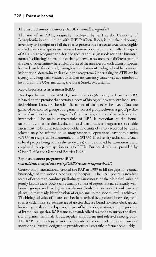
328 | Forest as habitat

All taxa biodiversity inventory (ATBI) �www.dlia.org/atbi/ �The aim of an ABTI, originally developed by staff at the University ofPennsylvania in conjunction with INBIO (Costa Rica), is to make a thoroughinventory or description of all the species present in a particular area, using highlytrained taxonomic specialists recruited internationally and nationally. The goalsof ATBI are to recognize and describe species and assign stable scientific binomialnames (facilitating information exchange between researchers in different parts ofthe world); determine where at least some of the members of each taxon or specieslive and can be found; and, through accumulation of ecological and behaviouralinformation, determine their role in the ecosystem. Undertaking an ATBI can bea costly and long-term endeavour. Efforts are currently under way at a number oflocations in the USA, including the Great Smoky Mountains.

Rapid biodiversity assessment (RBA)

Developed by researchers at MacQuarie University (Australia) and partners, RBAis based on the premise that certain aspects of biological diversity can be quanti-fied without knowing the scientific names of the species involved. Data aregathered on selected groups of organisms. Several groups, chosen as good ‘predic-tor sets’ or ‘biodiversity surrogates’ of biodiversity, are needed at each locationinventoried. The main characteristic of RBA is reduction of the formaltaxonomic content in the classification and identification of organisms, to enableassessments to be done relatively quickly. The units of variety recorded by such ascheme may be referred to as morphospecies, operational taxonomic units(OTUs) or recognizable taxonomic units (RTUs). Biodiversity technicians (suchas local people living within the study area) can be trained by taxonomists andemployed to separate specimens into RTUs. Further details are provided byOliver (1996) and Oliver and Beattie (1996).

Rapid assessment programme (RAP)�www.biodiversityscience.org/xp/CABS/research/rap/methods/ �Conservation International created the RAP in 1989 to fill the gaps in regionalknowledge of the world’s biodiversity ‘hotspots’. The RAP process assemblesteams of experts to conduct preliminary assessments of the biological value ofpoorly known areas. RAP teams usually consist of experts in taxonomically well-known groups such as higher vertebrates (birds and mammals) and vascularplants, so that ready identification of organisms to the species level is achieved.The biological value of an area can be characterized by species richness, degree ofspecies endemism (i.e. percentage of species that are found nowhere else), specialhabitat types, threatened species, degree of habitat degradation, and the presenceof introduced species. RAP teams use standardized methods to survey the diver-sity of plants, mammals, birds, reptiles, amphibians and selected insect groups.The RAP methodology is not a substitute for more in-depth inventories ormonitoring, but it is designed to provide critical scientific information quickly.

Assessing forest biodiversity | 329

Often, rather than survey all groups of organisms, forest biodiversity is assessedby using indicators. The design and use of such indicators is considered in section8.6. There has been particular interest among both researchers and practitioners incombining biodiversity assessments with standard approaches to forest inventory, anissue that is also considered in the following chapter. An example of a plot-basedmethod for simultaneously assessing a range of different components of biodiversityis described in Box 7.2.

Box 7.2 Example of a method for assessing biodiversity within forest stands:

the Biodiversity Assessment Project of the Forestry Commission, UK

As part of a national research programme to characterize the biodiversity of foreststands in the UK, sample plots were established at a range of sites distributedthroughout the country and surveyed over a 2–4 year period. At each site, mea-surements were made of structural aspects of biodiversity (for example verticalfoliage cover and deadwood), taxa important in ecosystem functioning (forexample fungi), and a range of different groups that make up the ‘compositional’

Standingdeadwood

20 3 10 m plots

Deer assessmentplots 7 3 7 m

(10 per plot on central transects)

Structureassessment

points

Pitfall traps

Malaisetrap

Permanent markets atfour corners of plot

Fallendeadwoodtransects

10 3 10 mmensuration

plots

Nested 2 3 2 mvegetation

quadrat

Treefogging

Fig. 7.18 Sample plot design used to produce an inventory of biodiversity in

forest stands as implemented in the Biodiversity Assessment Project of the

UK Forestry Commission. (After Humphrey et al. 2003a © Crown Copyright.

Reproduced with permission of the Forestry Commission.)

330 | Forest as habitat

aspect of biodiversity (for example higher and lower plants, invertebrates). Plotswere established stands at different stages of development, and in both semi-natural and plantation forests.

Sample plots were established by using the design illustrated in Figure 7.18.Plots were situated in areas selected to minimize internal heterogeneity in termsof stand structure, species composition, topography, and hydrology. The plotswere permanently marked with concrete posts. A standardized system of assess-ment was developed to maximize potential comparisons between measuredattributes and to minimize disturbance during sampling (Table 7.4).

Table 7.4 Summary of variables measured and methods used for assessment ofthe biodiversity of forest stands, as implemented in the Biodiversity AssessmentProject of the UK Forestry Commission (after Humphrey et al. 2003a). Thesemethods were implemented by using the plot design illustrated in Figure 7.18.

Variable of interest Assessment method

Deer Densities estimated from 10 7 � 7 m faecal pelletgroup clearance plots per 1 ha.

Small mammals Live capture/release with paired Longworth traps.

Songbirds Point counts within and adjacent to each 1 haplot, plus territory mapping.

Invertebrates Sampling stratified by ground, subcanopy,canopy strata, and deadwood. Five pitfall trapsper 1 ha, one Malaise trap per 1 ha, one treefogged, deadwood emergence traps.

Bryophytes and lichens Species frequency and abundance estimates on growing on pieces individuals growing on deadwood. of deadwood

Macrofungi Frequency and abundance of sporocarps recorded 3 times yearly over 4 years in each mensuration plot (note that microfungi were not recorded).

Deadwood: fallen (logs), Volume and length of logs recorded on two standing (snags) and diagonal transects by using the line interceptstumps method, volume of snags and stumps recorded in

8 20 � 10 m plots.

Soil microbial 32 soil samples taken from each 1 ha plot, 4 incommunities each mensuration plot.

Ground vegetation Percentage cover and frequency in 2 � 2 m(bryophytes, lichens and quadrats nested within the 8 10 � 10 mvascular plants) mensuration plots.

Soil seed banks One sample per plot bulked from collections ineach mensuration plot.

Assessing forest biodiversity | 331

This example is provided as an illustration of how one group of researchersaddressed the challenge of assessing forest biodiversity at the stand scale; it is notintended to provide a blueprint for other studies. There were some particular dif-ficulties with the chosen design: for example, using faecal pellet counts to esti-mate deer densities is thought not to provide an accurate assessment at the scaleof 1 ha adopted here. The problem of scale is also evident from the songbird data,as bird territories range over a spatial extent much greater than 1 ha. Other prob-lems were encountered with the small-mammal sampling, which was abandonedafter only 1 year owing to excessive costs and logistical difficulties. The assessmentof diverse groups such as fungi and insects was reliant on specialist taxonomicexpertise; the samples collected took far longer to identify than to simply collect,adding significantly to the cost of the project (which was substantial). However,the project is notable for providing a rare example of an attempt to assess multi-ple components of biodiversity simultaneously, and illustrates how this can beachieved in practice. Results of the project are summarized by Humphrey et al.(2003b).

Natural regeneration of Height of all seedlings recorded in 10 randomlyseedlings (�1.3 m located 40 � 40 cm plots within each in height) mensuration plot.

Mensuration Dbh, height to live crown, height of all treeswithin the 8 10 � 10 m plots.

LAI Estimated from light measurements alongtransects with each 1 ha plot (by using ahandheld Decagon sunfleck ceptometer; seesection 3.7.3).

Vertical structure Percentage cover of foliage estimated in fourvertical strata—ground, shrub, lower and uppercanopy layers—at 16 sampling points (see section 7.3).

Soil chemistry and litter One soil pit dug per 1 ha plot and described,chemical analysis of two strata—32 bulkedsamples per strata per 1 ha sample plot. Meanlitter depth ha–1 estimated from 32 randomsamples (4 in each mensuration plot).

Climate variables Obtained from national climate model.

8Towards effective forest conservation

8.1 Introduction

Effective conservation is not achieved simply by following a well-defined scientificmethod or set of protocols. What works well in one area may not work well inanother. As noted in Chapter 1, conservation management is a complex social,economic, and political process, requiring recognition of the values held by differ-ent people and an ability to identify the trade-offs and compromises that need tobe addressed in reaching a practical solution. As it is largely about dealing withpeople, conservation management is more of an art than a science. So what contri-bution can scientific methods make to practical conservation efforts?

Many ecological researchers are very concerned about the current dividebetween conservation science and practice. There is a widespread belief that theeffectiveness of much conservation action could be improved by strengthening thescientific foundation on which it is based, for example by implementing scientificallyrigorous approaches to environmental survey and monitoring, and by selectingmanagement interventions on the basis of the best scientific evidence available.Unfortunately, such evidence is often lacking, partly because the scientificcommunity has traditionally failed to address research questions of direct relevanceto management practice, and partly because the scientific information that is avail-able is often not readily accessible by conservation managers. Although this is nowgradually changing, it is certain that conservation managers are often faced withmaking decisions without access to any reliable scientific information about whatthe potential outcomes of alternative management actions might be.

Are there lessons to be learned from forestry? I believe so. Certainly, how forestryis generally practised provides some interesting contrasts with forest managementthat has purely conservation objectives. There is arguably a much longer traditionof research informing forestry practice than is the case for conservation manage-ment (even if today the distinction between these two disciplines is increasinglybecoming blurred). Foresters have long understood the value of a quantitativeapproach to estimating growth and yield, and the importance of using experimentalevidence from silviculture to inform management practice. The economic value oftimber has prompted substantial investment in the forest sector in many countries,which has supported research, inventory, and monitoring. The technical, financial,and information resources available to many practising foresters are enough tomake any conservation manager deeply envious. It is no coincidence that when it

comes to reporting on the state of the global environment (for example theMillennium Ecosystem Assessment �www.maweb.org/�) the most reliable andcomprehensive statistics are always those relating to estimates of forest cover.Significantly, forestry research has an enviable tradition of being related directly tothe practical problems facing managers, even if the research has traditionallyneglected some areas (such as biodiversity conservation) that should have playeda much greater role in informing management practice in the past.

This chapter provides a brief overview of some techniques that can contributeto more effective forest conservation. The aim here is to identify those approachesthat can help bridge the gap between conservation research and management, andhelp communicate the results of research to those making decisions about howforests are managed. Methods are also presented that can help ensure that man-agement decisions are based on scientifically rigorous information. Inevitably,this chapter is more a reflection of my own personal beliefs and prejudices thanthe others. This reflects the fact there is no single method by which effectiveconservation can be achieved; choice of approach will depend strongly on local cir-cumstances. As everywhere else in this book, the reader is encouraged to criticallyevaluate the methods presented. However, it is in this area of linking scientificmethods with conservation practice that there lies greatest scope for improve-ment, and for identifying new approaches that can make a real difference to forestconservation.

8.2 Approaches to forest conservation

How can a forest be conserved? There are three main approaches:

● protection, through designation and management of some form of pro-tected area

● sustainable forest management, involving sustainable harvesting of forestproducts to provide a source of financial income

● restoration or rehabilitation.

The choice of which approach to adopt will be governed by local socioeconomic,political, and ecological circumstances. These approaches are not mutuallyexclusive: a forest management plan might potentially incorporate elements ofall three.

If the principal goal is biodiversity conservation, designation of a protected areawill always be the preferred approach. Harvesting of forest products may bepreferred if there is a need to generate financial income, beyond the amount thatcan be provided by a protected area (which can be substantial, for example throughtourism revenues). Restoration is appropriate on sites that have been degraded orperhaps deforested entirely. Each of the three approaches is briefly considered here,by referring to methods and information resources that can help ensure effectiveness.In following sections, methods and tools are described that are relevant to theimplementation of all three approaches.

Approaches to forest conservation | 333

8.2.1 Protected areas

The development of protected area networks is widely recognized to be the mostimportant approach for forest conservation. Protected areas range from strictreserves to areas where some degree of harvesting is permitted. IUCN (1994) hasdeveloped a classification system for protected areas that is widely used:

I strict nature reserve/wilderness area: protected area managed mainly forscience of wilderness protection

II national park: protected area managed mainly for ecosystem protection andrecreation

III natural monument: protected area managed mainly for conservation ofspecific natural features

IV habitat/species management area: protected area managed mainly forconservation through management intervention

V protected landscape/seascape: protected area managed mainly for landscape/seascape protection and recreation.

VI managed resource protected area: protected area managed mainly for thesustainable use of natural ecosystems.

This classification system can be difficult to apply in some situations. Forexample, how should sacred groves or watershed protection forests be classified?Guidance on application of the IUCN classification system explicitly to forests,and a consideration of the many different kinds of protected forests that exist, isprovided by Dudley and Phillips (2006).

Although the global forest area designated as protected continues to grow,protected areas are not always successful at preventing losses of biodiversity. Theproblems faced by protected areas are considered in detail by Brandon et al. (1998),through consideration of a series of case studies. Widespread threats include infra-structural development close to reserve boundaries, colonization, and mineralextraction, as well as policy-related issues such as weak government institutions,conflicting policies and resource tenure (Brandon et al. 1998). The extent to whichprotected areas are effective in conserving biodiversity is receiving increasingattention from researchers (see, for example, Bruner et al. 2001, DeFries et al.2005, Román-Cuesta and Martínez-Vilalta 2006). For example, in Nepal,Bajracharya et al. (2005) were able to evaluate the effectiveness of community-based approaches to management of the Annapurna Conservation Area, bycomparing forest structure and composition inside and outside the reserve. Thisinvestigation considered effectiveness in terms of impacts on biodiversity, butother authors have considered effectiveness in terms of the management processand in terms of the coverage of the protected area network (Ervin 2003b).

Protected area management can be envisaged as a cycle of planning, implemen-tation and evaluation, consisting of a series of stages (Hockings et al. 2000,Ervin 2003a) (Figure 8.1). Each of these stages should be assessed as part of anoverall process of evaluation. Tools for this kind of evaluation are provided by

334 | Towards effective forest conservation

Hockings et al. (2000) and by the WWF/World Bank Alliance (the RAPPAMmethodology; Box 8.1). Such evaluations are usually achieved by holding interactiveworkshops in which protected area managers, policy-makers, and other stakeholdersparticipate in evaluating the protected areas, analysing the results, and identifyingsubsequent next steps (Ervin 2003a). RAPPAM provides a series of questionnairesand simple scoring tools to assist in this process.

Other approaches for evaluating the effectiveness of protected areas are describedby Lü et al. (2003) and Pressey et al. (2002). The latter authors applied six measuresto assess the effectiveness to conservation areas in north-eastern New South Wales,Australia, namely: (1) number of conservation areas; (2) total extent of conservationareas; (3) representativeness (the proportion of natural features such as forest typesrepresented in conservation areas), (4) efficiency or representation bias (the extentto which some features are protected above target levels at the expense of others thatremain poorly protected); (5) relative protection of vulnerable areas in public land

Approaches to forest conservation | 335

Fig. 8.1 Proposed assessment and management cycle for protected areas This is

used as a basis of the RAPPAM methodology (see Box 8.1). The stages in the

cycle can include: (a) vision, including goals and objectives, describing what the

programme is trying to achieve; (b) assessment of how context—existing status,

threats, and external factors—affects the ability to achieve the objectives; (c)

assessment of the suitability of planning and design for achieving the objectives;

(d) assessment of the adequacy of resources and inputs for achieving the

objectives; (e) assessment of management processes, and their consistency with

the objectives; (f) assessment of the management outputs, and their adequacy for

achieving objectives; (g) assessment of the actual outcomes, and whether or not

objectives were met; (h) reflection on the system as a whole, including an

assessment of the weakest links and the most important areas for improvement.

(After Hockings et al. 2000 and Ervin 2003a.)

Vision, Goals,

and Objectives

ITERATIVEASSESSMENT

PROCESS

Where are the weak links inthe management cycle?

What do we wantto achieve?

How do externalfactors affect the

objectives?

How well doesplanning achievethe objectives?

Are inputs sufficient forachieving the objectives?

Are management processesconsistent with the objectives?

Are the outputsadequate for achieving

the objectives?

Were the objectivesachieved?

Context and

Status

Planning and

Design

Inputs

Management

Processes

Management

Outputs

Outcomes

Reflection and

Evaluation

336 | Towards effective forest conservation

Box 8.1 Sources of information on effective management of protected areas.

A useful overview is provided by Lockwood et al. (2006).

IUCN Programme on Protected Areas (PPA)�www.iucn.org/themes/wcpa/ppa/programme.htm�Supports the work of the IUCN World Commission on Protected Areas(WCPA), and shares the same mission and vision as WCPA. A useful onlinesource of information, including the Guidelines for Protected Area ManagementCategories.

UNEP World Conservation Monitoring Centre �www.unep-wcmc.org/protected_areas/protected_areas.htm�Manages the World Database of Protected Areas (WDPA), among other data sets,some of which can be accessed on-line. Also produces a range of publicationsrelevant to protected area management and biodiversity conservation (see, forexample, Chape et al. 2005).

World Commission on Protected Areas (WCPA)�www.iucn.org/themes/wcpa/ �Describes itself as ‘the world’s premier network of protected area expertise’, withover 1000 members, spanning 140 countries. It is administered by IUCN’sProgramme on Protected Areas. The WCPA produces a range of publications thatcan be freely downloaded, including Best Practice Guidelines for the planningand management of protected areas (see, for example, Hockings et al. 2000).

WWF and World Bank Alliance

�www.panda.org/about_wwf/what_we_do/forests/our_solutions/protection/rappam/tracking_tool/index.cfm�These organizations have developed the Rapid Assessment and Prioritization ofProtected Areas Management (RAPPAM) methodology, which provides tools forassessing the effectiveness of protected area management, and a Tracking Tool tomonitor progress towards this goal (Ervin 2003a). These are based on the WCPAframework and can be freely downloaded.

(i.e. those suitable for agriculture); and (6) relative protection of vulnerable areasacross all land tenures.

The coverage of protected area networks, in terms of the species and habitatsthat they conserve, is another issue that has attracted increasing attention fromresearchers (Rodrigues et al. 2004). This reflects the recent development of sys-tematic approaches to conservation planning (Margules and Pressey 2000) such asgap analysis (Jennings 2000) (see section 7.8). Such systematic approaches seek toaddress the biases inherent in many protected area networks with respect to the

species or habitats incorporated within them. Margules and Pressey (2000)identified six main stages in systematic conservation planning:

● Compile data on the biodiversity of the planning region, by reviewing existingdata and carrying out new field surveys if necessary.

● Identify conservation goals for the planning region, by setting quantitativeconservation targets for species, habitat types, the minimum size and connect-ivity of habitat patches, etc.

● Review existing conservation areas, to assess the extent to which conservationgoals are currently being met. This should include an assessment of threats tobiodiversity within the planning region.

● Select additional conservation areas, for example by using reserve selectionalgorithms or decision-support tools.

● Implement conservation actions in the areas that have been selected.● Maintain the required values of conservation areas, by setting conservation

goals for each individual conservation area and monitoring progress towardsthese goals by using appropriate indicators.

A number of software tools are now available to assist with systematic conservationplanning (Box 8.2). It is important that such tools are not used uncritically. There hasbeen some debate about the practical applicability of such approaches, and the reli-ability of the results obtained. For example, the outcome of the analyses can be influ-enced by the characteristics of the data that are entered. Critical assessments ofdifferent analytical approaches have been undertaken by a variety of differentauthors, such as Csuti et al. (1997), Fischer and Church (2005), Moore et al. (2003),Pressey et al. (1997, 1999), and Williams et al. (2004). Meir et al. (2004) question thevalue of optimal approaches to designing protected area networks, suggesting thatsimple decision rules, such as protecting the available site with the highest speciesrichness, may be more effective when implementation occurs over many years.

Approaches to forest conservation | 337

Box 8.2 Selected software tools and analytical approaches available to

support systematic conservation planning.

C-Plan �www.uq.edu.au/~uqmwatts/cplan.html �C-Plan (Conservation Planning System) was developed by the National Parksand Wildlife Service in Australia to identify conservation areas in heavily influ-enced landscapes. Although it links with ESRI GIS software (ArcView), itrequires the Borland Database Engine and the user is required to build a databaseusing GIS layers.

MARXAN �www.ecology.uq.edu.au/marxan.htm�When provided with data on species, habitats, and/or other biodiversity featuresand information on planning units, MARXAN minimizes the cost (calculated as

338 | Towards effective forest conservation

a weighted sum of area and boundary length) while meeting user-definedbiodiversity targets. The software employs a simulated annealing optimizationalgorithm for this task. See Ball and Possingham (2000), Possingham et al.(2000). Available as a free download.

Reserves.xla �www.lifesciences.napier.ac.uk/staff/rob/software/reserves/�This is a freely downloadable add-in for Microsoft Excel that implements avariety of reserve selection algorithms (Briers 2002).

ResNet �http://uts.cc.utexas.edu/~consbio/Cons/ResNet.htm��www.consnet.org/manuals/ResNet.mnl-1.2.htm�The algorithms implemented in ResNet consider three aspects: rarity, comple-mentarity between sites, and species richness. The aim of the algorithms is toachieve the set targets by selecting as few places as possible that together reach thestipulated conservation goal (Pressey and Nicholls 1989). The software isavailable as a free download (Garson et al. 2002).

Sites �www.biogeog.ucsb.edu/projects/tnc/overview.html�Developed by the Nature Conservancy, this program employs two differentalgorithms for reserve selection (Andelman et al. 1999). The ‘greedy heuristic’algorithm adds planning units in a stepwise fashion to reduce overall cost. The‘simulated annealing’ algorithm compares the costs of whole sets of sites to eachother. Has some similarities to MARXAN.

WORLDMAP �www.nhm.ac.uk/research-curation/projects/worldmap/�A GIS-based software program developed to examine geographic patterns ofbiological diversity and identify areas of conservation priority (Williams et al.1996).

ZONATION �www.helsinki.fi/science/metapop/�The Metapopulation Research Group at the University of Helsinki have inprogress a number of research projects investigating different approaches toreserve selection, one of which is ZONATION. This method is based on iterativeremoval of least valuable areas with the value of remaining habitat being updatedsimultaneously. The method has recently been applied to determine conservationpriority areas for threatened butterflies in the UK (Moilanen et al. 2005).

8.2.2 Sustainable forest management

Sustainable forest management (SFM) has been the central issue in internationalforest policy since the statement of Forest Principles and Chapter 11 of Agenda 21,which were formulated at the 1992 United Nations Conference on Environmentand Development (UNCED) (see Chapter 1.6). The Forest Principles aim to‘contribute to the management, conservation and sustainable development of forests’and note the need for setting relevant standards for forest use. Sustainability concepts

have in fact been recognized by foresters for at least 200years (Wiersum 1995).Traditionally, the concept was equated with the principle of sustained yield oftimber; in recent years the concept has broadened to include environmental andsocio-economic aspects (Wiersum 1995). SFM has been defined in a variety ofdifferent ways but most authors agree that it comprises three main components:environmental, social, and economic (Nussbaum and Simula 2005). Environmentalsustainability requires that an ecosystem be able to support healthy organisms,while maintaining its productivity, adaptability and capability for renewal; socialsustainability requires that an activity not stretch a community beyond its tolerancefor change; and economic sustainability requires that some form of equivalentcapital (such as a natural resource) be handed down from one generation to thenext. Here the focus is on the first of these three elements, and on biodiversity inparticular.

International policy dialogue has led to the development of a wide variety ofdifferent criteria and indicators (C&I), designed to assess progress towards SFM.Criteria may be defined as the essential elements or major components that defineSFM, whereas indicators are qualitative or quantitative parameters of a criterion,which provide a basis for assessing the status of, and trends in, forests and forestmanagement. The C&I have been developed under a series of internationalprocesses, including ITTO, the Pan-European (or ‘Helsinki’) Process, theMontreal Process, and the Tarapoto, Lepaterique, Near East, Dry Zone Asia, andDry Zone Africa processes, each of which have generated sets of C&I (FAO2001a). Although the processes share similar objectives and overall approach, theC&I they have developed are different.

These processes provide a valuable source of information on the indicators thatare considered important for forests in different regions. However, it is importantto note that most processes have focused on developing C&I for application at theregional or national level. Only four of the nine processes—ATO, ITTO,Lepaterique (as a follow up to the 1997 process), and Tarapoto—have producedsets of C&I for application at the forest management unit (FMU) level, which isthe scale most likely to be of value in supporting practical forest management. Thedevelopment of indicators at the FMU level has primarily been driven by thegrowth of interest in forest certification. Certification is a tool for promotingresponsible forestry practices, and involves certification of forest managementoperations by an independent third party against a set of standards. Typically,forest products (generally timber but also non-timber forest products) from certi-fied forests are labelled so that consumers can identify them as having been derivedfrom well-managed sources. There are now many different organizations certifyingforests against a variety of different standards (Box 8.3), including the SustainableForestry Initiative (SFI) Program, American Tree Farm System (ATFS), CanadianStandards Association (CSA) Sustainable Forest Management Program and theForest Stewardship Council (FSC). Holvoet and Muys (2004) provide a detailedcomparison of forest standards developed to date, drawing on those generated byboth certification bodies and C&I processes.

Approaches to forest conservation | 339

340 | Towards effective forest conservation

Box 8.3 Information sources on SFM.

Higman et al. (2005) provide a useful guide to how SFM can be achieved inpractice, and Nussbaum and Simula (2005) provide an authoritative account offorest certification, including a description of relevant standards. Internetresources are listed below:

Food and Agriculture Organization of the United Nations (FAO)�www.fao.org/forestry/�FAO plays a major role in supporting SFM initiatives among member states, andalso provides a substantial on-line information resource. The FAO is also respon-sible for producing the Global Forest Resources Assessment (FAO 2001b), whichis regularly updated, and is increasingly being designed to support efforts at SFM.

International Tropical Timber Organization (ITTO) �www.itto.or.jp/�ITTO assists tropical member countries plan for SFM, including the develop-ment and implementation of criteria and indicators, and aspects such as reducedimpact logging, community forestry, fire management and biodiversity andtransboundary conservation, forest law enforcement and the sustainable use andconservation of mangrove ecosystems.

Centre for International Forestry Research (CIFOR) �www.cifor.cgiar.org/�An international research organization that has played a major role in undertak-ing research into the development and implementation of criteria and indicatorsfor SFM. Extensive information resources including publications and decision-support tools available online.

Forest certification: Programme for the Endorsement of Forest Certification(PEFC) schemes �www.pefc.org/�A non-profit, non-governmental organization that promotes sustainablymanaged forests through independent third-party certification. PEFC is a globalumbrella organization for the assessment of national forest certification schemesdeveloped in a multi-stakeholder process. PEFC has in its membership 32 inde-pendent national forest certification systems, making it the world’s largest certifi-cation scheme.

Forest Stewardship Council (FSC) �www.fsc.org/en/�The FSC is an international network that promotes responsible management ofthe world’s forests. It sets international standards for responsible forest manage-ment and accredits independent third-party organizations who can certify forestmanagers and forest producers to FSC standards. Over the past 10 years, over73 million ha in more than 72 countries have been certified according to FSCstandards and several thousand products carry the FSC trademark.

How can SFM be assessed in practice? Essentially, the process involves checkingwhether the standards are being met, through some form of field survey or evalu-ation. The process of verification differs between organizations and from place toplace (Rametsteiner and Simula 2003). Further details are given by Nussbaum andSimula (2005). Has the process of certification actually improved forest manage-ment? Based on a review of the available evidence, Rametsteiner and Simula(2003) conclude that there is little direct evidence that forest certification is aneffective instrument for biodiversity conservation. The main impact of certifica-tion appears to have been some improvement in internal auditing and monitoringof forest organizations, and increased sensitivity of forest managers to issues suchas natural regeneration/afforestation, reduced impact harvesting, road construc-tion, and the use of fertilizers and pesticides. However, impacts on biodiversityconservation appear to have been slight.

One of the main problems is that most, if not all, of the proposed indicatorsrelating to forest biodiversity for use at the local level are in some sense deficient(Prabhu et al. 1996, Stork et al. 1997). Many are difficult to measure in practice.There is scope for research here, to develop indicators that can readily be applied inthe field, and that genuinely capture or represent important aspects of ecologicalprocesses relevant to biodiversity conservation (see section below).

Newton and Kapos (2002) examined the biodiversity indicators that have beenproposed by existing C&I processes, with the aim of identifying how data requiredfor such indicators could be derived through the use of standard forest inventoryapproaches. Although a large number of different biodiversity indicators have beenproposed previously, they can be divided into eight generalized groups:

● forest area by type, and successional stage relative to land area● protected forest area by type, successional stage and protection category rela-

tive to total forest area● degree of fragmentation of forest types● rate of conversion of forest cover (by type) to other uses● area and percentage of forests affected by anthropogenic and natural disturbance● complexity and heterogeneity of forest structure● numbers of forest-dependent species● conservation status of forest-dependent species.

Brief suggestions for how these can be measured in practice are provided inTable 8.1. This list does not consider indicators of genetic variation, whichgenerally require sophisticated laboratory-based analyses (see section 6.5 andNamkoong et al. 1996; but see Jennings et al. 2001). Appropriate analysis andpresentation of the data collected are of critical importance. As many of the bio-diversity indicators considered here (Table 8.1) relate directly to forest area, GIS is ofparticular value for both data analysis and communicating results (see section 2.6).For example, spatial data relating to species distributions or protected areas can beoverlaid on to maps of forest cover, to examine the linkages between them, and togenerate statistics relevant for use as indicators.

Approaches to forest conservation | 341

34

2|

Tow

ard

s effe

ctive fo

rest co

nse

rvatio

nTable 8.1 Methods for collecting information required for biodiversity indicators proposed for assessment of sustainable forest

management (adapted from Newton and Kapos 2002).

Indicator Methods Considerations

Forest area by type, and Remote sensing or aerial survey combined with Remote survey data need to be of appropriate scale and successional stage relative carefully designed sample of ground inventory resolution. Sampling design of inventory needs to be ofto land area plots. Remote survey (see Chapter 2) provides adequate intensity and representativeness. Remote survey can be

estimate of forest extent. Plots provide ground truth used for stratification. Ground inventory must incorporate and refinement of estimated forest extent derived measures that elucidate forest type and successional stage, such from remote survey, as well as data on composition as diameter class distribution, species composition, and occurrence and structure (see Chapter 3) that in turn can be of distinctive structural elements such as vines and epiphytes. used to identify forest types and successional stages. Forest types need to be defined in a national context, but with

reference to international systems such as UNESCO or IGBP to facilitate regional and global assessments.

Protected forest area by Remote sensing or aerial survey combined with sample of Protected area boundary maps need to be available intype, successional stage ground inventory plots and mapped data on protected (or converted to) electronic form.and protection category areas (and/or PA inventory data). (See section 8.2.1 for IUCN management categories are the most widelyrelative to total forest area information on protected areas.) Remote survey provides accepted classification of protection (see section 8.2.1).

estimate of forest extent. Plots provide ground truth Mapped boundaries need to be attached to category.and refinement of estimated forest extent derived from Care needs to be taken to avoid double counting of remote survey, as well as data on composition and forest in overlapping protected areas.structure that in turn can be used to identify forest types and successional stages. Overlay of protected areas

. boundaries to determine proportion protected

Degree of fragmentation GIS analysis of forest cover data derived from above Care needs to be taken in the selection and interpretation of of forest types approaches to provide summary statistics on forest area fragmentation metrics, in relation to the scale and resolution of

belonging to different classes or categories of the data used for analysis (see sections 2.7 and 7.4).fragmentation (see section 2.7 for methods).

Ap

pro

ach

es to

fore

st con

serva

tion

|3

43

Rate of conversion of Reiteration over time of above approaches and comparison The timescale of re-assessment needs to be decided. Reassessment forest cover (by type) to of results. Initial estimate will require use of historical methods need to be consistent over time, including with respect to other uses data, which may require calibration for comparison. scale and resolution (or cross-calibration required). The possibility

Land use data are needed if specific changes in use are to of re-establishment of forest cover needs to be included.be reported. Change in cover is more easily verified.

Area and percentage of Recording in ground inventory of frequency or intensity Factors recorded and disturbance classes will need to be forests affected by of characteristic evidence of principal forms of determined according to local conditions and needs. Spatialanthropogenic and disturbance, e.g. paths, cut stumps, fire scars, evidence analysis of exposure or accessibility to human activity can natural disturbance of grazing animals (see section 4.2.3). Extrapolation via serve as useful indicator of anthropogenic pressure

remote survey and spatial analysis (see section 8.4). related to disturbance.

Complexity and Ground-based forest inventory that includes The importance of various structural characteristics varies with heterogeneity of forest measures of stand structure and canopy openness management priorities. Therefore specific measures may need to structure (see Chapter 3). be decided in the national (or local) context and aggregation

based on classification of forest area.

Numbers of forest- Ground-based forest inventory can provide tree species Dbh thresholds will determine the richness recorded; data are dependent species richness, and could be used to express forest area in terms more complete if broader dbh ranges are adopted. For non-tree

of tree species richness classes. Other species groups species, defining and confirming forest dependence is problematic.require purpose-designed sampling of their own and skilled Measurement of species numbers in relation to survey area survey teams—likely to be outside the scope of standard and/or sampling effort is essential for monitoring or forest inventory (see section 7.9). Estimates can be derived cross-comparison of the data.from review of national fauna lists combined with distribution data and/or habitat requirement information.

Conservation status Species lists (see above) cross-referenced to national and Endemic species should be among national priorities for of forest-dependent global assessments of conservation status (e.g. Red Lists, inventory and assessment.species CITES) and/or specific assessments. Global and national conservation status may be very different.

For forest management to be genuinely sustainable, appropriate indicatorsshould be used as a basis for monitoring, to support a process of adaptive manage-ment (see section 8.3). Further consideration of how appropriate biodiversityindicators might be developed and implemented in this context is given later inthis chapter (section 8.6).

8.2.3 Sustainable use of tree species

Whereas SFM considers the impact of tree harvesting on the entire forest ecosys-tem, it is also useful to consider the impact of harvesting on the population dynam-ics of the individual tree species concerned. It should not be assumed that allspecies sourced from a forest certified as ‘sustainably managed’ are necessarilythemselves sustainably harvested. For example, management of peat swamp forestsin Sarawak achieved a sustainable yield in terms of total timber volume, but themost valuable timber species in this forest type (ramin, Gonystylus bancana) wasseverely overcut (ITTO 1990). Similarly, although forest management in areas ofQuintana Roo, Mexico, has been certified as sustainable, regeneration of the mainspecies of economic value (mahogany, Swietenia macrophylla) is inadequate tomaintain current population size (Snook 1996) (Figure 8.2).

Sustained yield may be defined as maintaining a regular and continuing supply offorest products without impairing the capacity of the land to support production

344 | Towards effective forest conservation

Fig. 8.2 Community-based forest management of mahogany (Swietenia

macrophylla) in southern Mexico (Quintana Roo). This was the first forest in Latin

America to be certified, but despite careful management, concerns remain about

whether timber harvesting is genuinely sustainable, because of the difficulty of

ensuring adequate regeneration of mahogany. (Photo by Adrian Newton.)

Approaches to forest conservation | 345

(after Matthews 1989). The key objective is the achievement of an appropriate(‘normal’) distribution of size classes of trees within the area under management(the inverse-J shape; section 3.7.1). Two main silvicultural approaches are used toregulate which trees should be cut annually, to achieve the required age or sizedistribution. These are (D.M. Smith 1986):

● the area method, which consists of dividing the forest area into as many equallyproductive units as there are years in the planned rotation, and harvesting oneunit each year

● the volume method, in which the allowable cut is defined in terms of the vol-ume of wood, based on assessments of current and future growth rate, and theexisting and desired volume of growing stock.

The volume method usually depends on regulating diameter distributions,assessed by measuring dbh and calculating the size class distribution. The allowableannual cut (AAC) is then allocated among the various diameter classes followingcomparison of the actual size class distribution with that desired for sustainableyield. The AAC is defined by whatever volume the remaining growing stock willyield in annual growth (Smith 1986). In practice this requires data on growth ratesassessed in sample plots, and often computer simulation techniques.

Although the area method is the most dependable technique of achievingsustained yield, it does not provide sufficient flexibility for dealing with the non-uniform stands that are often encountered in natural forests, or in forests managedfor environmental objectives. For this reason, many management schemes com-bine elements of both approaches (Smith 1986). Whatever method is used, thevolume of timber that may be cut in one year in any given area (the AAC) shouldbe set at a level that ensures that no deterioration occurs in the prospects for futureharvests.

The following points highlight some of aspects relating to management forsustained yield (based in part on Smith 1986):

● An accurate inventory of the forest stand is essential, both to determine thecurrent size class distribution and to estimate future growth (see Chapters 2and 3).

● The achievement of an inverse-J-shaped diameter distribution does not nec-essarily guarantee sustained yield. The approach is based on the assumptionthat trees of each size class will continue to grow, which may not occur if (forexample) the smaller trees are suppressed. The continuing recruitment ofseedlings and saplings is essential for sustained yield, but can be easilyneglected.

● It is often assumed that the allowable annual harvest is equal to the annualincrement of the stand under management, but in fact this only holds if thestand has a ‘normal’ age or size class distribution.

● Usually the whole forest rather than an individual stand of trees is managed forsustained yield. By integrating many stands, the deficiencies in size classes in

some stands may be compensated for in others. Therefore, the fact that an indi-vidual stand does not demonstrate the required size class distribution does notindicate that sustained yield will not be obtained from the forest as a whole.

● When only the largest (or most valuable) trees are cut (‘high-grading’), sus-tained yield is possible but difficult to achieve. Careful scrutiny is required toensure that the rate of removal of large trees is kept in balance with the abilityof the remaining stand to maintain a supply of large trees of adequate qualityin the future.

● The minimum diameter for cut has often been based on industry require-ments rather than precise calculations of what is required for sustained yield,because long-term data on growth rates are often lacking, particularly intropical forests. Growth, yield, and regeneration data from permanent sampleplots are required to determine the pattern of harvesting, the detailed mark-ing of trees for felling and for retention, the silvicultural system to be applied,the length of the cutting cycle, and the nature of the future crop. Such datamay therefore be seen as an essential prerequisite for sustainable harvesting(Palmer and Synnott 1992).

Although management for sustained yield is a traditional objective in forestry, itmay conflict with other components of sustainability. For example, large ancienttrees of primary (or ‘old growth’) forests may be felled to produce a size structureappropriate for sustained yield, despite their exceptionally high ecological value.Sustained yield concepts have also been criticized for failing to take account of nat-ural ecological processes in forest ecosystems, leading to ecologically inappropriatemanagement (Mladenoff and Pastor 1993). Although some authors have sug-gested that sustained yield (resulting in a continuous flow of forest products) is anessential component of sustainability (ITTO 1992), it is arguable whether this isin fact the case.

In order for the use of a particular tree species to be sustainable, the species mustretain sufficient genetic variation to be able to adapt to changing environmentalconditions, and the processes enabling this adaptation to occur must be main-tained (see Chapter 6). In addition, sufficient numbers of individuals must also bemaintained to avoid extinction. This requires that key regenerative processes, suchas pollination, seed development and dispersal, seedling establishment andgrowth, should be maintained (see Chapters 4 and 5). Methods of modellingpopulation dynamics of tree species, such as transition matrix models (Chapter 5)can be used to assess the potential impact of harvesting on population viability, andthereby to define harvesting regimes that are sustainable.

Peters (1994) makes the important observation that tree species differ in theirpotential for sustainable use, as a result of their contrasting biological characteris-tics. This variation in potential provides an alternative basis for assessment ofsustainability. The biological characteristics that determine the ability of a speciesto withstand use are those that enable the species to tolerate or to recover afterharvesting. The key characteristics, therefore, are those that determine the

346 | Towards effective forest conservation

Approaches to forest conservation | 347

regeneration capacity of the species, including reproductive biology and regener-ation characteristics. Differences between species in such characteristics can beused to classify them according to their potential for sustainable use (see Table 8.2).

Species with relatively regular and copious production of flowers and fruits, andwith relatively abundant pollinators and seed dispersers, are more likely to be ableto maintain populations through natural regeneration. Such species may beconsidered to have a relatively high potential for sustainable use (Table 8.2). Incontrast, natural regeneration of species with highly specific pollinators, seeddispersers, or requirements for seedling establishment, may be irregular or highlysporadic, leading to populations with few young individuals or a high proportionof individuals within a narrow range of age classes. Such species are much less ableto maintain population size if individuals are removed by harvesting; these speciesmay therefore be considered to have a relatively low potential for sustainable use(Table 8.2). The same applies to species that occur at low density, particularly withuneven or ‘clumped’ distributions (Peters 1994).

Peters (1994) also describes a useful a strategy for ensuring that tree species areharvested sustainably (Figure 8.3). Although it was developed for non-timberforest products, the strategy applies equally well to timber trees. The strategyrepresents a form of adaptive management: critically, the impact of harvesting theresources is regularly monitored, then harvesting levels are adjusted to minimizeimpacts on the resource.

8.2.4 Forest restoration

Forest restoration refers to the process of assisting the recovery of a forest ecosystemthat has been degraded, damaged, or destroyed (Mansourian 2005). This mayinvolve the re-establishment of the characteristics of a forest ecosystem, such ascomposition, structure, and function, which were prevalent before its degradation(Higgs 1997, Hobbs and Norton 1996, Jordan et al. 1987). Ecological restorationhas been defined in a variety of ways in the past decade; earlier definitions indicatedthat the purpose of restoration is the comprehensive re-creation of a specified his-torical ecosystem, including structural, compositional, and functional aspects(Jordan 1994). Such definitions emphasize the importance of historical fidelity asan endpoint of restoration. By contrast, more recent definitions allow a more flex-ible set of objectives, noting that cultural values may be important and that a rangeof ecological variables can be acceptable as endpoints (Higgs 1997).

A number of related terms are widely used in the literature, but are interpretedvariously by different authors. Care should therefore be taken when using them.

● Rehabilitation emphasizes ecosystem recovery, without including the re-establishment of some pre-existing state as a management goal.

● Reclamation generally refers to the environmental improvement of minedlands, and may incorporate soil stabilization and aesthetic improvement. Inthis case there may be less emphasis on restoring the original biodiversitypresent at a degraded site, and greater emphasis on restoring productivity.

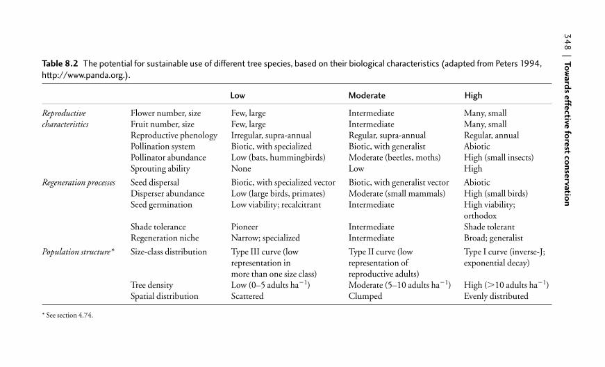
34

8|

Tow

ard

s effe

ctive fo

rest co

nse

rvatio

n

Table 8.2 The potential for sustainable use of different tree species, based on their biological characteristics (adapted from Peters 1994,

http://www.panda.org.).

Low Moderate High

Reproductive Flower number, size Few, large Intermediate Many, smallcharacteristics Fruit number, size Few, large Intermediate Many, small

Reproductive phenology Irregular, supra-annual Regular, supra-annual Regular, annualPollination system Biotic, with specialized Biotic, with generalist AbioticPollinator abundance Low (bats, hummingbirds) Moderate (beetles, moths) High (small insects)Sprouting ability None Low High

Regeneration processes Seed dispersal Biotic, with specialized vector Biotic, with generalist vector AbioticDisperser abundance Low (large birds, primates) Moderate (small mammals) High (small birds)Seed germination Low viability; recalcitrant Intermediate High viability;

orthodoxShade tolerance Pioneer Intermediate Shade tolerantRegeneration niche Narrow; specialized Intermediate Broad; generalist

Population structure* Size-class distribution Type III curve (low Type II curve (low Type I curve (inverse-J;representation in representation of exponential decay)more than one size class) reproductive adults)

Tree density Low (0–5 adults ha�1) Moderate (5–10 adults ha�1) High (�10 adults ha�1)Spatial distribution Scattered Clumped Evenly distributed

* See section 4.74.

Approaches to forest conservation | 349

● Forest landscape restoration (FLR) is a term that has been developed by WWFand IUCN (see Box 8.4), referring explicitly to restoration at the landscapescale. The concept of FLR embraces improvement of social, cultural, andeconomic benefits to people, as well as ecological recovery.

● Afforestation and reforestation refer to the establishment of trees on a site, in theformer case where no trees existed before, and in the latter case followingdeforestation (Mansourian 2005).

One of the main concerns among forest restoration ecologists has been the needto differentiate between interventions aiming at ecological recovery and conven-tional plantation forestry undertaken with purely commercial aims. For example,it is widely assumed that establishment of native tree species will confer greater

1. Species selection

2. Forest inventory

3. Yield studies

Monitoring

Baselinedata

4. Periodicregeneration

surveys

Adequate regeneration?

6. Harvest adjustments

No No

YesYes

Adequate productivity?Harvest controls effective?

5. Periodicharvest

assessments

Fig. 8.3 Flow chart of the basic strategy for exploiting tree species on a

sustainable basis. The process is composed of six steps: (1) species selection;

(2) forest inventory, to assess the extent of the resource; (3) yield studies, to

determine productivity; (4) regeneration surveys, to ascertain whether the tree

species is regenerating adequately from seed; (5) harvest assessments, to assess

the impact of harvesting on the individual trees; and (6) serial harvest

adjustments, by which the results of monitoring are used to adjust harvesting

levels. (From Peters 1994.)

350 | Towards effective forest conservation

Box 8.4 Information sources for forest restoration.

Mansourian et al. (2005) provide a useful overview of forest restoration, includ-ing a number of practical tools and techniques. Other useful informationresources are provided by Lamb and Gilmour (2003) and Perrow and Davy(2002). Internet resources are listed below.

Forest Restoration Information Service (FRIS) �www.unep-wcmc.org/forest/restoration/�FRIS is a web-based information service developed by the UNEP WorldConservation Monitoring Centre, in collaboration with a range of partners. Thesite includes an online database of forest restoration projects throughout theworld, and a number of tools to facilitate the prioritization, design and executionof forest restoration efforts.

Global Partnership on Forest Landscape Restoration (www.unep-wcmc.org/forest/restoration/globalpartnership/index.htm�The Global Partnership is a network of governments, organizations, communi-ties and individuals active in forest restoration at the landscape scale (FLR). Thepartnership is designed to support international efforts at forest restoration byfostering information exchange (for example through FRIS), and by linkingpolicy and practice.

IUCN Forest Conservation Programme (www.iucn.org/themes/fcp/experience_lessons/flr.htm)

One of the key elements of the work of the IUCN Forest Programme focuses onFLR, which aims to ‘bring people together to identify, negotiate and put in placepractices that optimize the environmental, social and economic benefits of forestsand trees within a broader pattern of land uses’. This is achieved through a num-ber of field-based projects.

WWF’s Forest for Life Programme �www.panda.org/forests/restoration/ �WWF has established a global network of over 300 forest conservation projects innearly 90 countries, including a portfolio of forest landscape restoration pro-grammes undertaken in collaboration with IUCN. WWF has adopted a target torestore forests in 20 landscapes of outstanding importance within priorityecoregions by 2020.

Society for Ecological Restoration International �www.ser.org/�A non-profit organization with more than 2000 members worldwide, widelyrecognized as a source for expertise on restoration science, practice, and policy.Although it does not engage in restoration projects directly itself, the Societysupports dialogue and information exchange through its website and throughpublication of academic journals such as Restoration Ecology.

Approaches to forest conservation | 351

environmental benefits than establishing the non-native tree species oftenemployed in commercial plantation forestry. However, plantation forests of exotictree species can be of significant habitat value for wildlife (Humphrey et al. 2003b),and in some cases it may be necessary to first establish non-native tree species to actas a ‘nurse’ for establishing native species. In such circumstances restoration goalsmight focus most usefully on improving habitat quality, rather than striving toachieve ecological fidelity (sensu Higgs 1997). This may be achieved by targetingthe specific attributes of ecosystems, with an emphasis on manipulating processesthat have changed, rather than on a comprehensive re-creation of historicalecosystem composition, something that can often be difficult to define (Newtonet al. 2001).

Although the number of practical restoration projects being implemented hasincreased rapidly in recent years, there is a perception that these activities have beenundertaken with relatively little input from the scientific community. This isdespite the fact that many of the decisions which need to be made in restorationprojects are essentially based on scientific concepts. This raises questions aboutwhat constitutes ‘good’ or appropriate restoration practice, and the role of eco-logical theory in informing the process of restoration (Higgs 1997, Moore et al.1999, Stephenson 1999). It has been suggested that practical restoration projectsneed to be based much more firmly on an understanding of ecological processes,and that such an understanding could help resolve many key questions facingrestoration practitioners, such as selecting an appropriate baseline for restoration,determining the evolutionary viability of restored populations, predicting whetherspecies will be able to colonize newly available habitat, and measuring the ecologicalsuccess of restoration efforts (Clewell and Rieger 1997).

Different approaches to forest restoration vary in terms of their relative cost,their benefits to biodiversity, and their potential impact on provision of otherecological services, such as water regulation and nutrient cycling (Table 8.3). Ingeneral, the preferred method is to allow the forest to recover naturally through aprocess of succession (‘passive restoration’, Table 8.3). For such successional recov-ery to occur, the following conditions must be met (Lamb and Gilmour 2003):

● The disturbing agent or agents must be removed. If disturbances such as fire,timber harvesting, or grazing continue, succession is interrupted and recoveryis unlikely.

● Plants and animals must remain at the site or in the region as a source ofnew colonists, and must be able to move across the landscape and recolonizethe degraded area. The more distant these source populations are, theslower the recolonization process. Potentially, connecting habitat fragmentsor ‘stepping stones’ can increase the rate of the recovery process. This is anargument for planning forest restoration at the landscape scale (Humphreyet al. 2003c).

● Soils at the site must remain reasonably intact. If severe erosion has takenplace or if fertility has been depleted the soils may no longer be suitable for the

original species, and other species (perhaps not native to the area) may cometo dominate.

● Weed species, invasive exotic species, or animal pests must be excluded orcontrolled if the original community is to be re-established successfully.

In order to estimate the rate of forest recovery, the modelling techniques describedin Chapter 5 can potentially be used. Similarly, the techniques described inChapter 4 are of value in analysing the factors influencing successional processes,which are of crucial importance to forest recovery.

In some situations the forest may be so degraded that natural recovery will be verylimited (such as the case of Carrifran, Box 6.1). In such situations there may be a needto establish trees artificially, through methods such as direct seeding or planting oftree seedlings (Table 8.3). Key decisions include (Newton and Ashmole 1998):

● Which tree species should be established? This can be determined by reference toresults from pollen analysis or historical records.

● What should their spatial distribution and relative abundance be? Field surveysof soil characteristics and topographic variation across the site to be restored,together with autoecological information about the tree species selected, canbe used to ensure that species are correctly matched to the microsites on which

352 | Towards effective forest conservation

Table 8.3 Relative costs and benefits of various methods of overcoming forest

degradation (from Lamb and Gilmour 2003 http://www.panda.org.).

Method Relative Relative rate Potential direct cost of biodiversity ecological

gain services benefit

(a) Prime focus of biodiversity restorationPassive restoration Low Slow HighEnrichment planting Low–medium Slow–medium HighDirect seeding Low–medium Medium HighScattered plantings Low Slow MediumClose plantings of a few Medium Medium HighspeciesIntensive plantings after High Fast Highmining

(b) Prime focus on productivity and biodiversityManaging secondary forests Low–Medium Medium HighEnrichment plantings Low–medium Medium Medium–highAgroforestry Medium–high Medium Medium–highMonoculture High Slow Mediumplantations with buffers Mosaics of monocultures High Slow Low–mediumMixed species plantations High Slow MediumEnhanced understorey Low Slow Medium–highdevelopment

Approaches to forest conservation | 353

they are to be established. If the aim is to mimic natural forest structures, thenspacing of trees should be irregular, and individuals of each species should begrouped (Rodwell and Patterson 1994).

● How should planting stock be sourced? For native woodland establishment to besuccessful, planting material should be well adapted to the site conditions,and therefore local sources should be used. Genetic effects such as geneticdrift and inbreeding may reduce the viability of planting stock obtained fromisolated forest fragments; genetic analyses may be required to assess such risks(see Chapter 6).

● How much of the area should be forested? Open spaces within forest areas areimportant as wildlife habitat, and therefore as much as 30–40% of an area maybe left unplanted initially, both to provide long-term open space and to provideareas for future tree establishment by natural regeneration or planting.

Mapping tools such as GIS (see Chapter 2.6) are likely to be of value whenplanning restoration projects. Increasingly, forest restoration projects are beingplanned and implemented at large spatial scales (as in the case of FLR projects,Box 8.4), and in such cases GIS becomes particularly valuable (Humphrey et al.2003c). Another key issue is the need to monitor restoration progress, ideally aspart of an adaptive management cycle (see section 8.3). Many restoration projectsneglect this important aspect. Once restoration targets or management goals havebeen identified, indicators will have to be developed (see section 8.6) to help trackprogress towards these goals (Figure 8.4). This can be achieved by examining thethreats (pressures) affecting the forest, and identifying the specific management

Grasses

Num

ber

of

spec

ies

in n

ew s

yste

m

Number of species in orginal system

Reptlies

Canopy birds

Shrubs

Sub-canopy birdsTress withlarge fruitFrogs

Tress withsmall fruit

Fig. 8.4 One approach to monitoring forest restoration. Forest recovery can be

monitored by comparing the number of species in different life forms in the

recovering forest with those present originally. In this illustration, the numbers of

reptiles, birds found in the forest canopy, and trees with small fruit have recovered

to near their original condition, whereas there are fewer species of most other life

forms than in the original forest. On the other hand, the site now has more grass

species. (After Lamb and Gilmour 2003.)

interventions needed to address these threats (O’Connor et al. 2005). Furtherinformation on monitoring techniques is provided below.

8.3 Adaptive management

Whichever approach to forest management and conservation is adopted, adaptivemanagement techniques should be employed. Particularly useful resources on thistopic have been developed by Foundations of Success, a not-for-profit organiza-tion committed to improving the practice of conservation through the process ofadaptive management. A number of information resources are accessible fromtheir website �http://fosonline.org/�; see Margoluis and Salafsky (1998) and Salafskyet al. (2001, 2002). This brief account is based on these sources, which should beconsulted for more details.

Adaptive management can be defined as the integration of design, manage-ment, and monitoring to systematically test assumptions in order to adapt andlearn. It also offers a method by which research can be incorporated into conserva-tion action. The approach includes the following elements:

● Testing assumptions. This involves systematically trying different managementactions to achieve a desired outcome. This depends on first thinking about thesituation at the specific project site, developing a specific set of assumptionsabout what is occurring, and considering what actions could be taken to affectthese events. These actions are then implemented and the results are moni-tored to assess how they compare to the ones predicted at the outset, on thebasis of the assumptions.

● Adaptation. If the expected results were not obtained, then the assumptionswere wrong, the actions were poorly executed, the conditions at the projectsite have changed or the monitoring was faulty. Adaptation involves changingassumptions and interventions in response to the information obtained as aresult of monitoring. This is the defining feature of adaptive management.

● Learning. This refers to the process of systematically documenting the man-agement process, and the results achieved. This helps avoid repeating the samemistakes in the future.

The adaptive management process involves six steps (Figure 8.5):

Start Define the objectives clearly. This is a crucially important first step in any con-servation programme, yet is surprisingly often neglected, and as a result manage-ment objectives are often vague or poorly defined. This makes it very difficult toascertain whether the programme is being successful or not.

Step A Design an explicit model of the system. A model is a simplified version of reality.Such models can help to integrate and organize information, provide a frameworkfor identifying and comparing management interventions, and support discussionabout how the management should be undertaken. The models used need not bequantitative; methods of developing conceptual models are described in section

354 | Towards effective forest conservation

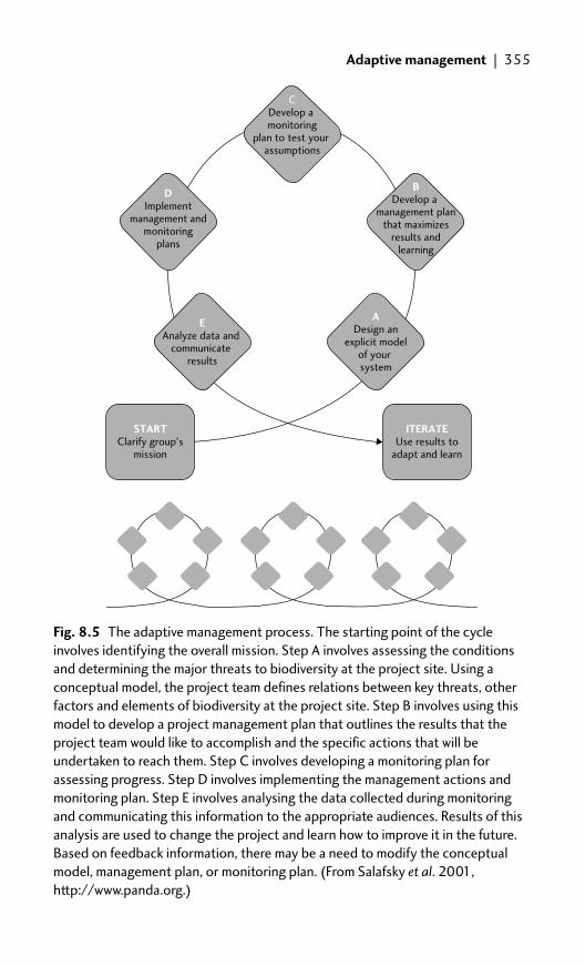
Adaptive management | 355

CDevelop a monitoring

plan to test your assumptions

DImplement

management andmonitoring

plans

EAnalyze data and

communicate results

A Design an

explicit modelof your system

B Develop a

management planthat maximizes

results andlearning

STARTClarify group's

mission

ITERATEUse results to

adapt and learn

Fig. 8.5 The adaptive management process. The starting point of the cycle

involves identifying the overall mission. Step A involves assessing the conditions

and determining the major threats to biodiversity at the project site. Using a

conceptual model, the project team defines relations between key threats, other

factors and elements of biodiversity at the project site. Step B involves using this

model to develop a project management plan that outlines the results that the

project team would like to accomplish and the specific actions that will be

undertaken to reach them. Step C involves developing a monitoring plan for

assessing progress. Step D involves implementing the management actions and

monitoring plan. Step E involves analysing the data collected during monitoring

and communicating this information to the appropriate audiences. Results of this

analysis are used to change the project and learn how to improve it in the future.

Based on feedback information, there may be a need to modify the conceptual

model, management plan, or monitoring plan. (From Salafsky et al. 2001,

http://www.panda.org.)

7.8.1. The model should incorporate the assumed linkages between the variousdirect and indirect threats or factors that affect the conservation targets of interest.

Step B Develop a management plan. This is a crucial element of any conservationprogramme. The plan should outline the factors or threats that need to beaddressed and the specific actions that will be undertaken to change them.Selection of actions should be based on the results that are desired. Experimentscan be undertaken to help define which actions are successful. The plan canusefully be informed by the conceptual model developed under Step A. A usefulfirst step is to rank the various threats identified in the model and decide whichcause the biggest problems and therefore need addressing first. Then a specificobjective should be developed for each threat or factor, and proposed activitiesdefined to achieve each objective. Further details of how to develop a conservationmanagement plan are presented by Sutherland (2000).

Step C Develop a monitoring plan. Monitoring is essential to the adaptive manage-ment process, to assess whether the management actions are being effective.Adaptive management requires testing explicit assumptions about the area of interestand collecting only the data that are needed to test these assumptions. Developmentof the conceptual model under Step A can greatly help decide what should be mon-itored. Indicators will need to be chosen for measurement, representing both thethreats or factors influencing the conservation targets, and the targets themselves.A monitoring plan must be produced describing which methods will be used tocollect data on the indicators. Many of the techniques described in this book couldbe of value here. The challenge is to avoid collecting too much data, and insteadfocus on the critical factors that are most relevant to the project. Further informa-tion on indicators and monitoring is given in the following sections.

Step D Implement the management and monitoring plans. The most importantstep!

Step E Analyse data and communicate results. Many practitioners feel that they aretoo busy with day-to-day work and problems to analyse the data that they collect.Yet it is very important to include analysis and communication efforts in the workplan. If the project is planned properly, then the conceptual model and manage-ment plan should contain the objectives set, the assumptions made, and the inter-ventions being undertaken. The monitoring plan should outline the data beingcollected. The main additional need is to analyse and interpret what these resultsmean and then communicate them in a way that addresses the needs of key audi-ences. Analysis is most effectively done in the context of specific questions beingasked or assumptions being tested.

Iterate Use results to adapt and learn. As illustrated in Figure 8.4, the adaptive man-agement process is iterative. It is important to return to the original conceptualmodel and to the assumptions that were identified at the outset and then testedexperimentally, through the management activities. If the management interven-tions or experiments turn out exactly as predicted, then the assumptions will havebeen confirmed. If not, the results need to be used to change the actions being

356 | Towards effective forest conservation

Assessing threats and vulnerability | 357

undertaken. The model itself will also need to be changed. This will capture thelearning accomplished and incorporate it into the project’s institutional know-ledge. A new round of assumptions can then be identified for future testing. Overtime, the cycle may be passed through many times, learning more each time,ultimately leading to better conservation.

There is no doubt that adaptive management approaches can be very successfulif implemented properly. One of the main challenges is to undertake managementinterventions in the form of experiments; ideally this requires appropriate controlsand replication, something often very difficult to achieve in practice. Often theresults of interventions or experiments may be difficult to interpret or ambiguous;in such cases it can be difficult to decide how best to amend the managementaction. There can also be resistance among practitioners in visualizing theirsystems as conceptual models, and their interventions as experiments (Sutherland2000). Given the potential benefits of the approach, there is enormous scope forresearchers to work closely alongside practitioners to provide support in its imple-mentation, and thereby to improve the effectiveness of conservation.

8.4 Assessing threats and vulnerability

Effective conservation depends strongly on a full appreciation of the causes of bio-diversity loss. Yet identifying such threats or ‘threatening processes’ has receivedremarkably little attention from researchers. Surprisingly, the issue is ignored bymany conservation biology textbooks. There is enormous scope for improvingmethods for assessing threats and diagnosing their impacts, and improving thequality of information available to conservation managers. However, identifyingthe precise causes of decline in the abundance of a particular species can often besurprisingly difficult.

Different types of threat may be identified. Direct threats are those that aredirectly responsible for loss or degradation of forests, or their associated biodiver-sity. Indirect threats are the underlying causes of such direct threats. For example,an underlying threat such as a government policy may be responsible for the directthreat of forest conversion to agriculture. Other terms used to describe threatsinclude ‘drivers’ or ‘pressures’; these terms may be preferred because they implythat effects on biodiversity can be either negative or positive, whereas the term‘threat’ implies only negative impacts. However, it should be remembered that dif-ferent authors interpret these terms in different ways. Salafsky et al. (2002) listmany of the most widespread threats to biodiversity.

Robinson (2005) identifies the following main methods of assessing threats:

● Conceptual modelling, used to illustrate the relation between threats and theirimpacts, and for providing a strategic framework for identifying appropriatemanagement interventions (see section 7.8.1).

● Threat matrices. Matrices can vary from simple tables to complex logicalframeworks linking different threats and interventions to conservation

358 | Towards effective forest conservation

targets. Matrices are relatively simple to implement and can readily beupdated, but their dependence on subjective information is a weakness. Anexample of a threat matrix is illustrated in Table 8.4.

● Participatory threat mapping, which can involve use of pictorial maps or three-dimensional models to elicit information about changes in forest habitatquality or quantity, when working with community groups.

● GIS-based mapping, incorporating quantitative spatial data. Direct threats,such as habitat fragmentation (see section 2.7), can be assessed and displayedby using GIS. Spatial models of forest dynamics (see section 5.5) can be usedto explore and illustrate the potential impacts of different threats on forestextent, structure and composition.

Wilson et al. (2005b) provide a detailed review of the concept of vulnerability inconservation planning, noting that information on threatening processes and therelative vulnerability of areas and features to these threats pervades the process ofconservation planning. Pressey et al. (1996) defined vulnerability as ‘the likelihoodor imminence of biodiversity loss to current or impending threatening processes’.Wilson et al. (2005b) extend this definition by distinguishing three dimensions ofvulnerability, exposure, intensity, and impact, and provide the following informa-tion regarding their measurement:

● Exposure can be measured either as the probability of a threatening processaffecting an area over a specified time, or the expected time until an area isaffected. Exposure is commonly measured categorically, for example as ‘high’,‘medium’, or ‘low’ suitability for agriculture, but has also been measured oncontinuous scales by some authors. Maps can be produced illustrating therelative exposure of different areas to a particular threat.

● Intensity measures might include magnitude, frequency, and duration of thethreat. Examples include livestock density, volume of timber extracted perhectare of a forest type, or the density of an invasive plant species. Intensitycan also be estimated categorically, and can be mapped across whole planningareas.

● Impact refers to the effects of a threatening process on particular features suchas the distribution, abundance, or likelihood of persistence of a species ofinterest. For example, logging may have much greater impact on animalspecies dependent on old growth forests than on species that inhabit a varietyof post-logging stages. Impact might also depend on the spatial pattern of thethreatening process, for example on the degree of connectivity between oldgrowth patches retained after logging operations.

As conservation planning is generally spatial, a key issue is whether vulnerabilitycan be mapped, and therefore integrated with other spatial information such asforest cover, boundaries of management units etc. According to Wilson et al.(2005b), this requires mapping of spatial predictions of the future distribution ofthreatening processes. Maps of exposure can be based on the current distributionsof threats and knowledge of variables that could predispose areas or features to those

Asse

ssing th

reats a

nd

vuln

era

bility

|3

59

Table 8.4 Example of a simple method of scoring the different pressures or threats affecting a forest area (from Ervin 2003a, http://www.

panda.org.). Here, different human activities have been scored on a simple scale with respect to three variables: extent, impact, and

permanence. Extent is the area across which the impact of the activity occurs. Impact is the degree, either directly or indirectly, to which the

threat affects overall forest resources. Permanence is the length of time needed for the affected area to recover with or without human

intervention. A combined score (‘degree’) has been produced by multiplying the individual scores together.

Activity Extent Impact Permanence Degree Description and rationale

NTFP Localized Mild Short term 1 NTFP collection consists primarily of mushroom harvesting for collection (1) (1) (1) consumption by local residents. Harvesting occurs near an adjacent

village, and harvesters generally leave large areas undisturbed.

Road Scattered Moderate Mediumterm 8 A road is planned through a portion of a protected area. The actual (2) (2) (2) impact of construction will be minimized by using

environmental best practices. It is a gravel access road, and will only be used seasonally by park staff and visitors with permits.

Tourism Localized High Short term 9 Tourists have recently begun to drive motorized off-road vehicles (3) (3) (1) through sensitive wetlands. Springtime vehicle use has already

disrupted the mating and denning habits of large numbers of bears,considered a key species in this protected area.

Poaching Widespread High Medium term 18 The main species poached is tiger, which is extensively poached in (3) (3) (2) the protected area. A large percentage of the tiger population is

killed annually.

Alien species Widespread High Long term 27 An invasive plant species (Chromolaena) covers a quarter of the park. (3) (3) (3) It has rendered large areas of rhino and elephant habitat unsuitable,

and is extremely difficult to control or eradicate.

Dam building Throughout Severe Permanent 64 A large-scale hydro-electric dam is planned that would flood at least (4) (4) (4) half of the protected area.

threats. For example, the likelihood of forest conversion to agriculture is oftenrelated to the suitability of the soil for agricultural crops, topography, and proxim-ity to infrastructure or population centres (see, for example, Mertens and Lambin1997). Spatial predictions of intensity are less common in the literature thanpredictions of exposure; for some threats, such as forest clearing, intensity is consideredas binary (either cleared or not). Impact is the most difficult dimension of vulnera-bility to map, as this may require feature-specific information on the effects ofdifferent levels of intensity, spatial information on features relative to variations inintensity, and ways of integrating this information across assemblages of species, setsof vegetation types, or other groups of features (Wilson et al. 2005b).

Wilson et al. (2005b) also reviewed the different methods that have been usedby previous researchers to assess the three dimensions of vulnerability. The meth-ods were grouped into four groups based on the types of data used (Table 8.5).Little information is available in the literature to indicate which approach wouldbe preferable in a given situation; it is likely that a combination of approaches willgive the best overall result (Wilson et al. 2005b). As noted by these authors, a com-prehensive assessment of vulnerability would consider all of the threats affecting anarea and also include the dynamic responses of threats to conservation actions.Combining vulnerability scores for multiple threats is analytically tractable andcan be achieved by differentially weighting threats to reflect their relative import-ance, ideally informed by their respective impacts. An example of the latterapproach is provided by Miles et al. (2006), in their global assessment of the con-servation status of tropical dry forests. Here, GIS techniques were used to analyseand combine maps of different threats derived from remote sensing data to iden-tify those forest areas vulnerable to multiple threats. Such methods, coupled withspatial analysis and statistical modelling techniques, offer the potential for power-ful and sophisticated analyses of threats at a range of different scales.

It should be remembered that risk analysis and hazard assessment are widelypracticed by foresters, and a substantial literature exists on this topic (see alsoBurgman 2005). This literature has been little used by the conservation commu-nity to date. Methods for assessing different types of forest disturbance aredescribed in Chapter 4. Such measurements can be used as a basis for assessing risk,as described briefly below for some of the most important types of disturbance.

● Fire. Forest fire risk is generally assessed by identifying the potentiallycontributing variables and integrating them into a mathematical expression orindex. The index is used to indicate the level of risk, and can be mapped. A widevariety of different approaches are used to produce such indices, which varyparticularly in terms of the timescales involved. Estimates of the probability offire occurrence are typically based on variables such as the amount and type offuel available for burning, topographic variables, vegetation characteristics,and meteorological variables. Further details of the most common methodscan be found in Chuvieco (1999) and San-Miguel-Ayanz et al. (2003).

● Wind. A number of different approaches to analysing and modelling wind-throw risk have been developed. Statistical models use empirical information

360 | Towards effective forest conservation

Asse

ssing th

reats a

nd

vuln

era

bility

|3

61

Table 8.5 Methods used to assess vulnerability (adapted from Wilson et al. 2005b). The table is based on a thorough review of the

literature; for full references, see Wilson et al. (2005b).

Concept Method of measurement Dimension of vulnerability Example reference

Group 1: Methods based on Vulnerability is estimated from coverage in existing Exposure Castley and Kerley tenure and land use conservation areas (1996)

Vulnerability is estimated from permitted or Exposure and intensity Abbitt et al. (2000)projected land uses

Group 2: Methods based on The past impacts of threatening processes are used Exposure Myers et al. (2000)environmental or spatial to indicate the vulnerability of features. These values variables are then given to presently unaffected areas that

contain the same featuresCharacteristics of areas or features exposed to threats Exposure and intensity Sisk et al. (1994)in the past are used in qualitative or informal quantitative analyses to predict vulnerabilityCharacteristics of areas or features exposed to threats Exposure and intensity Wilson et al. (2005a)in the past are used in spatially explicit, quantitative models to predict vulnerability

Group 3: Threatened species The number of threatened species and their relative Exposure, intensity, and Brooks et al. (2001)are used to indicate vulnerability threat ratings are combined to indicate vulnerability impactGroup 4: Experts decide on Opinions are sought from experts on the relative Exposure, intensity, and Ricketts et al. (1999)relative vulnerability vulnerability of areas or features impact

on damage collated over a number of years in selected areas, whereas deter-ministic models consider tree or stand characteristics and the windiness of a siteor the critical wind speed (Lanquaye-Opoku and Mitchell 2005, Quine 1995).An example of a widely used mechanistic model is GALES, developed by theForestry Commission in the UK (Gardiner et al. 2004), which estimates thethreshold wind speeds required for overturning and breaking the mean tree ofa stand. The resulting decision support system (DSS), ForestGALES, can be usedto predict the wind damage risk for 19 different conifer species, growing inhomogenous, even-aged stands in Europe. Spatially explicit models of forestdynamics such as LANDIS (see section 5.5) also offer tools for exploring thepotential impacts of different wind regimes.

● Herbivory. The determination of browsing damage on forest regeneration at agiven time can be used to forecast impacts in the future, for example when thetimber is harvested or when the function of the forest is seen to have beencompromised. The effects of browsing and the resulting damage can bedecades apart. In order to estimate the long-term impacts of browsing,indicators may need to be specified for young forest stands at the time whentop-twig browsing is no longer possible (Reimoser et al. 1999). Ultimately therisk of damage by herbivores is a function of animal behaviour, somethingthat is difficult to predict but is also an active area of research.

● Deforestation. Research has indicated that deforestation can be related to arange of factors, such as population density, population growth, agriculturalexpansion, income levels, and amount of timber harvesting (Allen and Barnes1985, Uusivuori et al. 2002). Typically, deforestation is assessed by compar-ing the forest cover at different times by means of remote sensing images (seeChapter 2). To calculate deforestation rate, the following formula can be used(Puyravaud, 2003) (see FAO (1995) for an alternative):

where A1 and A2 are the forest cover at times t1 and t2, respectively and P is percent-age per year. Deforestation can then be analysed by using multivariate statistics andregression techniques, to identify the influence of different pressures or drivers. Forexample, Wilson et al. (2005a) analysed deforestation in southern Chile, by firstidentifying where native forests had been converted to plantations, then using amultivariate, spatially explicit statistical model to identify the variables responsiblefor this conversion. Predictions were then made of where native forest conversion islikely to occur in the future, as a function of patterns of climate, topography, soilsand proximity to roads and towns, providing an assessment of relative vulnerabilityto deforestation. Similarly, in Cameroon, Mertens and Lambin (1997) found anegative relation between deforestation and proximity to roads, which could poten-tially be used to identify areas vulnerable to future forest loss.

Modelling of land-use changes such as deforestation requires combiningspatially explicit ecological data with information on socio-economic as well as

P �100

t2 � t1ln

A2

A1

362 | Towards effective forest conservation

Monitoring | 363

biophysical variables. A range of models of land-use change have been developed,based on a variety of analytical approaches (Mladenoff and Baker 1999, Veldkampand Lambin 2001). For example, GEOMOD is a GIS-based model that simulatesthe location of deforested cells by using geophysical attributes as well as spatial dataof forest cover at different time intervals (Pontius et al., 2001), and is now com-mercially available as part of the IDRISI software program (�www.clarklabs.org�).In a review of the current understanding of land-cover change in tropical regions,Lambin et al. (2003) emphasize the complexity of the issue and highlight the roleof market forces, policy interventions, and changes in social organization and atti-tudes. Relatively simple statistical models are unlikely to capture this complexity,and instead these authors highlight the role of agent-based systems and narrativeperspectives to provide an explanation and prediction of land-use changes.

Although important advances have been made in modelling the spatial patternof deforestation, ecosystem heterogeneity and lack of data (particularly for relevantsocioeconomic drivers) continue to constrain analyses and the development ofdeforestation scenarios (Grainger 1999). As deforestation cuts across a range ofdisciplines (sociology, economics, ecology, and geography), some researchers haveencouraged a focus on the interactions between these disciplinary approachesrather than on the details of each subcomponent (Dale and Pearson 1997).

8.5 Monitoring

Monitoring is the process of periodically collecting and using data to inform man-agement decisions (O’Connor et al. 2005). Monitoring is a critically importantaspect of any conservation project, to help ensure that management interventionsare effective. As noted above, monitoring is an essential component of adaptivemanagement approaches. The monitoring should not be initiated only at the end ofthe project, but should be integrated into the overall project cycle. Detailedguidance on monitoring is provided by Hurford and Schneider (2006), Spellerberg(1991), and Sutherland (2000).

Many of the techniques described in this book can be used as part of a monitor-ing programme. Field-based forest monitoring is usually achieved by establishingand repeatedly surveying permanent sample plots (section 4.7), incorporatingassessment of forest stand structure and composition (Chapter 3) and habitatcharacteristics (Chapter 7). Such field surveys may be complemented by use ofremote sensing analyses (Chapter 2). Here, some general issues and principles aredescribed that should be borne in mind when designing and implementing amonitoring programme.

Yoccoz et al. (2001) highlight the fact that many biodiversity monitoringprogrammes are inadequate. Specifically, inadequate attention is given to threebasic questions:

● Why monitor?● What should be monitored?● How should monitoring be carried out?

The following recommendations are made by these authors, in a critical reviewof current practice:

● It is essential to clearly define the objectives of monitoring. Many programmes arebased on the assumption that collecting any information about a system willbe useful, but such an approach is inefficient and can result in large amountsof irrelevant information being collected. Two main types of objective can bedifferentiated: scientific objectives, focusing on understanding of the behaviourand dynamics of the system, and management objectives, designed to provideinformation for informing management decisions.

● Monitoring, management and research should be closely integrated, as explicitlyrequired in adaptive management approaches (see above). Research can play acritical role in identifying appropriate management actions, and it can beargued that monitoring is trivial unless it is linked to experimental work tounderstand the mechanisms underpinning system changes. In practice, mon-itoring is often limited to the assessment of management policies.

● Decisions regarding what to monitor should be determined by the a priorihypotheses to be addressed by the programme and by the relative values ofdifferent components of diversity as specified in management objectives.

● The sampling design will be dependent on the choice of biological diversitymeasures. For some objectives, it might be adequate to focus on species rich-ness of some groups. For others it will be necessary to estimate the abundancesof each species in the community of interest, which requires greater effort. Itis also important that monitoring programmes provide data to estimate notonly the state variables of interest, but also the rate parameters that determinesystem dynamics.

● It is important to estimate detection error, which arises because few surveymethods permit the detection of all individuals, or even all species, in sur-veyed areas. Distance sampling methods (see section 3.5.3) can be used toestimate detection probabilities associated with count statistics. Monitoringprogrammes should estimate the detection probabilities associated with theselected survey methods; without these, it is not possible to draw stronginferences about the monitored system.

● Spatial variation is a second source of error because of the inability to surveylarge areas entirely. Most surveys are not based on an appropriate spatial sam-pling scheme, and therefore do not provide unbiased estimates of biodiversityat larger spatial scales. Sample locations for monitoring programmes shouldnot be selected arbitrarily, but be selected to permit inference to the larger areaof interest. Sampling designs should be chosen with respect to their efficiency,in terms of the precision of resulting estimates.

Legg and Nagy (2006) similarly point out that much current monitoring ofbiodiversity is a waste of time, because of the lack of detailed goal and hypothesisformulation, inadequate survey design and data quality, and lack of assessment ofstatistical power at the outset. As a result, most programmes are unlikely to be

364 | Towards effective forest conservation

Monitoring | 365

capable of rejecting a false null hypothesis with reasonable power. Along with anumber of other recommendations (Box 8.5), these authors suggest that in anymonitoring programme a power analysis shoule be done at the outset, to ensurethat the proposed design is sufficiently robust. Statistical power is 1.0 minus theprobability of a type II error, i.e. the probability of rejecting the null hypothesiswhen it is false. The power of a statistical test depends on effect size, error variance,sample size, and the type I error rate (Legg and Nagy 2006). For example,

Box 8.5 Recommendations for the design and implementation of

biodiversity monitoring programmes.

Recommendations for good management of a monitoring programme

● Secure long-term funding and commitment.● Develop flexible goals.● Refine objectives.● Pay adequate attention to information management.● Train personnel and ensure commitment to careful data collection.● Locations, objectives, methods, and recording protocols should be detailed

in the establishment report.● Obtain peer review and statistical review of research proposals and

publications.● Obtain periodic research programme evaluation and adjust sampling

frequency and methodology accordingly.● Develop an extensive outreach programme.

Recommendations for good design and field methods in monitoring

● Take an experimental approach to sampling design.● Select methods appropriate to the objectives and habitat type.● Minimize physical impact to the site.● Avoid bias in selection of long-term plot locations.● Field markings must be adequate to guard against loss of plots.● Ensure adequate spatial replication.● Ensure adequate temporal replication.● Blend theoretical and empirical models with the means (including experi-

ments) to validate both.● Synthesize retrospective, experimental and related studies● Integrate and synthesize with larger- and smaller-scale research, inventory,

and monitoring programmes.

(after Legg and Nagy 2006).

following these authors, the power of a t-test is derived from the t-distribution andthe value of t given by:

The sample size required to detect a difference between means of � with power(1–�) is:

where n is sample size, s2 is an estimate of variance, � is the minimum detectabledifference, ta,� is the critical value of t for a probability of � (one-tailed or two-tailedas appropriate), tb,� is the critical value of t for a one-tailed probability level �, � isthe probability of type II error and � is the degrees of freedom. Note that t is a func-tion of n and so the solution must be obtained by iteration (Legg and Nagy 2006).

The simplest way to increase power is to increase sample size, but this costs timeand money. There is therefore a trade-off between sample size and the quality ofinformation that can be obtained from each observation (Legg and Nagy 2006).For example, estimates of plant cover made by averaging the visual estimates ofcover in subunits within gridded quadrats show much less between-observer andwithin-observer error than visual estimates from ungridded quadrats. If thebetween-quadrat variance is high, then large numbers of low-precision ungriddedquadrats give greater power than the same amount of time spent on a few high-quality gridded quadrats (Legg and Nagy 2006). Prior knowledge or a pilot studywill therefore often be required to find the optimal method.

A simple approach to defining required sample sizes is provided by Manley(1992). First, the maximum size of sample that can be collected is estimated, giventhe resources available. From this, the power of the test that one wishes to apply canbe estimated. If the estimated power is inadequate, then a decision needs to bemade regarding whether to proceed or to abandon the study altogether. There is lit-tle point in a monitoring programme that cannot reject a null hypothesis that isfalse (Legg and Nagy 2006). Ideally, monitoring programmes should be designedaround a simple and powerful statistical model such as analysis of variance(ANOVA) that can make use of all of the information available to reduce residualerrors. Parametric statistical tests are usually more powerful than non-parametrictests (Legg and Nagy 2006).

Sheil (2001b) has provided a particularly valuable critique of biodiversity mon-itoring in tropical countries. He points out that monitoring activities can actuallyhinder, rather than improve, conservation action, as limited resources are divertedaway from practical management activities. Sheil makes the following recommen-dations, which should be considered whenever assessments are being planned:

● Monitoring and assessment activities must be allocated with sensitivity tolocal priorities and limitations, especially when local resources are involved.

n �s2

�2(t�,� � t�(1),�)2

t�(1),���

s2/n�t�,�

366 | Towards effective forest conservation

Indicators | 367

● Researchers should ensure that they are familiar with local management issuesbefore they become general advisers on local conservation needs.

● Care must be exercised whenever monitoring activities are promoted at thepossible expense of important conservation actions.

● Managers should only be required to collect data that are useful to them inways that they understand.

● High-level monitoring is vital: information is needed on threats to biodiver-sity, and conservation priorities should be continually refined in the light ofsuch information. However, the costs and responsibilities for generating suchinformation must be allocated with care.

● Interventions should bolster, and not undermine, the attainment of conser-vation goals; case-by-case assessment is needed.

8.6 Indicators

Indicators are surrogates for properties or responses of a system that is too difficultor costly to measure in its entirety (Hyman and Leibowitz 2001). They provideinsight into the state and dynamics of the environment, and may help makedetectable a trend or phenomenon of interest (Niemeijer 2002). They can helpisolate key aspects from complex situations to help decision-makers see what ishappening, and help them determine what action is appropriate (Niemeijer 2002).Indicators can be derived from measurements of ecological features, either byfield survey or by using remote sensing data. Therefore in their broadest sense,ecological indicators include anything that can be measured by using any of thetechniques described in this book. These measurements can be used directly orcombined into summary values (as some form of index, for example).

Indicators are generally used to monitor trends. At the local scale they are animportant tool for monitoring and adaptive management, as described in previoussections, enabling progress towards management objectives to be assessed. Atnational and international scales they are used to monitor progress towards achiev-ing policy goals and as the basis of environmental reporting. The types of indicatorrequired for these different purposes may be quite different. However, informationgathered at the local scale can be aggregated for reporting at the national scale.Given that the choice of potential indicators is so broad, a key issue is how to makean appropriate choice and to make sure that the right things are measured.

The use of ecological indicators has recently been reviewed by Niemi andMcDonald (2004), who point out that most attempts to use ecological indicatorshave rightly been heavily criticized. As noted earlier, many attempts at environ-mental monitoring suffer from a lack of clear objectives and a failure to considerdifferent sources of error (Yoccoz et al. 2001). Other criticisms levied at indicatorshave focused on the lack of: (1) identification of the appropriate context (spatialand temporal) for the indicator, (2) a conceptual framework for what the indicatoris supposed to indicate, and (3) validation of the indicator (Niemi and McDonald

2004). Development and testing of biodiversity indicators is area of activeresearch, designed to address such problems.

This section first addresses the issue of conceptual frameworks, then providessome guidance on selection and implementation of appropriate indicators.Further information on the topic is provided by McKenzie et al. (1992) and Noss(1990, 1999), and a range of examples drawn from European forests is presentedby Angelstam et al. (2004a).

8.6.1 Indicator frameworks

It is widely recognized that some form of framework is required in order formeaningful indicators to be developed. The most widely used framework is pres-sure–state–response (PSR), which was developed by the Organisation for EconomicCo-operation and Development (OECD 1993) on the basis of the stress–responsemodel developed by Friend and Rapport (1979). The PSR framework states thathuman activities exert pressures on the environment (such as clearance of forest foragriculture), which can induce changes in the state of the environment (for example,the extent of forest cover). Society may then respond to changes in pressures orstate with policies and programmes intended to prevent, reduce or mitigatepressures and thereby reduce environmental damage. The PSR frameworkhas been widely applied to indicator development, particularly for monitoringprogress towards policy goals; for example, it is explicitly recognized by the CBD.

This approach was further expanded by the European Environment Agency toinclude drivers (D) and impacts (I), forming the DPSIR framework (EEA 1998).Both the PSR and the extended DPSIR frameworks are based on the fact thatdifferent societal activities (drivers) cause a pressure on the environment, causingquantitative and qualitative changes of it (changing state and impact). Societyhas to respond to these changes in order to achieve sustainable development.According to the DPSIR framework, different indicators of sustainability may bedeveloped, relating to drivers, pressure, state, impact, and response.

A number of other indicator frameworks have been proposed by researchers. Forexample, Noss (1990) presents a hierarchical framework for development ofbiodiversity indicators, recognizing that three attributes of biodiversity, compos-ition, structure, and function, can be considered at a number of different levels oforganization. This framework is relevant only to biodiversity ‘state’ indicators.Stork et al. (1997) provide a framework based on a conceptual model of therelationship between anthropogenic activities affecting forests, and the processesthat influence biodiversity. Indicators may therefore be developed for particularhuman interventions or mediators (pressure indicators), as well as processes main-taining biodiversity, and biodiversity itself (state indicators).

Frameworks can be of great value in helping to organize information. Environ-mental measurements can readily be categorized as representing either ‘pressure’,‘state’ or ‘response’ variables, according to the PSR framework. Information onthreats (see section 8.4), for example, can be considered as pressures, whereas foreststructure and composition can be considered as ‘state’ indicators. Yet often the use of

368 | Towards effective forest conservation

Indicators | 369

frameworks is neglected in practice, leading to confusion. For monitoring theeffectiveness of management at the local scale, it is ‘state’ indicators that are of par-amount importance, yet often the indicators used in practice are those representingmanagement responses (mostly because these are easier to measure). The DPSIRframework is somewhat more difficult to implement in practice than PSR, mostlybecause of the difficulty of separating out ‘state’ from ‘impact’ variables. However, italso draws attention to the ‘drivers’ or underlying causes of biodiversity loss, whichultimately need to be addressed if loss of biodiversity is to be prevented.

Development of a conceptual model (see section 7.8.1) can also be of great valuein identifying the relevance of different indicators, by identifying the relationshipsbetween proposed indicators the features of interest, such as biodiversity (Hymanand Leibowitz 2001). Note that there is some confusion in the scientific literature;the terms ‘framework’ and ‘conceptual model’ are often used interchangeably. Infact a conceptual model and a framework are both required for indicator develop-ment, the former to define the relationship between the indicator and the featureof interest (the ‘endpoint’), and the latter to categorize the variables and helporganize the collection and reporting of information. Of course a conceptualmodel can adopt an indicator framework (such as PSR) as its basic structure, andin fact this is a logical and useful way of going about developing such a model.

Could quantitative models of forest dynamics (see Chapter 5) also be of value inidentifying suitable indicators? At the very least, such models could enable the sen-sitivity of indicators to environmental pressures to be explored, and their relevanceto be tested. Remarkably little research seems to have been done in this area to date.

8.6.2 Selection and implementation of indicators

The choice of indicator will depend primarily on the objectives of the investigation.People working on forests have an enormous range of potential indicators to choosefrom, because of all the work undertaken on development of criteria and indicatorsfor sustainable forest management (see section 8.2.2). A first step might thereforeusefully be to examine the lists of indicators that have been developed by the variousSFM C&I processes, and those developed for the purposes of forest certification(section 8.2.2). The aim should be to identify those indicators that relate mostclosely to the management and monitoring objectives of the area being investigated.

It may often be necessary to develop new indicators that are specific to some par-ticular local circumstance. According to Noss (1990), indicators should be:

● sufficiently sensitive to provide an early warning of change● widely applicable● capable of providing a continuous assessment over a wide range of conditions● relatively independent of sample size● easy and cost-effective to measure, collect, assay and/or calculate● able to differentiate between natural cycles or trends and those induced by

human activities● relevant to ecologically significant phenomena

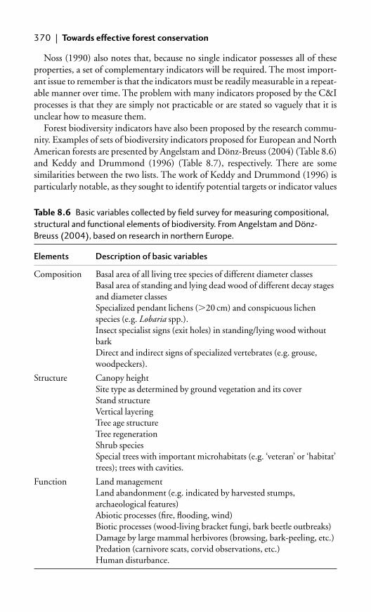
Noss (1990) also notes that, because no single indicator possesses all of theseproperties, a set of complementary indicators will be required. The most import-ant issue to remember is that the indicators must be readily measurable in a repeat-able manner over time. The problem with many indicators proposed by the C&Iprocesses is that they are simply not practicable or are stated so vaguely that it isunclear how to measure them.

Forest biodiversity indicators have also been proposed by the research commu-nity. Examples of sets of biodiversity indicators proposed for European and NorthAmerican forests are presented by Angelstam and Dönz-Breuss (2004) (Table 8.6)and Keddy and Drummond (1996) (Table 8.7), respectively. There are somesimilarities between the two lists. The work of Keddy and Drummond (1996) isparticularly notable, as they sought to identify potential targets or indicator values

370 | Towards effective forest conservation

Table 8.6 Basic variables collected by field survey for measuring compositional,

structural and functional elements of biodiversity. From Angelstam and Dönz-

Breuss (2004), based on research in northern Europe.

Elements Description of basic variables

Composition Basal area of all living tree species of different diameter classesBasal area of standing and lying dead wood of different decay stages and diameter classesSpecialized pendant lichens (�20 cm) and conspicuous lichen species (e.g. Lobaria spp.).Insect specialist signs (exit holes) in standing/lying wood without barkDirect and indirect signs of specialized vertebrates (e.g. grouse, woodpeckers).

Structure Canopy heightSite type as determined by ground vegetation and its coverStand structureVertical layeringTree age structureTree regenerationShrub speciesSpecial trees with important microhabitats (e.g. ‘veteran’ or ‘habitat’trees); trees with cavities.

Function Land managementLand abandonment (e.g. indicated by harvested stumps, archaeological features)Abiotic processes (fire, flooding, wind)Biotic processes (wood-living bracket fungi, bark beetle outbreaks)Damage by large mammal herbivores (browsing, bark-peeling, etc.)Predation (carnivore scats, corvid observations, etc.)Human disturbance.

Indicators | 371

Table 8.7 Ecological attributes for the evaluation, management and restoration

of temperate deciduous forest ecosystems, based on forests in eastern USA

(adapted from Keddy and Drummond 1996).

Property Potential values

Tree size Old growth forests tend to be characterized by relativelyhigh numbers of large trees. A mean basal area of29 4 m2 ha–1 was recorded on 10 pristine sites.

Canopy composition Mature forests tend to be dominated by only a few relativelyshade-tolerant species.Successional forests tend to incorporate a larger number oftree species, including shade-intolerant species.

Coarse woody debris Includes fallen logs, snags, and large branches. An important habitat component for many organisms including birds, mammals, invertebrates and fungi. Highest volumes tend to be recorded in old growth stands (a mean of 27 Mg ha–1 recorded on 10 pristine sites).

Herbaceous layer Many temperate deciduous forests are characterized by adiverse herbaceous flora, which may be sensitive to loggingand especially grazing.

Epiphytic bryophytes Diverse communities of cryptogams (mosses and lichens)and lichens may typically be present on the trunks and branches of

trees, particularly in undisturbed forests unaffected by aerial pollution, in humid environments.

Wildlife trees Many birds, mammals, and invertebrates require trees with particular characteristics for habitat (e.g. as sites fornesting, perching, roosting or foraging). Large-diametersnags (standing dead trees) and cavity trees (live trees with central decay) are of particular importance. Oldgrowth forests tend to be characterized by � 4 wildlife trees per 10 ha.

Fungi Temperate forests are often characterized by diverse communities of larger fungi, which play a critical role indecomposition and nutrient cycling. Many temperate trees form associations with ectomycorrhizal fungi, which assist in nutrient uptake and form an important food resource for many other organisms. The compositionof fungal communities remains poorly documented, but diversity in old growth forests may exceed 100 species ha–1.

Birds The composition of bird communities appears to be particularly sensitive to the area of forest patches, somespecies being dependent on large areas of intact forest.

associated with relatively undisturbed or pristine sites. This is much more difficultto achieve in heavily deforested areas such as Europe, but the approach is a valuableone and should be replicated elsewhere. These lists are presented for illustrativepurposes only: appropriate indicators for forests in other regions, such as thelowland tropics and Mediterranean regions, might be quite different. It should alsobe remembered that these examples represent biodiversity ‘state’ indicators, notpressure or response indicators. Most of these indicators can be measured by usingtechniques described in previous chapters.

Another possibility is to monitor the populations of selected species, termedindicator species. Noss (1999) identifies the types of species that might be suitablefor forest monitoring as follows:

● Area-limited species, which require large patch sizes to maintain viable popula-tions. These species typically have large home ranges and/or low populationdensities, such as many mammalian carnivores.

● Dispersal-limited species, which are limited in their ability to move betweenhabitat patches, or face a high mortality risk in trying to do so. Examplesinclude flightless insects limited to forest interiors, lungless salamanders,small forest mammals, and large mammals subject to roadkill or hunting.

● Resource-limited species, which require specific resources that are often in criticallyshort supply. Resources include large snags, nectar sources, fruits, etc. Examplesare hummingbirds, frugivorous birds, and cavity-nesting birds and mammals.

● Process-limited species, which are sensitive to the level, rate, spatial characteris-tics or timing of some ecological process, such as flooding, fire, grazing orpredation. Examples include plant species that require fire for germination.

372 | Towards effective forest conservation

Table 8.7 (Cont.)

Property Potential values

Large carnivores As large carnivores tend to be at the top of food chains, theirpresence indicates an intact food web. They may play animportant role in keeping herbivore numbers in check, preventing overgrazing and browsing. Large carnivores haveexplicitly been exterminated in many temperate forests andmay therefore need to be considered as an explicit objectiveof restoration action.

Forest area In many areas, once continuous tracts of forest have been highly fragmented as a result of human activity.Fragmentation reduces species diversity and changes speciescomposition in remaining forests. Mammals and birds aremost affected because of their large territorial requirements.For a forest to contain the full complement of species, itmust be large enough to accommodate those species withlargest area requirements (i.e. �100 000 ha).

Indicators | 373

● Keystone species, which are ecologically pivotal species whose impact on acommunity or ecosystem is disproportionately large for their abundance.Examples include dominant tree species, cavity-excavating birds, and herbiv-orous insects subject to outbreaks.

● Narrow endemic species, which are species restricted to a small geographicrange (say �50 000 km2).

● Flagship species, which are those that can be used to promote public supportfor conservation efforts, such as the giant panda.

Once target or indicator species have been chosen, then demographic or geneticattributes will need to be selected for measurement. Important issues includewhether a decline in abundance is occurring, and how much habitat needed forpersistence (see Chapter 7.8), but these can be challenging to determine. Thepopulations most in need of tracking are often the most difficult to monitor (Noss1999).

How may indicators be validated? This is an area neglected by much previousresearch (Noss 1990), yet it is critically important. For example, measures of forestfragmentation may be obtained fairly readily (see sections 2.7 and 7.4). But howdo these measures relate to the potential impact of fragmentation on organisms?Angelstam et al. (2004b) provide some suggestions regarding how indicatorsmight be validated:

● Examine how the value of a given indicator correlates with other elements ofbiodiversity; for example, the presence of a habitat might correlate with thepresence of a particular species, and some habitat features might correlatewith species richness.

● Compare their level in gradients from intensively managed forests to naturalor near-natural forests. If an indicator shows a consistent trend whenmeasured across that gradient, then it can be considered a reliable indicator ofnatural forest conditions.

Ultimately the validation of indicators depends on a comprehensive under-standing of the links between biodiversity patterns and the processes responsiblefor producing them. This is a job for the research community, and there remainsenormous scope for further research in this area. The job is an important one.Consider the Natura 2000 network of protected areas, one of the main coordi-nated actions being undertaken at the European level towards biodiversity conser-vation. The main aim of the Natura 2000 network is to maintain a favourableconservation status (FCS) to help ensure the maintenance of biodiversity of naturalhabitats and of wild flora and fauna in the European territory. A laudable goal, buthow will anyone be sure that this target is being met? The only way of providingsuch information is to monitor FCS, enabling the performance of Natura 2000network to be evaluated. This requires development of appropriate indicators.Astonishingly, few indicators have been proposed to date, and their validation isin its infancy (Cantarello 2006).

It is also important to remember that indicators are essentially tools for com-municating results. They can provide a useful way of making a link betweenresearch and management practice, and between research and policy. Once datahave been collected, they have to be presented in a form that can be readilyinterpreted by the decision-makers for whom they are intended. Newton andKapos (2002) suggest that this can most readily be achieved by summarizing datain categorical form, and presenting them in relation to forest area. For example,species richness could be presented as the area of forest possessing more than acertain number of tree species, or forest fragmentation could be presented as forestareas with particular values of fragmentation indices. This approach enables resultsto be mapped, facilitating communication and integration with other data. Theapproach can also assist in the aggregation of data across different scales formonitoring and reporting purposes.

8.7 Scenarios

Conservation actions are generally based upon some expectation about whatmight happen in the future. For example, if a species is declining in abundance,then a conservation intervention might be planned based on an assumption thatthis decline is likely to continue unless action is taken. However, the future ishighly unpredictable. Even if models of ecological dynamics are available (Chapter5), they will be based on a range of assumptions and uncertainties. Scenario plan-ning offers a framework for developing conservation approaches under suchuncertain conditions. A scenario can be defined in this context as an account of aplausible future (Peterson et al. 2003). The development of scenarios is a recog-nized tool in business planning and economic forecasting, but has only recentlybeen applied to conservation. Peterson et al. (2003) provide a valuable introduc-tion to the use of scenarios in a conservation context. An attempt to develop globalbiodiversity scenarios is described by Sala et al. (2000), elaborated further byChapin et al. (2001) (see also Carpenter et al. 2005).

Scenario planning provides a tool to explore the uncertainty surrounding thefuture consequences of a decision, by developing a small number of contrastingscenarios. Generally scenarios are developed by a diverse group of people in asystemic process of collecting, discussing, and analysing information, through aseries of workshops. The group might involve research scientists, forest managers,conservation practitioners or activists, policy-makers, local community members,and other stakeholders. The scenarios may draw upon a variety of quantitative andqualitative information, such as the results of ecological surveys and outputs frommodelling exercises. Peterson et al. (2003) suggest that the major benefits of usingscenario planning for conservation are (1) increased understanding of key uncer-tainties, (2) incorporation of alternative perspectives into conservation planning,and (3) greater resilience of decisions to surprise.

374 | Towards effective forest conservation

Scenarios | 375

Peterson et al. (2003) describe scenario planning as consisting of six interactingstages:

● Identification of a focal issue or problem. This may usefully be phrased as aquestion, such as how to maintain a functional oak forest in a protected areafor the next 20 years, or how to make an existing reserve network more robust.

● Assessment. This should include an assessment of the people, institutions,ecosystems, and linkages among them that define a system. External changesshould also be identified, including both ecological and social factors thatinfluence system dynamics. This might usefully include an assessment ofthreats, pressures, or driving forces (see previous section). Uncertainties thatmay have a large impact on the focal issue should be identified. For example,climatic change may be a key uncertainty in the planning of a park system.

● Identification of alternatives. The aim of this stage is to identify alternativeways that the system could evolve. The alternatives should be plausible andrelevant to the original question. A commonly used way of defining a set ofalternatives is to choose two or three uncertain or uncontrollable drivingforces, such as population growth and settlement pattern, which can beused to define alternatives such as increased migration to cities, increasedmigration to rural areas, and general population decline. The uncertaintieschosen to define the alternatives should have differences that are directlyrelated to the defining question or issue. The set of alternatives provides aframework around which scenarios can be constructed.

● Building scenarios. Scenarios are developed around some of the alternativesdefined in the previous step, considering the key uncertainties. The scenariosshould usefully expand and challenge current thinking about the system. Thenumber of scenarios is generally three or four. The scenarios are built by con-verting the key alternatives into narratives by describing a credible series ofexternal forces and actors’ responses, linking historical and present events withhypothetical future events. Each scenario should be clearly anchored in thepast, with the future emerging from the past and present in a seamless way, andshould track key indicator variables (such as percentage of intact old-growthforest). Usually each scenario is given a name that evokes its main features (seeBox 8.6)—this is often the part that is most fun! Successful scenarios are vividand different, can be told easily, and plausibly capture possible future change.

● Testing scenarios. The dynamics of scenarios must be plausible. The scenariosshould be tested for consistency; this can be achieved through expert opinionor by comparison with other scenarios. Simulation models can be used to testthe dynamics of a scenario, but models are not the primary tool for scenariodevelopment. The key issue to check is the behaviour of actors; expectedchanges within each scenario should be examined from the perspective ofeach key actor within it.

● Policy screening. Once developed, scenarios can be used to test, analyse, and cre-ate policies. This is achieved by assessing how existing policies would fare underdifferent scenarios, enabling the properties of relatively weak or strong policies

to be identified. For example, scenarios could be used to help identify land-management strategies that produce protected areas that are resilient inresponse to change. It is important to identify traps and opportunities andaspects of the current situation that could influence these scenario features. Theprocess may suggest novel policies, areas for research, and issues to monitor.

Although scenarios have not been used widely in conservation planning to date, theyoffer a tractable and stimulating method of engaging in a debate about what mighthappen in the future and how to deal with it. The method therefore has great poten-tial. Scenarios are increasingly being used in environmental assessment at global andregional scales (Box 8.6), but the approach can potentially be implemented at thelocal scale, such as an individual forest management unit or protected area.

376 | Towards effective forest conservation

Box 8.6 Information resources on scenarios.

Millennium Ecosystem Assessment �/www.maweb.org/ �This international environmental assessment developed a set of four scenariosthrough a major collaborative effort. The report produced can be freely down-loaded from this website. The scenarios were defined as:

● Global Orchestration, defined as socially conscious globalization, in whichequity, economic growth, and public goods are emphasized, reacting toecosystem problems when they reach critical stages.

● Order from Strength, representing a regionalized approach, in which theemphasis is on security and economic growth, again reacting to ecosystemproblems only as they arise.

● Adapting Mosaic, defined also as a regionalized approach, but one thatemphasizes proactive management of ecosystems, local adaptation, andflexible governance.

● TechnoGarden, which is a globalized approach with an emphasis on greentechnology and a proactive approach to managing ecosystems.

Global Environment Outlook �www.unep.org/geo/ �Another international environmental assessment process, coordinated by UNEP,which has used scenarios extensively in the past. Materials freely downloadablefrom the website.

Shell Global Scenarios �www.shell.com/scenarios/ �Shell has been involved in scenario development for some 30 years. The websiteoffers introductory information about scenario planning as well as several down-loadable scenarios.

Scenarios for Sustainability �www.scenariosforsustainability.org�A very useful online resource offering practical tools for scenario development.

Postscript: making a difference | 377

8.8 Evidence-based conservation

Concern has been growing in recent years that much conservation practice is basedon tradition or the experience of practitioners, rather than on the results of scien-tific research. To increase the effectiveness of conservation, some researchers haverecently proposed that conservation action should become more ‘evidence-based’,by drawing more heavily on the results of scientific research (Pullin and Knight2001, 2003, Pullin et al. 2004, Sutherland et al. 2004b). This has been inspired bythe ‘effectiveness revolution’ that has occurred in medicine over the past twodecades, aimed at linking medical research with medical practice (Sutherland2000).

A key element of the evidence-based approach is systematic review, whichinvolves reviewing the scientific literature and unpublished sources, criticallyassessing the methods used and synthesizing the evidence in relation to a researchquestion or management issue. The approach differs from conventional literaturereviews in following a strict methodological protocol, often incorporating someform of meta-analysis. The aim is to provide a comprehensive, unbiased andobjective assessment of available evidence.

Results of the first systematic reviews of conservation evidence are now becom-ing available (Stewart et al. 2005), although to date, none of the reviews hasfocused on forest ecosystems. Websites have been created aiming to support thedissemination of research results to conservation practitioners (examples are�www.cebc.bham.ac.uk� and �www.conservationevidence.com�). Although such ini-tiatives are clearly to be welcomed, one of the problems facing the conservationcommunity is just how little well-designed research has been undertaken on manyconservation problems. The most reliable form of evidence is a fully replicatedexperiment, but such experiments may be difficult or even impossible under fieldconditions (Diamond 1986), and for almost any conservation issue such experi-ments are few in number. Conservation management is likely to continue todepend on a blend of experience, tradition and scientific evidence, but the chal-lenge for researchers is to help ensure that their research results are communicatedeffectively to practitioners in a form that can directly support decision-making.Indicators, models, GIS, and other decision-support tools (see �http://ncseonline.org/NCSSF/DSS� for a useful compendium) can all help in this process, but thereis ultimately no substitute for researchers and practitioners collaborating moreclosely, perhaps implementing an adaptive management approach together.

8.9 Postscript: making a difference

So, at the end of the day, how can we make a difference to conservation? In otherwords, how can we ensure that the work we do really has an impact on the ground,and helps save the forests that we care about? Make no mistake, working on forestconservation is often a depressing business. Devastated forests are all too easy to

find. The problems can often seem so overwhelming that the contribution we canmake as individuals may seem trivial or insignificant. It can seem as if our work isjust a drop in the ocean. ‘But what is an ocean but a multitude of drops?’ (Mitchell2004).

There is no doubt that individuals can make a difference. Think of WangariMaathai, recently awarded the Nobel Peace prize for having planted 30 milliontrees. In my own experience, I have been inspired by individuals such as AlanWatson of Trees for Life �www.treesforlife.org.uk� and Philip Ashmole of theCarrifran Wildwood Project �www.carrifran.org�, who through their own personalvision and dedication have successfully developed and implemented large-scaleforest restoration projects in the UK, despite having to overcome many obstaclesin the process. It is possible to make a difference through environmental activism,campaigning, or advocacy; by being a politician or government official; by runninga large business; or simply by being rich and spending your money on creating aprotected area.

But what can we achieve as researchers? Can science help conservation? Or, assome have suggested (Whitten et al. 2001), is conservation biology merely a ‘dis-placement activity for academics’? There are many dedicated conservation practi-tioners who make a real difference on a daily basis, with no scientific training at all.On the other hand, some of them make mistakes. If asked to provide evidence ofthe impacts of management interventions they have undertaken, most practition-ers are unable to provide anything beyond anecdotal observations. Scientificallyrobust forest monitoring is actually very rare. Consequently, adaptive manage-ment is very rare. Truly sustainable forest management is also very rare (perhaps itdoesn’t exist at all). When we start to consider all the organisms other than trees—the insects, fungi, lichens, mammals, reptiles, amphibians, birds, and many othercreatures that inhabit forests—we start to realize how very little we know aboutmost forest communities. In fact, we cannot even estimate with reasonable accur-acy how many species are being lost as a result of current deforestation. This issomething that should shame us all.

The need for scientific research into forest ecology and conservation is immense.The challenge is often to convince non-scientists—whether they be local commu-nities, politicians, business leaders, funding agencies, or the public at large—thatthis is the case. Furthermore, it is essential to ensure that the scientific work that isbeing carried out is relevant to the problems that need addressing. The responsi-bility for ensuring this lies with just one person. The person holding this book.

378 | Towards effective forest conservation

References

Abbitt, R. J. F., Scott, J. M., and Wilcove, D. S. (2000). The geography of vulnerability:incorporating species geography and human development patterns into conservation planning.Biological Conservation, 96, 169–175.

Acevedo, M. F., Urban, D. L., and Ablan, M. (1995). Transition and gap models of forestdynamics. Ecological Applications, 5(4), 1040–1055.

Acevedo, M. F., Urban, D. L., and Ablan, M. (1996a). Landscape scale forest dynamics: GIS,gap and transition models. In GIS and environmental modeling: Progress and research issues, eds.M. F. Goodchild, L. T. Steyaert, and B. O. Parks, pp. 181–185. GIS World Books, FortCollins, CO.

Acevedo, M. F., Urban, D. L., and Shugart, H. H. (1996b). Models of forest dynamics based onroles of tree species. Ecological Modelling, 87, 267–284.

Adams, J. B., Sabol, D. E., Kapos, V., Filho, R. A., Roberts, D., Smith, M. O., and Gillespie, A. R.(1995). Classification of multispectral images based on fractions of endmembers: applicationsto land-cover change in the Brazilian Amazon. Remote Sensing of Environment, 52, 137–152.

Adams, W. T., Strauss, S. H., Copes, D. L., and Griffin, A. R. (eds.) (1992). Population geneticsof forest trees. Springer-Verlag, Berlin.

Agee, J. K. (1993). Fire ecology in Pacific Northwest forests. Island Press, Washington DC.Agyeman, V. K., Swaine, M. D., and Thompson, J. (1999). Responses of tropical forest tree

seedlings to irradiance and the derivation of a light response index. Journal of Ecology, 87,815–827.

Akçakaya, H. R. and Root, W. (2002). RAMAS Metapop: Viability analysis for stage-structuredmetapopulations (ver. 4.0). Applied Biomathematics, Setauket, NY.

Akçakaya, H. R. and Sjögren-Gulve, P. (2000). Population viability analysis in conservationplanning: an overview. Ecological Bulletins, 48, 9–21.

Akçakaya, H. R., Radeloff, V. C., Mladenoff, D. J., and He, H. S. (2004). Integrating landscapeand metapopulation modelling approaches: viability of the sharp-tailed grouse in a dynamiclandscape. Conservation Biology, 18, 526–537.

Alder, D. and Synnott, T. J. (1992). Permanent sample plot techniques for mixed tropical forest.Tropical Forestry Papers 25, Oxford Forestry Institute, Oxford.

Aldred, A. H. and Alemdag, I. S. (1988). Guidelines for forest biomass inventory. Petawawa NationalForestry Institute Report PI-X-77. Canadian Forest Service, Natural Resources Canada, Ottawa.

Aldrich, P. R., Parker, G. R., Ward, J. S., and Michler, C. H. (2003). Spatial dispersion of treesin an old-growth temperate hardwood forest over 60 years of succession. Forest Ecology andManagement, 180(1–3), 475–491.

Allen, J. and Barnes, D. (1985). The causes of deforestation in developing countries. Annals ofthe Association of American Geographers, 75, 163–184.

Allnutt, T. R., Thomas, P., Newton, A. C., and Gardner, M. F. (1998). Genetic variation inFitzroya cupressoides cultivated in the British Isles, assessed using RAPDs. Botanical Journal ofEdinburgh, 55(3), 329–341.

Allnutt, T. R., Newton, A. C., Lara, A., Premoli, A., Armesto, J. J., Vergara, R., and Gardner, M.(1999). Genetic variation in Fitzroya cupressoides (alerce), a threatened South Americanconifer. Molecular Ecology, 8, 975–987.

Alonso, D. and Sole, R. V. (2000). The DivGame Simulator: a stochastic cellular automatamodel of rainforest dynamics. Ecological Modelling, 133(1–2), 131–141.

Alvarez-Aquino, C., Williams-Linera, G., and Newton, A. C. (2005). Composition of the seedbank in disturbed fragments of Mexican cloud forest. Biotropica, 37(3), 337–342.

Alvarez-Buylla, E. R. and Slatkin, M. (1991). Finding confidence limits on population growthrates. Trends in Ecology and Evolution, 6, 221–224.

Alves, D. S., Pereira, J. L. G., De Sousa, C. L., Soares, J. V., and Yamaguchi, F. (1999).Characterising landscape changes in central Rondonia using Landsat TM imagery.International Journal of Remote Sensing, 20, 2877–2882.

Amarnath, G., Murthy, M. S. R., Britto, S. J., Rajashekar, G., and Dutt, C. B. S. (2003).Diagnostic analysis of conservation zones using remote sensing and GIS techniques in wetevergreen forests of the Western Ghats—an ecological hotspot, Tamil Nadu, India.Biodiversity and Conservation, 12(12), 2331–2359.

Amaro, A., Reed, D., and Saores, P. (eds.) (2003). Modelling forest systems. CABI Publishing,Wallingford.

Andelman, S., Ball, I., Davis, F., and Stoms, D. (1999). Sites 1.0: An analytical toolbox fordesigning ecoregional conservation portfolios. Manual prepared for The Nature Conservancy,Arlington, VA.

Andersen, M. (1991). Mechanistic models for the seed shadows of wind-dispersed plants.American Naturalist, 137, 476–497.

Anderson, M. C. (1964). Studies of the woodland light climate. I. The photographic computa-tion of light conditions. Journal of Ecology, 52, 27–41.

Anderson, R. P., Lew, D., and Peterson, A. T. (2003). Evaluating predictive models of species’distributions: criteria for selecting optimal models. Ecological Modelling, 162, 211–232.

Angelstam, P. and Dönz-Breuss, M. (2004). Measuring forest biodiversity at the stand scale—anevaluation of indicators in European forest history gradients. Ecological Bulletins, 51, 305–332.

Angelstam, P., Dönz-Breuss, M., and Roberge, J.-M. (2004a). Targets and tools for the mainten-ance of forest biodiversity. (Ecological Bulletins No. 51) Blackwell Science, Oxford.

Angelstam, P., Roberge, J.-M., Dönz-Breuss, M., Burfield, I. J., and Ståhl, G. (2004b).Monitoring forest biodiversity—from the policy level to the management unit. EcologicalBulletins, 51, 295–304.

Armenteras, D., Gast, F., and Villareal, H. (2003). Andean forest fragmentation and the represen-tativeness of protected natural areas in the eastern Andes, Colombia. Biological Conservation,113, 245–256.

Arno, S. F. and Sneck, K. M. (1977). A method for determining fire history in coniferous forests ofthe Mountain West. US Department of Agriculture, Forest Service, General Technical ReportINT-42.

Ashley, C. and Carney, D. (1999). Sustainable livelihoods: Lessons from early experience. DFID,London.

Ashton, P. M. S. (1995). Seedling growth of co-occurring Shorea species in the simulated lightenvironments of a rain forest. Forest Ecology and Management, 72, 1–12.

Ashton, P. M. S., Gunatilleke, C. V. S., and Gunatilleke, I. A. U. N. (1995). Seedling survival andgrowth of four Shorea species in Sri Lankan rainforest. Journal of Tropical Ecology, 11, 263–279.

Ashton, P. S. and Hall, P. (1992). Comparisons of structure among mixed dipterocarp forests ofnorth-western Borneo. Journal of Ecology, 80, 459–481.

Asner, G. P., Hicke, J. A. and Lobell, D. B. (2003). Per-pixel analysis of forest structure.In Remote sensing of forest environments, eds. M. A. Wulder and S. E. Franklin, pp. 209–254.Kluwer, Dordrecht.

Attiwill, P. M. (1994). The disturbance of forest ecosystems: the ecological basis for conservativemanagement. Forest Ecology and Management, 63, 247–300.

Augspurger, C. K. (1983). Seed dispersal of the tropical tree, Platypodium elegans, and the escapeof its seedlings from fungal pathogens. Journal of Ecology, 71, 759–771.

380 | References

References | 381

Augspurger, C. K. (1984). Light requirements of neotropical tree seedlings: a comparative studyof growth and survival. Journal of Ecology, 72, 777–795.

Augspurger, C. K. and Hogan, K. P. (1983). Wind dispersal of fruits with variable seed numberin a tropical tree (Lonchocarpus pentaphyllus, Leguminosae). American Journal of Botany, 70,1031–1037.

Augspurger, C. K. and Kelly, C. K. (1984). Pathogen mortality of tropical tree seedlings: experi-mental studies of the effects of dispersal distance, seedling density, and light conditions.Oecologia, 61, 211–217.

Austin, M. P. and Heyligers, P. C. (1989). Vegetation survey design for conservation: gradsectsampling of forests in Northeast New South Wales. Biological Conservation, 50, 13–32.

Austin, M. P. and Heyligers, P. C. (1991). New approach to vegetation survey design: gradsectsampling. In Nature conservation: Cost effective biological surveys and data analysis, eds.C. R. Margules and M. P. Austin, pp. 31–36. CSIRO, Canberra, Australia.

Avery, T. E. (1968). Interpretation of aerial photographs, 2nd edition. Burgess, Minneapolis, MN.Avery, T. E. (1978). Forester’s guide to aerial photo interpretation. USDA Forest Service,

Agriculture Handbook no. 308. US Department of Agriculture, Washington, DC.Avery, T. E. and Berlin, G. L. (1992). Fundamentals of remote sensing and airphoto interpretation,

5th edition. Macmillan, NY.Avery, T. E. and Burkhart, H. E. (2002). Forest measurements, 5th edition. McGraw-Hill, NY.Bachmann, P., Köhl, M., and Päivinen, R. (eds.). (1998). Assessment of biodiversity for improved

forest planning. Kluwer, Dordrecht.Bacles, C. F. E., Lowe, A. J., and Ennos, R. A. (2004). Genetic effects of chronic habitat

fragmentation on tree species: the case of Sorbus aucuparia in a deforested Scottish landscape.Molecular Ecology, 13, 573–584.

Bacles, C. F. E., Lowe, A. J., and Ennos, R. A. (2006). Effective seed dispersal across a fragmentedlandscape. Science, 311, 628.

Baguette, M. (2004). The classical metapopulation theory and the real, natural world: a criticalappraisal. Basic and Applied Ecology, 5, 213–224.

Bajracharya, S. B., Furley, P. A., and Newton, A. C. (2005). Effectiveness of community involve-ment in delivering conservation benefits to the Annapurna Conservation Area, Nepal.Environmental Conservation, 32(3), 239–247.

Baker, A. (ed.) (2000). Molecular methods in ecology. Blackwell Science, Oxford.Baker, P. J. and Wilson, J. S. (2000). A quantitative technique for the identification of canopy

stratification in tropical and temperate forests. Forest Ecology and Management, 127, 77–86.Baker, T. R., Swaine, M. D., and Burslem, D. F. R. P. (2003). Variation in tropical forest growth

rates: combined effects of functional group composition and resource availability. Perspectivesin Plant Ecology, Evolution and Systematics, 6/1(2), 21–36.

Baldocchi, D. and Collineau, S. (1994). The physical nature of solar radiation in heterogeneouscanopies: spatial and temporal attributes. In Exploitation of environmental heterogeneity byplants, eds. M. M. Caldwell and R. W. Pearcy, pp. 21–71. Academic Press, San Diego, CA.

Ball, I. R. and Possingham, H. P. (2000). MARXAN (V1.8.2): Marine reserve design using spa-tially explicit annealing, a manual. University of Queensland, Australia.

Ball, I. R., Lindenmayer, D. B., and Possingham, H. P. (1999). A tree hollow dynamics simula-tion model. Forest Ecology and Management, 123(2–3), 179–194.

Balmford, A., Bennun, L., ten Brink, B. et al. (2005). The Convention on Biological Diversity’s2010 target. Science, 307(5707), 212–213.

Balzter, H., Braun, P. W., and Kohler, W. (1998). Cellular automata models for vegetationdynamics. Ecological Modelling, 107(2–3), 113–125.

Barabesi, L. and Fattorini, L. (1995). Kernel plant density estimation by a ranked set samplingof point-to-plant distances. In The Monte Verita conference on forest survey designs, eds.

M. Köhl, P. Bachmann, P. Brassel, and G. Preto, pp. 71–80. WSL/ETHZ, Birmensdorf,Switzerland

Bardon, R. E., Countryman, D. W., and Hall, R. B. (1995). A reassessment of using light-sensitive diazo paper for measuring integrated light in the field. Ecology, 76, 1013–1016.

Barnes, B. V., Zak, D. R., Denton, S. R., and Spurr, S. H. (1998). Forest ecology, 4th edition.Wiley, New York.

Barot, S., Gignoux, J., and Menaut, J.-C. (1999). Demography of a savanna palm tree:predictions from comprehensive spatial pattern analyses. Ecology, 80, 1987–2005.

Baskent, E. (1999). Controlling spatial structure of forested landscapes: a case study towardslandscape management. Landscape Ecology, 14, 83–97.

Baskent, E. Z. and Jordan, G. A. (1995). Characterizing spatial structure of forest landscapes.Canadian Journal of Forest Research, 25, 1830–1849.

Baskin, C. C. and Baskin, J. M. (1998). Seeds: Ecology, biogeography and evolution of dormancyand germination. Academic Press, San Diego, CA.

Bass, B., Hansell, R., and Choi, J. (1998). Towards a simple indicator of biodiversity.Environmental Monitoring and Assessment, 49, 337–347.

Batista, W. B., Platt, W. J., and Macchiavelli, R. E. (1998). Demography of a shade-tolerant tree(Fagus grandifolia) in a hurricane-disturbed forest. Ecology, 79, 38–53.

Bawa, K. S. and Hadley, M. (eds.) (1990). Reproductive ecology of tropical forest plants. Man andthe Biosphere Series vol. 7. UNESCO, Paris.

Bebber, D., Brown, N., Speight, M., Moura-Costa, P., and Sau Wai, Y. (2002). Spatial structureof light and dipterocarp seedling growth in a tropical secondary forest, Forest Ecology andManagement, 157(1–3), 65–75.

Bebi, P., Kienast, F., and Schonenberger, W. (2001). Assessing structures in mountain forests asa basis for investigating the forest’s dynamics and protective function. Forest Ecology andManagement, 145, 3–14.

Becker, M. (1971). Une technique nouvelle d’utilization des photographies hémisphériquespour la mesure du climat lumineux en forêt. Annales des Sciences Forestières, 28, 425–442.

Beers, T. W. (1969). Slope correction in horizontal point sampling. Journal of Forestry, 67, 188–192.Begon, M. and Mortimer, M. (1981). Population ecology: a unified study of animals and plants.

Blackwell Scientific, Oxford.Begon, M., Harper, J. L., and Rownsend, C. R. (1996). Ecology: Individuals, populations and

communities. Blackwell Science, Oxford.Behera, M. D., Kushwaha, S. P. S., and Roy, P. S. (2005). Rapid assessment of biological richness

in a part of Eastern Himalaya: an integrated three-tier approach. Forest Ecology andManagement, 207(3), 363–384.

Bekessy, S. A., Allnutt, T. R., Premoli, A. C. et al. (2002a). Genetic variation in the vulnerableand endemic Monkey Puzzle tree, detected using RAPDs. Heredity, 88, 243–249.

Bekessy, S. A., Sleep, D., Stott, A. et al. (2002b). Adaptation of Monkey Puzzle to arid environ-ments reflected by regional differences in stable carbon isotope ratio and allocation to rootbiomass. Forest Genetics, 9(1), 63–70.

Bekessy, S. A., Ennos, R. A., Ades, P. K., Burgman, M. A., and Newton, A. C. (2003). NeutralDNA markers fail to detect divergence in an ecologically important trait. BiologicalConservation, 110, 267–275.

Bekessy, S. A., Newton, A. C., Fox, J. C. et al. (2004). The monkey puzzle tree in southern Chile.In Species conservation and management: Case studies using RAMAS GIS, eds. H. R. Açkakaya,M. A. Burgman, O. Kindval, P. Sjögren-Gulve, J. Hatfield and M. McCarthy, pp. 48–63.Oxford University Press, Oxford.

Bellingham, P. J., Tanner, E. V. J., and Healey, J. R. (1994). Sprouting of trees in Jamaicanmontane forests after a hurricane. Journal of Ecology, 82, 747–758.

382 | References

Bellingham, P. J., Tanner, E. V. J., and Healey, J. R. (1995). Damage and responsiveness ofJamaican montane tree species after disturbance by a hurricane. Ecology, 76, 2562–2580.

Bertault, J. G. and Sist, P. (1997). An experimental comparison of different harvesting intensitieswith reduced-impact and conventional logging in East Kalimantan, Indonesia. Forest Ecologyand Management, 94(1–3), 209–218.

Bhadresa, R. (1986). Faecal analysis and exclosure studies. In Methods in plant ecology, 2ndedition, eds. P. D. Moore and S. B. Chapman, pp. 61–71. Blackwell Scientific, Oxford.

Bierzychudek, P. (1999). Looking backwards: assessing the projections of a transition matrixmodel. Ecological Applications, 9, 1278–1287.

Blasco, F., Whitmore, T. C., and Gers, C. (2000). A framework for the worldwide comparisonof tropical woody vegetation types. Biological Conservation, 95, 175–189.

Bond, W. J. (1997). Functional types for predicting changes in biodiversity: a case study in Capefynbos. In Plant functional types, eds. T. M. Smith, H. H. Shugart, and F. I. Woodward,pp. 174–194. Cambridge University Press, Cambridge.

Bond, W. J. (1998). Ecological and evolutionary importance of disturbance and catastrophes inplant conservation. In Conservation in a changing world, eds. G. M. Mace, A. Balmford, andJ. R. Ginsberg, pp. 87–106. Cambridge University Press, Cambridge.

Boose, E. R., Chamberlin, K. E., and Foster, D. R. (2001). Landscape and regional impacts ofhurricanes in New England. Ecological Monographs, 71, 27–48.

Boot, R. G. A. and Gullison, R. E. (1995). Approaches to developing sustainable extractionsystems for tropical forest products. Ecological Applications, 5(4), 896–903.

Borrough, P. A. and McDonnell, R. (1998). Principles of geographical information systems (spatialinformation systems). Clarendon Press, Oxford.

Boshier, D. H., Chase, M. R., and Bawa, K. S. (1995). Population genetics of Cordia alliodora(Boraginaceae), a neotropical tree. 2. Mating system. American Journal of Botany, 82, 476–483.

Bossard, C. C. (1990). Tracing of ant-dispersed seeds: a new technique. Ecology, 71, 2370–2371.Botkin, D. B. (1993). Forest dynamics: An ecological model. Oxford University Press. Oxford.Botkin, D. B., Janak, J. R., and Wallis, J. R. (1972a). Rationale, limitations and assumptions of

a northeast forest growth simulator. IBM Journal of Research and Development, 16, 101–116.Botkin, D. B., Janak J. F., and Wallis, J. R. (1972b). Some ecological consequences of a computer

model of forest growth. Journal of Ecology, 60, 849–872.Boucher, D. H. and Mallona, M. A. (1997). Recovery of the rain forest tree Vochysia ferruginea

over 5 years following Hurricane Joan in Nicaragua: a preliminary population projectionmatrix. Forest Ecology and Management, 91, 195–204.

Bower, D. R. and Blocker, W. W. (1966). Accuracy of bands and tape for measuring diameterincrements. Journal of Forestry, 64, 21–22.

Bradbeer, J. W. (1988). Seed dormancy and germination. Blackie, Glasgow.Bradstock, R. A. and Kenny, B. J. (2003). Application of plant functional traits to fire management

in a conservation reserve in southeastern Australia. Journal of Vegetation Science, 14, 345–354.Brändli, U. B., Kaufmann, E., and Stierlin, H. R. (1995). Survey of biodiversity at the forest mar-

gin in the second Swiss NFI. In The Monte Verita conference on forest survey designs, eds. M. Köhl,P. Bachmann, P. Brassel, and G. Preto, pp. 141–150. WSL/ETHZ, Birmensdorf, Switzerland.

Brandon, K., Redford, K. H., and Sanderson, S. E. (eds.) (1998). Parks in peril. People, politicsand protected areas. Island Press, Washington, DC.

Bréda, N. J. J. (2003). Ground-based measurements of leaf area index: a review of methods,instruments and current controversies. Journal of Experimental Botany, 54(392), 2403–2417.

Briers, R. A. (2002). Incorporating connectivity in reserve selection procedures. BiologicalConservation, 103, 77–83.

Briggs, D. and Walters, S. M. (1997). Plant variation and evolution, 3rd edition. CambridgeUniversity Press, Cambridge.

References | 383

384 | References

Brigham, C. A. and Schwartz, M. A. (eds.) (2003). Population viability in plants. Conservation,management and modeling of rare plants. Ecological Studies 165, Springer-Verlag, Berlin.

Brigham, C. A. and Thomson, D. M. (2003). Approaches to modeling population viability inplants: an overview. In Population viability in plants. Conservation, management and modelingof rare plants, eds. C. A. Brigham and M. A. Schwartz, pp. 145–171. Ecological Studies 165,Springer-Verlag, Berlin.

Brockhaus, J. A., Khorram, S., Bruck, R., Campbell, M. V., and Stallings, C. (1992). A comparison of Landsat TM and SPOT HRV data for use in the development of forestdefoliation models. International Journal of Remote Sensing, 13, 3235–3240.

Brokaw, N. V. (1985). Treefalls, regrowth, and community structure in tropical forests. In Theecology of natural disturbance and patch dynamics, eds. S. T. A. Pickett and P. S. White,pp. 53–69. Academic Press, Orlando, FL.

Brokaw, N. V. L. and Lent, R. A. (1999). Vertical structure. In Maintaining biodiversity in forestecosystems, ed. M. L. Hunter, pp. 373–399. Cambridge University Press, Cambridge.

Brommit, A., Charbonneau, N., Contreras, T. A., and Fahrig, L. (2004). Crown loss andsubsequent branch sprouting of forest trees in response to a major ice storm. Journal of theTorrey Botanical Society, 131, 169–176.

Brook, B. W., O’Grady, J. J., Chapman, A. P., Burgman, M. A., Akçakaya, H. R., and Frankham,R. (2000). Predictive accuracy of population viability analysis in conservation biology.Nature, 404, 385–387.

Brook, B. W., Burgman, M. A., Akçakaya, H. R., O’Grady, J. J., and Frankham, R. (2002).Critiques of PVA as the wrong questions: throwing the heuristic baby out with the numericalbath water. Conservation Biology, 16(1), 262–263.

Brooks, R. P. (1997). Improving habitat suitability index models. Wildlife Society Bulletin, 25,163–167.

Brooks, T., Balmford, A., Burgess, N., Fjeldså, J., Hansen, L. A., Moore, J., Rahbek, C., andWilliams, P. (2001). Toward a blueprint for conservation in Africa. Bioscience, 51, 613–624.

Brown, A. H. D. (1990). Genetic characterization of plant mating systems. In Plant Populationgenetics, breeding and genetic resources, eds. A. H. D. Brown, M. T. Clegg, A. L. Kahler, and B.S. Weir, pp. 145–162. Sinauer Associates, Sunderland, MA.

Brown, N. D. and Jennings, S. (1998). Gap-size niche differentiation by tropical rainforest trees:a testable hypothesis or a broken-down bandwagon? In Dynamics of tropical communities, eds.D. M. Newbery, H. H. T. Prins, and N. Brown, pp. 79–94. Blackwell Science, Oxford.

Brown, N., Jennings, S., Wheeler, P., and Nabe-Nielson, J. (2000). An improved method for therapid assessment of forest understorey light environments. Journal of Applied Ecology, 37,1044–1053.

Brown, S. L., Schroeder, P., and Kern, J. S. (1999). Spatial distribution of biomass in forests ofthe eastern USA. Forest Ecology and Management, 123, 81–90.

Brown, V. K. and Gange, A. C. (1989). Differential effects of above- and below-ground insectherbivory during early plant succession. Oikos, 54, 67–76.

Brown, V. K., Gange, A. C., Evans, I. M., and Storr, A. L. (1987). The effect of insect herbivoryon the growth and reproduction of two annual Vicia species at different stages in plantsuccession. Journal of Ecology, 75, 1173–1189.

Bruner, A. G., Gullison, R. E., Rice, R. E., and da Fonseca, G. A. B. (2001). Effectiveness ofparks in protecting tropical biodiversity. Science, 291(5501), 125–128.

Bryant, D., Nielsen, D., and Tangley, L. (1997). The last frontier forests. Ecosystems and economieson the edge. World Resources Institute, Washington, DC.

Buckland, S. T., Anderson, D. R., Burnham, K. P., Laake, J. L., Borchers, D. L., and Thomas, L.(2001). Introduction to distance sampling: Estimating abundance of biological populations.Oxford University Press, Oxford.

Bucur, V. (2003). Nondestructive characterization and imaging of wood. Springer-Verlag, New York.Bugmann, H. (2001). A review of forest gap models. Climatic Change, 51(3–4), 259–305.Bugmann, H. (2003). Predicting the ecosystem effects of climate change. In Models in ecosystem

science, eds. C. D. Canham, J. J. Cole, and W. K. Lauenroth, pp. 385–409. PrincetonUniversity Press, Princeton, NJ.

Bullock, J. (1996). Plants. In Ecological census techniques. A handbook, ed. W. J. Sutherland,pp. 111–138. Cambridge University Press, Cambridge.

Bullock, J. M. and Clarke, R. T. (2000). Long distance seed dispersal by wind: measuring andmodelling the tail of the curve. Oecologia, 124, 506–521.

Bunnell, F. L. and Vales, D. J. (1990). Comparison of methods for estimating forest overstorycover: differences among techniques. Canadian Journal of Forest Research, 20, 101–107.

Bunyavejchewin, S., LaFrankie, J. V., Baker, P. J., Kanzaki, M., Ashton, P. S., and Yamakura, T.(2003). Spatial distribution patterns of the dominant canopy dipterocarp species in a seasonaldry evergreen forest in western Thailand. Forest Ecology and Management, 175(1–3), 87–101.

Burgess, N., D’Amico Hales, J., Underwood, E. et al. (2005). The terrestrial ecoregions of Africaand Madagascar. Island Press, Washington, DC.

Burgman, M. (2005). Risks and decisions for conservation and environmental management.Cambridge University Press, Cambridge.

Burgman, M. A., Breininger, D. R., Duncan, B. W., and Ferson, S. (2001). Setting reliabilitybounds on habitat suitability indices. Ecological Applications, 11, 70–78.

Burk, T. E. and Newberry, J. D. (1984). A simple algorithm for moment-based recovery ofWeibull distribution parameters. Forest Science, 30, 329–332.

Burkhart, H. E. (2003). Suggestions for choosing an appropriatge level for modelling foreststands. In Modelling forest systems, eds. A. Amaro, D. Reed, and P. Saores, pp. 3–10. CABIPublishing, Walligford.

Burslem, D. F. R. P., Turner, I. M., and Grubb, P. J. (1994). Mineral nutrient status of coastal hilldipterocarp forest and adinandra belukar in Singapore: bioassays of nutrient limitation.Journal of Tropical Ecology, 10, 579–599.

Burslem, D. F. R. P., Whitmore, T. C., and Brown, G. C. (2000). Short-term effects of cycloneimpact and long-term recovery of tropical rain forest on Kolombangara, Solomon Islands.Journal of Ecology, 88(6), 1063–1078.

Busby, J. R. (1991). BIOCLIM—a bioclimate analysis and prediction system. In Nature conser-vation: Cost-effective biological surveys and data analysis, eds. C. R. Margules, and M. P. Austin,pp. 64–68. CSIRO, Canberra, Australia.

Busing, R. T. and Mailly, D. (2004). Advances in spatial, individual-based modelling of forestdynamics. Journal of Vegetation Science, 15(6), 831–842.

Butin, H. (1995). Tree diseases and disorders: Causes, biology, and control in forest and amenity trees.Oxford University Press, Oxford.

Byram, G. M. (1959). Combustion of forest fuels. In Forest fire: Control and use, ed. K. P. Davis,pp. 61–89. McGraw-Hill, New York.

Cadenasso, M. L., Traynor, M. M., and Pickett, S. T. A. (1997). Functional location of forestedges: gradients of multiple physical factors. Canadian Journal of Forest Research, 27, 774–782.

Cahill, J. F., Castelli, J. P., and Casper, B. B. (2001). The herbivore uncertainty principle: visitingplants can alter herbivory. Ecology, 82, 307–312.

Cailliez, F. (1980). Forest volume estimation and yield prediction. Vol. 1. Volume estimation. FAOForestry Paper 22/1. FAO, Rome.

Cain, M. L., Milligan, B. G., and Strand, A. E. (2000). Long-distance seed dispersal in plantpopulations. American Journal of Botany, 87, 1217–1227.

Cain, S. A. and de Oliveira Castro, G. M. (1959). Manual of vegetation analysis. Harper & Row,New York.

References | 385

386 | References

Calcote, R. R. (1995). Pollen source area and pollen productivity: evidence from forest hollows.Journal of Ecology, 83, 591–602.

Caldecott, J. and Miles, L. (eds.) (2005). World atlas of great apes and their conservation.University of California Press, Berkeley, CA.

Campbell, D. R. and Waser, N. M. (1989). Variation in pollen flow within and amongpopulations of Ipomopsis aggregata. Evolution, 43, 1444–1455.

Campbell, J. E. and Gibson, D. J. (2001). The effect of seeds of exotic species transported viahorse dung on vegetation along trail corridors. Vegetatio, 157(1), 23–35.

Campbell, J. B. (1996). Introduction to remote sensing, 2nd edition. Taylor and Francis, London.Campbell, P., Comiskey, J., Alonso, A. et al. (2002). Modified Whittaker plots as an assessment

and monitoring tool for vegetation in a lowland tropical rainforest. EnvironmentalMonitoring and Assessment, 76(1), 19–41.

Canham, C. D., Finzi, A. C., Pacala, S. W., and Burbank, D. H. (1994a). Causes and conse-quences of resource heterogeneity in forests: Interspecific variation in light transmission bycanopy trees. Canadian Journal of Forest Research, 24, 337–349.

Canham, C. D., McAninch, J. B., and Wood, D. W. (1994b). Effects of the frequency, timing,and intensity of simulated browsing on growth and mortality of tree seedlings. CanadianJournal of Forest Research, 24(4), 817–825.

Canham, C. D., Cole, J. J., and Lauenroth, W. K. (eds.) (2003). Models in ecosystem science.Princeton University Press, Princeton, NJ.

Cannas, S. A., Paes, S. A., and Marco, D. E. (1999). Modeling plant spread in forest ecologyusing cellular automata. Computer Physics Communications, 122, 131–135.

Cannell, M. G. R. and Grace, J. (1993). Competition for light: detection, measurement, andquantification. Canadian Journal of Forest Research, 23, 1969–1979.

Cant, E. T., Smith, A. D., Reynolds, D. R., and Osborne, J. L. (2005). Tracking butterfly flightpaths across the landscape with harmonic radar. Proceedings of the Royal Society of London,B272, 785–790.

Cantarello, E. (2006). Towards cost-effective indicators to maintain Natura 2000 sites in afavourable conservation status. PhD thesis, University of Parma, Italy.

Carey, P. D. (1996). DISPERSE: a cellular automaton for predicting the distribution of speciesin a changed climate. Global Ecology and Biogeography Letters, 5, 217–226.

Carle, J. and Holmgren, P. (2003). Definitions related to planted forests. Forest ResourcesAssessment Programme Working Paper 79. FAO, Rome.

Carney, D. (2002). Sustainable livelihoods approaches: Progress and possibilities for change. DFID,London.

Carpenter, G., Gillison, A. N., and Winter, J. (1993). DOMAIN: a flexible modelling procedurefor mapping potential distributions of plants and animals. Biodiversity and Conservation, 2,667–680.

Carpenter, G. A., Gopal, S., Macomber, S., Martens, S., Woodcock, C. E., and Franklin, J.(1999). A neural network method for efficient vegetation mapping. Remote Sensing ofEnvironment, 70, 326–338.

Carpenter, S. R., Pingali, P. L., Bennett, E. M., and Zurek, M. B. (eds.) (2006). Millenniumecosystem assessment. Ecosystems and human well-being: scenarios. Findings of the scenarios work-ing group. Millennium Ecosystem Assessment Series, Island Press, Washington, DC. Availableat �www.maweb.org/�.

Carter, R. E., MacKenzie, M. D., and Gjerstad, D. H. (1999). Ecological land classificationin the Southern Loam Hills of south Alabama. Forest Ecology and Management, 114,395–404.

Castañeda, F. (2001). Collaborative action and technology transfer as means of strengtheningthe implementation of national-level criteria and indicators. In Criteria and indicators for

sustainable forest management, ed. R. J. Raison, A. G. Brown, and D. W. Flinn, pp. 145–163.IUFRO Research Series No. 7. CABI Publishing, Wallingford.

Castley, J. G. and Kerley, G. I. H. (1996). The paradox of forest conservation in South Africa.Forest Ecology and Management, 85, 35–46.

Caswell, H. (1989). Matrix population models: Construction, analysis and interpretation. SinauerAssociates, Sunderland, MA.

Caswell, H. (2000). Prospective and retrospective analyses: their roles in conservation biology.Ecology, 81, 619–627.

Caswell, H. (2001). Matrix population models: Construction, analysis and interpretation, 2ndedition. Sinauer Associates, Sunderland, MA.

Cavers, S., Navarro, C., and Lowe, A. J. (2003). Chloroplast DNA phylogeography revealscolonization history of a Neotropical tree, Cedrela odorata L., in Mesoamerica. MolecularEcology, 12, 1451–1460.

Cavers, S., Navarro, C., and Lowe, A. J. (2004). A combination of molecular markers (cpDNA,PCR-RFLP, AFLP) identifies evolutionarily significant units in Cedrela odorata L. (Meliaceae)in Costa Rica. Conservation Genetics, 4, 571–580.

Cavers, S., Degen, B., Caron, H., Hardy, O., Lemes, M., and Gribel, R. (2005). Optimalsampling strategy for estimation of spatial genetic structure in tree populations. Heredity, 95,281–289.

Cayuela, L., Golicher, D. J., Salas Rey, J., and Rey Benayas, J. M. (2006). Classification of acomplex landscape using Dempster-Shafer theory of evidence. International Journal of RemoteSensing, 27(10), 1951–1971.

Chambers, J. Q. and Trumbore, S. E. (1999). An age old problem. Trends in Plant Sciences,4, 385–386.

Chambers, R. (1992). Rural appraisal: Rapid, relaxed, and participatory. Discussion Paper 311,Institute of Development Studies, Brighton.

Chambers, R. (2002). Participatory workshops: A sourcebook of 21 sets of ideas and activities.Earthscan, London.

Chambers, R. and Conway, G. (1992). Sustainable rural livelihoods: practical concepts for the 21stcentury. Discussion Paper 296, Institute of Development Studies, Brighton.

Chao, A., Hwang, W.-H., Chen, Y.-C., and Kuo, C. Y. (2000). Estimating the number of sharedspecies in two communities. Statistica Sinica, 10, 227–246.

Chape, S., Harrison, J., Spalding, M., and Lysenko, I. (2005). Measuring the extent and effect-iveness of protected areas as an indicator for meeting global biodiversity targets. PhilosophicalTransactions of the Royal Society, B360, 443–455.

Chapin, F. S., Sala, O. E., and Huber-Sannwald, E. (eds.) (2001). Global biodiversity in a changingenvironment. Scenarios for the 21st century. Ecological Studies 152, Springer-Verlag, New York.

Chapman, C. A., Chapman, L. J., Wangham, R., Hunt, R., Gebo, D., and Gardner, L. (1992).Estimators of fruit abundance of tropical trees. Biotropica, 24(4), 527–531.

Chapman, C. A., Wangham, R., Chapman, L. J., Kennard, D. K., and Zanne, A. E. (1999).Fruit and flower phenology at two sites in Kibale National Park, Uganda. Journal of TropicalEcology, 15, 189–211.

Charlesworth, D. (1988). A method for estimating outcrossing rates in natural populations ofplants. Heredity, 61, 469–471.

Chase, M. W. and Hills, H. H. (1991). Silica gel: an ideal material for field preservation of leafsamples for DNA studies. Taxon, 40, 215–220.

Chason, J. W., Baldocchi, D. D., and Huston, M. A. (1991). A comparison of direct and indirectmethods for estimating forest canopy leaf area. Agricultural and Forest Meteorology, 57, 107–128.

Chazdon, R. L., Colwell, R. K., Denslow, J. S., and Guariguata, M. R. (1998). Statisticalmethods for estimating species richness of woody regeneration in primary and secondary rain

References | 387

forests of NE Costa Rica. In Forest biodiversity research, monitoring and modeling: Conceptualbackground and Old World case studies, eds. F. Dallmeier and J. A. Comiskey, pp. 285–309.Parthenon, Paris.

Chazdon, R. L. and Field, C. B. (1987). Photographic estimation of photosynthetically activeradiation: evaluation of a computerized technique. Oecologia, 73, 525–532.

Chen, J. M. and Cihlar, J. (1995). Quantifying the effect of canopy architecture on opticalmeasurements of leaf area index using two gap size analysis methods. IEEE Transactions onGeoscience and Remote Sensing, 33, 777–787.

Chiariello, N. R., Mooney, H. A., and Williams, K. (1989). Growth, carbon allocation and costof plant tissues. In Plant physiological ecology, eds. R. W. Pearcy, J. R. Ehleringer, H. A.Mooney, and P. W. Rundel, pp. 327–365. Chapman & Hall, London.

Chirici, G., Corona, P., Marchetti, M., and Travaglini, D. (2003). Testing Ikonos and Landsat 7ETM� potential for stand-level forest type mapping by soft supervised approaches.In Advances in forest inventory for sustainable forest management and biodiversity monitoring,eds. P. Corona, M. Köhl, and M. Marchetti, pp. 71–86. Kluwer, Dordrecht.

Chuvieco, E. (ed.) (1999). Remote sensing of large wildfires in the European Mediterranean basin.Springer-Verlag, Berlin.

Clark, D. A. and Clark, D. B. (1992). Life history diversity of canopy and emergent trees ina neotropical rainforest. Ecological Monographs, 62, 314–344.

Clark, D. F., Kneeshaw, D. D., Burton, P. J., and Antos, J. A. (1998a). Coarse woody debris insub-boreal spruce forests of west-central British Columbia. Canadian Journal of ForestResearch, 28, 284–290.

Clark, J. S. and Royall, P. S. (1995). Transformation of a northern hardwood forest by aboriginal(Iroquois) fire: charcoal evidence from Crawford Lake, Ontario, Canada. The Holocene, 5, 1–9.

Clark, J. S., Macklin, E., and Wood, L. (1998b). Stages and spatial scales of recruitmentlimitation in southern Appalachian forests. Ecological Monographs, 68, 213–235.

Clark, J. S., Beckage, B., Camill, P. et al. (1999a). Interpreting recruitment limitation in forests.American Journal of Botany, 86, 1–16.

Clark, J. S., Silman, M., Kern, R., Macklin, E., and Hillerislambers, J. (1999b). Seed dispersalnear and far: patterns across temperate and tropical forests. Ecology, 80, 1475–1494.

Clark, J. S., Ladeau, S., and Ibanez, I. (2004). Fecundity of trees and the colonization–competitionhypothesis. Ecological Monographs, 74(3), 415–442.

Clark, N. A., Wayne, R. H., and Schmidt, D. L. (2000). A review of past research on dendrom-eters. Forest Science, 46, 570–576.

Clark, P. J. and Evans, F. C. (1954). Distance to nearest neighbour as a measure of spatialrelationships in populations. Ecology, 35, 445–453.

Clark, T. L., Radke, L., Coen, J., and Middleton, D. (1999c). Analysis of small-scale convectivedynamics in a crown fire using infrared video camera imagery. Journal of Applied Meteorology,38, 1401–1420.

Clarke, K. R. and Warwick, R. M. (2001). Change in marine communities: An approach tostatistical analysis and interpretation, 2nd edition. Primer-E, Plymouth Marine Laboratory,Plymouth.

Clewell, A. and Rieger, J. (1997). What practitioners need from restoration ecologists.Restoration Ecology, 5(4), 350–354.

Cochran, W. G. (1977). Sampling techniques, 3rd edition. Wiley, New York.Cohen, W. B., Fiorella, M., Gray, J., Helmer, E., and Anderson, K. (1998). An efficient and

accurate method for mapping forest clearcuts in the Pacific Northwest using Landsat imagery.Photogrammetric Engineering and Remote Sensing, 64, 293–300.

Cohen, W. B. and Goward, S. N. (2004). Landsat’s role in ecological applications of remotesensing. BioScience, 54(6), 535–545.

388 | References

Cohen, W. B. and Spies, T. A. (1992). Estimating structural attributes of Douglas-fir/westernhemlock forest stands from Landsat and SPOT imagery. Remote Sensing of Environment,41, 1–17.

Cohen, W. B., Spies, T. A., and Fiorella, M. (1995). Estimating the age and structure of forestsin a multiownership landscape of western Oregon, USA. International Journal of RemoteSensing, 16, 721–746.

Colpaert, N., Cavers, S., Bandou, E., Caron, H., Gheysen, G., and Lowe, A. J. (2005). Samplingtissue for DNA analysis of trees: trunk cambium as an alternative to canopy leaves. SilvaeGenetica, 54(6), 265–269.

Colwell, R. K. (2004a). EstimateS 7 User’s Guide (online). University of Connecticut, Storrs,�http://viceroy.eeb.uconn.edu/EstimateS7Pages/EstS7UsersGuide/EstimateS7UsersGuide.htm�.

Colwell, R. K. (2004b). EstimateS 7.00: Statistical estimation of species richness and shared speciesfrom samples. �http://viceroy.eeb.uconn.edu/EstimateS�.

Colwell, R. K. and Coddington, J. A. (1994). Estimating terrestrial biodiversity through extrapo-lation. Philosophical Transactions of the Royal Society of London B345, 101–118.

Colwell, R. K., Mao, C. X., and Chang, J. (2004). Interpolating, extrapolating, and comparingincidence-based species accumulation curves. Ecology, 85(10), 2717–2727.

Comeau, P. G., Gendron, F., and Letchford, T. (1998). A comparison of several methods forestimating light under a paper birch mixed-wood stand. Canadian Journal of Forest Research,28, 1843–1850.

Condit, R. (1998). Tropical forest census plots. Springer-Verlag, Berlin.Condit, R., Hubbell, S. P., Lafrankie, J. V. et al. (1996a). Species-area and species-individual

relationships for tropical trees: A comparison of three 50-ha plots. Journal of Ecology, 84(4),549–562.

Condit, R., Hubbell, S. P., and Foster, R. B. (1996b). Assessing the response of plant functionaltypes to climatic change in tropical forests. Journal of Vegetation Science, 7(3), 405–416.

Condit, R., Foster, R., Hubbell, S. P. et al. (1998). Assessing forest diversity on small plots:calibration using species-individual curves from 50-ha plots. In Forest biodiversity research,monitoring and modeling: Conceptual background and Old World case studies, eds. F. Dallmeierand J. A. Comiskey, pp. 247–268. UNESCO/Parthenon, Paris.

Condit, R., Ashton, P. S., Baker, P. et al. (2000). Spatial patterns in the distribution of tropicaltree species. Science, 288, 1414–1418.

Connell, J. H. (1971). On the role of natural enemies in preventing competitive exclusion insome marine animals and in rain forest trees. In Dynamics of populations, eds. P. J. dem Boerand G. R. Gradwell, pp. 298–312. Centre for Agricultural Publishing and Documentation,Wageningen.

Cook, E. R. and Kairiukstis, L. A. (1990). Methods of dendrochronology: Applications in the envir-onmental sciences. Kluwer, New York.

Cook, J. G., Stutzman, T. W., Bowers, C. W., Brenner, K. A., and Irwin, L. L. (1995). Sphericaldensiometers produce biased estimates of forest canopy cover. Wildlife Society Bulletin, 23,711–717.

Coombs, J., Hall, D. O., Long, S. P., and Scurlock, J. M. O. (eds.) (1985). Techniques inbioproductivity and photosynthesis, 2nd edition. Pergamon, Oxford.

Coomes, D. A. and Grubb, P. J. (1998). Responses of juvenile trees to above- and belowgroundcompetition in nutrient-starved Amazonian rain forest. Ecology, 79, 768–782.

Cooney, R. (2004). The precautionary principle in biodiversity conservation and natural resourcemanagement. An issue paper for policy-makers, researchers and practitioners. Policy and GlobalChange Series, IUCN, Gland.

Corona, P., Köhl, M., and Marchetti, M. (eds.) (2003). Advances in forest inventory for sustainableforest management and biodiversity monitoring. Kluwer, Dordrecht.

References | 389

Comeau, P. G., Gendron, F., and Letchford, T. (1998). A comparison of several methods forestimating light under a paper birch mixedwood stand. Canadian Journal of Forest Research,28, 1843–1850.

Cornelissen, J. H. C., Lavorel, S., Garnier, E. et al. (2003). A handbook of protocols forstandardized and easy measurement of plant functional traits worldwide. Australian Journalof Botany, 51, 335–380.

Cornelius, J. (1994). Heritabilities and additive genetic coefficients of variation in forest trees.Canadian Journal of Forest Research, 24, 372–379.

Cottrell, T. R. (2004). Seed rain traps for forest lands: Considerations for trap construction andstudy design. BC Journal of Ecosystems and Management 5(1). �www.forrex.org/jem/2004/vol5/no1/art1.pdf �.

Coulson, T., Mace, G. M., Hudson, E., and Possingham, H. (2001). The use and abuse ofpopulation viability analysis. Trends in Ecology and Evolution, 16, 219–221.

Coutts, M. P. and Grace, J. (eds.) (1995). Wind and trees. Cambridge University Press,Cambridge.

Crandall, K. A., Bininda-Edmonds, O. R. P., Mace, G. M., and Wayne, R. K. (2000).Considering evolutionaty processes in conservation biology: an alternative to ‘evolutionarysignificant units’. Trends in Ecology and Evolution, 15, 290–295.

Crawley, M. J. (1993). GLIM for ecologists. Blackwell Scientific, Oxford.Crawley, M. J. (1997). Plant-herbivore dynamics. In Plant ecology, ed. M. J. Crawley, 2nd

edition, pp.401–474. Blackwell Science, Oxford.Croker, B. H. (1959). A method for estimating the botanical composition of the diet of sheep.

New Zealand Journal of Agricultural Research, 2, 72–85.Csuti, B., Polaski, S., Williams, P. H. et al. (1997). A comparison of reserve selection algorithms

using data on terrestrial vertebrates in Oregon. Biological Conservation, 80(1), 83–97.Cumming, S. and Vernier, P. (2002). Statistical models of landscape pattern metrics, with

applications to regional scale dynamic forest simulations. Landscape Ecology, 17, 433–444.Cumming, S. G., Schmiegelow, F. K. A., and Burton, P. J. (2000). Gap dynamics in boreal aspen

stands: is the forest older than we think? Ecological Applications, 10(3), 744–759.Curran, P. J. and Williamson, H. D. (1985). The accuracy of ground data used in remote sensing

investigations. International Journal of Remote Sensing, 6, 1637–1651.Curran, P. J., Dungan, J., and Gholz, H. L. (1992). Seasonal LAI measurements in slash pine

using Landsat TM. Remote Sensing of Environment, 39, 3–13.Cushman, S. A. and Wallin, D. O. (2000). Rates and patterns of landscape change in the Central

Sikhote-alin Mountains, Russian Far East. Landscape Ecology, 15(7), 643–659.Czaplewski, R. L. (2003). Accuracy assessment of maps of forest condition. In Remote sensing of

forest environments, eds. M. A. Wulder and S. E. Franklin, pp. 115–140. Kluwer, Dordrecht.Dafni, A. (1992). Pollination ecology. A practical approach. IRL Press/Oxford University Press,

Oxford.Dale, M. R. T. (1999). Spatial pattern analysis in plant ecology. Cambridge University Press,

Cambridge.Dale, V. H. and Pearson, S. M. (1997). Quantifying habitat fragmentation due to land use

change in Amazonia. In Tropical forest remnants, eds. W. Laurance and R. Bierregaard,pp. 400–414. University of Chicago Press, Chicago.

Dallmeier, F. and Comiskey, J. (eds.) (1998a). Forest biodiversity research, monitoring and model-ing: Conceptual background and Old World case studies. Man and the Biosphere Series, Vol. 20.UNESCO/Parthenon, Paris.

Dallmeier, F. and Comiskey, J. (eds.) (1998b). Forest biodiversity in North, Central, and SouthAmerica, and the Caribbean: Research and monitoring. Man and the Biosphere Series, Vol. 21.UNESCO/Parthenon, Paris.

390 | References

Danson, F. M. and Curran, P. J. (1993). Factors affecting the remotely sensed response ofconiferous forest plantations. Remote Sensing of Environment, 43, 55–65.

D’eca-Neves, F. F. and Morellato, L. P. C. (2004). Methods applied for sampling and estimatetropical forest phenology. Acta Botanica Brasiliana, 18(1), 99–108.

DeFries, R., Hansen, A., Newton, A. C., and Hansen, M. C. (2005). Increasing isolation ofprotected areas in tropical forests over the past twenty years. Ecological Applications, 15(1),19–26.

Degen, B., Gregorius, H.-R., and Scholtz, F. (1996). ECO-GENE, a model for simulationstudies on the spatial and temporal dynamics of genetic structure of tree populations. SilvaeGenetica, 45, 323–329.

Degen, B., Petit, R. J., and Kremer, A. (2001). SGS—Spatial Genetic Software: a computerprogram for analysis of spatial genetic and phenotypic structures of individuals and popula-tions. Journal of Heredity, 92, 447–448.

De Kroon, H., Plaiser, A., van Groenendael, J. M., and Caswell, H. (1986). Elasticity as ameasure of the relative contribution of demographic parameters to population growth rate.Ecology, 67, 1427–1431.

De Kroon, H., van Groenendael, J. M., and Ehrlen, J. (2000). Elasticities: a review of methodsand model limitations. Ecology, 81, 607–618.

Del Tredici, P. (2001). Sprouting in temperate trees: A morphological and ecological review.Botanical Reviews, 67, 21–140.

DeMers, M. N. (2005). Fundamentals of geographic information systems. Wiley, New York.Dennis, B. (1996). Discussion: should ecologists become Bayesians? Ecological Applications,

6(4), 1095–1103.Denslow, J. S. (1980). Gap partitioning among tropical rainforest trees. Biotropica, 12(Suppl.),

47–55.Dettmers, R. and Bart, J. (1999). A GIS modeling method applied to predicting forest songbird

habitat. Ecological Applications, 9, 152–163.de Vries, P. G. (1986). Sampling theory for forest inventory: A teach yourself course. Springer-Verlag,

New York.Diamond, J. (1986). Overview: laboratory experiments, field experiments, and natural experi-

ments. In Community Ecology, eds. J. Diamond and T. K. Case, pp. 3–22. Harper & Row,New York.

Diaz, N. M. (1996). Landscape metrics: a new tool for forest ecologists. Journal of Forestry, 94,12–16.

Digby, P. G. N. and Kempton, R. A. (1987). Multivariate analysis of ecological communities.Chapman & Hall, London.

Diggle, P. J. (1979). On parameter estimation and goodness-of- fit testing for spatial pointpatterns. Biometrics, 35, 87–101.

Diggle, P. J. (1983). Statistical analysis of spatial point patterns. Academic Press, New York.Dinerstein, E., Olson, D. J., Graham, D. M. et al. (1995). A conservation assessment of the

terrestrial ecoregions of Latin America and the Caribbean. World Bank, Washington, DC.Donovan, M. L., Rabe, D. L., and Olson, C. E. (1987). Use of Geographic Information Systems

to develop habitat suitability models. Wildlife Society Bulletin, 15, 574–579.Dow, B. D. and Ashley, M. V. (1996). Microsatellite analysis of seed dispersal and parentage of

saplings in bur oak, Quercus macrocarpa. Molecular Ecology, 5, 615–627.Drechsler, M., Lamont, B. B., Burgman, M. A., Akçakaya, H. R., Witkowski, E. T. F., and

Supriyadi (1999). Modelling the persistence of an apparently immortal Banksia species afterfire and land clearing. Biological Conservation, 88, 249–259.

Droege, S., Cyr, A., and Larivée, J. (1998). Checklists: an under-used tool for the inventory andmonitoring of plants and animals. Conservation Biology, 12, 1134–1138.

References | 391

Dubayah, R. O. and Drake, J. B. (2000). Lidar remote sensing for forestry. Journal of Forestry,98, 44–46.

Ducey, M. J., Gove, J. H., Ståhl, G., and Ringvall, A. (2001). Clarification of the mirage methodfor boundary correction, with possible bias in plot and point sampling. Forest Science, 47,242–245.

Dudley, N. and Phillips, A. (2006). Forests and protected areas. Guidance on the use of the IUCNprotected area management categories. World Commission on Protected Areas (WCPA). BestPractice Protected Area Guidelines Series No. 12. IUCN, Gland.

Durrett, R. and Levin, S. A. (1994). Stochastic spatial models: a user’s guide to ecologicalapplications. Philosophical Transactions of the Royal Society of London, B343, 329–350.

Dyck, W. J., Cole, D. W., and Comerford, N. B. (1994). Impacts of forest harvesting on long-termsite productivity. Chapman & Hall, London.

Dytham, C. (2003). Choosing and using statistics. A biologist’s guide, 2nd edition. Blackwell,Oxford.

Easter, M. J. and Spies, T. A. (1994). Using hemispherical photography for estimatingphotosynthetic photon flux density under canopies and in gaps in Douglas-fir forests of thePacific Northwest. Canadian Journal of Forest Research, 24, 2050–2058.

Eberhardt, L. L. (1978). Transect methods for population studies. Journal of WildlifeManagement, 42, 1–31.

Ebert, T. A. (1999). Plant and animal populations: Methods in demography. Academic Press,New York.

Echeverría, C. M. (2003). Deforestation and forest fragmentation of temperate forests in Chile.MPhil thesis, University of Cambridge.

Echeverría, C. M. (2005). Fragmentation of temperate rain forests in Chile: patterns, causes, andimpacts. PhD thesis, University of Cambridge.

EEA (1998). Europe’s environment—The 2nd assessment. European Environment Agency, Officefor Publications of the European Communities, Brussels.

Ehtisham-Ul-Haq, M., Allnutt, T. R., Armesto, J. J., Smith, C., Gardner, M., and Newton, A. C.(2001). Patterns of genetic variation in the threatened Chilean vine Berberidopsis corallinaHook. f. sampled in and ex situ, detected using RAPD markers. Annals of Botany, 87(6),813–821.

Ejrnæs, R., Aude, E., Nygaard, B., and Münier, B. (2002). Prediction of habitat quality usingordination and neural networks. Ecological Applications, 12(4), 1180–1187.

Ek, A. R., Shifley, S. R., and Burk, T. E. (eds.) (1988). Forest growth modelling and prediction.General Technical Report NC-120. USDA Forest Service, Washington, DC.

Elderd, B. D., Shahani, P., and Doak, D. F. (2003). The problems and potential of count-basedpopulation viability analyses. In Population viability in plants. Conservation, management andmodeling of rare plants, eds. C. A. Brigham and M. A. Schwartz, pp. 173–202. EcologicalStudies 165, Springer-Verlag, Berlin.

Elith, J. and Burgman, M. A. (2003). Habitat models for population viability analysis.In Population viability in plants. Conservation, management and modeling of rare plants, eds.C. A. Brigham and M. A. Schwartz, pp. 203–235. Ecological Studies 165, Springer-Verlag,Berlin.

Ellison, A. M. (1996). An introduction to Bayesian inference for ecological research and envir-onmental decision-making. Ecological Applications, 6(4), 1036–1046.

Ellner, S. P., Fieberg, J., Ludwig, D., and Wilcox, C. (2002). Precision of population viabilityanalysis. Conservation Biology, 16(1), 258–261.

Engeman, R. M. and Sugihara, R. T. (1998). Optimization of variable area transect samplingusing Monte Carlo simulation. Ecology, 79(4), 1425–1434.

Engeman, R. M., Sugihara, R. T., Pank, L. F., and Dusenberry, W. E. (1994). A comparison ofplotless density estimators using Monte Carlo simulation. Ecology, 75(6), 1769–1779.

392 | References

References | 393

Englund, S. R., O’Brien, J. J., and Clark, D. B. (2000). Evaluation of digital and filmhemispherical photography and spherical densiometry for measuring forest light environments.Canadian Journal of Forest Research, 30, 1999–2005.

Ennos, A. R. (1997). Wind as an ecological factor. Trends in Ecology and Evolution, 12(3), 108–111.Ennos, R. A. (1994). Estimating the relative rates of pollen and seed migration among plant

populations. Heredity, 72, 250–259.Ennos, R. A. (1996). Utilising genetic information in plant conservation programmes. In Aspects

of the genesis and maintenance of biological diversity, eds. M. E. Hochberg, J. Clobert, andR. Barbault, pp. 278–291. Oxford University Press, Oxford.

Ennos, R. (1998). Genetic constraints on native woodland restoration. In Native Woodlandrestoration in southern Scotland: Principles and practice, eds. A. C. Newton and P. Ashmole,pp. 27–34. Borders Forest Trust, Ancrum, Jedburgh.

Ennos, R. A., Worrell, R., and Malcolm, D. C. (1998). The genetic management of nativespecies in Scotland. Forestry, 71, 1–23.

Enright, N. J. and Ogden, J. (1979). Application of transition matrix models in forest dynamics:Araucaria in Papua New Guinea and Nothofagus in New Zealand. Australian Journal ofEcology, 4, 3–23.

Erdelen, M. (1984). Bird communities and vegetation structure: I. Correlations and comparisonsof simple diversity indices. Oecologia, 61, 277–284.

Erickson, A. A., Saltis, M., Bell, S. S., and Dawes, C. J. (2003). Herbivore feeding preferences asmeasured by leaf damage and stomatal ingestion: a mangrove crab example. Journal ofExperimental Marine Biology and Ecology, 289(1), 123–138.

Ervin, J. (2003a). WWF: Rapid assessment and prioritization of protected area management(RAPPAM) methodology. WWF, Gland.

Ervin, J. (2003b). Protected area assessments in perspective. BioScience, 53(9), 819–822.Estabrook, G. F., Winsor, J. A., Stephenson, A. G., and Howe, H. F. (1982). When are two

phenological patterns different? Botanical Gazette, 143(3), 374–378.Eva, H. and Lambin, E. F. (2002). Fires and land-cover change in the tropics: a remote sensing

analysis at the landscape scale. Journal of Biogeography, 27, 765–776.Evans, G. C. (1972). The quantitative analysis of plant growth. Studies in Ecology, vol. 1. University

of California Press, Berkeley, CA.Evans, G. C. and Coombe, D. E. (1959). Hemispherical and woodland canopy photography

and the light climate. Journal of Ecology, 47, 103–113.Fahrig, L. (2003). Effects of habitat fragmentation on biodiversity. Annual Review of Ecology,

Evolution and Systematics, 34, 487–515.Fairbanks, D. H. K. and McGwire, K. C. (2004). Patterns of floristic richness in vegetation

communities of California: regional scale analysis with multi-temporal NDVI. GlobalEcology and Biogeography, 13(3), 221–235.

Faith, D. P., Nix, H. A., Margules, C. R. et al. (2001). The BioRap biodiversity assessment andplanning study for Papua New Guinea. Pacific Conservation Biology, 6, 279–288.

FAO (1995). Forest Resources Assessment 1990. Global Synthesis. FAO, Rome.FAO (2001a). Criteria and indicators for sustainable forest management: a compendium. Forest

Management Working Papers no. 5, FAO, Rome.FAO (2001b). Global forest resources assessment. Main report. FAO, Rome.FAO (2003). Workshop on the FAO approach to National Forest Resources Assessment and ongoing

projects. Forest Resources Assessment WP 70, FAO, Rome.FAO (2005). Proceedings of the third expert meeting on harmonizing forest-related definitions for use

by various stakeholders, 17–19 January 2005. FAO, Rome.Fassnacht, K. S., Gower, S. T., MacKenzie, M. D., Nordheim, E. V., and Lillesand, T. M. (1997).

Estimating the leaf area index of north central Wisconsin forests using Landsat ThematicMapper. Remote Sensing of Environment, 61, 229–245.

Fazakas, Z. and Nilsson, M. (1996). Volume and forest cover estimation over southern Swedenusing AVHRR data calibrated with TM data. International Journal of Remote Sensing, 17,1701–1709.

Fazakas, Z., Nilsson, M., and Olsson, H. (1999). Regional forest biomass estimation by use ofsatellite data and ancilliary data. Agriculture and Forest Metereology, 98/99, 417–425.

Feinsinger, P. and Busby, W. H. (1987). Pollen carryover: experimental comparisons betweenmorphs of Palicourea lasiorrachis (Rubiaceae), a distylous, bird-pollinated, tropical treelet.Oecologia, 73(3), 231–235.

Feldpausch, T. R., Jirka, S., Passos, C. A. M., Jasper, F., and Riha, S. J. (2005). When big treesfall: damage and carbon export by reduced impact logging in southern Amazonia. ForestEcology and Management, 219(2–3), 199–215.

Fenner, M. (Ed.) (2000). Seeds: The ecology of regeneration in plant communities. CABI,Wallingford.

Ferment, A., Picard, N., Gourlet-Fleury, S., and Baraloto, C. (2001). A comparison of fiveindirect methods for characterizing the light environment in a tropical forest. Annals of ForestScience, 58, 877–891.

Ferris-Kaan, R., Peace, A. J., and Humphrey, J. W. (1998). Assessing structural diversity inmanaged forests. In Assessment of forest biodiversity for improved forest management, eds.P. Bachmann, M. Köhl and R. Päivinnen, pp. 331–342. Kluwer, Dordrecht.

Fieberg, J. and Ellner, S. P. (2000). When is it meaningful to estimate an extinction probability?Ecology, 81(7), 2040–2047.

Fieberg, J. and Ellner, S. P. (2001). Stochastic matrix models for conservation and management:a comparative review of methods. Ecology Letters, 4, 244–266.

Fieldings, A. H. and Bell, J. F. (1997). A review of methods for the assessment of predictionerrors in conservation presence: absence models. Environmental Conservation, 24(1), 38–49.

Feinsinger, P. (2001). Designing field studies for biodiversity conservation. Island Press,Washington, DC.

Fiorella, M. and Ripple, W. J. (1993). Determining the successional stage of temperate conifer-ous forest with Landsat satellite data. Photogrammetric Engineering and Remote Sensing, 59,239–246.

Fischer, D. T. and Church, R. L. (2005). The SITES reserve selection system: A critical review.Environmental Modeling and Assessment, 10(3), 215–228.

Fisher, B. L., Howe, H. F., and Wright, S. J. (1991). Survival and growth of Virola surinamensisyearlings: water augmentation in gap and understorey. Oecologia, 86, 292–297.

Flinn, K. M. and Vellend, M. (2005). Recovery of forest plant communities in post-agriculturallandscapes. Frontiers in Ecology and Evolution, 3, 243 –250.

Foody, G. M. (1996). Fuzzy modeling of vegetation from remotely sensed imagery. EcologicalModelling, 85, 3–12.

Foody, G. M. (2003). Remote sensing of tropical forest environments: towards the monitoringof environmental resources for sustainable development. International Journal of RemoteSensing, 24(20), 4035–4046.

Foody, G. M. and Cutler, M. E. J. (2003). Tree biodiversity in protected and logged Borneantropical rain forests and its measurement by satellite remote sensing. Journal of Biogeography,30(7), 1053–1066.

Foody, G. M., Boyd, D. S., and Cutler, M. E. J. (2003). Predictive relations of tropical forestbiomass from Landsat TM data and their transferability between regions. Remote Sensing ofEnvironment, 85(4), 463–474.

Foody, G., Palubinskas, G., Lucas, R. M., Curran, P. J., and Honzak, M. (1996). Identifyingterrestrial carbon sinks: classification of successional stages in regenerating tropical forestsfrom Landsat Thematic Mapper data. Remote Sensing of Environment, 55, 205–216.

394 | References

Ford, E. D. (2000). Scientific method for ecological research. Cambridge University Press,Cambridge.

Forget, P.-M. and Wenny, D. (2005). How to elucidate seed fate? A review of methods used tostudy seed removal and secondary seed dispersal. In Seed fate. Predation, dispersal and seedlingestablishment, eds. P.-M. Forget, J. E. Lambert, P. E. Hulme, and S. B. Vander Wall,pp. 379–393. CABI Publishing, Wallingford, Oxford.

Forman, R. T. T. and Godron, M. (1986). Landscape ecology. Wiley, New York.Fortin, M. J. and Dale, M. R. T. (2005). Spatial analysis: a guide for ecologists. Cambridge

University Press, Cambridge.Fournier, R. A., Mailly, D., Walter, J.-M. N., and Soudani, K. (2003). Indirect measurement of

forest canopy structure from in situ optical sensors. In Remote sensing of forest environments,eds. M. A. Wulder and S. E. Franklin, pp. 77–113. Kluwer, Dordrecht.

Frank, K., Lorek, H., Köster, F., Sonnenschein, M., Wissel, C., and Grimm, V. (2003). META-X—Software for metapopulation viability analysis. Springer-Verlag, Berlin.

Frankham, R., Ballou, J. D., and Briscoe, D. A. (2002). Introduction to conservation genetics.Cambridge University Press, Cambridge.

Franklin, J., Phinn, S. R., Woodcock, C. E., and Rogan, J. (2003). Rationale and conceptualframework for classification approaches to assess forest resources and properties. In Remotesensing of forest environments, eds. M. A. Wulder and S. E. Franklin, pp. 279–300. Kluwer,Dordrecht.

Franklin, S. E. (2001). Remote sensing for sustainable forest management. Lewis Publishers/CRCPress, Boca Raton, FL.

Franklin, S. E. (2006). Forest disturbance and spatial pattern: Remote sensing and GIS approaches.CRC Press, Boca Raton, FL.

Franklin, S. E. and Raske, A. (1994). Satellite remote sensing of spruce budworm defoliation inwestern Newfoundland. Canadian Journal of Remote Sensing, 21, 299–308.

Fransson, J. E. S., Walter, F., and Olsson, H. (1999). Identification of clear-felled areas usingSPOT P and Almaz-1 SAR data. International Journal of Remote Sensing, 20, 3583–3593.

Fraser, D. J. and Bernatchez, L. (2001). Adaptive evolutionary conservation: towards a unifiedconcept for defining conservation units. Molecular Ecology, 10, 2741–2752.

Fraver, S. (1994). Vegetation responses along edge-to-interior gradients in the mixed hardwoodforests of the Roanoke River basin, North Carolina. Conservation Biology, 8, 822–832.

Frazer, G. W., Canham, C. D., and Lertzman, K. P. (1999). Gap Light Analyzer (GLA), Version2.0: Imaging software to extract canopy structure and gap light transmission indices from true-colour fisheye photographs, users manual and program documentation. Simon Fraser University,Burnaby, BC and the Institute of Ecosystem Studies, Millbrook, NY.

Frazer, G. W., Fournier, R. A., Trofymow, J. A., and Hall, R. J. (2001). A comparison of digitaland film fisheye photography for analysis of forest canopy structure and gap light transmission.Agricultural and Forest Meteorology, 109, 249–263.

Freckleton, R. P., Silva Matos, D. M., Bovi, M. L. A., and Watkinson, A. R. (2003). Predictingthe impacts of harvesting using structured population models: the importance of density-dependence and timing of harvest for a tropical palm tree. Journal of Applied Ecology, 40,846–858.

Frelich, L. E. (2002). Forest dynamics and disturbance regimes. Studies from temperate evergreen-deciduous forests. Cambridge University Press, Cambridge.

Frelich, L. E. and Lorimer, C. G. (1991). A simulation of landscape-level stand dynamics in thenorthern hardwood region. Journal of Ecology, 79, 223–233.

Frelich, L. E., Sugita, S., Reich, P. B., Davis, M. B., and Friedman, S. K. (1998).Neighbourhood effect in forests: implication for within patch structure. Journal of Ecology,86, 149–161.

References | 395

Fridman, J. and Walheim, M. (2000). Amount, structure, and dynamics of dead wood onmanaged forestland in Sweden. Forest Ecology and Management, 131, 23–36.

Friend, A. and Rapaport, D. (1979). Towards a comprehensive framework for environmentstatistics: A stress-response approach. Statistics Canada, Ottawa, Canada.

Friend, A. D., Shugart, H. H., and Running, S. W. (1993). A physiology-based model of forestdynamics. Ecology, 74, 792–797.

Friend, A. D., Stevens, A. K., Knox, R. G., and Cannell, M. G. R. (1997). A process-based,terrestrial biosphere model of ecosystem dynamics (Hybrid v3.0). Ecological Modelling, 95,249–287.

Friend, D. T. C. (1961). A simple method of measuring integrated light values in the field.Ecology, 42, 577–580.

Fritts, H. C. (1976). Tree rings and climate. Academic Press, New York.Fritts, N. C. and Fritts, E. C. (1955). A new dendrograph for recording radial changes of a tree.

Forest Science, 1, 271–276.Fujita, T., Itaya, A., Miura, M., Manabe, T., and Yamamoto, S. (2003a). Canopy structure in a

temperate old-growth evergreen forest analyzed by using aerial photographs. Plant Ecology,168(1), 23–29.

Fujita, T., Itaya, A., Miura, M., Manabe, T., and Yamamoto, S. (2003b). Long-term canopydynamics analysed by aerial photographs in a temperate old-growth evergreen broad-leavedforest. Journal of Ecology, 91(4), 686–693.

Fuller, R. J. (1995). Bird life of woodland and forest. Cambridge University Press, Cambridge.Furusawa, T., Pahari, K., Umezaki, M., and Ohtsuka, R. (2004). Impacts of selective logging on

New Georgia Island, Solomon Islands evaluated using very-high-resolution satellite(IKONOS) data. Environmental Conservation, 31(4), 349–355.

Galiano, E. F. (1982). Pattern detection in plant populations through the analysis of plant-to-all-plants distances. Vegetatio, 49, 39–43.

Gardiner, B., Peltola, H., and Kellomaki, S. (2000). Comparison of two models for predictingthe critical wind speeds required to damage coniferous trees. Ecological Modelling, 129, 1–23.

Gardiner, B., Suárez, J., Achim, A., Hale, S., and Nicoll, B. (2004). ForestGALES. A PC-basedwind risk model for British forests. User’s Guide version 2.0. Forestry Commission, Cambridge.

Gardner, R. H. and Urban, D. L. (2003). Model validation and testing: past lessons, presentconcerns, future prospects. In Models in ecosystem science, eds. C. D. Canham, J. J. Cole, andW. K. Lauenroth, pp. 185–203. Princeton University Press, Princeton, NJ.

Garrison, G. A. (1949). Uses and modifications for the ‘Moosehorn’ crown closure estimator.Journal of Forestry, 47, 733–735.

Garson, J., Aggarwal, A., and Sarkar, S. (2002). ResNet Manual Ver. 1.2. University of Texas atAustin, TX.

Gendron, F., Messier, C., and Comeau, P. G. (1998). Comparison of various methods for esti-mating the mean growing season percent photosynthetic photon flux density in forests.Agricultural and Forest Meteorology, 92, 55–70.

Gentry, A. H. (1982). Patterns of neotropical plant species diversity. Evolutionary Biology,15, 1–84.

Gentry, A. H. (1988). Changes in plant community diversity and floristic composition onenvironmental and geographical gradients. Annals of the Missouri Botanical Garden, 75, 1–34.

Ghazoul, J. and McAllister, M. (2003). Communicating complexity and uncertainty in deci-sion making contexts: Bayesian approaches to forest research. International Forestry Review,5(1), 9–19.

Gibbons, P., Lindenmayer, D. B., Barry, S. C., and Tanton, M. T. (2002). Hollow selection byvertebrate fauna in forests of southeastern Australia and implications for forest management.Biological Conservation, 103, 1–12.

396 | References

References | 397

Gibson, D. J. (2002). Methods in comparative plant population ecology. Oxford University Press,Oxford.

Gill, F. B., Mack, A. L., and Ray, R. T. (1982). Competition beween hermit hummingbirdsPhaethorninae and insects for nectar in a Costa Rican rain forest. Ibis, 124, 44–49.

Gill, R. M. A. (1992). A review of damage by mammals in north temperate forests 3. Impact ontrees and forests. Forestry, 65(4), 363–388.

Gillet, E. and Gregorius, H. R. (2000). Qualified testing of single-locus codominant inheritanceusing single tree progenies. Biometrics, 56, 801–807.

Gillies, A. C. M., Navarro, C., Lowe, A. J. et al. (1999). Genetic diversity in Mesoamericanpopulations of mahogany (Swietenia macrophylla), assessed using RAPDs. Heredity, 83, 722–732.

Gillison, A. (2002). A generic, computer-assisted method for rapid vegetation classification andsurvey: tropical and temperate case studies. Conservation Ecology, 6(2), 3 �www.consecol.org/vol6/iss2/art3�.

Gillison, A. N. and Brewer, K. R. W. (1985). The use of gradient directed transects or gradsectsin natural resource surveys. Journal of Environmental Management, 20, 103–127.

Ginzburg, L. R., Ferson, S., and Akçakaya, H. R. (1990). Reconstructability of density depend-ence and the conservative assessment of extinction risks. Conservation Biology, 4, 63–70.

Gitay, H. and Noble, I. R. (1997). What are functional types and how should we seek them? InPlant functional types, eds. T. M. Smith, H. H. Shugart, and F. I. Woodward, pp. 3–19.Cambridge University Press, Cambridge.

Glaubitz, J. C. and Moran, G. F. (2000). Genetic tools: the use of biochemical and molecularmarkers. In Forest conservation genetics. Principles and practice, eds. A. Young, D. Boshier, andT. Boyle, pp. 39–59. CSIRO, Collingwood, Australia and CABI, Wallingford.

Goldingay, R. L., Carthew, S. M., and Whelan, R. J. (1991). The importance of non-flyingmammals in pollination. Oikos, 61(1), 79–87.

Goldsmith, F. B., Harrison, C. M., and Morton, A. J. (1986). Description and analysis ofvegetation. In Methods in plant ecology, eds. P. D. Moore and S. B. Chapman, pp. 437–524.Blackwell Scientific, Oxford.

Golicher, D. J., O’Hara, R. B., Ruíz-Montoya, L., and Cayuela, L. (2006). Lifting a veil ondiversity: a Bayesian approach to fitting relative-abundance models. Ecological Applications,16(1), 202–212.

Gong, P. and Xu, B. (2003). Remote sensing of forests over time. In Remote sensing of forestenvironments, eds. M. A. Wulder and S. E. Franklin, pp. 301–333. Kluwer, Dordrecht.

Goovaerts, P. (1997). Geostatistics for natural resources evaluation. Oxford University Press, Oxford.Gordon, J. E. (2005). Biodiversity conservation and non-governmental organisations in Oaxaca,

Mexico. PhD thesis, University of Durham.Gordon, J. E., Hawthorne, W. D., Reyes-García, A., Sandoval, G., and Barrance, A. J. (2004).

Assessing landscapes: a case study of tree and shrub diversity in the seasonally dry tropicalforests of Oaxaca, Mexico and southern Honduras. Biological Conservation, 117, 429–442.

Gotelli, N. J. and Colwell, R. K. (2001). Quantifying biodiversity: procedures and pitfalls in themeasurement and comparison of species richness. Ecology Letters, 4, 379–391.

Gould, W. (2000). Remote sensing of vegetation, plant species richness, and regional biodiver-sity hotspots. Ecological Applications, 10(6), 1861–1870.

Gove, J. H., Ringvall, A., Ståhl, G., and Ducey, M. J. (1999). Point relascope sampling of coarsewoody debris. Canadian Journal of Forest Research, 29(11), 1718–1726.

Gove, J. H., Ducey, M. J., Ståhl, G., and Ringvall, A. (2001). Point relascope sampling: a newway to assess downed coarse woody debris. Journal of Forestry, 99, 4–11.

Gove, J. H., Ducey, M. J., and Valentine, H. T. (2002). Multistage point relascope and random-ized branch sampling for downed coarsewoody debris estimation. Forest Ecology andManagement, 155, 153–162.

Grabe, D. F. (ed.) (1970). Tetrazolium testing handbook for agricultural seeds. Association ofOfficial Seed Analysts, Stillwater, OK.

Grace, J. (1977). Plant responses to wind. Academic Press, London.Grace, S. L. and Platt, W. J. (1995). Effects of adult tree density and fire on the demography of

pregrass stage juvenile longleaf pine (Pinus palustris Mill.). Journal of Ecology, 83, 75–86.Grainger, A. (1999). Constraints on modelling the deforestation and degradation of tropical

open woodlands. Global Ecology and Biogeography, 8, 179–190.Gray, A. (2003). Monitoring stand structure in mature coastal Douglas-fir forests: effect of plot

size. Forest Ecology and Management, 175(1–3), 1–16.Greene, D. F. and Calogeropoulos, C. (2002). Measuring and modelling seed dispersal of

terrestrial plants. In Dispersal ecology, eds. J. M. Bullock, R. E. Kenward, and R. S. Hails,pp. 3–23. Blackwell, Oxford.

Greene, D. F. and Johnson, E. A. (1989). A model of wind dispersal of winged or plumed seeds.Ecology, 70, 339–347.

Greene, D. F. and Johnson, E. A. (1994). Estimating the mean annual seed production of trees.Ecology, 75, (3), 642–647.

Greene, D. F. and Johnson, E. A. (1997). Secondary dispersal of tree seeds on snow. Journal ofEcology, 85, 329–340.

Greenpeace International (2002). The last of the world’s ancient forests. Greenpeace International,Amsterdam.

Greenwood, J. J. D. (1996). Basic techniques. In: Ecological census techniques. A handbook, ed.W. J. Sutherland, pp. 11–110. Cambridge University Press, Cambridge.

Gregoire, T. C. (1982). The unbiasedness of the mirage correction procedure for boundary over-lap. Forest Science, 28, 504–508.

Grieg-Smith, P. (1957). Quantitative plant ecology. Academic Press, New York.Grimm, V., Lorek, H., Finke, J. et al. (2004). META-X: generic software for metapopulation

viability analysis. Biodiversity and Conservation, 13, 165–188.Grove, S. J. (2001). Extent and composition of dead wood in Australian lowland tropical

rainforest with different management histories. Forest Ecology and Management, 154, 35–53.Guisan, A. and Zimmermann, N. E. (2000). Predictive habitat distribution models in ecology.

Ecological Modelling, 135, 147–186.Guisan, A., Weiss, S. B., and Weiss, A. D. (1999). GLM versus CCA spatial modeling of plant

species distribution. Plant Ecology, 143, 107–122.Gutzwiller, K. J. (ed.) (2002). Applying landscape ecology in biological conservation. Springer-

Verlag, Berlin.Haig, S. M. (1998). Molecular contributions to conservation. Ecology, 79, 413–425.Hale, S. E. and Brown, N. (2005). Use of the canopy-scope for assessing canopy openness in

plantation forests. Forestry, 78(4), 365–371.Hall, D. O., Scurlock J. M. O., Bolhar-Nordenkampf, H. R., Leegood, R., and Long, S. P. (eds.)

(1992). Photosynthesis and production in a changing environment: A field and laboratory man-ual. Kluwer, Dordrecht.

Hall, J. B. (1991). Multiple-nearest-tree sampling in an ecological survey of Afromontane catch-ment forest. Forest Ecology and Management, 42, 245–266.

Hall, P. and Bawa, K. (1993). Methods to assess the impact of extraction of non-timber tropicalforest products on plant-populations. Economic Botany, 47(3), 234–247.

Hall, P., Ashton, P. S., Condit, R., Manokaran, N., and Hubbell, S. P. (1998). Signal and noisein sampling tropical forest structure and dynamics. In Forest Biodiversity research, monitoringand modeling: Conceptual background and Old World case studies, eds. F. Dallmeier andJ. A. Comiskey, pp. 63–77. UNESCO/Parthenon Paris.

398 | References

Hall, R. J. (2003). The roles of aerial photographs in forestry remote sensing image analysis.In Remote sensing of forest environments, eds. M. A. Wulder and S. E. Franklin, pp. 47–76.Kluwer, Dordrecht.

Hall, R. J., Kruger, A. R., Scheffer, J., Titus, S. J., and Moore, W. C. (1989a). A statistical evaluationof Landsat TM and MSS data for mapping forest cutovers. Forestry Chronicle, 65, 441–449.

Hall, R. J., Morton, R., and Nesby, R. (1989b). A comparison of existing models for dbh esti-mation from large-scale photos. Forestry Chronicle, 65, 114–120.

Hall, R. J., Dams, R. V., and Lyseng, L. N. (1991). Forest cutover mapping from SPOT satellitedata. International Journal of Remote Sensing, 12, 2193–2204.

Hamrick, J. L. and Godt, M. J. W. (1990). Allozyme diversity in plant species. In Plant popula-tion genetics, breeding and genetic resources, eds. A. H. D. Brown, M. T. Clegg, A. L. Kahler, andB. S. Weir, pp. 43–63. Sinauer Associates, Sunderland, MA.

Hamrick, J. L. and Nason, J. D. (2000). Gene flow in forest trees. In Forest conservation genetics.Principles and practice, eds. A. Young, D. Boshier, and T. Boyle, pp. 81–90. CSIRO,Collingwood, Australia and CABI, Wallingford.

Hamrick, J. L., Godt, M. J. W., Murawski, D. A., and Loveless, M. D. (1991). Correlationsbetween species traits and allozyme diversity: implications for conservation biology.In Genetics and conservation of rare plants, eds. D. A. Falk and K. E. Holsinger, pp. 75–86.Oxford University Press, Oxford.

Hamrick, J. L., Godt, M. J. W., and Sherman-Broyles, S. L. (1992). Factors influencing levels ofgenetic diversity in woody plant species. New Forests, 6, 95–124.

Hanan, N. P. and Bégué, A. (1995). A method to estimate instantaneous and daily interceptedphotosynthetically active radiation using a hemispherical sensor. Agriculture ForestMeteorology, 74, 155–168.

Hansen, A. J., Spies, T. A., Swanson, F. J., and Ohmann, J. L. (1991). Conserving biodiversityin managed forests. BioScience, 41, 382–392.

Hansen, M. J., Franklin, S. E., Woudsma, C. G., and Peterson, M. (2001). Caribou habitatmapping and fragmentation analysis using Landsat MSS, TM, and GIS data in theNorth Columbia Mountains, British Columbia, Canada. Remote Sensing of Environment,77, 50–65.

Hanski, I. (1994). A practical model of metapopulation dynamics. Journal of Animal Ecology,63, 151–162.

Hanski, I. (1999). Metapopulation ecology. Oxford University Press, Oxford.Hanski, I. (2004). Metapopulation theory, its use and misuse. Basic and Applied Ecology,

5, 225–229.Hargis, C. D., Bissonette, J. A., and David, J. L. (1998). The behavior of landscape metrics

commonly used in the study of habitat fragmentation. Landscape Ecology, 13, 167–186.Haridasan, M. and de Araújo, G. M. (1988). Aluminium-accumulating species in two forest

communities in the cerrado region of central Brazil. Forest Ecology and Management, 24,15–26.

Harmon, M. E. and Sexton, J. (1996). Guidelines for measurements of woody detritus in forestecosystems. Publication No. 20, US Long-term Ecological Research Network Office,University of Washington �http://old.lternet.edu/research/pubs/woodydetritus/�.

Harmon, M. E., Franklin, J. F., Swanson, F. J. et al. (1986). Ecology of coarse woody debris intemperate ecosystems. Advances in Ecological Research, 15, 133–302.

Harper, K. A. and MacDonald, S. E. (2001). Structure and composition of riparian boreal forest:new methods for analyzing edge influence. Ecology, 82, 649–659.

Harrison, S. and Ray, C. (2002). Plant population viability and metapopulation-level processes.In Population viability analysis, eds. S. Beissinger and D. McCullogh, pp. 109–122. Universityof Chicago Press, Chicago.

References | 399

Hawthorne, W. D. (1995). Ecological profiles of Ghanaian forest trees. Tropical Forestry Paper 29,Oxford Forestry Institute, Oxford.

Hawthorne, W. D. (1996). Holes in sums of parts in Ghanaian forest: regeneration scale andsustainable use. Proceedings of the Royal Society of Edinburgh, 104(B), 75–176.

Hawthorne, W. D. and Abu-Juam, M. (1995). Forest protection in Ghana. IUCN, Gland.Hayes, D. J. and Sader, S. A. (2001). Comparison of change-detection techniques for monitor-

ing tropical forest clearing and vegetation regrowth in a time series. PhotogrammetricEngineering and Remote Sensing, 67(9), 1067–1075.

He, F. L. and Duncan, R. P. (2000). Density-dependent effects on tree survival in an old-growthDouglas fir forest./Journal of Ecology, 88, 676–688.

He, H. S. and Mladenoff, D. J. (1999). Spatially explicit and stochastic simulation of forestlandscape fire disturbance and succession. Ecology, 80, 81–99.

He, H. S., Mladenoff, D. J., and Boeder, J. (1999). Object-oriented design of LANDIS, a spatially explicit and stochastic landscape model. Ecological Modelling, 119, 1–19.

Hemingway, C. A. and Overdorff, D. J. (1999). Sampling effects on food availability estimatesphenological method, sample size, and species comparition. Biotropica, 31(2), 354–364.

Henderson, P. A. (2003). Practical methods in ecology. Blackwell, Oxford.Hendricks, W. A. (1956). The mathematical theory of sampling. Scarecrow Press,

New Brunswick, NJ.Henle, K., Sarre, S., and Wiegand, K. (2004). The role of density regulation in extinction

processes and population viability analysis. Biodiversity and Conservation, 13, 9–52.Henry, J. D. and Swan, J. M. A. (1974). Reconstruction of forest history from live and dead

plant material: an approach to the study of forest succession in southwest New Hampshire.Ecology, 55, 772–783.

Heslop-Harrison, J. (1964). Forty years of genecology. Advances of Ecological Research, 2, 159–247.Higgs, E. S. (1997). What is good ecological restoration? Conservation Biology, 11(2), 338–348.Higman, S., Mayers, J., Bass, S., Judd, N., and Nussbaum, R. (2005). Sustainable forestry

handbook, 2nd edition. Earthscan, London.Hilborn, R. and Mangel, M. (1997). The ecological detective: Confronting models with data.

Princeton University Press, Princeton, NJ.Hill, D., Fasham, M., Tucker, G., Shewry, M., and Shaw, P. (eds.) (2005). Handbook of

biodiversity methods. Survey, evaluation and monitoring. Cambridge University Press, Cambridge.Hill, M. O. (1979). TWINSPAN—A FORTRAN programme for arranging multivariate data in

an ordered two-way table by classification of individuals and attributes. Cornell University,Ithaca, NY.

Hill, M. O., Bunce, R. G. H., and Shaw, M. W. (1975). Indicator species analysis, a divisivepolythetic method of classification and its application to a survey of native pinewoods inScotland. Journal of Ecology, 63, 597–613.

Hill, R. A. (1999). Image segmentation for humid tropical forest classification in Landsat TMdata. International Journal of Remote Sensing, 20, 1039–1044.

Hill, R. A. and Foody, G. M. (1994). Separability of rain-forest types in Tambopata-Candamoreserved zone, Peru. International Journal of Remote Sensing, 15, 2687–2693.

Hinckley, T. M., Sprugel, D. G., Batista, J. L. F. et al. (1996). Use of the JABOWA family ofindividual-tree based models for exploration of forest responses to global climate change.NCASI Technical Bulletin No. 717, II1–II54.

Hinsley, S. A., Hill, R. A., Gaveau, D. L. A., and Bellamy, P. E. (2002). Quantifying woodlandstructure and habitat quality for birds using airborne laser scanning. Functional Ecology, 16,851–857.

Hirata, Y., Akimaya, Y., Saito, H., Miyamoto, A., Fukuda, M., and Nishizono, T. (2003).Estimating forest canopy structure using helicopter-borne Lidar measurement. In Advances

400 | References

in forest inventory for sustainable forest management and biodiversity monitoring, eds. P. Corona,M. Köhl, and M. Marchetti, pp. 125–134. Kluwer, Dordrecht.

Hirzel, A. H., Hausser, J., and Perrin, N. (2001a). BIOMAPPER 1.0—A new software to computehabitat-suitability maps. Laboratory for Conservation Biology, University of Lausanne,Switzerland �www.unil.ch/biomapper�.

Hirzel, A. H., Helfer, V., and Metral, F. (2001b). Assessing habitat suitability models with avirtual species. Ecological Modelling, 145, 111–121.

Hirzel, A., Hausser, J., and Perrin, N. (2002). Ecological-niche factor analysis: How to computehabitat-suitability maps without absence data? Ecology, 83(7), 2027–2036.

Hobbs, J. E., Currall, J. E., and Gimingham, C. H. (1984). The use of ‘thermocolor’ pyrometersin the study of heath fire behaviour. Journal of Ecology, 72, 241–250.

Hobbs, R. J. and Norton D. A. (1996). Towards a conceptual framework for restoration ecology.Restoration Ecology, 4(2), 93–110.

Hochberg, M. E., Menaut, J. C., and Gignoux, J. (1994). The influences of tree biology and firein the spatial structure of the West African savannah. Journal of Ecology, 82, 217–226.

Hockings, M., Stolton, S., and Dudley, N. (2000). Evaluating effectiveness. A framework forassessing the management of protected areas. World Commission on Protected Areas. BestPractice Protected Area Guidelines no. 6. IUCN, Gland.

Hodgson, J. G., Wilson, P. J., Hunt, R., Grime, J. P., and Thompson, K. (1999). Allocating C-S-R plant functional types: a soft approach to a hard problem. Oikos, 85, 282–294.

Hohn, M. E., Liebhold, A. M., and Gribko, L. S. (1993). A geostatistical model for forecastingthe spatial dynamics of defoliation caused by the gypsy moth, Lymantria dispar (Lepidoptera:Lymantriidae). Environmental Entomology, 22, 1066–1077.

Holland, J. and Campbell, J. (eds.) (2005). Methods in development research. Combining qualita-tive and quantitative approaches. ITDG, Rugby.

Holmgren, J., Joyce, S., Nilsson, M., and Olsson, H. (1999). Estimating stem volume and basalarea in forest compartments by combining satellite image data with field data. ScandinavianJournal of Forest Research, 15, 103–111.

Holmgren, P. and Thuresson, T. (1998). Satellite remote sensing for forestry planning—areview. Scandinavian Journal of Forest Research, 13S, 90–110.

Holvoet, B. and Muys, B. (2004). Sustainable forest management worldwide: a comparativeassessment of standards. International Forestry Review, 6(2), 99–122.

Hope, J. C. E. (2003). Modelling forest landscape dynamics in Glen Affric, northern Scotland. PhDthesis, University of Stirling.

Horler, C. N. H. and Ahern, F. J. (1986). Forestry information content of Thematic Mapperdata. International Journal of Remote Sensing, 7, 405–428.

Horn, D. J. (1988). Ecological approach to pest management. Elsevier, London.Horn, H. S. (1975). Markovian properties of forest succession. In Ecology and evolution of

communities, eds. M. L. Cody and J. M. Diamond, pp. 196–211. Harvard University Press,Cambridge, MA.

Horn, H. S. (1976). Succession. In Theoretical ecology, ed. R. M. May, pp. 187–204. BlackwellScientific, Oxford.

Horn, H. S., Nathan, R., and Kaplan, S. R. (2001). Long-distance dispersal of tree seeds bywind. Ecological Research, 16, 877–885.

Horning, N. (2004). Remote sensing guides. Center for Biodiversity and Conservation. AmericanMuseum of Natural History �http://cbc.rs-gis.amnh.org/guides/�.

Houle, A. C., Chapman, C., and Vickery, W. L. (2004). Tree climbing strategies for primateecological studies. International Journal of Primatology, 25, 237–260.

House, S. M. (1989). Pollen movement to flowering canopies of pistillate individuals of threerain forest tree species in tropical Australia. Australian Journal of Ecology, 14(1), 77–93.

References | 401

Hubbell, S. P. (2001). The unified neutral theory of biodiversity and biogeography. PrincetonUniversity Press, Princeton, NJ.

Hubbell, S. P. and Foster, R. B. (1986). Biology, chance and history, and the structure of tropicaltree communities. In Community ecology, ed. J. M. Diamond and T. J. Case, pp. 314–324.Harper & Row, New York.

Hubbell, S.P., Foster, R.B., O’Brien, S.T. et al. (1999). Light-gap disturbances, recruitmentlimitation, and tree diversity in a neotropical forest. Science, 283(5401), 554–557.

Hudson, W. D. (1991). Photo interpretation of montane forests in the Dominican Republic.Photogrammetric Engineering and Remote Sensing, 57, 79–84.

Hughes, J. W., Fahey, T. J., and Brown, B. (1987). A better seed and litter trap. Canadian Journalof Forest Research, 17, 1623–1624.

Humphrey, J., Ferris, R., and Peace, A. (2003a). The biodiversity assessment project: objectives,site selection and survey methods. In Biodiversity in Britain’s planted forests. Results fromthe Forestry Commission’s Biodiversity Assessment Project, eds. J. Humphrey, R. Ferris, andC. Quine, pp. 11–18. Forestry Commission, Edinburgh.

Humphrey, J., Ferris, R., and Quine, C. (eds.) (2003b). Biodiversity in Britain’s planted forests.Results from the Forestry Commission’s Biodiversity Assessment Project, Forestry Commission,Edinburgh.

Humphrey, J., Newton, A., Latham, J. et al. (eds.) (2003c). The restoration of wooded landscapes.Forestry Commission, Edinburgh.

Hurlbert, S. H. (1984). Pseudoreplication and the design of ecological field experiments.Ecological Monographs, 54, 187–211.

Hunt, R. (1978). Plant growth analysis. Edward Arnold, London.Hunt, R. and Parsons, I. T. (1974). A computer program for deriving growth functions in plant

growth-analysis. Journal of Applied Ecology, 11, 297–307.Hunter, M. L. (ed.) (1999). Maintaining biodiversity in forest ecosystems. Cambridge University

Press, Cambridge.Hurford, C. and Schneider, M. (2006). Monitoring nature conservation in cultural habitats:

a practical guide and case studies. Springer-Verlag, Berlin.Husch, B., Beers, T. W., and Kershaw, J. A. (2003). Forest mensuration. Wiley, New York.Hutchings, M. J. (1986). Plant population biology. In Methods in plant ecology, eds. P. D. Moore

and S. B. Chapman, pp. 377–435. Blackwell Scientific, Oxford.Hutchings, M. J., Booth, K. D., and Waite, S. (1991). Comparison of survivorship by the

logrank test: criticisms and alternatives. Ecology, 72, 2290–2293.Huth, A. and Ditzer, T. (2000). Simulation of the growth of a lowland Dipterocarp rain forest

with FORMIX3. Ecological Modelling, 134(1), 1–25.Huth, A., Ditzer, T., and Bossel, H. (1998). The rain forest growth model FORMIX3—Model

description and analysis of forest growth and logging scenarios for the Deramakot forest reserve(Malaysia), Erich Goltze, Göttingen.

Hyman, J. B. and Leibowitz, S. G. (2001). JSEM: a framework for identifying and evaluatingindicators. Environmental Monitoring and Assessment, 66, 207–232.

Hyyppä, J., Hyyppä, H., Inkinen, M., Engdahl, M., Linko, S., and Zhu, Y. H. (2000). Accuracycomparison of various remote sensing data sources in the retrieval of forest stand attributes.Forest Ecology and Management, 128, 109–120.

Imbernon, J. and Branthomme, A. (2001). Characterization of landscape patterns of deforest-ation in tropical rain forests. International Journal of Remote Sensing, 22, 1753–1765.

Ingram, J. C., Dawson, T. P., and Whittaker, R. J. (2005). Mapping tropical forest structure insoutheastern Madagascar using remote sensing and artificial neural networks. Remote Sensingof Environment, 94(4), 491–507.

Innes, J. L. (1993). Forest health: Its assessment and status. CABI, Wallingford.

402 | References

Isaaks, E. H. and Srivastava, R. M. (1989). Applied geostatistics. Oxford University Press, Oxford.ITTO (1990). Guidelines for the sustainable management of natural tropical forests. Policy

Development Series No.1, ITTO, Yokohama.ITTO (1992). Criteria for the measurement of sustainable tropical forest management. Policy

Development Series No.3, ITTO, Yokohama.IUCN (1994). Guidelines for protected area management categories. IUCN and the World

Conservation Monitoring Centre, Gland.IUCN (2001). Red List categories and criteria. Version 3.1. IUCN Species Survival Commission,

Gland.IUCN, PROFOR, and World Bank (2004). Ecosystem approaches and sustainable forest

management. A discussion paper for the UNFF Secretariat, 28 February 2004. IUCN, Gland.IUCN/WWF International. (1999). Forest Quality. An Introductory Booklet. IUCN/WWF

International, Gland.Iverson, L. R., Yaussy, D. A., Rebbeck, J., Hutchinson, T. F., Long, R. P., and Prasad, A. M.

(2004). A comparison of thermocouples and temperature paints to monitor spatial andtemporal characteristics of landscape-scale prescribed fires. International Journal of WildlandFire, 13(3), 1–12.

Izhaki, I., Walton, P. B., and Safriel, U. N. (1991). Seed shadows generated by frugivorous birdsin an eastern Mediterranean scrub. Journal of Ecology, 79, 575–590.

Jack, W. H. and Saville, P. S. (1973). The causes of tattering of flags under natural conditions.International Journal of Biometeorology, 17, 185–192.

Jackson, L. J., Trebitz, A. S., and Cottingham, K. L. (2000). A simulation primer for ecologicalmodelling. BioScience, 50, 694–706.

Jacoby, P. W., Ainsley, R. J., and Trevino, B. A. (1992). An improved method for measuringtemperatures during range fires. Journal of Range Management, 45, 216–220.

Janzen, D. H. (1970). Herbivores and the number of tree species in tropical forests. AmericanNaturalist, 104, 501–528.

Jennings, M. D. (2000). Gap analysis: concepts, methods, and recent results. Landscape Ecology,15, 5–20.

Jennings, S. B., Brown, A. G., and Sheil, D. (1999). Assessing forest canopies and understoreyillumination: canopy closure, canopy cover and other measures. Forestry, 72(1), 59–73.

Jennings, S. B., Brown, N. D., Boshier, D. H., Whitmore, T. C., and Lopes, J. do. C. A. (2001).Ecology provides a pragmatic solution to the maintenance of genetic diversity in sustainablymanaged tropical rain forests. Forest Ecology and Management, 154, 1–10.

Jennings, S., Nussbaum, R., Judd, N., and Evans, T. (2003). The high conservation value foresttoolkit. Edition 1. Proforest, Oxford.

Jermy, A. C., Long, D., Sands, M. J. S., Stork, N. E., and Winser, S. (eds.) (1995). Biodiversityassessment: A guide to good practice. Department of the Environment/HMSO, London.

Johansson, T. (1985). Estimating canopy density by the vertical tube method. Forest Ecology andManagement, 11, 139–144.

Johns, A. D. (1992). Species conservation in managed tropical forests. In Tropical Deforestationand Species Extinction, eds. T. C. Whitmore and J. A. Sayer, pp. 15–53. IUCN ForestConservation Programme, Chapman & Hall, London.

Johnsen, K. L., Johnsen, K., Samuelson, L., Teskey, R., McNulty, S., and Fox, T. (2001). Processmodels as tools in forestry research and management. Forest Science, 47(1), 2–8.

Johnson, E. A. (1992). Fire and vegetation dynamics: Studies from the North American boreal forest.Cambridge University Press, Cambridge.

Johnson, E. W. (2001). Forest sampling desk reference. CRC Press, Boca Raton, FL.Johnson, N. C., Milk, A. J., Sari R. C., and Sexton, W. T. (1999). Ecological stewardship:

a common reference for ecosystem management. Elsevier Science, Oxford.

References | 403

Johnston, C. A. (1998). Geographic information systems in ecology. Blackwell Science, Oxford.Jongman, R. H. G., ter Braak, C. J. F., and van Tongeren, O. F. R. (eds.) (1995). Data analysis in

community and landscape ecology. Cambridge University Press, Cambridge.Jones, F. A., Chen, J., Weng, J., and Hubbell, S. P. (2005). A genetic evaluation of seed dispersal

in the neotropical tree Jacaranda copaia (Bignoniaceae). American Naturalist, 166(5),543–555.

Jordan, G. J., Ducey, M. J., and Gove, J. H. (2004). Comparing line-intersect, fixed-area, andpoint relascope sampling for dead and downed coarse woody material in a managed northernhardwood forest. Canadian Journal of Forest Research, 34(8), 1766–1775.

Jordan, W. R. (1994). ‘Sunflower Forest’: ecological restoration as the basis for a new environ-mental paradigm. In Beyond preservation: Restoring and inventing landscapes, eds. A. D. Baldwin, J. de Luce, and C. Pletsch, pp. 17–34. University of Minnesota Press,Minneapolis, MN.

Jordan, W., Gilpin, M., and Aber, J. (eds.) (1987). Restoration ecology: A synthetic approach toecological research. Cambridge University Press, Cambridge.

Jorge, L. A. B. and Garcia, G. J. (1997). A study of habitat fragmentation in Southern Brazilusing remote sensing and geographic information systems (GIS). Forest Ecology andManagement, 98, 35–47.

Jorgensen, A. F. and Nohr, H. (1996). The use of satellite images for mapping landscape andbiological diversity. International Journal of Remote Sensing, 17, 99–109.

Kammesheidt, L., Köhler, P., and Huth, A. (2001). Sustainable timber harvesting in Venezuela:a modelling approach. Journal of Applied Ecology, 38, 756–770.

Katul, G. G., Porporato, A., Nathan, R. et al. (2005). Mechanistic analytical models for long-distance seed dispersal by wind. American Naturalist, 166(3), 368–381.

Kearns, C. A. and Inouye, D. W. (1993). Techniques for pollination biologists. University Press ofColorado, Niwot, CO.

Keddy, P. A. and Drummond, C. G. (1996). Ecological properties for the evaluation, management,and restoration of temperate deciduous forest ecosystems. Ecological Applications, 6(3), 748–762.

Keeley, J. E. and Fotheringham, C. J. (2005). Plot shape effects on plant species diversitymeasurements. Journal of Vegetation Science, 16(2), 249–256.

Kellomäki, S. and Väisänen, H. (1991). Application of a gap model for the simulation of forestground vegetation in boreal conditions. Forest Ecology and Management, 42, 35–47.

Kenkel, N. C., Juhász-Nagy, P., and Podani, J. (1989). On sampling procedures in populationand community ecology. Vegetatio, 83, 195–207.

Kent, M. and Coker, P. (1992). Vegetation description and analysis. Wiley, Chichester.Kerr, J. T. and Ostrovsky, M. (2003). From space to species: ecological applications for remote

sensing. Trends in Ecology and Evolution, 18(6), 299–305.Kershaw, K. A. and Looney, J. H. H. (1985). Quantitative and dynamic plant ecology, 3rd edition.

Edward Arnold, London.Kesteven, J. L., Brack, C. L., and Furby, S. L. (2003). Using remote sensing and a spatial plant

productivity model to assess biomass change. In Advances in forest inventory for sustainable forest management and biodiversity monitoring, eds. P. Corona, M. Köhl, and M. Marchetti,pp. 33–56. Kluwer, Dordrecht.

Kilkki, P. and Päivinen, R. (1987). Reference sample plots to combine field measurements andsatellite data in forest inventories. University of Helsinki, Department of Forest Mensuration andManagement, Research Notes, 19, 209–215.

Kimmins, J. P. (1997). Forest ecology. A foundation for sustainable management. 2nd edition.Prentice Hall, Englewood Cliffs, NJ.

Kindt, R. and Coe, R. (2005). Tree diversity analysis. A manual and software for common statisticalmethods for ecological and biodiversity studies. World Agroforestry Centre (ICRAF), Nairobi.

404 | References

Kint, V., Robert, D. W., and Noel, L. (2004). Evaluation of sampling methods for the estimationof structural indices in forest stands. Ecological Modelling, 180(4), 461–476.

Kleinn, C. (2003). New technologies and methodologies for national forest inventories.Unasylva, 53, 10–15.

Kleinn, C. and Traub, B. (2003). Describing landscape pattern by sampling methods. InAdvances in forest inventory for sustainable forest management and biodiversity monitoring, eds.P. Corona, M. Köhl, and M. Marchetti, pp. 175–189. Kluwer, Dordrecht.

Knight, F. B. and Heikkenen, H. J. (1980). Principles of forest entomology, 5th edition. McGraw-Hill, New York.

Kobe, R. K. (1999). Light gradient partitioning among tropical tree species through differentialseedling mortality and growth. Ecology, 80, 187–201.

Kobe, R. K., Pacala, S. W., Silander, J. A., and Canham, C. D. (1995). Juvenile tree survivorshipas a component of shade tolerance. Ecological Applications, 5, 517–532.

Koenig, W. D., Knops, J. M. H., Carmen, W. J., Stanback, M. T., and Mumme, R. L. (1994a).Estimating acorn crops using visual surveys. Canadian Journal of Forest Research, 24, 2105–2112.

Koenig, W. D., Mumme, R. L., Carmen, W. J., and Stanback, M. T. (1994b). Acorn productionby oaks in central coastal California: variation within and among years. Ecology, 75, 99–109.

Köhl, M. and Gertner, G. Z. (1997). Geostatistics in evaluating forest damage surveys: consid-erations on methods for describing spatial distributions. Forest Ecology and Management, 95,131–140.

Köhl, M. and Lautner, M. (2001). Erfassung von Waldökosystemen durch Hyperspektraldaten,Photogrammetrie-Fernerkundung. Geoinformation, 2, 107–117.

Köhler, P. and Huth, A. (1998). The effect of tree species grouping in tropical rain forestmodelling—simulation with the individual based model Formind. Ecological Modelling, 109,301–321.

Kohyama, T. (1993). Size-structured tree populations in gap-dynamic forest: the forest architec-ture hypothesis for the stable coexistence of species. Journal of Ecology, 81, 131–143.

Kohyama, T. (2005). Scaling up from shifting gap mosaic to geographic distribution in themodeling of forest dynamics. Ecological Research, 20, 302–312.

Kohyama, T. and Shigesada, N. (1995). A size-distribution-based model of forest dynamicsalong a latitudinal environmental gradient. Vegetatio, 121, 117–126.

Kollmann, J. and Goetze, D. (1998). Notes on seed traps in terrestrial plant communities. Flora,193, 31–40.

Koukal, T. and Schneider, W. (2003). Mapping and monitoring of tree resources outside theforest in Central America. In Advances in forest inventory for sustainable forest management andbiodiversity monitoring, eds. P. Corona, M. Köhl, and M. Marchetti, pp. 313–323. Kluwer,Dordrecht.

Koutsias, N. and Karteris, M. (2000). Burned area mapping using logistic regression modelingof a single post-fire Landsat-5 Thematic Mapper image. International Journal of RemoteSensing, 21, 673–687.

Krebs, C. J. (1999). Ecological methodology, 2nd edition. Addison-Wesley, Menlo Park, CA.Kremer, A., Caron, H., Cavers, S. et al. (2005). Monitoring genetic diversity in tropical trees

with multilocus dominant markers. Heredity, 95, 274–280.Kushla, J. D. and Ripple, W. J. (1998). Assessing wildfire effects with Landsat Thematic Mapper

data. International Journal of Remote Sensing, 19, 2493–2507.Kwit, C., Horvitz, C. C., and Platt, W. J. (2004). Conserving slow-growing, long-lived tree species:

input from the demography of a rare understory conifer, Taxus floridana. Conservation Biology,18(2), 432–443.

Lachowski, H., Maus, P., and Roller, N. (2000). From pixels to decisions: digital remote sensingtechnologies for public land managers. Journal of Forestry, 98, 13–15.

References | 405

Lacy, R. C. (1993). VORTEX: a computer simulation model for population viability analysis.Wildlife Research, 20(1), 45–65.

LaDeau, S. and Clark, J. S. (2001). Rising CO2 and the fecundity of forest trees. Science, 292,95–98.

Laffan, M., Jordan, G., and Duhig, N. (2001). Impacts on soils from cable-logging steep slopesin northeastern Tasmania, Australia. Forest Ecology and Management, 144(1–3), 91–99.

Lamb, D. and Gilmour, D. (2003). Rehabilitation and restoration of degraded forests.IUCN/WWF, Gland.

Lambers, H. and Poorter, H. (1992). Inherent variation in growth rate between higher plants:a search for physiological causes and ecological consequences. Advances in Ecological Research,23, 187–261.

Lambert, R. C., Lang, G. E., and Reiners, W. A. (1980). Loss of mass and chemical change indecaying boles of a subalpine balsam fir forest. Ecology, 61, 1460–1473.

Lambin, E. F. (1999). Monitoring forest degradation in tropical regions by remote sensing: somemethodological issues. Global Ecology and Biogeography, 8(3–4), 191–198.

Lambin, E., Turner, B., Geist, H. et al. (2001). The causes of land-use and land-cover change:moving beyond the myths. Global Environmental Change, 11, 261–269.

Lambin, E. F., Gesit, H. J., and Lepers, E. (2003). Dynamics of land-use and land-cover changein tropical regions. Annual Review of Environment and Resources, 28, 205–241.

Landsberg, J. (2003). Modelling forest ecosystems: state of the art, challenges, and future direc-tions. Canadian Journal of Forest Research, 33(3), 385–397.

Landsberg, J. J. and Gower, S. T. (1997). Applications of physiological ecology to forest management.Academic Press, San Diego, CA.

Langlet, O. (1971). Two hundred years of genecology. Taxon, 20, 653–722.Lanquaye-Opoku, N. and Mitchell, S. J. (2005). Portability of stand-level empirical windthrow

risk models. Forest Ecology and Management, 216, 134–148.Larsen, D. R. and Kershaw, J. A. (1990). The measurement of leaf area. In Techniques in forest

tree ecophysiology, eds. J. Lassoie and T. Hinkley, pp. 465–475. CRC Press, Boca Raton, FL.Larson, A. L. (1971). Two-way thermogradient plates for seed germination research: construction

plans and procedures. USDA Agricultural Research Service Report 51–41. US GovernmentPrinting Office, Washington DC.

Larsson, B., Bengtsson, B., and Gustafsson, M. (2004). Nondestructive detection of decay in liv-ing trees. Tree Physiology, 24, 853–858.

Latham, P. A., Zuuring, H. R., and Coble, D. W. (1998). A method for quantifying vertical for-est structure. Forest Ecology and Management, 104, 157–170.

Laurance, W. F. and Yensen, E. (1991). Predicting the impacts of edge effects in fragmentedhabitats. Biological Conservation, 55, 77–92.

Laurance, W. F., Ferreira, L. V., Rankin-de Merona, J. M., and Hutchings, R. W. (1998a).Influence of plot shape on estimates of tree diversity and community composition in centralAmazonia. Biotropica, 30(4), 662–665.

Laurance, W. F., Ferreira, L. V., Rankin-De Merona, J. M., and Laurance, S. G. (1998b). Rainforest fragmentation and the dynamics of Amazonian tree communities. Ecology, 79,2032–2040.

Leck, M. A., Parker, V. T., and Simpson, R. L. (eds.) (1989). Ecology of soil seed banks. AcademicPress, San Diego, CA.

Leckie, D. G., Yuan, X., Ostaff, D. P., Piene, H., and MacLean, D. A. (1992). Analysis of highresolution multispectral MEIS imagery for spruce budworm damage assessment on a singletree basis. Remote Sensing of Environment, 40, 125–136.

Ledig, F. T. (1988). The conservation of diversity in forest trees: why and how should genes beconserved? BioScience, 38, 471–479.

406 | References

Lee, E. T. (1992). Statistical methods for survival data analysis. Wiley, New York.Lefsky, M. A., Cohen, W. B., Acker, S. A., Parker, G. G., Spies, T. A., and Harding, D. (1999a).

Lidar remote sensing of canopy structure and biophysical properties of Douglas-fir westernhemlock forests. Remote Sensing of Environment, 70, 339–361.

Lefsky, M. A., Harding, D., Cohen, W. B., Parker, G., and Shugart, H. H. (1999b). Surface lidarremote sensing of basal area and biomass in deciduous forests of eastern Maryland, USA.Remote Sensing of Environment, 67, 83–98.

Lefsky, M. A., Cohen, W. B., Parker, G. G., and Harding, D. J. (2002). Lidar remote sensing forecosystem studies. BioScience, 52, 19–30.

Legendre, P. and Legendre, L. (1998) Numerical ecology, 2nd edition. Developments inEnvironmental Modelling. Elsevier, Amsterdam.

Legg, C. J. and Nagy, L. (2006). Why most conservation monitoring is, but need not be, a wasteof time. Journal of Environmental Management, 78, 194–199.

Leishman, M. R. and Westoby, M. (1992). Classifying plants into groups on the basis of associ-ations of individual traits—evidence from Australian semi-arid woodlands. Journal of Ecology,80, 417–424.

Lemmon, P. E. (1956). A spherical densiometer for estimating overstorey density. Forest Science,2, 314–320.

Leslie, A. D. (2004). The impacts and mechanics of certification. International Forestry Review,6(1), 30–39.

Levin, S. A., Muller-Landau, H. C., Nathan, R., and Chave, J. (2003). The ecology andevolution of seed dispersal: a theoretical perspective. Annual Review of Ecology, Evolution,and Systematics, 34, 575–604.

Lewis, S. L., Phillips, O. L., Sheil, D. et al. (2004). Tropical forest tree mortality, recruitment andturnover rates: calculation, interpretation and comparison when census intervals vary. Journalof Ecology, 92(6), 929–944.

Lewontin, R. C. (1972). The apportionment of human diversity. Evolutionary Biology, 6, 381–398.Li, H. and Reynolds, J. F. (1993). A new contagion index to quantify spatial patterns of

landscapes. Landscape Ecology, 8, 155–162.LI-COR Inc. (1992). LAI-2000 plant canopy analyzer operating manual. LI-COR Inc., Lincoln,

NE.Lieberman, D., Lieberman, M., Peralta, R., and Hartshorn, G. S. (1985). Mortality patterns and

stand turnover rates in a wet tropical forest in Costa Rica. Journal of Ecology, 73, 915–924.Lieberman, M., Lieberman, D., and Peralta, R. (1989). Forests are not just Swiss cheese: canopy

stereogeometry of non-gaps in tropical forests. Ecology, 70(3), 550–552.Lillesand, T. M. and Kiefer, R. W. (1994). Remote sensing and image interpretation, 3rd edition.

Wiley, New York.Lindenmayer, D. B. and Franklin, J. F. (2002). Conserving forest biodiversity. A comprehensive

multiscaled approach. Island Press, Washington, DC.Lindenmayer, D. B., Burgman, M. A., Akçakaya, H. R., Lacy, R. C., and Possingham, H. P.

(1995). A review of the generic computer programmes ALEX, RAMAS/space and VORTEXfor modeling the viability of wildlife populations. Ecological Modelling, 82, 161–174.

Lindenmayer, D. B., Cunningham, R. B., Pope, M. L., Gibbons, P., and Donnelly, C. F. (2000).Cavity sizes and types in Australian eucalypts from wet and dry forest types—a simple rule ofthumb for estimating size and number of cavities. Forest Ecology and Management, 137,139–150.

Lindner, M., Sievänen, R., and Pretzsch, H. (1997). Improving the simulation of stand structurein a forest gap model. Forest Ecology and Management, 95, 183–195.

Lines, R. and Howell, R. S. (1963). The use of flags to estimate the relative exposure of trial planta-tions. Forestry Commission Forest Record 51. HMSO, London.

References | 407

408 | References

Liu, J. G. and Ashton, P. S. (1995). Individual-based simulation-models for forest successionand management. Forest Ecology and Management, 73(1–3), 157–175.

Liu, J. and Ashton, P. S. (1998). FORMOSAIC: an individual-based spatially explicit model forsimulating forest dynamics in landscape mosaics. Ecological Modelling, 106, 177–200.

Liu, Q.-H. and Hytteborn, H. (1991). Gap structure, disturbance and regeneration in aprimeval Picea abies forest. Journal of Vegetation Science, 2(3), 391–402.

Lobo, A. (1997). Image segmentation and discriminant analysis for the identification of landcover units in ecology. IEEE Transactions on Geoscience and Remote Sensing, 35, 1136–1145.

Lockwood, M., Warboys, G., and Kothari, A. (2006). Managing protected areas. A global guide.IUCN/Earthscan, London.

Löfstrand, R., Folving, S., Kennedy, P. et al. (2003). Habitat characterization and mapping forumbrella species—an integrated approach using satellite and field data. In Advances in forestinventory for sustainable forest management and biodiversity monitoring, eds. P. Corona,M. Köhl, and M. Marchetti, pp. 191–204. Kluwer, Dordrecht.

Longino, J. T., Coddington, J., and Colwell, R. K. (2002). The ant fauna of a tropical rain forest:estimating species richness three different ways. Ecology, 83, 689–702.

Longley, P. A., Goodchild, M. F., Maguire, D. J., and Rhind, D. W. (2005). Geographicalinformation systems and science, 2nd edition. Wiley, New York.

López-Barrera, F. and Newton, A. C. (2005). Edge type effect on germination of oak tree speciesin the Highlands of Chiapas, Mexico. Forest Ecology and Management, 217(1), 67–79.

López-Barrera, F., Newton, A. C., and Manson, R. (2005). Edge effects in a tropical montaneforest mosaic: experimental tests of post-dispersal acorn removal. Ecological Research, 20(1),31–40.

López-Barrera, F., Manson, R. H., Gonzalez-Espinosa, M., and Newton, A. C. (2006a). Effectsof varying forest edge permeability on seed dispersal in a neotropical montane forest.Landscape Ecology. In press.

López-Barrera, F., Manson, R. H., Gonzalez-Espinosa, M., and Newton, A. C. (2006b). Effectsof the type of montane forests edge on oak seedling establishment along forest–edge–exteriorgradients. Forest Ecology and Management, 225(1–3), 234–244.

Lorimer, C. G. (1985). Methodological considerations in the analysis of forest disturbancehistory. Canadian Journal of Forest Research, 15, 200–213.

Loveless, M. D. (1992). Isozyme variation in tropical trees: patterns of genetic organisation.New Forests, 6, 67–94.

Lowe, A., Harris, S., and Ashton, P. (2004). Ecological genetics. Design, analysis and application.Blackwell, Oxford.

Lowe, A. J., Boshier, D., Ward, M., Bacles, C. F. E., and Navarro, C. (2005). Genetic resourceimpacts of habitat loss and degradation; reconciling empirical evidence and predicted theoryfor neotropical trees. Heredity, 95, 255–273.

Lowell, K. E., Edwards, G., and Kucera, G. (1996). Modelling the heterogeneity and change ofnatural forests. Geomatica, 50, 425–440.

Lowman, M. D. and Wittman, P. K. (1996). Forest canopies: methods, hypotheses, and futuredirections. Annual Review of Ecology and Systematics, 27, 55–81.

Lü, Y., Chen, L., Fu, B., and Liu, S. (2003). A framework for evaluating the effectiveness ofprotected areas: the case of Wolong Biosphere Reserve. Landscape and Urban Planning, 63(4),213–223.

Ludwig, D. (1999). Is it meaningful to estimate a probability of extinction? Ecology, 80(1),298–310.

Lynch, M. and Milligan, B. G. (1994). Analysis of population genetic structure with RAPDmarkers. Molecular Ecology, 3, 91–99.

MacArthur, R. H. and MacArthur, J. W. (1961). On bird species diversity. Ecology, 42(3), 594–598.

Mace, G. M., Balmford, A., Boitani, L. et al. (2000). It’s time to work together and stopduplicating conservation efforts. Nature, 405, 393.

Machado, J.-L. and Reich, P. B. (1999). Evaluation of several measures of canopy openness aspredictors of photosynthetic photon flux density in deeply shaded conifer-dominated forestunderstory. Canadian Journal of Forest Research, 29, 1438–1444.

Mack, A. L. (1995). Distance and non-randomness of seed dispersal by the dwarf cassowaryCasuarius bennetti. Ecography, 18, 286–295.

Madany, M. H., Swetnam, T. W., and West, N. E. (1982). Comparison of two approaches fordetermining fire dates from tree scars. Forest Science, 28, 856–861.

Magurran, A. E. (2004). Measuring biological diversity. Blackwell, Oxford.Mäkelä, A., Landsberg, J., Ek, A. R. et al. (2000). Process-based models for forest ecosystem

management: current state of the art and challenges for practical implementation. TreePhysiology, 20(5–6), 289–298.

Mancke, R. G. and Gavin, T. A. (2000). Breeding bird density in woodlots: effects of depth andbuildings at the edges. Ecological Applications, 10, 598– 611.

Manel, S., Dias, J.-M., and Ormerod, S. J. (1999). Comparing discriminant analysis, neuralnetworks and logistic regression for predicting species distributions: a case study with aHimalayan river bird. Ecological Modelling, 120, 337–347.

Manley, B. F. J. (1992). The design and analysis of research studies. Cambridge University Press,Cambridge.

Mansourian, S. (2005). Overview of forest restoration strategies and terms. In Forest restorationin landscapes. Beyond planting trees, eds. S. Mansourian, D. Vallauri, and N. Dudley, pp. 8–13.Springer, New York.

Mansourian, S., Vallauri, D., and Dudley, N. (eds.) (2005). Forest restoration in landscapes.Beyond planting trees. Springer, New York.

Margoluis, R. and Salafsky, N. (1998). Measures of success: Designing, managing, and monitoringconservation and development projects. Island Press, Washington, DC.

Margules, C. R. and Pressey, R. L. (2000). Systematic conservation planning. Nature, 405,243–253.

Marren, P. (2002). Nature conservation. HarperCollins, LondonMarshall, E., Schreckenberg, K., and Newton, A. C. (eds.) (2006). Commercialization of

non-timber forest products: Factors influencing success. Lessons learned from Mexico and Boliviaand policy implications for decision-makers. UNEP World Conservation Monitoring Centre,Cambridge.

Martínez-Ramos, M. and Alvarez-Buylla, E. R. (1999). How old are tropical forest trees? Trendsin Plant Sciences, 3, 400–405.

Maser, C., Anderson, R. G., Cromack, K. Jr., Williams, J. T., and Martin, R. E. (1979). Deadand down woody material. In Wildlife habitats in managed forests: The Blue Mountains ofOregon and Washington, ed. J. W. Thomas, pp. 79–85. USDA Forest Service and AgricultureHandbook 553, Washington, DC.

Matlack, G. R. (1989). Secondary dispersal of seed across snow in Betula lenta, a gap-colonisingtree species. Journal of Ecology, 77, 858–869.

Matlack, G. R. and Litvaitis, J. A. (1999). Forest edges. In Maintaining biodiversity in forestecosystems, ed. M. L. Hunter, pp. 210–233. Cambridge University Press, Cambridge.

Matthews, E. (2001). Understanding the FRA 2000. Forest Briefing No. 1. World ResourcesInstitute, Washington, DC.

Matthews, J. D. (1989). Silvicultural systems. Clarendon Press, Oxford.Mayaux, P., Holmgren, P., Achard, F., Eva, H., and Stibig, H. (2005). Tropical forest cover

change in the 1990s and options for future monitoring. Philosophical Transactions of the RoyalSociety of London, B360(1454), 373–384.

References | 409

Mayers, J. and Bass, S. (2004). Policy that works for forests and people: Real prospects for governanceand livelihoods. Earthscan, Sterling, VA.

Mayhew, J. and Newton, A. C. (1998). Silviculture of mahogany. CABI Bioscience, Wallingford.McCallum, H. (2000). Population parameters. Estimation for ecological models. Blackwell

Science, Oxford.McCarthy, M. A., Possingham, H. P., Day, J. R., and Tyre, A. J. (2001). Testing the accuracy of

population viability analysis. Conservation Biology, 15, 1030–1038.McComb, W. and Lindenmayer, D. (1999). Dying, dead, and down trees. In Maintaining

biodiversity in forest ecosystems, ed. M. L. Hunter, pp. 335–372. Cambridge University Press,Cambridge.

McCracken, J. A., Pretty, J. N., and Conway, G. R. (1988). An introduction to rapid ruralappraisal for agricultural development. International Institute for Environment andDevelopment, London.

McDonald, R. I., Peet, R. K., and Urban, D. L. (2003). Spatial pattern of Quercus regenerationlimitation and Acer rubrum invasion in a Piedmont forest. Journal of Vegetation Science,14, 441–450.

McElhinny, C., Gibbons, P., Brack, C., and Bauhus, J. (2005). Forest and woodland stand struc-tural complexity: its definition and measurement. Forest Ecology and Management, 218, 1–24.

McEuen, A. B. and Curran, L. M. (2005). Plant recruitment bottlenecks in temperate forestfragments: seed limitation and insect herbivory. Plant Ecology, 184(2), 297–309.

McGarigal, K. (2002). Landscape pattern metrics. In Encyclopedia of environmetrics, Volume 2A,eds. H. El-Shaarawi and W. W. Piegorsch, pp. 1135–1142. Wiley, Chichester.

McGarigal, K. and Marks, B. (1995). Fragstats: spatial pattern analysis program for quantifyinglandscape structure (Fragstats NT Version 2.0). USDA Forest Service General Technical reportPNW-GTR-351, Portland, OR.

McGarigal, K., Cushman, S. A., Neel, M. C., and Ene, E. (2002). Fragstats: Spatial patternanalysis program for categorical maps. University of Massachusetts, Landscape EcologyProgram �www.umass.edu/landeco/research/fragstats/fragstats.html�

McKenzie, D. H., Hyatt, D. E., and McDonald, V. J. (eds.) (1992). Ecological indicators. Vols.1, 2. Elsevier Applied Science, London.

McNab, W. H., Browning, S. A., Simon, S. A., and Fouts, P. E. (1999). An unconventionalapproach to ecosystem unit classification in western North Carolina, USA. Forest Ecology andManagement, 114, 405–420.

McPeek, M. A. and Kalisz, S. (1993). Population sampling and bootstrapping in complexdesigns: demographic analysis. In Design and analysis of ecological experiments, 2nd edition,eds. S. M. Scheiner and J. Gurevitch, pp. 232–252. Oxford University Press, New York.

McRoberts, N., Finch, R. P., Sinclair, W. et al. (1999). Assessing the ecological significance ofmolecular diversity data in natural plant populations. Journal of Experimental Botany,50, 1635–1655.

Medhurst, J. L. and Beadle, C. L. (2002). Sapwood hydraulic conductivity and leaf area-sapwood area relationships following thinning of a Eucalyptus nitens plantation. Plant, Celland Environment, 25, 1011–1019.

Meir, E., Andelman, S., and Possingham, H. P. (2004). Does conservation planning matter in adynamic and uncertain world? Ecology Letters, 7, 615–622.

Menges, E. S. (1990). Population viability analysis for an endangered plant. ConservationBiology, 4(1), 52–62.

Menges, E. S. (2000). Population viability analyses in plants: challenges and opportunities.Trends in Ecology and Evolution, 15, 51–56.

Mergen, F. (1954). Mechanical aspects of windbreak and windfirmness. Journal of Forestry,52, 119–125.

410 | References

Mertens, B. and Lambin, E. F. (1997). Spatial modelling of deforestation in southernCameroon: spatial disaggregation of diverse deforestation processes. Applied Geography,17, 143–162.

Messier, C. and Puttonen, P. (1995). Spatial and temporal variation in the light environment ofdeveloping Scots pine stands: the basis for a quick and efficient method of characterizing light.Canadian Journal of Forest Research, 25, 343–354

Michener, W. K. and Houhoulis, P. F. (1997). Detection of vegetation changes associated withextensive flooding in a forested ecosystem. Photogrammetric Engineering and Remote Sensing,63, 1363–1374.

Middleton, B. A. (1995). Sampling devices for the measurement of seed rain and hydrochory inrivers. Bulletin of the Torrey Botanical Club, 122, 152–155.

Miles, L., Newton, A. C., DeFries, R., Kapos, V., Blyth, S., and Gordon, J. (2006). A globaloverview of the conservation status of tropical dry forests. Journal of Biogeography,33, 491–505.

Millar, C. I. and Libby, W. J. (1991). Strategies for conserving clinal, ecotypic and disjunctpopulation diversity in widespread species. In Genetics and conservation of rare plants, eds.D. A. Falk and K. E. Holsinger, pp. 149–170. Oxford University Press, New York.

Millington, A. C., Velez-Liendo, X. M., and Bradley, A. V. (2003). Scale dependence in multi-temporal mapping of forest fragmentation in Bolivia: implications for explaining temporaltrends in landscape ecology and applications to biodiversity conservation. PhotogrammetricEngineering and Remote Sensing, 57, 289–299.

Mills, L. S., Doak, D. F., and Wisdom, M. J. (1999). Reliability of conservation actions based onelasticity analysis of matrix models. Conservation Biology, 13, 815–829

Mitchell, A. W. (1982). Reaching the rain forest roof. A handbook on techniques of access and studyin the canopy. Leeds Literary and Philosophical Society, Leeds.

Mitchell, A. W. (1986). The enchanted canopy. Collins, Glasgow.Mitchell, D. (2004). Cloud atlas. Hodder & Stoughton, London.Mittermeier, R. A., Gil, P. R., Hoffman, M. et al. (2004). Hotspots revisited: Earth’s biologically

richest and most threatened terrestrial ecoregions. Conservation International, Washington, DC.Mladenoff, D. J. (2004). LANDIS and forest landscape models. Ecological Modelling, 180, 7–19.Mladenoff, D. J. and Baker, W. L. (1999). Development of forest modeling approaches. In

Spatial modelling of forest landscape change: Approaches and applications, eds. D. J. Mladenoffand W. L. Baker, pp.1–13. Cambridge University Press, Cambridge.

Mladenoff, D. J. and He, H. S. (1999). Design and behavior of LANDIS, an object-orientedmodel of forest landscape disturbance and succession. In Spatial modelling of forest landscapechange: Approaches and applications, eds. D. J. Mladenoff and W. L. Baker, pp. 125–162.Cambridge University Press, Cambridge.

Mladenoff, D. J. and Pastor, J. (1993). Sustainable forest ecosystems in the northern hardwoodand conifer forest region: concepts and management. In Defining sustainable forestry, eds. G. H.Aplet, N. Johnson, J. T. Olson, and V. A. Sample, pp. 145–180. Island Press, Washington, DC.

Moffett, M. W. (1993). The High Frontier. Harvard University Press, Cambridge, MA.Moilanen, A., Franco, A. M. A., Eary, R. I., Fox, R., Wintle, B., and Thomas, C. D. (2005).

Prioritizing multiple-use landscapes for conservation: methods for large multi-speciesplanning problems. Proceedings of the Royal Society of London, B272(1575), 1885–1891.

Moisen, G. G. and Frescino, T. S. (2002). Comparing five modeling techniques for predictingforest characteristics. Ecological Modelling, 157, 209–225.

Molofsky, J. and Fisher, B. L. (1993). Habitat and predation effects on seedling survival andgrowth in shade-tolerant tropical trees. Ecology, 74, 261–265.

Moloney, K. (1986). A generalised algorithm for determining category size. Oecologia,69, 176–180.

References | 411

Monserud, R. A. (2003). Evaluating forest models in a sustainable forest management context.Forest Biometry, Modelling and Information Sciences, 1, 35–47.

Monteil, C., Deconchat, M., and Balent, G. (2005). Simple neural network reveals unexpectedpatterns of bird species richness in forest fragments. Landscape Ecology, 20(5), 513–527.

Moore, A. D. and Noble, I. R. (1990). An individualistic model of vegetation stand dynamics.Environmental Management, 31, 61–81.

Moore, J. L., Folkmann, M., Balmford, A. et al. (2003). Heuristic and optimal solutions for set-covering problems in conservation biology. Ecography, 26(5), 595–601.

Moore, M. M., Covington, W. W., and Fulé, P. Z. (1999). Reference conditions and ecologicalrestoration: a southwestern ponderosa pine perspective. Ecological Applications, 9(4), 1266–1277.

Moore, P. D. and Chapman, S. B. (eds.) (1986). Methods in plant ecology, 2nd edition. BlackwellScientific, Oxford.

Morisita, M. (1954). Estimation of population density by spacing method. Memoirs of theFaculty of Science, Kyushu University, Series E 1, 187–197.

Morisita, M. (1957). A new method for the estimation of density by the spacing method applic-able to nonrandomly distributed populations. Physiology and Ecology, 7, 134–144.

Moritz, C. (1994). Applications of mitochondrial DNA analysis in conservation: a criticalreview. Molecular Ecology, 3, 401–411.

Moritz, C. (1995). Uses of molecular phylogenies for conservation. Philosophical Transactions ofthe Royal Society of London, B349, 113–118.

Morrison, M. L., Marcot, B. G., and Mannan, R. W. (1992). Wildlife-habitat relationships:Concepts and applications. University of Wisconsin Press, Madison, WI.

Mueller-Dombois, D. and Ellenberg, H. (1974). Aims and methods of vegetation ecology. Wiley,New York.

Mukai, Y. and Hasegawa, I. (2000). Extraction of damaged areas of windfall trees by typhoonsusing Landsat TM data. International Journal of Remote Sensing, 20, 2703–2721.

Munro, D. D. (1974). Forest growth models: A prognosis. In Growth models for tree and standsimulation, ed. J. Fries, pp. 7–21. Research Notes 30, Department of Forest Yield Research,Royal College of Forestry, Stockholm.

Myers, N. (1988). Threatened biotas: ‘Hotspots’ in tropical forests. The Environmentalist, 8, 1–20.Myers, N. (1990). The biodiversity challenge: Expanded hot-spots analysis. The Environmentalist,

10, 243–256.Myers, N. (2003). Biodiversity hotspots revisited. BioScience, 53, 916–917.Myers, N., Mittermeier, R. A., Mittermeier, C. G., da Fonseca, G. A. B., and Kent, J. (2000).

Biodiversity hotspots for conservation priorities. Nature, 403, 853–858.Naef-Daenzer, B., Früh, D., Stalder, M., Wetli, P., and Weise, E. (2005). Miniaturization (0.2g)

and evaluation of attachment techniques of telemetry transmitters. Journal of ExperimentalBiology, 208, 4063–4068.

Naesset, E. (1997). Estimating timber volume of forest stands using airborne laser scanner data.Remote Sensing of Environment, 61, 246–253.

Naesset, E. and Bjerknes, K.-O. (2001). Estimating tree heights and number of stems in youngstands using airborne laser scanner data. Remote Sensing of Environment, 78, 328–340.

Nagendra, H. (2001). Using remote sensing to assess biodiversity. International Journal ofRemote Sensing, 22(12), 2377–2400.

Nagendra, H. and Gadgil, M. (1999). Biodiversity assessment at multiple scales: Linkingremotely sensed data with field information. Proceedings of the National Academy of Sciences ofthe USA, 96(16), 9154–9158.

Namkoong, G., Boyle, T., Gregorius, H.-R. et al. (1996). Testing criteria and indicators forassessing the sustainability of forest management: genetic criteria and indicators. Working PaperNo. 10, CIFOR, Bogor, Indonesia.

412 | References

Nanos, N., Gonzalez-Martinez, S. C., and Bravo, F. (2004). Studying within-stand structureand dynamics with geostatistical and molecular marker tools. Forest Ecology and Management,189(1–3), 223–240.

Nathan, R., Perry, G., Cronin, J. T., Strand, A. E., and Cain, M. L. (2003). Methods forestimating long-distance dispersal. Oikos, 103, 261–273.

National Research Council (1991). Managing global genetic resources. Forest trees. NationalAcademy Press, Washington, DC.

Nei, M. (1973). Analysis of gene diversity in subdivided populations. Proceedings of the NationalAcademy of Sciences of the USA, 70, 3321–3323.

Nelson, B. W., Ferreira, C., Da Silva, M., and Kawasaki, M. (1990). Endemism centers, refugiaand botanical collection density in Brazilian Amazonia. Nature, 345, 714–716.

Newbery, D. M., Alexander, I. J., Thomas, D. W., and Gartlan, J. S. (1988). Ectomycorrhizalrainforest legumes and soil phosphorus in Korup National Park, Cameroon. New Phytologist,109, 433–450.

Newstrom, L. E., Frankie, G. W., and Baker, H. G. (1994). A new classification for plantphenology based on flowering patterns in lowland tropical rain forest trees at La Selva, CostaRica. Biotropica, 26(2), 141–159.

Newton, A. C. (1998). Restoration of native woodland in southern Scotland: the CarrifranWildwood project. Restoration and Management Notes, 16(2), 212–213.

Newton, A. C. and Ashmole, P. (1998). How may native woodland be restored to southernScotland? Scottish Forestry, 52, 168–171.

Newton, A. C. and Kapos, V. (2002). Biodiversity indicators in national forest inventories.Unasylva, 53, 56–64.

Newton, A. C. and Oldfield, S. (2005). Forest policy, the precautionary principle and sustainableforest management. In: Biodiversity and the precautionary principle. Risk and uncertainty in con-servation and sustainable use, eds. R. Cooney and B. Dickson, pp. 21–38. Earthscan, London.

Newton, A. C. and Pigott, C. D. (1991). Mineral nutrition and mycorrhizal infection ofseedling oak and birch. II. The effect of application of fertilizers on growth, mineral uptakeand mycorrhizal infection. New Phytologist, 117, 45–52.

Newton, A. C., Cornelius, J. P., Mesén, J. F., and Leakey, R. R. B. (1995). Genetic variation inapical dominance of Cedrela odorata seedlings in response to decapitation. Silvae Genetica,44(2–3), 146–150.

Newton, A. C., Allnutt, T., Gillies, A. C. M., Lowe, A., and Ennos, R. A. (1999a). Molecularphylogeography, intraspecific variation and the conservation of tree species. Trends in Ecologyand Evolution, 14(4), 140–145.

Newton, A. C., Watt, A. D., Lopez, F., Cornelius, J. P., Mesén, J. F., and Corea, E. (1999).Genetic variation in host susceptibility to attack by the mahogany shoot borer, Hypsipylagrandella (Zeller). Agriculture and Forest Entomology, 1, 11–18.

Newton, A. C., Stirling, M., and Crowell, M. (2001). Current approaches to native woodlandrestoration in Scotland. Botanical Journal of Scotland, 53(2), 169–196.

Niemeijer, D. (2002). Developing indicators for environmental policy: data-drive and theory-drive approaches examined by example. Environmental Science and Policy, 5, 91–103.

Niemi, G. J. and McDonald, M. E. (2004). Application of ecological indicators. Annual Reviewof Ecology, Evolution and Systematics, 35, 89–111.

Nilsson, M., Folving, S., Kennedy, P. et al. (2003). Combining remote sensing and field data forderiving unbiased estimates of forest parameters over large regions. In Advances in forestinventory for sustainable forest management and biodiversity monitoring, eds. P. Corona,M. Köhl, and M. Marchetti, pp. 19–31. Kluwer, Dordrecht.

Nix, H. A., Faith, D. P., Hutchinson, M. F. et al. (2000). The BioRap toolbox: A national study ofbiodiversity assessment and planning for Papua New Guinea. Consultancy Report to the World

References | 413

Bank. Centre for Resource and Environmental Studies, Australian National University,Canberra.

Noble, I. R. and Slatyer, R. O. (1980). The use of vital attributes to predict successional changesin plant communities subject to recurrent disturbance. Vegetatio, 43, 5–21.

Norman, J. M. and Campbell, G. S. (1989). Canopy structure. In Plant Physiological Ecology,eds. R. W. Pearcy, J. R. Ehleringer, H. A. Mooney, and P. W. Rundel, pp. 301–325. Chapman& Hall, London.

Normand, F., Habib, R., and Chaduf, J. (2002). A stochastic flowering model describing anasynchronically flowering set of trees. Annals of Botany, 90, 405–415.

Noss, R. F. (1990). Indicators for monitoring biodiversity: a hierarchical approach. ConservationBiology, 4(4), 355–364.

Noss, R. F. (1999). Assessing and monitoring forest biodiversity: a suggested framework andindicators. Forest Ecology and Management, 115, 135–146.

Noy-Meir, I. (1975). Stability of grazing systems: an application of predator graphs. Journal ofEcology, 63, 459–481.

Nussbaum, R. and Simula, M. (2005). The forest certification handbook. Earthscan, London.Nybom, H. and Bartish, I. V. (2000). Effects of life history traits and sampling strategies on

genetic diversity estimates obtained with RAPD markers in plants. Perspectives in PlantEcology, Evolution and Systematics, 3(2), 93–114.

O’Connor, S., Salafsky, N., and Salzer, D. W. (2005). Monitoring forest restoration projects inthe context of an adaptive management cycle. In Forest restoration in landscapes. Beyondplanting trees, eds. S. Mansourian, D. Vallauri, and N. Dudley, pp. 145–149. Springer,New York.

OECD (1993). OECD Core Set of Indicators for Environmental Performance Reviews.Environmental Monograph No 83, OECD, Paris.

Okubo, A. and Levin, S. A. (1989). A theoretical framework for data analysis of wind dispersalof seeds and pollen. Ecology, 70, 329–338.

Olden, J. D. (2003). A species-specific approach to modeling biological communities and itspotential for conservation. Conservation Biology, 17(3), 854–863.

Oldfield, S., Lusty, C., and MacKinven, A. (1998). The world list of threatened trees. WorldConservation Press, WCMC, Cambridge.

Oliver, C. D. and Larson, B. C. (1996). Forest stand dynamics. Wiley, New York.Oliver, C. D. and Stephens, E. P. (1977). Reconstruction of a mixed forest in central

New England. Ecology, 58, 562–572.Oliver, I. (1996). Rapid biodiversity assessment and its application to invertebrate conservation

in production forests. Australian Journal of Ecology, 21, 349–350.Oliver, I. and Beattie, A. J. (1996). Designing a cost-effective invertebrate survey: a test of some

methods for the rapid assessment of invertebrate biodiversity. Ecological Applications, 6(2),594–607.

Olmsted, I. and Alvarez-Buylla, E. (1995). Sustainable harvesting of tropical forest trees:demography and matrix models of two palm species in Mexico. Ecological Applications,5, 484–500.

Olson, D. M. and Dinerstein, E. (1998). The global 200: a representation approach toconserving the Earth’s most biologically valuable ecoregions. Conservation Biology, 12(3),502–515.

Olson, D. M., Dinerstein, E., Abell, R. et al. (2000). The global 200: A representation approachto conserving the earth’s distinctive ecoregions. Conservation Science Program, WorldWildlife Fund-US, Washington, DC.

Olson, D. M., Dinerstein, E., Wikramanayake, E. D. et al. (2001). Terrestrial ecoregions of theworld: a new map of life on Earth. BioScience, 51, 933–938.

414 | References

Olthof, I. and King, D. J. (2000). Development of a forest health index using multispectralairborne digital camera imagery. Canadian Journal of Remote Sensing, 26, 166–176.

O’Neill, R. V., Krummel, J. R., Gardner, R. H. et al. (1988). Indices of landscape pattern.Landscape Ecology, 1, 153–162.

O’Neill, R. V., Hunsaker, C. T., Timmins, S. P., Jackson, B. L., Jones, K. B., and Riitters, K. H.(1996). Scale problems in reporting landscape pattern at the regional scale. Landscape Ecology,11, 169–180.

Oosterhoorn, M. and Kappelle, M. (2000). Vegetation structure and composition along aninterior-edge-exterior gradient in a Costa Rican montane cloud forest. Forest Ecology andManagement, 126, 291–307.

Osawa, A., Shoemaker, C. A., and Stedinger, J. R. (1983). A stochastic model of balsam fir budphenology utilizing maximum likelihood parameter estimation. Forest Science, 29, 478–490.

Osunkoya, O. O., Ash, J. E., Hopkins, M. A., and Graham, A. W. (1994). Influence of seed sizeand seedling ecological attributes on shade-tolerance of rain-forest tree species in northernQueensland. Journal of Ecology, 82, 149–163.

Ouborg, N. J., Piquot, Y., and Van Groenendael, J. M. (1999). Population genetics, molecularmarkers and the study of dispersal in plants. Journal of Ecology, 87, 551–568.

Pacala, S. W., Canham, C. D., and Silander Jr., J. A. (1993). Forest models defined by fieldmeasurements: I. The design of a northeastern forest simulator. Canadian Journal of ForestResearch, 23, 1980–1988.

Pacala, S. W., Canham, C. D., Saponara, J., Silander, J. A., Kobe, R. K., and Ribbens, E. (1996).Forest models defined by field measurement: estimation, error analysis and dynamics.Ecological Monographs, 66, 1–43.

Paciorek, C. J., Condit, R., Hubbell, S. P., and Foster, R. B. (2000). The demographicsof resprouting in tree and shrub species of a moist tropical forest. Journal of Ecology,88(5), 765–777.

Page, B. G. and Thompson, W. T. (1997). The insecticide, herbicide, fungicide quick guide.Thompson, Fesno, CA.

Paine, R. T. (1980). Food webs: linkage interaction strength and community infrastructure.Journal of Animal Ecology, 49, 667–685.

Palmer, J. and Synnott, T. J. (1992). The management of natural forests. In Managing the world’sforests, ed. N. P. Sharma, pp. 337–374. Kendall/Hunt, Dubuque, IA.

Parent, S. and Messier, C. (1996). A simple and efficient method to estimate microsite lightavailability under a forest canopy. Canadian Journal of Forest Research, 26, 151–154.

Parker, G. G. and Brown, M. J. (2000). Forest canopy stratification—is it useful? The AmericanNaturalist, 155(4), 473–484.

Parker, K. R. (1979). Density estimation by variable area transect. Journal of WildlifeManagement, 43(2), 484–492.

Parker, P. G., Snow, A. A., Schug, M. D., Booton, G. C., and Fuerst, P. A. (1998). What mol-ecules can tell us about populations: choosing and using a molecular marker. Ecology,79, 361–382.

Parmenter, A. W., Hansen, A., Kennedy, R. E. et al. (2003). Land use and land cover change inthe Greater Yellowstone Ecosystem: 1975–1995. Ecological Applications, 13(3), 687–703.

Parrado-Rosselli, A., Machado, J.-L., and Tatiana, P.-L. (2006).Comparison between twomethods for measuring fruit production in a tropical forest. Biotropica, 38(2), 267–271.

Patenaude, G., Milne, R., and Dawson, T. P. (2005). Synthesis of remote sensing approaches forforest carbon estimation: reporting to the Kyoto Protocol. Environmental Science and Policy,8(2), 161–178.

Patil, G. P., Burnham, K. P., and Kovner, J. L. (1979). Nonparametric estimation of plant densityby the distance method. Biometrics, 35, 597–604.

References | 415

416 | References

Payandeh, B. and Ek, A. R. (1986). Distance methods and density estimators. Canadian Journalof Forest Research, 16, 918–924.

Pearcy, R. W., Ehleringer, J. R., Mooney, H., and Rundel, P. W. (eds.) (1990). Plant physiologicalecology: Field methods and instrumentation. Springer-Verlag, New York.

Peck, S. L. (2000). A tutorial for understanding ecological modeling papers for the nonmodeler.American Entomologist, 46, 40–49.

Pekkarinen, A. and Tuominen, S. (2003). Stratification of a forest area for multisource forestinventory by means of aerial photographs and image segmentation. In Advances in forestinventory for sustainable forest management and biodiversity monitoring, eds. P. Corona,M. Köhl, and M. Marchetti, pp. 111–123. Kluwer, Dordrecht.

Peng, C. (2000). Growth and yield models for uneven-aged stands: past, present and future.Forest Ecology and Management, 132, 259–279.

Pennanen, J. and Kuuluvainen, T. (2002). A spatial simulation approach to the natural forestlandscape dynamics in boreal Fennoscandia. Forest Ecology and Management, 164, 157–175.

Pereira, J. M. C., Tomé, M., Carreiras, J. M. B. et al. (1997). Leaf area estimation from treeallometrics in Eucalyptus globulus plantations. Canadian Journal of Forest Research, 27, 166–173.

Peres, C. A., Baider, C., Zuidema, P. A. et al. (2003). Demographic threats to the sustainabilityof Brazil nut exploitation. Science, 302, 2112–2114.

Perrow, M. and Davy, A. (eds.) (2002). Handbook of ecological restoration. Cambridge UniversityPress, Cambridge.

Petchey, O. L. and Gaston, K. J. (2002a). Extinction and the loss of functional diversity.Proceedings of the Royal Society of London, B269, 1721–1727.

Petchey, O. L. and Gaston, K. J. (2002b). Functional diversity (FD), species richness andcommunity composition. Ecology Letters, 5, 402–411.

Peterken, G. F. (1996). Natural woodland. Ecology and conservation in northern temperate regions.Cambridge University Press, Cambridge.

Peters, C. M. (1994) Sustainable harvest of non-timber plant resources in tropical moist forest: anecological primer. Biodiversity Support Programme, World Wildlife Fund, Washington DC.

Peters, C. M. (1996). The ecology and management of non timber forest resources. Technical Paper322. World Bank, Washington, DC.

Peters, R. H. (1991). A critique for ecology. Cambridge University Press, Cambridge.Peterson, A. T., Ortega-Huerta, M. A., Bartley, J. et al. (2002). Future projections for Mexican

faunas under global climate change scenarios. Nature, 416, 626–629.Peterson, C. J. (2000). Damage and recovery of tree species after two different tornadoes in the

same old growth forest: a comparison of infrequent wind disturbances. Forest Ecology andManagement, 135, 237–252.

Peterson, C. J. and Rebertus, A. J. (1997). Tornado damage and initial recovery in three adjacent,low-land temperate forests in Missouri. Journal of Vegetation Science, 8, 559–564.

Peterson, G. D., Cumming, G. S., and Carpenter, S. R. (2003). Scenario planning: a tool forconservation in an uncertain world. Conservation Biology, 17(2), 358–366.

Petit, R. J., Aguinagalde, I., de Beaulieu, J.-L. et al. (2003). Glacial refugia: hotspots but notmelting pots of genetic diversity. Science, 300, 1563–1565.

Philip, M. S. (1994). Measuring trees and forests, 2nd edition. CABI, Wallingford.Phillips, O. L. and Gentry, A. H. (1994). Increasing turnover through time in tropical forests.

Science, 263, 954–958.Phillips, O. L., Hall, P., Gentry, A. H., Sawyer, S. A., and Vásquez, M. R. (1994). Dynamics and

species richness of tropical rainforests. Proceedings of the National Academy of Sciences of theUSA, 91, 2805–2809.

Phillips, O. L., Malhi, Y., Higuchi, N. et al. (1998). Changes in the carbon balance of tropicalforest: evidence from long-term plots. Science, 282, 439–442.

References | 417

Phillips, O. L., Malhi, Y., Vinceti, B et al. (2002a). Changes in growth of tropical forests:evaluating potential biases. Ecological Applications, 12, 576–587.

Phillips, O. L., Vásquez, M. R., Arroyo, L. et al. (2002b). Increasing dominance of large lianasin Amazonian forests. Nature, 418, 770–774.

Phillips, O. L., Vásquez Martínez, R., Núñez Vargas, P. et al. (2003). Efficient plot-based floristicassessment of tropical forests. Journal of Tropical Ecology 19, 629–645.

Pickett, S. T. A. and White, P. S. (eds.) (1985). The ecology of natural disturbance and patchdynamics. Academic Press, New York.

Pickett, S. T. A., Kolasa, J., and Jones, C. G. (1994). Ecological understanding. Academic Press,San Diego, CA.

Pigott, C. D., Newton, A. C., and Zammit, S. (1991). Predation of acorns and oak seedlings bygrey squirrel. Quarterly Journal of Forestry, 85, 173–178.

Pillar, V. D. and Sosinski, Jr., E. E. (2003). An improved method for searching plant functionaltypes by numerical analysis. Journal of Vegetation Science, 14, 323–332.

Pinard, M. (1993). Impacts of stem harvesting on populations of Iriartea deltoidea (Palmae) inan extractive reserve in Acre, Brazil. Biotropica, 25(1), 2–14.

Pontius, R. G., Cornell, J., and Hall, C. (2001). Modelling the spatial pattern of land-use changewith GEOMOD2: application and validation for Costa Rica. Agriculture, Ecosystems andEnvironment, 85, 191–203.

Poorter, L. (1999). Growth responses of 15 rainforest tree species to a light gradient: the relativeimportance of morphological and physiological traits. Functional Ecology, 13, 396–410.

Poorter, L. (2001). Light-dependent changes in biomass allocation and their importance forgrowth of rain forest tree species. Functional Ecology, 15, 113–123.

Poorter, L., Bongers, F., Kouame, F. N., and Hawthorne, W. D. (eds.) (2004). Biodiversity ofWest African forests. An ecological atlas of woody plant species. CABI, Wallingford.

Porte, A. and Bartelink, H. H. (2002). Modelling mixed forest growth: a review of models forforest management. Ecological Modelling, 150(1–2), 141–188.

Poso, S., Wang, G., and Tuominen, S. (1999). Weighting alternative estimates when usingmulti-source auxiliary data for forest inventory. Silva Fennica, 33, 41–50.

Possingham, H. P. and Davies, I. (1995). ALEX: A population viability analysis model forspatially structured populations. Biological Conservation, 73, 143–150.

Possingham, H. P., Ball, I. R., and Andelman, S. (2000). Mathematical methods for identifyingrepresentative reserve networks. In Quantitative methods for conservation biology, eds. S. Fersonand M. Burgman, pp. 291–305. Springer, New York.

Prabhu, R., Colfer, C. J. P., Venkateswarlu, P., Tan, L. C., Soekmadi, R., and Wollenberg, E.(1996). Testing criteria and indicators for the sustainable management of forests: phase I. Finalreport. CIFOR, Jakarta, Indonesia.

Premoli, A. C., Souto, C. P., Allnut, T. R., and Newton, A. C. (2001). Effects of populationdisjunction on isozyme variation in the widespread Pilgerodendron uviferum. Heredity,87(3), 337–343.

Premoli, A. C., Souto, C. P., Rovere, A. E., Allnut, T. R., and Newton, A. C. (2002). Patterns ofisozyme variation as indicators of biogeographic history in Pilgerodendron uviferum (D. Don)Florín. Diversity and Distributions, 8, 57–66.

Premoli, A. C., Vergara, R., Souta, C. P., Lara, A., and Newton, A. C. (2003). Lowland valleysshelter the ancient conifer Fitzroya cupressoides in the Central Depression of southern Chile.Journal of the Royal Society of New Zealand, 33(3), 623–631.

Pressey, R. L. and Nicholls, A. O. (1989). Efficiency in conservation evaluation: scoring versusiterative approaches. Biological Conservation, 50, 199–218.

Pressey, R. L., Ferrier, S., Hager, T. C., Woods, C. A., Tully, S. L., and Weinman, K. M. (1996).How well protected are the forests of north-eastern New South Wales? Analyses of forest

environments in relation to formal protection measures, land tenure and vulnerability toclearing. Forest Ecology and Management, 85, 311–333.

Pressey, R. L., Possingham, H. P., and Day, J. R. (1997). Effectiveness of alternative heuristicalgorithms for identifying indicative minimum requirements for conservation reserves.Biological Conservation, 80, 207–219.

Pressey, R. L., Possingham, H. P., Logan, V. S., Day, J. R., and Williams, P. H. (1999). Effects ofdata characteristics on the results of reserve selection algorithms. Journal of Biogeography,26, 179–191.

Pressey, R. L., Whish, G. L., Barrett, T. W., and Watts, M. E. (2002). Effectiveness of protectedareas in north-eastern New South Wales: recent trends in six measures. Biological Conservation,106(1), 57–69.

Pretty, J. N., Guijt, I., Thompson, J., and Scoones, I. (1995). Participatory learning and action.A trainer’s guide. IIED, London �www.iied.org/sarl/pubs/particmethod.html�.

Price, M. (1986). The analysis of vegetation change by remote sensing. Progress in PhysicalGeography, 10, 473–491.

Price, M. V. and Reichman, O. J. (1987). Distribution of seeds in Sonoran desert soils: implica-tions for heteromyid rodent foraging. Ecology, 68, 1797–1811.

Price, M. V. and Waser, N. M. (1979). Pollen dispersal and optimal outcrossing in Delphiniumnelsonii. Nature, 277, 294–296.

Prins, E. and Kikula, I. S. (1996). Deforestation and regrowth phenology in miombo woodlandassessed by Landsat Multispectral Scanner System data. Forest Ecology and Management,84, 263–266.

Pullin, A. S. and Knight, T. M. (2001). Effectiveness in conservation practice: pointers frommedicine and public health. Conservation Biology, 15, 50–54.

Pullin, A. S. and Knight, T. M. (2003). Support for decision making in conservation practice: anevidence-based approach. Journal for Nature Conservation, 11, 83–90.

Pullin, A. S., Knight, T. M., Stone, D. A., and Charman, K. (2004). Do conservation managers usescientific evidence to support their decision-making? Biological Conservation, 119, 245–252.

Putman, R. J. (1986). Grazing in temperate ecosystems. Large herbivores and the ecology of the NewForest. Croom Helm, London.

Putman, R. J. (1996). Ungulates in temperate forest ecosystems: perspectives and recommenda-tions for future research. Forest Ecology and Management, 88, 205–214.

Puyravaud, J. P. (2003). Standardizing the calculation of the annual rate of deforestation. ForestEcology and Management, 177, 593–596.

Pyle, C. and Brown, M. M. (1999). Heterogeneity of wood decay classes within hardwood logs.Forest Ecology and Management, 114, 253–259.

Quine, C. P. (1995). Assessing the risk of wind damage; practice and pitfalls. In: Wind and trees,eds. M. P. Coutts and J. Grace, pp. 379–403. Cambridge University Press, Cambridge.

Quine, C. P. and White, I. M. S. (1994). Using the relationship between rate of tatter andtopographic variables to predict site windiness in upland Britain. Forestry, 67, 245–256.

Rackham, O. (1986). History of the countryside. Dent, London.Rackham, O. (2003). Ancient woodland: Its history, vegetation and uses in England. Castlepoint

Press, Dalbeattie, Kirkcudbrightshire.Rametsteiner, E. and Simula, M. (2003). Forest certification—an instrument to promote

sustainable forest management? Journal of Environmental Management, 67(1), 87–98.Ramirez-Garcia, P., Lopez-Blanco, J., and Ocana, D. (1998). Mangrove vegetation assessment

in the Santiago River Mouth, Mexico, by means of supervised classification using Landsat TMimagery. Forest Ecology and Management, 105, 217–229.

Ramsay, E. W. III., Chappell, D. K., Jacobs, D. M., Sapkota, S. K., and Baldwin, D. G. (1998).Resource management of forest wetlands: hurricane impact and recovery mapped by

418 | References

combining Landsat TM and NOAA AVHRR data. Photogrammetric Engineering and RemoteSensing, 64, 733–738.

Ranneby, B., Cruse, T., Hägglund, B., Jonasson, H., and Swård, J. (1987). Designing a newnational forest survey for Sweden. Studia Forestalia Suecica, 177. Swedish University ofAgricultural Sciences, Faculty of Forestry, Uppsala.

Ranta, P., Blom, T., Niemela, J., Joensuu, E., and Siitonen, M. (1998). The fragmented Atlanticrain forest of Brazil: size, shape and distribution of forest fragments. Biodiversity andConservation, 7, 385–403.

Rapoport, E. H. (1982). Aerography. Pergamon, Oxford.Read, H. (2000). Veteran trees: A guide to good management. English Nature, Peterborough.Redford, K. H., Coppolillo, P., Sanderson, E. W. et al. (2003). Mapping the conservation

landscape. Conservation Biology, 17(1), 116–131.Reed, D. D. and Mroz, G. D. (1997). Resource assessment in forested landscapes. Wiley, New York.Reimoser, F., Armstrong, H., and Suchant, R. (1999). Measuring forest damage of ungulates:

what should be considered. Forest Ecology and Management, 120, 47–58.Rhodes, M., Wardell-Johnson, G. W., Rhodes, M. P., and Raymond, B. (2006). Applying

network analysis to the conservation of habitat trees in urban environments: a case study fromBrisbane, Australia. Conservation Biology. In press.

Ribbens, E. J., Silander, J. A., and Pacala, S. W. (1994). Seedling recruitment in forests:calibrating models to predict patterns of tree seedling dispersion. Ecology, 75, 1794–1806.

Rich, P. M. (1989). A manual for analysis of hemispherical canopy photography. Report LA-11733-M, Los Alamos National Laboratory, Los Alamos, NM.

Rich, P. M. (1990). Characterizing plant canopies with hemispherical photographs. RemoteSensing Reviews, 5, 13–29.

Rich, P. M., Clark, D. B., Clark, D. A., and Oberbauer, S. F. (1993). Long-term study of solar-radiation regimes in a tropical wet forest using quantum sensors and hemisphericalphotography. Agricultural and Forest Meteorology, 65, 107–127.

Richards, P. W. (1996). The tropical rain forest, 2nd edition. Cambridge University Press,Cambridge.

Ricketts, T. H., Dinerstein, E., Olson, D. M. et al. (1999). Terrestrial ecoregions of North America:A conservation assessment. Island Press. Washington, DC.

Ries, L., Fletcher, R. J., Battin, J., and Sisk, T. D. (2004). Ecological responses to habitat edges:mechanisms, models, and variability explained. Annual Review of Ecology, Evolution andSystematics, 35, 491–522.

Rieseberg, L. H. and Swensen, S. M. (1996). Conservation genetics of endangered island plants.In Conservation genetics: Case histories from nature, eds. J. C. Avise and J. L. Hamrick,pp. 305–334. Chapman & Hall, New York.

Riitters, K. H., O’Neill, R. V., Hunsaker, C. T. et al. (1995). A factor analysis of landscapepattern and structure metrics. Landscape Ecology, 10, 23–39.

Ringvall, A. and Ståhl, G. (1999a). Field aspects of line intersect sampling for assessing coarsewoody debris. Forest Ecology and Management, 119, 163–170.

Ringvall, A. and Ståhl, G. (1999b). On the field performance of transect relascope sampling forassessing downed coarse woody debris. Scandinavian Journal of Forest Research, 14, 552–557.

Ripley, B. D. (1981). Spatial statistics. Wiley, New York.Ripley, B. D. (1988). Statistical inference for spatial processes. Cambridge University Press,

Cambridge.Ritland, K. (1986). Joint maximum likelihood estimation of genetic and mating structure using

open-pollinated progenies. Biometrics, 42, 25–43.Ritland, K. (1990). A series of FORTRAN computer programs for estimating plant mating

systems. Journal of Heredity, 81, 235–237.

References | 419

Ritland, K. (2002). Extension of models for the estimation of mating systems using n independentloci. Heredity, 88, 221–228.

Roberts, D. W. (1996). Landscape vegetation modelling with vital attributes and fuzzy systemstheory. Ecological Modelling, 90, 175–184.

Roberts, H. A. (1981). Seed banks in soils. Advances in Applied Biology, 6, 1–55.Robertson, A., Newton, A. C., and Ennos, R. A. (2004). Breeding systems and continuing

evolution in the endemic Sorbus taxa on Arran. Heredity, 93(5), 487–495.Robertson, G. P. (1987). Geostatistics in ecology: interpolating with known variance. Ecology,

68, 744–748.Robinson, D. (2005). Assessing and addressing threats in restoration programmes. In Forest

restoration in landscapes. Beyond planting trees, eds. S. Mansourian, D. Vallauri, and N. Dudley,pp. 73–77. Springer, New York.

Rodrigues, A. S. L., Andelman, S. J., Bakarr, M. I. et al. (2004) Effectiveness of the globalprotected area network in representing species diversity. Nature, 428, 640–643.

Rodwell, J. S. and Patterson, G. S. (1994). Creating new native woodlands. Bulletin 112. HMSO,London.

Rorison, I. H. and Robinson, D. (1986). Mineral nutrition. In Methods in plant ecology,2nd edition, eds. P. D. Moore and S. B. Chapman, pp. 145–213. Blackwell Scientific,Oxford.

Roloff, G. J. and Kernohan, B. J. (1999). Evaluating reliability of habitat suitability indexmodels. Wildlife Society Bulletin, 27, 973–985.

Román-Cuesta, R. M. and Martínez-Vilalta, J. (2006). Effectiveness of protected areas inmitigating fire within their boundaries: Case study of Chiapas, Mexico. Conservation Biology,20, 1074–1086.

Rosenzweig, M. L. (1995). Species diversity in space and time. Cambridge University Press,Cambridge.

Roxburgh, J. R. and Kelly, D. (1995). Uses and limitations of hemispherical photographyfor estimating forest light environments. New Zealand Journal of Ecology, 19(2), 213–217.

Roy, P. S. and Tomar, S. (2000). Biodiversity characterization at landscape level using geospatialmodelling technique. Biological Conservation, 95(1), 95–109.

Roy, P. S., Padalia, H., Chauhan, N. et al. (2005). Validation of geospatial model for biodiversitycharacterization at landscape level—a study in Andaman & Nicobar Islands, India. EcologicalModelling, 185(2–4), 349–369.

Rubino, D. L. and McCarthy, B. C. (2004). Comparative analysis of dendroecological methodsused to assess disturbance events. Dendrochronologia, 21(3), 97–115.

Rundel, P. W. and Jarrell, W. M. (1989). Water in the environment. In Plant physiological ecology,eds. R. W. Pearcy, J. R. Ehleringer, H. A. Mooney, and P. W. Rundel, pp. 29–56. Chapman &Hall, London.

Runkle, J. R. (1981). Gap regeneration in some old-growth forests of the eastern United States.Ecology, 62, 1041–1051.

Runkle, J. R. (1982). Patterns of disturbance in some old-growth mesic forests of eastern NorthAmerica. Ecology, 63, 1533–1546.

Runkle, J. R. (1992). Guidelines and sample protocol for sampling forest gaps. Gen.Tech.Rep.PNW-GTR-283. US Department of Agriculture, Forest Service, Pacific Northwest ResearchStation Portland, OR.

Running, S. W., Nemani, R. R., Peterson, D. L. et al. (1989). Mapping regional forest evapo-transpiration and photosynthesis by coupling satellite data with ecosystem simulation.Ecology, 70, 1090–1101.

Rutter, N. (1966). Tattering of flags under controlled conditions. Agricultural and ForestMeteorology, 3, 153–l 65.

420 | References

Rutter, N. (1968a). Tattering of flags at different sites in relation to wind and weather.Agricultural and Forest Meteorology, 5, 163–181.

Rutter, N. (1968b). Geomorphic and tree shelter in relation to surface wind conditions, time ofday and season. Agricultural and Forest Meteorology, 5, 319–334.

Ryan, T. P. (1997). Modern regression methods. Wiley, New York.Sabersky, R. H., Acosta, A. J., and Hauptman, E. G. (1989). Fluid flow, 3rd edition, Macmillan,

New York.Sader, S. A., Waide, R. B., Lawrence, W. T., and Joyce, A. T. (1989). Tropical forest biomass and

successional age class relationships to a vegetation index derived from Landsat data. RemoteSensing of Environment, 28, 143–156.

Saito, K. (2001). Flames. In Forest fires. Behaviour and ecological effects, eds. E. A. Johnson andK. Miyanishi, pp. 11–54. Academic Press, San Diego, CA.

Sala, O. E., Chapin III, F. S., Armesto, J. J. et al. (2000). Global biodiversity scenarios for theyear 2100. Science, 287, 1770–1774.

Salafsky, N., Margoluis, R., and Redford, K. (2001). Adaptive management: A tool for conservationpractitioners. Biodiversity Support Program, Washington, DC.

Salafsky, N., Margoluis, R., Redford, K., and Robinson, J. (2002). Improving the practice ofconservation: a conceptual framework and agenda for conservation science. ConservationBiology, 16, 1469–1479.

Salvador, R., Valeriano, J., Pons, X., and Diaz-Delgado, R. (2000). A semi-automatic methodologyto detect fire scars in shrubs and evergreen forests with Landsat MSS time series. InternationalJournal of Remote Sensing, 21, 655–671.

Sample, V. A. and Cheng, A. S. (2004). Forest conservation policy: A reference handbook. ABCClio, Santa Barbara, CA.

San-Miguel-Ayanz, J., Carlson, J. D., Alexander, M. et al. (2003). Current methods to assessfire danger potential. In Wildland fire danger estimation and mapping—The role of remote sensingdata, ed. E. Chuvieco, pp. 21–61. Series in Remote Sensing Volume 4. World Scientific,Singapore.

Sarathchandra, S. U., Dimenna, M. E., Burch, G. et al. (1995). Effects of plant parasitic nema-todes and rhizosphere microorganisms on the growth of white clover (Trifolium repens L.) andperennial rye grass (Lolium perenne L.). Soil Biology and Biochemistry, 27, 9–16.

SAS (2002). SAS online documentation, version 9. SAS Institute, Cary, NC �www.support.sas.com/�.Schaal, B. A., Leverich, W. J., and Rogstad, S. H. (1991). A comparison of methods for assessing

genetic variation in plant conservation biology. In Genetics and conservation of rare plants, eds.D. A. Falk and K. E. Holsinger, pp. 123–134. Oxford University Press, Oxford.

Schamberger, M., Farmer, A. H., and Terrell, J. (1982). Habitat suitability index models:Introduction. FW/OBS-82/10 USDI Fish and Wildlife Service, Washington DC.

Schirone, B., Leone, A., Mazzoleni, S., and Spada, F. (1990). A new method of survey and dataanalysis in phenology. Journal of Vegetation Science, 2, 27–34.

Schnitzer, S. A., Reich, P. B., Bergner, B., and Carson, W. P. (2002). Herbivore and pathogendamage on grassland and woodland plants: a test of the herbivore uncertainty principle.Ecology Letters, 5, 531–539.

Schreuder, H. T., Gregoire, T. G., and Wood, G. B. (1993). Sampling methods for multi-resourceforest inventory. Wiley, New York.

Schulenberg, T. S., Short, C. A., and Stephenson, P. J., (eds.) (1999). A biological assessment ofParc National de la Marahoué, Côte d’Ivoire. RAP Working Papers 13. ConservationInternational, Washington, DC.

Schume, H., Jost, G., and Katzensteiner, K. (2003). Spatio-temporal analysis of the soil watercontent in a mixed Norway spruce (Picea abies (L.) Karst.)–European beech (Fagus sylvatica L.)stand. Geoderma, 112(3–4), 273–287.

References | 421

Schwartz, M. W. (2003). Assessing population viability in long-lived plants. In Populationviability in plants. Conservation, management and modeling of rare plants, eds. C. A. Brighamand M. A. Schwartz, pp. 239–266. Ecological Studies 165. Springer-Verlag, Berlin.

Schweingruber, F. H. (1988). Tree rings: Basics and applications of dendrochronology. Kluwer,Dordrecht.

Seaman, D. E., Griffith, B., and Powerll, R. A. (1998). KERNELHR: a program for estimatinganimal home ranges. Wildlife Society Bulletin, 26, 95–100.

Sedgeley, J. A. and O’Donnell, C. F. J. (1999). Roost selection by the longtailed bat,Chalinolobus tuberculatus, in temperate New Zealand rainforest and its implications for theconservation of bats in managed forests. Biological Conservation, 88, 261–276.

Shaw, P. J. A. (2003). Multivariate statistics for the environmental sciences. Arnold, London.Sheil, D. (1995). A critique of permanent plot methods and analysis with examples from

Budongo Forest, Uganda. Forest Ecology and Management, 77, 11–34.Sheil, D. (1996). Species richness, tropical forest dynamics and sampling: Questioning cause

and effect. Oikos, 76(3), 587–590.Sheil, D. (1999). Developing tests of successional hypotheses with size-structured populations,

and an assessment using long-term data from a Ugandan rain forest. Plant Ecology, 140(1),117–127.

Sheil, D. (2001a). Long-term observations of rain forest succession, tree diversity and responsesto disturbance. Plant Ecology, 155(2), 183–199.

Sheil, D. (2001b). Conservation and biodiversity monitoring in the tropics: realities, prioritiesand distraction. Conservation Biology, 15(4), 1179–1182.

Sheil, D. (2003). Growth assessment in tropical trees: large daily diameter fluctuations and theirconcealment by dendrometer bands. Canadian Journal of Forest Research, 33(10), 2027–2035.

Sheil, D. and Ducey, M. (2002). An extreme-value approach to detect clumping and an appli-cation to tropical forest gap-mosaic dynamics. Journal of Tropical Ecology, 18, 671–686.

Sheil, D. and May, R. M. (1996). Mortality and recruitment rate evaluations in heterogeneoustropical forests. Journal of Ecology, 84(1), 91–100.

Sheil, D., Burslem, D. F. R. P., and Alder, D. (1995). The interpretation and misinterpretationof mortality-rate measures. Journal of Ecology, 83, 331–333.

Sheil, D., Jennings, S., and Savill, P. (2000). Long-term permanent plot observations of vegeta-tion dynamics in Budongo, a Ugandan rain forest. Journal of Tropical Ecology, 16, 765–800.

Sheil, D., Ducey, M. J., and Sidiyasa, K. (2003). A new type of sample unit for the efficientassessment of diverse tree communities in complex forest landscapes. Journal of Tropical ForestScience, 15(1), 117–135.

Sheil, D., Salim, A., Chave, J., Vanclay, J., and Hawthorne, W. D. (2006). Illumination–sizerelationships of 109 coexisting tropical forest tree species. Journal of Ecology, 94, 494–507.

Shettigara, V. K. and Sumerling, G. M. (1998). Height determination of extended objects usingshadows in SPOT images. Photogrammetric Engineering and Remote Sensing, 64, 35–44.

Shiver, B. D. and Borders, B. E. (1996). Sampling techniques for forest resource inventory. Wiley,New York.

Shortle, W. C. and Smith, K. T. (1987). Electrical properties and rate of decay in spruce and firwood. Phytopathology, 77, 811–814.

Shugart, H. H. (1984). A theory of forest dynamics: The ecological emplications of forest successionmodels. Springer, New York.

Shugart, H. H. (1997). Plant and ecosystem functional types. In Plant functional types, eds. T. M. Smith, H. H. Shugart, and F. I. Woodward, pp. 20–43. Cambridge University Press,Cambridge.

Shugart, H. H. (1998). Terrestrial ecosystems in changing environments. Cambridge UniversityPress, Cambridge.

422 | References

Shugart, H. H. and Smith, T. M. (1996). A review of forest patch models and their applicationto global change research. Climatic Change, 34(2), 131–153.

Shugart, H. H. and West, D. C. (1977). Development of an Appalachian forest successionmodel and its application to assessment of the impact of the chestnut blight. Journal ofEnvironmental Management, 5, 161–179.

Shugart, H. H. and West, D. C. (1980). Forest succession models. BioScience, 30, 308–313.Silvertown, J. W. and Lovett Doust, J. (1993). Introduction to plant population biology. Blackwell

Scientific, Oxford.Silvertown, J., Franco, M., and Menges, E. (1996). Interpretation of elasticity matrices as an aid

to the management of plant populations for conservation. Conservation Biology, 10, 591–597.Sisk, T. D., Lanner, A. E., Switky, K. R., and Ehrlich, P. R. (1994). Identifying extinction threats:

global analyses of the distribution of biodiversity and the expansion of the human enterprise.Bioscience, 44, 592–604.

Sisk, T. D., Haddad, N. M., and Ehrlich, P. R. (1997). Bird assemblages in patchy woodlands:modeling the effects of edge and matrix habitats. Ecological Applications, 7, 1170–1180.

Sjögren-Gulve, P. and Hanski, I. (2000). Metapopulation viability analysis using occupancymodels. Ecological Bulletins, 48, 53–71.

Smith, D. M. (1986). The practice of silviculture, 8th edition. Wiley, New York.Smith, J. L. (1986). Evaluation of the effects of photo measurement errors on predictions of

stand volume from aerial photography. Photogrammetric Engineering and Remote Sensing,52, 401–410.

Smith, N. J. H., Williams, J. T., Plucknett, D. P., and Talbot, J. P. (1992). Tropical Forests andtheir Crops. Cornell University Press, Ithaca, NY.

Snook, L. K. (1996). Catastrophic disturbance, logging and the ecology of mahogany (Swieteniamacrophylla King): Grounds for listing a major tropical timber species on CITES. BotanicalJournal of the Linnean Society, 122(1), 35–46.

Soehartono, T. and Newton, A. C. (2000). Conservation and sustainable use of tropical trees inthe genus Aquilaria. I. Status and distribution in Indonesia. Biological Conservation, 96, 83–94.

Soehartono, T. and Newton, A. C. (2001). Conservation and sustainable use of tropical trees inthe genus Aquilaria. II. The impact of gaharu harvesting in Indonesia. Biological Conservation,97(1), 29–41.

Sokal, R. R. and Oden, N. (1978). Spatial autocorrelation in biology, 1. Methodology.Biological Journal of the Linnean Society, 10, 199–228.

Sollins, P. (1982). Input and decay of coarse woody debris in coniferous stands in westernOregon and Washington. Canadian Journal of Forest Research, 12, 18–28.

Sollins, P., Cline, S. P., Verhoeven, T., Sachs, D., and Spycher, G. (1987). Patterns of log decayin old-growth Douglas-fir forests. Canadian Journal of Forest Research, 17, 1585–1595.

Solomon, A. M. and Bartlein, P. J. (1992). Past and future climate change: response by mixeddeciduous-coniferous forest ecosystems in northern Michigan. Canadian Journal of ForestResearch, 22, 1727–1738.

Soltis, D. E. and Soltis, P. S. (eds.) (1990). Isozymes in plant biology. Advances in Plant SciencesSeries, Vol. 4. Chapman & Hall, London.

Sørensen, L. L., Coddington, J. A., and Scarff, N. (2002). Inventorying and estimating sub-canopy spider diversity using semi-quantitative sampling methods in an Afromontane forest.Environmental Entomology, 31, 319–330.

Sork, V. L. (1984). Examination of seed dispersal and survival in red oak, Quercus rubra(Fagaceae), using metal-tagged acorns. Ecology, 65, 1020–1022.

Southwood, T. R. E. and Henderson, P. A. (2000). Ecological methods, 3rd edition. BlackwellScience, Oxford.

Spellerberg, I. F. (1991). Monitoring ecological change. Cambridge University Press, Cambridge.

References | 423

Spetich, M. A., Shifley, S. R., and Parker, G. R. (1999). Regional distribution and dynamics ofcoarse woody debris in midwestern old-growth forests. Forest Science, 45, 302–313.

Spies, T. (1997). Forest stand structure, composition and function. In Creating a forestry for the21st century. The science of ecosystem management, eds. K. A. Kohm and J. F. Franklin,pp. 11–30. Island Press, Washington, DC.

Spies, T. and Turner, M. G. (1999). Dynamic forest mosaics. In Maintaining biodiversity in forestecosystems, ed. M. L. Hunter, pp. 95–160. Cambridge University Press, Cambridge.

Spies, T. A., Franklin, J. F., and Thomas, T. B. (1988). Coarse woody debris in Douglas-fir forestsof Western Oregon and Washington. Ecology, 69, 1689–1702.

Ståhl, G., Ringvall, A., and Fridman, J. (2001). Assessment of coarse woody debris—amethodological overview. Ecological Bulletins, 49, 57–70.

Starfield, A. M., Smith, K. A., and Bleloch, A. L. (1990). How to model it: Problem solving for thecomputer age. McGraw-Hill, New York.

Staus, N., Strittholt, J., Dellasala, D., and Robinson, R. (2002). Rate and patterns of forestdisturbance in the Klamath-Siskiyou ecoregion, USA between 1972 and 1992. LandscapeEcology, 17, 455–470.

Stellingwerf, D. A. and Hussin, Y. A. (1997). Measurements and estimations of forest standparameters using remote sensing. VSP, Utrecht.

Stephenson, N. L. (1999). Reference conditions for Giant Sequoia forest restoration: structure,process and precision. Ecological Applications, 9(4), 1253–1265.

Stern, M. J. (1998). Field comparisons of two rapid vegetation assesment techniques withpermanent plot inventory data in Amazonian Peru. In Forest biodiversity research, monitoringand modeling: Conceptual background and Old World case studies, eds. F. Dallmeier andJ. A. Comiskey, pp. 269–283. UNESCO/Parthenon, Paris.

Stevenson, P. R., Quiñones, M. J., and Ahumada, J. A. (1998). Annual variation in fruitingpattern using different methods in a lowland tropical forest, Tinigua National Park,Colombia. Biotropica, 30(1), 129–134.

Stewart, G. B., Coles, C. F., and Pullin, A. S. (2005). Applying evidence-based practice inconservation management: Lessons from the first systematic review and disseminationprojects. Biological Conservation, 126(2), 270–278.

Stewart, G. H. and Burrows, L. E. (1994). Coarse woody debris in old-growth temperatebeech (Nothofagus) forests of New Zealand. Canadian Journal of Forest Research, 24,1989–1996.

Stiles, F. G. (1977). Coadapted competitors: the flowering seasons of hummingbird-pollinatedplants in a tropical forest. Science, 196, 1177–1178.

Stiles, F. G. (1978). Temporal organization of flowering among the hummingbird foodplants ofa tropical wet forest. Biotropica, 10, 194–210.

Stockman, A. K., Beamer, D. A., and Bond, J. E. (2006). An evaluation of a GARP model as anapproach to predicting the spatial distribution of non-vagile invertebrate species. Diversityand Distributions, 12, 81–89.

Stockwell, D. R. B. (1999). Genetic algorithms II. In Machine learning methods for ecologicalapplications, ed. A. H. Fielding, pp. 123–144. Kluwer, Boston, MA.

Stockwell, D. R. B. and Peters, D. P. (1999). The GARP modelling system: Problems andsolutions to automated spatial prediction. International Journal of Geographic InformationSystems, 13, 143–158.

Stohlgren, T. J., Falkner, M. B., and Schell, L. D. (1995). A Modified-Whittaker nestedvegetation sampling method. Vegetatio, 117, 113–121.

Stork, N. E., Boyle, T. J. B., Dale, V. et al. (1997). Criteria and indicator for assessing the sustain-ability of forest management: conservation of biodiversity. Working Paper no. 17. CIFOR,Jakarta, Indonesia.

424 | References

Strickler, G. S. (1959). Use of the densiometer to estimate density of canopy on permanent sampleplots. Research Note no. 180, USDA Forest Service, Washington, DC.

Summers, R. W. (1998). The lengths of fences in Highland woods: the measure of a collisionhazard to woodland birds. Forestry, 71(1), 73–76.

Sutherland, W. (ed.) (1996). Ecological census techniques, a handbook. Cambridge UniversityPress, Cambridge.

Sutherland, W. J. (2000). The conservation handbook. Research, management and policy.Blackwell Science, Oxford.

Sutherland, W. J., Newton, I., and Green, R. E. (eds.) (2004a). Bird ecology and conservation.A handbook of techniques. Techniques in Ecology and Conservation Series. Oxford UniversityPress, Oxford.

Sutherland, W. J., Pullin, A. S., Dolman, P. M., and Knight. T. M. (2004b). The need forevidence-based conservation. Trends in Ecology and Evolution, 19(6), 305–308.

Sutton, S. L. (2001). Alice grows up: canopy science in transition from Wonderland to Reality.Plant Ecology, 153, 13–21.

Swaine, M. D., Lieberman, D., and Putz, F. E. (1987). The dynamics of tree populations intropical forest: a review. Journal of Tropical Ecology, 3, 359–366.

Swaine, M. D. and Whitmore, T. C. (1988). On the definition of ecological species groups intropical rain forests. Vegetatio, 75, 81–86.

Swartzman, G. L. and Kaluzny, S. P. (1987). Ecological simulation primer (biological resourcemanagement). Macmillan, New York.

Tallent-Halsell, N. G. (ed.) (1994). Forest health monitoring: 1994 field methods guide.EPA/620/R-94/-027. U. S. Environmental Protection Agency, Washington, DC.

Taylor, A. H. and Halpern, C. B. (1991). The structure and dynamics of Abies magnifica forestsin the Southern Cascade Range, USA. Journal of Vegetation Science, 2, 189–200.

ter Braak, C. J. F. (1986). Canonical correspondence analysis: a new eigenvector technique formultivariate direct gradient analysis. Ecology, 67, 1167–1179.

ter Braak, C. J. F. (1988). CANOCO: an extension of DECORANA to analyze species–environment relationships. Vegetatio, 75, 159–160.

ter Braak, C. J. F. and Smilauer, P. (1998). CANOCO reference manual and user’s guide to Canocofor Windows: Software for canonical community ordination (version 4). Microcomputer Power,Ithaca, NY.

ter Steege, H. (1998). The use of forest inventory data for a National Protected Area Strategy inGuyana. Biodiversity and Conservation, 7, 1457–1483.

ter Steege, H. (1994). HEMIPHOT, a programme to analyze vegetation indices, light and lightquality from hemispherical photographs. Tropenbos Documents 03, Tropenbos International,Wageningen.

Theis, J. and Grady, H. (1991). Participatory rapid appraisal for community development. Save theChildren Fund, London.

Thomas, L. and Krebs, C. J. (1997). A review of statistical power analysis software. Bulletin ofthe Ecological Society of America, 78, 126–139.

Thompson, K. (1993). Persistence in soil. In Methods in comparative plant ecology, eds. G. A. F.Hendry and J. P. Grime, pp. 199–202. Chapman & Hall, London.

Thompson, K., Bakker, J. P., and Bekker, R. M. (1997). The soil seed banks of north west Europe:Methodology, density and longevity. Cambridge University Press, Cambridge.

Thompson, P. A. and Fox, D. J. C. (1971). A simple thermo-gradient bar designed for use in seed germination studies. Proceedings of the International Seed Testing Association,36, 255–263.

Ticktin, T. (2004). The ecological implications of harvesting non-timber forest products.Journal of Applied Ecology, 41(1), 11–21.

References | 425

Tischendorf, L. (2001). Can landscape indices predict ecological processes consistently?Landscape Ecology, 16(3), 235–254.

Tischendorf, L. and Fahrig, L. (2000a). How should we measure landscape connectivity?Landscape Ecology, 15, 633–641.

Tischendorf, L. and Fahrig, L. (2000b). On the usage and measurement of landscape connect-ivity. Oikos, 90, 7–9.

Tomppo, E. (1993). Multi-source national forest inventory of Finland. In Proceedings of theIlvessalo symposium on national forest inventories, ed. A. Nyssönen, pp. 52–59. Research Paper444, Finnish Forest Research Institute, Helsinki.

Toms, J. D. and Lesperance, M. L. (2003). Piecewise regression: a tool for identifying ecologicalthresholds. Ecology, 84, 2034–2041.

Trakhtenbrot, A., Nathan, R., Perry, G., and Richardson, D. M. (2005). The importance of long-distance dispersal in biodiversity conservation. Diversity and Distributions, 11, 173–181.

Trani, M. K. and Giles R. H. (1999). An analysis of deforestation: metrics used to describe pat-tern change. Forest Ecology and Management, 114, 459–470.

Trotter, C. M., Dymond, J. R., and Goulding, C. J. (1997). Estimation of timber volume in aconiferous forest using Landsat TM. International Journal of Remote Sensing, 18, 2209–2223.

Tuomisto, H., Linna, A., and Kalliola, R. (1994). Use of digitally processed satellite images instudies of tropical rain forest vegetation. International Journal of Remote Sensing, 15, 1595–1610.

Tuomisto, H., Ruokolainen, K., Kalliola, R., Linna, A., Danjoy, W., and Rodriguez, Z. (1995).Dissecting Amazonian biodiversity. Science, 269, 63–66.

Turner, I. M. (2001). The ecology of trees in the tropical rain forest. Cambridge University Press,Cambridge.

Turner, M. G., Gardner, R. H., and O’Neill, R. V. (2001). Landscape ecology in theory andpractice. Springer, New York.

Turner, W., Spector, S., Gardiner, N., Fladeland, M., Sterling, E., and Steininger, M. (2003).Remote sensing for biodiversity science and conservation. Trends in Ecology and Evolution,18(6), 306–314.

Ulanova, N. G. (2000). The effects of windthrow on forests at different spatial scales: a review.Forest Ecology and Management, 135, 155–167.

Underwood, A. J. (1990). Experiments in ecology and management: their logics, functions andinterpretations. Australian Journal of Ecology, 15, 365–389.

Underwood, A. J. (1997). Experiments in ecology: Their logical design and interpretation usinganalysis of variance. Cambridge University Press, Cambridge.

Urban, D. L. (1990). A versatile model to simulate forest pattern: a user’s guide to ZELIG version1.0. Department of Environmental Sciences, University of Viginia, Charlottesville, VA.

Urban, D. L., Bonan, G. B., Smith, T. M., and Shugart, H. H. (1991). Spatial applications ofgap models. Forest Ecology and Management, 42, 95–110.

Uusivuori, J., Lehto, E., and Palo, M. (2002). Population, income and ecological conditionsas determinants of forest area variation in the tropics. Global Environmental Change,12, 313–323.

USDA Forest Service. (2001). Down woody debris and fuels. In Field Inventory and AnalysisField Methods for Phase 3 Measurements, 2001. USDA Forest Service, Washington, DC�http://fia.fs.fed.us/manuals/p3sec14_2001.doc�

Vales, D. J. and Bunnell, F. L. (1988). Comparison of methods for estimating forest overstorycover. I. Observer effects. Canadian Journal of Forest Research, 18, 606–609.

Vanclay, J. K. (1994). Modelling forest growth and yield: Applications to mixed tropical forests.CABI, Wallingford.

Vanclay, J. K. (1995). Growth models for tropical forests: a synthesis of models and methods.Forest Science, 41, 7–42.

426 | References

Vanclay, J. K., Skovsgaard, J. P., and Hansen, C. P. (1995). Assessing the quality of permanentsample plot databases for growth modeling in forest plantations. Forest Ecology andManagement, 71, 177–186.

Vanclay J. K., Gillison, A. N., and Keenan, R. J. (1997). Using plant functional attributes toquantify stand dynamics in mixed forests for growth modelling and yield prediction. ForestEcology and Management, 94, 149–163.

Vandermeer, J. (1978). Choosing category size in a stage projection matrix. Oecologia, 32, 79–84.Van der Pijl, L. (1982). Principles of dispersal in higher plants. Springer, New York.Vander Wall, S. B., Kuhn, K. M., and Beck, M. J. (2005). Seed removal, seed predation, and

secondary dispersal. Ecology, 86(3), 801–806.van Dorp, D., Schippers, P., and Groenendael, J. M. (1997). Migration rates of grassland plants

along corridors in fragmented landscape assessed with a cellular automation model. LandscapeEcology, 12, 39–50.

Veblen, T. T. (1979). Structures and dynamics of Nothofagus forests near timberline in SouthChile. Ecology, 60, 937–945.

Veblen, T. T. (1985). Stand dynamics in Chilean Nothofagus forests. In The ecology of naturaldisturbance and patch dynamics, eds. S. T. A. Pickett and P. S. White, pp. 35–51. AcademicPress, New York.

Veblen, T.T., Donoso, C., Schlegel, F. M., and Veblen, A. T. (1981). Forest dynamics in south-central Chile. Journal of Biogeography, 8, 211–247.

Veenendaal, E. M., Swaine, M. D., Lecha, R. T., Walsh, M. F., Abebrese, I. K., and Owusu-Afriyie, K. (1996). Responses of West African forest tree seedlings to irradiance and soilfertility. Functional Ecology, 10, 501–511.

Veldkamp, A. and Lambin, E. F. (2001). Predicting land-use change. Agriculture, Ecosystems andEnvironment, 85, 1–6.

Vellend, M. (2001). Do commonly used indices of beta-diversity measure species turnover?Journal of Vegetation Science, 12(4), 545–552.

Vera, F. W. M. (2000). Grazing ecology and forest history. CABI, Wallingford.Verissimo, A., Barreto, P., Tarifa, R., and Uhl, C. (1995). Extraction of a high-value natural-

resource in Amazonia—the case of mahogany. Forest Ecology and Management, 72(1),39–60.

Villard, M.-A., Trzcinski, M. K., and Merriam, G. (1999). Fragmentation effects on forest birds:relative influence of woodland cover and configuration on landscape occupancy. ConservationBiology, 13, 774–783.

Vogler, P. and Desalle, R. (1994). Diagnosing units of conservation management. ConservationBiology, 8, 354–363.

Voysey, B. C., McDonald, K. E., Rogers, M. E., Tutin, C. E. G., and Pannell, R. J. (1999).Gorillas and seed dispersal in the Lopé Reserve, Gabon. I. Gorilla acquisition by trees. Journalof Tropical Ecology, 15, 23–28.

Wackernagel, H. (2003). Multivariate geostatistics: An introduction with applications. Springer-Verlag, Berlin.

Wade, P. R. (2000). Bayesian methods in conservation biology. Conservation Biology, 14(5),1308–1316.

Waggoner, P. E. and Stephens, G. R. (1970). Transition probabilities for a forest. Nature, 225,1160–1161.

Wagner, D. H. (1991). The ‘1-in-20’ rule for plant collectors. Plant Science Bulletin, 37(2), 11.Wagner, H. H. (2003). Spatial covariance in plant communities: integrating ordination,

geostatistics, and variance testing. Ecology, 84, 1045.Walter, J. and Soos, J. (1962). The gimbal sight for the projection of crown radius. Research Note

No. 39, Faculty of Forestry, University of British Columbia, Vancouver, BC.

References | 427

Ward, M., Dick, C. W., Gribel, R., Lemes, M., Caron, H., and Lowe, A. J. (2005). To self, or notto self: A review of outcrossing and pollen-mediated gene flow in neotropical trees. Heredity,95, 246–254.

Watkinson, A. R. (1997). Plant population dynamics. In Plant ecology, ed. M. J. Crawley, 2ndedition, pp. 359–400. Blackwell Science, Oxford.

Watt, A. S. (1947). Pattern and process in the plant community. Journal of Ecology, 35, 1–22.Weaver, P. L. (2000). Elfin woodland recovery 30 years after a plane wreck in Puerto Rico’s

Luquillo mountains. Caribbean Journal of Science, 36(1–2), 1–9.Weber, R. O. (2001). Wildland fire spread models. In Forest fires. Behaviour and ecological effects,

eds. E. A. Johnson and K. Miyanishi, pp. 151–169. Academic Press, San Diego, CA.Webster, R. and Oliver, M. A. (2000). Geostatistics for environmental scientists. Wiley, New York.Weihs, U., Dubbel, V., and Krummheuer, F. (1999). Die Elektrische Wiederstandstomographie—

Ein vielversprechendes Verfahren zur Farbkerndiagnose am stehenden Rotbuchenstamm. Forstund Holtz, 6, 166–170.

Werner, P. A. (1975). A seed trap for determining patterns of seed deposition in terrestrial plants.Canadian Journal of Botany, 54, 1189–1197.

Wesseling, C. G., Karssenberg, D., Van Deursen, W. P. A., and Burrough, P. A. (1996).Integrating dynamic environmental models in GIS: the development of a dynamic modellinglanguage. Transactions in GIS, 1, 40–48.

West, D. C., Shugart, H. H. and Botkin, D. B. (eds.) (1981). Forest succession: Concepts andapplications. Springer, New York.

West, P. W. (2004). Tree and forest measurement. Springer-Verlag, Berlin.Westoby, M. and Leishman, M. (1997). Categorizing plant species into functional types. In

Plant functional types, eds. T. M. Smith, H. H. Shugart, and F. I. Woodward, pp. 104–121.Cambridge University Press, Cambridge.

Whelan, R. J. (1995). The ecology of fire. Cambridge University Press, Cambridge.White, G. M. and Boshier, D. H. (2000). Fragmentation in Central American dry forests:

genetic impacts on Swietenia humilis (Meliaceae). In Genetics, demography and viability offragmented populations, eds. A. G. Young and G. M. Clarke, pp. 293–311. CambridgeUniversity Press, Cambridge.

White, P. S. (1979). Pattern, process, and natural disturbance in vegetation. Botanical Reviews,45, 229–299.

White, T. L., Adams, W. T., and Neale, D. B. (2002). Forest genetics. CABI, Wallingford.Whitehead, C. J. (1969). Oak mast yields on wildlife management areas in Tennessee. Tennessee

Wildlife Resource Agency, Nashville, TN.Whitman, A. A., Brokaw, N. V. L., and Hagan, J. M. (1997). Forest damage caused by selection

logging of mahogany (Swietenia macrophylla) in northern Belize. Forest Ecology andManagement, 92(1–3), 87–96.

Whitmore, T. C. (1990). An introduction to tropical rain forests. Oxford University Press, Oxford.Whitmore, T. C. and Brown, N. D. (1996). Dipterocarp seedling growth in rain forest canopy

gaps during six and a half years. Philosophical Transactions of the Royal Society of London, B351,1195–1203.

Whitmore, T. C., Brown, N. D., Swaine, M. D., Kennedy, D. K., Goodwin-Bailey, C. I., andGong, W. K. (1993). Use of hemisphere photographs in forest ecology: measurement of gap sizeand radiation totals in a Bornean tropical rain forest. Journal of Tropical Ecology, 9, 131–151.

Whittaker, R. H. (1975). Communities and ecosystems, 2nd edition. Macmillan, New York.Whitten, T., Holmes, D., and MacKinnon, K. (2001). Conservation biology: a displacement

behaviour for academia? Conservation Biology, 15(1), 1–3.Wiant, H. V., Wood, G. B., and Furnival, G. M. (1992). Estimating log volume using the

centroid position. Forest Science, 38, 187–191.

428 | References

Wiegand, T. and Moloney, K. A. (2004). Rings, circles, and null-models for point patternanalysis in ecology. Oikos, 104, 209–229.

Wiegand, T., Jeltsch, F., Hanski, I., and Grimm, V. (2003). Using pattern-oriented modeling forrevealing hidden information: a key for reconciling ecological theory and application. Oikos,100, 209–222.

Wiegert, R. G. (1962). The selection of an optimum quadrat size for sampling the standing cropof grasses and forbs. Ecology, 43, 125–129.

Wiersum, K. F. (1995). 200 years of sustainability in forestry: lessons from history.Environmental Management, 19(3), 321–329.

Wikramanayake, E., Dinerstein, E., Loucks C. J. et al. (2002). Terrestrial ecoregions of the Indo-Pacific. A conservation assessment. Conservation Science Program, WWF-US. IslandPress, Washington, DC.

Williams, J. C., ReVelle, C. S., and Levin, S. A. (2004). Using mathematical optimizationmodels to design nature reserves. Frontiers in Ecology and the Environment, 2(2), 98–105.

Williams, P., Gibbons, D., Margules, C., Rebelo, A., Humphries, C., and Pressey, R. (1996).A comparison of richness hotspots, rarity hotspots, and complementary areas for conservingdiversity of British birds. Conservation Biology, 10, 155–174.

Williams, W. T., Lance, G. N., Webb, L. J., Tracey, J. G., and Connell, J. H. (1969). Studies inthe numerical analysis of complex rain-forest communities. IV. The elucidation of small-scaleforest pattern. Journal of Ecology, 57, 635–654.

Willson, M. F. (1983). Plant reproductive ecology. Wiley, New York.Willson, M. F. (1993). Dispersal mode, seed shadows, and colonization patterns. Vegetatio, 108,

261–280.Wilson, K., Newton, A., Echeverría, C., Weston, C., and Burgman, M. (2005a). A vulnerability

analysis of the temperate forests of south central Chile. Biological Conservation, 122, 9–21.Wilson, K., Pressey, B., Newton, A., Burgman, M., Possingham H., and Weston, C. (2005b).

Measuring and incorporating vulnerability into conservation planning. EnvironmentalManagement, 35(5), 527–543.

Winn, A. A. (1989). Using radionuclide labels to determine the post-dispersal fates of seeds.Trends in Ecology and Evolution, 4, 1–2.

Woldendorp, G., Spencer, R. D., Keenan, R. J., and Barry, S. (2002). An analysis of samplingmethods for coarse woody debris in Australian forest ecosystems. Bureau of Rural Sciences,Commonwealth of Australia, Canberra �www.affa.gov.au/brs�

Wolf, P. R. and Dewitt, B. A. (2000). Elements of photogrammetry with applications in GIS, 3rdedition. McGraw-Hill, New York.

Wolter, P. and White, M. (2002). Recent forest cover type transitions and landscape structuralchanges in northeast Minnesota, USA. Landscape Ecology, 17, 133–155.

Woodward, F. I. and Yaqub, M. (1979). Integrator and sensors for measuring photosyntheticallyactive radiation and temperature in the field. Journal of Applied Ecology, 16(2), 545–552.

Wright, S. (1951). The genetical structure of populations. Annals of Eugenics, 15, 323–354.Wright, S. J., Muller-Landau, H. C., Condit, R., and Hubbell, S. P. (2003). Gap-dependent

recruitment, realized vital rates, and size distributions of tropical trees. Ecology, 84(12),3174–3185.

Wulder, M. A. and Franklin, S. E. (eds.) (2003). Remote sensing of forest environments. Conceptsand case studies. Kluwer, Dordrecht.

Yaussy, D. A. (2000). Comparison of an empirical forest growth and yield simulator and a forestgap simulator using actual 30-year growth from two even-aged forests in Kentucky. ForestEcology and Management, 126, 385–398.

Yoccoz, N. G., Nichols, J. D., and Boulinier, T. (2001). Monitoring of biological diversity inspace and time. Trends in Ecology and Evolution, 16(8), 446–453.

References | 429

Young, A., Boshier, D., and Boyle, T. (eds.) (2000). Forest conservation genetics. Principles andpractice. CSIRO, Collingwood, Australia/CABI, Wallingford.

Young, A. G. and Clarke, G. M. (eds.) (2000). Genetics, demography and viability of fragmentedpopulations. Cambridge University Press, Cambridge.

Yumoto, T. (1999). Seed dispersal by Salvin’s curassow, Mitu salvini (Cracidae), in a tropicalforest of Columbia: direct measurements of dispersal distance. Biotropica, 31, 654–660.

Zaniewski, A. E., Lehmann, A., and Overton, J. M. (2002). Predicting species distributionusing presence-only data: a case study of native New Zealand ferns. Ecological Modelling, 157,261–280.

Zapata, T. R. and Arroyo, M. T. K. (1978). Plant reproductive ecology of a secondary deciduoustropical forest in Venezuela. Biotropica, 10, 221–230.

Zeide, B. (1993). Analysis of growth equations. Forest Science, 39, 594–616.Zhang, Q. F., Devers, D., Desch, A., Justice, C. O., and Townshend, J. (2005). Mapping tropical

deforestation in Central Africa. Environmental Monitoring and Assessment, 101(1–3), 69–83.Zhang, S.-Y. and Wang, L.-X. (1995). Comparison of three fruit census methods in French

Guiana. Journal of Tropical Ecology, 11, 281–294.Zimmerman, J. K., Everham, E. M., Waide, R. B., Lodge, D. J., Taylor, C. M. and Brokaw,

N. V. L. (1994). Responses of tree species to hurricane winds in subtropical wet forest inPuerto Rico: implications for tropical tree life histories. Journal of Ecology, 82, 911–922.

Zobel, B. and Talbert, J. (1984). Applied forest tree improvement. Wiley, New York.Zuidema, P. A. (ed.) (2000). Demography of exploited tree species in the Bolivian Amazon.

PROMAB Scientific Series 2. Riberalta, Bolivia.Zuidema, P. A. and Boot, R. G. A. (2002). Demography of the Brazil Nut Tree (Bertholletia

excelsa) in the Bolivian Amazon: impact of seed extraction on recruitment and populationdynamics. Journal of Tropical Ecology 18(1): 1–31.

Zuidema, P. A. and Zagt, R. J. (2000). Using population matrices for long-lived species: a reviewof published models for 35 woody plants. In Demography of exploited tree species in the BolivianAmazon, ed. P. A. Zuidema, pp. 159–182. PROMAB Scientific Series 2. Riberalta, Bolivia.

430 | References

Index of authors and names

Acevedo, M.F. et al. 227Adams, J.B. et al. 62Agee, J.K. 153Akçakaya, H.R. 216Akçakaya, H.R. and Sjögren-Gulve, P. 213–14Alder, D. and Synnott, T.J. 182Alves, D.S. et al. 58Amarnath, G. et al. 67Amaro, A. et al. 221Anderson, M.C. 170Anderson, R.P. et al. 323Angelstam, P. and Dönz-Breuss M. 370Angelstam, P. et al. 373Arno, S.F. and Sneck, K.M. 153Ashmole, Philip 378Ashton, P.M.S. 192Ashton, P.M.S. and Hall, P. 299Asner, G.P. et al. 61, 63, 64Augspurger, C.K. 201Avery, T.E. 38Avery, T.E. and Berlin, G.L. 38Avery, T.E. and Burkhart, H.E. 86, 91

Bajracharya, S.B. et al. 334Baker, P.J. and Wilson, J.S. 299Baldocchi, D. and Collineau, S. 169Ball, I.R. et al. 312Balzter, H. et al. 228Barabesi, L. and Fattorini, L. 120Bardon, R.E. et al. 174Barot, S. et al. 122Baskin, C.C. and Baskin, J.M. 197, 250Bawa, K.S. and Hadley, M. 235Bebber, D. et al. 125Becker, M. 170Begon, M. and Mortimer, M. 205Behera, M.D. et al. 68Bekessy, S.A. et al. 216–18, 283Bertault, J.G. and Sist, P. 160Bhadresa, R. 155, 157, 193Blasco, F. et al. 145Boose, E.R. et al. 151Boshier, D.H. et al. 275Botkin, D.B. 231–4Bradbeer, J.W. 197–8, 250Bradstock, R.A. and Kenny, B.J. 200Brändli, U.B. et al. 86, 303Brandon, K. et al. 334Bréda, N.J.J. 116, 117Briggs, D. and Walters, S.M. 279Brigham, C.A. and Schwartz, M.A. 213, 214

Brigham, C.A. and Thomson, D.M. 214Brokaw, N.V.L. and Lent, R.A. 300Brook, B.W. et al. 214Brown, N.D. et al. 176–8Brown, S.L. et al. 64Brown, V.K. et al. 155Buckland S.T. et al. 95, 97Bugmann, H. 226, 234Bullock, J.M. 97, 313–15Bullock, J.M. and Clarke, R.T. 259–61Bunnell, F.L. and Vales, D.J. 176Burgman, M.A. 318Burkhart, H.E. 221Byram, G.M. 153

Cahill, J.F. et al. 157Cailliez, F. 112Campbell, J.B. 32Campbell, J.E. and Gibson, D.J. 256Campbell, P. et al. 99Cannell, M.G.R. and Grace, J. 170Carter, R.E. et al. 144Cavers, S. et al. 275–6Cayuela, L. et al. 62Chambers, R. 29Chapin, F.S. et al. 374Chapman, C.A. et al. 250Charlesworth, D. 242Chase, M.W. and Hills, H.H. 263Chazdon, R.I. et al. 125, 127, 128Chiariello, N.R. et al. 189Clark, D.A. and Clark, D.B. 175, 194Clark, D.F. et al. 294Clarke, K.R. and Warwick, R.M. 135Clark, J.S. et al. 260–1Clark, N.A. et al. 108Clark, P.J. and Evans, F.C. 121Cochran, W.G. 91Cohen, W.B. et al. 62, 66Cohen, W.B. and Goward, S.N. 32Colwell, R.K. and Coddington, J.A.

125–8Colwell, R.K. et al. 126Comeau, P.G. et al. 178Condit, R. et al. 100, 128, 132–3, 199Cook, J.G. et al. 176Cooney, R. 25Cornelissen, J.H.C. et al. 201Corona, P. et al. 32, 47Crandall, K.A. et al. 278Crawley, M.J. 157–9

Curran, P.J. and Williamson, H.D. 65Cushman, S.A. and Wallin, D.O. 58Czaplewski, R.L. 53

Dafni, A. 235Dale, M.R.T. 121Dallmeier, F. and Comiskey, J. 94D’eca-Neves, F.F. and Morellato, L.P.C. 247DeFries, R. et al. 65Dennis, B. 8de Vries, P.G. 87Diamond, J. 194Digby, P.G.N. and Kempton, R.A. 136Diggle, P.J 121–2Dow, B.D. and Ashley, M.V. 274Durrett, R. and Levin, S.A. 228Dytham, C. 8

Eberhardt, L.L. 95Ebert, T.A. 205Ek, A.R. et al. 221Elith, J. and Burgman, M.A. 324Ellner, S.P. et al. 214Engeman, R.M. et al. 95, 96Englund, S.R. et al. 177Ennos, R.A. 270, 273Erickson, A.A. et al. 157Estabrook, G.F. et al. 248Evans, G.C. 189Evans, G.C. and Coombe, D.E. 170

Fahrig, L. 300, 325Fairbanks, D.H.K. and McGwire, K.C. 67Fassnacht, K.S. et al. 64Feisinger, P. and Busby, W.H. 244Feldpausch, T.R. et al. 160Fenner, M. 250Ferment, A. et al. 178Fieberg, J. and Ellner, S.P. 210Fiorella, M. and Ripple, W.J. 62Foody, G.M. and Cutler, M.E.J. 68Foody, G.M. et al. 62, 64Ford, E.D. 8, 203Forget, P.-M. and Wenny, D. 257–8Fortin, M.J. and Dale, M.R.T. 121Fournier, R.A. et al. 64Franklin, S.E. 32, 34, 41, 64Fransson, J.E.S. et al. 66Fraser, D.J. and Bernatchez, L. 278Frazer, G.W. et al. 172Freckleton, R.P. et al. 210Frelich, L.E. 161, 162–3Frelich, L.E. et al. 229Fridman, J. and Walheim, M. 294Friend, A. and Rapaport, D. 368Friend, D.T.C. 174Fritts, N.C. and Fritts, E.C. 184

Gardner, R.H. and Urban, D.L. 233Gendron, F. et al. 169Gentry, A.H. 99, 100Ghazoul, J. and McAllister, M. 8Gibbons, P. et al. 308–9Gibson, D.J. 187, 230Gillet, E. and Gregorius, H.R. 268Gillison, A. 200Gill, R.M.A. 159Glaubitz, J.C. and Moran, G.F. 268Gong, P. and Xu, B. 56Gordon, J.E. 99Gordon, J.E. et al. 101Gotelli, N.J. and Colwell, R.K. 128–9Gove, J.H. et al. 291, 292Gray, A. 100 101Greene, D.F. and Calogeropoulos, C. 261Greene, D.F. and Johnson, E.A. 252Guisan, A. and Zimmerman, N.E. 324

Hale, S.E. and Brown, N.D. 178Hall, J.B. 96Hall, P. et al. 99Hall, R.J. 34Hall, R.J. et al. 66Hamrick, J.L. and Nason, J.D. 270Hanski, I. 219Haridasan, M. and de Araújo, G.M. 96Harmon, M.E. et al. 290Harmon, M.E. and Sexton, J. 287, 290Hawthorne, W.D. 101, 143Hawthorne, W.D. and Abu-Juam, M. 143Hayes, D.J. and Sader, S.A. 58He, F.L. and Duncan, R.P. 210–11Hemingway, C.A. and Overdorff, D.J. 247Hendricks, W.A. 102Henle, K. et al. 215Heslop-Harrison, J. 279Higman, S. et al. 340Hill, M.O. 138Hinsley, S.A. et al. 54Hirata, Y. et al. 54Hochberg, M.E. et al. 227Hockings, M. et al. 334–5Hohn, M.E. et al. 125Holland, J. and Campbell, J. 29Holmgren, P. and Thuresson, T. 40Holvoet, B. and Muys, B. 339Hope, J.C.E. 228Horn, H.S. 227Horn, H.S. et al. 261Horning, N. 32, 61Houle, A.C. et al. 103House, S.M. 247Hubbell, S.P. 11, 126Hudson, W.D. 60Humphrey, J. et al. 331

432 | Index of authors and names

Hunter, M.L. 326Hunt, R. 189Hunt, R. and Parsons, I.T. 190Husch, B. et al. 86, 97, 101, 107, 307Hutchings, M.J. 187, 195, 196

Imbernon, J. and Branthomme, A. 84Ingram, J.C. et al. 63Iverson, L.R. et al. 152Izhaki, I. et al. 256

Jennings, S.B. et al. 111–12, 174, 176, 178Johnson, E.A. 153Johnston, C.A. 68, 69Jones, F.A. et al. 262Jongman, R.H.G. et al. 136Jordan, G.J. et al. 294

Kearns, C.A. and Inouye, D.W. 235Keddy, P.A. and Drummond, C.G. 370–3Keeley, J.E. and Fotheringham, C.J. 99, 100Kenkel, N.C. et al. 98Kent, M. and Coker, P. 136Kesteven, J.L. et al. 64Kimmins, J.P. 144Kindt, R. and Coe, R. 129–30Kint, V. et al. 100Kleinn, C. 86Kleinn, C. and Traub, B. 77Kobe, R.K. et al. 201–2Koenig, W.D. et al. 250Köhl, M. and Gertner, G.Z. 125Köhl, M. and Lautner, M. 61Kohyama, T. 228Krebs, C.J. 8, 9, 95, 97

Laffan, M. et al. 160Lamb, D. and Gilmour, D. 350–2Lambers, H. and Poorter, H. 189Lambert, R.C. et al. 296Lambin, E.F. 59Lambin, E.F. et al. 363Langlet, O. 279Latham, P.A. et al. 299Leck, M.A. et al. 195Lefsky, M.A. et al. 54Legendre, P. and Legendre, L. 136Legg, C.J. and Nagy, L. 364–6Leishman, M.R. and Westoby, M. 199Lemmon, P.E. 176Levin, S.A. et al. 261Lieberman, M. et al. 176Lilledsand, T.M. and Kiefer, R.W. 32Lindenmayer, D.B. et al. 309Lindner, M. et al. 224Liu, J.G. and Ashton, P.S. 224, 229Lobo, A. 62

Lockwood, M. et al. 336Longino, J.T. et al. 126, 128López-Barrera, F. et al. 257–9López-Barrera, F. and Newton, A.C.

303–4Lowe, A.J. et al. 275Lowman, M.D. and Wittman, P.K. 103Ludwig, D. 214Lü, Y. et al. 335

Maathai, Wangari 378MacArthur, R.H. and MacArthur, J.W. 297McCarthy, M.A. et al. 215McComb, W. and Lindenmayer, D. 312McCracken, J.A. et al. 29Mace, G.M. et al. 16McElhinny, C. et al. 299–300Machado, J.-L. and Reich, P.B. 178McNab, W.H. et al. 144Madany, M.H. et al. 153Magurran, A.E. 125, 126, 131, 133Manley, B.F.J. 366Mansourian, S. et al. 350Margoluis, R. and Salafsky, N. 354Margules, C.R. and Pressey, R.L. 337Maser, C. et al. 310Matlack, G.R. and Litvaitis, J.A. 303Matthews, E. 21Mayaux, P. et al. 58Mayers, J. and Bass, S. 17Mayhew, J. and Newton, A.C. 194Mertens, B. and Lambin, E.F. 362Messier, C. and Puttonen, P. 169Miles, L. et al. 145, 360Mills, L.S. et al. 215Mitchell, A.W. 103Moffett, M.W. 103Mueller-Dombois, D. and Ellenberg, H. 144Munro, D.D. 221Myers, N. 16

Nagendra, H. 67Nanos, N. et al. 125Nathan, R. et al. 261Nei, M. 269Newstrom, L.E. et al. 247Newton, A.C. et al. 283–4Newton, A.C. and Kapos, V. 87, 341, 374Newton, A.C. and Oldfield, S. 25Niemi, G.J. and McDonald, M.E. 367Nilsson, M. et al. 65Noble, I.R. and Slatyer, R.O. 199Normand, F. et al. 249Noss, R.F. 368–70, 372–3Nussbaum, R. and Simula, M. 340, 341

Olson, D.N. et al. 145

Index of authors and names | 433

O’Neill, R.V. et al. 77Osawa, A. et al. 248–9

Parker, G.G. and Brown, M.J. 298–9Parmenter, A.W. et al. 58Parrado-Rosselli, A. et al. 251Patil, G.P. et al. 120Payandeh, B. and Ek, A.R. 96Peng, C. 221Pennanen, J. and Kuuluvainen, T. 231Perrow, M. and Davy, A. 350Petchey, O.L. and Gaston, K.J. 200Peterken, G.F. 22Peters, C.M. 346–7Peterson, A.T. et al. 323Peterson, G.D. et al. 374–6Peters, R.H. 3, 8, 10–11, 19Petit, R.J. et al. 278Philip, M.S. 86Phillips, O.L. et al. 98, 99, 182Pillar, V.D. and Sosinski, E.E. 200–1Poorter, H. 189Pressey, R.L. et al. 335, 358Pretty, J.N. et al. 29Price, M.V. and Reichman, O.J. 196Prins, E. and Kikula, I.S. 58Putman, R.J. 159

Quine, C.P. and White, I.M.S. 151

Rackham, O. 161Rametsteiner, E. and Simula, M. 341Ramirez-Garcia, P. et al. 61–2Ranneby, B. et al. 86Redford, K.H. et al. 16Reed, D.D. and Mroz, G.D. 86, 91Reimoser, F. et al. 155Rhodes, M. et al. 309Ribbens, E.J. et al. 256Richards, P.W. 102, 116Rich, P.M. 170Ries, L. et al. 304–5, 306Riitters, K.H. et al. 84Ringvall, A. and Ståhl, G. 294Ripley, B.D 121–2Ritland, K. 274–5Roberts, H.A. 195, 196Robinson, D. 357–8Rorinson, I.H. and Robinson, D. 193Rosenzweig, M.L. 126Rubino, D.L. and McCarthy, B.C. 164Runkle, J.R. 165

Sabersky, R.H. et al. 152Sader, S.A. et al. 64Salafsky, N. et al. 354, 357Sala, O.E. et al. 374

Sample, V.A. and Cheng, A.S. 17Schirone, B. et al. 249–50Schnitzer, S.A. et al. 157Schume, H. et al 125Schwartz, M.W. 220Schweingruber, F.H. 153Shaw, P.J.A. 136Sheil, D. 182, 184, 366–7Sheil, D. et al. 96, 188, 201Sheil, D. and May, R.M. 188Shiver, B.D. and Borders, B.E. 87Shugart, H.H. 231, 233Smith, D.M. 345Sørensen, L.L. et al. 133–5Soehartono, T. and Newton, A.C. 87, 159Soltis, D.E. and Soltis, P.S. 264Southwood, T.R.E. and Henderson, P.A. 8Spetich, M.A. et al. 310Spies, T. et al. 288, 294Ståhl, G. et al. 287, 289, 290, 293Stellingwerf, D.A. and Hussin, Y.A. 34Stern, M.J. 100Stiles, F.G. 247Stockman, A.K. et al. 323Stork, N.E. et al. 368Strickler, G.S. 176Swaine, M.D. et al. 165Swaine, M.D. and Whitmore, T.C. 201Swartzman, G.L. and Kaluzny, S.P. 233

Tallent-Halsell, N.G. 112ter Braak, C.J.F. 141ter Steege, H. 87Theis, J. and Grady, H. 29Thomas, L. and Krebs , C.J. 9Thompson, K. et al. 195–7Trakhtenbrot, A. et al. 261Turner, I.M. 201Turner, M.G. et al. 77

Ulanova, N.G. 150Underwood, A.J. 2, 6, 8

Vanclay, J.K. 221Vander Wall, S.B. et al. 259Veblen, T.T. 147Velland, M. 135Vera, F.W.M. 11, 159Verissimo, A. et al. 161Villard, M.-A. et al. 301Voysey, B.C. et al. 256

Wade, P.R. 8Waggoner, P.E. and Stephens, G.R. 227Ward, M. et al. 275Watkinson, A.R. 205Watson, Alan 378

434 | Index of authors and names

Watt, A.S. 7, 164Weber, R.O. 153West, P.W. 86Whelan, R.J. 153Whitman, A.A. et al. 161Whitmore, T.C. et al. 170Whittaker, R.H. 144Whitten, T. et al. 16Wiegand, T. 122Wiegand, T. and Moloney, K.A. 122Wiegert, R.G. 101Willson, M.E. 235

Wilson, K. et al. 358, 360–2Wolf, P.R. and Dewitt, B.A. 34, 36Woodward, F.I. and Yaqub, M. 167Wright, S. 269–70, 274Wulder, M.A. Franklin, S.E. 32

Yaussy, D.A. 224Yoccoz, N.G. et al. 363–4

Zhang, Q.F. et al. 58Zhang, S.-Y. and Wang, L.-X. 251Zuidema, P.A. and Zagt, R.J. 211–13

Index of authors and names | 435

This page intentionally left blank

Subject index

Note: page numbers in italics refer to material in Figures, Tables and Boxes.

3D Mapper 37

absence data 322–3abundance, response to herbivory 158abundance-based coverage estimator (ACE) 127AccuPAR 118accuracy 26

of GPS systems 92–3of mapping 53of models 233of remote sensing 61, 65

adaptive cluster sampling 291, 293adaptive management 25, 347, 349, 354–7

forest restoration 353adaptive management cycle 355additive variance 282–3adult survival rate assessment 211–12Aerial Image Corrector (AIC) 37aerial photography 33–4, 40

forest cover changes assessment 55–6forest structure assessment 63forest type mapping 60image acquisition 34–6image processing 36–8timber volume estimation 64tree height estimation 63

age distribution, in assessment of disturbancehistory 162–4

age estimation 104–7gaps 166–7

age structure of stands 113aggregation 81airborne platform imaging 54air temperature measurement 179Alber’s equal area projection 74ALEX 215allowable annual cut (AAC) 345allozymes 264all taxa biodiversity inventory (ABTI) 328�-hulls 320altitude measurement, GPS systems 93AMI (SAR) 45amplified fragment length polymorphisms

(AFLP) 265–8, 276Analytica 318analytical methods, GIS 75–6ancient forests 161–2

Greenpeace campaign 14–15ancient trees

felling 346

habitat value 307–8anemometers 150anemophily, testing for 240angle gauge 291annual rings 105–7ANOVA (analysis of variance)

estimation of heritability 283use with PCA 140

anthropogenic disturbances 148–9assessment 343

use of molecular markers 275–6harvesting 159–61

ANUCLIM 321APACK 83Aquilaria spp.

A. malaccensis, life table and transitionmatrix 208

population size estimation 87Araucaria araucana

population viability analysis (PVA) 216–18progeny tests 283

ArcGIS/ ArcView/ ArcInfo 72ArcView Image Analysis 37area-limited species 372area method, silviculture 345area metrics 78, 79, 80artificial forest restoration 352–3artificial neural net classification 52, 63assumption testing 354ASTER 45atmospheric conditions, in assessment of forest

cover changes 59ATTILA 83attractiveness index 245authenticity of forests 22average canopy height 116AVHRR (advanced very high resolution

radiometer) sensor 43, 45, 46, 48biomass estimation 64fire detection 66timber volume estimation 65

AWiFS 45azimuthal projections 74

bar graphs, phenology data 247, 249bark thickness measurement 108bats, use of habitat trees 309Bayesian methods 8

of classification 52of habitat modelling 324

bayonet hollows 310below-ground herbivory, assessment 153belt inventory, CWD 288–9Berger–Parker index 131, 132beta diversity 133, 135bias

avoidance 26in distance-based sampling 97in searches 100–1

BIOCLIM 321bioclimatic forest types 145biodiversity

conservation, CBD 18, 19effects of fragmentation 300–2effects of sustainable forest management 341vertical stand structure, importance 297see also species diversity; species richness

biodiversity assessment 326–9UK Forestry Commission 329–31

biodiversity hotspots 14, 16biodiversity indicators 341, 342–3, 370–2,

373–4biodiversity information, use of national forest

inventories 87biodiversity mapping, remote sensing 66–8biodiversity monitoring 363–7biological characteristics, and potential for

sustainable use 346–8BIOMAP 321BIOMAPPER 322biomass estimation, remote sensing 63–4biophysical classifications 144BioRAP Toolbox 327biplots 141–2bird communities 371birds, use of tree cavities 308blowdown 149–50bole height 110bootstrap estimator, species richness 127Borneo, satellite remote sensing 41boundaries, remote sensing imagery 53branch-end hollows 310branch whorl counting 104Braun–Blanquet classification, vegetation

types 145Braun–Blanquet scale, plant cover 313Brazil nuts, reproductive ecology 235broad-sense heritability 282–3browsing 154, 155browsing pressure indicators 156bryophytes 371

assessment 330bucket seed traps 255buffering, GIS data 76butt hollows 310buttressed trees, diameter measurement

108

C&I (criteria and indicators) processes 17–18,20, 369, 370

sustainable forest management 339calipers 108

measurement of diameter increments 184–5camera angle, aerial photography 35–6CANOCO 137, 321canonical correspondence analysis (CCA) 141,

321, 324canopies, access techniques 103canopy closure (density) 112

measurement 174–8canopy closure index 176canopy composition, as biodiversity

indicator 371canopy cover 111–12, 174, 175canopy loss estimation 150canopy-scope 177–8canopy stratification 298–9capacitance hygrometers 179Carrifran Wildwood Project 271–3, 378Cartesian coordinates 75catastrophic windthrow 149categorical data analysis 259category selection, matrix modelling 209cavities 308–9, 310Cedrela odorata, progeny tests 281, 283–4cellular automata 227–8

use in habitat modelling 324census interval 188–9census period 188Center for International Forestry Research

(CIFOR) 340centroid sampling 119–20CEPFOR Project 29–30ceptometers 168certification of forests 18–19, 339, 340,

341, 344chance variables 319Chao 1, Chao 2 127chloroform, use in assessment of herbivory 153CI-110 Imager 173circular plots 94, 95, 99CITES 143–4classification 144–5

landscape pattern studies 77of protected areas 334of satellite images 49–54

classification confusion matrix 53clearcuts, remote sensing 66climate change, Kyoto Protocol 19climatic atlases 151climatic classifications 144climatic envelopes 321climbing trees 102, 104clipping, GIS data 76clonal plants, density measurement 120

438 | Subject index

‘closed’ forest edges 304cloud cover, satellite imagery 47clumpiness 81clumping 121cluster analysis 136–8clustering, in simple random sampling 89cluster sampling 86, 90coarse woody debris (CWD) 285–6

as biodiversity indicator 371decay class assessment 294–6, 311decay rate estimation 296–7survey methods 287–8

adaptive cluster sampling 291choice of method 293–4line intercept sampling 289–90point and transect relascope sampling

291–3sample plot inventory 288strip surveying 288–9

volume assessment 286–7wood density assessment 296

co-dominant crown position 115co-dominant marker systems 265cohort life tables 205colour allocation, satellite imagery 47, 48column vectors 206commission, errors of 53common garden experiments 280community involvement in forest management

27–31Community Analysis Package (CAP) 137community-level models 220comparative method 194compass, use in location of sample units 91composition metrics 78computer software

for conservation planning 337–8for functional classification 200–1GIS 68–9, 70, 71

programs 72selection 71, 73

image processing packagesaerial photography 37satellite imagery 40, 48–9

for landscape metric estimation 82, 83for matrix calculations 207for outcrossing rates assessment 275patch occupancy models 218for PVA 214–15, 277for species richness estimation 127, 129–30for statistical analysis 122

ANOVA 283cluster analysis 136F-statistics 270multivariate analysis 136, 137spatial autocorrelation analysis 276

CONABIO, Mexico 326

conceptual habitat models 317–20, 319conceptual level of models 232conceptual modelling 369

assessment of threats 357configuration metrics 78conformal projections 74‘confusion’ matrix 233connectivity 79, 81, 82conservation 332–3, 377–8

adaptive management 354–7approaches 333

forest restoration 347, 349, 350–4protected areas 334–8sustainable forest management 338–44sustainable use of tree species 344–7, 349

evidence-based 377indicators 367–74minimum habitat requirements 325modelling 231monitoring 363–7relevance of projects 12–16role of ecological understanding 1scenarios 374–6threats and vulnerability assessment 357–63

Conservation International 13, 14, 16conservation planning 336–8

use of molecular marker data 276–9conservation status, forest-dependent

species 343consumer cameras, use for hemispherical

photography 172, 174contagion 79, 81contingency tables 233continuous fields mapping 53controls 9Convention on Biological Diversity (CBD)

18, 19ecosystem approach 25

convex hulls 320coordinate systems, GIS 75core area models 305core extraction 105–6core metrics 79, 80correlation, landscape metrics 82, 84Costa Rica, INBIO 326course of flowering 246cover 120

understorey vegetation 313cover index (CI) 298C-Plan 337criteria and indicators (C&I) 17–18, 20, 369,

370sustainable forest management 339

crossing experiments 268crown length 110crown measurement 112crown position classification 115

Subject index | 439

crown position indices 175–6cup anemometers 150cylindrical form factor 307cytoplasmic DNA (cpDNA) markers 274, 278

data analysisin adaptive management 356GIS 73, 75–6

data collectionhabitat models 325matrix modelling 209

data-defined approaches, functionalclassifications 199

data formats 71data loggers 180–1data presentation 374data type selection, GIS 73–4datums 75Daubenmire classification 145dead trees

classification 310, 311volume assessment 287see also coarse woody debris (CWD)

deadwood, assessment 330decay classes 311

coarse woody debris 150, 294–6standing dead trees 310

decay rate estimation, coarse woody debris296–7

decay status assessment 310, 312decision tree classification 52decision variables 319DECORANA 137, 141deductive approaches, functional classifications

199deer

assessment 330browsing 154

defoliation, remote sensing 66deforestation

assessment 362–3assessment of impact 274–5detection from satellite imagery 58

deforestation rate calculation 362Delta-T devices 179DEMON 118Dempster–Shafer theory 52, 62dendrochronology 104–7, 151

assessment of disturbance history 162–4dendrograms 136, 138

in assessment of functional diversity 200dendrographs 184dendrometer bands 184, 185density, understorey vegetation 312–13density dependence

PVA 215transition matrix models 210–11

density estimation 120density of trees 96depletion curves 185–6depth of edge influence (DEI) 305detection error 364deterministic gap models 222detrended correspondence analysis (DCA,

DECORANA) 137, 141dial-gauge micrometers 184diameter at breast height (dbh) 107–8

in assessment of disturbance history 162relationship to use of hollows 309remote sensing 64

diameter-exposed crown-area distribution 162diameter growth measurement 184–5diameter measurements 107–9, 113–15diameter tapes 108diazo paper, light measurement 174, 178diffuse non-interceptance (DIFN) 168digital elevation models (DEMs) 36, 37, 53,

325use in classification of forest type 61use in habitat mapping 67use of lidar 54

Digital Globe 43, 45digital images, aerial photography 35digital number (DN), satellite imagery 47dispersal-limited species 372dispersal of pollen 237–9dispersal of seeds 252–62dispersion metrics 79, 81distance-based sampling methods 93, 95–8distance measurement 91–2disturbances 148–9

assessment 343fires 151–3harvesting 159–61herbivory 153–9historical analysis 161–4microclimate assessment 178–81removal 351risk assessment 360–3wind 149–51

diversity see biodiversity; species diversitydiversity indices 131–2DNA markers see molecular markersDOMAIN 321dominant crown position 115dominant eigenvalues 207, 209dominant marker systems 265, 268Domin scale, plant cover 313DPSIR framework 368, 369droppings traps 256dry mass 190dry mass estimation, coarse woody

debris 296duplication in conservation assessments 16

440 | Subject index

ecological communities, mapping 60–2ecological models 221–2

gap models 222–6transition models 226–8

ecological niche-factor analysis (ENFA) 322economic sustainability 339ecoregions 15, 16ecosystem approach 23, 25ecosystemic classifications 144ecosystem management 25edge characteristics and effects 302–6edge density 79edge effect, relationship to plot shape 95edge metrics 78, 80edge responses 305edges, mechanistic model 306edge-to-area ratio 79effective area models 305efficiency

index of 91of sampling methods 99–100

elasticities, matrix modelling 209, 212electronic rangefinders 92elliptical stems, diameter measurement 108elongation 80endangered species, assessment of presence

142–4environmental sustainability 339equal area projections 74equation of population flux 204–5ERDAS IMAGINE 37, 48ER Mapper 37errors

in combination of remote sensing with forestinventory data 65

in mapping 53in sampling 88

establishment conditions, functionalclassification 200

EstimateS software 127, 129ETM� 45, 48Euler equation 205European Space Agency, provision of satellite

data 42evaluation

of habitat models 325of protected areas 334–6

even-aged stands 113evenness, measures of 131–2evidence-based conservation 12, 377evolutionarily significant units (ESUs) 277–8experimental design 8–9expert knowledge, use in habitat modelling

317–18exposure 358extinction risk assessment, use of molecular

marker data 277

extinction risk curves 218extinction vulnerability assessment 220

see also population viability analysis (PVA)

faecal analysis 155, 157Fauna and Flora International (FFI) 14favourable conservation status (FCS) 373fenced enclosures, use in assessment of

herbivory 154, 193field-based research, problems 193–4film types, aerial photography 35fire disturbance 153fire response estimation 200fires

intensity 153remote sensing 66risk assessment 360temperature measurement 151–2velocity measurement 152

first-order Markov processes 226Fisher’s � 131, 132‘fish-eye’ lenses 170

see also hemispherical photographyfissures 310fixation index (FST) 269–70, 274fixed-area sampling methods 93, 94–5,

98–101flagship species 373flat seed traps 253floods, remote sensing 66floristic composition analysis 135–6

importance values 142ordination 139–42TWINSPAN 138–9

floristic composition classifications 145flower collection 247flowering curves 246flowering phenology 245–50flower marking 236fluorescent powdered dyes, use in pollen

dispersal studies 238–9fluorochromatic reaction (FCR) test, pollen

viability 236foliage height diversity (FHD) 297Food and Agriculture Organization of the

United Nations (FAO) 280, 340forest classifications 145forest-related definitions 23, 24national forest inventories 86–7

foraging behaviour, pollinators 244–5foraging rate 245forecasts 234forest area, as biodiversity indicator 372forest certification 18–19forest cover, analysis of changes, remote sensing

techniques 55–9forest disturbances see disturbances

Subject index | 441

forest dynamics 147assessment

height and stem diameter growth 184–5natural regeneration surveys 182–4permanent sample plots (PSPs) 181–2plant growth analysis 189–90survival and mortality measurement

185–9growth and survival, influencing factors

191–5forest extent, assessment 340ForestGALES 362forest gaps 164–5

characterization protocol 165–7forest habitat see habitatforest harvesting

impacts 159–61remote sensing 66

forest inventoriessampling approaches 93–4

distance-based sampling 95–8fixed area methods 94–5line intercept method 95

sampling designs 87–90sampling intensity 91sampling unit location 91–3sampling unit selection 98–102types 85–7

forest inventory data, combination with remotesensing 65

forest landscape dynamics models (FLDM)228–30

forest landscape restoration (FLR) 349, 350Forest Law Enforcement and Governance

(FLEG) processes 19forest management 24forest management unit (FMU) inventories 87forest management unit (FMU) level 339forest policy 16–21Forest Policy Experts (POLEX) 17Forest Principles, UNCED 338forest recovery monitoring 353forest restoration 333, 347, 349, 351–4

information sources 350Forest Restoration Information Service (FRIS)

350forest restoration methods, relative costs 352forestry practices, lessons for conservation

management 332–3forests, definition 21–2forest standards 339Forest Stewardship Council (FSC) 19, 340forest structure, assessment 343forest structure mapping, remote sensing 62–3forest types, mapping, remote sensing methods

60–2FORET 222, 225, 230

form factors 307FORMIND 225, 228FORMIX 225, 228form quotients 307FORSKA 224fossil evidence of disturbances 161Foundations of Success 354FPA solution 237fractal dimension 79, 80fragmentation 76–7, 301, 342, 372

assessment of impact 274–5, 300–2edge characteristics and effects 302–6metric selection 78–82see also landscape pattern description

FRAGSTATS 82, 83frame quadrats 313–14frameworks 368–9frequency, understorey vegetation

312, 314fresh mass 190Frontier Forests campaign 15fruit, counting methods 250–2fruit collection 247fruiting curves 246fruiting phenology 245–50FSTAT 270F-statistics 269–70full-sib offspring 281functional groups 198–202fungal pathogens, effects 191fungi 371

assessment 330funnel seed traps 255–6fuzzy classification methods 52

gaharu collection, Indonesia 159, 160GALES 362Galileo GPS system 92gap analysis 327gap aperture 167gap-fraction-based methods, LAI

measurement 117, 118gap markers 166gap models 222–6, 230gap phase 164GAPPS 277gap size measurement 166GARP 323Geary’s c statistic 123, 124genecology 280gene flow estimation 270, 274GENEPOP 270generalized additive models (GAMs) 322generalized linear models (GLMs) 322general variables 319gene resource management units (GRMUs)

278

442 | Subject index

genetic algorithms 323genetic differentiation measures 269genetic diversity measures 268–74genetic variation assessment

molecular markers 262–3anthropogenic disturbance assessment

275–6choice of marker system 265, 268collection of material 263–4gene flow and mating system analysis 270,

274–5genetic diversity and differentiation

assessment 268–70types of marker 264–5, 266–7use in conservation planning 276–9

quantitative variation 279–80heritability 282–3nursery and glasshouse experiments

283–4progeny test 281–2provenance test 280–1

geographical information systems (GIS) 32,48, 68–71

analytical methods 75–6data type selection 73–4georeferencing 38geostatistics 124linkages to forest dynamics models 228–9,

230, 231mapping woodland cover 69map projections 74software programs 72software selection 71, 73use in assessment of threats 358, 360use in forest restoration projects 353use in habitat modelling 324

geographic envelopes 320–1geometric processing, satellite imagery 47GEOMOD 363georeferencing (ground registration) 36, 38geostatistics 124–5germination, pollen 237germination test 197–8gimbal balance 112glasshouse experiments 191–2

provenance and progeny tests 283–4Global Environment Outlook 376Global Forest Resources Assessment (GFRA)

18Global Forest Watch 15Global Land Cover Facility (GLCF) 43Global Partnership on Forest Landscape

Restoration 350Global Tree Campaign 14GLONASS 92Google Earth 34GPS (global positioning systems) 92–3

GRASS 72gravimetric water content of soil 179grazing pressure indicators 156‘greedy heuristic’ algorithm, Sites 338Greenpeace 14–15‘grey’ literature 4grey-scale format, satellite imagery 47gridded quadrats 313–14, 366ground control points (GCPs) 36, 38ground registration (georeferencing) 36, 38ground vegetation, assessment 330group definition, cluster analysis 137growth

influencing factors 191–5size-dependence 212

growth analysis 189–90growth chamber experiments 191growth increment, gap models 223growth increment models 107growth patterns, in assessment of disturbance

history 162–3growth–yield models 220–1

comparison with gap models 224GST 269Guatemala, national forest inventory 87guided transect sampling 293gut content analysis 157Guyana, national forest inventory 87gypsum resistance blocks 180

habitat 285coarse woody debris (CWD) 285–6

decay class assessment 294–6decay rate estimation 296–7survey methods 287–94volume assessment 286–7

edge characteristics and effects 302–6fragmentation 300–2understorey vegetation 312–16vertical stand structure 297–300

habitat management areas 334habitat mapping, remote sensing 67habitat models 316–17

choice of method 324–6climatic envelopes 321conceptual models 317–20, 319geographic envelopes 320–1machine learning methods 323–4multivariate association methods 321–2regression analysis 322–3tree-based methods 323

habitat suitability index (HSI) 318–20habitat trees 307–12, 371half-sib offspring 281hand pollination 243–4‘hard’ classification methods 51‘hard’ forest edges 303, 304

Subject index | 443

harvestingimpacts 159–61remote sensing 66

hazard function 163–4height of forest stands 115–16height growth measurement 184height measurement 109–11Heip’s index of evenness 131HEMIPHOT 172hemispherical photography 117, 170–2, 178

commercial systems 173HemiView 171, 173herbaceous layer 371herbivore uncertainty principle 157herbivory

assessment of impact 153–9, 193, 362effects 191

heritability 282–3heterogeneity, measures of 131–2hierarchical classification schemes 146hierarchical cluster analysis 136high conservation value forest (HCVF) 23‘high-grading’ 346historical analysis, forest disturbances 161–4historical ecology 161holding times, semi-Markov models 227holistic approach 27hollows 308–9, 310HOLSIM 312horizontal point sampling 291Horvitz-Thompson (HT) estimation

principle 287hotspots 14, 16HRG 45HRS 45HRV 45Huber’s formula 119, 287Hugin Expert 318human capital 31human impacts 148–9humidity measurement 179HYBRID 224hydrochory 252hyperspectral sensors 43, 46hypothesis testing 5, 7–8, 11hypothetico-deductive scientific method 7hypsometers 110–11, 184

Idrisi32 72IDRISI 363IDV 49Ikonos 43, 45, 46

forest type assessment 61illegal logging, policy developments 19image acquisition

aerial photography 34–6satellite remote sensing 42–7

image classification, satellite remotesensing 49–54

image comparison, assessment of forestchange 56–9

image difference (ratio) 56image processing

aerial photography 36, 38computer software 37, 71

satellite remote sensing 47–9image rectification, aerial photography 36image segmentation 52image tone or colour, aerial photography 38immigrant numbers, estimation 270impact assessment, PVA 213impact of threatening processes 358, 360impedance tomography 312importance sampling 119–20importance values 142inbreeding coefficients (FIS, FIT) 269, 270inbreeding depression 279

incorporation into PVA 277incidence-based coverage estimator (ICE),

species richness 128increment analysis 162–4increment borers 105–6, 162index of efficiency 91index of flowering magnitude 246index of self-incompatibility (ISI) 241–2indicator frameworks 368–9indicators 367–8

of biodiversity 329, 341selection and implementation 369–74

indicator species 372–3indigocarmine test, seed viability 198individual-based sampling 125, 129Indonesia, national forest inventory 87influence diagrams 318, 319information sources

aerial photography 34remote sensing and GIS technologies 32satellite remote sensing data 42–5

infrared gas analysers 179infrared photography

image colour 38temperature measurement 152

insect attack, remote sensing 66insecticides, use in assessment of herbivory 154insects, extraction of pollen 239Instituto Nacional de Biodiversidad (INBIO),

Costa Rica 326intensity of disturbance 148intensity of vulnerability 358, 360Intergovernmental Panel on Forests (IPF) 18intermediate crown position 115International Forum on Forests (IFF) 18International Tropical Timber Organization

(ITTO) 340

444 | Subject index

International Union of Forest ResearchOrganizations (IUFRO) 280

intersecting, GIS data 76interspersion 79, 81inventories see forest inventoriesinverse J structure 114invertebrates, assessment 330investigative frameworks 5–8, 6IRS 45, 46ISODATA 52isolation metrics 79, 81isozyme studies 264–8

collection of material 264IUCN (World Conservation Union) 15

authenticity of forests 22Forest Restoration Programme 350Programme on Protected Areas (PPA) 336Red List 142, 143, 320terminology 23

JABOWA 222, 225, 230Jaccard similarity index 134, 135jackknife estimators, species richness 127juvenile survivorship classification 201–2

kappa (�) statistic 53, 233kernel density estimators 320keystone species 199, 373K-function, Ripley 121–2k nearest neighbour (kNN) method 65kriging 124, 125k values, leaves 184Kyoto Protocol 19

LAI-2000 118Lambert’s projections 74land cover, definition 51landform classifications 144LANDIS models 225, 229–31, 362Landsat 32, 43, 45, 46, 48

biomass estimation 64forest type assessment 61, 62image comparison 57, 58timber volume estimation 65

landscape ecology 68landscape matrix 76landscape pattern description 76–8

metric estimation 82–4metric selection 78–82

landscape-scale modelling 231landscape-scale studies, fragmentation 301,

302LANDSIM 230land use, definition 51land use assessment 343land use change models 363latitude–longitude system 75

leaf area index (LAI) 116–18, 168hemispherical photography 173remote sensing 64

leaf area measurement 183leaf area ratio (LAR) 189leaf litter collection 117leaf mass ratio (LMR) 190leaf scar counting 104leaves

assessment for herbivore damage 154–5collection for genetic analysis 263–4staining for microscopy 155

Lefkovitch matrices 206, 207Leslie matrices 206–7lichens 371

assessment 330lidar (light detection and ranging) 54–5

biomass estimation 64life cycle stage 188life history, use in functional classification 200life tables 205, 208light availability, effects on growth and

survival 191–3light environment measurements

canopy closure measurement 174–8choice of method 178hemispherical photography 170–4light-sensitive paper 174light sensors 167–9

linear plant-herbivore interaction 158line intercept sampling

CWD 289–90, 293, 294understorey vegetation 316

line transects 95LISS 45logging

impacts 159–61remote sensing 66

logistic growth function 158logistic regression 322logs

decay scales 150, 311volume assessment 286see also coarse woody debris (CWD)

long-distance seed dispersal 261–2luxmeters 168–9

machine learning methods, habitat modelling323–4

magnetic resonance imaging 312mahogany harvesting 344

impact 161mahogany silviculture, experimental trials 194managed resource protected areas 334management

of habitat trees 312see also adaptive management

Subject index | 445

management cycle, protected areas 335management interventions, prediction of

response 213management plans 356management units (MUs) 278MapInfo 72Map Maker 72mapping of vulnerability 358, 360map projections, GIS 74maps, accuracy 53marginality 322markers for plots 181Markov models 226–7MARXAN 337–8mating systems 239–42

analysis, use of molecular markers 274–5matrices, assessment of threats 357–9matrix graphs, phenology data 247, 249matrix models 159, 203, 205–13

PVA 214matrix multiplication 207maximum likelihood method, image

classification 52metal tagging, seeds 257metapopulation models, PVA 215, 218–20META-X 215metric estimation, landscape pattern

description 82–4metric selection, landscape pattern description

78–82Mexico, CONABIO 326Michaelis–Menten equation 126microclimate assessment 178–81microhabitats, in gaps 166micrometerological stations 180, 181microsatellite markers (SSR) 265–8, 276microwave scanning 312midpoint flowering time 246Millennium Ecosystems Assessment 333, 376minimum habitat requirements 325mirage method 288MISR 45mitochondrial DNA (mtDNA) 278MLTR 275modelling 203–4, 222, 228–34

in adaptive management 354, 356community-level 220ecological models 221–2

gap models 222–6transition models 226–8

growth and yield models 220–1population dynamics 204

equation of population flux 204–5life tables 205transition matrix models 205–7, 209–13

population viability analysis (PVA) 213–20seed dispersal 259, 261

modified-Whittaker plot (MWP) 98–9MODIS 41, 45–7

fire detection 66molecular markers 262–3

anthropogenic disturbance assessment275–6

choice of marker system 265, 268collection of material 263–4gene flow and mating system analysis 270,

274–5genetic diversity and differentiation

measurement 268–70marker types 264–7seed dispersal estimation 262use in conservation planning 276–9

molecular phylogeography 278monitoring 3

role in conservation 363–7monitoring plans 356monitoring programmes, design and

implementation 365Monte Carlo simulations 210Moosehorn 176, 177Moran’s I statistic 123, 124Morisita–Horn index of similarity 134–5Morisita’s index of dispersion (I�) 122mortality rates 185, 188MOSAIC 225MSS 45multiple-nearest-tree technique 96MultiSpec 49multispectral satellite imagery 43, 46

image processing 47–8multistemmed trees, diameter measurement

108multivariate analysis, computer software 136,

137multivariate association methods, habitat

modelling 321–2

narrow endemic species 373narrow-sense heritability 283NASA, provision of satellite data 42national forest inventories (NFIs) 86–7, 303national parks 334native species, use in forest restoration 349,

351Natura 2000 network 373natural experiments 194natural forest 24naturalness 22natural regeneration surveys 182–4natural seed traps 256nature reserves 334NAVSTAR-GPS system 92nearest individual sampling method 96, 97nearest-neighbour clustering 136

446 | Subject index

nearest-neighbour distances 121nearest-neighbour functions 121–2negative edge responses 305nested plot designs 288net multiplication rate of population (�) 204,

207, 209, 212–13net seed traps 253–5neural networks 52, 63, 323–4neutron probes 180Newton’s formula 119, 287Neyman (optimal) allocation 89NOAA 45, 46non-governmental organizations (NGOs)

13–16, 20information on forest policy 17

non-hierarchical cluster analysis 136non-native species, use in forest restoration 351non-parametric estimators, species richness

127–8non-timber forest products (NTFPs), CEPFOR

study 29–30normalized difference vegetative index

(NDVI) 48relationship to species richness 67

null hypothesis 6, 7nursery experiments, provenance and progeny

tests 283–4

old-growth forest 24remote sensing 62

omission, errors of 53OpenEV 49‘open’ forest edges 304open-pollinated offspring 281open spaces, value 353optical rangefinders 92optimal (Neyman) allocation 89Orbimage 43Orbview 45ordination 139–42organelle markers, parentage analysis 274organophosphates, use in assessment of

herbivory 153O-ring statistic 122Orthoengine 37orthophotos 36orthorectification, aerial photographs 36

computer software 37, 71OSSIM 49outcrossing rates, assessment 274–5overall inbreeding coefficient (FIT) 270overdispersion 121overlaying, GIS data 76overtopped (suppressed) crown position 115

paint, temperature-sensitive 151–2pair-correlation function (g) 121

parametersgap models 223–4PVA 214

parentage analysis 274PAR (photosynthetically active radiation)

quantum sensors 167–9, 178participatory rural appraisal (PRA) 28participatory threat mapping 358passive microwave sensors 44Patch Analyst 83patch cohesion 81patch identification 77–8patch occupancy models 218patch-scale studies, fragmentation 301, 302patch size 79, 80PC-ORD 137PCRASTER 229peak of flowering 246penetrometers 296percentage similarity 135periodograms 250permanent sample plots (PSPs) 181–2persistence method, functional

classification 200phenology 245–50

variables 246phenophases 250photogrammetry 34photographic frame quadrats 314photographic sensors, spectral resolution 43photography

aerial 33–40forest cover changes assessment 55–6forest structure assessment 63forest type mapping 60image acquisition 34–6image processing 36–8timber volume estimation 64tree height estimation 63

hemispherical 117, 170–2, 178commercial systems 173

value in location of sample units 91photosensitive paper 174, 178photosynthetic photon flux density (PPFD)

168, 169physiognomic classifications 144–5physiographic classifications 144pitot tubes 152pixel size 44

aerial photography 35and landscape metric estimation 82

plantation forests 22plant canopy analysers 168plant growth analysis 189–90plant–herbivore interactions 157–9plant location techniques 183plant-to-all-plants distance analysis 121

Subject index | 447

plot-based designs, landscape patternstudies 77

plot designs 94–5, 98–101biodiversity assessment 329–30coarse woody debris surveys 288

plot location 181plot size 101–2point-centred quarter method 96, 97point quadrats 315point relascope sampling 292–4point-to-plant distances 120point transect technique 316policy 16–19policy-relevance of projects 19–21policy screening, scenario planning 375–6pollen germination ability 237pollination bags 239–41pollination ecology 235–6

flower marking 236hand pollination 243–4mating systems 239–42pollen dispersal 237–9pollen viability 236–7pollinator behaviour 244–5

pollinator movement studies 237–8pollinators

exclusion from flowers 239–40extraction of pollen 239

polylines 73POPGENE 270population ceilings, matrix models 210population density 97population dynamics modelling 204

equation of population flux 204–5impact of harvesting 159life tables 205transition matrix models 205–7, 209–13

population recruitment curve (PRC) 182population structure, and potential for

sustainable use 348population viability analysis (PVA) 213–18,

277avoiding mistakes 216example score sheet 219spatially explicit models 215, 218–20

position errors 53positive edge responses 305potted seedlings, use in experiments 193power analysis 9

monitoring programmes 365–6practicality of projects 10practical value of research 4precautionary principle 25precision 26–7, 91precision dendrographs 184predictions 234pressure-state-response (PSR) framework 368

primary forest 24Primer 5 137principal components analysis (PCA) 139–40principal coordinates analysis (PCO) 141prior, Bayesian inference 8probability density functions 114–15process-limited species 372process models 222profile diagrams 116Programme for the Endorsement of Forest

Certification (PEFC) schemes 340projection matrices 206–7projections 234proportional representation 89protected areas 333, 334–8

assessment 342Natura 2000 network 373

provenance test 280–1proximity metrics 79, 81pseudospecies, use in TWINSPAN 138psychrometers 179, 180pyranometers 168pyrometers 151–2

quadratic paraboloid stem shape 119quadrats 313–14, 366

point quadrats 315sizes 314–15

quantitative genetic variation 279–80heritability 282–3nursery and glasshouse experiments 283–4progeny tests 281–2provenance test 280–1

quantitative trait loci (QTL) 279querying, GIS data 75–6Quickbird 43, 45, 46

forest type assessment 61

rabbits, exclusion 154radar, biomass estimation 64radar imaging 312radar sensors 44, 54radial increment analysis 162–4radiation measurement methods, LAI 117radioactive tagging, seeds 257, 258radiocarbon dating 107radiometric processing, satellite imagery 47radiometric resolution

aerial photography 35satellite imagery 44

raked-ground surveys, fruits 251RAMAS packages 214–16, 231random amplified polymorphic DNA

(RAPD) 264–7random dispersion 121randomization 9random numbers 89

448 | Subject index

random sampling see sampling designsrangefinders 92rapid assessment programme (RAP) 328rapid biodiversity assessment (RBI) 328rapid rural appraisal (RRA) 28–9RAPPAM methodology 335, 336rarefaction curves 129rare species, sampling methods 97raster data 73–4ratio-dependent plant-herbivore interaction

158receiver-operator characteristic (ROC) curves

233, 325reclamation 347recognizable taxonomic units (RTUs) 328recording dendrographs 184recruitment assessment 185recruitment failure, identification 220recruitment limitation 260–1rectangular coordinates 183rectangular plots 94, 95, 100rectification of images, aerial photography 36

computer software 37Red List, IUCN 15, 142, 143, 320reforestation 349regeneration assessment 182–4regeneration capacity 346–7, 348regeneration surveys 58regression analysis, habitat modelling 322–4rehabilitation 347relascopes 109relascope sampling 291–3, 294relative cover, understorey vegetation 313relative flowering intensity 246relative growth rate (RGR) 189relative growth rate of height (RGRH) 190relative population viability assessment, score

sheet example 219release identification 162–4remote sensing 32, 54–5

aerial photography 33–4forest cover changes assessment 55–6forest structure assessment 63forest type mapping 60image acquisition 34–6image processing 36–8timber volume estimation 64tree height estimation 63

application 55analysis of forest cover changes 55–9biodiversity and habitat mapping 66–8forest structure mapping 62–3mapping different forest types 60–2mapping height, biomass, volume and

growth 63–5mapping threats to forests 66

biodiversity indicators 342

combination with forest inventory data 65satellite techniques 39–42

biomass estimation 64forest cover change analysis 56–9forest structure assessment 63forest type mapping 60–2image acquisition 42–7image classification 49–54image processing 47–9raster data 73timber volume estimation 64tree height estimation 63

replication in experimental design 9, 26,131, 133

reproductive characteristics, and potential forsustainable use 348

reproductive ecology 235flowering and fruiting phenology 245–50pollination 235–6

flower marking 236hand pollination 243–4mating systems 239–42pollen dispersal 237–9pollen viability 236–7pollinator behaviour 244–5

seed ecologyseed dispersal and predation 252–62seed production 250–2

reproductive success, variables 242resampling methods 210research 3

conservation relevance 12–16experimental design 8–9investigative framework 5–8objectives 2–5policy relevance 16–21precision and accuracy 26–7scientific value 9–11

resistance blocks 180ResMap 43ResNet 338resolution, aerial photography 34resource-limited species 372restoration of forest 333, 347, 349, 351–4

information sources 350restriction fragment length polymorphism

analysis (RFLP) 264, 266–8right eigenvector 207ring counts 105–7ring width changes, interpretation 162–3r.le 83root competition, effects 191

sample-based assessment 125, 129sample designs, cluster sampling 90sample plot inventory, CWD surveys

288, 293

Subject index | 449

sample size 366species diversity estimation 133

sampling approaches 9, 93–4in biodiversity monitoring 364coarse woody debris (CWD) 288collection of phenology data 247distance-based sampling 95–8fixed-area methods 94–5for gaps 165–6for genetic analysis 263–4, 275, 276in increment analysis 163line intercept method 95seed bank studies 196for taxonomic determination 102–4understorey vegetation 316see also survey methods

sampling designs 87–8, 125simple random sampling 88–9stratified random sampling 89systematic sampling 90

sampling error 88sampling intensity 91sampling unit location 91–3sampling unit selection 98–102saplings, definition 182satellite imagery 39–42

biomass estimation 64forest cover change analysis 56–9forest structure assessment 63forest type mapping 60–2image acquisition 42–7image classification 49–54image processing 47–9raster data 73timber volume estimation 64tree height estimation 63

saturating plant–herbivore interaction 158scale

aerial photography 34, 39landscape pattern studies 77, 82satellite imagery 45–6

scanning, aerial photographs 35scarring from fires 153scenarios 234, 374–6

information resources 376Scenarios for Sustainability 376seasonal variation, remote sensing 59secondary forest 24second-order statistics 121–2sectional method, volume measurement

118–19, 287seed banks, assessment 330seed bank studies 195–8seed dispersal 252

dispersal curves 259–60long-distance 261–2movement observations 256–8recruitment limitation 260–1

seed traps 252–6seeding, forest restoration 352seedling experiments, relevance 194seedling planting, forest restoration 352–3seedling regeneration, assessment 331seedlings

definition 182height measurement 184

seed marking 257seed predation 258–9seed production 250–2seed rain 252seeds

extraction from soil 196–7viability tests 198

seed sampling, trapless methods 256seed shadow 259seed transfer zones 273seed traps 250–6segmentation of images 52self-incompatibility index (ISI) 241–2self-pollination, testing for 240–2self-pollination frequency 242self-thinning, 3/2 law 120semi-Markov models 226, 227semi-natural forest 24semivariograms (variograms) 124sensitivity analysis 209, 233sequential flowering 247, 249severity of disturbance 148shadehouse experiments 191–3shade-tolerance 201–2shadows, aerial photography 39Shannon evenness measure 131Shannon’s index of genetic diversity 269Shannon–Weiner function 132shape metrics 78–80shapes, aerial photography 39Shell Global Scenarios 376shifting-patch modelling 228shigometers 312sighting tubes 112sigmoid plant-herbivore interaction 158silica gel, use for preservation of material

263–4similarity 81similarity indices 134–5

use in cluster analysis 136simple random sampling 88–9Simpson’s index 131, 132Simpson’s measure of evenness 131, 132‘simulated annealing’ algorithm, Sites 338single-link clustering 136Sites software 338size-dependent relations, use in matrix

models 211Smalian’s formula 118, 287small mammals, assessment 330

450 | Subject index

small trees, sampling in subplots 94SmartImage 37snags, volume assessment 286Sørensen’s quantitative index 134Sørensen’s similarity index 134, 135social capital 31social issues 27–31social survey techniques 28–9social sustainability 339Society for Ecological Restoration (SER)

International 350‘soft’ classification methods 51, 53, 62‘soft’ forest edges 303, 304soil, effects of harvesting 160soil corers 195soil microbes, assessment 330soil moisture, effect on remote sensing 59soil moisture measurement 179–80soil seed bank studies 195–8, 330soil seed traps 253–4Solarcalc 172solar energy measurement 168solar illumination, in assessment of forest

cover changes 59solarimeters 168songbirds, assessment 330SORTIE models 225, 228, 230, 231space agencies, provision of satellite data 42Space Imaging 45Spatial Analyst 83spatial autocorrelation 81, 123–4, 276spatial distribution of disturbances 148spatiality of models 231–2spatially explicit models 215, 217–20spatial resolution

aerial photography 34, 35in assessment of forest cover changes 59landscape pattern studies 77lidar systems 54satellite imagery 44–7

spatial structure of tree populations 121–5species abundance distribution 126species accumulation curves 126, 129species–area curves 126species composition 85species density 130–1species diversity 125

see also biodiversityspecies diversity measurement 131–3Species diversity and richness software 129species: individual ratios, pitfalls 129, 130species management areas 334species numbers, use in monitoring forest

recovery 353species richness

measurement 125–31, 343see also biodiversity

Species Survival Commission, IUCN 15

specific leaf area (SLA) 116, 190specimen collection 102–3spectral analysis, phenological patterns 250spectral change vector analysis 56spectral mixture analysis 61spectral radiometers 168spectral resolution

in assessment of forest cover changes 59satellite imagery 44, 46

spectral sensitivity, aerial photography 35spherical crown densiometers 176–7splines 322splitting 81S-Plus software 122SPOMSIM 1.0 218SPOT 43, 45, 46SPOT VEGETATION 2 45, 46

fire detection 66SPRING 49sprouts, definition 182square plots 94, 95, 100SSR (microsatellite markers) 265–8, 276staining

tree rings 107use in pollen dispersal studies 238

stakeholders, involvement 27–31standard volume function 286stand basal areas 113stand density 120stand scale modelling 231stand structure 113

age and size structure 113–15height and vertical structure 115–16leaf area 116–18vertical structure 297–300

stand tables 113stand volume 118–20statistical analysis 8–9, 11, 73

categorical data 259monitoring programmes 365–6phenological data 248–50

statistical analysis software 122ANOVA 283cluster analysis 136F-statistics 270multivariate analysis 136, 137spatial autocorrelation analysis 276

stem diameter measurement 107–9stem form assessment 307stem volume measurement 118–20stereoscopic examination, aerial photographs

36sticky seed traps 254–5stigma, examination of pollen germination

237stochastic gap models 222–3stochasticity, incorporation into matrix

models 210

Subject index | 451

stochastic patch occupancy model 218strategic management 232stratification index 299stratified random sampling 89strips 94strip surveying, CWD 288–9, 293structural characteristics, remote

sensing 62–3subjective approaches, functional

classifications 199subplots 94successional changes, prediction 199–200successional recovery 351–2succession models 222

gap models 222–6transition models 226–8

suitability indices (SI) 319SunScan 118supervised classification, satellite images 50,

51, 52suppressed (overtopped) crown position 115surface temperature measurement 179survey methods, coarse woody debris (CWD)

287–8adaptive cluster sampling 291choice of method 293–4line intercept sampling 289–90point and transect relascope

sampling 291–3sample plot inventory 288strip surveying 288–9

survival, influencing factors 191–5survival rates 185, 187survivorship curves 185–7sustainable forest management (SFM) 23–4,

333, 338–9, 344assessment 341–3information sources 340policies 17–19

Sustainable Forestry Initiative (SFI) Program19

sustainable livelihoods approach (SLA)29, 30

sustainable rural livelihoods framework29, 31

sustainable use of tree species 344–7, 349SYNCSA Minor software 201systematic review, conservation

evidence 377systematic sampling 90

taggingof flowers 236of seeds 257

taper functions 287tapes, use for diameter measurement 108tatter flags 150–1

taxonomic determination, samplingtechniques 102–4

Temiplaq 151temperature, effects on seed germination 198temperature measurement 179

fires 151–2Tempil tablets 152temporal resolution, satellite imagery 44tensiometers 180terminology 19–24

proposed definitions 24Terraserver 43, 45tetrazolium test 198texture, aerial photography 38thematic errors 53theories, identification 11thermal imagery 54thermistors 179thermocouples 151, 152, 179threatened species, assessment of presence

142–4threat matrices 357–9threats

assessment 357–8, 363scoring method 359

remote sensing 66three-dimensional imaging, lidar 54, 55threshold values, hemispherical photography

172timber volume estimation 85

remote sensing 64time series graphs, phenology data 247, 248time series population counts 220timing of disturbance 148tip-up mounds 161TM 45tone, aerial photography 38total edge 80total edge contrast index 80total tree height 109trait matrices 200trampling 155transect inventory, CWD 288–9transect lengths, line intercept method 290transect relascope sampling 292–4transects, assessment of edge characteristics

303transition matrix models 159, 205–7,

208, 209–13PVA 214

transition models 226–8transition probabilities 226, 227transmitters, pollinator movement studies

237–8traversability 81tree-based methods, habitat modelling 323tree climbing 102, 104

452 | Subject index

tree crowns, access techniques 103treefalls 150tree height estimation, remote sensing 63tree location techniques 183tree markers 181–2Tree Radar Unit (TRU) 312tree size

as biodiversity indicator 371implications for plot design 100relationship to seed production 252

tree species 85sustainable use 344–7, 349

tree species identification, remote sensing 60–1

tropical trees, functional classifications 201T-square sampling method 96, 97, 98TSTRAT 299t-test, power analysis 366tube solarimeters 168TWINSPAN (Two-Way INdicator SPecies

ANalysis procedure) 137–9two-stage clustering 90

UK Forestry Commission, BiodiversityAssessment Project 329–31

ultrasound rangefinders 92uncertain values, management in matrix

modelling 212understorey vegetation 312–16

impact of tree felling 159uneven-aged stands 113ungulate herbivory 154, 155unions, GIS data 76United Nations Conference on Environment

and Development (UNCED) 17, 18,338

United Nations Environment ProgrammeWorld Conservation MonitoringCentre UNEP-WCMC 14, 336

UNEP-WCMC Threatened Plants database143

United Nations Forum on Forests (UNFF) 18United Nations Framework Convention on

Climate Change (UNFCCC) 19United Nations Millennium Development

Goals 19Universal Transverse Mercator (UTM)

projection 74, 75unsupervised classification, satellite images

50, 52UPGMA (Unweighted Pair Group Method

with Arithmetic mean) 136upper stem diameter measurement 109

validation of images 57validation of indicators 373validation procedures, modelling 233–4

vane anemometers 150variability, assessment 26variable-area transect sampling

method 96variable choice, modelling 232variables 10–11

conceptual models 319variograms 124vector data 73, 74VegClass software 200vegetation classification 144–6verification procedures, modelling 233vertical air photographs 35–6vertical stand structure 297–300vertical structure, forest stands 115–16veteran trees, habitat value 307–8VI sensor 45visitation rates, pollinators 244–5vital dyes, assessment of pollen

viability 237volume assessment, coarse woody debris

(CWD) 286–7, 290volume method, silviculture 345volumetric water content of soil 179VORTEX 214, 215, 277vulnerability assessment 357–63

PVA 213

water availability, effects 191Weibull function 115, 164wet seed traps 255Whittaker’s measure, beta diversity

133, 135wide-angle relascope 291wilderness areas 334wildfires

remote sensing 66see also fires

wildlife tress 307–12, 371wind dispersal, seeds 261wind disturbance 149–51wind pollination, testing for 240winds

remote sensing 66risk assessment 360, 362

wind speed measurement 150windthrow 149–50WINPHOT 172WinSCANOPY 173wood density measurement 296woodland cover, application of GIS 69World Bank toolkit 327World Commission on Protected Areas

(WCPA) 336World Conservation Union (IUCN) 15

authenticity of forests 22Forest Restoration Programme 350

Subject index | 453

Programme on Protected Areas (PPA) 336

Red List 142, 143, 320terminology 23

World Database of Protected Areas 336World List of Threatened Trees 143WORLDMAP 338World Resources Institute (WRI) 15World Summit on Sustainable Development

(WSSD) 19World Wide Fund for Nature (WWF) 13, 15,

16, 22Forest for Life Programme 350

WWF and World Bank Alliance 335, 336wounding

from fires 153from wind disturbance 150

X-ray tomography 312

yield models 220–1comparison with gap models 224

ZELIG 224, 225, 227, 230ZONATION 338zoochory 252, 256, 261

454 | Subject index