
Proceedings of the Baltic Marine Science Conference - ICES
345
ICES COOPERATIVE RESEARCH REPORT RAPPORT DES RECHERCHES COLLECTIVES NO. 257 Proceedings of the Baltic Marine Science Conference Rønne, Denmark, 22–26 October 1996 Edited by Hans Dahlin SMHI SE-601 76 Norrköping Sweden Bernt Dybern Institute of Marine Research Box 4 SE-453 21 Lysekil Sweden and Siân Petersson EuroGOOS Office SMHI SE-601 76 Norrköping Sweden International Council for the Exploration of the Sea Conseil International pour l’Exploration de la Mer Palægade 2–4 DK-1261 Copenhagen K Denmark April 2003
-
Upload
khangminh22 -
Category
Documents
-
view
3 -
download
0
Transcript of Proceedings of the Baltic Marine Science Conference - ICES

ICES COOPERATIVE RESEARCH REPORT
RAPPORT DES RECHERCHES COLLECTIVES
NO. 257
Proceedings of the Baltic Marine Science Conference
Rønne, Denmark, 22–26 October 1996
Edited by
Hans Dahlin
SMHI SE-601 76 Norrköping
Sweden
Bernt Dybern Institute of Marine Research
Box 4 SE-453 21 Lysekil
Sweden
and
Siân Petersson EuroGOOS Office
SMHI SE-601 76 Norrköping
Sweden
International Council for the Exploration of the Sea Conseil International pour l’Exploration de la Mer
Palægade 2–4 DK-1261 Copenhagen K Denmark
April 2003

Final manuscript received from the Editors in April 2003.
Recommended format for purposes of citation:
ICES. 2003. Proceedings of the Baltic Marine Conference, Rønne, Denmark, 22–26 October 1996. ICES Cooperative Research Report No. 257. 334 pp. https://doi.org/10.17895/ices.pub.5393
For permission to reproduce material from this ICES Cooperative Research Report, apply to the General Secretary.
ISSN 2707-7144ISBN 978-87-7482-381-0

ICES Cooperative Research Report, No. 257
Proceedings of the Baltic Marine Science Conference
Contents
H. Dooley Foreword vii
B. Dybern and H. Dahlin Preface viii
Statement from the Baltic Marine Science Conference, Rønne, Denmark, 22–26 October 1996
1
J. Šyvokiene and L. Mickeniene Micro-organisms in the digestive tracts of Baltic fish 3
D. Nehring and G. Nausch Fertiliser consumption in the catchment area and eutrophication of the Baltic Sea
8
M. Nausch and E. Kerstan Chemical and biological interactions in mixing gradients in the Pomeranian Bight
13
V. Jermakovs and H. Cederwall Distribution and morphological parameters of the polychaete Marenzelleria viridis population in the Gulf of Riga
21
H. Schubert, L. Schlüter, and P. Feuerpfeil
The ecophysiological consequences of the underwater light climate in a shallow Baltic estuary
29
G. Sapota Chlorinated hydrocarbons in marine biota and sediments from the Gulf of Gdańsk
38
B. Skwarzec and P. Stepnowski Polonium, uranium, and plutonium in the Southern Baltic ecosystem 44
J. Urbanski The application of dynamic segmentation in coastal vulnerability mapping
49
T. Szczepanska and K. Sokolowski Variability of the chemical composition of interstitial water of surficial bottom sediments in the region of the Gdańsk Bay and Puck Bay
56
D. Maksymowska, H. Jankowska, and B. Oldakowski
Geological conditions in the artificial pits of the western part of the Gulf of Gdańsk
66
J. B. Jensen, A. Kuijpers, and W. Lemke
Seabed sediments and current-induced bedforms in the Fehmarn Belt–Arkona Basin
78
R. Bojanowski, Z. Radecki, S. Uscinowicz, and D. Knapinska-Skiba
Penetration of Caesium-137 into sandy sediments of the Baltic Sea 85
D. Dannenberger and A. Lerz Organochlorines in surface sediments and cores of the Western Baltic and inner coastal waters of Mecklenburg–West Pomerania
90
N. Kuten, B. Klagish, and Y.Goldfarb
Lithology and stratigraphy of glacial deposits in the Sambian–Kura area of the Baltic Sea
96
K. Bradtke and A. Latala Particle size distributions in the Gulf of Gdańsk 107
B. Larsen, M. Pertillä, and Research Group
Sediment monitoring in the Baltic Sea: results of the Baltic Sea Sediment Baseline Study
114
E. Kaniewski, Z. Otremba, A. Stelmaszewski, and T. Szczepanska
Oil pollution in the sediments of the Southern Baltic 118
iii

ICES Cooperative Research Report, No. 257
G. Witt, K. W. Schramm, and B. Henkelmann
Occurrence and distribution of organic micropollutants in sediments of the Western Baltic Sea and the inner coastal waters of Mecklenburg–Vorpommern (Germany)
121
C. Christiansen, H. Kunzerdorf, K.-C. Emeis, R. Endler, U. Struck, D.
Benesch, T. Neumann, and V. Sivkov
Sedimentation rate variabilities in the eastern Gotland Basin 126
R. Endler, K.-C. Emeis, and T. Förster
Acoustic images of Gotland Basin sediments 134
P. Alenius Water exchange, nutrients, hydrography, and database of the Gulf of Riga
138
EU project contract: MAS3–CT96–0058
BASYS: Baltic Sea System Study 142
M. Chomka and T. Petelski The sea aerosol emission from the coastal zone 145
B. V. Chubarenko and I. P. Chubarenko
The transport of Baltic water along the deep channel in the Gulf of Kaliningrad and its influence on fields of salinity and suspended solids
151
S. Fonselius Baltic research in a wider perspective 157
M. Graeve and D. Wodarg Seasonal and spatial variability of major organic contaminants in solution and suspension of the Pomeranian Bight
168
E. Hagen, K.-C. Emeis, and C. Zülicke
GOBEX: Gotland Basin Experiment–a European research initiative 174
F. Jakobsen, N. H. Petersen, H. M. Petersen, J. S. Møller, T. Schmidt,
and T. Seifert
Hydrographic investigations in the Fehmarn Belt in connection with the planning of the Fehmarn Belt link
179
H. R. Jensen and J. S. Møller Nested 3D model of the North Sea and the Baltic Sea 190
S. Krueger, W. Roeder, and K.-P. Wlost
Baltic Stations Darss Sill and Oder Bank 198
H.-V. Lass, T. Schmidt, and T. Seifert
Hiddensee upwelling field measurements and modelling results 204
J. Mattson Geostrophic flow resistance in the Öresund 209
K. Nagel Distribution patterns of nutrients discharged by the river Odra into the Pomeranian Bight
214
Z. Otremba, A. Stelmaszewski, K. Kruczalak, and R. Marks
Petroleum hydrocarbons in the onshore zone 220
M. Otsmann, V. Astok, T. Kullas, and Ülo Suursaar
Two-channel model for water exchange (the Gulf of Riga case) 225
V. T. Paka, N. N. Golenko, and V. M. Zhurbas
Investigation on mesoscale dynamics of the Baltic Sea 232
J. Piskozub, V. Drozdowska, T. Krol, Z. Otremba, and A. Stelmaszewski
Oil content in Baltic Sea water and possibilities for detection and identification by the Lidar method
244
iv

ICES Cooperative Research Report, No. 257
P. P. Provotorov, V. P. Korovin, Y. I. Lyakhin, A. V. Nekrasov, and V. Y.
Chantsev
Hydrographic and hydrochemical structure of waters in the Luga–Koporye region during the summer period
248
A. Rosemarin An assessment of the functional linkages between Baltic marine research and the development of resource management policies
254
N. Spirkauskaite, K. Stelingis, V. Lujanas, G. Lujaniene, and T.
Petelski
Effects of Baltic Sea coastal zone atmospheric peculiarities (during BAEX) on the formation of the 7Be concentration in the air
263
Ü. Suusaar, V. Astok, T. Kullas, and M. Ostmann
Water and nutrient exchange through the Suur Strait (Väinameri) in 1993–1995
267
N. Tarasiuk, N. Spirkauskaité, K. Stelingis, G. Lujaniené, M. Schultz,
and R. Marks
Investigation of the atmospheric impurity washout in the Baltic Sea coastal wave breaking zone during BAEX using radioactive tracers
274
B. Woznaik, A. Rozwadowska, S. Kaczmarek, S. B. Wozniak, and M.
Ostrowska
Seasonal variability of the solar radiation flux and its utilisation in the Southern Baltic
280
Z. Zhang and M. Lepparanta Numerical study on the reducing influence of ice on water pile-up in Bothnian Bay
299
C. Zülicke, E. Hagen, A. Stips, I. Schuffenhauer, and O. Hennig
Surface mixed-layer dynamics 307
S. V. Victorov Towards operational regional satellite oceanography for the Baltic Sea 313
I. P. Chubarenko Vistula Lagoon water level oscillations: numerical modelling and field data analysis
318
J. S. Møller DYNOCS: Status October 1996 321
List of contributors 325
List of participants 330
v


ICES Cooperative Research Report, No. 257 Baltic Marine Science Conference, Rønne, Denmark, 22–26 October 1996 Foreword When ICES agreed to publish this collection of papers from the 1996 Baltic Marine Science Conference it had just completed devising a new structure for its Science Committees. This structure included an ecosystem-based group, the Baltic Committee, which reflected the strong interest of ICES in supporting the community of Baltic scientists, as well as its recognition that the Baltic would provide a valuable test bed for its ambition of developing ways to manage ecosystems in an integrated way. This ambition is still cherished and is manifested now, not only in a thriving Baltic Committee, but also through its active support, in its Secretariat, of the Project Office of the World Bank’s GEF “Baltic Sea Regional Project (BSRP)” under the leadership of Jan Thulin. BSRP is an ambitious new project for managing the Baltic Sea ecosystem. ICES recognised the importance of the Conference by sending the Chair of its Advisory Committee on the Marine Environment (Dr Katherine Richardson) to represent its interests there. Katherine contributed to the Conference by making a presentation on “The Baltic Sea – A Grand Challenge for ICES”. In this she explained ICES interests from a Baltic perspective and how ICES supports Baltic science. In particular she noted that almost half of the Member Countries of ICES are in fact Baltic countries, which meant that ICES interests in the region had a very firm foundation. She also noted that Baltic science must be steered to address all the vital problems of the area in a multidisciplinary way, and that ICES is the organisation best suited to undertake the required steering. This collection of papers represents an excellent cross-section of most of the current science issues pertaining to the Baltic. It is a document that will be put to good use within ICES and that will also be of great value to the whole Baltic community and anyone else interested in the scientific understanding of the Baltic Sea. Harry Dooley ICES Science Coordinator 1 February 2003
vii

ICES Cooperative Research Report, No. 257 Baltic Marine Science Conference, Rønne, Denmark, 22–26 October 1996
Preface Marine Scientific activities in the Baltic Sea are carried out by a number of national and international organisations and groups as well as by individual researches belonging to different institutes, universities, etc. Some are concerned with applied science such as fish stock assessment and anthropogenic influence on the marine environment, others devote themselves to more basic hydrographical, marine geological or marine biological work. It had long been a wish among many Baltic scientists to simplify and coordinate the activities of various groups to achieve better efficiency regarding work on the Baltic problems when the Baltic Marine Science Conference was arranged in Rønne on the Danish island of Bornholm on 22–26 October 1996. The organisers were the Baltic Marine Biologists (BMB), the Baltic Oceanographers (CBO), and a group consisting of Baltic Geologists. The Conference was also co-sponsored by the Baltic Marine Environment Protection Commission (HELCOM) and the International Council for the Exploration of the SEA (ICES). The intention was to bring together people and groups working within different branches of Baltic marine research to facilitate contacts and discussions and to bring information on ongoing research and results of research projects. The outcome was a number of papers in different scientific fields, some of which are published in this volume, as well as results from fairly deep discussions on Baltic problems and the future organisation of Baltic Research. Some of the differences in opinion could not be bridged at once, but time has shown that Baltic cooperation is increasing, for example through a similar, well-visited conference in Stockholm in 2001 and the next conference planned in Helsinki in 2003. BMB and CBO also co-sponsored the Baltic Sea Science Conference in Rostock-Warnemünde in 1998. The printing of this volume has been delayed for technical reasons. It has, however, been considered valuable to publish these papers which deal with current problems. We thank the International Council for the Exploration of the Sea (ICES) for the valuable assistance in printing the volume. Bernt Dybern Hans Dahlin For BMB for CBO International Steering Committee Hans Dahlin, CBO, Chair Ingemar Cato, BMG Bernt Dybern, BMB Hans Peter Hansen, CBO Bodo v. Bodungen, CBO Matti Perttilä, CBO Sigurd Schultz, BMB Serge Victorov, CBO Erik Buch, CBO HELCOM and ICES Local Organising Committee Erik Buch, Chair Gunni Ærtebjerg Birger Larsen Jørn Bo Jensen Karsten Bolding Lars Hagerman Lars Chresten Lund-Hansen
viii

ICES Cooperative Research Report, No. 257 Baltic Marine Science Conference, Rønne, Denmark, 22–26 October 1996
Statement from the Baltic Marine Science Conference Rønne, Denmark, 22–26 October 1996 The Baltic Sea is an ecosystem with unique features and its ecological condition is of great importance for the surrounding human population. In the past years, several indications of improved environmental conditions in the Baltic Sea have been found, but the overall view on the system is that it is still severely threatened in many respects. If these threats are not met by proper management, serious environmental, economic and political problems and even conflicts may develop in the future. Baltic marine scientists have a comprehensive knowledge and expertise in relevant research, monitoring and management programmes. The knowledge of the scientists has to be used more efficiently, and it is a challenge for both the scientists and the politicians to achieve this. The Baltic Sea is recognised world-wide as the cradle of modern oceanography, and extraordinary test site where the implementation of measurement systems, new marine biological techniques, remotely sensed data, management processes and assessment of short– and long–term trends has led to a high degree of operationality. Experiences gained during decades and the present socio-economic situation in Europe makes the Baltic marine scientists suggest a better usage of the multidisciplinary modern research results in the Baltic Sea Region than hitherto. Statement discussed and adopted on 26 October 1996.
1


Janina Šyvokiene and Liongina Mickeniene 3
ICES Cooperative Research Report, No. 257 Baltic Marine Science Conference, Rønne, Denmark, 22–26 October 1996
Micro-organisms in the digestive tracts of Baltic fish
Janina Šyvokiene and Liongina Mickeniene
AbstractInvestigations of the aerobic bacterial flora in the digestive tract of the following fish were carried out in 1995:
• European flounder (Platichthys flesus)• burbot (Lota lota)• Baltic herring (Clupea harengus membras)• bullrout (Myoxocephalus scorpius)• European pike-perch (Stizostedion lucioperca)• European whitefish (Coregonus lavaretus)• ruffe (Gymnocephalus cernuus)• plaice (Pleuronectes platessa)• Baltic cod (Gadus morhua callarias)• European smelt (Osmerus eperlanus) from the Lithuanian coast (Baltic Sea). Heterotrophic bacteria predominated in the bacteriocenosis of the digestive tract of the tested fish, proteolytic and amylo-lytic bacteria were isolated too. Increasing environmental pollution by various xenobiotics affects the bacteriocenosis ofthe digestive system of animals. Hydrocarbon-degrading bacteria were detected in great abundance in the digestive tractof the tested species, and counts were highest in autumn with a maximum of about 3×10⁵ cells g–1 in ruffe. Hydro-carbon-degrading bacteria get into the digestive tract of fish from the environment and oil products—with food. Oilproducts taken up by fish may be partly degraded by enzymes of micro-organisms present in the intestines. We argue thatfish with well developed intestinal microflora have a greater opportunity to assimilate food with high efficiency, and thatincreasing environmental pollution by xenobiotics may effect the bacteriocenosis of the digestive tract.
IntroductionThe gut is sterile until hatching, but soon after hatching, the fish comes into contact with the environment and live foodthat leads to successive colonisation by a variety of microbes (Hansen et al., 1992; Munro et al., 1994; Ringø et al., 1996,Ringø, Olsen, 1999). The balance of this microbiota is influenced by a variety of factors including food, animal physi-ology and immunological factors (Ringø, Strøm, 1994). The establishment of a normal gut flora may be regarded ascomplementary to the establishment of digestive enzymes and under normal conditions it serves as a barrier againstinvading pathogens (Sugita et al., 1988; Ringø, Gastesoupe, 1998). It has been indicated, however, that the gastrointes-tinal microflora of aquatic animals is less abundant in both generic diversity and population number compared with thatof terrestrial mammals (Sakata, 1990). Recently, these bacteria were found to be important for the physiology of suchaquatic animals by producing vitamins, digestive enzymes and amino acids similar to those of mammals (Šyvokiene,1989; Sugita et al., 1991; Mickeniene, 1992). Most studies on the intestinal microbial community in fish focus on thetotal microbiota found in the intestinal contents or in intestinal homogenates (Sugita et al., 1985; Cahill, 1990).Increasing environmental pollution has an undoubtless influence on hydrobionts, as well as fish, and on microorganismsassociated with their digestive tract (Mironov, 1987, Suchanek, 1992; Leahy, Colwell, 1992). Changes in life conditionsof the macroorganism cause changes in the structure of communities of intestinal microorganisms and functioningregularities of separate populations of microorganisms (Sugita et al., 1987). Published data about the microorganisms ofthe digestive tract of Baltic fish from the Lithuanian coastal zone are scare. The aim of this study was to determinequantitative and qualitative indices of the microflora in the digestive tract of various fish species from the Baltic Sea inrelation to feeding mode and season.

Micro-organisms in the digestive tracts of Baltic fish4
Material and MethodsQuantitative and qualitative compositions of the bacteriocenosis of the digestive tract of 10 species of fish were analysedunder laboratory conditions. The aerobic bacterial population from the digestive tract was investigated as described bySegi (1983), Romanenko (1985), Kuznecov and Dubinina (1989).
Fish samples were taken from the Lithuanian coastal zone in spring (March and April), summer (August), and autumn(November) 1995. All fish were caught before midday according to guidelines given by Thoresson (1996). The fish werekilled by a blow to the head and brought to the laboratory on ice (with a maximum 6 hours from catching to sampling).Preliminary experiments showed that the contents of cultivatable bacteria in the intestine did not change significantlyduring this period, neither qualitatively nor quantitatively (Onarheim et al., 1994). Five specimens were analysed perspecies and sampling date. The fish were cleaned externally with ethanol and the intestines dissected under sterile condi-tions. The contents were squeezed, weighed and placed in a physiological NaCl solution, diluted in the range from 1:10to 1:1000000. Subsamples of 0.1ml of at least of three dilutions expected to give between 30 and 300 colony formingunits were placed on four different nutrient media and incubated at 20–22oC. The media chosen were:
• beef agar (for isolation of heterotrophic bacteria): 1l beef water, 10.0g peptone, 5.0g NaCl, 20.0g agar;• milk agar (for proteolytic bacteria): 1l distilled water, 20.0g agar and 40ml skimmed milk;• starch agar (for amylolytic bacteria): 1l distilled water, 0.5g KH2PO4, 0.5g K2HPO4, 0.2g MgSO4·7H2O, 0.2g
(NH4)2SO4, 10.0g starch, 20.0g agar
• Dianova and Voroshilova medium (for hydrocarbon-degrading bacteria): 1l distilled water, 1.0g NH4NO3, 1.0gKH2PO4, 1.0g K2HPO4·3H2O, 0.2g MgSO4·7H2O, 0.02g CaCl2·6H2O, traces of FeCl3·6H2O, 20.0g agar; a thinlayer of black oil was spread on the agar medium as hydrocarbon source. The same medium without the hydrocarbonsource was used as a control.
Bacterial colonies appearing on each plate were counted and a count of viable bacteria per g wet weight of intestinalcontents was obtained accordingly. Proteolytic bacteria were identified according to zones of protein (casein) hydrolysison milk agar, amylolytic bacteria were determined according to zones of starch hydrolysis under the action of iodinesolution.
The digestive tracts of 57 fish were investigated including the following species: European flounder (Platichthys flesus),burbot (Lota lota), Baltic herring (Clupea harengus membras), bullrout (Myoxocephalus scorpius), European pike-perch(Stizostedion lucioperca), European whitefish (Coregonus lavaretus), ruffe (Gymnocephalus cernuus). plaice(Pleuronectes platessa), Baltic cod (Gadus morhua callarias), European smelt (Osmerus eperlanus).
ResultsThe data obtained have shown that viable counts of bacteria in the cenoses of the digestive tract of fish from Baltic Seawere mainly predominated by the populations of heterotrophic bacteria. Counts of the different types of bacteria in thedigestive tract of fish varied among seasons and fish species (Figure 1, Figure 2 and Figure 3). In flounder, no micro-organisms were detected in early March. Comparing all fish species considered in spring (Figure 1) heterotrophic andproteolytic bacteria dominated. Numbers of hydrocarbon-degrading bacteria fluctuated more significantly and werecomparatively high in burbot, herring and bullrout. In the digestive tract of cod and plaice hydrocarbon-degradingbacteria were less abundant. Proteolytic bacteria were comparatively numerous in cod compared with other groups ofbacteria. Amylolytic bacteria were not detected in any fish investigated in spring.

Janina Šyvokiene and Liongina Mickeniene 5
Figure 1 Viable count of bacteria in the digestive tract of fish in Spring
High counts of viable heterotrophic bacteria (14.5×10⁶g–1) were obtained in the digestive tract of flounder in summer(Figure 2), at the time of intensive feeding. Proteolytic and hydrocarbon-degrading bacteria were observed in similarnumbers in flounder and were an order of magnitude less abundant than heterotrophic. The highest viable count of hydro-carbon-degrading bacteria amounting 1.6×10⁶g–1 of intestine contents was isolated from the digestive tract of 2 year-oldflounder.
Figure 2 Viable count of bacteria in the digestive tract of fish in the summer
In autumn, the viable count of heterotrophic bacteria in the digestive tract of flounder decreased compared with summer.Heterotrophic bacteria predominated in the digestive tract of flounder and pike-perch (Figure 3). In cod, proteolytic andamylolytic bacteria were detected in similar numbers, not much less than the heterotrophic bacteria. Viable hydrocarbon-degrading bacteria were isolated in high numbers from all species, with a maximum in ruff—0.3×10⁶g–1.
0,00
1,00
2,00
3,00
4,00
5,00
6,00
Via
ble
coun
t of b
acte
ria lo
g(g
-1)
Burbot Baltic herring Plaice Baltic cod Bullrout
Heterotrophic bacteria
Proteolytic bacteria
Amylolytic bacteria
Hydrocarbon-degradingbacteria
0,00
1,00
2,00
3,00
4,00
5,00
6,00
7,00
8,00
Via
ble
coun
t of b
acte
ria lo
g(n.
g -1
)
European flounder (two-year-old) European flounder (three-year-old)
Heterotrophic bacteriaProteolytic bacteriaAmylolytic bacteriaHydrocarbon-degrading bacteria

Micro-organisms in the digestive tracts of Baltic fish6
Figure 3 Viable count of bacteria in the digestive tract of fish in autumn
DiscussionNumerous studies have been carried out on the intestinal microflora of various fishes in the world (Ringø and Strøm,1994; Ringø and Gatesoupe, 1998; Ringø and Olsen, 1999; Sakata, 1990; Sugita et al., 1985, 1988, 1991). There isevidence that dense bacterial populations occur within the intestinal contents of fish indicating that the intestines providefavourable ecological niches for these organisms. The data obtained have shown that the intestinal microflora of fish,however, is influenced by endogenous and exogenous factors including the developing stage, structure of fish gastroin-testinal tract, rearing conditions, handling stress, oral administration of antibiotics, diet etc. Additionally it was shownthat there are daily fluctuations and inter-individual variations in the intestinal microflora of fish (Sugita et al., 1982;1988, 1988a, Ringø and Olsen, 1999).
Our studies revealed that dense bacterial populations occur in the digestive tract of the fish studied. Heterotrophicbacteria dominated in the digestive tract of the fish studied from the Baltic Sea. Counts of the different types of bacteriain the digestive tract of fishes varied between seasons and fish species. However, hydrocarbon-degrading bacteria wereobtained in high numbers. Viable hydrocarbon-degrading bacteria were isolated in high numbers from all species, with amaximum in ruffe of 0.3×10⁶g–1. If the microflora of fish reflects that of their habitat, fish could even harbour variousbacteria such as pathogens, if grown in contaminated water (Cahill, 1990). Hydrocarbons are naturally occurring organiccompounds, and it is not surprising that microorganisms have evolved the ability to utilize these compounds. The mostwidely documented response of microbial communities to exposure to oil is the rapid increase in the size of the hydro-carbon-utilising component of the community (Leachy, Colwell, 1990). High numbers of hydrocarbon-degradingbacteria in the digestive tract of fish may be taken as an indication of high amounts of hydrocarbon in the environment,which could either been produced by other organisms or be due to a polluted environment. An understanding of theresponse of microflora in the digestive tract of fish to the environment may help to explain effects of pollution.
ReferencesCahill, M. M. 1990. Bacterial flora of fishes: a review. Microb. Ecol. 19: 21–41.
Hansen, G. H., Strum E. Olafsen J. A., 1992. Effect of different holding regimes in the intestinal microflora of herring(Clupea harengus) larvae. Appl. Environ. Microbiol. 8:461–470.
Kuznetsov, S. I., Dubinina, G. A. 1989. Methods of investigation of aquatic microorganisms (In Russian). Moscow, 285pp.
Leahy, J. G., Colwell, R. R. 1990. Microbial degradation of hydrocarbons in the environment. Microbiol. Rev. 54(3):305–315.
Mickeniene, L. 1992. Microflora of the digestive tract of crayfish and its relation with feeding (In Russian). Minsk, 23pp.
Mironov, O. G. 1987. Microflora of Mytilus galloprovincialis. Microbiology, 56(1): 162–163 (In Russian).
0,00
1,00
2,00
3,00
4,00
5,00
6,00
Baltic herring Europeanflounder
Baltic cod Europeansmelt
Europeanpikeperch
Europeanwhitefish
Bullrout Ruffe
Heterotrophic bacteria
Proteolytic bacteria
Amylolytic bacteria
Hydrocarbon-degradingbacteria
Via
ble
coun
t of b
acte
ria lo
g(n.
g -1
)

Janina Šyvokiene and Liongina Mickeniene 7
Munro, P. D., Barbour, A., Birkbeck, T. H. 1994. Comparison of the gut bacterial flora of start-feeding turbot larvaereared under different conditions. J. Appl. Bacteriol. 77: 560–566.
Onarheim, A. M., Wiik, K. R., Burghardt, J., Stackebrandt, E. 1994. Characterization and identification of two Vibriospecies indigenous to the intestine of fish in cold sea water. Description of Vibrio iliopiscarius sp. nov. System.Appl. Microbiol. 17: 370–379.
Ringø, E., Strøm, E. 1994. Microflora of Arctic char Salvelinus alpinus (L.); gastrointestinal microflora of free-livingfish and effect of diet and salinity on the intestinal microflora. Aquacult. Fish. Manage. 25: 623–629.
Ringø, E., Gatesoupe, F. J. 1998. Lactic acid bacteria in fish: a review. Aquaculture. 160: 177–203.
Ringø E., Olsen, R. E. 1999. The effect of diet on aerobic bacterial flora associated with intestine of Arctic char(Salvelinus alpinus) J. Appl. Microbiol. 86(1): 22–28.
Romanenko, V. I. 1985. Microbiological processes of production and destruction of organic matter in inland water-bodies. (In Russian). Leningrad, 295 pp.
Segi, J. 1983. Methods of soil microbiology. (In Russian). Moscow, 295 pp.
Suchanek, T. H. 1992. Oil impact on marine invertebrate populations and communities. Amer. Zool. 32(5): 115A.
Sakata, T. 1990. Microflora in the digestive tract of fish and shellfish, p.171–176. In: R. Lesel (ed.) Microbiology ofpoecilotherms, Elsevier Science Publishers, Amsterdam.
Sugita H., Ishida Y., Deguchi Y., Kadota H. 1992. Aerobic microflora attached to wall surface in the gastrointestine ofTilapia nilotica. Bull. Coll. Agric. Vet. Med. Nihon. Univ. 39: 212–217
Sugita, H., Takuyama, K., Deguchi, Y. 1985. The intestinal microflora of carp Cyprinus carpio, grass carp Ctenopharyn-godon idella and tilapia Sarotherodon niloticus. Bull. Jap. Soc. Sci. Fish. 51: 1325–1329.
Sugita, H., Takahashi, T., Kamemeoto, F., Deguchi, Y. 1987. Aerobic bacterial flora in the digestive tract of freshwatershrimp Palaemon paucidens acclimated with sea water. Bull. Jap. Soc. Sci. Fish. 53: 511–513.
Sugita, H., Tsunohara, M., Ohkoshi, T., Deguchi, Y. 1988. The establishment of an intestinal microflora in developinggoldfish (Carassius auratus) of culture ponds. Microbiol. Ecol. 15: 333–344.
Sugita H., Fukumoto M., Koyama H., Deguchi Y. 1988a Changes in the fecal microflora of goldfish Carassius auratuswith oral administration of oxytetracycline. Bull. Jap. Soc. Sci. Fish. 54: 2181–2187.
Sugita, H., Miyajima, C., Deguchi, Y. 1991. The vitamin B12-producing ability of the intestinal microflora of freshwaterfish. Aquaculture 92: 267–276.
Šyvokiene, J. 1989. Ecological aspects of symbiotic digestion in hydrobionts. (In Russian). Moscow, 40 pp.
Šyvokiene, J. 1989a. Symbiotic digestion in hydrobionts and insects. Mokslas, Vilnius, 222 pp.
Thoresson G. 1996. Guidelines for coastal fish monitoring. Oregund Kustrapport Publishers. 34pp.

Fertiliser consumption in the catchment area and eutrophication of the Baltic Sea8
ICES Cooperative Research Report, No. 257 Baltic Marine Science Conference, Rønne, Denmark, 22–26 October 1996
Fertiliser consumption in the catchment area and eutrophi-cation of the Baltic Sea
Dietwart Nehring and Günther Nausch
SummaryThe increasing use of synthetic fertilisers in the catchment areas is very often the main cause of eutrophication in shelfseas. The drastic reduction in fertiliser consumption mainly caused by the great economic changes in the countries of theformer East Block bordering the Baltic Sea began in the late 1980s and is reflected in decreasing winter concentrations ofphosphate in the middle of the 1990s especially in the Arkona and Bornholm Basins, whereas nitrate concentrations stillremain at their high level.
Eutrophication will slowly lose its significance as a problem in the Baltic Sea due to decreasing consumption of syntheticphosphorus and nitrogen fertilisers and the creation of modern waste water treatment plants. This optimism is based onthe assumption that the measures for the protection and restoration of ecological balance of the Baltic Sea are imple-mented consequently by the countries present in the catchment area.
IntroductionEutrophication is one of the most serious environmental problems in the Baltic Sea. This process increases theproduction of organic matter and thus the microbial oxygen demand in stagnant deep waters. Due to the accumulation oforganic material in the sediments, oxygen depletion and hydrogen sulphide formation are also being increasinglyrecorded in shallow coastal areas (10–15 m depth) during calm weather conditions in summer, thereby producing verysteep redox gradients (Nehring et al., 1995a). Although these unfavourable conditions continue only for a few days (<2weeks), the consequences are dramatic for the benthic community, which needs years to recover completely (cf. Weigelt,Rumohr, 1986).
The increasing use of fertilisers in the catchment area is discussed as the main cause of eutrophication in shelf seas(Nixon, 1995). Fertilisers are applied to increase agricultural production. Consequently, waste production by livestock,the food industries and human population is also increasing.
Large amounts of fertiliser are retained by the soil or lost by denitrification. Only a small fraction of the synthetic ferti-lisers applied in the drainage areas reaches the coastal zone after transformation by various biogeochemical and techno-logical processes.
ResultsThe catchment area of the Baltic Sea covers 1.7×10⁶km2, which is four times greater than the Baltic Sea (0.415×10⁶km2). Especially in its southern and eastern parts and around the Kattegat, the catchment area drains regions withextensive crop production, intensive animal production and large foodstuffs industry (Figure 1). Additionally, largetowns and numerous villages in these regions generate great amounts of communal sewage which are often not or onlyinsufficiently cleaned by waste water treatment plants.

Dietwart Nehring and Günther Nausch 9
Figure 1 Hot spots identified by HELCOM (1993) in the catchment area of the Baltic Sea.
Table 1 Five (eleven) year averaged winter concentrations of phosphate and nitrate (µmoldm–3) in the surface layer (0–10m) of main subregions in the Baltic Proper (exact position of stations cf. Nehring et al., 1995b); number of data
available in parenthesis (mainly from Germany but also from Sweden, former USSR, IBY and HELCOM)
Synthetic fertiliser consumption in the countries contributing to the nutrient load in the catchment area of the Baltic Seabegan to increase rapidly in the early 1960s (FAO, 1952–1993). The phosphorus and nitrogen fertilisers applied in thevarious countries have been set in proportion to the respective drainage areas to give a more realistic picture (Figure 2).These amounts are compared with the winter concentrations of phosphate and nitrate in the surface layer averaged overfive (eleven) year periods (Table 1). The increasing number of data available for these periods indicates the intensifi-
Period 1958/68 1969/73 1974/78 1979/83 1984/88 1989/93Arkona Sea(average of Stat. 069, 109, 113)Phosphate (Jan–Mar)
- 0.26±0.07(5) 0.49±0.12(16) 0.48±0.11(50) 0.67±0.09(52) 0.61±0.17(155)
Nitrate (Jan–Feb)
- 2.68±0.14(4) 3.93±0.78(14) 4.61±0.83(20) 4.74±0.46(35) 4.17±0.79(84)
Bornholm Sea(average of Stat. 200, 213, 214)Phosphate (Jan–Mar)
0.32±0.15(22) 0.35±0.12(50) 0.56±0.14(46) 0.58±0.21(53) 0.67±0.19(88) 0.64±0.18(89)
Nitrate (Jan–Mar)
0.69±0.37(3) 2.08±0.73(34) 3.16±0.56(46) 3.89±0.94(53) 4.37±1.16(90) 3.90±0.83(89)
Eastern Gotland Sea(average of Stat. 250, 255, 259, 260, 270, 271)Phosphate (Feb–Mar)
0.27±0.09(24) 0.26±0.14(95) 0.54±0.09(61) 0.59±0.16(60) 0.60±0.15(125) 0.67±0.11(182)
Nitrate (Jan–Apr)
0.97±0.36(5) 2.44±0.40(75) 3.81±0.94(61) 4.15±0.93(60) 4.30±0.99(132) 4.23±1.28(200)

Fertiliser consumption in the catchment area and eutrophication of the Baltic Sea10
cation of monitoring activities initiated by HELCOM. Fertiliser consumption in the catchment area is reflected in thephosphate and nitrate winter concentrations in the surface layer of the Baltic Proper after a delay of five to ten years(Figure 2). The figures for the nutrient distributions are quite similar for all central Baltic basins (cf. Table 1).
Figure 2 Consumption of synthetic phosphorus (above) and nitrogen (below) fertilisers (lines) in the drainage area of the Baltic Sea and five (eleven) year averaged phosphate and nitrate winter concentrations (columns) in the surface layer (0–
10 m depth) of the Bornholm Basin (cf. Nehring et al., 1995b)
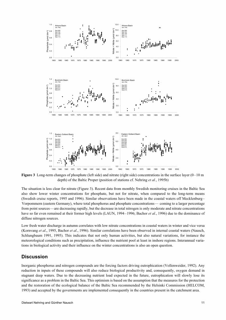
A drastic reduction in fertiliser consumption, mainly caused by the great economic changes in the countries of the formerEast Block, began in the late 1980s and is thus not yet reflected significantly by the mean nutrient conditions in the BalticProper (Table 1, Figure 2). However, signs of the decrease are now becoming apparent in the figures for the long-termbehaviour of phosphate (Figure 3). Winter concentrations of this nutrient, which increased on average until the mid-1980s, now show a decreasing tendency in central Baltic surface waters (Nehring et al., 1995b). This phenomenon ismore pronounced in the Arkona and Bornholm Basins, where the stations are located nearer to the coast, than in theEastern Gotland Basin with its more offshore stations.
Dietwart Nehring and Günther Nausch 11
Figure 3 Long-term changes of phosphate (left side) and nitrate (right side) concentrations in the surface layer (0–10 m depth) of the Baltic Proper (position of stations cf. Nehring et al., 1995b)
The situation is less clear for nitrate (Figure 3). Recent data from monthly Swedish monitoring cruises in the Baltic Seaalso show lower winter concentrations for phosphate, but not for nitrate, when compared to the long-term means(Swedish cruise reports, 1995 and 1996). Similar observations have been made in the coastal waters off Mecklenburg–Vorpommern (eastern Germany), where total phosphorus and phosphate concentrations— coming to a larger percentagefrom point sources—are decreasing rapidly, but the decrease in total nitrogen is only moderate and nitrate concentrationshave so far even remained at their former high levels (LAUN, 1994–1996; Bachor et al., 1996) due to the dominance ofdiffuse nitrogen sources.
Low fresh water discharge in autumn correlates with low nitrate concentrations in coastal waters in winter and vice versa(Kornvang et al., 1995, Bachor et al., 1996). Similar correlations have been observed in internal coastal waters (Nausch,Schlungbaum 1991, 1995). This indicates that not only human activities, but also natural variations, for instance themeteorological conditions such as precipitation, influence the nutrient pool at least in inshore regions. Interannual varia-tions in biological activity and their influence on the winter concentrations is also an open question.
DiscussionInorganic phosphorus and nitrogen compounds are the forcing factors driving eutrophication (Vollenweider, 1992). Anyreduction in inputs of these compounds will also reduce biological productivity and, consequently, oxygen demand instagnant deep waters. Due to the decreasing nutrient load expected in the future, eutrophication will slowly lose itssignificance as a problem in the Baltic Sea. This optimism is based on the assumption that the measures for the protectionand the restoration of the ecological balance of the Baltic Sea recommended by the Helsinki Commission (HELCOM,1993) and accepted by the governments are implemented consequently in the countries present in the catchment area.
1960 1965 1970 1975 1980 1985 1990 1995 2000
0.0
2.0
4.0
6.0
8.0
( )
Eastern Gotland BasinJan.-April
Stat.250Stat.255Stat.259Stat.260Stat.271Stat.272
1955 1960 1965 1970 1975 1980 1985 1990 1995 2000
0.0
0.2
0.4
0.6
0.8
1.0
1.2
( )
Eastern Gotland BasinJan.-April
Stat.250Stat.255Stat.259Stat.260Stat.271Stat.272
Pho
sp
ha
te (
µm
ol d
m-3)
Nitra
te +
Nitrite
(µ
mo
l d
m-3)
1955 1960 1965 1970 1975 1980 1985 1990 1995 2000
0.0
0.2
0.4
0.6
0.8
1.0
1.2
1.4
( )
Bornholm BasinJan.-Feb.
Stat.200Stat.202Stat.213Stat.214
1960 1965 1970 1975 1980 1985 1990 1995 2000
0.0
2.0
4.0
6.0
8.0
10.0
12.0
( )
Arkona BasinJan.-Feb.
Stat.069Stat.102Stat.109Stat.111Stat.113
1955 1960 1965 1970 1975 1980 1985 1990 1995 2000
0.0
0.2
0.4
0.6
0.8
1.0
( )
Arkona BasinJan.-Feb.
Stat.069Stat.102Stat.109Stat.111Stat.113
Pho
sp
ha
te (
µm
ol d
m-3)
Pho
sp
ha
te (
µm
ol d
m-3)
Nitra
te +
Nitrite
(µ
mo
l d
m-3)
Nitra
te +
Nitrite
(µ
mo
l d
m-3)
1960 1965 1970 1975 1980 1985 1990 1995 2000
0.0
2.0
4.0
6.0
8.0
10.0
( )
Bornholm BasinJan.-Feb.
Stat.200Stat.202Stat.213Stat.214

Fertiliser consumption in the catchment area and eutrophication of the Baltic Sea12
With respect to diffuse nutrient sources from agriculture (non-point sources), the most promising approach will be thereduction of fertiliser application to the level which meets only the most essential requirements of the plants. Pointsources contain phosphorus and nitrogen compounds indirectly resulting from fertilisers after transformation vialivestock, the food industry and man. Nutrients from point sources can be eliminated without difficulty by modern wastewater treatment plants.
Altogether, the recovery of the Baltic sea is a lengthy process since the changes in the ecosystem caused by the nutrientloads for more than 50 years cannot be reversed within a few years. Realistic estimations of the time scale needed aredifficult to obtain because for example information about accumulation in and remobilisation from the sediments isinsufficient. Bearing in mind the long residence times of the Baltic Sea (Wulff et al., 1990) at least several decades haveto be taken into account.
ReferencesBachor, A., v.Weber, M., and Wiemer, R., 1996. Die Entwicklung der Wasserbeschaffenheit der Küstengewässer
Mecklenburg–Vorpommerns. Wasser und Boden 48, 26–32.
FAO, 1952–1993. Yearbook Fertilizer. FAO Statistic Series, 1952–1993.
HELCOM, 1993. The joint comprehensive action programme. Baltic Sea Environment Proc. 49, 1–58.
Kornvang, B., Aertjeberg, G., Grant, R., Kristenson, P., Hovmand, M., and Kirkegaard, J., 1993. Nationwide monitoringof nutrients and ecological effects: State of the Danish aquatic environment. Ambio 22, 632–638.
LAUN, 1994–1996. Küstengewässer-Monitoring Mecklenburg–Vorpommern. Küsten-gewässerberichte 1994–1996des Landesamtes für Umwelt und Natur Mecklenburg–Vorpommern.
Nausch, G., and Schlungbaum, G., 1991. Eutrophication and restoration measures in the Darss–Zingst Bodden chain.Int. Revues ges. Hydriobiol. 76, 451–464.
Nausch, G. and Schlungbaum, G., 1995. Nährstoffdynamik in einem flachen Brackwassersystem (Darß–ZingsterBoddenkette) unter dem Einfluß variierender meteorologischer und hydrographischer Bedingungen. Bodden 2,153–164.
Nehring, D., and Aertjeberg, G., 1996. Verteilungsmuster und Bilanzen anorganischer Nährstoffe sowie Eutrophierung.In: Lozan, J.L., Lampe, R., Matthäus, W., Rachor, E., Rumohr, H., v.Westernhagen, H. (Hrsg.), Warnsignale ausder Ostsee. Berlin, Parey 1996, 61–68.
Nehring, D., Matthäus, W., Lass, H.-U., Nausch, G., and Nagel, K., 1995a. The Baltic Sea 1994—consequences of thehot summer and inflow events. Dt. Hydrogr. Z. 47, 131–144.
Nehring, D., Matthäus, W., Lass, H.-U., Nausch, G., and Nagel, K., 1995b. The Baltic Sea 1995—beginning of a newstagnation period in its central deep waters and decreasing nutrient load in its surface layer. Dt. Hydrogr. Z. 47,319–327.
Nixon, S.W., 1995. Coastal marine eutrophication: a definition, social causes, and future concerns. Ophelia 41, 199–219.
Vollenweider, R.A., 1992. Coastal marine eutrophication: principles and control. Sci. Of Total Environ., Suppl. 1992, 1–20.
Weigelt, M., Rumohr, H., 1986. Effects of wide-range oxygen depletion on benthic fauna and demersal fish in Kiel Bay1981–1983. Meeereforsch 31, 124–136.
Wullf, F., Stigebrandt, A., Rahm, L., 1990. Nutrient dynamics of the Baltic Sea. Ambio 19, 126–133.

M. Nausch and E. Kerstan 13
ICES Cooperative Research Report, No. 257 Baltic Marine Science Conference, Rønne, Denmark, 22–26 October 1996
Chemical and biological interactions in mixing gradients in the Pomeranian Bight
M. Nausch and E. Kerstan
AbstractThe changes of inorganic nutrients, dissolved carbohydrates and activities of carbohydrate degrading enzymes(glucosidase, glucosaminidase) were investigated during the mixing of water from the river Oder and water from theopen Pomeranian Bight from 1994 to 1996. In winter, nutrients were introduced mainly in inorganic form. Physicalmixing processes dominated the changes in the salinity gradient because the biological activities were low. During thegrowth season, the input was mainly in organic form as can be shown by particulate organic carbon and chlorophyll. Theinfluence of physical and biological processes on the alteration of introduced material cannot be distinguished clearly.However, the interaction between biochemical parameters and bacterial activities could be demonstrated on the exampleof dissolved carbohydrates and glucosidase activity. Concentrations of total dissolved carbohydrates (TCHO) anddissolved monosaccarides (MCHO) decreased if the uptake by bacteria exceeded the hydrolytic activity. In the salinitygradient ranging between 1.9 and 7.8 PSU, TCHO decreased from 15.1µmol l–1 to 2.8µmol l–1 and MCHO from3.4µmol l–1 to 1.1 µmol l–1. The hydrolysis rate (Hr) of glucosidase and glucosaminidase (Chitinase) reduced from13.9% h–1 to 0.3% h–1 and 9.9% h–1 to 0.2% h–1, respectively.
IntroductionThe river Oder is the largest external source of nutrients entering the Pomeranian Bight (Pastuszak et al., 1996). Theriver load amounts to 17% of phosphate and 15% of fluvial nitrogen for the whole Baltic Sea (Rosemarin et al., 1990).Beside inorganic nutrients, river load contains also organic material in large quantities (Wedborg et al,.1994). In marinesystems, carbohydrates represent up to 35% of the dissolved organic carbon (DOC) (Benner et al., 1992). They are themain component of DOC beside amino acids and lipids (Hellebust, 1965, 1974). Carbohydrates are products ofphytoplankton photosynthesis and are released by phytoplankton exudation, cell lysis and microbial degradation.Furthermore, zooplankton excretion is a source of dissolved carbohydrates (Klok et al., 1984, Mopper et al., 1991, Lee &Hinrichs, 1993). Low molecular weight carbohydrates such as monosaccharides are directly released from phytoplanktoninto the surrounding seawater or they are released from polymeric carbohydrates after degradation by microbialenzymes. High concentrations of low molecular weight carbohydrates are produced during intensive primary production(Münster & Chrost, 1991). But in water, they remain on a low level due to high rates of bacterial uptake (Libes, 1992). Inmarine systems, glucose is the most important carbohydrate in monomeric form (monosaccharide) and in polymeric form(polysaccharide) such as glucanes and cellulose (Handa & Domiga, 1969, Liebezeit & Bölter, 1991).
The activity of glucosidases is often used to describe the degradation of polymeric carbohydrates (Münster, 1991, Vrba,1992, Marxen, 1991, Hoppe et al., 1998). High ß-glucosidase activity was measured during the breakdown of a planktonbloom (Chrost, 1991). Rath et al. (1993) and Hoppe et al. (1998) describe the behaviour of glucosidase activities introphic gradients.
The main objectives of the interdisciplinary project TRUMP (transport and modification processes in the Pomeranianbight) of the Baltic Sea Research Institute Warnemünde were investigations on the distribution, modification and fate ofmaterial transported by the Oder river via the Szczecin Lagoon into the coastal ecosystem of the Pomeranian Bight.Physical transport and biochemical modification of different classes of material are described over the seasonal cycle andthe salinity gradient (v. Bodungen et al., 1995). During this study, the distribution of dissolved carbohydrates andglucosidase activity as a marker for carbohydrate degradation as well as the relationship between these parameters wereinvestigated.
Investigation Area and MethodsIn June/July 1994, July and September 1995 and in January 1996 several drift experiments and high resolution samplingtransections in the salinity gradients were performed in the Pomeranian Bight to describe the mixing and biological and
Chemical and biological interactions in mixing gradients in the Pomeranian Bight 14
chemical transformation of introduced river water. However, the river Oder does not enter the bight directly. A shallowlagoon, the Szczecin Lagoon (Odra Haff), is situated between the river mouth and the open bight. The Szczecin Lagoonand the Pomeranian Bight are connected via the rivers Peene and Szwina and lead to mixing of river water with waterfrom the bight. The lagoon water with a salinity range between 0.5 and 2 PSU (practical salinity units) enters the Pomer-anian Bight in a pulse like manner and in plumes of different size and is mixed with bight water within 2 or 3 days(v.Bodungen et al., 1995).
Water samples were taken at depths of 1–2, 5–6 and 8–10 m with a rosette sampler combined with sensors for conduc-tivity, temperature and density (CTD) as well as a sensor for fluorescence.
Inorganic nutrients were analysed using standard colorimetric methods according to Rohde & Nehring (1979) andGrasshoff et al. (1983).
For the determination of dissolved carbohydrates, samples were filtered through GF/F filters. Dissolved monosaccarideswere estimated according to the 3-methyl-2-benothiazolon-hydrazon (MBTH) method (Johnson & Sieburth, 1977). Forthe determination of total dissolved carbohydrates (TCHO), filtered water samples were hydrolysed with 0.09N HCl at100°C for 20h followed by the application of MBTH method.
For the characterisation of the degradation of carbohydrates by bacteria, glucosidase and glucosaminidase (chitinase)activity were investigated. Glucosidase degrades preliminary oligosaccharides. Glucosaminidase acts on aminopolysac-charides like chitin. The enzyme activities were determined according to Hoppe (1993) using the model substrates 4-methylumbelliferryl (MUF)-a-glucoside, -ß-glucoside and MUF-glucosaminide. For estimation of in situ hydrolysis ofnatural substrates, the hydrolysis rate (Hr (%h–1)) was measured at final concentrations of 100 nM MUF-a-or ß-glucosideand at in situ temperatures.
Turnover rates (To (%h–1)) of glucose were determined with D-[U-14C] glucose at final concentrations of 80nM at insitu temperatures (Jost & Pollehne, 1998).
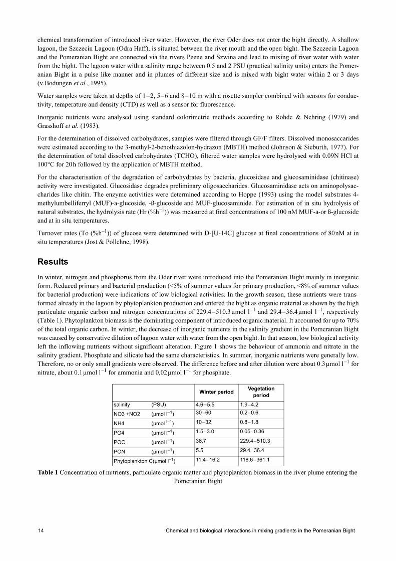
ResultsIn winter, nitrogen and phosphorus from the Oder river were introduced into the Pomeranian Bight mainly in inorganicform. Reduced primary and bacterial production (<5% of summer values for primary production, <8% of summer valuesfor bacterial production) were indications of low biological activities. In the growth season, these nutrients were trans-formed already in the lagoon by phytoplankton production and entered the bight as organic material as shown by the highparticulate organic carbon and nitrogen concentrations of 229.4–510.3µmol l–1 and 29.4–36.4µmol l–1, respectively(Table 1). Phytoplankton biomass is the dominating component of introduced organic material. It accounted for up to 70%of the total organic carbon. In winter, the decrease of inorganic nutrients in the salinity gradient in the Pomeranian Bightwas caused by conservative dilution of lagoon water with water from the open bight. In that season, low biological activityleft the inflowing nutrients without significant alteration. Figure 1 shows the behaviour of ammonia and nitrate in thesalinity gradient. Phosphate and silicate had the same characteristics. In summer, inorganic nutrients were generally low.Therefore, no or only small gradients were observed. The difference before and after dilution were about 0.3µmol l–1 fornitrate, about 0.1µmol l–1 for ammonia and 0,02µmol l–1 for phosphate.
Table 1 Concentration of nutrients, particulate organic matter and phytoplankton biomass in the river plume entering the Pomeranian Bight
Winter period Vegetation period
salinity (PSU) 4.6–5.5 1.9–4.2
NO3 +NO2 (µmol l–1) 30–60 0.2–0.6
NH4 (µmol l–1) 10–32 0.8–1.8
PO4 (µmol l–1) 1.5–3.0 0.05–0.36
POC (µmol l–1) 36.7 229.4–510.3
PON (µmol l–1) 5.5 29.4–36.4
Phytoplankton C(µmol l–1) 11.4–16.2 118.6–361.1

M. Nausch and E. Kerstan 15
Figure 1 Ammonia and nitrate concentrations in the salinity gradient in winter 1996
The highest concentrations of dissolved carbohydrates were measured near to the Swina mouth in the growing season.Concentrations of TCHO up to 15.1µmol l–1 (Figure 2) and MCHO up to 4.8µmol l–1 (Figure 3) were estimated. Inwinter, the values were significantly lower. TCHO and MCHO concentrations of about 4µmol l–1 and 1µmol l–1 weredetermined. Dissolved carbohydrates had the same concentrations in summer and in autumn. The pattern of dissolvedcarbohydrates in the salinity gradient varied from year to year and from season to season. TCHO showed a significantdecrease with increasing salinities in July 1994 and September 1995. During the other investigations, the TCHO concen-trations remained on the same level: 3–4µmol l–1 in January 1996 and about 7.3µmol l–1 in July 1995. MCHO showeda clear relationship to salinity only in autumn 1995 (Figure 3). Its concentrations scattered from 1.1 to 3.4µmol l–1.
Figure 2 TCHO concentrations in the surface layer in winter and in the growth season

Chemical and biological interactions in mixing gradients in the Pomeranian Bight 16
Figure 3 MCHO concentrations in salinity gradients
The hydrolysis rate of the carbohydrate degrading enzymes a-glucosidase, ß-glucosidase and glucosaminidase showedthe same pattern in the salinity gradient and between the seasons. The values of these enzyme activities were in the samerange and decreased linearly in the salinity gradient. In summer, glucosidase activity reduced from 13.9% h–1 to 0.3% h–1 and the glucosaminidase activity from 9.9% h–1 to 0.2% h–1 during mixing processes. Bacteria are the carrier of theseenzymes. The decrease of glucosidase activities is higher (by factor 46) than the decrease of bacterial counts (by factor2.5). From that it can be deduced that the activity per bacterial cell decreased and that the specific activity is the dominantfactor influencing the pattern of glucosidase activities. In winter, glucosidase- and glucosaminidase activities amountedto only 8% of summer values (Figure 4).
Figure 4 Glucosidase activities in winter and in the growth season
Glucosidase- and glucosaminidase activity correlated with the MCHO and TCHO (Table 2). These relationships wereespecially clear at low glucosidase activities up to 4.5% h–1 and glucosaminidase activities up to 2% h–1 (Figure 5). Athigher glucosidase activities in the outflowing lagoon water where the highest bacterial production (Jost & Pollehne1998) and enzyme activities were measured this relationship was not evident.
Table 2 Correlation coefficients between dissolved carbohydrate concentrations and glucosidase activities up to 4.5%h–1 and glucosaminidase activities up to 2% h–1
MCHO µmol l–1 TCHO
µmol l–1
glucosidase activity (% h–1) 0,38 n=36, p=0.05
0,22n.s.
glucosaminidase activity (% h–1) 0,81 n=36, p=0.01
0,67n=33, p=0.01

M. Nausch and E. Kerstan 17
Figure 5 Relation between MCHO and TCHO concentrations and glucosidase activities
The uptake of low molecular weight substances by bacteria, determined as glucose turnover (To), was highest insummer. At this time, glucose turnover rates up to 30% h–1 were measured in the outflowing lagoon water. After dilutionin the salinity gradient the values were reduced to 1–2% h–1. In winter, turnover rates ranged between 0.2 and 0.5% h–1.
The quotient between To and Hr (To/Hr) can be used as an index for coupling of glucose uptake and release viaenzymatic degradation by bacteria. In the outflowing lagoon water, a median To/Hr-ratio of 1.6 was determined in winterand a ratio of 4.2 in summer. In the growing season, the To/Hr-ratio had a relatively constant level in a salinity rangebetween 1.9 and 7 PSU. Between 7 and 7.8 PSU, the quotient rose up to 21.4 (Figure 6). The increase is due to the factthat Hr was more (factor 4.8) reduced than To (factor 2.1). At salinities >5 PSU, the relationship between uptake ofglucose and the hydrolysis rate of carbohydrates and the concentration of MCHO could be observed. In this range, thedistribution of dissolved monosaccharides and the To/Hr-quotient were independent from the salinity. There was anegative correlation between the To/Hr-quotient and MCHO concentrations (Figure 7).
Figure 6 Relation of glucose turnover and glucosidase activity in the salinity gradient

Chemical and biological interactions in mixing gradients in the Pomeranian Bight18
Figure 7 Relation between To/Hr-quotients and concentrations of MCHO and TCHO at salinities >5 PSU
DiscussionOrganic and inorganic material introduced into the Pomeranian Bight can be modified by physical dilution or by transfor-mation via biological processes. These processes cannot be distinguished clearly, biological processes are masked byphysical dilution. However, we could show by the example of glucose turnover and enzymatic carbohydrate degradationthat an interaction of different parts of planktonic community existed.
Carbohydrates are produced as a result of photosynthesis and are released into seawater by exudation fromphytoplankton and cell lysis as well as sloppy feeding of zooplankton (Klok et al., 1984, Mopper et al., 1991, Münster &Chrost, 1991). We assume that phytoplankton was the main source of dissolved carbohydrates in the Pomeranian Bightbecause the highest TCHO and MCHO concentrations were found near the Swina mouth where the phytoplanktonbiomass was also highest (Jost & Pollehne, 1998). Zooplankton biomass in the outflowing lagoon water was not higherthan in the open bight. However, there was a shift from limnetic to more marine species (Postel & Mumm, 1995).
For stock parameters (POC and chlorophyll) as well as for activity parameters (primary production, bacterial production)a linear decrease was observed in all gradients (Jost & Pollehne, 1998). In contrast to that, dissolved carbohydrates hadnot such a strong relationship to salinity. Especially in summer, the MCHO concentrations were not correlated with thesalinity. According to Jost & Pollehne (1998), the primary production near the Swina mouth is more light-limited than inthe open bight. Respiratory processes exceeded the primary production and a negative carbon balance was calculated forthe whole water column. Due to the deeper light penetration, the carbon balance in the open bight was positive. Theserelationships between autotrophic and heterotrophic processes could have an influence on the concentrations of TCHOand MCHO.
Bacteria are the main consumers of low molecular weight substances and they possess extracellular enzymes for carbo-hydrate degradation. For the characterisation of extracellular enzymes the maximum enzyme activity (Vmax) is used(Hoppe, 1993). In this context, the enzyme activities at low MUF-substrate concentrations (Hr) were used for a betterdescription of the in situ substrate hydrolysis. The distribution of Vmax of glucosidase activities in the salinity gradientof the Pomeranian Bight is shown in Nausch et al. (1998). Vmax and Hr correlated.
TCHO are substrates for glucosidase- and glucosaminidase activity. The mechanism of substrate stimulation can bemade responsible for the correlation of these parameters. The rapid degradation of TCHO and uptake of MCHO can leadto a constant or lower level of dissolved TCHO and MCHO in this area. The relationship between glucosidase activityand MCHO was not so tight because MCHO can be directly released by phytoplankton in addition to the release afterdegradation of polysaccharides.
Figure 7 demonstrates the connection between glucose turnover, the hydrolysis of carbohydrates and the concentrationsof MCHO and TCHO at salinities >5PSU. The To/Hr quotient correlated with MCHO as well with TCHO. The negativecorrelation between the To/Hr quotient and TCHO can be explained by substrate stimulation as a regulatory mechanismof extracellular enzyme activities (Münster, 1991, Rath et al., 1993, Karner & Rassoulzadegan, 1995). The decrease ofTCHO may cause a lower stimulation of glucosidase activity with the result that the importance of hydrolysis productsfor bacterial uptake is reduced. This assumption was supported by the decrease of the specific glucosidase activities in

M. Nausch and E. Kerstan 19
the salinity gradient. The negative correlation between To/Hr quotients and MCHO can be attributed to the turnoverwhich exceeded the hydrolysis and caused the decrease of MCHO-concentrations coming from other sources.
AcknowledgementsThis study was funded by the German Ministry for Education, Research and Technology (03F0105B). We are grateful toDr. K. Nagel, Dr. F. Pollehne and Dr. G. Jost for values of POC, PON, primary production and bacterial glucoseturnover.
ReferencesBenner, B., Pakulski, J. D., McCarthy, M., Hedges, J. I., Hatcher, P. G. (1992): Bulk chemical characterization of
dissolved organic matter in the ocean. Science 255,1561–1564.
Chrost, R. J. (1991): Environmental control of the synthesis and activity of aquatic microbial ectoenzymes. In: Chrost, R.J. (ed.) Microbial enzymes in aquatic environments, Springer–Verlag, pp 29–59.
Grasshoff, K., Ehrhardt, M., Kremling, K. (eds.) (1983): Methods of seawater analysis, 2nd edition, Verlag Chemie,Weinheim, pp 419.
Handa, N., Tominga, H. (1969): A detailed analysis of carbohydrates in marine particulate matter. Mar. Biol. 2, 228–235.
Hellebust, J. A. (1965): Excretion of some organic compounds by marine phytoplankton. Limnol. Oceanogr. 10, 192–206.
Hellebust, J. A. (1974): Extracellular products. In Stewart, W.D.P. (ed.) Algal physiology and biochemistry. Blackwell,Oxford, pp 838–863.
Hoppe, H. G. (1993): Use of fluorogenic model substrates for extracellular enzyme activity (EEA) measurement ofbacteria. In: Kemp, P.F., Sherr, B.F., Sherr, E.B., Cole J.J. (eds.) Handbook of methods in aquatic microbialecology, Lewis Publishers, Boca Raton, pp 423–431.
Hoppe, H. G., Giesernhagen, H. C., Gocke, K. (1998): Changing patterns of bacterial substrate decomposition in aeutrophication gradient. Aquat. Microb. Ecol. 15, 1–13.
Johnson, K. M., Sieburth, J. McN. (1977): Dissolved carbohydrates in seawater I. A precise spectrophotometric analysisfor monosaccharides. Mar.Chem. 5, 1–13.
Jost, G., Pollehne, F. (1998): Coupling of autotrophic and heterotrophic processes in a Baltic estuarine mixing gradient(Pomeranian Bight). Hydrobiol. 363, 107–115.
Karner, M., Rassoulzadegan, C., Rassoulzadegan, F. (1995): Extracellular enzyme activity: indications for short-termvariability in a coastal marine ecosystem. Microb. Ecol. 30, 143–156.
Klok, J., Cox, H. C., Baas, M., Schuyl, P. J. W.,de Leeuw, J. W., Schenck, P. A. (1984): Carbohydrates in recent marinesediments—I. Origin and significance of deoxy- and O- methyl-monosaccharides. Org. Geochem. 7, 73–84.
Lee, C., Henrichs, S. M. (1993): How the nature of dissolved organic matter might affect the analysis of dissolvedorganic carbon. Mar. Chem. 41, 105–120.
Libes, S. L. (1992): An introduction to marine biogeochemistry. John Wiley & Sons, pp 394–422.
Liebezeit, G., Bölter, M. (1991): Water-extractable carbohydrates in particulate matter of the Bransfield Strait. Mar.Chem. 35, 389–398.
Mopper, K., Zhou, X., Kieber, R. J., Sirorski, D. J., Jones, R. D. (1991): Photochemical degradation of dissolved organiccarbon and its impact on the oceanic carbon cycle. Nature 353, 60–62.
Münster, U., Chrost, R. J. (1990): Origin, composition, and microbial utilization of dissolved organic matter. In:Overbeck, J.,Chróst, R.J. (eds.) Aquatic microbial ecology. Biochemical and molecular approaches. Springer–Verlag, New York, pp 8–46.

Chemical and biological interactions in mixing gradients in the Pomeranian Bight 20
Münster, U. (1991) Extracellular enzyme activity in eutrophic and polyhumic lakes. In: Chrost, R. J. (ed.) Microbialenzymes in aquatic environments, Springer–Verlag, pp 96–122.
Nausch, M., Kerstan, E., Pollehne, F. (1998): Extracellular enzyme activities in relation to hydrodynamics in the Pomer-anian Bight (Southern Baltic Sea) Microb. Ecol. 36, 251–258.
Pastuszak, M., Nagel, K., Nausch, G. (1996): Variability in nutrient distribution in the Pomeranian Bay in September1993. Oceanologia 38, 195–225.
Postel, L., Mumm, N., Krajewska-Soltys, A. (1995): Metazooplankton distribution in the Pomeranian Bay, (SouthernBaltic)—Species composition, biomass, and respiration. Bull. Sea Fish. Inst. 3, 61–73.
Rath, J., Schiller, C., and Herndl, G. J. (1993): Ectoenzymatic activity and bacterial dynamics along a trophic gradient inthe Caribbean Sea. Mar. Ecol. Prog. Ser. 102, 89–96.
Rohde, K. H., Nehring, D. (1979): Ausgewählte Methoden zur Bestimmung von In-halts-stoffen im Meer- und Brack-wasser. Geod. Geoph. Veröff. R.IV 27, 1–68.
Rosemarin, A., Notini, M., Soederstroem, M., Jensen, S., Landener, L. (1990): Fate and effects of pulp mill chlorophe-nolic 4,5,6-trichloroguaiacol in a model brackish water ecosystem. Sci. Total Environ. 92, 69–89.
Vrba, J. (1992): Seasonal extracellular enzyme activities in decomposition of polymeric organic matter in a reservoir.Ergeb. Limnol. Adv. Limnol. 37, 33–42.
v.Bodungen, Graeve, M., Kube, J., Lass, U., Meyer-Harms, B., Mumm, N., Nagel, K., Pollehne, F., Powilleit, M.,Reckermann, M., Sattler, C., Siegel, H., Wodarg, D. (1995): Stoffflüsse am Grenz-fluß—Transport- und Umsatz-prozesse im Übergangsbereich zwischen Oderästuar und Pommerscher Bucht (TRUMP). Geowiss. 12/13, 4–79–485.
Wedborg, M., Skoog, A., Folgeqvist, E. (1994): Organic carbon and humic substances in the Baltic Sea, the Kattegat, andthe Skagerrak. In: Senesi, N., T.M. Miano (eds.) Humic substances in the global environment and implications inhuman health. Elsevier Pub., Amsterdam, pp 914–924.

Vadims Jermakovs and Hans Cederwall 21
ICES Cooperative Research Report, No. 257 Baltic Marine Science Conference, Rønne, Denmark, 22–26 October 1996
Distribution and morphological parameters of the polychaete Marenzelleria viridis population in the Gulf of Riga
Vadims Jermakovs and Hans Cederwall
IntroductionIn the Baltic Sea M. viridis was found first in 1985 in the Darss–Zingst estuary (Bick and Burckhardt, 1989) and inPolish waters (Gruszka, 1991). In 1988, this polychaete was found in the southeastern part of the Baltic Sea and near theshore region of Lithuania (Olenin and Chubarova, 1992).
Near the southern coasts of Sweden and Finland M. viridis was observed for the first time in 1989 and 1990 (Persson,1990; A.-B. Andersin, unpubl.; Norrko et al., 1993). Presently this species has become an important component in someBaltic coastal benthic communities (Kube et al., 1996).
In the Gulf of Riga the first findings of M. viridis were done in 1988, near the mouth of the river Daugava (Lagzdins andPallo, 1994). During the period 1988–1994 M. viridis spread all over the Gulf of Riga and became one of the dominatingbenthic species (Cederwall et al., 1999).
The present study describes the distribution of M. viridis in the Gulf of Riga six years after introduction. Data on themorphological parameters of M. viridis in the Gulf are also presented.
The Gulf of Riga is one of the most eutrophied areas of the Baltic Sea. The annual primary production has been estimatedto 4 million tons per year in 1989 (Andrushaitis et al., 1992). This is about 290 gcm–2yr–1 which is approximately twotimes more than average for the entire Baltic proper (Elmgren, 1989). The area of the Gulf of Riga is 16330 km2, and thedrainage area is 8 times as large (Pastors, 1967). The mean and maximum depth of the Gulf is 27m and 62m, respec-tively.
The Gulf of Riga is seasonally (April–October) stratified thermally, with a thermocline between 20 and 30 m. Salinityvaries between 4–7‰ (Yurkovskis et al., 1993; Berzinsh, 1995).
Oxygen concentration in the near bottom water is usually between 4–8 mll–1, but can decrease to 0.7 mll–1 during yearsof water stagnation (Botva et al., 1987).
The macrozoobenthos of the Gulf of Riga has been monitored almost continuously since 1945 (Lagzdins, 1990). A clearincrease in total abundance and biomass of macrozoobenthos has been observed since the beginning of the 1970s. Theabundance of the dominating crustacean species, Monoporeia affinis and Pontoporeia femorata, decreased considerably,but that of Macoma balthica and the annelids increased (Gaumiga and Lagzdins, 1995).
Material and MethodsSamples were collected from 56 stations (Figure 1, Figure 2).
During July 1993 the sampling of sediments was done with a modified 0.05m2 van Veen bottom-grab. During 1994samples were taken with a BMB standard 0.1m2 van Veen grab (Dybern et al., 1976). The results of intercalibration donot show a significant difference between modified 0.05m2 and BMB standard 0.1m2 van Veen grabs. The samplingefficiency of these two bottom-grabs is similar (Jermakovs, unpubl.).
Five replicate samples were taken from each station in 1993 and one to three replicates were taken in 1994. A total of 162samples have been analysed.
Sediments were sieved through a nylon net with 0.5mm mesh. The original construction of the sieves is described in“Comparisons between Soviet and Swedish methods of sampling and treating soft bottom macrofauna” (Ankar et al.,1978). The residue of sediments with organisms was preserved in 4% formaldehyde solution, buffered with hexamine.The organisms were sorted under stereomicroscope. The organisms were weighed after drying on filter paper.
The specimens of Marenzelleria viridis were measured using a stereomicroscope, with a measuring ocular at ×16 magni-fication.

Distribution and morphological parameters of the polychaete Marenzelleria Viridis population in the Gulf of Riga22
Figure 1 Map showing the location of the sampling stations in the Gulf of Riga.
Figure 2 Map showing the location of the eight transects in the southernmost part of the Gulf of Riga. I– transect near the western coast of the Gulf of Riga; II– transect westward from the mouth of the river Lielupe; III– transect near the mouth of the river Lielupe; IV– transect between the mouths of the rivers Lielupe and Daugava; V– transect near the
mouth of the river Daugava; VI– transect eastward from the mouth of the river Daugava; VII– transect near the mouth of the river Gauja; VIII– transect near the eastern coast of the Gulf of Riga.

Vadims Jermakovs and Hans Cederwall 23
Results and DiscussionGenerally the highest concentrations of M. viridis were observed in the southern part of the Gulf, in the areas near themouths of the large rivers—Lielupe, Daugava and Gauja (Figure 3). Mean densities of the polychaete ranged herebetween 500–3000 ind.·m–2. Another area with high density of M. viridis was noticed near the mouth of Salaca river—in eastern part of the Gulf. In the central part of the Gulf the abundance of Marenzelleria was much lower—heredensities did not exceed 150 ind.·m–2.
Figure 3 Average abundance and biomass of Marenzelleria viridis at selected stations from the Gulf of Riga. Error bars show standard deviation.
The maximum value for the Gulf of Riga, 8300 ind.·m–2, was recorded in July 1993 at site G1 near the mouth of theDaugava. One year earlier Lagzdins and Pallo (1994) reported the maximal density to be only 1380 ind.·m–2 in the samearea.
The density of M. viridis in the southwestern Baltic Sea, especially in estuaries and coastal lagoons is much higher—upto 39000 ind.·m–2 (Kube at al., 1996; Zettler, 1996). In these lagoons chlorophyll concentrations are 2–10 times higherthan in the Gulf of Riga (Jansone, 1995; Kube at al., 1996). Here a clear positive relationship between distribution,abundance and population dynamics of M. viridis and phytoplankton concentration was observed, because the watercolumn in shallow waters is usually well mixed by wind (Kube at al., 1996). The Gulf of Riga is thermally stratifiedwhich may cause the absence of a strong positive relationship between phytoplankton concentrations and distribution ofM. viridis.
In the southwestern Baltic Sea a high density of Marenzelleria was observed in the areas around the mouths of largerivers and in lagoons (Kube at al., 1996). High numbers of M. viridis near the mouth of the river Salaca (station G12,eastern part of the gulf) and especially in the southern part of the Gulf of Riga support the hypothesis that the riveroutflow has a positive influence on the distribution and density of M. viridis (Figure 3, Figure 4).
In the sandy sediments at 10m depth the benthic community is dominated by polychaetes: Pygospio elegans, Manay-unkia aestuarina, Marenzelleria viridis and Nereis diversicolor, which constitute about 66% of the total makrozoob-enthos abundance (1650 ind.·m–2). At the same time polychaetes constitute only 7% of the benthos biomass (57.5 g·m–2)(Jermakovs, unpubl.). On average, M. viridis alone constitutes 25% and 1.4% of the total abundance and biomass,respectively. At a 30m depth Marenzelleria constitutes 74% and 64% of the total biomass and total abundance, respec-tively. In comparison with other 20m deep sites, high M. viridis abundance (Figure 4) was observed at a 20m deepsampling site from the fifth transect, near the mouth of the river Daugava (Figure 2). This is probably due to depositionof large quantities of river-transported organic matter. That in turn provides plenty of fresh detritus at the surface ofsandy sediment.
0500
10001500200025003000350040004500
G1
G11
G12
G14
A
G16 G4
G12
0 T2
G21 T1 G7
G10
A
G5 T3
GR
2
Stations
ind.
*m-2
0500
10001500200025003000350040004500
T5 T6 G6
G8
G9
G15
G22
Rag
G18
G19
NL1
NL2
NL3
NL4
NL5 T4
Stations
ind.
*m-2
8340
0
10
20
30
40
50
60
70
80
G1
G11
G12
G14
A
G16 G4
G12
0 T2
G21 T1 G7
G10
A
G5 T3
GR
2
Stations
g*m
-2
01020304050607080
T5 T6 G6
G8
G9
G15
G22
Rag
G18
G19
NL1
NL2
NL3
NL4
NL5 T4
Stations
g*m
-2

Distribution and morphological parameters of the polychaete Marenzelleria Viridis population in the Gulf of Riga24
Figure 4 Average abundance and biomass of Marenzelleria viridis in the southernmost part of the Gulf of Riga.
In muddy sand and sandy sediments at 10 and 20m depth the population of Marenzelleria was dominated by juveniles(body width 0.3–0.6mm), while in muddy sediments at 30m depth adult specimens of Marenzelleria dominated (bodywidth 0.9–1.8mm). It can be partly explained by young M. viridis avoiding high concentrations of adult individuals, aswas observed in the Ems estuary (Essink and Kleef, 1993).
Animal size was measured both as their length and width, the latter since many of the animals found were broken duringthe sampling and sieving process. Significant correlations were found between length and weight of Marenzelleria aswell as between width and weight and width and length (Figure 5). The results of regression analyses are given in Table1.
The morphological parameters of M. viridis from the Gulf of Riga and other regions of the Baltic Sea are different. InGermany, in the Darss–Zingst estuary and in Oderhaff the maximum body width of M. viridis is 2.8–3.1mm (Zettler etal., 1995; Kube et al., 1996). Specimens of M. viridis from the Pomeranian Bay have a maximum body width of 2.5–2.6mm (Kube et al., 1996). Along the East coast of North America, the native land of M. viridis, in Great Sippenissettsalt marsh (Massachusetts, USA) the body width of M. viridis at 5th segments are 2.5mm (Sarda et al., 1995). Thegreatest worms from the Gulf of Riga were recorded by Lagzdins and Pallo (1994), having more that 260 segments, bodylength 100mm and width at the 7–10 segments up to 2.5mm.
I II III IV V VI VII VIII
1020
300
5001000150020002500300035004000
ind.
*m-2
Transects
Depth m
I II III IV V VI VII VIII
1020
300
20
40
60
80
100
120
g*m
-2
Transects
Depth m

Vadims Jermakovs and Hans Cederwall 25
Figure 5 Relations between length, width and weight of Marenzelleria viridis from the Gulf of Riga in comparison with data from Darss–Zingst estuary (Zettler, 1996).
The size–weight relationship of M. viridis was studied more detailed in Germany, in the Darss–Zingst estuary (Zettler,1996). The specimens of M. viridis from the Gulf of Riga have 0.5–1mm less width than those of the same length fromDarss–Zingst estuary. Consequently M. viridis from the Gulf of Riga have less width than specimens of the same weightof M. viridis from the Darss–Zingst estuary (Figure 5). The methods of measuring the morphological parameters of M.viridis in Latvia and in Germany were not intercalibrated, but they are approximately the same. If the difference inwidth–length–weight ratio between the Darss–Zingst estuary and the Gulf of Riga was due to incompatibility ofmethods, then the regression lines for the size–weight relationship should be parallel. However, that was not the case.Therefore, more probably the observed difference was due to different environmental conditions between the studiedregions.
0
20
40
60
80
100
120
0 0,5 1 1,5 2 2,5 3width mm
leng
th m
mgg
g
Gulf of RigaDarss- Zingst est.
0
0,050,1
0,15
0,2
0,250,3
0,35
0,4
0 0,5 1 1,5 2 2,5 3width mm
wet
wei
ght,g
gg
Gulf of RigaDarss- Zingst est.
0
0,05
0,1
0,15
0,2
0,25
0,3
0,35
0,4
0 20 40 60 80 100 120length mm
wet
wei
ght,g
gg
Gulf of RigaDarss- Zingst est.
n=194
n=177
n=177

Variables Number of measured specimens
Coefficient of determination r2
Linear equation
Length/width 194 0.8813 Y=36.94·X1.6812 Weight/length 177 0.9787 Y=7.82·10-6·X2.269 Weight/width 177 0.8913 Y=0.0303·X3.792
Table 1 Results of regression analysis on size-weight relationship of Marenzelleria viridis from the Gulf of Riga, Baltic.
Conclusions
• M. viridis was the most abundant species in the soft-bottom macrozoobenthos community of the Gulf of Riga in the mid-1990s.
• The highest abundances of M. viridis were found near the outflow of the three largest rivers in the southern part of the Gulf.
• In the southern part of the Riga Gulf adult individuals of M. viridis dominate on the soft muddy sediments at depths of around 30m, while juveniles dominate in the shallow waters and on sandy sediments.
• Significant correlations between length, width and weight of M. viridis give a possibility to estimate the length and weight of fragmented specimens from data on body width.
Acknowledgements
This study was supported by grants from the Latvian Council of Science and the Nordic Council of Ministers.
Distribution and morphological parameters of the polychaete Marenzelleria Viridis population in the Gul of Riga 26

References
Andrushaitis, G., Andrushaitis, A., Bitenieks, Y., Lenshs, E. and. Priede, S., 1992. Organic carbon balance of the Gulf of Riga. Proceedings of the 17th CBO Conference, Norrköping 1990, Swedish Hydrological & Meteorological Institute Report, p. 59–66.
Ankar., S., Cederwall, H., Lagzdins, G. and Norling, L., 1978. Comparison between Soviet and Swedish methods of sampling and treating soft bottom macrofauna—Final report from the Soviet–Swedish Expert Meeting on Intercalibration of Biological Methods and Analyses, Askö, July 5–12, 1975. Contrib. Askö Lab. Univ. Stockholm, 23:1–38.
Berzinsh, V., 1995. Hydrology. In: E. Ojaveer (editor), Ecosystem of the Gulf of Riga between 1920 and 1990. Estonian Academy Publishers, Tallinn: 7–31.
Bick, A. and Burckhardt, R., 1989. First record of Marenzelleria viridis (Polychaeta: Spionidae) in the Baltic Sea, with a key to the Spionidae of the Baltic Sea. Mitt. Zool. Mus. Berl. 65: 237–247.
Botva, U., Filmanovicha, R. and Alksne, M., 1987. Areal survey of hydrochemistry in the Eastern Baltic Proper, the Gulf of Riga and the Gulf of Finland. Hydrobiological and hydrochemical characteristics of the eastern part of Baltic Sea. The Gulf of Riga and the Gulf of Finland. Riga: 20–39. (in Russian).
Cederwall, H., Jermakovs, V. and Lagzdins, G., 1999. Long-term changes in the soft-bottom macrofauna of the Gulf of Riga. ICES Journal of Marine Science, 56, Suppl.: 41–48.
Dybern, B.I., Ackefors, H. and Elmgren, R., 1976. Recommendations on methods for marine biological studies in the Baltic Sea. BMB Publ. No. 1: 1–98.
Elmgren, R., 1989. Man’s impact on the ecosystem of the Baltic Sea: Energy flows today and at the turn of the century. Ambio, 18: 326–332.
Essink., K., and Kleef, H. L., 1993. Distribution and life cycle of the North American Spionid Polychaete Marenzelleria viridis (Verrill, 1873) in the Ems Estuary. Neth. J. Aquat.Ecol.27:237–246.
Gaumiga, R. and Lagzdins, G., 1995. Macrozoobenthos. In: E. Ojaveer (editor), Ecosystems of the Gulf of Riga between 1920 and 1990. Estonian Acad. Publ. Tallinn: 198–211.
Gruszka, P., 1991. Marenzelleria viridis (Verill, 1873) (Polychaeta, Spionidae)—a new component of shallow water benthic community in the southern Baltic. Acta Ichtyol. Pisc. 21, Suppl.: 57–65.
Jansone, B., 1995. Concentration of chlorophyll “a” in the Gulf of Riga. In: E. Ojaveer (editor), Ecosystem of the Gulf of Riga between 1920 and 1990. Estonian Academy Publishers, Tallinn: 127–130.
Kube, J., Zettler, M. L., Gosselck, F., Ossig, S. and Powilleit, M., 1996. Distribution of Marenzelleria viridis (Verrill, 1873) (Polychaeta: Spionidae) in the southwestern Baltic Sea in 1993/94—ten years after introduction.Sarsia 81: 131–142.
Lagzdins, G., 1990. Gulf of Riga. In: HELCOM, Second periodic assessment of the State of the marine environment of the Baltic Sea, 1984–1988. Background document. Baltic Sea Environmental Proceedings 35B. Helsinki: 257–258.
Lagzdins, G., and Pallo, P., 1994. Marenzelleria viridis (Verrill) (Polychaeta, Spionidae)—a new species for the Gulf of Riga. Proc. Estonian Acad. Sci. Biol., 43(3): 184–188.
Norrko, A., Bondsdorff, E., and Boström, C., 1993. Observations of the polychaete Marenzelleria viridis (Verrill) on a shallow sandy bottom on the south coast of Finland. Memoranda Soc. Fauna Flora Fennica, 69: 112–113.
Olenin, S. and Chubarova, S., 1992. Recent introduction of the North American spionid polychaete Marenzelleria viridis (Polychaeta, Spionidae) in the coastal areas of the south-eastern part of the Baltic Sea. In: International Symp. On Functioning of Coastal Ecosystems in Various Geographical Regions.September 23–25, 1992. Gdansk University, Poland, p.20
Vadims Jermakovs and Hans Cederwall 27

Distribution and morphological parameters of the polychaete Marenzelleria Viridis population in the Gul of Riga 28
Pastors, A., 1967. Water and heat balance in the Gulf of Riga. Morzskie zalivy kak priyomniki stochnykh vod. Riga, Zinatne: 8–20. (in Russian).
Persson, L. -E., 1990. The national Swedish environmental monitoring programme (PMK): Soft-bottom macrofauna monitoring of the south coast of Sweden—Annual Report 1990. Naturvårdsverket Rapport, 3937: 5–12.
Sarda, R., Valiela, I. and Foreman, K., 1995. Life cycle, demography, and production of Marenzelleria viridis in a salt marsh of southern New England. J. mar. biol. Ass. U.K. 75: 725–738.
Yurkovskis, A., Wulff, F., Rahm, L., Andrushaitis, A. and Rodrigues-Medina, M., 1993. A nutrient budget of Gulf of Riga, Baltic Sea. Estuarine, Coastal and Shelf Sci. 37: 113–127.
Zettler., M. L., Bick, A. and Bochert, R., 1995. Distribution and population dynamics of Marenzelleria viridis (Polychaeta: Spionidae) in a coastal water of the southern Baltic. Arch. Fish. Mar. Res. 43(3): 209–224.
Zettler, M. L., 1996. Ökologische Untersuchungen am Neozoon Marenzelleria viridis (Verrill, 1873) (Polychaeta, Spionidae) in einem Küstengewässer der südlichen Ostsee. Dissertation, Rostock University, Rostock, Germany.
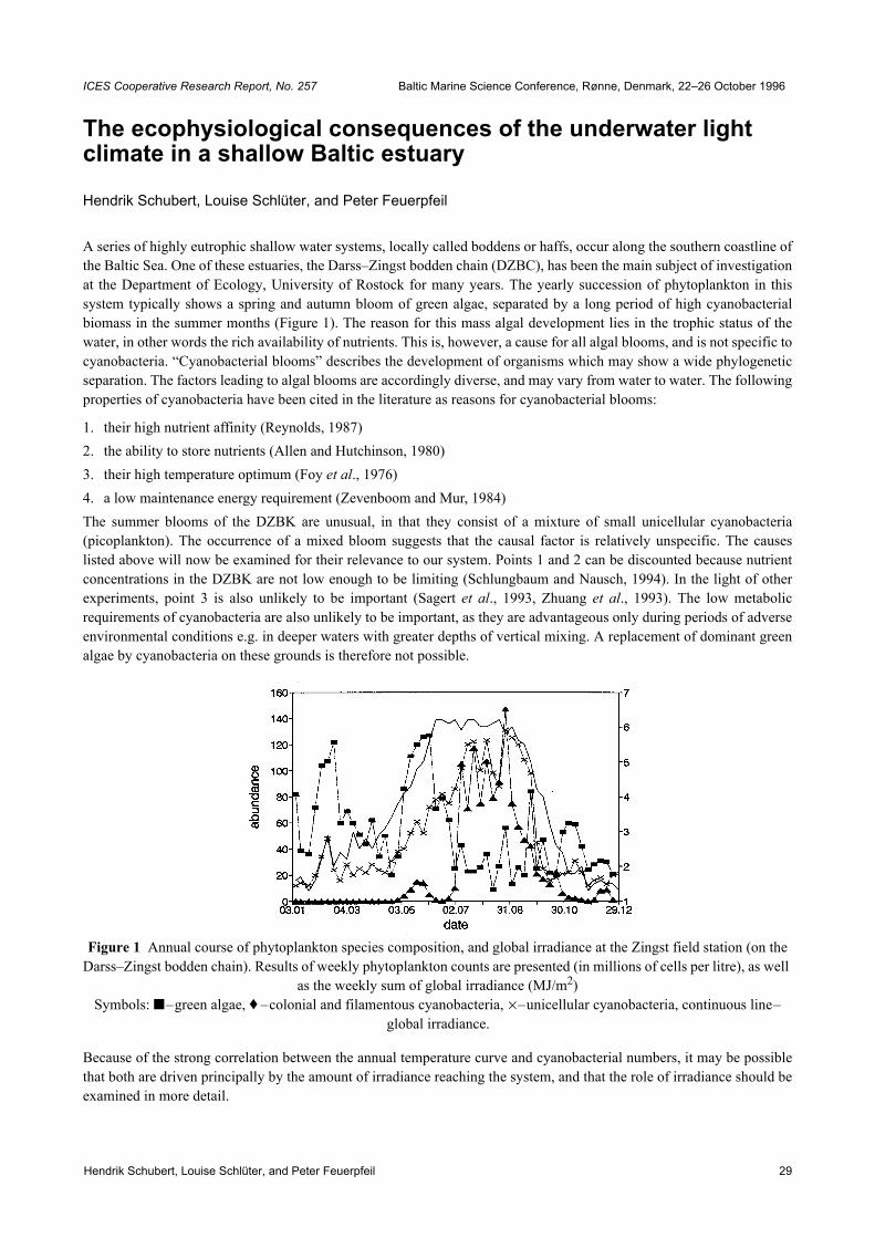
Hendrik Schubert, Louise Schlüter, and Peter Feuerpfeil 29
ICES Cooperative Research Report, No. 257 Baltic Marine Science Conference, Rønne, Denmark, 22–26 October 1996
The ecophysiological consequences of the underwater light climate in a shallow Baltic estuary
Hendrik Schubert, Louise Schlüter, and Peter Feuerpfeil
A series of highly eutrophic shallow water systems, locally called boddens or haffs, occur along the southern coastline ofthe Baltic Sea. One of these estuaries, the Darss–Zingst bodden chain (DZBC), has been the main subject of investigationat the Department of Ecology, University of Rostock for many years. The yearly succession of phytoplankton in thissystem typically shows a spring and autumn bloom of green algae, separated by a long period of high cyanobacterialbiomass in the summer months (Figure 1). The reason for this mass algal development lies in the trophic status of thewater, in other words the rich availability of nutrients. This is, however, a cause for all algal blooms, and is not specific tocyanobacteria. “Cyanobacterial blooms” describes the development of organisms which may show a wide phylogeneticseparation. The factors leading to algal blooms are accordingly diverse, and may vary from water to water. The followingproperties of cyanobacteria have been cited in the literature as reasons for cyanobacterial blooms:
1. their high nutrient affinity (Reynolds, 1987) 2. the ability to store nutrients (Allen and Hutchinson, 1980) 3. their high temperature optimum (Foy et al., 1976) 4. a low maintenance energy requirement (Zevenboom and Mur, 1984)The summer blooms of the DZBK are unusual, in that they consist of a mixture of small unicellular cyanobacteria(picoplankton). The occurrence of a mixed bloom suggests that the causal factor is relatively unspecific. The causeslisted above will now be examined for their relevance to our system. Points 1 and 2 can be discounted because nutrientconcentrations in the DZBK are not low enough to be limiting (Schlungbaum and Nausch, 1994). In the light of otherexperiments, point 3 is also unlikely to be important (Sagert et al., 1993, Zhuang et al., 1993). The low metabolicrequirements of cyanobacteria are also unlikely to be important, as they are advantageous only during periods of adverseenvironmental conditions e.g. in deeper waters with greater depths of vertical mixing. A replacement of dominant greenalgae by cyanobacteria on these grounds is therefore not possible.
Figure 1 Annual course of phytoplankton species composition, and global irradiance at the Zingst field station (on the Darss–Zingst bodden chain). Results of weekly phytoplankton counts are presented (in millions of cells per litre), as well
as the weekly sum of global irradiance (MJ/m2) Symbols: –green algae, ♦ –colonial and filamentous cyanobacteria, ×–unicellular cyanobacteria, continuous line–
global irradiance.
Because of the strong correlation between the annual temperature curve and cyanobacterial numbers, it may be possiblethat both are driven principally by the amount of irradiance reaching the system, and that the role of irradiance should beexamined in more detail.
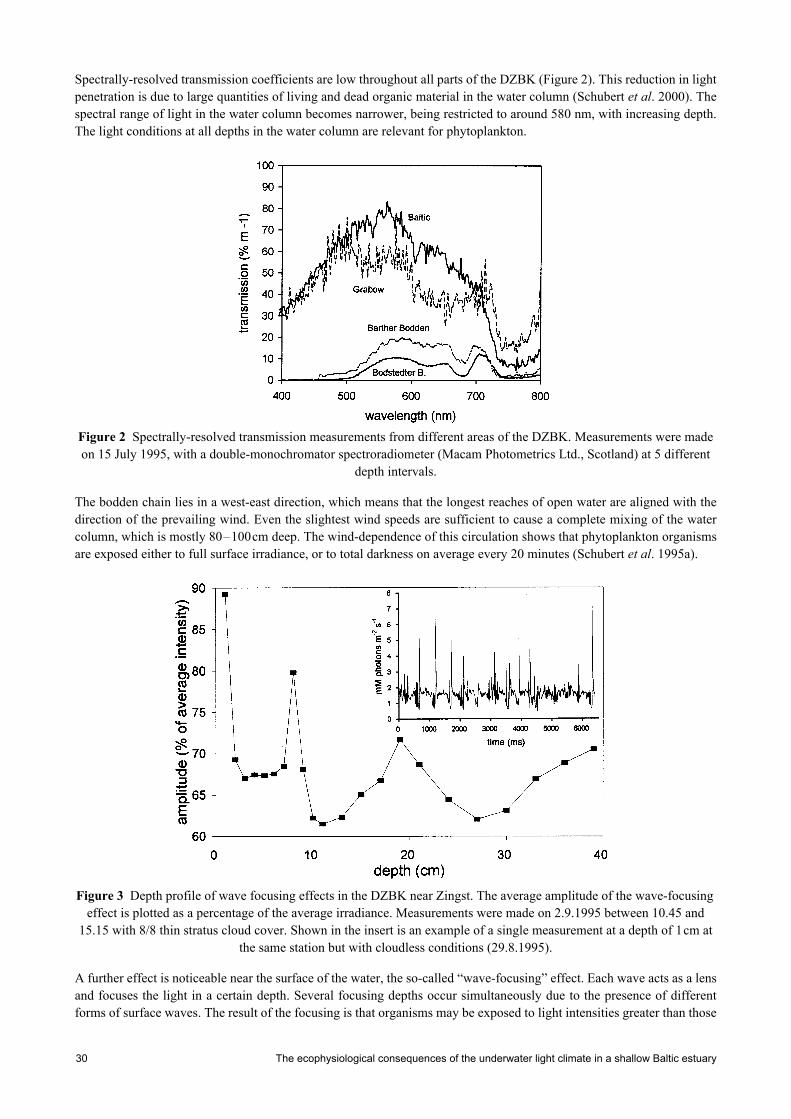
The ecophysiological consequences of the underwater light climate in a shallow Baltic estuary30
Spectrally-resolved transmission coefficients are low throughout all parts of the DZBK (Figure 2). This reduction in lightpenetration is due to large quantities of living and dead organic material in the water column (Schubert et al. 2000). Thespectral range of light in the water column becomes narrower, being restricted to around 580 nm, with increasing depth.The light conditions at all depths in the water column are relevant for phytoplankton.
Figure 2 Spectrally-resolved transmission measurements from different areas of the DZBK. Measurements were made on 15 July 1995, with a double-monochromator spectroradiometer (Macam Photometrics Ltd., Scotland) at 5 different
depth intervals.
The bodden chain lies in a west-east direction, which means that the longest reaches of open water are aligned with thedirection of the prevailing wind. Even the slightest wind speeds are sufficient to cause a complete mixing of the watercolumn, which is mostly 80–100cm deep. The wind-dependence of this circulation shows that phytoplankton organismsare exposed either to full surface irradiance, or to total darkness on average every 20 minutes (Schubert et al. 1995a).
Figure 3 Depth profile of wave focusing effects in the DZBK near Zingst. The average amplitude of the wave-focusing effect is plotted as a percentage of the average irradiance. Measurements were made on 2.9.1995 between 10.45 and
15.15 with 8/8 thin stratus cloud cover. Shown in the insert is an example of a single measurement at a depth of 1cm at the same station but with cloudless conditions (29.8.1995).
A further effect is noticeable near the surface of the water, the so-called “wave-focusing” effect. Each wave acts as a lensand focuses the light in a certain depth. Several focusing depths occur simultaneously due to the presence of differentforms of surface waves. The result of the focusing is that organisms may be exposed to light intensities greater than those

Hendrik Schubert, Louise Schlüter, and Peter Feuerpfeil 31
at the surface (Figure 3). Irradiance is increased to 4 to 5 times the surface irradiance at the first focusing depth (1cm,Figure 3, insert); this irradiance is clearly “oversaturating”. The focusing effect is weak at 6cm depth, but increases againat 8cm to form a second maximum. A third, weaker maximum is seen at approx. 20cm. Planktonic organisms aretherefore exposed to extremely fast changes in the light climate, of both quantitative, and, with increasing depth, quali-tative nature.
The ability to react to these changes, and to adapt to either the short, concentrated light pulses at the surface, or to makeoptimal photosynthetic use of the longer periods of low light availability, may give a competitive advantage.
Adaptation to high light always consists of a change in the pigmentation of the organisms, e.g. a change in the ratio ofphotoprotective pigments to photosynthetically-active light harvesting pigments.
Carotenoids are the main photoprotective pigments in both green algae and cyanobacteria. Photosynthesis and lightharvesting are due, with the exception of the outer (PSII) antenna, to chlorophyll a (chl a). Chl a in the reaction centres isthe pigment most likely to be damaged by excess light. The ratio of carotenoids to chl a give an indication of the highlight tolerance. Published values for this ratio are difficult to compare because of differences in the light sources and lightmeasuring equipment used. Therefore, an experiment was carried out in which the pigmentation of 10 species of cyano-bacteria (5 unicellular, 2 filamentous and 3 colonial) and 7 green algal species were measured after culture at light inten-sities between 20 and 260 µmol photons m–2s–1(Figure 4). The chl a / carotenoid ratio of cyanobacteria is always lowerthan that of green algae. In effect, more protective pigments are available per chl a. This type of analysis does not showthe extent to which these pigments are actually active in photoprotection.
Figure 4 Chlorophyll a / carotenoid ratios (mole/mole) for 10 species of cyanobacteria (m) and 7 green algal species (7) after precultivation for 6 days at different irradiances (x-axis).
The next major difference between cyanobacteria and green algae is found in the composition of the carotenoidpigments. Green algae (and higher plants) have the three pigments of the “xanthophyll cycle”, violaxanthin, antherax-anthin and zeaxanthin, which are interconvertible in the presence of light. Of the three xanthophyll cycle pigments, onlyzeaxanthin is detectable in cyanobacteria, which rules out the presence of a xanthophyll cycle. Cyanobacteria, however,possess a range of glycosidic carotenoids (sugar-carotene compounds), which have up to 14 conjugated double bonds,and are otherwise only known in the myxobacteria.
The simplest form of photoprotection occurs when the carotenes, because of their high molar absorption coefficients,reduce the irradiance inside the cell and act as filters. The efficiency of this form of photoprotection in cyanobacteria isonly an energetic problem: sufficient quantities of carotene must be produced to form the filter. Otherwise, the blockingof the blue region of the spectrum by carotenoid pigments does not interfere with the light-harvesting process, as light-harvesting in these algae is largely due to phycobiliproteins, which absorb outside of the blue range.
A problem occurs when this type of photoprotection is used by green algae. Carotenoids absorb the complete blue part ofthe spectrum, to 500 nm. A carotenoid accumulation would cause shading not only of the reaction centres, but also of themain chl a / chl b light-harvesting antenna. This has important consequences under the fluctuating conditions of theDZBC. Accumulation of carotenoids to provide photoprotection at the surface will result in loss of light harvestingability when cells leave the surface and return to low light conditions. Alternatively, a low concentration of carotenoidsmay cause the cells to be light-damaged during the short periods at the surface. Two mutually exclusive strategies basedon fixed chl a / carotene ratios would appear to be possible, and the two extreme forms of these strategies are indeedexhibited between the mature and spore stages of some green algae. However, other possibilities may have developed

The ecophysiological consequences of the underwater light climate in a shallow Baltic estuary32
during evolution. The xanthophyll cycle offers a more flexible photoadaptive strategy. Forms of the xanthophyll cyclehave been found in all eukaryotic photoautotrophs, other than those (such as the red algae) which utilise phycobilipro-teins as light-harvesting pigments and avoid the antenna-shading problem altogether. There is still debate over which ofthe many suggested protective mechanisms is actually fulfilled by the xanthophyll cycle. Zeaxanthin is suggested to beactive in the conversion of absorbed light energy to harmless heat energy. The light dependent conversion ofvioloxanthin to zeaxanthin results in a decreased efficiency of light energy transfer in the antenna and between theantenna and reaction centres. This reduces the excitation pressure on the reaction centre.
A simple uncoupling of the antenna from the reaction centre will also achieve this, as has been shown for cyanobacteria(Mullineaux, 1988). Why is this method not possible for green algae, or for all organisms with a chl a / chl b antenna?
Overexcitation of chl can lead to the formation of long-lasting, triplet excitation states, which can transfer their energy tooxygen molecules. The result is the formation of a highly energetic oxygen radical, capable of oxidising and destroyingall biomolecules in its vicinity. An uncoupling of the antenna may save the reaction centre, but without additional mecha-nisms to protect itself, the antenna may be oxidised.
The energy level of the (singlet) excitation state of all carotenoids becomes lower as the number of double bonds isincreased (Murasecco–Suardi et al., 1988). Carotenoids with 9 conjugated double bonds are able to transfer energy to chla. Functionally active light harvesting carotenes with this number of bonds are common on diatoms and brown algae. Theenergy level of the first excited state is higher than the first excited state of chl a. In contrast, carotenes with 11 or moreconjugated double bonds show both in vivo and in vitro an ability to quench excited chlorophyll and oxygen molecules(Krinsky, 1971).
The conversion of violoxanthin to zeaxanthin means that a light harvesting pigment has been converted to an “energytrap”, which can reduce excitation pressure in the antenna and quench oxygen radicals. [The reaction centre, according toTelfer and Barber (1995) contains only ß-carotene, which acts as a quencher but not as energy trap due to its distancefrom chl a. This is undoubtedly a sensible compromise between efficiency of light use, and protection requirements.]
The production of an energy trap via enzymatic deepoxidation has a further advantage: during the quenching of oxygenradicals the zeaxanthin may be destroyed with probability of 1:1000 (Foote et al., 1970). Some of the reaction productsare the epoxy-compounds, antheraxanthin and violaxanthin. These products will be immediately converted back tozeaxanthin, so that a recycling of the destroyed photoprotective pigments takes place. This explains the low carotene / chla ratio of green algae.
Continuous shading of the light-harvesting antenna is avoided by the production of protective pigments only under stressconditions (Schubert et al., 1994). Phycobiliprotein-containing organisms which absorb light energy outside thecarotenoid bands do not require this series of reactions, and can afford to have excessive concentrations of carotenoidswithout the danger of self-shading. There is still the consideration of overexcitation within the light-harvesting antennaitself. It appears that no antenna protection mechanisms are present in this group of organisms. The reason is that phyco-biliproteins, although structurally similar to the chlorophylls, are not able to form excited triplet states (at least not inmeasurable quantities, pers. comm. Prof. H. Scheer, München), and will not produce oxygen radicals. The phyco-biliprotein antenna system can be safely decoupled from its reaction centre. This may be the reason why cyanobacteriaand red algae can “misuse” their antenna as a nitrogen-store, without the dangers of excessive overexcitation. Thepresence of these storage antenna are apparent in the form of increased PBS fluorescence emission in comparison to PS IIfluorescence, showing that the antenna are not coupled to the reaction centre. This explains the frequent descriptions of“inverse adaptation” in the cyanobacteria (Raps et al., 1983). Increasing light intensity makes more energy available forthe deposition of N stores, so that the PBS content per cell increases and the antenna size increases. Observation of theemission spectrum shows that only a small part of the pigment pool functions as an antenna. Decreasing the nitrogensupply reduces the antenna emission so that the oft-cited and astonishingly high energy-transfer value of 98% is reached(Figure 5).
On the other hand, photosynthesis is only possible in the presence of chl a, and cyanobacterial reaction centres also havethis pigment.

Hendrik Schubert, Louise Schlüter, and Peter Feuerpfeil 33
Figure 5 Absorption-corrected 660/685 nm fluorescence emission ratios of Synechocystis sp. 6803 cultured with different concentrations of nitrate in the medium.
The emission ration was corrected for the absorption at 625 nm. Measurements were made after 6 days growth in BG-11 medium, after replacement of all N-sources in the medium with the concentrations of NaNO3 shown on the X-axis.
Insert: emission spectra of Synechocystis sp. 6803 with 580 nm excitation light. Dashed line: final state after culture with saturating N-supply (BG11 medium), continuous line: condition after 5 generations in N-free BG-11 medium. The
emission spectra consist of: a shoulder at 660 nm which is due to autoemission of the phycobilisome, a fluorescence maximum at 685 nm from PS II. The PS II peak is derived from excitation energy transferred from the phycobilisome, as
PS II does not absorb at the chosen excitation wavelength of 580 nm.
The danger of an overexcitation of the reaction centre under stress conditions, with subsequent triplet formation andactive oxygen formation, is reduced by decoupling of the antenna, and by shading of the reaction centre, but there is stillsome risk to the reaction centre under normal operating conditions. There is a need for additional protective quenchingmechanisms in addition to the shading provided by carotenoids. The reaction centre itself is protected in cyanobacteriaand in green algae by the internal presence of a ß-carotene molecule. Other photoprotective functions, for example forthe lipids of the various membrane systems, may be performed by not by the “filter” carotenoids, but by other(membrane-bound?) carotenoids. The latter pool should have a much shorter lifetime (higher turnover). Radiocarbon-labelling experiments were performed in order to separate between the active and passive photoprotection roles ofcarotenoids. There were only small differences between the rates of pigment labelling in Synechocystis and Chlorellaafter exposure to the irradiance at which they were grown (not shown). Synechocystis reacted to an increase in theincident irradiance by immediately increasing the rate of carotenoid metabolism (Figure 6). The speed of the response,less than 15 min, is surprisingly fast. Equally surprising was the finding that myxothanophyll, previously thought of ashaving only a shading function, showed the highest turnover. Due to the speed and flexibility of its carotenoid response,Synechocystis appears to be able to react much faster to a light stress than Chlorella, in which a delay was noticedbetween stress and response (Figure 6). The frequency at which the irradiance changes between high light and low lightis likely to determine which photoprotective strategy will be most successful. The speed at which chlorophyll-breakdownproducts (phaeophytins) appear is a good indicator of the damage caused by the light stress (Figure 7). The short-termphotoprotective mechanisms of Synechocystis appear to work well, as the first breakdown products do not appear untilafter 45 min. Phaeophytin products are detectable in Chlorella soon after the start of the light stress, indicating insuffi-cient photoprotection, but after 60 minutes the production has stabilised and there is evidence of an adaptation.
Cyanobacteria can withstand short periods of high light stress firstly because of their larger available pool of carotenoids,and secondly because of the greater flexibility of their metabolism. Green algae appear to be better adapted to withstandlonger periods of light stress due to their possession of a recycling system, and their K-strategy oriented acclimationreactions.
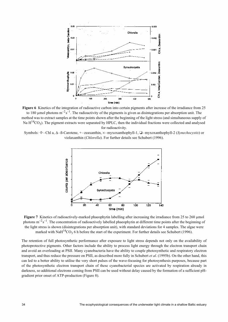
The ecophysiological consequences of the underwater light climate in a shallow Baltic estuary34
Figure 6 Kinetics of the integration of radioactive carbon into certain pigments after increase of the irradiance from 25 to 180 µmol photons m–2s–1. The radioactivity of the pigments is given as disintegrations per absorption unit. The
method was to extract samples at the time points shown after the beginning of the light stress (and simultaneous supply of Na H14CO3). The pigment extracts were separated by HPLC, then the individual fractions were collected and analysed
for radioactivity. Symbols: –Chl a, ∆–ß-Carotene, +–zeaxanthin, ×–myxoxanthophyll-1, –myxoxanthophyll-2 (Synechocystis) or
violaxanthin (Chlorella). For further details see Schubert (1996).
Figure 7 Kinetics of radioactively-marked phaeophytin labelling after increasing the irradiance from 25 to 260 µmol photons m–2s–1. The concentration of radioactively labelled phaeophytin at different time points after the beginning of the light stress is shown (disintegrations per absorption unit), with standard deviations for 4 samples. The algae were
marked with NaH14CO3 6 h before the start of the experiment. For further details see Schubert (1996).
The retention of full photosynthetic performance after exposure to light stress depends not only on the availability ofphotoprotective pigments. Other factors include the ability to process light energy through the electron transport chainand avoid an overloading at PSII. Many cyanobacteria have the ability to couple photosynthetic and respiratory electrontransport, and thus reduce the pressure on PSII, as described more fully in Schubert et al. (1995b). On the other hand, thiscan led to a better ability to utilise the very short pulses of the wave-focusing for photosynthesis purposes, because partof the photosynthetic electron transport chain of these cyanobacterial species are activated by respiration already indarkness, so additional electrons coming from PSII can be used without delay caused by the formation of a sufficient pH-gradient prior onset of ATP-production (Figure 8).

Hendrik Schubert, Louise Schlüter, and Peter Feuerpfeil 35
Figure 8 Dependency of PSII-fluorescence from light intensity, dark period and duration of short light pulses compa-rable to wave focusing events.
The values of triggered fluorescence (Ft) are shown, as a percentage of the variable fluorescence measured in the dark before switching on the pulses generated by a 660 nm LED. The x-axes indicate the length of the dark period between two successive pulses. Intensities of the pulses in µmol photons m–2s–1: –12, –24, ∆–34, –50, –64, –114.
Left panels (A, C, E): Synechocystis spec. PCC 6803 (Cyanobacteria), right panels (B, D, F): Chlorella vulgaris (Chloro-phyta). Duration of the individual pulses: A, B – 3µs, C, D – 5µs, E, F – 10µs. The pronounced shoulder in the left side
of A and B indicate photosynthetic activity of Synechocystis already at very long dark intervals, whereas electron transport in Chlorella start much later at approx. 20–15µs dark intervals.
The experimental setup is described in detail in Schubert (1996).
A further advantage for cyanobacteria in the light conditions of the DZBC comes from their better ability to achieve anequilibration of excitation energy between the photosystems (state transition) in comparison with green algae. Asdescribed in Schubert et al. (1995a), cyanobacteria can react almost without delay to a change in light quality whereasthe slower reaction in green algae may lead to a loss in efficiency.
In addition to all of the above factors, it can be seen that the wavelengths of light which penetrate most deeply in theDZBC (at 580 nm) are better absorbed by cyanobacteria then their green algal competitors. Therefore, the gradient inirradiance in the water column is less steep for cyanobacteria than for green algae.
The highly unstable light climate with periods of extreme high light stress do not seem to be a problem for cyanobacteria,and may even give a selective advantage, as shown in experiments where cyanobacteria were exposed to high frequencylight stress (Schubert et al., 1995c). If photoinhibtion occurs immediately after light stress, as in green algae, thenrecovery may not be fully complete before the start of the next light phase. This means that both the optimal and subop-timal irradiances occurring after the surface exposure will not be utilised efficiently, which can be a disadvantage underfluctuating light conditions. The reason for the sensitivity of cyanobacteria to continuous light stress can only be specu-lated. The green algal response to an increase in irradiance, namely to reduce the capacity of the light reactions, seems tobe necessary in order to balance the metabolic requirements after the change from light limitation to nutrient limitation.
It could be possible that cyanobacteria under fluctuating light conditions become nutrient-limited at a later stage thangreen algae. This is because nutrient storage takes place under optimal conditions, the reserves may last for severalgenerations. Limitation is most likely to be due to the CO2 supply, in this case water movement does not increase thesupply. Large changes have been observed in the cyanobacterial photosynthetic apparatus during CO2 limitation experi-ments, and changes caused by this factor can not be ruled out (Reuter and Müller, 1993).

The ecophysiological consequences of the underwater light climate in a shallow Baltic estuary36
Finally, it should be mentioned again that cyanobacterial diversity is very high in comparison to green algae. Not all ofthe mechanisms described above will occur in every cyanobacterial species, and not all of the physiological mechanismscan be explained. The selection presented here was chosen for their relevance to the particular problems of the DZBC.
AcknowledgementsThis work was supported by a research fellowship from the German Academy of Natural Sciences “Leopoldina”, and bya grant of the German Ministry of Education and Research (BMBF, grant no. BEO/52/F0266D), which is gratefullyacknowledged.
ReferencesAllen, M.M. and Hutchinson, F, 1980, Nitrogen limitation and recovery in the cyanobacterium Aphanocapsa 6308. Arch
Microbiol. 128, 1–7
Foote, C.S., Chang, Y.C. and Denny, R.W., 1970, Chemistry of singlet oxygen. XI. Cis-trans isomerization of carote-noids by singlet oxygen and a probable quenching mechanism. J. Am. Chem. Soc. 92, 5218–5219
Foy, R.H., Gibson, C.E. and Smith, R.V., 1976, The influence of daylength, light intensity and temperature on the growthrates of planktonic blue-green algae. Br. Phycol. J. 18, 267–273
Krinsky, N.I.: Function. In: Isler, O. (Ed.), 1971, Carotenoids. 36–92. Basel: Birkhäuser–Verlag
Mullineaux, C.W. and Allen, J.F., 1988, Fluorescence transients indicate dissociation of photosystem II from the phyco-bilisome during the state-2 transition in the cyanobacterium Synechococcus 6301. Biochim. Biophys. Acta 934,96–107
Murasecco–Suardi, P., Oliveros, E., Braun, A.M. and Hansen, H., 1988, Singlet-oxygen quenching by carotenoids:steady-state luminescence experiments. Helv. Chim. Acta 71, 1005–1010
Raps, S., Wyman, K., Siegelman, H.W. and Falkowski, P.G., 1983, Adaptation of the cyanobacterium Microcystisaeruginosa to light intensity. Plant Physiol. 72, 829–832
Reuter,W. and Müller, C., 1993, Adaptation of the photosynthetic apparatus of cyanobacteria to light and CO2. J.Photochem. Photobiol. B. Biol. 21, 3–27
Reynolds, C.S., 1987, Cyanobacterial water-blooms. In: Callow, P. (Ed.): Advances in botanical Research 13. S. 67–143. London: Academic Press
Sagert, S., Schubert, H. and Suchau, A., 1993, Light and temperature adaptation of two picoplankton species in thebodden chain south of the Darss–Zingst peninsula. J. Plankt. Res. 15, 953–964
Schlungbaum, G. and Nausch, G., 1994, Die Darß–Zingster Boddenkette-ein typisches Flachwasserästuar an dersüdlichen Ostseeküste. Rostock. Meeresbiol. Beitr. 2, 5–26
Schubert, H., 1996, Ökophysiologie der Lichtanpassung des Phytoplanktons eutropher Flachgewässer. Habilitationss-chrift, Univ. Rostock, Rostock, 179 pp.,
Schubert, H., Forster, R. and Sagert, S., 1995a, In situ measurement of state transition in cyanobacterial blooms: kineticsand extent of the change in relation to underwater light and vertical mixing. Mar. Ecol. Progr. Ser. 128, 99–108.
Schubert, H., Sagert, S. and Forster, R., 2000, Evaluation of the different levels of variability in the underwater light fieldof a shallow estuary. Helgoland Marine Res.
Schubert, H., Kroon, B.M.A. and Matthijs, H.C.P., 1994, In vivo manipulation of the Xanthophyll cycle and the role ofzeaxanthin in the protection against photodamage in the green alga Chlorella pyrenoidosa. J. Biol. Chem. 269,7267–7272
Schubert, H., Matthijs, H.C.P. and Mur, L.R., 1995b, In vivo assay of P700 redox changes in the cyanobacteriumFremyella diplosiphon and the role of cytochrome-c-oxidase in regulation of photosynthetic electron transfer.Photosynthetica, 31(4), 517–527

Hendrik Schubert, Louise Schlüter, and Peter Feuerpfeil 37
Schubert, H., Matthijs, H.C.P., Mur, L.R. and Schiewer, U., 1995c, Blooming of cyanobacteria in turbulent water withsteep light gradients: the effect of intermittent light and dark periods on the oxygen evolution capacity ofSynechocystis sp. PCC 6803. FEMS Microbiol. Ecol., 18, 237–245
Telfer, A. and Barber, J., 1995, Role of carotenoid bound to the photosystem II reaction centre. Photosynth. Res. Suppl.1, 11
Zevenboom, W. and Mur, L.R., 1984, Growth and photosynthetic response of the cyanobacterium Microcystisaeruginosa in relation to photoperiodicity and irradiance. Arch. Microbiol. 139, 232–239
Zhuang, S., Schubert, H. and Schiewer, U., 1993, Influence of irradiance and temperature on the Cyanobacterium Aphan-othece stagnina Sprengel isolated from the Darss–Zingst estuary (Southern Baltic) under continuous turbidostatculture. Arch. Hydrobiol. Algological studies 70, 51–63

Chlorinated hydrocarbons in marine biota and sediments from the Gulf of Gdansk38
ICES Cooperative Research Report, No. 257 Baltic Marine Science Conference, Rønne, Denmark, 22–26 October 1996
Chlorinated hydrocarbons in marine biota and sediments from the Gulf of Gdansk
Grazyna Sapota
AbstractThe aim of this work was establishing the level of pollution by highly persistent polychlorinated contaminants in the Gulfof Gdansk.
Concentrations of PCBs, DDT and its metabolites, HCH-isomers and HCB were determined in stratified sediments (from2 stations—1cm slices from 0 to 10cm depth) and in marine biota (Salmo trutta trutta, Halicryptus spinulosus, Saduriaentomon, Mytilus trossulus, Macoma baltica, Mya arenaria) from 3 sampling stations. For bivalves, toxic substanceswere analysed in tissue and shell.
All investigated substances were present in sediment and biota samples from the Gulf of Gdansk in concentrations abovethe detection limit (0.01ng·g–1) of the method used.
IntroductionChlorinated hydrocarbons are some of the mostly widely distributed environmental pollutants (Dunn et. al., 1984). Thesesynthetic substances are produce mainly for agriculture, horticulture, forestry and many branches of industry. PCBs andDDTs are especially well-known as global contaminants due to their persistency in the environment (Flower, 1990).Pollutants adsorb to suspend particles in the water and are sooner or later associated with the sediments. When concen-tration in the water decreases, the sediments can act as a source to the water (Rasmunson et. al., 1990).
Materials and Methods
SamplingFifteen 8 years old sea trout (Salmo trutta trutta) were caught in late autumn (October and November 1995) from stationNo 3 (54o 23' N, 18o 57' 5" E). Weight, length and sex of each fish were determined. For each sea trout a segment of themuscle was taken from below the dorsal fin, after which the samples were frozen (–27oC).
The benthic animals were taken with drag from two sampling stations (station 1: 540 35' N, 180 40' E and station 2: 54035' N, 180 44' E) in early spring (March 1996). Saduria entomon was grouped into length classes. The bivalves (Macomabaltica, Mya arenaria, Mytilus trossulus) were espoused for 24h in filtrated sea water, then grouped into length classes.Tissue and shell were separated. All individuals from species Halicryptus spinulosus were similar in size and treated asone sample. Saduria entomon cultivated in aquatic system for half a year was analysed as comparable material. Allsamples were frozen (–27oC).
The sediment samples were taken (from stations 2 and 3 in March 1996) with a Niemistö corer, separated into 1cm slicesto 10cm depth and frozen (–27oC).
Sample preparationMuscle tissue of fish, tissues, shells and sediments were freeze-dried to complete dryness and divided into small pieces.A portion of about 1–2 g was transferred to a glass extraction vial and Soxhlet-extracted in hexane and acetone at 180oCfor 2 hours. Octachloronaphtalene was used as an internal standard and added prior to the extraction. After extraction,water was added to the extract to separate the hexane (containing the fat and lipophilic pollutants) from the acetone/waterphase. Concentrated H2SO4 was added to oxidise the fat. The hexane phase was then evaporated in a vacuum centrifugeto dryness. The remaining material was dissolved in 400µl hexane and eluted with hexane/dichlorometane through acolumn containing two layers of silica gel to which K2CO3 and H2SO4 had been added. The eluate was then evaporatedto dryness and dissolved in isooctane.

Grazyna Sapota 39
AnalysisThe cleaned-up extract was analysed for persistent pollutants by capillary GC/ECD on VARIAN STAR 3400. Investi-gated substances were separated on a 30-m DB-5 quartz capillary column. Injection technique was split/splitless. H2(1.5mlmin–1) was used as a carrier gas and N2 (50mlmin–1) as a make-up gas. The oven temperature was programmedas follows:
• Initially 15 min at 80oC
• Increase by 4oC per min to 320oC• Hold for 15 min.
• Injection temperature—330oC
• Detection temperature—340oCA pesticide mixture containing p,p'-DDE, p,p'-DDD, o,p'-DDT, p,p'-DDT, a-HCH, b-HCH, g-HCH and HCB was usedas a standard. Clophen A 60 was used as a PCB standard. All substances were identified and quantified according toMullin et. al. (1984) and Schultz et. al. (1989).
Dry weight and fat content (without shell) was determined for each sample. Fat content was determined in Soxhletextraction (Ewald et. al., 1998).
Results and DiscussionThe vertical distribution of the concentration of all investigated substances in sediments was very similar for bothstations, but values at station 3 were higher than at station 2 (Figure 1). The highest concentration of all analysedsubstances was observed between the 3rd and 7thcm of sediment. The sediments from station 2 belong to very finepowdered sands and from station 3 to very fine organic powdered sands. Duinker and Hillebrand (1979) estimated that inorganic sediments the amount of chlorinated hydrocarbons is much higher than in inorganic sands. In 1977 Trzosinskaand Baumgartner reported that concentrations of SDDT for surface sediments from the Gulf of Gdansk varied from14.6ng·g–1 d.w. to 29.3ng·g–1 d.w. In 1979 Andrulewicz et. al. estimated for the same area concentrations for sands:DDE –4ng·g–1 d.w., DDD –1ng·g–1 d.w., DDT –2ng·g–1 d.w. and for mud: DDE –7ng·g–1 d.w., DDD –2ng·g–1 d.w.,DDT –8ng·g–1 d.w. In 1987 Slaczka et al. gave concentrations of SDDT for sound sediments from Southern Baltic—5ng·g–1 d.w. and for mud—20ng·g–1 d.w. In comparison to these data it could be stated that concentrations of DDT andits metabolites in the Gulf of Gdansk decrease.
Generally in all analysed samples the pattern of concentrations of investigated substances was similar. It was observedthat the highest amount of DDE among DDT and its metabolites is an effect of metabolic degradation of DDT (Larssonand Okla, 1989). In analysed benthic organisms concentrations of all investigated substances increase with increase of fatcontent (Table 1, Figure 2, Figure 3, Figure 4, Figure 5). This statement is also valid taking into account the same speciesfrom the different stations (Figure 2, Figure 3, Figure 5). Saduria entomon cultivated in aquatic system shows lowerconcentrations than the same species from environment. Tooby and Durbin (1975) estimated that residue substanceswere rapidly eliminated from tissues when organisms were placed into clean water. In analysed benthic organismsconcentrations increase with increase of size of animals. Comparison of concentrations calculated on wet weight in tissueand shells shows much higher concentrations in tissue (except Mya arenaria) (Figure 6). The highest concentrations ofinvestigated substances were found in sea trout (Figure 4). Bremle et. al. (1995) stated that the level of fish contami-nation mainly depends on the food web. Sea trout is the fish at the top of the marine food web.

Chlorinated hydrocarbons in marine biota and sediments from the Gulf of Gdansk40
Table 1 Fat content (in % of wet weight) in analysed species from the Gulf of Gdansk
Figure 1 Concentrations of investigated substances in stratified sediments from stations 2 and 3
Station No Species Length class [cm] Fat content [% w. w.]1 Halicryptus spinulosus 0.78
Macoma baltica 1.0–1.5 2.551.6–2.0 1.72
Mya arenaria 1.0–1.5 2.401.6–2.0 1.272.1–2.5 1.742.6–3.0 1.68
Mytilus trossulus 2.6–3.0 2.133.1–3.5 2.82
Saduria entomon 1.6–2.5 9.092.6–3.5 8.403.6–4.5 5.644.6–5.5 5.625.6–6.5 5.916.6–7.5 5.94
2 Macoma baltica 1.0–1.5 1.561.6–2.0 1.592.1–2.5 1.74
Saduria entomon 2.6–3.5 7.313.6–4.5 4.634.6–5.5 4.586.6–7.5 4.35
3 Salmo trutta trutta 7.78cultivated Saduria entomon 1.6–2.5 4.44
2.6–3.5 3.383.6–4.5 1.944.6–5.5 2.385.6–6.5 2.356.6–7.5 2.17

Grazyna Sapota 41
Figure 2 Concentrations of investigated substances in animals from station 1
Figure 3 Concentrations of investigated substances in animals from station 2

Chlorinated hydrocarbons in marine biota and sediments from the Gulf of Gdansk42
Figure 4 Concentrations of investigated substances in fish from station 3
Figure 5 Concentrations of investigated substances in cultivated Saduria entomon
Figure 6 Concentrations of investigated substances in tissues and shells of bivalves calculated on wet weight

Grazyna Sapota 43
Conclusions• The presence of all investigated substances in biota and sediments from the Gulf of Gdansk was confirmed.• Fat content was the governing factor for the distribution of persistent pollutants.• Persistent pollutant concentrations vary in marine biota in due to size.• Concentrations of chlorinated hydrocarbons in cultivated Saduria entomon were lower than in Saduria entomon from
the environment.• Concentrations of persistent pollutants increase towards higher trophic levels.• In bivalves, concentration of investigated substances were higher in tissue than in shell.• The amount of analysed chlorinated hydrocarbons was higher in marine biota than in sediments.
AcknowledgementsThe author would like to thank Per Larsson and Lennart Okla from University of Lund, Sweden, for their help and possi-bility to work in Lund’s laboratory.
Thank you to Monika Normant for cultivated Saduria entomon.
ReferencesAndrulewicz, E., Brzezinska, A., Trzosinska, A., 1979. Some aspects of the chemical composition of particulate matter
in the Southern Baltic. Ref. Marine Environ.
Bremle, G., Okla, L., Larsson, P., 1995. Uptake of PCBs in fish in a contaminated river system: bioconcentrations factorsin the field. Environ. Sci. Technol. 29 (8), 2010–2015.
Duinker, J.C., Hillebrand, M.T.J., 1979. Behaviour of PCB, hexachlorobenzene, a-HCH, b-HCH, g-HCH, dieldrin,endrin and p,p'-DDD in the Rhinemeuse Estuary and the adjacent coastal area. Neth. J. Sea Res. 13 (2), 256–281.
Dunn, W.J., Stalling, D.L., Schwartz, T.R., Hogan, J.W., Petty, J.D., Johansson, E, Wold, S., 1984. Pattern recognitionfor classification and determination of Polychlorinated biphenyls in environmental samples. Anal. Chem. 56 (8),1308–1313.
Ewald, G., Bremle, G., Karlsson, A., 1998. Differences between Bligh and Dyer and Soxhlet extractions of PCB andlipids from fat and lean fish muscle: Implications for data evaluation. Mar. Pollut. Biul. 36 (3), 222–230.
Flower, S.W., 1990. Critical review of selected heavy metal and chlorinated hydrocarbon concentration in the marineenvironment. Mar. Environ. Res. 29, 1–64.
Larsson, P., Okla, L., 1989. Atmospheric transport of chlorinated hydrocarbons to Sweden in 1985 compared to 1973.Atmos. Environ. 23 (8), 1699–1711.
Mullin, M.D., Pochini, C.M., McCrindle, S., Romkes, M., Safe, S.H., Safe, L.M., 1984. High-resolution PCB analysis:synthesis and chromatographic properties of all 209 PCB congeners. Environ. Sci. Technol. 18 (6), 468–476.
Rasmunson, A., Lindgren, M., Jones, C., 1990. Release of contaminants from sediments as compered to remedial actionsinvolving dredging and land disposal. Report No 3871; Swedish National Protection Board.
Schulz, D.E., Petrick, G., Duinker, J.C., 1989. Complete characterization of polychlorinated biphenyls congeners incommercial Aroclor and Clophen mixtures by multidimensional Gas Chromatography—Electron CaptureDetection. Environ. Sci. Technol. 23 (7), 852–859.
Slaczka, W., Andrulewicz, E., Trzosinska, A., 1987. Harmful substances. Baltic Sea Environment Proceedings No. 17B,First Periodic Assessment of the State of Baltic Sea.
Tooby, T.E., Dubrin, F.J., 1975. Lindane residue accumulation and elimination in rainbow trout (Salmo gairdnerRichardson) and roach (Rutilus rutilus Linnaeus). Environ. Pollut. (8), Applied Science Publishers Ltd., England,79–89.
Trzosinska, A., Baumgartner, D.J., 1977. Hydrological, chemical and physical processes affecting pollution of the BalticSea. Final Report, Gdynia.

Polonium, uranium, and plutonium in the Southern Baltic ecosystem44
ICES Cooperative Research Report, No. 257 Baltic Marine Science Conference, Rønne, Denmark, 22–26 October 1996
Polonium, uranium, and plutonium in the Southern Baltic ecosystem
Bogdan Skwarzec and Piotr Stepnowski
Introduction210Po belongs to the natural uranium decay series starting from 238U and its fate depends on further members of thisseries such as 226Ra, and most of all on 210Pb. 222Rn escaping from the Earth’s surface constitutes the source of atmos-pheric 210Po (Scholander et al., 1961). the total amount of 210Po in the air depends directly on the amount of 210Pbsupplied and formed in the atmosphere (Jaworowski and Kownacka, 1976). Apart from the 210Po formed by the decay of210Pb contained in the air, additional quantities are emitted directly from the Earth as a result of forest fires (Moore et al.,1976) and volcanic eruptions (Lambert et al., 1970; Danielsen, 1981). Atmospheric precipitation of 210Po and, to asmaller extent, precipitation of 210Pb itself onto the surface of seas and oceans are the principal sources of 210Po thatenter the marine environment. A small amount of 210Po is formed in situ as a result of the radioactive decay of uraniumcontained in sea water.
Uranium occurs naturally in the Earth’s crust and is present in much higher concentrations— along with thorium andrare-earth elements—in areas where heavy mineral sands occur. The major source of uranium in the marine environmentis the atmospheric precipitation of terrigenic (rock) derived material, together with river water (Ku et al., 1974).
Plutonium belongs to a group of man-made radionuclides that have attracted considerable attention from the radioeco-logical point of view due to their high radiotoxicity, long physical half-life, high chemical reactivity and long residencein biological systems. The principal source of plutonium radionuclides in the Baltic Sea is the atmospheric fallout fromnuclear weapons tests (Hardy et al., 1973). Other sources such as releases from nuclear power plants and the Europeannuclear reprocessing facilities at Sellafield (UK) and Cap de la Hague (France), while not fully documented, are oftenconsidered less important. Since 26 April 1986 another source of plutonium isotopes, from Chernobyl-originating radio-active debris, has had to be taken into account (Aarkog, 1988).
Marine plants and animals are capable of absorbing both natural and artificial radionuclides from their surroundings(Carlson, 1990; Carlson and Holm, 1990; Dahlgaard and Boelskifte, 1992) and are often used as bioindicators of radio-active pollution in the environment. For example, the brown algae Fucus vesiculosus has been found to preferentiallyaccumulate radionuclides in the following order: technetium>americium>plutonium>cesium (Carlson, 1990; Carlsonand Holm, 1990). Among the natural emitters of alpha radiation, 210Po is often accumulated to a high degree by marineorganisms. The great ability of organisms to accumulate 210Po means that they are exposed to a large ionising radiationdose. The 210Po and uranium isotopes are responsible for over 90% of all natural radiation to which many organisms aresubjected (Cherry and Heyraud, 1982; Woodhead, 1973).
Materials and MethodsSeawater and biota were collected between 1980 and 1991 in various regions in the southern Baltic Sea.
The radioanalytical procedure for determination of polonium, uranium and plutonium in the Baltic Sea samples arepresented in Figure 1. All details about activity determination of 210Po, 234U, 238U and 239+240Pu are given by Skwarzec(1996).

Bogdan Skwarzec and Piotr Stepnowski 45
Figure 1 The radioanalytical procedure for determination of Po, U and Pu in the Baltic Sea samples
Results and Discussion The activity concentration of 210Po, 234U, 238U and 239+240Pu in the southern Baltic water and sediments are presentedin Figure 2 and Figure 3.
Figure 2 The activity concentration of 210Po, 238U and 239+240Pu in the Southern Baltic water
Figure 3 The activity concentration of 210Po, 238U and 239+240Pu in the Southern Baltic sediments

Polonium, uranium and plutonium, in the Southern Baltic ecosystem46
The analysis of seawater samples revealed that the mean concentration of 210Po in Baltic water was 0.6mBqdm–3, 80%of which consisted of soluble forms (Skwarzec and Bojanowski, 1988). There were significant differences in the concen-trations of dissolved polonium in the samples analysed. The mean concentrations of 210Po in the waters of the SlupskFurrow and Lübeck Bay (0.57 and 0.52mBqdm–3 respectively) were over three times as high as the mean concentrationof this nuclide in the water of the Bornholm Deep (0.17mBqdm–3).
The uranium concentrations were within the range of 0.68 to 0.85µgdm–3 in surface seawater samples, but from 0.64 to1.28µgdm–3 in Vistula river water. The mean 234U/238U activity ratio in Baltic seawater was found to be 1.17, and inVistula river water it was 1.31. The uranium concentration in seawater increased, while values of the 234U/238U activityratio decreased with salinity (Skwarzec, 1995).
The average 234U/238U activity ratio in the suspended matter is about 1.0, i.e. similar to that in sediments. This indicatedthat terrigenic material is the source of uranium in the Baltic sediments. Since the 234U/238U activity ratio in Balticorganisms, in the 1.12–1.15 range, is similar to that in seawater, it can be inferred that the dissolved forms of this elementin seawater are the source of uranium in Baltic biota (Skwarzec, 1995).
The average level of 239+240Pu in Baltic seawater was found to be 4.8µBqdm–3, 70% of which constituted filterableforms (<0.45mm). The concentration of plutonium in the suspended matter was 1.5Bqkg–1 dry wt., and the distributioncoefficient (DC) of plutonium was of the order of 4·105 (Skwarzec and Bojanowski, 1992). These results agree well withthose from for Danish, Swedish and Finnish waters (Aarkog et al., 1980; Holm et al., 1980; Kautsky et al., 1986;Leskinen et al., 1987).
The activity concentrations of 210Po, 234U, 238U and 239+240Pu in the southern Baltic ecosystems are shown in Figure 4.Investigation of the 210Po and 239+240Pu content in the Baltic biota showed that organisms display a strong affinity forthem. Mean values of the bioaccumulation factor (BCF) in the Baltic organisms, calculated on the basis of the poloniumcontent fell within the range 4.1·103–3.5·104 (Skwarzec, 1995).
In the case of planktonic organisms the BCF values increased in the sequence:phytoplankton<macrozooplankton<mesozooplankton, while in the zoobenthos they increased in the following order:Polychaeta<Priapulida<Malacostraca<Bivalvia (soft tissue) (Skwarzec and Bojanowski, 1988). The data on Saduriaentomon crustacea, and Mya arenaria bivalves indicated that 210Po is non-uniformly distributed in their bodies. Thepolonium content in the internal organs of these animals decreased in the sequence: hepatopancreas>alimentarytract>gills>muscles (Skwarzec and Falkowski, 1988). It was additionally demonstrated that in the fish the organsdirectly connected with digestion (intestine, liver, spleen, pyloric caeca) contain much higher 210Po concentrations ascompared to muscle tissue (Skwarzec 1988). On the basis of the data on 210Po content in fish, it is suggested that thisnuclide is removed from seawater by fish.
Figure 4 The activity concentration of 210Po, 238U and 239+240Pu in the Southern Baltic ecosystem

Bogdan Skwarzec and Piotr Stepnowski 47
The 239+240Pu concentrations in the Baltic organisms ranged from 14mBqkg–1 dry wt. (fish) to 957mBqkg–1 dry wt.(Priapulida), and respective BCFs from 900 to 27000 (Skwarzec, 1995). In the seaweeds the highest plutonium concen-trations were found in Pilayella litoralis collected in Puck Bay in 1987. In the zoobenthos, plutonium concentrationswere higher in Priapulida and Polychaeta and lower in Entomostraca, Malacostraca and Bivalvia (soft tissue)(Skwarzec and Bojanowski, 1992).
The average 238Pu/(239+240Pu) activity ratio in seaweeds was 0.032 i.e. not very different from that in typical fallout(Perkins and Thomas, 1980). This means that the impact of the Chernobyl-derived plutonium [238Pu/(239+240Pu) activityratio was about 0.60] on the Baltic plants was small (a few percent).
The mean 238Pu/(239+240Pu) activity ratio in some benthic animals was found to be 0.093, which is generally higher thanin marine plants as a whole. The impact of the Chernobyl-derived plutonium on the benthic organisms was calculated tobe about 10%. It appears that benthic organisms have responded to the increased level of plutonium faster and morenoticeably than seaweeds have. It can therefore be concluded that the impact of Chernobyl-derived plutonium on thesouthern Baltic ecosystem was not of great significance (Skwarzec, 1995).
Marine algae and benthic animals concentrated uranium isotopes to a small extent only. The BCF ranged from 30 to 55(Skwarzec, 1995). The mean uranium concentration in phytoplankton was about twice as high as in zooplankton. Onlysmall differences were observed between the uranium levels in benthic organisms. The higher values were found in theBivalvia, the lower ones in the Crustacea. Investigations on fish showed that uranium is non-uniformly distributed intheir bodies, its concentration increasing in the sequence: muscle<skeleton<viscera.
On the basis of the content of the radionuclides analysed in the Baltic samples, it can be concluded that poloniumprobably circulates in the southern Baltic ecosystem in the same way as organic matter does. On the other hand, sedimen-tation and diffusion from sediments to deep seawater are important ways in which uranium and plutonium migrate withinthis ecosystem (Skwarzec, 1995).
References and Notes Aarkrog, A. 1988. The radiological impact of the Chernobyl debris compared with that from nuclear weapon fallout. J.
Environ. Radioactivity, 6, 151–162.
Aarkrog, A., Dahlgaard, H. and Nilsson, K. 1980. Studies on the distribution of transuranics in the Baltic Sea, the DanishBelts, the Kattegat and the North Sea. In: Transuranic Cycling in the Marine Environment. IAEA-TECDOC-265,Vienna, 23–29.
Carlson, L. 1990. Effects of biotic and abiotic factors on the accumulation of radionuclides in Fucus vesiculosus L.,Ph.D. Thesis, Department of Ecology, Marine Ecology, University of Lund. Sweden.
Carlson, L. and Holm, E. 1990. Radioactivity in the Baltic Sea following the Chernobyl accident, SSI project 393–86,University of Lund, Sweden.
Cherry, R.D. and Heyraud, M. 1982. Evidence of high natural radiation doses in certain mid-water oceanic organisms,Science, 218, 54–56.
Dahlgaard, H. and Boelskifte, S. 1992. “SENSI”, A Model describing the Accumulation and Time-Integration of Radio-active Discharges in the Bioindicator Fucus vesiculosus, J.Environ. Radioactivity, 16, 49–63.
Danielsen, E.F. 1981. Trajectories of the Mount St. Helens plume, Science, 221, 819–921.
Hardy E. P, Krey P. W., Volchak H. L., 1973. Global inventory and distribution of fallout plutonium, Nature, 241, 444–445.
Holm, E., Persson, B.B., and Mattsson, S. 1980. Studies of concentration and transfer factors of natural and artificialactinide elements in a marine environment. In: Proc. 5th Int. Congress of the International Radiation ProtectionAssociation, Vol III, Jerusalem, 9–14 March, 311.
Jaworowski, Z. and Kownacka, L. 1976. Lead and radium in the lower stratosphere. Nature, 263, 303–304.
Kautsky, H., Wedekind, C. and Eicke, H.F. 1986. Radiological investigations in the Baltic Sea. Including the DanishStrains and the Kattegat during 1982 and 1983. In: Study of Radioactive Materials in the Baltic Sea. IAEA-TECDOC-362, Vienna, 110–117.

Polonium, uranium and plutonium, in the Southern Baltic ecosystem48
Ku T. L., Knauss K. G. and Mathien G. G., 1977. Uranium in open ocean: concentration and isotopic composition, Deep-Sea Res., 24, 1005–1017.
Lambert, G., Buisson, A., Sanak, J. and Ardonin, B. 1979. Modification of the atmospheric polonium-210 to lead-210ratio by volcanic emissions. J. Geophys. Res., 84, 6980–6986.
Leskinen, S., Miettinen, J.K. and Jaakkola T. 1987. Behaviour of 239,240Pu and 241Am in the Baltic Sea; Measure-ments and interpretations in 1980–1984, J. Radioanal. Nucl. Chem., 115, 289–298.
Moore, H.E., Martell, E.A. and Poet, S.E. 1976. Sources of polonium-210 in the atmosphere. Envir. Sci. Technol., 10,586–591.
Perkins, R.W. and Thomas, C.W. 1980. Worldwide fallout. In: Transuranic elements in the environment, Hanson, W.C.(ed.). Technical Information Center/US Department of Energy, USA, 53–82.
Scholander, P.F., Hemmingsen, E.A., Coachman, L.K. and Nutt, D.C. 1961. Composition of gas bubbles in Greenlandicebergs, J. Glacial., 3, 813–822.
Skwarzec B. 1988, Accumulation of 210Po in selected species of Baltic fish, J. Environ. Radioactivity, 8, 111–118.
Skwarzec, B. 1995. Polonium, uranium and plutonium in the southern Baltic ecosystem, Rozprawy i monografie KBMPAN, 6, (in Polish, summary in English).
Skwarzec, B. 1996. Radiochemical methods for determination of polonium, radiolead uranium and plutonium in environ-mental samples, Chem. Anal. (in press).
Skwarzec, B. and Bojanowski, R. 1988. The 210Po content in sea water and its accumulation in southern Baltic plankton,Mar.Biol., 97, 301–307.
Skwarzec B. and Bojanowski R., 1992. Distribution of plutonium in selected components of the Baltic ecosystem withinthe Polish economic zone, J. Envir. Radioactivity, 15, 249–263.
Skwarzec, B. and Falkowski, L. 1988. Accumulation of 210Po in Baltic invertebrates, J.Environ.Radioactivity, 8, 99–109.
Woodhead, D.S. 1973. Levels of radioactivity in the marine environment and the dose commitment to marine organisms,In: Radioactive contamination of the marine environment. IAEA, Vienna, STI/PUB/313, 499–525.

Jacek Urbanski 49
ICES Cooperative Research Report, No. 257 Baltic Marine Science Conference, Rønne, Denmark, 22–26 October 1996
The application of dynamic segmentation in coastal vulnera-bility mapping
Jacek Urbanski
AbstractThis paper discusses the application of a dynamic segmentation data model in the development of a coastal GIS. Thediscussion presents a hybrid data model of the coast, which combines a raster data model with dynamic segmentation.Several cartographic modelling methods are presented for working with this data model. The model was used to developan oil spill vulnerability map for the Bay of Gdansk coastline. The following factors were evaluated: probability of an oilspill occurrence, oil residence time, degree of exposure to wind and wave action, fish potential and seabird potential. TheMulti-Criteria/Single-Objective decision making technique was used to calculate the vulnerability index.
IntroductionThe coastal zone, which is defined as the space in which terrestrial environments influence marine environments and viceversa (Carter 1988), is a complex dynamic system. Because of the strong, diverse and often uncoordinated humanactivity in this zone, its living resources and environment are sensitive to many factors created by man. The state of theMarine Environment (GESAMP, 1990) report concluded that “In contrast to the open ocean, the margins of the sea areaffected by man almost everywhere, and encroachment on coastal areas continues worldwide...”. Coastal ZoneManagement is used to find a wise balance between the many conflicting elements exerting their influence on the coastalenvironment, ensuring that its limits of tolerance and its capacity for sustainability are not exceeded (Tortell, 1992). Thisprocess needs reliable and accurate data about different environmental factors and human activities.
One of the basic methods for representing and evaluating this type of data is the use of thematic maps of the coastal zone.Table 1, adopted partially from Tortell (1992), illustrates resources, demands and issues that can be featured in such amap.
Table 1 Resources, demands and issues that can be featured in thematic maps of a coastal zone
In order to convert data to useful information, different kinds of spatial data processing techniques are used. One of thetechniques is to create vulnerability maps which describe the sensitivity of the coast to threats of different kinds using anundimensional sensitivity index. These maps are produced by overlaying thematic maps of processes or issues which are
Resources, demands and issues that can be featured in thematic maps of a coastal zone
Maritime shipping operations and navigation lanesEcological sanctuaries and other protective measuresTourism and recreational facilities and usesAdministrative boundaries and zonesSolid wastes dumping sitesDischarge points for liquid wastesFisheries activity and methods usedLand coverBottom coverBottom sedimentsFish potentialBird potentialWave conditionsBathymetry and elevationWater pollutionCoastline typesProbability map of oil spill accidentsCommercial port facilitiesTemperature of waterSediment transportSea level variationSalinity of water

The application of dynamic segmentation in coastal vulnerability mapping50
important factors in sensitivity evaluation. Vulnerability maps were successfully used to evaluate the vulnerability of thecoast to oil spill impact (Jansen et al., 1990, Populus et al., 1995) and sea level rise (McCall and Devoy, 1995). GISconstitutes the best method for data processing using the cartographic modelling concept, since all processed data arespatial data. The cartographic modelling is the processing of spatial data via a sequence of transformations. The spatialdata are organised in a data model which represents reality.
Data modelThere are two data models—the raster data model and the vector data model—which are most often implemented incontemporary GIS systems. Testing of these models for coastal applications to solve problems in the coastal zone,especially for creating vulnerability maps, shows that they are generally poor at representing the distinctive nature of thecoastal system, for reasons given below.
The coastal waters are an essential area of the geographic space covered by a Coastal Geographic Information Systemincluded in the vulnerability analyses. The main problem in the development of successful coastal waters applications isthe lack of a well-suited data model for this area. Although raster and vector data models may be used to represent nearlyall the elements of the terrestrial part of the coast, only a few elements of coastal waters like bottom elevation or bottomcover may be described using these models. The main reason for this is the variability in time of the many parametersused to describe coastal waters like temperature, salinity, amount of nutrients or wave heights (Langran, 1993). Anadditional difficulty in designing the new model is posed by the necessity to retain compatibility with existing GISsystems to facilitate their utilisation in the analysis process. One of the possible solutions is to replace the attributes withthe probability of occurrence of a particular range of attributes, for example we would use a map of the probability thatsalinity would be below some threshold value instead of mean salinity map.
The area “near the waterline” is especially essential in vulnerability analyses of the coastal zone. At the same time it isvery difficult to model this area using raster or vector data models. Firstly, most of the entities within the coastal zonelack clear boundaries. For example, a sandy beach may gradually change into a cobble or gravel beach. A secondproblem emerges out of the very great range of spatial scales of coastal phenomena, which range from centimetres to tensof kilometres. Many coastal objects have a strongly shaped anisotropy, a beach which is a few meters wide may beseveral kilometres long. Objects are often overlaid, for example seabird breeding areas are placed on the beach. Anotherproblem is created by the variability of some objects in time, which necessitates the additional inclusion of the temporaldimension (Bartlett 1994). A solution which has been proposed recently to overcome some of disadvantages of raster andvector models is the dynamic segmentation model. The dynamic segmentation (Figure 1) is the line data model in whichspatial objects are referenced based on the distance along the polyline. The polyline consists of arcs defined by nodes.Localisation of the object is described by the start and end point position using the percentage of arcs as a units. Becauseall objects are referenced based on their distance along the polyline, attributes may be connected to any segment of thispolyline. Closely linked to the application of the model is the development of a comprehensive coastal classificationscheme (McCall and Devoy, 1995). This model was successfully used by McCall and Devoy (1995) in sensitivityanalyses of the coast of Ireland to the threat posed by rising sea level. They classified the coastal zone using weightedcombinations of the attributes at each location. The main problem in using the dynamic segmentation model for vulnera-bility analyses is how to integrate this model with a raster data model in which many factors are represented. The fact thatmany decision making techniques are implemented using raster data models is also important.
Figure 1 The dynamic segmentation data model

Jacek Urbanski 51
To enable cartographic modelling of a wide spectrum of coastal zone problems and use different models for differentfactors in vulnerability analyses, all the data models presented above should be combined together to form one hybriddata model to represent the complex nature of the coast. It should be emphasised that the term data modelling refers to acomprehensive set of conceptual tools for organising data and the creation of this data model (Bartlett, 1994).
The hybrid data model (Figure 2) is centred around the raster data model which offers considerably greater potential forincorporating fuzzy techniques, uncertainty and decision making techniques. The raster data model format is also theoutput format of many simulation models and satellite images. The second block in the raster column of the model is thedynamic raster data model which is used to create the raster maps of probability using time variable data from a typicaloceanographic relational database or from modelling. A separate column in the model is created by a vector data modelfor typical vector data like the coastline, roads, rivers and the dynamic segmentation model. All data processed in thedynamic segmentation model may be converted into a vector format. The link between the two columns of the model ismade possible via the conversion of vector data to raster form. The typical data sources for particular blocks of the modelare also represented on the figure.
Figure 2 The hybrid data model
Oil spill vulnerability mappingOil spills are one of the major threats to coastal areas throughout the world. The potential damage to economic activitiesand the natural environment requires some planning and preparation. One of the aims of this process is to establish inquantitative terms the sensitivity or vulnerability of the surrounding environment to an oil spill (Populus et al., 1995). Anexample of a hybrid data model application is provided by the oil spill vulnerability map of the Gdansk Bay Coast. TheMulti-Criteria/Single-Objective decision making technique was used (Eastman et al., 1995).
The area of Gdansk Bay is presented in Figure 3. Three big ports are located on the coast of the bay, including oildischarge facilities. Several shipping lanes cross this area which increases the probability of an oil spill. The coastal zoneof the Gdansk Bay is a very diverse environment. There are four wildlife sanctuaries, several recreational areas, citywater fronts, ports, marinas and industrial facilities along the 150 kilometres long coastline. The waters of the bay arealso an area of intensive commercial fishing and spawning.

The application of dynamic segmentation in coastal vulnerability mapping52
Figure 3 The Gdansk Bay
Figure 4 The factor maps used in the oil spill vulnerability modelling of Gdansk Bay coast

Jacek Urbanski 53
It was decided in this project that the coast sensitivity depends on five factors: probability of an oil spill, oil residencetime, degree of exposure to wind and wave action, fish potential and seabird potential. These factors with minor modifi-cations have been used for a number of coastal environments from the Arctic to the tropics (Tortell 1992). The first stagewas to create the maps for the particular factors (Figure 4).
The vector map of the probability of an oil spill was created from the results of 120 numerical oil spill experiments usingthe numerical model (Gajewski et al., 1991). The location of accidents and wind scenarios were included using afrequency distribution of both parameters. The map was transformed to a raster map of the probability which was reclas-sified to 5 classes where the probability ranged from very low to very high.
Table 2 Types of objects on the coast of Gdansk Bay
Oil residence time depends on the type of the coastline. For example seawalls and exposed sand beaches are lesssensitive because they are usually cleaned by natural forces or can be effectively cleaned by man (Jansen et al., 1990). Tomap the types of coastline a dynamic segmentation data model was used. The classification scheme for the coast of theGdansk Bay had to be created. The 9 types of objects on the shore were defined (Table 2) each with 3 to 9 attributes. TheDGPS—Global Positioning System with differential correction—was used to prepare an inventory of all objects of theGdansk Bay coast. All data was stored in a relational database. The implementation of the model required new customsoftware for input data, reclassification, overlay, length calculation and appending sets of data. The type of coast wasclassified for 7 classes according to oil residence time. The classified segments were saved in vector format and thentransformed to a raster data model.
The map of the degree of exposure to wind and wave action was created as a map of the probability that wind exposurewould be greater than 10km. Custom software was written to combine the coastal geometry and wind direction statisticinformation. The map used 6 classes of probability of wind exposure greater than 10km.
The map of fish potential was created as a raster map. The biomass and biodiversity of 15 species (fish and shrimp) andadditionally intensive fishing areas were considered (Sapota and Skora, 1996). The map used 5 classes.
The sea bird potential map is a result of a 3-year investigation of sea bird appearance along the coast (Meissner 1996).The average amount of birds, biodiversity and appearance of threatened birds were considered. The map was createdusing a dynamic segmentation model then saved in vector format and transformed to a raster data model. The map used 5classes.
The criteria for creating the map of the sensitivity index were combined by means of cartographic modelling according tothe formula
where:
Weights of factors were calculated using Saaty’s technique by taking the principal eigenvector of a square reciprocalmatrix of pairwise comparisons between the criteria. All calculations were made using Idrisi for Windows GIS software.The final result of modelling is shown on Figure 5A.
Entity DescriptionBeach Accumulation of sand/gravel/cobbles near the water line.Dune Ridge of loose well-sorted sand shaped by wind and water.Cliff or undercut dune Sediment near vertical wall maintained by erosion.Sand spit Local sediment forms build above water level by littoral drift
and wave action.Marsh Poorly drained area of mixed vegetation.River mouth Mouth of river or canal.Low coast Low coast without beach, dune or marsh.Artificial Man-made structures on coast.
xi = criterion score of factor i (normalised to 0–255)wi = weight of factor icj = criterion score of constraint j (1 for coast, 0 for the rest)
S wixi∑ cj∏=

The application of dynamic segmentation in coastal vulnerability mapping54
The main source of uncertainty of the method is a subjective process of weights evaluation. To determine the degree ofconsensus the coefficient of variation ν of the oil spill vulnerability index calculated for each cell for 8 independentevaluations was used. The coefficient was calculated according the formula
where:
Figure 5B presents the coefficients of variation of oil spill vulnerability index of the created map.
Figure 5 Coastal oil spill vulnerability map (A) and map of coefficients of variation of vulnerability index (B)
ConclusionThe aim of this paper was to present the work undertaken in the development of a decision support system for the coastalzone management operations. The database of the system was designed using the hybrid data model which allowed us tocombine the raster data model and the dynamic segmentation model. The Multi-Criteria/Single-Objective techniqueimplemented for the raster data model was used to create an oil spill vulnerability map. The uncertainty of this map wasevaluated using different weights derived from a group of individuals.
ReferencesBartlett, D. (1994). GIS and coastal zone: Past, present and future. AGI Publication 3/94.
Carter, R. (1988). Coastal Environment. Academic Press, London.
Eastman, J., Kyem, P., Toledano, J., and Weigen, J. (1995). GIS and Decision Making. Explorations in GIS Technology.vol.4, UNITAR, Geneva.
Gajewski, L., Krezel, A., and Urbanski, J. (1991). System symulacji rozlewow olejowych w Zatoce Gdanskiej. Budown-ictwo okretowe i gospodarka morska. nr 2, pp.23–27.
xi = x1,2,3,4,5,6,7,8n = 8
σxi xs–( )2∑
n-----------------------------=
ν σxi----=
xs
xi∑n
-----------=

Jacek Urbanski 55
GESAMP (1990). The State of the Marine Environment. GESAMP Reports & Studies. No. 39. UNEP, Nairobi.
Jansen, J., Ramsey, E., Holmes, J., Michel, J., Savitsky, B. and Davis, B. (1990). Environmental sensitivity index (ESI)mapping for oil spills using remote sensing and geographic information system technology. Int. J. GeographicalInformation Systems, vol.4, no.2.
Langran, G. (1993). Time in Geographic Information Systems. Taylor & Francis, London.
McCall, S., and Devoy, R. (1995). Applications of Geographic Information Systems to Coastal Management Approachesin Ireland. Directions in European Coastal Management. Healy and Doody (eds), Samara Publishing Limited,Cardigan.
Meissner, W. (1996). Database of birds—Gdansk Bay. (personal communication).
Populus, J., Moreau, F., Coquelet, D., and Xavier, J. (1995). An assessment of environmental sensitivity to marine pollu-tions: solutions with remote sensing and Geographical Information Systems (GIS). Int. J. Remote Sensing, vol.16, no. 1, 3–15.
Sapota, M., and Dkora, K. (1996). Database—Gdansk Bay. (personal communication)
Tortell, P. (1992). Coastal Zone Sensitivity Mapping and its Role in Marine Environmental Management. MarinePollution Bulletin, Volume 25, 1–4, pp 88–89.

Variability of the chemical composition of interstitial water of surficial bottom sediments in the region of the Gdansk Deep, GdanskBay, and Puck Bay
56
ICES Cooperative Research Report, No. 257 Baltic Marine Science Conference, Rønne, Denmark, 22–26 October 1996
Variability of the chemical composition of interstitial water of surficial bottom sediments in the region of the Gdansk Deep, Gdansk Bay, and Puck Bay
Teresa Szczepanska and Krzysztof Sokolowski
IntroductionThe Gdansk Bay and Gdansk Deep are reported to be one of the most polluted regions of the Baltic Sea (Pempkowiak,1994, Szczepanska and Uscinowicz 1994, Szczepanska 1995) and it is the most international part of the Baltic Seacatchment area. The sources of pollutants are rivers, domestic and industrial waste-waters and atmospheric dust.Pollutants accumulate in suspended matter which become bottom sediments. Heavy metals occurring in surficialsediments and in interstitial water play a important role in disturbing the ecological equilibrium of the marineenvironment. They have a toxic influence on marine organisms, especially “filtering” organisms, which live in constantcontact with interstitial water in the pore spaces in the uppermost levels of the sediments.
According to definition, the interstitial water (pore water) fills pores and gaps in sediments independently of the degreeof connection with the mineral skeleton. It consists of free water, water imprisoned in pores, capillary water and virtuallyconnected water (Szczepanska et al., 1980).
Interstitial water contains from a few to about a dozen times higher concentration of elements than sea water (Shiskhina,1972, Lisitzin and Emelianov, 1981, Bolalek and Szczepanska, 1986, and Golimowski and Szczepanska, 1996). This isdue to several factors, e.g. the limited circulation of water at high rates of sedimentation, desorption and dissolution ofchemical compounds occurring in sediments in specific conditions of pH and Eh and the ion exchange processes.
The special interest in the water/deposit contact zone is connected with intense processes of translocation of elements.Bottom surface sediments are the habitat of over a dozen species of sea bottom fauna, living mainly in the 0–3cm layer.Many of these species have adapted themselves to anaerobic conditions, however the presence of some chemical compo-nents, including certain metals and non-metals, can result in protracted illnesses. In addition, elements that were thoughtfor a long time to be nontoxic, such as Al or Be, can also exert a negative influence when their concentrations exceed thelevel tolerated by marine organisms.
The objective of the investigations was to present the distribution of typical toxic metals Pb, Cu, Co, Cr and Ni, and alsoof elements which when appearing in higher concentrations have a negative influence on marine flora and fauna (Al, Fe,Mn, Sr, Li, B and Ba) in interstitial waters of mud/clay bottom surface deposits in the 0–25cm layer.
The degree of enrichment of interstitial waters with these elements in comparison with sea water is given. The layer ofdeposits with interstitial waters containing concentrations of elements exceeding levels of tolerance of marine organismsis determined. This information is very important since concentrations of elements become many times higher as theypass through the food chain.
Materials and MethodsInvestigations were carried out in two areas of the Gdansk Deep, part VII (central) located between 18°40' to 18°57' Eand 54°43' to 55°07' N and part VIII (eastern) located between 19°03' to 19°20' E and 54°43' to 55°07' N (Figure 1 andFigure 2). These areas cover a part of the Gdansk Bay, defined by Majewski (1990). However, part VII of Gdansk Deepreaches westward outside the boundary of the Deep given by that author.
The sea-floor of the Gdansk Deep is covered by clayey mud, on the surface of dark grey or grey-olive colour, passing,generally below 1.5–2cm, to black mud. In the ceiling parts of the cores there is a slight smell of H2S, in the middle partsthe smell is very strong. The deposits are generally semi-liquid (the water content is 92–98%), homogeneous, in places ofgel-like consistency, saturated with diagenetic gasses. At contact with water there is a 2–4mm thick minilayer offlocculent deposit. These are fragments of the brown algae Pylaiella litoralis, which change their colour with periods ofvegetation (in Summer from creamy to dark yellow, in the Autumn from brown to black). The values of the physical andchemical parameters of the deposits change in vertical as follows: pH increases from 6.50 to 6.90 and Eh decreases from

Teresa Szczepanska and Krzysztof Sokolowski 57
+64 to –110mV (point 30/91) (Figure 3). Contemporary deposits in the Southern Baltic show typical pH and Eh values,depending on the stage of early diagenesis. Generally, in the 0–2cm layer pH is 6.8–7.2 and Eh ranges from smallpositive values, ca. +50mV, to negative values of –150 to –180mV (Szczepanska, 1993). The rate of sedimentation ofthe deposits, as determined by the Pb210 method is 1.65±0.16mmyear–1 at point 34/91 and 1.85±0.18mmyear–1 at point2 El 96/92 (Szczepanska and Uscinowicz, 1994).
In the Gdansk Bay the investigated area was located between the coordinates 18o53' to 19o27' E and 54o27' to 54o37' N.The surface of the muddy deposits was covered with flocculent fragments of decayed Pylaiella litoralis. Down to a depthof 15cm, in places even to 30cm, black mud with a strong H2S smell was present, and below dark grey mud occurred. Inthis last layer numerous Macoma baltica shells were found. The pH value of the deposits changed vertically from 6.70 to7.10, and the redox potential from –12 to –160mV (point 1/92). Besides, in the shallow water zones marked by the 70mdepth contour bottom dwelling molluscs occurred such as Mesidotea entomon, Pontoporeia femorata and Mysis mixta. Alarge concentration of shells was found at point 15/91. They were unbroken, well preserved but coloured black. At thispoint pH variability in the profile is quite large and changes from 7.14 to 7.59, and Eh from +13 to –324mV, which is thelowest recorded value of Eh for this part of the sea. The rate of sedimentation is 1.86±0.16mmyear–1 (point 8/93). Thesurface area of the investigated area of the Gdansk Deep and Gdansk Bay is about 4700km2.
Figure 1 The investigation area. Area with geochemically differing deposits in the Gdansk Basin according to the Geological Atlas of the Baltic Sea 1:500 000, tab.XIX.

Variability of the chemical composition of interstitial water of surficial bottom sediments in the region of the Gdansk Deep, GdanskBay, and Puck Bay
58
Figure 2 Location of research stations
Figure 3 Vertical profiles pH and Eh in sediment and metals concentration in interstitial water () and bottom water (X)
The area investigated in the Puck Bay lies within 18°37' to 18°50' E and 54°33' to 54°38' N. Mud/clay deposits herecover about 100km2 of the sea-floor. They are granulometrically differentiated, though their composition is quite similar
0
5
10
15
20
25
0 5 10 15
Al
(cm)
X0
5
10
15
20
25
0 1 2 3 4
B
(cm)
0
5
10
15
20
25
0.0 0.1 0.2 0.3
Ba
(cm)
X 0
5
10
15
20
25
0.00 0.02 0.04 0.06
Cd
(cm)
0
5
10
15
20
25
0.00 0.01 0.02
Co
(cm)
0
5
10
15
20
25
0.00 0.02 0.04
Cr
(cm)
0
5
10
15
20
25
0.00 0.05 0.10
Cu
(cm)
X 0
5
10
15
20
25
0 10 20
Fe
(cm)
0
5
10
15
20
25
0.00 0.05 0.10 0.15
Li
(cm)
X 0
5
10
15
20
25
0 1000 2000 3000
Mn
(cm)
0
5
10
15
20
25
0.00 0.02 0.04
Mo
(cm)
0
5
10
15
20
25
0 0.1 0.2
Ni
(cm)
0
5
10
15
20
25
0.00 0.50 1.00 1.50
Pb
(cm)
0
5
10
15
20
25
0 2 4 6
Sr
(cm)
X
0
5
10
15
20
25
0.00 0.05 0.10 0.15
V
(cm)
0
5
10
15
20
25
0 5000 10000 15000
Zn
(cm)

Teresa Szczepanska and Krzysztof Sokolowski 59
to the muds of the Gdansk Bay. At the surface, in the zone of contact of sea water and sediments, there is a 4mm thicklayer of brown, flocculent deposits. In the part nearest to the Hel Peninsula homogenous clayey mud occurs, with lightgrey nests, with a strong H2S smell. West and south of the Peninsula there is a 2–3cm layer of light brown sandy mud.Deeper, there is about a dozen centimetres of black mud with gel-like consistency and H2S smell. Dark grey mud ispresent to a depth of about 40cm. Vertically, from the ceiling downwards, pH increases from 6.85 to 7.19 at the 16cmhorizon, and the redox potential Eh from +34 to –90mV (points 12/92, 2 ZG/92). The highest saturation with diageneticgasses such as H2S, CH4, CO2 is observed in the central part of the investigated area, which causes sponginess in thedeposit. pH values there change vertically from 7.19 to 7.39 and Eh decreases from –15 to –200mV. This indicates asignificant diagenetic processing of the deposits. Muds in the eastern part are most strongly diagenesed, pH changessignificantly vertically from 6.90 to 7.62, and Eh from +24 to –290mV (point 12/91).
Clayey silts containing over 75% of the fine fraction <0.063mm cover central parts of this region. The content of totalorganic carbon is 1.46–8.77% (mean 5.59%), cadmium 0.5–2.3ppm (mean 1.4ppm), lead 8–92ppm (mean 66ppm), zinc65–259ppm (mean 169ppm) and copper 21–57ppm (mean 41ppm) (Szczepanska and Uscinowicz, 1994).
In the investigated region 28 research stations are located, 24 in the Gdansk Deep and Gdansk Bay and 4 in the Puck Bay.190 samples of interstitial water (140 samples from the Gdansk Deep and Gdansk Bay and 50 from the Puck Bay) wereanalysed.
Interstitial waters were obtained from sediment samples taken in 1991–1993 on board r/v “Oceania” and “Dr Lubecki”using Kajak and Niemistö corers. After dividing into 2cm thick slices and measuring pH and Eh, the samples werecentrifuged for 20 min. at 5000rpm at a temperature of 4°C. The obtained interstitial water was divided into two parts—one for determination of chloride ions and alkalinity and the other to determine the content of metals. The second part ofthe interstitial water sample was acidified by concentrated HCl ultrapure in proportion 2.5cm3 acid to 100cm3 of investi-gated water. Nalge polyethylene bottles were used for storing the water samples at a temperature of 4°C.
The content of heavy metals in the water was determined by the ICP method (Table 1).
Table 1 Detection limits and analytical conditions of determination of metals by ICP method.
The acidified sample was filtered by hard filter in order to separate accidental grains. The filter was produced inGermany. The sample’s volume for analysis was usually 20cm3. Standard curves were prepared on the ground of ourown standard. A blank test was analysed simultaneously. The conditions of measurements and detection limits are givenin Table 1.
Each result is the average value of 5 measurements. Precision of determination is specified by relative standard deviation(RSD). For concentrations near detection limit RSD= <20%, for concentrations 10 times larger, RSD = 10% and forconcentrations 100 times larger, RSD = 1%. Accuracy for the 95% confidence level is confidence interval (m) for thearithmetic mean (the result for five measurements).
We can define it as: m = average result ± result·RSD/100.
Element Wave length(nm)
Detection limit(mgdm–3)
1 Al 308.215 0.12 B 208.893 0.023 Ba 233.527 0.0054 Ca 317.933 0.15 Cd 226.502 0.0066 Co 228.616 0.0057 Cr 267.716 0.018 Cu 324.754 0.0059 Fe 259.940 0.0110 Li 670.776 0.0211 Mn 257.610 0.00512 Ni 231.604 0.0213 Pb 220.353 0.0414 Sr 407.771 0.00215 Zn 213.856 0.005

Variability of the chemical composition of interstitial water of surficial bottom sediments in the region of the Gdansk Deep, GdanskBay, and Puck Bay
60
For example Zn, which was measured on the level near detection limit i.e. 0.005mgdm–3 with precision RSD < 20%, hasm = 0.005±0.005·20/100 = 0.005±0.001; and for concentration Zn 10 times larger i.e. 0.050mgdm–3 and RSD < 3%, m= 0.050±0,05·3/100 = 0.05±0.0015.
The total organic carbon content by modified coulometric titration was determined in the Central Chemical Laboratory ofthe Polish Geological Institute in Warsaw.
Results and DiscussionThe results obtained were analysed statistically. The analysis comprised:
• calculation of geometric and arithmetic means of content of elements in interstitial water in analysed layers in thePuck Bay and Gdansk Bay and in two areas of the Gdansk Basin (Table 2)
• calculation of correlation coefficients between concentrations of elements (Table 3)• linear regression on element concentration (Figure 4)Vertical profiles of metal concentrations are shown in Figure 3. Cadmium, lead, zinc and copper concentrations in inter-stitial water 2–8cm layer and concentrations harmful to marine organisms are shown in Figure 5.
Interstitial waters of Gdansk Deep deposits, part VII, contain more chlorides (mean from 5.24 to 6.11gdm–3) than partVIII of that basin (mean from 4.87 to 5.24gdm–3). Alkalinity is comparable in both areas and the vertical mean increasesfrom 1.59 to 4.75mvaldm–3 (Szczepanska, 1996). In the interstitial waters, 2–8cm layer, of Gdansk Deep deposits,aluminium is nonuniformly distributed, in part VII the mean is 1.11mgdm–3, less than half of the amounts found in partVIII, where its content is 3.10mgdm–3.
Only four elements occur in comparable amounts in interstitial waters, 2–8cm layer, in both parts of the Gdansk Deep,and the ranges of values are rather narrow: boron 1.96–2.01; barium 0.090–0.108; strontium 2.45–2.68 and calcium 131–149mgdm–3. Cadmium, cobalt, chromium, nickel and lead occur in concentrations equal or lower than the limit concen-trations measurable by the ICP method (Table 1). This makes comparative analyses of distribution of these metals ratherdifficult.
In part VII of Gdansk Deep, interstitial waters 2–8cm layer contain significant amounts of iron (mean 16.22mg·dm–3)and manganese (mean 6828mgdm–3). In part VIII the content of these metals in interstitial waters is much lower: ironmean 8.83mgdm–3 and manganese mean 2429mgdm–3. On the other hand, there is more copper (mean 18mgdm–3) andzinc (mean 147mgdm–3). Concentrations of lithium are nearly constant (0.07–0.08mgdm–3) and moreover an increase ofconcentration with depth was observed only in interstitial waters of deposits of part VIII of Gdansk Deep.
In the Gdansk Bay, part IX, amounts of chlorides in interstitial waters are lower (3.62–5.10gdm–3) than in the GdanskDeep, but alkalinity is higher. Alkalinity increases vertically to 6.05mvaldm–3 in the 8–20cm layer (Szczepanska, 1996).As in the Gdansk Deep, most of the elements accumulate in interstitial waters of the 2–8cm layer, though in lowerconcentrations. Only calcium and zinc occur in comparable amounts. In the coastal zone of the Gdansk Bay (points14/93, 15/93, 16/93) the content of iron, manganese and zinc were several times 1/3 higher than in the central part of theBay.

Teresa Szczepanska and Krzysztof Sokolowski 61
Table 2 Content of metals in interstitial water in selected enrichment layers of bottom surface sediments, where;Xg is the geometric mean concentration,X is the arithmetic mean concentration,
min is the minimum value of concentrationmax is the maximum value of concentration
n is the number of water samples
Layer (cm)
Para-meters Al B Ba Ca Cd Co Cr Cu Fe Li Mn Ni Pb Sr Zn
(mg·dm–3) (µg·dm–3) (mg·dm–3) (µg·dm–3) (mg·dm–3) (µg·dm–3)Gdansk Deep, area VII
0–2
Xg 0.98
-
0.060 123
<6-
<10
7 7.34
-
3768<20
<0.04
2.42 99X 1.02 0.062 124 9 9.33 3956 2.44 248
min 0.71 0.049 111 <5 2.62 2380 2.07 35max 1.60 0.076 142 17 18.70 5633 20 2.85 1160
n 6 6 4 6 6 6 6 6 6 6 6 6
2–8
Xg 1.11 1.96 0.090 147<6
<10<10
14 16.22 0.07 6828<20 <0.04
2.68 111X 1.30 1.97 0.093 148 16 21.32 0.07 8289 2.69 127
min 0.55 1.70 0.046 138 6 3.75 0.06 2077 2.43 56max 3.70 2.29 0.146 171 8 12 38 43.50 0.08 30653 20 0.07 3.28 283
n 15 4 15 11 15 4 15 15 15 4 15 15 15 15 15Gdansk Deep, area VIII
0–2
Xg 1.96 1.71 0.074 118<6 <10
<10 16 7.42 0.07 2081 <20 z0.04 2.34 103X 3.66 1.73 0.087 122 10 25 12.69 0.07 2248 20 0.05 2.41 130
min 0.46 1.39 0.032 79 <10 <5 0.76 0.05 1240 <20 <0.04 1.28 42max 25.8 2.15 0.238 174 6 10 70 130 49.20 0.10 4371 70 0.28 3.46 472
n 16 9 16 7 16 9 16 16 16 9 16 16 16 16 16
2–8
Xg 3.10 2.01 0.108 131<6 <10
11 18 8.83 0.08 2429 20 0.04 2.45 147X 9.09 2.03 0.131 134 27 44 22.1 0.08 3001 30 0.13 2.53 263
min 0.56 1.55 0.030 67 <10 <5 0.88 0.06 313 <20 <0.04 1.12 25max 84.1 2.99 0.360 163 44 20 240 400 167 0.13 12466 240 1.50 4.26 1600
n 38 18 38 20 38 18 38 38 38 18 38 38 38 38 38Gdansk Bay, area IX
0–2
Xg 1.60 1.62 0.078 139
<6 <10
<10 17 4.73 0.06 671<20
<0.04 2.24 101X 2.50 1.68 0.093 140 10 20 6.51 0.06 762 0.04 2.27 130
min 0.37 1.25 0.041 119 <10 <5 1.25 0.05 222 <0.04 1.70 15max 12.70 2.92 0.263 152 50 52 24.10 0.07 1558 40 0.11 3.21 329
n 13 9 13 4 13 9 13 13 13 9 13 13 13 13 13
2–8
Xg 1.86 1.64 0.101 142<6 <10
<10 19 3.24 0.06 808 <20 0.04 1.86 147X 3.20 1.69 0.114 143 12 27 5.51 0.06 973 20 0.05 1.97 198
min 0.52 1.22 0.044 127 <10 5 1.04 0.05 281 20 0.04 0.63 42max 15.8 2.69 0.259 153 6 10 50 182 29.9 0.08 3088 50 0.42 2.80 924
n 30 22 30 8 30 22 30 30 30 22 30 30 30 22 30Puck Bay, area X
0–2
Xg 0.93
-
0.113 106
<6-
<107 4.08
-
859
<20<0.04
1.66 73X 1.25 0.148 108 8 4.85 2007 1.70 80
min 0.17 0.028 83 <5 1.78 132 1.16 37max 3.43 0.346 136 10 19 9.52 8370 0.05 2.51 138
n 7 7 7 7 7 7 7 7 7 7 7 7
2–8
Xg 6.43
-
0.251 130.7 <6
-
28 42 17.96
-
1128 40 0.08 1.69 310X 49.59 0.371 154.2 11 239 231 130.1 1857 180 0.42 1.82 267
min 0.37 0.063 55.5 <6 <10 <5 0.81 181 <20 <0.04 0.82 38max 334 1.280 499 87 1820 1420 951 10300 1410 2.94 4.21 8640
n 17 17 17 17 17 17 17 17 17 17 17 17

Variability of the chemical composition of interstitial water of surficial bottom sediments in the region of the Gdansk Deep, GdanskBay, and Puck Bay
62
Table 3 Correlation coefficients of concentrations of metals occurring in interstitial water.
Figure 4 Linear regression on element concentration in interstitial water 2–8cm layer in the Puck Bay.
Gdansk Deep, area VII
Al B Ba Ca Cr Cu Fe Li Mn Ni Pb Sr ZnAl X 0.36 -0.32 -0.43 0.62 0.65 -0.49 0.70 0.55 0.54 0.76 0.46 0.72B X 0.94 - 0.45 0.15 0.49 0.92 0.35 -0.32 0.98 0.99 0.59Ba X 0.44 -0.15 -0.25 0.38 0.98 0.20 -0.42 -0.23 0.21 -0.51Ca X 0.00 -0.10 -0.28 - 0.72 0.00 0.00 0.86 -0.05Cr X 0.66 -0.41 0.40 0.70 0.82 0.77 0.45 0.79Cu X -0.08 0.24 0.47 0.66 0.55 0.19 0.73Fe X 0.78 -0.05 -0.47 -0.57 -0.42 -0.48Li X 0.57 -0.30 0.89 0.95 0.49Mn X 0.50 0.38 0.32 0.38Ni X 0.45 0.06 0.69Pb X 0.73 0.81Sr X 0.47Zn X
Puck Bay, area X
Al Ba Ca Cd Cr Cu Fe Mn Ni Pb Sr ZnAl X 0.54 0.96 0.93 0.99 1.00 1.00 0.94 0.98 0.99 0.86 0.99Ba X 0.52 0.50 0.53 0.55 0.53 0.52 0.52 0.54 0.37 0.54Ca X 0.91 0.95 0.95 0.96 0.92 0.95 0.95 0.95 0.96Cd X 0.97 0.92 0.95 0.96 0.98 0.96 0.84 0.96Cr X 0.98 1.00 0.97 1.00 1.00 0.86 1.00Cu X 0.99 0.92 0.97 0.99 0.85 0.99Fe X 0.97 0.99 1.00 0.87 1.00Mn X 0.98 0.97 0.86 0.96Ni X 0.99 0.87 0.99Pb X 0.85 1.00Sr X 0.87Zn X

Teresa Szczepanska and Krzysztof Sokolowski 63
Figure 5 Metal concentration occurring in interstitial water 2–8cm layer
In the Puck Bay, part X, interstitial waters of sea bottom deposits are characterised by the lowest content of chlorides(1.66–3.97gdm–3) and low alkalinity (below 3.6mvaldm–3; Szczepanska, 1996). In the 2–8cm layer of these watersthere are higher concentrations with mean values of aluminium 6.43; barium 0.251; calcium 130.7; iron 17.96mgdm–3,and chromium 28, manganese 1128, nickel 40, lead 80 and zinc 310mgdm–3. Concentration peaks at the 3–4cm horizonwere observed (Figure 3). It is characteristic that in this water area there is twice or even three times as much aluminium,barium, chromium, copper, nickel, lead and zinc then in interstitial waters of the Gdansk Deep and Gdansk Bay. Theexceptions are iron in part VII of the Gdansk Deep and manganese in both parts of the Gdansk Deep occurring in highestconcentrations. Concentrations of calcium in interstitial waters are comparable in all the investigated areas, while theconcentration of strontium is significantly lower in interstitial waters of the Puck Bay (Table 2).
ConclusionsThe presented distribution of elements in deposits and in interstitial waters shows that processes of sedimentation areclosely related with the circulation of waters in the Southern Baltic. This circulation is rather well documented for thearea of the Gdansk Bay (Jankowski and Staskiewicz, 1994). In the Puck Bay this circulation periodically reaches only tothe eastern part of the Bay.
The chemical composition of interstitial waters is formed appropriately to the degree of enrichment of the deposits withvarious elements. The higher coefficient of anthropogenic enrichment, the higher the content of chemical elements in theinterstitial waters. The best example supporting this conclusion is the area of the Puck Bay, where the bottom is coveredby muds characterised by coefficients of anthropogenic enrichment nearly twice as high as the mean values for theSouthern Baltic (Szczepanska and Uscinowicz, 1994, Szczepanska, 1996) and interstitial water contains the elements inhighest concentrations.
Maximum concentrations of elements in interstitial water are observed most often in the 5–6 and 6–8cm layers (Suess,1976, Lisicyn and Emelianow, 1981, Brügmann, 1988), and this confirms the data obtained in this work. In our opinion,the 2–8cm range is more adequate.
The chemical composition of interstitial waters depends on a number of competing processes such as precipitation,sorption by clayey minerals, organic matter, formation of organic complexes and various diagenetic reactions leading tothe change of physical and chemical properties.
The redox potential decides about the spatial distribution of metals easily changing valency, such as iron and manganese.In deposits of the 0 to 2cm, and in places to 3.5cm, there are oxidising conditions, and rather insoluble hydrated oxidesFe3+, Mn3+ and Mn4+ predominate. These compounds absorb in turn other elements. In the lower lying depositsreduction conditions rule (Eh ranges from about –50 to about –300mV), and processes of metal sulphide generation(precipitation) at a lower level of oxidation, such as Fe2+ and Mn2+ predominate. The zero potential line (redoxline) lies
Cd Pb Cu Zn
0.01
0.1
1
10
100
1000
10000µg·dm-3
Fig. 4. Metal concentration occuring in interstitial water 2–8 cm layer Gdañsk Deep, Gdañsk Bay, Puck Bay
Vertical lines show the ranges of concentration harmfulto marine organisms (vide Pempkowiak, 1994)

Variability of the chemical composition of interstitial water of surficial bottom sediments in the region of the Gdansk Deep, GdanskBay, and Puck Bay
64
as a rule in the layer of higher concentrations—ions of Fe2+ and Mn2+ and metals forming organic complexes collecthere.
In the coastal zone of the Gdansk Bay, where muddy deposits are chemically enriched due to the influence of the Vistula,interstitial waters also contain more components. The distribution of calcium in the interstitial water is limited by cationexchange, Ca2+ and K+ ions are freed into the water, while Mg2+ and Na+ ions pass into the deposit.
In part VIII of the Gdansk Deep significant amounts of chemical components collect, mainly for two reasons: highersupply caused by typical circulation of waters from the north-east and east, and because of the higher percentage ofclayey fractions in sea bottom deposits. This last factor is connected with bathymetry: 2/3 of the area VIII lies below the100m water depth, which forms better conditions for sedimentation. Accumulation is also facilitated in this region by thehigher reduction potential of the deposits.
Elements such as Ba, Cd, Co, Cu, Cr, Fe, Ni, Pb and Zn are quickly bioaccumulated in the phyto- and zooplankton(Kabata-Pendias, Pendias 1993) and then get into the food chain. In chemical compounds most of these metals are strongpoisons. Their negative influence on marine organisms becomes visible when concentrations of Cd and Cu exceed6.8mgdm–3, Pb exceeds 11mgdm–3 and Zn exceeds 45mgdm–3 (see Pempkowiak, 1994). The obtained results indicatethat in the investigated areas concentrations of Cu and Zn in interstitial waters have exceeded these levels, in the PuckBay also the permissible concentration of Pb is exceeded. Only Cd occurs in below-toxic concentrations.
Because of the mobility of Al, Cu, Cr, Fe, Mn, Ni, Pb and Zn ions and the possibility of their remobilisation fromdeposits into the nearbottom water, the existence of marine organisms is strongly endangered. Because of this, concentra-tions of the elements in deposits and interstitial waters should be periodically monitored.
Al, Ba, Ca and Sr show small variability in the vertical profile. The quotients of mean concentrations of elements is 1.5–16 (Table 4). Manganese shows both smallest and highest accumulation of strontium. Significant local differences in thedistribution of metals in interstitial water in areas with differing geochemical characteristics were observed.
Table 4 Quotients of mean concentrations values of elements in interstitial water 2–8cm layer versus mean concentration in bottom water 0–10cm layer (a) and sea water (b).
Interstitial water obtained from the 2–8cm layer of sediments contains the highest concentration of metals due toremobilisation of these metals under reduced conditions and limited possibly migration of elements at high rate ofsedimentation of deposits.
Vertical variability of elements in interstitial water is a characteristic of the Puck Bay deposits. Maximum values wereobserved in the 2–4cm layer.
In most of investigated profiles in the Gdansk Deep and Gdansk Bay area, maximum concentrations are strongly markedin the 2–8cm layer, but sometimes the distribution of elements in interstitial water can be irregular.
The similarity of data obtained in consecutive years and similar vertical profiles of concentration of elements testify to asteady state of balance between dissolved forms of metals and forms deposited in the bottom sediments.
Pb, Cu and Zn occur in interstitial water in the sediments of the Gdansk Basin and Puck Bay in concentrations higherthan are harmful to marine organisms.
Al B Ba Ca Cr Cu Fe Li Mn Ni Pb Sr Zn Al
Gdansk Deep, area VIIa 1.3 1.3 2.3 1.4 - 1.3 8.8 - 37 - - 1.5 3.8
Gdansk Deep, area VIIIa 5.4 3.2 2.9 1.5 2.5 6.0 5.9 2.7 12.7 ~2.0 ~2.0 1.7 5.1b 22.2 2.0 3.9 2.3 - 5.0 232 1.8 427 ~2.0 ~2.0 1.6 10.5
Gdansk Bay, area IXa 2.8 2.5 4.0 1.7 - 4.0 2.1 3.0 10.5 - - 1.5 4.6b 23.3 1.6 4.0 1.3 - 3.0 32.4 1.5 80.8 - ~2.0 1.1 7.0
Puck Bay, area Xa 5.6 - 4.8 1.8 5.6 14.0 6.8 - 16.1 4.0 4.0 1.6 8.9b - - 7.4 1.9 5.6 14.0 600 - 125 2.0 4.0 1.6 38.8

Teresa Szczepanska and Krzysztof Sokolowski 65
Statistical analysis was carried out using the STATISTICA 5.0 program. Partial values of linear correlation coefficients rfor probability p<0.05 and 95% confidence level were calculated. The obtained high correlation coefficients for vapoursof elements result from the similar chemical properties and similar role in the geochemical circulation. An exception isthe good correlation with aluminium, which has a different geochemical characteristic. This may be explained by precip-itation of this element in interstitial water with high alkalinity caused by diagenetic processes. Significant correlationbetween concentrations of metals in interstitial waters 2–8cm layer (r>0.9, n>16) was obtained for the following pairs:
Al and Ca, Sr; Sr and Li, Ca in the Gdansk Deep (area VII),
Al and Mn, Cr, Cu; Ba–Sr; Cr and Cu, Pb, Zn in the Gdansk Deep (area VIII),
Ca and Sr, Cu and Cd, Cr, Fe, Ni, Pb, Zn in the Puck Bay (area X).
ReferencesBolalek J., and Szczepanska T., 1986. The distribution of Cu, Zn, Pb, Cd on Gotland Deep sea bottom in the area of sea
water-sediment-pore water contact. 15th CBO, Copenhagen.
Brügmann L., 1988. Some peculiarities of the trace metal distribution in Baltic waters and sediments. Mar. Poll. Bull. 12,no. 6.
Golimowski J., and Szczepanska T., 1996. Voltammetric method for the determination of Zn, Cd, Pb, Cu and Ni in inter-stitial water. Fres. J. Anal. Chem., 354. Springer Verlag. Berlin.
Jankowski A., and Staskiewicz A.,1994. Currents in: Atlas of the Baltic Sea. IMWM Warsaw (in Polish).
Kabata-Pendias A., and Pendias H., 1993. Biogeochemistry of the trace elements. PWN Warsaw (in Polish).
Lisitzin A. P., and Emelianov E.M., 1981. Sedimentation processes in the Baltic Sea. Science. Moscow (in Russian).
Majewski A., 1990. Gdansk Bay. General morphometric character of the Gdansk Bay. IMWM. PGI. Warsaw (in Polish).
Pempkowiak J., 1994. Assessment of the degree of heavy metals threat of natural environment of the Inner Puck Bay in:Puck Bay, possibilities of renovation. IEP, Warsaw (in Polish).
Shiskhina V., 1972. Geochemistry of marine and oceanic interstitial waters. Science. Moscow (in Russian).
Suess E., 1976. Porenlösungen mariner Sedimente ihre Zusammensetzung als Ausdruck Frühddiagenetisssschervorgänge. Arch. Univ. Kiel.
Szczepanska T., 1993. Geochemical properties of the quaternary sediments and chemical composition of the interstitialwaters of the South Baltic Sea in relation to stratigraphy. Works PIG CXLI. Warsaw (in Polish).
Szczepanska T., 1995. Geochemistry of surficial bottom sediments. Plate XXIX, in: Geological atlas of the SouthernBaltic 1:500 000. PGI. Warsaw.
Szczepanska J., Szczepanski A., and Vu Ngock Ky, 1980. On the influence of pressures on results of studies on porewater chemistry. Quart. Geol., V. 24, 4.
Szczepanska T., and Uscinowicz S., 1994. Geochemical atlas of the Southern Baltic 1:500 000. PGI. Warsaw.
Szczepanska T., 1996. Variability of the chemical composition of the sea water and interstitial water in area of theGdansk Basin. Arch. PGI Sopot-Warsaw (in Polish).

Geological conditions in the artificial pits of the western part of the Gulf of Gdansk 66
ICES Cooperative Research Report, No. 257 Baltic Marine Science Conference, Rønne, Denmark, 22–26 October 1996
Geological conditions in the artificial pits of the western part of the Gulf of Gdansk
Dorota Maksymowska, Halina Jankowska and Bogdan Oldakowski
AbstractThis paper deals with the study of sedimentological conditions in 2 post-dredging pits in the Puck Bay (western part ofthe Gulf of Gdansk), in order to determine the rate of deposition of recent sediment based on lithological analysis ofsediment and modelling of sediment transport.
The post dredging pits make up two individual sedimentational environments. Kuznica B pit is characterised as havingweak water dynamics. Sediments deposited in this pit are formed from suspended organic and fine grained mineralmatter, as well as materials slumping due to gravity. Lithological variability occurred throughout the vertical profile ofcore samples; the surface sediment layer is comprised of a higher percentage of silt than that of deep original sedimentexposed following dredging. A high concentration of organic matter (up to 47%) was also observed in these sediment.The Kuznica A pit is characterised as having a strong water dynamic. Consequently, erosion, traction, and to a lesserextent slumping were determined to be the predominant processes of sedimentation.
The geometry of deep pits may affect the propagation of current field throughout the surrounding area.
The rate of deposition of recent sediment varied between post dredging pits, with estimated values ranging between 0.5and 4cm per year.
IntroductionHuman interference in the environment of the marine bottom sediments, such as dredging activities, may result in somechanges to the sea floor morphology and sedimentation conditions. These changes are not irrelevant to the other compo-nents of the ecosystem and their impact is usually disadvantageous to the environment. Research to determine theinfluence of artificial pits after dredging in the sea environment has been carried out by many authors, among othersNichols et al. (1990) and Wolanski et al. (1992). In the Polish coastal zone the underwater work was carried out by thesuction method. As a result, five deep post dredging pits were formed in the bottom of the western part of the Gulf ofGdansk–Puck Bay.
These deep artificial pits have been determined to affect the bay’s geometry (Figure 2), hydrodynamic conditions,biological life and sedimentological processes.
This paper deals with the study of sedimentological conditions in post dredging pits, including the lithological characterof recent deposits and the rate of deposition of recent sediment.

Dorota Maksymowska, Halina Jankowska and Bogdan Oldakowski 67
Figure 1 Bathymetry of the Puck Bay
Figure 2 Comparison of natural depth of the Western part of the Gulf of Gdansk–Puck Bay and depth of post-dredging pits.
Study AreaResearch work has been carried out in the western part of the Gulf of Gdansk–Puck Bay, in two of the post-dredging pits:Kuznica A and Kuznica B (Figure 1). In this area the natural depth of the bay varies between 0.8 and 1.9m (Figure 2),medium sand was the predominant type of sediment, and organic matter content varied between 0.5 to 3%.
Kuznica A pit is located 10.6km from the root of the Hel Peninsula, at a distance of 220–440m from the peninsula coastline (Figure 3). The pit is nearly parallel to the coast line, and it length is about 1000m and width is 50–250m. Themaximum pit depth is 11m. The total dredged material taken from this pit between 1990 and 1992 was 1.108·103m3
(Cieslak, 1990, 1991, 1992).
Kuznica B pit is located 13.6km from the root of the Hel Peninsula (Figure 4). A large portion of this pit covers theKuznica fairway. The distance between the Hel Peninsula coast line and the pit edge is 420–850m. The pit is 1100m longand 100–250m wide. The maximum depth reached 13m. The amount of all dredged material (between 1989 and 1991)was 1.437 thousand cubic meters (Cieslak; 1989, 1990, 1991).
The bathymetry of artificial post dredging pits stand in distinct contrast with the natural bathymetry of the Puck Bay.They are the deepest parts of the shallow part of the Puck Bay, where the average depth is 3.5m (Figure 2).
1 – Post dredging pits2 – Investigated post dredging pitsA –Kuznica A pitB –Kuznica B pit

Geological conditions in the artificial pits of the western part of the Gulf of Gdansk 68
Figure 3 Bottom bathymetry of the Kuznica A pit (1990).
Figure 4 Bottom bathymetry of the Kuznica B pit (1990)
Materials and MethodsSediment samples were collected by scuba divers in May, August and November 1992, using a plexiglas sedimentsampler and gravitation sampler. Both sampling methods obtained undisturbed sediment cores. The length of sedimentcores varied between 10cm and 1m.
In the Kuznica A pit, 6 cores were collected, from depths of 6, 6.7, 8, 9 and 10m (Figure 3).
In the Kuznica B pit, 17 cores were collected, from depths of 4, 5, 6, 7, 8, 9, 10, 11.5, 12 and 13m (Figure 4).
Immediately following their collection the sediment cores were divided into segments according to lithological varia-bility, or into 1cm segments.
Laboratory analyses on the segmented samples included grain-size analysis and organic matter content.
Sediment analyses included:
• granulometric composition:- by sieve method (sandy fraction, on calibrated strainers: 2.0; 1.0; 0.5; 0.25; 0.16; 0.125; 0.09; 0.063mm) - by laser sedimentograph (silt and clay fractions (0.0015mm–0.063mm)

Dorota Maksymowska, Halina Jankowska and Bogdan Oldakowski 69
• organic matter content was determined as the ignition loss at a temperature of 550oC.Sediment types were distinguished according to Shepard (1954). The statistical parameters of the sediments were calcu-lated using equations proposed by Folk and Ward (1957) in addition to the Task’s (1939) sorting coefficient. Thedynamic of the sedimentological environment was determined by the method proposed by Passega and Byramjee (1969).
Surface sediment layer deposited after completion of dredging works were distinguished based on changes of lithology,statistical parameters of sediment, organic matter content and Passega and Byramjee’s (1969) types along depth in cores.
Modelling of sediment transport was done using the MIKE 21 program (Danish Hydraulic Institute, 1992). The sedimenttransport model was based on a two-dimensional hydrodynamic model for stationary conditions; constant direction andvelocity of wind were used. The influence of wave action on sediment transport was not taken into consideration and anon-cohesive character of the sediment was assumed because most of bottom sediments in the modelled area were sandy.A mean size of 0.23mm (Cieslak, 1991, 1992) was used for model calculation for sediment of Kuznica A and Kuznica Bpits area.
Only transport of bottom sediment was considered, suspended material was not taken into consideration duringmodelling.
The modelling areas covered the post dredging pits (Kuznica A, Kuznica B) along with a 1km area surrounding each pit.Modelling was set at 100 and 25m gridspacing for X and Y axis, respectively. The X axis was set perpendicular to theHel Peninsula axis.
Extended bathymetry was used in the pit areas. Simplifications of boundary conditions were introduced.
As a result of modelling, the sediment transport value was obtained as bottom divergence in cmyear–1.
Results and DiscussionResults from this work revealed that there is a considerable differentiation in lithological types of recent sediments ineach pit, and in addition, estimated rates of deposition of recent sediment were also different. This implied that each pitforms an individual specific sedimentary environment.
Kuznica A PitBased on changes of granulometric composition, statistical parameters and organic matter distribution through verticalprofiles of sediment cores, a clear contact between the surface layer of fresh deposits and the lower layer of middle sandwas distinguished. This contact was observed at a depth of 4–5cm in the deeper pit area and at 3cm depth of sediment inthe shallow one (Figure 5).
The surface 3–5cm sediment layer of Kuznica A pit is characterised by fine grained material: silty sand, sandy silt, andsilt; with a mean size ranging from 3.74 to 5.97 Ø and an average of 4.66 Ø (Figure 5). In this surface sediment layer anenrichment with silty fraction compared to the surrounding area took place.

Geological conditions in the artificial pits of the western part of the Gulf of Gdansk 70
Figure 5 Lithological profiles of sediment of the Kuznica A pit.
The TRASK sorting coefficient (So) varied from 1.23 to 3.60 (Figure 6) and was considerably greater then in deeperlayers. This upper 3–5cm sediment layer is poorly sorted, indicating that it was formed during dynamic changes ofsedimentary environment (Trask, 1939).
Figure 6 Organic matter in sediment profiles of Kuznica A pit.
The skewness coefficient (SKI) varied from –0.001 to +0.75 in sediment cores from the Kuznica B pit, with a majority ofvalues from +0.30 to +0.55 (Table 1). Such skewness coefficient values indicated that the sediment rubble was suppliedconstantly with fine material by low velocity currents (Folk and Ward, 1957). The SKI coefficient did not change in thevertical sediment profile. This does not allow for a distinction of the border between in-situ sediment and these depositedafter the conclusion of dredging works in this area.
In the surface sediment layer (2–4cm) the kurtosis (KG) was usually below 1.5 (Table 1). Low values of KG coefficientindicated fast deposition of rubble and pulsative dynamic changes of the sedimentary environment (Folk and Ward,1957; Racinowski and Szczypek, 1985).
010
2030
4050
0-1
1-2
2-3
3-4
4-5
5-6
6-7
7-8
Stat
ion
5
[cm
]
[%]
010
2030
4050
0-1
1-2
2-3
3-4
4-5
5-6
6-7
7-8
Stat
ion
6
[cm
]
[%]

Dorota Maksymowska, Halina Jankowska and Bogdan Oldakowski 71
According to Passega and Byramjee (1969) classification (Figure 5) the surface sediment layer (type VII), was depositedmostly from homogeneous suspended matter without density changes throughout the vertical profile of the watercolumn. Passega and Byramjee (1969) classification indicated that the Kuznica A pit was a low dynamic sedimentationalarea.
Organic matter content for the surface 3–5cm sediment layer of Kuznica B pit varied from 3.8 to 47% (Figure 7) andusually reached maximum at the depth of 1–2cm, decreasing with increasing depth of sediment.
Figure 7 Trask’s sorting coefficient in sediment profiles of Kuznica A pit
Such a high organic matter content is only found in areas of peat formation and in deep clay sediment in the Puck Bay(Jankowska, 1993).
A high content of organic matter in the 0–5cm sediment layer, shows a slow mineralisation ratio in anoxic condition(H2S was present in most samples).
In contrast to the surface sediment layer, the layer below the 3–5cm depth, depending on the area of pit, is composed offine sand with a mean diameter ranging from 2.68 to 3.42 Ø.
The Trask Sorting coefficient (So) (Figure 6), as well as a high kurtosis coefficient (KG) (Table 1) indicate that it wasdeposited during homogenous dynamical conditions (Trask, 1939; Folk and Ward, 1957).
According to Passega and Byramjee (1969) classification, deeper sediment layer was formed from fractional suspendedmatter differentiated in respect towards density and grain size throughout the vertical profile of the water column, as wellas rolling material by low turbulent currents (type V, Figure 5).
Sandy sediment was characterised by low organic matter content varied from 0.35 to 1.02% (Figure 7).
Such lithological characteristic of the deeper sediment layer allow to suppose that these are original, older sediment—typical for Puck Bay.
As a result of above analysis, the silt, sandy silt and silty sand surface sediment of Kuznica A pit have an estimatedaverage rate of deposition of recent sediment from 2–4cmyear–1.
01
23
40-
1
1-2
2-3
3-4
4-5
5-6
6-7
7-8 [cm
]
KA
-1K
A-2
KA
-3
KA
-4
KA
-5K
A-6

Geological conditions in the artificial pits of the western part of the Gulf of Gdansk72
Table 1 Grain size distribution coefficients of geological profiles from Kuznica A pit.
Kuznica B PitIn Kuznica B pit medium sand and fine sand are deposited, however in some places, sandy silt, silty sand, and clay sandoccurred (Figure 8).
The mean size (Mz) of sandy sediment ranged from 1.80 to 3.38 with an average of 2.5Ø (Figure 8), while in fine grainedsediment it ranged from 3.73 to 4.74Ø.
The trask sorting coefficient (So) varied from 1.17 to 3.21, with an average of 2.20 (Table 2), and indicated that sandysediment from Kuznica B pit were well sorted.
The skewness coefficient (SKI) varied from –0.05 to +0.62 in sediment cores. The majority of sediment samples hadpositively skewed grain size distribution (+0.01–+0.30) (Table 2).
The kurtosis coefficient (KG) varied from 0.82 to 2.24. Values most often ranged between 1.00 and 1.50 (Table 2).
Sample Mean Size Standard deviation
Skewness coefficient
Kurtosis coefficient
Trask's sorting
coefficient
Passega classifi-cation
1KA– 0-1 3.34 1.65 0.48 1.42 1.89 V1KA– 1-2 2.99 1.15 0.33 1.38 1.58 V1KA– 2-3 3.76 1.41 0.47 2.01 1.52 VII1KA– 3-4 3.53 0.98 0.39 1.95 1.35 VII1KA– 4-5 3.38 0.81 0.39 1.76 1.33 V2KA– 0-1 5.59 2.17 0.56 0.82 2.91 VII2KA– 1-2 5.97 2.16 0.47 0.65 2.55 VII2KA– 2-3 5.94 2.16 0.49 0.64 2.57 VII2KA– 3-4 4.72 1.96 0.65 1.25 2.05 VII2KA –4-5 3.89 1.55 0.58 2.46 1.44 VII2KA– 5-6 3.34 1.06 0.49 2.47 1.34 V3KA– 0-1 4.11 1.98 0.56 1.93 1.78 VII3KA– 1-2 4.7 2.11 0.59 2.15 1.86 VII3KA– 2-3 3.79 1.21 0.45 2.82 1.29 VII3KA– 3-4 3.74 1.26 0.51 2.26 1.39 VII3KA– 4-5 4.14 1.56 0.54 1.85 1.61 VII3KA– 5-6 3.42 0.99 0.54 1.88 1.37 V3KA– 6-7 3.05 0.54 0.37 1.22 1.24 V3KA– 7-9 2.69 0.39 -0.01 1.47 1.16 V4KA– 0-1 4.65 2.11 0.61 0.99 2.55 VII4KA– 1-2 5.78 2.36 0.39 0.71 3.56 VII4KA– 2-3 5.91 2.32 0.34 0.71 3.61 VII4KA– 3-4 5.87 2.27 0.44 0.69 3.54 VII4KA– 4-5 2.95 0.91 0.66 6.01 1.11 V4KA– 5-6 2.79 0.37 0.31 2.35 1.11 V4KA– 6-7 2.78 0.36 0.29 2.33 1.11 V4KA– 7-8 2.75 0.35 0.29 2.34 1.11 V4KA– 8-9 2.68 0.19 0 0.99 1.09 V5KA –0-1 3.82 1.59 0.65 1.52 1.79 VII5KA– 1-2 3.77 1.65 0.75 1.47 1.86 V5KA– 2-3 3.92 1.64 0.59 1.49 1.84 VII5KA– 3-4 4.22 1.71 0.51 1.42 1.89 VII5KA– 4-5 3.15 0.81 0.66 1.86 1.28 V5KA– 5-6 2.74 0.28 0.19 1.63 1.11 V5KA– 6-7 2.95 0.44 0.46 2.07 1.12 V5KA– 7-8 2.94 0.44 0.45 1.94 1.12 V6KA– 0-1 3.81 1.59 0.65 1.53 1.79 V6KA– 1-2 4.51 1.76 0.51 1.49 1.84 VII6KA– 2-3 5.57 2.36 0.39 1.73 3.56 VII6KA– 3-4 2.82 0.81 0.59 1.87 1.31 V6KA– 4-5 2.82 0.85 0.63 1.85 1.29 V6KA– 5-6 3.02 0.26 0.21 1.64 1.11 V6KA– 6-7 2.81 0.43 0.44 2.19 1.13 V6KA– 7-9 2.68 0.37 0.19 1.62 1.14 V

Dorota Maksymowska, Halina Jankowska and Bogdan Oldakowski 73
Figure 8 Chosen lithological profiles of sediment of the Kuznica B pit.
Table 2 Grain size distribution coefficients of geological profiles from Kuznica B pit.
Based on the Passega and Byramjee (1969) classification, collected surface sediment layer represented IV and V types,which indicates that they were formed from fractional suspended matter, as well as bottom rolling of material byturbulent currents.
Sample Mean Size Standard deviation
Skewness coefficient
Kurtosis coefficient
Trask's sorting
coefficient
Passega classifi-cation
1KB– 0-2 1.99 0.42 0.01 1.02 1.22 IV2KB– 0-1 3.38 1.58 0.33 1.69 1.68 V2KB– 1-2 3.73 1.73 0.37 1.69 1.77 VII2KB– 2-3 4.01 1.91 0.35 1.53 1.94 VII2KB– 3-4 4.29 1.93 0.37 1.44 1.99 VII2KB– 4-5 4.74 1.32 0.36 1.32 2.04 VII2KB– 5-6 4.02 1.49 0.53 1.85 1.59 VII3KB– 0-5 2.32 0.72 0.33 1.44 1.32 V6KB– 0-9 2.71 0.64 0.41 1.12 1.32 V7KB– 0-9 3.11 0.89 0.32 1.14 1.49 V7KB–9-19 4.96 2.21 0.44 0.94 2.81 VII7KB– 19-24 5.42 2.29 0.33 0.82 3.21 VII8KB– 0-2 2.36 0.99 0.01 1.08 1.55 V8KB– 2-12 2.36 1.02 0.11 0.98 1.62 IV8KB– 12-24 1.32 1.61 -0.04 1.11 1.31 I9KB– 0-4 2.48 0.47 0.04 1.29 1.21 V9KB– 4-10 2.51 0.51 0.13 1.46 1.21 V10KB– 0-6 1.93 2.56 0.21 1.22 1.26 IV10KB– 6-13 2.19 2.56 0.19 1.23 1.27 IV10KB–13-19 2.72 2.57 0.21 1.29 1.25 V11KB– 0-3-5 1.81 0.44 0.13 1.17 1.19 IV11KB–3-5-9 3.07 0.83 0.09 0.84 1.53 V12KB– 0-6 1.87 0.46 0.09 1.05 1.23 IV12KB– 6-12 1.96 0.56 0.06 1.06 1.29 IV12KB–12-20 2.39 0.59 0.11 1.26 1.27 V13KB– 0-5 2.65 0.79 0.24 1.19 1.39 V13KB– 5-8 2.29 0.48 0.09 1.26 1.21 IV13KB– 8-9 2.65 0.62 0.09 1.22 1.29 V15KB– 0-1 2.35 0.43 0.01 1.14 1.21 V15KB– 1-4 2.38 0.41 0.02 1.19 1.89 V15KB– 4-12 2.51 0.39 0.15 1.29 1.17 V15BI– 12-27 2.96 0.68 0.29 1.21 1.32 V16KB– 0-2 2.36 0.46 0.12 1.32 1.19 V16KB– 2-7 2.42 0.38 0.05 1.23 1.17 V16KB– 7-18 2.58 0.39 0.07 1.19 1.18 V16KB–18-24 2.61 0.45 0.04 1.24 1.21 V
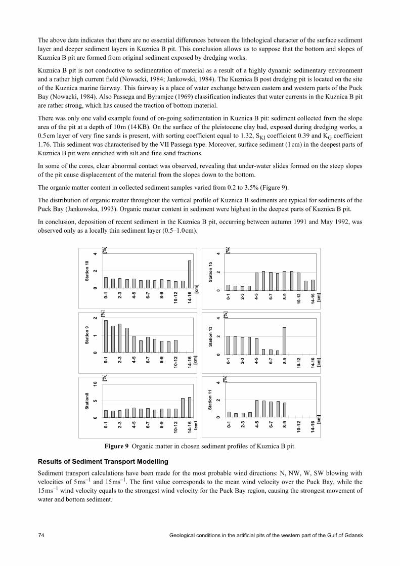
Geological conditions in the artificial pits of the western part of the Gulf of Gdansk 74
The above data indicates that there are no essential differences between the lithological character of the surface sedimentlayer and deeper sediment layers in Kuznica B pit. This conclusion allows us to suppose that the bottom and slopes ofKuznica B pit are formed from original sediment exposed by dredging works.
Kuznica B pit is not conductive to sedimentation of material as a result of a highly dynamic sedimentary environmentand a rather high current field (Nowacki, 1984; Jankowski, 1984). The Kuznica B post dredging pit is located on the siteof the Kuznica marine fairway. This fairway is a place of water exchange between eastern and western parts of the PuckBay (Nowacki, 1984). Also Passega and Byramjee (1969) classification indicates that water currents in the Kuznica B pitare rather strong, which has caused the traction of bottom material.
There was only one valid example found of on-going sedimentation in Kuznica B pit: sediment collected from the slopearea of the pit at a depth of 10m (14KB). On the surface of the pleistocene clay bad, exposed during dredging works, a0.5cm layer of very fine sands is present, with sorting coefficient equal to 1.32, SKI coefficient 0.39 and KG coefficient1.76. This sediment was characterised by the VII Passega type. Moreover, surface sediment (1cm) in the deepest parts ofKuznica B pit were enriched with silt and fine sand fractions.
In some of the cores, clear abnormal contact was observed, revealing that under-water slides formed on the steep slopesof the pit cause displacement of the material from the slopes down to the bottom.
The organic matter content in collected sediment samples varied from 0.2 to 3.5% (Figure 9).
The distribution of organic matter throughout the vertical profile of Kuznica B sediments are typical for sediments of thePuck Bay (Jankowska, 1993). Organic matter content in sediment were highest in the deepest parts of Kuznica B pit.
In conclusion, deposition of recent sediment in the Kuznica B pit, occurring between autumn 1991 and May 1992, wasobserved only as a locally thin sediment layer (0.5–1.0cm).
Figure 9 Organic matter in chosen sediment profiles of Kuznica B pit.
Results of Sediment Transport ModellingSediment transport calculations have been made for the most probable wind directions: N, NW, W, SW blowing withvelocities of 5ms–1 and 15ms–1. The first value corresponds to the mean wind velocity over the Puck Bay, while the15ms–1 wind velocity equals to the strongest wind velocity for the Puck Bay region, causing the strongest movement ofwater and bottom sediment.
02
4
0-1
2-3
4-5
6-7
8-9
10-1
2
14-1
6
Stat
ion
11
[cm
]
[%]
02
4
0-1
2-3
4-5
6-7
8-9
10-1
2
14-1
6
Stat
ion
13
[cm
]
[%]
02
4
0-1
2-3
4-5
6-7
8-9
10-1
2
14-1
6
Stat
ion
15
[cm
]
[%]
05
10
0-1
2-3
4-5
6-7
8-9
10-1
2
14-1
6
Stat
ion8
[cm
]
[%]
01
2
0-1
2-3
4-5
6-7
8-9
10-1
2
14-1
6
Stat
ion
9
[cm
]
[%]
02
4
0-1
2-3
4-5
6-7
8-9
10-1
2
14-1
6
Stat
ion
10
[%]
[cm
]

Dorota Maksymowska, Halina Jankowska and Bogdan Oldakowski 75
Modelling of the current pattern, derived by the wind field clearly shows the near shore flow, from the base of HelPeninsula to its promontory. Similar characteristic current directions have also been observed by Jankowski (1984). Inthe post dredging pits areas, the current direction and velocity are changed (Figure 10).
Figure 10 Depth integrated current field in Kuznica A and Kuznica B pits area, wind NW 15ms–1.
Prevailing 5ms–1 winds has a little influence on the transport of bottom sediment. For such wind conditions, results ofmodelling of current pattern show that the depth integrated current speed has a value ranging from 0.02 to 0.1ms–1, anddoes not cause an intensive sediment movement. Bottom divergence varies from –0.1 to 0.1cmyear–1, which indicatesthat erosional-depositional processes are almost in a state of equilibrium.
The model results for the Kuznica A pit indicate that there are no significant differences in current pattern and sedimenttransport for winds: NE, SW and W blowing with a velocity of 15ms–1. Sediment movement occurred in the largest areaof the bottom with a modelled NW wind.
Figure 11 Bottom divergence (cm year–1) in Kuznica A and Kuznica B pits area, wind NW 15ms–1.
In the edge area of the pit sediment is being resuspended and then deposited in the surrounding area. The calculatedbottom divergence in the edge area of the pit varied from –5 to 5cmyear–1. Stronger bottom divergence occurred in theeastern part of the pit, due to higher current speed affected by smaller water depth (Figure 10). Bottom divergence in thisarea reaches values of up to –3cmyear–1. The deposition of the sediment occurs in the eastern edge of the pit and in thenorthern edge region, and has a value of +3cmyear–1. In deeper parts of the Kuznica A pit, calculated bottom divergencevaries from –1 to 1cmyear–1 (Figure 11).
From sedimentological analysis the rate of sedimentation in Kuznica A pit is estimated at 2–4cm per year. It must benoted that a vertical element like suspended matter, which has not been included in the model, plays an important role inthe sediment deposition.
The decreasing velocity of the current in the pit area does not affect the movement of sand fraction sediments in thedeeper parts of the pit.
From the model results, it has been observed than in Kuznica B pit the current velocity is a little greater than in the otherpit. The bottom erosion occurs in the eastern and south-eastern edges of the pit (up to –10cm year–1) for calculated windconditions. At the south-western pit edge erosion of the sediments occurred with a subsequent fast deposition of thematerial (Figure 11).
Geological conditions in the artificial pits of the western part of the Gulf of Gdansk 76
Erosion of the sandy Seagull Reef (which is very close to Kuznica B pit) is shown very clearly. Material from SeagullReef is then deposited in the surrounding area and does not enter Kuznica B pit (Figure 11).
In this post-dredging pit bottom divergence varies from –1 to 1cmyear–1, which indicates that erosional-depositionalprocesses are almost in equilibrium. This value is similar to the sedimentation rate estimated from sedimentologicalanalysis, which means that there is almost no accumulation of recent sediment in Kuznica B pit. The calm sedimentationof suspended material in the Kuznica A pit is impossible because of a strong water dynamic.
ConclusionsFrom the above discussion the following conclusion are reached:
• the geometry of deep post dredging pits in the Puck Bay may affect propagation of current fields throughoutsurrounding area
• in the edge area of post dredging pits erosion and subsequent fast deposition occur• suspended fine sand, silt, as well as suspended organic matter, are accumulated in pits; materials shifted by traction
has only a slight influence on the sedimentation processes• each of the post dredging pits forms an individual sedimentary environment according to different hydrodynamic
conditions, flow of sedimentary material and mode of transportation• Kuznica A pit is characterised by a weak water dynamic, and forms a kind of sedimentation trap for organic matter
and fine-grained mineral suspended matter; the geometry of this pit stabilises sediment and does not allow for itsredeposition
• in Kuznica A pit sedimentation of suspended organic and fine grained mineral matter as well as slumping occur• Kuznica B pit is not conductive to sedimentation, mainly erosion, traction and to some extent slumping occur; only in
the deepest parts of the pit slow sedimentation of suspended matter takes place• the rate of deposition of recent sediment (fresh and uncompacted material) varies with respect to post dredging pit,
and has an estimated values ranges between 0.5 and 4cm per year.
ReferencesByers S.C., Mills E.L., Stewart P.L., 1978, A comparison of method of determining organic carbon in marine sediments,
with suggestion for a standard method, Hydrobiologia 58, 43–47.
Cieslak A., red., 1990, 1991, 1992, Kompleksowa Ochrona Pólwyspu Helskiego (Comprehensive protection of the HelPeninsula), Mimeo. Instytut Morski, Gdansk (in Polish).
Danish Hydraulic Institute, 1992, Mike 21, Sedimental Processes—Release Module, Total Transport, Pure Current, 1–40.
Folk R.L., Ward W. C.,1957, Brazos River bar; a study in the significance of grain size parameters, Journ. Sed. Petrol.,vol.27, no.1, 3–26.
Jankowska H., 1993, The bottom deposits of the Puck Bay, Stud. Mater. Oceanolog., Marine Pollution 3, KBN PAN,Sopot, 64, 163–172.
Jankowski A., 1984, Przeplywy wiatrowe w Zatoce Gdanskiej (Current field in the Gulf of Gdansk), Stud. Mater.Oceanolog., KBN PAN, Sopot, 43, 5–80, (in Polish).
Musielak S., 1984, Osady denne Zalewu Puckiego (Sediment of the Puck Lagoon), Zesz. Nauk., Wydz. BiNOZ Uniw.Gdanski, Oceanografia, 10, 35–56, (in Polish).
Nichols M.M., Diaz R.J., Schaffner L.C., 1990, Effects of Hopper Dredging and sediment deposition, Chesapeake Bay,Environ. Geol. Water Sci., vol.15, no.1, 31–43.
Nowacki J., 1993, Cyrkulacja i wymiana wód, [in:] Zatoka Pucka (Puck Bay), Korzeniewski K. (Ed.), Fundacja RozwojuUniwersytetu Gdanskiego, Gdansk, 416–421, (in Polish).
Passega R., Byramjee R., 1969, Grain-size image of clastic deposits, Sedimentology, 13, 233–252.

Dorota Maksymowska, Halina Jankowska and Bogdan Oldakowski 77
Racinowski R., Szczypek T., 1985, Prezentacja i interpretacja wyników badan uziarnienia osadów czwartorzedowych(Presentation and interpretation of grain size analyses of Quantetary deposits), Katowice, Uniw. Slaski, Skryptynr 3598, 143, (in Polish).
Shepard F.P., 1954, Nomenclature based on sand–silt–clay ratio, Journ. of Sed. Petrol., vol.24.
Trask P.D., 1939, Origin and environment of source sediments of petroleum, Gulf Publ., Houston, Texas, 323.
Wolanski E., Gibbs R., Ridd P., Mehta A., 1992, Settling of Ocean-dumped dredged material, Towsville, Australia,Estuarine, Coastal and Shelf Science, 35, 473–489.

Seabed sediments and current-induced bedforms in the Fehmarn Belt—Arkona Basin 78
ICES Cooperative Research Report, No. 257 Baltic Marine Science Conference, Rønne, Denmark, 22–26 October 1996
Seabed sediments and current-induced bedforms in the Fehmarn Belt—Arkona Basin
Jørn Bo Jensen, Antoon Kuijpers and Wolfram Lemke
AbstractThe sediment map “Map sheet Fehmarn Belt—Arkona Basin, Late Quaternary sediments” is based on marine-geologicalinvestigations including shallow-seismic profiling and coring data. In addition to lithology, information on sedimentages, deposition environments and recent sediment dynamics is given. Due to the resolution of the seismic and coringdata the sediment map represents an average sediment type of the uppermost 0.5m.
Glacial till deposits form the eldest Pleistocene unit exposed in the shallow marginal parts of the survey area. At water-depths above 20m, in the Fehmarn Belt–Mecklenburg Bucht–Arkona Basin areas, the till deposits are covered by varvedclay bottomsets and in the Darss Sill area by sandy deltaic sediments. These sediments were deposited in the western partof the dammed, late-glacial Baltic Ice Lake. Oscillating Holocene lake levels and the Littorina Sea transgression resultedin deposition of Holocene freshwater and marine fine-grained sediments and sandy palaeo coastal sediments, respec-tively.
The marine transgression of the Darss Sill and subsequent current activity are responsible for strong erosion in thewestern Fehmarn Belt area, where late-glacial clay is exposed and only a few remains of Holocene sediments exist alongthe margin of the basin. Eastward, the erosive effect diminishes and in the central parts of Mecklenburg Bay no current-induced erosion is inferred.
Besides the removal of sediments, current-induced bedforms such as sandwaves and comet marks prove periodic,eastward inflow of saline bottom waters at water-depths of more than 15m, while westward outflow of low-salinityBaltic water influences the seafloor in the northern part of Fehmarn Belt at water-depths of less than 15m.
The characteristic sediment distribution and current-induced bedforms indicated on the map clearly reflect the postglacialdevelopment, whereas trawl tracks reveal recent human activity in the area.
IntroductionThe map discussed in this publication deals with the Late Quaternary seabed sediments of the Fehmarn Belt and westernpart of the Arkona Basin. The extent of Danish and German territory covered by this map is roughly the same.
The actual bathymetry shows water depths of up to more than 40m in the Arkona Basin and around 30m in large parts ofthe Fehmarm Belt and Mecklenburg Bucht. A threshold, i.e. the Darsser Schwelle, separates the two basins for the largestpart. A connection between the deeper basins is formed by the Kadet Channel with a maximum water depth of about30m. This erosional feature extends in a NE-SW direction just south of Gedser Rev. The prevailing water depthelsewhere in the Darsser Schwelle area is less than 20m.
The map was made within the framework of the Danish program for mapping of offshore sand and gravel resources,which since 1990 was carried out in this area in close co-operation with the “Institut für Ostseeforschung” (IOW) inWarnemünde. The data used for the map were collected partly through individual investigations of respective institutes,partly through joint cruises of the R/Vs “Alexander von Humboldt”, “Professor A. Penck”, “Marie Miljø” and “MetteMiljø”, during which shallow seismic investigations and sediment coring was carried out.
Methods
GeneralThis map, which shows the area distribution of Late quaternary seabed sediments in the Fehmarn Belt and western ArkonaBasin, is based on shallow seismic data and results from vibrocoring. Due to limitations of seismic resolution, character-isation of the seabed sediments applies to the sediment type found at about 0.5m subbottom depth. It is stressed that themap not only provides lithological information, but also illustrates the regional Late quaternary stratigraphy with a 14C-

Jørn Bo Jensen, Antoon Kuijpers and Wolfram Lemke 79
based chronology and it includes information on the depositional environment as well. Various surveying techniquescould not be applied at water depths of less than about 4m, which implies that information from the coastal zone is notincluded in the map.
Apart from the sediment distribution, this publication also shows the occurrence of current-induced bedforms andevidence of direct human impact on the seafloor present in the form of trawl marks. Information from this map thus mayhelp to distinguish between erosional, non-depositional and sediment accumulation areas, while also indicating bottomcurrent transport directions.
Notwithstanding the restrictions referred to above, the data presented in this publication may significantly add toknowledge of the seabed conditions in the Fehmarn Belt and western Arkona Basin.
Shallow SeismicsShallow seismic data were collected using an Elac 30kHz echosounder, an ORE 3.5kHz pinger system and DatasonicsCHIRP (1–10kHz) subbottom profiler system, a Uniboom (0.8–16kHz) and an Edo Western and EG&G 100kHz sidescan sonar. The total track length is about 3000km. The analogue data were recorded on an EPC/Klein graphic printerand stored either on analogue tape or in digital form.
Positioning was carried out using differential GPS and the Sercel Syledis precision navigational system with an accuracyof within 10m.
The echosounder information was used to determine the water depth, whereas interpretation of the data from thesubbottom profiler and Uniboom systems enabled a regional seismostratigraphic model to be established. This was donefollowing seismostratigraphic principles introduced by Vail et al. (1977). These principles have previously been shownto be a useful tool in connection with the exploration of marine raw materials (Jensen 1992). When applying theseseismostratigraphic analyses, depositional sequences are being defined by nonconformities as they cut off the variousreflectors. In addition, the internal reflector pattern of the sequences is described.
A characterisation of the depositional environment was inferred from this seismic information and used for the selectionof the coring sites.
Sediment investigationsA lithological description of about 300 vibrocores was made, whereas selected cores were subsampled for the purpose ofgrain size determination, loss on ignition and determination of the carbonate content. Moreover, a larger number of coreswere subsampled at selected subbottom levels for 14C-dating and the study of macroflora remains in order to obtainfurther information on the age and depositional environment of the cores. The selection of these samples was made byOle Bennike, GEUS. The samples were dated either by conventional 14C-dating at the Dating Laboratory of the NationalMuseum and GEUS, or by Accelerator Mass Spectrometry (AMS) 14C-dating at the Institute of Physics, AarhusUniversity, following the method described by Heinemeier and Andersen (1983). The stratigraphy used in the presentpublication is based on these dating results. Further and more detailed information on the 14C-dating is beyond the scopeof the description of this map.
Postglacial geological developmentThe data referred to forms the base of the interpretation of the late- and postglacial geological development of the area.
During deglaciation, ground moraines were formed, whereas flow tills and esker ice marginal deposits were also leftbehind by the retreating ice. Ice lake deposits accumulated in front of the melting ice masses. These deposits can berelated to the earliest stage of the Baltic Ice Lake. After further retreat of the ice, changes of the lake water level resultedin various episodes (Baltic Ice Lake, Ancylus Lake) during which, amongst others, a series of littoral sediments andcoastal deposits were formed in the area. Finally around 7000 years ago, the Littorina transgression occurred and marineconditions were established. In the course of this transgression, another series of (marine) coastal deposits was formed.
The development described here has resulted in the typical sediment distribution as can be observed on the map. Theoccurrence and area distribution of current-induced bedforms reflects actual sediment transport and bottom currentconditions. A direct human impact on the seabed is seen for example by virtue of trawl marks.

Seabed sediments and current-induced bedforms in the Fehmarn Belt—Arkona Basin80
SedimentsThe seabed sediments found include glacial till mostly with a thin cover of sandy or gravely lag sediments, late glacialfreshwater clay, silt or sand, Holocene freshwater and brackish (muddy) sand and sandy mud, and Holocene marine sandand mud.
Moraine–Glacial tillThe oldest deposits exposed in the area are moraine deposits dominating along the basin margins where water depth isless than 15–20m. Two different moraine deposits can be distinguished, i.e. a consolidated ground moraine generallywith a rough surface topography and an unconsolidated flow till with a smooth surface topography. Both morainedeposits are characterised by the occurrence of a thin (approx. 0.10m) layer of lag sediments of mainly gravel andcoarser material.
Late glacial freshwater clay–sandThe late glacial deposits consist of ice lake sediments exposed in the central part of Fehmarn Belt, along the northern andeastern margin of Mecklenburg Bucht, and in large parts of the area between the Darsser Schwelle and Arkona Basin.Clayey and typically varved distal ice lake deposits are the most widespread late glacial surface sediments found in theFehmarn Belt and in the area immediately south-east of Møn. Late glacial sandy deposits predominate, however, in thearea south of Gedser Rev and along the south-western margin of the Arkona Basin. These sandy deposits reflect sedimentinput from a late glacial Warnow river system discharging in this area.
Holocene freshwater–brackish (muddy) sand and sandy mudDuring the early Holocene, organic-rich fine-grained sediments were deposited in the deeper parts of the Fehmarn Beltarea. These sediments were deposited during the development of the Ancylus Lake and partly also during the followingbeginning marine transgression (Mastogloia Sea). The sandy littoral faces of these sediments in the northern part ofFehmarn Belt have been eroded in a narrow zone at a depth of around 20m. The Ancylus sediments were also depositedsouth and north-east of Gedser Rev filling the older channel system and deeper parts of this area. Erosional remnants ofthese deposits are locally exposed on the seafloor here.
Holocene marine sandMarine sand overlying moraine deposits is locally found at water depths of less than 20m.
This sand originates for a large part from former coastal deposits formed during the Littorina Transgression. Subse-quently, reworking of the sandy deposits may have occurred locally.
Furthermore, at the Darsser Schwelle in the vicinity of Gedser Rev and more to the east larger areas are found, coveredby up to 4m of sand. The water depth in these areas is around 20m. The thickness of the sand layer gradually decreases inan easterly direction.
Holocene marine mudAreas where marine mud has been accumulating are found in the central part of the Mecklenburg Bucht, in the ArkonaBasin and in the south-western part of Fehmarn Belt. In addition, a smaller mud basin is present immediately east of Møn.A characteristic feature of the mud depositional area in the Fehmarn Belt is the evidence of erosion found in the northernand western part of this area. This is indicated by an erosional inconformity and the occurrence of sediment waves. Thus,a record of continuous accumulation of recent sediments can be expected to be found only in the central parts of theMecklenburg Bucht and Arkona Basin.
However, large-scale reworking of recent sediments may still occur here, as is suggested by the widespread occurrenceof trawling marks in these areas.
Current-induced bedformsThe actual circulation pattern of the Fehmarn Belt is responsible for modifying older deposits and for the generation ofspecific current-induced bedforms. As outlined before, the non-tidal current system in this area is controlled by the large-scale weather pattern over NW Europe, and in particular, by wind-induced sea-level changes in the Kattegat and Baltic.Another factor to be taken into consideration is the layering of the water column with a general inflow of saline waters inthe lower part of the water column and outflow of low-salinity Baltic water at the surface. The effect of the earth rotation(Coriolis force) further complicates this two-layer flow pattern.

Jørn Bo Jensen, Antoon Kuijpers and Wolfram Lemke 81
A general conclusion is that the seabed in the southern part of the investigated area is mainly affected by inflowing salinewaters from the Great Belt and Kattegat, whereas Baltic outflow affects the seafloor at shallower (<15m) depths in thenorthern part of the area.
Typical current-induced bedforms are described below, illustrated by seismic examples from the Fehmarn Belt area(Figure 1 to Figure 5).
Figure 1 Location of seismic examples presented.
Sandwaves and megaripplesThese transverse bedforms clearly indicate current-induced sediment transport (Figure 2). Sandwave and megaripplefields occur in various parts of the investigated area and are often found in relation to fossil sandy coastal deposits. Insuch areas they originate from erosional processes affecting the fossil deposits upstream, whereas downstream they areformed by accumulation processes (Figure 3).
Figure 2 Side scan sonar image (B7) of sandwaves in the south-western part of Fehmarn Belt. Location indicated on Figure 1.
Figure 3 Pinger profile (B8) of sandwaves in the western part of Fehmarn Belt. Location indicated on Figure 1.
Investigations have previously been made of a sandwave field found between 12 and 22m water depth north of Fehmarn(Werner and Newton, 1970; Werner and Wolf, 1974). The wavelength of these sandwaves is between 40 and 70m, theirheight is 1–2m, and they consist of medium to coarse sand (Figure 2 and Figure 3) (Werner and Wolf, 1974). The

Seabed sediments and current-induced bedforms in the Fehmarn Belt—Arkona Basin82
sandwaves have a markedly asymmetric appearance with the steep sides facing east, which is indicative of an easterlycurrent direction. The current speed required for the formation of such sand waves is in the range of 0.70 to 1.00ms–1
(Rubin and McCulloch, 1980; Kuijpers, 1980). Current measurements demonstrate that in the area of investigationbottom current velocities are normally below this critical range; extreme bottom current events with the speed requiredoccur at a time-scale of months or years (Wyrtki, 1953, 1954; Kuijpers, 1980). This is supported by seabed observationsshowing that the surface of the sandwaves can be covered by small-scale current marks and a Mya arenaria fauna indic-ative of long-term conditions with a largely inactive sand bed (Werner and Wolf, 1974).
Investigations of the Gedser Rev area (Lemke et al., 1995) have shown the occurrence of sandwaves indicative of bothinflow and outflow. Moreover, repeated observations indicated a change of bedform configurations in this area, i.e. areversal of large sandwaves as well as the disappearance of a megaripple field (Kuijpers, 1991). The present study showsthat sandwave fields also occur in the north-western part of Fehmarn Belt. These sandwaves are mainly found at waterdepths in excess of 15m, which correspond to the depth range of the sandwave field present in the vicinity of Fehmarn.
Isolated sediment (sand-silt) wavesThe seismic data demonstrate the presence of isolated sediment waves of presumably sand or silt in the central parts ofthe Fehmarn Belt at water depths in excess of 20m (Figure 4).
Figure 4 Pinger profile (B15) of isolated sand-silt waves in the central part of Fehmarn Belt. Location indicated on Figure 1.
These features are transverse bedforms and appear as NE-SW striking ridges of considerable length. The distancebetween the individual sediment waves is up to 500m. Their height is 0.5–1.0m, whereas they are about 50m wide. Thesingle occurrence of these bedforms is ascribed to sparse sediment supply preventing a more widespread occurrence. Acharacteristic feature is that they occur on various substrates ranging from late glacial clay in the western part of theFehmarn Belt to Holocene marine mud in the eastern part of this strait. In contrast to the sandwaves referred to above, theseisolated sediment waves do not display a clear asymmetry or preferred orientation with regard to bottom current direc-tions.
Comet marksThese longitudinal structures have been defined as obstacle marks characterised by a downstream erosional area of whichthe length is much larger than its width (Werner and Newton 1974). In the Fehmarn Belt they are preferably formed inareas where moraine deposits are locally covered by a thin layer of fine sand (Figure 5). Erratics from the moraineprovide the obstacle required to form these erosional features developed in the fine sand layer. Often, however, a minorsand shadow is present downstream immediately behind the obstacle. The comet marks can be classified into varioustypes depending on the hydrodynamic environment in which they are formed (Werner et al., 1980). The comet marksobserved in the Fehmarn Belt mostly have a parabolic appearance typically reflecting bottom current conditions compa-rable to those required for the formation of sandwaves. The areas with comet marks are found in the northern sector ofthe Fehmarn Belt and, more generally, along the northern margin of the deeper parts of the strait at water depths between15 and 20m. Without exception, they all display an easterly tail direction indicative of the inflow of saline bottom waterfrom the Great Belt.

Jørn Bo Jensen, Antoon Kuijpers and Wolfram Lemke 83
Figure 5 Side scan sonar image (B19) of comet marks in the western part of Fehmarn Belt. Location indicated on Figure 1.
Sand ribbonsSmall sand ribbons are widespread at a shallow (<15m) depth over the entire area in the northern part of the Fehmarn Belt.In just a few cases it was possible to determine the current direction from these longitudinal bedforms.
Bottom current conditionsInitially, the deeper parts of the Fehmarn Belt and Mecklenburg Bucht had been covered by freshwater and marine depositsfrom the earlier part of the Holocene. After the marine transgression of the Darsser Schwelle, current intensitiesincreased and erosion started to prevail in particular in the western narrow part of the Fehmarn Belt. Presently, late glacialice lake clay deposits are exposed widespread on the seabed in this area. Remnants from the Holocene freshwater andmarine deposits referred to above still occur locally, however, along the margin of the Fehmarn Belt. Generally, erosion isless towards the Mecklenburg Bucht. Current-induced erosion is probably negligible only in the central parts of this bay.
The occurrence of strong bottom currents is not only evident from widespread erosion as described above, but is alsodemonstrated by the various current-induced bedform types observed in the area. Both the occurrence of sandwave fieldsand comet marks correspondingly indicate a prevailing easterly bottom current with maximum speeds of up to 1.0ms–1.These extreme current events are concluded to be relatively rare, normally occurring for a time scale of months or years(Wyrtki, 1954; Kuijpers, 1985). Also the isolated sediment waves in the deepest part of Fehmarn Belt suggest a relativelyhigh-energy hydrodynamic environment. Thus it can be shown that bottom currents at water depths in excess of 15mreach their maximum speed during inflow conditions. An easterly sediment transport direction is also found north-east ofGedser Rev in the area characterised by the presence of an up to 4m thick marine sand layer getting thinner towards theeast.
A more complicated bottom current pattern is observed around Gedser Rev, where both inflow- and outflow-inducedbedforms occur. Previous investigations by Lemke et al. (1994) demonstrate that inflow of saline bottom water prevailsin the Kadet Channel and in the area to the south, whereas outflow affects the seabed at water depths of less than 15mnorth of the Kadet Channel. The bedform pattern around Gedser Rev suggest that in a situation of strong outflow ananticyclonic gyre will develop on the (western) leeside of Gedser Rev.
Finally, it can be concluded that, generally, outflow is the dominating sediment transport agent at shallow (<15m) depthin the northern sector of the Fehmarn Belt off Lolland as well as in the coastal zone of Falster just north of Gedser Rev.
AcknowledgementsThe authors sincerely acknowledge the permission given by the military authorities of the former German DemocraticRepublic (DDR) and Denmark to conduct shallow seismic and sediment sampling operations in the territorial waters ofrespective countries at the beginning (1990) of the co-operation between IOW and GEUS.
In addition Dr. Figge Bundesamt für seeschiffahrt und Hydrographie (BSH), is acknowledged for permission to includeGerman data and the Danish Natural Science Research Council for funding of AMS 14C dates performed at theUniversity of Aarhus, under the supervision of Dr. Jan Heinemeier.

Seabed sediments and current-induced bedforms in the Fehmarn Belt—Arkona Basin84
The crews of R/Vs “Alexander von Humboldt”, “Professor A. Penck”, “Marie Miljø” and “Mette Miljø” are acknowl-edged for excellent assistance.
ReferencesBjörck, S. 1995. A review of the history of the Baltic Sea, 13.0–8.0 ka BP. Quaternary International, 27, 19–40.
Heinemeier, J & Andersen, H.H. 1983. Production of C directly from CO2 using the anis sputter source. Radiocarbon,25, No. 2, 761–769.
Jensen, J.B. 1992. Råstofgeologiske undersøgelser i Østersøen. Fakse Bugt, område 520. DGU kunderapport nr. 51.1992. 41 p.
Jensen, J.B., Bennike, O., Witkowski, A., Lemke W. & Kuijpers, A. in prep. The Baltic Ice Lake in the southwesternBaltic: Mecklenburg Bay–Arkona Basin.
Kolp, O. 1965. Paläogeographische Ergebnisse der Kartierung des Meeresgrundes der westlichen Ostsee zwischenFehmarn und Arkona. Beiträge zur Meereskunde, 12–14, 1–59.
Kuijpers, A. 1980. Sediment patterns and bedforms, and their relationship to the flow regime in the Belt Sea and theSound. Unveröffentlicht Dissertation, Geologich-Paläontologiches Institut. Universitet Kiel, 138 p.
Kuijpers, A. 1985. Current-induced Bedforms in the Danish straits between Kattegat and Baltic Sea. Meyniana, 37, 97–127.
Kuijpers, A. 1991. Råstofgeologiske undersøgelser i Østersøen: Gedser, område 560. DGU Kunderapport nr. 21. 1991.67 p.
Lemke, W., Kuijpers. A., Hoffmann, G., Milkert, D. and Atzler, R. 1995. The Darss Sill, hydrographic threshold in thesouth-western Baltic: Late Quaternary geology and recent sediment dynamics. Continental Shelf Research, 14,47–70.
Lemke, W., Jensen, J.B., Bennike, O. & Witkowski, A. in prep. Sequence stratigraphy of submarine Late Pleistocene andHolocene deposits in Mecklenburg Bay, south-western Baltic Sea. Sveriges Geologiska Undersökning, Ser Ca
Mörner, N.-A. 1983. The Fennoscandian Uplift: Geological data and their Geodynamical Implication. In: (eds.) D.E.Smith and A.G. Dawson. Shorelines and isostasy Academic Press, Institute of British Geographers special publi-cation, no. 16, 251–284.
Rubin, D.M. and McCulloch, D.S. 1980. Single and superimposed bedforms: a synthesis of San Francisco Bay and flumeobservations. Sedimentary Geology, 26, 207–231.
Rørbeck, D.M. 1995. Late Quaternary sedimentology and seismic stratigraphy of the northern Storebælt, Denmark.Unpublished Ph.D. thesis. Geologisk Institut, Københavns Universitet. 202 p.
Svensson, N.O. 1989. Late Weichselian and Early Holocene shore displacement in the central Baltic, based on strati-graphical and morphological records from eastern Småland and Gotland, Sweden. Lundqua Thesis, 25, LundUniversitet, 195 p.
Vail, P.R., Mitchum, R.M., Jr, Todd, R.G., Widmier, J.M., Thompson, S., III, Sangree, J.B., Bubb, J.N., and Hatlelid,W.G., 1977. Seismic stratigraphy and global changes of sea level. In: Clayton, C.E., (Ed.), Seismic stratigraphy—Applications to Hydrocarbon Exploration. American. Association of Petroleum Geologists Memoir, 26, 49–212.
Werner, F. And Newton, R.S., 1970. Riesenrippeln im Fehmarnbelt (westliche Ostsee). Meyniana, 20, 83–90.
Werner, F., Wolf, E.A. and Tauchgruppe Kiel 1974. Sedimentologi und Ökologie eines ruhenden Riesenrippelfeldes.Meynianna, 26, 39–62.
Werner, F., Unsöld, G., Koopmann, B. and Stefano, A. 1980. Field observations and flume experiments on the nature ofcomet marks. Sedimentary Geology, 26, 133–262.
Winn, K., Averdieck, F.R., Erlemkeuser, H. & Werner, F. 1986. Holocene Sea Level Rise in the Western Baltic and theQuestion of Isostatic Subsidence. Meyniana, 38, 61–80.
Wyrtki, K. 1954. Die Dynamik der Wasserbewegungen im Fehmarn-belt II. Kieler Meeresforschung, 10, 162–181.

R. Bojanowski, Z. Radecki, S. Uscinowicz and D. Knapinska-Skiba 85
ICES Cooperative Research Report, No. 257 Baltic Marine Science Conference, Rønne, Denmark, 22–26 October 1996
Penetration of Caesium-137 into sandy sediments of the Baltic Sea
R. Bojanowski, Z. Radecki, S. Uscinowicz and D. Knapinska-Skiba
AbstractLarge areas of the Southern Baltic floor are covered by sand and gravel. It is a common belief that such materials do nothold appreciable amounts of pollutants because their sorption capacity is low. Our measurements have shown, however,that the activities of caesium and Pu radionuclides locked in these loose sedimentary structures are not negligible.Actually, half of the total Cs-137 inventory was found to be associated with hard bottom, which occupies 64 per cent ofthe Polish Economic Zone.
Although activity concentrations of Cs-137 and Pu-239+240 are an order of magnitude lower in sands, compared tomuddy sediments, their cumulative deposition, expressed in total amounts per unit area, differs only by a factor of two.
A relatively large accumulation of these radionuclides in coarse-grained deposits is made possible by incorporation ofradioactive particles within the bottom material and the particles’ downward displacement by mechanical forces. Thepenetration depth depends on hydrodynamical conditions prevailing at the sampling sites, and can vary from severalcentimetres to a few meters. The knowledge of this parameter is prerequisite for reliable assessment of radionuclideinventories in marine sediments.
IntroductionMonitoring of hazardous substances in the marine environment requires sampling of various materials for analyticalpurposes. Bottom sediments represent an important part of the marine realm because it is there where many pollutantsaccumulate. By studying vertical distribution of substances in sediment cores it is possible to reconstruct pollutionhistory of aquatic basins, trace sources of pollutants and estimate their inventories.
Polluting substances combine frequently with fine-grained particles which carry them away to areas where they cansettle. Sandy deposits, which normally occur in areas of high hydrodynamic activity, are considered free of these contam-inants and are given little attention. However, our studies of the behaviour of Cs-137 in the Baltic Sea have shown, thatthe amounts of this radionuclide in sandy sediments are not negligible (Bojanowski et al., 1995a).
Figure 1 Sampling stations of the bottom sediments in the Southern Baltic
56o N
55o
54o
14o 15o 16o 17o 18o 19o 20o E
11
8
8
P39
82
P5
8
32
733
51
23
2SM1
4213
271822
P110
P116
P1
3591
P63
18
3442P2
208212
12
P140
6
P3
9
34B
91B 73B 51B
89B50B
82B
18B
10A
90S
1K 2K
35G42G
3K
7K
30V
27V
26V
25V
21V4V
3V
5V
6V
7V
8V9V
10V2V
20V45V
20A
28V29V5K
6K
4K

Penetration of Caesium-137 into sandy sediments of the Baltic Sea86
Sandy bottom is difficult to sample. The reaching depth of popular devices such as Van Veen and Pettersen grabsamplers rarely exceeds 20cm and the retrieved material does not preserve undisturbed structure. Box cores are moresuitable, but are difficult to operate due to their weight. As a result, the depth distribution of pollutants in such sedimentsis poorly known. This is a serious drawback for inventory studies, which must rely on correct assessment of allinput/output components.
Part of our laboratory’s activity is devoted to studying the behaviour of radioactive elements in the Baltic Sea. Most ofour work is confined to the Polish Exclusive Zone (Figure 1). It is a shallow water body which occupies an area of about30.5 thousand square kilometres. Two thirds of the bottom area is covered by sand and gravel (Table 1).
Table 1 Area of soft and hard sediments within the Polish Economic Zone.
Our earlier studies showed that Cs-137 is present in the southern Baltic in appreciable amounts and that its occurrence isnot limited to soft sediments only. In 1986, before the Chernobyl accident, typical levels of Cs-137 were 0.2 and 0.5kBqm–2 for sandy and muddy bottoms, respectively, but during 1991–93 they increased respectively to 1 and 2 kBqm–2,on average. The total inventory of this radionuclide was divided between hard and soft type bottoms in the proportion3:2.
Our inventory estimations were based on the belief, that the sampling depth of our device (which was then about15±5cm on average) was sufficient for this purpose. At that time we had no technical means to prove it. It is onlyrecently that we have gained access to longer, undisturbed cores, which allowed us to test that assumption.
MethodsCores of sandy deposits were collected at the stations shown in Figure 2 with a vibration corer 10cm in diameter. Itcollected relatively undisturbed cores up to 3m long. The material was cut into segments and kept in plastic bags untilanalysis.
Figure 2 Location of sampling stations
Each segment was homogenised and transferred to counting vessels of the Marinelli type. The measurements were madeby a gamma spectrometer equipped with a HPGe detector (20% rel. eff. and 1.8keVFWHM resolution for a 1.33MeV60Co line) and the standard S100 Canberra electronics. The counting efficiency was determined using a standardisedmixture of radionuclides provided by the PTB Braunschweig (Germany). Analytical quality control was assured by usingthe reference materials IAEA-300 (Baltic sediment) and IAEA-375 (soil). Stability of counting efficiency and
Gdansk Bay Southern Baltic Total
Area of mixed bottom [km2] - 2 147 (8%) 2 147 (7%)
Area of soft bottom [km2] 1 733 (58%) 7 080 (26%) 8 813 (29%)
Area of hard bottom [km2] 1 266 (42%) 18 307 (66%) 19 573 (64%)
Total area [km2] 2 999 27 534 30 533
18o 19o 20o E54o
55o N
28
10 2123
1116

R. Bojanowski, Z. Radecki, S. Uscinowicz and D. Knapinska-Skiba 87
background variation was monitored throughout the whole period of measurements. During the applied conditions (about1 kg sample and 80.000 s. counting time) the minimum detectable activity was close to 0.2Bqkg–1 d.w.
Results and DiscussionIn this paper we present results for the first seven cores which were collected in the shallow parts, of the Gulf of Gdansk.This region is known for the relatively high Cs-137 levels in sediments, so the chance of observing any activity gradientsin the sandy bottom seemed promising.
Table 2 Vertical distribution of Cs-137 and Cs-134 in the analysed cores at the stations 2, 10 and 23.
Table 2, Figure 3 and Figure 4 shows typical vertical distribution of this radionuclide in the selected analysed cores. Withthe exception of core 2 (Figure 5) all other cores display the same distribution pattern, i.e. the highest activity is in theuppermost segment and then steadily decreases. The shape of the distribution curves differs from one core to another butthe differences are small, considering the variable hydrodynamic conditions in this area and different depths. Some 80 to90 percent of the total inventory resides in the layer that is 15–20cm thick, but here the activity gradients are the steepest.It seems that the action of waves and currents affect the surficial sandy sediment structure not much deeper than that inthe study area.
StationCoordinates Depth
[m]Segment
[cm]Activity [Bq.m–2±1 σ]
E N Cs-137 Cs-1342 18o56.77’ 54o23.61’ 22 0.00–0.11 480+13 8+3
0.11–0.21 1230+28 23+50.21–0.32 2630+43 39+60.32–0.40 1990+23 26+40.40–0.48 770+13 20+40.48–0.60 1110+19 17+30.60–0.70 1200+22 17+30.70–0.83 1210+23 22+50.83–0.90 154+7 <80.90–1.00 50+6 <91.00–1.10 23+6 <81.10–1.20 <16 <91.20–1.30 <17 <10
10 18o50.29’ 54o22.64’ 13 0.00–0.05 1332+25 14+5
0.05–0.19 1150+23 18+30.19–0.24 55+6 <70.24–0.36 42+6 <80.36–0.45 <12 <8
23 19o36.31’ 54o27.27’ 16 0.00–0.10 2460+45 36+6
0.10–0.20 980+25 15+30.20–0.31 260+12 <80.31–0.40 130+10 <70.40–0.50 59+6 <80.50–0.60 23+3 <50.60–0.70 <17 <8

Penetration of Caesium-137 into sandy sediments of the Baltic Sea88
Figure 3 Vertical deposition of Cs-137 at station 10 (54o22.64'; 18o50.29')
Figure 4 Vertical deposition of Cs-137 at station 23 (54o27.27'; 19o36.31')
Figure 5 Vertical deposition of Cs-137 at station 2 (54o23.61'; 18o56.77')
In Table 3 the characteristic features of the Cs-137 distribution in the examined cores are summarised. We have definedthe penetration depth of Cs-137 as the depth in the sea floor, below which less than 5 percent of the integral totalinventory remains. In most cases this depth does not exceed 30cm and it does not appear to be related to the water depthnor to the magnitude of total deposition. The latter varies by an order of magnitude and is much higher on average than inother parts of the Southern Baltic (Bojanowski et al., 1995a and 1995b). That attests to the Vistula river as a major sourceof Cs-137 in the Gdansk Bay.
0
20
40
60
80
100
120
0 2000 30001000
Deposition [Bq.m-2]
< 17 Bq.m-2
Dep
th [c
m]
fine sand slightly muddy,carbonateless
fine sand, carbonate
fine sand in upper part laminated, carbonateless
fine sand, slightly carbonate
clay, cabonatelesswith pockets of muddy sand
0
20
40
60
80
100
120
0 2000 30001000
Deposition [Bq.m-2]
< 16 Bq.m-2Dep
th [c
m]
fine sand, carbonateless,dusky yellow green
fine sand, carbonateless,light olive gray
fine sand, carbonateless,dark reenish gray
0
20
40
60
80
100
120
0 2000 30001000
Deposition [Bq.m-2]
Dep
th [c
m]
fine sand, dark greenish gray
fine sand, greenish gray
fine sand, dark gray
very coarse sand with fine gravel
fine sand, with interbedding black fine sand

R. Bojanowski, Z. Radecki, S. Uscinowicz and D. Knapinska-Skiba 89
Table 3 Summary of Cs-137 deposition characteristics in sandy deposits of the Baltic Sea.
Presenting Cs-137 activities in activity concentrations units (Bqkg–1 of sediment) has little meaning because such valuesdepend, to a large extent, on how the sample was taken. It is however, interesting to note, that in the uppermost layer theconcentrations varied a lot with ranges of 6 to 101 Bqkg–1 d.w., whereas below the penetration depths they in some casesapproached detection limits.
The observed features are not claimed to be applicable to sandy sediments as a whole. The distribution at station 2 is atpresent difficult to explain but it demonstrates that such cases do exist. Some records also have evidence of homoge-neous distribution of Cs-137 down to 15cm sampling limit in Pomeranian Bay sediments (Bojanowski et al., 1995b).Clearly, more information is needed on this subject, and measurements on cores from other regions are underway.
ConclusionsThe most important conclusion resulting from our measurements is that the Cs-137 occurs down to about 30cm in someBaltic near-shore sandy sediments. This observation can be extended to include other pollutants that are bound to partic-ulate matter and are of recent origin, such as the Chernobyl fallout. Sampling to that depth is thus a prerequisite forquantitative inventory assessment of such substances.
ReferencesR. Bojanowski, D. Knapinska-Skiba, Z. Radecki, J. Tomczak, T. Szczepanska, 1995a: Accumulation of radioactive
Caesium (137Cs) in Southern Baltic Sediments. Prace Panstwowego Instytutu Geologicznego CXLJX, 145–150
R. Bojanowski, Z. Radecki, D. Knapinska-Skiba. 1995b: Distribution of 137Cs, 239+240Pu and 210Po in the PomeranianBight ecosystem. Bulletin of the Sea Fisheries Institute, 3 (136)
StationWater depth
[m]
Totaldeposition [kBq.m–2]
Sediment thickness
[cm]
Percent Cs-137 in this layer
Next segment
Horizon [cm]
Percent depositio
n
Activity [Bqkg–1
d.w.]2 22 10.8 83 98 83–90 1.5 1.5
8 30 1.27 40 98 40–50 1.3 <0.2
10 13 2.58 19 96 19–24 2.2 0.9
11 15 9.58 23 99 23–32 0.5 0.4
16 27 5.36 29 96 29–40 2.0 0.8
21 24 4.14 25 96 25–35 2.6 0.7
23 16 3.92 31 95 31–40 3.3 1.3

Organochlorines in surface sediments and cores of the Western Baltic and inner coastal waters of Mecklenburg-West Pomerania90
ICES Cooperative Research Report, No. 257 Baltic Marine Science Conference, Rønne, Denmark, 22–26 October 1996
Organochlorines in surface sediments and cores of the Western Baltic and inner coastal waters of Mecklenburg-West Pomerania
Dirk Dannenberger and Astrid Lerz
IntroductionOrganochlorine compounds, e.g. chlorobiphenyls (CBs) and organochlorine pesticides, are among the most widespreadand persistent environmental contaminants. Also, these substances enter the Baltic Sea via rivers, atmosphericdeposition, spills and dumping of dredging material. Most of them have only short residence times in the water column,due to their hydrophobic character (low water solubility) which leads to bioaccumulation and strong sorption ontosuspended particulate matter (SPM). They are carried to the bottom water and are finally trapped in marine sediments(Tolosa et al., 1995; van Bavel et al., 1996).
The area under investigation covered the western Baltic Sea (Beltsea, Arkona Sea, Pomeranian Bight) and the inner-coastal waters of Mecklenburg-Vorpommern (Germany). The sediment structures in the western Baltic differ widely.There are large regions with a high content of mud or clay in the sediments of the innercoastal waters (Brügmann andBachor 1990; Schlungbaum et al., 1994) and of the accumulation area of the Lübeck Bight and the Arkona Basin(Brügmann and Lange, 1990). The sedimentation rates in these areas are on average 1–2mmyr–1 (Perttilä and Brügmann,1992). Other regions in the western Baltic are dominated by fine and mixed sand with gravel and stones, e.g. the DarßSill and the central parts of the Pomeranian Bight.
The present state of knowledge of organochlorines in Baltic Sea sediments is fragmentary and there is a lack of infor-mation for some regions (Perttilä and Brügmann, 1992; HELCOM, 1993). Recent data on organic micropollutants inBaltic Sea sediments were reported by Broman (1992, 1993), Nyland et al. (1992), Kjeller and Rappe (1995), Witt(1995), and Dannenberger (1996). Until now, no data about the distribution of organochlorines in the innercoastal watersof Mecklenburg-Vorpommern have been available.
Methods and Materials
Sampling and sample preparation
Figure 1 Locations and sediment characteristics of the samples
11.00 11.50 12.00 12.50 13.00 13.50 14.00 14.50
54.00
54.50
55.00
10
22O2
29WB6
WB3WB5
WB1
44UW4UW3
DB19
DB16
DB10DB6 DB2
72
30
69
113109
120
150O11
131
160
162133P20
P42
P48P74
KHM KHJ
OB4165
163
KB90
RB1 RB6 RB10
S66GB1 GB19 GB10
UW223
- sediment core
Lübeck BightDarß-ZingstBodden chain
Pomeranian Bight
Arkona Basin
12
station
Wismar
Unterwarnow GreifswaldBodden
Peene
Oderhaff
GERMANY
DENMARK

Dirk Dannenberger and Astrid Lerz 91
Surface sediment samples were taken by a corer and Van Veen-grab during cruises with R/V “A.v. Humboldt” and R/V“Strelasund” in October/November 1993 and 1994. The sediment cores were taken by a Nimistö-corer. The samplingsites are shown in the map in Figure 1.
The surface sediment samples (0–3cm) and sediment layers of the cores were separated with a stainless steel spoonstored in precleaned (acetone, n-hexane) aluminium boxes and frozen at –20oC until sample preparation.
For the determination of dry weights and total organic carbon contents (TOC), a part of each sediment sample wasfreeze-dried. The carbon measurements were carried out with a CS-analyser (Metralyt CS100/100, ELTRA).
We used the extraction method in the ultrasonic bath suggested by Perttilä and Haahti (1984) and Fucco et al. (1993).After thawing and thorough mixing of the sample, 20g of the moist sediment were ground with anhydrous sodiumsulphate. The resulting powder was extracted in a glass flask for 2 hours in an ultrasonic bath with n-hexane/acetone(3:1/v:v) at 45oC. As a first step for sample clean up a solid phase extraction (SPE) on deactivated Al2O3 (2g)/Florisil(3g) was performed. Elemental sulphur and sulphur compounds, which were also partly extracted, were removed withprecleaned metallic mercury (extraction with n-hexane) in an ultrasonic bath. After this procedure an HPLC clean upfollowed by a fractionation of the organochlorines on silicagel (Merck, Germany) was performed. A modification of themethod suggested by Petrick et al. (1988) was applied and further details of the whole clean up have been described byDannenberger (1995, 1996).
The concentrations of organochlorine compounds in the extracts were quantified by high resolution gas chromatography(HRGC) on two capillary columns of different polarity (DB-5, 60m×0.25mm, film thickness 0.25µm; DB-17,30m×0.25mm, film thickness 0.25µm; J&W Scientific, USA). We used an HP 5890 gaschromatograph with electronicpressure control (EPC) and software HP 3365 (Hewlett Packard, USA). Conditions: Injector (splitless), temperature250oC, detector temperature (ECD) 320oC, oven temperature programme: 60oC-1min-50oC/min-170oC-3oC/min-200oC-4oC/min-250oC-10min. Blank investigations of the applied method, recovery rates with certificated marinesediments (HS-1, HS-2; National Research Council, Institute of Biosciences, Canada) and microcontaminant spiked n-hexane solutions were carried out. The limit of detection of organochlorines using the present method is about 10pgg–1
d.w. (Dannenberger, 1996).
Results
Surface sedimentsChlorobiphenyls (CBs)
The distribution of CBs (sum of 23 congeners) is presented in Figure 2. The concentrations ranged from <100 to214000pgg–1 d.w. (dry weight). In some sandy samples the concentrations of CBs were below the detection limit of100pgg–1 d.w. The highest values were detected in innercoastal areas (Warnow estuary, Wismar Bight) and in theaccumulation areas of the western Baltic–Lübeck Bight (station 12 and 22) and the Arkona Sea (station 69, 113 and109). Accumulation and deposition of suspended particulate matter (SPM) occurs predominantly in these areas of thewestern Baltic Sea.
One method for comparing micropollutant concentrations in a large area with different sediment structure is the normal-isation to TOC. After TOC-normalisation no significant variations of the CB distribution in the western Baltic wereobserved. The distribution of CBs in the sedimentation areas of the Lübeck Bight, the Arkona Sea and the PomeranianBight was more homogeneous after normalisation to TOC, caused by high sediment dynamics in the area under investi-gation. The concentrations ranged between 50 and 800ngg–1C, with higher values in the Fehmarnbelt and the ArkonaSea. The local influence of the river Oder via the Oderhaff into the Pomeranian Bight was detected. It can be assumedthat most of the particle-bound CBs are deposited in the Oder estuary (Oderhaff), which act as trap and filtration basinfor particulate matter. A part of it will be transported as well, through the narrow mouth of the Oderhaff and via thePeenestrom to reach the Pomeranian Bight. In the small sedimentation strip along the Islands of Usedom and Rügenthere were higher CB concentrations than the central part of the Pomeranian Bight. The CB values in the Bodden chainof Darß-Zingst and Rügen were low.

Organochlorines in surface sediments and cores of the Western Baltic and inner coastal waters of Mecklenburg-West Pomerania92
Figure 2 CB concentrations in surface sediments in the western Baltic and innercoastal waters of Mecklenburg-Vorpommern, on dry weight basis
Higher chlorinated Chlorobiphenyl congeners (CBs -138, -153, -180) were detected at elevated concentrations in almostall samples, due to their relatively low water solubility. Vice versa, the congeners with a lower chlorination degree (CBs31, 28, 52) and higher solubility occurred at lower concentration levels. The non-ortho substituted CB congeners (CB -126, -169), characterised as the most toxic compounds as compared to 2,3,7,8-TCDD (SAFE, 1990), were below thedetection limit of 10pgg–1 in all sediment samples studied in the area under investigation.
DDT and metabolitesThe distribution of DDTs (sum of p,p'-DDT, o,p'-DDT, p,p'-DDE and p,p'-DDD) is presented in Figure 3. The valuesvaried between <500pgg–1 d.w. in areas with a fine and mixed sand structure and 85000pgg–1 d.w. in the muddysediments of the Warnow estuary and the sedimentation areas of the Lübeck Bight and the Arkona Sea.
Figure 3 DDT concentrations in surface sediments of the western Baltic and innercoastal waters of Mecklenburg-Vorpommern, on dry weight basis
After TOC normalisation higher DDT values also occurred in the western part of the Pomeranian Bight (10–500ngg–1
TOC). These higher values for DDTs are not surprising, bearing in mind that DDT was used in the former G.D.R.(German Democratic Republic) as an insecticide until the end of 1988, especially in forestry (Röber, pers. comm.).
10.50 11.00 11.50 12.00 12.50 13.00 13.50 14.00 14.50 15.00
54.00
54.50
55.00
55.50
sum CBng/g d.w.
0 - 0.50.5 - 11 - 10
10 - 50
50 - 200
sum CBs -31, -28, -52, -101, -90, -110, -77, -118, -123, -149, -153, -105, -132,- 138,-163, -164, -158, -160, -126, -178, -129, -180, -169
10.50 11.00 11.50 12.00 12.50 13.00 13.50 14.00 14.50 15.00
54.00
54.50
55.00
55.50
sum DDTng/g d.w.
0 - 0.50.5 - 1
1 - 5
5 - 10
10 - 200
sum of p,p'-DDT, o,p'-DDT, p,p'-DDE and p,p'-DDD
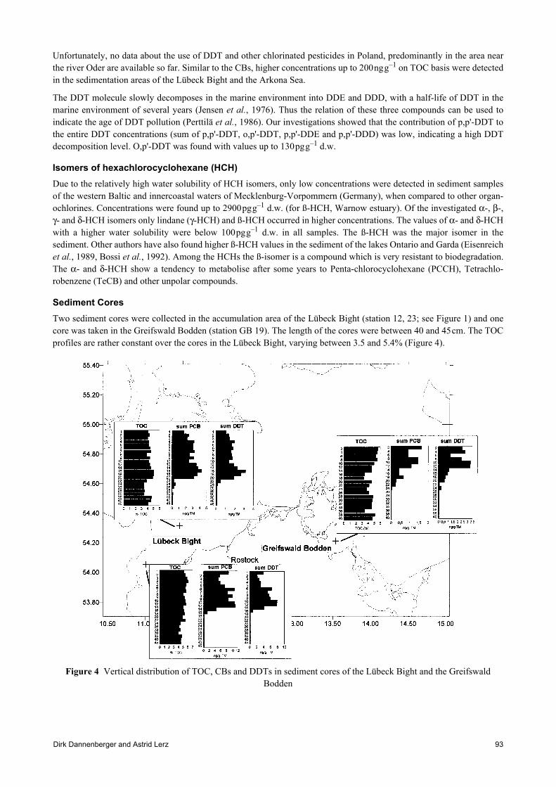
Dirk Dannenberger and Astrid Lerz 93
Unfortunately, no data about the use of DDT and other chlorinated pesticides in Poland, predominantly in the area nearthe river Oder are available so far. Similar to the CBs, higher concentrations up to 200ngg–1 on TOC basis were detectedin the sedimentation areas of the Lübeck Bight and the Arkona Sea.
The DDT molecule slowly decomposes in the marine environment into DDE and DDD, with a half-life of DDT in themarine environment of several years (Jensen et al., 1976). Thus the relation of these three compounds can be used toindicate the age of DDT pollution (Perttilä et al., 1986). Our investigations showed that the contribution of p,p'-DDT tothe entire DDT concentrations (sum of p,p'-DDT, o,p'-DDT, p,p'-DDE and p,p'-DDD) was low, indicating a high DDTdecomposition level. O,p'-DDT was found with values up to 130pgg–1 d.w.
Isomers of hexachlorocyclohexane (HCH)Due to the relatively high water solubility of HCH isomers, only low concentrations were detected in sediment samplesof the western Baltic and innercoastal waters of Mecklenburg-Vorpommern (Germany), when compared to other organ-ochlorines. Concentrations were found up to 2900pgg–1 d.w. (for ß-HCH, Warnow estuary). Of the investigated α-, β-,γ- and δ-HCH isomers only lindane (γ-HCH) and ß-HCH occurred in higher concentrations. The values of α- and δ-HCHwith a higher water solubility were below 100pgg–1 d.w. in all samples. The ß-HCH was the major isomer in thesediment. Other authors have also found higher ß-HCH values in the sediment of the lakes Ontario and Garda (Eisenreichet al., 1989, Bossi et al., 1992). Among the HCHs the ß-isomer is a compound which is very resistant to biodegradation.The α- and δ-HCH show a tendency to metabolise after some years to Penta-chlorocyclohexane (PCCH), Tetrachlo-robenzene (TeCB) and other unpolar compounds.
Sediment CoresTwo sediment cores were collected in the accumulation area of the Lübeck Bight (station 12, 23; see Figure 1) and onecore was taken in the Greifswald Bodden (station GB 19). The length of the cores were between 40 and 45cm. The TOCprofiles are rather constant over the cores in the Lübeck Bight, varying between 3.5 and 5.4% (Figure 4).
Figure 4 Vertical distribution of TOC, CBs and DDTs in sediment cores of the Lübeck Bight and the Greifswald Bodden
Organochlorines in surface sediments and cores of the Western Baltic and inner coastal waters of Mecklenburg-West Pomerania94
The vertical distribution of CBs (sum 23 congeners) and DDTs (sum of p,p'-DDT, o,p'-DDT, p,p'-DDE and p,p'-DDD)showed a similar pattern. Generally, an approximately uniform CB and DDT distribution was found in both cores downto 15 and 20 cm, without detection of great maxima.
This fact may be explained by advective processes (postdepositional mobilisation and bioturbation) and high sedimentdynamics combined with mix thorough of the sediment layers down to 20cm and 15cm. Because of sedimentation ratesbetween 1–2mmyr–1 (Perttilä and Brügmann, 1992) CB or DDT maxima should occur at upper sediment layers. In thesecases it is impossible to detect correct historical inputs of organic microcontaminants.
On the contrary, the vertical CB and DDT distributions of the core from the Greifswald Bodden show a decrease ofconcentrations with increase of sediment depth. The CB- and DDT maxima occurred between 10 and 12cm, due tohigher discharges of PCBs and DDTs between 1945 and 1955.
SummaryOrganochlorines were investigated in surface sediments and three different sediment cores of the western Baltic, theArkona Sea, the Pomeranian Bight and inner coastal waters of Mecklenburg-Vorpommern (Germany). Chlorinatedbiphenyls (CBs), isomers of hexachlorocyclohexane (HCH), dichlorodiphenyltrichloroethane (DDT) and some of itsmetabolites were analysed by gaschromatographic techniques (HRGC-ECD/ECD).
The organochlorine concentrations varied due to differences in the sediment structure and showed strong correlations tothe TOC contents. The highest concentrations up to 220000pgg–1 d.w. were measured for CBs (sum of 23 congeners)and DDTs (sum of p,p'-DDT, o,p'-DDT, p,p'-DDE and p,p'-DDD) in innercoastal waters (Warnow-Estuary, Oderhaff). Inthe sedimentation areas of the Lübeck Bight and Arkona Basin, the CB concentrations ranged between 2200 and11400pgg–1 d.w. The more hydrophilic HCHs were found between 10 to 2900pgg–1 d.w., with higher values for the ß-isomer. In the sandy areas of the Pomeranian Bight all compounds investigated remained below the detection limit of10pgg–1 d.w. Inputs via rivers (Oder, Peene) into the Baltic Sea and discharges of industrial point sources wereidentified.
The distribution of organochlorines in surface sediments in the western Baltic was approximately homogenous afterTOC-normalisation.
Sediment cores from the Lübeck Bight showed uniform CB- and DDT distribution down to 15 or 20cm. By contrast, forthe vertical CB- and DDT distribution in the core from the Greifswald Bodden, maxima in the upper layers (0–2cm) andat 10cm depth were measured. The historical inputs of organochlorines via the Peene river and from industrial sourceswere detected.
Referencesvan Bavel, Näf, C., Bergquist, C.A., Broman, D., Lundgren, K. Papakosta, O., Rollf, K., Strandberg, B., Zebühr, I., Zook,
D., and Rappe, C., 1996. Levels of PCBs in the aquatic environment of the Gulf of Bothnia: benthic species andsediments. Mar Poll. Bull. 32, 210–218
Brügmann, L., and Bachor, A., 1990. Present state of the Baltic Coastal Waters of Mecklenburg-Vorpommern, Germany.Geo-Journal 22.2, 185–194
Brügmann, L. and Lange, D., 1990. Metal distribution in sediments of the Baltic Sea. Limnologica 20, 15–28
Broman, D., Bandh, C., Ishaq, R., Näf, C., Pettersen, H., and Zebühr, Y., 1992. Sediment trap fluxes, residence times andsurface sediment concentration variability of PCBs, PCDD/Fs and PAH in the Baltic. Organohalogen Compounds9, 43–46
Broman, D., Näf, C., Zebühr, Y., Bandh, C., Ishaq, R., and Pettersen, H., 1993. Occurrence, distribution and turnover ofsome toxic substances in the water mass and sediments in the Baltic Sea. Baltic News 4, 6–10
Bossi, R., Larsen, B., and Premazzi, G., 1992. Polychlorinated biphenyl congeners and other chlorinated hydrocarbons inbottom sediment cores of lake Garda (Italy). The Science of Total Environment 121, 77–93
Dannenberger, D., 1995. Ostseewasser—Analytik im Subspurenbereich (Teil 1). CLB—Chemie in Labor undBiotechnik 46, 589–592

Dirk Dannenberger and Astrid Lerz 95
Dannenberger, D., 1996. Chlorinated microcontaminants in surface sediments of the Baltic Sea—investigations in theBelt Sea, the Arkona Sea and Pomeranian Bight. Mar. Poll. Bull., in press
Eisenreich, S.J., Capel, P.D., Robbins, J.A. and Bourbonniere, R., 1989. Accumulation and diagenesis of chlorinatedhydrocarbons in lacustrine sediments. Environ. Sci. Technol. 23, 1116–1126
Fucco, R., Colombini, M. P., and Samcova, E., 1993. Individual determination of ortho and non-ortho substitutedpolychlorophenyls (PCBs) in sediments by high performance liquid chromatographic pre-separation and gaschro-matography-ECD detection. Chromatographia 36, 65–70
HELCOM, 1993. First assessment of the state of the coastal waters of the Baltic Sea. Baltic Sea Environ. Proc. 54, 160pp
Jensen, S. and Olsson, M., 1976. AMBIO Sp. Rep., 4:111
Kjeller, L.-O. and Rappe, C., 1995. Time trends in levels, pattern and profiles for polychlorinated dibenzo-p-dioxins,dibenzofurans and biphenyls in a sediment core from the Baltic Proper. Environ. Sci. Technol. 29, 346–355
Nylund, K., Asplund, L., Jansson, B., Jonsson, P., Litzen, K., and Sellström, U., 1992. Analysis of some polychlorinatedpollutants in sediment and sewage sludge. Chemosphere 24, 1721–1730
Perttilä, M., and Haahti, H., 1986. Chlorinated hydrocarbons in the water and sediments of the seas around Finland. Publ.Water Res. Inst. 68, 197–200
Perttilä, M., and Brügmann, L., 1992. Review of contaminants in Baltic sediments, ICES Coop. Res. Rep. 180, 135 pp
Petrick, G., Schulz, D. and Duinker, J.C., 1988. Clean up of environmental samples by HPLC for analysis of organo-chlorine compounds by GC with ECD. J. Chromatogr. 435, 241–248
Safe, S., 1990. PCBs, PCDDs, PCDFs and related compounds: Environmental and mechanistic considerations whichsupport the development of toxic equivalency factors (TEF). Critical Reviews in Toxicology 21, 51–88
Schlungbaum, G., Nausch, G., and Baudler, H., 1994. Sedimentstruktur und Sedimentdynamik in der Darß-Zingster-Boddenkette. Rostock. Meeresbiolog. Beitr. 2, 27–40
Tolosa, I., Bayona, J.M., and Albaiges, K., 1995. Spatial and temporal distribution, fluxes and budgets of organochlo-rinated compounds in northwest Mediterranean sediments. Environ. Sci. Technol. 29, 2519–2527
Witt, G., 1995. Polycyclic aromatic hydrocarbons in water and sediment of the Baltic Sea. Mar. Poll. Bull. 31, 237–248

Lithology and stratigraphy of glacial deposits in the Sambian-Kura area of the Baltic Sea96
ICES Cooperative Research Report, No. 257 Baltic Marine Science Conference, Rønne, Denmark, 22–26 October 1996
Lithology and stratigraphy of glacial deposits in the Sambian-Kura area of the Baltic Sea
N. Kuten, B. Klagish and Y. Goldfarb
AbstractThis paper considers the lithological features of the glacial formation sediments for one of the most interesting oil fieldsof the SE Baltic sea—the Sambian-Kura high. It is well known that the different ages of glacial deposits are relativelysimilar to each other in that they inherit some common peculiarities regarding mineral composition and texture, none theless detailed by sequential studies of mineral typomorphism and clay mineral assemblages. The upper Pleistocene till ischaracterised by abundant hydromicas, which range up to 80%, with some caolinite-chlorite. The middle and LowerPleistocene tills differ from the latter by having an essential content of swelling phases (mainly montmorillonite), whichreaches 40%, but in the underlying Cretaceous glauconite sands and sandstones they increase to 39–85%. This factallows us to suppose that pertinent increase of swelling clayey phases in the Middle and Lower ones are connected tolocal bed rock erosion and redeposition by the glaciers. The criteria for different ages of till separation have beenspecified as hornblende roundness, clay mineral composition, granulometric composition and physical-mechanicalproperties.
Figure 1 Chart of engineering-geological zonation of the Baltic sea (I. Dzilna [5]).(· 21) shows the position of a bore hole and its number.
Boundaries1–engineering-geological region2–engineering-geological area A–SE part of Baltic shieldC–southern slope of Baltic shieldCI–southern part of Finnish GulfCII–High of Estonian archipelago and Western-Saaremaas stepB–Baltic synecliseBI–low of Riga GulfBII–Gotland lowBIII–Liepaja-Klaipeda’s high with Ventspils stepBIV–Neman’s lowBV–Kura highBVI–Gdansk low
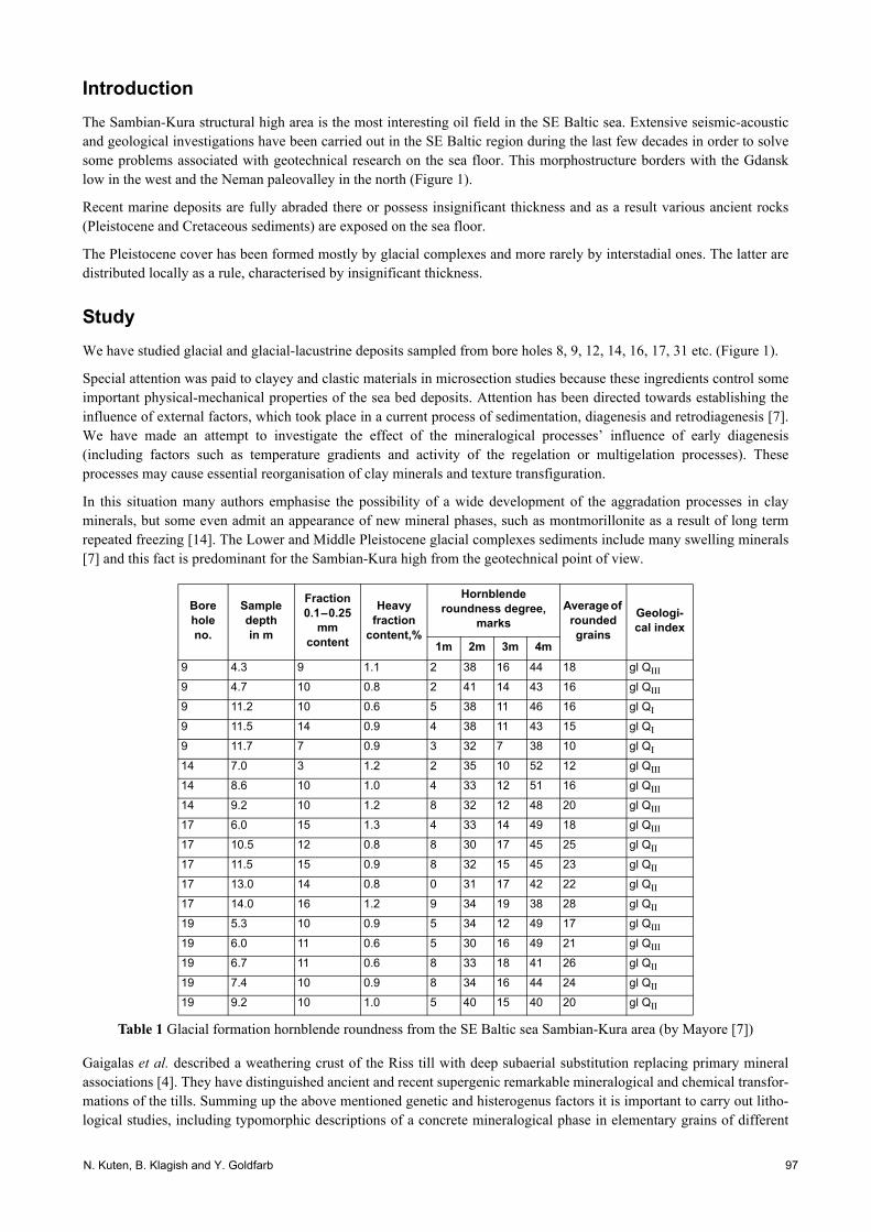
N. Kuten, B. Klagish and Y. Goldfarb 97
IntroductionThe Sambian-Kura structural high area is the most interesting oil field in the SE Baltic sea. Extensive seismic-acousticand geological investigations have been carried out in the SE Baltic region during the last few decades in order to solvesome problems associated with geotechnical research on the sea floor. This morphostructure borders with the Gdansklow in the west and the Neman paleovalley in the north (Figure 1).
Recent marine deposits are fully abraded there or possess insignificant thickness and as a result various ancient rocks(Pleistocene and Cretaceous sediments) are exposed on the sea floor.
The Pleistocene cover has been formed mostly by glacial complexes and more rarely by interstadial ones. The latter aredistributed locally as a rule, characterised by insignificant thickness.
StudyWe have studied glacial and glacial-lacustrine deposits sampled from bore holes 8, 9, 12, 14, 16, 17, 31 etc. (Figure 1).
Special attention was paid to clayey and clastic materials in microsection studies because these ingredients control someimportant physical-mechanical properties of the sea bed deposits. Attention has been directed towards establishing theinfluence of external factors, which took place in a current process of sedimentation, diagenesis and retrodiagenesis [7].We have made an attempt to investigate the effect of the mineralogical processes’ influence of early diagenesis(including factors such as temperature gradients and activity of the regelation or multigelation processes). Theseprocesses may cause essential reorganisation of clay minerals and texture transfiguration.
In this situation many authors emphasise the possibility of a wide development of the aggradation processes in clayminerals, but some even admit an appearance of new mineral phases, such as montmorillonite as a result of long termrepeated freezing [14]. The Lower and Middle Pleistocene glacial complexes sediments include many swelling minerals[7] and this fact is predominant for the Sambian-Kura high from the geotechnical point of view.
Table 1 Glacial formation hornblende roundness from the SE Baltic sea Sambian-Kura area (by Mayore [7])
Gaigalas et al. described a weathering crust of the Riss till with deep subaerial substitution replacing primary mineralassociations [4]. They have distinguished ancient and recent supergenic remarkable mineralogical and chemical transfor-mations of the tills. Summing up the above mentioned genetic and histerogenus factors it is important to carry out litho-logical studies, including typomorphic descriptions of a concrete mineralogical phase in elementary grains of different
Bore hole no.
Sample depth in m
Fraction 0.1–0.25
mm content
Heavy fraction
content,%
Hornblende roundness degree,
marksAverage of
rounded grains
Geologi-cal index
1m 2m 3m 4m9 4.3 9 1.1 2 38 16 44 18 gl QΙΙΙ
9 4.7 10 0.8 2 41 14 43 16 gl QΙΙΙ
9 11.2 10 0.6 5 38 11 46 16 gl QΙ
9 11.5 14 0.9 4 38 11 43 15 gl QΙ
9 11.7 7 0.9 3 32 7 38 10 gl QΙ
14 7.0 3 1.2 2 35 10 52 12 gl QΙΙΙ
14 8.6 10 1.0 4 33 12 51 16 gl QΙΙΙ
14 9.2 10 1.2 8 32 12 48 20 gl QΙΙΙ
17 6.0 15 1.3 4 33 14 49 18 gl QΙΙΙ
17 10.5 12 0.8 8 30 17 45 25 gl QΙΙ
17 11.5 15 0.9 8 32 15 45 23 gl QΙΙ
17 13.0 14 0.8 0 31 17 42 22 gl QΙΙ
17 14.0 16 1.2 9 34 19 38 28 gl QΙΙ
19 5.3 10 0.9 5 34 12 49 17 gl QΙΙΙ
19 6.0 11 0.6 5 30 16 49 21 gl QΙΙΙ
19 6.7 11 0.6 8 33 18 41 26 gl QΙΙ
19 7.4 10 0.9 8 34 16 44 24 gl QΙΙ
19 9.2 10 1.0 5 40 15 40 20 gl QΙΙ

Lithology and stratigraphy of glacial deposits in the Sambian-Kura area of the Baltic Sea98
till faces. In connection with the well known close genetic relationship and lithological similarity of the different age tills,this has caused difficulties in studying the Quaternary deposits.
Separation of different age tills has been carried out using the following methods: typomorphic examination of the samepredominant minerals including hornblendes from grain-size fraction for estimation of roundness, study of clay mineralcomposition and fabric peculiarities, mutual surface ions’ absorption capacity and physical-mechanical properties [4, 5,6, 7, 13] (Table 1, Table 2 and Table 3).
Table 2 The clay mineral composition of glacial and underlying Cretaceous sediments from the SE Baltic sea (X-ray difractometric analyses of the fraction <0.002mm) [7]
Approximate content,%
Bore hole numbers
Depth of sampling,
mGeological
index Lithological description Hydrom-ica, %
Kaolinite & chlorite,
%
Montmo-rillonite,
%8 1.0 gl QΙΙΙ
Red-brown, yellow-grey tight carbon-ateferous clay till with appreciable
amount silty sand content & irregular distributed psephite presented the main various carbonates, quarzites, markedly weathered, often decomposed granite,
migmatites, typical minor content glauconite sandstone, chert,
phosphorite.
80 20 -
8 6.5 gl QΙΙΙ 80 20 -
8 8.5 gl QΙΙΙ 81 20 -
8 10.0 gl QΙΙΙ 77 23 -
12 5.5 gl QΙΙΙ 79 21 -
12 7.0 gl QΙΙΙ 66 23 11
31 3.9 gl QΙΙΙ 76 24 -
31 5.0 gl QΙΙΙ 78 22 -
31 6.0 gl QΙΙΙ 67 18 15
31 10.0 gl QΙΙΙ 64 24 12
31 13.0 gl QΙΙΙ 76 24 -
16 16.0 gl QΙΙΙ 72 28 -
14 7.5 gl QΙΙGrey hard clay till with admixture of
various psephite–boulders, rare pebbles, abundant gravel presented
carbonates, glauconite, granites, gabbros.
48 18 34
14 10.0 gl QΙΙ 48 20 32
14 12.0 gl QΙΙ 45 20 35
17 1.0 gl QΙΙ 58 14 28
17 6.5 gl QΙΙ 57 17 26
17 11.0 gl QΙΙ 45 15 40
9 10.7 gl QΙΙ Deep grey hard sandy till with carbonates, sandstone boulders, pebbles with mainly decomposed
granites.
70 20 10
9 13.5 gl QΙ 63 22 15
9 15.0 gl QΙ 60 21 19
9 17.0 gl QΙ 56 20 24
D26–1 17.0 K2
Glauconite-quarts clayey sand with sandstone of the same mineralogy &
composition with subordered quantity of hydromuscovite locally replaced by
autogenetic kaolinite. In same layers it is also noted disseminated fine
secondary pyrite and magnetite.
23 - 77
D26–1 17.2 K2 20 - 80
D26–1 18.4 K2 29 - 71
D26–1 20.2 K2 15 - 85
D26–1 21.6 K2 48 - 52
D2–1 22.7 K2 17 7 76
D2–1 24.0 K2 25 10 65
D2–1 25.4 K2 50 10 39
D2–1 26.5 K2 99 - -D2–1 29.8 K2 50 10 40

N. Kuten, B. Klagish and Y. Goldfarb 99
Table 3 The midrange data of granulometric and clay mineral compositions, surface ions’ absorption capacity, physical and mechanical properties of the SE Baltic sea glacial formation sediments [7].
The Upper Pleistocene complex is widespread throughout the Sambian-Kura neotectonic structural high with amaximum thickness of 25m. The upper complex part has been formed by glacial-lacustrine deposits (lgIII) with athickness reaching 10m. These sediments represent yellow-brown calcerous sandy clay and clay with interlaying siltysand and insignificant quantities of irregularly distributed psephite material.
The lower complex part was formed by red-brown and grey morainic sandy clay, so called “till” (gIII) with a remarkablecontent of psephite contributed by glacier and passing over in clay sand and glacial-fluvial sediments facially alteredlaterally (Figure 2 and Figure 3).
Figure 2 Silty till (gl QIII) with admixture of rounded fine sand grains and gravel size black angular limestone fragments. The clayey matrix (dark) contains dispersed quartz, carbonates, feldspars and other mineral debris. The Baltic sea, Sambian-Kura high, bore hole 12, depth 5.5m. Photomicrograph of the thin section in transmitted light, magn. 40 X.
Geological index
Total granulom-etric composition,
per cent, mm
Mineral composition,
%
Mutual surface ions complex M
oisture content
Liquid limit
Plasticity index
Liquidity index
Bulk density
Skeleton density
Porosity coefficient
Laboratory tests
Shear tests
Oedometer
Triaxial tests
>2.0
2.0–0.05
0.05–0.005
< 0.005
Hydrom
ica
Caolinite + chlorite
Montm
orillonite
Absorbtion capacity
Ca
2+ + Mg
2+
Ca
2+
K+
Na
+
Angle of internalfriction
Cohesion
Modulus of
deformation
Cohesion
Angle of internal friction
mgr-eq/100 s. gr per cent part unit gcm–1 part
unit o KPa MPa KPa o
gl QIII 6 44 21 29 74 22 4 13.9 8.0 4.8 1.2 4.6 15 24 9 0–0.2 2.18 1.90 0.425 23° 60 9.0 20 25
*tgl QII
**/
7-1
59-
17
18-
39
16-
43
-52-
-18-
-33-
-21.8
-
-12.4
-
-6.4-
-2.2-
-7.7-
13-
19
20-
29
5-
10
<0-
<0
2.24-
2.06
1.99-
1.77
0.350-
0.320
28°-
23°
30-
65
17-
8.5
---
---
m QI-II - 14 12 74 69 25 6 - - - - - 27 47 22 0.1 1.96 1.54 0.730 25° 51 3.4 - -gl QI 4 52 25 21 63 22 15 14.3 8.0 5.5 1.2 4.4 11 19 5 <0 2.28 2.05 0.320 30° 70 17.5 - 33°
Note: (*) and (**) mean “gravelly” and “ungravelly”.

Lithology and stratigraphy of glacial deposits in the Sambian-Kura area of the Baltic Sea100
Figure 3 Calcerous silty till (gl QIII) with incorporated weathered plagioclase, markedly altered by the fine flakes of hydromica. Baltic sea, Sambian-Kura high, bore hole 12, depth 5.5m. Photomicrograph of the thin section between
crossed nicols, magn. 32 X.
The glacial-lacustrine complex sediments (lgIII) have been studied at their maximal thickness (in depth interval 0.0–9.5m) by profile of bore hole 16. They have been formed during a single glacier oscillation and are characterised byvarved clayey deposits of low and upper parts of the sequence appearing more sandy and crudely bonded. Clasticmaterial consists essentially of quartz, which inherits typomorphical peculiarities compared to those of the till: well-rounded, slightly-rounded angular and sharp-edged grains.
The largest part of silty-size particles was carried from the melting glacier and shows elements of typical relics due torather delicate differentiation, transit in a liquid medium and resedimentation of detrital material. The longer axis ofcoarse clastic grains, as a rule, are oriented perpendicular to the top base plane of a bedding as a result of the gravitationalprecipitation from floating glacons.
There are a large amount of pelitic (0.001–0.006mm) not usually fine grained (size up to 0.01mm) carbonate particles inthe clayey matrix, resedimented from the till, which causes high carbonatisation of this sediment type. Observations inthin sections below show that fine dispersional carbonates mainly represent “glacier flour” although they may partly bechemogenically sedimented in melt water lacustrine sediments in glacier lakes.
Glacial complex sediments, till (gIII) are represented by red-brown coarse-grained stiff morainic sandy clay and greyhard clayey sand. The clastic material includes rounded pebbles and fine-medium gravel particles consisting essentiallyof carbonates (total psephite content exceeds 10%). There are organogenic and chemogenic fine-grained limestones,dolomite, siderite and unusual clots of argillite in psephite. Some carbonate grains are encircled by a cover of crushedmaterial with a grain size of about 0.06mm.
The erratic material e.g. boulders, various rock fragments, pebbles and gravel grains represent slightly weatheredunrounded granite fragments, typomorphic glacial rock debris, scale-form grains and blocks of acid plagioclase, oftenwith alteration marks of sericite. Also it consists of specific lode quartz grains with remains of shelly fractures, thattestify to the conditioning of originally outlined glacial forms (Figure 4).

N. Kuten, B. Klagish and Y. Goldfarb 101
Figure 4 Silty carbonateferous till (gl QI) with subparallel elongated grain arrangement. The top right corner shows displaced weathered plagioclase grain and below it—typomorphical for glacial sediments—coarse quartz grain with
undulated outlines (fish-shaped). Baltic sea, Sambian-Kura high, bore hole 9, depth 10.7m. Photomicrograph of the thin section between cross nicols, magn, 32 X.
Severely weathered granitoid psephite is characteristic for the Lower Pleistocene till, less for the Middle Pleistoceneones, and only the single bore holes (17,18) of the Upper Pleistocene till registered more intensively weathered samplesthan the Middle Pleistocene ones. The significant parts of the psephite are transitive carbonatic rocks, quarzite, argilliteand local glauconitic sandstones, aleurolite, phosphorite and flint. A distinctive glauconite content in glauconitic bearingsandstones reaches 20%. The cementing matrix of the till contains about 40–50% of psammite fraction including aremarkable admixture of glauconite (up to 3–5%), phosphorite and flint (up to 1%). This testifies that material has beenincorporated from underlying Cretaceous rocks (Table 3).
In the composition of a psammite fraction, quartz dominates with about 60–70%, plagioclase content is about 7%,microcline (12%), carbonate (up to 7–10%) more often represented by monocrystalline forms, glauconite (1–4%),garnet (up to 1%), hornblende (up to 1%).
A sand fraction quartz is composed of some morphologic types: the isometric subrounded grains (roundness 0.55–0.62)and angular grains (roundness 0.1–0.30). The first ones are obviously incorporated from underlying Mezozoic andPaleozoic and are likely to have endured some cycles of resedimentation, whereas the latter ones represent the erraticclastic rock debris delivered by the glaciers from the Baltic Shield.
Some grains of acid plagioclase show peripheral retrodiagenetic replacement cover of hydromica (Figure 6). This alter-ation changes processes obviously started in outcrops of bed-rock, continued during the process of their transportationand even “in situ” after their deposition and burying.
We agree with S. Astapova, that the till is in principle formed in a zone of supergenesis, where soil formation took place,biogeochemical processes and all weathering factors alongside with disintegration, new mineral creation and extensivemigration of chemical elements [1]. The correlation ratio of the potash feldspars and plagioclases vary widely, which canbe explained by the erosion of different weathering crust zones on the Precambrian Shield, leading to retrodiageneticdisintegration and glacial resedimentation too. These transformations might also occur as a result of condense intrusionbetween strata from deep oil structures [9].
The pelitic fraction is characterised by an abundance of illite and clastic hydromuscovite mixed with a fine dispersionalcarbonate, silty feldspar and quartz. The Upper Pleistocene till (gIII) clay mineral matrix contains extremely highpercentages of hydromica, about 74%. Its maximal content has been marked in an upper profile part of bore hole 8(reaching 80%) and contains a negligible admixture of montmorillonite (4%) and some kaolinite-chlorite (7–14%).
The Middle Pleistocene glacial complex (gII) in cores of bore holes 14,16 and 17 is represented mainly by grey-greencobbled clayey sand, which is laid directly over the exarated Cretaceous rocks (Figure 5). These sediments include about5 layers of so called “ungravelly” sandy clay (bore hole 14, interval 1.8–12.8m from sea bed) with a negligible quantity

Lithology and stratigraphy of glacial deposits in the Sambian-Kura area of the Baltic Sea102
of psephite (about 1–2%) and psammite (up to 17%). The pelite and silty fractions dominate (on average more than 80%)and define specific physical-mechanical properties of these sediments (Table 2).
Figure 5 Silty carbonateferous till (gl QII) with sand and gravel admixture containing quartz, feldspars, granite and carbonate rock fragments incorporated in a dark clayey matrix, which is full of dusty sharp-edged clastic. Baltic sea,
Sambian-Kura high, bore hole 14, depth 2.5m. Photomicrograph of the thin section between cross nicols, magn. 32 X.
The psephite material of the till (about 7%) is composed of limestones monomineralic quartzite, glauconitic sandstone,fragments of leucocratic and hornblende granites, blocks of plagioclase, rounded grains of microcline and debris ofhornblende, gabbro and amphibolite (Figure 5).
The psammite and aleurite materials generally include quartz with a little admixture of feldspar (generally acid plagi-oclase) and calcite, glauconite (up to 3%, which coloured sediments with a green hue). The psammite grains arecommonly more rounded than the silty (aleurite) ones.
A pelite matrix of the till has been formed mainly of clay minerals, silty carbonates, quartz and feldspar. It is interestingto note that there is a greater content of montmorillonite, less illite and invariably a low percentage of caolinite andchlorite in the matrix. The Middle Pleistocene till differs from the Upper one by having a greater montmorillonite contentwith a maximum of about 40% (Table 2).
Similar peculiarities of the tills have been reported by A. Vvedenskaya et al. [2] and G. Nemtsova [10] for the Russianplatform, where they interpreted the till’s clay minerals as an allogenic glacial material assimilated from bedrock.H.B.Willman et al. [15] received excellent data in their exhaustive study of the Illinois state glacial tills.
The Lower Pleistocene glacial complex sediments (gI) have been discovered by a profile of bore hole 9 for an interval of10.7–17.0m under the Upper Pleistocene limnetic glacial sediments. This till is represented by dark-grey hard clayeysand uncommon in the lower profile part—sandy clay (Figure 6 and Figure 7).

N. Kuten, B. Klagish and Y. Goldfarb 103
Figure 6 Sandy carbonateferous till (gl QI) with deeply weathered detrital feldspar grains. In the centre, dark feldspar grains occur, replaced by clay minerals with plagioclase relics (little white spots) and nearby coarse angular and
markedly decomposed quartz grain with microcracks and fine crioclastic. The elongated grains are spaced subparallely along the long axis thus recording fluidal sediment texture. Baltic sea, Sambian-Kura high, bore hole 9, depth 10.7m,
magn. 40 X.
Figure 7 Clayey carbonateferous till (gl QI) with admixture of silt sand and coarse inclusions of erratic (Precambrian) quartz fragment typomorphical for the till. The specific shape of this grain is determined by crack systems and inherited
shell fracture. There is a dark cementing matrix consisting of very fine clay mineral particles and sharp-edged dusty debris. Baltic sea, Sambian-Kura high, bore hole 9, depth 17.0m. Photomicrograph of the thin section between cross
nicols, magn. 20 X.
These sediments are characterised by comparatively less content of psephite, averaging about 4%. The psephite materialis presented as erratic, fully weathered granite and migmatite fragments with deep alterated feldspar and dark-colouredminerals, transit gravely fine-grained and rounded carbonatic rocks and organogenic detrital limestones.
Some constituents of the granitic rubble such as a dark coloured minerals and feldspars are the most unstable insupergene conditions and they break down. So, the first ones frequently have been substituted by hydrochlorite, and thesecond ones by hydromica and more rarely by caolinite.
The acid and intermediate plagioclases from the till psephite are much more weathered than microcline. The marks ofmineral degradation display themselves in local changes of the plagioclase blocks by their transformation and

Lithology and stratigraphy of glacial deposits in the Sambian-Kura area of the Baltic Sea104
replacement by fine-scaled hydromica, which, as a rule, contains more or less fresh relics (Figure 7). At the initial phase,cementing bonds are essentially weakened as a result of these processes, and it causes a partial or complete rock decom-position. The marked content of granitoide debris is abundant in all described stratigraphic units, though its quantitysomehow varies in some stratigraphic ones. The observations confirmed that the rocks in their Prequaternary historyendured influences of the supergene processes in exposure on the adjacent Scandinavian Shield.
A fine gravel fraction contains rounded magmatic and hydrothermal quartz grains and typomorphic clastic chips of thequartz with a characteristic lower content of monocrystalline grains of feldspars and limestones. (Figure 4, Figure 6 andFigure 7).
The psammite material (about 50%) can be compared to gravel due to its mineral composition, but differs in grainroundness, which evidently decreases according to its reducing tendency of grain size (Figure 6). For example, if thepsammite fraction is characterised by middle roundness, then for the aleuritic (silty) fractions minor roundness coeffi-cient is typical and the fine silty fraction, as a rule, is represented by unrounded clasts with wedge shaped particles. Itsmineral assemblage, except dominated quartz, feldspars and carbonates, includes some mixture of glauconite (2%),muscovite (2%) and an insignificant quantity of biotite, green hornblende, pyroxene, garnet, etc.
The cementing clayey matrix is filled up with the mentioned detrital minerals and finely dispersed carbonatic silty grains.The clay mineral association reveals a similarity to the Middle Pleistocene one, though analyses show a distinctivedecreasing of montmorillonite to 10–24% and increasing of illite (by invariable minor content of kaolinite and chlorite).If the stable montmorillonite increases in the vertical profile of glacial sediments it clearly shows their relation to bedrockand allows us to conclude that they had been derived from the underlying Cretaceous rocks (which were redeposited bythe glacier; Table 2). This fact has been confirmed by a comparatively high content of glauconite in the till psammitefraction, which may be incorporated from the basement rocks.
To consider the Lower Pleistocene complex it should be noted that it remained on the Cretaceous eroded bedrock surfacemostly in depressions, paleovalleys and incisions. This till possesses unique peculiarities of mineral composition, textureand physical-mechanical properties. In particular, it contains significantly more severely weathered disintegrated detritalmaterial in coarse and sandy fractions (Figure 6), than has been revealed in overlapped younger tills. This indicates thepresence in the alimentary area of the Prequaternary weathering cover.
The second Lower till peculiarity related to its physical-mechanical properties is mainly caused by its compact texture.This is confirmed by some indexes summarised in Table 3, i.e. characteristic minimal values of porosity, moisture,plasticity and maximal mean value of density. Ascertaining these data we came to the conclusion that this was caused bythe gravity effect of successive glaciers, which overlapped the area at least twice and thus altered the till’s texture andproperties.
Hence, the characteristics of different stratigraphical units show that geotechnical properties are the result of origin oflocal facial conditions including alimentary and depositional areas as well as gravity effect of subsequent glaciers.
SummarySumming up the above information we can visualise different age characteristics of lithostratigraphical types ofmoraines, which differ in their granulometric and mineral composition and as a degree of their supergenic and possiblyretrodiagenetic transformations. The lithological factors stated above determined the peculiarities of their physical-mechanical properties too (Table 3). This is characteristic for all tills related to the Middle Pleistocene, which havecomparatively high clay content (about 43%) of a specific mineral composition. There are 33% of swelling phases in theclayey matrix (Table 3).
Montmorillonite is more dispersed and hydrophilic than the hydromica and this is characterised by the much highersurface adsorption capability of the clay particles, manifested in the high surface mutual ions adsorption capacity—21.8milligram-equivalent/100 soil grams (Table 3). Easily hydrated ions, previously Na-ion (7.7mg-eq/100 s.g.) significantlyincrease the hydrophilicity of clayey matrix and, as a result, it decreases the soil stability during mechanical influence[8]. It becomes clear that the tendency of cohesion increasing (65 KPa) with comparatively low data on the angle ofinternal friction (23o) independently of the relatively high moisture (19%) and porosity coefficient (0.520) manifestsitself much more clearly (Table 3).
N. Kuten, B. Klagish and Y. Goldfarb 105
Special attention has been paid to till fabric studies, using the oriented thin section (with undisturbed samples) applyingoptical microscopy methods with polarised light at about 200–600 power magnification. The term “fabric” is used tocharacterise the geometrical arrangement (spacing and orientation) of clay and associated mineral particles.
The summarised results gained from microscopic examinations led us to the conclusion that two microfabric typesdominate the till studied. The most common in morainic deposits is dense, isotropic cement filled with the finest grainsof carbonate, quartz, feldspars and other debris, as well as the originally dispersed calcite grains inherited from marls.This phenomena considerably increases the markedly raised matrix density.
E.Sergeev et al. [12] calls this cement microfabric a “matrix” type fabric with continuous highly disoriented clay mass,containing the irregular tightly interlocked fine mineral grains mentioned above. Due to an interaction in the clay matrixthe aggregates have been formed in the arrangements “face-to-face”, “face-to-edge” and “edge-to-edge”. It is character-istic that this type of fabric lacks any observed preferred clay particle orientation, and, on the contrary, the so called“turbulent” fabric oriented clay aggregates arrangement with “face-to-face”, and, more rarely, “face-to-edge” prevails.Flat multiparticle aggregate streamline the incorporated grains, forming a structure pattern according to till stratification.
The mode of the till origin allows us to suggest that the retention of terrigenous material inherited multiparticle aggre-gates with steady arrangement, had been formed in the Prequaternary periods.
A.Larionov [8] and E.Sergeev et al. [13] regard that the units with the montmorillonite-hydromica clayey matrix assem-blage are characterised by the “face-to-face” arrangement type interaction during clay aggregates for motion. The micro-scopic flake-shaped particles of the montmorillonite with uncertainly outlined, undulating edges, partially interlay eachother and have a tendency to “coalescence” in their contact zones. As a result, we can not outline their boundaries. Thecohesion of clayey microaggregates segregately increase and also improve the soil cohesion.
The hydromica matrix characterises another type of the clay particle and aggregates “edge-to-face” interaction. Theparticles of hydromica with well-traced borders have an insignificant cohesion with each other and, as a result, tend todecrease the soil cohesion. Our microscopic studies of the cemented thin section show that the hydromica cement is lessorganised and forms a chaotic, disordered clayey matrix texture, increasing the angle of internal friction (Table 3) [6,7,9].
From the other side, the high hydrophilicity of montmorillonite determines the lesser modulus of deformation of theMiddle Pleistocene till (8.5MPa) in comparison to the younger ones and especially to hydromica’s composition of theUpper Pleistocene till (9MPa, Table 3). The tills of different ages are alike with regard to the angle of internal friction,due to the similar contents of psephite and psammite fractions.
There is a tendency that sequential increasing of physical-mechanical properties of the till are caused by their ageaccording to inherited minerallic and granulometric composition. The obvious exception displays the properties of theMiddle Pleistocene till, whose decrease of “ungravelly” sediment layers is explained by a specific glacial-marine origin[7]. Distinctive differences in physical-mechanical properties for these stratigraphic units can be associated with thespecific clay mineral composition, which formed due to the local glacial erosion plane, exchanged on the Low andMiddle Pleistocene boundary.

Lithology and stratigraphy of glacial deposits in the Sambian-Kura area of the Baltic Sea106
References1. . . . .: . .
. . . . .,1981, .98-100.
2. . . . .- . .
. . . . . . . . .
. .,1981, .117-124.
3. Willman H.B., Glass H.D., Frye J.C. Glacial tills Part 1. Illinois state geological survey
circular 347, Urbana, 1963.- 28p.
4. . . , . .
. . - . ,- 1962,
28 .
5. Goldfarb Y.I., Savvaitov A.S., StelleV.Y. Structure & stratigraphy of quarternary deposits
of the SE Baltic. The second marine geologic confer. The Baltic. Rostock-Warnemunde,
1991.
6. . ., . . -
( ) .
. ,1989, .24-30.
7. . .
. . . . . . -
. , , 1991.-214 .
8. . . - . . . . .-
.: ,1966.-326 .
9. . , . .-
,1987-184
10. . . . .
. : . . . . .
.1. .,1986, .69-77.
11. . . . . . .
. . . . . . . . . .
XI . .1981, .153.
12. . . . . . . ,1987.
.120.
13. . , - , . . .
. ì î N 2, 1979.- . 48-58.
14. . ., . . . . . .
. // .- ,
N5, 1964.- .33-61.
15. . . . . .
. . , 1988, .88-92.

Katarzyna Bradtke and Adam Latala 107
ICES Cooperative Research Report, No. 257 Baltic Marine Science Conference, Rønne, Denmark, 22–26 October 1996
Particle size distributions in the Gulf of Gdansk
Katarzyna Bradtke and Adam Latala
AbstractSuspended matter concentrations were measured in the Gulf of Gdansk in the years 1992-1993. Water samples werecollected every month. The size and concentration of particles were analysed with Multisizer-II Coulter Counter. Againsta background of corresponding hydrological conditions seasonal variability of suspended particles size distributions wasstudied.
The results show strong spatial and temporal variations of the particle size distributions. In space the horizontal variationof the PSDs appear to be stronger than the vertical. The Vistula River input seems to be reason of this variability. In time,particle size concentration distribution shows variations according to cycles of the biological activity and dynamicalprocesses in the Gulf of Gdansk.
IntroductionThe characteristics of suspended particulate material are related to basic biological, chemical and physical processes inthe seas, for example scattering and absorption of light by sea water or transport of substances in the sea. As a conse-quence, knowledge about the properties and distribution of suspended particles can provide valuable information aboutthe oceanographic processes affected by these particles.
The extent to which suspended particles influence these processes depends strongly on their size distribution, i.e. thenumber of particles in a volume of water as a function of their diameters. For quantitative characterisation of theseinfluence and for purposes of the modelling of marine environment processes, it is important to find an approximation ofparticle size distribution by a simple arithmetic function with not too many parameters whose variability range needs tobe evaluated.
In oceans, particle size distributions are predictable and described in detail (Carder et al., 1971, Zalewski, 1977, Jonasz,1983), but in coastal regions, like the Gdansk Bay, they vary due to large input of different materials from rivers orsewage, and require careful study (Jonasz, 1983).
The aim of this paper is to characterise the particle size distributions in the Gdansk Bay and to outline their spatial andtemporal variability.
Materials and MethodsThe data discussed here were collected during 1992 and 1993 at locations shown in Figure 1 and analysed with a Multi-sizer II Coulter Counter. If measurements couldn’t be completed within a few hours after collection of the samples, theywere frozen (volume ~100ml) onboard the ship and analysed later. A Coulter counter with a 200µm orifice and 2000µlsample volume was used to measure number of particles per unit volume for at least 50 size classes of equivalentspherical diameter in the range of 4 to 30µm. The equivalent spherical diameter is used to characterise the size of theirregularly shaped particles and means the diameter of a sphere having a volume equal to that of the particle. To limiterrors resulting from inhomogenity of distribution of particles in water sample, average values of the particle concen-tration in every size class of at least 3 measurements were used to determine particle size distribution (PSD).

Particle size distributions in the Gulf of Gdansk108
Figure 1 Location of sampling stations. Capital letters denote names of sampling profiles as follows: PU–Puck, ME–Mechelinki, JA–Jastarnia, SO–Sopot, GD–Gdansk, SW–Swibno, ST–Stegna, KM–Krynica Morska.
The particle size distribution function FD(D) is defined by the equation
where dN is the number of particles per unit volume of sea water with diameters D in the range of (D,D+dD).
The particle size distribution FD(D) was determined by differentiation of the cumulative distribution, CD(D), of particlesizes, defined by the equation
where CD(D) is simply the number of particles per unit volume having diameter greater than D. To evaluation, simplifiedprocedure described by Jonasz (1983) was used. In this procedure, to convert CD(Di) into FD(Di) the least squaresapproximation to CD(D) by the function KD–m was constructed at three points: Di–1, Di, Di+1 and its derivative at D=Diwas evaluated. In the first and last step additionally its value at D=D1 and Dn respectively was assigned to FD(D1) andFD(Dn).
Figure 2 Particle size distribution characteristic for the Gulf of Gdansk presented in various manners.
18.5° 19.0° 19.5°54.3°
54.6°
54.9°
Sampling stations monthly monitored additionally in V , VI '92+♦
PUCK BAY
GULF OF GDANSK
KMSTSW
GD
SO
PU
ME
JA
dN FD D( )dD=
CD D( ) FD D'( ) D'dD
∞
∫=
particle diameter D [µm]
parti
cle
size
dis
tribu
tion
1
10
100
1000
4 8 12 16 20 24 28 32
CD(D) [cm-3]
FD(D) [cm-3µm-1]
N [cm-3µm-1]

Katarzyna Bradtke and Adam Latala 109
FD(D) computed in this procedure and the histogram ∆N(D,D+∆D) show a high goodness of fit (Figure 2). The relativeerror of CD(D=4µm) in all computed PSDs was smaller then 5%.
Results and Discussion
Distribution of particle concentration Results of measurements show differences between two main seasons, e.g. spring–summer and autumn–winter, charac-terised respectively by high (1.7×10³<CD(4µm)<55×103cm–3) and low (0.6×10³<CD(4µm)<26×103cm–3) concen-tration of particles suspended in water. This fact is thought to be a direct consequence of an autumn–winter minimum inbiological activity and land runoff of suspended matter.
Figure 3 Surface distributions and vertical profiles of particle concentration (CD(4µm)) characteristic for the Gulf of Gdansk in a) spring and summer, b) autumn and winter months
Figure 3 shows representative surface distributions and vertical profiles of particle concentrations (CD(4µm)) found forspring–summer and for autumn–winter seasons. The most characteristic feature of these distributions are the division ofthe Gulf of Gdansk into two parts: eastern, that is strongly influenced by the Vistula river waters, rich in suspendedmatter, and western (called Puck Bay) with a relative lower concentration of particles.
The vertical distributions of suspended particle concentration differ in these regions and are time-dependent too,however, this variability is much smaller than the spatial variability. Puck Bay is characterised by rather uniform particleconcentration, particularly in the autumn–winter season. In regions with higher amounts of particles the concentration
18.25° 18.50° 18.75° 19.00° 19.25° 19.50°
54.25°
54.50°
54.75°
30
20
10
0 ♦♦♦ ♦
30
20
10
0♦ ♦ ♦
40
30
20
10
0 ♦♦♦ ♦ ♦
SPRING-SUMMER
SO SW KM
18.25° 18.50° 18.75° 19.00° 19.25° 19.50°
54.25°
54.50°
54.75°
30
20
10
0 ♦♦♦ ♦
AUTUMN-WINTER
40
30
20
10
0♦ ♦ ♦♦♦
30
20
10
0♦ ♦ ♦
SO SWKM
0 5 10 15 20 25 30x×10 3[cm-3µm-1]
a)
b)

Particle size distributions in the Gulf of Gdansk110
was generally found to decrease with depth. An increase in particle concentration has been observed near the bottom dueto resuspension of bottom sediments and in the layer just above the seasonal thermocline (in summer). The concentrationof larger particles (D>20µm) was not found to vary as strongly as that of all particles (D>4µm). The concentration oflarger particles appeared to stay approximately the same in the entire water column, except the thin surface layer whenamounts of larger particles resulting from biological activity were found (Figure 4).
Figure 4 Vertical profiles of particles concentration for different size ranges, typical for deeper stations in summer, when seasonal thermocline occurs (June, 1992, 54°34'N 18°45'E)
Particle size distributionsAnalysed particle size distributions from the Gulf of Gdansk show in most cases a regular shape with concentrationsquickly decreasing with increasing particle diameter. The particle size distributions may be approximated using a hyper-bolic function (Figure 5).
Figure 5 Mean particle size distribution function in the Gulf of Gdansk. Vertical bars show the minimum and maximum values for diameter D.
For parametrisation of the PSD a hyperbolic function with two segments was used:
5 10 150
10
20
30
40
50
4000 8000 12000
0 500 1000
CD(4µm)
CD(10 or 20µm)
temperature
Z[m] CD(4µm) [cm ]
CD(10µm)
CD(20µ)
temperature [ºC]
particle diameter D [µm]
parti
cle
size
dis
tribu
tion
FD(D
) [cm
-3µm
-1]
2000
8000
14000
20000
26000
32000
5 10 15 20 25 30
MeanMin-Max
FD D( )
FD D( )k1D m1– 2µm D Db≤ ≤( )
k2D m2– Db D< 32µm≤( )
=

Katarzyna Bradtke and Adam Latala 111
In this equation k1, m1, m2, Db are parameters of the best fit and (Jonasz, 1983). Parametersm1 and m2 characterise slope of the particle size distribution in log-log scale. The relative square error of the approxi-mation, ε, was less than 2% in about 80% of the measured PSDs. Only PSDs from water rich in suspended matter e.g.sampled during phytoplankton bloom or in regions closed to the land sources of particles, have shown deviations fromthat described by this function. They should be approximate rather by the sum of this function and a Gaussian function orby some statistical methods (Jonasz, 1983).
Table 1 The values of parameters of the best fit found for Gdansk Bay particle size distributions
Since Db has been found to be close to the lower limit of the analysed diameter range, only PSDs with at least 5 sizeclasses of diameter in the range (4µm,Db) were included for further consideration.
The slopes m1 and m2 differ negligibly, and m1 varies in a wider range than m2. A correlation between m1 and m2 was notfound, but m1 shows a slight relation (correlation coefficient r=–0.46) to the mass concentration of suspended matter in[mg×dm–3] (Figure 6). It may suggest that the mass of suspended matter is determined mostly by the amount of particleswith diameter D<10µm. The seasonal variations of m1 and m2 are shown in Figure 7. It is worthwhile noting that therelation between m1 and m2 is different for water with high and with low particle concentration. Generally m1>m2 whenCD(4µm)<104cm–3µm–1 and m1<m2 when CD(4µm)>104cm–3mm–1. The slopes m1 and m2 of the particle size distri-bution differ negligibly whereas k1 is up to 10 times higher then k2.
Figure 6 Relationship between the slope of the first segment of particle size distribution function m1 and the dry mass concentration of suspended matter
Parameter min max mean standard deviation
number of data
Db 4.63 9.58 7.38 1.87 1276
m1 0.20 9.19 3.64 0.78 864
m2 1.35 5.37 3.47 0.57 864
k1 3.7 E3 21.3 E6 26.8 E6 726 E6 864
k2 k1Dbm1– m2+=
C [mg·dm-3]
m1
1
2
3
4
5
6
0 1 2 3 4 5 6 7 8 9 10
m1=4.96-0.25·C [mg·dm-3],r=-0.46

Particle size distributions in the Gulf of Gdansk112
Figure 7 Temporal variations of parameters m1 and m2 during the analysed period for low (left) and high (right) amounts of particles in water volume
In space the vertical variation of the PSD appears to be weaker than the horizontal. The horizontal variability is wider forthe first segment resulting from the variability of particle concentration connecting with land source activity. Figure 8shows the evolution of the particle size distribution with depth in the spring–summer and in the winter–autumn seasons.The vertical variability occurs here rather than in the second segment and is evident only in the subsurface layer (deepershape of PSD remains stable). This fact may suggest a biological reason for this variability.
Figure 8 The evolution of the normalised particle size distribution with depth
ConclusionsDistributions of particle concentration in Gdansk Bay vary between the two main seasons: the spring–summer withhigher and the autumn–winter with lower particle concentration, due to variation in biological activity and land runoff ofsuspended matter cycles.
The Vistula river waters, rich in suspended matter, influence the distribution of particle concentrations resulting in highervalues in areas close to the river mouth during the whole year.
The vertical variability of the suspended particle concentration is much smaller than the spatial. The concentrationsgenerally decrease with depth.
1992 1993
0
1
2
3
4
5
6
7
8
9
10
1 2 3 4 5 6 7 8 9 10 11 12 1 2 3 4 5 6 7 8 9 10 11 12
CD(4µm)<103 [cm-3]
m1
m2
1992 1993
1 2 3 4 5 6 7 8 9 10 11 12 1 2 3 4 5 6 7 8 9 10 11 12
CD(4µm)>103 [cm-3]m1m2
0.001
0.01
0.1
1
3 10 20 10 20 10 20 10 20
0.001
0.01
0.1
1
3 10 20 10 20 10 20 10 20
particle diameter D [µm]
norm
alis
ed p
artic
le si
ze d
istri
butio
n FD
'(D) [
rel.
units
]
SUMMER
AUTUMN
0 m
0 m
10 m
10 m
20 m
20 m
30 m
30 m
PSD: ...... on surface ___on given depth
Katarzyna Bradtke and Adam Latala 113
The particle size distributions measured in the Gulf of Gdansk can be described fairly well using hyperbolic functionswith two segments. The parameters in the Gulf of Gdansk do not correlate between segments and the limiting diameterDb is about 7µm.
Parameters of the particle size distribution best fit vary in time and space. The variability of the first segment of theparticle size distribution can be attributed to variations in particle concentrations due to presence of the land sources ofwater rich in suspended matter while the second segment is due to the biological activity in surface layer. In the verticalthe amount of particles relate to the density distributions and the concentrations of particles with D>20µm vary only inthe surface layer due to biological activity.
ReferencesCarder K. L., Beardsley Jr. G.F., Pak H., 1971. Particle Size Distributions in the Eastern Equatorial Pacific, J. Geophys.
Res., vol. 76, 21.
Jonasz M., 1983. Particle size distributions in the Baltic, Tellus, 35B, 346–358.
Zalewski S. M., 1977. Analysis of the size spectrum of the marine suspended particles, Doctor thesis, PAS, Sopot.

Sediment monitoring in the Baltic Sea: results of the Baltic Sea Sediment Baseline Study114
ICES Cooperative Research Report, No. 257 Baltic Marine Science Conference, Rønne, Denmark, 22–26 October 1996
Sediment monitoring in the Baltic Sea: results of the Baltic Sea Sediment Baseline Study
Birger Larsen, Matti Pertillä and research group
IntroductionIn the mid 80s the Scientific Technological Committee of the Helsinki Commission discussed whether monitoring ofsediments of the Baltic Sea should be included in the Baltic Pollution Assessments every 5 years. In order to address thisquestion the Sediment Baseline Study was planned and organised by a group within the ICES Working group on theBaltic Marine Environment. It was agreed to first carry out a review of the existing investigations of contaminants in theBaltic Sea sediments and the relevant methods. The review was published as (Pertillä and Brügmann 1992). A multitudeof interesting investigations were identified. However one of the conclusions was that sampling, positioning or analysismethods of previous data obtained from different laboratories were seldom comparable. This is due to the differentobjectives, the use of different methods or lack of documentation. It was recommended that a baseline study was carriedout. It was not expected that the baseline study should result in major new information on the distribution of trace metalsand other contaminants, but it was intended to produce a reliable set of data which may serve as reference for furtherstudies, and to identify and evaluate the suitability of sediment stations for regional types of trend monitoring of contam-inants in the major Baltic basins. With this as a starting point, the requirements have been tested in regard to proceduresand quality assurance of all elements of a reliable sediment monitoring system for all the Baltic Basins. In this contri-bution we briefly report the general conduct of the study, review the experiences gained with respect to selection ofsampling sites and the necessary quality assurance procedures and mention a few results.
What is sediment monitoring? Sediment monitoring is the repeated measurement of concentrations of contaminants in surface sediments in order todetect changes. The reason for the monitoring can be a periodic health check of the local benthic environment or it can beto detect changes in the flux (e.g. mgm–2yr–1) through time “pollution historical records”. A first requirement is that thechemical determinations have the detection limits and the stability through time to produce comparable and significantresults.
The sediment trend monitoring can be based on at least two different methods. A statistic evaluation of many samples orthe development in few stations in areas of little disturbance of the accumulation of sediments. The first is based on astatistical comparison of a large number of determinations made on whole bottom samples or their fine grainedcomponent from the same general area through time. This is useful where the top few centimetres of sediment moveabout frequently and where the areal variations in concentrations of metals and other contaminants to a large extent aregoverned by variation in grainsize and associated mineralogical composition and organic contents. Measurements on thefine grained component in the mostly sandy sediments in the Southern North Sea area provides an example of thisapproach (North Sea Task Force 1993, Rowlatt 1996, Albrecht personal communication).
The second approach—which was selected for the Baltic Baseline investigation—is based on one or a small number ofstations. It is assumed that the sediment type and the sedimentation rate (mmyr–1) is reasonably stable through time. Fora health check it is sufficient to know that the monitored sediment types are comparable. In trend monitoring, focusing onthe time variation in fluxes, it is important to analyse each time those sediments, which corresponds to the “recent” stateof pollution load. It is necessary to know the time interval represented by the individual samples.
The response to a given change in flux of a substance measured as change in concentrations of a surface sample (say 0–1cm) of a sediment monitoring station is according to (Larsen and Jensen 1989) a function of:
• the accumulation rate of the sediment• intensity of mixing and thickness of involved layer (bioturbation)• the thickness of sample slice and time between samplings and the chemical reproducibility. The two first factors can be assessed using Pb210, the last are technical choices. A factor which has to be fulfilled is thatthe spatial variability is low compared with the precision obtainable in refinding the sampling station.

Birger Larsen, Matti Pertillä and research group 115
Selection and documentation of sample stations One or a few areas for sampling were selected in each of the major Baltic basins based on previous marine-geologicalexperience. Areas with presumed continuous and high net mud sedimentation were sought. In this context continuousdeposition only implies that the average mean net deposition over the 1–5 years it takes to deposit the 1cm thick sampleis constant. Collection of samples was carried out from the Finnish research vessel “Aranda” June–July 1993. Theselection of the final position of the sampling position was based on topography and structure of the sedimentary cover asdocumented by a small grid of sediment-echograph profiles (10Khz and 110KHz) and occasional side scan records.Two- or three-dimensional topographic pictures of the sampling area considerably improved the quality of the siteselection. The sediment surface was inspected with a video camera system and in some cases by a sediment camera.Utmost care was exercised in the precise positioning of the ship for sediment sampling and in accurate position holding,using a Differential Global Positioning System, DGPS. Later analysis showed that R/V “Aranda” can keep the samplingstation within 15 m for hours. Samples were taken with the double core (Gemini), internal diameter 80mm, and samplelength ca 30–50cm. Sediment type, layering, bioturbation structures etc. were described for one core onboard and laterby X-ray photos on a special rectangular corer (Axelsson 1983). Several cores were taken from each station and immedi-ately cut into 1cm thick slices and deep frozen. In most cases they were later freeze-dried and distributed for chemicaland other analysis. PH and redox potential were measured on a special set of samples on board the ship.
Quality control and analysisThe objective of the study was to provide a baseline study, which should provide a reliable set of data to serve asreference for further studies. Consequently a comprehensive quality assurance plan for the description of the projectincluding objectives and data quality is needed. This include site selection criteria, sampling procedures for each majormeasurement including subsampling, storage procedures and a plan for laboratory quality control checks. Each step ofeach procedure should be duly documented in order to provide the possibility of tracing the results both in time andquality. It was decided that analysis should be carried out by few expert laboratories with formal accreditation and/orquality assurance systems checked by external intercalibrations, among others Quasimeme. It was also decided todetermine total metal contents (total digestion), because partial leaching fractions are not well defined.
The following parameters were determined:
• Metals: Al, Li, As, Cd, Cr, Cu, Hg, Ni, Pb, Ti, V, Zn, Fe, Mn and in some cores also Ag and Co• Organic compounds: PCBs, PAHs, PBDEs, DDTs, EOCl, EPOBr, AOX. • Supporting parameters: N, P, TC, TOC (S, LOI), water content. • Dating: Cs137 and Pb210. • Grain size and mineralogical composition were determined for certain samples.
Selected results The results of the Baltic Baseline Study will be reported in the near future as an ICES Cooperative Report. Only a fewselected results are given here.
The trace element analysis was done by FIMR (Pertillä and Leivouri) and BSH, Hamburg (Albrecht). Looking at theconcentrations in the surface samples the outstanding features are as expected (Brügmann & Lange 1990)—highconcentrations of Cd, Cu, Zn, Ag, Ni, and Co in the central deep basins, high concentrations of Hg in the Bothnian Bayand in the north eastern Gulf of Finland and very high concentration of As in the Bothnian Bay. For Pb, Cd and Hgapparently anthropogenically influenced distribution patterns were found (Figure 1), with high concentrations in theWestern Baltic and Gdansk Bay, in the eastern part of the Gulf of Finland and in the Bothnian Bay, but for lead not in thedeep basins.
The baseline study also includes locations previously difficult to access by western research—The Gulf of Riga, offLithuania and the inner part of the Gulf of Finland. Although these areas are clearly contaminated to some degree, thetrace element concentrations are not particular high relative to other areas of the Baltic.

Sediment monitoring in the Baltic Sea: results of the Baltic Sea Sediment Baseline Study116
Figure 1 As surface distribution (3.89-221µgg–1)Cd surface distribution (0.085-10.93µgg–1)
Pb surface distribution (20.7-200µgg–1)
Analysis of organic compounds were mostly the responsibility of SNV. According to Per Jonsson, PCBs and PAHs showan even spatial distribution pattern with somewhat higher concentrations in the south, indicating significant input fromthe atmosphere. PBDE seem to be spread all over the Baltic while EOCl (extractable organic chlorines) show a similarspatial and downcore distribution pattern in the Gulf of Bothnia and the Baltic proper as in the mid 1980s, with highconcentrations off pulp mills. DDTs and PHAs show similar time trends (down core) with peak values in the 1970s.There seems to be a significant difference between the information yielded by the vertical profiles of the chlorinatedhydrocarbons in sediments (PCBs), as compared to the long-term development in these compounds in biota. In severalcores, the PCB concentration in sediments seems to indicate increasing PCB concentrations upwards, in contrast to thedevelopment noted in biota. This is possibly partly explained by the increased deposition of organic matter due toeutrophication and consequently increasing sequestering of PCB to the sediments, reducing their residence time in biota.
Evaluation of stations for monitoring The content of unsupported Pb210 (that is Pb210 not produced in the sediment) decreases regularly downwards in undis-turbed and steadily deposited sediment due to radioactive decay. Departure from this predictable profile permits anassessment of the mixing and/or intermittent erosion as well as the rate of deposition. This is base for an estimate of thesensitivity of the sediment station (Larsen and Jensen 1989). As a supplement, the Csl37 profile and X-ray pictures of thesedimentary structures have been used for an estimate of the expected response of a change of the flux of a persistentcontaminant. Of the 25 stations investigated 4 were so disturbed, that no dating or estimate of accumulation rates waspossible. Core stations with high accumulation rates (4.5–15mmyr–1) and/or low mixing by bioturbation are excellent fordating and trend monitoring purposes. Such stations were identified in the Gdansk Basin, off the Lithuanian coast, in theGulf of Riga, two stations in the Gulf of Finland and 3 in the Bothnian Sea and Gulf. Most of the other stations haveaccumulation rates around 1.5–2.5mmyr–1 or 250–500gm–2yr–1 and with mixing of the upper 2–4cm. The sensitivityanalysis was based on the following; assuming monitoring by sampling of the uppermost 1cm every 5 years, a steadystate in relation to net accumulation rate and mixing depth and rate, and a 10% relative standard deviation for chemicalanalysis. Using the results from the individual stations, the sensitivity analysis indicates that we can expect to be able todetect changes in flux of a contaminant in the order of 10-15% (in 5 years) for the best stations, while a 60-200% changein flux is needed to cause a significant change in concentrations at the other stations (See Figure 2). If the standarddeviation in the analysis is halved, the needed change is also halved.
In the East Gotland Deep a 7-10cm layer of fluffy very water-rich material was seen on top of the sea-floor. The fluffystuff contains relatively high concentrations of Pb210 and high but variable Cs137 contents. Both the Pb210 and themetals distribution with depth suggests that some sediment layers are missing below the fluffy layer. The disturbedPb210 profiles do not permit an acceptable dating. Niemistö has seen the fluffy stuff at station F81 in 1992—before theinflow (personal communication) and it is speculated that it could be the result of redeposition of nearly recent sedimentbefore the inflow of new bottom water in 1993. In this period the stability of the water column was very low, accordingto Fonselius. P. Jonsson and V. Axelsson have suggested, based on the faint layers and the distribution of organicpollutants, that in the station in the East Gotland Deep the linear sedimentation rate of the fluffy top layer is very high—about 15mm in 1990–1992 even if the mass accumulation is only 310gm–2yr–1. If so, the laminated sediments at thestations in the Gotland deep could be used for monitoring—this has to be verified.

Birger Larsen, Matti Pertillä and research group 117
Figure 2 Result of sensitivity analysis based on evaluation of the Pb210 profile
Conclusions• A reliable set of sediment parameters has been established covering the major basins in the Baltic Sea. • The sediments provide relevant information on the development of the contaminant status, at least in certain areas,
and thus can be included in the pollution monitoring programmes of HELCOM. Monitoring in this sense is to beunderstood as a programme of repeated sediment studies. The main utility of the sediments, however, is to indicatelarge scale spacial variability rather than variation over time.
• Sediments respond slowly to input changes so annual trend monitoring is not recommended. • For selected stations, sediment monitoring is recommended at 5 years intervals. • Some of the areas sampled in the Sediment Baseline Study should be investigated again for better positions; this is
particularly the case for Kattegat, the Bornholm Basin, the Arkona Basin and the northern central Baltic Proper. • Detailed recommendations for the monitoring program will be given in the final ICES report.
References Axelsson, V., 1983. The use of X-ray radiographic methods in studying sedimentary properties and rates of sediment
accumulation. Hydrobiologica 103,65–69.
Brügmann, L., and Lange, D., 1990. Metal Distribution in Sediment in the Baltic Sea. Limnologica 20, 15–28.
Larsen, B. and Jensen, A., 1989. Evaluation of the Sensitivity of Sediment Stations in Pollution Monitoring. MarinePollution Bulletin. 320,556–560. (reprinted in ICES Coop.Res. Rep 180).
North Sea Task Force, 1993. North Sea Assessment Report, 1993. Quality Status Report of the North Sea, Subregion 4(Chapter 3.13).
Pertillä., M., and Brügmann, L., 1992. Review of the sediment studies in the Baltic. ICES Coop.Res.Report 180.Rowlatt, S.M., 1996: NSTF Baseline Survey of Sediments, in Andersen, J., Karup, H.& Nielsen, U.(eds.) 1996:Scientific Symposium on North Sea Quality Status Report 1993. 18–21 April 1994 Ebeltoft Denmark.Proceedings. Danish Environmental Protection Agency.
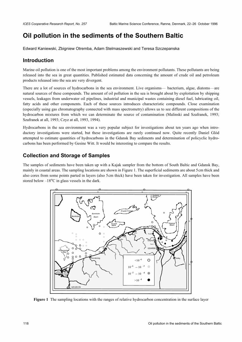
Oil pollution in the sediments of the Southern Baltic118
ICES Cooperative Research Report, No. 257 Baltic Marine Science Conference, Rønne, Denmark, 22–26 October 1996
Oil pollution in the sediments of the Southern Baltic
Edward Kaniewski, Zbigniew Otremba, Adam Stelmaszewski and Teresa Szczepanska
IntroductionMarine oil pollution is one of the most important problems among the environment pollutants. These pollutants are beingreleased into the sea in great quantities. Published estimated data concerning the amount of crude oil and petroleumproducts released into the sea are very divergent.
There are a lot of sources of hydrocarbons in the sea environment. Live organisms— bacterium, algae, diatoms—arenatural sources of these compounds. The amount of oil pollution in the sea is brought about by exploitation by shippingvessels, leakages from underwater oil pipelines, industrial and municipal wastes containing diesel fuel, lubricating oil,fatty acids and other components. Each of these sources introduces characteristic compounds. Close examination(especially using gas chromatography connected with mass spectrometry) allows us to see different compositions of thehydrocarbon mixtures from which we can determinate the source of contamination (Malinski and Szafranek, 1993;Szafranek at all, 1993; Czyz at all, 1993, 1994).
Hydrocarbons in the sea environment was a very popular subject for investigations about ten years ago when intro-ductory investigations were started, but these investigations are rarely continued now. Quite recently Daniel Glódattempted to estimate quantities of hydrocarbons in the Gdansk Bay sediments and determination of policyclic hydro-carbons has been performed by Gesine Witt. It would be interesting to compare the results.
Collection and Storage of SamplesThe samples of sediments have been taken up with a Kajak sampler from the bottom of South Baltic and Gdansk Bay,mainly in coastal areas. The sampling locations are shown in Figure 1. The superficial sediments are about 5cm thick andalso cores from some points parted in layers (also 5cm thick) have been taken for investigation. All samples have beenstored below –18oC in glass vessels in the dark.
Figure 1 The sampling locations with the ranges of relative hydrocarbon concentration in the surface layer
OderLagoon
Wolin
Gdynia
Elbl€g
GDAŃSK
Bornholm
SZCZECIN
Gdańsk Basin
S•upsk FurrowBornholm
Basin
S•upsk Bank
Gotland Basin
Ko•obrzeg
Ustka
ŁebaPuck
Vistula
Lago
onSopot
Hel
10
80
80
18o
16o
14o
20o
55o
54o
20
100
20
100
100
20
80
Pomeranian Bay
-4
-4
-5
-6<10
-- 10
-- 10
>10
-5
-610
10
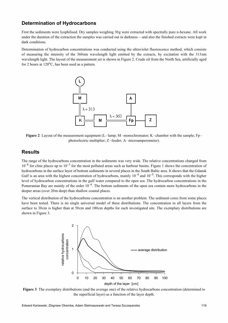
Edward Kaniewski, Zbigniew Otremba, Adam Stelmaszewski and Teresa Szczepanska 119
Determination of HydrocarbonsFirst the sediments were lyophilised. Dry samples weighing 30g were extracted with spectrally pure n-hexane. All workunder the duration of the extraction the samples was carried out in darkness—and also the finished extracts were kept indark conditions.
Determination of hydrocarbon concentrations was conducted using the ultraviolet fluorescence method, which consistsof measuring the intensity of the 360nm wavelength light emitted by the extracts, by excitation with the 313nmwavelength light. The layout of the measurement set is shown in Figure 2. Crude oil from the North Sea, artificially agedfor 2 hours at 120oC, has been used as a pattern.
Figure 2 Layout of the measurement equipment (L–lamp; M–monochromator; K–chamber with the sample; Fp–photoelectric multiplier; Z–feeder; A–microamperometer).
ResultsThe range of the hydrocarbons concentration in the sediments was very wide. The relative concentrations changed from10–8 for cline places up to 10–3 for the most polluted areas such as harbour basins. Figure 1 shows the concentration ofhydrocarbons in the surface layer of bottom sediments in several places in the South Baltic area. It shows that the GdanskGulf is an area with the highest concentration of hydrocarbons, mainly 10–4 and 10−5. This corresponds with the higherlevel of hydrocarbon concentrations in the gulf water compared to the open sea. The hydrocarbon concentrations in thePomeranian Bay are mainly of the order 10–6. The bottom sediments of the open sea contain more hydrocarbons in thedeeper areas (over 20m deep) than shallow coastal places.
The vertical distribution of the hydrocarbons concentration is an another problem. The sediment cores from some placeshave been tested. There is no single universal model of these distributions. The concentration in all layers from thesurface to 30cm is higher than at 50cm and 100cm depths for each investigated site. The exemplary distributions areshown in Figure 3.
Figure 3 The exemplary distributions (and the average one) of the relative hydrocarbons concentration (determined to the superficial layer) as a function of the layer depth.
0
1
2
0 10 20 30 40 50 60 70 80 90 100depth of the layer [cm]
rela
tive
hydr
ocar
bons
co
ncen
tratio
n
average distribution

Oil pollution in the sediments of the Southern Baltic120
Another question is the dependence of the hydrocarbon concentrations on the type of sediment. The organic mattercontent in some samples of sediment has been measured. The organic matter was determined as a decrement of mass of adry sample, which has been roasted at 550oC for 1 hour. This test has not shown any correlation between content oforganic matter and hydrocarbons concentration (correlation coefficient is 0.48). Figure 4 presents the concentration ofhydrocarbons in bottom sediments as a function of their organic matter content.
Figure 4 The hydrocarbon concentrations in the South baltic sediments as a function of their organic matter contents.
ConclusionThe relative hydrocarbon concentrations in sediments of the South Baltic bottom is in general at a level of 10–7 for theopen sea area. This level could be accepted as a level of natural concentration of hydrocarbons. The higher hydrocarbonconcentrations in the Pomeranian Bay sediments (10–6) and specially in sediments of the Gdansk Gulf (up to almost 10–3) show that oil pollution is the essential source of hydrocarbons in this environment. The results of determination ofthe hydrocarbon concentrations in water from open sea, Gulf of Gdansk and river waters [Otremba and Stelmaszewski,1994] confirm this conclusion.
Measurements of the concentrations of the total hydrocarbons is a first step in the investigation of hydrocarbons in thebottom sediments. The results of these measurements could give a general view of hydrocarbon concentrations insediments in several areas. This prospect would also allow us to select the most interesting places and investigate themusing more precise methods.
ReferencesCzyz B., Otremba Z., Stelmaszewski A., Targowski W., 1993. The total fluorescence spectra and prospects of utilising
them to identification of pollution sources. Proc. of the Conference TERB’93, Gdynia, 76–85.
Czyz B., Otremba Z., Stelmaszewski A., Targowski W., 1994. Oil identification by using the total fluorescence spectra.Proc. of the XIX CBO, Sopot, 657–666.
Glód D., 1994. The policyclic aromatic hydrocarbons in the bottom sediments in the Gdansk Bay. Dissertation, Gdynia.
Malinski E., Szafranek J., 1993. Application GC/MS to differentiation and to defining of origin petro- and pirogeniccontaminations in the sea environment. Proc. of the Conference TERB’93, Gdynia, 61–74.
Otremba Z., Stelmaszewski A., 1994. Concentration and Origin of the contaminations in the Gdansk Bay coast water.Proc. of the XIX CBO, Sopot, 630–637.
Szafranek J., Zachowicz J., Szczepanska T., Malinski E., 1993. Cycloalcanes as the molecular markers determiningorigin of contaminations sea with crude oil. Proc. of the Conference TERB’93, Gdynia, 38–52.
Witt G., 1994. Policyclic Aromatic Hydrocarbons in the Baltic Sea. Proc. of the XIX CBO, Sopot, 622–629.
0
10
20
30
40
0 5 10 15contents of organic matter [%]
conc
entra
tion
of h
ydro
carb
ons
[mg/
kg]
G. Witt, K. W. Schramm, and B. Henkelmann 121
ICES Cooperative Research Report, No. 257 Baltic Marine Science Conference, Rønne, Denmark, 22–26 October 1996
Occurrence and distribution of organic micropollutants in sediments of the western Baltic Sea and the inner coastal waters of Mecklenburg–Vorpommern (Germany)
G. Witt, K. W. Schramm, and B. Henkelmann
SummaryThe occurrence and distribution of polycyclic aromatic hydrocarbons, polychlorinated dibenzo-p-dioxins and dibenzo-furans (PCDD/Fs) were investigated in surface sediments (0–2cm) of the Belt Sea, the Arkona Sea and the internal andexternal coastal waters of Mecklenburg–Vorpommern. The concentrations of different toxic PAHs and PCDD/Fscongeners were measured.
Sedimentological properties affect the accumulation of organic pollutants. Strong correlations between concentrations ofPCDD/Fs and the content of organic carbon (TOC) were established. The results were normalised to TOC.
The sum of PAHs varied between 2.1µgkg–1 TOC and 66.5µgkg–1 TOC for muddy sediments in the Belt Sea andArkona Sea. Elevated concentrations up to 46µgkg–1 TOC were observed in the surface sediments of the internal coastalwaters with highest concentrations in the Warnow estuary and in the Oder Haff. This indicates the significant contri-bution of river discharge to the contamination of sediments with PAHs. The distribution of the individual PAHs insediments varies widely depending on their structure and molecular weight. The higher molecular 4 to 6 ring aromaticspredominate due to their higher persistence.
The sum of dioxins varied between 2.1µgkg–1 TOC and 66.2µgkg–1 TOC. Higher concentrations were observed in thesurface sediments of the internal coastal waters especially in the Warnow estuary and the Oder Haff. This indicates asignificant contribution of river discharge to the contamination of sediments with dioxins. Elevated concentrations ofdibenzofurans were observed in the Wismar Bight. The most toxic congener, 2,3,7,8-Tetrachlor-p-dibenzodioxin,(Seveso dioxin) was found at only 4 stations.
The fingerprint profiles of the different congener groups are similar in the whole investigated area. The concentration ofthe dioxins increased with increasing degree of chlorination. Octachlordibenzo-p-dioxin predominates in the wholewestern Baltic Sea and in the internal coastal waters.
IntroductionThe investigations of polycyclic aromatic hydrocarbons, polychlorinated dibenzo-p-dioxins and dibenzofurans have beenextensive during the last few years. These compounds are of high environmental concern due to their toxicity and carci-nogenic activity.
The distribution of PAHs and PCDD/Fs in different areas of the world ocean have been reported by several authors(Bopp et al., 1991; Broman, 1991; Mosse, 1993, but only very few data are available for the Baltic Sea (Witt, 1995;Broman et al., 1993; Zebühr, 1992; Poutanen, 1981) and there is a lack of information for many regions of the Baltic Sea.
The investigated substances mainly originate from domestic and industrial waste water, river run-off and especiallyatmospheric deposition of combustion products. Major sources of industrial processes contributing to their productionare the combustion of fossil fuels, and especially for the PCDD/Fs metallurgical processes, such as chlorine bleaching ofpaper pulp and the production of chlorine compounds (PCBs, Pentachlorphenol).
Atmospheric transport should be a major pathway for the input of PAHs and PCDD/Fs into the aquatic environment. Inthe water column, they become frequently associated with particulate matter due to their hydrophobic nature and mayaccumulate to high concentrations in sediments (Broman et al., 1989).
Sampling areaThe investigated sea area covers parts of the western Baltic Sea and the Baltic Proper. The sampling area also includes alarge system of internal coastal waters—Bodden and Haff areas—along the 340km long southern part of the Baltic

Occurrence and distribution of organic micropollutants in sediments of the western Baltic Sea and the inner coastal waters ofMecklenburg–Vorpommern (Germany)
122
coastline of north-eastern Germany (Mecklenburg–Vorpommern). Boddens and Haffs are lagoons, connected to the seaby shallow or narrow natural sea channels. This coastline is typical for Mecklenburg–Vorpommern. The hydrography ofthe inner coastal seas is governed mainly by changes in the intensity of water exchange with the Baltic Sea. Freshwaterinflow via rivers plays an important role. The main rivers in this area are the Warnow, the Uecker, the Peene and theOder. The inner coastal waters function as pre-purification areas and are thereby a sink for all types of anthropogeniccontaminants.
The investigated surface sediments (0–2cm) comprise muddy sediments with a high amount of organic carbon. Sincesediment structure varies between different sampling sites (grain size effect) a normalisation to TOC was performed tocorrect this effect. This procedure allows us to compare contamination levels between the different areas.
Sample preparation and analysesThe surface sediment samples were collected with a Van-Veen grab (0–2cm). The samples were stored in aluminiumboxes at –21°C until analysis. The water content, the carbon content and the fraction <63µm were determined. Thecarbon content (TC) and inorganic carbon content (TIC) were measured using an ELTRA C/S analyser (METALYT CS1000S). The difference between TC and TIC yields gives total organic carbon content (TOC).
PAH preparation and analysis are given by Witt (1995). PCDD/F analysis is described by Schramm et al. (1995).
Results
Distribution of PAHs in surface sediments The sum of PAHs varied between 7.5µgg–1 TOC and 36µgg–1 TOC in the Belt and Arkona Sea. The highest concentra-tions were found in the river Warnow. There the concentrations varied between 6.2µgg–1 and 15.4µgg–1 TOC (Figure1).
Figure 1 Distribution of PAHs in surface sediments in the investigated area
These high concentrations should be a result of a high anthropogenic input of PAHs in this region. Sources are industrialwaste water especially from the shipyards near Rostock, the traffic around Rostock and coke oven emissions.
The PAH content in the muddy sediments of the Oder Haff and the Peenestrom is also relatively high and ranges between3.45 and 8.14µgg–1 TOC. The Oder river should be the main source of the significantly higher PAH content in theseareas.
The distribution of the individual PAHs varies widely depending on their structure. The higher molecular PAH (e.g.benzo(a)pyrene) predominated due to their higher persistence. A concentration gradient was found with decreasing PAHconcentrations from the Oderhaff to the open sea (Figure 2), suggesting that the Oder river could be the major source ofsignificant higher PAH content in this region.
The concentrations of PAHs are more than 1000 times higher than the concentrations of PCDD/Fs.
* sum of 15 components
11.50 12.00 12.50 13.00 13.50 14.00 14.50
53.60
53.80
54.00
54.20
54.40
54.60
54.80
0 - 5 µg/kg TOC5 - 10 µg/kg TOC
10 - 15 µg/kg TOC15 - 20 µg/kg TOC
> 20 µg/kg TOC
Germany (Mecklenburg-Vorpommern)
Mecklenburg Bight
Oder Bight
Denmark
Oderhaff
RügenDarss
Stralsund
Rostock
Wismar

G. Witt, K. W. Schramm, and B. Henkelmann 123
Figure 2 Concentration gradient of naphthalene from the inner coastal water to the open sea
Distribution of PCDD/Fs in surface sediments
Figure 3 Distribution of PCDDs (a) and PCDFs (b) in the investigated sea area
The concentrations of 15 PCDD/Fs congeners and of the sum of the tetra- (TCDD/F), penta- (PNCDD/F), hexa-(HCDD/F) hepta- (HPCDD/F) and octa- (OCDD/F) dibenzo-p-dioxins and dibenzofurans as well as the total concen-tration of PCDD/Fs were investigated.
The concentrations in the different sediments show wide variations, depending on the investigated region. The totalconcentration of the polychlorinated dibenzo-p-dioxins varied between 2.1µgkg–1 and 66.2 µgkg–1TOC and the concen-trations of the PCDFs ranged between 2.4µgkg–1 TOC and 65µgkg–1 TOC (Figure 3) The 2,3,7,8-TCDD, most toxiccongener was found at only 4 stations.
Naphthalene
2
4
6
8
KHJ KHM P 74 P 48 GB 1 GB10
GB19
131 69 113 109 120
c [µ
g/g
TOC
]
Peene RiverOderhaff Arkona BasinGreifswalder Bodden
Oder-Trough
WB1WB3
22 UW2UW3UW4
DB19
RB10
KB90
GB19
P48
KHJKHM
69 109
131
11.00 11.50 12.00 12.50 13.00 13.50 14.00 14.5053.60
53.80
54.00
54.20
54.40
54.60
54.80
55.00
Rostock
Wismar
Mecklenburg Bight
Oder-haff
Oder Bight
Rügen
Arkona Basin
Darss
Germany
Denmark
2 - 8 µg/kg 8 - 10 µg/kg 10 - 16 µg/kg 16 - 24 µg/kg 24 - 70 µg/kg
WB1WB3
22 UW2UW3UW4
DB19
RB10
KB90
GB19
P48
KHJKHM
69 109
131
11.00 11.50 12.00 12.50 13.00 13.50 14.00 14.5053.60
53.80
54.00
54.20
54.40
54.60
54.80
55.00
Rostock
Wismar
Mecklenburg Bight
Oder-haff
Oder Bight
Rügen
Arkona Basin
Darss
Germany
Denmark
1 - 4 µg/kg 4 - 8 µg/kg 8 - 16 µg/kg 16 - 24 µg/kg 24 - 66 µg/kg
(a)
(b)

Occurrence and distribution of organic micropollutants in sediments of the western Baltic Sea and the inner coastal waters ofMecklenburg–Vorpommern (Germany)
124
The highest concentrations of PCDDs were measured in the river estuaries of the river Warnow and the river Oder(Oderhaff). The concentration of the sum of the investigated dioxins in sediments of the Warnow river ranged between23 and 66.2µgkg–1 TOC. The concentration of the dibenzofurans varied between 5.6 and 9.3µgkg–1 TOC. The values ofthe sediments of the Oderhaff ranged between 9.9 and 21.1µgkg–1 TOC for the sum of the investigated dioxins andbetween 2.4 and 10.4µgkg–1 for the sum of dibenzofurans.
The high concentrations in the Warnow estuary may be a result of a high anthropogenic input of PCDD/Fs in this region.Sources are industrial waste water especially from the shipyards near Rostock, the traffic around Rostock and coalcombustion emissions. High PCDD/Fs concentrations were also measured near the shipyard of the city of Wismar.
The concentration levels of the PCDD/F in the Boddens are rather low compared to the other parts of the investigatedareas. The PCDD concentrations (sum of 6 congeners) ranged between 2.4µgkg–1 and 4.5µgkg–1 TOC in the sedimentsof the Bodden area.
The fingerprint profiles of the different congener groups are similar in the whole investigated area (Figure 4). Theconcentration of the PCDD increased with increasing degree of chlorination (Cl4<Cl5<Cl6<Cl7<Cl8). This trend inconjunction with the presence of Cl4-Cl8 PCDFs strongly suggests the influence of combustion sources. These distri-bution patterns are also reported as typical profiles in air samples (Reed et al., 1990). The most abundant congener in thewhole investigated area was octachlordibenzo-p-dioxin (OCDD). This compound is thought to be a major component ofcombustion produced PCDDs (Marklund et al., 1986). The highest concentrations, up to 54µgg–1 TOC, were analysed inthe Warnow river estuary.
Figure 4 Fingerprint profiles of the different congener groups in the Warnow river estuary
ConclusionsThe distribution of polycyclic aromatic hydrocarbons, polychlorinated dibenzo-p-dioxins and dibenzofurans in surfacesediments of the Arkona Sea, Belt Sea and the inner coastal area of Germany were investigated.
The highest concentrations of these organic micropollutants were recorded at the rivers and Haff areas. In this case, agreat part of the inner coastal waters functions as a trap and a pre-purification basin for organic pollutants which aremainly adsorbed on particulate matter (SPM).
A seaward trend of decreasing PAH concentrations was found especially for the lower molecular weight PAHs. Thistrend was not observed for the PCDD/F congeners due to their higher persistence.
It is difficult to make an assessment of all potential sources of PCDD/F contamination in the western Baltic Sea. Oneimportant source for PAH input to the Oder Haff and the Arkona Basin is the river Oder. Industrial waste water from theshipyards is thought to be the major source for the elevated PAH and PCDD concentrations near Wismar and Rostock.According to the distribution patterns of the individual congener groups of PCDD/Fs another major source might be theatmospheric input of combustion-derived PCDD/F from central Europe.
5
10
15
20
25
30
TCD
D
PN
CD
D
HC
DD
HP
CD
D
OC
DD
TCD
F
PN
CD
F
HC
DF
HP
CD
F
OC
DF
UW2UW3UW4
Warnow River 54,7
30,9
[µg/
kg T
OC
]

G. Witt, K. W. Schramm, and B. Henkelmann 125
ReferencesBopp, R.F., Gross M.L., Tong H., Simpson H.J., Monson S.J., Deck, B.L., and Moser, F.C., 1991. A major incident of
dioxin contamination: Sediments of New Jersey Estuaries. Environ. Sci. Technol., Vol. 25, No. 5, 951–956.
Broman, D., Näf, C., Zebühr, Y., Bandh, C., Ishaq, R., and Pettersen, H., 1993. Occurrence, distribution and turnover ofsome toxic substances un the water mass and sediments in the Baltic Sea. Baltic News, 4, 6–10.
Broman, D., Näf, C., and Zebühr Y., 1991. Long-Term high and low volume air sampling of polychlorinated dibenzo-p-dioxins and dibenzofurans and polycyclic aromatic hydrocarbons along a transect from urban to remote areas onthe Swedish Baltic coast. Environ. Sci. Technol., 25, No. 11, 1841–1849.
Broman D., Näf, C., Rolff C., Zebühr Y., Fry B., and Hobbie J., 1992. Using ratios of stable isotopes to estimate bioaccu-mulation and flux of polychlorinated dibenzo-p-dioxins and dibenzofurans (PCDFs) in two food chains from thenorthern Baltic. Environmental Technology and Chemistry, 11, 331–345.
Marklund, S., Kjeller, L.-O., Hansson, M., Tysklind, M., Rappe, C.; Ryan, C., Collazo, H., Dougherty, R. (1986). Deter-mination of PCDDs and PCDFs in incineration samples and pyrolytic products. In: Chlorinated dioxins anddibenzofurans in perspective; Rappe, C., Ryan, C., Choudhary, G., Keith, L.H., Eds.; Lewis Publishers: Chelsea,MI, 79–92.
Mosse P.R.L., and Haynes D., 1993. Dioxin and furan concentration in uncontaminated waters, sediments and biota ofthe Ninety Mile Beach, Base Strait Australia. Mar. Pollut. Bull., 26, 465–468.
Näf, C., 1991. Some biotic and abiotic aspects of the environmental chemistry of PAHs (polycyclic aromatic hydro-carbons) and PCDD/Fs (polychlorinated dibenzodioxins and dibenzofurans). Thesis. Department of AnalyticalChemistry, Stockholm University, ISBN 91–87272–24–5, 66 pp.
Poutanen, E.L., 1988. Hydrocarbon concentrations in water and sediments of the Baltic Sea. In: Proceedings of the 16thconference of Baltic Oceanographers, 882–892. Institute of Marine Research of Kiel, Germany.
Schramm, K.W., Henkelmann, B., Kettrup, A., 1995. PCDD/F sources and levels in river Elbe sediments, Wat. Res., 29,2160–2166.
Wenning, R.J., Paustenbach, D.J., Harris, M.A., Bedbury, H., 1993. Principal component analysis of potential sources ofpolychlorinated dibenzodioxins and dibenzofuran residues in surficial sediments from Newark Bay, New Jersey.Arch. Environ. Contam. Toxicol., 24, 271–289.
Witt, G., 1995. Polycyclic aromatic hydrocarbons in water and sediment of the Baltic Sea. Mar.Pollut.Bull., 31, 237–248.
Zebühr, Y., 1992. Trace analysis of polychlorinated dibenzo-p-dioxins and dibenzofurans and related compounds inenvironmental matrices, Department of Analytical Chemistry, Stockholm University, 1992.

Sedimentation rate variabilities in the eastern Gotland Basin126
ICES Cooperative Research Report, No. 257 Baltic Marine Science Conference, Rønne, Denmark, 22–26 October 1996
Sedimentation rate variabilities in the eastern Gotland Basin
Christian Christiansen, Helmar Kunzerdorf, Kay-Christian Emeis, Rudolf Endler, Ulrich Struck, Dagmar Benesch, Thomas Neumann and Vadim Sivkov
AbstractThis study examines sedimentation rates with a variety of methods. In contrast to previous studies they reveal bothspatial and temporal variations in the rates. High resolution seismic recordings and correlation with long sediment coresshow increased thickness of strata and higher sedimentation rates (0.8mma–1) in the SE part of the deep basin than in theNW part (0.2mma–1) since the Littorina transgression some 7650 years B.P. On shorter time scales, estimates ofsedimentation rates based on radiometric dating (210Pb) are in general twice as high as those observed 25 years ago withthe same method. This may partly be due to eutrophication, as more carbon is buried in the sediment, and partly due toincreased erosion in shallow water areas. However, strong lateral variations are observed. The average rate variesbetween 119 and 340 gm–2a–1 (corresponding to 2.1–2.5mma–1) in the deepest part of the basin. Very high rates of 6100gm–2a–1 (30mma–1) are observed in an intraslope basin off the coast of Latvia at a water depth of only 70m. The radio-metrically determined rates are up to three times higher than rates estimated from average water column concentrationsof suspended matter.
IntroductionSedimentation rates in depositional areas of the Baltic Sea mirror the extent of erosion in the catchment area on land andon the sea floor as well as the state of the chemical and biological environment. They are influenced by riverinedischarge, by hydrography, by climatic changes, and by increased biological production as a consequence of an increasedsupply of nutrients. Oxic or anoxic conditions on the sediment water interface determine whether laminated sedimentsare deposited at any given time.
A number of methods have been used to evaluate sedimentation rates in the Baltic Sea. By counting varves in postglacialsediments, Ignatius (1958) found that the rate was approximately 1mma–1 over a period of about one thousand years.Ignatius et al. (1971) used the depth of dry substance deposited in the Gotland Deep during the last 7000 years to suggesta sedimentation rate of approximately 1mma–1. 210Pb dating of recent upper unconsolidated sediment from thebeginning of the 1970s yielded modern sedimentation rates that were 1.0–1.3mma–1 (Niemestö & Voipio, 1974). Similaror slightly higher rates were observed by a number of authors e.g. Suess (1978). Such observations supported theconclusion reached by Ignatius et al. (1981) that “the rate of sedimentation has been surprisingly uniform for severalthousand years” in the Gotland Basin.
Recent studies have shown greater variabilities in sedimentation rates. Biostratigraphical methods were used by Gelum-bauskaite & Grigelis (1995) to infer that 540mm were deposited at a deep water station in the Gotland Basin during thelast millennium, whereas only 25mm were deposited on the saddle between the Gotland Deep and the Faro Deep in thesame period of time. Varve-counting in the upper 5cm of recent laminated sediments (Jonsson et al. 1990) showedsedimentation rates in the range 1.5–4.2mma–1. Many shallow water parts of the Baltic Sea are non-depositional. Thedepth limit of deposition depends both on the wave base and the position of the permanent pycnocline. Therefore thedepth limit is situated at a depth of about >50m in the western part of the Baltic around the Bornholm Basin (Christiansen& Emelyanov, 1995), and about a depth of >80m in the Baltic proper (Jonsson et al., 1990).

Christian Christiansen, Helmar Kunzerdorf, Kay-Christian Emeis, Rudolf Endler, Ulrich Struck, Dagmar Benesch, Thomas Neumann and Vadim Sivkov
127
Figure 1 Location map showing seismic line and core sampling positions in the Gotland Basin. Isobaths in m.
The purpose of this paper is to study sedimentation rate variabilities and to reconcile the diverging estimates. For thispurpose we have used a number of the above methods in the Gotland Basin (Figure 1).
Methods and MaterialA GeoChirp Subbottom Profiler was used for acoustic surveys during the expedition (1994) with R/V “A. v. Humboldt”.The Chirp profiler (transmitting signals 2–8kHz or 1.5–11.5kHz, depending on operating mode) consisted of a deck unitand a tow fish. The penetration depth of the unit was up to 40m below the seafloor and typically had high resolution(0.3–0.5 m). Based on results of the acoustic surveys, sediment stations were targeted to areas where echogramsindicated either high sediment accumulation and a sufficiently resolved recent sediment cover, or where acoustic unitswere within reach of the gravity coring techniques used. Different tools were used to obtain sediment samples.
1. A multi-corer provided up to eight sediment cores from an area of 1.5m2 to a depth of 45cm and recovered bottomwater and an intact sediment/water interface. Several of these subcores were sliced in 1cm thick discs on board andeither stored frozen for shore-based analyses or were left intact for radiometric dating.
2. For longer cores a gravity corer with an inner plastic liner was used. The corer had a top weight of 1200kg. Amaximum length of 10m sediment was recovered with this weight, which was found to be sufficient for penetratingthe soft sediment of the Gotland Basin to the icelake stage. The liners were cut into sections of 1m length, capped,and stored for shore-based logging of p-wave velocity, magnetic susceptibility, bulk density with a gamma-ray atten-uation porosity evaluator, and structures with a 600 dpi grey-scale scanner in a GEOTEC Multisensor Track.
3. Finally, a Kastenlot of 15x15cm diameter and variable length was used, weighted by 1200–2200kg lead. The longestcore recovered with this tool was 970cm. These cores were opened on board, slabs and u-channels were taken overthe entire length for x-ray photography and magnetic measurements, and the cores were described after visual exami-nation.
Recent net sedimentation rates were determined from dating of multicores using low-level Gamma-spectrometricmeasurements. Measurements of 210Pb, 137Cs, and 226Ra activities were carried out using a reverse-electrode coaxialGe-detector (10 percent rel. efficiency) with energy resolution values of 640eV (at 5.9keV) and 1.7keV (at 1332keV).Subtracting 210Pb supported, i.e. the amount equivalent to the 226Ra activity, the unsupported activity 210Pbunsup is usedto estimate linear sedimentation rates for the cores using the constant initial concentration (CIC) model of interpretation.

Sedimentation rate variabilities in the eastern Gotland Basin128
The historical profiles were constructed using petrophysical core data (density and porosity) and the constant rate ofsupply (CRS) model for 210Pb.
Under stationary conditions in the sea bottom layer there is a sedimentation-diffusion equilibrium, or a vertical distri-bution of suspension concentration, at which the gravity flow of sedimentary particles is balanced by the process of verti-cally oriented diffusion. A concentration gradient is caused by gravity, which results in downward flux of suspensionsPS:
(1)
where U = settling velocity of suspended particles and C = concentration of particles.
According to Fick’s first law, the gradient of concentration gives rise to a diffusive flow Pd, directed upwardly:
(2)
where D = coefficient of turbulent diffusion, C = concentration of suspension, z = depth.
Thus, the sedimentation-diffusion equilibrium can be expressed as follows:
(3)
By integrating equation (3), using separation of variables, we will obtain the exponential (logarithmic) law of verticaldistribution of suspension. If suspension concentration in close proximity to the bottom C0 is considered as a boundarycondition, the following expression is available as a result of integration:
(4)
where and Cz = concentration of suspended matter at a distance z from the bottom.
To calculate α, and further U, we will use expression (4).
Suspension concentrations, found by Stryuk (V.L. Stryuk, personal communication) in the course of expeditions carriedout in the central part of Gotland Deep by the Atlantic Branch of the Russian Academy of Science during the last decade,were used as original data for computations. A total of 170 concentration values, obtained by means of nuclear filters(ultra-filtration method), having pore diameter of 0.45µm have been used to build up an averaged vertical profile ofsuspension concentration.
Results
Long term sedimentation ratesExamining the high-resolution seismic record of the mud distribution, a clear asymmetry in the thickness of the mostrecent basinal sediment is discerned (Figure 2). The asymmetry must be a reflection of a deep circulation system in theGotland Basin, which induces sediment winnowing and accumulation and which results in spatially heterogeneoussediment records at the deep basin floor. Based on the reflector geometry, the asymmetric deposition of sediment in thedeep basin began immediately after brackish conditions of the current Littorina stage of Baltic Sea development wereestablished some 7650 years ago. From the reflector geometry, sedimentation rates generally vary from 0.2mma–1 in thenorth-western part of the deep basin over 0.4mma–1 in the central part of the basin to 0.8mma–1 in the south-eastern part.
PS UC=
Pd D– dCdz-------=
UC D– dCdZ-------=
CzC0------ ln αz–=
α UD----=

Christian Christiansen, Helmar Kunzerdorf, Kay-Christian Emeis, Rudolf Endler, Ulrich Struck, Dagmar Benesch, Thomas Neumann and Vadim Sivkov
129
Figure 2 NW-SE seismic profile across the Gotland Basin. The stratigraphy is based on core correlations. For location of the line see Figure 1.
Recent sedimentation rates from concentrations of suspended matterThe vertical concentration profile of suspended matter, in the region with depths ranging from 120 to 220m, is notexponential (Figure 3). This suggests an occurrence of sedimentation-diffusion inbalance due to action of additionalsources of suspension. At these depths two such sources occur:
1. crystallisation of Fe, Mn and other elements from solution at the geochemical barrier H2S–O2
2. resuspension of bottom deposits by bottom currents, especially over slopes of the basin, where decreased stability ofsediments occurs
As the water column in Gotland Deep is strongly stratified, the gravity sedimentation of suspension material, suppliedfrom the above mentioned sources, is hindered, resulting in accumulation of suspension at a depth of the sources. At adepth below the level of 220m the Gotland Deep bottom flattens, reducing conditions predominate in the water column,while the above mentioned sources are inessential. Thus, the assumption of sedimentation-diffusion balance maygenerally be valid in the deepest layer of Gotland Deep (220–240m). Therefore, the computations were carried out usingdata from this layer only.
Using C0 = 1.1mg l–1, z = 20m, Cz = 0.60mg l–1, according to means of observations (Figure 3), the followingexpression is derived:
α = 0.03 (m–1)=3·10–4 (cm–1)
Taking the coefficient of vertical turbulent diffusion D to be equal to 1cm2 s–1 (Dyer, 1986), the settling velocity will beas follows:
U=αD= 3·10–4 (cm s–1)
Since the vertical flow of suspension Pz is determined as Pz = UCz, then for the bottom level (where Cz = C0) it willamount to:
P0=(3·10–4) · (1.1·10–3) = 3.3·10–7 (mgcm2 s–1) = 106 (gm–2year–1)
This value of P0 characterises the minimal possible rate of sedimentation, because besides gravitational sedimentationthere are other mechanisms of sediment accumulation (saltation, sliding over slope, redeposition, authigenous sedimen-tation).

Sedimentation rate variabilities in the eastern Gotland Basin130
Figure 3 Vertical profile of suspension concentration in the Gotland Deep. Dotted linesshow the geochemical “O2–H2S” barrier.
Recent sedimentation rates from datingThe accumulation rates calculated from 210Pb profiles and determination of physical properties are highly variable andreflect very different sedimentation rates (Table 1). However, we are confident that they represent true trends and rates,because the 137Cs profiles resulting from the Chernobyl accident corroborate the 210Pb datings in all cores and none hadirregular features that indicate hiatuses. In the basinal stations, the accumulation rates range from 119 (upper portion ofcore 20004) to 322gm–2a–1 at the site of core 20001. The calculated sedimentation rates are between 2.1 and 2.5mma–1,respectively. The slope station 20000 displays a disturbed upper layer of 8cm thickness; fitting the 210Pb profile belowthis interval suggests an accumulation rate of 340gm–2a–1 and an average sedimentation rate of 2.5mma–1. The station20008 in a small intraslope basin (68m water depth) has uncharacteristically high sedimentation and accumulation rates:The data suggest that the sediment accumulates at a rate of 6100gm–2a–1 and has an average sedimentation rate of30mma–1. Using wave prediction formula, storm with winds from the west in the area of this intraslope basin may reachthe following characteristics: height ~5m, length ~100m and period ~8s. Near-bottom maximum orbital velocities forsuch waves in areas with a depth of 40–50m can reach 20–30cms–1. Such orbital velocities exceed the threshold velocityfor grains with sizes of up to 60µm (Christiansen & Emelyanov, 1995). Therefore, the very high sedimentation rate in thebasin most probably reflects intensive shallow water erosion along the rim of the basin.
Table 1 Dating results for the cores
Stations on the steep eastern slope of Gotland Basin have disturbances in the depth profiles of both 210Pb and 137Csactivity in the upper centimetres of the sediment (Figure 4). There is no decrease in 210Pb activity, which suggests
Core PositionAverage sediment
rate (mma–1)
Average sediment accumul. rate
(g m–2a–1)Remarks
20001 57o 18.33 N200 03.00 E
2.1 ± 0.1 322 ± 79
20004 57o 18.28 N20o 13.66 E
2.5 ± 0.1 279 ± 37
20007 57o 23.32 N20o 15.15 E
4.3 ± 0.6 238 ± 19 Disturbed surface
20000 57o 15.17 N20o 33.64 E
2.5 ± 0.5 340 ± 30 Disturbed surface
20038 3.5 ± 0.3 399 ± 32 Disturbed surface
20008 57o 27.60 N21o 09.60 E
30 ± 6 6099 ± 1860 Doubtful core

Christian Christiansen, Helmar Kunzerdorf, Kay-Christian Emeis, Rudolf Endler, Ulrich Struck, Dagmar Benesch, Thomas Neumann and Vadim Sivkov
131
sediment mixing and the 137Cs activity increases towards the top which indicate that the mixed layer is settled fromsuspension. Further, grainsize analysis from station 798 (Figure 5) corroborate such observations in that a general fining-upward sequence in the upper layer is twice abruptly interrupted by sediment coarsening. These observations togetherindicate that the sediment disturbance is not due to bioturbation. The Chernobyl peak in 137Cs is displaced with depthindicating that the disturbance has taken place in recent years.
Figure 4 Radiometric profiles of sediment cores from the Gotland Basin. For location of sampling position see Figure 1. A) Depth profiles of supported 210Pb activities.
B) Depth profiles of 137Cs activities.
Figure 5 Down-core variations in grain-size and organic matter content of the slope core 20000.
DiscussionThe areal asymmetrical distribution of long term sedimentation rates with high rates in the southeastern basinal part maybe an indication of winnowing of the steep southeastern slope and lateral transport, as well as for possible contouritedeposition in a depth interval characterised by anticlockwise currents around the rim of the Gotland Basin and at deeperlevels. Observational data supporting this view of a dynamic deep-basin sedimentary environment have been collectedduring GOBEX (Mittelstaedt, 1994). Even though detailed measurements of near-bottom currents are scant in theGotland Basin, initial observations suggest that current speeds at the sediment/water interface are of the order of 1–3cms–1 over periods of days, reaching maxima of up to 20cms–1 during events of hourly duration (E. Hagen, pers.comm. 1995). The image of a stagnant, quiescent and anoxic sedimentary environment in the Gotland Basin thus may beerroneous.
Such a conclusion is corroborated by additional evidence. Estimated sediment accumulation rates from the averagedsuspended matter concentration profile were generally 3 times smaller in the central basin than rates from core datings,indicating more sources of sedimentation than primary sedimentation. There is a strong variation in the vertical concen-tration of suspended matter on Figure 3. However, the estimated sediment accumulation rates (106gm–2y–1) are in

Sedimentation rate variabilities in the eastern Gotland Basin132
reasonable agreement with observations from sediment trap studies. Saarso (1995) observed that fluxes in traps rangedfrom 33–107gm–2y–1. One additional sediment source may be sliding of sediment on slopes. This is evidenced by obser-vations that cores taken on the slope to the central basin had disturbances in their radiometric profiles and their downcoregrain-size distributions showed signs of redeposition. Further, geochemical data from the present cores show differencesbetween the deep basin and the slope in enrichment patterns of organic matter (and associated trace elements) and ofsulphides (and associated trace elements), suggesting lateral transport (Emeis et al., 1996).
Recent net sedimentation rates from the present study seem to be 1.5–2 times higher than observed from 210Pb datings20–25 years ago (Ignatius et al., 1971; Niemestö & Voipio, 1974). The present study thereby corroborates the findingsby Jonsson et al. (1990) estimated from varve counting in recent laminated sediments. A number of factors may explainthis apparent increase in sedimentation rate:
1. It may be accidental in that only a few number of datings are involved and the regional variability seems to be high. Ina much smaller area in the southwestern Kattegat Christiansen et al. (1996a) observed a high variability in thatsedimentation rates on accumulation bottoms ranged from 469 to 4290 gm–2a–1.
2. An increase in organic matter is observed in the upper parts of the present cores (Figure 5, see also Neuman et al.,1996). Such observations corroborate the estimations made by Jonsson & Carman (1994) that in general, a more than1.7-fold increase in sediment organic matter content has taken place in the Baltic proper between the late 1920s andthe late 1980s. This may be explained by higher primary production in connection with the present eutrophication.
3. A 16 year long period of bottom water anoxia in recent years (Neumann et al., 1997) may have contributed to betterpreservation of organic matter and authigenetic mineral production.
4. Erosion of shallow water sediments seems to be the major source of sedimentation in the Gotland Basin. In theirnutrient budget for the Baltic proper Jonsson et al. (1990) found that as much as 85% of the organic matter andnutrients sequestered in the laminated sediments in the Baltic deeps may have originated from shallow water erosion.Such observations have been corroborated by resuspension studies (Christiansen & Emelyanov, 1995). Shallow watererosion may have been enhanced in recent years. This is apparently the case in the southern Kattegat where a shift inthe wind regime has caused increased coastal and shallow water erosion (Christiansen et al. 1993) and induced highersedimentation rates since the beginning of the 1970s (Christiansen et al. 1996b). Also, the number of storm surges onthe German Baltic coast has increased in the last decades (Baerens & Hupfer, 1995).
AcknowledgementsC. Christiansen and V. Sivkov gratefully acknowledges the invitation from the Institute of Baltic Sea Research to takepart in one of their R/V “Alexander von Humboldt” expeditions to the Gotland Basin. This research was performed underthe Gotland Basin Experiment (GOBEX) as part of the ECOPS Baltic Sea Initiative.
ReferencesBaerens, C. & Hupfer, P., 1995: On the frequency of storm surges at the German Baltic coast. Proceedings of the 19th
Conference of the Baltic Oceanographers, Sopot. Vol. 1, 311–316.
Christiansen, C., Christoffersen, H. & Binderup, M., 1993: Coastal and near shore erosion at Vejrø, Denmark: Combinedeffects of a changing wind climate and near shore dredging. In: Sterr, J., Hofstede, H.-P. & Plag, P. (eds.):Proceedings of the International Coastal Congress, ICC. Verlag Peter Lang, Frankfurt. 566–575.
Christiansen, C. & Emelyanov, E., 1995: Nutrients and organic matter in southern Kattegat western Baltic Seasediments: Effects of resuspension. Danish Journal of Geography. 95, 19–27.
Christiansen, C., Gertz, F., Laima, M. J. C., Lund-Hansen, L. C., Vang, T. & Jürgensen, C., 1997: Nutrient dynamics inthe southwestern Kattegat, Scandinavia: Sedimentation and resuspension effects. Environment. Geol. 29, 66–77.
Christiansen, C., Kunzendorf, H., Laima, M. J. C., Lund-Hansen, L. C. & Pedersen, A. M., 1996: Recent changes inenvironmental conditions in the southern Kattegat, Scandinavia. Norges geologiske undersøkelse. Bulletin. 430,137–144.
Dyer, K. R., 1986. Coastal Estuarine Sediment Dynamics. Chichester, Wiley. 342p.

Christian Christiansen, Helmar Kunzerdorf, Kay-Christian Emeis, Rudolf Endler, Ulrich Struck, Dagmar Benesch, Thomas Neumann and Vadim Sivkov
133
Emeis, K.-C., Neumann, T., Endler, R., Struck, U., Kunzendorf, H. & Christiansen, C., 1996 Geochemical records ofsediments in the Gotland Basin—products of sediment dynamics in a not-so-stagnant anoxic basin? AppliedGeochemistry (submitted)
Gelambauskaite, Z. & Grigelis, A., 1995: Contribution to geomorphology of the Gotland depression. GOBEX-Newsletter. 2/5, 4–11.
Ignatius, H., 1958: On the rate of sedimentation in the Baltic Sea. Bulletin de la Commission géologique de Finlande.180, 135–145.
Ignatius, H., Axberg, S., Niemestö, L. & Winterhalter, B., 1981: Quaternary geology. In: Voipio, A. (Ed.): The BalticSea. p. 54–104.
Ignatius, H., Niemestö, L. & Voipio, A., 1971: Variations of redox conditions in the recent sediments of the GotlandDeep. Geologi. 3, 43–46.
Jonsson, P., Carman, R. & Wulff, F., 1990: Laminated sediments in the Baltic—A tool for evaluating nutrient massbalances. Ambio. 19, 152–158.
Mikkelstaedt, B., 1994: Preliminary results of a hydrographic survey in November/December 1993 with R/V Gauss: Thesubsurface circulation in the Gotland Deep. GOBEX Newsletter. 2/94, 3–5.
Neumann, T., Christiansen, C., Clasen, S., Emeis, K.-C. & Kunzendorf, H., 1997: Geochemical records of salt-waterinflow into the deep basins of the Baltic Sea. Continental Shelf Research. 17, 95–115.
Niemestö, L. & Voipio, A., 1974: Studies on the recent sediments in the Gotland Deep. Havforskningsinstitutets Skrift,Finland. 238, 17–32.
Saarso, M., 1995: Vertical variability of particulate flux in the Baltic Sea. In: Floderus, S., Heiskanen, A.-S., Olesen, Mand Wassmann, P. (eds): Sediment trap studies in the Nordic countries. 3. Symposium Proceedings. NurmiPrint,Nurmijarvi. p. 168–183.
Suess, E., 1978: Distribution between natural and anthropogenetic material in sediments. In: Goldberg, E. D. (Ed.)Biogeochemistry of Estuarine Sediments. UNESCO, Paris. p. 224–237.

Acoustic images of Gotland Basin sediments134
ICES Cooperative Research Report, No. 257 Baltic Marine Science Conference, Rønne, Denmark, 22–26 October 1996
Acoustic images of Gotland Basin sediments
R. Endler, K.-C. Emeis and T. Förster
AbstractHigh resolution acoustic profiling using chirp sonar technology was performed in the Gotland Basin as part of theGotland Basin Experiment (GOBEX). Digital processing techniques of acoustic data were used to epitomise the acousticimages for general views of the entire postglacial sediment sequence as well as for detailed investigations of the acousticcharacter of selected layers and structures. Based on the acoustic results, core sampling locations were selected foroptimal recovery of sediments representing the depositional environment of the central Baltic Sea.
The acoustic data clearly reflect the character and development of the sedimentation processes (depositional, nondeposi-tional, erosional) in the several regions of the Gotland Basin. Up to nine major acoustic units can be separated in theprofiles. They encompass the entire late glacial and postglacial series starting from the glacial till and ending with therecent very soft mud. It is possible to trace them over the entire central basin. Baltic Ice Lake sequences show ratherlimited lateral variations in thickness and mainly follow the relief of the underlying till. In contrast, the thickness of theLitorina sequence increases from WNW to ESE and has a maximum thickness at the base of the sharp ESE basin slopeoffshore Latvia. This implies a change in the hydrographic/depositional regime since the end of the Baltic Ice Lake stage.
The first results presented demonstrate the high potential of the acoustic method which may contribute to the betterunderstanding of the structure, of the recent depositional processes, and of the Holocene development of the Gotlandbasin. Further work in the frame of the GOBEX activity will concentrate on the detailed recognition and geological inter-pretation of the different reflectors and structural features based on multi-sensor core logging and acoustic modelling.
The Gotland Basin Experiment (GOBEX)The Gotland Basin (Figure 1) is the largest basin of the Baltic Sea. Because of its size, its location between northern andsouthern Baltic Sea and its properties it was chosen as a region for integrated studies of the recent oceanographic,biological, chemical and geological environment as well as of the geological history. The water column (with a thicknessof about 240m in the central part) is usually well stratified causing anoxic conditions at the sea bottom. Because of thisthe sedimentary history is well preserved in the laminated sequences (no bioturbation). The present study focuses on thephysical (mainly acoustic) properties of the sediments in order to reconstruct the postglacial history of the basin.
Figure 1 GOBEX working area

R. Endler, K.-C. Emeis and T. Förster 135
Material and MethodsIn the frame of the GOBEX activity one expedition with R/V “A. v. Humboldt” (1994) and two cruises with R/V“Poseidon” (1995, 1996) were performed to collect acoustic profiling data and sediment samples (Figure 1). A GeoChirpsubbottom profiling system (GeoAcoustics) consisting of the tow fish (transmitter, receiver), the chirp-processor, a SonarEnhancement System (SES) and a thermo-recorder (Wideline 200/138, Ultra Electronics) were used for acousticsurveys. The bandwidth of the transmitted acoustic pulses was 2–8kHz with a duration of 32ms. Reflected acousticsignals were received by a ministreamer (which was attached to the end of the tow fish), amplified and sent to the chirp-processor for matched filtering (signal compression). Further onboard processing, on-line printing and digital storing(SEGY format, 8mm ExaByte) were performed with the Sonar Enhancement System. Navigation data were collectedfrom a GPS receiver (Sercel NR51, WGS84). During profiling the tow fish was towed at a depth of about 20m (due tolimited cable length) and with a speed of about 5 knots. Two pulses per second were transmitted giving a firing distanceof about 1.3m (at 5 knots). Depending on the sediment type a penetration down to 40m was achieved with a verticalresolution of about 0.3–0.5m. Later on, postprocessing using an extended Seismic Unix-package (Cohen & Stockwell,1994) was performed on an IBM R6000 workstation. The general structure of the postglacial sediments is depicted bytwo GeoChirp profiles in Figure 2 and Figure 3.
Figure 2 Acoustic image of Gotland Basin sediments—transversal sectiona) Geochirp line 940823 western partb) GeoChirp line 940823 eastern part
Major acoustic reflectors are named by letters (sound velocity for time to depth conversion: 1450ms–1)
Figure 3 Acoustic image of Gotland Basin sediments—longitudinal sectiona) GeoChirp line 940830 northern partb) GeoChirp line 940830 southern part
Major acoustic reflectors are named by letters (sound velocity for time to depth conversion 1450ms–1)
a) b)
b)a)

Acoustic images of Gotland Basin sediments136
Based on the acoustic records a variety of sediment sampling locations were selected. Gravity corers (6m, 12m) withplastic liners were used for sampling the postglacial sediment layers. After recovery the liners were cut into 1m sections,capped and stored (4°C). The physical properties of the split sediment cores were measured with a Multi Sensor CoreLogger (MSCL, GEOTEK): optical scan of sediment surface along the core (by gray scale line scanner), wet bulk density(by gamma ray attenuation), sound velocity (by 500kHz pulse transmission) and magnetic susceptibility (Bartington loopand point sensors). Based on the logging data subsamples were taken for further analyses. First results of the measure-ments on core 20048 are presented in Figure 4.
Figure 4 Physical properties of Gotland Basin sediments—results of MSCL logging core 20048 SL
Results and DiscussionIn general the central Gotland Basin shows an asymmetric structure. Along the longitudinal basin axis (Figure 3) thewater depth slowly increases from about 140m in the north to about 240m in the central part. Further to the south thecentral basin is bordered by a small elevation with water depth of 230m. The same asymmetric morphology is displayedin the cross section of Figure 2.
The acoustic images of Figure 2 and Figure 3 reflect the structure of the postglacial basin fill which is well penetrated bythe acoustic signals. In general the sediments are well layered. Based on the acoustic characteristics a variety of majorreflectors were chosen, marked by letters and traced by lines. Because a definitive link from all the acoustic reflectors tothe several sedimentological sequences is not yet established, the choice of the reflector names is not based on sedimen-tological units (e.g. Andren & Sohlenius, 1995).
The lower light line I marks the very rough surface of the glacial deposits (sand, gravel, till). The next sequence up toreflector D contains the varved clays of the Baltic Ice Lake. The thickness of this sequence is approximately 20m and isnearly constant over the entire central basin. During that time sedimentation was rapid without lateral transport (no nearbottom currents). From the acoustic image, the varved clays of the Baltic Ice Lake can be subdivided into several unitsseparated by the reflectors H, G and E. This set of reflectors in the varved clays suggests that the sedimentation duringthe Baltic Ice Lake was not only influenced by seasonal variations (varves) but also by depositional, possibly climaticchanges of longer periods. The sediments below reflector H show an acoustically turbulent image in the very centralbasin whereas a band of reflections appear in the more distal regions. A very prominent reflector is G (from the signalstrength) which is the lower boundary of a strong reflection sequence. This reflector can be traced over the entire basin.The reflection band is bounded at the upper end by the reflector F (not indicated in the figures). A rather transparentregion follows up to reflector E indicating continuous sedimentation during this period. In the interval between reflectors
R. Endler, K.-C. Emeis and T. Förster 137
G and E, black and irregularly distributed dots appear over the entire basin. It is unclear whether these spots are causedby diagenetic processes or local anomalies during sedimentation.
In Figure 4 an enlarged part of the acoustic record at station 20048 is compared with the core log depth profiles. Thesubbottom depth of the selected reflectors is calculated with a sound velocity of 1400ms–1 and marked in the loggingprofiles. The acoustic reflectors correspond to gradients in the acoustic impedance profile. Most prominent changes inthe physical properties occur in the subbottom depth interval between 6m (reflector D) and 4.5m (reflector C) indicatingthe transition from typical Baltic Ice Lake sedimentation (varved clays) to the younger Littorina environment (transitionclays of Ancylus and Yoldia stages according to Winterhalter, 1992). The reflector D also marks a change in thesedimentation regime. As a result of strong lateral sediment transport (start of the near bottom circulation) the thicknessof the sediments overlying reflector D continuously increases from west towards the steep eastern slope of the basin(Figure 2). A maximum thickness of about 12m is reached just at the lower edge of the eastern slope. The uppermostband of reflections bounded by reflectors B and A (surface of the recent mud) shows the transition from well laminatedgyttja clays of the Litorina stage to the recent very soft, black sulphitic mud. Because of the high water content theuppermost mud is easily transported by lateral currents.
ConclusionsIt was demonstrated that the physical properties of the sediment column clearly reflect the variations in the sedimentaryenvironment during the postglacial history of the Baltic Sea. They give important additional information for paleoenvi-ronmental reconstructions which can not be obtained by other methods.
ReferencesAndren, T. & Sohlenius, G. (1995). Late Quaternary development of the north western Baltic Proper—results from the
clay-varve investigation. Quaternary International, Vol. 27, pp. 5–10
Cohen, J. K. & Stockwell, J. (1994). Seismic Unix, V. 22 ff. Center for Wave Phenomena, Colorado School of MinesGolden, CO 80401; [email protected]
Winterhalter, B. (1992). Late-Quaternary Stratigraphy of Baltic Sea Basins—a Review. Bull. Geol. Soc. Finland 64, Part2, 189–194

Water exchange, nutrients, hydrography, and database of the Gulf of Riga138
ICES Cooperative Research Report, No. 257 Baltic Marine Science Conference, Rønne, Denmark, 22–26 October 1996
Water exchange, nutrients, hydrography, and database of the Gulf of Riga
Pekka Alenius
AbstractThe Gulf of Riga is a semi-enclosed basin connected by two straits to the Baltic Sea. One of the straits, the Irbe Strait, isbroad and the other, Suur Strait, is small. The Gulf of Riga receives large fresh water inputs from rivers. There iscontinuous water exchange between the Gulf and the Baltic Sea through the straits. The processes governing the waterexchange and the water and material balances have been subjects of the physical oceanography sub-project of a jointNordic Baltic research programme, the Gulf of Riga project, within the Nordic Environmental Programme 1993–1997financed by the Nordic Council of Ministers. The research programme included a three year field experiment period in1993–1995 and continues with data analysis and a modelling phase in 1996–1997. This paper gives an introduction to thesub-projects of the physical programme in the Gulf of Riga Project. Extensive measurements in both straits have givenqualitative and quantitative pictures of the exchange processes. The observations show that both of the straits areimportant in the overall water exchange. The processes in the large Irbe Strait are more complicated than in the smallSuur Strait. The Suur Strait, however, also contributes significantly into the water exchange because the unidirectionalsimple exchange can have significant volume fluxes. Both methodologies and databases for reliably estimating the totalamounts of nutrients in the Gulf have been further developed within the project. Numerical modelling with several typesof models are being continued. The models include both 1D models and 3D models up to a 3D ecosystem model. Acommon Gulf of Riga database has been established during the project. The project is considered to be a continuation tothe valuable research carried out over the last decades by Estonian and Latvian oceanographers in the Gulf of Riga.
Introduction In 1991 the Nordic Council of Ministers declared a Nordic Environmental Research Programme 1993–1997. Theprogramme has three main fields of interest:
1. Research on climate changes2. Co-operation on Environmental Research in the Baltic Sea region: The Gulf of Riga Project 3. Research on the socio-economic and political requirements related to the implementation of environmental policiesThe projects began by inviting letters of intent of relevant research in these fields. In late 1992, after numerous letters ofintent, the expert committee of the Gulf of Riga Project decided to support 18 co-operation projects. They also decided tocollect the projects under five coordinated sub-projects:
1. “Drainage basin and the load of the Gulf of Riga”2. “Pelagic eutrophication”3. “Sediment and benthos”4. “Water exchange, nutrients, hydrography and data base”5. “Toxic substances”In 1995 a sixth sub-project was established:
6. “Production and transformation of nutrients in the littoral zone”This paper briefly describes sub-project 4 of the Gulf of Riga Project.
Structure of the water exchange project The “Water exchange, nutrients, hydrography and data base” project includes three separately funded parts:
• Hydrographic investigations I• Hydrographic investigations II

Pekka Alenius 139
• Database The two first mentioned parts focus on process studies and modelling on hydrography and nutrients. The third partconsists of the establishment of a common database for the Gulf of Riga data and its updating and maintenance. The aimof these studies is to estimate the water and material balances of the Gulf of Riga and to model these processes in order toget tools for environmental management. The division to two hydrographic groups has been based in the slightlydifferent focuses. The “Hydrographic investigations I” has focused most of its field experiments into the Suur Straitwhereas the “Hydrographic investigations II” has focused mainly on the Irbe Strait. Both of these parts have operated inthe open Gulf of Riga and have had intensive modelling efforts. In the modelling work the focus of “Hydrographic inves-tigations I” is more inclined towards 3D ecosystem modelling and the “Hydrographic investigations II” is more focusedon physical processes in its 3D modelling.
The Gulf of Riga project is a joint Nordic–Baltic project. The number of participating institutions and countries isdifferent in each sub-project. Our project had participating institutions from Finland, Sweden, Estonia and Latvia. Theparticipating institution from Finland were the Finnish Institute of Marine Research, from Sweden the Swedish Meteoro-logical and Hydrological Institute, University of Gothenburg and University of Stockholm, from Estonia the EstonianMarine Institute, Estonian Meteorological and Hydrological Institute and Tallinn Technical University and from Latviathe Latvian Hydrometeorological Agency, Latvian Fisheries Research Institute and Latvia University (laboratory formathematical modelling of environmental and technological processes and the Institute of Aquatic Ecology). Over 20scientists have been active.
The project work is divided into two phases. The first phase was the collection of old data into a database and a fieldexperiment phase in 1993–1995. In 1993 the database was established and preliminary field experiments were organised.The following two years, 1994 and 1995, were so called full scale field experiment years. The second phase 1996–1997is for data analysis, intensified modelling and synthesis of the results.
The paper gives only an idea of the project. For the results of the project the reader is encouraged to look at the refer-ences. The results of the project are described in separate papers in Baltic Marine Science Conference 1996 by the partic-ipating scientists. By autumn 1996 five special joint volumes have been published (Toompuu and Elken, 1995, Lips andLilover, 1995, Kouts and Håkansson, 1995, Suursaar and Astok, 1996 and Tamsalu, 1996). Results are also found inpapers in journals and conferences.
The Gulf of Riga as a physical environment The Gulf of Riga is a semi-enclosed sea area in the Baltic Sea. It is connected to the rest of the Baltic Sea by two straitsthat are considerably different from each other in character. The area of the Gulf is 16330km2 and its volume is about424km3 (Berzinsh, 1995). The annual fresh water inflow is about 30km3 mainly entering the Gulf in the south, from theriver Daugava. The two straits are almost opposite in character. The Irbe Strait in the west is much wider and deeper thanthe narrow and shallow Suur Strait in the north. The water exchange characteristics are therefore very different. In theSuur Strait (or Muhu sound or Virtsu sound as it is also called) the water flows practically uni-directionally at times andhas rather high velocities up to over 1ms–1. In the Irbe Strait, the flow is variable in both horizontal and vertical direc-tions making the estimation of net water exchange more difficult.
The Gulf of Riga is in some sense like a miniature Baltic Sea. The large freshwater input from one end and exchange ofwater with the more saline basin on the other end characterises the physics of the Gulf. The Baltic Sea proper watersenter the Gulf through the Irbe Strait and flow along the bottom southwards at the western coast of the Gulf. The freshwater input tends to flow northwards along the eastern side of the Gulf. The saline waters seem to form a quite thin layernear the bottom. There is a clear halocline separating this near bottom layer from the mid layers in summer. The verticalconvection reaches the bottom in spring and autumn when the water is generally vertically homogeneous except in theriver mouths and strait areas.
Investigations in the Suur Strait The northern strait of the Gulf of Riga has many names: the Suur Strait, the Virtsu Strait or the Muhu Strait. These namesare used variably in different contexts. The experiments and scientific analysis of the data from the Suur Strait have beenconducted by a group at the Estonian Marine Institute led by V. Astok. Altogether 10 expeditions were carried out in thearea. The length of the experiments varied between one and four weeks. Water exchange data has been collected during

Water exchange, nutrients, hydrography, and database of the Gulf of Riga140
all seasons including mid-winter when the Gulf is ice covered. The measurements include a total of 434 days of currentmeasurements, about 2300 nutrient analyses and wind measurements for 16 months (Suursaar et al., 1996a).
The net water exchange through the Virtsu Strait has been estimated to be of the order of –25 – –30km3yr–1 (Suursaar etal., 1996b). The contribution of the Virtsu Strait to the total water exchange of the Gulf of Riga is estimated to be about32% (Suursaar et al., 1996b). These figures show the importance of the narrow strait for the whole system. This is animportant aspect for numerical modelling, too. The models should describe the water exchange through the Virtsu Straitin order to describe the Gulf of Riga at all. The water exchange has been modelled by an analytical model (Otsmann etal., 1996). According to the model, the wind is the main driving force for the water exchange in the Gulf. This model canbe used for providing boundary conditions for 3D ecosystem model, too.
Investigations in the Irbe Strait The Irbe Strait investigations have been conducted under the leadership of a group at the Estonian Marine Institute led byJ. Elken in international co-operation. The Irbe Strait is the large strait connecting the Gulf of Riga to the Baltic Seaproper. It could a priori be expected that the main water exchange between the Gulf and the Baltic Sea goes through theIrbe Strait. The Strait is a wide area where the more saline Baltic Sea waters and less saline Gulf of Riga waters meet andmix. It is a strong salinity front area where surface salinity change is even 1ppm (Lips et al., 1995). Because the Strait iswide and has a complicated bottom topography, there is room for complicated frontal processes. A large experimentIRBEX-95 was organised in the Strait (Lips and Lilover 1995) within the framework of our project.
The complexity of the water exchange is seen in the shape of the front in the Irbe Strait. The less saline water generallyflows out at the northern coast of the Strait and more saline water goes in at the southern coast of the Strait (Lips et al.,1995, Lilover et al., 1995b). Estimates of the water exchange through the straits show that both of the straits areimportant in water exchange (Lilover et al., 1995a).
Investigations in the open Gulf of Riga The open part of the Gulf of Riga has been studies by Estonian and Latvian scientists.
Also the Finnish R/V “Aranda” conducted three cruises to the Gulf of Riga as a part of our project. We tried to have acruise to the Gulf in each month of 1994 and 1995 in order to get data on the seasonal variability of the hydrographic andnutrient fields. This goal was not fully reached, but the amount of cruises was, however, larger than the number ofmonths both in 1994 and 1995. The only season that we missed is the mid winter, January and February, when no cruiseswere organised. In addition to the cruises to the open parts of the Gulf of Riga, also near bottom current measurementshave been conducted in the middle of the Gulf (Kõuts, 1995).
Modelling studies Numerical modelling studies have been made in both of the hydrographic groups. The spectrum of models includesseveral models from one dimensional to fully 3D coupled hydrodynamic-ecosystem model.
One-dimensional models have been applied to the processes of the Gulf by Sennikovs and Bethers (1995) and Vôsumaaet al. (1995). The use of one-dimensional models for describing certain processes is one branch of numerical modellingin the project. The other branch is three-dimensional modelling. The GFDL (Princeton) circulation model has beenapplied to describe the hydrographic problems of the Gulf and the frontal area in the Irbe Strait (Raudsepp and Elken,1995). The nutrient cycles and ecosystem of the Gulf of Riga have been modelled by a coupled 3D hydrodynamic andecosystem model FinEst (Tamsalu, 1996).
Summary The Gulf of Riga Project is a joint system-oriented effort to describe a whole sea area as thoroughly as possible inextensive international co-operation. The Gulf of Riga has already been studied for decades (Ojaveer, 1995). A lot ofinformation already exists, but the Gulf of Riga project has considerably increased the amount of data and understandingof the processes in the Gulf. Within our sub-project this is especially true in the case of water exchange through theStraits. The field experiment phase of the Gulf of Riga Project in 1993–1995 can be considered a success. The modelling

Pekka Alenius 141
efforts have already given very promising results. We now have a sound basis for the second phase, of the project 1996–1997 that aims at modelling and scientific synthesis of the processes of the Gulf of Riga.
References Berzinsh, V., 1995. Hydrological regime—in Ojaveer, E. (ed.) Ecosystem of the Gulf of Riga between 1920 and 1990,
Academia No.5, Estonian Academy Publishers, pp. 7–31.
Berzinsh, V., Bethers, U. and Sennikovs, J., 1994. Gulf of Riga: bathymetric, hydrological and meteorological databasesand calculation of the water exchange—Proc. Of the Latvian Academy of Sciences No.7 /8.
Kõuts, T., 1995. Variability of near-bottom current properties in Gulf of Riga—SMHI RO No. 23, 85–106.
Kõuts, T. and Håkansson, B., (eds.), 1995. Observations of water exchange, currents, cO sea levels and nutrients in theGulf of Riga.—SMHI RO No. 23.; 141 pp.
Lilover, M.-J., Raudsepp, U. and Kõuts, T., 1995a. Velocity fields in the Gulf of Riga—EMI Report Series, No.1, 35–81.
Lilover, M.-J., Vôsumaa, Ü., Liljebladh, B. and Eilola, K., 1995b. Hydrographic measurements by R/V Skagerrak—inLips and Lilover (eds.) IRBEX-95 Data Report, EMI Report Series No.2., 30–50.
Lips, U., Laanearu, J. and Mägi, L., 1995. Hydrographic measurements by R/V Kiir—in Lips and Lilover (eds.) IRBEX-95 Data Report, EMI Report Series No.2., 12–29.
Lips, U. and Lilover, M.-J., (eds.), 1995. IRBEX-95 Data Report—EMI Report Series, No.2., 112 pp.
Ojaveer, E., (ed.) 1995. Ecosystem of the Gulf of Riga between 1920 and 1990—Academia No.5, Estonian Academy ofSciences., 277 pp.
Otsmann, M., Astok, V., Suursaar, Ü. and Kullas, T., 1996. Water exchange model for the Gulf of Riga—EMI Reportseries No.3, 81–94.
Sennikovs, J. and Bethers, U., 1995. Modelling of the vertical temperature and salinity structure of the Gulf of Riga—Latvian Journal of Physics and Technical Sciences, No.1, 19–41.
Suursaar, Ü. And Astok, Y., (eds.), 1996. Studies on measuring and modelling the water and nutrient exchange of theGulf of Riga—EMI Report Series, No.3., 109 pp.
Suursaar, Ü, Astok, V., Kullas, T., Otsmann, M. and Alenius, P., 1996. Thermohaline regime and currents in the SuurStrait in 1993–1995—EMI Report Series, No.3, 7–58.
Suursaar, Ü., Astok, V., Kullas, T. and Otsmann, M., 1996. New estimation of the water and nutrient exchange betweenthe Gulf of Riga and the Baltic Proper—EMI Report series No.3., 95–108.
Tamsalu, R., (ed.), 1996. Coupled 3D hydrodynamic and ecosystem model FinEst—RMI Report Series, No.5., 113 pp.
Toompuu, A. and Elken, J., (eds.), 1995. Hydrographic studies within the Gulf of Riga Project, 1993–1994—EMIReport Series, No.1, 176 pp.
Vosumaa, Ü., Eilola, K. and Stigebrandt, A., 1995. Application of an enhanced one-dimensional model to the Gulf ofRiga—EMI Report Series, No.1, 121–141.

BASYS :Baltic Sea System Study142
ICES Cooperative Research Report, No. 257 Baltic Marine Science Conference, Rønne, Denmark, 22–26 October 1996
BASYS: Baltic Sea System Study
EU project contract: MAS3-CT96-0058EU programme: MAST—Marine Science and TechnologyEuropean Commission—Directorate General 12: Science, Research and DevelopmentParticipating countries: Denmark, Germany, Estonia, Finland, Lithuania, Latvia, Netherlands, Norway, Poland, Russia, Sweden, United KingdomNumber of partner institutes: 50Duration:1996-08-01—1999-97-30
Objectives and methodologyRecent evaluations have described the lack of capability to predict unequivocally future developments as the mostserious gap in environmental research in the coastal oceans. It was identified that this is mainly due to insufficient quanti-fication of fluxes of key elements and the inability to differentiate between the effects of climate variability and humaninterventions. Albeit the Baltic Sea is one of the best investigated marine areas in the world, this, in general holds alsotrue for this semi-enclosed marginal sea.
Therefore, to improve this situation, two overall objectives were chosen for BASYS:
• to further the understanding of the susceptibility of the Baltic Sea to external forces• to improve the quantification of past and present fluxes
Figure 1 Fluxes through the Baltic Sea. Major external forcing is manifested through the fluxes to the North Sea, atmos-pheric load, coastal and riverine discharge and position of matter in the sediments. Biogeochemical cycles are involved at
each stage of description. The subproject activities are indicated by their numbers.
To achieve a significant progress towards these objectives a system approach was chosen which requires a multitude ofscientific activities, handling of large amounts of data and close international cooperation. This is reflected by the largenumber of participants from EU-member countries and all riparian countries as well as by the according subdivision ofBASYS into a Coordination-Data management subproject and 10 scientific subprojects.
The methodologies chosen in BASYS cover the application of a selected range of modem analyses of variables sampledin the field, data processing and model tools which are described in detail in the individual subprojects. Generally, theapproach of BASYS to meet the objectives covers time scales from seasons, years, decades and centuries including thepostglacial development of the ecosystem to which all subprojects will contribute individually as well as collectively:
• Present day fluxes on biogenic and non-biogenic matter into and within the system are investigated on seasonal andannual scales in the pelagial and the benthal from the coast-line to the deep basins.
• Natural variability in the ecosystem on the decadal scale is analysed by evaluation of historical data on climatology,hydrography, chemistry and biology including anecdotal information which will reach into the pre-industrial period.
• Results will be integrated by model simulation, model experiments and data assimilation including hindcasting of 20to 100 years.

EU project contract: MAS3-CT96-0058 143
• Time scales from 5000 years BP to present are followed by the use of a variety of proxies for ecosystem variables inlaminated sediments with high resolution particularly for the last 500 years.
Figure 2 Target regions for BASYS subprojects.
Figure 3 Schematic graph of the system study approach of BASYS: fluxes dependent on the actual state of the environment (internal biogeochemical fluxes) and on external forcing (past fluxes and response in the ecosystem)
The various subsystems in the Baltic Sea differ considerably in their biogeochemical behaviour. The field work onvertical and lateral fluxes in the pelagial and benthal, therefore, covers the major basins in the Baltic Proper and BothnianSea. Lateral fluxes will be studied from the Odra mouth into the Arkona and Bornholm Basin and from the Gulf ofFinland into the Gotland Basin. Results from the field work are upscaled by historical data sets and model efforts. Theatmospheric load scenario will encompass the entire Baltic Sea embedded in a Europe wide model. The studies on Basincirculation and diapycnal processes will be focused on the Arkona, Bornholm and Gotland basin. The effects of varia-tions in sea ice formation in the northern Baltic will be investigated for the entire Baltic Sea circulation. The sample forthe reconstruction of the paleoenvironment will be obtained from the central basins.
Figure 4 Methodological approaches utilised in BASYS
dx/dt=j(x,p)Scale Variables Parameters
Flux
es Internal dynamics
Response to external forcing

BASYS :Baltic Sea System Study144
The combination between process oriented work, assembling of historic data, geological record and modelling will allowfor robust testing for the predictive capability of modelling and for the development of generic strategies for ecosystemresearch in coastal oceans.
Task structure of the projectTo meet the objectives we organised the work into analytical and synthetic parts:
Subproject tasks—analytical workEach subproject has tasks and subtasks according to the specific scientific questions (Table 1).
Table 1 BASYS subprojects
Cross-project research foci—synthetic workHowever, to enforce scientific, functional and operational links throughout the BASYS project beyond the commitmentto the project’s objectives, a conceptual frame is established. This is illustrated by the multiple contributions of the tasksof the respective subprojects to the major research foci of BASYS. The research foci are identified in Table 2.
Table 2 BASYS research foci
SP1b: Processing of historical dataSP2: Pelagic fluxesSP3a: Coastal-basin fluxesSP3b: Basin-basin fluxesSP4: Nearshore and coastline processesSP5: Atmospheric loadSP6: Baltic sea IceSP7: Paleo-environmentSP8: System analysis and modelsSP9: Circulation and diapycnal exchange
Focus A: External and internal biogeochemical fluxes, matter balances and accumulation in the system
Focus B: Assessment of spatial and temporal scales of significant changesFocus C: Differentiation between natural and anthropogenically induced climate variabilityFocus D: Upscaling of model hierarchies, nesting and data assimilation

Maria Chomka and Tomasz Petelski 145
ICES Cooperative Research Report, No. 257 Baltic Marine Science Conference, Rønne, Denmark, 22–26 October 1996
The sea aerosol emission from the coastal zone
Maria Chomka and Tomasz Petelski
Abstract The problem of modelling of the aerosol emission from the coastal zone is presented in this paper. The model has beenbased on the equation describing wind wave energy dissipation within the coastal zone of the sea.
The model enables calculation of the emission of the aerosol from any coastal zone when the parameters of undulating atdeep sea and bathymetry are known.
The calculations of the aerosol emission for the real bottom profile (the coastal station in Lubiatowo, south Baltic Sea)are shown.
The effect of the sea bottom profile on the aerosol emission has been discussed on the grounds of numerous implemen-tation of the model. The logarithmic relation between the total flux of aerosol emission from the coastal zone and thetangent of the slope of the bottom as well as the increased total aerosol emission from the coastal zone from over thesmooth-profile sea bottom in comparison to the emission from over the rough bottom have been realised. The aerosolemission flux does not depend on the wave size of the deep water for smaller distances from the shore.
Introduction The problem of physical parametrisation and obtaining models that describe the flux of the sea aerosol emission underthe influence of the dynamics of its interaction with the atmosphere is the subject of profound research. A lot of modelsdescribing the aerosol emission from open sea areas have already been developed. However, as far as the mostenergoactive area—i.e. the coastal zone—is concerned, no models, in which the complex conditions characteristic ofonly this zone are taken into account, have been known yet. So far the following parameters have been taken to describeaerosol emission flux from the coastal zone: the sea surface covered by whitecaps (Monahan, 1971, Monahan &MacNicall, 1986), Reynolds roughness (Garbalewski, 1983), as well as humidity and latent heat transfer (Ling i Leo,1976). The above examples concerning transfer of the sea aerosol do not comprise the effect of the sea bottom, which isparticularly important for the emission within the coastal zone. The effect of dissipation of wind wave energy on massemission and the model of aerosol emission within the coastal zone are presented in this paper. The model is based on theequation of wave energy where bathymetry was taken into consideration.
Measurements The data were collected in the coastal zone of the southern Baltic sea at the Lubiatowo station and onboard r/v“Oceania”. The aerosol formation was measured with six-stage impactors located at different heights. According to thesurvey made using impactors the concentration of the sea salt in the unit of volume at various altitudes on the beach aswell as at open sea was calculated.
Interesting results were obtained, among others through the comparison of the mass concentration of sea salt for the opensea and the beach (Figure 1). In this picture the concentration of the aerosol on the beach is considerably higher at opensea, whereas the differences of concentrations are small when the wind is weak and they are significant when the windreaches the velocity of 7.0 ms–1. It should be stressed that the reverse tendency in concentrations was observed at points10 and 19—an increase in concentration despite a decrease in wind velocity. This is the result of continuous undulationwithin the coastal zone. At the sea, aerosol concentrations respond quicker to the change of the wind velocity.

The sea aerosol emission from the coastal zone146
Figure 1 The comparison of the mass concentration of sea salt for the open sea and the beach as a function of wind speed.
The findings presented in Figure 1 were a prerequisite for the statement that the aerosol emission within the coastal zoneshould be related to the undulation parameters rather than to the changes of wind velocity. The values of aerosol fluxwere calculated and correlated with various dynamic quantities in order to check whether or not it was worth searchingfor such a parametrisation. The maximum correlation coefficient of 0.87 was obtained for the energy loss to the 3/4power. This means the idea that the wind wave energy as the key factor of parametrisation of aerosol emission fluxwithin the coastal zone was right. This concept was applied to create the model.
Assumption of model The aerosol emission model within the coastal zone was based on the following assumptions:
• coordinate system: - x: horizontal axis perpendicular to the shoreline - y: horizontal axis parallel to the shoreline - z: vertical axis (upwards)
• stationariness • horizontal homogeneity along the shoreline • breaking waves is the only mechanism of the aerosol emission • the number of bursting air bubbles is proportional to the size of the water thrown by the wave • the volume of water thrown by the wave is proportional to the change of the wave height to the third power
Model Having taken into consideration the above assumptions and according to analysis carried out by Thorton and Guzy(1982, 1983) we obtain the following model equations:

Maria Chomka and Tomasz Petelski 147
(1)
where:
Cgx is the group wave velocity component,
E is the wave energy,
Hrms is the wave height quadratic mean,
C is the phase velocity of the wave,
θ is the angle between the wave radius and the line perpendicular to the shoreline,
k is the index of wave refraction,
f is the undulation frequency,
γf is the parameter representing the slope of the sea bottom i the value of the wave curvature.
Constants in the modelParameters B and γf regarding wave breaking and the wave slope were adopted from the Szmytkiewicz and Skaja (1993)model for the experiment conditions, that is B=0.88 and γf=0.41. In case there is not enough experimental dataconcerning undulation, it is possible, according to the Thornton model, to assume that B=1.54, γf=0.42. In this model itis crucial to determine the parameter Ap connecting aerosol emission and wave energy dissipation. Average values ofemission flux which was calculated from balance of aerosol emission flux over coastal zone (Petelski and Chomka,1996) and dissipation of undulating energy for all the coastal zone were used to calculate the parameter Ap. The averagewave energy related to the sea area unit was calculated assuming that the energy is lost evenly along all the breakingzone:
(2)
where:
Ep is the total undulating energy loss within the breaker zone,
Dp is the width of the breaker zone.
The values of Ep and Dp parameters were obtained using the Thornton model, where the sum of all values of Ep wastaken as Ep and the maximum distance where dissipation of wave energy was more than 0.001 (that is dE>0.001) wastaken as Dp. Figure 2 shows the relation between the aerosol emission flux and the above stated average undulatingenergy dissipation to the power of 3/4. The regression line in this picture is described by the equation FE=99.4(dE)+3.5.For these values the correlation coefficient is 0.86. The broken curves on both sides of the straight line represent a 95%confidence interval. Consequently the Ap factor can be taken as 99.4.
FE AP dE⟨ ⟩( )34---
=
x∂∂ ECgx dE⟨ ⟩=
CgxC2---- 1 2kh
2khsinh--------------------+
θcos=
dE⟨ ⟩ 3 π16
----------ρw g B3 fH5
rms
γf h3⋅-------------- 1 1
1Hrmsγf h⋅-----------
2+
52---
-------------------------------------–⋅ ⋅ ⋅=
dE⟨ ⟩EpDp------=

The sea aerosol emission from the coastal zone148
Figure 2 the emission flux of aerosol as a function of dissipation of wave energy to the power of 3/4
Calculations of model The presented model enables calculating the aerosol emission along the profile perpendicular to the shoreline when weknow the following quantities:
• quadratic mean of wave height • direction of wave propagation • bathymetry• frequency Calculations should be carried out from the deep water to the shore throughout the point network with a 0.5m step. Theground is the following equation written in the form of finite differences and solved numerically.
On the basis of further equations the average loss of energy, the component (along the x-axis) of the waves’ groupvelocity for each point and the quadratic mean of the wave height for each point were calculated, which made it possibleto determine the aerosol emission flux according to the formula.
Result and discussionThe values of aerosol emission flux in Lubiatowo were numerically obtained from the model. The sea ground profile inLubiatowo is shown in Figure 4.
The values of aerosol emission flux shown in Figure 3 were calculated on the basis of the model for three variations ofboundary conditions characteristic of that area, that is gentle and moderate wind as well as stormy. The top line shows thevalues calculated with the assumption that the wave coming into the modelled zone has the average height of 3.6m andits period is 8 s whereas the middle line assumed 1.6m and 5.5s accordingly. In Figure 3 the emission does not depend onthe wave size at the deep water for the actual sea bottom as well as for the bottom of constant slope and also for smalldistances from the shore. The maximum values of aerosol emission occur in such places where there are shoals accom-panied by considerably sloping bottom. The more local sloping of the bottom, at limited depths, the bigger values of themaximum emission flux. Not only is this conclusion true for local values of maximum but also for the sloping bottomthroughout the coastal zone.

Maria Chomka and Tomasz Petelski 149
Figure 3 The aerosol emission flux obtained from model for three boundary conditions for the sea bottom profile in Lubiatowo
Figure 4 The sea bottom profile in Lubiatowo (BAEX I. II)
Conclusions The presented model enables us to obtain the horizontal profile of the value of the emission flux within the coastal zoneif the undulating beyond the zone and the bottom profile are known.
To sum up there can be some interesting conclusions drawn from numerical experiments run using this model:
• the slope of the sea bottom within the coastal zone has a decisive effect on aerosol emission; the steeper the slope ofthe sea bottom the smaller values of the emission from the coastal zone
• the total emission from the coastal zone is higher over the bottom of a smooth profile than from a rough bottom. Thebigger the amplitude of the sea bottom the smaller is the total emission and the average value of the emission from thecoastal zone
• local values of the aerosol emission flux behave reversely to the total emission; the maximum values of the emissionflux occur where there is maximum shoal. The steeper the local slope of the sea bottom, the bigger the values of themaximum emission flux
• the emission flux does not depend on boundary conditions for deep water and is entirely determined by the depth inthe shallower, active part of the zone
• for each wave size outside the coastal zone there is such an area, within the zone, from which the emission will notincrease despite the general increase in the undulating. This means that the width of the breaker zone is a parameterwhich accurately describes the quantity of aerosol emission from the coastal zone

The sea aerosol emission from the coastal zone150
References Garbalewski, C., 1983. Aerosol exchange between atmosphere and sea. Stud. i Mater. Oceanol., 50,10–18.
Ling, S. C., and Leo, T. W., 1976. Parametrisation of Moisture and Heat Transfer Process over the Ocean underWhitecap Sea States. J. Phys. Oceanogr. 6,306–315. Monahan E.C, 1971, Oceanic whitecaps. J. Phys. Oceanogr.1, 139–144.
Monahan, E. C., and MacNicall, G., 1986. Oceanic whitecaps and their role in air-sea exchange processes. D. ReidelPub. Co., Dortrecht, Holland, 1–129.
Petelski, T., and Chomka, M., 1996. Marine aerosol fluxes in the coastal zone—BAEX experimental data. Oceanologia,4.
Szmytkiewicz, M., and Skaja, M., 1993. Model pradow wzdluzbrzegowych dla rewowego profilu dna i wielokrotnegozalamywania fali. Rozp. Hydrotech., PAS mw, 56, 86–110 (in Polish).
Thornton, E. B., and Guza, R. T., 1982. Energy saturation and phase speeds measured on a natural beach. J. Geophys.Res. 87, 3564–3579.
Thornton, E. B., and Guza, R. T., 1983. Transformation of wave height distribution. J. Geophys. Res. 88, 5925–5938.

Boris V. Chubarenko and Irina P. Chubarenko 151
ICES Cooperative Research Report, No. 257 Baltic Marine Science Conference, Rønne, Denmark, 22–26 October 1996
The transport of Baltic water along the deep channel in the Gulf of Kaliningrad and its influence on fields of salinity and suspended solids
Boris V. Chubarenko and Irina P. Chubarenko
Introduction The deep (8–10m) Kaliningrad Navigable Channel (Figure 1, points 11–21) passes along the northern coast of theshallow (up to 5m depth) Gulf of Kaliningrad (Russian part of the Vistula lagoon), and is a continuation of the Pregelriver, whose mouth is located in the eastern corner of the Gulf of Kaliningrad (marked in Figure 1 by points 22–26). Thechannel goes directly to the Baltic coast and is separated from the proper Gulf by a set of dams (artificial islands) withnarrow (10–30m) and shallow (0.5–1.5m) straits between them.
These features determine the specific regime of water exchange in this lagoon-river system. The main water exchangebetween the Navigable Channel and the Gulf is realised in two ways, the first is through a strait of 5m depth betweenislands near the Pregel mouth (between points 21 and 22), and the second one through the part of the Channel (point 13)with a depth of 4m which is not closed by islands.
Figure 1 Chart of monitoring stations in the Gulf of Kaliningrad and Kaliningrad Marine Channel
The Channel, together with both the downstream area of the Pregel river and the Gulf of Kaliningrad, forms theestuarine-lagoon system, characterised by seasonal and short-term variations in vertical and horizontal structure. Theresults of the combination and inter-influence of these systems are considered here in terms of salinity and suspendedmatter fields.
MethodsThe field data on salinity and suspended matter were collected on the net of monitoring stations (Figure 1). Seven ofthem are in the central and eastern parts of the Vistula lagoon. The rest of the stations are located in the aquatory of theKaliningrad Navigable Channel and downstream of the Pregel river (Chubarenko, et al., 1998). The data for the lagoonarea were collected during 1994–1995, whereas the monitoring program in the Channel was held only in 1995. Thefrequency of measurements was about once per month. A period of a week was used only for station 1, situated near theriver Pregel mouth.
The CTD profiler “Seacat profiler” (production “Sea-bird Electronics”) 0.7m long and 0.1m in diameter was used forsalinity measurements. It was observed that relative deviation in salinity between instantly repeated measurements isclose to 3.5% at station 1 and 1.7% at station 6, while the equipment accuracy is 0.1%. Permanent occurrence of this

The transport of Baltic water along the deep channel in the Gulf of Kaliningrad and its influence on fields of salinity andsuspended solids
152
difference speaks for the existence of natural patchiness of salinity fields. This natural microscale variability is a majorsource of measurement result variations and defines the accuracy of monitoring data. It is reasonable to consider, thatnatural patchiness of water does not permit the measuring of any parameter with accuracy greater than 3.3% and 1.7% inthe vicinity of river Pregel mouth and lagoon entrance respectively.
Drifter current measurements in the Kaliningrad Marine Channel were performed during autumn of 1994. Upper (1m)and bottom (6m) layers drifters with a sail area of 0.3m2 were used. It was theoretically evaluated (for the construction ofdrifter used) that wind forcing does not exceed 7% of current driving force.
Analyses on suspended solids were obtained by filtration of 250–400ml of water through the GF/C WhatmanProduction filters (England) with a general diameter 4.7cm, and also nuclear filters of Incorporated Institute of NuclearResearches (Dubna, Russia) with a general diameter 4.7cm and diameter of holes of 0.5microns. The average error forsuspended solids concentration was within the limits of 1.0–1.1mg per litre (Chubarenko et al., 1998).
ResultsThree typical situations of salinity distribution along the Kaliningrad Navigable Channel are represented in Figure 2 andclearly visualise that the studied area has a typical estuarine hydrological behaviour.
Figure 2 Salinity distributions along the Kaliningrad Marine Channel in Spring (a), Summer (b) and Autumn (c)
Salinity distribution after the spring maximum of river discharge (Figure 2a, 21 April 1995) is characterised by thespreading of river water (isohaline 1ppm) up to the middle of the Channel. The other half of the Channel area is occupiedby water with intermediate salinity (1–3.5ppm). The water with salinity greater than 5ppm was found in the bottom layerof the deepest Channel area. The mixing zone is characterised by a horizontal gradient of 0.2ppm per km in the upper andintermediate layers, and 0.4ppm per km in the bottom layer. The vertical gradient ranges up to 0.6ppm per m.
The salinity distribution on 7th June (Figure 2b) represents a typical summer situation, when river water (salinity lessthan 1ppm) was observed only in the upper layer far above the geographical mouth of the Pregel river (point 22). Thecentral Channel area (points 13–20) is covered by vertically stratified water with salinity from 2–3ppm in the upper layerto 6ppm at the bottom. All isohalines have an inclination caused by opposite movement of water in the upper and bottomlayers. The horizontal gradient varies from 0.08ppm per km in the upper layer to 0.2ppm per km in the bottom layer. Thevertical gradient is 0.5ppm per m on average.
The weak river drain during summer causes penetration of saline water far upstream along the Pregel river in the autumn(Figure 2c, 20 September 1996). The water with boundary salinity (1ppm) shifts to the centre of the Kaliningrad city(point 25) in the upper layer, meanwhile, bottom salinity here already reaches 4 ppm. The transition zone is narrow and itis shifted far upstream along the Pregel river. It is characterised by a horizontal salinity gradient of 1ppm per km in thebottom layer and 0.25ppm per km in upper one. The vertical gradient exceeds 1.2 ppm per m. The Channel area isoccupied by well-mixed water this time.
Horizontal variations and the temporal course are the dominant characteristics of salinity distribution in the Vistulalagoon. Vertical gradients were observed only near the Pregel river mouth and lagoon entrance (Baltyisk strait) during
(a) (b)
(c)

Boris V. Chubarenko and Irina P. Chubarenko 153
the spring time or during the strong sea water inflow in the lagoon. The spatial-temporal diagram of the upper layersalinity variations in the Gulf of Kaliningrad (points 1–7) is represented in Figure 3.
Figure 3 Spatial and temporal variability of upper layer salinity in the Gulf of Kaliningrad
Minimum salinity in the Gulf was observed after the spring high rivers drain. Then the salinity of lagoon waters increasesduring summer and autumn till ice coverage. It is stipulated by the periodic penetration of salty water in the lagoon basincaused by variations in the wind and sea level. In the autumn period of 1994 and 1995 the salinity increased up to 4.9 and4.5ppm nearest to the Pregel river mouth (Station 1) and up to 6.5 and 6ppm for the central part of the lagoon (Station 6).
The salinity averaged over a year has a maximum in the region adjacent to the lagoon entrance and minimum in theeastern part of the lagoon, where the influence of the Pregel river (the main fresh waters source for the Vistula lagoon) ismaximal. The strongest spatial variations in the salinity field are observed in the spring, when the horizontal gradientexceeds 0.11ppm per km. The spatial gradient of salinity decreases from spring to autumn. Maximal annual salinityvariations take place in the part of the lagoon closed to the Pregel river (0.5–4.9ppm), and minimal variation is found inits southern part (2.7–4.3ppm).
Current measurements in the Kaliningrad Navigable Channel were made on 27, 28 September and 7, 11, 14, 18, 21, 28,October 1994 at 5 points of the Channel at two levels (1 and 6m depth). The arrows on Figure 4 simultaneously representthe data for two layers in the Channel bottom currents in the lagoon (measured by current meters) and wind. The occur-rence of currents in the opposite direction of the wind in the central part of the Channel is usual for winds of more than5ms–1 lengthwise along the lagoon axis. During gentle wind conditions the Channel is the natural continuation of thePregel river and has a current structure like in the river.
DiscussionThe central part of the Channel plays a specific role in the water dynamics of the Vistula lagoon eastern part. For winddirections along the lagoon axis it plays a specific compensating role in water dynamics providing water flux backwardinto the wind. This mode appears under strong winds (more than 5ms–1) from the south-eastern or north-western direc-tions, which drives the big mass of water along the central the line of the lagoon main aquatory.
Pushed by the south-western wind the upper layer lagoon water comes to the Pregel river mouth, and both goes in partupstream the Pregel river and forms the compensating current (opposite to the wind direction) in the Channel and in thedeep along the lagoon axis (Figure 4b). The compensating current along the channel also appears for north-eastern windsand directs to the Pregel river mouth (Figure 4a), but this process is usually not so distinct as for south-western winds.
The main driving force for this feature of the Channel is the barotropic pressure difference between its ends which isbigger than the wind stress. The barotropic pressure gradient is caused by surge water level differences, and, at the sametime, the wind stress is reduced by islands with the trees on them. The influence of the wind on the currents in thechannel is also restricted because of the high ratio between the Channel depth and its width.

The transport of Baltic water along the deep channel in the Gulf of Kaliningrad and its influence on fields of salinity andsuspended solids
154
Figure 4 Currents in Kaliningrad Marine Channel and the Gulf of Kaliningrad with winds from the south-east and south-west
The existence of this large natural mixing system in the eastern part of the Vistula lagoon results in the formation ofhomogenous salinity and suspended matter fields here. The hydrological surveys along the Channel at the end of summerand the beginning of autumn show the low spatial salinity gradients between stations 13 and 20. Analogously, smallspatial variations in salinity (Figure 3) or suspended matters (Figure 5) are observed between stations 1, 2 and 3 in thesecond half of the year.
Figure 5 Spatial variability of annual mean values of fixed and volatile suspended solids for the Gulf of Kaliningrad
The next effect of the deep Channel influence on the lagoon hydrodynamics is the transport of salty water in the deeplayers of the Channel toward the Pregel river mouth (station 22). Weekly hydrological measurements sometimes indicateintrusions of salt water into the eastern part of the Vistula lagoon from the Channel. Such salt water transport is a typicalestuarine feature in the behaviour of the joined system of the Channel and the Pregel river (Figure 2).
Thus, there are three points of salty water penetration into the Vistula lagoon aquatory:
1. the lagoon entrance2. an open area of the Channel that is not closed by the dam's islands (around station 13, Figure 1)3. strange though it may seem, the region near the Pregel river mouth
(a)(a)
(b)

Boris V. Chubarenko and Irina P. Chubarenko 155
Both of these effects result in a more intensive process of salinity increase than can be proposed without taking intoconsideration the existing of the Channel. For example, the results of annual salinity course simulation fulfilled by theMIKE21 numerical model (Prioritising Hot Spot Remediations ..., 1998) in comparison with real monitoring data arerepresented on Figure 6. These simulations were performed on the course grid without taking into account the realChannel bathymetry, and results show:
1. the general salinity level is less than in reality2. the difference in salinity between the stations 1, 2 and 3 is higher than in monitoring data.
Figure 6 Annual course of salinity for stations 1, 3 and 7; simulation results and the monitoring data
ConclusionsThe deep Kaliningrad Navigable Channel forms a part of the Pregel river estuary together with the down stream area ofthe Pregel and plays a specific role in water dynamics of eastern part of the Vistula lagoon. Its influence becomesespecially significant after the spring maximum river drain. The transport of salty water along the Channel toward thePregel river mouth supplies the income of salty water to the eastern part of the Vistula lagoon, which is the reason formore intensive salting of the lagoon water up to the end of autumn. This process depends on seasonal and short-termwater level and local wind variations.
The Channel is the pass for intensive compensating flows (opposite to wind direction) occurring during western andeastern winds. This effect of intensive large scale water mixing between the Channel and the eastern part of the lagoonmakes possibility for more homogeneous conditions in salinity and suspended matter fields in the lagoon than it wouldbe without existence of the Channel.
It is necessary to develop special sink-source techniques for two-dimensional numerical simulations with the aim oftaking into consideration the effect of additional salty water inflow in the point of the Pregel river mouth.
AcknowledgementsThe field data sampling and MIKE21 simulations for the Vistula lagoon were fulfilled in the score of internationalDanish–Polish–Russian project (Prioritising Hot Spot Remediations ..., 1998). We are sincerely grateful to all expeditionstaff of the P. P. Shirshov Institute of Oceanology, Atlantic Branch for high quality of field measurements data, andespecially to Viktor I. Shkurenko, Vladimir A. Chechko and Alexey F. Kuleshov.
ReferencesChubarenko, Boris V., Chubarenko, Irina P., and Kuleshov, Alexey F. (1998). The results of 1994–1997 investigations of
hydrological structure and transparency of water in the Russian part of the Vistula lagoon—Proceedings ofSymposium “Freshwater fish and the herring population in the coastal lagoons: environment and fisheries”, May6–7, 1998, Gdynia, Poland—Sea Fishery Institute, Gdynia, 1998, Pp. 45–59.(in English).
Chubarenko, B.V., Kuleshov, A.F., and Chechko, V.A. (1998). Field study of spatial-temporal variability of suspendedsubstances and water transparency in Russian part of Vistula lagoon. In Monographs in System Ecology (Eds.

The transport of Baltic water along the deep channel in the Gulf of Kaliningrad and its influence on fields of salinity andsuspended solids
156
Tilickis, B., Razinkovas, A., Stankevicius, A., Lapinskas, E., Gaziunaite, Z.) Vol.2. Klaipeda, 1998, pp.12–17. (inEnglish).
Prioritising Hot Spot Remediations in Vistula Lagoon Catchment: Environmental Assessment and Planning for thePolish and Kaliningrad parts of the lagoon (1994–1997). Report on the international project. Erik K. Rasmussen(Ed.). Water Quality Institute, Danish Hydraulic Institute, GEOMOR, Atlantic Branch of P.P. ShirshovOceanology Institute. Hoersholm, Denmark, 1998.

Stig Fonselius 157
ICES Cooperative Research Report, No. 257 Baltic Marine Science Conference, Rønne, Denmark, 22–26 October 1996
Baltic research in a wider perspective
Stig Fonselius
IntroductionSome twenty years ago the R/V “Atlantis II” from Woods Hole Oceanographic Institution visited the Baltic Sea. Theship spent some days in Kiel. The chief scientist explained in a presentation speech that the Americans had come to theBaltic sea in order to fill up this white spot on the oceanographic world map. Everybody who knew Klaus Grasshoff, canimagine his reaction on this statement.
Modern oceanography was actually born in the Baltic sea area. Names such as Fritjof Nansen (Norway), Martin Knudsen(Denmark), Otto Pettersson and Vagn Walfrid Ekman (Sweden), Kurt Buch (Finland), Karl Möbius, Otto Krümmel,Victor Hensen and Hermann Wattenberg (Germany) may be mentioned as examples of world famous pioneers inoceanographic research from the Baltic sea area.
In this connection I would like to mention A. E. Nordenskjöld, who was the first to sail through the North east passage.On this voyage, oceanographic observations were made. I was born in Finland and I learned at school that Nordenskjöldwas a very famous Finnish scientist. When I moved to Sweden in 1951, I found out that Nordenskjöld was considered tobe a very famous Swedish scientist. In 1966 I visited the Arctic Institute in Leningrad. On the wall there was a largepainting showing Nordenskjöld. I was told by the Russian scientists that Nordenskjöld was a very famous Russianscientist. Well, Nordenskjöld was born in Finland and studied at the University of Helsinki. That means he was a Finn.But Finland was at that time a part of Russia and therefore the Russians considered him to be a Russian. But because ofsome political activities Nordenskjöld was forced to move to Sweden and from Sweden he started his famous voyagewith the VEGA. Thus he was a Swede. This may serve as an example of a real Baltic scientist (Figure 1).
Figure 1 A. E. Nordenskjöld (1832–1901)
Many other Baltic scientists will be mentioned in connection with the different problems mentioned here. The Interna-tional Council for Exploration of the Sea, the ICES, was founded by scientists from the Baltic sea area. The Baltic sea isprobably the most investigated sea in the world. Observation series of salinity, temperature and oxygen exist from the1890s for several deep stations.

Baltic research in a wider perspective158
General Here I will mainly limit myself to internationally important work in oceanography in the Baltic sea area from the timebefore WW II. I will not include the work on water level, waves, sediments, etc. The first salt and water exchange calcu-lations for the water exchange between the Baltic sea and the Kattegat were carried out by Martin Knudsen in 1901 andthe well known Knudsen’s formula was established (Knudsen, 1900a). At that time most general facts of the Baltic seawere already known, the halo- and thermoclines, the low oxygen content of the deep water, etc. Pettersson and G. Ekmanhad in 1897 come to the conclusion that the state and variations of the Baltic sea could be kept track of by measuringhydrographic data from only a few deep stations. It should therefore be easy to follow these variations from season toseason and year to year by measuring the main hydrographic parameters regularly at the main stations (Pettersson andEkman, 1897).
Another important theoretical contribution by V. W. Ekman in 1902–1905 was the well-known “Ekman spiral” (Ekman1906).
Major components of seawaterThe Swedish scientist T. O. Bergman analysed seawater in 1788. He reported the following components: Common salt,salinited magnesia (magnesium chloride) and loose gypsum. He also observed that sea water was slightly alkaline(Bergman, 1788).
The Danish scientist J. G. Forchhammer analysed several hundred samples of seawater in 1865 for calcium, magnesium,chloride and sulphate and a few samples for potassium. He determined the sodium by difference, assuming that thecations were equivalent to the chloride plus sulphate and ignoring the presence of carbonate and bicarbonate. Salinitywas calculated as the sum of these components (Forchhammer, 1865) (Figure 2). Forchhammer’s work confirmedMarcet’s conclusion that sea water over the whole world contained the same ingredients and nearly in the same propor-tions. Forchhammer also established that the amount of the total dissolved salts could be obtained by multiplying thechloride content with the factor 1.812, not very far from the value used today, 1.80655.
Figure 2 Composition of sea water by different scientists in the 1800s
TemperatureThe difficulty in temperature measurements was of course, that the temperature changed on the way up to the surface. Onthe Pommerania expedition in 1871 a well isolated thermometer was used (Figure 3). The thermometer had to be held forone hour at the desired depth and had to be transported up to the deck within 10 minutes, not a very practical arrangement(Meyer et al., 1873). In the Swedish investigations during the 1870s–1880s Ekman’s insulated water sampler was used.Around 1900 Richter, in collaboration with Nansen, developed the reversing thermometer. In this connection thereversing Nansen series water sampler was constructed (Dietrich, 1967). The principle of the reversing thermometer hasbeen used all over the whole world. J. P. Jacobsen already used an electric conductivity thermometer in 1931 (Jacobsen,1935). In the Baltic sea we have temperature observation series beginning from the 1890s (Figure 4).

Stig Fonselius 159
Figure 3 Deep sea thermometer used on board the “Pommerania” in 1871
Figure 4 Temperature variations in the Landsort Deep at 200–259 m from 1877 to 1994.
SalinityThe interrelationship between chlorinity, salinity and density of seawater was investigated by Forch, Knudsen andSörensen and definitions of chlorinity and salinity were worked out in 1902 (Forch et al., 1902). In 1899 Knudsenpublished an elegant routine method for determination of chlorinity and salinity by titrating with silver nitrate (Knudsen,1899). He also introduced the “Normal water” as a standard for the silver nitrate solution. The chlorinity titration methodis still used in some laboratories, but has in most cases been replaced by conductivity methods. In 1901 Knudsen togetherwith S. P. I. Sørensen and Nils Bjerrum prepared the world famous Knudsen Tables for calculation of salinity, densityand other physical parameters of sea water. These tables were used all over the whole world until the 1960s, when themeasurement of salinity by the electrical conductivity method made it possible to replace them with more accurate tablesworked out by UNESCO. The technique had however been known since the beginning of the century (Knudsen, 1900)(Figure 5).
Figure 5 Martin Knudsen (1871–1949)
In earlier times the density of seawater was used for salinity determinations using different kinds of hydrometers. At theBornö field station of the Swedish Board of Fisheries a gold chain hydrometer was used for routine salinity determina-

Baltic research in a wider perspective160
tions until the 1970s. In the Baltic sea we have salinity observations at the major deep stations from around 1890 (Figure6).
Figure 6 Salinity variations in the deep water in different parts of the Baltic sea from 1890 to 1994. Left: Bornholm Deep. Right: Landsort Deep (BY31), Åland Deep (F64), Ulvö Deep (F24), Bjurö Deep (F9)
OxygenO. Jacobsen in 1873 used a method by Bunsen for removal of gases from sea water for determination of dissolvedoxygen on board the “Pommerania” (Jacobsen, 1873). The Winkler titration method (Winkler, 1888) is still, in slightlymodified form, the standard method for oxygen analysis in sea water. Also for oxygen we have observation series at thedeep stations from the beginning of the century (Figure 7).
Figure 7 The oxygen and hydrogen sulphide variations in the Landsort Deep at approximately 400 m from 1891 to 1994 in mll–1. Hydrogen sulphide is expressed as negative oxygen.
J. P. Jacobsen in 1912 used the Winkler method for investigating the diurnal variations of the oxygen content, caused bythe photosynthesis and respiration of plants (Jacobsen, 1912).
Carbon dioxide, alkalinity and pHBergman (1788) was the first to observe the alkalinity of seawater in 1788. Lichtenberg (1811), Hamberg from Finland(1885) and Krogh from Denmark (1904) contributed to determination of carbon dioxide in seawater.
No satisfactory method for pH determinations existed until the pioneer work of Sørensen and Palitzsch in 1910 on thecolorimetric determination of pH (Sørensen et al., 1910).
In 1917 the Finnish scientist K. Buch started his monumental work on the carbonic acid equilibrium in sea water byinvestigating the quantitative relationship between the total concentration and partial pressure of carbon dioxide, thealkalinity and the hydrogen ion concentration (Buch, 1917). Together with Harvey, Wattenberg and Gripenberg, in 1932Buch made very careful measurements of the first and second apparent dissociation constants of carbonic acid at varioussalinities and temperatures and published tables for calculation of the different carbonic acid parameters (Buch et al.,1932). Buch found that the relation Salinity/Alkalinity increases with decreasing salinity in the Baltic sea (Figure 8).

Stig Fonselius 161
Figure 8 The relation Salinity/Alkalinity in the Baltic sea
The carbon dioxide cycle now has renewed worldwide interest in connection with the discussion of the “Greenhouseeffect”.
Hydrogen sulphideForchhammer was the first scientist to observe the existence of hydrogen sulphide in seawater, rich in organic matter, in1865. He observed that the ratio of sulphate to chloride was apparently lower in such water and explained that, I quote,“in this kind of decomposition where sulphuretted hydrogen is formed, the organic matter is changed into carbonic acidand water while the oxygen which this change requires, is taken from the sulphates” (Forchhammer, 1865). It is inter-esting to note that the formation of hydrogen sulphide from sulphate ions in the sea was known 130 years ago. In theBaltic sea hydrogen sulphide was observed for the first time in 1931–32, but the concentration was not measured. In theBaltic sea there is a clear relation between high density and low hydrogen sulphide concentration, which demonstratesthe effects of salt water inflows (Figure 9).
Figure 9 Measurements in the Gotland Deep from 1893–1994 showing density distribution (above) and oxygen condi-tions (below)
Trace elementsIn 1825 Pfaff from Germany detected iodine in Baltic water. Until that time no trace elements had been definitelydetected in seawater (Pfaff, 1825). In 1865 Forchhammer detected ammonia, phosphate, silica, manganese, iron,aluminium and barium in addition to the major components strontium and fluorine (Forchhammer, 1865). Winklershowed in 1916 that both iodide and iodate were present in the water (Winkler 1916).
The German scientist Karl Brandt (Brandt, 1899, 1902) investigated the cycles of nitrogen and phosphorus in the seaduring 1899 to 1902 and was able to show that marine plants assimilated ammonia, nitrite and nitrate from the sea and

Baltic research in a wider perspective162
built them into organic compounds, needed for their metabolism. He also found that dissolved inorganic nitrogencompounds were not formed in the sea by bacterial nitrification of dissolved nitrogen. He concluded that ionic nitrogenwas supplied to the sea by rivers or rainwater. He and also Feitel (1903) found seasonal variations of the nutrient saltsand discussed the possible production limiting effect of phosphate (Brandt, 1916–1920) (Figure 10). Also here we cansee that the limiting effect of nutrients in seawater was known at the beginning of the century.
Figure 10 The phosphate (above) and nitrate (below) distribution at the Gotland Deep station from 1878 to 1994 in µmoll–1
In 1925 Hermann Wattenberg developed photometric methods for the routine determination of micronutrients. Hedesigned and set up a chemical laboratory on the “Meteor” in which analyses were carried out for salinity, dissolvedoxygen, pH, phosphate, alkalinity and partial pressure of carbon dioxide, demonstrating that useful chemical routinework was possible at sea (Dietrich 1967).
Optics and organic matterIn 1922 Martin Knudsen studied the penetration of light in seawater (Knudsen, 1922). Hans Pettersson constructed atransparency meter in 1934 and studied transparency in seawater. Kurt Kalle worked with organic matter in 1933 andintroduced the expression “Yellow substance” which is related to the humus concentration (Kalle, 1933). In the Balticsea the humus concentration increases with lower salinities (Figure 11).
Figure 11 Example of the relation between salinity and humus in the Baltic sea, the Kattegat and the Skagerrak
Primary productionThe Danish scientist Steeman-Nielsen developed a new method in 1952 for measurement of the primary planktonproduction using the well known carbon-14 method. This production measurement method is used all over the world(Steeman-Nielsen, 1952) (Figure 12).

Stig Fonselius 163
Figure 12 Results of primary production measurements at Askö in 1976–1986. The numbers above the peaks show the yearly production as gCm–2 for every year.
RadioactivityHans Pettersson and his co-workers developed methods for radium analysis in sediments (Pettersson, 1930). Føyn,Karlik, Pettersson and Rona analysed the radioactivity of seawater (Føyn et al., 1939).
Oceanographic instrumentsOtto Pettersson constructed a photographically registering current meter in 1911, which worked excellently. Theworking time was 2 weeks (Svansson, 1996) (Figure 13). The American Richardson current meter from around 1960 wasconstructed on the same principle. Another well-known current meter was constructed by V. W. Ekman in 1905.
Figure 13 Current measurements with the Pettersson current meter in the Jutland current in August 1913 at 80 m depth. Component towards ENE.
Another world famous instrument is the deep sea piston corer, which was constructed by B. Kullenberg in 1946. As ananecdote I can mention that from the beginning it was thought that the long sediment core could be forced out from themetal tube by help of compressed air. The result was that when the pressure increased, the core started slowly to moveout, but suddenly it flew over the ship rail far out in the sea splashing sediment over the whole deck.
These are some examples of the influence of scientists from the Baltic sea area on the development of oceanographicresearch.
Earlier monitoring workIf we look closer at the oceanographic work carried out in the Baltic sea, we find that real routine work was started in the1890s. Observations on light ships had already started in the 1870s. Temperature, salinity and currents were measured.
The International Council for Exploration of the Sea, the ICES, was founded by scientists from the Baltic sea area. Thefounding of the ICES in 1902 signified the start of regular reporting and publication of oceanographic observations(Figure 14). Data were collected at fixed stations, including the most important deep stations, e.g. the Gotland Deep, theLandsort Deep, the Åland Deep, the Ulvö Deep, the Bornholm Deep, etc. The Baltic sea was divided into different areasand these areas were worked by Finland, Sweden, Denmark and Germany.

Baltic research in a wider perspective164
Figure 14 ICES participants on board S/S. “Poseidon” during the Hamburg meeting in 1904
I believe that few young scientists today realise the enormous work behind the data from the beginning of the century.All data for salinity, oxygen and alkalinity had to be titrated, pH had to be determined colorimetrically by comparing thecolour of the sample with standards. The work on board was often carried out by the leading scientists themselves. Thedrawing of maps and diagrams had to be done by hand, mean values had to be computed without help of calculators.Reports and scientific papers had to be written. Few scientists had the help of competent assistants. Before WW I, onlytemperature, salinity and dissolved oxygen were reported on a routine basis. All years were not covered and for mostyears only one series of results exists for the main deep stations. After WW I we find in addition alkalinity and pH in thedata reports. A few nutrient values were published. The work still had to be carried out by hand. Due to the slow workand few available research ships, we mostly find only one observation series per year. A large gap in the observations inthe open sea exists for the war years from 1914 to 1921. Also WW II caused a long gap in observations from 1939 to1950. Due to the scarce series of observations it was difficult to draw conclusions on the secular changes of salinity andoxygen and obviously nobody really tried to do that (Figure 15).
Figure 15 Salinity variations at different levels in the Gotland Deep from 1890 to 1994
What I really miss is results from Russian observations. The routine observations before WW I were carried out byFinland, which at that time was in union with Russia. After WW I the Soviet Union was not very eager to report theirresults. In Soviet publications from the first decades after WW II, we find some long time series from the Gotland Deep,but the data until WW II obviously mostly originate from the Finnish annual expeditions (Soskin, 1963). When thehydrographic work again started after WW II around 1950, the difficulties were enormous. Few research ships remained,many scientists had died in the war or had disappeared, oceanographic laboratories had been destroyed, equipment wasmissing. Anyhow the work was slowly started and after 1960 routine analysis of phosphate was introduced and someyears later routine analysis of nitrite and nitrate. Later also analysis of silicate and ammonia were added.
I still remember the conditions in the Göteborg laboratory in 1960. Artur Svansson was head of the laboratory and I washis assistant. For the routine work, which consisted of salinity and oxygen titrations, we had two laboratory technicians.We had very few beakers, flasks and pipettes, but we had got a spectrophotometer. For work at sea we sometimes hadhelp from the Navy hydrographic office. Our research ship, the “Skagerrak”, was in bad condition and had been usedduring the war as an auxiliary cruiser, actually the only Swedish man of war which managed to shoot down an intrudingaeroplane.

Stig Fonselius 165
During the 1920s and 30s conferences of Baltic hydrologists had been held for example in Tallinn (1928), Warsaw(1930), Leningrad (1933), Finland (1936) and Germany (1938). These traditions were renewed in 1957 as Conferencesof Baltic oceanographers.
In 1943 Kalle described the large water exchange in 1932 in the Gotland Deep (Kalle 1943). A new much larger inflowof salt water occurred in 1951. This caused a stagnation period in the Gotland Deep, which lasted until 1961. This wassomething new in the Baltic research and that started an intensive study of the chemical changes in the deep water.Cooperative programmes were introduced. The amount of routine hydrographic data increased enormously due to newfaster standard methods. Long-term results for salinity, temperature, oxygen and later nutrients could be worked outcovering the time from around 1900 to present time. A whole new era began in which the secular variations could bestudied.
Modelling of water, salt, and nutrient balances could now be carried out. The introduction of electronic equipment forsampling, calculations and, later, computers sped up the scientific work both on board ships and in the shore laboratories.Autoanalysers for determination of nutrients and several other parameters were introduced.
Before WW II there were very few cooperative ships expeditions. One was carried out in the central Baltic sea in 1938with participants from Finland, Sweden and Germany. When the Conferences of Baltic Oceanographers were organised,the first cooperative program was carried out in 1964 with participants from Helsinki, Leningrad, Riga, Gdynia,Warnemünde, Kiel and Göteborg. The cooperation was very good and a new cooperation, called the International BalticYear was carried out in 1969–1970. According to the programme, expeditions by different ships were carried out almostevery month, according to a schema which included the important deep stations. Several intercalibrations of methodswere performed, for example in Leningrad (1966) and Copenhagen (1968). The cooperation was very successful andimportant results were achieved. After that followed the BOSEX 77, the PEX 86 and the SKAGEX 90–91.
These large cooperative expeditions, the SKAGEX with 16 participating ships, have shown that scientific cooperationcan successfully be carried out with scientists from very different countries with different political systems. Basic scienceis of course the same regardless of political systems.
The futureNow it is no longer necessary for the scientists to go out with the research ships for sampling data, most of the work isdone automatically and the equipment on board is operated by skilled technicians. The scientists can sit at home in thelaboratory, working on modelling with the help of computers. All calculations are carried out with the help of computersand diagrams are also drawn by the computer. Much more time is available for scientific thinking. Data may be correctedby the computer by introducing error limits. There are, however, some dangers in this development. The scientist maylose contact with reality. He may accept all data delivered by the computer as correct. He has poor or no knowledge ofhow well the sampling is carried out, the contamination danger on board a ship and even the condition of the assistantcarrying out the work on board. Seasickness is a reality on board ship and may reduce the accuracy of the work. Amachine may be able to draw figures with isolines but the intelligent guess of an experienced scientist cannot be replacedby a computer and unrealistic isolines may be introduced.
The enormous capability and possibilities of the modern computers have given us a new tool for working out mathe-matical models for different sea areas, which can predict hydrographical and ecological changes.
Remote sensing is the newest tool in oceanography. The sea surface is studied with the help of satellites (Figure 16).Already the first results from satellite images have shown that the sea surface is much more complicated than what wasbelieved earlier. By help of infrared cameras we can see the distribution of colder and warmer water, we can seeupwelling areas, borders between water masses, gyros, etc. Earlier we had the view that the sea surface was quite homog-enous and that only few measurements of temperature, salinity or some other parameter were enough for describing theconditions. Drifting buoys can now be followed by help of satellites.

Baltic research in a wider perspective166
Figure 16 Bloom of blue-green algae in the Baltic sea in July 1991
During the last decade the Baltic sea scientists have been involved in international scientific work on a much wider scale.Baltic sea scientists have a lot of experience on ice conditions and winter work and have therefore been invited to Arcticand Antarctic expeditions. Even ships from the Baltic sea countries have participated in such work, for example the“Aranda” from Finland, the “Ymer” and the “Oden” from Sweden and the “Polarstern” from Germany.
I will finish my talk with the following remark. We have worked in the Baltic sea for more than hundred years, but stillwe do not know enough to be able to tell our governments and the general public in a convincing way exactly whateffects discharge of nutrients, especially nitrogen compounds, from the atmosphere the and in the rivers and theconstruction of the bridges and tunnels between Sweden, Denmark and Germany will have on the hydrography andecology of the Baltic sea itself. Our governments are spending enormous amounts of research money on oceanographicwork, for example in the Antarctic sea. I saw some weeks ago in a newspaper that the costs for the Swedish “Oden”expedition to the Arctic last summer amounted to over 20 million Swedish Kronor. For Baltic research it is very difficultto get enough money. It would be good if some of these millions could be spared for enforcing research on physical andecological effects of human activities in the Baltic sea itself. Such studies would perhaps be possible with the modellingtechnique and computer capability we have today if enough money is available.
ReferencesBergman, T. O. (1788). Physical and chemical Essays, Vol. III. J. Murray, London.
Brandt, K. (1899). Wissensch.Meeresunters. Abt. Kiel, N. F. 4, 213
Brandt, K. (1902). Ibid. 6, 24
Brandt, K. (1916–1920). Ibid. 18, 185.
Buch, K. (1917). Finn. Hydrol, biol. Untersuch. Nr. 14.
Buch, K., Harvey, H. W., Wattenberg, H., and Gripenberg, S. (1933). Rapp. Cons. Explor. Mer, 79, 1.
Ekman, V. W. (1906). Ann. d Hydrographie u Marit. Meteorologie 34 pp 423–430.
Dietrich, G. (1967). General Oceanography. John Wiley et Sons Inc., p 126
Forch, C., Jacobsen, J. P., Knudsen, M., and Sørensen, S. P. L. (1902). Kongl. Danske Vidensk. Selsk. 12.1
Forchhammer, G. (1865). Phil. Trans. 155, p 203.
Føyn, E., Karlik, B., Pettersson, H., and Rona, E. (1939). Göteborgs Kungl. Vetensk. o. Vitterh. Samh. Handl. (Medd.Oceanogr. Inst Göteborg) Följd 5, Ser. B, band 6, Nr. 12.
Stig Fonselius 167
Hamberg, A. (1885). Bihang Sv. Vetensk. Akad. Handl. 10, p 31
Jacobsen, J. P. (1912). Rep. Dan. Ocean. Exp Medit. (1908–1910), 1. p 207
Jacobsen, J. P. (1935). Medd. fra Komm. for Danmarks Fiskeri- og Havunsers. Ser. Hydrogr. Bd. 3 Nr. 1, 1935
Jacobsen, O. (1873). Liebigs Ann. 167, 1.
Kalle, K. (1933). Ber. Dtsch. Komm. Meeresforsch. 6, p 273.
Kalle, K. (1943). Ann. Hydrogr. 71, pp 4–6.
Knudsen, M. (1899). The Danish Ingolf exp. Vol. 1, part 2, pp 22–161. Copenhagen 1899.
Knudsen, M. (1900a). Ann. der Hydrogr. u. Marit. Meteorologie, Juli 1900.
Knudsen, M. (1900b). Beretn. Komm. for Vidensk. Undersøg. Danske Farvende 2. 15 pp København.
Knudsen, M. (1901). Hydrogr. Tables. G. E. C. Gadd, Copenhagen.
Knudsen, M. (1922). Bull. de Circonstance No 76.
Krogh, A. (1904). Medd. Grönland, 26 p 331.
Lichtenberg, F. D. (1811). J. f. Chemie u. Physik 2, p 252.
Meyer, H. A., Möbius, K., Karsten, G., and Hensen, V. (1873). Jahresb. der Komm. zur wissensch. Untersuch. DerDeutschen Meere in Kiel f.das Jahr1871.
Pettersson, H. (1930). Imp.de Monaco, Fasc. 81, 1.
Pettersson, O. (1883). Vegaexpeditionens vetenskapliga iakttagelser Bd 2, pp 247–380. Utg. av A. E. Nordensjöld.
Pettersson, O., and Ekman, G. (1897). Kungl. Sv. Vetensk. Akad. Handl. 29 (5) pp 1–125.
Pfaff, C. (1825). J. Chem. u. Physik 15, p 378.
Soskin, I. M. (1963). Hydrometeorological Press, Leningrad (in Russian).
Steeman Nielsen, E. (1952). J. Cons. Int. l´Éxplor. Mer 18:2.
Svansson, A. (1996). Vikarvets årsberättelse 1994–1995, pp 106–114.
Sørensen, S. P. L., and Palitzsch, S. (1910). C. R. Lab. Carlsberg 9, 8.
Winkler, L. W. (1888). Ber. Dtsch. chem. Ges. 21, 2843.
Winkler, L. W. (1916). J. angew. Chemie 29, p 205.

Seasonal and spatial variability of major organic contaminants in solution and suspension of the Pomeranian Bight168
ICES Cooperative Research Report, No. 257 Baltic Marine Science Conference, Rønne, Denmark, 22–26 October 1996
Seasonal and spatial variability of major organic contaminants in solution and suspension of the Pomeranian Bight
M. Graeve and D. Wodarg
AbstractStudies of hexachlorocyclohexane-isomers (HCHs) and selected triazine herbicides in solution and suspension werecarried out in the Pomeranian Bight in 1995. The concentrations of HCHs and triazines were determined by gas-liquidchromatography (GC) or by GC in connection with quadrupole mass spectrometry (GC/MS). Particulate and dissolvedmaterial were separated by means of an in-situ filtration/extraction system.
The seasonal variability and regional distribution of the various components were investigated in January, April, July andSeptember 1995. Their distribution in the western Pomeranian Bight is described. The concentrations of individualhexachlorocyclohexane-isomers were in the range of 100–1000 pgl–1 in solution and 20 to 60pgl–1 in suspension. Thelevels of the triazines in solution showed pronounced differences between the individual components (atrazine (2–20ngl–1), simazine (5–30ngl–1), terbuthylazine (<5ngl–1)), but they were one order of magnitude higher compared withthe hexachlorocyclohexane-isomers. The concentration of triazines in suspension was low, often below the limit ofdetection (25pgl–1).
Introduction The triazine herbicides (e.g. atrazine, simazine) are the most used pesticides in the world. They amount to about 50% ofthe world market of pesticides. The greatest quantity is used in U.S.A., France, Japan and Germany. In 1992 Germanyproduced about 40000 tons of herbicides (Hock et al., 1995). They are mainly applied to corn, sugar cane and wheat.
The major derivatives of the s-triazines used in Germany are atrazine, simazine and terbuthylazine, they are usuallyapplied pre-emergence as a water dispersed spray or in liquid fertiliser, although preplant and post emergent applicationsare occasionally used. Triazines enter the Baltic and North Sea via riverine runoffs and atmospheric transport. InGermany atrazine and simazine have been prohibited since 1991 and 1992 respectively.
Triazines are inhibitors of the photosystem II, effecting the electron transport within the chloroplasts. Due to thisproperty, triazines are able to effect phytoplankton, macrophytes, zooplankton benthic invertebrates and fish (Peichel etal., 1985, Stay et al., 1989, Solomon et al., 1996).
Recent investigations of atrazine, simazine and terbuthylazine were carried out in the western Baltic Sea and the Arconabasin by Bester and Hühnerfuβ (1993). They reported on triazine concentrations of 1–13 ngl–1. However, there is a lackof information about the concentration of triazines in the Pomeranian Bight and the coastal areas off Rügen and Usedom.Our investigation gives an overview of the distribution and concentration of major triazines in the pelagial of the Pomer-anian Bight.
Lindane or gamma-hexachlorocyclohexane (γ-HCH) is an organochlorine insecticide which had been used worldwide ona wide range of insects. Commercial lindane contains up to 99% percent γ-hexachlorocyclohexane. Technical-gradehexachlorocyclohexane is a mixture of isomers containing 64% α-, 10% β-, 13% γ-, 9% δ- and 1% ε-HCH. These valuesmay vary with the manufacturer. Lindane is highly toxic and persistent. There is sufficient evidence for the cancerogenityof technical-grade hexachlorocyclohexane and α- hexachlorocyclohexane and limited evidence to establish the carcino-genicity to the beta and gamma isomers.
Materials and Methods Samples were taken during a cruise of R/V “A. v. Humboldt” to the Pomeranian Bight in different seasons in 1995.Applying an in-situ filtration and extraction system (Petrick et al., 1996) at a 5m depth, samples were separated intodissolved and suspended material. By means of our sampling system the seston was separated by a GF/C-glass filter(Ø=140mm), precombusted at 500°C. The filtrate (60–160l) was pumped through an adsorption column, which hadbeen filled with 90g precleaned XAD-2 adsorption resin. This set-up allowed for extraction of non polar and less polar

M. Graeve and D. Wodarg 169
substances. The whole sampling procedure lasted for 4–6 hours. The columns were stoppered with glass seals and kept at4°C. The GF/C-filters were tightly wrapped in aluminium foil and kept deep-frozen.
In the laboratory water samples were processed according to the method of Schulz et al. (1995) using a soxlett-extractormodified after Ehrhardt (1987). The XAD-2 were extracted with 150ml acetonitrile:water (85:15, v:v) for 3 hours.Subsequently the extract was concentrated with a rotary evaporator to 50ml. To obtain the HCH-isomers the extract wasshaken three times with 10ml hexane for 15 minutes. The combined hexane phases were dried over sodium sulphate andconcentrated to a volume of about 100µl. Thereafter the samples were extracted again three times with 10ml dichlo-romethane (DCM) to get the triazines followed by the drying procedure as described for the hexane phase.
The filter samples were shaken for 1 hour with acetonitrile. Thereafter the extract was concentrated to 10–15ml by arotary evaporator, 30ml bidistilled water was added and the solvent was concentrated down to 10ml to removeacetonitrile. Subsequently the solution was extracted as described before. Lipids were removed by applying an aluminiacolumn. HCH-isomers were estimated by GC, whereas the measurement of the herbicides was performed by using a GC-MS method.
Results and Discussion
Regional distribution Our study is focused on three triazine derivatives (atrazine, simazine, terbuthylazine) and the α-, β- and γ-isomers ofhexachlorocyclohexane. The samples were taken at various seasons and stations along different transects in 1995 (Figure1). The summer cruise (July 1995) was selected in order to show the regional distribution of pesticides. A strong easterlywind during this cruise was responsible for an Odra outflow, which was directed north-westwards along the coast ofUsedom. Due to this reason, strong increasing levels of simazine from North-East-Rügen (8ngl–1) to the Swina mouth(22ngl–1) were observed (transect A, Figure 2). From the total quantity of pesticides used in Poland during 1989,simazine amounted for only 0.5% and atrazine for 3.1% (Zeleckowska 1992). This circumstance implies higher levels ofatrazine than those of simazine.
Figure 1 Location of stations during the “A. v. Humboldt” cruise to the Pomeranian Bight in 1995
Along transect B (Figure 2) from the Greifswalder Bodden (station 992) via the Odra Bank to the 25m depth line (#152)of the outer Pomeranian Bight a strong gradient occurred between station #133 and #160. From the Greifswalder Bodden(#992) to the station #160 and #17 the concentration of simazine decreased from about 15–27ngl–1 to less than 5ngl–1.At the Odra Bank (#39) slightly higher levels were found. Atrazine followed this trend, but at all stations, it was only halfof the levels of simazine. One reason could be the limitations of using atrazine (since 1991) and simazine (since 1992) bythe German government. However, on the territory of the former GDR old inventories of both triazines are probably stillin use.

Seasonal and spatial variability of major organic contaminants in solution and suspension of the Pomeranian Bight170
Figure 2 Concentrations of selected triazine components in the Pomeranian Bight in July 1995
Beside the main triazines, terbuthylazine was detected in the area of the Greifswalder Bodden. Concentrations of about2ngl–1 were analysed, however, with increasing distance to the Bodden their levels reached the limit of detection. Theslightly higher levels of terbuthylazine in vicinity to the Greifswalder Bodden in comparison to other areas investigated,may be explained by the intensive agriculture in this region especially the cultivation of sugar cane.
The regional distribution of dissolved lindane and α-HCH, β-HCH at both transects in July 1995 was more homogenousas compared to trazines. On transect A the concentrations of HCH-isomers were in the range of about 100pgl–1 to300pgl–1 except at station #51, #952 and #133 (Figure 3). At these spots the concentration of the HCH-isomers wererelatively high (400–1050pgl–1). The HCH-concentrations on transect B also showed a homogenous distribution withhighest levels at station #133 and lowest at station #152. This finding could be explained by mixing processes by waterfrom the outer Baltic Sea. For this area Gaul (1991) reported on HCH-concentrations of about 4400pgl–1 (α-HCH) and2200pgl–1 (γ-HCH). Later investigations showed concentrations between 500–1000pgl–1 for α-HCH and 1500–1800pgl–1 for the γ-HCH (Dannenberger 1995). As reported by the latter author we could not detect spatial differencesbetween the alpha- and gamma-isomers of HCH.
Figure 3 Concentrations of dissolved hexachlorocyclohexane-isomers in the Pomeranian Bight in July 1995
In contrast to the HCH-isomers in solution, a clear spatial distribution was found for HCH-isomers in suspension (Figure4). From station #51 to #10 their values increased from 10pgl–1 to 70pgl–1. The high amounts of HCH-isomers at station#39 are remarkable, situated on the Odra Bank. Due to the low water depth (8m), it is possible that HCH-isomers boundto sediment particles influenced the distribution of HCH-isomers in the suspended material of the upper water layer. Thespecific load of SPM by HCH-isomers follows the trend of the absolute concentration of HCHs (Figure 5).

M. Graeve and D. Wodarg 171
Figure 4 Concentration of suspended hexachlorocyclohexane-isomers in the Pomeranian Bight in July 1995
Figure 5 Specific load of HCH-isomers (ngg–1 SPM)
Seasonality The seasonal distribution of trazines and hexachlorocyclohexane-isomers at station #10, #992, #133 and #39 is shown onFigure 6, Figure 7 and Figure 8 respectively.
A pronounced seasonality existed for atrazine and simazine at the Greifswalder Bodden (#992) with highest concentra-tions in July and April. This is in accordance with the application period for those herbicides, which is mainly in thespring. Lowest levels were found in October when the ground was cultivated. A more or less pronounced seasonality wasfound for stations #10 and #133.
The comparison of the seasonal distribution of HCH-isomers of the water phase at selected stations indicates a decreaseof HCH-levels from January to October (Figure 7). For γ-HCH highest levels were found in January except at station #39(Odra Bank) The average levels of α- and γ-HCH were slightly higher than those of the beta-isomer (Figure 8). Thegamma/alpha-isomer ratio showed only in January at station #10 an enhanced level (γ/α-HCH 3.7), all other values werein the range 1.0–2.0. Investigations by Knauth et al. (1993) corroborate our data. These findings indicated an input of“fresh” γ-HCH in winter 1995 from the Swina-mouth. Hühnerfuβ et al. (1990) suggests that the relations of concentra-tions of γ-HCH/α-HCH can be utilised for characterising ages of water body. Water masses stemming directly from riverinflows exhibits γ-HCH/α-HCH of 3–4 and older inventories showed values of γ-HCH/α-HCH of about 1.

Seasonal and spatial variability of major organic contaminants in solution and suspension of the Pomeranian Bight172
Less pronounced seasonal variations could be observed for HCH-isomers in suspended material. The beta-isomer was thedominating component of the SPM with values of about 10–65pgl–1. The HCH-isomers investigated, revealed highestaverage data in July (α-HCH: 6pgl–1; β-HCH: 52pgl–1; γ-HCH: 17pgl–1) and lowest values in October with 0.5pgl–1
α-, 10pgl–1 β- and 3pgl–1 γ- HCH (Figure 8). The concentration of HCH-isomers in suspension was about 2 orders ofmagnitude lower than those of the water phase. The specific load of SPM in the Pomeranian Bight compared to the Elbeestuary showed a maximum in late winter as well.
Differences in biological activities and main agricultural application in spring are the major reason of the variabilities ofHCH-isomers.
Figure 6 Seasonality of triazines in the Pomeranian Bight in 1995
Figure 7 Seasonality of HCH-isomers in solution in the Pomeranian Bight in 1995

M. Graeve and D. Wodarg 173
Figure 8 Seasonality of HCH-isomers in suspension in the Pomeranian Bight in 1995
ReferencesBester, K., and Huhnerfuss, H. (1993). Triazines in the Baltic and North Sea. Mar. Pollut. Bull. 26: 301–312.
Dannenberger, D., and Lerz, A. (1995). The Distribution of Selected Chlorinated Microcontaminants in Baltic Waters,1992 to 1994. Dt. hydrogr. Z. 47 H5 253–272
Ehrhardt, M. (1987). Lipophilic organic material: An apparatus for extracting solids for their concentration from seawater. ICES, Techniques in the marine environmental science, No.4
Gaul, H. (1991). Temporal and spatial trends of organic micropollutants in sea water of the Baltic Sea, North Sea andNE-Atlantic. In: ICES, Variability Symp. No. 8, Session 1
Hock, B., Fedtke, C., and Schmidt, R.R. (eds.) (1995). Herbizide-Entwicklungen, Anwendungen, Wirkungen, Neben-wirkungen. Thieme Verlag Stuttgart, pp 358.
Huhnerfuβ, H., Dannhauer, H., Faller, J., and Ludwig, P. (1990). Dt. hydrogr. Z. 43 H5 253–272
Knauth, H.-D., Sturm, R., and Gandraβ, J. (1993). Vorkommen und Verhalten organischer und anorganischerMikroverunreinigungen in der mittleren und unteren Elbe. Forschungsbericht 102 04 363. UmweltbundesamtBerlin (ed), Erich Schmidt Verlag Berlin, pp 1–351.
Peichel, L., Lay, J.P., and Korte, F. (1985). Effects of atrazine and 2,4-dichloro- phenoxyacetic acid to the populationdensity of phyto- and zooplankton in an aquatic outdoor system. J. Water-Wastewater-Res. 18: 217–222.
Petrick, G., Schulz, D.E., and Duinker, J.C. (1988). Clean-up of environmental samples by high-performance liquidchromatography for analysis of organochlorine compounds by gas chromatography with electron-capturedetection. J. Chromatogr. 435: 241–248.
Petrick, G., Schulz, D.E., Martens, V., and Duinker, J.C. (1996). An in-situ filtration/extraction system for the determi-nation of trace organics in sea water solution and suspension down to 6000 m depth. Mar. Chern. (in press).
Schulz-Bull, D.E., Petrick, G., Kannan, N., and Duinker, J.C. (1995). Distribution of individual chlorobiphenyls (PCB)in solution and suspension in the Baltic Sea. Mar. Chem., 48: 245–270.
Solomon, K.R., Baker, D.B., Richards, R.P., Dixon, K.R., Klaine, S.J., La Point, T.W., Kendall, R.J., Weisskopf, C.P,Giddings, J.M., Giesy, J.P., Hall, L.W., and Williams, W.M. (1996). Ecological risk assessment of atrazine inNorth American surface waters. Environ. Toxicol. Chem., 15: 31–76.
Stay, F.S., Katho, A., Rohm, C.M., Fix, M.A., and Larsen, D.L. (1989). The effects of atrazine on microcosms developedfrom natural ponds. Arch. Environ. Contam. Toxicol. 18: 866–875.
Zeleckowska, A. (1992). Pesticides in the surface waters of Poland and agricultural pollution. Proceedings of theHELCOM workshop on from diffuse sources, Nov. 1992, Gdansk, Presentation No 13.
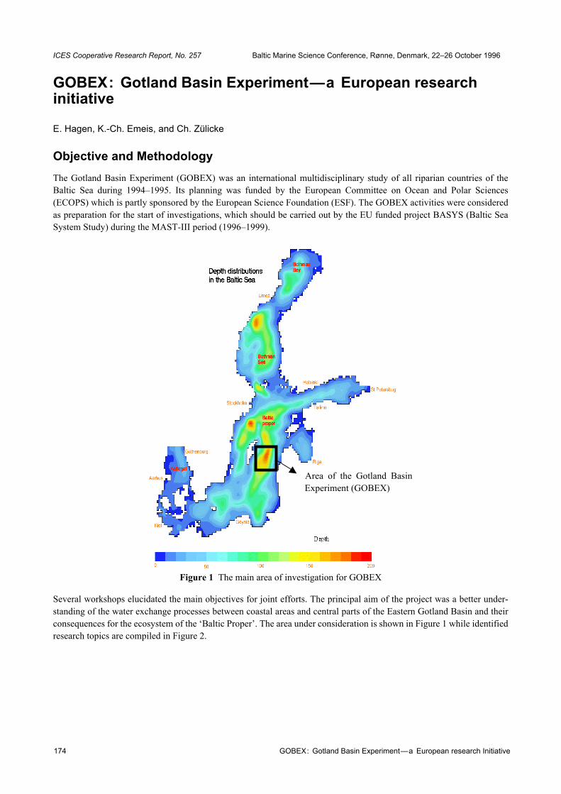
GOBEX : Gotland Basin Experiment—a European research Initiative174
ICES Cooperative Research Report, No. 257 Baltic Marine Science Conference, Rønne, Denmark, 22–26 October 1996
GOBEX: Gotland Basin Experiment—a European research initiative
E. Hagen, K.-Ch. Emeis, and Ch. Zülicke
Objective and MethodologyThe Gotland Basin Experiment (GOBEX) was an international multidisciplinary study of all riparian countries of theBaltic Sea during 1994–1995. Its planning was funded by the European Committee on Ocean and Polar Sciences(ECOPS) which is partly sponsored by the European Science Foundation (ESF). The GOBEX activities were consideredas preparation for the start of investigations, which should be carried out by the EU funded project BASYS (Baltic SeaSystem Study) during the MAST-III period (1996–1999).
Figure 1 The main area of investigation for GOBEX
Several workshops elucidated the main objectives for joint efforts. The principal aim of the project was a better under-standing of the water exchange processes between coastal areas and central parts of the Eastern Gotland Basin and theirconsequences for the ecosystem of the ‘Baltic Proper’. The area under consideration is shown in Figure 1 while identifiedresearch topics are compiled in Figure 2.
Area of the Gotland BasinExperiment (GOBEX)

E. Hagen, K.-Ch. Emeis, and Ch. Zülicke 175
Figure 2 GOBEX research topics
Scheduled field campaigns should be concentrated in the Eastern Gotland Basin. It was recommended that most of thehydrographic station positions coincide with those of the Baltic Year (BY) programme, which was carried out in 1969–1970. These efforts included, inter alia, the quantification of various past and present fluxes between different inorganicand organic compartments, different ecological zonations and food webs. In a first approximation step there were thesetup of four working groups:
• Meso-scale dynamics• Benthic processes• Data management—hydrography/geology• History of the Baltic Proper Such an approach involves all marine disciplines working on different temporal and spatial scales. For example,sedimentation processes of the basin scale should be influenced by the deep water circulation, associated water-masstransformation, and related mixing and exchange processes, which are based on different physical mechanisms. Theirbetter understanding is needed for the development of an integrated model describing these relationship in a proper way.
Figure 3 Time table summarising all cruise activities of participating research vessels (R/V: A.v.H. = “Alexander von Humboldt”) and moored current measurements (M) in the area shown in Figure 1
Air-Sea Exchange
Baltic Sea—North SeaWater Exchange and General
Circulation
Inshore and Coastline Processes
Coastal—Basin Interactions
GOBEX
Data Management and Ecosystem Analysis
Food Web Dynamics and Berthic-Pelagic Coupling
Processes of Anthropogenic Influence
Paleoenvironment
N D J F M A M J J A S O N D
Gauss
Oceania
Livonia
Vejas
A.v.H.
Aranda
R/V 09.-20.12. 07.-20.09.
30.05.-09.06.
02.-08.03.
25.11.-11.12. 22.-25.02. 02.-08.03. 04.-06.05. 17.06.-02.07. 20.08.-08.09.
10.-23.02. 01.-10.03. 03.-27.05. 15.-27.07. 09.08.- 02.09. 14.-29.09. 26.10.-01.11.
25.11.-02.12. 11.-24.04. 27.06.-05.07. 15.-26.08.
1993 1994
M
M
GOBEX- Activities

GOBEX : Gotland Basin Experiment—a European research Initiative176
The GOBEX programme only provided the first step in that direction. The success of marine investigations strictlydepends on planned cruise logistics as well as on the ease of data access. The management of the national hydrographicdata was, for instance, supported by the ICES in Copenhagen/Denmark. In summary, Figure 3 depicts the timetable of allcruise activities. Time windows of moored current measurements are also indicated. Their logistics were coordinated bythe Institute for Baltic Sea Research Warnemünde (IOW)/Germany. Relevant news was distributed monthly/bimonthlyvia e-mail as the GOBEX-Newsletter, which served for a fast presentation of preliminary results as well as for logistics,data exchange, device calibration procedures, guest researchers, etc.
Selected Research TopicsThe interdisciplinary research was conducted mainly in hydrography and geology. For instance, the GOBEX hydro-graphic data set of the IOW was represented by Zülicke and Hagen (1997) while the corresponding status report ofgeological efforts was provided by Emeis and Struck (1998). With respect to further details we refer to Neumann et al.(1997), Emeis et al. (1998), and Kunzendorf et al. (1998). From the hydrographic point of view, first scientific resultswere published in the GOBEX Summary Report (Baltic Marine Science Reports, Vol.19, Baltic Sea Research InstituteWarnemünde, 1996). Here, we briefly introduce the major research topics and quote a selection of results from the report.Central topics of hydrographic investigation were:
• Parametrisation of exchange processes between atmosphere and ocean acting on different temporal and spatial scales• How do the sporadically appearing salt water inflows affect the water masses below the halocline in different Baltic
basins?• For which time scales does water exchange between the basins take place and what are the basic trigger mechanisms
that start sill overflow?• How does the basin ecosystem at different trophic levels react on a salt water inflow?Joint experimental and theoretical studies are necessary for a sufficient description of dynamics within the turbulentsurface mixed layer. Released mixing controls all fluxes between atmosphere and ocean. It is usually parametrised byexchange coefficients describing the vertical momentum transfer. Acceptable values can be estimated at the base of 1-hour means of meteorological standard parameters and radiometer measurements, Zülicke et al. 1996. Microstructuremeasurements in coastal zones and central parts of deep Baltic basins indicate the magnitude of 10–6 Wkg–1 for theassociated dissipation rate of kinetic energy, Stips (1996). In open Baltic areas, most of the dissipation results from alocal production via the Reynolds-stress. Within coastal zones, however, patches of enhanced dissipation rates arefrequently not balanced locally. Coastal jets sporadically advect intensified dissipation patches, cf. Zülicke and Henning(1996), Zülicke et al. (1996), and Zülicke et al. (1998). Resulting eddy diffusivities fluctuate in the relatively large rangebetween 10–2–10–4m2s–1.
Following Elken et al. (1988) with respect to the existence of eddy-like water lenses in deep layers of the EasternGotland Basin, the IOW carried out an expedition with R/V “Alexander von Humboldt” during 14–29 September, 1994.Its main objective was the study of the exchange of deep water from the Bornholm Basin through the Stolpe Furrow intothe Gotland Basin. Inter alia, time series measurements for over three days (22.09.95-06:00–25.09.95-03:00 UTC) weredone at the Baltic Year station BY15A, just above the Gotland Deep. The series was sampled once per hour to resolveshort-term fluctuations. The temporal behaviour of isopycnals is plotted in Figure 4. The intrusion of denser water(PD>9.7kgm–3) occurs in layers deeper than 200m for about 40h. This has to interpreted as a hint for the existence oftemporal/spatial changes in the baroclinic mass field with a time scale of a few days.
Their origin and associated trigger mechanisms are still unclear. Such events could be caused by single baroclinic eddiestravelling with the deep background circulation or it could be ingredients of topographically trapped low-frequencywaves. Nevertheless, there is some observational evidence that such eddy-like phenomena start in the transition areabetween the Stolpe Furrow and the entrance of the Eastern Gotland Basin, Zhurbas and Paka (1996). It is expected thatassociated fluctuations in the motion field rhythmically modify the deep circulation in the central part of the EasternGotland Basin. Current measurements, which were carried at three positions along the 220m depth contour during twoweeks in November 1993, suggest a cyclonic deep water circulation with velocities between 2cms–1 and 6cms–1, Mittel-staedt (1996).

E. Hagen, K.-Ch. Emeis, and Ch. Zülicke 177
Figure 4 Plotted time series of the potential density (PD) sampled with a time step of 1h at the position of station BY15A above the Gotland Deep according to Hagen and Feistel (1996); PD>9.7kgm–3 is black
Sporadically occurring intrusions of dense deep water into the deepest parts of the basin elucidate not only their impacton changed hydrochemical conditions, cf. Nausch and Matthäus (1996), but also on sedimentation and deposition.Relevant research topics of geological efforts were:
• Which accumulation rates have to be expected for inorganic/organic material in different Baltic basins during theseasonal cycle?
• At which spatio-temporal scales does the sedimentation in the basins proceed under distinct hydrographic conditions?• Is it possible to reconstruct the ecosystem state from sediments and to explain its temporal response on hydrographi-
cally determined changes in the past?The analysis of porewater, which is based on three sediment cores sampled at 68m, 112m, and 236m water depth,revealed that each of them indicates a different amount of organic matter as well as different redox-conditions,Matthiesen (1996). During August 1994 two cruises with R/V “Alexander von Humboldt” were carried out to theGOBEX area. In particular, signals of inflows to the Gotland Basin in the sedimentary record were studied by Chris-tiansen and Kunzendorf (1996). The analysis of a multicore probe near the station BY15A showed the following results:Significant peaks in the Fe and Mn concentrations were also found in the 70 and 100mm level. These can be attributed tothe 1971 and 1951 salt water inflow with the 210Pb dating method. This finding suggests that inflows not only may beobserved in concentrations of imported elements. Hence, it seems to be possible to recognise such events from sedimentsfrom ancient times and to increase knowledge on the cyclic behaviour of their appearance.
ReferencesChristiansen Ch., and Kunzendorf, H. (1996). Signals of inflows to the Gotland Basin in the sedimentary record. In: E.
Hagen (Editor), GOBEX—Summary Report. Meereswissenschaftliche Berichte, No.19. Institut für Ostseefors-chung Warnemünde, 10–13.
Elken, J., Pajuste, M., and Kouts, T. (1988). On intrusive lenses their role in mixing in the Baltic deep layers.Proceedings of the 16th Conference of the Baltic Oceanographers, Institute of Marine Research Kiel, Kiel, 367–376.
Emeis, K.C., Neumann, T., Endler, R., Struck, U., Kunzendorf, H., and Christiansen, Ch. (1998). Geochemical records ofsediments in the Gotland Basin—products of sediment dynamics in a not-so-stagnant anoxic basin? AppliedGeochemistry, 13, 349–358.

GOBEX : Gotland Basin Experiment—a European research Initiative178
Emeis, K.-C., and Struck, U. (Editors) (1998). Gotland Basin Experiment (GOBEX): Status report on investigationsconcerning benthic processes, sediment formation and accumulation. Meereswissenschaftliche Berichte, No. 34.,Institut für Ostseeforschung Warnemünde, 1–122.
Hagen, E., and Feistel, R. (1996). Lenses of relative saline deep water in the Eastern Gotland Basin. In: E. Hagen(Editor), GOBEX—Summary Report. Meereswissenschaftliche Berichte, No.19. Institut für OstseeforschungWarnemünde, 34–37.
Kunzendorf, H., Emeis, K. C., and Christiansen, Ch. (1998). Sedimentation in the Central Baltic Sea as viewed by non-destructive Pb-210 dating. Danish Journal of Geography, 98, 1–9.
Matthiesen, H. (1996). Fe and S in sediment from 3 stations from the GOBEX area. In: E. Hagen (Editor), GOBEX—Summary Report. Meereswissenschaftliche Berichte, No.19. Institut für Ostseeforschung Warnemünde, 15–19.
Mittelstaedt, E. (1996). The subsurface circulation in the Gotland Deep. In: E. Hagen (Editor), GOBEX—SummaryReport. Meereswissenschaftliche Berichte, No.19. Institut für Ostseeforschung Warnemünde, 20–23.
Nausch, G., and Matthäus, W. (1996). Present changes of the hydrographical and hydrochemical situation in the GotlandDeep. In: E. Hagen (Editor), GOBEX—Summary Report. Meereswissenschaftliche Berichte, No.19. Institut fürOstseeforschung Warnemünde, 30–33.
Neumann, T., Christiansen, Ch., Clasen, S., Emeis, K. C., and Kunzendorf, H. (1997). Geochemical records of salt-waterinflows into the deep basins of the Baltic Sea. Cont. Shelf Res., 17(1), 95–115.
Stips, A. (1996). First investigations of the near surface turbulence structure and energy dissipation caused by windmixing in the Baltic Sea. In: E. Hagen (Editor), GOBEX—Summary Report. Meereswissenschaftliche Berichte,No.19. Institut für Ostseeforschung Warnemünde, 64–75.
Zhurbas V. M. and Paka, V.T. (1996). Observations of meso-scale eddy-like structures and thermohaline intrusions in theGotland Basin after the 1993 Major Baltic Inflow. In: E. Hagen (Editor), GOBEX—Summary Report.Meereswissenschaftliche Berichte, No.19. Institut für Ostseeforschung Warnemünde, 38–63.
Zülicke, Ch., Schuffenhauer, I., and Stips, A. (1996). Baltic measurements of turbulence in the surface mixed layer. In:E. Hagen (Editor), GOBEX—Summary Report. Meereswissenschaftliche Berichte, No.19. Institut für Ostseefor-schung Warnemünde, 76–91.
Zülicke, Ch., and Hagen, E. (1997). GOBEX Report: hydrographic data at IOW. Meereswissenschaftliche Berichte,No.21. Institut für Ostseeforschung Warnemünde, 1–72.
Zülicke, Ch., Hagen, E., and Stips, A. (1998). Dissipation and mixing in a coastal jet: a Baltic Sea case study. AquaticSciences, 60 (3), 220–235.
Zülicke, Ch. and Henning, O.(1996). Surface energy fluxes and mixed layer depth. In: E. Hagen (Editor), GOBEX—Summary Report. Meereswissenschaftliche Berichte, No.19. Institut für Ostseeforschung Warnemünde, 92–104.

Flemming Jakobsen, Niels H. Petersen, Helmer M. Petersen, Jacob S. Møller, Thomas Schmidt, and Torsten Seifert 179
ICES Cooperative Research Report, No. 257 Baltic Marine Science Conference, Rønne, Denmark, 22–26 October 1996
Hydrographic investigations in the Fehmarn Belt in connection with the planning of the Fehmarn Belt link
Flemming Jakobsen, Niels H. Petersen, Helmer M. Petersen, Jacob S. Møller, Thomas Schmidt, and Torsten Seifert
AbstractThe hydrographic investigations in connection with a Fehmarn Belt link connecting Denmark and Germany are beingcarried out by the Fehmarn Belt Environmental Consultants as subconsultant to COWI-Lahmeyer Joint Venture. Theclients are Trafikministeriet (Denmark) and Bundesministerium für Verkehr (Germany). The planning of the Fehmarnbelt link will involve environmental design criteria, but these are not finally decided yet. Phase I of the preliminary inves-tigation was carried out from December 1, 1995 to June 1, 1996 and included collection and analysis of hydrographicdata, as well as 3-dimensional simulations of the flow in the Fehmarn Belt by two independent oceanographic models.Some results from the investigations are outlined, e.g. the flow distribution in the Fehmarn Belt and the size and impor-tance of the blocking of the planned link solutions. During phase II a permanent monitoring programme outlined for 3-dimensional simulations was installed. The first measurements from the programme are presented.
Introduction The hydrographic investigations in connection with a Fehmarn Belt link connecting Denmark and Germany are beingcarried out by the Fehmarn Belt Environmental Consultants (FEC). FEC consists of the Danish Hydraulic Institute,Water Quality Institute, Institut für Ostseeforschung Warnemünde and LIC engineering. FEC act as a subconsultant tothe COWI-Lahmeyer Joint Venture. The clients are Trafikministeriet (Denmark) and Bundesministerium fur Verkehr(Germany). The sole responsibility for the contents of the present paper lies on the authors.
The planning of the Fehmarn Belt link will involve environmental design criteria. The Great Belt and the Øresund linkinvolve the environmental design criteria, that the links should not alter the transport of water and salt (zero blockingsolutions), thereby ensuring that no change in the physical and biological conditions should occur in the Baltic Sea due tothe links. The zero blocking solutions are achieved by compensating the increased flow resistance induced by bridgepiers and causeways by means of dredging close to the link (Møller & Ottesen Hansen, 1990). The design criteria for theFehmarn Belt link are not yet finally decided.
Phase I of the environmental investigation by FEC was carried out from December 1, 1995 to June 1, 1996 and includedcollection and analysis of hydrographic data (Trafikministeriet, 1996; COWI-Lahmeyer, 1996A + B), as well as 3-dimensional simulations of the flow in the Fehmarn Belt by two independent oceanographic models (COWI-Lahmeyer,1996C). The 3-dimensional simulations were used to investigate the influence of 7 different link solutions. Also oxygenconditions, sediment transport and coastal morphology are investigated by FEC, but are not treated further in the presentpaper.
During phase II, amongst other things, a permanent monitoring programme outlined for 3-dimensional simulations hasbeen installed. The monitoring programme was measuring on October 15, 1996 and is planned to be stopped on October15, 1997. As part of the monitoring programme two surveys of two weeks each, are planned to take place as follows: onein January 1997 and one in August 1997.
The paper is divided as follows. Firstly, the important features regarding the overall and local hydrography are outlined.Secondly, the velocity distribution in the Fehmarn Belt is discussed. Thirdly, the investigated link solutions are outlinedand the blocking of the link solutions is related to other influences. Finally, the most important conclusions are summa-rised.
Hydrographical introductionThe drainage basin of the Baltic Sea is 1721200km2 and the mean (1921–75) river inflow is determined to be14895m3s–1, see HELCOM (1986). This inflow of fresh water combined with the inflow of high saline water from the

Hydrographic investigations in the Fehmarn Belt in connection with the planning of the Fehmarn Belt link180
North Sea creates a stratified system in the Baltic Sea. During periods with decreasing river inflow the salinity at thesurface at Anholt will increase and vice versa, see Figure 1. The close and strong correlation between the river inflow andthe hydrography of the Baltic demonstrates the sensitivity of the Baltic to changes within the boundary conditions(including the bathymetry of the transition area). The influence of a link can crudely be imagined as a very small butsystematic increase in the river inflow.
Figure 1 The relation between the five-year moving average surface salinity at Anholt and the five-year moving average river inflow into the Baltic Sea, where the salinity is compared to the river inflow one year earlier. Based on river inflow data in HELCOM (1986) and salinity data in Svansson (1975), though the yearly mean salinity in 1914 was corrected to
be 20.7PSU.
The Baltic Sea has changed considerably on several time scales, see e.g. Møller & Hansen (1994). Such changes areimportant when considering a zero-solution of a bridge construction in the transition:
• how large and rapid are the natural changes compared to the influence of the construction? • is it possible to observe and/or measure a change caused by a fixed link? Seen on the geological time scale, bathymetrical changes are the main reasons for the changing conditions of the BalticSea. Today we still experience a land elevation of up to 1cm per year in the northern part of the Baltic Sea, while there isno elevation in the Danish Straits (Binderup & Frich, 1993). Measurements of the hydrographic conditions in the BalticSea have existed through the last 120 years. The time series show a fluctuating pattern for the parameters measured: e.g.salinity, temperature and oxygen; and also for some parameters, a general trend (Matthäus, 1979). In the future, the greenhouse effect will inevitably affect the hydrography of the Baltic, see later.
Local hydrographyThe Fehmarn Belt, the Kiel Bight and the Mecklenburg Bight are part of the Belt Sea (Figure 2), which hydrographicallyforms part of the transition area between the Baltic Proper and the North Sea. It is important to note the shallow DarssSill (~18m depth) between the Fehmarn Belt and the Arkona Sea, which acts as a salt water trap, and the 90 degreesturning from the Langelands Belt to the Fehmarn Belt.
The water masses in the Belt Sea and the Kattegat consist of low saline water from the Baltic Proper, which, close to thesurface, flows through the Belt Sea and the Kattegat, and high saline water from the North Sea, which forms a lowerlayer. In June, the wind conditions are weak, and the two-layer exchange flow between the North Sea and the BalticProper is clearly identified to provide a strongly stratified water column in the Belt Sea, see Figure 3 and Figure 4. InDecember, the wind conditions are strong whereby the stratification is destroyed by mixing of the water masses, see alsoMatthäus & Franck (1992) and Jakobsen (1995) on major inflows during this season.

Flemming Jakobsen, Niels H. Petersen, Helmer M. Petersen, Jacob S. Møller, Thomas Schmidt, and Torsten Seifert 181
Figure 2 Detailed map of the near Fehmarn Belt area. In the Kiel Bight three topographic fixed eddies are shown, and in the Mecklenburg Bight one quasi-stationary eddy is shown.
Figure 3 Cross-section showing the longitudinal salinity distribution as monthly means from Skagerrak through Fehmarn Belt and into the Baltic Proper (the vertical link shows the position of the planned link). Drawn by data given in
Sparre (1984A), Lange et al. (1991) and Jakobsen (1991).
Figure 4 The yearly salinity variation at Fehmarn Belt lightship based on monthly average conditions presented in Lange et al. (1991). The hatching shows the minimum and maximum salinity.

Hydrographic investigations in the Fehmarn Belt in connection with the planning of the Fehmarn Belt link182
The short-term variation of the hydrography is mainly determined by the meteorological variations: westerly winds forceinflow while easterly winds force outflow. The winds are controlled by high and low pressures passing Scandinavia at atime scale of about one week, see Stigebrandt (1980) and Lass et al. (1987).
A typical situation changing between in- and outflow can be described as follows. During an inflow to the Baltic Properthe salinity of the inflowing water is higher than the Baltic Proper surface water, which causes the inflowing water toplunge south of the Darss sill, see COWI-Lahmeyer (1996B). The plunging position is also referred to as the Belt front.When the current changes from in- to outflowing most of the water with a salinity higher than 10–15 PSU, which passedthe sill during the inflow, continues to flow into the Baltic Proper along the bottom. One may consider the sill as a saltwater trap. At the beginning of an outflowing current situation, water with a salinity of 10–15 PSU from the Baltic Properflows as a plume into the Belt Sea across the Darss sill, pushing and entraining Kattegat surface water with a salinity ofapproximately 20PSU down and out. The flushing time scale of the sill area is less than 2 days. A front between theBaltic Proper and Kattegat surface water masses is present, it moves outwards and out of the Belt Sea within one week. Ifthe strong wind and current conditions cease, the system will rapidly develop into a two-layer system even at the Darsssill. Thus, moderate, high saline Kattegat surface water is baroclinically transported into the Baltic Proper.
Statistically, the surface current in the Fehmarn Belt shows inflow during 47% of time and outflow during 54% of time,while the current near the bottom shows inflow during 67% of time and outflow during 33% of time, see Lange et al.(1991). The inflow is thus more frequent in the lower layer. Most inflow situations at the surface have a duration less than3 to 5 days, while outflow situations tend to last 1 or 2 days longer. The longest inflow situation lasted 14 days, and thelongest outflow 17 days. Near the bottom, the inflow has a typical duration of 3 to 5 days, with the longest situationobserved lasting 21 days. Outflow is very rare but has occurred with durations up to 5 to 7 days.
The velocity distributionThe velocity distribution along the alignment is very important when designing the link. On the basis of historicalmeasurements some information can be obtained, see Figure 5.
Figure 5 The position of the stations in the Fehmarn Belt area.
The surface current roses in Figure 6 show two main current directions in the upper layer: A) towards WNW or NW,which is out of the Baltic Proper; and B) towards ESE or SE, which is into the Baltic Proper. The main directions are notas clearly defined at a 20 m depth.

Flemming Jakobsen, Niels H. Petersen, Helmer M. Petersen, Jacob S. Møller, Thomas Schmidt, and Torsten Seifert 183
Figure 6 Current roses: a) at Fehmarn Belt lightship during the period 1970 to 1984b) station 528 during the Belt Project at 7m depth
c) station 528 during the Belt Project at 20m depth.
Comparison of the current at Fehmarn Belt lightship and at 7m depth at station 528 shows, in Figure 7, that the currentmagnitudes and direction are highly correlated (secondary flow seems not too important).
On this basis: current roses and comparison; we may assume that the current in the Fehmarn Belt is strongly related to thebathymetry and the water exchange, and only weakly related to secondary flows (eddies)—it behaves in many respectsas a channel. This will be further elucidated through the ongoing field measurement programme.
Three DYNOCS field campaigns have been carried out with R/V “Prof. A. Penck” in the Fehmarn Belt area. Unfortu-nately, the survey lines did not cover the area close to the Danish coast. Still, based on the surveys, the following conclu-sions were made. In the quasi-stationary situation in the upper layer by far the most water exchange takes place as a uni-directed current, while in the lower layer only a weak counter-current takes place. During transient situations, the currentfeatures might be much more complicated, but this is not considered important, because these situations are characterisedby short duration and weak currents.
a)
b) c)

Hydrographic investigations in the Fehmarn Belt in connection with the planning of the Fehmarn Belt link184
Figure 7 Current development at station 528 at 7m depth (above) and at the Fehmarn Belt lightship (below).
Hardtke (1978) presented the velocity distribution in the Fehmarn Belt during inflow to the Baltic based on ship measure-ments, see Figure 8. The distribution shows an outflow near Lolland. In Pedersen (1996) it is argued that the outflow nearLolland is a typical feature during inflow to the Baltic.
Figure 8 The velocity distribution in the Fehmarn Belt during inflow to the Baltic based on ship measurements from 15.00 to 16.30 on 27 June, 1977.
The current speed towards N at station 532 at 10m depth in Langelands Belt, towards E at station 528 at 12m depth andat Fehmarn Belt lightship is shown in Figure 9. The measurements in Langelands Belt show a constant inflow to theBaltic during the period, while a redistribution is seen in the Fehmarn Belt with a current change near Lolland. Investi-gating the salinity variations revealed that the current change near Lolland is caused by up-welling of dense bottomwater, which only very rarely takes place, see COWI-Lahmeyer (1997).
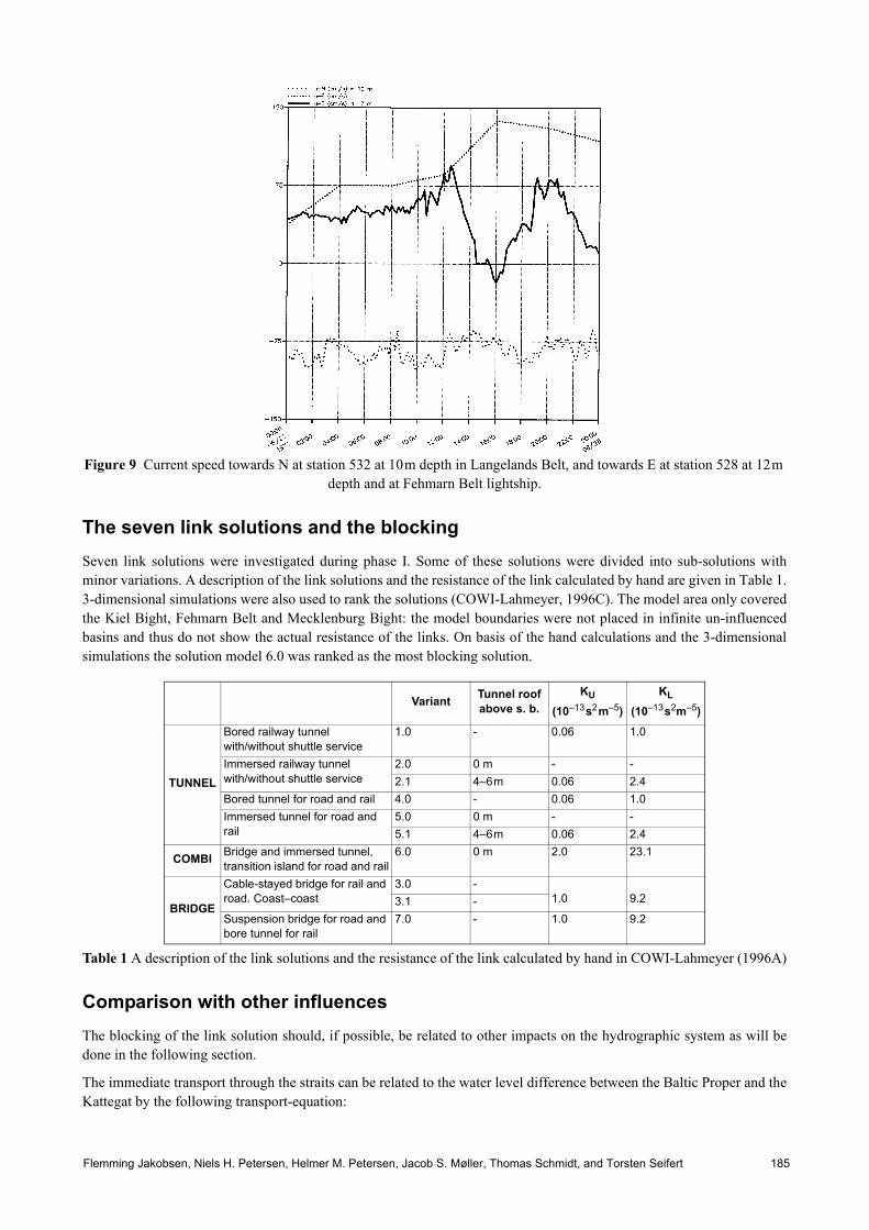
Flemming Jakobsen, Niels H. Petersen, Helmer M. Petersen, Jacob S. Møller, Thomas Schmidt, and Torsten Seifert 185
Figure 9 Current speed towards N at station 532 at 10m depth in Langelands Belt, and towards E at station 528 at 12m depth and at Fehmarn Belt lightship.
The seven link solutions and the blockingSeven link solutions were investigated during phase I. Some of these solutions were divided into sub-solutions withminor variations. A description of the link solutions and the resistance of the link calculated by hand are given in Table 1.3-dimensional simulations were also used to rank the solutions (COWI-Lahmeyer, 1996C). The model area only coveredthe Kiel Bight, Fehmarn Belt and Mecklenburg Bight: the model boundaries were not placed in infinite un-influencedbasins and thus do not show the actual resistance of the links. On basis of the hand calculations and the 3-dimensionalsimulations the solution model 6.0 was ranked as the most blocking solution.
Table 1 A description of the link solutions and the resistance of the link calculated by hand in COWI-Lahmeyer (1996A)
Comparison with other influencesThe blocking of the link solution should, if possible, be related to other impacts on the hydrographic system as will bedone in the following section.
The immediate transport through the straits can be related to the water level difference between the Baltic Proper and theKattegat by the following transport-equation:
Variant Tunnel roof above s. b.
KU (10–13s2m–5)
KL (10–13s2m–5)
TUNNEL
Bored railway tunnel with/without shuttle service
1.0 - 0.06 1.0
Immersed railway tunnel with/without shuttle service
2.0 0 m - -2.1 4–6m 0.06 2.4
Bored tunnel for road and rail 4.0 - 0.06 1.0Immersed tunnel for road and rail
5.0 0 m - -5.1 4–6m 0.06 2.4
COMBI Bridge and immersed tunnel, transition island for road and rail
6.0 0 m 2.0 23.1
BRIDGE
Cable-stayed bridge for rail and road. Coast–coast
3.0 -1.0 9.23.1 -
Suspension bridge for road and bore tunnel for rail
7.0 - 1.0 9.2

Hydrographic investigations in the Fehmarn Belt in connection with the planning of the Fehmarn Belt link186
(1)
where ∆η (m) is the water level difference from the Baltic Proper to the Kattegat, KBØ[s2m–3] is the ‘resistance’ and Q[m3s–1] is the discharge.
The resistance through the Great Belt and the Fehmarn Belt (KGB) is determined to be
38·10–12[s2m–5] (Jacobsen, 1980),
through the Little Belt and the Fehmarn Belt (KLB) to be
3439·10–12[s2m–5] (recalculated according to equation (1), see Jakobsen & Ottavi, 1996),
and through the Øresund (KØ) to be approximately
239·10–12[s2m–5] (Jakobsen et al., 1996).
The resistance through the Great and Little Belt Sea can be calculated to be:
(2)
and through the Belt Sea to be:
(3)
The Great Belt link without compensation dredging increases the resistance in the Great Belt (KGB) by
0.38–0.77·10–12[s2m–5]
corresponding to a blocking of the gross flow through the Belt Sea of 0.33–0.66%, while the Øresund link withoutcompensation dredging increases the resistance in Øresund (KØ) by
2.41·10–12[s2m–5]
corresponding to a blocking of the gross flow through the Belt Sea of 0.13%, see also Stigebrandt (1992). The Little Beltlinks increase the resistance in Little Belt (KØ) by
48.2·10–12[s2m–5]
(recalculated according to equation (1), see Jakobsen & Møller, 1996) corresponding to a blocking of the gross flowthrough the Belt Sea of 0.05%. Disregarding solution model 6.0 the Fehmarn Belt link without compensation dredgingincreases the resistance in the Fehmarn Belt (KB) by a maximum of
0.06·10–12[s2m–5] (bridge solution assuming the upper and lower layer to be parallelly connected)
corresponding to a blocking of the gross flow through the Belt Sea and Øresund of 0.07%. The maximum blocking is thusapproximately equal to the blocking of the Little Belt links.
To evaluate the greenhouse effect on the Baltic Sea we shall at this point only consider the water rise of 0.4–0.6 m (DMI,1992). The decrease in the resistance may be evaluated on the basis of the following equation, see DHI/LIC (1995):
(4)
where H is a typical water depth in the Belt Sea. This shows that the changes due to the expected green house effects aretwo order of magnitude larger than the influence of the Fehmarn Belt Link.
The phase II monitoring programmeThe monitoring stations during phase II are shown in Figure 10. Two ADCPs are placed on the bottom in the investigatedalignment. During the surveys, effort will be made to investigate the flow distribution along the alignment.
∆η KB∅abs Q( )Q≈
KBKGBKLB
KGB KLB+( )2
------------------------------------------ 31.1 10 12– s2m 5–[ ]⋅= =
KB∅KBK∅
KB K∅+( )2
------------------------------------ 16.4 10 12– s2m 5–[ ]⋅= =
Blocking 3∆ηH
-------– 30.5m25m------------–≈ -6.0%= =

Flemming Jakobsen, Niels H. Petersen, Helmer M. Petersen, Jacob S. Møller, Thomas Schmidt, and Torsten Seifert 187
Figure 10 The monitoring stations during phase II
Figure 11 shows some of the first measurements from the monitoring station. The measurements only cover a very shortperiod and are not analysed yet.
Figure 11 Examples of first measurements coming from the monitoring stations during phase II.
Conclusion The changes of the Baltic Sea on all time scales are important, when considering the environmental impact of a bridgeconstruction in the transition:
• how large and rapid are the natural changes compared to the influence of the construction?• is it possible to observe and/or measure a change caused by a fixed link? The answers to the questions are, that we expect the natural changes to be larger than the influence of the construction,and that it is not possible to measure the change caused by the fixed link, especially if the environmental design criteriaare set as restrictively as in the Great Belt and Øresund link cases.
The velocity distribution along the alignment is very important, when designing the details of the link between Denmarkand Germany. On the basis of historical measurements, we may assume that the current in the Fehmarn Belt is strongly

Hydrographic investigations in the Fehmarn Belt in connection with the planning of the Fehmarn Belt link188
related to the bathymetry and the water exchange, and only weakly related to secondary flows. It should, however, benoted that during inflow to the Baltic an outflow near Lolland may be a typical feature, which needs to be furtherexplored during phase II.
Seven link solutions were investigated during phase I. On the basis of the hand calculations and the 3-dimensionalsimulations, the solution model 6.0—the combi solution—was ranked as the most blocking solution and will not beconsidered in phase II. Disregarding solution 6.0, the maximum blocking of the Fehmarn Belt link solutions is approxi-mately equal to the blocking of the Little Belt link, and much smaller than the estimated influence of the expected green-house effect.
References Binderup M., and Frich, P. (1993). Sea-level variations, trends and cycles, Denmark 1890–1990: Proposal for a reinter-
pretation. Ann. Geophysicae, 11, pp. 753–760.
DHI/LIC (1995). Hydrographic investigations, Campaign I–VI. Report for Øresundskonsortiet by DHI/LIC and SMHI.7209/FU.
DMI (1965). Oceanographical observations from Danish light-vessels and coastal stations. Yearbook from the DanishMeteorological Institute.
DMI (1992). Drivhuseffekt og klimarendringer. Særtryk Danmarks Meteorologiske Institut, 103 pp.
COWI-Lahmeyer (1996A). Initial Environmental Design Evaluation Fehmarn Belt Feasibility Study, Phase 1, Technicalnote by FEC.
COWI-Lahmeyer (1996B). Hydrographic data collection and review Fehmarn Belt Feasibility Study, Phase 1, Technicalnote by FEC.
COWI-Lahmeyer (1996C). Hydraulic modelling Fehmarn Belt Feasibility Study, Phase 1, Technical note by FEC.
COWI-Lahmeyer (1997). Determination of cross sectional velocity Fehmarn Belt Feasibility Study, Phase 2, Technicalnote by Prof. Fl. Bo Pedersen & FEC.
Hardtke, G. (1978). About the velocity field in the Kiel Bay. Proceedings, Conference of Baltic Oceanographers(Rostock, Germany, pp. 756–779).
HELCOM (1986). Water Balance of the Baltic Sea” Helsinki Commission, Baltic Marine Environment ProtectionCommission, Baltic Sea Environment Proceedings, 16.
Jacobsen, T.S. (1980). Sea Water Exchange of the Baltic, Measurements and methods. The Belt Project, 106 pp.
Jakobsen, Fl. (1991). The Bornholm Basin—Estuarine Dynamics. Technical University of Denmark, Institute of Hydro-dynamics and Hydraulic Engineering, Series Paper, 52, 199 pp.
Jakobsen, Fl. (1995). The Major Inflow to the Baltic Sea during January 1993. Journal of Marine Systems, Vol. 6, No.3,pp. 227–240.
Jakobsen, Fl., Lintrup, M.J., and Møller, J.S. (1996). Observations of the Specific Resistance in Øresund. Submitted.
Jakobsen, Fl., and Møller, J.S. (1996). Transporten gennem Lillebælt. Submitted.
Jakobsen, Fl., and Ottavi, J. (1996). The transport through the contraction area in the Little Belt. Submitted.
Lange, W., Mittelstaedt, E. and Klein, H. (1991).Strömungsdaten aus der Westlichen Ostsee. Deutsche HydrographischeZeitschrift, Ergänzungsheft Reihe B, 24.
Lass, H.-U., Matthäus, W., Francke, E., and Schwabe, R. (1987). On the dynamics of water exchange between Baltic andNorth Sea. Beiträge zur Meereskunde, 56, pp. 27–49.
Matthäus, W. (1979). Long term Variations in the primary Halocline in the Gotland Basin. ICES, C.M. 1979/C:22,mimeo.
Matthäus, W., and Franck, H. (1992). Characteristics of major Baltic inflows—a statistical analysis. Continental ShelfResearch, 36, pp. 1375–1400.

Flemming Jakobsen, Niels H. Petersen, Helmer M. Petersen, Jacob S. Møller, Thomas Schmidt, and Torsten Seifert 189
Møller, J.S., and Hansen, I.S. (1994). Hydrographic processes and changes in the Baltic Sea. Dana, 10, pp. 87–104.
Møller, J.S., & Ottesen Hansen, N.-E. (1990). The Great Belt Link, How to achieve zero environmental impact on theBaltic Sea. Twenty-Second Coastal Engineering Conference. Coastal Eng. Res. Council/ASCE, July 2–6 1990,Delft.
Pedersen, FI.B. (1996). Hydrografiske forhold i Kiel Bugt–Femer Bælt–Darss Tærsklen. Unpublished manuscript, 60pp.
Sparre, A. (1984A). Salinity A; means, extremes and frequency. The climate of Denmark, Summaries of observationsfrom light vessels IV, No. 11.
Stigebrandt, A. (1980). Barotropic and baroclinic response of a semi-enclosed basin to barotropic forcing from the sea.In: Fjord Oceanography, Eds. H.J. Freeland, D.M. Farmer & C.D. Levings, Plenum, pp. 151–164.
Stigebrandt, A. (1992). Bridge-induced Flow Reduction in Sea Straits with Reference to Effects of a Planned BridgeAcross Öresund. Ambio, 21, 2, pp. 130–134.
Svansson, A. (1975). Physical and Chemical Oceanography of the Skagerrak and Kattegat. Fishery Board of Sweden,Institute of Marine Research, Report No.1, 88 pp.
Trafikministeriet (1996). Undersegelser vedrerende Femer Bælt-forbindelsen. Fase 1 af kyst til kyst-undersøgelserne,128 pp.
Nested 3D model of the North Sea and the Baltic Sea190
ICES Cooperative Research Report, No. 257 Baltic Marine Science Conference, Rønne, Denmark, 22–26 October 1996
Nested 3D model of the North Sea and the Baltic Sea
H. René Jensen and Jacob S. Møller
Abstract A two-way interactive nested three dimensional model of the North Sea, the Baltic Sea and the Danish waters has beenestablished under the MAST II research project DYNOCS. The objective of the modelling is to hindcast a period of oneyear and investigate the dynamics of the complicated flow in the Danish waters between the North Sea and the BalticSea.
Introduction As part of the CEC-sponsored MAST II research project DYNOCS (DYNamics Of Connected Seas), a three dimensionalnumerical model of the North Sea, the Baltic Sea and the Danish waters has been established. The model is based onDanish Hydraulic Institute’s (DHI) general 3D modelling system, MIKE 3, which is a non-hydrostatic baroclinic model.To resolve the narrow Danish straits a special version of MIKE 3 which includes an interactive two-way nesting facilityhas been applied. The objective of the project is to hindcast a one year period of the complicated flow in the Danishwaters which to a high degree is governed by the dynamics of the North Sea and the Baltic Sea. This paper describes themodel set-up and some preliminary results.
The numerical model The MIKE 3 model is a general non-hydrostatic numerical modelling system developed by DHI (Rasmussen et al., 1990)for a wide range of applications in areas such as oceanography, coastal regions, estuaries and lakes. It simulates unsteadythree-dimensional flows, taking into account density variations, bathymetry and external forcing such as meteorology,tidal elevations, currents and other hydrographical conditions.
The mathematical foundation in MIKE 3 is the mass conservation equation;
the Reynolds-averaged Navier-Stokes equations, including the effects of turbulence and variable density (the momentumequations);
and the conservation equations for salinity and temperature in three dimensions;
together with the equation of state relating the local density to salinity, temperature and pressure.
There are several types of equations of state for the density of sea water. In MIKE 3, the definitions given by UNESCO(1981) have been adopted.
In the equations, ρ is the local density of the fluid, ui the velocity in the xi-direction, Ωij the Coriolis tensor, P the fluid pressure, gj the gravitational vector,
1ρcs
2-------- P∂
t∂------
ui∂xi∂
-------+ SSS=
DuiDt--------- 2Ωjiuj+ 1
ρ--- P∂
xi∂------- gi–
xj∂∂ νt
uj∂xi∂
-------ui∂xj∂
-------+
Fext uiSSS+ + +=
1ρ---D ρS( )
Dt----------------
xj∂∂ DS
S∂xj∂
------- SSS+=
1ρ---D ρT( )
Dt----------------
xj∂∂ DT
T∂xj∂
------- 1
ρ---QH SSS+ +=

H. René Jensen and Jacob S. Møller 191
νT the turbulent eddy viscosity, δ the Kronecker’s delta, k the turbulent kinetic energy, cs is the speed of sound in sea water, S is the salinity, T is temperature, DS and DT are the dispersion coefficients for salinity and temperature, respectively, QH is the heat exchange with the atmosphere and t denotes the time. SSS refers to the respective source-sink terms and differs from equation to equation.
In most three-dimensional models the fluid is assumed incompressible. However, using the divergence-free (incom-pressible) mass equation, the set of equations will inevitably form a mathematically ill-conditioned problem. In mostmodels this is solved through the hydrostatic pressure assumption whereby the pressure is replaced by information aboutthe surface elevation. In order to retain the full vertical momentum equation (i.e. non-hydrostatic conditions) an alter-native approach has been adopted in MIKE 3. This approach is known as the artificial compressibility method (Chorin,1967, and Rasmussen, 1993) in which an artificial compressibility term is introduced whereby the set of equationsmathematically speaking becomes hyperbolically dominated.
The decomposition of the prognostic variables into a mean quantity and a turbulent fluctuation leads to Reynolds stressand turbulent flux terms in the governing equations to account for the non-resolved processes both in time and space. Bythe adoption of the eddy viscosity concept these effects are expressed through the eddy viscosity and the gradient of themean quantity. The problem of determining the eddy viscosity is solved in MIKE 3 by using closure models such as theSmagorinsky sub-grid (zero equation) model, the k- (one equation) model, the k-epsilon (two-equation) model, see Rodi(1980) or a mixed Smagorinsky-k-epsilon model. In the present case the sub-grid model proposed by Smagorinsky(1963) is applied, in which the eddy viscosity is linked to the filter size (grid spacing) and the eddy strain rate, i. e.gradients of the resolved flow field. Buoyancy effects are accounted for via a damping function depending on theRichardson number, see for example Munk and Anderson (1948).
The equations are spatially discretised on a rectangular Arakawa C staggered grid. Scalar quantities such as pressure,salinity, temperature, etc. are defined in the grid nodes, whereas the velocity components are defined halfway betweenadjacent nodes in the respective directions. The adopted staggered grid allows for the spatial discretisation of thegoverning partial differential equations into a finite-difference scheme.
The mass equation and the three momentum equations thus form a (huge) set of differential equations in time, which issolved by an Alternating Direction Implicit (ADI) algorithm. Usually, iterative methods are required for the inversion ofthe system matrices due to the non-linear terms in the momentum equations. However, a non-iterative ADI algorithm isapplied in MIKE 3 through the use of the “fractional-step” technique (basically a time-staggering of the prognosticvariables) and “side-feeding” (a semi-linearisation of the non-linear terms).
For the advection-diffusion of salinity and temperature the QUICKEST scheme (Quadratic Upwind Interpolation forConservative Kinematics with Estimated Streaming Terms) is applied, see Leonard (1979) and Vested et al. (1992). Thismethod is based on a control volume formulation. Upstream interpolation is used to determine higher order derivatives.This procedure limits the stability problems of central differencing while remaining free of the inaccuracies of numericaldiffusion associated with usual upstream differencing. The resolution of fronts is further improved by the implementationof an exponential interpolation at steep fronts (SHARP), see Leonard (1988).
Bottom-fitted co-ordinates have been introduced in MIKE 3. The model equations at the bottom grid cells have beenadjusted to take into account the exact water depths. Thus, the position of the sea bed is not just truncated to fit theapplied constant vertical grid size.
MIKE 3 also includes a “flood and dry” facility, making it possible to include the effects of flooding and drying ofshallow areas when the water surface moves up and down due to e. g. tidal variations or wind set-up.
Heat exchange with the atmosphere is implemented based on the four physical processes: sensible heat flux (convection),latent heat flux (vaporisation), net short wave radiation and net long wave radiation.
An interactive two-way nesting grid facility has been developed for MIKE 3 which allows for nesting from coarser tofiner grids by a factor of three.

Nested 3D model of the North Sea and the Baltic Sea192
Model set-up The model consists of three levels of nesting: A 9nm grid covering the North Sea and the Baltic Sea, a 3nm grid coveringthe Danish waters and a 1nm grid of the Danish Straits and the western Baltic Sea, see Figure 1.
Figure 1 The DYNOCS model set-up with 3 levels of two-way interactive nesting; 9nm, 3nm and 1nm grid resolution
The vertical resolution is 2m with up to 40 layers. So-called bottom-fitted co-ordinates are applied within the lower layerto account for the actual depths and depths larger than approximately 80m. The surface layer thickness is initially 5m butvaries with the movements of the free surface. The thickness of the surface layer is limited by the maximum andminimum surface elevation as this layer must not be dry during simulation (only in shallow areas, where the seabed isjust below!). In the DYNOCS model this is most critical along the East coast of England due to the high tides.
The barotropic forcing of the model consists of tidal forcing and meteorological forcing:
At the two open boundaries in the North Sea; in the British Channel (between Dungeness (UK) and Wissant (France))and between Wick (Scotland) and Stavanger (Norway), the tidal water levels are prescribed by tidal predictions based onthe 10 largest tidal constituents (M2, S2, N2, K2, µ2, K1, O1, P1, M4, MS4) along the boundaries.
Figure 2 Applied Meteorological Forcing (Example from 24 November 1994, 00 GMT, every second vector is shown)

H. René Jensen and Jacob S. Møller 193
The meteorological forcing consists of analysed wind (10m) and surface air pressure fields covering the full so-calledDYNOCS Year (starting 15 September 1994). The meteorological data taken from the operational meteorological model,HIRLAM (Danish Meteorological Institute (DMI)) has a temporal resolution of 6 hours and a spatial resolution of 0.21degrees. In Figure 2, the model wind and air pressure for the 24 November 1994, after spatial interpolation from themeteorological grid to the DYNOCS 9nm grid, is shown. The meteorological fields are further (automatically) interpo-lated to the 3nm and the 10nm grids during simulation.
The reduced wind over land is due to the higher friction.
The baroclinic forcing at the two open boundaries in the North Sea consists of monthly climatological salinities andtemperatures in each grid point which have been established based on data provided by ICES.
The model has been initialised by climatological (10 year September average values) 3D fields of salinity and temper-ature. In Figure 3 and Figure 4, the initial surface salinities and temperatures, respectively, are shown for the fine grid(1nm resolution) where the largest gradients exist. The 3D fields have been established by application of Akima (Akima,1970) and Kriging (Cressie, 1991) interpolation methods in data provided by ICES.
Figure 3 Initial surface layer salinity (1nm grid)
Figure 4 Initial surface layer temperature (1nm grid)
To simulate the long term physical processes of an almost enclosed basin such as the Baltic Sea, it is important to includeall elements of the water balance in the model. Accordingly, the fresh water inflow (20 year average, Mikulski, 1986, and

Nested 3D model of the North Sea and the Baltic Sea194
Bergström, 1993) to the Baltic Sea has been employed by a relative distribution of monthly discharge to the main rivers.Also, main rivers of the North Sea have been included bringing the total numbers of rivers up to 17.
Model fields of precipitation and evaporation have been established on a monthly basis using climatological mean valuesfor 7 sub-basins of Kattegat and the Baltic Sea (Dahlström, 1986). For the North Sea an annual mean value of precipi-tation and evaporation was used (Grindley, 1972) with an added monthly variability deduced from the Baltic Sea clima-tology.
For the heat balance calculations the model needs input in the form of air temperatures 2m above sea level which havebeen provided by DMI on a 6 hourly basis over the whole model (9nm horizontal resolution, as for the wind and airpressure). An example of the temperature fields is shown in Figure 5.
Figure 5 Example of air temperature distribution used in the heat exchange calculations (24 November 1994 00 GMT)
Results Within the defined DYNOCS Year, three field campaigns have been carried out to establish a data base, together with alarge number of permanent stations in the area, for calibration and validation of the numerical model. The model will beused for hindcasting the DYNOCS year and for providing boundary data, within selected periods, to local models of thewestern Baltic Sea established by Institut für Ostseeforschung (IOW), Sveriges Meteorologiska och HydrologiskaInstitut (SMHI) and DMI/DHI, respectively. As the DYNOCS project is still ongoing (November 1996) only preliminaryresults from part of the year to be simulated will be presented here.
Figure 6 Comparison of calculated and measured water levels at Hanstholm

H. René Jensen and Jacob S. Møller 195
As an example of the barotropic behaviour a time-series of the calculated and measured water levels at the entrance to theDanish waters in Skagerrak (Hanstholm) for a period of 2.5 months is shown in Figure 6. This signal contains both thetidal and the meteorological effects.
In Figure 7, the surface current and salinity distribution in the fine grid (1nm resolution) are shown for a strong inflowsituation the 24 November 1994. The figure clearly shows the position of the Drogden Sill and the Darss Sill fronts.
Figure 7 Calculated surface currents and salinities in 1nm grid (24 November 1994, every second vector is shown)
Figure 8 and Figure 9 show the vertical distribution of salinity and temperature along a line from the Kattegat through theGreat Belt, the Fehmarn Belt, the Darss Sill, the Arkona Basin to the Bornholm Basin for the same inflow situation.
Figure 8 Vertical distribution of salinity along a line from Kattegat to Bornholm Basin (24 November 1994)
Figure 9 Vertical distribution of temperature along a line from Kattegat to Bornholm Basin (24 November 1994)

Nested 3D model of the North Sea and the Baltic Sea196
Again, the Darss Sill front is easy to identify. Notice also the cooling of the surface layer and the pull-down of cold waterat the Darss Sill front into the Arkona Basin (Figure 9).
The calculated discharge through Øresund is compared to measured (actually estimated based on current measurements,see Jacobsen (1995) and Jacobsen (1996)) discharges in Figure 10.
Figure 10 Calculated and measured discharge through Øresund (positive is outflow from Baltic Sea)
From the figure, it is seen that the transports to the Baltic Sea are overestimated in the model for the inflow situation of24 November, but the magnitude is still realistic.
A time-series of calculated salinities is shown in Figure 11 where calculated and measured salinities at station NordreRøse in Øresund are compared.
Figure 11 Calculated and measured salinity at Nordre Røse in Øresund (5.4m below surface).
The DYNOCS project will be finalised by mid 1997.
Acknowledgements The DYNOCS project is sponsored by the CEC through MAST II contract no. MAS2- CT94-0088. Furthermore, thefollowing institutes and companies are acknowledged for their contribution: ICES, A/S Storebæltsforbindelsen, Øresund-skonsortiet and the DYNOCS project group (which, besides DHI consists of IOW, SMHI, DMI, Norwegian Hydrotech-nical Laboratory and Aalborg University).
References Akima, A. (1970). A new method of interpolation and smooth curve fitting based on local procedures, Journal of Applied
Computational Mathematics, J J 7, 589–602.

H. René Jensen and Jacob S. Møller 197
Bergström, S., and Carlsson, B. (1993). Hydrology of the Baltic Basin. Inflow of fresh water from rivers and land for theperiod 1950–1990, Report No.7. SMHI, Sweden.
Chorin, A. J. (1967). A numerical method for solving incompressible viscous flow problems, J. Comput. Phys., 2, J 2–26.
Cressie, N. (1991). Statistics for spatial data, John Wiley and Sons Inc., 900 pp.
Dahlström, B. (1986). Determination of areal precipitation for the Baltic Sea, Report No. RMK 54. SMHI, Sweden.
Grindley, J. (1972). Hydrology of the North Sea: Run-off and precipitation, Meteorological Magazine, 101.
Jacobsen, Fl., and Castejon, S. (1995). Calculation of the discharge through Øresund at the Drogden Sill by two fixedstation measurements, Nordic Hydrology, Vol. 26, No. 3, pp. 237–258.
Jacobsen, Fl., and Lintrup, M. J. (1996). The exchange of water and salt across the Drogden Sill in Øresund during theperiod from September 1993 to November 1994, Nordic Hydrology, in press.
Leonard, B.P. (1979). A Stable and Accurate Convective Modelling Procedure Based on Upstream Interpolation.Computational Methods in Applied Mechanical Engineering, 19,59–98.
Leonard, B.P. (1988). Simple High Accuracy Resolution Program for Convective Modelling of Discontinuities, Interna-tional Journal for Numerical Methods in Fluids, 8, 1291–1318.
Mikulski, Z. (1986). Inflow from drainage basin, Baltic Sea Environment, Proceedings, No. 16. Baltic MarineEnvironment Protection Commission, Helsinki Commission
Munk, W. H., and E. R. Anderson (1948). Notes on a theory of the thermocline, J. Mar. Res. 7, 276–295.
Rasmussen, E.B., H.J. Vested, P. Justesen and L.C. Ekebjærg, (1990), SYSTEM3: A Three Dimensional Hydrody-namical Model, Danish Hydraulic Institute.
Rasmussen, E.B. (1993). Three-dimensional Hydrodynamic Models, in Abbott, MB. and N.A. Price (eds.): Coastal,Estuarial and Harbour Engineers’ Reference Book, Chapman & Hall, London.
Rodi, W. (1980). Turbulence Models and their Application in Hydraulics, A State of the Art Review, SFB 80/T/127. Inc,London.
Smagorinsky, J. (1963). General Circulation Experiments with the Primitive Equations, 1. The Basic Experiment, Mon.Wea.Rev., 91, 99–164.
UNESCO (1981). The practical salinity scale 1978 and the international equation of state of seawater 1980, UNESCOtechnical papers on marine science.
Vested, H.J., Justesen, P. and Ekebjærg, L.C. (1992), Advection-dispersion modelling in three dimensions, Appl. Math.Modelling, 16, 506–519.

Baltic Stations Darss Sill and Oder Bank198
ICES Cooperative Research Report, No. 257 Baltic Marine Science Conference, Rønne, Denmark, 22–26 October 1996
Baltic Stations Darss Sill and Oder Bank
Siegfried Krueger, Wolfgang Roeder, and Klaus-Peter Wlost
The Baltic Sea Research Institute in Warnemünde carries out the German Baltic Sea Monitoring by contract with theFederal Maritime Agency (BSH) in Hamburg. In addition to the ship-borne monitoring the IOW got the task to constructand to operate four new automatic Baltic Fixed Monitoring Stations in front of the Mecklenburg coast. With these fournew stations the BSH extends the German Coastal Monitoring Network to the western Baltic. The new stations will belocated on the “Darss Sill”, in the “Pomeranian Bay”, the “Arkona Sea” and in the “Mecklenburg Bay”.
Figure 1 Locations of the new stations
The Fixed Monitoring Stations will continuously measure physical, chemical, biological water parameters and meteoro-logical data.
Every hour each station sends a message via METEOSAT to the BSH in Hamburg. There the data are stored in adatabase and can be accessed by different users via the German science Network (WINET, FTP). These four new stationswill play an important role in the German contribution to GOOS.
The first new IOW-station has been in operation on the “Darss Sill” since 1993. The Darss Sill is an important barrierlimiting the water exchange between the North Sea and the Baltic Sea. Near bottom inflowing salt-rich North Sea wateris normally impeded by the shallow Darss Sill from flowing into the deeper Basins except a small permanent under-current. Only at specific meteorological conditions larger salt water inflows can pass the Darss Sill.
The monitoring and observation of this processes is the main task of the automatic station DARSS SILL. The actualdesign is based on the so called IOW-Articulated Mast. The basic idea of this construction is a cigar-like mast of differentair-filled aluminium tube modules. This “cigar” is fixed on the bottom in a flexible way by a heavy bottom weight and auniversal joint. In the water the mast is erected by the buoyancy force, so that the top comes out of the water and cancarry a platform. The buoyancy force carries the mast like a reversed pendulum in the water. For a water depth on theDarss Sill of 21 m, a 25 m long “cigar” was designed. The diameter of the biggest tube module is 75cm. Because theBaltic Sea has practically no tides the platform is always about 4m above the surface. The buoyancy force is so enormous
ARKONA SEAplanned for 1998
Mast DARSS SILLin operation since 1993
Discus Buoy ODER-BANKin operation since 1996
MECKLENBURG BAYplanned for 2000
55°
54°
12° 14°

Siegfried Krueger, Wolfgang Roeder, and Klaus-Peter Wlost 199
that the platform can carry more than 500 kg of equipment. The mean inclination is about ±3°, in very heavy weatherseldom more than ±10°. The roll period is about 15 sec, higher wave frequencies have practically no energy.
For the Mast station the IOW-group developed a new instrumentation concept with split intelligence and split resources,which is supplied by environmental energy only (wind, solar). This concept gave a very high reliability of the stationsince the start in 1993. The station currently records 30 meteorological, hydrological and housekeeping parameters. Infour main levels the water temperature, the conductivity, oxygen and current are measured. In some extra levels thesystem measures additional temperatures. The complete instrumentation is modular and expandible. All instrumentshave their own battery, which can be “overridden” by the main power supply. They are equipped with their own intelli-gence, their own time base and with long term storage facilities. All instruments and communication units are connectedvia RS232-lines with the platform-host (multitasking handheld). Every hour a complete data set is transmitted via aMETEOSAT-satellite to the data base in Hamburg. An additional bidirectional online connection via GSM-radiotele-phone is available for service, extra data transmission and event handling.
Figure 2 Baltic Station—DARSS SILL Mast
The main power supply system is a balanced combination of a wind generator, 4 solar panels and a 400Ah dryfit leadbattery package. This system can supply about 1.5A at 24V permanently. The instrumentation needs about 0.5A. Withfully charged batteries all systems can operate about 50 days without any wind or solar energy input. An extraordinary
54° 42´N12° 42´Ein operationsince Nov. 1993
Telemetry I
Telemetry II
Energy Sources(environmental only)
Energy Storage
Data Processing
-7 m
-12 m
-17 m
-19 m
-2 m
-5 m
bottom
accu set
(-21 m)
9 m
4 m
Meteorology
Operating Data
Subsurface Instruments
– via satellite METEOSAT– simplex type, leaving
(20 W transmitter "DCP")– frequency about 402 MHz– two transmission slots per
hour (per max. 1298 byte)
– via digital radio telephone net(GSM-D-Net)
– 2 way (bi-directional, 2,5/6 Wbase station)
– data access on request (virtualstand-by connection, 9600 baud)
A: wind generator 24V / max. 150 W
B: solar panels 24V / max. 180 W
DryFit lead accumulator,no service required24V / 400Ah
– 16-bit-host 80c86 (PSION)multitasking operating system,512Kbyte main memory, 2xmax. 2Mbyte plug-in , Solid StateDiscs (SSD) for data/program,LC-display (160*80pixel), 53 keymini keyboard, ports: max 3xparallel + 3x RS232 powersupply: 12V, 130mA mass: 540g,dimesion: 200x80x35 mm
– 1 ⇔ 12 multiplexer, RS232two way sequential access todifferent oceanographic andcommunication equipment (4spare RS232 expansion ports)
bottom: ADCP (acousticdoppler current profiler, option)
– wind direction– wind speed– air temperature– humidity– air pressure– global solar radiation
– battery voltage– internal voltage– solar charge current– wind charge current– inclination “X”– inclination “Y”
2m: temperature
5m: temperature
7m– temperature– conductivity– (pressure as option)– 2x dissolved oxygen– acoustic current meter– RADIO ACTIVITY– expansion ports
12m– temperature– conductivity– 2x dissolved oxygen (option)
17m– temperature– conductivity– 2x dissolved oxygen (option)
19m– temperature– conductivity– pressure– 2x dissolved oxygen
bottom– temperature (option)

Baltic Stations Darss Sill and Oder Bank200
advantage of the IOW-Mast is the possibility to fill some sections with water, to put down the complete carrier on to thesea bed in the case of sea ice, as it was necessary from February to April 1996.
Table 1 Parameters measured on the IOW “DARSS SILL” mast station
The second new station near the “ODER-BANK” (Pomeranian Bay) started in May 1996. The station helps to monitorthe complicated water exchange between the Pomeranian Bay and the Arkona Sea.
The platform of this station is a heavy discus buoy (ø10m) with an instrumentation container (ø 4m×4m), developed byBSH. This concept was chosen as a more robust design for a shallower region with ice every year. The container givesmore room for special instrumentation in the future.
The IOW-group designed and constructed the basic instrumentation concept. It is similar to the system on the Mast“Darss Sill”. 25 parameters are measured here for the time being, under water parameters in two main levels.
The environmental energy supply has twice the capacity for extensions and an extra diesel generator and heating areavailable. The sampling concept is a little bit different according to the effects of the faster moving buoy on the measure-ments.
General recording frequency(database at BSH, Hamburg; transmission via METEOSAT) (2nd connection to IOW via GSM-D-Net radio telephone, bidirectional)
1 complete scan per hour
operating data: sensor/system recorded data* battery voltage*** internal voltage IOW/@ 1 MV3 per hour*** solar charge current*** wind charge current* inclination 1* inclination 2
meteorological parameters:parameter range precision sensor/system recorded data
*** wind speed 0.3–40ms–1 ±0.2ms–1 @ 1 MV1 per hour*** wind direction 0–360° 2° @ 1 MV2 per hour*** air temperature –30–+80°C ±0.3K @ 1 MV1 per hour*** air pressure 800–1060hPa ±0.5hPa @ 1 MV3 per hour*** humidity 0–100% ±3% @ 1 MV3 per hour*** solar radiation 0–1400Wm–2 ±0.5% @ 1 MV1 per hour
hydrological parameters:parameter range precision sensor/system recorded data
***** 2m temperature –10–+30°C ±10mK Pt1000/IOW/$ 1 MV3 per hour***** 5m temperature –10–+30°C ±10mK Pt1000/IOW/$ 1 MV3 per hour*** 7m radioactivity #/@ 1 MV4 per hour* temperature –5–+35°C ± 10mK 1 MV3 per hour* conductivity 0–70mScm–1 ±10µScm–1 $ 1 MV3 per hour* pressure 0–680kPa ±1kPa $ 1 MV3 per hour**** oxygen 1 0–15mll–1 ±0.2mll–1 § 1 MV3 per hour**** oxygen 2 0–15mll–1 ±0.2mll–1 § 1 MV3 per hour**** current ± 2ms–1 1cms–1 ACCM-§/@ 1 MV5 per hour*** 12m temperature –5–+35°C ±10mK $ 1 MV3 per hour*** conductivity 0–70mScm–1 ±10µScm–1 $ 1 MV3 per hour*** 17m temperature –5–+35°C ±10mK $ 1 MV3 per hour*** conductivity 0–70mScm–1 ±10µScm–1 $ 1 MV3 per hour** 19m temperature –5–+35°C ±10mK $ 1 MV3 per hour** conductivity 0–70mScm–1 ±10µScm–1 $ 1 MV3 per hour***** oxygen 1 0–15mll–1 ±0.2mll–1 $ 1 MV3 per hour***** oxygen 2 0–15mll–1 ±0.2mll–1 $ 1 MV3 per hour** pressure 0–680 kPa ±1kPa $ 1 MV3 per hour

Siegfried Krueger, Wolfgang Roeder, and Klaus-Peter Wlost 201
The station works with the same reliability as DARSS SILL since May 1996.
The plans for at least four IOW stations will be continued. The carrier for the third new station (ARKONA SEA) isalready under development.
Figure 3 Discus Buoy at ODER BANK for monitoring of the exchange processes between the Pomeranian Bay and the Arkona Basin
meteorological sensors and antenna assemby
wind generator ODAS-light
solar panels
discus buoywith moon pool UW-level 1
sensor chain
UW-level 2
– Wind direction– wind speed– air temperature– humidity– air pressure– global radiation
Meteorology
Data transmission
– METEOSAT (> BSH 1 per hour)– GSM-D-telephone (<> on request)
– 16-bit host computer 80c86,multitasking system, 2x max. 4Mbchipcards display (160*80 pix),ports: max. 3x parallel + 3x serialpower consumption: 12V, 130 mA
– 1 ⇔ 12 multiplexer, RS232
Data processing
– Supply voltages– solar charge current– wind charge current– inclination– earth magnetic field components– GPS-position (opt.)
Housekeeping parameters
– wind generator max. 200 W– solar panels max. 360 W– dryfit lead batteries 24V/960 Ah– Diesel generator max. 2400 W– Diesel heating max. 4500 W
Power supply
3m, 12m– temperature– conductivity– oxygen– acoust. currentmeter– spare inputs
In situ parameters
Instrumentation container– data acquisition systems– special instruments– radio equipment– batteries– Diesel generator

Baltic Stations Dars Sill and Oder Bank202
Table 2 Parameters measured on the IOW Discus Buoy station “Oder Bank”
Table 3 Explanation for Table 1 and Table 2
General recording frequency(database at BSH, Hamburg; transmission via METEOSAT) (2nd connection to IOW via GSM-D-Net radio telephone, bidirectional)
1 complete scan per hour
operating data:* battery voltage* internal voltage* diesel starter voltage* solar charge current* wind charge current* (consumed) supply current* earth magnetic field components (HDG)** inclination 1** inclination 2
(see also meteo. parameters)
meteorological parameters:parameter range precision sensor/system recorded data
* wind speed 0.3–40ms–1 ±0.2 ms–1 @ 1 MV1 per hour* wind direction 0–360 ° 2° @ 1 MV2 per hour* air temperature –30–+80°C ±0.3 K @ 1 MV1 per hour* air pressure 800–1060 hPa ±0.5 hPa @ 1 MV3 per hour* humidity 0–100% ±3% @ 1 MV3 per hour* solar radiation 0–1400 Wm–2 ±0.5% @ 1 MV1 per hour
hydrological parameters:parameter range precision sensor / system recorded data
* 3m temperature –5–+35°C ±10mK $ 1 MV5 per hour* conductivity 0–70mScm–1 ±10µScm–1 $ 1 MV5 per hour* oxygen 0–15mll–1 ±0.2mll–1 $ 1 MV5 per hour* current ±2ms–1 1cms–1 ACCM-§ 1 MV5 per hour* spare volt. inp. 0–+5V ±1mV $ 1 MV5 per hour* spare volt. inp. 0–+5V ±1mV $ 1 MV5 per hour** extra temp. –10–+30°C ±10mK $ 1 MV5 per hour** extra temp. –10–+39°C ±10mK $ 1 MV5 per hour* 12m temperature –5–+35°C ±10mK $ 1 MV3 per hour* conductivity 0–70mScm–1 ±10µScm–1 $ 1 MV3 per hour* pressure 0–680kPa ±1kPa $ 1 MV3 per hour* oxygen 0–15mll–1 ±0.2mll–1 $ 1 MV3 per hour* current ±2ms–1 1cms–1 ACCM-§ 1 MV5 per hour* spare volt. inp. 0–+5V ±1mV $ 1 MV5 per hour* spare volt. inp. 0–+5V ±1mV $ 1 MV5 per hour** extra temp. –10–+30°C ±10mK $ 1 MV5 per hour
@ Integrated measuring system— Ammonit, Germany MV Mean value, general measuring frequency 0.1 Hz
# Radioactivity-logger— BSH, Germany MV1 MV of continuous measurement bursts over one hour
$ SeaCat— Seabird, USA MV2 Special procedure; speed and direction calculated from the MVs of 6 component measurement bursts (10 min long)
§ Oxygen sensors, ACCM— ME, Germany MV3 MV of 6 single measurements (every 10 minutes)
* In operation since 16/11/93 MV4 MV of a 1000 s continuous measurement burst (once per hour)
** In operation since 15/12/93 MV5 MV of a 10 min continuous measurement burst (once per hour)
*** In operation since 8/06/94**** In operation since 17/10/94***** In operation since 20/05/96

Siegfried Krueger, Wolfgang Roeder, and Klaus-Peter Wlost 203
Figure 4 Measurements from mast station “DARSS SILL” for January 1996
Figure 5 Measurements from mast station “DARSS SILL” for October 1996
0123456
tem
p. [°
C]
temp. 7m temp. 12mtemp. 17m temp. 19m
temp. - 4 levels
5
10
15
20
sal.
[PSU
]
sal. 7m sal. 12msal. 17m sal. 19m
salinity - 4 levels
0
60
120
180
240
300
360
01 04 07 10 13 16 19 22 25
win
d di
rect
ion
(deg
)
0
5
10
15
20
win
d sp
eed
(m/s
)
10
11
12
13
14
15
tem
p. [°
C]
temp. 7m temp. 12m
temp. 17m temp. 19m
temp. - 4 levels
5
10
15
20
sal.
[PS
U]
sal. 7m sal. 12msal. 17m sal. 19m
salinity - 4 levels
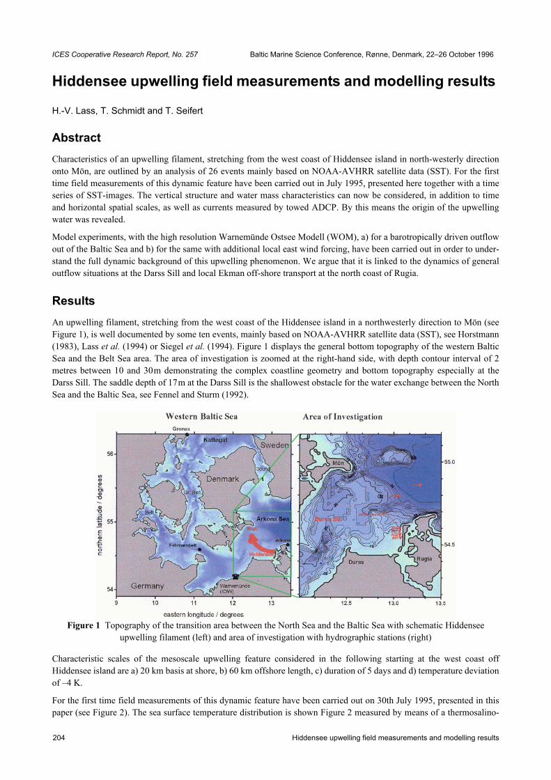
Hiddensee upwelling field measurements and modelling results204
ICES Cooperative Research Report, No. 257 Baltic Marine Science Conference, Rønne, Denmark, 22–26 October 1996
Hiddensee upwelling field measurements and modelling results
H.-V. Lass, T. Schmidt and T. Seifert
Abstract Characteristics of an upwelling filament, stretching from the west coast of Hiddensee island in north-westerly directiononto Mön, are outlined by an analysis of 26 events mainly based on NOAA-AVHRR satellite data (SST). For the firsttime field measurements of this dynamic feature have been carried out in July 1995, presented here together with a timeseries of SST-images. The vertical structure and water mass characteristics can now be considered, in addition to timeand horizontal spatial scales, as well as currents measured by towed ADCP. By this means the origin of the upwellingwater was revealed.
Model experiments, with the high resolution Warnemünde Ostsee Modell (WOM), a) for a barotropically driven outflowout of the Baltic Sea and b) for the same with additional local east wind forcing, have been carried out in order to under-stand the full dynamic background of this upwelling phenomenon. We argue that it is linked to the dynamics of generaloutflow situations at the Darss Sill and local Ekman off-shore transport at the north coast of Rugia.
Results An upwelling filament, stretching from the west coast of the Hiddensee island in a northwesterly direction to Mön (seeFigure 1), is well documented by some ten events, mainly based on NOAA-AVHRR satellite data (SST), see Horstmann(1983), Lass et al. (1994) or Siegel et al. (1994). Figure 1 displays the general bottom topography of the western BalticSea and the Belt Sea area. The area of investigation is zoomed at the right-hand side, with depth contour interval of 2metres between 10 and 30m demonstrating the complex coastline geometry and bottom topography especially at theDarss Sill. The saddle depth of 17m at the Darss Sill is the shallowest obstacle for the water exchange between the NorthSea and the Baltic Sea, see Fennel and Sturm (1992).
Figure 1 Topography of the transition area between the North Sea and the Baltic Sea with schematic Hiddensee upwelling filament (left) and area of investigation with hydrographic stations (right)
Characteristic scales of the mesoscale upwelling feature considered in the following starting at the west coast offHiddensee island are a) 20 km basis at shore, b) 60 km offshore length, c) duration of 5 days and d) temperature deviationof –4 K.
For the first time field measurements of this dynamic feature have been carried out on 30th July 1995, presented in thispaper (see Figure 2). The sea surface temperature distribution is shown Figure 2 measured by means of a thermosalino-

H.-V. Lass, T. Schmidt and T. Seifert 205
graph unit, mounted within the cooling water inlet of r/v “Professor Albrecht Penck”, placed 1.2 metres below the seasurface. Dots represent every tenth value of the continuous temperature recording along the ships track, white cm-stations and ADCP-tracks have been performed. 10 and 20m depth contours are included as dashed lines for better orien-tation. The survey was performed within approx. 30 hours under a steady outflow and calm east wind regime. The lowestsea surface temperature observed was approximately 11°C within the upwelling illament, white the ambient surfacewater temperature was up to 21°C.
Figure 2 Distribution of sea surface temperature measured by the thermosalinograph of r/v “Professor Albrecht Penck”. The dotted lines mark the ship’s tracks.
Figure 3 Distribution of sea surface temperature derived from NOAA-AVHRR data
A time series of NOAA-A VHRR satellite sea surface temperature (SST) scenes (provided by courtesy of BSH Hamburgand Dr. Siegel of IOW) shown in Figure 3 covers the whole event. This series reveals that the upwelling water appearedat the sea surface after 26th July, clearly seen at 27th July 07 UTC as darker shaded filament-like structure. The cloud

Hiddensee upwelling field measurements and modelling results206
coverage is blanked e.g. on 29th July. The coincidence of ship and satellite based surface temperature measurements at30th July is remarkable, even in details as e.g. the warm water intrusion at Darss Sill.
Vertical CTD-sections of water temperature (Figure 6) and salinity (not shown here) reveal that cold intermediate winterwater of the Arkona Basin welled up at the northern coast of Hiddensee island. In Figure 6 CTD-casts along stationsA01–A04, measured at 30th July 1995 have been supplemented by CTD profiles taken on stations 114 and 115 duringthe seasonal cruise of r/v “Alexander von Humboldt” on 5th August 1995, for position see Figure 1. The temperaturesection to station 115 located at the eastern slope of Darss Sill doesn’t show intermediate winter water of the Arkonabasin in contrast to the section ending in the central Arkona Basin at station 114. Obviously, the cold water tongue at theDarss Sill as seen in Figure 2 and Figure 3 is not due to local upwelling.
The upwelled water is advected westward from the north coast of Rügen and Hiddensee islands within the filament by astrong surface jet with velocities up to 75 cms–1 as shown in Figure 4. The observed velocities in this jet are comparableto current observations north of Rügen Island reported by Lass and Schmidt, 1992. Velocity was measured by acatamaran towed along the track, shown in Figure 1, carrying a downward looking 300 kHz broad band ADCP. Theprojected current component is regarded as perpendicular to the track pointing into the Baltic. The jet is trapped at thebottom slope just northward of Hiddensee island between approx. the 20m and 10m depth contours. Its width is about20km. The jet deepens at its southern edge, reaching down to the bottom within a band with a width of about 4km.
Figure 4 Projected component of current measured by a towed 600kHz ADCP of RDI. Positive values are towards 63o. The bottom contour is shaded grey.
A comparison between Figure 3 and Figure 5 reveals that the upwelling filament appeared on 27th July 1995 simultane-ously with the onset of outflow marked by the change of current direction in Fehmarn belt to 300°. Moreover Figure 5displays the turn of the wind direction from west to east (see negative east component of wind at Arkona; data of weatherstation Arkona by courtesy of German Weather Service). The easterly wind caused the observed lowering of sea level inthe Kattegat at Grenaa and subsequently the decrease of the mean sea level of the Baltic (tide gauge at Landsort). Afterthe decline of this outflow event the upwelling filament also disappeared (satellite picture for 5th August).

H.-V. Lass, T. Schmidt and T. Seifert 207
Figure 5 Time series of east component of wind velocity measured at the meteorological station Arkona (blue), sea level at Grenaa in the Kattegat (red) and Landsort in the Baltic proper (green), and direction of current measured in the
Fehmarn Belt at a depth of 6m (black). Outflow from the Baltic Sea toward the Kattegat is about 310o in the Fehmarn Belt.
Figure 6 Vertical temperature distribution from the central Arkona Basin towards Hiddensee (above) and from the eastern rim of the Darss Sill towards Hiddensee (below). The locations of the stations are shown in Figure 1.
Simulations of the described observations with a high resolution circulation model of the Baltic Sea (WOM, see Fennelet al. (1994)) reveal that a westward directed jet establishes a response to the lowering of sea level in the Kattegat (seeFigure 7). The jet stretches from the Darss Sill to the west coast of Hiddensee island continuing along the northern coastof Rügen island. Local Ekman upwelling at the northern coasts of Rügen and Hiddensee islands driven by easterly windsfeeds this jet with cold intermediate water from the Arkona Sea.

Hiddensee upwelling field measurements and modelling results208
Figure 7 Modelled sea surface temperature (left) and current (right), 96h after a step-like lowering of the sea level of the North Sea by 30cm and the onset of a localised east wind in the Western Baltic
SummaryThe Hiddensee upwelling filament fed by local upwelling with cold intermediate water from the Arkona Sea is generatedby an adjustment process between the Darss Sill and the southern Arkona basin to a lowering of the sea level in theKattegat. This is in contrast to upwelling filaments commonly observed at straight coasts which are mainly driven byadvection of long lasting Ekman offshore transport.
Comparisons between observations and modelling reveal that both modelled currents and temperature fronts are tooweak. This may be due to large horizontal exchange coefficients used in the model.
References Fennel, W., and Sturm, M. (1992). Dynamics of the western Baltic, Journal of Marine Systems, Vol. 3, p. 183–205
Fennel, W., Schmidt, M., and Siefert, T. (1994). Hochauflösendes Zirkulationsmodell der westlichen Ostsee, (Highresolution circulation modell of the western Baltic Sea) Abschluβbericht (Report) BMFT, BEO/7l 03F0057A
Horstman, U. (1983). Distribution patterns of temperature and water colour in the Baltic Sea as recorded in satelliteimages: Indicators for Phytoplankton Growth, Berichte aus dem Institut für Meereskunde Kiel, Nr. 106, Vol. 1
Lass, H.U., and Schmidt, Th. (1992). Observations of coastal jets in the Arkona Basin, Proceedings of 18th Conferenceof Baltic Oceanographers, St. Petersburg, 1993 and International Council for Exploration of the Sea, Rostock,Paper C.M. 1992/C:32, pp 11
Lass, H.U., Schmidt, Th., and Siefert, T. (1994). On the dynamics of upwelling observed at the Darss Sill, Proceedings of19th Conference of Baltic Oceanographers, Sopot, p. 247–261
Siegel, H., Gerth, M., Rudloff, R., and Tschersich, G. (1994). Dynamical features in the western Baltic Sea investigatedusing NOAA-AVHRR data, Deutsche Hydrographische Zeitschrift, Vol. 46, No.3, p. 191–209

Johan Mattson 209
ICES Cooperative Research Report, No. 257 Baltic Marine Science Conference, Rønne, Denmark, 22–26 October 1996
Geostrophic flow resistance in the Öresund
Johan Mattson
Figure 1 Map of the area
The idea of a geostrophic flow resistance was probably first presented by Garrett and Toulany in a pair of papers from thebeginning of the eighties (Garrett and Toulany, 1982, and Toulany and Garrett, 1984). It appeared in a model of the flowthrough a strait driven by the sea level difference between two basins connected by the strait.
Figure 2 The sea level (η) at various positions in and outside a strait with flow rate Q=VHW
The model (Figure 2) is based on an assumption of cross-strait geostrophy
(1)η2 η4– η3 η5– fWg
-------V= =

Geostrophic flow resistance in the Öresund210
and an along-strait balance between the pressure gradient due to sea surface slope, acceleration and friction
(2)
L is the length of the strait and g the gravitational accelerationV is the mean velocity, W is the width of the strait and f is the Coriolis parameter.
The problem is closed by a coupling between the basin and the strait sea levels. The assumptions that the highest level inthe strait equals the upstream level (η2=η1) and the lowest level in the strait equals the downstream sea level (η6=η5),give together with (1) and (2) a relationship between the flow rate and the sea level difference between the basins
(3)
where ∆η=(η1–η6) is the forcing sea level difference between the two basins. The flow rate for given forcing is deter-mined by the flow resistance. Thus, the effect of rotation is a contribution to the flow resistance, according to this model.
A feature of this model which was given special attention by its originators, is its form in the limit of steady state and nofriction. In this case the sea level difference across the strait equals the sea level difference between the two basins. Byarguing that it cannot be more, this state is referred to as a state of geostrophic control. In conclusion, we have
(4)
The idea of geostrophic resistance, which, quoting Chris Garrett, “seemed good at the time”, has had some trouble beingaccepted. This is obviously due to the matching conditions between the basins and the strait, which completely governthe solution but are somewhat arbitrarily determined. In the major part of the treatments discussing the geostrophiccontrol, the proposed flow situation is realised by propagating Kelvin waves (Pratt, 1991). While the basin–straitmatching is consistent with Kelvin wave propagation in two infinite basins with equal depth in the basins and the strait,problems arise with unequal depths in the basins and the strait, or with basins having finite area. Further objections canbe raised when long time scales are considered. Linear solutions to the Rossby adjustment problem in a strait give Kelvinwaves propagating away from the initial discontinuity, leaving a steady flow equal to that given by the geostrophiccontrol. The non-linear solutions show that this realisation is slowly advected, however, leaving a symmetric flowbehind. This solution is identical to the subcritical solution given by inviscid hydraulic theory. For hydraulicallysubcritical flows the solution is symmetric and the sea level difference between the upstream and the downstream basin iszero.
An assumption of downstream dissipation is often used in models of non-rotating strait flow (Stigebrandt, 1980).Potential energy is spent to accelerate the flow through the narrow strait, but it is assumed that, as the flow expands, itcannot climb the pressure hill. This means that the lowest level in the strait equals the downstream basin sea level. Ineffect, downstream dissipation causes energy losses, i.e. flow resistance. This is in contrast with inviscid hydraulictheory, by which the only possible energy losses are through hydraulic jumps.
Thus, it appears that downstream dissipation is a prerequisite for geostrophic resistance in steady state. There is no way,however, to find an analytical solution involving downstream dissipation based on the equations of motion. Theexistence of a geostrophic resistance has to be shown empirically.
A modification of the above theory will be presented. In what follows a steady state is described and the along-straitbalance is frictional, given by
(5)
The frictional resistance is modelled using a quadratic friction law, where cD is a drag coefficient. The model of Toulanyand Garrett was originally designed to analyse time series of sea level data in the frequency domain, and so is linear bynecessity. The advective terms are neglected and the frictional effects are modelled with a linear friction law. Due to therather unrealistic linear friction law the model cannot explain the flow resistance in a shallow strait like the Öresund,where frictional effects dominate.
η2 η3– η4 η5– Lg--- acc fric+( )V= =
VWH Q gH∆η f acc fric+( ) LW-----+
1–= =
Q gHf
-------∆η≤
η2 η3– η4 η5–cDLgH---------V2= =

Johan Mattson 211
As suggested by the concept of downstream dissipation, the lowest level in the strait will still be assumed equal to thedownstream basin sea level, i.e. (η6=η5). The coupling between the upstream basin and the strait is the sum of a non-rotating and a rotating part η1–η4=(η1–ηRT)+(ηRT–η4) (cf. Whitehead, 1986), where the non-rotating part is
(6)
and the rotating part is:
(7)
The non-rotating part is the Bernoulli setdown, caused by the acceleration towards the strait. The rotating part is based oncross-strait geostrophy, and the factor 1/2 corresponds to a geostrophic tilt that is distributed such that the sea level isdepressed over half the width of the strait compared to the non-rotating solution. These basin-strait couplings result in theexpression
(8)
However, for V< fW, the sea level at the right hand side of the strait may formally become higher than the upstream sealevel (η2>η1). This is not possible for streamlines originating in a motionless upstream basin. By simply requiring thatη2=η1 for V< fW we have
(9)
This is the model that should be tested against observations, and which accurately describes the low frequency flowthrough the Öresund. The model gives the flow resistance as a combination of the linear contribution from thegeostrophic resistance and two quadratic contributions, one related to the Bernoulli setdown and the other due tofrictional drag. The physical explanation for the geostrophic resistance is then clear. A pressure drop is required to accel-erate the water towards the strait, and this pressure drop is not recovered downstream. This may be seen as a kind of formdrag. In rotating systems an additional pressure drop is needed to geostrophically balance the flow, and this effects addsto the form drag.
Expression (9) can be written
(10)
where Kt and Kq are flow resistance coefficients to be determined from observations. In a paper by the present author(Mattsson, 1995), where 1802 simultaneous observations of sea level difference and flow rate from the Öresund wereused (Figure 3), a least-squares fit gave Kq=1.29·10–10s2m–5 and Kt=0.32·10–5sm–2.
Figure 3 1802 simultaneous estimates of flow rate and sea level difference
η1 ηRT– 12g------V2=
ηRT η4–( ) 12--- fW
g-------V=
∆η 12--- fW
g-------V 1
2g------
cDLgH---------+
V2+=
∆η 12--- fW
g-------V 1
2g------
cDLgH---------+
V2 V fW≥;+=
∆η fWg
-------VcDLgH---------V2 V fW<;+=
∆η KtQ KqQ2+=

Geostrophic flow resistance in the Öresund212
Returning to expression (9), which can be written
(11)
it follows that
(12)
Inserting appropriate values (cf. Mattsson, 1996) and using an amplitude distribution based on the observations, Ktshould during 40 percent of the time correspond to 0.37·10–5 and to 0.31·10–5 during 60 percent of the time. Theweighted sum is 0.33·10–5, which is very close to what was empirically found. Thus, the data strongly supports theexistence of a geostrophic resistance as defined by the model.
Traditionally, the flow resistance in the Öresund has been modelled using a quadratic relation only (e.g. Jacobsen, 1980,Omstedt, 1987 and Stigebrandt, 1992). The skill of such a model appears to be very good, measured by an explainedvariance of over 80 percent. The reason for its success is obviously the strong frictional influence on the flow resistance.When the geostrophic resistance is included the explained variance only increases by about 2 percent. This appears insig-nificant, and has put the combined model (the model combining a quadratic and a linear term) in doubt. However, theincrease by 2 percent is exactly what can be expected. In a hypothetical case, trying to fit a quadratic function to a linearrelation, the explained variance would differ by only 6.25 percent, and any combined model having both a quadratic anda linear term would have a smaller difference.
Instead, the main effect of using a quadratic model without the geostrophic term is an incorrect amplitude frequencydistribution. A closer inspection shows that flow rates for weak forcing are systematically overestimated and vice versa.This becomes clear in a plot of the amplitude probability density function for the flow rate, based on observations, thequadratic model and the combined model (Figure 4). The least-squares fit using the quadratic model, in its attempt tominimise the deviation (i.e., maximise the explained variance), apparently shifts the distribution towards higher flowrates. The combined model is much more successful in explaining the correct distribution. Again measuring the skill withthe explained variance, the geostrophic term increases the explained variance by 30 percent, from 67 to 97 percent. Thelinear term, i.e., the geostrophic resistance, is obviously necessary to model the flow resistance and hence reproduce theflow through the Öresund.
Figure 4 The probability density function of the absolute flow rate, p(|Q|), for the observed flow rate (solid line), the flow rate according to the quadratic model (dashed line) and according to the combined model (dotted line)
∆η 12--- f
gH-------Q 1
2gH2W2---------------------
cDL
gH3W2-----------------+
Q2 Q fHW2≥;+=
∆η fgH-------Q
cDL
gH3W2-----------------Q2 Q fHW2<;+=
Ktf
2gH----------- Q fHW2≥;=
Ktf
gH------- Q fHW2<;=

Johan Mattson 213
In the general case, guidance can be provided by the non-dimensional version of expression (11). Introducing the primeddimensionless variables ∆η=H∆η' and Q=(g1/2H3/2W)Q' gives
(13)
where a is the Rossby radius of deformation. The geostrophic control limit refers to cases where the strait is of order ofthe deformation radius, small length to depth ratios and for small flow rates .
References Garrett, C. and Toulany, B., 1982. Sea level variability due to meteorological forcing in the northeast Gulf of St.
Lawrence, J. Geophys. Res., 87, 1969–1978.
Jacobsen, T. S., 1980. Sea Water Exchange of the Baltic. Measurements and Methods, The Belt Project. 107 pp. TheNational Agency for Environmental Protection. Denmark.
Mattsson. J., 1995. Observed linear flow resistance in the Öresund due to rotation, J. Geophys. Res. 100, C10. 20779–20791.
Mattsson, J., 1996. Some comments on the barotropic flow through the Danish straits and the division of the flowbetween the Belt Sea and the Öresund. Tellus, 48A. 456–464.
Omstedt. A., 1987. Water cooling in the entrance of the Baltic Sea. Tellus. 39A, 254–265.
Pratt. L. J., 1991. Geostrophic versus critical control in straits. J. Phys. Oceanogr. 21. 728–732.
Stigebrandt, A., 1980. Barotropic and baroclinic response of a semi-enclosed basin to barotropic forcing from the sea. inFjord Oceanography. pp. 151–164. Plenum Press. New York.
Stigebrandt. A., 1992. Bridge-induced flow reduction in sea straits with reference to effects of a planned bridge acrossÖresund, Ambio. 21. 130–134.
Toulany, B. and Garrett, C., 1984. Geostrophic control of fluctuating barotropic flow through straits. J. Phys. Oceanogr.14. 649–655.
Whitehead, J. A., 1986. Flow of homogeneous rotating fluid through straits. Geophys. Astrophys. Fluid Dyn. 6. 101–125.
∆η' 12---W
a-----Q' 1
2--- cD
LH----+
Q'2 Q' Wa-----≥;+=
∆η' Wa-----Q' cD
LH----Q'
2Q' W
a-----<;+=
Q' 0→

Baltic Sea Science Conference Rønne, Denmark, 22–26 October 1996 214
ICES Cooperative Research Report, No. 257 Baltic Marine Science Conference, Rønne, Denmark, 22–26 October 1996
Distribution patterns of nutrients discharged by the river Odra into the Pomeranian Bight
Klaus Nagel
Summary With a focus on chemical parameters, several types of distribution patterns for the matter discharged by the river Odrainto the Pomeranian Bight can be classified. Two types of hydrographically controlled distribution patterns arediscussed, the ‘west wind situation’ and the ‘east wind situation’. Both types are characterised by the directions in whichthe riverine material is transported. The amount of discharged material that reaches the offshore regions of the Baltic Seadoes not only depend on water supply, but also on transformation and modification processes taking place in the plume.The influence of these processes on the distribution patterns is dominated by seasonal effects, mainly controlled by thebiological activity in the water.
Introduction The TRUMP project (Transport and Turnover Processes in the Pomeranian Bight) was established to describe thetransport and transformation of material discharged by the river Odra and some smaller freshwater inflows into thePomeranian Bight and the influence of these processes upon the marine ecosystem in the offshore regions of the BalticSea. In an interdisciplinary approach, complex datasets of meteorological, hydrographic, chemical and biological param-eters were analysed in cooperation with Polish and German institutions.
Objectives of the project are the characterisation of the transport mechanisms and distribution patterns of the dischargedmaterial and the description of processes responsible for the transformation and modification of this material.
Experimental strategies Between September 1993 and January 1996, seven cruises were performed within the TRUMP project as multishipsurveys. At least two ships were operating simultaneously for 2–3 weeks in the area under investigation. Experiments onone ship focused on transport processes while the second ship concentrated on the analysis of transformation processes.
For the characterisation of transport processes and distribution patterns, samples were taken within 60–80 hours by oneof the ships on a station grid covering the whole bight (Figure 1). Besides standard meteorological, hydrographic andchemical parameters, which were analysed at all stations, additional measurements were performed at selected stations:dissolved and particulate organic carbon and nitrogen, some naturally occurring organic compounds (e. g. urea, carbohy-drates, amino acids, etc.), contaminants, biological variables, sediment analysis, etc. 2–4 samples were taken at the gridstations in time intervals of 48–96 hours during each cruise.
During the experiments, additional measurements were performed by other Polish and German ships and institutions inthe river mouth, the lagoons and at inshore stations.
This paper focuses on the classification of distribution patterns of nutrients depending on meteorological and seasonalconditions. An illustration of other aspects of the TRUMP project is given elsewhere (e.g. Bulletin of Sea FisheriesInstitute 3 (136), 1995; TRUMP, 1996).

Klaus Nagel 215
Figure 1 TRUMP: Station grid in the Pomeranian Bight
Results During the TRUMP cruises in 1993–1996 concentrations of nutrient salts were measured in the plumes of the river Odra(via the rivers Swina and Dziwna) or the river Peene (via Greifswalder Bodden). Concentrations of all nutrient salts arehighly variable showing great fluctuations within one or two days. As an example, variations of nitrate concentrationsvery close to the Swina mouth are shown in Figure 2. Factors responsible for these high variations are:
• ‘Preconditioning’ of the riverine discharge in the lagoons, mainly due to the modification and transformationprocesses caused by high biological activity found in the lagoons in late spring and in summer. This preconditioningeffect is strengthened by the fact that freshwater discharge from the river Odra is lower in the period with highbiological activity (May–November) and higher in the period of low biological activity (December–April).
• ‘Pulsating’ of the riverine outflow showing distinct ‘outflow events’ (Figure 3). Outflow events are mainly controlledby differences of the water levels between the Baltic Sea and the lagoons (Lass, 1994; Lass et al., 1995a). Theriverine water with low salinity spreads in the surface layer during an outflow event, while mixing with subsurfacewater occurs in a second step which is controlled by meteorological and hydrographic factors (e.g. wind directedcirculation of water masses).
Figure 2 Concentrations of nitrate in the surface and bottom layer at station 10 situated very close to the Swina mouth. Results obtained during each experiment are linked by a line.
13.5 14.0 14.5 15.0 15.5Longitude
53.8
54.0
54.2
54.4
54.6
54.8
Latit
ude
IOW - MeereschemieK.Nagel 10/21/96
Date 24/0
9/93
28/0
9/93
01/1
0/93
24/0
6/94
28/0
6/94
02/0
7/94
17/0
1/95
21/0
1/95
25/0
1/95
16/0
4/95
20/0
4/95
24/0
4/95
24/0
6/95
28/0
6/95
02/0
7/95
06/0
7/95
10/0
7/95
25/0
9/95
29/0
9/95
20/0
1/96
24/0
1/96
Nitr
ate
( µm
ol /
l )
0
20
40
60
80
NO3 concentration surface layerNO3 concentration bottom layer
09 / 1993 06 / 1994 01 / 1995 04 / 1995 06 / 1995 09/1995 01/1996 Experiment
13.5 14.0 14.5 15.0 15.5Longitude
53.8
54.0
54.2
54.4
54.6
54.8
Latit
ude

Distribution patterns of nutrients discharged by the river Odra into the Pomeranian Bight216
Figure 3 Distribution patterns of nitrate in the surface layer before (left) and during (right) and outflow event in September 1993. Sampling positions are marked on the map with a plus (+))
Generally, concentrations of all nutrients in the outflowing riverine water are higher during winter and early springtime.While amounts of N-containing nutrients are significantly lower during the summer, phosphate is depleted in thedischarges in late springtime and summer. In autumn an increase of phosphate is observed some weeks before theincrease of nitrate concentrations starts again. This difference in seasonal minima of N- and P-containing nutrient salts iscaused by the tie-lag between the start of plankton bloom in the lagoons and the inner parts of the Pomeranian Bight inspringtime and the beginning of remineralisation processes in both areas in late summer. As a result of the phosphatedepletion in the discharged water biological activity in the inner parts of the bight can be limited by phosphate in latespringtime.
Characterisation of standard and special situations
‘West wind situation’ and ‘Summer conditions’ (TRUMP experiment in June/July 1994) Material of the river plume is transported in a small strip along the coast towards the eastern parts of the Baltic if westerlywinds (including directions from north to southwest) predominate for several days (Figure 4). Such transport bands cansometimes be followed from the Pomeranian Bight to the Gulf of Gdansk in satellite images (Lass et al., 1995a). Theriverine water with lower salinity is mixed down to the bottom layer in this shallow area. In summer, similar ‘transportbands’ shown for nitrate in Figure 4 are also found for salinity and chlorophyll.
Figure 4 Distribution pattern of nitrate in June 1994. Samples have been taken from the surface layer at the first sampling from the grid stations.
13.5 14.0 14.5 15.0 15.5Longitude
53.8
54.0
54.2
54.4
54.6
54.8
Latit
ude
IOW - Meereschemie Autoanalyzer Measurement M. Graeve / K. Nagel K.Nagel [1h1_n300] 09/22/98
0.1
0.6
1.1
1.6
2.1
2.6
3.1
3.6
4.1
4.6
Nitrate + Nitrite Surface Layer min. Contour : 0.1 µmol / l Contour Distance : 0.5 µmol / l
13.5 14.0 14.5 15.0 15.5Longitude
53.8
54.0
54.2
54.4
54.6
54.8
Latit
ude
IOW - Meereschemie Autoanalyzer Measurement M. Graeve / K. Nagel K.Nagel [1h2_n300] 09/22/98
0.1
0.6
1.1
1.6
2.1
2.6
3.1
3.6
4.1
4.6
Nitrate + Nitrite Surface Layer min. Contour : 0.1 µmol / l Contour Distance : 0.5 µmol / l
13.5 14.0 14.5 15.0 15.5Longitude
53.8
54.0
54.2
54.4
54.6
54.8
IOW - Meereschemie Autoanalyzer Measurement B. Sadkowiak / K. Nagel K.Nagel [2h1_n300] 09/22/98
0.5
2.5
4.5
6.5
8.5
10.5
12.5
Nitrate Surface Layer min. Contour : 0.5 µmol / l Contour Distance : 2.0 µmol / l

Klaus Nagel 217
Nutrient salts are nearly depleted in the whole bight due to the high biological activities in summer. While phosphate andnitrate are near or below the detection limit in the central parts of the bight, low concentrations are found for ammoniaand silicate (0.1–3µmoles·dm–3 and 5–15µmoles·dm–3, respectively).
Distribution patterns differ significantly for the individual nutrient salts in the plume since transformation processes andmodification of material take place in the lagoons as well. Highest concentrations of ammonia were found in the Dziwnaestuary (far more than 3µmoles·dm–3), while the main source of nitrate was the Swina during this cruise. Phosphate wasbelow the detection limit at all stations in this region. Silicate concentrations were higher in the coastal zone, but nopronounced effect of the plume was observed (Nausch et al., 1995).
As the fate of the riverine matter in the bight is mainly controlled by transformation and modification of material undersummer conditions, these processes superimpose the effects caused by the transport of the freshwater discharge.
‘East wind situation’ and ‘Winter conditions’ (TRUMP experiment in January 1996) ‘East wind situations’ become established if the dominating wind directions are between northeast and south for severaldays. Under this regime, riverine water is spread northwards along the coast of Usedom and Rügen within an areacovering the whole western part of the bight (Figure 5). Distribution of material is more homogenous than during ‘westwind situations’ and no steep horizontal and vertical concentration gradients are found.
Figure 5 Distribution pattern of phosphate in January 1996. Samples have been taken from the surface layer at the first sampling from the grid stations.
The distribution patterns for salinity and the individual nutrient salts were found to be very similar in the experimentsperformed in winter. Due to low biological activity at this time of the year, transformation processes seem to be negli-gible. Variations in the distribution patterns are primarily based on the transport of material by advective processes andmixing of riverine water with the seawater in the bight. This effect is expressed by significant correlations between theindividual nutrients and between nutrients and salinity (Figure 6).
13.5 14.0 14.5 15.0 15.5Longitude
53.8
54.0
54.2
54.4
54.6
54.8
Latit
ude
IOW - Meereschemie Autoanalyzer Measurement B. Sadkowiak / K. Nagel K.Nagel [7h1_n600] 09/22/98
y ( ; )
0.2
0.4
0.6
0.8
1.0
1.2
1.4
1.6
Phosphate Surface Layer min. Contour : 0.2 µmol / l Contour Distance : 0.2 µmol / l

Distribution patterns of nutrients discharged by the river Odra into the Pomeranian Bight218
Figure 6 Correlations between the concentrations of individual nutrient salts in January 1996. Samples have been taken from the surface layer at the first sampling from the grid stations.
Distribution patterns caused by special situations (e.g. TRUMP experiments in September 1993 and September/October 1995) During some cruises, distinct areas were found which differ significantly from the surroundings with respect to hydro-graphic conditions, nutrient concentrations or the biological activity. Examples for such patterns were observed duringthe cruises in September 1993 (for details see Pastuszak et al., 1996) and in September/October 1995 (Figure 7). North ofUsedom a water body was identified which is characterised by low salinity and nutrient concentrations but highbiological activity. It had been observed for several days in the same area. This ‘enclosure’ developed after the reversalof water circulation in the bight caused by the change of the wind direction from south to west shortly after an outflowevent occurred. As verified by ADCP measurements, this water mass is stabilised by two currents: one is moving directlynear the coastal line to northwest, the other one is going southwest several miles in front of the coast (Lass et al., 1995b).Physicals aspects of this phenomenon are discussed elsewhere (Mohrholz 1998).
Figure 7 Distribution pattern of nitrate in September 1995. Samples have been taken from the surface layer at the first sampling from the grid stations.

Klaus Nagel 219
A separated and stable water body like that observed in September 1995 offers an excellent opportunity to study in detailthe transformation and modification processes in an ‘enclosure’ under natural conditions.
ConclusionsDistribution patterns of nutrients identified during the TRUMP experiments can be classified according to the predomi-nance of transport or transformation processes. Transport mechanisms are dominated by meteorological factors (westwind–east wind situations), while the comparison of seasonal patterns (summer–winter conditions) reveal the influenceof transformation and modification processes mainly controlled by the biological activity. Data sets produced duringeach of those standard situations are a good tool for the test and verification of numeric models, which are necessary todescribe the influence of riverine inputs on the marine ecosystem in offshore regions of the Baltic Sea. Water massesseparated and stabilised by hydrodynamic mechanisms are of special interest for the estimation and validation of trans-formation rates needed for the forcing of models taking into account biological processes.
Acknowledgement The TRUMP project was supported by Federal Ministry of Education, Science, Research and Technology (Project03F01058 im Forschungsverbund Mecklenburg-Vorpommersche Küste).
ReferencesLass, H. U. (1994). Preliminary Studies of a Pilot Study of TRUMP. Proc. 5th German-Polish Seminar on Coastal and
Estuary Dynamics, October 26-30, 1993, Geesthacht, 5: 261–279
Lass, H. U., Fennel, W., Siegel, H., Sattler, K., Gerth, M., and Rüβ, D. (1995a). Zirkulations- und Transportprozesse inder Pommerschen Bucht. TRUMP, 1. Zwischenbericht 1994, pp 17–38
Lass, H. U., Mohrholz, V., and Nagel, K. (1995). Beobachtungen in einer isolierten Fluβwasserfahne vor der KüsteUsedoms. (Poster zum 2. Statusseminar des GOAP-Projekts in Greifswald (13 & 14/12/1995)
Mohrholz, V. (1998). Transport- und Vermischungsprozesse in der Pommerschen Bucht. MeereswissenschaftlicheBerichte 33: 1–106.
Nausch, G., Nagel, K., Nehring, D., Kerstan, E., Sadkowiak, B., and Welz, A.-M. (1995). Verteilungsgradientenchemischer Ökosystemparameter in der Pommerschen Bucht. TRUMP, 1. Zwischenbericht 1994, pp 39–68
Pastuszak, M., Nagel, K., and Nausch, G. (1996). Variability in nutrient distribution in the Pomeranian Bay in September1993. Oceanologica 38: 195–225
TRUMP, 2. Zwischenbericht 1995 (1996)

Petroleum hydrocarbons in the onshore zone220
ICES Cooperative Research Report, No. 257 Baltic Marine Science Conference, Rønne, Denmark, 22–26 October 1996
Petroleum hydrocarbons in the onshore zone
Zbigniew Otremba, Adam Stelmaszewski, Krystyna Kruczalak, and Roman Marks
IntroductionPetroleum hydrocarbons in the onshore zone have different origins; the main source is discharge by rivers (over 50%),storm water from municipalities and municipal sewage (20%), operational and accidental discharges from shipping (1–20%) and the remainder come from atmospheric deposition, oil terminals, etc. (Enckell, 1986). Recent investigationsconducted at the Maritime Academy in Gdynia also confirmed significantly higher petroleum hydrocarbons contami-nation of river waters compare to that recorded in the Baltic Sea coastal waters (Otremba and Stelmaszewski, 1996).
General data on the distribution of oil pollution concentrations in water as recorded within the 1µgdm–3 range are plottedin Figure 1. The predominant occurrence of petroleum hydrocarbons in the sea water ranged within 1–2µgdm–3, while inthe river water the recorded concentrations ranged from 10 to 50µgdm–3. The results again confirmed that rivers andstreams are the main source of oil pollution in Baltic Sea onshore regions.
Figure 1 Oil content in the sea water and water from rivers entering the Baltic Sea on the Polish coast
Part of the petroleum hydrocarbons entering the coastal waters are transferred into sediments. Within the Polish coastalwaters very high concentrations in sediments were recorded in the Gulf of Gdansk and the Pomeranian Bay. The highestvalues were recorded in the Gulf of Gdansk, eastward from the Vistula river mouth (Figure 2). This might be caused bycontinuous transport of oil pollution by river water and their sedimentation at the bottom.
Petroleum hydrocarbons in the sea water are subject to continuous transformation. After entering into the sea water theoil is degraded by bacteria and sunlight. The decay intensity depends on environmental conditions like temperature orcoastal dynamics. In the coast zone the wave/sediments interaction may in particular control both dispersion and furtherhorizontal and vertical transport. In addition however the sea to air transport of oil pollution can be expected. Thisparticular research has been undertaken by our group. Until now however only preliminary data have been collected.
In order to trace the fate of the petroleum hydrocarbons in the coastal environment, complex measurements of thepetroleum hydrocarbon concentration in water, sand, sediments and sea foam were performed.

Zbigniew Otremba, Adam Stelmaszewski, Krystyna Kruczalak, and Roman Marks 221
Figure 2 Concentration of hydrocarbons in the sediments near the Polish coast (Kaniewski et al., 1995)
MethodData presented in this work were collected within the Baltic Aerosol Experiment (BAEX). Measurements wereconducted at Lubiatowo Research Station located over Southern Baltic Sea Coast. Data were collected during two fieldexperiments in the autumn of 1994 and 1995 (Schulz et al., 1996). During the BAEX experiment 53 subsurface watersamples, 34 aerosol samples and 8 sand samples were collected. Water samples were taken from surface layer,subsurface and at 1m depth. The thicknesses of the collect surface layers were 90µm and 250µm depending on method.The foam samples were collected along the shore. Oil pollution content in the sea water, foam, aerosol and sand wereanalysed by the spectrofluorymetry method at the Gdynia Maritime Academy. All samples were extracted with hexaneand the extracts were excited by 313nm light. The fluorescence intensity (wavelength 360nm) was a measured of amountof oil concentration. The quantity of oil was determined base on a calibration curve obtained for a standard which wasthe crude oil from the North Sea aged at 120oC for 2 hours.
Results As a first approach all data on oil content in the sea water as related to offshore distance are plotted in Figure 3, Figure 4and Figure 5. As shown in Figure 3 the recorded concentrations of oil in subsurface decreases with increasing distancefrom the water line. The same tendency was observed for surface water samples, see Figure 4. In this case however therecorded concentrations were about four times higher than that for subsurface water. At the same time oil in the micro-layer (250µm), see Figure 5, appears to have about ten times lower concentrations than in the surface layer (90µm). Thisresult suggests than oil might be concentrated at the surface and near the bottom. Probably oil pollution accumulates insuspended matter which can sediment at the bottom or can be resuspended and fractionated by the breaking waves andbubbles.
Figure 3 Concentration of hydrocarbons in subsurface layer as related to offshore distance

Petroleum hydrocarbons in the onshore zone222
Figure 4 Concentration of hydrocarbons in the surface layer as related to offshore distance
Figure 5 Concentration of hydrocarbons in the microlayer as related to offshore distance
As part of the experiment, the oil concentrations in aerosol were also investigated. Aerosol samples were collected onWhatman filters and were analysed using the same method as for the water. The data obtained are plotted in Figure 6 andFigure 7. In general the data recorded demonstrate a significant scatter (Figure 6). Further study however confirmed thatdistribution of data points strongly depends on the wind direction sector (Figure 7).
Figure 6 Concentrations of hydrocarbons in the air. Width of rectangles represents time of collection
Figure 7 Concentrations of hydrocarbons in air as related to air advections from sea, beach and land

Zbigniew Otremba, Adam Stelmaszewski, Krystyna Kruczalak, and Roman Marks 223
For comparison in Figure 8 the data on oil concentration in water as measured in various offshore distances is plotted fordifferent wind direction sectors. Interpretation of these results is difficult, although data distribution suggest possibleinterpretation.
Figure 8 Concentration of hydrocarbons in seawater for different wind sectors: from sea, from land or along the coast.
In Figure 9 the concentration of oil in the onshore water is plotted against wind speed. The results obtained suggest thatthe amount of oil in the onshore water strongly depends on wind speed and breaking wave action, which may possiblycontrol both dispersion and transport of oil contaminated sediments.
Figure 9 Hydrocarbon concentrations in subsurface water as a function of wind speed. Data collected in the breaking wave zone (Lubiatowo, September 1995)
To complete the experimental measurements the oil concentration in sand were also investigated. The vertical profile ofthe oil content in sand samples is plotted in Figure 10. Recorded lower concentrations of oil in surface sand can be aneffect of intense degradation due to microbe and sun radiation. Next to the surface the amount of oil showed highestvalues and than decreased with distance from the surface. The lower oil concentrations in sand at 1m or below suggestsignificant degradation by bacteria.
Figure 10 Concentration of hydrocarbons in beach sand for different depths

Petroleum hydrocarbons in the onshore zone224
Extremely high oil concentrations were found in foam. Measured concentrations were 1000 times higher than in thewater sampled at the same place.
ConclusionsOil pollution is spread over the Southern Baltic Sea environment and is present in air, water, sand, sediments and inparticular in foam.
The concentrations of oil pollution in the coastal waters were found to increase with increasing wind speed and waveaction.
Significant amounts of petroleum hydrocarbons can be advected with land originated air pollution.
The petroleum hydrocarbons are concentrated at the water surface, therefore sea to air oil pollution transport can beexpected.
Complex modelling of the fate of petroleum hydrocarbons in water/air/sediments system over the Southern Balticenvironment is currently underway.
Acknowledgments This research has been supported by the Commission of the European Communities via the Contract No CIPA-CT 93-0086.
ReferencesOtremba Z., and Stelmaszewski A., 1996. Amount and origin of petroleum hydrocarbons at the Polish east coast. Under
preparation.
Enkell E., 1986. Oil pollution load to the Baltic Sea; A compilation of measured and estimated load. Baltic SeaEnvironment Proceedings No. 22.
Schulz M., Marks R., and Spirkauskaite N., 1996. BAEX—Baltic Aerosol Experiment, Joint research project. Progressreport No. 4, EU—Contract NO. CIPA-CT93-0086.
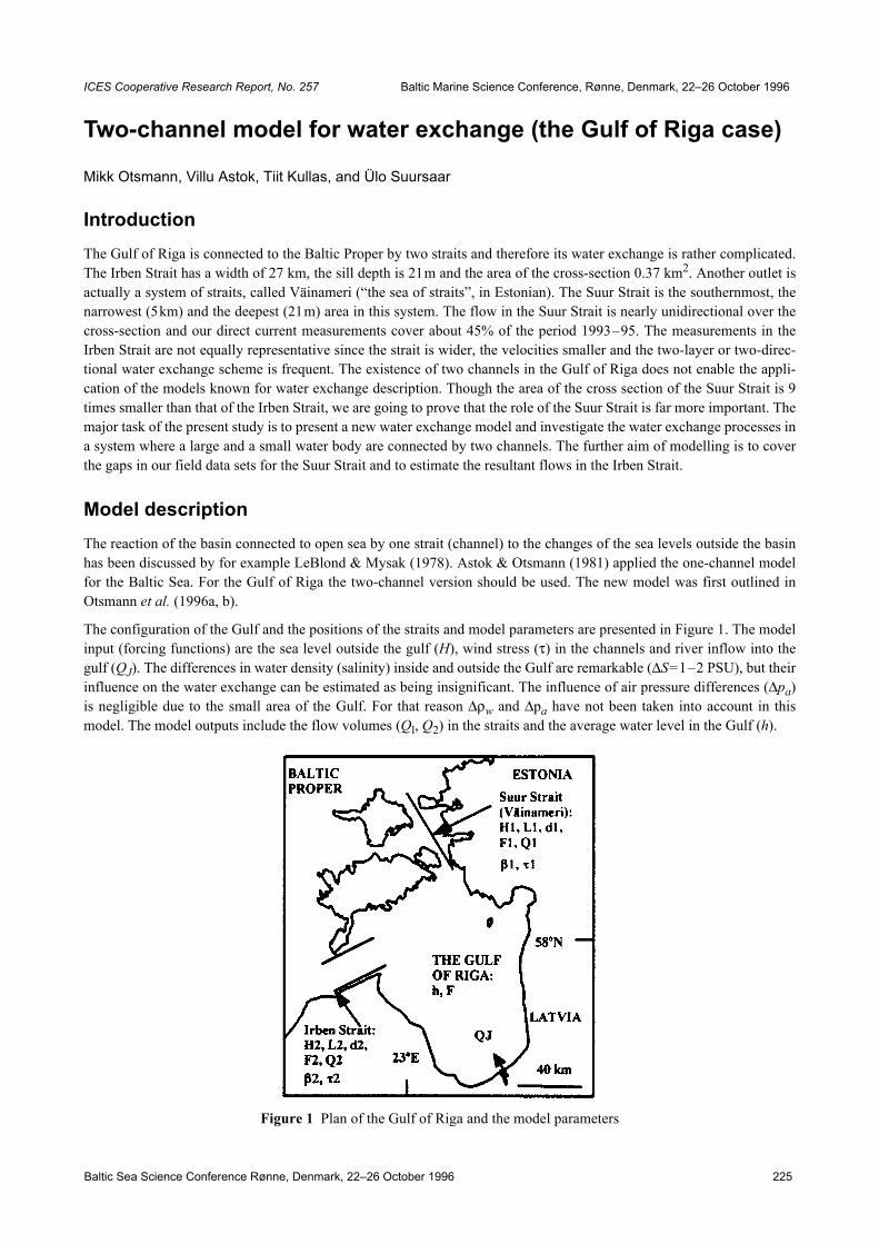
Baltic Sea Science Conference Rønne, Denmark, 22–26 October 1996 225
ICES Cooperative Research Report, No. 257 Baltic Marine Science Conference, Rønne, Denmark, 22–26 October 1996
Two-channel model for water exchange (the Gulf of Riga case)
Mikk Otsmann, Villu Astok, Tiit Kullas, and Ülo Suursaar
Introduction The Gulf of Riga is connected to the Baltic Proper by two straits and therefore its water exchange is rather complicated.The Irben Strait has a width of 27 km, the sill depth is 21m and the area of the cross-section 0.37 km2. Another outlet isactually a system of straits, called Väinameri (“the sea of straits”, in Estonian). The Suur Strait is the southernmost, thenarrowest (5km) and the deepest (21m) area in this system. The flow in the Suur Strait is nearly unidirectional over thecross-section and our direct current measurements cover about 45% of the period 1993–95. The measurements in theIrben Strait are not equally representative since the strait is wider, the velocities smaller and the two-layer or two-direc-tional water exchange scheme is frequent. The existence of two channels in the Gulf of Riga does not enable the appli-cation of the models known for water exchange description. Though the area of the cross section of the Suur Strait is 9times smaller than that of the Irben Strait, we are going to prove that the role of the Suur Strait is far more important. Themajor task of the present study is to present a new water exchange model and investigate the water exchange processes ina system where a large and a small water body are connected by two channels. The further aim of modelling is to coverthe gaps in our field data sets for the Suur Strait and to estimate the resultant flows in the Irben Strait.
Model description The reaction of the basin connected to open sea by one strait (channel) to the changes of the sea levels outside the basinhas been discussed by for example LeBlond & Mysak (1978). Astok & Otsmann (1981) applied the one-channel modelfor the Baltic Sea. For the Gulf of Riga the two-channel version should be used. The new model was first outlined inOtsmann et al. (1996a, b).
The configuration of the Gulf and the positions of the straits and model parameters are presented in Figure 1. The modelinput (forcing functions) are the sea level outside the gulf (H), wind stress (τ) in the channels and river inflow into thegulf (QJ). The differences in water density (salinity) inside and outside the Gulf are remarkable (∆S=1–2 PSU), but theirinfluence on the water exchange can be estimated as being insignificant. The influence of air pressure differences (∆pa)is negligible due to the small area of the Gulf. For that reason ∆ρw and ∆pa have not been taken into account in thismodel. The model outputs include the flow volumes (Ql, Q2) in the straits and the average water level in the Gulf (h).
Figure 1 Plan of the Gulf of Riga and the model parameters

Two-channel model for water exchange (the Gulf of Riga case)226
The model is based on the motion equations in straits integrated along the coordinates z, y, z, and the water balanceequation for the Gulf:
(1)
(2)
where:
(3)
i=1 in the Suur Strait; i=2 in the Irben Straitt– timeF–area of the Gulf of Riga (the value used was 1.63·1010m2)Fi–cross-section of the channel (F1=4·104; F2=3.7·105m2)Li–length of the channel (L1=7.5·104; L2=2·104m)di–channel depth (d1=10.5; d2=19m)g–acceleration of gravityR–friction coefficient (3.5·10–5s–1)Qi–volume flow in the channel; ui=Qi/FiQj–river inflow (1·103m3s–1)Hi–water level in the Baltic Properh–water level in the Gulfτi–wind stress projection on direction of channels; β1=155o; β2=65o;
(4)
ρa–air density, ρw–water density, ua–wind velocity,ϕ–wind directionc–nondimensional coefficient (c=1.2·10–3)
RQi(t) in the left side of equation (1) describes the influence of the bottom friction on the motion in the linear approxi-mation. This approximation could be used in small motion velocities (determined as cm2s–2) since the descriptionof the motion with nonlinear friction in the analytical case is more complicated but essentially of the same nature. In thenumerical solution the nonlinear friction was used in the realistic forcings. Combining (1) with (2) we obtain theequations for Qi(t), h(t) and Q(t)=Q1(t)+Q2(t):
(5)
(6)
(7)
where: (8)
Equations (5) to (7) are known in mechanics as the forced oscillation equations. The right sides of the equations representthe sum of external forces evoking the oscillations. Parameters ω0 and ω0i are the eigenoscillation frequencies of thesystem in the absence of frictional forces. The given model parameter values (including friction) yield the period of theeigenoscillations:
dQi t( )dt
---------------- RQi t( )gFiLi
--------h t( )+ + fi t( )=
Fdh t( )dt
------------- Qi t( ) Qk t( ) QJ t( )+ +=
fi t( ) FigLi----Hi t( )
τi t( )di
----------+ i k, , 1 2 i k≠;,= =
τi τ 1–( ) βi ϕ–( ) τ,cos cρaρw------ ua
2= =
τ 1≤
d2
dt2------- R td
d ω02+ +
h t( )f1 t( ) f2 t( )+
F---------------------------- 1
F---
tdd R+
QJ t( )+=
d2
dt2------- R td
d ω02+ +
Q t( )td
d f1 t( ) f2 t( )+( ) ω02QJ t( )–=
d2
dt2------- R td
d ω02+ +
Q t( )td
d f1 t( ) ω0i2 Qk t( ) QJ t( )+( )–=
ω02 ω01
2 ω022 ; ω0i
2+gFiLiF--------; i,k=1,2; i k≠= =

Mikk Otsmann, Villu Astok, Tiit Kullas, and Ülo Suursaar 227
The oscillations with a period of 24h are common in the current velocity records obtained for the Irben Strait (ΠeTpoB,1979). The oscillations with a period of 3–4 days could be also found in the spectra calculated from the velocities of theSuur Strait (Suursaar et al., 1995), but the influence of atmospheric synoptical activities should also be considered in thatcase.
The model shows that the reaction of the straits to the change of the external forcings is very different. Note also that theeigenoscillation frequency of the system of the Gulf with two channels is higher than the frequencies of individualchannels:
ω0>max(ω01, ω02) and T0<min(T01, T02). If in (7), we get the equation describing the one-channel basinwater exchange.
Model behaviour: response to quasistationary and changing conditions Although stationary conditions could be rarely observed in the Gulf of Riga, the analysis of the stationary case isjustified, since it takes longer than one day for the flow to pass through the strait and the role of oscillations with periodsof less than one day is considerably smaller than the motions induced by atmospheric synoptical activities (3–4 days)(Suursaar et al., 1995). For the model the water exchange could be considered quasistationary in the frequencies
. For that frequency band the derivative (by time) could be omitted in equation (1).
Figure 2 Dependence of velocities and volume transports in the Suur Strait and the Irben Strait on the wind direction (ϕ, module=7ms–1) and on existence of ice in the Suur Strait area. Qj=H1=H2=0.
T012πω01-------- 90h; T02≈ 2π
ω02-------- 24h≈= =
Qk t( ) 0≡
ω2 ω02«

Two-channel model for water exchange (the Gulf of Riga case)228
The maximum flows (and the difference in the sea levels |h(t)–H(t)|=0) in case the wind directions are ϕ=164° and164°+180° (Figure 2 and Figure 3A): the forces of the wind stress are in balance with the frictional forces. In case of onechannel such an intensive wash-through does not exist, since the difference in the sea levels balances with wind stressand therefore Q=0. For wind directions ϕ=74° and 254° the flow does not exist in the straits, but the sea level deviationsinside the Gulf are maximal (Figure 3B). When one of the straits (Suur Strait) is covered by ice, the volume flows aresmaller and the “optimal” wind directions for the exchange are 65° and 245° (Figure 2B, C and Figure 3C), butrespective inflows–outflows appear in different straits in reversed order. It is interesting to note that the flow does notexist both in 155° and 335°, and the sea level (h) is then 0. On the contrary, the level h=0 is coupled with the maximalvelocities in the absence of ice (Figure 3A vs. Figure 3D).
The response of the Gulf to the alternating external conditions is reflected in the model outputs. But the form of thefrequency-relationship k(ω), and hence the displacement and the form of the resonance peak depend only on the ω0 andR, i.e., on the measures of the channels and the Gulf and frictional forces.
Figure 3 Water exchange and mean sea level in the Gulf of Riga for some special wind directions (τ=1cm2s–2, Q2=-Q1, see also Figure 2). A and B show the situation without ice while C and D show ice on the Väinameri area (typical winter situation). The situation with the wind from 344° is similar to A but with opposite flows in the straits; 254° is similar to B
but with the sea level h=2cm; 65° is similar to C but with the sea level h=–2cm and 155° is identical to D.
The response to the rise of the sea level outside the Gulf (Figure 4B) and reaction to the rapid increase in the windvelocity are different (Figure 4A). Should the open sea level increase close to one channel, the response on that channelwould be maximal. (Figure 4B). Should both the H1 and H2 have an equal increase, the flows Ql and Q2 would be veryweak, and the level h equal to the levels H1=H2. The directions 74° (Figure 4A), 164°, 65° and 155° are the exceptionaldirections which also appear prominently in Figure 2 and Figure 3. The direction 119° is the average of 74° and 164°.
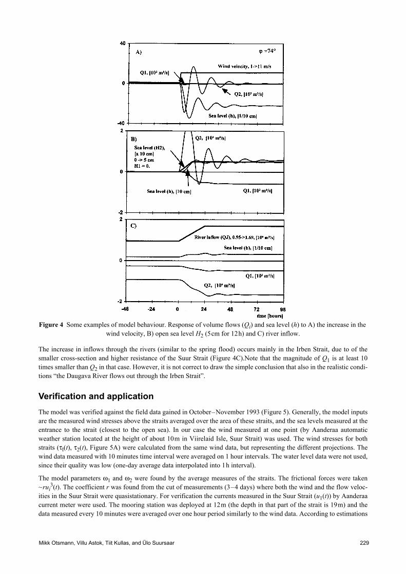
Mikk Otsmann, Villu Astok, Tiit Kullas, and Ülo Suursaar 229
Figure 4 Some examples of model behaviour. Response of volume flows (Qi) and sea level (h) to A) the increase in the wind velocity, B) open sea level H2 (5cm for 12h) and C) river inflow.
The increase in inflows through the rivers (similar to the spring flood) occurs mainly in the Irben Strait, due to of thesmaller cross-section and higher resistance of the Suur Strait (Figure 4C).Note that the magnitude of Q1 is at least 10times smaller than Q2 in that case. However, it is not correct to draw the simple conclusion that also in the realistic condi-tions “the Daugava River flows out through the Irben Strait”.
Verification and application The model was verified against the field data gained in October–November 1993 (Figure 5). Generally, the model inputsare the measured wind stresses above the straits averaged over the area of these straits, and the sea levels measured at theentrance to the strait (closest to the open sea). In our case the wind measured at one point (by Aanderaa automaticweather station located at the height of about 10m in Viirelaid Isle, Suur Strait) was used. The wind stresses for bothstraits (τl(t), τ2(t), Figure 5A) were calculated from the same wind data, but representing the different projections. Thewind data measured with 10 minutes time interval were averaged on 1 hour intervals. The water level data were not used,since their quality was low (one-day average data interpolated into 1h interval).
The model parameters ω1 and ω2 were found by the average measures of the straits. The frictional forces were taken~rui
3(t). The coefficient r was found from the cut of measurements (3–4 days) where both the wind and the flow veloc-ities in the Suur Strait were quasistationary. For verification the currents measured in the Suur Strait (u1(t)) by Aanderaacurrent meter were used. The mooring station was deployed at 12m (the depth in that part of the strait is 19m) and thedata measured every 10 minutes were averaged over one hour period similarly to the wind data. According to estimations

Two-channel model for water exchange (the Gulf of Riga case)230
based on velocity profilings (Suursaar et al., 1996) the values obtained at the depth of 10–12m could be taken as averagevelocities over the whole cross-section of the Suur Strait.
The measured and calculated velocities in the Suur Strait were in good accordance and other calculated results were alsoreasonable. It should be noted, that quite a good correlation coefficient (0.95) between the u1 and u1* (Figure 5) wasobtained without using the sea level data and the actual data of the wind stress above the other strait. It shows, onceagain, the leading role of the wind stress in the water exchange processes of the Gulf of Riga. However, we hope to geteven better results using the whole complex of inputs. This could also provide adjusted values for ω01, ω02 and r.
In future we intend to apply this model for water and nutrient exchange calculations in tIe Gulf of Riga using the wind,sea level and nutrient data.
Figure 5 Comparison of the modelled and measured velocities in the Suur Strait (C) and some other modelled values (B) in the realistic external forcings (A). Note the malfunction (entangling) of the measuring equipment on the 8th day (Q1*
in C).
Conclusions • Due to the existence of two channels the water exchange is more intensive than in the case of one channel. The water
exchange depends considerably on the direction and configuration of the channels. • The system of the Gulf of Riga amplifies oscillations with a period of about 24 hours, which can be noted signifi-
cantly in the velocities in the Irben Strait. • The main factor for the water exchange in the Gulf of Riga is wind. The sea-level differences and salinity gradients
are secondary factors. The water exchange is the most intensive with SSE and NNW winds. In winters with ice-cover

Mikk Otsmann, Villu Astok, Tiit Kullas, and Ülo Suursaar 231
the water exchange scheme is different: the velocities are 3–4 times smaller and the water exchange is the mostintensive with WSW and ENE winds.
• The described model can be used for water and nutrient exchange calculations and for providing boundary conditionsfor the ecological models of the Gulf of Riga.
Acknowledgements The Gulf of Riga Project is financially supported by the Nordic Council of Ministers. Special thanks are due to PekkaAlenius from Finnish Institute of Marine Research, the scientific coordinator of the sub-project: “Water exchange,nutrients, hydrography and database”.
References Astok, V., and Otsmann, M., 1981. A model tor calculating water exchange between the North and Baltic Seas. Investi-
gations and modelling of processes in the Baltic Sea, Part II, Tallinn, 5–10.
LeBlond, P.H., and Mysak, L.A., 1978. Waves in the Ocean. Elsevier Oceanographic Series 20, Amsterdam. 602 pp.
Otsmann, M., Astok, V., and Suursaar, Ü., 1996a. A model for water exchange between a large and a small water body:the case of the Baltic Sea and the Gulf of Riga. Nordic Hydrological Conf. 1996, Akureyri, Iceland. NHP-ReportNo. 40, Vol. 2, 496–505.
Otsmann, M., Astok, V., Suursaar, Ü., and Kullas, T., 1996b. Water exchange model for the Gulf of Riga. Studies onmeasuring and modelling the water and nutrient exchange of the Gulf of Riga. EMI Report Series, No.3, 81–94.
Suursaar, Ü., Astok, V., Kullas, T., and Otsmann, M., 1996. New estimation of the water and nutrient exchange betweenthe Gulf of Riga and the Baltic Proper. EMI Report Series, 3, 95–108.
Suursaar, Ü., Astok, V., Kullas, T., Nõmm, A., and Otsmann, M., 1995. Currents in the Suur Strait and their role in thewater and nutrient exchange between the Gulf of Riga and the Baltic Proper. Proc. Estonian Acad. Sci. Ecol.,1995, 5, 3/4, 103–123.
Петров, B. C. 1979. Водный бaлaнc и вoдooбмен Pижcкoгo заливa c Балтийск им мopeм.In: Cб. Paбoт Pижcкoй гидpoмeтeopoлoгичecкoй oбcepвaтop ий, 18, 20-40.
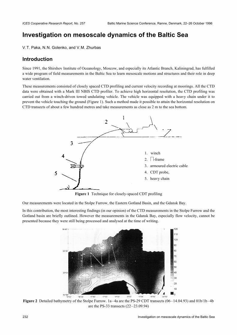
Investigation on mesoscale dynamics of the Baltic Sea232
ICES Cooperative Research Report, No. 257 Baltic Marine Science Conference, Rønne, Denmark, 22–26 October 1996
Investigation on mesoscale dynamics of the Baltic Sea
V.T. Paka, N.N. Golenko, and V.M. Zhurbas
Introduction Since 1991, the Shirshov Institute of Oceanology, Moscow, and especially its Atlantic Branch, Kaliningrad, has fulfilleda wide program of field measurements in the Baltic Sea to learn mesoscale motions and structures and their role in deepwater ventilation.
These measurements consisted of closely spaced CTD profiling and current velocity recording at moorings. All the CTDdata were obtained with a Mark III NBIS CTD profiler. To achieve high horizontal resolution, the CTD profiling wascarried out from a winch-driven towed undulating vehicle. The vehicle was equipped with a heavy chain under it toprevent the vehicle touching the ground (Figure 1). Such a method made it possible to attain the horizontal resolution onCTD transects of about a few hundred metres and take measurements as close as 2 m to the sea bottom.
Figure 1 Technique for closely-spaced CDT profiling
Our measurements were located in the Stolpe Furrow, the Eastern Gotland Basin, and the Gdansk Bay.
In this contribution, the most interesting findings (in our opinion) of the CTD measurements in the Stolpe Furrow and theGotland basin are briefly outlined. However the measurements in the Gdansk Bay, especially flow velocity, cannot bepresented because they were still being processed and analysed at the time of writing.
Figure 2 Detailed bathymetry of the Stolpe Furrow. 1a–4a are the PS-29 CDT transects (06–14.04.93) and 01b/1b–4b are the PS-33 transects (22–23.09.94)
1. winch2. -frame3. armoured electric cable4. CDT probe,5. heavy chain

V.T. Paka, N.N. Golenko, and V.M. Zhurbas 233
Mesoscale thermohaline structure of the Stolpe Furrow and its dynamicsThe Stolpe (Slupsk) Channel (Furrow) is an area of special interest for Baltic oceanographers. Being the only pass for thesalty water from the Bornholm Basin to enter the Gotland Deep and Gdansk Bay, this elongated basin is extremelyimportant to deep water ventilation in the Central and Northern Baltic.
Here, we closely analyse the spaced CTD surveys from two cruises: the 29th cruise of r/v “Professor Shtockman” (PS-29, 6-14 April, 1993) and the 33rd cruise of the same vessel (PS-33, 22-23 September, 1994). A map of PS-29 and PS-33CTD surveys in the Stolpe Channel is shown in Figure 2. The PS-29 measurements were carried out two and a halfmonths after the January 1993 Baltic inflow event, just in time to catch the inflowing waters finishing their way to theGotland Deep (Matthäus, 1993). To distinguish the data of two cruises, the four CTD transects of PS-29 are referred as#la–#4a, while the four transects of PS-33 are referred as #lb–#4b. Temperature T, salinity S and potential densityanomaly σt versus distance and depth for all the transects are presented in Figure 3–Figure 6 using standard orientation:North is to the right. The transects 2a and 1b/01b are located in the vicinity of the Stolpe Sill (about 60m deep) whichseparates the Stolpe Channel from the Bornholm Basin, the transects la, 3a, 2b, 3b are from the central part of the channelwhere the maximum sea depth is about 90 m, and the transects 4a, 4b are from the marginal zone between the StolpeChannel and the Gdansk/Gotland Basin where the drainage depth is about 80m.
The weather conditions during the field measurements were as follows: On 6 April, 1993 (transect la), the Baltic Sea wasunder the cast periphery of a cyclone centred over Scotland and moving in a south-east direction with a wind speed of 3–8 ms–1. On 12–14 April, 1993 (transects 2a–4a), the weather was determined by an anticyclone with its centre overNorthern Scandinavia, and the north-east wind speed was 4–9 ms–1. On 22–23 September, 1994 (transects lb–4b) overthe Stolpe Channel the prevailing west wind velocity was from 2–8 ms–1.
Western part of the Stolpe Channel In April 1993, the thermohaline structure of the western part of the Stolpe Channel was characterised by a two layersystem: the upper mixed layer with salinity of about 7.5 PSU and temperature 3.2°C, and the lower, halocline layer ofhigher temperature and salinity (Figure 3). In September 1994, there was an intermediate cold layer over the halocline,separated from the upper warm mixed layer by a sharp seasonal thermocline at a depth varying from 22 to 42m. For theintermediate layer, the core of cold water, where T<3°C, is shifted to south and located at the southern edge of the#1b/01b transect. The upper boundary of intermediate layer is not flat, being subjected to internal wave deformation witha long wave length of about 25–30 km, and a short one of about 2–3 km.
Figure 3 Temperature, salinity, and potential density anomaly vs. distance and depth in the western part of the Stolpe Furrow (over the sill). Top panels are from transect 2a (April 1993, 29th cruise of r/v “Professor Shtockman”), and
bottom panels are from transect 1b/01b (September 1994, 33rd cruise of r/v “Professor Shtockman”)
The upper boundary of the permanent halocline is characterised by an isohaline of 8.5 PSU. Both in April 1993 andSeptember 1994, it was inclined with respect to the horizon being deepened when advancing north. The line of the sea

Investigation on mesoscale dynamics of the Baltic Sea234
bed at the central part of the transects 2a and 1b/01b has the same slope, so the thickness of halocline layer is nearlyconstant at about 8–10 meters. The maximum salinity was 13.93 PSU for transect 2a and 14.26 PSU for transect #1b/0lb.
Resemblance of the upper boundary of the halocline and the sea bed shape suggests that the halocline tilt could be of nowave-induced origin implying an eastward flow of salty underlying water over the Stolpe Sill both in April 1993 andSeptember 1994. Geostrophic estimate of the velocity of this flow can be obtained using the two layer model. Thevelocity difference ∆u=u2–u1 across inclined, geostrophically balanced front is expressed by a formula
(1)
where
∆ρ=ρ2–ρ1 is the tilt of the front in yz-plane with respect to y-axis, ρ2, ρ1, u2, u1 are density and x-component of current velocity for the lower (subscript 2) and the upper (subscript 1)layers, g is gravity acceleration,f=2Ωsinϕ is the Coriolis parameter, Ω is the angular velocity of the Earth rotation, ϕ is latitude, ρ0 is reference density, x, y, z -axes are directed east, north, and upward respectively.
This expression is known from literature on atmospheric dynamics as the Margules formula.
Assuming from Figure 3 that α=–5·10–4l°C–1, ∆ρ/ρ0=0.005, and taking g=9.8ms–2, f=1.2·10–4s–1 (ϕ=55.3°), we get20cms–1.
Hence, if the velocity of the overlying layer is taken to be zero, the salty water in the halocline is estimated to moveeastward over the Stolpe Sill at a speed of about 20 cms–1, whether it is April 1993 or September 1994. In the case oftransects 2a and 1b, the cross-section area of the halocline over the sill is about 8m×25 km = 0.2km2, and if the value of2cms–1 is taken, the mean volume rate of salty water inflow through the channel to deep basins will be estimated as4·104m3s–1 =3.5km3 per day=1260km3 per year. The last value is unexpectedly high and more measurements arerequired to examine whether the situation we have observed is typical, and also the role of internal waves in salty watertransport across the Stolpe Sill.
Central part of the Stolpe Channel In April 1993 the mean depth of the upper boundary of the halocline (8.5 PSU isohaline) was 52 and 54 metres fortransects #la and #3a respectively, which is a bit less than that of the western part of the channel (56m for the #2atransect).
The shape of the maximum gradient layer in the halocline has changed from bending down on 6 April to bending up on13 April which is most likely to be caused by internal waves (Figure 4). The bending down shape of the halocline insection #la is accompanied by a sharp breaking of isolines as soon as they reach the northern slope of the channel. Thislooks like the internal surf, but more data are needed to confirm this suggestion and to examine the conditions when ithappens.
The maximum salinity in the bottom layer in April 1993 was rather high, namely 15.20 PSU for transect #la and 15.06PSU for transect #3a. This seems to be about the only direct remnant of the recent January 1993 inflow event, because bySeptember 1994 maximum salinity in the central part of the channel had lowered to 14.03 PSU and 13.86 PSU for #2band #3b transects respectively (Figure 5). For the same period, the mean depth of 8.5 PSU isohaline had increased to 60mfor #2b transect and to 63m for #3b transect, implying a substantial decrease of the cross-section area for the salty waterlayer.
∆u g αtanf
---------------∆ρρ0-------–=
∆u ≈

V.T. Paka, N.N. Golenko, and V.M. Zhurbas 235
Figure 4 Temperature, salinity, and potential density anomaly vs. distance and depth for transects across the Stolpe Furrow (April 1923, 29th cruise of r/v “Professor Shtockman”). Top panels are from transect 1a and bottom panels are
from transect 3a.
Figure 5 Temperature, salinity, and potential density anomaly vs. distance and depth for transects across the Stolpe furrow (September 1994, 33rd cruise of r/v “Professor Shtockman”). Top panels are from transect 2b, and bottom panels
are from transect 3b.
In contrast to the western part of the channel, the seasonal cold intermediate layer in the central part has two core struc-tures. The first, more pronounced cold core is located above the northern slope of the channel, while the second one islocated close to its longitudinal axis. Like the upper boundary of the halocline in April 1993, in September 1994 theshape of upper boundaries for both intermediate and halocline layers varies in a manner indicating internal waves withamplitudes of the order 10m.
The most remarkable feature concerning thermohaline structure in the central part of the Stolpe Channel, especially forSeptember 1994 (#2b and #3b transects), is its prominent asymmetry observed in the halocline. That is, the interfacebetween halocline and overlying intermediate (or upper mixed) layers being sharp over the northern slope of the channelwidens to the south, and a fan-like divergence of isohalines/isopycnals takes place. This “fan-like” effect is accompanied

Investigation on mesoscale dynamics of the Baltic Sea236
with northward displacement of the saltiest and densest water pool from the deepest connection line of the channel. Thefan-like effect and the northward displacement of densest water took place not only in September 1994, but to someextent in April 1993 (see #la and #3a transects).
Eastern part of the Stolpe Channel For the eastern part of the channel, the fan-like effect and the northward displacement of densest water were clearlyrevealed both in April 1993 and September 1994 (see Figure 6, transects #4a and #4b).
Figure 6 Temperature, salinity, and potential density anomaly vs. distance and depth for transects across the eastern part of the Stolpe Furrow. Top panels are from transect 4a (April 1923, 29th cruise of r/v “Professor Shtockman”), and
bottom panels are from transect 4b (September 1994, 33rd cruise of r/v “Professor Shtockman”)
The sea bottom in the eastern part of the Stolpe Channel is also elevated relative to its central part, but less than in thewestern one. This is evidenced by Figure 2, plotted according to the data being taken from the Polish geological map(Pikies, 1990). The bottom topography is illustrated there with an isobath offset of 5m. As the sea bottom is lower downfurther to the east and the north-east, this elevation must also be considered as a sill for the near-bottom currents, directedinto the Gdansk/Gotland Basin. The eastern sill is 20km wider than the western one, and its profile is more complicated.In its middle part there is a spacious elevation of the bottom up to 67–70m. Both to the north and south of this elevation,there are two valleys of nearly the same depth (about 80m) open to the east which may be considered as preferablepassages for salty water from the Stolpe Channel to get the Gdansk/Gotland basin. When the depth of the upper boundaryof halocline is greater or close to that of the bottom elevation, as it took place in the case of #4a transect, the near bottomflow of high salinity water separates into two parts: the wide southern and the narrow northern ones.
Due to the fan-like effect and the northward displacement of densest water, both in April 1993 and September 1994salinity of near bottom water for the northern valley was more than 1 PSU greater than that for the southern one. It meansthat the northern passage, despite being narrower (only 3–4 km wide), is more important for the deep water ventilation inthe Central and Northern Baltic than the southern one which is several times wider at the same depth.
Discussion First of all we shall try to examine what features of thermohaline structure are common for both of the periods of obser-vation in the Stolpe Channel. The weather conditions have changed from moderate south-east winds on April 12–14,1993 to moderate westerly winds on September 22–24, 1994, and the common features should be considered asindependent from the wind direction, at least for weak and moderate winds.
The first common feature is the deepening of the upper boundary of halocline at the sill in the western part of the channelwhen advancing north. It implies eastern transport of underlying salty water from the Bornholm Basin to the StolpeChannel for both of the periods of observation. This results is not consistent with the numerical modelling of circulationin the Baltic (Krauss and Brügge, 1991). The model predicted westward transport through the Stolpe Channel in its lowerlayers only for northerly and easterly winds, while southerly and westerly winds developed the opposite, eastward
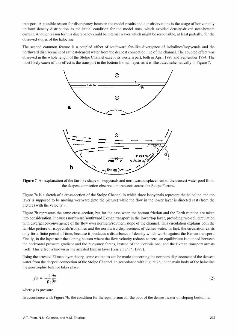
V.T. Paka, N.N. Golenko, and V.M. Zhurbas 237
transport. A possible reason for discrepancy between the model results and our observations is the usage of horizontallyuniform density distribution as the initial condition for the model runs, which avoided density-driven near-bottomcurrent. Another reason for this discrepancy could be internal waves which might be responsible, at least partially, for theobserved slopes of the halocline.
The second common feature is a coupled effect of southward fan-like divergence of isohalines/isopycnals and thenorthward displacement of saltiest/densest water from the deepest connection line of the channel. The coupled effect wasobserved in the whole length of the Stolpe Channel except its western part, both in April 1993 and September 1994. Themost likely cause of this effect is the transport in the bottom Ekman layer, as it is illustrated schematically in Figure 7.
Figure 7 An explanation of the fan-like shape of isopycnals and northward displacement of the densest water pool from the deepest connection observed on transects across the Stolpe Furrow.
Figure 7a is a sketch of a cross-section of the Stolpe Channel in which three isopycnals represent the halocline, the toplayer is supposed to be moving westward (into the picture) while the flow in the lower layer is directed east (from thepicture) with the velocity u.
Figure 7b represents the same cross-section, but for the case when the bottom friction and the Earth rotation are takeninto consideration. It causes northward/southward Ekman transport in the lower/top layer, providing two-cell circulationwith divergence/convergence of the flow over northern/southern slope of the channel. This circulation explains both thefan-like picture of isopycnals/isohalines and the northward displacement of denser water. In fact, the circulation existsonly for a finite period of time, because it produces a disturbance of density which works against the Ekman transport.Finally, in the layer near the sloping bottom where the flow velocity reduces to zero, an equilibrium is attained betweenthe horizontal pressure gradient and the buoyancy forces, instead of the Coriolis one, and the Ekman transport arrestsitself. This effect is known as the arrested Ekman layer (Garrett et al., 1993).
Using the arrested Ekman layer theory, some estimates can be made concerning the northern displacement of the densestwater from the deepest connection of the Stolpe Channel. In accordance with Figure 7b, in the main body of the haloclinethe geostrophic balance takes place:
(2)
where p is pressure.
In accordance with Figure 7b, the condition for the equilibrium for the pool of the densest water on sloping bottom is:
fu 1ρ0----- p∂
y∂-----–=

Investigation on mesoscale dynamics of the Baltic Sea238
(3)
where (∆ρ)b is the density anomaly for the pool (the difference between water density of the pool and that of the deepestconnection), αb is the bottom slope for a place where the pool is located.
Using (2) and (3), an expression for u, the flow velocity in the halocline interior required to equilibrate the pool at thesloping bottom, is obtained:
(4)
According to the transects #2b–3b (see Figure 5), 1.8·10–3 (0.2–0.5)·10–3. This yields the estimate:u=3–7.5cms–1.
Another, simpler kinematic explanation of the fan-like effect even without the direct application of the Ekman layerdynamics can be made using only the Margules formula (1). The density structure in the halocline and its upper vicinitymay be considered as a number of homogeneous layers of different density, and formula (1) is applicable to every pair ofthese layers. If we suppose that in the central layers of such a halocline there is an eastward flow which reduces to zero inthe top and bottom layers, formula (1) will predict upward sloping interfaces (i.e. isopycnals) between the top layers anddownward sloping for the bottom layers when advancing south—just the fan-like behaviour of isopycnals that wasobserved in the central and eastern part of the Stolpe Channel.
An important result following from this last explanation is the possibility to use the fan-like distribution of isopycnals asevidence of eastward flowing salty water through the Stolpe Channel for the both periods of observation.
It is worth noting that the fan-like effect implies non-instant, time-averaged eastward flow, and the period of averagingcan be estimated as equal to the “shut down time” for the Ekman layer to be arrested. In our case the shut-down time t* isestimated as t*= l/uE, where l is the distance between the deepest connection and the place where the maximum densitypool is located, and uE is the velocity of the Ekman layer transport.
Assuming that (Garrett et al.,1993),
and, in accordance with our data, taking u=3cms–1, l=1 km, we obtain
t* = 3.3·105s=3.9 days.
We expect that our estimate of t* is still on the low side because in fact uE should be much less than u.
At least two important consequences follow from the above estimate of t*.:
1. Quite a long period of time is required to develop the fan-like structure, and it explains why this structure was notobserved in the western part of the Stolpe Channel: the salty water in that place is too “young” since it just came fromthe relatively deep Bornholm Basin.
2. Our obtained value for t* is a bit larger than the typical synoptic period (3 days), and it explains why our observationsof thermohaline structure predict eastward flow in the halocline regardless of the direction of the wind blowing overthe area. This is likely to be the main reason for discrepancy in our results with the predictions of numericalmodelling of Baltic circulation (Krauss and Brügge, 1991).
The above statement is strong evidence for the fan-like effect to be a permanent feature of thermohaline structure in thecentral and especially eastern part of the Stolpe Channel. It makes the narrow northern valley in the eastern part of thechannel exclusively important for the salty water to pass from the Bornholm Basin to deep central and northern basins.
Underwater mesoscale cyclonic eddy in the Gotland Basin after the 1993 inflow eventIn the PS-29, a 157km long closely spaced CTD transect, A–B, was carried out in the Eastern Gotland Basin on 17–18April 1993. The location of the transect is shown in Figure 8.
p∂y∂
----- αbcos– g ∆ρ( )b αbsin=
u gf--- αb
∆ρ( )bρ0
--------------tan=
αb ≈∆ρ( )bρ0
-------------- =
uE u≈

V.T. Paka, N.N. Golenko, and V.M. Zhurbas 239
Figure 8 A map of the experiment in the Eastern Gotland Basin, March–April, 1993. Filled circles of different sizes, mainly coupled by bold lines, are CTD stations of the second stage of the experiment (16–18 April). The large dotted
circle close to the breakpoint of the A–B transect denotes the location of the cyclone.
Figure 9 displays the potential density anomaly, σθ, versus pressure and distance for the halocline layer of the ABtransect. The most outstanding feature in Figure 9 is a convergence of isopycnals inside the halocline at a distance of 48–55km, which may be interpreted as a mesoscale cyclonic eddy covering the whole halocline layer. In addition, there area few cases of local divergence of isopycnals, namely at distances of 116–129km and 138–150km, which may beconsidered as anticyclonic eddies covering only some parts of the halocline layer.
Figure 9 Potential density vs. pressure and distance from the A–B transect
To be sure that the feature of 48–55km is really a mesoscale cyclone rather than, for example, a topographically steeredtongue of intrusion, we have to have at least a few differently directed transects across it. Unfortunately, we had no possi-bility to make any additional transects, and the following should be considered as an “eddy hypothesis”, which providesa likely, self-consistent description of the data and will stimulate field studies in this area in the near future.
We shall consider dynamic properties of the hypothetical cyclone in more detail. It is worth doing, because such eddiescan contribute to the salt water transfer and deep water ventilation in the Baltic Sea.
Using density versus hydrostatic pressure and distance, ρ(p,x), the empirical geostrophic flow function Fg(p,x) has beencomputed:

Investigation on mesoscale dynamics of the Baltic Sea240
(5)
where ρ(p,∞) is the background density versus pressure away from the cyclone, p0 is some reference pressure level of no geostrophic current. The value of p0 was taken to be equal to 140 decibars, thepressure just above the sea bed at the cyclone location.
The cross-transect component of geostrophic velocity, ug, is written as the x-derivative of the flow function .
Figure 10 shows the geostrophic flow function computed for a fragment of the A–B transect, which includes the centralpart of the cyclone and its northern periphery, where the pressure at the sea bed is no less than 140 decibars. This functionis a minimum at 107 decibars, indicating a horizon of the cyclone’s core, and increases to a close-to-zero noise levelover the halocline and away from the cyclone. Thus, we can conclude that the cyclone is located in the halocline, beingdynamically undetectable on the sea surface.
Figure 10 Geostrophic flow function vs. pressure and distance for a fragment of the A–B transect including the cyclone and its northern periphery
To estimate characteristics of the cyclone (its size and velocity of rotation), according to Zhurbas et al. (1992), theempirical geostrophic flow function at the level of p=107 decibars has been approximated by an analytical function,namely the Gauss curve:
(6)
where A, x0, R are parameters to be determined.
Using the least square technique (non-linear regression), the following values were obtained:
A= –1116 m2s–1, x0=51.15km and R=2.94km.
Since only a single transect across the cyclone is available, the distance between the transect and the cyclone’s centre isunknown. One should estimate what kind of errors are introduced into parameters of the cyclone by this uncertainty. Ifthe cyclone is axisymmetric and its flow function is described by the two-dimensional Gauss curve:
Fg p x,( ) 1f--- 1
ρ p x,( )----------------- 1
ρ p ∞,( )------------------– pd
p
p0
∫=
ugFg∂x∂
---------≡
p ≈
Fg x( ) Fg p x,( ) p 107 dbar=≡ Aexpx x0–( )2
2R2---------------------–=

V.T. Paka, N.N. Golenko, and V.M. Zhurbas 241
(7)
where x0', y0, R', A' are “real” parameters of the flow function. Making the transect along the x-axis at the distance of y1–y0 from the eddy’s centre, we will come to (6) instead of (7) with the following relationships between “real” and“measured” parameters: x0=x0', R=R', A=A'exp[–(y1–y0)2/2R'2]<A'. Thus, having a single transect, the right value ofthe eddy’s size R and underestimated values of the eddy’s intensity A will be obtained. Otherwise, if the flow function isequal to a non-zero constant inside an axisymmetric eddy, turning into zero outside it, a single transect will give the rightvalue of the eddy’s intensity and underestimated values of its size. The first case, with Gauss-like flow function, seems tocorrespond more closely to reality. That is why we expect that we have got the right value of the cyclone’s size, while thecyclone’s intensity and, as a consequence, its frequency of rotation could be underestimated.
According to (6), geostrophic estimates of azimuthal velocity and frequency of the cyclone’s rotation are:
(8)
where r=x–x0 is the radius of that feature. With the above values of A and R, the second of formulae (8) yields
ωg=1.29·10–4s–1 which is comparable with the value of the Coriolis parameter f=2Ωsinϕ=1.22·10–4s–1.
Here Ω is the frequency of Earth rotation, ϕ is the latitude; Ω=0.727·10–4s–1, ϕ=56.7°. Since ωg and f are of the sameorder of magnitude, a centripetal acceleration u2/r (u is azimuthal velocity) must be taken into account. Thus, instead ofgeostrophic balance, the cyclone has to be described by the balance of Coriolis acceleration, horizontal pressure gradient,and non-linear term of equation of motion, namely the centripetal acceleration:
(9)
By solving quadratic equation (9) for u, we obtain:
(10)
(10) gives the following expression for the frequency of eddy rotation:
(11)
By substituting the above values of ωg and f into (11), we calculate ω=0.785·10–4s–1=1.29(f/2). Thus, with regard tocentripetal acceleration, the estimate of frequency of the cyclone rotation is decreased by factor 1.64 with respect to thatof geostrophic balance. Nevertheless, it remains greater than 1/2, the upper limit for frequency of anticyclone rotation,confirming the well-known statement that cyclones are more energetic than anticyclones in both the atmosphere and theocean. As for the maximum azimuthal velocity in our cyclone, umax, the geostrophic estimate, ugmax=23cms–1 atr=2.94m, decreases to the value of umax=16cms–1 at r=3.33km when centripetal acceleration is taken into account. Itshould be noted that, having been calculated from single transect data, the above values of ω and umax are probably onthe low side.
The thermohaline structure of the cyclone is shown in Figure 11, where isolines of temperature in the distance–potentialdensity plane are presented. In the upper layer of halocline, at Oθ<6.4kgm–3, the cyclone is purely baroclinic: despite astrong deformation of isopycnals (see Figure 3), the temperature on isopycnals is nearly constant. On the contrary, in themiddle layer of halocline, at 6.4kgm–3<σθ<8.4kgm–3, the temperature of isopycnals inside the cyclone is 0.2–0.3° Cbelow its value outside the cyclone. At last, in the lower layer, adjusted to the sea bed, density and salinity inside thecyclone are greater then their respective maximum values in the surroundings. Thus, the cyclone is shown to transportheterogeneous water in the middle and lower layers of the halocline, while in the upper layer it reduces to a solitone-wave-like bend of isopycnals of no thermohaline anomaly.
Fg x y,( ) A'expx x0'–( )2 y y0–( )2+
2R'2-------------------------------------------------–=
ug r( )Fg∂r∂
---------≡ ArR2------– exp r2
2R2--------- ωg
ug∂r∂
--------r 0=
≡,– AR2------–= =
u2
r-----– fug– fu+=
u r( ) fr2---- 1 1
4ugfr
--------+
12---
––=
ω u∂r∂
-----r 0=
≡ f2--- 1 1
4ωgf
---------+
12---
––=

Investigation on mesoscale dynamics of the Baltic Sea242
Figure 11 Temperature vs. potential density and distance in the cyclone
To illustrate the transfer of salty water by the cyclone, Figure 12 displays the same fragment of A–B transect in salinity.The maximum salinity in the cyclone is greater than 11.5 PSU. It is worth remembering that the maximum salinity in thebottom layer of the Gotland Deep was 11.0 PSU in the middle of March, 1993, and increased to 11.7 PSU by June due tothe major Baltic inflow in January 1993 (Dahlin et al., 1993). Thus, the cyclone is proved to transfer salty water origi-nated from the 1993 inflow event, contributing to the deep water renewal in the Eastern Gotland basin.
Figure 12 Salinity vs. pressure and distance in the cyclone

V.T. Paka, N.N. Golenko, and V.M. Zhurbas 243
Conclusions and Perspectives Closely spaced CTD profiling in the Stolpe Channel and the Eastern Gotland Basin made it possible to reveal and inves-tigate two interesting mesoscale dynamic features associated with salty water motion toward deep basins of Central andNorthern Baltic.
The first is the northward displacement of denser water from the deepest connection of the Stolpe Channel which isaccompanied by a fan-like divergence of isopycnals when advancing south. This effect has been explained taking intoaccount the Ekman transport by sloping boundary of the channel.
The second is the underwater cyclonic eddy which was revealed south the Gotland Deep in April 1993. The cyclone wascarrying salty water after the 1993 inflow event. Such eddies should be considered as a possible way of ventilating deepwaters in the Baltic Sea.
In the near future we will carry out specialised field experiments to answer the following questions:
• What is the role of internal waves in salty water transfer over the Stolpe Sill and how can it be quantified? • What drives thermohaline intrusions in the Baltic halocline and what is the role of inertial oscillations in this?
References Dahlin, H., Fonselius, S., and Sjöberg, B., 1993. The changes of the hydrographic conditions in the Baltic Proper due to
inflow to the Baltic sea. ICES Statutory Meeting 1993, C.M.1993/C:58, Session V.
Garrett, C., MacCready, P., and Rhines, P., 1993. Boundary mixing and arrested Ekman layers: rotating stratified flofnear a sloping boundary. Annu. Rev. Fluid Mech., v.25, p.291–323
Krauss, W., and Brügge, B., 1991. Wind-produced water exchange between the deep basins of the Baltic Sea. J. Phys.Oceanogr. v.21. #3 p.373–384.
Matthäus, W., Lass, H.-V., and Tiesel, R., 1993. The major Baltic inflow in January 1993. ICES Statutary Meeting 1993,C.M.1993/C:51, Sess. V.
Paka, V.T., 1996. Thermohaline structure of the water on cross-sections in the Slupsk Channel of the Baltic Sea in springof 1993. Oceanology, v.36–2, pp. 207–217.
Pikies, R. 1990. Geological map of the Baltic Sea. Ed. Mojski E. Sheets 15, 16. Slupsk Channel. Warsaw.
Zhurbas, V.M., Kouts, T., Laanemets, J.J., Lips, V.K., Sagdiev, A.M., and Elken, J., 1992. Spatial distribution offinestructure intensity in a Mediterranean salt lens. Oceanology (Engl. Ed.), 32(3). 273–278.

Oil content in Baltic Sea water and possibilities for detection and identification by the Lidar method244
ICES Cooperative Research Report, No. 257 Baltic Marine Science Conference, Rønne, Denmark, 22–26 October 1996
Oil content in Baltic Sea water and possibilities for detection and identification by the Lidar method
Jacek Piskozub, Violetta Drozdowska, Tadeusz Krol, Zbigniew Otremba, and Adam Stelmaszewski
IntroductionOil contamination measurements in sea water are carried out by intensively employing many physical and chemicalmethods. In recent years remote measurements of the marine environment for detection of oils and other substanceswhich occur in the sea water has started to play an important role.
In our experiment we applied the lidar method which enables remote detection of fluorescent substances in the sea water(Wehry et al., 1981), (Bristow et al., 1981) and the laboratory system for fluorescence measurements of oil substances(Otremba and Stelmaszewski, 1994).
So far, laser-induced fluorescence spectroscopy for quantitative classification of aromatic hydrocarbons and formeasuring of water contamination with oil components has been used (Bublitz and Schade, 1995), (Moise et al., 1995).In recent years scientists have used the lidar because of the many possibilities of application of lidar methods for thedetection of oil distribution (Goncharov et al., 1995).
This experiment attempts to measure oil contamination in the surface layer of water by the lidar method in the southernBaltic Sea. The measurements carried out in the Institute of Oceanology PAN used the lidar system FLS-12. This lidarallows for registration of fluorescence in the range of 425nm to 800nm which is sufficient for the measurements of thereal distribution of oil components and other fluorescent substances in the sea water.
To confirm and verify the correctness of this method we simultaneously took up the water probes from the same sites touse for standard fluorescent laboratory method measurements. Figure 1 shows a map of the southern Baltic Sea with thesites of the remote measurements and observations carried out during expeditions of the research vessel “Oceania”.Figure 2 shows a distribution curve for all results obtained in the open sea and in the Gdansk Bay.
Figure 1 Map showing sites of measurements and observations visited by r/v “Oceania”

Jacek Piskozub, Violetta Drozdowska, Tadeusz Krol, Zbigniew Otremba, and Adam Stelmaszewski 245
Figure 2 Distribution of the results contained in several concentration intervals for open sea and bay water
MethodsThe FLS-12 lidar system used for the measurements is a tuneable laser system designed for remote sensing of the aquaticenvironment in the visible spectrum (Piskozub et al., 1994). It consists of two lasers: the excimer laser (308nm) which isthe UV pumping source and the dye laser. We used the dye “coumarine 120” with maximum fluorescence at 440nm.
The backscatter signal is collected by the telescope and registered by CCD camera. The measurements are controlled byspecial software. The lidar-emitted light excites all sea water components possessing fluorescence properties. Thebackscattered signal is made up of the lidar and the water Raman backscattered light and fluorescence comes from allfluorescent components. The fluorescent maxima for the basic Baltic water components are as follows (Babichenko etal., 1992): phycoerythrin (575nm), phycocyanin (645nm), chlorophyll ‘a’ (685nm), humus substances (600nm) and oilsubstances (250nm–500nm). Figure 3 presents backscattered laser signal (440nm), backscattered water Raman signal(521nm), oil fluorescence (470nm), fluorescence of pigments and humus substances (635nm) and fluorescent band ofchlorophyll‘a’ (685nm). Assuming that we know maxima and halfwidths of all fluorescent bands we can approximatethe experimental curve to the theoretical gauss curve and then to reduce it to component gauss curves (Figure 4).
Figure 3 Experimental and calculated fluorescent spectrum
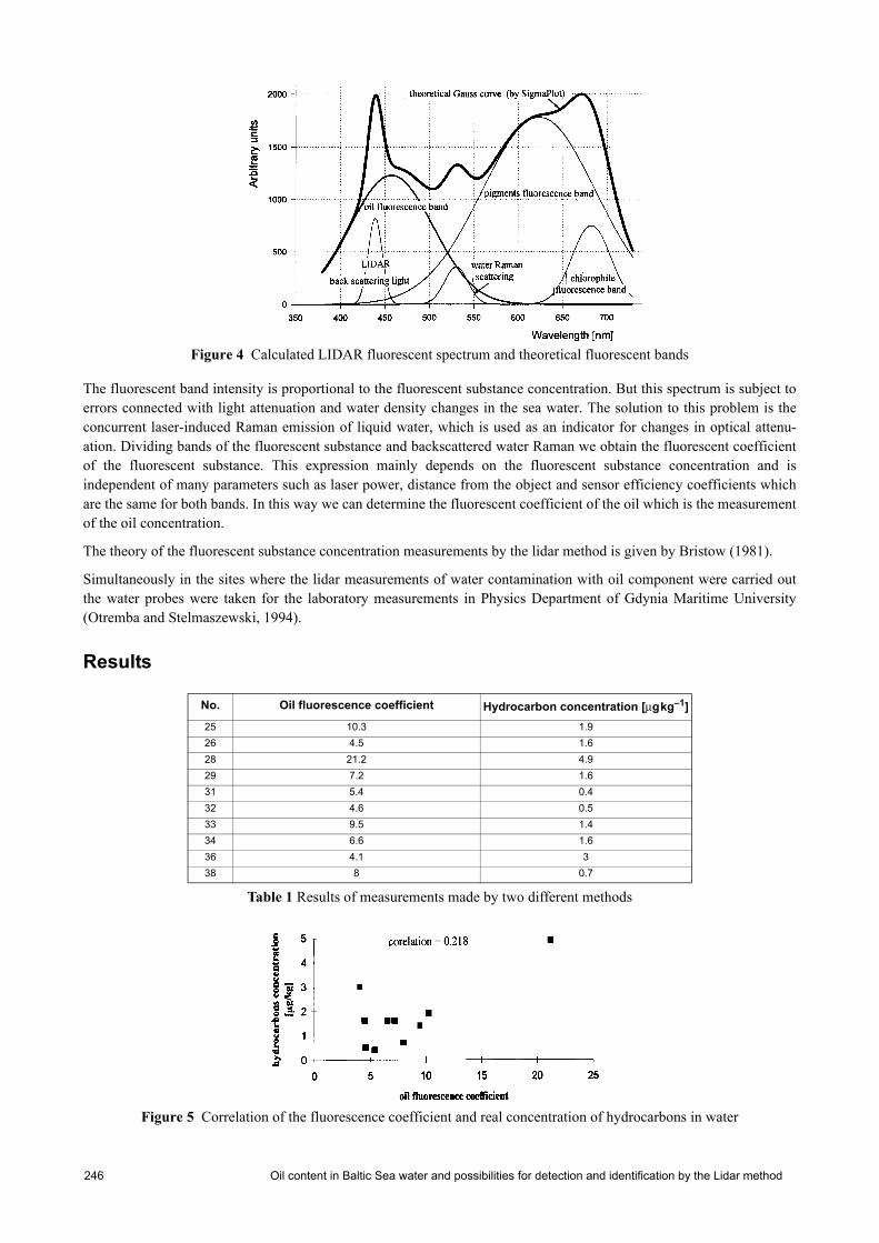
Oil content in Baltic Sea water and possibilities for detection and identification by the Lidar method246
Figure 4 Calculated LIDAR fluorescent spectrum and theoretical fluorescent bands
The fluorescent band intensity is proportional to the fluorescent substance concentration. But this spectrum is subject toerrors connected with light attenuation and water density changes in the sea water. The solution to this problem is theconcurrent laser-induced Raman emission of liquid water, which is used as an indicator for changes in optical attenu-ation. Dividing bands of the fluorescent substance and backscattered water Raman we obtain the fluorescent coefficientof the fluorescent substance. This expression mainly depends on the fluorescent substance concentration and isindependent of many parameters such as laser power, distance from the object and sensor efficiency coefficients whichare the same for both bands. In this way we can determine the fluorescent coefficient of the oil which is the measurementof the oil concentration.
The theory of the fluorescent substance concentration measurements by the lidar method is given by Bristow (1981).
Simultaneously in the sites where the lidar measurements of water contamination with oil component were carried outthe water probes were taken for the laboratory measurements in Physics Department of Gdynia Maritime University(Otremba and Stelmaszewski, 1994).
Results
Table 1 Results of measurements made by two different methods
Figure 5 Correlation of the fluorescence coefficient and real concentration of hydrocarbons in water
No. Oil fluorescence coefficient Hydrocarbon concentration [µgkg–1]25 10.3 1.926 4.5 1.628 21.2 4.929 7.2 1.631 5.4 0.432 4.6 0.533 9.5 1.434 6.6 1.636 4.1 338 8 0.7

Jacek Piskozub, Violetta Drozdowska, Tadeusz Krol, Zbigniew Otremba, and Adam Stelmaszewski 247
Table 1 shows results of the measurements made by both of methods. Generally a good correlation does not occurbetween them (Figure 5).
The small correlation which is shown in Table 1 can be caused by the fact that backscattered light, which is registered bythe lidar, originates from the surface of water but water probes are collected partially from under surface of water. Thisway measurements can give different results.
Secondly if there was oil emulsion on the surface of water the backscattered lidar signal would indicate a large oilconcentration as opposed to the laboratory fluorescent method.
Moreover the light which radiates in sea water is absorbed and reduced in many ways so the backscattered lidar signalcan be attenuated and change the real information about the oil concentration.
ConclusionResults show that oil investigations in the sea water should use the UV-source of the excitation, because using 440nmwavelength lidar excitation gives two overlapping bands. It also can lead to incorrect results obtaining by the lidarmethod.
ReferencesWehry, E. (ed.), 1981. Modern Fluorescence Spectroscopy. Plenum Press, New York and London (Chap.5 and 7).
Bristow M. et al., 1981. Laser Fluorosensor Use of Water Raman Emission to Correct Airborn Data for Effect of WaterOptical Attenuation. Appl.Opt.Vol.20 pp.2889–2906.
Babichenko S. et al., 1992. Laser Remote Sensing of Phytoplankton. Remote Sensing of Environment.
Bublitz J., and Schade W., 1995. Multiwavelength laser-induced fluorescence spectroscopy for quantitative classificationof aromatic hydrocarbons, Proc.SPIE, Vol.2504, p.265–276, Environmental Monitoring and Hazardous WasteSite Remediation.
Moise N. et al., 1995. Measuring of water and soil contamination with oil components using laser-induced fluorescencetransmitted through optical filters, Proc.SPIE, Vol.2461, p.636–643.
Goncharov V. et al., 1995. Possibilities of application of lidar methods for the discovery of oil discharge from under-water sources on the sea shelf, Proc. SPIE, Vol. 2380, p.344–348.
Klimkin V. et al., 1993. Spectrofluorimeter for remote analysis of oils on the surface of water. Proc SPIE Vol. 2107,p.18–231
Vinas M. et al., 1992. Fluorescent sensor as an engine oil quality indicator, Proc. of the meeting, Los Angeles, CA,p.238–247.
Zhu Y., and Junfu M., 1992. Study on determination of micro amount oil in water by laser time-resolution fluorescencespectroscopic technique, Proc. SPIE Vol. 1637, p.285–290.
Gillispie G., and Germain R., 1992. In-situ tunable laser fluorescence analysis of hydrocarbons, Proc. SPIE Vol. 1637,p.151–162.
Piskozub J. et al., 1994. Oil content in the Baltic Sea Water and Possibilities of Detection and Identification by the LidarMethod, Proc.19th CBO, p.166–171.
Otremba Z., and Stelmaszewski A., 1994. Concentration and Origin of Oil Contaminations in the Gdansk Bay CoastWater, Proc. CBO, p.593–603.

Hydrographic and hydrochemical structure of waters in the Luga-Koporye region during the summer period248
ICES Cooperative Research Report, No. 257 Baltic Marine Science Conference, Rønne, Denmark, 22–26 October 1996
Hydrographic and hydrochemical structure of waters in the Luga-Koporye region during the summer period
Pyotr P. Provotorov, Vladimir P. Korovin, Yuri I. Lyakhin, Alexei V. Nekrasov, and Valery Y. Chantsev
The hydrographic and hydrochemical structure of waters in the Luga-Koporye region (south-east part of the Gulf ofFinland) is studied on evidence derived from the four (1993–1996) summer surveys of the oceanographic “polygon”20×50 sea miles (Figure 1) performed within the framework of the UNESCO/IOC/HELCOM “Baltic FloatingUniversity” programme. STD measurements of water samples at about 45 stations in the polygon carried out during thecruises of research vessels “Professor Sergei Doirofeev” (1993), “Persey” (1994) and “Nikolai Matusevich” (1995 and1996) have been used together with a few hundred sounding measurements with 2m vertical spacing at anchored stationswith duration up to 6 days. The near-shore shallow stations of each survey were measured by the sailing catamaran“Orients”.
Figure 1 Positions of stations at the Luga-Koporye polygon (survey of July 24–29, 1995, r/v “Nikolai Matusevich” and “Orients”)
The temperature (T), salinity (S) and density (ρ) patterns reproduced from the measurements are typical for the stage ofsummer heating, being composed of: (a) upper mixed layer 10–15m thick; (b) transient layer with pronounced gradientsof characteristics and (c) near-bottom thermohalocline resulting from transformed waters penetrating from the open partof the Gulf using the irregularities of bottom topography. Given the obvious stratification of waters, the T, S-curves(Figure 2), even for the mostly offshore stations, have the form of straight “mixing lines” indicating that the quasista-tionary diffusion seems to suggest the formation of the vertical thermohaline structure in the Eastern Gulf of Finland.
•–stations monitored by r/v “Nikolai Matusevich”–stations monitored by catamaran “Orients”
–“shoreline points” monitored by catamaran “Orients”

Pyotr P. Provotorov, Vladimir P. Korovin, Yuri I. Lyakhin, Alexei V. Nekrasov, and Valery Y. Chantsev 249
Figure 2 T, S-curves for stations of the Luga-Koporye polygon obtained from STD-sounding with vertical spacing z=2cm
Figure 3 Vertical profiles of temperature (1) and salinity (2) as well as m.r.s. deviations (3) and (4). Extreme values Tmin (5) and Tmax (6), Smin (7) and Smax (8) are shown together with the correlation coefficient between T and S (9)
Figure 3 demonstrates the vertical T and S profiles (averaged over all the stations of the polygon) with their r.m.s. andextreme values at different depths. The most spatial variability is inherent in the near-bottom layer where the deviationsof T and S reach, correspondingly, 5oC and 0.5%. The coefficients of correlation R between the fields of T and S, calcu-lated for different levels from the observational data and considered as random samples, are negative across the wholedepth (curve 9 in Figure 3). The elevated (in magnitude) values of R for the undersurface and near-bottom layers arecircumstantial evidence that the corresponding horizontal surfaces are isopycnic. For intermediate layers, the diapyc-nicity is more characteristic, resulting in a rather weak interrelation between the temperature and salinity fields.
It is known that the density background of the vertical stratification in the Baltic Sea is formed mainly after the type of“complete stability” with an inherent drop in T and increase in S with depth. A fragment of a stratification diagramdeveloped with the use of the temperature (ET) and salinity (ES) stability components for the Luga-Koporye stations isgiven in Figure 4. Such a background stratification is not favourable for a fine structure development and, consequently,mixing is caused by the differential-diffusive (thermoconcentration) convection. The mixing and exchange of substances

Hydrographic and hydrochemical structure of waters in the Luga-Koporye region during the summer period250
in the Eastern Baltic summer pycnocline is effected by the internal wave break-up, some edge effects and turbulentdiffusion in coastal waters [1,2].
Figure 4 Types of thermohaline conditions characterising stratification (K. Ferorov’s diagram) obtained from the measurements at stations of the polygon. C–solt fingers-like, Y–complete stability, K–layer-to-layer convection, AH–
complete non-stability. ET and ES are temperature and salinity stability components.
Judging from the density relation:
(1)
(α, β being coefficients of thermal expansion and salinity compaction of water and ∆T, ∆S differences in T and S acrossthe layer) both the factors are contributive in the density stratification. However, the salinity contribution prevails in theupper layer while the temperature effects dominate near the bottom (Figure 5).
Figure 5 Distribution of density relation Rρ=–ET/ES at the transect along the parallel of latitude 60o N (stations 36-31-26-21-15-9-4-1)
Spatial patterns of T and S distribution are caused by local differences in heating by radiation, freshwater runoff andwind/wave mixing. The inflow of relatively cold and saline water from the open part of the Gulf is mostly in evidence at
Rρα∆Tβ∆S-----------
ETES------–= =

Pyotr P. Provotorov, Vladimir P. Korovin, Yuri I. Lyakhin, Alexei V. Nekrasov, and Valery Y. Chantsev 251
the western polygon boundary whence it propagates to the east by mixing progressively with the shallow waters. Thelocal spots of advective origin are fixed between the Luga and Koporye bights.
The course of T, S and ρ isolines at the meridianal and latitudinal transects implies a weak baroclinity (isopycnic linesand isobars are parallel) and absence of distinct frontal separations. Only in the vicinity of the mouth of the Luga River isit possible to perceive salinity frontal zones due to local freshwater discharge.
The peculiarities of stratification and probability of fronts formation between stratified and mixed waters can be charac-terised by the potential energy anomaly [3]
(2)
where is a vertically mean density in a water column.
ϕ is the anomaly of potential energy if a stratified water column to that of a totally mixed one. Formation of frontal zonesis probable where the elevated values of horizontal gradients of ϕ take place. Estimation of this criterion for the Luga-Koporye stations shows that the probability of frontal separation does not seem to be very high. The existing weakfrontal zones belong to a thermoclinic type. Unlike baroclinic fronts, these can be manifested in T and S fields but thecontributions of T and S compensate each other in a density field.
The arrow of STD data obtained from the 6-day (one hour timely spaced measurements) anchored station (59°50'N,28°10'E) provides the basis for revealing the features of thermohaline variability. During the period of measurements(28.07–03.08.1995), the weather was sunny, anticyclonic, with a weak wind of variable direction—favourable forintensive heating of water. The temperature variations in the upper layer lie in the range 16.98–19.79°C with the meantemperature equal to 18.53°C and r.m.s.= 0.65°C. The corresponding characteristics for salinity are 2.56–3.57%, meansalinity equal to 3.06 and r.m.s.=0.20%. In the transient layer the variability of T and S decreases but in the near-bottomthermocline it sharply increases again. The evolution of thermocline structure can be demonstrated by plotting T and S asa function of z (depth) and t (time). It can be seen that intensive oscillations (increasing as the bottom is approached) aremanifested against the background of diurnal variations and intensive surface heating.
To be able to judge the type and possible mechanism of local thermocline structure violations, the so-called δ-parameterwas calculated:
(3)
where is a combination akin to the density relation constructed of m.r.s. amplitudes of temporal T and S
series for fixed depths;
is the mean density relation for the layer considered;
are the T and S vertical gradients in this layer averaged over the period of measurements.
It is evident that in case of purely isopycnic (advective) intrusion the conditions
(4)
are fulfilled, whereas in the case when the vertical processes dominate in forming the structure, the following conditionholds.
(5)
ϕ 1H---- ρ ρi–( )gz zd
H–
0
∫=
ρ 1H---- ρ zd
H–
0
∫=
δRρ 1–Rρ 1–------------------=
Rραρtβρs--------=
Rρα∆Tz
β∆Sz-------------=
∆Tz ∆Sz,
ρtσs----- β
α--- δ 0→;≈
ρtσs----- ∆Tz
∆Sz--------- δ 1→;≈

Hydrographic and hydrochemical structure of waters in the Luga-Koporye region during the summer period252
Estimation of δ-criterion showed that it tends to zero in the near-bottom layer and grows to 0.6–0.8 above. This meansthat on average the T and S variations were caused by horizontal (near the bottom) and vertical (in the remainder of watercolumn) processes.
The hydrochemical investigations were related appreciably with the study of nutrients concentration and eutrophicationstate of the areas under consideration. The Eastern Gulf of Finland is subjected to a strong influence of runoff of manyrivers (Neva, Luga and others) providing the discharge of great amount of nutrients and organic matters (both natural andanthropogenic). During 1960–1990 the anthropogenic load grew, resulting in trends of many hydrochemical character-istics and producing an eutrophication hazard in this basin. The variability of hydrochemical conditions in the Luga-Koporye region can be followed basing on the data obtained.
The hydrochemical structure of this region follows the hydrographic one and also consists of three layers: the upper quasihomogeneous layer, the transient layer and the near-bottom layer. In the upper 6–8m the intensive blooming of planktontakes place by which the nutrients are extracted from the water as the oxygen content as well as pH increase. In transientand deep layers the organic detritus is subjected to a biochemical decomposition, the pH and oxygen content reduces andnutrients regenerate. However, as it was shown by investigations during last four years, the qualitative characteristics ofthese processes do not remain unchanged.
According to observations of 1993 the area considered was entirely encompassed by a powerful blooming ofphytoplankton with the blue-green algae dominating in the layer from the surface to a depth of 6–8m. Very high valuesof pH (up to 8.7) and oxygen concentration (110–125%) were measured here with extraordinary (for summer) concentra-tions of phosphates (9–15µgl–1) and nitrates (20–40µgl–1) and with nitrites universally present (up to 3µgl–1). Belowthe thermocline and close to the bottom the pH values decreased down to 7.50–7.70 with oxygen content being about70–80%, while the concentration of phosphates increased up to 25–40µgl–1 and that of nitrates—up to 160–250µgl–1.The data led to the noting of a deep eutrophication in the Luga-Koporye region. The runoff of nutrients from the land(especially that provided by the Luga River) was so large that the phytoplankton, even though enormously developed,could not completely utilise the phosphates and nitrates from the upper layer waters.
The data from August 1994 show that the end of the summer in the Luga-Koporye region was characterised by a appre-ciable decay in the photosynthesis activity since the pH values and oxygen content reduced to 8.1–8.3 and 100–110%correspondingly while the nutrients concentration diminished to 0–4µgl–1 (phosphates) and 10–20µgl–1 (nitrates).However, in the near-bottom layers the value of pH reduced to 7.1–7.2 with the oxygen content being 20–30% andphosphates and nitrates concentrations increasing up to 40–50 and 200–260µgl–1, correspondingly. The situation origi-nated in relation to the nutrient discharge provided by rivers. Hence, while the phytoplankton was able to cope at the endof the summer with most of nutrient load, the destruction of the abundance of detritus provokes a critical state ofintensive eutrophication in the near-bottom layer.
Results obtained in 1995 revealed a radical alteration in the state of the Luga-Koporye region in comparison withpreceding years.
The amount of phytoplankton reduced considerably while the proportion of diatoms noticeably increased. Hydro-chemical gradients between upper and bottom layers were smoothed. In the upper layer the pH values were 8.4–8.6 withoxygen content being 105–110%, phosphates—0–2.5µgl–1, nitrates—0–3µgl–1. In the bottom layer the pH valueswere 7.9–8.2 with oxygen content being 80–90%, phosphates—3–6µgl–1 nitrates—2.5–16µgl–1. This is indicative ofa reduction of nutrient load, the values of hydrochemical parameters approaching normal long-standing means with noevidence of eutrophication.
In July 1996 the distribution pattern of nutrients was obtained for the whole area of the Eastern Gulf of Finland.Maximum concentrations of phosphates (more than 30µgl–1) and nitrates (up to 70µgl–1) were observed at the surface inthe head of the Gulf (29°20' E), which can be explained by the discharges from the northern and southern St. Petersburgpurification systems in the Neva Bight. In spite of diluting and consumption by phytoplankton, the nutrients seem to betransported up to and including the Luga-Koporye region and even further to the west. Additional coastal sources ofnutrients were noticeable in the Luga and Koporye Bights. As a result, the concentrations of phosphates and nitrates haverelatively high levels (7–20µgl–1 and 0–10µgl–1, correspondingly) in the upper layer of the area considered. Theoxygen content in the bottom layer of the Luga-Koporye region is somewhat below the level of 1995, but much higherthan that in 1994 (the latter can be considered as an eutrophic year). The amount of nutrients in the water was much lessthan in 1993, but rather more than in oligotrophic 1995. It is believed that the nutrient runoff from land had beenincreased in 1996 and hence a further development of eutrophication should be expected.

Pyotr P. Provotorov, Vladimir P. Korovin, Yuri I. Lyakhin, Alexei V. Nekrasov, and Valery Y. Chantsev 253
References

An assessment of the functional linkages between Baltic marine research and the development of resource management policies254
ICES Cooperative Research Report, No. 257 Baltic Marine Science Conference, Rønne, Denmark, 22–26 October 1996
An assessment of the functional linkages between Baltic marine research and the development of resource management policies
Arno Rosemarin
AbstractThere is a large gap between the scientific/technical knowledge base surrounding natural systems making up the BalticSea and the governance/policy systems that attempt to manage these resources. This paper analyses the organisation ofmarine research in the Baltic area (the major scientific disciplines) including nodes of government and universityexpertise. It also assesses the development of priorities for research based on the “needs-to-know” of the various sectorsof society (e.g. transportation, defence, recreation, fisheries, marine information, minerals, oil/gas, etc.). It takes a criticalview of monitoring programmes that tend to collect “non-targeted” data. It then reviews the major modes of publicationand outreach in Baltic marine science, where the material is being published and how accessible it is, including citationfrequencies. The plague of specialist science in today’s world that needs systems solutions, is a major theme here. Thepaper then reviews the available functional linkages between scientific knowledge and policy development at interna-tional, national and local levels (including the role of HELCOM, ICES, the high-level ministerial meetings in recentyears and the media). How marine science fits into the other sciences of the Baltic drainage basin especially in the coastalzone where human and natural systems intimately interact, is a key to discovery here. A few case examples are givenincluding pulp and paper industry, transportation sector, oil spills and eutrophication, where engineering assessmentsseem to dominate and natural ecosystem aspects appear misunderstood or neglected. Science organisations such as BMB,MGB and CBO need to rethink and reorganise somewhat in order to participate better in the on-going full-scale devel-opment of management policy in the Baltic arena.
IntroductionThat the Baltic Sea has received much attention in the area of environmental research in an attempt to aid the process ofpolicy development to improve environmental protection is common knowledge. Just how effective this process worksand to what extent the existing bottlenecks in the system slow things down is the subject of this paper. What alwaysamazes is the contrast between the impressive amount of knowledge that exists surrounding natural and man-madeprocesses within the Baltic drainage basin and the rather crude, highly politicised governance systems that have managedto persist in, for example, the carrying out of environmental impact assessment—may it be a planned bridge overÖresund, the building of a sewage treatment plant in St. Petersburg, expansion of oil terminal in Klaipéda or pulp mill inMönsterås. The theme is recurring—technology assessment takes priority and licensing occurs on a piecemeal basis—comprehensive ecosystem evaluation is given very little central attention. As a result, environmental issues are stilltreated as they were 20 years ago—in the form of confrontation. The voice for natural science is usually split up andbureaucratised with specialists dealing with disconnected issues. The holistic aspects are taken on by NGOs such asWWF and Greenpeace and some university research groups. Thus the confrontational approach continues.
Marine scientists could play a much stronger role in policy development if they were better represented through theirprofessional organisations, through systems analysis groups and proper national and international assessments thatexamine trends on an independent basis. The natural scientists are usually only token contributors to important debatesand not central in the process of building public opinion. Swedish marine science has traditionally been a rather silentcomponent in Swedish society. Not until 1988 when there occurred massive mortalities of fish, invertebrates and algaedue to toxic blooms of Chrysochromulina polylepis (Rosenberg et al., 1988) and also death of seals due to an aphocinedistemper virus epidemic (Helander, 1990), was there some public interest in marine biological science in Sweden. Thegradually polluted Baltic with dead bottom zones that came and went along with saltwater influxes received much inter-national attention during the 1970s but never really hit home politically like the acute mortalities along the west coast.The vulnerability of natural ecosystems was finally addressed by politicians and more money than ever before becameavailable for research. But the gap between science and policy is still large.

Arno Rosemarin 255
The Natural Step (DNS), an organisation that makes its living by exploiting the gap between science and policy in theeyes of big industry, claims that we researchers are only noisy apes on the tree of research science spitting out conflictingpieces of evidence and only confusing the policy makers, public and industry. This message we should take moreseriously because it is an indication of failure on the part of the scientists to communicate their work to society—thepeople paying the bills. There IS more than one way to examine a problem involving natural systems and there AREmore than one or two possible explanations for natural phenomena. We have to make this clear. Simplification is not thegoal, explanation is.
The percolation rate of critical scientific material from the research desk to the international policy arena is extremelyslow. Much of the fine tuning available from research is lost in the rather awkward political process of internationalnegotiation. Such decisions as the 50% reduction target for all effluents (point and diffuse) to the Baltic Sea (1985)within 10 years reflect just how gross the political machinery is in its attempt to create policy. This goal was mainlypolitical and impossible to achieve in reality. Whose fault is this? Where were the marine scientists in determining policyfor the 1990 Prime Ministerial meeting in Ronneby and where were they again in 1996 in Visby?
HELCOMOne could argue that there is a well-developed system in HELCOM for dissemination of technical knowledge about theBaltic Sea and appropriate policy development. HELCOM is primarily involved with the environmental protection of themarine environment. It does not take on a systems approach in suggesting policies to prevent land-based resource-useactivities such as forestry, agriculture practice, energy use, transportation, etc.
HELCOM was, however, put in the limelight following the Ronneby meeting in 1990. This meeting resulted in the JointComprehensive Environmental Action Programme (JCP) which identified some 132 pollution hot-spots for cleanup. TheProgramme is very ambitious and encompasses a 20 billion ECU investment over 20 years. There has been success in thefinancing of sewage treatment plants but much work is required to reduce diffuse sources of nitrogen (agriculture andtraffic) and certain industrial effluents. A personal observation however (Rosemarin, 1996) is that the natural scientistshave had very little to do with this gigantic programme. It has primarily been a question of engineering companies andbanks. The question is what scientific ecosystem criteria have gone into the norms used to assess the degree of pollutionand how will the politicians and financial institutions know that the investments have succeeded in environmentalimprovements. There is a need for rapid appraisal methods, something very few marine scientists are prepared todevelop. The gap between marine ecosystem science and marine engineering science is enormous. What can be done?
Bringing Agenda 21 into the Baltic Sea Region—the need for a systems approach towards sustainable developmentAs follow up to the Heads of State meeting in Visby, May 1996, an informal meeting of Baltic environment ministers onOctober 20–21 1996, in Sweden, was set up to discuss a possible regional Agenda 21. A declaration was drafted andagreed upon. Linking the work arising from the Earth Summit (1992) in Rio to the Baltic Sea Region is in fact unique forthe world. No regional Agenda 21 plan of this scale has been suggested before. A background document for the Octobermeeting describes in broad terms what sort of challenge an Agenda 21 for the Baltic Region will be (SEI, 1996). Agenda21 is really nothing more than a policy platform encompassing many aspects of natural and human systems. Its successwill only be as good as the technical/scientific information fed into it and the degree of understanding and participationamong all stakeholders (sectors of society). Thus it is of interest for Baltic marine scientists to become more aware of andcontribute to the Baltic 21 activities.
Giving HELCOM a broader mandateThe CBSS (Council of the Baltic Sea States) meeting in Kalmar in July 1996 has led to certain planned improvements forHELCOM. In particular the following has been highlighted:
• the up-dating and strengthening of the JCP and the instrumental role of HELCOM and the JCP in the development ofan Agenda 21 for the Baltic Sea Region
• the establishment of the long-term goal for hazardous substances, meaning the reduction of discharges, emissions andlosses of hazardous substances thereby moving towards the target of their cessation within one generation (25 years)
• the speedy implementation of the HELCOM Strategy for Port Reception Facilities and the international assessment offuture environmental risks of increased handling and transportation of oil in the Baltic Sea Region

An assessment of the functional linkages between Baltic marine research and the development of resource management policies256
• the strengthening of actions to further limit leaking of nutrients from agriculture consistent with the goal to restore theecological balance of the Baltic Sea, and the development of an annex to the Helsinki Convention on agriculture
• the development of a coherent policy for sustainable fishing in the Baltic Sea by the Baltic Sea Fisheries Commission • the protection of biodiversity and nature conservation, including the further development of integrated coastal zone
management.So between an enhanced HELCOM and an Agenda 21 for the Baltic Region, there is ample opportunity for policy devel-opment in the whole area of sustainability.
ResearchHow then is marine research organised around the Baltic? Where is the expertise and what mechanisms exist to broadcastcritical results? The attempt here is not to deliver an all-encompassing assessment of Baltic marine research, but toanalyse some of the functions connecting research with policy. Research can be divided into various categories mainlydepending on purpose and funding source.
Generation of needs and priorities in a sectored societyThis is essentially a sector-driven system whereby information priorities arise on a need-to-know basis. A systemsapproach for this has not yet evolved. The two latest developments, VASAB (Vision 2010 for spatial planning and devel-opment) (VASAB, 1994) and Baltic 21 (an Agenda 21 for the Baltic Region) (SEI, 1996) discussed by the ministers aslate as Oct 20–21, 1996 have potential. Five spheres of interest can be identified:
• government or intergovernmental orientation (part of a legal instrument)• industrial applications• financial institutions• research foundations—government or private (applied or basic)• NGOsIt is necessary that the research community give policy makers clear objectives and timetables as well as criteria that canbe used to measure progress. The best example I have seen of this is something produced by the Swedish EnvironmentalProtection Agency (SEPA, 1996). It is a list of some 18 environmental quality objectives for the marine coastal zone.They are sufficiently detailed and sophisticated to design a research program as well as a policy programme around. Atthe same time they are sufficiently simple enough for non-specialists and the general public to be able to appreciate. Theyare not based on engineering or technology criteria, but biological and chemical criteria connected to an ecosystem sub-system.
Expertise in marine science—a multitude of sector disciplinesExpertise is found sectored within:
• governmental bodies (national, regional, local) and intergovernmental organisations• universities• industry• financial institutions• NGOs• mediaResearch and policy expertise is distributed throughout these sectors. Marine science research is dominated bygovernment and university institutions with geographic and scientific specialisation. Regional projects occasionally bringtogether the research, especially in the co-ordination of large monitoring projects e.g. Baltic Basin Drainage Project, Gulfof Riga Project, BASYS, Baltic Basin Case Study Towards Sustainability (EU-MAST), Gulf of Bothnia Year, Gulf ofFinland Year, BALTEX, etc. There are the professional organisations (e.g. BMB, CBO, MGB, etc.) as well.
Marine science is highly sectored as a multitude of applied sciences, e.g. hydrology, meteorology, geology, oceanog-raphy, ecology, engineering, biology, chemistry plus all the sub-categories associated with each discipline. Most univer-sities are split up into a large array of institutions each specialising in a narrow scientific niche.

Arno Rosemarin 257
Organisation of policy—overlapping sectorsPolicy development in the Baltic Sea Region is also highly sectored. Many of the different organisations deal with thesame questions and the sectors tend to converge somewhat. The following is a partial list of actors involved:
• National parliaments and governments (environment, foreign affairs, trade, industry and energy, transportation andcommunication, agricultural and fisheries, health and welfare, etc.)
• HELCOM• ICES• IMO• EU• OECD• UNDP• UNEP• Nordic Council of Ministers• CBSS—Council of the Baltic Sea States • BCCA—Baltic Chambers of Commerce• Financial Institutions e.g. NEFCO, EBRD, IBRD, EIB, IMF, NIB, Associations of commercial banks, national banks, • Associations of Cities, Municipalities and Regions
- UBC—Union of Baltic Cities• Federations of Industry and Employers Associations, • Farmer’s Associations and Chambers of Agriculture• Trade Unions• Academies of Science and University and College Associations
- Baltic University• Youth and Sports Organisations• Equality Affairs• Environmental and Nature Conservation NGOs
- CCB—Coalition Clean Baltic- WWF- Greenpeace
The red tape of monitoring programmesA lot of the research competence available to policy makers has been given the task of performing monitoring. This formof applied research in many cases has dominated the activities of entire university institutions. Creative researchers havebeen able to introduce innovation into these programmes, in order to test new hypotheses. Routine monitoring, however,is not something that helps the science develop and can in fact hamper creativity. It also can end up alienating the expertfrom the policy arena, where he/she is needed the most by society.
Monitoring programmes try to provide a basis for trends, that is, certain parameters are on the way up or on the waydown. Large-scale changes do not usually occur overnight or in one season unless there they are driven mainly by majorshifts in weather (i.e. high precipitation, extreme temperatures, extremes in meteorological phenomena). Trends inecosystem response are usually slow and can only be observed accurately over long observation periods. Policy systemsare not at all equipped to work along such time restrictions. People want to see immediate effects. Monitoring cantherefore become a misunderstood activity—a sort of “Catch 22”. There is general criticism of “blind” institutionalised,non-adaptive monitoring—that appears to be collecting data for no obvious purpose. It is important that monitoringprogrammes be creative and as systems-oriented as possible. Especially important, however, is the annual or biannualreporting of trend data. This has to be done in a sufficiently attractive and useful manner that environmental statisticsturn out to be an “added value” product that can interest various sectors of society—much like the stock market is for theeconomic world. Software that examines the trends is usually difficult to translate into simple terms and politicaldecision makers have really no clue as to what is being measured or what the trends really look like. Satellite imagery is

An assessment of the functional linkages between Baltic marine research and the development of resource management policies258
expensive and doesn’t answer all the questions at hand. So monitoring can turn out to be self-defeating if we the marinescientists do not develop interesting methods to communicate these results.
GIS and black box computer modelsResearchers can make beautiful things like maps and diagrams that attempt to simplify complex data series and aid thereader. These are becoming more and more available. At the same time, a generation of “visual graphics”-oriented scien-tists has evolved, where information technology and environmental accounting has evolved almost completely empty ofthe rudiments of natural science. The ISO 14001 standard for environmental accounting within industry has yet to incor-porate ecosystem-based targets or quality objectives. For that matter the entire Baltic Sea Action Plan for clean up isessentially free of ecosystem science and is steered entirely by technological criteria. There is much to be done by marinescientists in the area of bringing critical information central into the technological sphere.
Publication processPublication is the prime method used by scientists to communicate their work. Launching of new concepts throughconferences and workshops can, of course, add to this process, but publication is the definitive platform combined withpeer review. Publication strategies for a specialist researcher may not at all include policy formulation as a priority.Publishing therefore Baltic science in a refereed international journal in Australia or North America can have its merits.As a result, databases have to be rigorous in order to be able to search and find particular results. The tragedy of profes-sional publication is that because there is so much being produced, there is little time to read and the use the materialeffectively. Most scientific publications receive only a few citations. What is worse, however, is that very little effort ismade to write reviews that take on general themes. It might be useful for Baltic scientists to consider initiating a newreview journal dealing with Baltic marine science.
Journalists and politicians are the least informed groups with the most influence. Scientists are the most informed (atleast when it comes to specific technical issues) but have little or no political influence. The vehicles available to system-atically inform society are many but most scientists are not normally involved in using them. For example outreach canbe accomplished by targeting publications and summaries of research results to policy makers. In the case of the BalticSea Region, HELCOM and ICES are the most obvious fora to use. HELCOM’s committee system with representativesfrom each country should be able to funnel critical findings to the surface. But there is still an enormous wealth of infor-mation and knowledge within the scientific community that has not seeped down into the public-policy arena.
Where is Baltic Science being published today?Dialog
Dialog is an on-line search system that connects to all major abstract databases that covers published papers in scientificjournals. Using the search profile 1980 to 1996 and Baltic Sea, 3323 papers were uncovered from 30 different databasesincluding Aquatic Science Abstracts, BIOSIS, Oceanic Abst, SciSearch, GEOBASE, Toxline, Geoarchive, CABAbstracts, Pollution Abstracts, Environline, Meteor. & Geoastro. Abs.
LIBRIS
LIBRIS is probably the most common database used by policy-makers, at least in Sweden. A search for the period 1970to present and the key words Baltic and marine gave only 130 hits in LIBRIS which contains some 5.2 million reports,books and conference proceedings. Changing the search words to Baltic Sea gave 376 hits but these included all aspectsof the Baltic including transportation, trade, co-operation, politics, security, health, energy, naval policy, Baltic Europe,economy, technology transfer and education. Of the marine publications listed, they include material from HELCOM(Proceedings series, workshops, etc.), University of Stockholm, BMB (symposium proceedings and special publica-tions), SMHI, ICES, Marine Geological Conferences, Nordic Council of Ministers, Linköping University, ÖresundConsortium, SNV, Finnish Department of Environment, Kiel university, Latvia Academy of Sciences, Finnish Instituteof Marine Research, Geological Survey of Finland, Karlskrona Conferences, University of Helsinki, French Hydro-graphic and Oceanographic Service, Gothenburg County, University of Gothenburg, Finnish Geological Service, TallinnTechnical University, OECD, Åbo Academy, University of Sczcecin, SCB, Estonian Geological Institute, StockholmContributions in Geology (series), IVL, MFG, Beijer Institute, SLU (Uppsala), Warnemünde, Association of FinnishLocal Authorities, Lund University, Tallinn Technical University, Societas Scientarium Fennica. This may be animpressive list but it only covers a very small percentage of the publications available and institutions involved.

Arno Rosemarin 259
This shows that the marine literature on the Baltic Sea is not easily accessible using LIBRIS. Almost all the easternBaltic publications are not listed and only sporadic or uneven entries are found. There are occasional PhD theses but onlya few, conference proceedings, the odd book produced by an independent publisher, a special BMB publication (onlysome of them are listed, and so on). The literature that the experts are aware of is not accessible. LIBRIS is the mostaccessible of databases and cheapest to use but does not, unfortunately, serve our purposes at present.
BALTIC marine database
HELCOM’s literature database specialising in the Baltic Sea area marine environment is available online via theSwedish EPA library, and includes some 10000 entries going back to 1970. It is also available on the Internet on acommercial server in Finland (http://otatrip.hut.fi/vtt/baltic/intro.html). For the entire database the rate of growth ofentries has been impressive with about 360 entries per year on average (Figure 1).
Figure 1 Number of literature entries added to the Baltic Marine Database (http://otatrip.hut.fi/vtt/baltic/intro.html) at 5-year intervals between 1970 and 1996.
Searching for the term Baltic finds 4,173 entries. There are of course entries that are specific to areas such as theBothnian Sea, Gulf of Finland or Gulf of Riga, etc.
Growth in the Baltic Database with the term Baltic in the text is as follows:
Sweden and Finland have together produced some 5600 titles. Germany follows with some 1500 titles, followed byRussia and Poland (about 1000 each) and the finally the Baltic States (around 200 in total) (Figure 2). The language ofpublication has been predominately English but there are high percentages of the published materials only available inone of the Baltic Sea region languages, which restricts international communication (Figure 3).
The HELCOM marine database tends to provide fairly good coverage of the grey literature generated within the regionand many of the institutionally generated reports. In the early period (1970–85) not all journals around the world weremonitored. The database seems to cover the eastern and western Baltic literature very well including the commercial andacademic refereed journals.
1970–74 320
1975–79 483
1980–84 808
1985–89 1340
1990–96 1055
0
500
1000
1500
2000
2500
1970-74 1975-79 1980-84 1985-89 1990-96
num
ber o
f rec
ords
add
ed
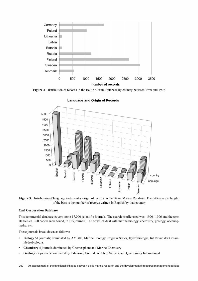
An assessment of the functional linkages between Baltic marine research and the development of resource management policies260
Figure 2 Distribution of records in the Baltic Marine Database by country.between 1980 and 1996
Figure 3 Distribution of language and country origin of records in the Baltic Marine Database. The difference in height of the bars is the number of records written in English by that country
Carl Corporation Database
This commercial database covers some 17,000 scientific journals. The search profile used was: 1990–1996 and the termBaltic Sea. 360 papers were found, in 135 journals; 112 of which deal with marine biology, chemistry, geology, oceanog-raphy, etc.
These journals break down as follows:
• Biology 51 journals; dominated by AMBIO, Marine Ecology Progress Series, Hydrobiologia, Int Revue der Gesam.Hydrobiologia.
• Chemistry 5 journals dominated by Chemosphere and Marine Chemistry• Geology 27 journals dominated by Estuarine, Coastal and Shelf Science and Quarternary International
0 500 1000 1500 2000 2500 3000 3500
Denmark
Sweden
Finland
Russia
Estonia
Latvia
Lithuania
Poland
Germany
number of records
Engl
ish
Dan
ish
Swed
ish
Finn
ish
Rus
sian
Esto
nian
Latv
ian
Lith
uani
an
Polis
h
Ger
man
language
country
0
500
1000
1500
2000
2500
3000
3500
4000
4500
5000
Language and Origin of Records

Arno Rosemarin 261
• Oceanography 13 journals dominated by Oceanology and Beitrage zer Meereskunde and Limnology and Oceanog-raphy
• Policy 16 journals• General environmental 18 journals dominated by Marine Pollution Bulletin and Science of the Total Environment• General interest 6 journals
Role of MediaMedia’s role in communicating to the public the problems at hand has been plagued with incompetence and a lack ofinterest to invest in comprehensive journalism. “The Baltic is dying” is all that was heard in the 1980s. It is no longerfashionable to describe the Baltic in these terms since it hasn’t died yet and does not appear to be approaching death inany way. Now we hear messages like nothing is being done or very little about the steady improvements actually beingmade. All in all marine scientists are not properly heard through the media. Some speciality science programmes andscience pages cover Baltic marine questions, but the policy assessment linkages are seldom made. Science is consideredas a separate media product quite disconnected from the mainstream political news. Such phenomena as blue-green algalblooms, increases in pollution, extremes in ice conditions or mass mortalities of fish due to anoxic conditions canoccasionally make headlines only because of the drastic nature of these occurrences.
The problems of being blinded by the Baltic Sea Proper, ignoring the more site-specific coastal zone issuesIn an attempt to make generalisations about the Baltic as a whole, or some of the larger gulfs, the coastal zones have beenvery much ignored and poorly assessed by HELCOM and its designated scientists. Even the national programmes havesimilar handicaps. The sheer size of the water mass is a distracting phenomenon. As a result, when policy makers, mediaand the general public say Baltic Sea we don’t really know what they mean. Is it the coastal zone areas, where pollutionis most obvious? Or is it the pelagic zones, deep holes, etc. Coastal zone management is site-specific in nature andmonitoring and research programmes need to be tailor-made. This requires a different approach to problem diagnosis andsolution than when dealing with large pelagic areas. Coastal zone management is receiving much attention around theworld. Surprisingly, the Baltic Sea is slow in getting the attention it needs in this area.
The controversy of nitrogen limitation arises in this regard. Pelagic oceanographers think it unnecessary to build sewageplants that remove nitrate. Coastal zone biologists beg to differ since nitrate in the coastal zones during the spring causesbenthic algal overgrowth (filamentous forms) and planktonic algal blooms. Both groups of scientists are actually correctin their arguments. It is just a matter of temporal and spatial perspective that causes the split in opinion. Policy makerswill become very confused if such matters are not clearly explained by such organisations as BMB and CBO.
Conclusions• there is a large gap between the scientific/technical knowledge base surrounding natural systems making up the Baltic
Sea and the governance/policy systems that attempt to manage these resources• environmental issues are still treated as they were 20 years ago—highly sectored, piecemeal and in the form of
confrontation between interest groups• marine scientists could play a much stronger role in policy development if they were better represented through
professional organisations, through systems analysis groups and proper national and international assessments thatexamine trends on an independent basis
• HELCOM’s function is not all-encompassing since it focuses on the marine environment and many of the sources ofthe environmental and natural resource problems have their origin higher up in the drainage basins
• Future sustainable development within the Baltic Sea Region will depend on how well HELCOM can adapt andenhance its role, to what extent a Baltic 21 can be developed for the Region and to what extent the VASAB 2010vision initiative can make use of these two capabilities
• Research activities and policy work are highly sectored making it difficult to extract a systems view• The publication process is somewhat fragmented and there is sometimes difficulty in finding the results of work
carried out. The HELCOM Marine Database, however, is a dependable source of literature and is now on the Internet.

An assessment of the functional linkages between Baltic marine research and the development of resource management policies262
• There is a need for comprehensive scientific reviews of published materials generated within the Baltic Region; asuggestion is that Baltic marine scientists initiate a new journal specialising in reviews only
ReferencesAMBIO, 1996. The Gulf of Bothnia Year 1991. Special Report No. 8. 35 p.
Helander, B., 1990. Inventeringar av gråsäl och knubbsäl vid svenska Östersjökusten. Rapport till PMK för verksamhet-såret 1989. Swedish Museum of Natural History.
HELCOM, 1993. The Baltic Sea Joint Comprehensive Environmental Action Programme.
Ministry for Foreign Affairs, Sweden, 1996. Actors Around the Baltic Sea: An Inventory of Infrastructures, Initiatives,Agreements and Actors. Compiled by Carl-Einar Stålvant.
Rosemarin, A., 1996. Development of a Rapid Appraisal System for the Shallow Coastal Zone of the Baltic Sea: Criteriato Set Clean-up Targets and to Evaluate Incremental Environmental Improvements. Proc BMB 14. Pärnu,Estonia.
Rosenberg, R., Lindahl, O., and Blank, H., 1988. Silent Spring in the Sea. Ambio 17: 289–290.
SEI, 1996. Baltic 21: Creating an Agenda 21 for the Baltic Sea Region. Background Report for the EnvironmentMinisters Meeting on Oct 21–22, 1996 in Saltsjöbaden, Sweden.
Swedish Environmental Protection Agency. 1996. The Baltic—A European Sea. Enviro No. 20.
VASAB, 1994. Visions and Strategies around the Baltic Sea 2010. Report to the Third Conference of Ministers forSpatial Planning and Development. Tallinn, Dec 7–8, 1994. 96 p.

Baltic Sea Science Conference Rønne, Denmark, 22–26 October 1996 263
ICES Cooperative Research Report, No. 257 Baltic Marine Science Conference, Rønne, Denmark, 22–26 October 1996
Effects of Baltic Sea coastal zone atmospheric peculiarities (during BAEX) on the formation of the 7Be concentration in the air
Narciza Spirkauskaite, Klemensas Stelingis, Viktoras Lujanas, Galina Lujaniene, and Tomasz Petelski
Abstract This paper documents the analysis of the 7Be atmospheric concentrations, measured in the Baltic Sea coastal zone, whenstudying their time variations depending on weather conditions. It was unexpectedly found that an increase in 7Beconcentrations was related to air masses transported from the Atlantic Ocean or over the Baltic Sea, in spite of thewashout processes taking place near the water surface.
Introduction In the frame of Baltic Aerosol Experiment (BAEX), cosmogenic 7Be was used as a tracer in the study of the processes ofatmospheric pollutants’ transfer through the air-sea interface in the southern part of the Baltic Sea coastal zone. Thisinvolved an analysis of the 7Be atmospheric concentrations, measured in the Baltic Sea coastal zone, when studying theirtime variations depending on weather conditions. In spite of the presence of large number of investigations studying 7Beconcentration variations depending on the latitude, seasons, weather conditions, sun activity, etc. (Lujanas, 1979; Youngand Sieker, 1974; Wallbrink and Murray, 1994; Bettoli et al., 1995), the question on the 7Be concentration over the sea isstill open.
Following one of the main BAEX aims—to answer the question of whether processes of atmospheric self-cleaning fromthe pollutants taking place in the coastal zone may be compared with the open sea ones, it had to be cleared up whetherthe factors affecting the concentration variations of 7Be (as a tracer of constant rate of production in the atmosphere overthe Baltic sea latitude) in the coastal zone are the same as those on the continent. It is known (Lujanas, 1979) that 7Beconcentrations at the same latitudes are higher in air masses of continental origin due to the existence of the secondary7Be component (resuspension of the nuclide from the earth’s surface with dust). 7Be concentrations in the air decreaseduring precipitation owing to the washout of the carriers of this nuclide (Lujanas et al., 1993). A significant increase inthe 7Be concentration in the air takes place in the stratospheric air having entered the troposphere through the tropopauzebreaks (Lujanas, 1979). During BAEX-3 in the Baltic Sea southern region (12–29 September, 1995) baric situationspromoting such tropopauze penetrations were not observed.
The coastal zone is distinguished for specific peculiarity—the transfer of pollutants, including radionuclides from sea toland in sea sprays (McKay et al., 1994). Investigations of these processes have showed that increased concentrations ofsome artificial radionuclides were observed in vegetation within 1000m of the seashore zone (Nelis et al., 1994).
Experiment Daily 7Be concentrations were measured during BAEX-3 (12–29 September, 1995) in Lubiatowo (seashore, Poland), inPreila station (seashore, Lithuania) and in Vilnius (continent, Lithuania, –350 km from the Baltic Sea).
Atmospheric aerosol samples were collected on Petrianow type filters FPP-15-1.7. The productivity of air-pumps wasequal to 700 m3·h–1 (in Lubiatowo and in Preila). In Vilnius equipment with 2000 m3·h–1 productivity was used. Themeasurements of the 7Be carrier sizes were made using a 6-stage SIERRA 230 impactor.
To determine the air mass origin (continental or marine), short-lived radon daughter products were used as tracers. Forthe evaluation of the concentration of the short-lived radon daughter products in the air, a small air pump (flow rate –2.83m3·h–l) with the Petrianow filters of RSP type (diameter 2.4cm) and an alpha-radiometer RV-4 were used. 7Beconcentrations of the aerosol samples were measured by a gamma-spectrometer with the Ge(Li) semiconductor detector.

Effects of Baltic Sea coastal zone atmospheric peculiarities (during BAEX) on the formation of the 7Be concentration in the air264
Results and discussionMeasurement results show that 7Be concentrations in the air during the experiment changed in the same manner andranged from 0.86·10–3 to 7.2·10–3Bq·m–3 in Lubiatowo, from 0.76·10–3 to 6.43·10–3Bq·m–3 in Preila and from 2.1·10–3
to 6.02·10–3Bq·m–3 at the continental site (Vilnius) (Table 1). The mean 7Be concentrations were found to be4.07mBq·m–3, 4.06mBq·m–3 and 4.08mBq·m–3, respectively.
Minimum 7Be concentrations were measured when it rained (7Be carriers were washed out from the ground atmosphericlayer) (15, 23, 28, 29 September, Table 1).
Table 1 Concentrations of 7Be in air samples during BAEX-3
Analysis of the 7Be air concentration course during BAEX-3 shows that contrary to Vilnius data a significant increase in7Be concentration in the air was measured on 19–22 and 26–27 September in Lubiatowo as well as in Preila (Figure 1).These values of 7Be concentrations during BAEX-3 (7.2; 6.43; 5.93; 5.41mBq·m–3) were the largest (Table 1) when thewhole sea surface was covered with white caps producing intensive flux of spray droplets to the atmosphere.
Figure 1 Distribution of the 7Be concentration in the air in Lubiatowo (◊), in Preila (∆) and in Vilnius () during BAEX-3 (September 1995)
Measurements of the 7Be carriers’ activity size distribution, carried out with a 6-stage Sierra impactor in Lubiatowoduring 15–21 September on the beach, show that a large percent of coarse particles in this period in the air wasmeasured. 7Be carriers in air masses of stratospheric origin over the continent are as a rule <0.4µm in size. 7Be enrichment factors of sea foam samples, collected during 17–24 September, reached a value of –1.2·10–3. It isknown that with increased wind velocity, the surf zone foam is blown out to the beach, and may also be resuspended.
Lubiatowo Preila Vilnius
Date, Sept 1995
Weather Wind dir. mBq.m-3 Weather Wind
dir. mBq.m-3Date, Sept 1995
Wind dir. mBq.m-3
11 - - - rain SW 2.23 8–11 W 3.1112 calm sea S 1.92 rain W 2.38
12–13 NE 3.1513 calm sea SE 2.69 rain NE 1.7914 calm sea SE 3.69 fog E 2.71
14–15 E 2.7415 rain NW 1.16 rain E 0.7616 rain E 0.86 rain E 3.81
16–18 E 6.0217 white caps on sea E 5.08 white caps on sea E 4.0018 calm sea SE 2.94 white caps on sea E 5.8819 calm sea SE 5.25 small waves E 6.28
19–20 W 4.1220 calm sea E 6.80 calm sea W 4.8821 white caps on sea NE 7.20 white caps on sea NE 5.01
21–22 N 4.0522 white caps on sea NW 5.70 white caps on sea N 6.4323 small waves W 3.63 rain W 3.22
23–25 S 4.6724 calm sea SW 3.60 small waves SW 3.2425 calm sea SW 3.91 small waves S 4.2126 white caps on sea W 5.93 rain SW 5.41
26–27 SW 3.8227 white caps on sea W 4.74 rain SW 4.9528 storm, rain NW 1.75 storm, rain SW 1.76
29–29 SW 2.1029 rain, storm NW 1.75 rain, storm SW 2.62

Narciza Spirkauskaite, Klemensas Stelingis, Viktoras Lujanas, Galina Lujaniene, and Tomasz Petelski 265
A decrease in the α-activity of short-lived radon daughter products in Lubiatowo on 21 and 26 September, when 7Beconcentrations in the air reached a maximum, showed that marine air advection had taken place in this region (Figure 2).This is also confirmed by the air masses transport trajectories to Lubiatowo during BAEX-3 (Figure 3).
Figure 2 Distribution of the α-activity of short-lived radon daughter products in the air in Lubiatowo during BAEX-3 (September 1995)
Figure 3 Diagram showing air mass transfer trajectories during BAEX-3 (12–28 September, 1995). Numbers on the curves show the date of air mass arrival at Lubiatowo along the track covered in 24 hours. Numbers in brackets show the
α-activity of the short-lived radon daughter products (imp/84min)
Analysis of the synoptic charts of 21 and 26 September showed that weather conditions in the southern Baltic Sea regionwere caused by cyclonic circulation (Figure 4). However, any 7Be concentration increase during the air masses’ transportin the same low pressure field systems was not observed in Vilnius. At that time 7Be concentrations in the air in thecoastal zone in Lubiatowo as well as in Preila at comparatively strong onshore or along-shore winds (5–7 m·s–l) weretwice as high as those in Vilnius (continent) (Table 1).

Effects of Baltic Sea coastal zone atmospheric peculiarities (during BAEX) on the formation of the 7Be concentration in the air266
Figure 4 Synoptic charts from 00h 21.09.95 (left) and 00h 26.09.95 (right)
Conclusions An increase in 7Be concentrations in the air in the Baltic Sea coastal zone in some cases during BAEX-3, in spite of thedominating along seashore and offshore wind directions, shows that, when studying processes at the air-sea interface inthe coastal zone, 7Be secondary atmospheric component must be taken into account.
Acknowledgements We would like to express our gratitude to Dr. Michael Schulz from the Institute of Inorganic and Applied Chemistry ofthe University of Hamburg for the chance to use the high pressure 6-stage SIERRA 230 impactor. This work is a part ofa project funded by the European Union contract No CIPA-CT93- 0086.
References Bettoli, M.G., Cantelli, L., Degetto, S., Tositti, L., Tubertini, O. and Walcher, S., 1995. Preliminary investigations of 7Be
as a tracer in the study of environmental processes. J. of Radioanalytical and Nuclear Chemistry, 190, 1, 137–147.
Lujanas, V., 1979. Cosmogenic radionuclides in the atmosphere. Mokslas Publishers, Vilnius, 192.
Lujaniene, G., Lujanas, V., Spirkauskaite, N., Tarasiuk, N. and Grenda, S., 1993. Physico-chemical properties ofartificial and cosmogenic radionuclides in the environment. J. Ecol. Chern., 2–3, 139–144.
McKay, W.A., Garland, J.A., Livesley, D., Halliwell, C.M. and Walker, M.I., 1994. The characteristics of the shore-linesea spray aerosol and the landward transfer of radionuclides discharged to coastal sea water. AtmosphericEnvironment, 28, 20, 3299–3309.
Nelis, P.M., Branford, D. and Unsworth, M.H., 1994. A model of the transfer of radioactivity from sea to land in seaspray. Atmospheric Environment, 28, 20, 1213–1223.
Wallbrink, P.J. and Murray, A.S., 1994. Fallout of 7Be in South Eastern Australia. J. Environ. Radioactivity, 25, 213–228.
Young, J.A. and Silken, W.B., 1974. The determination of air-sea exchange and oceanic mixing rates using 7Be duringthe Bomex Experiment. J. of Geophysical Research, 79, 30, 4481–4489.

Ülo Suursaar, Villu Astok, Tiit Kullas, and Mikk Ostmann 267
ICES Cooperative Research Report, No. 257 Baltic Marine Science Conference, Rønne, Denmark, 22–26 October 1996
Water and nutrient exchange through the Suur Strait (Väinameri) in 1993–1995
Ülo Suursaar, Villu Astok, Tiit Kullas, and Mikk Ostmann
Introduction and the study area This paper is mainly focused on the role of the Suur Strait in the water and nutrient exchange between the Gulf of Rigaand the Baltic Proper. In addition, the Gulf of Riga with its two outlets is an interesting and quite complex system forstudying the interaction processes between the open sea and coastal areas. The Gulf of Riga has an area of 16395km2,and a volume of 424km3. Ecologically the Gulf of Riga is under the influence of heavily loaded river water inflowaveraging 31km3 a year. Its nutrient conditions therefore differ substantially from those of the Baltic Proper and featureespecially high nitrogen content and hypothetical phosphorus-limiting conditions for phytoplankton. The influence of theheavily polluted Gulf of Riga on the water quality of the Baltic Proper depends on the efficiency of nutrient sedimen-tation within the Gulf and on the intensity of the water exchange processes via the straits.
The Irben Strait is one of the two straits connecting the Gulf of Riga to the Baltic Proper. It has a width of 27km, a silldepth of about 21m and a cross-sectional area of 0.37km2. For a long time this strait has been considered to be the mainand the only connection. Another outlet, the Väinameri (Figure 1) first proceeds through the Suur Strait, which is thenarrowest (4–5km) area in this system. The area of the cross-section is 0.04km2. The maximum depth of the strait is20m, but northwards the strait becomes wider and shallower. The minimum sill depth of the whole system is only 5m onthe southern side of the Väinameri basin. The next strait on the northern border of the Väinameri is the Hari Kurk Strait,having a width of 8–10km and a sill depth of about 10m. The Väinameri has an area of 2243km2 and a volume of10.6km3. It could really be treated as a separate sub-basin of the Baltic (analogous to the Archipelago Sea). If not, itshould rather be regarded more as a part of the Gulf of Riga than of the Baltic Proper.
Figure 1 The Väinameri area and the cross-section of the Suur Strait; current velocities in cms–1. AI, A2 and A3 mark the positions of the mooring stations.
Measurements Extensive investigations were carried out within the Gulf of Riga Project in 1993–96. The field-work in the Väinameriarea was done during ten expeditions lasting from one to four weeks each. Two recording current meters (AanderaaRCM-7 and RCM-4) were used, providing data on the directions and velocities of currents as well as water temperaturesand salinities. Additional current measurements were carried out between the expeditions as well. The upper instrument
Water and nutrient exchange through the Suur Strait (Väinameri) in 1993–1995268
was moored at a depth of 3–6 m in the Suur Strait and the lower at 10–13m. The direct current measurements coveraltogether about 470 days. The spatial structure of the currents was investigated by salinity and temperature (CTD) andvelocity (ACM) profiles carried out in spring and autumn of 1993, and by measurements with Hammer’s pendulumcurrent meters (HPCM) carried out in the Hari Kurk Strait and the Suur Strait in 1995 and 1996 (e.g. Figure 1B).
We have tried to measure currents, water temperatures and salinities simultaneously with nutrient measurements. Thewater samples for analysing nutrient concentrations (Ptot and Ntot) were collected on board R/V “Junga” (expeditions I,II, IV), “Lest” (V), “Kiir” (VII, VIII), from ice (III, IX) and by boat (VI). The samples were usually taken at two layers(0–1m and 15–16m), mostly three times a day during expeditions or along certain spatial sections. Components ofnutrients (P-PO4, N-NO2, N-NO3, N-NH4) were measured less frequently. Chemical analyses were performed mostly bythe laboratory of the Environmental Engineering Institute, Tallinn Technical University. Altogether about 2300 analysesof nutrients were made in 1993–96. In addition, regular vertical soundings of O2 and temperature using a Marvet Fluidanalyser and Secchi measurements of water transparency were carried out. A more comprehensive overview of measure-ments can be found in the reports (e.g. Suursaar and Astok, 1996).
Results and discussion
Variability of currents. thermohaline regime and nutrients Currents seem to be the crucial factor for the state of the Väinameri since the front dividing the quite different watermasses (the Gulf of Riga estuarine-type and the Baltic Sea marine-type) happens to be located somewhere in theVäinameri and pulsating north- or southwards depending on prevailing winds and currents. For example, though season-ality is the main factor influencing water temperatures, also advective variations up to 6 –8°C within less than 24 hourswere found, especially in early summer when the shallow Väinameri becomes warmer than the larger and deeper neigh-bouring basins. Also the salinity regime in the Suur Strait is very variable since it is affected by two water masses alter-nating from time to time. The salinity differences through the front are usually 1–1.5 PSU. The average gradients wereestimated as 0.02–0.05 PSUkm–1. Also, because of its shallowness and clearly defined morphometry, the Väinameri actsas a certain buffer-zone, where mixing processes of the different water masses take place. Therefore the frontal zone mayappear somewhat diffused in some cases.
Spatially the currents have a relatively simple and mostly unidirectional structure in the Suur Strait. It was thereforepossible to find simple empirical relationships between the flow volume and the mean current velocity for differentpositions of the mooring stations. Two directions of currents clearly dominated (130–160° and 340–350°), determinedby the bottom topography of this relatively narrow strait. The variance of the axial (NNW–SSE) component of thevelocity vector fluctuations comprises about 92–97% of the total variance, leaving only a small share for the perpen-dicular component. Temporal variations are far more interesting. The dominant feature of the temporal variability ofcurrents in the Suur Strait is the prevalence of motions induced by atmospheric synoptic activities over the diurnal, semi-diurnal and other short-term components. The relatively significant peak above the background spectra at 12.5 (±0.1–0.3)h, which could be the M2 (lunar semi-diurnal) tide, still has, in absolute terms, a smaller amplitude than the motionswith the periods of 24–30h and 3–4 days. The periodicity of 24h is the most prominent feature in the Irben Strait (e.g.ΠeTpoB, 1979) and it seems to be also the period of the eigenoscillations of the Gulf of Riga in the system with two straits(see also Otsmann et al., 1996).
The seasonal and interannual variability could also be substantial, depending on the variability of large-scale atmosphericcirculation types above the North Atlantic and ice conditions in the Gulf. According to our investigations the meanvelocity module in the Suur Strait was about 25cms–1 in 1993–95. According to Petrov (ΠeTpoB, 1979) the meanvelocity in the Irben Strait is about 6cms–1. Thus, the smallness of the Suur Strait compared to the Irben Strait iscompensated by higher velocities. The maximum velocities measured up to now for the Suur Strait (103cms–1 in theupper layer) were presented by Mey (1922). The maximum values measured by us were 100cms–1 for both the inflowing(at 12m on 1 October 1995) and outflowing currents (at 12m on January, 23, 1995; Wind velocities were up to 27ms–1 atViirelaid). As these values were obtained in a relatively deep part of the strait, the real maximum values in the surfacecould be estimated as 1.3 to 1.5ms–1.
The differences in chemical properties of the above mentioned water masses acting in the Väinameri are even moreevident. It is a well known fact that the trophic status in the Gulf of Riga is considerably higher compared to the BalticProper and even in the Väinameri. While the long-term average concentrations of phosphates in the Gulf of Riga areabout 0.4–0.8µM in early winters and the typical values for nitrates are about 10–20µM, the corresponding values in theBaltic Proper and in the entrance section of the Gulf of Finland are about 0.3–0.6µM PO4 and only 4–10µM NO3. The

Ülo Suursaar, Villu Astok, Tiit Kullas, and Mikk Ostmann 269
corresponding Ptot content is roughly 1–1.5 vs 0.7–1µM and 30–50 vs 15–30µM for Ntot (e.g. Suursaar, 1995).Average values obtained during our expeditions can be seen in Figure 2.
Figure 2 Long-term variations in average values of Ntot, NO3, PO4 and Ptot content during the expeditions in 1993–1996.
It was found that a connection between the nitrogen content and the currents can often be followed in the Suur Strait area,especially when the flow has been long-standing (Figure 3A, B). However, the dependence of the phosphorus content onthe currents is rather weak. The explanation could be that the gradients in the phosphorus values between the Gulf ofRiga and the Baltic Proper are not as strong as those in nitrogen. Moreover, some local effects tend to overshadow suchvariations. For example, a strong release of phosphorus compounds with the suspended material occurs in the Suur Straitarea during storms (e.g. Figure 3C, D). A simultaneous decrease in water transparency after each storm event could benoticed. A strong relationship (R=–0.81) between the measured transparency and corresponding phosphorus values wasfound.
Figure 3 Temporal variations in salinity (A) and total nitrogen content (B) on 09.05–01.06.1994. Temporal variations in water transparency (C) and total phosphorus content (D) on 19.10–20.11.1994.
The role of the Suur Strait in the water and nutrient exchange between the Gulf of Riga and the Baltic Proper It was quite easy to convert the velocities in the Suur Strait into volume flows. However, problems arise in the case of thesecond strait and also at a conceptual level. It is easy to see that the different methods for obtaining the water exchangeestimates—direct measurements of currents, flow estimations by the volume changes inside the basin and by retainingthe volume and salt balances, density gradients, frontal positions, etc.—and the different time-scales for averagingrepresent somewhat different aspects of the water exchange processes and produce quite different estimates. Thus for theIrben Strait it has been found several times in the past that the direct measurements could not be applicable, because the

Water and nutrient exchange through the Suur Strait (Väinameri) in 1993–1995270
strait is relatively wide and two-layer-two-directional flow regime is quite frequent. Therefore, it was decided that thesalt-budget (also Knudsen) method or the volume-difference methods could be the best choices.
Unfortunately the other outlet, the narrow-seeming Suur Strait, was neglected. However it is now evident that these flowsin the Suur Strait are too remarkable to be neglected. Moreover, it was found that the water exchange processes of thewhole Gulf take place due to the existence of two straits: the straits “work together” (Otsmann et al., 1996).
We start with the Suur Strait, not because the strait is “better”, just because our information on that Strait is moreextensive. Summing up the measured individual flows may lead to almost correct averages provided the number of directmeasurements is very high. Such calculations in our case yield in total 165km3 of inflows and 189km3 for outflows(Qout) per year, and the annual net exchange (Qnet) will be –20km3. Mardiste ( , 1975) had about 100, –150and –50 kmyr–1, respectively. Figure 4 presents the evolution of the estimates according to the length of the measuredseries. The total extension of measurements is quite big to stabilise (convergement) results in the vicinity of certain“true” values.
Figure 4 Evolution of the estimates of total in- and outflows and net exchanges depending on the lengthening of the direct measurements series in 1993–95
Evidently these Qin and Qout values describe all the volumes participating in the water exchange, and therefore also alarge extent of the to-and-fro movements of the same water, which actually may not be exchanged. While Qnet describesthe lower boundary of the water exchange, Qin and Qout represent the upper boundary for water exchange estimates, in allaspects and whatever method applied. The “real”, or let us say, “effective” flows should be something between Qnet andQin or Qout. They could be calculated simply as the integral (or cumulative) water transport. Such cumulative transportcurves are presented in Figure 5. We need to decide which kind of change in directions to consider as relevant. Fortu-nately it can be seen that even quite typical periods of oscillations around 3–4 days and below (which usually produceflows less than 5km3) are smoothed down. Figure 5 indicates that the flows in different months tend to group on aseasonal basis. Summer (Figure 5A) mostly displays the inflows (ranging from –2 to +13km3 in a month), winter (Figure5B) displays strong outflows (from +2 to –26km3 per month) and spring and autumn are certain transition periods whenboth the inflows and outflows may occur (±8km3). In winter the water exchange depends strongly on the existence if theice-cover in the northern part of the Gulf of Riga. We have experiences with both mild winters (such as 1994/95) andwith severe winters (1993/94 and 1995/96).
Figure 5 Integral volume transports grouped by seasons and months.
Mapдиcтe

Ülo Suursaar, Villu Astok, Tiit Kullas, and Mikk Ostmann 271
When we arrange all the curves (some of them depicted in Figure 5) in consecutive order with the actual gaps betweenthe measurements, we obtain one of the curves (“measured”) presented in Figure 6. (Again, the dominant seasonalpattern is very clear). By filling the gaps from Oct. 1993 to Oct. 1995 we get an estimation of a continuous two-yearperiod (the other curve, “measured/estimated”) representing the years with both cold and mild winters. The fill-up wasmade based on the wind-coefficient (if the wind data were available) or on the similarity of the curves presented inFigure 5. In future the gaps will be covered using the water exchange model (Otsmann et al., 1996).
Figure 6 Cumulative volume transport in the Suur Strait in 1993–95. The gaps in measurements are filled to obtain a continuous measured/estimated curve.
We got the “effective” flows in the Suur Strait for two “seasons” or “half-years”. Now, from also knowing the riverinflows, we can easily find the resultant flows in the Irben Strait. The problem is dividing these resultant flows betweensimultaneous in- and outflowing components. From the work by Berzhins et al. (1994) we obtained the water exchangeestimates in the “cold” and “warm” half-years for the whole Gulf of Riga (attributed to one anonymous strait). They werecalculated by the modified Knudsen method on the basis of salinity and water level data obtained in Latvia. Adding thedata we just got for the Suur Strait we obtain: The inflow in the cold half-year averaged 53 km3 (all through the IrbenStrait) and for outflow –80 km3 (–45 km3 via the Suur Strait and –35 km3 via the Irben Strait). The average river inflowduring the cold half-year was 22 km3 and the volume change –5 km3. The average inflows during the warm half-yearswere 59 km3 (32 km3 for the Suur strait and 27 km3 for the Irben Strait) and outflows –68 km3 (–15 and –53 km3 respec-tively). In summer river inflow is 14 km3 and the volume changes about +5 km3 (Figure 7).
Figure 7 Sketch of the water exchange in “summer” (A: May–October) and in “winter” (B: November–April). The flows and the volume differences (^V) in km3 for the corresponding half-years.
Discussing these results we would like to stress that they are really sketches in a quantitative meaning, but as a principlethey should be quite representative. Comparing our results with the findings by Petrov (ΠeTpoB, 1979) and Pastors(ΠacTopc, 1963) we notice that the estimates by Petrov are about twice as large (about 320 km3 both for inflows andoutflows in the Irben Strait). Pastors (ΠacTopc 1963) gave 183 km3 for inflow and 215 km3 for outflow (not sharedbetween the straits). The study by Petrov has usually been taken as a prestigious source for other studies. We explain theoverestimation of volume flows presented by Petrov by his choices of typical salinities in filling the salt-budget

Water and nutrient exchange through the Suur Strait (Väinameri) in 1993–1995272
equations. Namely, filling in the balance-equations he used the typical salinities of inflows and outflows (having consid-erably smaller differences due to mixing processes in the transition-areas of the straits) against the average salinity of theGulf. Since the difference in salinities he used was only about 0.5 PSU, we realise that in order to keep the salt balance,such water masses must be exchanged in 2 times larger volumes than in the case where the difference is 1 PSU, forexample. The water exchange estimates by Petrov also represent the backflows in addition to “pure” exchange in thetransition zones of straits.
In our case, the share of the Suur Strait in “effective” flows could be quantified at about 32%, the share of the Irben Straitabout 57%, leaving about 11% for the rivers. (neglecting precipitation and evaporation, which are equally around 9km3 ayear). Assuming that the inflowing currents carry waters with concentrations of 0.8µM Ptot and 20µM Ntot, andoutflowing 1.2µM Ptot and 40µM Ntot we obtain the nutrient fluxes through the straits as follows: The annual loss ofphosphorus is 2500–2800t, and 49000–54000t for nitrogen. The estimates of annual outflowing fluxes of Ptot (2700t)by Yurkovskis et al. (1993) are surprisingly close to our results. Unfortunately Yurkovskis et al. (1993) has no estimatesfor Ntot, but fluxes of inorganic nitrogen are presented at about –22000t. The estimates close to ours could be obtained ifthe proportion of inorganic nitrogen from the total nitrogen were taken as 30%. Yurkovskis et al. (1993) argue that themajor proportion of the (inorganic) nitrogen load entering the Gulf of Riga (about 100000t per year) is deposited in thebottom sediments and only 25% is exported via the straits, while the phosphorus load (2800t per year) is exported almostentirely. However, it could also be argued that both N and P are exported proportionally (about 15–20%) to their pools inthe Gulf. Still, nitrogen appears in excess (the N:P molar ratio in the Gulf is well over the Redfield’s 16:1 ratio) and thegradients between the open Baltic and the Gulf are much stronger in nitrogen contents than in the case of phosphorus.Therefore, the water exchange processes in the straits ventilate the Gulf of Riga especially in relation to excessivenitrogen amounts.
We can speculate about one more effect: The absence of ice in winters 1988/89, 1989/90, 1991/92, 1992/93 and 1994/95could be a remarkable cause for the negative nutrient trends reported for the Gulf of Riga in the last 5–10 years.(Measurements made by us for only 3–4 years display these negative trends as well—see Figure 7). The outflows duringautumn and ice-free winter could be about twice as strong as in cold winters, roughly –50... –80 vs –30... –40km3, whichmakes some 1000–1500 extra outflowing tons of phosphorus and 10000–20000 tons of nitrogen. That is doubtlessly aremarkable proportion compared to the total annual load to the Gulf (about 100000t of nitrogen and 3000t of phosphorusaccording to Andrushaitis et al., 1995). It is also evident now, that the above mentioned nutrient amounts driven bycurrents are considerably bigger than the local pollution load entering the Haapsalu and Matsalu Bay (in total roughlyabout 70–100t of Ptot and 2000–3000t of Ntot annually). The amounts entering the Väinameri from these bays are evensmaller due to nutrient sedimentation processes within these bays. Thus, local pollution from these much discussed bayshas only a very limited effect on the state of the Väinameri.
Conclusions 1. The mechanisms controlling the hydrophysical and nutrient regime in the Väinameri could be listed as: normal
seasonality; pulsations of the frontal zone and alternating of the water masses of different types; storm events causingstrong turbulent mixing and catching up the suspended material from bottom sediments in the shallow waters; thenegative trend caused by increased water exchange and decreased pollution load; the local pollution load from theMatsalu and Haapsalu Bays. Due to strong variability of currents and hydrochemical situation, the Väinameri is notsuitable for (low-frequency) water quality monitoring.
2. The present study gives the estimates of the water exchange in the Suur Strait as follows: total inflows to the Gulf ofRiga 120–140km3 per year; total outflows 150–170km3 per year, the net exchange about –20–30km3 per year and80–100km3 per year for integral (“effective”) flows. Inflows of saline water usually take place in warm seasons andoutflows in cold seasons. Maximum velocities in the Suur Strait could be estimated as 1–1.5ms–1, the average valuesbeing about 0.25ms–1.
3. The share of the Suur Strait in the water budget of the Gulf of Riga is about 32%, the Irben Strait has about 57% andthe rivers about 11% (neglecting precipitation and evaporation). The different results by different authors exploit thedifferent aspects of the water exchange. Our estimates for the water exchange in the Irben Strait are about two timeslower than those presented by Petrov. We think that the results by Petrov include in addition to “pure” exchange alsothe backflows in the transition zones of straits. It might have been the result of the fact that the salt-budget method isvery sensitive to choosing the “right” salinities, and to averagings.

Ülo Suursaar, Villu Astok, Tiit Kullas, and Mikk Ostmann 273
4. The annual nutrient loss due to the water exchange through the straits is about 2500–2800t of Ptot and 49000–54000tof Ntot, which are 1.2–2 times lower than the loads entering the Gulf. The improvement in the ecological state of theGulf of Riga during the last 5–6 years could partly be explained by successive ice–free winters (1988/89, 1989/90,1991/92, 1992/93, 1994/95) enabling a strong ventilation of the Gulf through the straits.
Acknowledgements The Gulf of Riga Project is financially supported by the Nordic Council of Ministers. Special thanks are due to PekkaAlenius from the Finnish Institute of Marine Research, the scientific coordinator of the sub-project: “Water exchange,nutrients, hydrography and database”.
References Andrushaitis, A., Seisuma, Z., Legzdina, M., and Lenshs, E., 1995. River load of eutrophying substances and heavy
metals into the Gulf of Riga. In: Ecosystem of the Gulf of Riga Between 1920 and 1990. (Ed. by E. Ojaveer),Academia, 5, 32–40. Estonian Academy Publishers, Tallinn.
Berzhins, V., Bethers, U., and Sennikovs, J., 1994. Gulf of Riga: bathymetric, hydrological and meteorologicaldatabases, and calculation of the water exchange. Proc. Latvian A cad. Sci. Section B, No. 7/8, 107–117.
Mey, J., 1922. Baltimere hüdrograafia ill. Laevandus, 7, 179–182.
Suursaar, Ü., 1995. Nutrients in the Gulf of Riga. In: Ecosystem of the Gulf of Riga Between 1920 and 1990. (Ed. by E.Ojaveer), Academia, 5, 41–50. Estonian Academy Publishers, Tallinn.
Suursaar, Ü., and Astok, V. (ed.), 1996. Studies on measuring and modelling the water and nutrient exchange of the Gulfof Riga. EMI Report Series, 3, 109 p.
Otsmann, M., Astok, V., and Suursaar, Ü., 1996. A model for water exchange between a large and a small water body:the case of the Baltic Sea and the Gulf of Riga. Nordic Hydrological Conference, Akureyri, Iceland 13–15 August1996. NHP Report No 40, Vol. 2,496–505.
Yurkovskis, A., Wulff, F., Rahm, L., Andruzaitis, A., and Rodriguez-Medina, M., 1993. A nutrient budget of the Gulf ofRiga; Baltic Sea. Estuarine, Coastal and Shelf Science, 37, 113–137.
Mapдиcтe, X. X., 1975. O pacxoдax воды в пpoливax Myxi (Bяйиамери). In: Динамика вод Блтийскогоморя. Taлинн, Изд, AH ЭCCP, 88–94
Пacтopc, A. A., 1963. Водный бaлaнc Pижcкoгo заливa. – Tpyды ГOИH, 73, 96–105.
Петров, B. C., 1979. Водный бaлaнc и вoдooбмен Pижcкoгo заливa c Балтийск им мopeм. In: Cб. PaбoтPижcкoй гидpoмeтeopoлoгичecкoй oбcepвaтop ий, 18, 20–40.
Baltic Sea Science Conference Rønne, Denmark, 22–26 October 1996 274
ICES Cooperative Research Report, No. 257 Baltic Marine Science Conference, Rønne, Denmark, 22–26 October 1996
Investigation of the atmospheric impurity washout in the Baltic Sea coastal wave breaking zone during BAEX using radio-active tracers
Nikolaj Tarasiuk, Narciza Spirkauskaité, Klemensas Stelingis, Galina Lujaniené, Michael Schultz, and Roman Marks
Abstract 7Be and 137Cs as radionuclides of different origin were used as tracers to study the influence of the surf zone upon thedry deposition of atmospheric pollutants and to study effects of sea self cleaning in the coastal zone during BAEX (BalticAerosol Experiment, 1994–1995) in Lubiatowo (northern Poland) and Preila (western Lithuania) stations. 7Be drydeposition velocities were measured depending on the distance from the shoreline. A considerable growth of thisvelocity (up to 30 mm·s–1) was fixed in stormy weather near the surf zone. Estimations show that 7Be secondary atmos-pheric component (resuspended from the sea surface with spray droplets and salt particles) is responsible for 38% of thisvalue.
Activity size distributions of 7Be carriers in the air show that the main part of 7Be during experiments was associatedwith submicron aerosols of geometric mean aerodynamic diameters of 0.52–0.72µm.
Temporary sediments of the coastal zone are actively participating in the sea coastal zone self-cleaning onshore fluxexisting as onshore pollutant secondary atmospheric and foam fluxes.
Evaluating the 137Cs load of the unstable part of the sea beach (changeable by storms), sand may be treated as seasediments and characterised by the 137Cs partition coefficient Kd.
IntroductionThe sea coastal zone where wave energy dissipates is an area of the most intensive interaction between the sea and theatmosphere. Wave breaking and spray generation, arising in shallow waters at comparatively weak winds, enhance thedry deposition of particles by shunting high transfer resistance to a smooth water surface (Williams, 1981). Calculationsshow that in this case the dry deposition velocity of submicron aerosols may be of the same order as the velocity of themomentum transfer. This effect may be very strong for the Baltic Sea where shallow water areas are very extensive andatmospheric loadings of the coastal zone must be taken into account in the balance of the total atmospheric load.
Possible effects of enhancement of the dry deposition flux of atmospheric pollutants in the Baltic Sea coastal zone werestudied in the frame of Baltic Aerosol Experiment (BAEX) using cosmogenic 7Be as a tracer. Among a number ofadvantages of this nuclide (Lujanas et al., 1994; Bettoli et al., 1995), the most important ones are those that 7Be is ofatmospheric origin and activity size distribution of its carriers is typical of aerosol particles of industrial pollutants oflong-term transport (Papastefanou and Joannidou, 1995). 137Cs and 7Be were used as tracers in the study of associatedproblems with sea self cleaning in the coastal zone.
ExperimentThe experiment aimed to measure the enhanced dry deposition flux of 7Be to the beach close to the surf zone, wherespray droplets were blown to the beach by onshore wind, deposited owing to large gravitational settling velocities to thebeach surface on their pathways capturing submicron aerosols marked by 7Be. The method was thought to be a compar-ative one, when 7Be dry deposition velocity, calculated for collectors deployed near the surf zone, is compared with thedata measured for collectors exposed on the land under the same weather conditions. Since exposure times lasted forseveral days (up to a week), 7Be dry deposition velocities were averaged over all meteorological situations (except rain,when collectors were closed). The experiment was carried out in Lubiatowo (northern Poland) and Preila (westernLithuania) in 1994 (BAEX-2) and 1995 (BAEX-3). During BAEX-2 dry depositions of 7Be were collected on horizontalPetrianow filters 0.85×l.5m2 deployed on the beach and at two different distances from the shoreline (40m and 150m).Filters exposed on the beach near the surf zone were mounted on 80cm high platforms; the others on a solid background

Nikolaj Tarasiuk, Narciza Spirkauskaité, Klemensas Stelingis, Galina Lujaniené, Michael Schultz, and Roman Marks 275
5cm thick. During BAEX-3 near the surf zone two filters were exposed simultaneously on platforms of differentheight—60 and 120cm—and for comparison one filter on the top of the dune. Filters were placed facing the atmosphereon a gauze surface and mounted on book-type holders which were closed manually before rain and taken away.
Two air pumps in Lubiatowo and Preila with a flow-rate of 700 m3·h–1 were used for daily sampling of the atmosphericaerosols on Petrianow filters.
An optical counter LAS-X (PMS), providing 46 size classes for aerosols from 0.1 to 7.5µm, was used to measurehorizontal profiles of sea droplets and particles near the surf zone over the beach during BAEX-2 in Lubiatowo. Thecounter was mounted on a mobile platform.
A high pressure slotted impactor (Sierra instruments, series 230) of 5 stages and with a back up filter was used inLubiatowo during BAEX-3 to evaluate activity size distribution of 7Be carriers in the air over the beach (at about 15mfrom the surf zone). Calculated aerodynamic cut-off diameters for used flow rate (68 m3·h–l) were as follows for stagesfrom 1 to 5: 7.0, 3.0, 1.7, 0.86, 0.47µm (Steiger et al., 1989). Aerosol deposits on the impactor stages were collected onWhatman-41 filters.
To study the effects of sea self-cleaning from radionuclides in the coastal zone during BAEX, beach sand cores12×12cm2 and sea foam samples were taken. 137Cs vertical profiles were measured in beach sand cores up to the depthof 60–90cm to evaluate the radionuclide load of the beach. Sea foam samples (volume up to 1.5L) were filtered throughFiltrak type filters for separate definition of radionuclide content in filtrate and suspended matter form.
A γ-spectrometer with the Ge(Li) semiconductor detector was used for 7Be and 137Cs nuclides analysis of the samples.Calibration was carried out using radioactive sources of different density and mixed radionuclide content prepared by theRussian Scientific Research Institute of Physico-Technical and Radiometric Measurements (Moscow). Measurementerrors of radionuclide content values for aerosol samples of the pumps, beach sand and sea foam samples as well asimpactor back up and high number stages filters and high activity filter of dry depositions were equal to about 30%.These errors for reasonable measurement time (about a day) amounted to 50% for collector filters of long-termexposition and deposits on middle stages of the impactor. Deposits on low number stages of the impactor as well as drydeposition filters exposed for a short time during BAEX-3 were measured with errors of about 100%.
Results and discussionThe course of the 7Be concentration in the air over the beach in Lubiatowo during BAEX-3 is depicted in Figure 1. Gapsin the 7Be concentration course are related to precipitations.
Figure 1 Course of the 7Be concentration in the air over the beach in Lubiatowo during BAEX-3 (1995)
The velocity of 7Be dry deposition was evaluated using the following expression:
where
A is the 7Be dry deposition activity of the filterSF is the surface area of the filterCi is the 7Be concentration in air in accordance with the course of variations during collector filter exposition (Figure 1)∆ti is the time interval of constant Ci value.
V A
SF Ci∆tii∑
--------------------------=

Investigation of the atmospheric impurity washout in the Baltic Sea coastal wave breaking zone during BAEX using radioactivetracers
276
Data of 7Be dry deposition velocity evaluation experiments in Lubiatowo during BAEX program realisation are shown inTable 1 and Table 2. Meteorological data were used from Leba Station—one of the nearest to Lubiatowo Polish stationson the Baltic Sea coast. Table 1 and Table 2 inform about time intervals of dry deposition filters exposition and impactormeasurements, periods of the use of the optical particle counter as well as present visual observation data of the wavingand wind direction during light time in Lubiatowo and calculated values of 7Be dry deposition velocities.
Table 1 Data of 7Be dry deposition experiment in Lubiatowo during 20–29 September, 1994 (BAEX-2)
Table 2 Data of 7Be dry deposition experiment in Lubiatowo during 12–29 September, 1995 (BAEX-3)
As may be seen from Table 1 and Table 2, weather conditions were not convenient for the experiment—offshore windsand winds along the seashore direction dominated. 7Be dry deposition velocities in good weather for the filter on the topof the dune (and in the forest—for BAEX-2 only) in Lubiatowo were: 1–1.1mm·s–1 (2.2mm·s–1 in Preila at the sametime) during BAEX-2 and in the range of 0.4–0.7mm·s–1 (0.4–0.5mm·s–1 in Preila) during BAEX-3. Somewhat highervalues were measured for filters near the surf zone—1.4mm·s–1 in Lubiatowo (2.7 mm·s–1 in Preila) during BAEX-2 andin the range of 0.7–2.0mm·s–1 for filters deployed in the surf zone (small waves) during BAEX-3 (0.5–1.0mm·s–1 inPreila). It has to be noted that with the exception of one case (including Preila’s data) filters mounted on the lowerplatform in the surf zone were somewhat more activated than those on the higher platform.
Date 20 21 22 23 24 25 26 27 28 29Leba station, GMT=0
wind direction E NE NNE SSE WSW WSW SW WNW SW
Leba station, GMT=0Max wind velocity ms–1 1.5 7.9 5.4 1.5 1.5 0.2 7.9 7.9 20.7 13.8
Lubiatowo, waves:— calm sea, * small,
** white caps, *** stormy— ** ** * * — * * *** ***
Lubiatowo, direction of air advection:
offshore–off (S, SE, SW)onshore–on (N, MW, NE)
along shore–al. (E, W)
al.(E)
al.(E)
al.(W)
al.(W) — off
(SW)off
(SW)on
(NW)on
(NW)al.
(W)
Optical particle counterdry deposition filter exposure (——) showing dry deposition
velocity of 7BeF1–open square in the forest F1(155.3)
F2–on top of dune F2(154.7)
F3–on platform near surf zone F3(74)
Fi(t)–net time of exposure (h) F3(24)
Date 12 13 14 15 16 17 18 19 20 21 22 23 24 25 26 27 28 29Leba station, GMT=0
wind direction S E W E E ESE SE ESE NE SSW WSW SSW S SW SSW W W
Leba station, GMT=0Max wind velocity ms–1 3.3 0.2 10.7 3.3 5.4 7.9 3.3 3.3 7.9 7.9 1.5 10.7 3.3 5.4 10.7 3.3 20.7 10.7
Lubiatowo, waves:— calm sea, * small,
** white caps, *** stormy— — — ** * ** — — — ** ** * — — * ** *** ***
Lubiatowo, direction of air advection:
offshore–off (S, SE, SW)onshore–on (N, MW, NE)
along shore–al. (E, W)
off(S) — off
(SW)on
(NW)al.(E)
al.(E)
off(SE)
off(SE)
al.(E)
on(NE)
on (NW)
al.(W)
off (SW)
off(SW)
al. (W)
al. (W)
on(NW)
al.(W)
Impactor measurements
dry deposition filter expo-sure (——) showing dry deposition
velocity of 7BeF2(121)
F2(141.3)F2(75.7)F3'(30.3)F3'(39.3)F3'(31.3)F3''(26)
F3''(39.3)F3''(31.3)
F2–on top of dune
F3'–at 60cm in surf zone
F3''– at 120cm in surf zone
Fi(t)–net time of exposure
30.2mm·s–1
1.4mm·s–11.0mm·s–1
1.1mm·s–1
1.0mm·s–10.7mm·s–1
1.2mm·s–1
0.7mm·s–1
0.4mm·s–1
0.5mm·s–1
0.8mm·s–1
2.0mm·s–1
0.8mm·s–1

Nikolaj Tarasiuk, Narciza Spirkauskaité, Klemensas Stelingis, Galina Lujaniené, Michael Schultz, and Roman Marks 277
Data of the measurements of horizontal profiles of sea aerosol concentrations in the air across the beach carried out inLubiatowo during BAEX-2 for wind of WNW direction helped to analyse the situation during filter activation near thesurf zone (Table 3). A large decrease in the concentration of coarse particles in the size range 2.55–7.5µm with theincreasing distance from the shoreline showed that filter activation might be mainly efficient only directly near or insidethe surf zone.
Table 3 Horizontal profile of aerosol particle concentration on the beach of Lubiatowo on 23 September, 1994 (wind WNW, 3-5ms–1)
Activity size distributions of 7Be carriers were measured for two aerosol samples taken with the high pressure impactorduring BAEX-3 (Table 2, Figure 2). They are both almost log-normal, but activity size distribution of the first sample(13–15.09.95) is shifted to the left to larger aerodynamic diameters of 7Be carriers, apparently owing to the transport ofthe activated sea aerosols from the surf zone. A geometric mean aerodynamic diameter (GMAD) of this distribution is0.72µm. It seems that air masses of off-shore wind direction dominated during the second long-term aerosol sampling(15–21 September, 1995). So 7Be was mainly associated in this sample with the particles of smaller aerodynamicdiameters (GMAD was equal to 0.52µm). Nevertheless in good weather these differences had a small influence on the7Be dry deposition velocity value (Table 2) and may testify to the existence of the 7Be secondary atmospheric componentin the coastal zone (Figure 2a), resuspended from the sea surface with droplets and salt particles.
Figure 2 7Be carrier size g-activity distribution in the air over the beach in Lubiatowo during BAEX-3:a) air sample volume 3400m3 (13–15.09.1995)b) air sample volume 7980m3 (15–21.09.1995)
Cut-off diameters of stages (µg): 1—7.0, 2—3.0, 3—1.7, 4—0.86, 5—0.47, 6—backup filter. dg is the geometric mean aerodynamic diameter (DMAD) of 7Be carriers.
We succeeded in exposing one filter in stormy weather with an onshore NW wind (Table 1). An extraordinarily largevalue of 7Be dry deposition velocity (30.2mm·s–1) was calculated, larger than it was predicted in theory (Williams,1982), and corrected for possible collector filter pollution by 7Be secondary (resuspension) component. Data of radionu-clide content in a foam sample taken during the filter exposition (Table 4) and measured total amount of main ions (Na+,Mg+, K+, Cl–) in the filter (130mg, Flame Photometer) were used for the evaluation of this correction. Calculationshowed that filter pollution by 7Be secondary component was responsible for 38% of the measured value of the 7Be drydeposition velocity (Table 1). So a residual part of this value (about 18 mm·s–1) may be treated as evidence of theexistence of large dry deposition fluxes of atmospheric pollutants to the sea surface in stormy weather. At the same timeit is evident that dry deposition velocity data, presented in Table 1 and Table 2 were only the upper limit of these values,and also must be corrected for the 7Be secondary atmospheric component.
Distance from
shoreline (m)
Time of measurement
Particle concentration (cm-3)
Size range (µm)
0.1–7.5 0.1–0.2 0.2–0.75 0.75–2.55 2.55–7.50 16h26'17'' 1395 911.4 475.2 8.06 0.2645 16h32'20'' 1340 889.1 447.0 4.21 0.06210 16h38'19'' 1340 891.3 445.3 3.71 0.04415 16h44'13'' error error 435.2 3.30 0.03420 16h51'44'' 1302 863.4 435.6 3.37 0.07230 16h57'39'' 1283 849.6 430.2 3.35 0.05840 17h3'46'' 1295 848.2 443.8 3.46 0.062

Investigation of the atmospheric impurity washout in the Baltic Sea coast wave breaking zone during BAEX using radioactivetracers
278
Table 4 Concentrations of 137Cs and 7Be in sea foam samples (filtrate and suspended matter) and enrichment factors (EF) during BAEX
Data of the foam radionuclide content (Table 4) show that temporary sediments of the shallow waters owing to theflotation actively participate in the self-cleaning processes of the coastal zone—the main part of 137Cs is associated withthe suspended matter (7Be depositing to the sea surface is not in time to be dissolved and also is associated in foam withthe suspended particles). It is known that onshore radionuclide flux related with foam is followed by other sea self-cleaning fluxes related to spray droplets and salt particles, where dissolved substances (with enriched concentrations) andsediment particles also take part (Belot et al., 1982; McKay et al., 1994). It is obvious because sea foam and spraydroplets originate from the sea surface microlayer. Therefore radionuclide content of 7Be secondary atmosphericcomponent owing to the sea aerosol onshore flux may be compared to that of sea foam. Large enrichment factors (EF) of137Cs and 7Be in sea foam in stormy weather show that secondary atmospheric components of these nuclides under thesestormy conditions may be very significant. Evaluating EF values for 7Be (Table 4), concentration of this nuclide in seawater was taken from publications (Olsen et al., 1989).
Data of the investigations of possible additional radioactive pollution of the beach (compared with soil) owing to theexistence of the onshore radionuclide flux in the sea coastal zone are depicted in Figure 3.
Figure 3 Vertical profiles of 137Cs specific activity in soil and beach sand:a) Lubiatowo, beach sand, 16m from surf zone
b) Lubiatowo, soil sample from the meadowc) Lubiatowo, beach sand, 11m from surf zone
d) Preila, beach sand, 32m from surf zoneA is the 137Cs load of sand core
The analysis shows that the sea beach area may be divided into a stable part with a typical 137Cs vertical profile in sandcores (Figure 3d) and an unstable part (changeable by storms)—137Cs vertical profiles in Figure 3a and c (also typical).All sand cores 137Cs vertical profiles (Figure 3) are more extended than the soil profile owing apparently to the higherrate of nuclides vertical migration and are irregularly peaked due to possible fixation of 137Cs in sand layers by organicsubstances and alternate impulses of radioactive foam during storms. 137Cs vertical profile in the Preila sand core
Samples, date
137Cs, β(γ)-activity, Bq·m–3
EF*
7Be, γ-activity, Bq·m–3
EF*Filtrate Suspended
matter Filtrate Suspended matter
Lubiatowo, BAEX-2
28.09.19943.16·103 2.42·104 320 4.37·103 9.11·104 6.4·104
Lubiatowo, BAEX-3
17–24.09.1995170 860 12 430 1300 1200
Lubiatowo, BAEX-3
29.09.1995930 1500 28 5000 4700 6500
Preila, BAEX-3 28.09.1995 93 420 6 200 510 470
* Enrichment factors were evaluated for 137Cs and 7Be concentrations in sea water equal to 87 and 1.5 Bq·m–3 respectively

Nikolaj Tarasiuk, Narciza Spirkauskaité, Klemensas Stelingis, Galina Lujaniené, Michael Schultz, and Roman Marks 279
decreases up to 137Cs zero concentrations in sand layers and underlaying fresh water. The 137Cs load of this sample isabout the same as environment soil ones (0.11–0.12 Ci·km–2). Sand in the unstable part of the beach (as a rule—anarrow strip of about 15–20 m width—in Preila) may be treated as sea sediments with the characteristic 137Cs partitioncoefficient Kd (of about 3.4·10–2m3·kg–1 for Lubiatowo sand), when beach sand and underlaying sea water are reallyjoint vessels. Apparently the 137Cs surplus on the beach surface is quickly removed to the sea water by fast horizontaland vertical migration. Therefore the 137Cs load of the beach over the sea water level (in the unstable part) grows withthe increase in distance from the shoreline proportionally to the thickness of a sand layer over the level of underlayingsea water. So the 137Cs load of the beach reaches its maximum values at the upper limit of the beach unstable zone.
Conclusions • Dry deposition flux of the atmospheric pollutants to the sea surface in the coastal zone owing only to the washout of
submicron aerosols by spray droplets in stormy weather may rise ten-fold. Investigations of the dry deposition fluxesin the coastal zone are essential for the evaluation of the total atmospheric load to the Baltic Sea.
• Owing to the existence of the onshore flux of spray droplets and salt particles, the secondary atmosphericcomponent—onshore atmospheric flux of radionuclides (137Cs, 7Be) and other pollutants (heavy metals, organiccompounds, etc.)—exists. This component must be taken into account when evaluating dry deposition fluxes of theatmospheric pollutants to the beach and coastal zone, especially in stormy weather.
• Due to the flotation processes, temporary sediments of the sea coastal zone take part in the formation of the onshoreflux of pollutants in the form of secondary atmospheric component and foam.
• When evaluating the 137Cs load in the unstable part of the beach, sand may be treated as sea sediments and charac-terised by the 137Cs partition coefficient Kd.
Acknowledgements This work is a part of a project funded by the European Union contract No CIP A-CT93-0086.
References Belot, Y., Caput, C., and Gauthier, D., 1982. Transfer of americium from sea water to atmosphere by bubble bursting.
Atmospheric Environment, 16, 1463–1466.
Bettoli, M.G., Cantelli, L., Degetto, S., Tositti, L., Tubertini, O., and Valcher, S., 1995. Preliminary investigations on7Be as a tracer in the study of environmental processes. J. of Radioanal. and Nucl. Chemistry, Articles, 190, 137–147.
Lujanas, V., Lujaniene, G., Tarasiuk, N., Stelingis, K., and Spirkauskaite, N., 1994. Possibilities of application of radio-active tracers in the aerosol washout studies in the wave breaking zone on the seashore. Proceedings of the 19thConference of the Baltic Oceanographers, Sopot, Poland, 29 August–1 September, 1994, p.p. 47–51.
McKay, W.A., Garland, J. A., Livesley, D., Halliwell, C. M., and Walker, M.I., 1994. The characteristics of the shore-line sea spray aerosol and the landward transfer of radionuclides discharged to the coastal sea water. AtmosphericEnvironment, 28, 3299–3309.
Olsen, C.R., Ihein, M., Larsen, I.L., Lowry, P.D., Mulholland, J., Cutshall, N. H., Byrd, J.T., and Windom, H.L., 1989.Plutonium, lead-210 and carbon isotopes in the Savannah estuary: Riverborne versus marine sources. Environ.Sci. Technol., 23, 1475–1481.
Papastefanou, C., and Ioannidou, A., 1995). Aerodynamic size association of 7Be in ambient aerosols. J. Environ. Radio-activity, 26, 273–282.
Steiger, M., Schulz, M., Schwikowski, M., Naumann, K., and Dannecker, W., 1989. Variability of aerosol size and itsimplication to dry deposition estimates. J. Aerosol Sci., 20, 1229–1232.
Williams, R.M., 1982. A model for the dry deposition of particles to natural water surfaces. Atmospheric Environment,16, 1933–1938.

Seasonal variability of the solar radiation flux and its utilisation in the Southern Baltic280
ICES Cooperative Research Report, No. 257 Baltic Marine Science Conference, Rønne, Denmark, 22–26 October 1996
Seasonal variability of the solar radiation flux and its utilisation in the Southern Baltic
B. Wozniak, A. Rozwadowska, S. Kaczmarek, S. B. Wozniak, and M. Ostrowska
AbstractThe results of theoretical analysis and experimental studies of the solar radiation transfer through the atmosphere to theSouth Baltic waters as well as its utilisation for different processes in the sea, especially for heating and primaryproduction, are presented. The following results were achieved:
• typical values of the optical parameters of the Baltic atmosphere were determined and a initial spectral model of thesolar radiation transfer through the atmosphere was developed
• analytical approximation of the relationships between both solar radiation transmittance and reflectance by the wave-roughened sea surface, and hydro-meteorological factors was determined
• the model of the bio-optical states of the Baltic was developed. It relates the main characteristics of the spectralunderwater light field to the chlorophyll field and primary production in the sea. It also allows determination of thesolar energy absorbed at different depths. Based on the statistical models and generalisations, seasonal variability ofthe selected elements of the solar radiation balance for three exemplary areas of a different trophic types in the SouthBaltic was determined.
IntroductionEcosystem productivity and climate are the main natural determinants in mankind’s existence. Incoming solar radiationis the critical factor influencing both climate and biosphere on Earth. What is meant here is first of all the energy budgetof this radiation (i.e. alternative possibilities of energy utilisation for various processes) and heat balance of an area in thetraditional meaning (Pomeranec, 1966 and Dera, 1992). In this paper they both are referred to as energy balance (seeFigure 1).
Figure 1 The main elements of energy balance in the atmosphere-sea system

B. Wozniak, A. Rozwadowska, S. Kaczmarek, S. B. Wozniak, and M. Ostrowska 281
Utilisation of solar radiation energy for various processes (backward scattering and absorption by the atmosphere,reflectance by the sea or land surface, backward scattering in the oceans, global absorption, absorption by phytopig-ments, photosynthetically used (stored) radiation, etc. (see fluxes (1)–(13) in Figure 1) indirectly determines the amountof vegetation biomass, which, in turn, is food for the all links of the trophic chain at the end of which is a human being(Lieth and Whittaker, 1975).
This outgoing solar energy along with both reverse and feedback processes forced by energy circulation (infraredradiation, latent heat flux connected with water evaporation and condensation and ice melting and water freezing, andsensible heat flux connected with conductivity and turbulent energy exchange) completes the heat balance of earth or itsregions as well as determine thermal regimes and global or local circulations determining the climate (Trenberth, 1992).
Therefore precise quantitative estimation of elements of solar radiation energy balance and global scale processes stimu-lated by this radiation is indispensable for both climate and biosphere modelling on earth. It can only be achieved bymeans of precise local investigations carried out in various seas and land areas. Our research, confined to the Baltic, hastwo aspects:
1. energetic feeding of ecosystems (bioproduction) by solar radiation inflow2. stimulation of climate-shaping processes by solar radiation absorption.The choice of the Baltic as an area to be investigated is very important because of its great impact on the Europeanenvironment.
In spite of some significant achievements in Baltic research, the problem of precise determination of its energy balance isstill open.
Pomeranec (1966) elaborated the complex model of heat budget in the Baltic Sea. He used about 70000 hydro-meteoro-logical measurements, carried out from 1867 to 1955 together with available actinometric data. Pomeranec approxi-mately described all elements of the energy budget (which are necessary for climate modelling). However, in the case ofradiative fluxes he gave non-spectral characteristics. Later, many methodical works, useful for the budget component’sanalysis, were published (see monographic reviews: Iwanoff, 1972, Timofeyev, 1985, Dera, 1992, Omstedt, 1995, etc.).Also some complex models of Baltic region climate were elaborated (BM—BALTEX Modell, EM—Europa Modell),but the complete model of the energy budget for the Baltic was still not performed. The repetition of Pomeranec’sprocedure, including new data sets and spectral characteristics of radiative fluxes, will be very profitable.
The theoretic goal of this paper is to develop the complex modelling of the energy budget in the Baltic, which enablesanalysis of transfer and utilisation of solar radiation in various processes in the sea–atmosphere system. The second,practical goal, is the application of the model to the estimation of seasonal variability of the solar radiation flux and itsutilisation in the South Baltic, for different South Baltic areas. The paper contains the initial version of the model, whichwas applied for description of seasonal variability of main energy fluxes in three various Baltic Sea regions.
ModellingThe following semi-empirical and theoretical mathematical models for solar radiation–environment interaction weredeveloped by our team:
• Spectral model for solar radiation transmittance through the atmosphere over the South Baltic (Wozniak and Rozwa-dowska, 1995),
• Model for solar radiation transmittance and reflectance by wind-ruffled sea surface (Wozniak, 1996a, b, 1997),• Bio-optical model for solar radiation transmittance, backscattering, absorption and utilisation for photosynthesis in
the Baltic (Wozniak et al., 1992, 1995a, b, Kaczmarek and Wozniak, 1995).These models with necessary supplements constitute the core of the complex model for solar radiation fluxes and itsutilisation for various processes in the sea, presented in this paper. In Figure 2 the simplified block diagram of thiscomplex model is shown. The mathematical apparatus of the model (with necessary parameters) is given in the appen-dices. The mathematical formulae enable computation of various parameters influencing the transmittance and utilisationof solar energy in the atmosphere–sea system as well as, in further stages of the model, 12 elementary energy fluxes(fluxes 1 to 7 and 9 to 13 in Figure 1).

Seasonal variability of the solar radiation flux and its utilisation in the Southern Baltic282
.
Figure 2 Block diagram of the algorithm (Dera et al., 1995)
Moreover, we include the formulae for approximate values of effective infrared radiation of sea (flux 14 in Figure 1) andradiation scattered upward by water (flux 8 in Figure 1) used here, which are not included in the algorithm presented inFigure 2.
The energy flux scattered upward by sea to atmosphere was calculated from modelled values of radiation entering the seaEd(0+,λ) according to the dependencies:
Eu(0–,λ)=Ed(0+,λ)·R'(λ)
and
Ed(0–,λ,τ)·R'(λ,τ)dλdt
where R'(λ) gives the spectral values of the irradiance reflectance coefficients. The seasonal changes of these coeffi-cients, typical for investigated areas (see section 4, Figure 4), were calculated by Darecki from empirical data (Figure3—unpublished materials).
η7
λ=300nm
4000nm
∫tr
ts
∫=

B. Wozniak, A. Rozwadowska, S. Kaczmarek, S. B. Wozniak, and M. Ostrowska 283
Figure 3 Seasonal and spatial variability of irradiance reflectance coefficient
Figure 4 Location of sites for which radiative energy budget components are modelled
The flux of effective infrared radiation of sea (flux 14) was estimated approximately, using hydro-meteorological data(surface air temperature T1 [K], water temperature T [K], surface humidity of air e1 [mb], total cloud cover n):
where:
s=0.95,σ is the Stefan-Boltzmann constant for a time period of twenty four hours (σ = 4.899·10–3Jday–1m–2K–4)
A similar algorithm was proposed by Efimova (see Timofeyev, 1983). It was modified using information and numericaldata from Pomeranec (1966), Dera (1992), and Ivanoff (1972). More accurate estimation of this energy flux needs furtherinvestigation.
The experimental verification of the modelsTo check the accuracy of the energy fluxes estimated by the algorithm, some estimated values, Xmodel were comparedwith measured ones, Xmeasur the sets of relative errors, εi were calculated using formula:
The arithmetic and logarithmic statistics of these errors sets were elaborated. A mean error ε means the systematic errorof the model, whereas the standard deviation σ means statistical error. The examples of such verification are presented inTable 8. It can be seen that both types of error are relatively small, especially concerning daily doses of energy.
η14 sσT14 0.39 0.0077e1–( ) 1 0.75n2–( ) 4σT1
3 T T1–( )+=
εiXmodel,i Xmeasur,i–( )
Xmeasur,i-----------------------------------------------=

Seasonal variability of the solar radiation flux and its utilisation in the Southern Baltic284
Results of model applicationSeasonal variability of some radiative budget components were analysed for the following South Baltic areas, different inboth location and water trophic type:
• site 1, representative of the open sea conditions (surface chlorophyll concentration: mean 1.7mgm–3, variabilityrange 0.5–3.0mgm–3)
• site 2, near Deep of Gdansk (surface chlorophyll concentration: mean 2.2mgm–3, variability range 0.35–5.4mgm–3)
• site 3, Bay of Gdansk (surface chlorophyll concentration: mean 3.4mgm–3, variability range 1–9mgm–3).Locations of these sites are shown in Figure 4.
The following data sets were adopted as model input data (see Table 9):
• average values of meteorological data from 1956–1980 (Augustyn, 1985)• average values of surface chlorophyll concentration from 1973–1995 (our data).Radiative energy fluxes (1)–(14) (see Figure 1) were estimated using the models and the principles briefly describedabove.
The results obtained are presented in Table 10 and Table 11 as well as in Figure 5 and Figure 6.
Figure 5 Seasonal variability of: a) radiation fluxes at the sea surface, b) radiative balance and its components, and c) radiation absorbed in the sea (9) and photosynthetically stored radiation (13)

B. Wozniak, A. Rozwadowska, S. Kaczmarek, S. B. Wozniak, and M. Ostrowska 285
Figure 6 Spectra of a) downward and b) upward radiation fluxes (example values for May 15, solar noon, site 1).
ConclusionsThe modelling results presented, which were made for three various regions of the Baltic show that our complex model(even in its initial form) enables estimation of the values of energy fluxes in the atmosphere–sea system. The next step ofthis modelling is elaboration of the similar yearly characteristics of the energy fluxes for the Polish coastal zone(rectangles in Figure 4). To improve the model the following work is needed:
• development of parametrisation of the other radiation fluxes in the sea and the atmosphere,• development of parametrisation of the radiative fluxes in the atmosphere on the basis of a layered model of the
atmosphere and more realistic approach to clouds,• take into account seasonal and spatial variability of aerosol optical thickness, • application of more realistic albedo of sea foam,• improvement of mathematical description of relationships between characteristics of underwater irradiance fields and
sea water components,• improvement of dependency of quantum yield of photosynthesis on solar radiation and other abiotic factors,• continuation of field work to improve empirical dependencies.The above tasks need numerous sets of empirical data to precise mathematical formulae and its verification.
ReferencesAugustyn M., 1985. Characteristics of Southern Baltic Climate, IMGW, Gdynia, 61.
Bird, E. R., and Riodan, C., 1986. Simple solar spectral model for direct and diffuse irradiance on horizontal and titledplanes at the Earth surface for cloudless atmospheres. Solar Energy, 25, 87–97.
Dera, J., 1992. Marine physics, Elsevier, Amsterdam etc., 515.
Dera, J., Wozniak, B., Rozwadowska, and A., Kaczmarek, S., 1995. Solar Radiation Energy Absorbed by Baltic Waters;the Example of the Gdansk Basins, [in:] Omstedt [ed.], 1995, (op. cit.), 63.
Dziewulska–Losiowa, A., 1991. Ozone in atmosphere, (in Polish), PWN, Warszawa, 396.
Hale, G. M., and Querry, M. R., 1973. Optical constants of water in the 200–nm to 200–microm wavelength region,Appl. Opt.12 (3) 555–563.
Ivanoff, A., 1972. Introducion a L’Oceanographie, Paris Libraire Vuibert, Paris, (authors used Russian translation,1978), 574.
Kaczmarek, S., and Wozniak, B., 1995. The application of the optical classification of waters in the Baltic Sea investi-gation (Case 2 waters), Oceanologia 37 (2), 285–297.
Krylov, J. M., Striekalov, S. S., and Cyplukhin, V. F., 1976. Wind waves and its effect on marine constructions, Gidrom-eteoizdat, Leningrad, 256.
Seasonal variability of the solar radiation flux and its utilisation in the Southern Baltic286
Lieth, H., and Whittaker, R. H., 1975. Primary productivity of the Biosphere, Springer–Verlag, Berlin etc., 339.
Omstedt, A., [ed.], 1995. First Study Conference on BALTEX, Visby, Sweden, August 28–September 1, 1995,Conference Proceedings, SMHI–Norrköping, Sweden, 190.
Pomeranec, K. S., 1966. Baltic Sea heat budget, (in Polish), Report PIHM, 1, 19–48.
Timofeyev, N. A., 1983. Radiation Regime of the Oceans, (in Russian), Nauk. Dumka, Kiyev, 247.
Trenberth, K. E. [ed.], 1992. Climate System Modelling, Cambridge University Press, 788.
Wozniak, B., Dera, J., and Koblentz–Mishke, O. J., 1992. Bio-optical relationships for estimating primary production inthe Ocean, Oceanologia, 33, 5–38.
Wozniak, B., Dera, J., Semovski, S., Hapter, R., Ostrowska, M., and Kaczmarek, S., 1995a. Algorithm for estimatingprimary production in the Baltic by remote sensing, SiMO, 68–Marine Physics 8, 91–123.
Wozniak, B., Smekot–Wensierski, W., and Darecki, M., 1995b. Semi-empirical modelling of backscattering and lightreflection coefficients in WC1 seas, SiMO 68–Marine Physics 8, 61–90.
Wozniak, B., and Rozwadowska, A., 1995. Mathematical semi-empirical model for solar radiation transmittance throughthe atmosphere over the South Baltic, Internal report IO PAN, Sopot, 15.
Wozniak, S. B., 1996a. Sea surface slope distribution and foam coverage as functions of the mean height of wind waves,Oceanologia, 38 (3), 317–332.
Wozniak, S. B., 1996b. Mathematical preliminary spectral model of solar irradiance reflectance and transmittance by thewind ruffled sea surface. Part 1: Physical problem and mathematical apparatus, Oceanologia, 38 (4), 447–467.
Wozniak, S. B., 1997. Mathematical preliminary spectral model of solar irradiance reflectance and transmittance by thewind ruffled sea surface. Part 2: Modelling results and application, Oceanologia, 39 (1), 17–34.

B. Wozniak, A. Rozwadowska, S. Kaczmarek, S. B. Wozniak, and M. Ostrowska 287
Appendix 1: Sun-Earth geometry formulae determining incoming solar
radiation
Input parameters of the model are the number of the day in the year - dN , local solar time - lt [h] and latitude
of the observation point.
Model formulae are:
1) A formula for spectral downward irradiance at the top of the atmosphere ),( tES [W m-2nm-1] is:
SSS fStE cos),( , (A1.1)
where:
LHAS coscoscossinsincos , (A1.2)
18015 ltLHA , (A1.3)
/180)3sin001480.03cos002697.02sin000907.0
2cos006758.0sin070257.0cos399912.0006918.0((A1.4)
2sin000077.02cos000719.0sin00128.0cos034221.000011.1Sf (A1.5)
365/)1(360 dN (A1.6)
2) The daily values doses of incoming solar radiation 1 (flux (1)) are calculated using the formula:
coscostgtgcossin180
sinsintgtgcos480
cos
4000
300
,1
arcarcfS
dtdfS
S
t
t
nm
nm
SS
s
r (A1.7)
where:
nm
nm
dSS
4000
300
, and t r , t s are sunrise and sunset times respectively; the angles are expressed in
degrees.
Appendix 2: Mathematical apparatus of atmospheric transmittance
optical model (Wozniak and Rozwadowska, 1995)
Input parameters of the model are: meteorological data, such as: atmospheric pressure - p [hPa], surface air
temperature - T [K], surface relative humidity - e [range 0 -1], total cloud cover n - (range 0 - 1),
atmospheric aerosol amount and contents – ( aer ), atmospheric ozone amount - ( 3O ) [atm-cm].
Model formulae are:
1) Inherent spectral optical properties of the atmosphere, such as: total optical thicknesses )( , single
scattering albedos )(0 and the parameters 1x , as well as their constituents (for Rayleigh scattering R ,
gas absorption g, ozone absorption OZ , water vapour absorption OH 2 , aerosol absorption and scattering
( aer ) can be computed on the basis of meteorological parameters and light propagation directions cos
using following formulae:
)()()()()()(2 aerOHOZgR (A2.1)
)(
)()()(0
scat
aerR (A2.2)
)()(
)()()(
,1
1 scat
aerR
aer
scat
aer xx (A2.3)

Seasonal variability of the solar radiation flux and its utilisation in the Southern Baltic288
24500
05022.0exp500
10131380.0)(
pR (A2.4)
45.0
00
)()(3.1181)(41.1)(p
pma
p
pa ggg (A2.5)
000303978.00102963.0149864.0
0096467.0148386.0002432.1)(
23
2
m (A2.6)
3)()( OaOZOZ (A2.7)
where: )(OZa is the ozone absorption coefficient (see table 1),
the 3O values used to the model are shown in table 2
45.0)](25.251[3.0)(222
mwawa OHOHOH (A2.8)
where: 0
)1134.0exp()(2
dhhhw OH (A2.9)
)008.014.1)(0024.0214.0(
0
02
2
10
)012.01()(
hhOH
hnh (A2.10)
T
Te
51.461
23.265416
exp
10000 (A2.11)
)()](1[)( ,0 aeraer
abs
aer (A2.12)
)()()( ,0 aeraer
scat
aer (A2.13)
For mean values of aer , )(,0 aer and )(,1 aerx for the South Baltic as well as absorption coefficients
)(ga , )(OZa , OHa2
and ozone amount ( 3O ), see tables 1, 2 and 3, respectively.
2) Dependencies of the total ),(0
ST , direct ),(,0
S
ST , and diffuse ),(,0
S
DT irradiance
transmittances for the clear parts of the sky on the solar zenith angle S ( SS cos ) and the real
properties of the atmosphere are as follows:
0= for
)(exp)(1)()(exp)(ln2
)(
0 for
)()(exp)()(exp11)(
1ln)(
2
)(
),(
0
10
0
S
i
S
SS
S
S
S
E
mCmm
m
T (A2.14)
)(exp)()()(
)()()()()(exp)(
1
1
iS
SiSS
Em
mEmmC(A2.14a)
)()(exp),(,0
SS
S mT (A2.15)
),(),(),( ,00,0
S
S
SS
D TTT (A2.16)
)()(3
)()](3[)(
01
010
x
x(A2.17)

B. Wozniak, A. Rozwadowska, S. Kaczmarek, S. B. Wozniak, and M. Ostrowska 289
)()(3
)(1)( 0
1x(A2.18)
The symbols , )(xEi , )(xEi denotes Euler constant, integral-differential function for positive and negative
arguments respectively.
3) The average for the South Baltic empirical relationships between irradiance transmittance for the clouds
)(TC and the total cloud cover n and cloud type are:
)()()( ,, NCSELCC TTT (A2.19)
opaquetypenfor
ttransparentypenfor
nfornnn
T NC
,1204.0
,1453.0
1421.0487.0787.01
)(
32
, (A2.20)
)(exp)(, wCSELC awT (A2.21)
where: aw
( ) - absorption coefficient for liquid water (see Table 4),
ttransparentypenfor
opaquetypenandnforwC
,126.0
,1161.0(A2.22)
4) Total dE , direct S
dE , and diffuse D
dE spectral downward irradiances at the sea surface under the real
atmosphere as well as the diffuseness d E can be calculated on the basis of )(0T , )(,0 ST , )(CT , SE and
n using formulae:
),,0()(),,0()(1(),,0( ,0 tEntEntE DC
dSdSd (A2.23)
)sec1)(0(5.0exp)0(11)( nnn (A2.24)
27.104.3 6764.03236.0)0( nnn (A2.25)
00 ),,0( TEtE Sd (A2.26)
),(),,0(),,0( 0, nTtEtE Cd
DC
d (A2.27)
),,0()(1),,0( ,0 tEntE S
dS
S
d (A2.28)
S
S
S
d TEtE ,0,0 ),,0( (A2.29)
),,0(),,0(),,0( tEtEtE S
dd
D
d (A2.30)
),,0(
),,0(),,0(
tE
tEtd
d
D
dE (A2.31)
5) Total fluxes of daily solar energy doses: absorbed and scattered upward by the atmosphere 2 (fluxes
(2+2')), direct 3 (flux (3)), diffuse 4 (flux (4)) and total 5 (flux (5)) radiation reaching the sea surface,
are calculated on the basis of known irradiances (see stage 4) and known 1 using formulae:
dtdtEs
r
t
t
nm
nm
D
d
4000
300
4 ,,0 , (A2.32)
dtdtEs
r
t
t
nm
nm
S
d
4000
300
3 ,,0 , (A2.33)
dtdtEs
r
t
t
nm
nm
d
4000
300
5 ,,0 , (A2.34)

Seasonal variability of the solar radiation flux and its utilisation in the Southern Baltic290
512 (A2.35)
Appendix 3: Mathematical apparatus of the model of energy transfer
through sea surface (Wo niak, 1996c).
Input data: sun zenithal angle , diffuseness of irradiance Ed , cardioidal distribution parametr B of diffuse
irradiance, the mean height of wind waves H (or hydrometeorological and geometrical factors: the wind
speed v , the wind fetch D , the sea depth h , the shape of the coastal region, etc., which are functionally
connected with H , using e.g. Krylov’s method (see Krylov et al.,1976))
(an example of Krylov’s formula for a straight coast line):
22/1
2
3
8.0
2
2
2/1
2
3
2
100.611
625.0
100.61
1116.0
v
gD
v
gh
th
v
gDv
Hg(A3.0)
g- acceleration due to gravity.
Approximate equations for:
- real surface solar irradiance reflectance
)()()()1()1()( fDESE AsRdRdsR (A3.1)
- real surface solar irradiance transmittance
)()()()1()1()( fDESE TsTdTdsT (A3.2)
where elements are given by equations:
- surface reflectance and transmittance of solar irradiance with direct light
3
0
,,
3
0
)(cosexp)(j
ji
ji
i
S HaR (A3.3)
)(1)( SS RT (A3.4)
- surface reflectance and transmittance of solar irradiance with diffuse light
2
0
2
0
,,)(j
ji
i
jiD HBbR (A3.5)
)(R)(T DD 1 (A3.6)
- surface foam coverage
)46.1for ( 99.046,55225,046,55102,1
)46.1for ( 46,55102,1
3,35
3,35
mHHHs
mHHs (A3.7)
-spectral albedo and transmittance of the foam, in this work for a simplification one assumed constant value
8.0)(fA (A3.8)
2.0)(fT (A3.9)
Appendix 4: Mathematical apparatus of the model of marine primary
production (Wo niak et al. 1992, 1995a).
Input parameters of the model are the chlorophyll concentration vertical profile )0(aC [mg m-2], available
solar irradiance at the surface )0,,( tEd [quanta m-2 nm-1 s-2] and sea surface temperature T [ C]
Model formulae are:

B. Wozniak, A. Rozwadowska, S. Kaczmarek, S. B. Wozniak, and M. Ostrowska 291
1) Dependences between vertical profiles of chlorophyll )(zCa , surface concentration )0(aC and number of
the day in the year dN are as follows:
2
max
2
max
exp
exp)0()(
zmconst
zmconstaa
zCC
zzCCCzC (A4.1)
where:
)0(
365
742cos13.077.0
aC
dconst
NC
365
1202cos11136.0
2
1 )0( dC
m
NMM
MC a
1)765.0(25.2)0(aC
M
32
max ))0((log18.1))0((log213.0)0(log43.218.9 aaa CCCz
32 ))0((log112.0))0((log0139.0)0(log113.0118.0 aaaz CCC
2) Dependences of downwelling irradiance attenuation coefficient )(dK [m-1] and its phytoplankton )(plK
[m-1] and allochtonic substances )(K [m-1] on chlorophyll concentration aC are given by:
)(exp ,11 KkCaACKK idaawd (A4.2)
jcaapl kCaACK ,22 exp (A4.3)
5500117.0exp0716.0)(K (A4.4)
where - [nm]
For the values of constant )(1A , )(1a )(,idk , )(2A , )(2a , )(, jck and the attenuation of pure water
)(wK , seeTable 7.
3) Dependences of the photosynthesis quantum yield )(z [quanta (atom C)-1] on underwater irradiance
)(, zE PARd in PAR (photosynthetic active radiance 400-700 nm) range, sea surface chlorophyll concentration
)0(aC and euphotic zone temperature eT , are given by:
)()(
)()0()( ,
,2/1,,
2/1,,
max PARd
PARdePARd
ePARd
a EIzETE
TECz (A4.5)
66.0
66.0
max)0(44.0
)0(051.0)0(
a
aa
C
CC
PARdPARd EquantasmEI ,
1221
, 109.4exp)(
10/1219
2/1,, 21016.3)( eT
ePARd smquantaTE
(let eT be approximately equal to sea surface temperature T ).
Principles of computations of some environmental characteristics of primary production in the sea:
1) Vertical profiles of spectral optical properties ),( zKd and ),( zK pl can be calculated on the basis of
)(zCa using eqs (A4.1),(A4.2) and (A4.3);
2) Vertical profiles of the downward spectral irradiance ),,( ztEd [quanta m-2 s-1 nm-1], the daily irradiance
dose in the PAR )(zPAR and total )(z spectral range [quanta m-2], the average downward irradiance in
the PAR range )(zEPAR [quanta m-2 s-1] and daily energy absorbed by phytoplankton )(zPUR [quanta m-

Seasonal variability of the solar radiation flux and its utilisation in the Southern Baltic292
3], admixture other than phytoplankton pigments )z( [quanta m-3], and water )z(w [quanta m-3], can
be calculated on the basis of ),( zKd , ),( zK pl , ),( zK w and the input data of surface irradiance
)0,,( tEd using the formulae:
z
ddd dzzKtEztE0
),(exp)0,,(),,( (A4.6)
dtdztEzs
r
t
t
nm
nm
dPAR
700
400
,, (A4.7)
dtdztEzs
r
t
t
d
2
1
,, (A4.8)
where rt and st are the sunrise and sunset times respectively;
)/( rsPARPAR ttzzE (A4.9)
dtdzKztEz pl
t
t
nm
nm
dPUR
s
r
,,,2.1
700
400
(A4.10)
dtdzKzKzKztEz plwd
t
t
nm
nm
d
s
r
,,,,,2.1
700
400
(A4.11)
dtdzKztEz w
t
t
nm
nm
dw
s
r
,,,2.1
700
400
(A4.12)
4) Daily values of vertical distributions of primary production )(zP [atoms C m-3] are calculated on the basis
of known )(zPUR , )(zEPAR , )0(aC and the formulae:
zzzP PUR)( ;
)0(
0
)(
Pz
tot dzzPP (A4.13)
5) Total fluxes of energy in water column [quanta m-2 day-1]: absorbed in the sea 9 (flux (9) in Figure 1),
absorbed by water 10 (flux (10)), absorbed by phytoplankton PUR12 (flux (12)), total primary
production PSR13 (flux (13)), are calculated from known )(z , )(z , )(zPUR , )(zP , using
formulae:
min
0
10 )(
z
w dzz ; min
0
11 )(
z
dzz ; min
0
12 )(
z
PUR dzz ; min
0
23
13 )(101.1
z
dzzP (A4.14)
where minz is the depth at which irradiance or primary production decreases to a level so small that it does not
affect the overall production 13totP .

B. Wozniak, A. Rozwadowska, S. Kaczmarek, S. B. Wozniak, and M. Ostrowska 293
Table 1 Spectral distribution of the solar constant and absorption coefficient for the atmospheric gases (after Bird and Riordan, 1986)
Table 2 Monthly means of the ozone content O3 in the atmosphere in Belsk, after Dziewulska-Losiowa, 1991
Wave-length [nm]
Solar constant
[Wm–2nm–1][cm2g–1] [atm-cm–1] [km–1]
Wave-length [nm]
Solar constant
[Wm–2nm–1][cm2g–1] [atm-cm–1] [km–1]
300.0 0.5359 0.0 10.0 0.0 980.0 0.7670 1.48 0.0 0.0305.0 0.5583 0.0 4.8 0.0 993.5 0.7576 0.1 0.0 0.0310.0 0.6220 0.0 2.7 0.0 1040.0 0.6881 0.00001 0.0 0.0315.0 0.6927 0.0 1.35 0.0 1070.0 0.6407 0.001 0.0 0.0320.0 0.7151 0.0 0.8 0.0 1100.0 0.6062 3.2 0.0 0.0325.0 0.8329 0.0 0.38 0.0 1120.0 0.5859 115.0 0.0 0.0330.0 0.9619 0.0 0.16 0.0 1130.0 0.5702 70.0 0.0 0.0335.0 0.9319 0.0 0.075 0.0 1145.0 0.5641 75.0 0.0 0.0340.0 0.9006 0.0 0.04 0.0 1161.0 0.5442 10 0.0 0.0345.0 0.9113 0.0 0.019 0.0 1170.0 0.5334 5.0 0.0 0.0350.0 0.9755 0.0 0.007 0.0 1200.0 0.5016 2.0 0.0 0.0360.0 0.9759 0.0 0.0 0.0 1240.0 0.4775 0.002 0.0 0.05370.0 1.1199 0.0 0.0 0.0 1270.0 0.4427 0.002 0.0 0.30380.0 1.1038 0.0 0.0 0.0 1290.0 0.4400 0.1 0.0 0.02390.0 1.0338 0.0 0.0 0.0 1320.0 0.4168 4.0 0.0 0.0002400.0 1.4791 0.0 0.0 0.0 1350.0 0.3914 200.0 0.0 0.00011410.0 1.7013 0.0 0.0 0.0 1395.0 0.3589 1000.0 0.0 0.00001420.0 1.7404 0.0 0.0 0.0 1442.5 0.3275 185.0 0.0 0.05430.0 1.5872 0.0 0.0 0.0 1462.5 0.3175 80.0 0.0 0.011440.0 1.8370 0.0 0.0 0.0 1477.0 0.3073 80.0 0.0 0.005450.0 2.0050 0.0 0.003 0.0 1497.0 0.3004 12.0 0.0 0.0006460.0 2.0430 0.0 0.006 0.0 1520.0 0.2928 0.16 0.0 0.0470.0 1.9870 0.0 0.009 0.0 1539.0 0.2755 0.002 0.0 0.005480.0 2.0270 0.0 0.014 0.0 1558.0 0.2721 0.0005 0.0 0.13490.0 1.8960 0.0 0.021 0.0 1578.0 0.2593 0.0001 0.0 0.04500.0 1.9090 0.0 0.030 0.0 1592.0 0.2469 0.00001 0.0 0.06510.0 1.9270 0.0 0.040 0.0 1610.0 0.2440 0.0001 0.0 0.13520.0 1.8310 0.0 0.048 0.0 1630.0 0.2435 0.001 0.0 0.001530.0 1.8910 0.0 0.063 0.0 1646.0 0.2348 0.01 0.0 0.0014540.0 1.8980 0.0 0.075 0.0 1678.0 0.2205 0.036 0.0 0.0001550.0 1.8920 0.0 0.085 0.0 1740.0 0.1908 1.1 0.0 0.00001570.0 1.8400 0.0 0.120 0.0 1800.0 0.1711 130.0 0.0 0.00001593.0 1.7680 0.075 0.119 0.0 1860.0 0.1445 1000.0 0.0 0.0001610.0 1.7280 0.0 0.120 0.0 1920.0 0.1357 500.0 0.0 0.001630.0 1.6580 0.0 0.09 0.0 1960.0 0.1230 100.0 0.0 4.3656.0 1.5240 0.0 0.065 0.0 1985.0 0.1238 4.0 0.0 0.20667.6 1.5310 0.0 0.051 0.0 2005.0 0.1130 2.9 0.0 21.0690.0 1.4200 0.016 0.028 0.15 2035.0 0.1085 1.0 0.0 0.13710.0 1.3990 0.0125 0.018 0.0 2065.0 0.0975 0.4 0.0 1.0718.0 1.3740 1.8 0.015 0.0 2100.0 0.0924 0.22 0.0 0.08724.4 1.3730 2.5 0.012 0.0 2148.0 0.0824 0.25 0.0 0.001740.0 1.2980 0.061 0.01 0.0 2198.0 0.0746 0.33 0.0 0.00038752.5 1.2690 0.0008 0.008 0.0 2270.0 0.0683 0.50 0.0 0.001757.5 1.2450 0.0001 0.007 0.0 2360.0 0.0638 4.0 0.0 0.0005762.5 1.2230 0.00001 0.006 4.0 2450.0 0.0495 80.0 0.0 0.00015767.5 1.2050 0.00001 0.005 0.35 2500.0 0.0485 310.0 0.0 0.00014780.0 1.1830 0.0006 0.0 0.0 2600.0 0.0386 15000.0 0.0 0.00066800.0 1.1480 0.035 0.0 0.0 2700.0 0.0366 22000.0 0.0 100.0816.0 1.0910 1.6 0.0 0.0 2800.0 0.0320 8000.0 0.0 150.0823.7 1.0620 2.5 0.0 0.0 2900.0 0.0281 650.0 0.0 0.13831.5 1.0380 0.5 0.0 0.0 3000.0 0.0248 240.0 0.0 0.0095840.0 1.0220 0.155 0.0 0.0 3100.0 0.0221 230.0 0.0 0.001860.0 0.9987 0.00001 0.0 0.0 3200.0 0.0196 100.0 0.0 0.8880.0 0.9472 0.0026 0.0 0.0 3300.0 0.0175 120.0 0.0 1.9905.0 0.8932 7.0 0.0 0.0 3400.0 0.0157 19.5 0.0 1.3915.0 0.8682 5.0 0.0 0.0 3500.0 0.0141 3.6 0.0 0.075925.0 0.8297 5.0 0.0 0.0 3600.0 0.0127 3.1 0.0 0.01930.0 0.8303 27.0 0.0 0.0 3700.0 0.0115 2.5 0.0 0.00195937.0 0.8140 55.0 0.0 0.0 3800.0 0.0104 1.4 0.0 0.004948.0 0.7869 45.0 0.0 0.0 3900.0 0.0095 0.17 0.0 0.29965.0 0.7683 4.0 0.0 0.0 4000.0 0.0086 0.0045 0.0 0.025
Month I II III IV V VI VII VIII IX X XI XII
O3 [atm-cm–1] 0.360 0.390 0.399 0.405 0.386 0.372 0.310 0.331 0.310 0.298 0.296 0.326

Seasonal variability of the solar radiation flux and its utilisation in the Southern Baltic294
Table 3 The optical properties of the Baltic aerosol
Table 4 Absorbtion coefficients for liquid water, after Hale and Querry (1973)
Wavelength [nm]
τaer(λ) ω0,aer(λ) χ1,aer(λ) Wavelength [nm]
τaer(λ) ω0,aer(λ) χ1,aer(λ)
300 0.2022 0.9410 2.1551 1536 0.1005 0.9574 2.2803330 0.1914 0.9531 2.1469 1800 0.0928 0.9655 2.3153400 0.1753 0.9620 2.1553 2000 0.0874 0.9658 2.3379488 0.1597 0.9640 2.1641 2250 0.0820 0.9683 2.3657515 0.1550 0.9621 2.1648 2500 0.0750 0.9500 2.4211550 0.1507 0.9624 2.1607 2700 0.0647 0.7996 2.5638633 0.1407 0.9656 2.1756 3000 0.0778 0.5036 2.4467694 0.1353 0.9649 2.1837 3200 0.0798 0.6758 2.3132860 0.1237 0.9600 2.2059 3392 0.0760 0.8652 2.23481060 0.1147 0.9576 2.2311 3500 0.0736 0.9205 2.22491300 0.1064 0.9582 2.2531 3750 0.0684 0.9557 2.2436
4000 0.0646 0.9497 2.2594
Wavelength [nm] aw(λ) [m–1] Wavelength
[nm] aw(λ) [m–1] Wavelength [nm] aw(λ) [m–1]
300 0.6702 800 1.9635 2800 516118.7931325 0.4176 825 2.7722 2850 815711.7767350 0.2334 850 4.3317 2900 1161305.9740355 0.1239 875 5.6154 2950 843437.7565400 0.0584 900 6.7858 3000 1139350.9357425 0.0384 925 14.4004 3050 988829.1631450 0.0285 950 38.7573 3100 778304.2445475 0.0247 975 44.8523 3150 538558.7406500 0.0251 1000 36.3168 3200 362853.9515525 0.0316 1200 103.5678 3250 235861.1100550 0.0448 1400 1238.6851 3300 140134.0723575 0.0787 1600 671.5154 3350 97905.1561600 0.2283 1800 802.8515 3400 72071.8315625 0.2795 2000 6911.5038 3450 48080.0267650 0.3171 2200 1650.7641 3500 33749.6811675 0.4152 2400 5005.6043 3600 17976.8913700 0.6014 2600 15321.3057 3700 12226.7390725 1.5860 2650 28926.3625 3800 11243.5948750 2.6138 2700 88430.0154 3900 12244.1560775 2.3998 2750 269605.7695 4000 14451.3262

B. Wozniak, A. Rozwadowska, S. Kaczmarek, S. B. Wozniak, and M. Ostrowska 295
Table 5 Constants of the model aλ,i,j and bλ,i,j (see appendix 2)
Table 6 Systematic and statistical errors of estimated reflectances RS and RD where is the mean value of
, is the standard deviation of and likewise for
aλ,i,j bλ,i,j
wavelength [nm] j\i 0 1 2 3 0 1 2
350
0 -0.422144 -4.11179 -2.81417 3.48857 0.062803 -0.00513406 0.0003283981 -0.313709 -0.664235 3.66746 -2.7454 -0.0134884 0.000431751 0 2 0.153736 0.00921289 -0.965797 0.799547 0.00435328 0 03 -0.0227758 0.0113698 0.109506 -0.0969769
480
0 -0.423154 -4.11331 -2.84072 3.50759 0.062479 -0.00511804 0.0003269181 -0.31501 -0.659662 3.66509 -2.74634 -0.0133878 0.000428375 02 0.154337 0.006869 -0.964053 0.799565 0.00431201 0 03 -0.0228619 0.0117175 0.109222 -0.0969571
680
0 -0.427284 -4.11999 -2.94761 3.58434 0.061228 -0.00508236 0.0003246591 -0.320352 -0.640599 3.65458 -2.74974 -0.0133197 0.000430917 02 0.156806 -0.00290944 -0.956486 0.798391 0.00430214 0 03 -0.0232161 0.013169 0.107996 -0.0968376
2600
0 -0.441766 -4.14907 -3.30258 3.84156 0.057095 -0.00495214 0.000316311 -0.339206 -0.570636 3.61049 -2.75739 -0.0130499 0.00042926 02 0.165523 -0.0385433 -0.926851 0.796917 0.00425764 0 03 -0.0244664 0.0184469 0.103261 -0.0961647
2740
0 -0.533176 -4.51611 -4.9941 5.14654 0.0378804 -0.00400513 0.0002546651 -0.464031 -0.027848 3.11038 -2.67879 -0.0109745 0.00037837 02 0.223327 -0.308517 -0.641764 0.725397 0.00371896 0 03 -0.0327639 0.0581536 0.0595172 -0.0840167
3070
0 -0.356327 -4.08803 -0.656739 1.97162 0.0917298 -0.00562398 0.0003610171 -0.226101 -0.917913 3.6931 -2.60154 -0.0151908 0.000440104 02 0.113329 0.144452 -1.02752 0.765038 0.00471862 0 03 -0.0169861 -0.00891757 0.120924 -0.0937082
10000
0 -0.501932 -4.2762 -4.66126 4.82568 0.0437964 -0.00438208 0.0002792171 -0.414819 -0.268795 3.39228 -2.76796 -0.0116649 0.000401383 02 0.20055 -0.191008 -0.789481 0.778009 0.00386879 0 03 -0.0244951 0.0409813 0.0816163 -0.0921739
18000
0 -0.334154 -3.47745 -0.685479 1.70815 0.119294 -0.0064136 0.0004122551 -0.107732 -1.3199 4.03758 -2.65854 -0.0172609 0.000467475 02 0.0550908 0.316047 -1.13213 0.749172 0.00519396 0 03 -0.00841382 -0.0305541 0.127307 -0.0853786
estimated reflectance RS estimated reflectance RD
wavelength [nm] systematic errors statistical errors systematic errors statistical errors
350 0.000338 0.0264 0.00101 0.0391480 0.000338 0.0268 0.00102 0.0393680 0.000337 0.0264 0.00106 0.0403
2600 0.000356 0.0274 0.00119 0.0432740 0.0005 0.0324 0.0024 0.06283070 0.000249 0.0226 0.00051 0.026410000 0.00134 0.0515 0.00189 0.055518000 0.000203 0.0205 0.000361 0.0218total 0.000458 0.0301 0.00118 0.042
εRS⟨ ⟩ σε RS, εRD
⟨ ⟩ σε RD,
εRS⟨ ⟩
εRS
εRS estimated, εRS model,–( )εRS model, σε RA,,
---------------------------------------------------------= σε RS, εRSεRDS

Seasonal variability of the solar radiation flux and its utilisation in the Southern Baltic296
Table 7 Parameters in the bio-optical classification of seas
Table 8 Errors of the models
wavelength [nm] a1 [m3mg–1] a2 [m3mg–1] A1 [m2mg–1] A2 [m2mg–1] kd,i [m2mg–1] kc,j [m
2mg–1] Kw* [m–1]
400 0.441 1.94 0.141 0.0531 0.0675 0.0251 0.0209 410 0.495 1.83 0.137 0.0720 0.0643 0.0273 0.0197 420 0.531 1.80 0.131 0.0730 0.0626 0.0284 0.0187 430 0.580 1.70 0.119 0.0730 0.0610 0.0309 0.0177 440 0.619 1.70 0.111 0.0733 0.0609 0.0317 0.0176 450 0.550 1.68 0.107 0.0690 0.0569 0.0308 0.0181 460 0.487 1.60 0.0950 0.0685 0.0536 0.0285 0.0189 470 0.500 1.59 0.0970 0.0660 0.0479 0.0265 0.0198 480 0.500 1.47 0.0780 0.0645 0.0462 0.0242 0.0205 490 0.509 1.53 0.0774 0.0610 0.0427 0.0221 0.0230 500 0.610 1.63 0.0672 0.0570 0.0389 0.0197 0.0276 510 0.594 1.85 0.0598 0.0480 0.0363 0.0182 0.0371 520 0.590 2.03 0.0610 0.0390 0.0319 0.0169 0.0473 530 0.693 2.02 0.0573 0.0337 0.0288 0.0144 0.0513 540 0.606 1.93 0.0506 0.0289 0.0285 0.0118 0.0567 550 0.514 1.91 0.0432 0.0217 0.0274 0.0106 0.0640 560 0.465 1.61 0.0425 0.0143 0.0248 0.0100 0.0720 570 0.384 2.57 0.0288 0.0114 0.0240 0.00988 0.0810 580 0.399 3.49 0.0230 0.00820 0.0231 0.00987 0.107 590 0.365 3.60 0.0180 0.00619 0.0231 0.00970 0.143 600 0.333 3.90 0.0171 0.00478 0.0225 0.00944 0.212 610 0.304 3.95 0.0159 0.00337 0.0216 0.00918 0.236 620 0.316 4.03 0.0150 0.00173 0.0225 0.00936 0.264 630 0.421 4.10 0.0183 0.00135 0.0225 0.00944 0.295 640 0.420 5.08 0.0216 0.00058 0.0226 0.0105 0.325 650 0.346 5.40 0.0164 0.00045 0.0236 0.0133 0.343 660 0.348 5.4 0.0141 0 0.0260 0.0190 0.393 670 0.173 0.00939 0 0.0267 0.0230 0.437 675 0.173 0.00436 0 0.0270 0.0255 0.455 680 0.173 0 0 0.0258 0.0246 0.478 690 0 0 0.0190 0.0180 0.535 700 0 0 0.0125 0.0115 0.626 710 0 0 0.0050 0.0044 0.830 720 0 0 0.0016 0.0014 1.178 730 0 0 0.0005 0.0004 1.807 740 0 0 0.00007 0.00007 2.430 750 0 0 0.00001 0.00001 2.510* for infrared range Kw(λ) were calculated based on the aw(λ) taken after Hale and Querry, 1973 (see Table 4))
estimated properties systematic error [%] statistical error [%] Data numberhourly means of irradiances reaching sea surface: (arithmetic statistics)total - 4.9 ±43.2 375
UV+VIS - 3.7 ±43.0 375
IR - 4.8 ±48.2 375
Daily fluxes of solar irradiation reaching sea surface: (arithmetic statistics)total - 5.9 ±14.1 22
UV+VIS - 6.6 ±14.1 22
IR - 5.1 ±14.6 22
Irradiance attenuation coefficients in the sea (logarithmic statistics) +4.37
-19ca 4700
+34.4total daily primary production in water column +2.0
-44177
+77

B. Wozniak, A. Rozwadowska, S. Kaczmarek, S. B. Wozniak, and M. Ostrowska 297
Table 9 The set of model input data: n–cloud cover (range 0–1), t1–air temperature over sea surface, p–atmospheric
pressure, e–relative humidity over sea surface (range 0–1), v–wind speed, WD–wind direction, –mean height of wind waves, t0–surface water temperature, Ca–surface chlorophyll “a” concentration.
Site 1
Month n t1[oC]
p[hPa]
e v[ms–1]
WD[m]
t0[oC]
Ca
[mgm–3]January 0.92 2.3 1015.3 0.852 7 W 0.5 3.9 0.60February 0.75 0.0 1014.5 0.846 6 W 0.5 2.3 0.53
March 0.72 0.6 1014.3 0.818 7 E 0.6 2.3 0.54April 0.59 4.5 1013.2 0.820 5 W 0.4 3.7 3.02May 0.55 7.7 1015.6 0.799 5 SW 0.4 6.4 2.54June 0.49 14.3 1014.7 0.798 5 NE 0.6 12.7 1.72July 0.62 15.6 1013.6 0.826 6 W 0.5 15.3 2.04
August 0.59 17.1 1014.4 0.834 5 W 0.4 17.1 2.11September 0.66 12.7 1015.2 0.830 8 E 0.6 13.2 2.02
October 0.78 10.5 1016.1 0.852 6 W 0.5 12.1 2.99November 0.84 5.8 1011.8 0.857 10 SW 0.8 7.8 1.99December 0.91 4.6 1013.0 0.860 5 W 0.4 6.2 0.86
Site 2
Month n t1[oC]
p[hPa]
e v[ms–1]
WD[m]
t0[oC]
Ca
[mgm–3]January 0.91 0.3 1015.3 0.872 6 SW 0.3 3.3 0.35February 0.71 -0.1 1015.4 0.868 7 W 0.5 2.1 0.34
March 0.66 2.9 1015.6 0.836 6 E 0.3 2.4 0.65April 0.66 5.0 1013.9 0.837 5 NE 0.4 3.9 5.36May 0.45 9.4 1016.1 0.821 5 NE 0.4 8.2 4.51June 0.68 14.0 1015.0 0.800 6 W 0.4 13.5 1.79July 0.60 16.3 1013.3 0.822 5 N 0.7 16.4 3.11
August 0.61 16.9 1014.2 0.828 6 NE 0.4 17.7 2.57September 0.68 14.2 1015.7 0.831 7 S 0.3 15.4 2.56
October 0.65 10.5 1016.4 0.857 5 E 0.3 12.8 1.99November 0.81 6.0 1013.7 0.873 8 S 0.3 9.4 2.35December 0.84 3.8 1013.2 0.879 10 SW 0.6 6.2 0.90
Site 3
Month n t1[oC]
p[hPa]
e v[ms–1]
WD[m]
t0[oC]
Ca
[mgm–3]January 0.86 0.3 1015.3 0.872 6 SE 0.2 2.7 0.92February 0.78 -0.1 1015.4 0.868 6 S 0.2 1.9 1.24
March 0.62 2.9 1015.6 0.836 6 E 0.4 2.4 4.25April 0.65 5.7 1013.9 0.837 5 NE 0.4 4.7 9.00May 0.51 10.6 1016.1 0.821 5 NE 0.4 9.3 6.74June 0.63 14.8 1015.0 0.800 5 W 0.3 14.1 3.52July 0.66 16.1 1013.3 0.822 5 N 0.6 16.3 4.30
August 0.61 16.9 1014.2 0.828 6 NE 0.4 18.1 2.93September 0.66 14.1 1015.7 0.831 7 SW 0.2 15.4 2.70
October 0.64 9.8 1016.4 0.857 5 SE 0.2 12.5 2.33November 0.78 4.9 1013.7 0.873 8 S 0.2 8.4 1.45December 0.77 2.5 1013.2 0.879 9 SW 0.3 5.5 1.02
H
H
H
H

Seasonal variability of the solar radiation flux and its utilisation in the Southern Baltic298
Table 10 Radiation budget and its elements. Monthly means of daily totals [Jm–2day–1] and annual sums [Jm–2year–1]. Numbers in the header correspond to the fluxes’ numbers given in Figure 1
Table 11 Values of photosynthetic index, εTOT [%], e.g. ratio of Photosynthetically Stored Radiation to Photosyntheti-cally Available Radiation
Open Sea Station (Site 1)
Month 1 2+2’ 3 4 5 6 7 8 9 10 11 12 13 14 Balance 9-14
1 5.79E+6 4.82E+6 4.37E+4 9.25E+5 9.68E+5 5.10E+4 9.17E+5 3.07E+3 9.14E+5 6.49E+5 2.35E+5 2.99E+4 1.94E+3 2.99E+6 -2.08E+62 1.15E+7 7.61E+6 9.87E+5 2.86E+6 3.85E+6 2.52E+5 3.60E+6 1.20E+4 3.58E+6 2.54E+6 9.32E+5 1.13E+5 7.06E+3 4.37E+6 -7.87E+53 1.96E+7 1.17E+7 2.97E+6 4.96E+6 7.92E+6 4.41E+5 7.48E+6 2.50E+4 7.45E+6 5.23E+6 1.99E+6 2.41E+5 1.51E+4 4.30E+6 3.15E+64 2.96E+7 1.46E+7 7.85E+6 7.16E+6 1.50E+7 7.20E+5 1.43E+7 4.79E+4 1.43E+7 9.45E+6 3.78E+6 1.02E+6 9.06E+4 4.22E+6 1.00E+75 3.75E+7 1.73E+7 1.16E+7 8.60E+6 2.02E+7 8.50E+5 1.93E+7 1.33E+5 1.92E+7 1.28E+7 5.19E+6 1.22E+6 1.06E+5 4.15E+6 1.50E+76 4.15E+7 1.76E+7 1.47E+7 9.17E+6 2.39E+7 9.90E+5 2.29E+7 2.03E+5 2.27E+7 1.53E+7 6.26E+6 1.15E+6 9.37E+4 4.36E+6 1.83E+77 3.99E+7 1.94E+7 1.10E+7 9.43E+6 2.05E+7 8.60E+5 1.96E+7 1.82E+5 1.94E+7 1.28E+7 5.49E+6 1.09E+6 9.21E+4 3.97E+6 1.55E+78 3.33E+7 1.62E+7 9.23E+6 7.95E+6 1.72E+7 7.80E+5 1.64E+7 1.33E+5 1.63E+7 1.08E+7 4.56E+6 9.22E+5 7.80E+4 4.33E+6 1.19E+79 2.41E+7 1.38E+7 4.56E+6 5.72E+6 1.03E+7 5.22E+5 9.76E+6 5.31E+4 9.70E+6 6.47E+6 2.70E+6 5.34E+5 4.50E+4 4.27E+6 5.43E+610 1.48E+7 1.06E+7 1.14E+6 3.10E+6 4.24E+6 2.46E+5 4.00E+6 2.18E+4 3.98E+6 2.61E+6 1.08E+6 2.86E+5 2.56E+4 4.13E+6 -1.55E+511 7.64E+6 6.15E+6 1.73E+5 1.32E+6 1.49E+6 8.80E+4 1.40E+6 7.65E+3 1.40E+6 9.48E+5 3.72E+5 7.63E+4 6.47E+3 3.82E+6 -2.42E+612 4.61E+6 3.94E+6 2.15E+4 6.49E+5 6.71E+5 3.50E+4 6.36E+5 3.46E+3 6.32E+5 4.48E+5 1.62E+5 2.30E+4 1.65E+3 3.13E+6 -2.50E+6
Year 8.23E+9 4.38E+9 1.96E+9 1.89E+9 3.85E+9 1.78E+8 3.67E+9 2.52E+7 3.65E+9 2.44E+9 9.99E+8 2.05E+8 1.72E+7 1.46E+9 2.18E+9
Deep of Gdansk (Site 2)
Month 1 2+2’ 3 4 5 6 7 8 9 10 11 12 13 14 Balance 9-14
1 6.08E+6 5.01E+6 5.87E+4 1.01E+6 1.07E+6 5.90E+4 1.01E+6 4.17E+3 1.01E+6 7.24E+5 2.56E+5 2.57E+4 1.45E+3 3.55E+6 2.54E+62 1.18E+7 7.46E+6 1.25E+6 3.06E+6 4.31E+6 2.91E+5 4.02E+6 1.66E+4 4.00E+6 2.87E+6 1.03E+6 1.02E+5 5.68E+3 4.76E+6 7.60E+53 1.99E+7 1.09E+7 3.81E+6 5.22E+6 9.03E+6 5.28E+5 8.50E+6 3.51E+4 8.47E+6 5.92E+6 2.25E+6 2.91E+5 1.92E+4 3.90E+6 4.57E+64 2.98E+7 1.58E+7 6.74E+6 7.26E+6 1.40E+7 6.60E+5 1.33E+7 8.32E+4 1.33E+7 8.44E+6 3.41E+6 1.40E+6 1.33E+5 3.67E+6 9.59E+65 3.76E+7 1.56E+7 1.39E+7 8.19E+6 2.20E+7 9.30E+5 2.11E+7 1.61E+5 2.09E+7 1.36E+7 5.39E+6 1.93E+6 1.80E+5 4.61E+6 1.63E+76 4.15E+7 2.20E+7 9.86E+6 9.69E+6 1.95E+7 8.00E+5 1.87E+7 1.56E+5 1.86E+7 1.23E+7 5.29E+6 9.88E+5 8.14E+4 3.74E+6 1.48E+77 4.00E+7 1.90E+7 1.16E+7 9.36E+6 2.09E+7 8.80E+5 2.00E+7 1.66E+5 1.99E+7 1.29E+7 5.50E+6 1.46E+6 1.30E+5 4.20E+6 1.57E+78 3.35E+7 1.68E+7 8.80E+6 7.94E+6 1.67E+7 7.60E+5 1.60E+7 1.20E+5 1.59E+7 1.04E+7 4.43E+6 1.02E+6 8.90E+4 4.62E+6 1.12E+79 2.43E+7 1.44E+7 4.28E+6 5.66E+6 9.94E+6 5.08E+5 9.43E+6 5.71E+4 9.37E+6 6.17E+6 2.61E+6 6.02E+5 5.26E+4 4.54E+6 4.83E+610 1.51E+7 9.77E+6 1.95E+6 3.43E+6 5.37E+6 3.40E+5 5.03E+6 3.05E+4 5.00E+6 3.38E+6 1.35E+6 2.69E+5 2.27E+4 5.17E+6 1.68E+511 7.93E+6 6.29E+6 2.26E+5 1.42E+6 1.64E+6 1.05E+5 1.54E+6 9.31E+3 1.53E+6 1.03E+6 4.06E+5 9.27E+4 8.07E+3 4.55E+6 -3.02E+612 4.88E+6 4.01E+6 5.56E+4 8.16E+5 8.71E+5 4.94E+4 8.22E+5 4.97E+3 8.17E+5 5.78E+5 2.09E+5 3.02E+4 2.18E+3 3.90E+6 3.08E+6
Year 8.31E+9 4.48E+9 1.91E+9 1.92E+9 3.83E+9 1.80E+8 3.65E+9 2.58E+7 3.63E+9 2.39E+9 9.81E+8 2.51E+8 2.22E+7 1.56E+9 2.07E+9
Gdansk Bay (Site 3)
Month 1 2+2’ 3 4 5 6 7 8 9 10 11 12 13 14 Balance 9-14
1 6.22E+6 4.94E+6 1.09E+5 1.17E+6 1.28E+6 7.90E+4 1.20E+6 3.65E+3 1.20E+6 8.40E+5 3.10E+5 4.58E+4 3.32E+3 3.68E+6 -2.48E+62 1.19E+7 8.11E+6 9.27E+5 2.88E+6 3.81E+6 2.53E+5 3.56E+6 1.08E+4 3.55E+6 2.44E+6 9.50E+5 1.56E+5 1.21E+4 4.03E+6 -4.84E+53 2.01E+7 1.04E+7 4.33E+6 5.30E+6 9.63E+6 5.62E+5 9.07E+6 5.35E+4 9.01E+6 5.89E+6 2.31E+6 8.12E+5 7.54E+4 4.12E+6 4.89E+64 2.99E+7 1.57E+7 6.97E+6 7.28E+6 1.42E+7 6.60E+5 1.36E+7 1.08E+5 1.35E+7 8.22E+6 3.35E+6 1.90E+6 1.88E+5 3.84E+6 9.63E+65 3.77E+7 1.66E+7 1.26E+7 8.47E+6 2.11E+7 8.90E+5 2.02E+7 1.87E+5 2.00E+7 1.26E+7 5.03E+6 2.39E+6 2.31E+5 4.45E+6 1.55E+76 4.16E+7 2.07E+7 1.12E+7 9.64E+6 2.09E+7 8.60E+5 2.00E+7 1.95E+5 1.98E+7 1.28E+7 5.43E+6 1.60E+6 1.45E+5 3.98E+6 1.58E+77 4.00E+7 2.05E+7 1.01E+7 9.45E+6 1.95E+7 8.20E+5 1.87E+7 1.77E+5 1.85E+7 1.17E+7 5.04E+6 1.71E+6 1.59E+5 4.03E+6 1.45E+78 3.36E+7 1.68E+7 8.85E+6 7.95E+6 1.68E+7 7.50E+5 1.61E+7 1.34E+5 1.59E+7 1.04E+7 4.42E+6 1.12E+6 9.92E+4 4.81E+6 1.11E+79 2.44E+7 1.41E+7 4.59E+6 5.72E+6 1.03E+7 5.31E+5 9.78E+6 6.35E+4 9.72E+6 6.39E+6 2.68E+6 6.44E+5 5.66E+4 4.80E+6 4.92E+610 1.53E+7 9.75E+6 2.06E+6 3.48E+6 5.54E+6 3.56E+5 5.18E+6 3.36E+4 5.15E+6 3.46E+6 1.38E+6 3.05E+5 2.63E+4 5.40E+6 -2.54E+511 8.08E+6 6.27E+6 2.90E+5 1.52E+6 1.81E+6 1.22E+5 1.69E+6 1.10E+4 1.68E+6 1.16E+6 4.45E+5 7.65E+4 6.13E+3 4.77E+6 -3.09E+612 5.02E+6 3.96E+6 1.04E+5 9.58E+5 1.06E+6 7.00E+4 9.92E+5 6.44E+3 9.86E+5 6.97E+5 2.51E+5 3.79E+4 2.82E+3 4.57E+6 -3.58E+6
Year 8.35E+9 4.50E+9 1.90E+9 1.95E+9 3.85E+9 1.82E+8 3.67E+9 3.01E+7 3.63E+9 2.34E+9 9.65E+8 3.30E+8 3.07E+7 1.60E+9 2.03E+9
Month: 1 2 3 4 5 6 7 8 9 10 11 12 yearS1 0.423 0.407 0.423 1.362 1.179 0.877 0.978 0.989 0.947 1.280 0.916 0.520 0.986S2 0.288 0.296 0.477 2.110 1.854 0.902 1.354 1.154 1.140 0.925 1.045 0.534 1.274S3 0.559 0.700 1.771 2.933 2.464 1.515 1.760 1.281 1.188 1.044 0.728 0.579 1.755

Zhanhai Zhang and Matti Lepparanta 299
ICES Cooperative Research Report, No. 257 Baltic Marine Science Conference, Rønne, Denmark, 22–26 October 1996
Numerical study on the reducing influence of ice on water pile–up in Bothnian Bay
Zhanhai Zhang and Matti Lepparanta
Introduction The aim of this work is to examine the dynamic behaviour of the ice-ocean response on wind force and especially thereducing influence of ice on water pile-up in the Baltic Sea. Also, a goal is to test the possibility to use a coupled ice–ocean dynamic model for predicting sea level changes in wintertime.
In the Baltic Sea, the wind stress is the principal force for the circulation and piling up of water. In winter when largeparts of the sea are ice-covered, the motion of the sea is highly affected by the extent and strength of the ice pack. The airstress acting on the moving ice cover transmits energy into the ice–ocean system. A portion of the energy is dissipatedthrough internal ice friction and ridging processes and the remainder is transmitted into the sea. The momentum energyinput to the sea is then changed. At conditions of high ice concentration and strength, the mobility of the ice cover rapidlydecreases and the energy transferred to the sea from air is therefore strongly prevented.
The reducing influence of ice on the wind-driven water pile-up in the Baltic Sea winter was first reported by Lisitzin(1957). She examined the Kemi–Vaasa water level difference in the Gulf of Bothnia and found that this difference wasdamped down to 1/3 from ice-free cases in severe ice seasons. This damping is due to internal friction which uses muchof the wind energy input in the ice deformation (Lepparanta, 1981). Omstedt and Nyberg (1991) further examined sealevel statistics and obtained a maximum ice damping factor of 1/2 for the water level slope.
The role of sea ice in winter time circulation and water pile-up is examined in this work using a coupled ice–oceandynamics model. The area of study is the Bothnian Bay, the northern basin of the Gulf of Bothnia (Figure 1). In section 2we describe the ice–ocean model and cases studied in this work. In section 3 simulated results are shown and arecompared with the observed data. In addition, the energy budget in the ice–ocean system is discussed.
Figure 1 The Gulf of Bothnia, divided (at about the Vaasa level) into the Bay of Bothnia and the Sea of Bothnia

Numerical study on the reducing influence of ice on water pile–up in Bothnian Bay300
Numerical Model
Model equations A dynamically coupled ice–ocean model (Zhang and Lepparanta, 1995) is applied to investigate the dynamic behaviourof the ice–ocean system. The ice model is a modified version of Hibler (1979), in which the momentum equation is in thesteady state form and a three level description is used for the ice thickness. The ice model equations are
(1)
(2)
where indicates the ice velocity, f is the Coriolis parameter,
is the unit vector vertically upward, ρi is the ice density, h the ice thickness,A the ice compactness, hu, hd are the thicknesses of undeformed and deformed ice, respectively A(hu+hd)=h, and
is the mechanical thickness redistributor
is internal ice force (Hibler, 1979), and are stresses of wind and water on ice, usually expressed by the quadratic dependencies on velocities (Zhang and
Lepparanta, 1995).
The ocean part is a two-dimensional vertically integrated hydrodynamic model and the governing equations are
(3)
(4)
where is vertically integrated current velocity of the ocean, ζ is the elevation of free surface, H is the water depth,
is the wind stress on the water (Garratt, 1977) and
is the bottom friction stress.
Note that is now the vertically integrated average current velocity.
The coupling between ice and ocean is described by the tangential stress on the ice/water interface which in the two-dimensional case is
(5)
where Cwi is the ice–water drag coefficient, and θ is the turning angle in the water (Lepparanta and Omstedt, 1990).
Note that drives the ice while drives the sea.
The open sea boundary is fixed along the 58°N latitude (see Figure 1). In the ice model, at the land boundary the icevelocity and mass are zero, and the velocity of fast ice is taken as zero and its concentration is one. In the ocean model,on the coast the normal velocity is zero.
The spatial discretisation of the model is made in Arakawa’s ‘B’ and ‘C’ grid configurations for the ice and oceanmodels, respectively. The grid size is 10 nautical miles, and the time-steps are 6 hours and half hour, respectively. Theinitial velocities and the sea level elevation are zero. The numerical solution of the model is obtained using a finite-
∇σ A τai τwi+( ) σihfk Vi×–+ 0=
t∂∂ A hu hd, ,( ) Vi ∇ A huhd,( ) ΨA Ψu Ψd, ,( ) 0 A 1≤ ≤,+⋅–=
Vi
k
ΨA Ψu Ψd, ,( )
∇στai τwi,
tdd Vw fk Vw×+ g∇ζ– 1
ρw H ζ+( )------------------------- 1 A–( )τaw Aτwi– τb–[ ]+=
ζ∂t∂
----- ∇ H ζ+( )Vw[ ]+ 0=
Vw
τaw
τb
Vw
τwi ρwCwi Vw Vi– θ Vw Vi–( ) θk Vw Vi–( )sin+cos[ ]=
τwi τwi–

Zhanhai Zhang and Matti Lepparanta 301
difference technique. When integrating the oceanic part, the ice variables are kept fixed and vice versa. The details ofnumerical methods are found in Hibler (1979) and Zhang and Lepparanta (1995).
CasesStudied cases with strong wind were simulated during the periods of 25 February to l March 1982 and 1 to 5 March 1986.The initial ice data consisted of compactness and thickness (see Figure 2) obtained from the ice maps of the FinnishInstitute of Marine Research (FIMR, 1982, 1986). The ice almost covered the Bothnian Bay and Sea and the fast icecovered the skerries along the coasts. The wind fields were based on estimates of regional surface wind (10 regions in theNorthern Baltic Sea) given by the Finnish Meteorological Institute (FMI). In case 1, strong southerly winds weredominant and northerly and southerly winds prevailed alternately in case 2. The averaged wind speed and direction ofboth cases in the Bothnian Bay is showed in Figure 3. The sea level data are hourly values from the FIMR stations atKemi and Vaasa.
Figure 2 The initial ice situations in the Gulf of Bothnia for the two study cases

Numerical study on the reducing influence of ice on water pile–up in Bothnian Bay302
Figure 3 Wind speed (solid line) and direction (dashed line) for the two study cases
Model runs were performed with the full coupled ice–ocean model and, for comparisons, with an “ice-free” model wherethe ice cover was totally ignored. The difference between these two kind of model runs gives information about modifi-cations due to the ice on circulation and sea level changes.
Results and discussion The calculations for the water pile-up between Kemi and Vaasa (Figure 4) agrees quite well with the observations whilethe ice-free model shows considerably different output. The reducing influence of the ice on water pile-up is thus seenclearly. The influence is remarkable for strong wind s but not noticeable for weak winds. The ice-caused slope reductionfactor (ζi/ζ,ζi is the elevation in an ice-covered situation) was 0.28 in case 1 and was 0.24 in case 2, a bit stronger than theLisitzin’s factor of 1/3 (averaged value for February and March). Also, the results illustrate that the coupled model issuitable for the winter sea level calculation.
The influence of sea ice on current fields was pronounced. The model velocity fields from case 1, averaged for the strongwind period (24 hours), are given in Figure 5. It is seen that the speed is decreased by a factor of five when the ice coveris included. Also the current direction is modified by the ice. The maximum damping in the current is found in the fast iceareas.

Zhanhai Zhang and Matti Lepparanta 303
Figure 4 Time series of the water pile-up between Kemi and Vaasa. The solid line indicates observed data, the dashed line is from the coupled model and the dash-dot line is from the ice-free model.

Numerical study on the reducing influence of ice on water pile–up in Bothnian Bay304
Figure 5 The depth-averaged current velocity in the Bay of Bothnia in case 1. The velocities are means over the strongest winds period (24 hours)
The spectra of time series of the water pile-up were calculated, and the result for case 1 is shown in Figure 6. The spectraldensity peaks at low frequencies; over 95% of the total variance is at less than 0.04 cycles per hour (cph) cycle perday. It can be seen that the agreement between the coupled model and the observed data is quite good. The spectral leveldecreases substantially due to the presence of the ice.
Figure 6 The spectra of the water pile-up between Kemi and Vaasa (case 1). The solid line indicates observed data, the dashed line is from the coupled model and the dash-dot line is from the ice-free model.
To illustrate how the energy from wind stress can be dissipated into the ice–ocean coupled system, attention is turned toexamine energy balance. Firstly, let us linearise the ocean model, then multiply the equations (3) and (4) scalarly with
and , respectively. Furthermore, averaging over a finite area, the equation of the energy balance for theocean part is obtained
(6)
1≈
ρwHVw ρwgζ
t∂∂ Ep Ek+( ) E a
w----
Eobp E iw----
– Ebot–+=

Zhanhai Zhang and Matti Lepparanta 305
where the left-hand side indicates the rate of change of mechanical energy averaged over the area, on the right-hand side,the first terms denote the power input from wind into the ocean, the second indicates the horizontal flux of the power viaopen sea boundary, the third represents the power done on the ocean by ice/ocean interface stress, and the fourth is thepower dissipated by ocean bottom friction.
An equation expressing the energy balance for the ice cover has been derived by Coon and Pritchard (1979) in a generalform
(7)
where each term indicates an average of power over the finite area, the first term represents the power input from wind,the second gives the rate of work done on the ice by ice/ocean stress, the third is the rate at which work is done on theboundary and the fourth indicates the energy that is dissipated or stored in the ice cover. The signs in equation (6) and (7)have been chosen so that the terms are positive.
We select the Bothnian Bay as the finite area and the open boundary locates at 65° N. Integrating equations (6) and (7)over the strong wind period (24 hours) in case l, we gain the quantitative calculations of the energies. Table 1 and Table2 show the results of ice-free and ice-covered situation, respectively. It is seen that about half of total input energy wasdissipated by the bottom friction, and 23% and 12% were transferred to change of the potential and kinetic energies inthe ice-free situation. The change of potential energy was large than that of kinetic energy. The deviation (13%) of theenergy between input and output may be due to omitting the nonlinear term in the ocean model.
Table 1 Calculated energy budget for ice-free situation in case 1 (unit: Jm–2)
Table 2 Calculated energy budget for ice-covered situation in case 1 (unit: Jm–2)
The energy budget in the ice-covered situation (Table 2) reveals that much less energy (4% of ice-free value) wasdirectly input into the region from the air and the open boundary. It should be noted that the change of the mechanical(potential and kinetic) energy of the ocean was substantially decreased compared with the ice-free situation. On the otherhand, it is seen that 46% of the energy transmitted from the atmosphere to the ice cover was lost due to the ocean drag. Inpresent cases, because no work is done on the land boundary and the horizontal flux of the ice at the open boundary wasalmost negligible (because of the presence of fast ice there, the open area of the sea is quite narrow), the term Ef then canbe omitted. Thus the difference indicates the energy dissipated by the ice deformation.
In other words, all the energy in the ice was dissipated since it cannot be transmitted across the boundaries.
Conclusions The influence of sea ice on wind-driven sea level variations has been examined. A coupled ice–ocean model was used tosimulate the evolution of the sea level in various ice and wind forcing situations.
Energy input Change of mechanical energy
Energy dissi-pation
Ea/w Eobd Ep Ek Ebot
2473 335 653 327 1585
Einp divided by Einp
2808 23% 12% 56%
Energy input into water Change of mechanical energy Energy dissipation Energy input into ice
Ea/w Eobd Ep Ek Ebot Ei/w Ea/i Ew/i
65 43 56 10 17 21 3300 1512
Einp divided by Einp Ew/i/Ea/i
108 52% 9% 16% 19% 46%
Eai---
Ewi----
– Ef Ed–+ 0=
Ed Eai---
Ewi----
–=

Numerical study on the reducing influence of ice on water pile–up in Bothnian Bay306
The results show that variations in the water pile-up in the Bay of Bothnia are strongly suppressed in winter due to thepresence of ice. The results agree with observations fairly well. It has been clear that the ice cover reduces the water pile-up variations particularly at low frequencies (less than 0.04 cph). This reducing influence is related to the strength of theice cover, i.e. ice compactness and thickness. In the present cases the sea surface slope may drop to less than 1/3 of theice-free value in similar wind conditions. Besides reducing the sea level changes the ice cover also affects the currentfield. In the severe ice cage the modelled current speeds were only 20 percent of the ice free values. Maximum decreasein current velocity was found in the fast ice areas.
The analysis on the energy budget indicates that the change of the mechanical energy of the ocean was substantiallydecreased when the ice cover was presence. The energy transmitted from the atmosphere to the ice was dissipated in twoways, a portion of it (a little bit more than half) was lost in the ice deformation and the remainder was transmitted into theocean.
Acknowledgements This work is financed by the Academy of Finland. It was done in the Department of Geophysics of the University ofHelsinki; The first author is grateful to Prof. Juhani Vina, director of the Department for his support. Also, we would liketo thank Dr. Anders Omstedt and Mr. Jari Haapala for useful discussions. A portion of financial support for the firstauthor has been obtained from the National Natural Science Foundation of China, which is gratefully acknowledged.
References Coon, M.D. and Pritchard, R.S., 1979. Mechanical energy considerations in sea–ice dynamics, J. Glacio., 24(9), 377–
389.
FIMR, 1982, 1986. Ice charts over the Baltic Sea. Published twice a week, Finnish Institute of Marine Research,Helsinki.
Garratt, J.R., 1977. Review of drag coefficients over oceans and continents. Mon. Wea. Rev., 105,915–929.
Hibler, W.D. III, 1979. A dynamic thermodynamic sea ice model. J. Phys. Oceanogr., 9(4),815–846.
Lepparanta, M., 1981. On the structure and mechanics of pack ice in the Bothnian Bay. Finnish Marine Research, 248, p.3–86.
Lepparanta, M. and Hibler, W.D. III, 1985. The role of plastic ice interaction in marginal ice zone dynamics. J. Geophys.Res. 90(C6), 11899–11909.
Lepparanta, M. and Omstedt, A., 1990. Dynamic coupling of sea ice and water for an ice field with free boundaries.Tellus, 42A, 482–495.
Lisitzin, E., 1957. On the reducing influence of sea ice on the pile-up of water due to wind stress. Commentat. Physico-Math. Soc. Sci. Fenn., 20(7), 1–12.
Omstedt, A. and Nyberg, L., 1991. Sea level variations during ice-covered periods in the Baltic Sea. Geophysica, 27(1–2): 41–61.
Zhang, Zh.-h. and Lepparanta, M., 1995: Modeling the influence of ice on sea level variations in the Baltic Sea,Geophysica, 31(2), 31–45.
Zhang, Zh.-h. and Wu, H.-D., 1990: Numerical simulation for storm surges in the China Sea. Marine Forecasts, Vol. 7,No. 2, 10–19 (in Chinese).

Christoph Zülicke, Eberhard Hagen, Adolf Stips, Ingo Schuffenhauer, and Olaf Hennig 307
ICES Cooperative Research Report, No. 257 Baltic Marine Science Conference, Rønne, Denmark, 22–26 October 1996
Surface mixed-layer dynamics
Christoph Zülicke, Eberhard Hagen, Adolf Stips, Ingo Schuffenhauer and Olaf Hennig
Introduction Exchange processes between air and sea are essential parameters, which influence both atmospheric and oceanicdynamics. Unfortunately, many numerical approaches use coarse-grained grids, which can not sufficiently resolve theinvolved spatial temporal scale of contributing processes. Coupled circulation models need their parametrisation for aproper description of associated fluxes on different spatial and temporal scales. To measure associated fluxes, fieldcampaigns were carried out sporadically by research vessels, ships of opportunity, moored and drifting buoys, aircraft,and satellites in different regions during different environmental conditions. In shallow water areas of semi-enclosedbasins, like that of the Baltic Sea, we have a wind-driven hydrographic regime, which mainly determines all circulationdynamics and associated fluxes on different spatial and temporal scales.
From the experimental point of view time series of meteorological and hydrological parameters should allow for theadequate description of the mean boundary conditions near the air-sea interface. Friction at this density jump causesturbulent fluctuations in conjunction with increased dissipation. Hence, it is necessary to directly measure such turbulentparameters, which appear to be highly variable at the micro-scale (cms–1) and intermittent at the meso-scale (mhour–1).
The turbulent quantities are guided by the turbulent kinetic energy (TKE):
(1)
Here, primes denote fluctuations from the mean value and brackets indicate mean values. The dynamics of the TKE canbe expressed for the statistically stationary and horizontally homogeneous model case (Landolt & Boernstein, 1986,NSV/3b page 169 eq. 48a; Monin and Ozmidov, 1982, eq. 2.16; Kraus, 1972, corrected eq. 1.52') using a right-handcoordinate system (x, y, z) respectively velocities (u, v, w), pointing to the East, North and upwards.
(2)
Here, as usual, t denotes the time, g the acceleration due to gravity, ρ the density, ν the kinematic viscosity and the dissi-pation ε is
According to equation (2), turbulence is changed by buoyancy (first term) and shear (second term) and it is lost throughdissipation (third term). Non-local effects are described with the flux term (last item).
Fluctuations lead to mean transports through cross-correlation with the velocity components. In particular we find thisfor the vertical turbulent transport of density <ρ'w'>. This quantity corresponds to an transport of buoyancy, i.e. potentialenergy (cf. first term of eq. (2)). Another aspect is that the vertical flux of density realises diapycnic mixing, which altersthe thermodynamic properties of water masses. Turbulent transports can be approximated by diffusion-like ansatzesrelating the mean flux to the driving force in the form of the mean gradient:
(3)
Here, the eddy coefficient for density is denoted by Kρ—for which ansatzes have to be made. On the other hand thisquantity can easily be introduced into numerical models.
Considering the net energy balance of the Surface Mixed Layer (SML), bulk formulations of this kinetically mixed slabare useful for a coarse-grained description. The central quantity is the Surface Mixed Layer Depth (SMLD) h1 which isthe distance between the surface and the pycnocline. It is defined as
Eturbρ2--- u'2⟨ ⟩ v'2⟨ ⟩ w'2⟨ ⟩+ +( )=
Eturb∂t∂
------------- g ρ'w'⟨ ⟩– ρ u'w'⟨ ⟩ u∂z∂
-----– ρε– z∂∂jEturb–=
ε ν u'∂z∂
------- 2 v'∂
z∂------ 2 w'∂
z∂-------- 2
+ +⟨ ⟩=
ρ'w'⟨ ⟩ Kρp∂z∂
-----–=

Surface mixed-layer dynamics308
(4)
where Eturb,1 is the average turbulent kinetic energy in the layer between z=0 and z= –h1. In general, such bulk modelsgive information on the time evolution of energy, density, temperature and salt in the SML and the effective couplingwith the waters below the pycnocline.
In the following sections we briefly summarise field observations gathered during some cruises, where we attempted tocharacterise turbulent exchange processes. We give the relevant theoretical background, design the instrumental setupand sampling strategy and derive conclusions for future campaigns.
Turbulent Transport Coefficient A frequently used approach for the eddy coefficient Kρ based on the dissipation method is recommended by Peters et al.,(1978):
(5)
with the empirically introduced mixing intensity γmix=0.2. Further, the variations in the transport coefficient Kρ arerelated to the non-dimensional Richardson number:
(6)
as a measure of the strength of shear in relation to shear. This way, the turbulent fluctuations are parametrised throughmean values only:
(7)
The database was acquired during the GOBEX expedition “GX950307.AVH” (07.03–17.03.95) of the Institute forBaltic Sea Research Warnemünde in cooperation with the Institute for Remote Sensing Applications (Ispra). Severaldissipation profiles were obtained offboard the R/V “Professor Albrecht Penck” accompanied by meteorological andhydrographic measurements including a shallow water mooring system (for more details see Zülicke et al., 1996). InTable 1 we indicate the coordinates of the selected time series.
Table 1 R6B station parameters of the cruise GX950307.AVH
This station was located at the North-West of the Rügen island. During most of the time the wind was blowing fromNorth-North-East between 4 and 10 ms–1 and the ship was anchored in the wind shadow of the island.
The vertical profiles of dissipation and CTD were first projected onto a 1metre/1hour grid. Based on this, at each gridpoint the transport coefficient was calculated according to equation (5). The time series is shown in Figure 1.
In Table 2, 10-hour average values over the bulk of the surface near layer (z=–4.5 – –10.5m) are represented. Thenotation for this bulk average is:
(8)
in contrast to the bulk estimate:
(9)
which is based on depth averages or differences.
Station Position (Deg) Time (UTC) Time (DOY) Depth (m) R6B 54.3980 N
13.09867 E16.03.95–05:45 16.03.95–16:10
75.239583–75.673608
18
h1Eturb
Eturb,1-------------- zd∫=
Kρ γmixεN 2–=
Ri N2
z∂∂ρ =
ρ'w'⟨ ⟩ Kρ Ri( ) z∂∂ρ–=
Kρ⟨ ⟩ γmixεN 2–⟨ ⟩bulk=
Kρ⟨ ⟩bulk γmix ε⟨ ⟩bulk N 2–⟨ ⟩bulk=

Christoph Zülicke, Eberhard Hagen, Adolf Stips, Ingo Schuffenhauer, and Olaf Hennig 309
Table 2 10-hourly mean values and standard deviations over the depth interval 4.5–10.5m
Figure 1 Space-time contour plot of exchange coefficient Kρ: the parameter shown over depth (m) and time (days) is the eddy coefficient for the density Kρ in contours of 0.025m2s–1. Quite high values (larger than 0.1m2s–1) are characteristic at the beginning; there is an increase again with higher values above 4 and below 6m in time. The white region at the top
corresponds to extremely low density gradients.
The mean dissipation rate <ε> is quite high, what can be attributed mainly to the strong shear (average current velocitieswere just about 50cms–1). Hence, our measurements are locally representative for a coast-near site with strong coastaljet. The estimated transport coefficients are just above three orders of magnitude larger then the kinematic molecularviscosity. We would like to point out the fact that the average over the metre/hour values is two times larger then the bulkestimate. This underlines the necessity of the proper resolution of energy-rich events at this scale.
In a correlation analysis we related both quantities to the Richardson number Ri. The result is shown in Table 3:
Table 3 Regression of exchange coefficient with Richardson number based on 10 hour samples (with 80% significance t-test)
We noticed a weak, but still significant correlation (13% explained variance) of the mean correlation coefficient <Kρ>.For the bulk estimate <Kρ>bulk, naturally, the noise is suppressed and the correlation is larger (46% explained variance).However, this observation must be interpreted as a hint for energy rich fluctuations, which must be averaged outproperly. This requires a time series long enough to cover a number of these events. If we imagine these as connectedwith baroclinic processes, this translates into some inertia periods (14h), i.e. at least one day.
10–3 s–2 10+3s2
<ε>10–6Wkg–1
<Kρ>10–3m2s–1
<Kρ>bulk
10–3m2s–1
0.90 ± 0.42 1.16 ± 0.14 1.03 ± 0.48 121 ± 26 50.0 ± 15.9 27.4 ± 38.0
Regression coefficient <Kρ> ~ Ribulk Kρ,bulk ~ Ribulk
r 0.36 ± 0.29 0.68 ± 0.23
z∂∂u
bulk
2Nbulk
2– 1Ribulk-------------

Surface mixed-layer dynamics310
Surface Mixed Layer Depth Here, we attempt to discuss the energy balance of the surface mixed layer in conjunction with the Surface Mixed LayerDepth (SMLD). Following the general ideas of Krauss & Turner (1967) (Niiler and Kraus, 1977) we imagine a movinghomogeneous slab of the thickness h1. For the energy balance, we depth-average the equation for the turbulent kineticenergy for the stationary case (i.e. no entrainment/detrainment). This results in:
(10)
Here, the first term is the production of TKE at the surface by wind and waves (the maximal available mechanic energyflux is given with m1=1; u*0 is the surface friction velocity). The second terms produces TKE as well, namely throughfriction at the pycnocline at the bottom of the SML (in this context a parametrisation of the momentum flux with a dragcoefficient CDI=1.0·10–3 was made). The third term models destabilisation by surface cooling (buoyancy flux):
(11)
The effects of solar radiation are described with the next term:
(12)
First we have a destabilising contribution due to the absorption of solar radiation in the bulk of the water leading to aheating there (equivalent to a cooling at the surface) and then the stabilising contribution due to heating over theabsorption length l/γ (set to l/γ=10.0m for later calculations). The last, but not least, item is the energy dissipation withthe average rate of ε1.
The data were acquired by two cruises of the R/V “Alexander von Humboldt” during running GOBEX activities in theArkona, Bornholm, and Eastern Gotland Basin in March and September, 1994 (cf. Zülicke and Hennig, 1996). Ourmeasurements were carried out in the framework of the sub-project “Baltic Radiation Budget (BARB)”, which wasjointly organised by the Institute for Baltic Sea Research Warnemünde (IOW) and the Institute for Remote SensingApplications (IRSA) of the European Research Centre in Spar, Italy, to provide new calibration procedures for remotelysensed data in the Baltic Sea. The acronyms used are tabulated in Table 4 together with timetables and target areas.Obtained data cover standard meteorological parameters in combination with measurements of solar and thermalradiation.
Table 4 Data acronyms, time table, and target areas of the GOBEX sub-project BARB
The surface energy fluxes were estimated from the atmospheric side using standard bulk formulae for meteorologicalmeasurements (Landolt and Boernstein). The mean values over the cruises are listed in Table 5.
Table 5 Mean values of surface flux quantities
Now we estimate the SMLD from equation (10):
Acronym GX940301.AVH GX940913.AVH Time 01.03.94–10.03.94 013.09.94–29.09.94 Target region Arkona Basin
Bornholm BasinBornholm Basin Gotland Basin
Parameter / Mean and Standard Deviation GX940301.AVH GX940913.AVH
Surface friction velocity u*0 (ms–1) 0.0139 ± 0.0113 0.0117 ± 0.0118
Surface heat flux Q0 (Wm–2) (upwards positive; latent and sensible heat and thermal radiation)
30.9 ± 59.2 120.2 ± 71.8
Surface solar radiation flux RSW0 (Wm–2) (downwards positive)
50.2 ± 97.7 71.1 ± 116.9
0 m1u*03 CD1u1
3
3---------------
h1B02
-----------h12----- 1
γ---–
R0 ε1h1–+ + +=
B0 g αcpρ--------Q0 βS0 E0 P0–( )– =
R0 g αcpρ--------RSW0=
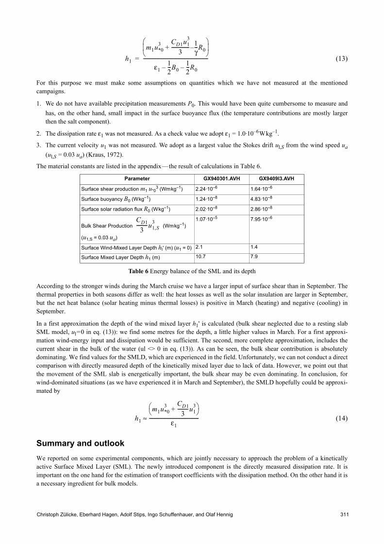
Christoph Zülicke, Eberhard Hagen, Adolf Stips, Ingo Schuffenhauer, and Olaf Hennig 311
(13)
For this purpose we must make some assumptions on quantities which we have not measured at the mentionedcampaigns.
1. We do not have available precipitation measurements P0. This would have been quite cumbersome to measure andhas, on the other hand, small impact in the surface buoyance flux (the temperature contributions are mostly largerthen the salt component).
2. The dissipation rate ε1 was not measured. As a check value we adopt ε1 = 1.0·10–6Wkg–1.
3. The current velocity u1 was not measured. We adopt as a largest value the Stokes drift ul,S from the wind speed ua(ul,S = 0.03 ua) (Kraus, 1972).
The material constants are listed in the appendix—the result of calculations in Table 6.
Table 6 Energy balance of the SML and its depth
According to the stronger winds during the March cruise we have a larger input of surface shear than in September. Thethermal properties in both seasons differ as well: the heat losses as well as the solar insulation are larger in September,but the net heat balance (solar heating minus thermal losses) is positive in March (heating) and negative (cooling) inSeptember.
In a first approximation the depth of the wind mixed layer h1' is calculated (bulk shear neglected due to a resting slabSML model, ul=0 in eq. (13)): we find some metres for the depth, a little higher values in March. For a first approxi-mation wind-energy input and dissipation would be sufficient. The second, more complete approximation, includes thecurrent shear in the bulk of the water (ul <> 0 in eq. (13)). As can be seen, the bulk shear contribution is absolutelydominating. We find values for the SMLD, which are experienced in the field. Unfortunately, we can not conduct a directcomparison with directly measured depth of the kinetically mixed layer due to lack of data. However, we point out thatthe movement of the SML slab is energetically important, the bulk shear may be even dominating. In conclusion, forwind-dominated situations (as we have experienced it in March and September), the SMLD hopefully could be approxi-mated by
(14)
Summary and outlook We reported on some experimental components, which are jointly necessary to approach the problem of a kineticallyactive Surface Mixed Layer (SML). The newly introduced component is the directly measured dissipation rate. It isimportant on the one hand for the estimation of transport coefficients with the dissipation method. On the other hand it isa necessary ingredient for bulk models.
Parameter GX940301.AVH GX9409l3.AVH
Surface shear production m1 u*03 (Wmkg–1) 2.24·10–6 1.64·10–6
Surface buoyancy B0 (Wkg–1) 1.24·10–8 4.83·10–8
Surface solar radiation flux R0 (Wkg–1) 2.02·10–8 2.86·10–8
Bulk Shear Production (Wmkg–1)
(u1,S = 0.03 ua)
1.07·10–5 7.95·10–6
Surface Wind-Mixed Layer Depth hI' (m) (u1 = 0) 2.1 1.4
Surface Mixed Layer Depth h1 (m) 10.7 7.9
h1
m1u*03 CD1u1
3
3--------------- 1
γ---R0–+
ε112---B0– 1
2---R0–
-------------------------------------------------------=
CD13
---------u1,S3
h1
m1u*03 CD1
3---------u1
3+
ε1------------------------------------------≈

Surface mixed-layer dynamics312
The dissipation measurements were made in near coastal zones. The regime in the bulk of the water was mainly deter-mined by the current shear. However, the background field of stratification influenced the transports as well. Especiallyin the Baltic vertical gradients both the current as well as in the density field are quite large. This is based on the wind-induced mixing from above and the strong stratification due to riverine input of fresh water and the subduction of saltywater from the North Sea. Hence, the Baltic seems to be a good candidate for the test of different flux parametrisationsunder extreme conditions. Measurements of dissipation, current and density profiles combined with direct measurementsof vertical fluxes of density <w'ρ'> at fixed depths should be performed jointly with the observation of the atmosphericparameters.
We may conclude that, with enough data in time, there is a good possibility to estimate turbulent quantities. However, toattribute more distinct short-term and long-term effects to the turbulence and transport variability and to obtain moreaccurate numeric relations, it is necessary to extend the length of time series to some days (at least some inertia periods).The sampling rate of 15 minutes was appropriate.
ReferencesKraus, E. B., 1972. Atmosphere-Ocean Interaction. (Clarendon, Oxford).
Kraus, E.B., and Turner. A one-dimensional model of the seasonal thermocline. II: The general theory and its conse-quences. Tellus 19 (1967) 98–106.
Landolt & Boernstein. Numerical Data and Functional Relationships in Science and Technology (Springer, Berlin).
Monin, A.S., and Ozmidov, R.Y., 1982. Turbulence in the Ocean. (Reidel, Dordrecht).
Niiler, P.P. and Kraus, E.B. One-dimensional models of the upper ocean. in: Modelling and Prediction of the UpperLayers of the Ocean. Proc. NATO Advanced Study Inst. (E.B.Kraus Ed.) (pergamon, Oxford, 1977) 143–172;
Peters, H., Gregg, M.C., and Toole, J.M., 1988. On the parametrisation of equatorial turbulence. J. Geophys. Res. 93,C2, 1199–1218
Zülicke, Ch. and Hennig, O. Surface Energy Fluxes and Mixed Layer Depth. in E. Hagen (Editor): GOBEX SummaryReport. Marine Science Reports. Volume 19 (Baltic Sea Research Institute, Warnemünde, 1996) page 92 ff.
Zülicke, Ch., Schuifenhauer, I., and Stips, A. Exchange coefficients and dissipation measurements. in E. Hagen (Editor):GOBEX Summary Report. Marine Science Reports. Volume 19 (Baltic Sea Research Institute, Warnemünde,1996) page 76 ff.
Appendix Material constants (Landolt & Boernstein)
Parameter (Landolt & Boernstein) Baltic Sea (Rheinheimer) (p=0; T=15; S=20)
Isobaric thermal expansion coefficient α (K–1) 1.69·10–4
Isobaric heat capacity cp (Jkg–1K–1) 4069
Density ρ (kgm–3) 1014
Serge V. Victorov 313
ICES Cooperative Research Report, No. 257 Baltic Marine Science Conference, Rønne, Denmark, 22–26 October 1996
Towards operational regional satellite oceanography for the Baltic Sea
Serge V. Victorov
Abstract This paper supports the EuroGOOS objective for space-based information on operational oceanography. The paperprovides discussion of the two branches of modern Satellite Oceanography (SO), namely Regional SO and Global SO.Requirements for satellite data for problems of Regional SO are presented. State-of-the-art of Regional SO in the Balticstates is discussed with an emphasis on its operationalisation. Technological and managerial aspects of future devel-opment of Operational Regional SO in the Baltic area are briefly discussed. Relevant recommendations on two-levelinternational cooperation are made.
IntroductionIn recent years satellite oceanography has obviously shown a tendency to split into two branches, namely Global SatelliteOceanography and Regional Satellite Oceanography. Regional Satellite Oceanography is an interdisciplinary(oceanography/remote sensing) science which is based on satellite imagery analysis and deals with processes andphenomena mainly in the seas, coastal zones and separate parts of the ocean, while Global Satellite Oceanography dealsmainly with processes and phenomena in the World Ocean as a whole.
There are many differences between the Regional SO and the Global SO. The two differ in:
• Objects and objectives of studies• Requirements for satellite data (temporal, spatial and spectral), which may lead to different modes of payload
operation• Availability and quality of sea-true in situ data, which may lead to different levels of accuracy of information retrieval
in Regional and Global SO• Algorithms for data processing• Users• Formats of output information products, etc. For comprehensive analysis of the two branches of SO see (Victorov, 1996). Nowadays the Regional Satellite Oceanog-raphy is focused on:
• Operational marine forecasting • Monitoring of the marine environment • Study of water masses dynamics within the water body • Study of spread of river discharge • Monitoring of water quality and transfer of pollutants• Study of biological productivity in local areas• Complex monitoring of coastal zone • Study of the interaction between coastal zone and off-shore waters• Study of ice cover morphology, etc. Further we will focus on the problems of Regional Satellite Oceanography and its operationalisation.
Regional satellite oceanography: State-of-the-artIt is believed that Regional Satellite Oceanography is capable of providing operational/non-operational information inthe following three areas (the concept of these areas is taken from (ESA, 1995):

Towards operational regional satellite oceanography for the Baltic Sea314
Mapping and monitoring• Sea surface wave patterns • Surface slicks • Sea-ice extent, type, concentration and thickness • Sea-ice movement • Sea surface temperature • Sea water colour anomalies (‘water quality’) • Shallow water bathymetry
Process understanding• Ocean features (eddies, upwellings, jets, frontal boundaries) • Sea-ice related processes
Modelling for forecasting• Regional circulation • Estuarine processes • Coastal sediment transport and erosion• Climate-change-related predictions A detailed review of the achievements of Regional Satellite Oceanography, including the case study of the Baltic Sea, isgiven in (Victorov, 1996).
The Steering Committee of the Baltic Marine Science Conference has developed a concept of presentation of papersdealing with the use of satellite data. According to this concept the original contributions with satellite images andrelevant charts and schemes were to be presented as posters. This was aimed at providing sufficient time for viewing theimagery and discussion of patterns and features recorded in the imagery between the authors and other participants ratherthan just a quick look at the images projected on overheads. As a member of the Steering Committee I would like tothank the authors of very interesting posters giving a strong impression of real development of the Baltic RegionalSatellite Oceanography in recent years.
Requirements for satellite dataGeneralised requirements for satellite data in problems of regional satellite oceanography are presented in Table 1(Victorov, 1996).
Table 1 Requirements for satellite data
In recent years the issue of “Requirements” has attracted the attention of many science and technology communities,international organisations and their committees and panels.
The right balance between the desired requirements, the real needs—sometimes the dreams —on the one hand, and therealistic capabilities of technology, engineering and informational sciences, on the other hand, was the goal of numerousdiscussions.
Among others, I would like to mention two sources of information on this subject.
ParameterProblems
General LocalDimension of studied area, km 50–1000 1–50Ground resolution, m 100–1000 20–100Temporal resolution, h 3–24 3–6

Serge V. Victorov 315
Source 1 Polar Orbiting Satellites and Applications to Marine Meteorology and Oceanography (1996). Report of the CMM-IGOOS-IODE Sub-group on Ocean Satellites and Remote Sensing (OSRS) set up by the Intergovernmental Oceano-graphic Commission (of UNESCO) and the World Meteorological Organisation.
Along with the overview of requirements for satellite data relevant to some of the GOOS modules, this documentcontains assessments of the ability of a certain satellite sensor to deliver the data with the characteristics required. Eachoceanographic/geophysical parameter is assessed for each instrument type capable of making that measure and thedegree to which parameter can address the requirement. These assessments were made for global and regional scales.The assessments provide quantitative answers to the question ‘how many sensors/satellites do we need to match therequirements sanctioned by WMO and IOC?’ and thus clearly show the distance between the real operational satelliteoceanography of the 2020s and that of the 1990s.
Source 2 Use of Satellite Data for Environmental Purposes in Europe (1994) Final Report. Scot Conseil and Smith SystemEngineering Ltd. in conjunction with DGXII-D-4 of the European Commission.
This document presents the requirements for satellite data with an emphasis on environmental issues. It gives qualitativeassessments of the sensors capabilities to provide data according to the requirements in the European context.
Detailed analysis of both sources and the comparison of the requirements presented in them, is given in (Victorov, 1996).
What kind of operational satellite oceanography exists in the Baltic area nowadays?Operational marine applications require rapid processing, interpretation and dissemination of information to regionalusers. It is recognised that demonstration of the potential to extract information from satellite data is not enough.Relevant infrastructure, technical facilities and services should be and are currently being established in some regionalseas. Operational sea-state forecasts are being made available to marine users community. Shipping companies (optimalrouting) and oil/gas companies (logistics of seismic surveys, mooring strategies for the connection of oil tankers to riserpipes, large-scale engineering works for offshore operations etc.) are notable here.
Nowadays many research groups and teams are working in the area of the Baltic Regional Satellite Oceanography. Inmany cases they do not exchange their ideas, approaches and results (or do it with a great delay). The Baltic MarineScience Conferences should provide a platform for these contacts in future. Nevertheless among many other regionalseas the Baltic Sea should be considered as an area with advanced operational oceanographic applications of satellitedata.
Satellite information is being incorporated into operational Sea-ice monitoring and forecasting services and routinelyused by ice centres in Sweden, Finland and Russia. ERS SAR-based Oil-slick services which are operational in Norwaysince 1994 (Pedersen et al., 1996) are being developed and integrated with existing services in other countries. Space-based Algal bloom monitoring and forecasting services are being developed in the Baltic countries.
In the above mentioned activities the following sensors/satellites are being used in (quasi-) operational mode:
• A VHRR/NOAA—4–6 and more orbits daily• SAR/ERS-1, -2—depends on cycle Still gaps exist and will continue to exist in the future for cloudiness and technological reasons. The ways out are:
1. To use models to interpolate between two consequent satellite observations2. To use operational technologies with satellite data assimilation into models Strictly speaking, both mean: Quasi-operational Regional Satellite Oceanography at best. According to Johannessenet al. (1996), “There has, over the last decade, been a rapid development of various data assimilation methods which canbe used with ocean and ecosystem models. At present, none of these methods are used operationally”. This was a generalstatement. As for the Baltic Sea the HIROMB (High Resolution Operational Model of the Baltic Sea) (Kleine, 1996)which, according to Funkquist (1996), “has been in a so called preoperational mode since autumn 1995”, is probably themost promising one. At least, sea-surface temperature simulation results obtained with this eddy-resolving model will becompared with relevant satellite patterns (Funkquist, 1996).

Towards operational regional satellite oceanography for the Baltic Sea316
Future satellites and sensorsWhat are the prospects for operationalisation of Regional Satellite Oceanography from the satellite/sensors side? Futurecivilian satellites and sensors (with contribution to operational regional oceanography) are:
ERS-2 1995–2000 with altimeter, scatterometer, SAR (Synthetic Aperture Radar), ATSR (Along-Track ScanningRadiometer)
ENVISAT 1999–2004 with the same advanced instruments: Sltimeter, SAR, ATSR and a new instrument: MERIS(Medium Resolution Imaging Spectrometer)
METOP 2002–2017 with advanced scatterometer
NOAA series with modified scanning radiometers AVHRR/3 (1994–1999) and VIRSR (1997–2000)
RADARSAT (since 1995) is currently providing data on sea state and ice
SeaStar satellite with Sea WiFS colour scanner is expected to be launched in 1997; if not, a similar instrument EOSCOLOUR will be launched on EOS satellite in the late 1990s.
Meanwhile ADEOS with another ocean colour instrument OCTS was launched on 18 August 1996.
OKEAN-O missions with real aperture radar RAR and MSU-SK scanner as well as RESURS-O missions with MSU-SK,MSU-E scanners will be continued in the late 1990s.
Though the above list is not complete (for a comprehensive information see Polar ..., 1996), it is obvious that there willbe no drastic improvements in terms of operational satellite oceanographic SYSTEM in the next decade. Various pilotoperational and quasi-operational single satellites and series of satellites will still complement each other, and it willprobably be a difficult task to harmonise data from various sources. Data handling (acquisition, storage, processing,fusion, interpretation, assimilation, dissemination of output informational products) will definitely become a crucialpoint in the Baltic Regional Satellite Oceanography in the nearest future.
Future: Institutional / Managerial aspectsFrom the technological point of view, one Centre can provide satellite data acquisition, processing and dissemination ofoutput informational products for the whole Baltic Sea region. It is possible for this Centre to run the sophisticated oceanmodels (now and in the nearest future) and ecological models (in the distant future) in operational mode. And it probablycould be the best option in terms of costs and benefits.
Do we need one or more centres? Will we need one or more centres for the Baltic area in the future united Europe?
Here is an attempt to answer the questions basing on the technical reasons only.
On the regional levelFor the open Baltic Sea a single Joint Centre of Operational Oceanography could well provide marine forecasts and othercentralised services within the area. The use of standard codes, measuring devices, data processing schemes and stand-ardised output informational products for most oceanographic parameters by the Centre could save both financial andhuman resources in the Baltic states. Presumably a single Unit of Regional Satellite Oceanography could fit the needs ofthe Joint Centre of Operational Oceanography. Needless to say that this approach goes in line with the EuroGOOSconcept.
On the local levelBroadly speaking, it is up to the local authorities and local users communities to decide whether they should run localoperational oceanographic services in the existence of the Joint Centre of Operational Oceanography. It is probablyworthwhile to run them if they needs detailed information for some specific purposes, when local in situ data bases andknowledge bases are required, and if tailor-made oceanographic informational products are actually needed.
Examples: ice conditions and water quality in local bays
Serge V. Victorov 317
Interplay between the Regional and the Local levelsLocal level operational oceanographic units could provide the Joint Centre of Operational Oceanography with a selectedinformational products which could be used in the Centre to tune their models and algorithms for the relevant local areas.In its turn the Centre could supply the local operational units with high resolution satellite data for local areas, thusproviding integration of local level in situ data with regional level remotely sensed data complemented with localknowledge bases.
Concluding remarks and suggestions• Current achievements of Joint Centre of Operational Oceanography in the Baltic Sea are encouraging • Baltic Operational Satellite Oceanography exists, though, mainly, in quasi-operational mode • The level of operationalisation of Joint Centre of Operational Oceanography in the Baltic Sea varies considerably for
different oceanographic parameters • Further progress in satellite sensors and space-based ocean observing systems is needed to meet the requirements of
Regional Operational Satellite Oceanography • There is high scientific potential for cooperation in the Baltic Operational Satellite Oceanography which is as yet
unclaimed. The Baltic Marine Science community is kindly invited to start discussions aimed at:
• Working out a concept of the Joint Centre of Operational Oceanography in the Baltic Sea • Working out a concept of joint regional satellite monitoring in the (open) Baltic Sea• Finding mechanisms for cooperation in the development of methods of satellite monitoring of the Baltic coastal zone
(with an emphasis on coastal erosion, sedimentation, shallow water bathymetry, ‘water quality’)
AcknowledgementsThe author is grateful to Mr. Hans Dahlin (Swedish Meteorological and Hydrological Institute) for helpful discussions ofa wide scope of problems relevant to the Baltic Operational Oceanography and its satellite segment.
References ESA, 1995. New Views of the Earth. Scientific Achievements of ERS-1.SP-1176/1, p.152. Funkquist, L., 1996.
Modelling of Physical Processes in the Baltic. In: Abstracts of the Baltic Marine Science Conference, (22–26October, Rønne, Denmark), p.31.
Johannessen, O.M., Bjorgo, E., Petterson, L.H., et al., 1996. Proposed strategy for the use of satellite remote sensing inEuroGOOS. In: Conference Preprints of the First International Conference on EuroGOOS, (7–11 October 1996,The Hague), pp.93–114.
Kleine, E., 1996. HIROMB—a High Resolution Operational Model of the Baltic. In: Abstracts of the Baltic MarineScience Conference, (22–26 October, Rønne, Denmark), pp. 30–31.
Pedersen, J.P., Seljelv, L.G., Bauna, T., et al., 1996. Towards an operational oil spill detection service in the Mediter-ranean? The Norwegian experience: A pre-operational early warning detection service using ERS SAR data. In:Proc. ERS Thematic Workshop on Oil Pollution Monitoring in the Mediterranean, Frascati, Italy, ESA.
Polar Orbiting Satellites and Applications to Marine Meteorology and Oceanography, 1996. Report of the CMM-IGOOS-IODE Sub-group on Ocean Satellites and Remote Sensing. Marine Meteorology and Related Oceano-graphic Activities. Report No.34. WMO/TD No.763.
Victorov, S. V., 1996. Regional Satellite Oceanography. Taylor and Francis, London, 312 pp.

Vistula Lagoon water level oscillations: numerical modelling and field data analysis318
ICES Cooperative Research Report, No. 257 Baltic Marine Science Conference, Rønne, Denmark, 22–26 October 1996
Vistula Lagoon water level oscillations: numerical modelling and field data analysis
Irina P. Chubarenko
IntroductionThe response of complicated geophysical systems on external actions depends essentially on its own features. TheVistula Lagoon (Baltic Sea) can be considered as a hydrodynamic system, where the level and current oscillations areunder external forcing of local wind, Baltic level variations and river drain. Aiming to estimate the influence of externalparameters oscillations on the lagoon water body requires determination of its own oscillation characteristics.
The level oscillations in various parts of the aquatory, which appear after the disturbance of the level from the horizontalequilibrium by wind action, were analysed. The comparison between the temporal periodicity of external forcing and thetime periods of response in the lagoon level oscillations gave rise to the conclusions both for hierarchy of external forcingfactors for different time scales and their energetic significance for hydrodynamic processes in the lagoon.
MethodsThe main point of the work presented was to study (with help of numerical modelling) the features of level oscillationprocesses in Vistula lagoon after instant switch off of the wind action. Numerical model MIKE21 of Danish HydraulicInstitute was used for simulations. The hydrodynamic module of MIKE21 is based on the two-dimensional “shallowwater” hydrodynamic equations (MIKE21, 1993). The model was preliminary saturated by real data (bathymetry, riverdischarges and its positions) and calibrated on the results of a special autumn 1994 field study during the Danish-Russian-Polish project “Vistula lagoon” (Prioritising..., 1998). The results of calibration were as follows: wind frictioncoefficient—0.0017, bed resistance coefficient—32 m1/3s–1, eddy viscosity coefficient—20 m2s–1. It was concludedafter verification of the model that it quite satisfactorily represents not only the current structure and relative level oscil-lations, but also the absolute values of level variations (Calibration..., 1996).
The bathymetry field was determined in the nodes of a grid with 1km steps. Water level temporal variations were calcu-lated in six points located at the lagoon coast (Kaliningrad, Baltiysk, Krasnoflotskoe, Nowa Paslenka, Tolkmicko, NowoBatorowe; see Figure 1). External conditions were as follows: the rectangle wind impulse (10ms–1) for each of 8 direc-tions: N, NE, E, SE, S, SW, W and NW. Some simulations for 5ms–1 and 35ms–1 were also done for testing. The timeduration of constant wind action was not less than 3–5 periods of steady currents establishment for the whole lagoonaquatory. The non-disturbed level and zero currents were used as initial conditions. The rivers’ discharges and Balticlevel variations were not included in the consideration, because precisely the own inertial oscillations in the lagoon wereunder investigation.
Figure 1 Vistula Lagoon

Irina P. Chubarenko 319
Results and discussionsThe simulation results were obtained in the form of
1. temporal level courses for six points 2. steady currents charts for each wind direction (Chubarenko, 1996). The main results are presented in Table 1.
Table 1 Water level variations characteristics. Numerical model MIKE21. Wind speed 10ms–1.
Wind was changed during the simulations as follows: momentarily started up to 10ms–1 and simultaneously switched offafter two weeks of modelling time. Under this condition the times intervals of the establishment of steady solution inlevel (level variations not exceed 1cm) and current were 12 hours and 3 days correspondingly for any point along thelagoon coast. Under lengthways wind of 5ms–1 and 10ms–1 the simulated level diversities between north-east and south-west ends of lagoon (Kaliningrad and Nowo Batorowe) were 13.5cm and 52cm respectively. This is in good agreementwith field measurements.
As a whole, the general behaviour of level variation curves allow the conclusion that the classical inertial damping oscil-lations are excited in the lagoon after the impulsive wind influence. While the oscillations at different points around thelagoon have different characteristics, and the most complicated oscillations occur in the northeastern part of the lagoonunder transverse winds (SE and NW), the amplitude everywhere of the first oscillation is an order of magnitude greaterthan the other ones. Therefore, it may be concluded that the lagoon behaves as a single oscillating system in summation.As for processes of level relaxation after both lengthways and cross-wise winds, the own oscillating period is about 9.5hours for all points in the aquatory (see Table 1). The relaxation times, i.e. the times after which a lapse of which waterlevel variations become smaller than 1cm, are also presented in Table 1.
The axis of lengthwise oscillations of the Vistula lagoon is easily indicated from the simulation: it is located betweenNowa Paslenka and Krasnoflotskoe, slightly north of the Russian–Polish border. The axis direction is 315 degrees (SE–NW). The axis of transverse oscillations has a direction of 50 degrees (SW–NE).
The water level variations have an interesting feature during the process of level establishment after wind switch-off:level deviation aspires to zero (non-disturbed position), but, at first, passes an equilibrium position and then deviatesfrom it in the opposite direction with an amplitude of little more then before switching of the wind. This peak deviation ischaracterised by the following values: its maximum (or minimum) value does not exceed the stationary level (beforeswitching off the wind) more then 4cm (for 10ms–1 wind), the relaxation time (from peak to zero level) is no more than5 hours. It is necessary to take this feature into consideration when forecasting the storm surge or high level events,especially at the ends of the lagoon (Kaliningrad and Nowo Batorowe).
The following hierarchy of the significancy of external factors influenced on water level variations in the lagoon can bededuced from the analysis of natural data and numerical solutions:
• both river discharge and long-term Baltic water level variations determine the annual and seasonal mean volume ofwater in the lagoon reservoir;
• the Baltic water level near the lagoon entrance determines the present-day level of equilibrium of lagoon water body;
Winds along the length-wise axes Cross-wise winds
StationsNE SW NW SE
trel, h T, h trel, h T, h trel, h T, h trel, h T, h
Kaliningrad 14.3 10 15 9.5 6.8 10, 9 6.8 10Baltiysk 8.8 9.5 9 9.5 1.6 10 1 10Krasnoflotskoe 6 9.5 6 9.5 2.6 9 1.5 10.5Nova Paslenka 4 9.5 4 9.5 2 10 2.5 10Tolkmicko 18.5 9.5 19 9.5 8 9 8 9Nova Batorove 19.3 9 19.5 9.5 8.3 10 8.5 8
trel relaxation time; after this time lapse the water level variations become less than 1 cm
T period of the main oscillation.

Vistula Lagoon water level oscillations: numerical modelling and field data analysis320
• the wind action gives the main input in short-period dynamics of level oscillation. Extremely high or low water levelevents (in south-western and north-eastern corners of the lagoon) are almost entirely stipulated by local wind.
The lagoon’s own oscillations of periods 2–15 hours are presented also both in the Baltic level and wind variations.According to the statistical analysis performed by Dr.V.F. Dubravin (Institute of Oceanology of Russian Academy ofSciences, Atlantic Branch), the oscillations with a 9-hour period, for example, are contained both in level variations inBaltic and wind over the lagoon with a certainty of not less than 0.8. So, they should pump a considerable part of energyinto lagoon water body dynamics. It is quite probable, that exactly this agreement between external influence and internallagoon response was the main reason of the forming of the current lagoon geomorphological shape, characterised by themain period of its own inertial oscillation of the same order (near 9.5 hours) as external cumulative forcing from theBaltic wind and level.
AcknowledgementsAll the simulations were done in Atlantic Branch of P.P. Shirshov Institute of Oceanology (Russian Academy ofSciences) with the help of the MIKE21 numerical model of Danish Hydraulic Institute, installed for the Vistula lagoonduring an international Danish–Polish–Russian project (Prioritising..., 1998).
ReferencesCalibration of HD and EU-modules of numerical model MIKE21 and simulations of annual salinity field dynamics in
Vistula lagoon. Report on Vistula Lagoon Project. Book 4. 1996. P.P. Shirshov Institute of Oceanology, AtlanticBranch, Kaliningrad, Russia. (in Russian).
Chubarenko. I.P., 1996. Investigation of the Vistula Lagoon water level own oscillations after wind forcing: results ofnumerical modelling (MIKE21). Atlas. P.P.Shirshov Institute of Oceanology, Atlantic Branch, Kaliningrad,Russia. (in Russian).
MIKE21. Coastal Hydraulics and Oceanography. Hydrodynamic Module. Release 1.4. User Guide and ReferenceManual, Danish Hydraulic Institute, Copenhagen, Denmark, 1993.
Prioritising Hot Spot Remediations in Vistula Lagoon Catchment: Environmental Assessment and Planning for thePolish and Kaliningrad parts of the lagoon (1994–1997): Report on the international project. Erik K. Rasmussen(Ed.). Water Quality Institute, Danish Hydraulic Institute, GEOMOR, Atlantic Branch of P.P. ShirshovOceanology Institute, Hoersholm, Denmark, 1998.

Jacob S. Møller 321
ICES Cooperative Research Report, No. 257 Baltic Marine Science Conference, Rønne, Denmark, 22–26 October 1996
DYNOCS: Status October 1996
Jacob S. Møller
Abstract DYNOCS (Dynamics of Connecting Seas) is a CEC-sponsored MAST II research project, which runs from 1994 till1997. The project, which is multidisciplinary, aims at a better understanding of the marine environment betweenconnecting seas and focus on the transition area between the North Sea and the Baltic, an area characterised by complexresponses of stratified flow due to changing winds and buoyancy forcing. The DYNOCS project group consists of sixresearch institutes from northern European countries situated in the Baltic area:
• Danish Hydraulic Institute (DHI), Denmark • Institut für Ostseeforschung Warnemünde (IOW), Germany • Swedish Meteorological and Hydrological Institute (SMHI), Sweden• Norwegian Hydrotechnical Laboratory (NHL), Norway• Danish Meteorological Institute (DMI), Denmark• Aalborg University (AUC), Denmark The purpose of DYNOCS is to provide a sound scientific basis for the understanding and modelling of hydrodynamicsand the associated transport processes of transition areas between connecting seas. This objective is pursued through anintegration of numerical modelling, field campaigns and laboratory experiments. The project has been divided into thefollowing six main tasks:
• analysis of key processes• field measurements • laboratory experiments • data acquisition and dissemination• 3D numerical modelling • transport and ecological modelling The project improves our general scientific knowledge of the processes studied and ends up with a 3D baroclinic eddy-resolving model of the complete marine system between the North Sea and the Baltic.
Scientific approach
Analysis of key procedures The objective of this has been pursued through a conceptual description of the processes in the transition area, devel-opment of conceptual and analytical models, and development of subgrid-scale algorithms and parametrisation, all aspart of a systematic validation of the numerical modelling of the key processes.
Field measurements This objective has been pursued through four field campaigns with the research vessel R/V “Prof. Albrecht Penck” ofIOW and with the research vessel R/V “Dana” hired by DHI from the Danish Ministry of Fisheries, and through coordi-nation with ongoing national field programmes.

DYNOCS : Status October 1996322
Table 1 List of DYNOCS Cruises
Laboratory experiments Advective processes, including the natural mesoscale eddy instabilities, have been simulated in a rotating basin with thebest available bathymetry of the Skagerrak–Kattegat area, vertically distorted within the realm of Froude similitude. Thelaboratory model was forced by controlling the density and volume fluxes of water masses from the Baltic Sea, theGerman Bight, the Norwegian Sea and the Central North Sea.
Tracers from chosen sources were used to identify and quantify transport routes. 3D photogrammetric tracking of neutralbuoys, and in situ profiling of fluorescence provided the necessary velocity and mass distributions across chosen sectionswhich are coincident with field measurements and numerical model boundaries. The transport routes and mesoscalemixing processes provide a windless and tideless data set for physical understanding and numerical model testing. Theexperiments are reported in technical notes and video.
Data acquisition and dissemination An initialisation data set for the North Sea-Baltic region has been established on the basis of available data from theregion. The data set is comprised of salinity, temperature and 10m mean wind stress and 2m temperature for the atmos-phere.
Collection of time series of current, salinity, temperature, wind and water level data at selected key sites have beenundertaken for a period of 12 months. This hindcast data set is based on ongoing national programmes, the fieldcampaigns and the laboratory experiment. The hindcast period covers 12 months (15 September 1994–15 September1995) including three of the field measurement periods. In particular, data from the ongoing programmes in the GreatBelt and the Sound have been used. The database comprises currents, water levels, salinities and temperatures beingmeasured as part of the field programme. The database sets also include (for the periods of the three field campaignsonly) analysed meteorological pressure and wind fields from high resolution, limited area models of the region(HIRLAM), assimilated and interpolated to the appropriate model grids.
3D numerical modelling (Three different primitive equation models have been applied. These three primitive equation models range from a fullynonhydrostatic grid, implicitly coupled model (the DHI 3D model) to the modified hydrostatic, free-surface version ofthe Bryan-Cox model, WOM (Warnemünde Ostsee Model), to the Bundesamt für Seeschiffahrt und Hydrographie(BSH) model.
A far field model is used to establish boundary and initialisation conditions for fine grid models. The DHI model hasbeen set up to simulate the three field campaign periods using a rather large horizontal grid covering the North Sea to theBaltic. The far field grid provides boundary data to near field models which will cover the transition area or parts of thisarea. The boundary data have been provided using a nested grid technique with two-way coupling to enhance theresolution of narrow straits. The near field models use rather small grids in order to resolve the Rossby Radius of defor-mation which is a measure of the typical length scale of baroclinic eddies.
The calibration and validation of 3D baroclinic models of the transition area have placed particular emphasis on theresolution of the hydrodynamic complexities and scaling problems resulting from the irregular coastline, complex andsteep topographies and stratification in the region. The performance of the different models is now (October 1996) beinganalysed through a direct comparison between models as well as their ability to reproduce measured data. Model inter-comparison will be carried out based on hindcasts of the field experiments and the laboratory experiments. This approachwill establish an independent set of measured validation data for comparison with the numerical modelled data.
No. Period Area Vessel1 26/8–29/9, 1993 Fehmarn/Darss R/V “Albrecht Penck” (IOW)2 07/10–17/10, 1994 Bornholm R/V “Dana” (DHI) 3 15/11–24/11,1994 Fehmarn/Darss R/V “Albrecht Penck” (IOW)4 18/07–30/07, 1995 Fehmarn/Darss
Kattegat/LillebæltR/V “Albrecht Penck” (IOW)R/V “Dana” (DHI)

Jacob S. Møller 323
Transport and ecological studies The quantification of water masses, buffering effects and major transport routes is being pursued through simulations ofpassive substances and marked water masses. The hydrodynamic input for these simulations is 3D flow fields taken fromthe 3D numerical modelling.
In general, the temporal and spatial scales used in ecological modelling are an order of magnitude larger than in hydrody-namical modelling, due to the number of ecological components and the biological timescales involved, and this consti-tutes a serious problem in ecological modelling. Often the large spatial resolution in ecological models leads to excessivenonphysical diffusion of substances. The scientific challenge is to see how the time and length scales of the hydrody-namics and ecology are best combined to ensure a scientifically and economically feasible approach.
AcknowledgementsThe following companies and institutes are acknowledged for their contributions to the DYNOCS project: The DanishResearch Council (Statens Naturvidenskabelige Forskningsråd), A/S Storebælts-forbindelsen and Øresundskonsortiet.
ResultsA number of intensive field campaigns have been carried out under the DYNOCS project. During each campaign,selected subareas were intensively surveyed for approximately two weeks by making ADCP measurements and byfrequent profiling of various parameters, primarily temperature and salinity.
Figure 1 Example of measured current profiles along a transect crossing the Bornholm Strait at the entrance to the Baltic Sea
Figure 2 Example of measured salinity distributions along a transect crossing the Bornholm Strait at the entrance to the Baltic Sea
A laboratory model of a circular part of the Skagerrak–Kattegat region was built and mounted in the rotating Coriolisbasin of NHL. The ocean circulation in the basin was forced by controlling the inflows of Atlantic Water from theNorwegian Sea and Brackish waters from the Baltic Sea and the German Bight, according to field data. The modelledhorizontal/vertical ratio is distorted by a factor of 100. Figure 3 shows the rotating tank with three co-rotating camers;

DYNOCS : Status October 1996324
image (x, y, z) calibration frame (X, Y, Z)fr, model (X, Y, Z)mod and modified model (X', Y', Z') coordinate systems. Thedifferent coordinate systems were used in the calibration and particle tracking procedures.
Figure 3 Laboratory model of a circular part of the Skagerrak–Kattegat region
Figure 4 A numerical model bathymetry, covering the entire North Sea–Baltic Sea area has been compiled from echo sounding survey data and from navigational sea charts. The bathymetry has a resolution of one nautical mile and is based
on more than 3 million data points.

Baltic Marine Science Conference, Rønne, Denmark, 22–26 October 1996 325
List of contributors
Pekka Alenius (p 138)Finnish Institute of Marine Research P.O.Box 33FIN-OO93 1 Helsinki, Finland Phone: 358-9-613941, Fax: 358-9-61394494e-mail: [email protected]
Villu Astok (p 225, p 267)Estonian Marine Institute1 Paldiski Rd.TallinnEE0001Estonia
Dagmar Benesch (p 126)Institute of Baltic Sea ResearchSeestr. 1518119 Rostock, Germany
R. Bojanowski (p 85)Polish Academy of SciencesInstitute of Oceanology81-712 Sopot, Poland
Katarzyna Bradtke (p 107)University of Gdansk, Institute of OceanographyAl. Marszalka Pilsudskiego 4681-378 Gdynia, [email protected]
Hans Cederwall (p 21)Dept. of Systems EcologyStockholm UniversityS–106 91 Stockholm, Sweden
Valery Y. Chantsev (p 248)Russian State Hydrometeorological Institute 195196 Malookhtinsky Pro 98St. Petersburg, Russia
Maria Chomka (p 145)Polish Academy of Sciences Institute of Oceanology e-mail: [email protected]
Christian Christiansen (p 126)Institute of GeographyUniversity of CopenhagenØster Voldgade 101350 Copenhagen K, Denmark
Boris V. Chubarenko (p 151)P. P. Shirshov Institute of Oceanology, Atlantic BranchProspect Mira, 1236000, Kaliningrad, RussiaTel: (+0112) 451574, Fax: (+0112) 272945E-mail: [email protected]
Irina P. Chubarenko (p 151, p 318)P. P. Shirshov Institute of Oceanology, Atlantic BranchProspect Mira, 1236000, Kaliningrad, RussiaTel: (+0112) 451574, Fax: (+0112) 272945e-mail: [email protected]
Dirk Dannenberger (p 90)Baltic Sea Research Institute WarnemündeNow ofResearch Institute for Biology of Farm AnimalsDepartment of Muscle Biology and Growth18196 Dummersdorf, GermanyTel: +49 38208 68857, Fax: +49 38208 68852e-mail: [email protected]
Violetta Drozdowska (p 244)Institute of Oceanology PASul.Powstancow Warszawy 55PL-81712 Sopot, Poland
Kay-Christian Emeis (p 126, p 134, p 174)Institute of Baltic Sea Research WarnemündeSeestr. 15D-19119 Rostock, Germany Tel: +49 381 5197 370, Fax: +49 381 5197 352
Rudolf Endler (p 126, p 134)Institute of Baltic Sea ResearchSeestr. 15D-19119 Rostock, FRG Tel: +49 381 5197 370, Fax: +49 381 5197 352e-mail: [email protected]
Peter Feuerpfeil (p 29)Ernst-Moritz-Arndt-UniversityInstitute of EcologyGrimmer Strasse 88D-17487 Greifswald, Germany
Stig Fonselius (p 157)SMHI Oceanographic LaboratoryNya Varvet Byggn. 31S-426 71 Västra Frölunda, SwedenTel. 46 31 696534, Fax 46 31 690418
T. Förster (p 134)Institute of Baltic Sea ResearchSeestr. 15D-19119 Rostock, FRG Tel: +49 381 5197 370, Fax: +49 381 5197 352
Y.Goldfarb (p 96)Latvian UniversityRiga, Latvia
N.N. Golenko (p 232)Shirshov Institute of OceanologyKaliningrad/Moscow
M. Graeve (p 168)Baltic Sea Research InstituteP. O. Box 301161D-18112 Rostock, Germany
Eberhard Hagen (p 174, p 307)Institute for Baltic Sea Research WarnemündeSeestrasse 15D-18119 Rostock, Germany
B. Henkelmann (p 121)GSF Forschungszentrum für Umwelt und GesundheitInstitut für Ökologische ChemieIngolstädter Landstr.1D-85764 Oberschleißheim, Germany

List of contributors326
Olaf Hennig (p 307)Rostock UniversityDepartment of PhysicsGermany
Flemming Jakobsen (p 179)Danish Hydraulic InstituteAgern Allé 5DK-2970 Hørsholm, DenmarkTel: +45 45 76 95 55 Fax: +45 45 76 25 67 E-mail: [email protected]
Halina Jankowska (p 66)Institute of OceanographyUniversity of Gdansk, Gdynia
H. René Jensen (p 190)Danish Hydraulic InstituteAgern AIlé 5DK-2970 Hørsholm, Denmark
Jørn Bo Jensen (p 78)Geological Survey of Denmark and GreenlandThoravey 8DK-2400 Copenhagen NV, Denmark
Vadims Jermakovs (p 21)Institute of Aquatic EcologyUniversity of LatviaMiera str. 3LV–2169 SALASPILS, Latvia
S. Kaczmarek (p 280)Institute of Oceanology, Polish Academy of SciencesSopot, Poland
Edward Kaniewski (p 118)Gdynia Maritime Academy, Physics Departmentul. Morska 8381–225 GDYNIA, Poland
E. Kerstan (p 13)Baltic Sea Research Institute WarnemündeSeestraße 1518119 Rostock, GermanyTel: 49 (0) 381 –5197–227, Fax: 40(0) 381–5197–440
B. Klagish (p 96)Latvian UniversityRiga, Latvia
D. Knapinska-Skiba (p 85)Polish Academy of SciencesInstitute of Oceanology, 81-712 Sopot, Poland
Vladimir P. Korovin (p 248)Russian State Hydrometeorological Institute 195196 Malookhtinsky Pro 98St. Petersburg, Russia
Tadeusz Krol (p 244)Institute of Oceanology PASul.Powstancow Warszawy 55PL-81712 Sopot, Poland
Krystyna Kruczalak, (p 220)Institute of Oceanology PASul.Powstancow Warszawy 55PL-81712 Sopot, Poland
Siegfried Krueger (p 198)Institute for Baltic Sea Research WarnemündeSeestrasse 15D-18119 Rostock, Germany
Antoon Kuijpers (p 78)Geological Survey of Denmark and GreenlandThoravey 8DK-2400 Copenhagen NV, Denmark
Tiit Kullas (p 225, p 267)Estonian Marine Institute1 Paldiski Rd.TallinnEE0001Estonia
Helmar Kunzerdorf (p 126)Risø National LaboratoryDepartment of Environmental Science and TechnologyPostboks 49, 4000 Roskilde, Denmark
N. Kuten (p 96)Science Technical Company “Geoprojektas”Klaipeda, Lithuania
Birger Larsen (p 114)Geological Survey of Denmark and Greenland (GEUS)Thoravej 8DK2400 Copenhagen, DenmarkFax +4538142050 email [email protected]
H.-V. Lass (p 204)Institute for Baltic Sea Research WarnemündeSeestrasse 15D-18119 Rostock, Germany
Adam Latala (p 107)University of Gdansk, Institute of OceanographyAl. Marszalka Pilsudskiego 46, 81-378 Gdynia, [email protected]
Wolfram Lemke (p 78)Baltic Sea Research InstituteSeestrasse 15, D-18119 Rostock-Warnemünde, Germany
Matti Lepparanta (p 299)Department of GeophysicsP.O. Box 4FIN-00014 University of Helsinki, Finland
Astrid Lerz (p 90)Baltic Sea Research Institute WarnemündeDepartment of Marine Chemistry Seestraße 1518119 Rostock, GermanyTel: +49 381 5197-325, Fax: +49 381 5197-302
Viktoras Lujanas (p 263)Institute of PhysicsA. Gootauto 122600 Vilnius, Lithuania

Baltic Marine Science Conference, Rønne, Denmark, 22–26 October 1996 327
Galina Lujaniené (p 263, p 274)Institute of PhysicsA. Gootauto 122600 Vilnius, Lithuania
Yuri I. Lyakhin (p 248)Russian State Hydrometeorological Institute 195196 Malookhtinsky Pro 98St. Petersburg, Russia
Dorota Maksymowska (p 66)Institute of OceanographyUniversity of Gdansk, Gdynia
Roman Marks (p 220, p 274)Institute of Oceanology PASul.Powstancow Warszawy 55PL-81712 Sopot, Poland
Johan Mattson (p 209)SMHI601 76 Norrköping, Sweden
Liongina Mickeniene (p 3)Institute of EcologyAkademijos g. 2LT–2600 Vilnius, LithuaniaTel: 72 92 41 Fax: (370–2) 72 92 57 E-mail: liong@takas lt
Jacob S. Møller, Ph.D. (p 179, p 190, p 321)Danish Hydraulic InstituteAgern Allé 5DK-2970 Hørsholm, DenmarkTel.: +45 45 76 95 55 Fax: +45 45 76 25 67
Klaus Nagel (p 214)Institute for Baltic Sea Research WarnemündeSeestrasse 15D-18119 Rostock, Germany
Günther Nausch (p 8)Baltic Sea Research Institute WarnemündeSeestraße 1518119 Rostock, Germany
Monika Nausch (p 13)Baltic Sea Research Institute WarnemündeSeestraße 1518119 Rostock, GermanyTel: 49 (0) 381 –5197–227, Fax: 40(0) 381–5197–440e-mail: [email protected]
Dietwart Nehring (p 8)Baltic Sea Research Institute WarnemündeSeestraße 1518119 Rostock, Germany
Alexei V. Nekrasov (p 248)Russian State Hydrometeorological Institute 195196 Malookhtinsky Pro 98St. Petersburg, Russia
Thomas Neumann (p 126)Institut für Petrographie und GeochemieUniversität KarlsruheKaiserstr. 1276128 Karlsruhe, Germany
Bogdan Oldakowski (p 66)Institute of OceanographyUniversity of Gdansk, Gdynia
M. Ostrowska (p 280)Institute of Oceanology, Polish Academy of SciencesSopot, Poland
Zbigniew Otremba (p 118, p 220, p 244)Gdynia Maritime Academy, Physics Departmentul. Morska 83, 81–225 Gdynia, Poland
Mikk Otsmann (p 225, p 267)Estonian Marine Institute1 Paldiski Rd.TallinnEE0001Estonia
V.T. Paka (p 232)Shirshov Institute of OceanologyKaliningrad/MoscowE-mail: [email protected]
Matti Pertillä (p 114)Finnish Institute for Marine Research (FIMR)PO 33 FIN 00931 Helsinki, Finland
Tomasz Petelski (p 145, p 263)Institute of Oceanology of the Polish Academy of Sciencesul. Powst. Warszawy 5581-712. Sopot, Poland
Helmer M. Petersen (p 179)Danish Hydraulic InstituteAgern Allé 5DK-2970 Hørsholm, DenmarkTel.: +45 45 76 95 55 Fax: +45 45 76 25 67
Niels H. Petersen (p 179)Danish Hydraulic InstituteAgern Allé 5DK-2970 Hørsholm, DenmarkTel: +45 45 76 95 55 Fax: +45 45 76 25 67
Jacek Piskozub (p 244)Institute of Oceanology PASul.Powstancow Warszawy 55PL-81712 Sopot, Poland
Pyotr P. Provotorov (p 248)Russian State Hydrometeorological Institute 195196 Malookhtinsky Pro 98St. Petersburg, Russia
Z. Radecki (p 85)Polish Academy of SciencesInstitute of Oceanology81-712 Sopot, Poland
Wolfgang Roeder (p 198)Institute for Baltic Sea Research WarnemündeSeestrasse 15D-18119 Rostock, Germany

List of contributors328
Arno Rosemarin PhD (p 254)Stockholm Environment InstituteBox 2142103 14 Stockholm, SwedenTel: +46 8 412 1418, Fax: +46 8 723 0348E-mail: [email protected]
A. Rozwadowska (p 280)Institute of OceanologyPolish Academy of SciencesSopot, Poland
Grazyna Sapota (p 38)Institute of Meteorology and Water Management, Maritime Branchul. Waszyngtona 4281–342 Gdynia, Polande-mail: [email protected]
Louise Schlüter (p 29)Water Quality InstituteAgern Alle 11 DK-2970 Hørsholm, Denmark
Thomas Schmidt (p 179, p 204)Institute für Ostseeforschung WarnemündeD-2530 Rostock-Warnemünde, Germany
K. W. Schramm (p 121)GSF Forschungszentrum für Umwelt und GesundheitInstitut für Ökologische ChemieIngolstädter Landstr.1D-85764 Oberschleißheim, Germany
Hendrik Schubert (p 29)Ernst-Moritz-Arndt-UniversityInstitute of EcologyGrimmer Strasse 88D-17487 Greifswald, GermanyTel: +49 3834 864123, fax: +49 3834 864123e-mail: [email protected]
Ingo Schuffenhauer (p 307)Rostock UniversityDepartment of ElectrotechnicsGermany
Michael Schultz (p 274)Institute of Inorganic and Applied ChemistryUniversity of HamburgMartin-Luther-King-Platz 620146 Hamburg, Germany
Torsten Seifert (p 179, p 204)Institute für Ostseeforschung WarnemündeD-2530 Rostock-Warnemünde, Germany
Vadim Sivkov (p 126)Atlantic Branch Institute of OceanologyRussian Academy of ScienceProspect Mira 1236000 Kaliningrad, Russia
Bogdan Skwarzec (p 44)Polish Academy of Sciences, Institute of Oceanology, Bioradiochemistry Laboratory81-712 Sopot, ul. Powstancow Warszawy 55, P. O. Box 68, Poland
Krzysztof Sokolowski (p 56)Polish Geological InstituteBranch of Marine GeologyPolna Str. 6281-740 Sopot, Poland
Narciza Spirkauskaité (p 263, p 274)Institute of PhysicsA. Gootauto 122600 Vilnius, Lithuania
Klemensas Stelingis (p 263, p 274)Institute of PhysicsA. Gootauto 122600 Vilnius, Lithuania
Adam Stelmaszewski (p 118, p 220, p 244)Gdynia Maritime Academy, Physics Departmentul. Morska 8181–225 Gdynia, Poland
Piotr Stepnowski (p 44)Polish Academy of SciencesInstitute of Oceanology, Bioradiochemistry Laboratory81-712 Sopot, ul. Powstancow Warszawy 55, P. O. Box 68, Polandalso University of GdanskFaculty of Chemistry, Physical Chemistry DepartmentRadiochemistry Laboratory80-952 Gdansk, ul. Sobieskiego 18/19, Poland.
Adolf Stips (p 307)Joint Research Centre of the CECSpace Applications InstituteItaly
Ulrich Struck (p 126)Institute of Baltic Sea ResearchSeestr. 1518119 Rostock, Germany
Ülo Suursaar (p 225, p 267)Estonian Marine Institute1 Paldiski Rd.TallinnEE0001Estonia
Janina Šyvokiene (p 3)Institute of EcologyAkademijos g. LT–2600 Vilnius, LithuaniaTel: 72 92 41 Fax: (370–2) 72 92 57 E-mail: [email protected]
Teresa Szczepanska (p 56, p 118)Polish Geological Institute, Marine Geology Branchul. Polna 6281–720 SOPOT, Poland
Nikolaj Tarasiuk (p 274)Institute of PhysicsA.Gostauto 122600 Vilnius, Lithuania

Baltic Marine Science Conference, Rønne, Denmark, 22–26 October 1996 329
Jacek Urbanski (p 49)University of GdanskInstitute of OceanographyAl. Pilsudskiego 4681-378 Gdynia, Poland
S. Uscinowicz (p 85)Polish Geological InstituteBranch of Marine Geology81-740 Sopot, Poland
Serge V. Victorov (p 313)State Oceanographic InstituteSt.Petersburg and Russian National Institute of Remote Sensing Methods for GeologyE-mail: [email protected]
G. Witt (p 121)Institute of Baltic Sea ResearchSeestr. 15D-18119 Rostock, Germany
Klaus-Peter Wlost (p 198)Institute for Baltic Sea Research WarnemündeSeestrasse 15D-18119 Rostock, Germany
D. Wodarg (p 168)Baltic Sea Research InstituteP. O. Box 301161D-18112 Rostock, Germany
B. Wozniak (p 280)Institute of Oceanology, Polish Academy of SciencesSopot, PolandalsoInstitute of Physics, Pedagogical UniversitySlupsk, Poland
S. B. Wozniak (p 280)Institute of Oceanology, Polish Academy of SciencesSopot, Poland
Zhanhai Zhang (p 299)Department of GeophysicsP.O. Box 4FIN-00014 University of Helsinki, Finland
V.M. Zhurbas (p 232)Shirshov Institute of OceanologyKaliningrad/MoscowE-mail: [email protected]
Christoph Zülicke (p 174, p 307)Institute for Baltic Sea Research WarnemündeSeestrasse 15D-18119 Rostock, Germany

List of participants330
List of participants
Denmark
Estonia
Michael AndersenDanmarks FiskeriforeningStudiestræde 31455 København K
Vibeke HuessDanmarks Meteorologiske InstitutLyngbyvej 1002100 København Ø
Henning Matthiesen Kemisk Institut Århus Universitet Langelandsgade 140 8000 Århus
Ole Norden Andersen Skov- og Naturstyrelsen Haraldsgade 53 2100 København Ø
Flemming Jacobsen Dansk Hydraulisk Institut Agern Alle 5 2970 Hørsholm
Jacob Steen MøllerDansk Hydraulisk InstitutAgern Alle 52970 Hørsholm
Hanne Bach Vandkvalitetsinstituttet Agern Alle 11 2970 Hørsholm
Jørgen Norrevang Jensen Danmarks Miljøundersøgelser Frederiksborgvej 399 4000 Roskilde
Gitte Nielsen Teknisk Forvaltning Roskilde Amt Kogevej 80 4000 Roskilde
Ole Bagge Danmarks Fiskeriundersogelser Charlottenlund Slot 2920 Charlottenlund
Jørn Bo JensenGEUSThoravej 82400 København NV
Jacob Woge NielsenDanmarks Meteorologiske InstitutLyngbyvej 1002100 København Ø
Ole Bennike Geological Survey of Denmark and Greenland Thoravej 8, 2400 København NV
Kurt JensenVandkvalitetsinstituttetAgern Alle 112970 Hørsholm
Palle Bo Nielsen Farvandsvæsenet Overgaden O.Vandet 62B 1023 Copenhagen K
Karsten BoldingDanmarks Meteorologiske InstitutLyngbyvej 1002100 København Ø
Henrik JespersenBornholms AmtØ. Ringvej 13700 Rønne
Knud Mose PoulsenA/S StorebæltVester Søgade 101601 København V
Benny BruhnStorstrøms AmtMiljøkontoretParkvej 374800 Nykøbing F
Carsten Jürgensen Fyens Amt Amtsgården Ørbækvej 100 5220 Odense SØ
Erik Rasmussen VandkvalitetsinstituttetAgern Alle 112970 Hørsholm
Erik Buch Farvandsvæsenet Overgaden O.Vandet 62B 1023 Copenhagen K
Anton Kuipers GEUS Thoravej 8 2400 Copenhagen NV
Mike St. John Danrnarks Fiskeriundersøgelser Charlottenlund Slot 2920 Charlottenlund
Harley Bundgard Madsen Fyens Amt Amtsgården Ørbækvej 100 5220 Odense SØ
Birger Larsen GEUS Thoravej 8 2400 København NV
Gunni Ærtebjerg Ministry of Environment and Energy, P.O. Box 358 Frederiksborgvej 399 4000 Roskilde
Christian Christiansen Dept. of Earth Science Ny Munkegade, bygn. 520 8000 Århus C
Søren Larsen Fyens Amt Amtsgården Ørbækvej I 00 5220 Odense SØ
Villu Astok Estonian Marine Institute Paldiski St. 1, EE0001 Tallin
Evald Ojaveer Estonian Marine Institute Paldiski St. 1, EE0001 Tallin
UIo Suursaar Estonian Marine Institute Paldiski St. 1, EE0001 Tallin
Jüri ElkenEstonian Marine Institute Paldiski St. 1, EE0001 Tallin
Kaarel Orviku Merin Ltd. Rävala pst. 8, EE0001 Tallin
Lembit TalpseppEstonian Marine InstitutePaldiski St. 1,EE0001 Tallin

Baltic Marine Science Conference, Rønne, Denmark, 22–26 October 1996 331
Finland
Germany
Tarmo Kaouts Estonian Meteorological and Hydrological Institute,P.O. Box 160 Kehra EE-2240
Mikk Otsmann Estonian Marine Institute Paldiski St. 1, EE0001 Tallin
Siim VeskiInstitute of GeologyEstonia Puistee 7EE0001 Tallin
Urmas Lips Estonian Marine Institute Paldiski St. 1, EE0001 Tallin
Urmas Raudsepp Estonian Marine Institute Paldiski St. 1, EE0001 Tallin
Pekka Alenius Finnish Institute of Marine Research P.O. Box 3300931 Helsinki
Ari Laine Finnish Institute of Marine Research P.O.Box 3300931 Helsinki
Eija Rantajärvi Finnish Institute of Marine Research P.O. Box 3300931 Helsinki
Eva Maria Blomquist Husø Biological StationFin-22220 Emkarby
Kai MyrbergFinnish Institute of Marine Research P.O. Box 33,00931 Helsinki
Zhang, Zhanhai Dept. of GeophysicsP.O. Box 4 F-00014 Helsinki
Jari Haapala University of Helsinki Department of Geophysics Fabianinkatu 24A, P.O. Box 4 SF-00014 Helsinki
Eeva-Liisa Poutanen HELCOM Katajanokanlaituri 6 B F-00160 Helsinki
Dagmar Barthel Düsternbrooker Weg 20 D-24105 Kiel
Eckhard Kleine BSH P.O. Box 301220 D-20305 Hamburg
Heye Remuhr Inst für Meereskunde Düsternbrooker weg 20 D-24105 Kiel
Henning Baudler University of Rostock Department of BiologyMuhlenstrasse 6D-18340 Zingst
SIegfried Krüger Institut für Ostseeforschung WarnemündeP.O. Box 301038D-18111 Rostock
Martin Schmidt Institut fur Ostseeforschung Warnemünde P.O. Box 30 10 38 D-18111 Rostock I
Claudia Bitteau Institut fur Meereskunde Düsternbrooker Weg 20 D-24105 Kiel
Sönke Lakaschus Institute für Ostseeforschung Seestr. 15 D-18119 Warnemünde
Dr. U. Schramm Institut für Meereskunde Düsternbrooker Weg 20 D-24105 Kiel
Dr. Dirk Dannenberger Baltic Sea Research Institute PF 301038, Seestr. 15 D-18119 Warnemünde
Hans Ulrich Lass Institut für Ostseeforschung Warnemünde P.O. Box 30 10 38 D-18111 Rostock
Hendrik Schubert University Rostock Freiligrathstr. 718 D-18055 Rostock
Prof Kay-Christian Emeis Institut für Ostseeforschung WarnemündeSeestrasse 15 D-18119 Warnemunde
Wolfgang Matthäus Institut für Ostseeforschung WarnemündeP.O.Box 301038 D-18111 Rostock
Sigurd Schultz Cessingstr. 22 D-18055 Rostock
Rudolf Endler Baltic Sea Research Institute PF 301038, Seestr. 15 D-18119 Warnemünde
Volker Mohrholtz lnstitut für Ostseeforschung Warnemünde P.O. Box 301038 D-I8111 Rostock
Torsten Seifert lnstitut für Ostseeforschung WarnemündeP.O. Box 301038 D-18111 Rostock
Wolfgang Fennel lnstitut für Ostseeforschung Warnemünde P.O. Box 30 1038 D-I8111 Rostock
Dr. Klaus Nagel Inst. für Ostseeforschung Seestr. 15 D-18119 Warnemünde
Prof. Dr. Günter Weichart Erlenweg 32 25469 Halstenbek

List of participants332
Lithuania
Latvia
Poland
Martin Graeve Inst. für Ostseeforschung Seestr.15 D-18119 Warnemünde
Prof. Dr. Dietwart Nehring Institute für Ostseeforschung Seestr. 15 D-18119 Warnemünde
Dr. Gesime Witt Baltic Sea Research Institute PF 301038, Seestrasse 15 D-18119 Warnemünde
Andreas Jahn Institute für Meereskunde Düsternbrooker Weg 20 D-24105 Kiel
Thomas Neumann Institut für Ostseeforschung Warnemünde P.O.Box 30 10 38 D-18 III Rostock
Christoph Zülicke Institut für Ostseeforschung WarnemündeP.O.Box 301038 D-18 III Rostock
Eberhard Kerstan Baltic Sea Research Institute PF 301038, Seestr. 15 D-18119 Warnemünde
Christa Pohl Inst. für Ostseeforschung Seestr. 15 D-18119 Warnemünde
Egidijus Bemotas Institute of EcologyAkademijas 2 1Vilnius 2600
N. Kuten STC “Geoprojektas" Danes, 23-6 5802 Klaipeda
Kestutis Joksas Institute of Geography Akademijos 2 2600 Vilnius
Tomas Zolubas Fisheries Research Laboratorium P.O. 108 Klaipda
Vadim Jermakovs Inst. of Aquatic EcologyUniversity of Latvia Miera Str. 3 ILV-2169 Salaspils
Zinta Seisuma University of Latvia Inst. of Aquatic Ecology Miera 3, LV-2169 Salaspils
Irina Kulikova University of Latvia Inst. of Aquatic EcologyMiera 3, LV-2169 Salaspils
A. YorkovskisMarine Monitoring Centre University of Latvia Miera 3, LV-2169 Salaspils
Ilze Plankova Latvian Hydrometeorological Agency 165 Maskavas Str. LV-1019 Riga
Agnieszka Beszczynska-Möller Powstancow Warszawy 55 817-12 Sopot
Jolanta Kusmierczyk-MichulecInst. of OceanologyPolish Academy of Science81-712 Sopot
D. Skalka lnst. of Oceanology Polish Academy of Science81-712 Sopot
Bozena Bogaczericz-Adamczaklnst. of Oceanology University of Gdansk 81-378, Gdynia
Leszek Leczynski lnst. of Oceanology University of Gdansk 81-378, Gdynia
Adam StelmaszewskiMaritime Academy 81-378 Gdynia
Katarzyna Bradtke AI. Marzalka Pilsudskiego 46 81-378 Gdynia
Hanna Mazur Dept. Plant PhysiologyUniversity of Gdansk 81-378 Gdynia
Piotr Stepnowski Inst. of Oceanology Dept. of Marine ChemistryP.O. Box 68, Sopot
Dorota Burska lnst. of Oceanology University of Gdansk 81-378, Gdynia
Ksenia Pazdro lnst. of Oceanology Polish Academy of Science81-712 Sopot
Joanna Szczucka Inst. of Oceanology Polish Academy of Science P.O. Box 68, Sopot
Baltic Marine Science Conference, Rønne, Denmark, 22–26 October 1996 333
Sweden
Violetta Drozdowska Inst. of OceanologyPolish Academy of Science81-712 Sopot
J. PempkowiakInst. of Oceanology Polish Academy of Science P.O. Box 68, Sopot
Kazimierz Szefler Maritime Institute Gdansk Dlugi Torg 41/42 str. 80-830 Gdansk
Elzbieta Eysiak-Pastuzak Institute of Metrology And Water Management 81-378 Gdynia
Halina Piekarek-Jankowska Inst. of OceanographyUniversity of Gdansk 81-378 Gdynia
Marzenna Sztobrynul. Waszyngtona 42 81-342 Gdynia
Lucyna FalkowskaInst. of Oceanology University of Gdansk P.O. Box 37, Gdansk
Jacek Piskozub Inst. of Oceanology Polish Academy of Science P.O. Box 68, Sopot
Jaroslaw Tegowski lnst. of Oceanology Polish Academy of Science81-712 Sopot
Juliusz Gajewski Maritime Institute Gdansk Dlugi Targ 41/42 str. 80-830 Gdansk
Zbigniew Radecki Inst. of OceanologyPolish Academy of Science P.O. Box 68, Sopot
Dr. Jacek Urbanski University of Gdansk Institute of OceanographyAI. Pilsudskiego 46 81-378 Gdynia
Bozena Graca Inst. of Oceanopraphy University of Gdansk 81-378 Gdynia
J. Rokicki University Gdansk AI. Marzalka Pilsudskiego 46 81-378 Gdynia
Krystyna Wiktor Institute of Oceanology Powstancow Warszawy 55817-12 Sopot
S. Kaczmazek lnst. of Oceanology Polish Academy of Science81-712 Sopot
Stonislow Ruclowski Maritime Institute Dlugi Torg 41/42 str 808-30 Gdansk
Malgorzata Witak lnst. of Oceanology University of Gdansk 81-378, Gdynia
Alicja KosakowskaInst. of OceanologyPolish Academy of Science P.O. Box 68, Sopot
Grazyna Sapota Inst. of Meteorology and Water Management Maritime Branch 81-345 Gdynia
Otremba ZbigniewMaritime Academy 81-342 Gdynia
Dr. Adam Krezel University of Gdansk Institute of OceanographyAI. Pilsudskiego 46 81-378 Gdynia
S. V. Semovski lnst. of Oceanology Polish Academy of Science81-712 Sopot
Cecilia AmbjömSwedish Meteorological and Hydrological InstituteS-60 176 Norrköping
Hans DahlinSwedish Meteorological and Hydrological InstituteS-601 76 Norrköping
Johan MattssonSwedish Meteorological and Hydrological InstituteS-601 76 Norrköping
Elinor AndrenDept. of Quaternary ResearchUniversity of StockholmS-113 22 Stockholm
Stig FonseliusOceanografiska Lab.Byggn. 31, Nya VarvetS-426 71 Vestra Frölunda
Anders Nisslinglnstitute of Marine ResearchP.O. Box 4S-45321 Lysekil
Thomas AndrenDept. of Quaternary ResearchUniversity of StockholmS-113 22 Stockholm
Lennart FunkquistSwedish Meteorological and Hydrological InstituteS-601 76 Norrköping
Mats OhlsonSwedish Meteorological and Hydrological InstituteS-426 71 Vestra Frölunda
Bengt Erik Bengtsson Bertil HåkanssonSwedish Meteorological and Hydrological InstituteS-601 76 Norrköping
Dr. Arno RosemarinPublication and Information ManagerStockholm Environment InstituteBox 2142S-10314 Stockholm
Barry BromanSwedish Meteorological and Hydrological InstituteS-60 176 Norrköping
Ingrid JanssonNaturvårdsverketS-10648 Stockholm
Pauline SnoeÿsDepartment of Ecological BotanyUppsala UniversityVillavägen 14S-75236 Uppsala

List of participants334
Russia
Hans CederwallDepartment of Systems EcologyStockholm UniversityS-106 91 Stockholm
Greger LindebergGeological Survey of SwedenP.O.Box 670S-75128 Uppsala
Gustav SohleniusDept of Quaternary Research University of Stockholm S-113 22 Stockholm
Bemt I. DybemInstitute of Marine Research45321 LysekilP.O.Box 4
Eleanor MarmefeltSwedish Meteorological and Hydrological InstituteS-60 I 76 Norrköping
Per WestmanKvartärgeologiska Inst.University of StockholmS-I 1322 Stockholm
Irina P. Chubarenko P. P. Shirshov Institute of Oceanology Russian Academy of Science Pr. Mira 1236000 Kaliningrad
Nikolay Golenko Institute of Oceanology, Atlantic Branch pr. Mira 1 236000 Kaliningrad
Sergei Victorov State Oceanographic Institute 2A, 23 linie 199026 St. Petersburg
Boris Czubarenko P.P. Shirshov Institute of Oceanology Russian Academy of Science Pr.Mira 1236000 Kaliningrad
Alexei V. Nekrasov, 195196 Malookhtinsky pr. 98 Russian State Hydrometeorological Inst. St. Petersburg
V. Zhurbas Institute of Oceanology, Atlantic Branch pr. Mira 1236000 Kaliningrad
Emelyan Emelyanov P.P. Shirshov Institute of Oceanology Russian Academy of Science Pr. Mira 1236000 Kaliningrad
V. T. Paka Institute of Oceanology, Atlantic Branch pr. Mira 1 236000 Kaliningrad
Vladimir L Zimin Emergency Response Centre for Radio-logical Monitoring and Assessment "Radium Institute" 2-nd Murinsky pr. 28, St. Petersburg
Prof. V Galtsova Zoological Inst. 2A, 23 linie 199026 St. Petersburg

Recent Titles Published in the ICES Cooperative Research Report Series
No. Title Price (Danish Kroner)
256 Report of the ICES Advisory Committee on the Marine Environment, 2002. 155 pp. 270
255 Report of the ICES Advisory Committee on Fishery Management, 2002. (Parts 1–3). 948 pp. 1200
254 Report of the ICES Advisory Committee on Ecosystems, 2002. 129 pp. 250
253 ICES Science 1979–1999: The View from a Younger Generation. 39 pp. 170
252 Report of the ICES/GLOBEC Workshop on the Dynamics of Growth in Cod. 97 pp. (including CD-Rom from ICES ASC 2001)
220
251 The Annual ICES Ocean Climate Status Summary 2001/2002. 27 pp. 180
250 ICES/GLOBEC Sea-going Workshop for Intercalibration of Plankton Samplers. A compilation of data, metadata and visual material, 2002. 34 pp.
190
249 Report of the ICES Advisory Committee on Ecosystems, 2001. 75 pp. 200
248 Report of the ICES Advisory Committee on the Marine Environment, 2001. 203 pp. 310
247 Effects of Extraction of Marine Sediments on the Marine Ecosystem. 80 pp. 200
246 Report of the ICES Advisory Committee on Fishery Management, 2001. (Parts 1–3). 895 pp. 1170
245 The Annual ICES Ocean Climate Status Summary 2000/2001. 21 pp. 150
244 Workshop on Gadoid Stocks in the North Sea during the 1960s and 1970s. The Fourth ICES/GLOBEC Backward-Facing Workshop. 55 pp.
160
243 Report of the 12th ICES Dialogue Meeting (First Environmental Dialogue Meeting). 28 pp. 130
242 Report of the ICES Advisory Committee on Fishery Management, 2000. (Parts 1–3). 940 pp. 1100
241 Report of the ICES Advisory Committee on the Marine Environment, 2000. 263 pp. 370
240 Report of the Young Scientists Conference on Marine Ecosystem Perspectives. 73 pp. 170
239 Report of the ICES Advisory Committee on the Marine Environment, 1999. 277 pp. 350
238 Report on Echo Trace Classification. 107 pp. 200
237 Seventh Intercomparison Exercise on Trace Metals in Sea Water. 95 pp. 190
236 Report of the ICES Advisory Committee on Fishery Management, 1999. (Part 1 and Part 2). 821 pp. 920
235 Methodology for Target Strength Measurements (With special reference to in situ techniques for fish and mikronekton). 59 pp.
160
234 Report of the Workshop on Ocean Climate of the NW Atlantic during the 1960s and 1970s and Consequences for Gadoid Populations. 81 pp.
180
233 Report of the ICES Advisory Committee on the Marine Environment, 1998. 375 pp. 440
232 Diets of Seabirds and Consequences of Changes in Food Supply. 66 pp. 170
231 Status of Introductions of Non-Indigenous Marine Species to North Atlantic Waters 1981–1991. 91 pp.
190
230 Working Group on Methods of Fish Stock Assessment. Reports of Meetings in 1993 and 1995. 259 pp.
330
229 Report of the ICES Advisory Committee on Fishery Management, 1998. (Part 1 and Part 2). 776 pp. 900
228 Report of the 11th ICES Dialogue Meeting on the Relationship Between Scientific Advice and Fisheries Management. 37 pp.
140

No. Title Price (Danish Kroner)
227 Tenth ICES Dialogue Meeting (Fisheries and Environment in the Bay of Biscay and Iberian Region: Can the Living Resources Be Better Utilized). 30 pp.
130
226 Report on the Results of the ICES/IOC/OSPARCOM Intercomparison Programme on the Determination of Chlorobiphenyl Congeners in Marine Media – Steps 3a, 3b, 4 and Assessment. 159 pp.
250
225 North Atlantic – Norwegian Sea Exchanges: The ICES NANSEN Project. 246 pp. 320
224 Ballast Water: Ecological and Fisheries Implications. 146 pp. 230
223 Report of the ICES Advisory Committee on Fishery Management, 1997. (Part 1 and Part 2). 780 pp. 760
222 Report of the ICES Advisory Committee on the Marine Environment, 1997. 210 pp. 250
221 Report of the ICES Advisory Committee on Fishery Management, 1996. (Part 1 and Part 2). 642 pp. 660
220 Guide to the Identification of North Sea Fish Using Premaxillae and Vertebrae. 231 pp (including 300 photographs)
560
219 Database Report of the Stomach Sampling Project, 1991. 422 pp. 410
218 Atlas of North Sea Benthic Infauna. 86 pp. (plus two diskettes containing relevant data) 210
217 Report of the ICES Advisory Committee on the Marine Environment, 1996. 159 pp. 210
216 Seabird/Fish Interactions, with Particular Reference to Seabirds in the North Sea. 87 pp. 140
215 Manual of Methods of Measuring the Selectivity of Towed Fishing Gears. 126 pp. 160
214 Report of the ICES Advisory Committee on Fishery Management, 1995. (Part 1 and Part 2). 636 pp. 1200
213 Report of the Results of the Fifth ICES Intercomparison Exercise for Nutrients in Sea Water. 79 pp. 125
212 Report of the ICES Advisory Committee on the Marine Environment, 1995. 135 pp. 175
211 Intercalibration Exercise on the Qualitative and Quantitative Analysis of Fatty Acids in Artemia and Marine Samples Used in Mariculture. 30 pp.
90
210 Report of the ICES Advisory Committee on Fishery Management, 1994. (Part 1 and Part 2). 534 pp. 575
209 Underwater Noise of Research Vessels: Review and Recommendations. 61 pp. 115
208 Results of the 1990/1991 Baseline Study of Contaminants in North Sea Sediments. 193 pp. 225
207 Report on the Results of the ICES/IOC/OSPARCOM Intercomparison Programme on the Analysis of Chlorobiphenyls in Marine Media – Step 2 and the Intercomparison Programme on the Analysis of PAHs in Marine Media – Stage 1. 104 pp.
150
206 Dynamics of Upwelling in the ICES Area. 73 pp. 125
205 Spawning and Life History Information for North Atlantic Cod Stocks. 150 pp. 190
204 Report of the ICES Advisory Committee on the Marine Environment, 1994. 122 pp. 165
203 Joint Report of the ICES Advisory Committee on Fishery Management and the Advisory Committee on the Marine Environment, 1994. 21 pp.
75
202 Chemicals Used in Mariculture. 100 pp. 150
201 Patchiness in the Baltic Sea (Symposium proceedings, Mariehamn, 1991). 126 pp. 150
200 Report of the Study Group on Ecosystem Effects of Fishing Activities. 120 pp. 165
199 Report of the Working Group on Methods of Fish Stock Assessments. 147 pp. 190 198 Report of the ICES Advisory Committee on the Marine Environment, 1993. 84 pp. 100

No. Title Price (Danish Kroner)
197 Ninth ICES Dialogue Meeting – “Atlantic Salmon: A Dialogue”. 113 pp. 140
196 Reports of the ICES Advisory Committee on Fishery Management, 1993 (Part 1 and Part 2). 474 pp. 475
195 Report of the Workshop on the Applicability of Spatial Statistical Techniques to Acoustic Survey Data. 87 pp.
100
193 Reports of the ICES Advisory Committee on Fishery Management, 1992, Part 1 and Part 2. 1993. 468 pp.
425
192 Report of the Baltic Salmon Scale Reading Workshop. 1993. 71 pp. 85
191 Reports of Working Group on Methods of Fish Stock Assessment. 1993. 249 pp. 215
190 Report of the ICES Advisory Committee on Marine Pollution, 1992. 203 pp. 170
189 ICES Seventh Round Intercalibration for Trace Metals in Biological Tissue ICES 7/TM/BT (Part 2). 1992. 118 pp.
110
188 Atlantic Salmon Scale Reading Guidelines. 1992. 46 pp. 65
187 Acoustic Survey Design and Analysis Procedures: A Comprehensive Review of Current Practice.131 pp.
125
186 Report of the Eighth Dialogue Meeting, 13–14 September 1991. 76 pp. 90
185 Report of the ICES-IOC Study Group Meeting on Models for Recruitment Processes, Paris, 7–11 May 1991. 46 pp.
50
These publications may be ordered from: ICES Secretariat, Palægade 2–4, DK-1261 Copenhagen K, Denmark, fax: +45 33 93 42 15, e-mail: [email protected]. An invoice including the cost of postage and handling will be sent. Publications are usually dispatched within one week of receipt of payment. Further information about ICES publications, including ordering and payment by credit card, cheques and bank transfer, may be found at: www.ices.dk/pubs.htm.