Electronic copy available at: http://ssrn.com/abstract=967914

Predicting the Term Structure of Interest Rates∗

Incorporating parameter uncertainty, model uncertaintyand macroeconomic information

Michiel de Pooter† Francesco Ravazzolo Dick van Dijk

Econometric Institute and Tinbergen Institute

Erasmus University Rotterdam, The Netherlands

October 25, 2007

Abstract

We assess the relevance of parameter uncertainty, model uncertainty, and macroe-conomic information for forecasting the term structure of interest rates. We studyparameter uncertainty by comparing Bayesian inference with frequentist estimationtechniques, and model uncertainty by combining forecasts from individual models. Weincorporate macroeconomic information in yield curve models by extracting commonfactors from a large panel of macro series. Our results show that accounting for pa-rameter uncertainty does not improve the forecast performance of individual models.The predictive accuracy of single models varies over time considerably and we demon-strate that mitigating model uncertainty by combining forecasts leads to substantialgains in predictability. Combining forecasts using a weighting method that is basedon relative historical performance results in highly accurate forecasts. The gains interms of forecast performance are substantial, especially for longer maturities, and areconsistent over time. In addition, we find that adding macroeconomic factors generallyis beneficial for improving out-of-sample forecasts.

Keywords: Term structure of interest rates, Nelson-Siegel model, Affine termstructure model, forecast combination, Bayesian analysis

JEL classification: C5, C11, C32, E43, E47

∗We thank Torben Andersen, Martin Martens and Richard Paap for helpful discussions and for providingdetailed comments. We also want to thank seminar participants at the Catholic University Leuven, FederalReserve Bank of New York, the 27th International Symposium on Forecasting (New York, June 2007), NorgesBank, the 17th (EC)2 meeting (Rotterdam, December 2006), Tinbergen Institute and Econometric Institutefor helpful comments. All remaining errors are ours alone.

†Corresponding author. Econometric Institute, Erasmus University Rotterdam, P.O. Box 1738, NL-3000 DR Rotterdam, The Netherlands. Tel.: +31-10-4082378, fax: +31-10-4089162. Email addresses:michieldepooter@gmail.com (M. de Pooter), francesco.ravazzolo@norges-bank.no (F. Ravazzolo),djvandijk@few.eur.nl (D. van Dijk). The appendix to this paper which contains extensive subsampleresults can be found on http://people.few.eur.nl/depooter/research.htm

Electronic copy available at: http://ssrn.com/abstract=967914

1 Introduction

Modelling and forecasting the term structure of interest rates is by no means an easy en-

deavor. As long yields are risk-adjusted averages of expected future short rates, yields of

different maturities are intimately related and therefore tend to move together, in the cross-

section as well as over time. At the same time, long and short maturities are known to

react quite differently to shocks hitting the economy. Furthermore, monetary policy author-

ities such as the Federal Reserve are actively targeting the short end of the term structure

to achieve their macroeconomic goals. Many forces are at work at moving interest rates.

Identifying these forces and understanding their impact is of crucial importance.

In recent years significant progress has been made in modelling the term structure, which

has come about mainly through the development of no-arbitrage factor models. The litera-

ture on these so-called affine models was kick-started by seminal papers of Vasicek (1977) and

Cox et al. (1985), characterized by Duffie and Kan (1996) and classified by Dai and Singleton

(2000).1 Affine models explain yield movements by a small number of latent factors that

can be extracted from the panel of yields for different maturities and impose cross-equation

restrictions that rule out arbitrage opportunities. Affine models, provided they are properly

specified, have been shown to accurately fit the term structure, see for example Dai and

Singleton (2000). The models are silent, however, about the links between the latent factors

and macroeconomic forces.

The current term structure literature is actively progressing to resolve this missing link.

Recent studies have yielded interesting approaches for studying the joint behavior of interest

rates and macroeconomic variables. One approach that has been taken is to extend existing

term structure models by adding in observed macroeconomic variables and to study their

interactions with the latent factors. A key contribution to this strand of the literature

is Ang and Piazzesi (2003) who were the first to augment a standard three-factor affine

model with macroeconomic variables. Studies such as Bikbov and Chernov (2005), Kim

and Wright (2005), Ang et al. (2007), Dai and Philippon (2006) and DeWachter and Lyrio

(2006) also incorporate various macroeconomic variables and study their explanatory power

for yield movements. Studies that take a more structural approach include Rudebusch and

Wu (2004), Wu (2005) and Hordahl et al. (2006), who all combine a model for the macro

economy with an arbitrage-free specification for the term structure. Moving away from the

1An excellent survey of issues involving the specification and estimation of affine models set in continuoustime is Piazzesi (2003), whereas discrete models are discussed in Backus et al. (1998).

1

realm of no-arbitrage interest rate models to that of more ad-hoc models, in particular the

Nelson and Siegel (1987) model, studies such as Diebold et al. (2006) and Monch (2006b)

also show that adding information that reflects the state of the economy is beneficial.2

Whereas modelling interest rate movements over time is already a strenuous task, accu-

rately forecasting future rates is an equally difficult challenge. Yields of all maturities are

close to being non-stationary, which makes it hard for any model to outperform the simple

random walk-based no-change forecast. Several studies have documented that beating the

random walk is indeed difficult, in particular for unrestricted yields-only vector autoregres-

sive (VAR) and standard affine models, see Duffee (2002) and Ang and Piazzesi (2003).

However, recently more favorable evidence for predictability of yields has been reported.

Whereas Duffee (2002) shows that more flexible affine specifications3 can beat the random

walk, Krippner (2005) and Diebold and Li (2006) show that a dynamic Nelson-Siegel factor

model forecasts particularly well. Even more promising results are obtained with models

that incorporate macroeconomic information. Ang and Piazzesi (2003) and Monch (2006a)

report improved forecasts for U.S. zero-coupon yields at various horizons using affine models

augmented with principal component-extracted macro factors. Hordahl et al. (2006) report

similar results for German zero-coupon yields.

In spite of the powerful advances in term structure modelling and forecasting, a number

of issues regarding estimation and forecasting have so far been largely neglected. This paper

tries to fill in some of these gaps by investigating the relevance of parameter uncertainty and,

in particular, model uncertainty. Especially for VAR and affine models, which are highly

parameterized if we attempt to model the complete term structure, parameter uncertainty

is likely to be substantial and should be accounted for. Regarding model uncertainty, when

looking at the historical time series of (U.S.) interest rates we can easily identify subperiods

across which yield curve dynamics are quite different. This not only concerns characteristics

such as the level and slope of the yield curve, but also the “stability” of the curve, that

is, the pace at which interest rates change. For example, the second half of the 1990’s

during which the yield curve was fairly stable was followed by a strong and fast decline in

2Macro variables mainly seem to help in capturing the dynamics of short(er) rates. Modelling long-termyields remains difficult, however. Dai and Philippon (2006) show that fiscal policy can account for someof the unexplained long rate dynamics whereas DeWachter and Lyrio (2006) show that long-run inflationexpectations are important for modelling long-term bond yields.

3Duffee (2002) denotes his preferred class of models “essentially affine” by allowing risk premia to dependon the entire state vector instead of being a multiple of volatility which is the assumption in standard affinemodels. Ang and Piazzesi (2003) remark that the essentially affine risk premia are not linear in the statevector and that using linear risk premia results in better forecasts.

2

interest rate levels accompanied by a pronounced widening of spreads after the burst of the

Internet bubble in the early 2000s. It seems unlikely that any individual model is capable of

consistently producing accurate forecasts under each of these different circumstances. As we

demonstrate below, the forecasting performance of various popular term structure models

does indeed vary substantially over time. In these situations, combining forecasts yields

diversification gains and can therefore be an attractive alternative to relying on forecasts

from a single model.

In addition to these two focal points, we also further examine the use of macroeconomic

diffusion indices in term structure models. Monch (2006a) documents that using factors

extracted from a large panel of macro series instead of individual series works well in affine

models. We extend the evidence by examining the use of diffusion indices also in the Nelson-

Siegel model as well as in simpler AR and VAR models. To summarize, the aim of this paper

is threefold and consists of examining (i) parameter uncertainty, (ii) model uncertainty and

(iii) the use of macro diffusion indices.

We analyze these objectives in the following manner. Using a relatively long time-series

of U.S. zero-coupon bond yields, we examine the forecasting performance of a range of mod-

els that have been used in the literature. We estimate each model and generate forecasts by

applying frequentist maximum likelihood techniques as well as Bayesian techniques to gauge

the effects of explicitly taking into account parameter uncertainty. Furthermore, we analyze

each model both with and without macro factors to assess the benefits of adding macroeco-

nomic information. Finally, after showing the instability of the forecasting performance of

the different models, we consider several forecast combination approaches.

Our results can be summarized as follows. For the out-of-sample period covering 1994-

2003 we show that the predictive ability of individual models varies considerably over time,

irrespective of using frequentist or Bayesian estimation methods. A prime example is the

Nelson-Siegel model, which predicts interest rates accurately in the 1990s but rather poorly

in the early 2000s. We find that models that incorporate macroeconomic variables are more

accurate in subperiods during which the future path of interest rates is more uncertain. This

is especially the case for the early 2000s with the pronounced drop in interest rates and the

widening of spreads. Models without macro information do particularly well in subperiods

where the yield curve is more stable. An example is the early 1990s, where these models

outperform the random walk RMSPE by sometimes well over 30%.

That different models forecast well in different subperiods confirms ex-post that alterna-

tive model specifications play a complementary role in approximating the interest rate data

3

generating process. This provides strong support for the use of forecast combination tech-

niques as opposed to believing in a single model. Our forecast combination results confirm

this conjecture. We show that combined forecasts are consistently more accurate than the

random walk benchmark across maturities and subperiods. We find that combining indi-

vidual models that incorporate macro factors using Bayesian estimation techniques works

extremely well, especially when using a weighting scheme that takes into account relative

historical performance using a long window of forecasts. We obtain the largest gains in

forecast performance for long maturities where the forecast combinations outperform the

random walk by sometimes as much as 20% and the best individual model by more than

10%.

The remainder of the paper is organized as follows. In Section 2 we discuss the set of U.S.

Treasury yields we analyze, and we provide details about the panel of macro series that we

employ to obtain our macro factors. We devote Section 3 to present the different models we

use to construct forecasts. In Section 4 we discuss results of the individual models whereas in

Section 5 we outline and discuss results of several forecasting combination schemes. Finally,

in Section 6 we conclude. The Appendix provides details on the frequentist and Bayesian

techniques that we use for estimating model parameters and for constructing forecasts.

2 Data

2.1 Yield data

The term structure data we use consists of end-of-month continuously compounded yields

on U.S. zero-coupon bonds. These yields have been constructed from average bid-ask price

quotes on U.S. Treasuries from the CRSP government bond files. CRSP filters the available

quotes by taking out illiquid bonds and bonds with option features. The remaining quotes

are used to construct forward rates using the Fama and Bliss (1987) bootstrap method as

outlined in Bliss (1997). The forward rates are averaged to construct constant maturity

spot rates.4 Similar to Diebold and Li (2006) and Monch (2006a), our dataset consists of

unsmoothed Fama-Bliss yields. These unsmoothed yields exactly price the included U.S.

Treasury securities.

Throughout our analysis we use yields with N = 13 different maturities of τ = 1, 3

4We kindly thank Robert Bliss for providing us with the unsmoothed Fama-Bliss forward rates and theprograms to construct the spot rates.

4

and 6 months and 1, 2,. . ., 10 years. We denote yields by y(τi) for i = 1, . . . , N . For the

Nelson-Siegel models we follow Diebold and Li (2006) and Diebold et al. (2006) by including

additional maturities of 9, 15, 18, 21 and 30 months in order to increase the number of

observations at the short end of the curve.

Our sample period covers January 1970 till December 2003 for a total of 408 monthly

observations. Similar to Duffee (2002) and Ang and Piazzesi (2003) we include data from

well before the Volcker period, despite the reservations expressed in Rudebusch and Wu

(2004) that it is likely that the pricing of interest rate risk and the relationship between

yields and macroeconomic variables have changed during such a long time span. We do so

for two main reasons: (i) to have enough observations to sufficiently accurately identify the

parameters of the models we consider, some of which are highly parameterized, and (ii) to

assess forecasting performance over (sub-)periods with different yield curve characteristics.

Figure 1 shows time-series plots for a subsample of the 13 maturities whereas Table

1 reports summary statistics. The stylized facts common to yield curve data are clearly

visible: the sample average curve is upward sloping and concave, volatility is decreasing

with maturity, autocorrelations are very high and increasing with maturity and the null of

normality is rejected due to positive skewness and excess kurtosis. Correlations between

yields of different maturities are high, especially for close-together maturities. Even the

maturities which are furthest apart (1 month and 10 years) still have a correlation of 86%.

2.2 Macroeconomic data

Our macroeconomic dataset originates from Stock and Watson (2005) and consists of 116

series.5 The macro variables are classified in 15 categories: (1) output and income, (2)

employment and hours, (3) retail, (4) manufacturing and trade sales, (5) consumption, (6)

housing starts and sales, (7) inventories, (8) orders, (9) stock prices, (10) exchange rates,

(11) federal funds rate, (12) money and credit quantity aggregates, (13) price indexes, (14)

average hourly earnings and (15) miscellaneous. Table 2 lists the series included in the macro

dataset and their designated category.

We transform the monthly recorded macro series, whenever necessary, to ensure station-

5We exclude all interest rate and interest rate spread related series from the original 132 series in thedataset (we discarded 16 series in total). We do include the federal funds rate because it closely follows thefederal funds target rate. The latter is the key monetary policy instrument of the Federal Reserve. Thefederal funds rate will therefore be important for capturing the movements of (especially) the short end ofthe term structure.

5

arity by using log levels, annual differences or annual log differences. Column 2 of Table 2

lists the applied transformations. We follow Ang and Piazzesi (2003), Monch (2006a) and

Diebold et al. (2006) in our use of annual growth rates. Monthly growth rates series are very

noisy and are therefore expected to add little information when included in the various term

structure models. Outliers in each individual series are recursively replaced by the median

value of the previous five observations, see Stock and Watson (2005) for details.

We need to be careful about the timing of the macro series relative to the interest rate

series to prevent the use of information that has not been released yet at the time when a

forecast is made. The interest rates we use are recorded at the end of the month. Although

macro figures tend to be released at the beginning or in the middle of the month, they

are usually released with a lag of one to sometimes several months. We accommodate for a

potential look-ahead bias by lagging all macro series by one month, except for S&P variables,

exchange rates and the federal funds rate which are all monthly averages.6

We extract a small number of common factors from our dataset, similar to Monch (2006a)

who, based on the work of Bernanke et al. (2005), builds a no-arbitrage Factor-Augmented

VAR with four factors from a large panel of macroeconomic variables. To this end we apply

principal component analysis, see Stock and Watson (2002a,b), to the full panel of macro

series which we standardize to have zero mean and unit variance. The use of common

factors instead of individual macro series allows us to incorporate information beyond that

contained in commonly used variables such as CPI, PPI, employment, output gap or capacity

utilization, while at the same time ensuring that the number of model parameters remains

manageable.

For the full sample period, the first common factor explains 35% of the variation in the

macro panel. The second and third factors explain an additional 19% and 8%, whereas the

first 10 factors together explain an impressive 85%. Figure 2 shows the R2 when regressing

each individual macro series on each of first three factors separately, which allows us to

attach economic labels to these factors. The first factor closely resembles the series in the

real output and employment categories (categories 1 and 2) and can therefore be labelled

6Note that Ang and Piazzesi (2003) and Monch (2006a) use contemporaneous macro information toconstruct their term structure forecasts. Using contemporaneous information may exaggerate the benefitsfrom using macroeconomic series when forecasting yields. Note, however, that we are only able to fullymimic the information available to the econometrician at the time of making forecasts by using ’vintagedata’. Croushore (2006) provides a discussion of the use of vintage data and shows that data revisions canlead to an improvement in perceived predictability. Here we use only revised macroeconomic series meaningthat this may effect our results as well.

6

business cycle or real activity factor. The second factor loads mostly on inflation measures

(category 13) which allows for the designation inflation factor. The third factor, although

the correlations are much lower than for factors one and two, is mostly related to money stock

and reserves (category 12) and could thus be labelled a monetary aggregates or money stock

factor. Figure 3 corroborates these interpretations graphically through time-series plots of

the three macro factors together with Industrial Production (total), Consumer Price Index

(all items) and Money Stock (M1), respectively.

We have chosen to include the first three factors as additional explanatory variables in

the term structure model because, together, these factors explain over 60% of the variation

in the macro panel.7 Given that we want to construct interest rate forecasts we also need to

forecast the macro factors. We explain in Section 3.1 in detail how we do this.

3 Models

We assess the individual and combined forecasting performance of a range of models that

are commonly used in the literature and in practice. Since previous studies have shown

that more parsimonious models often outperform sophisticated models, we consider models

with different levels of complexity. Our models range from unrestricted linear specifications

for yield levels (AR and VAR models), models that impose a parametric structure on factor

loadings (the Nelson-Siegel class of models) to models that impose cross-sectional restrictions

to rule out arbitrage opportunities (affine models). In this section we present the different

models. We defer to appendix A-C all specific details regarding the frequentist and Bayesian

techniques to draw inference and to generate (multi-step ahead) forecasts.

3.1 Adding macro factors

The approach we use to incorporate the three macro factors is the following. Denote Mt

as the (3 × 1) vector containing the time t values of the macro factors, which have been

extracted from the full panel of macro series. We add the factors to each of the term structure

models, contemporaneously8 as well as lagged by one month to capture any delayed effects of

macroeconomic news on the term structure. The exogenous explanatory macro information

7We also examined using more factors but the forecasting results were very similar. With only one ortwo factors we obtained worse results.

8Contemporaneous in the sense of same-month values for stock prices, exchange rates and the federalfunds rate but one-month lagged values for the remaining macro series, see Section 2.2 for further details.

7

that we add to the models is denoted by Xt, and is thus given by Xt = (M ′t M

′t−1)

′.

Our approach implies that when we forecast yields, we also need to model and forecast

the macro factors. We tackle this issue by following Ang and Piazzesi (2003) in only allowing

for a unidirectional link from macro variables to yields. Although this can be argued to be

a restrictive assumption as it does not allow for a potentially rich bidirectional feedback9, it

enables us to model the time-series behavior of the macro factors separately, which consider-

ably facilitates estimation. In particular, information criteria suggest to model and forecast

Mt using a VAR(3) model:

Mt = c+ Φ1Mt−1 + Φ2Mt−2 + Φ3Mt−3 +Hξt, εt ∼ N (0, I) (1)

where c is a (3 × 1) vector, Φi for i = 1, ..., 3 is a (3 × 3) matrix and H a (3 × 3) lower tri-

angular Cholesky matrix. We estimate the macro VAR using both frequentist and Bayesian

techniques as we also use both types of inference for the term structure models.

3.2 Models

Random walk

The first model that we consider is a random walk for each maturity τi, i = 1, . . . , N ,

y(τi)t = y

(τi)t−1 + σ(τi)ε

(τi)t , ε

(τi)t ∼ N (0, 1) (2)

In this model any h-step ahead forecast y(τi)T+h is equal to the most recently observed value

y(τi)T . It is natural to qualify this no-change model as the benchmark against which to judge

the predictive power of other models. Duffee (2002), Ang and Piazzesi (2003), Monch (2006a)

and Diebold and Li (2006) all show, using different models and different forecast periods, that

beating the random walk is quite an arduous task. The reported first order autocorrelation

coefficients in Table 1 indeed confirm that yields are potentially non-stationary as these are

all very close to unity. We denote the Random Walk by RW.

9In a forecasting exercise using German zero-coupon yields, Hordahl et al. (2006) show that term-structureinformation helps little in forecasting macroeconomic variables (more specifically (i) inflation and (ii) theoutput gap) which is a justification for forecasting macro variables outside of the term structure models.The authors note, however, that this might be due to the fact that their proposed macroeconomic modelhas an imperfect ability to describe the joint dynamics of German macroeconomic variables. Diebold et al.

(2006) and Ang et al. (2007) allow for bi-directional effects between macro and latent yield factors but bothstudies find that the causality from macro variables to yields is much higher than vice versa.

8

AR model

Although unreported results indicate that the null of a unit root for yield levels cannot be

rejected statistically, the assumption of nonstationary yields is difficult to interpret from an

economic point of view. It implies that interest rates can roam around freely and do not

revert back to a long-term mean, something which contradicts the Federal Reserve’s mone-

tary policy targets. The second model that we therefore consider is a first-order univariate

autoregressive model which allows for mean-reversion

y(τi)t = c(τi) + φ(τi)y

(τi)t−1 + ψ(τi)

′Xt + σ(τi)ε

(τi)t , ε

(τi)t ∼ N (0, 1) (3)

where c(τi), φ(τi) and σ(τi) are scalar parameters and ψ(τi) is a (6 × 1) vector containing the

coefficients on the macro factors. We construct forecasts both with and without macro

factors by setting ψ(τi) = 0. We denote the yield-only model by AR and the model with

macro factors by AR-X. For this and all other models we construct iterated h-step ahead

forecasts.10

VAR model

Vector autoregressive (VAR) models create the possibility to use the history of other matu-

rities on top of any maturity’s own history as additional information. We use the following

first-order VAR specification11,

Yt = c+ ΦYt−1 + ΨXt +Hεt, εt ∼ N (0, I) (4)

where Yt contains the yields for all 13 maturities; Yt = [y(1m)t , ..., y

(10y)t ]′, c is a (13 × 1)

vector, Φ a (13 × 13) matrix, Ψ a (13 × 6) matrix and H is the lower triangular Cholesky

decomposition of the (unrestricted) residual variance matrix S = HH ′ containing 12N(N +

1) = 91 free parameters. As noted in the introduction, our approach is similar in spirit to

10Another approach is to construct direct forecasts by regressing y(τi)t directly on its h-month lagged value

y(τi)t−h as in Diebold and Li (2006). For the state-space form of the Nelson-Siegel model and the affine model,

such an approach is, however, infeasible. Therefore, and for matters of consistency, we choose to constructiterated forecasts for all the models. Whether iterated forecasts are more accurate than direct forecasts is amatter of ongoing debate, see the recent discussion in Marcellino et al. (2006).

11For both the AR and VAR models we examined the benefits of including more lags by analyzing AR(p)and VAR(p) models with p = 2, . . . , 12. We found that using multiple lags resulted in nearly identicalforecasts compared to the AR(1) and VAR(1) models and these results are therefore not reported nor werethey included in the forecasting combination procedures in Sections 4 and 5.

9

the VAR models used in Evans and Marshall (1998, 2007) and Ang and Piazzesi (2003) in

the sense that we impose exogeneity of macroeconomic variables with respect to yields.

A well-known drawback of using an unrestricted VAR model for yields is that forecasts

can only be constructed for those maturities used in the estimation of the model. As we want

to construct forecasts for 13 maturities, this results in a considerable number of parameters

that need to be estimated. As an attempt to mitigate estimation error, and consequently, to

reduce the forecast error variance, we summarize the information contained in the explana-

tory vector Yt−1 by replacing it with a small number of common factors that drive yield curve

dynamics. Similar to Litterman and Scheinkman (1991) and many other studies, we find

that the first 3 principal components explain almost all the variation in yields (over 99%).

We replace Yt−1 in (4) accordingly with the (3 × 1) factor vector Ft−1:

Yt = c+ ΦFt−1 + ΨXt +Hεt, εt ∼ N (0, I) (5)

where Φ is now a (13×3) matrix. The VAR model without and with macroeconomic variables

is denoted by VAR and VAR-X respectively.

Nelson-Siegel model

Diebold and Li (2006) show that using the in essence static Nelson and Siegel (1987) model as

a dynamic factor model generates highly accurate interest rate forecasts. The Nelson-Siegel

model differs from the unrestricted VAR model in (5) by imposing a parametric structure on

the factor loadings. The factor loadings Φ are specified as exponential functions of maturity

and a single parameter λ. Following Diebold et al. (2006), the state-space representation of

the three-factor model, with a first-order autoregressive model for the dynamics of the state

vector, is given by

y(τi)t = β1,t + β2,t

[1−exp(−τi/λ)

τi/λ

]+ β3,t

[1−exp(−τi/λ)

τi/λ−exp(−τi/λ)

]+ ε

(τi)t (6)

βt = a+ Γβt−1 + ut (7)

The state vector βt = (β1,t, β2,t, β3,t)′ contains the latent factors at time t which can be

interpreted as level, slope and curvature factors (see Diebold and Li, 2006 for details). The

parameter λ governs the exponential decay towards zero of the factor loadings on β2,t and

β3,t, a is a (3×1) vector of parameters and Γ a (3×3) matrix of parameters. We assume that

the measurement equation and state equation errors in (6) and (7) are normally distributed

10

and mutually uncorrelated,[εt

ut

]∼ N

([018×1

03×1

],

[H 00 Q

])(8)

where H is a diagonal (18× 18) matrix and Q a full (3× 3) matrix. We follow Diebold and

Li (2006) by adding five maturities (τ = 9, 15, 18, 21 and 30 months) to the short end of the

yield curve to estimate the Nelson-Siegel model in (6)-(8). We use two different estimation

procedures: a two-step approach and a one-step approach. With the frequentist approach we

apply both the two-step and one-step estimation procedure whereas with Bayesian analysis

we consider only the one-step procedure.

The two-step approach is discussed in Diebold and Li (2006) and involves fixing λ and

estimating the factors βt in a first step using the cross-section of yields for each month t.

Given the estimated time-series for the factors from the first step, the second step consists

of modeling the factors in (7) by fitting either separate AR(1) models, thereby assuming

that both Γ and Q are diagonal, or a single VAR(1) model. We denote these approaches by

NS2-AR and NS2-VAR respectively.

The one-step approach follows from Diebold et al. (2006) and involves jointly estimating

(6)-(8) as a state space model using the Kalman filter. In this approach we assume that Γ

and Q are both full matrices, while λ is now estimated alongside the other parameters. We

denote the one-step model by NS1.

Diebold et al. (2006) show that the Nelson-Siegel model can be extended to incorporate

macro-economic variables by adding these as observable factors to the state vector and

writing the model in companion form:

y(τi)t = β1,t + β2,t

[1−exp(−τi/λ)

τi/λ

]+ β3,t

[1−exp(−τi/λ)

τi/λ−exp(−τi/λ)

]+ ε

(τi)t (9)

ft = a+ Γft−1 + ηt (10)[εt

ηt

]∼ N

([018×1

012×1

],

[H 00 Q

])(11)

The state vector now also contains observable factors, ft = (β1,t, β2,t, β3,t,Mt,Mt−1,Mt−2).

The dimensions of a, Γ andQ are increased appropriately and ηt is given by ηt = (u′t, ξ′t, 0, ..., 0)′.

The companion form enables us to incorporate the VAR(3) specification for the macro fac-

tors. We impose structure on Γ and Q to accommodate for the effects of macro factors while

maintaining the unidirectional causality from macro factors to yields.12 In particular, the

12Note that the macro factors are prevented from entering the measurement equations directly by only

11

lower left (9 × 3) block of Γ consists of zeros whereas Q is block diagonal with a non-zero

(3× 3) block Q1 for the yield factors and a non-zero (3× 3) block Q2 for the macro factors.

All other blocks on the diagonal contain only zeros. The Nelson-Siegel model with macro

factors can again be estimated using either a two-step approach with AR or VAR dynam-

ics for the yield factors, denoted by NS2-AR-X and NS2-VAR-X, or using the one-step

approach, denoted by NS1-X.

Affine model

Models that impose no-arbitrage restrictions have been examined for their forecast accuracy

in for example Duffee (2002), Ang and Piazzesi (2003) and Monch (2006a). The attractive

property of the class of no-arbitrage models is that sound theoretical cross-sectional restric-

tions are imposed on factor loadings to rule out arbitrage opportunities. In this study we

consider a Gaussian-type discrete time affine no-arbitrage model using the set-up from Ang

and Piazzesi (2003).

In particular, we assume that the vector of K underlying latent factors, or state variables,

Zt, which are assumed to drive movements in the yield curve, follow a Gaussian VAR(1)

process

Zt = µ+ ΨZt−1 + ut (12)

where ut ∼ N (0,ΣΣ′) with Σ a lower triangular Choleski matrix, µ a (K × 1) vector and Ψ

a (K ×K) matrix. The short interest rate is assumed to be an affine function of the factors

rt = δ0 + δ′1Zt (13)

where δ0 is a scalar and δ1 a (K × 1) vector. Furthermore, we adopt a standard form for the

pricing kernel, which is assumed to price all assets in the economy,

mt+1 = exp(−rt −

1

2λ′tλt − λ′tut+1

)

We specify market prices of risk to be time-varying and affine in the state variables

λt = λ0 + λ1Zt (14)

allowing the factor loadings of βt to be non-zero in (9). Diebold et al. (2006) impose this restriction tomaintain the assumption that three factors are sufficient for describing interest rate dynamics. Relaxing thisassumption would result in a substantial number of additional parameters.

12

with λ0 a (K×1) vector and λ1 a (K×K) matrix.13 Under the assumption that bond prices

are an exponentially-affine function of the state variables,

P(τ)t = exp[A(τ) +B(τ)′Zt] (15)

we can recursively determine the price of a τ−period bond using

P(τ)t = Et[mt+1P

(τ−1)t+1 ] (16)

where the expectation is taken under the risk-neutral measure. Ang and Piazzesi (2003)

show that this results in the following recursive formulas for the bond pricing coefficients

A(τ) and B(τ):

A(τ+1) = A(τ) +B(τ)′[µ− Σλ0] +1

2B(τ)′ΣΣ′B(τ) − δ0 (17)

B(τ+1)′ = B(τ)′[Ψ − Σλ1] − δ′1 (18)

when starting from A(0) = 0 and B(0) = 0. If bond prices are exponentially affine in the state

variables then yields are affine in the state variables since P(τ)t =exp[−y(τ)

t τ ]. Consequently,

it follows that y(τ)t = a(τ) + b(τ)′Zt with a(τ) = −A(τ)/τ and b(τ) = −B(τ)/τ . To estimate the

model we deviate from the popular Chen and Scott (1993) approach and assume that every

yield is contaminated with measurement error.

To summarize, we specify the following affine model

y(τi)t = a(τi) + b(τi)Zt + ε

(τi)t (19)

Zt = µ+ ΨZt−1 + ut (20)[εt

ut

]∼ N

([013×1

03×1

],

[H 00 Q

])(21)

where Q = ΣΣ′ and a(τi) and b(τi) are recursive functions of the parameters that govern the

dynamics of the state variables and of the risk premia parameters. We choose K = 3 and

we denote this model by ATSM.

We extend the model to include observable macroeconomic factors in a similar way as

for the Nelson-Siegel model,

y(τi)t = a(τi) + b(τi)ft + ε

(τi)t (22)

ft = µ+ Ψft−1 + ηt (23)

13Risk premia are constant over time if λ1 equals zero. With λ0 also equal to zero, risk premia are absent.

13

[εt

ηt

]∼ N

([013×1

012×1

],

[H 00 Q

])(24)

with ft = (Zt,Mt,Mt−1,Mt−2). The dimensions of a(τi), b(τi), µ, Ψ and Q are again increased

as appropriate and the state equation (23) is written in companion form. As in the Nelson-

Siegel model, Q is block diagonal with only two non-zero blocks, Q1 and Q2. Different from

the Nelson-Siegel model is, however, that the macro factors are now also directly related to

yield movements. We denote the affine model with macroeconomic factors by ATSM-X.

Adding macroeconomic variables to affine models can cause estimation problems as it fur-

ther increases the number of parameters in these already highly parameterized models.14 To

speed up and to facilitate the estimation procedure, we therefore use the two-step approach

of Ang et al. (2006) by making the latent yield factors observable. Contrary however to Ang

et al. (2006) who directly use the observed short rate and the term-spread as measures of

the level and slope of the yield curve, we use principal component analysis to extract the

first three common factors from the full set of yields and use these as our observable state

variables.

4 Forecasting

4.1 Forecast procedure

We divide our dataset into an initial estimation sample which covers the period 1970:1 -

1988:12 (228 observations) and a forecasting sample which is comprised of the remaining

period 1989:1 - 2003:12 (180 observations). The first 60 months of the forecasting period

are primarily used as a training sample to start up the forecast combinations discussed in

Section 5. Consequently, we report forecast results for the sample 1994:1 - 2003:12 (120

observations).

We recursively estimate all models using an expanding window of all data from 1970:1

onwards. To prevent data-snooping, we also recursively construct the macroeconomic factors

as discussed in Section 2.2 and the yield curve factors that are used in the VAR in (5). We

construct point forecasts for four different horizons: h = 1, 3, 6 and 12 months ahead. As

14Contrary to the reduced form affine model of Ang and Piazzesi (2003), Hordahl et al. (2006) use astructural affine model with macroeconomic variables in which the number of parameters can be kept down.They show that their model leads to better longer horizon forecasts compared to the Ang-Piazzesi model,which indicates that instead of only imposing no-arbitrage restrictions, which is the case in affine models,imposing also structural equations seems to mitigate overparameterization.

14

mentioned in the previous section, for horizons beyond h = 1 month we compute iterated

forecasts when using frequentist techniques whereas for Bayesian inference we compute the

mean of each model’s h-month ahead predictive density.

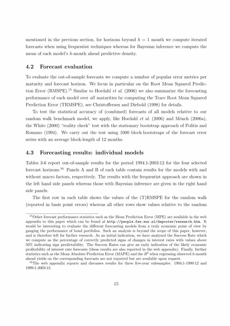
4.2 Forecast evaluation

To evaluate the out-of-sample forecasts we compute a number of popular error metrics per

maturity and forecast horizon. We focus in particular on the Root Mean Squared Predic-

tion Error (RMSPE).15 Similar to Hordahl et al. (2006) we also summarize the forecasting

performance of each model over all maturities by computing the Trace Root Mean Squared

Prediction Error (TRMSPE), see Christoffersen and Diebold (1998) for details.

To test the statistical accuracy of (combined) forecasts of all models relative to our

random walk benchmark model, we apply, like Hordahl et al. (2006) and Monch (2006a),

the White (2000) “reality check” test with the stationary bootstrap approach of Politis and

Romano (1994). We carry out the test using 1000 block-bootstraps of the forecast error

series with an average block-length of 12 months.

4.3 Forecasting results: individual models

Tables 3-6 report out-of-sample results for the period 1994:1-2003:12 for the four selected

forecast horizons.16 Panels A and B of each table contain results for the models with and

without macro factors, respectively. The results with the frequentist approach are shown in

the left hand side panels whereas those with Bayesian inference are given in the right hand

side panels.

The first row in each table shows the values of the (T)RMSPE for the random walk

(reported in basis point errors) whereas all other rows show values relative to the random

15Other forecast performance statistics such as the Mean Prediction Error (MPE) are available in the webappendix to this paper which can be found at http://people.few.eur.nl/depooter/research.htm. Itwould be interesting to evaluate the different forecasting models from a truly economic point of view bygauging the performance of bond portfolios. Such an analysis is beyond the scope of this paper, however,and is therefore left for further research. As an initial indication, we have analyzed the Success Rate whichwe compute as the percentage of correctly predicted signs of changes in interest rates with values above50% indicating sign predictability. The Success Rates can give an early indication of the likely economicprofitability of interest rate forecasts (these results are also reported in the web appendix). Finally, furtherstatistics such as the Mean Absolute Prediction Error (MAPE) and the R2 when regressing observed h-monthahead yields on the corresponding forecasts are not reported but are available upon request.

16The web appendix reports and discusses results for three five-year subsamples: 1994:1-1999:12 and1999:1-2003:12.

15

walk. Relative values for any forecast that are below one are highlighted in bold to indicate

that these forecasts are on average more accurate than those of the random walk. Stars

indicate statistically significant outperformance according to White’s reality check test.

The results for the 1-month horizon in Table 3 are not very encouraging. For nearly

all maturities the random walk gives more accurate forecasts than any of the models based

on yields only, even when parameter uncertainty is incorporated. The results are in line,

however, with other studies showing that it is very difficult to outperform the RW for short

horizon forecasts. Especially for short horizons the near unit root behavior of yields seems

to dominate and model-based yield forecasts add little.

Incorporating macroeconomic information as an additional source of information im-

proves forecasts for the AR and VAR models. The (T)RMSPE values are now very close

and often marginally below those of the RW. The largest improvements are shown for the

shortest maturities, in particular the 3-month maturity where the relative RMPSE for the

AR-X model is 0.95. Detailed inspection of the forecasts reveals that macroeconomic in-

formation helps especially to reduce the forecast bias. However, the improvements do not

appear substantial enough for the AR-X model to produce significantly better forecasts, as

judged by the White reality check test. The evidence for more complex model specifications

is mixed but, in general, adding macroeconomic information worsens predictive accuracy.

For example, for the 6-month maturity the relative RMSPE increases from 1.10 to 1.71 for

the Bayesian Nelson-Siegel model when including macro factors.

The results for the 3-month forecast horizon shown in Table 4 are very similar to those

for the 1-month horizon, although the RMSPE is now higher in absolute terms. The latter

is expected as the yield curve is subject to more new information when the forecast horizon

lengthens. It still proves very difficult for any of the models to provide forecasts that are

more accurate than the random walk. The AR-X model is again the only model that shows

promising results, which can be attributed to the macro factors, as it gives a lower TRMSPE

statistic than that of the random walk. The improvement is, however, not statistically

significant.

For a 6-month horizon somewhat more models start to outperform the random walk for

more maturities, as indicated by a larger number of relative RMSPEs below 1 in the panels

B of Table 5, although the results are still by no means impressive with the best model

improving upon the random walk by only a few percentage points for maturities of 3 months

or longer. Taking into account macroeconomic information as well as parameter uncertainty

results in reasonably accurate forecasts although there is still no significant outperformance.

16

Incorporating parameter uncertainty is very beneficial for the Nelson-Siegel model. The

Bayesian estimation of the state-space form of the model substantially reduces the relative

RMSPE compared to the frequentist approach. Models that keep struggling are the VAR

and affine models, especially for medium maturities between 6 months and 5 years. For

both models this is most likely due to the large number of yields (compared to for example

Duffee, 2002 and Ang and Piazzesi, 2003) that we use in estimation, resulting in a large

number of parameters.17 Note that the VAR model with Bayesian inference does worse than

when estimated using maximum likelihood. This can be explained by realizing that Bayesian

analysis requires drawing inference on the variance parameters of each of the 13 maturities

in addition to doing so for all the other parameters. With maximum likelihood this is not

necessary as we only generate point forecasts.

The longest horizon that we consider is h = 12, see Table 6. Two models produce

forecasts that consistently outperform the random walk across all maturities: the frequentist

VAR-X model and the Bayesian NS1-X model. For both models, the TRMSPEs are smaller

compared to the random walk. RMSPEs are on average 4% lower for the NS1-X model

although the differences are not significant. For all other models (with the exception of the

two-step Nelson-Siegel model for short- and medium-term maturities) the benefits of adding

macro factors are evident with all relative MSPEs going down considerably. Compared to

the frequentist results, the Bayesian VAR model still struggles.

It is interesting to compare our results with those of Monch (2006a) as he uses an almost

identical forecasting sample (1994:1 - 2003:9) but a much shorter estimation period (1983:1

- 1993:12) for the VAR, NS2-AR and NS2-VAR model. Our results for the RW are all but

identical, as they should be, which is a convenient check on our results. The RMSPEs we

find for the VAR(1) on yields and a 1-month horizon are somewhat higher for maturities

below five years whereas for longer maturities they are very similar. For a 12-month horizon

the differences are larger as Monch reports RMPSEs which are roughly 20% lower than ours.

The differences will partly be due to using a slightly different set of maturities and our use

of yield-factors when estimating the VAR instead of using lagged yields directly. The main

reason for the different results will, however, be due to our much longer estimation sample.

It seems that including the 1970s and beginning of 1980s leads to poorer yield forecasts

compared to those obtained when starting the sample after the early eighties. For the NS2-

17An obvious solution to this problem would be to estimate the affine models using a smaller set of yields.The reason we do not follow this strategy here is because we want to use a similar number of yields as inMonch (2006a).

17

AR and NS2-VAR the 1-month ahead results are again very similar. However, whereas

Monch finds that NS2-AR outperforms NS2-VAR for a 6- and 12-month horizon we find

that NS2-VAR is usually more accurate. Our affine model without macro variables provides

similar results as for the A0(3) model that Monch considers for h = 1 but less accurate results

for h = 6 and h = 12. However, we forecast the 1-month maturity much more accurately

which is most likely due to the fact that we estimate the short rate parameters δ0 and δ1

using only data on the 1-month yield instead of estimating these simultaneously with the

other model parameters. It is interesting to note that none of the models we consider here

have an out-of-sample performance which is as good as that of the FAVAR model advocated

by Monch. It would therefore be worthwhile to add this model to the model consideration

set but we leave this for further research.

As an overall summary for the 1994:1-2003:12 period we can remark that our results for

the individual models are not very encouraging as interest rate predictability appears to be

rather low. This may be attributed to a number of possible causes with one main reason being

the out-of-sample period we select. Except for Monch (2006a) who reports very promising

out-of-sample results for his FAVAR model for nearly the same period, Duffee (2002), Ang

and Piazzesi (2003), Diebold and Li (2006) and Hordahl et al. (2006) all use an out-of-sample

period that ranges from roughly the mid 1990s till 2000. As we also include the period from

2000 onwards, a possible explanation for our poor forecasting results seems to be associated

with that period. Figure 1 surely indicates that the interest rate behavior during that period

with its pronounced widening of spreads is rather different from the stable second half of

the 1990s. The subsample results reported in Monch (2006a) for the period 2000:1-2003:9

indicate that the VAR, NS2-AR and NS2-VAR models perform poorly compared to the RW

which is evidence that predictability is indeed low during that period. Through analyzing

TRMSPEs using a 60-month rolling window we hope to get more insight on this issue.

4.3.1 Rolling TRMSPE

To illustrate how the forecasting performance of different models varies over time we compute

TRMSPEs using a 60-month rolling window. Figures 4-7 show results for all forecast horizons

considered. Each graph shows the TRMSPE in levels (basis points) of the RW (right axis)

and the TRMSPE, relative to that of the RW for the [V]AR, NS2-[V]AR, NS1 and ATSM

models (left axis), either without (left panels) or with macro factors (right panels).

The rolling TRMSPEs capture out-of-sample periods which have been analyzed in other

forecasting studies. One example is the subperiod 1994-2000 which is the period that has

18

been most heavily investigated, with positive results found for different models. For example,

Duffee (2002) reports forecast results for affine models that hold up favorably against the

random walk for the period 1995:1-1998:12. Similarly, Ang and Piazzesi (2003) show that

a no-arbitrage Gaussian VAR model predicts well 1-month ahead for the period 1996:1-

2000:12 while Diebold and Li (2006) report outperforming forecasts for the Nelson-Siegel

model for the period 1994:1-2000:12.18 These studies suggest that there should be a high

degree of predictability for this subperiod. Figures 4-7 confirm this. TRMSPEs are fairly

stable until 1997 after which a decreasing trend sets in lasting until mid 2000. The high

degree of interest rate predictability during the 1994-1998 subperiod is the cause of the

decreasingly low TRMSPEs for the period 1998-2000. The model that produces the most

accurate forecasts in this period is the NS2-AR: forecasts significantly improve upon the no-

change forecast with its RMSPE being lower by sometimes as much as 30%. Adding macro

factors to the models tends to improve forecast accuracy for all horizons although there are

some exceptions. One example is the affine model with a 1-month horizon. This differs

from Ang and Piazzesi (2003), for example, who show that an affine model augmented with

an inflation and a real activity factor forecasts better than the random walk at a 1-month

horizon for maturities up to and including five years. This difference in results could be due

to the substantially larger number of yields that we use in estimation. Furthermore, Ang

and Piazzesi (2003) do not forecast beyond the 1-month horizon. Another example is the

NS2-AR-X which often gives the poorest forecasts thereby dramatically deteriorating the

performance of the NS2-AR model in the subperiod 1998-2000.

From 2001 onwards an increase is visible in TRMSPEs, indicating large forecasting errors

due to the sharp decline in interest rate levels and the widening of spreads during this period.

During these years, interest rates decline sharply by roughly 5% at the end of 2000 to a level

of 1% for the short rate accompanied by a substantial widening of spreads between long and

short rates. Adding macro factors improves longer term forecasts, but the only model that

seems capable of competing with the RW is the Bayesian NS1-X model and only consistently

so for the longest horizons. The frequentist AR-X model does well for shorter horizons, the

Bayesian AR-X model does well in 2001-2002. The VAR model shows a strikingly poor

performance in the 2000s indicating that the VAR model cannot cope with the downward

trend in interest rates. The Bayesian ATSM-X model often does better than the Bayesian

18Hordahl et al. (2006) construct 1 through 12-months ahead forecasts for the period 1995:1-1998:12 butthese authors apply their structural model to German zero-coupon data. Their results might therefore notbe directly comparable to the results for U.S. data.

19

VAR and predicts the short end of the curve reasonably well. This shows that imposing

no-arbitrage restrictions helps but not enough to beat simple univariate models. The NS2-

AR-X model forecasts very poorly in the 2000s with TRMSPEs sometimes being worse that

the RW by as much as 60% for long forecast horizons.

The main point to take from these graphs is that the performance of individual models

varies substantially over time and establishing a clear-cut ordering of the models which

holds across the entire 1994-2003 period seems infeasible. Therefore, believing in a single

forecasting model may be hazardous. In the next section, we therefore discuss several forecast

combination techniques as an alternative forecasting approach.

5 Forecast combination

Our rolling TRMPSE analysis reveals that it seems impossible to identify a single model

that consistently outperforms the random walk for the entire out-of-sample period (see also

the subperiod analysis in the web appendix). The forecasting ability of individual models

varies considerably over time. It seems that each model may play a complementary role

in approximating the data generating process of yields, at least during subperiods. Model

uncertainty is troublesome if one has hopes of obtaining a single model for forecasting.

A worthwhile endeavor for cushioning the effects of model uncertainty is to combine the

forecasts of different models, see Timmermann (2006) for a recent survey. In this section

we therefore examine several forecast combination schemes. Two combination methods are

standard approaches and can be applied to combine frequentist as well as Bayesian forecasts.

We also investigate a third combination method which is a truly Bayesian approach that can

only be applied to Bayesian forecasts. We first discuss the different methods and then move

on to examine the forecast combination results in comparison to the results of the individual

models.

5.1 Forecast combination: schemes

Assuming we are combining forecasts from M different models, a combined forecast for a

h-month horizon for the yield with maturity τi is given by y(τi)T+h =

∑Mm=1w

(τi)T+h,my

(τi)T+h,m,

where w(τi)T+h,m denotes the weight assigned to the forecast from the m-th model y

(τi)T+h,m.

20

Scheme 1: Equally weighted forecasts

The first forecast combination method assigns an equal weight to the forecasts from all

individual models, that is w(τi)T+h,m = 1/M for m = 1, . . . ,M . We denote the resulting

combined forecast as Forecast Combination - Equally Weighted (FC-EW). As explained

in Timmermann (2006) this approach is likely to work well if forecast errors from different

models have similar variances and are highly correlated, which is certainly the case here.

Scheme 2: Inverted MSPE-weighted forecasts

The second forecast combination scheme we examine uses weights that take into account

relative historical performance. In particular, combination weights are based on each model’s

(inverted) MSPE relative to those of all other models, computed over a window of the

previous υ months and we denote these by Forecast Combination - MSPE (FC-MSPE).19

The weight for model m is computed as w(τi)T+h,m =

1/MSPE(τi)

T+h,m∑M

m=1(1/MSPE(τi)

T+h,m)

where MSPE(τi)T+h,m =

1υ

∑υr=1(y

(τi)T+h−r|T−r,m − y

(τi)T+h−r)

2. A model with a lower MSPE is given a relatively larger

weight than a worse performing model, see Timmermann (2006) for a discussion and Stock

and Watson (2004) for an application to forecasting GDP growth.20 Which value should

be used for υ is difficult to determine a priori. Using a smaller window will make weights

more responsive to changes in models’ forecasting accuracy but it will also make them more

noisy. The optimal choice of υ will therefore need to be determined empirically. Here we use

four different windows to compute model weights. We use an expanding window where υ

is initially set equal to 60 months but which increases with every new yield realization that

becomes available and we denote the resulting combination forecast as FC-MSPE-exp. We

also apply moving windows of different length, in particular υ = 12, 24 and 60 months. We

denote these by FC-MSPE-12, FC-MSPE-24 and FC-MSPE-60 respectively.

19Note that whereas in the tables we report results for the Root MSPE, Timmermann (2006) argues thatit is better to use the MSPE to construct model weights.

20The weights applied in this and the previous forecast combination scheme are always bounded betweenzero and one. Other approaches for which this does not necessarily needs to be the case, in particularOLS-based weights (see again Timmermann, 2006), proved to be problematic here due to multicollinearityproblems between the different forecasts. This resulted in often extreme (offsetting) weights and we thereforedid not further pursue these approaches.

21

Scheme 3: Bayesian predictive likelihood

The third and final combination scheme is a purely Bayesian model averaging scheme, which

we denote by BMA,21 and is based on the predictive likelihood approach proposed by Geweke

and Whiteman (2006). The probability of the realized value at time T +h is evaluated under

the Bayesian predictive density for T + h for a given model conditional on the information

at time T . The resulting probability is called predictive likelihood. Geweke and Whiteman

(2006) apply these probabilities to average individual models. The realized value will fall

near the center of the predictive density of a given model if this density is accurate. The

particular model then receives a large weight relative to a model for which the realization

ends up far out in the tail of its predictive density. Appendix C provides more specific

details.

The approach of Geweke and Whiteman (2006) is an alternative to the most commonly

used BMA method based on the marginal likelihood, see for example Madigan and Raftery

(1994). We choose the predictive likelihood BMA for three reasons. Firstly, the predictive

likelihood is a measure of out-of-sample performance, whereas the marginal likelihood is

a measure of in-sample fit. Secondly, the marginal likelihood of highly nonlinear models,

such as the Nelson-Siegel and affine models, cannot be derived analytically and may be very

difficult to compute by Monte Carlo simulation. Thirdly, Eklund and Karlsson (2007) show,

in a simulation setting and in an empirical application to Swedish inflation, that model

weights based on the predictive likelihood have better small sample properties and result in

better out-of-sample performance than weights based on the traditional marginal likelihood

measure.

Whereas we refer to the appendix for specific details, we do want to briefly discuss a major

difference between our forecast combination approach and that of Eklund and Karlsson

(2007). Unlike in their study, we do not apply the system of updating and probability

forecasting prequential, as defined by Dawid (1984). We compute the predictive density for

month T +h using information up until month T and we evaluate the realized value for time

T + h using the same density. The resulting probability is then used to compute the weight

for model m in constructing the forecast for T+2h made at time T+h. Eklund and Karlsson

(2007) on the other hand evaluate the fit of the predictive density over a small number of

observations, by means of the predictive likelihood, and then update the probability density

21In the remainder of the text, we often refer to this third scheme as forecast combination. With a slightabuse of denotation we share BMA in the class of forecast combination methods which, strictly speaking, isincorrect since BMA averages models instead of combining models.

22

for the forecasts. The latter approach results in weights which are based more on the fit of the

model, even when using out-of-sample data, than on the probability of out-of-sample realized

values. In an unreported simulation exercise we find that our approach reacts faster to out-

of-sample uncertainty and instability since it is not constrained to give more probability to

the model which provide the best fit of predicted values.

Finally, besides the weighting scheme w(τi)T+h,m an important question to answer when com-

bining forecasts is which models should be included. Here we combine forecasts using three

different sets of models. First we include only those specifications that do not incorporate

macro factors (M = 7 for the models estimated with frequentist methods and M = 5 for the

Bayesian counterpart); second, we use only those model specifications which do incorporate

macro factors (again M = 7 for the models estimated with frequentist methods and M = 5

for the Bayesian counterpart) and finally, we simply combine all specifications (M = 13 and

M = 9 respectively).22 By again making the distinction between models with and without

macro factors we can assess the added value of including macroeconomic information also

for the combined forecasts, just like we did for the individual models. The only model that

is always included in the forecast combinations is the random walk.

5.2 Forecast combination results

The results of the forecast combination methods for the 1994-2003 period are reported in

Panels C-E of Tables 3-6. The following main overall conclusions can be drawn. First, it holds

for all horizons that forecast combinations methods are a valuable alternative compared to

selecting any individual model, especially when combining forecasts from models estimated

with Bayesian methods. The reported TRMSPE numbers show that the best combination

scheme always outperforms the best individual model as well as the random walk, although

the differences are not statistically significant over the full sample. Second, Panels C-E show

that combining forecasts works increasingly well for longer forecast horizons. Indeed, for the

6-month and 12-month horizons, the best combination scheme outperforms the random walk

and the best individual model by several percentage points in terms of relative RMSPEs.

22Many other subsets can of course be selected. Aiolfi and Timmermann (2006) suggest filtering out theworst performing model(s) in an initial step. Preliminary analysis suggests that doing so does not lead tomuch improvement in forecasting performance in our case. However, a more thorough selection procedurethan simply including all available models as applied here, will most likely lead to better results for theforecast combination methods. Although this is a very interesting issue to examine in more detail, our mainpoint here is that want to show the benefits of combining forecasts as an alternative to putting all one’s eggsin a single model basket.

23

Third, results are particularly encouraging for long maturities. All the individual models

tend to forecast maturities beyond 5 years rather poorly, with some exceptions such as the

VAR-X and NS1-X models. This is not the case, however, for the combination schemes which

outperform the random walk by up to 7% for the 6-month horizon (FC-MSPE-X) and 8-9%

for the 12-month forecast horizon (again FC-MSPE-X). This is an important result as other

studies have documented substantial difficulties in accurately forecasting long maturities with

individual models. The claim that individual models provide complementary information

definitely seems to hold for longer maturities. Fourth, averaging models with macro factors

is the superior combination approach. When we compare the forecast combinations with

different model sets, in particular models with and without macro factors, there seems to

be no doubt that combining forecasts from only the models that include macro factors

provides the most accurate results. When models with macro factors are averaged (Panels

D), the resulting statistics are almost always below those of the random walk, irrespective

of the considered horizon, and this is true independently of the averaging scheme used. By

contrast, forecasts from combining models without macro factors (Panels C) always have

relative RMSPEs above one. Including all models in the averaging strategy therefore also

does not seem to be the most attractive approach, in particular not with a longer forecast

horizon. Fifth and finally, comparing the different forecast combination schemes in more

detail, we observe that MSPE-based weights work better than giving equal weight to all

models. Differences are most pronounced for long maturities and a long forecast horizon.

For example, for a 12-month horizon with the 10-year maturity using Bayesian inference, the

relative MSPE of FC-EW-X is 0.98 whereas that of FC-MSPE-X-exp is 6 percentage points

lower at 0.92. With respect to the length of the window that should be used to compute

the MSPE weights, we find that weights that are based on the relative performance over a

long history give the most accurate forecasts. Using an expanding window or a 60-month

rolling window works very well whereas using a shorter history deteriorates the combination

results.

The BMA scheme gives very similar results as the equal-weights scheme. Bayesian model

averaging has the attractive feature of being able to assign near-zero weights to, and thereby

effectively eliminating, the worst performing models. Although BMA outperforms the FC-

MSPE with υ = 12 and 24, like these schemes it assigns probability to models using only

the very recent historical performance. Our results indicate that a long history is important

to accurately assign weights to models.

24

5.2.1 Rolling TRSMPE

A valid question to ask is to what extent our results for the forecast combination schemes

are also sample specific. An answer to this question can be given by considering Figures

8-11. These graphs show the 60-month rolling TRMSPE for RW (right axis) and the relative

TRMSPE (left axis) for the equally-weighted and MSPE-weighted combination schemes

without macro factors (left panels) and with macro factors (right panels) and for frequentist

(Panels [a] and [b]) as well as Bayesian estimation methods (Panels [c] and [d]).

The graphs show that the forecast combination schemes which incorporate macro fac-

tors again nearly always outperform the schemes that do not incorporate macroeconomic

information, irrespective of the forecast horizon and the estimation method.23 What is most

striking though is that the averaging schemes with macro factors outperform the random

walk for nearly every five-year subperiod, except for a few samples ending in either the

second half of 2000 or at the end of 2003. This is particularly true when model forecasts

are constructed with Bayesian techniques. Moreover, these differences are often statistically

significant (see, for example, results for the subperiod 1994-1998 reported in the web ap-

pendix). The TRMSPEs relative to the random walk in panels (d) of Figures 8-11 are nearly

always below one with the FC-MSPE-X-60 scheme consistently being the best performing

combination method. Consequently, the performance of the forecast combinations is very

stable across time and indeed much more stable than for individual models.

When we focus more specifically on subperiods of the 1994-2003 period, we find that at

the beginning of the out-of-sample period improvements with respect to the random walk

are substantial. For short forecast horizons, some individual models, mainly the NS2-AR,

outperform the forecast combination schemes as is apparent from comparing for example

Figures 5(a) and 8. For the 6-month and 12-month horizons, forecast combinations with

macroeconomic information, based on the MSPE-weights using a long historical window are

however the most accurate forecasting methods. We find that the MSPE decreases by up to

20% compared to the random walk and over 10% compared to the best individual model for

the 12-month forecast horizon. It is also interesting to note that whereas for the individual

models (except for the VAR models) adding macro factors often worsens forecasting perfor-

mance for samples ending around 2001, for the forecast combination methods adding macro

factors is very beneficial, especially for long maturities.

23Note that the rolling TMSPEs seem to become more stable when the forecast horizon lengthens whichmay be counterintuitive. However, this is only due to the scaling of the left vertical axes in the graphs.

25

Figures 8-11 also show that the performance of averaging schemes is also still accurate

after 2001. Excluding the last few months of 2003, forecast combinations, especially when

based on the MSPE-weights using a long historical window, including macro factors and

applying Bayesian inference to individual models, forecast very precisely and better than

any other individual model.

6 Conclusion

This paper addresses the task of forecasting the term structure of interest rates. Several

recent studies have shown that significant steps forward are being made in this area. We

contribute to the existing literature by assessing the importance of incorporating macroe-

conomic information, parameter uncertainty, and, in particular, model uncertainty. Our

results show that these issues are worth accounting for as this leads to improved interest

rate forecasts.

We examine the forecast accuracy of a range of models with varying degrees of complexity.

Evaluating the model forecasts over a ten-year out-of-sample period, we show that the pre-

dictive ability of individual models varies over time considerably. Models that incorporate

macroeconomic variables seem more accurate in subperiods during which the uncertainty

about the future path of interest rates is substantial. As an example we mention the period

2000-2003 when spreads were high. Models without macro information do particularly well

in subperiods where the term structure has a more stable pattern such as in the early 1990s.

The fact that different models forecast well in different subperiods confirms ex-post that

alternative model specifications play a complementary role in approximating the data gener-

ating process. Our results provide a strong claim for using forecast combination techniques

as opposed to believing in a single model. Our model combination results show that rec-

ognizing model uncertainty and mitigating the likely effects, leads to substantial gains in

interest rate predictability. We show that combining forecasts of models that incorporate

macro factors are superior to forecasts of any individual model as well as the random walk

benchmark. Additionally, the outperformance of the optimal combination scheme which as-

signs weights to models based on the relative historical performance over a long sample is

very stable over time. We obtain the largest gains in predictability for long maturities.

We feel that our results open up exciting avenues for further research. In this study we

have only considered very generic models, in particular in our use of a three-factor Gaussian

affine model. It would therefore be interesting to expand the model consideration set with

26

more sophisticated models such as the FAVAR models of Monch (2006a) or the structural

model by Hordahl et al. (2006) both of which have been found to forecast well. More

sophisticated ways of combining forecasts are worth addressing as well, see e.g. Guidolin

and Timmermann (2007) who use a combination scheme with time-varying weights where

weights have regime switching dynamics. In terms of incorporating parameter uncertainty,

much more work can be done on the use of sensible informative priors. As an example

we mention the use of adaptive priors that could take into account likely changes in yield

dynamics due to clear political or economic reasons. Other, technical, issues that could

be addressed are more specifically related to estimation and forecasting procedures. For

example, changes in yield dynamics could also be accounted for by using rolling estimation

windows instead of the expanding window which we have used here.

27

References

Aiolfi, M. and A. Timmermann (2006), Persistence in Forecasting Performance and Condi-

tional Combination Strategies., Journal of Econometrics , 135, 31–53.

Ang, A., S. Dong, and M. Piazzesi (2007), No-Arbitrage Taylor Rules, Working paper,

Columbia University .

Ang, A. and M. Piazzesi (2003), A No-Arbitrage Vector Autoregression of Term Structure

Dynamics with Macroeconomic and Latent Variables, Journal of Monetary Economics ,

50, 745–787.

Ang, A., M. Piazzesi, and M. Wei (2006), What does the Yield Curve tell us about GDP

Growth?, Journal of Econometrics , 131, 359–403.

Backus, D., S. Foresi, and C. Telmer (1998), Discrete-Time Models of Bond Pricing, NBER

Working paper .

Bernanke, B. S., J. Boivin, and P. Eliasz (2005), Measuring the Effects of Monetary Policy:

A Factor-Augmented Vector Autoregressive (FAVAR) Approach, Quarterly Journal of

Economics , 120, 387–422.

Bikbov, R. and M. Chernov (2005), No-Arbitrage Macroeconomic Determinants of the Yield

Curve, Working paper, Columbia University .

Bliss, R. R. (1997), Testing Term Structure Estimation Methods, Advances in Futures and

Options Research, 9, 197–231.

Carter, C. and R. Kohn (1994), On Gibbs Sampling for State-Space Models, Biometrika,

81, 541–553.

Chen, R. R. and L. Scott (1993), Maximum Likelihood Estimation for a Multifactor Equilib-

rium Model of the Term Structure of Interest Rates, Journal of Fixed Income, 3, 14–31.

Christoffersen, P. F. and F. X. Diebold (1998), Cointegration and Long-Horizon Forecasting,

Journal of Business & Economic Statistics , 16, 450–458.

Cox, J., J. E. Ingersoll, and S. A. Ross (1985), A Theory of the Term Structure of Interest

Rates, Econometrica, 53, 385–407.

28

Croushore, D. (2006), Forecasting with Real-Time Macroeconomic Data, in G. Elliot,

C. Granger, and A. Timmermann (eds.), Handbook of Economic Forecasting , North-

Holland, 961-982.

Dai, Q. and T. Philippon (2006), Fiscal Policy and the Term Structure of Interest Rates,

NBER Working paper .

Dai, Q. and K. J. Singleton (2000), Specification Analysis of Affine Term Structure Models,

Journal of Finance, 55, 1943–1978.

Dawid, A. P. (1984), Statistical Theory: The Prequential Approach, Journal of the Royal

Statistical Society Series A, 147, 278–292.

DeWachter, H. and M. Lyrio (2006), Macro Factors and the Term Structure of Interest Rates,

Journal of Money, Credit and Banking , 38, 119–140.

Diebold, F. X. and C. Li (2006), Forecasting the Term Structure of Government Bond Yields,

Journal of Econometrics , 130, 337–364.

Diebold, F. X., G. D. Rudebusch, and B. Aruoba (2006), The Macroeconomy and the Yield

Curve: a Dynamic Latent Factor Approach, Journal of Econometrics , 131, 309–338.

Duffee, G. (2002), Term Premia and Interest Rate Forecasts in Affine Models, Journal of

Finance, 5, 405–443.

Duffie, D. and R. Kan (1996), A Yield-Factor Model of Interest Rates, Mathematical Finance,

6, 379–406.

Eklund, J. and S. Karlsson (2007), Forecast Combination and Model Averaging using Pre-

dictive Measures, Econometric Reviews , 26, 329–363.

Evans, C. L. and D. Marshall (1998), Monetary Policy and the Term Structure of Nominal

Interest Rates: Evidence and Theory, Carnegie-Rochester Conference Series on Public

Policy , 49, 53–111.

Evans, C. L. and D. Marshall (2007), Ecoomic Determinants of the Nominal Treasury Yield

Curve, Journal of Monetary Economics , 54, 1986–2003.

Fama, E. F. and R. R. Bliss (1987), The Information in Long-Maturity Forward Rates,

American Economic Review , 77, 680–692.

29

Geman, S. and D. Geman (1984), Stochastic Relaxation, Gibbs Distributions and the

Bayesian Restoration of Images, IEEE Transaction on Pattern Analysis and Machine

Intelligence, 6, 721–741.

Geweke, J. and C. Whiteman (2006), Bayesian Forecasting, in G. Elliot, C. Granger, and

A. Timmermann (eds.), Handbook of Economic Forecasting , North-Holland, 3-80.

Guidolin, M. and A. Timmermann (2007), Forecasts of US Short-term Interest Rates: A

Flexible Forecast Combination Approach, forthcoming in Journal of Econometrics .

Hordahl, P., O. Tristani, and D. Vestin (2006), A Joint Econometric Model of Macroeconomic

and Term-Structure Dynamics, Journal of Econometrics , 131, 405–444.

Kim, D. H. and J. H. Wright (2005), An Arbitrage-Free Three-Factor Term Structure Model

and the Recent Behavior of Long-Term Yields and Distant-Horizon Forward Rates, Work-

ing paper, Federal Reserve Board Washington, 33.

Koop, G. (2003), Bayesian Econometrics , John Wiley & Sons Ltd, West Sussex, England.

Krippner, L. (2005), An Intertemporally-Consistent and Arbitrage-Free Version of the Nelson

and Siegel Class of Yield Curve Models, Working paper, University of Waikato.

Litterman, R. and J. Scheinkman (1991), Common Factors Affecting Bond Returns, Journal

of Fixed Income, 54–61.

Madigan, D. M. and A. E. Raftery (1994), Model selection and accounting for model un-

certainty in graphical models using Occam’s Window, Journal of the American Statistical

Association, 89, 1335–1346.

Marcellino, M., J. H. Stock, and M. W. Watson (2006), A Comparison of Direct and It-

erated Multistep AR Methods for Forecasting Macroeconomic Time Series, Journal of

Econometrics , 127, 499–526.

Monch, E. (2006a), Forecasting the Yield Curve in a Data-Rich Environment: A No-

Arbitrage Factor-Augmented VAR Approach, Working paper, Humboldt University Berlin.

Monch, E. (2006b), Term Structure Surprises: The Predictive Content of Curvature, Level,

and Slope.pdf, Working paper, Humboldt University Berlin.

30

Nelson, C. R. and A. F. Siegel (1987), Parsimonious Modeling Of Yield Curves, Journal of

Business , 60, 473–489.

Piazzesi, M. (2003), Affine Term Structure Models, in Y. Ait-Sahalia and L. Hansen (eds.),

forthcoming in Handbook of Financial Econometrics , Elsevier.

Politis, D. N. and J. P. Romano (1994), The Stationary Bootstrap, Journal of the American

Stastical Association, 89, 1303–1313.

Rudebusch, G. D. and T. Wu (2004), A Macro-Finance Model of the Term-Structure, Mon-

etary Policy, and the Economy, forthcoming in Economic Journal .

Stock, J. H. and M. W. Watson (2002a), Macroeconomic Forecasting Using Diffusion Indexes,

Journal of Business & Economic Statistics , 20, 147–162.

Stock, J. H. and M. W. Watson (2002b), Forecasting Using Principal Components From a

Large Number of Predictors, Journal of the American Statistical Association, 97, 1167–

1179.

Stock, J. H. and M. W. Watson (2004), Combining Forecasts of Output Growth in a Seven-

Country Data Set, Journal of Forecasting , 23, 405–430.

Stock, J. H. and M. W. Watson (2005), Implications of Dynamic Factor Models for VAR

Analysis, Working paper .

Tanner, M. A. and W. H. Wong (1987), The Calculation of Posterior Distributions by Data

Augmentation, Journal of the American Statistical Association, 82, 528–550.

Timmermann, A. (2006), Forecast Combinations, in G. Elliot, C. Granger, and A. Timmer-

mann (eds.), Handbook of Economic Forecasting , North-Holland, 135-196.

Vasicek, O. A. (1977), An Equilibrium Characterization of the Term Structure, Journal of

Financial Economics , 5, 177–188.

White, H. (2000), A Reality Check for Data Snooping, Econometrica, 68, 1097–1126.

Wu, T. (2005), Macro Factors and the Affine Term Structure of Interest Rates, Working

paper, Federal Reserve Bank of San Francisco.

Zellner, A. (1971), An Introduction to Bayesian Inference in Econometrics , Wiley, New York.

31

Appendix

A Individual models

In this appendix we provide details on how we perform inference on the parameters of the models in Section3. We discuss each model separately and we distinguish between frequentist and Bayesian inference.

A.1 AR model

Frequentist Inference

We estimate the parameters (c(τi), φ(τi), ψ(τi)) using standard OLS. Given the parameter estimates we con-struct iterated forecasts as

y(τi)T+h = c(τi) + φ(τi)y

(τi)T+h−1 + ψ(τi)

′

XT+h (A-1)

with y(τi)T = y

(τi)T . We construct forecast both with and without the macroeconomic factors. The forecasts

of the macro factors, XT+h, are iterated forecasts constructed from the VAR(3) macro model.

Bayesian Inference

For the Bayesian inference, we use a Normal-Gamma conjugate prior for the parameters

(c(τi), φ(τi), ψ(τi), σ2(τi)),

(c(τi), φ(τi), ψ(τi), σ2(τi))′ ∼ NG(b, v, s2, ν) (A-2)

The marginal posterior densities of the parameters and the predictive density of y(τi)T+h, conditional on y

(τi)T

and XT+h, can be derived using standard Bayesian results, see for example Koop (2003).

A.2 VAR model

Frequentist Inference

We estimate the equation parameters (c,Φ,Ψ) in (5) using equation-by-equation OLS. Forecasts are obtainedas

YT+h = c+ ΦFT+h−1 + ΨXT+h (A-3)

We construct the yield factor forecasts, FT+h−1, by first calculating the principal component factor loadingsusing data only up until month T and then multiplying these with the iterated yields forecasts.

Bayesian Inference

We apply direct simulation to draw inference on VAR model. Note that this is a novel approach as theliterature commonly uses MCMC simulation algorithms. Direct simulation is faster and more precise sincetruly independent draws are used. Our derivation is based on Zellner (1971), who provides all the necessarycomputations with diffuse priors, and we extend the analysis to include informative priors.24

24We present here only the main results. Details of the derivations are available upon request.

32

Prior Specification We apply informative prior densities for the parameter matrices Π = [c Φ Ψ] andS in (5). For computational tractability we select the following conjugate priors:

Π|S ∼MN(B,S ⊗ V ) (A-4)

andS ∼ IW (S, µ) (A-5)

where MN indicates the mactrivariate normal distribution with mean B and variance matrix S ⊗ V , andwhere IW indicates the Inverted Wishart distribution.

Posterior Simulation The likelihood function of YT for the VAR is given by

p(YT |FT−1,XT ,Π, S) = (2π)−TN/2|S|−T/2 exp[−1

2tr(S−1(YT − ZT Π)′(YT − ZT Π))] (A-6)

where ZT = (eN , F′

T−1,X′

T ) and eN is a (N × 1) vector of ones. If we combine (A-6) with the prior densitiesin (A-4)–(A-5) we obtain the joint posterior density for (Π, S) as

p(Π, S|YT , FT−1,XT ) = p(YT |FT−1,XT ,Π, S)p(Π|S)p(S)

∝ |S|−(T+N+ν+1)/2 exp(− 12 tr(S

−1(S + (YT − ZT Π)′(YT − ZT Π) + (Π −B)′V −1(Π −B))))(A-7)

where ν = G+ ν with G the number of columns of Π. If we define WT = (YT , V−1/2B)′, VT = (ZT , V

−1/2)and apply the decomposition rule and the Inverted Wishart integration step, the posterior density for Π, con-ditional on (YT , FT−1,XT ), will be a generalized t-distribution with location parameter Π = (V ′V )−1V ′W ,

scale parameters S + (WT − VT Π)′(WT − VT Π) and (Z′

TZT + V −1) and T + ν degrees of freedom. That is,

p(Π|YT , FT−1,XT ) ∝ |S + (WT − VT Π)′(WT − VT Π) + (Π − Π)′(Z′

TZT + V −1)(Π − Π)|−(T+ν)/2 (A-8)

The posterior density of S conditional on (YT , FT−1,XT ) is:

S|YT , FT−1,XT ∼ IW (S + (WT − VT Π)′(WT − VT Π), T + ν) (A-9)

Forecasting The predictive density conditional on (YT ,XT ) and (FT+h−1,XT+h) is defined as:

p(YT+h|YT ,XT , FT+h−1,XT+h) =∫ ∫

p(YT+h,Π, S|YT ,XT , FT+h−1,XT+h)dΠdS

=∫ ∫

p(YT+h|FT+h−1,XT+h,Π, S)p(Π, S|YT ,XT )dΠdS(A-10)

By applying the inverted Wishart step to (A-10), and integrating with respect to Π, we have:

p(YT+h|YT ,XT , FT+h−1,XT+h) ∝ [S + (WT − VT Π)′(WT − VT Π)+

(YT+h − ZT+hΠ)′(I − ZT+hL−1Z ′

T+h)(YT+h − ZT+hΠ)]−(T+ν+h)/2

(A-11)

where L = (Z′

T+hZT+h + Z′

TZT + V −1), ZT+h = (Ih, FT+h−1,XT ) with Ih a (h× h) identity matrix.The predictive density of YT+h conditional on (YT ,XT , FT+h−1,XT+h) is thus a generalized t-distribution

with location parameter ZT+hΠ, scale parameters S+(WT −VT Π)′(WT −VT Π) and (IN −ZT+hL−1Z ′

T+h),and T + ν degrees of freedom. Following Zellner (1971) we rewrite (A-11) as:

p(YT+h|YT ,XT , FT+h−1,XT+h) = p(YT+1|FT ,XT+1) × . . .× p(YT+h|FT ,XT+1, ..., FT+H−1,XT+h) (A-12)

33

FT+h−1 and XT+h are generated from their predictive densities conditional on past values, independentlyfrom YT+h. Therefore, we substitute these densities in (A-12) and we apply direct simulation to draw thepredictive density of YT+h, conditional on YT and XT ,

p(YT+h|YT ,XT ) =

∫∫p(YT+h|YT ,XT , FT+h−1,XT+h)p(FT+h−1|FT+h−2)p(XT+h|XT+h−1)dFT+h−1dXT+h

(A-13)Note that we integrate with respect to the predictive density of the macroeconomic factors XT+h given XT .

A.3 Nelson-Siegel model

Frequentist Inference

With the frequentist approach we estimate the Nelson-Siegel model using the two-step approach of Dieboldand Li (2006) and the one-step approach of Diebold et al. (2006).

In the two-step approach we fix λ to 16.42, which, as shown in Diebold and Li (2006), maximizes thecurvature factor loading at a 30-month maturity. For every month we then estimate the vector of β’s byapplying OLS on the cross-section of 18 maturities. From this first step we obtain time-series for the threefactors, {βt}

Tt=1. The second step consists of modelling the factors in (7) by fitting either separate AR(1)

models or a single VAR(1) model.In the one-step approach we estimate the unknown parameters and latent factors by means of the Kalman

Filter using the prediction error decomposition for the State-Space model in (6)-(7). For each sample in therecursive estimation procedure, we first run the two-step approach with a VAR(1) specification for the statevector to obtain starting values. The unconditional mean and covariance matrix of {βt}T

t=1 are used tostart the Kalman Filter. We discard the first 12 observations when evaluating the likelihood. All varianceparameters of the diagonal matrix H and the full matrix Q are initialized to 1. The covariance terms in Qare initialized to 0. In the optimization procedure, we maximize the likelihood using the standard deviationsas parameters to ensure positive estimates for the variance parameters. Finally, λ is initialized to 16.42.

Iterated forecasts for the factors are obtained as

fT+h = a+ ΓfT+h−1 (A-14)

where fT+h = (β1,T+h, β2,T+h, β3,T+h, MT+h, MT+h−1, MT+h−2). These are then inserted in the measure-ment equation to compute interest rate forecasts:

y(τi)T+h = β1,T+h + β2,T+h

(1−exp(−τi/λ)

τi/λ

)+ β3,T+h

(1−exp(−τi/λ)

τi/λ−exp(−τi/λ)

)(A-15)

Bayesian Inference

The joint posterior densities for parameters of the Nelson-Siegel and affine models do not have a knownclosed-form expression. Therefore, we cannot analytically compute marginal densities for model parametersnor marginal predictive densities. We use Monte Carlo methods instead.

Prior Specification The model parameters are summarized by θ = (λ, σ2, a,Γ, Q), where σ2 is a(18 × 1) vector containing the diagonal elements of the measurement equation covariance matrix H. Tofacilitate the posterior simulation we use independent conjugate priors for the model parameters. For thevariance parameters σ(τi) we take the Inverted Gamma-2 prior

σ2(τi)∼ IG-2(ν(τi), δ(τi)) (A-16)

34

For the non-zero blocks in the state equation covariance matrix, Q1 and Q2, we assume Inverted Wishartdistributions,

Q1 ∼ IW(µ1,∆1) (A-17)

Q2 ∼ IW(µ2,∆2) (A-18)

For the linear regression parameters we assume a matricvariate Normal distribution,

[a,Γ] ∼MN(Γ, Q⊗ V Γ) (A-19)

Finally for λ we assume a uniform distribution,

λ ∼ U(aλ, bλ) (A-20)

We choose the parameters aλ and bλ to reflect the prior belief about the shape of the loading factors.

Posterior Simulation We obtain posterior results by using the Gibbs sampler of Geman and Geman(1984) with the data augmentation technique of Tanner and Wong (1987). The latent variables BT ={β1,t, β2,t, β3,t}T

t=1 are simulated alongside the model parameters θ.The complete data likelihood function is given by

p(YT , FT |θ) =T∏

t=1

18∏

i=1

p(y(τi)t |ft, λ, σ

2(τi))p(ft|ft−1, a,Γ, Q) (A-21)

where YT = {y(τ1)t , . . . , y

(τN )t }T

t=1 and where FT = {β1,t, β2,t, β3,t,Mt,Mt−1,Mt−2}Tt=1. The terms p(y

(τi)t |ft, λ, σ

2(τi)),and p(ft|ft−1, a,Γ, Q) are Normal density functions which follow directly from (6)–(7). When we combine(A-21) with the prior densities p(θ) in (A-16)–(A-20) we obtain the posterior density

p(θ,BT |YT ,MT ,MT−1,MT−2) ∝ p(YT , FT |θ)p(θ) (A-22)

We compute the full conditional posterior density for the latent regression parameters BT using thesimulation smoother as in Carter and Kohn (1994, Section 3) and we use the Kalman smoother to derivethe conditional mean and variance of the latent factors. For the initial value β0 we choose a multivariatenormal prior with mean zero.

To sample the θ parameters (excluding λ), we use standard results. Hence, the variance parameters σ(τi)

are sampled from inverted Gamma-2 distributions, the matrix Q1 is sampled from an Inverted Wishart dis-tribution, and the parameters (a1, Γ1) are sampled from matricvariate Normal distributions, where (a1,Γ1)are the non-zero blocks of a and Γ respectively. In our framework the macro variables have a VAR(3)structure independent from the latent factors. Therefore, we simulate a2, Γ2, and Q2 from their marginaldensities, respectively generalized t-distributions and an Inverted Wishart distribution to improve the speedof convergence.

Finally, the posterior density for λ, conditional on (YT , FT ,H) is:

p(λ|YT , FT ,H) ∝T∏

t=1

N∏

i=1

p(y(τi)t |ft, λ, σ

2(τi))p(λ) (A-23)

Equation (A-23) is not proportional to any known density. Therefore, λ has to be drawn by applyingMCMC methods. We use the Griddy Gibbs algorithm. The Griddy Gibbs sampler was developed by Ritterand Tanner (1992) and is based on the idea to construct a simple approximation of the inverse cumulativedistribution function of the target density on a grid of points25. More formally and referring to equation(A-23), we perform the following steps:

25Monch (2006b) applies a random walk Metropolis Hastings algorithm to draw λ. We choose the Griddy-Gibbs since the space of λ is well defined and only the cumulative density function needs to be estimated inthese grid points.

35

• We evaluate p(λ|YT , FT ,H) at points Vi = v1, ..., vn to obtain w1, ..., wn;

• We use w1, ..., wn to obtain an approximation to the inverse cdf of p(λ|YT , FT ,H);

• We sample a uniform (0,1) deviate and we transform the observation via the approximate inversecumulative density function.

Forecasting The h-step ahead predictive density of YT+h, conditional on YT and FT , is given by

p(YT+h|YT , FT ) =

∫∫p(y

(τi)T+h|fT+h, λ, σ

2(τi))p(fT+h|fT+h−1, a,Γ, Q)×

p(θ,BT |YT ,MT ,MT−1,MT−2)dfT+h dθ (A-24)

where p(y(τi)T+h|fT+h, λ, σ

2(τi)) and p(fT+h|fT+h−1, a,Γ, Q) follow directly from the state space system andwhere p(θ,BT |YT ,MT ,MT−1,MT−2) is the posterior density.

Simulating YT+h from the h-step ahead distribution (A-24) is straightforward. In each step of the Gibbssampler, we use the simulated values of (a,Γ, Q) to draw the out-of-sample values of fT+h. Then, fT+h, in

combination with the current Gibbs draws of H and λ, provides a simulated value for y(τi)T+h.

A.4 Affine model

Frequentist Inference

To estimate the affine model we assume that yields of every maturity are contaminated with measurementerror. We estimate the parameters in the resulting State-Space model by applying the two-step approachused in Ang et al. (2006). We make the latent factors Zt observable by extracting the first three principalcomponents from the panel of yields of different maturities. The first step of the estimation procedureconsists of estimating the equation and variance parameters of the state equations (23). In the second stepwe estimate the remaining parameters (δ0, δ1, λ0, λ1). We first estimate (δ0, δ1) by applying OLS to theshort rate equation (13) where we use the 1-month yield as the observable short rate. We then estimatethe risk premia parameters (λ0, λ1) by minimizing the sum of squared yields errors in the measurement

equations (22), giving the parameter estimates from the first step, (µ, Ψ, Σ) and the short rate parameters

(δ0, δ1). In the second step we initialize all risk premia parameters to zero. Common approaches for obtainingstarting values for the risk premia parameters by first estimating either λ0 or λ1 in a separate step yieldedunsatisfactory results.

Yield forecasts are generated by forward iteration of the state equations

fT+h = µ+ ΨfT+h−1 (A-25)

where fT+h = (Z1,T+h, MT+h−1, MT+h−2). With the estimated parameters substituted in a(τi) and b(τi) wethen construct interest rate forecasts as

y(τi)T+h = a(τi) + b(τi)fT+h (A-26)

Bayesian Inference

Bayesian inference on model (22)-(23) is very complex due to the high degree of nonlinearity and, above all,the large set of yields we model. It is particularly difficult to define the space of the short rate parameters.The likelihood is very sensitive to these parameters and small perturbations give very different and unrealisticresults. Therefore, an estimation approach similar to Ang et al. (2007) may not be the optimal solution.We opt for a normal approximation of the full posterior density around frequentist parameter estimates.This choice implies that the predictive density of YT+h, conditional on YT and Ft = {ft}

Tt=1, can be derived

without having to compute posterior densities.

36

Forecasting The h-step ahead predictive density of y(τi)T+h, conditional on YT and FT , is given by

p(y(τi)T+h|YT , FT ) =

∫∫p(y

(τi)T+h|fT+h, a

(τi), b(τi), σ2(τi))p(fT+h|fT+h−1, µ,Ψ, Q)p(θ|YT , FT )dfT+h dθ (A-27)

where p(y(τi)T+h|xT+h, a

(τi), b(τi), σ2(τi)), and p(fT+h|fT+h−1, µ,Ψ, Q) are the conditional predictive densitiesand where p(θ|YT ,XT ) is the posterior density for the parameter vector θ = (µ,Ψ,H,Q, a, b, λ0, λ1). Aswe discussed in the previous paragraph we approximate p(θ|YT ,XT ) in (A-27), with a normal distribution

around frequentist estimates: q(θ|YT ,XT ). Since fT+h can be drawn independently of YT+h, we use directsimulation to compute the predictive density of YT+h conditional on (YT , FT ):

p(y(τi)T+h|YT ,XT ) =

∫∫p(y

(τi)T+h|fT+h, a

(τi), b(τi), σ2(τi)

)p(fT+h|fT+h−1, µ, Ψ, Q)dfT+hdθ (A-28)

B Bayesian Model Averaging

We denote the predictive density of y(τi)T+h, given M individual models and conditional on the time T infor-

mation set DT by p(y(τi)T+h|YT ,DT ). This density is given by

p(y(τi)T+h|YT ,DT ) =

M∑

i=1

P (m(τi)j |YT ,DT )p(y

(τi)T+h|YT ,DT ,m

(τi)j ) (B-1)

for j = 1, ...,M and where P (m(τi)j |YT ,DT ) is the posterior probability of model mj for maturity τi, con-

ditional on data at time T , and where p(y(τi)T+h|YT ,DT ,m

(τi)j ) is the model mj predictive density of y

(τi)T+h,

conditional on YT and DT . The posterior probability of model mj for maturity τi is computed as:

P (m(τi)j |YT ,DT ) =

p(y(τi)T,o |YT ,DT ,m

(τi)j )P (m

(τi)j )

∑ks=1 p(y

(τi)T,o |YT ,DT ,m

(τi)s )P (m

(τi)s )

(B-2)

where P (m(τi)j ) is the prior probability of model mj for maturity τi. The predictive likelihood value for model

mj , p(yτi

T,o|YT ,DT ,m(τi)j ), is computed by substituting the realized value y

(τi)T,o in the predictive density

p(y(τi)T |YT ,DT ,m

(τi)j ). We average individual models independently for every maturity. The predictive

likelihood is computed over only a single forecast.

C Prior specification

In the literature uninformative priors or diffuse informative priors are often chosen to derive posterior den-sities that depend only on data information (the likelihood). We do not follow this approach as we applyinformative priors in our estimation and forecasting procedures. There are several motivations to do so.Firstly, for nonlinear models such as the Nelson-Siegel and affine models, it is very difficult to determinewhen a prior is non-informative. Secondly, the simulation algorithm might get stuck in some (nonsensical)regions of the parameter space and it may require a substantial number of simulations to converge, therebyenormously increasing estimation time. Thirdly, we believe that market agents will to some degree alwayshave prior information which can be partially incorporated in our models when forecasting interest rates.Finally, we want to study and underline differences between frequentist and Bayesian inference in forecastingyields, and the use of priors is one, if not the main, difference between the two approaches.

We briefly discuss the specification of the prior densities for the parameters of the models presented inAppendix A. We start with the AR model and the Normal-Gamma conjugate prior in (A-2) for parameters

37

(c(τi), φ(τi), ψ(τi), σ(τi)). We choose v = 0.01 to have a prior density for the vector (c(τi), φ(τi), ψ(τi)) concen-trated around the mean value. We choose the mean vector value b by calibrating it to the initial in-sampledata (1970:1-1993:12) and to prevent unit root type behavior. The prior for σ(τi) is less informative with νfixed to 20 and s2 again calibrated to in-sample data.

The calibration of the prior for the VAR model is more complex due to the high dimensionality of Πand S. Therefore, we relax our prior assumption and we choose a wider region for V and ν in (A-4)–(A-5).B is again calibrated with initial in-sample data and the resulting values imply plausible factor loadings ofthe yield factors.

The order of prior information in the Nelson-Siegel model is comparable to the VAR model. For theparameter λ we choose the following uniform prior density:

λ ∼ U(3.34, 33.45) (C-1)

By restricting λ in the interval [3.34, 33.45] we can make sure that the loading on the curvature factor β3,t

is at its maximum for a maturity between 6 months and 5 years.For the ATSM model we do not apply prior densities. We use a normal approximation of the conditional

predictive density around maximum likelihood parameter estimates. Indeed, because we consider a largenumber of maturities, which results in a substantial number of parameters that need to be estimated, thespeed of convergence of MCMC algorithms such as the Gibbs sampler is very slow. Moreover, some param-eters do not converge at all, and unrealistic values are simulated. However, we believe the approximation issatisfactory. We therefore still account for parameter uncertainty in the affine models.

Finally, in Bayesian model averaging we apply the same uninformative prior probability to each model,

P (m(τi)j ) = 1/M .

38

Table 1: Summary statistics

maturity mean stdev skew kurt min max JB ρ1 ρ12 ρ24

1-month 6.049 2.797 0.913 4.336 0.794 16.162 85.671 0.968 0.690 0.4023-month 6.334 2.896 0.871 4.237 0.876 16.020 76.380 0.974 0.708 0.4156-month 6.543 2.927 0.788 4.016 0.958 16.481 58.796 0.976 0.723 0.444

1-year 6.755 2.860 0.661 3.763 1.040 15.822 38.907 0.975 0.733 0.4742-year 7.032 2.724 0.644 3.672 1.299 15.650 35.240 0.978 0.748 0.5263-year 7.233 2.594 0.685 3.663 1.618 15.765 38.796 0.979 0.763 0.5604-year 7.392 2.510 0.728 3.607 1.999 15.821 41.640 0.980 0.771 0.5825-year 7.483 2.449 0.759 3.478 2.351 15.005 42.454 0.982 0.786 0.6076-year 7.611 2.406 0.791 3.437 2.663 14.979 45.236 0.983 0.797 0.6267-year 7.659 2.344 0.841 3.488 3.003 14.975 51.562 0.983 0.787 0.6238-year 7.728 2.320 0.841 3.365 3.221 14.936 49.798 0.984 0.809 0.6519-year 7.767 2.317 0.877 3.427 3.389 15.018 54.765 0.985 0.813 0.656

10-year 7.745 2.266 0.888 3.496 3.483 14.925 57.117 0.985 0.796 0.647

Notes: The table shows summary statistics for our sample of end-of-month continuously compounded U.S.zero-coupon yields. Reported are the mean, standard deviation, skewness, kurtosis, minimum, maximum,the Jarque-Bera test statistic for normality and the 1st, 12th and 24th sample autocorrelation. The resultsshown are for annualized yields (in %). The sample period is January 1970 - December 2003 (408 monthlyobservations).

39

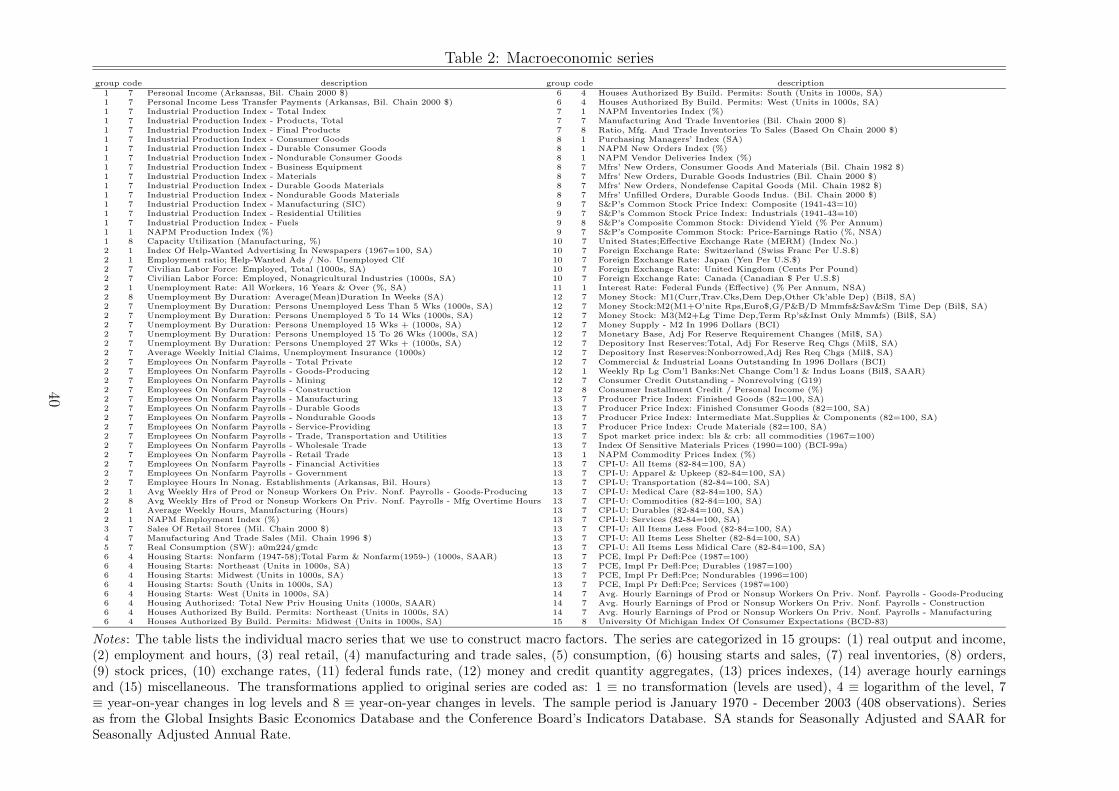
Table 2: Macroeconomic series

group code description group code description1 7 Personal Income (Arkansas, Bil. Chain 2000 $) 6 4 Houses Authorized By Build. Permits: South (Units in 1000s, SA)1 7 Personal Income Less Transfer Payments (Arkansas, Bil. Chain 2000 $) 6 4 Houses Authorized By Build. Permits: West (Units in 1000s, SA)1 7 Industrial Production Index - Total Index 7 1 NAPM Inventories Index (%)1 7 Industrial Production Index - Products, Total 7 7 Manufacturing And Trade Inventories (Bil. Chain 2000 $)1 7 Industrial Production Index - Final Products 7 8 Ratio, Mfg. And Trade Inventories To Sales (Based On Chain 2000 $)1 7 Industrial Production Index - Consumer Goods 8 1 Purchasing Managers’ Index (SA)1 7 Industrial Production Index - Durable Consumer Goods 8 1 NAPM New Orders Index (%)1 7 Industrial Production Index - Nondurable Consumer Goods 8 1 NAPM Vendor Deliveries Index (%)1 7 Industrial Production Index - Business Equipment 8 7 Mfrs’ New Orders, Consumer Goods And Materials (Bil. Chain 1982 $)1 7 Industrial Production Index - Materials 8 7 Mfrs’ New Orders, Durable Goods Industries (Bil. Chain 2000 $)1 7 Industrial Production Index - Durable Goods Materials 8 7 Mfrs’ New Orders, Nondefense Capital Goods (Mil. Chain 1982 $)1 7 Industrial Production Index - Nondurable Goods Materials 8 7 Mfrs’ Unfilled Orders, Durable Goods Indus. (Bil. Chain 2000 $)1 7 Industrial Production Index - Manufacturing (SIC) 9 7 S&P’s Common Stock Price Index: Composite (1941-43=10)1 7 Industrial Production Index - Residential Utilities 9 7 S&P’s Common Stock Price Index: Industrials (1941-43=10)1 7 Industrial Production Index - Fuels 9 8 S&P’s Composite Common Stock: Dividend Yield (% Per Annum)1 1 NAPM Production Index (%) 9 7 S&P’s Composite Common Stock: Price-Earnings Ratio (%, NSA)1 8 Capacity Utilization (Manufacturing, %) 10 7 United States;Effective Exchange Rate (MERM) (Index No.)2 1 Index Of Help-Wanted Advertising In Newspapers (1967=100, SA) 10 7 Foreign Exchange Rate: Switzerland (Swiss Franc Per U.S.$)2 1 Employment ratio; Help-Wanted Ads / No. Unemployed Clf 10 7 Foreign Exchange Rate: Japan (Yen Per U.S.$)2 7 Civilian Labor Force: Employed, Total (1000s, SA) 10 7 Foreign Exchange Rate: United Kingdom (Cents Per Pound)2 7 Civilian Labor Force: Employed, Nonagricultural Industries (1000s, SA) 10 7 Foreign Exchange Rate: Canada (Canadian $ Per U.S.$)2 1 Unemployment Rate: All Workers, 16 Years & Over (%, SA) 11 1 Interest Rate: Federal Funds (Effective) (% Per Annum, NSA)2 8 Unemployment By Duration: Average(Mean)Duration In Weeks (SA) 12 7 Money Stock: M1(Curr,Trav.Cks,Dem Dep,Other Ck’able Dep) (Bil$, SA)2 7 Unemployment By Duration: Persons Unemployed Less Than 5 Wks (1000s, SA) 12 7 Money Stock:M2(M1+O’nite Rps,Euro$,G/P&B/D Mmmfs&Sav&Sm Time Dep (Bil$, SA)2 7 Unemployment By Duration: Persons Unemployed 5 To 14 Wks (1000s, SA) 12 7 Money Stock: M3(M2+Lg Time Dep,Term Rp’s&Inst Only Mmmfs) (Bil$, SA)2 7 Unemployment By Duration: Persons Unemployed 15 Wks + (1000s, SA) 12 7 Money Supply - M2 In 1996 Dollars (BCI)2 7 Unemployment By Duration: Persons Unemployed 15 To 26 Wks (1000s, SA) 12 7 Monetary Base, Adj For Reserve Requirement Changes (Mil$, SA)2 7 Unemployment By Duration: Persons Unemployed 27 Wks + (1000s, SA) 12 7 Depository Inst Reserves:Total, Adj For Reserve Req Chgs (Mil$, SA)2 7 Average Weekly Initial Claims, Unemployment Insurance (1000s) 12 7 Depository Inst Reserves:Nonborrowed,Adj Res Req Chgs (Mil$, SA)2 7 Employees On Nonfarm Payrolls - Total Private 12 7 Commercial & Industrial Loans Outstanding In 1996 Dollars (BCI)2 7 Employees On Nonfarm Payrolls - Goods-Producing 12 1 Weekly Rp Lg Com’l Banks:Net Change Com’l & Indus Loans (Bil$, SAAR)2 7 Employees On Nonfarm Payrolls - Mining 12 7 Consumer Credit Outstanding - Nonrevolving (G19)2 7 Employees On Nonfarm Payrolls - Construction 12 8 Consumer Installment Credit / Personal Income (%)2 7 Employees On Nonfarm Payrolls - Manufacturing 13 7 Producer Price Index: Finished Goods (82=100, SA)2 7 Employees On Nonfarm Payrolls - Durable Goods 13 7 Producer Price Index: Finished Consumer Goods (82=100, SA)2 7 Employees On Nonfarm Payrolls - Nondurable Goods 13 7 Producer Price Index: Intermediate Mat.Supplies & Components (82=100, SA)2 7 Employees On Nonfarm Payrolls - Service-Providing 13 7 Producer Price Index: Crude Materials (82=100, SA)2 7 Employees On Nonfarm Payrolls - Trade, Transportation and Utilities 13 7 Spot market price index: bls & crb: all commodities (1967=100)2 7 Employees On Nonfarm Payrolls - Wholesale Trade 13 7 Index Of Sensitive Materials Prices (1990=100) (BCI-99a)2 7 Employees On Nonfarm Payrolls - Retail Trade 13 1 NAPM Commodity Prices Index (%)2 7 Employees On Nonfarm Payrolls - Financial Activities 13 7 CPI-U: All Items (82-84=100, SA)2 7 Employees On Nonfarm Payrolls - Government 13 7 CPI-U: Apparel & Upkeep (82-84=100, SA)2 7 Employee Hours In Nonag. Establishments (Arkansas, Bil. Hours) 13 7 CPI-U: Transportation (82-84=100, SA)2 1 Avg Weekly Hrs of Prod or Nonsup Workers On Priv. Nonf. Payrolls - Goods-Producing 13 7 CPI-U: Medical Care (82-84=100, SA)2 8 Avg Weekly Hrs of Prod or Nonsup Workers On Priv. Nonf. Payrolls - Mfg Overtime Hours 13 7 CPI-U: Commodities (82-84=100, SA)2 1 Average Weekly Hours, Manufacturing (Hours) 13 7 CPI-U: Durables (82-84=100, SA)2 1 NAPM Employment Index (%) 13 7 CPI-U: Services (82-84=100, SA)3 7 Sales Of Retail Stores (Mil. Chain 2000 $) 13 7 CPI-U: All Items Less Food (82-84=100, SA)4 7 Manufacturing And Trade Sales (Mil. Chain 1996 $) 13 7 CPI-U: All Items Less Shelter (82-84=100, SA)5 7 Real Consumption (SW): a0m224/gmdc 13 7 CPI-U: All Items Less Midical Care (82-84=100, SA)6 4 Housing Starts: Nonfarm (1947-58);Total Farm & Nonfarm(1959-) (1000s, SAAR) 13 7 PCE, Impl Pr Defl:Pce (1987=100)6 4 Housing Starts: Northeast (Units in 1000s, SA) 13 7 PCE, Impl Pr Defl:Pce; Durables (1987=100)6 4 Housing Starts: Midwest (Units in 1000s, SA) 13 7 PCE, Impl Pr Defl:Pce; Nondurables (1996=100)6 4 Housing Starts: South (Units in 1000s, SA) 13 7 PCE, Impl Pr Defl:Pce; Services (1987=100)6 4 Housing Starts: West (Units in 1000s, SA) 14 7 Avg. Hourly Earnings of Prod or Nonsup Workers On Priv. Nonf. Payrolls - Goods-Producing6 4 Housing Authorized: Total New Priv Housing Units (1000s, SAAR) 14 7 Avg. Hourly Earnings of Prod or Nonsup Workers On Priv. Nonf. Payrolls - Construction6 4 Houses Authorized By Build. Permits: Northeast (Units in 1000s, SA) 14 7 Avg. Hourly Earnings of Prod or Nonsup Workers On Priv. Nonf. Payrolls - Manufacturing6 4 Houses Authorized By Build. Permits: Midwest (Units in 1000s, SA) 15 8 University Of Michigan Index Of Consumer Expectations (BCD-83)

Notes: The table lists the individual macro series that we use to construct macro factors. The series are categorized in 15 groups: (1) real output and income,(2) employment and hours, (3) real retail, (4) manufacturing and trade sales, (5) consumption, (6) housing starts and sales, (7) real inventories, (8) orders,(9) stock prices, (10) exchange rates, (11) federal funds rate, (12) money and credit quantity aggregates, (13) prices indexes, (14) average hourly earningsand (15) miscellaneous. The transformations applied to original series are coded as: 1 ≡ no transformation (levels are used), 4 ≡ logarithm of the level, 7≡ year-on-year changes in log levels and 8 ≡ year-on-year changes in levels. The sample period is January 1970 - December 2003 (408 observations). Seriesas from the Global Insights Basic Economics Database and the Conference Board’s Indicators Database. SA stands for Seasonally Adjusted and SAAR forSeasonally Adjusted Annual Rate.

40

Table 3: [T]RMSPE 1994:1 - 2003:12, 1-month forecast horizon

FREQUENTIST INFERENCE BAYESIAN INFERENCE

Models TRMSPE 1m 3m 6m 1y 2y 5y 7y 10y TRMSPE 1m 3m 6m 1y 2y 5y 7y 10y

RW 101.59 30.12 21.18 21.82 25.71 29.12 30.48 29.3 27.95 101.59 30.12 21.18 21.82 25.71 29.12 30.48 29.3 27.95

Panel A: Individual models without macro factors

AR 1.02 1.04 1.07 1.06 1.05 1.03 1.01 1.01 1.01 1.02 1.03 1.05 1.05 1.04 1.02 1.01 1.01 1.01VAR 1.06 0.83 1.03 1.23 1.14 1.13 1.04 1.05 1.11 1.04 0.87 1.10 1.30 1.15 1.11 1.01 1.02 1.03NS2-AR 1.10 0.94 1.13 1.27 1.24 1.19 1.11 1.06 1.07 - - - - - - - - -NS2-VAR 1.04 0.94 0.96∗ 1.10 1.10 1.11 1.06 1.03 1.06 - - - - - - - - -NS1 1.06 1.16 1.09 1.08 1.05 1.10 1.07 1.04 1.06 1.08 1.08 1.05 1.10 1.07 1.15 1.10 1.04 1.08ATSM 1.07 0.84 0.93 1.15 1.23 1.18 1.04 1.08 1.07 1.08 0.84 0.93 1.15 1.23 1.19 1.05 1.09 1.07

Panel B: Individual models with macro factors

AR-X 0.99 0.98 0.95 0.96 0.98 0.98 0.99 1.00 0.99 0.99 0.97 0.95 0.96 0.98 0.98 0.99 1.00 0.99

VAR-X 1.02 0.83 0.99 1.03 1.01 1.12 1.02 1.02 1.03 1.02 0.83 1.00 1.04 1.01 1.12 1.02 1.03 1.04NS2-AR-X 1.09 0.90 1.22 1.31 1.28 1.17 1.05 1.06 1.06 - - - - - - - - -NS2-VAR-X 1.05 0.83 1.05 1.17 1.20 1.13 1.03 1.05 1.05 - - - - - - - - -NS1-X 1.05 0.98 1.01 1.04 1.08 1.10 1.04 1.05 1.06 1.28 1.11 1.66 1.71 1.58 1.31 1.11 1.22 1.21ATSM-X 1.13 0.85 1.13 1.18 1.29 1.42 1.04 0.99 1.06 1.12 0.86 1.15 1.16 1.26 1.39 1.03 1.01 1.11

Panel C: Forecast combinations without macro factors

FC-EW 1.02 0.91 0.98 1.08 1.08 1.09 1.02 1.02 1.03 1.01 0.92 0.99 1.07 1.06 1.07 1.01 1.02 1.02FC-MSPE-exp 1.02 0.89 0.98 1.07 1.06 1.08 1.02 1.02 1.03 1.01 0.91 0.99 1.06 1.05 1.06 1.00 1.02 1.02FC-MSPE-60 1.02 0.90 0.98 1.07 1.07 1.08 1.02 1.02 1.03 1.01 0.91 0.99 1.06 1.06 1.06 1.01 1.02 1.02FC-MSPE-24 1.02 0.89 0.98 1.06 1.06 1.08 1.02 1.02 1.03 1.01 0.91 0.98 1.05 1.05 1.06 1.01 1.02 1.02FC-MSPE-12 1.01 0.89 0.97 1.05 1.06 1.07 1.02 1.02 1.03 1.01 0.91 0.98 1.04 1.04 1.06 1.01 1.02 1.02BMA - - - - - - - - - 1.02 0.95 1.01 1.06 1.04 1.06 1.01 1.02 1.02

Panel D: Forecast combinations with macro factors

FC-EW-X 1.01 0.85 0.97 1.03 1.06 1.09 1.00 1.01 1.01 1.00 0.87 0.98 1.00 1.02 1.08 0.99 0.99 0.99

FC-MSPE-X-exp 1.00 0.85 0.96 1.01 1.04 1.07 1.00 1.01 1.01 0.99 0.87 0.95 0.97 1.00 1.05 0.99 1.00 0.99

FC-MSPE-X-60 1.00 0.86 0.96 1.01 1.04 1.07 1.00 1.01 1.01 0.99 0.87 0.95 0.97 1.00 1.05 0.99 1.00 0.99

FC-MSPE-X-24 1.00 0.85 0.94 1.01 1.04 1.07 1.00 1.01 1.01 0.99 0.87 0.94 0.96 0.99 1.04 0.99 1.00 0.99

FC-MSPE-X-12 1.00 0.84 0.93 1.01 1.04 1.07 1.00 1.01 1.01 0.99 0.87 0.93 0.95 0.98 1.04 0.99 1.00 0.99

BMA-X - - - - - - - - - 0.99 0.87 0.95 0.98 1.00 1.04 0.99 1.00 0.99

Panel E: Forecast combinations with all models

FC-EW-ALL 1.00 0.86 0.94 1.02 1.05 1.08 1.01 1.01 1.02 0.98 0.86 0.91 0.95 0.99 1.05 0.99 1.00 1.00FC-MSPE-ALL-exp 1.00 0.85 0.94 1.01 1.04 1.07 1.01 1.01 1.02 0.99 0.86 0.93 0.97 1.00 1.04 0.99 1.00 1.00FC-MSPE-ALL-60 1.00 0.86 0.94 1.01 1.04 1.07 1.01 1.01 1.02 0.99 0.86 0.93 0.97 1.00 1.04 0.99 1.00 1.00FC-MSPE-ALL-24 1.00 0.85 0.93 1.01 1.04 1.07 1.01 1.01 1.02 0.99 0.86 0.93 0.97 1.00 1.04 0.99 1.00 1.00FC-MSPE-ALL-12 1.00 0.85 0.92 1.00 1.03 1.07 1.01 1.01 1.02 0.98 0.85 0.91 0.94 0.98 1.03 0.99 1.00 1.00BMA-ALL - - - - - - - - - 0.98 0.87 0.91 0.95 0.98 1.03 0.99 1.00 1.01

Notes: The table reports the [Trace] Root Mean Squared Prediction Error ([T]RMPSE) for individual yield models, with and without macro factors, estimated using the frequentistand Bayesian estimation approach in Panels A and B. Panels C - E show results for different forecast combination methods for the frequentist and Bayesian estimated models.All results are for a 1-month horizon for the out-of-sample period 1994:1 - 2003:12. The following model abbreviations are used: RW stands for the Random Walk, (V)AR forthe first-order (Vector) Autoregressive Model, NS2-(V)AR for the two-step Nelson-Siegel model with a (V)AR specification for the factors, NS1 for the one-step Nelson-Siegelmodel, ATSM for the affine model, FC-EW and FC-MSPE for the forecast combination based on equal weights and MSPE-based weights respectively, BMA for the Bayesian ModelAveraging forecast. The affix ’X’ indicates that macro factors have been added as additional variables. For the forecast combinations ’-X’ indicates that only forecasts are combinedfrom model with macro factors whereas ’-ALL’ indicates that forecasts from all the models are combined. For the FC-MSPE method ’-exp’, ’-60’, ’-24’ and ’-12’ means that themodel weights are determined using an expanding, or a 60, 24 or 12-month moving window respectively. The first line in the table reports the value of [T]RMSPE (expressed in basispoints) for the Random Walk model (RW) while all other lines reports statistics relative to those of the RW. Bold numbers indicate outperformance relative to the RW whereas ∗,∗∗ and ∗∗∗ indicate significant outperformance at the 90%, 95% and 99% level respectively according to the White (2000) reality check using 1000 block-bootstraps and an averageblock-length of 12.

41

Table 4: [T]RMSPE 1994:1 - 2003:12, 3-month forecast horizon

FREQUENTIST INFERENCE BAYESIAN INFERENCE

Models TRMSPE 1m 3m 6m 1y 2y 5y 7y 10y TRMSPE 1m 3m 6m 1y 2y 5y 7y 10y

RW 195.81 53.61 48.24 50.71 55.36 59.86 57.25 53.47 49.72 195.81 53.61 48.24 50.71 55.36 59.86 57.25 53.47 49.72

Panel A: Individual models without macro factors

AR 1.05 1.11 1.10 1.09 1.08 1.04 1.02 1.03 1.03 1.04 1.08 1.08 1.07 1.05 1.03 1.03 1.03 1.01VAR 1.10 0.90 1.08 1.21 1.20 1.16 1.09 1.08 1.13 1.10 1.04 1.22 1.31 1.23 1.14 1.04 1.03 1.03NS2-AR 1.13 1.02 1.16 1.24 1.26 1.23 1.13 1.07 1.06 - - - - - - - - -NS2-VAR 1.05 0.94 0.99 1.08 1.11 1.11 1.06 1.03 1.05 - - - - - - - - -NS1 1.06 1.09 1.09 1.11 1.10 1.10 1.06 1.02 1.03 1.01 0.98 0.99 1.03 1.02 1.04 1.01 1.00 1.02ATSM 1.06 0.85 0.96 1.11 1.18 1.14 1.02 1.07 1.06 1.06 0.85 0.96 1.11 1.19 1.15 1.03 1.08 1.06

Panel B: Individual models with macro factors

AR-X 0.98 0.98 0.95 0.96 0.98 0.98 0.99 0.99 0.99 0.98 0.94 0.95 0.95 0.98 0.98 0.99 1.00 1.00VAR-X 0.99 0.87 0.98 1.00 1.00 1.03 0.99 0.99 1.00 1.02 0.84 0.96 1.03 1.07 1.11 1.03 1.01 1.01NS2-AR-X 1.13 1.03 1.24 1.27 1.28 1.20 1.08 1.07 1.04 - - - - - - - - -NS2-VAR-X 1.07 0.85 1.04 1.13 1.19 1.16 1.05 1.05 1.03 - - - - - - - - -NS1-X 1.03 0.84 0.96 1.04 1.10 1.10 1.04 1.03 1.03 1.02 0.84 1.01 1.06 1.09 1.04 0.99 1.04 1.05ATSM-X 1.04 0.80 0.94 1.04 1.14 1.20 1.03 1.00 1.01 1.04 0.80 0.95 1.02 1.14 1.19 1.03 1.00 1.02

Panel C: Forecast combinations without macro factors

FC-EW 1.04 0.94 1.02 1.09 1.10 1.09 1.03 1.02 1.03 1.02 0.96 1.02 1.07 1.07 1.05 1.01 1.01 1.01FC-MSPE-exp 1.04 0.94 1.02 1.09 1.10 1.09 1.04 1.03 1.04 1.02 0.96 1.03 1.07 1.07 1.06 1.01 1.02 1.01FC-MSPE-60 1.04 0.94 1.03 1.09 1.11 1.09 1.04 1.03 1.04 1.02 0.97 1.03 1.07 1.07 1.06 1.01 1.02 1.01FC-MSPE-24 1.03 0.93 1.01 1.09 1.10 1.08 1.03 1.03 1.03 1.02 0.96 1.01 1.06 1.07 1.05 1.01 1.01 1.01FC-MSPE-12 1.03 0.93 1.00 1.07 1.09 1.07 1.03 1.02 1.03 1.02 0.95 1.00 1.05 1.06 1.05 1.01 1.01 1.01BMA - - - - - - - - - 1.01 0.98 1.01 1.03 1.03 1.03 1.00 1.00 1.01

Panel D: Forecast combinations with macro factors

FC-EW-X 1.00 0.87 0.96 1.01 1.05 1.06 1.00 1.00 0.99 0.97 0.85 0.91 0.96 1.00 1.02 0.98 0.98 0.98

FC-MSPE-X-exp 1.00 0.87 0.95 1.01 1.04 1.05 1.01 1.00 1.00 0.98 0.85 0.92 0.97 1.00 1.02 0.99 0.99 0.98

FC-MSPE-X-60 1.00 0.87 0.96 1.01 1.04 1.05 1.01 1.00 1.00 0.98 0.85 0.93 0.97 1.00 1.02 0.99 0.99 0.98

FC-MSPE-X-24 1.00 0.86 0.94 1.00 1.03 1.05 1.00 1.00 1.00 0.97 0.84 0.92 0.96 0.99 1.02 0.98 0.98 0.98

FC-MSPE-X-12 1.00 0.85 0.92 1.00 1.04 1.06 1.00 1.00 1.00 0.97 0.84 0.90 0.95 0.99 1.02 0.98 0.99 0.98

BMA-X - - - - - - - - - 0.97 0.87 0.92 0.96 0.99 1.01 0.98 0.98 0.98

Panel E: Forecast combinations with all models

FC-EW-ALL 1.00 0.86 0.93 1.01 1.05 1.06 1.01 1.00 1.00 0.98 0.86 0.92 0.97 1.00 1.02 0.99 0.99 0.98

FC-MSPE-ALL-exp 1.00 0.86 0.94 1.01 1.05 1.06 1.01 1.01 1.01 0.98 0.85 0.93 0.98 1.01 1.02 0.99 0.99 0.99

FC-MSPE-ALL-60 1.01 0.86 0.95 1.02 1.06 1.06 1.02 1.01 1.01 0.98 0.86 0.93 0.98 1.01 1.03 0.99 0.99 0.99

FC-MSPE-ALL-24 1.00 0.86 0.95 1.02 1.06 1.06 1.01 1.01 1.01 0.98 0.86 0.93 0.98 1.01 1.02 0.99 0.99 0.99

FC-MSPE-ALL-12 1.00 0.85 0.93 1.01 1.05 1.06 1.01 1.00 1.00 0.98 0.85 0.91 0.96 1.00 1.02 0.98 0.99 0.99

BMA-ALL - - - - - - - - - 0.97 0.88 0.92 0.96 0.99 1.01 0.98 0.99 0.99

Notes: The table reports forecast results for a 3-month horizon for the out-of-sample period 1994:1 - 2003:12. See Table 3 for further details.

42

Table 5: [T]RMSPE 1994:1 - 2003:12, 6-month forecast horizon

FREQUENTIST INFERENCE BAYESIAN INFERENCE

Models TRMSPE 1m 3m 6m 1y 2y 5y 7y 10y TRMSPE 1m 3m 6m 1y 2y 5y 7y 10y

RW 300.94 83.60 82.31 85.20 89.24 92.74 86.36 79.23 72.50 300.94 83.60 82.31 85.20 89.24 92.74 86.36 79.23 72.50

Panel A: Individual models without macro factors

AR 1.07 1.15 1.12 1.10 1.10 1.06 1.03 1.04 1.04 1.06 1.11 1.10 1.09 1.08 1.05 1.06 1.05 1.08VAR 1.20 1.11 1.22 1.31 1.31 1.24 1.14 1.15 1.21 1.24 1.34 1.43 1.47 1.38 1.23 1.10 1.13 1.22NS2-AR 1.12 1.05 1.12 1.18 1.22 1.20 1.11 1.06 1.06 - - - - - - - - -NS2-VAR 1.05 1.02 1.03 1.09 1.11 1.10 1.04 1.02 1.06 - - - - - - - - -NS1 1.06 1.16 1.12 1.13 1.11 1.08 1.02 1.00 1.03 1.00 0.99 0.99 1.02 1.02 1.01 0.99 0.99 1.02ATSM 1.06 0.95 1.02 1.12 1.17 1.12 1.01 1.07 1.07 1.07 0.96 1.02 1.13 1.18 1.13 1.02 1.07 1.08

Panel B: Individual models with macro factors

AR-X 1.00 0.97 0.96 0.97 0.99 1.00 1.01 1.00 1.01 0.98 0.93 0.96 0.96 0.99 0.99 1.00 1.00 0.99

VAR-X 0.98 0.93 0.98 1.00 1.01 1.00 0.97 0.97 0.99 1.03 0.91 0.99 1.06 1.11 1.11 1.01 0.99 1.00NS2-AR-X 1.13 1.10 1.22 1.24 1.26 1.18 1.06 1.05 1.04 - - - - - - - - -NS2-VAR-X 1.07 0.94 1.07 1.14 1.19 1.15 1.04 1.03 1.03 - - - - - - - - -NS1-X 1.02 0.87 0.96 1.03 1.09 1.08 1.01 1.00 1.01 0.97 0.87 0.93 0.97 1.00 0.98 0.96 0.99 1.01ATSM-X 1.02 0.84 0.95 1.04 1.11 1.12 0.99 0.98 1.01 1.02 0.85 0.96 1.04 1.11 1.12 0.99 0.98 1.01

Panel C: Forecast combinations without macro factors

FC-EW 1.05 1.02 1.05 1.10 1.11 1.08 1.02 1.02 1.04 1.04 1.04 1.07 1.10 1.09 1.05 1.01 1.02 1.05FC-MSPE-exp 1.05 1.03 1.07 1.10 1.11 1.08 1.02 1.01 1.03 1.03 1.04 1.07 1.09 1.07 1.04 0.99 1.00 1.03FC-MSPE-60 1.05 1.03 1.07 1.11 1.12 1.09 1.02 1.02 1.03 1.03 1.04 1.06 1.08 1.07 1.04 0.99 1.00 1.02FC-MSPE-24 1.05 1.02 1.06 1.11 1.12 1.09 1.03 1.03 1.04 1.04 1.01 1.04 1.08 1.09 1.06 1.01 1.02 1.05FC-MSPE-12 1.05 1.02 1.06 1.11 1.13 1.09 1.03 1.03 1.05 1.03 1.02 1.06 1.10 1.10 1.06 1.01 1.03 1.06BMA - - - - - - - - - 1.01 1.00 1.02 1.03 1.03 1.02 0.99 1.00 1.00

Panel D: Forecast combinations with macro factors

FC-EW-X 0.99 0.90 0.96 1.01 1.04 1.04 0.99 0.98 0.99 0.97 0.88 0.93 0.97 1.00 1.00 0.97 0.96 0.97

FC-MSPE-X-exp 0.97 0.90 0.96 0.99 1.01 1.01 0.96 0.95 0.95 0.95 0.89 0.94 0.96 0.98 0.98 0.94 0.94 0.93

FC-MSPE-X-60 0.97 0.91 0.97 1.00 1.02 1.01 0.96 0.96 0.96 0.95 0.90 0.95 0.97 0.99 0.98 0.94 0.94 0.93

FC-MSPE-X-24 1.00 0.90 0.96 1.00 1.03 1.04 1.00 0.99 1.00 0.97 0.89 0.95 0.98 1.00 1.00 0.97 0.97 0.98

FC-MSPE-X-12 1.00 0.89 0.94 1.00 1.04 1.05 1.00 1.00 1.00 0.97 0.88 0.94 0.97 1.01 1.01 0.97 0.97 0.98

BMA-X - - - - - - - - - 0.97 0.91 0.94 0.97 0.99 0.99 0.97 0.97 0.97

Panel E: Forecast combinations with all models

FC-EW-ALL 0.99 0.90 0.95 1.00 1.04 1.03 0.98 0.98 0.99 0.98 0.92 0.95 0.99 1.02 1.01 0.97 0.98 1.00FC-MSPE-ALL-exp 0.98 0.91 0.96 1.01 1.04 1.02 0.97 0.96 0.97 0.97 0.91 0.96 0.99 1.00 0.99 0.96 0.96 0.97

FC-MSPE-ALL-60 0.99 0.92 0.98 1.02 1.05 1.04 0.97 0.97 0.98 0.97 0.92 0.97 1.00 1.01 1.00 0.96 0.96 0.97

FC-MSPE-ALL-24 1.02 0.93 0.99 1.04 1.07 1.06 1.01 1.01 1.01 1.00 0.93 0.97 1.02 1.04 1.03 0.99 0.99 1.00FC-MSPE-ALL-12 1.03 0.93 0.99 1.05 1.08 1.07 1.02 1.02 1.03 1.01 0.93 0.99 1.04 1.05 1.03 0.99 1.00 1.02BMA-ALL - - - - - - - - - 0.97 0.93 0.95 0.98 1.00 0.99 0.97 0.98 0.99

Notes: The table reports forecast results for a 6-month horizon for the out-of-sample period 1994:1 - 2003:12. See Table 3 for further details.

43

Table 6: [T]RMSPE 1994:1 - 2003:12, 12-month forecast horizon

FREQUENTIST INFERENCE BAYESIAN INFERENCE

Models TRMSPE 1m 3m 6m 1y 2y 5y 7y 10y TRMSPE 1m 3m 6m 1y 2y 5y 7y 10y

RW 452.51 136.94 140.61 145.03 146.89 141.77 121.21 108.58 98.96 452.51 136.94 140.61 145.03 146.89 141.77 121.21 108.58 98.96

Panel A: Individual models without macro factors

AR 1.10 1.15 1.11 1.09 1.10 1.09 1.07 1.09 1.10 1.07 1.07 1.10 1.08 1.08 1.06 1.06 1.06 1.10VAR 1.43 1.36 1.41 1.44 1.42 1.40 1.41 1.46 1.55 1.64 1.74 1.77 1.76 1.68 1.58 1.52 1.57 1.65NS2-AR 1.10 1.02 1.04 1.06 1.10 1.14 1.13 1.12 1.13 - - - - - - - - -NS2-VAR 1.08 1.09 1.07 1.08 1.08 1.09 1.07 1.07 1.12 - - - - - - - - -NS1 1.09 1.21 1.15 1.13 1.10 1.09 1.05 1.04 1.08 0.99 1.00 0.99 1.00 1.00 1.00 0.97 0.98 1.01ATSM 1.10 1.06 1.07 1.11 1.14 1.12 1.04 1.12 1.13 1.10 1.06 1.08 1.12 1.14 1.12 1.05 1.13 1.13

Panel B: Individual models with macro factors

AR-X 1.02 0.95 0.95 0.98 1.00 1.03 1.06 1.05 1.06 1.01 0.94 0.96 0.98 1.01 1.03 1.04 1.03 1.02VAR-X 0.98 0.97 0.97 0.98 0.99 0.99 0.96 0.97 0.99 1.14 1.06 1.09 1.10 1.13 1.14 1.13 1.15 1.20NS2-AR-X 1.14 1.15 1.19 1.18 1.19 1.16 1.09 1.09 1.08 - - - - - - - - -NS2-VAR-X 1.11 1.07 1.13 1.14 1.17 1.15 1.07 1.06 1.05 - - - - - - - - -NS1-X 1.01 0.91 0.96 1.00 1.05 1.06 1.01 1.00 1.01 0.96 0.93 0.94 0.96 0.97 0.97 0.95 0.96 0.98

ATSM-X 1.02 0.93 0.99 1.04 1.07 1.08 0.99 1.00 1.02 1.02 0.93 0.99 1.03 1.07 1.07 0.99 1.00 1.04Panel C: Forecast combinations without macro factors

FC-EW 1.08 1.08 1.08 1.09 1.10 1.09 1.07 1.08 1.11 1.08 1.09 1.10 1.11 1.10 1.08 1.05 1.07 1.10FC-MSPE-exp 1.09 1.11 1.10 1.11 1.11 1.10 1.07 1.08 1.10 1.05 1.09 1.09 1.08 1.07 1.05 1.02 1.04 1.06FC-MSPE-60 1.09 1.10 1.10 1.11 1.11 1.11 1.07 1.08 1.10 1.04 1.07 1.07 1.06 1.06 1.04 1.01 1.03 1.04FC-MSPE-24 1.09 1.08 1.08 1.10 1.11 1.11 1.07 1.08 1.10 1.06 1.05 1.06 1.08 1.09 1.08 1.04 1.05 1.06FC-MSPE-12 1.11 1.11 1.11 1.13 1.15 1.13 1.09 1.10 1.11 1.04 1.10 1.12 1.14 1.14 1.11 1.07 1.08 1.09BMA - - - - - - - - - 1.02 1.01 1.03 1.03 1.03 1.02 1.01 1.01 1.03

Panel D: Forecast combinations with macro factors

FC-EW-X 1.00 0.94 0.97 0.99 1.02 1.03 1.00 1.00 1.00 0.96 0.91 0.93 0.96 0.98 0.99 0.96 0.97 0.98

FC-MSPE-X-exp 0.95 0.95 0.97 0.97 0.98 0.97 0.94 0.94 0.92 0.94 0.94 0.95 0.95 0.96 0.95 0.93 0.93 0.92

FC-MSPE-X-60 0.96 0.97 1.00 0.99 0.99 0.98 0.94 0.94 0.92 0.94 0.95 0.96 0.96 0.96 0.95 0.92 0.92 0.91

FC-MSPE-X-24 1.01 0.95 0.98 1.00 1.02 1.04 1.02 1.02 1.02 1.00 0.94 0.97 0.99 1.01 1.02 1.01 1.01 1.01FC-MSPE-X-12 1.03 0.95 0.98 1.00 1.03 1.06 1.04 1.04 1.04 1.02 0.96 0.99 1.00 1.03 1.04 1.03 1.04 1.05BMA-X - - - - - - - - - 0.98 0.95 0.96 0.97 0.99 0.99 0.98 0.98 0.98

Panel E: Forecast combinations with all models

FC-EW-ALL 0.99 0.93 0.95 0.97 1.00 1.01 0.99 1.00 1.01 1.00 0.97 0.98 1.00 1.01 1.01 0.99 1.01 1.03FC-MSPE-ALL-exp 0.98 0.96 0.98 0.99 1.00 1.00 0.97 0.97 0.97 0.98 0.97 0.99 0.99 0.99 0.98 0.96 0.97 0.98

FC-MSPE-ALL-60 0.99 0.99 1.00 1.01 1.02 1.01 0.97 0.97 0.97 0.97 0.98 0.99 0.99 0.99 0.98 0.95 0.96 0.96

FC-MSPE-ALL-24 1.04 1.00 1.03 1.05 1.07 1.07 1.04 1.03 1.04 1.03 0.99 1.02 1.04 1.06 1.06 1.03 1.03 1.04FC-MSPE-ALL-12 1.11 1.05 1.08 1.10 1.12 1.14 1.11 1.11 1.10 1.09 1.05 1.08 1.11 1.12 1.11 1.07 1.08 1.09BMA-ALL - - - - - - - - - 0.99 0.97 0.98 1.00 1.01 1.01 0.99 0.99 1.00

Notes: The table reports forecast results for a 12-month horizon for the out-of-sample period 1994:1 - 2003:12. See Table 3 for further details.

44

Figure 1: U.S. zero-coupon yields

1970 1974 1978 1982 1986 1990 1994 1998 20020

1

2

3

4

5

6

7

8

9

10

11

12

13

14

15

16

17

yiel

d (%

)

3m yield

6m yield

1y yield

5y yield

10y yield

Notes: The figure shows time series plots for end-of-month U.S. zero coupon yields for a subset of maturities.The yields have been constructed using the Fama and Bliss (1987) bootstrap method. The sample periodis January 1970 - December 2003 (408 observations). The vertical line divides the sample in the initialestimation period (1970:1 - 1988:12) and the out-of-sample period (1989:1 - 2003:12).

45

Figure 2: R2 in regressions of individual macro series on PCA factors

1.00

0.75

0.50

0.25

0.00

R2

3 4 5 6 7 8 9 10 11 122 13 141 15

(a) PCA factor #1

1.00

0.75

0.50

0.25

0.00

R2

3 4 5 6 7 8 9 10 11 122 13 141 15

(b) PCA factor #2

1.00

0.75

0.50

0.25

0.00

R2

3 4 5 6 7 8 9 10 11 122 13 141 15

(c) PCA factor #3

Notes: The figure shows R2-s when regressing the individual series in the macro panel on each of the firstthree macro factors. The macro dataset consists of 116 series (transformed to ensure stationarity) and thesample period is January 1970 - December 2003 (408 monthly observations). Panels (a), (b) and (c) showthe results for the first, second and third macro factor respectively. In each panel the macro series aregrouped according to the 15 categories as indicated on the horizontal axis. The group categories are (1)real output and income, (2) employment and hours, (3) real retail, (4) manufacturing and trade sales, (5)consumption, (6) housing starts and sales, (7) real inventories, (8) orders, (9) stock prices, (10) exchangerates, (11) federal funds rate, (12) money and credit quantity aggregates, (13) prices indexes, (14) averagehourly earnings and (15) miscellaneous.

46

Figure 3: Macro factors compared to individual macro series

1974 1978 1982 1986 1990 1994 1998 20021970

0.8

0.6

0.4

0.2

0.0

-0.2

-0.4

-0.6

-0.8

-1.0PCA: factor 1

IP: total

(a) PCA factor #1 - IP:total

1974 1978 1982 1986 1990 1994 1998 20021970

PCA: factor 2

CPI-U: all items

0.6

0.4

0.2

0.0

-0.2

-0.4

-0.6

-0.8

(b) PCA factor #2 - CPI-U:total

1974 1978 1982 1986 1990 1994 1998 20021970

0.6

0.4

0.2

0.0

-0.2

-0.4

-0.6

-0.8

PCA: factor 3

M1

(c) PCA factor #3 - M1

Notes: The figure shows timeseries plots of the first three macro factors and the main individual macroseries within the category to which the factor is most related. The first factor is plotted together withIndustrial Production Index: Total Index (R2 is 0.88), the second factor is plotted with the Consumer PriceIndex: All Items (R2 is 0.77) and the third factor is plotted with Money Stock: M1 (R2 is 0.44). The macrodataset consists of 116 (transformed to ensure stationarity) series and the sample period used is January1970 - December 2003 (408 monthly observations). The group categories are (1) real output and income,(2) employment and hours, (3) real retail, (4) manufacturing and trade sales, (5) consumption, (6) housingstarts and sales, (7) real inventories, (8) orders, (9) stock prices, (10) exchange rates, (11) federal fundsrate, (12) money and credit quantity aggregates, (13) prices indexes, (14) average hourly earnings and (15)miscellaneous.

47

Figure 4: 60-month moving TRMSPE: 1-month forecast horizon

1994 1996 1998 2000 2002

1.0

1.2

1.4

80

110

2004

RW

AR

VAR

NS2-AR

NS2-VAR

NS1

ATSM

(a) classical inference

1994 1996 1998 2000 2002

1.0

1.2

1.4

80

110

RW

2004

AR-X

VAR-X

NS2-AR-X

NS2-VAR-X

NS1-X

ATSM-X

(b) classical inference

1994 1996 1998 2000 2002

1.0

1.2

1.4

80

110

AR

VAR

NS1

ATSM

2004

RW

(c) Bayesian inference

1994 1996 1998 2000 2002

1.0

1.2

1.4

80

110

RW

AR-X

VAR-X

NS1-X

ATSM-X

2004

(d) Bayesian inference

Figure 5: 60-month moving TRMSPE: 3-month forecast horizon

1994 1996 1998 2000 2002 0.8

1.0

1.2

1.4

1.6

150

220

2004

RW

AR

VAR

NS2-AR

NS2-VAR

NS1

ATSM

(a) classical inference

1994 1996 1998 2000 20020.8

1.0

1.2

1.4

1.6

150

220

2004

RW

AR-X

VAR-X

NS2-AR-X

NS2-VAR-X

NS1-X

ATSM-X

(b) classical inference

1994 1996 1998 2000 2002 0.8

1.0

1.2

1.4

1.6

150

220

AR

VAR

NS1

ATSM

2004

RW

(c) Bayesian inference

1994 1996 1998 2000 2002 0.8

1.0

1.2

1.4

1.6

150

220

2004

RW

AR-X

VAR-X

NS1-X

ATSM-X

(d) Bayesian inference

Notes: The figure shows the 60-month rolling window TRMSPE for the Random Walk [RW] (in levels onthe right axis and the relative TRMSPEs (relative to the RW on the left axis) for individual models. The left(right) panels show models without (with) macro factors. The TRMSPEs are shown for the out-of-sampleperiod 1994:1-2003:12 for a 1-month horizon in Figure 4 and a 3-month horizon in Figure 5. The modelsdepicted are the first order (Vector) Autoregressive model [(V)AR], the two-step Nelson-Siegel model with(V)AR factor dynamics [NS2-(V)AR], the one-step Nelson-Siegel model [NS1] and the affine model [ATSM].The affix ’X’ indicates that macro factors have been added as additional explanatory variables.

48

Figure 6: 60-month moving TRMSPE: 6-month forecast horizon

1994 1996 1998 2000 2002 0.8

1.0

1.2

1.4

1.6

210

270

330

AR

VAR

NS2-AR

NS2-VAR

NS1

ATSM

2004

RW

(a) classical inference

1994 1996 1998 2000 2002 0.8

1.0

1.2

1.4

1.6

210

270

330

2004

RW

AR-X

VAR-X

NS2-AR-X

NS2-VAR-X

NS1-X

ATSM-X

(b) classical inference

1994 1996 1998 2000 2002 0.8

1.0

1.2

1.4

1.6

210

270

330

AR

VAR

NS1

ATSM

2004

RW

(c) Bayesian inference

1994 1996 1998 2000 2002 0.8

1.0

1.2

1.4

1.6

210

270

330

2004

RW

AR-X

VAR-X

NS1-X

ATSM-X

(d) Bayesian inference

Figure 7: 60-month moving TRMSPE: 12-month forecast horizon

1994 1996 1998 2000 2002

0.8

1.0

1.2

1.4

1.6

300

400

500

AR

VAR

NS2-AR

NS2-VAR

NS1

ATSM

2004

RW

(a) classical inference

1994 1996 1998 2000 2002

0.8

1.0

1.2

1.4

1.6

300

400

500

2004

RW

AR-X

VAR-X

NS2-AR-X

NS2-VAR-X

NS1-X

ATSM-X

(b) classical inference

1994 1996 1998 2000 2002

0.8

1.0

1.2

1.4

1.6

300

400

500

AR

VAR

NS1

ATSM

2004

RW

(c) Bayesian inference

1994 1996 1998 2000 2002

0.8

1.0

1.2

1.4

1.6

300

400

500

2004

RW

AR-X

VAR-X

NS1-X

ATSM-X

(d) Bayesian inference

Notes: The figure shows the 60-month rolling window TRMSPE for the out-of-sample period 1994:1-2003:12for a 6-month horizon in Figure 6 and a 12-month horizon in Figure 7. See Figure 5 for further details.

49

Figure 8: 60-month moving TRMSPE: 1-month forecast horizon

1999 2001 2003 0.95

1.00

1.05

1.10

80

110

FC-EW FC-MSPE-60

RW

(a) classical inference

1999 2001 2003 0.95

1.00

1.05

1.10

80

110

FC-EW-X FC-MSPE-60-X

RW

(b) classical inference

1999 2001 2003 0.95

1.00

1.05

1.10

80

110

FC-EW FC-MSPE-60 BMA

RW

(c) Bayesian inference

1999 2001 2003 0.95

1.00

1.05

1.10

80

110

FC-EW-X FC-MSPE-60-X BMA-X

RW

(d) Bayesian inference

Figure 9: 60-month moving TRMSPE: 3-month forecast horizon

1999 2001 2003 0.90

0.95

1.00

1.05

1.10

1.15

150

220

FC-EW FC-MSPE-60

RW

(a) classical inference

1999 2001 2003 0.90

0.95

1.00

1.05

1.10

1.15

150

220

FC-EW-X FC-MSPE-60-X

RW

(b) classical inference

1999 2001 2003 0.90

0.95

1.00

1.05

1.10

1.15

150

220

FC-EW FC-MSPE-60 BMA

RW

(c) Bayesian inference

1999 2001 2003 0.90

0.95

1.00

1.05

1.10

1.15

150

220

FC-EW-X FC-MSPE-60-X BMA-X

RW

(d) Bayesian inference

Notes: The figure shows the 60-month rolling window TRMSPE for the Random Walk [RW] (in levels onthe right axis) and the relative TRMSPEs (relative to the RW on the left axis) for forecast combinationmethods. The left (right) panels show models without (with) macro factors. The TRMSPE is shown forthe out-of-sample period 1999:1-2003:12 for a 1-month horizon in Figure 8 and a 3-month horizon in Figure9. Results are depicted for combined forecasts using equal weights [FC-EW], MSPE-based weights basedon a moving window of the last 60 forecasts [FC-MSPE-60] and combined forecasts using the Bayesianmodel averaging approach [BMA]. The affix ’X’ indicates that only individual models with macro factorsare combined whereas otherwise only individual models without macro factors are considered in the forecastcombination approaches.

50

Figure 10: 60-month moving TRMSPE: 6-month forecast horizon

1999 2001 2003 0.85

0.90

0.95

1.00

1.05

1.10

1.15

210

270

330

FC-EW FC-MSPE-60

RW

(a) classical inference

1999 2001 2003 0.85

0.90

0.95

1.00

1.05

1.10

1.15

210

270

330

FC-EW-X FC-MSPE-60-X

RW

(b) classical inference

1999 2001 2003 0.85

0.90

0.95

1.00

1.05

1.10

1.15

210

270

330

FC-EW FC-MSPE-60 BMA

RW

(c) Bayesian inference

1999 2001 2003 0.85

0.90

0.95

1.00

1.05

1.10

1.15

210

270

330

FC-EW-X FC-MSPE-60-X BMA-X

RW

(d) Bayesian inference

Figure 11: 60-month moving TRMSPE: 12-month forecast horizon

1999 2001 2003 0.7

0.8

0.9

1.0

1.1

1.2

300

400

500

FC-EW FC-MSPE-60

RW

(a) classical inference

1999 2001 2003 0.7

0.8

0.9

1.0

1.1

1.2

300

400

500

FC-EW-X FC-MSPE-60-X

RW

(b) classical inference

1999 2001 2003 0.7

0.8

0.9

1.0

1.1

1.2

300

400

500

FC-EW FC-MSPE-60 BMA

RW

(c) Bayesian inference

1999 2001 2003 0.7

0.8

0.9

1.0

1.1

1.2

300

400

500

FC-EW-X FC-MSPE-60-X BMA-X

RW

(d) Bayesian inference

Notes: The figure presents the 60-month moving average TRMSPE for forecast combination methods usingindividual models without macro factors (left panels) and with macro factors (right panels). The TRMSPEis shown for the out-of-sample period 1999:1-2003:12 for a 6-month horizon in Figure 10 and a 12-monthhorizon in Figure 11. See Figure 9 for further details.

51