Climatic ChangeDOI 10.1007/s10584-009-9689-9

Persistent multi-decadal Greenland temperaturefluctuation through the last millennium

Takuro Kobashi · Jeffrey P. Severinghaus ·Jean-Marc Barnola · Kenji Kawamura ·Tara Carter · Tosiyuki Nakaegawa

Received: 28 April 2008 / Accepted: 28 July 2009© The Author(s) 2009. This article is published with open access at Springerlink.com

Abstract Future Greenland temperature evolution will affect melting of the ice sheetand associated global sea-level change. Therefore, understanding Greenland temper-ature variability and its relation to global trends is critical. Here, we reconstruct thelast 1,000 years of central Greenland surface temperature from isotopes of N2 andAr in air bubbles in an ice core. This technique provides constraints on decadal tocentennial temperature fluctuations. We found that northern hemisphere tempera-ture and Greenland temperature changed synchronously at periods of ∼20 years and

T. Kobashi · J. P. Severinghaus · K. KawamuraScripps Institution of Oceanography, University of California,San Diego, La Jolla, CA 92093, USA

T. Kobashi (B)Institute for Global Environmental Strategies (IGES),Hayama, Kanagawa, 240-0115 Japane-mail: kobashi@iges.or.jp

J.-M. BarnolaLaboratoire de Glaciologie et Géophysique de l’Environnement,CNRS, Saint-Martin-d’Héres, France

K. KawamuraNational Institute of Polar Research, Itabashi-ku, Tokyo, Japan

T. CarterDepartment of Anthropology, University of California,San Diego, La Jolla, CA 92093, USA

T. NakaegawaMeteorological Research Institute,Japan Meteorological Agency, Tsukuba, Japan

Climatic Change

40–100 years. This quasi-periodic multi-decadal temperature fluctuation persistedthroughout the last millennium, and is likely to continue into the future.

1 Introduction

Most instrumental temperature records extend back only for 150 years (NationalResearch Council (U.S.) Committee on Surface Temperature Reconstructions forthe Last 2000 Years 2006), limiting our understanding of climate dynamics on alonger time scale. Therefore, many proxies for temperature have been developedto extend the temperature history (Hegerl et al. 2007; Jones and Mann 2004; Mannet al. 2008; Moberg et al. 2005; National Research Council (U.S.) Committee onSurface Temperature Reconstructions for the Last 2000 Years 2006). However, manyof the proxies are qualitative and seasonally biased, and often the assumption ofstationary relationships between the proxy and the short instrumental record cannotbe verified (National Research Council (U.S.) Committee on Surface TemperatureReconstructions for the Last 2000 Years 2006). In Greenland, oxygen isotopes ofice (Stuiver et al. 1995) have been extensively used as a temperature proxy, butthe data are noisy and do not clearly show multi-centennial trends for the last1,000 years in contrast to borehole temperature records that show a clear “LittleIce Age” and “Medieval Warm Period” (Dahl-Jensen et al. 1998). Oxygen isotopessuffer known biases from factors other than temperature, such as the frequency ofstorm precipitation and the seasonality of precipitation (Stuiver et al. 1995). Onthe other hand, the resolution of the borehole surface temperature reconstructionis rapidly lost as time goes back, due to diffusion of heat (Alley and Koci 1990;Dahl-Jensen et al. 1998). Inert gas isotopes provide independent constraints inthe decadal-centennial band that complement these traditional temperature proxies(Severinghaus et al. 1998).

We used an ice core (GISP2) from central Greenland (72◦36′ N 38◦30′ W;3,203 masl), and analyzed nitrogen (15N/14N) and argon (40Ar/36Ar) isotopic ratios(Kobashi et al. 2008b). Because these isotopic compositions are constant in theatmosphere for >105 years (Allegre et al. 1987; Mariotti 1983), deviations of theseisotopic compositions in an ice core can be attributed to processes in the firn layer(unconsolidated snow layer on the top of glacial ice; 60–70 m thick in centralGreenland) (Severinghaus et al. 1998). The thickness of the firn layer and the temper-ature gradient between the top and bottom of the firn layer causes known amountsof isotopic separation by gravitational and thermal fractionation, respectively(Severinghaus et al. 1998). Measurements of two isotopic ratios with differing sen-sitivity (δ15N and δ40Ar) allow us to separate the two effects, providing the past firnthickness and temperature gradient �T (Kobashi et al. 2007, 2008a, b; Severinghausand Brook 1999). Surface temperature can be calculated from the �T and accu-mulation rate data (Kobashi et al. 2008a), combined with a firn-densification/heatdiffusion model (Goujon et al. 2003). The reconstructed temperature at centralGreenland is a decadal average owing to smoothing of the record by gas diffusionin the firn and by the bubble close-off process. Notably, the record is not seasonallybiased, and does not require any calibration to instrumental records, and resolvesdecadal to centennial temperature fluctuations. Therefore, this method provides apromising independent temperature history for the last 1,000 years.

Climatic Change

2 Methodologies

2.1 Chronology

We employed visual stratigraphy for the ice age chronology (Alley et al. 1997b).The uncertainty of the ice age is estimated to be 1% (Alley et al. 1997b). The gasage is calculated by the Goujon model (Goujon et al. 2003) with inputs of surfacetemperature from calibrated oxygen isotopes of ice (Cuffey and Clow 1997) andaccumulation rate (Alley et al. 1997b; Cuffey and Clow 1997). The additional gasage uncertainty is estimated to be 10% of the gas–ice age difference or 20 years (thegas–ice age difference is 200 ± 4 years for the last 1,000 years, varying with changesin firn condition).

2.2 Data description

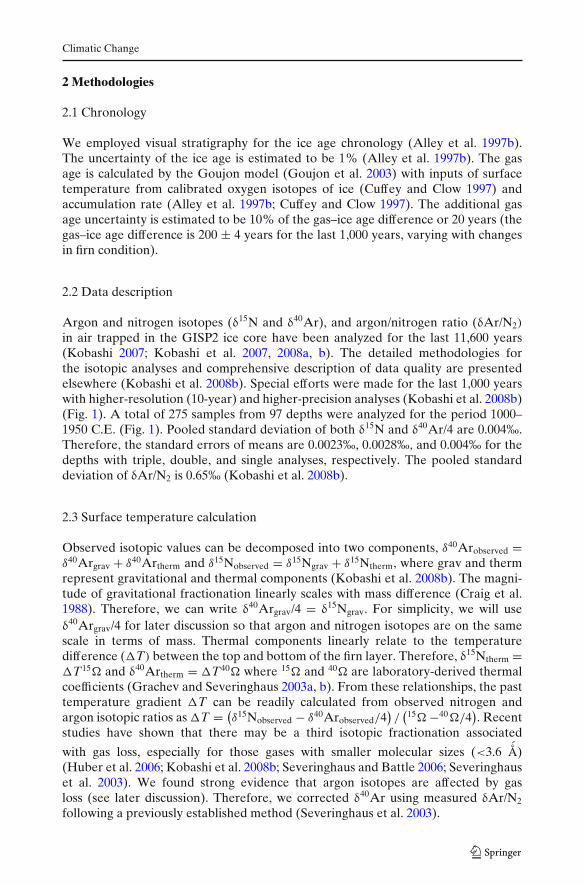
Argon and nitrogen isotopes (δ15N and δ40Ar), and argon/nitrogen ratio (δAr/N2)

in air trapped in the GISP2 ice core have been analyzed for the last 11,600 years(Kobashi 2007; Kobashi et al. 2007, 2008a, b). The detailed methodologies forthe isotopic analyses and comprehensive description of data quality are presentedelsewhere (Kobashi et al. 2008b). Special efforts were made for the last 1,000 yearswith higher-resolution (10-year) and higher-precision analyses (Kobashi et al. 2008b)(Fig. 1). A total of 275 samples from 97 depths were analyzed for the period 1000–1950 C.E. (Fig. 1). Pooled standard deviation of both δ15N and δ40Ar/4 are 0.004‰.Therefore, the standard errors of means are 0.0023‰, 0.0028‰, and 0.004‰ for thedepths with triple, double, and single analyses, respectively. The pooled standarddeviation of δAr/N2 is 0.65‰ (Kobashi et al. 2008b).

2.3 Surface temperature calculation

Observed isotopic values can be decomposed into two components, δ40Arobserved =δ40Argrav + δ40Artherm and δ15Nobserved = δ15Ngrav + δ15Ntherm, where grav and thermrepresent gravitational and thermal components (Kobashi et al. 2008b). The magni-tude of gravitational fractionation linearly scales with mass difference (Craig et al.1988). Therefore, we can write δ40Argrav/4 = δ15Ngrav. For simplicity, we will useδ40Argrav/4 for later discussion so that argon and nitrogen isotopes are on the samescale in terms of mass. Thermal components linearly relate to the temperaturedifference (�T) between the top and bottom of the firn layer. Therefore, δ15Ntherm =�T15� and δ40Artherm = �T40� where 15� and 40� are laboratory-derived thermalcoefficients (Grachev and Severinghaus 2003a, b). From these relationships, the pasttemperature gradient �T can be readily calculated from observed nitrogen andargon isotopic ratios as �T = (

δ15Nobserved − δ40Arobserved/4)/(

15� −40�/4). Recent

studies have shown that there may be a third isotopic fractionation associated

with gas loss, especially for those gases with smaller molecular sizes (<3.6 Å)(Huber et al. 2006; Kobashi et al. 2008b; Severinghaus and Battle 2006; Severinghauset al. 2003). We found strong evidence that argon isotopes are affected by gasloss (see later discussion). Therefore, we corrected δ40Ar using measured δAr/N2

following a previously established method (Severinghaus et al. 2003).

Climatic Change

0.30

0.31

0.32

-4

-3

-2

-1

0

1

2

3

0.31

0.32

0.33

1

2

3

20001000 1200 1400 1600 1800

Years (C.E.)

δ40A

r (‰

)/4

δ15N

(‰

)δA

r/N

2 (‰

)N

umbe

r of

sam

ples

(p

er d

epth

)

Fig. 1 Observed δ15N, δ40Ar, δAr/N2, and number of samples per depth. The circles are means, anderror bars are 1σ standard deviation of replicate samples. Three depths are represented by a singleanalysis, and so are shown only by circles without error bars

Climatic Change

Firn conditions such as densification rate and heat transport are controlled bysnow accumulation and surface temperature change (Goujon et al. 2003; Schwanderet al. 1997). Therefore, it is possible to numerically calculate the past firn conditionwith empirical glaciological models if surface temperature and accumulation rate areknown (Goujon et al. 2003; Schwander et al. 1997). Goujon et al. (2003) developedsuch a model to calculate the past firn condition based on a δ18Oice-derived surfacetemperature calibrated with the borehole temperature record (Alley et al. 1997a;Cuffey and Clow 1997) and accumulation rate (Cuffey and Clow 1997). The modelalso calculates the resultant isotopic fractionation of δ15N and δ40Ar in the firn.Goujon et al. found that the observed δ15N and δ40Ar are reproduced reasonablywell with the δ18O-based temperature for the transition from the last glacial periodto the Holocene in Greenland (Goujon et al. 2003; Kobashi et al. 2008b). The modelis also found to reproduce current firn conditions well over a range of environmentalconditions (Landais et al. 2006). One exception is that the model fails to generatethe observed isotopic signals (δ15N and δ40Ar) at Antarctic sites such as Vostok withvery cold and low accumulation during the last glacial (Goujon et al. 2003; Landaiset al. 2006).

The temperature gradient (�T) in the firn is constantly modified by changes insurface temperature and heat transport in firn and ice. As heat transport in the firnis much slower than gas diffusion, temperature gradient data (�T) derived fromobserved δ15N and δ40Ar can be used to calculate the heat transport in the firn ifcombined with accumulation rate data. Therefore, a surface temperature history canbe calculated from the �T history if the initial temperature profile of the firn and icesheet is known (Kobashi et al. 2008a, b). We used a borehole calibrated δ18Oice-basedsurface temperature record (Cuffey and Clow 1997; Stuiver et al. 1995) to create aninitial temperature profile (Severinghaus and Brook 1999). Actual calculation in themodel is conducted as follows. In a model year, the firn condition is forced by a newsurface temperature and accumulation rate. In the second model year, a new surfacetemperature (Ts) is obtained by adding �T from observed isotopic records to thetemperature (Tb) at the bottom of the firn layer in the previous year model run(Kobashi et al. 2008a, b).

Ts = Tb(model output from the previous model year

) + �T (observation) .

This calculation effectively takes the heat transport into account, and calculates asurface temperature from observed �T and accumulation rate.

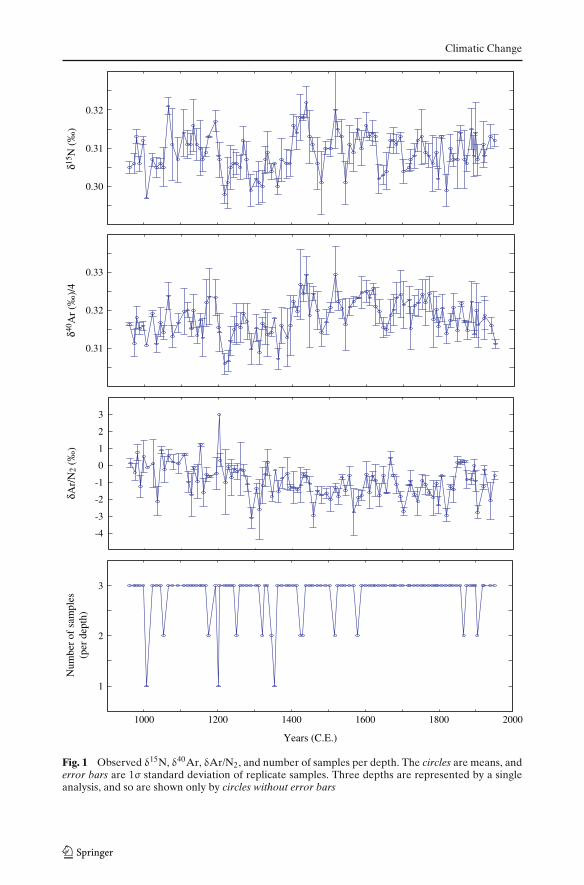
2.4 Surface temperature of the last 50 years

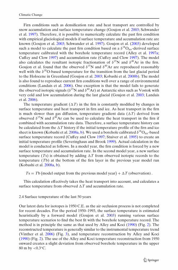
Our latest data for isotopes is 1950 C.E. as the air occlusion process is not completedfor recent decades. For the period 1950–1993, the surface temperature is estimatedheuristically by a forward model (Goujon et al. 2003) running various surfacetemperature scenarios to find the best fit with the borehole temperature record. Themethod is in principle the same as that used by Alley and Koci (1990) (Fig. 2). Thereconstructed temperature is generally similar to the instrumental temperature trend(Vinther et al. 2006) (Fig. 3), and temperature reconstruction by Alley and Koci(1990) (Fig. 2). The use of the Alley and Koci temperature reconstruction from 1950onward creates a slight deviation from observed borehole temperature in the upper80 m by <0.3◦C.

Climatic Change

Fig. 2 Temperaturereconstructions after 1950 byAlley and Koci (1990) (blue)and this study (green). Dottedlines are the ending years ofthe calculations (1989 forAlley and Koci and 1993 forthis study)

1950 1955 1960 1965 1970 1975 1980 1985 1990 1995 2000

-31.5

-31.0

-30.5

-30.0

-29.5

Years (C.E.)

Tem

pera

ture

(ºC

)

Alley and Koci (1990)

This study

2.5 �T-based temperature calculation

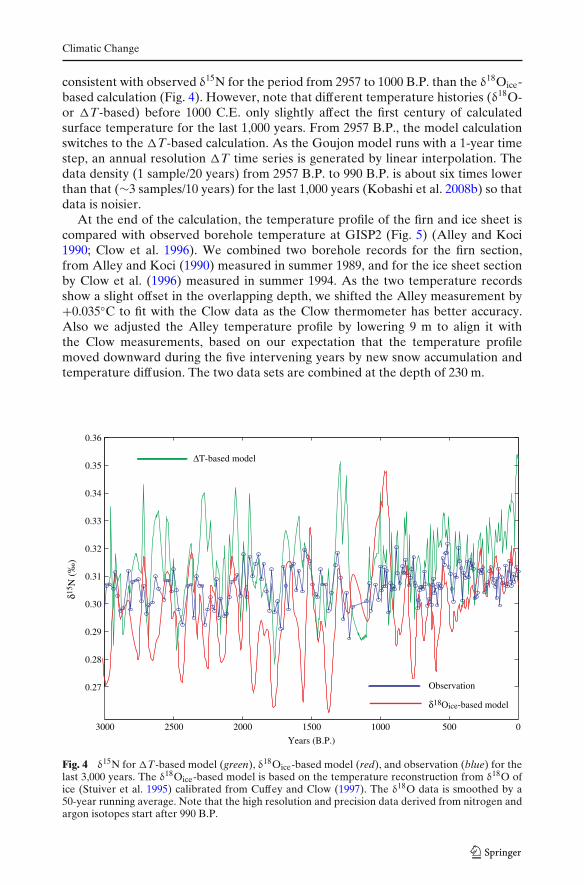
To apply the �T-based surface temperature calculation, a prerequisite is toknow the initial temperature profile of the firn and ice sheet. To accomplish this,we run the model from 24,300 B.P. (Before Present, present is defined as 1950C.E.) until 2957 B.P. with the δ18Oice-based borehole-calibrated surface temperature(Cuffey and Clow 1997; Stuiver et al. 1995). This surface temperature reconstructionis known to be robust for a long-term trend (Goujon et al. 2003; Kobashi et al.2008b). We employ the �T-based surface temperature calculation from 2957 B.P.onward. The �T-based surface temperature calculation produces δ15N results more

Years

Reconstructed tem

perature (ºC)

Obs

evre

d te

mpe

ratu

re (

ºC)

-5

-4

-3

-2

-1

1750 1800 1850 1900 1950 2000

-33

-32

-31

-300

Fig. 3 Observed (blue) and reconstructed (red) Greenland temperature records. The observedrecord is a compilation of records from llulissat, Nuuk, and Qaqurtop located along the south andwest coast of Greenland (Vinther et al. 2006). To smooth the observed data, a 2-year moving averageis applied

Climatic Change

consistent with observed δ15N for the period from 2957 to 1000 B.P. than the δ18Oice-based calculation (Fig. 4). However, note that different temperature histories (δ18O-or �T-based) before 1000 C.E. only slightly affect the first century of calculatedsurface temperature for the last 1,000 years. From 2957 B.P., the model calculationswitches to the �T-based calculation. As the Goujon model runs with a 1-year timestep, an annual resolution �T time series is generated by linear interpolation. Thedata density (1 sample/20 years) from 2957 B.P. to 990 B.P. is about six times lowerthan that (∼3 samples/10 years) for the last 1,000 years (Kobashi et al. 2008b) so thatdata is noisier.

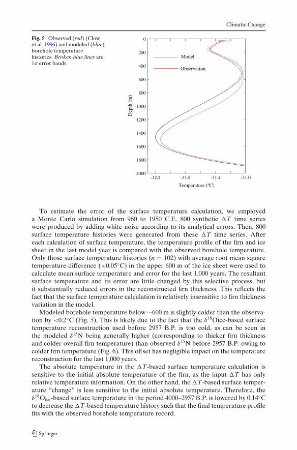
At the end of the calculation, the temperature profile of the firn and ice sheet iscompared with observed borehole temperature at GISP2 (Fig. 5) (Alley and Koci1990; Clow et al. 1996). We combined two borehole records for the firn section,from Alley and Koci (1990) measured in summer 1989, and for the ice sheet sectionby Clow et al. (1996) measured in summer 1994. As the two temperature recordsshow a slight offset in the overlapping depth, we shifted the Alley measurement by+0.035◦C to fit with the Clow data as the Clow thermometer has better accuracy.Also we adjusted the Alley temperature profile by lowering 9 m to align it withthe Clow measurements, based on our expectation that the temperature profilemoved downward during the five intervening years by new snow accumulation andtemperature diffusion. The two data sets are combined at the depth of 230 m.

1000150020002500

0.28

0.29

0.30

0.31

0.32

0.33

0.34

0.35

0.36

3000 0500

Years (B.P.)

δ15 N

(‰

)

0.27 Observation

δ18Oice-based model

ΔT-based model

Fig. 4 δ15N for �T-based model (green), δ18Oice-based model (red), and observation (blue) for thelast 3,000 years. The δ18Oice-based model is based on the temperature reconstruction from δ18O ofice (Stuiver et al. 1995) calibrated from Cuffey and Clow (1997). The δ18O data is smoothed by a50-year running average. Note that the high resolution and precision data derived from nitrogen andargon isotopes start after 990 B.P.

Climatic Change

Fig. 5 Observed (red) (Clowet al. 1996) and modeled (blue)borehole temperaturehistories. Broken blue lines are1σ error bands

0

200

400

600

800

1000

1200

1400

1600

1800

2000

Temperature (ºC)

Dep

th (

m)

Model

Observation

-32.2 -31.8 -31.4 -31.0

To estimate the error of the surface temperature calculation, we employeda Monte Carlo simulation from 960 to 1950 C.E. 800 synthetic �T time serieswere produced by adding white noise according to its analytical errors. Then, 800surface temperature histories were generated from these �T time series. Aftereach calculation of surface temperature, the temperature profile of the firn and icesheet in the last model year is compared with the observed borehole temperature.Only those surface temperature histories (n = 102) with average root mean squaretemperature difference (<0.05◦C) in the upper 600 m of the ice sheet were used tocalculate mean surface temperature and error for the last 1,000 years. The resultantsurface temperature and its error are little changed by this selective process, butit substantially reduced errors in the reconstructed firn thickness. This reflects thefact that the surface temperature calculation is relatively insensitive to firn thicknessvariation in the model.

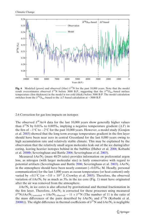
Modeled borehole temperature below ∼600 m is slightly colder than the observa-tion by <0.2◦C (Fig. 5). This is likely due to the fact that the δ18Oice-based surfacetemperature reconstruction used before 2957 B.P. is too cold, as can be seen inthe modeled δ15N being generally higher (corresponding to thicker firn thicknessand colder overall firn temperature) than observed δ15N before 2957 B.P. owing tocolder firn temperature (Fig. 6). This offset has negligible impact on the temperaturereconstruction for the last 1,000 years.

The absolute temperature in the �T-based surface temperature calculation issensitive to the initial absolute temperature of the firn, as the input �T has onlyrelative temperature information. On the other hand, the �T-based surface temper-ature “change” is less sensitive to the initial absolute temperature. Therefore, theδ18Oice-based surface temperature in the period 4000–2957 B.P. is lowered by 0.14◦Cto decrease the �T-based temperature history such that the final temperature profilefits with the observed borehole temperature record.

Climatic Change

δ15 N

(‰

)

10002000300040005000600070008000900010000

0.28

0.29

0.30

0.31

0.32

0.33

0.34

0.35

0.36

0

Years (B.P.)

Observation

Model

ΔT-basedδ18Oice-based

Fig. 6 Modeled (green) and observed (blue) δ15N for the past 10,000 years. Note that the modelresult overestimates observed δ15N before 3000 B.P., suggesting that the δ18Oice-based surfacetemperature (firn thickness) in the model is too cold (thick) before 3000 B.P. The model calculationswitches from the δ18Oice-based to the �T-based calculation at ∼3000 B.P.

2.6 Correction for gas loss impacts on isotopes

The observed δ40Ar/4 data for the last 10,000 years show generally higher valuesthan δ15N by 0.01‰ to 0.005‰, implying a negative temperature gradient (�T) inthe firn of −1◦C to −2◦C for the past 10,000 years. However, a model study (Goujonet al. 2003) showed that the long term average temperature gradient in the firn layershould have been near zero in central Greenland for the last 8,000 years owing tohigh accumulation rate and relatively stable climate. This may be explained by theobservation that the relatively small argon molecules leak out of the ice during/aftercoring, leaving heavier isotopes behind in the bubbles (Huber et al. 2006; Kobashiet al. 2008b; Severinghaus and Battle 2006; Severinghaus et al. 2003).

Measured δAr/N2 (mass 40/29 ratio) provides information on preferential argonloss, as nitrogen (with larger molecular size) is fairly conservative with regard topotential artifacts (Severinghaus and Battle 2006; Severinghaus et al. 2003). δAr/N2

in the atmosphere should have been nearly constant (<0.03‰; M. Headly, personalcommunication) for the last 1,000 years as ocean temperature (or heat content) onlyvaried by <0.1◦C (or ∼5.0 × 1023 J; Crowley et al. 2003). Therefore, the observedvariation of δAr/N2 by as much as 3‰ in the ice core (Fig. 1) must have originatedafter the air was removed from the atmosphere.

δAr/N2 in ice cores is also affected by gravitational and thermal fractionation inthe firn layer. Therefore, δAr/N2 is corrected for these processes using measuredδ15N:δAr/N2 corrected = δAr/N2 observed − 11 × δ15N (The number of 11 is the ratio ofthe mass differences of the pairs described by δAr/N2 and δ15N (Kobashi et al.2008b)). The slight difference in thermal coefficients of δ15N and δAr/N2 is negligible

Climatic Change

1000150020002500

-6

-5

-4

-3

-2

-1

0

1

500 03000

Years (B.P.)

Cor

rect

ed δ

Ar/

N2

(‰)

Fig. 7 Gas-loss-corrected δAr/N2. Note the decrease in mean value around 1000 C.E. from −3‰ to−5‰, suggesting that argon loss was more extensive for shallower ice

for the purpose of this correction. The corrected δAr/N2 is used as an indicator ofargon loss.

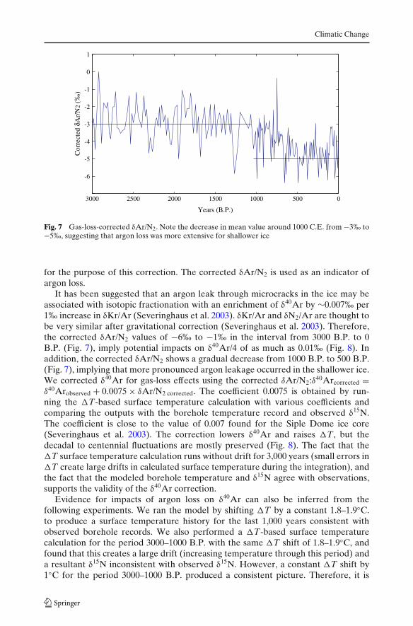
It has been suggested that an argon leak through microcracks in the ice may beassociated with isotopic fractionation with an enrichment of δ40Ar by ∼0.007‰ per1‰ increase in δKr/Ar (Severinghaus et al. 2003). δKr/Ar and δN2/Ar are thought tobe very similar after gravitational correction (Severinghaus et al. 2003). Therefore,the corrected δAr/N2 values of −6‰ to −1‰ in the interval from 3000 B.P. to 0B.P. (Fig. 7), imply potential impacts on δ40Ar/4 of as much as 0.01‰ (Fig. 8). Inaddition, the corrected δAr/N2 shows a gradual decrease from 1000 B.P. to 500 B.P.(Fig. 7), implying that more pronounced argon leakage occurred in the shallower ice.We corrected δ40Ar for gas-loss effects using the corrected δAr/N2:δ40Arcorrected =δ40Arobserved + 0.0075 × δAr/N2 corrected. The coefficient 0.0075 is obtained by run-ning the �T-based surface temperature calculation with various coefficients andcomparing the outputs with the borehole temperature record and observed δ15N.The coefficient is close to the value of 0.007 found for the Siple Dome ice core(Severinghaus et al. 2003). The correction lowers δ40Ar and raises �T, but thedecadal to centennial fluctuations are mostly preserved (Fig. 8). The fact that the�T surface temperature calculation runs without drift for 3,000 years (small errors in�T create large drifts in calculated surface temperature during the integration), andthe fact that the modeled borehole temperature and δ15N agree with observations,supports the validity of the δ40Ar correction.

Evidence for impacts of argon loss on δ40Ar can also be inferred from thefollowing experiments. We ran the model by shifting �T by a constant 1.8–1.9◦C.to produce a surface temperature history for the last 1,000 years consistent withobserved borehole records. We also performed a �T-based surface temperaturecalculation for the period 3000–1000 B.P. with the same �T shift of 1.8–1.9◦C, andfound that this creates a large drift (increasing temperature through this period) anda resultant δ15N inconsistent with observed δ15N. However, a constant �T shift by1◦C for the period 3000–1000 B.P. produced a consistent picture. Therefore, it is

Climatic Change

0.30

0.31

0.32

0.33

Years (C.E.)

δ 40Ar/4 (‰

)

Raw

Corrected

1000 1100 1200 1300 1400 1500 1600 1700 1800 1900 2000

-3

-2

-1

0

1

ΔT (º

C)

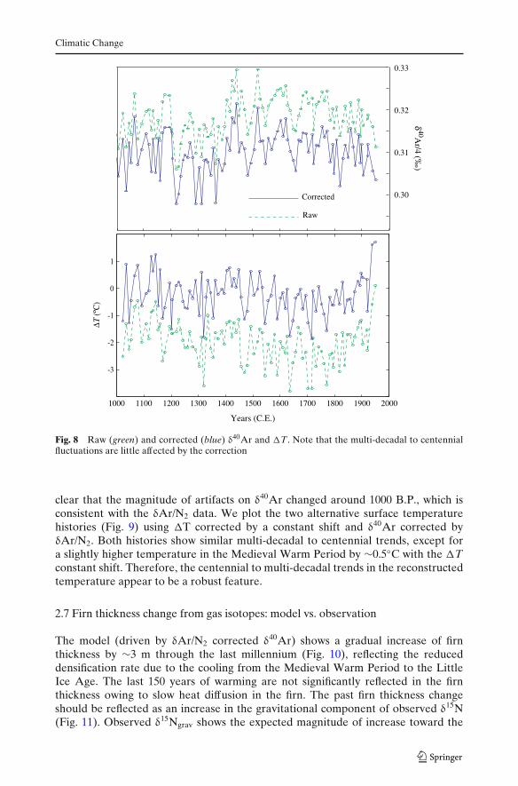
Fig. 8 Raw (green) and corrected (blue) δ40Ar and �T. Note that the multi-decadal to centennialfluctuations are little affected by the correction

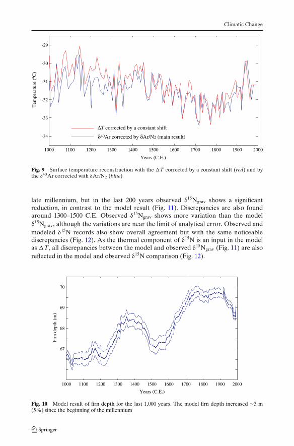
clear that the magnitude of artifacts on δ40Ar changed around 1000 B.P., which isconsistent with the δAr/N2 data. We plot the two alternative surface temperaturehistories (Fig. 9) using �T corrected by a constant shift and δ40Ar corrected byδAr/N2. Both histories show similar multi-decadal to centennial trends, except fora slightly higher temperature in the Medieval Warm Period by ∼0.5◦C with the �Tconstant shift. Therefore, the centennial to multi-decadal trends in the reconstructedtemperature appear to be a robust feature.

2.7 Firn thickness change from gas isotopes: model vs. observation

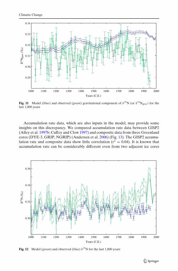
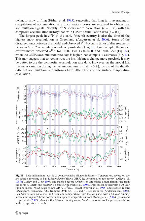
The model (driven by δAr/N2 corrected δ40Ar) shows a gradual increase of firnthickness by ∼3 m through the last millennium (Fig. 10), reflecting the reduceddensification rate due to the cooling from the Medieval Warm Period to the LittleIce Age. The last 150 years of warming are not significantly reflected in the firnthickness owing to slow heat diffusion in the firn. The past firn thickness changeshould be reflected as an increase in the gravitational component of observed δ15N(Fig. 11). Observed δ15Ngrav shows the expected magnitude of increase toward the

Climatic Change

1000 1100 1200 1300 1400 1500 1600 1700 1800 1900 2000

Years (C.E.)

-33

-32

-31

-30

-29

Tem

pera

ture

(ºC

)

-34

ΔT corrected by a constant shift

δ40Ar corrected by δAr/N2 (main result)

Fig. 9 Surface temperature reconstruction with the �T corrected by a constant shift (red) and bythe δ40Ar corrected with δAr/N2 (blue)

late millennium, but in the last 200 years observed δ15Ngrav shows a significantreduction, in contrast to the model result (Fig. 11). Discrepancies are also foundaround 1300–1500 C.E. Observed δ15Ngrav shows more variation than the modelδ15Ngrav, although the variations are near the limit of analytical error. Observed andmodeled δ15N records also show overall agreement but with the same noticeablediscrepancies (Fig. 12). As the thermal component of δ15N is an input in the modelas �T, all discrepancies between the model and observed δ15Ngrav (Fig. 11) are alsoreflected in the model and observed δ15N comparison (Fig. 12).

1000 1100 1200 1300 1400 1500 1600 1700 1800 1900 2000

67

68

69

70

Firn

dep

th (

m)

Years (C.E.)

Fig. 10 Model result of firn depth for the last 1,000 years. The model firn depth increased ∼3 m(5%) since the beginning of the millennium

Climatic Change

1000 1100 1200 1300 1400 1500 1600 1700 1800 1900 2000

Years (C.E.)

δ15 N

grav

(‰

)

0.29

0.30

0.31

0.32

0.33

0.34

Fig. 11 Model (blue) and observed (green) gravitational component of δ15N (or δ15Ngrav) for thelast 1,000 years

Accumulation rate data, which are also inputs in the model, may provide someinsights on this discrepancy. We compared accumulation rate data between GISP2(Alley et al. 1997b; Cuffey and Clow 1997) and composite data from three Greenlandcores (DYE-3, GRIP, NGRIP) (Andersen et al. 2006) (Fig. 13). The GISP2 accumu-lation rate and composite data show little correlation (r2 = 0.04). It is known thataccumulation rate can be considerably different even from two adjacent ice cores

1000 1100 1200 1300 1400 1500 1600 1700 1800 1900 2000

Years (C.E.)

0.30

0.32

0.34

0.36

δ15 N

(‰

)

Fig. 12 Model (green) and observed (blue) δ15N for the last 1,000 years

Climatic Change

owing to snow drifting (Fisher et al. 1985), suggesting that long term averaging orcompilation of accumulation rate from various cores are required to obtain realaccumulation signals. Notably, δ15N shows more correlation (r = 0.36) with thecomposite accumulation history than with GISP2 accumulation data (r = 0.1).

The largest peak in δ15N in the early fifteenth century is also the time of thehighest snow accumulation in Greenland (Andersen et al. 2006). Some of thedisagreements between the model and observed δ15N occur in times of disagreementsbetween GISP2 accumulation and composite data (Fig. 13). For example, the modeloverestimates observed δ15N for 1100–1150, 1300–1400, and 1600–1750 (Fig. 12),when the GISP2 accumulation rate data is higher than composite estimates (Fig. 13).This may suggest that to reconstruct the firn thickness change more precisely it maybe better to use the composite accumulation rate data. However, as the model firnthickness variation during the last millennium is small (<5%), the use of the slightlydifferent accumulation rate histories have little effects on the surface temperaturecalculation.

-34-33-32-31-30-29

Tem

pera

ture

(ºC

)

0.22

0.24

0.26

-35.0

-34.0

-35.5

-34.5

GIS

P2 δ

18O

ice

(‰)

GIS

P2 A

ccum

ulat

ion

rate

(m

/yr)

0.92

0.96

1.00

1.04

1.08

-0.4

-0.2

0.0

0.2

0.4

δ18O

ice anomaly (‰

)N

ormalized

accumulation rate

1000 1100 1200 1300 1400 1500 1600 1700 1800 1900 2000Years (A.D.)

-0.8

-0.6

-0.4

-0.2

0.0

N. H

emis

pher

ic

tem

pera

ture

. (ºC

)

-32

-31

-30

Greenland

temperature (ºC

)

Fig. 13 Last-millennium records of comprehensive climate indicators. Temperature record on thetop panel is the same as Fig. 1. Second panel shows GISP2 ice accumulation rate (green) (Alley et al.1997b; Cuffey and Clow 1997) and stacked record (black) for Greenland accumulation rate fromthe DYE-3, GRIP, and NGRIP ice cores (Andersen et al. 2006). Data are smoothed with a 20-yearrunning mean. Third panel shows GISP2 δ18Oice (green) (Stuiver et al. 1995) and stacked record(black) for Greenland δ18Oice from the DYE-3, GRIP, and NGRIP ice cores (Andersen et al. 2006).Red lines in each panel are the Greenland temperature from the top panel with a 50-year runningmean. Fourth panel shows northern hemisphere temperatures from Moberg et al. (2005) (green) andHegerl et al. (2007) (black) with a 20-year running mean. Shaded areas are cooler periods as shownin the temperature records

Climatic Change

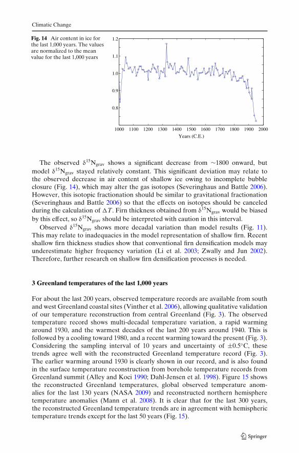
Fig. 14 Air content in ice forthe last 1,000 years. The valuesare normalized to the meanvalue for the last 1,000 years

1000 1100 1200 1300 1400 1500 1600 1700 1800 1900 2000

0.8

0.9

1.0

1.1

1.2

Years (C.E.)

The observed δ15Ngrav shows a significant decrease from ∼1800 onward, butmodel δ15Ngrav stayed relatively constant. This significant deviation may relate tothe observed decrease in air content of shallow ice owing to incomplete bubbleclosure (Fig. 14), which may alter the gas isotopes (Severinghaus and Battle 2006).However, this isotopic fractionation should be similar to gravitational fractionation(Severinghaus and Battle 2006) so that the effects on isotopes should be canceledduring the calculation of �T. Firn thickness obtained from δ15Ngrav would be biasedby this effect, so δ15Ngrav should be interpreted with caution in this interval.

Observed δ15Ngrav shows more decadal variation than model results (Fig. 11).This may relate to inadequacies in the model representation of shallow firn. Recentshallow firn thickness studies show that conventional firn densification models mayunderestimate higher frequency variation (Li et al. 2003; Zwally and Jun 2002).Therefore, further research on shallow firn densification processes is needed.

3 Greenland temperatures of the last 1,000 years

For about the last 200 years, observed temperature records are available from southand west Greenland coastal sites (Vinther et al. 2006), allowing qualitative validationof our temperature reconstruction from central Greenland (Fig. 3). The observedtemperature record shows multi-decadal temperature variation, a rapid warmingaround 1930, and the warmest decades of the last 200 years around 1940. This isfollowed by a cooling toward 1980, and a recent warming toward the present (Fig. 3).Considering the sampling interval of 10 years and uncertainty of ±0.5◦C, thesetrends agree well with the reconstructed Greenland temperature record (Fig. 3).The earlier warming around 1930 is clearly shown in our record, and is also foundin the surface temperature reconstruction from borehole temperature records fromGreenland summit (Alley and Koci 1990; Dahl-Jensen et al. 1998). Figure 15 showsthe reconstructed Greenland temperatures, global observed temperature anom-alies for the last 130 years (NASA 2009) and reconstructed northern hemispheretemperature anomalies (Mann et al. 2008). It is clear that for the last 300 years,the reconstructed Greenland temperature trends are in agreement with hemispherictemperature trends except for the last 50 years (Fig. 15).

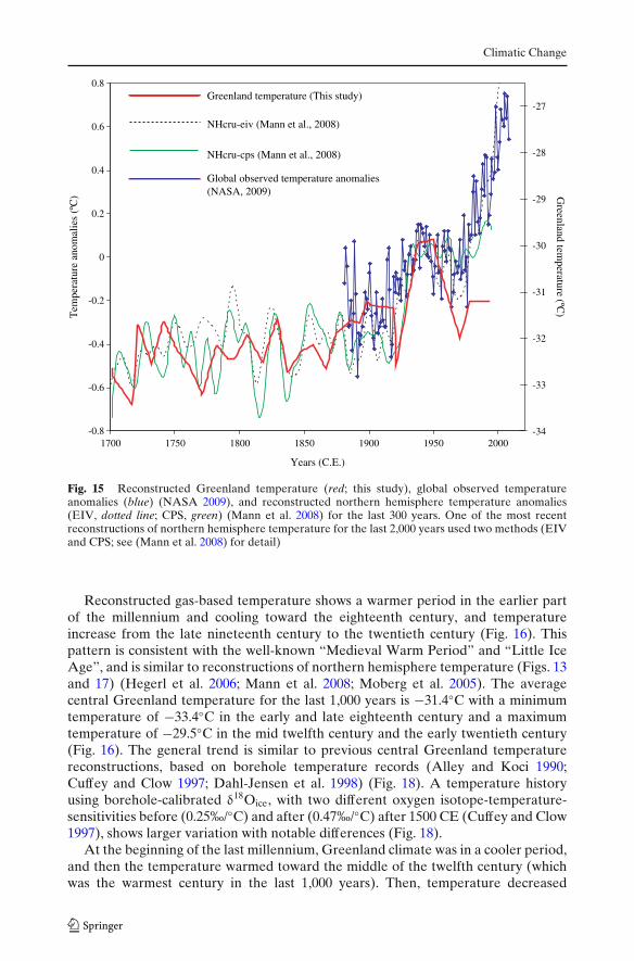
Climatic Change

-0.8

-0.6

-0.4

-0.2

0

0.2

0.4

0.6

0.8

1700 1750 1800 1850 1900 1950 2000-34

-33

-32

-31

-30

-29

-28

-27

NHcru-eiv (Mann et al., 2008)

Global observed temperature anomalies (NASA, 2009)

NHcru-cps (Mann et al., 2008)

Greenland temperature (This study)

Years (C.E.)

Tem

pera

ture

ano

mal

ies

(ºC

) Greenland tem

perature (ºC)

Fig. 15 Reconstructed Greenland temperature (red; this study), global observed temperatureanomalies (blue) (NASA 2009), and reconstructed northern hemisphere temperature anomalies(EIV, dotted line; CPS, green) (Mann et al. 2008) for the last 300 years. One of the most recentreconstructions of northern hemisphere temperature for the last 2,000 years used two methods (EIVand CPS; see (Mann et al. 2008) for detail)

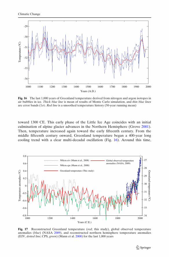
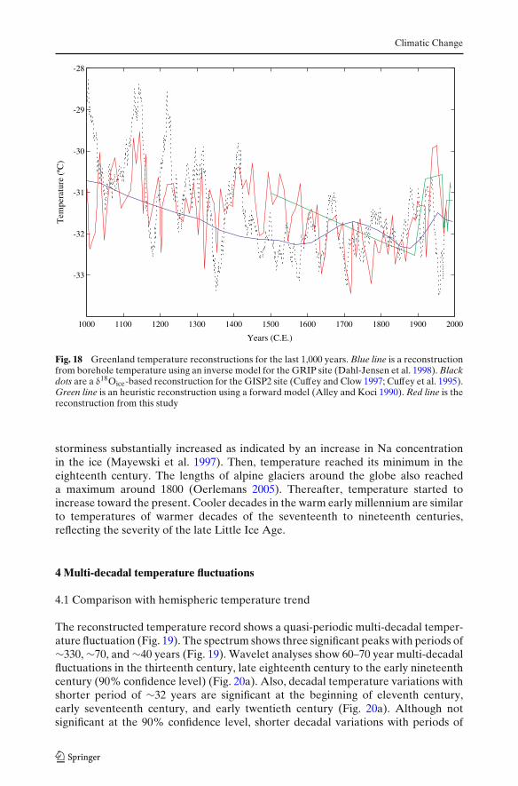
Reconstructed gas-based temperature shows a warmer period in the earlier partof the millennium and cooling toward the eighteenth century, and temperatureincrease from the late nineteenth century to the twentieth century (Fig. 16). Thispattern is consistent with the well-known “Medieval Warm Period” and “Little IceAge”, and is similar to reconstructions of northern hemisphere temperature (Figs. 13and 17) (Hegerl et al. 2006; Mann et al. 2008; Moberg et al. 2005). The averagecentral Greenland temperature for the last 1,000 years is −31.4◦C with a minimumtemperature of −33.4◦C in the early and late eighteenth century and a maximumtemperature of −29.5◦C in the mid twelfth century and the early twentieth century(Fig. 16). The general trend is similar to previous central Greenland temperaturereconstructions, based on borehole temperature records (Alley and Koci 1990;Cuffey and Clow 1997; Dahl-Jensen et al. 1998) (Fig. 18). A temperature historyusing borehole-calibrated δ18Oice, with two different oxygen isotope-temperature-sensitivities before (0.25‰/◦C) and after (0.47‰/◦C) after 1500 CE (Cuffey and Clow1997), shows larger variation with notable differences (Fig. 18).

At the beginning of the last millennium, Greenland climate was in a cooler period,and then the temperature warmed toward the middle of the twelfth century (whichwas the warmest century in the last 1,000 years). Then, temperature decreased

Climatic Change

1000 1100 1200 1300 1400 1500 1600 1700 1800 1900 2000

Years (A.D.)

-33

-32

-31

-30

-29

Tem

pera

ture

(ºC

)

-34

Fig. 16 The last 1,000 years of Greenland temperature derived from nitrogen and argon isotopes inair bubbles in ice. Thick blue line is mean of results of Monte Carlo simulation, and thin blue linesare error bands (1σ). Red line is a smoothed temperature history (50-year running mean)

toward 1300 CE. This early phase of the Little Ice Age coincides with an initialculmination of alpine glacier advances in the Northern Hemisphere (Grove 2001).Then, temperature increased again toward the early fifteenth century. From themiddle fifteenth century onward, Greenland temperature began a 400-year longcooling trend with a clear multi-decadal oscillation (Fig. 16). Around this time,

-0.8

-0.6

-0.4

0

0.2

0.4

0.6

0.8

1000 1200 1400 1600 1800 2000-34

-33

-32

-31

-30

-29

-28

-27

-0.5

NHcru-eiv (Mann et al., 2008) Global observed temperature anomalies (NASA, 2009)

NHcru-cps (Mann et al., 2008)

Greenland temperature (This study)

Years (C.E.)

Tem

pera

ture

ano

mal

ies

(ºC

) Greenland tem

perature (ºC)

Fig. 17 Reconstructed Greenland temperature (red; this study), global observed temperatureanomalies (blue) (NASA 2009), and reconstructed northern hemisphere temperature anomalies(EIV, dotted line; CPS, green) (Mann et al. 2008) for the last 1,000 years

Climatic Change

1000 1100 1200 1300 1400 1500 1600 1700 1800 1900 2000

Years (C.E.)

Tem

pera

ture

(ºC

)

-33

-32

-31

-30

-29

-28

Fig. 18 Greenland temperature reconstructions for the last 1,000 years. Blue line is a reconstructionfrom borehole temperature using an inverse model for the GRIP site (Dahl-Jensen et al. 1998). Blackdots are a δ18Oice-based reconstruction for the GISP2 site (Cuffey and Clow 1997; Cuffey et al. 1995).Green line is an heuristic reconstruction using a forward model (Alley and Koci 1990). Red line is thereconstruction from this study

storminess substantially increased as indicated by an increase in Na concentrationin the ice (Mayewski et al. 1997). Then, temperature reached its minimum in theeighteenth century. The lengths of alpine glaciers around the globe also reacheda maximum around 1800 (Oerlemans 2005). Thereafter, temperature started toincrease toward the present. Cooler decades in the warm early millennium are similarto temperatures of warmer decades of the seventeenth to nineteenth centuries,reflecting the severity of the late Little Ice Age.

4 Multi-decadal temperature fluctuations

4.1 Comparison with hemispheric temperature trend

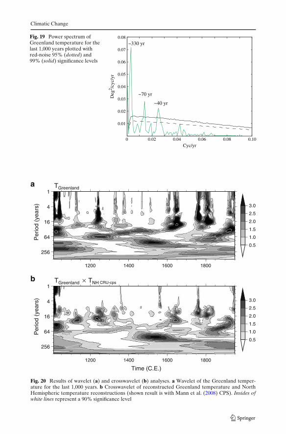
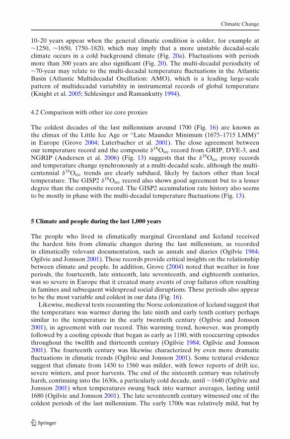
The reconstructed temperature record shows a quasi-periodic multi-decadal temper-ature fluctuation (Fig. 19). The spectrum shows three significant peaks with periods of∼330, ∼70, and ∼40 years (Fig. 19). Wavelet analyses show 60–70 year multi-decadalfluctuations in the thirteenth century, late eighteenth century to the early nineteenthcentury (90% confidence level) (Fig. 20a). Also, decadal temperature variations withshorter period of ∼32 years are significant at the beginning of eleventh century,early seventeenth century, and early twentieth century (Fig. 20a). Although notsignificant at the 90% confidence level, shorter decadal variations with periods of

Climatic Change

Fig. 19 Power spectrum ofGreenland temperature for thelast 1,000 years plotted withred-noise 95% (dotted) and99% (solid) significance levels

0 0.02 0.04 0.06 0.08 0.10

0.01

0.02

0.03

0.04

0.05

0.06

0.07

0.08

Cyc/yr

Deg

2 /cyc

/yr

~40 yr

~70 yr

~330 yr

1200 1400 1600 1800

0.5

1.0

1.5

2.0

2.5

3.0

1

4

16

64

256

Per

iod

(yea

rs)

TGreenland

1200 1400 1600 1800

0.5

1.0

1.5

2.0

2.5

3.0

1

4

16

64

256

Per

iod

(yea

rs)

CRU-cpsTGreenland TNH×

Time (C.E.)

a

b

Fig. 20 Results of wavelet (a) and crosswavelet (b) analyses. a Wavelet of the Greenland temper-ature for the last 1,000 years. b Crosswavelet of reconstructed Greenland temperature and NorthHemispheric temperature reconstructions (shown result is with Mann et al. (2008) CPS). Insides ofwhite lines represent a 90% significance level

Climatic Change

10–20 years appear when the general climatic condition is colder, for example at∼1250, ∼1650, 1750–1820, which may imply that a more unstable decadal-scaleclimate occurs in a cold background climate (Fig. 20a). Fluctuations with periodsmore than 300 years are also significant (Fig. 20). The multi-decadal periodicity of∼70-year may relate to the multi-decadal temperature fluctuations in the AtlanticBasin (Atlantic Multidecadal Oscillation: AMO), which is a leading large-scalepattern of multidecadal variability in instrumental records of global temperature(Knight et al. 2005; Schlesinger and Ramankutty 1994).

4.2 Comparison with other ice core proxies

The coldest decades of the last millennium around 1700 (Fig. 16) are known asthe climax of the Little Ice Age or “Late Maunder Minimum (1675–1715 LMM)”in Europe (Grove 2004; Luterbacher et al. 2001). The close agreement betweenour temperature record and the composite δ18Oice record from GRIP, DYE-3, andNGRIP (Andersen et al. 2006) (Fig. 13) suggests that the δ18Oice proxy recordsand temperature change synchronously at a multi-decadal scale, although the multi-centennial δ18Oice trends are clearly subdued, likely by factors other than localtemperature. The GISP2 δ18Oice record also shows good agreement but to a lesserdegree than the composite record. The GISP2 accumulation rate history also seemsto be mostly in phase with the multi-decadal temperature fluctuations (Fig. 13).

5 Climate and people during the last 1,000 years

The people who lived in climatically marginal Greenland and Iceland receivedthe hardest hits from climatic changes during the last millennium, as recordedin climatically relevant documentation, such as annals and diaries (Ogilvie 1984;Ogilvie and Jonsson 2001). These records provide critical insights on the relationshipbetween climate and people. In addition, Grove (2004) noted that weather in fourperiods, the fourteenth, late sixteenth, late seventeenth, and eighteenth centuries,was so severe in Europe that it created many events of crop failures often resultingin famines and subsequent widespread social disruptions. These periods also appearto be the most variable and coldest in our data (Fig. 16).

Likewise, medieval texts recounting the Norse colonization of Iceland suggest thatthe temperature was warmer during the late ninth and early tenth century perhapssimilar to the temperature in the early twentieth century (Ogilvie and Jonsson2001), in agreement with our record. This warming trend, however, was promptlyfollowed by a cooling episode that began as early as 1180, with reoccurring episodesthroughout the twelfth and thirteenth century (Ogilvie 1984; Ogilvie and Jonsson2001). The fourteenth century was likewise characterized by even more dramaticfluctuations in climatic trends (Ogilvie and Jonsson 2001). Some textural evidencesuggest that climate from 1430 to 1560 was milder, with fewer reports of drift ice,severe winters, and poor harvests. The end of the sixteenth century was relativelyharsh, continuing into the 1630s, a particularly cold decade, until ∼1640 (Ogilvie andJonsson 2001) when temperatures swung back into warmer averages, lasting until1680 (Ogilvie and Jonsson 2001). The late seventeenth century witnessed one of thecoldest periods of the last millennium. The early 1700s was relatively mild, but by

Climatic Change

the 1740s and into 1750s the average temperature was quite low. The 1760s to 1770sonce again saw a return to milder climate (Ogilvie and Jonsson 2001), only to befollowed by the 1780s, the coldest decade in the eighteenth century (Ogilvie andJonsson 2001). Perhaps not surprisingly, the Icelandic glaciers reached their Little IceAge maxima during the eighteenth century (Grove 2004). The 1810s, 1830s, 1860s,and 1880s were comparatively cold, but the middle nineteenth century was relativelymild (Ogilvie and Jonsson 2001). Although some of the descriptions are beyond ouruncertainty, the general trends from historical documents agree with our data quitewell (Fig. 16).

6 Northern hemispheric and Greenland temperatures

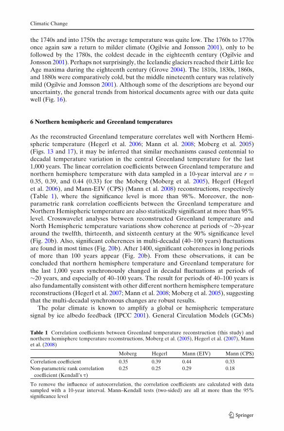
As the reconstructed Greenland temperature correlates well with Northern Hemi-spheric temperature (Hegerl et al. 2006; Mann et al. 2008; Moberg et al. 2005)(Figs. 13 and 17), it may be inferred that similar mechanisms caused centennial todecadal temperature variation in the central Greenland temperature for the last1,000 years. The linear correlation coefficients between Greenland temperature andnorthern hemisphere temperature with data sampled in a 10-year interval are r =0.35, 0.39, and 0.44 (0.33) for the Moberg (Moberg et al. 2005), Hegerl (Hegerlet al. 2006), and Mann-EIV (CPS) (Mann et al. 2008) reconstructions, respectively(Table 1), where the significance level is more than 98%. Moreover, the non-parametric rank correlation coefficients between the Greenland temperature andNorthern Hemispheric temperature are also statistically significant at more than 95%level. Crosswavelet analyses between reconstructed Greenland temperature andNorth Hemispheric temperature variations show coherence at periods of ∼20-yeararound the twelfth, thirteenth, and sixteenth century at the 90% significance level(Fig. 20b). Also, significant coherences in multi-decadal (40–100 years) fluctuationsare found in most times (Fig. 20b). After 1400, significant coherences in long periodsof more than 100 years appear (Fig. 20b). From these observations, it can beconcluded that northern hemisphere temperature and Greenland temperature forthe last 1,000 years synchronously changed in decadal fluctuations at periods of∼20 years, and especially of 40–100 years. The result for periods of 40–100 years isalso fundamentally consistent with other different northern hemisphere temperaturereconstructions (Hegerl et al. 2007; Mann et al. 2008; Moberg et al. 2005), suggestingthat the multi-decadal synchronous changes are robust results.

The polar climate is known to amplify a global or hemispheric temperaturesignal by ice albedo feedback (IPCC 2001). General Circulation Models (GCMs)

Table 1 Correlation coefficients between Greenland temperature reconstruction (this study) andnorthern hemisphere temperature reconstructions, Moberg et al. (2005), Hegerl et al. (2007), Mannet al. (2008)

Moberg Hegerl Mann (EIV) Mann (CPS)

Correlation coefficient 0.35 0.39 0.44 0.33Non-parametric rank correlation 0.25 0.25 0.29 0.18

coefficient (Kendall’s τ)

To remove the influence of autocorrelation, the correlation coefficients are calculated with datasampled with a 10-year interval. Mann–Kendall tests (two-sided) are all at more than the 95%significance level

Climatic Change

find that warming of polar regions will progress at a rate 1.2 to 3 times fasterthan the global average (IPCC 2001). Using our data, the ratio of Greenland toNorthern Hemisphere temperature change for the last 1,000 years is 2.3 with theHegerl reconstruction, 1.4 with the Moberg reconstruction, and 1.5 with the Mannreconstructions. These ratios are comparable to the GCM results (IPCC 2001) andthe ratio of 2.2 found from instrumental records (Chylek and Lohmann 2005). Thisconfirms that despite the recent departure in Northern Hemisphere and Greenlandtemperature trends, the future Greenland temperature will likely follow the globaltemperature trend with an amplified magnitude.

Changes in solar irradiance and volcanism can explain as much as 41 to 64%of variation of Northern Hemispheric temperature (Crowley 2000). The strongcorrelation between Greenland and Northern Hemisphere temperature suggests acommon causation. Energy balance model results with solar and volcanic forcingproduce the general trend we see in the Greenland temperature record, including thecool eleventh, thirteenth, and fourteenth centuries, the warm twelfth, fourteenth, andtwentieth centuries, and the cold seventeenth and nineteenth centuries. Therefore, itis clear that current and future climate change in Greenland is going to be affectedby these natural variations in addition to increasing human-made greenhouse gases(Crowley 2000; IPCC 2001). Projections of future Greenland temperature thus musttake these natural variations into account.

7 Conclusions

We present a new Greenland temperature record for the past 1,000 years based uponargon and nitrogen isotopes in trapped air in ice. The data show clear evidence of theMedieval Warm Period and Little Ice Age in agreement with documentary evidence.The overall trends are similar to northern hemisphere temperature records. Amulti-decadal temperature fluctuation with periods of 40–100 persisted for the lastmillennium, and so will likely continue into the future.

Acknowledgements We thank T. Crowley for reviewing the manuscripts and providing comments.We thank R. Alley, K. Cuffey, G. Clow, J. Ahn, and C. Shuman for the helpful information. Weappreciate the support of R. Beaudette and the staff of the National Ice Core Laboratory (NICL).This work was supported by NSF ATM-9905241.

Open Access This article is distributed under the terms of the Creative Commons AttributionNoncommercial License which permits any noncommercial use, distribution, and reproduction inany medium, provided the original author(s) and source are credited.

References

Allegre CJ, Staudacher T, Sarda P (1987) Rare-gas systematics—formation of the atmosphere,evolution and structure of the earths mantle. Earth Planet Sci Lett 81:127–150

Alley RB, Koci BR (1990) Recent warming in central Greenland? Ann Glaciol 14:6–8Alley RB, Mayewski PA, Sowers T, Stuiver M, Taylor KC, Clark PU (1997a) Holocene climatic

instability: a prominent, widespread event 8200 yr ago. Geology 25:483–486Alley RB, Shuman CA, Meese DA, Gow AJ, Taylor KC, Cuffey KM, Fitzpatrick JJ, Grootes PM,

Zielinski GA, Ram M, Spinelli G, Elder B (1997b) Visual-stratigraphic dating of the GISP2 icecore: basis, reproducibility, and application. J Geophys Res C Oceans 102:26367–26381

Climatic Change

Andersen KK, Ditlevsen PD, Rasmussen SO, Clausen HB, Vinther BM, Johnsen SJ, SteffensenJP (2006) Retrieving a common accumulation record from Greenland ice cores for the past1800 years. J Geophys Res-Atmos. doi:10.1029/2005JD006765

Chylek P, Lohmann U (2005) Ratio of the Greenland to global temperature change: comparison ofobservations and climate modeling results. Geophys Res Lett 32. doi:10.1029/2005GL023552

Clow GD, Saltus RW, Waddington ED (1996) A new high-precision borehole-temperaturelogging system used at GISP2, Greenland, and Taylor Dome, Antarctica. J Glaciol 42:576–584

Craig H, Horibe Y, Sowers T (1988) Gravitational separation of gases and isotopes in polar ice caps.Science 242:1675–1678

Crowley TJ (2000) Causes of climate change over the past 1000 years. Science 289:270–277Crowley TJ, Baum SK, Kim KY, Hegerl GC, Hyde WT (2003) Modeling ocean heat content changes

during the last millennium. Geophys Res Lett 30. doi:10.1029/2003GL017801Cuffey KM, Clow GD (1997) Temperature, accumulation, and ice sheet elevation in central

Greenland through the last deglacial transition. J Geophys Res C Oceans 102:26383–26396Cuffey KM, Clow GD, Alley RB, Stuiver M, Waddington ED, Saltus RW (1995) Large Arctic

temperature-change at the Wisconsin-Holocene glacial transition. Science 270:455–458Dahl-Jensen D, Mosegaard K, Gundestrup N, Clow GD, Johnsen SJ, Hansen AW, Balling N (1998)

Past temperatures directly from the Greenland Ice Sheet. Science 282:268–271Fisher DA, Reeh N, Clausen HB (1985) Stratigraphic noise in time series derived from ice cores.

Ann Glaciol 7:76–83Goujon C, Barnola JM, Ritz C (2003) Modeling the densification of polar firn including heat dif-

fusion: application to close-off characteristics and gas isotopic fractionation for Antarctica andGreenland sites. J Geophys Res-Atmos 108. doi:10.1029/2002JD003319

Grachev AM, Severinghaus JP (2003a) Determining the thermal diffusion factor for Ar-40/Ar-36 inair to aid paleoreconstruction of abrupt climate change. J Phys Chem A 107:4636–4642

Grachev AM, Severinghaus JP (2003b) Laboratory determination of thermal diffusion constants forN-29(2)/N-28(2) in air at temperatures from –60 to 0 degrees C for reconstruction of magnitudesof abrupt climate changes using the ice core fossil-air paleothermometer. Geochim CosmochimActa 67:345–360

Grove JM (2001) The initiation of the “Little Ice Age” in regions round the North Atlantic. ClimChange 48:53–82

Grove JM (2004) Little ice ages: ancient and modern. Routledge, LondonHegerl GC, Crowley TJ, Hyde WT, Frame DJ (2006) Climate sensitivity constrained by temperature

reconstructions over the past seven centuries. Nature 440:1029–1032Hegerl GC, Crowley TJ, Allen M, Hyde WT, Pollack HN, Smerdon J, Zorita E (2007) Detection

of human influence on a new, validated 1500-year temperature reconstruction. J Climate 20:650–666

Huber C, Beyerle U, Leuenberger M, Schwander J, Kipfer R, Spahni R, Severinghaus JP, WeilerK (2006) Evidence for molecular size dependent gas fractionation in firn air derived from noblegases, oxygen, and nitrogen measurements. Earth Planet Sci Lett 243:61–73

IPCC (2001) The scientific basis: contribution of working group I to the third assessment report ofthe intergovermental panel on climate change. Cambridge University Press, Cambridge

Jones PD, Mann ME (2004) Climate over past millennia. Rev Geophys 42. doi:10.1029/2003RG000143

Knight JR, Allan RJ, Folland CK, Vellinga M, Mann ME (2005) A signature of persistentnatural thermohaline circulation cycles in observed climate. Geophys Res Lett 32. doi:10.1029/2005GL024233

Kobashi T (2007) Greenland temperature, climate change, and human society during the last11,600 years. Ph.D. thesis, University of California, San Diego

Kobashi T, Severinghaus J, Brook EJ, Barnola JM, Grachev A (2007) Precise timing and charac-terization of abrupt climate change 8,200 years ago from air trapped in polar ice. Quat Sci Rev26:1212–1222

Kobashi T, Severinghaus JP, Barnola JM (2008a) 4 ± 1.5◦C abrupt warming 11,270 years agoidentified from trapped air in Greenland ice. Earth Planet Sci Lett 268:397–407

Kobashi T, Severinghaus JP, Kawamura K (2008b) Argon and nitrogen isotopes of trapped air in theGISP2 ice core during the Holocene epoch (0–11,600 B.P.): methodology and implications forgas loss processes. Geochim Cosmochim Acta 72:4675–4686

Landais A, Barnola JM, Kawamura K, Caillon N, Delmotte M, Van Ommen T, Dreyfus G, Jouzel J,Masson-Delmotte V, Minster B, Freitag J, Leuenberger M, Schwander J, Huber C, Etheridge D,

Climatic Change

Morgan V (2006) Firn-air delta N-15 in modern polar sites and glacial–interglacial ice: a model-data mismatch during glacial periods in Antarctica? Quat Sci Rev 25:49–62

Li J, Zwally HJ, Cornejo C, Yi DH (2003) Seasonal variation of snow-surface elevation in NorthGreenland as modeled and detected by satellite radar altimetry. Ann Glaciol 37:233–238

Luterbacher J, Rickli R, Xoplaki E, Tinguely C, Beck C, Pfister C, Wanner H (2001) The LateMaunder Minimum (1675–1715)—a key period for studying decadal scale climatic change inEurope. Clim Change 49:441–462

Mann ME, Zhang Z, Hughes MK, Bradley RS, Miller SK, Rutherford S, Ni F (2008) Proxy-basedreconstructions of hemispheric and global surface temperature variations over the past twomillennia. Proc Natl Acad Sci U S A 105:13252–13257

Mariotti A (1983) Atmospheric nitrogen is a reliable standard for natural N-15 abundance measure-ments. Nature 303:685–687

Mayewski PA, Meeker LD, Twickler MS, Whitlow S, Yang QZ, Lyons WB, Prentice M (1997)Major features and forcing of high-latitude northern hemisphere atmospheric circulation using a110,000-year-long glaciochemical series. J Geophys Res C Oceans 102:26345–26366

Moberg A, Sonechkin DM, Holmgren K, Datsenko NM, Karlen W (2005) Highly variable North-ern hemisphere temperatures reconstructed from low- and high-resolution proxy data. Nature433:613–617

NASA (2009) GISS surface temperature analysis. Available at http://data.giss.nasa.gov/gistemp/National Research Council (U.S.) Committee on Surface Temperature Reconstructions for the

Last 2000 Years (2006) Surface temperature reconstructions for the last 2,000 years. NationalAcademies Press, Washington, p xiv, 145

Oerlemans J (2005) Extracting a climate signal from 169 glacier records. Science 308:675–677Ogilvie AEJ (1984) The past climate and sea-ice record from Iceland. 1. Data to Ad 1780. Clim

Change 6:131–152Ogilvie AEJ, Jonsson T (2001) “Little Ice Age” research: a perspective from Iceland. Clim Change

48:9–52Schlesinger ME, Ramankutty N (1994) An oscillation in the global climate system of period

65–70 years. Nature 367:723–726Schwander J, Sowers T, Barnola JM, Blunier T, Fuchs A, Malaize B (1997) Age scale of the air in

the summit ice: implication for glacial–interglacial temperature change. J Geophys Res-Atmos102:19483–19493

Severinghaus JP, Battle MO (2006) Fractionation of gases in polar lee during bubble close-off: newconstraints from firn air Ne, Kr and Xe observations. Earth Planet Sci Lett 244:474–500

Severinghaus JP, Brook EJ (1999) Abrupt climate change at the end of the last glacial period inferredfrom trapped air in polar ice. Science 286:930–934

Severinghaus JP, Sowers T, Brook EJ, Alley RB, Bender ML (1998) Timing of abrupt climate changeat the end of the Younger Dryas interval from thermally fractionated gases in polar ice. Nature391:141–146

Severinghaus JP, Grachev A, Luz B, Caillon N (2003) A method for precise measurement of argon40/36 and krypton/argon ratios in trapped air in polar ice with applications to past firn thicknessand abrupt climate change in Greenland and at Siple Dome, Antarctica. Geochim CosmochimActa 67:325–343

Stuiver M, Grootes PM, Braziunas TF (1995) The GISP2 delta O-18 climate record of the past16,500 years and the role of the sun, ocean, and volcanoes. Quat Res 44:341–354

Vinther BM, Andersen KK, Jones PD, Briffa KR, Cappelen J (2006) Extending Greenland temper-ature records into the late eighteenth century. J Geophys Res 111. doi:10.1029/2005JD006810

Zwally HJ, Jun L (2002) Seasonal and interannual variations of firn densification and ice-sheetsurface elevation at the Greenland summit. J Glaciol 48:199–207