Interannual to Decadal Climate Predictability: A Multi-Perfect-Model-Ensemble Study

Interannual to Decadal Climate Predictability in the North Atlantic:A Multimodel-Ensemble Study

M. COLLINS,* M. BOTZET,� A. F. CARRIL,# H. DRANGE,@ A. JOUZEAU,& M. LATIF,** S. MASINA,#

O. H. OTTERAA,@ H. POHLMANN,�� A. SORTEBERG,## R. SUTTON,@@ AND L. TERRAY&

*Hadley Centre, Met Office, Exeter, United Kingdom�Max-Planck-Institut für Meteorologie, Hamburg, Germany

#Istituto Nazionale di Geofisica e Vulcanologia, Bologna, Italy@Nansen Environmental and Remote Sensing Center, and Bjerknes Centre for Climate Research, Bergen, Norway

&CERFACS, Toulouse, France**Max-Planck-Institut für Meterologie, Hamburg, and Leibniz-Institut für Meereswissenschaften, Kiel, Germany

��Department of Oceanography, Dalhousie University, Halifax, Nova Scotia, Canada##Bjerknes Centre for Climate Research, Bergen, Norway

@@Centre for Global Atmospheric Modelling, Reading, United Kingdom

(Manuscript received 8 October 2004, in final form 19 August 2005)

ABSTRACT

Ensemble experiments are performed with five coupled atmosphere–ocean models to investigate thepotential for initial-value climate forecasts on interannual to decadal time scales. Experiments are startedfrom similar model-generated initial states, and common diagnostics of predictability are used. We find thatvariations in the ocean meridional overturning circulation (MOC) are potentially predictable on interannualto decadal time scales, a more consistent picture of the surface temperature impact of decadal variations inthe MOC is now apparent, and variations of surface air temperatures in the North Atlantic Ocean are alsopotentially predictable on interannual to decadal time scales, albeit with potential skill levels that are lessthan those seen for MOC variations. This intercomparison represents a step forward in assessing therobustness of model estimates of potential skill and is a prerequisite for the development of any operationalforecasting system.

1. Introduction

Predictions of the future state of the climate systemare of potential benefit to society. The ability to predict(here we consider the potential ability to predict) canalso give insight into the physical aspects of the climatesystem that are not simply the averaged or integratedeffects of chaotic, unpredictable weather “noise.” Re-stricting attention to variations in climate that arepurely internally generated, predictability in the systemhints at processes that have long time scales or that mayhave periodic behavior. Quantifying the predictabilityassociated with such processes can lead to a greaterunderstanding of the climate system.

Operational predictions of climate on seasonal to in-terannual time scales associated with the El Niño–

Southern Oscillation (ENSO) are now commonplace(e.g., Goddard et al. 2001). Prediction systems for otherseasonal–interannual “modes” of climate are alsoemerging (e.g., Rodwell and Folland 2002). Here weconsider the predictability of interannual to decadalvariations in the North Atlantic region. On these timescales, both the initial conditions (principally the initialstate of the ocean) and the boundary conditions (asso-ciated with both natural and anthropogenic forcing ofthe system) are important (Collins and Allen 2002; Col-lins 2002), but here we focus solely on the initial valueproblem of the predictability of internally generatedinterannual to decadal climate variability.

The Atlantic meridional overturning circulation(MOC) is the main northward heat-carrying compo-nent of the ocean part of the climate system (e.g., Tren-berth and Caron 2001). Coupled atmosphere–oceanmodels (AOGCMs) exhibit internally generated varia-tions in the strength of the MOC and associated heattransport (e.g., Dong and Sutton 2001), and the surface

Corresponding author address: Dr. Matthew Collins, HadleyCentre, Met Office, Exeter, Devon EX1 3PB, United Kingdom.E-mail: [email protected]

1 APRIL 2006 C O L L I N S E T A L . 1195

© 2006 American Meteorological Society

JCLI3654

climate impact of those variations have also been seenin historical (Latif et al. 2004) and paleoclimatic records(Delworth and Mann 2000). Shorter records of oceanobservations (Dickson et al. 1996; Curry et al. 2003;Marsh 2000) also exhibit variations that have beenlinked with the MOC. Variations in the MOC thus rep-resent an ideal candidate for the study of interannual todecadal climate predictability.

Predictability studies with AOGCMs in which en-sembles of simulations with small perturbations to theinitial conditions have revealed the potential predict-ability in these MOC variations and in related surfaceand atmosphere variables (Griffies and Bryan 1997;Grötzner et al. 1999; Boer 2000; Collins and Sinha 2003;Pohlmann et al. 2004). While all studies show somelevel of potential predictability, it is difficult to formrobust conclusions because of the range of complexity(and hence realism) of the different models used, be-cause of the range of different initial states consideredand because of subtle differences in the measures ofpredictability employed. For example, it is well knownin weather forecasting that predictive skill can vary con-siderably with different initial conditions. Clearly it isimportant to quantify the potential skill level of inter-annual–decadal climate forecasts prior to the expensivedevelopment of operational prediction schemes and thedeployment of operational observing systems.

Here we present a step forward in making a robustestimate of the potential predictive skill of interannualto decadal climate predictions associated with inter-nally generated variations in the MOC. A coordinatedset of potential predictability experiments has beenperformed with five recently developed complexAOGCMs. An attempt is made to initiate the experi-ments from similar ocean states, and a common set ofmeasures of potential skill is used. This “multimodel”approach has proved useful in other areas of weatherand climate prediction. Here the emphasis is on a com-parison of the levels of potential predictability seen inthe different models. Other publications discuss the in-dividual model results (e.g., Collins and Sinha 2003;

Pohlmann et al. 2004, 2005, manuscript submitted to J.Climate) in more detail.

2. The ensemble experiments

Five coupled atmosphere–ocean models are used(see Table 1), as follows.

The version-3 Action de Researche Petite EchelleGrande Echelle “ORCA” Louvain-la-Neuve Sea-IceModel (ARPEGE3-ORCALIM) has an atmosphericcomponent (Déqué et al. 1994) with a horizontal spac-ing of T63 with 31 levels in the vertical direction (20 inthe troposphere). The ocean component, “ORCA2,” isthe global configuration of the Océan Parallélisé(OPA8) model (Madec et al. 1998) with a horizontalspacing of 2° in longitude and 0.5° to 2° in latitude. Itincludes a dynamic–thermodynamic sea ice model(Fichefet and Morales Maqueda 1997). The compo-nents are coupled through the Ocean–Atmosphere–SeaIce–Soil, version 2.5, software interface (OASIS 2.5;Valcke et al. 2000), which ensures the time synchroni-zation and performs spatial interpolation from one gridto another.

The Bergen Climate Model (BCM; Furevik et al.2003; Bentsen et al. 2004) uses the Miami IsopycnicCoordinate Ocean Model (Bleck et al.1992) coupled toa dynamic–thermodynamic sea ice module. The oceanmesh is formulated on a Mercator projection with anominal horizontal spacing of 2.4° and 24 vertical lay-ers. The atmospheric component is version 3 of theARPEGE model with a horizontal spacing of T63 and31 layers in the vertical direction—essentially the sameatmosphere that is used in ARPEGE3-ORCALIM.Freshwater and heat flux adjustments are applied.

The European Centre for Medium Range WeatherForecasts–Deutsches Klimarechenzentrum Hamburg,version 5/Max Planck Institute Ocean Model(ECHAM5/MPI-OM; Latif et al. 2004) uses theECHAM5 atmospheric model (Roeckner et al. 2003) atT42 horizontal spacing with 19 vertical layers. The oce-anic component, the MPI-OM (Marsland et al. 2003), is

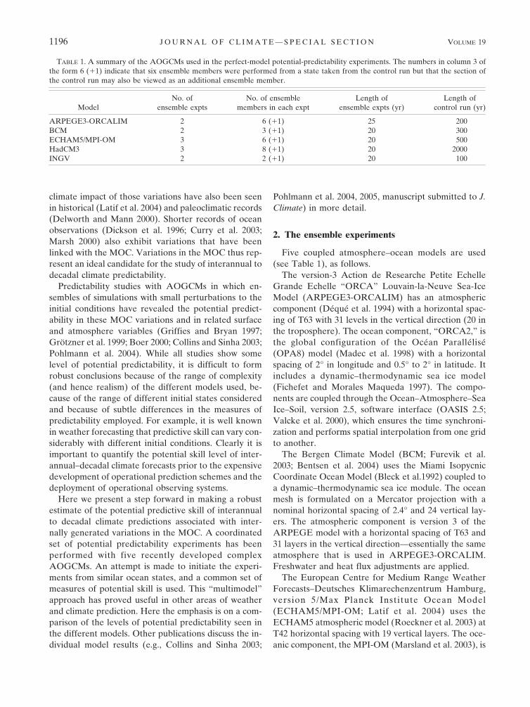
TABLE 1. A summary of the AOGCMs used in the perfect-model potential-predictability experiments. The numbers in column 3 ofthe form 6 (�1) indicate that six ensemble members were performed from a state taken from the control run but that the section ofthe control run may also be viewed as an additional ensemble member.

ModelNo. of

ensemble exptsNo. of ensemble

members in each exptLength of

ensemble expts (yr)Length of

control run (yr)

ARPEGE3-ORCALIM 2 6 (�1) 25 200BCM 2 3 (�1) 20 300ECHAM5/MPI-OM 3 6 (�1) 20 500HadCM3 3 8 (�1) 20 2000INGV 2 2 (�1) 20 100

1196 J O U R N A L O F C L I M A T E — S P E C I A L S E C T I O N VOLUME 19

run on a curvilinear grid with equatorial refinement and23 vertical levels. A dynamic–thermodynamic sea icemodel and a river-runoff scheme are included.

The Third Hadley Centre Coupled Ocean–Atmosphere GCM (HadCM3; Gordon et al. 2000; Col-lins et al. 2001) uses an oceanic component with a hori-zontal spacing of 1.25° longitude by 1.25° latitude and20 levels in the vertical direction. The atmosphericcomponent uses a gridpoint formulation with a hori-zontal spacing of 3.75° � 2.5° in longitude and latitudewith 19 unequally spaced vertical levels (Pope et al.2000). A simple thermodynamic sea ice scheme is used.

The Istituto Nazionale di Geofisica e Vulcanologia(INGV) model uses the ECHAM4 model (Roeckner1996) at T42 resolution with 19 vertical levels. Theocean component is essentially the same as that used inthe ARPEGE3-ORCALIM model. More details can befound in Gualdi et al. (2003) and Carril et al. (2004).

Ensemble experiments are performed from initialstates of anomalously high and anomalously low MOCtaken from a control (i.e., unforced) run of each model(Fig. 1). In addition, some models were used to performexperiments with initial states near the time-meanvalue of overturning. Perturbations to the initial condi-tions were made using the common method of takingdifferent atmospheric start conditions (in most casesatmosphere start conditions differ only by one day ofmodel integration) and identical ocean start conditionsfor the respective model (see e.g., Collins and Sinha

2003). Hence both atmosphere and ocean initial statesare in perfect balance with the model as they are takenfrom the respective control simulations and are thussolutions of the model equations. While this perturba-tion methodology is in no way optimal in terms of, forexample, sampling the likely range of atmosphere–ocean analysis error, it is sufficient to generate en-semble spread on the time scales of interest. Note that

FIG. 1. A schematic figure of the experimental design used inthis study. The thick black line represents decadal-time-scale in-ternally generated variations in the strength of the MOC from acontrol run of a coupled atmosphere–ocean model. The gray linesrepresent “perfect ensemble” experiments in which small pertur-bations to the initial conditions are made. For each of the modelsused in the study, we endeavored to initiate the ensemble experi-ments from a state of relatively strong and relatively weak over-turning. In addition, some models are used to initiate experimentsfrom a state of relatively normal overturning.

FIG. 2. Time series of the strength of the MOC taken from theunforced control runs of five coupled atmosphere–ocean models(black lines; names indicated on the figure) and from the perfect-ensemble experiments (gray lines). The measure is defined as themaximum of the annual-mean meridional streamfunction in theNorth Atlantic region of the model and, in general, varies withlatitude and depth, the exception being the ECHAM5/MPI-OM1model, where the MOC strength is measured at the constant lati-tude of 30°N, the latitude of its time-averaged maximum. MOCvariations arise purely because of the internal dynamics of thecoupled system, and model years are arbitrary. The drift seen inthe INGV model is a spinup effect, and the experiments are ex-cluded from any quantitative analysis.


the perturbation method produces ensemble experi-ments that are likely to give the upper limit of model-world predictability: hence the terms potential predict-ability and perfect-model or perfect-ensemble experi-ments.

The availability of computer resources limited thenumber of ensemble members and experiments thatcould be performed: nevertheless all experiments wereintegrated out to at least 20 yr. The experiments corre-spond to a total 1340 simulated years for the predict-ability experiments combined with a total of 3100 simu-

lated years for the control experiments used to assessbackground variability. Annual mean diagnostics areexamined because of the focus on interannual to dec-adal time scales.

3. Potential predictability of MOC variations

The first point to note is the wide range of time scalesand magnitudes of MOC variability in the differentmodels (Fig. 2). The ECHAM5/MPI-OM model showsthe largest variations in MOC strength with clear inter-

FIG. 3. Measures of the potential predictability of variations in the strength of the MOC from four of the five coupled models (seelegend). (left) The ACC (unity for perfect potential predictability; zero for no potential predictability) for (top) strong and (bottom)weak MOC initial conditions. (right) The normalized rmse (zero for perfect potential predictability; unity for no potential predictabil-ity) in the same order. Also shown in the figures are the multimodel average ACC and rmse (thick black line) and the multimodelaverage ACC for a simple damped persistence (thick gray line).


decadal variability present. HadCM3 and BCM alsoshow interdecadal variations but at a reduced level incomparison. The ARPEGE3-ORCALIM model hasthe lowest level of variability, but decadal–interdecadaltime scales are still clearly present in the time series.The large trend seen in the INGV model is almost cer-tainly due to a drift seen in this particular control ex-periment—the model has yet to reach equilibrium, andwe do not attempt to extract quantitative measures ofpredictability. Although not calculated, diagnostic mea-sures of predictability/variability (e.g., Boer 2000)would clearly show a range of different levels of MOCpotential predictability in these models. However, theonly reliable way to assess potential predictability is toperform ensemble experiments.

The perfect-ensemble experiments are also shown inFig. 2. Potential predictability is evident when the en-semble spread is small in comparison with the totallevel of variability in the control time series, or even if

the ensemble spread is relatively large but the center ofgravity of the ensemble is displaced significantly withrespect to the mean of the control (e.g., Collins 2002).We may imagine a background or climatological distri-bution that, in the absence of a forecast, would be allthe information we would have to form an assessmentof the future strength of the MOC. Alternatively, wemay imagine a form of damped persistence based onthe autocorrelation structure of past observations. Aforecast may allow us to reduce the potential range(low ensemble spread) or shift the mean of the distri-bution (displaced ensemble), or both. Both types of(potential) predictability are seen on interannual todecadal time scales in the experiments shown in Fig. 2.For example, the first HadCM3 ensemble (anomalouslystrong MOC initial conditions) has relatively small en-semble spread in the first decade of the experiment andthe ensemble is significantly shifted to stronger valueswith respect to the mean with no ensemble members

FIG. 4. The coefficient of regression (K Sv�1) of decadal mean SAT against decadal mean MOC strength from four of the five coupledatmosphere–ocean models. Regions are shaded only where the coefficient is significantly different from zero at the 5% confidence level(based on an F test).


indicating weaker than average overturning [see Collinsand Sinha (2003) for more details]. Other examples areclear.

There is a wide range of measures that may be usedfor forecast verification (as stated above, we measurethe potential skill of a perfect model forecast—an up-per limit). We examine two of the most simple mea-sures of forecast skill to quantify levels of potentialpredictability; the anomaly correlation coefficient(ACC) and normalized root-mean-square error (rmse).Formulas are given in Collins (2002).

Figure 3 shows both measures for the MOC in theensemble experiments discussed above. For the strongMOC initial states, the ACC is “high” for approxi-mately the first decade in all the model experiments,with high being above 0.6—a commonly used cutoffvalue in weather forecasting. The rmse is correspond-ingly low. After the first decade, the ARPEGE3 modelpredictability drops off rapidly whereas for the othermodels the ACC drops off slowly to low values by theend of the 20-yr experiments. The rmse similarly satu-rates in 20 yr. For the weak MOC initial states, errorgrowth and loss of predictability seem to happen soonerin the ensemble experiments, although there is somenoise in these measures because of small ensemblesizes. ACC and rmse are not shown for the normalinitial states because of the small sample size.

While the number of ensemble experiments is small,we may attempt to draw some conclusions about themultimodel estimate of potential predictability of MOCvariability in these experiments (Fig. 3, thick solid line).The multimodel ensemble indicates potential predict-ability of interannual–decadal MOC variations for one–two decades into the future. It also indicates that initialstates that have anomalously strong overturning aremore predictable than those with anomalously weakoverturning. This latter result is intriguing but is subjectto some uncertainty because of the relatively smallnumber of models and ensemble experiments includedin the multimodel analysis. Nevertheless, some consen-sus is emerging in contrast to the previous situation inwhich a large range of predictability is seen in the lit-erature. It would be safe to conclude that there is arobust signal of potential predictability of variations inthe MOC on interannual to decadal time scales.

4. Potential predictability of surface climatevariations

Predictions of MOC variability may be of interest toscientists, but they would be of little relevance to soci-ety unless they are accompanied by predictions of sur-face climate variables. A simple measure of the impactof MOC variations can be obtained be performing a

regression between decadal-averaged MOC strengthand decadal-averaged surface air temperature (SAT) inthe different models (Fig. 4). The general impression inall the models is of a warmer Northern Hemispherewhen the MOC is stronger and is transporting moreheat poleward. Differing levels of statistical significanceseen in Fig. 4 may be interpreted as resulting from dif-ferent levels of signal-to-noise in the sense that in mod-els with larger variations in MOC, the surface signal hasa better chance of overwhelming the noise of unrelatedrandom climate variations. What is interesting is thatthe magnitude of the surface response (in kelvins perSverdrup) is similar across all models.

The North Atlantic Ocean is a region in all the mod-els in which there is a significant relationship betweendecadal variations in SAT (and underlying SST) andthe MOC. Time series of annual mean SAT from thecontrol and ensemble experiments averaged over a re-

FIG. 5. As in Fig. 2, but for SAT averaged in the region40°–60°N, 50°–10°W.


gion of the North Atlantic [used in Collins and Sinha(2003) and Pohlmann et al. (2004)] are shown in Fig. 5.Strong similarities between these time series and thoseshown in Fig. 2 for the MOC are evident, althoughthere is clearly more noise in this variable as a result ofunrelated random atmospheric variability.

ACC and rmse measures of ensemble spread (Fig. 6)for North Atlantic SAT are similar to those computedfor MOC variations (Fig. 3), but the levels of potentialpredictability are clearly less and the differences be-tween ensemble members greater. It may be possible tofind greater levels of potential predictability for each

individual model by adjusting the boundaries of theregion chosen, but here we compare the models on anequal footing. Also, the effects of interannual noise,which are more prominent in this variable, may be re-duced by taking averages over a greater number ofyears. Nevertheless, the picture of potentially predict-able surface climate variations associated with varia-tions in the MOC appears consistent.

5. Discussion

Whereas previously it has been difficult to assess thepotential for making interannual to decadal forecasts of

FIG. 6. As in Fig. 3, but for SAT averaged in the region 40°–60°N, 50°–10°W. There is significantly more interannual “noise” in SATvariability (due to random atmospheric fluctuations); hence the high ACC values in all models around year 16 are likely to be asampling issue arising from the relatively small number of models and ensemble members.


climate because of different studies indicating differentlevels of predictability, a more complete picture of thepredictability is emerging. This intercomparison studyshows that

1) variations in the ocean meridional overturning cir-culation are potentially predictable on interannualto decadal time scales,

2) a more consistent picture of the surface temperatureimpact of decadal variations in the MOC is nowapparent, and

3) variations of surface air temperatures in the NorthAtlantic are also potentially predictable on interan-nual to decadal time scales, albeit with potential skilllevels that are less than those seen for MOC varia-tions.

Perhaps the biggest difference between the models isin the wide range of strengths of decadal variabilityevident in Fig. 2. In general, models with greater dec-adal MOC variability have greater levels of potentialpredictability—despite the fact that the ACC and rmseare signal-to-noise measures and thus allow for differ-ences in background natural variability. Investigationinto the mechanisms responsible for the different levelsof variability would seem to be a priority.

In any real-world prediction system, an estimate ofthe three-dimensional ocean state would have to bemade using data assimilation. Currently there are sig-nificant disagreements between estimates of even themean value of the overturning using such techniques,ranging from as little as 12 Sv (1 Sv � 106 m3 s�1; Stam-mer et al. 2002) to as much as 25 Sv [S. Masina et al.2005, unpublished result based on system outlined inMasina et al. (2004)], both being consistent with obser-vational estimates. Hence estimating anomalous inter-annual to decadal variations about this mean may seemalmost impossible, particularly given the relative pau-city of in situ ocean observations. We may take somehope though from ocean-model simulations driven byestimates of observed surface winds and fluxes thatgenerally show agreement between their MOC varia-tions over the latter part of the twentieth century(Bentsen et al. 2004). It may be the case that moreaccurate and balanced reconstructions of past varia-tions in surface fluxes (e.g., from weather forecast re-analysis products) coupled with recently deployedocean observations (Hirschi et al. 2003) and improvedmodels and data assimilation schemes could provideaccurate ocean initial states with which to initializeforecasts. Pilot forecast systems are in development.

The far more pertinent question is, of course, that ofthe (potential) prediction of surface climate variationsover land. The simple measures used in this study do

not reveal robustly predictable land signals. Collins andSinha (2003) and Pohlmann et al. (2005, manuscriptsubmitted to J. Climate) investigate probabilistic tech-niques more commonly used in medium-range and sea-sonal forecasting in the context of the interannual–decadal problem with some limited success. However,the application and verification of such measures (herethe assessment of potential skill) requires much largerensemble sizes and many more ensemble simulationsthan used here. It is hoped that such ensembles will beperformed in future. In addition, the modeling, initial-ization, and observational issues that need to be ad-dressed before we routinely produce interannual–decadal climate forecasts are numerous.

Acknowledgments. This work was performed whilethe lead author was based at the Centre for GlobalAtmospheric Modelling, Department of Meteorology,University of Reading. All authors received supportfrom the EU FP5 PREDICATE project (EVK2-CT-1999-00020) and from national sources.

REFERENCES

Bentsen, M., H. Drange, T. Furevik, and T. Zhou, 2004: Simulatedvariability of the Atlantic meridional overturning circulation.Climate Dyn., 22, doi:10.1007/s00382-004-0397-x.

Bleck, R., C. Rooth, D. Hu, and L. T. Smith, 1992: Salinity-driventhermohaline transients in a wind- and thermohaline-forcedisopycnic coordinate model of the North Atlantic. J. Phys.Oceanogr., 22, 1486–1515.

Boer, G. J., 2000: A study of atmosphere–ocean predictability onlong timescales. Climate Dyn., 16, 469–477.

Carril, A. F., A. Navarra, and S. Masina, 2004: Ocean, sea-ice,atmosphere oscillations in the Southern Ocean as simulatedby the SINTEX coupled model. Geophys. Res. Lett., 31,L10309, doi:101029/2004GL019623.

Collins, M., 2002: Climate predictability on interannual to decadaltime scales: The initial value problem. Climate Dyn., 19, 671–692.

——, and M. R. Allen, 2002: Assessing the relative roles of initialand boundary conditions in interannual to decadal climatepredictability. J. Climate, 15, 3104–3109.

——, and Sinha, B., 2003: Predictable decadal variations in thethermohaline circulation and climate. Geophys. Res. Lett., 30,1306, doi:10.1029/2002GLO16504.

——, S. F. B. Tett, and C. Cooper, 2001: The internal climatevariability of HadCM3, a version of the Hadley Centrecoupled model without flux adjustments. Climate Dyn., 17,61–81.

Curry, R., R. Dickson, and I. Yashayaev, 2003: A change in thefreshwater balance of the Atlantic Ocean over the past fourdecades. Nature, 426, doi:10.1038/nature02206.

Delworth, T. L., and M. E. Mann, 2000: Observed and simulatedmultidecadal variability in the Northern Hemisphere. Cli-mate Dyn., 16, 661–676.

Déqué, M., C. Dreveton, A. Braun, and D. Cariolle, 1994: Theclimate version of ARPEGE/IFS: A contribution to the


French community climate modelling. Climate Dyn., 10, 249–266.

Dickson, R., J. Lazier, J. Meincke, P. Rhines, and J. Swift, 1996:Long term coordinated changes in the convective activity ofthe North Atlantic. Progress in Oceanography, Vol. 38, Per-gamon, 241–295.

Dong, B., and R. T. Sutton, 2001: The dominant mechanisms ofvariability in Atlantic ocean heat transport in a coupledocean–atmosphere GCM. Geophys. Res. Lett., 28, 2445–2448.

Fichefet, T., and M. A. Morales Maqueda, 1997: Sensitivity of aglobal sea ice model to the treatment of ice thermodynamicsand dynamics. J. Geophys. Res., 102 (C6), 12 609–12 646.

Furevik, T., M. Bentsen, H. Drange, I. K. T. Kindem, N. G. Kvam-stø, and A. Sorteberg, 2003: Description and validation of theBergen Climate Model: ARPEGE coupled with MICOM.Climate Dyn., 21, doi:10.1007/s00382-003-0317-5.

Goddard, L., S. Mason, S. Zebiak, C. Ropelewski, R. Basher, andM. Cane, 2001: Current approaches to seasonal to interan-nual climate predictions. Int. J. Climatol., 21, 1111–1152.

Gordon, C., C. Cooper, C. A. Senior, H. Banks, J. M. Gregory,T. C. Johns, J. F. B. Mitchell, and R. A. Wood, 2000: Thesimulation of SST, sea ice extents and ocean heat transport ina version of the Hadley Centre coupled model without fluxadjustments. Climate Dyn., 16, 147–168.

Grötzner, A., M. Latif, A. Timmermann, and R. Voss, 1999: In-terannual to decadal predictability in a coupled ocean–atmosphere general circulation model. J. Climate, 12, 2607–2624.

Griffies, S. M., and K. Bryan, 1997: Predictability of North Atlan-tic multidecadal climate variability. Science, 275, 181–184.

Gualdi, S., E. Guilyardi, A. Navarra, S. Masina, and P. Delecluse,2003: The interannual variability in the tropical Indian Oceanas simulated by a CGCM. Climate Dyn., 20, 567–582.

Hirschi, J., J. Baehr, J. Marotzke, J. Stark, S. Cunningham, andJ.-O. Beismann, 2003: A monitoring design for the Atlanticmeridional overturning circulation. Geophys. Res. Lett., 30,1413, doi:10.1029/2002GL016776.

Latif, M., and Coauthors, 2004: Reconstructing, monitoring, andpredicting multidecadal-scale changes in the North Atlanticthermohaline circulation with sea surface temperature. J. Cli-mate, 17, 1605–1614.

Madec, G., P. Delecluse, M. Imbard, and C. Lévy, 1998: OPA 8.1Ocean General Circulation Model reference manual. Note

du Pôle de Modélisation, Institut Pierre-Simon Laplace, No.11, 91 pp.

Marsh, R., 2000: Recent variability of the North Atlantic thermo-haline circulation inferred from surface heat and freshwaterfluxes. J. Climate, 13, 3239–3260.

Marsland, S., H. Haak, J. Jungclaus, M. Latif, and F. Röske, 2003:The Max-Planck-Institute global ocean/sea ice model withorthogonal curvilinear coordinates. Ocean Modell., 5, 91–127.

Masina, S., P. Di Pietro, and A. Navarra, 2004: Interannual-to-decadal variability of the North Atlantic from an ocean dataassimilation system. Climate Dyn., 23, doi:10.1007/s00382-004-0453-6.

Pohlmann, H., M. Botzet, M. Latif, A. Roesch, M. Wild, and P.Tschuck, 2004: Estimating the decadal predictability of acoupled AOGCM. J. Climate, 17, 4463–4472.

Pope, V. D., M. L. Gallani, P. R. Rowntree, and R. A. Stratton,2000: The impact of new physical parametrizations in theHadley Centre climate model—HadAM3. Climate Dyn., 16,123–146.

Rodwell, M. J., and C. K. Folland, 2002: Atlantic air–sea interac-tion and seasonal predictability. Quart. J. Roy. Meteor. Soc.,128, 1413–1443.

Roeckner, E., and Coauthors, 1996: The atmospheric general cir-culation model ECHAM 4: Model description and simulationof present day climate. Max-Planck-Institut für Meteorolo-gie, Rep. 218, 90 pp.

——, and Coauthors, 2003: The atmospheric general circulationmodel ECHAM 5. Part I: Model description. MPI Rep. 349,Max-Planck-Institut für Meteorologie, Hamburg, Germany,127 pp.

Roullet, G., and G. Madec, 2000: Salt conservation, free surfaceand varying volume: A new formulation for Ocean GCMs. J.Geophys. Res., 105, 23 927–23 942.

Stammer, D., and Coauthors, 2002: Global ocean circulation dur-ing 1992–1997, estimated from ocean observations and a gen-eral circulation model. J. Geophys. Res., 107, 3118,doi:10.1029/2001JC000888.

Trenberth, K. E., and J. M. Caron, 2001: Estimates of meridionalatmosphere and ocean heat transports. J. Climate, 14, 3433–3443.

Valcke, S., L. Terray, and A. Piacentini, 2000: The OASIScoupled user guide version 2.4. Tech. Rep. TR/CMGC/00-10,CERFACS, 85 pp.


Interannual to Decadal Climate Predictability: A Multi-Perfect-Model-Ensemble Study

Documents

Transcript of Interannual to Decadal Climate Predictability: A Multi-Perfect-Model-Ensemble Study