Quarterly Journal of the Royal Meteorological Society Q. J. R. Meteorol. Soc. (2014) DOI:10.1002/qj.2379

Prospects for decadal climate prediction in the Mediterranean region

Virginie Guemas,a,b* Javier Garcıa-Serrano,a,c Annarita Mariotti,d Francisco Doblas-Reyesa,e

and Louis-Philippe Carona,f

aClimate Forecasting Unit, Institut Catala de Ciencies del Clima, Barcelona, SpainbGroupe de Meteorologie Grande Echelle et Climat, Groupe d’Etude de l’Atmosphere Meteorologique, Centre National de Recherches

Meteorologiques, Toulouse, FrancecVARCLIM-TG, LOCEAN-IPSL, Universite Pierre et Marie Curie, Paris, France

dNational Oceanic and Atmospheric Administration, Climate Program Office, Silver Spring, MD, USAeInstitucio Catalana de Recerca i Estudis Avancats, Barcelona, Spain

f Rossby Center, Swedish Meteorological and Hydrological Institute, Norrkoping, Sweden

*Correspondence to: V. Guemas. Institut Catala de Ciencies del Clima, Carrer Trueta 203, 08005 Barcelona, Spain.E-mail: virginie.guemas@ic3.cat

The Mediterranean region stands as one of the most sensitive to climate change, both interms of warming and drying. On shorter time-scales, internal variability has substantiallyaffected the observed climate and in the next decade might enhance or compensatelong-term trends. Here we compare the multi-model climate predictions produced withinthe framework of the CMIP5 (Coupled Model Intercomparison Project Phase 5) projectwith historical simulations to assess the level of multi-year climate prediction skill in theMediterranean region beyond that originating from the model accumulated response tothe external radiative forcings. We obtain a high and significant skill in predicting 4-yearaveraged annual and summer mean temperature over most of the study domain andin predicting precipitation for the same seasons over northern Europe and sub-SaharanAfrica. A lower skill is found during the winter season but still positive for temperature.Although most of this high skill originates from the model response to the external radiativeforcings, the initialization contributes to the temperature skill over the Mediterranean Seaand surrounding land areas. The high and significant correlations between the observedMediterranean temperatures and the observed Atlantic multidecadal oscillation (AMO) inthe summer and annual means are captured by the CMIP5 ensemble which suggests thatthe added skill is related to the ability of the CMIP5 ensemble to predict the AMO. Sucha link to the AMO seems restricted to western Africa and summer means only for theprecipitation case.

Key Words: climate prediction; initialization; Atlantic multidecadal oscillation; Mediterranean climate

Received 22 June 2013; Revised 24 January 2014; Accepted 24 March 2014; Published online in Wiley Online Library

1. Introduction

The Mediterranean region is projected to be among the mostheavily affected by the twenty-first century greenhouse gasinduced climate change, with significant regional warming anddrying by the end of the century (e.g. Mariotti et al., 2008). Inthe shorter term, a few decades into the future, decadal variabilityof both internal and external origin will largely determine theconditions to be experienced in the region, as already seen overthe course of the twentieth century (Mariotti and Dell’Aquila,2012). A key question and one of great societal relevance, is towhat extent will natural variability enhance or reduce externallyforced changes and for how long. In view of the seemingly robustclimate change signal in the Mediterranean region, projectedexternal forcing constitutes a source of decadal predictabilityfor this region. What remains to be understood is the degree

of predictability of regional internal decadal variability and itsimpact on our ability to predict future changes a few years ahead.

Early potential predictability studies highlighted the AtlanticOcean as the most promising region for decadal climateprediction (Griffies and Bryan, 1997; Boer, 2000; Pohlmannet al., 2004; Collins et al., 2006). The Atlantic Ocean exhibitsstrong multidecadal variability which involves variations in thestrength of the ocean thermohaline circulation associated with alarge-scale signature in sea-surface temperatures (SST) referred toas the Atlantic multidecadal oscillation (AMO: Kerr, 2000; Knightet al., 2005, 2006). Much of the current quest to predict futuredecadal climate variations hinges on the potential predictabilityassociated with the variations of the ocean gyres and the Atlanticmeridional overturning circulation (AMOC). At the edge betweenseasonal forecasting and climate change projections, the decadalclimate prediction exercise consists of initializing a climate

c© 2014 Royal Meteorological Society

V. Guemas et al.

model from an estimate of the observed climate state while alsoprescribing the changes in external radiative forcings, assumingthese are known (Hawkins and Sutton, 2009; Meehl et al., 2009;Murphy et al., 2010; Doblas-Reyes et al., 2011). Based on thisapproach, hindcast (i.e. retrospective climate prediction) studies(Smith et al., 2007, 2012; Keenlyside et al., 2008; Pohlmann et al.,2009) showed that the Atlantic Ocean stands out as a regionof increased forecast skill with initialization. The initializationallows for more accurate predictions of the AMO compared tocoupled experiments accounting only for the model accumulatedresponse to changes in external radiative forcings (Garcıa-Serranoet al., 2012), in particular in the multi-model ensemble climatehindcasts produced in the framework of the Climate ModelIntercomparison Project Phase 5 (CMIP5: Doblas-Reyes et al.,2013; Garcıa-Serrano et al., 2014).

A recent study using observational data and a regional climatemodel (Mariotti and Dell’Aquila, 2012) suggests a linkage betweenthe Atlantic multidecadal oscillation/variability (AMO/AMV)and decadal climate variability in the Mediterranean region.Mediterranean SSTs exhibit AMO-like variability, which inturn is reflected in AMO-like evaporation variability (Fenoglio-Marc et al., 2013). There is also a linkage between the AMOand Mediterranean surface air temperatures which appears tobe strong in summer, also present to a lesser extent in thetransition seasons, but negligible in winter. The modelling resultsfrom Mariotti and Dell’Aquila (2012) suggest that atmosphericprocesses are the primary mechanism connecting the AMO withthe Mediterranean rather than a direct influence of the Atlantic onthe Mediterranean Sea. This study therefore suggests the potentialfor a certain degree of decadal climate (namely, temperature andevaporation) predictability in the Mediterranean region, to theextent that the AMO is predictable. In contrast, decadal variabilityof regional precipitation was found to be largely affected by theseasonal manifestations of the North Atlantic Oscillation (NAO),rather than the AMO. It is currently unknown whether there isany predictability in NAO variability. Hence the prospects forpredicting regional precipitation variability, outside of what maybe the externally forced long-term drying trend, are also unclear.

In this article, we aim at assessing the level of decadalclimate prediction skill in the Mediterranean region beyond thatoriginating from the model accumulated response to the externalradiative forcings, and the seasonal dependence of this skill,contrasting summer (defined as June to August throughout ourstudy) and winter (December to February) values. We also aim atassessing to what extent the added-value from the initializationis originating from the predictability of the AMO and its linkageto the Mediterranean region. It should be noted that the focus ofthe present study is not on the AMO drivers (Ottera et al., 2010;Booth et al., 2012; Terray, 2012; Zhang et al., 2013) but on itsprediction skill and the predictability gained from simulating itsteleconnections, in particular over the Mediterranean region assuggested by Matei et al. (2012). These assessments rely on theCMIP5 multi-model ensemble (MME) climate hindcasts (Tayloret al., 2012) which are introduced in section 2 together withthe observational data used for verification and the skill scoresused to measure the performance of this MME. Section 3 thenillustrates the performance of the CMIP5 MME in predictingMediterranean temperatures and precipitation, and comparesthis skill with the one from historical climate simulations whichdo not take into account the internal variability as a source ofpredictability and which contain potential accumulated errorsin the model response to the external radiative forcings. Theadded-value from the initialization is then related to the abilityof the MME to capture the linkage between the AMO and thoseregional climate variables. Section 4 and 5 provide respectively adiscussion of major results and the conclusions from our study.

2. Methodology

2.1. Model data

The multi-model ensemble (MME) analysed here includes thecontributions to the CMIP5 project produced with the HadCM3,MRI-CGCM3, MIROC4h, MIROC5, CanCM4, CNRM-CM5,MPI-M, GFDL-CM2, CMCC-CM, IPSL-CM5 and EC-Earthv2.3 coupled climate models. These contributions consist in 10-year long hindcasts initialized from an estimate of the observedclimate state every 5 years over the period 1960–2006 between 1November and the following 1 January. This ensemble is referredto as Init hereafter. Complete calendar years from January toDecember are considered as forecast years here. Two rangesof forecast years are analysed in the following: from forecastyears 2 to 5 and 6 to 9, which are classically used as targetperiods for analyses of climate predictions (Doblas-Reyes et al.,2013). The MME hindcast set gives ten predicted values for aspecific forecast range. The forecast fields are interpolated usinga conservative method onto the grid of the observational datasetused for verification before any analysis. More details on themodel experiments analysed in this work are provided in Table 1.

A sister ensemble has been built from the ‘historical’ coupledsimulations and the first years of the climate projections followingthe CMIP5 RCP4.5 (Representative Concentration Pathway4.5 W m−2: Taylor et al., 2012) scenario run with the samemodels. In these experiments, the simulated natural variabilityis not constrained to follow the contemporaneous observed oneexcept through the effect of the external radiative forcings, whichare exactly the same as in the Init MME. Additionally, errors inthe response to the external radiative forcings could accumulateover time. This ensemble is referred to as NoInit hereafter.Both Init and NoInit CMIP5 experiments include observed time-dependent solar irradiance variations and volcanic aerosols until2005 whereas these would not be known in a true predictionexercise.

The Init and NoInit ensembles do not contain the same numberof members. We have checked that restricting those ensembles tothe subsets allowing for the same number of members for eachmodel in the two ensembles do not affect our main conclusions(not shown).

2.2. Observational data

For temperature verification, we have used a combinationof land surface temperatures from the National Centers forEnvironmental Prediction (NCEP) GHCN/CAMS dataset (Fanand van den Dool, 2008), SST from the National Climatic DataCenter (NCDC) ERSST v3b dataset (Smith et al., 2008) and, northof 60◦N, the GISTEMP dataset with 1200 km decorrelation scale(Hansen et al., 2010). This dataset covers the 1960–2012 period.For precipitation, a land-only monthly dataset is consideredbecause of the sparse observational coverage over the oceansbefore 1979. We use the Global Precipitation Climatology Centre(GPCC) v5 data (Rudolf et al., 2010) for the 1960–2012 period.For sea-level pressure, we have used the HadSLP2 dataset (Allanand Ansell, 2006) for the 1960–2004 period.

2.3. Forecast skill assessment

In our study we focus on the analysis of the skill for the annualvalues and contrast the summer (JJA) and winter (DJF) values.We compute JJA, DJF and annual means for both the modelexperiments and observations. The performance of the MMEis assessed for the average of the predicted values over forecastyears or seasons 2–5 and 6–9. For the winter season, the averageover forecast seasons 2–5 and 6–9 uses the December valuesfrom years 1 to 4 and 5 to 8 respectively. When initializedfrom an estimate of the observed climate state, climate modelsdrift towards their attractor, which leads to systematic errors in

c© 2014 Royal Meteorological Society Q. J. R. Meteorol. Soc. (2014)

Prospects for Decadal Climate Prediction in the Mediterranean Region

Table 1. CMIP5 model experiments analysed in this work. The number of ensemble members analysed in the Init and NoInit MME are specified.

Model Initialization methodology No. of Init members No. of NoInit members

HadCM3 (Gordon et al., 2000; Popeet al., 2000)

Coupled anomaly assimilation: ERA-40 and ERA Interimatmospheric reanalyses, ocean observations

10 10

MRI-CGCM3 (Yukimoto et al., 2001;Tatebe et al., 2012)

Full-field assimilation 9 1

MIROC4 (Sakamoto et al., 2012) Assimilation in the coupled model of ocean anomalies of griddedsubsurface observations of temperature (T) and salinity (S)

3 3

MIROC5 (Hasumi and Emori, 2004;Watanabe et al., 2010)

Assimilation in the coupled model of ocean anomalies of griddedsubsurface observations of temperature (T) and salinity (S)

6 1

CANCM4 (Fyfe et al., 2011; Merryfieldet al., 2013)

Coupled assimilation of the ERA40 and ERA-Interim atmosphericreanalyses, observed SSTs and SODA and GODAS subsurfaceocean T and S, beforehand adjusted to preserve T-S relationship

10 10

CNRM-CM5 (Voldoire et al., 2013) Ocean T and S nudged (3D Newtonian damping) towardNEMOVAR-COMBINE in the coupled model; NEMOVAR-COMBINE reanalysis produced using multivariate 3D-VAR dataassimilation in NEMO ocean model

10 6

MPI-M (Jungclaus et al., 2006; Mateiet al., 2012)

Nudging in the coupled model of T and S anomalies obtained froman ocean-only run forced with NCEP atmospheric reanalyses

10 3

GFDL-CM2 (Delworth et al., 2006;Yang et al., 2013)

Coupled assimilation of atmospheric reanalysis and oceanobservations of 3D T and S and SST

10 10

CMCC-CM (Scoccimarro et al., 2011;Bellucci et al., 2013)

Full field ocean initialization from three different realizations ofCMCC-INGV ocean synthesis of T and S

3 1

IPSL-CM5 (Dufresne et al., 2013;Swingedouw et al., 2013)

Nudging in the coupled model of SST anomalies to Reynoldsobservations

6 3

EC-Earth v2 (Hazeleger et al., 2010,2013; Du et al., 2012)

Full-field initialization: ERA-40 and ERA-Interim atmosphere/land reanalyses; NEMOVAR-S4 ocean reanalysis

10 11

climate forecasts. These systematic errors depend on the forecasttime and we therefore apply a drift correction to our multi-modelensemble (Goddard et al., 2013; Meehl et al., 2014). Anomaliesare computed using the so-called ‘per-pair’ methodology (Garcıa-Serrano and Doblas-Reyes, 2012): the modelled or observedclimatology is defined as a function of the forecast time (multi-year or multi-season average), by averaging the predicted variable(temperature or precipitation) across the start dates taking intoaccount only the predicted values for which observations areavailable at the corresponding date; a forecast-time-dependentclimatology is computed for each individual model averagingall members. The climatology of each model is then subtractedfrom each hindcast to obtain anomalies over the whole predictedperiod for each member of each model:

X′msf = Xmsf − 1

(M − 1)(S − 1)

∑M

∑S

Xmsf (Osf �= NA),

O′sf = Osf − 1

(S − 1)

∑S

Osf (Osf �= NA),

where Xmsf is the model variable at forecast time f , for start dates and member m, Osf is the corresponding observation, X′

msf and

O′sf , their respectively anomalies, M is the number of members,

S the number of start dates and NA refers to a missing value.Then, ensemble-mean anomalies are computed for each modelaveraging all its members and the multi-model ensemble-meananomalies are computed giving an equal weight to each model,regardless of the number of ensemble members available forthat model. The same method is applied to the observationsto obtain anomalies over the whole verification period. All theclimate prediction scores described below are computed fromthose anomalies.

Hindcast prediction skill is measured using the anomalycorrelation coefficient (ACC), the mean square skill score (MSSS)or the Brier Skill Score (BSS). The ACC is computed by correlatingthe predicted MME anomalies with the observed ones across the

start date dimension:

ACCf =1

S−1

∑S

X′sf O′

sf√(1

S−1

∑S

X′sf

2

) (1

S−1

∑S

O′sf

2

) ,

where X′sf is the MME mean anomaly for forecast time f and

start date s, and O′sf is the corresponding observed anomaly. A

t-test, after a Fisher-Z transformation, is performed to assessthe significance level of an ACC or of a difference in ACC,accounting for the autocorrelation of the data when computingthe degrees of freedom following von Storch and Zwiers (2001).Indeed, hindcasts initialized every 5 years cannot be consideredas independent when attempting to predict decadal climatevariability, hence our reduction of the degrees of freedom basedon von Storch and Zwiers (2001). It is worth noting that only 9 or10 observations (when verifying predictions for forecast years 6–9or 2–5 respectively) can be used to compute the ACC or any otherskill score, and those 9–10 data are reduced by about a factor 2to obtain the number of effective independent data. Increasingthe frequency of the start dates would not increase significantlythe number of independent data, since the additional hindcastswould still not be independent for analyses of decadal climatevariability. Extending backward the period which is sampled byour start dates would be necessary to obtain more independenthindcasts and more robust estimates of the added-value frominitialization in terms of skill scores. Obtaining accurate initialconditions is unfortunately harder to achieve as we extend thehindcast period back into the past.

The MSSS is computed as 1 minus the ratio of the mean squareerror (MSE) of the predicted per-pair MME anomalies over theMSE of a climatological forecast (Goddard et al., 2013):

MSSSf = 1 −1

S−1

∑S

(X′sf − O′

sf )2

1S−1

∑S

O′sf

2

A Fisher test is performed to assess the significance level of anMSSS accounting for the autocorrelation of the data following vonStorch and Zwiers (2001). Since the MME is used in the forecast

c© 2014 Royal Meteorological Society Q. J. R. Meteorol. Soc. (2014)

V. Guemas et al.

skill assessment through the ACC and the MSSS, externally forcedsignals and any signal due to the initialization will stand out (thatis, only the robust patterns consistent across members and modelswill stand out). In contrast, any ‘noise’ will be to a large extenteliminated by the MME averaging operation.

The BSS is computed for the lower, middle and upper terciles:

BSSft = 1 −1S

∑S

(pfst − ofst)2

ot(1 − ot)

where psft is the forecast probability for a given tercile t to occur,for forecast time f and start date s, osft is its observed probability(0 or 1) and ot is its observed climatological probability. Themodel terciles and the model forecast probabilities are estimatedfrom the multi-model ensemble of model mean anomalies whichmakes an ensemble of 11 values (models) for each start date,each variable and each forecast average. This approach ensuresequal representativeness for all models in a similar fashion as weoperated for the deterministic skill measures (ACC and MSSS).

The skill gained by the initialization process is assessedby computing the difference between Init and NoInit ACC.Whenever this difference in skill is positive the initializationprocess increases the skill beyond what is achievable basedon the integration of the model response to external radiativeforcing only. For temperature, we compute additionally the skillscores after detrending the observed, Init and NoInit grid-pointtemperature by subtracting their respective global land meanaveraged between 60◦S and 60◦N at land points and global oceanmean averaged between 60◦S and 60◦N at ocean points. Wehave checked that a linear detrending led to similar qualitativeconclusions (not shown). The robustness of our conclusionson the added-value from the initialization is also assessed bycomputing the ratio between the root mean square error (RMSE)of Init over the RMSE of NoInit. A Fisher test is performedto assess the significance level of this ratio accounting for theautocorrelation of the data following von Storch and Zwiers(2001).

The linkage between the AMO and Mediterranean temperatureand precipitation is assessed via correlation maps of observedtemperature and precipitation with the observed AMO index. TheAMO index used here is defined as in Trenberth and Shea (2006):the SST averaged over the North Atlantic (80◦W–0◦E/EQ–60◦N)minus the global (60◦S–60◦N) SST average. Previous researchshows that this definition largely decontaminates the AMO indexfrom the long-term warming (e.g. van Oldenborgh et al., 2009,2012). This AMO index represents the differential warming ofthe North Atlantic Ocean with respect to the global oceans.The ability of the CMIP5 MME to capture the linkage betweenthe AMO and Mediterranean temperature and precipitation isassessed by computing similar correlation maps but for thepredicted variables. The temperature is detrended prior to thecomputation of those correlation maps whereas the precipitationis not. The subsequent comparison between the AMO correlationpatterns and the ACC patterns aims at highlighting any AMO-derived predictability. By extending these analyses to the sea-levelpressure, we aim to highlight the atmospheric mechanisms bywhich the AMO predictability contributes to the Mediterraneantemperature and precipitation skill and to which extent those arecaptured by our MME.

3. Results

3.1. Temperature skill and role of the AMO

The Init ACC maps (Figure 1(a,b)) show a high and significant skillover most of the study domain for the temperature averaged overforecast years 2–5 (Figure 1(a)) and 6–9 (Figure 1(b)). Thoughslightly lower than the ACC, the MSSS maps show a very consistentpattern of high and broadly significant skill (Figure 1(g,h)). Most

of this high skill originates from the external radiatively forcedclimate signal since the differences in ACC between Init andNoInit are small (Figure 1(c,d)). None of the differences in ACCare significant. However, as mentioned in section 2.3, only 9(Figure 1(b,d,f,h,j)) or 10 (Figure 1(a,c,e,g,i)) data are used tocompute the ACC, and those 9–10 data, only 5 years apart, cannotbe considered as independent, hence a high significance threshold.Additionally, the skill in NoInit is already very high due to thelong-term warming trend. Hence, any increase in ACC whencapturing the superimposed internal variability or correcting themodel response to the external radiative forcings prior to theinitialization date is of minor magnitude compared to the NoInitACC. Despite the lack of significance of the differences in ACC,those differences show an increase in ACC over the easternAtlantic and the Mediterranean Sea. To highlight the added-valuefrom the initialization, we re-compute the maps of differencein ACC between Init and NoInit after detrending the grid-pointobserved and modelled (both Init and NoInit) temperature asdescribed in section 2.3 (Figure 1(e,f)). It highlights the increase inACC thanks to the initialization over the eastern Atlantic and theMediterranean Sea and a decrease over northern Europe and sub-Saharan Africa. The ratio between the Init RMSE and the NoInitRMSE (Figure 1(i,j)) exhibits again a similar pattern of improvedperformance with initialization over the eastern Atlantic and theMediterranean Sea and of decreased performance over northernEurope and sub-Saharan Africa. The probabilistic verification(Figure S2) shows broadly consistent features apart from oversub-Saharan Africa where there is no clear signal. In agreementwith the conclusions from the deterministic verification, weobserve: (i) a larger BSS in Init than NoInit over the easternAtlantic for all terciles and both forecast averages except for thelower tercile and forecast years 6–9, (ii) a larger BSS in Init thanNoInit over the Mediterranean Sea for the middle tercile but anoisier response for the other two terciles, and (iii) a lower BSS inInit than in NoInit over northern Europe for the lower and upperterciles but a noisier response for the middle tercile.

The increase in ACC over the eastern Atlantic and theMediterranean Sea with initialization might be associated withtheir linkage to the AMO, the latter already known to have anincreased skill with initialization in the CMIP5 MME (Doblas-Reyes et al., 2013; Garcıa-Serrano et al., 2014). The observedannual AMO index underwent a positive phase during the firstdecade of the hindcast period, followed by a negative phasethat lasted about three decades and a final positive phase,stronger than the first positive phase (Figure 2(a,b)). Thosemultidecadal oscillations produce a slight positive trend over thehindcast period. NoInit does not exhibit more than this slightpositive trend at both forecast averages. A higher and significantskill in predicting the annual AMO index is obtained in Initwhich captures the multidecadal oscillations, but also successfullyreproduces the minimum in the 1970s and the recent maximumat forecast years 2–5. The positive trend is less pronounced inthe winter (Figure 2(c,d)) than in the annual mean AMO index.Accordingly a larger added-value of the initialization appearsin winter: the difference between the Init and NoInit ACC islarger. By contrast, the positive trend is more pronounced insummer (Figure 2(e,f)) and the differences between Init andNoInit performance weaker. The difference between Init andNoInit performance decreases at forecast years 6–9 as comparedto forecast years 2–5 (Figure 2(b,d,f)).

The correlation maps of observed temperature with theobserved AMO index (Figure 3(a,b)) exhibit a rotated T-structure,with positive correlation covering the eastern Atlantic, northernAfrica and the Mediterranean Sea while negative correlationsappear over Europe. The maps for forecast years 2–5 (Figure3(a)) and 6–9 (Figure 3(b)) are very similar even though theyare based on different observed time windows (1962–1965 to2006–2009 for forecast years 2–5; 1966–1969 to 2006–2009for forecast years 6–9) which confirms the robustness of thiscorrelation pattern against sampling (which is not the case for

c© 2014 Royal Meteorological Society Q. J. R. Meteorol. Soc. (2014)

Prospects for Decadal Climate Prediction in the Mediterranean Region

Skill in annual temperature.

AC

C In

it

10N

30N

50N

10N

30N

50N

10N

30N

50N

10N

30N

50N

10N

30N

50N

10N

30N

50N

10N

30N

50N

10N

30N

50N

10N

30N

50N

10N

30N

50N

20W

(a) (b)

(c) (d)

(e) (f)

(g) (h)

(i) (j)

0 20E 40E

20W 0 20E 40E

20W 0 20E 40E

20W 0 20E 40E

20W 0 20E 40E 20W 0 20E 40E

20W 0 20E 40E

20W 0 20E 40E

20W 0 20E 40E

20W 0 20E 40E

−1 −0.8 −0.6 −0.4 −0.2 0 0.2 0.4 0.6 0.8 1

−1 −0.4 −0.3 −0.2 −0.1 0 0.1 0.2 0.3 0.4 1

−1 −0.8 −0.6 −0.4 −0.2 0 0.2 0.4 0.6 0.8 1

0 0.5 0.8 0.9 0.95 1 1.05 1.1 1.2 2 6

AC

C In

it-N

oIni

taf

ter

detr

end

MS

SS

Init

RM

SE

Init

/ NoI

nit

Figure 1. (a,b) Correlation between the ensemble-mean predicted and the observed temperature anomalies averaged along the forecast times ranging from (a,c,e,g,i)the second to fifth years and (b,d,f,h,j) the sixth to ninth years. (c,d) Difference between the correlations in the decadal hindcasts and the equivalent in the historicalsimulations. (e,f) Difference between the correlations in the decadal hindcasts and the equivalent in the historical simulations after detrending by subtracting theglobal mean SST to the grid-point SST and the global land temperature to the grid-point land temperature. (g,h) Mean Square Skill Score of the ensemble-meanpredicted anomalies. (i,j) Ratio of the root mean square error (RMSE) of the decadal hindcasts with respect to the historical simulations. The black dots indicate theregions where the correlation, the difference in correlation, the MSSS or the ratio of the RMSE is significant at the 95% level.

sea-level pressure for example as mentioned later). The patternof correlations between the ensemble-mean temperature andthe ensemble-mean AMO index is smoother than the observedpattern because of the MME averaging operator. Init captures thelinkage between the AMO and the eastern Atlantic, MediterraneanSea and northern North Africa (Figure 3(c,d)), which is consistent

with the increase in ACC with initialization in those regions.Init however exhibits negative correlations between the AMOindex and the temperature between about 10◦N and 20◦N andpositive correlations over Europe which do not appear in theobservations, probably at the origin of the decrease in ACC withinitialization in both regions. The AMO index exhibits a positive

c© 2014 Royal Meteorological Society Q. J. R. Meteorol. Soc. (2014)

V. Guemas et al.

Atlantic Multidecadal Oscillation Index.

0.1

0.2

0.1

0.2

-0.1

-0.1

-0.1

0.1

0.2

0.0

1960 1970 1980 1990 2000 2010

-0.2

-0.2

-0.2

0.1

0.2

0.1

0.2

-0.1

-0.1

-0.1

0.1

0.2

0.0

1960 1970 1980 1990 2000 2010

-0.2

-0.2

-0.2

0.1

0.2

0.1

0.2

-0.1

-0.1

-0.1

0.1

0.2

0.0

1960 1970 1980 1990 2000 2010

-0.2

-0.2

-0.2

0.1

0.2

0.1

0.2

-0.1

-0.1

-0.1

0.1

0.2

0.0

1960 1970 1980 1990 2000 2010

-0.2

-0.2

-0.2

0.1

0.2

0.1

0.2

-0.1

-0.1

-0.1

0.1

0.2

0.0

1960 1970 1980 1990 2000 2010

-0.2

-0.2

-0.2

0.1

0.2

0.1

0.2

-0.1

-0.1

-0.1

0.1

0.2

0.0

1960 1970 1980 1990 2000 2010

-0.2

-0.2

-0.2

DJF

JJA

ANNUAL

years 2-5

years 2-5 years 6-9

ERSST CMIP5 Init CMIP5 NoInit

years 2-5(a) (b)

(c) (d)

(e) (f)

years 6-9

years 6-9

0.600.88

0.300.71

0.550.74

0.180.70

0.710.80

0.660.64

Figure 2. Atlantic Multidecadal Oscillation Index in the observations (black), in the decadal hindcasts (red), and in the historical simulations (blue) averaged acrossthe forecast times ranging from (a,c,e) the second to fifth years and (b,d,f) the sixth to ninth years, for the annual mean (a,b) winter mean (c,d, DJF), summer mean(e,f, JJA). The multi-model ensemble mean is indicated by a continuous line and individual members by dots. The ACC skill is provided in the box in the right bottomcorner of each panel.

trend, related to its negative-to-positive phase transition describedabove, which might correlate well with the external radiativelyforced warming signal. Subtracting the correlation between theNoInit AMO and temperature from the correlation betweenthe Init AMO and temperature allows isolating the linkagebetween the temperature and the multidecadal AMO oscillationsaround the model accumulated response to the external radiativeforcings, identifying the AMO-related signature coming fromthe initialization. Such differences between Init and NoInitcorrelations of the AMO index with temperatures (Figure 3(e,f))share strong similarities with the differences between Init andNoInit ACC after detrending (see Figure 1(e,f)). The ability ofthe Init MME to capture the observed AMO variability seemsto contribute substantially to its skill in predicting multi-yearaveraged temperature over our study domain.

In boreal summer, the Init ACC is similarly high and significantin most of the study domain (Figure 4(a,b)), consistent with theInit MSSS pattern, and mostly originating from the externallyforced climate signal. The differences in ACC between Init andNoInit, though still small, show a slightly different pattern than forthe annual mean temperature, and are less spatially coherent. Theratio of the Init RMSE over the NoInit RMSE provides consistentpatterns of added-value from the initialization with the differences

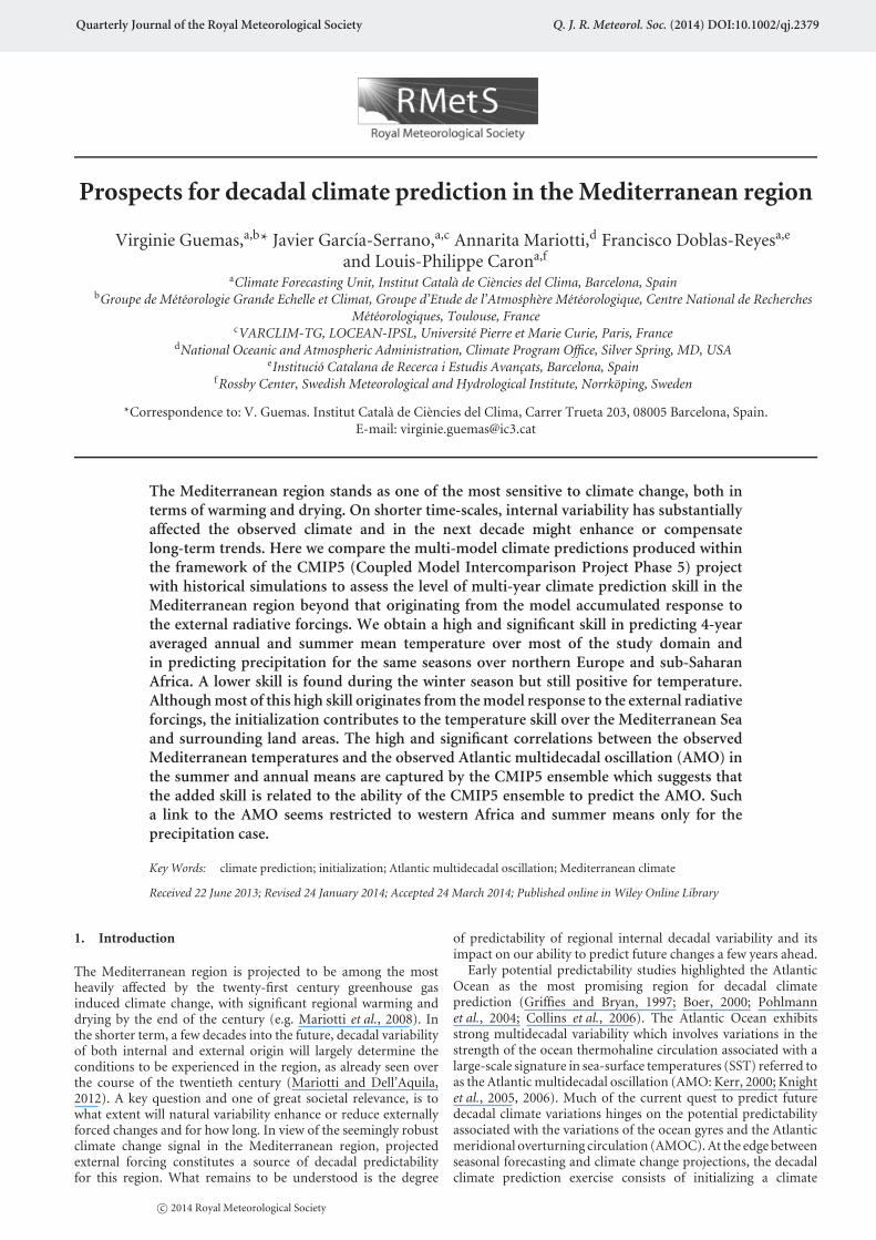
between Init ACC and NoInit ACC. There is still an increased skillover the eastern Atlantic with initialization but the added-valueover the Mediterranean Sea is less pronounced. There are alsotwo additional areas where the initialization tends to increase theskill: over eastern Europe and sub-Saharan Africa. In those tworegions, the correlation between the observed JJA AMO indexand the observed JJA temperature has an opposite sign to the onefor annual temperature: it becomes positive over eastern Europeand negative over sub-Saharan Africa (Figure 5(a,b)). The latteris probably due to the positive link between the AMO and theWest African monsoon (Mohino et al., 2011; van Oldenborghet al., 2012), which negatively feedbacks on local land-surfacetemperature (Giannini et al., 2003, 2005; Kucharski et al., 2013).The correlation between the Init JJA AMO index and the InitJJA temperature is positive over most of the domain except forsub-Saharan Africa (Figure 5(c,d)), as in the annual correlationmaps (Figure 3(c,d)). The Init and observed correlation maps aretherefore more consistent over eastern Europe and sub-SaharanAfrica for the JJA means than for the annual ones, hence a largeradded-value of the initialization in JJA over those two regions.The probabilistic verification (Figure S3) consistently shows anincreased BSS with initialization in the eastern Atlantic for the

c© 2014 Royal Meteorological Society Q. J. R. Meteorol. Soc. (2014)

Prospects for Decadal Climate Prediction in the Mediterranean Region

Correlation annual temperature with AMO index

Obs

erva

tions

10N

30N

50N

10N

30N

50N

10N

30N

50N

10N

30N

50N

10N

30N

50N

10N

30N

50N

20W

(a) (b)

(c) (d)

(e) (f)

0 20E 40E

20W 0 20E 40E 20W 0 20E 40E

20W 0 20E 40E20W 0 20E 40E

20W 0 20E 40E

Init

−1 −0.8 −0.6 −0.4 −0.2 0.2 0.4 0.6 0.8 1

Init-

NoI

nit

−1 −0.4 −0.3 −0.2 −0.1 0 0.1 0.2 0.3 0.4 1

Figure 3. Correlation between the AMO index and the temperature anomalies from (a,b) observational datasets, and (c,d) the ensemble mean decadal hindcasts,averaged along the forecast times ranging from (a,c,e) the second to fifth years and (b,d,f) the sixth to ninth years. (e,f) Difference between second row and itsequivalent in NoInit. The temperature anomalies have been detrended by subtracting the global mean SST to the grid-point SST and the global land temperatureto the grid-point land temperature prior to the computation of correlation. The black dots indicate the regions where the correlation or difference in correlation issignificant at the 95% level.

upper and middle terciles and in the Mediterranean region andover eastern Europe for all the terciles and forecast averages.

The winter (DJF) stands out as the season for which the increasein ACC with initialization is the largest, especially over the oceans(Figure 6(c–f)), and consistently the season for which the decreasein RMSE is the largest (Figure 6(i,j)). The skill, both deterministic(Figure 6) and probabilistic (Figure S4), remains improved overthe eastern Atlantic but it is also improved over eastern NorthAfrica, the eastern Mediterranean and eastern Europe, in termsof RMSE and ACC. The skill is strongly reduced though overwestern Africa and western Europe, especially for forecast years2–5, and over the Arabian Peninsula. DJF is also the season forwhich the Init ACC (Figure 6(a,b)) and MSSS (Figure 6(g,h)) skillare the lowest, as well as the BSS for all terciles (Figure S4). Thewarming trend has indeed lower relative amplitude in this seasoncompared to the amplitude of the internal natural variability(Figure S1). The correlation maps of observed DJF temperaturewith the observed DJF AMO index rather exhibit an L-pattern withpositive values over the eastern Atlantic, northern Africa, easternMediterranean Sea and the Arabian Peninsula, and negativevalues over Europe (Figure 7(a,b)). This pattern is however not

robust against the sampling (Figure 7(a,b)) and slightly differentfrom the one obtained by Mariotti and Dell’Aquila (2012) overa different period. The observed linkage between the DJF AMOand the DJF temperature is not properly captured by Init overEurope. Over the Mediterranean Sea, the signature is noisy(Figure 7(c,d)). The increase in skill with initialization in thoseregions therefore does not seem to be related to the ability of theMME in predicting the AMO. However, Init is able to simulate theobserved AMO correlation pattern over the eastern Atlantic andnorthern Africa reasonably well and over the Arabian Peninsula tosome extent. Although boreal winter (DJF) is the season for whichthe initialization allows for the largest increase in skill in predictingthe AMO index (Figure 2(c,d)), there is little agreement betweenthe pattern of differences in ACC skill Init-NoInit and the patternof Init-NoInit differences in correlations of the temperature withthe AMO index (Figure 7(e,f)). The ability of the MME to capturethe observed winter AMO seems to contribute to the skill inpredicting winter temperature only over confined regions such asthe Egypt–Sudan area and the eastern Atlantic.

c© 2014 Royal Meteorological Society Q. J. R. Meteorol. Soc. (2014)

V. Guemas et al.

AC

CIn

it

0

AC

CIn

it-N

oIni

t

0 0.5 0.8 0.9 0.95 1 1.05 1.1 1.2 2 6

10N

30N

50N

10N

30N

50N

10N

30N

50N

10N

30N

50N

10N

30N

50N

10N

30N

50N

10N

30N

50N

10N

30N

50N

10N

30N

50N

10N

30N

50N

20W 0 20E 40E 20W 0 20E 40E

20W 0 20E 40E20W 0 20E 40E

20W 0 20E 40E

20W 0 20E 40E

20W 0 20E 40E 20W 0 20E 40E

20W 0 20E 40E

20W 0 20E 40E

Skill in JJA temperature.

−1

(a) (b)

(c) (d)

(e) (f)

(g) (h)

(i) (j)

−0.8 −0.6 −0.4 −0.2 0.2 0.4 0.6 0.8 1

0−1 −0.8 −0.6 −0.4 −0.2 0.2 0.4 0.6 0.8 1

0−1 −0.4 −0.3 −0.2 −0.1 0.1 0.2 0.3 0.4 1

afte

rde

tren

dM

SS

S In

itR

MS

E In

it/N

o In

it

Figure 4. (a,b) Correlation between the ensemble-mean predicted and the observed summer (JJA) temperature anomalies averaged along the forecast times rangingfrom (a,c,e,g,i) the second to fifth years and (b,d,f,h,j) the sixth to ninth years. (c,d) Difference between the correlations in the decadal hindcasts and the equivalentin the historical simulations. (e,f) Difference between the correlations in the decadal hindcasts and the equivalent in the historical simulations after detrending bysubtracting the global mean SST to the grid-point SST and the global land temperature to the grid-point land temperature. (g,h) Mean Square Skill Score of theensemble-mean predicted anomalies. (i,j) Ratio of the root mean square error (RMSE) of the decadal hindcasts with respect to the historical simulations. The blackdots indicate the regions where the correlation, the difference in correlation, the MSSS or the ratio of the RMSE is significant at the 95% level.

3.2. Precipitation skill and role of the AMO

As discussed in the introduction, previous studies have nothighlighted any AMO-related precipitation variability in theMediterranean. Hence the basis for decadal precipitation

prediction is currently unclear. The precipitation patternsadditionally exhibit less spatial coherence than the temperaturepatterns. We therefore face a double challenge for precipitationforecast skill: the lack of knowledge about predictability sourcesand the spatial noise. Nevertheless, an exploratory analysis of

c© 2014 Royal Meteorological Society Q. J. R. Meteorol. Soc. (2014)

Prospects for Decadal Climate Prediction in the Mediterranean Region

Obs

erva

tions

10N

30N

50N

10N

30N

50N

10N

30N

50N

10N

30N

50N

10N

30N

50N

10N

30N

50N

20W

(a) (b)

(c) (d)

(e) (f)

0 20E 40E

20W 0 20E 40E

20W 0 20E 40E 20W 0 20E 40E

20W 0 20E 40E

20W 0 20E 40E

Init

−1 −0.8 −0.6 −0.4 −0.2 0.2 0.4 0.6 0.8 1

Init-

NoI

nit

−1 −0.4 −0.3 −0.2 −0.1 0 0.1 0.2 0.3 0.4 1

Correlation JJA temperature with AMO index

Figure 5. Correlation between the AMO index and the summer (JJA) temperature anomalies from (a,b) observational datasets, and (c,d) the ensemble-mean decadalhindcasts, averaged along the forecast times ranging from (a,c,e) the second to fifth years and (b,d,f) from the sixth to ninth years. (e,f) Difference between secondrow and its equivalent in NoInit. The temperature anomalies have been detrended by subtracting the global mean SST to the grid-point SST and the global landtemperature to the grid-point land temperature prior to the computation of the correlation. The black dots indicate the regions where the correlation or difference incorrelation is significant at the 95% level.

decadal prediction skill is presented here to potentially gainfurther insight in regional precipitation predictability includingthat from externally forced causes.

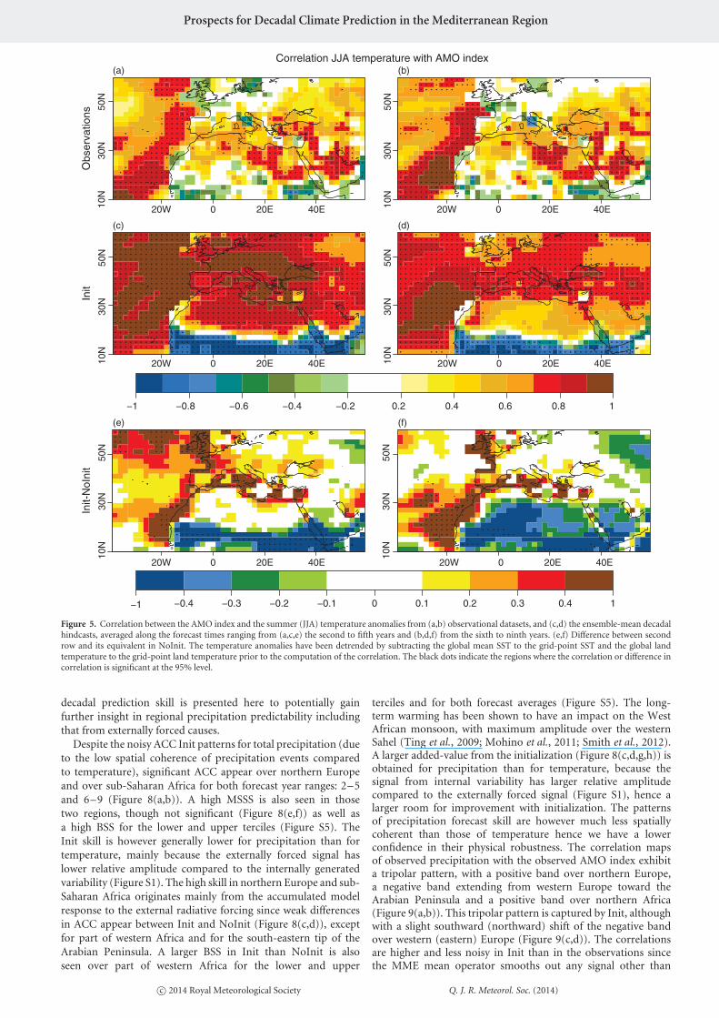
Despite the noisy ACC Init patterns for total precipitation (dueto the low spatial coherence of precipitation events comparedto temperature), significant ACC appear over northern Europeand over sub-Saharan Africa for both forecast year ranges: 2–5and 6–9 (Figure 8(a,b)). A high MSSS is also seen in thosetwo regions, though not significant (Figure 8(e,f)) as well asa high BSS for the lower and upper terciles (Figure S5). TheInit skill is however generally lower for precipitation than fortemperature, mainly because the externally forced signal haslower relative amplitude compared to the internally generatedvariability (Figure S1). The high skill in northern Europe and sub-Saharan Africa originates mainly from the accumulated modelresponse to the external radiative forcing since weak differencesin ACC appear between Init and NoInit (Figure 8(c,d)), exceptfor part of western Africa and for the south-eastern tip of theArabian Peninsula. A larger BSS in Init than NoInit is alsoseen over part of western Africa for the lower and upper

terciles and for both forecast averages (Figure S5). The long-term warming has been shown to have an impact on the WestAfrican monsoon, with maximum amplitude over the westernSahel (Ting et al., 2009; Mohino et al., 2011; Smith et al., 2012).A larger added-value from the initialization (Figure 8(c,d,g,h)) isobtained for precipitation than for temperature, because thesignal from internal variability has larger relative amplitudecompared to the externally forced signal (Figure S1), hence alarger room for improvement with initialization. The patternsof precipitation forecast skill are however much less spatiallycoherent than those of temperature hence we have a lowerconfidence in their physical robustness. The correlation mapsof observed precipitation with the observed AMO index exhibita tripolar pattern, with a positive band over northern Europe,a negative band extending from western Europe toward theArabian Peninsula and a positive band over northern Africa(Figure 9(a,b)). This tripolar pattern is captured by Init, althoughwith a slight southward (northward) shift of the negative bandover western (eastern) Europe (Figure 9(c,d)). The correlationsare higher and less noisy in Init than in the observations sincethe MME mean operator smooths out any signal other than

c© 2014 Royal Meteorological Society Q. J. R. Meteorol. Soc. (2014)

V. Guemas et al.

AC

C In

it10

N30

N50

N10

N30

N50

N

10N

30N

50N

10N

30N

50N

10N

30N

50N

10N

30N

50N

10N

30N

50N

10N

30N

50N

10N

30N

50N

10N

30N

50N

20W

(a) (b)

(c) (d)

(e) (f)

(g) (h)

(i) (j)

0 20E 40E

20W 0 20E 40E

20W 0 20E 40E

20W 0 20E 40E 20W 0 20E 40E

20W 0 20E 40E20W 0 20E 40E

20W 0 20E 40E

20W 0 20E 40E

20W 0 20E 40E

−1 −0.8 −0.6 −0.4 −0.2 0 0.2 0.4 0.6 0.8 1

AC

C In

it-N

oIni

taf

ter

detr

end

−1 −0.4 −0.3 −0.2 −0.1 0 0.1 0.2 0.3 0.4 1

MS

SS

Init

−1 −0.8 −0.6 −0.4 −0.2 0 0.2 0.4 0.6 0.8 1

0 0.5 0.8 0.9 0.95 1 1.05 1.1 1.2 2 6

Skill in DJF temperature.

RM

SE

Init

/ NoI

nit

Figure 6. (a,b) Correlation between the ensemble-mean predicted and the observed winter (DJF) temperature anomalies averaged along the forecast times rangingfrom (a,c,e,g,i) the second to the fifth years and (b,d,f,h,j) the sixth to ninth years. (c,d) Difference between the correlations in the decadal hindcasts and the equivalentin the historical simulations. (e,f) Difference between the correlations in the decadal hindcasts and the equivalent in the historical simulations after detrending bysubtracting the global mean SST to the grid-point SST and the global land temperature to the grid-point land temperature. (g,h) Mean Square Skill Score of theensemble-mean predicted anomalies. (i,j) Ratio of the root mean square error (RMSE) of the decadal hindcasts with respect to the historical simulations. The blackdots indicate the regions where the correlation, the difference in correlation, the MSSS or the ratio of the RMSE is significant at the 95% level.

externally forced or persisting initial conditions. The core ofthe positive correlation bands, i.e. over northern Europe andsub-Saharan Africa, which are well captured by Init, correspondsto high ACC and MSSS in Init. In transitional areas betweenpositive and negative correlation bands of precipitation with theAMO index (southern Europe and the Mediterranean Sea), Initfails to capture accurately the linkage between precipitation and

the AMO (slight shift of the patterns) and the ACC and MSSS

are low in those areas. The only region where the Init-NoInit

differences in correlation with the AMO index (Figure 9(e,f))

are consistent with the pattern of Init-NoInit differences in

ACC skill (Figure 8(c,d)) locates over the westernmost part of

North Africa.

c© 2014 Royal Meteorological Society Q. J. R. Meteorol. Soc. (2014)

Prospects for Decadal Climate Prediction in the Mediterranean Region

Obs

erva

tions

Init

−1 −0.8 −0.6 −0.4 −0.2 0.2 0.4 0.6 0.8 1

Init-

NoI

nit

−1 −0.4 −0.3 −0.2 −0.1 0 0.1 0.2 0.3 0.4 1

Correlation DJF temperature with AMO index

10N

30N

50N

10N

30N

50N

10N

30N

50N

10N

30N

50N

10N

30N

50N

10N

30N

50N

20W

(a) (b)

(c) (d)

(e) (f)

0 20E 40E 20W 0 20E 40E

20W 0 20E 40E

20W 0 20E 40E20W 0 20E 40E

20W 0 20E 40E

Figure 7. Correlation between the AMO index and the winter (DJF) temperature anomalies from (a,b) the observational datasets, and (c,d) the ensemble-meandecadal hindcasts, averaged along the forecast times ranging from (a,c,e) the second to fifth years and (b,d,f) the sixth to ninth years. Third row: difference between(c,d) and its equivalent in NoInit. The temperature anomalies have been detrended by subtracting the global mean SST to the grid-point SST and the global landtemperature to the grid-point land temperature prior to the computation of correlation. The black dots indicate the regions where the correlation or difference incorrelation is significant at the 95% level.

In summer (JJA), high and significant ACC cover also mostof northern Africa and a few points in northern Europe(Figure 10(a,b)). The pattern of Init skill is robust against the scoreconsidered but the MSSS (Figure 10(e,f)) and the BSS (Figure S6)show more modest performances. MSSS are significant over Egyptbut this performance is not supported by the other skill scores.Although the differences in ACC between Init and NoInit are notsignificant, a spatially coherent increase in ACC with initializationappears over western Africa (Figure 10(c,d)), together witha decrease in RMSE (Figure 10(g,h)). This low but positiveadded-value from the initialization in multi-year prediction skillover the West African monsoon region might be associatedwith the positive, although not statistically significant, skill ofthe Sahelian precipitation regime found by Garcıa-Serrano et al.(2013). The correlation maps of observed JJA precipitation withthe observed JJA AMO index exhibit a similar tripolar pattern tothe annual mean maps, but with a negative band centred on theMediterranean Sea (Figure 11(a,b)). The positive centre of actionover Africa is well captured by Init, including its shape, whichcould explain Init’s high skill in predicting JJA precipitation inthis area (Figure 11(b,c)). As for annual means, the westernmostpart of North Africa is the region showing the largest consistency

between Init-NoInit differences in correlation with the AMOindex (Figure 11(e,f)) and Init-NoInit differences in ACC skill(Figure 10(c,d)). This result is consistent with previous evidenceon the predictor role of the AMO upon the Sahelian rainfall(Mohino et al., 2011; van Oldenborgh et al., 2012; Garcıa-Serranoet al., 2013).

The winter Init ACC patterns are particularly noisy, with a fewpoints of significant ACC surrounded by negative ones spreadover northern Africa and a few positive ACC over northernEurope (Figure S7). The MSSS show a significant skill over theeastern Sahel which does not correspond to any positive ACCbut with a decrease in BSS for all terciles and forecast averages(Figure S8). The correlation maps of observed DJF precipitationwith the observed DJF AMO index exhibit a very differentpattern from the summer one with rather a dipolar structureacross the western Mediterranean which Init fails to capture(Figure S9).

4. Discussion

As mentioned in section 3.1, the AMO fluctuations exhibit arecent phase transition from negative conditions to positive

c© 2014 Royal Meteorological Society Q. J. R. Meteorol. Soc. (2014)

V. Guemas et al.

AC

CIn

it10

N30

N50

N

10N

30N

50N

10N

30N

50N

10N

30N

50N

10N

30N

50N

10N

30N

50N

10N

30N

50N

10N

30N

50N

20W

(a) (b)

(c) (d)

(e) (f)

(g) (h)

0 20E 40E

20W 0 20E 40E 20W 0 20E 40E

20W 0 20E 40E

20W 0 20E 40E20W 0 20E 40E

20W 0 20E 40E

20W 0 20E 40E

−1 −0.8 −0.6 −0.4 −0.2 0 0.2 0.4 0.6 0.8 1

AC

CIn

it-N

oIni

t

−1 −0.4 −0.3 −0.2 −0.1 0 0.1 0.2 0.3 0.4 1

MS

SS

Init

−1 −0.8 −0.6 −0.4 −0.2 0 0.2 0.4 0.6 0.8 1

RM

SE

Init

/ NoI

nit

0 0.5 0.8 0.9 0.95 1 1.05 1.1 1.2 2 6

Skill in annual precipitation.

Figure 8. (a,b) Correlation between the ensemble-mean predicted and the observed precipitation anomalies averaged along the forecast times ranging from (a,c,e,g)the second to fifth years and (b,d,f,h) the sixth to ninth years. (c,d) Difference between the correlations in the decadal hindcasts and the equivalent in the historicalsimulations. (e,f) Mean Square Skill Score of the ensemble-mean predicted anomalies. (g,h) Ratio of the root mean square error (RMSE) of the decadal hindcasts withrespect to the historical simulations. The black dots indicate the regions where the correlation, the difference in correlation, the MSSS or the ratio of the RMSE issignificant at the 95% level.

conditions, which shapes a positive trend. Note that this indexis computed as the SST averaged over the North Atlantic minusthe global SST average to minimize the effect of the long-termwarming. For consistency, the temperature has been detrendedby subtracting its global ocean mean at ocean grid points andits global land mean at land grid points prior to computing thecorrelation between the AMO and the grid-point temperatureas explained in section 2.3. The correlation between the AMOand grid-point temperature anomalies shown in Figures 3, 5 and

7 might be affected by a residual warming signal in the grid-point temperature. Similar qualitative results were obtained witha linear detrending method (not shown) but such a method doesnot filter out perfectly the warming signal either. Whether thisresidual warming and the warming trend in the AMO are relatedto a larger sensitivity to radiative forcings in our study domainthan in other regions or whether it is related to internal variabilityremains unclear. Given the shortness of the available time series,a proper assessment is highly challenging. For precipitation, we

c© 2014 Royal Meteorological Society Q. J. R. Meteorol. Soc. (2014)

Prospects for Decadal Climate Prediction in the Mediterranean Region

Obs

erva

tions

10N

30N

50N

10N

30N

50N

10N

30N

50N

10N

30N

50N

10N

30N

50N

10N

30N

50N

20W

(a) (b)

(c) (d)

(e) (f)

0 20E 40E 20W 0 20E 40E

20W 0 20E 40E20W 0 20E 40E

20W 0 20E 40E 20W 0 20E 40E

Init

−1 −0.8 −0.6 −0.4 −0.2 0.2 0.4 0.6 0.8 1

Init-

NoI

nit

−1 −0.4 −0.3 −0.2 −0.1 0 0.1 0.2 0.3 0.4 1

Correlation annual precipitation with AMO index

Figure 9. Correlation between the AMO index and the precipitation anomalies from (a,b) the observational datasets and (c,d) the ensemble-mean decadal hindcasts,averaged along the forecast times ranging from (a,c,e) the second to fifth years and (b,d,f) the sixth to ninth years. (e,f) Difference between (c,d) and its equivalent inNoInit. The black dots indicate the regions where the correlation or the difference in correlation is significant at the 95% level.

have chosen not to detrend because of the regional sensitivityto climate change and the uncertainties about whether thosechanges are attributable to climate change or not (Trenberth et al.,2007).

As explained in section 2.3, only 9–10 data can be usedto compute the skill scores shown in this article and those9–10 data are not independent since the CMIP5 retrospectivepredictions are initialized every 5 years and we focus on decadalclimate variability. An extension of the period sampled by ourstart dates would allow for more independent hindcasts andmore robust estimates of the added-value of initialization interms of skill scores. However, an extension backward in time ishighly challenging given the lack of accurate observational datato initialize the predictions. The denser observational networkthat grows with time will allow for a forward extension in thecoming decades and therefore for more robust estimates of theprediction skill scores. Likewise, 9–10 data are used to detrendtime series, which questions the accurate applicability of anymethod. This leads to consider that detrending methodologiesrepresent an important source of uncertainty in decadal climateprediction.

Mariotti and Dell’Aquila (2012) suggested that the linkagebetween the AMO and the Mediterranean region relies mainly on

atmospheric processes. To assess to what extent those atmosphericmechanisms are captured by the CMIP5 MME, we computedcorrelation maps of the AMO index with the sea-level pressurein both the observations and the model data for annual means(Figure S10), summer (Figure S11) and winter (Figure S12)values. The pattern obtained for the observations is not robustagainst the sampling, contrary to the patterns obtained previouslyfor temperature or precipitation, which suggests that the sea-levelpressure variability is dominated by other factors and we do nothave enough data to isolate accurately the AMO influence onthis variable. The MME fails to capture the observed patterns,but it remains unclear whether this failure is only an apparentfailure due to a sampling issue or a real failure suggesting someroom for improvement of the skill in predicting Mediterraneandecadal climate variability through a better representation of theatmospheric mechanism linking the Atlantic to the Mediterraneanregion.

5. Conclusions

In this article, we have used the extensive CMIP5 databaseof multi-model ensemble decadal hindcasts to assess the state-of-the-art skill in predicting Mediterranean temperature and

c© 2014 Royal Meteorological Society Q. J. R. Meteorol. Soc. (2014)

V. Guemas et al.

Skill in JJA precipitation.

AC

C In

it10

N30

N50

N10

N30

N50

N10

N30

N50

N10

N30

N50

N

10N

30N

50N

10N

30N

50N

10N

30N

50N

20W

(a) (b)

(c) (d)

(e) (f)

(g) (h)

0 20E 40E 20W 0 20E 40E

20W 0 20E 40E20W 0 20E 40E

20W 0 20E 40E 20W 0 20E 40E

−1 −0.8 −0.6 −0.4 −0.2 0 0.2 0.4 0.6 0.8 1

AC

C In

it-N

oIni

t

−1 −0.4 −0.3 −0.2 −0.1 0 0.1 0.2 0.3 0.4 1

MS

SS

Init

−1 −0.8 −0.6 −0.4 −0.2 0 0.2 0.4 0.6 0.8 1

RM

SE

Init

/ NoI

nit

0 0.5 0.8 0.9 0.95 1 1.05 1.1 1.2 2 6

Figure 10. (a,b) Correlation between the ensemble-mean summer (JJA) predicted and the observed precipitation anomalies averaged along the forecast times rangingfrom (a,c,e,g) the second to fifth years and (b,d,f,h) the sixth to ninth years. (c,d) Difference between the correlations in the decadal hindcasts and the equivalent inthe historical simulations. (e,f) Mean Square Skill Score of the ensemble-mean predicted anomalies. (g,h) Ratio of the root mean square error (RMSE) of the decadalhindcasts with respect to the historical simulations. The black dots indicate the regions where the correlation, the difference in correlation, the MSSS or the ratio ofthe RMSE is significant at the 95% level.

precipitation and the reasons behind this skill. High andsignificant skill in predicting 4-year averaged annual and summermean temperature is found over most of our study domain. Stillpositive but slightly lower skill is found during the winter season.Most of the high skill originates from the model accumulatedresponse to the external radiative forcings. The initializationcontributes however to the temperature forecast skill over the

Mediterranean Sea and surrounding land areas. The high andsignificant correlations between the observed Mediterraneantemperatures and the observed AMO in the summer and annualmeans which are captured by the multi-model ensemble suggestthat this added skill is related to the ability of the multi-modelensemble to predict the AMO. Although the winter seasonstands as the season with the largest increase in AMO forecast

c© 2014 Royal Meteorological Society Q. J. R. Meteorol. Soc. (2014)

Prospects for Decadal Climate Prediction in the Mediterranean Region

Obs

erva

tions

10N

30N

50N

10N

30N

50N

10N

30N

50N

10N

30N

50N

10N

30N

50N

10N

30N

50N

20W

(a) (b)

(c) (d)

(e) (f)

0 20E 40E 20W 0 20E 40E

20W 0 20E 40E20W 0 20E 40E

20W 0 20E 40E 20W 0 20E 40E

.

..

.

.

..

.

..

..

.

..

..

..

..

..

.

.

..

.

..

.

.

..

..

.

.

.

.

.

.

..

..

.

.

.

..

.

.

..

.. .........

.

..

..

.

.. ....

.

.

.

.

.. .. .. .. . .

.

..

.

. .

.

. .

.

.

..

.

.

.

.

.

..

.

.

.

..

.. .. .. ..

..

..

.

.

.

.. .

..

.

.

.

..

..

..

.. .

.

..

.

.

.

.

..

.

.

.. ..

.

..

.

.

..

.In

it

..

..

..

..

..

..

.

..

.

..

..

.

..

.

..

..

..

.

..

..

..

..

.

..

.

..

..

..

..

.

..

..

..

.

..

.

..

.

..

..

.

..

.

..

..

..

.

..

..

.

..

.

.

.

..

..

..

..

..

..

..

.

..

..

.

..

..

..

.

.

..

.

..

..

..

..

.

..

..

..

..

..

..

.

.

..

..

..

.

.

..

..

..

..

.

..

..

..

..

..

..

..

..

..

..

..

.

..

..

..

..

..

.

..

..

..

.

.

..

..

.

.

.

.

..

..

..

..

.

..

..

..

..

.

..

..

..

..

..

.

..

..

..

.

.

..

..

..

.

..

..

..

..

..

..

.

..

..

.

.

..

..

..

.

..

..

..

.

..

..

..

.

.

..

..

..

.

..

..

.

.

..

..

.

..

..

..

.

.

..

.

.

..

..

.

..

..

.

..

..

..

.

.

.

. .

.

. .. .. ..

..

.

.

.

..

..

..

..

..

.

..

.

..

.

..

.

..

.......

.

..

.

..

..

.

..

.

..

.

.

.

.. .. ..

..

..

..

.

..

..

..

..

.

..

..

.

..

..

..

..

.

..

..

..

..

.

..

.

..

..

.

..

..

.

..

..

.

..

..

.

..

..

.

..

..

..

..

.

..

..

..

..

.

..

..

..

..

..

..

..

.

..

.

..

..

..

..

.

..

.

.

..

..

..

.

..

..

..

.

.

.

..

.

..

..

..

.

.

..

.

.

.

.

.

.

..

.

.. . . .

.

.

−1 −0.8 −0.6 −0.4 −0.2 0.2 0.4 0.6 0.8 1

Init-

NoI

nit

..

..

..

..

..

.

..

..

..

..

..

..

..

..

..

...

.

..

..

..

..

..

.

.

..

.

..

.

..

..

..

..

..

.

..

..

..

.

..

.. .. .

. ..

.

. .

.

.

..

.

.

.

.

..

..

..

..

..

..

..

..

..

..

.

.

..

..

.

..

..

.

..

.

..

..

..

..

..

..

..

.

..

..

.

..

..

..

..

..

.

..

..

..

..

.

..

..

.

..

..

..

..

..

.

..

..

.

..

.

..

.

..

..

..

..

..

..

.

..

..

..

.

..

..

..

.

.

..

.

.

..

.... . .

. . . ..

.

..

.

..

..

..

.

.

.

.

.

. .

. .

.

.

−1 −0.4 −0.3 −0.2 −0.1 0 0.1 0.2 0.3 0.4 1

Correlation JJA precipitation with AMO index

Figure 11. Correlation between the AMO index and the summer (JJA) precipitation anomalies from (a,b) the observational datasets, and (c,d) the ensemble-meandecadal hindcasts, averaged along the forecast times ranging from (a,c,e) the second tofifth years and (b,d,f) the sixth to ninth years. (e,f) Difference between (c,d) andits equivalent in NoInit. The black dots indicate the regions where the correlation or difference in correlation is significant at the 95% level.

skill with initialization, the linkage between the AMO and theMediterranean temperatures is poorly captured by the multi-model ensemble. The increased skill in annual mean temperaturewith initialization seems to originate from the winter for theeastern Mediterranean and from the summer for the westernMediterranean. The results for the annual means are morerobust than the ones for the seasonal means though. High andsignificant skill is also found for annual and summer meanprecipitation over northern Europe and sub-Saharan Africa,which is mostly explained by the model accumulated responseto the external radiative forcings except over western Africa insummer. The positive correlation between summer observedAMO and precipitation in the latter region are well capturedby the multi-model ensemble which seems to contribute to theprecipitation forecast skill. The AMO-related skill in summerprecipitation does not seem to compensate for the weak signal inwinter. The winter precipitation forecast skill is much lowerand noisier than the summer and annual mean ones butimproving the winter precipitation forecast skill would be highlyrelevant. Improving the precipitation forecast skill stands as achallenge though, given the current lack of knowledge about itspredictability sources.

Acknowledgements

This work was supported by the EU-funded SPECS (FP7-ENV-2012-308378), NACLIM (FP7-ENV-2012-308299), QWeCI(FP7-ENV-2009-1-243964), CLIM-RUN (FP7-ENV-2010-1-265192) projects, the MICINN-funded RUCSS (CGL2010-20657) project, the Catalan Government and the NOAA grantNA10OAR4310208. Oriol Mula-Valls and Domingo Manubens-Gil are thoroughly acknowledged for their invaluable technicalsupport.

Supporting information

The following supporting information is available as part of theonline article:

Figure S1. Ratio of the slope of the long-term trend over thestandard deviation of the departures from the long-term trendin the observational datasets of temperature (first column) andprecipitation (second column). The trend and the departuresfrom the trends are computed from yearly means (first row),summer means (second row) and winter means (third row) afterapplying a 4-year running mean.

c© 2014 Royal Meteorological Society Q. J. R. Meteorol. Soc. (2014)

V. Guemas et al.

Figure S2. Brier Skill Score (BSS) of the multi-model ensembletemperature anomalies averaged along the forecast times rangingfrom the second to the fifth years (left) and the sixth to the ninthyears (right). The first two rows provide the BSS for the uppertercile in the decadal hindcasts and the historical simulations. Thethird and fourth rows provide the BSS for the middle tercile. Thebottom two rows provide the BSS for the lower tercile.

Figure S3. Brier Skill Score (BSS) of the multi-model ensemblesummer (JJA) temperature anomalies averaged along the forecasttimes ranging from the second to the fifth years (left) and thesixth to the ninth years (right). The first two rows provide the BSSfor the upper tercile in the decadal hindcasts and the historicalsimulations. The third and fourth rows provide the BSS for themiddle tercile. The bottom two rows provide the BSS for thelower tercile.

Figure S4. Brier Skill Score (BSS) of the multi-model ensemblewinter (DJF) temperature anomalies averaged along the forecasttimes ranging from the second to the fifth years (left) and thesixth to the ninth years (right). The first two rows provide the BSSfor the upper tercile in the decadal hindcasts and the historicalsimulations. The third and fourth rows provide the BSS for themiddle tercile. The bottom two rows provide the BSS for thelower tercile.

Figure S5. Brier Skill Score (BSS) of the multi-model ensembleprecipitation anomalies averaged along the forecast times rangingfrom the second to the fifth years (left) and the sixth to the ninthyears (right). The first two rows provide the BSS for the uppertercile in the decadal hindcasts and the historical simulations. Thethird and fourth rows provide the BSS for the middle tercile. Thebottom two rows provide the BSS for the lower tercile.

Figure S6. Brier Skill Score (BSS) of the multi-model ensemblesummer (JJA) precipitation anomalies averaged along the forecasttimes ranging from the second to the fifth years (left) and thesixth to the ninth years (right). The first two rows provide the BSSfor the upper tercile in the decadal hindcasts and the historicalsimulations. The third and fourth rows provide the BSS for themiddle tercile. The bottom two rows provide the BSS for thelower tercile.

Figure S7. First row: Correlation between the ensemble-meanwinter (DJF) predicted and observed precipitation anomaliesaveraged along the forecast times ranging from the second to thefifth years (left) and the sixth to the ninth years (right). Secondrow: Difference between the correlations in the decadal hindcastsand the equivalent in the historical simulations. Third row: MeanSquare Skill Score of the ensemble-mean predicted anomalies.Fourth row: Ratio of the root mean square error (RMSE) ofthe decadal hindcasts with respect to the historical simulations.The black dots indicate the regions where the correlation, thedifference in correlation, the MSSS or the ratio of the RMSE issignificant at the 95% level.

Figure S8. Brier Skill Score (BSS) of the multi-model ensemblewinter (DJF) precipitation anomalies averaged along the forecasttimes ranging from the second to the fifth years (left) and thesixth to the ninth years (right). The first two rows provide the BSSfor the upper tercile in the decadal hindcasts and the historicalsimulations. The third and fourth rows provide the BSS for themiddle tercile. The bottow two rows provide the BSS for the lowertercile.

Figure S9. Correlation between the AMO index and the winter(DJF) precipitation anomalies from the observational datasets(first row), and the ensemble-mean decadal hindcasts (secondrow), averaged along the forecast times ranging from the secondto the fifth years (left) and from the sixth to the ninth years (right).Third row: Difference between second row and its equivalent inNoInit. The black dots indicate the regions where the correlationor difference in correlation is significant at the 95% level.

Figure S10. Correlation between the AMO index and the sea-level pressure anomalies from the observational datasets (firstrow), the ensemble-mean decadal hindcasts (second row), andthe historical simulations (third row), averaged along the forecast

times ranging from the second to the fifth years (left) and fromthe sixth to the ninth years (right). The black dots indicate theregions where the correlation is significant at the 95% level.

Figure S11. Correlation between the AMO index and thesummer (JJA) sea-level pressure anomalies from the observationaldatasets (first row), the ensemble-mean decadal hindcasts (secondrow) and the historical simulations (third row), averaged alongthe forecast times ranging from the second to the fifth years (left)and from the sixth to the ninth years (right). The black dotsindicate the regions where the correlation is significant at the95% level.

Figure S12. Correlation between the AMO index and thewinter (DJF) sea-level pressure anomalies from the observationaldatasets (first row), the ensemble-mean decadal hindcasts (secondrow) and the historical simulations (third row), averaged alongthe forecast times ranging from the second to the fifth years (left)and from the sixth to the ninth years (right). The black dotsindicate the regions where the correlation is significant at the95% level.

References

Allan RJ, Ansell TJ. 2006. A new globally complete monthly historical meansea level pressure data set (HadSLP2). J. Clim. 19: 1850–2004.

Belluci A, Gualdi S, Masina S, Storto A, Scoccimarro E, Cagnazzo C, Fogli P,Manzini E, Navarra A. 2013. Decadal climate predictions with a coupledOAGCM initialized with oceanic reanalyses. Clim. Dyn. 40: 1483–1497, doi:10.1007/s00382-012-1468-z.

Boer GJ. 2000. A study of atmosphere–ocean predictability on long timescales.Clim. Dyn. 16: 469–472.

Booth BBB, Dunstone NJ, Halloran PR, Andrews T, Bellouin N. 2012. Aerosolsimplicated as a prime driver of twentieth-century North Atlantic climatevariability. Nature 484: 228–232.

Collins M, Botzet M, Carril AF, Drange H, Jouzeau A, Latif M, Masina S,Otteraa OH, Pohlmann H, Sorteberg A, Sutton R, Terray L. 2006.Interannual to decadal climate predictability in the North Atlantic: Amultimodel-ensemble study. J. Clim. 19: 1195–1203.

Delworth TL, Broccoli AJ, Rosati A, Stouffer RJ, Balaji V, Beesley JA, Cooke WF,Dixon KW, Dunne J, Dunne KA, Durachta JW, Findell KL, Ginoux P,Gnanadesikan A, Gordon CT, Griffies SM, Gudgel R, Harrison MJ,Held IM, Hemler RS, Horowitz LW, Klein SA, Knutson TR, Kushner PJ,Langenhorst AR, Lee H-C, Lin S-J, Lu J, Malyshev SL, Milly PCD,Ramaswamy V, Russell J, Schwarzkopf MD, Shevliakova E, Sirutis JJ,Spelman MJ, Stern WF, Winton M, Wittenberg AT, Wyman B, ZengF, Zhang R. 2006. GFDL’s CM2 global coupled climate models – Part 1:Formulation and simulation characteristics. J. Clim. 19: 643–674.

Doblas-Reyes FJ, Balmaseda MA, Weisheimer A, Palmer TN. 2011. Decadalclimate prediction with the European Centre for Medium-Range WeatherForecasts coupled forecast system: Impact of ocean observations. J. Geophys.Res. 116: D19111, doi: 10.1029/2010JD015394.

Doblas-Reyes FJ, Andreu-Burillo I, Chikamoto Y, Garcıa-Serrano J, Guemas V,Kimoto M, Mochizuki T, Rodrigues LRL, van Oldenborgh GJ. 2013.Initialized near-term regional climate change prediction. Nat. Commun. 4:1715, doi: 10.1038/ncomms2704.

Du H, Doblas-Reyes FJ, Garcıa-Serrano J, Guemas V, Soufflet Y, Wouters B.2012. Sensitivity of decadal predictions to the initial atmospheric and oceanicperturbations. Clim. Dyn. 39: 2013–2023, doi: 10.1007/s00382-011-1285-9.

Dufresne J-L, Foujols M-A, Denvil S, Caubel A, Marti O, Aumont O,Balkanski Y, Bekki S, Bellenger H, Benshila R, Bony S, Bopp L, Braconnot P,Brockmann P, Cadule P, Cheruy F, Codron F, Cozic A, Cugnet D, deNoblet N, Duvel J-P, Ethe C, Fairhead L, Fichefet T, Flavoni S, FriedlingsteinP, Grandpeix J-Y, Guez L, Guilyardi E, Hauglustaine D, Hourdin F, IdelkadiA, Ghattas J, Joussaume S, Kageyama M, Krinner G, Labetoulle S, LahellecA, Lefebvre M-P, Lefevre F, Levy C, Li ZX, Lloyd J, Lott F, Madec G, MancipM, Marchand M, Masson S, Meurdesoif Y, Mignot J, Musat I, ParoutyS, Polcher J, Rio C, Schulz M, Swingedouw D, Szopa S, Talandier C,Terray P, Viovy N. 2013. Climate change projections using the IPSL-CM5Earth System Model: From CMIP3 to CMIP5. Clim. Dyn. 40: 2123–2165,doi: 10.1007/s00382-012-1636-1.

Fan Y, van den Dool H. 2008. A global monthly land surface airtemperature analysis for 1948–present. J. Geophys. Res. 113: D01103, doi:10.1029/2007JD008470.

Fenoglio-Marc L, Mariotti A, Sannino G, Meyssignac B, Carillo A,Struglia MV, Rixen M. 2013. Decadal variability of net water flux atthe Mediterranean Sea Gibraltar Strait. Global Planet. Change 100: 1–10,doi: 10.1016/j.gloplacha.2012.08.007.

Fyfe JC, Merryfield WJ, Kharin V, Boer GJ, Lee W-S, von Salzen K. 2011.Skillful predictions of decadal trends in global mean surface temperature.Geophys. Res. Lett. 38: L22801, doi: 10.1029/2011GL049508.

Garcıa-Serrano J, Doblas-Reyes FJ. 2012. On the assessment of near-surface global temperature and North Atlantic multi-decadal variability

c© 2014 Royal Meteorological Society Q. J. R. Meteorol. Soc. (2014)

Prospects for Decadal Climate Prediction in the Mediterranean Region

in the ENSEMBLES decadal hindcast. Clim. Dyn. 39: 2025–2040, doi:10.1007/s00382-012-1413-1.

Garcıa-Serrano J, Doblas-Reyes FJ, Coelho CAS. 2012. Understanding Atlanticmulti-decadal variability prediction skill. Geophys. Res. Lett. 39: L18708,doi: 10.1029/2012GL053283.

Garcıa-Serrano J, Doblas-Reyes FJ, Haarsma RJ, Polo I. 2013. Decadalprediction of the dominant West African monsoon rainfall modes.J. Geophys. Res.–Atmos. 118: 1–20, doi: 10.1002/jgrd.50465.

Garcıa-Serrano J, Guemas V, Doblas-Reyes FJ. 2014. ‘Added-value frominitialization in skilful predictions of Atlantic multi-decadal variability’ .Clim. Dyn. (in press).

Giannini A, Saravanan R, Chang P. 2003. Oceanic forcing of Sahel rainfall oninterannual to interdecadal timescales. Science 302: 1027–1030.

Giannini A, Saravanan R, Chang P. 2005. Dyamics of the boreal summer Africanmonsoon in the NSIPP1 atmospheric model. Clim. Dyn. 25: 517–535.

Goddard L, Kumar A, Solomon A, Smith D, Boer G, Gonzalez P,Kharin V, Merryfield W, Deser C, Mason SJ, Kirtman BP, Msadek R,Sutton R, Hawkins E, Fricker T, Hegerl G, Ferro CAT, Stephenson DB,Meehl GA, Stockdale T, Burgman R, Greene AM, Kushnir Y, Newman M,Carton J, Fukumori I, Delworth T. 2013. A verification framework forinterannual-to-decadal prediction experiments. Clim. Dyn. 40: 245–272,doi: 10.1007/s00382-012-1481-2.

Gordon C, Cooper C, Senior C, Banks H, Gregory J, Johns T, Mitchell J,Wood R. 2000. The simulation of SST, sea ice extents and ocean heattransports in a version of the Hadley Centre coupled model without fluxadjustments. Clim. Dyn. 16: 147–168.

Hansen J, Ruedy R, Sato M, Lo K. 2010. Global surface temperature change.Rev. Geophys. 48: RG4004, doi: 10.1029/2010RG000345.

Griffies SM, Bryan K. 1997. Predictability of North Atlantic multidecadalclimate variability. Science 275: 181–184.

Hasumi H, Emori S. 2004. ‘K-1 coupled GCM (MIROC) description’,Technical report. Centre for Climate System Research, University of Tokyo.http://ccsr.aori.u-tokyo.ac.jp/ hasumi/miroc description.pdf (accessed 22May 2014).

Hawkins E, Sutton R. 2009. The potential to narrow uncertainty inregional climate predictions. Bull. Am. Meteorol. Soc. 90: 1095–1107, doi:10.1175/2009BAMS2607.1.

Hazeleger W, Severijns C, Semmler T, Stefanescu S, Yang ST, Wang XL,Wyser K, Dutra E, Baldasano JM, Bintanja R, Bougeault P, Caballero R,Ekman AML, Christensen JH, van den Hurk B, Jimenez P, Jones C,Kallberg P, Koenigk T, McGrath R, Miranda P, Van Noije T, Palmer TN,Parodi JA, Schmith T, Selten F, Storelvmo T, Sterl A, Tapamo H,Vancoppenolle M, Viterbo P, Willen U. 2010. EC-Earth: A seamlessEarth-system prediction approach in action. Bull. Am. Meteorol. Soc. 91:1357–1363.

Hazeleger W, Guemas V, Wouters B, Corti S, Andreu-Burillo I, Doblas-Reyes FJ, Wyser K, Caian M. 2013. Multiyear climate predictions usingtwo initialization strategies. Geophys. Res. Lett. 40: 1794–1798, doi:10.1002/grl.50355.

Jungclaus JH, Keenlyside N, Botzet M, Haak H, Luo J-J, Latif M, Marotzke J,Mikolajewicz U, Roeckner E. 2006. Ocean circulation and tropical variabilityin the coupled model ECHAM5/MPI-OM. J. Climate 19: 3952–3972.

Keenlyside NS, Latif M, Jungclaus J, Kornblueh L, Roeckner E. 2008. Advanceddecadal scale climate prediction in the North Atlantic sector. Nature 453:84–88, doi: 10.1038/nature06921.

Kerr RA. 2000. A North Atlantic climate pacemaker for the centuries. Science288: 1984–1985.

Knight JR, Allan RJ, Folland CK, Vellinga M, Mann ME. 2005. A signatureof persistent natural thermohaline circulation cycles in observed climate.Geophys. Res. Lett. 32: L20708, doi: 10.1029/2005GL024233.

Knight JR, Folland CK, Scaife AA. 2006. Climate impacts of theAtlantic Multidecadal Oscillation. Geophys. Res. Lett. 33: L17706, doi:10.1029/2006GL026242.

Kucharski F, Zeng N, Kalnay E. 2013. A further assessment of vegetationfeedback on decadal Sahel rainfall variability. Clim. Dyn. 40: 1453–1466,doi: 10.1007/s00382-012-1397-x.

Mariotti A, Dell’Aquila A. 2012. Decadal climate variability in theMediterranean region: Roles of large-scale forcings and regional processes.Clim. Dyn. 38: 1129–1145, doi: 10.1007/s00382-011-1056-7.

Mariotti A, Zeng N, Lau K-M. 2002. Euro-Mediterranean rainfall and ENSO – Aseasonally varying relationship. Geophys. Res. Lett. 29: 59–1–59–4, doi:10.1029/2001GL014248.

Mariotti A, Zeng N, Yoon J-H, Artale V, Navarra A, Alpert P, Li LZX.2008. Mediterranean water cycle changes: Transition to drier 21st centuryconditions in observations and CMIP3 simulations. Environ. Res. Lett. 3:044001, doi: 10.1088/1748-9326/3/4/044001.

Matei D, Pohlmann H, Jungclaus J, Muller W, Haak H, Marotzke J. 2012.Two tales of initializing decadal climate predictions experiments with theECHAM5/MPI-OM model. J. Clim. 25: 8502–8523.

Meehl GA, Goddard L, Murphy J, Stouffer RJ, Boer G, Danabasoglu G,Dixon K, Giorgetta MA, Greene AM, Hawkins E, Hegerl G, Karoly D,Keenlyside N, Kimoto M, Kirtman B, Navarra A, Pulwarty R, Smith D,Stammer D, Stockdale T. 2009. Decadal prediction Bull. Am. Meteorol. Soc.90: 1467–1485.

Meehl GA, Goddard L, Boer G, Burgman R, Branstator G, Cassou C, Corti S,Danabasoglu G, Doblas-Reyes F, Hawkins E, Karspeck A, Kimoto M,

Kumar A, Matei D, Mignot J, Msadek R, Navarra A, Pohlmann H,Rienecker M, Rosati T, Schneider E, Smith D, Sutton R, Teng HY, vanOldenborgh GJ, Vecchi G, Yeager S. 2014. Decadal climate prediction:An update from the trenches. Bull. Am. Meteorol. Soc. 95: 243–267, doi:10.1175/BAMS-D-12-00241.1.

Merryfield WJ, Lee W-S, Boer GJ, Kharin VV, Scinocca JF, Flato GM,Ajayamohan RS, Fyfe JC, Tang Y, Polavarapu S. 2013. The Canadianseasonal to interannual prediction system. Part I: Models and initialization.Mon. Weather Rev. 141: 2910–2945, doi: 10.1175/MWR-D-12-00216.1.

Mohino E, Janicot S, Bader J. 2011. Sahelian rainfall and decadal to multidecadalSST variability. Clim. Dyn. 37: 419–440.

Murphy JM, Kattsov V, Keenlyside N, Kimoto M, Meehl G, Mehta V,Pohlmann H, Scaife A, Smith D. 2010. Towards prediction of decadalclimate variability and change. Procedia Environ. Sci. 1: 287–304.

van Oldenborgh GJ, te Raa LA, Dijkstra HA, Philip SY. 2009. Frequency- oramplitude-dependent effects of the Atlantic meridional overturning on thetropical Pacific Ocean. Ocean Sci. 5: 293–301.

van Oldenborgh GJ, Doblas-Reyes FJ, Wouters B, Hazeleger W. 2012. Decadalprediction skill in a multi-model ensemble. Clim. Dyn. 38: 1263–1280.

Ottera OH, Bentsen M, Drange H, Suo L. 2010. External forcing as a metronomefor Atlantic multidecadal variability. Nat. Geosci. 3: 688–694.

Pohlmann H, Botzet M, Latif M, Roesch A, Wild M, Tschuck P. 2004.Estimating the decadal predictability of a coupled AOGCM. J. Clim. 17:4463–4472.

Pohlmann H, Jungclaus JH, Kohl A, Stammer D, Marotzke J. 2009. Initializingdecadal climate predictions with the GECCO oceanic synthesis: Effects onthe North Atlantic. J. Clim. 22: 3926–3938, doi: 10.1175/2009JCLI2535.1.

Pope VD, Gallani ML, Rowntree PR, Stratton RA. 2000. The impact of newphysical parametrizations in the Hadley Centre climate model – HadAM3.Clim. Dyn. 16: 123–146, doi: 10.1007/s003820050009.

Rudolf B, Becker A, Schneider U, Meyer-Christoffer A, Ziese M.2010. ‘The new ‘‘GPCC Full Data Reanalysis Version 5’’ pro-viding high-quality gridded monthly precipitation data forthe global land-surface is public available since December2010’, Status Report. Global Precipitation Climatology Centre.http://www.dwd.de/bvbw/generator/DWDWWW/Content/Oeffentlichkeit/KU/KU4/KU42/en/Reports Publications/GPCC status report 2010,templateId=raw,property=publicationFile.pdf/GPCC status report 2010.pdf (accessed 22 May 2014).

Sakamoto TT, Komuro Y, Ishii M, Tatebe H, Shiogama H, Hasegawa A,Toyoda T, Mori M, Suzuki T, Imada-Kanamaru Y, Nozawa T, Takata K,Mochizuki T, Ogochi K, Nishimura T, Emori S, Hasumi H, Kimoto M.2012. MIROC4h – A new high-resolution atmosphere–ocean coupledgeneral circulation model. J. Meteorol. Soc. Jpn. 90: 325–359.

Scoccimarro E, Gualdi S, Bellucci A, Sanna A, Fogli PG, Manzini E, Vichi M,Oddo P, Navarra A. 2011. Effects of tropical cyclones on ocean heattransport in a high resolution coupled general circulation model. J. Clim.24: 4368–4384.

Smith DM, Cusack S, Colman AW, Folland CK, Harris GR, Murphy JM. 2007.Improved surface temperature prediction for the coming decade from aglobal climate model. Science 317: 796–799.

Smith T, Reynolds R, Peterson T, Lawrimore J. 2008. Improvements to NOAA’shistorical merged land–ocean surface temperature analysis (1880–2006).J. Clim. 21: 2283–2296, doi: 10.1175/2007JCLI2100.1.

Smith DM, Scaife AA, Kirtman BP. 2012. What is the current state of scientificknowledge with regard to seasonal and decadal forecasting? Environ. Res.Lett. 7: 15602–15612, doi: 10.1088/1748-9326/7/1/015602.

Swingedouw D, Mignot J, Labetoulle S, Guilyardi E, Madec G. 2013.Initialisation and predictability of the AMOC over the last 50 years in aclimate model. Clim. Dyn. 40: 2381–2399, doi: 10.1007/s00382-012-1516-8.

Tatebe H, Ishii M, Mochizuki T, Chikamoto Y, Sakamoto TT, Komuro Y,Mori M, Yasunaka S, Watanabe M, Ogochi K, Suzuki T, Nishimura T,Kimoto M. 2012. Initialization of the climate model MIROC for decadalprediction with hydrographic data assimilation. J. Meteorol. Soc. Jpn. 90A:275–294.

Taylor KE, Stouffer RJ, Meehl GA. 2012. An overview of CMIP5 andthe experiment design. Bull. Am. Meteorol. Soc. 93: 485–498, doi:10.1175/BAMS-D-11-00094.1.

Terray L. 2012. Evidence for multiple drivers of North Atlantic multi-decadal climate variability. Geophys. Res. Lett. 39: L19712, doi: 10.1029/2012GL053046.

Ting M, Kushnir Y, Seager R, Li C. 2009. Forced and internal twentieth-centurySST trends in the North Atlantic. J. Clim. 22: 1469–1481.

Trenberth KE, Shea DJ. 2006. Atlantic hurricanes and natural variability in2005. Geophys. Res. Lett. 33: L12704, doi: 10.1029/2006GL026894.

Trenberth KE, Jones PD, Ambenje G, Bojiaru R, Easterling DR, KleinTank AMG, Parker DE, Renwick JA, Rahimzadeh F, Rusticucci MM,Soden BJ, Zhai P-M. 2007. Observations: Surface and atmospheric climatechange. In Climate Change 2007: The Physical Science Basis Contribution ofWorking Group I to the Fourth Assessment Report of the IntergovernmentalPanel on Climate Change, Solomon S, Qin D, Manning M, Chen Z,Marquis M, Averyt KB, Tignor M, Miller HL (eds). Cambridge UniversityPress: Cambridge, UK and New York, NY; 235–336.

Voldoire AE, Sanchez-Gomez E, Salas y Melia, Decharme B, Cassou CSenesiS, Valcke, Beau, Alias A, Chevallier M, Deque, Deshayes, Douville,Fernandez, Madec, Maisonnave, Moine M-P, Planton, Saint-Martin,

c© 2014 Royal Meteorological Society Q. J. R. Meteorol. Soc. (2014)

V. Guemas et al.

Szopa S, Tyteca, Alkama, Belamari, Braun, Coquart, Chauvin F. 2013.The CNRM-CM5.1 global climate model: Description and basic evaluation.Clim. Dyn. 40: 2091–2121, doi: 10.1007/s00382-011-1259-y.

Von Storch H, Zwiers F. 2001. Statistical Analysis in Climate Research.Cambridge University Press: Cambridge, UK, 484 pp.

Watanabe M, Suzuki T, O’ishi R, Komuro Y, Watanabe S, Emori S, Takemura T,Chikira M, Ogura T, Sekiguchi M, Takata K, Yamazaki D, Yokohata T,Nozawa T, Hasumi H, Tatebe H, Kimoto M. 2010. Improved climatesimulation by MIROC5: Mean states, variability, and climate sensitivity.J. Clim. 23: 6312–6335.

Yang XS, Rosati A, Zhang SQ, Delworth TL, Gudgel RG, Zhang R, Vecchi GA,Anderson WG, Chang Y-S, DelSole T, Dixon KW, Msadek R, Stern WF,

Wittenberg AT, Zeng FR. 2013. A predictable AMO-like patternin the GFDL fully coupled ensemble initialization and decadalforecasting system. J. Clim. 26: 650–661, doi: 10.1175/JCLI-D-12-00231.1.

Yukimoto S, Noda A, Kitoh A, Sugi M, Kitamura Y, Hosaka M, Shibata K,Maeda S, Uchiyama T. 2001. The new Meteorological Research InstituteCoupled GCM(MRI-CGCM2): Model climate and variability. Pap.Meteorol. Geophys. 51: 47–88.

Zhang R, Delworth TL, Sutton R, Hodson DLR, Dixon KW, Held IM, Kushnir Y,Marshall J, Ming Y, Msadek R, Robson J, Rosati AJ, Ting M, Vecchi GA.2013. Have aerosols caused the observed Atlantic multi-decadal variability?J. Atmos. Sci. 70: 1135–1143.

c© 2014 Royal Meteorological Society Q. J. R. Meteorol. Soc. (2014)