Predictability indices of the binary genetic tests ENG 2014

ISSN 2079�0597, Russian Journal of Genetics: Applied Research, 2014, Vol. 4, No. 2, pp. 146–158. © Pleiades Publishing, Ltd., 2014.Original Russian Text © A.V. Rubanovich, N.N. Khromov�Borisov, 2013, published in Ekologicheskaya Genetika, 2013, Vol. 11, No. 1, pp. 77–90.

146

INTRODUCTION

The global abundance of the studies of statisticalassociation between genotype and predisposition tocommon diseases has raised a sharp discussion on themethods of assessing the prognostic efficiency of themarkers revealed as a result of these studies (Poste,2011; Kraemer et al., 2011; Pepe et al., 2010; Kraftet al., 2009; Jakovdottir et al., 2009; Tan et al., 2004).Generally, the authors agreed that the high values ofthe indices of the association of a marker with a traitdo not guarantee the usage of this marker for the prog�nosis of a phenotypic expression of the genotype. Inparticular, many authors emphasize that a statisticallyhighly significant association of the disease with agenetic marker is a necessary but insufficient condi�tion for the usage of such a marker for the predictionof susceptibility to the disease. For instance, numerousgenes revealed by genome�wide scanning as associatedwith prostate cancer increase the prognostic efficiencyof the traditional biomarkers only by several percents(PSA, Gleason score) (see, for example, Aly et al.,2011 and editor comments Bjartell, 2011).

In this regard, we undertook a theoretical study ofsituations that arise when attempting to describe thestatistical associations “genotype–binary trait”. Weare primarily interested in the question: what values ofOR (odds ratio) can reassure researcher? At which val�ues of OR obtained on the basis of the revealed geneticassociations an effective biomarker predisposed to thedisease can be created? Here we will show that theanswers to these questions depend considerably on the

prevalence of the disease and the frequency of occur�rence of the marker. The aim of the article is to studyin detail the functional dependency of the standardindices of test efficiency on three independent param�eters: OR, the population frequency of a marker (pM),and the prevalence of a disease (pD).

REVIEW OF THE INDICES OF THE EFFICIENCY OF THE BINARY TEST

The number of measures of association suggestedfor qualitative traits long exceeds all reasonable limits.The work (Tan et al., 2004) enumerates 21 associationindices which characterize the four�fold contingencytable. The attempts to put in order feasible indices andmeasures of association are also varied. The recentwork (Bossuyt, 2010) suggests the following classifica�tion: (1) error�based measures—sensitivity, specificityand their derivatives; (2) information�based mea�sures—absolute risks at positive and negative testresults and the likelihood ratio; (3) association�basedmeasures—odds ratio OR, relative risks and Cohen’skappa coefficient. This classification does not look toonatural. In fact, all measures related to case�controlstudies are regarded as indicators of accuracy, andmeasures typical for cohort studies are regarded asindicators of infomativity. Absolute risks are regardedas indicators of informativeness, and their ratio (rela�tive risk) – as indicators of association. Furthermore,when OR � 1, the kappa coefficient and relative risks

Theoretical Analysis of the Predictability Indices of the Binary Genetic Tests

A. V. Rubanovicha and N. N. Khromov�Borisovb–d

aVavilov Institute of General Genetics, Russian Academy of Sciences, Moscow, RussiabFirst Pavlov State Medical University of St. Petersburg, Saint Petersburg, Russia[N1]

cRussian Scientific Research Institute of Hematology and Transfusiology, St. Petersburg, RussiadVreden Russian Scientific Research Institute of Traumatology and Orthopedics, St. Petersburg, Russia

Received March 8, 2012; in final form, October 1, 2012

Abstract—A set of formulas for the indices of the performance and predictive ability of the binary genetictests is presented. Their dependence on disease prevalence and the population frequency of a genetic markeris characterized. It is shown that a marker with the odds ratio OR < 2.2 has an initially low prognostic effi�ciency in every sense and at any frequencies of the disease and the marker. A marker can be a good classifier,when OR > 5.4, but only in case its population frequency is rather high (pM > 0.3). The formulas are presentedthat allow obtaining indirect estimates of the absolute and relative risk of the disease for the carrier of a markerin the case�control studies.

Keywords: genetic association studies, odds ratio, area under curve (AUC); predictive genetic testing.

DOI: 10.1134/S2079059714020087

Nikita

Cross-Out

RUSSIAN JOURNAL OF GENETICS: APPLIED RESEARCH Vol. 4 No. 2 2014

THEORETICAL ANALYSIS OF THE PREDICTABILITY INDICES 147

may be arbitrarily small and the high likelihood ratiodoes not guarantee a high level of absolute risks.

We will adhere to the following simple classifica�tion: (1) total indicators, i.e., dependent on the entirecontingency table; (2) conditional indicators whosecalculation uses only either the rows or columns of thecontingency table. In the second case, we will stronglyemphasize the symmetry of the situation—every lineindex corresponds to a similar column index. In fact,it is the only possible way not to get confused in thevariety of possible test characteristics. Furthermore,such a classification is dictated by the data structure inthe “genetics of predispositions”. Geneticists rarelyhave the opportunity to conduct a population�basedstudy of genotypes and calculate the probability of thecoincidence of a genetic marker and a disease. Usuallyit is only possible to estimate the conditional probabil�ities of the carriage of a marker under the presence ofthe disease (case�control studies), or the probability ofthe occurrence of the disease under the marker car�riage (cohort studies with the selected marker carri�ers). These two options correspond to the assessmentof conditional indices by columns or by rows.

Let the joint probability distribution of the occur�rence of a marker M and a disease D be given in theform of a standard 2 x 2 contingency table (matrix)

(1)

with normalization P(M, D) + P(M, ) + P( D) +

P( ) = 1.Here, we assume that binary random variables M

and D take the values: M ∈ {M, } and D ∈ {D, }.Marker M means predisposing genotype (allele, hap�

lotype) associated with disease D. means the set of

alternative genetic variants. means the absence of adisease.

Let us introduce the notations for the marginalsums:

pD = P(M, D) + P( D) is the prevalence of a dis�ease, and

pM = P(M, D) + P(M, ) is the population fre�quency of a marker. Easily verifiable identity P(M, D) –

pMpD = P( ) – (1 – pM)(1 – pD) = pM(1 – pD) –

P(M, ) makes possible to present the initial matrix Pin the form

(2)

P P M D,( ) P M D,( )

P M D,( ) P M D,( )⎝ ⎠⎜ ⎟⎛ ⎞

=

D M,

M, D

M D

M

D

M,

D

M, D

D

P pMpD pM 1 pD–( )

pD 1 pM–( ) 1 pM–( ) 1 pD–( )⎝ ⎠⎜ ⎟⎛ ⎞

=

+ Δ 1 1–

1– 1⎝ ⎠⎜ ⎟⎛ ⎞

.

In this sum the first matrix corresponds to the caseof independent random variables M and D, and thesecond is the additive that arises due to their interac�tion. Hereinafter, we will consider only the case Δ ≥ 0(positive association between a marker and a disease).

The case Δ < 0 corresponds to the interchange M ↔

The quantity Δ = P(M, D) – pMpD is one of the pos�sible (but rarely used) measures of association betweenM and D. The definitions of the most common indicesof statistical association are presented in Table 1.

Intergal Indicators of Association

They include odds ratio (OR), accuracy (ACC),correlation coefficient (r), and Cohen’s kappa coeffi�cient, κC (Cohen, 1960).

An obvious advantage of the OR indicator consistsin its versatility, in terms of its applicability to anyscheme of the study (cases�controls, cohort studies).The remaining total indicators can be estimateddirectly only in population�based studies (without tar�geted selection of “just the person with the disease” or“just the marker carriers”).

Intuitively appealing for understanding is the indi�cator ACC (another name: FC, Fraction Correct(Mitchell, 2009a, b)), which is defined as the proportionof correct test results (the trace of P matrix). Strictlyspeaking, ACC is not a measure of association sinceACC > 0 at OR = 1. Furthermore, when pM ≈ pD � 1, thequantity ACC depends only weakly on OR and is closeto 1, even in the absence of statistical association.

In fact, in the indices r and κ the difference Δ =P(M, D) – pMpD is used. Nevertheless, the correlationcoefficient r does not practically figure in the geneticstudies of predispositions because it is directly assessedonly in population studies. The quantity r primarilyreflects the linearity of the M and D interactions, i.e.,the proximity of the P matrix to a diagonal form.

Herewith, unlike OR, the correlation coefficientmay not register the situations (to be close to zero), inwhich marker carriage is only the necessary (or onlythe sufficient) condition of a disease.

The κC coefficient is often used to test the agree�ment between two methods of diagnostics or betweenopinions of two diagnosticians. And the agreement isconsidered good when 0.6 ≤ κC ≤ 0.8 and perfect at0.8 ≤ κC ≤ 1.0 (Landis, Koch, 1977).

In practice, the κC coefficient is close to the corre�lation coefficient, but always κC ≤ r with an equalitywhen pM = pD. More precisely

M.

r κC12��

pD 1 pM–( )pM 1 pD–( )��

pM 1 pD–( )pD 1 pM–( )��+⎝ ⎠

⎛ ⎞ κC.≥=

Nikita

Comment on Text

отформатировать - отцентрировать, т.е. приподнять строки внутри скобок

Nikita

Comment on Text

отформатировать, отцентрировать, т.е. приподнять строки внутри скобок

148


RUBANOVICH, KHROMOV�BORISOV

Conditional Indicators of Associations

Conditional indicators (see the lower part of Table 1)can be calculated either by columns or by rows in thecontingency table depending on the study design.

Usually the conditional probabilities of the appear�ance of true�positive and true�negative test results areused. In the case�control studies by columns the sen�sitivity (SE) and specificity (SP) of the test may bedirectly estimated. When conducting cohort studiesthe dual indicators are amenable to direct assessmentby rows: predictive values for the positive (PPV) andnegative (NPV) results of diagnostic test results (posi�tive/negative predictive value).

For each pair of indices, the relative risks (LR andRR), which are always less than OR may be deter�mined.

The duality of the determination of the conditionalindices stipulates the fulfillment of the identities:

It is clear that OR > RR > LR when pM > pD andOR > LR > RR when pM > pD.

The quantity LR is called a likelihood ratio and isoften designated as LR meaning the fulfillment of theidentity:

SEPPV��

SE pM–PPV pD–�� OR LR–

OR RR–��

pM

pD

��.= = =

LR+SE

1 SP–��

P M D( )

P M D( )��= =

= P D M( )/ 1 P D M( )–( )

pD/ 1 pD–( )��,

which allows to interprets LR+ as the ratio of posteriorodds of a disease after receiving the information on thecarriage of a marker to the prior odds of a diseasebefore getting such information. Herewith, the similarindex is introduced for the negative�test results:

We will consider only LR ≡ LR+ owing to its dualityin relation to conditional index RR (relative risk).

The average efficiency of the test is often character�ized by the difference in absolute risks:

(in case�control studies), and

(in cohort studies).It is easy to see that the indicators of the average

efficiency are the slope coefficients for the corre�sponding regression lines

(3)

where = pM(1 – pM), = pM(1 – pM), bM |D andbD |M are slopes of the regression lines M on D and D onM, respectively.

LR–1 SE–

SP��

LR+

OR��= =

= P D M( )/ 1 P D M( )–( )

pD/ 1 pD–( )��.

P M D( ) P M D( )– SE 1 SP–( )–=

P M D( ) P D M( )– PPV 1 NPV–( )–=

SE SP 1–+P M D,( ) pMpD–

pD 1 pD–( )�� r

σM

σD

�� bM D,= = =

PPV NPV 1–+P M D,( ) pMpD–

pM 1 pM–( )�� r

σD

σM

�� bD M,= = =

σM2 σM

2

Table 1. Indices of the association of marker (M) and disease (D) for contingency matrix P

Total indices of association

OR

ACC P(M, D) + P( )

Δ P(M, D) – pMpD

r

κC 2Δ/(pM(1 – pD) + pD(1 – pM))

Conditional indices of association

true positives true negatives risk ratio risk difference

By columns SE = P(M |D ) SP = P( ) LR = SE/(1 – SP ) SE + SP – 1

By lines PPV = P(D |M) NPV = P(D|M) RR = PPV/(1 – NPV ) PPV + NPV – 1

SE—Sensitivity, i.e., probability of marker presence in a person with a disease; SP—Specificity, i.e., the probability of marker absencein a person without a disease; LR—Likelihood Ratio; RR—Risk Ratio; PPV—Positive Predictive Value, i.e., the probability of the pres�ence of a disease in a person with a marker; NPV—Negative Predictive Value, i.e., the probability of absence of a disease in a personwithout a marker.

P M D,( )P M D,( )

P M D,( )P M D,( )��

M, D

Δ/ pD 1 pD–( )pM 1 pM–( )

M D,

Nikita

Cross-Out

Nikita

Inserted Text

<

Nikita

Cross-Out

Nikita

Inserted Text

D

Nikita

Cross-Out

Nikita

Inserted Text

D

Nikita

Cross-Out

Nikita

Inserted Text

D



We mean here the regressions that are calculated

after recoding: → 0; M, D → 1.Obviously, the index bD |M , being the slope coeffi�

cient of the regression D to M and the difference ofabsolute risks characterizes the average diagnostic effi�ciency of a marker; i.e., the ability to predict the indi�vidual predisposition to a disease by testing the markercarriage. With respect to the index bM|D, it will beshown in the next section that to some extent thisindex characterizes the abilities of a marker to solveclassification tasks. Nothing else could be expected:the bM|D index being the slope coefficient of regressionM to D characterizes the test’s abilities to distinguishbetween samples of persons with the disease andhealthy persons without the disease.

It is clear that the correlation coefficient is the geo�metrical mean of the conditional indices of the test’sefficiency:

Let us note also that the quantities bM|D and bD |M areoften called the Youden index (Youden, 1950) and thepredictive summary index (PSI ) (Linn, Grunau,2006) respectively.

PROBABILISTIC INTEPRETATIONS OF A TEST EFFICIENCY INDICES

The PPV and NPV indices (and their derivative, theRR index) have an obvious and practically importantinterpretation: they are conditional probabilities ofdisease development under the carriage or absence ofthe marker. The prognostic value of dual indicators bycolumn (SE and SP) seems to be less obvious.

In this respect, let us consider several possibleprobabilistic interpretations of indices related to withbM |D = SE + SP – 1.

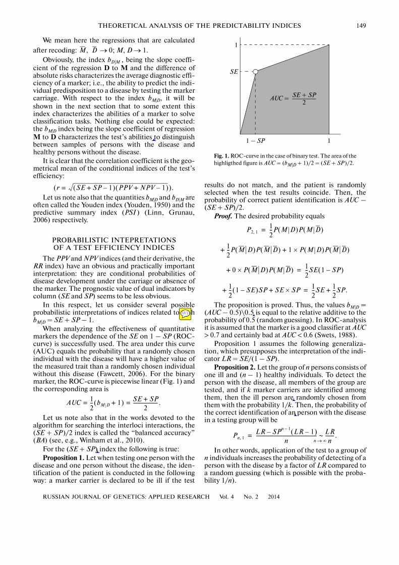
When analyzing the effectiveness of quantitativemarkers the dependence of the SE on 1 – SP (ROC�curve) is successfully used. The area under this curve(AUC) equals the probability that a randomly chosenindividual with the disease will have a higher value ofthe measured trait than a randomly chosen individualwithout this disease (Fawcett, 2006). For the binarymarker, the ROC�curve is piecewise linear (Fig. 1) andthe corresponding area is

Let us note also that in the works devoted to thealgorithm for searching the interloci interactions, the(SE + SP)/2 index is called the “balanced accuracy”(BA) (see, e.g., Winham et al., 2010).

For the (SE + SP) index the following is true:Proposition 1. Let when testing one person with the

disease and one person without the disease, the iden�tification of the patient is conducted in the followingway: a marker carrier is declared to be ill if the test

M, D

r SE SP 1–+( ) PPV NPV 1–+( )=( ).

AUC 12�� bM D 1+( ) SE SP+

2��= = .

results do not match, and the patient is randomlyselected when the test results coincide. Then, theprobability of correct patient identification is AUC –(SE + SP)/2.

Proof. The desired probability equals

The proposition is proved. Thus, the values bM |D =(AUC – 0.5)\0.5 is equal to the relative additive to theprobability of 0.5 (random guessing). In ROC�analysisit is assumed that the marker is a good classifier at AUC> 0.7 and certainly bad at AUC < 0.6 (Swets, 1988).

Proposition 1 assumes the following generaliza�tion, which presupposes the interpretation of the indi�cator LR = SE/(1 – SP).

Proposition 2. Let the group of n persons consists ofone ill and (n – 1) healthy individuals. To detect theperson with the disease, all members of the group aretested, and if k marker carriers are identified amongthem, then the ill person are randomly chosen fromthem with the probability 1/k. Then, the probability ofthe correct identification of an person with the diseasein a testing group will be

In other words, application of the test to a group ofn individuals increases the probability of detecting of aperson with the disease by a factor of LR compared toa random guessing (which is possible with the proba�bility 1/n).

P2 1,

12��P M D( )P M D( )=

+ 12��P M D( )P M D( ) 1 P M D( )P M D( )×+

+ 0 P M D( )P M D( )× 12��SE 1 SP–( )=

+ 12�� 1 SE–( )SP SE SP×+ 1

2��SE 1

2��SP.+=

Pn 1,

LR SPn 1– LR 1–( )–n

�� LRn

��.∼=n → ∞

1

SE

AUC =

11 – SP

SE + SP2

Fig. 1. ROC�curve in the case of binary test. The area of thehighligthed figure is AUC = (bM |D + 1)/2 = (SE + SP)/2.

Nikita

Cross-Out

Nikita

Inserted Text

ability

Nikita

Cross-Out

Nikita

Sticky Note

удалить

Nikita

Sticky Note

Marked set by Nikita

Nikita

Sticky Note

Marked set by Nikita

Nikita

Cross-Out

Nikita

Inserted Text

(SE + SP)/2

Nikita

Cross-Out

Nikita

Inserted Text

is

Nikita

Cross-Out

Nikita

Inserted Text

a

Nikita

Cross-Out

Nikita

Cross-Out

Nikita

Cross-Out

Nikita

Cross-Out

Nikita

Inserted Text

(AUC – 0.5)/0.5

150



Proof. The desired probability is

The proposition is proved. At n = 2, we have theformula from Proposition 1.

The indices inverse to bM |D and bD |M obtained wideuse for the estimate of the average number of tests con�ducted until the appearance of the first correctresponse of a marker. This approach was borrowedfrom the works which evaluate the efficiency of thera�peutic methods which are, as a rule, cohort studies(therapy T performs as a marker M). These works often

use the index NNT = (P(D| ) – P(D|T)) – 1,which assesses the minimal size of a group of peoplewho underwent therapy at which the number of curedpeople is one person more than in the same controlgroup (Number Needed to Treat). Analogously, for theassessment of the efficiency of using markers, differentauthors suggested (see, Anonymous, 1996 and discus�sion: e.g., Mitchell, 2009a, b) the following notions:

• The Number Needed to Diagnose for the case�control studies

• The Number Needed to Predict for cohort stud�ies

Herewith, the quantity NND is often interpreted asthe average population of the sample size which needsto be tested to identify one person with the disease(Mitchell, 2009a,b). The other authors assume thatNND is the average number of tests needed until theany correct result of the test will be obtained (correctidentification of a person with the disease or the per�son without the disease) (Linn, Grunau, 2006).

It seems to us that both interpretations are incor�rect. The counterexample is given by matrix P in theform

Pn 1,

1n�� 1 SE–( )SPn 1– SE 1

k 1+��

k 0=

n 1–

∑ Cn 1–k+=

× SPn 1– k–1 SP–( )k 1

n�� 1 SE–( )SPn 1–=

+ SE 1 SPn–n 1 SP–( )�� 1

n�� SPn 1– SE

1 SP–�� 1 SPn 1––( )+⎝ ⎠

⎛ ⎞=

= 1n�� LR SPn 1– LR 1–( )–( ).

bD T1– T

NND bM D1– P M D( ) P M D( )–( )

1–= =

= 1SE SP 1–+��;

NNP bD M1– P M D( ) P D M( )–( )

1–= =

= 1PPV NPV 1–+��.

P 10 6– 1 0

99 999 900⎝ ⎠⎜ ⎟⎛ ⎞

.=

In this case SE = 0.01 and SP = 1 (all marker car�riers are ill).

Then, NND = 100, although 1/pM = 106 tests arerequired on average to detect an ill person by using amarker. At the same time the proportion of correctoperations of the test is practically equal to unity(ACC – 0.999901). As concerns the indicator NND =

only the following may be asserted. Let one per�son with the disease and one person without the dis�ease be tested on marker carriage in a single timeperiod. Then, the average waiting time of the event“the number of marker carriers among persons withthe disease is higher than among persons without the

disease” is = (SE + SP – 1)–1. And the probabil�ity that the number of marker carriers in the sample ofpersons with the disease is always higher than in thesample of persons without the disease is SE + SP –1.

Similarly, when considering the growing sample ofmarker carriers, the average waiting time of the event“the number of persons with the disease among themarker carriers is higher than among persons withoutthe marker” is

DEPENDENCE OF INDICATORS OF EFFICIENCY ON THE PREVALENCE OF A DISEASE AND THE POPULATION

FREQUENCY OF A MARKER

Contemporary databases allow to get prior infor�mation on the frequencies of occurrence of potentialmarker genes (pM), along with the data on the preva�lence of the disease under study (pD). The predictiveefficiency of the genetic test in the searched associativestudies will essentially depend on the population fre�quency of the chosen marker. In this regard, it is nec�essary to imagine the type of dependence of all indicesof the test efficiency on pM and pD at different levels ofassociation (OR values).

In this section we will present the catalog of formu�las describing the dependence of indices of the binarytest’s efficiency on three independent parameters: OR,pM, and pD. Let us begin with the key index Δ=P(M, D) – pM and pD [N2]. The quantity Δ is calcu�lated from the definition of OR.

wherefrom

(4)

bM D1–

,

bM D1–

NNP bD M1– PPV NPV 1–+( ) 1–

.= =

ORpMpD Δ+( ) 1 pM–( ) 1 pD–( ) Δ+( )pD 1 pM–( ) Δ–( ) pM 1 pD–( ) Δ–( )

��,=

Δ 12�� OR δ–

OR 1–�� pDpM 1 pD–( ) 1 pM–( )––⎝ ⎠

⎛ ⎞=

= 4σM

2 σD2 OR 1–( )

δ 1+( )2

pM pD–( )2 OR 1–( )2–��,

Nikita

Cross-Out

Nikita

Inserted Text

P(D|T))-1

Nikita

Cross-Out

Nikita

Cross-Out

Nikita

Cross-Out

Nikita

Cross-Out

Nikita

Inserted Text

=

Nikita

Cross-Out



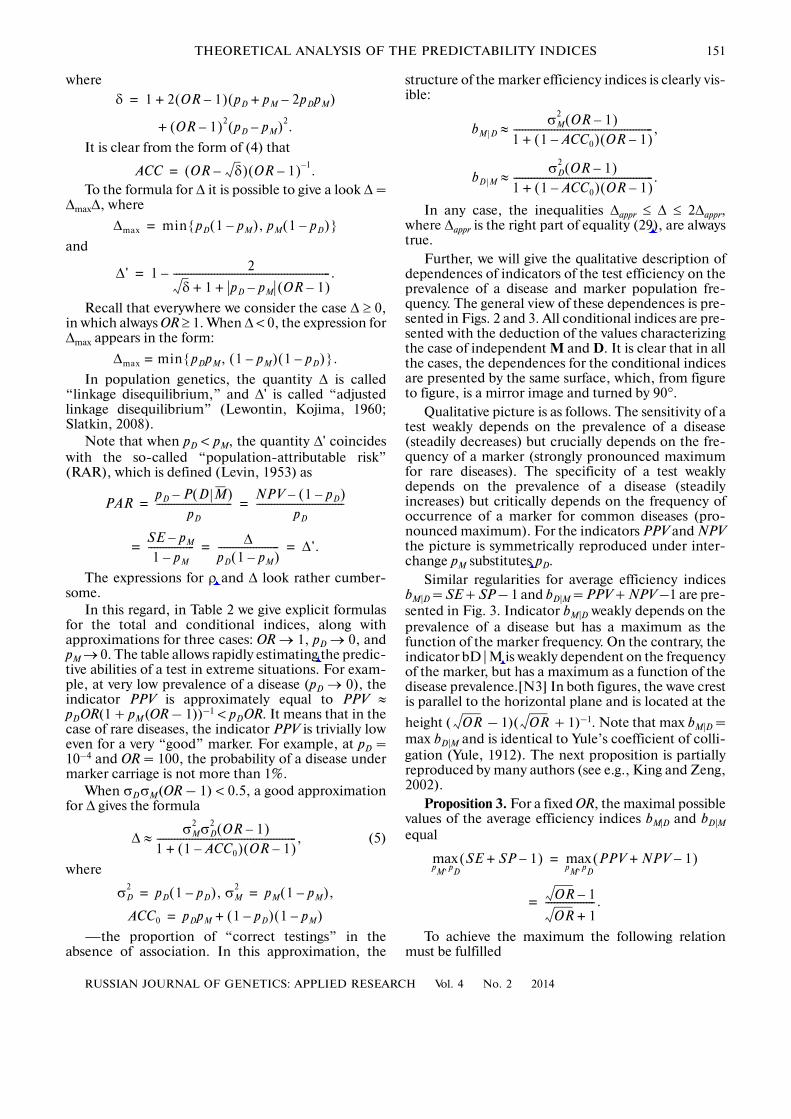
where

It is clear from the form of (4) that

To the formula for Δ it is possible to give a look Δ =ΔmaxΔ, where

and

Recall that everywhere we consider the case Δ ≥ 0,in which always OR ≥ 1. When Δ < 0, the expression forΔmax appears in the form:

In population genetics, the quantity Δ is called“linkage disequilibrium,” and Δ' is called “adjustedlinkage disequilibrium” (Lewontin, Kojima, 1960;Slatkin, 2008).

Note that when pD < pM, the quantity Δ' coincideswith the so�called “population�attributable risk”(RAR), which is defined (Levin, 1953) as

The expressions for ρ and Δ look rather cumber�some.

In this regard, in Table 2 we give explicit formulasfor the total and conditional indices, along withapproximations for three cases: OR → 1, pD → 0, andpM → 0. The table allows rapidly estimating the predic�tive abilities of a test in extreme situations. For exam�ple, at very low prevalence of a disease (pD → 0), theindicator PPV is approximately equal to PPV ≈pDOR(1 + pM(OR – 1))–1 < pDOR. It means that in thecase of rare diseases, the indicator PPV is trivially loweven for a very “good” marker. For example, at pD =10–4 and OR = 100, the probability of a disease undermarker carriage is not more than 1%.

When σDσM(OR – 1) < 0.5, a good approximationfor Δ gives the formula

(5)

where

—the proportion of “correct testings” in theabsence of association. In this approximation, the

δ 1 2 OR 1–( ) pD pM 2pDpM–+( )+=

+ OR 1–( )2 pD pM–( )2.

ACC OR δ–( ) OR 1–( ) 1–.=

Δmax min pD 1 pM–( ), pM 1 pD–( ){ }=

Δ ' 1 2

δ 1 pD pM– OR 1–( )+ +��– .=

Δmax min pDpM, 1 pM–( ) 1 pD–( ){ }= .

PARpD P D M( )–

pD

��NPV 1 pD–( )–

pD

��= =

= SE pM–1 pM–

�� ΔpD 1 pM–( )�� Δ '.= =

ΔσM

2 σD2 OR 1–( )

1 1 ACC0–( ) OR 1–( )+��,≈

σD2 pD 1 pD–( ), σM

2 pM 1 pM–( ),= =

ACC0 pDpM 1 pD–( ) 1 pM–( )+=

structure of the marker efficiency indices is clearly vis�ible:

In any case, the inequalities Δappr ≤ Δ ≤ 2Δappr,where Δappr is the right part of equality (29), are alwaystrue.

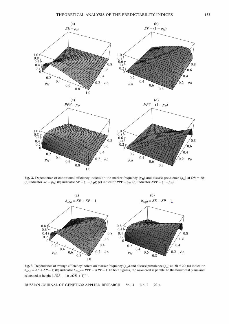
Further, we will give the qualitative description ofdependences of indicators of the test efficiency on theprevalence of a disease and marker population fre�quency. The general view of these dependences is pre�sented in Figs. 2 and 3. All conditional indices are pre�sented with the deduction of the values characterizingthe case of independent M and D. It is clear that in allthe cases, the dependences for the conditional indicesare presented by the same surface, which, from figureto figure, is a mirror image and turned by 90°.

Qualitative picture is as follows. The sensitivity of atest weakly depends on the prevalence of a disease(steadily decreases) but crucially depends on the fre�quency of a marker (strongly pronounced maximumfor rare diseases). The specificity of a test weaklydepends on the prevalence of a disease (steadilyincreases) but critically depends on the frequency ofoccurrence of a marker for common diseases (pro�nounced maximum). For the indicators PPV and NPVthe picture is symmetrically reproduced under inter�change pM substitutes pD.

Similar regularities for average efficiency indicesbM|D = SE + SP – 1 and bD|M = PPV + NPV –1 are pre�sented in Fig. 3. Indicator bM|D weakly depends on theprevalence of a disease but has a maximum as thefunction of the marker frequency. On the contrary, theindicator bD | M is weakly dependent on the frequencyof the marker, but has a maximum as a function of thedisease prevalence.[N3] In both figures, the wave crestis parallel to the horizontal plane and is located at the

height ( – 1)( + 1)–1. Note that max bM|D =max bD|M and is identical to Yule’s coefficient of colli�gation (Yule, 1912). The next proposition is partiallyreproduced by many authors (see e.g., King and Zeng,2002).

Proposition 3. For a fixed OR, the maximal possiblevalues of the average efficiency indices bM|D and bD|M

equal

To achieve the maximum the following relationmust be fulfilled

bM DσM

2 OR 1–( )1 1 ACC0–( ) OR 1–( )+��,≈

bD MσD

2 OR 1–( )1 1 ACC0–( ) OR 1–( )+�� .≈

OR OR

SE SP 1–+( )pM pD,max PPV NPV 1–+( )

pM pD,max=

= OR 1–

OR 1+��.

Nikita

Cross-Out

Nikita

Inserted Text

r

Nikita

Cross-Out

Nikita

Inserted Text

to estimate rapidly

Nikita

Cross-Out

Nikita

Inserted Text

↔

Nikita

Cross-Out

Nikita

Inserted Text

bD|M

Nikita

Cross-Out

Nikita

Cross-Out

Nikita

Inserted Text

5

152



Table 2. View of marker efficiency indices through OR, pM, and pD

Exact formulaApproximation formula at

OR → 1 pD → 0 pM → 0

Integral indices of association

ACC ACC0 1 – pM 1 – pD

Δ (OR – 1)

r σDσM(OR – 1)

κC

Conditional indices of association by columns

SE pm + pM + (1 – pD)(OR – 1)

SP 1 – pm + 1 – pM + pD(OR – 1) 1 – pM +

bM |D

RR OR – pM(OR – 1)

Conditional indices of association by rows

PPV pD + pD + (1 – pM)(OR – 1)

NPV 1 – pD + 1 – pD + pM(OR – 1) 1 – pD +

bD|M (OR – 1)

RR OR – pD(OR – 1)

Designationsp: δ = 1 + 2(OR – 1)(1 – ACC0) + (OR – 1)2(pD – pM)2, ACC0 = pDpM + (1 – pD)(1 – pM),

= pM(1 – pM), = pD(1 – pD).

OR δ–OR 1–

��

12�� ACC ACC0–( ) σM

2 σD2 σM

2pD OR 1–( )

1 pM OR 1–( )+��

σD2

pM OR 1–( )1 pD OR 1–( )+��

ΔσDσM

�� σM pD OR 1–( )1 pM OR 1–( )+��

σD pM OR 1–( )1 pD OR 1–( )+

��

2Δ1 ACC0–�� 2σM

2 σD2

OR 1–( )1 ACC0–

��2pD 1 pM–( ) OR 1–( )

1 pM OR 1–( )+��

2pM 1 pD–( ) OR 1–( )1 pD OR 1–( )+

��

ΔpD

�� σM2 pMOR

1 pM OR 1–( )+��

pMOR

1 pD OR 1–( )+��

Δ1 pD–�� σM

2 σM2

pD OR 1–( )1 pM OR 1–( )+�� 1

pM

1 pD OR 1–( )+��–

Δ

σD2

�� σM2

OR 1–( )σM

2OR 1–( )

1 pM OR 1–( )+��

pM OR 1–( )1 pD OR 1–( )+��

pMΔpD

��+

pMΔ

1 pD–��–

��OR

1 pM OR 1–( )+�� OR

pM OR 1–( )1 pD OR 1–( )+��–

ΔpM

�� σD2 pDOR

1 pM OR 1–( )+��

pDOR

1 pD OR 1–( )+��

Δ1 pM–�� σD

2 1pD

1 pM OR 1–( )+��– σD

2pM OR 1–( )

1 pD OR 1–( )+��

Δ

σM2

�� σD2 σD

2OR 1–( )

1 pD OR 1–( )+��

pD OR 1–( )1 pM OR 1–( )+��

pDΔ

pM

��+

pDΔ

1 pM–��–

�� ORpDOR OR 1–( )1 pM OR 1–( )+��–

OR1 pD OR 1–( )+��

σM2 σD

2

Nikita

Cross-Out



1.00.8

0.4

0

SE – pM

0.6

0.4

0.2

0.8

0.40.6

0.2

1.0

pMpD

0.6

0.20.8

1.00.8

0.4

0

SP – (1 – pM)

0.6

0.4

0.2

0.8

0.40.6

0.2

pMpD

0.6

0.20.8

1.00.8

0.4

0

PPV – pD

0.6

0.4

0.2

0.8

0.40.6

0.2

1.0

pMpD

0.6

0.20.8

1.00.8

0.4

0

NPV – (1 – pD)

0.6

0.4

0.2

0.8

0.40.6

0.2

pMpD

0.6

0.20.8

(a) (b)

(c) (d)

Fig. 2. Dependence of conditional efficiency indices on the marker frequency (pM) and disease prevalence (pD) at OR = 20:(a) indicator SE – pM; (b) indicator SP – (1 – pM); (c) indicator PPV – pD; (d) indicator NPV – (1 – pD).

0.8

0.4

0

bM|D = SE + SP – 1

0.6

0.4

0.20.8

0.40.6

0.2

1.0

pMpD

0.6

0.20.8

0.8

0.4

0

bM|D = SE + SP – 1

0.6

0.4

0.20.8

0.40.6

0.2

pMpD

0.6

0.20.8

(a) (b)

Fig. 3. Dependence of average efficiency indices on marker frequency (pM) and disease prevalence (pD) at OR = 20: (a) indicatorbM|D = SE + SP – 1; (b) indicator bD|M = PPV + NPV – 1. In both figures, the wave crest is parallel to the horizontal plane and

is located at height ( – 1)( + 1)–1.OR OR

Nikita

Cross-Out

Nikita

Inserted Text

bD|M = PPV + NPV – 1

154



Proof. The following identity is commonly known:OR = SE × SP(1 – SE)–1(1 – SP)–1.

For reasons of symmetry it is clear that the maxi�mum of the quantity bM|D = SE + SP – 1 = SE × SP(OR – 1)/OR is reached at SE = SP. Wherefrom, OR =SE2/(1 – SE)2, and the desired maximum equals

2SE – 1 = ( – 1)/( + 1)–1.Similarly, the maximum of the quantity

is reached at

PPV = NPV = ( + 1)–1

and equals

( – 1)( + 1)–1.The maximum does not depend on pM and pD (Fig.

2). And max bM|D is reached at

pM = (1 + pD( – 1))( + 1)–1.And max bM|D t

pD = (1 + pM( – 1))( + 1)–1.The proposition is proved.

pM pD–( )2OR 1 pM pD––( )2.=

OR OR

bD M PPV NPV 1–+ PPV NPV OR 1–( )/OR×= =

OR OR

OR OR

OR OR

OR OR

CASE OR � 1

At OR → ∞ the limit behavior of marker efficiencyindices in Table 1 essentially depends on the ratio ofmarker frequency and the prevalence of the disease.Two alternative situations, which are presented inTable 3, are possible.

From the Table it follows, in particular, that thehigh value of OR and high statistical significance of theeffect does not always denote the predictive efficiencyof a marker. Thus, at OR → ∞ and pM � pD the indica�tor of diagnostic efficiency bD|M = PPV = pD/pM < 1;i.e., it may be arbitrarily small in absolute value. In theopposite situation (pM � pD) at OR → ∞, the sensitivityof the test and corresponding indicator of the classifi�cation efficiency are trivially low:

bM|D = SE = pM/pD � 1.

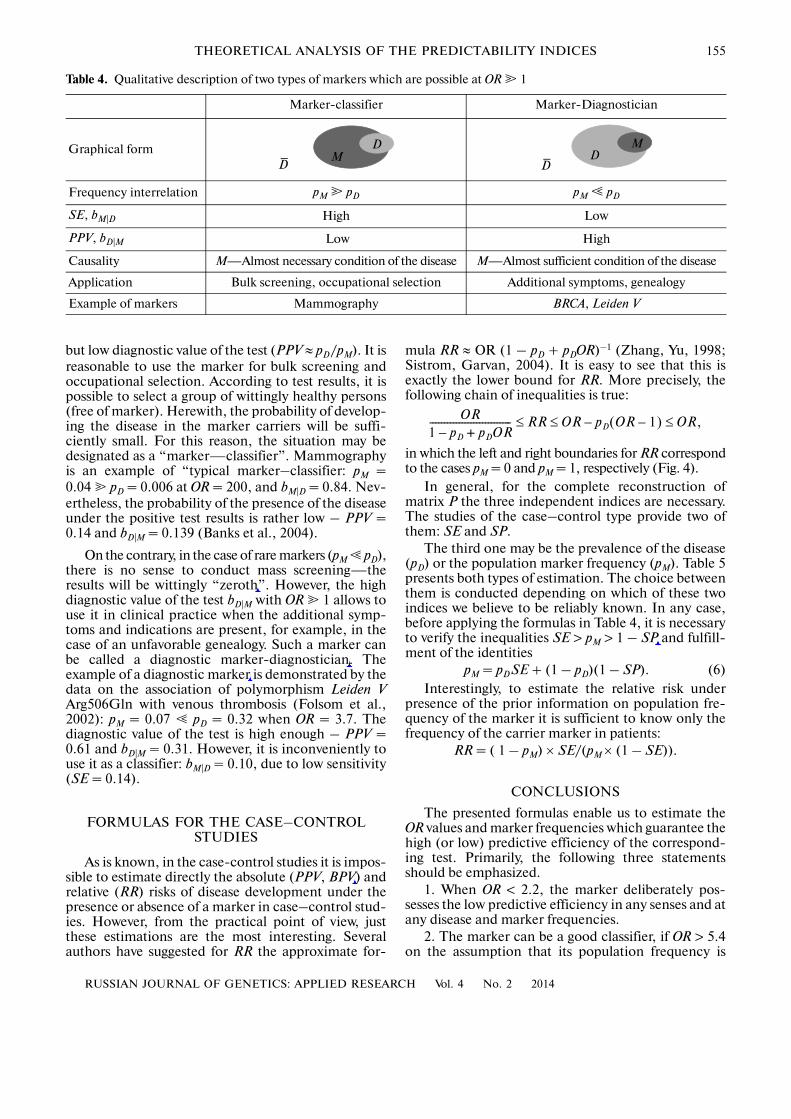
MARKERS� CLASSIFIERS AND MARKERS�DIAGNOSTICIANS

For the situations presented in Tables 3 and 4, itmakes sense to introduce special terms, reflecting themarker peculiarity. Under the high frequency ofoccurrence of the marker (pM � pD) and OR � 1, wehave a high sensitivity and classification efficiency bM|D

Table 3. Limit behavior of the test efficiency indices at OR → ∞

pM > pD pM < pD

Contingency table form

Graphical form

Causality M—Necessary condition of the disease M—Sufficient condition of the disease

SE 1 pM/pD

SP (1 – pM)/(1 – pD) 1

PPV pD/pM 1

NPV 1 (1 – pD)/(1 – pM)

LR (1 – pD)/(pM – pD) ∞

RR ∞ (1 – pM)/(pD – pM)

bM|D (1 – pM)/(1 – pD) pM/pD

bD|M pD/pM (1 – pD)/(1 – pM)

ACC 1 – (pM – pD) 1 – (pD – pM)

Δ pD(1 – pM) pM(1 – pD)

r

pD pM pD–

0 1 pM–⎝ ⎠⎜ ⎟⎛ ⎞ pM 0

pD pM– 1 pD–⎝ ⎠⎜ ⎟⎛ ⎞

DM

DD

M

D

pD 1 pM–( )pM 1 pD–( )��

pM 1 pD–( )pD 1 pM–( )��

Nikita

Comment on Text

раздвинуть столбцы и приподнять строки внутри скобок

Nikita

Comment on Text

раздвинуть стобцы и приподнять строки внутри скобок

Nikita

Comment on Text

курсив

Nikita

Comment on Text

курсив



but low diagnostic value of the test (PPV ≈ pD/pM). It isreasonable to use the marker for bulk screening andoccupational selection. According to test results, it ispossible to select a group of wittingly healthy persons(free of marker). Herewith, the probability of develop�ing the disease in the marker carriers will be suffi�ciently small. For this reason, the situation may bedesignated as a “marker—classifier”. Mammographyis an example of “typical marker–classifier: pM =0.04 � pD = 0.006 at OR = 200, and bM|D = 0.84. Nev�ertheless, the probability of the presence of the diseaseunder the positive test results is rather low – PPV =0.14 and bD|M = 0.139 (Banks et al., 2004).

On the contrary, in the case of rare markers (pM � pD),there is no sense to conduct mass screening—theresults will be wittingly “zeroth”. However, the highdiagnostic value of the test bD|M with OR � 1 allows touse it in clinical practice when the additional symp�toms and indications are present, for example, in thecase of an unfavorable genealogy. Such a marker canbe called a diagnostic marker�diagnostician. Theexample of a diagnostic marker is demonstrated by thedata on the association of polymorphism Leiden VArg506Gln with venous thrombosis (Folsom et al.,2002): pM = 0.07 � pD = 0.32 when OR = 3.7. Thediagnostic value of the test is high enough – PPV =0.61 and bD|M = 0.31. However, it is inconveniently touse it as a classifier: bM|D = 0.10, due to low sensitivity(SE = 0.14).

FORMULAS FOR THE CASE–CONTROL STUDIES

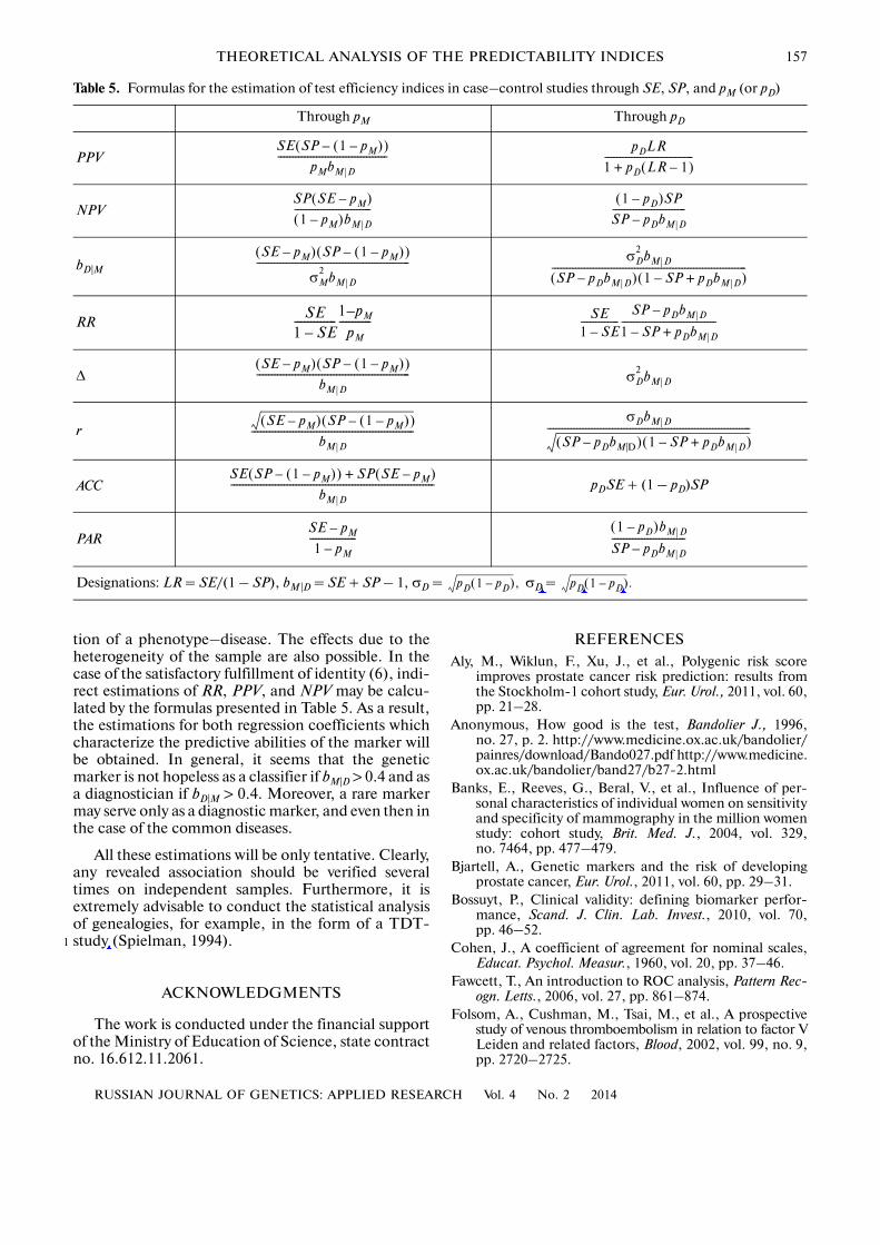
As is known, in the case�control studies it is impos�sible to estimate directly the absolute (PPV, BPV) andrelative (RR) risks of disease development under thepresence or absence of a marker in case–control stud�ies. However, from the practical point of view, justthese estimations are the most interesting. Severalauthors have suggested for RR the approximate for�

mula RR ≈ OR (1 – pD + pDOR)–1 (Zhang, Yu, 1998;Sistrom, Garvan, 2004). It is easy to see that this isexactly the lower bound for RR. More precisely, thefollowing chain of inequalities is true:

in which the left and right boundaries for RR correspondto the cases pM = 0 and pM = 1, respectively (Fig. 4).

In general, for the complete reconstruction ofmatrix P the three independent indices are necessary.The studies of the case–control type provide two ofthem: SE and SP.

The third one may be the prevalence of the disease(pD) or the population marker frequency (pM). Table 5presents both types of estimation. The choice betweenthem is conducted depending on which of these twoindices we believe to be reliably known. In any case,before applying the formulas in Table 4, it is necessaryto verify the inequalities SE > pM > 1 – SP and fulfill�ment of the identities

pM = pDSE + (1 – pD)(1 – SP). (6)Interestingly, to estimate the relative risk under

presence of the prior information on population fre�quency of the marker it is sufficient to know only thefrequency of the carrier marker in patients:

RR = ( 1 – pM) × SE/(pM × (1 – SE)).

CONCLUSIONS

The presented formulas enable us to estimate theOR values and marker frequencies which guarantee thehigh (or low) predictive efficiency of the correspond�ing test. Primarily, the following three statementsshould be emphasized.

1. When OR < 2.2, the marker deliberately pos�sesses the low predictive efficiency in any senses and atany disease and marker frequencies.

2. The marker can be a good classifier, if OR > 5.4on the assumption that its population frequency is

OR1 pD pD+ OR–�� RR OR pD OR 1–( ) OR,≤–≤≤

Table 4. Qualitative description of two types of markers which are possible at OR � 1

Marker�classifier Marker�Diagnostician

Graphical form

Frequency interrelation pM � pD pM � pD

SE, bM|D High Low

PPV, bD|M Low High

Causality M—Almost necessary condition of the disease M—Almost sufficient condition of the disease

Application Bulk screening, occupational selection Additional symptoms, genealogy

Example of markers Mammography BRCA, Leiden V

DM

DD

M

D

Nikita

Cross-Out

Nikita

Inserted Text

null

Nikita

Cross-Out

Nikita

Cross-Out

Nikita

Inserted Text

"marker-diagnostician"

Nikita

Cross-Out

Nikita

Inserted Text

"marker-diagnostician"

Nikita

Cross-Out

Nikita

Inserted Text

NPV

Nikita

Cross-Out

Nikita

Inserted Text

(1 – SP)

156



rather high (pM > 0.3). In practice this means that thelower limits of the 100 (1 – α) confidence interval forthe estimated ORL value should obey these inequali�ties, i.e., ORL < 2.2 in the first case and ORL > 5.4 in thesecond case, must obey the mentioned inequalities.Earlier, similar values for the critical levels of observedeffects have been suggested for the relative risks (RR < 2and RR > 5) (Ioannidis, 2006).

3. Even with very high values of OR, a marker is abad classifier (AUC < 0.6) if its population frequency islow (pM < 0.2 pD). Similarly, by virtue of the inequalityPPV < pD OR, practically every marker of a very raredisease is doomed to be a bad diagnostic index.

Indeed, from Proposition 3 we see that

Then, on the basis of definition of a “bad classifier”(AUC < 0.6), OR < 2.25. In this case, both conditionalindices of the mean efficiency (bM|D and bD|M) and cor�relation coefficient (r) are deliberately lower:

Further, based on the requirement AUC > 0.7, weget OR < 5.44. And according to Proposition 3, themaximum bM|D (and therefore, also AUC) is reached at

Note also that the case of AUC > 0.8 is only possiblewhen OR � 16 and pM > 0.2.

AUC bM D 1+( )/2 OR/ OR 1+( ).<=

2.25 1–( )/ 2.25 1+( ) 0.2.=

pM1 pD OR 1–( )+

OR 1+�� 1

OR 1+��>=

= 1

5.44 1+�� 0.3.=

Proposition 3 follows from the formulas given inTable 3[N5]. When OR � 1 and pM < pD, the marker isa bad classifier if

The outcome of this discussion consists in therather sad conclusion about the low predictive andclassification efficiencies of the results of majority ofthe published genetic association studies. As a rule,these results fit the situation in paragraph 1 and maynot be directly used in the clinical practice. Neverthe�less, stably reproduced associations even with smallOR values may indicate the participation of certaingenes in pathology development, giving fundamen�tally new information on the molecular mechanismsof the disease.

What should be calculated in the case of rare suc�cesses, when in the cases–control study a statisticallyhighly significant association with a high odds ratio,for example, OR > 6 is observed? We feel that, first ofall, it is necessary to test the obtained estimations SE andSP for consistency with the prior data on pM and pD. Thetesting procedure implies two points.

1)The test of pM ∈ (1 – SP, SE), i.e., the inclusionof the average estimations of the population frequencyof a gene�marker for the given ethnic group to theinterval (1 – SP, SE) obtained in the experiment.

2) The test of estimation pD = (pM – (1 – SP))/bM|D), notably, its correspondence to common con�cepts about the prevalence of this disease.

A strong deviations from the relation (6) like thedeviations from the Hardy�Weinberg equilibrium mayindicate the genotyping errors and/or misidentifica�

AUC 12�� 1

pM

pD

��+⎝ ⎠⎛ ⎞ 0.6 or pM 0.2pD.<,<=

1.00.8

0.4

0

1 – pD

0.6

0.4

0.2

0.8

0.40.6

0.2pM

pD

0.6

0.20.8

1/OR

RR/OR

OR – 1OR

11 + pD (OR – 1)

Fig. 4. Dependence of ratio RR/OR on the marker frequency (pM) and disease prevalence (pD) at OR = 5. The ratio RR/OR weaklydepends on pM and steadily decreases with an increase in pD. When pM → 0, this dependency appears as RR/OR = (1 – pD +

pDOR)–1.

Nikita

Cross-Out

Nikita

Inserted Text

test of belonging

Nikita

Cross-Out

Nikita

Inserted Text

similar to

Nikita

Cross-Out



tion of a phenotype–disease. The effects due to theheterogeneity of the sample are also possible. In thecase of the satisfactory fulfillment of identity (6), indi�rect estimations of RR, PPV, and NPV may be calcu�lated by the formulas presented in Table 5. As a result,the estimations for both regression coefficients whichcharacterize the predictive abilities of the marker willbe obtained. In general, it seems that the geneticmarker is not hopeless as a classifier if bM|D > 0.4 and asa diagnostician if bD|M > 0.4. Moreover, a rare markermay serve only as a diagnostic marker, and even then inthe case of the common diseases.

All these estimations will be only tentative. Clearly,any revealed association should be verified severaltimes on independent samples. Furthermore, it isextremely advisable to conduct the statistical analysisof genealogies, for example, in the form of a TDT�study (Spielman, 1994).

ACKNOWLEDGMENTS

The work is conducted under the financial supportof the Ministry of Education of Science, state contractno. 16.612.11.2061.

1

REFERENCESAly, M., Wiklun, F., Xu, J., et al., Polygenic risk score

improves prostate cancer risk prediction: results fromthe Stockholm�1 cohort study, Eur. Urol., 2011, vol. 60,pp. 21–28.

Anonymous, How good is the test, Bandolier J., 1996,no. 27, p. 2. http://www.medicine.ox.ac.uk/bandolier/painres/download/Bando027.pdf http://www.medicine.ox.ac.uk/bandolier/band27/b27�2.html

Banks, E., Reeves, G., Beral, V., et al., Influence of per�sonal characteristics of individual women on sensitivityand specificity of mammography in the million womenstudy: cohort study, Brit. Med. J., 2004, vol. 329,no. 7464, pp. 477–479.

Bjartell, A., Genetic markers and the risk of developingprostate cancer, Eur. Urol., 2011, vol. 60, pp. 29–31.

Bossuyt, P., Clinical validity: defining biomarker perfor�mance, Scand. J. Clin. Lab. Invest., 2010, vol. 70,pp. 46–52.

Cohen, J., A coefficient of agreement for nominal scales,Educat. Psychol. Measur., 1960, vol. 20, pp. 37–46.

Fawcett, T., An introduction to ROC analysis, Pattern Rec�ogn. Letts., 2006, vol. 27, pp. 861–874.

Folsom, A., Cushman, M., Tsai, M., et al., A prospectivestudy of venous thromboembolism in relation to factor VLeiden and related factors, Blood, 2002, vol. 99, no. 9,pp. 2720–2725.

Table 5. Formulas for the estimation of test efficiency indices in case–control studies through SE, SP, and pM (or pD)

Through pM Through pD

PPV

NPV

bD|M

RR

Δ

r

ACC pDSE + (1 – pD)SP

PAR

Designations: LR = SE/(1 – SP), bM|D = SE + SP – 1, σD = σD =

SE SP 1 pM–( )–( )pMbM D

��pDLR

1 pD LR 1–( )+��

SP SE pM–( )1 pM–( )bM D

��1 pD–( )SP

SP pDbM D–��

SE pM–( ) SP 1 pM–( )–( )

σM2

bM D

�� σD2

bM D

SP pDbM D–( ) 1 SP– pDbM D+( )��

SE1 SE–��

1 pM–pM

�� SE1 SE–��

SP pDbM D–

1 SP– pDbM D+��

SE pM–( ) SP 1 pM–( )–( )bM D

�� σD2

bM D

SE pM–( ) SP 1 pM–( )–( )bM D

��σDbM D

SP pDbM |D–( ) 1 SP– pDbM D+( )��

SE SP 1 pM–( )–( ) SP SE pM–( )+

bM D

��

SE pM–

1 pM–��

1 pD–( )bM D

SP pDbM D–��

pD 1 pD–( ), pD 1 pD–( ).

Nikita

Cross-Out

Nikita

Inserted Text

TDT-like studies

Nikita

Cross-Out

Nikita

Inserted Text

M

Nikita

Cross-Out

Nikita

Inserted Text

M

Nikita

Cross-Out

Nikita

Inserted Text

M

158



Ioannidis, J., Commentary: grading the credibility ofmolecular evidence for complex diseases, Int. J. Epide�miol., 2006, vol. 35, pp. 572–577.

Jakobsdottir, J., Gorin, M.B., Conley, Y.P., et al., Interpre�tation of genetic association studies: markers with rep�licated highly significant odds ratios may be poor clas�sifiers, PLoS Genet., 2009, vol. 5, no. 2.

King, G. and Zeng, L., Estimating risk and rate levels,ratios, and differences in case�control studies, StatisticsMed., 2002, vol. 21, pp. 1409–1427.

Kraemer, H.C., Frank, E., and Kupfer, D.J., How to assessthe clinical impact of treatments on patients, ratherthan the statistical impact of treatments on measures,Int. J. Methods Psychiatr. Res., 2011, vol. 20, pp. 63–72.

Kraft, P., Wacholder, S., Cornelis, M.C., et al., Beyondodds ratios—communicating disease risk based ongenetic profiles, Nature Rev. Genet., 2009, vol. 10,pp. 264–269.

Landis, J.R. and Koch, G.G., The measurement ofobserver agreement for categorical data, Biometrics,1977, vol. 33, pp. 159–174.

Levin, M.L., The occurrence of lung cancer in man, ActaUnion Int. Contra Cancrum, 1953, vol. 9, pp. 531–541.

Lewontin, R.C. and Kojima, K., The evolutionary dynamicsof complex polymorphisms, Evolution, 1960, vol. 14,pp. 458–472.

Linn, S. and Grunau, P.D., New patient�oriented summarymeasure of net total gain in certainty for dichotomousdiagnostic tests, Epidemiol. Perspect. Innovat., 2006,vol. V, no. 3, p. 11. http://www.epi�perspectives.com/content/3/1/11

Mitchell, A., How to: implement a screening programmefor distress in cancer settings, Psychooncology. Info.—Guide # 101, 2009a. http://www.psychooncology. info/PG_implement_ajmitchell.pdf

Mitchell, A., How To: Analyse a Screening or Diagnostic Study,Psycho�oncology.Info.—Guide # 104, 2009b. http://www.psycho�oncology.info/PG_analyse_ajmitchell.pdf

Pepe, M.S., Gu, J.W., and Morris, D.E., The potential ofgenes and other markers to inform about risk, CancerEpidemiol. Biomarkers Prevent., 2010, vol. 19, pp. 655–665.

Poste, G., Bring on the biomarkers, Nature, 2011, vol. 469,pp. 156–157.

Sistrom, C.L. and Garvan, C.W., Proportions, odds, andrisk, Radiology, 2004, vol. 230, pp. 12–19.

Slatkin, M., Linkage disequilibrium—understanding theevolutionary past and mapping the medical future,Nature Rev. Genet., 2008, vol. 9, pp. 477–485.

Spielman, R.S., McGinnis, R.E., and Ewens, W.J., Letterto the editor: the transmission/disequilibrium testdetects cosegregation and linkage, Am. J. HumanGenet., 1994, vol. 54, pp. 559–560.

Swets, J.A., Measuring the accuracy of diagnostic systems,Science, 1988, vol. 240, pp. 1285–1293.

Tan, P.N., Kumar, V., and Srivastava, J., Selecting the rightobjective measure for association analysis, Inform.Syst., 2004, vol. 29, pp. 293–313.

Winham, S.J., Slater, A.J., and Motsinger�Reif, A.A., Acomparison of internal validation techniques for multi�factor dimensionality reduction, BMC Bioinform.,2010, vol. 11, p. 394. http://www.biomedcentral.com/1471�2105/11/394

Youden, W.J., Index for rating diagnostic tests, Cancer,1950, vol. 3, pp. 32–35.

Yule, G.U., On the methods of measuring associationbetween two attributes, J. Royal Stat. Soc., 1912,vol. 75, pp. 579–652.

Zhang, J. and Yu, K.F., What’s the relative risk? A methodof correcting the odds ratio in cohort studies of com�mon outcomes, J. Amer. Med. Assoc., 1998, vol. 280,pp. 1690–1691.

Translated by N. Sokuevaand N. Khromov�Borisov

1

SPELL: 1. OK

Predictability indices of the binary genetic tests ENG 2014

Documents

Transcript of Predictability indices of the binary genetic tests ENG 2014