Performance-Based Analytics-Driven Seismic Design of Steel ...

UCLAUCLA Electronic Theses and Dissertations

TitlePerformance-Based Analytics-Driven Seismic Design of Steel Moment Frame Buildings

Permalinkhttps://escholarship.org/uc/item/5bd6r600

AuthorGUAN, XINGQUAN

Publication Date2021 Peer reviewed|Thesis/dissertation

eScholarship.org Powered by the California Digital LibraryUniversity of California

https://escholarship.org/uc/item/5bd6r600

https://escholarship.org

http://www.cdlib.org/

UNIVERSITY OF CALIFORNIA

Los Angeles

Performance-Based Analytics-Driven Seismic Design of Steel Moment Frame Buildings

A dissertation submitted in partial satisfaction

of the requirements for the degree

Doctor of Philosophy in Civil Engineering

by

Xingquan Guan

2021

© Copyright by

Xingquan Guan

2021

ii

ABSTRACT OF THE DISSERTATION

Performance-Based Analytics-Driven Seismic Design of Steel Moment Frame Buildings

by

Xingquan Guan

Doctoral of Philosophy in Civil Engineering

University of California, Los Angeles, 2021

Professor Henry Burton, Chair

With the embrace of the performance-based seismic design as the state-of-the-art design

method, recent emphasis has been placed on eliminating its drawbacks and facilitating its

application in practice. This study aims to propose an alternative design method: performance-

based analytics-driven seismic design, which is applied to steel moment resisting frame buildings.

First, the seismic performance of self-centering (with post-tensioned connections) and

conventional moment resisting frames (with reduced-beam section connection) is comparatively

assessed. The comparison indicates that the economic benefit for adopting the post-tensioned

connection is not significant. Then, an end-to-end computational platform, which automates the

seismic design, nonlinear structural model construction, and response simulation (static and

dynamic) of steel moment resisting frames is developed. Using this platform, a comprehensive

database is developed, which includes 621 special steel moment resisting frames designed in

iii

accordance with modern codes and standards and their corresponding nonlinear structural models

and seismic responses (i.e., peak story drifts, peak floor accelerations, and residual story drifts).

Using this database, the efficacy of mechanics-based, data-driven, and hybrid (combination of

mechanics-based and data driven) approaches to estimating the seismic drift demand are evaluated.

The evaluation results reveal that the hybrid approach has the best performance whereas the

mechanics-based model has the lowest performance. Next, a set of non-parametric and parametric

surrogate models are developed for estimating the engineering demand parameter distributions. A

comparative assessment of the proposed surrogate models and the simplified analysis method

proposed by FEMA P-58 is conducted to demonstrate the superior predictive performance of the

former. Finally, the effect of various design variables on the collapse performance of steel moment

resisting frames are evaluated. The research findings presented in this study helps to facilitate the

application of 2nd performance-based earthquake engineering framework in practice and thus better

help to create earthquake-resilient communities.

iv

The dissertation of Xingquan Guan is approved.

Ertugrul Taciroglu

Jingyi Li

John Wallace

Thomas Sabol

Henry Burton, Committee Chair

University of California, Los Angeles

2021

v

To my mom

For her unconditional love, unwavering support, valuable encourage,

and selfless dedication.

vi

Table of Contents

1. Introduction ................................................................................................................................. 1

1.1 Motivation and Background ............................................................................................... 1

1.2 Objectives ........................................................................................................................... 3

1.3 Organization and Outline .................................................................................................... 4

2. Nonlinear Modeling and Analysis Methodology of Steel Moment Resisting Frames ............... 9

2.1 Introduction ......................................................................................................................... 9

2.2 Modeling for Beam and Column Components ................................................................. 13

2.3 Modeling for Panel Zones ................................................................................................. 16

2.4 Modeling for Gravity Induced P-Δ Effect ........................................................................ 17

3. Python-Based Computational Platform to Automate Seismic Design, Nonlinear Structural

Model Construction and Analysis of Steel Moment Resisting Frames ........................................ 20

3.1 Introduction ....................................................................................................................... 20

3.2 Seismic Design of SMRFs ................................................................................................ 25

3.2.1 Overview of Design Criteria .................................................................................... 25

3.2.2 Nonlinear Modeling of SMRFs ............................................................................... 27

3.3 Seismic Design Module .................................................................................................... 27

3.3.1 Overview .................................................................................................................. 27

3.3.2 Preprocessing the Electronic Database of Wide Flange Sections ............................ 28

3.3.3 Design Automation Algorithms ............................................................................... 29

3.3.4 Object-Oriented Programming Structure ................................................................. 37

3.4 Nonlinear Model Construction and Analysis Module ...................................................... 38

3.5 Illustrative Examples ........................................................................................................ 40

3.5.1 Seismic Design......................................................................................................... 40

3.5.2 Efficiency in Time Needed to Complete Design ..................................................... 43

3.5.3 Verification of the Seismic Design Module............................................................. 44

3.5.4 Comparing Features of AutoSDA with Commercial Software: RAM Steel and SAP

2000............................................................................................................................................... 49

3.5.5 Nonlinear Static and Dynamic Analysis of SMRF Buildings ................................. 50

vii

3.6 Adaptability of the AutoSDA Platform and Possible Future Extensions ......................... 52

3.7 Summary ........................................................................................................................... 54

4. A Database of Seismic Design, Nonlinear Models, and Seismic Responses for SMRF

Buildings ....................................................................................................................................... 56

4.1 Introduction ....................................................................................................................... 56

4.2 Database of SMRF Designs, Nonlinear Models, and Seismic Responses ........................ 58

4.2.1 Design Tool for Generating the Database ................................................................ 59

4.2.2 Seismic Designs for Archetype SMRFs .................................................................. 61

4.2.3 Ready-to-Run Nonlinear Structural Models ............................................................ 71

4.2.4 Earthquake Ground Motions .................................................................................... 71

4.2.5 Nonlinear Responses of SMRFs .............................................................................. 76

4.3 Structure of the Data ......................................................................................................... 81

4.4 Summary and Possible Future Extensions ........................................................................ 83

5. Comparative Study for Steel Moment Resisting Frames Using Post-Tensioned and Reduced-

Beam Section Connections ........................................................................................................... 87

5.1 Introduction ....................................................................................................................... 87

5.2 Model Development in OpenSees .................................................................................... 90

5.2.1 Description of Prototype Building ........................................................................... 90

5.2.2 Component-Level Modeling .................................................................................... 92

5.2.3 Structural Modeling ............................................................................................... 100

5.3 Nonlinear Static and Dynamic Analyses ........................................................................ 103

5.3.1 Nonlinear Static Response ..................................................................................... 103

5.3.2 Incremental Dynamic Analysis and Collapse and Demolition Fragility Curves ... 104

5.3.3 Discussion on Comparison between SC-MRF and WMRF .................................. 106

5.4 Economic Loss Assessment ............................................................................................ 107

5.4.1 Overview of FEMA P-58 Methodology ................................................................ 107

5.4.2 Description of Building Components .................................................................... 110

5.4.3 Expected Loss Conditioned on Seismic Intensity .................................................. 112

5.4.4 Expected Annual Loss ........................................................................................... 113

5.5 Summary ......................................................................................................................... 114

viii

6. Seismic Drift Demand Estimation for SMRF Buildings: from Mechanics-Based to Data-

Driven Models ............................................................................................................................ 116

6.1 Introduction ..................................................................................................................... 116

6.2 Overview of Existing Simplified Methods for Estimating Seismic Drift Demands ....... 121

6.2.1 Shear and Flexural Beam Theory .......................................................................... 122

6.2.2 Elastoplastic Single-Degree-of-Freedom with Known Yield Strength (PSKY).... 123

6.2.3 Statistically Adjusted Spectral Displacement ........................................................ 124

6.2.4 Statistically Adjusted Response of a Linear Elastic MDOF with Known Yield

Strength (EMKY)........................................................................................................................ 125

6.3 Generalized Framework for Developing Hybrid and/or Data-Driven Models for Estimating

Building Structural Response Demands under Extreme Loading .............................................. 126

6.3.1 Overview of Framework ........................................................................................ 126

6.3.2 Model Evaluation and Performance Metrics ......................................................... 128

6.4 New ML-Based Hybrid and Data-Driven Models to Estimate Seismic Drift Demands 132

6.4.1 Dataset of SMRF Seismic Responses .................................................................... 132

6.4.2 Overview of Model Development ......................................................................... 133

6.4.3 ML-based Purely Data-Driven (MLDD) Models .................................................. 136

6.4.4 ML-based EMKY Model (ML-EMKY) ................................................................ 144

6.5 Comparative Assessment Among Existing and Newly Developed Models ................... 146

6.5.1 Evaluating the MLDD and “Reduced-Order” MLDD Models .............................. 146

6.5.2 Evaluating the ML-EMKY Model ......................................................................... 149

6.5.3 Evaluating the PSKY Model .................................................................................. 150

6.5.4 Evaluating the Statistically Adjusted EMKY Model ............................................. 151

6.5.5 Comparing the Predictive Performance and Required User-Effort Among Different

Models......................................................................................................................................... 152

6.6 Summary ......................................................................................................................... 155

7. Surrogate Models for Probabilistic Distribution of Engineering Demand Parameters of SMRF

Buildings under Earthquakes ...................................................................................................... 158

7.1 Introduction ..................................................................................................................... 158

7.2 Dataset of SMRFs ........................................................................................................... 160

7.3 Surrogate Model for Probabilistic Distribution of EDPs ................................................ 167

ix

7.3.1 Performance Metrics for Model Evaluation .......................................................... 168

7.3.2 Parametric Surrogate Model .................................................................................. 169

7.3.3 Non-parametric Surrogate Model .......................................................................... 174

7.3.4 Comparative Assessment Among Existing and Newly Developed Surrogate Models

..................................................................................................................................................... 181

7.3.5 Estimation of Covariance Matrix ........................................................................... 183

7.4 Economic Loss Assessment using EDPs from the Surrogate Model and NRHAs ......... 185

7.4.1 Overview of Economic Loss Assessment Methodology ....................................... 185

7.4.2 Description of Building Components .................................................................... 187

7.4.3 Expected Economic Loss Comparison .................................................................. 188

7.5 Summary ......................................................................................................................... 189

8. Effect of Different Design Variables on Seismic Collapse Performance of Steel Special

Moment Frames .......................................................................................................................... 191

8.1 Overview ......................................................................................................................... 191

8.2 Collapse Safety Assessment Framework ........................................................................ 191

8.3 Implementation of the Framework to Los Angeles Metropolitan Area .......................... 193

8.3.1 Gathering the Design Provisions for the SMRF .................................................... 193

8.3.2 Developing the Archetype Designs ....................................................................... 193

8.3.3 Nonlinear Model Development.............................................................................. 198

8.3.4 Characterize the Uncertainty.................................................................................. 199

8.3.5 Quantify the Margin of Safety Against Collapse ................................................... 200

8.3.6 Performance Evaluation ......................................................................................... 202

8.4 Summary ......................................................................................................................... 207

9. Summary, Conclusions and Future Research Needs .............................................................. 208

9.1 Overview ......................................................................................................................... 208

9.2 Findings and Conclusions ............................................................................................... 209

9.2.1 Chapter 2 Nonlinear Modeling and Analysis Methodology of Steel Moment Resisting

Frames ......................................................................................................................................... 209

9.2.2 Chapter 3 Python-Based Computational Platform to Automate Seismic Design,

Nonlinear Structural Model Construction and Analysis of Steel Moment Resisting Frames .... 209

9.2.3 Chapter 4 A Database of Seismic Design, Nonlinear Models, and Seismic Responses

x

for SMRF Buildings .................................................................................................................... 211

9.2.4 Chapter 5 Comparative Study for Steel Moment Resisting Frames Using Post-

Tensioned and Reduced-Beam Section Connections ................................................................. 211

9.2.5 Chapter 6 Seismic Drift Demand Estimation for SMRF Buildings: from Mechanics-

Based to Data-Driven Models ..................................................................................................... 212

9.2.6 Chapter 7 Surrogate Models for Probabilistic Distribution of Engineering Demand

Parameters of SMRF Buildings under Earthquakes ................................................................... 214

9.2.7 Chapter 8 Effect of Different Design Variables on Seismic Collapse Performance of

Steel Special Moment Frames .................................................................................................... 215

9.3 Limitations and Future Work .......................................................................................... 215

10. Reference .............................................................................................................................. 218

xi

List of Figures

Figure 1.1 Overview of the performance-based seismic design method .................................. 2

Figure 1.2 Overview of performance-based analytics-driven seismic design .......................... 3

Figure 2.1 Possible plastic behavior in SMRFs: (a) Schematic view of possible plasticity in a

beam-column connection, (b) beam yielding, (c) column yielding, and (d) shear yielding in panel

zones ............................................................................................................................................. 10

Figure 2.2 Different types of structural component models: (a) concentrated plasticity model,

(b) finite length plastic hinge model, (c) distributed plasticity model (e.g., elements with fiber

sections), and (d) continuum finite element model (adapted from Deierlein et al. [9]) ............... 10

Figure 2.3 Modified IMK material model: (a) monotonic backbone curve and (b) cyclic

response......................................................................................................................................... 14

Figure 2.4 Gravity tributary area for the (a) SMRF and (b) gravity system ........................... 18

Figure 2.5 Nonlinear model for the SMRF: (a) overview of the model, (b) beam-column

connection and (c) leaning column joint ....................................................................................... 19

Figure 3.1 Overview of the main AutoSDA platform modules .............................................. 23

Figure 3.2 Overview of the seismic design module ................................................................ 28

Figure 3.3 Overview of sub-algorithm used to achieve the desired target drift demand ........ 31

Figure 3.4 Overview of sub-algorithm used to check the feasibility of beams, columns and

connections ................................................................................................................................... 32

Figure 3.5 Overview of the sub-algorithm used to ensure that the design requirements for all

beam-column connections are satisfied ........................................................................................ 35

Figure 3.6 Overview of the sub-algorithm used to revise the beam sizes for ease of construction

....................................................................................................................................................... 36

Figure 3.7 Programing structure of the seismic design module.............................................. 39

Figure 3.8 Programming structure of the NMCA module ...................................................... 40

Figure 3.9 Building case used to illustrate the AutoSDA design process: (a) floor plan and (b)

elevation of SMRF ........................................................................................................................ 41

Figure 3.10 Changes in member sizes at different design stages: (a) initial sizes, (b) member

sizes after first optimization for drift requirement, (c) most economical sections satisfying drift

requirement, (d) section sizes after checking requirements for beams and columns, (e) design after

xii

checking strong-column-weak-beam criterion, (f) code-conforming design, (g) member sizes after

adjusting beams for ease of construction, and (h) final design ..................................................... 43

Figure 3.11 Three-story building used in the ATC 123 project [48]: (a) floor plan and (b)

elevation view ............................................................................................................................... 46

Figure 3.12 Nine-story building used in the ATC 123 project [48]: (a) floor plan and (b)

elevation view ............................................................................................................................... 46

Figure 3.13 Comparing design story drifts for the Englekirk and AutoSDA designs: (a) three-

story and (b) nine-story buildings ................................................................................................. 47

Figure 3.14 Four-story office building reported by Lignos [23] ............................................ 48

Figure 3.15 Monotonic pushover curve for the three-story building ...................................... 51

Figure 3.16 Collapse fragility for the three-story building ..................................................... 52

Figure 4.1 Overview of the database ...................................................................................... 59

Figure 4.2 Overview of AutoSDA modules ........................................................................... 60

Figure 4.3 ASCE 7-16 DBE and MCE spectra at the considered site .................................... 63

Figure 4.4 Typical structural framing plan layout for archetype buildings: (a) one-bay, (b)

three-bay, and (c) five-bay SMRFs as the LFRS .......................................................................... 63

Figure 4.5 Visualizing the designs for the 81 one-story SMRFs: (a) moment of inertia for

beams, (b) moment of inertia for exterior columns, (c) moment of inertia for interior columns, and

(d) design story drifts .................................................................................................................... 65

Figure 4.6 Visualizing the designs for the 162 five-story SMRFs: (a) moment of inertia for


(d) design story drifts. ................................................................................................................... 66

Figure 4.7 Visualizing the designs for the 162 nine-story SMRFs: (a) moment of inertia for


(d) design story drifts. ................................................................................................................... 67

Figure 4.8 Visualizing the designs for the 128 fourteen-story SMRFs: (a) moment of inertia

for beams, (b) moment of inertia for exterior columns, (c) moment of inertia for interior columns,

and (d) design story drifts ............................................................................................................. 68

Figure 4.9 Visualizing the designs for the 88 nineteen-story SMRFs: (a) moment of inertia for


(d) design story drifts .................................................................................................................... 70

xiii

Figure 4.10 Distribution of drift concentration factors for all 621 SMRFs: (a) boxplots for

buildings with different number of stories and (b) histogram of drift concentration factors ....... 71

Figure 4.11 Acceleration spectra for the 240 ground motion records .................................... 72

Figure 4.12 Ground motion response spectra at the SLE hazard level for the following

representative periods: (a) 0.5 sec, (b) 1.0 sec, and (c) 2.0 sec..................................................... 74

Figure 4.13 Ground motion response spectra at the DBE hazard level for the following

representative periods: (a) 0.5 sec, (b) 1.0 sec, and (c) 2.0 sec..................................................... 75

Figure 4.14 Ground motion response spectra at the MCE hazard level for the following

representative periods: (a) 0.5 sec, (b) 1.0 sec, and (c) 2.0 secs ................................................... 76

Figure 4.15 Structural responses for a typical one-story building subjected to 40 MCE level

ground motions: (a) peak story drift, (b) peak floor acceleration, and (c) residual story drift profiles

....................................................................................................................................................... 77

Figure 4.16 Structural responses for a typical five-story building subjected to 40 MCE level


....................................................................................................................................................... 78

Figure 4.17 Structural responses for a typical nine-story building subjected to 40 MCE-level


....................................................................................................................................................... 79

Figure 4.18 Structural responses for a typical fourteen-story building subjected to 40 MCE

level ground motions: (a) peak story drift, (b) peak floor acceleration, and (c) residual story drift

profiles .......................................................................................................................................... 80

Figure 4.19 Structural responses for a typical nineteen-story building subjected to 40 MCE

level ground motions: (a) peak story drift, (b) peak floor acceleration, and (c) residual story drift

profiles .......................................................................................................................................... 81

Figure 5.1 Schematic illustration of an (a) RBS welded connection and (b) PT connection . 88

Figure 5.2 Overview of study ................................................................................................. 90

Figure 5.3 Prototype building including (a) floor plan and (b) elevation of moment resisting

frame (adapted from Garlock et al. [89]). ..................................................................................... 91

Figure 5.4 Model for an exterior PT connection with top-and-seat angles and associated

column and beam .......................................................................................................................... 94

xiv

Figure 5.5 Schematic force-deformation response for (a) Self-centering and (b) Pinching4

material parameters ....................................................................................................................... 94

Figure 5.6 Experiment setup (adapted from Ricles et al. [80]) ............................................... 96

Figure 5.7 Comparison between the proposed model and experimental data for specimens (a)

PC2, (b) PC3, (c) PC4, and (d) 20s-18. ........................................................................................ 96

Figure 5.8 Calibration of PT connection model subjected to (a) monotonic and (b) cyclic

loading........................................................................................................................................... 98

Figure 5.9 A typical comparison of the backbone curve for three types of connections ...... 100

Figure 5.10 OpenSees model for the SC-MRF: (a) overview of the model, (b) details for SC-

MRF connection, and (c) details for leaning column joint ......................................................... 102

Figure 5.11 Monotonic pushover curves for the SC-MRF and WMRF ............................... 104

Figure 5.12 Fragility results: (a) collapse and (b) demolition fragility curves ..................... 106

Figure 5.13 Seismic hazard curve corresponding to the site of interest ............................... 110

Figure 5.14 Expected loss for the building with SC-MRFs .................................................. 112

Figure 5.15 Comparison of expected loss for WMRF and SC-MRF buildings including (a) total,

(b) collapse, (c) demolition, and (d) repair losses ....................................................................... 113

Figure 5.16 Comparison of annual expected loss between (a) SC-MRF and (b) WMRF

buildings ...................................................................................................................................... 114

Figure 6.1 Overview of the performance-based seismic design procedure .......................... 117

Figure 6.2 Overview of study ............................................................................................... 121

Figure 6.3 Framework for developing hybrid/data-driven models to estimate seismic demands

..................................................................................................................................................... 128

Figure 6.4 Trend line obtained from linear regression on the observed and predicted values: (a)

large dispersion and (b) small dispersion cases .......................................................................... 131

Figure 6.5 Initial set of predictor variables considered for the data-driven and hybrid models

..................................................................................................................................................... 136

Figure 6.6 Workflow for developing the MLDD model....................................................... 137

Figure 6.7 A schematic view of a decision tree model: (a) sample space split into five regions

considering two predictors 𝑋1 and 𝑋2, and (b) the corresponding decision tree model ............ 137

Figure 6.8 A schematic illustration of the random forest algorithm with three trees for an 𝑁-

data sample with 𝑝 features ........................................................................................................ 138

xv

Figure 6.9 Training and validation results for low-to-mid-rise buildings: (a) Observed versus

predicted story drift demand on the training and validation datasets, and (b) the distribution of

relative difference between the observed and predicted drift demand for the validation dataset 139

Figure 6.10 Training and validation results for high-rise buildings: (a) Observed versus


relative difference between the observed and predicted drift demands for the validation dataset

..................................................................................................................................................... 139

Figure 6.11 Normalized importance scores of the 35 predictors for the low-to-mid-rise

buildings: (a) building information, (b) modal information, (c) spectral parameters, and (d)

nonlinear static analysis parameters............................................................................................ 141

Figure 6.12 Normalized importance scores of the 35 predictors for the high-rise buildings: (a)

building information, (b) modal information, (c) spectral parameters, and (d) nonlinear static

analysis parameters ..................................................................................................................... 143

Figure 6.13 Workflow for developing the ML-EMKY model ............................................. 144

Figure 6.14 Workflow involved in applying the ML-EMKY, MLDD and Reduced Order

MLDD models ............................................................................................................................ 146

Figure 6.15 Predictive performance evaluation for the MLDD model applied to the low-to-

mid-rise buildings: (a) NRHA-based versus model predicted story drift demands and (b) the

distribution of relative difference between NRHA-based and model predicted story drifts ...... 147

Figure 6.16 Predictive performance evaluation for the MLDD model applied to the high-rise

buildings: (a) NRHA-based versus model predicted story drift demands and (b) the distribution of

relative difference between NRHA-based and model predicted story drifts .............................. 147

Figure 6.17 A spectrum of models for simplified seismic drift demand estimation............. 153

Figure 6.18 Comparing the performance based on 𝐷10% across the existing and newly

developed models for the (a) low-to-mid-rise and (b) high-rise buildings ................................. 154

Figure 6.19 Performance versus required effort for various seismic drift demand estimation

models ......................................................................................................................................... 155

Figure 7.1 Overview of the dataset ....................................................................................... 162

Figure 7.2 The distributions of building geometries and gravity loads in the database: (a)

number of stories, (b) bay widths, (c) first/typical story height ratios, (d) number of bays, (e) typical

floor dead loads, and (f) roof dead loads .................................................................................... 163

xvi

Figure 7.3 The Distribution of building periods ................................................................... 164

Figure 7.4 The distribution of spectral acceleration evaluated at the first-mode period ...... 164

Figure 7.5 A schematic plot for fitting the peak story drift with lognormal distribution ..... 165

Figure 7.6 Training and validation results for median peak story drift of: (a) low-to-mid-rise

buildings and (b) high-rise buildings. ......................................................................................... 171

Figure 7.7 The distribution of relative difference between the observed and predicted median

peak story drift for the validation dataset: (a) low-to-mid-rise buildings and (b) high-rise buildings

..................................................................................................................................................... 172

Figure 7.8 A schematic view of a decision tree model: (a) Two-feature sample space split into

to three subspaces and (b) the corresponding decision tree model ............................................. 175

Figure 7.9 A schematic illustration of the random forest algorithm with three trees for an 𝑁-

data sample with 𝑝 features ........................................................................................................ 176

Figure 7.10 Training and validation results for median peak story drift of (a) low-to-mid-rise

buildings and (b) high-rise buildings .......................................................................................... 177


peak story drift for the validation dataset: (a) low-to-mid-rise buildings and (b) high-rise buildings

..................................................................................................................................................... 177

Figure 7.12 Normalized importance scores of the 35 predictors for the low-to-mid-rise

buildings: (a) building information, (b) modal information, (c) spectral parameters, and (d)

nonlinear static analysis parameters............................................................................................ 179

Figure 7.13 Comparing the performance based on 𝐷25% across the existing and newly

developed models for: (a) peak story drift, (b) peak floor acceleration, and (c) residual story drift

..................................................................................................................................................... 182

Figure 7.14 A schematic view of the covariance matrix for the EDPs ................................. 184

Figure 7.15 The distribution of the covariance terms at MCE hazard level: (a) covariance terms

excluding the residual drift and (b) covariance terms relevant to residual drift ......................... 184

Figure 7.16 The distribution of the covariance terms at DBE hazard level: (a) covariance terms

excluding the residual drift and (b) covariance terms relevant to residual drift. ........................ 184

Figure 7.17 The distribution of the covariance terms at SLE hazard level: (a) covariance terms

excluding the residual drift and (b) covariance terms relevant to residual drift ......................... 185

xvii

Figure 7.18 Comparison of the economic loss based on the EDPs generated from the surrogate

model and NRHAs: (a) NRHA-based versus surrogate model-based economic loss and (b) the

distribution of the relative difference between the NRHA-based and surrogate model-based losses

..................................................................................................................................................... 189

Figure 7.19 Comparison of the economic loss based on the EDPs generated from the NRHAs

and surrogate models with the covariance observed from NRHAs: (a) NRHA-based versus

surrogate model-based economic loss and (b) the distribution of the relative difference between

the NRHA-based and surrogate model-based losses .................................................................. 189

Figure 8.1 Overview of FEMA P695 collapse performance assessment procedure ............. 193

Figure 8.2 The distribution of site parameters in Los Angeles metropolitan area: (a) 𝑆𝑀𝑆, (b)

𝑆𝑀1, (c) 𝑆𝐷𝑆, and (d) 𝑆𝐷1 ......................................................................................................... 194

Figure 8.3 The distribution of 𝑉𝑠30 in Los Angeles metropolitan area ............................... 195

Figure 8.4 Visualizing the design story drifts for the SMRFs designed using R = 8: (a) one-

story, (b) three-story, (c) five-story, (d) seven-story, and (e) nine-story buildings .................... 198

Figure 8.5 Distribution of drift concentration factors for all SMRFs: (a) boxplots for buildings

with different number of stories and (b) histogram of drift concentration factors ..................... 198

Figure 8.6 The histogram of ACMRs for (a) R = 8, (b) R = 9, and (c) R = 10 .................... 201

Figure 8.7 The distribution of ACMRs for buildings with different number of stories: (a) R =

8, (b) R = 9, and (c) R = 10 ......................................................................................................... 203

Figure 8.8 The distribution of ACMRs for buildings with different bay width: (a) R = 8, (b) R

= 9, and (c) R = 10 ...................................................................................................................... 204

Figure 8.9 The distribution of ACMRs for buildings with different number of bays: (a) R = 8,

(b) R = 9, and (c) R = 10 ............................................................................................................. 205

Figure 8.10 The distribution of ACMRs for buildings located in different seismicity region: (a)

R = 8, (b) R = 9, and (c) R = 10 .................................................................................................. 206

Figure 8.11 The distribution of ACMRs for buildings designed with different R factors ... 207

xviii

List of Tables

Table 2.1 Advantages and limitations of each model ............................................................. 11

Table 3.1 Design duration for buildings with different numbers of stories and bays ............. 44

Table 3.2 Comparing member sizes between designs produced by Englekirk and the AutoSDA

platform for the three-story building............................................................................................. 47


platform for the nine-story building design .................................................................................. 47

Table 3.4 Comparing member sizes between designs produced by the AutoSDA platform and

Lignos [23] .................................................................................................................................... 49

Table 3.5 Comparing features of RAM Steel, SAP 2000, and the AutoSDA platform ........... 50

Table 4.1 Parameters considered in developing the SMRF archetypes and their associated

ranges ............................................................................................................................................ 61

Table 4.2 Overview of attributes and associated descriptions ................................................ 84

Table 5.1 Design of prototype frames (adapted from Garlock et al. [90]). ............................ 92

Table 5.2 Parameters of Self-centering material for four specimens ...................................... 97

Table 5.3 Parameters of Pinching4 material for four specimens ............................................ 97

Table 5.4 Parameters for Self-centering material of PT connections ...................................... 99

Table 5.5 Parameters for Pinching4 material of PT connections............................................ 99

Table 5.6 Comparison of natural periods for WMRF and SC-MRF (unit: second). ............ 102

Table 5.7 Damageable components ...................................................................................... 111

Table 6.1 Some existing approaches for predicting seismic drift demands .......................... 118

Table 6.2 Multi-Metric Performance Evaluation for the MLDD Model .............................. 148

Table 6.3 Multi-Metric Performance Evaluation for the Reduced-Order MLDD Model .... 149

Table 6.4 Multi-Metric Performance Evaluation for ML-EMKY ........................................ 150

Table 6.5 Multi-Metric Performance Evaluation for PSKY ................................................. 151

Table 6.6 Multi-Metric Performance Evaluation for the Statistically Adjusted EMKY Model

..................................................................................................................................................... 152

Table 7.1 Initial set of predictor variables considered for the surrogate model ................... 166

Table 7.2 Initial coefficients of linear regression for predicting the central tendency of peak

story drifts ................................................................................................................................... 170

xix

Table 7.3 Performance evaluation for the parametric model on validation dataset .............. 174

Table 7.4 Summary of the parameters for the random forest model .................................... 180

Table 7.5 Performance evaluation for the non-parametric model on validation dataset ...... 180

Table 7.6 The range and median for covariance terms. ........................................................ 185

Table 7.7 . Damageable components for a five-story five-bay building .............................. 187

Table 8.1 The distribution of site class in Los Angeles metropolitan area ........................... 195

Table 8.2 Six typical sites in Los Angeles metropolitan area ............................................... 195

Table 8.3 Parameters considered in developing the SMF archetypes and their associated ranges

..................................................................................................................................................... 196

xx

BIOGRAPHICAL SKETCH

Education:

2009–2013 B.Sc. in Civil Engineering

Huazhong University of Science and Technology

Wuhan, Hubei, China

2013–2016 M.Sc. in Structural Engineering

Huazhong University of Science and Technology

Wuhan, Hubei, China

2016–2020 M.Sc. in Earthquake Engineering


Los Angeles, California, USA

2016–2021 Ph.D. candidate in Structural/Earthquake Engineering


Los Angeles, California, USA

Selected Journal Publications:

Guan, X., Burton, H., Shokrabadi, M., & Yi, Z. (2021). Seismic drift demand estimation for

SMF buildings: from mechanistic to data-driven models. Journal of Structural Engineering.

DOI: 10.1061/(ASCE)ST.1943-541X.0003004. (Accepted for publication)

Guan, X., Burton, H., & Shokrabadi, M. (2020). A database of seismic designs, nonlinear

models, and seismic responses for steel moment resisting frame buildings. Earthquake Spectra.

8755293020971209.

Guan, X., Burton, H., & Sabol, T. (2020). Python-based computational platform to automate

seismic design, nonlinear structural model construction and analysis of steel moment resisting

frames. Engineering Structures, 224, 111199.

Guan, X., Burton, H., & Moradi, S. (2018). Seismic performance of a self-centering steel

moment frame building: from component-level modeling to economic loss assessment. Journal

of Constructional Steel Research, 150, 129-140.

1

1. Introduction

1.1 Motivation and Background

The second-generation performance-based seismic design (PBSD) framework [1] enables

structural engineers to target specific stakeholder-driven building performance objectives. As

shown in Figure 1.1, PBSD begins with defining a set of performance objectives using some metric

of interest (e.g., reliability, resilience, and/or lifecycle cost), followed by a preliminary design.

Ideally, the building performance should then be assessed by conducting nonlinear response

history analyses (NRHAs) on a structural model of the design and using the generated engineering

demand parameters (e.g., peak story drifts, peak floor accelerations, and residual story drifts) to

evaluate earthquake-induced impacts (e.g., physical damage, economic losses, the probable

number of fatalities, and functional recovery time). Based on the results of this initial assessment,

the design is revised as needed and the assessment is repeated until the performance meets the

predefined objectives.

While PBSD is commonly considered to be a state-of-the-art design method that can

effectively target specific performance outcomes, it has not been widely adopted in practice. This

is partly because the majority of engineers rely on elastic models to estimate seismic demands,

which is generally not suitable for rigorous performance-based assessments. Even when nonlinear

models are employed, the iterative process of conducting NRHAs and revisiting the design would

be computationally expensive and labor intensive.

To address the challenges resulting from the computational expense and high labor-costs

associated with PBSD, a new design methodology, performance-based analytics-driven (PBAD)

seismic design, is developed. An essential part in PBAD is the utilization of surrogate models,

which are necessary for establishing statistical relationships between the design variables (e.g., site

2

condition, building dimensions, and load magnitudes), structural response (e.g., lateral load-

carrying capacity and collapse resistance), and the various decision metrics (e.g., economic losses,

downtime, and fatality). The surrogate models remove the need for costly structural response

simulation (which is typically done in OpenSees [2] or other similar platforms) and loss assessment

(which could be done by computing tools, such as SP3 [3] or PACT [4]), which can significantly

reduce computational demand. On the other hand, recent advances in prediction-analytics using

machine learning techniques have created the opportunity for data-driven or hybrid (combination

of data-drive and mechanics-based) surrogate models to accurately replicate mechanics-based

(numerical models that explicitly simulate the phenomena under consideration) simulation results.

With the help of such surrogate models, various tasks such as design optimization, design space

exploration, and sensitivity analysis, become much more feasible [5]. The current study is focused

on the development of the PBAD methodology and application to steel moment resisting frame

buildings.

Figure 1.1 Overview of the performance-based seismic design method

3

Figure 1.2 Overview of performance-based analytics-driven seismic design

1.2 Objectives

The objective of the current study is to develop the performance-based analytics-driven

seismic design framework and apply it to steel moment resisting frames. The resulting body of

research combines seismic design automation, archetype design database development, extensive

nonlinear structural analyses, and rapid characterization for the probabilistic distribution of seismic

responses and impacts. More specifically, the main objectives are outlined below:

1. Create an “end-to-end” computational platform that iteratively integrates seismic design,

structural response simulation, impact (e.g., economic loss and downtime) assessment, and

performance criteria evaluation for steel moment resisting frame buildings.

2. Establish a database of archetype steel moment resisting frame buildings using

performance-based grouping methodology, which considers the importance/sensitivity of design

variables to overall structural performance.

4

3. Assess the seismic performance of the self-centering moment resisting frame using post-

tensioned connections and the conventional moment resisting frame using reduced-beam section

connections.

4. Conduct nonlinear response history analyses and performance-based impact (economic

loss, collapse safety, and downtime) assessments for the set of archetype buildings using high

performance computing techniques.

5. Investigate the efficacy of mechanics-based, data-driven, and hybrid approaches in

estimating the story drift demands in steel moment resisting frames.

6. Develop surrogate models that provide a compact statistical relationship between key

design variables and structural response (including peak story drifts, peak floor accelerations,

residual story drifts) as well as performance outcomes (e.g., economic loss, collapse safety, and

downtime).

7. Quantify the influence of various design variables on the collapse performance of steel

moment resisting frames based on a large number of archetype buildings located on various sites.

1.3 Organization and Outline

The main body of the current study consists of eight chapters. Four of them are adopted

from published journal manuscripts which are cited at the beginning of the chapter.

Chapter 2 provides an in-depth literature review that summarizes recent advances in

structural modeling of steel moment resisting frames. Different models, including concentrated

plasticity, finite length plastic hinge, distributed plasticity, and continuum finite-element models,

are critically examined to reveal their advantages and limitations.

Chapter 3 presents an end-to-end computational platform, which automates seismic design,

nonlinear structural model construction, and response simulation (static and dynamic) of steel

5

moment resisting frames. A modular framework is adopted along with the object-oriented

programming paradigm to ensure the adaptability of the platform. The seismic design module

iteratively generates code-conforming section sizes and detailing for beams, columns, and beam-

column connections based on the relevant input design variables including the building

configuration (e.g., the number of stories, the number of lateral-force resisting systems, and the

building dimensions), loads (e.g., dead and live loads on each floor), and site conditions (mapped

spectral acceleration parameters). The nonlinear model construction and analysis module takes the

design results as input and produces structural models that capture flexural strength and stiffness

deterioration in the frame beam-column elements, and performs pushover and response history

analyses. Illustrative examples are presented to demonstrate the reliability, accuracy, and

efficiency of the platform, which significantly reduces the time and effort involved in producing

iterative structural designs and conducting nonlinear analyses, both of which are necessary for

performance-based seismic design. Additionally, the platform can be used to create an extensive

database of archetype steel moment frame buildings towards the development of analytics-driven

design methods.

Chapter 4 introduces the development of a comprehensive database, which includes 621

special steel moment resisting frames designed in accordance with modern codes and standards

and their corresponding nonlinear structural models and seismic responses (i.e., peak story drifts,

peak floor accelerations, and residual story drifts). The seismic responses for a subgroup of 100

steel moment resisting frames subjected to three groups of site-specific ground motions (with 40

records each) at the service-level, design-based, and maximum considered earthquake levels, are

also included. The database could be used to evaluate the performance of existing methods and

develop data-driven and hybrid (combination of mechanics-based + data-driven) models for

6

estimating seismic structural drift demands. The database can also be utilized in the development

and implementation of a performance-based analytics-driven seismic design methodology.

Chapter 5 presents a seismic performance comparison between steel moment resisting

frames with post-tensioned (PT) connections and welded connections. Firstly, a phenomenological

model that captures lateral load response and collapse behavior of PT connections is developed

and then verified using previous experiments. A prototype building, which has self-centering

moment resisting frames (SC-MRFs) as its lateral force resisting system, is considered selected for

the analytical modeling. Then a two-dimensional OpenSees model of the SC-MRF is created using

the newly-developed phenomenological model. With the same member sizes, an OpenSees model

is also created for a welded moment resisting frame (WMRF) that has reduced beam section

connections. Nonlinear static and dynamic analyses are performed on both SC-MRF and WMRF

models. The lateral load-carrying capacity, collapse resistance, and demolition intensity of both

frames are compared. Finally, the economic losses of both frame buildings are assessed using

FEMA P-58 methodology [4]. It is worth noting that the model for the SC-MRF adopted in this

part of the study is constructed by slightly adapting the structural model generated from the

AutoSDA platform (as introduced in Chapter 3). This demonstrates that the platform has the

potential to be extended to simulate various steel moment frame systems.

Chapter 6 lays out a spectrum of simplified methods for estimating building seismic drift

demands is conceptualized. On one extreme are mechanics-based approaches that are derived

solely from fundamental engineering principles. On the other end are purely data-driven models

that are developed using parametric datasets generated from nonlinear response history analyses.

Between these two extremes, there are models that combine elements of basic engineering

principles and statistical learning (hybrid models). First, the benefits and drawbacks of four

7

existing simplified seismic response estimation methodologies that fall within this spectrum of

approaches are critically examined. Subsequently, a generalized framework for developing and

validating hybrid and/or purely data-driven seismic demand estimation models is proposed. Using

this framework, two new machine learning-based models are developed and rigorously evaluated.

Finally, a comparative assessment of the existing and newly developed models is conducted while

focusing on their predictive performance and the level of effort needed to implement them.

Chapter 7 is focused on developing a set of parametric and non-parametric surrogate

models for estimating the median engineering demand parameters (EDPs) (including peak story

drifts, peak floor accelerations, and residual story drifts). A comparative assessment of the

proposed surrogate models and the simplified analysis method proposed by FEMA P-58 is

conducted to demonstrate the superior predictive performance of the former. Additionally, the

covariance between different EDPs is quantitatively investigated. Finally, the EDPs generated

using the surrogate “median” model and the assumed covariance matrix are used to calculate the

economic loss for 100 steel moment frame buildings and further compared with those computed

using the NRHA-based EDPs. The comparison indicates that the simulated EDPs produce

reasonable estimates of the economic loss.

Chapter 8 evaluates the collapse performance of steel special moment frames by applying

the FEMA P695 methodology [6]. By using the AutoSDA platform (as described in Chapter 3),

archetype designs for 198 steel moment resisting frames with different number of stories, number

of bays, bay widths, R factors, and site parameters are developed. Nonlinear models are

constructed and analyzed using the 44 FEMA P695 ground motions to predict the collapse

resistance of each archetype design. The adjusted collapse margin ratios (ACMRs) of different

building groups are compared and checked against the acceptable threshold specified by FEMA

8

P695. The research work conducted in this chapter highlights the importance of the AutoSDA

platform in generating the archetype design space with a broad range of various design variables.

Chapter 9 summarizes the findings of the previous chapters and discusses the limitations

of the current study and opportunities to improve the methodologies and frameworks presented in

the previous chapters.

9

2. Nonlinear Modeling and Analysis Methodology of Steel Moment

Resisting Frames

2.1 Introduction

Both performance-based seismic design and performance-based analytics-driven seismic

design require reliable numerical models that are capable of capturing the full range of structural

response associated with various performance targets. In the development of such models, two

main aspects are necessary to be considered. First, the model must reflect the strength and stiffness

deterioration attributable to damage accumulation (e.g., column yielding, beam yielding, and panel

zone shear yielding in steel moment resisting frames (SMRFs), as shown in Figure 2.1) that could

lead to local or global collapse. Second, the models for structural components need to be reliable,

robust, and computationally efficient. Idealized beam and column models for nonlinear structural

analysis vary greatly in terms of complexity and computational expense from phenomenological

model, such as the concentrated plasticity model (Figure 2.2(a)), finite length plastic hinge model

(Figure 2.2(b)), and distributed plasticity model (Figure 2.2(c)), to complex continuum finite

element model (e.g., solid elements as shown in Figure 2.2(d)). The advantages and limitations of

these models illustrated in Figure 2.2 are summarized in Table 2.1.

Continuum finite element models are generally accepted as the most reliable approach for

estimating the seismic demands in structural systems. However, the modeling process is typically

complex as it requires a great number of input parameters, such as material properties, contact

algorithms, mesh definitions, and restrains. Another remarkable shortage of the continuum finite

element model is its high computational expense. Because of these two drawbacks, continuum

finite element models are less practical for structural system level modeling, but more feasible for

component-level modeling. This is the primary reason why most of the existing studies relying on

10

finite element models are focused on either the beam/column component (e.g., [7]) or joint

connection (e.g., [8]) and are rarely targeting on the entire structural system.

(a)

(b)

(d)

(c)

Figure 2.1 Possible plastic behavior in SMRFs: (a) Schematic view of possible plasticity in a

beam-column connection, (b) beam yielding, (c) column yielding, and (d) shear yielding in panel

zones

(a)

(b)

(c)

(d)

Figure 2.2 Different types of structural component models: (a) concentrated plasticity model, (b)

finite length plastic hinge model, (c) distributed plasticity model (e.g., elements with fiber

sections), and (d) continuum finite element model (adapted from Deierlein et al. [9])

The development of distributed plasticity (DP) models dates back to the research work

done by Bazant [10]. Initially, the DP models were stated in displacement format. Soon later, the

model presented in force (or flexibility) format was developed. Neuehofer and Filippou [11]

evaluated displacement-based and force-based elements, and stated that the latter is better than the

Panel zone

(Shear yielding)

Beam

(Flexural yielding)

Column

(Flexural & axial yielding)

Column

(Flexural & axial yielding)

Plastic hinge

Elastic portionElastic portion

Finite length

hinge

Fiber section Finite

element

11

former in terms of the computation efficiency and accuracy. The representative of distributed

plasticity models are the elements with fiber sections (Figure 2.2(c)), which discretize the section

into “small squares” (known as fiber) and each fiber was assigned with stress-strain relationship.

As a result, the element permits the spread of plasticity along the element length. On the other

hand, it can capture the P-M (axial force and moment) interaction. However, the elements with

fiber sections have some limitations. First, the simulation result generated from elements with fiber

sections tend to be mesh-sensitive, especially when softening constitutive relationship is used. This

type of mesh dependence due to softening has been thoroughly studied by many scholars [12–14].

Second, the strength and stiffness deterioration, both of which are essential for assessing the

collapse behavior of structures, cannot be captured by the elements with available engineering

stress-strain relationship. Last, the elements with fiber sections are computationally expensive for

tall buildings. These limitations prevent the wide application of DP models.

Table 2.1 Advantages and limitations of each model

Concentrated plasticity Finite length plastic hinge

model Fiber model

Continuum finite-

element model

Pros

Fairly simple;

Computationally

efficient;

Explicit hinge length;

Reduced nodes, elements

and DOFs

Plasticity spread;

P-M interaction; Most reliable;

Cons Require calibration;

Miss P-M interaction;

Not mature to be used in

dynamic analyses;

Mesh dependence;

Hard to capture

deterioration;

Complex modeling;

Time-consuming

computation;

The issues arisen from DP models led the development of finite length plastic hinge (FLPH)

model. This model is a combination of DP (as introduced in the previous paragraph) and

concentrated plasticity (CP) models (which will be elaborated in the following paragraph). A

FLPH model typically consists of one linear elastic portion with two discrete distributed plastic

hinges at its two ends, as shown in Figure 2.2(b). The model alleviates the localization issue which

12

is arisen in DP models through appropriate selection of plastic hinge length and definition of

integration scheme. The FLPH model has two advantages [15]. First, the plastic hinge is defined

with explicit length, which allows the recovery of meaningful local cross section results (e.g.,

curvatures and bending moments). Third, compared with the DP model, this model involves less

number of nodes, elements, and degree of freedoms, which drastically alleviate the computational

burden. Meanwhile, the model has one limitation. The constitutive relationship for the plastic

hinge is required to be calibrated based on moment-rotation curves obtained from the experimental

data, which might not be always available. Some recent studies [15,16] on FLPH models aims to

provide calibration approach, but none of them provide a solid evidence that the model could be

implemented in OpenSees [2] for the dynamic analysis. As a result, the FLPH model might not be

a good option for modeling SMRFs.

CP model was firstly developed in the 1960s [17,18] and has been adapted and used by

scholars to this day. The model typically consists of a linear elastic portion with two inelastic

hinges at both ends. The inelastic hinge is usually represented as a zero-length rotational spring

assigned with a certain constitutive relationship. The CP model is fairly simple in terms of

modeling process and is extremely computationally-efficient, both of which make the model

widely embraced by researchers. The flaws of the CP model are that it cannot capture the P-M

interaction and it requires a calibration for the plastic hinge property. The former flaw is an

inherent limitation which cannot be possibly overcome except switching to other models. The

latter flaw has been partially addressed as many scholars have developed explicit formula to

calibrate the plastic hinge. Some commonly-used constitutive relationships include Clough and

Johnston Model [17], Takeda Model [19], Ramberg-Osgood Model [20], Ibarra-Medina-

Krawinkler (IMK) deterioration model [21], and so forth. Because of its simplicity, the CP model

13

is widely embraced to simulate the nonlinear behavior of beam and column components in SMRFs.

2.2 Modeling for Beam and Column Components

Concentrated plastic hinge beam-column elements consist of a linear elastic portion with

inelastic hinges at both ends, which are typically represented as zero-length rotational springs. The

modified Ibarra-Medina-Krawinkler (IMK) material model is often used in nonlinear hinge

elements [21,22]. It has been developed and adapted over the years to simulate the hysteretic

behavior of beam-column connections while incorporating both cyclic and in-cycle degradation.

As shown in Figure 2.3, its monotonic response envelope includes three segments: elastic,

hardening, and post-capping. The entire monotonic backbone curve is defined by three strength

parameters and three deformation parameters. The yield (My), capping (or peak moment) (Mc) and

residual moments (Mr) are the strength parameters. The deformation parameters include the yield

rotation (θy), rotation at peak moment (θc), and the rotation at which the strength degrades to zero

(θu). Three types of cyclic deterioration, including basic strength, post-capping strength, and

unloading stiffness, are incorporated by defining eight relevant parameters. While the material

model requires a total of 24 parameters, past studies [21,23–25] have provided empirical equations

and qualitative insights on how to determine each parameter (which are presented in the following

paragraphs). More specifically, the modeling parameters for the beam and column hinges are

determined using the empirical equations reported by Lignos and Krawinkler [24], and Lignos et

al. [25], respectively. The CP model is fairly simple to implement and is computationally efficient,

which is partly why it has been widely embraced. While the implemented version of the CP model

cannot capture P-M interaction, past studies have demonstrated that it is reliable enough to estimate

structural responses under earthquakes [23,24,26].

14

(a)

(b)

Figure 2.3 Modified IMK material model: (a) monotonic backbone curve and (b) cyclic response

The modified IMK model assumes that each component has a reference hysteretic energy

dissipation Et, which is independent on loading history applied to that component. The reference

energy dissipation is expressed as follows:

t p y yE M M= = (2.1)

Where p = is the reference cumulative rotation capacity and is an user specified

parameter. When it is set as zero, the deterioration is disabled.

The basic strength and post-capping deterioration are modeled by translating the two

strength bounds toward the origin at the rate of 1(1 )i i iM M −= − after every excursion i in which

energy is dissipated. The moment Mi is any reference strength value on each strength bound line

and βi is an energy-based deterioration parameter, as expressed as follows:

1

( )cii i

t j

j

E

E E

−

=

− (2.2)

Where Ei is hysteretic energy dissipated in excursion i, 1i

j

j

E−

is total energy dissipated in

past excursions, Et is reference energy dissipation capacity determined in the previous equation,

Mom

ent

Chord Rotation

Post-capping

Hardening

Elastic

Moment

Rotation

Mc

My

Mr = κ My

θp θpc

θy θc θu

15

and c is an empirical parameter and is usually set as 1.0.

Similarly, unloading stiffness deterioration is defined by the following equation:

1(1 )i i iK K −= − (2.3)

The empirical equations [24,25] used determine the modeling parameters are summarized

in Equations (2.4) to (2.12).

The pre-peak plastic rotation (θp) for beams with reduced-beam sections (RBS), other-than-

RBS beams, and columns are determined using Equation (2.4), (2.5), and (2.6), respectively.

210.314 0.100 0.185 0.113 0.760 0.0700.19 ( ) ( ) ( ) ( ) ( ) ( )

2 533 355

f unit yb unitp

w f y

b c FL c dh L

t t r d − − − − −

=

(2.4)

21

0.365 0.140 0.340 0.721 0.2300.0865 ( ) ( ) ( ) ( ) ( )2 533 355

f unit yunitp

w f

b c Fc dh L

t t d − − − −

=

(2.5)

0.7 1.61.7

294 1 0.20 radgb

p

w y ye

PLh

t r P

−−

= −

(2.6)

In the equations, h, tw, bf, tf, ry, and d are the section properties of steel wide-flange section.

L and Lb is are the component length and unbraced length, respectively. Pg/Pye is the gravity-

induced compressive load ratio. cunit1 and cunit

2 are coefficients for unit conversion and are both 1.0

if millimeters and megapascals are used. They are 25.4 and 6.895, respectively, if d is in inches

and Fy is in ksi.

The post-peak plastic deformation capacity (θpc) for beams with RBS, other-than-RBS

beams, and columns are given in Equations (2.7), (2.8), and (2.9), respectively.

21

0.513 0.863 0.108 0.3609.52 ( ) ( ) ( ) ( )2 533 355

f unit yunitpc

w f

b c Fc dh

t t − − − −

=

(2.7)

21

0.565 0.800 0.280 0.4305.63 ( ) ( ) ( ) ( )2 533 355

f unit yunitpc

w f

b c Fc dh

t t − − − −

=

(2.8)

16

0.8 2.50.8

90 1 0.30 radgb

pc

w y ye

PLh

t r P

−−

= −

(2.9)

The reference cumulative plastic rotation related parameter (Λ) that controls the

deterioration for beams with RBS and other-than-RBS beams are given in Equations (2.10) and

(2.11), respectively.

2

1.14 0.632 0.205 0.391585 ( ) ( ) ( ) ( )2 355

f unit yt b

y w f y

b c FE Lh

M t t r

− − − −

= =

(2.10)

2

1.34 0.595 0.360495 ( ) ( ) ( )2 355

f unit yt

y w f

b c FE h

M t t

− − −

= =

(2.11)

For beams, the values of basic strength, post-peak strength, and unloading stiffness

parameters (Λs, Λc, and Λk) could be estimated as 1.0 times the value of Λ.

For columns, the parameter that controls the cyclic basic strength deterioration (Λs) is given

by:

0.53 4.922.14

1.30 1.192.30

25000 1 3.0, if / 0.35

26800 1 3.0, if / 0.35

gbg ye

w y ye

s

gbg ye

w y ye

PLhP P

t r P

PLhP P

t r P

−−

−−

−

=

−

(2.12)

The post-peak strength and unloading stiffness deterioration parameters (Λc and Λk) could

be estimated as 0.9 times the value of Λs.

The qualitative and/or qualitative insights on the determination of other parameters

(including My, Mc/My, θu, and κ) could be found in the reference [24,25].

2.3 Modeling for Panel Zones

Apart from the beam and column components, the possible shear yielding at the panel

zones is also considered. Panel zone yielding usually initiates from the center towards the four

17

corners, which causes parallelogram-shaped deformations. The shear distortion relationship

developed by Krawinkler [27] is used to simulate this behavior. The governing parameters are

determined using the following equations:

(0.95 ) 0.553 3

y y

y eff c p y c p

F FV A d t F d t= = (2.13)

Where Vy is the panel zone shear yield strength, Fy is the yield strength of the steel material,

Aeff is the effective shear area, dc is the depth of the column, and tp is the thickness of the web

including doubler plates. The yield distortion (γy) is given as:

3

y

y

F

G =

(2.14)

Where G is the shear modulus of the column material.

The panel zone is modeled using a combination of elastic elements and zero length

rotational springs. More specifically, eight elastic elements with very high axial and flexural

rigidity are used as the boundary elements, which form a parallelogram with a width corresponding

to the column depth and a height that is the same as the beam depth. A trilinear rotational spring

is placed in one of the four corners to capture the shear distortion. The remaining three corners are

modeled as pinned connections. The thickness of the panel zone is taken as the sum of the column

web and doubler plate thicknesses. More modeling details for panel zones could be found in Gupta

and Krawinkler [28].

2.4 Modeling for Gravity Induced P-Δ Effect

A leaning column is included to account for the gravity-induced P-Δ effects. The leaning

column is connected to the frame through a truss element. The hinge for the leaning column is

modeled as a zero-length rotational spring with very small rotational stiffness so that it does not

18

add lateral stiffness to the structure. The gravity load on the SMRF (as shown in Figure 2.4(a)) is

uniformly applied to the beam elements, whereas the load on the part of the gravity system (as

shown in Figure 2.4(b)) that is not explicitly modeled is applied to the leaning column. The gravity

load applied to the model is calculated using the load combination of 1.05DL+0.25LL, where DL

is the nominal and superimposed dead loads and LL is the nominal live load. The floor mass is

uniformly assigned to each node at the same floor level. The floor mass is uniformly assigned to

each node at the same floor level. Two percent Rayleigh damping ratio (2%) is assigned at the first

and third mode of all nonlinear structural models following the approach reported by Zareian and

Medina [29].

(a)

(b)

Figure 2.4 Gravity tributary area for the (a) SMRF and (b) gravity system

A schematic illustration of a six-story, four-bay SMRF model is presented in Figure 2.5.

In summary, beams and columns are modeled using elastic beam-column elements. The plastic

hinges at the ends of beams and columns are modeled using zero-length rotational springs with

modified IMK material model. The panel zones in steel moment frames are modeled by adopting

the methodology presented in previous paragraph, as shown in Figure 2.5(b). A leaning column is

Gravity tributary area for the SMRF

SMRF

North

Gravity tributary area for the gravity system

Gravity system

19

required to account for P-Δ effects caused by the gravity and a truss element is used to connect the

leaning column to the steel moment frame, as shown in Figure 2.5(c).

(a)

(b)

(c)

Figure 2.5 Nonlinear model for the SMRF: (a) overview of the model, (b) beam-column

connection and (c) leaning column joint

Gravity

Leaning

column

Concentrated

load

Pinsupport

Panel zone.

See detailed

view in Figure

2.5(b)

See detailed

view in Figure

2.5(c)

Bottom

hingeFixedsupport

(3)

(1)

(2)

(3)(1)

(4)

(6)

(5)

(1)

(4)

(1) elastic beam-column element. (2) zero-length rotational spring with Hysteretic material.

(3) zero-length rotational spring with modified IMK material. (4) OpenSees node.

(5) zero-length rotational spring with very small stiffness. (6) truss element.

20

3. Python-Based Computational Platform to Automate Seismic

Design, Nonlinear Structural Model Construction and Analysis of

Steel Moment Resisting Frames

This chapter is adopted from the following study:

Guan, X., Burton, H., & Sabol, T. (2020). Python-based computational platform to

automate seismic design, nonlinear structural model construction and analysis of steel moment

resisting frames. Engineering Structures, 224, 111199.

3.1 Introduction

Steel moment resisting frames (SMRFs) are often used as a part of the lateral force-

resisting systems (LFRS’s) in buildings designed to resist earthquakes. Steel special moment

frames represent one of the few LFRS options that is permitted without restrictions in ASCE 7-16

[30] for buildings exceeding 160 ft (48.77 m) in regions of high seismicity. It is well-known that

SMRFs are able to provide significant inelastic deformation capacity through flexural yielding at

the beam ends and limited yielding in panel zones, which enables ductile response in moderate-to-

severe earthquakes. Another advantage of SRMFs is that they do not require structural walls or

diagonal braces and therefore offer an unobstructed line of sight, which provides flexibility in

architectural design. A recent study by Hamburger and Malley [31] showed that SMRFs typically

impose smaller forces on foundations compared other structural systems, resulting in more

economical sub-structure systems. Because of these advantages, SMRFs have been widely used in

industrial plants, low- and mid-rise residential and commercial buildings, and some tall buildings

as part of a dual LFRS.

There exists an abundance of experimental and numerical studies on developing reliable

modeling techniques for SMRFs [23,24,32], quantifying the influence of the gravity system on

21

collapse risk [33,34], improving the seismic performance through the use of novel devices [35–38]

and quantifying earthquake-induced socioeconomic impacts, such as economic losses, fatalities,

and downtime [4,39,40]. Because most of these studies were performed on one or a few prototype

buildings designed to comply with older or modern building code provisions, their findings cannot

be generalized. Ideally, a large number of building cases should be used to systematically capture

variations in key structural characteristics (e.g., number of stories, number of bays, bay widths,

story heights, and magnitude of dead loads).

To address the challenge of creating a generalizable design space, the concept of archetype

buildings has been proposed. Buildings with similar geometric configuration and/or structural

properties are grouped into representative archetypes. The archetype concept bridges the gap

between performance predictions for a single specific building and the generalized predictions for

a full class of structures [41]. A typical starting point for archetype studies in the domain of seismic

design, analysis and performance-based assessment is to create a design space by identifying the

variables that affect seismic performance and establishing the bounds for each one. Next, each

representative archetype building is designed to comply with the relevant building code(s) and

standard(s). Subsequently, nonlinear structural models are constructed using an appropriate

computational platform and seismic responses are obtained through the relevant analysis

procedures. The final step is to synthesize the results and develop general conclusions regarding

the seismic performance for an entire class of buildings.

The archetype concept has been extensively used in recent years to investigate the seismic

performance of building structures. Some of the earliest work in this area utilized the archetype

approach to assess the collapse risk of both modern (ductile) and older (non-ductile) reinforced

concrete (RC) special moment frame buildings [42–44]. The Applied Technology Council (ATC)

22

developed a systematic approach to assess seismic design provisions for building LFRS’s based

on archetype buildings/models [45]. Soon after, the archetype concept was adopted as part of the

FEMA P695 [6] guidelines, which provides a comprehensive methodology for quantifying the

collapse vulnerability of different LFRS’s. Since then, several other studies utilizing archetypal

buildings have been published (e.g., [34,46,47]). Given the growing significance and popularity of

the archetype concept in performance-based earthquake engineering, there is a need to develop a

set of computational tools and processes to automate seismic design, nonlinear structural model

construction and seismic response analyses (static and dynamic).

The seismic designs reported in the relevant literature [23,41,46,48–50] and engineering

practice are all performed using an iterative process that is based on extensive interactions between

the engineers and the design software. It typically starts by assigning preliminary member sizes

based on engineering judgement and established rule of thumbs. Then the design is evaluated with

the help of the software to determine whether it complies with the relevant building codes and

standards. Based on the evaluation results, the design is revisited accordingly. This process is

repeated until the design satisfies all the relevant requirements and is not excessively conservative.

The major drawback of this process is the extensive involvement of human effort in repeatedly

adjusting designs. While several studies [51–53] in structural engineering introduced the concept

of “computer-automated design”, they are all based on old versions of the building code and no

computation platforms were produced to facilitate the design. Consequently, the designs are still

performed in an iterative manner with extensive human effort. To significantly reduce the

engineers’ effort during the iterative process and to explore the possibility of seismic design

automation, a computational platform with appropriate algorithms, data structures, and

programing structures is developed.

23

This study introduces a Python-based platform that is able to automate the seismic design,

nonlinear structural model generation and response analyses for SMRFs. The Automated Seismic

Design and Analysis (AutoSDA) platform is developed using the object-oriented programing

paradigm and has the two modules shown in Figure 3.1. This first AutoSDA module takes in

building geometry and load information as input and generates code-conforming designs (e.g.,

SMRF member sizes and beam-column joint details). The second module takes in the design

information generated by the first module as input and constructs two dimensional (2D) nonlinear

structural models. It further automates the process of conducting nonlinear static and dynamic

analyses and post-processing the results. As shown in Figure 3.1, the linear static (during the design

process) and nonlinear analyses (of the final design) are performed in the Open System for

Earthquake Engineering Simulation (OpenSees) [2]. All other features have been implemented

using original Python scripts.

Figure 3.1 Overview of the main AutoSDA platform modules

There are several intellectual contributions that are embedded in the AutoSDA platform.

24

First, the object-oriented programing paradigm is used to automate the SMRF seismic designs,

which has the potential to revolutionize the design process. While the current version of the

AutoSDA platform is specific to SMRF’s, it is developed and presented in a generalized manner

such that it can be extended to other LFRS’s. Also, several of the sub-algorithms (e.g., adjusting

member sizes to meet drift requirements, evaluating the design requirements for beams, columns,

and connections, checking for constructability while maintaining design constraints) can be

adapted to other design contexts. Second, the AutoSDA platform enables users to conveniently

bridge the gap between design variables and seismic design and performance outcomes.

Consequently, it could be used to systematically investigate the influence of different design

variables on the design outcome and associated seismic performance (e.g., effect of lateral strength

and collapse resistance). Additionally, the AutoSDA platform drastically reduces the time and

effort involved in generating code-conforming designs and constructing nonlinear structural

models. As such, it could be used to generate a dataset of code-conforming SMRFs. One example

of such a dataset generated by AutoSDA can be found in Guan et al. [54,55]. It includes 621

SMRFs that have been designed in accordance with modern codes and standards, the

corresponding nonlinear structural models, and seismic responses. To the authors’ best knowledge,

this is the largest among all currently publicly available seismic design and response datasets.

Because of this, it can be used to evaluate existing simplified seismic demand estimation methods

and develop new data-driven models. Last, the AutoSDA platform enables the possibility of using

computer-automated (rather than computer-aided) design in the area of structural seismic design.

The inclusion of the details of how the platform is developed and the open source codes have the

potential to help researchers advance truly automated structural designs. The remainder of the

paper begins by introducing the design criteria and modeling strategies for SMRFs. Then, the

25

AutoSDA structure and development details are presented. Illustrative examples are provided to

demonstrate the reliability and efficiency of the platform. Finally, the limitations and possible

extensions of the AutoSDA platform are discussed.

3.2 Seismic Design of SMRFs

3.2.1 Overview of Design Criteria

The core aspect of seismic design for a SMRF is to determine the sizes and detailing for

three basic components: beams, columns, and beam-column connections. Three analysis

procedures, specifically equivalent lateral force (ELF), response spectrum analysis (RSA), and

response history analysis (RHA), are available to determine the design forces and deformations.

The ELF method is adopted in the current version of the computational platform with the

understanding that other alternative analysis methods (RSA and RHA) can be added in the future.

The following main steps are used to design a SMRF using the ELF analysis method:

Step 1: Seismic story forces are determined based on the approximate fundamental period

computed using Equation 12.8-7 of ASCE 7-16 [30]. Preliminary sizes for beams and columns are

determined, typically based on engineering judgement and established rules of thumb. Accidental

torsion is considered in accordance with Section 12.8.4.2 of ASCE 7-16 by assuming that the

center of mass deviates from the geometric centroid by a distance that is 5% of the diaphragm

dimension perpendicular to the direction of the applied forces.

Step 2: An elastic model of the SMRF is constructed and analyzed for a combination of

gravity and lateral seismic story forces. Structural deformations and member forces are obtained

from the elastic analysis.

Step 3: The story drifts obtained from Step 2 are adjusted using the deflection amplification

factor (as specified in Table 12.1-1 of ASCE 7-16) and compared with the drift limit. The drift

26

limit for SMRFs with seismic design categories D, E, or F is taken as Δa/ρ, where Δa is the limit

specific by Table 12.12-1 of ASCE 7-16 [30] and ρ is the redundancy factor determined by Section

12.3.4 of ASCE 7-16 [30]. For other seismic design categories, the drift limit is Δa. It is worth

noting that the story drifts here should include the diminished beam stiffness if reduced beam

section (RBS) connections are adopted. If the drifts are found to be greater than the limit, the

member sizes are increased, and Steps 1 to 3 are repeated. As prescribed in Section 12.8.7 of ASCE

7-16 [30], frame stability should also be checked at this stage unless P-Δ effects have been

explicitly incorporated in the elastic analysis.

Step 4: Column and beam sections are checked to ensure that they satisfy the “highly

ductile member” requirement, which requires the width-to-thickness ratios of flanges and webs to

be less than the limit specified in Table D1.1 of ANSI/AISC 341-16 [56]. The ability of columns

to resist axial loads, shear, bending moments, and axial-flexural demands is evaluated using the

equations specified in ANSI/AISC 360 [57] Chapters E3, G2, F2, and H1, respectively. All of the

demands are determined using the load combinations provided in Sections 2.3 and 2.4 of ASCE

7-16 [30]. Similarly, beams are checked to ensure that they have adequate strength to resist shear

and flexural demands. Additionally, the need for lateral bracing in beams is evaluated to avoid

lateral-torsional buckling.

Step 5: A commonly used prequalified connection, the RBS, is adopted in the current

version of the AutoSDA platform with the understanding that other types of connections (e.g.,

semi-rigid) can be incorporated in the future. The shear and flexural capacities of the beam-column

connections must be greater than the probable maximum shears and moments. According to AISC

341 Chapter E3, the column-beam moment ratio shall be greater than 1.0 to ensure that the strong-

column-weak-beam (SCWB) design criterion is met. For a single-story building or connections at

27

the roof of a multi-story building, the SCWB requirement is exempted. The need for doubler plates

and continuity plates is also evaluated in this step.

Step 6: At this stage, a design that satisfies all the requirements specified in the relevant

building code and standards is obtained. However, the design sizes might not be the most suitable

for construction purposes. For example, the same member size is typically used in every two or

three adjacent stories. Additionally, lower stories generally have deeper columns than upper stories

to accommodate splice connections and the beams at the lower floor levels are typically deeper

and stronger than the ones above.

Further details regarding the seismic design of SMRFs can be found in the relevant building

code and design standards (e.g., [30,56,57]).

3.2.2 Nonlinear Modeling of SMRFs

Key to the development of nonlinear structural models for SMRF’s is the numerical

representation of beams, columns, and beam-column connections. For nonlinear analyses ranging

from the onset of damage to collapse, the adopted technique should ideally capture the strength

and stiffness deterioration of these structural components, which has been shown to significantly

influence structural seismic responses. The widely used concentrated plasticity model is adopted

in the current version of the AutoSDA platform. Further details regarding the nonlinear structural

modeling of SMRFs can be found in Chapter 2.

3.3 Seismic Design Module

3.3.1 Overview

An overview of the workflow for the seismic design module is presented in Figure 3.2. A

one-time preprocessing of the electronic steel section database is first performed. Then, the

relevant seismic design parameters are received as input, beam and column sizes are initialized,

28

and the member-sizes are adjusted to satisfy the drift requirement. Subsequently, the beams,

columns, and connections are checked to ensure that they satisfy the relevant strength and detailing

requirements and the member sizes are revised as needed. Lastly, the member sizes are adjusted

to account for ease of construction and the final design is generated. The details of each of the

main steps in the procedure are presented in the following sections.

Figure 3.2 Overview of the seismic design module

3.3.2 Preprocessing the Electronic Database of Wide Flange Sections

To facilitate the iterative adoption of SMRF beam and column sizes, the electronic database

of wide flange sections provided by the American Institute of Steel Construction (AISC) is pre-

processed. The entire database includes all wide flange shapes that are currently manufactured in

the industry. However, only those satisfying the high ductility requirement can be used as a SMRF

column or beam section. Moreover, the adoption of RBS connections introduces more stringent

requirements on the beam and column sections. More specifically, the section depth, weight, and

29

flange thickness of beams must be less than W36, 300 lb/ft, and 1.75 inches, respectively. Also,

column section depths must be less than W36. Based on these requirements, the original database

is filtered to create two new sub-databases of all possible beam and column sections. The section

sizes are listed in descending order of the moment of inertia and the plastic section modulus in the

column and beam sub-database, respectively. An index beginning from zero and incremented at

values of one is attached to each sub-database to denote the order of section sizes (zero represents

the strongest section).

3.3.3 Design Automation Algorithms

The sub-algorithm used to optimize the member sizes to meet the relevant drift requirement

is presented in Figure 3.3. Two important coefficients are predefined by the user: the moment of

inertia ratio between the exterior and interior columns (Icol,ext/Icol,int) and the plastic section modulus

ratio between the beam and interior column (Zbm/Zcol,int). These two coefficients impose additional

constraints on the beam and column section sizes, which will be enforced throughout the entire

design process. Based on a review of industry-generated SMRF designs [48], Icol,ext/Icol,int typically

ranges from 0.6 to 0.8. The typical range for Zbm/Zcol,int is 0.7 to 0.8 for buildings with less than 10

stories and 0.45 to 0.7 for taller buildings.

As shown in Figure 3.3, after taking in the relevant input parameters, the algorithm begins

by initializing all the beams and columns in the SMRF with the maximum allowable sizes specified

in their respective section sub-database. Then a linear elastic model of the SMRF is constructed in

the Open System for Earthquake Engineering Simulation (OpenSees) [2] platform and subjected

to equivalent lateral story forces in accordance with ASCE 7 Section 12.8. Subsequently, the story

drifts obtained from the elastic analysis are compared with the allowable limit: 2% at the design

basis earthquake hazard level. The design module also allows the user to specify a different drift

30

limit based on a desired performance objective. Figure 3.3 summarizes the “brute force” approach

that is used to target the desired design drift level. First, the story that has the minimum drift is

identified and labeled as the “target story”. The size of the interior columns in the “target story” is

decreased such that the new section is just one index higher than the previous one in the column

section sub-database. Then, the design of the beams and exterior columns is revisited to ensure

that Icol,ext/Icol,int and Zbm/Zcol,int is within some acceptable tolerance of the value defined by the user.

At this stage, new section sizes are assigned to the members in the “target story” and the elastic

analysis is repeated to obtain updated drift demands and member forces. This process is repeated

until the maximum story drift exceeds 2%, which is followed by a comparison between the sections

in the current and initial designs (which is based on the maximum allowable sections). If these two

designs are the same, the implication is that no valid design exists within the member sub-databases.

Otherwise, the current member sizes are reduced by one index at a time until the design drift is

less than (but closest to) the allowable limit. At this stage, the member sizes have been optimized

to meet the drift requirement. Since P-Δ effects are explicitly included in the elastic analysis, a

frame stability check is not implemented.

31

Figure 3.3 Overview of sub-algorithm used to achieve the desired target drift demand

As shown in Figure 3.4, after the member sizes are proportioned to meet the drift

requirements, component-by-component checks are performed. While SMRF beam and column

sizes are typically governed by the drift requirements, strength evaluations are still performed to

ensure the robustness of the algorithm. Each column is individually evaluated to ensure that the

axial, shear, flexural, and axial-flexural strength requirements specified in ANSI/AISC 360 [57]

Chapters E3, G2, F2, and H1, respectively, are satisfied. If a column does not satisfy at least a

single strength requirement, its section size is increased such that the new size is one index lower

in the column section sub-database. Based on the newly determined column size, the elastic

analysis is repeated to ensure that the drift demands are still within the required limit. Meanwhile,

the force demands in each member are updated based on the results of this analysis. This procedure

is repeated until all columns in the SMRF satisfy the relevant strength requirements. A similar

process is implemented for the beams to ensure that they all satisfy the relevant requirements.

Initialize member sizes

Perform elastic analysis

If drift <= 2% Yes

No

Current sizes

= initial sizes?No solution exists

Yes

Find the story that has

minimum drift

Use size before last

iteration

No

Decrease interior column in

Target Story by one indexStory

Drifts

TargetStory

Zbm/Zint.col

Iext.col/Iint.colDetermine new exterior

column size in Target Story

Determine new beam size inTarget Story

New Sizes

Input

32

Figure 3.4 Overview of sub-algorithm used to check the feasibility of beams, columns and

connections

The algorithm subsequently evaluates each beam-column connection based on the

requirements specified in AISC 358 [58] Chapter 5. More specifically, the beams are checked to

ensure that they can resist the demands based on the expected flexural strength at the center of the

RBS. The beam-column connections are further checked to ensure that they comply with the

SCWB criterion. As shown in Figure 3.5, the following parameters are first computed: (1) the

required shear strength of the beam (Vu), which is based on the probable moment and shear caused

by gravity, (2) the probable maximum moment at the column face (Mf), (3) the shear capacity of

the beam (Vn), (4) the plastic moment of the beam based on expected yield stress (Mpe), (5) the

sum of the moments in the column above and below the joint at the intersection of the beam and

column centerlines (ΣMpc*), and (6) the sum of moments in the beams at the intersection of the

beam and column centerlines (ΣMpb*). A typical “switch-case” programing structure is then

Yes

Beam strength is

sufficient?

No Increase beam size


and ensure drift <= 2%

Optimal design results

Evaluate beam-column

connection

Column strength

is sufficient?

NoIncrease column size


and ensure drift <= 2%

MemberSizes

Yes

33

adopted to evaluate which design requirement is violated and an appropriate ameliorative measure

is taken. If the shear or bending moment capacity is found to be less than their corresponding

expected demands, the algorithm revises the beam design such that the new section size is one

index lower than the old one in the section sub-database. If the SCWB criterion is not met, the

column section is increased. Since a typical connection (with the exception of the roof) consists of

two columns (one in the upper story and the other in the lower story), the one that is adjusted is

determined based on the relationship between the plastic section modulus of those two columns.

The column in the upper story is selected if its plastic section modulus is found to be 50% less

than the one in the lower story. Otherwise, the column in the lower story is selected. Note that the

assumed 50% threshold could be adjusted by the user. The entire process of evaluating the strength

and SCWB ratio for the connections is repeated until all members and connections satisfy the

design requirements.

At this stage, the algorithm has generated SMRF member sizes that satisfy all design

requirements. Subsequently, the member sizes are further adjusted to account for ease of

construction. The beam sections are first adjusted such that identical section sizes are used over a

specified number of adjacent stories. The detailed algorithm for adjusting beam sizes is presented

in Figure 3.6. Starting from the roof and moving downward, the beams are grouped by the number

of adjacent floors specified by the user. Then, the algorithm determines whether the beams at the

current floor level i and the next lower level (i-1) belong to the same group (i.e., whether beams at

levels i and i-1 are supposed to have identical section sizes). If they belong to the same group, the

appropriate adjustments are made such that they have the same section size. Otherwise, the

algorithm takes another set of different actions to ensure that the beam at level i-1 has a larger

depth and moment of inertia than the one at level i. This process is coded using a compound “if-

34

else” structure and, as shown in Figure 3.6, there are ten possible cases in total. It should be noted

that the algorithm shown in Figure 3.6 is generic and can be used for other LFRS’s (e.g., RC

moment frames) to ensure the ease of construction. After adjusting the beam sizes, the size of those

columns that do not meet the SCWB criterion is increased. The previously described process is

repeated for columns to ensure that the same section size is used over a user-specified number of

adjacent stories. The detailed design of column splice is not implemented in the current version of

the AutoSDA platform. Additionally, the response of the splice connection is not explicitly

represented in the nonlinear structural model.

The algorithm eventually generates a design that complies with the relevant code and

standards while accounting for ease of construction. An additional elastic analysis is performed to

obtain the updated design information, including the column-to-beam flexural strength ratio,

demand-to-capacity ratio, design drifts, etc.

35

Figure 3.5 Overview of the sub-algorithm used to ensure that the design requirements for all

beam-column connections are satisfied

36

Figure 3.6 Overview of the sub-algorithm used to revise the beam sizes for ease of construction

No

Di-1 < DiNo Yes

Ii-1 < IiNo Yes

Si-1 = Si

(1) (2) (3) (4) (5)case:

(6) (7) (8) (10)case:

Ii-1 <= IiYesNo

(9)

next lower floor (i-1)

Find new size S' at i:

D' = Di and I' ˜ Ii-1

Yes

Si-1 = Si

Si-1 == Si

lump beams into

different groupsN, M Loop over from

top to bottom

YesNo

Di-1 <= Di

No

Ii-1 <= IiNo Yes

Si-1 = Si Si = Si-1

YesNo

Yes

Ii-1 <= Ii

Si-1 = SiFind new size S' at i:

D' = Di and I' ˜ I i-1

current floor i i and (i-1) are

in differentgroup

No

Yes

Di-1 == Di

Nomenclature:

N: number of stories for the building

M: number of stories that should be adjusted to have identical size

Si: section size at floor level i

Di: section depth at floor level i

Ii: moment of inertia of section at floor level i

Si == Si-1: condition if current section size is the same as the lower section size

Si = Si-1: change the section size at floor level i to be the same as that at level (i-1)

37

3.3.4 Object-Oriented Programming Structure

The AutoSDA platform is written in Python using the object-oriented paradigm. The

overall programming structure for the seismic design module including the associated class

definitions are shown in Figure 3.7. As noted earlier, the input parameters for the seismic design

module are the building geometry (number of stories, number of bays, story heights, bay widths,

and the number of SMRFs in each principal direction), loads (dead and live loads on each floor),

site conditions (mapped spectral acceleration parameters and site class), and the parameters used

in the equivalent lateral force procedure (response modification coefficient, importance factor,

deflection amplification factor, redundancy factor, and parameters used to estimate fundamental

period). Additional engineering-judgement based input parameters include the user-specified

allowable drift limit, Icol,ext/Icol,int, Zbm/Zcol,int, the threshold for the ratio of the column moment of

inertia in upper story to the one in the lower story (Ilower/Iupper), the number of adjacent stories that

are required to have the same section size, and a list of discrete values for the beam/column section

depths that will be considered. The design module outputs the member sizes, design drifts,

connection detailing, and demand-to-capacity ratios. The interface for the inputs and outputs are a

set of .csv files.

The seismic design module consists of six classes: Building, ElasticAnalysis, ElasticOutput,

Column, Beam, and Connection. The Building class reads all the building information from input

files, computes the necessary “higher-level” variables used for seismic design, initializes the

member sizes and the adjust designs. The ElasticAnalysis class incorporates a series of member

functions that generate a set of text files, which are used to construct the OpenSees model for the

elastic analysis. The role of the ElasticOutput class is to extract the member axial, shear, and

flexural demands from the analysis output files, implement the necessary load combinations and

38

determine the governing demands for the beams and columns. The Beam, Column, and Connection

classes check whether each component satisfies the relevant requirements and stores the pertinent

data (e.g., strengths, demands, and lateral bracing).

3.4 Nonlinear Model Construction and Analysis Module

The nonlinear model construction and analysis (NMCA) module takes the design results

as input, constructs nonlinear structural models, and performs static and/or dynamic structural

response analyses. As noted earlier, the current version of the AutoSDA platform only allows the

user to build a 2D structural model using the concentrated plasticity model for the beam-column

elements. However, future versions can be adapted to incorporate 3D models and other types of

beam-column elements (e.g., elements with fiber sections or finite length hinge model). The

overall programing structure and associated class definition for the NMCA module is shown in

Figure 3.8. There is only one class: NonlinearModelGeneration. It provides a set of static methods

to write the text files, which are further used to generate the nonlinear structural models in

OpenSees and perform eigenvalue, static pushover over, and dynamic analyses (including

incremental dynamic analysis to collapse). Once all the necessary text files have been generated,

the OpenSees execution file is called directly from the Python environment. Additionally, the

NMCA module provides a set of independent functions to visualize the analysis results. The

building weight, nodal forces and nodal displacements from the pushover analysis is used to plot

the normalized base shear vs. roof drift. Peak story drifts and floor accelerations and residual story

drifts can also be extracted from the dynamic analysis results. Three statistical methods, maximum

likelihood estimation, minimizing sum of squared errors and Probit regression, are available to fit

the extracted engineering demand parameters at different intensities to a lognormal distribution

[59], which can then be visualized (e.g., collapse fragility curve).

39

Figure 3.7 Programing structure of the seismic design module

ElasticOutputraw_column_load

raw_beam_load

dead_load_case

live_load_case

earthquake_load_case

load_combinations

dominate_load

member data:class name:

class method: read_load_from_OpenSees()

extract_column_load()

extract_beam_load()

perform_load_combination()

determine_dominate_load()

Column

section_sizedemand

strength

demand_capacity_ratio

plastic_hinge

is_feasible


check_geometry_limit()

check_axial_strength()

check_shear_strength()

check_flexural_strength

check_combined_loads()

compute_DC_ratio()

calculate_hinge_parameters()

class method:

Beam

section_sizedemand

strength

demand_capacity_ratio

plastic_hinge

is_feasible


check_geometry_limit()

check_shear_strength()

check_flexural_strength()

compute_DC_ratio()

calculate_hinge_parameters()

class method:

Connection

connection_typeRBS_dimension

momentshear_force

doubler_plate_thickness

is_feasible


determine_RBS_dimension()

compute_probable_moment()

compute_shear_force()

check_moment_capacity()

check_shear_capacity()

check_SCWB()

determine_doubler_plate()

class method:

Seismic Design Module

Additional parameters:

drift limit

Iext, col/Iint,col

Zbeam/Zint,col

Ilower/Iupper

number of story havingsame size

upscale_column()

upscale_beam()

constructability_beam()

constructability_column()

Output Member size:

interior column

exterior column

beam

Design drifts:

drift profile

under design

load

Connection design:

RBS dimension

Panel zone

SCWB ratio

Strength D/C ratios:demand to capacity

ratios for each

component

InputGeometry:number of story

number of bay

first story height

typical story height

bay width

number of SMRFs

Loads:

floor dead load

floor live load

roof dead load

roof live load

Site conditions:Ss, S1, site class

ELF parameters:

Cd, R, Ie, rho

Ct, x, TL

Member depths:beam depths

column depths

Python Class

Building

building_idgeometry

gravity_loads

elf_parameters

seismic_force

design_drifts

member_sizeconstruction_size

member data:read_geometry()

read_gravity()

read_elf_parameters()

compute_seismic_force()

determine_member_candidates()

initialize_member()

read_story_drift()

optimize_member_for_drift()

class method:class name:

ElasticAnalysiswrite_nodes()

write_fixities()

write_floor_constraint()

write_beam()

write_column()

write_leaning_column_spring()

write_mass()

write_all_recorders()

write_gravity_load()

write_lateral_load()

copy_baseline_files()

run_OpenSees_program()

class method:class name: Elastic model:

40

Figure 3.8 Programming structure of the NMCA module

3.5 Illustrative Examples

3.5.1 Seismic Design

Unlike currently available commercial software, which only provide the final results, the

seismic design module of AutoSDA documents all iterations of the design process. In other words,

the AutoSDA design process is not a black box and can be carefully scrutinized by the user. A

five-story office building located in Los Angeles (34.008°N, 118.152°W) is used to illustrate how

the design module iteratively updates member sizes to meet the relevant design criteria. As shown

in Figure 3.9, the building has SMRFs in the two principal directions. The floor and roof dead load

are taken to be 80 psf (3.83 kN/m2) and 67.5 psf (3.23 kN/m2), respectively. The live loads for a

typical floor and the roof are taken as 50 psf (2.39 kN/m2) and 20 psf (0.96 kN/m2), respectively,

in accordance with Table 4-1 of ASCE 7-16 [30]. The selected location corresponds to site class

D and the mapped response spectral accelerations are Ss = 2.25 g and S1 = 0.6 g. Besides these

variables, the following input parameters are defined: the range of member depths for the columns

Python ClassNonlinearModelGeneration

write_nodes()

write_fixities()

write_floor_constraint()

write_beam()

write_column()

write_beam_hinge()

write_column_hinge()

write_mass()

class method:class name:

write_panel_zone()

write_gravity()

write_all_recorders()

copy_baseline_files()

write_eigenvalue_analysis()

write_pushover_loading()

write_damping()

write_dynamic_analysis_parameters()

Model Generation Module

New class to be definedclass method:class name:

Model the SMRF using other modeling

techniques, e.g., fiber elements or

finite length plasticity.

Output: Structural Model in OpenSees Static and dynamic analysis visualization:

41

and beams are set as W14 and W21-W36, respectively. Icol,ext/Icol,int and Zbm/Zcol,int are both set to

0.70. For ease of construction, it is assumed that the SMRF beam and column sizes are the same

every two stories.

(a)

(b)

Figure 3.9 Building case used to illustrate the AutoSDA design process: (a) floor plan and (b)

elevation of SMRF

After receiving the input parameters, the program begins the iterative seismic design

process. The variation in member sizes during a subset of the iterations is illustrated in Figure 3.10.

To begin, all beams and columns are assigned the maximum allowable size from their respective

sub-database based on the user-specified depths (Figure 3.10(a)). Then, an elastic analysis is

performed, and it is determined that the minimum drift along the frame height is in the uppermost

story. Consequently, the interior column size in the uppermost story is reduced and the size of the

exterior columns and beams are determined based on the predefined Icol,ext/Icol,int and Zbm/Zcol,int

values (Figure 3.10(b)). The elastic analysis is repeated with the new section sizes to determine

which members should be optimized in the next step. After 54 iterations, the program reaches the

point where the section sizes that have the smallest moment of inertia and meet the drift

requirement are selected (Figure 3.10(c)). Subsequently, those section sizes are checked against

North

5@30 ft = 150 ft

(5@

9.1

m =

45.5

m)

5@

30 f

t =

150 f

t

([email protected] m = 45.5m)

(5@

3.9

6 m

= 1

9.6

5 m

)

3@30 ft = 90 ft

Ground

2nd Floor

3rd Floor

4th Floor

5th Floor

Roof

5@

13

ft

= 6

5 f

t

Floor dead load: 80 psf (3.83 kN/m2)

Roof dead load: 67.5 psf (3.23 kN/m2)

Site class: D Ss = 2.25 g, S1 = 0.6 g

42

the requirements for beams and columns, but no revision is needed (Figure 3.10(d)). Each

connection is evaluated, and it is found that all connections meet the SCWB criterion. Therefore,

no revision is made (Figure 3.10(e)). After all design requirements are satisfied, the program

outputs the code-conforming section sizes (Figure 3.10(f)). The beam and column sizes (Figure

3.10(g)) are adjusted to account for ease of construction, which produces the final design shown

in Figure 3.10(h).

(a)

(b)

(c)

(d)

W36X282

0.264%

0.458%

0.604%

0.660%

0.442%

W14X

730

drifts:

W14X

730

W14X

730

W36X282

W14X

730

W14X

730

W36X282

W14X

730

W14X

730

W36X282

W14X

730

W14X

730

W36X282

W14X

730

W14X

730

W36X282

0.290%

0.461%

0.604%

0.660%

0.442%

drifts:

W14X

730

W14X

730

W36X282

W14X

730

W14X

730

W36X282

W14X

730

W14X

730

W36X282

W14X

730

W14X

550

W36X256

W14X

665

W1

4X

23

3

W27X129

1.931%

1.896%

1.900%

1.865%

1.827%

drifts:

W1

4X

28

3

W1

4X

37

0

W36X170

W1

4X

45

5

W1

4X

28

3

W21X182

W1

4X

34

2

W1

4X

25

7

W21X166

W1

4X

31

1

W1

4X

13

2

W21X73

W1

4X

13

2

W1

4X

23

3

W27X129

1.931%

1.896%

1.900%

1.865%

1.827%

drifts:

W1

4X

28

3

W1

4X

37

0

W36X170

W1

4X

45

5

W1

4X

28

3

W21X182

W1

4X

34

2

W1

4X

25

7

W21X166

W1

4X

31

1

W1

4X

13

2

W21X73

W1

4X

13

2

43

(e)

(f)

(g)

(h)

Figure 3.10 Changes in member sizes at different design stages: (a) initial sizes, (b) member

sizes after first optimization for drift requirement, (c) most economical sections satisfying drift

requirement, (d) section sizes after checking requirements for beams and columns, (e) design

after checking strong-column-weak-beam criterion, (f) code-conforming design, (g) member

sizes after adjusting beams for ease of construction, and (h) final design

3.5.2 Efficiency in Time Needed to Complete Design

The time needed to design a single building is used as a measure of the efficiency of the

AutoSDA platform. To gain comprehensive insight into the design duration (from start to

W14X

233

W27X129

1.931%

1.896%

1.900%

1.865%

1.827%

drifts:

W14X

283

W14X

370

W36X170

W14X

455

W14X

283

W21X182W

14X

342

W14X

257

W21X166

W14X

311

W14X

132

W21X73

W14X

132

W14

X2

33

W27X129

1.931%

1.896%

1.900%

1.865%

1.827%

drifts:

W14

X2

83

W14

X3

70

W36X170

W14

X4

55

W14

X2

83

W21X182

W14

X3

42

W14

X2

57

W21X166

W14

X3

11

W14

X1

32

W21X73

W14

X1

32

W14X

233

W36X170

1.871%

1.830%

1.831%

1.433%

1.438%

drifts:

W14X

283

W14X

370

W36X170

W14X

455

W14X

283

W21X182

W14X

342

W14X

257

W21X182

W14X

311

W14X

132

W21X73

W14X

132

W36X170

1.866%

1.759%

1.817%

1.391%

0.942%

drifts:

W14X

455

W14X

370

W36X170

W14X

455

W14X

283

W21X182

W14X

342

W14X

283

W21X182

W14X

342

W14X

132

W21X73

W14X

132

W14X

370

44

generation of the final design), 11 buildings with different numbers of stories and bays are designed

using the AutoSDA platform on a computer with 16 GB RAM and Intel i7 3.6 GHz processor. The

number of stories and bays for those 11 buildings ranges from 1 to 19 and 1 to 5, respectively. All

other design information (gravity load, site condition, story heights, and plan dimensions) are the

same as the building presented in Section 3.5.1 except that the bay width for those 11 buildings is

20 ft (6.1 m). The design duration for those buildings is listed in Table 3.1. It is worth noting that

the design duration measured for the AutoSDA does not include the time for collecting the input

data (including building geometry, loads, ELF parameters, site conditions, and member depths).

All the input data are considered to be immediately available once the building information is

given. The design process for low-rise, mid-rise, and high-rise buildings takes approximately 1

minute, 5 minutes, and 40 minutes, respectively. This is significantly less than the time it would

take to perform these designs manually, which is an indication of the efficiency of the

computational platform.

Table 3.1 Design duration for buildings with different numbers of stories and bays

Number of stories

Number of bays

Design Duration (seconds)

1-story 5-story 9-story 14-story 19-story

1-bay 21 \* \ \ \

3-bay 28 162 295 1128 1368

5-bay 31 161 295 1902 2478 * The cells marked with “\” represent cases where either the design is impractical or no design solution exists for the

combination of bays and the number of stories.

3.5.3 Verification of the Seismic Design Module

Despite its efficiency and the ability to keep track of the entire process, the reliability of

the generated designs is a major concern. To address this issue, three buildings designed and

reviewed by industry structural engineers and researchers are selected to assess the reliability of

the module.

45

3.5.3.1 Comparison with designs produced by Englekirk Structural Engineers

As part of the ATC-123 project [48], three- and nine-story SMRF office buildings located

in Los Angeles were designed by Englekirk Structural Engineers (https://www.englekirk.com).

As shown in Figure 3.11 and Figure 3.12, both buildings have two SMRFs in the two orthogonal

directions. The SMRF in the North-South direction is designed using AutoSDA and compared

with the Englekirk designs. The dead loads on a typical floor and roof for both buildings are 106

psf (5.08 kN/m2) and 83 psf (3.97 kN/m2), respectively. The site class is D and the associated

spectral response accelerations are Ss = 2.25 g and S1 = 0.6 g. The comparison between the

Englekirk designs and the ones generated by the AutoSDA platform are summarized in Table 3.2

and Table 3.3. It is observed that the two designs are quite comparable. Figure 3.13 shows a

comparison of the design story drifts, which are also similar. Based on these two metrics, it is

concluded that the designs generated by AutoSDA are comparable to the overall Englekirk designs.

https://www.englekirk.com/

46

(a)

(b)

Figure 3.11 Three-story building used in the ATC 123 project [48]: (a) floor plan and (b)

elevation view

(a)

(b)

Figure 3.12 Nine-story building used in the ATC 123 project [48]: (a) floor plan and (b)

elevation view

4@

30

ft

= 1

20

ft

North

6@30 ft = 180 ft(4

@9

.1 m

= 3

6.4

m)

([email protected] m = 54.6 m)

4@30 ft = 120 ft

Ground

2nd Floor

3@

13 f

t =

39 f

t


Roof dead load: 83 psf (3.97 kN/m2)Site class: DSs = 2.25g, S1 = 0.6g

(3@

3.9

6 m

= 1

1.8

8 m

)

3rd Floor

Roof


5@30 ft = 150 ft

5@

30

ft

= 1

50 f

t

North


Roof dead load: 83 psf (3.97 kN/m2)

Site class: D

(5@

9.1

m =

45.5

m)


Ss = 2.25g, S1 = 0.6g

(5.5

m)

(8@

3.9

6 m

= 3

1.6

8 m

)


7th Floor

8th Floor

9th Floor

Roof

5@30 ft = 150 ft

18 f

t

Ground

2nd Floor

3rd Floor

4th Floor

5th Floor

6th Floor

8@

13 f

t =

104 f

t

47

(a)

(b)

Figure 3.13 Comparing design story drifts for the Englekirk and AutoSDA designs: (a) three-

story and (b) nine-story buildings


platform for the three-story building

Story

Englekirk Seismic Design Module

Exterior

column

Interior

column Beam

Exterior

column

Interior

column Beam

3 W14X211 W14X311 W27X94 W14X132 W14X159 W27X94

2 W14X311 W14X370 W33X130 W14X311 W14X455 W30X132

1 W14X311 W14X370 W33X130 W14X311 W14X455 W30X132


platform for the nine-story building design

Story Englekirk Seismic Design Module

Exterior column Interior column Beam Exterior column Interior column Beam

9 W14X233 W14X311 W27X94 W14X132 W14X145 W33X130

8 W14X233 W14X311 W30X116 W14X311 W14X455 W33X130

7 W14X370 W14X398 W36X150 W14X311 W14X455 W33X130

6 W14X370 W14X398 W36X150 W14X398 W14X550 W33X152

5 W14X398 W14X426 W36X182 W14X398 W14X550 W33X152

4 W14X398 W14X426 W36X194 W14X426 W14X605 W36X160

3 W14X455 W14X500 W36X232 W14X426 W14X605 W36X160

2 W14X455 W14X500 W36X232 W14X500 W14X665 W36X170

1 W14X455 W14X550 W36X232 W14X500 W14X665 W36X170

48

3.5.3.2 Comparing with designs produced by researchers

A four-story office building located in Los Angeles was developed by Lignos [23] and its

seismic performance was evaluated. As shown in Figure 3.14, the buildings have two SMRFs in

each orthogonal direction. The SMRF in the North-South direction was designed using the

AutoSDA platform. The floor and roof weights are 1050 kips (4670 kN) and 1200 kips (5338 kN),

respectively. The site class is D and the associated spectral acceleration parameters are Ss = 1.5 g

and S1 = 0.6 g. The allowable drift limit is taken as 2.5% because the building was designed using

the 2003 International Building Code [60]. Additional details of the building can be found in

Chapter 5 of Lignos [23]. The comparison between the designs reported by Lignos [23] and the

one generated by the AutoSDA platform is summarized in Table 3.4. It is observed that the section

sizes for the two designs are quite comparable, which demonstrates the reliability of the AutoSDA

platform.

(a)

(b)

Figure 3.14 Four-story office building reported by Lignos [23]

3@

30

ft

= 9

0 f

t

North

Floor weight: 1050 kips (4670 kN)

Roof weight: 1200 kips (5338 kN)

Site class: D

4@30 ft = 120 ft

(3@

9.1

m =

27

.3 m

)

([email protected] = 36.4 m)

Ss = 1.5 g, S1 = 0.6 g

4@30 ft = 120 ft

Ground

2nd Floor

3@

12

ft

= 3

6 f

t

3rd Floor

4th Floor

Roof


(4.5

7 m

)(3

@3

.66

m =

10

.98

m)

15

ft

49

Table 3.4 Comparing member sizes between designs produced by the AutoSDA platform and

Lignos [23]

Story Lignos [23] Seismic Design Module

Exterior/Interior column Beam Exterior/Interior column Beam

4 W24X76 W21X93 W24X76 W21X68

3 W24X76 W21X93 W24X76 W21X68

2 W24X117 W27X102 W24X131 W27X102

1 W24X117 W27X102 W24X131 W27X102

3.5.4 Comparing Features of AutoSDA with Commercial Software: RAM Steel and SAP

2000

The seismic design module is compared with commercial software to illustrate its

advantages and limitations. RAM Steel and SAP 2000, which are commonly used structural design

software, are selected for this purpose. The comparison is summarized in Table 3.5. In RAM Steel,

the user manually constructs the elastic SMRF model using a graphical user interface (GUI). In

contrast, this process is automated in the AutoSDA platform and SAP 2000 without the user’s

intervention. As for the design process, RAM Steel can only evaluate the feasibility of a specified

design. In other words, the member sizes must be assigned and adjusted by the user. While SAP

2000 provides an “auto-list” function that implies seismic design automation, it simply determines

the member sizes based on the demands from the previous elastic analysis without updating the

demands. The user needs to perform a manual iteration to finalize the design. These issues are not

present in the seismic design module of AutoSDA. As noted earlier, another advantage of the

AutoSDA platform is that it automatically tracks each change in member size during the entire

design process. However, both RAM Steel and SAP 2000 do not have this capability. Moreover,

the time spent to perform a design using RAM Steel and SAP 2000 depends on the user and is on

the order of several hours to days. In contrast, the longest running time for a single design using

the AutoSDA platform is less than one hour. A limitation of the AutoSDA platform is that its

50

current version is limited to 2D modeling and it cannot deal with torsional irregularity or other

three-dimensional effects. However, given the adopted object-oriented programming structure and

modular framework, the AutoSDA platform can be easily extended to consider three-dimensional

issues. Also, the current version of the AutoSDA platform can only produce designs using

equivalent lateral force analyses, whereas both SAP2000 and RAM Steel can accommodate produce

RSA- and RHA-based designs. Lastly, AutoSDA does not have a graphical user interface (GUI)

which is included in both SAP 2000 and RAM Steel.

Table 3.5 Comparing features of RAM Steel, SAP 2000, and the AutoSDA platform

Features RAM Steel SAP 2000 Seismic design module

Auto-modeling × √ √

Auto-iterative design × × √

Auto-tracking of the design process × × √

3D modeling (torsional irregularity) √ √ ×

Design duration depends on the user depends on the user < 1 hour

RSA and RHA-based design √ √ ×

Graphical User Interface (GUI) √ √ ×

3.5.5 Nonlinear Static and Dynamic Analysis of SMRF Buildings

The three-story building used in the ATC 123 project is used to illustrate the features of

the NMCA module. Both nonlinear static and dynamic analyses, including incremental dynamic

analyses, are performed. The pushover loading pattern is determined using the equivalent lateral

force procedure prescribed in Chapter 12 of ASCE 7-16 [30] and assuming that the response is

governed by the first mode of vibration. The pushover response for the North-South SMRF is

shown in Figure 3.15. The frame base shear is normalized with respect to its tributary seismic

weight. The maximum base shear observed in Figure 3.15 is 0.39, whereas the design base shear

is 0.1. The overstrength factor, which is defined as the ratio of the maximum base shear to the

code-design base shear [6], is computed as 3.86, which is greater than the code-specified minimum

51

of 3.0. The period-based ductility ratio, which is defined as the ratio of the roof drift corresponding

to a 20% drop in the maximum base shear to the yield roof drift [6], is also computed. The drift

corresponding to a 20% drop in the maximum base shear is 0.075 and the yield drift is 0.011.

Therefore, the ductility ratio is 6.97. The resulting values for the overstrength factor and ductility

ratio serve as further indication of the reliability of the AutoSDA-generated designs.

Figure 3.15 Monotonic pushover curve for the three-story building

The seismic performance of the three-story building is assessed using truncated

incremental dynamic analyses (IDA) [61]. The set of 44 (22 pairs) far-field ground motions

selected as part of the FEMA P695 project [6] is used. The scaling for the truncated IDAs is

performed such that the median spectral acceleration of the record-set matches the target intensity

levels, which ranges from 20% to 300% of the spectral acceleration corresponding to the maximum

considered earthquake (SaMCE).

The truncated results are used to generate a collapse fragility, where a lognormal

distribution function is used to fit the simulation data via the maximum likelihood method. The

collapse fragility curve for the three-story building is shown in Figure 3.16. The collapse margin

52

ratio (CMR), which is defined as the ratio of the median collapse spectral acceleration to SaMCE, is

computed. The median collapse capacity observed from Figure 3.16 is 3.44 g and the SaMCE is 1.22

g, which corresponds to a CMR of 2.81. This result is further adjusted by applying a spectral shape

factor of 1.36 (FEMA P695 Table 7-1). Thus, the adjusted collapse margin ratio (AMR) is 3.82.

According to Table 7-3 of FEMA P695, the minimum permissible ACMR, which is based on an

MCE level collapse probability of 10%, is 1.83. The ACMR for the three-story building is twice

the permissible value, indicating acceptable collapse performance. This observation serves as

further evidence of the reliability of the AutoSDA-based designs.

Figure 3.16 Collapse fragility for the three-story building

3.6 Adaptability of the AutoSDA Platform and Possible Future Extensions

The AutoSDA platform makes extensive use of object composition such that all data and

functions are encapsulated into abstract classes. The object-oriented programing structure allows

future developers to augment the platform and enhance its functionality. For example, it could be

easily adjusted to construct structural models using other types of nonlinear beam-column

53

elements (instead of or in addition to the concentrated plasticity model) by simply adding a new

class that can serve as an alternative to the current NonlinearModelGeneration class shown in

Figure 3.8. An “if-else” switch can then be added prior to the model generation module to

determine the desired modeling technique. Moreover, the platform could also be extended to

implement 3D structural modeling which can be used to investigate issues such as torsional

irregularities and orthogonal loading effects.

In addition to being object-oriented, the platform is highly modular. This allows future

developers to conveniently extend the platform by incorporating other applications without

changing the code in the existing modules. One possible extension is the addition of two more

modules that incorporate ground motion selection and economic loss assessment. The former will

take a target response spectrum and its standard deviation over a range of periods as input and will

output a list of scaled or unscaled earthquake records from the PEER NGA-WEST2 [62] database.

Those ground motion records can then be passed to the NMCA module for nonlinear response

history analyses. The loss assessment module can take the engineering demand parameters from

the NMCA module and use them to evaluate earthquake-induced financial losses using the FEMA

P-58 methodology [4]. The implementation of those two modules would produce an end-to-end

computational platform for performance-based seismic design.

The entire platform is well-encapsulated such that it could incorporate parallel computing.

As noted earlier in the Introduction, the number of buildings that are being used in archetype

studies continues to increase (as high as on the order of 103). By calling the encapsulated package

in parallel, multiple building cases can be simultaneously evaluated, which greatly improves the

efficiency. Lastly, while the algorithms and class definitions in the current version of AutoSDA

are developed for SMRFs, the workflow and structure can be adopted to incorporate other types

54

of structural systems such as reinforced-concrete moment frames.

3.7 Summary

This paper presents a Python-based platform that automates the seismic design, nonlinear

structural model generation, and response simulation of steel special moment resisting frames

(SMRFs). The first module of the automatic seismic analysis and design (AutoSDA) platform

takes building configuration, loads, and site parameters as input and outputs SMRF designs that

comply with the latest building code provisions while accounting for ease of construction. A

second module constructs two-dimensional nonlinear structural models in OpenSees based on the

generated designs and performs nonlinear static and dynamic analyses towards a comprehensive

evaluation of seismic performance. The efficiency, reliability, and accuracy of the AutoSDA

platform are demonstrated using several illustrative examples. The modular framework object

orientated programming structure makes the platform easily adaptable. Potential future

enhancements include the use of alternative strategies to account for beam-column material

nonlinearity, 3D modeling and economic loss assessment. The broad implication of the AutoSDA

platform is a drastic reduction in the time and effort involved in performance-based seismic design.

Moreover, it can be used to develop a database of archetype steel moment frame buildings towards

the development of analytics-driven design methodologies. It is worth noting that the development

details (e.g., platform structure and algorithm) documented in this paper can be used to create

similar platforms for other types of structural systems. A key limitation of the current version of

the AutoSDA platform is that it only allows the design of SMRFs using the equivalent lateral force

method. This limitation can be addressed by adding a feature that generates designs using the

results from response spectrum and/or response history analyses. Some other limitations include

the lack of column splice and foundation design, and the inclusion of a graphical user interface, all

55

of which could be easily incorporated in future versions. This platform has been implemented as

a part of EE-UQ (Earthquake Engineering with Uncertainty Quantification) framework developed

as part of the National Science Foundation Natural Hazards Engineering Research Infrastructure

(NHERI) SimCenter.

56

4. A Database of Seismic Design, Nonlinear Models, and Seismic

Responses for SMRF Buildings


Guan, X., Burton, H., & Shokrabadi, M. (2020). A database of seismic designs, nonlinear

models, and seismic responses for steel moment-resisting frame buildings. Earthquake Spectra,

8755293020971209.

4.1 Introduction

Estimating structural seismic response is fundamental to the second generation

performance-based earthquake engineering (PBEE) assessments [4]. Generally, conducting

nonlinear response history analysis (NRHA) is the most reliable approach to estimate the seismic

structural responses. However, in some cases, the effort associated with detailed modeling and

analysis may not be warranted or feasible. For example, when the second generation PBEE method

is used to assess regional seismic impacts, performing NRHAs for tens, hundreds of thousands, or

even millions of buildings may be impractical. In such a situation, a simplified process that

provides rapid and reasonable estimates of seismic demands is needed.

A number of simplified methodologies have been developed to estimate seismic drift

demands in buildings [4,47,63–67]. While these methods have greatly enhanced our ability to

rapidly estimate structural response demands, one common limitation is that they were validated

or tested on relatively small datasets (e.g., three to five buildings subjected to five to twenty ground

motions). Currently, the most widely used dataset for steel moment resisting frames (SMRFs) is

the one developed for the SAC (the Structural Engineers Association of California, the Applied

Technology Council, and Consortium of Universities for Research in Earthquake Engineering)

steel project. The dataset includes three-story four-bay, nine-story five-bay, and twenty-story five-

57

bay buildings, which were designed as standard office buildings located on stiff soil in three

regions with different seismicity (Los Angeles, Seattle, and Boston). More recently, Elkady and

Lignos [68] released a dataset that includes four archetype steel buildings designed with perimeter

SMRFs with their corresponding nonlinear structural models. However, the number of buildings

included in the aforementioned two datasets (three and four) is insufficient to support the

development and evaluation of seismic demand estimation methods. A larger dataset comprised

of 222 buildings with different types of lateral force resisting systems (LFRS’s) was assembled by

Esteghamati et al. [69] and made public through the DesignSafe cyberinfrastructure [70]. This

dataset contains the fragility parameters from the relevant literature, but it does not provide specific

building design details or structural models.

An ideal dataset should include a large number of building cases that reflect the variations

of key structural characteristics (e.g., number of stories, number of bays, bay widths, story heights,

and magnitude of dead loads) adopted in practice. To create such dataset, the archetype concept is

necessary. A typical starting point for archetype studies is to create a design space by identifying

the variables that affect seismic performance and establish the bounds for each one. Next, each

representative archetype building is designed to comply with the relevant building code(s) and

standard(s). Based on the building designs, nonlinear structural models are constructed, and

seismic responses are obtained through dynamic analyses.

This paper introduces the development of a comprehensive database of 621 SMRFs

designed using modern codes and standards, along with the corresponding nonlinear structural

models, and associated seismic responses (i.e., peak story drifts, peak floor accelerations, and

residual story drifts). It also includes the seismic responses for a subgroup of 100 SMRFs subjected

to three sets of site-specific ground motions (with 40 records each) selected based the service-level

58

earthquake (SLE), design-based earthquake (DBE), and maximum considered earthquake (MCE).

The remainder of the paper begins by introducing the computational platform used to generate the

database. Then the archetype design space, individual structural designs, the adopted nonlinear

modeling ground motion selection procedures, and post-processed nonlinear responses are

presented. The limitations and possible extensions of the current database are also discussed. The

database has been utilized by the authors (in a separate study) to evaluate the performance of

existing methods and develop new data-driven and hybrid (mechanics-based + data-driven)

models for estimating seismic structural demands. The database can also be used in the

development and implementation of performance-based analytics-driven seismic design

methodologies [5].

4.2 Database of SMRF Designs, Nonlinear Models, and Seismic Responses

Figure 4.1 presents an overview of the database, which is comprised of four modules. The

“code-conforming seismic design” module includes the design details for 621 SMRFs with various

geometric configurations and loads. The “ground motion” module consists of the 240 records

assembled by Miranda [71] and three groups of site-specific records (with 40 records each)

selected based on the SLE, DBE, and MCE hazard levels. The “nonlinear structural model” module

includes the 621 two-dimensional (2D) numerical models constructed in OpenSees [2], that are set

up to perform both static and dynamic analyses. The last module, which is entitled “EDPs from

NRHAs”, includes the engineering demand parameters (EDPs) for the 621 SMRFs subjected to

the 240 ground motions. The EDPs for a subgroup of 100 SMRFs subjected to the aforementioned

three groups of site-specific ground motions are also included in the last module.

59

Figure 4.1 Overview of the database

4.2.1 Design Tool for Generating the Database

To create a comprehensive database, a Python-based platform that is able to automate the

seismic design, nonlinear structural model construction, and response analyses of SMRFs is

developed. The Automated Seismic Design and Analysis (AutoSDA) platform is based on the

object-oriented programing paradigm and has three modules, as shown in Figure 4.2. The “code-

conforming seismic design” module receives building geometry, load, and site parameters as input

and generates the member sizes. The “nonlinear structural model construction” sub-module (takes

the design information and constructs two dimensional (2D) numerical models in OpenSees. The

“nonlinear static and dynamic analysis” sub-module automates the structural response analyses.

The ground motion records used in the dynamic analysis are selected using a stand-alone Python

60

program. The program takes in a target response spectrum and standard deviation as input and

selects a set of ground motions from the PEER NGA-WEST2 database [62] whose median

spectrum and associated standard deviation reasonably match the target over a period range of 0.01

sec to 10 sec [72]. The final module automatically post-processes the analysis results and gathers

the necessary outputs (e.g., base shears, floor displacements, peak story and roof drifts, peak floor

accelerations, and residual story drifts) from the nonlinear static/dynamic analyses, which are

stored in a set of .csv files and used to visualize the corresponding pushover curves, story drift and

floor acceleration profiles, and fragility curves. The reliability of the AutoSDA platform was

evaluated by comparing its design results with those generated by industry structural engineers

and other researchers. Additional details about the AutoSDA computational platform can be found

in Chapter 3.

Figure 4.2 Overview of AutoSDA modules

61

4.2.2 Seismic Designs for Archetype SMRFs

4.2.2.1 Establishing the Archetype Design Space

To explore the space of SRMF archetypes, the parameters known to significantly affect

their seismic design and/or performance are first identified. Then, lower and upper bound values

are defined based on the allowable limits specified in the building code and/or the standard of

practice. Table 4.1 summarizes those parameters based on four categories: building geometric

configuration (number of stories, number of bays, the ratio of first story to typical story height,

bay width, number of LFRS’s, and typical story height), load information (including floor and roof

dead loads), allowable drift limit, and steel material strength (namely yield stress).

Table 4.1 Parameters considered in developing the SMRF archetypes and their associated ranges

Category Parameters Values considered in archetype design Space

Geometric

configuration

Number of stories (𝑁𝑠) 1, 5, 9, 14, and 19

Number of bays (𝑁𝑏) 1, 3, and 5

First story/typical story height

(ℎ1 ℎ𝑡⁄ ) 1.0, 1.5, and 2.0

Bay width (𝑊𝑏) 20 ft (6.10 m), 30 ft (9.14 m), and 40 ft (12.19 m)

Number of LFRS’s (𝑁𝐿) Two in principal direction

Typical story height (ℎ𝑡) 13 ft (3.96 m)

Load information

Floor dead load (𝐷𝐿𝑓𝑙𝑜𝑜𝑟) 50 psf (2.39 kN/m2), 80 psf (3.83 kN/m2), and

110 psf (5.27 kN/m2)

Roof dead load (𝐷𝐿𝑟𝑜𝑜𝑓) 20 psf (0.96 kN/m2), 67.5 psf (3.23 kN/m2), and

115 psf (5.51 kN/m2)

Floor live load (L𝐿𝑓𝑙𝑜𝑜𝑟) 50 psf (2.39 kN/m2)

Roof live load (𝐿𝐿𝑟𝑜𝑜𝑓) 20 psf (0.96 kN/m2)

Design conservatism Allowable drift limit (𝜃) 2%

Steel strength Yield stress (𝐹𝑦) 50 ksi (345 MPa)

Based on a review of industry-generated SMRF designs [48] and consultation with

Englekirk Structural Engineers (https://www.englekirk.com), buildings with 1 to 20 stories, 1 to

5 bays, ratios of first story to typical story heights ranging from 1 to 2, and 20 ft (6.10 m) to 40 ft

(12.19 m) bay widths are considered. The number of SMRFs in each principal direction is fixed to

62

two, which is consistent with typical U.S. practice. The lower bound floor dead load is taken as 50

psf (2.39 kN/m2) and the upper bound is 110 psf (5.27 kN/m2), in accordance with scenarios using

light weight and normal weight concrete, respectively. The lower and upper bound for the roof

dead load are set as 20 psf (2.39 kN/m2) and 115 psf (5.27 kN/m2), respectively. The former refers

to the case using only a steel deck and the latter represents the scenario using a steel deck with

normal weight concrete for the roof. The allowable drift limit is taken as 2%, which is the default

value specified in Table 12.12-1 of ASCE 7-16 [30]. The yield stress for steel is 50 ksi (345 MPa),

which is commonly adopted in United States practice. Based on the information summarized in

Table 4.1, considering every combination of the considered parameter values would result in 1215

archetypical designs. As detailed later in the paper, approximately half of these are excluded,

because the parameter combinations result in unrealistic or unfeasible designs.

4.2.2.2 Seismic Design for SMRFs in Archetype Buildings

To represent buildings in a high seismicity zone, the archetypes are designed based on a

location in Los Angeles, California with site class D and associated spectral acceleration values of

Ss = 2.25 g and S1 = 0.6 g. These site conditions are consistent with what was used in the ATC 123

Project [48]. The DBE and MCE spectra for the site are shown in Figure 4.3. The periods of the

archetype buildings, which are calculated using the equation specified in ASCE 7-16 Chapter 12

[30], range from approximately 0.3 sec to 3.5 sec, and the associated design Sa(T1) values range

from 0.17g and 1.5g. The typical structural framing layout of the archetypical buildings is selected

to be same as the one adopted in the ATC 123 Project. As shown in Figure 4.4, the building has

the same length and width, and has two perimeter SMRFs as its LFRS in each principal direction.

All other parameters relevant to the seismic structural design are listed in Table 4.1. While the site

condition and structural framing layout are fixed, sites with different spectral parameters and

63

buildings with different plan layouts could be added to future versions of the database.

Figure 4.3 ASCE 7-16 DBE and MCE spectra at the considered site

(a)

(b)

(c)

Figure 4.4 Typical structural framing plan layout for archetype buildings: (a) one-bay, (b) three-

bay, and (c) five-bay SMRFs as the LFRS

North

64

For each archetype building, the SMRFs are designed using the AutoSDA platform, which

uses the equivalent lateral force (ELF) method specified in ASCE 7-16 [30]. The input parameters

for the seismic design include the building geometry (number of stories, number of bays, story

heights, bay widths, and the number of SMRFs in each principal direction), loads (dead and live

loads on each floor), site conditions (mapped spectral acceleration parameters and site class), and

the parameters used in the ELF procedure (response modification coefficient, importance factor,

deflection amplification factor, redundancy factor, and parameters used to estimate fundamental

period). The design results include the section sizes for beams and interior/exterior columns,

design story drifts, reduced-beam section (RBS) dimensions, panel zone thicknesses, strong-

column-weak-beam (SCWB) ratios, and strength demand-to-capacity ratios for all the components.

The design results also include the modal information, including the first through fourth modal

periods and associated modal shapes. All inputs and design results are stored in a set of .csv files.

Not all of the archetype buildings produced a valid design solution. For example, a 19-

story building with two one-bay SMRFs in each principal direction is not realistic or practical.

Among the 1215 archetypical buildings, 621 produced reasonable code-conforming designs,

including 81 one-story, 162 five-story, 162 nine-story, 128 fourteen-story, and 88 nineteen-story

SMRFs. The section properties of different members (including beam, exterior column, and

interior column) and design story drift are plotted against the story level, as shown in Figure 4.5

to Figure 4.9. The statistical distribution of the section properties in each story are presented using

a boxplot. The outermost short bars represent the smallest and largest section properties, excluding

any “outliers”, respectively. The inner lines in the rectangle represent the 25th, 50th, and 75th

percentiles. The “outliers”, which are not included between the two outermost bars, represent the

design cases for buildings either with extreme and/or atypical design parameter combinations (e.g.,

65

large first-story-to-upper-story-height ratios and dead loads, large number of bays and small dead

loads, etc.). Additionally, the median of the design story drifts for all buildings are approximately

uniformly distributed along the building height and within the code limit, indicating efficient

designs. To further examine this issue, the drift concentration factor

( DCF max story drift average story drift= ) for each design is computed and visualized in Figure

4.10. While some designs have high DCF values, more than 90% are less than 1.4. Note that the

uniformity of the drift profile as measured by the DCF has to be balanced against the

constructability constraints.

(a)

(b)

(c)

(d)

Figure 4.5 Visualizing the designs for the 81 one-story SMRFs: (a) moment of inertia for beams,

(b) moment of inertia for exterior columns, (c) moment of inertia for interior columns, and (d)

design story drifts

66

(a)

(b)

(c)

(d)

Figure 4.6 Visualizing the designs for the 162 five-story SMRFs: (a) moment of inertia for

beams, (b) moment of inertia for exterior columns, (c) moment of inertia for interior columns,

and (d) design story drifts.

67

(a)

(b)

(c)

(d)

Figure 4.7 Visualizing the designs for the 162 nine-story SMRFs: (a) moment of inertia for


and (d) design story drifts.

68

(a)

(b)

(c)

(d)

Figure 4.8 Visualizing the designs for the 128 fourteen-story SMRFs: (a) moment of inertia for


and (d) design story drifts

69

(a)

(b)

70

(c)

(d)

Figure 4.9 Visualizing the designs for the 88 nineteen-story SMRFs: (a) moment of inertia for


and (d) design story drifts

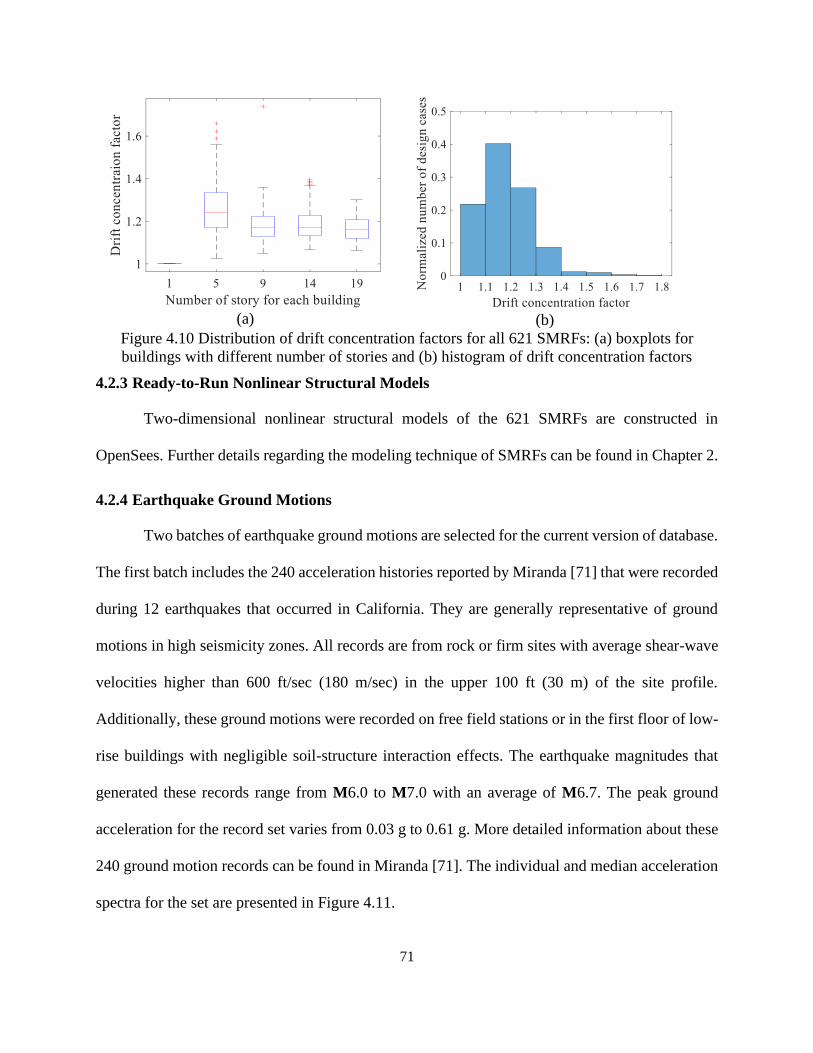
71

(a)

(b)

Figure 4.10 Distribution of drift concentration factors for all 621 SMRFs: (a) boxplots for

buildings with different number of stories and (b) histogram of drift concentration factors

4.2.3 Ready-to-Run Nonlinear Structural Models

Two-dimensional nonlinear structural models of the 621 SMRFs are constructed in

OpenSees. Further details regarding the modeling technique of SMRFs can be found in Chapter 2.

4.2.4 Earthquake Ground Motions

Two batches of earthquake ground motions are selected for the current version of database.

The first batch includes the 240 acceleration histories reported by Miranda [71] that were recorded

during 12 earthquakes that occurred in California. They are generally representative of ground

motions in high seismicity zones. All records are from rock or firm sites with average shear-wave

velocities higher than 600 ft/sec (180 m/sec) in the upper 100 ft (30 m) of the site profile.

Additionally, these ground motions were recorded on free field stations or in the first floor of low-

rise buildings with negligible soil-structure interaction effects. The earthquake magnitudes that

generated these records range from M6.0 to M7.0 with an average of M6.7. The peak ground

acceleration for the record set varies from 0.03 g to 0.61 g. More detailed information about these

240 ground motion records can be found in Miranda [71]. The individual and median acceleration

spectra for the set are presented in Figure 4.11.

72

Figure 4.11 Acceleration spectra for the 240 ground motion records

The second batch of ground motions includes three record-sets obtained from a site-

specific selection procedure [72] at three hazard levels: SLE, DBE and MCE, which correspond

to return periods of approximately 43 years, 475 years and 2475 years, respectively. Each group

consists of three suites of records (with 40 in each), which are selected for buildings with periods

of approximately 0.5 sec, 1.0 sec, and 2.0 sec, respectively, from the PEER NGA-WEST2 database

[62].

The first step in selecting each record set is to calculate the average characteristics of the

events that have return periods similar to the target return period. These characteristics include the

magnitude, distance, and spectral shape parameter (ε) of the seismic events with the target return

period, which are calculated using the United States Geologic Survey’s (USGS) seismic hazard

deaggregation tool (https://earthquake.usgs.gov/hazards/designmaps) based on the corresponding

site. As noted earlier, the archetype buildings are assumed to be located at a high-seismicity site

in Los Angeles (34.008°N, 118.152°W). The outcomes of the seismic hazard deaggregation

depend on the period of the structure being considered. Given the diversity of the archetype design

https://earthquake.usgs.gov/hazards/designmaps

73

space, their periods vary within a range of 0.30 sec to 3.0 sec. To keep the computational effort

associated with the seismic hazard deaggregation and record selection steps tractable, three typical

periods of 0.5 sec, 1.0 sec, and 2.0 sec are selected to represent the entire range of the periods for

the archetype buildings.

Once the seismic hazard deaggregation for each of the three representative periods is

complete, the mean characteristics of the seismic events are then used as inputs in the ground

motion model developed by Campbell and Bozorgnia [73], which provides a target horizontal

response spectrum and its associated standard deviations over a period range of 0.01 sec to 10.0

sec. These target spectra and associated standard deviations are used as the inputs into the ground

motion selection algorithm [72], which searches the PEER NGA-WEST2 database and selects the

desired number of records (40 in this study) that provide a good match with the target values. The

record selection tool uses the greedy ground motion selection algorithm developed by Jayaram et

al. [72]. The acceleration response spectra of the selected records at three hazard levels based on

periods of 0.5 sec, 1.0 sec, and 2.0 sec, are presented in Figure 4.12 to Figure 4.14.

Since the current version of the database is primarily developed to evaluate the structural

responses of the SMRFs and not collapse performance, no scaling of the selected ground motions

is performed.

74

(a)

(b)

(c)

Figure 4.12 Ground motion response spectra at the SLE hazard level for the following

representative periods: (a) 0.5 sec, (b) 1.0 sec, and (c) 2.0 sec

75

(a)

(b)

(c)

Figure 4.13 Ground motion response spectra at the DBE hazard level for the following

representative periods: (a) 0.5 sec, (b) 1.0 sec, and (c) 2.0 sec

76

(a)

(b)

(c)

Figure 4.14 Ground motion response spectra at the MCE hazard level for the following

representative periods: (a) 0.5 sec, (b) 1.0 sec, and (c) 2.0 secs

4.2.5 Nonlinear Responses of SMRFs

Two sub-datasets are included for the nonlinear responses. The first stores the structural

responses of the 621 SMRFs subjected to 240 ground motions, resulting in 621 × 240 = 149,040

peak story drift profiles, peak floor acceleration profiles, and residual story drift profiles. The other

contains the responses of a subgroup of 100 SMRFs (including 13 one-story, 26 five-story, 26

nine-story, 21 fourteen-story, and 14 nineteen-story buildings) subjected to three groups of site-

specific ground motions (with 40 ground motions in each group) at the SLE, DBE, and MCE levels.

This subset includes 12,000 peak story drift profiles, peak floor accelerations, and residual story

77

drift profiles. All response profiles are stored in .csv files as two-dimensional arrays (matrices).

Examples of story drift, peak floor acceleration, and residual story drift profiles for specific

archetypes subjected to a set of 40 MCE level ground motions are shown in Figure 4.15 to Figure

4.19. At this hazard level, the story drift demands for all archetypes and ground motions range

from 0.2% to 10% with medians between 1% and 2%. The medians of the residual story drift

demand for all archetypes are all less than 0.2%, which is less than the demolition drift limit of 1%

suggested by FEMA P-58 [4]. Moreover, the medians of the peak floor accelerations are within

the range of 0.5 g to 1.0 g.

(a)

(b)

(c)

Figure 4.15 Structural responses for a typical one-story building subjected to 40 MCE level

ground motions: (a) peak story drift, (b) peak floor acceleration, and (c) residual story drift

profiles

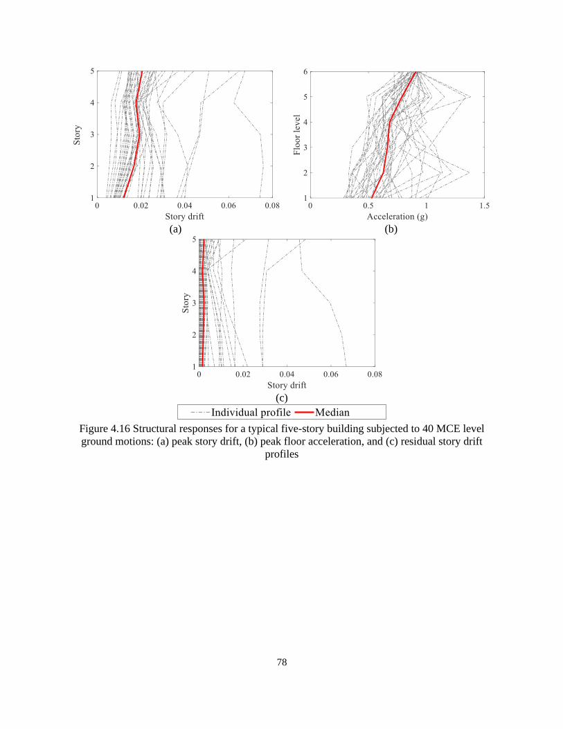
78

(a)

(b)

(c)

Figure 4.16 Structural responses for a typical five-story building subjected to 40 MCE level


profiles

79

(a)

(b)

(c)

Figure 4.17 Structural responses for a typical nine-story building subjected to 40 MCE-level


profiles

80

(a)

(b)

(c)

Figure 4.18 Structural responses for a typical fourteen-story building subjected to 40 MCE level


profiles

81

(a)

(b)

(c)

Figure 4.19 Structural responses for a typical nineteen-story building subjected to 40 MCE level


profiles

4.3 Structure of the Data

The dataset is stored in five separate folders which are named BuildingDesigns,

ElasticModels, NonlinearStructuralModels, GroundMotions and StructuralResponses. In each of

the first three folders, the relevant data for each building is stored in a subfolder which is named

based on the building ID. In the GroundMotions folder, the two batches of record-sets (as described

in Section 4.2.4) are stored in subfolders. In the StructuralResponses folder, there are two

subfolders named EDPsUnder240GMs and EDPsUnderSiteSpecificGMs. The former contains the

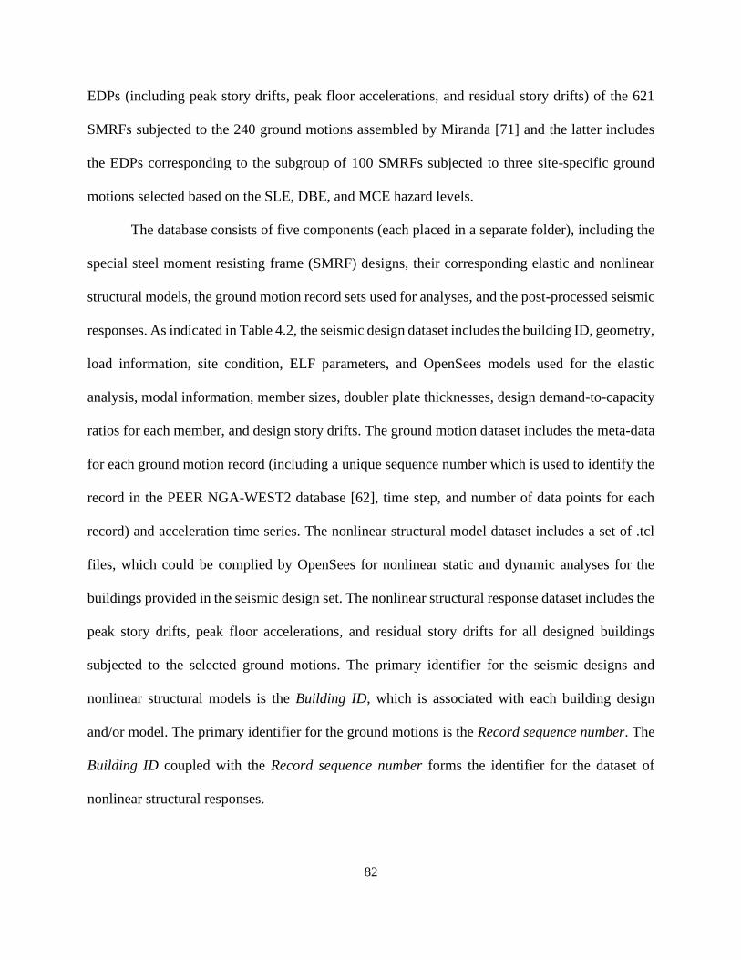
82

EDPs (including peak story drifts, peak floor accelerations, and residual story drifts) of the 621

SMRFs subjected to the 240 ground motions assembled by Miranda [71] and the latter includes

the EDPs corresponding to the subgroup of 100 SMRFs subjected to three site-specific ground

motions selected based on the SLE, DBE, and MCE hazard levels.

The database consists of five components (each placed in a separate folder), including the

special steel moment resisting frame (SMRF) designs, their corresponding elastic and nonlinear

structural models, the ground motion record sets used for analyses, and the post-processed seismic

responses. As indicated in Table 4.2, the seismic design dataset includes the building ID, geometry,

load information, site condition, ELF parameters, and OpenSees models used for the elastic

analysis, modal information, member sizes, doubler plate thicknesses, design demand-to-capacity

ratios for each member, and design story drifts. The ground motion dataset includes the meta-data

for each ground motion record (including a unique sequence number which is used to identify the

record in the PEER NGA-WEST2 database [62], time step, and number of data points for each

record) and acceleration time series. The nonlinear structural model dataset includes a set of .tcl

files, which could be complied by OpenSees for nonlinear static and dynamic analyses for the

buildings provided in the seismic design set. The nonlinear structural response dataset includes the

peak story drifts, peak floor accelerations, and residual story drifts for all designed buildings

subjected to the selected ground motions. The primary identifier for the seismic designs and

nonlinear structural models is the Building ID, which is associated with each building design

and/or model. The primary identifier for the ground motions is the Record sequence number. The

Building ID coupled with the Record sequence number forms the identifier for the dataset of

nonlinear structural responses.

83

4.4 Summary and Possible Future Extensions

This database is created using the archetype concept, which groups buildings with similar

geometric configurations and/or structural properties into representative sets, resulting in

generalized performance predictions for a full class of buildings [74]. The values of the parameters

considered in the archetype design space are determined based on the standard of structural

engineering practice. As a result, the database is representative of actual SMRFs located in a high

seismicity zones. In addition, practitioners from Englekirk Structural Engineers

(https://www.englekirk.com) have been involved in the development of the database, which

ensures that the designs are realistic. All datasets are stored as .csv files, which could be retrieved

based on a specific building ID. This allows the user/program to easily access the data. The

database [54] has been made publicly available through the DesignSafe cyberinfrastructure.

The database established in this study could be potentially utilized for a wide range of

purposes. For example, it could be used to identify the influence of various design parameters on

the seismic performance of SMRFs, assess the accuracy and reliability of existing seismic demand

prediction approaches, develop data-driven models for predicting seismic demands, and formulate

methods to explore optimal designs based on a predefined set of constraints.

One limitation of the current database is that the SMRF designs are based on a single set

of seismicity parameters (Ss = 2.25 g, S1 = 0.6 g, and stie class D). To make it more comprehensive,

buildings with different seismicity parameters should be added. This extension could be easily

achieved by changing the design input parameters relevant to the site condition and generating

new seismic designs and nonlinear models using the Python-based platform. Additionally, bi-

directional effects were not considered in the design of corner columns. Another limitation is that

the nonlinear response of the beam-column elements is simulated using concentrated plasticity

84

models with a Rayleigh damping ratio of 2%. Future versions could be extended to include other

modeling techniques, such as elements with fiber sections and/or finite length plastic hinge models,

and different damping assumptions.

The fact that the nonlinear models provided in this database do not capture local or global

buckling and axial shortening is noteworthy. Recent experimental findings [7,75] suggest that deep

wide-flange columns tend to experience axial shortening due to the local or global buckling, which

might affect the seismic response of SMRFs. This axial shortening phenomena cannot be simulated

using concentrated plasticity or fiber section models.

Table 4.2 Overview of attributes and associated descriptions

Dataset Attribute Property Description Unit

Seismic

design

Building ID \ A unique ID to identify the building unitless

Geometry

Number of stories An integer to denote the number of stories unitless

Number of bays An integer to denote the number of bays unitless

First story height A floating point number for the first story

height foot

Typical story

height

A floating point number for the typical story

height foot

Bay width A floating point number for the bay width foot

Number of LFRS's An integer for the number of LFRS's in each

principal direction unitless

Load

Floor weight A list of floating point numbers for the seismic

weight for each floor kip

Floor dead load A list of floating point numbers for the dead

load on each floor psf

Floor live load A list of floating point numbers for the live load

on each floor psf

Beam dead load A list of floating point numbers for the uniform

beam dead loads lb/ft

Beam live load A list of floating point numbers for the uniform

live loads on beam lb/ft

Leaning column

dead load

A list of floating point numbers for the dead

load on the leaning column kip

Leaning column

live load

A list of floating point numbers for the the live

load on the leaning column kip

Site

condition Ss

A floating point number for the short period

spectral response acceleration parameter g

85

S1 A floating point number for the 1 sec spectral

response acceleration parameter g

Site class An English letter to denote site class unitless

Parameters

relating to

ELF method

Cd A floating point number for the deflection

amplification factor

unitless

R A floating point number for the response

modification coefficient

I A floating point number for the importance

factor

ρ A floating point number for the redundancy

factor

Fa Two floating point numbers for the site

coefficient parameters Fv

Cu Three floating point numbers for the parameters

used to estimate the building period Ct

x

Modal

information

Modal periods A list of four floating point numbers of the 1st -

4th modal periods sec

Modal shapes A list of four vectors for the 1st - 4th modal

shapes unitless

Member

sizes

Beam A list of strings to denote the section sizes for

the beams, exterior columns, and interior

columns

unitless

Exterior column

Interior column

Design drifts \

A list of floating point numbers for the story

drifts under the design lateral forces (from

ELF)

Demand to

capacity

(DC) ratio

Beam shear DC

ratio

A two-dimensional array (matrix) with the DC

ratio for each beam/column subjected to

different loading conditions

Beam flexural DC

ratio

Column axial DC

ratio

Column shear DC

ratio

Column flexural

DC ratio

SCWB ratio \ A two-dimensional array (matrix) with the

SCWB ratio for each joint connection

Doubler plate

thickness \

A two-dimensional array (matrix) with the

thickness of the doubler plate at each joint inch

Elastic

Model \ \

A set of OpenSees .tcl files used for the elastic

analysis \

Ground

motion

Brief

information

Record sequence

number

A unique ID to denote the ground motion

record in the PEER NGA-WEST2 database unitless

86

Time step A floating point number for the time increment

in the time series sec

Number of time

points

An integer for the number of data points in the

time series unitless

Time series \ A list of floating point numbers for the

acceleration at each time step g

Nonlinear

structural

model

Nonlinear

model \

A set of OpenSees .tcl files used for nonlinear

analysis \

Nonlinear

structural

response

Peak story

drift \

A list of floating point numbers to denote the

seismic demands at each story/floor

unitless

Peak floor

acceleration \ inch/sec2

Residual

story drift \ unitless

87

5. Comparative Study for Steel Moment Resisting Frames Using

Post-Tensioned and Reduced-Beam Section Connections


Guan, X., Burton, H., & Moradi, S. (2018). Seismic performance of a self-centering steel

moment frame building: from component-level modeling to economic loss assessment. Journal of

Constructional Steel Research, 150, 129-140.

5.1 Introduction

In current seismic design codes, structures are designed to achieve a minimum level of

collapse safety by assuring ductile response during earthquake loading. As a result, conventional

steel structures may undergo permanent (or residual) deformations after a seismic event.

Mitigation of residual displacements in steel buildings is a critical issue as it directly relates to the

repair cost. In fact, large permanent deformations can render a building irreparable. For example,

because of excessive residual drifts, many buildings surviving the 2011 Christchurch earthquake

were declared unusable. The reconstruction cost for these buildings was estimated to be 40 billion

New Zealand dollars [76].

With the goal of minimizing residual deformations, researchers have been investigating the

application of alternative materials such as shape memory alloys [37,77,78]. However, the

widespread application of these new systems has been impeded by their high cost and the need for

new construction techniques and structural systems. To meet this challenge, post-tensioned (PT)

moment frame connections with top-and-seat angles have been proposed as an efficient approach

to reduce residual deformations in steel buildings [79,80]. Several experimental (e.g., [81]),

analytical (e.g., [40,81]), and numerical (e.g., [82–85]) studies have been conducted to evaluate

the behavior and potential advantages of PT connections. Figure 5.1 shows a reduced beam section

88

(RBS) welded moment connection and a PT beam-column connection with top-and-seat angles.

PT strands are used in the latter to provide restoring forces or self-centering (SC) capability, while

the top-and-seat angles are used to dissipate energy. Other types of energy dissipation mechanisms

such as viscous dampers [36] have also been used. As a result, structural damage in the connection

is localized at the angles, which can be easily replaced following an earthquake.

(a)

(b)

Figure 5.1 Schematic illustration of an (a) RBS welded connection and (b) PT connection

To assess the advantages of using self-centering moment resisting frames (SC-MRFs) with

PT connections, their seismic performance and potential cost-benefit should be studied. To achieve

this goal, a reliable modeling technique that captures the collapse behavior of SC-MRFs with PT

connections is needed. However, the existing modeling approaches are limited to PT connections

with other types of energy dissipation devices, such as web hourglass shape pins [35], friction

devices [86], and passive dampers [36]. Therefore, there is a need to develop a reliable, practical

and simplified modeling technique for PT connections with top-and-seat angles, which can be used

to predict the structural response of SC-MRFs subjected to earthquake loading.

In addition to the structural response, assessing earthquake-induced building economic

losses can also be used to quantitatively evaluate the advantages of SC-MRFs. Currently, several

Beam

Weld

Bolt

Column

Reduced Beam Section

Angle Beam

PT Strands

Reinforcing Plate

Column

89

methods are available to assess earthquake-induced losses of buildings. Porter et al. [87] proposed

an approach that involves conducting nonlinear dynamic analyses, prediction of damage at the

component level using fragility functions, and estimation of total building repair cost. The

approach was further enhanced as part of the second-generation performance-based earthquake

engineering (PBEE) methodology [88]. As part of the overall PBEE framework, Ramirez and

Miranda [39] demonstrated that the excessive residual drifts significantly influence earthquake-

induced building losses. A comprehensive description of the state-of-the-art methodology for

earthquake-induced economic loss estimation is described in FEMA P-58 [4]. This methodology

uses 2nd generation PBEE along with a complete database of damage fragility loss functions for

structural and nonstructural components and considers the influence of residual drifts.

In this study, a phenomenological model of top-and-seated angle PT connections is

developed in OpenSees [2] and is subsequently verified using prior experiments. A prototype

building, which has SC-MRFs as its lateral force resisting system, is selected. Using the proposed

phenomenological model of the PT connection, a 2D model for the SC-MRF is constructed. To

facilitate a comparative assessment, a welded moment resisting frame (WMRF) model, which has

the same member sizes as the SC-MRF but with RBS connections, is created. Nonlinear static and

dynamic analyses are performed on both the SC-MRF and WMRF models and their collapse

performance is quantified. Finally, the economic seismic losses for both buildings are assessed

using the FEMA P-58 methodology, which accounts for the influence of residual drifts and the

repair costs of structural and nonstructural components. Figure 5.2 illustrates the workflow of the

study.

90

Figure 5.2 Overview of study

5.2 Model Development in OpenSees

5.2.1 Description of Prototype Building

A 6-story office building with 6 bays in the E-W and N-S directions, which has been

developed by Garlock et al. [89], is selected as the prototype building in this study. The building

is located in the Los Angeles metropolitan area and has two identical MRFs to resist lateral loads

in each direction (Figure 5.3). A single MRF is considered for the current study. The frame is

designed as an SC-MRF with top-and-seat angle PT connections by Garlock et al. [89] using a ten-

step procedure. First, the equivalent lateral force (ELF) method is used to determine the seismic

story forces. The beam and column sections are then selected based on the ELF results and an

assumption regarding the relationship between the connection and beam moments. Subsequently,

an elastic analysis is performed to ensure that the story drift limit is satisfied. The force demands

91

at the design-based earthquake (DBE) and maximum-considered earthquake (MCE) levels are

estimated. Based on these demands, the connection detailing, including reinforcing plates and

panel zones, is determined. The design details of the SC-MRF, including the member sizes and

connection details are summarized in Table 5.1. Further details are provided in Garlock et al.

[89,90].

(a)

(b)

Figure 5.3 Prototype building including (a) floor plan and (b) elevation of moment resisting

frame (adapted from Garlock et al. [89]).

[email protected] m = 54.9 m

6@

9.1

5 m

= 5

4.9

m North

[email protected] m = 36.6 m

4.5

7 m

Ground Floor

2nd Floor

3rd Floor

4th Floor

5th Floor

6th Floor

Roof

5@

3.9

6 m

= 1

9.8

m

92

Table 5.1 Design of prototype frames (adapted from Garlock et al. [90]).

Floor Beam* Column* Doubler plate

thickness (mm)

Number of

PT strands

Initial PT force per

strand (kN)

Roof W2476 W14211 6 16 1352

6th floor W30108 W14211 25 20 1779

5th floor W30108 W14311 13 20 1957

4th floor W36150 W14311 25 28 2366

3rd floor W36160 W14370 19 28 2865

2nd floor W36170 W14370 25 32 3131 * The designation is based on sections specified in AISC Steel Construction Manual [57]

5.2.2 Component-Level Modeling

5.2.2.1 Phenomenological Model of PT Connection

A phenomenological model of the PT connection is developed in OpenSees, as shown in

Figure 5.4. Two main components govern the moment-rotation response of the PT connection: the

PT strands and top-and-seat angles. The PT strands provide restoring forces whereas the angles

dissipate energy. Similarly, in the modeling process, two materials acting in parallel are defined:

Self-centering and Pinching4 materials. The Self-centering material was developed for application

in systems and components that exhibits a flag-shaped hysteretic response. Its monotonic response

envelope includes four segments: initial, post-activation, slip, and post-slip stages. A total of seven

parameters are required to define the material. Three stiffness parameters are used to define the

slope for the loading path. A force parameter and two deformation parameters are used to define

the points where the stiffness changes. The area enclosed by the hysteretic curve is controlled by

a unitless parameter. The slip and post-slip stages are not considered for the material used in this

study. More details on the Self-centering material can be found in Mazzoni et al. [91]. The response

envelope (positive and negative) of the Pinching4 material, which is multilinear and includes

degrading and constant-residual-strength branches, is defined by force and deformation parameters

at each point where there is a change in stiffness (a total of eight parameters). Each unload-reload

path is defined by six parameters, which includes the load-deformation point at which unloading

93

occurs and four other parameters defined by some fraction of the force and deformation at the

unloading point. Fourteen parameters are used to define the hysteretic damage rules. A parallel

material that includes the Self-centering and Pinching4 materials is assigned to a rotational spring,

which represents the hinge of the beam. Figure 5.5 shows schematic representations of the Self-

centering and Pinching4 response. For the Self-centering material (shown in Figure 5.5(a)), the

parameters k1 and k2 determine the initial and hardening stiffness. The force parameter sigAct

defines the yield point. The unitless parameter β governs the area enclosed by the hysteretic loop.

For the Pinching4 material (Figure 5.5(b)), the force parameters ePf1 through ePf4 and the

associated displacement parameters ePd1 through ePd4 define the envelop for the positive segment,

whereas the parameters eNf1 through eNf4 and eNd1 through eNd4 define the negative segment.

Additional details about these parameters can be found in the OpenSees manual [91]. The beams

and columns are modeled using elastic beam-column elements. The column hinge is modeled

using a rotational spring with the modified IMK material [24].

94

Figure 5.4 Model for an exterior PT connection with top-and-seat angles and associated column

and beam

(a)

(b)

Figure 5.5 Schematic force-deformation response for (a) Self-centering and (b) Pinching4

material parameters

5.2.2.2 Validation of the Proposed Phenomenological Model

To assess the effectiveness of the proposed phenomenological model in capturing the

cyclic response of PT connections, the analytical lateral load-displacement response is compared

to data from four experiments. Specimens PC2, PC3, and PC4 from Ricles et al. [80] and specimen

Elastic beam

column element

Modified IMK Model

Force

Deformation

OpenSees Node

Elastic beam

column element

Self-centering material

Deformation

Force

Pinching4 material

Deformation

Force

Deformation

Force

k1

k2sigAct ß×sigAct

Deformation

Force

(ePf 1, ePd1)

(ePf 2, ePd2)(ePf 3, ePd3)

(ePf 4, ePd4)

(eNf 1, eNd1)

(eNf 2, eNd2)

(eNf 3, eNd3)

(eNf 4, eNd4)

95

20s-18 from Garlock et al. [79], are selected for the model validation. The experiment setup is

shown in Figure 5.6. The load applied at the top of the column and the associated displacement

are used to verify the proposed model. The reported lengths and cross-section properties of the

beams and columns in the experiments are used for the analytical models. The parameters for the

Self-centering and Pinching4 materials and percentage contribution of each material, are

determined using an iterative process. The experimental cyclic loading protocol is applied to the

model and the material parameters are adjusted until a reasonable match is obtained between the

simulated and experimental hysteretic response. First, the relative contribution from the Self-

centering and Pinching4 materials is tuned. This has the largest influence on the extent to which

the hysteretic loop takes on a flag shape and is therefore directly related to the self-centering

capability of the structure. The parameters controlling the envelope of the hysteretic curve (k1, k2,

sigAct, ePf1-ePf4, eNf1-eNf4, ePd1-ePd4, and eNd1-eNd4) are then adjusted. Finally, the parameter

governing the area of hysteretic loop (β) is determined. Figure 5.7 shows that the analytical and

experimental responses are comparable for all four specimens. The material parameters for the

four specimens are listed in Table 5.2 and Table 5.3. The response of the SC-MRF connection is

assumed to be symmetric. Therefore, the positive and negative Pinching4 material parameters are

identical.

96

Figure 5.6 Experiment setup (adapted from Ricles et al. [80])

(a)

(b)

(c)

(d)

Figure 5.7 Comparison between the proposed model and experimental data for specimens (a)

PC2, (b) PC3, (c) PC4, and (d) 20s-18.

Beam

Column

Pin Support

Roller Support

Horizontal Cyclic Load

97

Table 5.2 Parameters of Self-centering material for four specimens

Specimen No.

Self-centering material Fraction in

parallel k1

(kN-m/rad)

k2

(kN-m/rad)

sigAct

(kN-m) β

PC2 2.00108 7.00106 2.30105 0.12 0.85

PC3 4.00108 7.10106 2.40105 0.27 0.85

PC4 2.00108 1.25107 2.50105 0.50 0.70

20s-18 3.501010 3.70107 1.20106 0.98 0.90

Table 5.3 Parameters of Pinching4 material for four specimens

Specimen

No.

Pinching4 Material Fraction

in

Parallel ePf1

(kN-m)

ePf2

(kN-m)

ePf3

(kN-m)

ePf4

(kN-m)

ePd1

(rad)

ePd2

(rad)

ePd3

(rad)

ePd4

(rad)

PC2 6.80105 9.00105 1.13106 1.00106 0.001 0.01 0.03 0.30 0.10

PC3 6.80105 9.00105 1.13106 1.00106 0.001 0.01 0.03 0.30 0.10

PC4 6.80105 9.00105 1.13106 1.00106 0.001 0.01 0.03 0.30 0.15

20s-18 6.80105 9.00105 1.13106 1.00106 0.001 0.01 0.03 0.30 0.10

5.2.2.3 Calibration of PT Connections in the Prototype Building

The response of the PT connections in the SC-MRF of the prototype building are

represented using the proposed phenomenological model. In the absence of experimental data on

the hysteretic response of PT connections of varied geometry and design specifications, the

surrogate models (predictive equations) developed by Moradi [92] are used to determine backbone

curve parameters for the PT beam-column connections of the prototype building. These parameters

include the initial stiffness (Ki), gap-opening point (do, Fo), residual (post gap-opening) stiffness

(Kres), and ultimate strength (Fmax) for PT connections. The surrogate models can predict the lateral

load-drift response and the limit state behavior of PT connections with top-and-seat angles. Six

input parameters are needed including the initial post-tensioning force, beam depth, beam flange

thickness and width, span length, and column length [93]. In developing the surrogate models to

predict the lateral response characteristics of the PT connections, the reference study [92]

considered several damage mechanisms, including beam local buckling, angle fracture, strand

yielding, and excessive yielding of tensile bolts. The surrogate models were generated using a

98

verified response surface methodology based on 33 PT connection models (simulation runs) that

were developed and analyzed in ANSYS.

In the current study, the ratio of post-peak slope to initial stiffness is set as -0.167, which

is determined based on the average value for post-peak slopes observed from the experimental

response [79]. The residual strength for the PT connection is assumed to be 40% of its maximum

strength as sufficient experimental data is not available yet. This assumption is the same for

conventional welded connections [23]. The complete backbone curve can be obtained with the

surrogate model parameters, post-peak slope, and residual strength. The PT connections in the

prototype building are then calibrated based on the generated backbone curves. Figure 5.8 shows

typical calibration results for the PT connection at the 2nd floor level of the SC-MRF. The detailed

parameters for all the PT connections are summarized in Table 5.4 and Table 5.5.

(a)

(b)

Figure 5.8 Calibration of PT connection model subjected to (a) monotonic and (b) cyclic loading

99

Table 5.4 Parameters for Self-centering material of PT connections

Floor No.

Self-centering material Fraction in

parallel k1

(kN-m/rad)

k2

(kN-m/rad)

sigAct

(kN-m) β

2 1.13106 1.13104 1.81103 0.75 0.8

3 1.13106 1.13104 1.81103 0.75 0.8

4 1.13106 1.13104 1.58103 0.75 0.8

5 1.58106 9.04103 1.36103 0.75 0.8

6 1.13106 6.78103 1.36103 0.75 0.8

Roof 1.13106 4.52103 5.62102 0.75 0.8

Table 5.5 Parameters for Pinching4 material of PT connections

Floor No.

Pinching4 Material Fraction

in

Parallel ePf1

(kN-m)

ePf2

(kN-m)

ePf3

(kN-m)

ePf4

(kN-m)

ePd1

(rad)

ePd2

(rad)

ePd3

(rad)

ePd4

(rad)

2 1.39102 3.39103 7.34103 -4.52103 810-4 0.010 0.030 0.070 0.2

3 1.36102 2.03103 4.75103 -5.31103 510-4 0.010 0.025 0.070 0.2

4 1.02102 1.69103 4.41103 -4.52103 510-4 0.010 0.027 0.065 0.2

5 5.08101 1.41103 3.28103 -3.50103 510-4 0.010 0.024 0.065 0.2

6 5.08101 1.38103 3.62103 -3.39103 510-4 0.010 0.026 0.070 0.2

Roof 2.54101 7.91102 1.98103 -1.58103 510-4 0.010 0.025 0.066 0.2

5.2.2.4 Comparison of Backbone Curves for Different Types of Connections

Figure 5.9 shows a typical comparison of the backbone curves for the PT top-and-seated

angle and RBS welded connections as well as the top-and-seated angle connection without PT.

The backbone curve of the top-and-seat angle connection without PT is provided here to

quantitatively illustrate the flexural strength contribution of the PT strands. All the connections

have the same beam and column sizes. The backbone curve for the welded connection is

determined using the equations reported in Lignos and Krawinkler [24]. The backbone curve for

the top-and-seat angle connections is determined based on prior tests on angles [94]. The

experiment provides a relationship between axial load and associated displacement, which is

converted to a moment-rotation relationship using the approach presented by Kishi and Chen [95].

It can be observed that the peak strength of the PT connection is 38% lower than that of the RBS

welded connection. On the other hand, the strength of the PT connection is significantly higher

100

than that of the top-and-seat angle connection without PT, which is due to the large contribution

of PT strands to the flexural strength.

Figure 5.9 A typical comparison of the backbone curve for three types of connections

5.2.3 Structural Modeling

Two-dimensional (2D) nonlinear structural models of the SC-MRF prototype building are

constructed in OpenSees [2]. The model is constructed using the PT connection models described

earlier including elastic beam-column elements for beams and columns, rotational springs with the

modified IMK model for the column hinges, and rotational springs with Self-centering and

Pinching4 materials in parallel for the beam hinges. A schematic view for the SC-MRF structural

model is presented in Figure 5.10. The panel zones are modeled using the approach developed by

Gupta and Krawinkler [28], which includes eight elastic beam-column elements with very high

axial and flexural rigidity as the boundary elements for the panel zone and a trilinear rotational

spring in one of the four corners to capture the shear distortion of the panel zone. The remaining

three corners are modeled as pinned connections (Figure 5.10(b)). The column and beam depths

are used as the width and height of the panel zone element, respectively. The panel zone thickness

is taken as the summation of column web and doubler plate thicknesses. The thickness of the

0 0.05 0.1 0.150

2000

4000

6000

Rotation (rad)

Mom

ent

(kN

-m)

Welded connection

PT connection

Top-and-seat angle connection

101

doubler plates, which are only used for interior connections, is summarized in Table 5.1. A leaning

column is included to account for P-Δ effects. The gravity load carried by the lateral force resisting

system in the prototype building is applied as distributed loads acting on the beam, whereas the

gravity load carried by the gravity system is applied as concentrated loads acting on the leaning

column. The floor mass is uniformly assigned to each joint node.

A 2D model of the WMRF, which has the same member sizes as the SC-MRF, is also

constructed in OpenSees. Garlock et al. [89] determined the member sizes for the WMRF as an

intermediate step during the design of the SC-MRF. The forced demand for each member and the

story drift for the whole frame were checked to ensure that the strength and deformation are

satisfied. Since the WMRF and SC-MRF have the same member sizes, the WMRF and SC-MRF

have similar periods of vibration, as shown in Table 5.6. Except for the beam hinges, the modeling

of the WMRF is similar to that of the SC-MRF. In the WMRF model, the beam hinge is modeled

as a rotational spring with modified IMK material instead of the parallel combination of Self-

centering and Pinching4 materials. It should be noted that both WMRF and SC-MRF structural

models capture the flexural strength and stiffness deterioration of structural elements, which has

been shown to significantly influence the collapse behavior of the building.

102

(a)

(b)

(c)

Figure 5.10 OpenSees model for the SC-MRF: (a) overview of the model, (b) details for SC-

MRF connection, and (c) details for leaning column joint

Table 5.6 Comparison of natural periods for WMRF and SC-MRF (unit: second).

Mode WMRF SC-MRF

1st mode 1.94 2.10

2nd mode 0.71 0.75

Gravity

Leaning

Column

Concentrated

load

Pinsupport

Panel zone.

See detailed

view in Figure

5.10(b)

See detailed

view in Figure

5.10(c)

Bottom

hingeFixedsupport

(4)

(1)

(2)

(3)

(1)

(5)

(7)

(6)

(1)

(5)

(1) elastic beam-column element. (2) zero-length rotational spring with Hysteretic material.

(3) zero-length rotational spring with Self-centering and Pinching4 material in parallel.

(4) zero-length rotational spring with modified IMK material. (5) OpenSees node.

(6) zero-length rotational spring with very small stiffness. (7) truss element.

103

5.3 Nonlinear Static and Dynamic Analyses

5.3.1 Nonlinear Static Response

To compare the pushover response characteristics of the frame models, nonlinear static

analyses are performed for the SC-MRF and WMRF models. The pushover loading pattern is

calculated based on the equivalent lateral force procedure prescribed in ASCE 7-10 [30] and

assuming that the response is governed by the first-mode of vibration. Figure 5.11 shows the

pushover responses for the two models. The frame base shear force is normalized with respect to

its tributary seismic weight. The SC-MRF and WMRF reach their peak strength (referred to as

capping point) of 0.12 and 0.20 at roof drift ratios of 0.027 and 0.031, respectively. This indicates

that the peak strength of the SC-MRF is 40% lower than that of the WMRF. These results are

consistent with those of a study by Lin et al. [96], where the normalized base shear from nonlinear

static analysis of an SC-MRF was computed to be 0.08. They reported that the SC-MRF had an

initial stiffness that was the same as that of a comparable WMRF, but the SC-MRF had a lower

strength, which is partly attributed to the gap-opening response characteristics of PT connections.

The results of nonlinear response history analyses by Ricles et al. [97] also showed that moment

frames with PT connections experience lower base shears compared to moment frames with

welded connections.

To quantify the strength degradation, post-capping slopes of the two pushover curves are

compared by performing least-square fitting for the points between the capping point and

maximum roof drift [98]. The post-peak slopes for WMRF and SC-MRF are -1.68 and -1.20,

respectively, which indicates that the SC-MRF has a slower rate of strength degradation. This is

attributed to the load carrying mechanism of the frames. The PT connection resists external

moments primarily through gap opening and closing at the beam-column interface, whereas the

104

welded connection carries the external loads through forces on the beam and panel zone. As a

result, the strength of the WMRF is higher compared to the SC-MRF. This explanation is

consistent with the experimental study and findings reported by Lin et al. [96]. Additionally, both

frame models have an identical initial stiffness. These observations are also consistent with the

mechanical behavior of the beam-column connection used in the frame, as shown in Figure 5.9.

Figure 5.11 Monotonic pushover curves for the SC-MRF and WMRF

5.3.2 Incremental Dynamic Analysis and Collapse and Demolition Fragility Curves

The dynamic performance of the SC-MRF and WMRF is assessed using incremental

dynamic analysis (IDA) [61]. The set of 44 (22 pairs) far-field ground motion records specified in

FEMA P695 [6] are used. The magnitude for these records varies from M6.5 to M7.6 with an

average of M7.0. Thirty-two (16 pairs) of the ground motions were recorded at sites classified as

site class D and the remaining records are from site class C locations. The peak ground acceleration

for the record set varies from 0.21 g to 0.82 g with an average of 0.43 g. More detailed information

about the ground motion records can be found in Appendix A of FEMA P695. Scaling for IDAs

is performed such that the median spectral acceleration of the record set matches the specified

intensity levels, which ranges from 0.2 g to 3.0 g at an increment of 0.2 g.

0 0.02 0.04 0.06 0.08 0.10

0.05

0.1

0.15

0.2

0.25

Roof drift ratio

No

rmali

zed

base

sh

ear

WMRF

SC-MRF

105

During the IDAs, collapse is taken as the point at which dynamic instability occurs or the

collapse drift limit of 10% is exceeded. This assumption is consistent with Table 4-10 of the SAC

report [99], which states that collapse prevention performance is violated when the story drift

exceeds 10% for buildings with 4 to 12 stories.

The IDA results are used to generate fragilities for the WMRF and SC-MRF. Fragility

functions are used to quantify the probability that the structure will exceed a particular damage

state at a function of an intensity measure (IM). In this study, the probability of collapse and

demolition conditioned on the spectral acceleration level at the 1st mode period, is determined from

the IDA results. The empirical collapse and demolition data is fit to the lognormal cumulative

distribution function by utilizing the maximum likelihood method [59].

Figure 5.12(a) shows the collapse fragility curves for the SC-MRF and WMRF buildings.

As specified in FEMA P695 [6], the collapse margin ratio (CMR) is defined as the ratio of the

median collapse spectral acceleration to the spectral acceleration of the maximum considered

earthquake (MCE) (SaMCE) at the fundamental period of the structure. The median collapse capacity

(prior to adjusting for the spectral shape factor) for the WMRF and SC-MRF are 2.03 g and 1.07

g, respectively. This indicates that the WMRF has a much better collapse performance, which is

due to its higher lateral load carrying capacity. Further, the record-to-record variation, which is

described by the log-standard deviation of the collapse capacity, for the WMRF and SC-MRF are

0.35 and 0.33, respectively. With SaMCE = 0.69 g for the prototype building [89], the CMRs for the

WMRF and SC-MRF are 2.94 and 1.55, respectively. The CMR is further adjusted by multiplying

a spectral shape factor (1.44 for WMRF and 1.48 for SC-MRF) (FEMA P695 [6], Table 7-1). Thus,

the adjusted collapse margin ratios (ACMRs) for WMRF and SC-MRF are 4.23 and 2.30,

respectively. According to Table 7-3 in FEMA P695, the minimum permissible ACMR for the

106

WMRF and SC-MRF, which is based on a maximum MCE level collapse probability of 10%, is

1.83 and 2.02, respectively. In this case, the ACMRs for both WMRF and SC-MRF are greater

than their permissible values, which indicates that the collapse resistance of both frames is

acceptable.

Figure 5.12(b) shows the demolition fragility curves for the two frame models based on a

residual drift limit of 0.5% [100]. For the SC-MRF and WMRF, the median spectral intensity at

which demolition is triggered is 0.67 g and 0.57 g, respectively, which indicates that the PT

connection is able to reduce the effect of residual drifts. However, the median demolition capacity

of the SC-MRF is only 18% higher than the WMRF. In contrast, the median collapse capacity of

the WMRF is almost twice that of the SC-MRF.

(a)

(b)

Figure 5.12 Fragility results: (a) collapse and (b) demolition fragility curves

5.3.3 Discussion on Comparison between SC-MRF and WMRF

As noted earlier, the superior collapse performance of the WMRF compared to the SC-

MRF is due to the higher lateral force resistance of the former. The reason being that, unlike the

RBS connection, which has a yielding mechanism that is controlled by the strength of the beam,

the PT connection is controlled by gap opening and damage (yielding and local buckling) to the

top and seat angles. Previous studies [36,40] have shown that it is possible for SC-MRFs to have

0 1 2 3 4 50

0.2

0.4

0.6

0.8

1

SaT1

(g)

Pro

bab

ilit

y

WMRF

SC-MRF

0 0.5 1 1.5 20

0.2

0.4

0.6

0.8

1

SaT1

(g)

Pro

babil

ity

WMRF

SC-MRF

107

at least similar or higher collapse resistance than WMRFs. However, the PT connection in these

studies incorporated web hourglass pins (WHPs) that provided a flexural strength that is governed

by beam yielding. The same studies noted that the WHPs have an optimized shape with enhanced

fracture capacity, which is likely to enhance the overall collapse performance. Finally, Ahmadi

[101] showed that the collapse resistance of SC-MRF systems (compared to WMRF) depends on

the adopted design procedure. More specifically, they designed two SC-MRFs and one WMRF.

The two SC-MRFs had identical member sizes but different connection detailing (number of

strands, PT force, and reinforcing plate length). Their results showed that, compared to the WMRF,

the collapse resistance was higher for one of the SC-MRFs and lower for the other. All of these

factors support the results in the current study, which is also consistent with the findings reported

by Lin et al. [96]. However, it is important to highlight that the collapse performance of the SC-

MRF can be significantly improved by adopting a PT connection whose flexural strength is

comparable to that of a WMRF.

5.4 Economic Loss Assessment

5.4.1 Overview of FEMA P-58 Methodology

The methodology specified in FEMA P-58 [4], which is applied in this study, is generally

divided into four sections: hazard assessment, structural analysis, damage evaluation, and loss

estimation. These four elements are briefly described below:

Earthquake hazard assessment involves conducting probabilistic seismic hazard analysis

to determine the mean annual frequency of exceeding a range of ground motion intensities at the

building site (λ[IM]). The analysis identifies earthquake sources, characterizes the distribution of

earthquake magnitudes and source to site distance, predicts ground motion intensity, and

eventually combines the associated uncertainties. In this study, the spectral acceleration at the

108

fundamental period (Sa(T1)) of the building is used as the ground motion intensity. The hazard

curve, which is shown in Figure 5.13, is obtained from the Unified Hazard Tool [102] provided by

the USGS website (https://earthquake.usgs.gov) using a site class D location with an SaMCE

corresponding to the value used to design the prototype building.

Structural analyses are used to obtain the probability distribution of various engineering

demand parameters (EDPs) conditioned on the ground motion intensity. In this study, the EDPs,

which include peak story drift ratios (PSDRs), peak floor accelerations (PFAs), and residual drift

ratios, are extracted from the IDA results presented in Section 5.3.2.

The damage evaluation uses fragility functions to probabilistically describe the damage to

individual building components. The fragility specification includes a description of the

component, a description of the possible damage states, and the probabilistic relationship between

the damage measure (DM) and the EDPs. Detailed information about the fragility specifications is

provided in the Fragility Database of FEMA P-58. As specified in FEMA P-58, the building

components are grouped based on the governing EDPs (e.g., SDRs or PFAs), locations (e.g., a

certain story), and type (e.g., wall partitions or water piping system). The damage states for each

group describe the required repair efforts to restore the components to the undamaged state. This

process is conducted using the online tool Seismic Performance Prediction Program [3].

Loss estimation links the damage measures to decision variables (DVs), such as economic

losses, downtime, and fatalities. In this study, only economic losses are considered.

The four main steps of the FEMA P-58 methodology are related by the total probability

theorem as follows [88]:

( ) | | | ( )DV G DV DM dG DM EDP dG EDP IM d IM = (5.1)

where G[DV|DM] denotes the conditional probability of exceeding a specified loss amount

https://earthquake.usgs.gov/

109

given the level of damage, G[DM|EDP] denotes the conditional probability of exceeding a

specified level of damage given the structural response, G[EDP|IM] denotes the conditional

probability of exceeding some structural response demand given the ground motion intensity, λ[IM]

is the mean annual frequency of exceeding some ground motion intensity level, and λ[DV] is the

mean annual frequency of exceeding a given loss amount. Economic losses conditioned on a

specific intensity level is computed using the following relationship [39]:

[ ] [ ] [ ]

[ | ] [ | ] [ | ] [ | ]

E L| IM E L| NC R,IM P NC R | IM

E L NC D P NC D IM E L C P C IM

=

+ + (5.2)

The expected economic loss conditioned on the ground motion intensity (E[L|IM]) is

calculated by considering three scenarios: E(L|NC∩R, IM) is the expected loss for a non-collapse

scenario and the building is repaired. This loss is calculated based on the repair cost for different

damage states of each component in the building, which is specified in the FEMA P-58 database.

E(L|NC∩D, IM) is the expected loss when no collapse occurs but the building is demolished

because of excessive residual drifts. In this case, the loss is 100% of the building value plus an

additional 25% of the construction cost for removing the debris [4]. E[L|C] is the expected loss

conditioned on collapse, which is identical to E(L|NC∩D, IM), i.e., 125% of the building

construction cost. To facilitate the calculation, Equation (5.2) can be further simplified as follows

[39]:

[ ] [L | NC , ]{1 P(D | NC, IM}{1 P(C | IM)}

[ | NC ]P[D | NC, IM]{1 P(C | IM)} [ | ] [ | ]

E L| IM E R IM

E L D E L C P C IM

= − −

+ − + (5.3)

In Equation (5.3), P[C|IM] represents the probability of collapse when subjected to a

certain intensity level of ground motion. It can be directly obtained from the collapse fragility

curve (Figure 5.12(a)) generated using incremental dynamic analysis. P[D|NC, IM] corresponds to

the probability that the structure will be demolished conditioned on non-collapse and the ground

110

motion intensity level, which can be calculated using the following equation [39]:

0

[ | , ] [ | ] [ | , ]P D NC IM P D RDR dP RDR NC IM

= (5.4)

where P[D|RIDR] is the probability that the building will be demolished given the peak

residual story drift. As Ramirez and Miranda [39] suggested, P[D|RIDR] is assumed to follow a

lognormal distribution with a median of 0.015 and a logarithmic standard deviation of 0.3.

By probabilistically combining the losses associated with the three aforementioned

scenarios, the economic loss conditioned on the ground motion intensity (E[L|IM]) is obtained.

The expected annual loss is calculated by integrating the intensity-based losses times the slope of

the hazard curve for the site:

0

d ( )[ ] [ | ] d

d

IME L E L IM IM

IM

= (5.5)

where d ( )

dd

IMIM

IM

is calculated based on the seismic hazard curve in Figure 5.13.

Figure 5.13 Seismic hazard curve corresponding to the site of interest

5.4.2 Description of Building Components

Table 5.7 lists the damageable structural and nonstructural components adopted in the

10-2

10-1

100

10-4

10-3

10-2

10-1

100

100

SaT1

(g)

(

Sa)

111

current study. Since the fragility specifications (damage states, repair cost, etc.) for PT connections

are not specifically stated in FEMA P-58, the damage states are defined based on the experimental

observations reported by Garlock et al. [79]. More specifically, the two damage states defined for

the PT connection are beam local buckling and angle fracture, respectively. The corresponding

median story drift ratios for these two states are 1.85% and 4.0%. The construction cost per square

foot is 235 US dollars (2530 US dollars per square meter) based on the estimate provided by

Seismic Performance Prediction Program [3]. The total construction cost for the building is 45.7

million US dollars. All economic losses are normalized with respect to the building’s replacement

cost excluding the cost of demolition. The demolition cost, which includes the removal of debris,

is taken as 25% of the initial construction cost [4].

Table 5.7 Damageable components

Component

category Building component Unit EDP

Quantity per

story

Structural

component

Structural steel moment frames Each SDR 16

Exterior connections Each SDR 8

Interior connections Each SDR 12

Non-structural

component

Curtain walls 30 ft2 SDR 156

Partition walls 100 ft SDR 32.44

Wall partition finishes 100 ft SDR 2.45

Suspended ceiling 250 ft2 PFA 130

Independent pendant lighting Each PFA 49

Potable water piping 1000 ft PFA 5.55

Potable water pipe bracing 1000 ft PFA 5.55

HVAC Ducting 1000 ft PFA 3.08

Fire sprinkler water piping 1000 ft PFA 6.49

Fire sprinkler drop ×100 PFA 2.92

Heating water piping 1000 ft PFA 0.32

Heating water piping bracing 1000 ft PFA 0.32

Sanitary waste piping 1000 ft PFA 1.85

Sanitary waste piping bracing 1000 ft PFA 1.85

Traction elevator Each PFA 6*

* Quantity is for the entire building

112

5.4.3 Expected Loss Conditioned on Seismic Intensity

Figure 5.14 shows the expected losses for the building with SC-MRFs as its lateral force

resisting system. The total loss increases linearly with the ground motion intensity and gradually

reaches a plateau, approaching the summation of demolition and replacement costs (125%

normalized expected loss). The losses are further disaggregated into the expected losses associated

with collapse, demolition, and repair. As shown in Figure 5.14, when the intensity of the ground

motion is lower than 0.45 g, the total loss is dominated by repairs. As the intensity increases beyond

0.45 g, the demolition cost governs the total economic loss. The collapse cost does not dominate

until the intensity reaches 1.1 g, which is approximately one and a half times the MCE level. These

observations indicate that: (1) the building experiences slight damage under low-intensity ground

motions (Sa ≤ 0.45 g) and is therefore repairable; (2) under medium-intensity ground motions (0.45

g < Sa ≤ 1.1 g), there is a higher likelihood of irreparable damage because of excessive residual

drift; and (3) under high-intensity ground motions (Sa > 1.1 g), collapse safety is a concern.

Figure 5.14 Expected loss for the building with SC-MRFs

Figure 5.15 compares the expected losses for the WMRF and SC-MRF buildings.

0.2 0.4 0.6 0.8 1 1.20 %

25%

50%

75%

100%

125%

SaT1

(g)

Norm

ali

zed r

epair

cost

Total loss

Collapse

Residual drift

Repair

113

Generally, the total loss for the SC-MRF building is slightly higher compared to the WMRF

building. More specifically, the collapse losses are higher in the SC-MRF and the demolition costs

are higher in the WMRF building at all ground motion intensity levels. This is because the SC-

MRF has a lower collapse resistance and a smaller residual drift, both of which are related to the

characteristics of PT connections. Compared to the RBS welded connection, the PT connection

has a lower strength, but it is efficient in minimizing the residual drift. The loss associated with

component repair is almost the same for the two buildings.

(a)

(b)

(c)

(d)

Figure 5.15 Comparison of expected loss for WMRF and SC-MRF buildings including (a) total,

(b) collapse, (c) demolition, and (d) repair losses

5.4.4 Expected Annual Loss

The expected annual loss is obtained by integrating the IM-Loss relationship shown in

0.2 0.4 0.6 0.8 1 1.20 %

25%

50%

75%

100%

125%

To

tal

loss

SaT1

(g)

WMRF

SC-MRF

0.2 0.4 0.6 0.8 1 1.20 %

25%

50%

75%

100%

125%

Co

llap

se l

oss

SaT1

(g)

WMRF

SC-MRF

0.2 0.4 0.6 0.8 1 1.20 %

25%

50%

75%

100%

125%

Dem

oli

tion l

oss

SaT1

(g)

WMRF

SC-MRF

0.2 0.4 0.6 0.8 1 1.20 %

25%

50%

75%

100%

125%

Rep

air

loss

SaT1

(g)

WMRF

SC-MRF

114

Figure 5.14 with the hazard curve (in Figure 5.13). The normalized (by total cost) expected annual

losses for the SC-MRF and WMRF buildings are 0.51% and 0.42%, respectively. Figure 5.16

shows the expected annual loss disaggregated based on the contributing factors. Collapse accounts

for 25.5% and 4.8% of the expected annual loss for the SC-MRF and WMRF buildings,

respectively. The expected annual loss associated with demolition of the SC-MRF and WMRF

buildings is 41.3% and 75.9%, respectively. These observations again illustrate that the SC-MRF

is effective in minimizing permanent damage caused by excessive residual drifts but has inferior

collapse performance.

(a)

(b)

Figure 5.16 Comparison of annual expected loss between (a) SC-MRF and (b) WMRF buildings

5.5 Summary

A comparative assessment of the seismic performance and economic losses for a self-

centering moment resisting frame (SC-MRF) and reduced beam section (RBS) welded moment

resisting frame (WMRF) is presented, where the SC-MRF and WMRF have identical beam and

column sizes. First, a reliable phenomenological model for PT beam-column connections with top-

and-seat angles is developed and verified against past experimental results. A prototype building,

which has SC-MRFs as its lateral force resisting system, is selected. Using the developed

phenomenological model, a model of the entire frame is constructed in OpenSees. Nonlinear static

Collapse (25.5%)

Demolition (41.3%)

Repair (33.2%) Collapse (4.8%)

Demolition (75.9%)

Repair (19.3%)

115

and response history analyses are subsequently performed to study the response of the frame

models. The pushover analysis results indicate that the strength of the SC-MRF is 40% lower than

that of the WMRF. The dynamic analysis results show that the WMRF has higher collapse

resistance, whereas the SC-MRF undergoes smaller residual drifts. However, it is worth noting

that the collapse resistance of both frames is within the permissible values of acceptable collapse

margin ratio of the FEMA P695 guidelines. Finally, the economic seismic losses for the SC-MRF

and WMRF buildings are assessed using the FEMA P-58 methodology, which accounts for the

influence of residual drift and the repair costs of structural and nonstructural components. The

results reveal that the expected annual loss for the SC-MRF building is 21% higher than that for

the WMRF building. More specifically, the SC-MRF building has a lower expected loss associated

with demolition, but higher losses associated with collapse.

It is important to reiterate the context of the findings from the current study which involved

a comparative seismic performance assessment for a “designed” SC-MRF and a WMRF with the

same member sizes obtained from SC-MRF design. Moreover, the considered SC-MRF

incorporated a PT connection with top-and-seated angles. The performance of the SC-MRF could

be significantly improved by using a connection detail that provides flexural strengths that are

comparable to a WMRF (e.g., web hour glass pinned connection).

116

6. Seismic Drift Demand Estimation for SMRF Buildings: from

Mechanics-Based to Data-Driven Models


Guan, X., Burton, H., Shokrabadi, M., & Yi, Z. (2021). Seismic drift demand estimation

for SMF buildings: from mechanistic to data-driven models. Journal of Structural Engineering.

DOI: 10.1061/(ASCE)ST.1943-541X.0003004. (Accepted for publication)

6.1 Introduction

The second-generation performance-based seismic design (PBSD) framework [1] enables

structural engineers to target specific stakeholder-driven building performance objectives. As

shown in Figure 6.1, PBSD begins with defining a set of performance objectives using some metric

of interest (e.g., reliability, resilience, and/or lifecycle cost), followed by a preliminary design.

Ideally, the building performance should then be assessed by conducting nonlinear response

history analyses (NRHAs) on a structural model of the design and using the generated engineering

demand parameters (EDPs) (e.g., peak story drifts, peak floor accelerations, residual story drifts)

to evaluate earthquake-induced impacts (e.g., physical damage, economic losses, the probable

number of fatalities, functional recovery time). Based on the results of this initial assessment, the

design is revised as needed and the assessment is repeated until the performance meets the

predefined objectives.

While PBSD is commonly considered to be a state-of-the-art design method that can

effectively target specific performance outcomes, it has not been widely adopted in practice. This

is partly because the majority of engineers rely on elastic models to estimate seismic demands,

which is generally not suitable for rigorous performance-based assessments. Even when nonlinear

models are employed, the iterative process of conducting NRHAs and revisiting the design would

117

be computationally expensive and labor intensive.

Apart from the computational challenges associated with building-specific PBSD, recent

efforts have been directed towards using the 2nd generation performance-based earthquake

engineering (PBEE) methodology [88] to assess regional seismic impacts (e.g., economic losses,

fatalities) [103]. PBEE-based regional earthquake impact assessments are intended to replace the

more simplistic methods embedded in platforms such as HAZUS [104] and OpenQuake [105].

However, using NRHAs to generate the EDPs needed to conduct PBEE-type assessments for

hundreds of thousands or even millions of buildings may be impractical under some circumstances.

Figure 6.1 Overview of the performance-based seismic design procedure

To address the aforementioned challenges, several simplified methodologies have been

developed and used to estimate seismic drift demands in buildings (summarized in Table 6.1).

Some of these techniques are derived solely based on classical mechanics (e.g., shear and flexural

beam theory), structural dynamics, and/or linear models coupled with static analyses (referred to

as mechanics-based models in the remainder of this paper) (e.g., [64–66]). These models are often

preferred by practicing engineers because they are assumed to be highly generalizable and easy to

118

interpret. However, these methods often rely on many simplifications, which can reduce the

accuracy of response estimates. Moreover, the assumptions underlying these models may not be

applicable to specific conditions. Some other methods have been developed based on some

combination of mechanics-based and statistical approaches (e.g., linear regression and other

machine learning techniques) (referred to as hybrid models in the remainder of this paper) [4,63].

These models attempt to strike a balance between interpretability and applicability. The final

category of methods rely solely on advanced statistical or machine learning models (e.g., artificial

neural network) (referred to as data-driven models) [47,67]. While these methods are less reliant

on convenient simplifications, the excessive use of complex statistical models might render them

difficult to interpret and therefore draw skepticism from the practicing structural engineering

community.

Table 6.1 Some existing approaches for predicting seismic drift demands

Model Type Reference Model Basis Advantages Limitations

Mechanics-

based

Miranda [65];

Miranda and

Reyes [66]

Shear and flexural beam

theory

Simple to

implement and

interpret

Relies on several limiting

assumptions;

Two coefficients need to

be calibrated

Lin and Miranda

[64] Elasto-plastic SDOF

Based on

structural

dynamics

principles

Only three building cases

used to evaluate the

method

Hybrid

Gupta and

Krawinkler [63]

Four empirical

coefficients used to link

spectral displacements

to peak story drifts

Easy-to-follow

procedure

No generalizable approach

to computing empirical

coefficients provided

FEMA P-58 [4] Linear models with

static analyses

Simple to

implement

Relies on several limiting

assumptions;

Limited to buildings <= 15

stories

Purely data-

driven

Morfidis and

Kostinakis [106]

Artificial neural

networks

Does not rely on

any assumptions Difficult to interpret

Zhang et al. [67]

Deep long short-term

memory (LSTM)

networks

Estimates the

entire response

history

Difficult to interpret

Cook et al. [107] “Structural response

prediction engine”

Simple to

implement

Underlying details not

revealed

119

The methodologies summarized in Table 6.1 have greatly enhanced our ability to rapidly

estimate seismic structural response demands. However, the following limitations still exist in their

development and implementation: Method: these existing approaches either rely on a series of

simplifications or involve relatively complex deep learning models, both of which pose an

impediment to their adoption in structural engineering practice. Data used for calibration and/or

validation: most of the available methods are validated against a few (three to five) buildings

subjected to a very small number of ground motions (maximum of five). As a result, whether they

can provide reliable predictions under a broad range of conditions remains unknown. Model

development and testing approach: For the existing data-driven or hybrid (mechanics-based +

data-driven) methods, none of them utilized rigorous model performance evaluation, which, again,

brings into question the breadth of their applicability. A rigorous hybrid or data-driven model

development and evaluation procedure would include training, validation, and testing using three

different datasets. The testing set should be independent of the training and validation sets.

Prediction accuracy: most of the existing methods are evaluated using a single error metric (e.g.,

mean squared error, relative difference, or mean absolute relative deviation), which only reveals

partial information about the model accuracy. Ideally, the proposed methods should be assessed

such that their accuracy are fully transparent to the users. To address these limitations, there is a

need to develop a framework that strikes a balance among accuracy, convenience, and

interpretability. Additionally, new models should be developed using a rigorous process and large

diverse dataset, then evaluated using a range of error indicators.

Recent advancements in data-driven techniques (e.g., statistical/machine learning),

combined with the availability of large amounts of data and breakthroughs in computational tools

and resources, have created opportunities to revolutionize the process of estimating structural

120

response quantities in earthquake engineering. Data-driven approaches are especially useful when

there is no analytical model to predict the metric of interest or the available models are excessively

complicated and/or rely on many simplifying assumptions. Harnessing big data and statistical

learning methods in many cases would result in predictions that are as accurate as many

sophisticated engineering models but can be obtained with less effort. The Seismic Performance

Prediction Program (SP3) (https://www.hbrisk.com/) provides the option for users to adopt its

built-in data-driven methods to estimate seismic demands as a sub-step in PBEE assessments.

However, no details are provided on the adopted statistical techniques and evaluation approaches

[107].

The specific contributions of the current study are to: (1) propose a generalized framework

for developing data-driven or hybrid models to estimate building structural responses under

extreme event loading, (2) develop data-driven and hybrid models for estimating seismic drift

demands in special steel moment resisting frames (SMRFs), thus illustrating the framework

application, (3) quantitatively measure the relative importance of structural and spectral

parameters for estimating seismic demands, (4) comparatively assess the newly developed and

existing models for predicting seismic drift demands in SMRFs focusing on their predictive

performance and level of end-user effort needed to apply them. As outlined in Figure 6.2, four

previously developed methodologies are introduced, and their benefits and drawbacks are

examined. Then, a general framework for developing seismic demand estimation models is

proposed such that it can be adapted to other types of lateral force resisting systems (LFRS’s).

Using the same framework, new data-driven and hybrid models are formulated and rigorously

tested against a comprehensive database that includes structural responses obtained by subjecting

the 621 SMRFs designed in accordance with modern codes and standards to 240 ground motions.

https://www.hbrisk.com/

121

Finally, a comparative assessment among the new and existing models is performed to highlight

where they fall on the spectrum of approaches, evaluate their predictive performance, and elucidate

the end-user effort needed to apply them. All models are rigorously evaluated using multiple

performance metrics and a separate dataset of responses for a subgroup of 100 special moment

resisting frames (SMRFs) subjected to three sets of site-specific ground motions (different from

the 240 used to develop the new models) selected based on the service-level earthquake (SLE),

design-based earthquake (DBE), and maximum considered earthquake (MCE).

Figure 6.2 Overview of study

6.2 Overview of Existing Simplified Methods for Estimating Seismic Drift

Demands

Within the current literature, there are several simplified methodologies for estimating

seismic drift demands. One common theme among them is that they are all rooted in the

fundamental principles of structural dynamics and/or beam theory. Some rely solely on basic

122

physics, whereas others have attempted to integrate statistical regression using the structural

response data generated from NRHAs. These existing methods form a spectrum with purely

mechanics-based models on one end and purely data-driven models on the other. Between these

two extremes, there are models that combine elements of engineering mechanics and statistical

learning. Four existing representative methods that fall within this spectrum are examined in this

section.

6.2.1 Shear and Flexural Beam Theory

Miranda and Reyes [66] developed an approximate method to estimate the maximum

lateral displacement demands (which are eventually converted to story drifts) in multistory

buildings using beam theory. A multistory building is idealized as an equivalent continuum

structure consisting of a combination of shear and flexural cantilever beams connected via axially

rigid links, such that they have the same lateral deflection at the same points along the height. After

a series of derivations based on differential equations that are intended to capture both shear and

flexural response, the maximum roof displacement and maximum story drift ratio are estimated by

Equations (6.1) and (6.2), respectively. In Equation (6.1), the 𝛽1 factor is applied to the spectral

displacement evaluated at the fundamental period of the structure (𝑆𝑑) to obtain the elastic roof

displacement, which is further amplified by 𝛽3 to calculate the maximum inelastic roof

displacement ( 𝑢𝑟𝑜𝑜𝑓 ). Similarly, in Equation (6.2), the maximum elastic roof displacement

(𝑢𝑟𝑜𝑜𝑓,𝑒𝑙𝑎𝑠𝑡𝑖𝑐) is first normalized by the building height (𝐻) and then converted to the maximum

elastic story drift via 𝛽2. This elastic story drift is further amplified by 𝛽4 to obtain the maximum

inelastic story drift (𝑆𝐷𝑅𝑚𝑎𝑥).

More details on the derivation process are provided in Miranda and Reyes [66].

1 3roof du S = (6.1)

123

,

max 2 4

roof elasticuSDR

H = (6.2)

The method developed based on beam theory is relatively easy to interpret and provides an

approximation for the preliminary design of new buildings. However, it has several limitations.

First, the underlying assumption that the mass is uniformly distributed along the building height

might not be applicable since the weight of the roof is generally different from that of typical floors

in real buildings. Second, determining an important parameter (𝛼0) that reflects the degree of

participation of overall flexural and shear deformation in the simplified model of multistory

buildings requires significant effort. Consequently, the value of 𝛼0 is typically determined based

on engineering judgement and established rule of thumbs, which might be unreliable. Third, for

buildings with varying lateral stiffness, the differential equation set is difficult to solve. Last, the

output of this method is a single maximum story drift not the peak story drift profile. The latter is

critical for PBEE-type evaluations. All of these aforementioned drawbacks reduce the

effectiveness of this method in engineering practice.

6.2.2 Elastoplastic Single-Degree-of-Freedom with Known Yield Strength (PSKY)

Lin and Miranda [64] proposed a methodology that uses an equivalent elastoplastic single-

degree-of-freedom (SDOF) system coupled with the lateral yield strength of the building to

estimate the maximum inelastic roof displacement demand of regular steel frame buildings. The

equivalent elastoplastic SDOF is constructed using the first-mode period (𝑇1), effective height

(𝐻𝑒𝑓𝑓), effective mass (𝑀𝑒𝑓𝑓), effective stiffness (𝐾𝑒𝑓𝑓), and yield strength (𝑉𝑦,𝑆𝐷𝑂𝐹). The first

four parameters are derived from structural dynamics principles [108] and the last parameter is

estimated by idealizing the pushover curve generated by a multi-degree-of-freedom system

(MDOF) of the building into a bilinear response. The equations to obtain 𝐻𝑒𝑓𝑓, 𝑀𝑒𝑓𝑓, 𝐾𝑒𝑓𝑓, and

124

𝑉𝑦,𝑆𝐷𝑂𝐹 are provided in Chopra [108]. Inelastic displacements (∆𝑆𝐷𝑂𝐹) are obtained by performing

NRHAs on the elastoplastic SDOF system. The roof displacement demand is estimated using

Equation (6.3).

1 SDOFu PF= (6.3)

where the modal participation factor 𝑃𝐹1 is computed using a normalized mode shape that

takes on a value of 1.0 at the roof level. While it was not noted in the original study [64], this

method could be adapted to estimate full profile story drift demands (∆𝑚𝑢𝑙𝑡𝑖) using the following

equation [108]:

1 1multi SDOFPF = (6.4)

where 𝜙1 is the first-mode shape.

The PSKY method was validated on a relatively small dataset that included the structural

responses from three steel moment frame buildings subjected to 72 earthquake ground motions.

Moreover, it requires performing nonlinear static analysis on the entire structure and nonlinear

response history analyses on an elastoplastic SDOF. As such, a reasonable argument can be made

that the level of effort required is comparable to performing nonlinear response history analyses

on an MDOF. However, it is worth noting that there are existing simplified expressions that could

be used to compute 𝑉𝑦 (e.g., Equation (5-2) in FEMA P-58 [4]).

6.2.3 Statistically Adjusted Spectral Displacement

Gupta and Krawinkler [63] proposed a framework that establishes a relationship between

elastic spectral displacements and inelastic story drift demands using a set of statistically derived

coefficients (i.e., 𝛼𝑀𝐷𝑂𝐹, 𝛼𝐼𝑁𝐸𝐿 , 𝛼𝑃𝛥, and 𝛼𝑆𝑇). The framework starts by relating the elastic spectral

displacement demand at the first mode period of the structure (𝑆𝑑(𝑇1)) to the elastic roof drift

125

obtained from a MDOF system (neglecting P- effects) via a unitless coefficient 𝛼𝑀𝐷𝑂𝐹. Then, the

elastic roof drift demand is further amplified to obtain the inelastic roof drift by applying an

inelasticity factor 𝛼𝐼𝑁𝐸𝐿. The resulting inelastic roof drift demand is subsequently amplified by a

P- modification factor (𝛼𝑃𝛥). Finally, the inelastic roof drift demand is related to the individual

story demands via a modification factor 𝛼𝑆𝑇. The recommendations regarding the values of these

four coefficients are provided in Gupta and Krawinkler [63].

The framework developed by Gupta and Krawinkler [63] provides a clear path from

spectral displacement to individual story drift demand using a set of four coefficients. While it is

useful during the conceptual design phase and is rooted in a fundamental understanding of the

seismic behavior of SMRFs, it has two key limitations. First, the quantitative descriptions for two

of the coefficients (𝛼𝑃𝛥 and 𝛼𝑆𝑇) are not immediately available. Additionally, the framework was

developed using nonlinear analysis results from nine SMRFs subjected to three sets of 40 ground

motions, which brings its generalizability into question.

6.2.4 Statistically Adjusted Response of a Linear Elastic MDOF with Known Yield

Strength (EMKY)

FEMA P-58 [4] provides a simplified method to estimate the seismic responses that are

needed for 2nd generation PBEE-type assessments. The simplified analysis procedure uses linear

elastic MDOF structural models, static analyses, an estimate of the lateral yield strength, and linear

regression to generate median estimates of the seismic drift demands. The details of the

methodology are provided in Section 5.3 of the FEMA P-58 guidelines. This approach can be

viewed as employing a combination of mechanics (i.e., an elastic analysis) and statistical learning

(i.e., simple linear regression). It is relatively straightforward to apply and interpret. However, the

method was evaluated on a dataset that includes four SMRFs subjected to 25 pairs of ground

126

motions [109]. Additionally, no details were provided on whether the accuracy of the model was

assessed, and if so, what metrics were used.

6.3 Generalized Framework for Developing Hybrid and/or Data-Driven

Models for Estimating Building Structural Response Demands under Extreme

Loading

6.3.1 Overview of Framework

In general, hybrid and/or data-driven models utilize statistical and machine learning

techniques to infer patterns in data, which can then be used to forecast different type of phenomena

under uncertain conditions. A generalized framework for developing such models to estimate

seismic structural responses is illustrated in Figure 6.3. The entire framework consists of six main

steps:

Step 1: a comprehensive database of responses is developed from the results of NRHAs

applied to a reasonably large number of structural models representing buildings designed based

on the archetype concept. Note that these responses could also be obtained from physical

experiments or instrumented buildings that have been subjected to earthquake shaking. More

specifically, the parameters that are known to significantly influence seismic structural response

are first identified, then, lower and upper bound values are specified based on the allowable limits

specified in the building code and/or the standard of practice. Next, the possible values of each

parameter are defined such that they uniformly fill the gap between the lower and upper bounds.

These considered parameter values are then combined to form a design space. The resulting

parameter-combinations are used to design a set of buildings in accordance with the relevant

building codes and standards and their seismic responses under ground motion excitations are

retrieved. The dataset included in the database is divided into three mutually exclusive subsets that

127

will be used for training, validating, and testing the model.

Step 2: the variables that are known to influence the response variable (also known as

features or predictor variables) are identified based on domain knowledge or preliminary statistical

analyses. These variables will be used as the inputs for the model developed in Step 3.

Step 3: a model is formulated to link the predictors to the target response variable. From

the perspective of the user, a hybrid (mechanics-based + data-driven) model requires that they

perform some type of mechanic-based analysis (e.g., a modal or linear static structural analysis on

an SDOF or MDOF) to generate some intermediate results (e.g., elastic story drifts). Then, the gap

between the intermediate results and the target response variable (with the predictors as input) is

bridged using some type of function approximator (a machine learning (ML) model in the current

study). A purely data-driven model directly links the predictors to the target response variable

without any type of intermediate mechanic-based analysis.

Step 4: the datasets obtained from Step 1 are used to train and validate the ML models. The

hyperparameters that comprise the ML models are tuned during the training process. Generally,

different ML models should be investigated and an appropriate one is selected based on their

relative accuracy and level of training effort.

Step 5: the selected ML model is diagnosed to ensure that the underlying assumptions are

satisfied. For instance, if a linear regression model is selected in Step 4, then the residuals (the

difference between the predicted and observed values) are checked using a Q-Q plot to test whether

it follows a normal distribution. A sensitivity analysis is then performed to investigate the influence

of different predictors on the model performance. The predictors that are found to have a negligible

influence are removed using either backward stepwise or forward stepwise methods.

Step 6: The model obtained from Step 5 is tested using the dataset from Step 1 to check if

128

it is generalizable. If applicable, the performance of the developed model on testing dataset should

also be compared with existing models to assess their relative accuracy.

The framework presented herein is generalized enough such that it can be used to develop

hybrid and/or data-driven models for estimating the responses for different types of structures (e.g.,

reinforced concrete moment resisting frame or shear wall system) subjecting to loading from

different extreme events (e.g., hurricanes and earthquakes)

Figure 6.3 Framework for developing hybrid/data-driven models to estimate seismic demands

6.3.2 Model Evaluation and Performance Metrics

This section focuses on the metrics that could be used to evaluate the data-driven or hybrid

models that are developed using regression. During the development process, it is essential to

adopt the appropriate performance assessment metrics such that the reliability and accuracy of the

models could be rigorously evaluated. Several criteria can be used to determine the efficacy of a

129

model performance metric. First, the metric should be able to provide an overview of the error

distribution. More specifically, the metric should describe how the proposed method performs both

on average and in the worse/best scenarios. Second, the metric should be easily interpretable by

engineers with a limited background in statistics. Last, the metric should be versatile enough such

that the user could adjust the threshold to decide on the acceptable level of accuracy.

One conventional approach to quantifying the accuracy of a model is to use the relative

difference (𝐷) between the actual and predicted values corresponding to a single data point [110],

which is defined as:

y y

Dy

−= (6.5)

where �� is the predicted value (e.g., obtained using simplified model) and 𝑦 is the actual

value (e.g., obtained from nonlinear response history analyses). The relative difference measures

to what extent a single prediction deviates from its true value. However, it does not consider

whether the prediction method underestimates or overestimates the result. Moreover, a single

relative difference provides limited information. To overcome these two challenges, the relative

difference is re-defined as Equation (6.6), and the mean (𝜇) and standard deviation (𝜎) are used to

describe its overall statistical distribution.

ˆ

i ii

i

y yD

y

−= (6.6)

1

1 N

iiD

N

== (6.7)

2

2

1

1( )

N

iiD

N

== − (6.8)

where 𝑁 is the number of data points. These two variables (𝜇 and 𝜎) indicate the central

130

tendency and dispersion of the relative difference between the predicted and actual values.

Additionally, the mean ( 𝜇 ) reveals to what extent the model produces predictions that are

systematically higher or lower than the observed values (which is known as bias). A zero mean

indicates no bias and positive and negative mean values are indications that the model

systematically overestimates and underestimates the demands, respectively. While a low standard

deviation and a mean close to zero indicate a high accuracy, it is difficult to quantitatively

determine to what extent the standard deviation is small enough to be acceptable.

Similar to the mean relative difference, Sun et al. [111] measured the error in a statistical

model using the median absolute relative deviation (𝑀𝐴𝑅𝐷), which is given by

ˆ

Median( )i i

i

y yMARD

y

−= (6.9)

Although 𝑀𝐴𝑅𝐷 provides the central tendency of the relative deviation, it does not provide

any information regarding the dispersion of the error and whether the prediction is systematically

higher or lower than its true value. Another indicator that is commonly used to evaluate the

performance of regression models is the coefficient of determination (𝑅2), which is defined as

follows:

2

2 1

2

1

ˆ( )1

( )

N

i ii

N

ii

y yR

y y

=

=

−= −

−

(6.10)

which reflects the proportion of the variance in the outcome variable that is predictable

from the input variables. While this coefficient measures a model’s goodness of fit, it does not

explicitly quantify its accuracy.

Morfidis et al. [106] suggests that the error could be measured by the slope of a straight

line that is obtained from applying linear regression to a dataset comprised of the predicted and

131

actual values of the response variable (See Figure 6.4). A slope close to 1.0 generally implies that

the associated accuracy is relatively high. However, this is not always true as the slope of the line

does not convey any information regarding the error dispersion. For instance, the slope in Figure

6.4(a) is closer to 1.0 than in Figure 6.4(b), but the prediction presented in the latter figure is

deemed to be better than that of the former because the dispersion in Figure 6.4(b) is significantly

smaller.

(a)

(b)

Figure 6.4 Trend line obtained from linear regression on the observed and predicted values: (a)

large dispersion and (b) small dispersion cases

The mean squared error (𝑀𝑆𝐸), which is another metric that is often used to describe the

accuracy of a statistical model, is given by

2

1

1ˆ( )

N

i iiMSE y y

N == − (6.11)

𝑀𝑆𝐸 describes the average of the squared difference between the predicted and the actual

values. However, it is dependent on the unit of the response variable (��𝑖). This metric is useful for

comparing the accuracy among different approaches. However, it is less effective when evaluating

a single method because it is difficult to determine the extent to which the 𝑀𝑆𝐸 is small enough

for the model to be deemed acceptable.

Based on the aforementioned three criteria, a new performance metric is proposed. It is the

132

fraction of the dataset whose relative difference does not exceed a predefined percentage.

Mathematically, it is defined as:

%

ˆcountif %i i

i

X

y yX

yD

N

−

= (6.12)

where 𝑐𝑜𝑢𝑛𝑡𝑖𝑓 is a function that counts the number of data points satisfying the condition

in the square brackets, ��𝑖 is the predicted value, 𝑦𝑖 is the actual value, 𝑋 is a threshold defined by

the user, and 𝑁 is the total number of data points. The predicted value (��𝑖) is provided by the

hybrid or data-driven models whereas the actual value (𝑦𝑖) is obtained from NRHAs.

𝐷𝑋% is flexible because the threshold could be adjusted based on the specific context. In

this study, thresholds of 10% and 25% are adopted (𝐷10% and 𝐷25%). Together, these two metrics

describe the distribution of the error. Moreover, they are fairly easy to interpret even by individuals

with limited knowledge of statistics, and the user can determine the acceptable limit for 𝐷10% and

𝐷25% based on heuristic considerations. The simplified seismic drift estimation models considered

in this study are evaluated using all the aforementioned metrics to provide a complete and

transparent assessment of their accuracy.

6.4 New ML-Based Hybrid and Data-Driven Models to Estimate Seismic Drift

Demands

6.4.1 Dataset of SMRF Seismic Responses

As part of a separate study, 621 SMRFs with various geometric configurations and loads

were designed in accordance with current building codes and standards [30,56–58,112]. Based on

the developed code-conforming designs, two-dimensional (2D) nonlinear structural models were

constructed in OpenSees. NRHAs were then performed on these models by subjecting them to a

set of 240 ground motions and the corresponding EDPs (peak story drifts, peak floor accelerations,

133

and residual story drifts) were extracted. There are 81 one-story, 162 five-story, 162 nine-story,

128 fourteen-story, and 88 nineteen-story SMRFs in this database. The typical story height for

these SMRFs is 3.96 m (13 ft) and the ratios of first story to upper story height are 1.0, 1.5, and

2.0. The fundamental periods (estimated using the equation in ASCE 7-16 [30]) for all buildings

range from 0.2 sec to 2.5 sec. Additionally, the EDPs for a subgroup of 100 SMRFs (including 13

one-story, 26 five-story, 26 nine-story, 21 fourteen-story, and 14 nineteen-story SRMFs) subjected

to three sets of site-specific ground motions (with 40 records each) at the SLE, DBE, and MCE

levels, were also obtained. Additional details on the development and content of the database can

be found in Chapter 4.

6.4.2 Overview of Model Development

Inspired by the previously developed methods, two types of models are developed to

predict the seismic story drift demands in SMRFs using the framework (presented in Section 6.3.1):

one of them integrates mechanics and ML techniques (i.e. hybrid models) and the other is purely

data-driven or ML-based. The hybrid model is an adaption of the statistically adjusted EMKY

model. The purely data-driven model is proposed to directly link the building features with the

drift demands. These two models are developed to estimate median drift demands with the

understanding that the appropriate record-to-record variability can be addressed separately (e.g.,

using log-standard deviation values based on heuristics or prior studies).

The dataset described in the previous sub-section, which is used to formulate both the

hybrid and data-driven models, consists of two sub-datasets: the drift demands obtained for 621

SMRFs subjected to 240 ground motions and the demands for 100 SMRFs subjected to three sets

of site-specific ground motions selected based on the SLE, DBE, and MCE hazard levels. The first

dataset (from the 621 SMRFs) is further randomly divided into two subsets comprised of 80% and

134

20% of the original data. The former is used to train the ML model and the latter is used for

validation purposes. Once the model has been trained and validated, it is further tested using the

second dataset (100 SMRFs). This strategy ensures that there are no shared data points among the

training, validation, and testing subsets.

The 240 ground motions used to develop the training/validation dataset are first binned

based on the 𝑆𝑎(𝑇1) value. A total of six bins are formed ensuring that none of them have less than

10 ground motions. The median value of each spectral intensity measure (e.g., 𝑆𝑎(𝑇1)) is used as

one of the predictor variables. In the second dataset, the ground motions associated with each

hazard level (SLE, DBE, or MCE) are considered as one set, and their median intensity measure

is used to validate the data-driven model.

As shown in Figure 6.5, 35 variables (predictors) that have been preliminarily identified as

having an influence on seismic story drift demands, are grouped into four categories: building

information, modal analysis results, spectral intensity parameters, and nonlinear pushover analysis

results. Among these four groups of predictors, the building information parameters are easily

obtained since they could be acquired without any type of structural analysis, whereas the variables

related to pushover analysis are relatively difficult to obtain since they require the construction of

a nonlinear structural model. There are 7 building information predictors: the number of stories

(𝑁𝑠), number of bays (𝑁𝑏), floor height ratio(ℎ𝑖/𝐻) (which is defined as the ratio of the height for

floor 𝑖 to the total building height), bay width (𝑊𝑏), typical floor dead load (𝐷𝐿𝑓𝑙𝑜𝑜𝑟), roof dead

load (𝐷𝐿𝑟𝑜𝑜𝑓), and fundamental period (𝑇) determined using the equation specified in Chapter 12

of ASCE 7-16 [30]. The total building height (𝐻) is not included as an individual predictor since

the floor height ratio (ℎ𝑖/𝐻) already contains the information of the total height. Moreover, prior

studies [4,65,66] suggest that the height ratio is a better predictor than the total building height for

135

estimating the story drift. There are 12 modal analysis parameters included in the predictors: the

first to fourth modal periods (𝑇1, 𝑇2, 𝑇3, and 𝑇4) and the associated four modal shapes (𝜙1, 𝜙2, 𝜙3,

and 𝜙4) and the modal mass participation factors (𝑀𝑀𝑃1, 𝑀𝑀𝑃2, 𝑀𝑀𝑃3, and 𝑀𝑀𝑃4). The modal

shapes are scaled such that the maximum value is 1.0. Each modal shape is a vector including 𝑁 +

1 elements that correspond to each of the floor levels (including the ground level). The input value

used to estimate the drift in story 𝑖 is the (𝑖 + 1)𝑡ℎ element in the vector. The 10 spectral intensity

predictors include the spectral acceleration and displacement values evaluated at the first to fourth

modal periods and the empirical period based on ASCE 7-16 [30] (𝑆𝑎(𝑇1), 𝑆𝑎(𝑇2), 𝑆𝑎(𝑇3), 𝑆𝑎(𝑇4),

𝑆𝑎(𝑇), 𝑆𝑑(𝑇1), 𝑆𝑑(𝑇2), 𝑆𝑑(𝑇3), 𝑆𝑑(𝑇4), and 𝑆𝑑(𝑇)). The following 6 predictors are obtained from

the results of nonlinear static analysis: the force and drift corresponding to the yield point (𝐹𝑦 and

𝛥𝑦), the peak force and associated drift (𝐹𝑝 and 𝛥𝑝), the force at 2% drift (𝐹2%), and the strength

ratio (𝑆) determined using Equation (5-6) in FEMA P-58 [4]. A variable selection process is

performed in the development of each model to determine the relative importance among these 35

predictors and to evaluate the predictive performance with different subsets.

Higher mode effects are expected to be negligible for low-rise buildings but significant for

taller buildings. As such, the relative importance among the various predictors will be different for

these two building groups. Therefore, the data-driven models are developed separately for low-to-

mid-rise buildings (with less than 10 stories) and high-rise buildings (with 10 to 19 stories).

136

Figure 6.5 Initial set of predictor variables considered for the data-driven and hybrid models

6.4.3 ML-based Purely Data-Driven (MLDD) Models

6.4.3.1 Model Formulation

A data-driven model that is solely based on ML is developed to provide a direct link

between the 35 input variables and the nonlinear story drift demands (Figure 6.6). Several ML

algorithms are initially considered including multivariate linear regression [113], kernel ridge

regression [114], random forest [115], XGBoost [116], and artificial neural network [117]. Across

these different models, random forest had the best performance in terms of the various evaluation

metrics and training time. The random forest algorithm belongs to a family of models known as

decision trees, which recursively sub-divides the dataset based on a series of decisions and

associated consequences. A schematic view of a decision tree together with the associated sample

space, which is split into five regions, is presented in Figure 6.7. A basic decision tree model is

highly sensitive to the specific training dataset and thus has a high variance. This drawback is

addressed by generating a number of sub-datasets via the Bootstrap technique [118] and growing

a decision tree on each resampled sub-dataset. These multiple trees are aggregated (which is known

137

as bagging) to provide better predictions. However, bagging is highly likely to produce highly

correlated trees due to the application of the greedy algorithm, where all predictors are considered

at each split. To reduce the correlation among different trees, the greedy algorithm is applied to a

randomly selected portion of the original predictors at each split. This series of adjustments relative

to basic decision trees define the random forest algorithm [115]. A schematic representation of

random forest with three trees for a 𝑁-data sample with 𝑝 predictors is shown in Figure 6.8.

Figure 6.6 Workflow for developing the MLDD model

(a)

(b)

Figure 6.7 A schematic view of a decision tree model: (a) sample space split into five regions

considering two predictors 𝑋1 and 𝑋2, and (b) the corresponding decision tree model

138

Figure 6.8 A schematic illustration of the random forest algorithm with three trees for an 𝑁-data

sample with 𝑝 features

The training and validation results obtained from the random forest algorithm for low-to-

mid-rise buildings are shown in Figure 6.9, in which there are 14,094 maximum story drift data

points in total. As shown in Figure 6.9(a), the training data points are located exactly at the

reference line and the validation points are symmetrically located near the reference line,

indicating that the random forest model is able to provide an unbiased estimation on the training

and validation datasets. Figure 6.9(b) shows that the relative difference follows a normal

distribution. Additionally, the D10% and D25% for the validation dataset are approximately 84% and

100%, respectively, indicating that the random forest model has a high level of accuracy when

predicting the story drift demands for both the training and validation datasets.

Similarly, the random forest model for the high-rise buildings is trained and validated using

the corresponding datasets. The training and validation results are presented in Figure 6.10, in

139

which there are 20,784 maximum story drift demand data points in total. As shown in Figure 6.10,

all training and validation data points are symmetrically clustered near the reference line and 93%

of the validation data points have a relative difference within the range of -10% to +10%. All these

observations demonstrate that the random forest is able to provide an unbiased estimation and has

a relatively high level of accuracy on the training and validation datasets of the high-rise buildings.

A comparison of the relative difference distribution between the low-to-mid-rise and high-rise

buildings indicates similar overall performance.

(a)

(b)

Figure 6.9 Training and validation results for low-to-mid-rise buildings: (a) Observed versus


relative difference between the observed and predicted drift demand for the validation dataset

(a)

(b)

Figure 6.10 Training and validation results for high-rise buildings: (a) Observed versus predicted

story drift demand on the training and validation datasets, and (b) the distribution of relative

difference between the observed and predicted drift demands for the validation dataset

140

6.4.3.2 Sensitivity of the Model Performance to Adopted Predictors

While the initial set of predictors includes 35 variables, they have different levels of

influence on the predictive performance. To measure their relative effects, the importance score

generated by random forest is computed. When fitting a dataset with random forest, the out-of-bag

error for each training data point is recorded and averaged over the whole forest. After training,

the values for a specific feature are permuted among the training data and the out-of-bag error is

computed again based on this perturbed training dataset. The importance score of the feature is

then computed by averaging the difference in the out-of-bag error before and after the permutation

over all trees. Features with large scores are deemed more important than those with lower scores.

More details on the computation of importance scores are provided in Breiman [119].

Figure 6.11 shows the importance scores for all 35 predictors and the low-to-mid-rise

buildings, which are normalized by the maximum score. It is observed that the spectral acceleration

parameter evaluated at the fundamental period (𝑆𝑎(𝑇)) has the greatest influence on the predictive

performance. The spectral acceleration at the first-mode period (𝑆𝑎(𝑇1)) has the second highest

important score. With the exception of the floor height ratio, all building information predictors

have near zero importance scores. Among the predictors obtained from modal analysis, the first-

mode shape (𝜙1) has the highest importance. With the exception of 𝑆𝑎(𝑇), 𝑆𝑎(𝑇1), 𝑆𝑑(𝑇), and

𝑆𝑑(𝑇1), all other spectral intensity predictors have negligible importance. As for the predictors

extracted from nonlinear static analysis, they capture the level of nonlinearity and dissipated

hysteretic energy in the structural response. However, only the strength ratio (𝑆) is found to be

essential for predictive performance.

141

(a)

(b)

(c)

(d)

Figure 6.11 Normalized importance scores of the 35 predictors for the low-to-mid-rise buildings:

(a) building information, (b) modal information, (c) spectral parameters, and (d) nonlinear static

analysis parameters

Based on the aforementioned importance measurement, a variable selection process is

performed to reduce the number of features required for predicting the amplification factor using

the random forest model. It is worth noting that the variable selection should not be solely based

on the predictors’ importance rank, but also the relative level of difficulty in obtaining each one.

For example, the fist modal period (𝑇1) and yield drift (Δ𝑦) have comparable importance scores.

However, the former could be easily obtained by a modal analysis whereas the latter requires a

pushover analysis. Other forms of engineering judgement are employed in selecting the predictor

variables. For example, while the first modal period has a relatively low importance score, they

142

are known to be essential for predicting the performance of low-rise buildings (e.g., stories <= 3).

With these considerations, the first-round variable selection is to remove all variables in

the building information category except the floor height ratio and all predictors obtained from

nonlinear static analysis except the strength ratio. Consequently, 24 predictors are left. Then a

random forest model is trained with these 24 predictors as inputs to predict the story drift demands.

The trained model is further validated to examine to what extent the accuracy is reduced after

removing these 11 predictors and the feature importance score is updated. Subsequently, a new-

round of variable selection is conducted. This process is repeated until the validation accuracy

significantly decreases (e.g., the drop in 𝐷10% exceeds 5%), or all predictors left are deemed to be

essential based on engineering judgement. The finalized predictor set for the low-to-mid-rise

buildings includes 15 variables: h𝑖/𝐻 , 𝜙1– 𝜙4 , 𝑀𝑀𝑃1– 𝑀𝑀𝑃4 , 𝑆𝑎(𝑇), 𝑆𝑎(𝑇1), 𝑆𝑑(𝑇), 𝑆𝑑(𝑇1),

𝑆𝑑(𝑇2), and 𝑆.

The importance scores of the 35 predictors for the high-rise buildings are presented in

Figure 6.12. Unlike the observations for low-to-mid-rise buildings, all intensity measures except

𝑆𝑑(𝑇3) and 𝑆𝑑(𝑇4) have a significant influence (importance score >= 0.10). Meanwhile, the floor

height ratio and strength ratio are also essential. An iterative variable selection process is

performed and the finalized set of predictors includes 18 variables: h𝑖/𝐻, 𝜙1– 𝜙4, 𝑀𝑀𝑃1– 𝑀𝑀𝑃4,

𝑆𝑎(𝑇), 𝑆𝑎(𝑇1), 𝑆𝑎(𝑇2), 𝑆𝑎(𝑇3), 𝑆𝑎(𝑇4), 𝑆𝑑(𝑇), 𝑆𝑑(𝑇1), 𝑆𝑑(𝑇2), and 𝑆.

143

(a)

(b)

(d)

(d)

Figure 6.12 Normalized importance scores of the 35 predictors for the high-rise buildings: (a)

building information, (b) modal information, (c) spectral parameters, and (d) nonlinear static

analysis parameters

6.4.3.3 Reduced-Order MLDD Model

While the MLDD model simplifies the seismic drift demand estimation to a great extent,

it still requires 15 and 17 predictors for low-to-mid-rise and high-rise buildings, respectively.

Fourteen of these parameters (𝜙1– 𝜙4, 𝑀𝑀𝑃1– 𝑀𝑀𝑃4 , 𝑆𝑎(𝑇1), 𝑆𝑎(𝑇2), 𝑆𝑎(𝑇3), 𝑆𝑎(𝑇4), 𝑆𝑑(𝑇1),

and 𝑆𝑑(𝑇2)) rely on a modal analysis which requires constructing a linear elastic structural model.

To explore whether the purely data-driven model could be used when no structural model is

available, a “reduced-order” MLDD model is developed using nine predictors (𝑇, 𝑆𝑎(𝑇), 𝑆𝑑(𝑇),

h𝑖/𝐻 , 𝑁𝑠 , 𝑊𝑏 , 𝐷𝐿𝑓𝑙𝑜𝑜𝑟 , and 𝐷𝐿𝑟𝑜𝑜𝑓 ). None of these parameters require structural

144

modeling/analysis and all are available during the preliminary design stage. The training and

validation results show that the 𝐷10% and 𝐷25% are higher than 77% and 97%, respectively,

illustrating that the model has a reasonably high level of accuracy for these two datasets.

6.4.4 ML-based EMKY Model (ML-EMKY)

An ML-based EMKY model is developed in the current study. This approach can be

viewed as an improvement (based on later results) of the statistically adjusted EMKY model

presented earlier. As shown in Figure 6.13, the overall workflow involved in the model

development could be divided into mechanic-based, transition, and statistical learning parts. First,

an elastic MDOF model of the building is subjected to the pseudo lateral force determined using

Equation (5-3) of FEMA P-58 [4] and the associated story drifts are recorded. Subsequently, the

ratios between the drift demands from NRHAs and the elastic MDOF analysis are computed. These

ratios, which are defined as “amplification” factors, are unique to each story. In the last step, an

ML model is used to establish a relationship between the original 35 predictor variables and the

MDOF elastic drift amplification factor. The training and validation results show that the 𝐷10%

and 𝐷25% are greater than 96% and 99%, respectively, demonstrating good overall performance

on these two datasets.

Figure 6.13 Workflow for developing the ML-EMKY model

The importance scores for the 35 original predictors reveal that the floor height ratio is the

145

dominating feature. For low-to-mid-rise and high-rise buildings, the second most important

features are 𝑆𝑎(𝑇) and 𝑆𝑑(𝑇1) , respectively. A variable selection process is performed and

eventually 12 predictors are used: 𝑇1, h𝑖/𝐻, 𝜙1– 𝜙4, 𝑀𝑀𝑃1~𝑀𝑀𝑃4, 𝑆𝑎(𝑇), and 𝑆𝑑(𝑇).

The overall workflow for applying the ML-EMKY, MLDD and reduced-order MLDD

models in practice is presented in Figure 6.14. It assumes that the basic building design information

(e.g., member sizes, design spectra, and building dimension) and an elastic structural model are

available. The pseudo lateral force, spectral parameters, floor height ratio, and modal properties

are then obtained based on the design constraints and modal analysis. Subsequently, the pseudo

lateral force is applied to the MDOF model to obtain the elastic story drift demands. The floor

height ratio and modal properties are used as inputs to the random forest algorithm and the

amplification factors are generated. Finally, the seismic drift demand is predicted by multiplying

the elastic story drift demand with the story-specific amplification factor. The workflow for the

MLDD model is similar to the ML-EMKY model. The main difference is that the nonlinear drift

demands are obtained directly from the user inputs (without intermediate elastic drift demands).

For the reduced order MLDD model, there is a direct path from the building information (via the

random forest model) to the nonlinear drift demands without the need for structural modeling and

analysis on the part of the user.

146

Figure 6.14 Workflow involved in applying the ML-EMKY, MLDD and Reduced Order MLDD

models

6.5 Comparative Assessment Among Existing and Newly Developed Models

The performance of the existing and newly developed (in this study) models is evaluated

against a testing dataset, which includes the seismic responses for 100 SMRFs subjected to three

groups of site-specific ground motions selected based on the SLE, DBE, and MCE hazard levels.

The shear and flexural beam theory [65,66] and statistically adjusted spectral displacement [63]

models do not provide estimates of the full drift profile and are therefore not evaluated.

6.5.1 Evaluating the MLDD and “Reduced-Order” MLDD Models

The predictive performance of the final MLDD model is evaluated against the testing

dataset and the results are shown in Figure 6.15 (where 1131 story drift data points are included)

and Figure 6.16 (where a total of 1680 data points are included). The data points in Figure 6.15(a)

are located at the upper left side of the reference line and the histogram (Figure 6.15(b)) is left

skewed, which indicates that the MLDD model tends to underestimate the drift demands in low-

to-mid-rise buildings under all three intensity levels. This observation is also confirmed by the fact

147

that the mean values summarized in Table 6.2 are all less than zero. For the high-rise buildings,

Figure 6.16 shows that the MLDD model systematically underestimates the MCE-level demands

but overestimates the DBE-level demands. Meanwhile, it provides an unbiased estimation at the

SLE level. These observations are confirmed by the positive, negative, and zero values for the

mean relative difference at the MCE, DBE, and SLE hazard levels, respectively (See Table 6.2).

(a)

(b)

Figure 6.15 Predictive performance evaluation for the MLDD model applied to the low-to-mid-

rise buildings: (a) NRHA-based versus model predicted story drift demands and (b) the

distribution of relative difference between NRHA-based and model predicted story drifts

(a)

(b)

Figure 6.16 Predictive performance evaluation for the MLDD model applied to the high-rise

buildings: (a) NRHA-based versus model predicted story drift demands and (b) the distribution

of relative difference between NRHA-based and model predicted story drifts

148

Table 6.2 Multi-Metric Performance Evaluation for the MLDD Model

Building groups Indicators Testing at MCE Testing at DBE Testing at SLE

Low-to-midrise

buildings

𝑀𝐴𝑅𝐷 0.12 0.08 0.10

𝜇 -0.05 -0.07 -0.04

𝜎 0.19 0.15 0.16

𝐷10% 38.73% 55.70% 49.60%

𝐷25% 84.35% 89.92% 88.86%

Slope of linear

fitting 𝑦 = 1.11𝑥 𝑦 = 1.04𝑥 𝑦 = 0.99𝑥

𝑀𝑆𝐸 8.63 × 10−6 3.48 × 10−6 1.38 × 10−6

𝑅2 0.67 0.68 0.64

High-rise

buildings

𝑀𝐴𝑅𝐷 0.10 0.10 0.10

𝜇 -0.10 0.05 0.00

𝜎 0.13 0.17 0.11

𝐷10% 43.04% 46.43% 47.32%

𝐷25% 86.96% 83.04% 93.53%

Slope of linear

fitting 𝑦 = 1.14𝑥 𝑦 = 0.98𝑥 𝑦 = 1.03𝑥

𝑀𝑆𝐸 3.99 × 10−6 1.52 × 10−6 3.00 × 10−7

𝑅2 0.60 0.56 0.55

The performance metric values for the MLDD model are summarized in Table 6.2. For

low-to-mid-rise buildings, all metrics except 𝜎 and 𝑀𝑆𝐸 show that the model performs best at the

DBE level, whereas for the high-rise buildings, it performs best at the SLE level. The value of 𝜎

is approximately the same across the three intensity levels and building sub-groups, indicating that

the MLDD model is relatively stable in terms of the dispersion. When evaluated based on 𝑀𝑆𝐸,

the model has the best performance for both building groups at the SLE level. As noted earlier, the

𝑀𝑆𝐸 is very sensitive to the magnitude of the predicted value. The SLE drift demands are

relatively small (compared to the DBE and MCE demands) and thus the associated 𝑀𝑆𝐸 value is

always smallest. This observation demonstrates the inability of 𝑀𝑆𝐸 to reflect the actual model

performance.

The performance metric values for the reduced order MLDD model are summarized in

149

Table 6.3. All metrics except 𝜎 and 𝑀𝑆𝐸 reveal that it has a relatively low accuracy in estimating

MCE-level demands in low-to-mid-rise buildings and DBE-level demands in tall buildings. The

value of 𝜎 suggests that the model has a higher error dispersion at the DBE level for the high-rise

buildings. Despite the performance being worse than that of the MLDD model (Table 6.2), the

reduced order MLDD model is still deemed acceptable for use in the preliminary design stage with

the understanding that the estimation can be improved with more predictors when the results from

a modal analysis become available.

Table 6.3 Multi-Metric Performance Evaluation for the Reduced-Order MLDD Model

Building groups Indicators Validation at

MCE Validation at DBE Validation at SLE

Low-to-midrise

buildings

𝑀𝐴𝑅𝐷 0.17 0.09 0.11

𝜇 -0.11 -0.02 0.01

𝜎 0.18 0.15 0.19

𝐷10% 28.65% 52.25% 43.77%

𝐷25% 72.94% 90.45% 82.76%

Slope of linear

fitting 𝑦 = 1.18𝑥 𝑦 = 1.05𝑥 𝑦 = 1.02𝑥

𝑀𝑆𝐸 1.24 × 10−5 3.55 × 10−6 4.12 × 10−7

𝑅2 0.63 0.68 0.50

High-rise

buildings

𝑀𝐴𝑅𝐷 0.11 0.21 0.11

𝜇 -0.08 0.16 0.11

𝜎 0.12 0.21 0.17

𝐷10% 43.21% 18.21% 43.75%

𝐷25% 91.43% 59.82% 76.96%

Slope of linear

fitting 𝑦 = 1.12𝑥 𝑦 = 0.88𝑥 𝑦 = 0.90𝑥

𝑀𝑆𝐸 3.10 × 10−6 3.12 × 10−6 1.25 × 10−7

𝑅2 0.64 0.50 0.49

6.5.2 Evaluating the ML-EMKY Model

The performance metric values for the ML-EMKY model are summarized in Table 6.4.

For the low-to-mid-rise building group, the 𝐷10% and 𝐷25% consistently increase from MCE to

SLE, suggesting that the model performs best at the SLE level. For high-rise buildings, all metrics

150

except 𝐷10% show nearly the same value across the three intensity levels. The 𝐷10% metric

indicates that the model has a relatively low performance in estimating the DBE-level drift

demands. This observation partially confirms the superiority of 𝐷𝑋% as a performance evaluation

metric. An interesting phenomenon observed in Table 6.4 is that the value of σ does not vary

significantly across the different intensities and building sub-groups, implying the proposed model

is “stable” in predicting demands for buildings with different heights under various hazard levels.

Table 6.4 Multi-Metric Performance Evaluation for ML-EMKY


Low-to-mid-rise

buildings

𝑀𝐴𝑅𝐷 0.10 0.07 0.06

𝜇 0.08 0.00 -0.01

𝜎 0.10 0.10 0.09

𝐷10% 48.28% 67.37% 76.39%

𝐷25% 95.76% 98.94% 98.67%

Slope of linear

fitting 𝑦 = 0.93𝑥 𝑦 = 1.00𝑥 𝑦 = 1.03𝑥

𝑀𝑆𝐸 3.19 × 10−6 1.40 × 10−6 1.20 × 10−7

𝑅2 0.89 0.86 0.86

High-rise

buildings

𝑀𝐴𝑅𝐷 0.08 0.11 0.08

𝜇 -0.03 -0.06 0.04

𝜎 0.11 0.13 0.10

𝐷10% 57.86% 49.11% 55.89%

𝐷25% 95.36% 93.39% 98.04%

Slope of linear

fitting 𝑦 = 1.03𝑥 𝑦 = 1.06𝑥 𝑦 = 0.96𝑥

𝑀𝑆𝐸 1.75 × 10−6 1.23 × 10−6 4.17 × 10−8

𝑅2 0.70 0.59 0.68

6.5.3 Evaluating the PSKY Model

The performance metric values for the PSKY model are summarized in Table 6.5. In

general, all the listed metrics consistently show that PSKY has equally poor performance for the

two building groups and across the three intensity levels. More specifically, 𝐷10% and 𝐷25% values

are zeros or near-zeros in all cases.

151

Table 6.5 Multi-Metric Performance Evaluation for PSKY


Low-to-mid-rise

buildings

𝑀𝐴𝑅𝐷 3.75 3.61 3.67

𝜇 4.46 4.33 4.68

𝜎 1.85 2.03 2.75

𝐷10% 0.00% 0.00% 0.00%

𝐷25% 0.00% 0.00% 0.00%

Slope of linear

fitting 𝑦 = 0.16𝑥 𝑦 = 0.15𝑥 𝑦 = 0.11𝑥

𝑀𝑆𝐸 5.60 × 10−3 4.10 × 10−3 7.06 × 10−4

𝑅2 -1.50 -1.34 -1.09

High-rise

buildings

𝑀𝐴𝑅𝐷 2.57 2.46 2.35

𝜇 2.55 2.44 2.17

𝜎 0.39 0.53 0.38

𝐷10% 0.00% 0.00% 0.00%

𝐷25% 0.00% 0.00% 0.00%

Slope of linear

fitting 𝑦 = 0.28𝑥 𝑦 = 0.30𝑥 𝑦 = 0.31𝑥

𝑀𝑆𝐸 4.73 × 10−4 2.18 × 10−4 1.14 × 10−5

𝑅2 0.33 0.11 0.04

6.5.4 Evaluating the Statistically Adjusted EMKY Model

The performance metric values for the statistically adjusted EMKY model are summarized

in Table 6.6. With the exception of the 𝑀𝑆𝐸, the best performance for the low-to-mid-rise and

high-rise buildings is achieved at the DBE and MCE level, respectively. Additionally, the 𝐷25%-

based accuracy at the MCE level for both building groups is lower than the SLE and DBE estimates.

This is because the structural response under MCE is highly nonlinear, which is not well-captured

by the adopted linear regression model. The metrics listed in Table 6.6 also show that the

statistically adjusted EMKY model generally provides better seismic drift estimates for low-to-

mid-rise buildings compared to high-rise buildings. This is attributed to the fact that the model

only accounts for parameters relevant to the first mode (i.e., 𝑇1 and 𝑆𝑎(𝑇1)) and does not capture

the higher mode effects that are significant for high-rise buildings.

152

Table 6.6 Multi-Metric Performance Evaluation for the Statistically Adjusted EMKY Model


Low-to-mid-rise

buildings

𝑀𝐴𝑅𝐷 0.16 0.10 0.20

𝜇 0.19 0.00 -0.16

𝜎 0.24 0.16 0.13

𝐷10% 33.16% 47.21% 18.04%

𝐷25% 65.78% 90.98% 71.88%

Slope of linear

fitting 𝑦 = 0.86𝑥 𝑦 = 1.01𝑥 𝑦 = 1.16𝑥

𝑀𝑆𝐸 1.40 × 10−5 4.05 × 10−6 6.54 × 10−7

𝑅2 0.55 0.60 0.49

High-rise

buildings

𝑀𝐴𝑅𝐷 0.24 0.17 0.13

𝜇 -0.21 -0.14 -0.09

𝜎 0.15 0.14 0.15

𝐷10% 14.46% 28.04% 35.54%

𝐷25% 53.21% 75.00% 85.00%

Slope of linear

fitting 𝑦 = 1.30𝑥 𝑦 = 1.19𝑥 𝑦 = 1.11𝑥

𝑀𝑆𝐸 8.75 × 10−6 2.77 × 10−6 1.25 × 10−7

𝑅2 0.36 0.44 0.18

6.5.5 Comparing the Predictive Performance and Required User-Effort Among Different

Models

The existing and newly developed simplified seismic drift demand estimation models fall

into a spectrum of methodologies where mechanics-based models are located at one end and purely

data-driven models are on the other end. Between these two extremes, there are hybrid models that

integrate both mechanics-based and data-driven techniques. As shown in Figure 6.17, the models

based on shear and flexural beam theory and PSKY belong to the category of purely mechanics-

based models. The MLDD and reduced-order MLDD models developed in this study are primarily

data-driven. The statistically adjusted EMKY and ML-EMKY models are developed based on a

combination of mechanics-based and statistical learning methods and are therefore considered

hybrid approaches.

153

Figure 6.17 A spectrum of models for simplified seismic drift demand estimation

To compare the performance of the various models, 𝐷10% values for the low-to-mid-rise

and high-rise buildings are shown in Figure 6.18, from which several conclusions can be drawn:

First, the purely mechanics-based model (PSKY) showed poor performance having almost zero

𝐷10% at all intensity levels. The statistically adjusted EMKY model performed reasonably well.

Across all hazard levels, the 𝐷10% values are in the range of 20% to 50% and 15% to 40% for the

low-to-mid-rise and high-rise building datasets, respectively. Second, the hybrid model developed

in this study (ML-EMKY) shows the best performance with 𝐷10% values greater than 50% across

all intensity levels in both building groups. Last, the MLDD model developed in the current study

generally outperforms the existing models (PSKY and EMKY) with 𝐷10% values larger than 45%

in all cases. The 𝐷10% value of the reduced-order MLDD model is between 20% and 50%, which

is comparable to the previously developed statistically adjusted EMKY model. Overall, the

comparison suggests that models integrating both mechanics-based and statistical learning

outperform those that are purely data-driven or mechanics-based (with simplifying assumptions).

154

(a)

(b)

Figure 6.18 Comparing the performance based on 𝐷10% across the existing and newly developed

models for the (a) low-to-mid-rise and (b) high-rise buildings

Figure 6.19 compares the predictive performance and required effort (on the part of the

user) for the newly developed and existing models considered in this study. The reduced-order

MLDD model requires the least effort as the results generated by any type of structural analysis

(e.g., modal analysis, linear elastic analysis) are not needed. Meanwhile, this model provides

155

estimates of seismic drift demands that are comparable to those generated by the previously

developed statistically adjusted EMKY model, which makes it useful during the preliminary

design stage when no structural analysis results are available. In contrast, all other models could

only be applied once the elastic structural model has been developed. PSKY requires the greatest

effort as it requires performing nonlinear response history analysis, but it has the lowest accuracy.

The effort associated with the statistically adjusted EMKY, ML-EMKY, and MLDD models, fall

between the aforementioned two extremes since they only rely on linear elastic analysis, which is

typically incorporated as part of the conventional design process.

Figure 6.19 Performance versus required effort for various seismic drift demand estimation

models

6.6 Summary

A spectrum of simplified methods for estimating seismic drift demands is presented and

evaluated. On one end of the spectrum are fully mechanics-based approaches that are derived

solely based on engineering principles. On the other end are purely data-driven models that are

established by applying statistical and machine learning methods to a parametric dataset of drift

demands generated from nonlinear response history analyses (NRHAs). Between these two

156

extremes, there are hybrid methods that integrate both fundamental mechanics and

statistical/machine learning techniques. Four existing methods that fall within this spectrum of

approaches are reviewed, and their benefits and drawbacks are discussed. They are based on shear

and flexural beam theory, an elastoplastic single-degree-of-freedom system with known yield

strength (PSKY), statistically adjusted spectral displacement, and the statistically adjusted

response of a linear elastic multi-degree-of-freedom system with known yield strength (EMKY).

A framework for developing hybrid and/or data-driven models to estimate structural

responses under extreme events is established. A systematic step-to-step procedure is presented

that is agnostic to the type of demand parameter (e.g., story drifts and floor accelerations) and

lateral-force resisting system being considered. Meanwhile, the advantages and limitations of

different metrics used for evaluating model performance are discussed and a new metric 𝐷𝑋%

(defined as the fraction of the dataset whose relative difference does not exceed 𝑋%) is proposed.

The framework is then used to develop purely data-driven and hybrid models for estimating

seismic drift demands in steel special moment resisting frames (SMRFs). These two models are

described as (i) machine learning based and purely data-driven (MLDD) and (ii) machine learning

based adjusted response of an EMKY (ML-EMKY). Both are formulated based on a dataset of

seismic structural responses from 621 modern code-based SMRF designs subjected to 240 ground

motions. During the model development process, the sensitivity of the model performance to 35

potential predictor variables is investigated. For the hybrid model, the floor height ratio (defined

as the ratio of the height of floor 𝑖 to the total building height) and intensity measures (𝑆𝑎(𝑇) and

𝑆𝑑(𝑇1)) are the two most influential types of predictors, whereas, in the purely data-driven model,

the intensity measure 𝑆𝑎(𝑇1) alone dominates the response estimation.

Finally, a comparative assessment of the predictive performance among the existing and

157

newly developed models is performed. More specifically, previously developed PSKY and

statistically adjusted EMKY models and newly developed MLDD and ML-EMKY models, are

evaluated on a testing dataset including the responses of 100 SMRFs subjected to three sets of site-

specific ground motions selected based on the service-level earthquake (SLE), design-based

earthquake (DBE), and maximum considered earthquake (MCE) levels. The evaluation results

suggest that the hybrid model generally has a higher accuracy than the purely data-driven or

mechanics-based models. A comparison of the level of the effort required to apply the different

models reveals that the mechanics-based model (PSKY) requires the greatest effort whereas the

reduced-order MLDD model needs the least effort. The latter could be applied during the

preliminary design stage.

158

7. Surrogate Models for Probabilistic Distribution of Engineering

Demand Parameters of SMRF Buildings under Earthquakes

7.1 Introduction

Steel moment-resisting frames (SMRFs) are often used as a part of the lateral force-

resisting systems (LFRS’s) in building structures designed to resist earthquakes and/or winds. Steel

special moment frames is one of the few LFRS options that is permitted for tall buildings exceeding

160 ft (48.77 m) in the regions of high seismicity according to ASCE 7-16 [30]. It is well-known

that SMRFs are capable of providing significant inelastic deformation capacity through flexural

yielding at the beam ends and limited yielding in panel zones, which enables ductile response in

moderate-to-severe earthquakes. A key advantage of SMRFs is that they do not require structural

walls and diagonal braces, and thus offer an unobstructed line of sight, which provides flexibility

in architectural design. A recent study [31] indicated that SMRFs typically impose smaller forces

on foundations compared with other structural systems, resulting in more economic foundation

designs. Owning to the aforementioned advantages, SMRFs have been widely adopted in industrial

plants, commercial buildings, and some skyscrapers as part of a dual LFRS.

The widely accepted approach for estimating the seismic structural response is to perform

a nonlinear response history analysis (NRHA) on a detailed analytical model subjected to a suite

of representative ground motions. However, NRHA often relies on a carefully calibrated structural

model and in some cases, the analysis process can be time-consuming, making the effort associated

with detailed modeling and analysis unfeasible. For example, when the 2nd performance-based

earthquake engineering (PBEE) framework is used to assess regional seismic impacts, performing

NRHAs for tens or hundreds of thousands or even millions of buildings may be impractical. In

such a situation, a simplified process that provides rapid and reasonable estimates of seismic

159

demands is much needed.

Surrogate models have been proven to be useful for providing rapid and reliable estimation.

They are typically constructed using data-driven approaches on a representative dataset that is

derived from a mechanics-based simulation model. Through the training process, surrogate models

mimic the relationship between multiple input parameters (or features) and the outcomes (or

responses). There have been extensive applications of surrogate models in some areas such as

mechanical engineering [120], environmental engineering [121], and hydrology [122], as well as

earthquake engineering [4,67,106,107,123]. Some of these proposed surrogate models [4,63] rely

on a combination of mechanics-based and statistical approaches whereas others [67,106,107,123]

are completely based on the machine learning techniques (e.g., artificial neural networks).

The aforementioned studies have greatly enhanced our ability to rapidly estimate seismic

structural response demands. However, the following limitations still exist in their development

and implementation. First, the dataset used to calibrate and/or validate the surrogate models are

relatively small. Most of the available surrogate models are validated against three to ten buildings

subjected to a maximum of 100 ground motions. Second, for the models that rely on statistical

analyses, none of them utilized a rigorous performance evaluation, which brings into question of

the breadth of their applicability. Additionally, most of these existing simplified models target a

single type of engineering demand parameter (EDP) and fail to provide dispersion or covariance

within and between different EDPs, which prevents their application in economic loss assessment

based on the FEMA P-58 [4] framework. It is worth noting that stakeholders are typically more

interested in economic loss indicators (e.g., expected annual loss) rather than the EDPs.

To address the aforementioned limitations, a set of parametric and non-parametric

surrogate models that are able to estimate the central tendency of EDPs (including peak story drifts,

160

peak floor accelerations, and residual story drifts) are developed based on a comprehensive

database of 621 SMRFs and associated seismic responses. The suggested values for the variance

of each EDP and the correlation between different EDPs are also provided. The remainder of this

paper begins by introducing the dataset used for developing the surrogate models. Then the

development details and implementation of the parametric and non-parametric surrogate models

are presented. The predictive performance of the proposed surrogate models are evaluated and

compared with the existing simplified analysis procedure specified in FEMA P-58 [4].

Subsequently, the terms in the covariance matrix that describe the possible correlation among

different EDPs are quantitatively investigated. Then, the EDPs generated from the surrogate model

and assumed covariance matrix are used to calculate the economic loss for 100 SMRF buildings

and further compared with those determined using the EDPs obtained from NRHAs.

7.2 Dataset of SMRFs

To create the database required for developing the surrogate model, a Python-based

computational platform that automates seismic design for SMRFs, nonlinear structural model

construction, and seismic response simulation is developed using the object-oriented programming

paradigm. This automated seismic design and analysis (AutoSDA) platform [124] takes the

necessary input parameters (including the building geometry, load, and site information), generates

structural designs (including section sizes for each component, demand-to-capacity ratios, and

joint connection details), constructs the corresponding nonlinear structural models, and performs

the nonlinear structural analysis in OpenSees [2].

Based on the AutoSDA platform, a database [54,55] that comprises four modules (code-

conforming seismic designs, ground motions, nonlinear structural models, and structural responses)

is developed, as shown in Figure 7.1. The “code-conforming seismic designs” module includes the

161

design details (e.g., building configurations, beam and column section sizes, and joint connection

details) for 621 SMRFs with various geometric configurations and gravity loads. The distributions

of building geometries and gravity loads are illustrated in Figure 7.2. The entire design dataset

includes 81 one-story, 162 five-story, 162 nine-story, 128 fourteen-story, and 81nineteen-story

buildings (Figure 7.2(a)). The distributions of bay width and first-to-typical story height ratio are

relatively uniform (Figure 7.2(b) and (c)) across all buildings. Figure 7.2(d) indicates that the

buildings with more bays are more common in the dataset, which is due to the fact that adopting

less bays for taller buildings results in unrealistic or unfeasible designs. Figure 7.2(e) and (f) shows

that less designs are developed for the case with higher gravity load. The 𝑃 − Δ effect induced by

high gravity load is more severe and thus also produces designs that are sometimes unfeasible. The

distribution of building periods (including the periods estimated using the equation in ASCE 7-16

[30] and 1st-4th periods obtained from the modal analysis) is shown in Figure 7.3. The ASCE- and

first-mode periods for the buildings range from 0.2 sec to 2.5 sec and 0.35 sec to 2.6 sec,

respectively. Based on the distribution of these parameters, the designs in this dataset could be

considered as representative of a broad range of designs produced in practice.

The “ground motions” module contains two sets of acceleration records. The first set

includes the 240 ground motion records assembled by Miranda [71], which is a representative of

ground motions in high seismicity zones. The second batch of ground motions includes three

record sets obtained from a site-specific selection procedure [72] at three hazard levels: service-

level, design-based, and maximum considered earthquakes (SLE, DBE, and MCE), which

correspond to return periods of approximately 43, 475, and 2475 years, respectively. Figure 7.4

illustrates the distribution of the spectral acceleration evaluated at the first-mode period (𝑆𝑎(𝑇1)).

The 𝑆𝑎(𝑇1)) for the first and second batch of ground motions ranges from 0.0 g to 2.5 g and 0.01

162

g to 3.2 g, respectively, which is considered to be wide enough to cover intensities in regions of

high seismicity (e.g., Los Angeles Metropolitan area).

Figure 7.1 Overview of the dataset

163

(a)

(b)

(c)

(d)

(e)

(f)

Figure 7.2 The distributions of building geometries and gravity loads in the database: (a) number

of stories, (b) bay widths, (c) first/typical story height ratios, (d) number of bays, (e) typical floor

dead loads, and (f) roof dead loads

164

Figure 7.3 The Distribution of building periods

Figure 7.4 The distribution of spectral acceleration evaluated at the first-mode period

The “nonlinear structural models” module includes 621 two dimensional (2D) numerical

models constructed in OpenSees [2] that are set up to perform both static and dynamic analyses.

The nonlinear behavior of beams and columns are simulated using the concentrated approach

which consists uses a linear elastic element with inelastic hinges placed at both ends. The modified

Ibarra-Medina-Krawinkler material model [22] is adopted to describe the flexural behavior of the

inelastic hinges. Additionally, the inelastic behavior of the panel zone is considered by modeling

it with a combination of eight elastic elements and zero-length rotational springs [27].

The “structural responses” module includes two sub-datasets. The first includes the

responses of the 621 SMRFs subjected to the 240 ground motions, resulting in 621 × 240 =

165

149,040 peak story drifts profiles, peak floor acceleration profiles, and residual story drift profiles.

The other contains the response of a subgroup of 100 (including 13 one-story, 26 five-story, 26

nine-story, 21 fourteen-story, and 14 nineteen-story) SMRFs subjected to three sets of site-specific

ground motions at the SLE, DBE, and MCE hazard levels. The EDPs are assumed to follow a

lognormal distribution. An example of peak story drift data points and the fitted lognormal

distribution is illustrated in Figure 7.5. More details on the development and content of the

database can be found in Chapter 4.

Figure 7.5 A schematic plot for fitting the peak story drift with lognormal distribution

Based on the findings in prior studies [4,67,123], a total of 35 variables are identified as

having an influence on the engineering demand parameters. As shown in Table 7.1, these 35

predictors are grouped into four categories based on their sources: building information, modal

analysis results, spectral intensity parameters, and nonlinear pushover features. There are 7

predictors in the category of building information: the number of stories, number of bays, floor

height ratio (that is defined as the ratio of floor height 𝑖 to the total building height), bay width,

floor dead load, roof dead load, and ASCE period determined using Equation (12.8-7) specified in

ASCE 7-16 [30]. The modal analysis result category includes 12 predictors: the first- to fourth-

mode periods, associated modal shapes, and modal mass participation factors. The modal shapes

166

are scaled such that the maximum element equals to 1.0. The 10 spectral intensity parameters

include the spectral acceleration and displacement evaluated at ASCE period and first- to fourth-

mode periods. It is worth noting that some of these parameters (e.g., 𝑆𝑎(𝑇1) and 𝑆𝑑(𝑇1)) are

linearly dependent and they will be removed later in a variable selection process (which is

presented in the following sections). The remaining 6 predictors are obtained from nonlinear

pushover analysis: the force (that is normalized with respect to the seismic weight) and roof drift

at the yield point, the peak force and associated roof drift, the force at 2% roof drift, and the

strength ratio determined using Equation (5-6) in FEMA P-58 [4].

Table 7.1 Initial set of predictor variables considered for the surrogate model

Category Predictors Symbol Number of

predictors

Building

information

Number of stories 𝑁𝑠

7

Number of bays 𝑁𝑏

Bay width 𝑊𝑏

Floor height ratio ℎ𝑖/𝐻

Typical floor dead load 𝐷𝐿𝑓𝑙𝑜𝑜𝑟

Roof dead load 𝐷𝐿𝑟𝑜𝑜𝑓

Fundamental period 𝑇𝑎

Modal

analysis

results

First- to fourth-mode periods 𝑇1– 𝑇4

12 First- to fourth-mode shapes 𝜙1

– 𝜙4

First to fourth modal mass participation factors 𝑀𝑀𝑃1– 𝑀𝑀𝑃4

Spectral

intensity

parameters

Spectral accelerations evaluated at empirical period and

first- to fourth-mode periods

𝑆𝑎(𝑇𝑎)

𝑆𝑎(𝑇1)– 𝑆𝑎(𝑇4) 10

Spectral displacements evaluated at empirical period and

first- to fourth-mode periods

𝑆𝑑(𝑇𝑎)

𝑆𝑑(𝑇1)– 𝑆𝑑(𝑇4)

Nonlinear

pushover

features

Normalized force and drift at yielding point and peak

point 𝐹𝑦, Δ𝑦, 𝐹𝑝, Δ𝑝

6 Normalized force at a drift of 2% 𝐹2%

The strength ratio 𝑆

This study aims to estimate the overall probabilistic distribution of EDPs (including peak

story drifts, peak floor accelerations, and residual story drifts). According to FEMA P-58 [4], the

167

EDPs can be modeled using a joint lognormal distribution, which could be described by a vector

of logarithmic mean values (𝜇𝑙𝑛 𝐸𝐷𝑃 ) and a covariance matrix (𝛴ln 𝐸𝐷𝑃 ). In other words, the

response variables predicted by the surrogate model are 𝜇𝑙𝑛 𝐸𝐷𝑃 and 𝛴ln 𝐸𝐷𝑃. It is worth noting that,

for a lognormal distribution, the mean of the variable in log space (𝜇𝑙𝑛 𝐸𝐷𝑃) can be obtained by

taking the natural log of the median (𝐸𝐷𝑃0.5).

To compute these two statistical variables (𝐸𝐷𝑃0.5 and 𝛴ln 𝐸𝐷𝑃), the 240 ground motions

are firstly binned based on the 𝑆𝑎(𝑇1). A total of six bins are formed to ensure that none of them

have less than 11 ground motions. Then the structural responses (i.e., EDPs) under the ground

motions in each bin are modeled using a joint lognormal distribution and the median vector and

covariance matrix are computed. As for the response under the three sets of site-specific ground

motions corresponding to the SLE, DBE, and MCE, the EDPs at each hazard level are considered

as one bin and the associated median vector and covariance matrix are directly obtained.

To facilitate the development of the surrogate model, 70% of the data from the analysis of

the 621 SMRFs subjected to the 240 ground motions are assembled to form the training dataset,

which is used to tune the parameters of the surrogate model. The rest 30% data are gathered to

construct the validation dataset, which aims to provide an unbiased estimation of the model fit. All

the data collected from the analysis of the 100 SMRFs subjected to the three sets of site-specific

ground motions are used to establish a testing dataset, which is used to evaluate the predictive

performance of the model.

7.3 Surrogate Model for Probabilistic Distribution of EDPs

Based on the adopted machine learning algorithms, the surrogate models developed in this

study could be divided into two categories: parametric and non-parametric. The parametric model

is based on an explicit mathematical equation to describe the relationship between the predictor

168

and response variables. Consequently, it is relatively straightforward to interpret and thus is

preferred by engineers in practice. However, the parametric models often rely on some

assumptions that can negatively affect their performance. The non-parametric model does not rely

on and assumed functional form and thus have high flexibility. However, they are sometimes

viewed as “black boxes” due to the lack of interpretability. The rest of this section presents the

performance metrics used to evaluate the predictive performance, the details of the development

and implementation of surrogate models, a comparison of the predictive performance among the

different models, and the covariance matrix.

7.3.1 Performance Metrics for Model Evaluation

To quantitively measure the predictive performance of the surrogate model, three metrics

are adopted: the coefficient of determination (𝑅2), median absolute relative deviation (𝑀𝐴𝑅𝐷)

[111], and the fraction of the data points whose relative difference does not exceed 25% (𝐷25%)

[125]. Mathematically, these three metrics are defined as follows:

0.5 0.5,2 1

0.5, 0.5,1

( )1

( )

N

NRHAi

N

NRHA NRHAi

EDP EDPR

EDP EDP

=

=

−= −

−

(7.1)

0.5 0.5,

0.5,

MedianNRHA

NRHA

EDP EDPMARD

EDP

− =

(7.2)

0.5 0.5,

0.5,

25%

countif 25%NRHA

NRHA

EDP EDP

EDPD

N

− = (7.3)

where 𝐸𝐷��0.5 represents the predicted median EDP, 𝐸𝐷𝑃0.5,𝑁𝑅𝐻𝐴 is the actual median

value observed from NRHAs, and 𝐸𝐷𝑃 0.5,𝑁𝑅𝐻𝐴 refers to the average of observed median of EDP

from NRHAs. countif is a function that counts the number of data points satisfying the condition

169

in the square brackets, and 𝑁 is the total number of data points.

𝑅2 is the proportion of the variance in the outcome variable that is captured by the input

variables and a value of 1.0 implies that the model perfectly fits the data points. 𝑀𝐴𝑅𝐷 provides

the central tendency of the relative deviation and a value of 0.0 means that the model provides an

unbiased estimation. 𝐷25% measures the fraction of predicted responses that are within 25% of the

observed values.

7.3.2 Parametric Surrogate Model

For the parametric surrogate model, linear regression [113] is used to build a relationship

between the 35 input variables and the median of EDPs. In linear regression, the response variable

is estimated using the following equation:

ˆy y X = + = + (7.4)

where 𝑦 in this study is the observed central tendency of each EDP obtained from NRHAs

and �� represents the predicted central tendency in logarithm space. 𝑋 is the feature matrix and 𝜀

represents the residual. In the feature matrix, the variable 𝑆𝑎(𝑇1) is log-transformed. Using the

predictors and responses observed from the dataset, the coefficient vector 𝛽 is obtained using the

following closed-form solution:

1( )T TX X X y −= (7.5)

The coefficients used to predict the peak story drift could be obtained using Equation (7.5)

on the training dataset summarized in Table 7.2. It is worth noting that the higher mode effects are

expected to be negligible for low-rise buildings but significant for taller buildings. As such, the

relative importance among the various predictors is different for these two buildings groups.

Therefore, the surrogate models are developed separately for low-to-mid-rise buildings (with less

than 10 stories) and high-rise buildings (with 10 to 19 stories). The training and validation results

170

for these two building groups are visualized in Figure 7.6. There are 14,094 and 20784 data points

in Figure 7.6(a) and (b), respectively. The training data points are located exactly at the reference

line and the validation points are symmetrically located near the reference line, indicating that the

linear regression is able to provide an unbiased estimation on the training and validation dataset

Table 7.2 Initial coefficients of linear regression for predicting the central tendency of peak story

drifts

Feature Low-to-mid-rise buildings High-rise buildings

𝑇𝑎 −7.40 × 10−2 −3.96 × 10−1

𝑇1 −7.31 × 10−1 9.0 × 10−2

𝑇2 −8.42 × 10−1 1.21 × 100

𝑇3 1.09× 100 −1.79× 100

𝑇4 −2.59× 10−1 2.26 × 100

𝑆𝑎(𝑇𝑎) 1.83× 10−1 −1.07 × 100

𝑆𝑎(𝑇1) 1.04× 100 9.32 × 10−1

𝑆𝑎(𝑇2) −8.45× 10−1 6.51 × 10−1

𝑆𝑎(𝑇3) 2.94× 10−1 −5.50 × 10−1

𝑆𝑎(𝑇4) −8.96× 10−2 4.12 × 10−1

𝑆𝑑(𝑇𝑎) −3.32× 10−2 4.79 × 10−2

𝑆𝑑(𝑇1) −2.34× 10−2 −4.44 × 10−2

𝑆𝑑(𝑇2) 2.83× 10−1 1.67 × 10−2

𝑆𝑑(𝑇3) 2.85× 10−2 4.26 × 10−1

𝑆𝑑(𝑇4) −2.05× 10−1 −6.75 × 10−1

ℎ𝑖/𝐻 −2.61× 100 −1.45 × 100

𝑁𝑠 −4.94× 10−2 3.09 × 10−2

𝑊𝑏 3.63× 10−4 2.41 × 10−4

𝑁𝑏 −9.09× 10−3 −1.30 × 10−2

𝐷𝐿𝑓𝑙𝑜𝑜𝑟 −1.30× 10−4 2.93 × 10−4

𝐷𝐿𝑟𝑜𝑜𝑓 5.30 × 10−4 −3.08 × 10−5

𝜙1 2.78 × 100 1.62 × 100

𝜙2 3.11 × 10−4 1.47 × 10−2

𝜙3 2.55 × 10−2 6.37 × 10−2

𝜙4 −1.40 × 10−2 −1.89 × 10−2

Δ𝑦 5.22 × 10−1 4.80 × 10−1

𝐹𝑦 −2.04 × 10−1 −3.26 × 10−1

Δ𝑝 2.14 × 10−4 −4.11 × 10−2

𝐹𝑝 −1.75 × 10−1 −2.97 × 10−2

𝐹2% −2.83 × 10−2 −3.62 × 10−3

𝑀𝑀𝑃1 −1.55 × 100 2.61 × 10−1

171

𝑀𝑀𝑃2 2.02 × 100 3.06 × 100

𝑀𝑀𝑃3 1.57 × 10−1 3.01 × 100

𝑀𝑀𝑃4 −1.24 × 10−2 1.81 × 100

𝑆 −3.65 × 10−2 −1.39 × 10−1

Intercept −0.70 × 100 −2.95 × 100

(a)

(b)

Figure 7.6 Training and validation results for median peak story drift of: (a) low-to-mid-rise

buildings and (b) high-rise buildings.

While the initial set of predictors include 35 variables, not all of them are essential in

producing a good prediction. To reduce the number of predictors required for the linear regression,

a backward variable selection process is performed. To start with, all 35 variables are included in

the model and then the feature with the lowest statistical significance is removed. A new model

with 34 variables is fit and a new round of variable selection process is performed. This process is

repeated until the validation accuracy significantly decreases. The finalized regression equations

for predicting the median peak story drifts (𝑃𝑆𝐷0.5) for low-to-mid-rise and high-rise buildings are

presented in Equations (7.6) and (7.7), respectively.

( )0.5 1 1 1 1exp 2.82 0.59 1.09ln ( ) 1.55 1.73 1.34 0.16ia

hPSD T S T MMP S

H

= − + + − + − −

(7.6)

172

( )1 2 1 2

0.5

1 1

4.40 0.11 1.17 0.93ln ( ) 0.53 ( ) 0.55exp

0.75 0.25 0.11

ia a

hT T S T S T

PSD H

MMP S

− − + + + − = + + −

(7.7)

The relative difference between the predicted and the observed median peak story drift for

the low-to-mid-rise and high-rise building groups is shown in Figure 7.7, respectively. The

difference approximately follows a normal distribution with more than 80% of the data points are

within the range of -20% to +20%. The associated performance metric values are summarized in

Table 7.3. The 𝑅2 for both building groups is higher than 0.9, indicating that the proposed model

could also fit the validation dataset well. Additionally, the 𝑀𝐴𝑅𝐷 is close to 0.0 and 𝐷25% is

higher than 80%, indicating that the proposed regression equation has a high level of accuracy

when predicting the median peak story drift for the validation dataset.

(a)

(b)


peak story drift for the validation dataset: (a) low-to-mid-rise buildings and (b) high-rise

buildings

By adopting a similar process, the regression equations for predicting the median peak floor

acceleration (𝑃𝐹𝐴0.5) and residual story drift (𝑅𝑆𝐷0.5) for low-to-mid-rise and high-rise buildings

are given by:

173

( )0.5 1 1 1 1exp 0.88 0.35 0.71ln ( ) 1.60 1.06 1.86 0.03ia

hPFA T S T MMP S

H

= + + + − − −

(7.8)

( )1 2 1 2 1

0.5

1

0.39 0.34 0.51 0.51ln ( ) 1.19 ( ) 2.48 1.97exp

1.61 0.07

ia a

hT T S T S T

PFA H

MMP S

− − − + + + − = − −

(7.9)

( )1 1 1

0.5

1

6.97 1.07 0.88ln ( ) 3.11 2.67exp

0.91 0.09

ia

hT S T

RSD H

MMP S

− + + − + = − −

(7.10)

( )1 2 1 2

0.5

1 1

7.27 0.25 0.74 0.89ln ( ) 0.08 ( )

exp3.58 2.98 0.51 0.05

a a

i

T T S T S T

RSD hMMP S

H

− + + + − = − + + −

(7.11)

The multiple performance metric values for these regression equations are summarized in

Table 7.3. Similar to the observation for peak story drift, all metrics show that Equations (7.8) and

(7.9) can provide reasonable estimates of the median peak floor acceleration. However, the metrics

in Table 7.3 indicate that the predictive performance for the residual story drift is slightly worse

than that for peak floor acceleration and peak story drift, which is partially because the former is

highly sensitive to the component modeling assumption and therefore not stable enough for the

regression equation to capture the relevant trends [4]. Another reason is that the magnitude of the

median residual story drift is very small (in the order of 10−6 to 10−3). Consequently, even a small

deviation between the predicted and observed values results in a relatively large difference, which

is reflected by the metrics.

174

Table 7.3 Performance evaluation for the parametric model on validation dataset

Building groups Indicator Peak story

drift

Peak floor

acceleration

Residual story

drift

Low-to-mid-rise buildings

𝑅2 0.91 0.92 0.50

𝑀𝐴𝑅𝐷 0.10 0.09 0.19

𝐷25% 83.97% 86.72% 60.52%

High-rise buildings

𝑅2 0.90 0.94 0.62

𝑀𝐴𝑅𝐷 0.09 0.08 0.17

𝐷25% 87.15% 91.49% 68.25%

7.3.3 Non-parametric Surrogate Model

The random forest algorithm [115] is used to develop the non-parametric surrogate model.

It belongs to a family of non-parametric models known as decision trees, which recursively divides

the feature space into subspaces until a termination criterion is met. A schematic view of a decision

tree together with the associated two-feature sample space is presented in Figure 7.8. To construct

this tree, the greedy algorithm [126] is used to determine the optimal split (a combination of the

feature and a specified threshold). After training, the decision tree divided the sample space into

three independent regions (𝑅1, 𝑅2, and 𝑅3) based on the two predictors: 𝑋1 and 𝑋2. The response

predicted by the tree model is the average of the observed responses for all nodes in a specific

region.

175

(a)

(b)

Figure 7.8 A schematic view of a decision tree model: (a) Two-feature sample space split into to

three subspaces and (b) the corresponding decision tree model

A major drawback of the decision tree model is its high sensitivity to the specific training

dataset. This limitation is addressed by generating a number of sub-datasets via the Bootstrap

technique [118] and growing an individual tree on each resampled sub-dataset. Meanwhile, to

reduce the potential correlation among different trees, the greedy algorithm is only applied to a

randomly selected portion of the original predictors at each split. These adjustments relative to the

basic decision tree model define the random forest algorithm. To construct the random forest, the

following parameters need to be tuned via the training process: the number of trees, maximum

depth of each tree, minimum number of samples required to split an internal node, and the

minimum number samples required to be at a leaf node. A schematic representation of random

forest with three trees for a 𝑁-data sample with 𝑝 predictors is shown in Figure 7.9.

176

Figure 7.9 A schematic illustration of the random forest algorithm with three trees for an 𝑁-data

sample with 𝑝 features

The median peak story drifts for low-to-mid-rise and high-rise buildings predicted by the

random forest algorithm are compared with those observed from NRHAs in Figure 7.10(a) and (b),

respectively. All the training and validation data points are clustered around the reference line,

indicating that the random forest algorithm successfully capture the relationship between the input

variables and the median peak story drift. Additionally, the distribution of the relative difference

in Figure 7.11 demonstrates that more than 90% of the validation points have a relative difference

within the range of -10% to +10%, which suggests that the random forest has a high level of

accuracy when predicting the median peak story drift for the validation dataset.

177

(a)

(b)

Figure 7.10 Training and validation results for median peak story drift of (a) low-to-mid-rise

buildings and (b) high-rise buildings

(a)

(b)


peak story drift for the validation dataset: (a) low-to-mid-rise buildings and (b) high-rise

buildings

To quantitatively measure the effect of each predictor, the importance score [119]

generated by random forest is computed. Figure 7.12 shows the importance score (normalized by

the maximum score) of all 35 predictors for the low-to-mid-rise buildings. The spectral

acceleration parameter evaluated at the first-mode period (𝑆𝑎(𝑇1)) has the largest importance score,

which is consistent with the expectation that the first mode typically dominates the response of

low-to-mid-rise buildings. As for the variables in the category of building information, all of them

have near zero importance score except the floor height ratio. Among the predictors obtained from

178

the modal analysis, the first-mode shape (𝜙1) has the highest importance. With the exception of

𝑆𝑎(𝑇) and 𝑆𝑑(𝑇1), all other spectral intensity predictors have negligible importance. As for the

predictors measuring the level of nonlinearity and dissipated hysteretic energy, only the strength

ratio (𝑆) is found to be essential for predictive performance.

Based on the aforementioned importance measurement, a variable selection process is

performed to reduce the number of variables required for predicting the median peak story drift

using the random forest model. The first-round of variable selection is to remove all variables in

the building information category except the floor height ratio. Consequently, 29 predictors are

left. Then a random forest model is trained with these 29 predictors as inputs to predict the median

peak story drift. The trained model is further validated to examine to what extent the accuracy

drops after removing the 6 predictors and the feature importance score is updated. Subsequently,

a new-round of variable selection is performed. This process is repeated until the validation

accuracy significantly decreases. The finalized predictor set for the low-to-mid-rise buildings

includes 9 variables: ℎ𝑖 𝐻⁄ , 𝜙1 –𝜙2 , 𝑀𝑀𝑃1 –𝑀𝑀𝑃2 , 𝑆𝑎(𝑇), 𝑆𝑎(𝑇1 ), 𝑆𝑎(𝑇2), and 𝑆 . A similar

variable selection process is also conducted for the high-rise building group and the finalized

predictors include ℎ𝑖 𝐻⁄ , 𝜙1–𝜙4, 𝑆𝑎(𝑇), 𝑆𝑎(𝑇1)–𝑆𝑎(𝑇4), and 𝑆.

179

(a)

(b)

(c)

(d)

Figure 7.12 Normalized importance scores of the 35 predictors for the low-to-mid-rise buildings:

(a) building information, (b) modal information, (c) spectral parameters, and (d) nonlinear static

analysis parameters

By using a similar development process, the random forest models for predicting the

median peak floor acceleration and residual story drift are obtained and the associated details are

summarized in Table 7.4. The floor height ratio (ℎ𝑖 𝐻⁄ ) and strength ratio (𝑆) are essential for

predicting both peak story drift and residual story drift but not for estimating the peak floor

acceleration. Instead, the number of stories plays a vital role in estimating the acceleration demand.

The number of trees, maximum tree depth, and minimum number samples at an internal node for

all random forest models are 1000, 50, and 2, respectively. The minimum number of samples at a

leaf node is 2 for all models except the ones for estimating the acceleration demand. The

180

performance metrics for the random forest models on validation dataset are summarized in Table

7.5. All metrics indicate that the proposed non-parametric surrogate model has a high level of

accuracy for all EDPs in both building groups.

Table 7.4 Summary of the parameters for the random forest model

EDP Peak story drift Peak floor acceleration Residual story drift

Building

group

Low-to-mid-

rise buildings

High-rise

buildings

Low-to-mid-

rise buildings

High-rise

buildings

Low-to-mid-

rise buildings

High-rise

buildings

Input

variables

ℎ𝑖 𝐻⁄ , 𝜙1,

𝜙2,

𝑀𝑀𝑃1,

𝑆𝑎(𝑇),

𝑆𝑎(𝑇1),

𝑆𝑎(𝑇2), 𝑆

ℎ𝑖 𝐻⁄ , 𝜙1–

𝜙4, 𝑆𝑎(𝑇),

𝑆𝑎(𝑇1)–


𝑁𝑠, 𝜙1–𝜙

3,

𝑀𝑀𝑃1–

𝑀𝑀𝑃3,

𝑆𝑎(𝑇1),

𝑆𝑑(𝑇1)

𝑁𝑠, 𝜙1–𝜙

4,

𝑀𝑀𝑃1–

𝑀𝑀𝑃4,

𝑆𝑎(𝑇1)–

𝑆𝑎(𝑇4)

ℎ𝑖 𝐻⁄ , 𝜙1–

𝜙4, 𝑀𝑀𝑃1–

𝑀𝑀𝑃4,

𝑆𝑎(𝑇),

𝑆𝑑(𝑇1), 𝑆

ℎ𝑖 𝐻⁄ , 𝜙1–

𝜙4, 𝑀𝑀𝑃1–

𝑀𝑀𝑃4, 𝑆𝑎(𝑇

), 𝑆𝑎(𝑇1)–


Number of

trees 1000 1000 1000 1000 1000 1000

Maximum

depth of tree 50 50 50 50 50 50

Minimum

number of

samples at

internal node

2 2 2 2 2 2

Minimum

number of

samples at

leaf node

2 2 1 1 2 2

Table 7.5 Performance evaluation for the non-parametric model on validation dataset

Building groups Indicator Peak story

drift

Peak floor

acceleration

Residual story

drift

Low-to-mid-rise

buildings

𝑅2 0.98 0.99 0.82

𝑀𝐴𝑅𝐷 0.04 0.01 0.10

𝐷25% 97.98% 99.97% 83.08%

High-rise buildings

𝑅2 0.98 0.99 0.93

𝑀𝐴𝑅𝐷 0.03 0.0182 0.07

𝐷25% 99.42% 99.93% 91.44%

181

7.3.4 Comparative Assessment Among Existing and Newly Developed Surrogate Models

Apart from the parametric and non-parametric surrogate models developed in this study,

FEMA P-58 [4] also provides a simplified method to estimate the median demands for peak story

drift, peak floor acceleration, and residual story drift. More specifically, the method provides a set

of empirical equations to compute adjustment coefficients, which are used to correct the elastic

story drift demand and peak ground acceleration to obtain the peak story drift and peak floor

acceleration, respectively. An analytical equation is provided to compute the residual story drift

based on the peak story drift and yielding drift. More details about this simplified analysis

procedure can be found in Chapters 5.3 and 5.4 of FEMA P-58 [4].

The performance of the proposed parametric and non-parametric surrogate models together

with the simplified analysis model recommended by FEMA P-58 [4] is evaluated against the

testing dataset, which includes the seismic responses for 100 SMRFs subjected to three groups of

site-specific ground motions selected based on the SLE, DBE, and MCE hazard levels. Figure 7.13

compares the 𝐷25% values for both the existing and newly developed models on testing dataset.

The comparison indicates that the non-parametric surrogate model has the best performance in

estimating all types of EDPs. The simplified analysis method recommended by FEMA P-58

performs reasonably well in estimating the peak story drift (with 𝐷25% greater than 60%) but

shows poor performance in predicting the acceleration demand and residual story drift (with 𝐷25%

lower than 20%). The performance of the parametric surrogate model is between the

aforementioned two models. Figure 7.13 shows that all models have relatively inferior

performance in estimating the residual drift compared to other two EDPs. One of the main reasons

is that the nonlinear analysis using typical modeling techniques does not result in accurate

assessment of residual drift [4], which prevents the surrogate model from capturing the actual

182

relationship between the predictors and residual drift demand. This limitation could only be

resolved by proposing more advanced component modeling techniques and adopting software (e.g.,

ABAQUS) that supported more detailed finite element analysis, both of which are beyond the

scope of the current study. Another reason is that the magnitude of the residual drift is in the order

of 10−6 to 10−3 and a small deviation between the predicted and the actual value results in a large

error. This is particularly reflected by the zero value of 𝐷25% at the SLE intensity level.

(a)

(b)

(c)

Figure 7.13 Comparing the performance based on 𝐷25% across the existing and newly developed

models for: (a) peak story drift, (b) peak floor acceleration, and (c) residual story drift

183

7.3.5 Estimation of Covariance Matrix

To characterize the complete lognormal distribution of the EDPs, a covariance matrix is

required. The off-diagonal terms in the covariance matrix are a measure of the correlation among

the different EDPs while capturing modeling uncertainty (not considered in the current study) and

record-to-record variability. It is worth noting that the dimension for a covariance matrix is

dependent on the number of stories for a building. More specifically, the EDPs for a building with

𝑁 stories include 𝑁 peak story drifts, 𝑁 + 1 peak floor accelerations, and 𝑁 residual story drift,

which results in a covariance matrix with a dimension of (2𝑁 + 1) × (2𝑁 + 1). Given the large

number of terms included in the matrix, deriving a set of generic equations to estimate each of

these covariance terms is impractical. As a result, this section aims to provide a series of

suggestions regarding the range of these terms based on a close examination of the data collected

from the NRHAs.

As shown in Figure 7.14, the elements in the covariance matrix for the EDPs can be placed

I 9 groups. The terms in groups 1 to 3 are the variance of each EDP and the elements in groups 4

to 6 reflect the correlation among the same type of EDP at different locations. The terms in groups

7 to 9 represent the correlation among different types of EDPs. The distribution of the values for

the terms in the covariance matrix at MCE, DBE, and SLE hazard levels are shown in Figure 7.15-

Figure 7.17. Most of the terms ranges from 0.0 to 0.5 except those in groups 3 and 6, which reveal

the variance and correlation for the residual drifts. The terms in groups 3 and 5 are significantly

greater than those in the other groups (2 to 6). A detailed statistical distribution for the covariance

terms is summarized in Table 7.6. For rapid estimation of EDPs, the median values listed in the

table could be used to construct the covariance matrix.

184

Figure 7.14 A schematic view of the covariance matrix for the EDPs

(a)

(b)

Figure 7.15 The distribution of the covariance terms at MCE hazard level: (a) covariance terms

excluding the residual drift and (b) covariance terms relevant to residual drift

(a)

(b)

Figure 7.16 The distribution of the covariance terms at DBE hazard level: (a) covariance terms

excluding the residual drift and (b) covariance terms relevant to residual drift.

1

2

3

6

7 8

9

Residual story

drift

4

5

Peak story drift Peak floor acceleration Residual story drift

Peak story drift

Peak floor

acceleration

185

(a)

(b)

Figure 7.17 The distribution of the covariance terms at SLE hazard level: (a) covariance terms

excluding the residual drift and (b) covariance terms relevant to residual drift

Table 7.6 The range and median for covariance terms.

Group

Number MCE DBE SLE

Statistics Range Median Range Median Range Median

1 (0.05, 0.47) 0.15 (0.11, 0.6) 0.30 (0.35, 0.60) 0.46

2 (0.05, 0.20) 0.10 (0.05, 0.35) 0.22 (0.25, 0.50) 0.38

3 (1, 4.5) 2.50 (1.8, 6.5) 3.80 (2.3， 6.0) 3.70

4 (0.015, 0.27) 0.11 (0.10, 0.47) 0.27 (0.30, 0.60) 0.44

5 (0.05, 0.15) 0.07 (0.10, 0.30) 0.20 (0.23, 0.47) 0.35

6 (0, 3.50) 1.60 (1.4, 5.0) 3.10 (2.0, 5.0) 3.30

7 (0, 0.14) 0.07 (0.10, 0.31) 0.20 (0.16, 0.50) 0.35

8 (0, 0.75) 0.28 (0, 1.0) 0.55 (0, 1.0) 0.55

9 (0, 0.37) 0.15 (0, 1.0） 0.35 (0, 0.8) 0.38

7.4 Economic Loss Assessment using EDPs from the Surrogate Model and

NRHAs

7.4.1 Overview of Economic Loss Assessment Methodology

With the central tendency estimated from the surrogate model and the assumed covariance

matrix, simulated EDPs could be generated using the jointly lognormal distribution. Based on the

simulated demands, the economic losses for 100 SMRFs at MCE, DBE, and SLE are evaluated

and compared with the loss computed using NRHA-based EDPs. Only the non-parametric

surrogate model is selected to generate the estimation of central tendency for the EDPs since it has

186

the best predictive performance (as indicated in Section 7.3.4).

The expected economic loss conditioned on a single ground motion intensity (𝐸[𝐿|𝐼𝑀]) is

computed using the following relationship [39]:

[ ] [ ] [ ]

[ | ] [ | ] [ | ] [ | ]

E L| IM E L| NC R,IM P NC R | IM

E L NC D P NC D IM E L C P C IM

=

+ + (7.12)

where 𝐸[𝐿|𝑁𝐶 ∩ 𝑅, 𝐼𝑀] is the expected loss for a non-collapse scenario and the building

is repairable. This loss is calculated based on the repair cost for various damage states of each

component in the building, which is specified in the FEMA P-58 database [4]. 𝐸[𝐿|𝑁𝐶 ∩ 𝐷] is the

expected loss when the building does not collapse but is demolished because of excessive residual

drifts. In this case, the loss is 100% of the building value plus an additional 25% of the construction

cost to account for the removal of the debris. 𝐸[𝐿|𝐶] is the expected loss conditioned on collapse,

which is identical to 𝐸[𝐿|𝑁𝐶 ∩ 𝐷, 𝐼𝑀], i.e., 125% of the building construction cost. To facilitate

the calculation, Eq. (7.12) is further simplified as follows:

[ ] [L | NC , ]{1 P(D | NC, IM}{1 P(C | IM)}

[ | NC ]P[D | NC, IM]{1 P(C | IM)} [ | ] [ | ]

E L| IM E R IM

E L D E L C P C IM

= − −

+ − + (7.13)

In Equation (7.13), 𝑃(𝐶|𝐼𝑀) corresponds the probability of collapse at a specific ground

motion intensity level. 𝑃(𝐷|𝑁𝐶, 𝐼𝑀) represents the probability that the structure is demolished

conditioned on non-collapse and the ground motion intensity level, which is calculated using

Equation (7.14) [39].

0

[ | , ] [ | ] [ | , ]P D NC IM P D RDR dP RDR NC IM

= (7.14)

where 𝑃[𝐷|𝑅𝑆𝐷] is the probability that the building is demolished given the residual story

drift. As Ramirez and Miranda [39] suggested, 𝑃[𝐷|𝑅𝑆𝐷] is assumed to follow a lognormal

distribution with a median of 0.015 and a logarithmic standard deviation of 0.3. This loss

187

assessment process is performed using the open-source Python package Pelicun [127].

7.4.2 Description of Building Components

To evaluate the economic loss, structural and non-structural components for the 100 SMRF

buildings are defined. The structural components include bolted shear tab gravity connections,

steel column base plates, and welded steel moment connection. The non-structural components

include the non-structural wall, floor ceiling, water pipes, elevator, and HVAC equipment. The

quantity of each component is determined based on the structural framing and architectural layout

of each SMRF building. One example of damageable components together with their quantities

for a five-story five-bay SMRF building is summarized in Table 7.7. The damage states and

fragility parameters recommended by FEMA P-58 [4] Volume 3 are adopted for these components.

Table 7.7 . Damageable components for a five-story five-bay building

Component

category Building component Unit Governing EDP Quantity

per story

Structural

component

Shear tab gravity connections Each Peak story drift 80

Steel column base plates Each Peak story drift 24

Exterior connections Each Peak story drift 8

Interior connections Each Peak story drift 16

Non-structural

component

Curtain walls 30 ft2 Peak story drift 86.67

Partition walls 100 ft Peak story drift 10

Wall partition finishes 100 ft Peak story drift 0.756

Suspended ceiling 250 ft2 Peak floor acceleration 9

Independent pendant lighting Each Peak floor acceleration 15

Potable water piping 1000 ft Peak floor acceleration 1.26

Potable water pipe bracing 1000 ft Peak floor acceleration 1.26

HVAC Ducting 1000 ft Peak floor acceleration 0.95

Fire sprinkler water piping 1000 ft Peak floor acceleration 2

Fire sprinkler drop ×100 Peak floor acceleration 0.9

Heating water piping 1000 ft Peak floor acceleration 0.10

Heating water piping bracing 1000 ft Peak floor acceleration 0.10

Sanitary waste piping 1000 ft Peak floor acceleration 0.57

Sanitary waste piping bracing 1000 ft Peak floor acceleration 0.57

Traction elevator Each Peak floor acceleration 2a

a Quantity is for entire building.

188

7.4.3 Expected Economic Loss Comparison

The economic losses based on the EDPs generated from the non-parametric surrogate

model and NRHAs are compared in Figure 7.18 where a total of 300 data points (corresponding

to 100 SMRFs at three intensity levels) are included. Figure 7.18(a) indicates that using the EDPs

generated from the surrogate model, on average, slightly underestimates the economic loss at SLE,

but the MCE losses are overestimated. The surrogate model-based loss is relatively unbiased at

the DBE. The distribution of the relative difference shown in Figure 7.18(b) shows that more than

80% of the data points have a difference within -50% to +50%. The measurable differences

between the surrogate model EDP-based and NRHA-based loss is primarily due to the

discrepancies in the covariance matrix since the median values listed in Table 7.6 are used for the

former. To further testify the cause of this discrepancy, EDPs generated from the lognormal

distribution using the median predicted by the surrogate model and the true covariance observed

from NRHAs are used to evaluate the economic loss, which is further compared with the

completely NRHA-based loss, as shown in Figure 7.19. The surrogate model-based economic loss

shows a better agreement with the NRHA-based loss in Figure 7.19 rather than in Figure 7.18,

suggesting that the discrepancy shown in Figure 7.18 is mainly caused by the covariance terms.

This comparison is an indication of the tradeoff between accuracy and the time and effort required

to evaluate the building performance. Adopting the surrogate model and assumed covariance

matrix allows for rapid generation of EDPs but this comes with some loss of accuracy. The

coefficient of the determination (𝑅2) for Figure 7.18(a) is 0.80, indicating that, overall, using the

EDPs generated from the surrogate model yields reasonable estimation of the economic loss.

189

(a)

(b)

Figure 7.18 Comparison of the economic loss based on the EDPs generated from the surrogate

model and NRHAs: (a) NRHA-based versus surrogate model-based economic loss and (b) the

distribution of the relative difference between the NRHA-based and surrogate model-based

losses

(a)

(b)

Figure 7.19 Comparison of the economic loss based on the EDPs generated from the NRHAs and

surrogate models with the covariance observed from NRHAs: (a) NRHA-based versus surrogate

model-based economic loss and (b) the distribution of the relative difference between the

NRHA-based and surrogate model-based losses

7.5 Summary

A set of parametric and non-parametric surrogate models are developed to estimate the

median engineering demand parameters (EDPs) (including peak story drifts, peak floor

accelerations, and residual story drifts) from nonlinear response history analysis (NRHA). These

models are constructed using a data-driven approach based on a comprehensive database that

190

includes 621 steel moment resisting frames (SMRFs) and their seismic responses. The

performance of the proposed surrogate models on the training and validation datasets indicates

that they are well-suited to capturing the relationship between the predictors and the EDPs. The

predictive performance of these models is further evaluated against a testing dataset that includes

the response of 100 SMRFs subjected to three groups of site-specific ground motions. A


recommended by FEMA P-58 is conducted to evaluate the predictive performance of the proposed

surrogate models. Additionally, the terms in the covariance matrix are quantitatively investigated

and the suggested values for each term are provided. Finally, the EDPs generated using the

surrogate model and the assumed covariance matrix are used to calculate the economic loss for

100 SMRF buildings and further compared with the loss computed using the NRHA-based EDPs.

The comparison indicates that the surrogate-based EDPs yield reasonable estimates of the

economic loss relative to the EDPs generated from NRHA.

191

8. Effect of Different Design Variables on Seismic Collapse

Performance of Steel Special Moment Frames

8.1 Overview

This chapter presents a study conducted as an application of the AutoSDA platform (as

described in Chapter 3). The collapse performance of steel moment resisting frames (SMRFs)

designed in accordance with modern building codes and standards is evaluated by applying the

FEMA P695 methodology [6]. More specifically, the research study aims to investigate whether

the current design guidelines for steel special moment frames produces an acceptable margin of

collapse resistance and the influence of various design variables on the collapse performance. The

remainder of the chapter starts with the introduction of the collapse performance assessment

framework, followed by an implementation of the methodology for evaluating 197 SMRFs (with

different number of stories, number of bays, bay widths, R factors, and site parameters) located in

Los Angeles metropolitan area. Finally, the general and specific observations on the seismic

performance of these SMRFs. It is worth noting that the seismic design and seismic response

simulation (both of which are the core parts of FEMA P695 methodology) are performed using

the AutoSDA platform, which highlights the importance and capability of the platform in seismic

performance evaluation.

8.2 Collapse Safety Assessment Framework

FEMA P695 provides a systematic guidance on quantifying the building system

performance in terms of the collapse safety. More specifically, it quantitatively specifies an

acceptable safety margin against collapse for a lateral force resisting system designed with a

specific response modification coefficient ( 𝑅 factor). Figure 8.1 illustrates the FEMA P695

collapse performance assessment procedure. The assessment process starts with gathering the

192

relevant design provisions for a certain type of lateral force resisting system, which is substantiated

by component testing information and professional design experience. Then the archetype design

space is developed as a representative of the current building stock and each archetype is designed

to comply the aforementioned design provisions. The archetypes are required to cover the expected

range of building geometric and structural parameters. Afterwards, the structural models are

constructed for the archetypes using reliable modeling techniques. It is worth noting that the

adopted modeling technique should leverage the existing component testing data and incorporates

all modes of collapse. The next step is to characterize the uncertainty, which comes from the

following four sources: record-to-record uncertainty, design requirements uncertainty, test data

uncertainty, and modeling uncertainty. Subsequently, the collapse safety of archetypes is evaluated

by examining whether it meets the following two criteria: (1) the collapse margin for each

individual archetype exceeds the threshold and (2) the collapse margin for a family of archetypes

(denoted as performance groups) exceeds a certain threshold. The acceptable threshold is

determined based on the characterized total uncertainty. If an individual system’s collapse safety

margin or the performance group collapse safety margin does not meet the required performance,

the seismic performance factor should be modified and archetypes are redesigned. This loop

continues until the proposed seismic performance factor can provide adequate collapse safety.

193

Figure 8.1 Overview of FEMA P695 collapse performance assessment procedure

8.3 Implementation of the Framework to Los Angeles Metropolitan Area

This section aims to apply the FEMA P695 methodology introduced in Section 8.2 to

SMRFs located in Los Angeles metropolitan area.

8.3.1 Gathering the Design Provisions for the SMRF

In this study, equivalent lateral force (ELF) procedure is used to design the SMRFs. A

typical design process using the ELF and associated criteria are introduced in Section 3.2.1. More

details regarding the seismic design criteria of SMRFs can be found in the relevant building code

and design standards [30,56,57].

8.3.2 Developing the Archetype Designs

To appropriately capture the seismicity across the Los Angeles metropolitan area, a total

of 12,059 sites are analyzed to gather the associated site parameters. As shown in Figure 8.2, the

194

𝑆𝑀𝑆, 𝑆𝑀1, 𝑆𝐷𝑆, and 𝑆𝐷1 ranges from 1.498 g to 2.995 g, 0.855 g to 1.613 g, 0.998 g to 1.997 g, and

0.570 g to 1.076 g, respectively. Figure 8.3 illustrates the distribution of 𝑉𝑠30 over Los Angeles

region and the site class determined based on the value of 𝑉𝑠30 is summarized in Table 8.1. It could

be seen that a vast majority of the sites in Los Angeles belong to the class 𝐶 and 𝐷. Based on the

gathered data, six fictious sites are generated as a representative of the typical sites in Los Angeles,

as shown in Table 8.2.

(a)

(b)

(c)

(d)

Figure 8.2 The distribution of site parameters in Los Angeles metropolitan area: (a) 𝑆𝑀𝑆, (b) 𝑆𝑀1,

(c) 𝑆𝐷𝑆, and (d) 𝑆𝐷1

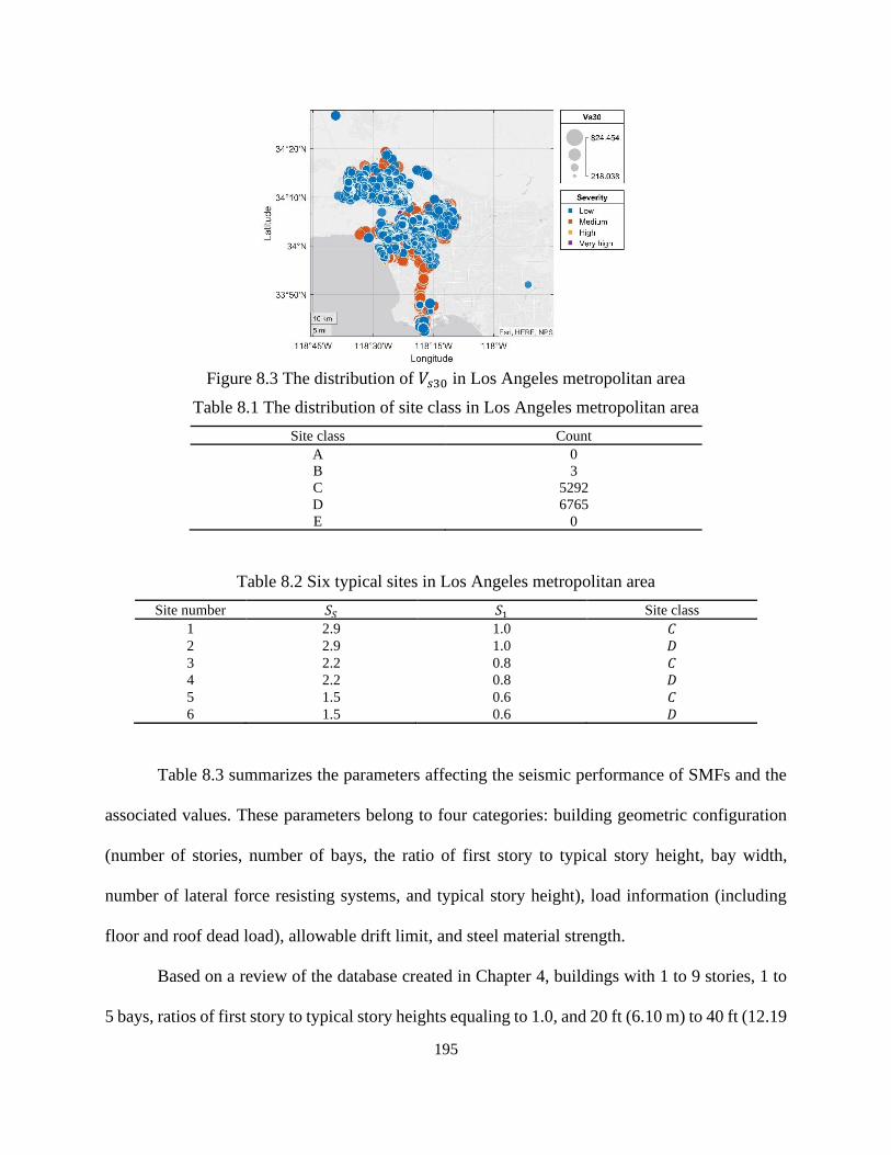
195

Figure 8.3 The distribution of 𝑉𝑠30 in Los Angeles metropolitan area

Table 8.1 The distribution of site class in Los Angeles metropolitan area

Site class Count

A 0

B 3

C 5292

D 6765

E 0

Table 8.2 Six typical sites in Los Angeles metropolitan area

Site number 𝑆𝑆 𝑆1 Site class

1 2.9 1.0 𝐶

2 2.9 1.0 𝐷

3 2.2 0.8 𝐶

4 2.2 0.8 𝐷

5 1.5 0.6 𝐶

6 1.5 0.6 𝐷

Table 8.3 summarizes the parameters affecting the seismic performance of SMFs and the

associated values. These parameters belong to four categories: building geometric configuration

(number of stories, number of bays, the ratio of first story to typical story height, bay width,

number of lateral force resisting systems, and typical story height), load information (including

floor and roof dead load), allowable drift limit, and steel material strength.

Based on a review of the database created in Chapter 4, buildings with 1 to 9 stories, 1 to

5 bays, ratios of first story to typical story heights equaling to 1.0, and 20 ft (6.10 m) to 40 ft (12.19

196

m) bay widths are considered. The number of SMRFs in each principal direction is fixed to two,

which is consistent with typical U.S. practice. The floor dead load is taken as 80 psf (2.39 kN/m2)

and the roof dead load is set as 67.5 psf (2.39 kN/m2). The allowable drift limit is taken as 2%,

which is the default value specified in Table 12.12-1 of ASCE 7-16 [30]. The yield stress for steel

is 50 ksi (345 MPa), which is commonly adopted in United States practice. Based on the

information summarized in Table 8.2 and Table 8.3, considering every combination of the

considered parameter values would result in a total of 594 cases (including 99 archetypical

buildings located at 6 sites).

Table 8.3 Parameters considered in developing the SMF archetypes and their associated ranges

Category Parameters Values considered in archetype design Space

Geometric

configuration

Number of stories (𝑁𝑠) 1, 3, 5, 7, and 9

Number of bays (𝑁𝑏) 1, 3, and 5

First story/typical story height

(ℎ1 ℎ𝑡⁄ ) 1.0

Bay width (𝑊𝑏) 20 ft (6.10 m), 30 ft (9.14 m), and 40 ft (12.19 m)

Number of LFRS’s (𝑁𝐿) Two in principal direction

Typical story height (ℎ𝑡) 13 ft (3.96 m)

Load information

Floor dead load (𝐷𝐿𝑓𝑙𝑜𝑜𝑟) 80 psf (3.83 kN/m2)

Roof dead load (𝐷𝐿𝑟𝑜𝑜𝑓) 67.5 psf (3.23 kN/m2)

Floor live load (L𝐿𝑓𝑙𝑜𝑜𝑟) 50 psf (2.39 kN/m2)

Roof live load (𝐿𝐿𝑟𝑜𝑜𝑓) 20 psf (0.96 kN/m2)

Design conservatism Allowable drift limit (𝜃) 2%

R 8, 9, 10

Steel strength Yield stress (𝐹𝑦) 50 ksi (345 MPa)

Each of the archetype is designed using the AutoSDA platform (as introduced in Chapter

3) and the design story drift profile for one-story, three-story, five-story, seven-story, and nine-

story buildings are presented in Figure 8.4. The median of the design story drifts for all buildings

are approximately uniformly distributed along the building height and within the code limit,

indicating the safety of the designs. To further examine the uniformity of drift distribution, the

197

drift concentration factor (which is defined as the ratio of the maximum story drift to the average

story drift over the building height) for each design is computed and visualized in Figure 8.4. More

than 90% of the DCFs are less than 1.1, which again demonstrates that the design drift is uniformly

distributed along the building height.

(a)

(b)

(c)

198

(d)

(e)

Figure 8.4 Visualizing the design story drifts for the SMRFs designed using R = 8: (a) one-story,

(b) three-story, (c) five-story, (d) seven-story, and (e) nine-story buildings

(a)

(b)

Figure 8.5 Distribution of drift concentration factors for all SMRFs: (a) boxplots for buildings

with different number of stories and (b) histogram of drift concentration factors

8.3.3 Nonlinear Model Development

Two-dimensional structural model for each archetype building realization is constructed in

OpenSees [2]. The modeling details are introduced in Chapter 2.

199

8.3.4 Characterize the Uncertainty

Four sources of uncertainty are considered in the collapse assessment process.

(1) Record-to-record uncertainty (𝛽𝑅𝑇𝑅): it is due to the variability in the response of the

index archetypes to different ground motions. This variability is caused by a combined effect of

variation in frequency content and dynamic characteristics of different records and variation in the

hazard characterization [6]. According to FEMA P695, the uncertainty of the 22-pair far-field

ground motion set is assumed to be 0.40 for the structural systems with significant period

elongation. This assumption holds for SMRFs as they are capable of providing significant inelastic

deformation capacity through flexural yielding at beam ends and limited yielding in panel zones.

(2) Design requirements uncertainty (𝛽𝐷𝑅): it is relevant to the completeness and robustness

of the design requirement and the extent to which they provide safeguards against unanticipated

failure modes. Since the design provision for SMRFs evolves over past decades by including the

lessons learned from major earthquakes (e.g., Northridge earthquake), the design requirements are

categorized as “(A) Superior” in Section 3.4 of FEMA P695 [6] and thus the associated uncertainty

is 0.10. This value is also consistent with the suggestion made by Zareian et al. [46].

(3) Test data uncertainty (𝛽𝑇𝐷): it is related to the completeness and robustness of the test

data used to define the structural system. Based on the guidelines of Section 3.6 of FEMA P695,

the test data quality is rated as “(B) Good” since there is a shortage of data for the deep columns

subjected to high axial forces and cyclic bending moments. Moreover, more experiments are

required to quantify the influence of concrete slab on the beam strength and stiffness. Based on

the rating, the test data uncertainty is 0.20.

(4) Modeling uncertainty 𝛽𝑀𝐷𝐿: it is associated to how well the index archetype models

represent the full range of structural response characteristics and how well the nonlinear analysis

200

can capture the collapse behavior through direct simulation or non-simulated component checks.

Based on existing observations from earthquakes, the primary failure mode for SMRFs is the

flexural hinging leading to sideway collapse, which is well captured by the modeling approach

(i.e., concentrated plasticity model) adopted in the current study. Meanwhile, the archetype design

space in this study covers a wide range of configurations. Based on these considerations, the

modeling quality is categorized “(A) Superior” and the associated uncertainty is 0.10.

The total system uncertainty (𝛽𝑇𝑂𝑇) is calculated using Equation (8.1) and the result is

0.469. According to Section 7.3 of FEMA P695, 𝛽𝑇𝑂𝑇 should be rounded to the nearest 0.025 and

thus the final total system uncertainty should be 0.475. This value is later used to determine the

acceptable threshold of adjusted collapse margin ratio (ACMR).

2 2 2 2

TOT RTR DR TD MDL = + + + (8.1)

8.3.5 Quantify the Margin of Safety Against Collapse

The dynamic performance of the archetype is assessed using truncated incremental

dynamic analysis (IDA) [61]. The set of 44 (22 pairs) far-field ground motion records specified in

FEMA P695 [4] are used. The magnitude for these records varies from M6.5 to M7.6 with an

average of M7.0. Thirty-two (16 pairs) of the ground motions were recorded at sites classified as

site class 𝐷 and the remaining records are from site class 𝐶 locations. The peak ground

acceleration for the record set varies from 0.21g to 0.82g with an average of 0.43g. More detailed

information about the ground motion records can be found in Appendix A of FEMA P695. The

scaling for the truncated IDAs is performed such that the median spectral acceleration of the

record-set matches the target intensity levels, which ranges from 25% to 250% of the spectral

acceleration corresponding to the maximum considered earthquake (𝑆𝑎𝑀𝐶𝐸)

The truncated results are used to generate a collapse fragility, where a lognormal

201

distribution function is used to fit the simulation data via the maximum likelihood method. The

collapse margin ratio (CMR), which is defined as the ratio of the median collapse spectral

acceleration to 𝑆𝑎𝑀𝐶𝐸, is computed based on the collapse fragility. Then CMR is further adjusted

by multiplying with a spectral shape factor, which then becomes adjusted collapse margin ratio

(ACMR). The histogram of ACMRs for SMRFs designed with different R factors is shown in

Figure 8.6. While more than 80% of ACMRs are greater than 2.0, there is still 10% of ACMRs

that are relatively small (less than 1.5). A more rigorous evaluation on ACMRs is performed in the

following section.

(a)

(b)

(c)

Figure 8.6 The histogram of ACMRs for (a) R = 8, (b) R = 9, and (c) R = 10

202

8.3.6 Performance Evaluation

The building performance is evaluated by comparing the ACMR of the structure with an

acceptable ACMR, which is determined based on the value of total system uncertainty (as described

in Section 8.3.4). According to Table 7-3 of FEMA P695 [6], the acceptable values of ACMR with

acceptable collapse probability of 10% (𝐴𝐶𝑀𝑅10%) and 20% (𝐴𝐶𝑀𝑅20%) are 1.84 and 1.49,

respectively. Acceptable performance is achieved if the following criteria is met:

(1) The average value of ACMRs for each performance group exceeds 𝐴𝐶𝑀𝑅10%.

(2) The individual value of ACMR for each index archetype within a performance group

exceeds 𝐴𝐶𝑀𝑅20%.

As shown in Figure 8.6, there is about 10% of design cases that is less than 𝐴𝐶𝑀𝑅20%

across R factors. This suggests that a small portion of the designs complied with the current

building code and design standards still fail to pass the acceptability check specified by FEMA

P695. To further examine the effect of different design variables on ACMRs, the buildings are

lumped into different groups based on their number of stories, bay widths, number of bays, and

site conditions and the distributions of ACMRs of different groups are shown in Figure 8.7 to

Figure 8.10. Figure 8.7 shows a trend that the ACMR decreases as the number of stories increase,

indicating that the collapse resistance decreases with building height. This observation is consistent

with the findings reported by Zareian et al. [46]. Moreover, while all building groups have an

average value exceeding 𝐴𝐶𝑀𝑅10%, the buildings with three to nine stories fail to meet the second

performance criterion. Figure 8.8 indicates that increasing the bay width does not affect the median

of the collapse resistance but increase the dispersion a bit. The observation in Figure 8.9 indicates

that when R = 8, the collapse resistance decreases with the number of bays. However, the ACMR

does not vary with the number of bays when R = 9 and 10..Figure 8.10 reveals that the seismicity

203

does not affect the distribution of ACMR in all cases. The phenomenon in Figure 8.11 indicates

that as R factor increases, the median of ACMR drops a bit from 2.5 to 2.25.

To summarize, while most of the archetype buildings’ ACMRs are higher than the

acceptable threshold, there is still 10% of the designs failing to meet the threshold of 𝐴𝐶𝑀𝑅10%.

This finding should raise the awareness and cautiousness of engineers when designing SMRFs

located at high seismicity regions (e.g., Los Angeles metropolitan area).

(a)

(b)

(c)

Figure 8.7 The distribution of ACMRs for buildings with different number of stories: (a) R = 8,

(b) R = 9, and (c) R = 10

204

(a)

(b)

(c)

Figure 8.8 The distribution of ACMRs for buildings with different bay width: (a) R = 8, (b) R =

9, and (c) R = 10

205

(a)

(b)

(c)

Figure 8.9 The distribution of ACMRs for buildings with different number of bays: (a) R = 8, (b)

R = 9, and (c) R = 10

206

(a)

(b)

(c)

Low seismic intensity: Ss = 1.5 g, S1 = 0.6 g

Medium seismic intensity: Ss = 2.2 g, S1 = 0.8 g

High seismic intensity: Ss = 2.9 g, S1 = 1.0 g

Figure 8.10 The distribution of ACMRs for buildings located in different seismicity region: (a) R

= 8, (b) R = 9, and (c) R = 10

207

Figure 8.11 The distribution of ACMRs for buildings designed with different R factors

8.4 Summary

This chapter evaluates the collapse performance of steel special moment frames by

applying FEMA P695 methodology. Archetype designs comprise 594 SMFs that are designed with

different number of stories, number of bays, bay widths, R factors, and site parameters. Nonlinear

models are constructed and analyzed under 44 ground motions to predict the collapse resistance of

each archetype design. The adjusted collapse margin ratios (ACMRs) of different building groups

are compared and the following conclusions are drawn: (1) The collapse resistance decreases with

building height. (2) Increasing the bay width does not affect the median of ACMRs but increases

the dispersion a bit. (3) When R = 8, the collapse resistance decreases with the number of bays.

However, the ACMR does not vary with the number of bays when R = 9 and 10. (4) The seismicity

does not affect the ACMR. (5) When R increases from 8 to 10, the ACMR only drop a bit from

2.5 to 2.25. (6) while most of the archetype buildings’ ACMRs are higher than the acceptable

threshold, there is still 10% of the designs failing to meet the threshold of 𝐴𝐶𝑀𝑅10%. This finding

should raise the awareness and cautiousness of engineers when designing SMRFs located at high

seismicity regions (e.g., Los Angeles metropolitan area).

208

9. Summary, Conclusions and Future Research Needs

9.1 Overview

This study aims to develop and apply the performance-based analytics-driven seismic

design methodology to steel moment resisting frame buildings. The body of work includes seismic

design automation, archetype design database construction, extensive nonlinear structural

analyses, and rapid characterization for the probabilistic distribution of seismic responses and

impacts. The research findings can be viewed as a complement to the current performance-based

earthquake engineering framework to facilitate its application in practice. The specific issues that

addressed include

1. Examining the advantages and limitations of different modeling techniques for steel

moment resisting frames and determining the optimal one that strikes a balance between the

reliability of analysis results and computational expense (Chapter 2).

2. Creating a framework and computational platform for automating seismic design,

structural response simulation, seismic impact assessment, and performance criteria evaluation for

steel moment frame buildings (Chapter 3).

3. Creating a comprehensive database that could potentially be used to evaluate the

performance of existing methods and develop data-driven and hybrid (combination of mechanics-

based + data-driven) models for estimating seismic structural responses (Chapter 4).

4. Investigating the difference in seismic performance between the self-centering moment

resisting frame using post-tensioned connections and the conventional moment resisting frames

using reduced-beam section connections (Chapter 5).

5. Formulating a framework for developing hybrid and/or data-driven models for

estimating building structural response demands under extreme loading and applying it to predict

209

the seismic drift demands in steel moment resisting frames (Chapter 6).

6. Proposing a set of parametric and non-parametric surrogate models for estimating the

median SMRF engineering demand parameters (including peak story drifts, peak floor

accelerations, and residual story drifts) (Chapter 7).

7. Performing a systematic study to quantify the influence of various design variables on

the collapse resistance of steel moment resisting frames located in Los Angeles metropolitan area

(Chapter 8).

9.2 Findings and Conclusions

The key findings from Chapters 2 to 8 are summarized in this section.

9.2.1 Chapter 2 Nonlinear Modeling and Analysis Methodology of Steel Moment Resisting

Frames

This chapter provides an in-depth literature review that summarizes the recent advances in

structural modeling of steel moment resisting frames. Different models, including concentrated

plasticity, finite length plastic hinge, distributed plasticity, and continuum finite-element models,

are critically examined to reveal their advantages and limitations. Based on the examination, the

concentrated plasticity model is found to strike a balance between the reliability of the analysis

results and computational expense. Consequently, it is consistently adopted throughout the entire

study.

9.2.2 Chapter 3 Python-Based Computational Platform to Automate Seismic Design,

Nonlinear Structural Model Construction and Analysis of Steel Moment Resisting Frames

This chapter presents a Python-based platform that automates the seismic design, nonlinear

structural model generation, and response simulation of steel special moment resisting frames

(SMRFs). The first module of the automatic seismic analysis and design (AutoSDA) platform

210

takes building configuration, loads, and site parameters as input and outputs SMRF designs that

comply with the latest building code provisions while accounting for ease of construction. A

second module constructs two-dimensional nonlinear structural models in OpenSees based on the

generated designs and performs nonlinear static and dynamic analyses towards a comprehensive

evaluation of seismic performance. The efficiency, reliability, and accuracy of the AutoSDA

platform are demonstrated using several illustrative examples. The adopted object orientated

programming structure makes the platform easily adaptable. Potential future enhancements

include the use of alternative strategies to account for beam-column material nonlinearity, 3D

modeling and economic loss assessment. The broad implication of the AutoSDA platform is a

drastic reduction in the time and effort involved in performance-based seismic design. Moreover,

it can be used to develop a database of archetype steel moment frame buildings (as introduced in

Chapter 4) towards the development of analytics-driven design methodologies. It is worth noting

that the development details (e.g., platform structure and algorithm) documented in this chapter

can be used to create similar platforms for other types of structural systems. A key limitation of

the current version of the AutoSDA platform is that it only allows the design of SMRFs using the

ELF method. This limitation can be addressed by adding a feature that generates designs using the

results from response spectrum and/or response history analyses. Some other limitations include

the lack of column splice and foundation design, and the absence of a graphical user interface, all

of which could be easily incorporated in future versions. This platform has been implemented as

a part of EE-UQ framework developed as part of the National Science Foundation Natural Hazards

Engineering Research Infrastructure (NHERI) SimCenter.

211

9.2.3 Chapter 4 A Database of Seismic Design, Nonlinear Models, and Seismic Responses

for SMRF Buildings

The database introduced in this chapter was created using the archetype concept, which

groups buildings with similar geometric configurations and/or structural properties into

representative sets, resulting in generalized performance predictions for a full class of buildings

[74]. The values of the parameters considered in the archetype design space are determined based

on the standard of structural engineering practice. As a result, the database is representative of

actual SMRFs located in high seismicity zones. In addition, practitioners from Englekirk Structural

Engineers (https://www.englekirk.com) have been involved in the development of the database,

which ensures that the designs are realistic. All datasets are stored as .csv files, which could be

retrieved based on a specific building ID. This allows the user/program to easily access the data.

The database [54] has been made publicly available through the DesignSafe cyberinfrastructure.

The database could potentially be utilized for a wide range of purposes. For example, it

could be used to identify the influence of various design parameters on the seismic performance

of SMRFs (as presented in Chapter 8), assess the accuracy and reliability of existing seismic

demand prediction approaches (as introduced in Chapter 6), develop data-driven models for

predicting seismic demands (as described in Chapter 7), and formulate methods to explore optimal

designs based on a predefined set of constraints.

9.2.4 Chapter 5 Comparative Study for Steel Moment Resisting Frames Using Post-

Tensioned and Reduced-Beam Section Connections

In this chapter, a comparative assessment of the seismic performance and economic losses

for a self-centering moment resisting frame (SC-MRF) and reduced beam section (RBS) welded

moment resisting frame (WMRF) is presented, where the SC-MRF and WMRF have identical

beam and column sizes. First, a reliable phenomenological model for the PT beam-column

212

connections with top-and-seat angles is developed and verified against past experimental results.

A prototype building, which has SC-MRFs as its lateral force resisting system, is selected. Using

the developed phenomenological model, the entire frame is modeled in OpenSees. Nonlinear static

and response history analyses are subsequently performed to study the response of the frame

models. The pushover analysis results indicate that the strength of the SC-MRF is 40% lower than

that of the WMRF. The dynamic analysis results show that the WMRF has higher collapse

resistance, whereas the SC-MRF undergoes smaller residual drifts. However, it is worth noting

that the collapse resistance of both frames is within the permissible values of acceptable collapse

margin ratio of the FEMA P695 guidelines. Finally, the economic seismic losses for the SC-MRF

and WMRF buildings are assessed using the FEMA P-58 methodology, which accounts for the

influence of residual drift and the repair costs of structural and nonstructural components. The

results reveal that the expected annual loss for the SC-MRF building is 21% higher than that for

the WMRF building. More specifically, the SC-MRF building has a lower expected loss associated

with demolition, but higher losses associated with collapse.

9.2.5 Chapter 6 Seismic Drift Demand Estimation for SMRF Buildings: from Mechanics-

Based to Data-Driven Models

A spectrum of simplified methods for estimating seismic drift demands is presented and

evaluated. On one end of the spectrum are fully mechanics-based approaches that are derived

solely based on engineering principles. On the other end are purely data-driven models that are

established by applying statistical and machine learning methods to a parametric dataset of drift

demands generated from nonlinear response history analyses (NRHAs). Between these two

extremes, there are hybrid methods that integrate both fundamental mechanics and

statistical/machine learning techniques. Four existing methods that fall within this spectrum of

213

approaches are reviewed, and their benefits and drawbacks are discussed. They are based on shear

and flexural beam theory, an elastoplastic single-degree-of-freedom system with known yield

strength (PSKY), statistically adjusted spectral displacement, and the statistically adjusted

response of a linear elastic multi-degree-of-freedom system with known yield strength (EMKY).

A framework for developing hybrid and/or data-driven models to estimate structural

responses under extreme events is established. A systematic step-to-step procedure is presented

that is agnostic to the type of demand parameter (e.g., story drifts and floor accelerations) and

lateral-force resisting system being considered. Meanwhile, the advantages and limitations of

different metrics used for evaluating model performance are discussed and a new metric 𝐷𝑋%

(defined as the fraction of the dataset whose relative difference does not exceed 𝑋%) is proposed.

The framework is then used to develop purely data-driven and hybrid models for estimating

seismic drift demands in steel special moment resisting frames (SMRFs). These two models are

described as (i) machine learning based and purely data-driven (MLDD) and (ii) machine learning

based adjusted response of an EMKY (ML-EMKY). Both are formulated based on a dataset of

seismic structural responses from 621 modern code-based SMRF designs subjected to 240 ground

motions. During the model development process, the sensitivity of the model performance to 35

potential predictor variables is investigated. For the hybrid model, the floor height ratio (defined

as the ratio of the height of floor 𝑖 to the total building height) and intensity measures (𝑆𝑎(𝑇) and

𝑆𝑑(𝑇1)) are the two most influential types of predictors, whereas, in the purely data-driven model,

the intensity measure 𝑆𝑎(𝑇1) alone dominates the response estimation.

Finally, a comparative assessment of the predictive performance among the existing and

newly developed models is performed. More specifically, previously developed PSKY and

statistically adjusted EMKY models and newly developed MLDD and ML-EMKY models, are

214

evaluated on a testing dataset including the responses of 100 SMRFs subjected to three sets of site-

specific ground motions selected based on the service-level earthquake (SLE), design-based

earthquake (DBE), and maximum considered earthquake (MCE) levels. The evaluation results

suggest that the hybrid model generally has a higher accuracy than the purely data-driven or

mechanics-based models. A comparison of the level of the effort required to apply the different

models reveals that the mechanics-based model (PSKY) requires the greatest effort whereas the

reduced-order MLDD model needs the least effort. The latter could be applied during the

preliminary design stage.

9.2.6 Chapter 7 Surrogate Models for Probabilistic Distribution of Engineering Demand

Parameters of SMRF Buildings under Earthquakes

A set of parametric and non-parametric surrogate models are developed to estimate the

median engineering demand parameters (EDPs) (including peak story drifts, peak floor

accelerations, and residual story drifts) from nonlinear response history analysis (NRHA). These

models are constructed using a data-driven approach based on a comprehensive database that

includes 621 steel moment resisting frames (SMRFs) and their seismic responses. The

performance of the proposed surrogate models on the training and validation datasets indicates

that they are well-suited to capturing the relationship between the predictors and the EDPs. The

predictive performance of these models is further evaluated against a testing dataset that includes

the response of 100 SMRFs subjected to three groups of site-specific ground motions. A


recommended by FEMA P-58 is conducted to evaluate the predictive performance of the proposed

surrogate models. Additionally, the terms in the covariance matrix are quantitatively investigated

and the suggested values for each term are provided. Finally, the EDPs generated using the

215

surrogate model and the assumed covariance matrix are used to calculate the economic loss for

100 SMRF buildings and further compared with the loss computed using the NRHA-based EDPs.

The comparison indicates that the surrogate-based EDPs yield reasonable estimates of the

economic loss relative to the EDPs generated from NRHA.

9.2.7 Chapter 8 Effect of Different Design Variables on Seismic Collapse Performance of

Steel Special Moment Frames

This chapter evaluates the collapse performance of steel special moment frames by

applying FEMA P695 methodology. Archetype designs for 135 SMRFs with different number of

stories, number of bays, bay widths, R factors, and site parameters, are developed. Nonlinear

models are constructed and analyzed using the 44 FEMA P695 ground motions to predict the

collapse resistance of each archetype design. The adjusted collapse margin ratios (ACMRs) of

different building groups are compared and the following conclusions are drawn: (1) The collapse

resistance decreases with building height. (2) Increasing the bay width does not affect the median

of ACMRs but increases the dispersion a bit. (3) When R = 8, the collapse resistance decreases

with the number of bays. However, the ACMR does not vary with the number of bays when R =

9 and 10. (4) The seismicity does not affect the ACMR. (5) When R increases from 8 to 10, the

ACMR only drop a bit from 2.5 to 2.25. (6) while most of the archetype buildings’ ACMRs are

higher than the acceptable threshold, there is still 10% of the designs failing to meet the threshold

of 𝐴𝐶𝑀𝑅10% . This finding should raise the awareness and cautiousness of engineers when

designing SMRFs located at high seismicity regions (e.g., Los Angeles metropolitan area).

9.3 Limitations and Future Work

The limitations and possible future extensions of the current body of work are as follows:

1. As mentioned in Chapter 2, the concentrated plasticity model was adopted throughout

216

the current study to simulate the inelastic behavior of beam and column components in steel

moment resisting frames and Rayleigh damping model is used in the dynamic analysis.

Consequently, all the findings reported here all are based on the aforementioned modeling strategy.

To improve the robustness of reported findings, various modeling techniques (such as elements

with fiber sections or finite length plastic hinge models) could be utilized and the corresponding

analysis results could be compared with the results presented.

2. As introduced in Chapter 3, the automated seismic design and analysis (AutoSDA)

platform does not incorporate design based on the response spectrum analysis. Additionally, its

current version does not address torsional irregularity or other 3-dimensional effects. Potential

enhancements include the incorporation alternative design methods and 3D modeling. In this case,

the database (Chapter 4) created using the AutoSDA platform could be used to investigate the

influence of different design methods and 3D-related issues on the collapse performance of steel

moment resisting frames.

3. The archetype designs introduced in Chapter 4 are generated using a “brute-force”

approach that considers every possible combination of the considered parameter values. This

approach yields an excessively large number of archetype designs, which increase the

computational expense required to analyze each design. A future enhancement includes using the

smart sampling method to generate the design space and thus reduces the required number of

sampling points.

4. One promising extension of current work is to use data-driven approaches to construct a

surrogate model that links the building variables to the earthquake-induced economic loss. Then a

cost-benefit analysis could be performed to determine the optimized design space for a specific

design condition. Generating the design within this optimized design space would achieve the most

217

desirable overall performance outcome considering multiple objectives.

5. This entire study focused on a single type of lateral force resisting systems. As a possible

extension, a generalized seismic response prediction model could be developed for various

building structural systems (including but not limited to reinforced concrete frames, shear walls,

and dual systems). Such a generalized model enables the decision maker to conduct rapid

assessment on city-scale response during and after earthquakes and thus better direct the resources

required for building earthquake-resilient communities.

218

10. Reference

[1] FEMA. Guidelines for performance-based seismic design of buildings. Redwood City, CA:

Applied Technology Council; 2018.

[2] McKenna F, Fenves GL, Scott MH, others. Open system for earthquake engineering

simulation. University of California, Berkeley, CA 2000.

[3] Haselton Baker Risk Group. Seismic Performance Prediction Program. 2017.

[4] FEMA. Seismic performance assessment of buildings. Redwood City, CA: Applied

Technology Council; 2012.

[5] Burton H. A framework for performance-based analytics driven design. 11th National

Conference in Earthquake Engineering, Los Angeles, California, USA: 2018.

[6] FEMA. Quantification of building seismic performance factors. Redwood City, CA: Applied

Technology Council; 2009.

[7] Elkady A, Lignos DG. Analytical investigation of the cyclic behavior and plastic hinge

formation in deep wide-flange steel beam-columns. Bulletin of Earthquake Engineering

2015;13:1097–118.

[8] Khandelwal K, El-Tawil S. Collapse behavior of steel special moment resisting frame

connections. Journal of Structural Engineering 2007;133:646–55.

[9] Deierlein G, Reinhorn A, Willford M. NEHRP Seismic design technical brief No. 4-nonlinear

structural analysis for seismic design: a guide for practicing engineers. 2010.

[10] Bazant ZP, Bhat PD. Prediction of hysteresis of reinforced concrete members. ASCE J Struct

Div 1977;103:153–67.

[11] Neuenhofer A, Filippou FC. Evaluation of nonlinear frame finite-element models. Journal of

Structural Engineering 1997;123:958–66.

[12] Engelen RA, Geers MG, Baaijens FP. Nonlocal implicit gradient-enhanced elasto-plasticity

219

for the modelling of softening behaviour. International Journal of Plasticity 2003;19:403–33.

[13] Jirásek M, Rolshoven S. Comparison of integral-type nonlocal plasticity models for strain-

softening materials. International Journal of Engineering Science 2003;41:1553–602.

[14] Bažant ZP, Jirásek M. Nonlocal integral formulations of plasticity and damage: survey of

progress. Journal of Engineering Mechanics 2002;128:1119–49.

[15] Ribeiro FL, Barbosa AR, Scott MH, Neves LC. Deterioration modeling of steel moment

resisting frames using finite-length plastic hinge force-based beam-column elements. Journal

of Structural Engineering 2014;141:04014112.

[16] Kolwankar S, Kanvinde A, Kenawy M, Lignos D, Kunnath S. Simulating local buckling-

induced softening in steel members using an equivalent nonlocal material model in

displacement-based fiber elements. Journal of Structural Engineering 2018;144:04018192.

[17] Clough RW. Effect of stiffness degradation on earthquake ductility requirements.

Proceedings of Japan earthquake engineering symposium, 1966.

[18] Giberson MF. The response of nonlinear multi-story structures subjected to earthquake

excitation 1967.

[19] Takeda T, Sozen MA, Nielsen NN. Reinforced concrete response to simulated earthquakes.

Journal of the Structural Division 1970;96:2557–73.

[20] Ramberg W, Osgood WR. Description of stress-strain curves by three parameters 1943.

[21] Ibarra LF, Medina RA, Krawinkler H. Hysteretic models that incorporate strength and

stiffness deterioration. Earthquake Engineering & Structural Dynamics 2005;34:1489–511.

[22] Ibarra LF, Krawinkler H. Global collapse of frame structures under seismic excitations.

Pacific Earthquake Engineering Research Center Berkeley, CA; 2005.

[23] Lignos D. Sidesway collapse of deteriorating structural systems under seismic excitations.

Doctoral dissertation. Stanford University, 2008.

220

[24] Lignos DG, Krawinkler H. Deterioration modeling of steel components in support of collapse

prediction of steel moment frames under earthquake loading. Journal of Structural

Engineering 2010;137:1291–302.

[25] Lignos DG, Hartloper AR, Elkady A, Deierlein GG, Hamburger R. Proposed updates to the

ASCE 41 nonlinear modeling parameters for wide-flange steel columns in support of

performance-based seismic engineering. Journal of Structural Engineering

2019;145:04019083.

[26] Hwang S-H, Lignos DG. Earthquake-induced loss assessment of steel frame buildings with

special moment frames designed in highly seismic regions. Earthquake Engineering &

Structural Dynamics 2017;46:2141–62.

[27] Krawinkler H. Shear in beam-column joints in seismic design of steel frames. Engineering

Journal 1978;15.

[28] Gupta A, Krawinkler H. Seismic demands for the performance evaluation of steel moment

resisting frame structures. PhD Thesis. Stanford University, 1998.

[29] Zareian F, Medina RA. A practical method for proper modeling of structural damping in

inelastic plane structural systems. Computers & Structures 2010;88:45–53.

[30] ASCE 7-16. Minimum design loads and associated criteria for buildings and other structures.

Reston, VA: 2016.

[31] Hamburger RO, Malley JO. Seismic design of steel special moment frames. NIST GCR

2009:09–917.

[32] Lignos DG, Krawinkler H. A steel database for component deterioration of tubular hollow

square steel columns under varying axial load for collapse assessment of steel structures

under earthquakes. Proc. 7th Int. Conf. on Urban Earthquake Engineering (7CUEE), Center

for Urban Earthquake Engineering, Tokyo Institute of Technology Tokyo; 2010.

[33] Flores FX, Charney FA, Lopez-Garcia D. Influence of the gravity framing system on the

collapse performance of special steel moment frames. Journal of Constructional Steel

221

Research 2014;101:351–62.

[34] Elkady A, Lignos DG. Effect of gravity framing on the overstrength and collapse capacity of

steel frame buildings with perimeter special moment frames. Earthquake Engineering &


[35] Dimopoulos AI, Karavasilis TL, Vasdravellis G, Uy B. Seismic design, modelling and

assessment of self-centering steel frames using post-tensioned connections with web

hourglass shape pins. Bulletin of Earthquake Engineering 2013;11:1797–816.

https://doi.org/10.1007/s10518-013-9437-4.

[36] Dimopoulos AI, Tzimas AS, Karavasilis TL, Vamvatsikos D. Probabilistic economic seismic

loss estimation in steel buildings using post-tensioned moment-resisting frames and viscous

dampers. Earthquake Engineering & Structural Dynamics 2016;45:1725–41.

https://doi.org/10.1002/eqe.2722.

[37] Fang C, Yam MCH, Lam ACC, Xie L. Cyclic performance of extended end-plate connections

equipped with shape memory alloy bolts. Journal of Constructional Steel Research

2014;94:122–36. https://doi.org/10.1016/j.jcsr.2013.11.008.

[38] Moradi S, Alam MS. Feasibility study of utilizing superelastic shape memory alloy plates in

steel beam–column connections for improved seismic performance. Journal of Intelligent

Material Systems and Structures 2015;26:463–75.

[39] Ramirez CM, Miranda E. Significance of residual drifts in building earthquake loss

estimation. Earthquake Engineering & Structural Dynamics 2012;41:1477–93.

https://doi.org/10.1002/eqe.2217.

[40] Tzimas A, Kamaris G, Karavasilis T, Galasso C. Collapse risk and residual drift performance

of steel buildings using post-tensioned MRFs and viscous dampers in near-fault regions.

Bulletin of Earthquake Engineering 2016;14:1643–62.

[41] Haselton CB. Assessing seismic collapse safety of modern reinforced concrete moment frame

buildings. PhD Thesis. Stanford University, 2006.

222

[42] Liel AB, Deierlein GG. Assessing the collapse risk of California’s existing reinforced

concrete frame structures: metrics for seismic safety decisions. vol. 69. 2008.

[43] Haselton CB, Liel AB, Deierlein GG, Dean BS, Chou JH. Seismic collapse safety of

reinforced concrete buildings. I: Assessment of ductile moment frames. Journal of Structural

Engineering 2010;137:481–91.

[44] Liel AB, Haselton CB, Deierlein GG. Seismic collapse safety of reinforced concrete

buildings. II: Comparative assessment of nonductile and ductile moment frames. Journal of


[45] Deierlein GG, Liel AB, Haselton CB, Kircher CA. ATC 63 methodology for evaluating

seismic collapse safety of archetype buildings. Structures Congress 2008: Crossing Borders,

2008, p. 1–10.

[46] Zareian F, Lignos D, Krawinkler H. Evaluation of seismic collapse performance of steel

special moment resisting frames using FEMA P695 (ATC-63) methodology. Structures

Congress 2010, 2010, p. 1275–86.

[47] Morfidis K, Kostinakis K. Seismic parameters’ combinations for the optimum prediction of

the damage state of R/C buildings using neural networks. Advances in Engineering Software

2017;106:1–16.

[48] FEMA P-2012. Assessing seismic performance of buildings with configuration irregularities.

Redwood City, CA: Applied Technology Council; 2018.

[49] Khoshnoudian F, Mehrparvar B, others. Evaluation of IBC equivalent lateral response

procedure for seismic isolated structures. Australian Structural Engineering Conference 2005,

Engineers Australia; 2005, p. 992.

[50] Whittaker AS, Constantinou MC, Ramirez OM, Johnson MW, Chrysostomou CZ. Equivalent

lateral force and modal analysis procedures of the 2000 NEHRP Provisions for buildings with

damping systems. Earthquake Spectra 2003;19:959–80.

[51] Xu L, Grierson DE. Computer-automated design of semirigid steel frameworks. Journal of

223


[52] Moharrami H, Grierson DE. Computer-automated design of reinforced concrete frameworks.

Journal of Structural Engineering 1993;119:2036–58.

[53] Kavlie D, Moe J. Automated design of frame structures. Journal of the Structural Division

1971;97:33–62.

[54] Guan X, Burton H, Shokrabadi M. A Database of Seismic Designs, Nonlinear Models, and

Seismic Responses for Steel Moment Resisting Frame Buildings. DesignSafe-CI

Https://DoiOrg/1017603/Ds2-8yc7-1285 2020.

[55] Guan X, Burton H, Shokrabadi M. A database of seismic designs, nonlinear models, and

seismic responses for steel moment-resisting frame buildings. Earthquake Spectra

2020:8755293020971209.

[56] American Institute of Steel Construction (AISC). Seismic provisions for structural steel

buildings. ANSI/AISC 341-16. American Institute of Steel Construction: Chicago, IL 2016.

[57] American Institute of Steel Construction (AISC). Specification for structural steel buildings.

ANSI/AISC 360-16. American Institute of Steel Construction: Chicago, IL 2016.

[58] American Institute of Steel Construction (AISC). Prequalified connections for special and

intermediate steel moment frames for seismic applications. ANSI/AISC 358-16. American

Institute of Steel Construction: Chicago, IL 2016.

[59] Baker JW. Efficient analytical fragility function fitting using dynamic structural analysis.

Earthquake Spectra 2015;31:579–99.

[60] International Code Council. International building code 2003. International Code Council;

2002.

[61] Vamvatsikos D, Cornell CA. Incremental dynamic analysis. Earthquake Engineering &


224

[62] Ancheta TD, Darragh RB, Stewart JP, Seyhan E, Silva WJ, Chiou BS, et al. Peer NGA-West2

database 2013.

[63] Gupta A, Krawinkler H. Estimation of seismic drift demands for frame structures. Earthquake

Engineering & Structural Dynamics 2000;29:1287–305.

[64] Lin Y-Y, Miranda E. Estimation of maximum roof displacement demands in regular

multistory buildings. Journal of Engineering Mechanics 2009;136:1–11.

[65] Miranda E. Approximate seismic lateral deformation demands in multistory buildings.


[66] Miranda E, Reyes CJ. Approximate lateral drift demands in multistory buildings with

nonuniform stiffness. Journal of Structural Engineering 2002;128:840–9.

[67] Zhang R, Chen Z, Chen S, Zheng J, Büyüköztürk O, Sun H. Deep long short-term memory

networks for nonlinear structural seismic response prediction. Computers & Structures

2019;220:55–68.

[68] Elkady A, Lignos DG. Two-dimensional OpenSees numerical models for archetype steel

buildings with special moment frames 2019.

[69] Esteghamati MZ, Lee J, Musetich M, Flint MM. INSSEPT: An open-source relational

database of seismic performance estimation to aid with early design of buildings. Earthquake

Spectra 2020.

[70] Rathje EM, Dawson C, Padgett JE, Pinelli J-P, Stanzione D, Adair A, et al. DesignSafe: new

cyberinfrastructure for natural hazards engineering. Natural Hazards Review

2017;18:06017001.

[71] Miranda E. Inelastic displacement ratios for structures on firm sites. Journal of Structural

Engineering 2000;126:1150–9.

[72] Jayaram N, Lin T, Baker JW. A computationally efficient ground-motion selection algorithm

for matching a target response spectrum mean and variance. Earthquake Spectra

225

2011;27:797–815.

[73] Campbell KW, Bozorgnia Y. NGA-West2 Campbell-Bozorgnia ground motion model for

the horizontal components of PGA, PGV, and 5%-damped elastic pseudo-acceleration

response spectra for periods ranging from 0.01 to 10 sec. Pacific Earthquake Engineering

Research Center; 2013.

[74] Haselton CB, Deierlein GG. Assessing seismic collapse safety of modern reinforced concrete

moment-frame buildings. vol. 67. 2007.

[75] Ozkula G, Harris J, Uang C-M, Maison BF. Observations from cyclic tests on deep, wide-

flange beam-columns. Engineering Journal 2019;56:3–5.

[76] Christchurch rebuild to cost $10b more. Newshub 2017.

[77] Asgarian B, Moradi S. Seismic response of steel braced frames with shape memory alloy

braces. Journal of Constructional Steel Research 2011;67:65–74.

https://doi.org/10.1016/j.jcsr.2010.06.006.

[78] Miller DJ, Fahnestock LA, Eatherton MR. Development and experimental validation of a

nickel–titanium shape memory alloy self-centering buckling-restrained brace. Engineering

Structures 2012;40:288–98. https://doi.org/10.1016/j.engstruct.2012.02.037.

[79] Garlock MM, Ricles JM, Sause R. Experimental studies of full-scale posttensioned steel


https://doi.org/10.1061/(ASCE)0733-9445(2005)131:3(438).

[80] Ricles JM, Sause R, Peng SW, Lu LW. Experimental evaluation of earthquake resistant

posttensioned steel connections. Journal of Structural Engineering 2002;128:850–9.


[81] Christopoulos C, Filiatrault A, Uang C-M, Folz B. Posttensioned energy dissipating

connections for moment-resisting steel frames. Journal of Structural Engineering

2002;128:1111–20.

226

[82] Vasdravellis G, Karavasilis TL, Uy B. Finite element models and cyclic behavior of self-

centering steel post-tensioned connections with web hourglass pins. Engineering Structures

2013;52:1–16.

[83] Kim H-J, Christopoulos C. Numerical models and ductile ultimate deformation response of

post-tensioned self-centering moment connections. Earthquake Engineering & Structural

Dynamics 2009;38:1–21.

[84] Moradi S, Alam MS. Finite-element simulation of posttensioned steel connections with

bolted angles under cyclic loading. Journal of Structural Engineering 2015;142:04015075.

[85] Moradi S, Alam MS, Milani AS. Cyclic response sensitivity of post-tensioned steel

connections using sequential fractional factorial design. Journal of Constructional Steel

Research 2015;112:155–66.

[86] Rojas P, Ricles JM, Sause R. Seismic performance of post-tensioned steel moment resisting

frames with friction devices. Journal of Structural Engineering 2005;131:529–40.


[87] Porter KA, Kiremidjian AS, LeGrue JS. Assembly‐based vulnerability of buildings and its

use in performance evaluation. Earthquake Spectra 2001;17:291–312.

https://doi.org/10.1193/1.1586176.

[88] Deierlein G. Overview of a framework methodology for earthquake performance assessment.

Performance-Based Seismic Design: Concepts and Implementation, Bled, Slovenia: 2004, p.

15–26.

[89] Garlock MM, Sause R, Ricles JM. Behavior and design of posttensioned steel frame systems.


[90] Garlock MM, Ricles JM, Sause R. Influence of design parameters on seismic response of

post-tensioned steel MRF systems. Engineering Structures 2008;30:1037–47.

[91] Mazzoni S, McKenna F, Scott MH, Fenves GL. The open system for earthquake engineering

simulation (OpenSEES) user command-language manual 2006.

227

[92] Moradi S. Simulation, response sensitivity, and optimization of post-tensioned steel beam-

column connections. Doctoral dissertation. University of British Columbia, 2016.

[93] Moradi S, Alam MS. Lateral load–drift response and limit states of posttensioned steel beam-

column connections: parametric study. Journal of Structural Engineering

2017;143:04017044.

[94] Garlock MM, Ricles JM, Sause R. Cyclic load tests and analysis of bolted top-and-seat angle


[95] Kishi N, Chen W-F. Moment-rotation relations of semirigid connections with angles. Journal

of Structural Engineering 1990;116:1813–34.

[96] Lin YC, Sause R, Ricles JM. Seismic performance of steel self-centering, moment-resisting

frame: hybrid simulations under design basis earthquake. Journal of Structural Engineering

2013;139:1823–32.

[97] Ricles JM, Sause R, Garlock MM, Zhao C. Posttensioned seismic-resistant connections for

steel frames. Journal of Structural Engineering 2001;127:113–21.

[98] Fragiadakis M, Vamvatsikos D. Fast performance uncertainty estimation via pushover and

approximate IDA. Earthquake Engineering & Structural Dynamics 2010;39:683–703.

[99] Venture SJ, Committee GD, others. Recommended seismic design criteria for new steel

moment-frame buildings. Federal Emergency Management Agency; 2000.

[100] McCormick J, Aburano H, Ikenaga M, Nakashima M. Permissible residual deformation

levels for building structures considering both safety and human elements. Proceedings of

the 14th world conference on earthquake engineering, 2008, p. 12–7.

[101] Ahmadi O. Seismic collapse assessment of self-centering steel moment resisting frame

systems with web friction devices. Lehigh University; 2016.

[102] USGS. Unified Hazard Tool. Available at: https://earthquake.usgs.gov/hazards/interactive/.

228

[103] DeBock DJ, Liel AB. A comparative evaluation of probabilistic regional seismic loss

assessment methods using scenario case studies. Journal of Earthquake Engineering

2015;19:905–37.

[104] FEMA. Multi-hazard loss estimation methodology earthquake model: technical manual.

Washington DC: NIST 2003.

[105] Pagani M, Monelli D, Weatherill G, Danciu L, Crowley H, Silva V, et al. OpenQuake

engine: an open hazard (and risk) software for the global earthquake model. Seismological

Research Letters 2014;85:692–702.

[106] Morfidis K, Kostinakis K. Seismic parameters’ combinations for the optimum prediction

of the damage state of R/C buildings using neural networks. Advances in Engineering

Software 2017;106:1–16.

[107] Cook D, Wade K, Haselton C, Baker J, DeBock D. A structural response prediction engine

to support advanced seismic risk assessment. 11th National Conference in Earthquake

Engineering, Los Angeles, California, USA: 2018.

[108] Chopra AK. Dynamics of structures theory and applications to earthquake engineering.

1995.

[109] Huang Y-N, Whittaker A. Simplified analysis procedures for next-generation

performance-based seismic design. Applied Technology Council, Redwood City, CA; 2012.

[110] Bennett JO, Briggs WL, Badalamenti A. Using and understanding mathematics: A

quantitative reasoning approach. Pearson Addison Wesley Reading; 2008.

[111] Sun H, Burton H, Zhang Y, Wallace J. Interbuilding interpolation of peak seismic response

using spatially correlated demand parameters. Earthquake Engineering & Structural

Dynamics 2018;47:1148–68.

[112] International Code Council. International building code. International Code Council,

Inc(Formerly BOCA, ICBO and SBCCI) 2018;4051:60478–5795.

229

[113] Yan X, Su X. Linear regression analysis: theory and computing. World Scientific; 2009.

[114] Nadaraya EA. On estimating regression. Theory of Probability & Its Applications

1964;9:141–2.

[115] Ho TK. Random decision forests. Proceedings of 3rd international conference on document

analysis and recognition, vol. 1, IEEE; 1995, p. 278–82.

[116] Chen T, Guestrin C. Xgboost: A scalable tree boosting system. Proceedings of the 22nd

acm sigkdd international conference on knowledge discovery and data mining, 2016, p. 785–

94.

[117] McCulloch WS, Pitts W. A logical calculus of the ideas immanent in nervous activity. The

Bulletin of Mathematical Biophysics 1943;5:115–33.

[118] Efron B, Tibshirani RJ. An introduction to the bootstrap. CRC press; 1994.

[119] Breiman L. Random forests. Machine Learning 2001;45:5–32.

[120] Forrester AI, Keane AJ. Recent advances in surrogate-based optimization. Progress in

Aerospace Sciences 2009;45:50–79.

[121] Hussain MS, Javadi AA, Ahangar-Asr A, Farmani R. A surrogate model for simulation–

optimization of aquifer systems subjected to seawater intrusion. Journal of Hydrology

2015;523:542–54.

[122] Asher MJ, Croke BF, Jakeman AJ, Peeters LJ. A review of surrogate models and their

application to groundwater modeling. Water Resources Research 2015;51:5957–73.

[123] Xu Y, Lu X, Cetiner B, Taciroglu E. Real-time regional seismic damage assessment

framework based on long short-term memory neural network. Computer-Aided Civil and

Infrastructure Engineering 2020.

[124] Guan X, Burton H, Sabol T. Python-based computational platform to automate seismic

design, nonlinear structural model construction and analysis of steel moment resisting frames.

230

Engineering Structures 2020;224:111199.

[125] Guan X, Burton H, Shokrabadi M, Yi Z. Seismic drift demand estimation for SMRF

buildings: from mechanics-based to data-driven models. Journal of Structural Engineering

2021. https://doi.org/10.1061/(ASCE)ST.1943-541X.0003004. (Accepted for publication)

[126] Cormen TH, Leiserson CE, Rivest RL, Stein C. Introduction to algorithms. vol. 5. MIT

press Cambridge; 2001.

[127] Zsarnoczay A. NHERI-Simcenter/pelicun: pelicun. 2019.

Performance-Based Analytics-Driven Seismic Design of Steel ...

Documents

Transcript of Performance-Based Analytics-Driven Seismic Design of Steel ...