performance and capacity of isolated steel reinforced concrete ...
274
Council on Tall Buildings and Urban Habitat | www.ctbuh.org | www.skyscrapercenter.com Global Headquarters: The Monroe Building, 104 South Michigan Avenue, Suite 620, Chicago, IL 60608, USA | 1 (312) 283-5599 | [email protected] Research & Academic Office: Iuav University of Venice, Dorsoduro 2006, 30123, Venice, Italy | +39 041 257 1276 | [email protected] Asia Headquarters: Wenyuan Building, Tongji University, 1239 Si Ping Rd, Yangpu District, Shanghai, China 200092 | +86 21 65982972 | [email protected] PERFORMANCE AND CAPACITY OF ISOLATED STEEL REINFORCED CONCRETE COLUMNS AND DESIGN APPROACHES ENGINEERING CONSULTING & DESIGN INSTITUTE: CHINA ACADEMY OF BUILDING RESEARCH (CABR) TECHNOLOGY CO., LTD. T: +86 10 84280389 | F: +86 10 84279246 | Email: [email protected] | www.cabr-ec.com Address: No. 30 Beisanhuandonglu, Beijing 100013, China Drafted by: DENG Fei Checked by: CHEN Tao Approved by: XIAO Congzhen RESEARCH PROPONENT & SPONSOR: ARCELORMITTAL (AM) RESEARCH COORDINATOR: COUNCIL ON TALL BUILDINGS AND URBAN HABITAT (CTBUH) ENGINEERING PARTNER: MAGNUSSON KLEMENCIC ASSOCIATES (MKA)
-
Upload
khangminh22 -
Category
Documents
-
view
4 -
download
0
Transcript of performance and capacity of isolated steel reinforced concrete ...

Council on Tall Buildings and Urban Habitat | www.ctbuh.org | www.skyscrapercenter.com
Global Headquarters: The Monroe Building, 104 South Michigan Avenue, Suite 620, Chicago, IL 60608, USA | 1 (312) 283-5599 | [email protected] Research & Academic Office: Iuav University of Venice, Dorsoduro 2006, 30123, Venice, Italy | +39 041 257 1276 | [email protected]
Asia Headquarters: Wenyuan Building, Tongji University, 1239 Si Ping Rd, Yangpu District, Shanghai, China 200092 | +86 21 65982972 | [email protected]
PERFORMANCE AND CAPACITY OF
ISOLATED STEEL REINFORCED CONCRETE
COLUMNS AND DESIGN APPROACHES
ENGINEERING CONSULTING & DESIGN INSTITUTE:
CHINA ACADEMY OF BUILDING RESEARCH (CABR) TECHNOLOGY CO., LTD.
T: +86 10 84280389 | F: +86 10 84279246 | Email: [email protected] | www.cabr-ec.com
Address: No. 30 Beisanhuandonglu, Beijing 100013, China
Drafted by: DENG Fei
Checked by: CHEN Tao
Approved by: XIAO Congzhen
RESEARCH PROPONENT & SPONSOR:
ARCELORMITTAL (AM)
RESEARCH COORDINATOR:
COUNCIL ON TALL BUILDINGS AND URBAN HABITAT (CTBUH)
ENGINEERING PARTNER:
MAGNUSSON KLEMENCIC ASSOCIATES (MKA)

REPORT – ISRC COMPOSITE COLUMN
REPORT – ISRC COMPOSITE COLUMN
Abstract
Steel reinforced concrete (SRC) columns are widely used in super high-rise buildings, since
they can provide larger bearing capacity and better ductility than traditional reinforced
concrete (RC) columns. As the height of the building increases, the dimensions of
mega-columns have to be enlarged to carry the increasing gravity load. However, with the
increase of section dimensions, weld work will increase incredibly at the construction site at
the same time, thus violating the integrity of the steel sections, increasing the labor cost, and
leading to safety issues as well. This report investigates a new configuration of mega-columns
– isolated steel reinforced concrete (ISRC) columns. The ISRC columns adopt multiple
separate steel sections without any connections with each other, making the construction
process more convenient and increasing the return on investment of the projects. This
program examines the performance of ISRC columns under static and quasi-static loads.
Current standards/codes have incorporated various ways to calculate the ultimate strength of
SRC columns. Relative studies and different approaches to the design of SRC columns were
reviewed, including Eurocode4 (2004), AISC-LRFD (1999), ACI 318 (2008), AIJ-SRC (2002)
and Chinese codes YB 9082 (2006) and JGJ 138 (2001). An evaluation of the code
predictions on the capacities of ISRC columns was conducted.
A two-phase test was conducted on scaled ISRC columns designed based on a typical
mega-column of a super high-rise building to be constructed within China. Phase 1 of the
study includes six 1/4-scaled ISRC columns under static loads: every two of the specimens
were loaded statically with the eccentricity ratio of 0, 10%, and 15%, respectively. Phase 2 of
the study includes four 1/6-scaled ISRC columns under quasi-static loads: every two of the
specimens were loaded under simulated seismic loads with the equivalent eccentricity ratios
of 10% and 15%, respectively. A finite element analysis (FEA) was conducted as a
supplement to the physical tests to provide a deeper insight into the behavior of ISRC
columns. Both the static and quasi-static tests have yielded stable test results, suggesting a
desirable performance of ISRC columns under static and simulated seismic loads. It is
concluded from these experiments that sufficient composite action exists between the
concrete and the steel sections for the tested ISRC specimens, and that the current code
provisions are applicable in predicting the flexural capacity of ISRC columns when the
eccentricity ratio is less than or equal to 15%.

REPORT – ISRC COMPOSITE COLUMN
REPORT – ISRC COMPOSITE COLUMN
I
Table of Contents
Abstract ..................................................................................................................................... II
Table of Contents ........................................................................................................................ I
List of Tables ............................................................................................................................. V
List of Figures ........................................................................................................................ VII
1 Introduction ............................................................................................................................ 1
1.1 Overview of typical SRC columns .............................................................................. 1
1.2 Introduction of ISRC columns ..................................................................................... 4
1.3 Research objectives ..................................................................................................... 5
1.4 Project overview .......................................................................................................... 6
1.5 Notation ....................................................................................................................... 6
2 Previous research .................................................................................................................... 8
2.1 Composite action ......................................................................................................... 8
2.2 Bond stress and shear connectors ................................................................................ 9
2.3 Behavior of SRC columns ......................................................................................... 12
3 Experimental study – phase 1 ............................................................................................... 15
3.1 Test overview ............................................................................................................. 15
3.2 Materials .................................................................................................................... 16
3.3 Specimen design and fabrication ............................................................................... 17
3.4 Test setup ................................................................................................................... 20
3.5 Test measurement ...................................................................................................... 22
3.6 General behavior of static specimens ........................................................................ 23
3.6.1 Pure axial specimens (E00-1/E00-2) ...................................................................... 23
3.6.2 Eccentric specimens (E10-1/E10-2/E15-1/E15-2) ................................................. 27
3.6.3 Summary of failure modes and capacities .............................................................. 30
3.7 Moment – curvature behaviors .................................................................................. 33
3.8 Interaction curve ........................................................................................................ 35
3.9 Cross-section strain distribution ................................................................................ 36
3.9.1 Specimen E00-1/E00-2 ........................................................................................... 36
3.9.2 Specimen E10-1/E10-2 ........................................................................................... 37
3.9.3 Specimen E15-1/E15-2 ........................................................................................... 38
3.10 Stiffness reduction ................................................................................................... 40
3.10.1 Pure axial specimens (E00-1/E00-2) .................................................................... 40
REPORT – ISRC COMPOSITE COLUMN
II
3.10.2 Eccentric specimens (E10-1/E10-2/E15-1/E15-2) ............................................... 41
3.11 Interface slip ............................................................................................................ 43
3.11.1 Pure axial specimens (E00-1/E00-2) .................................................................... 43
3.11.2 Eccentric specimens (E10-1/E10-2/E15-1/E15-2) ............................................... 43
3.12 Summary of phase1 test ........................................................................................... 45
4 Experimental study – phase 2 ............................................................................................... 46
4.1 Test Design ................................................................................................................ 46
4.2 Materials .................................................................................................................... 49
4.3 Loading protocol ....................................................................................................... 50
4.4 Test measurement ...................................................................................................... 52
4.5 General behavior of the specimens ............................................................................ 53
4.5.1 Specimen D10-1/D10-2 .......................................................................................... 54
4.5.2 Specimen D15-1/D15-2 .......................................................................................... 56
4.5.3 Summary of failure mode ........................................................................................ 58
4.6 Hysteretic behavior .................................................................................................... 62
4.7 Capacities and deformations ...................................................................................... 65
4.8 Strain distribution ...................................................................................................... 68
4.9 Lateral stiffness ......................................................................................................... 70
4.10 Energy dissipation ................................................................................................... 71
4.11 Summary of phase 2 test .......................................................................................... 73
5 FEA – phase 1 ....................................................................................................................... 74
5.1 FE model development .............................................................................................. 74
5.2 Capacity ..................................................................................................................... 77
5.3 Loading curve ............................................................................................................ 78
5.4 Deformation pattern and stress distribution ............................................................... 80
5.4.1 Pure axial specimens .............................................................................................. 80
5.4.2 Eccentric specimens ............................................................................................... 81
5.5 Analysis of studs ........................................................................................................ 83
5.5.1 Pure axial specimens .............................................................................................. 83
5.5.2 Eccentric specimens ............................................................................................... 84
5.6 Effect of beam and shear stud .................................................................................... 86
5.7 Summary of phase 1 FEA .......................................................................................... 88
REPORT – ISRC COMPOSITE COLUMN
III
6 FEA – phase 2 ....................................................................................................................... 89
6.1 FE model development .............................................................................................. 89
6.2 Comparison between FEA and test results ................................................................ 90
6.2.1 Envelop curves........................................................................................................ 90
6.2.2 Capacities ............................................................................................................... 91
6.3 Stress distributions and deformation patterns ............................................................ 92
6.4 Influence of the shear resistance ................................................................................ 95
6.5 Summary of phase 2 FEA ........................................................................................ 100
7 Code evaluations ................................................................................................................ 101
7.1 Code predictions on axial resistance ....................................................................... 101
7.2 Code predictions on flexural resistance ................................................................... 104
7.3 Design approaches for Chinese codes ..................................................................... 108
8 Conclusions ......................................................................................................................... 114
8.1 Comparing results to previous studies ...................................................................... 114
8.2 Comparing results to code provisions ...................................................................... 115
8.3 Insights provided by FEA ......................................................................................... 116
9 Simplified method for the design of composite columns with several embedded steel
profiles subjected to axial force and bending moment – according to Eurocode 4 ................ 117
9.1 Introduction. Eurocode 4 Simplified Method. .......................................................... 117
9.2 Equivalent plates for definition of rebar layers and steel profiles. .......................... 120
9.2.1 Flange layer of rebar. ........................................................................................... 121
9.2.2 Web layer of rebar. ............................................................................................... 121
9.2.3 Equivalent steel profiles. ...................................................................................... 122
9.3 3 Evaluation of neutral axis position - “hn”. ........................................................... 123
9.3.1 Simplified Method ................................................................................................. 123
9.4 Evaluation of MplRd. ................................................................................................. 127
9.5 Reduction of the N-M interaction curve due to buckling. ....................................... 129
9.5.1 Axial force reduction. ........................................................................................... 129
9.5.2 Bending moment reduction. .................................................................................. 130
9.6 Validation of the method using FEM numerical models and experimental results . 131
9.6.1 FEM numerical models created in SAFIR. ........................................................... 131
9.6.2 Validation of neutral axis position. ...................................................................... 135

REPORT – ISRC COMPOSITE COLUMN
IV
9.6.3 FEM numerical models created in Abaqus. ......................................................... 136
10 Simplified Design method and examples of codes application ........................................ 142
10.1 Case 1: Eurocode 4 ................................................................................................ 142
10.1.1 Example 1 ...................................................................................................... 142
10.1.1 Example 2 ...................................................................................................... 159
10.2 Case 2: AISC 2016 draft version / ACI 318-14 ..................................................... 177
10.2.1 Example 1 ...................................................................................................... 177
10.2.2 Example 2 ...................................................................................................... 191
10.3 Case 3: Chinese code JGJ 138-2016: Code for Design of Composite Structures . 206
10.3.1 Design approaches. ....................................................................................... 206
10.3.2 Material properties. ....................................................................................... 206
10.3.3 Example 1. ..................................................................................................... 211
10.3.4 Example 2 and 3 ............................................................................................ 226
11 Conclusions ...................................................................................................................... 244
Appendix A 1:1 Scale Column Predesign .......................................................................... 245
A.1 Determine the material properties of the column .............................................. 246
A.2 Determine column unbraced length and effective length factor ........................ 246
A.3 Select embedded steel shapes, and longitudinal reinforcement ......................... 247
A.4 Determine the column axial capacity ................................................................ 248
A.5 Determine the axial reduction factor for the maximum unbraced length .......... 250
A.6 Determine the P-M interaction diagram ............................................................ 250
A.7 Select column transverse reinforcement ............................................................ 251
A.8 Select load transfer mechanism between steel and concrete ............................. 253
12 References ........................................................................................................................ 256
13 Code References ............................................................................................................... 256
REPORT – ISRC COMPOSITE COLUMN
V
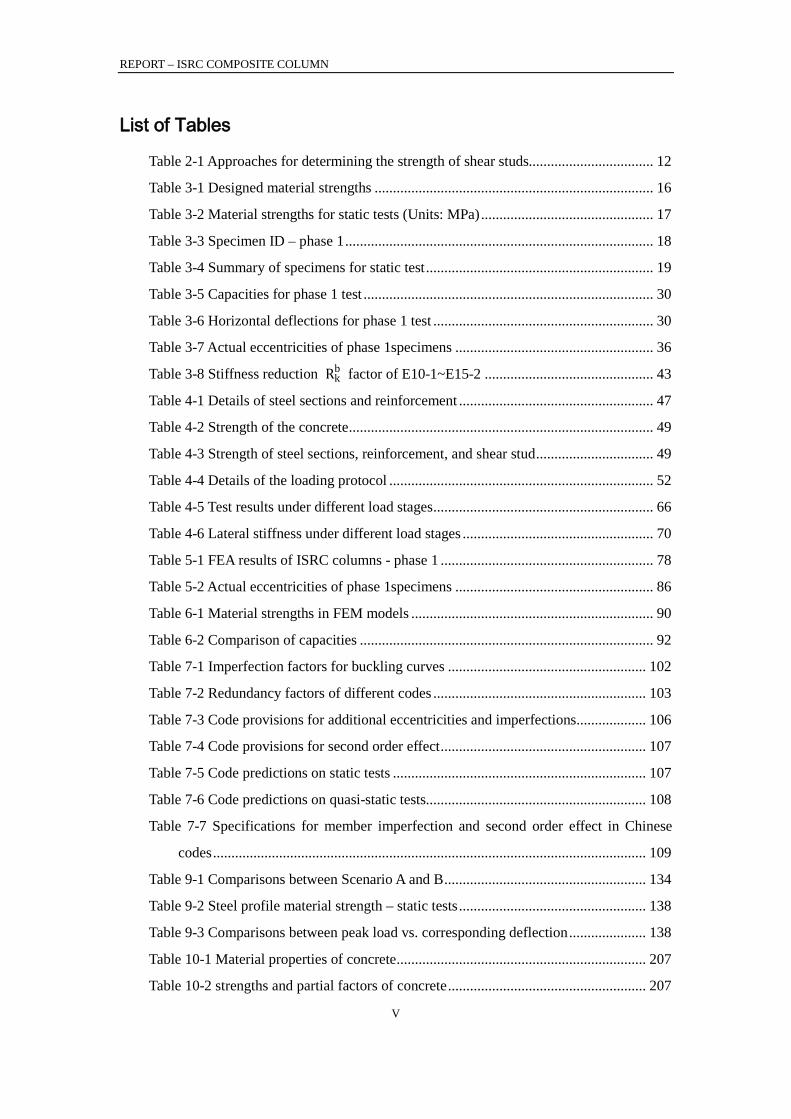
List of Tables
Table 2-1 Approaches for determining the strength of shear studs.................................. 12
Table 3-1 Designed material strengths ............................................................................ 16
Table 3-2 Material strengths for static tests (Units: MPa) ............................................... 17
Table 3-3 Specimen ID – phase 1 .................................................................................... 18
Table 3-4 Summary of specimens for static test .............................................................. 19
Table 3-5 Capacities for phase 1 test ............................................................................... 30
Table 3-6 Horizontal deflections for phase 1 test ............................................................ 30
Table 3-7 Actual eccentricities of phase 1specimens ...................................................... 36
Table 3-8 Stiffness reduction Rkb factor of E10-1~E15-2 .............................................. 43
Table 4-1 Details of steel sections and reinforcement ..................................................... 47
Table 4-2 Strength of the concrete ................................................................................... 49
Table 4-3 Strength of steel sections, reinforcement, and shear stud ................................ 49
Table 4-4 Details of the loading protocol ........................................................................ 52
Table 4-5 Test results under different load stages ............................................................ 66
Table 4-6 Lateral stiffness under different load stages .................................................... 70
Table 5-1 FEA results of ISRC columns - phase 1 .......................................................... 78
Table 5-2 Actual eccentricities of phase 1specimens ...................................................... 86
Table 6-1 Material strengths in FEM models .................................................................. 90
Table 6-2 Comparison of capacities ................................................................................ 92
Table 7-1 Imperfection factors for buckling curves ...................................................... 102
Table 7-2 Redundancy factors of different codes .......................................................... 103
Table 7-3 Code provisions for additional eccentricities and imperfections ................... 106
Table 7-4 Code provisions for second order effect ........................................................ 107
Table 7-5 Code predictions on static tests ..................................................................... 107
Table 7-6 Code predictions on quasi-static tests............................................................ 108
Table 7-7 Specifications for member imperfection and second order effect in Chinese
codes ...................................................................................................................... 109
Table 9-1 Comparisons between Scenario A and B ....................................................... 134
Table 9-2 Steel profile material strength – static tests ................................................... 138
Table 9-3 Comparisons between peak load vs. corresponding deflection ..................... 138
Table 10-1 Material properties of concrete .................................................................... 207
Table 10-2 strengths and partial factors of concrete ...................................................... 207

REPORT – ISRC COMPOSITE COLUMN
VI
Table 10-3 Material properties of reinforcing bars ........................................................ 208
Table 10-4 Strengths and partial factors of reinforcing bars ......................................... 208
Table 10-5 Material properties of steel profiles ............................................................. 209
Table 10-6 Strengths and partial factors of steel profiles .............................................. 209
Table 10-7 Determining the moment capacity at a given axial load – example 1 ......... 212
Table 10-8 Reduction factor for buckling ...................................................................... 217
Table 10-9 Axial capacity .............................................................................................. 217
Table 10-10 Determining the moment capacity at a given axial load – example 2 ....... 227
Table 10-11 Reduction factor for buckling .................................................................... 233
Table 10-12 Axial capacity ............................................................................................ 233
Table A-1 Material Properties ........................................................................................ 246
REPORT – ISRC COMPOSITE COLUMN
VII
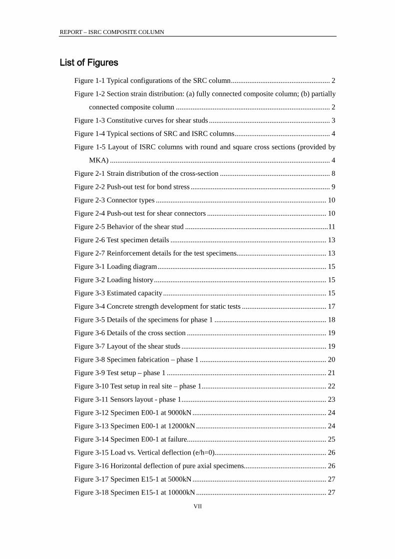
List of Figures
Figure 1-1 Typical configurations of the SRC column ...................................................... 2
Figure 1-2 Section strain distribution: (a) fully connected composite column; (b) partially
connected composite column .................................................................................... 2
Figure 1-3 Constitutive curves for shear studs .................................................................. 3
Figure 1-4 Typical sections of SRC and ISRC columns .................................................... 4
Figure 1-5 Layout of ISRC columns with round and square cross sections (provided by
MKA) ........................................................................................................................ 4
Figure 2-1 Strain distribution of the cross-section ............................................................ 8
Figure 2-2 Push-out test for bond stress ............................................................................ 9
Figure 2-3 Connector types ............................................................................................. 10
Figure 2-4 Push-out test for shear connectors ................................................................. 10
Figure 2-5 Behavior of the shear stud .............................................................................. 11
Figure 2-6 Test specimen details ..................................................................................... 13
Figure 2-7 Reinforcement details for the test specimens................................................. 13
Figure 3-1 Loading diagram ............................................................................................ 15
Figure 3-2 Loading history .............................................................................................. 15
Figure 3-3 Estimated capacity ......................................................................................... 15
Figure 3-4 Concrete strength development for static tests .............................................. 17
Figure 3-5 Details of the specimens for phase 1 ............................................................. 18
Figure 3-6 Details of the cross section ............................................................................ 19
Figure 3-7 Layout of the shear studs ............................................................................... 19
Figure 3-8 Specimen fabrication – phase 1 ..................................................................... 20
Figure 3-9 Test setup – phase 1 ....................................................................................... 21
Figure 3-10 Test setup in real site – phase 1 .................................................................... 22
Figure 3-11 Sensors layout - phase 1 ............................................................................... 23
Figure 3-12 Specimen E00-1 at 9000kN ......................................................................... 24
Figure 3-13 Specimen E00-1 at 12000kN ....................................................................... 24
Figure 3-14 Specimen E00-1 at failure............................................................................ 25
Figure 3-15 Load vs. Vertical deflection (e/h=0)............................................................. 26
Figure 3-16 Horizontal deflection of pure axial specimens............................................. 26
Figure 3-17 Specimen E15-1 at 5000kN ......................................................................... 27
Figure 3-18 Specimen E15-1 at 10000kN ....................................................................... 27
REPORT – ISRC COMPOSITE COLUMN
VIII
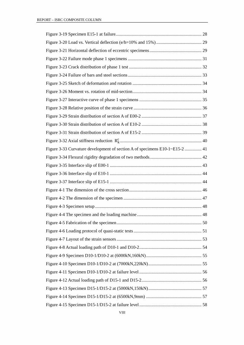
Figure 3-19 Specimen E15-1 at failure............................................................................ 28
Figure 3-20 Load vs. Vertical deflection (e/h=10% and 15%) ........................................ 29
Figure 3-21 Horizontal deflection of eccentric specimens .............................................. 29
Figure 3-22 Failure mode phase 1 specimens ................................................................. 31
Figure 3-23 Crack distribution of phase 1 test ................................................................ 32
Figure 3-24 Failure of bars and steel sections ................................................................. 33
Figure 3-25 Sketch of deformation and rotation ............................................................. 34
Figure 3-26 Moment vs. rotation of mid-section ............................................................. 34
Figure 3-27 Interactive curve of phase 1 specimens ....................................................... 35
Figure 3-28 Relative position of the strain curve ............................................................ 36
Figure 3-29 Strain distribution of section A of E00-2 ..................................................... 37
Figure 3-30 Strain distribution of section A of E10-2 ..................................................... 38
Figure 3-31 Strain distribution of section A of E15-2 ..................................................... 39
Figure 3-32 Axial stiffness reduction Rkc ........................................................................ 40
Figure 3-33 Curvature development of section A of specimens E10-1~E15-2 ............... 41
Figure 3-34 Flexural rigidity degradation of two methods .............................................. 42
Figure 3-35 Interface slip of E00-1 ................................................................................. 43
Figure 3-36 Interface slip of E10-1 ................................................................................. 44
Figure 3-37 Interface slip of E15-1 ................................................................................. 44
Figure 4-1 The dimension of the cross section ................................................................ 46
Figure 4-2 The dimension of the specimen ..................................................................... 47
Figure 4-3 Specimen setup .............................................................................................. 48
Figure 4-4 The specimen and the loading machine ......................................................... 48
Figure 4-5 Fabrication of the specimen ........................................................................... 50
Figure 4-6 Loading protocol of quasi-static tests ............................................................ 51
Figure 4-7 Layout of the strain sensors ........................................................................... 53
Figure 4-8 Actual loading path of D10-1 and D10-2 ....................................................... 54
Figure 4-9 Specimen D10-1/D10-2 at (6000kN,160kN) ................................................. 55
Figure 4-10 Specimen D10-1/D10-2 at (7000kN,220kN) ............................................... 55
Figure 4-11 Specimen D10-1/D10-2 at failure level ....................................................... 56
Figure 4-12 Actual loading path of D15-1 and D15-2 ..................................................... 56
Figure 4-13 Specimen D15-1/D15-2 at (5000kN,150kN) ............................................... 57
Figure 4-14 Specimen D15-1/D15-2 at (6500kN,9mm) ................................................. 57
Figure 4-15 Specimen D15-1/D15-2 at failure level ....................................................... 58
REPORT – ISRC COMPOSITE COLUMN
IX
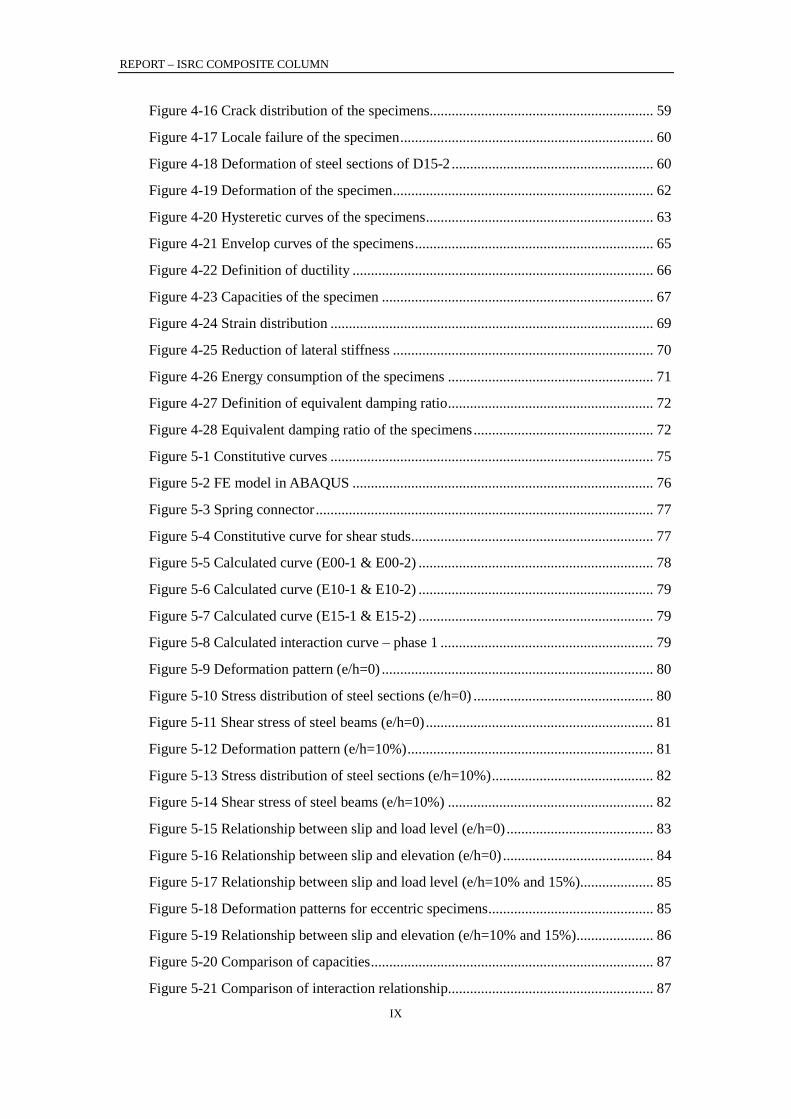
Figure 4-16 Crack distribution of the specimens ............................................................. 59
Figure 4-17 Locale failure of the specimen ..................................................................... 60
Figure 4-18 Deformation of steel sections of D15-2 ....................................................... 60
Figure 4-19 Deformation of the specimen ....................................................................... 62
Figure 4-20 Hysteretic curves of the specimens .............................................................. 63
Figure 4-21 Envelop curves of the specimens ................................................................. 65
Figure 4-22 Definition of ductility .................................................................................. 66
Figure 4-23 Capacities of the specimen .......................................................................... 67
Figure 4-24 Strain distribution ........................................................................................ 69
Figure 4-25 Reduction of lateral stiffness ....................................................................... 70
Figure 4-26 Energy consumption of the specimens ........................................................ 71
Figure 4-27 Definition of equivalent damping ratio ........................................................ 72
Figure 4-28 Equivalent damping ratio of the specimens ................................................. 72
Figure 5-1 Constitutive curves ........................................................................................ 75
Figure 5-2 FE model in ABAQUS .................................................................................. 76
Figure 5-3 Spring connector ............................................................................................ 77
Figure 5-4 Constitutive curve for shear studs .................................................................. 77
Figure 5-5 Calculated curve (E00-1 & E00-2) ................................................................ 78
Figure 5-6 Calculated curve (E10-1 & E10-2) ................................................................ 79
Figure 5-7 Calculated curve (E15-1 & E15-2) ................................................................ 79
Figure 5-8 Calculated interaction curve – phase 1 .......................................................... 79
Figure 5-9 Deformation pattern (e/h=0) .......................................................................... 80
Figure 5-10 Stress distribution of steel sections (e/h=0) ................................................. 80
Figure 5-11 Shear stress of steel beams (e/h=0) .............................................................. 81
Figure 5-12 Deformation pattern (e/h=10%) ................................................................... 81
Figure 5-13 Stress distribution of steel sections (e/h=10%) ............................................ 82
Figure 5-14 Shear stress of steel beams (e/h=10%) ........................................................ 82
Figure 5-15 Relationship between slip and load level (e/h=0) ........................................ 83
Figure 5-16 Relationship between slip and elevation (e/h=0) ......................................... 84
Figure 5-17 Relationship between slip and load level (e/h=10% and 15%) .................... 85
Figure 5-18 Deformation patterns for eccentric specimens ............................................. 85
Figure 5-19 Relationship between slip and elevation (e/h=10% and 15%) ..................... 86
Figure 5-20 Comparison of capacities ............................................................................. 87
Figure 5-21 Comparison of interaction relationship ........................................................ 87
REPORT – ISRC COMPOSITE COLUMN
X
Figure 5-22 Shear stress distribution of steel beams (e/h=10%) ..................................... 88
Figure 6-1 FE model in ABAQUS .................................................................................. 89
Figure 6-2 FEA envelop curves ....................................................................................... 90
Figure 6-3 Stress distribution for specimens with e/h=10% ............................................ 92
Figure 6-4 Stress distribution for specimens with e/h=15% ............................................ 93
Figure 6-5 Distribution of PEEQ of the concrete ............................................................ 94
Figure 6-6 Free body diagram of the steel sections ......................................................... 96
Figure 6-7 Influence of shear resistance index ................................................................ 97
Figure 6-8 Efficiency of the shear resistance .................................................................. 98
Figure 7-1 Reduction factors ......................................................................................... 103
Figure 7-2 Code predictions – static tests ...................................................................... 106
Figure 7-3 Code predictions – quasi-static tests ............................................................ 106
Figure 7-4 Transformation of steel sections and bars ..................................................... 110
Figure 7-5 Position of the neutral axis............................................................................ 113
Figure 9-1 Simplified method: point A, B, C, and D ...................................................... 117
Figure 9-2 Point A – stress distribution .......................................................................... 118
Figure 9-3 Point B – stress distribution .......................................................................... 119
Figure 9-4 Point C – stress distribution .......................................................................... 119
Figure 9-5 Point D – stress distribution ......................................................................... 120
Figure 9-6 Equivalent plates for steel profiles and rebar ............................................... 120
Figure 9-7 Flange layer and the equivalent plate .......................................................... 121
Figure 9-8 Flange layer and the equivalent plate .......................................................... 122
Figure 9-9 Subtracting the components of the stress distribution combination at point B
& C – PNA is within the inner profile equivalent rectangular plates .................... 124
Figure 9-10 Subtracting the components of the stress distribution combination at point B
& C – PNA is between the profile equivalent rectangular plates .......................... 124
Figure 9-11 Subtracting the components of the stress distribution combination at point B
& C – PNA is between the outer profile equivalent rectangular plates ................. 125
Figure 9-12 Subtracting the components of the stress distribution combination at point B
& C – PNA is between the steel profiles and rebar ............................................... 126
Figure 9-13 Subtracting the components of the stress distribution combination at point B
& C – PNA is within the equivalent rebar plates ................................................... 126
Figure 9-14 Subtracting the components of the stress distribution combination at point B
& C – PNA is above the equivalent rebar plates ................................................... 127
REPORT – ISRC COMPOSITE COLUMN
XI
Figure 9-15 Parameter β ................................................................................................ 130
Figure 9-16 Definition of the section in Safir Software (Section 1) .............................. 131
Figure 9-17 Safir – numerical model definition and experimental set-up configuration
............................................................................................................................... 132
Figure 9-18 Scenario A and B considered in FEM Safir ............................................... 133
Figure 9-19 Static experimental set-up length ............................................................... 133
Figure 9-20 Stress distribution in the mid-height section (E00-1) subject to Npm,Rd ..... 135
Figure 9-21 Stress distribution in the mid-height section (E00-2) subject to Npm,Rd ..... 135
Figure 9-22 Abaqus FE Model – static specimen .......................................................... 136
Figure 9-23 Static experimental set-up length ............................................................... 137
Figure 9-24 Deformed shape for E00-1 and E00-2 specimens...................................... 139
Figure 9-25 Deformed shape for E10-1 and E10-2 specimens...................................... 139
Figure 9-26 Deformed shape for E15-1 and E15-2 specimens...................................... 140
Figure 9-27 N – M Interaction curves for specimens E00-1 and E00-2 ........................ 141
Figure 9-28 N – M Interaction curves for specimens E10-1 and E10-2 ........................ 141
Figure 9-29 N – M Interaction curves for specimens E15-1 and E15-2 ........................ 141
Figure 10-1 Encased composite member section (EC4 Design) – Example 1 .............. 142
Figure 10-2 Axial force - bending moment interaction curve (EC4 Design) – Example 1
............................................................................................................................... 152
Figure 10-3 Definition of sections bc3, bc4, and bs (EC4 Design) – Example 1 .......... 153
Figure 10-4 Homogenized equivalent concrete section bs – Example 1 ....................... 155
Figure 10-5 Encased composite member section (EC4 Design) – Example 2 .............. 159
Figure 10-6 Axial force - bending moment interaction curve (EC4 Design) – Example 2
............................................................................................................................... 168
Figure 10-7 Definition of sections bc1, bc3, bs2, and bs4 (EC4 Design) – Example 2 169
Figure 10-8 Homogenized equivalent concrete section bs – Example 2 ....................... 173
Figure 10-9 Encased composite member section (AISC Design) – Example 1 ............ 177
Figure 10-10 Axial force - bending moment interaction curve (AISC Design) – Example
1 ............................................................................................................................. 185
Figure 10-11 Definition of sections bc3, bc4, and bs (AISC Design) – Example 1 ...... 185
Figure 10-12 Homogenized equivalent concrete section bs – Example 1 ..................... 188
Figure 10-13 Encased composite member section (AISC Design) – Example 2 .......... 191
Figure 10-14 Axial force - bending moment interaction curve (AISC Design) – Example
2 ............................................................................................................................. 199
REPORT – ISRC COMPOSITE COLUMN
XII
Figure 10-15 Definition of sections bc1, bc3, bs2, and bs4 (AISC Design) – Example 2
............................................................................................................................... 199
Figure 10-16 Homogenized equivalent concrete section bs – Example 2 ..................... 202
Figure 10-17 Equivalent stress distribution ................................................................... 210
Figure 10-18 Section 1 dimensions ................................................................................ 211
Figure 10-19 Interaction curves with nominal strengths - Section 1 ............................. 216
Figure 10-20 Interaction curves with and without material partial factors - Section 1 . 216
Figure 10-21 Interaction curves with and without considering buckling and second order
effects (Material partial factors have already been considered) - Section 1 .......... 219
Figure 10-22 Definition of sections bc3, bc4, and bs (EC4 Design) – Example 1 ........ 220
Figure 10-23 Homogenized equivalent concrete section bs – Example 1 ..................... 223
Figure 10-24 Section 2 dimensions ............................................................................... 226
Figure 10-25 Section 3 dimensions ............................................................................... 226
Figure 10-26 Interaction curves with nominal strengths ............................................... 232
Figure 10-27 Interaction curves with and without material partial factors ................... 232
Figure 10-28 Interaction curves with and without considering buckling and second order
effects (Material partial factors have already been considered) ............................ 235
Figure 10-29 Definition of sections bc1, bc3, bs2, and bs4 (EC4 Design) – Example 2
............................................................................................................................... 236
Figure 10-30 Homogenized equivalent concrete section bs – Example 2 ..................... 239
Figure A-1 3D isometric of composite building column (Information provided by MKA
2016) ...................................................................................................................... 245
Figure A-2 Column free body diagram (Information provided by MKA 2016) ............ 246
Figure A-3 Column section (Information provided by MKA 2016).............................. 248
Figure A-4 P-M interaction curve for flexure about the x axis (Information provided by
MKA 2016) ............................................................................................................ 251

REPORT – ISRC COMPOSITE COLUMN
XIII
REPORT – ISRC COMPOSITE COLUMN
1
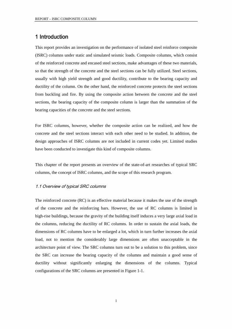
1 Introduction
This report provides an investigation on the performance of isolated steel reinforce composite
(ISRC) columns under static and simulated seismic loads. Composite columns, which consist
of the reinforced concrete and encased steel sections, make advantages of these two materials,
so that the strength of the concrete and the steel sections can be fully utilized. Steel sections,
usually with high yield strength and good ductility, contribute to the bearing capacity and
ductility of the column. On the other hand, the reinforced concrete protects the steel sections
from buckling and fire. By using the composite action between the concrete and the steel
sections, the bearing capacity of the composite column is larger than the summation of the
bearing capacities of the concrete and the steel sections.
For ISRC columns, however, whether the composite action can be realized, and how the
concrete and the steel sections interact with each other need to be studied. In addition, the
design approaches of ISRC columns are not included in current codes yet. Limited studies
have been conducted to investigate this kind of composite columns.
This chapter of the report presents an overview of the state-of-art researches of typical SRC
columns, the concept of ISRC columns, and the scope of this research program.
1.1 Overview of typical SRC columns
The reinforced concrete (RC) is an effective material because it makes the use of the strength
of the concrete and the reinforcing bars. However, the use of RC columns is limited in
high-rise buildings, because the gravity of the building itself induces a very large axial load in
the columns, reducing the ductility of RC columns. In order to sustain the axial loads, the
dimensions of RC columns have to be enlarged a lot, which in turn further increases the axial
load, not to mention the considerably large dimensions are often unacceptable in the
architecture point of view. The SRC columns turn out to be a solution to this problem, since
the SRC can increase the bearing capacity of the columns and maintain a good sense of
ductility without significantly enlarging the dimensions of the columns. Typical
configurations of the SRC columns are presented in Figure 1-1.

REPORT – ISRC COMPOSITE COLUMN
2
Figure 1-1 Typical configurations of the SRC column
The interaction between the concrete and the steel section is a critical issue in the design of
SRC columns. Since the capacity of the column under combined compression and bending is
dependent on the axial force, the connection between the concrete and the steel section is a
key factor in determining the ultimate strength of SRC columns. If the concrete and the steel
section are fully connected, there will be no relative slip on the concrete-steel interfaces, and
the normal strain of these two materials on the interface will be compatible (Figure 1-2(a)).
The transfer of axial force between the concrete and the steel section is realized by shear force
on the concrete-steel interfaces. If the concrete and steel section are partially connected (or
without connection), the shear force on the concrete-steel interfaces will not be large enough
to ensure zero relative slip on that interface, and the strain distribution of the concrete and the
steel section will not be in the same plane (Figure 1-2(b)). Namely, the plane sections do not
remain plane.
Figure 1-2 Section strain distribution: (a) fully connected composite column; (b) partially
connected composite column
REPORT – ISRC COMPOSITE COLUMN
3
The shear resistance on the concrete-steel interfaces is provided by the bond stress and shear
connectors, such as studs, deformed rebar, steel shapes, etc. Japanese researchers found that
the bond stress between concrete and steel section is less than 45% of the bond stress between
concrete and smooth rebar (AIJ-SRC 2002). Therefore, if no particular measures have been
taken to increase the roughness of the steel section, it is reasonable to neglect the bond stress
if shear connectors are applied. However, the bond stress can be very large when the surfaces
of the steel sections are made rough, or ribs are employed on the surfaces of the steel sections.
In practice, shear connecters are usually provided in composite columns. The major purpose
of shear connectors is to transfer the axial force between the concrete and the steel section. It
is convinced that the existence of shear connectors will increase the bearing capacity of
composite members (Macking, 1927). Studs are the most commonly used shear connectors
nowadays, since the production and fabrication of shear studs is relatively easy. Furthermore,
shear studs are isotropic and ductile components, which may mitigate the stress concentration
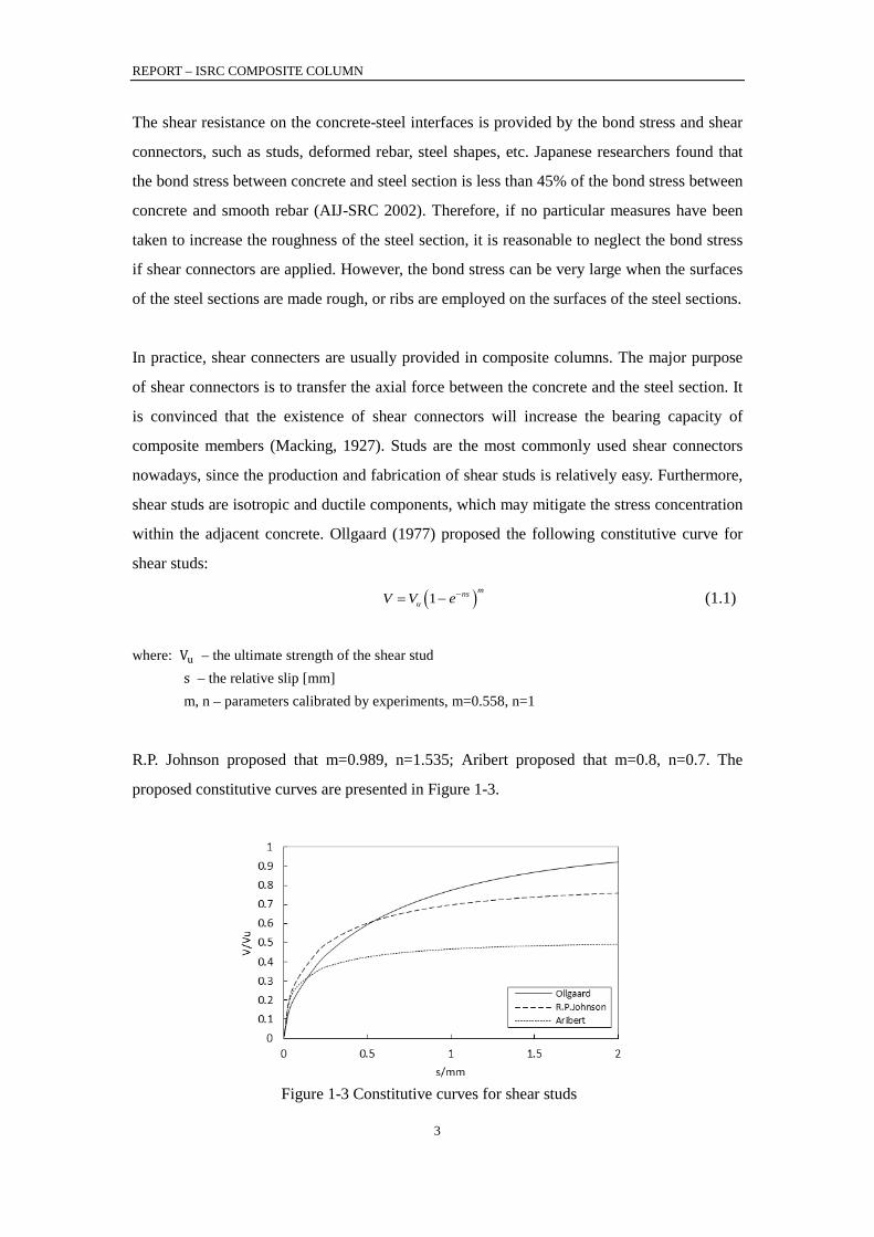
within the adjacent concrete. Ollgaard (1977) proposed the following constitutive curve for
shear studs:
( )1mns
uV V e−= − (1.1)
where: Vu – the ultimate strength of the shear stud s – the relative slip [mm] m, n – parameters calibrated by experiments, m=0.558, n=1
R.P. Johnson proposed that m=0.989, n=1.535; Aribert proposed that m=0.8, n=0.7. The
proposed constitutive curves are presented in Figure 1-3.
Figure 1-3 Constitutive curves for shear studs
REPORT – ISRC COMPOSITE COLUMN
4
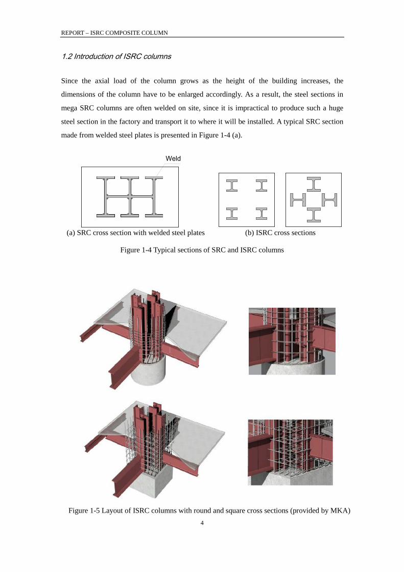
1.2 Introduction of ISRC columns
Since the axial load of the column grows as the height of the building increases, the
dimensions of the column have to be enlarged accordingly. As a result, the steel sections in
mega SRC columns are often welded on site, since it is impractical to produce such a huge
steel section in the factory and transport it to where it will be installed. A typical SRC section
made from welded steel plates is presented in Figure 1-4 (a).
Weld
(a) SRC cross section with welded steel plates
(b) ISRC cross sections
Figure 1-4 Typical sections of SRC and ISRC columns
Figure 1-5 Layout of ISRC columns with round and square cross sections (provided by MKA)

REPORT – ISRC COMPOSITE COLUMN
5
Contrary to traditional SRC columns, multiple separate steel sections are encased in ISRC
columns without connection with each other. The steel sections are often placed in the
position that fits the connection to the beams or other structural elements (Figure 1-4 (b) and
Figure 1-5).
If the results of this research program are able to validate the reliance of ISRC columns (with
eccentricity ratios no more than 15%), then it is an alternate approach to use ISRC columns in
the design of super high-rise buildings. The adoption of ISRC columns can produce the
following benefits:
1) Reduce the construction cost
Welding work at the construction site will be reduced by either adopting hot-rolled steel
sections or steel sections welded in the factory, reducing the labor cost significantly.
Besides, duration of the project may also be shortened because of the easy construction.
2) Improve the construction safety
The reduction of welding work reduces the risk of fire. An easy installation is also
beneficial to safety issues.
3) Avoid the adverse effect of residual stress and weld imperfection
Steel structures are sensitive to residual stress and the quality of welds, especially for
large and thick steel plates. Adopting ISRC columns may reduce the adverse effect of
these two problems.
1.3 Research objectives
Although current codes have accommodated design provisions for SRC columns, provisions
for ISRC columns are not included. With the considerable benefits ISRC columns may bring,
it is urgent to validate the reliance of this kind of composite columns, and explore simplified
design approaches. This research hopes to present an insight into the mechanism of ISRC
columns. Objectives of this research include:
1) Perform a literature survey of past researches on the study of SRC/ISRC columns, collect
related data and projects for the research;
2) Design and carry out the tests. Record the behavior of the ISRC columns during the test,
and examine the failure modes of the concrete, rebar and steel sections. Record the test
data, and evaluate the performance of ISRC columns based on the analysis of the
collected data;
3) Carry out the finite element analysis (FEA) as an supplement to the physical tests;

REPORT – ISRC COMPOSITE COLUMN
6
4) Present suggestions and simplified approaches to the design and construction of ISRC
columns.
1.4 Project overview
This research project is a two-phase test program investigating the performance of ISRC
columns. Phase 1 of the study consists of static tests on six 1/4-scaled ISRC columns: every
two of the specimens will be loaded statically with eccentricity ratio of 0, 10% and 15%
respectively. Only an axial load will be applied to the columns with different eccentricities to
examine the performance of ISRC columns under static loads, and the test results will serve
as a guide to the subsequent phase. Phase 2 of the study consists of quasi-static tests on four
1/6-scaled ISRC columns: every two of the specimens with be loaded under simulated seismic
loads with an equivalent eccentricity ratio of 10% and 15% respectively. The capacity,
ductility, failure mode and crack distribution of the specimens will be examined.
1.5 Notation
Ac = area of concrete [mm2]
Ap = area of steel section [mm2]
As = gross area of longitudinal rebar [mm2]
Ast = cross area of a shear stud [mm2]
δ = steel contribution ratio
e = eccentricity [mm]
eb = balanced eccentricity [mm] (Compressive concrete fiber fails and tensile
steel fiber yields at the same time.)
Ec = secant modulus of concrete [MPa]
Es = modulus of elasticity of longitudinal bar [MPa]
Ep = modulus of elasticity of steel section [MPa]
ε = normal strain of the cross section
fc = axial compressive strength of concrete [MPa]
fu = shear strength of stud [MPa]
fp = yield strength of steel section [MPa]
fs = yield strength of longitudinal rebar [MPa]
ϕ = curvature of the cross section [mm−1]
h = height of the cross section [mm]
REPORT – ISRC COMPOSITE COLUMN
7
Ic = moment of inertia of concrete [mm4]
Is = moment of inertia of concrete [mm4]
Ip = moment of inertia of concrete [mm4]
lu = unsupported length of the ISRC column [mm]
Mu = flexural resistance under combined compression and bending [kN·m]
Mu0 = plastic resistance under pure bending (Nominal strength) [kN·m]
Nu = axial resistance under combined compression and bending [kN]
Nu0 = axial resistance under pure compression [kN]
P = applied axial load [kN]
r = radius of gyration of the cross section [mm]
Rkc = stiffness reduction factor for compression
Rkb = stiffness reduction factor for bending
ρa = reinforcement ratio of steel sections
ρs = reinforcement ratio of longitudinal bars
ρsv = volume ratio of transverse reinforcement
Vu = shear capacity of a shear stud [kN]
ϕc = resistance factor for compression in AISC
ϕb = resistance factor for bending in AISC
REPORT – ISRC COMPOSITE COLUMN
8
2 Previous research
The SRC column concept was first introduced to the design of steel structures as a method to
enhance the durability and fire resistance of the structural steel. The structural steel can be
either hot-rolled steel sections or welded steel plates. Compared to steel columns, the
reinforced concrete can prevent the steel section from local buckling, increase the rigidity of
the column, and improve the durability and fire resistance of the structural steel. On the other
hand, the steel section helps increase the bearing capacity, especially shear capacity, of the
column, thus improving the seismic behavior of the column. The composite action between
the concrete and the steel section makes the bearing capacity of SRC columns higher than the
summation of the bearing capacities of the concrete and the steel section. Therefore,
neglecting the interaction between the concrete and the steel section will lead to a more
conservative design result. The mechanism of load transfer between the concrete and the steel
section has to be explored before a reliable design method can be developed.
2.1 Composite action
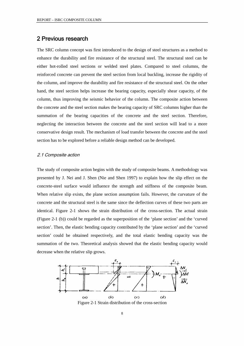
The study of composite action begins with the study of composite beams. A methodology was
presented by J. Nei and J. Shen (Nie and Shen 1997) to explain how the slip effect on the
concrete-steel surface would influence the strength and stiffness of the composite beam.
When relative slip exists, the plane section assumption fails. However, the curvature of the
concrete and the structural steel is the same since the deflection curves of these two parts are
identical. Figure 2-1 shows the strain distribution of the cross-section. The actual strain
(Figure 2-1 (b)) could be regarded as the superposition of the ‘plane section’ and the ‘curved
section’. Then, the elastic bending capacity contributed by the ‘plane section’ and the ‘curved
section’ could be obtained respectively, and the total elastic bending capacity was the
summation of the two. Theoretical analysis showed that the elastic bending capacity would
decrease when the relative slip grows.
Figure 2-1 Strain distribution of the cross-section
REPORT – ISRC COMPOSITE COLUMN
9
It could be proved that the plastic flexural capacity and the stiffness of the composite beam
were also reduced because of the slip effect. However, only the reduction in elastic bending
capacity was validated by the experiment – the plastic flexural capacity of the composite
beam did not drop. This was because the strengthening of the steel after yielding offset the
adverse effect of slip. Therefore, for fully connected composite beams, slip effect can be
neglected if one is only interested in the ultimate flexural strength.
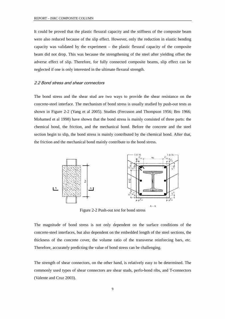
2.2 Bond stress and shear connectors
The bond stress and the shear stud are two ways to provide the shear resistance on the
concrete-steel interface. The mechanism of bond stress is usually studied by push-out tests as
shown in Figure 2-2 (Yang et al 2005). Studies (Fercuson and Thompson 1956; Bro 1966;
Mohamed et al 1998) have shown that the bond stress is mainly consisted of three parts: the
chemical bond, the friction, and the mechanical bond. Before the concrete and the steel
section begin to slip, the bond stress is mainly contributed by the chemical bond. After that,
the friction and the mechanical bond mainly contribute to the bond stress.
Figure 2-2 Push-out test for bond stress
The magnitude of bond stress is not only dependent on the surface conditions of the
concrete-steel interfaces, but also dependent on the embedded length of the steel sections, the
thickness of the concrete cover, the volume ratio of the transverse reinforcing bars, etc.
Therefore, accurately predicting the value of bond stress can be challenging.
The strength of shear connectors, on the other hand, is relatively easy to be determined. The
commonly used types of shear connectors are shear studs, perfo-bond ribs, and T-connectors
(Valente and Cruz 2003).

REPORT – ISRC COMPOSITE COLUMN
10
Shear stud
Perfo-bond connector
T connector
Figure 2-3 Connector types
According to Eurocode4, the push-out tests should be conducted to study the behavior of
shear connectors. A standard push-out test specified in Eurocode4 consists of a steel section
held vertically in the middle by two identical reinforced concrete slabs. Each of the concrete
is connected with the steel section via two rows of shear connectors. The axial load is applied
to the steel section, and the behavior of the shear connectors can be obtained.
Figure 2-4 Push-out test for shear connectors
It is found that (Ollgaard et al 1971) the behavior of shear studs in a composite structure is
similar to an elastic beam foundation (Figure 2-5 (a)). Suppose the concrete serves as the
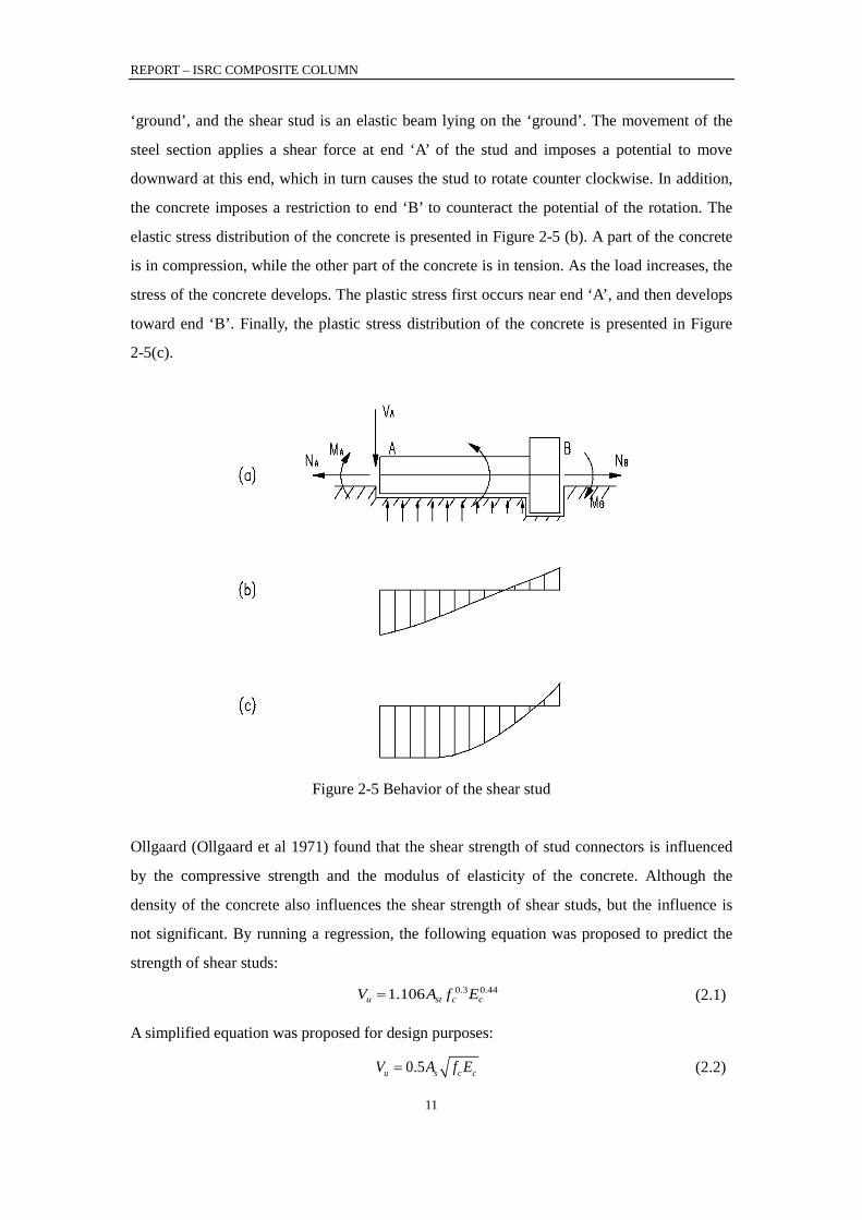
REPORT – ISRC COMPOSITE COLUMN
11
‘ground’, and the shear stud is an elastic beam lying on the ‘ground’. The movement of the
steel section applies a shear force at end ‘A’ of the stud and imposes a potential to move
downward at this end, which in turn causes the stud to rotate counter clockwise. In addition,
the concrete imposes a restriction to end ‘B’ to counteract the potential of the rotation. The
elastic stress distribution of the concrete is presented in Figure 2-5 (b). A part of the concrete
is in compression, while the other part of the concrete is in tension. As the load increases, the
stress of the concrete develops. The plastic stress first occurs near end ‘A’, and then develops
toward end ‘B’. Finally, the plastic stress distribution of the concrete is presented in Figure
2-5(c).
Figure 2-5 Behavior of the shear stud
Ollgaard (Ollgaard et al 1971) found that the shear strength of stud connectors is influenced
by the compressive strength and the modulus of elasticity of the concrete. Although the
density of the concrete also influences the shear strength of shear studs, but the influence is
not significant. By running a regression, the following equation was proposed to predict the
strength of shear studs:
0.3 0.441.106u st c cV A f E= (2.1)
A simplified equation was proposed for design purposes:
0.5u s c cV A f E= (2.2)
REPORT – ISRC COMPOSITE COLUMN
12
Table 2-1 lists different methods and specifications for the design of shear studs.
Table 2-1 Approaches for determining the strength of shear studs
Code Strength of shear studs Specifications
Eurocode4
22 / 0.290.8min ,
4 c
V Vu
cufVd f Ed απ
γ γ=
where:
0.2 1 , 3 4
1 4
h hfor
d dh
ford
α
α
= + ≤ ≤
= >
fu ≤ 500 MPa 16mm ≤ d ≤ 25mm concrete density not less than
1750kg/m3
Chinese GB50017
2 2
40.43min0.7 ,
4u c
uc
d dfV f Eπ πγ=
where γ – ratio of tensile to yield strength of the stud
h/d ≥ 4 when the stud is not
positioned right over the web: (1) d ≤ 1.5tf if the flange is designed to be in tension; (2) d ≤ 2.5tf if not.
AISC-LRFD 2 20.5min ,
4
4u cu
cd dV f Ef π π
=
h/d ≥ 4 concrete density not less than
1440kg/m3 d ≤ 2.5tf if the stud is not
positioned right over the web
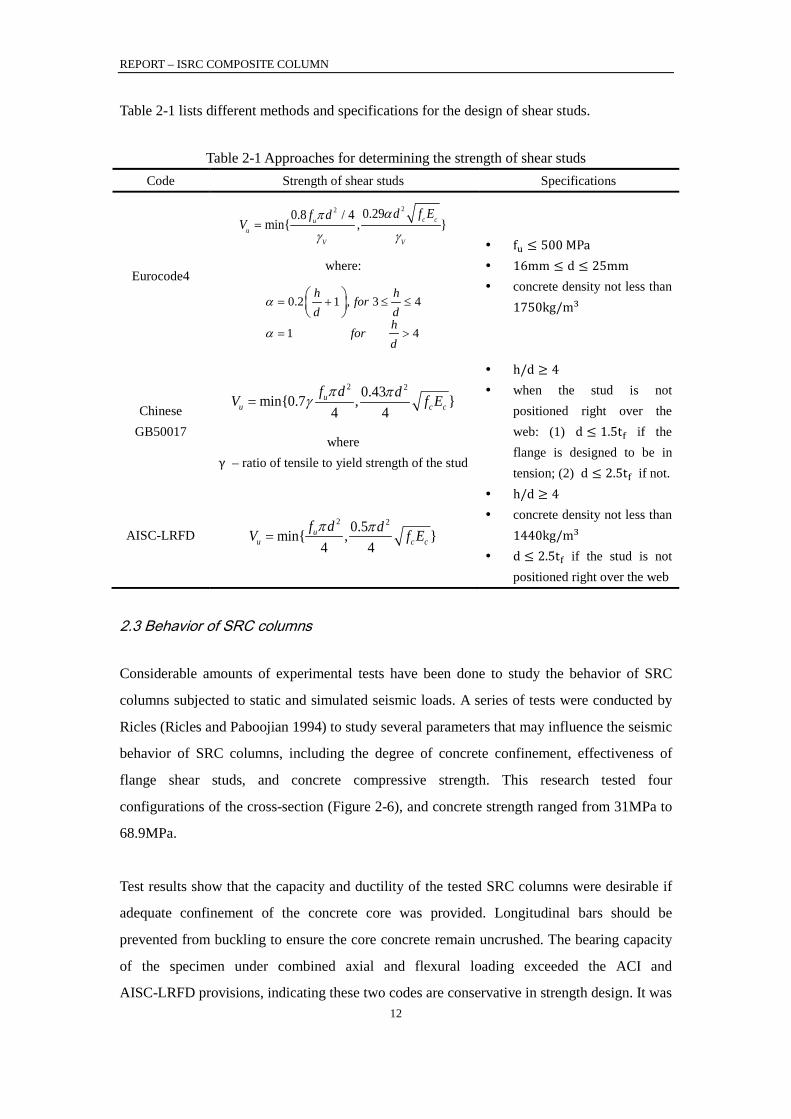
2.3 Behavior of SRC columns
Considerable amounts of experimental tests have been done to study the behavior of SRC
columns subjected to static and simulated seismic loads. A series of tests were conducted by
Ricles (Ricles and Paboojian 1994) to study several parameters that may influence the seismic
behavior of SRC columns, including the degree of concrete confinement, effectiveness of
flange shear studs, and concrete compressive strength. This research tested four
configurations of the cross-section (Figure 2-6), and concrete strength ranged from 31MPa to
68.9MPa.
Test results show that the capacity and ductility of the tested SRC columns were desirable if
adequate confinement of the concrete core was provided. Longitudinal bars should be
prevented from buckling to ensure the core concrete remain uncrushed. The bearing capacity
of the specimen under combined axial and flexural loading exceeded the ACI and
AISC-LRFD provisions, indicating these two codes are conservative in strength design. It was
REPORT – ISRC COMPOSITE COLUMN
13
also concluded that shear studs installed on the flange of the steel sections did not have
significant effect on the flexural strength and stiffness of the SRC columns. However, shear
studs are still necessary to transfer gravity load from steel beams to the composite columns.
Figure 2-6 Test specimen details
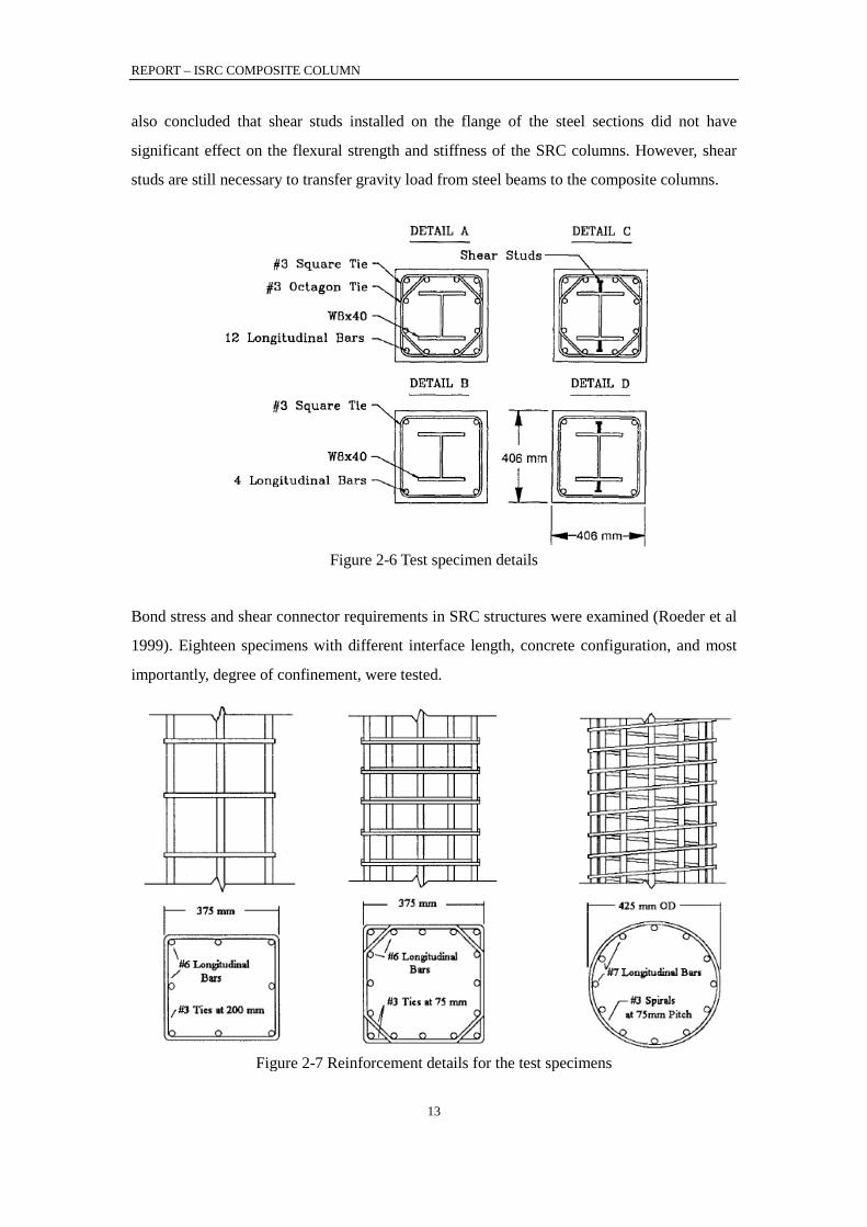
Bond stress and shear connector requirements in SRC structures were examined (Roeder et al
1999). Eighteen specimens with different interface length, concrete configuration, and most
importantly, degree of confinement, were tested.
Figure 2-7 Reinforcement details for the test specimens

REPORT – ISRC COMPOSITE COLUMN
14
Test results showed that the confinement had little impact on the maximum bond stress on the
interface, but a larger confinement increased the post slip resistance. The results validated the
theory that bond stress was exponentially distributed along the embedded length under service
load, and was approximately uniformly distributed when the loads were approaching the
ultimate capacity. Cyclic test results showed that when the load was under 40% of the
maximum capacity, there was no significant deterioration on the interface; interface
deterioration was significant after that load.
Two specimens with shear studs were tested. The results suggested that the existence of shear
connectors might damage the adjacent concrete by inducing location deformation and stress
concentration. Therefore, it was recommended that shear connectors would not be used if the
shear requirement were less than the shear capacity provided by the bond stress. That is,
design the load to be transferred either by bond stress or by shear connectors, but not by the
combination of the two.
SRC columns using high strength steel was also tested (Wakabayashi 1992). Test results
suggested that the SRC members were more ductile when the steel had a higher ultimate
strength. Biaxial loaded SRC columns also show desirable performance (Munoz et al 1997;
Dundar et al 2007)
REPORT – ISRC COMPOSITE COLUMN
15
3 Experimental study – phase 1
The first phase of the research was completed in March 2015 at the structural laboratory of
Tsinghua University, China. The objective of this phase of the experiment was to study the
behavior of ISRC columns under combined compression and bending conditions. Six reduced
scaled specimens were tested. This chapter presents a detailed description of the experiment
program.
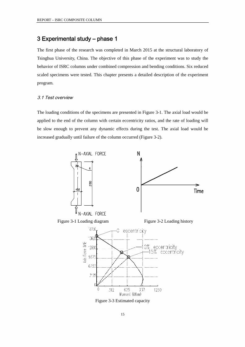
3.1 Test overview
The loading conditions of the specimens are presented in Figure 3-1. The axial load would be
applied to the end of the column with certain eccentricity ratios, and the rate of loading will
be slow enough to prevent any dynamic effects during the test. The axial load would be
increased gradually until failure of the column occurred (Figure 3-2).
Figure 3-1 Loading diagram Figure 3-2 Loading history
Figure 3-3 Estimated capacity

REPORT – ISRC COMPOSITE COLUMN
16
Figure 3-3 shows the planned loading paths and the estimated capacities of the specimens.
Since mega columns are primarily designed in high-rise buildings, columns at the bottom of
the buildings are often carried with very large gravity loads. Therefore, the eccentricities in
mega columns are usually less than balanced eccentricity (eb), which is defined as the
eccentricity corresponding to the balanced strain condition. Therefore, the maximum
eccentricity in this test program was set to 15% - a reasonable limit based on project
experience. However, the real eccentricity at failure could exceed the initial eccentricity
because of the second order effect. The horizontal deflection in the middle of the column was
measured to account for the second order effect during the test.
3.2 Materials
Strength grades of the materials were selected based on both the design in real projects and
the limits of the loading machines. Table 3-1 presents the material strength designed for phase
1.
Table 3-1 Designed material strengths
Material Strength
Concrete C60 (fcu,k = 60MPa)
maximum aggregate size no more than 5mm.
Steel sections S355 fyk ≥ 355MPa
produced by ArcelorMittal, shipped to China
Longitudinal bars HRB 400 fyk ≥ 400MPa
Ties HRB 500 fyk ≥ 500MPa
To be adjusted according to available bars.
Studs 6mm × 25mm or 5mm × 20mm headed studs or Grade 4.8 bolts
Since concrete strength was sensitive to its age, concrete cubes for each specimen were tested
right before or after the specimen was tested. Figure 3-4 shows the concrete strength
development for phase 1. The first specimen was tested 42 days after the concrete had been
placed. By then, the average concrete cubic strength was fcu,m = 61.17 MPa, which met the
expected strength (60 MPa).

REPORT – ISRC COMPOSITE COLUMN
17
Figure 3-4 Concrete strength development for static tests
Table 3-2 Material strengths for static tests (Units: MPa)
Specimen
ID
Concrete
cubic
strength
Concrete
axial
strength
Yield
strength of
steel
section
flange*
Yield
strength of
steel
section
web*
Yield
strength of
longitudinal
bar
Yield
strength of
transverse
bar
E00-1 61.2 61.2 408 523
438
f3.25
= 597MPa
f4.80
= 438MPa
E00-2 56.6 55.0 398 411
E10-1 60.9 56.4 423 435
E10-2 72.8 59.2 383 415
E15-1 66.1 57.2 377 404
E15-2 67.6 56.3 389 405
Average 64.8 57.6 396 432 - -
where:
f3.25 – yield strength for bars of 3.25mm diameter
f4.80 – yield strength for bars of 4.80mm diameter
* Material strength for steel sections are provided by ArcelorMittal
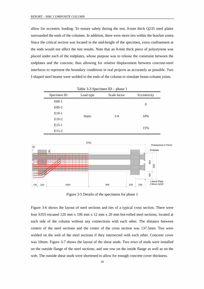
3.3 Specimen design and fabrication
Six identical specimens were designed in phase 1, and each set of two were loaded under the
same eccentricity ratio: 0, 10%, and 15%, respectively (Table 3-3). Figure 3-5 shows the
dimensions and details of these specimens. The specimen was 2700 mm in length, and the
typical section size was 450 mm x 450 mm. There was a bracket at each end of the column to
REPORT – ISRC COMPOSITE COLUMN
18
allow for eccentric loading. To ensure safety during the test, 8-mm thick Q235 steel plates
surrounded the ends of the columns. In addition, there were more ties within the bracket zones.
Since the critical section was located in the mid-height of the specimen, extra confinement at
the ends would not affect the test results. Note that an 8-mm thick piece of polystyrene was
placed under each of the endplates, whose purpose was to release the constraint between the
endplates and the concrete, thus allowing for relative displacement between concrete-steel
interfaces to represent the boundary conditions in real projects as accurately as possible. Two
I-shaped steel beams were welded to the ends of the column to simulate beam-column joints.
Table 3-3 Specimen ID – phase 1
Specimen ID Load type Scale factor Eccentricity
E00-1
Static 1/4
0 E00-2
E10-1 10%
E10-2
E15-1 15%
E15-2
2700
225225
450
180
630
25
900
80
Endplate
Lateral Plate t=8mm Q235
Polystyrene t=10mm
130 220 1000
Figure 3-5 Details of the specimens for phase 1
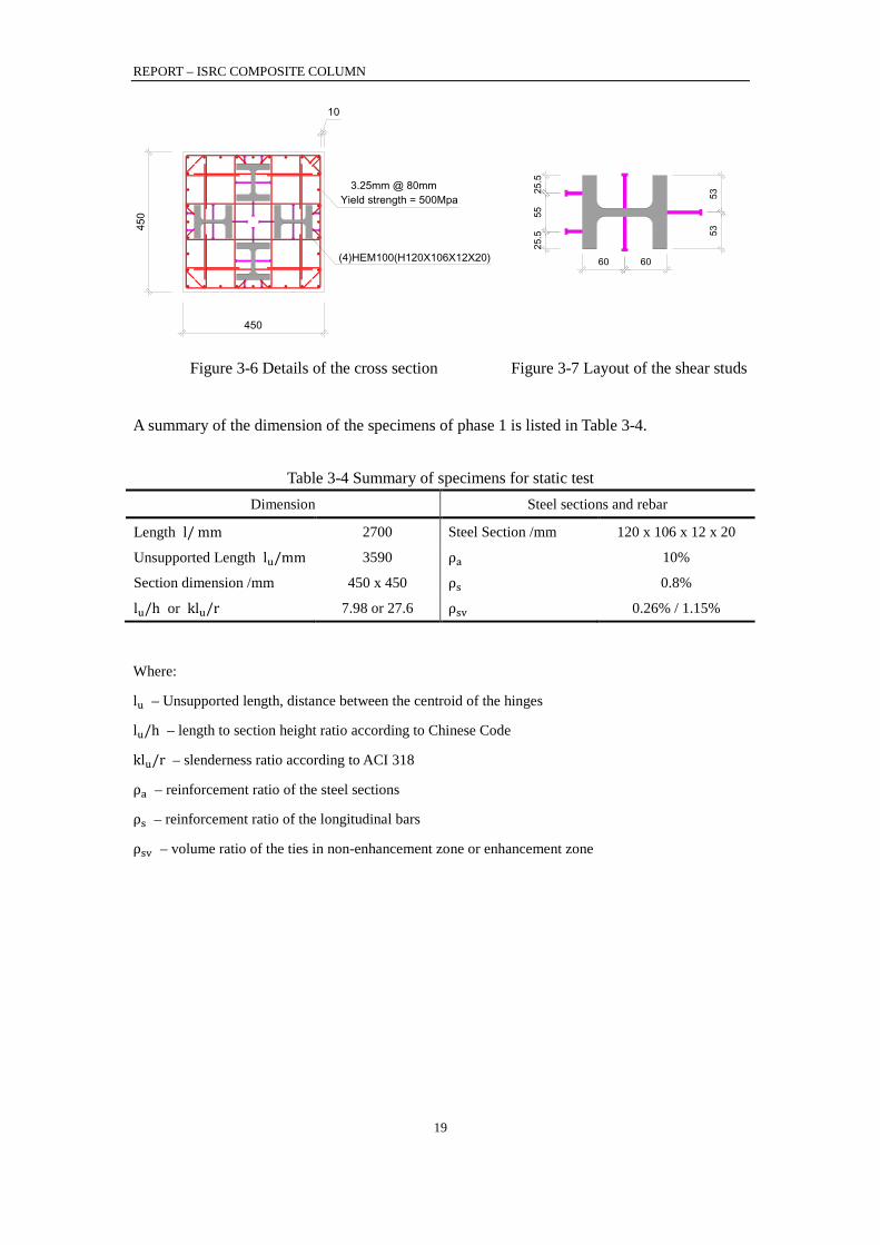
Figure 3-6 shows the layout of steel sections and ties of a typical cross section. There were
four S355 encased 120 mm x 106 mm x 12 mm x 20 mm hot-rolled steel sections, located at
each side of the column without any connections with each other. The distance between
centers of the steel sections and the center of the cross section was 137.5mm. Ties were
welded on the web of the steel sections if they intersected with each other. Concrete cover
was 10mm. Figure 3-7 shows the layout of the shear studs. Two rows of studs were installed
on the outside flange of the steel sections, and one row on the inside flange as well as on the
web. The outside shear studs were shortened to allow for enough concrete cover thickness.
REPORT – ISRC COMPOSITE COLUMN
19
450
450
10
3.25mm @ 80mmYield strength = 500Mpa
(4)HEM100(H120X106X12X20)
6060
535325
.555
25.5
Figure 3-6 Details of the cross section
Figure 3-7 Layout of the shear studs
A summary of the dimension of the specimens of phase 1 is listed in Table 3-4.
Table 3-4 Summary of specimens for static test
Dimension Steel sections and rebar
Length l/ mm 2700 Steel Section /mm 120 x 106 x 12 x 20
Unsupported Length lu/mm 3590 ρa 10%
Section dimension /mm 450 x 450 ρs 0.8%
lu/h or klu/r 7.98 or 27.6 ρsv 0.26% / 1.15%
Where:
lu – Unsupported length, distance between the centroid of the hinges
lu/h – length to section height ratio according to Chinese Code
klu/r – slenderness ratio according to ACI 318
ρa – reinforcement ratio of the steel sections
ρs – reinforcement ratio of the longitudinal bars
ρsv – volume ratio of the ties in non-enhancement zone or enhancement zone
REPORT – ISRC COMPOSITE COLUMN
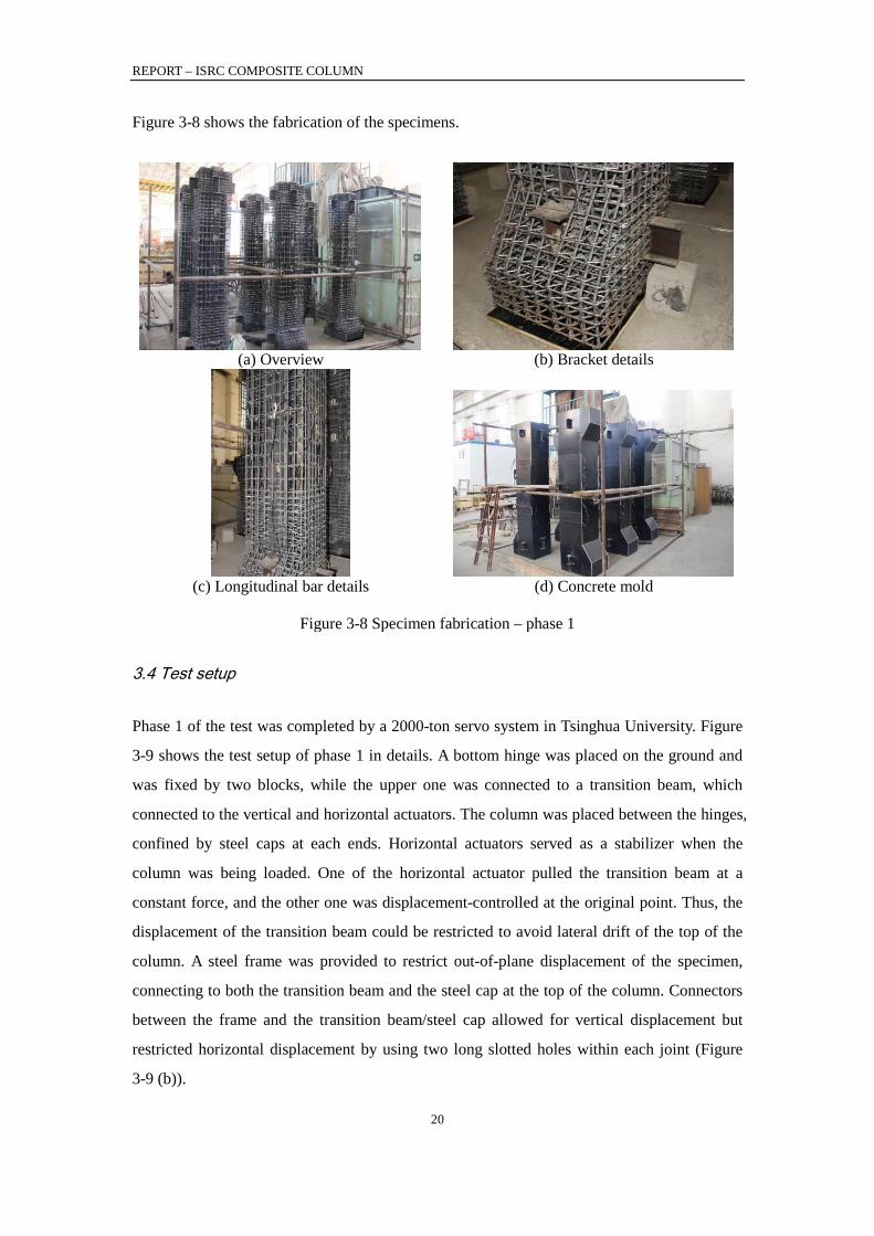
20
Figure 3-8 shows the fabrication of the specimens.
(a) Overview
(b) Bracket details
(c) Longitudinal bar details
(d) Concrete mold
Figure 3-8 Specimen fabrication – phase 1
3.4 Test setup
Phase 1 of the test was completed by a 2000-ton servo system in Tsinghua University. Figure
3-9 shows the test setup of phase 1 in details. A bottom hinge was placed on the ground and
was fixed by two blocks, while the upper one was connected to a transition beam, which
connected to the vertical and horizontal actuators. The column was placed between the hinges,
confined by steel caps at each ends. Horizontal actuators served as a stabilizer when the
column was being loaded. One of the horizontal actuator pulled the transition beam at a
constant force, and the other one was displacement-controlled at the original point. Thus, the
displacement of the transition beam could be restricted to avoid lateral drift of the top of the
column. A steel frame was provided to restrict out-of-plane displacement of the specimen,
connecting to both the transition beam and the steel cap at the top of the column. Connectors
between the frame and the transition beam/steel cap allowed for vertical displacement but
restricted horizontal displacement by using two long slotted holes within each joint (Figure
3-9 (b)).
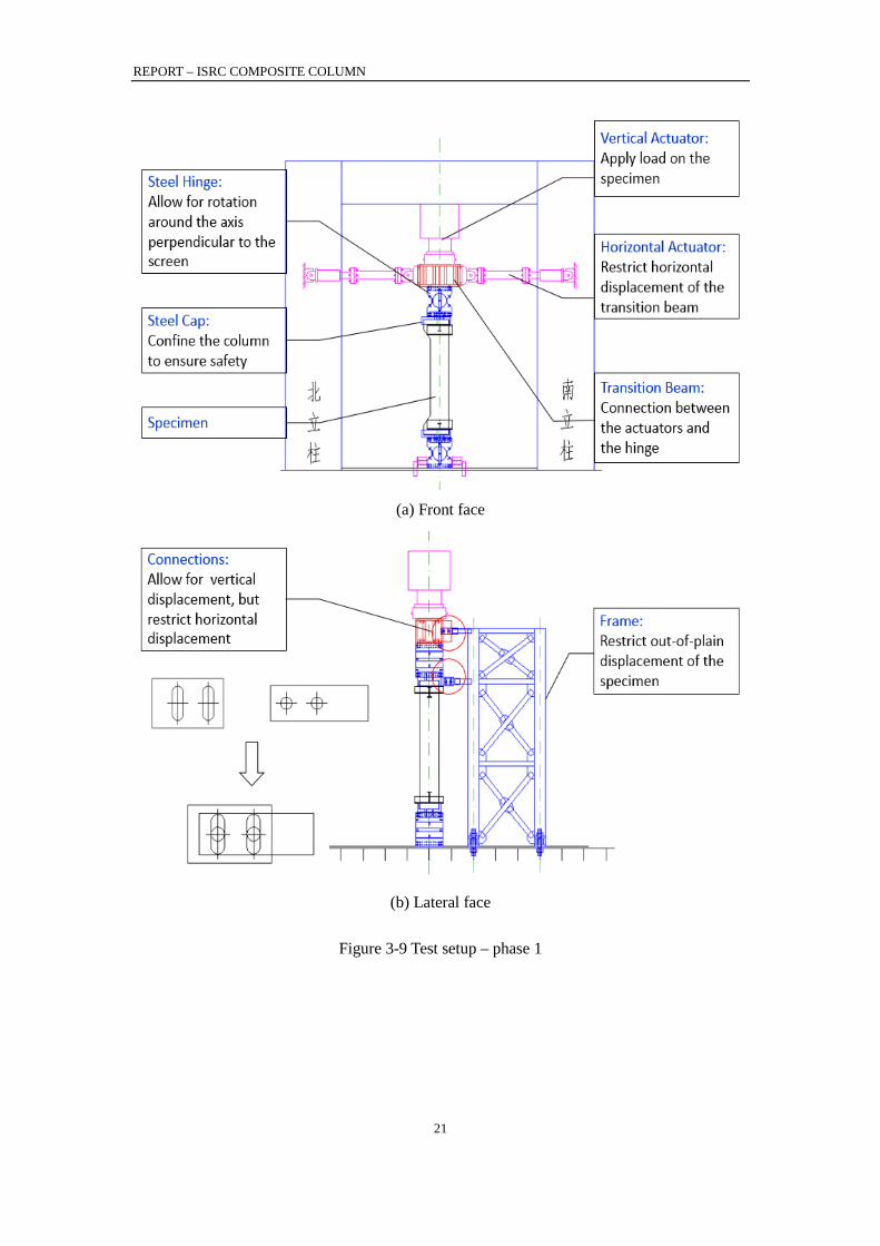
REPORT – ISRC COMPOSITE COLUMN
21
(a) Front face
(b) Lateral face
Figure 3-9 Test setup – phase 1
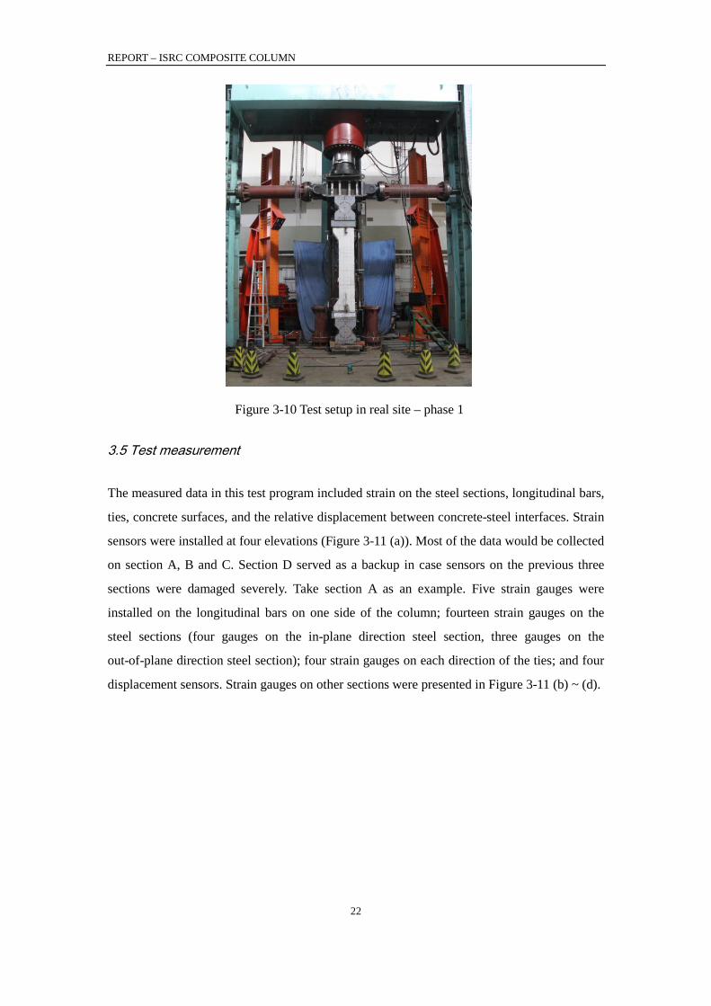
REPORT – ISRC COMPOSITE COLUMN
22
Figure 3-10 Test setup in real site – phase 1
3.5 Test measurement
The measured data in this test program included strain on the steel sections, longitudinal bars,
ties, concrete surfaces, and the relative displacement between concrete-steel interfaces. Strain
sensors were installed at four elevations (Figure 3-11 (a)). Most of the data would be collected
on section A, B and C. Section D served as a backup in case sensors on the previous three
sections were damaged severely. Take section A as an example. Five strain gauges were
installed on the longitudinal bars on one side of the column; fourteen strain gauges on the
steel sections (four gauges on the in-plane direction steel section, three gauges on the
out-of-plane direction steel section); four strain gauges on each direction of the ties; and four
displacement sensors. Strain gauges on other sections were presented in Figure 3-11 (b) ~ (d).

REPORT – ISRC COMPOSITE COLUMN
23
(a) Elevation of critical planes
(b) Section A
(c) Section B (C)
(d) Section D
Figure 3-11 Sensors layout - phase 1
3.6 General behavior of static specimens
3.6.1 Pure axial specimens (E00-1/E00-2)
The two pure axial loaded specimens failed in a same pattern, and the phenomena of these
two specimens were very similar to each other. Therefore, take E00-1 as an example:

REPORT – ISRC COMPOSITE COLUMN
24
(a) Vertical cracks occurred on the front face of the column when axial load reached 9000kN
(53% of the ultimate capacity). The crack was located in the middle of the front face,
where concrete cover was relative small because a longitudinal bar was placed right
inside the concrete at this location. No visible horizontal deflection was detected.
Figure 3-12 Specimen E00-1 at 9000kN
(b) The length of the crack increased with the axial load, but no other cracks developed
besides the first one. At axial load level 12000kN, the crack stopped growing. Similar
phenomena could be observed on other faces of the column.
Figure 3-13 Specimen E00-1 at 12000kN
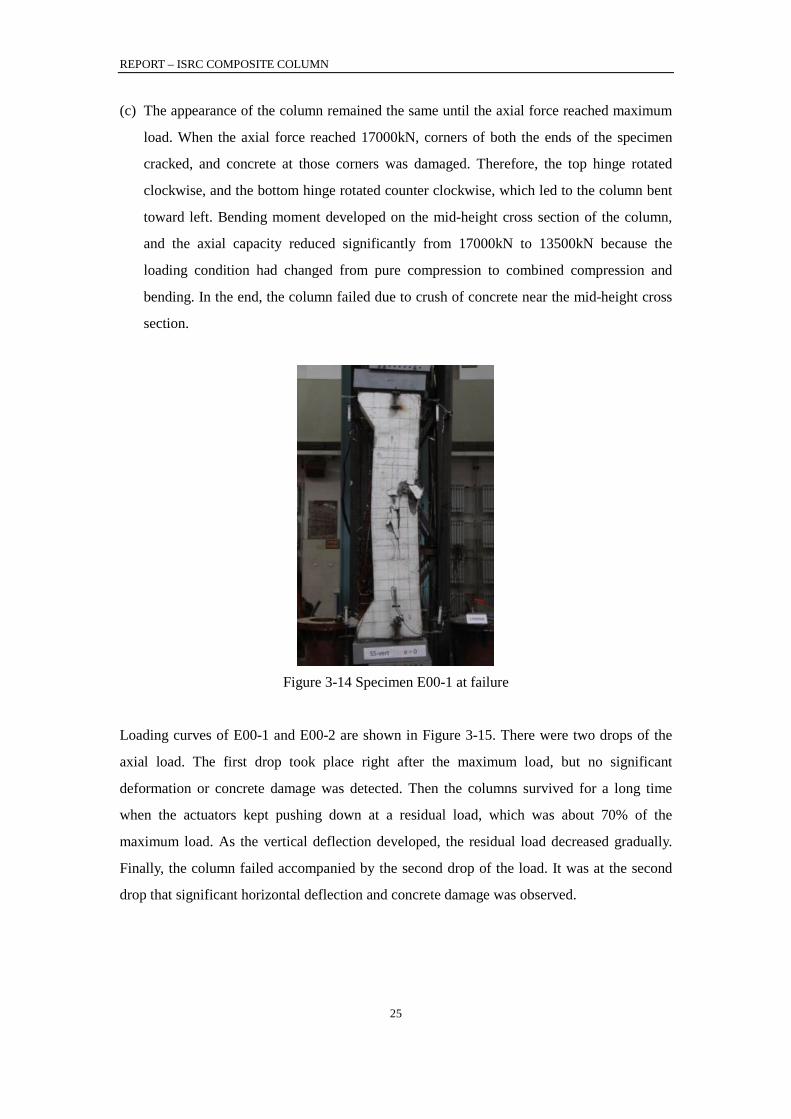
REPORT – ISRC COMPOSITE COLUMN
25
(c) The appearance of the column remained the same until the axial force reached maximum
load. When the axial force reached 17000kN, corners of both the ends of the specimen
cracked, and concrete at those corners was damaged. Therefore, the top hinge rotated
clockwise, and the bottom hinge rotated counter clockwise, which led to the column bent
toward left. Bending moment developed on the mid-height cross section of the column,
and the axial capacity reduced significantly from 17000kN to 13500kN because the
loading condition had changed from pure compression to combined compression and
bending. In the end, the column failed due to crush of concrete near the mid-height cross
section.
Figure 3-14 Specimen E00-1 at failure
Loading curves of E00-1 and E00-2 are shown in Figure 3-15. There were two drops of the
axial load. The first drop took place right after the maximum load, but no significant
deformation or concrete damage was detected. Then the columns survived for a long time
when the actuators kept pushing down at a residual load, which was about 70% of the
maximum load. As the vertical deflection developed, the residual load decreased gradually.
Finally, the column failed accompanied by the second drop of the load. It was at the second
drop that significant horizontal deflection and concrete damage was observed.
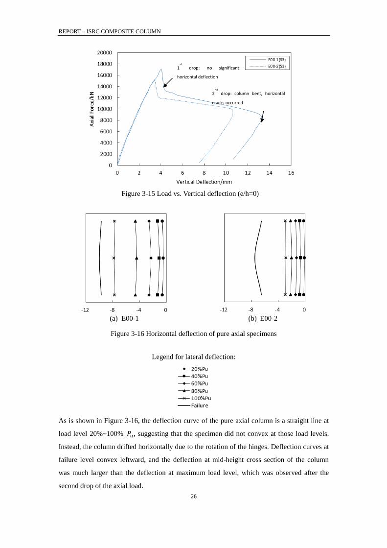
REPORT – ISRC COMPOSITE COLUMN
26
Figure 3-15 Load vs. Vertical deflection (e/h=0)
(a) E00-1
(b) E00-2
Figure 3-16 Horizontal deflection of pure axial specimens
Legend for lateral deflection:
As is shown in Figure 3-16, the deflection curve of the pure axial column is a straight line at
load level 20%~100% 𝑃𝑢, suggesting that the specimen did not convex at those load levels.
Instead, the column drifted horizontally due to the rotation of the hinges. Deflection curves at
failure level convex leftward, and the deflection at mid-height cross section of the column
was much larger than the deflection at maximum load level, which was observed after the
second drop of the axial load.
1st
drop: no significant
horizontal deflection
2nd
drop: column bent, horizontal
cracks occurred
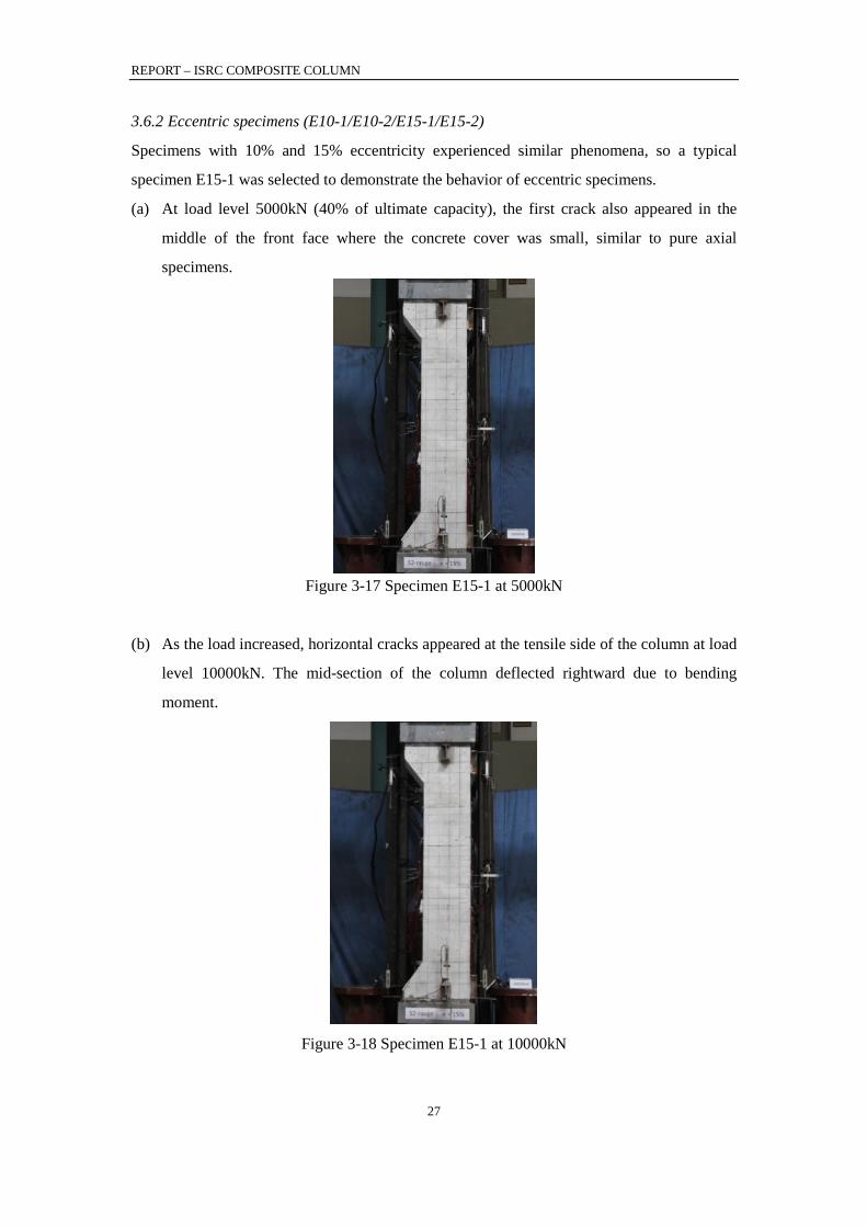
REPORT – ISRC COMPOSITE COLUMN
27
3.6.2 Eccentric specimens (E10-1/E10-2/E15-1/E15-2)
Specimens with 10% and 15% eccentricity experienced similar phenomena, so a typical
specimen E15-1 was selected to demonstrate the behavior of eccentric specimens.
(a) At load level 5000kN (40% of ultimate capacity), the first crack also appeared in the
middle of the front face where the concrete cover was small, similar to pure axial
specimens.
Figure 3-17 Specimen E15-1 at 5000kN
(b) As the load increased, horizontal cracks appeared at the tensile side of the column at load
level 10000kN. The mid-section of the column deflected rightward due to bending
moment.
Figure 3-18 Specimen E15-1 at 10000kN
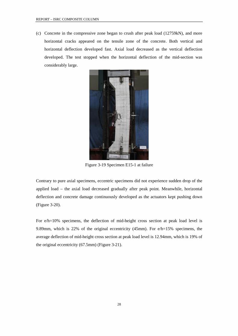
REPORT – ISRC COMPOSITE COLUMN
28
(c) Concrete in the compressive zone began to crush after peak load (12759kN), and more
horizontal cracks appeared on the tensile zone of the concrete. Both vertical and
horizontal deflection developed fast. Axial load decreased as the vertical deflection
developed. The test stopped when the horizontal deflection of the mid-section was
considerably large.
Figure 3-19 Specimen E15-1 at failure
Contrary to pure axial specimens, eccentric specimens did not experience sudden drop of the
applied load – the axial load decreased gradually after peak point. Meanwhile, horizontal
deflection and concrete damage continuously developed as the actuators kept pushing down
(Figure 3-20).
For e/h=10% specimens, the deflection of mid-height cross section at peak load level is
9.89mm, which is 22% of the original eccentricity (45mm). For e/h=15% specimens, the
average deflection of mid-height cross section at peak load level is 12.94mm, which is 19% of
the original eccentricity (67.5mm) (Figure 3-21).
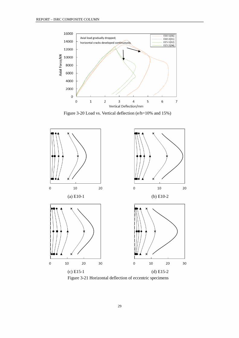
REPORT – ISRC COMPOSITE COLUMN
29
Figure 3-20 Load vs. Vertical deflection (e/h=10% and 15%)
(a) E10-1
(b) E10-2
(c) E15-1
(d) E15-2
Figure 3-21 Horizontal deflection of eccentric specimens
Axial load gradually dropped; horizontal cracks developed continuously.

REPORT – ISRC COMPOSITE COLUMN
30
3.6.3 Summary of failure modes and capacities
Table 3-5 and Table 3-6 summarize the capacities and horizontal deflections of the specimens
in phase 1. The percentiles in the brackets are the ratios of measured horizontal deflections to
the initial eccentricities of the column. It is clear that the actual eccentricities became larger
because of the second order effect.
Table 3-5 Capacities for phase 1 test
Specimen ID Capacity Pu/kN Vertical deflection at Pu /mm
E00-1 17082 4.07
E00-2 15325 3.43
E10-1 14360 3.55
E10-2 13231 3.46
E15-1 12041 2.79
E15-2 12759 2.70
Table 3-6 Horizontal deflections for phase 1 test
Specimen Deflection at peak load Deflection at failure
Average Average
E00-1 -7.78(-) -5.31(-)
-9.98 (-) -8.73(-)
E00-2 -2.84(-) -7.47(-)
E10-1 10.97(24.38%) 11.96(26.58%)
14.26(31.69%) 16.76(37.24%)
E10-2 12.95(28.78%) 19.25(42.78%)
E15-1 20.15(31.29%) 16.21(24.01%)
25.82(38.25%) 25.73 (38.11%)
E15-2 12.30(18.22%) 25.63(37.97%)
The failure patterns of all of the six specimens were combined compression and bending. The
pure axial specimens bent toward the bracket direction, while the eccentric specimens bent
toward the other direction. Both compressive cracks and tensile cracks could be detected on
the concrete surfaces. In the end, the specimens failed due to concrete crush in the middle of
the specimens (Figure 3-22).

REPORT – ISRC COMPOSITE COLUMN
31
(a) Specimen E00-1
(b) Specimen E00-2
(c) Specimen E10-1
(d) Specimen E10-2
(e) Specimen E15-1
(f) Specimen E15-2
Figure 3-22 Failure mode phase 1 specimens
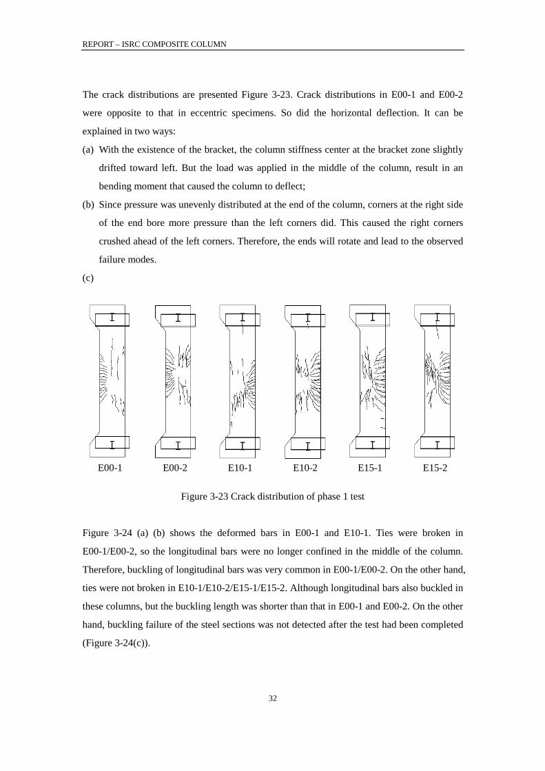
REPORT – ISRC COMPOSITE COLUMN
32
The crack distributions are presented Figure 3-23. Crack distributions in E00-1 and E00-2
were opposite to that in eccentric specimens. So did the horizontal deflection. It can be
explained in two ways:
(a) With the existence of the bracket, the column stiffness center at the bracket zone slightly
drifted toward left. But the load was applied in the middle of the column, result in an
bending moment that caused the column to deflect;
(b) Since pressure was unevenly distributed at the end of the column, corners at the right side
of the end bore more pressure than the left corners did. This caused the right corners
crushed ahead of the left corners. Therefore, the ends will rotate and lead to the observed
failure modes.
(c)
E00-1 E00-2 E10-1 E10-2 E15-1 E15-2
Figure 3-23 Crack distribution of phase 1 test
Figure 3-24 (a) (b) shows the deformed bars in E00-1 and E10-1. Ties were broken in
E00-1/E00-2, so the longitudinal bars were no longer confined in the middle of the column.
Therefore, buckling of longitudinal bars was very common in E00-1/E00-2. On the other hand,
ties were not broken in E10-1/E10-2/E15-1/E15-2. Although longitudinal bars also buckled in
these columns, but the buckling length was shorter than that in E00-1 and E00-2. On the other
hand, buckling failure of the steel sections was not detected after the test had been completed
(Figure 3-24(c)).
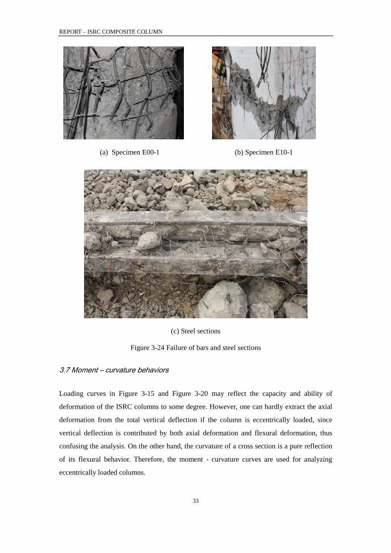
REPORT – ISRC COMPOSITE COLUMN
33
(a) Specimen E00-1
(b) Specimen E10-1
(c) Steel sections
Figure 3-24 Failure of bars and steel sections
3.7 Moment – curvature behaviors
Loading curves in Figure 3-15 and Figure 3-20 may reflect the capacity and ability of
deformation of the ISRC columns to some degree. However, one can hardly extract the axial
deformation from the total vertical deflection if the column is eccentrically loaded, since
vertical deflection is contributed by both axial deformation and flexural deformation, thus
confusing the analysis. On the other hand, the curvature of a cross section is a pure reflection
of its flexural behavior. Therefore, the moment - curvature curves are used for analyzing
eccentrically loaded columns.
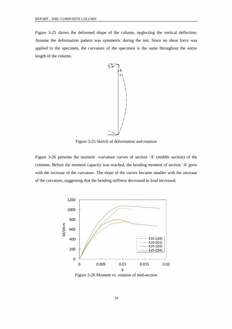
REPORT – ISRC COMPOSITE COLUMN
34
Figure 3-25 shows the deformed shape of the column, neglecting the vertical deflection.
Assume the deformation pattern was symmetric during the test. Since no shear force was
applied to the specimen, the curvature of the specimen is the same throughout the entire
length of the column.
Figure 3-25 Sketch of deformation and rotation
Figure 3-26 presents the moment –curvature curves of section ‘A’ (middle section) of the
columns. Before the moment capacity was reached, the bending moment of section ‘A’ grew
with the increase of the curvature. The slope of the curves became smaller with the increase
of the curvature, suggesting that the bending stiffness decreased as load increased.
Figure 3-26 Moment vs. rotation of mid-section

REPORT – ISRC COMPOSITE COLUMN
35
It can be concluded that the ductility of the column, in the perspective of moment versus
curvature, was good for ISRC columns with eccentricity ratio no more than 15%. Axial load
dropped rapidly as the vertical deflection increased, but the bending moment on the
mid-height cross section barely dropped. This is because the axial load and the lateral
deflection contribute to the bending moment on the mid-height cross section (M = P(e + δ)).
When the axial load began to drop after the maximum capacity, the horizontal deflection grew
rapidly, which counteracts with the decrease of the axial load.
3.8 Interaction curve
The interaction curves of phase 1 specimens are shown in Figure 3-27; results given by
Plumier et al are also shown in the figure (Simple Model). Confinement effect had been
considered when calculating the interaction curves, but it still underestimated the capacity of
the columns when the eccentricity ratio was more than 10%, which demonstrated that the
confinement effect was beyond expectation. In fact, the middle part of the concrete was
confined, not only by ties, but also by four steel sections. Limited studies have been
conducted to investigate the confinement effect provided by the steel sections.
Because of the second order effect, the actual eccentricity ratios got larger as load level
increased. The actual eccentricities of the four specimens are listed in Table 3-7. The
maximum eccentricity ratio of specimen E15-1 almost reached 20% due to the slenderness
effect.
Figure 3-27 Interactive curve of phase 1 specimens

REPORT – ISRC COMPOSITE COLUMN
36
Table 3-7 Actual eccentricities of phase 1specimens Specimen ID Original eccentricity Actual eccentricity
E10-1 10%
12.4%
E10-2 12.9%
E15-1 15%
19.9%
E15-2 17.9%
3.9 Cross-section strain distribution
The mid-height cross section was selected to be the critical section to study strain
development of the specimens.
Note that the horizontal axis of the strain curve in Figure 3-29~Figure 3-31 is defined as
follows. Assume the bracket is on the left, the distance between a strain sensor and the left
bound of the column is defined as ‘relative position’, regardless of the position in the
perpendicular direction (Figure 3-28).
Figure 3-28 Relative position of the strain curve
3.9.1 Specimen E00-1/E00-2
Figure 3-29 shows the strain distribution of longitudinal reinforcing bars, steel sections, and
the concrete of specimen E00-2, respectively. At each load level, strains at different relative
positions were nearly the same. Strains of the three materials agreed with each other very well.
The strains of longitudinal bars and steel sections at load level 100%Pu were less than
2000µε, suggesting that longitudinal bars and steel sections remained elastic when the
column reached its maximum capacity.
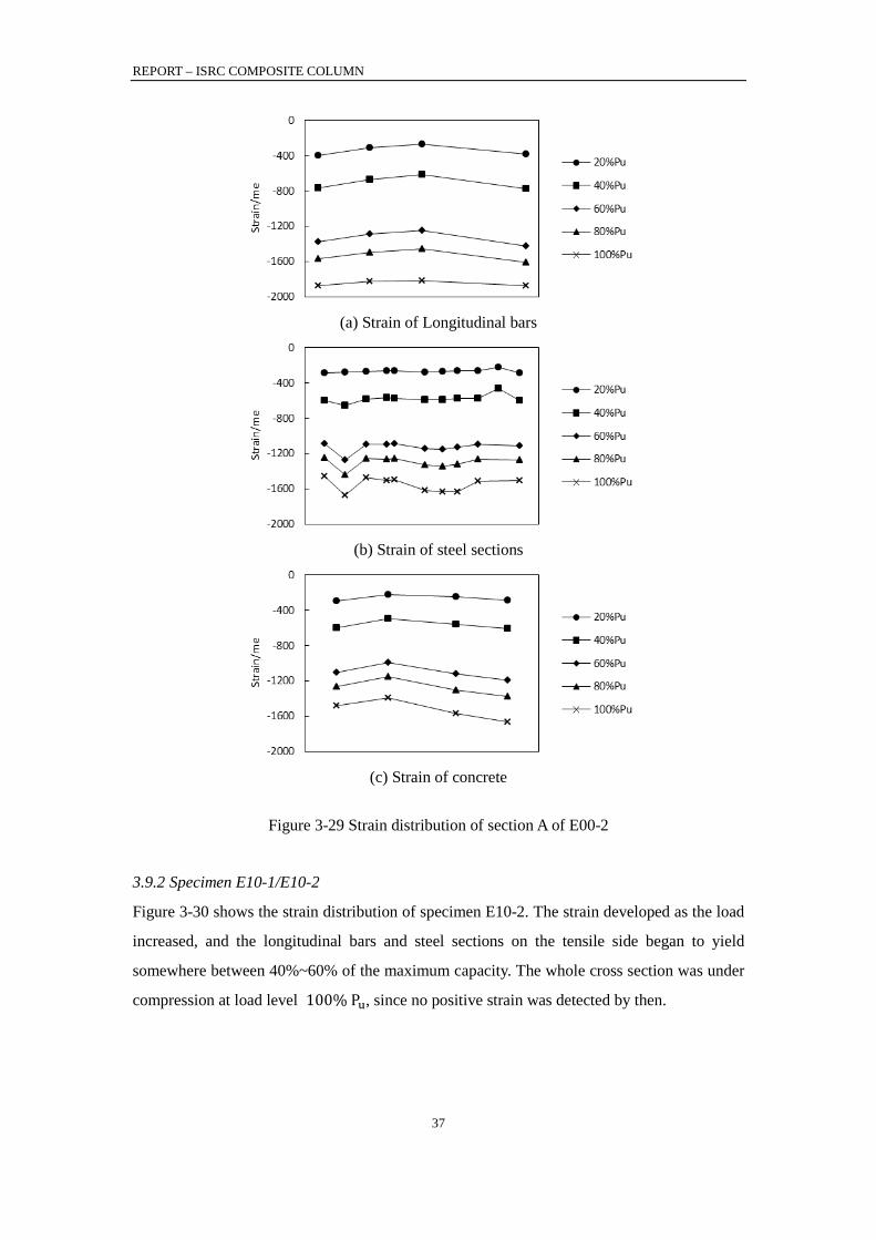
REPORT – ISRC COMPOSITE COLUMN
37
(a) Strain of Longitudinal bars
(b) Strain of steel sections
(c) Strain of concrete
Figure 3-29 Strain distribution of section A of E00-2
3.9.2 Specimen E10-1/E10-2
Figure 3-30 shows the strain distribution of specimen E10-2. The strain developed as the load
increased, and the longitudinal bars and steel sections on the tensile side began to yield
somewhere between 40%~60% of the maximum capacity. The whole cross section was under
compression at load level 100% Pu, since no positive strain was detected by then.
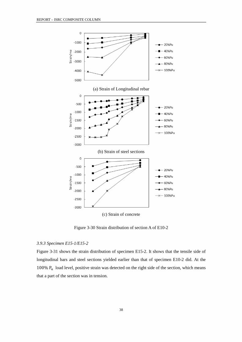
REPORT – ISRC COMPOSITE COLUMN
38
(a) Strain of Longitudinal rebar
(b) Strain of steel sections
(c) Strain of concrete
Figure 3-30 Strain distribution of section A of E10-2
3.9.3 Specimen E15-1/E15-2
Figure 3-31 shows the strain distribution of specimen E15-2. It shows that the tensile side of
longitudinal bars and steel sections yielded earlier than that of specimen E10-2 did. At the
100% Pu load level, positive strain was detected on the right side of the section, which means
that a part of the section was in tension.
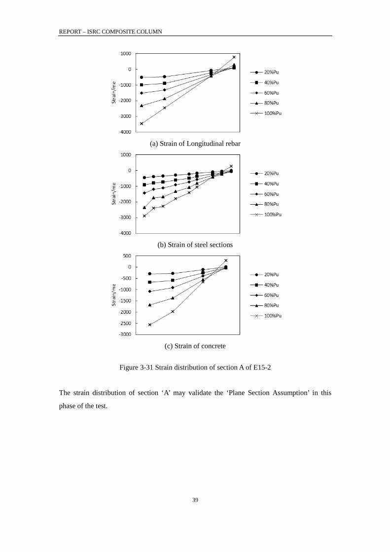
REPORT – ISRC COMPOSITE COLUMN
39
(a) Strain of Longitudinal rebar
(b) Strain of steel sections
(c) Strain of concrete
Figure 3-31 Strain distribution of section A of E15-2
The strain distribution of section ‘A’ may validate the ‘Plane Section Assumption’ in this
phase of the test.

REPORT – ISRC COMPOSITE COLUMN
40
3.10 Stiffness reduction
Both axial and flexural stiffness will decrease as load level increases. In the US codes
(ACI318) and Eurocode4 (2004), the first order analysis of a structure should be calculated
based on the reduced stiffness where sway frame or non-sway frame is to be designed. This
section of the report studies the rules of stiffness reduction for both pure axial and
eccentrically loaded columns.
3.10.1 Pure axial specimens (E00-1/E00-2)
The axial rigidity EA of pure axial columns was reduced due to the concrete cracking,
leading to the reduction of stiffness of the entire column. There are two ways of calculating
the reduction factor (Rkc ): (a) ratio of reduced axial stiffness to the original axial stiffness of
the whole section, which is also called the ACI 318 method; and (b) ratio of reduced axial
stiffness to the original axial stiffness of the concrete, which is called the EC 4 method.
In method (a), Rk can be defined as:
( )c p pck c s sE A E A E AP R ε+ += (3.1)
In method (b), Rk can be defined as:
( )ck c c s s p pR E A E AP E A ε+ += (3.2)
where:
P – Axial load
ε – Equivalent average axial stain of the column
EcAc – Original axial stiffness of concrete
EsAs – Original axial stiffness of longitudinal rebar
EpAp – Original axial stiffness of steel sections
(a) ACI 318 method
(b) EC 4 method
Figure 3-32 Axial stiffness reduction Rkc
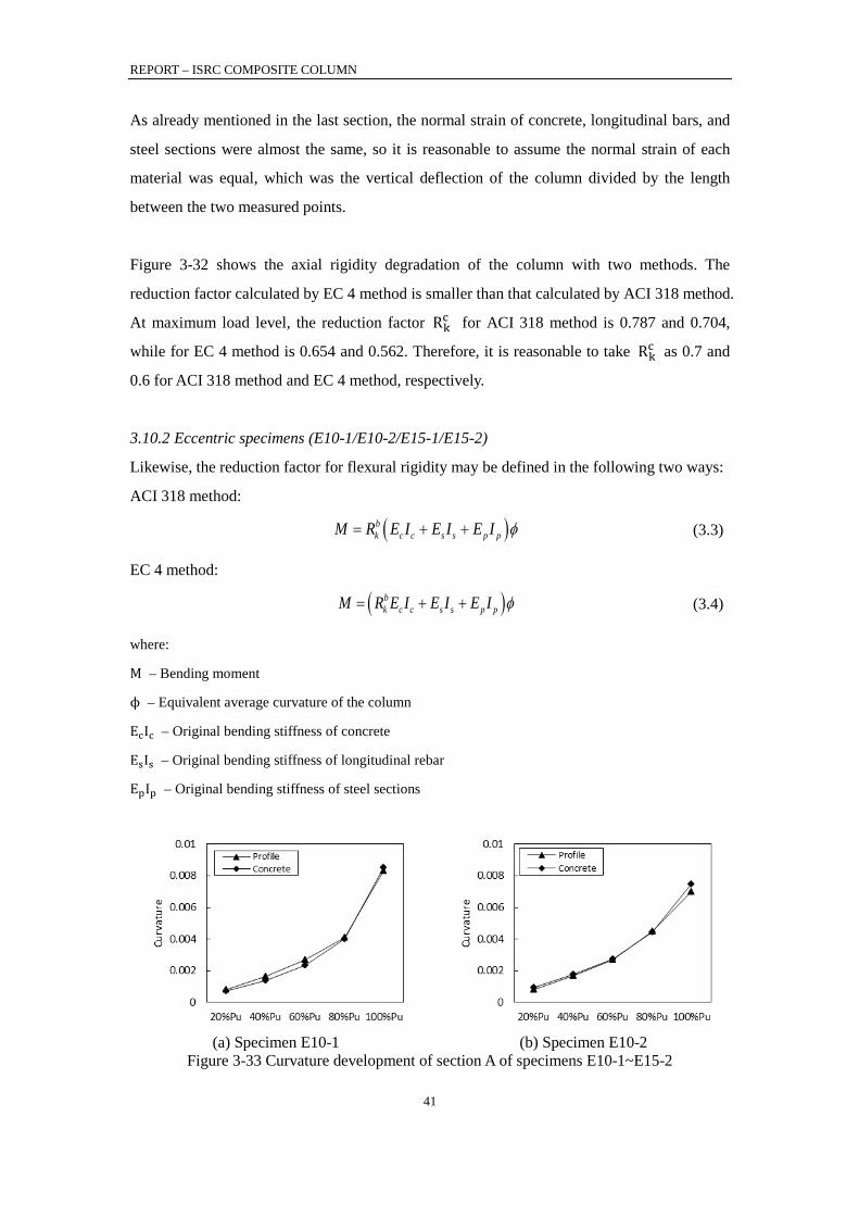
REPORT – ISRC COMPOSITE COLUMN
41
As already mentioned in the last section, the normal strain of concrete, longitudinal bars, and
steel sections were almost the same, so it is reasonable to assume the normal strain of each
material was equal, which was the vertical deflection of the column divided by the length
between the two measured points.
Figure 3-32 shows the axial rigidity degradation of the column with two methods. The
reduction factor calculated by EC 4 method is smaller than that calculated by ACI 318 method.
At maximum load level, the reduction factor Rkc for ACI 318 method is 0.787 and 0.704,
while for EC 4 method is 0.654 and 0.562. Therefore, it is reasonable to take Rkc as 0.7 and
0.6 for ACI 318 method and EC 4 method, respectively.
3.10.2 Eccentric specimens (E10-1/E10-2/E15-1/E15-2)
Likewise, the reduction factor for flexural rigidity may be defined in the following two ways:
ACI 318 method:
( )c p pbk c s sE I E I E IM R φ+ += (3.3)
EC 4 method:
( )bk c c s s p pR E I E IM E I φ+ += (3.4)
where:
M – Bending moment
ϕ – Equivalent average curvature of the column
EcIc – Original bending stiffness of concrete
EsIs – Original bending stiffness of longitudinal rebar
EpIp – Original bending stiffness of steel sections
(a) Specimen E10-1
(b) Specimen E10-2
Figure 3-33 Curvature development of section A of specimens E10-1~E15-2
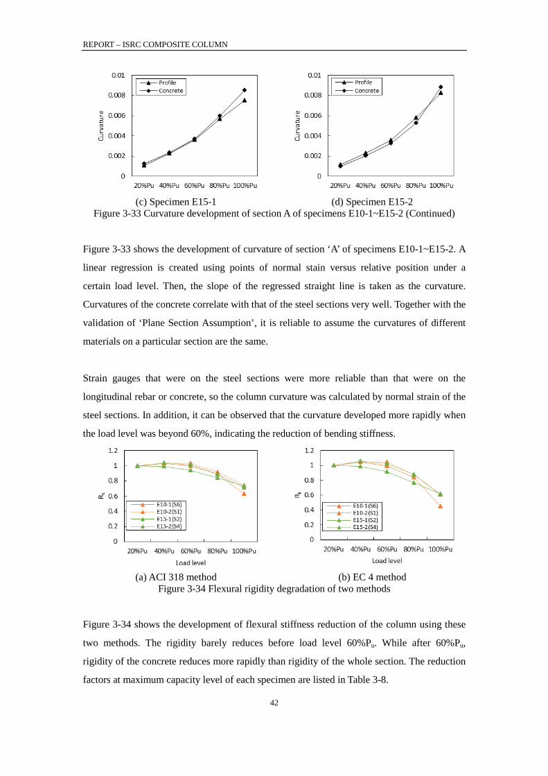
REPORT – ISRC COMPOSITE COLUMN
42
(c) Specimen E15-1
(d) Specimen E15-2
Figure 3-33 Curvature development of section A of specimens E10-1~E15-2 (Continued)
Figure 3-33 shows the development of curvature of section ‘A’ of specimens E10-1~E15-2. A
linear regression is created using points of normal stain versus relative position under a
certain load level. Then, the slope of the regressed straight line is taken as the curvature.
Curvatures of the concrete correlate with that of the steel sections very well. Together with the
validation of ‘Plane Section Assumption’, it is reliable to assume the curvatures of different
materials on a particular section are the same.
Strain gauges that were on the steel sections were more reliable than that were on the
longitudinal rebar or concrete, so the column curvature was calculated by normal strain of the
steel sections. In addition, it can be observed that the curvature developed more rapidly when
the load level was beyond 60%, indicating the reduction of bending stiffness.
(a) ACI 318 method
(b) EC 4 method
Figure 3-34 Flexural rigidity degradation of two methods
Figure 3-34 shows the development of flexural stiffness reduction of the column using these
two methods. The rigidity barely reduces before load level 60%Pu. While after 60%Pu,
rigidity of the concrete reduces more rapidly than rigidity of the whole section. The reduction
factors at maximum capacity level of each specimen are listed in Table 3-8.

REPORT – ISRC COMPOSITE COLUMN
43
Table 3-8 Stiffness reduction Rkb factor of E10-1~E15-2
Specimen ID ACI 318 method EC 4 method
E10-1 0.629 0.448
E10-2 0.738 0.607
E15-1 0.736 0.619
E15-2 0.709 0.614
In conclusion, for both axial and flexural behavior, the reduction factor (Rk) can always be
taken as 0.7 for the ACI 318 method, and 0.6 for the EC 4 method.
3.11 Interface slip
3.11.1 Pure axial specimens (E00-1/E00-2)
Figure 3-35 presents the slip on concrete-steel interface of specimen E00-1. A negative slip
means the concrete is compressed more than the steel section is. As concrete damage grew
with the increase of load level, the strain at some local points on the concrete was larger than
that on the steel sections. Therefore, the cumulated strain difference resulted in relative slips
on the interface. Under pure compression, the slip was very small. In this test, the maximum
slip was less than 0.04mm.
Figure 3-35 Interface slip of E00-1
3.11.2 Eccentric specimens (E10-1/E10-2/E15-1/E15-2)
Figure 3-36 and Figure 3-37 shows the interface slip of E10-1 and E15-1. It is shown that the
concrete-steel interface began to slip at load level 0.1~0.4, and the maximum slip increased as
the eccentricities. For e/h=10%, the maximum slip was 2.22mm and 1.19mm for section B
and section C respectively; for e/h=15%, the maximum slip was 5.22mm and 4.43mm for
section A and section B respectively (Note: for e/h=15%, the actual slip may exceed the rage
of the displacement sensors).
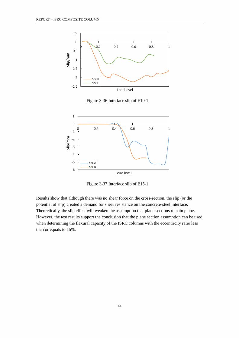
REPORT – ISRC COMPOSITE COLUMN
44
Figure 3-36 Interface slip of E10-1
Figure 3-37 Interface slip of E15-1
Results show that although there was no shear force on the cross-section, the slip (or the potential of slip) created a demand for shear resistance on the concrete-steel interface. Theoretically, the slip effect will weaken the assumption that plane sections remain plane. However, the test results support the conclusion that the plane section assumption can be used when determining the flexural capacity of the ISRC columns with the eccentricity ratio less than or equals to 15%.
REPORT – ISRC COMPOSITE COLUMN
45
3.12 Summary of phase1 test
1) The maximum applied load of the ISRC column decreases as eccentricity increases. The
pure axial column experiences drops of axial load twice: one right after the peak load, and
the other right before failure. For eccentric specimens, the axial loads decrease gradually
after they reach peak loads.
2) The moment - curvature curves of the mid-height cross section shows a good sense of
ductility.
3) The ‘Plane Section Assumption’ can be verified in the test when the column is subjected
to combined compression and bending with eccentricity ratio less than or equal to 15%.
Curvatures of the concrete and the steel section are nearly the same during the loading
process.
4) The capacity of the ISRC columns corresponds with the theoretical interaction curve well,
which is calculated by fiber model based on ‘Plane Section Assumption’.
5) Both axial and flexural rigidity decreases as load increases. The stiffness reduction factor
Rk at failure level may be taken as 0.7 for both axial and flexural rigidity if the ACI 318
method (method ‘a’) is applied or 0.6 if the EC4 method (method ‘b’) is applied.
6) Although slip is detected on the concrete-steel interfaces, it does not affect the ultimate
capacity of the specimens.
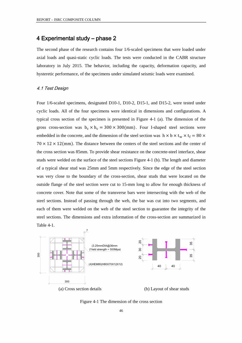
REPORT – ISRC COMPOSITE COLUMN
46
4 Experimental study – phase 2
The second phase of the research contains four 1/6-scaled specimens that were loaded under
axial loads and quasi-static cyclic loads. The tests were conducted in the CABR structure
laboratory in July 2015. The behavior, including the capacity, deformation capacity, and
hysteretic performance, of the specimens under simulated seismic loads were examined.
4.1 Test Design
Four 1/6-scaled specimens, designated D10-1, D10-2, D15-1, and D15-2, were tested under
cyclic loads. All of the four specimens were identical in dimensions and configurations. A
typical cross section of the specimen is presented in Figure 4-1 (a). The dimension of the
gross cross-section was bc × hc = 300 × 300(mm) . Four I-shaped steel sections were
embedded in the concrete, and the dimension of the steel section was h × b × tw × tf = 80 ×
70 × 12 × 12(mm). The distance between the centers of the steel sections and the center of
the cross section was 85mm. To provide shear resistance on the concrete-steel interface, shear
studs were welded on the surface of the steel sections Figure 4-1 (b). The length and diameter
of a typical shear stud was 25mm and 5mm respectively. Since the edge of the steel section
was very close to the boundary of the cross-section, shear studs that were located on the
outside flange of the steel section were cut to 15-mm long to allow for enough thickness of
concrete cover. Note that some of the transverse bars were intersecting with the web of the
steel sections. Instead of passing through the web, the bar was cut into two segments, and
each of them were welded on the web of the steel section to guarantee the integrity of the
steel sections. The dimensions and extra information of the cross-section are summarized in
Table 4-1.
300
300
7
(3.25mmDIA@36mm (Yield strength = 500Mpa)
(4)HEM80(H80X70X12X12)
(a) Cross section details
4040
353520
3020
(b) Layout of shear studs
Figure 4-1 The dimension of the cross section
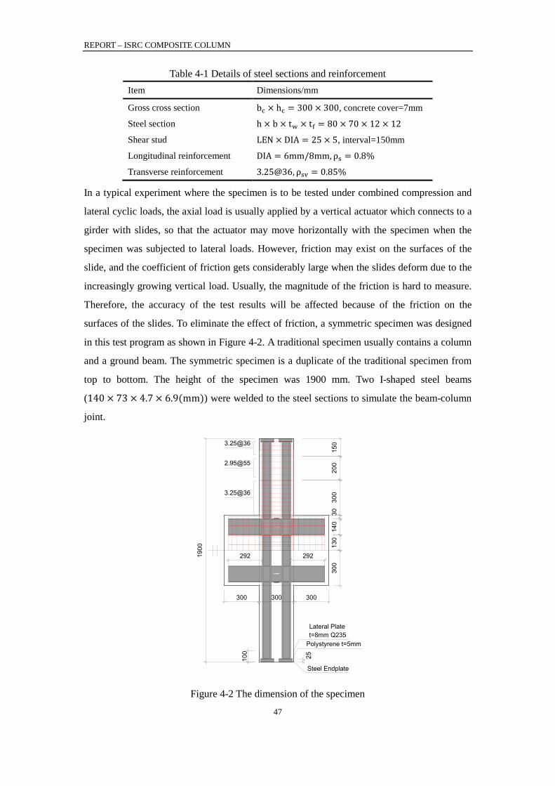
REPORT – ISRC COMPOSITE COLUMN
47
Table 4-1 Details of steel sections and reinforcement Item Dimensions/mm
Gross cross section bc × hc = 300 × 300, concrete cover=7mm
Steel section h × b × tw × tf = 80 × 70 × 12 × 12
Shear stud LEN × DIA = 25 × 5, interval=150mm
Longitudinal reinforcement DIA = 6mm/8mm, ρs = 0.8%
Transverse reinforcement 3.25@36, ρsv = 0.85%
In a typical experiment where the specimen is to be tested under combined compression and
lateral cyclic loads, the axial load is usually applied by a vertical actuator which connects to a
girder with slides, so that the actuator may move horizontally with the specimen when the
specimen was subjected to lateral loads. However, friction may exist on the surfaces of the
slide, and the coefficient of friction gets considerably large when the slides deform due to the
increasingly growing vertical load. Usually, the magnitude of the friction is hard to measure.
Therefore, the accuracy of the test results will be affected because of the friction on the
surfaces of the slides. To eliminate the effect of friction, a symmetric specimen was designed
in this test program as shown in Figure 4-2. A traditional specimen usually contains a column
and a ground beam. The symmetric specimen is a duplicate of the traditional specimen from
top to bottom. The height of the specimen was 1900 mm. Two I-shaped steel beams
(140 × 73 × 4.7 × 6.9(mm)) were welded to the steel sections to simulate the beam-column
joint.
3.25@36
2.95@55
3.25@36
100
Lateral Platet=8mm Q235
Polystyrene t=5mm
Steel Endplate
130
140
292 292
300300 300
300
25
1900
3030
020
015
0
Figure 4-2 The dimension of the specimen
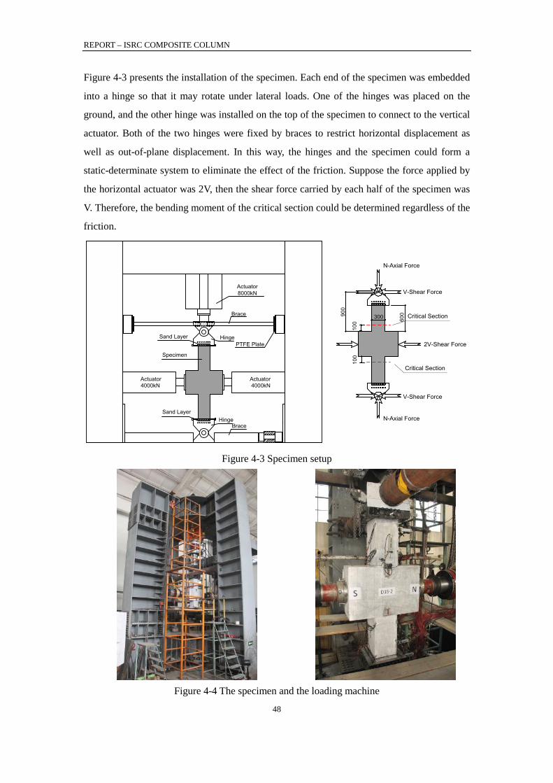
REPORT – ISRC COMPOSITE COLUMN
48
Figure 4-3 presents the installation of the specimen. Each end of the specimen was embedded
into a hinge so that it may rotate under lateral loads. One of the hinges was placed on the
ground, and the other hinge was installed on the top of the specimen to connect to the vertical
actuator. Both of the two hinges were fixed by braces to restrict horizontal displacement as
well as out-of-plane displacement. In this way, the hinges and the specimen could form a
static-determinate system to eliminate the effect of the friction. Suppose the force applied by
the horizontal actuator was 2V, then the shear force carried by each half of the specimen was
V. Therefore, the bending moment of the critical section could be determined regardless of the
friction.
PTFE PlateHinge
Brace
BraceHinge
Sand Layer
Sand Layer
Specimen
4000kNActuator
4000kNActuator
Actuator8000kN
60030090
02V-Shear Force
N-Axial Force
V-Shear Force
V-Shear Force
N-Axial Force
100
100
Critical Section
Critical Section
Figure 4-3 Specimen setup
Figure 4-4 The specimen and the loading machine
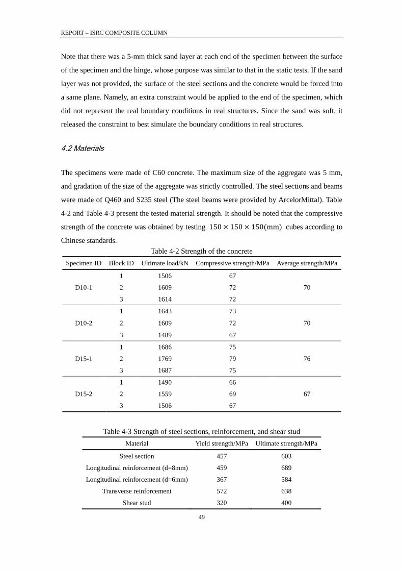
REPORT – ISRC COMPOSITE COLUMN
49
Note that there was a 5-mm thick sand layer at each end of the specimen between the surface
of the specimen and the hinge, whose purpose was similar to that in the static tests. If the sand
layer was not provided, the surface of the steel sections and the concrete would be forced into
a same plane. Namely, an extra constraint would be applied to the end of the specimen, which
did not represent the real boundary conditions in real structures. Since the sand was soft, it
released the constraint to best simulate the boundary conditions in real structures.
4.2 Materials
The specimens were made of C60 concrete. The maximum size of the aggregate was 5 mm,
and gradation of the size of the aggregate was strictly controlled. The steel sections and beams
were made of Q460 and S235 steel (The steel beams were provided by ArcelorMittal). Table
4-2 and Table 4-3 present the tested material strength. It should be noted that the compressive
strength of the concrete was obtained by testing 150 × 150 × 150(mm) cubes according to
Chinese standards. Table 4-2 Strength of the concrete
Specimen ID Block ID Ultimate load/kN Compressive strength/MPa Average strength/MPa
D10-1
1 1506 67
70 2 1609 72
3 1614 72
D10-2
1 1643 73
70 2 1609 72
3 1489 67
D15-1
1 1686 75
76 2 1769 79
3 1687 75
D15-2
1 1490 66
67 2 1559 69
3 1506 67
Table 4-3 Strength of steel sections, reinforcement, and shear stud
Material Yield strength/MPa Ultimate strength/MPa
Steel section 457 603
Longitudinal reinforcement (d=8mm) 459 689
Longitudinal reinforcement (d=6mm) 367 584
Transverse reinforcement 572 638
Shear stud 320 400

REPORT – ISRC COMPOSITE COLUMN
50
Shown in Figure 4-5 are the fabrications of the specimen. The concrete was placed in June
2015 when the temperature was about 25°C~30°C.
Figure 4-5 Fabrication of the specimen
4.3 Loading protocol
In real structures, the axial force and shear force in a column may vary with the intensity of
the earthquake, so a constant vertical load is not appropriate in quasi-static tests. Therefore, a
two-phase loading protocol was proposed to simulate the seismic reaction of a column under
earthquakes. During stop 1, only axial load was applied to the specimen. The target axial load
N0 in step 1 represented the gravity load in a structure, and it was determined as follows:
01.25 0.7Nc c p p
NA f A f
µ = =+
(4.1)
where µN is the axial compression ratio of the specimen, defined as the axial force divided
by the axial capacity of the column; Ac and Ap are the area of the concrete and steel
sections respectively; fc is the specified design axial compressive strength of C60 concrete
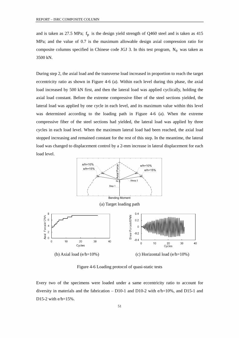
REPORT – ISRC COMPOSITE COLUMN
51
and is taken as 27.5 MPa; fp is the design yield strength of Q460 steel and is taken as 415
MPa; and the value of 0.7 is the maximum allowable design axial compression ratio for
composite columns specified in Chinese code JGJ 3. In this test program, N0 was taken as
3500 kN.
During step 2, the axial load and the transverse load increased in proportion to reach the target
eccentricity ratio as shown in Figure 4-6 (a). Within each level during this phase, the axial
load increased by 500 kN first, and then the lateral load was applied cyclically, holding the
axial load constant. Before the extreme compressive fiber of the steel sections yielded, the
lateral load was applied by one cycle in each level, and its maximum value within this level
was determined according to the loading path in Figure 4-6 (a). When the extreme
compressive fiber of the steel sections had yielded, the lateral load was applied by three
cycles in each load level. When the maximum lateral load had been reached, the axial load
stopped increasing and remained constant for the rest of this step. In the meantime, the lateral
load was changed to displacement control by a 2-mm increase in lateral displacement for each
load level.
e/h=15%e/h=10%
e/h=15%e/h=10%
N0
Axia
l For
ce
Bending Moment
Step 1
Steop 2
(a) Target loading path
(b) Axial load (e/h=10%)
(c) Horizontal load (e/h=10%)
Figure 4-6 Loading protocol of quasi-static tests
Every two of the specimens were loaded under a same eccentricity ratio to account for
diversity in materials and the fabrication – D10-1 and D10-2 with e/h=10%, and D15-1 and
D15-2 with e/h=15%.
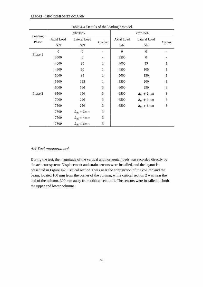
REPORT – ISRC COMPOSITE COLUMN
52
Table 4-4 Details of the loading protocol
Loading
Phase
e/h=10% e/h=15%
Axial Load
/kN
Lateral Load
/kN Cycles
Axial Load
/kN
Lateral Load
/kN Cycles
Phase 1 0 0 - 0 0 -
3500 0 - 3500 0 -
Phase 2
4000 30 1 4000 55 1
4500 60 1 4500 105 1
5000 95 1 5000 150 1
5500 125 1 5500 200 1
6000 160 3 6000 250 3
6500 190 3 6500 Δm + 2mm 3
7000 220 3 6500 Δm + 4mm 3
7500 250 3 6500 Δm + 6mm 3
7500 Δm + 2mm 3
7500 Δm + 4mm 3
7500 Δm + 6mm 3
4.4 Test measurement
During the test, the magnitude of the vertical and horizontal loads was recorded directly by the actuator system. Displacement and strain sensors were installed, and the layout is presented in Figure 4-7. Critical section 1 was near the conjunction of the column and the beam, located 100 mm from the corner of the column, while critical section 2 was near the end of the column, 300 mm away from critical section 1. The sensors were installed on both the upper and lower columns.

REPORT – ISRC COMPOSITE COLUMN
53
(a) Strain sensors on the concrete
(b) Strain sensors on critical section 1
(c) Strain sensors on critical section 2
Figure 4-7 Layout of the strain sensors
4.5 General behavior of the specimens
The sign of horizontal loads and displacements during the test is defined as follows: the
lateral loads and displacements are positive when the left actuator pushes the specimen and
the specimen moves right, and vice versa.
Like the static tests, initial vertical cracks occurred first on the face of the column. Then, the
cracks and the damage of the concrete developed as the load increased. All of the specimens
failed in compression-controlled flexural patterns with severe damage at the corners of the
concrete. At the end of the test, a large amount of vertical cracks and crush of the concrete
were registered. Details of the behavior of the specimens were discussed in the following
sections.
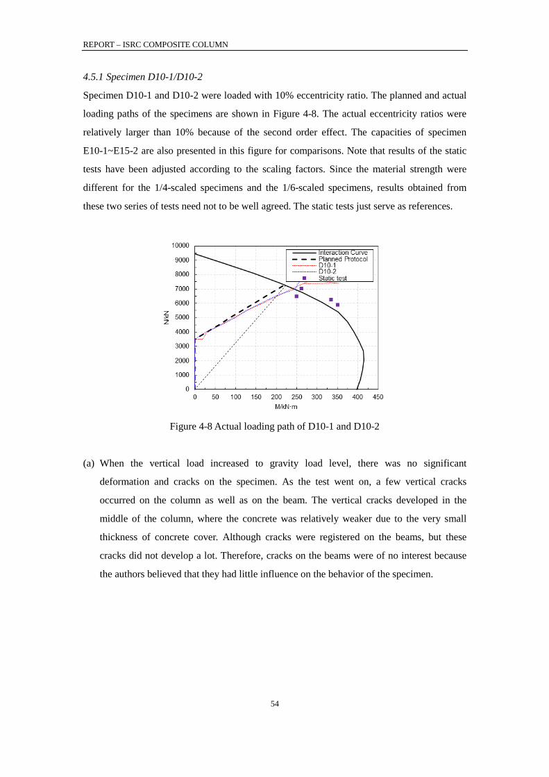
REPORT – ISRC COMPOSITE COLUMN
54
4.5.1 Specimen D10-1/D10-2
Specimen D10-1 and D10-2 were loaded with 10% eccentricity ratio. The planned and actual
loading paths of the specimens are shown in Figure 4-8. The actual eccentricity ratios were
relatively larger than 10% because of the second order effect. The capacities of specimen
E10-1~E15-2 are also presented in this figure for comparisons. Note that results of the static
tests have been adjusted according to the scaling factors. Since the material strength were
different for the 1/4-scaled specimens and the 1/6-scaled specimens, results obtained from
these two series of tests need not to be well agreed. The static tests just serve as references.
Figure 4-8 Actual loading path of D10-1 and D10-2
(a) When the vertical load increased to gravity load level, there was no significant
deformation and cracks on the specimen. As the test went on, a few vertical cracks
occurred on the column as well as on the beam. The vertical cracks developed in the
middle of the column, where the concrete was relatively weaker due to the very small
thickness of concrete cover. Although cracks were registered on the beams, but these
cracks did not develop a lot. Therefore, cracks on the beams were of no interest because
the authors believed that they had little influence on the behavior of the specimen.
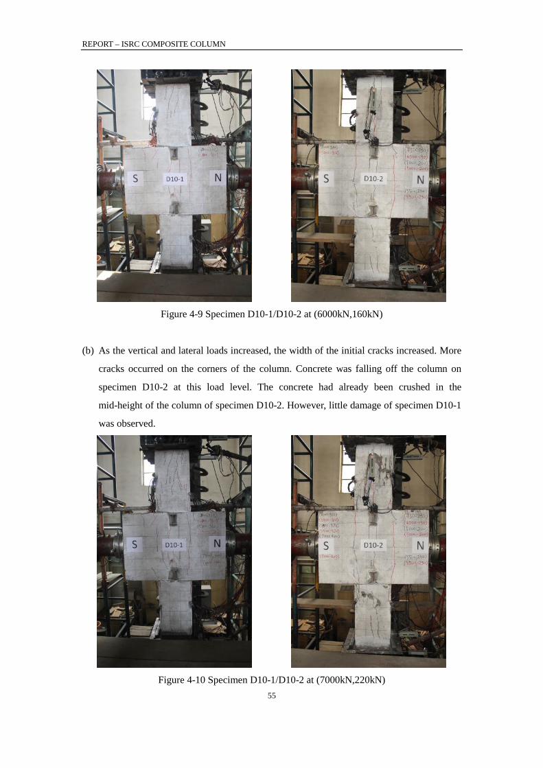
REPORT – ISRC COMPOSITE COLUMN
55
Figure 4-9 Specimen D10-1/D10-2 at (6000kN,160kN)
(b) As the vertical and lateral loads increased, the width of the initial cracks increased. More
cracks occurred on the corners of the column. Concrete was falling off the column on
specimen D10-2 at this load level. The concrete had already been crushed in the
mid-height of the column of specimen D10-2. However, little damage of specimen D10-1
was observed.
Figure 4-10 Specimen D10-1/D10-2 at (7000kN,220kN)
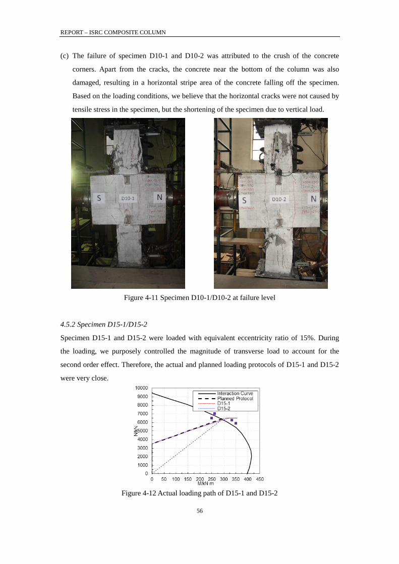
REPORT – ISRC COMPOSITE COLUMN
56
(c) The failure of specimen D10-1 and D10-2 was attributed to the crush of the concrete
corners. Apart from the cracks, the concrete near the bottom of the column was also
damaged, resulting in a horizontal stripe area of the concrete falling off the specimen.
Based on the loading conditions, we believe that the horizontal cracks were not caused by
tensile stress in the specimen, but the shortening of the specimen due to vertical load.
Figure 4-11 Specimen D10-1/D10-2 at failure level
4.5.2 Specimen D15-1/D15-2
Specimen D15-1 and D15-2 were loaded with equivalent eccentricity ratio of 15%. During
the loading, we purposely controlled the magnitude of transverse load to account for the
second order effect. Therefore, the actual and planned loading protocols of D15-1 and D15-2
were very close.
Figure 4-12 Actual loading path of D15-1 and D15-2
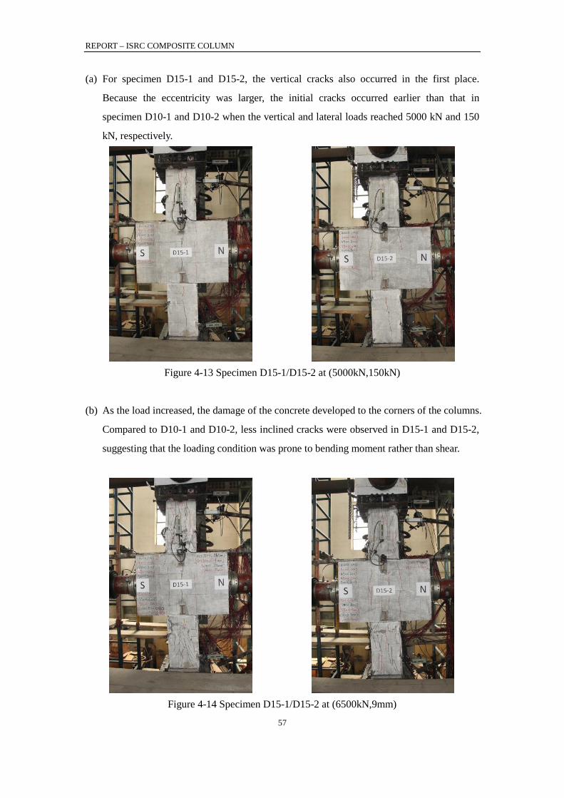
REPORT – ISRC COMPOSITE COLUMN
57
(a) For specimen D15-1 and D15-2, the vertical cracks also occurred in the first place.
Because the eccentricity was larger, the initial cracks occurred earlier than that in
specimen D10-1 and D10-2 when the vertical and lateral loads reached 5000 kN and 150
kN, respectively.
Figure 4-13 Specimen D15-1/D15-2 at (5000kN,150kN)
(b) As the load increased, the damage of the concrete developed to the corners of the columns.
Compared to D10-1 and D10-2, less inclined cracks were observed in D15-1 and D15-2,
suggesting that the loading condition was prone to bending moment rather than shear.
Figure 4-14 Specimen D15-1/D15-2 at (6500kN,9mm)

REPORT – ISRC COMPOSITE COLUMN
58
(c) The corners of the column were crushed in the end, causing the specimen to fail. In
addition, some of the concrete fell off the faces of the column.
Figure 4-15 Specimen D15-1/D15-2 at failure level
4.5.3 Summary of failure mode
All of the four specimens failed in combined compression and bending – the specimen failed
because the corners of the concrete were crushed – which met the purpose of the experiment
program. The final crack distributions of the specimens are presented in Figure 4-16. The
specimens held integrity during the whole loading process. Despite the surrounding concrete
was damaged due to lack of confinement, the core concrete remain intact because of the
confinement effect provided by the steel sections. In turn, the core concrete helped ensure that
the steel sections would not buckle when the vertical load was very large.

REPORT – ISRC COMPOSITE COLUMN
59
(a) D10-1
(b) D10-2
(c) D15-1
(d) D15-2
Figure 4-16 Crack distribution of the specimens
After the specimen was severely damaged, locale buckling of the longitudinal reinforcement
and break of the transverse reinforcement was detected at places where the concrete fell off.
Most of the buckling areas lay where the volume ratio of the transverse reinforcement
changed from 0.85% to 0.25%.
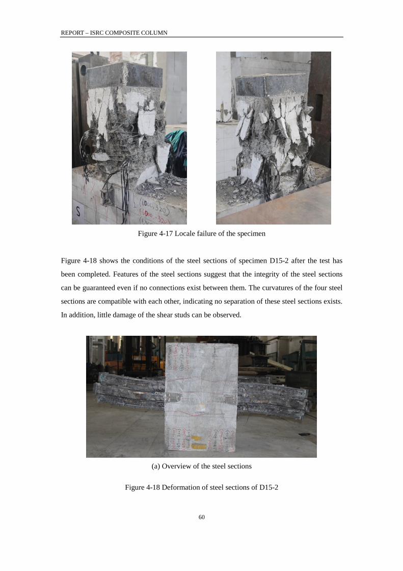
REPORT – ISRC COMPOSITE COLUMN
60
Figure 4-17 Locale failure of the specimen
Figure 4-18 shows the conditions of the steel sections of specimen D15-2 after the test has
been completed. Features of the steel sections suggest that the integrity of the steel sections
can be guaranteed even if no connections exist between them. The curvatures of the four steel
sections are compatible with each other, indicating no separation of these steel sections exists.
In addition, little damage of the shear studs can be observed.
(a) Overview of the steel sections
Figure 4-18 Deformation of steel sections of D15-2

REPORT – ISRC COMPOSITE COLUMN
61
(b) Feature of the upper column
(c) Feature of the lower column
(e) Feature of the shear studs
(f) Figure 4-18 Deformation of steel sections of D15-2 (Continued)
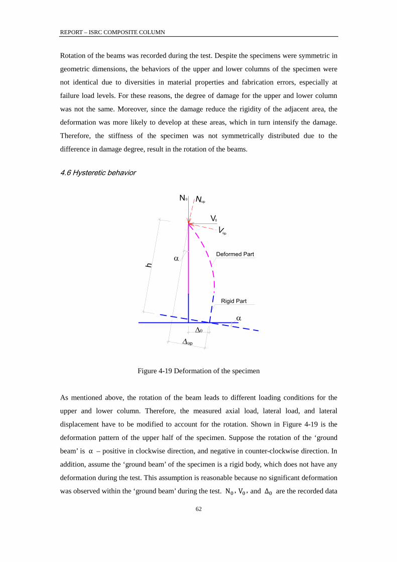
REPORT – ISRC COMPOSITE COLUMN
62
Rotation of the beams was recorded during the test. Despite the specimens were symmetric in
geometric dimensions, the behaviors of the upper and lower columns of the specimen were
not identical due to diversities in material properties and fabrication errors, especially at
failure load levels. For these reasons, the degree of damage for the upper and lower column
was not the same. Moreover, since the damage reduce the rigidity of the adjacent area, the
deformation was more likely to develop at these areas, which in turn intensify the damage.
Therefore, the stiffness of the specimen was not symmetrically distributed due to the
difference in damage degree, result in the rotation of the beams.
4.6 Hysteretic behavior
α
α
∆up
h
∆0
Vup
NupN0
V0
Rigid Part
Deformed Part
Figure 4-19 Deformation of the specimen
As mentioned above, the rotation of the beam leads to different loading conditions for the
upper and lower column. Therefore, the measured axial load, lateral load, and lateral
displacement have to be modified to account for the rotation. Shown in Figure 4-19 is the
deformation pattern of the upper half of the specimen. Suppose the rotation of the ‘ground
beam’ is α – positive in clockwise direction, and negative in counter-clockwise direction. In
addition, assume the ‘ground beam’ of the specimen is a rigid body, which does not have any
deformation during the test. This assumption is reasonable because no significant deformation
was observed within the ‘ground beam’ during the test. N0,V0,and Δ0 are the recorded data
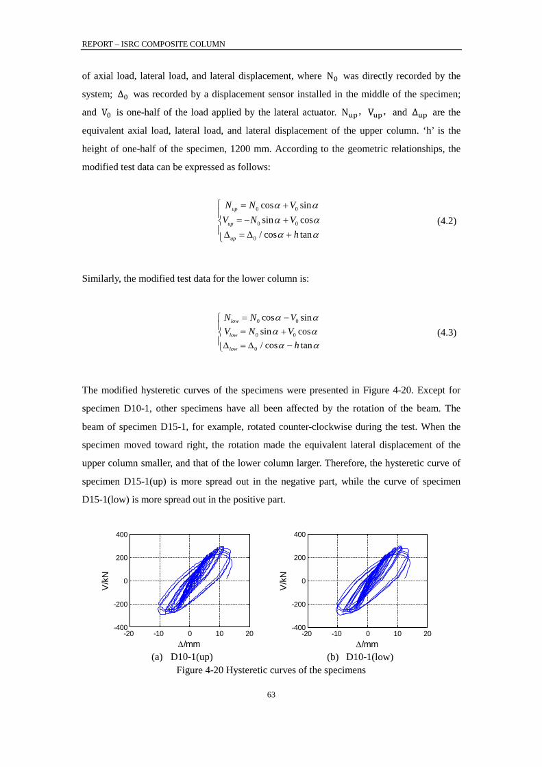
REPORT – ISRC COMPOSITE COLUMN
63
of axial load, lateral load, and lateral displacement, where N0 was directly recorded by the
system; Δ0 was recorded by a displacement sensor installed in the middle of the specimen;
and V0 is one-half of the load applied by the lateral actuator. Nup,Vup,and Δup are the
equivalent axial load, lateral load, and lateral displacement of the upper column. ‘h’ is the
height of one-half of the specimen, 1200 mm. According to the geometric relationships, the
modified test data can be expressed as follows:
0
0
0
0
0
sinsin cos
/ co
os
t
c
s an
up
up
up
VV N V
h
N N α αα αα α
+= − +
∆ = ∆ +
=
(4.2)
Similarly, the modified test data for the lower column is:
0
0
0
0
0
sinsin cos/ cos ta
co
n
slow
low
low
VV
h
NV
NN
α αα αα α
−= +=
∆ = ∆ −
(4.3)
The modified hysteretic curves of the specimens were presented in Figure 4-20. Except for
specimen D10-1, other specimens have all been affected by the rotation of the beam. The
beam of specimen D15-1, for example, rotated counter-clockwise during the test. When the
specimen moved toward right, the rotation made the equivalent lateral displacement of the
upper column smaller, and that of the lower column larger. Therefore, the hysteretic curve of
specimen D15-1(up) is more spread out in the negative part, while the curve of specimen
D15-1(low) is more spread out in the positive part.
(a) D10-1(up)
(b) D10-1(low)
Figure 4-20 Hysteretic curves of the specimens
-20 -10 0 10 20-400
-200
0
200
400
∆/mm
V/k
N
-20 -10 0 10 20-400
-200
0
200
400
∆/mm
V/k
N

REPORT – ISRC COMPOSITE COLUMN
64
(c) D10-2(up)
(d) D10-2(low)
(e) D15-1(up)
(f) D15-1(low)
(g) D15-2(up)
(h) D15-2(low)
Figure 4-20 Hysteretic curves of the specimens (Continued)
Although the behaviors of the specimens were affected by the rotation of the beams, the
hysteretic curves are still stable. The specimens showed some pinching at the beginning of the
test, but the degree of pinching was mitigated as the lateral displacement was increasing. For
the last several circles of the loading, the hysteretic curves are round and stable, suggesting a
good ability of energy dissipation.
-20 -10 0 10 20-400
-200
0
200
400
∆/mm
V/k
N
-20 -10 0 10 20-400
-200
0
200
400
∆/mm
V/k
N
-20 -10 0 10 20-400
-200
0
200
400
∆/mm
V/k
N
-20 -10 0 10 20-400
-200
0
200
400
∆/mm
V/k
N
-20 -10 0 10 20-400
-200
0
200
400
∆/mm
V/k
N
-20 -10 0 10 20-400
-200
0
200
400
∆/mm
V/k
N

REPORT – ISRC COMPOSITE COLUMN
65
-20 -10 0 10 20-400
-200
0
200
400
∆/mm
V/kN
D10-1(up)D10-1(low)D10-2(up)D10-2(low)
(a) D10-1/D10-2
-20 -10 0 10 20-400
-200
0
200
400
∆/mm
V/kN
D15-1(up)D15-1(low)D15-2(up)D15-2(low)
(b) D15-1/D15-2
Figure 4-21 Envelop curves of the specimens
4.7 Capacities and deformations
Shown in Table 4-5 are the test results of the specimen under three different load stages –
yield stage, peak stage, and ultimate stage. The yield point of a specimen is determined based
on reduced stiffness method (Figure 4-22). The equivalent secant modulus of a specimen is
determined by the original point and the 0.6Vp point on the ascending branch of the envelop
curve, and the yield point is determined accordingly. The ultimate point is defined as the
0.85Vp point on the descending branch of the envelop curve, or the point where the test stops,
whichever is larger.
According to the test data or the envelop curves, the initial lateral stiffness of the specimens
are almost the same, regardless of the eccentricity ratio. When the maximum lateral load is
reached, the lateral load barely descends afterwards until the specimen fails. This
phenomenon is caused by the unique loading protocol employed in this test program. During
step 2 in the quasi-static test, the vertical load keeps increasing as the test going on. When the
lateral load reaches its peak, the combination of axial load and bending moment on the critical
section of the column has already reached the interaction curve, which means the specimen is
just about to fail. At the same time, the axial compression ratio for design was 1.50 and 1.14
for e/h=10% specimens and e/h=15% specimens respectively. The extremely high axial load
causes the specimen to fail right after the maximum lateral load is reached.
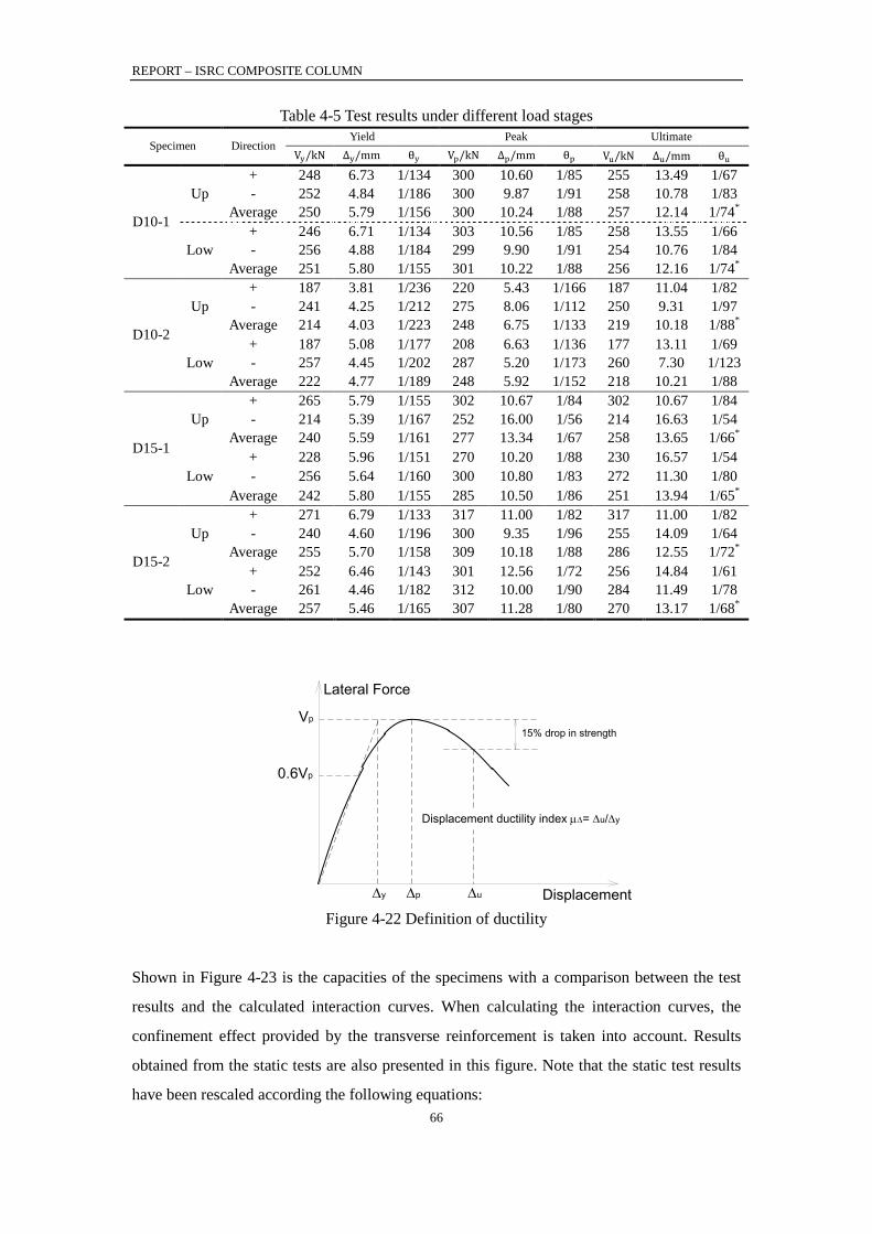
REPORT – ISRC COMPOSITE COLUMN
66
Table 4-5 Test results under different load stages
Specimen Direction Yield Peak Ultimate
Vy/kN Δy/mm θy Vp/kN Δp/mm θp Vu/kN Δu/mm θu
D10-1
Up + 248 6.73 1/134 300 10.60 1/85 255 13.49 1/67
- 252 4.84 1/186 300 9.87 1/91 258 10.78 1/83 Average 250 5.79 1/156 300 10.24 1/88 257 12.14 1/74*
Low + 246 6.71 1/134 303 10.56 1/85 258 13.55 1/66
- 256 4.88 1/184 299 9.90 1/91 254 10.76 1/84 Average 251 5.80 1/155 301 10.22 1/88 256 12.16 1/74*
D10-2
Up + 187 3.81 1/236 220 5.43 1/166 187 11.04 1/82
- 241 4.25 1/212 275 8.06 1/112 250 9.31 1/97 Average 214 4.03 1/223 248 6.75 1/133 219 10.18 1/88*
Low + 187 5.08 1/177 208 6.63 1/136 177 13.11 1/69
- 257 4.45 1/202 287 5.20 1/173 260 7.30 1/123
Average 222 4.77 1/189 248 5.92 1/152 218 10.21 1/88
D15-1
Up + 265 5.79 1/155 302 10.67 1/84 302 10.67 1/84 - 214 5.39 1/167 252 16.00 1/56 214 16.63 1/54
Average 240 5.59 1/161 277 13.34 1/67 258 13.65 1/66*
Low + 228 5.96 1/151 270 10.20 1/88 230 16.57 1/54
- 256 5.64 1/160 300 10.80 1/83 272 11.30 1/80 Average 242 5.80 1/155 285 10.50 1/86 251 13.94 1/65*
D15-2
Up + 271 6.79 1/133 317 11.00 1/82 317 11.00 1/82 - 240 4.60 1/196 300 9.35 1/96 255 14.09 1/64
Average 255 5.70 1/158 309 10.18 1/88 286 12.55 1/72*
Low + 252 6.46 1/143 301 12.56 1/72 256 14.84 1/61
- 261 4.46 1/182 312 10.00 1/90 284 11.49 1/78 Average 257 5.46 1/165 307 11.28 1/80 270 13.17 1/68*
Lateral Force
Displacement
Vp
0.6Vp
∆y ∆p ∆u
15% drop in strength
Displacement ductility index µ∆= ∆u/∆y
Figure 4-22 Definition of ductility
Shown in Figure 4-23 is the capacities of the specimens with a comparison between the test
results and the calculated interaction curves. When calculating the interaction curves, the
confinement effect provided by the transverse reinforcement is taken into account. Results
obtained from the static tests are also presented in this figure. Note that the static test results
have been rescaled according the following equations:
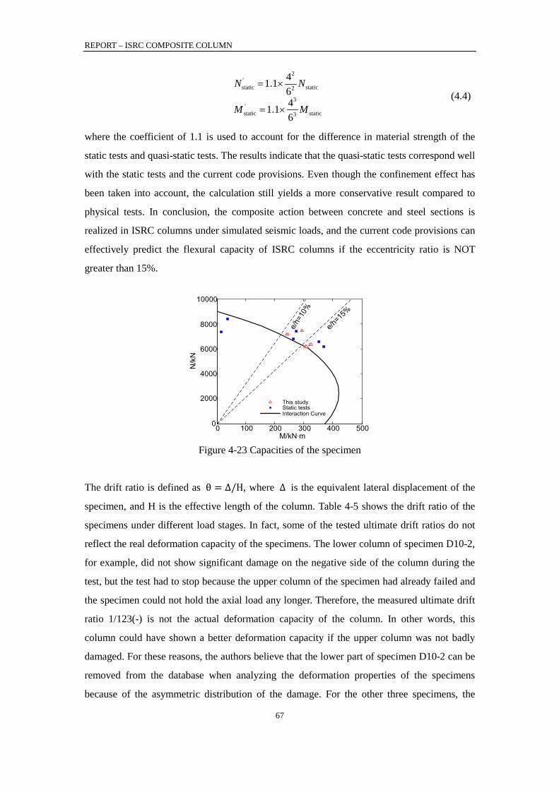
REPORT – ISRC COMPOSITE COLUMN
67
2
static'static
'static
2
3
static3
1.1
1.1
4646
N
M
N
M×=
×= (4.4)
where the coefficient of 1.1 is used to account for the difference in material strength of the
static tests and quasi-static tests. The results indicate that the quasi-static tests correspond well
with the static tests and the current code provisions. Even though the confinement effect has
been taken into account, the calculation still yields a more conservative result compared to
physical tests. In conclusion, the composite action between concrete and steel sections is
realized in ISRC columns under simulated seismic loads, and the current code provisions can
effectively predict the flexural capacity of ISRC columns if the eccentricity ratio is NOT
greater than 15%.
0 100 200 300 400 5000
2000
4000
6000
8000
10000
M/kN·m
N/k
N
e/h=1
0%
e/h=15
%
This studyStatic testsInteraction Curve
Figure 4-23 Capacities of the specimen
The drift ratio is defined as θ = Δ/H, where Δ is the equivalent lateral displacement of the
specimen, and H is the effective length of the column. Table 4-5 shows the drift ratio of the
specimens under different load stages. In fact, some of the tested ultimate drift ratios do not
reflect the real deformation capacity of the specimens. The lower column of specimen D10-2,
for example, did not show significant damage on the negative side of the column during the
test, but the test had to stop because the upper column of the specimen had already failed and
the specimen could not hold the axial load any longer. Therefore, the measured ultimate drift
ratio 1/123(-) is not the actual deformation capacity of the column. In other words, this
column could have shown a better deformation capacity if the upper column was not badly
damaged. For these reasons, the authors believe that the lower part of specimen D10-2 can be
removed from the database when analyzing the deformation properties of the specimens
because of the asymmetric distribution of the damage. For the other three specimens, the

REPORT – ISRC COMPOSITE COLUMN
68
damage distributions were almost symmetric although the ‘foundation beam’ rotated during
the test. Except for D10-2(lower), the average ultimate drift ratios of the specimens (market
with ‘*’ in Table 4-5) all exceed 1/100, which is the specified limit in Chinese codes JGJ 3
(2010), suggesting sufficient deformation capacities under simulated seismic loads.
4.8 Strain distribution
Figure 4-24 shows the strain distribution of the specimens under different load stages. The
horizontal axis in these figures indicates the distance between the strain gauges and the left
side of the cross section. Because the steel sections are separate from each other, the strain
values are not on the same steel section in Figure 4-24 (a) (c) (e) (f). Specifically, the left steel
section lies within [0mm, 110mm]; the two middle steel sections lie within [110mm, 190mm],
and average values of the strain of these two steel sections are presented in the figure; the
right steel section lies within [190mm, 300mm].
For specimen D10-1 and D10-2, the plane section assumption (almost) holds effective from
the beginning to the end of the loading process for both the steel sections and the longitudinal
reinforcement. For specimen D15-1 and D15-2, the plane section assumption is effective
under gravity and yield load level. However, under peak and ultimate load level, the strain
distribution of the longitudinal reinforcement clearly violates the plane section assumption
because of the buckling of the bars.
In addition, the strain distribution of steel sections is more complex. Although the plane
section assumption roughly remains effective, the three steel sections actually form three
different planes, especially for specimen D15-1/D15-2 under peak and ultimate load level.
Actually, the violation of plane section assumption is attributed to the slip effect of
concrete-steel interface. Test results indicate that the slip effect gets larger as the load
increases, and it is more evident for D15-1/D15-2 than D10-1/D10-2. Theoretically, the
flexural capacity of composite columns will decrease if slip effect exists. However, the
decrease in capacity can be offset by the strengthening of the steel sections. Therefore, the
capacity of the specimen does not decrease in practices.
To summary, the plane section assumption is more likely to fail when the eccentricity ratio
gets larger. Within 15% eccentricity ratio, the plane section assumption is, broadly speaking,
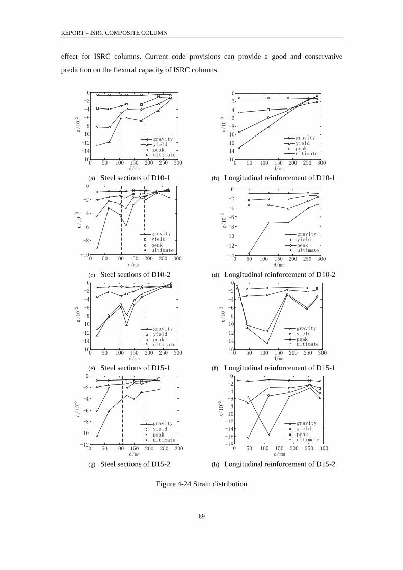
REPORT – ISRC COMPOSITE COLUMN
69
effect for ISRC columns. Current code provisions can provide a good and conservative
prediction on the flexural capacity of ISRC columns.
0 50 100 150 200 250 300-16
-14
-12
-10
-8
-6
-4
-2
0
d/mm
ε /10
-3
gravityyieldpeakultimate
(a) Steel sections of D10-1
0 50 100 150 200 250 300-16
-14
-12
-10
-8
-6
-4
-2
0
d/mm
ε /10
-3
gravityyieldpeakultimate
(b) Longitudinal reinforcement of D10-1
0 50 100 150 200 250 300-10
-8
-6
-4
-2
0
d/mm
ε /10-3
gravityyieldpeakultimate
(c) Steel sections of D10-2
0 50 100 150 200 250 300-14
-12
-10
-8
-6
-4
-2
0
d/mm
ε /10
-3
gravityyieldpeakultimate
(d) Longitudinal reinforcement of D10-2
0 50 100 150 200 250 300-16
-14
-12
-10
-8
-6
-4
-2
0
d/mm
ε /10
-3
gravityyieldpeakultimate
(e) Steel sections of D15-1
0 50 100 150 200 250 300-16
-14
-12
-10
-8
-6
-4
-2
0
d/mm
ε /10
-3
gravityyieldpeakultimate
(f) Longitudinal reinforcement of D15-1
0 50 100 150 200 250 300-12
-10
-8
-6
-4
-2
0
d/mm
ε /10-3
gravityyieldpeakultimate
(g) Steel sections of D15-2
0 50 100 150 200 250 300-18
-16
-14
-12
-10
-8
-6
-4
-2
0
d/mm
ε /10
-3
gravityyieldpeakultimate
(h) Longitudinal reinforcement of D15-2
Figure 4-24 Strain distribution

REPORT – ISRC COMPOSITE COLUMN
70
4.9 Lateral stiffness
The lateral stiffness of a column is defined as the lateral load divided by the lateral
displacement. Shown in Table 4-6 is the lateral stiffness of the columns under different load
stages. Test results suggest that the lateral stiffness decreases as the loading increases, but the
eccentricity ratio has little influence on the lateral stiffness.
Table 4-6 Lateral stiffness under different load stages
Specimen K/kN · mm−1
Yield Peak Ultimate
D10-1 Up 44.47 29.35 21.42 Low 44.56 29.49 21.32
D10-2 Up 52.85 37.33 21.90 Low 47.24 43.28 24.55
D15-1 Up 42.75 22.03 20.59 Low 41.88 27.12 18.96
D15-2 Up 46.03 30.45 23.46 Low 48.78 27.59 20.98
Figure 4-25 shows the reduction of lateral stiffness in terms of lateral displacement. The
vertical axis in these figures indicates the ratio of lateral stiffness to the initial lateral stiffness
of the column, and the unit is in percentile. Results show that the lateral stiffness decreases
linearly as the displacement grows. Under yield load stage, the lateral stiffness is 60%~80%
of the initial ones; under peak load stage, this ratio is 40%~60%; and under ultimate load
stage, this ratio is 20%~40%.
-20 -10 0 10 200
20
40
60
80
100
∆/mm
K/K0/%
D10-1(up)D10-1(low)D10-2(up)D10-2(low)
(a) Specimen D10-1/D10-2
-20 -10 0 10 200
20
40
60
80
100
∆/mm
K/K0/%
D15-1(up)D15-1(low)D15-2(up)D15-2(low)
(b) Specimen D15-1/D15-2
Figure 4-25 Reduction of lateral stiffness

REPORT – ISRC COMPOSITE COLUMN
71
4.10 Energy dissipation
The ability of energy consumption is a very important aspect when evaluating the seismic
performance of a composite column. A good energy consumption ability means the element
may dissipate more energy from the earthquake, and be less damaged. Since the hysteretic
curve reflects the relationship between the lateral load and lateral top displacement of the
specimen, the area surround by the curves indicates the energy dissipated by the specimen
during the loading. By integrating the product of lateral load and displacement, one can get
the dissipated energy under different load levels, as shown in Figure 4-26. When the lateral
displacement is small, the specimen does not yield yet, so the energy consumption is very
small. When the lateral displacement grows, the materials yield, and friction between the
materials also consumes energy. Therefore, the energy consumption becomes larger and larger
as the lateral displacement increases. Figure 4-26(c) compares the ability of energy
dissipation between specimen D10-1/D10-2 and specimen D15-1/D15-2. The ability of
energy dissipation does not change much as the eccentricity ratio grows. This is probably
because the increase in eccentricity ratio is not large enough to provide a significant change in
the ability of energy dissipation.
0 5 10 150
1
2
3
4
5
6
E/kN
·m
∆/mm
D10-1(up)D10-1(low)D10-2(up)D10-2(low)
(a) Specimen D10-1/D10-2
0 5 10 150
1
2
3
4
5
6
E/kN
·m
∆/mm
D15-1(up)D15-1(low)D15-2(up)D15-2(low)
(b) Specimen D15-1/D15-2
0 5 10 150
1
2
3
4
5
6
E/kN
·m
∆/mm
D10-1(up)D10-2(up)D15-1(up)D15-2(up)
(c) Comparison of energy consumption
Figure 4-26 Energy consumption of the specimens

REPORT – ISRC COMPOSITE COLUMN
72
Another index used to evaluate the ability of energy consumption is equivalent damping ratio.
The equivalent-damping ratio he is defined in Figure 4-27:
1
2loop
eAOB COD
Sh
S Sπ=
+ (4.5)
where Sloop is the area surround by the hysteretic curve; SAOB and SCOD is the area of the
shaded triangles. The larger the equivalent damping ratio, the stronger the ability of energy
consumption the specimen has.
Figure 4-27 Definition of equivalent damping ratio
0
0.1
0.2
0.3
0.4
0.5
0 5 10 15∆ /mm
h e
D10-1(up)D10-1(low)D10-2(up)D10-2(low)
(a) Specimen D10-1/D10-2
0 5 10 15∆ /mm
0
0.1
0.2
0.3
0.4
0.5
h e
D15-1(up)D15-1(low)D15-2(up)D15-2(low)
(b) Specimen D15-1/D15-2
0 5 10 15∆ /mm
0
0.1
0.2
0.3
0.4
0.5
h e
D10-1(up)D10-2(up)D15-1(up)D15-2(up)
(c) Comparison of equivalent damping ratio
Figure 4-28 Equivalent damping ratio of the specimens
REPORT – ISRC COMPOSITE COLUMN
73
Figure 4-28 shows the relationships between the equivalent damping ratio and the lateral
displacement. For all of the specimens, the equivalent damping ratio decreases as the lateral
displacement grows before yield displacement, and increases as the lateral displacement
grows afterwards. Test results show that the hysteretic curves ‘pinch’ when the specimen is
being unloaded. Caused by slip effect and cracking of the concrete, this phenomenon is
unfavorable for dissipating energy since it reduces the area surrounded by the hysteretic
curves. The pinch effect is more evident when the lateral displacement is small and most of
the materials remain elastic. When the lateral displacement gets larger, more and more parts
of the steel sections and longitudinal reinforcement develop into plastic state, improving the
specimen’s ability to consume energy. Therefore, the equivalent-damping ratio gets larger as
the load increases.
4.11 Summary of phase 2 test
1) The four specimens fail in combined compression and bending. Shear failure is not
evident during the test. Although there is no connection between the steel sections, the
composite action still works during the test. The specimens fail due to crush of the
concrete corners. Buckling of the longitudinal reinforcement and breaking of the
transverse reinforcement is detected. The steel sections are well confined by the concrete,
hence no buckling or separations of the steel sections are found.
2) The flexural capacities of the specimens agree with the static tests as well as the
calculated interaction curves based on ACI 318, Eurocode4, and YB 9082 with the
confinement effect of the concrete included. The current code provisions can provide a
good and conservative prediction on the capacity of ISRC columns.
3) The plane section assumption weakens as the eccentricity ratio grows. However, within
15% eccentricity ratio, the plane section assumption is effective in general.
4) The drift ratios of the specimens under ultimate loads levels suggest sufficient
deformation capacities of ISRC columns.
5) The specimens show a desirable ability in energy dissipation. The energy dissipation does
not show significant change as the eccentricity ratio grows.

REPORT – ISRC COMPOSITE COLUMN
74
5 FEA – phase 1
Finite element (FE) analysis was carried out to verify the test results and provide a more
detailed stress distribution of the inner part of the column. ABAQUS was chosen to do the
analysis due to its ability of complex calculation and friendly interactive interface.
5.1 FE model development
There are three material models for concrete in ABAQUS: smeared crack model, damaged
plasticity model, and brittle cracking model. In ABAQUS standard modules, the damaged
plasticity model is preferred in analyzing the behavior of concrete.
The uni-axial constitutive curve for concrete is obtained by using Mander model (Mander et
al 1988) with confinement effect taken into account. The confined compressive strength and
corresponding compressive strain are:
' '0 1cc c lf f k f= +
'
0 2 '0
1 1cccc c
c
fkf
ε ε
= + −
(5.1a)
(5.1b)
where fc0′ and εc0 are the compressive strength and the corresponding strain for unconfined
concrete; fcc′ and εcc is the compressive strength and the corresponding strain for confined
concrete; fl is the confining pressure applied to the concrete; k1 and k2 are two
coefficients. Richart (Richart et al 1928) conducted a series of tests and concluded that
k1 = 4.1 and k2 = 5. Mander proposed a theoretical model in which the constitutive curve for
the compressive concrete is given by the following equations:
'
1cc
c r
f xrfr x
=− +
c
cc
x εε
=
sec
c
c
ErE E
=−
'
0 '0
1 5 1cccc c
c
ff
ε ε
= + −
(5.2a)
(5.2b)
(5.2c)
(5.2d)
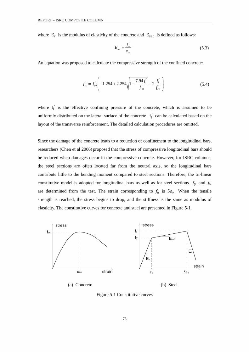
REPORT – ISRC COMPOSITE COLUMN
75
where Ec is the modulus of elasticity of the concrete and Esec is defined as follows:
'
secc
cc
cfEε
= (5.3)
An equation was proposed to calculate the compressive strength of the confined concrete:
' '' '
0 ' '0 0
7.941.254 2.254 1 2l lcc c
c c
f ff ff f
= − + + −
(5.4)
where fl′ is the effective confining pressure of the concrete, which is assumed to be
uniformly distributed on the lateral surface of the concrete. fl′ can be calculated based on the
layout of the transverse reinforcement. The detailed calculation procedures are omitted.
Since the damage of the concrete leads to a reduction of confinement to the longitudinal bars,
researchers (Chen et al 2006) proposed that the stress of compressive longitudinal bars should
be reduced when damages occur in the compressive concrete. However, for ISRC columns,
the steel sections are often located far from the neutral axis, so the longitudinal bars
contribute little to the bending moment compared to steel sections. Therefore, the tri-linear
constitutive model is adopted for longitudinal bars as well as for steel sections. 𝑓𝑦 and 𝑓𝑢
are determined from the test. The strain corresponding to 𝑓𝑢 is 5𝜀𝑦 . When the tensile
strength is reached, the stress begins to drop, and the stiffness is the same as modulus of
elasticity. The constitutive curves for concrete and steel are presented in Figure 5-1.
stress
strain
fcc’
εcc
(a) Concrete
stress
strain
fy
εy
fu
5εy
Es
Esoft
Es
(b) Steel
Figure 5-1 Constitutive curves
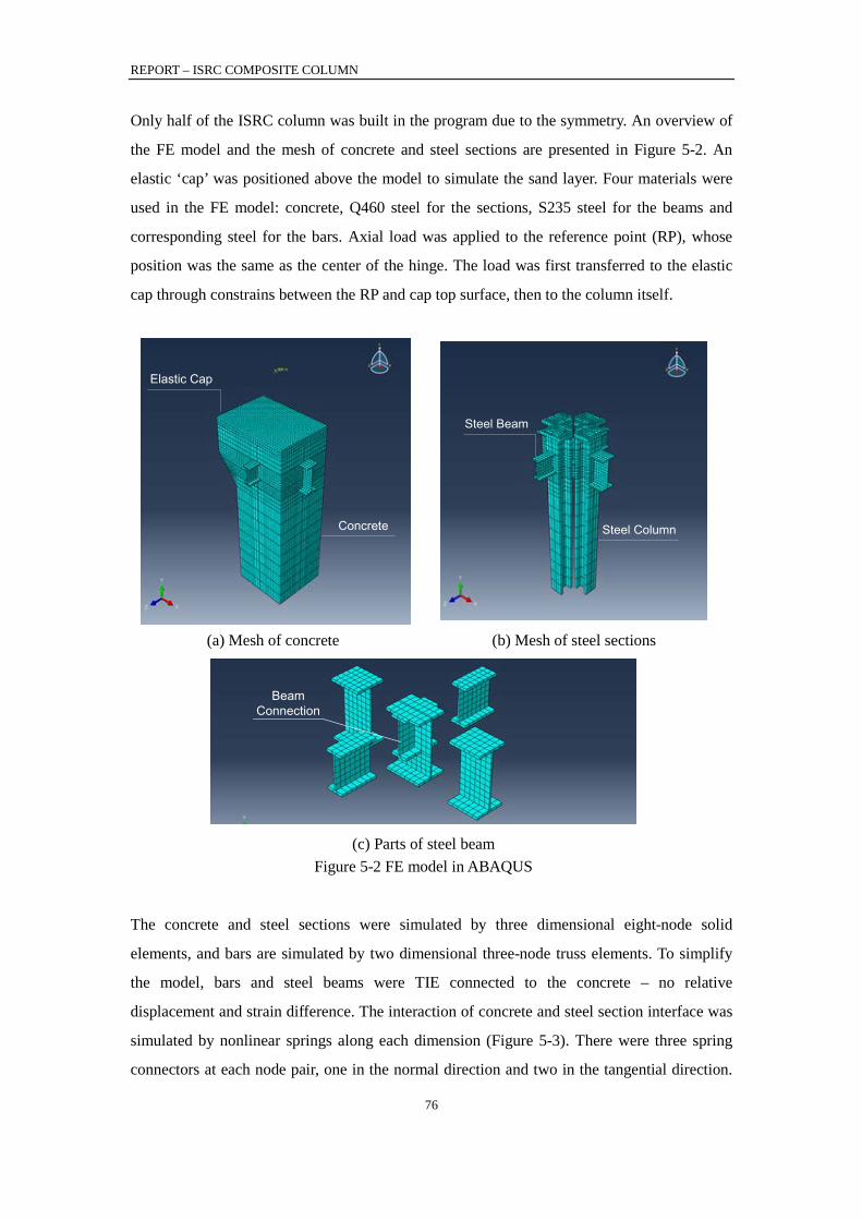
REPORT – ISRC COMPOSITE COLUMN
76
Only half of the ISRC column was built in the program due to the symmetry. An overview of
the FE model and the mesh of concrete and steel sections are presented in Figure 5-2. An
elastic ‘cap’ was positioned above the model to simulate the sand layer. Four materials were
used in the FE model: concrete, Q460 steel for the sections, S235 steel for the beams and
corresponding steel for the bars. Axial load was applied to the reference point (RP), whose
position was the same as the center of the hinge. The load was first transferred to the elastic
cap through constrains between the RP and cap top surface, then to the column itself.
Elastic Cap
Concrete
(a) Mesh of concrete
Steel Beam
Steel Column
(b) Mesh of steel sections
Beam Connection
(c) Parts of steel beam
Figure 5-2 FE model in ABAQUS
The concrete and steel sections were simulated by three dimensional eight-node solid
elements, and bars are simulated by two dimensional three-node truss elements. To simplify
the model, bars and steel beams were TIE connected to the concrete – no relative
displacement and strain difference. The interaction of concrete and steel section interface was
simulated by nonlinear springs along each dimension (Figure 5-3). There were three spring
connectors at each node pair, one in the normal direction and two in the tangential direction.
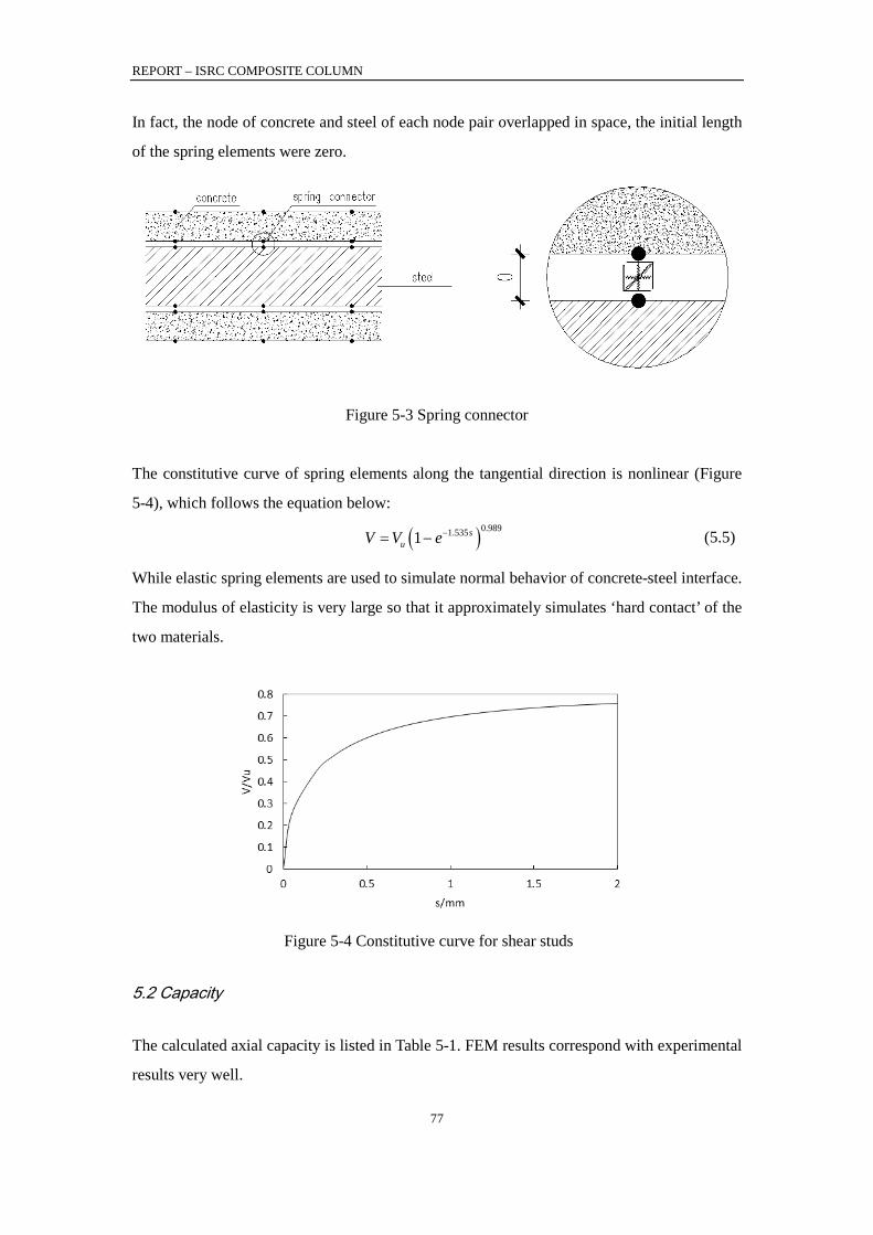
REPORT – ISRC COMPOSITE COLUMN
77
In fact, the node of concrete and steel of each node pair overlapped in space, the initial length
of the spring elements were zero.
Figure 5-3 Spring connector
The constitutive curve of spring elements along the tangential direction is nonlinear (Figure
5-4), which follows the equation below:
( )0.9891.5351 suV V e−= − (5.5)
While elastic spring elements are used to simulate normal behavior of concrete-steel interface.
The modulus of elasticity is very large so that it approximately simulates ‘hard contact’ of the
two materials.
Figure 5-4 Constitutive curve for shear studs
5.2 Capacity
The calculated axial capacity is listed in Table 5-1. FEM results correspond with experimental
results very well.
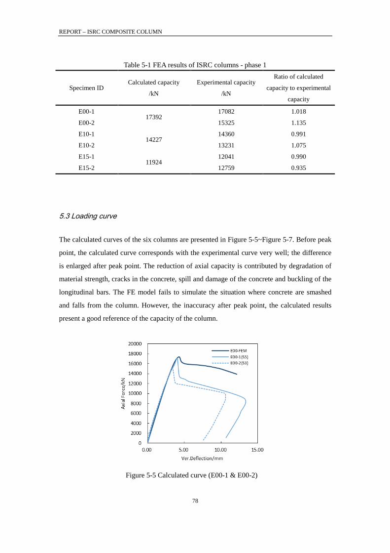
REPORT – ISRC COMPOSITE COLUMN
78
Table 5-1 FEA results of ISRC columns - phase 1
Specimen ID Calculated capacity
/kN
Experimental capacity
/kN
Ratio of calculated
capacity to experimental
capacity
E00-1 17392
17082 1.018
E00-2 15325 1.135
E10-1 14227
14360 0.991
E10-2 13231 1.075
E15-1 11924
12041 0.990
E15-2 12759 0.935
5.3 Loading curve
The calculated curves of the six columns are presented in Figure 5-5~Figure 5-7. Before peak
point, the calculated curve corresponds with the experimental curve very well; the difference
is enlarged after peak point. The reduction of axial capacity is contributed by degradation of
material strength, cracks in the concrete, spill and damage of the concrete and buckling of the
longitudinal bars. The FE model fails to simulate the situation where concrete are smashed
and falls from the column. However, the inaccuracy after peak point, the calculated results
present a good reference of the capacity of the column.
Figure 5-5 Calculated curve (E00-1 & E00-2)
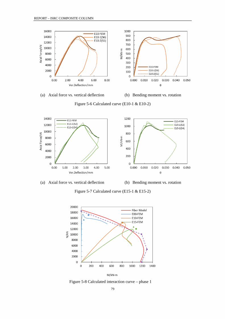
REPORT – ISRC COMPOSITE COLUMN
79
(a) Axial force vs. vertical deflection
(b) Bending moment vs. rotation
Figure 5-6 Calculated curve (E10-1 & E10-2)
(a) Axial force vs. vertical deflection
(b) Bending moment vs. rotation
Figure 5-7 Calculated curve (E15-1 & E15-2)
Figure 5-8 Calculated interaction curve – phase 1
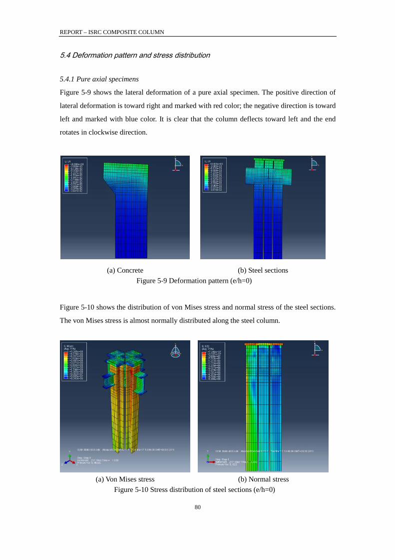
REPORT – ISRC COMPOSITE COLUMN
80
5.4 Deformation pattern and stress distribution
5.4.1 Pure axial specimens
Figure 5-9 shows the lateral deformation of a pure axial specimen. The positive direction of
lateral deformation is toward right and marked with red color; the negative direction is toward
left and marked with blue color. It is clear that the column deflects toward left and the end
rotates in clockwise direction.
(a) Concrete
(b) Steel sections Figure 5-9 Deformation pattern (e/h=0)
Figure 5-10 shows the distribution of von Mises stress and normal stress of the steel sections.
The von Mises stress is almost normally distributed along the steel column.
(a) Von Mises stress
(b) Normal stress Figure 5-10 Stress distribution of steel sections (e/h=0)
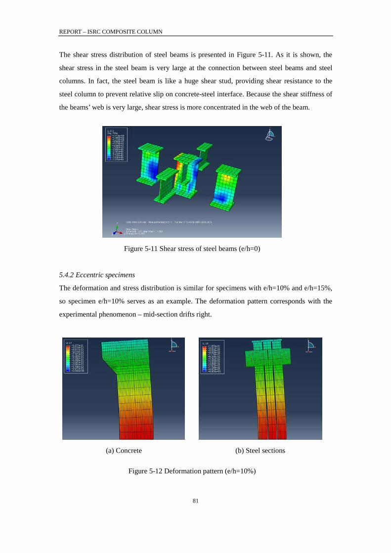
REPORT – ISRC COMPOSITE COLUMN
81
The shear stress distribution of steel beams is presented in Figure 5-11. As it is shown, the
shear stress in the steel beam is very large at the connection between steel beams and steel
columns. In fact, the steel beam is like a huge shear stud, providing shear resistance to the
steel column to prevent relative slip on concrete-steel interface. Because the shear stiffness of
the beams’ web is very large, shear stress is more concentrated in the web of the beam.
Figure 5-11 Shear stress of steel beams (e/h=0)
5.4.2 Eccentric specimens
The deformation and stress distribution is similar for specimens with e/h=10% and e/h=15%,
so specimen e/h=10% serves as an example. The deformation pattern corresponds with the
experimental phenomenon – mid-section drifts right.
(a) Concrete
(b) Steel sections
Figure 5-12 Deformation pattern (e/h=10%)
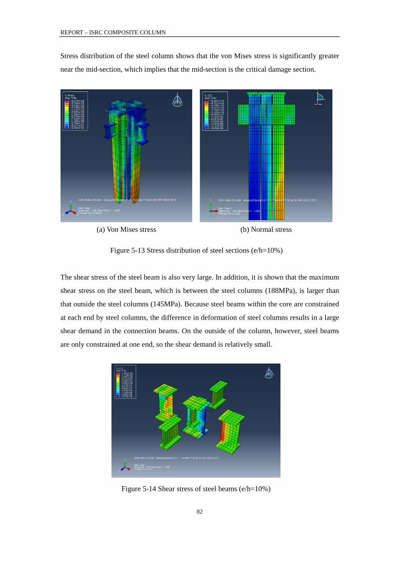
REPORT – ISRC COMPOSITE COLUMN
82
Stress distribution of the steel column shows that the von Mises stress is significantly greater
near the mid-section, which implies that the mid-section is the critical damage section.
(a) Von Mises stress
(b) Normal stress
Figure 5-13 Stress distribution of steel sections (e/h=10%)
The shear stress of the steel beam is also very large. In addition, it is shown that the maximum
shear stress on the steel beam, which is between the steel columns (188MPa), is larger than
that outside the steel columns (145MPa). Because steel beams within the core are constrained
at each end by steel columns, the difference in deformation of steel columns results in a large
shear demand in the connection beams. On the outside of the column, however, steel beams
are only constrained at one end, so the shear demand is relatively small.
Figure 5-14 Shear stress of steel beams (e/h=10%)
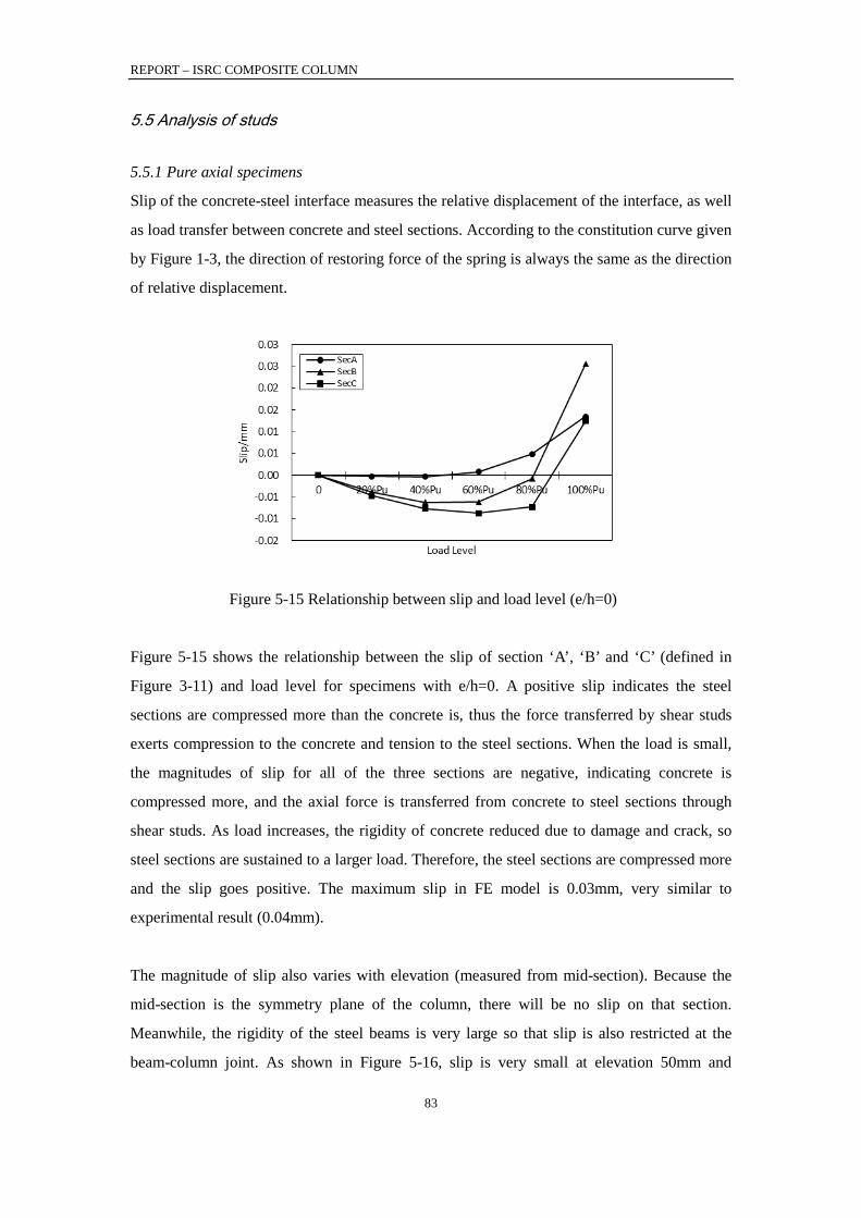
REPORT – ISRC COMPOSITE COLUMN
83
5.5 Analysis of studs
5.5.1 Pure axial specimens
Slip of the concrete-steel interface measures the relative displacement of the interface, as well
as load transfer between concrete and steel sections. According to the constitution curve given
by Figure 1-3, the direction of restoring force of the spring is always the same as the direction
of relative displacement.
Figure 5-15 Relationship between slip and load level (e/h=0)
Figure 5-15 shows the relationship between the slip of section ‘A’, ‘B’ and ‘C’ (defined in
Figure 3-11) and load level for specimens with e/h=0. A positive slip indicates the steel
sections are compressed more than the concrete is, thus the force transferred by shear studs
exerts compression to the concrete and tension to the steel sections. When the load is small,
the magnitudes of slip for all of the three sections are negative, indicating concrete is
compressed more, and the axial force is transferred from concrete to steel sections through
shear studs. As load increases, the rigidity of concrete reduced due to damage and crack, so
steel sections are sustained to a larger load. Therefore, the steel sections are compressed more
and the slip goes positive. The maximum slip in FE model is 0.03mm, very similar to
experimental result (0.04mm).
The magnitude of slip also varies with elevation (measured from mid-section). Because the
mid-section is the symmetry plane of the column, there will be no slip on that section.
Meanwhile, the rigidity of the steel beams is very large so that slip is also restricted at the
beam-column joint. As shown in Figure 5-16, slip is very small at elevation 50mm and
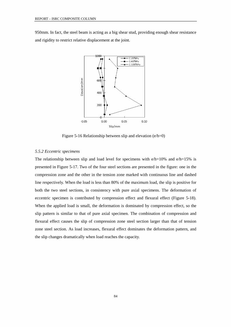
REPORT – ISRC COMPOSITE COLUMN
84
950mm. In fact, the steel beam is acting as a big shear stud, providing enough shear resistance
and rigidity to restrict relative displacement at the joint.
Figure 5-16 Relationship between slip and elevation (e/h=0)
5.5.2 Eccentric specimens
The relationship between slip and load level for specimens with e/h=10% and e/h=15% is
presented in Figure 5-17. Two of the four steel sections are presented in the figure: one in the
compression zone and the other in the tension zone marked with continuous line and dashed
line respectively. When the load is less than 80% of the maximum load, the slip is positive for
both the two steel sections, in consistency with pure axial specimens. The deformation of
eccentric specimen is contributed by compression effect and flexural effect (Figure 5-18).
When the applied load is small, the deformation is dominated by compression effect, so the
slip pattern is similar to that of pure axial specimen. The combination of compression and
flexural effect causes the slip of compression zone steel section larger than that of tension
zone steel section. As load increases, flexural effect dominates the deformation pattern, and
the slip changes dramatically when load reaches the capacity.
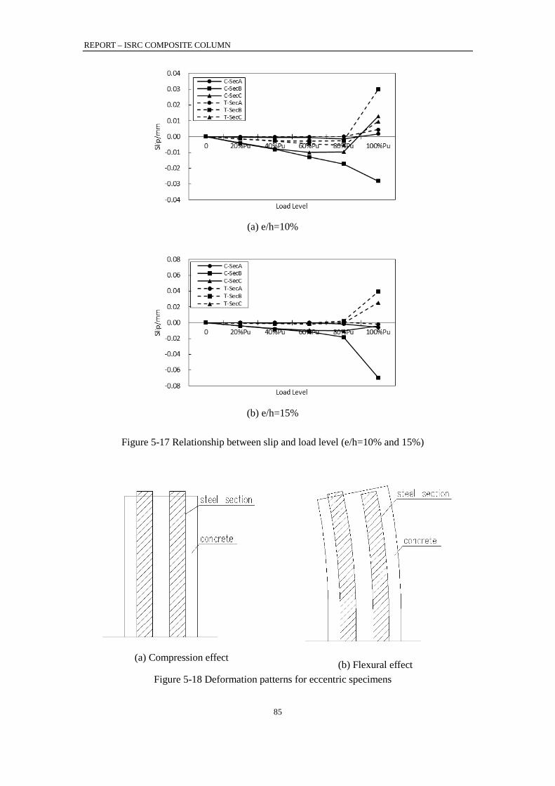
REPORT – ISRC COMPOSITE COLUMN
85
(a) e/h=10%
(b) e/h=15%
Figure 5-17 Relationship between slip and load level (e/h=10% and 15%)
(a) Compression effect
(b) Flexural effect Figure 5-18 Deformation patterns for eccentric specimens
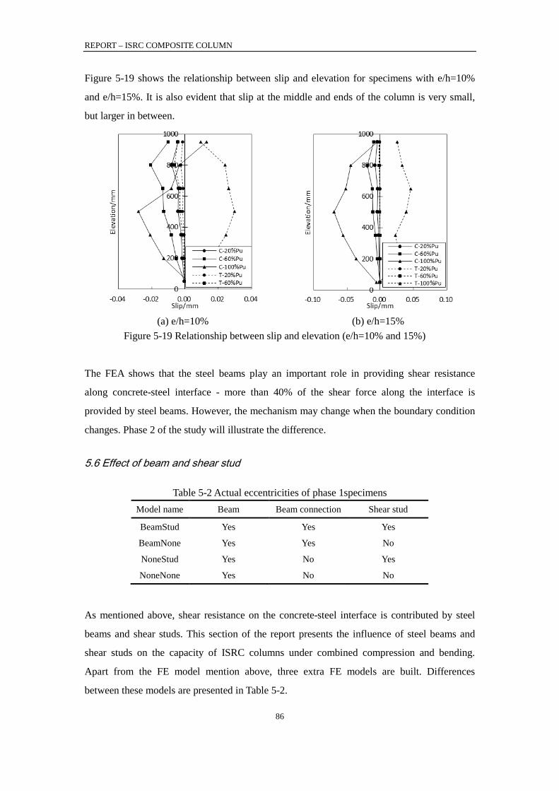
REPORT – ISRC COMPOSITE COLUMN
86
Figure 5-19 shows the relationship between slip and elevation for specimens with e/h=10%
and e/h=15%. It is also evident that slip at the middle and ends of the column is very small,
but larger in between.
(a) e/h=10%
(b) e/h=15%
Figure 5-19 Relationship between slip and elevation (e/h=10% and 15%)
The FEA shows that the steel beams play an important role in providing shear resistance
along concrete-steel interface - more than 40% of the shear force along the interface is
provided by steel beams. However, the mechanism may change when the boundary condition
changes. Phase 2 of the study will illustrate the difference.
5.6 Effect of beam and shear stud
Table 5-2 Actual eccentricities of phase 1specimens Model name Beam Beam connection Shear stud
BeamStud Yes Yes Yes
BeamNone Yes Yes No
NoneStud Yes No Yes
NoneNone Yes No No
As mentioned above, shear resistance on the concrete-steel interface is contributed by steel
beams and shear studs. This section of the report presents the influence of steel beams and
shear studs on the capacity of ISRC columns under combined compression and bending.
Apart from the FE model mention above, three extra FE models are built. Differences
between these models are presented in Table 5-2.

REPORT – ISRC COMPOSITE COLUMN
87
Figure 5-20 and Figure 5-21 shows the capacities of the four different models. It can be
concluded that beam connections and shear studs can help increase the capacity of ISRC
columns under combined compression and bending, but the effect is very small. For e/h=0,
the capacity of ISRC column is about 3% lower if beam connection is removed from the
model. For e/h=10% and e/h=15%, the capacity decreases less than 1% if the beam
connection is removed. Effect of the shear studs is even smaller. For columns with or without
shear studs, the capacity almost remains constant. It should be noticed that this conclusion
does not mean shear studs and beam connections are not important in ISRC columns. If the
column is subjected to horizontal load, the influence of shear studs will be very strong
(Discussed in following chapters).
Figure 5-20 Comparison of capacities
Figure 5-21 Comparison of interaction relationship
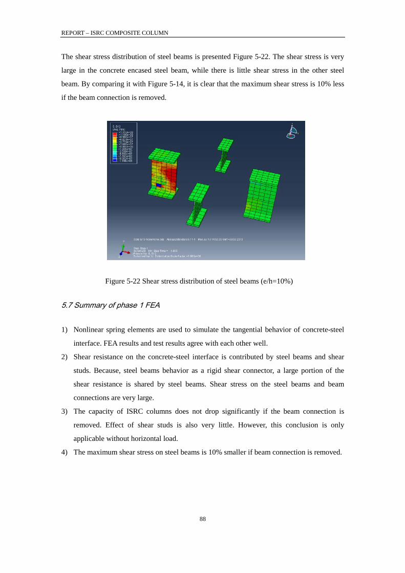
REPORT – ISRC COMPOSITE COLUMN
88
The shear stress distribution of steel beams is presented Figure 5-22. The shear stress is very
large in the concrete encased steel beam, while there is little shear stress in the other steel
beam. By comparing it with Figure 5-14, it is clear that the maximum shear stress is 10% less
if the beam connection is removed.
Figure 5-22 Shear stress distribution of steel beams (e/h=10%)
5.7 Summary of phase 1 FEA
1) Nonlinear spring elements are used to simulate the tangential behavior of concrete-steel
interface. FEA results and test results agree with each other well.
2) Shear resistance on the concrete-steel interface is contributed by steel beams and shear
studs. Because, steel beams behavior as a rigid shear connector, a large portion of the
shear resistance is shared by steel beams. Shear stress on the steel beams and beam
connections are very large.
3) The capacity of ISRC columns does not drop significantly if the beam connection is
removed. Effect of shear studs is also very little. However, this conclusion is only
applicable without horizontal load.
4) The maximum shear stress on steel beams is 10% smaller if beam connection is removed.
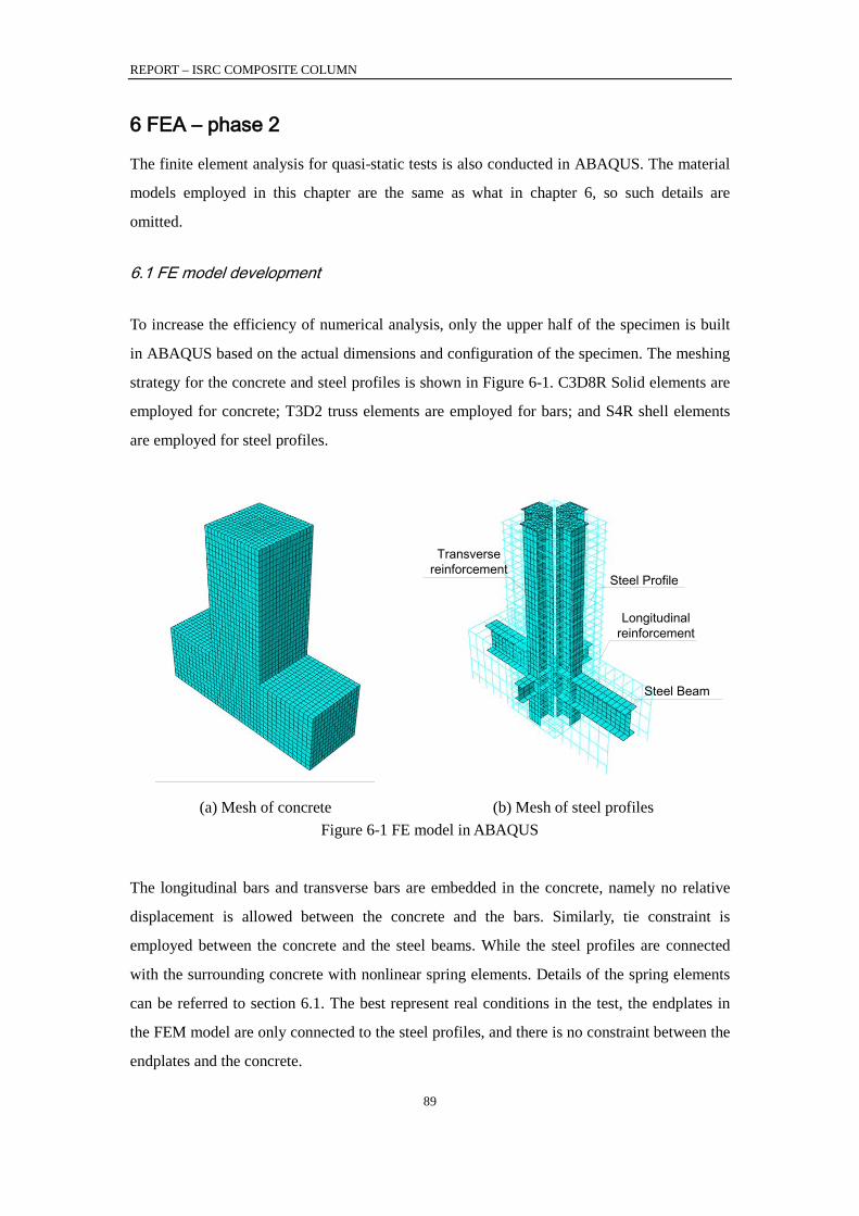
REPORT – ISRC COMPOSITE COLUMN
89
6 FEA – phase 2
The finite element analysis for quasi-static tests is also conducted in ABAQUS. The material
models employed in this chapter are the same as what in chapter 6, so such details are
omitted.
6.1 FE model development
To increase the efficiency of numerical analysis, only the upper half of the specimen is built
in ABAQUS based on the actual dimensions and configuration of the specimen. The meshing
strategy for the concrete and steel profiles is shown in Figure 6-1. C3D8R Solid elements are
employed for concrete; T3D2 truss elements are employed for bars; and S4R shell elements
are employed for steel profiles.
(a) Mesh of concrete
Steel Profile
Steel Beam
Longitudinal reinforcement
Transverse reinforcement
(b) Mesh of steel profiles
Figure 6-1 FE model in ABAQUS
The longitudinal bars and transverse bars are embedded in the concrete, namely no relative
displacement is allowed between the concrete and the bars. Similarly, tie constraint is
employed between the concrete and the steel beams. While the steel profiles are connected
with the surrounding concrete with nonlinear spring elements. Details of the spring elements
can be referred to section 6.1. The best represent real conditions in the test, the endplates in
the FEM model are only connected to the steel profiles, and there is no constraint between the
endplates and the concrete.
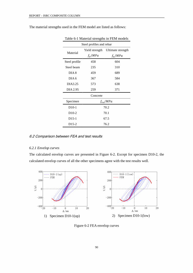
REPORT – ISRC COMPOSITE COLUMN
90
The material strengths used in the FEM model are listed as follows:
Table 6-1 Material strengths in FEM models
Steel profiles and rebar
Material Yield strength
𝑓𝑦/𝑀𝑃𝑎
Ultimate strength
𝑓𝑢/𝑀𝑃𝑎
Steel profile 458 604
Steel beam 235 310
DIA 8 459 689
DIA 6 367 584
DIA3.25 573 638
DIA 2.95 259 371
Concrete
Specimen 𝑓𝑐𝑢/𝑀𝑃𝑎
D10-1 70.2
D10-2 70.1
D15-1 67.5
D15-2 76.2
6.2 Comparison between FEA and test results
6.2.1 Envelop curves
The calculated envelop curves are presented in Figure 6-2. Except for specimen D10-2, the
calculated envelop curves of all the other specimens agree with the test results well.
-20 -10 0 10 20-400
-200
0
200
400
V/kN
∆/mm
D10-1(up)FEM
1) Specimen D10-1(up)
-20 -10 0 10 20-400
-200
0
200
400
V/kN
∆/mm
D10-1(low)FEM
2) Specimen D10-1(low)
Figure 6-2 FEA envelop curves
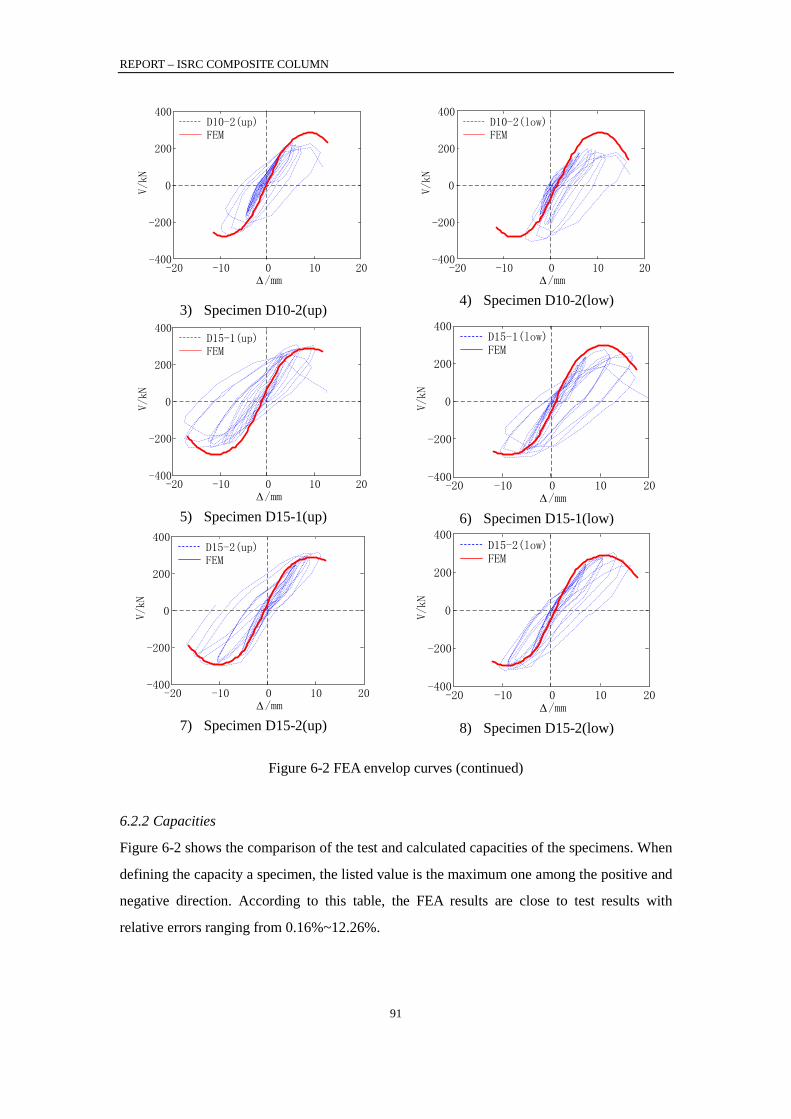
REPORT – ISRC COMPOSITE COLUMN
91
-20 -10 0 10 20-400
-200
0
200
400
V/kN
∆/mm
D10-2(up)FEM
3) Specimen D10-2(up)
-20 -10 0 10 20-400
-200
0
200
400
V/kN
∆/mm
D10-2(low)FEM
4) Specimen D10-2(low)
-20 -10 0 10 20-400
-200
0
200
400
V/kN
∆/mm
D15-1(up)FEM
5) Specimen D15-1(up)
-20 -10 0 10 20-400
-200
0
200
400
V/kN
∆/mm
D15-1(low)FEM
6) Specimen D15-1(low)
-20 -10 0 10 20-400
-200
0
200
400
V/kN
∆/mm
D15-2(up)FEM
7) Specimen D15-2(up)
-20 -10 0 10 20-400
-200
0
200
400
V/kN
∆/mm
D15-2(low)FEM
8) Specimen D15-2(low)
Figure 6-2 FEA envelop curves (continued)
6.2.2 Capacities
Figure 6-2 shows the comparison of the test and calculated capacities of the specimens. When
defining the capacity a specimen, the listed value is the maximum one among the positive and
negative direction. According to this table, the FEA results are close to test results with
relative errors ranging from 0.16%~12.26%.
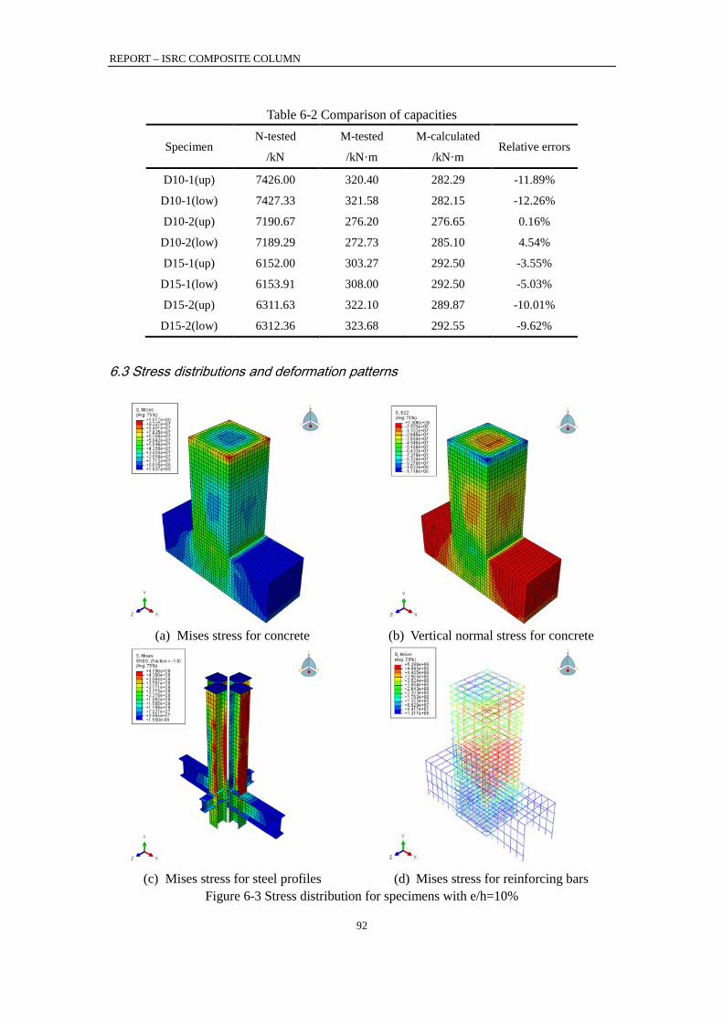
REPORT – ISRC COMPOSITE COLUMN
92
Table 6-2 Comparison of capacities
Specimen N-tested
/kN
M-tested
/kN·m
M-calculated
/kN·m Relative errors
D10-1(up) 7426.00 320.40 282.29 -11.89%
D10-1(low) 7427.33 321.58 282.15 -12.26%
D10-2(up) 7190.67 276.20 276.65 0.16%
D10-2(low) 7189.29 272.73 285.10 4.54%
D15-1(up) 6152.00 303.27 292.50 -3.55%
D15-1(low) 6153.91 308.00 292.50 -5.03%
D15-2(up) 6311.63 322.10 289.87 -10.01%
D15-2(low) 6312.36 323.68 292.55 -9.62%
6.3 Stress distributions and deformation patterns
(a) Mises stress for concrete
(b) Vertical normal stress for concrete
(c) Mises stress for steel profiles
(d) Mises stress for reinforcing bars
Figure 6-3 Stress distribution for specimens with e/h=10%
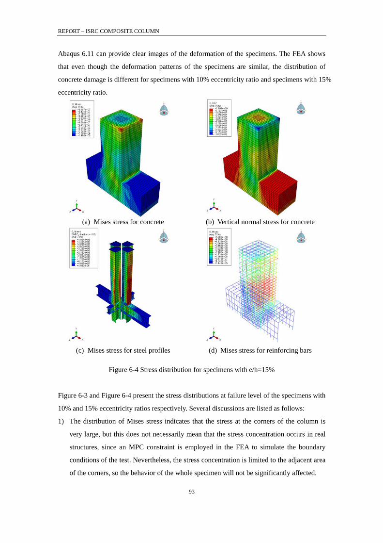
REPORT – ISRC COMPOSITE COLUMN
93
Abaqus 6.11 can provide clear images of the deformation of the specimens. The FEA shows
that even though the deformation patterns of the specimens are similar, the distribution of
concrete damage is different for specimens with 10% eccentricity ratio and specimens with 15%
eccentricity ratio.
(a) Mises stress for concrete
(b) Vertical normal stress for concrete
(c) Mises stress for steel profiles
(d) Mises stress for reinforcing bars
Figure 6-4 Stress distribution for specimens with e/h=15%
Figure 6-3 and Figure 6-4 present the stress distributions at failure level of the specimens with
10% and 15% eccentricity ratios respectively. Several discussions are listed as follows:
1) The distribution of Mises stress indicates that the stress at the corners of the column is
very large, but this does not necessarily mean that the stress concentration occurs in real
structures, since an MPC constraint is employed in the FEA to simulate the boundary
conditions of the test. Nevertheless, the stress concentration is limited to the adjacent area
of the corners, so the behavior of the whole specimen will not be significantly affected.

REPORT – ISRC COMPOSITE COLUMN
94
2) Figure 6-3 (b) and Figure 6-4 (b) shows the normal stress of the concrete in the
longitudinal direction of the specimen. At failure load level, tensile stress occurs in the
column of the specimen with 15% eccentricity ratio, but does not occur in that with 10%
eccentricity ratio.
Critical Section
200
200
(a) Specimens with e/h=10%
Critical Section
100
100
(b) Specimens with e/h=15% Figure 6-5 Distribution of PEEQ of the concrete

REPORT – ISRC COMPOSITE COLUMN
95
The cumulative damage of the concrete results in a plastic hinge at the bottom of the column,
whose length is dependent on the distribution of damage of the concrete. The position of the
critical section can be regarded as the center of the plastic hinge. By using plastic damage
model of the concrete, the analytical results can sometimes provide a meaningful insight into
the damage of the concrete. Shown in Figure 6-5 are the distributions of PEEQ of specimens
with 10% and 15% eccentricity ratios respectively. It is obvious that the position of damage is
higher for the specimen with 10% eccentricity ratio than that of the specimen with 15%
eccentricity ratio. Test results also support this phenomenon. Compared to specimen D15-1,
the damage of concrete of specimen D10-1 occurred at a higher place. Based on both the test
results and the FEA, the critical section is 200 mm away from the bottom of the column for
specimens with 10% eccentricity ratio, and 100 mm away from the bottom of the column for
specimens with 15% eccentricity ratio.
6.4 Influence of the shear resistance
Since the number of specimens was limited, a parametric study was conducted to investigate
how the shear resistance on the concrete-steel interface would influence the capacity of ISRC
columns. According to the superimposition method, the flexural capacity of the composite
column is dependent on the axial carried by the concrete and the steel sections, respectively.
Since in the longitudinal direction, the axial load between the concrete and the steel sections
is transferred by the shear force on the concrete-steel interface. Therefore, the flexural
capacity of the composite column is directly related to the shear resistance provided by the
combination of bond stress and shear studs.
Shown in Figure 6-6 is a free body diagram of the steel sections. A segment, from the top
surface to the critical section of the column, is extracted from one of the steel sections. Based
on the equilibrium in vertical forces, one may have the following equation:
2 1V N N= − (6.1)
where V is the shear force provided by the bond stress and shear studs; 𝑁1 and 𝑁2 are the
axial force on the two sides of the segment.
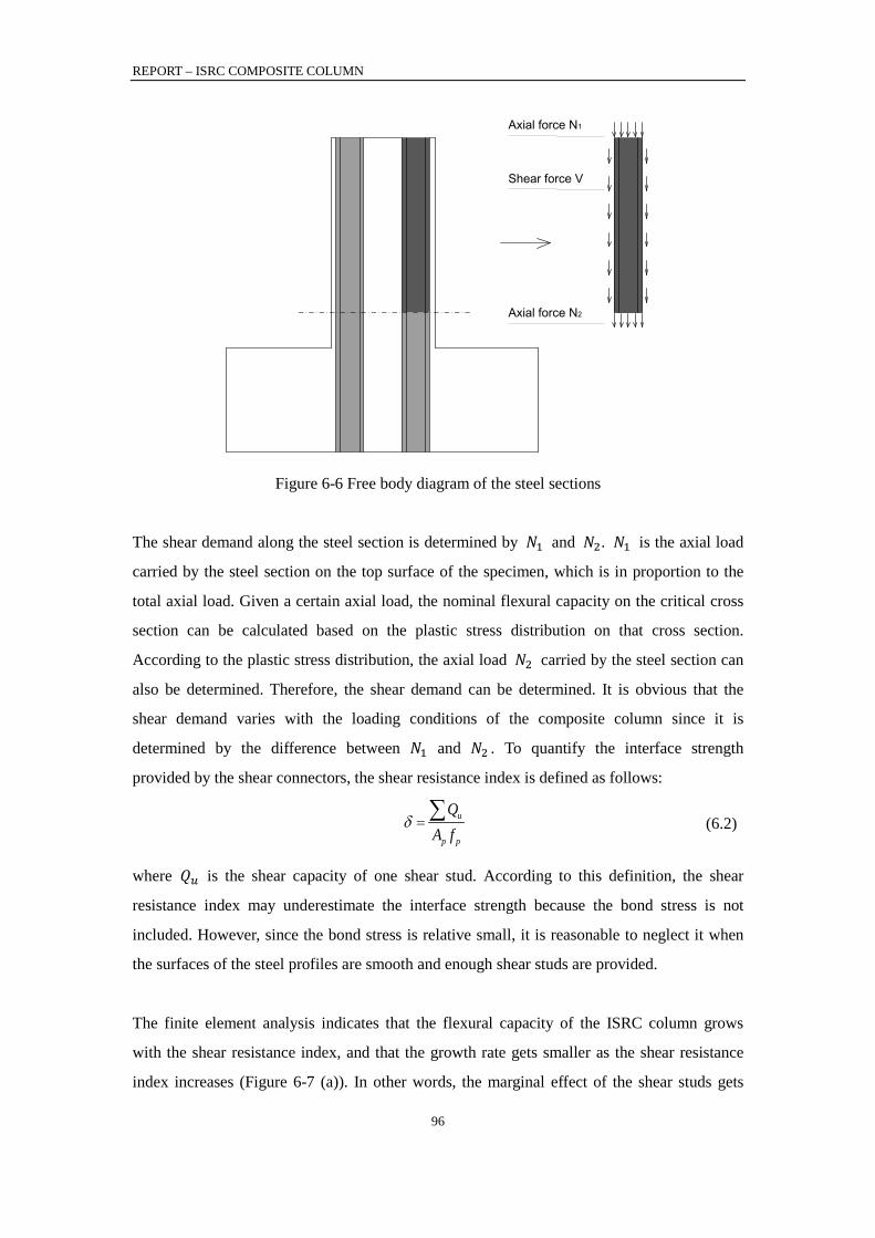
REPORT – ISRC COMPOSITE COLUMN
96
Shear force V
Axial force N1
Axial force N2
Figure 6-6 Free body diagram of the steel sections
The shear demand along the steel section is determined by 𝑁1 and 𝑁2. 𝑁1 is the axial load
carried by the steel section on the top surface of the specimen, which is in proportion to the
total axial load. Given a certain axial load, the nominal flexural capacity on the critical cross
section can be calculated based on the plastic stress distribution on that cross section.
According to the plastic stress distribution, the axial load 𝑁2 carried by the steel section can
also be determined. Therefore, the shear demand can be determined. It is obvious that the
shear demand varies with the loading conditions of the composite column since it is
determined by the difference between 𝑁1 and 𝑁2 . To quantify the interface strength
provided by the shear connectors, the shear resistance index is defined as follows:
u
p p
QA f
δ = ∑ (6.2)
where 𝑄𝑢 is the shear capacity of one shear stud. According to this definition, the shear
resistance index may underestimate the interface strength because the bond stress is not
included. However, since the bond stress is relative small, it is reasonable to neglect it when
the surfaces of the steel profiles are smooth and enough shear studs are provided.
The finite element analysis indicates that the flexural capacity of the ISRC column grows
with the shear resistance index, and that the growth rate gets smaller as the shear resistance
index increases (Figure 6-7 (a)). In other words, the marginal effect of the shear studs gets

REPORT – ISRC COMPOSITE COLUMN
97
smaller as the shear resistance index increases. When the shear resistance index is larger than
0.5, providing more shear studs will not significantly improve the capacity of ISRC columns.
The flexural capacities of columns with full composite action (δ = 1) are about 20% larger
than columns with no composite action (δ = 0).
0 0.25 0.5 0.75 1220
240
260
280
300
320
340
360
380
Shear resistance index
M/k
N·m
e/h=10%e/h=15%e/h=20%
D10-1
D10-2
D15-2
D15-1
(a) Flexural capacity
0 100 200 300 400 5000
2000
4000
6000
8000
10000
M/kN·mN
/kN
e/h=1
0%
e/h=15
%
e/h=20%
Interaction Curve
e/h=10%e/h=15%e/h=20%
(b) Interaction relationship
Figure 6-7 Influence of shear resistance index
In practice, accurately predicting the flexural capacity of ISRC columns can be complex, so a
more convenient while conservative way to determine the flexural capacity of ISRC columns
is to draw a straight line between the starting point and the ending point of the curve, and then
determine the flexural capacity according to the actual shear resistance index. For example,
the shear resistance index in this test program was:
2 20.5min , 5.064kN4 4
uu c c
fQ d d f Eπ π= =
3
25 5.064 0.122352 460 10
u
p p
QA f
δ −
×= = ≈
× ×∑
(6.3a)
(6.3b)
By conducting linear interpolation, the predicted flexural capacities are 228kN · m and
288kN · m for 10% and 15% specimens respectively. Because the actual curves are concave
and the contribution of bond stress is not considered, the predictions are conservative.
Note that both the axial capacity and the flexural capacity vary with the shear resistance index
because of the special loading protocol employed in this test. In fact, each point on the curves
in Figure 6-7 (a) represents a particular axial load. Projecting these points on an M-N
coordinate, a more clear relationship between the capacity and the shear resistance index can
be obtained (Figure 6-7 (b)). As it is shown in this figure, both the axial capacity and the
flexural capacity will be enhanced when the shear resistance index increases.
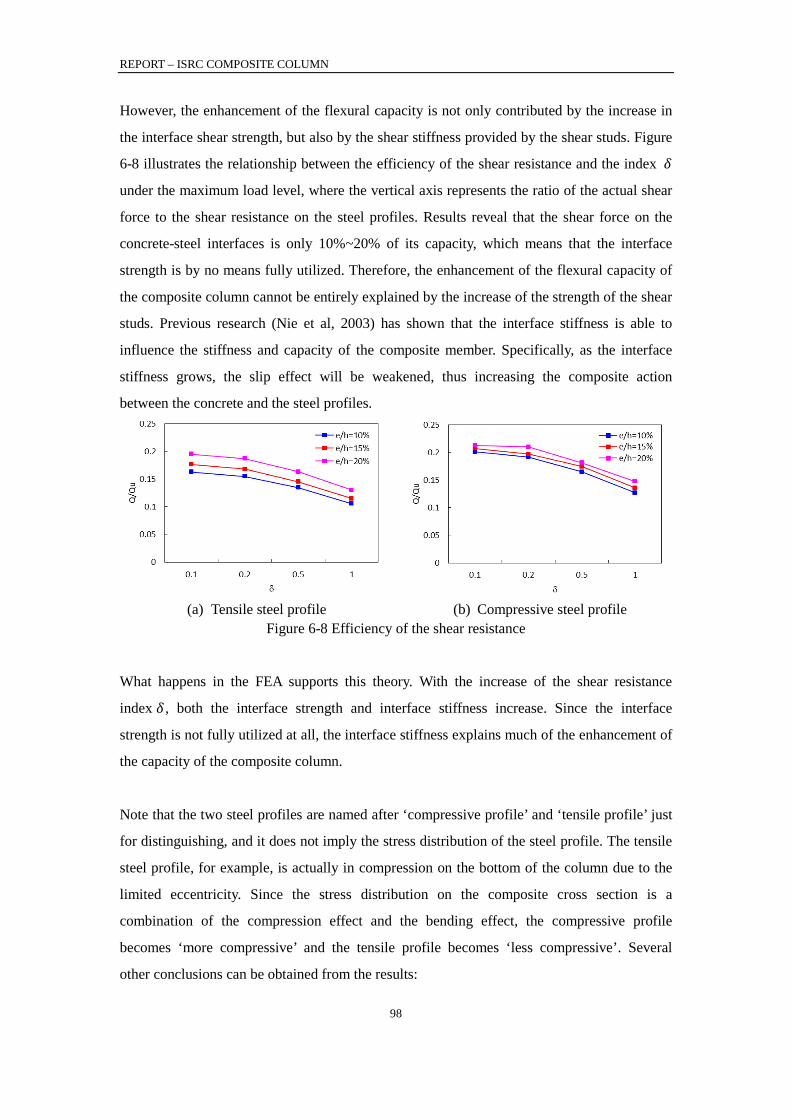
REPORT – ISRC COMPOSITE COLUMN
98
However, the enhancement of the flexural capacity is not only contributed by the increase in
the interface shear strength, but also by the shear stiffness provided by the shear studs. Figure
6-8 illustrates the relationship between the efficiency of the shear resistance and the index 𝛿
under the maximum load level, where the vertical axis represents the ratio of the actual shear
force to the shear resistance on the steel profiles. Results reveal that the shear force on the
concrete-steel interfaces is only 10%~20% of its capacity, which means that the interface
strength is by no means fully utilized. Therefore, the enhancement of the flexural capacity of
the composite column cannot be entirely explained by the increase of the strength of the shear
studs. Previous research (Nie et al, 2003) has shown that the interface stiffness is able to
influence the stiffness and capacity of the composite member. Specifically, as the interface
stiffness grows, the slip effect will be weakened, thus increasing the composite action
between the concrete and the steel profiles.
(a) Tensile steel profile
(b) Compressive steel profile
Figure 6-8 Efficiency of the shear resistance
What happens in the FEA supports this theory. With the increase of the shear resistance
index 𝛿 , both the interface strength and interface stiffness increase. Since the interface
strength is not fully utilized at all, the interface stiffness explains much of the enhancement of
the capacity of the composite column.
Note that the two steel profiles are named after ‘compressive profile’ and ‘tensile profile’ just
for distinguishing, and it does not imply the stress distribution of the steel profile. The tensile
steel profile, for example, is actually in compression on the bottom of the column due to the
limited eccentricity. Since the stress distribution on the composite cross section is a
combination of the compression effect and the bending effect, the compressive profile
becomes ‘more compressive’ and the tensile profile becomes ‘less compressive’. Several
other conclusions can be obtained from the results:

REPORT – ISRC COMPOSITE COLUMN
99
1) The shear force on the compressive steel profile is larger than that on the tensile steel
profile with all else equal. This is because the shear demand on the compressive profile is
larger than that on the tensile profile, which is a result of the small eccentricity.
2) The shear force on the steel profile increases as the eccentricity increases with all else
equal. Similarly, this can also be explained by the shear demand on the interface.
3) The efficiency of the shear resistance drops as the index 𝛿 increases. This conclusion, in
fact, is a direct inference of the constitutive law of the shear stud. As shown in Figure 5-4,
the strength of the shear stud can be reached only when the slip is fully developed. The
fact that more shear studs increases the interface stiffness, which leads to smaller slip,
which further leads to less effective of utilizing the strength of the shear studs.
In addition, two issues should be noted:
1) This relationship between the capacity and the shear resistance index is only valid when
the failure pattern of the composite column is combined compression and bending. The
relationship will be violated if other failure patterns occur, such as shear failure or other
premature failures.
2) In a real project, the actual shear resistance index can be very small. For example, the
shear resistance index in this test program is only 0.12, which means that the composite
columns have a large potential to increase the capacities. However, this does not mean
that the more shear studs, the better. First, as mentioned above, it is not economical when
the shear resistance index is very large. Second, more shear studs will make the
construction and fabrication work considerably difficult. Third, more shear studs may
further harm the bond conditions between the concrete and the steel sections.
In this phase of the test, since the steel beams are located near the plane of symmetry of the
specimens, very little shear demand is created on the interface of the steel beams and the steel
sections. As a result, the behavior of the specimens will not be significantly influenced if the
steel beams are removed from the model. Similar to the static test, test results and FEA in
phase 2 do not mean that the steel beams are not important in real structures. However, this
test program cannot reflect the influence of the steel beams.
REPORT – ISRC COMPOSITE COLUMN
100
6.5 Summary of phase 2 FEA
1) The FEA indicates that the position of the critical cross section of the specimen with
e/h=10% is higher than that of the specimen with e/h=15%. A similar phenomenon was
also observed in the test. In this test program, the distance between the critical section and
the bottom of the column is 2/3h and 1/3h for specimens with 10% and 15% eccentricity
ratios respectively, where ‘h’ is the width of the cross section.
2) Shear studs have a strong influence on the flexural capacity of the specimen. The FEA
indicates that shear studs are more efficient when the shear resistance index is less than
0.5; otherwise, providing more shear studs will not significantly increase the flexural
capacity of the specimen.
3) The enhancement in the capacity of ISRC columns can be explained by both the interface
strength and the interface stiffness.
4) In this test program, the existence of steel beams and connections do not have much
influence on the capacity of the specimen since the beam-column joint is near the plane of
symmetry where the shear demand on the concrete-steel interface is relatively small.
REPORT – ISRC COMPOSITE COLUMN
101
7 Code evaluations
This chapter of the report presents a description of the design philosophies and procedures in
current codes from the U.S., Europe, and China. More detailed design procedures in Chinese
codes are discussed in the last section of this chapter.
Since the main purpose of the test program is to investigate the performance ISRC columns,
this chapter of the report focuses on the code provisions concerning how to determine the
resistance of the ISRC columns, and the load factors will not be discussed. Therefore, the
safety factors calculated in section 8.1 and 8.2 do not reflect the degree of redundancy of
these codes comprehensively. However, the calculated safety factors do provide an insight to
evaluate the code provisions to determine the resistance of the composite columns.
7.1 Code predictions on axial resistance
The procedures for determining the pure axial resistance of a composite column include three
steps: (1) compute the cross-sectional resistance of the composite column, (2) include the
reduction factors to account for the minimum eccentricity ratios, imperfections, and buckling
effects to obtain the nominal axial resistance, and (3) include the strength reduction factors to
obtain the factored axial resistance of the composite column.
The minimum design eccentricity is included in many codes to serve as a means of reducing
the axial design resistance of a section in pure compression to account for accidental
eccentricities that may exist in a compression member but not considered in the analysis, and
to recognize that concrete strength may be reduced under sustained high loads. In early
editions of the codes, the minimum eccentricity requirement was employed to limit the
maximum design axial load of a compression member. This is now accomplished directly by
limiting the axial resistance of a section in pure compression.
In ACI 318, the nominal axial resistance is limited to 85% and 80% of the cross-sectional
axial resistance for spirally reinforced and tied reinforced members, respectively. In Chinese
code GB 50010, the nominal axial resistance is limited to 90% of the cross-sectional axial
resistance, regardless of the configuration of transverse reinforcement.
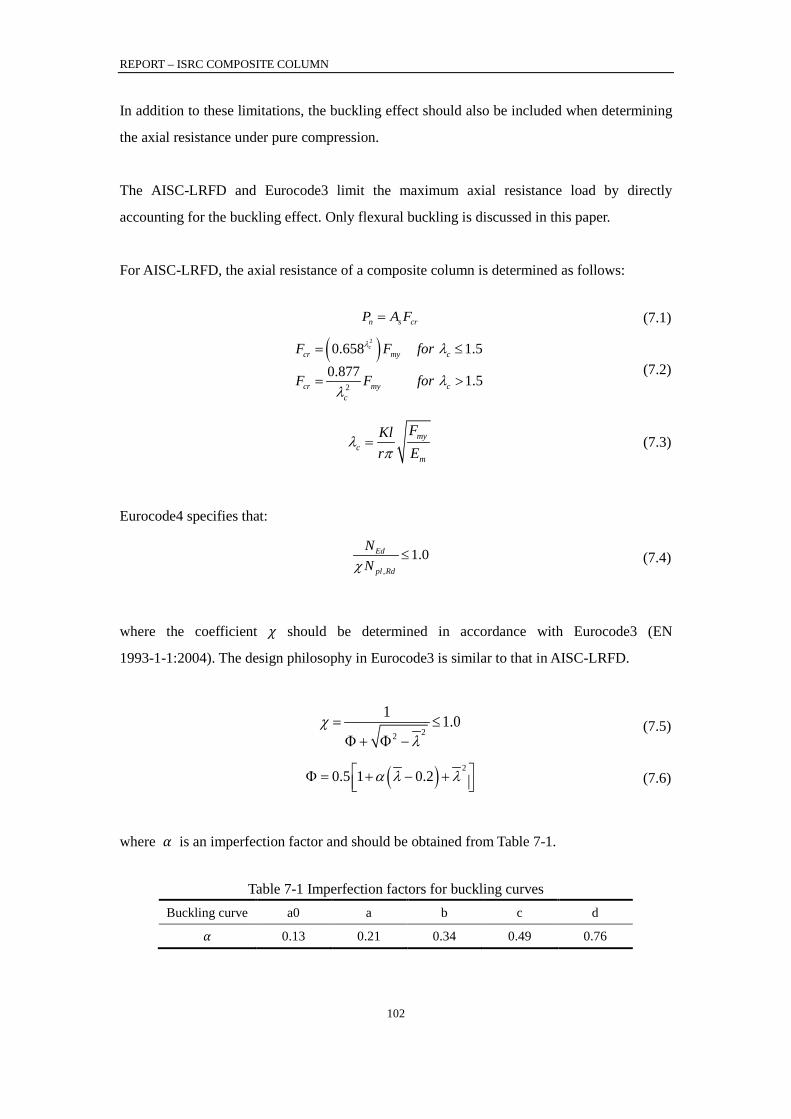
REPORT – ISRC COMPOSITE COLUMN
102
In addition to these limitations, the buckling effect should also be included when determining
the axial resistance under pure compression.
The AISC-LRFD and Eurocode3 limit the maximum axial resistance load by directly
accounting for the buckling effect. Only flexural buckling is discussed in this paper.
For AISC-LRFD, the axial resistance of a composite column is determined as follows:
n s crP A F= (7.1)
( )2
2
1.50.870.65
7 .5
8
1
cc
cr cc
cr my
myF
F F for
F for
λ λ
λλ
≤
= >
=
(7.2)
myc
m
FKlr E
λπ
=
(7.3)
Eurocode4 specifies that:
,
1.0p
d
l
E
Rd
NNχ
≤
(7.4)
where the coefficient 𝜒 should be determined in accordance with Eurocode3 (EN
1993-1-1:2004). The design philosophy in Eurocode3 is similar to that in AISC-LRFD.
22
1 1.0χλ
= ≤Φ + Φ −
(7.5)
( ) 20.5 1 0.2α λ λ Φ = + − +
(7.6)
where 𝛼 is an imperfection factor and should be obtained from Table 7-1.
Table 7-1 Imperfection factors for buckling curves
Buckling curve a0 a b c d
𝛼 0.13 0.21 0.34 0.49 0.76

REPORT – ISRC COMPOSITE COLUMN
103
Figure 7-1 Reduction factors
A comparison between the buckling curves from AISC-LRFD, Eurocode3, and GB 50010 is
presented in Figure 7-1. Results given by Eurocode3 are plotted in dashed lines, with
buckling curves ‘a0’, ‘a’, ‘b’, ‘c’, and ‘d’ ordered from top to bottom. Results suggest that the
buckling curve given by AISC-LRFD resembles buckling curves ‘a’ and ‘b’ given by
Eurocode3, and that the GB 50010 is less conservative when the relative slenderness is larger
than 1.0.
Table 7-2 Redundancy factors of different codes
Speci
men
𝑁𝑡𝑒𝑠𝑡
/kN
Un-factored
Factored
𝑁𝑡𝑒𝑠𝑡𝑁𝐴𝐶𝐼
𝑁𝑡𝑒𝑠𝑡𝑁𝐴𝐼𝑆𝐶
𝑁𝑡𝑒𝑠𝑡𝑁𝐸𝐶4
𝑁𝑡𝑒𝑠𝑡𝑁𝑌𝐵
𝑁𝑡𝑒𝑠𝑡𝜙𝑁𝐴𝐶𝐼
𝑁𝑡𝑒𝑠𝑡𝜙𝑁𝐴𝐼𝑆𝐶
𝑁𝑡𝑒𝑠𝑡𝜙𝑁𝐸𝐶4
𝑁𝑡𝑒𝑠𝑡𝜙𝑁𝑌𝐵
E00-1 17082 1.22 1.25 1.17 1.14 1.87 1.48 1.49 1.46
E00-2 15325 1.13 1.16 1.08 1.07 1.73 1.36 1.37 1.34
AVE 1.18 1.21 1.13 1.11 1.80 1.42 1.43 1.40
Figure 7-2 shows the ratios of test results to the nominal axial resistance of specimen E00-1
and E00-2. Note that buckling curve ‘b’ is employed in Eurocode4. The AISC-LRFD
produces results that are more conservative with the average redundancy of 1.21. However,
this does not necessarily mean that the AISC-LRFD provides more conservative results
compared with other codes, because the strength reduction factor 𝜙 has not been included
yet.
ACI 318 specifies that the 𝜙 factor to be taken as 0.65 for compression-controlled sections
with tie reinforcement, and the 𝜙 factor is permitted to be linearly increased from 0.65 to

REPORT – ISRC COMPOSITE COLUMN
104
0.90 as the net tensile strain in the extreme tension steel at nominal strength increases from
the compression-controlled strain limit to 0.005. The 𝜙 factor specified by AISC-LRFD is
0.85 for axial strength. For flexural strength, the 𝜙 factor is also taken as 0.85 if the nominal
flexural strength is determined based on the plastic stress distribution of the composite cross
section (If other design philosophies are adopted, the 𝜙 factor can be different). Chinese
codes and Eurocode4 do not apply the strength reduction factors to the calculated strength of
the cross section. Rather, the strength reduction factors are applied to the material strength.
According to Chinese codes (GB50010 2010; GB50017 2003), the design strength of the
material is the characteristic value of the material strength divided by 𝛾𝑅. The values of 𝛾𝑅
for concrete, reinforcing bars, and steel sections are 1.40, 1.10, and 1.11 respectively.
Similarly, the values of 𝛾𝑅 specified by Eurocode2 are 1.50, 1.15, and 1.00 for concrete,
reinforcing bars, and steel sections, respectively. In addition, Eurocode4 also employs a 𝜙
factor to the design flexural resistance. The 𝜙 factor should be taken as 0.9 for steel grades
between S235 to S355, and be taken as 0.8 for steel grades S420 and S460.
With the strength reduction factors being included, the ACI 318 produces the most
conservative results with the average redundancy factor of 1.80, while the other three codes
produce similar results with redundancy factors around 1.42.
7.2 Code predictions on flexural resistance
Current code provisions provide distinct ways to determine the flexural capacity of
concrete-encased composite columns. Most of the design philosophies are based on the
following assumptions:
(1) Plane sections remain plane.
(2) Full composite action between the concrete and the steel sections holds effective up
to failure of the composite column.
(3) The tensile strength of the concrete is neglected.
According to ACI 318, the flexural capacity of the composite column is determined based on
the plastic stress distribution of the cross section. The coefficient of 0.85 is applied to the
concrete compressive strength. As mentioned above, the nominal axial resistance of the
composite members shall not exceed 85% or 80% of the cross-sectional pure axial resistance,
depending on the configurations of the transverse reinforcement.

REPORT – ISRC COMPOSITE COLUMN
105
In AISC-LRFD (1999), the design philosophy for composite columns derives from the design
of steel columns. The modified material strength and modulus of elasticity should be
calculated based on the configuration of the composite column, and then the nominal axial
capacity of the column can be obtained. Similar to ACI 318, the nominal flexural capacity of
the composite column is determined based on the plastic stress distribution on the composite
cross section. The interaction curve of the column is determined by the following two
equations:
80.2 1.09n n b
u u u
nP PP P
MMFor
φ φ φ≥ + ≤ (7.7a)
20.2 1.0
n n
u u
b n
uP PP
MFoP M
rφ φ φ
< + ≤
(7.7b)
The design philosophy in Chinese code Technical Specification of Steel-Reinforced Concrete
Structures (YB 9082) derived from the Japan code AIJ standards for structural calculation of
steel reinforced concrete structures (AIJ-SRC), in which the so called ‘superimposition
method’ is used for determining the capacity of concrete-encased composite columns under
combined compression and bending. However, YB 9082 employs a more rational strategy to
allocate the axial load carried by the concrete and the steel sections respectively, resulting in
more accurate predictions on the capacity of the composite columns.
Predictions provided by these codes are presented in Figure 7-2 together with the test results.
To evaluate the code provisions, the redundancy factor is defined as follows:
(1) Draw a straight line between the origin and the test result;
(2) The redundancy factor is defined as the ratio of the distance between the origin and the
test result to the distance between the origin and the intersection of the straight line and the
interactive curve (Figure 7-2).
For un-factored predictions, the ACI 318 and YB 9082 yield similar results, but the YB 9082
has a higher plateau than the ACI 318 since the ACI 318 has a more restrict limitation on the
pure axial strength. The key points of Eurocode4 well agreed with ACI 318 and YB 9082, but
Eurocode4 is more conservative since a linear relationship between the axial and flexural
capacity is employed. Buckling curve ‘b’ is employed in determining the axial strength of the
composite columns. As shown in the figure, the buckling curve ‘b’ is close to Chinese codes.
The AISC-LRFD provides the most conservative results among these four codes.
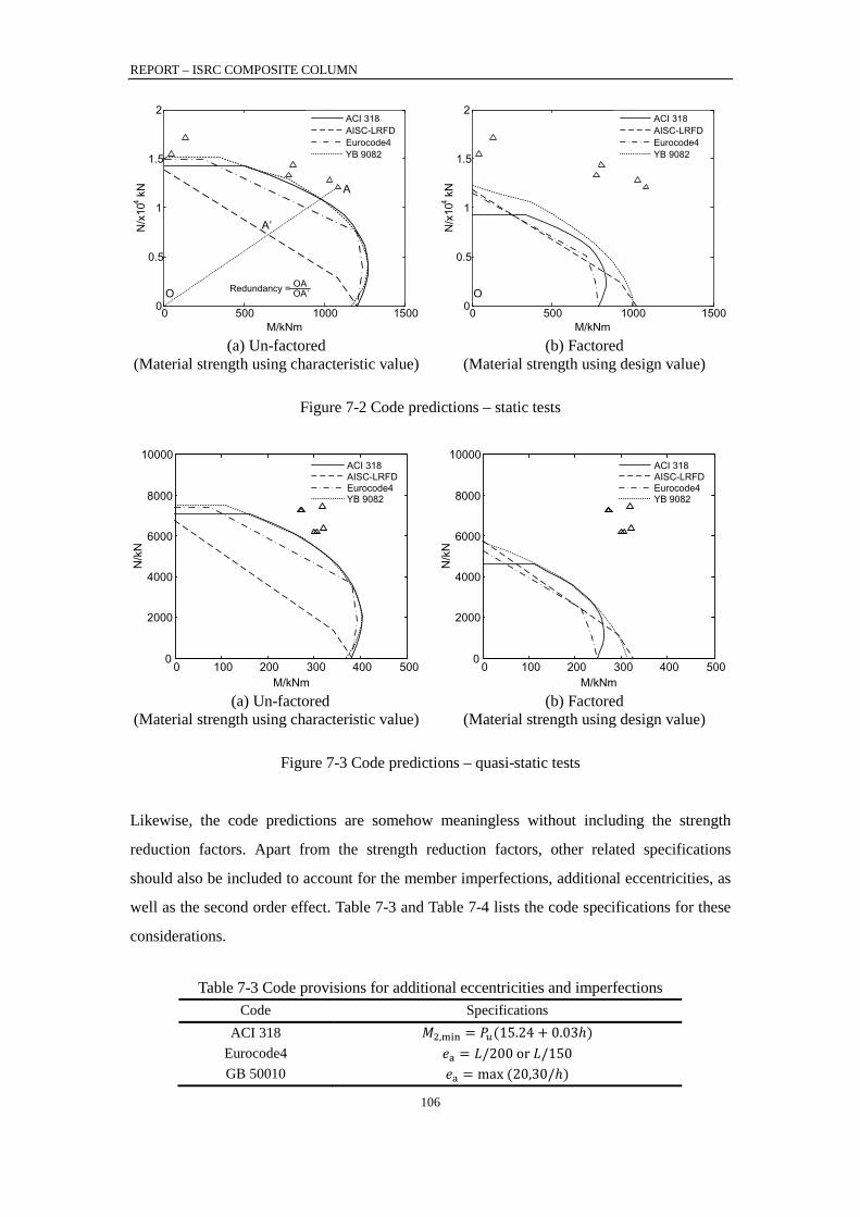
REPORT – ISRC COMPOSITE COLUMN
106
0 500 1000 15000
0.5
1
1.5
2
4
M/kNm
N/x
10 k
N
A’
O
A
Redundancy = OAOA’
ACI 318AISC-LRFDEurocode4YB 9082
(a) Un-factored (Material strength using characteristic value)
0 500 1000 15000
0.5
1
1.5
2
4
M/kNm
N/x
10 k
N
O
ACI 318AISC-LRFDEurocode4YB 9082
(b) Factored (Material strength using design value)
Figure 7-2 Code predictions – static tests
0 100 200 300 400 5000
2000
4000
6000
8000
10000
M/kNm
N/k
N
ACI 318AISC-LRFDEurocode4YB 9082
(a) Un-factored (Material strength using characteristic value)
0 100 200 300 400 5000
2000
4000
6000
8000
10000
M/kNm
N/k
N
ACI 318AISC-LRFDEurocode4YB 9082
(b) Factored
(Material strength using design value)
Figure 7-3 Code predictions – quasi-static tests
Likewise, the code predictions are somehow meaningless without including the strength
reduction factors. Apart from the strength reduction factors, other related specifications
should also be included to account for the member imperfections, additional eccentricities, as
well as the second order effect. Table 7-3 and Table 7-4 lists the code specifications for these
considerations.
Table 7-3 Code provisions for additional eccentricities and imperfections
Code Specifications ACI 318 𝑀2,min = 𝑃𝑢(15.24 + 0.03ℎ)
Eurocode4 𝑒a = 𝐿/200 or 𝐿/150 GB 50010 𝑒a = max (20,30/ℎ)
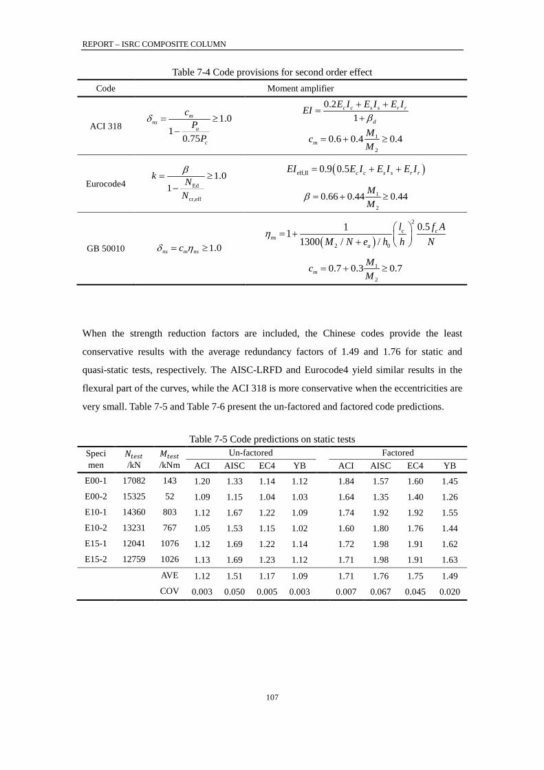
REPORT – ISRC COMPOSITE COLUMN
107
Table 7-4 Code provisions for second order effect Code Moment amplifier
ACI 318 1.0
10.75
mns
u
c
cP
P
δ = ≥−
0.2
1c c s s r
d
rE I E I E IEIβ
+ +=
+
1
2
0.6 0.4 0.4mMcM
= + ≥
Eurocode4 Ed
cr,eff
1.01
k NN
β= ≥
− ( )eff,II 0.9 0.5 c c s s r rEI E I E I E I= + +
1
2
0.66 0.44 0.44MM
β = + ≥
GB 50010 1.0ns m nscδ η= ≥ ( )
2
2 0
0.5111300 / /
c cns
a
l f AM N e h h N
η = + +
1
2
0.7 0.3 0.7mMcM
= + ≥
When the strength reduction factors are included, the Chinese codes provide the least
conservative results with the average redundancy factors of 1.49 and 1.76 for static and
quasi-static tests, respectively. The AISC-LRFD and Eurocode4 yield similar results in the
flexural part of the curves, while the ACI 318 is more conservative when the eccentricities are
very small. Table 7-5 and Table 7-6 present the un-factored and factored code predictions.
Table 7-5 Code predictions on static tests
Specimen
𝑁𝑡𝑒𝑠𝑡 /kN
𝑀𝑡𝑒𝑠𝑡 /kNm
Un-factored
Factored ACI AISC EC4 YB ACI AISC EC4 YB
E00-1 17082 143 1.20 1.33 1.14 1.12 1.84 1.57 1.60 1.45 E00-2 15325 52 1.09 1.15 1.04 1.03 1.64 1.35 1.40 1.26 E10-1 14360 803 1.12 1.67 1.22 1.09 1.74 1.92 1.92 1.55 E10-2 13231 767 1.05 1.53 1.15 1.02 1.60 1.80 1.76 1.44 E15-1 12041 1076 1.12 1.69 1.22 1.14 1.72 1.98 1.91 1.62 E15-2 12759 1026 1.13 1.69 1.23 1.12 1.71 1.98 1.91 1.63
AVE 1.12 1.51 1.17 1.09 1.71 1.76 1.75 1.49 COV 0.003 0.050 0.005 0.003 0.007 0.067 0.045 0.020
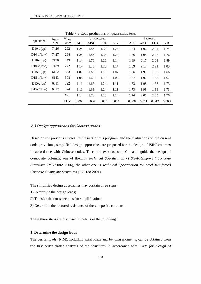
REPORT – ISRC COMPOSITE COLUMN
108
Table 7-6 Code predictions on quasi-static tests
Specimen 𝑁𝑡𝑒𝑠𝑡 /kN
𝑀𝑡𝑒𝑠𝑡 /kNm
Un-factored Factored ACI AISC EC4 YB ACI AISC EC4 YB
D10-1(up) 7426 292 1.24 1.84 1.36 1.24 1.74 1.96 2.04 1.74 D10-1(low) 7427 294 1.24 1.84 1.36 1.24 1.76 1.98 2.07 1.76 D10-2(up) 7190 249 1.14 1.71 1.26 1.14 1.89 2.17 2.21 1.89
D10-2(low) 7189 242 1.14 1.71 1.26 1.14 1.89 2.17 2.21 1.89 D15-1(up) 6152 303 1.07 1.60 1.19 1.07 1.66 1.91 1.95 1.66
D15-1(low) 6153 308 1.08 1.65 1.19 1.08 1.67 1.92 1.96 1.67 D15-2(up) 6311 322 1.11 1.69 1.24 1.11 1.73 1.98 1.98 1.73
D15-2(low) 6312 324 1.11 1.69 1.24 1.11 1.73 1.98 1.98 1.73
AVE 1.14 1.72 1.26 1.14 1.76 2.01 2.05 1.76 COV 0.004 0.007 0.005 0.004 0.008 0.011 0.012 0.008
7.3 Design approaches for Chinese codes
Based on the previous studies, test results of this program, and the evaluations on the current
code provisions, simplified design approaches are proposed for the design of ISRC columns
in accordance with Chinese codes. There are two codes in China to guide the design of
composite columns, one of them is Technical Specification of Steel-Reinforced Concrete
Structures (YB 9082 2006), the other one is Technical Specification for Steel Reinforced
Concrete Composite Structures (JGJ 138 2001).
The simplified design approaches may contain three steps:
1) Determine the design loads;
2) Transfer the cross sections for simplification;
3) Determine the factored resistance of the composite columns.
These three steps are discussed in details in the following:
1. Determine the design loads
The design loads (N,M), including axial loads and bending moments, can be obtained from
the first order elastic analysis of the structures in accordance with Code for Design of
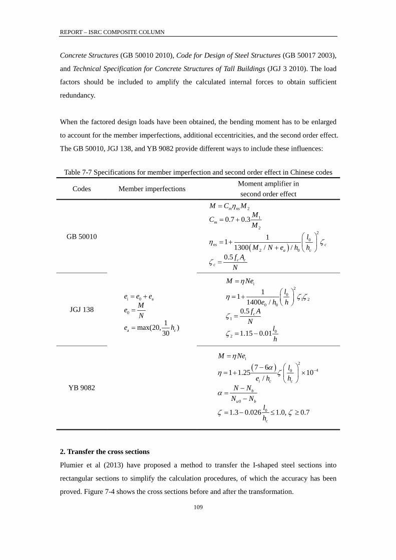
REPORT – ISRC COMPOSITE COLUMN
109
Concrete Structures (GB 50010 2010), Code for Design of Steel Structures (GB 50017 2003),
and Technical Specification for Concrete Structures of Tall Buildings (JGJ 3 2010). The load
factors should be included to amplify the calculated internal forces to obtain sufficient
redundancy.
When the factored design loads have been obtained, the bending moment has to be enlarged
to account for the member imperfections, additional eccentricities, and the second order effect.
The GB 50010, JGJ 138, and YB 9082 provide different ways to include these influences:
Table 7-7 Specifications for member imperfection and second order effect in Chinese codes
Codes Member imperfections Moment amplifier in second order effect
GB 50010
i 0 a
0
a1max(20, )30 c
e e eMeN
e h
= +
=
=
( )
2
1
22
0
2 0
0.7 0.3
111300 / /
0.5
ns
m
ns ca c
c c
m
c
MMCM
lM
M
N e h hf A
C
N
η
η ζ
ζ
= +
= +
=
=
+
JGJ 138
i2
01 2
0 0
1
02
111400 /
0.5
1.15 0.01
c
Nel
e h h
h
M
f AN
l
η
η ζ ζ
ζ
ζ
= +
=
= −
=
YB 9082
( )i
240
0
0
7 61 1.25 10
/
1.3 0.026 1.0, 0.7
i c c
b
u b
c
Nel
e h hN
M
NN N
lh
ηα
η ζ
α
ζ ζ
−− = + ×
−
=−
= − ≤ ≥
=
2. Transfer the cross sections
Plumier et al (2013) have proposed a method to transfer the I-shaped steel sections into
rectangular sections to simplify the calculation procedures, of which the accuracy has been
proved. Figure 7-4 shows the cross sections before and after the transformation.
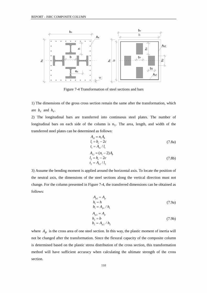
REPORT – ISRC COMPOSITE COLUMN
110
1) The dimensions of the gross cross section remain the same after the transformation, which
are 𝑏𝑐 and ℎ𝑐.
2) The longitudinal bars are transferred into continuous steel plates. The number of
longitudinal bars on each side of the column is 𝑛1. The area, length, and width of the
transferred steel plates can be determined as follows:
1 1
1
1 1 1
2/
s b
c
s
A n Al b ct A l
== −=
(7.8a)
2 1
2
2 2 2
( 2)2/
s b
c
s
A n Al h ct A l
= −= −=
(7.8b)
3) Assume the bending moment is applied around the horizontal axis. To locate the position of
the neutral axis, the dimensions of the steel sections along the vertical direction must not
change. For the column presented in Figure 7-4, the transferred dimensions can be obtained as
follows:
1
1
1 1 1/
p p
p
A Ah hb A h
===
(7.9a)
2
2
2 2 2/
p p
p
A Ah bb A h
===
(7.9b)
where 𝐴𝑝 is the cross area of one steel section. In this way, the plastic moment of inertia will
not be changed after the transformation. Since the flexural capacity of the composite column
is determined based on the plastic stress distribution of the cross section, this transformation
method will have sufficient accuracy when calculating the ultimate strength of the cross
section.
l1
l2
As2
As1
b2
h2
b1
h1
hc
bc
ep
b
h
c
hc
bc
As
Figure 7-4 Transformation of steel sections and bars
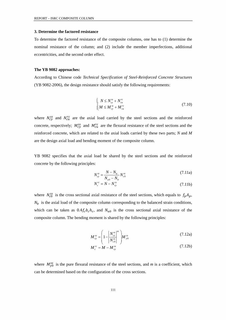
REPORT – ISRC COMPOSITE COLUMN
111
3. Determine the factored resistance
To determine the factored resistance of the composite columns, one has to (1) determine the
nominal resistance of the column; and (2) include the member imperfections, additional
eccentricities, and the second order effect.
The YB 9082 approaches:
According to Chinese code Technical Specification of Steel-Reinforced Concrete Structures
(YB 9082-2006), the design resistance should satisfy the following requirements:
ss rccy cuss rccy cu
N N NM M M ≤ + ≤ +
(7.10)
where 𝑁𝑐𝑦𝑠𝑠 and 𝑁𝑐𝑢𝑟𝑐 are the axial load carried by the steel sections and the reinforced
concrete, respectively; 𝑀𝑐𝑦𝑠𝑠 and 𝑀𝑐𝑢
𝑟𝑐 are the flexural resistance of the steel sections and the
reinforced concrete, which are related to the axial loads carried by these two parts; N and M
are the design axial load and bending moment of the composite column.
YB 9082 specifies that the axial load be shared by the steel sections and the reinforced
concrete by the following principles:
00
ss ssbcy c
u brc ssc cy
N NN NN N
N N N
−=
−= −
(7.11a)
(7.11b)
where 𝑁𝑐0𝑠𝑠 is the cross sectional axial resistance of the steel sections, which equals to 𝑓𝑝𝐴𝑝,
𝑁𝑏 is the axial load of the composite column corresponding to the balanced strain conditions,
which can be taken as 0.4𝑓𝑐𝑏𝑐ℎ𝑐, and 𝑁𝑢0 is the cross sectional axial resistance of the
composite column. The bending moment is shared by the following principles:
00
1mss
cyss sscy yss
c
rc ssc cy
NM M
N
M M M
= −
= −
(7.12a)
(7.12b)
where 𝑀𝑦0𝑠𝑠 is the pure flexural resistance of the steel sections, and m is a coefficient, which
can be determined based on the configuration of the cross sections.

REPORT – ISRC COMPOSITE COLUMN
112
For the steel sections part, the axial and flexural resistance of the steel sections automatically
exceeds the carried axial load and bending moment according to Eq. 7.11a and Eq. 7.12a. For
the reinforced concrete part, the position of the neutral axis can be obtained from the carried
axial load 𝑁𝑐𝑟𝑐, and the corresponding axial and flexural resistance can be obtained from the
following equations:
( )( ) ( ) ( )
' ' ' ' '1 0 0
' ' ' ' ' ' '1 0 0 0 0 02
c y s s s p p p p p
rc
rcc
cu c y s s p p
u
p p
f bx f A A f A AxM M f bx h f A h a f
N N
A h a
α σ σ σ
α σ
+ − − − −
≤ = − + − − − −
≤ =
(7.13a)
(7.13b)
In general, the YB 9082 permits to calculate the flexural resistance of the steel sections and
the reinforced concrete separately based on the axial loads carried by these two parts, and the
flexural resistance of the composite column is the sum of the flexural resistance of these two
parts.
JGJ 138 approaches: The JGJ 138 permits to calculate the nominal resistance of the composite columns based on the plastic stress distribution of the composite cross sections. A simplified method is proposed in JGJ 138 to calculate concrete-encased composite columns with a single I-shaped steel section in the middle of the cross section. This method, however, is not suitable for ISRC columns. Therefore, a more appropriate approach is proposed based on the basic principles of JGJ 138: (1) plane sections remain plane, (2) tensile strength of the concrete is neglected, and (3) the ultimate compressive strain for concrete is 0.0033.
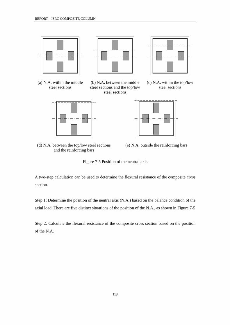
REPORT – ISRC COMPOSITE COLUMN
113
A two-step calculation can be used to determine the flexural resistance of the composite cross
section.
Step 1: Determine the position of the neutral axis (N.A.) based on the balance condition of the
axial load. There are five distinct situations of the position of the N.A., as shown in Figure 7-5
Step 2: Calculate the flexural resistance of the composite cross section based on the position
of the N.A.
(a) N.A. within the middle steel sections
(b) N.A. between the middle steel sections and the top/low
steel sections
(c) N.A. within the top/low steel sections
(d) N.A. between the top/low steel sections and the reinforcing bars
(e) N.A. outside the reinforcing bars
Figure 7-5 Position of the neutral axis

REPORT – ISRC COMPOSITE COLUMN
114
8 Conclusions
A series of structural tests were conducted on concrete-encased composite columns with
separate steel profiles. The test specimens were designed to achieve high levels of composite
action between the concrete and the steel profiles. A two-phase test program was carried out.
Phase 1 of the study included six 1/4-scaled static tests, and phase 2 of the study included four
1/6-scaled quasi-static tests. The following sections provide the conclusions found by this
research program.
8.1 Comparing results to previous studies
Since very few tests were conducted on ISRC columns, there are limited comparable results.
However, comparing the test results to previous SRC tests can still provide some insight.
1. Shear demand for ISRC columns is larger
Previous studies (Ricles and Paboojian, 1994; Mirza et al, 1996) found that the shear
connectors had little influence on the ultimate capacity of SRC columns. This is because the
shear demand on the concrete-steel interfaces is relatively small for SRC columns. Therefore,
installing more shear connectors could not improve the capacity of SRC columns significantly.
Test results of this test program revealed that the Plane Section Assumption was generally
valid for specimens with e/h=10% and e/h=15%, but the interface slip grew with the
eccentricity, which suggested that the shear demand was relatively larger for ISRC columns.
2. Confinement provided by the steel profiles is helpful The confinement effect may increase the ultimate compressive strain of the concrete, thus improving the ductility of the composite column. For SRC columns, the confinement effect is often provided by transverse reinforcement and the steel flanges. For ISRC columns, however, the concrete core surrounded by the steel profiles was also highly confined, thus increasing the ductility of the ISRC column.
REPORT – ISRC COMPOSITE COLUMN
115
8.2 Comparing results to code provisions
1. Code predictions on ultimate capacity
The current ACI 318, AISC-LRFD, Eurocode4, JGJ 138, and YB 9082 were evaluated in this
test program. The first four of these codes are based on the Plane Section Assumption, while
the last code is based on the superimposition method. For the test specimens, the current
codes were able to provide precise predictions on the axial and flexural capacities with
sufficient margins of safety.
2. Requirements for lateral deformation
Both the static and quasi-static specimens showed sufficient deformation capacity. In static
tests, the specimens were able to maintain the bending moment as high as the maximum while
the curvature was developing up to failure. In quasi-static tests, the ultimate drift ratios of the
specimens were 1/54~1/97, which met the minimum requirement - 1/100 - specified by
Chinese code Technical specification for concrete structures of tall building (JGJ 3 - 2010).
Previous studies have revealed that the transverse reinforcement was very helpful in
improving the ductility and deformation capacity of SRC columns. The authors believe that
the same rule applies to ISRC columns. However, since the test specimens were limited, the
influence of transverse reinforcement was not deeply investigated in this test program.
3. Coefficients of stiffness reduction
The code provisions allow the use of the reduced stiffness of a concrete member (or
composite member) to calculate the first order elastic reaction of the structure as a simplified
way to account for the second order effect and concrete crack under medium or severe
earthquakes. Test results of this program support the conclusion that the stiffness reduction
factor be taken as 0.7 for ACI 318 method (The factor is applied to the entire composite cross
section.) or 0.6 for Eurocode4 method (The factor is applied to the concrete part only.).
4. Simplified design methods
Simplified design approaches were proposed and described in this report in accordance with
Chinese codes JGJ 138 and YB 9082. The design approaches are applicable to ISRC columns
within 15% eccentricity ratio.
REPORT – ISRC COMPOSITE COLUMN
116
8.3 Insights provided by FEA
The finite element analyses were conducted as a supplementary to the test research. FEA
demonstrated that the interface strength and stiffness influenced the capacity of ISRC
columns dramatically when subjected lateral loads. This implied that the shear demand on the
interfaces became much larger when the steel profiles were separate from one another.
Specifically, the flexural capacity of the ISRC column might increase by as much as 20% if
enough shear studs were provided.
More thoughtful analyses imply that the enhancement in capacity was contributed by both the
interface strength and interface stiffness, and that the efficiency of shear studs got smaller as
the number of shear studs grew. In a real structure, however, the shear force between the
concrete and the steel profiles is contributed by shear studs, bond stress, and friction, but the
FEA results only reflect the influence of shear studs. With the existence of bond stress and
friction, the influence of shear studs in a real structure may not be as significant as it is shown
in the FEA.
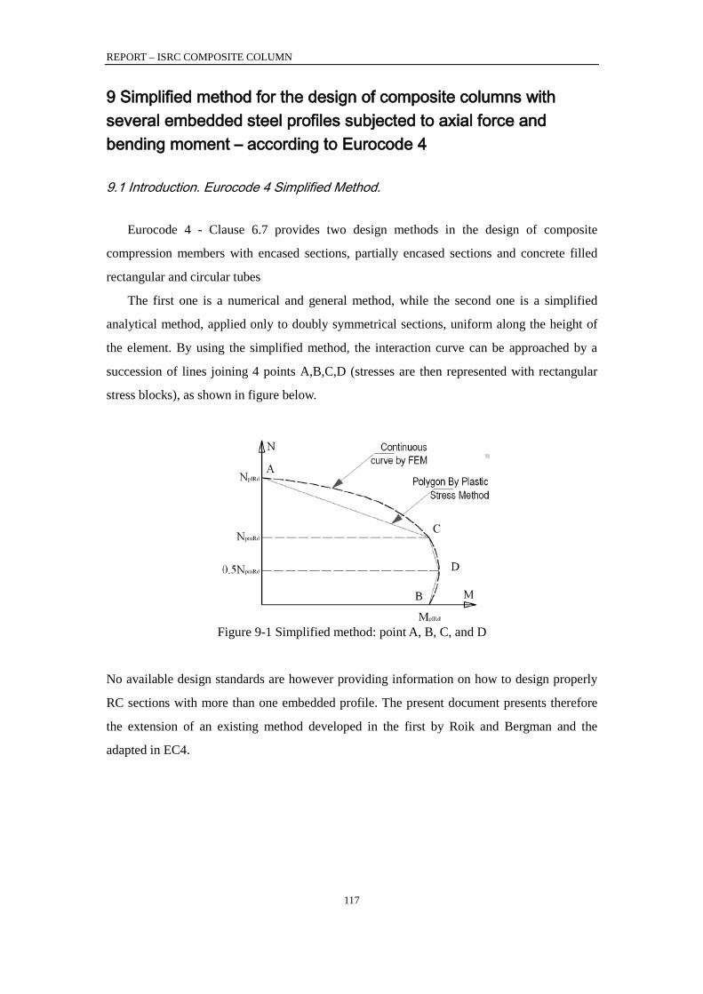
REPORT – ISRC COMPOSITE COLUMN
117
9 Simplified method for the design of composite columns with several embedded steel profiles subjected to axial force and bending moment – according to Eurocode 4
9.1 Introduction. Eurocode 4 Simplified Method.
Eurocode 4 - Clause 6.7 provides two design methods in the design of composite
compression members with encased sections, partially encased sections and concrete filled
rectangular and circular tubes
The first one is a numerical and general method, while the second one is a simplified
analytical method, applied only to doubly symmetrical sections, uniform along the height of
the element. By using the simplified method, the interaction curve can be approached by a
succession of lines joining 4 points A,B,C,D (stresses are then represented with rectangular
stress blocks), as shown in figure below.
No available design standards are however providing information on how to design properly
RC sections with more than one embedded profile. The present document presents therefore
the extension of an existing method developed in the first by Roik and Bergman and the
adapted in EC4.
Figure 9-1 Simplified method: point A, B, C, and D
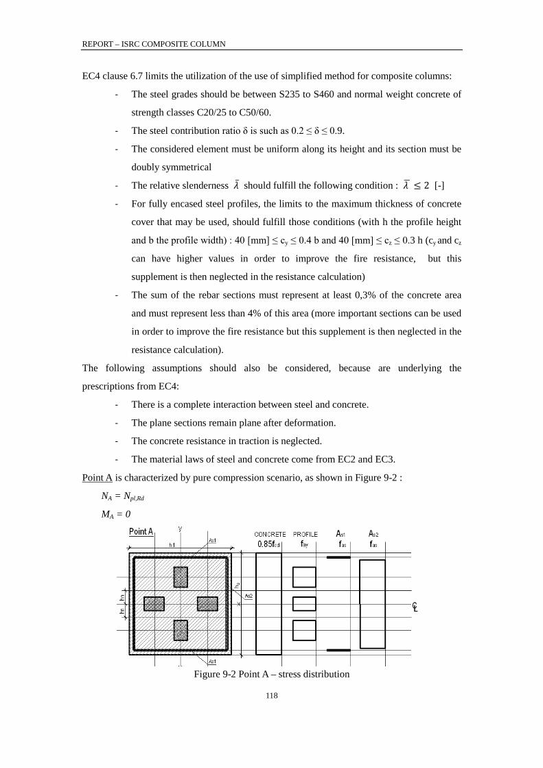
REPORT – ISRC COMPOSITE COLUMN
118
EC4 clause 6.7 limits the utilization of the use of simplified method for composite columns:
- The steel grades should be between S235 to S460 and normal weight concrete of
strength classes C20/25 to C50/60.
- The steel contribution ratio δ is such as 0.2 ≤ δ ≤ 0.9.
- The considered element must be uniform along its height and its section must be
doubly symmetrical
- The relative slenderness should fulfill the following condition : 𝜆 ≤ 2 [-]
- For fully encased steel profiles, the limits to the maximum thickness of concrete
cover that may be used, should fulfill those conditions (with h the profile height
and b the profile width) : 40 [mm] ≤ cy ≤ 0.4 b and 40 [mm] ≤ cz ≤ 0.3 h (cy and cz
can have higher values in order to improve the fire resistance, but this
supplement is then neglected in the resistance calculation)
- The sum of the rebar sections must represent at least 0,3% of the concrete area
and must represent less than 4% of this area (more important sections can be used
in order to improve the fire resistance but this supplement is then neglected in the
resistance calculation).
The following assumptions should also be considered, because are underlying the
prescriptions from EC4:
- There is a complete interaction between steel and concrete.
- The plane sections remain plane after deformation.
- The concrete resistance in traction is neglected.
- The material laws of steel and concrete come from EC2 and EC3.
Point A is characterized by pure compression scenario, as shown in Figure 9-2 :
NA = Npl,Rd
MA = 0
Figure 9-2 Point A – stress distribution
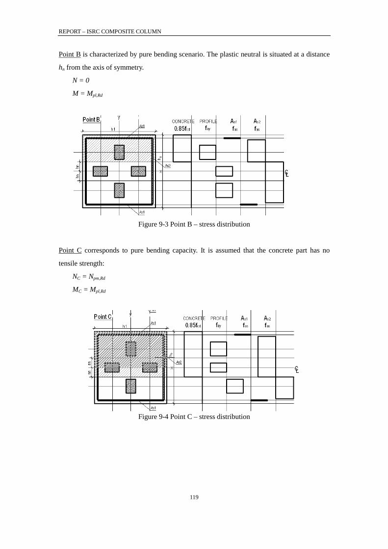
REPORT – ISRC COMPOSITE COLUMN
119
Point B is characterized by pure bending scenario. The plastic neutral is situated at a distance
hn from the axis of symmetry.
N = 0
M = Mpl,Rd
Point C corresponds to pure bending capacity. It is assumed that the concrete part has no
tensile strength:
NC = Npm,Rd
MC = Mpl,Rd
Figure 9-3 Point B – stress distribution
Figure 9-4 Point C – stress distribution

REPORT – ISRC COMPOSITE COLUMN
120
Point D is defined by:
ND = 0.5 . Npm,Rd
MD = Mmax,Rd
9.2 Equivalent plates for definition of rebar layers and steel profiles.
The development of a method of calculation of concrete sections with several encased steel
sections requires the calculation of section characteristics like the moment of inertia, the
plastic moment, the elastic neutral axis and the plastic neutral axis. Such calculation can be
made numerically or “hand - made”, in which case the calculation becomes tedious. In order
to facilitate such calculation two simplifications are proposed, as shown in Figure 9-6. The
first one is to replace the amount of longitudinal rebar by equivalent plates.
Figure 9-5 Point D – stress distribution
Figure 9-6 Equivalent plates for steel profiles and rebar
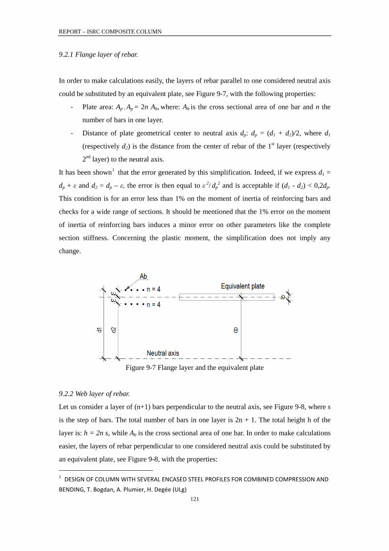
REPORT – ISRC COMPOSITE COLUMN
121
9.2.1 Flange layer of rebar.
In order to make calculations easily, the layers of rebar parallel to one considered neutral axis
could be substituted by an equivalent plate, see Figure 9-7, with the following properties:
- Plate area: Ap : Ap = 2n Ab, where: Ab is the cross sectional area of one bar and n the
number of bars in one layer.
- Distance of plate geometrical center to neutral axis dp: dp = (d1 + d2)/2, where d1
(respectively d2) is the distance from the center of rebar of the 1st layer (respectively
2nd layer) to the neutral axis.
It has been shown1 that the error generated by this simplification. Indeed, if we express d1 =
dp + ε and d2 = dp – ε, the error is then equal to ε 2/ dp2 and is acceptable if (d1 - d2) < 0,2dp.
This condition is for an error less than 1% on the moment of inertia of reinforcing bars and
checks for a wide range of sections. It should be mentioned that the 1% error on the moment
of inertia of reinforcing bars induces a minor error on other parameters like the complete
section stiffness. Concerning the plastic moment, the simplification does not imply any
change.
9.2.2 Web layer of rebar.
Let us consider a layer of (n+1) bars perpendicular to the neutral axis, see Figure 9-8, where s
is the step of bars. The total number of bars in one layer is 2n + 1. The total height h of the
layer is: h = 2n s, while Ab is the cross sectional area of one bar. In order to make calculations
easier, the layers of rebar perpendicular to one considered neutral axis could be substituted by
an equivalent plate, see Figure 9-8, with the properties: 1 DESIGN OF COLUMN WITH SEVERAL ENCASED STEEL PROFILES FOR COMBINED COMPRESSION AND BENDING, T. Bogdan, A. Plumier, H. Degée (ULg)
Figure 9-7 Flange layer and the equivalent plate
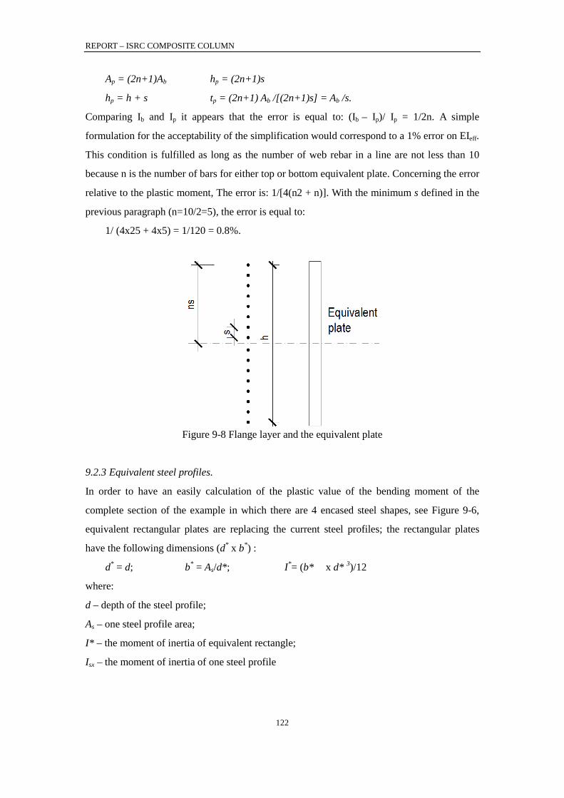
REPORT – ISRC COMPOSITE COLUMN
122
Ap = (2n+1)Ab hp = (2n+1)s
hp = h + s tp = (2n+1) Ab /[(2n+1)s] = Ab /s.
Comparing Ib and Ip it appears that the error is equal to: (Ib – Ip)/ Ip = 1/2n. A simple
formulation for the acceptability of the simplification would correspond to a 1% error on EIeff.
This condition is fulfilled as long as the number of web rebar in a line are not less than 10
because n is the number of bars for either top or bottom equivalent plate. Concerning the error
relative to the plastic moment, The error is: 1/[4(n2 + n)]. With the minimum s defined in the
previous paragraph (n=10/2=5), the error is equal to:
1/ (4x25 + 4x5) = 1/120 = 0.8%.
9.2.3 Equivalent steel profiles.
In order to have an easily calculation of the plastic value of the bending moment of the
complete section of the example in which there are 4 encased steel shapes, see Figure 9-6,
equivalent rectangular plates are replacing the current steel profiles; the rectangular plates
have the following dimensions (d* x b*) :
d* = d; b* = As/d*; I*= (b* x d* 3)/12
where:
d – depth of the steel profile;
As – one steel profile area;
I* – the moment of inertia of equivalent rectangle;
Isx – the moment of inertia of one steel profile
Figure 9-8 Flange layer and the equivalent plate

REPORT – ISRC COMPOSITE COLUMN
123
9.3 3 Evaluation of neutral axis position - “hn”.
9.3.1 Simplified Method
To determine points A, B, C, D from the interaction curve, as shown in Figure 9-1, the
following equations are used:
𝑁𝑝𝑙,𝑅𝑑 = 𝐴𝑠 .𝑓𝑦𝑑 + 𝐴𝑠𝑟 .𝑓𝑠𝑑 + 𝐴𝑐 . 0,85 .𝑓𝑐𝑑
𝑁𝑝𝑚,𝑅𝑑 = 𝐴𝑐 . 0,85 .𝑓𝑐𝑑
𝑀𝑚𝑎𝑥,𝑅𝑑 = 𝑍𝑠 .𝑓𝑦𝑑 + 𝑍𝑠𝑟 .𝑓𝑠𝑑 + 0,5 .𝑍𝑐 . 0,85 .𝑓𝑐𝑑
The subscript “d” represents the design value. The overstregth factors are being used for
concrete and reinforcement rebars:
𝑓𝑦𝑑 = 𝑓𝑦𝑘/𝛾𝑎 𝑓𝑠𝑑 = 𝑓𝑠𝑘/𝛾𝑠 𝑓𝑐𝑑 = 𝑓𝑐𝑘/𝛾𝑐.
Where:
𝛾𝑎 = 1, 𝛾𝑠 = 1.15 𝑎𝑛𝑑 𝛾𝑐 = 1.5
This equation for 𝑀𝑚𝑎𝑥,𝑅𝑑 is due to the fact that for point D, the neutral axis is situated at
the axis of symmetry of the cross section (the 0,5 coefficient results from the assumption that
concrete tensile strength is neglected).
In order to determine the plastic moment Mpl,Rd, the position of the neutral axis must be
evaluated. Several scenarios needs to be taken into account: they are detailed below while
considering different scenarios.
Scenario 1 In this scenario, ℎ𝑛 is between the rectangular plates and so ℎ𝑛 ≤ 𝑏∗/2, as shown in Figure 9-9. Let NB and Nc be the axial effort corresponding to points B and C from the simplified interaction curve, then:
𝑁𝑏 – 𝑁𝑐 = 0,85 .𝐴𝑐 .𝑓𝑐𝑑 𝑁𝑏 – 𝑁𝑐 =
2 .ℎ𝑛 . ℎ1 .0,85 .𝑓𝑐𝑑 + 2 .ℎ𝑛 . 2 .𝑑 . 𝑓𝑦𝑑 − 0,85 .𝑓𝑐𝑑 + 2 .ℎ𝑛 . 2 . 𝑏𝑠2 . (𝑓𝑠𝑑 − 0,85 .𝑓𝑐𝑑)
This implies that:
ℎ𝑛 = 0,85 .𝐴𝑐 .𝑓𝑐𝑑
2 .ℎ1 .0,85 .𝑓𝑐𝑑 + 4𝑑 .𝑓𝑦𝑑 − 4𝑑 .0,85 . 𝑓𝑐𝑑 + 4𝑏𝑠2 .𝑓𝑠𝑑 − 4𝑏𝑠2 .0,85 . 𝑓𝑐𝑑
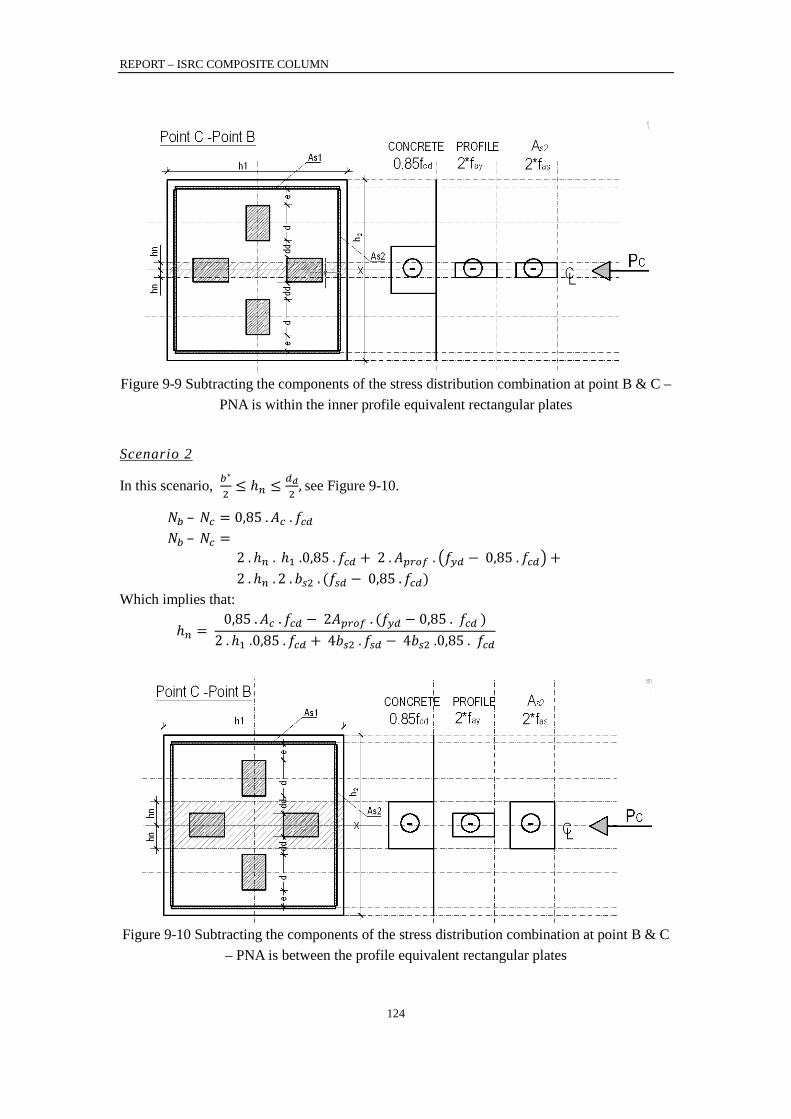
REPORT – ISRC COMPOSITE COLUMN
124
Scenario 2
In this scenario, 𝑏∗
2≤ ℎ𝑛 ≤
𝑑𝑑2
, see Figure 9-10.
𝑁𝑏 – 𝑁𝑐 = 0,85 .𝐴𝑐 .𝑓𝑐𝑑 𝑁𝑏 – 𝑁𝑐 =
2 .ℎ𝑛 . ℎ1 .0,85 .𝑓𝑐𝑑 + 2 .𝐴𝑝𝑟𝑜𝑓 . 𝑓𝑦𝑑 − 0,85 .𝑓𝑐𝑑+ 2 .ℎ𝑛 . 2 . 𝑏𝑠2 . (𝑓𝑠𝑑 − 0,85 .𝑓𝑐𝑑)
Which implies that:
ℎ𝑛 = 0,85 .𝐴𝑐 .𝑓𝑐𝑑 − 2𝐴𝑝𝑟𝑜𝑓 . (𝑓𝑦𝑑 − 0,85 . 𝑓𝑐𝑑 )
2 .ℎ1 .0,85 .𝑓𝑐𝑑 + 4𝑏𝑠2 .𝑓𝑠𝑑 − 4𝑏𝑠2 .0,85 . 𝑓𝑐𝑑
Figure 9-9 Subtracting the components of the stress distribution combination at point B & C –
PNA is within the inner profile equivalent rectangular plates
Figure 9-10 Subtracting the components of the stress distribution combination at point B & C
– PNA is between the profile equivalent rectangular plates

REPORT – ISRC COMPOSITE COLUMN
125
Scenario 3
In this scenario, 𝑑𝑑2≤ ℎ𝑛 ≤
𝑑𝑑2
+ 𝑑, see Figure 9-11.
𝑁𝑏 – 𝑁𝑐 = 0,85 .𝐴𝑐 .𝑓𝑐𝑑
𝑁𝑏 – 𝑁𝑐 = 2 .ℎ𝑛 . ℎ1 .0,85 .𝑓𝑐𝑑 + 2 .𝐴𝑝𝑟𝑜𝑓 . 𝑓𝑦𝑑 − 0,85 .𝑓𝑐𝑑 +
2 . (ℎ𝑛 −𝑑𝑑2
) . 𝑏∗ . 𝑓𝑦𝑑 − 0,85 .𝑓𝑐𝑑 + 2 .ℎ𝑛 . 2 . 𝑏𝑠2 . (𝑓𝑠𝑑 − 0,85 .𝑓𝑐𝑑)
This implies that:
ℎ𝑛 =0,85 .𝐴𝑐 .𝑓𝑐𝑑 − 2𝐴𝑝𝑟𝑜𝑓 . ( 𝑓𝑦𝑑 − 0,85 𝑓𝑐𝑑 ) + dd . b∗ . fyd − dd . b∗ .0,85 . fcd
2.ℎ1. 0,85 𝑓𝑐𝑑 + 2𝑏∗.𝑓𝑦𝑑 − 2𝑏∗. 0,85𝑓𝑐𝑑 + 4𝑏𝑠2 .𝑓𝑠𝑑 − 4𝑏𝑠2 .0,85 𝑓𝑐𝑑
Scenario 4
In this scenario, 𝑑𝑑2
+ 𝑑 ≤ ℎ𝑛 ≤𝑑𝑑2
+ 𝑑 + 𝑒, , see Figure 9-12.
𝑁𝑏 – 𝑁𝑐 = 0,85 .𝐴𝑐 .𝑓𝑐𝑑
𝑁𝑏 – 𝑁𝑐 =
2 .ℎ𝑛 . ℎ1 .0,85 .𝑓𝑐𝑑 + 4 .𝐴𝑝𝑟𝑜𝑓 . 𝑓𝑦𝑑 − 0,85 .𝑓𝑐𝑑+
2 .ℎ𝑛 . 2 . 𝑏𝑠2 . (𝑓𝑠𝑑 − 0,85 .𝑓𝑐𝑑)
This implies that:
ℎ𝑛 =0,85 .𝐴𝑐 .𝑓𝑐𝑑 − 4𝐴𝑝𝑟𝑜𝑓 . (𝑓𝑦𝑑 − 0,85 𝑓𝑐𝑑 )
2.ℎ1. 0,85 𝑓𝑐𝑑 + 4𝑏𝑠2 .𝑓𝑠𝑑 − 4𝑏𝑠2 .0,85 . 𝑓𝑐𝑑
Figure 9-11 Subtracting the components of the stress distribution combination at point B & C
– PNA is between the outer profile equivalent rectangular plates
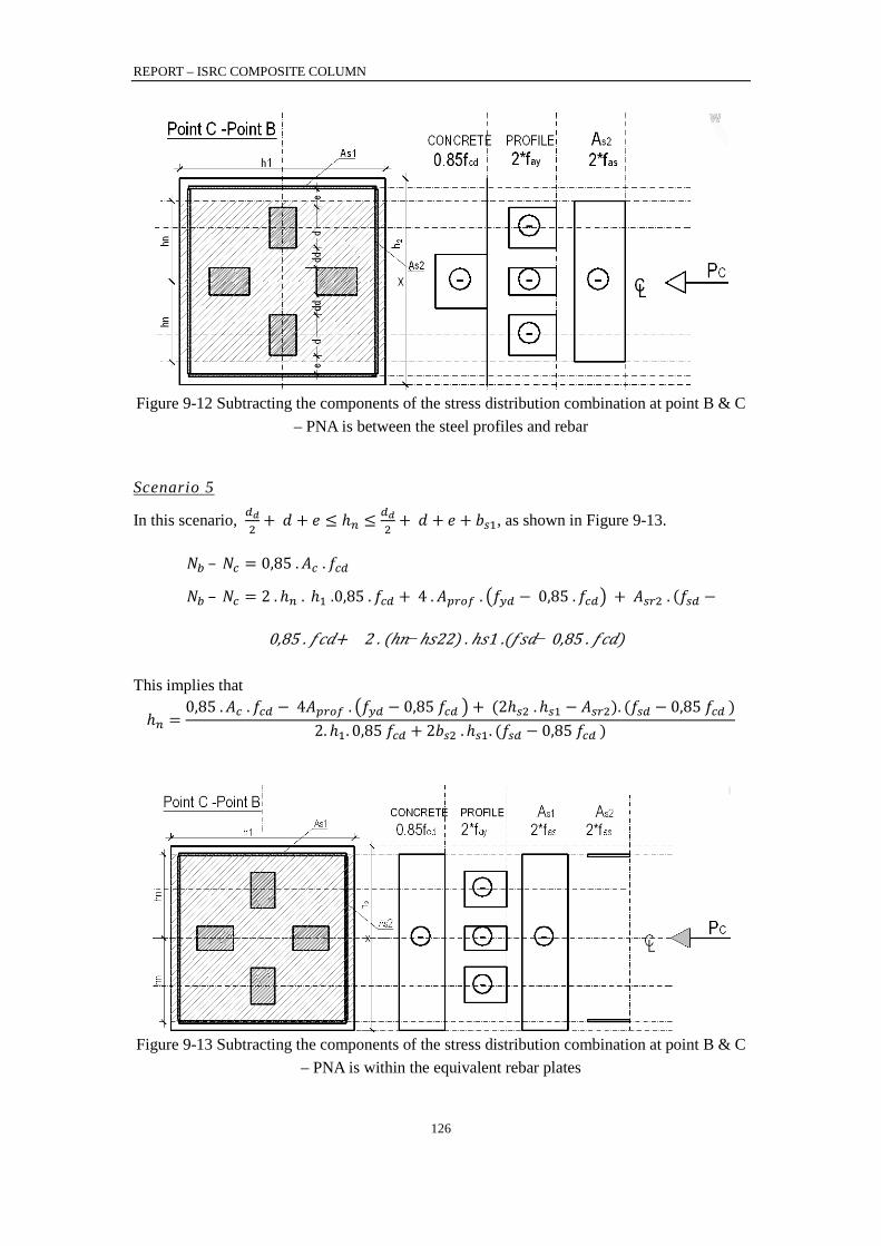
REPORT – ISRC COMPOSITE COLUMN
126
Scenario 5
In this scenario, 𝑑𝑑2
+ 𝑑 + 𝑒 ≤ ℎ𝑛 ≤𝑑𝑑2
+ 𝑑 + 𝑒 + 𝑏𝑠1, as shown in Figure 9-13.
𝑁𝑏 – 𝑁𝑐 = 0,85 .𝐴𝑐 .𝑓𝑐𝑑
𝑁𝑏 – 𝑁𝑐 = 2 .ℎ𝑛 . ℎ1 .0,85 .𝑓𝑐𝑑 + 4 .𝐴𝑝𝑟𝑜𝑓 . 𝑓𝑦𝑑 − 0,85 .𝑓𝑐𝑑 + 𝐴𝑠𝑟2 . (𝑓𝑠𝑑 −
0,85 . 𝑓𝑐𝑑+ 2 . (ℎ𝑛−ℎ𝑠22) . ℎ𝑠1 .(𝑓𝑠𝑑− 0,85 . 𝑓𝑐𝑑)
This implies that
ℎ𝑛 =0,85 .𝐴𝑐 .𝑓𝑐𝑑 − 4𝐴𝑝𝑟𝑜𝑓 . 𝑓𝑦𝑑 − 0,85 𝑓𝑐𝑑 + (2ℎ𝑠2 .ℎ𝑠1 − 𝐴𝑠𝑟2). (𝑓𝑠𝑑 − 0,85 𝑓𝑐𝑑 )
2.ℎ1. 0,85 𝑓𝑐𝑑 + 2𝑏𝑠2 .ℎ𝑠1. (𝑓𝑠𝑑 − 0,85 𝑓𝑐𝑑 )
Figure 9-12 Subtracting the components of the stress distribution combination at point B & C
– PNA is between the steel profiles and rebar
Figure 9-13 Subtracting the components of the stress distribution combination at point B & C
– PNA is within the equivalent rebar plates
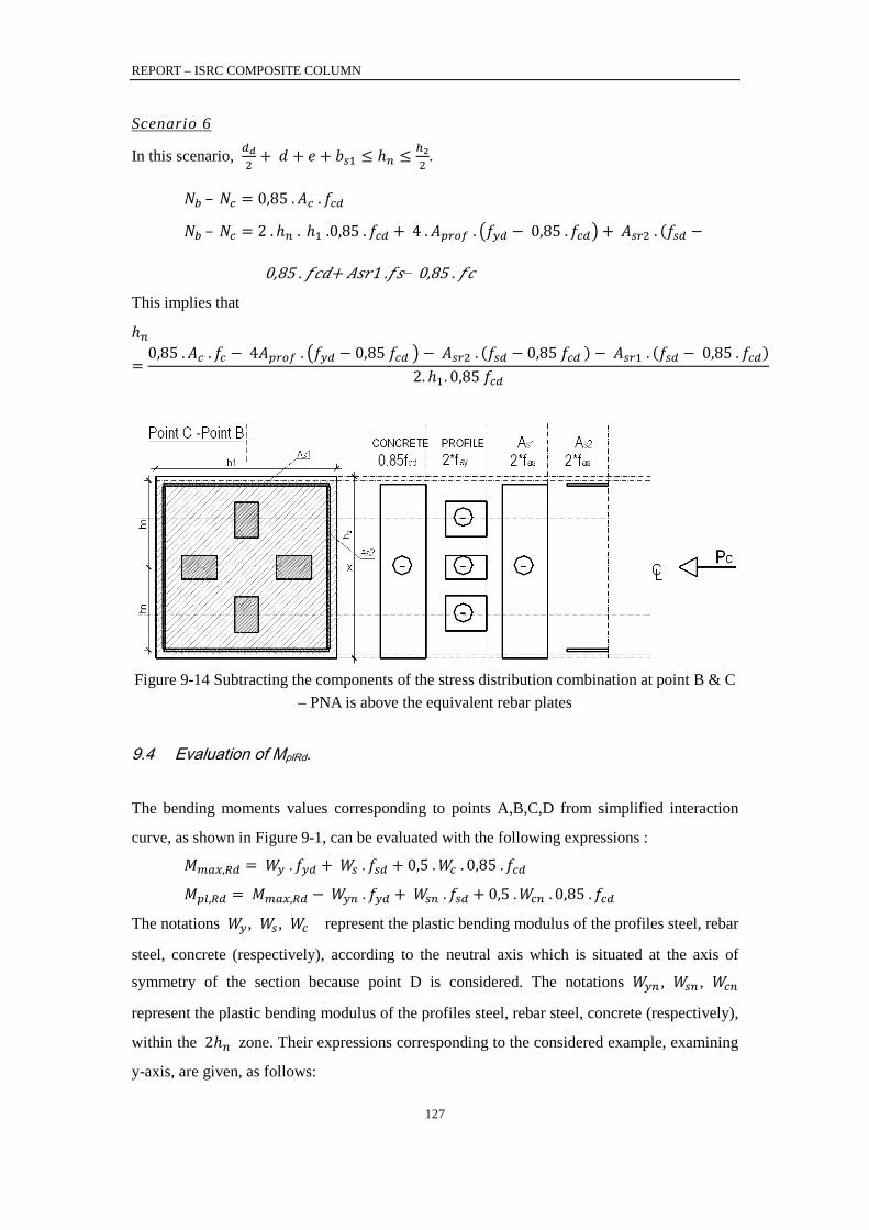
REPORT – ISRC COMPOSITE COLUMN
127
Scenario 6
In this scenario, 𝑑𝑑2
+ 𝑑 + 𝑒 + 𝑏𝑠1 ≤ ℎ𝑛 ≤ℎ22
.
𝑁𝑏 – 𝑁𝑐 = 0,85 .𝐴𝑐 .𝑓𝑐𝑑
𝑁𝑏 – 𝑁𝑐 = 2 .ℎ𝑛 . ℎ1 .0,85 .𝑓𝑐𝑑 + 4 .𝐴𝑝𝑟𝑜𝑓 . 𝑓𝑦𝑑 − 0,85 .𝑓𝑐𝑑+ 𝐴𝑠𝑟2 . (𝑓𝑠𝑑 −
0,85 . 𝑓𝑐𝑑+ 𝐴𝑠𝑟1 .𝑓𝑠− 0,85 . 𝑓𝑐
This implies that
ℎ𝑛
=0,85 .𝐴𝑐 .𝑓𝑐 − 4𝐴𝑝𝑟𝑜𝑓 . 𝑓𝑦𝑑 − 0,85 𝑓𝑐𝑑 − 𝐴𝑠𝑟2 . (𝑓𝑠𝑑 − 0,85 𝑓𝑐𝑑 ) − 𝐴𝑠𝑟1 . (𝑓𝑠𝑑 − 0,85 .𝑓𝑐𝑑)
2.ℎ1. 0,85 𝑓𝑐𝑑
9.4 Evaluation of MplRd.
The bending moments values corresponding to points A,B,C,D from simplified interaction
curve, as shown in Figure 9-1, can be evaluated with the following expressions :
𝑀𝑚𝑎𝑥,𝑅𝑑 = 𝑊𝑦 .𝑓𝑦𝑑 + 𝑊𝑠 .𝑓𝑠𝑑 + 0,5 .𝑊𝑐 . 0,85 .𝑓𝑐𝑑
𝑀𝑝𝑙,𝑅𝑑 = 𝑀𝑚𝑎𝑥,𝑅𝑑 − 𝑊𝑦𝑛 .𝑓𝑦𝑑 + 𝑊𝑠𝑛 .𝑓𝑠𝑑 + 0,5 .𝑊𝑐𝑛 . 0,85 .𝑓𝑐𝑑
The notations 𝑊𝑦, 𝑊𝑠, 𝑊𝑐 represent the plastic bending modulus of the profiles steel, rebar
steel, concrete (respectively), according to the neutral axis which is situated at the axis of
symmetry of the section because point D is considered. The notations 𝑊𝑦𝑛 , 𝑊𝑠𝑛 , 𝑊𝑐𝑛
represent the plastic bending modulus of the profiles steel, rebar steel, concrete (respectively),
within the 2ℎ𝑛 zone. Their expressions corresponding to the considered example, examining
y-axis, are given, as follows:
Figure 9-14 Subtracting the components of the stress distribution combination at point B & C
– PNA is above the equivalent rebar plates
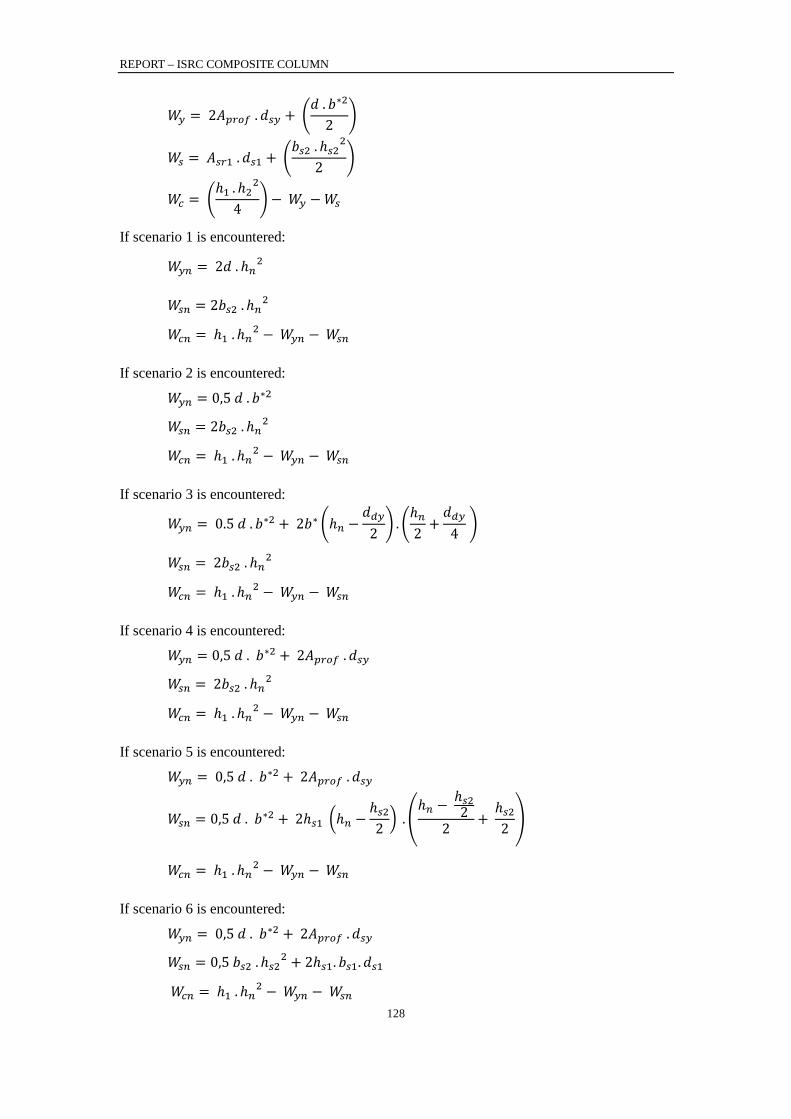
REPORT – ISRC COMPOSITE COLUMN
128
𝑊𝑦 = 2𝐴𝑝𝑟𝑜𝑓 .𝑑𝑠𝑦 + 𝑑 . 𝑏∗2
2
𝑊𝑠 = 𝐴𝑠𝑟1 .𝑑𝑠1 + 𝑏𝑠2 .ℎ𝑠2
2
2
𝑊𝑐 = ℎ1 .ℎ2
2
4 − 𝑊𝑦 −𝑊𝑠
If scenario 1 is encountered:
𝑊𝑦𝑛 = 2𝑑 .ℎ𝑛2
𝑊𝑠𝑛 = 2𝑏𝑠2 .ℎ𝑛2
𝑊𝑐𝑛 = ℎ1 .ℎ𝑛2 − 𝑊𝑦𝑛 − 𝑊𝑠𝑛
If scenario 2 is encountered:
𝑊𝑦𝑛 = 0,5 𝑑 . 𝑏∗2
𝑊𝑠𝑛 = 2𝑏𝑠2 .ℎ𝑛2
𝑊𝑐𝑛 = ℎ1 .ℎ𝑛2 − 𝑊𝑦𝑛 − 𝑊𝑠𝑛
If scenario 3 is encountered:
𝑊𝑦𝑛 = 0.5 𝑑 . 𝑏∗2 + 2𝑏∗ ℎ𝑛 −𝑑𝑑𝑦
2 .ℎ𝑛2
+𝑑𝑑𝑦
4
𝑊𝑠𝑛 = 2𝑏𝑠2 .ℎ𝑛2
𝑊𝑐𝑛 = ℎ1 .ℎ𝑛2 − 𝑊𝑦𝑛 − 𝑊𝑠𝑛
If scenario 4 is encountered:
𝑊𝑦𝑛 = 0,5 𝑑 . 𝑏∗2 + 2𝐴𝑝𝑟𝑜𝑓 .𝑑𝑠𝑦
𝑊𝑠𝑛 = 2𝑏𝑠2 .ℎ𝑛2
𝑊𝑐𝑛 = ℎ1 .ℎ𝑛2 − 𝑊𝑦𝑛 − 𝑊𝑠𝑛
If scenario 5 is encountered:
𝑊𝑦𝑛 = 0,5 𝑑 . 𝑏∗2 + 2𝐴𝑝𝑟𝑜𝑓 .𝑑𝑠𝑦
𝑊𝑠𝑛 = 0,5 𝑑 . 𝑏∗2 + 2ℎ𝑠1 ℎ𝑛 −ℎ𝑠22 .
ℎ𝑛 − ℎ𝑠222
+ ℎ𝑠22
𝑊𝑐𝑛 = ℎ1 .ℎ𝑛2 − 𝑊𝑦𝑛 − 𝑊𝑠𝑛
If scenario 6 is encountered:
𝑊𝑦𝑛 = 0,5 𝑑 . 𝑏∗2 + 2𝐴𝑝𝑟𝑜𝑓 .𝑑𝑠𝑦
𝑊𝑠𝑛 = 0,5 𝑏𝑠2 .ℎ𝑠22 + 2ℎ𝑠1. 𝑏𝑠1.𝑑𝑠1
𝑊𝑐𝑛 = ℎ1 .ℎ𝑛2 − 𝑊𝑦𝑛 − 𝑊𝑠𝑛
REPORT – ISRC COMPOSITE COLUMN
129
9.5 Reduction of the N-M interaction curve due to buckling.
In order to have a realistic interaction curve, the buckling effects should be taken into account. This phenomenon of instability lowers the resisting values of bending moment and axial force.
9.5.1 Axial force reduction.
𝑁𝑝𝑙,𝑏,𝑅𝑑 is the plastic resisting axial force, considering buckling. It can be determined by
multiplying 𝑁𝑝𝑙,𝑅𝑑 by a coefficient χ whose value is between 0 and 1. The evaluation of the
coefficient is presented in the following steps.
a) First, the Euler force must be determined: 𝑁𝑐𝑟 = 𝜋2 𝐸𝐼𝑙𝑓2
, with 𝑙𝑓 the buckling length which
depends on the element length but also on the supports. The flexural stiffness is determined
with the following formula:
𝐸𝐼 = 𝐸𝑦 . 𝐼𝑦 + 𝐸𝑠 . 𝐼𝑠 + 𝐾𝑒 .𝐸𝑐,𝑒𝑓𝑓 . 𝐼𝑐
Where:
− 𝐸𝑦 and 𝐸𝑠 the Young modulus of profile steel and rebars steel (respectively),
− 𝐼𝑦, 𝐼𝑠 and 𝐼𝑐 the inertia of profile steel, rebars steel and concrete (respectively),
− 𝐾𝑒 = 0,6
− 𝐸𝑐,𝑒𝑓𝑓 = 𝐸𝑐𝑚1
1 + 𝜑𝑡 . (𝑁𝐺 ,𝐸𝑑𝑁𝐸𝑑
)
− 𝐸𝑐𝑚 the Young modulus of concrete,
− 𝜑𝑡 the creep coefficient of concrete,
− 𝑁𝐸𝑑 the total applied axial force,
− 𝑁𝐺,𝐸𝑑 the permanent part of this force
b) Next, the relative slenderness can be calculated:
𝜆 = 𝑁𝑝𝑙,𝑅𝑘/𝑁𝑐𝑟
Where:
𝑁𝑝𝑙,𝑅𝑘 = 𝐴𝑠 .𝑓𝑦𝑘 + 𝐴𝑠𝑟 .𝑓𝑠𝑘 + 𝐴𝑐 . 0,85 .𝑓𝑐𝑘. − the plastic resisting axial force
c) The coefficient ɸ is equal with ɸ = 0,5 . (1 + α . (𝜆 − 0,2) + 𝜆2) , where α is an
imperfection factor whose value depends on the choosed buckling curve. EC4 recommends to
use α = 0.34 for buckling axis y and α = 0.49 for buckling axis z.
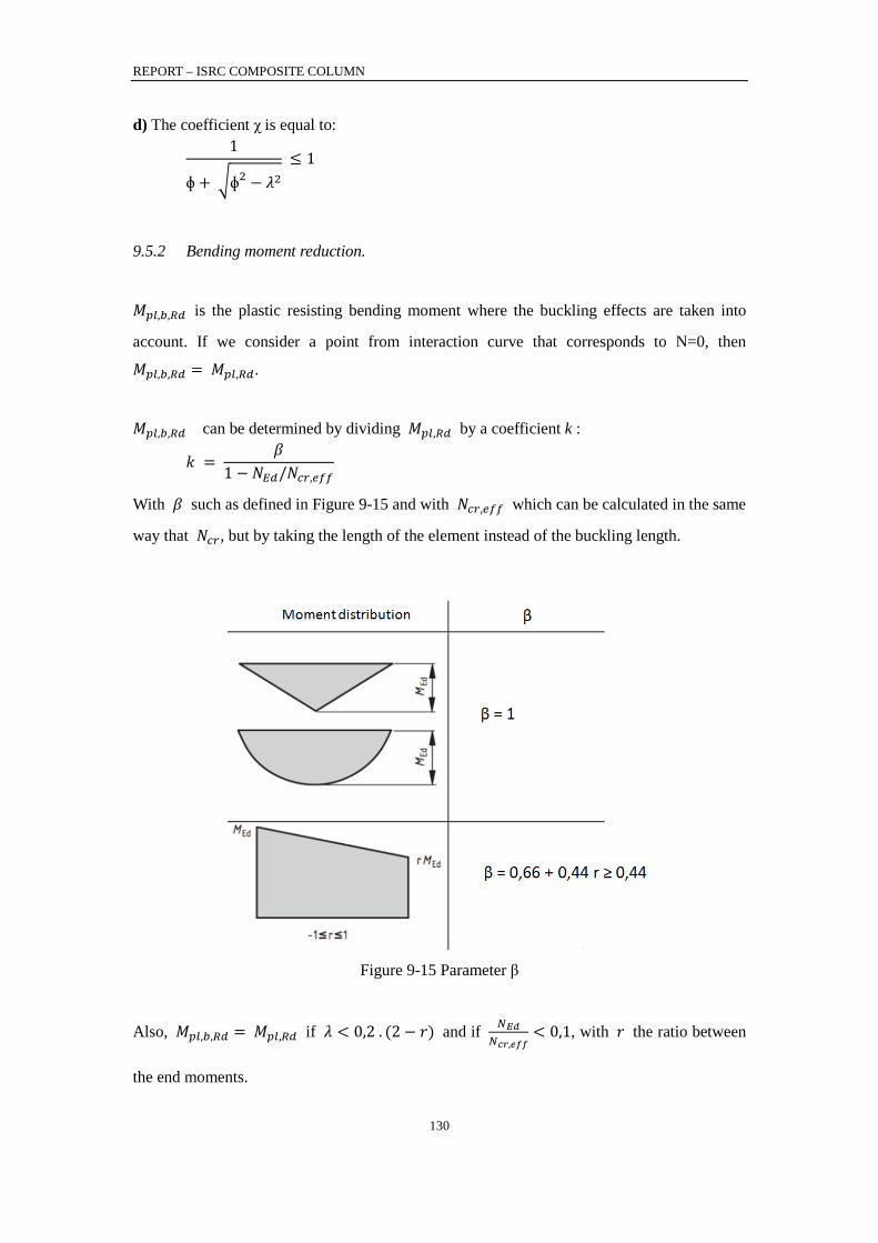
REPORT – ISRC COMPOSITE COLUMN
130
d) The coefficient χ is equal to: 1
ɸ + ɸ2 − 𝜆2 ≤ 1
9.5.2 Bending moment reduction.
𝑀𝑝𝑙,𝑏,𝑅𝑑 is the plastic resisting bending moment where the buckling effects are taken into
account. If we consider a point from interaction curve that corresponds to N=0, then
𝑀𝑝𝑙,𝑏,𝑅𝑑 = 𝑀𝑝𝑙,𝑅𝑑.
𝑀𝑝𝑙,𝑏,𝑅𝑑 can be determined by dividing 𝑀𝑝𝑙,𝑅𝑑 by a coefficient k :
𝑘 = 𝛽
1 −𝑁𝐸𝑑/𝑁𝑐𝑟,𝑒𝑓𝑓
With 𝛽 such as defined in Figure 9-15 and with 𝑁𝑐𝑟,𝑒𝑓𝑓 which can be calculated in the same
way that 𝑁𝑐𝑟, but by taking the length of the element instead of the buckling length.
Also, 𝑀𝑝𝑙,𝑏,𝑅𝑑 = 𝑀𝑝𝑙,𝑅𝑑 if 𝜆 < 0,2 . (2 − 𝑟) and if 𝑁𝐸𝑑𝑁𝑐𝑟,𝑒𝑓𝑓
< 0,1, with 𝑟 the ratio between
the end moments.
Figure 9-15 Parameter β
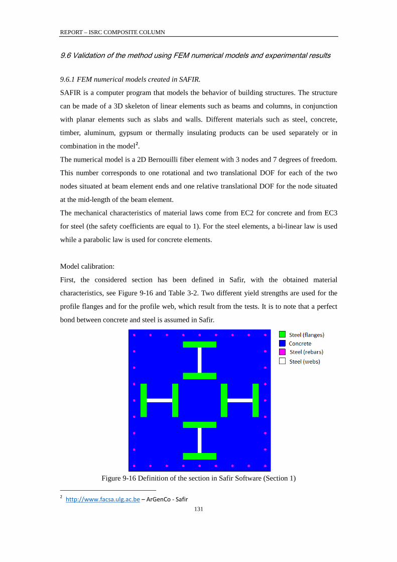
REPORT – ISRC COMPOSITE COLUMN
131
9.6 Validation of the method using FEM numerical models and experimental results
9.6.1 FEM numerical models created in SAFIR.
SAFIR is a computer program that models the behavior of building structures. The structure
can be made of a 3D skeleton of linear elements such as beams and columns, in conjunction
with planar elements such as slabs and walls. Different materials such as steel, concrete,
timber, aluminum, gypsum or thermally insulating products can be used separately or in
combination in the model2.
The numerical model is a 2D Bernouilli fiber element with 3 nodes and 7 degrees of freedom.
This number corresponds to one rotational and two translational DOF for each of the two
nodes situated at beam element ends and one relative translational DOF for the node situated
at the mid-length of the beam element.
The mechanical characteristics of material laws come from EC2 for concrete and from EC3
for steel (the safety coefficients are equal to 1). For the steel elements, a bi-linear law is used
while a parabolic law is used for concrete elements.
Model calibration:
First, the considered section has been defined in Safir, with the obtained material
characteristics, see Figure 9-16 and Table 3-2. Two different yield strengths are used for the
profile flanges and for the profile web, which result from the tests. It is to note that a perfect
bond between concrete and steel is assumed in Safir.
2 http://www.facsa.ulg.ac.be – ArGenCo - Safir
Figure 9-16 Definition of the section in Safir Software (Section 1)

REPORT – ISRC COMPOSITE COLUMN
132
Definition of the numerical model is presented in Figure 9-17, the length of the specimen is
3.6m and it has an initial eccentricity of L/200 (EC4 – Table 6.5) to be able to take into
account the second order effects. The vertical displacement is blocked at the bottom of the
column, while the horizontal displacement is blocked at the both the top and bottom (see
Figure 18). The column cross section is constant along the length of the element, shown in
Figure 9-16.
The actual length of the tested specimen is 2.7 meters, but the test device has the distance
between the two articulations of 3.6 m (Figure 9-19). To be able to take into account the real
buckling length, a second cross section is defined at the extremities of the column. The
section has the same geometry as the composite one, 450 x 450 mm and contains only one
material, steel that has the strength of 450 MPa.
The experimental setup does not contain a constant cross-section along its element (see
Figure9-18). To simplify the numerical model, a constant cross section has been defined in
Safir. The specimens contains at the both extremities two I shaped steel profiles in order to
simulate beam-column joints. Two composite length scenarios have then been considered, as
shown in Figure 9-18 – where the Section 1 is composite and section 2 is made of steel:
- Scenario A: for which the section N°2 is assigned on the length where the metallic
part is present (3,6 – 2,72
= 0,45 meter at each end)
- Scenario B: for which the section N°2 is assigned on the length where the metallic
part and the reinforced part are present (0.9 meter at each end) (see Figure 19).
Figure 9-17 Safir – numerical model definition and experimental set-up configuration

REPORT – ISRC COMPOSITE COLUMN
133
The obtained results are given in the Table 9-1. The results obtained with scenarios A and B
are similar and gives similar results with the experimental part. In order to keep the numerical
model simple, the scheme of scenario A is considered thereafter.
Figure 9-18 Scenario A and B considered in FEM Safir
Figure 9-19 Static experimental set-up length
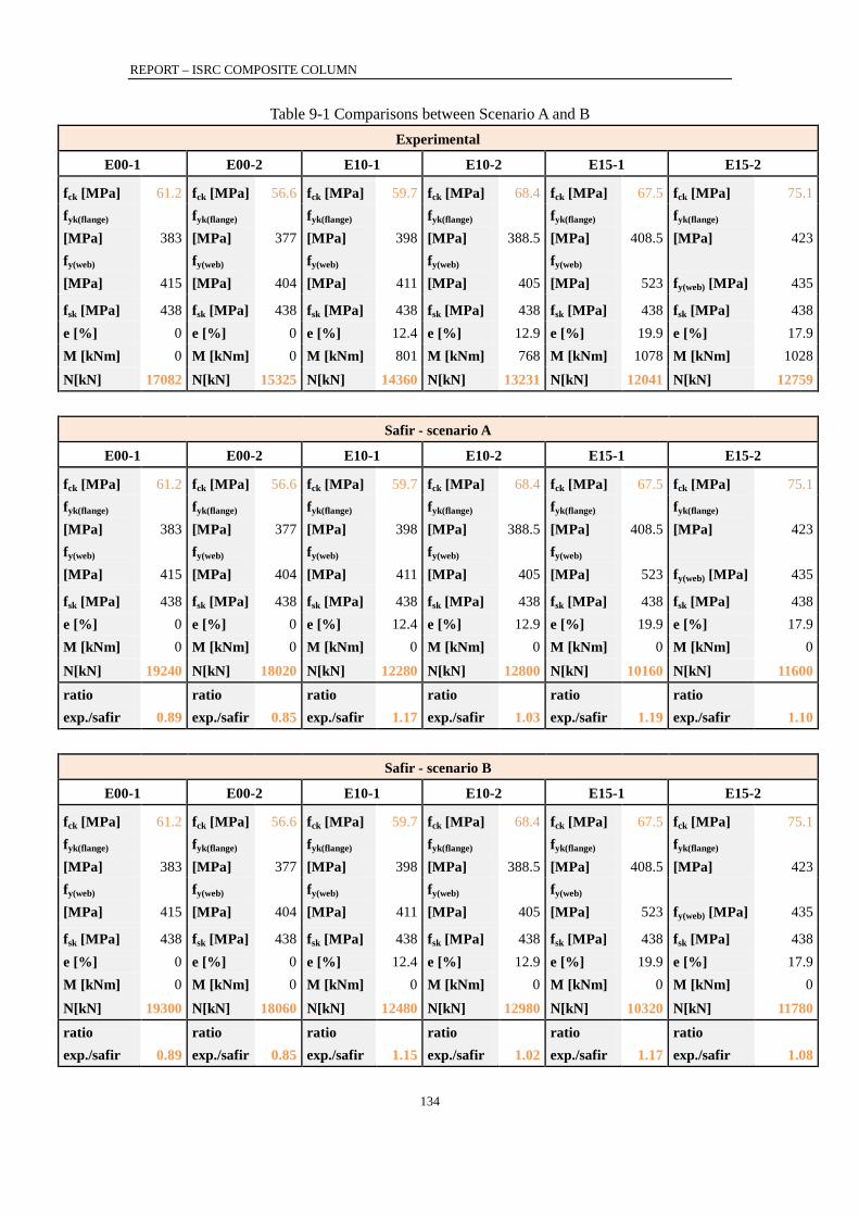
REPORT – ISRC COMPOSITE COLUMN
134
Table 9-1 Comparisons between Scenario A and B Experimental
E00-1 E00-2 E10-1 E10-2 E15-1 E15-2
fck [MPa] 61.2 fck [MPa] 56.6 fck [MPa] 59.7 fck [MPa] 68.4 fck [MPa] 67.5 fck [MPa] 75.1 fyk(flange) [MPa] 383
fyk(flange) [MPa] 377
fyk(flange) [MPa] 398
fyk(flange) [MPa] 388.5
fyk(flange) [MPa] 408.5
fyk(flange) [MPa] 423
fy(web) [MPa] 415
fy(web) [MPa] 404
fy(web) [MPa] 411
fy(web) [MPa] 405
fy(web) [MPa] 523 fy(web) [MPa] 435
fsk [MPa] 438 fsk [MPa] 438 fsk [MPa] 438 fsk [MPa] 438 fsk [MPa] 438 fsk [MPa] 438 e [%] 0 e [%] 0 e [%] 12.4 e [%] 12.9 e [%] 19.9 e [%] 17.9 M [kNm] 0 M [kNm] 0 M [kNm] 801 M [kNm] 768 M [kNm] 1078 M [kNm] 1028
N[kN] 17082 N[kN] 15325 N[kN] 14360 N[kN] 13231 N[kN] 12041 N[kN] 12759
Safir - scenario A
E00-1 E00-2 E10-1 E10-2 E15-1 E15-2
fck [MPa] 61.2 fck [MPa] 56.6 fck [MPa] 59.7 fck [MPa] 68.4 fck [MPa] 67.5 fck [MPa] 75.1 fyk(flange) [MPa] 383
fyk(flange) [MPa] 377
fyk(flange) [MPa] 398
fyk(flange) [MPa] 388.5
fyk(flange) [MPa] 408.5
fyk(flange) [MPa] 423
fy(web) [MPa] 415
fy(web) [MPa] 404
fy(web) [MPa] 411
fy(web) [MPa] 405
fy(web) [MPa] 523 fy(web) [MPa] 435
fsk [MPa] 438 fsk [MPa] 438 fsk [MPa] 438 fsk [MPa] 438 fsk [MPa] 438 fsk [MPa] 438 e [%] 0 e [%] 0 e [%] 12.4 e [%] 12.9 e [%] 19.9 e [%] 17.9 M [kNm] 0 M [kNm] 0 M [kNm] 0 M [kNm] 0 M [kNm] 0 M [kNm] 0
N[kN] 19240 N[kN] 18020 N[kN] 12280 N[kN] 12800 N[kN] 10160 N[kN] 11600
ratio exp./safir 0.89
ratio exp./safir 0.85
ratio exp./safir 1.17
ratio exp./safir 1.03
ratio exp./safir 1.19
ratio exp./safir 1.10
Safir - scenario B
E00-1 E00-2 E10-1 E10-2 E15-1 E15-2
fck [MPa] 61.2 fck [MPa] 56.6 fck [MPa] 59.7 fck [MPa] 68.4 fck [MPa] 67.5 fck [MPa] 75.1 fyk(flange) [MPa] 383
fyk(flange) [MPa] 377
fyk(flange) [MPa] 398
fyk(flange) [MPa] 388.5
fyk(flange) [MPa] 408.5
fyk(flange) [MPa] 423
fy(web) [MPa] 415
fy(web) [MPa] 404
fy(web) [MPa] 411
fy(web) [MPa] 405
fy(web) [MPa] 523 fy(web) [MPa] 435
fsk [MPa] 438 fsk [MPa] 438 fsk [MPa] 438 fsk [MPa] 438 fsk [MPa] 438 fsk [MPa] 438 e [%] 0 e [%] 0 e [%] 12.4 e [%] 12.9 e [%] 19.9 e [%] 17.9 M [kNm] 0 M [kNm] 0 M [kNm] 0 M [kNm] 0 M [kNm] 0 M [kNm] 0
N[kN] 19300 N[kN] 18060 N[kN] 12480 N[kN] 12980 N[kN] 10320 N[kN] 11780
ratio exp./safir 0.89
ratio exp./safir 0.85
ratio exp./safir 1.15
ratio exp./safir 1.02
ratio exp./safir 1.17
ratio exp./safir 1.08

REPORT – ISRC COMPOSITE COLUMN
135
9.6.2 Validation of neutral axis position.
With Safir software, is possible to get the stress distribution in a certain section. The (N, M)
values corresponding to point D of the simplified interaction curve (i.e. Npm,Rd and Mmax,Rd)
obtained with the EC4 method, using mechanical characteristics of E00-1 and E00-2
specimens, are applied to the column in Safir.
In the first case (using E00-1 data), the stress distribution in the mid-height section that is
obtained is represented on Figure 9-20. It can be seen that the neutral axis (i.e. the axis
where the stress have zero value) is placed at the middle of the section. This position
corresponds to the position given by EC4. In the second case (using E00-2 data), the stress
distribution in the mid-height section that is obtained is represented on Figure 9-21. The
same conclusion can be drawn concerning the neutral axis.
Figure 9-20 Stress distribution in the mid-height section (E00-1) subject to Npm,Rd
Figure 9-21 Stress distribution in the mid-height section (E00-2) subject to Npm,Rd
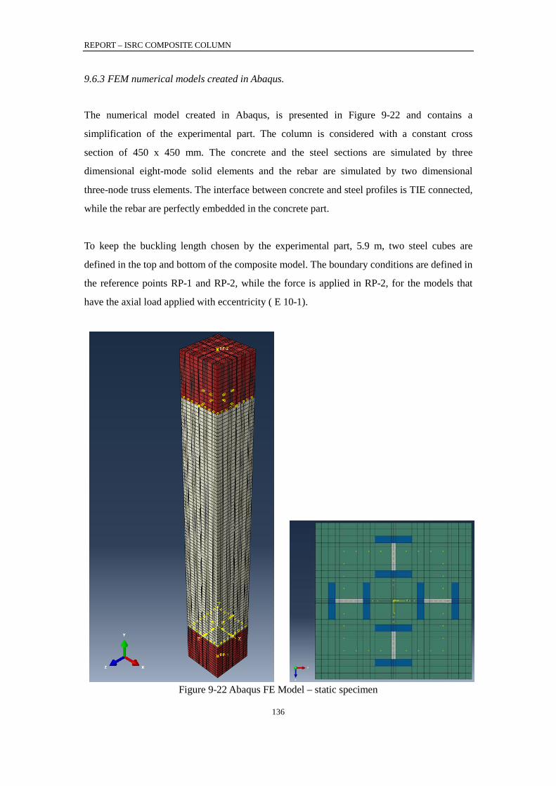
REPORT – ISRC COMPOSITE COLUMN
136
9.6.3 FEM numerical models created in Abaqus.
The numerical model created in Abaqus, is presented in Figure 9-22 and contains a
simplification of the experimental part. The column is considered with a constant cross
section of 450 x 450 mm. The concrete and the steel sections are simulated by three
dimensional eight-mode solid elements and the rebar are simulated by two dimensional
three-node truss elements. The interface between concrete and steel profiles is TIE connected,
while the rebar are perfectly embedded in the concrete part.
To keep the buckling length chosen by the experimental part, 5.9 m, two steel cubes are
defined in the top and bottom of the composite model. The boundary conditions are defined in
the reference points RP-1 and RP-2, while the force is applied in RP-2, for the models that
have the axial load applied with eccentricity ( E 10-1).
Figure 9-22 Abaqus FE Model – static specimen
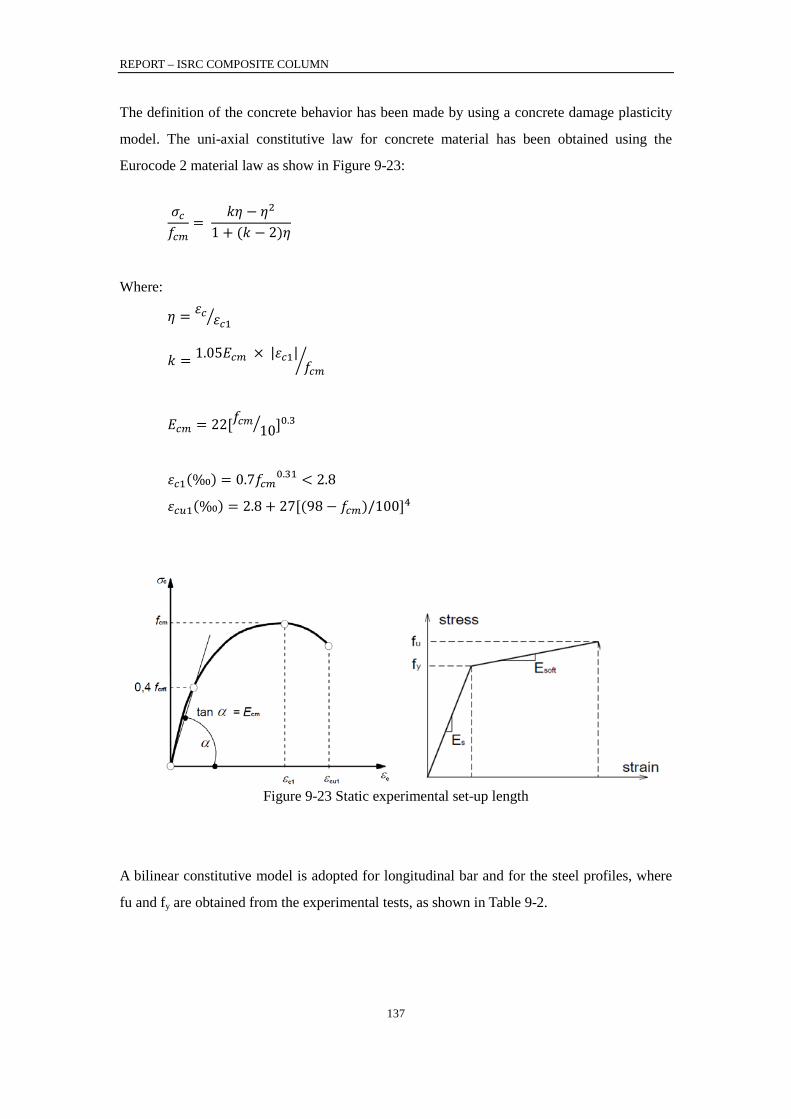
REPORT – ISRC COMPOSITE COLUMN
137
The definition of the concrete behavior has been made by using a concrete damage plasticity
model. The uni-axial constitutive law for concrete material has been obtained using the
Eurocode 2 material law as show in Figure 9-23:
𝜎𝑐𝑓𝑐𝑚
= 𝑘𝜂 − 𝜂2
1 + (𝑘 − 2)𝜂
Where:
𝜂 = 𝜀𝑐 𝜀𝑐1
𝑘 = 1.05𝐸𝑐𝑚 × |𝜀𝑐1|𝑓𝑐𝑚
𝐸𝑐𝑚 = 22[𝑓𝑐𝑚 10 ]0.3
𝜀𝑐1(‰) = 0.7𝑓𝑐𝑚0.31 < 2.8
𝜀𝑐𝑢1(‰) = 2.8 + 27[(98 − 𝑓𝑐𝑚)/100]4
A bilinear constitutive model is adopted for longitudinal bar and for the steel profiles, where
fu and fy are obtained from the experimental tests, as shown in Table 9-2.
Figure 9-23 Static experimental set-up length

REPORT – ISRC COMPOSITE COLUMN
138
Table 9-2 Steel profile material strength – static tests Specimen ID Location Yield Strength/Mpa Ultimate Strength/Mpa Elongation %
E00 – 1 Flange
410 539 33.9
407 Web 523 546 27.1
E00 – 2 Flange
404 528 33.8
392 Web 411 535 27.3
E10 – 1 Flange
433 554 32.4
413 Web 435 568 26.0
E10 – 2 Flange
420 534 33.80
346 Web 415 530 28.9
E15 – 1 Flange
378 500 32.8
376 Web 404 529 29.9
E15– 2 Flange
393 516 34.6
384
Web 405 520 30.2
Table 9-3 contains a comparison between the experimental results and the numerical models.
The peak values and the corresponding displacement are compared. It can be observed that
the numerical results are similar with the experimental part.
Table 9-3 Comparisons between peak load vs. corresponding deflection
Specimen ID
Experimental values Numerical values
Capacity Pu /kN Vertical deflection Pu /
mm
Capacity Pu /kN Vertical deflection Pu /
mm
E00 – 1 17082 4.17 17006.8 3.98 E00 - 2 15325 3.43 15879 4.25 E10 – 1 14360 3.55 14500 3.60 E10 - 2 13231 3.46 14031 3.34 E15 – 1 12041 2.79 12521 3.35 E15 - 2 12759 2.70 13012 3.43
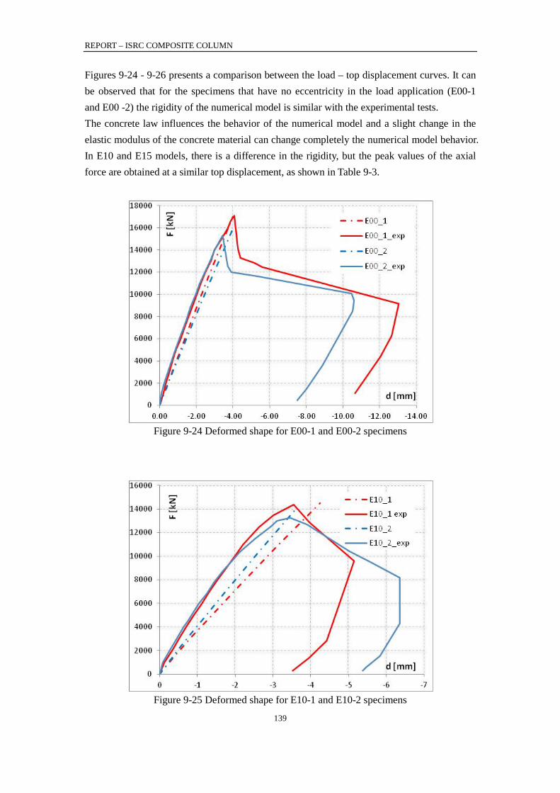
REPORT – ISRC COMPOSITE COLUMN
139
Figures 9-24 - 9-26 presents a comparison between the load – top displacement curves. It can be observed that for the specimens that have no eccentricity in the load application (E00-1 and E00 -2) the rigidity of the numerical model is similar with the experimental tests. The concrete law influences the behavior of the numerical model and a slight change in the elastic modulus of the concrete material can change completely the numerical model behavior. In E10 and E15 models, there is a difference in the rigidity, but the peak values of the axial force are obtained at a similar top displacement, as shown in Table 9-3.
Figure 9-24 Deformed shape for E00-1 and E00-2 specimens
Figure 9-25 Deformed shape for E10-1 and E10-2 specimens
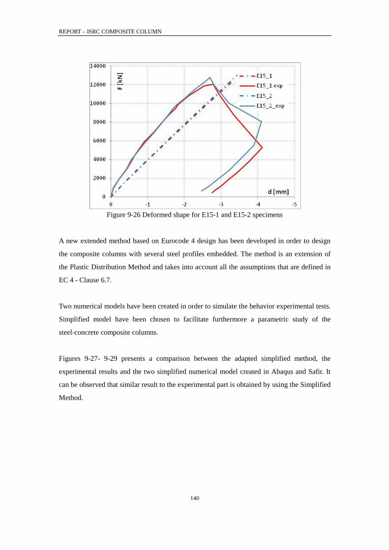
REPORT – ISRC COMPOSITE COLUMN
140
A new extended method based on Eurocode 4 design has been developed in order to design
the composite columns with several steel profiles embedded. The method is an extension of
the Plastic Distribution Method and takes into account all the assumptions that are defined in
EC 4 - Clause 6.7.
Two numerical models have been created in order to simulate the behavior experimental tests.
Simplified model have been chosen to facilitate furthermore a parametric study of the
steel-concrete composite columns.
Figures 9-27- 9-29 presents a comparison between the adapted simplified method, the
experimental results and the two simplified numerical model created in Abaqus and Safir. It
can be observed that similar result to the experimental part is obtained by using the Simplified
Method.
Figure 9-26 Deformed shape for E15-1 and E15-2 specimens
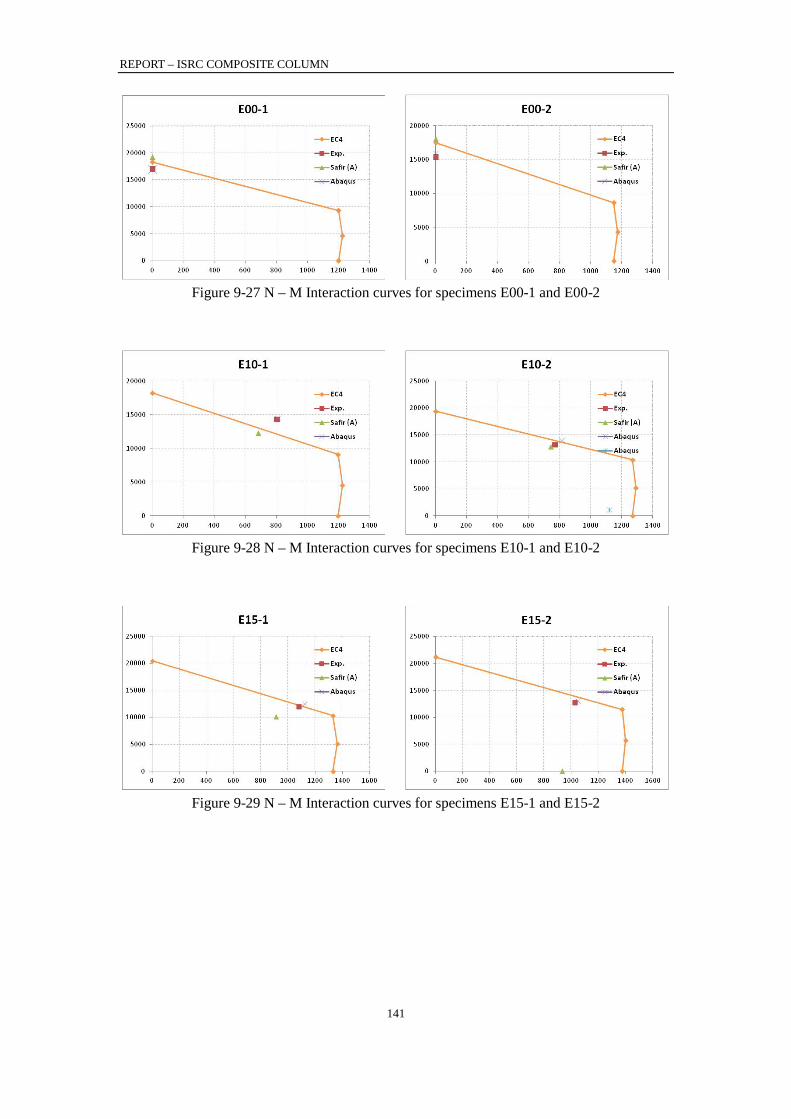
REPORT – ISRC COMPOSITE COLUMN
141
Figure 9-27 N – M Interaction curves for specimens E00-1 and E00-2
Figure 9-28 N – M Interaction curves for specimens E10-1 and E10-2
Figure 9-29 N – M Interaction curves for specimens E15-1 and E15-2
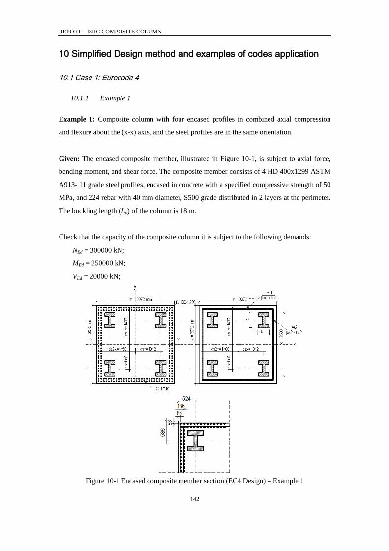
REPORT – ISRC COMPOSITE COLUMN
142
10 Simplified Design method and examples of codes application
10.1 Case 1: Eurocode 4
10.1.1 Example 1
Example 1: Composite column with four encased profiles in combined axial compression
and flexure about the (x-x) axis, and the steel profiles are in the same orientation.
Given: The encased composite member, illustrated in Figure 10-1, is subject to axial force,
bending moment, and shear force. The composite member consists of 4 HD 400x1299 ASTM
A913- 11 grade steel profiles, encased in concrete with a specified compressive strength of 50
MPa, and 224 rebar with 40 mm diameter, S500 grade distributed in 2 layers at the perimeter.
The buckling length (Lo) of the column is 18 m.
Check that the capacity of the composite column it is subject to the following demands:
NEd = 300000 kN;
MEd = 250000 kN;
VEd = 20000 kN;
Figure 10-1 Encased composite member section (EC4 Design) – Example 1

REPORT – ISRC COMPOSITE COLUMN
143
Steel profile HD 400x1299 (W14x16x873) properties are:
ASTM A913- 11 Grade 65 - fy = 450MPa;
Es = 210000 MPa;
b = 476 mm;
d = 600 mm;
tw = 100 mm;
tf = 140 mm;
Zsx = 33250 cm3;
Zsy = 16670 cm3; 4 4754600 10 mmHDxI = ⋅ ; 4 4254400 10 mmHDyI = ⋅ ;
Aa = 165000 mm2; 4
2 2
i 14 165000mm 660000mm ;s aA A
=
= = ⋅ =∑
dsx = 1012 mm;
dsy = 950mm;
dx = 2500 mm;
dy = 2500mm;
Reinforcement properties are:
224 = total amount of vertical rebar;
db = 40mm for a T40 diameter bar;
fs = 500MPa;
Esr = 200000 MPa; 21256.63mmsriA = ;
n2
i 1281486.7mmsr sriA A
=
= =∑ ;
Concrete section’s properties are:
h1 = 3072mm;
h2 = 3072mm;
cx = 86mm;
cy = 86mm;
Concrete class C50: fck = 50MPa;
fcm = fck + 8 MPa=58 MPa; 0.3 0.3
22 22 37278MPa;10 10
cmcm
f 58E = ⋅ = ⋅ =
2(3072mm) (3072mm) 9437184mmg 1 2A h h= ⋅ = × = ;
REPORT – ISRC COMPOSITE COLUMN
144
Solution:
• The partial safety factors for materials:
To determine resistance, the following partial safety factors should be applied to the following
materials:
γa the partial factor for structural steel
γs the partial factor for the reinforcement
γc the partial factor for reinforced concrete
Thus: 450MPa 450MPa1
yyd
a
ff = γ = =
the design value of yield strength of the structural steel 500MPa 434.78MPa1.15
ssd
a
ff = γ = =
the design value of yield strength of the reinforcement 50MPa 33.33MPa1.5
ccd
c
ff = γ = =
the design value of yield strength of the concrete
• Definition of plates equivalent to rebar:
The definition of the equivalent horizontal plates (As1 and As2) is based off the following:
1) As1 plate:
i = 2 = the amount of rebar layers in one equivalent plate
nx = 30 = the amount of rebar in one layer
sx = 100 mm = the spacing between 2 vertical rebar
2 22 30 1256.64mm 75398.2mms1 x sriA =i n A =⋅ ⋅ ⋅ ⋅ =
21
11
75398.2mm =26mm2900mm
ss
s
Abh
= =
( )
1
2
1
3072mm -86mm 1450mm2
3072mm -186mm 1350mm2
1450mm 1350mm 1400mm2
y
y
iys y
d
d
dd i
= =
= =
+= = =∑
2 8 32 2 75398.2mm 1400mm 2.1112 10 mmsr1x s1 s1yZ A d= ⋅ ⋅ = ⋅ ⋅ = ⋅
2 2 2 11 4x2 i 2 2 30 1256.64mm (1400mm) 2.9556 10 mmsr1x sri s1yI n A d= ⋅ ⋅ ⋅ ⋅ = ⋅ ⋅ ⋅ ⋅ = ⋅
REPORT – ISRC COMPOSITE COLUMN
145
2) As2 plate:
2 2 2s y sri s sA n A b h= ⋅ = ⋅
j = 2 = the number of rebar layers in one equivalent plate ny = 26 = the number of rebar in one layer
2 2y 2 26 1256.64mm 65345.1mms2 sriA =j n A =⋅ ⋅ ⋅ ⋅ =
2 ( 1) 25 100mm=2500mms y yh n s= − ⋅ = ⋅
22
22
65345mm =26.1mm2500mm
ss
s
Abh
= =
1
2
2
3072mm -86mm 1450mm2
3072mm -186mm 1350mm2
1450mm 1350mm 1400mm2
x
x
jxs x
d
d
dd j
= =
= =
+= = =∑
2 27 326.1mm (2500mm)2 8.168 10 mm
4 2s2 s2
sr2xb hZ ⋅ ⋅
= ⋅ = = ⋅ 3 3
10 426.1mm (2500mm)2 6.807 10 mm12 6
s2 s2sr2x
b hI ⋅ ⋅= ⋅ = = ⋅
• Definition of plates equivalent to steel profiles:
The definition of the equivalent horizontal plates is made according to the following:
* 600mmd d= =
5 2*
*
6.6 10 mm 275mm600mm
sAbd
⋅= = =
5 2 8 3
a 4 1.65 10 mm 950mm 6.27 10 mmsx syZ n A d= ⋅ ⋅ = ⋅ ⋅ ⋅ = ⋅
2 5 2 2 9 4 11 4a xn 4 1.65 10 mm (950mm) 4 7.564 10 mm 6.258 10 mmsx syI n A d I= ⋅ ⋅ + ⋅ = ⋅ ⋅ ⋅ + ⋅ ⋅ = ⋅
REPORT – ISRC COMPOSITE COLUMN
146
• Stiffness evaluation:
( ) c,eff c
5 11 4 5 11 4 10 4
4 12 4
17 2
2.1 10 MPa 6.258 10 mm 2.0 10 MPa (2.955 10 mm 6.81 10 mm )0.6 1.75 10 MPa 6.43 10 mm
2.719 10 N mm
s s sr sr eeffEI E I E I K E I
= ⋅ + ⋅ + ⋅ ⋅
= ⋅ ⋅ ⋅ + ⋅ ⋅ ⋅ + ⋅ +
+ ⋅ ⋅ ⋅ ⋅
= ⋅ ⋅
( ) 17 29
2 2o
2.719 10 N mm 8.281 10 N(18m)
2 2eff
cr
π EI πNL
⋅ ⋅ ⋅ ⋅= = = ⋅
,,
1 1 0.47 37278 MPa=17543 MPa1 0.75 1.51
c eff cm cmG Ed
tEd
E E EN
N
= = = ⋅+ ⋅ + ⋅ϕ
where: - 0.6eK = the correction factor - tϕ is the creep coefficient according to EN 1992-1-1, 3.1.4 or 11.3.3, depending on
the age (t) of the concrete at the moment considered at the age (to) at loading. In this example, we consider the creep coefficient equal to 1.5.
- NEd is the total design force - NG,Ed is the part of the normal force that is permanent
In high-rise buildings, there is a significant amount of long-term loads, approximately 75% of total loads. Therefore, the ratio of the normal forces in this example is considered equal to:
, 0.75G Ed
Ed
NN =
• Limitation when using the extended simplified method:
1) The steel contribution ratio δ should fulfill the following condition 0.2 < δ < 0.9
5 26.6 10 mm 450MPa 0.45660096.9kN
s yd
pl.Rd
A fN⋅ ⋅ ⋅
δ = = = EN 1994-1-1:2004 – Eq (6.27)
where:
( )5 2 5 2 6 2
0.85
6.6 10 mm 450MPa 3.81 10 mm 434.78MPa 8.455 10 mm 0.85 33.3MPa660096.9kN
pl.Rd s yd sr sd c cdN A f A f A f
= ⋅ + ⋅ + ⋅ ⋅
= ⋅ ⋅ + ⋅ ⋅ + ⋅ ⋅ ⋅
=
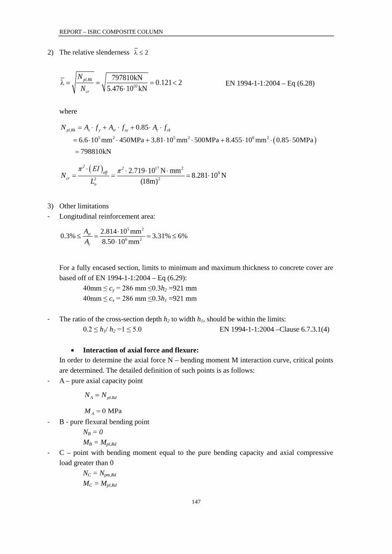
REPORT – ISRC COMPOSITE COLUMN
147
2) The relative slenderness 2λ ≤
10
797810kN 0.121 25.476 10 kN
pl.Rk
cr
NN
λ = = = <⋅
EN 1994-1-1:2004 – Eq (6.28)
where
( )5 2 5 2 6 2
0.85
6.6 10 mm 450MPa 3.81 10 mm 500MPa 8.455 10 mm 0.85 50MPa798810kN
pl.Rk s y sr sy c ckN A f A f A f
= ⋅ + ⋅ + ⋅ ⋅
= ⋅ ⋅ + ⋅ ⋅ + ⋅ ⋅ ⋅
=
( ) 17 29
2 2o
2.719 10 N mm 8.281 10 N(18m)
2 2eff
cr
π EI πNL
⋅ ⋅ ⋅ ⋅= = = ⋅
3) Other limitations - Longitudinal reinforcement area:
5 2
6 2
2.814 10 mm0.3% 3.31% 6%8.50 10 mm
sr
c
AA
⋅≤ = = ≤
⋅
For a fully encased section, limits to minimum and maximum thickness to concrete cover are based off of EN 1994-1-1:2004 – Eq (6.29):
40mm ≤ cy = 286 mm ≤0.3h2 =921 mm 40mm ≤ cx = 286 mm ≤0.3h1 =921 mm
- The ratio of the cross-section depth h2 to width h1, should be within the limits: 0.2 ≤ h1/ h2 =1 ≤ 5.0 EN 1994-1-1:2004 –Clause 6.7.3.1(4)
• Interaction of axial force and flexure:
In order to determine the axial force N – bending moment M interaction curve, critical points are determined. The detailed definition of such points is as follows:
- A – pure axial capacity point
A pl.RdN N=
0 MPaAM =
- B - pure flexural bending point NB = 0 MB = Mpl,Rd
- C – point with bending moment equal to the pure bending capacity and axial compressive load greater than 0
NC = Npm,Rd MC = Mpl,Rd
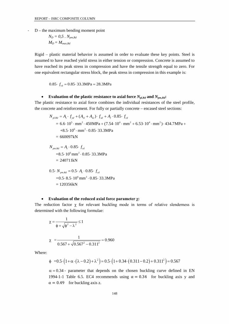
REPORT – ISRC COMPOSITE COLUMN
148
- D – the maximum bending moment point ND = 0,5 . Npm,Rd MD = Mmax,Rd
Rigid – plastic material behavior is assumed in order to evaluate these key points. Steel is assumed to have reached yield stress in either tension or compression. Concrete is assumed to have reached its peak stress in compression and have the tensile strength equal to zero. For one equivalent rectangular stress block, the peak stress in compression in this example is:
cd0.85 0.85 33.3MPa 28.3MPaf⋅ = ⋅ =
• Evaluation of the plastic resistance to axial force Npl,Rd and Npm,Rd: The plastic resistance to axial force combines the individual resistances of the steel profile, the concrete and reinforcement. For fully or partially concrete – encased steel sections:
5 2 4 2 4 2
6 2
( ) 0.85
6.6 10 mm 450MPa (7.54 10 mm 6.53 10 mm ) 434.7MPa8.5 10 mm 0.85 33.3MPa
660097kN
pl.Rd s yd s1 s2 sd c cdN A f A A f A f
= + =
= ⋅ + + ⋅ + ⋅ ⋅
⋅ ⋅ ⋅ + ⋅ ⋅ + ⋅ ⋅ ⋅ +
⋅ ⋅ ⋅ ⋅
6 2
0.85
8.5 10 mm 0.85 33.3MPa240711kN
pm.Rd c cdN A f
= =
= ⋅ ⋅
⋅ ⋅ ⋅
6 2
0.5 0.5 0.85
0.5 8.5 10 mm 0.85 33.3MPa120356kN
pm.Rd c cdN A f
= =
⋅ = ⋅ ⋅ ⋅
⋅ ⋅ ⋅ ⋅
• Evaluation of the reduced axial force parameter χ:
The reduction factor χ for relevant buckling mode in terms of relative slenderness is determined with the following formulae:
2 2
1 1χ = ≤φ + φ − λ
2 2
1 0.9600.567 0.567 0.311
=χ =+ −
Where:
( )( ) ( )( )2 20.5 1 0.2 0.5 1 0.34 0.311 0.2 0.311 0.567 =φ ⋅ + α ⋅ λ − + λ = ⋅ + ⋅ − + =
0.34α = - parameter that depends on the chosen buckling curve defined in EN 1994-1-1 Table 6.5. EC4 recommends using α = 0.34 for buckling axis y and α = 0.49 for buckling axis z.
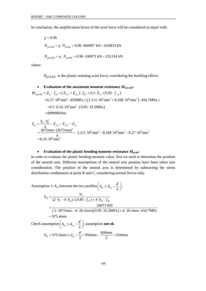
REPORT – ISRC COMPOSITE COLUMN
149
In conclusion, the amplification factor of the axial force will be considered as equal with:
0.96χ =
0.96 660097 kN 633833 kNpl.b.Rd pl.RdN N = χ ⋅ = ⋅ =
0.96 240071 kN 231134 kNpm.b.Rd pm.RdN N = χ ⋅ = ⋅ =
where:
𝑁𝑝𝑙,𝑏,𝑅𝑑 is the plastic resisting axial force, considering the buckling effects
• Evaluation of the maximum moment resistance Mmax.Rd:
( ) ( )( )
( )
8 3 8 3 8 3
9 3
0.5 0.85
6.27 10 mm 450MPa 2.111 10 mm 8.168 10 mm 434.7MPa
0.5 6.33 10 mm 0.85 33.3MPa499099kNm
max.Rd sx yd r1x r2x sd cx cdM Z f Z Z f Z f
=
+ =
= ⋅ + + ⋅ + ⋅ ⋅ ⋅
⋅ ⋅ + ⋅ + ⋅ ⋅ +
⋅ ⋅ ⋅ ⋅
r2x
8 3 8 3 8 3
9 3
Z4
3072mm (3072mm) 2.111 10 mm 8.168 10 mm 6.27 10 mm4
6.33 10 mm
21 2
cx r1x sx
2
h hZ Z Z
=
=
⋅= − − −
⋅− ⋅ − ⋅ − ⋅
⋅
• Evaluation of the plastic bending moment resistance Mpl.Rd:
In order to evaluate the plastic bending moment value, first we need to determine the position of the neutral axis. Different assumptions of the neutral axis position have been taken into consideration. The position of the neutral axis is determined by subtracting the stress distribution combination at point B and C, considering normal forces only.
Assumption 1: hnx between the two profiles2nx sydh d ≤ −
:
( )
( )
1 4 ) 0.85 4240711kN
2 3072mm 4 26.1mm) 0.85 33.3MPa 4 26.1mm 434.7MPa975.4mm
Cnx
s2 cd s2 sd
Nh(2 h b f b f
(
=⋅ − ⋅ ⋅ ⋅ + ⋅ ⋅
=⋅ − ⋅ ⋅ + ⋅ ⋅
=
Check assumption2nx sydh d ≤ −
: assumption not ok
600mm975.4mm 950mm 650mm2 2nx sydh d= ≤ − = − =
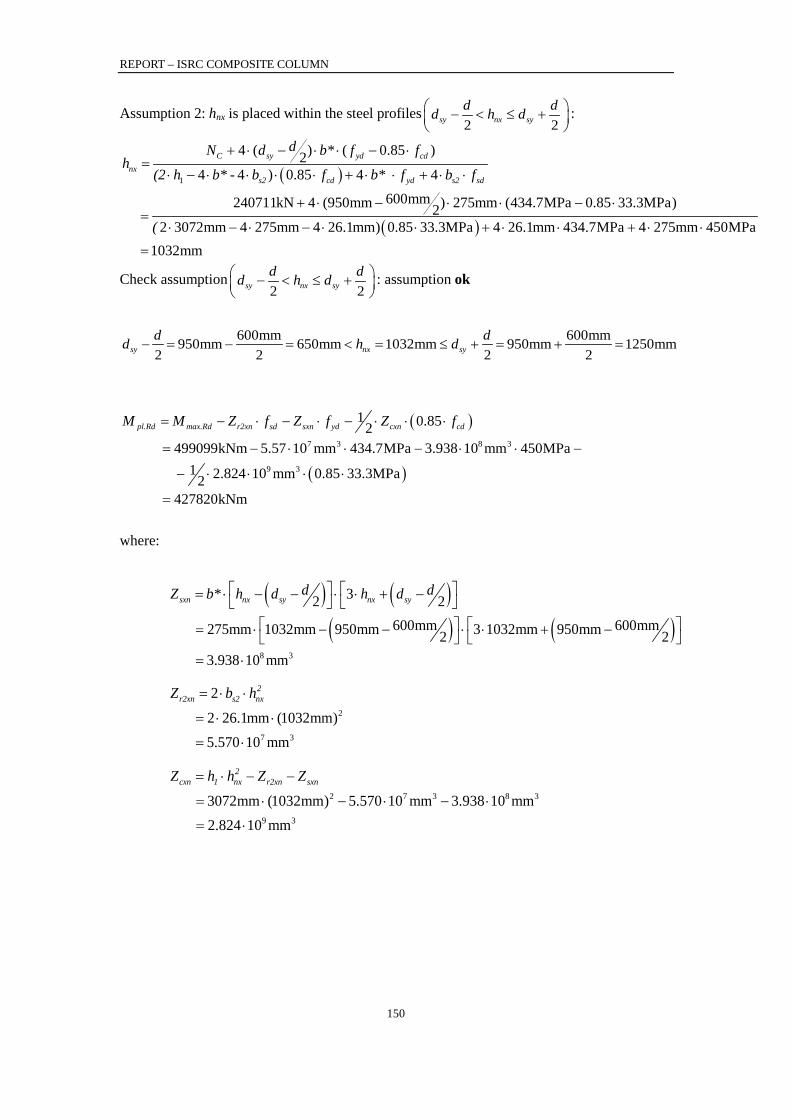
REPORT – ISRC COMPOSITE COLUMN
150
Assumption 2: hnx is placed within the steel profiles2 2sy nx syd dd h d − < ≤ +
:
( )
( )
1
4 ( ) ( 0.85 )24 - 4 ) 0.85 4 4
600mm240711kN 4 (950mm ) 275mm (434.7MPa 0.85 33.3MPa)22 3072mm 4 275mm 4 26.1mm) 0.85 33.3MPa 4 26.1mm 434.7MPa 4
C sy yd cdnx
s2 cd yd s2 sd
dN d b* f fh
(2 h b* b f b* f b f
(
+ ⋅ − ⋅ ⋅ − ⋅=
⋅ − ⋅ ⋅ ⋅ ⋅ + ⋅ ⋅ + ⋅ ⋅
+ ⋅ − ⋅ ⋅ − ⋅=
⋅ − ⋅ − ⋅ ⋅ + ⋅ ⋅ + ⋅275mm 450MPa1032mm
⋅
=
Check assumption2 2sy nx syd dd h d − < ≤ +
: assumption ok
600mm 600mm950mm 650mm 1032mm 950mm 1250mm
2 2 2 2sy nx syd dd h d− = − = < = ≤ + = + =
( )
( )
7 3 8 3
9 3
1 0.852499099kNm 5.57 10 mm 434.7MPa 3.938 10 mm 450MPa
1 2.824 10 mm 0.85 33.3MPa2427820kNm
pl.Rd max.Rd r2xn sd sxn yd cxn cdM M Z f Z f Z f
= − ⋅ − ⋅ − ⋅ ⋅ ⋅
= − ⋅ ⋅ − ⋅ ⋅ −
− ⋅ ⋅ ⋅ ⋅
=
where:
( ) ( )( ) ( )
8 3
32 2600mm 600mm275mm 1032mm 950mm 3 1032mm 950mm2 2
3.938 10 mm
sxn nx sy nx syd dZ b* h d h d
= ⋅ − − ⋅ ⋅ + −
= ⋅ − − ⋅ ⋅ + −
= ⋅
2
7 3
2
2 26.1mm (1032mm)5.570 10 mm
2r2xn s2 nxZ b h
= ⋅ ⋅
= ⋅ ⋅
= ⋅
2 7 3 8 3
9 3
3072mm (1032mm) 5.570 10 mm 3.938 10 mm2.824 10 mm
2cxn 1 nx r2xn sxnZ h h Z Z
= ⋅ − −
= ⋅ − ⋅ − ⋅
= ⋅
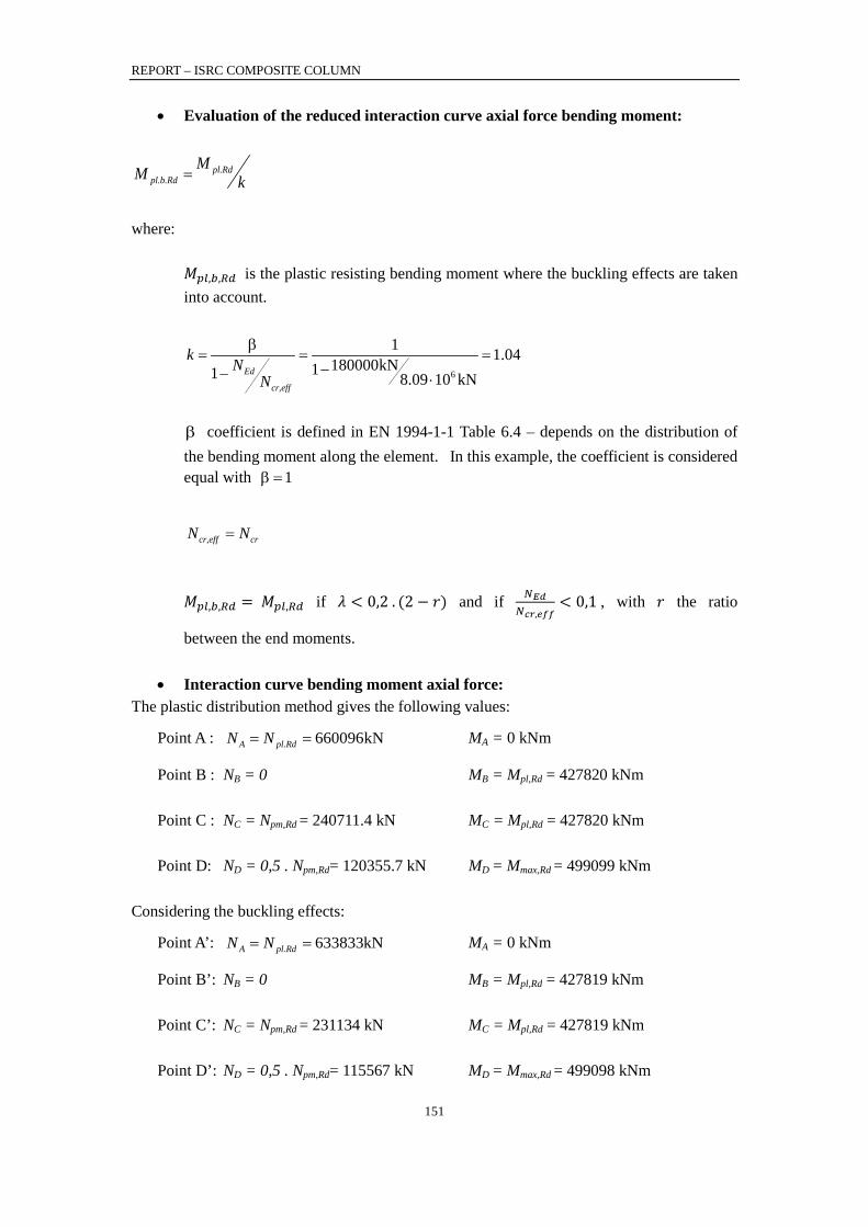
REPORT – ISRC COMPOSITE COLUMN
151
• Evaluation of the reduced interaction curve axial force bending moment:
pl.Rdpl.b.Rd
MM k=
where:
𝑀𝑝𝑙,𝑏,𝑅𝑑 is the plastic resisting bending moment where the buckling effects are taken into account.
6
1 1.04180000kN11 8.09 10 kNEd
cr,eff
k NN
β= = =
−− ⋅
β coefficient is defined in EN 1994-1-1 Table 6.4 – depends on the distribution of the bending moment along the element. In this example, the coefficient is considered equal with 1β =
cr,eff crN N=
𝑀𝑝𝑙,𝑏,𝑅𝑑 = 𝑀𝑝𝑙,𝑅𝑑 if 𝜆 < 0,2 . (2 − 𝑟) and if 𝑁𝐸𝑑𝑁𝑐𝑟,𝑒𝑓𝑓
< 0,1 , with 𝑟 the ratio
between the end moments.
• Interaction curve bending moment axial force: The plastic distribution method gives the following values:
Point A : 660096kNA pl.RdN N= = MA = 0 kNm
Point B : NB = 0 MB = Mpl,Rd = 427820 kNm Point C : NC = Npm,Rd = 240711.4 kN MC = Mpl,Rd = 427820 kNm Point D: ND = 0,5 . Npm,Rd= 120355.7 kN MD = Mmax,Rd = 499099 kNm
Considering the buckling effects:
Point A’: 633833kNA pl.RdN N= = MA = 0 kNm
Point B’: NB = 0 MB = Mpl,Rd = 427819 kNm Point C’: NC = Npm,Rd = 231134 kN MC = Mpl,Rd = 427819 kNm Point D’: ND = 0,5 . Npm,Rd= 115567 kN MD = Mmax,Rd = 499098 kNm
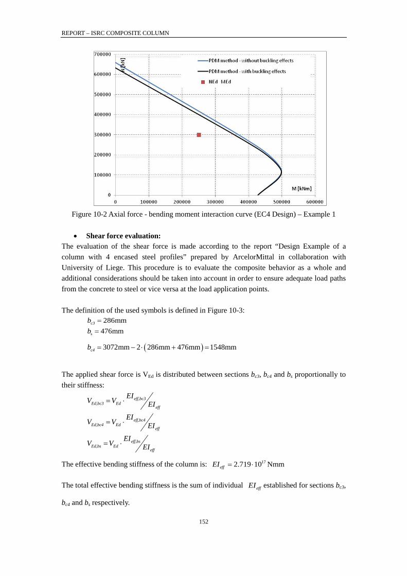
REPORT – ISRC COMPOSITE COLUMN
152
Figure 10-2 Axial force - bending moment interaction curve (EC4 Design) – Example 1
• Shear force evaluation:
The evaluation of the shear force is made according to the report “Design Example of a column with 4 encased steel profiles” prepared by ArcelorMittal in collaboration with University of Liege. This procedure is to evaluate the composite behavior as a whole and additional considerations should be taken into account in order to ensure adequate load paths from the concrete to steel or vice versa at the load application points. The definition of the used symbols is defined in Figure 10-3:
286mmc3b =
s 476mmb =
( )3072mm 2 286mm 476mm 1548mmc4b = − ⋅ + =
The applied shear force is VEd is distributed between sections bc3, bc4 and bs proportionally to their stiffness:
eff,bc3Ed,bc3 Ed
eff
EIV V EI= ⋅
eff,bc4Ed,bc4 Ed
eff
EIV V EI= ⋅
eff,bsEd,bs Ed
eff
EIV V EI= ⋅
The effective bending stiffness of the column is: 172.719 10 NmmeffEI = ⋅
The total effective bending stiffness is the sum of individual effEI established for sections bc3,
bc4 and bs respectively.
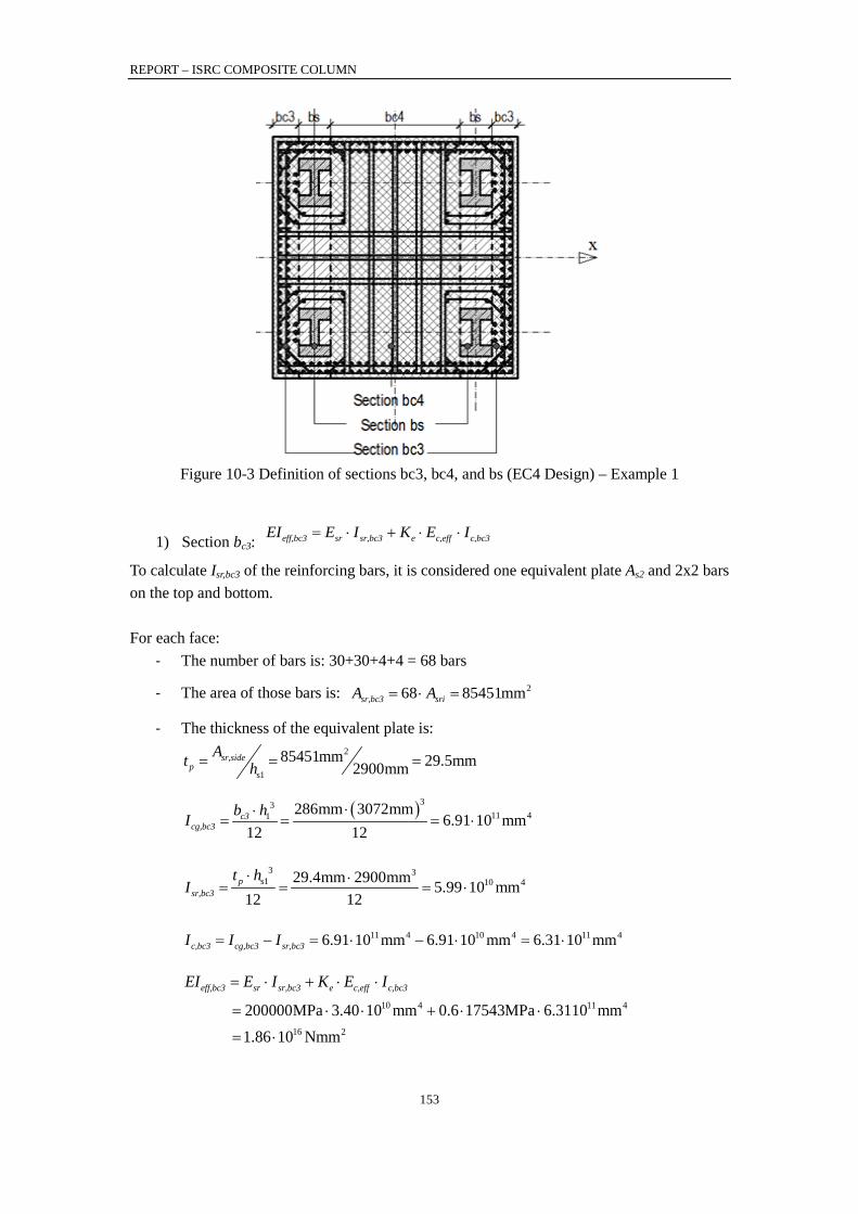
REPORT – ISRC COMPOSITE COLUMN
153
Figure 10-3 Definition of sections bc3, bc4, and bs (EC4 Design) – Example 1
1) Section bc3: eff,bc3 sr sr,bc3 e c,eff c,bc3EI E I K E I= ⋅ + ⋅ ⋅
To calculate Isr,bc3 of the reinforcing bars, it is considered one equivalent plate As2 and 2x2 bars on the top and bottom. For each face:
- The number of bars is: 30+30+4+4 = 68 bars
- The area of those bars is: 268 85451mmsr,bc3 sriA A= ⋅ =
- The thickness of the equivalent plate is: 2
s1
85451mm 29.5mm2900mmsr,side
pAt h= = =
( )3311 41 286mm 3072mm
6.91 10 mm12 12
c3cg,bc3
b hI⋅⋅
= = = ⋅
3 3s1 10 429.4mm 2900mm 5.99 10 mm
12 12p
sr,bc3
t hI
⋅ ⋅= = = ⋅
11 4 10 4 11 46.91 10 mm 6.91 10 mm 6.31 10 mmc,bc3 cg,bc3 sr,bc3I I I= − = ⋅ − ⋅ = ⋅
10 4 11 4
16 2
200000MPa 3.40 10 mm 0.6 17543MPa 6.3110 mm1.86 10 Nmm
eff,bc3 sr sr,bc3 e c,eff c,bc3EI E I K E I
= ⋅ + ⋅ ⋅
= ⋅ ⋅ + ⋅ ⋅
= ⋅
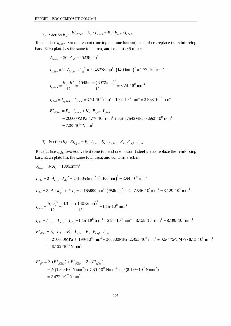
REPORT – ISRC COMPOSITE COLUMN
154
2) Section bc4: eff,bc4 sr sr,bc4 e c,eff c,bc4EI E I K E I= ⋅ + ⋅ ⋅
To calculate Isr,bc4, two equivalent (one top and one bottom) steel plates replace the reinforcing bars. Each plate has the same total area, and contains 36 rebar:
236 45238mmsr,bc4 sriA A= ⋅ =
( )22 2 11 42 2 45238mm 1400mm 1.77 10 mmsr,bc4 sr,bc4 s1yI A d= ⋅ ⋅ = ⋅ ⋅ = ⋅
( )3312 41 1548mm 3072mm
3.74 10 mm12 12
c4cg,bc4
b hI⋅⋅
= = = ⋅
12 4 11 4 12 43.74 10 mm 1.77 10 mm 3.563 10 mmc,bc4 cg,bc4 sr,bc4I I I= − = ⋅ − ⋅ = ⋅
11 4 12 4
16 2
200000MPa 1.77 10 mm 0.6 17543MPa 3.563 10 mm7.30 10 Nmm
eff,bc4 sr sr,bc4 e c,eff c,bc4EI E I K E I
= ⋅ + ⋅ ⋅
= ⋅ ⋅ + ⋅ ⋅ ⋅
= ⋅
3) Section bs: eff,bs s s,bs sr sr,bs e c,eff c,bsEI E I E I K E I= ⋅ + ⋅ + ⋅ ⋅
To calculate Isr,bs, two equivalent (one top and one bottom) steel plates replace the reinforcing bars. Each plate has the same total area, and contains 8 rebar:
28 10053mmsr,bs sriA A= ⋅ =
( )22 2 10 42 2 10053mm 1400mm 3.94 10 mmsr,bs sr,bs s1yI A d= ⋅ ⋅ = ⋅ ⋅ = ⋅
( )2 9 4 11 42 2 2 165000mm 950mm 2 7.546 10 mm 3.129 10 mm22s,bs a sy xI A d I= ⋅ ⋅ + ⋅ = ⋅ ⋅ + ⋅ ⋅ = ⋅
( )3312 41 476mm 3072mm
1.15 10 mm12 12
scg,bs
b hI⋅⋅
= = = ⋅
12 4 10 4 11 4 11 41.15 10 mm 3.94 10 mm 3.129 10 mm 8.199 10 mmc,bs cg,bs sr,bs s,bsI I I I= − − = ⋅ − ⋅ − ⋅ = ⋅
11 4 10 4 11 4
16 2
210000MPa 8.199 10 mm 200000MPa 2.955 10 mm 0.6 17543MPa 8.13 10 mm8.199 10 Nmm
eff,bs s s,bs sr sr,bs e c,eff c,bsEI E I E I K E I
= ⋅ + ⋅ + ⋅ ⋅
= ⋅ ⋅ + ⋅ ⋅ + ⋅ ⋅ ⋅
= ⋅
16 2 16 2 16 2
17 2
2 ( ) 2 ( )
2 (1.86 10 Nmm ) 7.30 10 Nmm 2 (8.199 10 Nmm )2.472 10 Nmm
eff eff,bc3 eff,bc4 eff,bsEI EI EI EI
= ⋅ + + ⋅
= ⋅ ⋅ + ⋅ + ⋅ ⋅
= ⋅
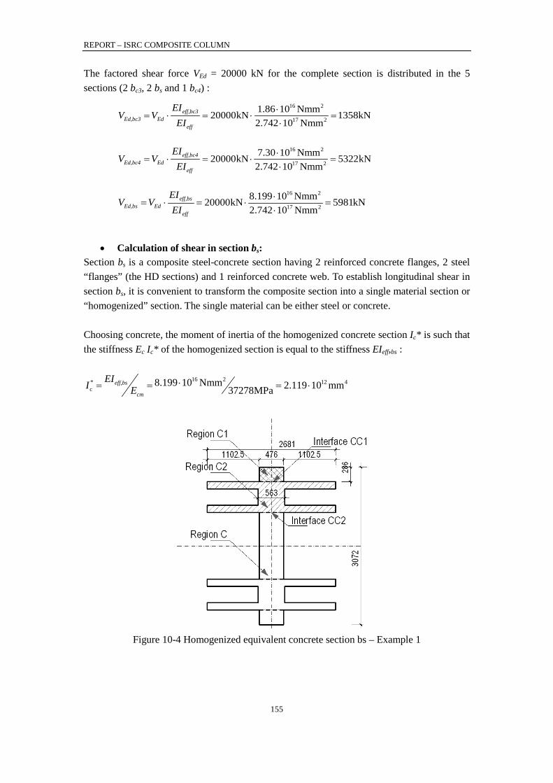
REPORT – ISRC COMPOSITE COLUMN
155
The factored shear force VEd = 20000 kN for the complete section is distributed in the 5 sections (2 bc3, 2 bs and 1 bc4) :
16 2
17 2
1.86 10 Nmm20000kN 1358kN2.742 10 Nmm
eff,bc3Ed,bc3 Ed
eff
EIV V
EI⋅
= ⋅ = ⋅ =⋅
16 2
17 2
7.30 10 Nmm20000kN 5322kN2.742 10 Nmm
eff,bc4Ed,bc4 Ed
eff
EIV V
EI⋅
= ⋅ = ⋅ =⋅
16 2
17 2
8.199 10 Nmm20000kN 5981kN2.742 10 Nmm
eff,bsEd,bs Ed
eff
EIV V
EI⋅
= ⋅ = ⋅ =⋅
• Calculation of shear in section bs:
Section bs is a composite steel-concrete section having 2 reinforced concrete flanges, 2 steel “flanges” (the HD sections) and 1 reinforced concrete web. To establish longitudinal shear in section bs, it is convenient to transform the composite section into a single material section or “homogenized” section. The single material can be either steel or concrete. Choosing concrete, the moment of inertia of the homogenized concrete section Ic* is such that the stiffness Ec Ic* of the homogenized section is equal to the stiffness EIeff,bs :
16 2* 12 4c
8.199 10 Nmm 2.119 10 mm37278MPaeff,bs
cm
EII E⋅= = = ⋅
Figure 10-4 Homogenized equivalent concrete section bs – Example 1
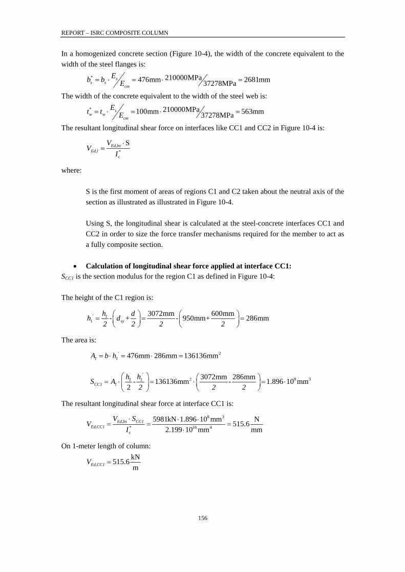
REPORT – ISRC COMPOSITE COLUMN
156
In a homogenized concrete section (Figure 10-4), the width of the concrete equivalent to the width of the steel flanges is:
210000MPa476mm 2681mm37278MPa* ss s
cm
Eb b E= ⋅ = ⋅ =
The width of the concrete equivalent to the width of the steel web is:
210000MPa100mm 563mm37278MPa* sw w
cm
Et t E= ⋅ = ⋅ =
The resultant longitudinal shear force on interfaces like CC1 and CC2 in Figure 10-4 is:
*c
SEd,bsEd,l
VV
I⋅
=
where:
S is the first moment of areas of regions C1 and C2 taken about the neutral axis of the section as illustrated as illustrated in Figure 10-4. Using S, the longitudinal shear is calculated at the steel-concrete interfaces CC1 and CC2 in order to size the force transfer mechanisms required for the member to act as a fully composite section.
• Calculation of longitudinal shear force applied at interface CC1:
SCC1 is the section modulus for the region C1 as defined in Figure 10-4: The height of the C1 region is:
' 3072mm 600mm950mm 286mm11 sy
h dh - d + - +2 2 2 2
= = =
The area is: ' 2476mm 286mm 136136mm1 1A b h= ⋅ = ⋅ =
'2 8 33072mm 286mm136136mm 1.896 10 mm
21 1
CC1 1h hS A - -
2 2 2 = ⋅ = ⋅ = ⋅
The resultant longitudinal shear force at interface CC1 is: 8 3
* 16 4c
5981kN 1.896 10 mm N515.62.199 10 mm mm
Ed,bs CC1Ed,CC1
V SV
I⋅ ⋅ ⋅
= = =⋅
On 1-meter length of column: kN515.6mEd,CC1V =
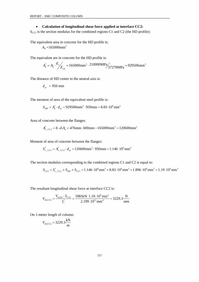
REPORT – ISRC COMPOSITE COLUMN
157
• Calculation of longitudinal shear force applied at interface CC2: SCC2 is the section modulus for the combined regions C1 and C2 (the HD profile): The equivalent area in concrete for the HD profile is:
Aa =165000mm2
The equivalent are in concrete for the HD profile is:
2 2210000MPa165000mm 929506mm37278MPa* sa a
cm
EA A E= ⋅ = ⋅ =
The distance of HD center to the neutral axis is:
syd = 950 mm
The moment of area of the equivalent steel profile is:
2 8 3929506mm 950mm 8.83 10 mm*HD a syS A d= ⋅ = ⋅ = ⋅
Area of concrete between the flanges:
2 2c _ CC2 476mm 600mm 165000mm 120600mm*
aA b d-A= ⋅ = ⋅ − =
Moment of area of concrete between the flanges:
2 8 3c _ CC2 c _ CC2 120600mm 950mm 1.146 10 mm* *
syS A d= ⋅ = ⋅ = ⋅
The section modulus corresponding to the combined regions C1 and C2 is equal to:
8 3 8 3 8 3 9 3c _ CC2 1.146 10 mm 8.83 10 mm 1.896 10 mm 1.19 10 mm*
CC2 HD CC1S S S S= + + = ⋅ + ⋅ + ⋅ = ⋅
The resultant longitudinal shear force at interface CC2 is:
9 3
* 12 4c
5981kN 1.19 10 mm N3229.32.199 10 mm mm
Ed,bs CC2Ed,CC2
V SV
I⋅ ⋅ ⋅
= = =⋅
On 1-meter length of column:
kN3229.3mEd,CC2V =
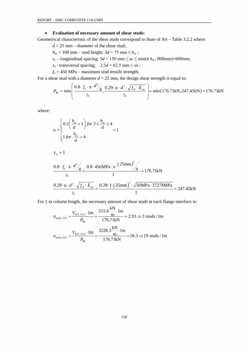
REPORT – ISRC COMPOSITE COLUMN
158
• Evaluation of necessary amount of shear studs: Geometrical characteristic of the shear studs correspond to State of Art – Table 3.2.2 where:
d = 25 mm – diameter of the shear stud; hsc = 100 mm – stud height; 3d = 75 mm ≤ hsc ; sc – longitudinal spacing; 5d = 150 mm ≤ sc ≤ min(6 hsc; 800mm)=600mm; sx –transversal spacing; 2.5d = 62.5 mm ≤ sx ; fu = 450 MPa – maximum stud tensile strength;
For a shear stud with a diameter d = 25 mm, the design shear strength is equal to:
( )2
20.8 0.294= min , min 176.71kN,247.45kN 176.71kNu ck cmRk
V V
df d f EP
γ γ
⋅ ⋅ π ⋅ ⋅α ⋅ ⋅ ⋅ = =
where:
0.2 1 4= 1
1 4
sc sc
sc
h h for 3d dh for d
+ ≤ ≤ α = >
Vγ 1=
( )22 25mm0.8 0.8 450MPa4 4 176.71kN
1u
V
df
γ
⋅ ⋅ π ⋅ ⋅ ⋅ π ⋅= =
( )220.29 0.29 1 25mm 50MPa 37278MPa247.45kN
1ck cm
V
d f Eγ
⋅α ⋅ ⋅ ⋅ ⋅ ⋅ ⋅ ⋅= =
For 1 m column length, the necessary amount of shear studs at each flange interface is: kN515.6 1m1m m 2.91 3 studs /1m
176.71kNEd1_CC1
studs_CC1Rk
Vn
P
⋅⋅= = = ⇒
kN3228.3 1m1m m 18.3 19 studs /1m176.71kN
Ed1_CC2studs_CC2
Rk
Vn
P
⋅⋅= = = ⇒

REPORT – ISRC COMPOSITE COLUMN
159
10.1.1 Example 2
Example 2: Composite column with four encased profiles in combined axial compression and flexure about the (x-x) axis, and the steel profiles have a different orientation Given: The encased composite member, illustrated in Figure 10-5, is subject to axial force, bending moment, and shear force. The composite member consist of 4 HD 400x634 S460 grade steel profiles, encased in concrete with a specified compressive strength of 60 MPa, and 32 pieces of rebar with 32 mm diameter, grade HRB 400 (fsy = 400MPa, distributed in 1 layer at the perimeter. The buckling length (Lo) of the column is 18 m. Check the capacity of the composite column subjected to the following demands:
NEd = 150000 kN; MEd = 40000 kN; VEd = 8000 kN;
Figure 10-5 Encased composite member section (EC4 Design) – Example 2

REPORT – ISRC COMPOSITE COLUMN
160
Steel profile HD 400x634 properties are: HISTAR 460 - fy = 460MPa; Es = 210000 MPa; b = 424 mm; d = 474 mm; tw = 51.2 mm; tf = 81.5 mm; Zsx = 14220 ⋅ 103 mm3;
Zsy = 4978 ⋅ 103 mm3; 4 4180200 10 mmHDxI = ⋅ ;
4 498250 10 mmHDyI = ⋅ ;
2 2808 10 mmaA = ⋅ ;
42 2 2
i 14 808 10 mm 323200mm ;s aA A
=
= = ⋅ ⋅ =∑
513mm;sxd =
513mmsyd = ;
dx = 375 mm; dy = 375mm;
Reinforcement properties are:
32 = the total number of vertical rebar; db = 32mm for a T32 diameter rebar; fs = 400MPa; Esr = 200000 MPa;
2804.24mmsriA = ;
n2
i 125735.93mmsr sriA A
=
= =∑ ;
Concrete section’s properties are:
fck = 60MPa; Ecm = 39100 MPa h1 = 1800 mm; h2 = 1800 mm; cx = 40 mm; cy = 40 mm;
6 2(1800mm) (1800mm) 3.24 10 mmg 1 2A h h= ⋅ = × = ⋅ ;
6 2 2 2 6 23.24 10 mm 25735.93mm 323200mm 2.89 10 mmc g sr sA A A A= − − = ⋅ − − = ⋅

REPORT – ISRC COMPOSITE COLUMN
161
Solution: • The partial safety factors for materials:
For the determination of resistance, the following partial safety factors should be applied for different materials:
γa is the partial factor for structural steel γs is the partial factor for the reinforcement γc is the partial factor for reinforced concrete
Thus:
460MPa 460MPa1y
yda
ff = γ = =
is the design value of yield strength of the structural steel
400MPa 347.8MPa1.15s
sda
ff = γ = =
is the design value of yield strength of the reinforcement
60MPa 40MPa1.5c
cdc
ff = γ = =
is the design value of yield strength of the concrete
• Definition of plates equivalent to rebar: The definition of the equivalent horizontal plates (As1 and As2) is as follows:
1) As1 plate:
i = 1 = the number of rebar layers in one equivalent plate nx = 9 = the amount of rebar in one layer
2 3 21 9 804.24mm 7.24 10 mms1 x sriA =i n A =⋅ ⋅ ⋅ ⋅ = ⋅
s1 x xh (n 1) s (9 1) 215mm 1720mm= − ⋅ = − ⋅ =
s1s1
s1
Ab 4.2mmh
= =
1y1800mmd 40mm 760mm
2-= =
iys1y
dd 760mmi= =∑
3 2 7 32 2 7.24 10 mm 760mm 1.1 10 mmsr1x s1 s1yZ A d= ⋅ ⋅ = ⋅ ⋅ ⋅ = ⋅
2 2 2 10 4x2 i 2 1 9 804.24mm (760mm) 2.837 10 mmsr1x sri s1yI n A d= ⋅ ⋅ ⋅ ⋅ = ⋅ ⋅ ⋅ ⋅ = ⋅

REPORT – ISRC COMPOSITE COLUMN
162
2) As2 plate:
2 2 2s y sri s sA n A b h= ⋅ = ⋅
j = 1 = the number of rebar layers in one equivalent plate ny = 7 = the amount of rebar in one layer
2 3 2y 1 7 804.24mm 5.63 10 mms2 sriA =j n A =⋅ ⋅ ⋅ ⋅ = ⋅
s2 y yh (n 1) s 6 215mm 1290mm== − ⋅ = ⋅
s2s2
s2
Ab 4.4mmh
= =
1x1800mmd 40mm 760mm
2-= =
jxs2x
dd 760mmj= =∑
2 26 34.4mm (1290mm)2 3.631 10 mm
4 2s2 s2
sr2xb hZ ⋅ ⋅
= ⋅ = = ⋅ 3 3
9 44.4mm (1290mm)2 1.561 10 mm12 6
s2 s2sr2x
b hI ⋅ ⋅= ⋅ = = ⋅
• Definition of plates equivalent to steel profiles:
The definition of the equivalent horizontal plates is made according the following: 474mm*d d= =
2a 80800mm 170.5mm
474mm*
*
Ab =d
= =
2 3 2 7 3a 2 80800mm 760mm 2 7117 10 mm 9.713 10 mmsx sy yZ 2 A d 2 Z= ⋅ ⋅ + ⋅ = ⋅ ⋅ + ⋅ ⋅ = ⋅
2 2 2 4 4 10 4a x2 2 80800mm (760mm) 2 250200 10 mm 4.449 10 mmsx syI 2 A d I= ⋅ ⋅ + ⋅ = ⋅ ⋅ + ⋅ ⋅ = ⋅
• Stiffness evaluation:
( ) c,eff cx
5 10 4 5 10 4 10 4
11 4
16 2
2.1 10 MPa 4.45 10 mm 2.0 10 MPa (2.837 10 mm 1.561 10 mm )0.6 18400MPa 8.004 10 mm
2.417 10 N mm
s sx sr srx eeffEI E I E I K E I
= ⋅ + ⋅ + ⋅ ⋅
= ⋅ ⋅ ⋅ + ⋅ ⋅ ⋅ + ⋅ +
+ ⋅ ⋅ ⋅
= ⋅ ⋅
( ) 16 28
2 2o
2.417 10 N mm 7.362 10 N(18m)
2 2eff
cr
π EI πNL
⋅ ⋅ ⋅ ⋅= = = ⋅

REPORT – ISRC COMPOSITE COLUMN
163
c,eff cm cmG,Ed
tEd
1 1E E E 0.47 39100 MPa 18400 MPaN 1 0.75 1.51 N
= = = = ⋅+ ⋅ + ⋅ϕ
Where:
the correction factor
is the creep coefficient according to EN 1992-1-1, 3.1.4 or 11.3.3, depending on
the age (t) of the concrete at the moment considered at the age (to) at loading. In this example, we consider the creep coefficient equal to 1.5. NEd is the total design force NG,Ed is the part f the normal force that is permanent
In high-rise buildings, there is a significant amount of long-term loads, approximately 75% of total loads. Therefore, the ratio of the normal forces in this example is considered equal to:
• Limitation when using the extended simplified method:
1) The steel contribution ratio δ should fulfill the following condition 0.2 < δ < 0.9 5 26.6 10 mm 460MPa 0.58
255920kNs yd
pl.Rd
A fN⋅ ⋅ ⋅
δ = = = EN 1994-1-1:2004 – Eq (6.27)
where:
( )2 2 6 2
0.85
323200mm 460MPa 25375.92mm 347.82MPa 2.89 10 mm 0.85 40MPa255920kN
pl.Rd s yd sr sd c cdN A f A f A f
= ⋅ + ⋅ + ⋅ ⋅
= ⋅ + ⋅ + ⋅ ⋅ ⋅
=
2) The relative slenderness 2λ ≤
8
306410kN 0.589 27.362 10 N
pl.Rk
cr
NN
λ = = = <⋅
EN 1994-1-1:2004 – Eq (6.28)
Where:
( )2 2 6 2
0.85
323200mm 460MPa 25375.92mm 400MPa 2.89 10 mm 0.85 60MPa306410kN
pl.Rk s y sr sy c ckN A f A f A f
= ⋅ + ⋅ + ⋅ ⋅
= ⋅ + ⋅ + ⋅ ⋅ ⋅
=
( ) 16 28
2 2o
2.417 10 N mm 7.362 10 N(18m)
2 2eff
cr
π EI πNL
⋅ ⋅ ⋅ ⋅= = = ⋅
0.6eK =
tϕ
, 0.75G Ed
Ed
NN =

REPORT – ISRC COMPOSITE COLUMN
164
3) Other limitations - Longitudinal reinforcement area:
2
6 2
25735.93mm0.3% 0.89% 6%2.89 10 mm
sr
c
AA
≤ = = ≤⋅
For a fully encased section, limits to minimum and maximum thickness to concrete cover are shown in EN 1994-1-1:2004 – Eq (6.29):
40mm ≤ cy = 40 mm ≤0.3h2 =540 mm 40mm ≤ cx = 40 mm ≤0.3h1 =540 mm
- The ratio of the cross-section depth h2 to width h1, should be within the limits: 0.2 ≤ h1/h2 =1 ≤ 5.0 EN 1994-1-1:2004 – Clause 6.7.3 (4)
• Interaction of axial force and flexure:
In order to determine the axial force N – bending moment M interaction curve, a few points are determined. The detailed definition of the points are as follows:
- A – pure axial capacity point
A pl.RdN N=
0 MPaAM =
- B - pure flexural bending point NB = 0 MB = Mpl,Rd
- C – point with bending moment equal to the pure bending capacity and axial compressive load greater than 0
NC = Npm,Rd MC = Mpl,Rd
- D – the maximum bending moment point ND = 0,5 . Npm,Rd MD = Mmax,Rd
Rigid – plastic material behavior is assumed in order to evaluate these key points. Steel is assumed to have reached yield stress in either tension or compression. Concrete is assumed to have reached its peak stress in compression and have the tensile strength equal to zero. For one equivalent rectangular stress block, the peak stress in compression in this example is:
cd0.85 0.85 40MPa 34MPaf⋅ = ⋅ =

REPORT – ISRC COMPOSITE COLUMN
165
• Evaluation of the plastic resistance to axial force Npl.Rd and Npm.Rd: The plastic resistance to axial force combines the individual resistances of the steel profile, the concrete and reinforcement. For fully or partially concrete – encased steel sections:
( )2 2 6 2
0.85
323200mm 460MPa 25375.92mm 347.82MPa 2.89 10 mm 0.85 40MPa255920kN
pl.Rd s yd sr sd c cdN A f A f A f
= ⋅ + ⋅ + ⋅ ⋅
= ⋅ + ⋅ + ⋅ ⋅ ⋅
=
6 2
0.85
2.89 10 mm 0.85 40MPa98296kN
pm.Rd c cdN A f
= =
= ⋅ ⋅
⋅ ⋅ ⋅
6 2
0.5 0.5 0.85
0.5 2.89 10 mm 0.85 40MPa49148kN
pm.Rd c cdN A f
= =
⋅ = ⋅ ⋅ ⋅
⋅ ⋅ ⋅ ⋅
• Evaluation of the reduced axial force parameter χ :
The reduction factor χ for the relevant buckling mode in terms of the relevant relative slenderness is determined with the following formulae:
2 2
1 1χ = ≤φ + φ − λ
2 2
1 0.840.74 0.74 0.589
=χ =+ −
where:
( )( ) ( )( )2 20.5 1 0.2 0.5 1 0.34 0.58 0.2 0.58 0.74 =φ ⋅ + α ⋅ λ − + λ = ⋅ + ⋅ − + =
0.34α = - parameter that depends on the chosen buckling curve defined in EN 1994-1-1 Table 6.5. EC4 recommends using α = 0.34 for buckling axis y and α = 0.49 for buckling axis z.
In conclusion, the amplification factor of the axial force will be considered as equal with:
0.84χ =
0.84 255920kN 215545kNpl.b.Rd pl.RdN N= χ ⋅ = ⋅ =
0.84 98296kN 82788kNpm.b.Rd pm.RdN N= χ ⋅ = ⋅ =
Where: 𝑁𝑝𝑙,𝑏,𝑅𝑑 is the plastic resisting axial force, considering the buckling effects

REPORT – ISRC COMPOSITE COLUMN
166
• Evaluation of the maximum moment resistance Mmax.Rd.:
( ) ( )( )
( )
7 3 7 3 6 3
9 3
0.5 0.85
9.71 10 mm 460MPa 1 10 mm 3.63 10 mm 347.8MPa
0.5 1.35 10 mm 0.85 40MPa76696kNm
max.Rd sx yd r1x r2x sd cx cdM Z f Z Z f Z f
=
+ =
= ⋅ + + ⋅ + ⋅ ⋅ ⋅
⋅ ⋅ + ⋅ + ⋅ ⋅ +
⋅ ⋅ ⋅ ⋅
r2x
7 3 6 3 7 3
9 3
Z4
1800mm (1800mm) 1.1 10 mm 3.63 10 mm 9.71 10 mm4
1.35 10 mm
21 2
cx r1x sx
2
h hZ Z Z
=
=
⋅= − − −
⋅− ⋅ − ⋅ − ⋅
⋅
• Evaluation of the plastic bending moment resistance Mpl.Rd.:
In order to evaluate the plastic bending moment value, first we need to determine the position of the neutral axis. Different assumptions of the neutral axis position have been taken into consideration. The position of the neutral axis is determined by subtracting the stress distribution combination at point B and C, considering normal forces only.
Assumption 1: hnx between the two profiles2nx
b*h ≤
:
( )
( )
1 2 4 ) 0.85 2 498296kN
2 1800mm 2 474mm 4 4.4mm) 0.85 40MPa 2 474mm 460MPa 4 4.4mm 347.8MPa179.5mm
Cnx
s2 cd yd s2 sd
Nh(2 h d b f d f b f
(
=⋅ − ⋅ − ⋅ ⋅ ⋅ + ⋅ ⋅ + ⋅ ⋅
=⋅ − ⋅ − ⋅ ⋅ + ⋅ ⋅ + ⋅ ⋅
=
Check assumption2nx
b*h ≤
: assumption not ok
170.5mm179.5mm 85.25mm
2 2nxb*h = ≤ = =
Assumption 2: hnx is placed within the steel profiles ( )2 2nx syb* d<h d≤ − :
( )
( )
1
2 2
2 0.85 24 ) 0.85 4
98296kN 2 80800mm 0.85 40MPa 2 80800mm 460MPa2 1800mm 2 4.4mm) 0.85 40MPa 4 4.4mm 347.8MPa
230mm
C a cd a ydnx
s2 cd s2 sd
N A f A fh
(2 h b f b f
(
+ ⋅ ⋅ ⋅ − ⋅ ⋅=
⋅ − ⋅ ⋅ ⋅ + ⋅ ⋅
+ ⋅ ⋅ ⋅ − ⋅ ⋅=
⋅ − ⋅ ⋅ + ⋅ ⋅
=
REPORT – ISRC COMPOSITE COLUMN
167
Check assumption ( )2 2nx syb* d<h d≤ − : assumption ok
170.5mm 474mm85.25mm 230mm 513mm 276mm2 2 2 2nx syb* d= = <h d= ≤ − = − =
2
5 3
2
2 4.4mm (230mm)4.631 10 mm
2r2xn s2 nxZ b h
= ⋅ ⋅
= ⋅ ⋅
= ⋅
6 3 6 32 2 7.12 10 mm 1.423 10 mmsxn yZ Z= ⋅ = ⋅ ⋅ = ⋅
( )2 5 3 6 3
6 3
450mm 157mm 4.631 10 mm 1.423 10 mm
8.08 10 mm
2cxn 1 nx r2xn sxnZ h h Z Z
- -
= ⋅ − −
= ⋅ ⋅ ⋅
= ⋅
( )
( )5 3 6 3 6 3
1 0.852176696kNm 4.631 10 mm 347.8MPa 1.423 10 mm 460MPa 8.08 10 mm 0.85 40MPa2
75162kNm
pl.Rd max.Rd r2xn sd sxn yd cxn cdM M Z f Z f Z f
- -
= − ⋅ − ⋅ − ⋅ ⋅ ⋅
= ⋅ ⋅ ⋅ ⋅ − ⋅ ⋅ ⋅ ⋅
=
• Evaluation of the reduced interaction curve axial force bending moment:
pl.Rdpl.b.Rd
MM k=
where:
𝑀𝑝𝑙,𝑏,𝑅𝑑 is the plastic resisting bending moment where the buckling effects are taken into account.
8
1 1.26150000kN11 7.362 10 NEd
cr,eff
k NN
β= = =
−− ⋅
1β = coefficient is defined in EN 1994-1-1 Table 6.4 – depends on the distribution
of the bending moment along the element.
87.362 10 Ncr,eff crN N= = ⋅
𝑀𝑝𝑙,𝑏,𝑅𝑑 = 𝑀𝑝𝑙,𝑅𝑑 if 𝜆 < 0,2 . (2 − 𝑟) and if 𝑁𝐸𝑑𝑁𝑐𝑟,𝑒𝑓𝑓
< 0,1 , with 𝑟 the ratio
between the end moments.

REPORT – ISRC COMPOSITE COLUMN
168
• Interaction curve bending moment axial force: The plastic distribution method gives the following values:
Point A : 255919kNA pl.RdN N= = MA = 0 kNm
Point B : NB = 0 MB = Mpl,Rd = 75162 kNm Point C : NC = Npm,Rd = 98296 kN MC = Mpl,Rd = 75162 kNm Point D: ND = 0,5 . Npm,Rd= 49148 kN MD = Mmax,Rd = 76696 kNm
Taking the buckling effects into account:
Point A’ : 215545.4kNA pl.RdN N= = MA = 0 kNm
Point B’ : NB = 0 MB = Mpl,Rd = 59847 kNm Point C’ : NC = Npm,Rd = 82788 kN MC = Mpl,Rd = 59847 kNm Point D’: ND = 0,5 . Npm,Rd= 41394 kN MD = Mmax,Rd = 61069 kNm
Figure 10-6 Axial force - bending moment interaction curve (EC4 Design) – Example 2

REPORT – ISRC COMPOSITE COLUMN
169
• Shear force evaluation: The evaluation of the shear force is made according to the report “Design Example of a column with 4 encased steel profiles” prepared by ArcelorMittal in collaboration with University of Liege. This procedure is to evaluate the composite behavior as a whole and additional considerations should be taken into account in order to ensure adequate load paths from the concrete to steel or vice versa at the load application points. The definition of the used symbols is defined in Figure 10-7:
150mmc1b = 474mms2b = 64mmc3b = 424mms4b =
Figure 10-7 Definition of sections bc1, bc3, bs2, and bs4 (EC4 Design) – Example 2
The applied shear force is VEd is distributed between sections bc3, bc4 and bs proportionally to their stiffness:
eff,bc1Ed,bc1 Ed
eff
EIV V EI= ⋅
eff,bc3Ed,bc3 Ed
eff
EIV V EI= ⋅
eff,bs1Ed,bs1 Ed
eff
EIV V EI= ⋅
eff,bs2Ed,bs2 Ed
eff
EIV V EI= ⋅
The effective bending stiffness of the column is:
162.417 10 NmmeffEI = ⋅

REPORT – ISRC COMPOSITE COLUMN
170
The total effective bending stiffness is the sum of individual effEI established for sections bc1,
bc3, bs2 and bs4 respectively.
1) Section bc1: 1eff,bc3 sr sr,bc1 e c,eff c,bc1EI E I K E I= ⋅ + ⋅ ⋅
To calculate Isr,bc3 of the reinforcing bars, it is considered one equivalent plate As2. For each face:
- The number of bars is: 9 bars
- The area of those bars is: 29 85451mmsr,bc3 sriA A= ⋅ =
- The thickness of the equivalent plate is: 2
s1
7238mm 4.2mm1720mmsr,bc1
pAt h= = =
( )3310 41 150mm 1800mm
7.29 10 mm12 12
c1cg,bc1
b hI⋅⋅
= = = ⋅
3 3s1 9 44.4mm 1720mm 1.784 10 mm
12 12p
sr,bc1
t hI
⋅ ⋅= = = ⋅
11 4 9 4 10 46.91 10 mm 1.784 10 mm 7.112 10 mmc,bc1 cg,bc1 sr,bc1I I I= − = ⋅ − ⋅ = ⋅
9 4 10 4
15 2
200000MPa 1.784 10 mm 0.6 18400MPa 7.112 10 mm1.142 10 Nmm
eff,bc1 sr sr,bc1 e c,eff c,bc1EI E I K E I
= ⋅ + ⋅ ⋅
= ⋅ ⋅ + ⋅ ⋅ ⋅
= ⋅
2) Section bc3: eff,bc3 sr sr,bc3 e c,eff c,bc3EI E I K E I= ⋅ + ⋅ ⋅
To calculate Isr,bc3, two equivalent (one top and one bottom) steel plates replace the reinforcing bars. Each plate has the same total area, and contains 1 rebar:
21 804.2mmsr,bc3 sriA A= ⋅ =
( )22 2 6 42 2 804.2mm 860mm 1.222 10 mmsr,bc3 sr,bc3 s1yI A d= ⋅ ⋅ = ⋅ ⋅ = ⋅
( )3310 41 64mm 1800mm
3.110 10 mm12 12
c3cg,bc3
b hI⋅⋅
= = = ⋅
6 4 10 4 10 41.222 10 mm 3.110 10 mm 3.110 10 mmc,bc3 cg,bc3 sr,bc3I I I= − = ⋅ − ⋅ = ⋅
6 4 10 4
14 2
200000MPa 1.222 10 mm 0.6 18400MPa 3.110 10 mm3.436 10 Nmm
eff,bc3 sr sr,bc3 e c,eff c,bc3EI E I K E I
= ⋅ + ⋅ ⋅
= ⋅ ⋅ + ⋅ ⋅ ⋅
= ⋅
REPORT – ISRC COMPOSITE COLUMN
171
3) Section bs2: eff,bs2 s s,bs2 sr sr,bs2 e c,eff c,bs2EI E I E I K E I= ⋅ + ⋅ + ⋅ ⋅
To calculate Isr,bs2, two equivalent (one top and one bottom) steel plates replace the reinforcing bars. Each plate has the same total area, and contains 2 rebar:
22 1608.5mmsr,bs2 sriA A= ⋅ =
( )22 2 9 42 2 1608.5mm 860mm 1.858 10 mmsr,bs2 sr,bs2 s1yI A d= ⋅ ⋅ = ⋅ ⋅ = ⋅
8 49.825 10 mms,bs2 yI I= = ⋅
( )3311 41 476mm 1800mm
2.304 10 mm12 12
s2cg,bs2
b hI⋅⋅
= = = ⋅
11 4 9 4 8 4 15 42.304 10 mm 1.858 10 mm 9.825 10 mm 3.090 10 mmc,bs2 cg,bs4 sr,bs2 s,bs2I I I I= − − = ⋅ − ⋅ − ⋅ = ⋅
8 4 9 4 11 4
15 2
210000MPa 9.825 10 mm 200000MPa 1.858 10 mm 0.6 18400MPa 2.304 10 mm3.090 10 Nmm
eff,bs2 s s,bs2 sr sr,bs2 e c,eff c,bs2EI E I E I K E I
= ⋅ + ⋅ + ⋅ ⋅
= ⋅ ⋅ + ⋅ ⋅ + ⋅ ⋅ ⋅
= ⋅
4) Section bs4: eff,bs4 s s,bs4 sr sr,bs4 e c,eff c,bs4EI E I E I K E I= ⋅ + ⋅ + ⋅ ⋅
To calculate Isr,bs4, two equivalent (one top and one bottom) steel plates replace the reinforcing bars. Each plate has the same total area, and contains 1 rebar:
21 804.2mmsr,bs4 sriA A= ⋅ =
( )22 2 8 42 2 804.2mm 860mm 9.291 10 mmsr,bs4 sr,bs4 s1yI A d= ⋅ ⋅ = ⋅ ⋅ = ⋅
( )22 2 10 4a2 2 80800mm 513mm 4.801 10 mms,bs4 syI A d= ⋅ ⋅ = ⋅ ⋅ = ⋅
( )3311 41 424mm 1800mm
2.061 10 mm12 12
s4cg,bs4
b hI⋅⋅
= = = ⋅
11 4 8 4 10 4 11 42.061 10 mm 9.291 10 mm 4.801 10 mm 2.061 10 mmc,bs4 cg,bs4 sr,bs4 s,bs4I I I I= − − = ⋅ − ⋅ − ⋅ = ⋅
10 4 8 4 11 4
16 2
210000MPa 4.253 10 mm 200000MPa 9.291 10 mm 0.6 18400MPa 2.061 10 mm1.254 10 Nmm
eff,bs4 s s,bs4 sr sr,bs4 e c,eff c,bs4EI E I E I K E I
= ⋅ + ⋅ + ⋅ ⋅
= ⋅ ⋅ + ⋅ ⋅ + ⋅ ⋅ ⋅
= ⋅

REPORT – ISRC COMPOSITE COLUMN
172
15 2 15 2 14 2 16 2
16 2
2 ( ) 2 ( ) 2 ( )
2 (1.142 10 Nmm ) 2 (3.090 10 Nmm ) 2 (3.436 10 Nmm ) 1.254 10 Nmm2.169 10 Nmm
eff eff,bc1 eff,bs2 eff,bc3 eff,bs4EI EI EI EI EI
= ⋅ + ⋅ + ⋅ +
= ⋅ ⋅ + ⋅ ⋅ + ⋅ ⋅ + ⋅
= ⋅
The factored shear force VEd = 20000 kN for the complete section is distributed in the 5 sections (2 bc3, 2 bs and 1 bc4):
16 2
16 2
1.142 10 Nmm20000kN 421kN2.169 10 Nmm
eff,bc1Ed,bc1 Ed
eff
EIV V
EI⋅
= ⋅ = ⋅ =⋅
14 2
16 2
3.436 10 Nmm20000kN 127kN2.169 10 Nmm
eff,bc1Ed,bc3 Ed
eff
EIV V
EI⋅
= ⋅ = ⋅ =⋅
15 2
16 2
3.090 10 Nmm20000kN 1139kN2.169 10 Nmm
eff,bs2Ed,bs2 Ed
eff
EIV V
EI⋅
= ⋅ = ⋅ =⋅
16 2
16 2
1.254 10 Nmm20000kN 4626kN2.169 10 Nmm
eff,bs4Ed,bs4 Ed
eff
EIV V
EI⋅
= ⋅ = ⋅ =⋅
• Calculation of shear in section bs4:
Section bs2 is a composite steel-concrete section having 2 reinforced concrete flanges, 2 steel “flanges” (the HD sections) and 1 reinforced concrete web. To establish longitudinal shear in section bs, it is convenient to transform the composite section into a single material section or “homogenized” section. The single material can be either steel or concrete. Choosing concrete, the moment of inertia of the homogenized concrete section Ic* is such that the stiffness Ec Ic* of the homogenized section is equal to the stiffness EIeff,bs2 :
16 2* 11 4c
1.254 10 Nmm 3.208 10 mm39100MPaeff,bs4
cm
EII E⋅= = = ⋅

REPORT – ISRC COMPOSITE COLUMN
173
Figure 10-8 Homogenized equivalent concrete section bs – Example 2
In a homogenized concrete section (Figure 10-8), the width of the concrete equivalent to the width of the steel flanges is:
210000MPa424mm 2277mm39100MPa* ss s4
cm
Eb b E= ⋅ = ⋅ =
The width of the concrete equivalent to the width of the steel web is:
210000MPa51.2mm 275mm39100MPa* sw w
cm
Et t E= ⋅ = ⋅ =
The resultant longitudinal shear force on interfaces like CC1 and CC2 in Figure 10-8 is:
*c
SEd,bs2Ed,l
VV
I⋅
=
where: S is the first moment of areas of regions C1 or C2 taken about the neutral axis of the section as illustrated in Figure 10-8. Using S, the longitudinal shear is calculated at the steel-concrete interfaces CC1 and CC2 in order to size the force transfer mechanisms required for the member to act as a fully composite section.

REPORT – ISRC COMPOSITE COLUMN
174
• Calculation of longitudinal shear force applied at interface CC1: SCC1 is the section modulus for the region C1 as defined in Figure 10-8: The height of the C1 region is:
' 1800mm 474mm513mm 150mm11 sy
h dh - d + - +2 2 2 2
= = =
The area is:
' 2424mm 150mm 63600mm1 1A b h= ⋅ = ⋅ =
'2 7 31800mm 150mm63600mm 5.247 10 mm
21 1
CC1 1h hS A - -
2 2 2 = ⋅ = ⋅ = ⋅
The resultant longitudinal shear force on interface CC1 is:
7 3
* 11 4c
4045kN 5.247 10 mm N7573.208 10 mm mm
Ed,bs CC1Ed,CC1
V SV
I⋅ ⋅ ⋅
= = =⋅
On 1-meter length of column:
kN757mEd,CC1V =
• Calculation of longitudinal shear force applied at interface CC2: SCC2 is the section modulus for the combined regions C1 and C2 (the HD profile): The equivalent area in concrete for the HD profile is:
Aa =80800 mm2
The equivalent are in concrete for the HD profile is:
2 2210000MPa80800mm 433966mm39100MPa* sa a
cm
EA A E= ⋅ = ⋅ =
The distance of HD center to the neutral axis is:
syd = 513 mm
The moment of area of the equivalent steel profile is:
2 8 3433966mm 513mm 2.226 10 mm*HD a syS A d= ⋅ = ⋅ = ⋅
Area of concrete between the flanges:
2 2c _ CC2 424mm 474mm 80800mm 120176mm*
aA b d-A= ⋅ = ⋅ − =
REPORT – ISRC COMPOSITE COLUMN
175
Moment of area of concrete between the flanges: 2 7 3
c _ CC2 c _ CC2 120176mm 513mm 6.165 10 mm* *syS A d= ⋅ = ⋅ = ⋅
The section modulus of combined regions C1 and C2, is equal to:
7 3 8 3 7 3 8 3c _ CC2 6.165 10 mm 2.226 10 mm 5.247 10 mm 3.367 10 mm*
CC2 HD CC1S S S S= + + = ⋅ + ⋅ + ⋅ = ⋅
The resultant longitudinal shear force at interface CC2 is:
8 3
* 11 4c
4045kN 3.367 10 mm N48553.208 10 mm mm
Ed,bs CC2Ed,CC2
V SV
I⋅ ⋅ ⋅
= = =⋅
On 1-meter length of column:
kN4855mEd,CC2V =
• Evaluation of necessary amount of shear studs: Geometrical characteristic of the shear studs correspond to State of Art – Table 3.2.2 where:
d = 25 mm – diameter of the shear stud; hsc = 100 mm – stud height; 3d = 75 mm ≤ hsc ; sc – longitudinal spacing; 5d = 150 mm ≤ sc ≤ min(6 hsc; 800mm)=600mm; sx –transversal spacing; 2.5d = 62.5 mm ≤ sx ; fu = 450 MPa – maximum stud tensile strength;
For a shear stud with a diameter d = 25 mm, the design shear strength is equal to:
( )2
20.8 0.294= min , min 176.71kN,247.45kN 176.71kNu ck cmRk
V V
df d f EP
γ γ
⋅ ⋅ π ⋅ ⋅α ⋅ ⋅ ⋅ = =

REPORT – ISRC COMPOSITE COLUMN
176
Where:
0.2 1 4= 1
1 4
sc sc
sc
h h for 3d dh for d
+ ≤ ≤ α = >
Vγ 1=
( )22 25mm0.8 0.8 450MPa4 4 176.71kN
1u
V
df
γ
⋅ ⋅ π ⋅ ⋅ ⋅ π ⋅= =
( )220.29 0.29 1 25mm 50MPa 37278MPa247.45kN
1ck cm
V
d f Eγ
⋅α ⋅ ⋅ ⋅ ⋅ ⋅ ⋅ ⋅= =
For a length of a column of 1 m, the necessary amount of shear studs at the steel profile interfaces is:
kN757 1m1m m 4.28 5 studs /1m176.71kN
Ed1_CC1studs_CC1
Rk
Vn
P
⋅⋅= = = ⇒
kN4855 1m1m m 27.47 28 studs /1m176.71kN
Ed1_CC2studs_CC2
Rk
Vn
P
⋅⋅= = = ⇒
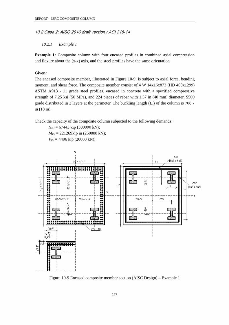
REPORT – ISRC COMPOSITE COLUMN
177
10.2 Case 2: AISC 2016 draft version / ACI 318-14
10.2.1 Example 1
Example 1: Composite column with four encased profiles in combined axial compression and flexure about the (x-x) axis, and the steel profiles have the same orientation Given: The encased composite member, illustrated in Figure 10-9, is subject to axial force, bending moment, and shear force. The composite member consist of 4 W 14x16x873 (HD 400x1299) ASTM A913 - 11 grade steel profiles, encased in concrete with a specified compressive strength of 7.25 ksi (50 MPa), and 224 pieces of rebar with 1.57 in (40 mm) diameter, S500 grade distributed in 2 layers at the perimeter. The buckling length (Lo) of the column is 708.7 in (18 m). Check the capacity of the composite column subjected to the following demands:
NEd = 67443 kip (300000 kN); MEd = 221269kip in (250000 kN); VEd = 4496 kip (20000 kN);
Figure 10-9 Encased composite member section (AISC Design) – Example 1
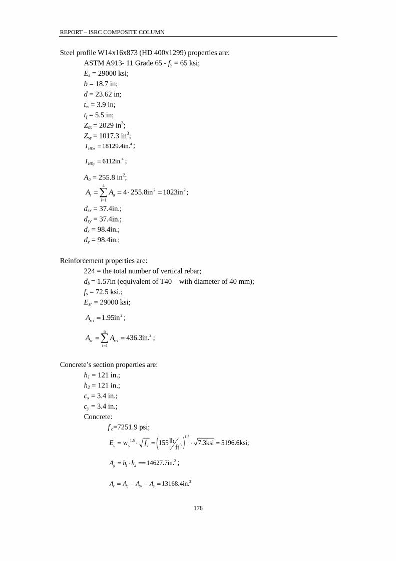
REPORT – ISRC COMPOSITE COLUMN
178
Steel profile W14x16x873 (HD 400x1299) properties are: ASTM A913- 11 Grade 65 - fy = 65 ksi; Es = 29000 ksi; b = 18.7 in; d = 23.62 in; tw = 3.9 in; tf = 5.5 in; Zsx = 2029 in3; Zsy = 1017.3 in3;
418129.4in.HDxI = ; 46112in.HDyI = ;
Aa = 255.8 in2;
4
2 2
i 14 255.8in 1023in ;s aA A
=
= = ⋅ =∑
dsx = 37.4in.; dsy = 37.4in.; dx = 98.4in.; dy = 98.4in.;
Reinforcement properties are: 224 = the total number of vertical rebar; db = 1.57in (equivalent of T40 – with diameter of 40 mm); fs = 72.5 ksi.; Esr = 29000 ksi;
21.95insriA = ;
n2
i 1436.3in.sr sriA A
=
= =∑ ;
Concrete’s section properties are:
h1 = 121 in.; h2 = 121 in.; cx = 3.4 in.; cy = 3.4 in.; Concrete:
f c=7251.9 psi;
( )1.51.5
3clbw 155 7.3ksi 5196.6ksi;ftc cE f = ⋅ = ⋅ =
214627.7in.g 1 2A h h= ⋅ == ;
213168.4in.c g sr sA A A A= − − =
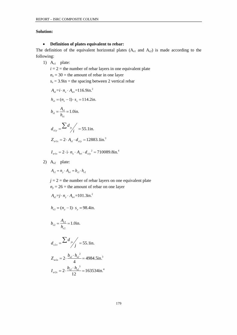
REPORT – ISRC COMPOSITE COLUMN
179
Solution:
• Definition of plates equivalent to rebar: The definition of the equivalent horizontal plates (As1 and As2) is made according to the following:
1) As1 plate: i = 2 = the number of rebar layers in one equivalent plate nx = 30 = the amount of rebar in one layer sx = 3.9in = the spacing between 2 vertical rebar
2116.9in.s1 x sriA =i n A =⋅ ⋅
1 ( 1) 114.2in.s x xh n s= − ⋅ =
11
1
1.0in.ss
s
Abh
= =
1 55.1in.iys y
dd i= =∑
32 12883.1in.sr1x s1 s1yZ A d= ⋅ ⋅ =
2 4x2 i 710089.8in.sr1x sri s1yI n A d= ⋅ ⋅ ⋅ ⋅ =
2) As2 plate:
2 2 2s y sri s sA n A b h= ⋅ = ⋅
j = 2 = the number of rebar layers on one equivalent plate ny = 26 = the amount of rebar on one layer
2y 101.3in.s2 sriA =j n A =⋅ ⋅
2 ( 1) 98.4in.s y yh n s= − ⋅ =
22
2
1.0in.ss
s
Abh
= =
2 55.1in.jxs x
dd j= =∑
232 4984.5in.
4s2 s2
sr2xb hZ ⋅
= ⋅ =
342 163534in.
12s2 s2
sr2xb hI ⋅
= ⋅ =
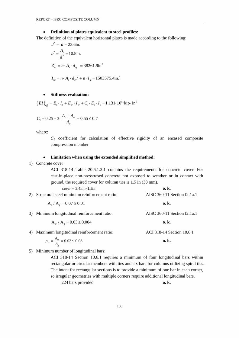
REPORT – ISRC COMPOSITE COLUMN
180
• Definition of plates equivalent to steel profiles: The definition of the equivalent horizontal plates is made according to the following:
* 23.6in.d d= =
** 10.8in.sAb
d= =
3a 38261.9insx syZ n A d= ⋅ ⋅ =
2 4a xn 1503575.4in.sx syI n A d I= ⋅ ⋅ + ⋅ =
• Stiffness evaluation:
( ) 11 21 c c 1.131 10 kip ins s sr sreff
EI E I E I C E I= ⋅ + ⋅ + ⋅ ⋅ = ⋅ ⋅
1 0.25 3 0.55 0.7s sr
g
A ACA+
= + ⋅ = ≤
where: C1 coefficient for calculation of effective rigidity of an encased composite compression member
• Limitation when using the extended simplified method:
1) Concrete cover ACI 318-14 Table 20.6.1.3.1 contains the requirements for concrete cover. For cast-in-place non-presstresed concrete not exposed to weather or in contact with ground, the required cover for column ties is 1.5 in (38 mm).
3.4in 1.5incover = > o. k. 2) Structural steel minimum reinforcement ratio: AISC 360-11 Section I2.1a.1
s gA / A 0.07 0.01= ≥ o. k.
3) Minimum longitudinal reinforcement ratio: AISC 360-11 Section I2.1a.1
sr gA / A 0.03 0.004= ≥ o. k.
4) Maximum longitudinal reinforcement ratio: ACI 318-14 Section 10.6.1
0.03 0.08srsr
g
Aρ
A= = ≤ o. k.
5) Minimum number of longitudinal bars: ACI 318-14 Section 10.6.1 requires a minimum of four longitudinal bars within rectangular or circular members with ties and six bars for columns utilizing spiral ties. The intent for rectangular sections is to provide a minimum of one bar in each corner, so irregular geometries with multiple corners require additional longitudinal bars.
224 bars provided o. k.
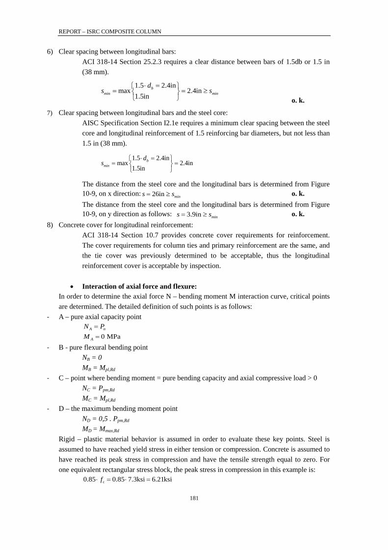
REPORT – ISRC COMPOSITE COLUMN
181
6) Clear spacing between longitudinal bars: ACI 318-14 Section 25.2.3 requires a clear distance between bars of 1.5db or 1.5 in (38 mm).
1.5 2.4inmax 2.4in
1.5inb
min min
ds s
⋅ = = = ≥
o. k.
7) Clear spacing between longitudinal bars and the steel core: AISC Specification Section I2.1e requires a minimum clear spacing between the steel core and longitudinal reinforcement of 1.5 reinforcing bar diameters, but not less than 1.5 in (38 mm).
1.5 2.4inmax 2.4in
1.5inb
min
ds
⋅ = = =
The distance from the steel core and the longitudinal bars is determined from Figure 10-9, on x direction: 26in mins s= ≥ o. k. The distance from the steel core and the longitudinal bars is determined from Figure 10-9, on y direction as follows: 3.9in mins s= ≥ o. k.
8) Concrete cover for longitudinal reinforcement: ACI 318-14 Section 10.7 provides concrete cover requirements for reinforcement. The cover requirements for column ties and primary reinforcement are the same, and the tie cover was previously determined to be acceptable, thus the longitudinal reinforcement cover is acceptable by inspection.
• Interaction of axial force and flexure:
In order to determine the axial force N – bending moment M interaction curve, critical points are determined. The detailed definition of such points is as follows:
- A – pure axial capacity point A nN P=
0 MPaAM = - B - pure flexural bending point
NB = 0 MB = Mpl,Rd
- C – point where bending moment = pure bending capacity and axial compressive load > 0 NC = Ppm,Rd MC = Mpl,Rd
- D – the maximum bending moment point ND = 0,5 . Ppm,Rd MD = Mmax,Rd
Rigid – plastic material behavior is assumed in order to evaluate these key points. Steel is assumed to have reached yield stress in either tension or compression. Concrete is assumed to have reached its peak stress in compression and have the tensile strength equal to zero. For one equivalent rectangular stress block, the peak stress in compression in this example is:
c0.85 0.85 7.3ksi 6.21ksif⋅ = ⋅ =

REPORT – ISRC COMPOSITE COLUMN
182
• Evaluation of the plastic resistance to axial force: The plastic resistance to axial force combines the individual resistances of the steel profile, the concrete and reinforcement. For concrete – encased steel sections:
( ) 92o
2.222 10 kip.2
effe
π EIP
L
⋅= = ⋅
80.877 0.658 if 2.25
1.736 10 kip0.877 if 2.25
noe
PP no
noe
nno
ee
PP P P PP P
⋅ ≤= = ⋅
⋅ >
Where:
8( ) 0.85 1.796 10 kipno s yd s1 s2 sd c cP A f A A f A f= ⋅ + + ⋅ + ⋅ ⋅ = ⋅
0.85 81171.1kippm.Rd c cP A f= ⋅ ⋅ =
0.85 40585.6kippm.Rd c c0.5 P 0.5 A f⋅ = ⋅ ⋅ ⋅ =
• Evaluation of the reduced axial force parameter λ: In accordance with AISC Specifications, commentary I5, the same slenderness reduction is applied to each of the remaining points on the interaction surface, using the coefficient λ, which reduce only the axial force values.
0.967n
no
P=P
λ =
• Evaluation of the maximum moment resistance Mmax.Rd.:
5 3r2xZ 3.862 10 in
4
21 2
cx r1x sxh hZ Z Z =⋅
= − − − ⋅
( ) ( ) 60.5 0.85 4.983 10 kip inmax.Rd sx yd r1x r2x sd cx cM Z f Z Z f Z f == ⋅ + + ⋅ + ⋅ ⋅ ⋅ ⋅ ⋅

REPORT – ISRC COMPOSITE COLUMN
183
• Evaluation of the plastic bending moment resistance Mpl.Rd.: In order to evaluate the plastic bending moment value, first we need to determine the position of the neutral axis. Different assumptions of the neutral axis position have been taken into consideration. The position of the neutral axis is determined by subtracting the stress distribution combination at point B and C, considering normal forces only.
Assumption 1: hnx between the two profiles2nx sydh d ≤ −
:
( )1
40.1in4 ) 0.85 4
Cnx
s2 cd s2 sd
Nh(2 h b f b f
= =⋅ − ⋅ ⋅ ⋅ + ⋅ ⋅
Check assumption2nx sydh d ≤ −
: assumption not ok
40.in 25.6in2nx sydh d= ≤ − =
Assumption 2: hnx is placed within the steel profiles 2 2sy nx syd dd h d − < ≤ +
:
( )1
4 ( ) ( 0.85 )2 42.8in4 - 4 ) 0.85 4 4
C sy yd cnx
s2 c yd s2 sd
dN d b* f fh
(2 h b* b f b* f b f
+ ⋅ − ⋅ ⋅ − ⋅= =
⋅ − ⋅ ⋅ ⋅ ⋅ + ⋅ ⋅ + ⋅ ⋅
Check assumption2 2sy nx syd dd h d − < ≤ +
: assumption ok
25.6in 42.8in 49.2in2 2sy nx syd dd h d− = < = ≤ + =
( ) 61 0.85 4.024 10 kip in2pl.Rd max.Rd r2xn sd sxn yd cxn cM M Z f Z f Z f= − ⋅ − ⋅ − ⋅ ⋅ ⋅ = ⋅ ⋅
where:
( ) ( ) 4 33 2.869 10 mm2 2sxn nx sy nx syd dZ b* h d h d = ⋅ − − ⋅ ⋅ + − = ⋅
3 32 3.770 10 mm2r2xn s2 nxZ b h= ⋅ ⋅ = ⋅
5 31.891 10 mm2cxn 1 nx r2xn sxnZ h h Z Z= ⋅ − − = ⋅
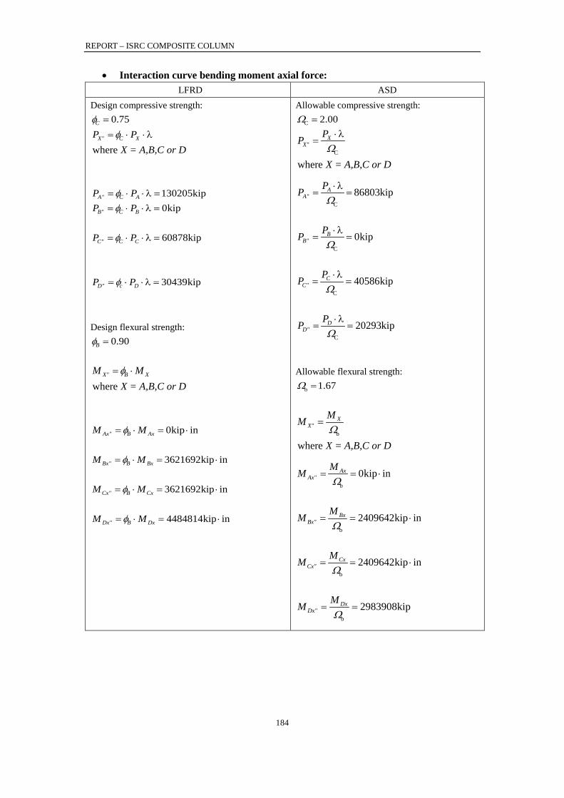
REPORT – ISRC COMPOSITE COLUMN
184
• Interaction curve bending moment axial force: LFRD ASD
Design compressive strength: 0.75Cφ =
whereX" C XP P
X = A,B,C or D= ⋅ ⋅λφ
130205kipA" C AP P= ⋅ ⋅λ =φ 0kipB" C BP P= ⋅ ⋅λ =φ
60878kipC" C CP P= ⋅ ⋅λ =φ
30439kipD" c DP P= ⋅ ⋅λ =φ
Design flexural strength:
0.90Bφ =
whereX" B XM M
X = A,B,C or Dφ= ⋅
0kip inAx" B AxM Mφ= ⋅ = ⋅
3621692kip inBx" B BxM Mφ= ⋅ = ⋅
3621692kip inCx" B CxM Mφ= ⋅ = ⋅
4484814kip inDx" B DxM Mφ= ⋅ = ⋅
Allowable compressive strength:
C 2.00Ω =
C
where
XX"
PP
X = A,B,C or D
⋅ λ=
Ω
C
86803kipAA"
PP ⋅ λ= =
Ω
C
0kipBB"
PP ⋅ λ= =
Ω
C
40586kipCC"
PP ⋅ λ= =
Ω
C
20293kipDD"
PP ⋅ λ= =
Ω
Allowable flexural strength:
b 1.67Ω =
b
where
XX"
MM
X = A,B,C or DΩ
=
b
0kip inAxAx"
MMΩ
= = ⋅
b
2409 kip in642BxBx"
MMΩ
= = ⋅
b
2409 kip in642CxCx"
MMΩ
= = ⋅
b
k298 90 i3 8 pDxDx"
MMΩ
= =
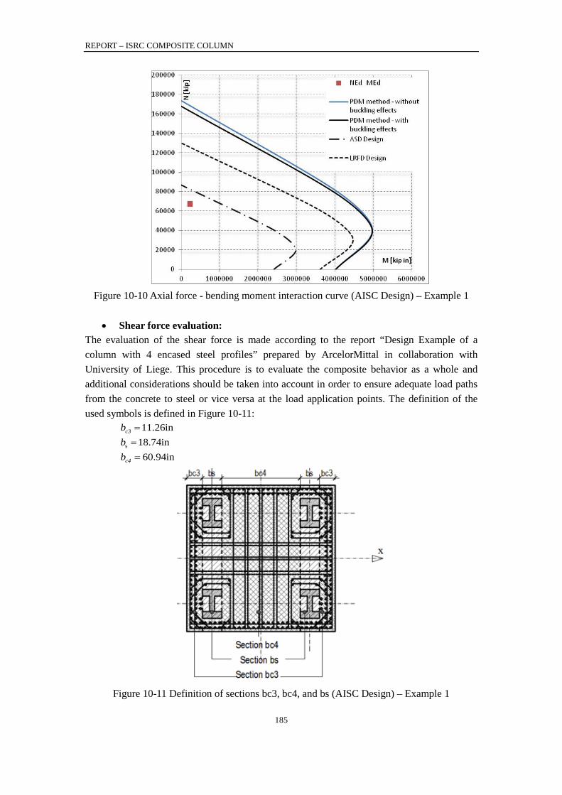
REPORT – ISRC COMPOSITE COLUMN
185
Figure 10-10 Axial force - bending moment interaction curve (AISC Design) – Example 1
• Shear force evaluation:
The evaluation of the shear force is made according to the report “Design Example of a column with 4 encased steel profiles” prepared by ArcelorMittal in collaboration with University of Liege. This procedure is to evaluate the composite behavior as a whole and additional considerations should be taken into account in order to ensure adequate load paths from the concrete to steel or vice versa at the load application points. The definition of the used symbols is defined in Figure 10-11:
11.26inc3b =
s 18.74inb = 60.94inc4b =
Figure 10-11 Definition of sections bc3, bc4, and bs (AISC Design) – Example 1

REPORT – ISRC COMPOSITE COLUMN
186
The applied shear force is VEd is distributed between sections bc3, bc4 and bs proportionally to their stiffness:
eff,bc3Ed,bc3 Ed
eff
EIV V EI= ⋅
eff,bc4Ed,bc4 Ed
eff
EIV V EI= ⋅
eff,bsEd,bs Ed
eff
EIV V EI= ⋅
The effective bending stiffness of the column is:
17 23.244 10 kip ineffEI = ⋅ ⋅
The total effective bending stiffness is the sum of individual effEI established for sections bc3,
bc4 and bs respectively.
1) Section bc3: ceff,bc3 sr sr,bc3 1 c,bc3EI E I C E I= ⋅ + ⋅ ⋅
To calculate Isr,bc3 of the reinforcing bars, it is considered one equivalent plate As2 and 2x2 bars on the top and bottom. For each face:
- The number of bars is: 30+30+4+4 = 68 bars
- The area of those bars is: 268 132.45insr,bc3 sriA A= ⋅ =
- The thickness of the equivalent plate is:
s11.16insr,side
pAt h= =
36 41 1.660 10 in
12c3
cg,bc3b hI ⋅
= = ⋅ ;
3s1 5 41.439 10 in
12p
sr,bc3
t hI
⋅= = ⋅ ;
6 41.516 10 inc,bc3 cg,bc3 sr,bc3I I I= − = ⋅ ;
9 21 8.501 10 kip ineff,bc3 sr sr,bc3 c c,bc3EI E I C E I= ⋅ + ⋅ ⋅ = ⋅ ⋅ ;
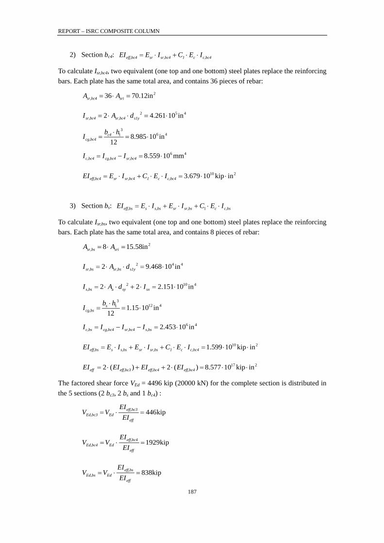
REPORT – ISRC COMPOSITE COLUMN
187
2) Section bc4: eff,bc4 sr sr,bc4 1 c c,bc4EI E I C E I= ⋅ + ⋅ ⋅
To calculate Isr,bc4, two equivalent (one top and one bottom) steel plates replace the reinforcing bars. Each plate has the same total area, and contains 36 pieces of rebar:
236 70.12insr,bc4 sriA A= ⋅ =
2 5 42 4.261 10 insr,bc4 sr,bc4 s1yI A d= ⋅ ⋅ = ⋅
36 41 8.985 10 in
12c4
cg,bc4b hI ⋅
= = ⋅
6 48.559 10 mmc,bc4 cg,bc4 sr,bc4I I I= − = ⋅
10 23.679 10 kip ineff,bc4 sr sr,bc4 1 c c,bc4EI E I C E I= ⋅ + ⋅ ⋅ = ⋅ ⋅
3) Section bs: 1eff,bs s s,bs sr sr,bs c c,bsEI E I E I C E I= ⋅ + ⋅ + ⋅ ⋅
To calculate Isr,bs, two equivalent (one top and one bottom) steel plates replace the reinforcing bars. Each plate has the same total area, and contains 8 pieces of rebar:
28 15.58insr,bs sriA A= ⋅ =
2 4 42 9.468 10 insr,bs sr,bs s1yI A d= ⋅ ⋅ = ⋅
2 10 4a2 2 2.151 10 ins,bs sy sxI A d I= ⋅ ⋅ + ⋅ = ⋅
312 41 1.15 10 in
12s
cg,bsb hI ⋅
= = ⋅
6 42.453 10 inc,bs cg,bc4 sr,bc4 s,bsI I I I= − − = ⋅
10 21.599 10 kip ineff,bs s s,bs sr sr,bs 1 c c,bc4EI E I E I C E I= ⋅ + ⋅ + ⋅ ⋅ = ⋅ ⋅
17 22 ( ) 2 ( ) 8.577 10 kip ineff eff,bc3 eff,bc4 eff,bc4EI EI EI EI= ⋅ + + ⋅ = ⋅ ⋅
The factored shear force VEd = 4496 kip (20000 kN) for the complete section is distributed in the 5 sections (2 bc3, 2 bs and 1 bc4) :
446kipeff,bc3Ed,bc3 Ed
eff
EIV V
EI= ⋅ =
1929kipeff,bc4Ed,bc4 Ed
eff
EIV V
EI= ⋅ =
838kipeff,bsEd,bs Ed
eff
EIV V
EI= ⋅ =
REPORT – ISRC COMPOSITE COLUMN
188
• Calculation of shear in section bs: Section bs is a composite steel-concrete section having 2 reinforced concrete flanges, 2 steel “flanges” (the HD sections) and 1 reinforced concrete web. To establish longitudinal shear in section bs, it is convenient to transform the composite section into a single material section or “homogenized” section. The single material can be either steel or concrete. Choosing concrete, the moment of inertia of the homogenized concrete section Ic* is such that the stiffness Ec Ic* of the homogenized section is equal to the stiffness EIeff,bs :
* 6 4c 3.077 10 ineff,bs
c
EII E= = ⋅
Figure 10-12 Homogenized equivalent concrete section bs – Example 1
In a homogenized concrete section (Figure 10-12), the width of the concrete equivalent to the width of the steel flanges is:
104.6in* ss s
cm
Eb b E= ⋅ =
The width of the concrete equivalent to the width of the steel web is:
21.9in* sw w
cm
Et t E= ⋅ =
The resultant longitudinal shear force on regions like CC1 and CC2 in Figure 10-12 is:
*c
SEd,bsEd,l
VV
I⋅
=
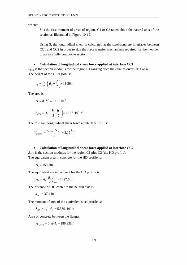
REPORT – ISRC COMPOSITE COLUMN
189
where: S is the first moment of areas of regions C1 or C2 taken about the natural axis of the section as illustrated in Figure 10-12. Using S, the longitudinal shear is calculated at the steel-concrete interfaces between CC1 and CC2 in order to size the force transfer mechanisms required for the member to act as a fully composite section.
• Calculation of longitudinal shear force applied at interface CC1:
SCC1 is the section modulus for the region C1 ranging from the edge to outer HD flange: The height of the C1 region is:
' 11.26in11 sy
h dh - d +2 2
= =
The area is: ' 2211.01in1 1A b h= ⋅ =
'4 31.157 10 in
21 1
CC1 1h hS A -
2
= ⋅ = ⋅
The resultant longitudinal shear force at interface CC1 is:
*c
kip3.15in
Ed,bs CC1Ed,CC1
V SV
I⋅
= =
• Calculation of longitudinal shear force applied at interface CC2:
SCC2 is the section modulus for the region C1 plus C2 (the HD profile): The equivalent area in concrete for the HD profile is:
2255.8inaA =
The equivalent are in concrete for the HD profile is: 21427.6in* s
a acm
EA A E= ⋅ =
The distance of HD center to the neutral axis is:
syd = 37.4 in
The moment of area of the equivalent steel profile is: 4 35.339 10 in*
HD a syS A d= ⋅ = ⋅
Area of concrete between the flanges: 2
c _ CC2 186.93in*aA b d-A= ⋅ =
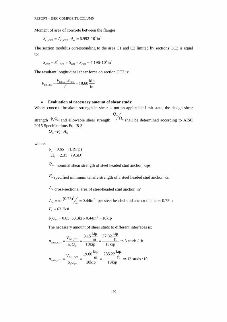
REPORT – ISRC COMPOSITE COLUMN
190
Moment of area of concrete between the flanges: 3 3
c _ CC2 c _ CC2 6.992 10 in* *syS A d= ⋅ = ⋅
The section modulus corresponding to the area C1 and C2 limited by sections CC2 is equal to:
4 3c _ CC2 7.196 10 in*
CC2 HD CC1S S S S= + + = ⋅
The resultant longitudinal shear force on section CC2 is:
*c
kip19.60in
Ed,bs CC2Ed,CC2
V SV
I⋅
= =
• Evaluation of necessary amount of shear studs:
Where concrete breakout strength in shear is not an applicable limit state, the design shear
strength v nvQφ and allowable shear strength v
nvQΩ shall be determined according to AISC
2015 Specifications Eq. I8-3: unv saQ =F A⋅
where:
0.65 (LRFD)v φ = v 2.31 (ASD) Ω =
nvQ nominal shear strength of steel headed stud anchor, kips
uF specified minimum tensile strength of a steel headed stud anchor, ksi
saA cross-sectional area of steel-headed stud anchor, in2
22(0.75) 0.44in4saA = π ⋅ = per steel headed stud anchor diameter 0.75in
63.3ksiuF =
20.65 63.3ksi 0.44in 18kipv nvQφ = ⋅ ⋅ =
The necessary amount of shear studs to different interfaces is: kipkip 37.823.15ftin 3 studs /1ft
18kip 18kipEd1_CC1
studs_CC1v nv
Vn
Q= = = ⇒
φ
kipkip 235.2219.60ftin 13 studs /1ft
18kip 18kipEd1_CC2
studs_CC2v nv
Vn
Q= = = ⇒
φ
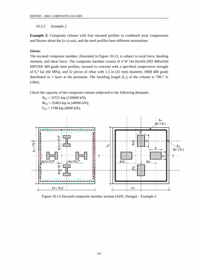
REPORT – ISRC COMPOSITE COLUMN
191
10.2.2 Example 2
Example 2: Composite column with four encased profiles in combined axial compression and flexure about the (x-x) axis, and the steel profiles have different orientations Given: The encased composite member, illustrated in Figure 10-13, is subject to axial force, bending moment, and shear force. The composite member consist of 4 W 14x16x426 (HD 400x634) HISTAR 460 grade steel profiles, encased in concrete with a specified compressive strength of 8.7 ksi (60 MPa), and 32 pieces of rebar with 1.3 in (32 mm) diameter, HRB 400 grade distributed in 1 layer at the perimeter. The buckling length (Lo) of the column is 708.7 in (18m). Check the capacity of the composite column subjected to the following demands:
NEd = 33721 kip (150000 kN); MEd = 35403 kip in (40000 kN); VEd = 1798 kip (8000 kN);
Figure 10-13 Encased composite member section (AISC Design) – Example 2
REPORT – ISRC COMPOSITE COLUMN
192
Steel profile W 14x16 x426 (HD 400x634) properties are: HISTAR 460 - fy = 66.7 ksi; Es = 29000 ksi; b = 16.7 in; d = 18.7 in; tw = 2.0 in; tf = 3.2 in; Zsx = 867.8 in3; Zsy = 434.3 in3;
46578.7inHDxI = ;
42360.5inHDyI =
2125.2inaA = ;
42 2
i 14 125.2 in 501 in ;s aA A
=
= = ⋅ =∑
20.2insx syd d= =
dx = dy = 14.8 in;
Reinforcement properties are: 32 = the total number of vertical rebar; db = 1.3 in equivalent T32 diameter rebar; fs = 58.ksi; Esr = 29000 ksi;
21.25insriA = ;
n2
i 139.9insr sriA A
=
= =∑ ;
Concrete section’s properties are:
fc = 8.7 ksi; Ec = 5692.6 ksi h1 = 70.9 in; h2 = 70.9 in; cx = 1.6 in; cy = 1.6 in;
25022ing 1 2A h h= ⋅ = ;
24481.2inc g sr sA A A A= − − =

REPORT – ISRC COMPOSITE COLUMN
193
Solution:
• Definition of plates equivalent to rebar: The definition of the equivalent horizontal plates (As1 and As2) is made according to the following:
1) As1 plate: i = 1= the number of rebar layers in one equivalent plate nx = 9 = the amount of rebar in one layer
211.2ins1 x sriA =i n A =⋅ ⋅ ;
s1h 67.7in= s1s1
s1
Ab 0.2inh
= =
iys1y
dd 29.9ini= =∑
32 1236.8insr1x s1 s1yZ A d= ⋅ ⋅ =
2 4 4x2 i 2.009 10 insr1x sri s1yI n A d= ⋅ ⋅ ⋅ ⋅ = ⋅
2) As2 plate:
2 2 2s y sri s sA n A b h= ⋅ = ⋅
j = 1= the number of rebar layers in one equivalent plate ny = 7 = the amount of rebar in one layer
2y 8.7ins2 sriA =j n A =⋅ ⋅ ; s2 y yh (n 1) s 50.8in;= − ⋅ =
s2s2
s2
Ab 0.2inh
= = ;
jxs2x
dd 29.9inj= =∑ ;
232 221.6in
4s2 s2
sr2xb hZ ⋅
= ⋅ = ;
33 42 3.751 10 in
12s2 s2
sr2xb hI ⋅
= ⋅ = ⋅
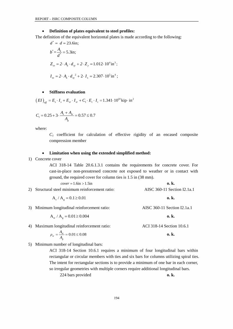
REPORT – ISRC COMPOSITE COLUMN
194
• Definition of plates equivalent to steel profiles: The definition of the equivalent horizontal plates is made according to the following:
23.6in;*d d= =
a 5.3in;**
Ab =d
=
4 3a 1.012 10 insx sy yZ 2 A d 2 Z= ⋅ ⋅ + ⋅ = ⋅ ;
2 5 4a x2 2.307 10 insx syI 2 A d I= ⋅ ⋅ + ⋅ = ⋅ ;
• Stiffness evaluation
( ) 10 21 c c 1.341 10 kip ins s sr sreff
EI E I E I C E I= ⋅ + ⋅ + ⋅ ⋅ = ⋅ ⋅
1 0.25 3 0.57 0.7s sr
g
A ACA+
= + ⋅ = ≤
where: C1 coefficient for calculation of effective rigidity of an encased composite compression member
• Limitation when using the extended simplified method:
1) Concrete cover ACI 318-14 Table 20.6.1.3.1 contains the requirements for concrete cover. For cast-in-place non-presstresed concrete not exposed to weather or in contact with ground, the required cover for column ties is 1.5 in (38 mm).
1.6in 1.5incover = > o. k. 2) Structural steel minimum reinforcement ratio: AISC 360-11 Section I2.1a.1
s gA / A 0.1 0.01= ≥ o. k.
3) Minimum longitudinal reinforcement ratio: AISC 360-11 Section I2.1a.1
sr gA / A 0.01 0.004= ≥ o. k.
4) Maximum longitudinal reinforcement ratio: ACI 318-14 Section 10.6.1
0.01 0.08srsr
g
Aρ
A= = ≤ o. k.
5) Minimum number of longitudinal bars: ACI 318-14 Section 10.6.1 requires a minimum of four longitudinal bars within rectangular or circular members with ties and six bars for columns utilizing spiral ties. The intent for rectangular sections is to provide a minimum of one bar in each corner, so irregular geometries with multiple corners require additional longitudinal bars.
224 bars provided o. k.
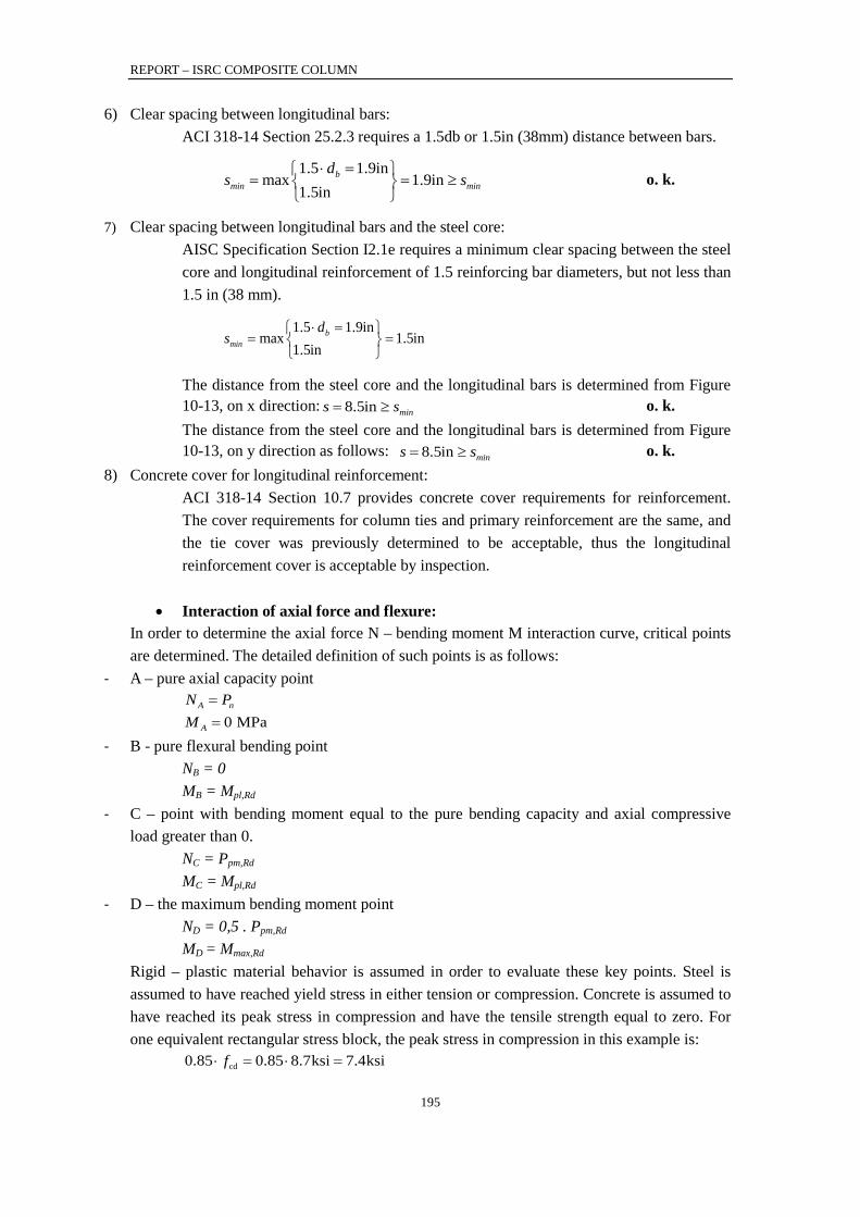
REPORT – ISRC COMPOSITE COLUMN
195
6) Clear spacing between longitudinal bars: ACI 318-14 Section 25.2.3 requires a 1.5db or 1.5in (38mm) distance between bars.
1.5 1.9inmax 1.9in
1.5inb
min min
ds s
⋅ = = = ≥
o. k.
7) Clear spacing between longitudinal bars and the steel core: AISC Specification Section I2.1e requires a minimum clear spacing between the steel core and longitudinal reinforcement of 1.5 reinforcing bar diameters, but not less than 1.5 in (38 mm).
1.5 1.9inmax 1.5in
1.5inb
min
ds
⋅ = = =
The distance from the steel core and the longitudinal bars is determined from Figure 10-13, on x direction: 8.5in mins s= ≥ o. k. The distance from the steel core and the longitudinal bars is determined from Figure 10-13, on y direction as follows: 8.5in mins s= ≥ o. k.
8) Concrete cover for longitudinal reinforcement: ACI 318-14 Section 10.7 provides concrete cover requirements for reinforcement. The cover requirements for column ties and primary reinforcement are the same, and the tie cover was previously determined to be acceptable, thus the longitudinal reinforcement cover is acceptable by inspection.
• Interaction of axial force and flexure:
In order to determine the axial force N – bending moment M interaction curve, critical points are determined. The detailed definition of such points is as follows:
- A – pure axial capacity point A nN P=
0 MPaAM = - B - pure flexural bending point
NB = 0 MB = Mpl,Rd
- C – point with bending moment equal to the pure bending capacity and axial compressive load greater than 0.
NC = Ppm,Rd MC = Mpl,Rd
- D – the maximum bending moment point ND = 0,5 . Ppm,Rd MD = Mmax,Rd
Rigid – plastic material behavior is assumed in order to evaluate these key points. Steel is assumed to have reached yield stress in either tension or compression. Concrete is assumed to have reached its peak stress in compression and have the tensile strength equal to zero. For one equivalent rectangular stress block, the peak stress in compression in this example is:
cd0.85 0.85 8.7ksi 7.4ksif⋅ = ⋅ =
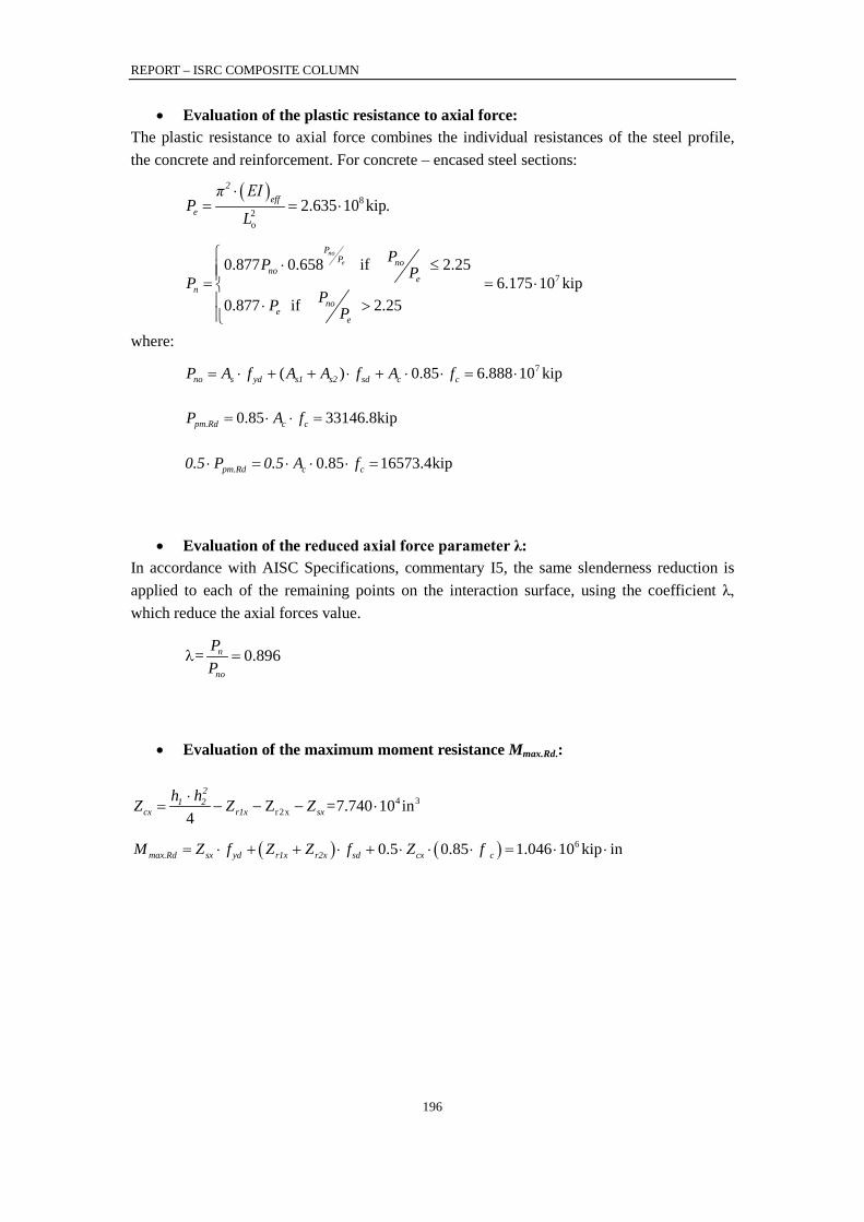
REPORT – ISRC COMPOSITE COLUMN
196
• Evaluation of the plastic resistance to axial force: The plastic resistance to axial force combines the individual resistances of the steel profile, the concrete and reinforcement. For concrete – encased steel sections:
( ) 82o
2.635 10 kip.2
effe
π EIP
L
⋅= = ⋅
70.877 0.658 if 2.25
6.175 10 kip0.877 if 2.25
noe
PP no
noe
nno
ee
PP P P PP P
⋅ ≤= = ⋅
⋅ >
where: 7( ) 0.85 6.888 10 kipno s yd s1 s2 sd c cP A f A A f A f= ⋅ + + ⋅ + ⋅ ⋅ = ⋅
0.85 33146.8kippm.Rd c cP A f= ⋅ ⋅ =
0.85 16573.4kippm.Rd c c0.5 P 0.5 A f⋅ = ⋅ ⋅ ⋅ =
• Evaluation of the reduced axial force parameter λ: In accordance with AISC Specifications, commentary I5, the same slenderness reduction is applied to each of the remaining points on the interaction surface, using the coefficient λ, which reduce the axial forces value.
0.896n
no
P=P
λ =
• Evaluation of the maximum moment resistance Mmax.Rd.:
4 3r2xZ 7.740 10 in
4
21 2
cx r1x sxh hZ Z Z =⋅
= − − − ⋅
( ) ( ) 60.5 0.85 1.046 10 kip inmax.Rd sx yd r1x r2x sd cx cM Z f Z Z f Z f= ⋅ + + ⋅ + ⋅ ⋅ ⋅ = ⋅ ⋅
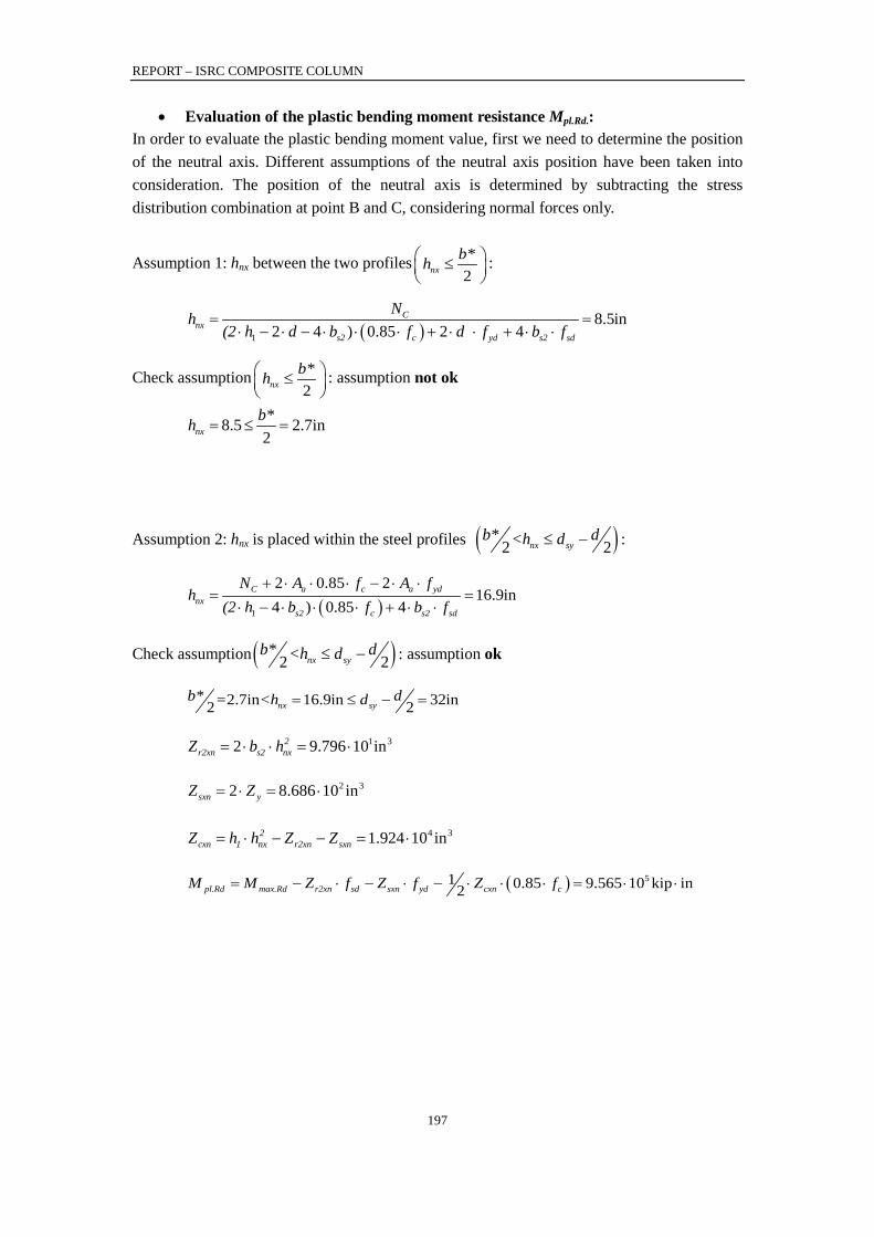
REPORT – ISRC COMPOSITE COLUMN
197
• Evaluation of the plastic bending moment resistance Mpl.Rd.: In order to evaluate the plastic bending moment value, first we need to determine the position of the neutral axis. Different assumptions of the neutral axis position have been taken into consideration. The position of the neutral axis is determined by subtracting the stress distribution combination at point B and C, considering normal forces only.
Assumption 1: hnx between the two profiles2nx
b*h ≤
:
( )1
8.5in2 4 ) 0.85 2 4
Cnx
s2 c yd s2 sd
Nh(2 h d b f d f b f
= =⋅ − ⋅ − ⋅ ⋅ ⋅ + ⋅ ⋅ + ⋅ ⋅
Check assumption2nx
b*h ≤
: assumption not ok
8.5 2.7in2nx
b*h = ≤ =
Assumption 2: hnx is placed within the steel profiles ( )2 2nx syb* d<h d≤ − :
( )1
2 0.85 216.9in
4 ) 0.85 4C a c a yd
nxs2 c s2 sd
N A f A fh
(2 h b f b f+ ⋅ ⋅ ⋅ − ⋅ ⋅
= =⋅ − ⋅ ⋅ ⋅ + ⋅ ⋅
Check assumption ( )2 2nx syb* d<h d≤ − : assumption ok
2.7in 16.9in 32in2 2nx syb* d= <h d= ≤ − =
1 32 9.796 10 in2r2xn s2 nxZ b h= ⋅ ⋅ = ⋅
2 32 8.686 10 insxn yZ Z= ⋅ = ⋅
4 31.924 10 in2cxn 1 nx r2xn sxnZ h h Z Z= ⋅ − − = ⋅
( ) 51 0.85 9.565 10 kip in2pl.Rd max.Rd r2xn sd sxn yd cxn cM M Z f Z f Z f= − ⋅ − ⋅ − ⋅ ⋅ ⋅ = ⋅ ⋅
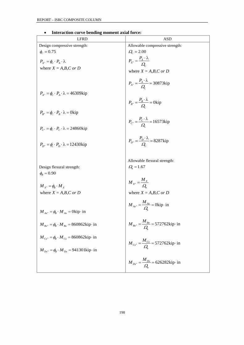
REPORT – ISRC COMPOSITE COLUMN
198
• Interaction curve bending moment axial force: LFRD ASD
Design compressive strength: 0.75Cφ =
X
whereX" CP P
X = A,B,C or D= ⋅ ⋅λφ
46309kipA" C AP P= ⋅ ⋅λ =φ
0kipB" C BP P= ⋅ ⋅λ =φ
24860kipC" C CP P= ⋅ ⋅λ =φ
12430kipD" c DP P= ⋅ ⋅λ =φ
Design flexural strength:
0.90Bφ =
whereX" B XM M
X = A,B,C or Dφ= ⋅
0kip inAx" B AxM Mφ= ⋅ = ⋅
860862kip inBx" B BxM M= ⋅ = ⋅φ
860862kip inCx" B CxM M= ⋅ = ⋅φ
941301kip inDx" B DxM M= ⋅ = ⋅φ
Allowable compressive strength:
C 2.00Ω =
where
XX"
C
PP
X = A,B,C or D
⋅ λ=
Ω
C
30873kipAA"
PP ⋅ λ= =
Ω
C
0kipBB"
PP ⋅ λ= =
Ω
C
C
16573kipC"PP ⋅ λ
= =Ω
C
8287kipDD"
PP ⋅ λ= =
Ω
Allowable flexural strength:
b 1.67Ω =
b
where
XX"
MM
X = A,B,C or DΩ
=
b
0kip inAxAx"
MMΩ
= = ⋅
b
572 kip in762BxBx"
MM = = ⋅Ω
b
572 kip in762CxCx"
MM = = ⋅Ω
b
626 kip in282DxDx"
MM = = ⋅Ω

REPORT – ISRC COMPOSITE COLUMN
199
Figure 10-14 Axial force - bending moment interaction curve (AISC Design) – Example 2
• Shear force evaluation:
The evaluation of the shear force is made according to the report “Design Example of a column with 4 encased steel profiles” prepared by ArcelorMittal in collaboration with University of Liege. This procedure is to evaluate the composite behavior as a whole and additional considerations should be taken into account in order to ensure adequate load paths from the concrete to steel or vice versa at the load application points. The definition of the used symbols is defined in Figure 10-15:
5.91inc1b = ; 16.69ins2b = ; 2.52inc3b = ; 16.7ins4b = ;
Figure 10-15 Definition of sections bc1, bc3, bs2, and bs4 (AISC Design) – Example 2
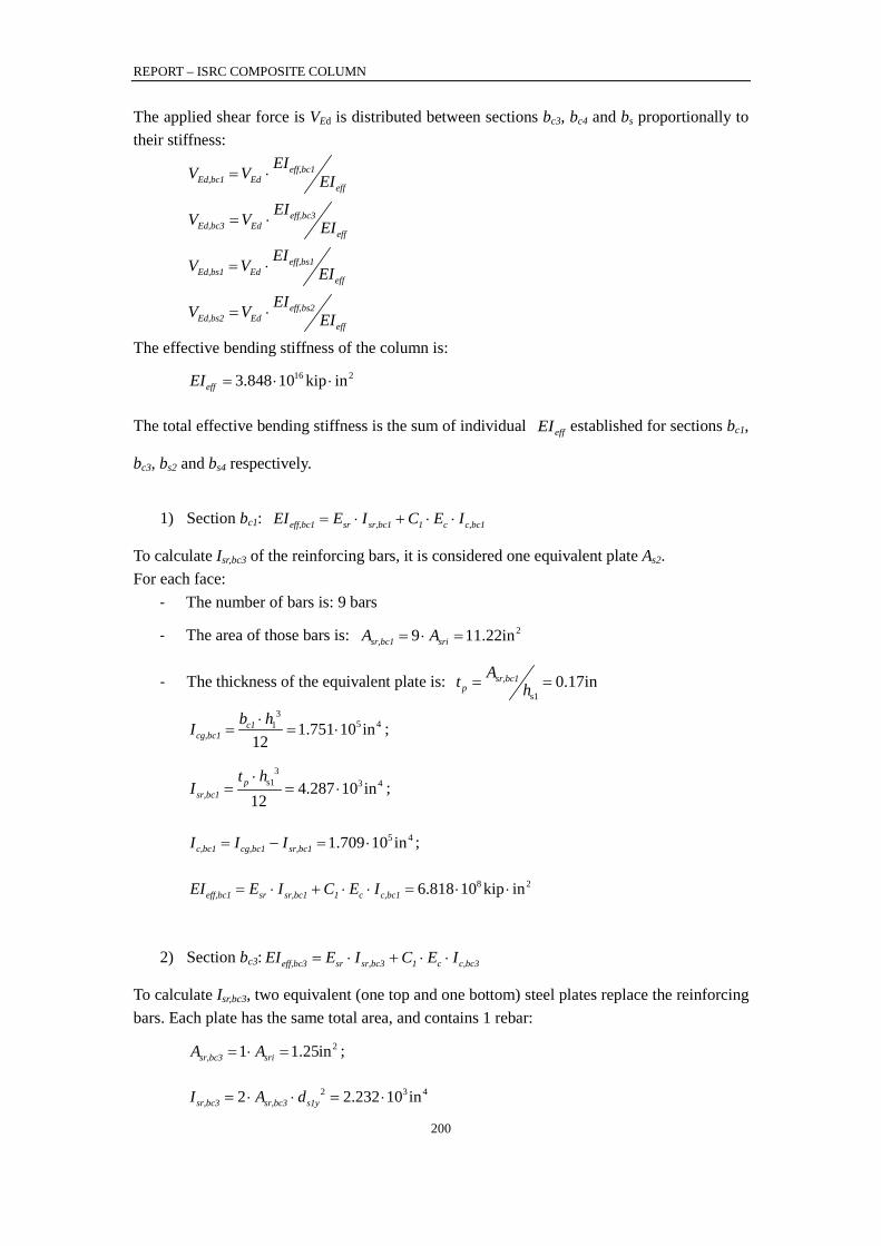
REPORT – ISRC COMPOSITE COLUMN
200
The applied shear force is VEd is distributed between sections bc3, bc4 and bs proportionally to their stiffness:
eff,bc1Ed,bc1 Ed
eff
EIV V EI= ⋅
eff,bc3Ed,bc3 Ed
eff
EIV V EI= ⋅
eff,bs1Ed,bs1 Ed
eff
EIV V EI= ⋅
eff,bs2Ed,bs2 Ed
eff
EIV V EI= ⋅
The effective bending stiffness of the column is: 16 23.848 10 kip ineffEI = ⋅ ⋅
The total effective bending stiffness is the sum of individual effEI established for sections bc1,
bc3, bs2 and bs4 respectively.
1) Section bc1: eff,bc1 sr sr,bc1 1 c c,bc1EI E I C E I= ⋅ + ⋅ ⋅
To calculate Isr,bc3 of the reinforcing bars, it is considered one equivalent plate As2. For each face:
- The number of bars is: 9 bars
- The area of those bars is: 29 11.22insr,bc1 sriA A= ⋅ =
- The thickness of the equivalent plate is: s1
0.17insr,bc1p
At h= =
35 41 1.751 10 in
12c1
cg,bc1b hI ⋅
= = ⋅ ;
3s1 3 44.287 10 in
12p
sr,bc1
t hI
⋅= = ⋅ ;
5 41.709 10 inc,bc1 cg,bc1 sr,bc1I I I= − = ⋅ ;
8 26.818 10 kip ineff,bc1 sr sr,bc1 1 c c,bc1EI E I C E I= ⋅ + ⋅ ⋅ = ⋅ ⋅
2) Section bc3: eff,bc3 sr sr,bc3 1 c c,bc3EI E I C E I= ⋅ + ⋅ ⋅
To calculate Isr,bc3, two equivalent (one top and one bottom) steel plates replace the reinforcing bars. Each plate has the same total area, and contains 1 rebar:
21 1.25insr,bc3 sriA A= ⋅ = ;
2 3 42 2.232 10 insr,bc3 sr,bc3 s1yI A d= ⋅ ⋅ = ⋅

REPORT – ISRC COMPOSITE COLUMN
201
34 41 7.437 10 in
12c3
cg,bc3b hI ⋅
= = ⋅ ;
4 47.250 10 inc,bc3 cg,bc3 sr,bc3I I I= − = ⋅
8 23.013 10 kip ineff,bc3 sr sr,bc3 1 c c,bc3EI E I C E I= ⋅ + ⋅ ⋅ = ⋅ ⋅
3) Section bs2: eff,bs2 s s,bs2 sr sr,bs2 1 c,eff c,bs2EI E I E I C E I= ⋅ + ⋅ + ⋅ ⋅
To calculate Isr,bs2, two equivalent (one top and one bottom) steel plates replace the reinforcing bars. Each plate has the same total area, and contains 2 rebar:
22 2.49insr,bs2 sriA A= ⋅ = ;
2 3 42 4.464 10 insr,bs2 sr,bs2 s1yI A d= ⋅ ⋅ = ⋅ ;
3 42.360 10 ins,bs2 yI I= = ⋅
35 41 4.951 10 in
12s2
cg,bs2b hI ⋅
= = ⋅
5 44.882 10 inc,bs2 cg,bs4 sr,bs2 s,bs2I I I I= − − = ⋅
9 21.791 10 kip ineff,bs2 s s,bs2 sr sr,bs2 e c,eff c,bs2EI E I E I K E I= ⋅ + ⋅ + ⋅ ⋅ = ⋅ ⋅
4) Section bs4: eff,bs4 s s,bs4 sr sr,bs4 1 c c,bs4EI E I E I C E I= ⋅ + ⋅ + ⋅ ⋅
To calculate Isr,bs4, two equivalent (one top and one bottom) steel plates replace the reinforcing bars. Each plate has the same total area, and contains 1 rebar:
21 16.7insr,bs4 sriA A= ⋅ =
2 5 42 3.907 10 insr,bs4 sr,bs4 s1yI A d= ⋅ ⋅ = ⋅
2 5 4a sx2 2 1.153 10 ins,bs4 syI A d I= ⋅ ⋅ + ⋅ = ⋅
35 41 4.951 10 in
12s4
cg,bs4b hI ⋅
= = ⋅
5 43.775 10 inc,bs4 cg,bs4 sr,bs4 s,bs4I I I I= − − = ⋅
9 23.411 10 kip ineff,bs4 s s,bs4 sr sr,bs4 1 c,eff c,bs4EI E I E I C E I= ⋅ + ⋅ + ⋅ ⋅ = ⋅ ⋅
9 22 ( ) 2 ( ) 2 ( ) 8.275 10 kip ineff eff,bc1 eff,bs2 eff,bc3 eff,bs4EI EI EI EI EI= ⋅ + ⋅ + ⋅ + = ⋅ ⋅

REPORT – ISRC COMPOSITE COLUMN
202
The factored shear force VEd = 1798 kip (8000 kN) for the complete section is distributed in the 5 sections (2 bc3, 2 bs and 1 bc4) :
142kipeff,bc1Ed,bc1 Ed
eff
EIV V
EI= ⋅ =
63kipeff,bc1Ed,bc3 Ed
eff
EIV V
EI= ⋅ =
372kipeff,bs2Ed,bs2 Ed
eff
EIV V
EI= ⋅ =
709kipeff,bs4Ed,bs4 Ed
eff
EIV V
EI= ⋅ =
• Calculation of shear in section bs4:
Section bs2 is a composite steel-concrete section having 2 reinforced concrete flanges, 2 steel “flanges” (the HD sections) and 1 reinforced concrete web. To establish longitudinal shear in section bs, it is convenient to transform the composite section into a single material section or “homogenized” section. The single material can be either steel or concrete. Choosing concrete, the moment of inertia of the homogenized concrete section Ic* is such that the stiffness Ec Ic* of the homogenized section is equal to the stiffness EIeff,bs2 :
* 5 4c 3.146 10 ineff,bs4
cm
EII E= = ⋅
Figure 10-16 Homogenized equivalent concrete section bs – Example 2
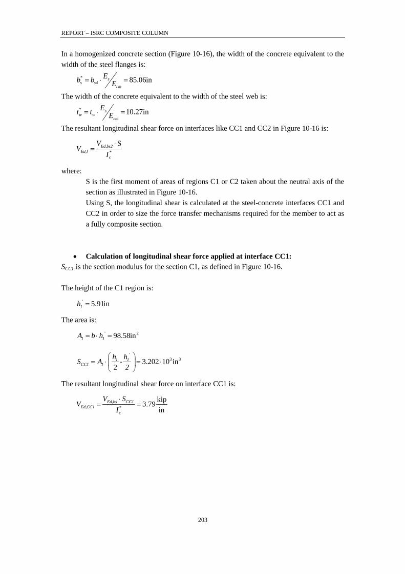
REPORT – ISRC COMPOSITE COLUMN
203
In a homogenized concrete section (Figure 10-16), the width of the concrete equivalent to the width of the steel flanges is:
85.06in* ss s4
cm
Eb b E= ⋅ =
The width of the concrete equivalent to the width of the steel web is:
10.27in* sw w
cm
Et t E= ⋅ =
The resultant longitudinal shear force on interfaces like CC1 and CC2 in Figure 10-16 is:
*c
SEd,bs2Ed,l
VV
I⋅
=
where: S is the first moment of areas of regions C1 or C2 taken about the neutral axis of the section as illustrated in Figure 10-16. Using S, the longitudinal shear is calculated at the steel-concrete interfaces CC1 and CC2 in order to size the force transfer mechanisms required for the member to act as a fully composite section.
• Calculation of longitudinal shear force applied at interface CC1: SCC1 is the section modulus for the section C1, as defined in Figure 10-16. The height of the C1 region is:
' 5.91in1h =
The area is: ' 298.58in1 1A b h= ⋅ =
'3 33.202 10 in
21 1
CC1 1h hS A -
2
= ⋅ = ⋅
The resultant longitudinal shear force on interface CC1 is:
*c
kip3.79in
Ed,bs CC1Ed,CC1
V SV
I⋅
= =

REPORT – ISRC COMPOSITE COLUMN
204
• Calculation of longitudinal shear force applied at interface CC2:
SCC2 is the section modulus for the combined regions C1 and C2. The equivalent area in concrete for the HD profile is:
Aa =125.24 in2
The equivalent are in concrete for the HD profile is: 2638.18in* s
a acm
EA A E= ⋅ =
The distance of HD center to the neutral axis is:
syd = 20.2 in
The moment of area of the equivalent steel profile is: 4 31.289 10 in*
HD a syS A d= ⋅ = ⋅
Area of concrete between the flanges: 2
c _ CC2 186.27in*aA b d-A= ⋅ =
Moment of area of concrete between the flanges: 3 3
c _ CC2 c _ CC2 3.762 10 in* *syS A d= ⋅ = ⋅
The section modulus of the combined regions C1 and C2: 4 3
c _ CC2 1.985 10 mm*CC2 HD CC1S S S S= + + = ⋅
The resultant longitudinal shear force at interface CC2 is:
*c
kip23.48in
Ed,bs CC2Ed,CC2
V SV
I⋅
= =
• Evaluation of necessary amount of shear studs: Where concrete breakout strength in shear is not an applicable limit state, the design shear
strength v nvQφ and allowable shear strength v
nvQΩ shall be determined according to AISC
2015 Specifications Eq. I8-3:
unv saQ =F A⋅
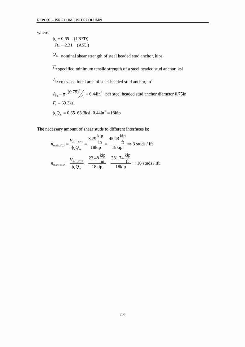
REPORT – ISRC COMPOSITE COLUMN
205
where: 0.65 (LRFD)v φ =
v 2.31 (ASD) Ω =
nvQ nominal shear strength of steel headed stud anchor, kips
uF specified minimum tensile strength of a steel headed stud anchor, ksi
saA cross-sectional area of steel-headed stud anchor, in2
22(0.75) 0.44in4saA = π ⋅ = per steel headed stud anchor diameter 0.75in
63.3ksiuF =
20.65 63.3ksi 0.44in 18kipv nvQφ = ⋅ ⋅ =
The necessary amount of shear studs to different interfaces is:
kipkip 45.433.79ftin 3 studs /1ft
18kip 18kipEd1_CC1
studs_CC1v nv
Vn
Q= = = ⇒
φ
kipkip 281.7423.48ftin 16 studs /1ft
18kip 18kipEd1_CC2
studs_CC2v nv
Vn
Q= = = ⇒
φ
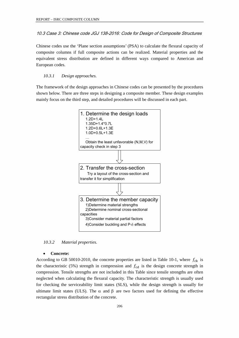
REPORT – ISRC COMPOSITE COLUMN
206
10.3 Case 3: Chinese code JGJ 138-2016: Code for Design of Composite Structures
Chinese codes use the ‘Plane section assumptions’ (PSA) to calculate the flexural capacity of composite columns if full composite actions can be realized. Material properties and the equivalent stress distribution are defined in different ways compared to American and European codes.
10.3.1 Design approaches.
The framework of the design approaches in Chinese codes can be presented by the procedures shown below. There are three steps in designing a composite member. These design examples mainly focus on the third step, and detailed procedures will be discussed in each part.
1. Determine the design loads 1.2D+1.4L 1.35D+1.4*0.7L 1.2D+0.6L+1.3E 1.0D+0.5L+1.3E … Obtain the least unfavorable (N,M,V) for capacity check in step 3
2. Transfer the cross-section Try a layout of the cross-section and transfer it for simplification
3. Determine the member capacity 1)Determine material strengths 2)Determine nominal cross-sectional capacities 3)Consider material partial factors 4)Consider buckling and P-δ effects
10.3.2 Material properties.
• Concrete: According to GB 50010-2010, the concrete properties are listed in Table 10-1, where 𝑓ck is the characteristic (5%) strength in compression and 𝑓cd is the design concrete strength in compression. Tensile strengths are not included in this Table since tensile strengths are often neglected when calculating the flexural capacity. The characteristic strength is usually used for checking the serviceability limit states (SLS), while the design strength is usually for ultimate limit states (ULS). The α and β are two factors used for defining the effective rectangular stress distribution of the concrete.
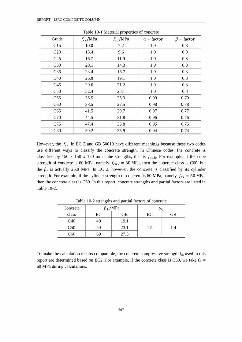
REPORT – ISRC COMPOSITE COLUMN
207
Table 10-1 Material properties of concrete Grade 𝑓ck/MPa 𝑓cd/MPa 𝛼 − factor 𝛽 − factor C15 10.0 7.2 1.0 0.8 C20 13.4 9.6 1.0 0.8 C25 16.7 11.9 1.0 0.8 C30 20.1 14.3 1.0 0.8 C35 23.4 16.7 1.0 0.8 C40 26.8 19.1 1.0 0.8 C45 29.6 21.2 1.0 0.8 C50 32.4 23.1 1.0 0.8 C55 35.5 25.3 0.99 0.79 C60 38.5 27.5 0.98 0.78 C65 41.5 29.7 0.97 0.77 C70 44.5 31.8 0.96 0.76 C75 47.4 33.8 0.95 0.75 C80 50.2 35.9 0.94 0.74
However, the 𝑓ck in EC 2 and GB 50010 have different meanings because these two codes use different ways to classify the concrete strength. In Chinese codes, the concrete is classified by 150 x 150 x 150 mm cube strengths, that is 𝑓cu,k. For example, if the cube strength of concrete is 60 MPa, namely 𝑓cu,k = 60 MPa, then the concrete class is C60, but the fck is actually 26.8 MPa. In EC 2, however, the concrete is classified by its cylinder strength. For example, if the cylinder strength of concrete is 60 MPa, namely 𝑓ck = 60 MPa, then the concrete class is C60. In this report, concrete strengths and partial factors are listed in Table 10-2.
Table 10-2 strengths and partial factors of concrete Concrete
class 𝑓ck/MPa 𝛾C
EC GB EC GB C40 40 19.1
1.5 1.4 C50 50 23.1 C60 60 27.5
To make the calculation results comparable, the concrete compressive strength fck used in this report are determined based on EC2. For example, if the concrete class is C60, we take fck = 60 MPa during calculations.
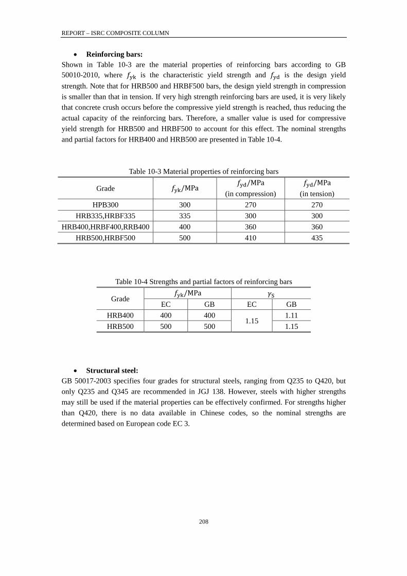
REPORT – ISRC COMPOSITE COLUMN
208
• Reinforcing bars: Shown in Table 10-3 are the material properties of reinforcing bars according to GB 50010-2010, where 𝑓yk is the characteristic yield strength and 𝑓yd is the design yield strength. Note that for HRB500 and HRBF500 bars, the design yield strength in compression is smaller than that in tension. If very high strength reinforcing bars are used, it is very likely that concrete crush occurs before the compressive yield strength is reached, thus reducing the actual capacity of the reinforcing bars. Therefore, a smaller value is used for compressive yield strength for HRB500 and HRBF500 to account for this effect. The nominal strengths and partial factors for HRB400 and HRB500 are presented in Table 10-4.
Table 10-3 Material properties of reinforcing bars
Grade 𝑓yk/MPa 𝑓yd/MPa
(in compression) 𝑓yd/MPa
(in tension) HPB300 300 270 270
HRB335,HRBF335 335 300 300 HRB400,HRBF400,RRB400 400 360 360
HRB500,HRBF500 500 410 435
Table 10-4 Strengths and partial factors of reinforcing bars
Grade 𝑓yk/MPa 𝛾S
EC GB EC GB HRB400 400 400
1.15 1.11
HRB500 500 500 1.15
• Structural steel: GB 50017-2003 specifies four grades for structural steels, ranging from Q235 to Q420, but only Q235 and Q345 are recommended in JGJ 138. However, steels with higher strengths may still be used if the material properties can be effectively confirmed. For strengths higher than Q420, there is no data available in Chinese codes, so the nominal strengths are determined based on European code EC 3.

REPORT – ISRC COMPOSITE COLUMN
209
Table 10-5 Material properties of steel profiles
Grade Thickness/mm 𝑓yk/MPa 𝑓yd/MPa
compression
tension flexure
shear
Q235
≤16 235 215 125 16~40 225 205 120 40~60 215 200 115 60~100 205 200 115
Q345
≤16 345 310 180 16~35 325 295 170 35~50 295 265 155 50~100 275 250 145
Q390
≤16 390 350 205 16~35 370 335 190 35~50 350 315 180 50~100 330 295 170
Q420
≤16 420 380 220 16~35 400 360 210 35~50 380 340 195 50~100 360 325 185
Table 10-6 Strengths and partial factors of steel profiles
Grade 𝑓yk/MPa 𝛾S
Thickness EC&GB EC GB
S355 t ≤ 40 mm 355
1.0 1.1
40 mm < 𝑡 ≤ 80 𝑚𝑚 355
S450 t ≤ 40 mm 440
40 mm < 𝑡 ≤ 80 𝑚𝑚 410
S460 t ≤ 40 mm 460
40 mm < 𝑡 ≤ 80 𝑚𝑚 430
• Equivalent steel distribution: PSA in Chinese codes slightly differs from PDM in American and European codes in the following two aspects: 1. In American and European codes, a 0.85 factor is used to discount the compressive
strength of the concrete. This 0.85 factor is not included in Chinese codes. Only the 𝛼 − factor is used to discount the effective strength of the concrete (see Table 10-1).
2. The actual concrete compressive stress distribution is represented by an equivalent rectangular diagram, where concrete strength is assumed to be 𝛼𝑓𝑐 and height of the equivalent rectangular diagram is 𝛽 times the actual height of the compressive stress distribution (see Figure 10-17).

REPORT – ISRC COMPOSITE COLUMN
210
x n
fc
T
C
x=βx
n
αfc
T
C
Figure 10-17 Equivalent stress distribution Although similar specifications are included in EC2 and ACI 318, EC4 also allows using another method to construct the plastic stress distribution of the concrete such that ‘the effective area of concrete in compression resists a stress of 0.85𝑓𝑐𝑑, constant over the whole depth between the plastic neutral axis and the most compressed fiber of the concrete’, which is the so called ‘plastic stress distribution method’ (PDM). However, Chinese standard only provides the PSA method but not the PDM method. Consequently, results obtained from these codes may be different.
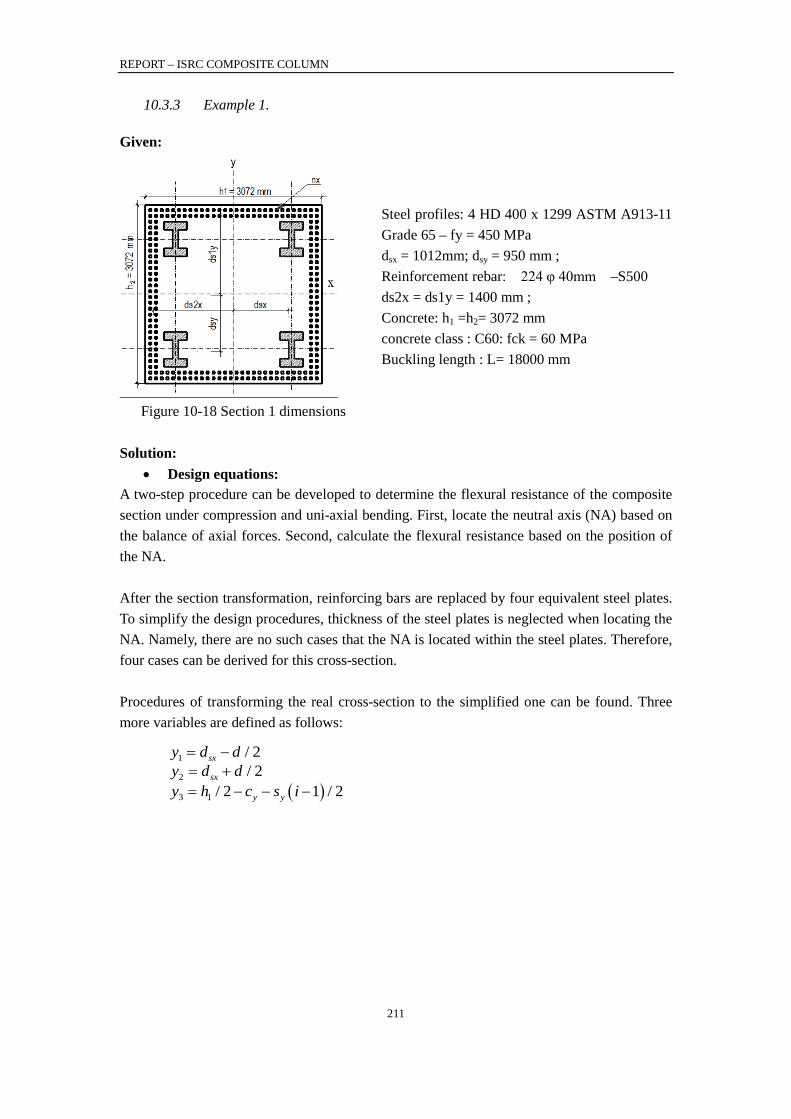
REPORT – ISRC COMPOSITE COLUMN
211
10.3.3 Example 1.
Given:
Figure 10-18 Section 1 dimensions
Steel profiles: 4 HD 400 x 1299 ASTM A913-11 Grade 65 – fy = 450 MPa dsx = 1012mm; dsy = 950 mm ; Reinforcement rebar: 224 φ 40mm –S500 ds2x = ds1y = 1400 mm ; Concrete: h1 =h2= 3072 mm concrete class : C60: fck = 60 MPa Buckling length : L= 18000 mm
Solution:
• Design equations: A two-step procedure can be developed to determine the flexural resistance of the composite section under compression and uni-axial bending. First, locate the neutral axis (NA) based on the balance of axial forces. Second, calculate the flexural resistance based on the position of the NA. After the section transformation, reinforcing bars are replaced by four equivalent steel plates. To simplify the design procedures, thickness of the steel plates is neglected when locating the NA. Namely, there are no such cases that the NA is located within the steel plates. Therefore, four cases can be derived for this cross-section. Procedures of transforming the real cross-section to the simplified one can be found. Three more variables are defined as follows:
( )
1
2
3 1
/ 2/ 2
/ 2 1 / 2
sx
sx
y y
y d dy d dy h c s i
= −= += − − −
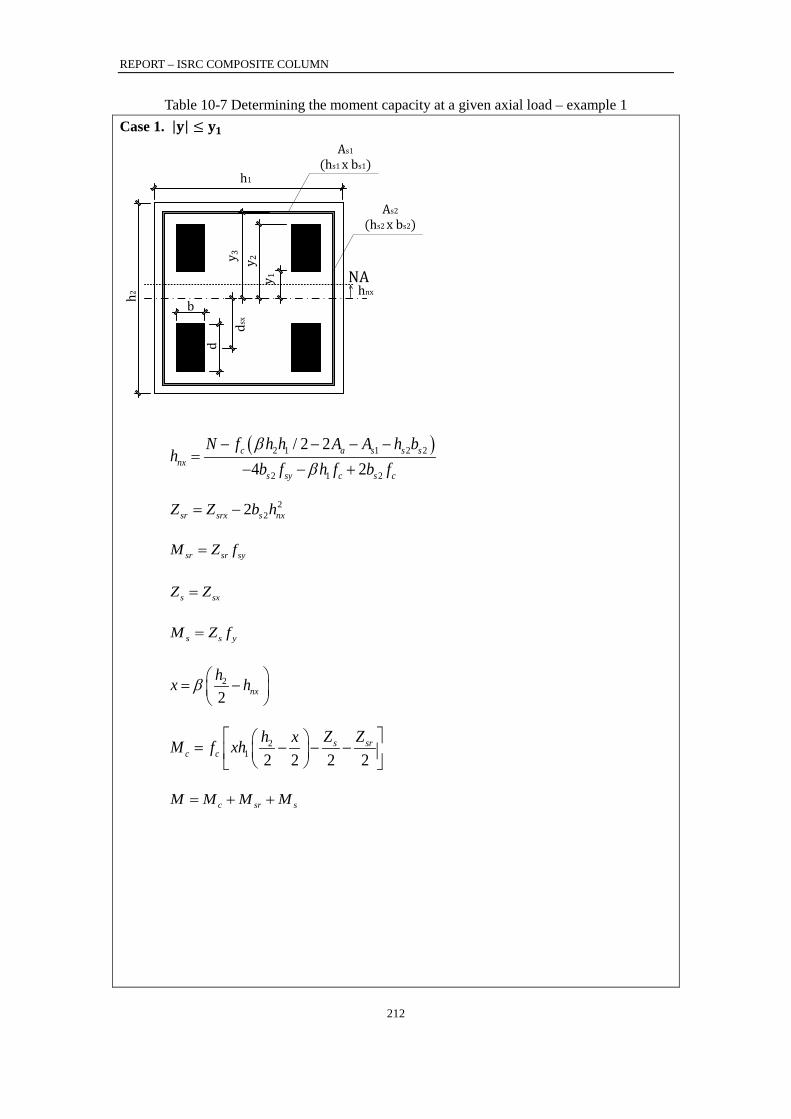
REPORT – ISRC COMPOSITE COLUMN
212
Table 10-7 Determining the moment capacity at a given axial load – example 1 Case 1. |𝐲| ≤ 𝐲𝟏
NAhnx
y 1y 2y 3
h1
b
d
dsx
h2As1
(hs1 x bs1)
As2
(hs2 x bs2)
( )2 1 1 2
2
2
1 2
/ 2 224
a s scnx
s
s
c s csy
N fh
b fh h A A h b
h f b fβ
β−
=−
+−− −
−
222sr srx s nxZ Z b h= −
sr sr syM Z f=
s sxZ Z=
s s yM Z f=
2
2 nxx h hβ −=
21 2 2 2 2
s src c
Z Zh xM f xh = − − −
c sr sM M M M= + +
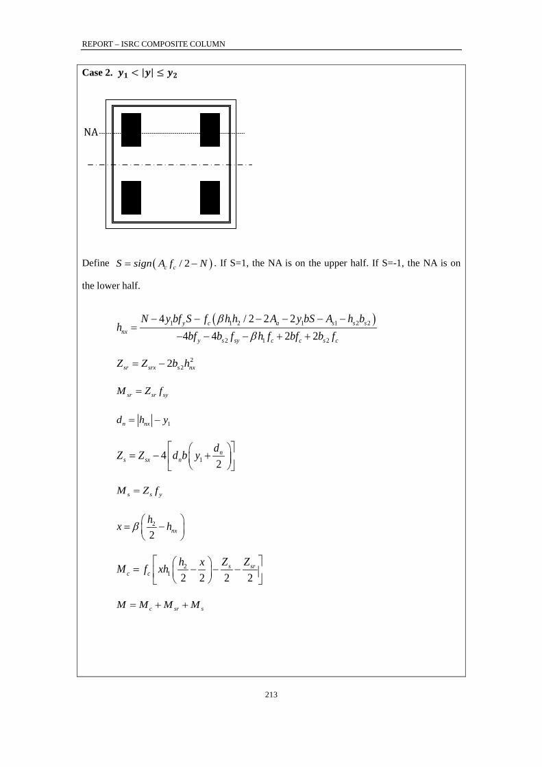
REPORT – ISRC COMPOSITE COLUMN
213
Case 2. 𝒚𝟏 < |𝒚| ≤ 𝒚𝟐
NA
Define ( )/ 2c cS sign A f N= − . If S=1, the NA is on the upper half. If S=-1, the NA is on
the lower half.
( )1 2 1 1 2 2
2
1
2 1
/ 2 24242
4 2y a s s s
c
cnx
y s sy c s c
h h A y bSN y bf S fh
bf bA h b
h f bf bf fβ
β− − − −
+ +
− −=
− − −
222sr srx s nxZ Z b h= −
sr sr syM Z f=
1n nxd h y= −
142
ns sx n
dZ Z d b y = − +
s s yM Z f=
2
2 nxx h hβ −=
21 2 2 2 2
s src c
Z Zh xM f xh = − − −
c sr sM M M M= + +
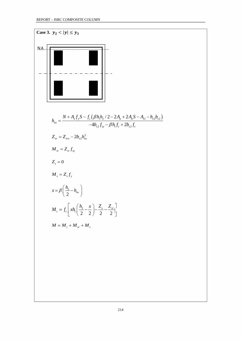
REPORT – ISRC COMPOSITE COLUMN
214
Case 3. 𝒚𝟐 < |𝒚| ≤ 𝒚𝟑
NA
( )1 2 1 2 2
12 2
/ 2 2 224
a a s s s
c
s y cnx
s s s cy
h h A A S AN A f S fh
b fh b
h f b fβ
β+ −
=− −
− + − −
+
222sr srx s nxZ Z b h= −
sr sr syM Z f=
0sZ =
s s yM Z f=
2
2 nxx h hβ −=
21 2 2 2 2
s src c
Z Zh xM f xh = − − −
c sr sM M M M= + +

REPORT – ISRC COMPOSITE COLUMN
215
Case 4. |𝒚| ≥ 𝒚𝟑
NA
( )1 2
1
/ 2 / 2 / 2/ 2 / 2s y sr sy c s sr srs
cnx
h hN A f S A f S f A SA Ah
hA S
fβ
β− − +
−
++ + −=
222sr srx s nxZ Z b h= −
sr sr syM Z f=
0sZ =
s s yM Z f=
2
2 nxx h hβ −=
21 2 2 2 2
s src c
Z Zh xM f xh = − − −
c sr sM M M M= + +

REPORT – ISRC COMPOSITE COLUMN
216
• Interaction curves – nominal strengths:
The N-M interaction curves are calculated based on the nominal material strengths, and no reduction factors are considered. Besides, the buckling effects and 𝑃 − 𝛿 effects are not considered either. Therefore, the N-M curves reflect the pure cross-sectional capacity of the composite members. The fiber results are obtained based on the FEM numerical calculations.
Figure 10-19 Interaction curves with nominal strengths - Section 1
• Interaction curve – partial factors:
Figure 10-20 Interaction curves with and without material partial factors - Section 1
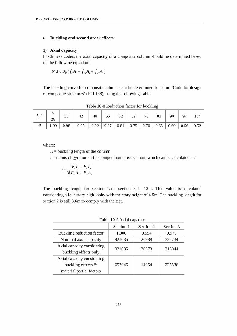
REPORT – ISRC COMPOSITE COLUMN
217
• Buckling and second order effects:
1) Axial capacity In Chinese codes, the axial capacity of a composite column should be determined based on the following equation:
The buckling curve for composite columns can be determined based on ‘Code for design of composite structures’ (JGJ 138), using the following Table:
Table 10-8 Reduction factor for buckling
28
35 42 48 55 62 69 76 83 90 97 104
1.00 0.98 0.95 0.92 0.87 0.81 0.75 0.70 0.65 0.60 0.56 0.52 where:
l0 = buckling length of the column i = radius of gyration of the composition cross-section, which can be calculated as:
c c a a
c c a a
E I E IiE A E A
+=
+
The buckling length for section 1and section 3 is 18m. This value is calculated considering a four-story high lobby with the story height of 4.5m. The buckling length for section 2 is still 3.6m to comply with the test.
Table 10-9 Axial capacity Section 1 Section 2 Section 3
Buckling reduction factor 1.000 0.994 0.970 Nominal axial capacity 921085 20988 322734
Axial capacity considering buckling effects only
921085 20873 313044
Axial capacity considering buckling effects &
material partial factors 657046 14954 225536
c c ys s ya a0.9 ( )N f A f A f Aϕ≤ + +
0 /l i≤
ϕ

REPORT – ISRC COMPOSITE COLUMN
218
2) Moment capacity: Chinese standard specifies that the second order 𝑃 − 𝛿 effect can be ignored if the following three criteria are satisfied:
where:
M1 = smallest design bending moment within the composite member M2 = largest design bending moment within the composite member N = design axial force Nu = short-column axial capacity of the composite member lc = buckling capacity i = radius of gyration of the composite cross-section
If the criteria are not satisfied, the 𝑃 − 𝛿 effect needs to be considered by multiplying the design bending moment with a coefficient that is greater than 1.0.
where: ea = max20mm,1/30hc h0 = effective height of the composite cross-section hc = cross-section dimension along the direction that the bending moment is considered fc = concrete compressive strength Ag = gross area of the cross-section
Shown in Figure 10-21 are the interaction curves given by Chinese with and without buckling and second order effects. The interaction curves have considered the material partial factors.
( )
1 2
u
c 1 2
(1) / 0.9(2) / 0.9(3) / 32 12 /
M MN Nl i M M
≤≤
≤ −
( )
ns 2
1m
22
cns c
2 a 0 c
c g
m
c
0.7 0.3
111300 /
0.5
MMCM
lM N e h h
f AN
M C η
η ζ
ζ
= +
= +
=
=
+

REPORT – ISRC COMPOSITE COLUMN
219
Figure 10-21 Interaction curves with and without considering buckling and second order
effects (Material partial factors have already been considered) - Section 1
• Shear force evaluation: The longitudinal shear force of the steel sections should be checked to avoid large slip and to ensure enough composite action. However, a unified method is still lacked in Chinese code to provide general design guidance. As a comparison between Chinese codes, European codes, and American codes, this part of the report checks the longitudinal shear force based on Chinese codes by using the same method proposed by ArcelorMittal and the University of Liege. Check the shear capacity of the composite column subjected to the following demands: (the same with the design capacities in Section 4.2.7)
NEd = 300000 kN; MEd = 250000 kN; VEd = 20000 kN;
The definition of the used symbols is defined in Figure 10-22:
286mmc3b =
s 476mmb =
( )3072mm 2 286mm 476mm 1548mmc4b = − ⋅ + =
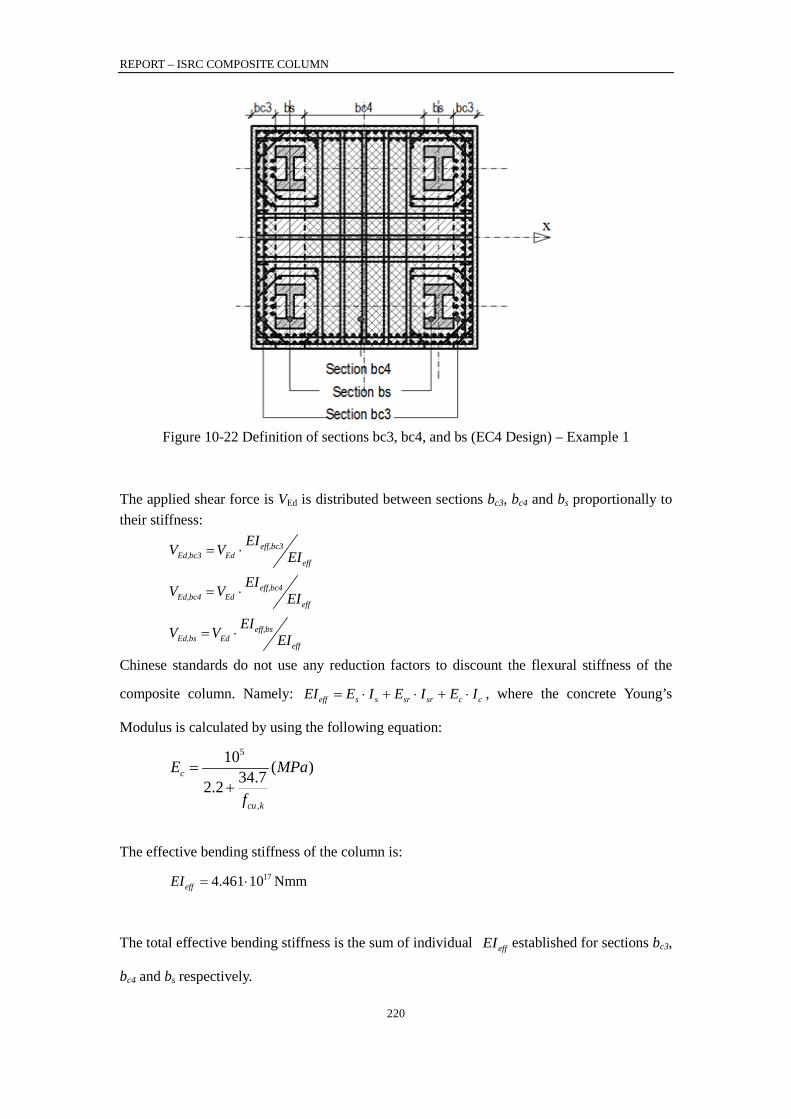
REPORT – ISRC COMPOSITE COLUMN
220
Figure 10-22 Definition of sections bc3, bc4, and bs (EC4 Design) – Example 1
The applied shear force is VEd is distributed between sections bc3, bc4 and bs proportionally to their stiffness:
eff,bc3Ed,bc3 Ed
eff
EIV V EI= ⋅
eff,bc4Ed,bc4 Ed
eff
EIV V EI= ⋅
eff,bsEd,bs Ed
eff
EIV V EI= ⋅
Chinese standards do not use any reduction factors to discount the flexural stiffness of the
composite column. Namely: eff s s sr sr c cEI E I E I E I= ⋅ + ⋅ + ⋅ , where the concrete Young’s
Modulus is calculated by using the following equation: 5
,
10 ( )34.72.2c
cu k
E MPa
f
=+
The effective bending stiffness of the column is:
174.461 10 NmmeffEI = ⋅
The total effective bending stiffness is the sum of individual effEI established for sections bc3,
bc4 and bs respectively.
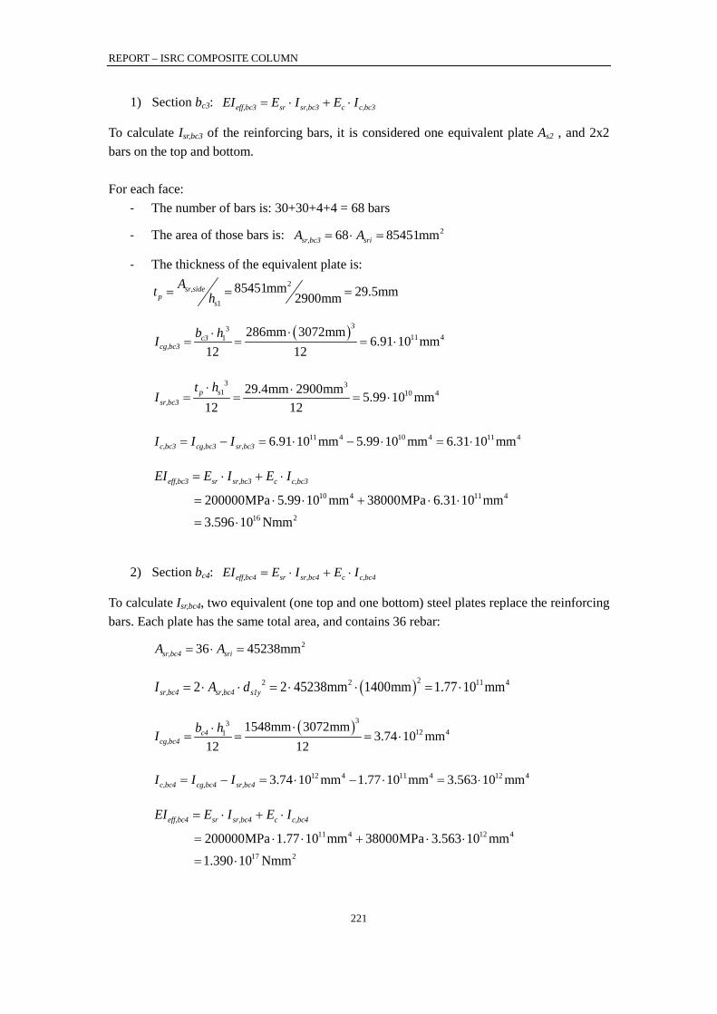
REPORT – ISRC COMPOSITE COLUMN
221
1) Section bc3: eff,bc3 sr sr,bc3 c c,bc3EI E I E I= ⋅ + ⋅
To calculate Isr,bc3 of the reinforcing bars, it is considered one equivalent plate As2 , and 2x2 bars on the top and bottom. For each face:
- The number of bars is: 30+30+4+4 = 68 bars
- The area of those bars is: 268 85451mmsr,bc3 sriA A= ⋅ =
- The thickness of the equivalent plate is: 2
s1
85451mm 29.5mm2900mmsr,side
pAt h= = =
( )3311 41 286mm 3072mm
6.91 10 mm12 12
c3cg,bc3
b hI⋅⋅
= = = ⋅
3 3s1 10 429.4mm 2900mm 5.99 10 mm
12 12p
sr,bc3
t hI
⋅ ⋅= = = ⋅
11 4 10 4 11 46.91 10 mm 5.99 10 mm 6.31 10 mmc,bc3 cg,bc3 sr,bc3I I I= − = ⋅ − ⋅ = ⋅
10 4 11 4
16 2
200000MPa 5.99 10 mm 38000MPa 6.31 10 mm3.596 10 Nmm
eff,bc3 sr sr,bc3 c c,bc3EI E I E I
= ⋅ + ⋅
= ⋅ ⋅ + ⋅ ⋅
= ⋅
2) Section bc4: eff,bc4 sr sr,bc4 c c,bc4EI E I E I= ⋅ + ⋅
To calculate Isr,bc4, two equivalent (one top and one bottom) steel plates replace the reinforcing bars. Each plate has the same total area, and contains 36 rebar:
236 45238mmsr,bc4 sriA A= ⋅ =
( )22 2 11 42 2 45238mm 1400mm 1.77 10 mmsr,bc4 sr,bc4 s1yI A d= ⋅ ⋅ = ⋅ ⋅ = ⋅
( )3312 41 1548mm 3072mm
3.74 10 mm12 12
c4cg,bc4
b hI⋅⋅
= = = ⋅
12 4 11 4 12 43.74 10 mm 1.77 10 mm 3.563 10 mmc,bc4 cg,bc4 sr,bc4I I I= − = ⋅ − ⋅ = ⋅
11 4 12 4
17 2
200000MPa 1.77 10 mm 38000MPa 3.563 10 mm1.390 10 Nmm
eff,bc4 sr sr,bc4 c c,bc4EI E I E I
= ⋅ + ⋅
= ⋅ ⋅ + ⋅ ⋅
= ⋅
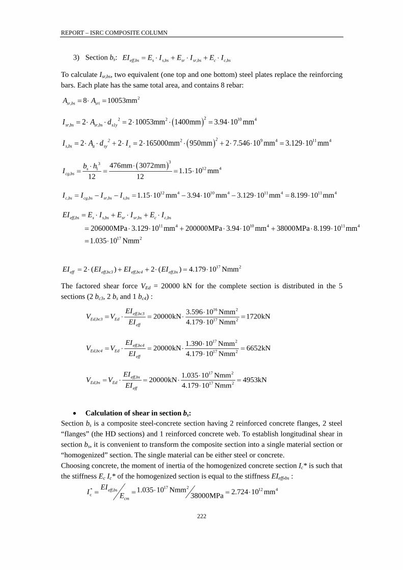
REPORT – ISRC COMPOSITE COLUMN
222
3) Section bs: eff,bs s s,bs sr sr,bs c c,bsEI E I E I E I= ⋅ + ⋅ + ⋅
To calculate Isr,bs, two equivalent (one top and one bottom) steel plates replace the reinforcing bars. Each plate has the same total area, and contains 8 rebar:
28 10053mmsr,bs sriA A= ⋅ =
( )22 2 10 42 2 10053mm 1400mm 3.94 10 mmsr,bs sr,bs s1yI A d= ⋅ ⋅ = ⋅ ⋅ = ⋅
( )2 9 4 11 42 2 2 165000mm 950mm 2 7.546 10 mm 3.129 10 mm22s,bs a sy xI A d I= ⋅ ⋅ + ⋅ = ⋅ ⋅ + ⋅ ⋅ = ⋅
( )3312 41 476mm 3072mm
1.15 10 mm12 12
scg,bs
b hI⋅⋅
= = = ⋅
12 4 10 4 11 4 11 41.15 10 mm 3.94 10 mm 3.129 10 mm 8.199 10 mmc,bs cg,bs sr,bs s,bsI I I I= − − = ⋅ − ⋅ − ⋅ = ⋅
11 4 10 4 11 4
17 2
206000MPa 3.129 10 mm 200000MPa 3.94 10 mm 38000MPa 8.199 10 mm1.035 10 Nmm
eff,bs s s,bs sr sr,bs c c,bsEI E I E I E I
= ⋅ + ⋅ + ⋅
= ⋅ ⋅ + ⋅ ⋅ + ⋅ ⋅
= ⋅
17 22 ( ) 2 ( ) 4.179 10 Nmmeff eff,bc3 eff,bc4 eff,bsEI EI EI EI= ⋅ + + ⋅ = ⋅
The factored shear force VEd = 20000 kN for the complete section is distributed in the 5 sections (2 bc3, 2 bs and 1 bc4) :
16 2
17 2
3.596 10 Nmm20000kN 1720kN4.179 10 Nmm
eff,bc3Ed,bc3 Ed
eff
EIV V
EI⋅
= ⋅ = ⋅ =⋅
17 2
17 2
1.390 10 Nmm20000kN 6652kN4.179 10 Nmm
eff,bc4Ed,bc4 Ed
eff
EIV V
EI⋅
= ⋅ = ⋅ =⋅
17 2
17 2
1.035 10 Nmm20000kN 4953kN4.179 10 Nmm
eff,bsEd,bs Ed
eff
EIV V
EI⋅
= ⋅ = ⋅ =⋅
• Calculation of shear in section bs:
Section bs is a composite steel-concrete section having 2 reinforced concrete flanges, 2 steel “flanges” (the HD sections) and 1 reinforced concrete web. To establish longitudinal shear in section bs, it is convenient to transform the composite section into a single material section or “homogenized” section. The single material can be either steel or concrete. Choosing concrete, the moment of inertia of the homogenized concrete section Ic* is such that the stiffness Ec Ic* of the homogenized section is equal to the stiffness EIeff,bs :
17 2* 12 4c
1.035 10 Nmm 2.724 10 mm38000MPaeff,bs
cm
EII E⋅= = = ⋅
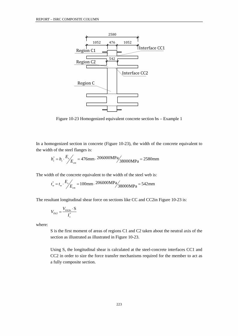
REPORT – ISRC COMPOSITE COLUMN
223
1052Interface CC1
476 1052
2580
542
Interface CC2
Region C
Region C1
Region C2
Figure 10-23 Homogenized equivalent concrete section bs – Example 1 In a homogenized section in concrete (Figure 10-23), the width of the concrete equivalent to the width of the steel flanges is:
206000MPa476mm 2580mm38000MPa* ss s
cm
Eb b E= ⋅ = ⋅ =
The width of the concrete equivalent to the width of the steel web is:
206000MPa100mm 542mm38000MPa* sw w
cm
Et t E= ⋅ = ⋅ =
The resultant longitudinal shear force on sections like CC and CC2in Figure 10-23 is:
*c
SEd,bsEd,l
VV
I⋅
=
where: S is the first moment of areas of regions C1 and C2 taken about the neutral axis of the section as illustrated as illustrated in Figure 10-23. Using S, the longitudinal shear is calculated at the steel-concrete interfaces CC1 and CC2 in order to size the force transfer mechanisms required for the member to act as a fully composite section.
REPORT – ISRC COMPOSITE COLUMN
224
• Calculation of longitudinal shear force applied at interface CC1:
SCC1 is the section modulus for the region C1 as defined in Figure 10-23: The height of the C1 section is:
' 3072mm 600mm950mm 286mm11 sy
h dh - d + - +2 2 2 2
= = =
The area is:
' 2476mm 286mm 136136mm1 1A b h= ⋅ = ⋅ =
'2 8 33072mm 286mm136136mm 1.896 10 mm
21 1
CC1 1h hS A - -
2 2 2 = ⋅ = ⋅ = ⋅
The resultant longitudinal shear force at interface CC1 is:
8 3
* 12 4c
4953kN 1.896 10 mm N345.32.72 10 mm mm
Ed,bs CC1Ed,CC1
V SV
I⋅ ⋅ ⋅
= = =⋅
On 1-meter length of column:
kN345.3mEd,CC1V =
• Calculation of longitudinal shear force applied at interface CC2: SCC2 is the section modulus for the combined regions C1 and C2 (the HD profile): The equivalent area in concrete for the HD profile is:
Aa =165000mm2
The equivalent are in concrete for the HD profile is:
2 2206000MPa165000mm 894474mm38000MPa* sa a
cm
EA A E= ⋅ = ⋅ =
The distance of HD center to the neutral axis is:
syd = 950 mm
The moment of area of the equivalent steel profile is:
2 8 3894474mm 950mm 8.50 10 mm*HD a syS A d= ⋅ = ⋅ = ⋅
REPORT – ISRC COMPOSITE COLUMN
225
Area of concrete between the flanges: 2 2
c _ CC2 476mm 600mm 165000mm 120600mm*aA b d-A= ⋅ = ⋅ − =
Moment of area of concrete between the flanges:
2 8 3c _ CC2 c _ CC2 120600mm 950mm 1.146 10 mm* *
syS A d= ⋅ = ⋅ = ⋅
The section modulus corresponding to the combined regions C1 and C2 is equal to:
8 3 8 3 8 3 9 3c _ CC2 1.146 10 mm 8.83 10 mm 1.896 10 mm 1.19 10 mm*
CC2 HD CC1S S S S= + + = ⋅ + ⋅ + ⋅ = ⋅
The resultant longitudinal shear force at interface CC2 is:
9 3
* 12 4c
4953kN 1.19 10 mm N21672.72 10 mm mm
Ed,bs CC2Ed,CC2
V SV
I⋅ ⋅ ⋅
= = =⋅
On 1-meter length of column:
kN2167mEd,CC2V =
• Evaluation of necessary amount of shear studs: Geometrical characteristic of the shear studs correspond to State of Art – Table 3.2.2 where:
d = 25 mm – diameter of the shear stud; hsc = 100 mm – stud height; Stud length is OK. fu = 450 MPa – maximum stud tensile strength;
For a shear stud with a diameter d = 25 mm, the design shear strength is equal to:
( ) ( )= min 0.43 0.7 min 246.1kN,154.4kN 154.4kNRk s c c u sP A E f , f A = =
For a length of a column of 1 m, the necessary amount of shear studs to different interfaces is:
kN345.3 1m1m m 2.24 3 studs /1m154.4kN
Ed1_CC1studs_CC1
Rk
Vn
P
⋅⋅= = = ⇒
kN2176 1m1m m 14.1 15 studs /1m154.4kN
Ed1_CC2studs_CC2
Rk
Vn
P
⋅⋅= = = ⇒
Suppose the studs are installed in three rows, then the space of the studs is 200mm. The JGJ code specifies that the space should not be less than 6 times the diameter of the stud, which is 150mm in this example. The space is OK.

REPORT – ISRC COMPOSITE COLUMN
226
10.3.4 Example 2 and 3
Given:
Figure 10-24 Section 2 dimensions
Steel profiles: 4 HEM 100 – fy = 406 MPa - average values from material tests (Table 10-12) dsx = dsy = 127.5 mm ; Reinforcement rebar: 32φ8mm – fys = 438 Mpa ds1x = ds1y = 208 mm ; Concrete: h1 =h2= 450mm - fck = 64.8 MPa - average values from material tests Buckling length : L= 3600 mm
Figure 10-25 Section 3 dimensions
Steel profiles : 4 HD 400 x 634 HISTAR 460 dsx = dsy = 513 mm ; Reinforcement rebar: 32 φ 32mm –HRB 400 ds2x = ds1y = 550 mm ; Concrete: h1 =h2= 1800mm - C60: fck = 60 MPa Buckling length : L= 18000 mm
Solution:
• Design equations: Likewise, the transformation of the real cross-section to the simplified one can found. Several other variables are defined as follows:
1 2
2 1
3 1
4 2
/ 2/ 2/ 2
sx
sx
s x
y dy d dy d dy d
== −= +=
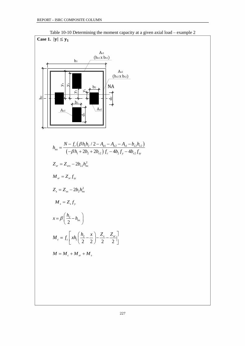
REPORT – ISRC COMPOSITE COLUMN
227
Table 10-10 Determining the moment capacity at a given axial load – example 2 Case 1. |𝐲| ≤ 𝐲𝟏
NAy 1y 2
y 4 y 3h1
b1
d1
h2
As1
(hs1 x bs1)
As2
(hs2 x bs2)
b2
d2Aa1 Aa2
( )( )
1 2 1 1 2
2
2
1 2
2
2 24/ 2
2 2 4a sc a
nxc y s sy
s s
s
h h A A b hN f Ah
f b f bh b fbβ
β− − − −
− −+−− +
=
222sr srx s nxZ Z b h= −
sr sr syM Z f=
222s sx nxZ Z b h= −
s s yM Z f=
2
2 nxx h hβ −=
21 2 2 2 2
s src c
Z Zh xM f xh = − − −
c sr sM M M M= + +
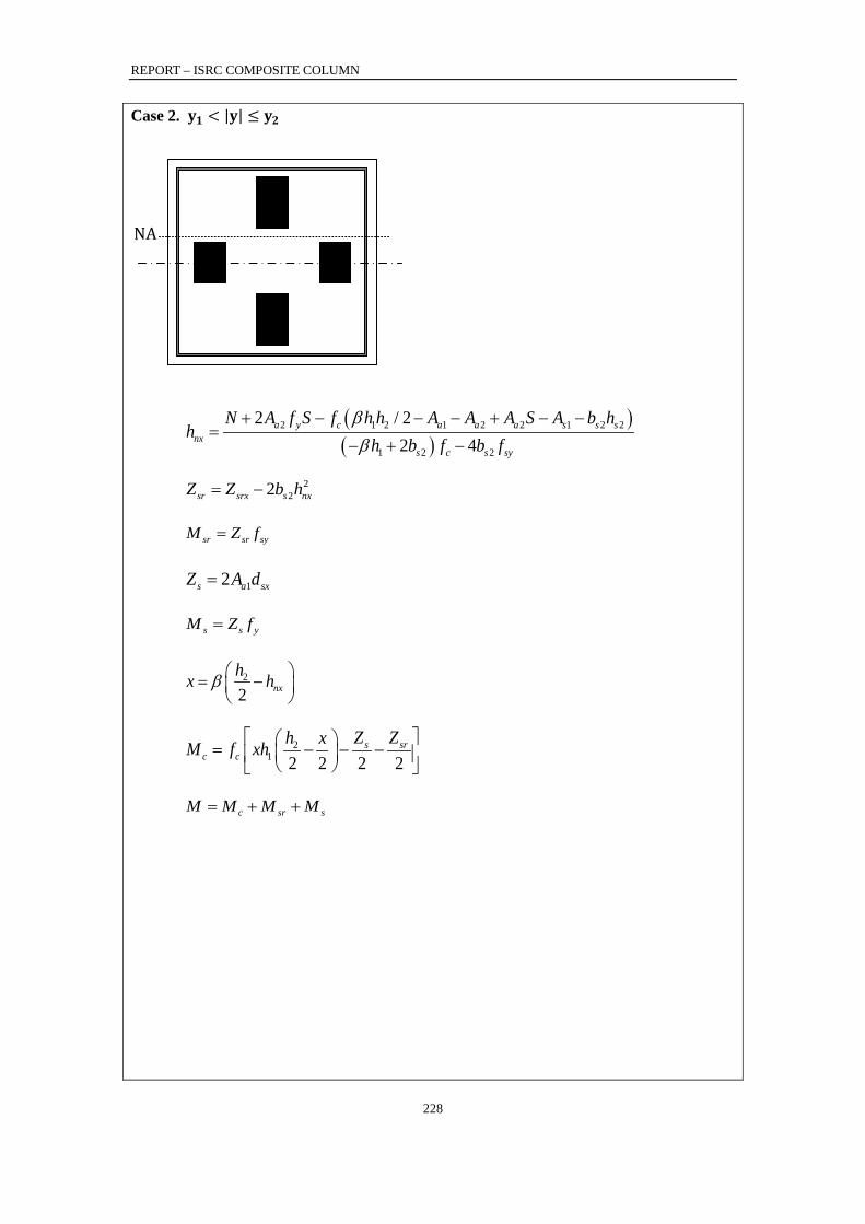
REPORT – ISRC COMPOSITE COLUMN
228
Case 2. 𝐲𝟏 < |𝐲| ≤ 𝐲𝟐
NA
( )( )
2 1 2 1 12 2 2 2
21 2
22 4
/ 2 a a s sa s
s
y c anx
c s sy
h h A A S A b hh b
N A f S f Ah
f b fββ
− ++ − −
+=
−
− −
−
222sr srx s nxZ Z b h= −
sr sr syM Z f=
12s a sxZ A d=
s s yM Z f=
2
2 nxx h hβ −=
21 2 2 2 2
s src c
Z Zh xM f xh = − − −
c sr sM M M M= + +
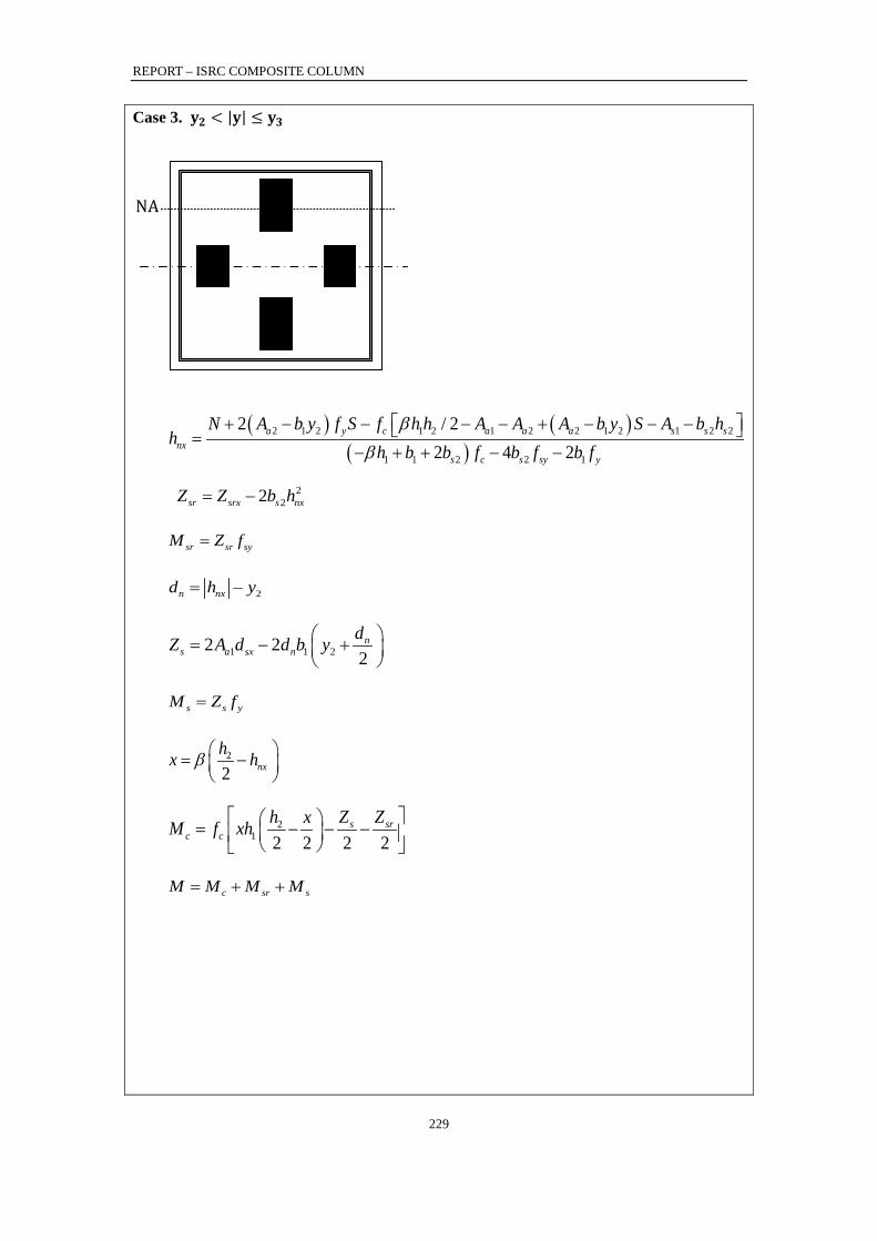
REPORT – ISRC COMPOSITE COLUMN
229
Case 3. 𝐲𝟐 < |𝐲| ≤ 𝐲𝟑
NA
( ) ( )( )
1 2 1 22 1 2 1 22 2 1
1
2
1 2 2 1
/22 4 2
2 a aa y c anx
c s
s s s
s sy y
N A b y f S h h A A b y S A b hh b bf A
hf b f b f
ββ
− + − −+ − − − −
−+=
− + −
222sr srx s nxZ Z b h= −
sr sr syM Z f=
2n nxd h y= −
1 1 22 22
ns a sx n
dZ A d d b y = − +
s s yM Z f=
2
2 nxx h hβ −=
21 2 2 2 2
s src c
Z Zh xM f xh = − − −
c sr sM M M M= + +
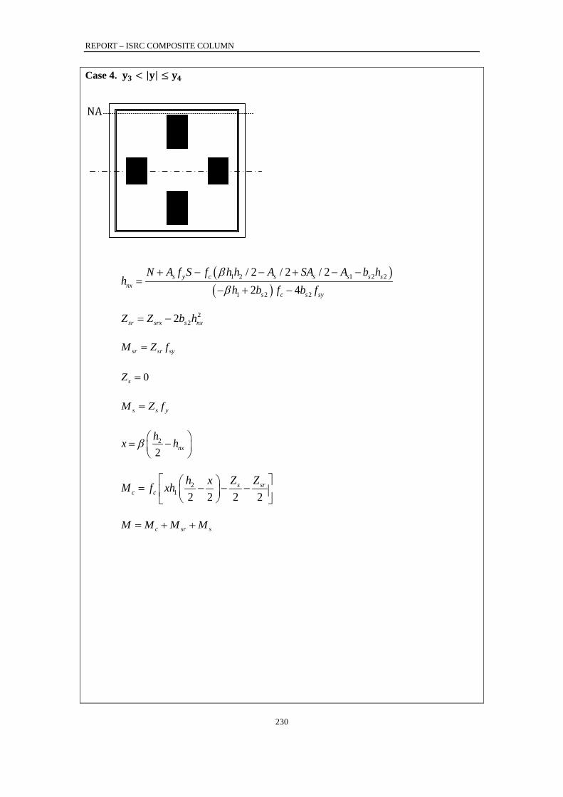
REPORT – ISRC COMPOSITE COLUMN
230
Case 4. 𝐲𝟑 < |𝐲| ≤ 𝐲𝟒
NA
( )( )
1 2 1 2 2
1 2 2
/ 2 / 2 / 22 4
s s s s ss y cnx
c s ys s
N A f S fh
fh h A SA A b hh b fb
ββ
− + −
−+
+ −=
−
−
222sr srx s nxZ Z b h= −
sr sr syM Z f=
0sZ =
s s yM Z f=
2
2 nxx h hβ −=
21 2 2 2 2
s src c
Z Zh xM f xh = − − −
c sr sM M M M= + +
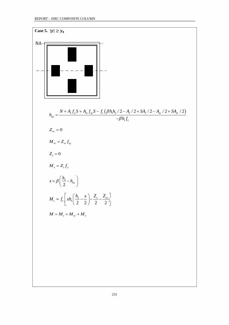
REPORT – ISRC COMPOSITE COLUMN
231
Case 5. |𝐲| ≥ 𝐲𝟒 NA
( )1 2
1
/ 2 / 2 / 2 / 2 / 2s y sr sy c s s sr srnx
c
h hN A f S A f A SS fh
A A Ah f
Sββ− − +
−
++ + −=
0srZ =
sr sr syM Z f=
0sZ =
s s yM Z f=
2
2 nxx h hβ −=
21 2 2 2 2
s src c
Z Zh xM f xh = − − −
c sr sM M M M= + +

REPORT – ISRC COMPOSITE COLUMN
232
• Interaction curve – nominal strength: The N-M interaction curves are calculated based on the nominal material strengths, and no reduction factors are considered. Besides, the buckling effects and 𝑃 − 𝛿 effects are not considered either. Therefore, the N-M curves reflect the pure cross-sectional capacity of the composite members. The fiber results are obtained based on the FEM numerical calculations.
(a) Section 2
(b) Section 3
Figure 10-26 Interaction curves with nominal strengths
• Interaction curve – partial factors:
(a) Section 2
(b) Section 3
Figure 10-27 Interaction curves with and without material partial factors

REPORT – ISRC COMPOSITE COLUMN
233
• Interaction curve - Buckling and second order effects: 1) Axial capacity
In Chinese codes, the axial capacity of a composite column should be determined based on the following equation:
The buckling curve for composite columns can be determined based on ‘Code for design of composite structures’ (JGJ 138), using the following Table:
Table 10-11 Reduction factor for buckling
28
35 42 48 55 62 69 76 83 90 97 104
1.00 0.98 0.95 0.92 0.87 0.81 0.75 0.70 0.65 0.60 0.56 0.52 where:
l0 = buckling length of the column i = radius of gyration of the composition cross-section, which can be calculated as:
c c a a
c c a a
E I E IiE A E A
+=
+
The buckling length for section 1and section 3 is 18m. This value is calculated considering a four-story high lobby with the story height of 4.5m. The buckling length for section 2 is still 3.6m to comply with the test.
Table 10-12 Axial capacity Section 1 Section 2 Section 3
Buckling reduction factor 1.000 0.994 0.970 Nominal axial capacity 921085 20988 322734
Axial capacity considering buckling effects only
921085 20873 313044
Axial capacity considering buckling effects &
material partial factors 657046 14954 225536
c c ys s ya a0.9 ( )N f A f A f Aϕ≤ + +
0 /l i≤
ϕ
REPORT – ISRC COMPOSITE COLUMN
234
2) Moment capacity Chinese standard specifies that the second order 𝑃 − 𝛿 effect can be ignored if the following three criteria are satisfied:
where:
M1 = smallest design bending moment within the composite member M2 = largest design bending moment within the composite member N = design axial force Nu = short-column axial capacity of the composite member lc = buckling capacity i = radius of gyration of the composite cross-section
If the criteria are not satisfied, the 𝑃 − 𝛿 effect needs to be considered by multiplying the design bending moment with a coefficient that is greater than 1.0.
where: ea = max20mm,1/30hc h0 = effective height of the composite cross-section hc = cross-section dimension along the direction that the bending moment is considered fc = concrete compressive strength Ag = gross area of the cross-section
Shown in Figure 10-28 are the interaction curves given by Chinese with and without buckling and second order effects. The interaction curves have considered the material partial factors.
( )
1 2
u
c 1 2
(1) / 0.9(2) / 0.9(3) / 32 12 /
M MN Nl i M M
≤≤
≤ −
( )
ns 2
1m
22
cns c
2 a 0 c
c g
m
c
0.7 0.3
111300 /
0.5
MMCM
lM N e h h
f AN
M C η
η ζ
ζ
= +
= +
=
=
+
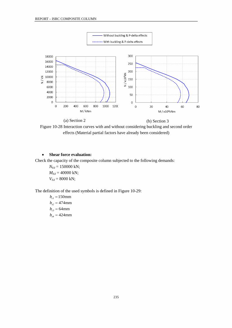
REPORT – ISRC COMPOSITE COLUMN
235
(a) Section 2
(b) Section 3
Figure 10-28 Interaction curves with and without considering buckling and second order effects (Material partial factors have already been considered)
• Shear force evaluation:
Check the capacity of the composite column subjected to the following demands: NEd = 150000 kN; MEd = 40000 kN; VEd = 8000 kN;
The definition of the used symbols is defined in Figure 10-29:
150mmc1b = 474mms2b = 64mmc3b = 424mms4b =

REPORT – ISRC COMPOSITE COLUMN
236
Figure 10-29 Definition of sections bc1, bc3, bs2, and bs4 (EC4 Design) – Example 2
The applied shear force is VEd is distributed between sections bc3, bc4 and bs proportionally to their stiffness:
eff,bc1Ed,bc1 Ed
eff
EIV V EI= ⋅
eff,bc3Ed,bc3 Ed
eff
EIV V EI= ⋅
eff,bs1Ed,bs1 Ed
eff
EIV V EI= ⋅
eff,bs2Ed,bs2 Ed
eff
EIV V EI= ⋅
The effective bending stiffness of the column is:
164.43 10 NmmeffEI = ⋅
The total effective bending stiffness is the sum of individual effEI established for sections bc1,
bc3, bs2 and bs4 respectively.
REPORT – ISRC COMPOSITE COLUMN
237
1) Section bc1: 1eff,bc3 sr sr,bc1 c c,bc1EI E I E I= ⋅ + ⋅
To calculate Isr,bc1 of the reinforcing bars, it is considered one equivalent plate As2. For each face:
- The number of bars is: 9 bars
- The area of those bars is: 29 7238mmsr,bc3 sriA A= ⋅ =
- The thickness of the equivalent plate is: 2
s1
7238mm 4.2mm1720mmsr,bc1
pAt h= = =
( )3310 41 150mm 1800mm
7.29 10 mm12 12
c1cg,bc1
b hI⋅⋅
= = = ⋅
3 3s1 9 44.4mm 1720mm 1.87 10 mm
12 12p
sr,bc1
t hI
⋅ ⋅= = = ⋅
10 4 9 4 10 47.29 10 mm 1.87 10 mm 7.10 10 mmc,bc1 cg,bc1 sr,bc1I I I= − = ⋅ − ⋅ = ⋅
9 4 10 4
15 2
200000MPa 1.87 10 mm 39262MPa 7.10 10 mm3.16 10 Nmm
eff,bc1 sr sr,bc1 c c,bc1EI E I E I
= ⋅ + ⋅
= ⋅ ⋅ + ⋅ ⋅
= ⋅
2) Section bc3: eff,bc3 sr sr,bc3 c c,bc3EI E I E I= ⋅ + ⋅
To calculate Isr,bc3, two equivalent (one top and one bottom) steel plates replace the reinforcing bars. Each plate has the same total area, and contains 1 rebar:
21 804.2mmsr,bc3 sriA A= ⋅ =
( )22 2 6 42 2 804.2mm 860mm 1.222 10 mmsr,bc3 sr,bc3 s1yI A d= ⋅ ⋅ = ⋅ ⋅ = ⋅
( )3310 41 64mm 1800mm
3.110 10 mm12 12
c3cg,bc3
b hI⋅⋅
= = = ⋅
10 4 6 4 10 43.110 10 mm 1.222 10 mm 3.110 10 mmc,bc3 cg,bc3 sr,bc3I I I= − = ⋅ − ⋅ = ⋅
6 4 10 4
15 2
200000MPa 1.222 10 mm 39262MPa 3.110 10 mm1.22 10 Nmm
eff,bc3 sr sr,bc3 c c,bc3EI E I E I
= ⋅ + ⋅
= ⋅ ⋅ + ⋅ ⋅
= ⋅
REPORT – ISRC COMPOSITE COLUMN
238
3) Section bs2: eff,bs2 s s,bs2 sr sr,bs2 c c,bs2EI E I E I E I= ⋅ + ⋅ + ⋅
To calculate Isr,bs2, two equivalent (one top and one bottom) steel plates replace the reinforcing bars. Each plate has the same total area, and contains 2 rebar:
22 1608.5mmsr,bs2 sriA A= ⋅ =
( )22 2 9 42 2 1608.5mm 860mm 1.858 10 mmsr,bs2 sr,bs2 s1yI A d= ⋅ ⋅ = ⋅ ⋅ = ⋅
8 49.825 10 mms,bs2 yI I= = ⋅
( )3311 41 476mm 1800mm
2.304 10 mm12 12
s2cg,bs2
b hI⋅⋅
= = = ⋅
11 4 9 4 8 4 11 42.304 10 mm 1.858 10 mm 9.825 10 mm 2.276 10 mmc,bs2 cg,bs4 sr,bs2 s,bs2I I I I= − − = ⋅ − ⋅ − ⋅ = ⋅
8 4 9 4 11 4
15 2
206000MPa 9.825 10 mm 200000MPa 1.858 10 mm 39262MPa 2.276 10 mm9.51 10 Nmm
eff,bs2 s s,bs2 sr sr,bs2 c c,bs2EI E I E I E I
= ⋅ + ⋅ + ⋅
= ⋅ ⋅ + ⋅ ⋅ + ⋅ ⋅
= ⋅
4) Section bs4: eff,bs4 s s,bs4 sr sr,bs4 c c,bs4EI E I E I E I= ⋅ + ⋅ + ⋅
To calculate Isr,bs4, two equivalent (one top and one bottom) steel plates replace the reinforcing bars. Each plate has the same total area, and contains 1 rebar:
21 804.2mmsr,bs4 sriA A= ⋅ =
( )22 2 8 42 2 804.2mm 860mm 9.291 10 mmsr,bs4 sr,bs4 s1yI A d= ⋅ ⋅ = ⋅ ⋅ = ⋅
( )22 2 10 4a2 2 80800mm 513mm 4.801 10 mms,bs4 syI A d= ⋅ ⋅ = ⋅ ⋅ = ⋅
( )3311 41 424mm 1800mm
2.061 10 mm12 12
s4cg,bs4
b hI⋅⋅
= = = ⋅
11 4 8 4 10 4 11 42.061 10 mm 9.291 10 mm 4.801 10 mm 1.572 10 mmc,bs4 cg,bs4 sr,bs4 s,bs4I I I I= − − = ⋅ − ⋅ − ⋅ = ⋅
10 4 8 4 11 4
16 2
206000MPa 4.801 10 mm 200000MPa 9.291 10 mm 39262MPa 1.572 10 mm1.625 10 Nmm
eff,bs4 s s,bs4 sr sr,bs4 c c,bs4EI E I E I E I
= ⋅ + ⋅ + ⋅
= ⋅ ⋅ + ⋅ ⋅ + ⋅ ⋅
= ⋅
16 22 ( ) 2 ( ) 2 ( ) 4.403 10 Nmmeff eff,bc1 eff,bs2 eff,bc3 eff,bs4EI EI EI EI EI= ⋅ + ⋅ + ⋅ + = ⋅
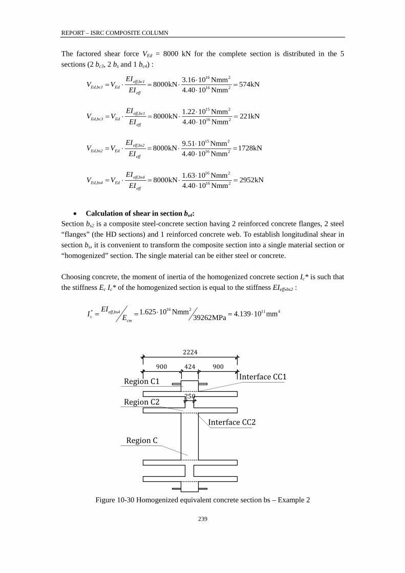
REPORT – ISRC COMPOSITE COLUMN
239
The factored shear force VEd = 8000 kN for the complete section is distributed in the 5 sections (2 bc3, 2 bs and 1 bc4) :
16 2
16 2
3.16 10 Nmm8000kN 574kN4.40 10 Nmm
eff,bc1Ed,bc1 Ed
eff
EIV V
EI⋅
= ⋅ = ⋅ =⋅
15 2
16 2
1.22 10 Nmm8000kN 221kN4.40 10 Nmm
eff,bc1Ed,bc3 Ed
eff
EIV V
EI⋅
= ⋅ = ⋅ =⋅
15 2
16 2
9.51 10 Nmm8000kN 1728kN4.40 10 Nmm
eff,bs2Ed,bs2 Ed
eff
EIV V
EI⋅
= ⋅ = ⋅ =⋅
16 2
16 2
1.63 10 Nmm8000kN 2952kN4.40 10 Nmm
eff,bs4Ed,bs4 Ed
eff
EIV V
EI⋅
= ⋅ = ⋅ =⋅
• Calculation of shear in section bs4:
Section bs2 is a composite steel-concrete section having 2 reinforced concrete flanges, 2 steel “flanges” (the HD sections) and 1 reinforced concrete web. To establish longitudinal shear in section bs, it is convenient to transform the composite section into a single material section or “homogenized” section. The single material can be either steel or concrete. Choosing concrete, the moment of inertia of the homogenized concrete section Ic* is such that the stiffness Ec Ic* of the homogenized section is equal to the stiffness EIeff,bs2 :
16 2* 11 4c
1.625 10 Nmm 4.139 10 mm39262MPaeff,bs4
cm
EII E⋅= = = ⋅
900Interface CC1
424 900
2224
250
Interface CC2
Region C
Region C1
Region C2
Figure 10-30 Homogenized equivalent concrete section bs – Example 2
REPORT – ISRC COMPOSITE COLUMN
240
In a homogenized concrete section (Figure 10-30), the width of the concrete equivalent to the width of the steel flanges is:
206000MPa424mm 2224mm39262MPa* ss s4
cm
Eb b E= ⋅ = ⋅ =
The width of the concrete equivalent to the width of the steel web is:
206000MPa47.6mm 250mm39262MPa* sw w
cm
Et t E= ⋅ = ⋅ =
The resultant longitudinal shear force on interfaces like CC1 and CC2 in Figure 10-30 is:
*c
SEd,bs2Ed,l
VV
I⋅
=
where: S is the first moment of areas of regions C1 or C2 taken about the neutral axis of the section as illustrated in Figure 10-30. Using S, the longitudinal shear is calculated at the steel-concrete interfaces CC1 and CC2 in order to size the force transfer mechanisms required for the member to act as a fully composite section.
• Calculation of longitudinal shear force applied at interface CC1:
SCC1 is the section modulus for the region C1 as defined in Figure 10-30: The height of the C1 region is:
' 1800mm 474mm513mm 150mm11 sy
h dh - d + - +2 2 2 2
= = =
The area is:
' 2424mm 150mm 63600mm1 1A b h= ⋅ = ⋅ =
'2 7 31800mm 150mm63600mm 5.247 10 mm
21 1
CC1 1h hS A - -
2 2 2 = ⋅ = ⋅ = ⋅
The resultant longitudinal shear force on interface CC1 is:
7 3
* 11 4c
2952kN 5.247 10 mm N3744.139 10 mm mm
Ed,bs CC1Ed,CC1
V SV
I⋅ ⋅ ⋅
= = =⋅
On 1-meter length of column:
kN374mEd,CC1V =

REPORT – ISRC COMPOSITE COLUMN
241
• Calculation of longitudinal shear force applied at interface CC2: SCC2 is the section modulus for the combined regions C1 and C2 (the HD profile): The equivalent area in concrete for the HD profile is:
Aa =80800 mm2
The equivalent are in concrete for the HD profile is:
2 2206000MPa80800mm 423942mm39262MPa* sa a
cm
EA A E= ⋅ = ⋅ =
The distance of HD center to the neutral axis is:
syd = 513 mm
The moment of area of the equivalent steel profile is:
2 8 3423942mm 513mm 2.175 10 mm*HD a syS A d= ⋅ = ⋅ = ⋅
Area of concrete between the flanges:
2 2c _ CC2 424mm 474mm 80800mm 120176mm*
aA b d-A= ⋅ = ⋅ − =
Moment of area of concrete between the flanges:
2 7 3c _ CC2 c _ CC2 120176mm 513mm 6.165 10 mm* *
syS A d= ⋅ = ⋅ = ⋅
The section modulus of combined regions C1 and C2, is equal to:
7 3 8 3 7 3 8 3c _ CC2 6.165 10 mm 2.175 10 mm 5.247 10 mm 3.334 10 mm*
CC2 HD CC1S S S S= + + = ⋅ + ⋅ + ⋅ = ⋅
The resultant longitudinal shear force at interface CC2 is:
8 3
* 11 4c
2952kN 3.334 10 mm N23784.139 10 mm mm
Ed,bs CC2Ed,CC2
V SV
I⋅ ⋅ ⋅
= = =⋅
On 1-meter length of column:
kN2378mEd,CC2V =
REPORT – ISRC COMPOSITE COLUMN
242
• Evaluation of necessary amount of shear studs: Geometrical characteristic of the shear studs correspond to State of Art – Table 3.2.2 where:
d = 25 mm – diameter of the shear stud; fu = 450 MPa – maximum stud tensile strength;
For a shear stud with a diameter d = 25 mm, the design shear strength is equal to:
( ) ( )= min 0.43 0.7 min 273.3kN,154.4kN 154.4kNRk s c c u sP A E f , f A = =
For a length of a column of 1 m, the necessary amount of shear studs to different interfaces is:
kN374 1m1m m 2.42 3 studs /1m154.4kN
Ed1_CC1studs_CC1
Rk
Vn
P
⋅⋅= = = ⇒
kN2378 1m1m m 15.4 18 studs /1m154.4kN
Ed1_CC2studs_CC2
Rk
Vn
P
⋅⋅= = = ⇒
Suppose the studs are installed in three rows, then the space of the studs is 167mm. The JGJ code specifies that the space should not be less than 6 times the diameter of the stud, which is 150mm in this example. The space is OK.

REPORT – ISRC COMPOSITE COLUMN
243
REPORT – ISRC COMPOSITE COLUMN
244
11 Conclusions
The results of the static and quasi-static tests on reinforced columns with four encased steel sections have been validated with FEM methods and compared with simplified code provisions methods. The simplified methods provided by codes are generally valid for composite compression members with one steel encased section. However, research program results show that code provisions are valid also for mega columns with more than one encased steel section. 1) Simplified design approaches are proposed and described in this report in accordance with Chinese codes JGJ 138. The design approaches are applicable to mega columns within a 15% eccentricity ratio. 2) A new extended method based on Eurocode 4 design has been developed in order to design the composite columns with several steel profiles embedded. The method is an extension of the Plastic Distribution Method and takes into account all the assumptions that are defined in EC 4 - Clause 6.7. Two numerical models have been created in order to simulate the behavior of experimental tests. Comparing the adapted simplified method and the two simplified numerical models created in Abaqus and Safir, similar results to the experimental part are obtained. The Adapted Distribution Method N – M interaction diagram has been obtained based on a simple method presented in the European design code EC4. These expressions have been developed for the cases of composite sections with several encased steel profiles and they are presented in Chapter 9. The simplified method can be used to quickly and easily do a manual evaluation of the axial force-bending moment interaction curve. 3) The current ACI 318, AISC-LRFD, Eurocode4, and JGJ 138 are evaluated in this test program. For the test specimens, the current codes are able to provide precise predictions on the axial and flexural capacities with sufficient margins of safety. 4) The finite element analyses are conducted as a supplementary to the test research. FEA demonstrated that the interface strength and stiffness influenced the capacity of mega columns dramatically when subjected lateral loads. This implied that the shear demand on the interfaces became much larger when the steel profiles were separate from one another. More thoughtful analyses imply that the enhancement in capacity was contributed by both the interface strength and interface stiffness, and that the efficiency of shear studs got smaller as the number of shear studs grew. In a real structure, however, the shear force between the concrete and the steel profiles is contributed by shear studs, bond stress, and friction, but the FEA results only reflect the influence of shear studs. With the existence of bond stress and friction, the influence of shear studs in a real structure may not be as significant as it is shown in the FEA.
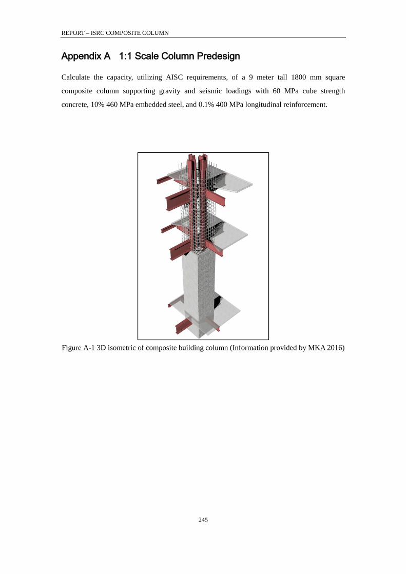
REPORT – ISRC COMPOSITE COLUMN
245
Appendix A 1:1 Scale Column Predesign
Calculate the capacity, utilizing AISC requirements, of a 9 meter tall 1800 mm square
composite column supporting gravity and seismic loadings with 60 MPa cube strength
concrete, 10% 460 MPa embedded steel, and 0.1% 400 MPa longitudinal reinforcement.
Figure A-1 3D isometric of composite building column (Information provided by MKA 2016)

REPORT – ISRC COMPOSITE COLUMN
246
A.1 Determine the material properties of the column
Table A-1 Material Properties
Material Grade Yield Stress (MPa)
Unit Weight (kg/m3)
Modulus of Elasticity
(E - MPa)
Concrete C60 50a 1500b 17664c
Embedded Steel HISTAR
460
460d 7850 200,000
Rebar HRB400 400d 7850 200,000
a. 21 MPa ≤ f’c ≤ 70 MPa
C60 refers to 60 MPa 28 day cube strength; however,
AISC requirements are with respect to 28 day cylinder
strength, which is 50 MPa for C60 concrete.
b. 1442 kg/m3 ≤ wc ≤ 2563 kg/m3
c. Ec = 0.043wc1.533f ′c
d. Fy ≤ 525 Mpa
[AISC I1.3(1)]
[AISC I2.1.1b]
[AISC I2.1.1b]
[AISC I1.3(2)]
A.2 Determine column unbraced length and effective length factor
Figure A-2 Column free body diagram (Information provided by MKA 2016)
REPORT – ISRC COMPOSITE COLUMN
247
The assumed buckled shape and boundary restraints for the column are shown in Figure A.1
above. The building’s floor diaphragms are assumed to restrain translational movement in
the x and y directions at the top and bottom of the column as indicated by the dashed arrows.
Additionally, the incoming floor framing connections are assumed to provide negligible
rotational stiffness; therefore, the column is assumed to freely rotate about each axis at its top
and bottom. Based on these assumed boundary conditions, the buckled shape (indicated by
the dashed line) and effective length factor, K, are determined per AISC Table C-A-7.1.
Column unbraced length:
Lb = 9 m
Colum effective length factor:
Kx = 1.0
For composite columns with floor diaphragms at the top and bottom, K = 1.0 is a conservative
value as there is some inherent rotational stiffness in the incoming floor framing. Taking this
stiffness into account will result in lower K values as calculated per AISC Appendix 7.
A.3 Select embedded steel shapes, and longitudinal reinforcement
Use an 1800 mm X 1800 mm section with (4) HD400X634 embedded steel shapes and (32)
32mm diameter longitudinal reinforcing bars (9 bars along each face).
Gross area of column section: Ag = B × H = 1800 mm × 1800 mm = 3,240,000 mm2 Area of embedded steel shapes: As = 4 × 80,800 mm2 = 323,2000 mm2 ρs ≥ 1% [AISC I2.1.1a(1)]
ρs = AsAg
= 323,200 mm2
3,240,000 mm2 = 9.98% ≥ 1% (𝑂𝐾)

REPORT – ISRC COMPOSITE COLUMN
248
Area of longitudinal reinforcement:
Asr = 32 × π 3222
= 25,736 mm2
ρsr ≥ 0.4% [AISC I2.1.1a(3)]
ρsr = AsrAg
= 25,736 mm2
3,240,000 mm2 = 0.79% ≥ 0.4% (𝑂𝐾)
Area of concrete: Ac = Ag − As − Asr = 3,240,000 mm2 − 323,200 mm2 − 25,736 mm2 = 2,891,064 mm2
Figure A-3 Column section (Information provided by MKA 2016)
A.4 Determine the column axial capacity
Compressive strength reduction factor:
Φc = 0.75 [AISC I2.1.1b]
Nominal axial compressive strength:
If Pno
Pe ≤ 2.25: Pn = Pno 0.658
PnoPe
If PnoPe
> 2.25: Pn = 0.877Pe [AISC I2.1.1b (I2-2 & I2-3)]
REPORT – ISRC COMPOSITE COLUMN
249
Where: Pno = FyAs + FysrAsr + 0.85f′cAc [AISC I2.1.1b (I2-4)] = 460 MPa × 323,200 mm2 + 400 MPa × 25,736 mm2 + 0.85 × 50 MPa × 2,891,064 mm2 = 281,836,594 N = 281,837 kN
𝑃𝑒 = 𝜋2𝐸𝐼𝑒𝑓𝑓(𝐾𝐿)2 [AISC I2.1.1b (I2-5)]
EIeff = EsIs + 0.5EsrIsr + C1EcIc [AISC I2.1.1b (I2-6)]
C1 = 0.1 + 2 AsAs+Ac
≤ 0.3 [AISC I2.1.1b (I2-7)]
= 0.1 + 2 323,200 mm2
323,200 mm2+2,891,064 mm2 = 0.3011 > 0.3
= 0.3 Is = 2 × IX,HD400X634 + 2 × AHD400X634 × dHD400X634
2 + 2 × IY,HD400X634 = 2 × 2.74 × 109 mm4 + 2 × 80,800 mm2 × (513 mm2)2 + 2 × 9.89 × 108 𝑚𝑚4 = 4.99 × 10¹⁰ 𝑚𝑚4 Isr = ∑I32mm rebar + A32mm rebar × ey,rebar
2 = 1.22 × 1010 mm4
Ic = BH3
12= 1800 mm × (1800 mm)3
12= 8.75 × 1011 mm4
EIeff = 200,000 MPa × 4.99 × 1010 mm4 + 0.5 × 200,000 MPa × 1.22 × 1010 mm4 + 0.3 × 17,664 MPa × 8.75 × 1011 mm4 = 1.58 × 10¹⁶ N− mm2 = 1.58 × 10¹³ kN− mm2
Pe = π2 × 1.58×1013 kN−mm2
(1.0 × 1000 × 9 m)2 = 1,928,744 kN
𝑃𝑛𝑜𝑃𝑒
= 281,837 𝑘𝑁1,928,744 𝑘𝑁
= 0.146 ≤ 2.25
PnoPe
≤ 2.25: Pn = 281,837 kN × (0.6580.146) = 265,116 kN
ΦPn = 0.75 × 265,116 kN = 198,837 kN

REPORT – ISRC COMPOSITE COLUMN
250
A.5 Determine the axial reduction factor for the maximum unbraced length
When calculating the axial-flexure (P-M) interaction diagram to determine the true column
capacity, an axial reduction factor (l) is applied to the axial capacities determined from the
strain-compatibility and plastic stress distribution methods. This axial reduction factor
serves to account for the reduced axial capacity due to buckling of the maximum unbraced
length of the column. The axial reduction factor is calculated as the ratio of the nominal
axial capacity (Pn) to the plastic axial capacity (Pno).
λ = PnPno
= 189,703 kN281,837 kN
= 0.897 [AISC Fig. C-I5.2]
A.6 Determine the P-M interaction diagram
Per AISC I1.2, it is permitted to use either the plastic stress distribution method, or the
strain-compatibility method to determine the strength of the encased composite section. AISC
P-M interaction capacities for bending about the x axis as determined by both the strain
compatibility and full plastic stress distributions are presented below in Figure A.4.
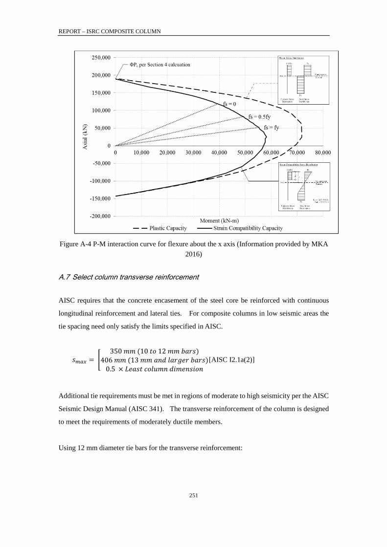
REPORT – ISRC COMPOSITE COLUMN
251
Figure A-4 P-M interaction curve for flexure about the x axis (Information provided by MKA
2016)
A.7 Select column transverse reinforcement
AISC requires that the concrete encasement of the steel core be reinforced with continuous
longitudinal reinforcement and lateral ties. For composite columns in low seismic areas the
tie spacing need only satisfy the limits specified in AISC.
𝑠𝑚𝑎𝑥 = 350 𝑚𝑚 (10 𝑡𝑜 12 𝑚𝑚 𝑏𝑎𝑟𝑠)
406 𝑚𝑚 (13 𝑚𝑚 𝑎𝑛𝑑 𝑙𝑎𝑟𝑔𝑒𝑟 𝑏𝑎𝑟𝑠)0.5 × 𝐿𝑒𝑎𝑠𝑡 𝑐𝑜𝑙𝑢𝑚𝑛 𝑑𝑖𝑚𝑒𝑛𝑠𝑖𝑜𝑛
[AISC I2.1a(2)]
Additional tie requirements must be met in regions of moderate to high seismicity per the AISC
Seismic Design Manual (AISC 341). The transverse reinforcement of the column is designed
to meet the requirements of moderately ductile members.
Using 12 mm diameter tie bars for the transverse reinforcement:

REPORT – ISRC COMPOSITE COLUMN
252
Required extent of hinge-zone ties:
Lo = Max
16
LbMax(B, H)450 mm
= Max 1500 mm1800 mm450 mm
[AISC 341 D1.4b(1)(2)]
= 1800 mm
Maximum spacing of ties:
smax = Min
⎣⎢⎢⎢⎡12
Min(B, H)8db,Longit24db,Ties300 mm
= Min 900 mm256 mm288 mm300 mm
[AISC 341 D1.4b(1)(1)]
= 256 mm; Used 200 mm (𝑂𝐾)
Note that, per AISC 341 D1.4b(1)(3), tie spacing outside of the 1800 mm hinge zones is not
permitted to exceed two times the smax calculated above.
The User Note in AISC I2.1.1a requires that ACI 318 sections 7.10 and 10.9.3 be satisfied in
addition to AISC tie requirements (10.9.3 pertains to spiral reinforcement and does not apply
to this example). Six legs of transverse reinforcement (two legs from exterior hoop and four
additional cross-ties) are provided in each direction to satisfy clear spacing requirements of
laterally unsupported longitudinal reinforcement.
sh,longit ≤ 152 mm [ACI 318-11 7.10.5.3]
sh,ties = B−2 ×covernlegs−1
= 1800 mm−2 ×40 mm6−1
= 344 mm
Ties are provided at no less than every other longitudinal bar.
sh,Longit = 12
sh,ties − db,Longit = 12
× 344 mm − 32 mm
= 140 mm < 152 𝑚𝑚 (𝑂𝐾)
REPORT – ISRC COMPOSITE COLUMN
253
A.8 Select load transfer mechanism between steel and concrete
For the test specimen design, mechanically connecting the concrete to the embedded steel
shapes is ensured through 20 mm diameter nelson stud engagement. Full capacity behavior
within a composite section when steel and concrete are combined is a research project goal.
For a typical design, load transfer required (V’r) is calculated based on whether the load
applying element (typically floor framing) is connected to steel:
V′r = Pr1− FyAs Pno⁄ [AISC I6.2a (I6-1)]
Or concrete:
V′r = PrFyAs Pno⁄ [AISC I6.2b (I6-2)]
Where Pr is the ultimate load applied at the connection point.
For example, if Pr for each embedded steel column of the test specimen is 3983 kN:
V′r = 3983 kN × (1 − (4 × 460 MPa × 80,800 mm2) 281,837 kN⁄ )
= 3983 kN × .472 = 1880 kN
V’r must then be transferred over the load introduction length (LIL), which extends above and
below the connecting element by two times the minimum dimension of the column parallel to
the incoming framing (see AISC Fig. C-I6.1).
Load introduction length:
LIL = 2 × (2 × B) + Connection Depth [AISC Fig. C-I6.1]
= 2 × (2 × 1800 𝑚𝑚) + 0(𝑐𝑜𝑛𝑛𝑒𝑐𝑡𝑖𝑜𝑛 𝑑𝑒𝑝𝑡ℎ 𝑛𝑒𝑔𝑙𝑒𝑐𝑡𝑒𝑑) = 7200 𝑚𝑚
Strength reduction factor for steel headed stud anchor in composite component:
Φv = 0.65 [AISC I8.3a]
Capacity of a single 20mm diameter nelson stud:
Qn = FuAsa [AISC I8.3a (I8-3)]
Qn = 460 MPa × π × 2022
= 144.4 kN
ΦQn = 0.65 × 144.4 kN = 94 kN
Determine number of studs required to transfer load:
n = V′rΦQn
= 1880 kN94 kN
= 20 studs per embedded steel column
With attaching studs to each flange and each side of the web:
ncolumn face = 20 ÷ 4 = 5 studs per face
REPORT – ISRC COMPOSITE COLUMN
254
Stud spacing required:
srequired = LILncolumn face
= 7200 mm5
= 1440 mm
smin = 4∅ = 4 × 20 mm = 80 mm (𝑂𝐾) [AISC I8.3e] smax = 32∅ = 32 × 20 mm = 640 mm (𝐶𝑜𝑛𝑡𝑟𝑜𝑙𝑠) [AISC I8.3e] sprovided = 400 mm < 640 𝑚𝑚 (𝑂𝐾)
The stud density of the test specimen, though, is potentially more than what may be required
from actual conditions in practice. Unlike the limitations due to the test specimen sizes, a
composite mega column will have multiple floors over which to develop the full capacity of
the embedded steel section. In actual practice, the engineer needs to consider a mechanical
interaction between concrete and steel to achieve the following:
Develop the contributory load from any one floor, over the load introduction length of
that floor.
Ensure concrete confinement for the concrete within the composite section, not
allowing the concrete/steel interface to be the weak link in the system.
Ensure strain compatibility can be maintained between the concrete and steel, so full
section capacities can be achieved.
Further research and code defined guidance is encouraged around the topic of
composite nelson stud minimum densities, or other forms of mechanical engagement
between the concrete and steel.

REPORT – ISRC COMPOSITE COLUMN
255
REPORT – ISRC COMPOSITE COLUMN
256
12 References
1. COMPOSITE MEGA COLUMNS WITH ENCASED STEEL SECTIONS:
EXPERIMENTAL CAMPAIGN. First methodological report. March – August 2014
2. COMPOSITE MEGA COLUMNS WITH ENCASED STEEL SECTIONS:
EXPERIMENTAL CAMPAIGN. Peer reviewers’ comments and responses of the research
team. November 2014
3. COMPOSITE MEGA COLUMNS WITH ENCASED STEEL SECTIONS:
EXPERIMENTAL CAMPAIGN. Third report: August 2014 – July 2015
4. COMPOSITE MEGA COLUMNS WITH ENCASED STEEL SECTIONS:
EXPERIMENTAL CAMPAIGN. Final report: December 2015 5. “DESIGN OF COLUMN WITH SEVERAL ENCASED STEEL PROFILES FOR COMBINED COMPRESSION AND BENDING”, A. Plumier, T. Bogdan, H. Degèe
6. “DESIGN FOR SHEAR OF COLUMNS WITH SEVERAL ENCASED STEEL
PROFILES. A PROPOSAL.”, A. Plumier, T. Bogdan, H. Degèe
All references listed above can be requested via e-mail to: Dario Trabucco;
13 Code References
1) Eurocode 4 (2004): Design of composite steel and concrete structures
2) AISC (2015): Specifications for Structural Steel Buildings – draft version
3) ACI 318-14: Building code requirements for structural concrete
4) Chinese code JGJ 138-2016: Code for Design of Composite Structures

Council on Tall Buildings and Urban Habitat | www.ctbuh.org | www.skyscrapercenter.com
Global Headquarters: The Monroe Building, 104 South Michigan Avenue, Suite 620, Chicago, IL 60608, USA | 1 (312) 283-5599 | [email protected] Research & Academic Office: Iuav University of Venice, Dorsoduro 2006, 30123, Venice, Italy | +39 041 257 1276 | [email protected]
Asia Headquarters: Wenyuan Building, Tongji University, 1239 Si Ping Rd, Yangpu District, Shanghai, China 200092 | +86 21 65982972 | [email protected]