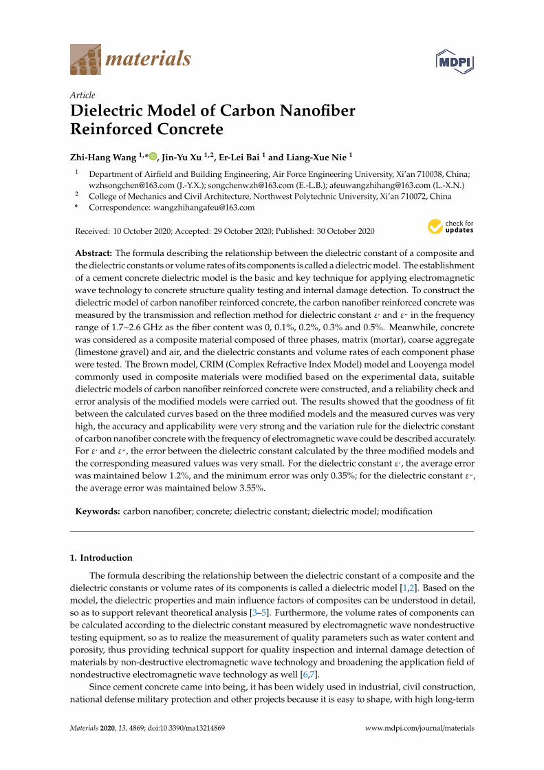
materials

Article

Dielectric Model of Carbon NanofiberReinforced Concrete

Zhi-Hang Wang 1,* , Jin-Yu Xu 1,2, Er-Lei Bai 1 and Liang-Xue Nie 1

1 Department of Airfield and Building Engineering, Air Force Engineering University, Xi’an 710038, China;wzhsongchen@163.com (J.-Y.X.); songchenwzh@163.com (E.-L.B.); afeuwangzhihang@163.com (L.-X.N.)

2 College of Mechanics and Civil Architecture, Northwest Polytechnic University, Xi’an 710072, China* Correspondence: wangzhihangafeu@163.com

Received: 10 October 2020; Accepted: 29 October 2020; Published: 30 October 2020�����������������

Abstract: The formula describing the relationship between the dielectric constant of a composite andthe dielectric constants or volume rates of its components is called a dielectric model. The establishmentof a cement concrete dielectric model is the basic and key technique for applying electromagneticwave technology to concrete structure quality testing and internal damage detection. To construct thedielectric model of carbon nanofiber reinforced concrete, the carbon nanofiber reinforced concrete wasmeasured by the transmission and reflection method for dielectric constant ε, and ε„ in the frequencyrange of 1.7~2.6 GHz as the fiber content was 0, 0.1%, 0.2%, 0.3% and 0.5%. Meanwhile, concretewas considered as a composite material composed of three phases, matrix (mortar), coarse aggregate(limestone gravel) and air, and the dielectric constants and volume rates of each component phasewere tested. The Brown model, CRIM (Complex Refractive Index Model) model and Looyenga modelcommonly used in composite materials were modified based on the experimental data, suitabledielectric models of carbon nanofiber reinforced concrete were constructed, and a reliability check anderror analysis of the modified models were carried out. The results showed that the goodness of fitbetween the calculated curves based on the three modified models and the measured curves was veryhigh, the accuracy and applicability were very strong and the variation rule for the dielectric constantof carbon nanofiber concrete with the frequency of electromagnetic wave could be described accurately.For ε, and ε„, the error between the dielectric constant calculated by the three modified models andthe corresponding measured values was very small. For the dielectric constant ε,, the average errorwas maintained below 1.2%, and the minimum error was only 0.35%; for the dielectric constant ε„,the average error was maintained below 3.55%.

Keywords: carbon nanofiber; concrete; dielectric constant; dielectric model; modification

1. Introduction

The formula describing the relationship between the dielectric constant of a composite and thedielectric constants or volume rates of its components is called a dielectric model [1,2]. Based on themodel, the dielectric properties and main influence factors of composites can be understood in detail,so as to support relevant theoretical analysis [3–5]. Furthermore, the volume rates of components canbe calculated according to the dielectric constant measured by electromagnetic wave nondestructivetesting equipment, so as to realize the measurement of quality parameters such as water content andporosity, thus providing technical support for quality inspection and internal damage detection ofmaterials by non-destructive electromagnetic wave technology and broadening the application field ofnondestructive electromagnetic wave technology as well [6,7].

Since cement concrete came into being, it has been widely used in industrial, civil construction,national defense military protection and other projects because it is easy to shape, with high long-term

Materials 2020, 13, 4869; doi:10.3390/ma13214869 www.mdpi.com/journal/materials

Materials 2020, 13, 4869 2 of 18

strength and low cost [8–11]. For this, there have been many studies on concrete mix proportion,relevant mechanical properties, durability, constitutive relation and dielectric models [12,13]. MohamedAB et al. studied the relationship between the dielectric constant of concrete and the moisture contentand found that the dielectric constant of concrete increases with the increase in moisture content.The moisture content of a concrete structure can be judged by testing the dielectric constant [14].Ya P.T. et al. designed and employed a nondestructive method to monitor the early hydration ofconcrete mixes and found that the dielectric properties of concrete mix can be used as an effective wayof studying the hydration progress of concrete during hydration [15]. Hashem A found that dielectricproperties are useful parameters for the detection of chloride in concrete material, and the amount ofchloride present in concrete can be determined [16]. Thus, the dielectric model of cement concreteis the basis for quality control and subsequent damage detection of concrete structures and has veryimportant theoretical value and engineering significance [17–19].

Carbon nanofiber reinforced concrete is a composite of good performance, with ordinary concreteas the base material and carbon nanofiber as the reinforced material [20–23]. Compared with ordinaryconcrete, carbon nanofiber reinforced concrete was greatly improved in not only the mechanicalproperties and durability [22–26] but also the dielectric properties [27–31]. Recently, scholars allover the world have conducted many studies on the dielectric model of cement concrete based ontemperature and frequency, with the chloride effect considered, but there are few reports on thedielectric model of carbon nanofiber reinforced concrete [32–35].

For this, this study utilized the transmission and reflection method to test the dielectric constantof carbon nanofiber reinforced concrete under different fiber content in the frequency range of 1.7 to2.6 GHz and established a modified dielectric model for the Brown model, CRIM model and Looyengamodel based on the experimental data.

2. Tests and Results

2.1. Materials and Specimen Preparation

The raw materials for the preparation of carbon nanofiber reinforced concrete were as follows:cement (Shaanxi Qinling Cement Group, Xi’an, China), gravel, sand, admixtures (water reducing agent(Shaanxi Haoyu Concrete Admixture Co., Ltd., Xi’an, China), defoamer (Shaanxi Lanxin Chemical Co.,Ltd., Xi’an, China)), water and carbon nanofiber (Beijing Dekedaojin Technology Co., Ltd., Beijing,China). The mix proportion of carbon nanofiber reinforced concrete was as shown in Table 1, where PCrepresents an ordinary concrete specimen without carbon nanofiber as the reference group specimen,while CNFRC1, CNFRC2, CNFRC3 and CNFRC5, respectively, represent nanofiber reinforced concretespecimens with carbon fiber content (v/v) of 0.1%, 0.2%, 0.3% and 0.5%.

Table 1. Mix proportion of carbon nanofiber reinforced concrete (kg/m3).

SpecimenNumber

Water CementRatio

CarbonNanofiber Cement Water Gravel Sand Water Reducing

Agent Defoamer

PC 0.36 0 495 180 1008 672 0 0CNFRC1 0.36 0.30 495 180 1008 672 5.0 0.30CNFRC2 0.36 0.45 495 180 1008 672 7.5 0.45CNFRC3 0.36 0.60 495 180 1008 672 10.0 0.60CNFRC5 0.36 0.90 495 180 1008 672 15.0 0.90

The preparation of carbon nanofiber reinforced concrete was based on the “sand envelopedmethod “, and the specific process was as shown in Figure 1. The freshly mixed concrete was placed ina steel mold and then on a vibrating table for vibration molding. The specimen was removed afterbeing placed in a room for 24 h, and then we performed 28 days of standard curing. The dimensions ofthe specimen were 108.22 mm × 53.61 mm × 40.00 mm.

Materials 2020, 13, 4869 3 of 18

Materials 2020, 13, x FOR PEER REVIEW  3 of 19 

being placed in a room for 24 h, and then we performed 28 days of standard curing. The dimensions 

of the specimen were 108.22 mm × 53.61 mm × 40.00 mm. 

 

Figure  1. Preparation process of  carbon  fiber  reinforced  concrete.  (a) PC group of  specimens;  (b) 

CNFCR1, CNFCR2, CNFCR3 and CNFCR5 groups of specimens. 

2.2. Test Protocol 

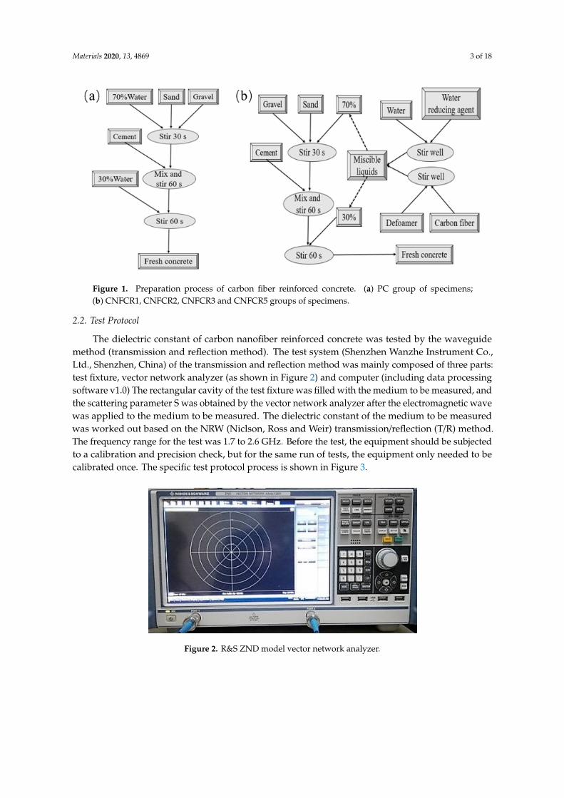
The dielectric constant of carbon nanofiber reinforced concrete was  tested by  the waveguide 

method (transmission and reflection method). The test system (Shenzhen Wanzhe  Instrument Co., 

Ltd.,  Shenzhen, China)  of  the  transmission and reflection method was mainly composed of  three 

parts:  test  fixture, vector network analyzer  (as  shown  in Figure 2) and  computer  (including data 

processing software v1.0) The rectangular cavity of the test fixture was filled with the medium to be 

measured, and  the scattering parameter S was obtained by  the vector network analyzer after  the 

electromagnetic wave was applied  to  the medium  to be measured. The dielectric  constant of  the 

medium  to  be  measured  was  worked  out  based  on  the  NRW  (Niclson,  Ross  and  Weir） transmission/reflection (T/R) method. The frequency range for the test was 1.7 to 2.6 GHz. Before the 

test, the equipment should be subjected to a calibration and precision check, but for the same run of 

tests, the equipment only needed to be calibrated once. The specific test protocol process is shown in 

Figure 3. 

 

Figure 2. R&S ZND model vector network analyzer. 

Figure 1. Preparation process of carbon fiber reinforced concrete. (a) PC group of specimens;(b) CNFCR1, CNFCR2, CNFCR3 and CNFCR5 groups of specimens.

2.2. Test Protocol

The dielectric constant of carbon nanofiber reinforced concrete was tested by the waveguidemethod (transmission and reflection method). The test system (Shenzhen Wanzhe Instrument Co.,Ltd., Shenzhen, China) of the transmission and reflection method was mainly composed of three parts:test fixture, vector network analyzer (as shown in Figure 2) and computer (including data processingsoftware v1.0) The rectangular cavity of the test fixture was filled with the medium to be measured, andthe scattering parameter S was obtained by the vector network analyzer after the electromagnetic wavewas applied to the medium to be measured. The dielectric constant of the medium to be measuredwas worked out based on the NRW (Niclson, Ross and Weir) transmission/reflection (T/R) method.The frequency range for the test was 1.7 to 2.6 GHz. Before the test, the equipment should be subjectedto a calibration and precision check, but for the same run of tests, the equipment only needed to becalibrated once. The specific test protocol process is shown in Figure 3.

Materials 2020, 13, x FOR PEER REVIEW  3 of 19 

being placed in a room for 24 h, and then we performed 28 days of standard curing. The dimensions 

of the specimen were 108.22 mm × 53.61 mm × 40.00 mm. 

 

Figure  1. Preparation process of  carbon  fiber  reinforced  concrete.  (a) PC group of  specimens;  (b) 

CNFCR1, CNFCR2, CNFCR3 and CNFCR5 groups of specimens. 

2.2. Test Protocol 

The dielectric constant of carbon nanofiber reinforced concrete was  tested by  the waveguide 

method (transmission and reflection method). The test system (Shenzhen Wanzhe  Instrument Co., 

Ltd.,  Shenzhen, China)  of  the  transmission and reflection method was mainly composed of  three 

parts:  test  fixture, vector network analyzer  (as  shown  in Figure 2) and  computer  (including data 

processing software v1.0) The rectangular cavity of the test fixture was filled with the medium to be 

measured, and  the scattering parameter S was obtained by  the vector network analyzer after  the 

electromagnetic wave was applied  to  the medium  to be measured. The dielectric  constant of  the 

medium  to  be  measured  was  worked  out  based  on  the  NRW  (Niclson,  Ross  and  Weir） transmission/reflection (T/R) method. The frequency range for the test was 1.7 to 2.6 GHz. Before the 

test, the equipment should be subjected to a calibration and precision check, but for the same run of 

tests, the equipment only needed to be calibrated once. The specific test protocol process is shown in 

Figure 3. 

 

Figure 2. R&S ZND model vector network analyzer. Figure 2. R&S ZND model vector network analyzer.

Materials 2020, 13, 4869 4 of 18

Materials 2020, 13, x FOR PEER REVIEW  4 of 19 

 

Figure 3. Test protocol flow chart. 

2.3. Test Results 

The test results for the dielectric constant of carbon nanofiber reinforced concrete specimens in 

the  frequency  range  of  1.7  to  2.6 GHz were  as  shown  in  Figure  4. Obviously,  for  the  dielectric 

constants of carbon nanofiber reinforced concrete, ε, was much higher than ε,,. With the increase in 

carbon nanofiber content, the dielectric constants of carbon nanofiber reinforced concrete, ε, and ε,, 

increased continuously, because the dielectric constant of carbon nanofiber was much higher than 

that of  the concrete. With  the  increase  in  frequency, ε,,  the dielectric constant of carbon nanofiber 

reinforced  concrete  increased  slowly  at  first,  then  decreased  slightly  and  showed  a  trend  of 

significant increase at last. 

 

Figure 4. Dielectric constant of carbon nanofiber reinforced concrete (a) ε, (b) ε,. 

3. Dielectric Model 

3.1. Dielectric Model Introduce 

The  composite  is  composed of at  least  two  substances while  the main  component phases of 

cement  concrete  include  cement  slurry  matrix,  coarse  aggregate,  fine  aggregate  and  water. 

Additionally, inside the cement concrete, there is a small amount of air. The dielectric constant of the 

Figure 3. Test protocol flow chart.

2.3. Test Results

The test results for the dielectric constant of carbon nanofiber reinforced concrete specimens inthe frequency range of 1.7 to 2.6 GHz were as shown in Figure 4. Obviously, for the dielectric constantsof carbon nanofiber reinforced concrete, ε, was much higher than ε„. With the increase in carbonnanofiber content, the dielectric constants of carbon nanofiber reinforced concrete, ε, and ε„ increasedcontinuously, because the dielectric constant of carbon nanofiber was much higher than that of theconcrete. With the increase in frequency, ε,, the dielectric constant of carbon nanofiber reinforcedconcrete increased slowly at first, then decreased slightly and showed a trend of significant increaseat last.

Materials 2020, 13, x FOR PEER REVIEW  4 of 19 

 

Figure 3. Test protocol flow chart. 

2.3. Test Results 

The test results for the dielectric constant of carbon nanofiber reinforced concrete specimens in 

the  frequency  range  of  1.7  to  2.6 GHz were  as  shown  in  Figure  4. Obviously,  for  the  dielectric 

constants of carbon nanofiber reinforced concrete, ε, was much higher than ε,,. With the increase in 

carbon nanofiber content, the dielectric constants of carbon nanofiber reinforced concrete, ε, and ε,, 

increased continuously, because the dielectric constant of carbon nanofiber was much higher than 

that of  the concrete. With  the  increase  in  frequency, ε,,  the dielectric constant of carbon nanofiber 

reinforced  concrete  increased  slowly  at  first,  then  decreased  slightly  and  showed  a  trend  of 

significant increase at last. 

 

Figure 4. Dielectric constant of carbon nanofiber reinforced concrete (a) ε, (b) ε,. 

3. Dielectric Model 

3.1. Dielectric Model Introduce 

The  composite  is  composed of at  least  two  substances while  the main  component phases of 

cement  concrete  include  cement  slurry  matrix,  coarse  aggregate,  fine  aggregate  and  water. 

Additionally, inside the cement concrete, there is a small amount of air. The dielectric constant of the 

Figure 4. Dielectric constant of carbon nanofiber reinforced concrete (a) ε, (b) ε,.

3. Dielectric Model

3.1. Dielectric Model Introduce

The composite is composed of at least two substances while the main component phases of cementconcrete include cement slurry matrix, coarse aggregate, fine aggregate and water. Additionally,

Materials 2020, 13, 4869 5 of 18

inside the cement concrete, there is a small amount of air. The dielectric constant of the compositeis not only related to the frequency of external electromagnetic field, but it is also greatly affected bythe structure and properties of the material itself, including the dielectric properties, volume rate, etc.In addition, it is also related to the environment of the material, e.g., temperature, humidity, and etc.The influence of these factors on the material may be transformed into a mathematical expression, so asto form a functional relationship between the main factors and the dielectric constant of the material,which is called the dielectric model of composite. At present, there are many dielectric models forcomposites. In this study, the dielectric model of carbon nanofiber reinforced concrete was constructedbased on three basic dielectric models: Brown model (linear model), CRIM model (root-mean-squaremodel) and Looyenga model (cube root model).

In the Lichtenecker–Rother (LR) model, each component phase inside the composite is regardedas a homogeneous medium, and the LR model expression is as follows.

(εm)c =

n∑i=1

vi(εi)c (1)

where εm is the dielectric constant of the composite; εi, vi, the dielectric constant and volume ofcomponent i for the material; c, factor of shape. The value of c depends on specific circumstances.It is related to the properties of the material. In fact, the value of c is generally between −1 and 1.Formula (1) can be evolved into the following common dielectric models dependent on different valuesof c:

When c = 1, the LR model is evolved into the Brown model, also known as the linear model.

εm =n∑

i=1

viεi (2)

When c = 0.5, the LR model is evolved into a complex refractive index model (CRIM), also knownas the root-mean-square model.

√εm =

n∑i=1

vi√εi (3)

When c = 1/3, the LR model is evolved into the Looyenga model, also known as the cuberoot model.

(εm)1/3 =

n∑i=1

vi(εi)1/3 (4)

3.2. Construction of Dielectric Model

3.2.1. Concept of Model Construction

For the component phases of carbon nanofiber reinforced concrete, such as cement, sand, gravel,water, fiber, admixture and internal air, when the corresponding dielectric constants are known,the dielectric constant of concrete can be calculated based on the dielectric model of composite. In fact,dielectric constants of materials such as fibers and admixtures are extremely difficult to obtain. At thesame time, due to factors such as pouring mode, curing conditions and external environment, it isdifficult to determine the hydration degree of cement, and thus, for the formed concrete, the volumerates of some phases (e.g., cement, water and admixtures) are difficult to measure. Therefore, it isnecessary to make some assumptions about the formed concrete and to eliminate the errors of thespecimens to be tested.

Considering that the Brown model (linear model), CRIM model (root mean square model) andLooyenga model (cube root model) are simply extensive models based on a composite, and a large

Materials 2020, 13, 4869 6 of 18

error may be caused if they are used directly, there should be a modification based on the three models,so as to construct an applicable dielectric model of carbon nanofiber reinforced concrete.

The three models regard component phases of the composite as independent ones which do notinterfere with each other. This paper considers that after the carbon nanofiber reinforced concrete isformed, the cement, water and admixture will form an independent matrix (mortar) after the physicaland chemical reaction. The matrix can be regarded as a single phase. The volume admixture method isused for the fiber, and the content of fiber is only 0.5%. Therefore, the influence of fiber on the dielectricparameters of concrete is negligible. The error exclusion treatment for the specimens is mainly for themoisture inside the specimens. Because it is difficult to accurately measure the moisture content ofthe concrete specimens at the end of curing, the specimens are dried to remove the free water inside.Therefore, the influence of water on the dielectric constant of the dehydrated specimens may alsobe neglected. The air phase inside the formed concrete cannot be ignored. Here, it is assumed thatall the pores inside the concrete are filled with air. Therefore, after certain assumptions and errorelimination treatment, the concrete is composed of three phases: matrix (mortar), coarse aggregate(limestone gravel) and air. Thus, the theoretical dielectric constant of concrete can be simply calculatedby the model after the dielectric constants of these three phases and their volume rates in concrete areworked out.

3.2.2. Determination of Dielectric Constants and Volume Rates of Each Component Phase

Generally, air is relatively stable in nature. Its dielectric constant is about 1, and its staticconductivity is 0. Since the dielectric parameters of air could be accurately measured with thetransmission and reflection method adopted in this study, relevant data from references were cited.

The coarse aggregate used in this test was limestone gravel. The gravel was cut and polishedinto specimens with dimensions of 108.22 mm × 53.61 mm × 40.00 mm, which were also tested bythe transmission and reflection method, and the test results were as shown in Figure 5. Obviously,for the dielectric constants of limestone gravel, ε, was far higher than ε„. The dielectric constants ε,

and ε„ were maintained at about 5.5 and 1.5, respectively, and both of them decreased slightly with theincrease in electromagnetic frequency. However, the amplitude of variation was not large on the whole.

Materials 2020, 13, x FOR PEER REVIEW  6 of 19 

formed,  the  cement, water  and  admixture will  form  an  independent matrix  (mortar)  after  the 

physical and chemical reaction. The matrix can be regarded as a single phase. The volume admixture 

method is used for the fiber, and the content of fiber is only 0.5%. Therefore, the influence of fiber on 

the dielectric parameters of concrete is negligible. The error exclusion treatment for the specimens is 

mainly  for  the moisture  inside  the  specimens.  Because  it  is  difficult  to  accurately measure  the 

moisture content of the concrete specimens at the end of curing, the specimens are dried to remove 

the free water inside. Therefore, the influence of water on the dielectric constant of the dehydrated 

specimens may also be neglected. The air phase inside the formed concrete cannot be ignored. Here, 

it  is  assumed  that  all  the  pores  inside  the  concrete  are  filled with  air.  Therefore,  after  certain 

assumptions  and  error  elimination  treatment,  the  concrete  is  composed  of  three  phases: matrix 

(mortar),  coarse  aggregate  (limestone  gravel)  and  air. Thus,  the  theoretical dielectric  constant  of 

concrete can be simply calculated by the model after the dielectric constants of these three phases 

and their volume rates in concrete are worked out. 

3.2.2. Determination of Dielectric Constants and Volume Rates of Each Component Phase 

Generally,  air  is  relatively  stable  in  nature.  Its  dielectric  constant  is  about  1,  and  its  static 

conductivity  is  0.  Since  the  dielectric  parameters  of  air  could  be  accurately measured with  the 

transmission and reflection method adopted in this study, relevant data from references were cited. 

The coarse aggregate used in this test was limestone gravel. The gravel was cut and polished into 

specimens with  dimensions  of  108.22 mm  ×  53.61 mm  ×  40.00 mm, which were  also  tested  by  the 

transmission and reflection method, and the test results were as shown in Figure 5. Obviously, for the 

dielectric constants of limestone gravel, ε, was far higher than ε,,. The dielectric constants ε, and ε,, were 

maintained at about 5.5 and 1.5, respectively, and both of them decreased slightly with the increase in 

electromagnetic frequency. However, the amplitude of variation was not large on the whole. 

 

Figure 5. Dielectric constant of limestone gravel. 

In order to obtain a cement mortar with matrix composition the same as the carbon nanofiber 

reinforced concrete, in this study, a cement mortar of the corresponding components was prepared 

additionally,  and  the  content  of  other  components  in  it  remained  the  same,  except  for  coarse 

aggregate. The test results for dielectric constants of cement mortar for each group were as shown in 

Figure 6. Obviously, compared with the complex dielectric constant of concrete in the same group as 

Figure 3, the complex dielectric constants of cement mortar were generally high. The main reason for 

this was that the complex dielectric constants of limestone gravel were relatively low. In addition, its 

variation  in  dielectric  constants  ε,  and  ε,,  with  electromagnetic  wave  frequency  was  generally 

consistent with that of concrete in the same group. With the increase in carbon nanofiber content, the 

dielectric  constants  of  cement mortar,  ε,  and  ε,,,  increased  continuously,  because  the  dielectric 

constant  of  carbon  nanofiber was  higher  than  that  of  the  cement mortar. With  the  increase  in 

frequency, ε, and ε,,, the dielectric constants of cement mortar in the PC group, decreased slightly, 

Figure 5. Dielectric constant of limestone gravel.

In order to obtain a cement mortar with matrix composition the same as the carbon nanofiberreinforced concrete, in this study, a cement mortar of the corresponding components was preparedadditionally, and the content of other components in it remained the same, except for coarse aggregate.The test results for dielectric constants of cement mortar for each group were as shown in Figure 6.Obviously, compared with the complex dielectric constant of concrete in the same group as Figure 3, thecomplex dielectric constants of cement mortar were generally high. The main reason for this was thatthe complex dielectric constants of limestone gravel were relatively low. In addition, its variation in

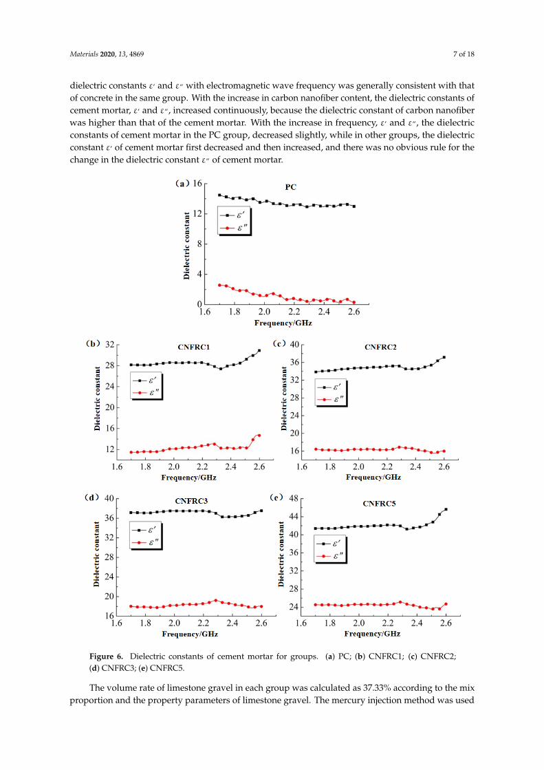
Materials 2020, 13, 4869 7 of 18

dielectric constants ε, and ε„ with electromagnetic wave frequency was generally consistent with thatof concrete in the same group. With the increase in carbon nanofiber content, the dielectric constants ofcement mortar, ε, and ε„, increased continuously, because the dielectric constant of carbon nanofiberwas higher than that of the cement mortar. With the increase in frequency, ε, and ε„, the dielectricconstants of cement mortar in the PC group, decreased slightly, while in other groups, the dielectricconstant ε, of cement mortar first decreased and then increased, and there was no obvious rule for thechange in the dielectric constant ε„ of cement mortar.

Materials 2020, 13, x FOR PEER REVIEW  7 of 19 

while in other groups, the dielectric constant ε, of cement mortar first decreased and then increased, 

and there was no obvious rule for the change in the dielectric constant ε,, of cement mortar. 

 

 

 

Figure 6. Dielectric constants of cement mortar for groups. (a) PC; (b) CNFRC1; (c) CNFRC2; (d) 

CNFRC3; (e) CNFRC5. 

The volume rate of limestone gravel in each group was calculated as 37.33% according to the 

mix proportion and the property parameters of limestone gravel. The mercury injection method was 

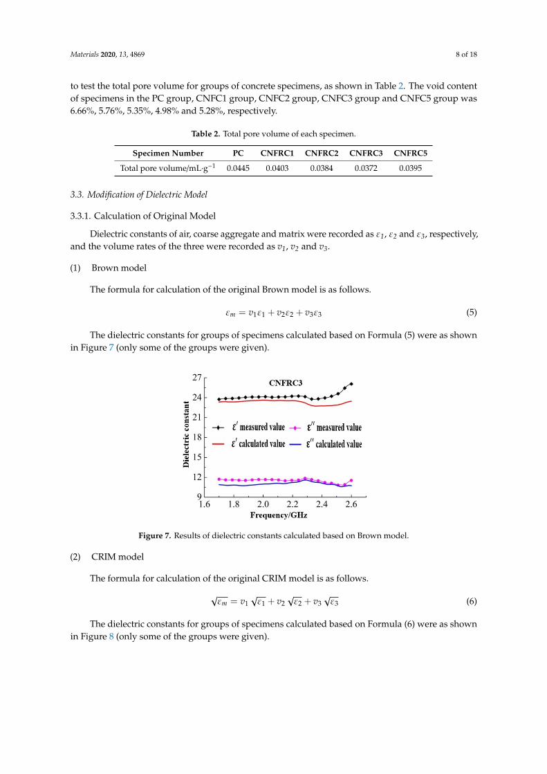
used to test the total pore volume for groups of concrete specimens, as shown in Table 2. The void 

content of  specimens  in  the PC group, CNFC1 group, CNFC2 group, CNFC3 group and CNFC5 

group was 6.66%, 5.76%, 5.35%, 4.98% and 5.28%, respectively. 

Figure 6. Dielectric constants of cement mortar for groups. (a) PC; (b) CNFRC1; (c) CNFRC2;(d) CNFRC3; (e) CNFRC5.

The volume rate of limestone gravel in each group was calculated as 37.33% according to the mixproportion and the property parameters of limestone gravel. The mercury injection method was used

Materials 2020, 13, 4869 8 of 18

to test the total pore volume for groups of concrete specimens, as shown in Table 2. The void contentof specimens in the PC group, CNFC1 group, CNFC2 group, CNFC3 group and CNFC5 group was6.66%, 5.76%, 5.35%, 4.98% and 5.28%, respectively.

Table 2. Total pore volume of each specimen.

Specimen Number PC CNFRC1 CNFRC2 CNFRC3 CNFRC5

Total pore volume/mL·g−1 0.0445 0.0403 0.0384 0.0372 0.0395

3.3. Modification of Dielectric Model

3.3.1. Calculation of Original Model

Dielectric constants of air, coarse aggregate and matrix were recorded as ε1, ε2 and ε3, respectively,and the volume rates of the three were recorded as v1, v2 and v3.

(1) Brown model

The formula for calculation of the original Brown model is as follows.

εm = v1ε1 + v2ε2 + v3ε3 (5)

The dielectric constants for groups of specimens calculated based on Formula (5) were as shownin Figure 7 (only some of the groups were given).

Materials 2020, 13, x FOR PEER REVIEW  8 of 19 

Table 2. Total pore volume of each specimen. 

Specimen Number  PC  CNFRC1  CNFRC2  CNFRC3  CNFRC5 

Total pore volume/mL∙g−1  0.0445  0.0403  0.0384  0.0372  0.0395 

3.3. Modification of Dielectric Model 

3.3.1. Calculation of Original Model 

Dielectric  constants  of  air,  coarse  aggregate  and  matrix  were  recorded  as  ε1,  ε2  and  ε3, 

respectively, and the volume rates of the three were recorded as v1, v2 and v3. 

(1) Brown model 

The formula for calculation of the original Brown model is as follows. 

1 1 2 2 3 3m v v v   (5) 

The dielectric constants for groups of specimens calculated based on Formula (5) were as shown 

in Figure 7 (only some of the groups were given). 

 

Figure 7. Results of dielectric constants calculated based on Brown model. 

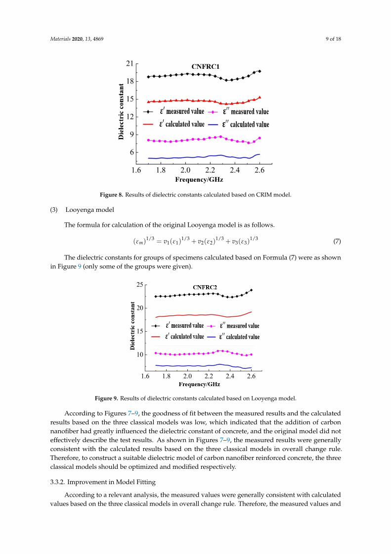
(2) CRIM model 

The formula for calculation of the original CRIM model is as follows. 

1 1 2 2 3 3m v v v   (6) 

The dielectric constants for groups of specimens calculated based on Formula (6) were as shown 

in Figure 8 (only some of the groups were given). 

Figure 7. Results of dielectric constants calculated based on Brown model.

(2) CRIM model

The formula for calculation of the original CRIM model is as follows.

√εm = v1

√ε1 + v2

√ε2 + v3

√ε3 (6)

The dielectric constants for groups of specimens calculated based on Formula (6) were as shownin Figure 8 (only some of the groups were given).

Materials 2020, 13, 4869 9 of 18

Materials 2020, 13, x FOR PEER REVIEW  9 of 19 

 

Figure 8. Results of dielectric constants calculated based on CRIM model. 

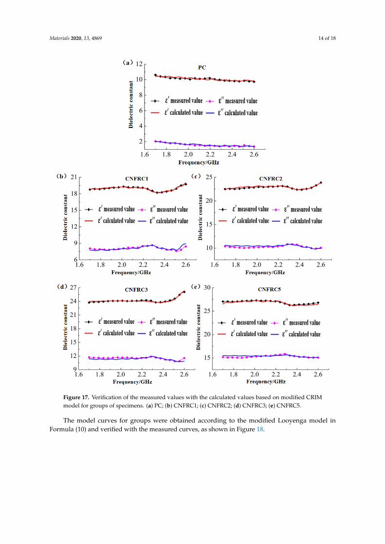
(3) Looyenga model 

The formula for calculation of the original Looyenga model is as follows. 

1/3 1/3 1/3 1/31 1 2 2 3 3( ) ( ) ( ) ( )m v v v   (7) 

The dielectric constants for groups of specimens calculated based on Formula (7) were as shown 

in Figure 9 (only some of the groups were given). 

 

Figure 9. Results of dielectric constants calculated based on Looyenga model. 

According to Figures 7–9, the goodness of fit between the measured results and the calculated 

results based on  the  three classical models was  low, which  indicated  that  the addition of carbon 

nanofiber had greatly influenced the dielectric constant of concrete, and the original model did not 

effectively describe the test results. As shown in Figures 7–9, the measured results were generally 

consistent with  the  calculated  results based on  the  three  classical models  in overall  change  rule. 

Therefore, to construct a suitable dielectric model of carbon nanofiber reinforced concrete, the three 

classical models should be optimized and modified respectively. 

3.3.2. Improvement in Model Fitting 

According to a relevant analysis, the measured values were generally consistent with calculated 

values based on  the  three classical models  in overall change rule. Therefore,  the measured values 

and calculated values were subjected to linear fitting first, and then the models were modified based 

on the fitting parameters. 

Figure 8. Results of dielectric constants calculated based on CRIM model.

(3) Looyenga model

The formula for calculation of the original Looyenga model is as follows.

(εm)1/3 = v1(ε1)

1/3 + v2(ε2)1/3 + v3(ε3)

1/3 (7)

The dielectric constants for groups of specimens calculated based on Formula (7) were as shownin Figure 9 (only some of the groups were given).

Materials 2020, 13, x FOR PEER REVIEW  9 of 19 

 

Figure 8. Results of dielectric constants calculated based on CRIM model. 

(3) Looyenga model 

The formula for calculation of the original Looyenga model is as follows. 

1/3 1/3 1/3 1/31 1 2 2 3 3( ) ( ) ( ) ( )m v v v   (7) 

The dielectric constants for groups of specimens calculated based on Formula (7) were as shown 

in Figure 9 (only some of the groups were given). 

 

Figure 9. Results of dielectric constants calculated based on Looyenga model. 

According to Figures 7–9, the goodness of fit between the measured results and the calculated 

results based on  the  three classical models was  low, which  indicated  that  the addition of carbon 

nanofiber had greatly influenced the dielectric constant of concrete, and the original model did not 

effectively describe the test results. As shown in Figures 7–9, the measured results were generally 

consistent with  the  calculated  results based on  the  three  classical models  in overall  change  rule. 

Therefore, to construct a suitable dielectric model of carbon nanofiber reinforced concrete, the three 

classical models should be optimized and modified respectively. 

3.3.2. Improvement in Model Fitting 

According to a relevant analysis, the measured values were generally consistent with calculated 

values based on  the  three classical models  in overall change rule. Therefore,  the measured values 

and calculated values were subjected to linear fitting first, and then the models were modified based 

on the fitting parameters. 

Figure 9. Results of dielectric constants calculated based on Looyenga model.

According to Figures 7–9, the goodness of fit between the measured results and the calculatedresults based on the three classical models was low, which indicated that the addition of carbonnanofiber had greatly influenced the dielectric constant of concrete, and the original model did noteffectively describe the test results. As shown in Figures 7–9, the measured results were generallyconsistent with the calculated results based on the three classical models in overall change rule.Therefore, to construct a suitable dielectric model of carbon nanofiber reinforced concrete, the threeclassical models should be optimized and modified respectively.

3.3.2. Improvement in Model Fitting

According to a relevant analysis, the measured values were generally consistent with calculatedvalues based on the three classical models in overall change rule. Therefore, the measured values and

Materials 2020, 13, 4869 10 of 18

calculated values were subjected to linear fitting first, and then the models were modified based on thefitting parameters.

It should be noted that although the rule for dielectric constants of the specimens within the wholetest frequency range was obvious, the values fluctuated greatly during the period. Especially for theCNFRC group, the linear fitting between measured values and calculated values were not satisfactory.Therefore, within the whole test frequency range, some representative points reflecting the variationrule for dielectric constants of the specimens were selected for fitting. This may not only improve theirfitting degree but also retain the overall rule, thus ensuring the reliability of the data.

(1) The fitting for the relation between measured values and calculated values based on the Brownmodel was as shown in Figures 10 and 11, respectively (only some groups were given).

Materials 2020, 13, x FOR PEER REVIEW  10 of 19 

It should be noted that although the rule for dielectric constants of the specimens within the whole 

test  frequency  range was obvious,  the values  fluctuated greatly during  the period. Especially  for  the 

CNFRC group, the linear fitting between measured values and calculated values were not satisfactory. 

Therefore, within the whole test frequency range, some representative points reflecting the variation rule 

for dielectric constants of the specimens were selected for fitting. This may not only improve their fitting 

degree but also retain the overall rule, thus ensuring the reliability of the data. 

(1) The fitting for the relation between measured values and calculated values based on the Brown 

model was as shown in Figures 10 and 11, respectively (only some groups were given). 

 

Figure 10. The  fitting  for  relation between measured values and calculated values  for  ε, based on 

Brown model. (a) PC; (b) CNFRC2. 

 

Figure 11. The  fitting  for relation between measured values and calculated values  for  ε,, based on 

Brown model. (a) PC; (b) CNFRC5. 

(2) The  fitting  for  the relation between measured values and calculated values based on  the 

CRIM model was as  shown  in Figures 12 and 13,  respectively  (only  some groups were 

given). 

Figure 10. The fitting for relation between measured values and calculated values for ε, based onBrown model. (a) PC; (b) CNFRC2.

Materials 2020, 13, x FOR PEER REVIEW  10 of 19 

It should be noted that although the rule for dielectric constants of the specimens within the whole 

test  frequency  range was obvious,  the values  fluctuated greatly during  the period. Especially  for  the 

CNFRC group, the linear fitting between measured values and calculated values were not satisfactory. 

Therefore, within the whole test frequency range, some representative points reflecting the variation rule 

for dielectric constants of the specimens were selected for fitting. This may not only improve their fitting 

degree but also retain the overall rule, thus ensuring the reliability of the data. 

(1) The fitting for the relation between measured values and calculated values based on the Brown 

model was as shown in Figures 10 and 11, respectively (only some groups were given). 

 

Figure 10. The  fitting  for  relation between measured values and calculated values  for  ε, based on 

Brown model. (a) PC; (b) CNFRC2. 

 

Figure 11. The  fitting  for relation between measured values and calculated values  for  ε,, based on 

Brown model. (a) PC; (b) CNFRC5. 

(2) The  fitting  for  the relation between measured values and calculated values based on  the 

CRIM model was as  shown  in Figures 12 and 13,  respectively  (only  some groups were 

given). 

Figure 11. The fitting for relation between measured values and calculated values for ε„ based onBrown model. (a) PC; (b) CNFRC5.

(2) The fitting for the relation between measured values and calculated values based on the CRIMmodel was as shown in Figures 12 and 13, respectively (only some groups were given).

Materials 2020, 13, 4869 11 of 18

Materials 2020, 13, x FOR PEER REVIEW  11 of 19 

 

Figure 12. The  fitting  for  relation between measured values and calculated values  for  ε, based on 

CRIM model. (a) PC; (b) CNFRC1. 

 

Figure 13. The  fitting  for relation between measured values and calculated values  for  ε,, based on 

CRIM model. (a) PC; (b) CNFRC3. 

(3) The  fitting  for  the relation between measured values and calculated values based on  the 

Looyenga model was as shown in Figures 14 and 15, respectively (only some groups were 

given). 

 

Figure 14. The  fitting  for  relation between measured values and calculated values  for  ε, based on 

Looyenga model. (a) PC; (b) CNFRC1. 

Figure 12. The fitting for relation between measured values and calculated values for ε, based on CRIMmodel. (a) PC; (b) CNFRC1.

Materials 2020, 13, x FOR PEER REVIEW  11 of 19 

 

Figure 12. The  fitting  for  relation between measured values and calculated values  for  ε, based on 

CRIM model. (a) PC; (b) CNFRC1. 

 

Figure 13. The  fitting  for relation between measured values and calculated values  for  ε,, based on 

CRIM model. (a) PC; (b) CNFRC3. 

(3) The  fitting  for  the relation between measured values and calculated values based on  the 

Looyenga model was as shown in Figures 14 and 15, respectively (only some groups were 

given). 

 

Figure 14. The  fitting  for  relation between measured values and calculated values  for  ε, based on 

Looyenga model. (a) PC; (b) CNFRC1. 

Figure 13. The fitting for relation between measured values and calculated values for ε„ based onCRIM model. (a) PC; (b) CNFRC3.

(3) The fitting for the relation between measured values and calculated values based on the Looyengamodel was as shown in Figures 14 and 15, respectively (only some groups were given).

Materials 2020, 13, x FOR PEER REVIEW  11 of 19 

 

Figure 12. The  fitting  for  relation between measured values and calculated values  for  ε, based on 

CRIM model. (a) PC; (b) CNFRC1. 

 

Figure 13. The  fitting  for relation between measured values and calculated values  for  ε,, based on 

CRIM model. (a) PC; (b) CNFRC3. 

(3) The  fitting  for  the relation between measured values and calculated values based on  the 

Looyenga model was as shown in Figures 14 and 15, respectively (only some groups were 

given). 

 

Figure 14. The  fitting  for  relation between measured values and calculated values  for  ε, based on 

Looyenga model. (a) PC; (b) CNFRC1. 

Figure 14. The fitting for relation between measured values and calculated values for ε, based onLooyenga model. (a) PC; (b) CNFRC1.

Materials 2020, 13, 4869 12 of 18

Materials 2020, 13, x FOR PEER REVIEW  12 of 19 

 

Figure 15. The  fitting  for relation between measured values and calculated values  for  ε,, based on 

Looyenga model. (a) PC; (b) CNFRC1. 

In Figures 10–15, the y axis represents the measured value in the test, and the x axis represents 

the calculated value based on  the models. Therefore, according  to  the above  fitting,  the modified 

formulas for calculation based on models can be obtained as follows. 

The modified formula for calculation based on the Brown model is as follows. 

1 1 2 2 3 3m B

B

bv v v

a

  (8) 

The modified formula for calculation based on the CRIM model is as follows. 

1 1 2 2 3 3m C

C

bv v v

a

  (9) 

The modified formula for calculation based on the Looyenga model is as follows. 

1/3

1/3 1/3 1/31 1 2 2 3 3( ) ( ) ( )m L

L

bv v v

a

  (10) 

According to the fitting results, the parameters for groups of specimens based on the modified 

Brown model, CRIM model and Looyenga model are summarized in Tables 3 and 4. 

Table 3. Parameter ε, based on modified models. 

Specimen 

No. 

Modified Brown Model  Modified CRIM Model  Modified Looyenga Model 

Ab  Bb  R2  Ab  Bb  R2  Ab  Bb  R2 

PC  3.8958  0.6512  0.9528  3.7408  0.7164  0.9148  3.6525  0.7535  0.9662 

CNFRC1  10.9010  1.6415  0.9391  6.7750  1.6451  0.9917  4.4815  1.6025  0.9681 

CNFRC2  1.8577  0.9560  0.9282  3.3751  1.4170  0.9908  4.8883  1.6272  0.9879 

CNFRC3  13.9716  0.4290  0.8539  15.9737  0.4135  0.9663  15.8701  0.4523  0.9179 

CNFRC5  7.8723  1.3218  0.8962  12.5804  1.8318  0.9582  10.8879  1.9125  0.9708 

Table 4. Parameter ε,, based on modified models. 

Specimen 

No. 

Modified Brown Model  Modified CRIM Model  Modified Looyenga Model 

aB  bB  R2  aB  bB  R2  aB  bB  R2 

PC  1.0879  0.4701  0.9902  1.0952  0.4965  0.9693  1.0949  0.5424  0.9779 

CNFRC1  0.1481  1.0650  0.9677  0.2006  1.4027  0.9826  1.1217  1.7709  0.9377 

CNFRC2  0.3029  1.0773  0.9261  2.1980  1.0797  0.9692  2.8046  1.1607  0.9646 

CNFRC3  1.3857  1.1472  0.9550  1.9174  1.1210  0.9725  2.2802  1.2617  0.9545 

CNFRC5  5.1358  0.7032  0.9426  9.1860  0.5736  0.9246  9.5073  0.6436  0.8973 

Figure 15. The fitting for relation between measured values and calculated values for ε„ based onLooyenga model. (a) PC; (b) CNFRC1.

In Figures 10–15, the y axis represents the measured value in the test, and the x axis represents thecalculated value based on the models. Therefore, according to the above fitting, the modified formulasfor calculation based on models can be obtained as follows.

The modified formula for calculation based on the Brown model is as follows.

εm − bB

aB= v1ε1 + v2ε2 + v3ε3 (8)

The modified formula for calculation based on the CRIM model is as follows.√εm − bC

aC= v1

√ε1 + v2

√ε2 + v3

√ε3 (9)

The modified formula for calculation based on the Looyenga model is as follows.(εm − bL

aL

)1/3

= v1(ε1)1/3 + v2(ε2)

1/3 + v3(ε3)1/3 (10)

According to the fitting results, the parameters for groups of specimens based on the modifiedBrown model, CRIM model and Looyenga model are summarized in Tables 3 and 4.

Table 3. Parameter ε, based on modified models.

SpecimenNo.

Modified Brown Model Modified CRIM Model Modified Looyenga Model

Ab Bb R2 Ab Bb R2 Ab Bb R2

PC 3.8958 0.6512 0.9528 3.7408 0.7164 0.9148 3.6525 0.7535 0.9662CNFRC1 10.9010 1.6415 0.9391 6.7750 1.6451 0.9917 4.4815 1.6025 0.9681CNFRC2 1.8577 0.9560 0.9282 3.3751 1.4170 0.9908 4.8883 1.6272 0.9879CNFRC3 13.9716 0.4290 0.8539 15.9737 0.4135 0.9663 15.8701 0.4523 0.9179CNFRC5 7.8723 1.3218 0.8962 12.5804 1.8318 0.9582 10.8879 1.9125 0.9708

Table 4. Parameter ε„ based on modified models.

SpecimenNo.

Modified Brown Model Modified CRIM Model Modified Looyenga Model

aB bB R2 aB bB R2 aB bB R2

PC 1.0879 0.4701 0.9902 1.0952 0.4965 0.9693 1.0949 0.5424 0.9779CNFRC1 0.1481 1.0650 0.9677 0.2006 1.4027 0.9826 1.1217 1.7709 0.9377CNFRC2 0.3029 1.0773 0.9261 2.1980 1.0797 0.9692 2.8046 1.1607 0.9646CNFRC3 1.3857 1.1472 0.9550 1.9174 1.1210 0.9725 2.2802 1.2617 0.9545CNFRC5 5.1358 0.7032 0.9426 9.1860 0.5736 0.9246 9.5073 0.6436 0.8973

Materials 2020, 13, 4869 13 of 18

3.4. Validation of Dielectric Model

The model curves for groups were obtained according to the modified Brown model in Formula (8)and verified with the measured curves, as shown in Figure 16.

Materials 2020, 13, x FOR PEER REVIEW  13 of 19 

3.4. Validation of Dielectric Model 

The model curves for groups were obtained according to the modified Brown model in Formula 

(8) and verified with the measured curves, as shown in Figure 16. 

 

 

 

Figure 16. Verification of the measured values with the calculated values based on modified Brown 

model for groups of specimens. (a) PC; (b) CNFRC1; (c) CNFRC2; (d) CNFRC3; (e) CNFRC5. 

The model curves for groups were obtained according to the modified CRIM model in Formula 

(9) and verified with the measured curves, as shown in Figure 17. 

Figure 16. Verification of the measured values with the calculated values based on modified Brownmodel for groups of specimens. (a) PC; (b) CNFRC1; (c) CNFRC2; (d) CNFRC3; (e) CNFRC5.

The model curves for groups were obtained according to the modified CRIM model in Formula (9)and verified with the measured curves, as shown in Figure 17.

Materials 2020, 13, 4869 14 of 18Materials 2020, 13, x FOR PEER REVIEW  14 of 19 

 

 

 

Figure 17. Verification of the measured values with the calculated values based on modified CRIM 

model for groups of specimens. (a) PC; (b) CNFRC1; (c) CNFRC2; (d) CNFRC3; (e) CNFRC5. 

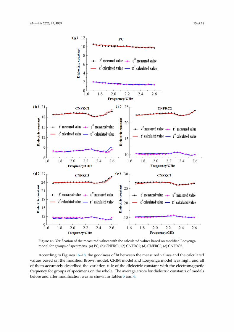
The model  curves  for  groups were  obtained  according  to  the modified Looyenga model  in 

Formula (10) and verified with the measured curves, as shown in Figure 18. 

Figure 17. Verification of the measured values with the calculated values based on modified CRIMmodel for groups of specimens. (a) PC; (b) CNFRC1; (c) CNFRC2; (d) CNFRC3; (e) CNFRC5.

The model curves for groups were obtained according to the modified Looyenga model inFormula (10) and verified with the measured curves, as shown in Figure 18.

Materials 2020, 13, 4869 15 of 18Materials 2020, 13, x FOR PEER REVIEW  15 of 19 

 

 

 

Figure  18.  Verification  of  the  measured  values  with  the  calculated  values  based  on  modified 

Looyenga model  for  groups  of  specimens.  (a)  PC;  (b)  CNFRC1;  (c)  CNFRC2;  (d)  CNFRC3;  (e) 

CNFRC5. 

According to Figures 16–18, the goodness of fit between the measured values and the calculated 

values based on the modified Brown model, CRIM model and Looyenga model was high, and all of 

them  accurately  described  the  variation  rule  of  the  dielectric  constant with  the  electromagnetic 

frequency  for  groups  of  specimens  on  the whole.  The  average  errors  for  dielectric  constants  of 

models before and after modification was as shown in Tables 5 and 6. 

Table 5. Average error for ε, of models before and after modification. 

Speci

men 

No. 

Brown Model  CRIM Model  Looyenga Model 

Before 

Modificat

After 

Modificat

Improve

ment 

Before 

Modificat

After 

Modificat

Improve

ment 

Before 

Modificat

After 

Modificat

Improve

ment 

Figure 18. Verification of the measured values with the calculated values based on modified Looyengamodel for groups of specimens. (a) PC; (b) CNFRC1; (c) CNFRC2; (d) CNFRC3; (e) CNFRC5.

According to Figures 16–18, the goodness of fit between the measured values and the calculatedvalues based on the modified Brown model, CRIM model and Looyenga model was high, and allof them accurately described the variation rule of the dielectric constant with the electromagneticfrequency for groups of specimens on the whole. The average errors for dielectric constants of modelsbefore and after modification was as shown in Tables 5 and 6.

Materials 2020, 13, 4869 16 of 18

Table 5. Average error for ε, of models before and after modification.

SpecimenNo.

Brown Model CRIM Model Looyenga Model

BeforeModification/%

AfterModification/%

ImprovementEffect/%

BeforeModification/%

AfterModification/%

ImprovementEffect/%

BeforeModification/%

AfterModification/%

ImprovementEffect/%

PC 4.95 1.20 3.75 11.92 0.96 10.96 14.64 1.04 13.6CNFRC1 3.68 0.91 2.77 17.51 0.43 17.08 22.78 0.38 22.4CNFRC2 3.57 0.49 3.08 19.17 0.35 18.82 25.13 0.49 24.64CNFRC3 3.66 0.46 3.2 19.79 0.53 19.26 25.97 0.39 25.58CNFRC5 2.93 1.05 1.88 19.67 0.56 19.11 26.36 0.53 25.83

Table 6. Average errors for ε„ before and after improvement of models.

SpecimenNo.

Brown Model CRIM Model Looyenga Model

BeforeModification/%

AfterModification/%

ImprovementEffect/%

BeforeModification/%

AfterModification/%

ImprovementEffect/%

BeforeModification/%

AfterModification/%

ImprovementEffect/%

PC 29.85 3.47 26.38 36.15 3.34 32.81 40.89 3.55 37.34CNFRC1 7.54 2.50 5.04 26.31 1.79 24.52 35.66 1.61 34.05CNFRC2 3.96 1.29 2.67 26.04 1.69 24.35 36.22 1.84 34.38CNFRC3 4.30 2.44 1.86 27.13 1.87 25.26 37.56 1.75 35.81CNFRC5 4.45 1.15 3.3 29.09 1.12 27.97 40.16 1.11 39.05

According to Table 5, the goodness of fit for ε, after modification of the models was greatlyimproved as compared with that before the modification. Only the average errors for ε, of the specimensin PC group and CNFRC5 group were more than 1.00%, but still below 1.20%, and the average errorsfor ε, of specimens in all the other groups were below 1.00%, with the minimum average error for ε, of0.35%. On the whole, the ε, was improved by 1.88~3.75% with the modified Brown model. With themodified CRIM model, the improvement effect for ε, was the best in the CFNRC5 group. The ε, inthe group was improved by 19.26%, and with modified Looyenga model, the ε, was improved by13.60~25.83%. Therefore, the effect of the modified Looyenga model was the best.

According to Table 6, after the models were modified, the average errors for ε„ of the specimens inthe PC group were still the largest, but within 3.55%. The improvement effect for errors of specimenswas very good in all other groups, and the maximum average error for ε„ after modification was only2.50% On the whole, with the modified Brown model, the ε„ was improved by 1.86~26.38%; with themodified CRIM model, the average errors for ε„ were controlled within 1.90% except for the PC group;with the modified Looyenga model, the improvement effect was still the best, and the ε„ was improvedby 34.05~39.05%.

4. Conclusions

The transmission and reflection method was used to measure the dielectric constants of carbonnanofiber reinforced concrete as the fiber content was 0, 0.1%, 0.2%, 0.3% and 0.5%. Then, the modifieddielectric constant models for the Brown model, CRIM model and Looyenga model were establishedbased on the experimental data. Lastly, the modified models were verified for reliability, and acomparative analysis of errors before and after the modification was conducted. The conclusions areas follows.

(1) The carbon nanofiber reinforced concrete can be considered as composed of three independentphases, matrix (mortar), coarse aggregate (limestone gravel) and air, and the dielectric modelsof carbon nanofiber reinforced concrete with different degrees of fiber content can be effectivelyestablished based on the Brown model, CRIM model and Looyenga model.

(2) The goodness of fit between the calculated curves based on the three modified models and themeasured curves was very high, and the variation rule for the dielectric constant of carbonnanofiber concrete with the frequency of electromagnetic wave can be described accurately.

(3) For the ε, and ε„ as dielectric constants calculated based on the modified models, the errorsrelative to corresponding measured values were effectively controlled. For the dielectric constantε,, the average error was maintained below 1.2%, and the minimum error was only 0.35%. For thedielectric constant ε„, the average error was maintained below 3.55%.

Materials 2020, 13, 4869 17 of 18

The results show that the three modified models can accurately describe the dielectric propertiesof carbon nanofiber reinforced concrete. Based on these models, qualitative or quantitative analysis anddetermination of moisture content, density, porosity and other aspects of carbon nanofiber reinforcedconcrete can be carried out based on the measured dielectric constant, providing data and technicalsupport for the quality evaluation of existing concrete structures. Therefore, the determination of thedielectric model of carbon nanofiber reinforced concrete has important theoretical and applicationvalue, and it is recommended to study in depth and promote.

Author Contributions: Conceptualization, Z.-H.W. and J.-Y.X.; data curation, Z.-H.W.; formal analysis, L.-X.N.;investigation, J.-Y.X. and Z.-H.W.; methodology, Z.-H.W. and L.-X.N.; project administration, E.-L.B.; supervision,Z.-H.W. and E.-L.B.; writing—original draft, Z.-H.W. and L.-X.N.; writing—review and editing, Z.-H.W. andE.-L.B. All authors have read and agreed to the published version of the manuscript.

Funding: This research was funded by the National Natural Science Foundation of China, grant no. 51208507.

Acknowledgments: The authors would like to thank the National Natural Science Foundation of China(under grant no. 51208507) for the financial support.

Conflicts of Interest: The authors declare no conflict of interest.

References

1. Fukuyama, T.; Okamoto, Y.; Hasegawa, T.; Senbu, O. Capacitor model of concrete coarse aggregate bydielectric relaxation properties. Cem. Sci. Concr. Technol. 2016, 70, 193–200. [CrossRef]

2. Meng, M.; Wang, F. Theoretical analyses and experimental research on a cement concrete dielectric model.J. Mater. Civ. Eng. 2013, 25, 1959–1963. [CrossRef]

3. Zhang, B.; Zhong, Y.H.; Liu, H.X.; Wang, F.M. Experimental research on dielectric constant model for asphaltconcrete Material. Adv. Mater. Res. 2011, 1270, 2760–2764. [CrossRef]

4. Lai, W.L.; Kou, S.C.; Tsang, W.F.; Poon, C.S. Characterization of concrete properties from dielectric propertiesusing ground penetrating radar. Cem. Concr. Res. 2009, 39, 687–695. [CrossRef]

5. Bourdi, T.; Eddine Rhazi, J.; Boone, F.; Ballivy, G. Application of Jonscher model for the characterization ofthe dielectric permittivity of concrete. J. Phys. D Appl. Phys. 2008, 41, 205410. [CrossRef]

6. Klysz, G.; Balayssac, J.P.; Ferrières, X. Evaluation of dielectric properties of concrete by a numerical FDTDmodel of a GPR coupled antenna—Parametric study. NDT E Int. 2008, 41, 621–631. [CrossRef]

7. Lachowicz, J.; Rucka, M. A novel heterogeneous model of concrete for numerical modelling of groundpenetrating radar. Constr. Build. Mater. 2019, 227, 116703. [CrossRef]

8. Siddika, A.; Mamun, M.A.A.; Ferdous, W.; Saha, A.K.; Alyousef, R. 3D-printed concrete: Applications,performance, and challenges. J. Sustain. Cem. Based Mater. 2019, 9, 127–164. [CrossRef]

9. Busari, A.A.; Akinmusuru, J.O.; Dahunsi, B.I.O.; Ogbiye, A.S.; Okeniyi, J.O. Self-compacting concrete inpavement construction: Strength grouping of some selected brands of cements. Energy Procedia 2017, 119,863–869. [CrossRef]

10. Aghaeipour, A.; Madhkhan, M. Mechanical properties and durability of roller compacted concrete pavement(RCCP)—A review. Road Mater. Pavement Des. 2020, 21, 1775–1798. [CrossRef]

11. Xue, J.; Briseghella, B.; Huang, F.; Nutti, C.; Tabatabi, H.; Chen, B. Review of ultra-high performance concreteand its application in bridge engineering. Constr. Build. Mater. 2020, 260, 119844. [CrossRef]

12. Pan, C.; Chen, N.; He, J.; Liu, S.; Chen, K.; Wang, P.; Xu, P. Effects of corrosion inhibitor and functionalcomponents on the electrochemical and mechanical properties of concrete subject to chloride environment.Constr. Build. Mater. 2020, 260, 119724. [CrossRef]

13. Liu, L.; Miramini, S.; Hajimohammadi, A. Characterising fundamental properties of foam concrete with anon-destructive technique. Nondestruct. Test. Eval. 2019, 34, 54–69. [CrossRef]

14. Bouhamla, M.A.; Beroual, A. Experimental characterisation of concrete containing different kinds of dielectricinclusions through measurements of dielectric constant and electrical resistivity. Proc. Environ. Sci. 2017, 37,647–654. [CrossRef]

15. Tian, Y.P.; Huang, D.C.; Li, B. Monitoring early hydration of concrete with ground penetrating radar.Key Eng. Mater. 2017, 4348, 115–119. [CrossRef]

Materials 2020, 13, 4869 18 of 18

16. Al-Mattarneh, H. Determination of chloride content in concrete using near- and far-field microwavenon-destructive methods. Corros. Sci. 2016, 105, 133–140. [CrossRef]

17. Hasan, M.I.; Yazdani, N. Ground penetrating radar utilization in exploring inadequate concrete covers in anew bridge deck. Case Stud. Constr. Mater. 2014, 1, 104–114. [CrossRef]

18. Höhlig, B.; Schmidt, D.; Mechtcherine, V.; Hempel, S.; Schrofl, C.; Trommler, U.; Roland, U. Effects of dielectricheating of fresh concrete on its microstructure and strength in the hardened state. Constr. Build. Mater. 2015,81, 24–34. [CrossRef]

19. Sánchez-Fajardo, V.M.; Torres, M.E.; Moreno, A.J. Study of the pore structure of the lightweight concrete blockwith lapilli as an aggregate to predict the liquid permeability by dielectric spectroscopy. Constr. Build. Mater.2014, 53, 225–234. [CrossRef]

20. Akono, A.T. Nanostructure and fracture behavior of carbon nanofiber-reinforced cement using nanoscaledepth-sensing methods. Materials 2020, 13, 3837. [CrossRef]

21. Wang, T.; Xu, J.; Meng, B.; Peng, G. Experimental study on the effect of carbon nanofiber content on thedurability of concrete. Constr. Build. Mater. 2020, 250, 118891. [CrossRef]

22. Gawel, K.; Taghipour Khadrbeik, M.A.; Bjørge, R.; Wenner, S.; Gawel, B.; Ghaderi, A.; Cerasi, P. Effects ofwater content and temperature on bulk resistivity of hybrid cement/carbon nanofiber composites. Materials2020, 13, 2884. [CrossRef] [PubMed]

23. Han, J.; Wang, D.; Zhang, P. Effect of nano and micro conductive materials on conductive properties ofcarbon fiber reinforced concrete. Nanotechnol. Rev. 2020, 9, 445–454. [CrossRef]

24. Hamidi, F.; Aslani, F. Constitutive relationships for CNF-reinforced engineered cementitious compositesand CNF-reinforced lightweight engineered cementitious composites at ambient and elevated temperatures.Struct. Concr. 2020, 21, 821–842. [CrossRef]

25. Wang, H.; Gao, X.; Liu, J.; Ren, M.; Lu, A. Multi-functional properties of carbon nanofiber reinforced reactivepowder concrete. Constr. Build. Mater. 2018, 187, 699–707. [CrossRef]

26. Wang, H.; Gao, X.; Liu, J. Coupling effect of salt freeze-thaw cycles and cyclic loading on performancedegradation of carbon nanofiber mortar. Cold Reg. Ence Technol. 2018, 154, 95–102. [CrossRef]

27. Yoo, D.Y.; You, I.; Youn, H.; Lee, S.J. Electrical and piezoresistive properties of cement composites withcarbon nanomaterials. J. Compos. Mater. 2018, 52, 3325–3340. [CrossRef]

28. Wang, H.; Gao, X.; Liu, J. Effects of salt freeze-thaw cycles and cyclic loading on the piezoresistive propertiesof carbon nanofibers mortar. Constr. Build. Mater. 2018, 177, 192–201. [CrossRef]

29. Zhu, X.; Gao, Y.; Dai, Z.; Corr, D.J.; Shah, S.P. Effect of interfacial transition zone on the Young’s modulus ofcarbon nanofiber reinforced cement concrete. Cem. Concr. Res. 2018, 107, 49–63. [CrossRef]

30. Galao, O.; Baeza, F.; Zornoza, E.; Garces, P. Carbon Nanofiber Cement Sensors to Detect Strain and Damageof Concrete Specimens Under Compression. Nanomaterials 2017, 7, 413. [CrossRef]

31. Howser, R.N.; Dhonde, H.B.; Mo, Y.L. Self-sensing of carbon nanofiber concrete columns subjected toreversed cyclic loading. Smart Mater. Struct. 2011, 20, 085031. [CrossRef]

32. Meng, M.L.; Meng, X.H. Effect of temperature and frequency on dielectric model of cement concrete.Bull. Chin. Ceram. Soc. 2015, 37, 1758–1764.

33. Liu, J.L.; Xu, J.Y.; Huang, H.; Chen, H. Microwave deicing efficiency and dielectric property of road concretemodified using different wave absorbing material. Cold Reg. Sci. Technol. 2020, 174, 103064. [CrossRef]

34. Liu, J.L.; Xu, J.Y.; Lu, S.; Chen, H. Investigation on dielectric properties and microwave heating efficiencies ofvarious concrete pavements during microwave deicing. Constr. Build. Mater. 2019, 225, 55–66. [CrossRef]

35. Jin, X.; Ali, M. Simple empirical formulas to estimate the dielectric constant and conductivity of concrete.Microw. Opt. Technol. Lett. 2019, 61, 386–390. [CrossRef]

Publisher’s Note: MDPI stays neutral with regard to jurisdictional claims in published maps and institutionalaffiliations.

© 2020 by the authors. Licensee MDPI, Basel, Switzerland. This article is an open accessarticle distributed under the terms and conditions of the Creative Commons Attribution(CC BY) license (http://creativecommons.org/licenses/by/4.0/).