Nonlinear numerical modeling of reinforced concrete panels ...
171
American University in Cairo American University in Cairo AUC Knowledge Fountain AUC Knowledge Fountain Archived Theses and Dissertations November 2021 Nonlinear numerical modeling of reinforced concrete panels Nonlinear numerical modeling of reinforced concrete panels subjected to impact loads subjected to impact loads Sherif Mohamed Shaaban The American University in Cairo AUC Follow this and additional works at: https://fount.aucegypt.edu/retro_etds Part of the Other Engineering Commons Recommended Citation Recommended Citation APA Citation Shaaban, S. M. (2021).Nonlinear numerical modeling of reinforced concrete panels subjected to impact loads [Thesis, the American University in Cairo]. AUC Knowledge Fountain. https://fount.aucegypt.edu/retro_etds/2451 MLA Citation Shaaban, Sherif Mohamed. Nonlinear numerical modeling of reinforced concrete panels subjected to impact loads. 2021. American University in Cairo, Thesis. AUC Knowledge Fountain. https://fount.aucegypt.edu/retro_etds/2451 This Thesis is brought to you for free and open access by AUC Knowledge Fountain. It has been accepted for inclusion in Archived Theses and Dissertations by an authorized administrator of AUC Knowledge Fountain. For more information, please contact [email protected].
-
Upload
khangminh22 -
Category
Documents
-
view
2 -
download
0
Transcript of Nonlinear numerical modeling of reinforced concrete panels ...

American University in Cairo American University in Cairo
AUC Knowledge Fountain AUC Knowledge Fountain
Archived Theses and Dissertations
November 2021
Nonlinear numerical modeling of reinforced concrete panels Nonlinear numerical modeling of reinforced concrete panels
subjected to impact loads subjected to impact loads
Sherif Mohamed Shaaban The American University in Cairo AUC
Follow this and additional works at: https://fount.aucegypt.edu/retro_etds
Part of the Other Engineering Commons
Recommended Citation Recommended Citation
APA Citation Shaaban, S. M. (2021).Nonlinear numerical modeling of reinforced concrete panels subjected to impact loads [Thesis, the American University in Cairo]. AUC Knowledge Fountain. https://fount.aucegypt.edu/retro_etds/2451
MLA Citation Shaaban, Sherif Mohamed. Nonlinear numerical modeling of reinforced concrete panels subjected to impact loads. 2021. American University in Cairo, Thesis. AUC Knowledge Fountain. https://fount.aucegypt.edu/retro_etds/2451
This Thesis is brought to you for free and open access by AUC Knowledge Fountain. It has been accepted for inclusion in Archived Theses and Dissertations by an authorized administrator of AUC Knowledge Fountain. For more information, please contact [email protected].
The American University in Cairo School of Sciences and Engineering
NONLINEAR NUMERICAL MODELING OF REINFORCED CONCRETE PANELS SUBJECTED
TO IMPACT LOADS
A Thesis Submitted in partial fulfillment of the requirements for
the degree of Master of Science in Construction Engineering
By
Sherif Mohamed Shaaban Osman
B.Sc. Civil Engineering
Under the supervision of
Dr. Mohamed Ahmed Naiem Abdel-Mooty
Professor of Construction and Architectural Engineering Department, AUC
August / 2011
ii
The American University in Cairo School of Sciences and Engineering
NONLINEAR NUMERICAL MODELING OF
REINFORCED CONCRETE PANELS SUBJECTED TO IMPACT LOADS
A Thesis Submitted by
Sherif Mohamed Shaaban Osman
To Construction and Architectural Engineering Department
August / 2011
In partial fulfillment of the requirements for
the degree of Master of Science
has been approved by
Thesis Committee Supervisor/Chair ______________________________
Affiliation __________________________________________________
Thesis Committee Reader/Examiner _____________________________
Affiliation __________________________________________________
Thesis Committee Reader/Examiner _____________________________
Affiliation __________________________________________________
Thesis Committee Reader/External Examiner ______________________
(if required by dept.)
Affiliation __________________________________________________
_________________ ________ _________________ ________ Dept. Chair/Director Date Dean Date
iii
DEDICATION
I would like to dedicate the work done in this research to my family namely my
mother, father, sisters, wife, and family kids (my kids and my sister's kids). Without
the help and support of them, I couldn't have finished this work. Since I graduated in
2001, they have been motivating me to purse my academic career. With their
motivations, I was able to get a Diploma in Reinforced Concrete, Cairo University
2004. I believe that the credit goes to my family not only for the work done in this
research but for my entire life.
iv
ACKNOWLEDGEMENTS
I would like to thank all those who helped me by all means in order to bring this
research work up to this level. There were many people who were involved in this
research work from various areas.
From AUC, I would like first to acknowledge my advisor, Dr. Mohamed Abdel-
Mooty , who had a major contribution in this research. He provided guidance, and
unlimited support in this research. He was very generous in terms of time and
availability during the entire thesis.
From the Construction and Architectural Engineering Department, I would like to
acknowledge Eng. Cherif Hussein who provided me with the data of his experimental
research that was used for validation. He was very supportive through this research. I
would like also to thank my colleagues; Eng. Ayman Thabit, Eng. Omar El-Kadi,
Eng. Rania Hamza, and Eng. Waleed Al-Kady who all helped me by advice,
guidance, contribution, technical and informational support, and criticism in this
research. I would like to thank the administration of the department of Construction
and Architectural Engineering, namely Dr. Mohamed Nagib Abou-zeid , Dr. Safwan
Khedr , and all staff members for their support and warm feelings.
From Cairo University, I would like to extend sincere thanks to Eng. Ahmed Shawky,
for his help and support to me in many problems I faced during the research.
From my friends, I would like to thank my dearest friends Mr. Ahmed Gaber and Eng.
Mohamed Zaki. They have been always offering help and support.
Last but not least , my family, I would like to acknowledge my family, namely my
mother , father , sisters , wife , family kids (my kids and my sister's kids) , father-in-
law , and mother-in-law.
v
ABSTRACT
In recent years, the public concern about safety has increased dramatically because of
the tremendous increase in the number of terrorist attacks all over the world. Although
the research on impact and blast loads initially focused on military applications, now
the risk of impact and blast events on civil structures has become of increasing
concerns. Constructing civil and commercial buildings capable of sustaining impact
and blast loads with acceptable damage has gained a lot of attention.
Impact Load is a relatively large dynamic load applied to the structure or part of it
over a very short period of time. This type of loading is similar to other short duration
loads such as blast load. Furthermore, blast events result in debris and fragments
striking building components, thus causing impact. Blast events are not presented in
this research; however, its effect can be modeled as simplified load history using
commercial application like ATBLAST software.
The performance of reinforced concrete façade element such as beams or one-way
slab panels under the effect of direct impact loads is studied in this research.
Numerical simulation of the impact phenomenon is developed and presented in this
thesis. The developed numerical model is verified against the experimental results of
a previous study presented at AUC. Such numerical simulations, once calibrated,
allows for detailed parametric study that investigates the effect of different design
parameters on the performance of the building façade under impact loads, thus saving
the prohibitive costs of experimental testing.
Nonlinear model was developed on numerical code (LS-DYNA) for a reinforced
concrete panel under impact loads. The developed model examined different model
factors such as mesh size, elements type, material models, and contact interface
elements. Impact loads were modeled by two methods; simplified impact load history
vi
and simulated pendulum analysis. Simplified impact analysis used the impact force-
time history from the literature to load the RC panel. On the other hand, simulated
pendulum analysis modeled the actual movement and impact of a pendulum mass that
drops from a specified height under free fall acceleration. One of the underlying
challenges in this research is the capability of the numerical model to represents the
rational behavior of the concrete under impact loads, including the nonlinear response
of the material under impact loads. Numerous material models that could be used for
concrete under varying stress and loading rate conditions were reviewed and critically
examined in this research.
The Nonlinear model was validated using experimental results from the literature. The
model did show good agreement with the experiment results for both loading
methods. The simplified impact analysis showed small difference in the order of
6.50% in the reaction force for Model-1 “MAT_GEOLOGIC_CAP_MODEL”;
however, the simulated pendulum analysis, away from small impact force, exhibited
minimum difference as 6.52%in the reaction force and 17.33% in the impact force for
other models.
Finally, the nonlinear model was refined through various model refinements and a
comprehensive parametric study was presented. Results were analyzed and
manipulated to figure out how we can increase the capacity of the panel to sustain
higher impact loads with minimum damage. Moreover, new supporting systems were
introduced to reduce the force transferred to the structure supporting the façade panel.
A specifically designed support connection that allows for absorbing the impact shock
is presented in this thesis. The introduced shock-absorber supporting system at the
back side of the RC panel reduced the reaction force transferred to the structure by
52.5 % compared to the control model with classical support system.

vii
TABLE OF CONTENTS
DEDICATION ............................................................................................................. iii
ACKNOWLEDGEMENTS .......................................................................................... iv
ABSTRACT ................................................................................................................... v
TABLE OF CONTENTS ............................................................................................. vii
LIST OF FIGURES ................................................................................................... xiii
LIST OF TABLES ...................................................................................................... xxi
CHAPTER 1: INTRODUCTION .................................................................................. 1
1.1 General Introduction ....................................................................................... 1
1.2 Impact Load..................................................................................................... 2
1.3 Blast Load ....................................................................................................... 4
1.4 Problem Statement .......................................................................................... 4
1.5 Research Objectives ........................................................................................ 5
1.6 Scope and Limitations ..................................................................................... 6
1.7 Units ................................................................................................................ 6
1.8 Central Processing Unit (CPU) ....................................................................... 7
1.9 Organization of the Thesis .............................................................................. 8
CHAPTER 2: LITERATURE REVIEW ....................................................................... 9
2.1 Impact Force Parameters ................................................................................. 9
2.2 Reinforced Concrete Targets Under Impact Load ........................................ 13
2.2.1 Experimental Tests................................................................................. 13
2.2.2 Numerical Simulations.......................................................................... 18
viii
2.3 Analytical and Empirical Analysis ................................................................ 33
2.3.1 Concrete Material Models...................................................................... 38
2.3.2 Steel Material Models ............................................................................ 42
CHAPTER 3: RESEARCH METHODOLOGY ......................................................... 43
3.1 Introduction ................................................................................................... 43
3.2 Model Description ......................................................................................... 43
3.2.1 Geometry................................................................................................ 43
3.2.2 Boundary Conditions ............................................................................. 44
3.2.3 Applied Loads ........................................................................................ 44
3.2.3.1 Simplified Pendulum Analysis ....................................................... 45
3.2.3.2 Simulated Pendulum Analysis ........................................................ 45
3.2.4 Software ................................................................................................. 46
3.2.5 Elements ................................................................................................. 47
3.2.6 Mesh Size ............................................................................................... 48
3.3 Material Models ............................................................................................ 49
3.3.1 Concrete Material Models...................................................................... 49
3.3.1.1 Material #025 .................................................................................. 49
3.3.1.2 Material #072R3 ............................................................................. 50
3.3.1.3 Material #084/085........................................................................... 50
3.3.1.4 Material #159 .................................................................................. 50
3.3.2 Steel Material Models ............................................................................ 50
3.3.2.1 Material #003 .................................................................................. 50
ix
3.3.2.2 Material #024 .................................................................................. 51
3.4 Model Verification ........................................................................................ 51
3.4.1 Experimental Setup ................................................................................ 51
3.4.1.1 Apparatus ........................................................................................ 51
3.4.1.2 RC Specimens................................................................................. 55
3.4.1.3 Data Used for Validation ................................................................ 55
3.4.2 Linear Models ........................................................................................ 57
3.4.3 Nonlinear Models................................................................................... 58
3.4.3.1 Simplified Pendulum Analysis ....................................................... 58
3.4.3.2 Simulated Pendulum Analysis ........................................................ 59
CHAPTER 4: ANALYSIS OF RESULTS AND DISCUSSIONS.............................. 61
4.1 Introduction ................................................................................................... 61
4.2 Linear Models ............................................................................................... 61
4.3 Nonlinear Models: Simplified Pendulum Analysis ....................................... 62
4.3.1 Analysis of results .................................................................................. 62
4.3.2 Comments .............................................................................................. 68
4.4 Nonlinear Models: Simulated Pendulum Analysis ....................................... 69
4.4.1 Analysis of results .................................................................................. 69
4.4.2 Comments .............................................................................................. 73
4.4.3 Model refinements ................................................................................. 76
4.4.3.1 Steel plate contact with RC beam ................................................... 76
4.4.3.2 Solid element formulations ............................................................. 77
x
4.4.3.3 Hourglass (HG) algorithms ............................................................ 79
4.4.3.4 Mesh element size .......................................................................... 80
4.4.4 Beam’s damage ...................................................................................... 82
4.4.4.1 RC Beam’s Damage for Model 1 ................................................... 83
4.4.4.2 RC Beam’s Damage for Model 2 ................................................... 84
4.4.4.3 RC Beam’s Damage for Model 3 ................................................... 85
4.4.4.4 RC Beam’s Damage for Model 4 ................................................... 86
4.5 Parametric Analysis: Simulated Pendulum Analysis .................................... 87
4.5.1 Effect of impact dropping mass ............................................................. 89
4.5.1.1 Analysis of results .......................................................................... 89
4.5.1.2 Comments ....................................................................................... 90
4.5.2 Effect of impact dropping height ........................................................... 91
4.5.2.1 Analysis of results .......................................................................... 91
4.5.2.2 Comments ....................................................................................... 92
4.5.3 Effect of the tension-side longitudinal reinforcement ........................... 93
4.5.3.1 Analysis of results .......................................................................... 93
4.5.3.2 Comments ....................................................................................... 95
4.5.4 Effect of the compression-side longitudinal reinforcement ................... 96
4.5.4.1 Analysis of results .......................................................................... 96
4.5.4.2 Comments ....................................................................................... 97
4.5.5 Effect of the front-plate thickness .......................................................... 98
4.5.5.1 Analysis of results .......................................................................... 98
xi
4.5.5.2 Comments ....................................................................................... 99
4.5.6 Effect of the back-plates thickness ...................................................... 100
4.5.6.1 Analysis of results ........................................................................ 100
4.5.6.2 Comments ..................................................................................... 101
4.5.7 Effect of the front-plate modulus of elasticity ..................................... 102
4.5.7.1 Analysis of results ........................................................................ 102
4.5.7.2 Comments ..................................................................................... 105
4.5.8 Effect of the back-plate modulus of elasticity ..................................... 106
4.5.8.1 Analysis of results ........................................................................ 106
4.5.8.2 Comments ..................................................................................... 109
4.5.9 Effect of using shock-absorber supporting elements ........................... 109
4.5.9.1 Analysis of results (Model A) ...................................................... 110
4.5.9.2 Comments (Model A) ................................................................... 114
4.5.9.3 Analysis of results (Model B) ....................................................... 115
4.5.9.4 Comments (Model B) ................................................................... 118
4.5.9.5 Analysis of results (Model C) ....................................................... 119
4.5.9.6 Comments (Model C) ................................................................... 122
4.5.9.7 Analysis of results (Model D) ...................................................... 123
4.5.9.8 Comments (Model D) ................................................................... 127
CHAPTER 5: SUMMARY , CONCLUSIONS AND RECOMMENDATTIONS ... 128
5.1 Summary ..................................................................................................... 128
5.2 Conclusions ................................................................................................. 136

xii
5.3 Recommendations for Future Research ...................................................... 138
REFERENCES .......................................................................................................... 142
xiii
LIST OF FIGURES
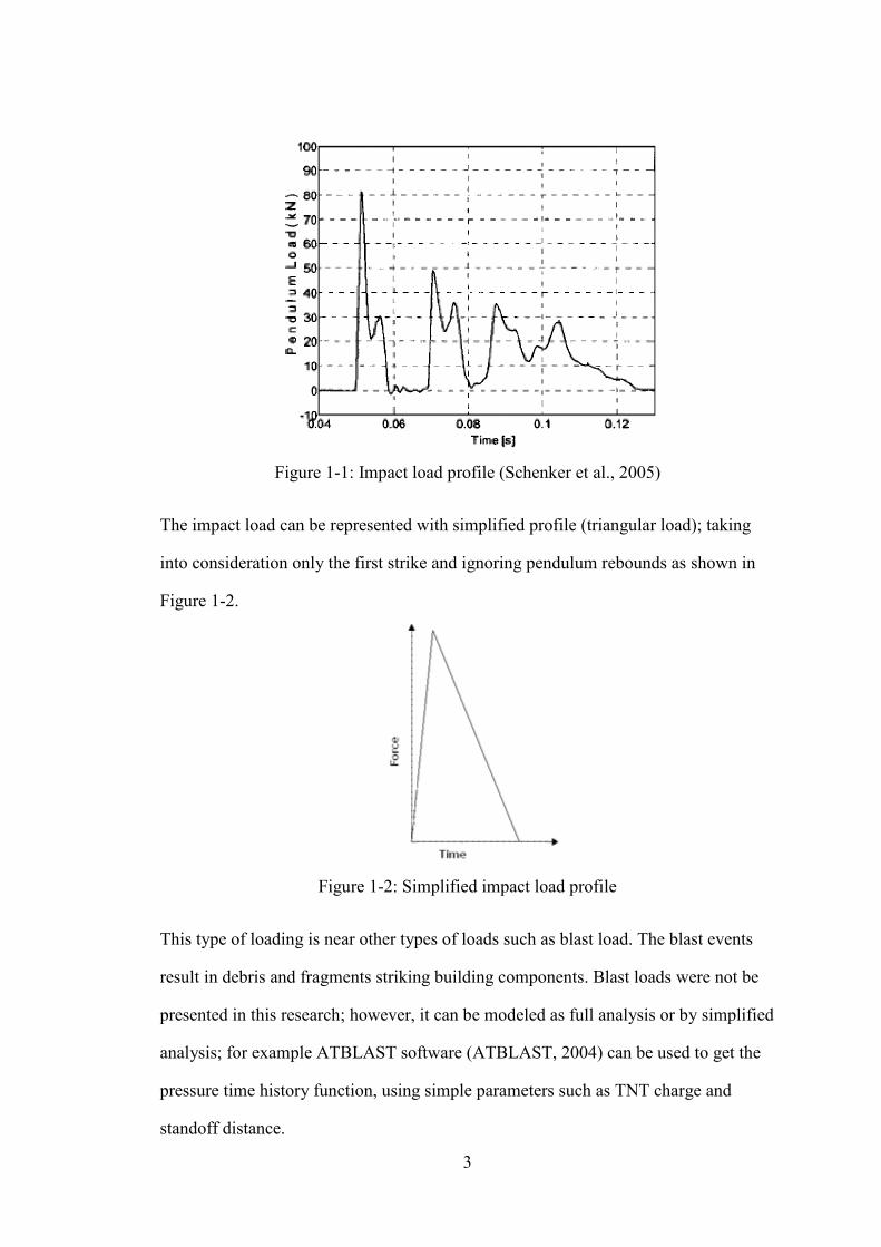
Figure 1-1: Impact load profile (Schenker et al., 2005) ................................................. 3
Figure 1-2: Simplified impact load profile .................................................................... 3
Figure 1-3: Reflected Blast Load Pressure (Davidson et al., 2005) ............................... 4
Figure 2-1: Impact force time history for test No.16 - type A4 , mass 300kg , v 5m/s
(Tachibana et al., 2010) ................................................................................................. 9
Figure 2-2: Impact force-time history, using Winfrith material models vs. experiment
results - falling mass = 98.7kg , height = 200mm ,and v =7.3 m/sec (Sangi and May,
2009) ............................................................................................................................ 10
Figure 2-3: Impact force -time history, using Concrete Damage Rel III material model
vs. experiment results - falling mass = 98.7kg , height = 200mm ,and v = 7.3m/sec
(Sangi and May, 2009) ................................................................................................. 10
Figure 2-4: Impact time history for B2 - falling mass = 98.7kg , height = 200mm ,and
v = 7.3m/sec (Chen and May, 2009) ............................................................................ 11
Figure 2-5: Impact time history - mass 400kg, drop height 0.6m (Kazunori et al.,
2009) ............................................................................................................................ 11
Figure 2-6: Comparison of the penetration depth between (a) the experimental data
and (b) the numerical model (Liu et al., 2011) ............................................................ 12
Figure 2-7: Front and back damaged area (Jose et al., 2010) ...................................... 14
Figure 2-8: Apparatus and measured items (Tachibana et al., 2010) .......................... 15
Figure 2-9: Local and overall failure of RC beams under impact load (Kazunori et al.,
2009) ............................................................................................................................ 17
Figure 2-10: Mode of failure for (a) S1616, (b) S1322, and (c) S2222 (Kazunori et al.,
2009) ............................................................................................................................ 17
Figure 2-11: Plain concrete failure under impact load (Murray et al., 2007) .............. 18
Figure 2-12: Impact of soft missile on slender RC slabs (Jose et al., 2010) ................ 19
xiv
Figure 2-13: Damage comparisons using Winfrith model (Sangi and May, 2009) ..... 19
Figure 2-14: Damage comparisons using Concrete damage Rel III model (Sangi and
May, 2009) ................................................................................................................... 20
Figure 2-15: Crack pattern for different mesh size where (a) coarse mesh, (e) fine
mesh, (f) experiment (Tahmasebinia, 2008) ................................................................ 21
Figure 2-16: Drop tower comparison between the numerical model and the
experimental results (Murray et al., 2007) ................................................................... 22
Figure 2-17: Oblique angle [DEG] vs. depth of penetration [DOP] (Liu et al., 2011) 23
Figure 2-18: Impact responses for different reinforcement configurations, S1616
(Top), S1322 (middle), and S2222 (bottom) (Kazunori et al., 2009) .......................... 24
Figure 2-19: Simulated damage mode for (a)Plain concrete , (b) Over-reinforced , and
(c) Under-reinforced concrete beams for a mass of 63.9kg (Kazunori et al., 2009) ... 25
Figure 2-20: Strain rates at different loading conditions (Ngo et al., 2007) ................ 26
Figure 2-21: Concrete and steel stress-strain curve (Silva et al., 2009) ...................... 27
Figure 2-22: Support reactions of the RC beam investigated under load applied at mid
span at various rates of loading: (a) 200 kN/ sec , (b) 2,000 kN/sec (c) 20,000 kN/sec ,
and (d) 200,000 kN/sec (Cotsovos et al., 2008) ........................................................... 28
Figure 2-23: Effective length for impact load with (a) low and (b) high rates of
loading (Cotsovos et al., 2008) .................................................................................... 29
Figure 2-24: RC slabs response to high-speed impact recorded by high speed camera
(Pires et al., 2010) ........................................................................................................ 30
Figure 2-25: Impact load history correlated with crack propagation for a beam (Chen
and May, 2009) ............................................................................................................ 30
Figure 2-26: High speed camera used to capture the cracks in one of the beam tested
at an impact velocity of 33.1 km/h (Murray et al., 2007) ............................................ 31
Figure 2-27: Slab response under blast load (Wesevich et al., 2010) .......................... 32
xv
Figure 2-28: Two-degree-of-freedom mass-spring-damper system model (Kazunori et
al., 2009) ...................................................................................................................... 34
Figure 2-29: Design flow of RC beam subjected to impact loading (Kazunori et al.,
2009) ............................................................................................................................ 35
Figure 2-30: Stress-strain diagram of a medium-carbon structural steel
(http://www.mathalino.com) ........................................................................................ 42
Figure 3-1: RC beam‘s geometry and reinforcement .................................................. 44
Figure 3-2: Pendulum mass lifted by steel wires ......................................................... 45
Figure 3-3: Pendulum mass lifted by steel wires & the supporting frame, (Cherif,
2009) ............................................................................................................................ 46
Figure 3-4: Exporting ANSYS input file to an LS-DYNA input file .......................... 47
Figure 3-5: SOLID164 and LINK160 (ANSYS, 2009) ............................................... 48
Figure 3-6: Mesh elements for different parts of the model ........................................ 48
Figure 3-7: Mat#025 - theory (LSTC, 2009) ............................................................... 49
Figure 3-8: Impact apparatus consists of winch, specimen supporting frame,
pendulum mass, and pendulum supporting system, (Cherif, 2009) ............................. 51
Figure 3-9: Beam end supporting conditions, (Cherif, 2009) ...................................... 52
Figure 3-10: Pendulum motion, (Cherif, 2009) ........................................................... 53
Figure 3-11: Main steel plate, holding additional weights, (Cherif, 2009) .................. 53
Figure 3-12: Additional weights attached to the pendulum mass, (Cherif, 2009) ....... 54
Figure 3-13: Load cell, (Cherif, 2009) ......................................................................... 54
Figure 3-14: RC specimen used for validation, (Cherif, 2009) ................................... 55
Figure 3-15: Beam and solid linear numerical models ................................................ 57
Figure 3-16: Time history function of the exp. results for M 142.87kg & H 100mm . 58
Figure 3-17: Simplified analysis - input forces used in the model .............................. 58
Figure 3-18: Density calculations for a mass of 142.87 kg ......................................... 59

xvi
Figure 3-19: Shock-absorber system, height = 100 & 300 mm ................................... 60
Figure 3-20: Shock-absorber system, cross-section ..................................................... 60
Figure 4-1: Simplified pendulum analysis – M 142.87kg & H 100mm (All models) . 63
Figure 4-2: Simplified pendulum analysis – M 142.87kg & H 100mm (Model-1 & 2)
...................................................................................................................................... 64
Figure 4-3: Simplified pendulum analysis – M 142.87kg & H 100mm (Model-3 & 4)
...................................................................................................................................... 64
Figure 4-4: Simplified pendulum analysis – M 142.87kg & H 200mm (All models) . 65
Figure 4-5: Simplified pendulum analysis – M 142.87kg & H 200mm (Model-1 & 2)
...................................................................................................................................... 65
Figure 4-6: Simplified pendulum analysis – M 142.87kg & H 200mm (Model-3 & 4)
...................................................................................................................................... 66
Figure 4-7: Simplified pendulum analysis – M 179.87kg & H 100mm ( All models) 66
Figure 4-8: Simplified pendulum analysis – M 179.87kg & H 100mm (Model-1 & 2)
...................................................................................................................................... 67
Figure 4-9: Simplified pendulum analysis – M 179.87kg & H 100mm (Model-3 & 4)
...................................................................................................................................... 67
Figure 4-10: Simplified pendulum analysis - reaction vs. increase in impact force .... 69
Figure 4-11: Simulated pendulum analysis – M 142.87kg & H 100mm (reaction) .... 70
Figure 4-12: Simulated pendulum analysis – M 142.87kg & H 200mm (reaction) .... 70
Figure 4-13: Simulated pendulum analysis – M 142.87kg & H 300mm (reaction) .... 71
Figure 4-14: Simulated pendulum analysis – M 179.87kg & H 100mm (reaction) .... 71
Figure 4-15: Simulated pendulum analysis - reaction vs. increase in impact force .... 72
Figure 4-16: Simulated pendulum analysis - Model-3 vs. Exp. results (reaction) ...... 73
Figure 4-17: Simulated pendulum analysis - Model-3 vs. Exp. results (force) ........... 75
Figure 4-18: Simulated pendulum analysis - Model-3 (force) ..................................... 75
xvii
Figure 4-19: Model refinements - separation gap distance of 1 mm (reaction) ........... 76
Figure 4-20: Model refinements - separation gap distance of 1 mm (force) ............... 77
Figure 4-21: Model refinements - fully integrated quadratic 8 node element with nodal
rotations – solid type 2 ................................................................................................. 78
Figure 4-22: Model refinements - Control vs. HG1 & HG3 (reaction) ....................... 79
Figure 4-23: Model refinements – Control mesh vs. mesh “A” (element size) ........... 80
Figure 4-24: Model refinements – Control mesh vs. mesh “B” (element size) ........... 80
Figure 4-25: Model refinements – mesh element size (reaction) ................................ 81
Figure 4-26: Damage @ time 0.47 sec - Model 1, M 800kg & H 100mm .................. 83
Figure 4-27: Damage @ time 0.60 sec - Model 1, M 800kg & H 100mm .................. 83
Figure 4-28: Damage @ time 0.47 sec - Model 2, M 800kg & H 100mm .................. 84
Figure 4-29: Damage @ time 0.60 sec - Model 2, M 800kg & H 100mm .................. 84
Figure 4-30: Damage @ time 0.47 sec - Model 3, M 800kg & H 100mm .................. 85
Figure 4-31: Damage @ time 0.60 sec - Model 3, M 800kg & H 100mm .................. 85
Figure 4-32: Damage @ time 0.47 sec - Model 4, M 800kg & H = 100mm ............... 86
Figure 4-33: Damage @ time 0.60 sec - Model 4, M 800kg & H 100mm .................. 86
Figure 4-34: PA: Response of the RC beam – M 142.87kg & H 100mm (Control); (a)
deflection , (b) impact & reaction force , and (c) stress-strain curve ........................... 88
Figure 4-35: PA: Impact mass vs. mid-span deflection ............................................... 89
Figure 4-36: PA: Impact mass vs. reaction force ......................................................... 89
Figure 4-37: PA: Impact mass vs. mid-span stress (back-side) ................................... 90
Figure 4-38: PA: Impact height vs. mid-span deflection ............................................. 91
Figure 4-39: PA: Impact height vs. reaction force ....................................................... 92
Figure 4-40: PA: Impact height vs. mid-span stress (back-side) ................................. 92
Figure 4-41: PA: Tension reinforcement bar diameter vs. mid-span deflection .......... 93
Figure 4-42: PA: Tension reinforcement bar diameter vs. reaction force ................... 94
xviii
Figure 4-43: PA: Tension reinforcement bar diameter vs. mid-span stress ................. 94
Figure 4-44: PA: Reaction time history using different tension reinforcement bar
diameters ...................................................................................................................... 95
Figure 4-45: PA: Compression reinforcement bar diameter vs. mid-span deflection . 96
Figure 4-46: PA: Compression reinforcement bar diameter vs. reaction force ........... 97
Figure 4-47: PA: Compression reinforcement bar diameter vs. mid-span stress ........ 97
Figure 4-48: PA: Front plate thickness vs. mid-span deflection .................................. 98
Figure 4-49: PA: Front plate thickness vs. reaction force ........................................... 99
Figure 4-50: PA: Front plate thickness vs. mid-span stress ......................................... 99
Figure 4-51: PA: Back plate thickness vs. mid-span deflection ................................ 100
Figure 4-52: PA: Back plate thickness vs. reaction force .......................................... 101
Figure 4-53: PA: Back plate thickness vs. mid-span stress ....................................... 101
Figure 4-54: PA: Front plate modulus of elasticity vs. mid-span deflection ............. 103
Figure 4-55: PA: Front plate modulus of elasticity vs. reaction force ....................... 103
Figure 4-56: PA: Front plate modulus of elasticity vs. mid-span stress .................... 104
Figure 4-57: PA: Reaction time history for different front plate modulus of elasticity's
.................................................................................................................................... 104
Figure 4-58: PA: Impact force time history for different front plate modulus of
elasticity's ................................................................................................................... 105
Figure 4-59: PA: Back plate modulus of elasticity vs. mid-span deflection ............. 107
Figure 4-60: PA: Back plate modulus of elasticity vs. reaction force ....................... 107
Figure 4-61: PA: Back plate modulus of elasticity vs. mid-span stress ..................... 108
Figure 4-62: PA: Reaction time history for different back plate modulus of elasticity's
.................................................................................................................................... 108
Figure 4-63: Shock-absorber – Model A – Shell thickness vs. Mid-span deflection 110
Figure 4-64: Shock-absorber – Model A – Shell thickness vs. Reaction force ......... 111
xix
Figure 4-65: Shock-absorber – Model A – Shell thickness vs. Mid-span stress ....... 111
Figure 4-66: Shock-absorber – Model A – mid-span deflection for t = 3 & 1 mm ... 112
Figure 4-67: Shock-absorber – Model A – reaction force for t = 3 & 1 mm ............. 112
Figure 4-68: Shock-absorber – Model A – Stress-strain relation for t = 3 & 1 mm .. 113
Figure 4-69: Damage in shock-absorber, Model A - t = 3 mm @ time = 0.6 sec ..... 113
Figure 4-70: Damage in shock-absorber, Model A - t = 1 mm @ time = 0.6 sec ..... 113
Figure 4-71: Shock-absorber – Model B – Shell thickness vs. Mid-span deflection 115
Figure 4-72: Shock-absorber – Model B – Shell thickness vs. Reaction force ......... 115
Figure 4-73: Shock-absorber – Model B – Shell thickness vs. Mid-span stress ........ 116
Figure 4-74: Shock-absorber – Model B – Mid-span deflection for t = 3 & 1 mm ... 116
Figure 4-75: Shock-absorber – Model B – Reaction force for t = 3 & 1 mm ............ 117
Figure 4-76: Shock-absorber – Model B – Stress-strain relation for t = 3 & 1 mm .. 117
Figure 4-77: Damage in shock-absorber, Model B - t = 3 mm @ time = 0.6 sec ...... 118
Figure 4-78: Damage in shock-absorber, Model B - t = 1 mm @ time = 0.6 sec ...... 118
Figure 4-79: Shock-absorber – Model C – Shell thickness vs. Mid-span deflection 119
Figure 4-80: Shock-absorber – Model C – Shell thickness vs. Reaction force ......... 120
Figure 4-81: Shock-absorber – Model C – Shell thickness vs. Mid-span stress ........ 120
Figure 4-82: Shock-absorber – Model C – Mid-span deflection for t = 3 & 1 mm ... 121
Figure 4-83: Shock-absorber – Model C – Reaction force for t = 3 & 1 mm ............ 121
Figure 4-84: Damage in shock-absorber, Model C - t = 3 mm @ time = 0.6 sec ...... 122
Figure 4-85: Damage in shock-absorber, Model C - t = 1 mm @ time = 0.6 sec ...... 122
Figure 4-86: Shock-absorber – Model D – Shell thickness vs. Mid-span deflection 123
Figure 4-87: Shock-absorber – Model D – Shell thickness vs. Reaction force ......... 124
Figure 4-88: Shock-absorber – Model D – Shell thickness vs. Mid-span stress ....... 124
Figure 4-89: Shock-absorber – Model D – Mid-span deflection for t = 3 & 1 mm ... 125
Figure 4-90: Shock-absorber – Model D – Reaction force for t = 3 & 1 mm ........... 125
xx
Figure 4-91: Shock-absorber – Model D – Stress-strain relation for t = 3 & 1 mm .. 126
Figure 4-92: Damage in Model D - t = 3 mm: Left (time @0.51sec), Right (time
@0.60sec) .................................................................................................................. 126
Figure 4-93: Damage in Model D - t = 1 mm: Left (time @0.51sec), Right (time
@0.60sec) .................................................................................................................. 126
Figure 5-1: Single Element – One bent ...................................................................... 139
Figure 5-2: Single Element – Two bents ................................................................... 139
Figure 5-3: Single Element – One bent with horizontal part ..................................... 139
Figure 5-4: Single Element – Two bents with horizontal part ................................... 140
Figure 5-5: Double Element – One bent .................................................................... 140
Figure 5-6: Double Element – Two bents .................................................................. 140
Figure 5-7: Double Element – One bent with horizontal part ................................... 141
Figure 5-8: Double Element – Two bents with horizontal part ................................. 141

xxi
LIST OF TABLES
Table 1-1: Consistent unit systems (ANSYS, 2009) ..................................................... 7
Table 2-1: Longitudinal reinforcement used in RC beams (Kazunori et al., 2009) ..... 16
Table 3-1: Experiment results for Spc.1 – summary of results (Cherif, 2009) ............ 56
Table 4-1: Static calculations: force of M 142.87kg & H 100mm striking a beam ..... 61
Table 4-2: Summary of static\dynamic linear analysis of M 142.87kg & H 100mm .. 62
Table 4-3: Concrete material models abbreviations .................................................... 63
Table 4-4: Summary of the exp. results and the simplified numerical models ............ 68
Table 4-5: Summary of the simulated pendulum analysis for Model-3 ...................... 72
Table 4-6: HG type’s description ................................................................................. 79
Table 4-7: Control model used in the parametric analysis .......................................... 87
Table 4-8: Shock-absorber models used in the parametric analysis .......................... 110
1
CHAPTER 1: INTRODUCTION
1.1 General Introduction
In recent years, the public concern about safety has increased dramatically because of
the tremendous increase in the number of terrorist attacks all over the world. Although
the research on impact and blast loads initially focused on military applications, now
the risk of impact and blast events on civil structures has increased tremendously.
Constructing civil and commercial buildings capable of sustaining impact and blast
loads with acceptable damage has gained a lot of attention.
One very common way to protect critical structures, such as embassies, ministries,
nuclear power plants...etc, from impact and blast events, is to have them built in
secured areas i.e with a stand-off distance from surrounding buildings and traffic.
Stand-off distance is the main parameter that affects the intensity of a blast load for a
given charge weight. Civil and commercial structures, on the other hand, do not have
any stand-off distance due to the nature, location, and the function of the building.
Therefore, it is very important to understand the nature of the impact and blast load to
design various structural elements for sustaining impact and blast loads with
minimum damage.
Blast attacks are one of the main sources of impact load because of the fragments and
debris associated with an explosion of a charge weight. In a typical explosion event,
the bomb case breaks after the initiation of the explosive filler material due to high
pressure. During swelling, cracks will be initiated and propagated in the bomb case;
accordingly fragments will be created (Ulrika and Nystro, 2009). According to the
2
distance between the detonation and the structure, fragments are coupled with
different range of velocities, ranging from hyper-velocity to low-velocity impacts.
The velocity of the impact governs the response of the structure. Low-velocity
impacts may cause quasi-static response, while hyper-velocity impacts can cause the
properties of the material to change (Jones, 1989). In other words, the dynamic
response of structural components subjected to short-duration impacts is different
from other type of loads.
Building façade is our main concern because it is the first layer that is exposed to such
type of loading. Building façade should be a protective layer, saving the occupants
from the hazards of blast and shock events. There is a lot of research work done on
non-structural components. For example, glass material is being designed to fail near
connections, falling as one piece very close to the façade will minimize the fragments
and debris that threaten the human life. In this research, the research will focus on the
structural component of the building façade. Concrete panels are commonly used in
building façades. The research introduced how these panels can exhibit local damage
to reduce the forces transmitted to the structural component to avoid collapse and
sudden failure.
1.2 Impact Load
Impact Load is a relatively large dynamic load applied to the structure or part of the
structure in a comparatively short period of time. Figure 1-1 shows the load time
history for the impact load event (Schenker et al., 2005). The figure shows that the
time of the entire process is very small, while the load is relatively large. The load
time history was due to a pendulum of a mass of 400 Kg striking from a height of 200
mm. The pendulum rebounds imply a repetitive load but with lower intensities.
3
Figure 1-1: Impact load profile (Schenker et al., 2005)
The impact load can be represented with simplified profile (triangular load); taking
into consideration only the first strike and ignoring pendulum rebounds as shown in
Figure 1-2.
Figure 1-2: Simplified impact load profile
This type of loading is near other types of loads such as blast load. The blast events
result in debris and fragments striking building components. Blast loads were not be
presented in this research; however, it can be modeled as full analysis or by simplified
analysis; for example ATBLAST software (ATBLAST, 2004) can be used to get the
pressure time history function, using simple parameters such as TNT charge and
standoff distance.
4
1.3 Blast Load
The most common explosives are either solids or liquids. When the explosive begins
to react it decomposes, producing heat and gas. The rapid expansion of this gas results
in the generation of shock pressures in any solid material with which the explosive is
in contact or blast waves if the expansion occurs in air. Blast load is a large dynamic
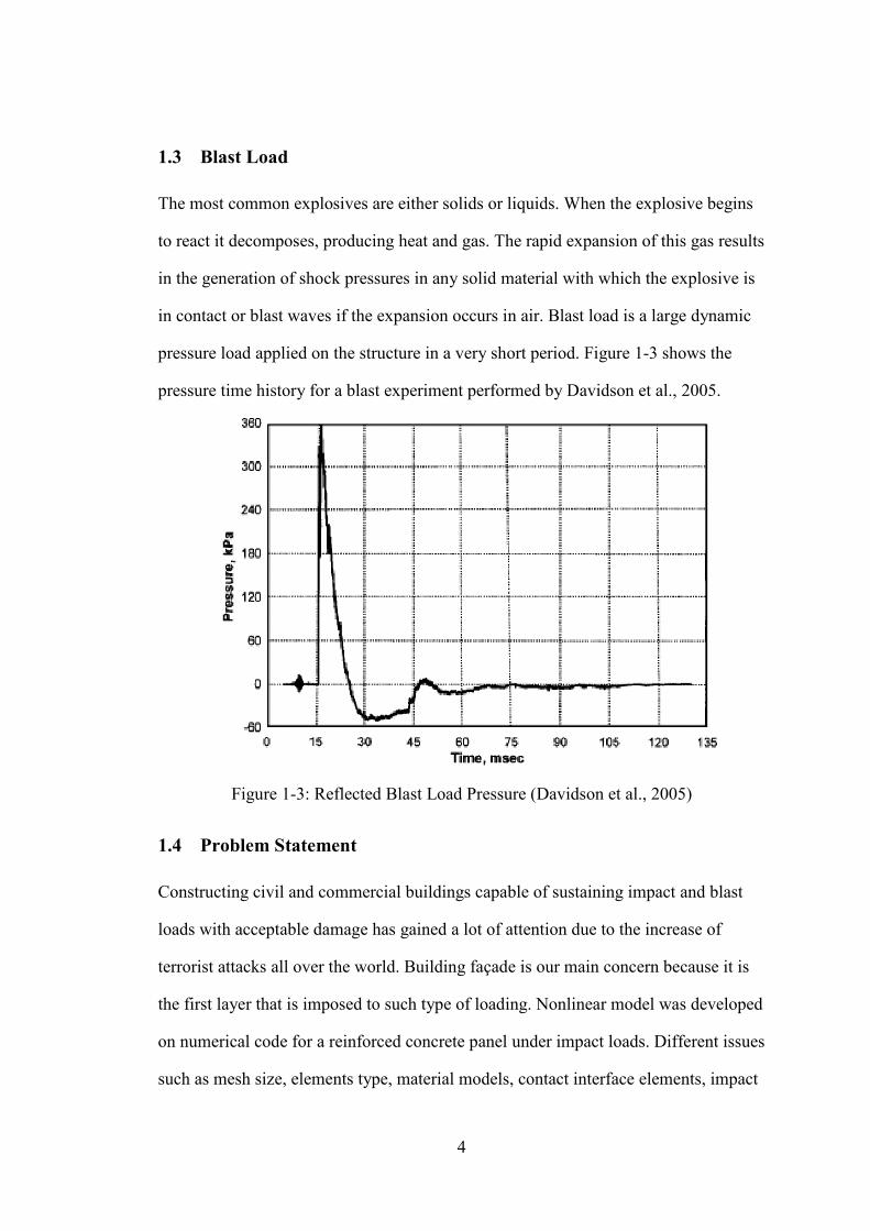
pressure load applied on the structure in a very short period. Figure 1-3 shows the
pressure time history for a blast experiment performed by Davidson et al., 2005.
Figure 1-3: Reflected Blast Load Pressure (Davidson et al., 2005)
1.4 Problem Statement
Constructing civil and commercial buildings capable of sustaining impact and blast
loads with acceptable damage has gained a lot of attention due to the increase of
terrorist attacks all over the world. Building façade is our main concern because it is
the first layer that is imposed to such type of loading. Nonlinear model was developed
on numerical code for a reinforced concrete panel under impact loads. Different issues
such as mesh size, elements type, material models, contact interface elements, impact
5
loads …etc were studied in details. Impact loads were modeled by two methods;
simplified pendulum analysis and simulated pendulum analysis. Both methods were
verified by experimental results from the literature. Simplified pendulum analysis
used the impact force-time history from the literature to load the RC panel; on the
other hand, simulated pendulum analysis modeled the pendulum mass that was lifted
to a dropping height and left to fall under free fall acceleration. Analysis of results and
parametric analysis were used to prepare means of increasing the capacity of the panel
to sustain high impact loads within acceptable damage; moreover, new supporting
systems were introduced to reduce the force transferred to the structure supporting the
concrete panel.
1.5 Research Objectives
The first objective of this research is to help building civil and commercial buildings
capable of sustaining impact and blast loads with acceptable damage to save the life
of the occupants. Reinforced concrete panels are commonly used in building façade.
The research will focus on a middle panel with one-way slab\beam action.
The second objective of this research is to develop a nonlinear model using a
numerical code. The developed model will examine different model factors such as
mesh size, elements type, material models, contact interface elements …etc. Various
mesh size were used. Four concrete material models were utilized due to the complex
nature of concrete.
The third objective of this research is to validate the developed model with
experimental results from the literature. Impact loads were modeled by two methods;
simplified pendulum analysis and simulated pendulum analysis. Simplified pendulum
analysis used the impact force-time history from the literature to load the RC panel;

6
on the other hand, simulated pendulum analysis modeled the pendulum mass that was
lifted to a dropping height and left to fall under free fall acceleration.
The forth objective of this research is to analyze and manipulate the results to see how
can the capacity of the panel increased to sustain high impact loads with minimum
damage; moreover, new supporting systems were introduced to reduce the force
transferred to the structure supporting the panel.
The fifth objective of this research is to gain the knowledge of how to design such
panels to resist impact loads while reducing the forces transferred to the structure
1.6 Scope and Limitations
The scope of this research is to analyze building façade subjected to shock and impact
loading; however, due to the lack of experimental results for building faced panels
imposed to impact loading, experimental setup conducted by Cherif , 2009 on
reinforced concrete beams under impact loading was used for validating the numerical
model.
The model is cable of simulating low-to-high velocity impacts; hyper velocities and
full penetrations may require model refinements such as contact issues, mesh size, and
eroding of materials upon pre-defined failure criteria(s).
1.7 Units
In general, it is the responsibility of the software user to unify the system of units used
in the numerical code. Due to the fact that, the majority of the information available in
the literature is in the English units system, we used the BIN consistent unit system in
the modeling process; however, to meet the Egyptian standards, all values and figures
7
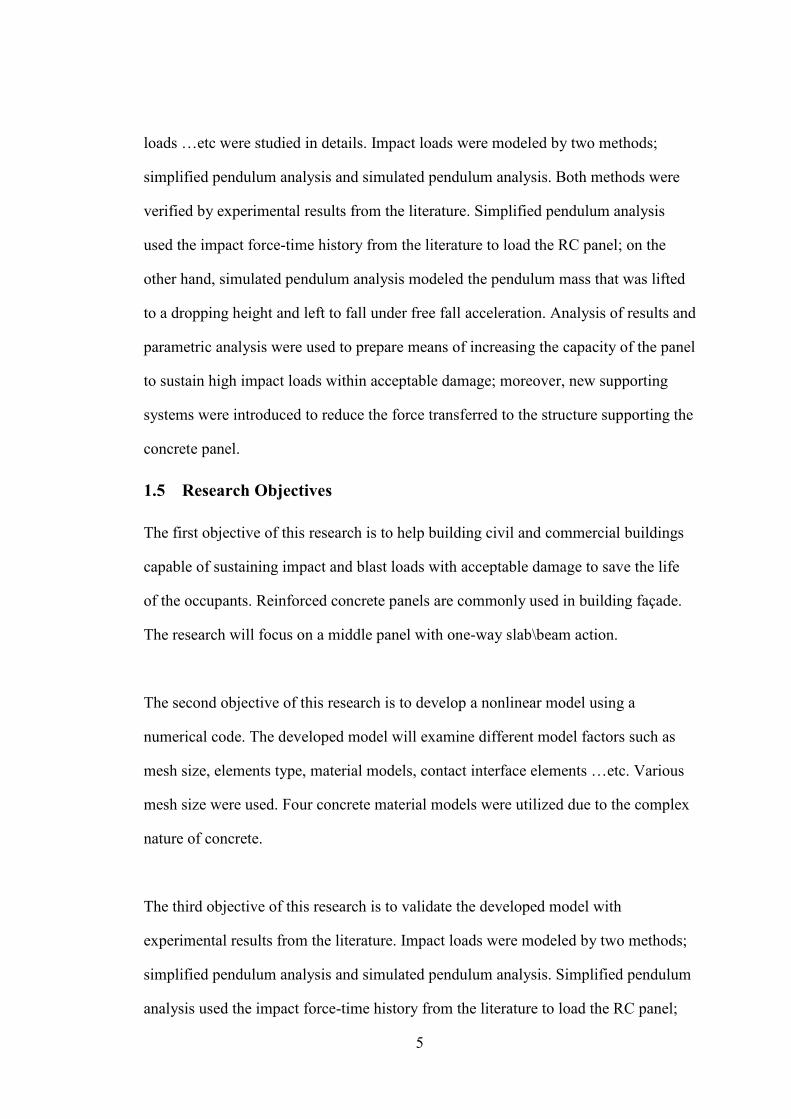
were presented in SI units. Table 1-1shows the common unit systems that are
available in the software.
Table 1-1: Consistent unit systems (ANSYS, 2009)
1.8 Central Processing Unit (CPU)
The analysis required high end processing units in addition to very large space for
storage. The specification of the CPU used in this research is as follows;
• Computer : Dell OPTIPLEX 760
• Processor: Intel® Core™ 2 Duo CPU E8500 , 3.16 GHz
• Main Memory: 5 GB
• Hard Disk (For Runs): 500 GB

8
• Hard Disk (For Storage): Ten hard discs were used for storage i.e. 10X250 GB
• Video Card : ATI Radeon HD 2400 , 256MB
• Operating System : Windows XP Pro-SP2 , 64 bit
1.9 Organization of the Thesis
The thesis consists of five chapters. Chapter one aims to present the topic through a
general introduction followed by definition of different loading types; in addition to,
the problem statement, research objectives, and scope & limitations. Unit systems and
specification of the processing unit are also described.
Chapter two presents literature review for the research done in the area of reinforced
concrete panels under impact loads. The chapter presents the literature review
organized with respect to relevant topics such as experimental tests for RC targets
under impact loads, numerical simulations of RC targets under impact loads,
nonlinear software packages, material models..etc
Chapter three describes the research methodology in terms of general introduction,
detailed description of the model (geometry, boundary conditions, applied loads,
software, element types and mesh size) , material models (concrete and steel) , and
data used for validation from the literature.
Chapter four analyzes the results of the linear and nonlinear models. The results of the
nonlinear simplified pendulum analysis and simulated pendulum analysis are
validated with a validation matrix of four experimental tests conducted by Cherif ,
(2009) at the American university in Cairo. The validation process is followed by
model refinements and comprehensive parametric analysis in order to study the effect
of different parameters on the response of the RC panel such as effect of
reinforcement, effect of steel plates thickness and elasticity, effect of a specifically
designed support connection that allows for absorbing the impact shock..etc
9
CHAPTER 2: LITERATURE REVIEW
2.1 Impact Force Parameters
In close analytical, experimental, or numerical study for concrete targets under
impact load , many researchers presented the impact force time-history which showed
the duration , the value , and the shape of the load (Tachibana et al., 2010, Sangi and
May, 2009, Chen and May, 2009 , and Kazunori et al., 2009)
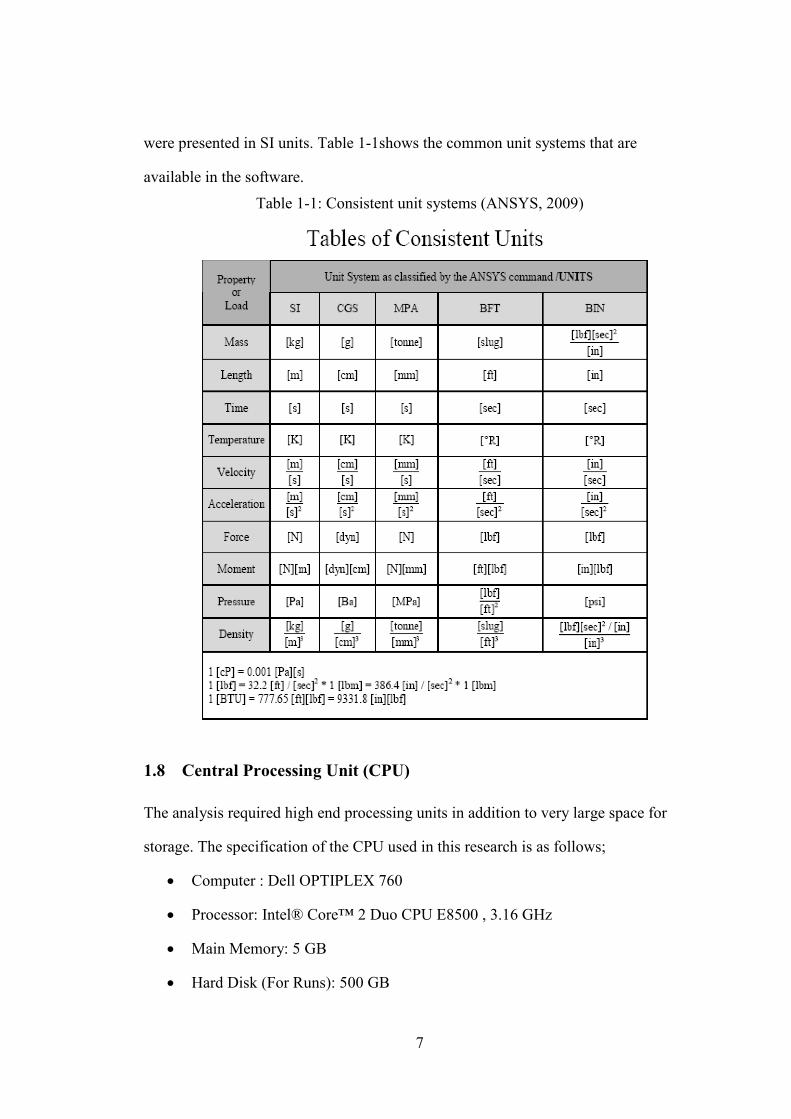
Tachibana et al., 2010 proposed a performance-based design method for a set of
reinforced concrete beams, having natural period of 2.5 up to 40.1 msec. In the entire
set of experimental results the impact duration ranged from 23.9 up to 105.6 ms
(Figure 2-1). The proposed method mentioned that the impacts force duration is
proportional to the ratio of the momentum of the weight divided by the static ultimate
bending capacity; however, there is a tendency observed that by increasing the static
ultimate bending capacity, the impact force duration decrease.
Figure 2-1: Impact force time history for test No.16 - type A4 , mass 300kg , v 5m/s
(Tachibana et al., 2010)
10
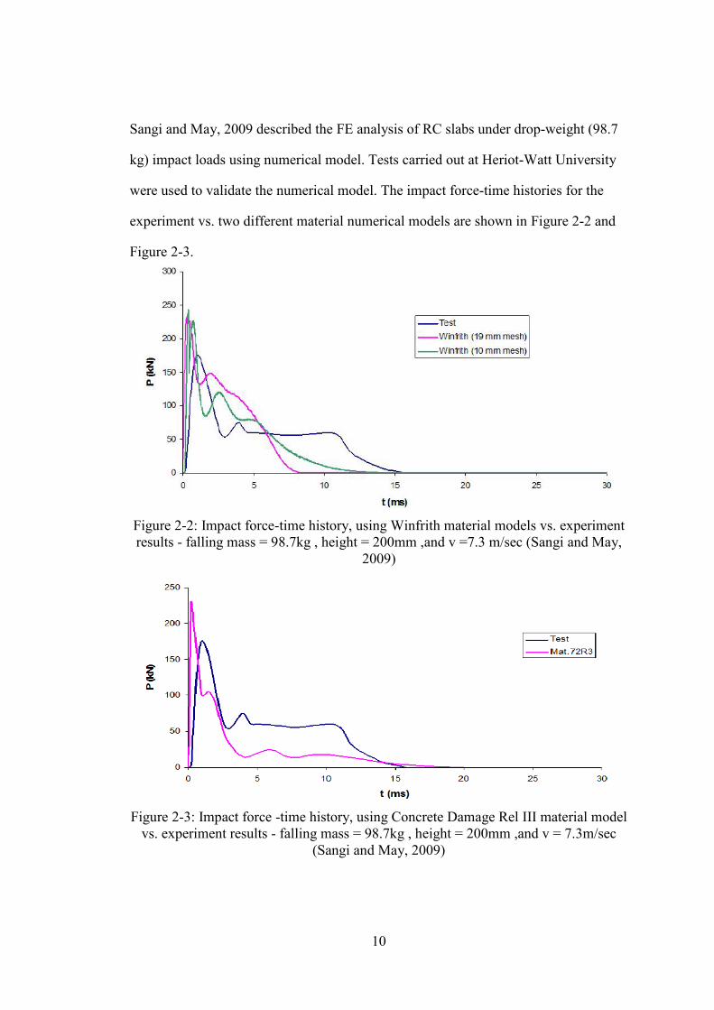
Sangi and May, 2009 described the FE analysis of RC slabs under drop-weight (98.7
kg) impact loads using numerical model. Tests carried out at Heriot-Watt University
were used to validate the numerical model. The impact force-time histories for the
experiment vs. two different material numerical models are shown in Figure 2-2 and
Figure 2-3.
Figure 2-2: Impact force-time history, using Winfrith material models vs. experiment results - falling mass = 98.7kg , height = 200mm ,and v =7.3 m/sec (Sangi and May,
2009)
Figure 2-3: Impact force -time history, using Concrete Damage Rel III material model
vs. experiment results - falling mass = 98.7kg , height = 200mm ,and v = 7.3m/sec (Sangi and May, 2009)
11
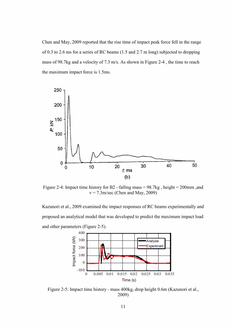
Chen and May, 2009 reported that the rise time of impact peak force fell in the range
of 0.3 to 2.6 ms for a series of RC beams (1.5 and 2.7 m long) subjected to dropping
mass of 98.7kg and a velocity of 7.3 m/s. As shown in Figure 2-4 , the time to reach
the maximum impact force is 1.5ms.
Figure 2-4: Impact time history for B2 - falling mass = 98.7kg , height = 200mm ,and
v = 7.3m/sec (Chen and May, 2009)
Kazunori et al., 2009 examined the impact responses of RC beams experimentally and
proposed an analytical model that was developed to predict the maximum impact load
and other parameters (Figure 2-5).
Figure 2-5: Impact time history - mass 400kg, drop height 0.6m (Kazunori et al.,
2009)

12
Liu et al., 2009 and Huanga et al., 2005 numerically studied the penetration of
reinforced concrete blocks and results were validated with experimental data.
Liu et al., 2009 numerically simulated oblique-angle penetration into concrete targets
by using the three-dimensional finite element. A constitutive model describes both the
compressive and tensile damage of concrete was implemented. Under different
oblique angles, the damage distribution and depths of penetration were recorded. The
numerical results were compared to experimental data from the literature. As shown
in Figure 2-6, it can be seen that the numerical results are in good agreement with the
experimental data.
Figure 2-6: Comparison of the penetration depth between (a) the experimental data
and (b) the numerical model (Liu et al., 2011)
13
Huanga et al., 2005, studied numerically the perforation of RC targets. The numerical
software predicted the crater diameters on front and back sides of the target. Using
experimental results reported in a previous research in the literature, the numerical
models were verified and did show good agreement with the experimental results.
During perforation of a RC target, the model simulates residual velocity of the
projectile, the crater formation, spall of concrete and the fracture. Moreover, the
model also captured the dynamic behavior of RC target and the effect of the steel
reinforcement on the penetration of RC target.
2.2 Reinforced Concrete Targets Under Impact Load
2.2.1 Experimental Tests
Jose et al., 2010 performed experimental setup for slender RC slabs, squat RC and PC
slabs under soft and hard missile impacts. RC slabs were also addressed by Chen and
May, 2009; and Tahmasebinia, 2008.
Slab specimens used in Phase I of the IMPACT program were divided to 10 slender
RC slabs (2.3x2.0x0.15 m) under soft missile impacts and 13 squat RC and PC slabs
(2.1 x 2.100x0.25 m) under hard missile impacts were tested experimentally (Jose et
al., 2010)Various parameters were examined such as impact loads, missile speeds,
effects of various slab designs, global and local response and damage; while, under
hard missile impacts, the penetration and overall slab damage were reported (Jose et
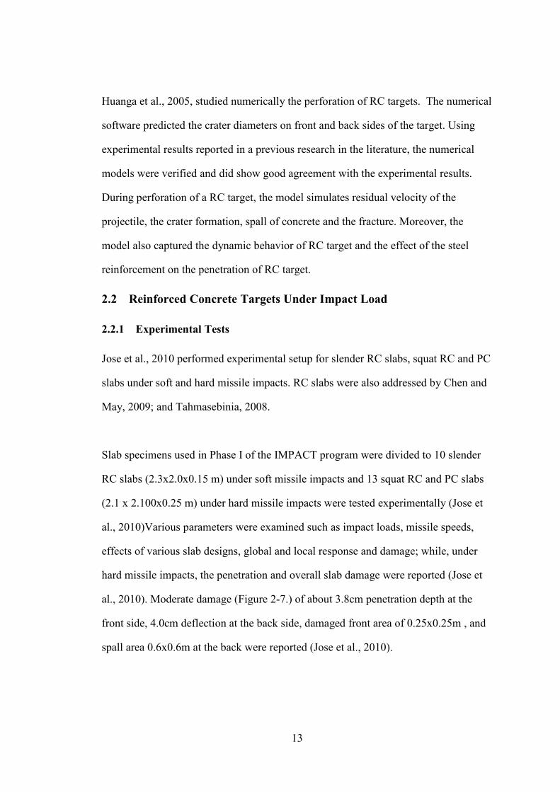
al., 2010). Moderate damage (Figure 2-7.) of about 3.8cm penetration depth at the
front side, 4.0cm deflection at the back side, damaged front area of 0.25x0.25m , and
spall area 0.6x0.6m at the back were reported (Jose et al., 2010).
14
Figure 2-7: Front and back damaged area (Jose et al., 2010)
Chen and May, 2009 aimed to capture the transient impact load, accelerations, and
strain in the steel reinforcement. For the slabs tests, the gained energy on the slab was
compared with empirical formulae of the minimum energy causing a slab to scab.
Comparing the experimental results with the empirical formula with respect to energy,
it can be seen that they were far from each other for 150mm thick slab; however, it
showed satisfactory predications for the 76mm thick slab.
Tahmasebinia, 2008 tested simply supported slabs along both edges under drop
hammer. The slabs were 1355x1090x90 mm .For better understanding of the
structural response under impact loading; several characteristics of impact load were
measured such as impact load and deflection at the center point of the slab.
Various experimental setups were carried out for RC beams (Chen and May, 2009;
Bhatti et al., 2009; and Tachibana et al., 2010). Beams specimens were tested with a
span of 2.7m and 1.5m under low-velocity and high-mass (Chen and May, 2009).
Bhatti et al., 2009 examined RC beams subjected to falling-weight impact. Beams
were simply supported with dimensions of 2.4x0.4x0.2 m. A steel mass of 400 kg was
15
dropped at the mid-span of RC beam. Tachibana et al., 2010 examined a series of RC
beams, having different spans, reinforcement, and cross-section.
Chen and May, 2009 confirmed that for beam tests, the impact load history was
correlated with the images of the crack propagation. The research confirmed the
findings of others related to beams subjected to impact; moreover, the research
indicated that beam span is more significant than the supporting conditions with
respect to the beam response.
Bhatti et al., 2009 examined shear-failure-type RC beams subjected to falling-weight
impact. Experimental results focused on some impact load characteristics such as time
histories of applied force, reaction force, mid-span deflection, and crack pattern of RC
beam.
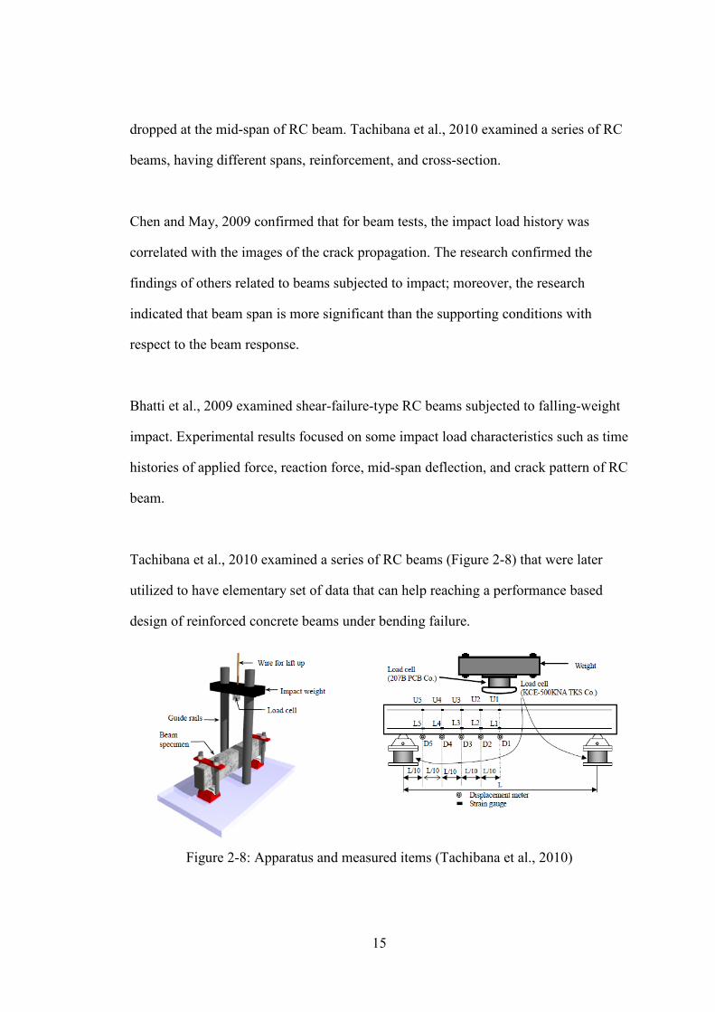
Tachibana et al., 2010 examined a series of RC beams (Figure 2-8) that were later
utilized to have elementary set of data that can help reaching a performance based
design of reinforced concrete beams under bending failure.
Figure 2-8: Apparatus and measured items (Tachibana et al., 2010)
16
Kazunori et al., 2009 through an experimental setup studied the influence of
longitudinal reinforcement (tension and compression) on the responses of RC beams
under impact load using a drop hammer impact test, while Murray et al., 2007 tested
forty-seven plain concrete, under-reinforced, and over-reinforced beams under drop
tower.
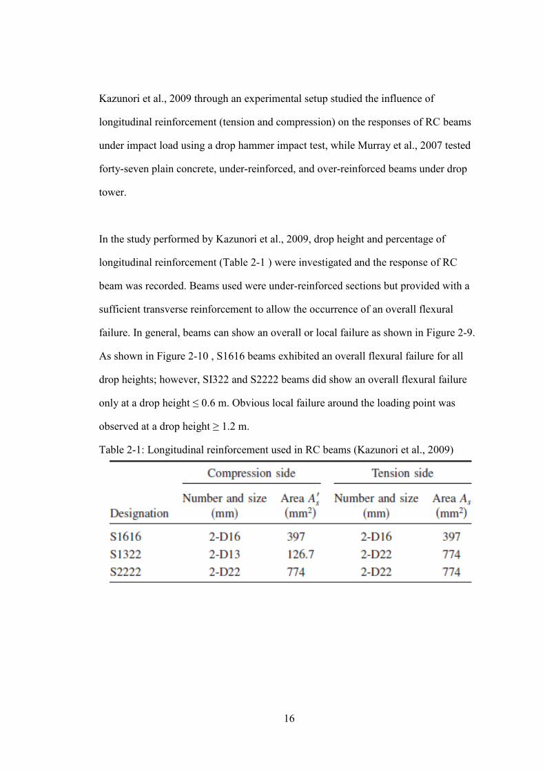
In the study performed by Kazunori et al., 2009, drop height and percentage of
longitudinal reinforcement (Table 2-1 ) were investigated and the response of RC
beam was recorded. Beams used were under-reinforced sections but provided with a
sufficient transverse reinforcement to allow the occurrence of an overall flexural
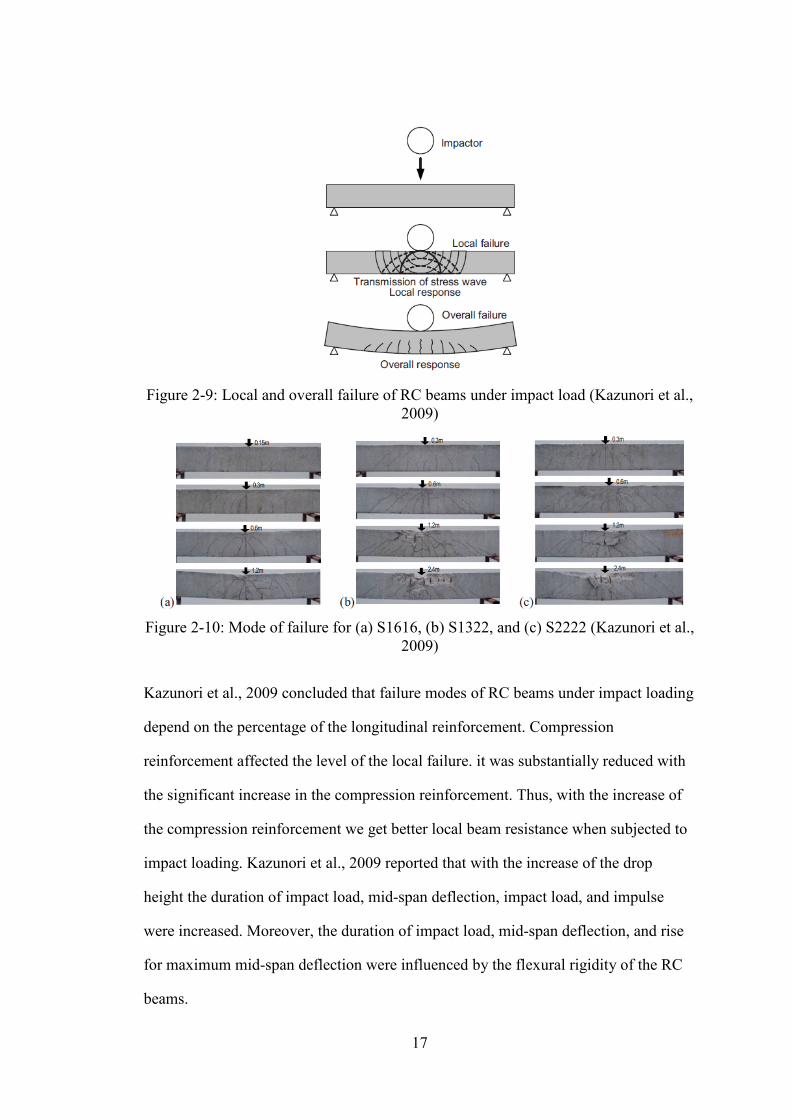
failure. In general, beams can show an overall or local failure as shown in Figure 2-9.
As shown in Figure 2-10 , S1616 beams exhibited an overall flexural failure for all
drop heights; however, SI322 and S2222 beams did show an overall flexural failure
only at a drop height ≤ 0.6 m. Obvious local failure around the loading point was
observed at a drop height ≥ 1.2 m.
Table 2-1: Longitudinal reinforcement used in RC beams (Kazunori et al., 2009)
17
Figure 2-9: Local and overall failure of RC beams under impact load (Kazunori et al.,
2009)
Figure 2-10: Mode of failure for (a) S1616, (b) S1322, and (c) S2222 (Kazunori et al.,
2009)
Kazunori et al., 2009 concluded that failure modes of RC beams under impact loading
depend on the percentage of the longitudinal reinforcement. Compression
reinforcement affected the level of the local failure. it was substantially reduced with
the significant increase in the compression reinforcement. Thus, with the increase of
the compression reinforcement we get better local beam resistance when subjected to
impact loading. Kazunori et al., 2009 reported that with the increase of the drop
height the duration of impact load, mid-span deflection, impact load, and impulse
were increased. Moreover, the duration of impact load, mid-span deflection, and rise
for maximum mid-span deflection were influenced by the flexural rigidity of the RC
beams.
18
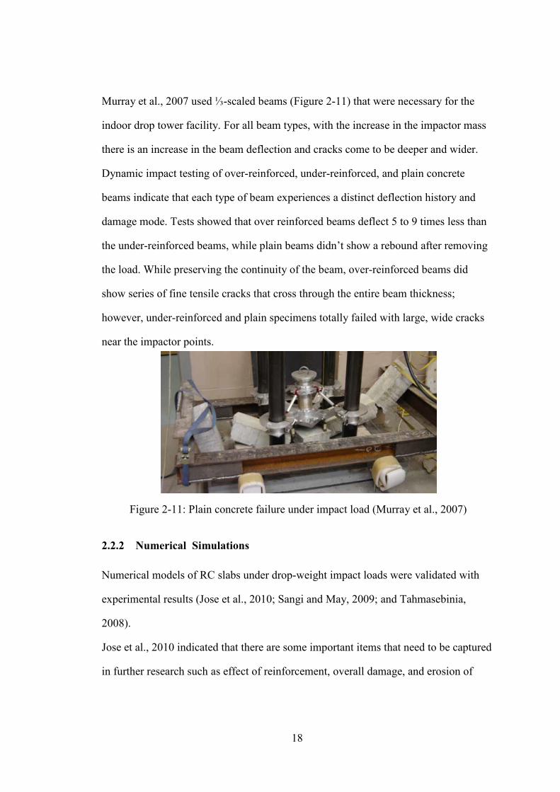
Murray et al., 2007 used ⅓-scaled beams (Figure 2-11) that were necessary for the
indoor drop tower facility. For all beam types, with the increase in the impactor mass
there is an increase in the beam deflection and cracks come to be deeper and wider.
Dynamic impact testing of over-reinforced, under-reinforced, and plain concrete
beams indicate that each type of beam experiences a distinct deflection history and
damage mode. Tests showed that over reinforced beams deflect 5 to 9 times less than
the under-reinforced beams, while plain beams didn’t show a rebound after removing
the load. While preserving the continuity of the beam, over-reinforced beams did
show series of fine tensile cracks that cross through the entire beam thickness;
however, under-reinforced and plain specimens totally failed with large, wide cracks
near the impactor points.
Figure 2-11: Plain concrete failure under impact load (Murray et al., 2007)
2.2.2 Numerical Simulations
Numerical models of RC slabs under drop-weight impact loads were validated with
experimental results (Jose et al., 2010; Sangi and May, 2009; and Tahmasebinia,
2008).
Jose et al., 2010 indicated that there are some important items that need to be captured
in further research such as effect of reinforcement, overall damage, and erosion of
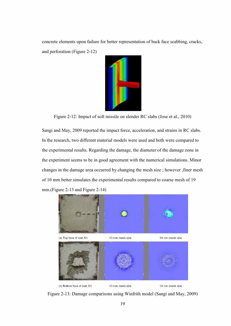
19
concrete elements upon failure for better representation of back face scabbing, cracks,
and perforation (Figure 2-12)
Figure 2-12: Impact of soft missile on slender RC slabs (Jose et al., 2010)
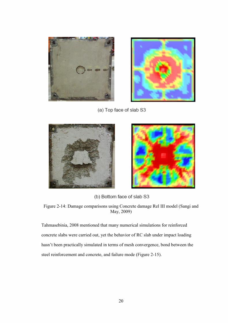
Sangi and May, 2009 reported the impact force, acceleration, and strains in RC slabs.
In the research, two different material models were used and both were compared to
the experimental results. Regarding the damage, the diameter of the damage zone in
the experiment seems to be in good agreement with the numerical simulations. Minor
changes in the damage area occurred by changing the mesh size ; however ,finer mesh
of 10 mm better simulates the experimental results compared to coarse mesh of 19
mm.(Figure 2-13 and Figure 2-14)
Figure 2-13: Damage comparisons using Winfrith model (Sangi and May, 2009)
20
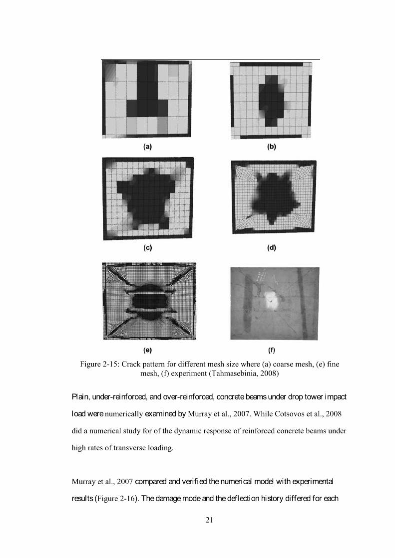
Figure 2-14: Damage comparisons using Concrete damage Rel III model (Sangi and
May, 2009)
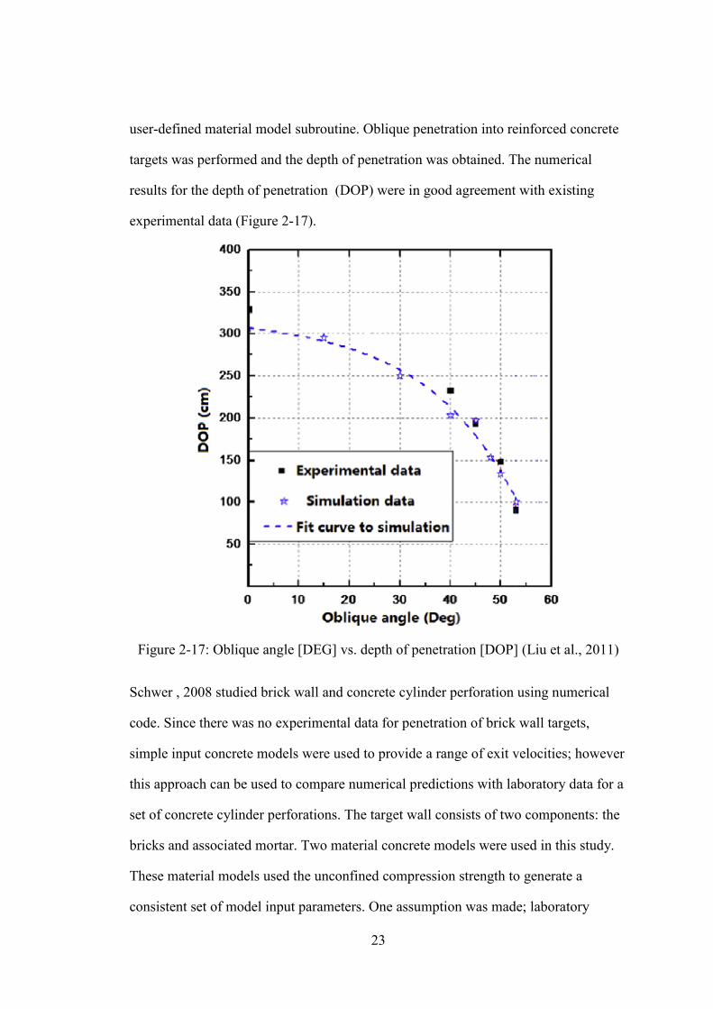
Tahmasebinia, 2008 mentioned that many numerical simulations for reinforced
concrete slabs were carried out, yet the behavior of RC slab under impact loading
hasn’t been practically simulated in terms of mesh convergence, bond between the
steel reinforcement and concrete, and failure mode (Figure 2-15).
21
Figure 2-15: Crack pattern for different mesh size where (a) coarse mesh, (e) fine
mesh, (f) experiment (Tahmasebinia, 2008)
Plain, under-reinforced, and over-reinforced, concrete beams under drop tower impact
load were numerically examined by Murray et al., 2007. While Cotsovos et al., 2008
did a numerical study for of the dynamic response of reinforced concrete beams under
high rates of transverse loading.
Murray et al., 2007 compared and verified the numerical model with experimental
results (Figure 2-16). The damage mode and the deflection history differed for each

22
type of beam; however, the model showed good agreement in terms of deflection
histories and damage modes. Related to our point of interest, Cotsovos et al., 2008
studied the localized impact loading such as that encountered in the case of blast
accidents and ballistic problems.
Figure 2-16: Drop tower comparison between the numerical model and the
experimental results (Murray et al., 2007)
Oblique penetration into reinforced concrete targets was conducted by Liu et al., 2011
through a dynamic constitutive model; Moreover, Schwer, 2008 and Akram, 2008
were interested in the perforation of brick wall , concrete cylinder and concrete barrier
respectively.
Liu et al., 2011 proposed a dynamic constitutive model based on the tensile (TCK
model) and the compressive damage models for concrete (HJC model). The
developed model was implemented into the numerical code, LS-DYNA, through a
23
user-defined material model subroutine. Oblique penetration into reinforced concrete
targets was performed and the depth of penetration was obtained. The numerical
results for the depth of penetration (DOP) were in good agreement with existing
experimental data (Figure 2-17).
Figure 2-17: Oblique angle [DEG] vs. depth of penetration [DOP] (Liu et al., 2011)
Schwer , 2008 studied brick wall and concrete cylinder perforation using numerical
code. Since there was no experimental data for penetration of brick wall targets,
simple input concrete models were used to provide a range of exit velocities; however
this approach can be used to compare numerical predictions with laboratory data for a
set of concrete cylinder perforations. The target wall consists of two components: the
bricks and associated mortar. Two material concrete models were used in this study.
These material models used the unconfined compression strength to generate a
consistent set of model input parameters. One assumption was made; laboratory
24
characterization of the brick material would be close to laboratory characterization of
concrete.
Akram, 2008 used LS-DYNA to model the concrete barrier to simulate the bogie
impact. Three material models in LS-DYNA (MAT72R3, 84 and 159) were used to
simulate the impact event. Comparisons between tests and numerical simulations in
terms of time history and deformations were addressed. This simulation showed the
overall behavior of a given bridge rail barrier. Moreover, good potential for using the
models in analyses of steel-reinforced concrete roadside safety barriers was
addressed.
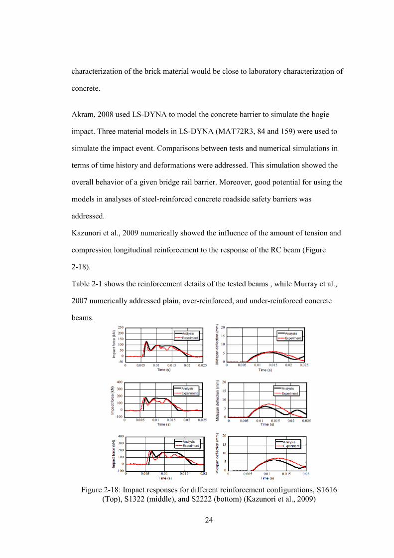
Kazunori et al., 2009 numerically showed the influence of the amount of tension and
compression longitudinal reinforcement to the response of the RC beam (Figure
2-18).
Table 2-1 shows the reinforcement details of the tested beams , while Murray et al.,
2007 numerically addressed plain, over-reinforced, and under-reinforced concrete
beams.
Figure 2-18: Impact responses for different reinforcement configurations, S1616
(Top), S1322 (middle), and S2222 (bottom) (Kazunori et al., 2009)
25
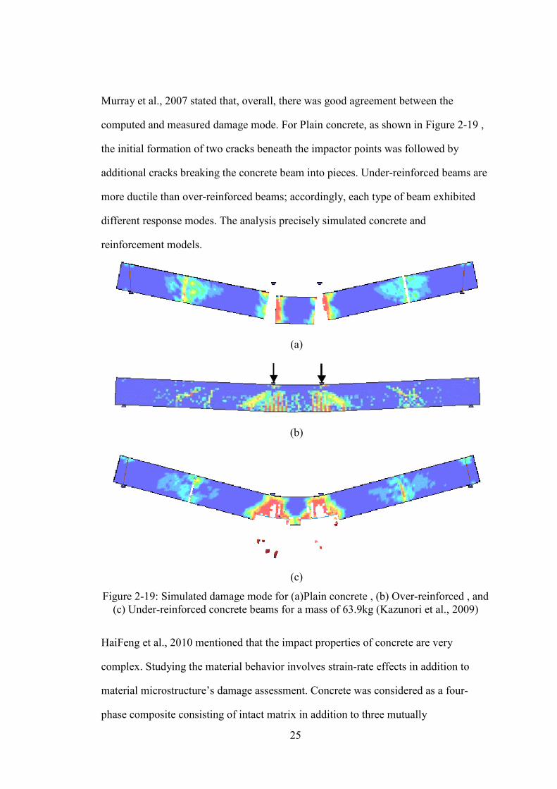
Murray et al., 2007 stated that, overall, there was good agreement between the
computed and measured damage mode. For Plain concrete, as shown in Figure 2-19 ,
the initial formation of two cracks beneath the impactor points was followed by
additional cracks breaking the concrete beam into pieces. Under-reinforced beams are
more ductile than over-reinforced beams; accordingly, each type of beam exhibited
different response modes. The analysis precisely simulated concrete and
reinforcement models.
(a)
(b)
(c)
Figure 2-19: Simulated damage mode for (a)Plain concrete , (b) Over-reinforced , and (c) Under-reinforced concrete beams for a mass of 63.9kg (Kazunori et al., 2009)
HaiFeng et al., 2010 mentioned that the impact properties of concrete are very
complex. Studying the material behavior involves strain-rate effects in addition to
material microstructure’s damage assessment. Concrete was considered as a four-
phase composite consisting of intact matrix in addition to three mutually
26
perpendicular groups of penny-shaped micro-cracks. In this composition, the intact
matrix was assumed to be elastic, homogeneous and isotropic. Impact compression
tests of concrete and cement mortar with various strain rates were used. It was shown
that the model predictions match the experimental results; accordingly, the model can
be used to simulate the dynamic mechanical behaviors of concrete.
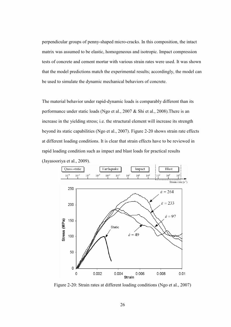
The material behavior under rapid-dynamic loads is comparably different than its
performance under static loads (Ngo et al., 2007 & Shi et al., 2008).There is an
increase in the yielding stress; i.e. the structural element will increase its strength
beyond its static capabilities (Ngo et al., 2007). Figure 2-20 shows strain rate effects
at different loading conditions. It is clear that strain effects have to be reviewed in
rapid loading condition such as impact and blast loads for practical results
(Jayasooriya et al., 2009).
Figure 2-20: Strain rates at different loading conditions (Ngo et al., 2007)
27
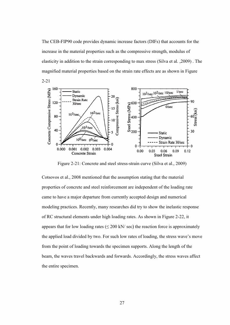
The CEB-FIP90 code provides dynamic increase factors (DIFs) that accounts for the
increase in the material properties such as the compressive strength, modulus of
elasticity in addition to the strain corresponding to max stress (Silva et al. ,2009) . The
magnified material properties based on the strain rate effects are as shown in Figure
2-21
Figure 2-21: Concrete and steel stress-strain curve (Silva et al., 2009)
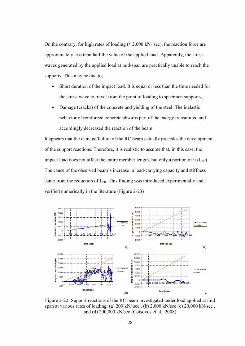
Cotsovos et al., 2008 mentioned that the assumption stating that the material
properties of concrete and steel reinforcement are independent of the loading rate
came to have a major departure from currently accepted design and numerical
modeling practices. Recently, many researches did try to show the inelastic response
of RC structural elements under high loading rates. As shown in Figure 2-22, it
appears that for low loading rates (≤ 200 kN/ sec) the reaction force is approximately
the applied load divided by two. For such low rates of loading, the stress wave’s move
from the point of loading towards the specimen supports. Along the length of the
beam, the waves travel backwards and forwards. Accordingly, the stress waves affect
the entire specimen.
28
On the contrary, for high rates of loading (≥ 2,000 kN/ sec), the reaction force are
approximately less than half the value of the applied load. Apparently, the stress
waves generated by the applied load at mid-span are practically unable to reach the
supports. This may be due to;
• Short duration of the impact load. It is equal or less than the time needed for
the stress wave to travel from the point of loading to specimen supports,
• Damage (cracks) of the concrete and yielding of the steel. The inelastic
behavior of reinforced concrete absorbs part of the energy transmitted and
accordingly decreased the reaction of the beam
It appears that the damage/failure of the RC beam actually precedes the development
of the support reactions. Therefore, it is realistic to assume that, in this case, the
impact load does not affect the entire member length, but only a portion of it (Leff)
The cause of the observed beam’s increase in load-carrying capacity and stiffness
came from the reduction of Leff. This finding was introduced experimentally and
verified numerically in the literature (Figure 2-23)
Figure 2-22: Support reactions of the RC beam investigated under load applied at mid span at various rates of loading: (a) 200 kN/ sec , (b) 2,000 kN/sec (c) 20,000 kN/sec ,
and (d) 200,000 kN/sec (Cotsovos et al., 2008)
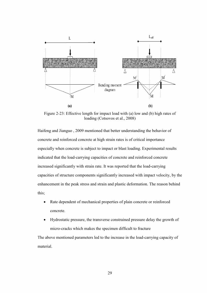
29
Figure 2-23: Effective length for impact load with (a) low and (b) high rates of
loading (Cotsovos et al., 2008)
Haifeng and Jianguo , 2009 mentioned that better understanding the behavior of
concrete and reinforced concrete at high strain rates is of critical importance
especially when concrete is subject to impact or blast loading. Experimental results
indicated that the load-carrying capacities of concrete and reinforced concrete
increased significantly with strain rate. It was reported that the load-carrying
capacities of structure components significantly increased with impact velocity, by the
enhancement in the peak stress and strain and plastic deformation. The reason behind
this;
• Rate dependent of mechanical properties of plain concrete or reinforced
concrete.
• Hydrostatic pressure, the transverse constrained pressure delay the growth of
micro-cracks which makes the specimen difficult to fracture
The above mentioned parameters led to the increase in the load-carrying capacity of
material.

30
Pires et al., 2010 numerically simulated hard-missile impacts on RC slabs. They did
use high speed camera to capture the response of the specimens subjected to higher
impact speeds. (Figure 2-24)
Figure 2-24: RC slabs response to high-speed impact recorded by high speed camera
(Pires et al., 2010)
Chen and May, 2009 used high speed camera (up to 4500 fps) to study a series of
experiment setups of RC beams and slabs subjected to the high-mass, low-velocity
impact. As shown in Figure 2-25 , load history was correlated to the development
images of cracks and scabbing to identify the local failure pattern of a beam under the
impact zone.
Figure 2-25: Impact load history correlated with crack propagation for a beam (Chen
and May, 2009)
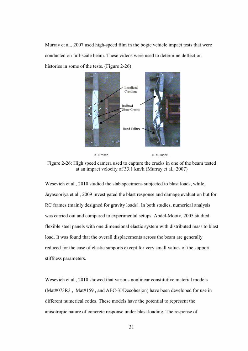
31
Murray et al., 2007 used high-speed film in the bogie vehicle impact tests that were
conducted on full-scale beam. These videos were used to determine deflection
histories in some of the tests. (Figure 2-26)
Figure 2-26: High speed camera used to capture the cracks in one of the beam tested
at an impact velocity of 33.1 km/h (Murray et al., 2007)
Wesevich et al., 2010 studied the slab specimens subjected to blast loads, while,
Jayasooriya et al., 2009 investigated the blast response and damage evaluation but for
RC frames (mainly designed for gravity loads). In both studies, numerical analysis
was carried out and compared to experimental setups. Abdel-Mooty, 2005 studied
flexible steel panels with one dimensional elastic system with distributed mass to blast
load. It was found that the overall displacements across the beam are generally
reduced for the case of elastic supports except for very small values of the support
stiffness parameters.
Wesevich et al., 2010 showed that various nonlinear constitutive material models
(Mat#073R3 , Mat#159 , and AEC-3I/Decohesion) have been developed for use in
different numerical codes. These models have the potential to represent the
anisotropic nature of concrete response under blast loading. The response of

32
reinforced concrete slab specimens subjected to blast loads were simulated and
evaluated using three different constitutive concrete models. Slabs were also
experimentally tested under shock tube component system. (Figure 2-27). Within a
scale of two, the three constitutive concrete models captured the peak deflection due
to blast loads in all the tests.
Figure 2-27: Slab response under blast load (Wesevich et al., 2010)
Jayasooriya et al., 2009 did a numerical analysis using the explicit finite element
software, LS DYNA. Numerical model was conducted for RC frames with blast
charge weights of 150, 350, 420, 500, 650 and 700 kg of TNT. The standoff distance
was fixed to 10 m. The initial and the residual capacity of the frame due to damage
were highlighted. The load applying sequence were addressed; for example ,initial
ramp loading to model gravity loads then applying blast loads and the application of
vertical displacement to the frame to evaluate the column residual capacities. Based
on the initial and residual capacities, damage indices for columns were addressed.
Damage index simply provided an assessment method for the damage of a typical
33
multi-storey building frame under an external bomb accident which is required in post
blast assessments.
Abdel-Mooty, 2005 modeled the supports of RC panels with springs that have
different stiffness ranging from zero for unsupported panels to very high values
(infinity) for rigid supports. It was found that using elastic supports instead of rigid
supports can significantly reduce support reaction and bending moments in addition to
overall displacement response.
2.3 Analytical and Empirical Analysis
Using a series of reinforced concrete beams subjected to low speed impact
experiments, Tachibana et al., 2010 established a performance-based design method;
while, Kazunori et al., 2009 proposed an analytical method. Shear behavior of RC has
always been a challenging issue; accordingly, Saatci and Vecchio, 2009 proposed a
procedure for the shear critical failure under dynamic loading of statically flexural-
critical specimens .While Bhatti et al., 2009 established a simple elasto-plastic impact
analysis method for shear-failure-type RC beams.
For Slabs, Chen and May, 2009 used the empirical formulas in the literature to
compare the imposed energy on the slab with the empirical formula in order to limit
the scabbing of concrete.
Tachibana et al., 2010 showed that the maximum displacement of RC beams can be
identified, based on a proposed equation, in terms of static ultimate bending capacity,
kinetic energy, and the velocity of the impact mass. It was also reported that the
impact impulse was proportional to the momentum of the impact mass and the impact
force duration. For the entire series of RC beams, the impact impulse was directly
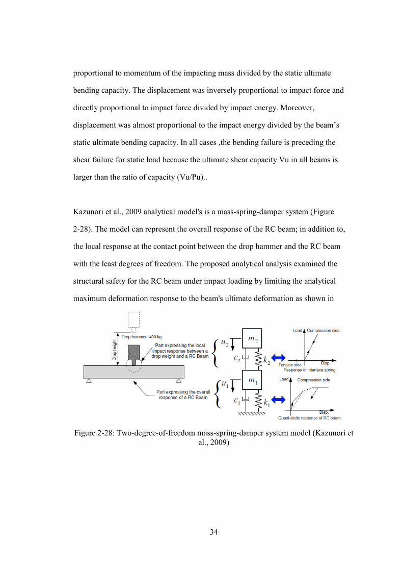
34
proportional to momentum of the impacting mass divided by the static ultimate
bending capacity. The displacement was inversely proportional to impact force and
directly proportional to impact force divided by impact energy. Moreover,
displacement was almost proportional to the impact energy divided by the beam’s
static ultimate bending capacity. In all cases ,the bending failure is preceding the
shear failure for static load because the ultimate shear capacity Vu in all beams is
larger than the ratio of capacity (Vu/Pu)..
Kazunori et al., 2009 analytical model's is a mass-spring-damper system (Figure
2-28). The model can represent the overall response of the RC beam; in addition to,
the local response at the contact point between the drop hammer and the RC beam
with the least degrees of freedom. The proposed analytical analysis examined the
structural safety for the RC beam under impact loading by limiting the analytical
maximum deformation response to the beam's ultimate deformation as shown in
Figure 2-28: Two-degree-of-freedom mass-spring-damper system model (Kazunori et
al., 2009)

35
Figure 2-29: Design flow of RC beam subjected to impact loading (Kazunori et al.,
2009)
Saatci and Vecchio, 2009 mentioned that the available methods in the literature for
modeling RC structure under impact loading, generally, exhibit some deficiencies in
aspects related to applicability, practicality, and accuracy. Shear behavior of RC has
always been a challenging issue. The study employed the disturbed stress field model
as an advanced method of modeling shear behavior under impact load. In the
36
proposed methodology, post peak vibration characteristics compared to test results
showed some minor discrepancies that comes from the behavior of steel and concrete
under high strain rates. The proposed method was not capable of predicting local
failure, penetration or scabbing and high-velocity impacts.
Bhatti et al., 2009 reported that the impact force, reaction force and displacement
wave of the RC beam can be predicted with a relatively good accuracy using the
proposed FE analysis technique.
There are few non-linear numerical codes used in the analysis of explicit dynamics
such as blast and impact loads on reinforced concrete structures. In the literature there
were few trials done on some software, namely AUTODYN (Nyström and Gylltoft,
2011), NLFEA (Saatci and Vecchio, 2009), ANSYS LS-DYNA (Cotsovos et al.,
2008), EPIC (Bush, 2010), and ABAQUS (Tahmasebinia, 2008)
On the other hand, the literature contains massive work done using LS-DYNA. it has
been used for numerical simulation of concrete structures under impact and blast
loading by (Liu et al., 2010; Sangi, 2009; Bhatti et al. , 2009 ;Silva et al., 2009;
Murray et al. , 2007; Raguraman et al. 2008; Farnam et al. , 2008; Schwer and Malvar
, 2005; Magallanes et al. , 20110; Jayasooriya et al. , 2009; Schwer , 2008; Akram ,
2008; Huanga et al. , 2005; and Abdel-Mooty and Shaaban , 2010).
Many authors verified LS-DYNA with experimental tests and/or analytical solutions.
It did show a good agreement in the validation process due to the wide range of
existing material models in addition to the user defined material models subroutine.
Part of the above mentioned references mentioned that LS-DYNA is best suited for
37
concrete impact and penetration problems, allowing realistic modeling for
experimental impact tests.
One of the underlying challenges in this research is the capability of the numerical
model to represents the rational behavior of the concrete under impact loads,
including the non linear response of the material under impact loads. Numerous
material models that could be used for concrete under varying stress and loading rate
conditions were reviewed, selected, modeled, and commented. Many of these models
are available in the LS-DYNA. In order for a numerical model to generate reliable
response of a concrete structure, it is vital to use a material model capable of
representing the mechanical processes of the material under this type of stress and
loading conditions. Concrete has complex nonlinear behavior that is difficult to be
simulated by a simple model (Tu & Lu, 2009).
LS-DYNA material database includes various material models for both concrete and
reinforcement. For concrete models, many of these models require multiple and
complex parameters that are not known without performing multiple material tests.
The details of each model parameters are not deeply described in the manuals (Sangi,
2009). However, recent versions of some models are privileged with the capability to
generate default parameters using only basic material properties (Schwer, 2005 &
Schwer, 2008). In this research, we used material models that do have different input
capabilities (LSTC, 2009 & Hallquist , 2006). They can be classified as;
• Material models that don’t have parameter generation capability like
MAT_GEOLOGIC_CAP_MODEL. It requires full input parameters.
• Material models that do have parameter generation capability like
MAT_CONCRETE_DAMAGE_REL3 and MAT_CSCM _CONCRETE.

38
• Material models that don’t have parameter generation capability but its
parameters can also be determined with relative ease like for
MAT_WINFRITH_CONCRETE. It requires a little bit more effort than just
entering the unconfined compressive strength of concrete; however, the other
inputs can be provided using empirical formulae.
Historically, concrete material models have been classified into numerous approaches
including elasticity, plasticity, and inelasticity theories; more recently, additional
approaches have appeared in the literature including fracturing, continuum damage,
and micro plane models (Bush, 2010).Plasticity models and continuum damage
models are the two well-known categories of concrete modeling.
In the early trials to model the yield and flow of materials, classical plasticity models
were utilized; however, they failed to capture the observed material responses in high
strain rate and impulsive loading conditions (Bush, 2010). Bush, 2010 added that
plasticity models have been incorporated in many of the common continuum damage
models for concrete in order to describe better more of the complex responses of
brittle materials under impulse loads specially those exceeding the elastic limits.
Recently, continuum damage models have many improvements including effects of
strain rate, damage, and confining pressures; however, they require rigorous efforts
for use and implementation (Bush, 2010). The process of selecting a material model
has become a balance between the availability of the experimental data and the need
to capture the complex material response.
2.3.1 Concrete Material Models
In tri-axial test conducted on plain concrete with different confinement pressures,
material #025, captured the behavior of concrete in the elastic range; Although, it

39
deviated at the post-peak section of the stress-strain curve (Yonten et al., 2002) . “One
major limitation of the model is that the formulation of the failure surfaces generates a
circular deviatoric cross section, whereas experimental data tend to indicate that for
brittle materials the shape of the deviatoric section is triangular at low pressures and it
only transits to circular at the high-pressure regime. This can cause unrealistic
behavior when the model is used in complex loading scenarios.” In addition, the cap
model cannot well predict the softening behavior of concrete and also cannot
represent satisfactorily the suppressing effect of the confining pressure on dilatancy of
concrete material (Tu & Lu, 2009).
In tri-axial test conducted on plain concrete with different confinement pressures,
material #072 captured the softening behavior of the concrete under different
confining pressures (Yonten et al., 2002). It showed high correlation between the
simulation and experimental results; however, there is a significant inconvenience
from using this material model because of its complex and multiple parameters
(Yonten et al., 2002). There is a true need for a simplified, but more efficient
concrete model that is easier for use.
A new release of the original formulation of material #072 introduced number of
improvements that have been implemented in material #072R3 (Schwer & Malvar,
2005). The new material model exhibits an automatic input capability for generic
concrete materials. Two methods are available: the first is used for the generic
concrete model when little is known other than the concrete’s compressive strength
and the second is used for advanced use of the model when sufficient data is available
(Magallanes et al., 2010).
40
Sangi & May, 2009 presented the simulated impact histories having good agreement
with the tests, using material #072R3. Thilakarathna et al., 2010 concluded that,
material #072R3 replicates the tri-axial state of stress under impact loads; however,
the mesh dependency of the fracture toughness can be better understood by a single
element model analysis to be able to simulate the tensile and shear failure conditions.
Moreover, other factors should be taken into consideration such as contact algorithms,
hourglass problems, and initial penetration condition (Thilakarathna et al., 2010).
The material model can accurately capture concrete behavior under impact-type
loading (Bush, 2010). Bush, 2010 added that the;
• Strength is modeled non-linearly versus pressure and varies between tensile
and compressive meridians
• Deformation includes limited shear dilation observed in concrete under
compression
• Damage incorporates strain rate and pressure effects ; in addition to , moving
the effective strength between the three failure surfaces of yield, maximum,
and residual for capturing the hardening and softening behavior
Others stated the same conclusion especially for concrete structures under dynamic
loads with varying stress and loading rate conditions (Schwer, 2005; Jayasooriya et
al., 2009; Sangi, 2009; Abu-Odeh, 2008; and Magallanes et al., 2010)
Considering concrete floors under low velocity impacts of heavy objects , the
reinforced concrete was modeled using material #084 / 085 (Algaard et al. , 2005). In
order to validate the model, Algaard et al., 2005 utilized empirical formulae that were
developed from experimental testing programs. In addition to some experimental
scale testing that was carried out by Heriot-Watt University (May, 2009). The

41
empirical and FE results showed very good perforation limit correlation for the entire
range of masses and velocities carried out in the validation process; moreover, direct
comparisons between experiments carried out at Heriot-Watt University and FE
revealed considerable agreement towards validating the model (Algaard et al. , 2005).
Cap models are classified as a continuum damage models for concrete (Bush, 2010).
A more recent implementation, the CSCM model extended the earlier cap
implementation known as the Geological Cap Model, material #025, that neglected
the third stress invariant, damage, and strain rate effects (Hallquist, 2006). Recently,
for roadside safety hardware testing, visco-plastic formulation and additional forms of
damage mechanics have been included in the CSCM model (Schwer & Murray, 2002
and Murray et al., 2007). The CSCM model is powered by effects of damage, strain
rate and tri-axial stress on the concrete strength (Bush, 2010).
The model has many input parameters; however, it is capable of generating the full
input parameters for standardized material properties, using only the unconfined
compressive strength and aggregate size.
Several validation tests were carried out through the development of the model for
conventional cylinder testing and impact tests (Murray et al., 2007). Modeling
cylinder tests showed that material #159 can realistically represent damage modes of
unconfined compression and tensile tests (Bush, 2010). Bush, 2010 added that the
numerical model results showed good agreement to test data for drop tower impact of
reinforced and plain concrete beams with respect to deflections and failure modes;
moreover, the model was also able to accurately simulate the displacement histories
and the damage modes of vehicle impact on reinforced concrete beams at velocities
ranging from 5.3 to 20.6 mph.
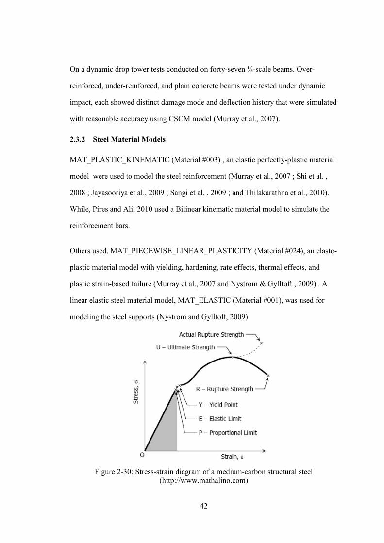
42
On a dynamic drop tower tests conducted on forty-seven ⅓-scale beams. Over-
reinforced, under-reinforced, and plain concrete beams were tested under dynamic
impact, each showed distinct damage mode and deflection history that were simulated
with reasonable accuracy using CSCM model (Murray et al., 2007).
2.3.2 Steel Material Models
MAT_PLASTIC_KINEMATIC (Material #003) , an elastic perfectly-plastic material
model were used to model the steel reinforcement (Murray et al., 2007 ; Shi et al. ,
2008 ; Jayasooriya et al., 2009 ; Sangi et al. , 2009 ; and Thilakarathna et al., 2010).
While, Pires and Ali, 2010 used a Bilinear kinematic material model to simulate the
reinforcement bars.
Others used, MAT_PIECEWISE_LINEAR_PLASTICITY (Material #024), an elasto-
plastic material model with yielding, hardening, rate effects, thermal effects, and
plastic strain-based failure (Murray et al., 2007 and Nystrom & Gylltoft , 2009) . A
linear elastic steel material model, MAT_ELASTIC (Material #001), was used for
modeling the steel supports (Nystrom and Gylltoft, 2009)
Figure 2-30: Stress-strain diagram of a medium-carbon structural steel
(http://www.mathalino.com)
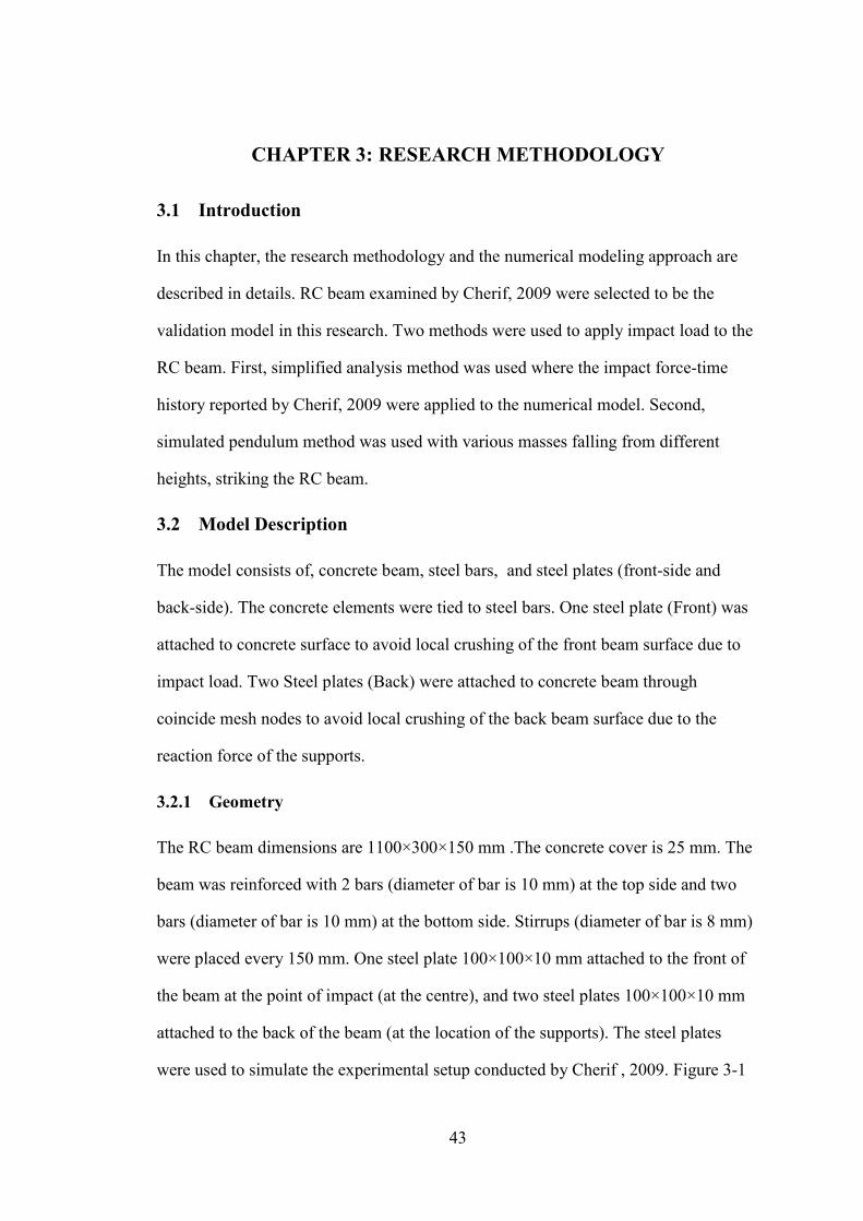
43
CHAPTER 3: RESEARCH METHODOLOGY
3.1 Introduction
In this chapter, the research methodology and the numerical modeling approach are
described in details. RC beam examined by Cherif, 2009 were selected to be the
validation model in this research. Two methods were used to apply impact load to the
RC beam. First, simplified analysis method was used where the impact force-time
history reported by Cherif, 2009 were applied to the numerical model. Second,
simulated pendulum method was used with various masses falling from different
heights, striking the RC beam.
3.2 Model Description
The model consists of, concrete beam, steel bars, and steel plates (front-side and
back-side). The concrete elements were tied to steel bars. One steel plate (Front) was
attached to concrete surface to avoid local crushing of the front beam surface due to
impact load. Two Steel plates (Back) were attached to concrete beam through
coincide mesh nodes to avoid local crushing of the back beam surface due to the
reaction force of the supports.
3.2.1 Geometry
The RC beam dimensions are 1100×300×150 mm .The concrete cover is 25 mm. The
beam was reinforced with 2 bars (diameter of bar is 10 mm) at the top side and two
bars (diameter of bar is 10 mm) at the bottom side. Stirrups (diameter of bar is 8 mm)
were placed every 150 mm. One steel plate 100×100×10 mm attached to the front of
the beam at the point of impact (at the centre), and two steel plates 100×100×10 mm
attached to the back of the beam (at the location of the supports). The steel plates
were used to simulate the experimental setup conducted by Cherif , 2009. Figure 3-1
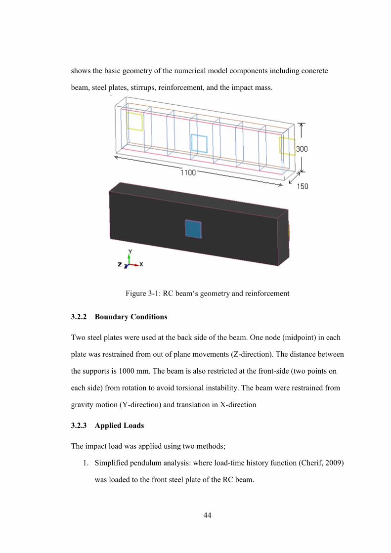
44
shows the basic geometry of the numerical model components including concrete
beam, steel plates, stirrups, reinforcement, and the impact mass.
Figure 3-1: RC beam‘s geometry and reinforcement
3.2.2 Boundary Conditions
Two steel plates were used at the back side of the beam. One node (midpoint) in each
plate was restrained from out of plane movements (Z-direction). The distance between
the supports is 1000 mm. The beam is also restricted at the front-side (two points on
each side) from rotation to avoid torsional instability. The beam were restrained from
gravity motion (Y-direction) and translation in X-direction
3.2.3 Applied Loads
The impact load was applied using two methods;
1. Simplified pendulum analysis: where load-time history function (Cherif, 2009)
was loaded to the front steel plate of the RC beam.
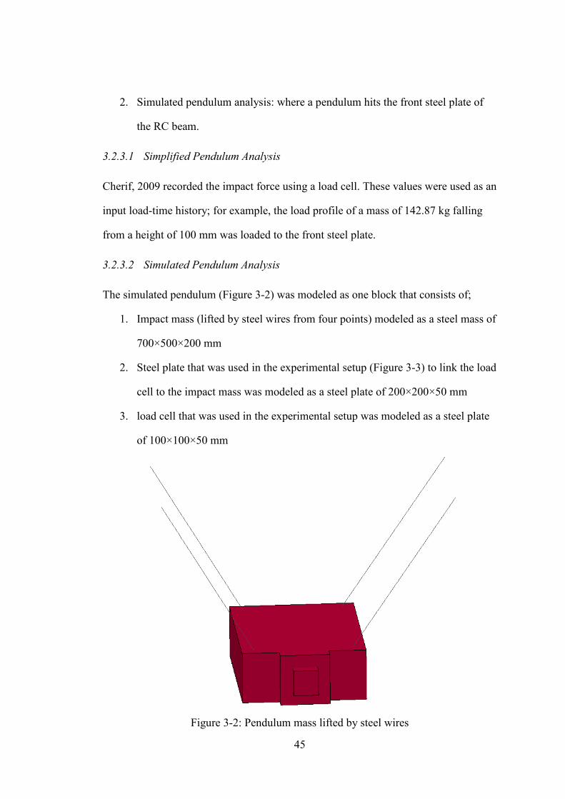
45
2. Simulated pendulum analysis: where a pendulum hits the front steel plate of
the RC beam.
3.2.3.1 Simplified Pendulum Analysis
Cherif, 2009 recorded the impact force using a load cell. These values were used as an
input load-time history; for example, the load profile of a mass of 142.87 kg falling
from a height of 100 mm was loaded to the front steel plate.
3.2.3.2 Simulated Pendulum Analysis
The simulated pendulum (Figure 3-2) was modeled as one block that consists of;
1. Impact mass (lifted by steel wires from four points) modeled as a steel mass of
700×500×200 mm
2. Steel plate that was used in the experimental setup (Figure 3-3) to link the load
cell to the impact mass was modeled as a steel plate of 200×200×50 mm
3. load cell that was used in the experimental setup was modeled as a steel plate
of 100×100×50 mm
Figure 3-2: Pendulum mass lifted by steel wires
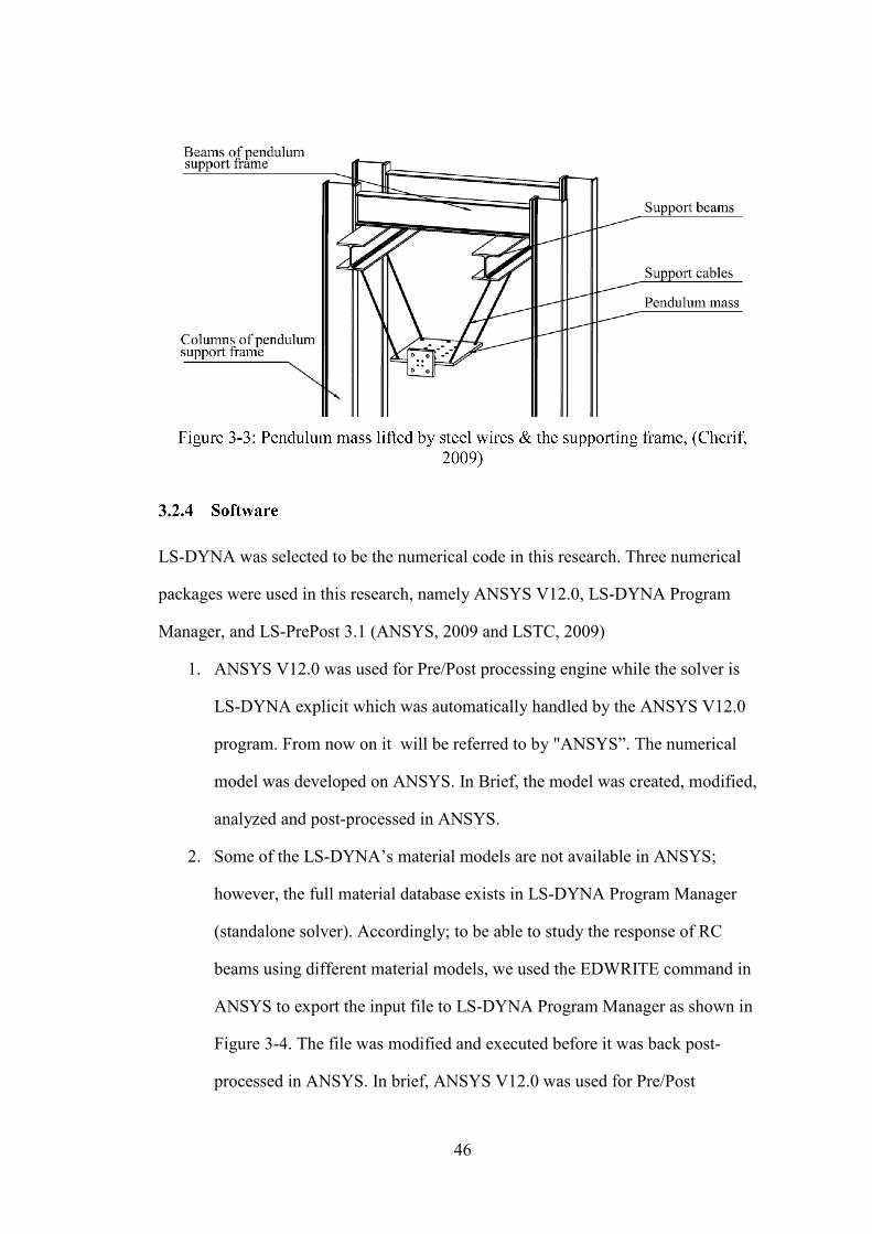
46
Figure 3-3: Pendulum mass lifted by steel wires & the supporting frame, (Cherif,
2009)
3.2.4 Software
LS-DYNA was selected to be the numerical code in this research. Three numerical
packages were used in this research, namely ANSYS V12.0, LS-DYNA Program
Manager, and LS-PrePost 3.1 (ANSYS, 2009 and LSTC, 2009)
1. ANSYS V12.0 was used for Pre/Post processing engine while the solver is
LS-DYNA explicit which was automatically handled by the ANSYS V12.0
program. From now on it will be referred to by "ANSYS”. The numerical
model was developed on ANSYS. In Brief, the model was created, modified,
analyzed and post-processed in ANSYS.
2. Some of the LS-DYNA’s material models are not available in ANSYS;
however, the full material database exists in LS-DYNA Program Manager
(standalone solver). Accordingly; to be able to study the response of RC
beams using different material models, we used the EDWRITE command in
ANSYS to export the input file to LS-DYNA Program Manager as shown in
Figure 3-4. The file was modified and executed before it was back post-
processed in ANSYS. In brief, ANSYS V12.0 was used for Pre/Post
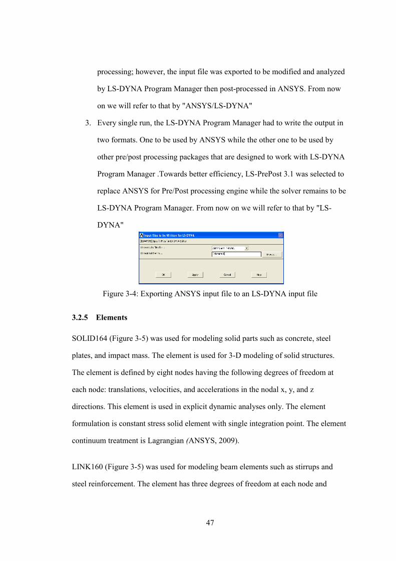
47
processing; however, the input file was exported to be modified and analyzed
by LS-DYNA Program Manager then post-processed in ANSYS. From now
on we will refer to that by "ANSYS/LS-DYNA"
3. Every single run, the LS-DYNA Program Manager had to write the output in
two formats. One to be used by ANSYS while the other one to be used by
other pre/post processing packages that are designed to work with LS-DYNA
Program Manager .Towards better efficiency, LS-PrePost 3.1 was selected to
replace ANSYS for Pre/Post processing engine while the solver remains to be
LS-DYNA Program Manager. From now on we will refer to that by "LS-
DYNA"
Figure 3-4: Exporting ANSYS input file to an LS-DYNA input file
3.2.5 Elements
SOLID164 (Figure 3-5) was used for modeling solid parts such as concrete, steel
plates, and impact mass. The element is used for 3-D modeling of solid structures.
The element is defined by eight nodes having the following degrees of freedom at
each node: translations, velocities, and accelerations in the nodal x, y, and z
directions. This element is used in explicit dynamic analyses only. The element
formulation is constant stress solid element with single integration point. The element
continuum treatment is Lagrangian (ANSYS, 2009).
LINK160 (Figure 3-5) was used for modeling beam elements such as stirrups and
steel reinforcement. The element has three degrees of freedom at each node and
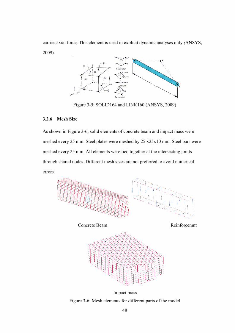
48
carries axial force. This element is used in explicit dynamic analyses only (ANSYS,
2009).
Figure 3-5: SOLID164 and LINK160 (ANSYS, 2009)
3.2.6 Mesh Size
As shown in Figure 3-6, solid elements of concrete beam and impact mass were
meshed every 25 mm. Steel plates were meshed by 25 x25x10 mm. Steel bars were
meshed every 25 mm. All elements were tied together at the intersecting joints
through shared nodes. Different mesh sizes are not preferred to avoid numerical
errors.
Concrete Beam Reinforcemnt
Impact mass
Figure 3-6: Mesh elements for different parts of the model
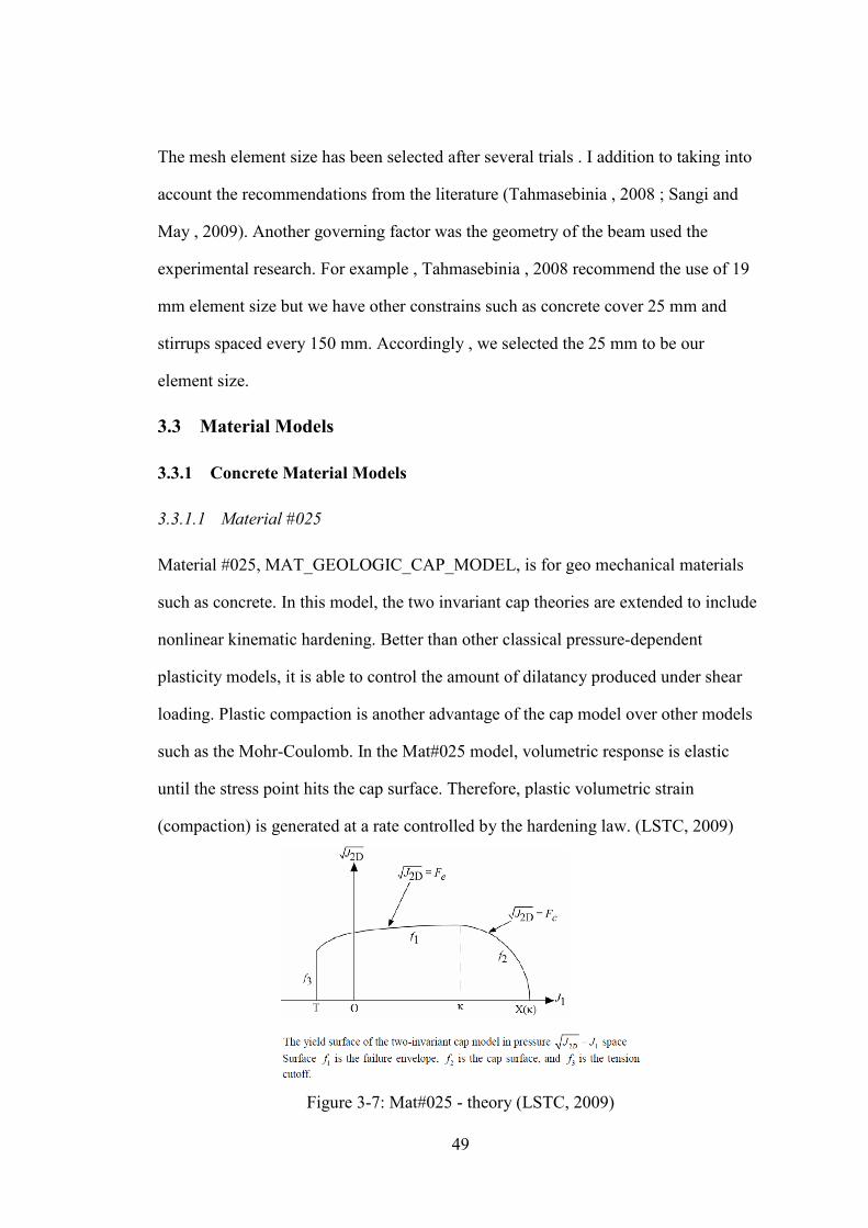
49
The mesh element size has been selected after several trials . I addition to taking into
account the recommendations from the literature (Tahmasebinia , 2008 ; Sangi and
May , 2009). Another governing factor was the geometry of the beam used the
experimental research. For example , Tahmasebinia , 2008 recommend the use of 19
mm element size but we have other constrains such as concrete cover 25 mm and
stirrups spaced every 150 mm. Accordingly , we selected the 25 mm to be our
element size.
3.3 Material Models
3.3.1 Concrete Material Models
3.3.1.1 Material #025
Material #025, MAT_GEOLOGIC_CAP_MODEL, is for geo mechanical materials
such as concrete. In this model, the two invariant cap theories are extended to include
nonlinear kinematic hardening. Better than other classical pressure-dependent
plasticity models, it is able to control the amount of dilatancy produced under shear
loading. Plastic compaction is another advantage of the cap model over other models
such as the Mohr-Coulomb. In the Mat#025 model, volumetric response is elastic
until the stress point hits the cap surface. Therefore, plastic volumetric strain
(compaction) is generated at a rate controlled by the hardening law. (LSTC, 2009)
Figure 3-7: Mat#025 - theory (LSTC, 2009)
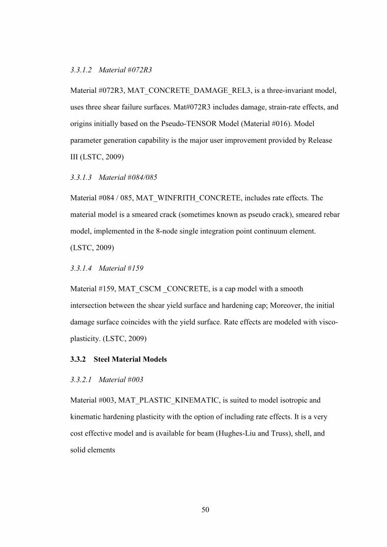
50
3.3.1.2 Material #072R3
Material #072R3, MAT_CONCRETE_DAMAGE_REL3, is a three-invariant model,
uses three shear failure surfaces. Mat#072R3 includes damage, strain-rate effects, and
origins initially based on the Pseudo-TENSOR Model (Material #016). Model
parameter generation capability is the major user improvement provided by Release
III (LSTC, 2009)
3.3.1.3 Material #084/085
Material #084 / 085, MAT_WINFRITH_CONCRETE, includes rate effects. The
material model is a smeared crack (sometimes known as pseudo crack), smeared rebar
model, implemented in the 8-node single integration point continuum element.
(LSTC, 2009)
3.3.1.4 Material #159
Material #159, MAT_CSCM _CONCRETE, is a cap model with a smooth
intersection between the shear yield surface and hardening cap; Moreover, the initial
damage surface coincides with the yield surface. Rate effects are modeled with visco-
plasticity. (LSTC, 2009)
3.3.2 Steel Material Models
3.3.2.1 Material #003
Material #003, MAT_PLASTIC_KINEMATIC, is suited to model isotropic and
kinematic hardening plasticity with the option of including rate effects. It is a very
cost effective model and is available for beam (Hughes-Liu and Truss), shell, and
solid elements
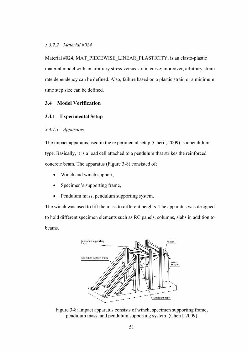
51
3.3.2.2 Material #024
Material #024, MAT_PIECEWISE_LINEAR_PLASTICITY, is an elasto-plastic
material model with an arbitrary stress versus strain curve; moreover, arbitrary strain
rate dependency can be defined. Also, failure based on a plastic strain or a minimum
time step size can be defined.
3.4 Model Verification
3.4.1 Experimental Setup
3.4.1.1 Apparatus
The impact apparatus used in the experimental setup (Cherif, 2009) is a pendulum
type. Basically, it is a load cell attached to a pendulum that strikes the reinforced
concrete beam. The apparatus (Figure 3-8) consisted of;
• Winch and winch support,
• Specimen’s supporting frame,
• Pendulum mass, pendulum supporting system.
The winch was used to lift the mass to different heights. The apparatus was designed
to hold different specimen elements such as RC panels, columns, slabs in addition to
beams.
Figure 3-8: Impact apparatus consists of winch, specimen supporting frame,
pendulum mass, and pendulum supporting system, (Cherif, 2009)
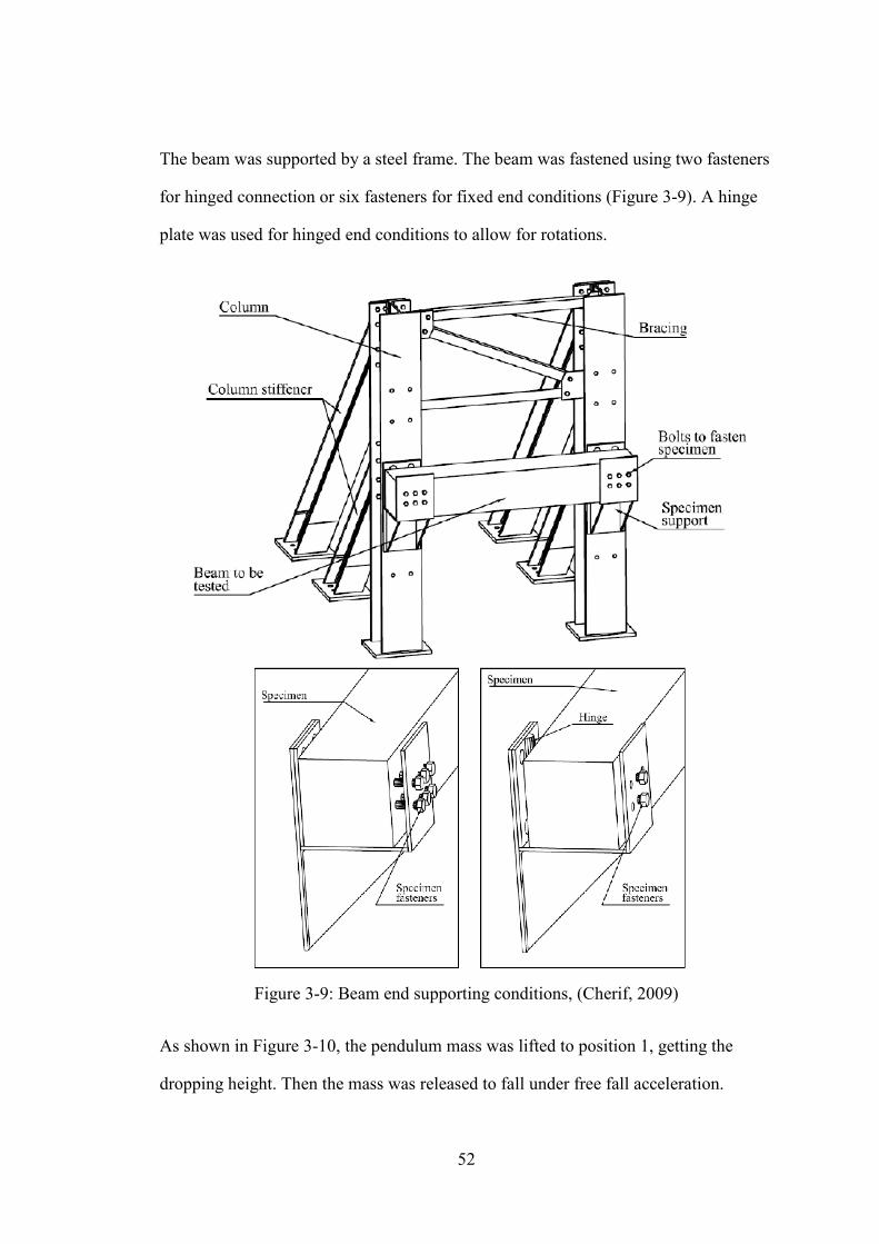
52
The beam was supported by a steel frame. The beam was fastened using two fasteners
for hinged connection or six fasteners for fixed end conditions (Figure 3-9). A hinge
plate was used for hinged end conditions to allow for rotations.
Figure 3-9: Beam end supporting conditions, (Cherif, 2009)
As shown in Figure 3-10, the pendulum mass was lifted to position 1, getting the
dropping height. Then the mass was released to fall under free fall acceleration.
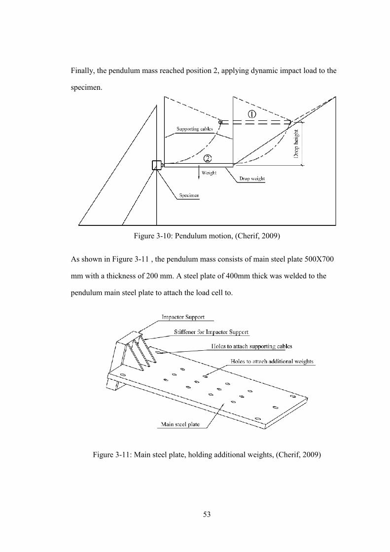
53
Finally, the pendulum mass reached position 2, applying dynamic impact load to the
specimen.
Figure 3-10: Pendulum motion, (Cherif, 2009)
As shown in Figure 3-11 , the pendulum mass consists of main steel plate 500X700
mm with a thickness of 200 mm. A steel plate of 400mm thick was welded to the
pendulum main steel plate to attach the load cell to.
Figure 3-11: Main steel plate, holding additional weights, (Cherif, 2009)
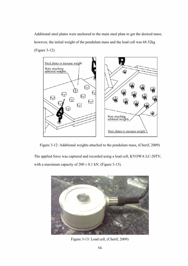
54
Additional steel plates were anchored to the main steel plate to get the desired mass;
however, the initial weight of the pendulum mass and the load cell was 68.52kg
(Figure 3-12).
Figure 3-12: Additional weights attached to the pendulum mass, (Cherif, 2009)
The applied force was captured and recorded using a load cell, KYOWA LC-20TV,
with a maximum capacity of 200 ± 0.1 kN. (Figure 3-13).
Figure 3-13: Load cell, (Cherif, 2009)
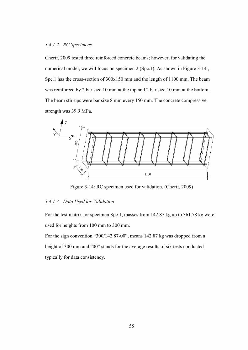
55
3.4.1.2 RC Specimens
Cherif, 2009 tested three reinforced concrete beams; however, for validating the
numerical model, we will focus on specimen 2 (Spc.1). As shown in Figure 3-14 ,
Spc.1 has the cross-section of 300x150 mm and the length of 1100 mm. The beam
was reinforced by 2 bar size 10 mm at the top and 2 bar size 10 mm at the bottom.
The beam stirrups were bar size 8 mm every 150 mm. The concrete compressive
strength was 39.9 MPa.
Figure 3-14: RC specimen used for validation, (Cherif, 2009)
3.4.1.3 Data Used for Validation
For the test matrix for specimen Spc.1, masses from 142.87 kg up to 361.78 kg were
used for heights from 100 mm to 300 mm.
For the sign convention “300/142.87-00”, means 142.87 kg was dropped from a
height of 300 mm and “00” stands for the average results of six tests conducted
typically for data consistency.
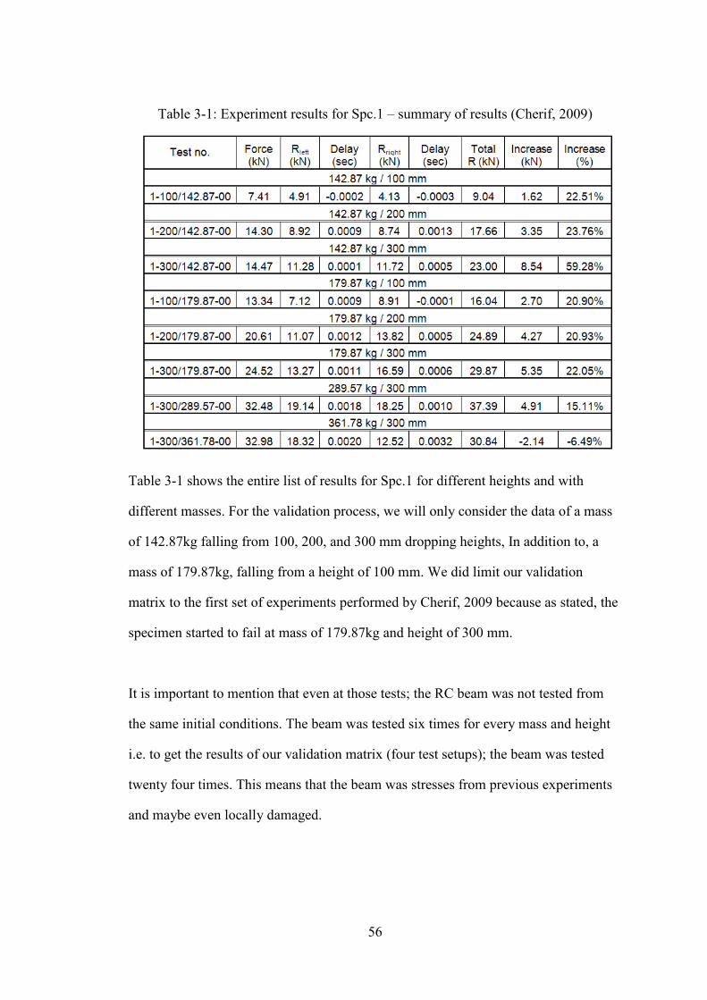
56
Table 3-1: Experiment results for Spc.1 – summary of results (Cherif, 2009)
Table 3-1 shows the entire list of results for Spc.1 for different heights and with
different masses. For the validation process, we will only consider the data of a mass
of 142.87kg falling from 100, 200, and 300 mm dropping heights, In addition to, a
mass of 179.87kg, falling from a height of 100 mm. We did limit our validation
matrix to the first set of experiments performed by Cherif, 2009 because as stated, the
specimen started to fail at mass of 179.87kg and height of 300 mm.
It is important to mention that even at those tests; the RC beam was not tested from
the same initial conditions. The beam was tested six times for every mass and height
i.e. to get the results of our validation matrix (four test setups); the beam was tested
twenty four times. This means that the beam was stresses from previous experiments
and maybe even locally damaged.
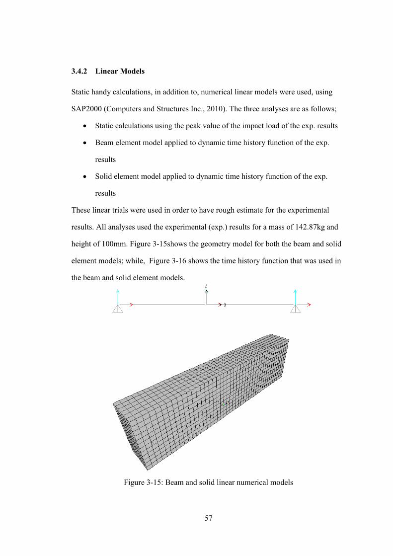
57
3.4.2 Linear Models
Static handy calculations, in addition to, numerical linear models were used, using
SAP2000 (Computers and Structures Inc., 2010). The three analyses are as follows;
• Static calculations using the peak value of the impact load of the exp. results
• Beam element model applied to dynamic time history function of the exp.
results
• Solid element model applied to dynamic time history function of the exp.
results
These linear trials were used in order to have rough estimate for the experimental
results. All analyses used the experimental (exp.) results for a mass of 142.87kg and
height of 100mm. Figure 3-15shows the geometry model for both the beam and solid
element models; while, Figure 3-16 shows the time history function that was used in
the beam and solid element models.
Figure 3-15: Beam and solid linear numerical models

58
Figure 3-16: Time history function of the exp. results for M 142.87kg & H 100mm
3.4.3 Nonlinear Models
3.4.3.1 Simplified Pendulum Analysis
Cherif, 2009 recorded the impact forces using load cell attached to the pendulum
mass. Those values were used as input force for the numerical model. Figure 3-17
shows the input forces used in the numerical models. The time-history functions were
for a mass of 142.87kg falling from a height of 100, 200, and 300 mm; in addition to,
a mass of 179.87kg falling from a height of 100 mm. The front steel plate attached to
the RC beam was load by these load functions.
Figure 3-17: Simplified analysis - input forces used in the model
-16
-14
-12
-10
-8
-6
-4
-2
0
2
0 0.02 0.04 0.06 0.08 0.1
Impa
ct fo
rce
(kN
)
Time (sec)
M142.87Kg , H 100mm - Experiment
M142.87Kg , H 200mm - Experiment
M142.87Kg , H 300mm - Experiment
M179.87Kg , H 100mm - Experiment
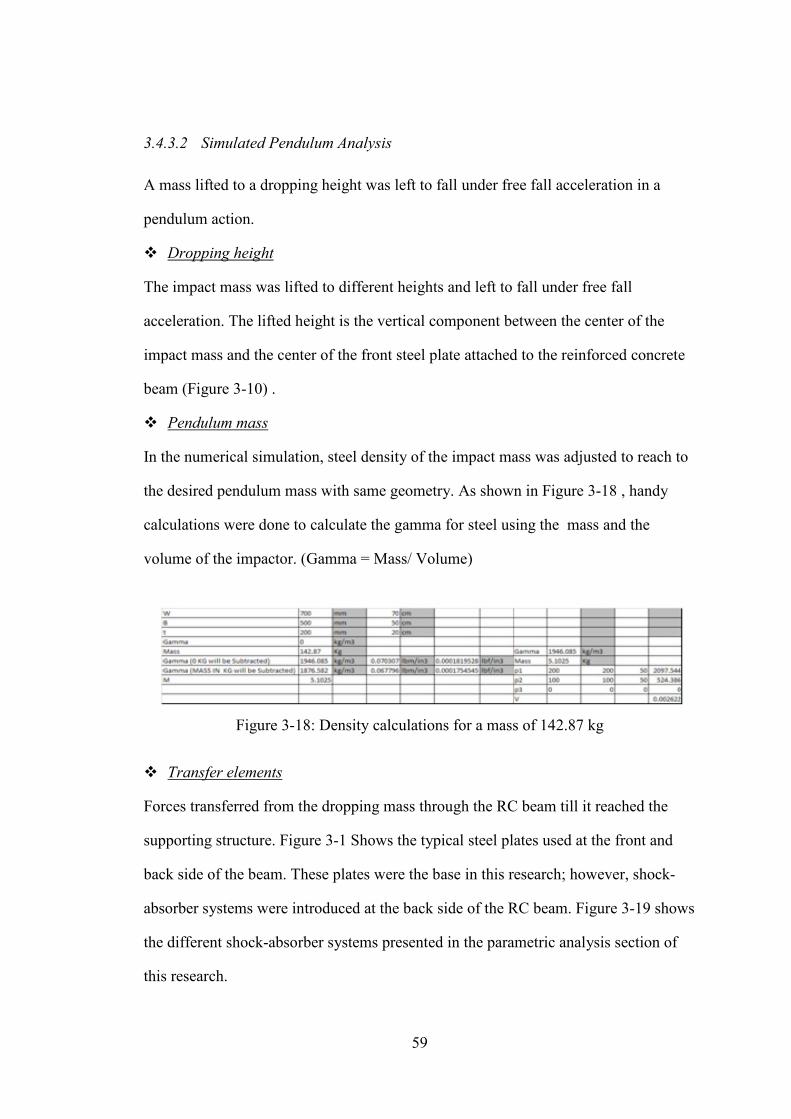
59
3.4.3.2 Simulated Pendulum Analysis
A mass lifted to a dropping height was left to fall under free fall acceleration in a
pendulum action.
The impact mass was lifted to different heights and left to fall under free fall
acceleration. The lifted height is the vertical component between the center of the
impact mass and the center of the front steel plate attached to the reinforced concrete
beam (
Dropping height
Figure 3-10) .
In the numerical simulation, steel density of the impact mass was adjusted to reach to
the desired pendulum mass with same geometry. As shown in
Pendulum mass
Figure 3-18 , handy
calculations were done to calculate the gamma for steel using the mass and the
volume of the impactor. (Gamma = Mass/ Volume)
Figure 3-18: Density calculations for a mass of 142.87 kg
Forces transferred from the dropping mass through the RC beam till it reached the
supporting structure.
Transfer elements
Figure 3-1 Shows the typical steel plates used at the front and
back side of the beam. These plates were the base in this research; however, shock-
absorber systems were introduced at the back side of the RC beam. Figure 3-19 shows
the different shock-absorber systems presented in the parametric analysis section of
this research.
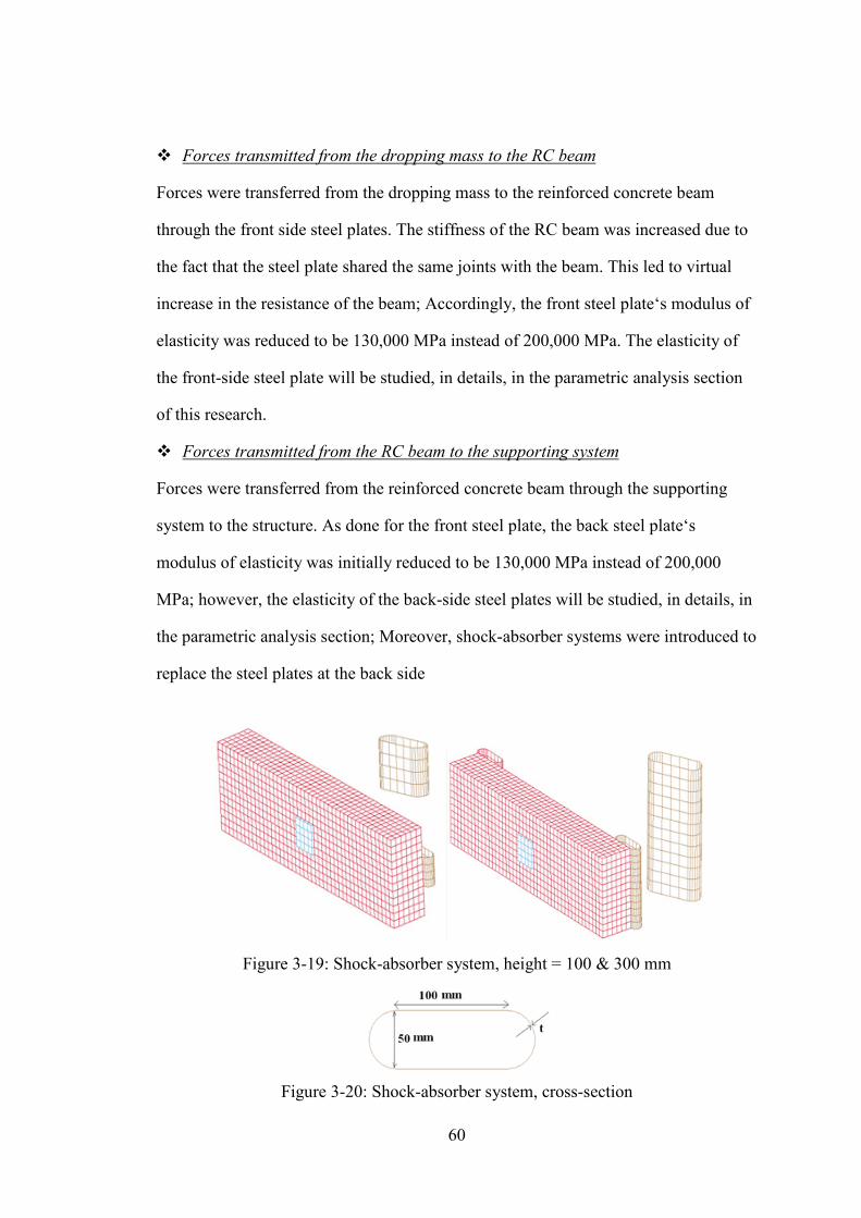
60
Forces were transferred from the dropping mass to the reinforced concrete beam
through the front side steel plates. The stiffness of the RC beam was increased due to
the fact that the steel plate shared the same joints with the beam. This led to virtual
increase in the resistance of the beam; Accordingly, the front steel plate‘s modulus of
elasticity was reduced to be 130,000 MPa instead of 200,000 MPa. The elasticity of
the front-side steel plate will be studied, in details, in the parametric analysis section
of this research.
Forces transmitted from the dropping mass to the RC beam
Forces were transferred from the reinforced concrete beam through the supporting
system to the structure. As done for the front steel plate, the back steel plate‘s
modulus of elasticity was initially reduced to be 130,000 MPa instead of 200,000
MPa; however, the elasticity of the back-side steel plates will be studied, in details, in
the parametric analysis section; Moreover, shock-absorber systems were introduced to
replace the steel plates at the back side
Forces transmitted from the RC beam to the supporting system
Figure 3-19: Shock-absorber system, height = 100 & 300 mm
Figure 3-20: Shock-absorber system, cross-section

61
CHAPTER 4: ANALYSIS OF RESULTS AND DISCUSSIONS
4.1 Introduction
In this chapter we will discuss the results of linear models using static calculations
and dynamic beam and solid element models conducted on SAP2000 using the impact
force-time history reported by Cherif, 2009 (Figure 3-17). The results for the non-
linear numerical models of the simplified analysis and the simulated pendulum were
reported. Further model refinements and parametric analysis were done to study the
influence of different factors.
4.2 Linear Models
Table 4-1 shows the handy calculations under a static load of 7.41 kN (Max. force for
a mass of 142.87kg falling from a height of 100mm).
Table 4-2 summarizes the results of the three different analysis types used as a rough
estimate value for the experiment.
Table 4-1: Static calculations: force of M 142.87kg & H 100mm striking a beam

62
Table 4-2: Summary of static\dynamic linear analysis of M 142.87kg & H 100mm
Reaction
Values (kN)
Max. Tensile Stress
(MPa)
Max. Deflection
(mm)
Static Calculations 3.69 M = 2063.45 kN.mm
𝑆 = 𝑀𝐼𝑦 = 1.75
0.087
Dynamic Beam
Element Model 3.84
M =2143.07 kN.mm
𝑆 = 𝑀𝐼𝑦 = 1.82
0.105
Dynamic Solid
Element Model 3.71 1.59 0.085
Experment 4.53 NA NA
4.3 Nonlinear Models: Simplified Pendulum Analysis
4.3.1 Analysis of results
The simplified pendulum analysis method was used as a preliminary method to check
the numerical model integrity. Moreover, the preliminary models were used to
identify the numerical model parameters such as the mesh size , time step , and
material properties because it is much easier to trace a model that takes 30 min
running time (100 MB on the disc drive) rather than a full model that takes around 5
hours to finish a run (5 GB on the disc drive).
Four different material models were used to model the concrete used in the
experiment. For presentation purposes, from now on, we will refer to different
material models used according to Table 4-3.
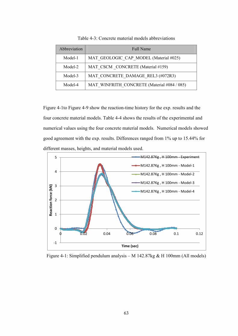
63
Table 4-3: Concrete material models abbreviations
Abbreviation Full Name
Model-1 MAT_GEOLOGIC_CAP_MODEL (Material #025)
Model-2 MAT_CSCM _CONCRETE (Material #159)
Model-3 MAT_CONCRETE_DAMAGE_REL3 (#072R3)
Model-4 MAT_WINFRITH_CONCRETE (Material #084 / 085)
Figure 4-1to Figure 4-9 show the reaction-time history for the exp. results and the
four concrete material models. Table 4-4 shows the results of the experimental and
numerical values using the four concrete material models. Numerical models showed
good agreement with the exp. results. Differences ranged from 1% up to 15.44% for
different masses, heights, and material models used.
Figure 4-1: Simplified pendulum analysis – M 142.87kg & H 100mm (All models)
-1
0
1
2
3
4
5
0 0.02 0.04 0.06 0.08 0.1 0.12
Reac
tion
forc
e (k
N)
Time (sec)
M142.87Kg , H 100mm - Experiment
M142.87Kg , H 100mm - Model-1
M142.87Kg , H 100mm - Model-2
M142.87Kg , H 100mm - Model-3
M142.87Kg , H 100mm - Model-4
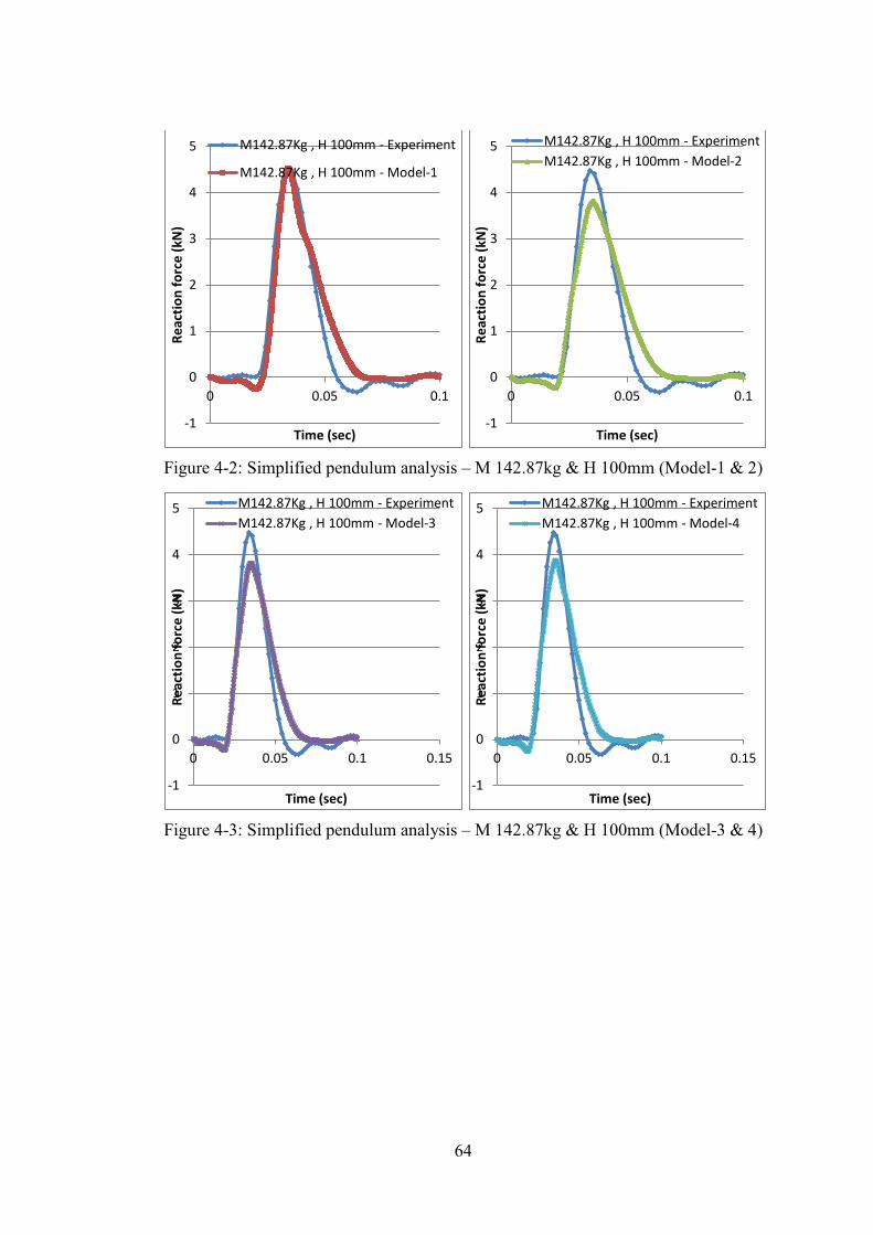
64
Figure 4-2: Simplified pendulum analysis – M 142.87kg & H 100mm (Model-1 & 2)
Figure 4-3: Simplified pendulum analysis – M 142.87kg & H 100mm (Model-3 & 4)
-1
0
1
2
3
4
5
0 0.05 0.1
Reac
tion
forc
e (k
N)
Time (sec)
M142.87Kg , H 100mm - Experiment
M142.87Kg , H 100mm - Model-1
-1
0
1
2
3
4
5
0 0.05 0.1
Reac
tion
forc
e (k
N)
Time (sec)
M142.87Kg , H 100mm - Experiment M142.87Kg , H 100mm - Model-2
-1
0
1
2
3
4
5
0 0.05 0.1 0.15
Reac
tion
forc
e (k
N)
Time (sec)
M142.87Kg , H 100mm - Experiment M142.87Kg , H 100mm - Model-3
-1
0
1
2
3
4
5
0 0.05 0.1 0.15
Reac
tion
forc
e (k
N)
Time (sec)
M142.87Kg , H 100mm - Experiment M142.87Kg , H 100mm - Model-4

65
Figure 4-4: Simplified pendulum analysis – M 142.87kg & H 200mm (All models)
Figure 4-5: Simplified pendulum analysis – M 142.87kg & H 200mm (Model-1 & 2)
-2
0
2
4
6
8
10
0 0.02 0.04 0.06 0.08 0.1 0.12
Reac
tion
forc
e (k
N)
Time (sec)
M142.87Kg , H 200mm - Experiment
M142.87Kg , H 200mm - Model-1
M142.87Kg , H 200mm - Model-2
M142.87Kg , H 200mm - Model-3
M142.87Kg , H 200mm - Model-4
-2
0
2
4
6
8
10
0 0.05 0.1 0.15
Reac
tion
forc
e (k
N)
Time (sec)
M142.87Kg , H 200mm - Experiment M142.87Kg , H 200mm - Model-1
-2
0
2
4
6
8
10
0 0.05 0.1 0.15
Reac
tion
forc
e (k
N)
Time (sec)
M142.87Kg , H 200mm - Experiment M142.87Kg , H 200mm - Model-2
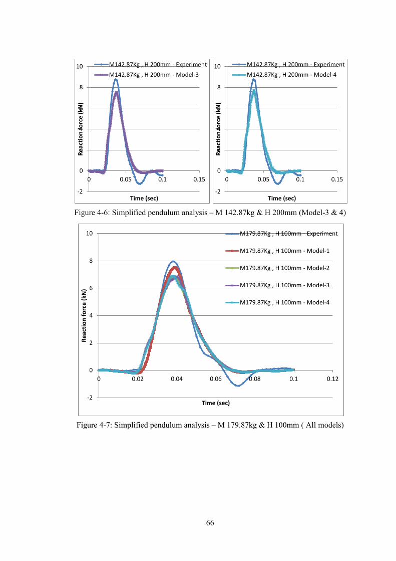
66
Figure 4-6: Simplified pendulum analysis – M 142.87kg & H 200mm (Model-3 & 4)
Figure 4-7: Simplified pendulum analysis – M 179.87kg & H 100mm ( All models)
-2
0
2
4
6
8
10
0 0.05 0.1 0.15
Reac
tion
forc
e (k
N)
Time (sec)
M142.87Kg , H 200mm - Experiment M142.87Kg , H 200mm - Model-3
-2
0
2
4
6
8
10
0 0.05 0.1 0.15
Reac
tion
forc
e (k
N)
Time (sec)
M142.87Kg , H 200mm - Experiment M142.87Kg , H 200mm - Model-4
-2
0
2
4
6
8
10
0 0.02 0.04 0.06 0.08 0.1 0.12
Reac
tion
forc
e (k
N)
Time (sec)
M179.87Kg , H 100mm - Experiment
M179.87Kg , H 100mm - Model-1
M179.87Kg , H 100mm - Model-2
M179.87Kg , H 100mm - Model-3
M179.87Kg , H 100mm - Model-4
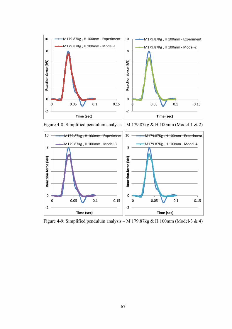
67
Figure 4-8: Simplified pendulum analysis – M 179.87kg & H 100mm (Model-1 & 2)
Figure 4-9: Simplified pendulum analysis – M 179.87kg & H 100mm (Model-3 & 4)
-2
0
2
4
6
8
10
0 0.05 0.1 0.15
Reac
tion
forc
e (k
N)
Time (sec)
M179.87Kg , H 100mm - Experiment
M179.87Kg , H 100mm - Model-1
-2
0
2
4
6
8
10
0 0.05 0.1 0.15
Reac
tion
forc
e (k
N)
Time (sec)
M179.87Kg , H 100mm - Experiment
M179.87Kg , H 100mm - Model-2
-2
0
2
4
6
8
10
0 0.05 0.1 0.15
Reac
tion
forc
e (k
N)
Time (sec)
M179.87Kg , H 100mm - Experiment
M179.87Kg , H 100mm - Model-3
-2
0
2
4
6
8
10
0 0.05 0.1 0.15
Reac
tion
forc
e (k
N)
Time (sec)
M179.87Kg , H 100mm - Experiment
M179.87Kg , H 100mm - Model-4
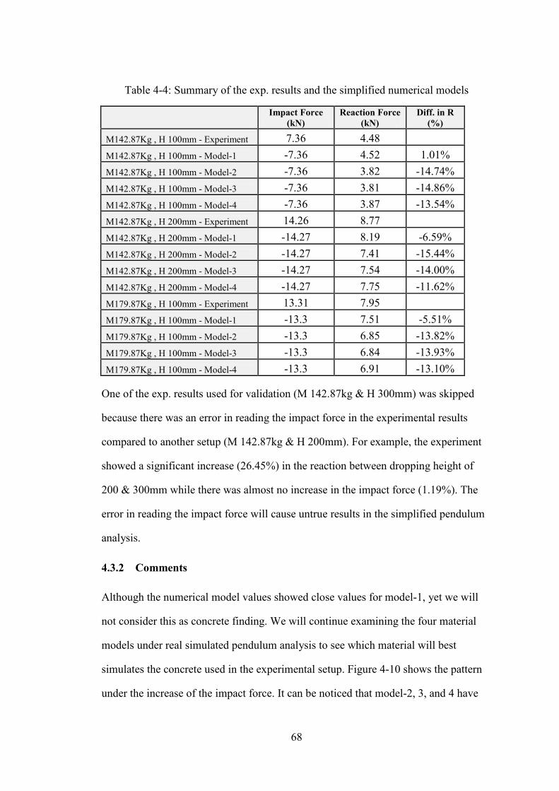
68
Table 4-4: Summary of the exp. results and the simplified numerical models
Impact Force
(kN) Reaction Force
(kN) Diff. in R
(%)
M142.87Kg , H 100mm - Experiment 7.36 4.48 M142.87Kg , H 100mm - Model-1 -7.36 4.52 1.01% M142.87Kg , H 100mm - Model-2 -7.36 3.82 -14.74% M142.87Kg , H 100mm - Model-3 -7.36 3.81 -14.86% M142.87Kg , H 100mm - Model-4 -7.36 3.87 -13.54% M142.87Kg , H 200mm - Experiment 14.26 8.77 M142.87Kg , H 200mm - Model-1 -14.27 8.19 -6.59% M142.87Kg , H 200mm - Model-2 -14.27 7.41 -15.44% M142.87Kg , H 200mm - Model-3 -14.27 7.54 -14.00% M142.87Kg , H 200mm - Model-4 -14.27 7.75 -11.62% M179.87Kg , H 100mm - Experiment 13.31 7.95 M179.87Kg , H 100mm - Model-1 -13.3 7.51 -5.51% M179.87Kg , H 100mm - Model-2 -13.3 6.85 -13.82% M179.87Kg , H 100mm - Model-3 -13.3 6.84 -13.93% M179.87Kg , H 100mm - Model-4 -13.3 6.91 -13.10%
One of the exp. results used for validation (M 142.87kg & H 300mm) was skipped
because there was an error in reading the impact force in the experimental results
compared to another setup (M 142.87kg & H 200mm). For example, the experiment
showed a significant increase (26.45%) in the reaction between dropping height of
200 & 300mm while there was almost no increase in the impact force (1.19%). The
error in reading the impact force will cause untrue results in the simplified pendulum
analysis.
4.3.2 Comments
Although the numerical model values showed close values for model-1, yet we will
not consider this as concrete finding. We will continue examining the four material
models under real simulated pendulum analysis to see which material will best
simulates the concrete used in the experimental setup. Figure 4-10 shows the pattern
under the increase of the impact force. It can be noticed that model-2, 3, and 4 have
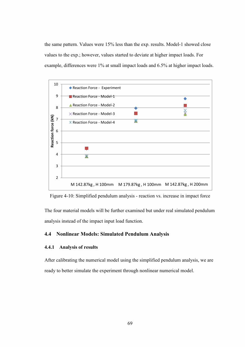
69
the same pattern. Values were 15% less than the exp. results. Model-1 showed close
values to the exp.; however, values started to deviate at higher impact loads. For
example, differences were 1% at small impact loads and 6.5% at higher impact loads.
Figure 4-10: Simplified pendulum analysis - reaction vs. increase in impact force
The four material models will be further examined but under real simulated pendulum
analysis instead of the impact input load function.
4.4 Nonlinear Models: Simulated Pendulum Analysis
4.4.1 Analysis of results
After calibrating the numerical model using the simplified pendulum analysis, we are
ready to better simulate the experiment through nonlinear numerical model.
2
3
4
5
6
7
8
9
10
Reac
tion
forc
e (k
N)
Reaction Force - Experiment
Reaction Force - Model-1
Reaction Force - Model-2
Reaction Force - Model-3
Reaction Force - Model-4
M 142.87kg , H 100mm M 142.87kg , H 200mm M 179.87kg , H 100mm
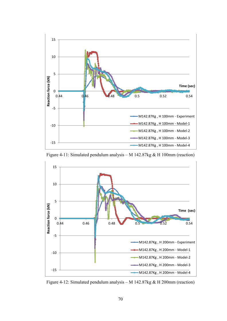
70
Figure 4-11: Simulated pendulum analysis – M 142.87kg & H 100mm (reaction)
Figure 4-12: Simulated pendulum analysis – M 142.87kg & H 200mm (reaction)
-15
-10
-5
0
5
10
15
0.44 0.46 0.48 0.5 0.52 0.54
Reac
tion
forc
e (k
N)
Time (sec)
M142.87Kg , H 100mm - Experiment
M142.87Kg , H 100mm - Model-1
M142.87Kg , H 100mm - Model-2
M142.87Kg , H 100mm - Model-3
M142.87Kg , H 100mm - Model-4
-15
-10
-5
0
5
10
15
0.44 0.46 0.48 0.5 0.52 0.54
Reac
tion
forc
e (k
N)
Time (sec)
M142.87Kg , H 200mm - Experiment
M142.87Kg , H 200mm - Model-1
M142.87Kg , H 200mm - Model-2
M142.87Kg , H 200mm - Model-3
M142.87Kg , H 200mm - Model-4
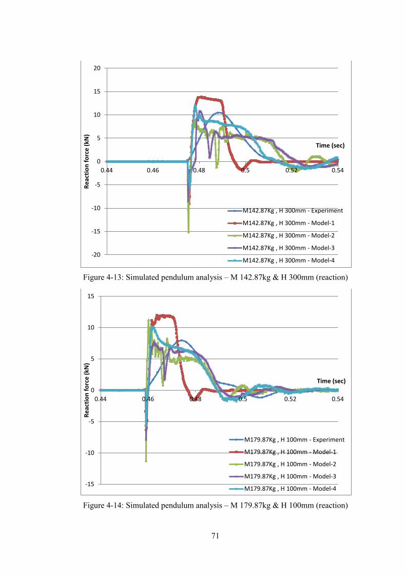
71
Figure 4-13: Simulated pendulum analysis – M 142.87kg & H 300mm (reaction)
Figure 4-14: Simulated pendulum analysis – M 179.87kg & H 100mm (reaction)
-20
-15
-10
-5
0
5
10
15
20
0.44 0.46 0.48 0.5 0.52 0.54
Reac
tion
forc
e (k
N)
Time (sec)
M142.87Kg , H 300mm - Experiment
M142.87Kg , H 300mm - Model-1
M142.87Kg , H 300mm - Model-2
M142.87Kg , H 300mm - Model-3
M142.87Kg , H 300mm - Model-4
-15
-10
-5
0
5
10
15
0.44 0.46 0.48 0.5 0.52 0.54
Reac
tion
forc
e (k
N)
Time (sec)
M179.87Kg , H 100mm - Experiment
M179.87Kg , H 100mm - Model-1
M179.87Kg , H 100mm - Model-2
M179.87Kg , H 100mm - Model-3
M179.87Kg , H 100mm - Model-4
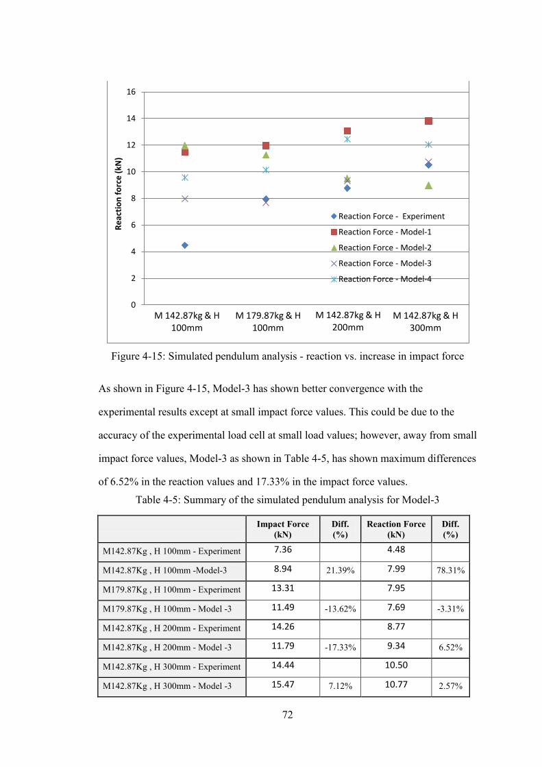
72
Figure 4-15: Simulated pendulum analysis - reaction vs. increase in impact force
As shown in Figure 4-15, Model-3 has shown better convergence with the
experimental results except at small impact force values. This could be due to the
accuracy of the experimental load cell at small load values; however, away from small
impact force values, Model-3 as shown in Table 4-5, has shown maximum differences
of 6.52% in the reaction values and 17.33% in the impact force values.
Table 4-5: Summary of the simulated pendulum analysis for Model-3
Impact Force
(kN) Diff. (%)
Reaction Force (kN)
Diff. (%)
M142.87Kg , H 100mm - Experiment 7.36
4.48 M142.87Kg , H 100mm -Model-3 8.94 21.39% 7.99 78.31%
M179.87Kg , H 100mm - Experiment 13.31
7.95 M179.87Kg , H 100mm - Model -3 11.49 -13.62% 7.69 -3.31%
M142.87Kg , H 200mm - Experiment 14.26
8.77 M142.87Kg , H 200mm - Model -3 11.79 -17.33% 9.34 6.52%
M142.87Kg , H 300mm - Experiment 14.44
10.50 M142.87Kg , H 300mm - Model -3 15.47 7.12% 10.77 2.57%
0
2
4
6
8
10
12
14
16
Reac
tion
forc
e (k
N)
Reaction Force - Experiment
Reaction Force - Model-1
Reaction Force - Model-2
Reaction Force - Model-3
Reaction Force - Model-4
M 142.87kg & H 100mm
M 179.87kg & H 100mm
M 142.87kg & H 200mm
M 142.87kg & H 300mm
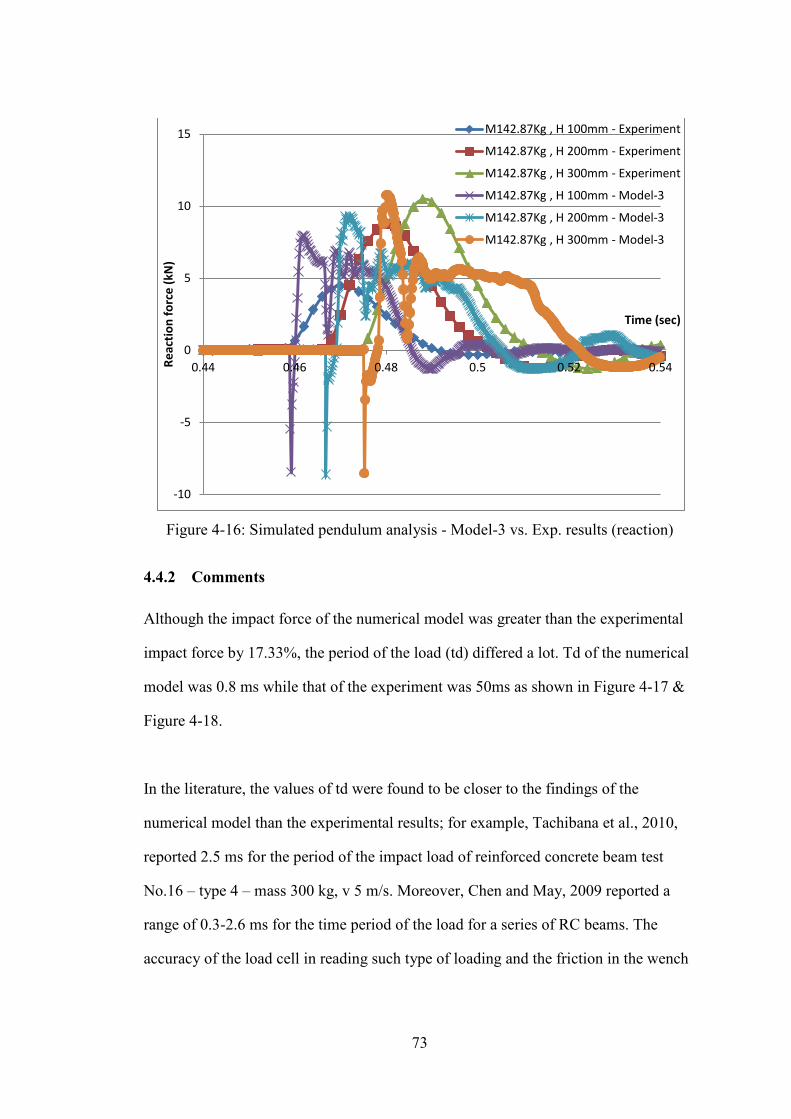
73
Figure 4-16: Simulated pendulum analysis - Model-3 vs. Exp. results (reaction)
4.4.2 Comments
Although the impact force of the numerical model was greater than the experimental
impact force by 17.33%, the period of the load (td) differed a lot. Td of the numerical
model was 0.8 ms while that of the experiment was 50ms as shown in Figure 4-17 &
Figure 4-18.
In the literature, the values of td were found to be closer to the findings of the
numerical model than the experimental results; for example, Tachibana et al., 2010,
reported 2.5 ms for the period of the impact load of reinforced concrete beam test
No.16 – type 4 – mass 300 kg, v 5 m/s. Moreover, Chen and May, 2009 reported a
range of 0.3-2.6 ms for the time period of the load for a series of RC beams. The
accuracy of the load cell in reading such type of loading and the friction in the wench
-10
-5
0
5
10
15
0.44 0.46 0.48 0.5 0.52 0.54 Reac
tion
forc
e (k
N)
Time (sec)
M142.87Kg , H 100mm - Experiment
M142.87Kg , H 200mm - Experiment
M142.87Kg , H 300mm - Experiment
M142.87Kg , H 100mm - Model-3
M142.87Kg , H 200mm - Model-3
M142.87Kg , H 300mm - Model-3
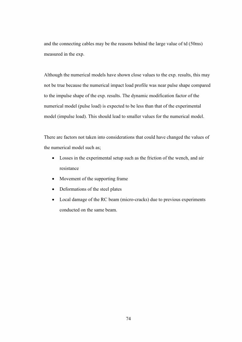
74
and the connecting cables may be the reasons behind the large value of td (50ms)
measured in the exp.
Although the numerical models have shown close values to the exp. results, this may
not be true because the numerical impact load profile was near pulse shape compared
to the impulse shape of the exp. results. The dynamic modification factor of the
numerical model (pulse load) is expected to be less than that of the experimental
model (impulse load). This should lead to smaller values for the numerical model.
There are factors not taken into considerations that could have changed the values of
the numerical model such as;
• Losses in the experimental setup such as the friction of the wench, and air
resistance
• Movement of the supporting frame
• Deformations of the steel plates
• Local damage of the RC beam (micro-cracks) due to previous experiments
conducted on the same beam.
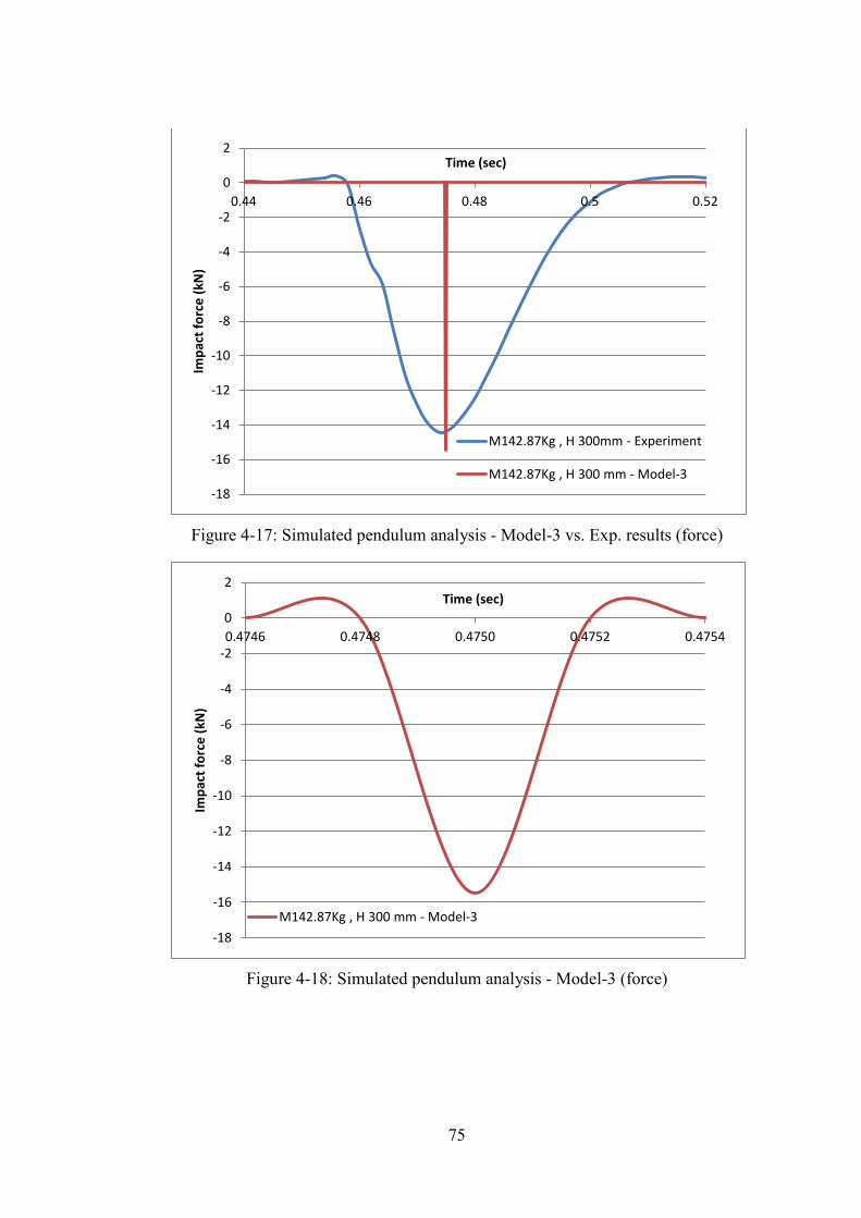
75
Figure 4-17: Simulated pendulum analysis - Model-3 vs. Exp. results (force)
Figure 4-18: Simulated pendulum analysis - Model-3 (force)
-18
-16
-14
-12
-10
-8
-6
-4
-2
0
2
0.44 0.46 0.48 0.5 0.52 Im
pact
forc
e (k
N)
Time (sec)
M142.87Kg , H 300mm - Experiment
M142.87Kg , H 300 mm - Model-3
-18
-16
-14
-12
-10
-8
-6
-4
-2
0
2
0.4746 0.4748 0.4750 0.4752 0.4754
Impa
ct fo
rce
(kN
)
Time (sec)
M142.87Kg , H 300 mm - Model-3
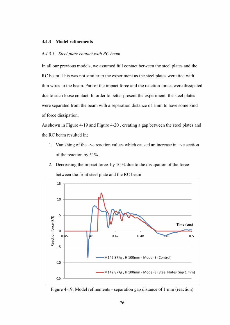
76
4.4.3 Model refinements
4.4.3.1 Steel plate contact with RC beam
In all our previous models, we assumed full contact between the steel plates and the
RC beam. This was not similar to the experiment as the steel plates were tied with
thin wires to the beam. Part of the impact force and the reaction forces were dissipated
due to such loose contact. In order to better present the experiment, the steel plates
were separated from the beam with a separation distance of 1mm to have some kind
of force dissipation.
As shown in Figure 4-19 and Figure 4-20 , creating a gap between the steel plates and
the RC beam resulted in;
1. Vanishing of the –ve reaction values which caused an increase in +ve section
of the reaction by 51%.
2. Decreasing the impact force by 10 % due to the dissipation of the force
between the front steel plate and the RC beam
Figure 4-19: Model refinements - separation gap distance of 1 mm (reaction)
-15
-10
-5
0
5
10
15
0.45 0.46 0.47 0.48 0.49 0.5
Reac
tion
forc
e (k
N)
Time (sec)
M142.87Kg , H 100mm - Model-3 (Control)
M142.87Kg , H 100mm - Model-3 (Steel Plates Gap 1 mm)

77
Figure 4-20: Model refinements - separation gap distance of 1 mm (force)
4.4.3.2 Solid element formulations
Since we used constant stress solid element which has a single integration point (solid
type 1), hourglass (HG) function need to be used in the non-linear numerical model
(LSTC, 2009). Hourglass modes are nonphysical properties. They are zero-energy
modes of deformation that impose no strain or stress to the model. As mentioned
before, hourglass modes occur only in under-integrated (single integration point)
elements such as solid, shell, and thick shell elements.
To eliminate usage of hourglass in LS-DYNA, you have to switch to higher element
formulations. For example, type 2 & 3 solids, with fully-integrated or selectively
reduced (S/R) integration (LSTC, 2009). There can be a drawback of using such
elements because;
• These element formulations are very expensive than the single point
formulation ( running time is 10 times more & storage size is 50 times more
than that of solid type 1)
• These element formulations tend to be much more unstable in large
deformation applications such as concrete under impact loads.
-12
-10
-8
-6
-4
-2
0
2
0.4582 0.4584 0.4586 0.4588 0.459 0.4592 0.4594 Im
pact
forc
e (k
N)
Time (sec)
M142.87Kg , H 100mm - Model-3 (Control)
M142.87Kg , H 100mm - Model-3 (Steel Plates Gap 1 mm)
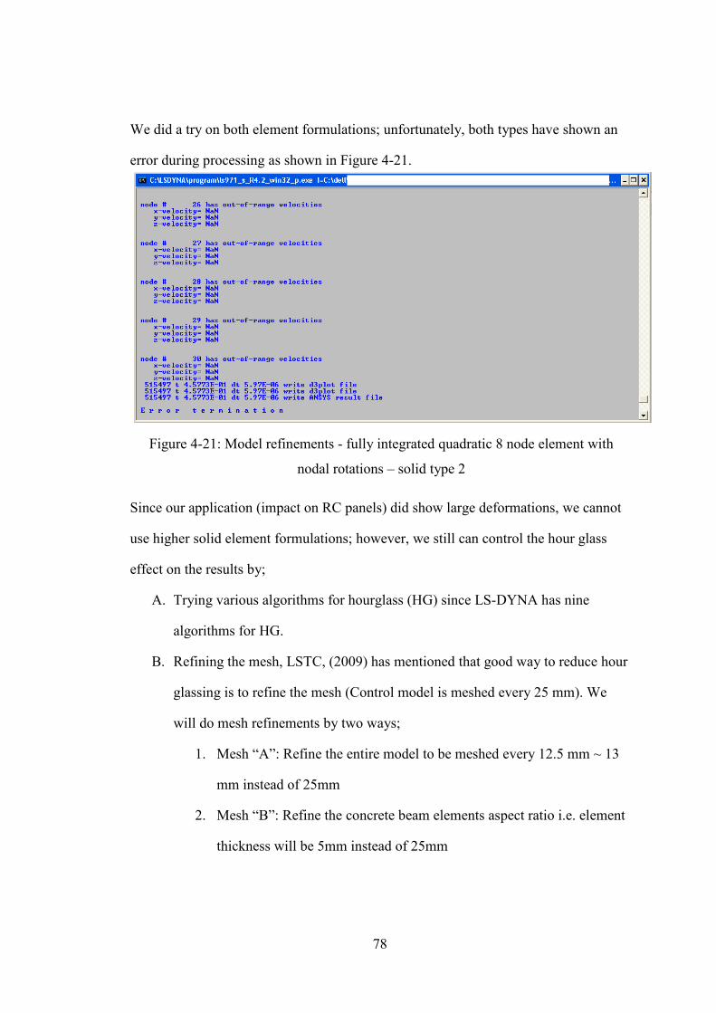
78
We did a try on both element formulations; unfortunately, both types have shown an
error during processing as shown in Figure 4-21.
Figure 4-21: Model refinements - fully integrated quadratic 8 node element with
nodal rotations – solid type 2
Since our application (impact on RC panels) did show large deformations, we cannot
use higher solid element formulations; however, we still can control the hour glass
effect on the results by;
A. Trying various algorithms for hourglass (HG) since LS-DYNA has nine
algorithms for HG.
B. Refining the mesh, LSTC, (2009) has mentioned that good way to reduce hour
glassing is to refine the mesh (Control model is meshed every 25 mm). We
will do mesh refinements by two ways;
1. Mesh “A”: Refine the entire model to be meshed every 12.5 mm ~ 13
mm instead of 25mm
2. Mesh “B”: Refine the concrete beam elements aspect ratio i.e. element
thickness will be 5mm instead of 25mm
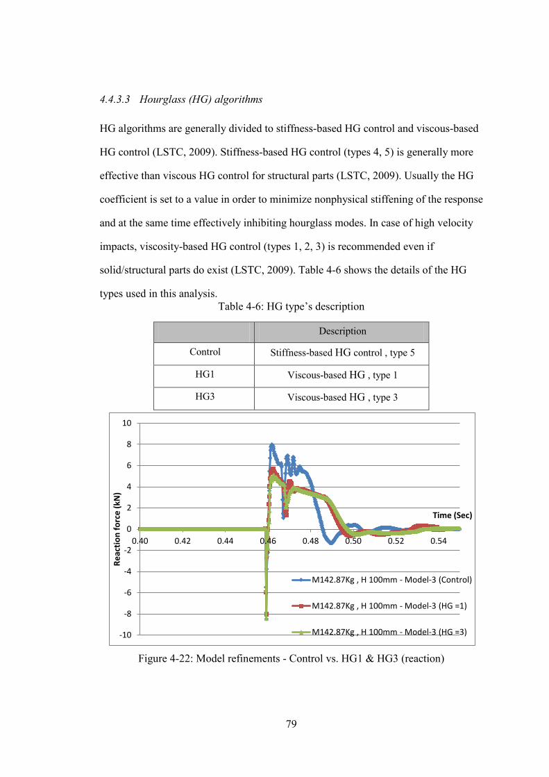
79
4.4.3.3 Hourglass (HG) algorithms
HG algorithms are generally divided to stiffness-based HG control and viscous-based
HG control (LSTC, 2009). Stiffness-based HG control (types 4, 5) is generally more
effective than viscous HG control for structural parts (LSTC, 2009). Usually the HG
coefficient is set to a value in order to minimize nonphysical stiffening of the response
and at the same time effectively inhibiting hourglass modes. In case of high velocity
impacts, viscosity-based HG control (types 1, 2, 3) is recommended even if
solid/structural parts do exist (LSTC, 2009). Table 4-6 shows the details of the HG
types used in this analysis. Table 4-6: HG type’s description
Description
Control Stiffness-based HG control , type 5
HG1 Viscous-based HG , type 1
HG3 Viscous-based HG , type 3
Figure 4-22: Model refinements - Control vs. HG1 & HG3 (reaction)
-10
-8
-6
-4
-2
0
2
4
6
8
10
0.40 0.42 0.44 0.46 0.48 0.50 0.52 0.54
Reac
tion
forc
e (k
N)
Time (Sec)
M142.87Kg , H 100mm - Model-3 (Control)
M142.87Kg , H 100mm - Model-3 (HG =1)
M142.87Kg , H 100mm - Model-3 (HG =3)
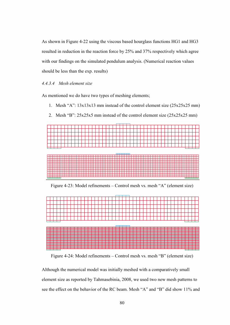
80
As shown in Figure 4-22 using the viscous based hourglass functions HG1 and HG3
resulted in reduction in the reaction force by 25% and 37% respectively which agree
with our findings on the simulated pendulum analysis. (Numerical reaction values
should be less than the exp. results)
4.4.3.4 Mesh element size
As mentioned we do have two types of meshing elements;
1. Mesh “A”: 13x13x13 mm instead of the control element size (25x25x25 mm)
2. Mesh “B”: 25x25x5 mm instead of the control element size (25x25x25 mm)
Figure 4-23: Model refinements – Control mesh vs. mesh “A” (element size)
Figure 4-24: Model refinements – Control mesh vs. mesh “B” (element size)
Although the numerical model was initially meshed with a comparatively small
element size as reported by Tahmasebinia, 2008, we used two new mesh patterns to
see the effect on the behavior of the RC beam. Mesh “A” and “B” did show 11% and
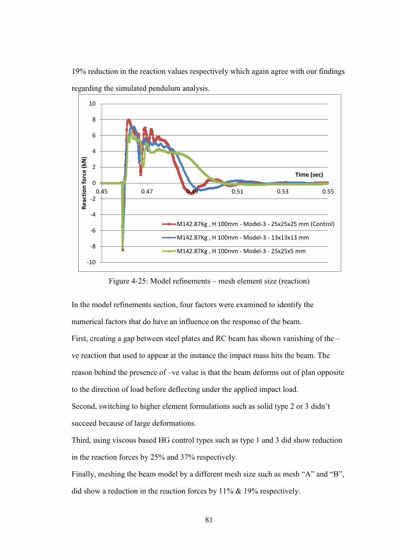
81
19% reduction in the reaction values respectively which again agree with our findings
regarding the simulated pendulum analysis.
Figure 4-25: Model refinements – mesh element size (reaction)
In the model refinements section, four factors were examined to identify the
numerical factors that do have an influence on the response of the beam.
First, creating a gap between steel plates and RC beam has shown vanishing of the –
ve reaction that used to appear at the instance the impact mass hits the beam. The
reason behind the presence of –ve value is that the beam deforms out of plan opposite
to the direction of load before deflecting under the applied impact load.
Second, switching to higher element formulations such as solid type 2 or 3 didn’t
succeed because of large deformations.
Third, using viscous based HG control types such as type 1 and 3 did show reduction
in the reaction forces by 25% and 37% respectively.
Finally, meshing the beam model by a different mesh size such as mesh “A” and “B”,
did show a reduction in the reaction forces by 11% & 19% respectively.
-10
-8
-6
-4
-2
0
2
4
6
8
10
0.45 0.47 0.49 0.51 0.53 0.55
Reac
tion
forc
e (k
N)
Time (sec)
M142.87Kg , H 100mm - Model-3 - 25x25x25 mm (Control)
M142.87Kg , H 100mm - Model-3 - 13x13x13 mm
M142.87Kg , H 100mm - Model-3 - 25x25x5 mm

82
Although the results of model refinements are valuable; yet, we will not make use of
these modifications in our parametric analysis because these factors need to be further
examined with different impact forces, impact velocities and using different material
models. In other words, in order to replace our control model with another better
model we need to do comprehensive analysis to reach to solid findings; accordingly,
our control model will continue to be used in the parametric analysis section.
4.4.4 Beam’s damage
RC beam’s level of damage for models 1, 2 , 3 , and 4 , under high impact loads were
recorded ; however , for presentation purposes we only prensented the damage in the
RC beam for a dropping mass of 800kg falling from a height of 100mm. Results were
reported at time 0.47 sec and 0.6 sec.In all the numerical models used , soild elements
were eroded upon faliure (max. strain).

83
4.4.4.1 RC Beam’s Damage for Model 1
Figure 4-26: Damage @ time 0.47 sec - Model 1, M 800kg & H 100mm
Figure 4-27: Damage @ time 0.60 sec - Model 1, M 800kg & H 100mm
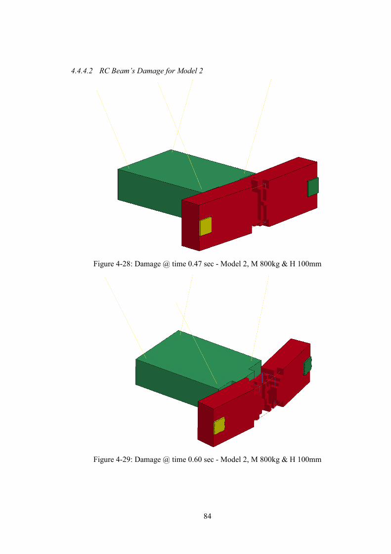
84
4.4.4.2 RC Beam’s Damage for Model 2
Figure 4-28: Damage @ time 0.47 sec - Model 2, M 800kg & H 100mm
Figure 4-29: Damage @ time 0.60 sec - Model 2, M 800kg & H 100mm
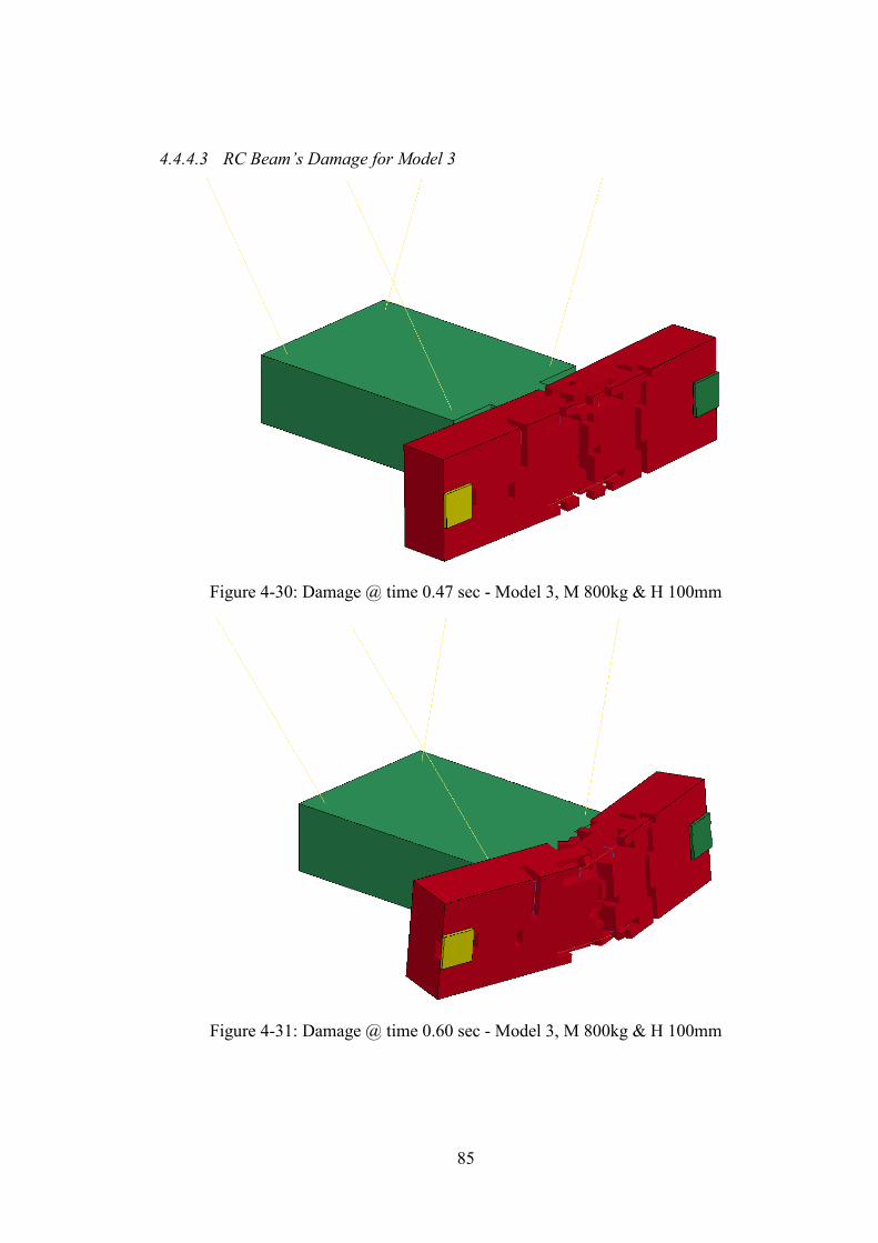
85
4.4.4.3 RC Beam’s Damage for Model 3
Figure 4-30: Damage @ time 0.47 sec - Model 3, M 800kg & H 100mm
Figure 4-31: Damage @ time 0.60 sec - Model 3, M 800kg & H 100mm
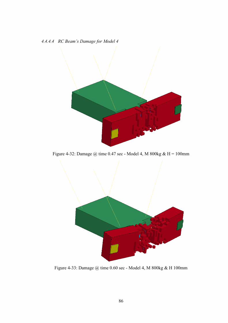
86
4.4.4.4 RC Beam’s Damage for Model 4
Figure 4-32: Damage @ time 0.47 sec - Model 4, M 800kg & H = 100mm
Figure 4-33: Damage @ time 0.60 sec - Model 4, M 800kg & H 100mm
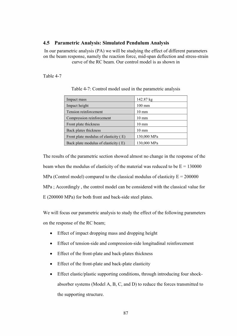
87
4.5 Parametric Analysis: Simulated Pendulum Analysis In our parametric analysis (PA) we will be studying the effect of different parameters on the beam response, namely the reaction force, mid-span deflection and stress-strain
curve of the RC beam. Our control model is as shown in
Table 4-7
Table 4-7: Control model used in the parametric analysis
Impact mass 142.87 kg Impact height 100 mm Tension reinforcement 10 mm Compression reinforcement 10 mm Front plate thickness 10 mm Back plates thickness 10 mm Front plate modulus of elasticity ( E) 130,000 MPa Back plate modulus of elasticity ( E) 130,000 MPa
The results of the parametric section showed almost no change in the response of the
beam when the modulus of elasticity of the material was reduced to be E = 130000
MPa (Control model) compared to the classical modulus of elasticity E = 200000
MPa ; Accordingly , the control model can be considered with the classical value for
E (200000 MPa) for both front and back-side steel plates.
We will focus our parametric analysis to study the effect of the following parameters
on the response of the RC beam;
• Effect of impact dropping mass and dropping height
• Effect of tension-side and compression-side longitudinal reinforcement
• Effect of the front-plate and back-plates thickness
• Effect of the front-plate and back-plate elasticity
• Effect elastic/plastic supporting conditions, through introducing four shock-
absorber systems (Model A, B, C, and D) to reduce the forces transmitted to
the supporting structure.
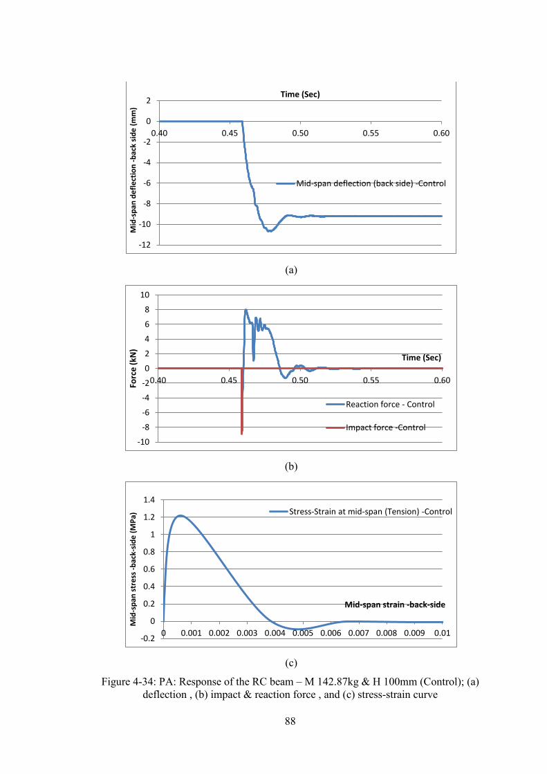
88
(a)
(b)
(c)
Figure 4-34: PA: Response of the RC beam – M 142.87kg & H 100mm (Control); (a) deflection , (b) impact & reaction force , and (c) stress-strain curve
-12
-10
-8
-6
-4
-2
0
2
0.40 0.45 0.50 0.55 0.60 M
id-s
pan
defle
ctio
n -b
ack
side
(mm
)
Time (Sec)
Mid-span deflection (back side) -Control
-10
-8
-6
-4
-2
0
2
4
6
8
10
0.40 0.45 0.50 0.55 0.60 Forc
e (k
N)
Time (Sec)
Reaction force - Control
Impact force -Control
-0.2
0
0.2
0.4
0.6
0.8
1
1.2
1.4
0 0.001 0.002 0.003 0.004 0.005 0.006 0.007 0.008 0.009 0.01
Mid
-spa
n st
ress
-bac
k-si
de (M
Pa)
Mid-span strain -back-side
Stress-Strain at mid-span (Tension) -Control
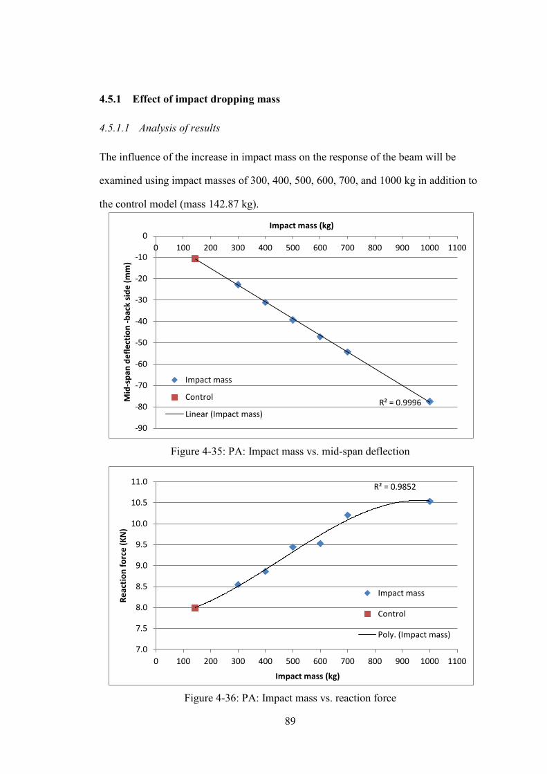
89
4.5.1 Effect of impact dropping mass
4.5.1.1 Analysis of results
The influence of the increase in impact mass on the response of the beam will be
examined using impact masses of 300, 400, 500, 600, 700, and 1000 kg in addition to
the control model (mass 142.87 kg).
Figure 4-35: PA: Impact mass vs. mid-span deflection
Figure 4-36: PA: Impact mass vs. reaction force
R² = 0.9996
-90
-80
-70
-60
-50
-40
-30
-20
-10
0 0 100 200 300 400 500 600 700 800 900 1000 1100
Mid
-spa
n de
flect
ion
-bac
k si
de (m
m)
Impact mass (kg)
Impact mass
Control
Linear (Impact mass)
R² = 0.9852
7.0
7.5
8.0
8.5
9.0
9.5
10.0
10.5
11.0
0 100 200 300 400 500 600 700 800 900 1000 1100
Reac
tion
forc
e (K
N)
Impact mass (kg)
Impact mass
Control
Poly. (Impact mass)

90
Figure 4-37: PA: Impact mass vs. mid-span stress (back-side)
4.5.1.2 Comments
In this section we will focus on the effect of the increase in impact mass on the
response of the beam. In summary for the beam response;
• With the increase in the impact mass, there is an almost linear increase in the mid-
span deflection as shown in Figure 4-35.
• With the increase in the impact mass, there is a steep increase in the reaction force
; however , Figure 4-36 shows that the slope is reducing and there will be an
inflection point at a mass of 1000kg i.e. without any increase in the impact mass ,
the reaction force will decrease or at least will not increase
• It was noticed that deflection increased linearly with the increase in the impact
mass (i.e increase in force) while the reaction has a nonlinear increase with the
increase of the impact force. In all our models the deflection was recorded at the
mid-span point which was directly affected by the increase in the impact force
through a linear relation ; however, the reaction values depends on many factors
such as the deformations of the panel all over the beam , rigid body motion of the
0.0
0.5
1.0
1.5
2.0
2.5
3.0
3.5
0 100 200 300 400 500 600 700 800 900 1000 1100
Mid
-spa
n st
ress
bac
k si
de (M
Pa)
Impact mass (kg)
Impact mass
Control
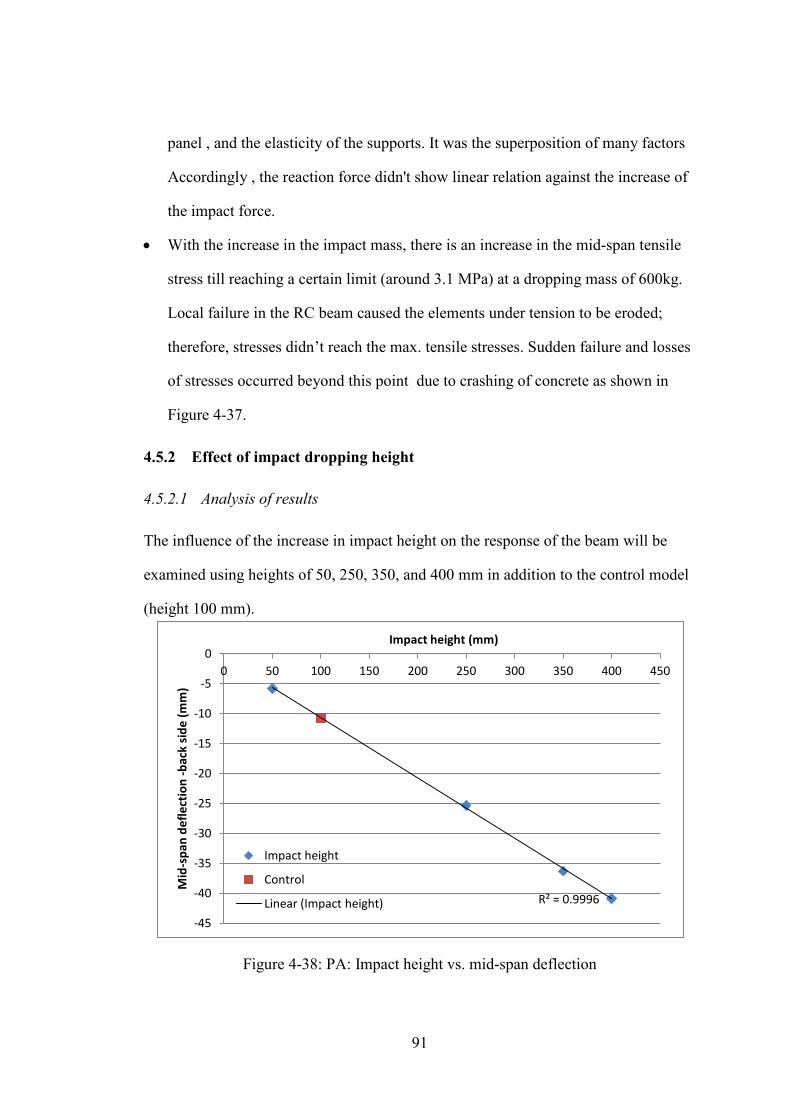
91
panel , and the elasticity of the supports. It was the superposition of many factors
Accordingly , the reaction force didn't show linear relation against the increase of
the impact force.
• With the increase in the impact mass, there is an increase in the mid-span tensile
stress till reaching a certain limit (around 3.1 MPa) at a dropping mass of 600kg.
Local failure in the RC beam caused the elements under tension to be eroded;
therefore, stresses didn’t reach the max. tensile stresses. Sudden failure and losses
of stresses occurred beyond this point due to crashing of concrete as shown in
Figure 4-37.
4.5.2 Effect of impact dropping height
4.5.2.1 Analysis of results
The influence of the increase in impact height on the response of the beam will be
examined using heights of 50, 250, 350, and 400 mm in addition to the control model
(height 100 mm).
Figure 4-38: PA: Impact height vs. mid-span deflection
R² = 0.9996
-45
-40
-35
-30
-25
-20
-15
-10
-5
0 0 50 100 150 200 250 300 350 400 450
Mid
-spa
n de
flect
ion
-bac
k si
de (m
m)
Impact height (mm)
Impact height
Control
Linear (Impact height)
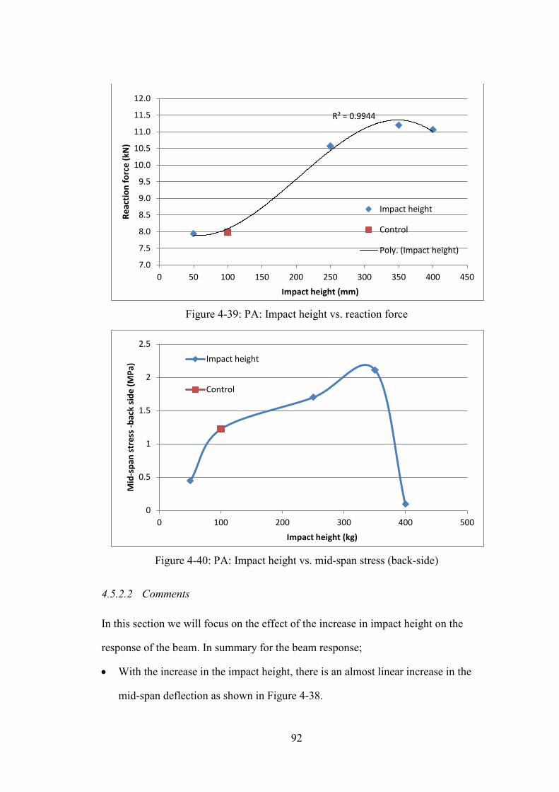
92
Figure 4-39: PA: Impact height vs. reaction force
Figure 4-40: PA: Impact height vs. mid-span stress (back-side)
4.5.2.2 Comments
In this section we will focus on the effect of the increase in impact height on the
response of the beam. In summary for the beam response;
• With the increase in the impact height, there is an almost linear increase in the
mid-span deflection as shown in Figure 4-38.
R² = 0.9944
7.0
7.5
8.0
8.5
9.0
9.5
10.0
10.5
11.0
11.5
12.0
0 50 100 150 200 250 300 350 400 450
Reac
tion
forc
e (k
N)
Impact height (mm)
Impact height
Control
Poly. (Impact height)
0
0.5
1
1.5
2
2.5
0 100 200 300 400 500
Mid
-spa
n st
ress
-bac
k si
de (M
Pa)
Impact height (kg)
Impact height
Control
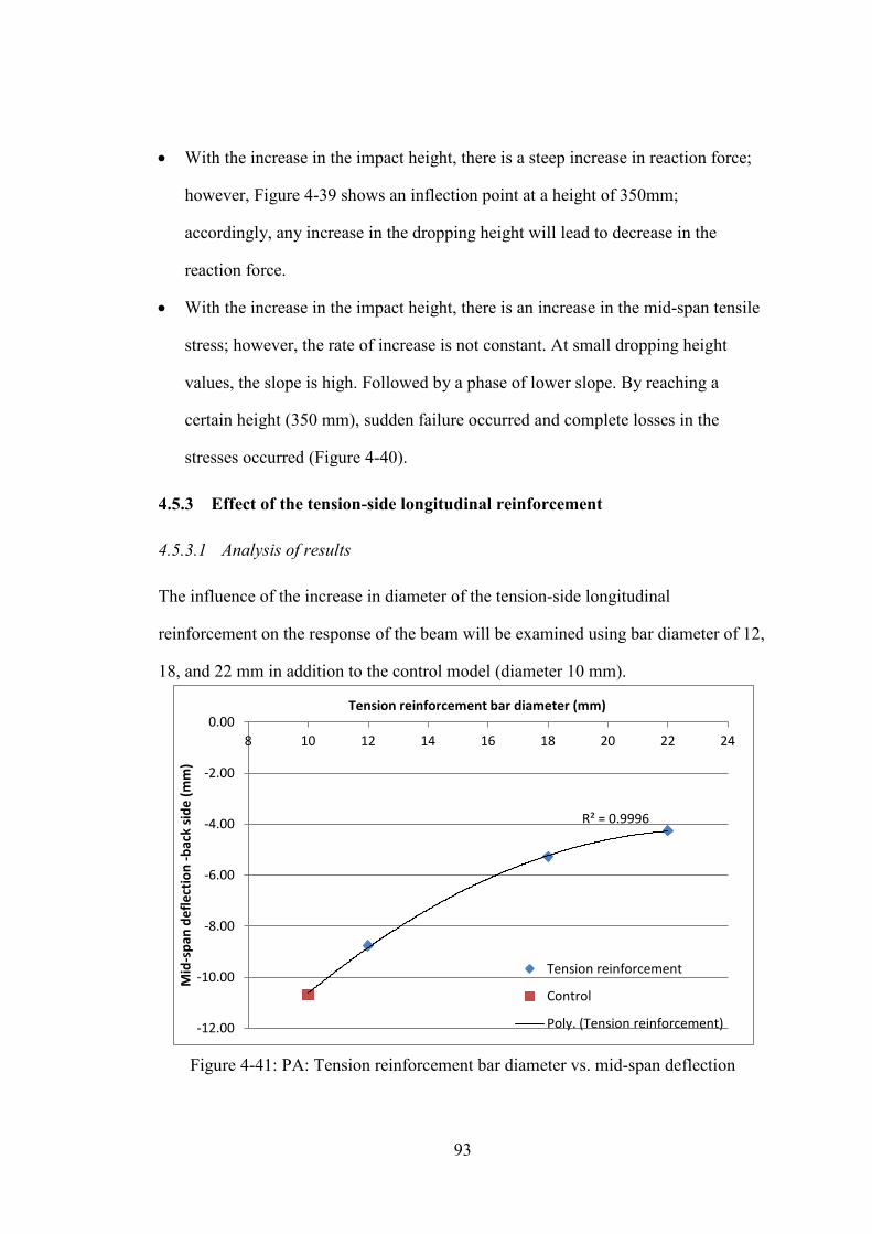
93
• With the increase in the impact height, there is a steep increase in reaction force;
however, Figure 4-39 shows an inflection point at a height of 350mm;
accordingly, any increase in the dropping height will lead to decrease in the
reaction force.
• With the increase in the impact height, there is an increase in the mid-span tensile
stress; however, the rate of increase is not constant. At small dropping height
values, the slope is high. Followed by a phase of lower slope. By reaching a
certain height (350 mm), sudden failure occurred and complete losses in the
stresses occurred (Figure 4-40).
4.5.3 Effect of the tension-side longitudinal reinforcement
4.5.3.1 Analysis of results
The influence of the increase in diameter of the tension-side longitudinal
reinforcement on the response of the beam will be examined using bar diameter of 12,
18, and 22 mm in addition to the control model (diameter 10 mm).
Figure 4-41: PA: Tension reinforcement bar diameter vs. mid-span deflection
R² = 0.9996
-12.00
-10.00
-8.00
-6.00
-4.00
-2.00
0.00 8 10 12 14 16 18 20 22 24
Mid
-spa
n de
flect
ion
-bac
k si
de (m
m)
Tension reinforcement bar diameter (mm)
Tension reinforcement
Control
Poly. (Tension reinforcement)
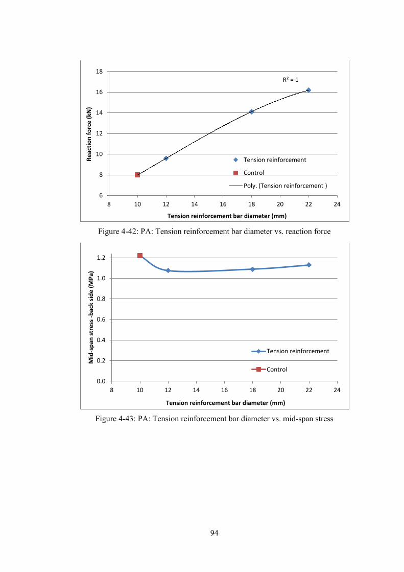
94
Figure 4-42: PA: Tension reinforcement bar diameter vs. reaction force
Figure 4-43: PA: Tension reinforcement bar diameter vs. mid-span stress
R² = 1
6
8
10
12
14
16
18
8 10 12 14 16 18 20 22 24
Reac
tion
forc
e (k
N)
Tension reinforcement bar diameter (mm)
Tension reinforcement
Control
Poly. (Tension reinforcement )
0.0
0.2
0.4
0.6
0.8
1.0
1.2
8 10 12 14 16 18 20 22 24
Mid
-spa
n st
ress
-bac
k si
de (M
Pa)
Tension reinforcement bar diameter (mm)
Tension reinforcement
Control
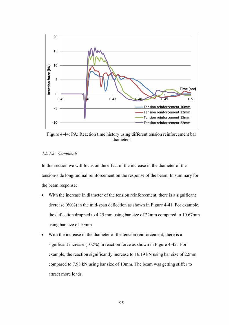
95
Figure 4-44: PA: Reaction time history using different tension reinforcement bar
diameters
4.5.3.2 Comments
In this section we will focus on the effect of the increase in the diameter of the
tension-side longitudinal reinforcement on the response of the beam. In summary for
the beam response;
• With the increase in diameter of the tension reinforcement, there is a significant
decrease (60%) in the mid-span deflection as shown in Figure 4-41. For example,
the deflection dropped to 4.25 mm using bar size of 22mm compared to 10.67mm
using bar size of 10mm.
• With the increase in the diameter of the tension reinforcement, there is a
significant increase (102%) in reaction force as shown in Figure 4-42. For
example, the reaction significantly increase to 16.19 kN using bar size of 22mm
compared to 7.98 kN using bar size of 10mm. The beam was getting stiffer to
attract more loads.
-10
-5
0
5
10
15
20
0.45 0.46 0.47 0.48 0.49 0.5
Reac
tion
forc
e (k
N)
Time (sec)
Tension reinforcement 10mm Tension reinforcement 12mm Tension reinforcement 18mm Tension reinforcement 22mm

96
• Figure 4-44 shows a little change in the reaction-time history profile with the
increase in the bar size of tension reinforcement. With the increase of the bar
diameter, the area under the curve is getting less.
• With the increase in diameter of the tension reinforcement, there is a decrease in
the mid-span tensile stress using a bar size of 12mm; however, additional increase
in the bar size led to almost no decrease in the stress as shown in Figure 4-43.
4.5.4 Effect of the compression-side longitudinal reinforcement
4.5.4.1 Analysis of results
The influence of the increase in the diameter of the compression-side longitudinal
reinforcement on the response of the beam will be examined using diameters of 12,
18, and 22 mm in addition to the control model (diameter 10 mm).
Figure 4-45: PA: Compression reinforcement bar diameter vs. mid-span deflection
R² = 1
-10.8
-10.6
-10.4
-10.2
-10.0
-9.8
-9.6 8 10 12 14 16 18 20 22 24
Mid
-spa
n de
flect
ion
-bac
k si
de (m
m)
Compression reinforcement bar diameter (mm)
Compression reinforcement
Control
Poly. (Compression reinforcement)
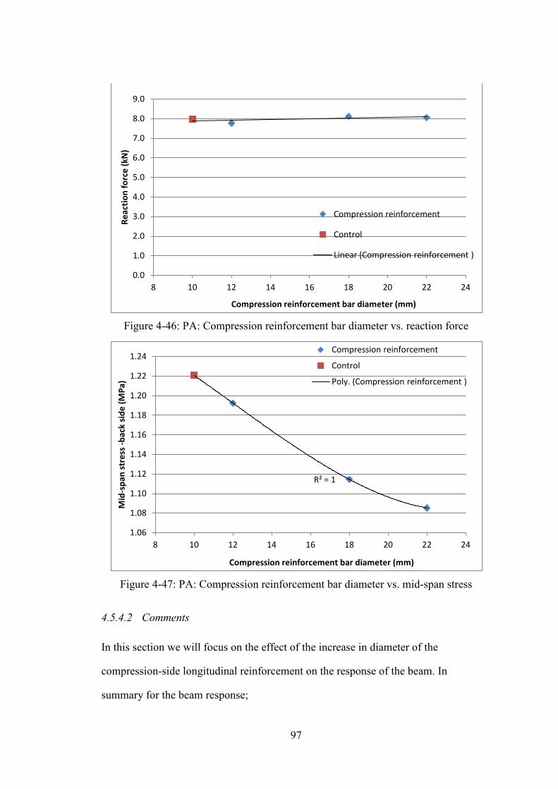
97
Figure 4-46: PA: Compression reinforcement bar diameter vs. reaction force
Figure 4-47: PA: Compression reinforcement bar diameter vs. mid-span stress
4.5.4.2 Comments
In this section we will focus on the effect of the increase in diameter of the
compression-side longitudinal reinforcement on the response of the beam. In
summary for the beam response;
0.0
1.0
2.0
3.0
4.0
5.0
6.0
7.0
8.0
9.0
8 10 12 14 16 18 20 22 24
Reac
tion
forc
e (k
N)
Compression reinforcement bar diameter (mm)
Compression reinforcement
Control
Linear (Compression reinforcement )
R² = 1
1.06
1.08
1.10
1.12
1.14
1.16
1.18
1.20
1.22
1.24
8 10 12 14 16 18 20 22 24
Mid
-spa
n st
ress
-bac
k si
de (M
Pa)
Compression reinforcement bar diameter (mm)
Compression reinforcement
Control
Poly. (Compression reinforcement )
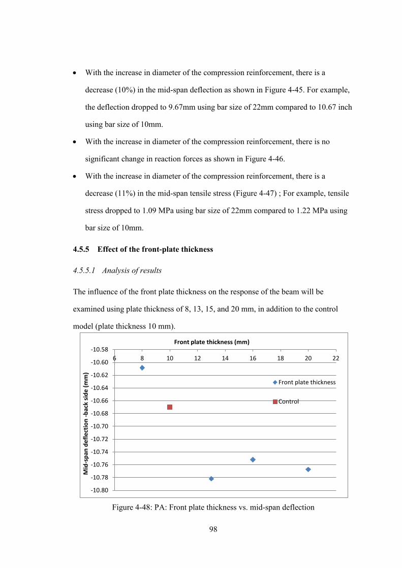
98
• With the increase in diameter of the compression reinforcement, there is a
decrease (10%) in the mid-span deflection as shown in Figure 4-45. For example,
the deflection dropped to 9.67mm using bar size of 22mm compared to 10.67 inch
using bar size of 10mm.
• With the increase in diameter of the compression reinforcement, there is no
significant change in reaction forces as shown in Figure 4-46.
• With the increase in diameter of the compression reinforcement, there is a
decrease (11%) in the mid-span tensile stress (Figure 4-47) ; For example, tensile
stress dropped to 1.09 MPa using bar size of 22mm compared to 1.22 MPa using
bar size of 10mm.
4.5.5 Effect of the front-plate thickness
4.5.5.1 Analysis of results
The influence of the front plate thickness on the response of the beam will be
examined using plate thickness of 8, 13, 15, and 20 mm, in addition to the control
model (plate thickness 10 mm).
Figure 4-48: PA: Front plate thickness vs. mid-span deflection
-10.80
-10.78
-10.76
-10.74
-10.72
-10.70
-10.68
-10.66
-10.64
-10.62
-10.60
-10.58 6 8 10 12 14 16 18 20 22
Mid
-spa
n de
flect
ion
-bac
k si
de (m
m)
Front plate thickness (mm)
Front plate thickness
Control
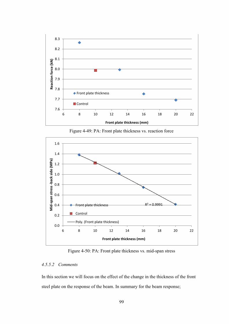
99
Figure 4-49: PA: Front plate thickness vs. reaction force
Figure 4-50: PA: Front plate thickness vs. mid-span stress
4.5.5.2 Comments
In this section we will focus on the effect of the change in the thickness of the front
steel plate on the response of the beam. In summary for the beam response;
7.6
7.7
7.8
7.9
8.0
8.1
8.2
8.3
6 8 10 12 14 16 18 20 22
Reac
tion
forc
e (k
N)
Front plate thickness (mm)
Front plate thickness
Control
R² = 0.9991
0.0
0.2
0.4
0.6
0.8
1.0
1.2
1.4
1.6
6 8 10 12 14 16 18 20 22
Mid
-spa
n st
ress
-bac
k si
de (M
Pa)
Front plate thickness (mm)
Front plate thickness
Control
Poly. (Front plate thickness)

100
• With the change in thickness of the front plate, there is no significant change (1%)
in the mid-span deflection as shown in Figure 4-48.
• With the change in thickness of the front plate, there is a small change in reaction
force as shown in Figure 4-49. For example, 3.7% decrease in reaction force at
plate thickness of 20 mm; while, 3.7% increase in the reaction force at plate
thickness of 8 mm compared to the control model.
• With the change in thickness of the front plate, there is a significant change in the
mid-span tensile stress as shown in Figure 4-50. For example, 66% decrease in the
mid-span tensile stress at plate thickness of 20 mm; while, 13% increase in the
mid-span tensile stress at plate thickness of 8 mm compared to the control model.
4.5.6 Effect of the back-plates thickness
4.5.6.1 Analysis of results
The influence of the back plate thickness on the response of the beam will be
examined using plate thickness of 8, 13, 15, and 20 mm, in addition to the control
model (plate thickness 10 mm).
Figure 4-51: PA: Back plate thickness vs. mid-span deflection
-10.76
-10.74
-10.72
-10.70
-10.68
-10.66
-10.64 0 5 10 15 20 25
Mid
-spa
n de
flect
ion
(bac
k si
de) ,
mm
Back plate thickness , mm
Black plate thickness Control
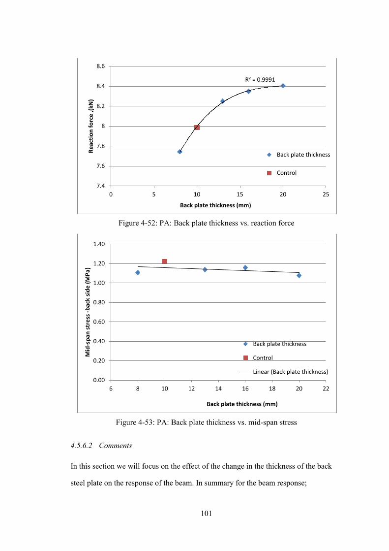
101
Figure 4-52: PA: Back plate thickness vs. reaction force
Figure 4-53: PA: Back plate thickness vs. mid-span stress
4.5.6.2 Comments
In this section we will focus on the effect of the change in the thickness of the back
steel plate on the response of the beam. In summary for the beam response;
R² = 0.9991
7.4
7.6
7.8
8
8.2
8.4
8.6
0 5 10 15 20 25
Reac
tion
forc
e ,(k
N)
Back plate thickness (mm)
Back plate thickness
Control
0.00
0.20
0.40
0.60
0.80
1.00
1.20
1.40
6 8 10 12 14 16 18 20 22
Mid
-spa
n st
ress
-bac
k si
de (M
Pa)
Back plate thickness (mm)
Back plate thickness
Control
Linear (Back plate thickness)
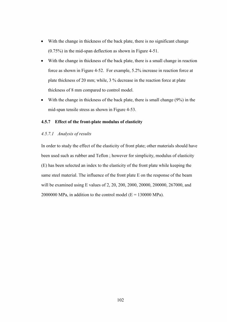
102
• With the change in thickness of the back plate, there is no significant change
(0.75%) in the mid-span deflection as shown in Figure 4-51.
• With the change in thickness of the back plate, there is a small change in reaction
force as shown in Figure 4-52. For example, 5.2% increase in reaction force at
plate thickness of 20 mm; while, 3 % decrease in the reaction force at plate
thickness of 8 mm compared to control model.
• With the change in thickness of the back plate, there is small change (9%) in the
mid-span tensile stress as shown in Figure 4-53.
4.5.7 Effect of the front-plate modulus of elasticity
4.5.7.1 Analysis of results
In order to study the effect of the elasticity of front plate; other materials should have
been used such as rubber and Teflon ; however for simplicity, modulus of elasticity
(E) has been selected an index to the elasticity of the front plate while keeping the
same steel material. The influence of the front plate E on the response of the beam
will be examined using E values of 2, 20, 200, 2000, 20000, 200000, 267000, and
2000000 MPa, in addition to the control model (E = 130000 MPa).
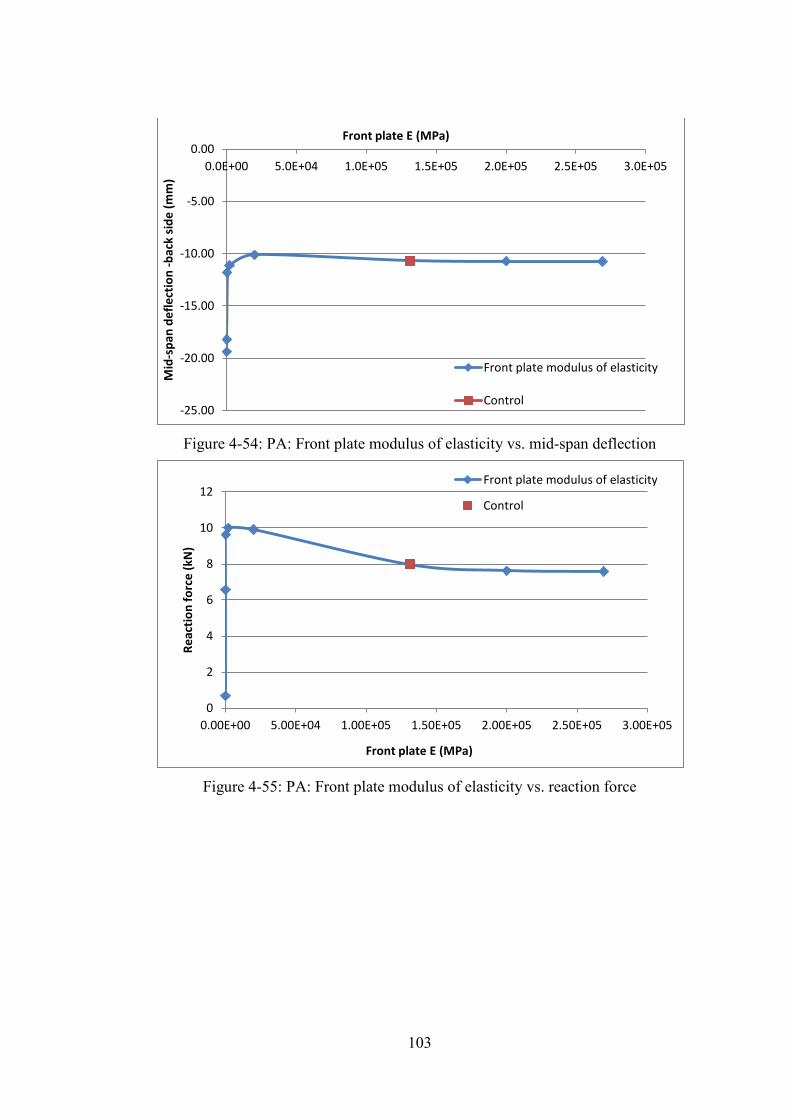
103
Figure 4-54: PA: Front plate modulus of elasticity vs. mid-span deflection
Figure 4-55: PA: Front plate modulus of elasticity vs. reaction force
-25.00
-20.00
-15.00
-10.00
-5.00
0.00 0.0E+00 5.0E+04 1.0E+05 1.5E+05 2.0E+05 2.5E+05 3.0E+05
Mid
-spa
n de
flect
ion
-bac
k si
de (m
m)
Front plate E (MPa)
Front plate modulus of elasticity
Control
0
2
4
6
8
10
12
0.00E+00 5.00E+04 1.00E+05 1.50E+05 2.00E+05 2.50E+05 3.00E+05
Reac
tion
forc
e (k
N)
Front plate E (MPa)
Front plate modulus of elasticity
Control
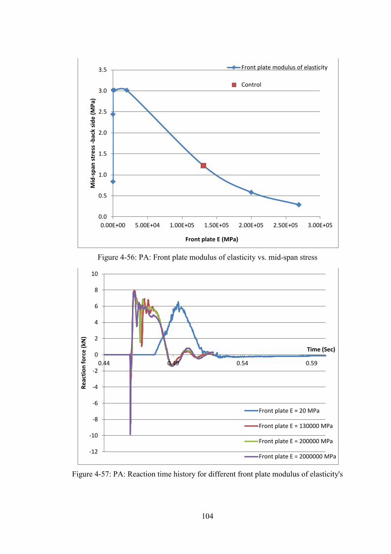
104
Figure 4-56: PA: Front plate modulus of elasticity vs. mid-span stress
Figure 4-57: PA: Reaction time history for different front plate modulus of elasticity's
0.0
0.5
1.0
1.5
2.0
2.5
3.0
3.5
0.00E+00 5.00E+04 1.00E+05 1.50E+05 2.00E+05 2.50E+05 3.00E+05
Mid
-spa
n st
ress
-bac
k si
de (M
Pa)
Front plate E (MPa)
Front plate modulus of elasticity
Control
-12
-10
-8
-6
-4
-2
0
2
4
6
8
10
0.44 0.49 0.54 0.59
Reac
tion
forc
e (k
N)
Time (Sec)
Front plate E = 20 MPa
Front plate E = 130000 MPa
Front plate E = 200000 MPa
Front plate E = 2000000 MPa

105
Figure 4-58: PA: Impact force time history for different front plate modulus of
elasticity's
4.5.7.2 Comments
In this section we will focus on the effect of the change of the front plate modulus of
elasticity (E) on the response of the beam. In summary for the beam response;
• With the decrease in E, there is a significant increase (69%) in the mid-span
deflection as shown in Figure 4-54. For example, at E = 20 MPa the mid-span
deflection was 18 mm; however, at E = 130000 MPa the mid-span deflection was
10.67 mm. On the other hand, with the increase in E, there is no significant
change in the mid-span deflection.
• With the decrease in E, there is a significant increase in the reaction values till
reaching a certain value (E= 2000 MPa) then the reaction force decreased as
shown in Figure 4-55. For example, the reaction force = 7.98 kN @ E = 130000
MPa increased to be 10 kN @ E = 2000 MPa; however, further reductions in E
-10
-9
-8
-7
-6
-5
-4
-3
-2
-1
0 0.44 0.45 0.46 0.47 0.48 0.49 0.5
Impa
ct fo
rce
( kN
)
Time (Sec)
Front plate E = 20 MPa
Front plate E = 200 MPa
Front plate E = 2000 MPa
Front plate E = 20000 MPa
Front plate E = 131000 MPa
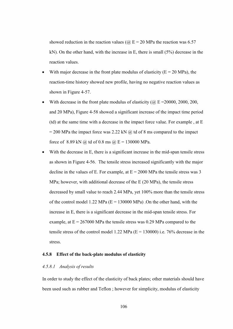
106
showed reduction in the reaction values (@ E = 20 MPa the reaction was 6.57
kN). On the other hand, with the increase in E, there is small (5%) decrease in the
reaction values.
• With major decrease in the front plate modulus of elasticity (E = 20 MPa), the
reaction-time history showed new profile, having no negative reaction values as
shown in Figure 4-57.
• With decrease in the front plate modulus of elasticity (@ E =20000, 2000, 200,
and 20 MPa), Figure 4-58 showed a significant increase of the impact time period
(td) at the same time with a decrease in the impact force value. For example , at E
= 200 MPa the impact force was 2.22 kN @ td of 8 ms compared to the impact
force of 8.89 kN @ td of 0.8 ms @ E = 130000 MPa.
• With the decrease in E, there is a significant increase in the mid-span tensile stress
as shown in Figure 4-56. The tensile stress increased significantly with the major
decline in the values of E. For example, at E = 2000 MPa the tensile stress was 3
MPa; however, with additional decrease of the E (20 MPa), the tensile stress
decreased by small value to reach 2.44 MPa, yet 100% more than the tensile stress
of the control model 1.22 MPa (E = 130000 MPa) .On the other hand, with the
increase in E, there is a significant decrease in the mid-span tensile stress. For
example, at E = 267000 MPa the tensile stress was 0.29 MPa compared to the
tensile stress of the control model 1.22 MPa (E = 130000) i.e. 76% decrease in the
stress.
4.5.8 Effect of the back-plate modulus of elasticity
4.5.8.1 Analysis of results
In order to study the effect of the elasticity of back plates; other materials should have
been used such as rubber and Teflon ; however for simplicity, modulus of elasticity
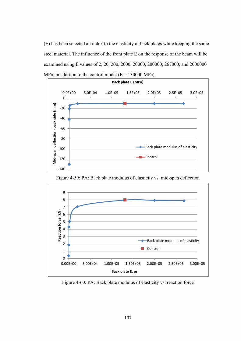
107
(E) has been selected an index to the elasticity of back plates while keeping the same
steel material. The influence of the front plate E on the response of the beam will be
examined using E values of 2, 20, 200, 2000, 20000, 200000, 267000, and 2000000
MPa, in addition to the control model (E = 130000 MPa).
Figure 4-59: PA: Back plate modulus of elasticity vs. mid-span deflection
Figure 4-60: PA: Back plate modulus of elasticity vs. reaction force
-140
-120
-100
-80
-60
-40
-20
0 0.0E+00 5.0E+04 1.0E+05 1.5E+05 2.0E+05 2.5E+05 3.0E+05
Mid
-spa
n de
flect
ion
-bac
k si
de (m
m)
Back plate E (MPa)
Back plate modulus of elasticity
Control
0
1
2
3
4
5
6
7
8
9
0.00E+00 5.00E+04 1.00E+05 1.50E+05 2.00E+05 2.50E+05 3.00E+05
Reac
tion
forc
e (k
N)
Back plate E, psi
Back plate modulus of elasticity
Control
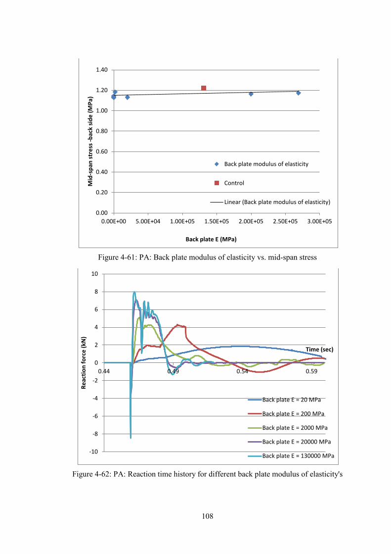
108
Figure 4-61: PA: Back plate modulus of elasticity vs. mid-span stress
Figure 4-62: PA: Reaction time history for different back plate modulus of elasticity's
0.00
0.20
0.40
0.60
0.80
1.00
1.20
1.40
0.00E+00 5.00E+04 1.00E+05 1.50E+05 2.00E+05 2.50E+05 3.00E+05
Mid
-spa
n st
ress
-bac
k si
de (M
Pa)
Back plate E (MPa)
Back plate modulus of elasticity
Control
Linear (Back plate modulus of elasticity)
-10
-8
-6
-4
-2
0
2
4
6
8
10
0.44 0.49 0.54 0.59
Reac
tion
forc
e (k
N)
Time (sec)
Back plate E = 20 MPa
Back plate E = 200 MPa
Back plate E = 2000 MPa
Back plate E = 20000 MPa
Back plate E = 130000 MPa
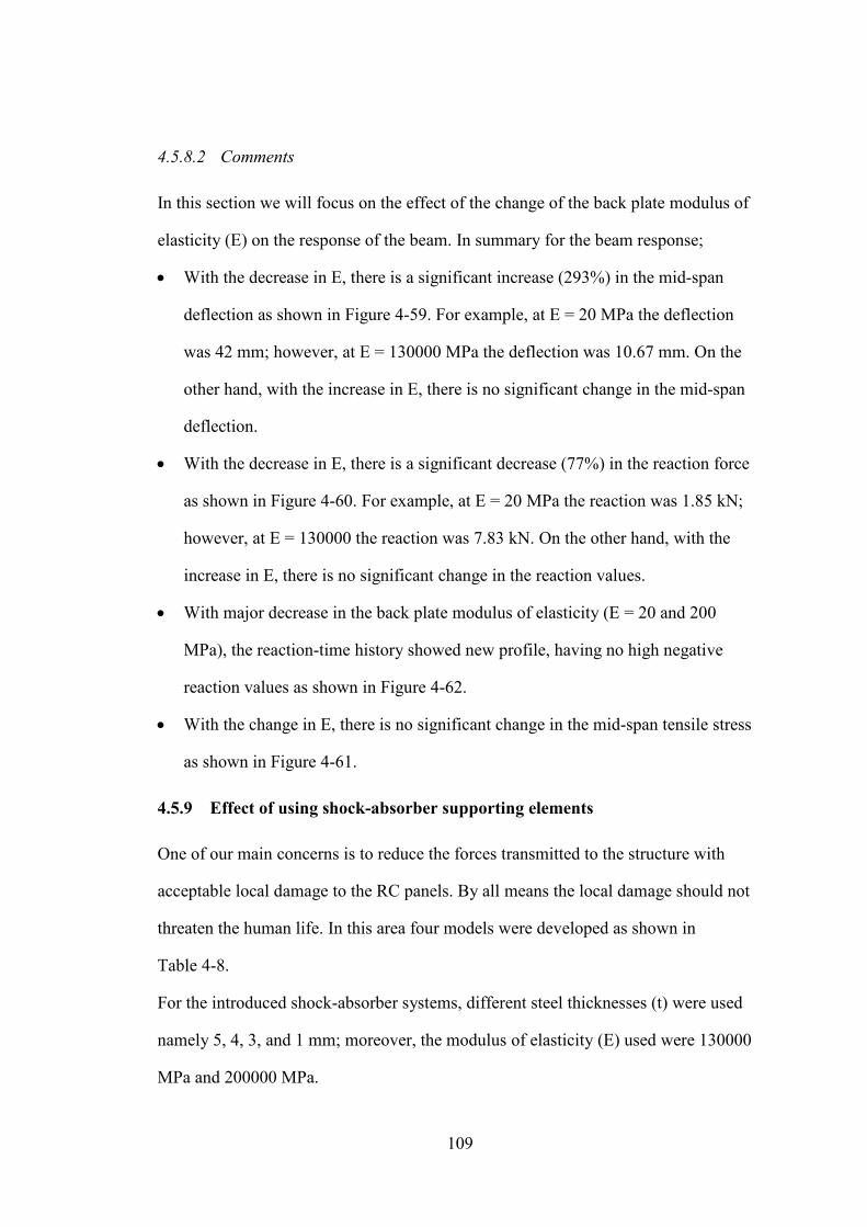
109
4.5.8.2 Comments
In this section we will focus on the effect of the change of the back plate modulus of
elasticity (E) on the response of the beam. In summary for the beam response;
• With the decrease in E, there is a significant increase (293%) in the mid-span
deflection as shown in Figure 4-59. For example, at E = 20 MPa the deflection
was 42 mm; however, at E = 130000 MPa the deflection was 10.67 mm. On the
other hand, with the increase in E, there is no significant change in the mid-span
deflection.
• With the decrease in E, there is a significant decrease (77%) in the reaction force
as shown in Figure 4-60. For example, at E = 20 MPa the reaction was 1.85 kN;
however, at E = 130000 the reaction was 7.83 kN. On the other hand, with the
increase in E, there is no significant change in the reaction values.
• With major decrease in the back plate modulus of elasticity (E = 20 and 200
MPa), the reaction-time history showed new profile, having no high negative
reaction values as shown in Figure 4-62.
• With the change in E, there is no significant change in the mid-span tensile stress
as shown in Figure 4-61.
4.5.9 Effect of using shock-absorber supporting elements
One of our main concerns is to reduce the forces transmitted to the structure with
acceptable local damage to the RC panels. By all means the local damage should not
threaten the human life. In this area four models were developed as shown in
Table 4-8.
For the introduced shock-absorber systems, different steel thicknesses (t) were used
namely 5, 4, 3, and 1 mm; moreover, the modulus of elasticity (E) used were 130000
MPa and 200000 MPa.
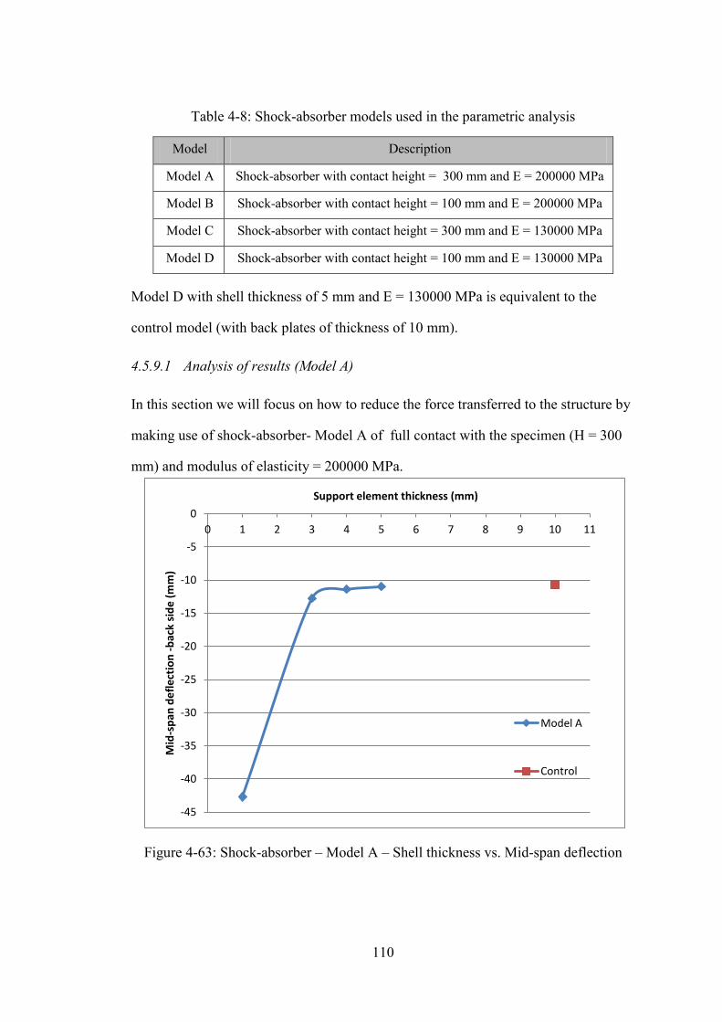
110
Table 4-8: Shock-absorber models used in the parametric analysis
Model Description
Model A Shock-absorber with contact height = 300 mm and E = 200000 MPa
Model B Shock-absorber with contact height = 100 mm and E = 200000 MPa
Model C Shock-absorber with contact height = 300 mm and E = 130000 MPa
Model D Shock-absorber with contact height = 100 mm and E = 130000 MPa
Model D with shell thickness of 5 mm and E = 130000 MPa is equivalent to the
control model (with back plates of thickness of 10 mm).
4.5.9.1 Analysis of results (Model A)
In this section we will focus on how to reduce the force transferred to the structure by
making use of shock-absorber- Model A of full contact with the specimen (H = 300
mm) and modulus of elasticity = 200000 MPa.
Figure 4-63: Shock-absorber – Model A – Shell thickness vs. Mid-span deflection
-45
-40
-35
-30
-25
-20
-15
-10
-5
0 0 1 2 3 4 5 6 7 8 9 10 11
Mid
-spa
n de
flect
ion
-bac
k si
de (m
m)
Support element thickness (mm)
Model A
Control
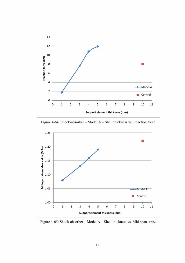
111
Figure 4-64: Shock-absorber – Model A – Shell thickness vs. Reaction force
Figure 4-65: Shock-absorber – Model A – Shell thickness vs. Mid-span stress
0
2
4
6
8
10
12
14
0 1 2 3 4 5 6 7 8 9 10 11
Reac
tion
forc
e (k
N)
Support element thickness (mm)
Model A
Control
1.00
1.05
1.10
1.15
1.20
1.25
0 1 2 3 4 5 6 7 8 9 10 11
Mid
-spa
n st
ress
-bac
k si
de (M
Pa)
Support element thickness (mm)
Model A
Control
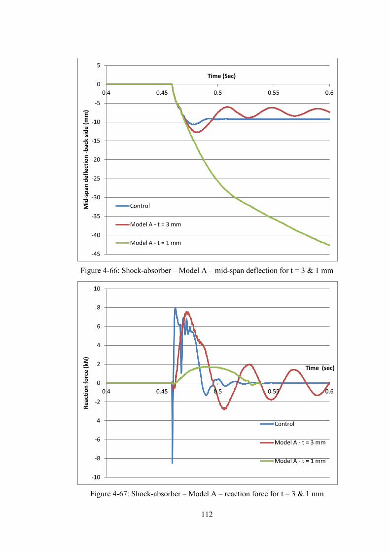
112
Figure 4-66: Shock-absorber – Model A – mid-span deflection for t = 3 & 1 mm
Figure 4-67: Shock-absorber – Model A – reaction force for t = 3 & 1 mm
-45
-40
-35
-30
-25
-20
-15
-10
-5
0
5
0.4 0.45 0.5 0.55 0.6 M
id-s
pan
defle
ctio
n -b
ack
side
(mm
) Time (Sec)
Control
Model A - t = 3 mm
Model A - t = 1 mm
-10
-8
-6
-4
-2
0
2
4
6
8
10
0.4 0.45 0.5 0.55 0.6
Reac
tion
forc
e (k
N)
Time (sec)
Control
Model A - t = 3 mm
Model A - t = 1 mm

113
Figure 4-68: Shock-absorber – Model A – Stress-strain relation for t = 3 & 1 mm
Figure 4-69: Damage in shock-absorber, Model A - t = 3 mm @ time = 0.6 sec
Figure 4-70: Damage in shock-absorber, Model A - t = 1 mm @ time = 0.6 sec
-0.2
0
0.2
0.4
0.6
0.8
1
1.2
1.4
0 0.002 0.004 0.006 0.008 0.01
Mid
-spa
n st
ress
-bac
k si
de (M
Pa)
Mid-span strain (back side)
Control
Model A - t = 3 mm
Model A - t = 1 mm
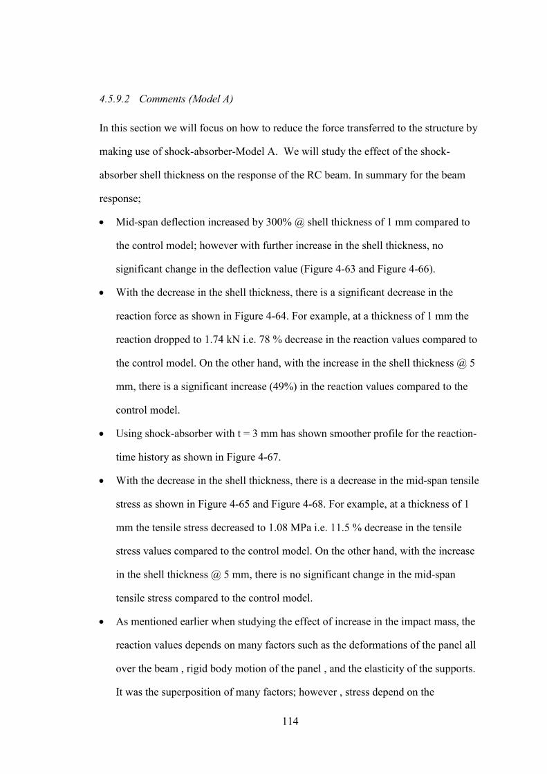
114
4.5.9.2 Comments (Model A)
In this section we will focus on how to reduce the force transferred to the structure by
making use of shock-absorber-Model A. We will study the effect of the shock-
absorber shell thickness on the response of the RC beam. In summary for the beam
response;
• Mid-span deflection increased by 300% @ shell thickness of 1 mm compared to
the control model; however with further increase in the shell thickness, no
significant change in the deflection value (Figure 4-63 and Figure 4-66).
• With the decrease in the shell thickness, there is a significant decrease in the
reaction force as shown in Figure 4-64. For example, at a thickness of 1 mm the
reaction dropped to 1.74 kN i.e. 78 % decrease in the reaction values compared to
the control model. On the other hand, with the increase in the shell thickness @ 5
mm, there is a significant increase (49%) in the reaction values compared to the
control model.
• Using shock-absorber with t = 3 mm has shown smoother profile for the reaction-
time history as shown in Figure 4-67.
• With the decrease in the shell thickness, there is a decrease in the mid-span tensile
stress as shown in Figure 4-65 and Figure 4-68. For example, at a thickness of 1
mm the tensile stress decreased to 1.08 MPa i.e. 11.5 % decrease in the tensile
stress values compared to the control model. On the other hand, with the increase
in the shell thickness @ 5 mm, there is no significant change in the mid-span
tensile stress compared to the control model.
• As mentioned earlier when studying the effect of increase in the impact mass, the
reaction values depends on many factors such as the deformations of the panel all
over the beam , rigid body motion of the panel , and the elasticity of the supports.
It was the superposition of many factors; however , stress depend on the
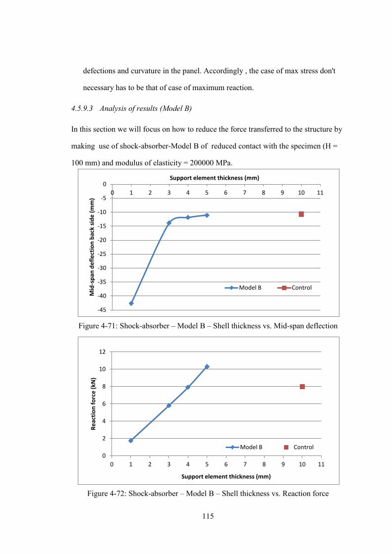
115
defections and curvature in the panel. Accordingly , the case of max stress don't
necessary has to be that of case of maximum reaction.
4.5.9.3 Analysis of results (Model B)
In this section we will focus on how to reduce the force transferred to the structure by
making use of shock-absorber-Model B of reduced contact with the specimen (H =
100 mm) and modulus of elasticity = 200000 MPa.
Figure 4-71: Shock-absorber – Model B – Shell thickness vs. Mid-span deflection
Figure 4-72: Shock-absorber – Model B – Shell thickness vs. Reaction force
-45
-40
-35
-30
-25
-20
-15
-10
-5
0 0 1 2 3 4 5 6 7 8 9 10 11
Mid
-spa
n de
flect
ion
back
side
(mm
)
Support element thickness (mm)
Model B Control
0
2
4
6
8
10
12
0 1 2 3 4 5 6 7 8 9 10 11
Reac
tion
forc
e (k
N)
Support element thickness (mm)
Model B Control
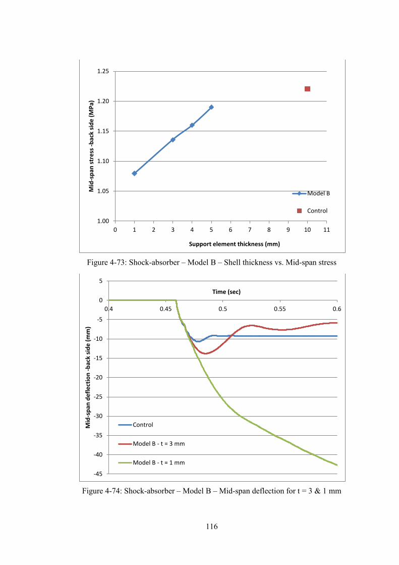
116
Figure 4-73: Shock-absorber – Model B – Shell thickness vs. Mid-span stress
Figure 4-74: Shock-absorber – Model B – Mid-span deflection for t = 3 & 1 mm
1.00
1.05
1.10
1.15
1.20
1.25
0 1 2 3 4 5 6 7 8 9 10 11
Mid
-spa
n st
ress
-bac
k si
de (M
Pa)
Support element thickness (mm)
Model B
Control
-45
-40
-35
-30
-25
-20
-15
-10
-5
0
5
0.4 0.45 0.5 0.55 0.6
Mid
-spa
n de
flect
ion
-bac
k si
de (m
m)
Time (sec)
Control
Model B - t = 3 mm
Model B - t = 1 mm
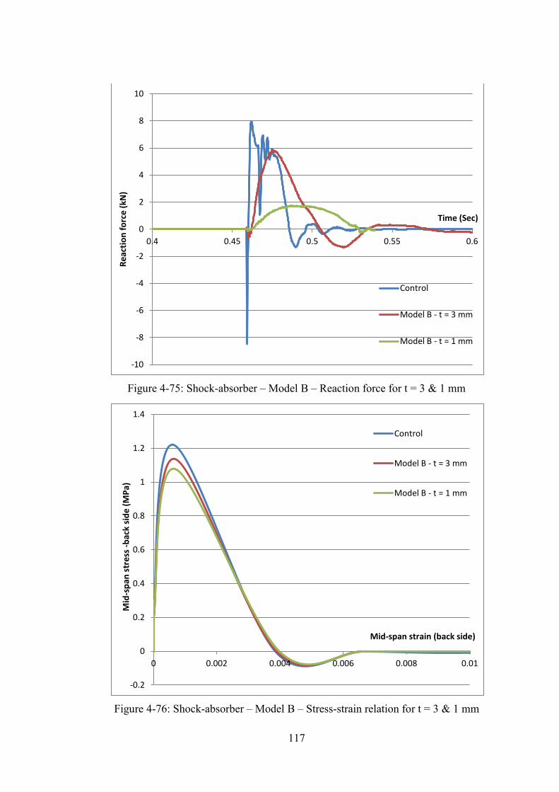
117
Figure 4-75: Shock-absorber – Model B – Reaction force for t = 3 & 1 mm
Figure 4-76: Shock-absorber – Model B – Stress-strain relation for t = 3 & 1 mm
-10
-8
-6
-4
-2
0
2
4
6
8
10
0.4 0.45 0.5 0.55 0.6
Reac
tion
forc
e (k
N)
Time (Sec)
Control
Model B - t = 3 mm
Model B - t = 1 mm
-0.2
0
0.2
0.4
0.6
0.8
1
1.2
1.4
0 0.002 0.004 0.006 0.008 0.01
Mid
-spa
n st
ress
-bac
k si
de (M
Pa)
Mid-span strain (back side)
Control
Model B - t = 3 mm
Model B - t = 1 mm

118
Figure 4-77: Damage in shock-absorber, Model B - t = 3 mm @ time = 0.6 sec
Figure 4-78: Damage in shock-absorber, Model B - t = 1 mm @ time = 0.6 sec
4.5.9.4 Comments (Model B)
In this section we will focus on how to reduce the force transferred to the structure by
making use of shock-absorber. Model B. We will study the effect of the shock-
absorber shell thickness on the response of the RC beam. In summary for the beam
response;
• Mid-span deflection increased by 300% @ shell thickness of 1 mm compared to
the control model; however with further increase in the shell thickness, no
significant change in the deflection values ( Figure 4-71 and Figure 4-74).
• With the decrease in the shell thickness, there is a significant decrease in the
reaction force as shown in Figure 4-72. For example, at a thickness of 1 mm the
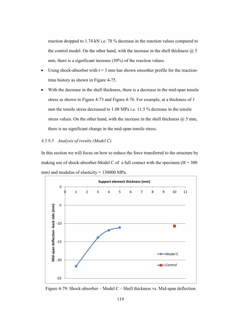
119
reaction dropped to 1.74 kN i.e. 78 % decrease in the reaction values compared to
the control model. On the other hand, with the increase in the shell thickness @ 5
mm, there is a significant increase (30%) of the reaction values.
• Using shock-absorber with t = 3 mm has shown smoother profile for the reaction-
time history as shown in Figure 4-75.
• With the decrease in the shell thickness, there is a decrease in the mid-span tensile
stress as shown in Figure 4-73 and Figure 4-76. For example, at a thickness of 1
mm the tensile stress decreased to 1.08 MPa i.e. 11.5 % decrease in the tensile
stress values. On the other hand, with the increase in the shell thickness @ 5 mm,
there is no significant change in the mid-span tensile stress.
4.5.9.5 Analysis of results (Model C)
In this section we will focus on how to reduce the force transferred to the structure by
making use of shock-absorber-Model C of a full contact with the specimen (H = 300
mm) and modulus of elasticity = 130000 MPa.
Figure 4-79: Shock-absorber – Model C – Shell thickness vs. Mid-span deflection
-25
-20
-15
-10
-5
0 0 1 2 3 4 5 6 7 8 9 10 11
Mid
-spa
n de
flect
ion
-bac
k si
de (m
m)
Support element thickness (mm)
Model C
Control

120
Figure 4-80: Shock-absorber – Model C – Shell thickness vs. Reaction force
Figure 4-81: Shock-absorber – Model C – Shell thickness vs. Mid-span stress
0
2
4
6
8
10
12
14
0 1 2 3 4 5 6 7 8 9 10 11
Reac
tion
forc
e (k
N)
Support element thickness (mm)
Model C
Control
1.0
1.1
1.1
1.2
1.2
1.3
0 2 4 6 8 10 12
Mid
-spa
n st
ress
-bac
k si
de (M
Pa)
Support element thickness (mm)
Model C
Control
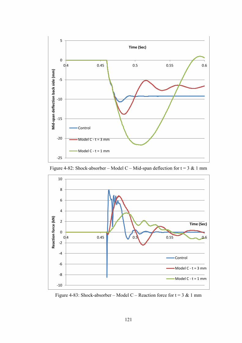
121
Figure 4-82: Shock-absorber – Model C – Mid-span deflection for t = 3 & 1 mm
Figure 4-83: Shock-absorber – Model C – Reaction force for t = 3 & 1 mm
-25
-20
-15
-10
-5
0
5
0.4 0.45 0.5 0.55 0.6
Mid
-spa
n de
flect
ion
back
side
(mm
) Time (Sec)
Control
Model C - t = 3 mm
Model C - t = 1 mm
-10
-8
-6
-4
-2
0
2
4
6
8
10
0.4 0.45 0.5 0.55 0.6
Reac
tion
forc
e (k
N)
Time (Sec)
Control
Model C - t = 3 mm
Model C - t = 1 mm
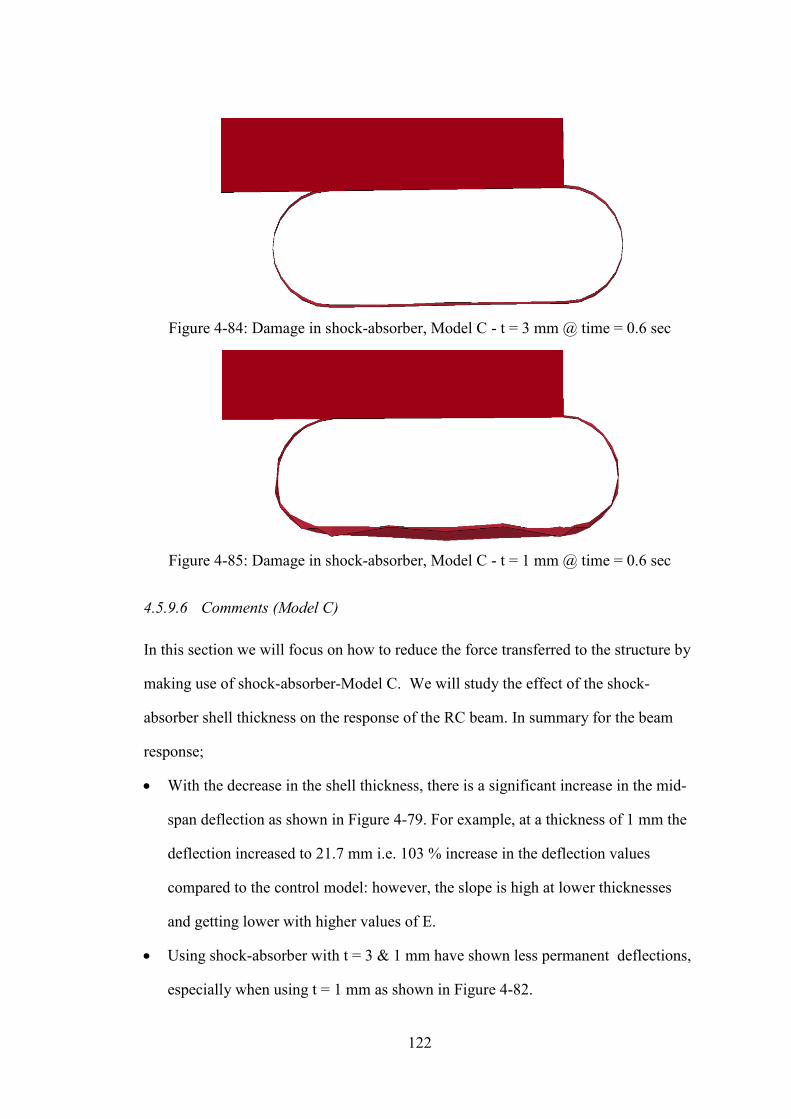
122
Figure 4-84: Damage in shock-absorber, Model C - t = 3 mm @ time = 0.6 sec
Figure 4-85: Damage in shock-absorber, Model C - t = 1 mm @ time = 0.6 sec
4.5.9.6 Comments (Model C)
In this section we will focus on how to reduce the force transferred to the structure by
making use of shock-absorber-Model C. We will study the effect of the shock-
absorber shell thickness on the response of the RC beam. In summary for the beam
response;
• With the decrease in the shell thickness, there is a significant increase in the mid-
span deflection as shown in Figure 4-79. For example, at a thickness of 1 mm the
deflection increased to 21.7 mm i.e. 103 % increase in the deflection values
compared to the control model: however, the slope is high at lower thicknesses
and getting lower with higher values of E.
• Using shock-absorber with t = 3 & 1 mm have shown less permanent deflections,
especially when using t = 1 mm as shown in Figure 4-82.
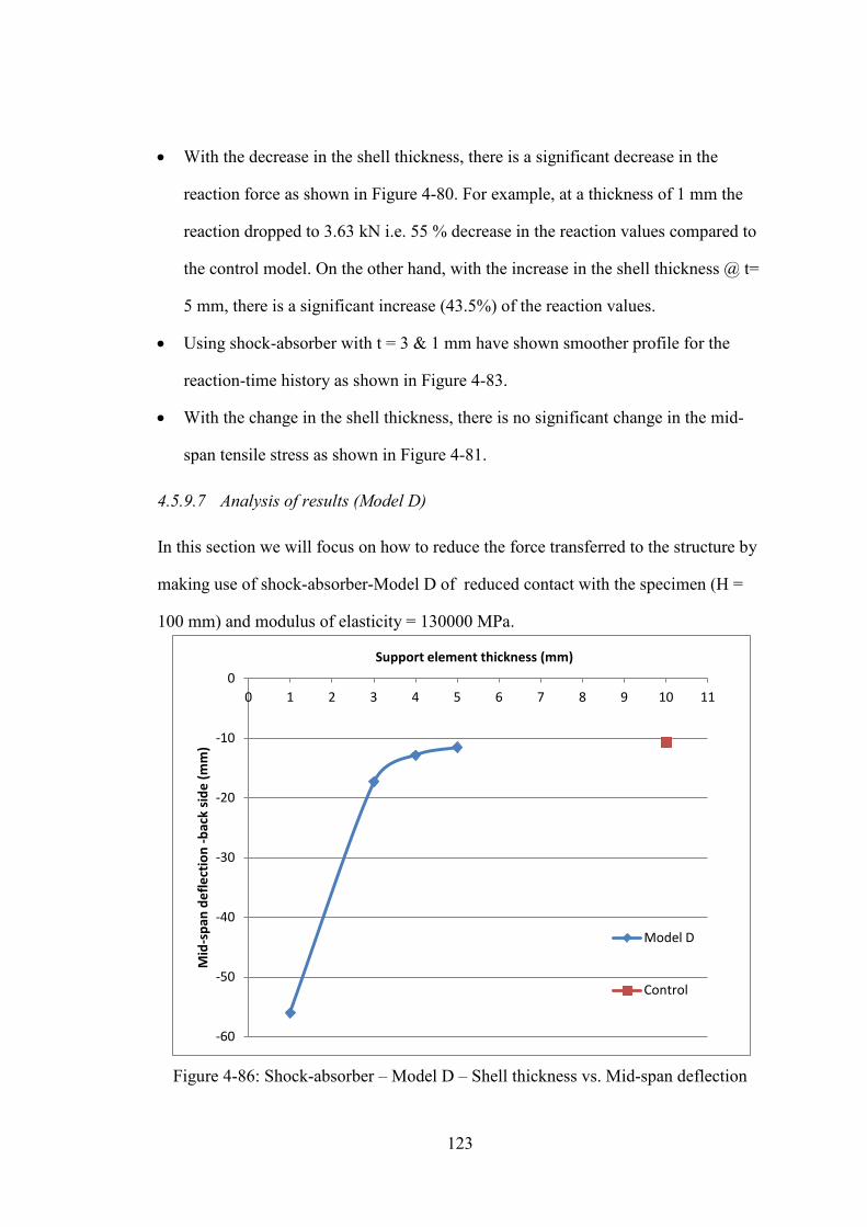
123
• With the decrease in the shell thickness, there is a significant decrease in the
reaction force as shown in Figure 4-80. For example, at a thickness of 1 mm the
reaction dropped to 3.63 kN i.e. 55 % decrease in the reaction values compared to
the control model. On the other hand, with the increase in the shell thickness @ t=
5 mm, there is a significant increase (43.5%) of the reaction values.
• Using shock-absorber with t = 3 & 1 mm have shown smoother profile for the
reaction-time history as shown in Figure 4-83.
• With the change in the shell thickness, there is no significant change in the mid-
span tensile stress as shown in Figure 4-81.
4.5.9.7 Analysis of results (Model D)
In this section we will focus on how to reduce the force transferred to the structure by
making use of shock-absorber-Model D of reduced contact with the specimen (H =
100 mm) and modulus of elasticity = 130000 MPa.
Figure 4-86: Shock-absorber – Model D – Shell thickness vs. Mid-span deflection
-60
-50
-40
-30
-20
-10
0 0 1 2 3 4 5 6 7 8 9 10 11
Mid
-spa
n de
flect
ion
-bac
k si
de (m
m)
Support element thickness (mm)
Model D
Control
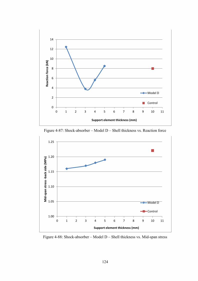
124
Figure 4-87: Shock-absorber – Model D – Shell thickness vs. Reaction force
Figure 4-88: Shock-absorber – Model D – Shell thickness vs. Mid-span stress
0
2
4
6
8
10
12
14
0 1 2 3 4 5 6 7 8 9 10 11
Reac
tion
forc
e (k
N)
Support element thickness (mm)
Model D
Control
1.00
1.05
1.10
1.15
1.20
1.25
0 1 2 3 4 5 6 7 8 9 10 11
Mid
-spa
n st
ress
-bac
k si
de (M
Pa)
Support element thickness (mm)
Model D
Control
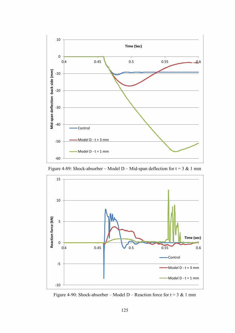
125
Figure 4-89: Shock-absorber – Model D – Mid-span deflection for t = 3 & 1 mm
Figure 4-90: Shock-absorber – Model D – Reaction force for t = 3 & 1 mm
-60
-50
-40
-30
-20
-10
0
10
0.4 0.45 0.5 0.55 0.6
Mid
-spa
n de
flect
ion
-bac
k si
de (m
m)
Time (Sec)
Control
Model D - t = 3 mm
Model D - t = 1 mm
-10
-5
0
5
10
15
0.4 0.45 0.5 0.55 0.6 Reac
tion
forc
e (k
N)
Time (sec)
Control
Model D - t = 3 mm
Model D - t = 1 mm

126
Figure 4-91: Shock-absorber – Model D – Stress-strain relation for t = 3 & 1 mm
Figure 4-92: Damage in Model D - t = 3 mm: Left (time @0.51sec), Right (time
@0.60sec)
Figure 4-93: Damage in Model D - t = 1 mm: Left (time @0.51sec), Right (time
@0.60sec)
-0.2
0
0.2
0.4
0.6
0.8
1
1.2
1.4
0 0.002 0.004 0.006 0.008 0.01
Mid
-spa
n st
ress
-bac
k si
de (M
Pa)
Mid-span strain (back side)
Control
Model D - t = 3 mm
Model D - t = 1 mm
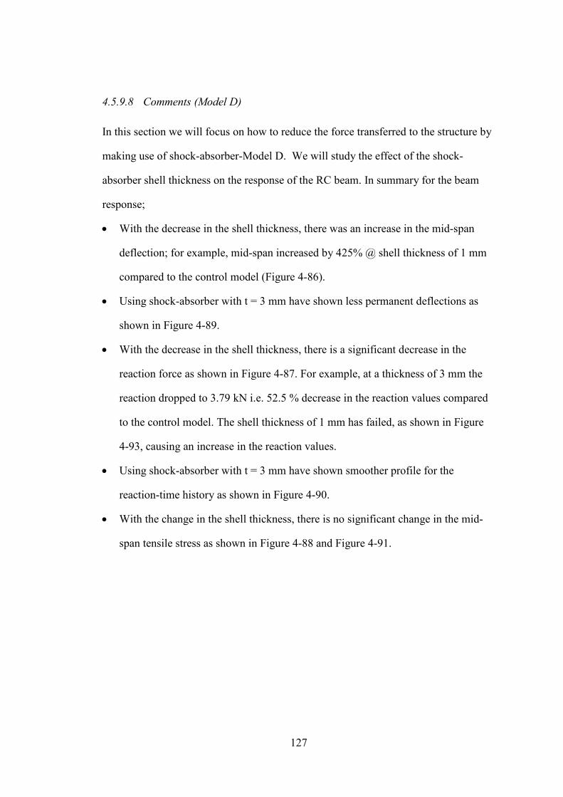
127
4.5.9.8 Comments (Model D)
In this section we will focus on how to reduce the force transferred to the structure by
making use of shock-absorber-Model D. We will study the effect of the shock-
absorber shell thickness on the response of the RC beam. In summary for the beam
response;
• With the decrease in the shell thickness, there was an increase in the mid-span
deflection; for example, mid-span increased by 425% @ shell thickness of 1 mm
compared to the control model (Figure 4-86).
• Using shock-absorber with t = 3 mm have shown less permanent deflections as
shown in Figure 4-89.
• With the decrease in the shell thickness, there is a significant decrease in the
reaction force as shown in Figure 4-87. For example, at a thickness of 3 mm the
reaction dropped to 3.79 kN i.e. 52.5 % decrease in the reaction values compared
to the control model. The shell thickness of 1 mm has failed, as shown in Figure
4-93, causing an increase in the reaction values.
• Using shock-absorber with t = 3 mm have shown smoother profile for the
reaction-time history as shown in Figure 4-90.
• With the change in the shell thickness, there is no significant change in the mid-
span tensile stress as shown in Figure 4-88 and Figure 4-91.
128
CHAPTER 5: SUMMARY , CONCLUSIONS AND
RECOMMENDATTIONS
5.1 Summary
Based on the scope covered and analysis of results in this research regarding the
numerical modeling for reinforced concrete panels under impact loads, the following
conclusions can be drawn:
• The numerical code, LS-DYNA, is capable of simulating explicit analysis such as
reinforced concrete structures under impact and blast loads.
• The impact phenomena can be modeled numerically either by time-history
function (simplified impact analysis) or real-time impact (simulated pendulum
analysis) with reasonable accuracy.
• It is much easier and less expensive to model impact load as time-history function
rather than real-time impact analysis, in terms of storage needed and running time.
• The developed numerical model can be tuned to simulate various concrete
material used in reality.
• LS-DYNA has built-in concrete material models that can be used at the presence
of laboratory data required to determine the material parameters. On the other
hand, there is a set of materials that do have minimum input parameters or
parameter generation capability that can be used when there is no enough data for
the casted concrete.
• The numerical model were compared and validated with experimental work done
in previous work at AUC by Cherif, (2009).
• For the entire validation matrix, comparisons between the simplified pendulum
results and the experimental values have shown good agreement for the entire set
129
of masses, heights, and material models, using four concrete material models.
Differences were in the range of 1% up to 15.44% in the reaction values.
• Away from small impact force values, comparisons between the simulated
pendulum results and the experimental values have shown good agreement for
Model-3. Maximum differences were6.52% in the reaction force and 17.33% in
the impact force.
• Nonlinear model showed that the impact load was near pulse values as the time
period (td) of the numerical was 0.8 ms while td of the experiment was 50 ms;
however , having elastic steel plate at the front-side of the beam, with reduced
modulus of elasticity = 200 MPa, increased td to 80 ms. This shows the
importance of simulating the contact between the impacting mass and the target.
• Simulated pendulum results could have decreased if the numerical model has
taken into consideration; 1- the losses in the experimental setup , 2- the movement
of the supporting frame, 3- the deformation of the steel plates , and 4-local
damage in the RC beam due to previous experiments.
• The experiment setup used steel plates to avoid local crushing. The contact
between the concrete specimens and these plates were examined in details.
Creating a gap of 1 mm between the steel plates and the concrete beam; 1-
increased the reaction force by 51%, 2- decreased the impact load by 10%, and 3-
eliminated the negative reaction values.
• In the numerical model, a single integration point solid element was used.
Accordingly, many factors were found to affect the accuracy of the results such as
element formulations, Hourglass (HG), and mesh size.
• In the presented model refinements, using higher element formulations to reach a
better results have failed during processing as previously expected in the user
manual of the program due to large deformations.
130
• In the model refinements through studying the effect of various HG algorithms,
using HG type 1 reduced the reaction force by 25%; while, using HG type 3
reduced the reaction force by 37% compared to the control model.
• In the model refinements by selecting the optimum mesh size, selecting mesh “A”
(element size 13x13x13 mm) reduced the reaction force by 11%; while, using
mesh “B” (element size 25x25x5 mm) reduced the reaction force by
19%compared to the control model.
• The parametric analysis concluded that with the increase in impact mass
compared to the control model ;
There is an almost linear increase in the mid-span deflection.
There is a steep increase in reaction force till a certain mass (1000 kg). Beyond
this mass there is no increase in the reaction value.
There is an increase in the mid-span tensile stress till reaching a certain limit (3.1
MPa) at a dropping mass of 600kg followed by significant losses in the tensile
stresses due to local failure of RC beam.
• The parametric analysis concluded that with the increase in impact height
compared to the control model;
There is an almost linear increase in the mid-span deflection.
There is a steep increase in reaction force till a certain height (350 mm).Beyond
this height there is a decrease in reaction values.
There is an increase in the mid-span tensile stress, having high slope at low
impact heights and small slope at higher impact height values; however, by
reaching a certain height (350mm), losses in stresses were observed due to failure
of RC beam.
• The parametric analysis concluded that with the increase in diameter of the
tension reinforcement when using 22 mm diameter bars instead of 10 mm:

131
There is a significant decrease (60%) in the mid-span deflection.
There is a significant increase (102%) in reaction force.
There is a change in the reaction-time history profile. Area under the curve is
getting smaller.
There is a decrease in the mid-span tensile stress using a bar size of 12mm;
however, additional increase in the bar size led to almost no reduction in
stress.
• The parametric analysis concluded that with the increase in diameter of the
compression reinforcement when using 22 mm diameter bars instead of 10 mm:
There is a decrease (10%) in the mid-span deflection.
There is no significant change in reaction forces.
There is a decrease (11%) in the mid-span tensile stress.
• The parametric analysis concluded that with the change in the thickness of the
front steel plate compared to the control model;
There is no significant change in the mid-span deflection.
There is a small change (-3.7% @ t = 20mm and +3.7% @ t = 8mm) in
reaction forces.
There is a significant change (-66% @ t = 20mm and +13% @ t = 8mm) in
the mid-span tensile stress
• The parametric analysis concluded that with the change in the thickness of the
back steel plate compared to the control model;
There is no significant change in the mid-span deflection.
There is a small change (5.2% @ t = 20mm and -3% @ t = 8mm) in reaction
forces.
There is no significant change in the mid-span tensile stress.
132
• The parametric analysis concluded that with the decrease of the front plate
modulus of elasticity compared to the control model;
There is a significant increase (69% @ E = 20 MPa) in the mid-span
deflection.
There is a significant increase in the reaction values till reaching a certain
value (E= 2000 MPa) then the reaction force decreased as shown in Figure
4-55. For example, the reaction force =7.98 kN @ E = 130000 MPa increased
to be 10 kN @ E = 2000 MPa; however, further reduction in E (20 MPa) has
shown a reaction of 6.57 kN.
There is a change in the reaction-time history profile , especially at very low
values for modulus of elasticity (E =20 MPa)
There is a significant increase of the impact time period attached with a
decrease in the impact force value.
There is a significant increase (146%) in the mid-span tensile stress till
reaching a certain value (@ E=2000 MPa) followed by decrease in the
values
• The parametric analysis concluded that with the increase of the front plate
modulus of elasticity compared to the control model;
There is no significant change in the mid-span deflection.
There is little (5% @ E = 267000 MPa) decrease in the reaction values.
There is a significant decrease (76% @ E = 267000 MPa) in the mid-span
tensile stress.
• The parametric analysis concluded that with the decrease of the back plate
modulus of elasticity compared to the control model;
There is a significant increase (293% @ E =20 MPa) in the mid-span
deflection.
133
There is a significant decrease (77% @ E =20 MPa) in the reaction forces.
There is a change in the reaction-time history profile , specially at low values
for modulus of elasticity (E =20 & 200 MPa)
There is no significant change in the mid-span tensile stress.
• The parametric analysis concluded that with the increase of the back plate
modulus of elasticity compared to the control model;
There is no significant change in the mid-span deflection.
There is no significant change in the reaction values.
There is no significant change in the mid-span tensile stress.
• The parametric analysis concerned with how to reduce the force transferred to the
structure by the use of shock-absorber- Model A , concluded that compared to the
control model:
Mid-span deflection increased by 300% @ t =1 mm; however with further
increase in the shell thickness, no significant change in the deflection value.
With the decrease in the shell thickness, there is a significant decrease in the
reaction force (78 % @ t = 1 mm). On the other hand, with the increase in the
shell thickness, there is a significant increase (49% @ t = 5 mm) of the
reaction values.
Using shock-absorber with t = 3 mm have shown smoother profile for the
reaction-time history.
With the decrease in the shell thickness, there is a decrease (11.5% @ t = 1
mm) in the mid-span tensile stress. On the other hand, with the increase in the
shell thickness, there is no significant change in the mid-span tensile stress.
• The parametric analysis concerned with how to reduce the force transferred to the
structure by the use of shock-absorber- Model B , concluded that compared to the
control model:
134
Mid-span deflection increased by 300% @ t =1 mm ; however with further
increase in the shell thickness , no significant change in the deflection value
With the decrease in the shell thickness, there is a significant decrease in the
reaction force (78 % @ t =1 mm). On the other hand, with the increase in the
shell thickness, there is a significant increase (30% @ t = 5 mm) of the
reaction values.
Using shock-absorber with t = 3 mm have shown smoother profile for the
reaction-time history.
With the decrease in the shell thickness, there is a decrease (11.5% @ t =1
mm) in the mid-span tensile stress. On the other hand, with the increase in the
shell thickness, there is no significant change in the mid-span tensile stress.
• The parametric analysis concerned with how to reduce the force transferred to the
structure by the use of shock-absorber- Model C , concluded that compared to the
control model ;
With the decrease in the shell thickness, there is a significant increase in the
mid-span deflection. For example, at a thickness of 1mm the deflection was
21.7 mm i.e. 103 % increase in the deflection values: however, the slope is
high at lower thicknesses.
Using shock-absorber with t = 3 & 1 mm have shown less permanent
deflections, especially when using t = 1 mm.
With the decrease in the shell thickness, there is a significant decrease (55%
@ t =1 mm) in the reaction force. On the other hand, with the increase in the
shell thickness, there is a significant increase (43.5% @ t = 3 mm) of the
reaction values.
Using shock-absorber with t = 3 & 1 mm have shown smoother profile for the
reaction-time history.
135
With the change in the shell thickness, there is no significant change in the
mid-span tensile stress.
• The parametric analysis concerned with how to reduce the force transferred to the
structure by the use of shock-absorber- Model D , concluded that compared to the
control model:
Mid-span deflection increased by 425% @ t=1 mm; however with further
increase in the shell thickness, no significant change in the deflection value.
Using shock-absorber with t = 3 mm have shown less permanent deflections.
With the decrease in the shell thickness, there is a significant decrease (52.5%
@ t = 3 mm) in the reaction force. On the other hand, with the increase in the
shell thickness, there is a significant increase (30%) of the reaction values.
Using shock-absorber with t = 3 mm have shown smoother profile for the
reaction-time history
With the change in the shell thickness, there is no significant change in the
mid-span tensile stress
136
5.2 Conclusions
• The numerical code, LS-DYNA, was successfully used in this research to analyze
the response of concrete panels under impact load through simulation of
pendulum movement dropped from elevated height up to and including the
contact impact and the nonlinear dynamic response of the RC panel to such
impact load as well as cracking and damage simulation.
• The impact phenomena can also be modeled numerically using simplified analysis
by having the short duration impact load history as input to the structural element.
This allows also for analysis not only under impact load but also under the effect
of blast load using ATBLAST to generate the load function.
• The developed numerical model can be used with various material models to
efficiently simulate response of RC panels under impact loads provided that they
have been verified with a full set of experimental results.
• The numerical models were validated against the results of previous experimental
work done at AUC.
• For the entire validation set, comparisons with experimental values have shown
very good agreement for the simplified analysis. Differences were in the range of
1% up to 15.44% in the reaction values for all material models. Material Model-1
has shown closest results to the experimental study especially at small values of
impact forces. As the force increase, Model-1 starts deviating from the
experimental results.
• Away from small impact force values, comparisons with experimental values
showed that Material Model-3 provides the closest results to the experimental
results with maximum differences of 6.52% in the reaction force and 17.33% in
the impact force
137
• Nonlinear model showed that the impact load was near pulse values as the time
period (td) of the numerical was 0.8 ms which agrees with what was found in the
literature for a series of RC beams under impact load with period ranging from 0.3
to 2.6 ms.
• To design the supporting structure, designers can use the simplified pendulum
analysis because it was able to simulate the reaction force with reasonable
accuracy and minimum running time. In the current study the impact was applied
at the mid-span point which is more critical for the panel. However, for the design
of the supporting frame different impact location can be easily considered with the
same approach.
• To design the RC panel, designers can use the simulated pendulum analysis to get
the beam response in terms of stress, strain, and deflection.
• It was found that the response is affected ;however, the following points should be
taken into consideration in the design process:
Mid-span deflection and stresses increase with the increase of the impact mass
and height
Mid-span deflection decreases with the increase in the elasticity (flexibility) of
the front and back steel plates. Accordingly, having an elastic layer in front of
the building facade will reduce the response.
Having a protective plate at the point of impact reduces the mid-span stress by
allowing for better distribution of impact stress over a wider portion of the
beam. This effect becomes more pronounced as the thickness of the plate
increases.
• It was found that the use of deformable support connection made of especially
bent steel plates acts as a shock absorber that reduces both the stresses in the panel
and the reactions at the support through elastic and plastic deformation of the
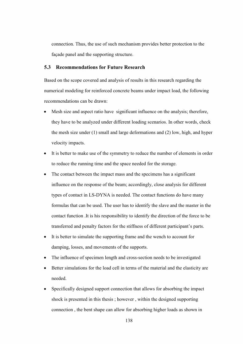
138
connection. Thus, the use of such mechanism provides better protection to the
façade panel and the supporting structure.
5.3 Recommendations for Future Research
Based on the scope covered and analysis of results in this research regarding the
numerical modeling for reinforced concrete beams under impact load, the following
recommendations can be drawn:
• Mesh size and aspect ratio have significant influence on the analysis; therefore,
they have to be analyzed under different loading scenarios. In other words, check
the mesh size under (1) small and large deformations and (2) low, high, and hyper
velocity impacts.
• It is better to make use of the symmetry to reduce the number of elements in order
to reduce the running time and the space needed for the storage.
• The contact between the impact mass and the specimens has a significant
influence on the response of the beam; accordingly, close analysis for different
types of contact in LS-DYNA is needed. The contact functions do have many
formulas that can be used. The user has to identify the slave and the master in the
contact function .It is his responsibility to identify the direction of the force to be
transferred and penalty factors for the stiffness of different participant’s parts.
• It is better to simulate the supporting frame and the wench to account for
damping, losses, and movements of the supports.
• The influence of specimen length and cross-section needs to be investigated
• Better simulations for the load cell in terms of the material and the elasticity are
needed.
• Specifically designed support connection that allows for absorbing the impact
shock is presented in this thesis ; however , within the designed supporting
connection , the bent shape can allow for absorbing higher loads as shown in
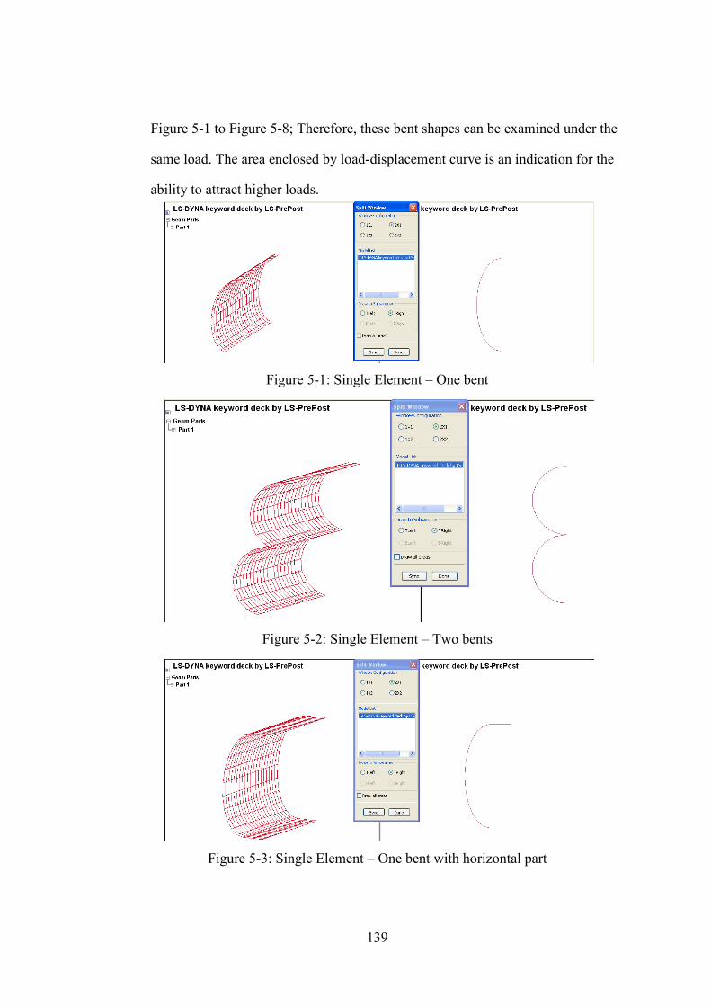
139
Figure 5-1 to Figure 5-8; Therefore, these bent shapes can be examined under the
same load. The area enclosed by load-displacement curve is an indication for the
ability to attract higher loads.
Figure 5-1: Single Element – One bent
Figure 5-2: Single Element – Two bents
Figure 5-3: Single Element – One bent with horizontal part
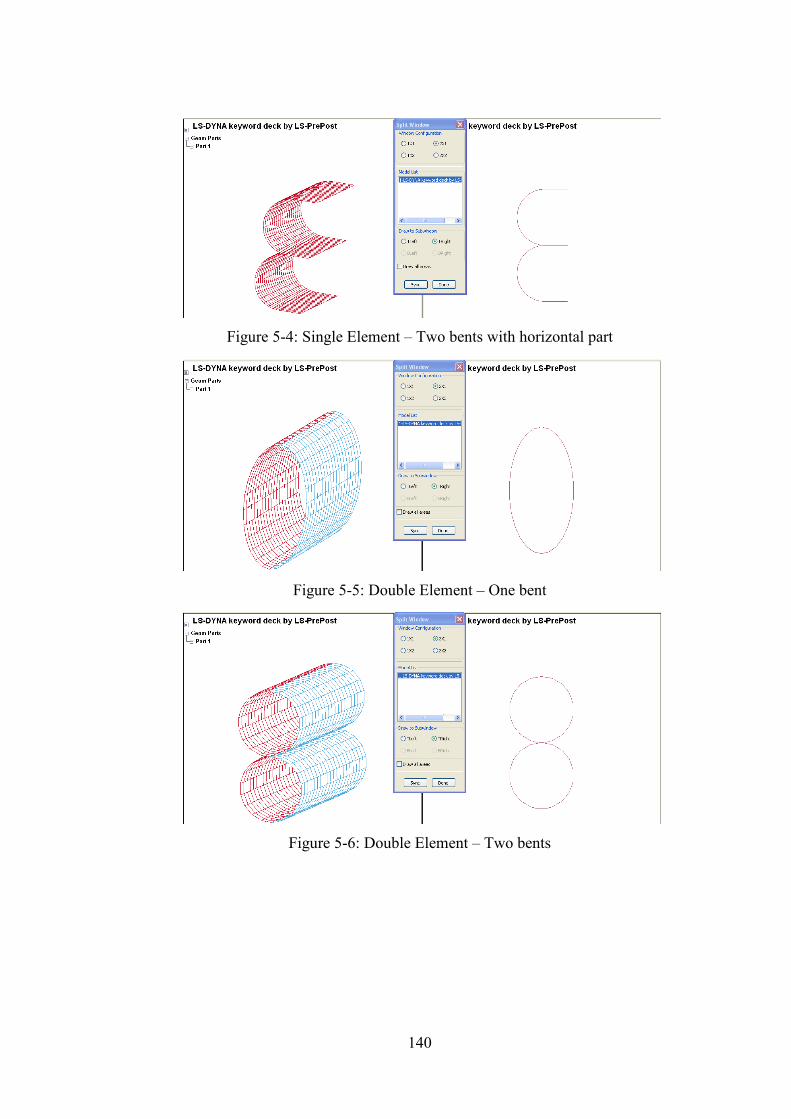
140
Figure 5-4: Single Element – Two bents with horizontal part
Figure 5-5: Double Element – One bent
Figure 5-6: Double Element – Two bents
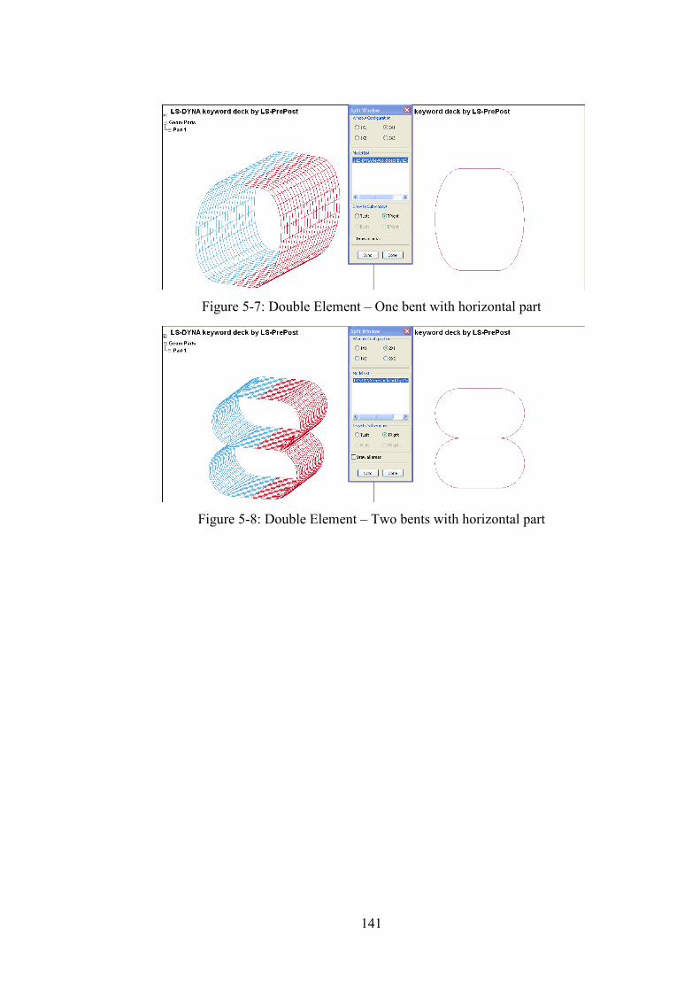
141
Figure 5-7: Double Element – One bent with horizontal part
Figure 5-8: Double Element – Two bents with horizontal part
142
REFERENCES
Abdel-Mooty M. (2005). “Dynamic Response of Flexible Panel To Blast Loads.”
Engng.Res.Jour., Vol. 97.pp.C 26-C45 , April 2005 Helwan University ,
Faculty of Engng., Mataria Cairo
Abdel-Mooty M. and Shaaban S. "Numerical Modeling of the Nonlinear Response of
RC Beams to Impact Loads” submitted to Computers and Structures
International Journal.
Abdel-Mooty M. and Shaaban S. (2010). "Numerical Modeling and Calibration of
Impact Testing of Reinforced Concrete Panels.", in B.H.V. Topping, J.M.
Adam, F.J. Pallarés, R. Bru, M.L. Romero, (Editors), "Proceedings of the
Tenth International Conference on Computational Structures Technology",
Civil-Comp Press, Stirlingshire, UK, Paper 103, 2010. doi:10.4203/ccp.93.103
Akram A. (2008). “Modeling and Simulation of Bogie Impacts on Concrete Bridge
Rails using LS-DYNA.” 10th International LS-DYNA® Users Conference
Algaard W., Lyle J., Izatt C. (2005). "Perforation of Composite Floors." 5th European
LS-DYNA Users Conference , Methods and Techniques (2)
ANSYS , (2009) , Version 12.0 , Help manual , ANSYS, Inc
Anwarul Islam A.K.M. (2005). “Performance of AASHTO Girder Bridges Under
Blast loading.” Doctor of Philosophy Thesis, Florida State University, FAMU-
FSU College of Engineering
143
Applied Research Associates Inc (2004). ATBLAST program Release 2.2, Protective
Glazing Council, (http://www.protectiveglazing.org), August 2004
Bhatti A. Q., Kishi N., Mikami H., and Ando T. ( 2009). “Elasto-plastic Impact
Response Analysis of Shear-Failure-type RC Beams with Shear Rebars.”
Materials and Design, 30 (2009) 502–510
Bush B. (2010). “Analytical Evaluation of Concrete Penetration Modeling
Techniques.” M.Sc. Thesis, the Graduate Faculty of North Carolina State
University
Chen Y. and May I.M. (2009). “Reinforced Concrete Members Under Drop-Weight
Impacts.” Proceedings of the institution of Civil Engineers Structures and
Buildings 162 ,February 2009 Issue SBl , 45-56
Cherif H. “Experimental Investigation Of Building Components Response To Impact
And Short Duration Loads.”, M.Sc. Thesis, the American University in Cairo,
2009
Computers & Structures, Inc. (V.14.1, 2010). “SAP2000 – Integrated Software for
Structural Analysis & Design, Technical Reference Manual”
Cotsovos D.M., Pavlovic M.N. (2008). “Numerical Investigation of Concrete
Subjected to Compressive Impact Loading. Part 1: A fundamental explanation
for the apparent strength gain at high loading rates.” Computers and Structures
86 (2008) 145–163

144
Cotsovos D.M., Pavlovic M.N. (2008). “Numerical Investigation of Concrete
Subjected to Compressive Impact Loading. Part 2: Parametric investigation of
factors affecting behaviour at high loading rates.” Computers and Structures
86 (2008) 164–180
Cotsovos M., Stathopoulos N. D., and Zeris C. A. (2008). “Behavior of RC Beams
Subjected to High Rates of Concentrated Loading.” Journal of Structural
Engineering, Vol. 134, No. 12 , pp.1839-1851, December 1, 2008
Davidson J. S., Fisher J. W., Hammons M. I., Porter J. R., and Dinan R. J. (2005).
“Failure Mechanisms of Polymer-Reinforced Concrete Masonry Walls
Subjected to Blast.” J. Struct. Eng., ASCE, 131(8), 1194-1205
Farnam Y., Mahoutian M. , Mohammadi S., Sherkarchi M. (2008). “Experimental
And Numerical Studies Of Impact Behavior Of Fiber Lightweight Aggregate
Concrete.” Structures 2008: Crossing Borders
Haifeng L. and Jianguo N. (2009). “Mechanical Behavior Of Reinforced Concrete
Subjected To Impact Loading.” Mechanics of Materials , 41 (2009) 1298–
1308
Haifeng L., HaiYan L. , and WeiDong S. (2010). “Fracture Characteristics Of
Concrete Subjected To Impact Loading.” Science China Physics, Mechanics
&Astronomy ,Vol. 53 No.2: 253−261
145
Hallquist J. O. (2006). “LS-DYNA Theory Manual.” Livermore, CA: Livermore
Software Technology Corporation
Huanga F., Wu H., Jin Q., Zhang Q. (2005). “A Numerical Simulation on the
Perforation of Reinforced Concrete Targets.” International Journal of Impact
Engineering 32 (2005) 173–187
Jayasooriya R. , Thambiratnam D. , Perera N., and Kosse V. (2009). ”Response And
Damage Evaluation Of Reinforced Concrete Frames Subjected To Blast
Loading.” In: 34th Conference on Our World In Concrete & Structures, 16-18
August 2009, Hotel Park Royal, Singapore
Johnson G. R., Beissel S. R., Gerlach C. A., Stryk R. A. , Holmquist T. J., and
Johnson A. A. (2006). “User Instructions for the 2006 Version of the EPIC.”
Minneapolis, MN: Network Computing Services, Inc.
Jones N. (1989). Structural Impact. Cambridge University Press, Cambridge
Jose A. , Pires A. , Syed A. , and Ali A. (2010). “Benchmarking Finite Element
Simulation of Hard Impacts Missile on Reinforced Concrete Slabs.” ACI Fall
2010 Convention , Pittsburgh, PA
Kazunori F., Bing L., and Sam S. (2009).”Impact Response of Reinforced Concrete
Beam and Its Analytical Evaluation.” Journal of Structural Engineering, Vol.
135, No. 8 , pp. 938-950, August 1, 2009
146
Liu Y., Huang F. , and Ma A. (2011). “Numerical Simulations Of Oblique
Penetration Into Concrete Targets.” Computers and Mathematics with
Applications , 6 (2011) 2168-2171
Liu Y., Ma A., and Huang F. (2009). “Numerical Simulations Of Oblique-Angle
Penetration By Deformable Projectiles Into Concrete Targets.” International
Journal of Impact Engineering 36 (2009) 438–446
Livermore Software Technology Corporation, LSTC (2009). “LS-DYNA Keyword
User’s Manual: Volume I & II,” Version 971/ Release 4, Livermore, CA
Magallanes J. M., Wu Y., and Crawford J. E. (2010). “Recent Improvements to
Release III of the K&C Concrete Model.” 11th International LS-DYNA®
Users Conference
Miyamoto A., King M. W., and Fujii M. (1989). “Non-linear Dynamic Analysis and
Design Concepts for RC Beams under Impulsive Loads.” New Zealand Nat.
Soc. Earthquake Eng. Bull, 222, 98–111
Murray Y. D., Abu-Odeh A., and Bligh R. (2007).“Evaluation of LS-DYNA Concrete
Material Model 159.” McLean, VA: U.S. Dept. of Transportation, FHA.
Ngo T., Mendis P., Gupta A. , and Ramasy J. (2007). “Blast Loading and Blast
Effects on Structure-An Overview.” Electronic Journal of Structural
Engineering- Special Issue: Loading on Structures – 2007: p.76-91.
147
Nyström U. and Gylltoft K. (2009). “Numerical Studies Of The Combined Effects Of
Blast And Fragment Loading.” International Journal of Impact Engineering 36
(2009) 995–1005
Nyström U. and Gylltoft K. (2011). “Comparative Numerical Studies Of Projectile
Impacts On Plain And Steel-Fiber Reinforced Concrete.” International
Journal of Impact Engineering , 38 (2011)
Raguraman M. , Deb A. , Gupta N.K., and Kharat D.K. (2008). “Numerical
Simulation of Projectile Impact on Mild Steel Armour Plates using LS-
DYNA, Part II Parametric Studies.” Defense Science Journal , Vol. 58 , No. 4
,july 2008 , pp 573-581
Saatci S. and Vecchio F. J. (2009). “Nonlinear Finite Element Modeling Of
Reinforced Concrete Structures Under Impact Loads.” ACI Structural Journal
, V.106 , No. 5
Sangi A. J. , May I. M. (2009). "High-Mass, Low-Velocity Impacts on Reinforced
Concrete Slabs." 7th European LS-DYNA Conference
Schenker A., Anteby I., Nizri E., Ostriach B., Kivity Y., Sadot O., Haham O.,
Michaelis R., Gal E. , and Ben-Dor G. (2005). “Foam-Protected Reinforced
Concrete Structures under Impact: Experimental and Numerical Studies.” J.
Struct. Eng., ASCE, 131(8), 1233-1242
148
Schwer L.E. (2008). “Simple Input Concrete Constitutive Models: An Illustration Of
Brick Wall & Concrete Cylinder Perforation.” 10th International LS-DYNA®
Users Conference , Penetration / Blast
Schwer L.E. (2010). “An Introduction to the Winfrith Concrete Model.” ,Schwer
Engineering & Consulting Services
Schwer L.E. and Malvar L.J. (2005). “Simplified Concrete Modeling With
*MAT_CONCRET_DAMAGE_REL3.” JRI LS-DYNA User Week 2005
Schwerand L. E. and Murray Y. D. (2002). “Continuous Surface Cap Model for
Geomaterial Modeling: A New LS-DYNA Material Type.” 7th International
LS-DYNA Users Conference (pp. 16-35). Dearborn, Michigan: LSTC & ETA.
Shi Y., Hao H., and Li Z. X. (2008). “Numerical Derivations Of Pressure Impulse
Diagrams For Prediction Of RC Column Damage To Blast Load.”
International Journal of Impact Engineering Vol 35, 2008, 1213-1227
Silva P. F., Mesia W. D. , Marzougui D. , and Badie S. S. (2009). “Performance
Evaluation of Flexure Impact Resistance Capacity of Reinforced Concrete
Members.” ACI Structural Journal , V. 106 No.5 , 726-736
Tachibana S., Masuya S., Hiroshi S., and Nakamura S. (2010). “Performance Based
Design Of Reinforced Concrete Beams Under Impact.” Natural Hazards and
Earth System Science, 10(6): 1069-1078
149
Tahmasebinia F. (2008). “Finite Element Simulation of Reinforced Concrete
Structures under Impact Accident.” Structural Survey, Vol. 26 No. 5, 2008 pp.
445-454
Thilakarathna H.M.I., Thambiratnam D.P., Dhanasekar M., and Perera N.
(2010).”Numerical Simulation Of Axially Loaded Concrete Columns Under
Transverse Impact And Vulnerability Assessment.” International Journal of
Impact Engineering, 37(11), pp. 1100-1112
Tu Z. and Lu Y. (2009). “Evaluation Of Typical Concrete Material Models Used In
Hydrocodes For High Dynamic Response Simulations.” International Journal
of Impact Engineering, Vol. 36, No. 1, pp. 132-146
Wesevich J., Bingham B., Bogosian D., Christiansen A., and Magnusson J. (2010).
“Constitutive Concrete Material Model, Comparison to Tested Reinforced
Slabs Subjected to Blast Loads.” 2010 ACI Fall Convention, Pittsburgh, PA
Yonten K., Manzari M., and Eskandarian A., and Marzougui D. (2002) “An
Evaluation of Constitutive Models of Concrete in LS-DYNA Finite Element
Code.” Proceedings of 15th ASCE Engineering Mechanics Conference,
Columbia Univ., New York, N.Y., June 2-5, CD ROM, pp. 1-8.