multiple degradation mechanisms in reinforced concrete ...
218
MULTIPLE DEGRADATION MECHANISMS IN REINFORCED CONCRETE STRUCTURES, MODELING AND RISK ANALYSIS DE-NE0008438 Project Period: Oct. 1, 2015 – Sept. 30, 2019 Roberto Ballarini University of Houston Bora Gencturk, Amit Jain, Hadi Aryan University of Southern California Yunping Xi, Mohamed Abdelrahman University of Colorado-Boulder Benjamin Spencer Idaho National Laboratory FINAL REPORT
-
Upload
khangminh22 -
Category
Documents
-
view
1 -
download
0
Transcript of multiple degradation mechanisms in reinforced concrete ...

MULTIPLE DEGRADATION MECHANISMS IN REINFORCED CONCRETE STRUCTURES, MODELING AND RISK ANALYSIS
DE-NE0008438 Project Period: Oct. 1, 2015 – Sept. 30, 2019
Roberto Ballarini
University of Houston
Bora Gencturk, Amit Jain, Hadi Aryan
University of Southern California
Yunping Xi, Mohamed Abdelrahman University of Colorado-Boulder
Benjamin Spencer
Idaho National Laboratory
FINAL REPORT

Page 2 of 218
LIST OF ACRONYMS ASR .................Alkali silica reaction / reactivity ASTM ..............American Society for Testing and Materials CDI ..................Chicago dial indicator CPS .................Concrete pore solution DEMEC ............Demountable mechanical strain gauge DOE ................Department of Energy DEF .................Delayed ettringite formation EDL .................Electric double layer FEM ................Finite element method INL ..................Idaho National Laboratory LSCT ................Linear strain conversion transducer LWRS ..............Light Water Reactor Sustainability MCS ................Monte Carlo simulation MOOSE ...........Multiphysics Object Oriented Simulation Environment NPP .................Nuclear power plant RC ...................Reinforced Concrete SCE ..................standard calomel electrode SFRC................Steel Fiber Reinforced Concrete SSD .................Saturated surface dry THCM..............Thermo-hygro-chemo-mechanical USC .................University of Southern California VCCTL .............Virtual Cement Concrete Testing Laboratory CU ...................University of Colorado w/c .................Water–cement ratio gi .....................Aggregate volume fraction
Page 3 of 218
TABLE OF CONTENTS LIST OF ACRONYMS ......................................................................................................................... 2
SUMMARY ....................................................................................................................................... 7
PROJECT OBJECTIVES................................................................................................................... 7
KEY RESEARCH OUTCOMES AND FINDINGS ................................................................................ 7
PROJECT PRODUCTS .................................................................................................................... 8
Codes and Software ................................................................................................................. 8
Thesis ....................................................................................................................................... 9
Journal Papers and Reports ................................................................................................... 10
Presentations or Conference Papers ..................................................................................... 10
..................................................................................................................................... 12
1.1. PROBLEM STATEMENT ................................................................................................... 12
1.2. SCOPE ............................................................................................................................. 13
Coupling between Moisture and Ion Transport in Concrete .................................. 13
Coupling Effects of Damage and Transport in Concrete ........................................ 13
Effects of Alkali-Silica Reaction Induced Damage on Shear Capacity of Reinforced Concrete Beams ..................................................................................................................... 14
Uncertainty Quantification of Concrete Models .................................................... 14
1.3. REPORT ORGANIZATION ................................................................................................ 15
..................................................................................................................................... 16
2.1. EFFECT OF W/C RATIO AND AGGREGATE VOLUME FRACTION ON CHLORIDE PENETRATION IN NON-SATURATED CONCRETE ....................................................................... 16
Introduction ............................................................................................................ 16
Theory ..................................................................................................................... 16
Experimental Program ............................................................................................ 17
Test Results ............................................................................................................. 20
Calculation of the Coupling Parameter DCl-H .......................................................... 24
Material Model for the Coupling Parameter DCl-H .................................................. 25
Conclusions ............................................................................................................. 32

Page 4 of 218
2.2. EFFECT OF ION CONCENTRATION ON MOISTURE DIFFUSION IN CONCRETE ................ 32
Introduction ............................................................................................................ 32
Experimental Program ............................................................................................ 32
Experimental Results .............................................................................................. 35
Interpretation of the Test Data ............................................................................... 42
Evaluation of Coupling Parameters ........................................................................ 48
Conclusions ............................................................................................................. 50
..................................................................................................................................... 51
3.1. PLASTIC DAMAGE MODEL FOR CONCRETE .................................................................... 51
Introduction ............................................................................................................ 51
Yield Function.......................................................................................................... 52
Plastic Potential....................................................................................................... 54
Strength of Concrete ............................................................................................... 54
Hardening Potential ................................................................................................ 57
Implementation ...................................................................................................... 58
Estimation of Crack Width ...................................................................................... 61
Model Verification .................................................................................................. 61
Conclusions ............................................................................................................. 71
3.2. MODELING THE EFFECT OF DRYING SHRINKAGE-INDUCED DAMAGE ON COUPLED MOISTURE AND CHLORIDE DIFFUSION INTO CONCRETE ......................................................... 72
Introduction ............................................................................................................ 72
Model Description .................................................................................................. 72
Transport Model ..................................................................................................... 73
Drying Shrinkage Model .......................................................................................... 77
Mechanical Model .................................................................................................. 80
Effect of Damage on Transport Properties ............................................................. 81
Numerical Results ................................................................................................... 82
Model Validation ..................................................................................................... 84
Numerical Example of Coupled Damage and Transport ........................................ 87
Conclusions.......................................................................................................... 89

Page 5 of 218
3.3. MODELING THE EFFECT OF DRYING SHRINKAGE-INDUCED DAMAGE ON MULTI-IONIC TRANSPORT IN NON-SATURATED CONCRETE ........................................................................... 90
Introduction ............................................................................................................ 90
Model Description .................................................................................................. 91
Transport Model for Coupled Multi-Species Diffusion ........................................... 91
Numerical Solution ................................................................................................. 93
Numerical Results ................................................................................................... 95
Conclusions ........................................................................................................... 103
3.4. MODELING OF CORROSION RATE IN REINFORCED CONCRETE ................................... 104
Introduction .......................................................................................................... 104
Model for Corrosion Current Density ................................................................... 104
Implementation .................................................................................................... 109
Results and Discussion .......................................................................................... 110
Conclusions ........................................................................................................... 113
3.5. MODELING CORRODED STEEL AND DEGRADATION OF CONCRETE BOND WITH CORROSION ............................................................................................................................. 114
Introduction .......................................................................................................... 114
Modeling Approach .............................................................................................. 116
Conclusions ........................................................................................................... 118
................................................................................................................................... 119
4.1. INTRODUCTION ............................................................................................................ 119
4.2. EXPERIMENTAL PROGRAM .......................................................................................... 120
Material Studies on ASR Affected Concrete ......................................................... 120
Mechanical Testing of Large-Scale Beams ............................................................ 133
Structural Tests ..................................................................................................... 140
Monitoring the Long-Term Expansion of ASR at the Material and Structural Scales 147
4.3. EXPERIMENTAL RESULTS .............................................................................................. 149
Results of Long-Term Expansion Monitoring at Material and Structural Scales .. 149
Material Mechanical Test Results ......................................................................... 159

Page 6 of 218
Structural Shear Test Results ................................................................................ 165
4.4. CONCLUSIONS .............................................................................................................. 199
................................................................................................................................... 203
5.1. INTRODUCTION ............................................................................................................ 203
5.2. FINITE ELEMENT MODEL FOR CHLORIDE DIFFUSION .................................................. 203
5.3. PROBABILISTIC DISTRIBUTION OF CHLORIDE CONTENT IN CONCRETE ....................... 205
5.4. CASE STUDY .................................................................................................................. 206
5.5. CONCLUSIONS .............................................................................................................. 210
................................................................................................................................... 211
6.1. CONCLUSIONS .............................................................................................................. 211
Experimental Studies on Coupling between Moisture and Ion Transport in Concrete ...... 211
Model Development for Coupling Effects of Damage and Transport in Concrete ............. 211
Experimental Study on the Effect of Alkali-Silica Reaction Induced Damage on Shear Capacity of Reinforced Concrete Beams ............................................................................................ 212
Uncertainty Quantification of Concrete Models ................................................................. 212
6.2. RECOMMENDATIONS FOR FUTURE RESEARCH ........................................................... 213
................................................................................................................................... 214

Page 7 of 218
SUMMARY PROJECT OBJECTIVES
The overarching goal of this project is to complement ongoing Department of Energy (DOE) Light Water Reactor Sustainability (LWRS)-funded Grizzly concrete modeling development efforts by providing improved multi-physics models for incorporation into the Grizzly and BlackBear codes. Objectives of this work identified at the outset of this project include:
1. Coupling between mechanical damage and transport processes. The mechanical damage will be characterized by nonlinear mechanical constitutive models appropriate for concrete used in nuclear power plants (NPPs).
2. Improved representation of the coupling among the transport process, building on the current moisture and thermal transport models in Grizzly. The parameters for coupling among heat and mass transport in the multi-physics model will be experimentally determined.
3. Coupling among different scale levels of concrete constituents, fine and coarse aggregates, cement paste, hydration products, and pore structure.
4. Probabilistic analysis of the random nature of the heterogeneous concrete structure and the environmental factors (ambient temperature and humidity) and their multiple effects on concrete deterioration.
5. Benchmark verification, validation and uncertainty quantification of the thermo-hygro-chemo-mechanical (THCM) concrete formulation.
The end goal of this work was to provide a comprehensive and robust simulation capability that can be applied at the engineering scale for analysis of realistic deterioration scenarios in NPP concrete structures.
KEY RESEARCH OUTCOMES AND FINDINGS
This project consisted of a combination of experimental and simulation efforts that have either directly contributed to the development of expanded capabilities in BlackBear or provided validation data for BlackBear models. Highlights of this work include:
• An experimental study to determine the effect of moisture transfer on chloride penetration in concrete was conducted. These tests showed higher concentrations of chloride in non-saturated specimens compared to saturated specimens due to this coupling effect. Based on the test data, a model was proposed to express this coupling parameter as a function of the concrete mix parameters.
• A comprehensive model for concrete damage that is widely used in practice for representing nonlinear mechanical response of concrete has been implemented for MOOSE-based codes. This model has been tested on a set of benchmark problems.
• Models were developed to account for the effect of damage induced by drying shrinkage on moisture and chloride diffusion in concrete. This model demonstrated how damage

Page 8 of 218
induced by drying shrinkage accelerates the transport of moisture both in and out of concrete.
• A model for diffusion of multiple species using the Nernst-Planck equations, which account for interactions between species to satisfy electrical neutrality conditions has been developed. This model has been coupled with moisture transport and mechanical models and used to demonstrate effects of damage on transport.
• A model for corrosion reaction rates in reinforcing bars that accounts for the effects of chloride ion concentration, oxygen, temperature, moisture content, pH, and electrical resistivity of concrete has been developed and validated.
• Models for the material properties of steel reinforcement and the steel-concrete bond have been developed. The effects of the degree of corrosion are taken into account in the bond-slip model and models for yield strength and rupture strain in the reinforcement.
• A set of three large-scale reinforced concrete beams containing highly reactive aggregates to accelerate the rate of the alkali-silica reaction (ASR) were subjected to conditions that resulted in varying levels of ASR. Testing of these beams indicated a negligible reduction in the shear capacity with an increase in ASR swelling.
• A set of equivalent material samples consisting of cylinders and prisms were also cast and subjected to equivalent conditions to the beams, and were tested to evaluate the effects of ASR on specific material parameters. These tests indicated that tensile strength shows the highest sensitivity and degradation to ASR. ASR was also observed to cause degradation of the modulus of rupture and the compressive strength, but the effect was less compared with the impact on tensile strength.
• These experiments provide valuable data that will be used to validate the models in BlackBear for the progression of ASR and its effect on structural capacity.
• An uncertainty quantification study was performed to evaluate the effects of uncertainty in the parameters governing chloride diffusion on the time-dependent chloride concentration profile in concrete members. The models for chloride ion diffusion developed in this project were used together with the built-in Monte Carlo sampling tools in MOOSE to assess the uncertainty in the chloride concentration profile as well as the sensitivity of the uncertain response to the input parameters.
PROJECT PRODUCTS
Codes and Software
• Mazars Damage Model (BlackBear). This is a basic damage model that was developed in a joint effort between this project and the LWRS program. This model was developed by Idaho National Laboratory (INL) based on an initial MATLAB implementation of this model by the University of Colorado (CU). This code is merged into the main BlackBear repository at https://github.com/idaholab/blackbear.html.
• Lee-Fenves Damaged Plasticity Model (BlackBear). This is a sophisticated model that uses a combination of plasticity and damage to represent nonlinear mechanical behavior of concrete in cyclic or monotonic tension and compression. It captures dilatancy effects and adjusts for element size effects to produce results that are minimally dependent on mesh

Page 9 of 218
size. This model has been developed in a private GitHub repository, and has been undergoing iterative development by the University of Sothern California (USC) with review by INL. This model is complete and is expected to be merged into the main BlackBear GitHub repository in the short term.
• Modeling of Corrosion Rate in Reinforced Concrete (MOOSE). This numerical model accounts for the temporal variation in temperature, relative humidity, chloride ions concentration, oxygen concentration, pH, and concrete resistivity to estimate corrosion potential, corrosion current density, and corrosion rate. The model was developed with a joint effort of INL and USC.
• Nernst-Planck Multispecies Diffusion Model (BlackBear). This set of models was developed and tested by an INL developer on a local version of the BlackBear code. This model is complete, but still needs some more testing and documentation to meet the software quality assurance (SQA) standards before merging into the main BlackBear GitHub repository.
• Coupled Moisture and Chloride Diffusion Model (BlackBear). This is a model for simulating the nonlinear transport process for coupled moisture and chloride in concrete. This model is developed by CU developer on a local version of the BlackBear code, and it will be merged into the main BlackBear GitHub repository.
• Drying Shrinkage Model (BlackBear). This model uses a three-phase, generalized, self-consistent model to evaluate the shrinkage strain of concrete. The model was developed by CU developer on a local version of the BlackBear code.
• Model for the effect of damage induced by drying shrinkage on coupled moisture and chloride transport in concrete (BlackBear). This model simulates the interactive effects between shrinkage induced by moisture variation and coupled chloride-moisture transport in concrete. The model was developed by CU developer on a local version of the BlackBear code. The model will be merged into the BlackBear GitHub repository.
• Model for multispecies transport in concrete (BlackBear). This model was developed based on the Nernst-Planck equations and Nil current relation to simulate multi-ions penetration through non-saturated concrete. The model was developed by CU developer on a local version of the BlackBear code. The model is complete and expected to be merged into the main BlackBear GitHub repository.
Thesis
1. Jain, A. (2020). “An Experimental, Numerical and Analytical Study of Multiscale Physiochemical Degradation of Reinforced Concrete Structures Due to Chloride Induced Corrosion,” PhD Dissertation, Department of Civil and Environmental Engineering, University of Southern California, Los Angeles, CA.
2. Aryan, H. (2019). “Influence of Alkali-Silica Reactivity Damage on the Shear Behavior of Reinforced Concrete Beams,” PhD Dissertation, Department of Civil and Environmental Engineering, University of Southern California, Los Angeles, CA.
3. Abdelrahman, M. (2019). “Experimental and Numerical Investigation of Multiple Degradation Mechanisms of Concrete” PhD Dissertation, Department of Civil,

Page 10 of 218
Environmental, and Architectural Engineering, University of Colorado at Boulder, Boulder, CO.
Journal Papers and Reports
1. Wilkins, A., Spencer, B. W., Jain, A., and Gencturk, B. (2019) “A Method for Smoothing Multiple Yield Functions,” International Journal for Numerical Methods in Engineering (Wiley) (accepted).
2. Wei, J., Gencturk, B., Jain, A., and Hanifehzadeh, M. (2019). “Mitigating Alkali-Silica Reaction-Induced Concrete Degradation Through Cement Substitution with Metakaolin and Bentonite,” Applied Clay Science (Wiley), 182(December 2019), 105257.
3. Abdelrahman, M. and Xi, Y. (2018) “The effect of w/c ratio and aggregate volume fraction on chloride penetration in non-saturated concrete”, Construction and Building Materials, 191, 260-269.
4. Abdelrahman, M. and Xi, Y. (2019) “Modeling the effect of drying shrinkage-induced damage on coupled moisture and chloride diffusion into concrete”, Construction and Building Materials, (submitted).
5. Mohammadipour, A., Willam, K. (2016). “Lattice Approach in Continuum and Fracture Mechanics,” Journal of Applied Mechanics, July 2016, Vol. 83, 071003-1-9.
Presentations or Conference Papers
1. Jain, A. and Gencturk, B. (2019). “Numerical Modeling of the Time-Varying Corrosion of Steel Reinforced Concrete Structures,” 2019 ASCE Structures Congress, Orlando, FL, April 25-27.
2. Jain, A. and Gencturk, B. (2018). “Performance of Aged Reinforced Concrete Columns under Lateral Loading,” 11th U.S. National Conference on Earthquake Engineering (11NCEE), Los Angeles, CA, June 25-29.
3. Willam, K. J., De Simoi, F., Mousavi, R., and Xotta, G. (2017). “A Three Invariant Formulation for Steel Behavior: Experimental Observations and Constitutive Models,” Engineering Mechanics Institute 2017 Conference (EMI 2017), San Diego, CA, June 4-7.
4. De Simoi, F., Mousavi, R., Xotta, G., and Willam, K. (2017). “Effect of Lode Angle and Stress Triaxiality on Steel Behaviour: Experimental and Numerical Investigations,” Fifth International Conference on Computational Modeling of Fracture and Failure of Materials and Structures (CFRAC 2017), Nantes, France, June 14-16.
5. Mousavi, R., Champiri, M., Beizaee, S., and Willam, K. (2016). “Application of a Bi-material Sandwich Element in Modeling of Interface De-bonding in Masonry Structures,” Proceedings of the ASME 2016 International Mechanical Engineering Congress & Exposition (IMECE16), Phoenix, AR, November 11-17.
6. Mousavi, R., Champiri, M., and Willam, K. (2016). “Efficiency of Damage-Plasticity Models in Capturing Compaction-Expansion Transition of Concrete under Different Compression Loading Conditions,” VII European Congress on Computational Methods in Applied Sciences and Engineering (ECCOMAS Congress 2016), Crete Island, Greece, June 5-10.
7. Mousavi, R., Champiri, M., and Willam, K. (2016). “A Comparative Study of Damage and Plasticity Based Formulations for Concrete Like Materials,” Engineering Mechanics Institute 2016 Conference (EMI 2016), Nashville, TN, May 22-25.

Page 11 of 218
8. Spencer, B., Huang, H., and Cai, G. (2016). “Tightly Coupled Multiphysics Simulation of Alkali-Silica Reaction,” ASCE Engineering Mechanics Institute 2016 Conference (EMI 2016), Nashville, TN, May 22-25.
9. Huang, H. and Spencer, B. (2016). “Grizzly Model of Fully Coupled Heat Transfer, Moisture Diffusion, Alkali-Silica Reaction and Fracturing Processes in Concrete.” In V. Saouma, J. Bolander, and E. Landis, editors, Proceedings of the 9th International Conference on Fracture Mechanics in Concrete Structures (FraMCoS-9), paper 194, Berkeley, CA, May 29–June 1.
Page 12 of 218
INTRODUCTION
1.1. PROBLEM STATEMENT
Structural components in nuclear power plants are subjected to harsh environments, and as a result can experience degradation over time. The fleet of commercial nuclear power plants (NPPs) currently operating in the United States provides an important source of clean electrical energy and managing the effects of degradation of the materials that comprise the structures that perform key safety functions is critical for the continued safe operation of those reactors. Reinforced concrete is used extensively in the construction of critical structures in nuclear power plants, including biological shield walls, containment vessels, spent fuel pools, and cooling towers.
Understanding the physical mechanisms leading to degradation of concrete structures and having validated predictive models for the progression of degradation and its effect on structural integrity is important for safe operation of these reactors. As part of its broader efforts to address the safety and economic viability of the existing light water reactors in the United States, the Department of Energy’s Light Water Reactor Sustainability (LWRS) program has been developing simulation tools for predicting degradation and its effects in structural components. Much of this effort is centered around the Grizzly and BlackBear codes being developed at Idaho National Laboratory (INL), which are based on the MOOSE multiphysics finite element framework. The Grizzly/BlackBear development is not only focused on concrete, but concrete modeling is an important part of that effort.
Many of the degradation mechanisms of interest in concrete structures involved the coupled effects of multiple physical phenomena, including temperature, moisture, and species transport, expansive chemical reactions, mechanical deformation, and corrosion. Grizzly and BlackBear leverage the abilities of MOOSE for modeling multiple physical models of the mechanisms involved in concrete degradation in a tightly coupled manner. BlackBear is an open-source code that contains models for concrete degradation that are generically applicable to any civil structures while Grizzly adds additional models specific to radiation effects. Because this project did not focus on irradiation damage, the code development and validation work in this project focused on the BlackBear code, but all of this work directly benefits Grizzly as well
The objective of this project was to support ongoing LWRS-funded efforts to develop a comprehensive and validated capability to model the wide variety of degradation mechanisms that are potentially a concern in the reinforced concrete structures that are essential for the safe long-term operation of light water reactors. This was done through a combination of development of new models, implementation of models in the Grizzly/BlackBear codes, and experimental work to provide validation of those computational models.

Page 13 of 218
1.2. SCOPE
This project addressed gaps in the state of knowledge and in the readiness of the Grizzly/BlackBear codes for modeling concrete degradation in the following four major areas:
Coupling between Moisture and Ion Transport in Concrete
The local moisture content in concrete is concrete is a factor in the progression of multiple important degradation mechanisms in concrete, including but not limited to alkali-silica reaction (ASR), radiation-induced volumetric expansion (RIVE), damage induced by freeze-thaw cycles, and reinforcing bar corrosion. Likewise, concentrations of ions such as chloride is also a contributor to other degradation mechanisms, notably reinforcing bar corrosion. As with other transport mechanisms in concrete, the spatial distribution of chloride concentration affects the moisture concentration and vice versa. Models are available to address the coupling effects between moisture and chloride concentration, and include additional terms in the governing equations to account for these coupling effects. These terms include coefficients that represent the effect of moisture diffusion on the chloride penetration (DCl-H) and the effect of the chloride concentration on the movement of the moisture (DH-Cl). Additional data is required to characterize these parameters, and especially the effects of the mix design on those parameters. An experimental study involving a large number of material specimens with varying mix parameters was conducted to characterize DCl-H and DH-Cl and develop models to describe their dependence on aggregate volume fraction and water/cement ratio.
Coupling Effects of Damage and Transport in Concrete
The local volumetric expansion driven by mechanisms such as ASR cause elevated compressive stresses in the regions where expansion occurs and tensile stresses in the surrounding regions, both of which induce damage. Damage also can also be induced by other loading including that induced by shrinkage and the mechanical loading that can occur during various scenarios that might be experienced during the lifecycle of a concrete structure. It is important to accurately represent the progression of damage to understand the effects of expansive degradation mechanisms on the structure’s load-bearing capacity. Damage also affects transport mechanisms in concrete because it creates pathways for accelerated movement of moisture (and with it, ions), so accounting for this effect is also important for modeling the progression of degradation, which is affected by these transport processes.
At the outset of this project, Grizzly had no models for damage, and only represented the mechanical response of concrete using linear elastic models. A major goal of this project was to implement a comprehensive model for damage that is applicable both for modeling the monotonic progression of damage due to expansive reactions as well as for modeling damage due to mechanical loading events, which may be cyclic in nature. This effort involved implementing a pre-existing state of the art model in the MOOSE environment so that can be used together with the models for other mechanisms in Grizzly/BlackBear.
Models were also developed to account for the effect of damage on moisture and chloride diffusion in concrete, including the effect of mix design parameters. This effort also included

Page 14 of 218
accounting for the interactions between multiple species using the Nernst-Planck equations, which enforce electrical neutrality conditions. Coupling between damage and transport was demonstrated on a model of damage induced by drying shrinkage.
Finally, reinforcing bar corrosion causes local expansion, which can also be an important driver for damage. A model for corrosion reaction rates in reinforcing bars that accounts for the effects of chloride ion concentration, oxygen, temperature, moisture content, pH, and electrical resistivity of concrete has been developed and demonstrated. Models for the material properties of steel reinforcement and the steel-concrete bond were also developed. The effects of the degree of corrosion are taken into account in the bond-slip model and models for yield strength and rupture strain in the reinforcement.
Effects of Alkali-Silica Reaction Induced Damage on Shear Capacity of Reinforced Concrete Beams
Simulation tools for concrete degradation need to not only represent the progression of the underlying degradation mechanisms, but also predict the degraded structural capacity of reinforced concrete members subjected to degradation. There is limited experimental data on the effect of ASR on the load-bearing capacity of structural members, particularly on their shear capacity. As capabilities in Grizzly/BlackBear become fully developed to represent the nonlinear response of reinforced concrete including the integral effects of concrete damage, nonlinear behavior of reinforcing bars, and bond slip, it will be essential to validate those models against experimental data.
To provide additional validation data, this project performed large-scale experiments on a set of three large-scale reinforced concrete beams containing highly reactive aggregates to accelerate the rate of ASR and subjected these beams to mechanical loading until they failed in shear. These beams contained extensive instrumentation that was used to monitor their behavior both during the progression of ASR and during the mechanical loading. In addition, an extensive set of material specimens subjected to equivalent conditions were tested to characterize the effects of ASR on material properties. This study represents an important contribution to the relatively small body of such experimental data.
Uncertainty Quantification of Concrete Models
There is considerable uncertainty in the parameters describing all aspects of the multiphysics models used to predict the progression of concrete degradation, and it is important to have a mechanism to propagate those uncertainties to models of the system response and understand the sensitivities of the response to the individual parameters. To demonstrate how this can be done using the models developed in this project, stochastic tools provided by the MOOSE framework were used to evaluate the effects of uncertainty in the parameters governing chloride diffusion on the time-dependent chloride concentration profile in concrete members as well as the sensitivity of the response to the individual parameters. This study was focused on a targeted set of physical phenomena, but this approach can be applied in the future to the full coupled physics problem.

Page 15 of 218
1.3. REPORT ORGANIZATION
The following chapters in this report document the areas of research conducted in this project in the order that they were introduced above. Chapter 2 describes the experimental efforts to characterize coupling between moisture and ion transport in concrete Chapter 3 describes modeling efforts to account for coupling effects of damage and transport in concrete. Chapter 4 documents the experimental efforts to characterize the effects of alkali-silica reaction induced damage on shear capacity of reinforced concrete beams. Chapter 5 demonstrates uncertainty quantification of the concrete models. Finally, Chapter 6 provides conclusions and recommendations for future work.
Equation Chapter 2 Section 1
Page 16 of 218
COUPLED MULTI-SPECIES TRANSPORT STUDIES FOR CONCRETE 2.1. EFFECT OF W/C RATIO AND AGGREGATE VOLUME FRACTION ON
CHLORIDE PENETRATION IN NON-SATURATED CONCRETE
Introduction
Ababneh and Xi (2002) developed a model to characterize the coupled transport processes in non-saturated concrete. In his model, two additional terms were added to the governing equations in order to consider two coupling effects: the effect of moisture diffusion on the chloride penetration (DCl-H.) and the effect of the chloride concentration on the movement of the moisture (DH-Cl). This chapter presents an experimental investigation to determine the first coupling parameters (the effect of moisture diffusion on the chloride penetration (DCl-H). In this work, the influence of concrete mix proportions on the coupling parameter DCl-H is considered. Specifically, the effects of the w/c ratio and the aggregate content is examined. Different water-cement ratios and volume fractions of aggregate were used to study their effects on the coupling parameter, and an empirical material model was developed based on the present test results.
Theory
The diffusion process of chloride into concrete is governed by Fick’s Law, in which the flux of chloride ions Jcl penetrating into a unit area of saturated porous media can be expressed as:
Cl Cl ClJ D C= − ∇ 2.1
where Jcl is the chloride ion flux, Dcl is the chloride diffusion coefficient, and Ccl is the chloride concentration.
The moisture in concrete can be represented by pore relative humidity H or by water content w. In the present formulation, the moisture content is expressed by pore relative humidity, which is considered to be an indicator for combined water vapor and liquid water (Bazant and Najjar, 1972). The flux of the moisture can be defined as a function of the gradient of the pore relative humidity:
H HJ D H= − ∇ 2.2
in which DH is the humidity diffusion coefficient and H is the pore relative humidity. As described in Ababneh's (2003) model, the transport processes of moisture and chloride ions in non-saturated concrete are considered to be two-way coupling processes between the two driving forces of moisture gradient and chloride concentration gradient. Therefore, the governing equations of the chloride flux and moisture flux need to be modified to include the coupling terms as follows:

Page 17 of 218
Cl Cl Cl Cl HJ D C D H−= − ∇ − ∇ 2.3
H H Cl Cl H HJ D C D H− −= − ∇ − ∇ 2.4
where Dcl-cl is the chloride diffusion coefficient; Ccl is the free chloride concentration ; DH-H is the humidity diffusion coefficient; H is the pore relative humidity; Dcl-H is the coupling parameter - which represents the coupling effect of moisture diffusion on chloride penetration; and, DH-cl is the coupling parameter - which represents the coupling effect of chloride ions on moisture diffusion. The governing equations for coupled chloride and moisture diffusion can be written using the mass conservation equation and the flux equations as follows:
( ) ( )ftcl cl f cl H
f
CC D C D HC t − −
∂∂= ∇ ∇ +∇ ∇
∂ ∂ 2.5
( ) ( )H cl f H Hw H D C D HH t − −
∂ ∂= ∇ ∇ +∇ ∇
∂ ∂ 2.6
in which ∂Cf/∂Ct is the chloride binding capacity and ∂w/∂H is the moisture capacity; Ct is the total chloride concentration, and w is the moisture content in concrete.
Experimental Program
The focus of this work is to investigate the influence of the water-cement ratio and the aggregate volume fraction on the coupling parameter (DCl-H). For this purpose, the chloride ponding test was conducted on concrete samples made of nine different mix designs exposed to different moisture conditions. The concrete mixes were designed with three different water-cement ratios: 0.4, 0.45, and 0.5; and three different aggregate volume fractions: 65%, 70%, and 75%. For each mix, the effect of moisture on chloride diffusion was studied by comparative chloride ponding tests on saturated and non-saturated concrete slabs. Samples from each concrete slab specimen were then collected after various periods of ponding times. Chloride concentration profiles were determined for the samples. Based on the test data obtained, the coupling parameter DCl-H was determined based on the theoretical Eqn. 2.5 and Eqn. 2.6.
2.1.3.a. Materials
The specimens tested were prepared using Type II Portland Cement conforming to current ASTM C150. All-purpose river sand was used as fine aggregate. The coarse aggregate used was a crushed granite with a maximum size of 6-12 mm. The mix designs for the nine mixes are shown in Table 2-1, Table 2-2 and Table 2-3. The specimens are denoted as Mxx-yy, where xx indicates the water/cement ratio expressed as a percentage, and yy indicates the aggregate volume fraction, also as a percentage. For example, M40-65 represents the specimen with a water-cement ratio = 0.4 and an aggregate volume fraction of 0.65.

Page 18 of 218
Table 2-1 Mix Proportions for M40 Mix Series
Mix Cement kg/m3
Aggregate kg/m3
Sand kg/m3
Water kg/m3
M40-65 360 730 550 144 M40-70 360 960 650 144 M40-75 360 1250 750 144
Table 2-2 Mix Proportions for M45 Mix Series
Mix Cement kg/m3
Aggregate kg/m3
Sand kg/m3
Water kg/m3
M45-65 360 730 550 162 M45-70 360 960 650 162 M45-75 360 1250 750 162
Table 2-3 Mix Proportions for M50 Mix Series
Mix Cement kg/m3
Aggregate kg/m3
Sand kg/m3
Water kg/m3
M50-65 360 730 550 180 M50-70 360 960 650 180 M50-75 360 1250 750 180
2.1.3.b. Experimental Methods
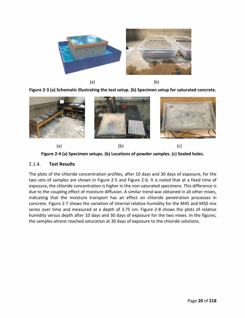
For each of the nine mixes, three cylinders and two slabs (300 x 300 x 105 mm) were cast from a single batch (see Figure 2-1) yielding a total of 18 slabs and 27 cylinders. After 24 hours, the specimens were demoulded and moist cured at 20°C and 95 ±5% RH for 28 days. After curing, the cylinder specimens were used for strength testing, and the slabs were divided into two sets. The first set (non-saturated samples) had four SHT75 Sensirion humidity and temperature sensors embedded at different depths to measure the relative humidity profile inside each slab (see Figure 2-2), then the slabs were kept at a room temperature of 23±2°C and 50±5% RH for 30 days until they reached equilibrium with the environmental temperature and humidity of the room. The four sides of the specimens were then sealed with silicon to prevent any lateral moisture loss. The bottom surfaces of the slabs were exposed to the room environment. The second set consisted of saturated slabs. These slabs were immersed in pure water for 30 days and then the four sides of the slabs were dried to a saturated surface dry (SSD) condition and sealed. The bottoms of the slabs were exposed to pure water (Figure 2-3). After the conditioning period, a 5% (by weight) sodium chloride solution was ponded on the top surface of the slabs. The chosen testing periods were 10 days and 30 days. At the end of each period, the sodium chloride solution was removed from the top surface of the specimens. Concrete powder samples were collected from each specimen by drilling vertically at three different locations and collecting the powder in depth increments of 1.25 cm (1.25 cm, 2.5 cm, 3.75 cm, 5 cm, and 6.25 cm) (see

Page 19 of 218
Figure 2-4b). The collected powder was kept in small plastic vials; the vial was sealed and labeled. After the powder samples had been collected, the holes in the slabs were sealed with silicon and then the chloride solution was re-applied to the top surface (Figure 2-4c). The chloride profiles for each slab were determined by analyzing the collected powder samples using acid-soluble chloride according to ASTM C1152 (2012) and ASTM C114 (2018b), and water-soluble chloride according to ASTM C1218 (2017b).
The idea of the test is that there are two driving forces in the first set of specimens which are non-saturated; and there is only one driving force in the second set of specimens which are saturated. Any difference between the chloride concentration profiles of the two sets of specimens must be due to the driving forces. When we compare the specimens with different water-cement ratios (keeping the other parameters the same), the difference must be due to water-cement ratio. Similarly, the effects of aggregate volume fraction on the coupling parameter can be determined.
Figure 2-1 Specimens from each mix.
(a) (b)
Figure 2-2 (a) Cross-sections of test slabs showing the location of the sensors. (b) Specimen with sensors installed.
Page 20 of 218
(a) (b)
Figure 2-3 (a) Schematic illustrating the test setup. (b) Specimen setup for saturated concrete.
(a) (b) (c)
Figure 2-4 (a) Specimen setups. (b) Locations of powder samples. (c) Sealed holes.
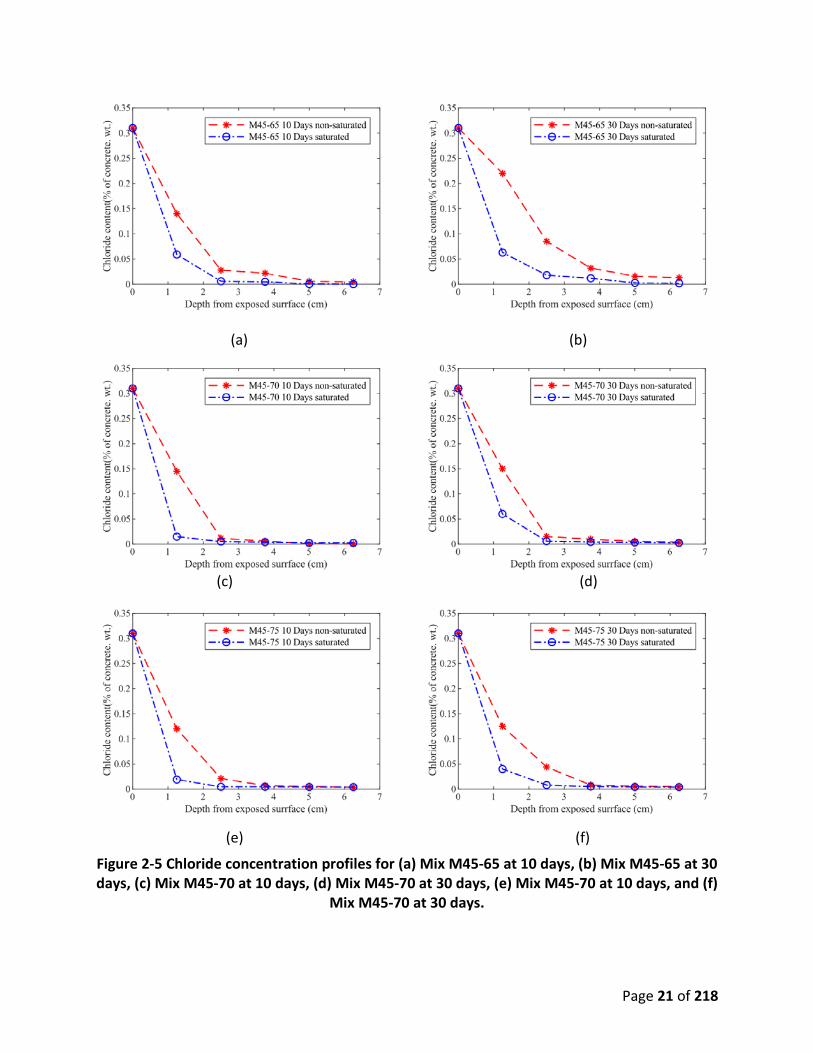
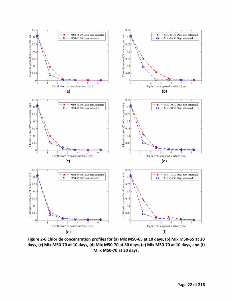
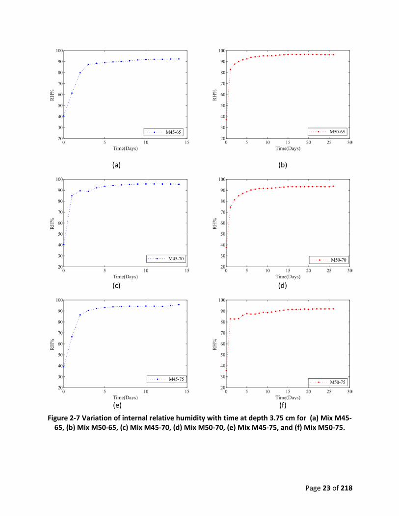
Test Results
The plots of the chloride concentration profiles, after 10 days and 30 days of exposure, for the two sets of samples are shown in Figure 2-5 and Figure 2-6. It is noted that at a fixed time of exposure, the chloride concentration is higher in the non-saturated specimens. This difference is due to the coupling effect of moisture diffusion. A similar trend was obtained in all other mixes, indicating that the moisture transport has an effect on chloride penetration processes in concrete. Figure 2-7 shows the variation of internal relative humidity for the M45 and M50 mix series over time and measured at a depth of 3.75 cm. Figure 2-8 shows the plots of relative humidity versus depth after 10 days and 30 days of exposure for the two mixes. In the figures, the samples almost reached saturation at 30 days of exposure to the chloride solutions.
Page 21 of 218
(a) (b)
(c) (d)
(e) (f)
Figure 2-5 Chloride concentration profiles for (a) Mix M45-65 at 10 days, (b) Mix M45-65 at 30 days, (c) Mix M45-70 at 10 days, (d) Mix M45-70 at 30 days, (e) Mix M45-70 at 10 days, and (f)
Mix M45-70 at 30 days.
Page 22 of 218
(a) (b)
(c) (d)
(e) (f)
Figure 2-6 Chloride concentration profiles for (a) Mix M50-65 at 10 days, (b) Mix M50-65 at 30 days, (c) Mix M50-70 at 10 days, (d) Mix M50-70 at 30 days, (e) Mix M50-70 at 10 days, and (f)
Miix M50-70 at 30 days.
Page 23 of 218
(a) (b)
(c) (d)
(e) (f)
Figure 2-7 Variation of internal relative humidity with time at depth 3.75 cm for (a) Mix M45-65, (b) Mix M50-65, (c) Mix M45-70, (d) Mix M50-70, (e) Mix M45-75, and (f) Mix M50-75.

Page 24 of 218
(a) (b)
(c) (d)
(e) (f)
Figure 2-8 Internal relative humidity profile after 10 days and after 30 days for (a) Mix M45-65, (b) Mix M50-65, (c) Mix M45-70, (d) Mix M50-70, (e) Mix M45-75, and (f) mix M50-75.
Calculation of the Coupling Parameter DCl-H
Eqn. 2.5 is used to evaluate the coupling parameter DCl-H, where the total chloride transport is driven by two forces: the coupled chloride and the moisture diffusion. The rate of total chloride

Page 25 of 218
diffusion is expressed as the sum of the chloride transport rate due to the chloride concentration gradient and the chloride transport rate due to the moisture gradient.
t t t
t Cl H
C C Ct t t
∂ ∂ ∂ = + ∂ ∂ ∂ 2.7
( ) ( )tCl H Cl H
H
C div J div D grad Ht − −
∂ = = ∂ 2.8
( ) ( )tCl Cl Cl
Cl
C div J div D grad Clt −
∂ = = ∂ 2.9
Eqn. 2.8 presents the effect of the internal relative humidity gradient on the chloride transfer. This equation can be rearranged as:
( ) ( )Cl H Cl HAdiv D grad H D grad H
A x− −= ∆ 2.10
in which A is the surface area and Δx is the distance between two adjacent points in the concentration profile. Substituting Eqn. 2.10 into Eqn. 2.8, and then Eqn. 2.7, and rearranging the equation, the coupling parameter DCl_H can be expressed as follows:
( )t t
Cl Ht Cl
C C xDt t H−
∂ ∂ ∆ = − ∂ ∂ ∇ 2.11
where (𝜕𝜕𝜕𝜕𝑡𝑡/𝜕𝜕𝜕𝜕)𝑡𝑡 is the rate of the variation of total chloride concentration due to the coupled chloride and moisture diffusion (non-saturated condition); (𝜕𝜕𝜕𝜕𝑡𝑡/𝜕𝜕𝜕𝜕)𝐶𝐶𝐶𝐶is the rate of the variation of total chloride concentration due to chloride penetration (saturated condition); and Δx is the distance between two chloride concentration readings. Based on the experimental data, the coupling parameter DCl-H can be calculated for each mix using Eqn. 2.11, where the quantities (𝜕𝜕𝜕𝜕𝑡𝑡/𝜕𝜕𝜕𝜕)𝑡𝑡 and (𝜕𝜕𝜕𝜕𝑡𝑡/𝜕𝜕𝜕𝜕)𝐶𝐶𝐶𝐶 are evaluated based on the data obtained from the chloride profiles of both the fully saturated and the partially saturated concrete samples. ∇𝐻𝐻 is evaluated based on the recorded relative humidity data; Δx is equal to 1.25 cm. As will be shown in the following analysis, the coupling parameter is not simply a constant but a variable that depends upon many parameters.
Material Model for the Coupling Parameter DCl-H
A material model is developed based on the present test data such that the coupling parameter DCl-H can be expressed as a function of the influential parameters. The purpose of developing the material model is that the coupling parameter DCl-H can be evaluated by the material model for concrete with various design parameters without any further testing. The influential parameters considered in this study are chloride concentration, exposure time, aggregate volume fraction, and water-cement ratio.

Page 26 of 218
2.1.6.a. Evaluation of the Coupling Parameter DCl-H Based on the Test Data
As shown in the figures on the chloride profiles, the chloride transport process depends strongly on the mix design parameters, as does the coupling parameter DCl-H. Figure 2-9 through Figure 2-13 show the effect of the chloride concentration, the water-cement ratio (w/c), and the aggregate volume fraction (gi) on the coupling parameter DCl-H. The coupling parameter DCl-H can be estimated using the multifactor method as follows:
( ). ( / ). ( ). ( )cl HD f cl f w c f gi f t− = 2.12
where the four factors in Eqn. 2.12 will be determined based on the test data as shown in the following sections.
Concentration dependence f(cl)
Analysis of the test results showed that the coupling parameter DCl-H is concentration dependent. Figure 2-9 illustrates the distribution of DCl-H versus the chloride concentration for mixes M45-70 and M50-70. It is clear from the obtained results that DCl-H a linear function of the chloride concentration. The expression of this function can be written as:
( ) ( )f cl A Cl= 2.13
where the value of the constant A can be obtained by curve fitting the test data such that only the influential parameter of the chloride concentration is taken into consideration as a variable, while the rest of the influential parameters are considered to be constants. By curve fitting the distribution of DCl-H versus the chloride concentration for mix M45-70 at 10 days, where the influence of aggregate volume fraction, water-cement ratio, and time are fixed at gi = 70%, w/c = 0.4, and t = 10 days (see Figure 2-10). The value of A is thus determined to be A = 0.0271.
(a) (b)
Figure 2-9 Variation of coupling parameter DCl-H with time for (a) Mix M45-70. (b) Mix M50-70.

Page 27 of 218
Figure 2-10 Effect of chloride concentration on coupling parameter DCl-H.
Ratio of w/c f(w/c)
The influence of w/c on the coupling parameter DCl-H is exhibited in Figure 2-11a. The plot shows the value of DCl-H versus total chloride concentration after 10 days of exposure for mixes with w/c = 0.45, 0.5, and gi = 65%. It is clear that, at any fixed chloride concentration, the coupling parameter DCl-H increases as the w/c increases. This is due to the fact that a higher w/c leads to a higher porosity, Thus, the higher the porosity, the faster the transport process in the concrete. An expression for the effect of w/c ratio on chloride ion diffusion coefficient can be used here (Hobbs and Matthews, 1998).
/( / ) ( )w cf w c a b= 2.14
The values of the two constants in the equation, a and b, can be determined based on the present test data (see Figure 2-11b) as a = 4.94E-11, and b = 7.47E14.

Page 28 of 218
(a) (b)
Figure 2-11 Effect of w/c on the coupling parameter. (a) Variation of the DCl-H with time at 0.05 total chloride concentration. (b) Comparisons of test data and model.
Aggregate volume fraction f(gi)
Figure 2-12a shows the effect of different aggregate volume fractions (0.65%, 0.7%, and 0.75%) on the coupling parameter DCl-H. In Figure 2-12a, the values of DCl-H are calculated from the three mixes with aggregate volume fractions (0.65%, 0.7%, and 0.75%) and fixed values of w/c = 0.45 after 10 days of exposure. Test results indicated that the value of the coupling parameter DCl-H of concrete specimens made using the same w/c ratio decreases with an increase in the aggregate volume fraction. The effect of the aggregate volume fraction on the diffusivity of concrete was modeled by Xi and Bazant (1999) based on the three-phase model (Christensen, 1979). The same model can be used to account for the effect of different aggregate volume fractions on the DCl-H.
( ) [ ]1
1 / 3 1/ ( / ) 1mi
ieff
i m
gD Dg D D
= + − − −
2.15
where Deff is the effective coupling parameter which depends on the configuration of the concrete, Di and Dm are the coupling parameters of inclusions (aggregate) and matrix (cement paste), and gi is the volume fraction of the aggregate. The values of Dm and Di can be determined based on curve fitting of the test data as shown in Figure 2-12b where they have the values of 0.00496 and 1.84E-06, respectively.

Page 29 of 218
(a) (b)
Figure 2-12 Effect of aggregate volume fraction on the coupling parameter ( a) Variation of the DCl-H with time at 0.05 total chloride concentration. (b) Comparisons of test data and
model.
Time of exposure f(t).
The general trend of the effect of time of exposure on chloride diffusion in concrete is that the chloride ingress decreases with time. Several factors may influence this reduction; the primary factor is the effects of the cement paste hydration, which increases with time leading to lower porosity of the concrete. Based on the results from mix M50-70 with different times for exposure (Figure 2-13a), the trend is that the value of DCl-H decreases with increases of the exposure time. By curve fitting the test data (Figure 2-13b), the influence of exposure time can be expressed as:
0.075( )f tt
= 2.16
where t is the time in days. The effect of exposure time can be explained by the tortuosity of microstructure of cement paste which depends mainly on the degree of hydration, and thus the age of the concrete. The general trend is that with increasing age, the degree of tortuosity of microstructure of cement paste increases and thus the transport rate decreases.

Page 30 of 218
(a) (b)
Figure 2-13 Effect of exposure time on coupling parameter DCl-H. (a) Variation of the DCl-H with time at 0.05 total chloride concentration. (b) Comparisons of test data and model.
General expression for the coupling parameter DCl-H
The general expression for the coupling parameter DCl-H can be written by combining Eqns. 2.13, 2.14, 2.15 and 2.16 as follows:
( ) [ ]7 14 / ( )10 .( 10 ) . . 1
1 / 3 1/ ( / ) 15.4866 7.47 m
i
w c icl H
i m
gClD Dt g D D
−−
= × × + − + −
2.17
This model accounts for the effects of chloride concentration, exposure time, w/c ratio, and aggregate volume fraction. Figure 2-14 presents a comparison of the data from the experiment and that of the model prediction (dashed lines). One can see that the model predictions agree with the test data quite well. Therefore, Eqn. 2.17 can be used to calculate the coupling parameter DCl-H.

Page 31 of 218
(a) (b)
(c) (d)
(e) (f)
Figure 2-14 Comparisons of test data and model predictions for (a) Mix M45-65, (b) Mix M50-65, (c) Mix M45-70, (d) mix M50-70, (e) Mix M45-75, and (f) Mix M50-75.

Page 32 of 218
Conclusions
• An experimental study and the method for determining the coupling parameter DCl-H, which is the effect of moisture transfer on chloride penetration in concrete, is presented. In the experimental study, a chloride ponding test was conducted on a series of concrete specimens with different aggregate volume fractions and water-cement ratios exposed to various moisture conditions
• The obtained test results show that the chloride concentration profiles in the non-saturated specimens have a higher chloride concentration comparing with the saturated specimens at a fixed time of exposure. The difference is due to the coupling effect of moisture diffusion.
• The coupling parameter DCl-H was determined based on the obtained test results by using a modified Fick’s law equation, where the DCl_H is expressed as a function of the variation chloride concentration and internal relative humidity gradient.
• The value of DCl-H obtained from the present test result data indicates a strong dependence on the concentration of chloride ions, the water to cement ratio, and the aggregate volume fraction.
• A material model was proposed for determining the coupling parameter DCl-H based on the experimental data. The experimental parameters used in the model included the concentration of chloride ions, the water to cement ratio, and the volume fraction of aggregate.
2.2. EFFECT OF ION CONCENTRATION ON MOISTURE DIFFUSION IN CONCRETE
Introduction
There is little information available in the existing literature on the effect of chloride concentration gradient on the rate of moisture transport in unsaturated concrete. Precisely, there is no test data available on the coupled effect of chloride on moisture transport, which makes the theoretical interpretation of this phenomenon unclear. This brought about the need to investigate this effect. In the previous section, an experimental study was carried out to determine the effect of moisture transport on the chloride penetration. Based on the obtained results, an empirical material model was developed. In this section, an experimental study was conducted to determine the second coupling effect (the effect of the chloride concentration on moisture transport DH-Cl).
Experimental Program
2.2.2.a. Materials and Mix Proportions
Specimens prepared with cement paste were used in this work. The cement used in the experiments was Type II Portland Cement conforming to current ASTM C150 (2019). All-purpose river sand was used as fine aggregate. A total of eighteen specimens measuring 12 cm diameter and 16 cm hight were prepared using nine different mixtures. The mixtures were designed with

Page 33 of 218
three different water-cement ratios: 0.45, 0.5, and 0.55; and three different aggregate volume fractions: 55%, 60%, and 65%. Detailed mix proportions of the concrete specimens are shown in Table 2-4, Table 2-5 and Table 2-6. The specimens are denoted as Mxx-yy, where xx indicates the water/cement ratio expressed as a percentage, and yy indicates the aggregate volume fraction, also as a percentage. For example, M45-65 represents the specimen with a water-cement ratio = 0.45 and an aggregate volume fraction = 0.65.
Table 2-4 Mix Proportions for M45 Mix Series.
Mix Cement kg/m3
Sand kg/m3
Water kg/m3
M45-55 360 650 162 M45-60 360 800 162 M45-65 360 970 162
Table 2-5 Mix Proportions for M50 Mix Series.
Mix Cement kg/m3
Sand kg/m3
Water kg/m3
M50-55 360 560 180 M50-60 360 810 180 M50-65 360 1005 180
Table 2-6 Mix Proportions for M55 Mix Series.
Mix Cement kg/m3
Sand kg/m3
Water kg/m3
M55-55 360 575 198 M55-60 360 680 198 M55-65 360 1040 198
2.2.2.b. Experimental Procedure
As shown in Figure 2-15, for each of the nine mixes, two identical cylinder specimens were prepared. After 24 hours, the specimens were demoulded and moist cured at 20°C and 95 ±5% RH for 28 days. In order to monitor the variation of internal relative humidity during the test, the specimens were first dried at a higher temperature with circulated air. As soon as the specimens reached equilibrium with the environmental humidity of the room, the sides of the specimens were then sealed with silicon to prevent any lateral moisture loss and ensure that only uniaxial moisture diffusion took place during the test. The internal relative humidity profile inside each specimen was measured using HT75 Sensirion humidity and temperature sensors. The sensors were installed in the specimens at different depths from the exposed surface (2.5 cm, 5 cm, 7.5 cm, and 10 cm) as shown in Figure 2-16. Then, 8% (by weight) sodium chloride solution was ponded on the top surface of the first specimen and distilled water was ponded on the top surface of the second one. The change of the reading of the internal relative humidity inside each specimen during the test was recorded in time increment of 1 min. After the internal relative

Page 34 of 218
humidity had stabilized, the sodium chloride solution was removed from the top surface of the specimens and concrete powder samples were collected from each specimen by drilling vertically and collecting the powder in depth increments of 2.5 cm. The free chloride profiles for each specimen were determined by analyzing the collected powder samples using water-soluble chloride according to ASTM C1218 (2017b).
(a)
(b)
Figure 2-15 (a) Schematic illustrating the number of specimens with the various concrete mix proportions (b) Concrete specimens used in the test.
gi= 0.55,0.60,0.65 W/C=0.45
gi= 0.55,0.60,0.65 W/C=0. 5
gi= 0.55,0.60,0.65 W/C=0.55
Water 8% NaCl Water 8% NaCl Water 8% NaCl

Page 35 of 218
(a) (b)
Figure 2-16 (a) Cross section showing the locations of the sensors. (b) Specimens with sensors installed.
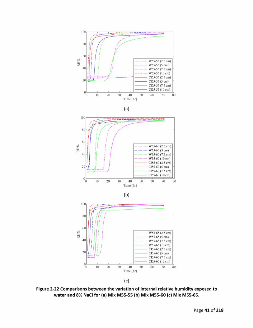
Experimental Results
Figure 2-17 through Figure 2-19 show the internal relative humidity profiles corresponding to the nine sets of mixes, exposed to distilled water and 8% NaCl, respectively. A comparison of the change in the internal relative humidity for the two sets of each mix over time measured at a depth of 2.5cm, 5 cm, 7.5 cm, and 10 cm is illustrated in Figure 2-20 through Figure 2-22. From these figures, it is noted that the specimens exposed to distilled water have higher moisture transport rates compared to the specimens exposed to 8% NaCl solution. For example, in Figure 2-17(e) and (f), distilled water vs. chloride solution, at a fixed time 50 hours, the values of relative humidity at different depths in (e) are much higher than those in (f) This trend was observed in most of the mixes, see Figure 2-19(a) and (b) and it is an evidence of the influence of NaCl on moisture transport. The trend means that the chloride ions actually slow down the rate of moisture transport.
The coupling effect of chloride ions on moisture transport is quite complicated due to the influences of several possible mechanisms. These mechanisms may have opposing influences on the moisture transport. First, there are two driving forces in the specimens ponded by chloride solutions, which are the moisture gradient and the chloride ion concentration gradient. In this test, the two gradients are in the same direction and thus the addition of the chloride ion concentration gradient should increase the rate of moisture penetration. However, the test data showed the opposite trend. So, in the next section, more influential mechanisms are discussed in depth.
2.5 cm 5 cm
7.5 cm 10 cm

Page 36 of 218
(a) (b)
(c) (d)
(e) (f)
Figure 2-17 Variation of internal relative humidity with time at different depths for (a) Mix M45-55 exposed to distilled water, (b) Mix M45-55 exposed to 8% NaCl, (c) Mix M45-60
exposed to distilled water, (d) Mix M45-60 exposed to 8% NaCl, (e) Mix M45-65 exposed to distilled water, (f) Mix M45-65 exposed to 8% NaCl.

Page 37 of 218
(a) (b)
(c) (d)
(e) (f)
Figure 2-18 Variation of internal relative humidity with time at different depth for (a) Mix M55-55 exposed to distilled water, (b) Mix M55-55 exposed to 8% NaCl, (c) Mix M55-60
exposed to distilled water, (d) Mix M55-60 exposed to 8% NaCl, (e) Mix M55-65 exposed to distilled water, (f) Mix M55-65 exposed to 8% NaCl.

Page 38 of 218
(a) (b)
(c) (d)
(e) (f)
Figure 2-19 Variation of internal relative humidity with time at different depth for (a) Mix M50-55 exposed to distilled water, (b) Mix M50-55 exposed to 8% NaCl, (c) Mix M50-60
exposed to distilled water, (d) Mix M50-60 exposed to 8% NaCl, (e) Mix M50-65 exposed to distilled water, (f) Mix M50-65 exposed to 8% NaCl.

Page 39 of 218
(a)
(b)
(c)
Figure 2-20 Comparisons between the variation of internal relative humidity exposed to water and 8% NaCl for (a) Mix M45-55 (b) Mix M45-60 (c) Mix M45-65.
0 50 100 150 2000
50
100
150
Time (hr)
RH% W 45-55 (2.5 cm)
Cl 45-55 (2.5 cm)W 45-55 (5 cm)Cl 45-55 (5 cm)W 45-55 (7.5 cm)Cl 45-55 (7.5 cm)W 45-55 (10 cm)Cl 45-55 (10cm)
0 50 100 150 2000
50
100
150
Time (hr)
RH% W 45-60 (2.5 cm)
Cl 45-60 (2.5 cm)W 45-60 (5 cm)Cl 45-60 (5 cm)W 45-60 (7.5 cm)Cl 45-60 (7.5 cm)W 45-60 (10 cm)Cl 45-60 (10cm)

Page 40 of 218
(a)
(b)
(c)
Figure 2-21 Comparisons between the variation of internal relative humidity exposed to water and 8% NaCl for (a) Mix M50-55 (b) Mix M50-60 (c) Mix M50-65.
Page 41 of 218
(a)
(b)
(c)
Figure 2-22 Comparisons between the variation of internal relative humidity exposed to water and 8% NaCl for (a) Mix M55-55 (b) Mix M55-60 (c) Mix M55-65.

Page 42 of 218
Interpretation of the Test Data
Different mechanisms are believed to have an effect on the transport behavior of NaCl solution in concrete which are partially related to the structure of the solution and partially to the characteristics (microstructure) of the concrete. The following is an attempt to describe two possible mechanisms to explain the influence of chloride ions on moisture transport.
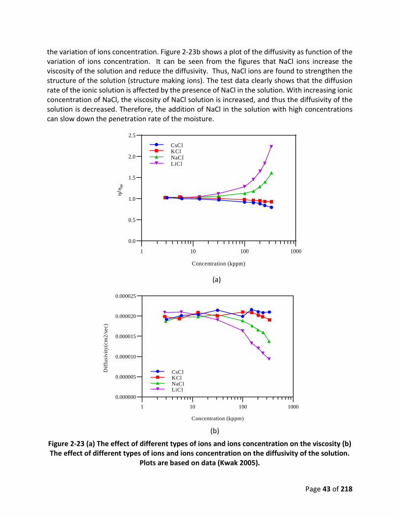
To understand the role of NaCl in this process, it was desirable to describe its effect on the structure of water. Under standard conditions, distilled water is a highly structured liquid that has an extensive network of hydrogen bonds, i.e., each water molecule has four hydrogen bonds with neighboring water molecules in four approximately tetrahedral directions (Wang, 1954). The potential of water at standard pressure is equal to zero which means that the water has the potential to move. When sodium chloride is added to the water, the negative solute potential reduces the overall potential of the solution by consuming part of the available water potential energy, where the water molecules bind solute molecules via hydrogen bonds and thus the consumed energy in the hydrogen bonds is not available in the system. This means that the solution has a lower potential to move. This effect also depends on the concentration of the ion, where the greater the concentration of the ion, the greater the ionic interaction. However, the influence of the formation of the oppositely charged water molecules surrounding the solute ion (ionic cloud or hydration shell) may either increase (structure making ion) or decrease (structure breaking ion) the strength of the water structure. The classification of solute ions based on their effects on water structure observed by macroscopic measurements in dilute solutions are shown in Table 2-6 (Marcus, 2009).
Table 2-7 Ions Arranged According to Their Effects on the Structure of Water (Marcus, 2009).
Ions ∆GHB Structure Breaking Ions K+, Rb+, Cs+, Tl+, Cl-, SH-, CN-, N3-, OCN-, NO2-, NO3-, ClO3-, -0.9 to -0.7 CH3NH3+, (CH3)4N+, Ra2+, SH-, HF2-, ClO2-, BrO3-, HCO2-, HSO3-, -0.7 to -0.4 NH4+, B(OH)4-, SO42-, MoO42-, WO42-, C2O42- -0.4 to -0.1 Borderline Ions Na+, Ag+, (C2H5)4N+, Ba2+, Pb2+, F-, IO3-, HCO3-, H2PO4- -0.1 to 0.1
Structure Making Ions Li+, Cu+, Au+, (C6H5)4As+, Sr2+, Sn2+, Al3+, Cr3+, Bi3+, OH-, CH3CO2-B(C6H5)4-, CO32-, SO32-
0.1 to 0.4
(∆GHB is the change in the average total geometrical factors)
Depending on the type of solute ion, its effect on the water structure contributes to the solution's viscosity as the water molecules to rearrange themselves around it and therefore the density of the water near the ions is higher than the rest of the solution (Marcus, 2009). Figure 2-23a-b show test result reported by Kwak et al. (2005) on the effect of different types of ions and ions concentration on the viscosity and the diffusivity of the solution. In Figure 2-23a, the ratio between the viscosity of solution η and the viscosity of pure water ηw is plotted as function of
Page 43 of 218
the variation of ions concentration. Figure 2-23b shows a plot of the diffusivity as function of the variation of ions concentration. It can be seen from the figures that NaCl ions increase the viscosity of the solution and reduce the diffusivity. Thus, NaCl ions are found to strengthen the structure of the solution (structure making ions). The test data clearly shows that the diffusion rate of the ionic solution is affected by the presence of NaCl in the solution. With increasing ionic concentration of NaCl, the viscosity of NaCl solution is increased, and thus the diffusivity of the solution is decreased. Therefore, the addition of NaCl in the solution with high concentrations can slow down the penetration rate of the moisture.
(a)
(b)
Figure 2-23 (a) The effect of different types of ions and ions concentration on the viscosity (b) The effect of different types of ions and ions concentration on the diffusivity of the solution.
Plots are based on data (Kwak 2005).
1 10 100 1000
0.0
0.5
1.0
1.5
2.0
2.5
Concentration (kppm)
η/η w
CsClKClNaClLiCl
1 10 100 1000
0.000000
0.000005
0.000010
0.000015
0.000020
0.000025
Concentration (kppm)
Dif
fusi
vity
(cm
2/se
c)
CsClKClNaClLiCl

Page 44 of 218
The other mechanism is related to the surface of pore structure in the cement paste of concrete. The diffusion behavior of NaCl solution can be affected by the microstructure of the concrete and the surface chemistry of the C-S-H/solution interface. Since the C-S-H develops a negative charge at its surface, an ionic cloud known as electric double layer (EDL) forms at the C-S-H/solution interface to balance the charge of the C-S-H surface and satisfy electro-neutrality condition of the system. Figure 2-24 shows a Gouy-Chapman-Stern model for the electric double layer. As can be seen in the figure, the first layer formed at the C-S-H/solution interface is the Stern layer. This layer consists of two planes, the inner Helmholtz plane (IHP), which contains the compact hydrogen atoms of water molecules at the interface. The outer Helmholtz plane (OHP) contains the adsorbed hydrated cations (Ca2. Na) in the alkaline pore solution (Zibara, 2001; Stojek, 2002). Due to the adsorption of cations in the Stern layer, a second layer forms outside the OHP; a so-called diffuse layer where the adsorption of the hydrated anions (chloride) occurs. Because the ions within the Stern layer are rigid and immobile, the motion of the ions and solvent molecules can only take place in the diffuse layer. The thickness of the Stern layer is defined as function of the radius of the hydrated cation, while the thickness of the electric double layer is determined by the Debye length. The surface potential is determined by the drop in the potential across the Stern layer and the diffuse layer which mainly depends on the ion’s type and the concentration of ions in the solution.
Figure 2-24 Gouy-Chapman-Stern model for the electric double layer.
Based on the described model, the interaction between the electrical double layer formed at the wall of capillary pores and the ionic clouds in the solution influence the velocity and diffusion rate of the ions and solvent molecules. Figure 2-25a illustrates the fluid velocity distribution inside the capillary pore. It can be noted from the figure that the fluid becomes immovable near the walls of capillary pores (ro=rx). In Figure 2-25b the effect of the capillary pore size on the fluid velocity is shown. It can be seen in this figure that the smaller the size of capillary pore compared to the thickness of the electric double layer, the slower the movement of ions and solvent (Zhang and Gjørv, 1996). Therefore, depending on the volume and size of the pores in cement paste, the
distance
pote
ntia
l

Page 45 of 218
formation of the double layer due to the ionic interaction at the pore wall may have a major effect on the transport processes. Basically, with decreasing pore sizes, the velocity of solution is decreased due to the reduce effective pore size which is related to the existence of the ions in the solution.
(a) (b)
Figure 2-25 (a) Fluid velocity distribution inside the pores. (b) The effect of the pore size on the velocity of fluid
The above described two mechanisms (viscosity of NaCl solution and effective size of pores) can slow down the moisture transport, which is opposite to the effect of the moisture gradient and chloride concentration gradient. The viscosity of NaCl solution depends on the concentration of chloride and the effective size of pores depends on the pore sizes. The pore sizes of cement paste depend on concrete mix design parameters, including the two parameters used in this study, i.e., water-cement ratio and aggregate volume fraction. The net result of this experimental study is that the 8% chloride solution actually reduced the penetration rate of moisture.
Now, let us observe the effect of water-cement ratio on the moisture transport. The variation of the internal relative humidity measured at different depths for the first group of the specimens are shown in Figure 2-26. In this group the aggregate volume fraction is fixed at 0.55 and the water-cement ratio varies from 0.45 to 0.55. From this figure, it can be observed that the diffusion rate increases when the water-cement ratio increases from 0.45 to 0.55. Similar trends were obtained for the chloride profile as shown in Figure 2-27. It is noted that at a fixed time of exposure, the chloride ions penetrate more deeply in the specimens having higher water-cement ratios.

Page 46 of 218
(a) (b)
(c)
Figure 2-26 Variation of the internal relative humidity measured at different depths for (a) Mix 45-55. (b) Mix 50-55. (c) Mix 55-55.
0 50 100 150 2000
50
100W55-55
Time (hr)
RH
(%)
2.5 cm5 cm7.5 cm10 cm
0 50 100 150 2000
50
100W50-55
Time (hr)
RH
(%)
2.5 cm5 cm7.5 cm10 cm
0 50 100 150 2000
50
100W45-55
Time (hr)
RH
(%)
2.5 cm5 cm7.5 cm10 cm

Page 47 of 218
Figure 2-27 Variation of chloride concentration at different depths.
This is because the water-cement ratio defines the porosity of concrete, which in turn influences the transport properties. As the hydration products in the specimens with low water-cement ratio (at the optimum value) are shaped, part of the small capillary pore spaces become isolated, resulting in decreasing the fraction of main pores that form the associated pathways for transport. As this procedure proceeds, the network of connected capillary pore spaces will be reduced, and thus the quick transport of water particles or ions through this network will end, and the transport would then be controlled by the C-S-H gel pores (Bentz, 1996). Figure 2-28 shows a plot of data obtained from a three-dimensional digital-image-based simulation model of cement paste microstructure (Bentz and Garboczi, 1991). In Figure 2-28b, the fraction of the total porosity that is connected (fraction connected) is plotted against the degree of hydration for different water cement ratios. It can be seen from the figure that the water-cement ratio has an influence on the reduction of the volume fraction for the connected pores as the hydration process occurs. The relationship between the capillary porosity and fraction connected is illustrated in Figure 2-28b. One can see from the figure that fraction connected is highly dependent on capillary porosity. This means that an increase in the capillary porosity resulting from increasing the water cement ratio will lead to formation of a continuous pore network, which in return affects the diffusion rate.
0 5 10 150.0
0.1
0.2
0.3
Depth from exposed surrface (cm)
Cl (
% g
/g)
45-6550-6555-65

Page 48 of 218
(a)
(b)
Figure 2-28 (a) Variation of fraction connected vs degree of hydration. (b) Variation of fraction connected vs capillary porosity (Bentz and Garboczi, 1991).
Evaluation of Coupling Parameters
Eqn. 2.18 can be used to evaluate the coupling parameter DH-Cl, where the moisture transport is influenced by two effects: moisture concentration gradient and chloride concentration gradient. The rate of moisture transport is expressed as the sum of the moisture transport rate due to the chloride concentration gradient and the moisture transport rate due to the moisture gradient.
0.0 0.2 0.4 0.6 0.8 1.00.0
0.2
0.4
0.6
0.8
1.0
Degree of hydration
Frac
tion
Con
nect
ed
0.35 W/C0.45 W/C0.5 W/C0.6 W/C0.7 W/C
0.0 0.2 0.4 0.6 0.80.0
0.2
0.4
0.6
0.8
1.0
Capillary porosity
Frac
tion
Con
nect
ed
0.35 W/C0.45 W/C0.5 W/C0.6 W/C0.7 W/C

Page 49 of 218
( ) ( )H Cl f H Hw H D C D HH t − −
∂ ∂= ∇ ∇ +∇ ∇
∂ ∂ 2.18
Eqn. 2.18 can be rewritten using the definition of divergence as:
2 2
( ) ( ) ( )H cl H H
w H t C x H xD DH t x x− −
∂ ∆ ∆ ∆= +
∂ ∆ ∆ ∆ 2.19
in which is Δx is the distance between two adjacent points in the concentration profile. Δt is the time interval. ∂w/ ∂H is the moisture capacity. The expression for the coupling parameter DCl_H can be obtained by rearranging Eqn. 2.19 as:
2
2
( )( )( )
H HCl H
D H xx w H tDC x H t x
−−
∆∆ ∂ ∆ = − ∆ ∂ ∆ ∆ 2.20
The value of DH-H can be determined at different depths from the relative humidity test data of the samples exposed to pure water the by using the analytical solution of Fick’s second law
( )
2
1
14 ,
1
xDt H x t Ho
efrHs Ho
−
=
− − −
2.21
where Ho is the initial relative humidity, Hs is the surface relative humidity, and H(x,t) is the relative humidity at distance x from the exposed surface at time t. ∂w/ ∂H is the moisture capacity determined based on an empirical model developed by Xi et al. (1994a) and Xi et al. (1994b). ∆H(t) is the variation of relative humidity between ∆t at fixed depth. ∆H(x) is variation of relative humidity between two adjacent points in the relative humidity profiles. ∆C is the variation chloride concentration between two adjacent points in the concentration profiles.
Eqn. 2.20 is developed based on Eqn. 2.18, which considers the effect of simultaneous chloride and moisture concentration profile. The other two influential mechanisms were not included: the effect of the viscosity of ionic solution and effective pore sizes when there is chloride in the pore system. Both of the mechanisms are related to the chloride concentration in the solution, which is not a constant but a variable depending on the depth of concrete. The present experimental study was designed to study the effect of two concentration gradients. The test data showed that the other two mechanisms are also very important. Therefore, the present test data are not sufficient to be used to evaluate the coupling parameter, DH-Cl, and then develop a material model for the coupling parameter. This is a very time-consuming test due to the time needed for the samples to reach a desired equilibrium moisture condition prior to the chloride ponding test, thus, there was not enough time for more tests to be conducted in the project period. More systematic experimental study will need to be performed in the future.

Page 50 of 218
Conclusions
• An experimental investigation on the effect of ion concentration on moisture transport in concrete is presented. The experimental study was conducted to determine the second coupling parameters (the effect of the chloride penetration on moisture diffusion DH-Cl).
• Ponding tests were carried out on a series of concrete specimens made with nine deferent concrete mixes with three different water-cement ratios: 0.45, 0.5, and 0.55; and three different aggregate volume fractions: 55%, 60%, and 65%. For each mix, the effect of the concentration of chloride ion on moisture diffusion was studied by comparative ponding tests on two specimens exposed to distilled water and 8% NaCl solution, respectively.
• The experimental data from this study indicated a noticeable correlation between the ion’s concentration and moisture transport. it was observed that the relative humidity profile changed at a reduced rate in the specimens exposed to 8% NaCl solution comparing to the specimens exposed to pure water. This is observed in all concrete samples with different water-cement ratios and aggregate volume fractions.
• Three possible coupling mechanisms were discussed: ionic concentration gradient, viscosity of the ionic solution, and the effective size of pores due to the appearance of the ions. In this study, the chloride concentration gradient can increase the rate of moisture penetration, and the viscosity of NaCl solution and the reduced effective size of pores can slow down the moisture transport. The net result of this experimental study is that the 8% chloride solution actually decreased the penetration rate of moisture.
• The viscosity of NaCl solution depends on the concentration of chloride and the effective size of pores depends on the pore sizes. The pore sizes of cement paste depend on concrete mix design parameters, including the two parameters used in this study, i.e. water-cement ratio and aggregate volume fraction. These two mechanisms for the coupling effect will need to be studied in the future.
• An analytic procedure was developed to determine the coupling parameter considering the effect of both chloride and moisture concentration gradient. It can be used when more test data become available in the future.
Equation Chapter 3 Section 1

Page 51 of 218
REINFORCED CONCRETE DAMAGE MECHANICS AND
COUPLING WITH TRANSPORT STUDIES 3.1. PLASTIC DAMAGE MODEL FOR CONCRETE
Introduction
A major goal of this project was to study and develop models for the effects of concrete damage on transport behavior. Damage can be induced by a variety of phenomena, including long-term degradation mechanisms such as ASR, as well as mechanical loading. At the outset of this project, Grizzly had no capabilities for modeling the nonlinear mechanical behavior of concrete, including damage. It was thus essential to develop a comprehensive, robust material model for concrete that could include the effects of damage.
The Lee (1996) model was selected in this study for concrete degradation modeling and was implemented in MOOSE (Gaston et al., 2009). Because this model accounts for many of the important nonlinear phenomena of mechanically-loaded concrete, this model has had widespread practical application. This material model accounts for the independent damage in tension and compression. It also accounts for degradation of the elastic modulus of the concrete as the loading goes beyond yielding in either tension or compression. The model uses the incremental theory of plasticity and decomposes the total strain, 𝝐𝝐, into elastic strain, 𝝐𝝐𝒆𝒆, and plastic strain, 𝝐𝝐𝒑𝒑, as follows
𝝐𝝐 = 𝝐𝝐𝑒𝑒 + 𝝐𝝐𝑝𝑝 3.1
where bold symbol represents a vectoral or tensorial quantity. The relation between the elastic strain tensor and the stress tensor, 𝝈𝝈, is given by
𝝐𝝐𝒆𝒆 = 𝕰𝕰−𝟏𝟏:𝝈𝝈 3.2
where 𝕰𝕰 is the undamaged elasticity tensor. Using Eqns. 3.1 and 3.2, the relation between 𝝐𝝐𝒑𝒑 and 𝝈𝝈 is expressed as
𝝈𝝈 = 𝕰𝕰: (𝝐𝝐 − 𝝐𝝐𝒑𝒑) 3.3
Since the model considers the effect of damage on elastic stiffness, an effective stress tensor, 𝝈𝝈 , is defined, where the stress for a given strain always corresponds to the undamaged elastic stiffness of the material, 𝕰𝕰0. The relation between 𝝈𝝈 , 𝝐𝝐, and 𝝐𝝐𝑝𝑝 is given by
𝝈𝝈 = 𝕰𝕰𝟎𝟎: (𝝐𝝐 − 𝝐𝝐𝒑𝒑) 3.4
To consider the degradation of reinforced-concrete structures, an isotropic damage was considered in concrete material. Hence, the relation between 𝝈𝝈 and 𝝈𝝈 can be established by the isotropic scalar degradation damage variable, D, as follows

Page 52 of 218
𝝈𝝈 = (1 − 𝐷𝐷)𝝈𝝈 3.5
𝝈𝝈 = (1 − 𝐷𝐷) 𝕰𝕰𝟎𝟎: (𝝐𝝐 − 𝝐𝝐𝒑𝒑) 3.6
The plastic damage model has various attributes to define the mechanical behavior of concrete in tension and compression such as the yield function, plastic potential, strength of material in tension and compression, and hardening and softening of the yield surface. These attributes are discussed in detail in the following sections. A method for the implementation of the plastic damage model and for the estimation of crack width are also presented in the upcoming sections.
Yield Function
The yield function, ℱ, is a function of 𝝈𝝈, the strength of the material in uniaxial tension, 𝑓𝑓𝑡𝑡, and the strength of the material in uniaxial compression, 𝑓𝑓𝑐𝑐. It is used to describe the admissible stress space. For this implementation, the yield function in stress space is defined as follows
ℱ(𝝈𝝈,𝑓𝑓𝑡𝑡 ,𝑓𝑓𝑐𝑐) = 11−𝛼𝛼
𝛼𝛼 𝐼𝐼1 + 𝐽𝐽2 + 𝛽𝛽 < 𝜎𝜎𝑚𝑚𝑚𝑚𝑚𝑚 > − 𝑓𝑓𝑐𝑐(𝜿𝜿) 3.7
where
𝐼𝐼1 : first invariant of the stress tensor 𝐽𝐽2 : second invariant of the deviatoric component of the stress tensor 𝜎𝜎𝑚𝑚𝑚𝑚𝑚𝑚 : algebraically maximum principal stress
𝛼𝛼 : material parameter = 𝑓𝑓𝑏𝑏0−𝑓𝑓𝑐𝑐02 𝑓𝑓𝑏𝑏0−𝑓𝑓𝑐𝑐0
𝑓𝑓𝑡𝑡0 : yield strength of concrete in uniaxial tensile loading 𝑓𝑓𝑏𝑏0 : yield strength of concrete in biaxial compressive loading 𝑓𝑓𝑐𝑐0 : yield strength of concrete in uniaxial compressive loading
𝛽𝛽 : material parameter = 𝑓𝑓𝑐𝑐0𝑓𝑓𝑡𝑡0
(𝛼𝛼 − 1) − (1 + 𝛼𝛼)
𝜿𝜿 : a vector of damage variables (= 𝜅𝜅𝑡𝑡 , 𝜅𝜅𝑐𝑐) 𝑓𝑓𝑐𝑐(𝜿𝜿) : strength of concrete in compression as a function of damage variable
The strength of the material in tension and compression is expressed in terms of damage variables as follows
𝑓𝑓𝑡𝑡 = 𝑓𝑓𝑡𝑡(𝜅𝜅𝑡𝑡) 3.8
𝑓𝑓𝑐𝑐 = 𝑓𝑓𝑐𝑐(𝜅𝜅𝑐𝑐) 3.9
where 𝜅𝜅𝑡𝑡 and 𝜅𝜅𝑐𝑐 are the damage variables in tension and compression, respectively, 𝑓𝑓𝑡𝑡(𝜅𝜅𝑡𝑡) is the strength of the material in tension as a function of 𝜅𝜅𝑡𝑡, and 𝑓𝑓𝑐𝑐(𝜅𝜅𝑐𝑐) is the strength of the material in compression as a function of 𝜅𝜅𝑐𝑐 . As mentioned above, the implementation first solves the given problem in the effective stress space and then transform the effective stress to stress

Page 53 of 218
space. Thus, the yield stress of the material under uniaxial loading is expressed as effective yield stress as follows
𝑓𝑓𝑡𝑡 = 1 − 𝐷𝐷𝑡𝑡(𝜅𝜅𝑡𝑡) 𝑓𝑓𝑡(𝜅𝜅𝑡𝑡) 3.10
𝑓𝑓𝑐𝑐 = 1 − 𝐷𝐷𝑐𝑐(𝜅𝜅𝑐𝑐) 𝑓𝑓𝑐(𝜅𝜅𝑐𝑐) 3.11
where 𝑓𝑓𝑡 and 𝑓𝑓𝑐 are the yield strength of the material in tension and compression in the effective stress space, respectively and 𝐷𝐷𝑡𝑡 and 𝐷𝐷𝑐𝑐 are the degradation damage variable in tension and compression, respectively such that 0 ≤ 𝐷𝐷𝑡𝑡 < 1 and 0 ≤ 𝐷𝐷𝑐𝑐 < 1 . The scalar degradation damage variable, D, is expressed in terms of 𝐷𝐷𝑡𝑡 and 𝐷𝐷𝑐𝑐 as follows
𝐷𝐷 = 𝐷𝐷(𝜿𝜿) = 1 − 1 − 𝐷𝐷𝑡𝑡(𝜅𝜅𝑡𝑡)1 − 𝐷𝐷𝑐𝑐(𝜅𝜅𝑐𝑐) 3.12
Hence, for uniaxial tension, 𝐷𝐷 = 𝐷𝐷𝑡𝑡, while for uniaxial compression, 𝐷𝐷 = 𝐷𝐷𝑐𝑐.The yield stress for multi-axial loading, i.e., Eqs. 3.11-3.12, can be rewritten as
𝑓𝑓𝑡𝑡 = (1 − 𝐷𝐷) 𝑓𝑓𝑡(𝜅𝜅𝑡𝑡) 3.13
fc = (1 − D) fc(κc) 3.14
Using Eq. 3.5, the first invariant of the effective stress tensor, 𝐼𝐼1 , is written in terms of 𝐼𝐼1 as follows
𝐼𝐼1 = (1 − 𝐷𝐷) 𝐼𝐼1 3.15
Similarly, using Eq. 3.5, the second invariant of the deviatoric effective stress tensor, 𝐽𝐽2 , is expressed in the terms of 𝐽𝐽2 as follows
𝐽𝐽2 = (1 − 𝐷𝐷)2 𝐽𝐽2 3.16
Similarly, using Eq. 3.5, maximum principal effective stress, 𝜎𝜎𝑚𝑚𝑚𝑚𝑚𝑚, is expressed in the terms of 𝜎𝜎𝑚𝑚𝑚𝑚𝑚𝑚 as follows
𝜎𝜎𝑚𝑚𝑚𝑚𝑚𝑚 = (1 − 𝐷𝐷) 𝜎𝜎𝑚𝑚𝑚𝑚𝑚𝑚 3.17
The yield function, ℱ(𝝈𝝈,𝑓𝑓𝑡𝑡,𝑓𝑓𝑐𝑐), is a homogenous function, i.e., 𝑥𝑥ℱ(𝝈𝝈,𝑓𝑓𝑡𝑡 ,𝑓𝑓𝑐𝑐) = ℱ(𝑥𝑥𝝈𝝈, 𝑥𝑥𝑓𝑓𝑡𝑡 , 𝑥𝑥𝑓𝑓𝑐𝑐). Hence, using Eqs. 3.13-3.17, the yield function in the effective stress space is obtained by multiplying by a factor (1 − 𝐷𝐷) of both sides of Eq. 3.7, as follows
ℱ𝝈𝝈,𝑓𝑓𝑡𝑡 , 𝑓𝑓𝑐𝑐 = 11−𝛼𝛼
𝛼𝛼 I1 + 3𝐽𝐽2 + 𝛽𝛽(𝜿𝜿) < 𝜎𝜎𝑚𝑚𝑚𝑚𝑚𝑚 > − 𝑓𝑓𝑐(𝜿𝜿) 3.18
where
𝝈𝝈 : eigenvalues of the effective stress tensor 𝜎𝜎𝑚𝑚𝑚𝑚𝑚𝑚 : algebraically maximum principal effective stress

Page 54 of 218
𝛽𝛽(𝜿𝜿) : material parameter = 𝑓𝑐𝑐(𝜅𝜅𝑐𝑐) 𝑓𝑡𝑡(𝜅𝜅𝑡𝑡)
(𝛼𝛼 − 1) − (1 + 𝛼𝛼)
Thus, the yield function for the plastic damage model is expressed in the effective stress space. All the parameters in Eq. 3.18 are also defined in effective stress space.
Plastic Potential
It has been found that for concrete, the Drucker-Prager flow rule describes the experimentally observed volumetric expansion of the material as opposed to the Von-Mises flow rule, which results in no volumetric expansion (Krabbenhøft, 2002). Since all the equations are solved in the effective stress space, the plastic flow potential is also defined in the effective stress space (Lee, 1996) as follows
𝜖𝜖𝑝𝑝 = 𝛾 𝛻𝛻𝜎𝜎𝛷𝛷(𝝈𝝈) 3.19
𝛷𝛷(𝝈𝝈) = 𝛼𝛼𝑝𝑝 𝐼𝐼1 + ‖𝒔𝒔‖ 3.20
where Φ is the plastic potential function, ‖𝐬‖ is the norm of the effective deviatoric stress tensor, 𝛼𝛼𝑝𝑝 is a parameter that governs dilatancy of concrete, and 𝛾 is the plastic consistency parameter. 𝛾 and ℱ𝝈𝝈,𝑓𝑓𝑡𝑡 ,𝑓𝑓𝑐𝑐 satisfy the following Kuhn-Tucker conditions
𝛾 ≥ 0
𝛾 ℱ𝝈𝝈,𝑓𝑓𝑡𝑡 ,𝑓𝑓𝑐𝑐 = 0 3.21
𝛾 ℱ𝝈𝝈,𝑓𝑓𝑡𝑡 ,𝑓𝑓𝑐𝑐 = 0
Thus, the plastic flow rule is used here in the effective stress space.
Strength of Concrete
Since the concrete shows strain-softening in tension and strain hardening in compression, the strength of the material is expressed as a combination of two exponential functions as follows
𝑓𝑓𝑁𝑁 = 𝑓𝑓𝑁𝑁0(1 + 𝑎𝑎𝑁𝑁) 𝑒𝑒𝑥𝑥𝑒𝑒(−𝑏𝑏𝑁𝑁𝜖𝜖𝑝𝑝) − 𝑎𝑎𝑁𝑁 𝑒𝑒𝑥𝑥𝑒𝑒(−2𝑏𝑏𝑁𝑁𝜖𝜖𝑝𝑝) 3.22
where 𝑓𝑓𝑁𝑁0 is the initial yield stress of the material, N = t, for the uniaxial tension, N = c, for uniaxial compression, aN and bN, are the material constants. Similarly, the degradation of the elastic modulus is also expressed as another exponential function as follows
1 − 𝐷𝐷𝑁𝑁 = 𝑒𝑒𝑥𝑥𝑒𝑒(−𝑑𝑑𝑁𝑁𝜖𝜖𝑝𝑝) 3.23
where 𝑑𝑑𝑁𝑁 is a constant. The strength of the material in the effective stress space is obtained using Eqns. 3.13, 3.14, 3.22, and 3.23, as follows

Page 55 of 218
𝑓𝑓𝑁 = 𝑓𝑓𝑁𝑁0 (1 + 𝑎𝑎𝑁𝑁) 𝑒𝑒𝑥𝑥𝑒𝑒 (−𝑏𝑏𝑁𝑁𝜖𝜖𝑝𝑝)1−𝑑𝑑𝑁𝑁𝑏𝑏𝑁𝑁
−𝑎𝑎𝑁𝑁(𝑒𝑒𝑥𝑥𝑒𝑒(−2𝑏𝑏𝑁𝑁𝜖𝜖𝑝𝑝))2−
𝑑𝑑𝑁𝑁𝑏𝑏𝑁𝑁
3.24
The damage variable, 𝜅𝜅𝑁𝑁, is defined as
𝜅𝜅𝑁𝑁 = 1𝑔𝑔𝑁𝑁∫ 𝑓𝑓𝑁𝑁(𝜖𝜖𝑝𝑝) 𝑑𝑑𝜖𝜖𝑝𝑝𝜖𝜖𝑝𝑝
0 3.25
where 𝑔𝑔𝑁𝑁 = ∫ 𝑓𝑓𝑁𝑁(𝜖𝜖𝑝𝑝) 𝑑𝑑𝜖𝜖𝑝𝑝∞0 = 𝑓𝑓𝑁𝑁0
𝑏𝑏𝑁𝑁1 + 𝑚𝑚𝑁𝑁
2 is the fracture energy density during the process
of cracking, which is derived from the fracture energy, 𝐺𝐺𝑁𝑁, which is a material property. The relation between 𝐺𝐺𝑁𝑁 and 𝑔𝑔𝑁𝑁 is expressed as follows
𝑔𝑔𝑁𝑁 = 𝐺𝐺𝑁𝑁𝐶𝐶𝑁𝑁
3.26
where 𝑙𝑙𝑁𝑁 is characteristic length or the size of the deformation localization zone. Thus, the plastic strain can be presented in terms of damage variable as follows
𝜖𝜖𝑝𝑝 = 1𝑏𝑏𝑁𝑁
log Φ𝑁𝑁
𝑚𝑚𝑁𝑁 3.27
where Φ𝑁𝑁 = 1 + 𝑎𝑎𝑁𝑁(2 + 𝑎𝑎𝑁𝑁)𝜅𝜅𝑁𝑁. Using Eqns. 3.22 and 3.25, the strength of the concrete can be expressed in terms of the damage variable as follows
𝑓𝑓𝑁𝑁 = 𝑓𝑓𝑁𝑁0 (1+𝑚𝑚𝑁𝑁)−𝛷𝛷𝑁𝑁(𝜅𝜅𝑁𝑁)
𝑚𝑚𝑁𝑁𝛷𝛷𝑁𝑁(𝜅𝜅𝑁𝑁) 3.28
Thus, the strength of the material and the degradation damage variable in the effective stress space can be written as
𝑓𝑓𝑁 = 𝑓𝑓𝑁𝑁0 (1+𝛼𝛼𝑁𝑁)−𝛷𝛷𝑁𝑁(𝜅𝜅𝑁𝑁)
𝑚𝑚𝑁𝑁1−𝑑𝑑𝑁𝑁𝑏𝑏𝑁𝑁
𝛷𝛷𝑁𝑁(𝜅𝜅𝑁𝑁) 3.29
𝐷𝐷𝑁𝑁 = 1 − (1+𝛼𝛼𝑁𝑁)−𝛷𝛷𝑁𝑁(𝜅𝜅𝑁𝑁)𝑚𝑚𝑁𝑁
𝑑𝑑𝑁𝑁𝑏𝑏𝑁𝑁
3.30
where 𝛼𝛼𝑁𝑁 ,𝑏𝑏𝑁𝑁 , and 𝑑𝑑𝑁𝑁 are three modeling parameters, which are evaluated from the given material properties. Since the maximum compressive strength of concrete, 𝑓𝑓𝑐𝑐𝑚𝑚, was used as a material property, 𝑓𝑓𝑐𝑐𝑚𝑚 was obtained in terms of 𝑎𝑎𝑐𝑐 by finding maximum value of compressive strength in Eqn. 3.22 as follows
𝑓𝑓𝑐𝑐𝑚𝑚 = 𝑓𝑓𝑐𝑐0(1+𝑚𝑚𝑐𝑐)2
4 𝑚𝑚𝑐𝑐 3.31
Thus, 𝑎𝑎𝑐𝑐 can be expressed as follows

Page 56 of 218
𝑎𝑎𝑐𝑐 = 2 𝑓𝑓𝑐𝑐𝑐𝑐𝑓𝑓𝑐𝑐0 − 1 + 2𝑓𝑓𝑐𝑐𝑐𝑐
𝑓𝑓𝑐𝑐02− 𝑓𝑓𝑐𝑐𝑐𝑐
𝑓𝑓𝑐𝑐0 3.32
Similarly, if 𝐺𝐺𝑐𝑐 and 𝑙𝑙𝑐𝑐 are known then 𝑏𝑏𝑐𝑐 can be expressed in term of known quantities as follows
𝑏𝑏𝑐𝑐 = 𝑓𝑓𝑐𝑐0𝐺𝐺𝑐𝑐𝑙𝑙𝑐𝑐
1 + 𝑚𝑚𝑐𝑐
2 3.33
A relationship between 𝑎𝑎𝑡𝑡 and 𝑏𝑏𝑡𝑡 is written as follows
𝑏𝑏𝑡𝑡 = 𝑓𝑓𝑡𝑡0𝐺𝐺𝑡𝑡𝑙𝑙𝑡𝑡
1 + 𝑚𝑚𝑡𝑡
2 3.34
Lubliner et al. (1989) suggested that if the slope of 𝜎𝜎 versus 𝜖𝜖𝑝𝑝 curve is known at 𝜖𝜖𝑝𝑝 = 0, then another relationship between 𝑎𝑎𝑡𝑡 and 𝑏𝑏𝑡𝑡 can be obtained as follows
𝑑𝑑𝜎𝜎𝑑𝑑𝜖𝜖𝑝𝑝
𝜖𝜖𝑝𝑝=0
= 𝑓𝑓𝑡𝑡0𝑏𝑏𝑡𝑡(𝑎𝑎𝑡𝑡 − 1) 3.35
Thus, 𝑎𝑎𝑡𝑡 is obtained using Eqns. 3.34 and 3.35 as follows
𝑎𝑎𝑡𝑡 = 94
+2𝐺𝐺𝑡𝑡𝑙𝑙𝑡𝑡
𝑑𝑑𝑑𝑑𝑑𝑑𝜖𝜖𝑝𝑝𝜖𝜖𝑝𝑝=0𝑓𝑓𝑡𝑡02
− 12 3.36
The minimum slope of the 𝜎𝜎 versus 𝜖𝜖𝑝𝑝 curve is 𝑑𝑑𝜎𝜎𝑑𝑑𝜖𝜖𝑝𝑝
𝜖𝜖𝑝𝑝=0
𝑚𝑚𝑚𝑚𝑚𝑚
= − 98 𝑓𝑓𝑡𝑡02
𝐺𝐺𝑡𝑡𝑙𝑙𝑡𝑡, which is a function
of the characteristic length in tension. Therefore, a mesh independent slope parameter, 𝜔𝜔 ∈(0,1), is defined such that
𝑑𝑑𝜎𝜎𝑑𝑑𝜖𝜖𝑝𝑝
𝜖𝜖𝑝𝑝=0
= 𝜔𝜔 × 𝑑𝑑𝜎𝜎𝑑𝑑𝜖𝜖𝑝𝑝
𝜖𝜖𝑝𝑝=0
𝑚𝑚𝑚𝑚𝑚𝑚
3.37
Using Eqns. 3.36 and 3.37, the expression for 𝑎𝑎𝑡𝑡 is rewritten as follows
𝑎𝑎𝑡𝑡 = 32 √1 − 𝜔𝜔 − 1
2 3.38
The ratio of 𝑑𝑑𝑐𝑐𝑏𝑏𝑐𝑐
is obtained by specifying degradation values for uniaxial compression case from
experiments. If the degradation in the elastic modulus is known, denoted as 𝐷𝐷𝑐𝑐 , when the material is unloaded from 𝜎𝜎𝑐𝑐 = 𝑓𝑓𝑐𝑐𝑚𝑚 , then 𝑑𝑑𝑐𝑐
𝑏𝑏𝑐𝑐 will be obtained using the following relation
at 𝜎𝜎𝑐𝑐 = 𝑓𝑓𝑐𝑐𝑚𝑚, 𝛷𝛷𝑐𝑐(𝜅𝜅𝑐𝑐) = (1+𝑚𝑚𝑐𝑐)2
𝐷𝐷𝑐𝑐 = 1 − 1+𝑚𝑚𝑐𝑐2 𝑚𝑚𝑐𝑐
𝑑𝑑𝑐𝑐𝑏𝑏𝑐𝑐 3.39

Page 57 of 218
𝑑𝑑𝑐𝑐𝑏𝑏𝑐𝑐
= log(1−𝐷𝐷𝑐𝑐)
log1+𝑎𝑎𝑐𝑐2 𝑎𝑎𝑐𝑐 3.40
Similarly, if degradation of the elastic modulus, denoted as 𝐷𝐷𝑡𝑡, is known, when the material is unloaded from 𝜎𝜎𝑡𝑡 = 𝑓𝑓𝑡𝑡0
2, on softening branch, then 𝑑𝑑𝑡𝑡
𝑏𝑏 𝑡𝑡 will be obtained using the following
relation at 𝜎𝜎𝑡𝑡 = 𝑓𝑓𝑡𝑡02
, 𝛷𝛷𝑡𝑡(𝜅𝜅𝑡𝑡) =1+𝑚𝑚𝑡𝑡+1+𝑚𝑚𝑡𝑡2
2
𝐷𝐷𝑡𝑡 = 1 − 1+𝑚𝑚𝑡𝑡−1+𝑚𝑚𝑡𝑡2
2 𝑚𝑚𝑡𝑡
𝑑𝑑𝑡𝑡𝑏𝑏𝑡𝑡
3.41
𝑑𝑑𝑡𝑡𝑏𝑏𝑡𝑡
= log(1−𝐷𝐷𝑡𝑡)
log1+𝑎𝑎𝑡𝑡−1+𝑎𝑎𝑡𝑡
2
2 𝑎𝑎𝑡𝑡
3.42
Thus, material modeling parameters 𝛼𝛼𝑁𝑁 , 𝑏𝑏𝑁𝑁 , and 𝑑𝑑𝑁𝑁 are obtained, which were used in defining the strength of concrete in both tension and compression as given in Eqn. 3.29. These parameters are also used to define the degradation damage variable in both tension and compression as indicated in Eqn. 3.30.
Hardening Potential
The vector of two damage variables, 𝜿𝜿 = 𝜅𝜅𝑡𝑡 𝜅𝜅𝑐𝑐, is used in the implementation as a set of state variables that describe the damage in tension and compression, separately. The evolution of these damage variables is defined in terms of the hardening potential, 𝐇𝐇, as
𝜅 = 𝛾 𝑯𝑯(𝝈𝝈,𝜿𝜿) 3.43
The evolution of the damage variable is expressed in terms of the evolution of 𝜖𝜖𝑝𝑝 as follows
𝜅𝜅𝑁 = 1𝑔𝑔𝑁𝑁𝑓𝑓𝑁(𝜅𝜅𝑁𝑁) 𝜖𝜖𝑝𝑝 3.44
where 𝑔𝑔𝑁𝑁 is dissipated energy density during the process of cracking. The scalar 𝜖𝜖𝑝𝑝 is extended to the multi-dimensional case as follows
𝜖𝜖𝑝𝑝 = 𝛿𝛿𝑡𝑡𝑁𝑁𝑟𝑟(𝝈𝝈)𝜖𝜖𝑚𝑚𝑚𝑚𝑚𝑝𝑝 + 𝛿𝛿𝑐𝑐𝑁𝑁 1 − 𝑟𝑟(𝝈𝝈) 𝜖𝜖𝑚𝑚𝑚𝑚𝑚
𝑝𝑝 3.45
where 𝛿𝛿𝑚𝑚𝑖𝑖 = 1 𝑖𝑖 = 𝑗𝑗0 𝑖𝑖 ≠ 𝑗𝑗 is the Dirac delta function, 𝑟𝑟(𝜎𝜎) =
0 𝑖𝑖𝑓𝑓 𝝈𝝈 = 𝟎𝟎 ∑ <𝜎𝜎𝑖𝑖>3𝑖𝑖=1∑ 𝜎𝜎𝑖𝑖3𝑖𝑖=1
𝑜𝑜𝜕𝜕ℎ𝑒𝑒𝑟𝑟𝑒𝑒𝑖𝑖𝑒𝑒𝑒𝑒 , < 𝑥𝑥 > =
(𝑚𝑚+|𝑚𝑚|)2
is the Macaulay bracket function, and 𝜖𝜖𝑚𝑚𝑚𝑚𝑚𝑝𝑝 and 𝜖𝜖𝑚𝑚𝑚𝑚𝑚
𝑝𝑝 are the maximum and minimum principal plastic strain, respectively. From Eqs. 3.43-3.45, the evolution of 𝜿𝜿 is obtained as

Page 58 of 218
𝜿 = 𝒉𝒉(𝝈𝝈,𝜿𝜿): 𝜖𝜖𝑝𝑝 3.46
where
𝒉𝒉(𝝈𝝈,𝜿𝜿) =
𝑟𝑟(𝝈𝝈)𝑔𝑔𝑡𝑡
𝑓𝑓𝑡(𝜅𝜅𝑡𝑡) 0 0
0 01−𝑟𝑟(𝝈𝝈)
𝑔𝑔𝑁𝑁𝑓𝑓𝑐(𝜅𝜅𝑐𝑐)
3.47
and ‘:’ represents products of two matrices. Hence, 𝐇𝐇(𝝈𝝈,𝜿𝜿) in Eq. 3.43 was obtained as follows
𝑯𝑯(𝝈𝝈,𝜿𝜿) = 𝒉𝒉 ∙ 𝛻𝛻𝝈𝝈𝛷𝛷(𝝈𝝈) 3.48
where ‘∙’ represents the dot product of a matrix and a vector, and ∇𝝈𝝈 is the gradient with respect to principal components of 𝝈𝝈 . Thus, the hardening potential that governs the evolution of damage variables is expressed in terms of effective stress space.
Implementation
In the model, material yielding depends on pressure, deviatoric stress, and maximum principal stress. Since 𝝈𝝈 and 𝜖𝜖𝑝𝑝 are frequently used in the above definitions, three principal stress components were considered as three parameters to implement the material model in MOOSE (Gaston et al., 2009). The spectral decomposition of the effective stress tensor, 𝝈𝝈, is used to convert the second-order tensor to a vector of principal components as follows
𝝈𝝈 = 𝝌𝝌𝑇𝑇 ∶ 𝝈𝝈 ∶ 𝝌𝝌 3.49
where 𝝌𝝌 is a matrix of orthogonal eigenvectors. An existing return mapping algorithm in MOOSE (Gaston et al., 2009) is then used to obtain the effective stress, plastic strain and damage variables for a given displacement increment. Figure 3-1 summarizes the procedure to obtain the unknown quantities in each step. As mentioned in the flow chart, the implementation first obtains a solution in the effective stress space, then the effective stress space is mapped back to the stress space in the last step of implementation as per Eq. 3.5. At first, the material is assumed to be linear elastic and 𝝈𝝈 was obtained by assuming undamaged elastic stiffness. The yield function, ℱ𝝈𝝈,𝑓𝑓𝑡𝑡 ,𝑓𝑓𝑐𝑐, is checked for admissibility of the stress space. If 𝝈𝝈 lies in the admissible domain, i.e., ℱ𝝈𝝈,𝑓𝑓𝑡𝑡 ,𝑓𝑓𝑐𝑐 ≤ 0, the material will be in the elastic domain and the plastic strain and damage variables will remain unchanged. If 𝝈𝝈 lies in the inadmissible domain, i.e., ℱ𝝈𝝈,𝑓𝑓𝑡𝑡 ,𝑓𝑓𝑐𝑐 > 0, the material state must return to the boundary of the admissible domain. In this case, the 𝝈𝝈, 𝝐𝝐𝒑𝒑, and 𝜿𝜿 are obtained from the return mapping algorithm as described below.

Page 59 of 218
Figure 3-1 Flow chart to obtain the stresses for given displacement increment.
Under a given strain increment, the state of stress is determined in three main steps as follows
1. Elastic predictor 2. Plastic corrector 3. Degradation corrector
In the elastic predictor, the trial stress was obtained as follows
𝜎𝜎𝑚𝑚+1𝑡𝑡𝑟𝑟 = 𝕰𝕰0: 𝝐𝝐𝑚𝑚+1 − 𝝐𝝐𝑚𝑚𝑝𝑝 3.50
In second step, if the trial stress is not in admissible region, it will be corrected as follows
𝜎𝜎𝑚𝑚+1 = 𝜎𝜎𝑚𝑚+1𝑡𝑡𝑟𝑟 − 𝕰𝕰0: 𝝐𝝐𝑚𝑚𝑝𝑝 3.51
In the third step, the stress is corrected for the degradation in the elastic modulus as follows
𝝈𝝈𝑚𝑚+1 = (1 − 𝐷𝐷𝑚𝑚+1) 𝝈𝝈𝑚𝑚+1 3.52
Per the flow rule defined in Eqn. 3.20, the plastic corrector equation can be rewritten as follows
𝛔𝛔𝑚𝑚+1 = 𝛔𝛔𝑚𝑚+1𝑡𝑡𝑟𝑟 − 𝛾𝛾 2𝐺𝐺 𝐬n+1‖𝐬n+1‖
+ 3𝐾𝐾𝛼𝛼𝑝𝑝𝐈𝐈 3.53

Page 60 of 218
where G is shear modulus and K is bulk modulus. From Lee and Fenves (2001) the following relationships between the deviatoric and volumetric parts are established:
𝐬n+1‖𝐬n+1‖
=𝐬𝐬n+1tr
‖𝐬𝐬n+1tr ‖
‖𝐬n+1‖ = ‖𝐬𝐬n+1tr ‖ − 2𝐺𝐺𝛾𝛾 3.54
(𝐼𝐼1)𝑚𝑚+1 = (𝐼𝐼1𝑡𝑡𝑟𝑟)𝑚𝑚+1 − 9𝐾𝐾𝛼𝛼𝑝𝑝𝛾𝛾
The plastic strain increment in the spectral decomposition can be written as follows:
𝛥𝛥𝝐𝝐𝒑𝒑 = 𝛾𝛾 𝜵𝜵𝛷𝛷(𝝈𝝈) 3.55
where Φ (𝝈𝝈) = Φ(𝝈𝝈) is the same function obtained by Lee and Fenves (2001), and 𝝐𝝐𝒑𝒑 is the spectral decomposition of plastic strain tensor. Thus, Eqn. 3.55 is further expanded as follows
𝛥𝛥𝝐𝝐𝒑𝒑 = 𝛾𝛾 𝒔𝒔𝑛𝑛+1𝒕𝒕𝒕𝒕
𝒔𝒔𝑛𝑛+1𝒕𝒕𝒕𝒕 + 𝛼𝛼𝑝𝑝𝑰𝑰 3.56
𝛥𝛥𝝐𝝐𝒑𝒑 = 𝛾𝛾 𝝈𝝈𝑛𝑛+1𝒕𝒕𝒕𝒕
𝒔𝒔𝑛𝑛+1𝒕𝒕𝒕𝒕 + 𝛼𝛼𝑝𝑝 −
𝐼𝐼1𝑡𝑡𝑡𝑡
3𝒔𝒔𝑛𝑛+1𝒕𝒕𝒕𝒕 𝑰𝑰 3.57
𝜎𝜎𝑚𝑚+1 = 𝜎𝜎𝑚𝑚+1𝑡𝑡𝑟𝑟 − 𝛾𝛾 2𝐺𝐺 𝝈𝝈𝑛𝑛+1𝒕𝒕𝒕𝒕
𝒔𝒔𝑛𝑛+1𝒕𝒕𝒕𝒕 + 3𝐾𝐾𝛼𝛼𝑝𝑝 −
2𝐺𝐺𝐼𝐼1𝑡𝑡𝑡𝑡
3𝒔𝒔𝑛𝑛+1𝒕𝒕𝒕𝒕 𝑰𝑰 3.58
For stress computation in the 3D or plain strain cases, the current stress should meet the following conditions
ℱ(𝝈𝝈𝑚𝑚+1, 𝜅𝜅𝑚𝑚+1) = 0 3.59
𝛼𝛼(𝐼𝐼1)𝑚𝑚+1 + 32‖𝒔𝒔𝑚𝑚+1‖ + 𝛽𝛽𝑚𝑚+1𝐻𝐻((𝝈𝝈𝑚𝑚𝑚𝑚𝑚𝑚)𝑚𝑚+1)(𝝈𝝈𝑚𝑚𝑚𝑚𝑚𝑚)𝑚𝑚+1 − (1 − 𝛼𝛼)(𝑓𝑓𝑐𝑐)𝑚𝑚+1 = 0 3.60
𝛼𝛼(𝐼𝐼1𝑡𝑡𝑟𝑟)𝑚𝑚+1 − 9𝐾𝐾𝛼𝛼𝑝𝑝𝛾𝛾+ 32‖𝑒𝑒𝑚𝑚+1𝑡𝑡𝑟𝑟 ‖ − √6𝐺𝐺𝛾𝛾 + 𝛽 (𝜎𝜎1𝑡𝑡𝑟𝑟)𝑚𝑚+1 − 𝛾𝛾 2𝐺𝐺
𝜎𝜎1𝒕𝒕𝒕𝒕𝑛𝑛+1𝒔𝒔𝑛𝑛+1𝒕𝒕𝒕𝒕
+ 3𝐾𝐾𝛼𝛼𝑝𝑝 −
2𝐺𝐺𝐼𝐼1𝑡𝑡𝑡𝑡
3𝒔𝒔𝑛𝑛+1𝒕𝒕𝒕𝒕 − (1 − 𝛼𝛼)(𝑓𝑓𝑐𝑐)𝑚𝑚+1 = 0 3.61
𝛾𝛾 =𝛼𝛼𝐼𝐼1𝑡𝑡𝑡𝑡𝑛𝑛+1+
32𝒔𝒔𝑛𝑛+1
𝑡𝑡𝑡𝑡 +𝛽𝛽𝜎𝜎1𝑡𝑡𝑡𝑡𝑛𝑛+1−(1−𝛼𝛼)(𝑓𝑓𝑐𝑐)𝑛𝑛+1
9𝐾𝐾𝛼𝛼𝛼𝛼𝑝𝑝+√6𝐺𝐺+𝛽𝛽2𝐺𝐺𝝈𝝈1𝒕𝒕𝒕𝒕𝑛𝑛+1𝒔𝒔𝑛𝑛+1𝒕𝒕𝒕𝒕
+3𝐾𝐾𝛼𝛼𝑝𝑝−2𝐺𝐺𝐼𝐼1
𝑡𝑡𝑡𝑡
3𝒔𝒔𝑛𝑛+1𝒕𝒕𝒕𝒕
3.62
where 𝛽 = 𝛽𝛽𝑚𝑚+1H((𝜎𝜎𝑚𝑚𝑚𝑚𝑚𝑚)𝑚𝑚+1). The converged solution of the stress parameters, 𝝈𝝈, are rotated back to the effective stress, 𝝈𝝈, according to
𝝈𝝈 = 𝝃𝝃 ∶ 𝝈𝝈 ∶ 𝝃𝝃𝑇𝑇 3.63

Page 61 of 218
The effective stress and plastic multiplier were used to obtain the damage variables, 𝜿𝜿 per Eqn. 3.46. Thus, the stress space, 𝝈𝝈, was obtained using Eqn. 3.5.
Estimation of Crack Width
Crack width in this model is calculated based on the plastic strain in the material. Since the material model represents the permanent deformation upon release of loading, the plastic strain in the material is used to characterize the crack width. As the material cracks, stress are released and redistributed through the material. The calculation of the crack width is illustrated in Figure 3-2. Thus, crack width, δ, is estimated as follows
𝛿𝛿 = 𝜖𝜖𝑝𝑝 × 𝑙𝑙𝑒𝑒 3.64
where 𝑙𝑙𝑒𝑒 is length of an element.
Figure 3-2 Estimation of crack width using plastic strain.
Model Verification
The MOOSE-based implementation of the plastic damage model described above has been tested both at the material scale and for modeling the response of larger members. The material scale testing consisted of subjecting a single finite element to various loading scenarios. A linear first-order Lagrange eight-noded cubic element as shown in Figure 3-3 was used for verification of the constitutive model. The various loading conditions that were applied are given in Table 3-1. Material parameters used for these simulations are given in Table 3-2.
The results for uniaxial and biaxial compression test are shown in Figure 3-4 and Figure 3-5, respectively. It was observed that the model simulates both linear-elastic behavior before yielding and strain hardening and softening behavior after yielding. Figure 3-5 shows both the uniaxial compression curve and biaxial compression curve. This model predicts higher strength in the case of biaxial compression as confinement causes a decrease in the first invariant of the stress tensor and keeps the same deviatoric stress tensor, which is one of the parameters in the

Page 62 of 218
yield function. The model also compares the results with results from Lee (Lee 1996). It can be observed that the results match well in both uniaxial compression and in the biaxial compression cases.
Figure 3-3 Eight-noded brick element used in material-scale tests.
Table 3-1 Boundary Conditions used in material-scale tests.
Loading case Boundary conditions
Uniaxial tension 𝑢𝑢𝑚𝑚𝑚𝑚 = 1 × 10⁻⁶ 𝑥𝑥 𝜕𝜕 ∀𝑖𝑖 ∈ 1,2, … ,8 𝑢𝑢𝑚𝑚𝑖𝑖 = 0 ∀𝑖𝑖 ∈ 1,2,3,4 𝑢𝑢𝑚𝑚𝑖𝑖 = 0 ∀𝑖𝑖 ∈ 3,4,7,8
Uniaxial compression 𝑢𝑢𝑚𝑚𝑚𝑚 = −1 × 10⁻⁵ 𝑥𝑥 𝜕𝜕 ∀𝑖𝑖 ∈ 1,2, … ,8 𝑢𝑢𝑚𝑚𝑖𝑖 = 0 ∀𝑖𝑖 ∈ 1,2,3,4 𝑢𝑢𝑚𝑚𝑖𝑖 = 0 ∀𝑖𝑖 ∈ 3,4,7,8
Biaxial tension 𝑢𝑢𝑚𝑚𝑚𝑚 = 1 × 10⁻⁶ 𝑥𝑥 𝜕𝜕 ∀𝑖𝑖 ∈ 1,2, … ,8 𝑢𝑢𝑚𝑚𝑖𝑖 = 1 × 10⁻⁶ 𝑦𝑦 𝜕𝜕 ∀𝑖𝑖 ∈ 1,2, … ,4 𝑢𝑢𝑚𝑚𝑖𝑖 = 0 ∀𝑖𝑖 ∈ 3,4,7,8
Biaxial compression 𝑢𝑢𝑚𝑚𝑚𝑚 = −1 × 10⁻⁵ 𝑥𝑥 𝜕𝜕 ∀𝑖𝑖 ∈ 1,2, … ,8 𝑢𝑢𝑚𝑚𝑖𝑖 = −1 × 10⁻⁵ 𝑦𝑦 𝜕𝜕 ∀𝑖𝑖 ∈ 1,2, … ,4 𝑢𝑢𝑚𝑚𝑖𝑖 = 0 ∀𝑖𝑖 ∈ 3,4,7,8
Shear 𝑒𝑒𝑓𝑓𝑖𝑖𝑚𝑚 = 1 × 10⁻³ 𝜕𝜕 ∀𝑖𝑖 ∈ 1,4 𝑒𝑒𝑓𝑓𝑖𝑖𝑖𝑖 = −1 × 10⁻³ 𝜕𝜕 ∀𝑖𝑖 ∈ 2,5 𝑢𝑢𝑚𝑚𝑖𝑖 = 0 ∀𝑖𝑖 ∈ 3,4,7,8
Dilatancy in uniaxial compression 𝑢𝑢𝑚𝑚𝑚𝑚 = −1 × 10⁻⁵ 𝑥𝑥 𝜕𝜕 ∀𝑖𝑖 ∈ 1,2, … ,8 𝑢𝑢𝑚𝑚𝑖𝑖 = 0 ∀𝑖𝑖 ∈ 1,2,3,4 𝑢𝑢𝑚𝑚𝑖𝑖 = 0 ∀𝑖𝑖 ∈ 3,4,7,8
𝑢𝑢𝑚𝑚𝑚𝑚 : displacement of node ′𝑖𝑖′ in ′𝑥𝑥′ direction 𝑒𝑒𝑓𝑓𝑖𝑖𝑚𝑚: pressure on face ′𝑓𝑓𝑚𝑚′ in ′𝑥𝑥′ direction

Page 63 of 218
Table 3-2 Parameters Used in all tests of the Concrete Model.
Parameters Symbol Value Elastic modulus of concrete (MPa) 𝐸𝐸 3.10 × 10⁴ Poisson’s ratio for concrete 𝜈𝜈 0.18 Parameter relating biaxial compressive strength to uniaxial compressive strength 𝛼𝛼 0.12
Parameter to control dilatancy behavior 𝛼𝛼𝑝𝑝 0.23 Yield strength in uniaxial tension (MPa) 𝑓𝑓𝑡𝑡 3.48 Fracture energy in tension (N/m) 𝐺𝐺𝑡𝑡 40 Yield strength in compression (MPa) 𝑓𝑓𝑐𝑐 -18.3 Fracture energy in compression (N/m) 𝐺𝐺𝑐𝑐 5690 Damage at peak compressive stress in uniaxial compression 𝐷𝐷𝑐𝑐 0.45 Damage at half of the peak tensile stress after yielding in uniaxial tension 𝐷𝐷𝑡𝑡 0.65
Slope parameter for 𝜎𝜎 − 𝜖𝜖𝑝𝑝curve at 𝜖𝜖𝑝𝑝 = 0 𝜔𝜔 0.8 Maximum compressive strength of concrete (MPa) 𝑓𝑓𝑐𝑐𝑚𝑚 -27.6
The results for the uniaxial and biaxial tension tests are shown in Figure 3-6 and Figure 3-7, respectively. It was observed that the model simulates both linear-elastic behavior before yielding and strain softening after yielding. Figure 3-6 also verifies the evolution of the damage variable in tension. Figure 3-7 shows both the uniaxial tension curve and biaxial tension curve. The model provides no significant difference in the strength in both loading conditions. These results all closely match the published results for this model from Lee (1996).
Application of shear loading was achieved by applying tensile forces on two opposite faces and compression forces of the same magnitude on another two opposite faces, as indicated in Table 3-1. It can be observed from Figure 3-8 that the model simulates the shear loading well and provides a good comparison with the Lee (1996) model.
In the case of cyclic loading in both tension and compression, the model predicts degradation in the elastic stiffness (refer Figure 3-9). Additionally, the model simulates the permanent deformation in both tension and compression cases. The slope of the degraded elastic stiffness differs from the behavior observed by Lee (1996). The difference may be due to lack of information for material parameters such as at, bt, ac, and bc. These parameters govern the shape of the material behavior beyond yielding as well as material degradation in both tension and compression
The model also simulates dilatancy behavior in uniaxial compression loading. It was observed in Figure 3-10 that the model can simulate the volumetric expansion of concrete under uniaxial compression. The changes in the dilatancy parameter provide different volumetric expansion of concrete and do not alter behavior such as maximum strength, yield strength in compression and linear-elastic behavior. The results also match well with the results obtained by Lee (1996),
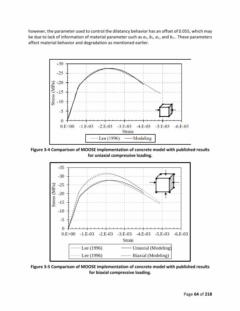
Page 64 of 218
however, the parameter used to control the dilatancy behavior has an offset of 0.055, which may be due to lack of information of material parameter such as at, bt, ac, and bc.. These parameters affect material behavior and degradation as mentioned earlier.
Figure 3-4 Comparison of MOOSE implementation of concrete model with published results
for uniaxial compressive loading.
Figure 3-5 Comparison of MOOSE implementation of concrete model with published results
for biaxial compressive loading.
-35
-30
-25
-20
-15
-10
-5
0-6.E-03-5.E-03-4.E-03-3.E-03-2.E-03-1.E-030.E+00
Stre
ss (M
Pa)
StrainLee (1996) Uniaxial (Modeling)Lee (1996) Biaxial (Modeling)

Page 65 of 218
Figure 3-6 Comparison of MOOSE implementation of concrete model with published results
for (a) stress strain behavior (b) evolution of damage variables in uniaxial tension.
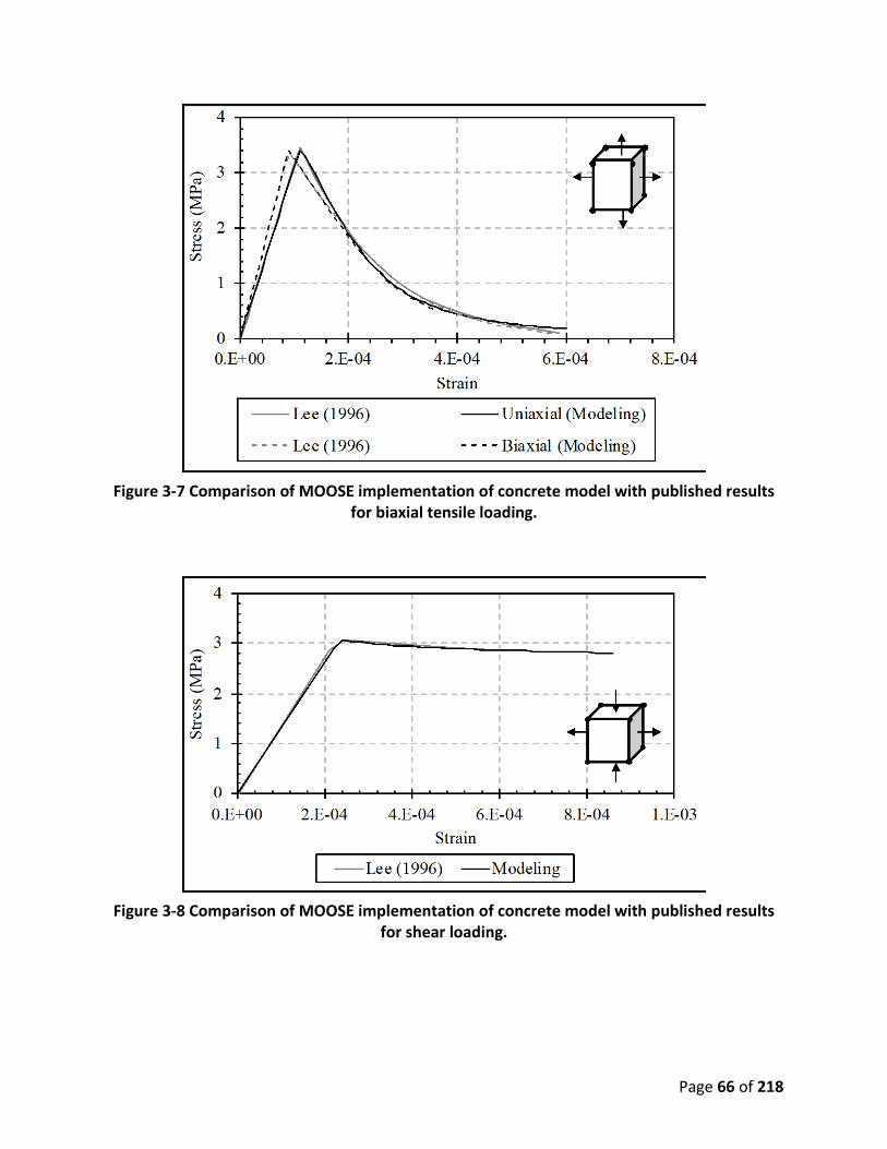
Page 66 of 218
Figure 3-7 Comparison of MOOSE implementation of concrete model with published results
for biaxial tensile loading.
Figure 3-8 Comparison of MOOSE implementation of concrete model with published results
for shear loading.
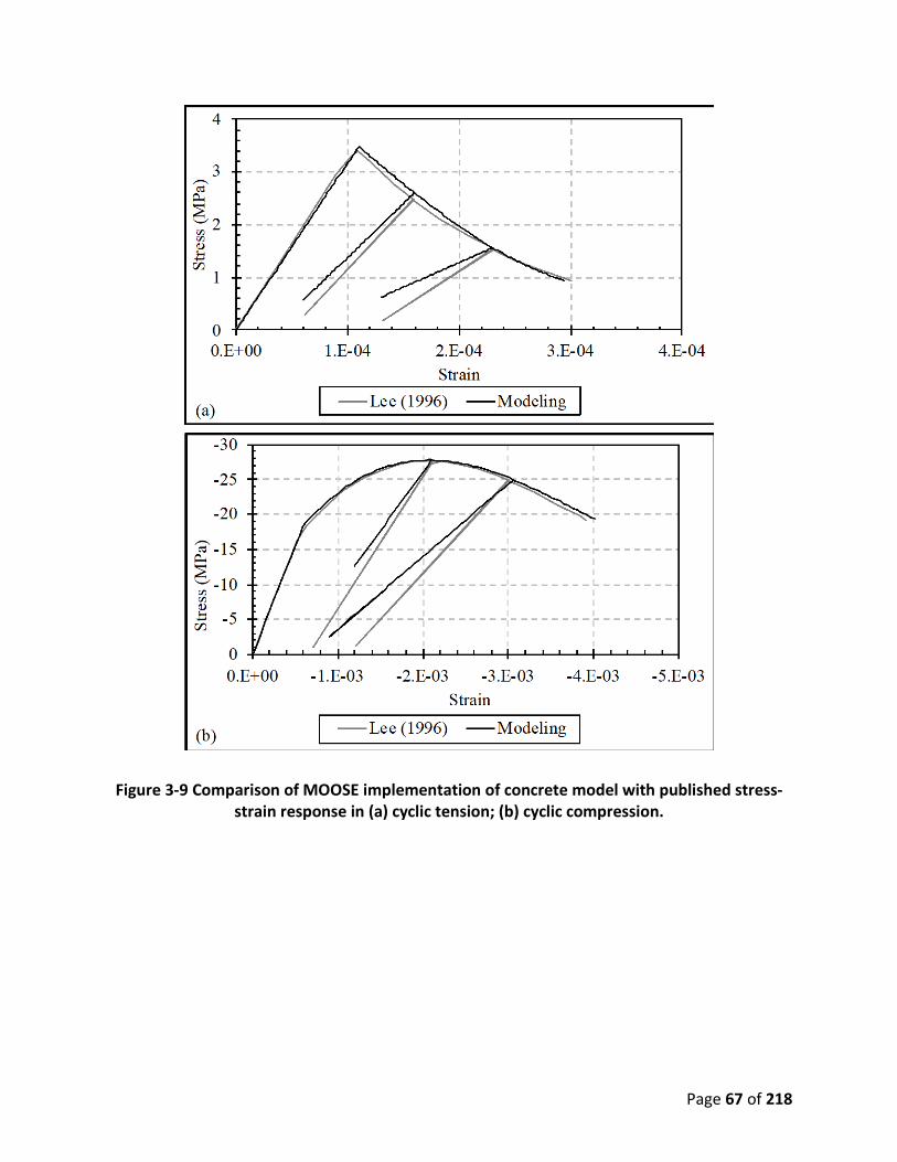
Page 67 of 218
Figure 3-9 Comparison of MOOSE implementation of concrete model with published stress-strain response in (a) cyclic tension; (b) cyclic compression.

Page 68 of 218
Figure 3-10 Comparison of MOOSE implementation of concrete model with published results
for dilatancy behavior in uniaxial compression.
The ability of this model to produce mesh-independent results was tested on a two-dimensional plane stress model. The plane stress condition was obtained in MOOSE (Gaston et al., 2009) by adding an additional field variable describing the out-of-plane strain and enforcing 𝜎𝜎𝑖𝑖𝑖𝑖 = 0 weakly. In this way, the algorithm for three-dimensional or plane strain case is not required to be modified, as it was required for Lee (1996). A two-dimensional rectangular domain was considered as shown in Figure 3-11. The same material parameters were used as in earlier tests as mentioned in Table 3-2. The results for different mesh sizes on the same geometrical model are shown in Figure 3-12. It was observed that the response of the MOOSE-based model is largely independent of the mesh size, however, the results differ somewhat from those obtained by Lee (1996), likely due to lack of information about some of the parameters as discussed previously.
The implementation has also been tested on multi-element models of a concrete cylinder subjected to uniaxial compression and split tension loading. The parameters used are the same as those mentioned in Table 3-2. Model details and simulation results of testing the concrete cylinder under compression are shown in Figure 3-13. Similarly, the loading and boundary conditions for a split tension test of the cylinder are provided in Figure 3-14. These simulations demonstrate that the implementation works well in both strain hardening in compression and strain softening in tension.
The implementation of the plastic-damage model for concrete has been tested here at two scales. First, the implementation was verified for a single element against the results obtained by Lee (1996). The results from the MOOSE implementation of the model generally match the

Page 69 of 218
reference solution very well; however, the results for the dilatancy are offset due to lack of information about a few parameters (such as at, bt, ac, and bc) that govern the material behavior beyond yielding and material degradation. The offset can be eliminated by changing the parameter, 𝛼𝛼𝑝𝑝 , for dilatancy by a constant value of 0.055. The implementation was also for simple structural elements for uniaxial compression and split tension test. In uniaxial compression case, the model predicts the compressive strength correctly and shows hardening behavior, while in split tension test, the model shows a softening behavior as expected.
(a) (b) (c)
Figure 3-11 (a) Coarse, (b) medium and (c) fine mesh for the mesh sensitivity problem.
Figure 3-12 Load-displacement curves for the concrete model using three different meshes to
demonstrate the mesh-independence of the MOOSE.

Page 70 of 218
(a)
(b)
Figure 3-13 Application of MOOSE damage plasticity model to concrete cylinder in uniaxial compression loading. (a) Damage field at maximum load, (b) load-displacement curve and
comparison of maximum value with theoretically assumed value.

Page 71 of 218
(a) (b) (c)
(d)
Figure 3-14 Application of MOOSE damage plasticity model to cylinder under splitting tension loading conditions (a) Geometry of the specimen, (b) loading and boundary conditions, (c)
finite element mesh, (d) load-displacement curve.
Conclusions
A material model for concrete that accounts for the degradation in the elastic stiffness both in tension and compression is implemented in MOOSE (Gaston et al., 2009). It has been shown that the model captures permanent deformation when the material is unloaded from after reaching the yield load both in tension and compression. The model also simulates the dilatancy behavior of concrete and provides similar results for different mesh sizes. The model has been validated
Page 72 of 218
against reference solutions using a single element model for uniaxial and multiaxial tension, compression, and shear loading. Moreover, the model has also been demonstrated to work well for modeling a more complex cylinder test under uniaxial compression and split tension loading to exhibit its performance for the analysis of a plain concrete structural element. The key conclusions of this research are as follows
• In this study, Lee (1996) model was implemented and developed further to link modeling parameters (such as at) with the properties of the softening curve in tension which are not mesh sensitive.
• The material was further developed for the estimation of crack width, which is a function of plastic strain. However, cracking of concrete forms stress-free surfaces and stresses redistribute in the concrete domain. The stress distribution was not considered in this research.
3.2. MODELING THE EFFECT OF DRYING SHRINKAGE-INDUCED DAMAGE ON COUPLED MOISTURE AND CHLORIDE DIFFUSION INTO CONCRETE
Introduction
Knowledge of the influence of cracks on the transport properties of concrete is crucial for determining its durability, since most degradation mechanisms -- such as corrosion, freeze-thaw, and leaching -- are mainly dependent on the ingress of water and aggressive ions through cracks in the concrete material. These cracks have a significant impact on transport properties. Micro-cracks that are randomly distributed have a different effect on transport properties than the localized and connected macro-cracks do. In fact, most concrete structures interact with an environment that subjects them to some form of cracking or other vulnerability. Microcracks provide flow channels for deleterious agents (e.g., water, chloride, oxygen, and sulphates). Subsequently, the deterioration of concrete can be accelerated, and the durability of concrete structures is altered. However, the influence of microcracks on transport properties of concrete is not well understood. Thus, understanding the link between microstructure and transport properties at the macro-scale, and in particular the effect of microcracks on transport processes, will lead to more accurate modelling of degradation processes and service-life prediction of concrete structures.
The following section presents a hygro-mechanical model for simulating the effect of damage induced by drying shrinkage on the coupled moisture and chloride diffusion in concrete. The objective of this model is to better predict the damage that may occur due to different factors under more realistic conditions as well as to reveal the interactive effects between shrinkage induced by dryness and coupled chloride-moisture diffusion.
Model Description
A coupled approach for modeling interaction of transport and mechanical responses are implemented in BlackBear. In this model, the humidity-dependent mechanical model is formulated as a time-dependent analysis where at each time step, The transport part of the

Page 73 of 218
model solves the nonlinear coupled moisture and chloride transport problem taking into account; the effect of water-to-cement ratio, curing time, types of cement and the aggregate content on transport properties. The calculated relative humidity is then used to evaluate the shrinkage strain, where the shrinkage strain of the concrete is calculated based on multiphase composite model. The calculated shrinkage strain is then used in the mechanical part of the model to evaluate the damage induced by the drying shrinkage strain. For the sake of simplicity in this study, the damage evolution in concrete is characterized through the framework of elastic damage mechanics, using a model that is significantly simpler than the damaged plasticity model described in the previous section, although the concepts could also be translated to that model. The interaction between the damage and chloride and moisture diffusion coefficients is considered by using the concept of composite damage mechanics while the effect of damage on the moisture capacity is evaluated by a composite model for effective moisture capacity of a two-phase composite.
Transport Model
3.2.3.a. Governing Equation
The formulation of the governing equation for the coupled moisture and chloride transport problem is based on the transport model proposed by Ababneh (2003). In this model, the transport processes of moisture and chloride ions in non-saturated concrete are considered as a two-way coupling process between the two driving forces of moisture gradient and chloride concentration gradient. The governing equations for the coupled system are presented as follows:
[ ]ftcl cl f cl H
f
CC div D C div D HC t − −
∂∂ = ∇ + ∇ ∂ ∂ 3.65
[ ]H cl f H Hw H div D C div D HH t − −
∂ ∂ = ∇ + ∇ ∂ ∂ 3.66
where Dcl-cl is the chloride diffusion coefficient; Ccl is the free chloride concentration; DH-H is the relative humidity diffusion coefficient; H is the gradient of pore relative humidity; Cf is the free chloride concentration gradient; Dcl-H is the coupling parameter - which represents the coupling effect of moisture diffusion on chloride penetration; DH-cl is the coupling parameter - which represents the coupling effect of chloride ions on moisture diffusion; 𝜕𝜕𝐶𝐶𝑓𝑓/𝜕𝜕𝐶𝐶𝑡𝑡 is the chloride binding capacity; ∂w/∂H is the moisture capacity; Ct is the total chloride concentration, and w is the moisture content in concrete.
3.2.3.b. Material Parameters
Moisture capacity (∂w/∂H)
A multiphase and multiscale model is used to determine the moisture capacity of the concrete (Xi, 1995a). In this model, the concrete is considered as two-phase material, in which phase one

Page 74 of 218
is comprised of the aggregates (inclusions), and phase two is comprised of the cement paste (matrix). Setting aside consideration of the effect of the shrinkage of the concrete, the moisture capacity of the concrete is then defined as the average of the moisture capacities of the two phases as follows:
w w wf fagg cpH H Hagg cp∂ ∂ ∂ = + ∂ ∂ ∂
3.67
Here, 𝑓𝑓𝑐𝑐𝑝𝑝 and 𝑓𝑓𝑚𝑚𝑔𝑔𝑔𝑔 are the weight percentages of the cement paste and the aggregate, and (𝜕𝜕𝑒𝑒 𝜕𝜕𝐻𝐻⁄ )𝑚𝑚𝑔𝑔𝑔𝑔 and (𝜕𝜕𝑒𝑒 𝜕𝜕𝐻𝐻⁄ )𝑐𝑐𝑝𝑝 are the moisture capacities of the aggregate and the cement paste, which can be evaluated based on the model developed by Xi et al. (1994a) and Xi et al. (1994b), and Xi (1995a) and Xi (1995b).
Humidity diffusion coefficient (DH-H)
The effective humidity diffusion coefficient of concrete can be expressed as a function of the diffusion coefficient of cement paste and the diffusion coefficient of the aggregate (Christensen, 1979), as shown here:
1[1 ] / 3 1/ [( / ) 1]
iH Hcp
i Hagg Hcp
gD Dg D D
= + − + −
3.68
where DHcp is the humidity diffusion coefficient of the cement paste; g i is the aggregate volume fraction, and DHagg is the humidity diffusion coefficient of the aggregate. Since the pores in the aggregate are discontinuous, the value of the humidity diffusion coefficient of the aggregate DHagg in Eqn. 3.68 is assumed to be zero (assuming impermeable aggregates). The humidity diffusion coefficient of the cement paste is calculated using the empirical model developed by Xi et al. (1994b).
Chloride binding capacity (𝜕𝜕𝐶𝐶𝑓𝑓/𝜕𝜕𝐶𝐶𝑡𝑡 )
The chloride binding capacity of concrete is defined as the ratio between the rate of change in the free chloride concentration and the rate of change in the total chloride concentration:
( )1 1 1
1
f
t bt f b
f ff
dCdC dCdC d C CdC dCdC
= = =+ +
3.69
In this study, an empirical model developed by Xi and Bažant (1999) based on the Ferundlich isotherm, is used:

Page 75 of 218
11
10135450 35.45
fAB
t fC S H
sol sol
dCdC CA β
β β
−
− −
=
+
3.70
where A and B are material constants related to chloride adsorption that take the values 0.3788 and 1.14, respectively (Wang et al., 2005); βC-S-H is the ratio between the weight of C-S-H gel and the weight of concrete (g/g) (Xi and Bažant, 1999), and can be expressed as follows:
C S HC S H
total
ww
β − −− − = 3.71
The parameter βsol is the ratio between the volume of the pore solution and the weight of the concrete (L/g) (Xi and Bažant, 1999):
( , )sol solsol
conc sol conc sol
V w n H Tw w
βρ ρ
= = = 3.72
where wconc is the weight of concrete; wsol and Vsol are, respectively, the weight and the volume of the pore solution, and ρsol is the density of the pore solution (g/L), which is dependent on the chloride concentration. The term wsol /wconc is the chloride adsorption isotherm, which is defined as a function of the temperature T and relative humidity H of the concrete. The expression of the water adsorption isotherm is given by averaging the adsorption isotherm of the aggregate and that of the cement paste as follows:
( ) ( ) ( ), , ,cp cp g gn H T f n H T f n H T= + 3.73
Here, fagg and fcp are the weight percentages of the aggregate and the cement paste, and nagg(H,T) and ncp(H,T) are the water adsorption isotherms of the aggregate and the cement paste, respectively. Eqn. 3.70 is valid only when the free chloride concentration is greater than 0.01 mol/l. The limitation of Eqn. 3.70 is that, when the free chloride concentration Cf is zero, the value of 𝜕𝜕𝐶𝐶𝑓𝑓/𝜕𝜕𝐶𝐶𝑡𝑡 will be equal to zero, which will cause 𝜕𝜕𝐶𝐶𝑓𝑓/𝜕𝜕𝜕𝜕 to also be equal to zero. This means that Cf will remain constant at all time steps and the diffusion process will not begin. In this work, the Langmuir isotherm is used when the value of free chloride concentration Cf is less than 0.05 mol/l. The Langmuir isotherm is expressed as:
2
1 1111
1
f
bt
ff
dCdCdCdC
Cα βα
= =++
+
3.74
where
'35450
bm C S H
sol
k C βαβ− −= 3.75

Page 76 of 218
1000
C S H bmCβ
β − −
= 3.76
Cf is the free chloride concentrations, Cbm is the bounded chloride concentration at saturated monolayer adsorption, and k’ is an adsorption constant (Wang et al., 2005). The values of k’ and Cbm can be obtained by curve fitting the adsorption test data.
Chloride diffusion coefficient
The chloride diffusion coefficient of concrete Dcl is calculated by using the multifactor method as follows (Ababneh, 2003):
( ) ( ) ( ) ( )1 2 3 4 5( , )cl o i fwD f t f g f H f T f Cc
= 3.77
where the factor f1(to, w/c) accounts for the effects of curing time and water-cement ratio on the chloride diffusion coefficient (Xi and Bažant, 1999). It is represented as follows:
( ) 6.55
1
2828 1( , )62500 4 300
ooo
ttw wf tc c
− − = + +
3.78
The factor f2(gi) accounts for the effect of the composite action on the cement paste and aggregate (Christensen, 1979). The expression for this factor is given as:
[ ] ( )2 ( ) 11 / 3 1/ / 1
ii cp
i agg cp
gf g Dg D D
= + − + −
3.79
where gi is the aggregate volume fraction, and Dcp and Dagg are the chloride diffusion coefficients of cement paste and aggregate, respectively. Dcp and Dagg can be determined by using the model for porous media (Martys et al., 1994).
The factor f3(H) accounts for the effect of the relative humidity. A model proposed by Bazant and Najjar (1972) is used in this study:
( ) ( )( )
14
3 4
11
1 C
Hf H
H
− −
= + −
3.80
The factor f4(T) accounts for the effect of temperature. Arrhenius’ equation is used to account for the temperature effect on the chloride diffusion coefficient, as shown below:
( )41 1expo
Uf TR T T
= −
3.81
Page 77 of 218
Here, R is the gas constant 8.314 J mol-1K-1; To and T are the reference and the current temperatures in Kelvin, respectively, (To = 296K°), and U is the activation energy, which depends on cement type and w/c ratio (Page et al., 1981).
The factor f5 (Cf) accounts for the effect of free chloride concentration on the chloride diffusion coefficient, which can be expressed as follows:
( ) ( )5 1m
f ion ff C k C= − 3.82
where kion = 8.333 and m = 0.5 (Xi and Bažant, 1999).
Coupling parameters
The values for both coupling parameter DH-Cl and DCl-H are determined based on the material models developed in Sections 2.2 and 3.2.
Drying Shrinkage Model
Drying shrinkage strain of concrete is evaluated by a multiphase composite model (Xi and Jennings, 1997). This model is based on a three-phase, generalized, self-consistent model developed by Christensen (1979) for establishing elastic property. In this model, concrete is considered as a heterogeneous composite material composed of two phases: aggregate and cement paste. The microstructure of the heterogeneous composite material is divided into small elements as shown in Figure 3-48a. The partitions of the elements can be adjusted into a spherical system of elements, in which each spherical element in the system has the same internal structure, and each phase within the elements has the same volume fraction Figure 3-48b.
Figure 3-15 Multiphase material with partitioned elements.
Since each phase within the elements has the same volume fraction regardless of its size, any one element can be used as a representative element. The representative element at the mesoscale level consists of three phases: phase 1 is the inclusion (aggregate); phase 2 is the
(a) (b)

Page 78 of 218
matrix (cement paste), and phase 3 is the effective homogeneous medium as shown in Figure 3-16b.
Figure 3-16 Schematic of a three-phase and four-phase composite.
Based on the multiphase composite model, the shrinkage strain and the bulk modulus of concrete at the mesoscale level can be expressed as:
1 1 2 2 2 2 1 2
2 1 2 2 2 1
(3 4 ) (1 )(3 4 )(3 4 ) 4 ( )
sh shsh i iconc
i
K g K G K g K GK K G g G K K
ε εε + + − +=
+ − − 3.83
2 1 2 2 2 1
1 2 2 1
(3 4 ) 4 ( )(3 4 ) 3 ( )
iconc
i
K K G g G K KKK G g K K
+ − −=
+ + − 3.84
where and , K1 and K2, and G1 and G2 are the shrinking strain, the bulk modulus, and the shear modulus for phase 1 and phase 2, respectively; and, gi is the aggregate volume fraction.
As stated earlier, concrete is assumed to be a two-phase composite, and since shrinkage of the aggregate is small and can be disregarded, only the shrinkage of the cement paste would contribute to the shrinkage of the concrete. To measure the shrinkage strain in the cement paste, the cement paste at mesoscale level is considered a four-phase composite material whose components are: phase 1 - the calcium hydroxide (CH) crystals, the ettringite crystals, and the un-hydrated cement particle; phase 2 -- the inner product of C-H-S gel (calcium silicate hydrate); phase 3 -- the outer hydration product of C-H-S gel; and phase 4 -- the effective homogeneous medium. Considering continuity conditions, both phase 1 and phase 2 can be represented as one sphere with an effective bulk modulus K12eff and an effective shrinkage strain 𝜀𝜀𝑒𝑒𝑓𝑓𝑓𝑓12 .
1shε 2
shε
Phase 1 Phase 2 Effective medium
Phase 1 Phase 2 Phase 3 Effective medium
(a) (b) (c)
Page 79 of 218
( )( )
( )( )
1 11 1 2 2 2 2 1 2
12 1 2 1 2
2 1 2 1 1 2 2 1 2
(3 4 ) 1 (3 4 )
(3 4 ) 4 / ( )
sh sh
sheff
f fK K G K K Gf f f f
K K G f f f K K G
ε εε
+ + − + + + =
+ − + − 3.85
( )
11 2
12 1 22
1213 3 3
1 2
( )( )
41 1 /( ) 3
eff
eff
f K Kf fK K
f K K K Gf f
−+
= + + − − + +
3.86
Similarly, the expression can be extended to the third phase as shown in Figure 3-17:
(a) (b)
Figure 3-17 (a) Schematic of a three-phase composite. (b) Schematic of effective homogeneous medium.
( ) ( )1212 121 2 3 3 3 3 3 312 12
3 3 1 2 3 3
(3 4 ) (3 4 )(3 4 ) 4( )( )
sh sheff eff effsh
cpeff eff
K f f K G K f K GK K G f f K K G
ε εε
+ + + +=
+ − + − 3.87
( )
121 2 3
312
3 3 3 3
( )( )41 /3
effcp
eff
f f K KK K
f K K K G
+ −= +
+ − +
3.88
in which 𝜀𝜀𝑠𝑠ℎ , G, K, and f are the shrinkage strain, shear modulus, bulk modulus, and volume fraction of phases 1, 2, and 3 of the cement paste.
Among these three phases, only the C-H-S gel expands or shrinks due to changes in the relative humidity. Whereas, based on the experimental result using environmental scanning electron microscopy, it was found that the shrinkage of the first phase (un-hydrated cement particles, calcium hydroxide (CH) crystals, and ettringite crystals) is very small and can be disregarded (Neubauer et al., 1997). Since the shrinkage of inner products (phase two) is also very small, even for the wide range in relative humidity of 30-40%, the shrinkage of C-S-H is mainly the result of the outer hydration product. Thus, Eqn. 3.88 becomes:
K1
K2
K3
K12eff

Page 80 of 218
( )( )
123 3 3 3
12 123 3 1 2 3 3
(3 4 )(3 4 ) 4 ( )
sheffsh
cpeff eff
K f K GK K G f f K K G
εε
+=
+ − + − 3.89
The volume fractions of the three phases can be calculated as follows:
1 core CH AFmf f f f= + + 3.90
( ) ( )3 10.706 / 0.131 1 pores poresf w c f f f= + − + + 3.91
2 1 31f f f= − + 3.92
where fCH, fAFm, and fcore are the volume fractions of the CH and AFm (ettringite crystals); fpores is the capillary volume fraction; and the volume fraction of the unreacted core of the cement particles’ force can be obtained using the comprehensive model developed by Jenning and Tennis (2007).
Mechanical Model
The mechanical model is formulated as a relative humidity dependent model in which the drying shrinkage strain is mainly dependent on the change in the pore relative humidity. The nonlinearity of the concrete mechanical behavior originating from the growth of micro-cracks along the concrete mass is taken into account by the concept of continuum damage mechanics. The damage models allow us to represent this mechanical behavior by assessing material stiffness as a function of strain increment. The Mazars concrete damage model (Mazars, 1984; Pijadudier-Cabot and Mazars, 2001) was used in this study. The model describes the elastic stiffness degradation and the softening behavior of concrete under both uniaxial tension and uniaxial compression using an isotropic scalar damage variable w. The damage variable depends only on the effective stresses applied to an undamaged area. The evolution of the damage is determined by the equivalent strain that quantifies the amount of the local extension state during the mechanical loading. It is calculated from the positive eigenvalues of the strain tensor as follows:
( )3 2
1i
iε ε
+=
= ∑ 3.93
where 𝜀𝜀𝑚𝑚 is the principal strain and ⟨∙⟩+ is the Macauley bracket and is defined as:
00 0
i i i
i i
ε ε εε ε
+
+
= ≥ = ≤
3.94
The loading damage threshold is defined as a function of equivalent strain as follows:
( ),f ε κ ε κ= − 3.95

Page 81 of 218
where 𝜅𝜅 is the parameter containing the threshold of damage growth. Initially, 𝜅𝜅 is equal to ft/Eo and then it takes the maximum value of the equivalent strain during the entire load history:
max( , )d oκ ε κ= 3.96
In order to account for the different behavior of the concrete in tension and in compression, the scalar damage w is defined as a combination of two damaging modes as expressed in:
t t c cw w wα α= + 3.97
where αt and αc are dimensionless coefficients and represent the contribution of each loading mode such that αt = 1 and αc = 0 under uniaxial tension; and, αt = 0 and αc = 1 under uniaxial compression. These coefficients are defined as functions of the strain that result from negative and positive stresses:
1(1 )t tkl ijkl ijw Cε σ−= − , 1(1 )c c
kl ijkl ijw Cε σ−= − 3.98
3
21
ti i
ti
βε ε
αε=
=
∑
, 3
21
ci i
ci
βε ε
αε=
=
∑
3.99
where at, ac, Bt, and Bc are material parameters that control the shape of the curve peak and are determined using compression and tension tests. After the scalar damage w is defined, the constitutive relation for the nominal stress is described by:
(1 ) :w Eσ ε= − 3.100
where 𝜎𝜎 is the effective stress tensor, 𝜀𝜀 is the strain tensor, E is the elastic stiffness tensor and w is the damage variable.
Effect of Damage on Transport Properties
3.2.6.a. Moisture Capacity
A composite model for the effective moisture capacity of a two-phase composite material (Xi, 1995b) was used in this study. The model was developed using the extreme energy principle method utilized by Rosen and Hashin (1970) to evaluate the effect of thermal strain on the heat capacity of two-phase composite material. In this model, Rosen and Hashin (1970) proposed that effective heat capacities could be expressed as a function of the volumetric average of the heat capacities of the constituent phases, the thermal expansion, and the bulk modulus of the material. Similarly, the effective moisture capacity can be represented by two terms: (a) the first term is the volumetric average of the moisture capacities of the constituent phases, and (b) the second phase is the coupling effect, which is defined as a function of the bulk modulus, the shrinkage coefficients of the constituents, and the volume fraction of the inclusion. The effective moisture capacity can be expressed as follows:
Page 82 of 218
2
0
0
1 19 1 1i m
im
avg conc
w w HH H RT K K
k K
β βψ
∂ ∂ − = + + ∂ ∂ −
3.101
1 m i
m i
g gK K K
= +
and
( ) ( )( )
1 / 4 / 3i m
conc m
i m m mm
ig K KK Kg k k k G
−= +
+ − + 3.102
where (dw/dH)avg is the volumetric average of moisture capacities of cement paste and aggregate without considering the effect of shrinkage, which can be determined based on the BET adsorption isotherm; Ψ is a factor used to convert units from mole/m3 to gram/gram; and, R is the gas constant in Joules/mole/K. The reference temperature and reference humidity are T° and H° (in Kelvin); β i and βm are the shrinkage coefficients for the aggregate and the cement paste; and Gm is the shear modulus of the cement paste. Km, K i,, and Kconc are the bulk modulus of cement paste, aggregate, and concrete, respectively. Furthermore, here gi and gm are the volume fraction of the aggregate and the cement paste.
3.2.6.b. Diffusion Coefficient
This study used a composite damaged model for diffusivity of distressed materials. The model defines the distressed material as a two-phase composite material with intact material as phase one and distressed material as phase two. The effective diffusivity of the composite material can be characterized by using the model developed by Christensen (1979) for determining the conductivity of the spherical spatial distribution of the constituent phases:
( ) [ ]21 2
( , ) 11 / 3 1/ ( / ) 1H
wD H w Dw D D
= + − + −
3.103
where D1 is the (humidity/chloride) diffusivity of undamaged concrete; D2 is the diffusivity of (humidity/chloride) in damaged concrete; and, w is the scalar damage parameter.
Numerical Results
The application of this model to simulate the effect of the moisture transport on chloride ion diffusion and the effect of concrete mix parameters on the diffusion process has been found to yield very good results. The following numerical simulation example focuses on chloride penetration into non-saturated concrete. In this example, a concrete slab is used in the numerical simulation. The slab was exposed to 100% relative humidity and a 3% Cl solution on the top surface. The other sides of the slab are assumed sealed. The initial relative humidity inside the slab is Hini = 0% and the initial free chloride concentration is Cl0 = 0. The values of material parameters used in the simulation are shown in Table 3-3.

Page 83 of 218
Figure 3-18 Geometry of the sample used in numerical analysis.
Table 3-3 Input Data for Concrete Sample.
Parameter Value Water–Cement ratio (w/c) 0.65 Aggregate volume fraction (gi) 0.7 Cement type I/II Curing time (day) 28 Temprature (k) 296o Initial free chloride concentration (g/g) 0 surface chloride concentration (g/g) 0.0065 Initial relative humidity % 50% surface relative humidity % 100%
Figure 3-19 shows a 3D plot of the distribution of the moisture and free chloride ions after 10 days of exposure. The change in the free chloride concentration profile and the relative humidity profile at different times of exposure (5 Days, 10 Days, 1 months, 2 months, and 3 months) are shown in Figure 3-20.
(a) (b) Figure 3-19 (a) Chloride ion distribution. (b) Moisture distribution

Page 84 of 218
(a) (b)
Figure 3-20 (a) Variation of relative chloride profile at different time of exposure.(b) Variation of relative humidity profile at different time of exposure.
Model Validation
3.2.8.a. Transport Model
In this section, the experimental data from Safeer Abbas and Moncef (2014) was used for validating the chloride diffusion model implemented in BlackBear. The specimens tested by Safeer were cylindrical cores extracted from conventional reinforced concrete (RC) and steel fiber-reinforced concrete (SFRC) tunnel segments. Cores were drilled through the entire segment depth (235 mm). The full depth core was divided into three specimens. The upper and bottom specimens represented the external (extrados or intrados faces of segments), while the middle part of the core represented the internal core of the segment. The external and internal core specimens of 100 mm (4 in.) diameter and 75 mm (3 in.) thickness from both RC and SFRC were used in the chloride ponding test. 3% sodium chloride (NaCl) solution was applied to the top surface of the specimens. At the end of 90 days of salt ponding, approximately 10 g (0.35 oz) of concrete powder samples were collected from the tested specimens at different depths from the top surface at intervals of 3 mm (0.12 in.) for determining the concentration and penetration of Cl– inside the concrete. The chloride concentration profiles obtained from the experiments were compared with the numerical results obtained from the present model as shown in Figure 3-21. The result predicted by the transport model for non-damaged concrete is in very good agreement with the test data.
0
0.005
0.01
0.015
0.02
0.025
0.03
0.035
0 0.5 1 1.5 2 2.5 3
Chl
orid
e lv
el (%
wig
ht o
f con
cret
e )
Depth Cm
5 Days10 Days30 Days60 Days90 Days
10%
20%
30%
40%
50%
60%
70%
80%
90%
100%
110%
0 1 2 3
Rel
ativ
e hu
mid
ity
Depth Cm
5 Days10 Days30 Days60 Days90 Days

Page 85 of 218
Figure 3-21 Comparison between the stress-strain responses obtained from the numerical
model compared with the experimental data.
3.2.8.b. Damage Model
To validate the accuracy of the damage model, the results from the numerical simulation were compared with available test data. The numerical simulation was conducted using a single quadrilateral finite element (82.6 mm x 82.6 mm). Figure 3-22a and Figure 3-22b illustrate a comparison between the stress-strain responses obtained from the numerical model compared with experimental data (Gopalaratnam and Surendra, 1985) in the tension case and in the compression case (Karsan and Jirsa, 1969). As can be seen in Figure 3-22, the numerical results agree well with the test data.
0
0.05
0.1
0.15
0.2
0.25
0.3
0.35
0 1 2 3 4 5
Chl
orid
e lv
el (%
wig
ht o
f con
cret
e )
Depth cm
ModelSFRC internalRC internalRC externalSFRC external

Page 86 of 218
(a)
(b)
Figure 3-22 Comparison between the stress-strain responses obtained from the numerical model compared with the experimental data for (a) compression case. (b) tension case.

Page 87 of 218
Numerical Example of Coupled Damage and Transport
In order to demonstrate the influence of the damage caused by drying shrinkage on the transport process, numerical experimentation was performed on a model of a concrete slab. The boundary conditions for the transport and mechanical analyses are shown in Figure 3-23. The initial relative humidity inside the slab was assumed to be 60% and the top surface of the slab was subjected to drying conditions for 30, 90, and 180 days, after which a 3% (by weight) sodium chloride solution was applied to the top surface of the specimen for 60 days. All other sides of the specimen were assumed be sealed so no flux is allowed. Since the material models used in the transport analysis are defined as function of a set of concrete mixing parameters, the specimen was assumed to be prepared using Type II Portland Cement, with w/c of 0.5, and aggregate volume fraction of 0.6.
Figure 3-23 Boundary conditions for the transport and mechanical analysis: (a) drying boundary conditions; (b) wetting boundary conditions, and, (c) mechanical boundary
conditions.
Figure 3-24 illustrates the distribution of relative humidity, the development and distribution of damage during the drying process, and the stress distribution due to the shrinkage strain at 10 days and 30 days. It can be seen from the figure that the damage occurs in the upper surface of the slab with short extension into the slab depth. The damage development is due to restrained differential shrinkage resulting from the change in the moisture gradient during the drying process.

Page 88 of 218
(a)
(b)
(c)
Figure 3-24 (a) Relative humidity distribution at 10 days and 30 days, (b)damage distribution at 10 days and 30 days (c) stress distribution at 10 days and 30 days.
The effect of drying-shrinkage damage on the transport properties is shown in Figure 3-25 and Figure 3-26. These figures show the analysis of the slab under two circumstances. In the first scenario, the slab was subjected to a periodical drying-wetting cycle without considering any evolution in damage. In the second scenario, the slab was subjected to the same periodic drying-wetting cycle with the evolution in damage noted. As shown in Figure 3-25, the chloride ions diffuse at a faster rate when the damage is considered in the analysis. Figure 3-26 shows how the presence of damage accelerated moisture diffusion as well. As expected, the rate of both moisture and chloride penetration depth increases with the increase in the damage evolution, which indicates that the formation of the microcracks induced by drying shrinkage accelerates the diffusion process and increases the rate of drying.

Page 89 of 218
Figure 3-25 The effect of drying-shrinkage damage on chloride ion penetration.
Figure 3-26 The effect of drying-shrinkage damage on moisture penetration.
Conclusions
• A finite element model was developed to evaluate the influence of the damage induced by drying shrinkage on coupled moisture and chloride diffusion in concrete.
0
0.005
0.01
0.015
0.02
0.025
0.03
0.035
0 0.5 1 1.5 2 2.5 3
Chl
orid
e lv
el (%
wig
ht o
f con
cret
e )
Depth Cm
No Damage
Damage
10%
20%
30%
40%
50%
60%
70%
80%
90%
100%
110%
0 0.5 1 1.5 2 2.5 3
Rel
ativ
e hu
mid
ity
Depth Cm
10 Days No Damage
10 Days Damage

Page 90 of 218
The FEM model is based on the coupled interaction approach of transport and mechanical responses.
• The transport part of the model was developed to consider the effect of different concrete mix parameters on the diffusion process, this effect is included in the material models for diffusivities, capacities, and coupling parameters.
• The drying shrinkage of concrete is calculated based on a multiphase composite model in which concrete is considered as a heterogeneous composite material composed of two phases: aggregate and cement paste.
• The damage induced by drying shrinkage was evaluated using the Mazars damage model in which the evolution of the damage is determined by the equivalent strain that quantifies the amount of the local extension state.
• The influence of the drying shrinkage damage on the moisture capacity is evaluated by a composite model for effective moisture capacity of a two-phase composite. The effect of drying shrinkage on chloride and moisture diffusion coefficients is considered using a composite-damaged model for diffusivity of distressed materials
• Based on the obtained results, it was found that the damage and cracks induced by drying shrinkage can accelerate the moisture movement in and out of concrete.
3.3. MODELING THE EFFECT OF DRYING SHRINKAGE-INDUCED DAMAGE ON MULTI-IONIC TRANSPORT IN NON-SATURATED CONCRETE
Introduction
In Section 3.2, the numerical model was developed using Fick’s laws of diffusion, which are based on the assumption that the diffused ions are considered to be uncharged particles (neutral particles). Thus, the electrical interactions between the chloride ions and other ions that may be present in the solution are not considered. When aggressive agents such as magnesium chloride (MgCl2), calcium chloride (CaCl2), and sodium chloride (NaCl) penetrate into concrete, chloride is not the only ion type diffusing in the concrete; other ions diffuse in the concrete simultaneously. In addition to these other ions, the solution present in the porous space is itself a highly charged ionic solution consisting of different species, mainly OH, Na+, K+, SO2 -4 and Ca+2. In an ionic solution, the electro-neutrality of the solution should be preserved locally at all points. To maintain this condition, all diffusing ions should drift at the same rate during the diffusion process. Since these species have different diffusion coefficients and different charge numbers, some of the species move faster than others, resulting in the creation of an electrical field, which then accelerates the slow-moving ions and slows down the faster ones. This section presents a numerical model for the effect of shrinkage damage on multi-species diffusion in concrete. In the transport part of the model, the Nernst-Planck equation is utilized to describe the diffusion of the multiple species in concrete while considering the influence of the electrical coupling between the different species. The coupling effect of moisture and multi-ion diffusion is also incorporated into the governing equation. Furthermore, the effect of drying shrinkage damage on the diffusion coefficients and coupling parameters of the different species is taken into account. The simulation results are then examined to determine the significance of the

Page 91 of 218
influence of the ionic interaction between the different species, and the effect of drying shrinkage damage on multi-ion diffusion.
Model Description
The model presented in this chapter is an extension of the coupled hygro-mechanical model developed in the previous section. Both models have identical shrinkage and mechanical damage algorithms. However, the transport part of the model is different in that in this model the Nernst-Planck equation is employed to simulate multi-ion penetration through non-saturated concrete considering the electrical coupling between the ions. The focus in this section will be on the implementation of the Nernst-Planck equation in the coupled hygro-mechanical model developed in the previous section.
Transport Model for Coupled Multi-Species Diffusion
3.3.3.a. Governing Equation
In the current formulation, extended Nernst-Planck equation is used to describe the transport process of multi-ions. The diffusive fluxes of each ion (i) is described by Nernst-Planck equation (Bard and Faulkner, 2001) as follows:
i i i i i iFJ D C z D C
RT = − ∇ + ∇Φ
3.104
where Ji is the flux value of ionic species i, Ci is the ionic concentration in the solution, D i is the effective diffusion coefficient, F is Faraday’s constant, R is the universal gas constant, T is the temperature, z is the valence number of the species, and Ф is the applied electrical potential. The two terms in the right-hand side of Eqn. 3.104 represent two different mechanisms. The first mechanism is the movement of ions induced by the concentration gradient, and the second mechanism is the effect of the electrical field. At this stage, the model does not account for the effect of the chemical activity.
The transport process for each ionic species in the solution can be described based on the principle of mass conservation:
ii
C Jt
∂= −∇
∂ 3.105
By substituting Eqn. 3.104 into Eqn. 3.105, the general mass balance equation for each individual ionic species can be expressed as:
it it ii i i i i
i
C C C FD C z D Ct C t RT
∂ ∂ ∂ = = ∇ ∇ + ∇Φ ∂ ∂ ∂ 3.106
To solve the system of equations, another relation is needed to evaluate the local electrical potential induced by the movement of the ions. Several relations can be used for this purpose,

Page 92 of 218
including the nil current and Poisson’s equation relations. The nil current relation (Wang et al., 2005) is based on the assumption that during the diffusion process the current in the system is equal to zero:
10
n
i ii
F J z=
=∑ 3.107
In the Poisson’s equation relation (Samson and Marchand, 2007), the variation of the electrical potential is defined according to the spatial distribution of the electrical charges:
2i i
F z Cε
∇ Φ = − ∑ 3.108
where ɛ is the dielectric constant of the solvent times the vacuum permittivity.
The electro-neutrality condition is based on the assumption that the electro-neutrality of the solution is preserved at all points:
10
n
i ii
C z=
=∑ 3.109
In this work, a nil current assumption will be used to solve for the electrical potential. Substituting Eqn. 3.107 into Eqn. 3.104, the expression for the electro-potential can be expressed as:
10
n
i i i i i ii
FF z D C z D CRT=
− ∇ − ∇Φ = ∑ 3.110
1
2
1
.
n
i i ii
n
i i ii
z D CRTFz D C
=
=
∇∇Φ = −
∑
∑ 3.111
By substituting Eqn. 3.111 into Eqn. 3.106, we obtain the general governing equation:
1
2
1
n
i i iit it i i
i i i i ini
i i ii
z D CC C C D C z D Ct C t z D C
=
=
∇ ∂ ∂ ∂ = = ∇ ∇ + −∂ ∂ ∂
∑
∑ 3.112
To account for the coupled interaction between the moisture movement and the diffusion of the different species, Eqn. 3.104 is modified to include the coupling term. The general governing equations for moisture and each individual ionic species, respectively, are expressed as:
( ) ( )H i i Hw H D C D HH t −
∂ ∂= ∇ ∇ +∇ ∇
∂ ∂ 3.113

Page 93 of 218
1
2
1
n
i i iit it i i
i i i i i H ini
i i ii
z D CC C C D C z D C D Ht C t z D C
=−
=
∇ ∂ ∂ ∂ = = ∇ ∇ + − + ∇∂ ∂ ∂
∑
∑ 3.114
where Di-H is the coupling parameter, which represents the coupling effect of moisture diffusion on ionic penetration; and DH-il is the coupling parameter, which represents the coupling effect of ions on moisture diffusion.
3.3.3.b. Material Parameters
Capacity and diffusivity coefficients
The material model used for the moisture capacity, chloride binding capacity, moisture diffusion coefficient, and chloride diffusion coefficient are similar to the material models introduced in Section 3.3.2. In these models the moisture capacity is defined as the average of the moisture capacities of cement paste and aggregate, and the chloride binding capacity is defined as the ratio between the change of free chloride content and total chloride. The moisture diffusion coefficient is calculated as a function of the diffusion coefficient of cement paste and the diffusion coefficient of aggregate. The chloride diffusion coefficient of can be estimated using the multifactor method. For other species, the capacity is employed as 1, and the diffusion coefficients are defined as constant values
Coupling parameters
The material model proposed in section 2-3 for determining the coupling parameters DCl-H and DH-cl were used to account for the effect of moisture on chloride diffusion and the effect of the chloride on moisture diffusion. Both coupling parameter Dcl –H and DH-ch are concentration dependent and they are expressed in terms of free chloride concentration. However, there are no available experimental data or material models for coupling parameters for the other species, A reasonable assumption can be made that the effect of moisture on ionic diffusions can be considered as being the same as the effect of moisture on chloride ions. This is due to the fact that the moisture movement can carry any other ions in the same way as it carries the chloride ions. On the other hand, the effact of the multiple species on the moisture diffusion is highly dependent on the diffusion rate of each single ionic species. We assume that the effect of the multiple species on the moisture diffusion can be estimated as the ratio between the specific ionic species and the chloride ions as shown:
.
l .f
i H ci i Ci
cl H c clf
D DD D C
δδ
−
−
= = 3.115
Numerical Solution
To solve the initial boundary value problem for Eqn. 3.114, both initial conditions at time (t = 0) and the boundary conditions are imposed on the functions. The initial condition is expressed as:

Page 94 of 218
( ) ( ), 0i ioC x t C x= = , ( )x∈ Ω∪Γ 3.116
Considering a Dirichlet boundary condition applied on boundary Γ𝑝𝑝:
( ),i i sC x t C= , px∈Γ 3.117
Considering continuity of Eqns. 3.113 and 3.114, the system of equations can be solved numerically. The above-mentioned equations were implemented in BlackBear and used to compute the concentration profiles of the different species, assuming the concentration of each ionic species varies linearly within each element. The nodal concentration of the free ions is solved by applying a Galerkin method to the weak forms of the governing equations. The finite element matrix can be obtained as follows:
Where
0e ei iM C K C + = 3.118
[ ][ ]e TK B D B d = Ω ∫ 3.119
Here [Me] is the capacity matrix; and, [Ke] is the conductivity matrix [m], and [D] can be expressed as:
0 0 0 0 0
0 0 0 0 0
0 0 0 0 0
0 0 0 0 0
0 0 0 0 0
0 0 0 0 0
t
f H H
t Cl H
f Na H
t K
f
t
f
t
f
wwtHTCtC DCf
Na DtNa DNa
K Dtt K
tOHOHOH
tCaCaCat
−
−
−
∂ ∂ ∂ ∂ ∂ ∂ ∂ ∂ ∂ ∂ ∂ ∂ ∂ = ∇ ∂ ∂ ∂ ∂ ∂∂ ∂ ∂ ∂∂ ∂ ∂ ∂
H Cl H Na H K H OH H Ca
Cl Cl Cl Na Cl K Cl OH Cl Ca
Na Cl Na Na Na K Na OH Na Ca
H K Cl K K K OH K CaK Na
OH K OH OH OH CaOH H OH Cl OH Na
Ca K Ca OH Ca CaCa NaCa H Ca Cl
D D D D D HD D D D D CD D D D DD D D DD
D D DD D DD D DDD D
− − − − −
− − − − −
− − − − −
− − − − −−
− − −− − −
− − −−− −
∇ ∇
lNaK
OHCa
∇ ∇ ∇ ∇
3.120
Considering the expression and origin of the self-induced electrical field from Eqn. 3.111, the fully coupled diffusion coefficient matrix [D] can be expressed as:

Page 95 of 218
32
1
32
1
32
1
32
1
2
.. . .. .
.. . .. .
.. . .. .
.. . .. .
.. . .. .
H ClH H
cl clCl cl cl cl
i i iCl H i
cl clNa Na Na
Na Hi i i
i
cl clK K K
K Hi i i
i
cl clOH OH OHOH H
i i ii
cl clCa H Ca Ca Ca
i i ii
DDZ DD Z D CZ D C
DZ DZ D CDZ D C
Z DZ D CDZ D C
Z DZ D CDZ D C
Z DD Z D CZ D C
−−
− =
−
=
−
=
−
=
−
=
−
−
−
−
−
∑
∑
∑
∑
32
1
32
1
32
1
32
1
3 32
1 1
. .. . . . . .. .
.. . .. .
.. . .. .
.. . .. .
.. . .. .
H Na H K
Na Na K Kcl cl cl cl cl cl
i i ii
Na NaNa Na Na Na
i i ii
Na NaK K K
i i ii
Na NaOH OH OH
i i ii
Na NaCa Ca Ca
i i ii
D DZ D Z DZ D C Z D CZ D C
Z DD Z D CZ D C
Z DZ D CZ D C
Z DZ D CZ D C
Z DZ D CZ D C
− −
=
=
=
=
=
− −
−
−
−
−
∑
∑
∑
∑
∑ ∑
3322
11
32
1
32
1
32
1
32
1
.. . .. .. .
.. . . .. . .. .
.. . .. .
.. . .. .
.. . .. .
H OH
OH OHcl cl cl
i i ii i iii
OH OHK KNa Na NaNa Na Na
i i ii
K KK K K K
i i ii
K KOH OH OH
i i ii
K KCa Ca Ca
i i ii
DZ DZ D C
Z D CZ D C
Z DZ D Z D CZ D CZ D C
Z DD Z D CZ D C
Z DZ D CZ D C
Z DZ D CZ D C
−
==
=
=
=
=
−
−−
−
−
−
∑∑
∑
∑
∑
∑
32
1
3 32 2
1 1
32
1
32
1
32
1
.. . .. .
.. . .. . . .
.. . . . . .. .
.. . .. .
.. . .. .
H Ca
Ca Cacl cl cl
i i ii
Ca CaNa Na Na
i i i i i ii i
OH OHK K K K K K
i i ii
OH OHOH OH OH OH
i i ii
OH OHCa Ca Ca
i i ii
DZ DZ D CZ D C
Z DZ D CZ D C Z D C
Z D ZZ D C Z D CZ D C
Z DD Z D CZ D C
Z DZ D CZ D C
−
=
= =
=
=
=
−
−
− −
−
−
∑
∑ ∑
∑
∑
∑
32
1
32
1
32
1
.
. .
.. . .. .
.. . .. .
Ca Ca
i i ii
Ca CaOH OH OH
i i ii
Ca CaCa Ca Ca Ca
i i ii
D
Z D C
Z DZ D CZ D C
Z DD Z D CZ D C
=
=
=
−
−
∑
∑
∑
3.121
The resulting nonlinear system of coupled equations is then solved using Jacobian-free Newton–Krylov method.
Numerical Results
The transport model described above has been tested using selected examples to simulate multi-ionic diffusion in non-saturated concrete. In this example, a concrete sample with dimensions of 30 cm by 6 cm was exposed to 3% NaCl and 3% CaCl2 solutions on the top surface; the other boundaries of the sample are assumed to be insulated (see Figure 3-27). The three main ionic species in the concrete pore solution -- potassium (K+), sodium (Na+), and hydroxyl (OH–) -- are considered. The physical coefficients present in the governing equations take the following values: F = 96500 C mol-‘, R = 8.314 J K-’ mol-‘, and T = 293.0 K. The diffusion coefficients, the initial conditions, and the boundary conditions of each individual ionic species are presented in Table 3-4.
Figure 3-27 Boundary conditions of the transport model.

Page 96 of 218
Table 3-4 Input Data for Numerical Simulation.
3.3.5.a. Effect of Electrical Interactions
In order to investigate the effect of the electrical interactions on the ionic ingress, Figure 3-28 through Figure 3-33 show the numerical result of the concentration profiles for chloride, sodium, calcium, hydroxyl, and potassium, for the saturated specimen at 10, 30, 60, and 90 days of exposure for two cases. In the first case, the electrical interactions between the ions is considered as shown in the figures via the solid line. In the second case, the electrical interactions between the ions is not considered as shown in the figures via the dashed line. As can be seen in these figures, the effects of the electrical potential on ionic diffusion induced by the movement of the dissolved ions in the solution are small at low ionic concentration. However, as the concentration of the ions increases, the influence of the electrical potential becomes more significant. Again, referencing the figures, the electrical potential induced by the movement of the ions in the solution, since they are electrically charged species, tends to accelerate the rate of diffusion of the sodium, calcium, and hydroxyl, while the diffusion rates of the chloride and potassium are slowed down.
Species K Na Cl OH Ca Charge number +1 +1 -1 -1 -2
Diffusion coefficient (m2/s) 4.00E-11 2.80E-11 Matrail
model 5.30E-10 1.60E-11
Initial condition at top surface (mol/liter) 0 0.531 1.053 0 0.27
Initial condition in pore solution (mol/liter) 0.0995 0.0389 0 0.1384 0
Cement type II Water-cement 0.55
Volume fraction of aggregate (gi) 0.65
Outside RH (%) 100 Inside RH (%) 60
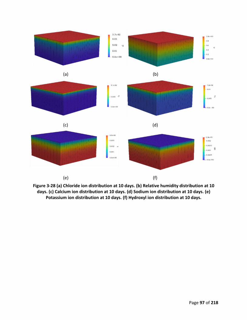
Page 97 of 218
(a) (b)
(c) (d)
(e) (f)
Figure 3-28 (a) Chloride ion distribution at 10 days. (b) Relative humidity distribution at 10 days. (c) Calcium ion distribution at 10 days. (d) Sodium ion distribution at 10 days. (e)
Potassium ion distribution at 10 days. (f) Hydroxyl ion distribution at 10 days.

Page 98 of 218
Figure 3-29 Effect of electrical interactions on concentration profiles for potassium ions at
different times of exposure.
Figure 3-30 Effect of electrical interactions on concentration profiles for hydroxyl ions at
different times of exposure.
0
0.0005
0.001
0.0015
0.002
0.0025
0.003
0.0035
0.004
0.0045
0 0.5 1 1.5 2 2.5 3
K (m
ol/l)
Depth Cm
10 Days ( Interaction)
30 Days ( Interaction)
60 Days (Interaction)
90 Days ( Interaction)
10 Days ( No interaction)
30 Days ( No interaction)
60 Days ( No interaction)
90 Days ( No interaction)
0
0.0005
0.001
0.0015
0.002
0.0025
0 0.5 1 1.5 2 2.5 3
OH
(mol
/l )
Depth Cm
10 Days ( Interaction)
30 Days ( Interaction)
60 Days (Interaction)
90 Days ( Interaction)
10 Days ( No interaction)
30 Days ( No interaction)
60 Days ( No interaction)
90 Days ( No interaction)

Page 99 of 218
Figure 3-31 Effect of electrical interactions on concentration profiles for sodium ions at
different times of exposure.
Figure 3-32 Effect of electrical interactions on concentration profiles for calcium ions at
different times of exposure.
0
0.002
0.004
0.006
0.008
0.01
0.012
0.014
0 0.5 1 1.5 2 2.5 3
Na(
mol
/l)
Depth cm
5 Days ( Interaction)
10 Days ( Interaction)
30 Days ( Interaction)
60 Days (Interaction)
90 Days ( Interaction)
5 Days ( No interaction)
10 Days ( No interaction)
30 Days ( No interaction)
60 Days ( No interaction)
90 Days ( No interaction)
0.00E+00
2.00E-03
4.00E-03
6.00E-03
8.00E-03
1.00E-02
1.20E-02
0 0.5 1 1.5 2 2.5 3
Ca
(mol
/l)
Depth cm
5 Days ( Interaction)
10 Days ( Interaction)
30 Days ( Interaction)
60 Days (Interaction)
90 Days ( Interaction)
5 Days ( No interaction)
10 Days ( No interaction)
30 Days ( No interaction)
60 Days ( No interaction)
90 Days ( No interaction)

Page 100 of 218
Figure 3-33 Effect of electrical interactions on concentration profiles for chloride ions at
different times of exposure.
3.3.5.b. Simulation Results for the Effect of Shrinkage-Induced Damage
To examine the influence of drying shrinkage damage on the ionic concentration profiles for chloride, sodium, calcium, hydroxyl, and potassium, numerical analysis was performed on a slab subjected to drying conditions for 30 days, after which 3% (by weight) sodium chloride solution was imposed on the top surface of the specimen for 90 days. In this analysis, two cases were considered: (a) in the first case, the numerical analysis is performed without considering any evolution in damage; and, (b) in the second case, the numerical analysis is performed with the evolution in damage noted. Figure 3-34 to Figure 3-38 show a comparison of the concentration profiles between the two cases for all the species after 60 days of exposure to the sodium chloride solution. It can be noted that in the second case, the ionic concentrations change at a higher rate compared to that of the first case. This indicates that the formation of microcracking induced by drying shrinkage accelerates the diffusion process and increases the rate of drying.
0
0.005
0.01
0.015
0.02
0.025
0.03
0.035
0.04
0 0.5 1 1.5 2 2.5 3
Chl
orid
e lv
el (%
wig
ht o
f con
cret
e )
Depth cm
5 Days ( Interaction)
10 Days ( Interaction)
30 Days ( Interaction)
60 Days (Interaction)
90 Days ( Interaction)
5 Days ( No interaction)
10 Days ( No interaction)
30 Days ( No interaction)
60 Days ( No interaction)
90 Days ( No interaction)
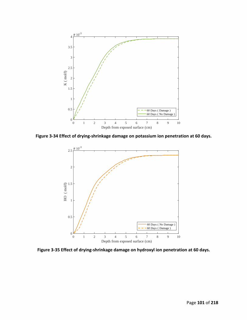
Page 101 of 218
Figure 3-34 Effect of drying-shrinkage damage on potassium ion penetration at 60 days.
Figure 3-35 Effect of drying-shrinkage damage on hydroxyl ion penetration at 60 days.
0 1 2 3 4 5 6 7 8 9 10Depth from exposed surface (cm)
0
0.5
1
1.5
2
2.5
3
3.5
4
K (
mol
/l)
# 10-3
60 Days ( Damage )60 Days ( No Damage )
0 1 2 3 4 5 6 7 8 9 10Depth from exposed surface (cm)
0
0.5
1
1.5
2
2.5
HO
( m
ol/l)
# 10-3
60 Days ( No Damage )60 Days ( Damage )

Page 102 of 218
Figure 3-36 Effect of drying-shrinkage damage on chloride ion penetration at 60 days.
Figure 3-37 Effect of drying-shrinkage damage on calcium ion penetration at 60 days.
0 1 2 3 4 5 6 7 8 9 10Depth from exposed surface (cm)
0
0.005
0.01
0.015
0.02
0.025
0.03
0.035
0.04
Cl (
g/g)
60 Days ( No Damage )60 Days ( Damage )
0 1 2 3 4 5 6 7 8 9 10Depth from exposed surface (cm)
0
0.002
0.004
0.006
0.008
0.01
0.012
Ca
( mol
/l)
60 Days ( No Damage)60 Days (Damage )

Page 103 of 218
Figure 3-38 Efffect of drying-shrinkage damage on sodium ion penetration at 60 days.
Conclusions
• A Finite element model for multi species diffusion in concrete was developed using the Nernst-Planck equation and electroneutrality condition to simulate the penetration process of multi-ions into unsaturated concrete considering the ionic interaction between the different species.
• The model considers the coupling effect of moisture and multi-ion diffusion where the effect of moisture on multi-ion diffusion and the effect of the multi-ion on moisture diffusion are incorporated in the model by introducing the coupling parameters in the governing equations.
• Different material parameters are employed in the model to consider the effect of chloride binding capacity, moisture capacity, and the dependence of diffusion coefficient on the ion concentration
• The numerical result shows that the electrical potential on ionic diffusion induced by the movement of the dissolved ions in the solution has an effect on the movement of the ions in the solution
• The transport model is implemented in the coupled hygro-mechanical model to simulate the effect of drying shrinkage-induced damage on multi-ionic transport in non-saturated concrete where the effect of damage induced by drying shrinkage on the transport properties is taken into account.
• The numerical result indicates that the formation of microcracking (damage) induced by drying shrinkage accelerates the diffusion process and increases the rate of drying.
0 1 2 3 4 5 6 7 8 9 10Depth from exposed surface (cm)
0
0.002
0.004
0.006
0.008
0.01
0.012
0.014
Na
( mol
/l)
60 Days ( No Damage )60 Days ( Damage )

Page 104 of 218
3.4. MODELING OF CORROSION RATE IN REINFORCED CONCRETE
Introduction
The corrosion of steel reinforcement depends on several factors such as the characteristic of the concrete pore solution (CPS) (e.g., pH, chloride concentration, and oxygen concentration), properties of hardened concrete (such as electrical resistivity), and environmental conditions, i.e., temperature and relative humidity. Accurate estimation of the corrosion reactions in RC structures is difficult for being dependent on various parameters such as concrete mixture proportions, the pH of the CPS and concrete resistivity, the environmental conditions such as temperature, relative humidity, and the type and concentrations of ions near the steel-concrete interface. It is difficult to account for the effect of these variables on the corrosion reactions. Previous researchers (Ge and Isgor, 2007; Ožbolt et al., 2016) have not considered the effect of these parameters in their numerical models. Additionally, most of the numerical models were not experimentally verified. Therefore, the use of the existing numerical models provides results with no confidence.
In this study, concrete microstructural properties such as the pH of the CPS and concrete resistivity were obtained from Virtual Cement Concrete Testing Laboratory (VCCTL) (Bentz, 1997, 2005), a code developed by the U.S. National Institute of Standards and Technology. Additionally, the effect of environmental conditions and concentration of ions near steel-concrete interface were obtained using coupled transport modeling of heat, humidity, chloride, and oxygen. An algorithm was also developed to study the effect of temporal variation in these parameters. The developed numerical model predicts the corrosion potential, corrosion current density, and corrosion rate throughout the concrete domain.
Model for Corrosion Current Density
The corrosion of steel reinforcement depends on the oxygen concentration near the steel-concrete interface. The corrosion rates in oxygen rich environments and oxygen deficient environments differ significantly. Therefore, an oxygen transport model is considered in this study to account for the oxygen concentration in the modeling for corrosion current density.
3.4.2.a. Governing Equations for Modeling of Current Density
After the initiation of the corrosion of steel reinforcement, corrosion reactions govern the rate of deterioration of an RC structure. The accumulation of the corrosion products at the anodic site of the reinforcement causes expansive pressure on the concrete, which results in the cracking of the concrete cover. Since the rate of corrosion reactions is one of the important parameters in predicting the time until cover cracking initiates, a numerical model was developed to estimate this parameter. The corrosion potential, V, is governed by the Laplacian equation as follows (Bergerhoff and Brown, 1987; Lutterotti et al., 1999; Pour-Ghaz et al., 2009).
∇2𝑉𝑉 = 0 in Ω 3.122

Page 105 of 218
where Ω is the concrete domain and ∇2 is the Laplacian operator. A relationship between the corrosion current density, 𝑖𝑖, and the corrosion potential is given by Ohm’s law as follows
𝑖𝑖 = −𝜔𝜔 𝜕𝜕𝜕𝜕𝜕𝜕𝑚𝑚
3.123
where 𝑛𝑛 is a normal vector on the surface of steel reinforcement and 𝜔𝜔 is the conductivity of the concrete. Corrosion potential on the anode and cathode is explained by the polarization curves as mentioned earlier. This polarization potential serves as the boundary conditions:
𝑉𝑉 = 𝑉𝑉𝑚𝑚 on 𝛤𝛤𝑚𝑚 3.124
𝑉𝑉 = 𝑉𝑉𝑐𝑐 on 𝛤𝛤𝑐𝑐 3.125
where 𝑉𝑉𝑚𝑚 is the half-cell potential at the anodic site, 𝑉𝑉𝑐𝑐 is the half-cell potential at the cathodic site, 𝛤𝛤𝑚𝑚 is the anodic boundary, and 𝛤𝛤𝑐𝑐 is the cathodic boundary. As mentioned earlier, the corrosion rate depends on the material properties such as concrete resistivity, the pH of the CPS, chloride ions concentration, temperature, relative humidity, and the Tafel slopes. The material properties of the concrete were obtained by simulating the concrete microstructure in VCCTL (Bentz, 1997, 2005). The temperature, relative humidity, and chloride ion concentrations were obtained by a coupled transport model.
Since the location and values of the boundary conditions are unknown, the Laplacian problem becomes complicated. Furthermore, the dependence of current density and potential on each other makes the problem highly non-linear. Thus, a simple problem becomes complex and can only be solved by implementing it in a finite element formulation, which was achieved using MOOSE (Gaston et al., 2009). An algorithm was developed to estimate the location of anode and cathode in the RC structure as described in the upcoming sections.
3.4.2.b. Estimating the Anodic and Cathodic Sites
As mentioned before, steel reinforcement in RC structures stays in the passive zone until a significant concentration of aggressive ions such as chlorides is present to break the passive layer. The breakage of the passive layer converts the steel surface to an active zone. The presence of the active and passive zone on the steel reinforcement determines the formation of anodic and cathodic sites in the corrosion process as shown in Figure 3-39. In this study, anodic site was considered at a location where chloride concentration exceeds a threshold limit of 0.73 kg/m3 as reported in Kassir and Ghosn (2002). Cathodic sites were considered the location(s) on steel reinforcement, which is electrically connected to the anodic sites.

Page 106 of 218
Figure 3-39 Formation of anode and cathode during the chloride transport in concrete: (a)
Beginning of the transport of chloride ions from concrete surface; (b) Chloride ions de-passivate a part of reinforcement to form anode for macro-cell corrosion, the remaining part of reinforcement acts as cathode; (c) Chloride ions de-passivate the complete rebar to form
anode and cathode adjacent to each other for micro-cell corrosion.
3.4.2.c. Estimating the Anodic and Cathodic Potential
The formation of anodic and cathodic sites further determines the nature of the corrosion process. If the anodic and cathodic sites form adjacent to each other, a micro-cell corrosion takes place. On the other hand, if the anodic and cathodic sites are spatially apart from each other, a macro-cell corrosion takes place.
A simplified polarization curve was considered to estimate the polarization potential of anodic and cathodic sites as shown in Figure 3-40. The half-cell potential at the anodic site is governed by the activation polarization, while at the cathodic site, it is governed by both activation and concentration polarizations due to a limitation in the supply of oxygen, according to
𝑉𝑉𝑚𝑚 = 𝑉𝑉𝑚𝑚0 + 𝑅𝑅𝑇𝑇𝑚𝑚𝑛𝑛𝑙𝑙𝑛𝑛 [𝑛𝑛𝑒𝑒++]
[𝑛𝑛𝑒𝑒] + 𝛽𝛽𝑚𝑚 𝑙𝑙𝑜𝑜𝑔𝑔𝑚𝑚𝑎𝑎𝑚𝑚𝑎𝑎0
3.126
𝑉𝑉𝑐𝑐 = 𝑉𝑉𝑐𝑐0 + 𝑅𝑅𝑇𝑇𝑚𝑚𝑛𝑛𝑙𝑙𝑛𝑛 [𝑂𝑂2]
[𝑂𝑂𝐻𝐻−]4 + 𝛽𝛽𝑐𝑐 𝑙𝑙𝑜𝑜𝑔𝑔𝑚𝑚𝑐𝑐𝑚𝑚𝑐𝑐0
+ 𝑅𝑅𝑇𝑇𝑚𝑚𝑛𝑛𝑙𝑙𝑛𝑛 1 − 𝑚𝑚𝑎𝑎
𝑚𝑚𝐿𝐿 3.127
concrete
rebar
Cl- ions
Anode
Cathode
Anode
Cathode
Anode
Cathode
(a)
(b)
(c)

Page 107 of 218
𝑖𝑖𝐿𝐿 = 6.25 × 𝑛𝑛 × [𝑂𝑂2] 3.128
where 𝑉𝑉𝑚𝑚0 is the standard half-cell potential of iron, 𝑉𝑉𝑐𝑐0 is the standard half-cell potential of oxygen, 𝑖𝑖𝐿𝐿 is the limiting current density at cathodic site, [. ] is the species concentration in the CPS at the steel-concrete interface, R is the universal gas constant, n is the number of electrons participating in cathodic reaction and F is the Faraday’s constant.
Figure 3-40 Simplified polarization curves for anode and cathode.
3.4.2.d. Algorithm for Time-Varying Corrosion Rate
Since the concrete microstructure, as well as the environmental conditions surrounding RC structures, change with time, the corrosion rate should also change with these changes. The effect of time-varying concrete microstructure and environmental conditions was studied in this modeling framework. An algorithm was developed to study the time-varying corrosion of steel reinforcement as described in Figure 3-41. The algorithm considers both micro-cell and macro-cell corrosion of steel reinforcement. It also accounts for the corrosion of steel reinforcement in both active and passive states.
Active zone of steel reinforcement
Reduction of oxygen
Reduction of oxygen limited by the
diffusion process
Current density (id)
Pote
ntial
(V)
iL
𝑉𝑉𝑚𝑚0
𝑉𝑉𝑐𝑐0
ia0ic0
Passive zone of steel reinforcement
Active micro-cell current density
Passive micro-cell current density
𝛽𝛽𝑚𝑚𝑚𝑚1
𝛽𝛽𝑐𝑐
1
𝛽𝛽𝑚𝑚𝑝𝑝
1

Page 108 of 218
Figure 3-41 Algorithm representing the time-varying corrosion of steel reinforcement.
At the start, when the passive layer of the reinforcement is intact, the anode and cathode form adjacent to each other to form micro-cell corrosion. At this point, steel reinforcement corrodes with uniform corrosion potential (Cao et al., 2013) corresponding to the intersection of curves 𝑎𝑎1, 𝜕𝜕1 or 𝑎𝑎1, 𝜕𝜕2 in Figure 3-42. When the ratio of chloride ions to hydroxyl ion exceeds a critical limit, the passive layer breaks down and the steel becomes active. Active steel participates in the micro-cell corrosion and the potential of the reinforcement is given by the intersection of curves 𝑎𝑎2, 𝜕𝜕1 or 𝑎𝑎2, 𝜕𝜕2 in Figure 3-42. As was observed in Figure 3-42, the rate of corrosion for an active micro-cell is higher than that of the passive micro-cell corrosion. If the active part of steel is electrically connected to the passive part of steel, the macro-cell corrosion takes place with an anode forming at the active part and cathode forming at the passive part of steel reinforcement. The corrosion rate for macro-cell corrosion depends on the concrete resistivity as charge must pass through the electrolyte, which is concrete in this case. Thus, once the passive layer breaks and if the active zone is connected to the passive zone, both micro-cell and macro-cell corrosion take place, otherwise micro-cell corrosion takes place.
Start
Yes
Yes
𝐶𝐶𝑙𝑙−
𝑂𝑂𝐻𝐻− >𝐶𝐶𝑙𝑙−
𝑂𝑂𝐻𝐻−𝑡𝑡ℎ
No
NoYes
(Active zone)
O2(x, t)
T(x, t)
Cl-(x, t)
H(x, t)
Passive micro-cell corrosion
Coupled micro-cell and macro-cell corrosion
Active micro-cell corrosion
Active zone
Passive zone
SteelNo(Passive
zone)
O2(t) T(t)
Cl-(t) H(t)
Active zone
Passive zone
Steel
Algorithm (Implemented in MOOSE)
Anode
Cathode
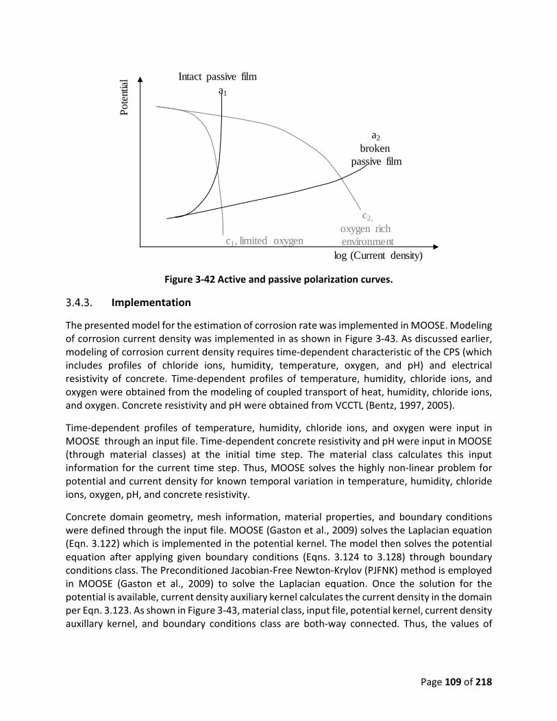
Page 109 of 218
Figure 3-42 Active and passive polarization curves.
Implementation
The presented model for the estimation of corrosion rate was implemented in MOOSE. Modeling of corrosion current density was implemented in as shown in Figure 3-43. As discussed earlier, modeling of corrosion current density requires time-dependent characteristic of the CPS (which includes profiles of chloride ions, humidity, temperature, oxygen, and pH) and electrical resistivity of concrete. Time-dependent profiles of temperature, humidity, chloride ions, and oxygen were obtained from the modeling of coupled transport of heat, humidity, chloride ions, and oxygen. Concrete resistivity and pH were obtained from VCCTL (Bentz, 1997, 2005).
Time-dependent profiles of temperature, humidity, chloride ions, and oxygen were input in MOOSE through an input file. Time-dependent concrete resistivity and pH were input in MOOSE (through material classes) at the initial time step. The material class calculates this input information for the current time step. Thus, MOOSE solves the highly non-linear problem for potential and current density for known temporal variation in temperature, humidity, chloride ions, oxygen, pH, and concrete resistivity.
Concrete domain geometry, mesh information, material properties, and boundary conditions were defined through the input file. MOOSE (Gaston et al., 2009) solves the Laplacian equation (Eqn. 3.122) which is implemented in the potential kernel. The model then solves the potential equation after applying given boundary conditions (Eqns. 3.124 to 3.128) through boundary conditions class. The Preconditioned Jacobian-Free Newton-Krylov (PJFNK) method is employed in MOOSE (Gaston et al., 2009) to solve the Laplacian equation. Once the solution for the potential is available, current density auxiliary kernel calculates the current density in the domain per Eqn. 3.123. As shown in Figure 3-43, material class, input file, potential kernel, current density auxillary kernel, and boundary conditions class are both-way connected. Thus, the values of
log (Current density)
Pote
ntial
Intact passive filma1
a2broken
passive film
c2,oxygen rich environmentc1, limited oxygen

Page 110 of 218
parameters are available from one class to another. The model outputs time-dependent corrosion potentials and corrosion current densities in the concrete domain.
Figure 3-43 Implementation of modeling of corrosion current density in MOOSE (Gaston et
al., 2009).
Results and Discussion
A numerical study by Ge and Isgor (2007) was used to verify the results of the modeling. Ge and Isgor (2007) considered an RC element as shown in Figure 3-44(a) to solve the above described governing equations under the given boundary conditions. The input parameters of the numerical study are given in Table 3-5. Only a part of RC structure was considered as a numerical domain as shown in Figure 3-44(b). In the numerical model, the cathode and the anode sites are equal in length. A steady-state solution of the problem was obtained using the Newton method. Since current density is a function of the potential, a fine mesh with 5 mm edge lengths was used for this model as shown in Figure 3-44(c) due to strong local gradients. A triangular mesh was considered over rectangular mesh to achieve better accuracy as reported by Wu and Lee (1997).
Table 3-5 Input Parameters for Finite Element Model
Parameter Value
Anodic exchange current density (𝑖𝑖𝑚𝑚0) Am2 1.875 × 10⁻⁴
Cathodic exchange current density (𝑖𝑖𝑐𝑐0) Am2 6.25 × 10⁻⁶
Anodic equilibrium potential (𝑉𝑉𝑚𝑚0) (V w.r.t. SCE) -0.78
Modeling for Corrosion Current Densityin MOOSE
• Concrete resistivity• pH
Input file• Domain• Variable definition• Potential distribution
kernels• Material properties• Boundary conditions• Executioner• Output
Potential kernel
Boundary Conditions Class
• Algorithm for time-varying corrosion rate
Material Class• Electrical resistivity of concrete• Tafel slopes for anodic and
cathodic sites• Exchange current density at
anodic and cathodic site• Standard potential at anode and
cathode
@ t = 0Current density Auxiliary kernel
Coupled Transport Modeling of Heat, Humidity, Chloride ions, and
Oxygen in Concrete
Temperature profile
Humidity profile
Chloride profile
Oxygen profile
VCCTL

Page 111 of 218
Cathodic equilibrium potential (𝑉𝑉𝑐𝑐0) (V w.r.t. SCE) 0.16
Tafel slope for anodic reaction (𝛽𝛽𝑚𝑚) Vdec 0.06
Tafel slope for cathodic reaction (𝛽𝛽𝑐𝑐) Vdec 0.16
Concrete conductivity (𝜔𝜔)(Ω ∙ m)−1 1/140
Limiting current density (𝑖𝑖𝐿𝐿) Am2 1
w.r.t.: with respect to; SCE: standard calomel electrode
Figure 3-44 (a) Consideration of anodic and cathodic sites on reinforcement in the RC
element; (b) numerical domain considered in MOOSE model (c) meshing of the numerical domain.
Comparisons of the results are shown in Figure 3-45 and Figure 3-46. The results from this model compare very closely with the results of another numerical study (Ge and Isgor, 2007). The results for the current density fluctuate at the intersection of anodic and cathodic boundaries. Since the potential changes abruptly at that intersection, the corresponding derivative is not defined,

Page 112 of 218
hence the results of the finite element model fluctuate, and they are sensitive to the mesh refinement.
Figure 3-45 Comparison of the corrosion potentials between the present model and a
reference solution.
Figure 3-46 Comparison of the current densities between the present model and a reference
solution.
In addition to the verification model described above, an experimental study from the literature (Yuan et al., 2011) was used to validate the results from the developed algorithm. In that experimental study, 4% NaCl was added to the fresh concrete during casting of the RC beam. Two types of reinforcement were used in the beam: steel and stainless steel. The stainless-steel reinforcement was electrically connected with the steel reinforcement using an external wire.
-0.8
-0.6
-0.4
-0.2
00 50 100 150 200 250 300
Pote
ntial
(V
)
Distance (mm)Potential (Ge and Isgor 2007) Potential (Model)
0
0.04
0.08
0.12
0 50 100 150 200 250 300
Cur
rent
den
sity
(A/m
2 )
Distance (mm)
Current density (Ge and Isgor 2007) Current density (Model)

Page 113 of 218
The presence of 4% chloride ions caused the breakage of the passive layer, thus the steel reinforcement acted as an anode while the stainless-steel reinforcement acted as a cathode. The corrosion current density was measured over time. It was observed that the corrosion current density achieves saturation 30-40 days after casting. The saturated values are compared with the results of the model here. A contour plot of the corrosion current density is presented in Figure 3-47. The corrosion current density from the experiment is compared with the node average current density from the simulation. The observed corrosion current density in the experiment is 3.5 × 10⁻² A
m2 while that from the simulation was obtained as 3.42 × 10⁻² Am2.
Figure 3-47 Corrosion current density in the concrete domain.
Conclusions
• A simulation capability was developed to model the corrosion reactions that account for the concentration of chloride ions and oxygen, heat, humidity (using modeling of coupled transport of heat, humidity, chloride, and oxygen), pH of the CPS, and resistivity of concrete (using modeling of concrete microstructural development using VCCTL (Bentz, 1997, 2005)). Temporal variation of these parameters to model both macro-cell corrosion and micro-cell corrosion was considered estimation of corrosion current density, which were missing in previous studies (Kranc and Sagüés, 1997; Liu and Weyers, 1998; Maruya et al., 2003; Isgor and Razaqpur, 2006; Cao et al., 2013).
• An algorithm for the time-varying corrosion rate was developed based on the chloride concentration, pH of the CPS, and arrangement of steel reinforcement. The algorithm provides temporal changes in the location and potentials of the anodic and cathodic site on steel reinforcement. The numerical model and developed algorithm were validated for a steady-state solution with another numerical study as well as an existing experimental study.

Page 114 of 218
• The developed model can be used to obtain accurate predictions of the corrosion current density. Thus, it helps predict the corrosion-induced damage in RC structures.
• The model can further be developed to include the effect of temporal changes in the electrochemical properties of steel reinforcement such as Tafel slope.
• pH of the CPS was obtained from the modeling of microstructural development of concrete using VCCTL (Bentz, 1997, 2005). However, the modeling does not account for the presence of other ions such as chloride ions on the properties of CPS such as pH. This is one of the important factors that can further improve the predictive capability of the model.
3.5. MODELING CORRODED STEEL AND DEGRADATION OF CONCRETE BOND WITH CORROSION
Introduction
In addition to the concrete, steel reinforcement (Almusallam, 2001; Francois et al., 2013) and the steel-concrete bond (Bazant, 1979; Liu and Weyers, 1998; Pantazopoulou and Papoulia, 2001; El Maaddawy and Soudki, 2003; Bhargava et al., 2006; Torres-Acosta et al., 2007; Kim et al., 2010) are also affected by the degree of corrosion of steel reinforcement. The corrosion products at the steel-concrete interface change the bond behavior at the steel-concrete interface. Uniform corrosion of steel reinforcement was considered to find mechanical properties of the steel-concrete bond as a function of degree of corrosion. Uniform corrosion with corrosion current density, 𝑖𝑖, causes a loss of metal from the steel reinforcement. The mass loss, 𝛥𝛥𝛥𝛥, can be related to i as follows
𝛥𝛥𝛥𝛥 = 9130 𝜋𝜋 𝑑𝑑0 ∫ 𝑖𝑖 𝑑𝑑𝜕𝜕 3.129
where 𝑑𝑑0 is the diameter of steel reinforcement (cm), 𝜕𝜕 is the duration of corrosion (year) and 9130 is the mass of iron (g) consumed from the transfer of 1 ampere-year of charge per Faraday’s law. Thus, the percentage of corrosion, η, based on volume loss, is obtained as follows
𝜂𝜂 = 400𝜋𝜋
𝛥𝛥𝜕𝜕𝑑𝑑02
3.130
where 𝛥𝛥𝑉𝑉 is the volume of steel consumed. Since uniform corrosion of steel reinforcement was considered in the study, the reduction in the diameter of steel reinforcement, 𝛥𝛥𝑑𝑑0, can be related to η and 𝑑𝑑0 as follows
𝛥𝛥𝑑𝑑0 = 𝑑𝑑0 1 −1 − 𝜂𝜂100 3.131
As the degree of corrosion, η, increases, the corrosion products first diffuse into the adjacent voids and do not exert pressure on the surrounding concrete (Almusallam et al., 1996; Liu, 1996; Fang et al., 2006), as shown in Figure 3-48. At this point, the bond strength between steel and concrete is considered to increase with η. After the voids are completely filled, the corrosion products start to exert pressure on the concrete and the bond strength decreases with η. A

Page 115 of 218
numerical model is used to include the effect of η on the bond strength. Bond strength is expressed in terms of the friction coefficient, 𝜇𝜇(𝑒𝑒), as (Fang et al., 2006)
𝜇𝜇(𝑒𝑒) = 𝜆𝜆(𝛥𝛥𝑑𝑑0/𝑑𝑑0) 𝜇𝜇0(𝑒𝑒), 𝜇𝜇0(𝑒𝑒) ≥ 0.4 3.132
where 𝜇𝜇0(𝑒𝑒) is the friction coefficient of the uncorroded reinforcement, 𝜆𝜆(𝛥𝛥𝑑𝑑0/𝑑𝑑0) is a function that accounts for the increase and decrease in bond strength with η, and 𝑒𝑒 is slip as shown in Figure 3-48.
Figure 3-48 (a) Bond strength-slip relationship of uncorroded reinforcement; (b) Effect of η on
bond strength (Fang et al., 2006).
For a slight degree of corrosion, the bond strength should increase as shown in Figure 3-48(b). This increase in bond strength can be attributed to the increase in the friction coefficient due to diffusion of corrosion products into the concrete pores. Once concrete pores are filled up, the friction coefficient is assumed (Fang et al., 2006) to decrease linearly to a lower limit. The lower
0
2
4
6
8
10
12
0 5 10 15 20
Bond
stre
ngth
(M
Pa)
Slip (mm)(a)
0.0
0.2
0.4
0.6
0.8
1.0
1.2
0 0.025 0.05 0.075 0.1
λ(Δd
0/d0)
Δd0/d0(b)

Page 116 of 218
limit corresponding to the friction between concrete and concrete because it was assumed (Fang et al., 2006) that under a high degree of corrosion, the pull-out mechanism of a bar depends on shear cracking between the ribs of the reinforcement.
The corrosion products at the steel-concrete interface diffuse into the concrete pores before exerting pressure on the surrounding concrete. The pressure increases the friction force between steel reinforcement and the concrete, which results in an initial increase in the bond strength at low levels of corrosion. The increase in friction force is limited by the cracking of concrete. Thus, an analytical study on the bond degradation due to corrosion of steel reinforcement is discussed in detail in the following sections. The yield strength of steel reinforcement is also affected by the degree of corrosion. Results of the existing experimental studies (Almusallam, 2001; Francois et al., 2013) on corroded steel reinforcement were used to address the deterioration in the yield strength of the corroded steel reinforcement as discussed in the following sections.
Modeling Approach
In the case when an anode forms only over a certain arc-length of the steel reinforcement (assuming that volume loss reduces the reinforcement area only in the radial direction, as shown in Figure 3-49), the loss of volume, 𝛥𝛥𝑉𝑉, can be expressed as
𝛥𝛥𝑉𝑉 = 𝑑𝑑𝑑𝑑8
(2𝑑𝑑0 − 𝛥𝛥𝑑𝑑0) 𝛥𝛥𝑑𝑑0 3.133
where 𝑑𝑑𝑑𝑑 is the arc-length of the corroded part of the steel reinforcement. The mass loss from Faraday’s law on this localized arc-length due to corrosion current density, i (A/cm2), in a given time, t (year), is given by
𝛥𝛥𝛥𝛥 = 9130 d02𝑑𝑑𝑑𝑑 ∫ 𝑖𝑖 𝑑𝑑𝜕𝜕 3.134
where 𝑑𝑑0 is in cm and 𝛥𝛥𝛥𝛥 is in g. Thus, using Eqns. 3.130, 3.133 and 3.134, the following relation is obtained
Δd0d0
= 1 −1 − η
100×dθ2π 3.135

Page 117 of 218
Figure 3-49 Volume loss due to localized corrosion of steel reinforcement
Thus, the mechanical behavior of the bond between steel and concrete can be expressed for localized corrosion of steel reinforcement using Eqn. 3.132. Corrosion of steel reinforcement affects its material and geometrical properties. The change in the geometrical properties, i.e., reduction in diameter for given current density, was determined per Eqn. 3.135.
The change in the yield stress and rupture strain of the corroded steel reinforcement are accounted for in this study. It was observed by Almusallam (1996) in uniaxial tensile tests of 6 mm and 12 mm corroded reinforcement that η decreases the nominal yield strength of steel reinforcement. The results of the test were used to relate η to the remaining capacitity of the corroded bars, expressed as fractions of the original yield strength and rupture strain, as shown in Figure 3-50. The tensile strength of steel does not change with η (Almusallam, 2001), however, the fraction of the nominal yield strength, 𝑓𝑓𝑖𝑖 , was assumed to follow a linear trend with the degree of corrosion as shown in Figure 3-50, as follows
𝑓𝑓𝑖𝑖 = 1 − 0.01 × 𝜂𝜂 3.136
The rupture strain of steel changes with η (Almusallam, 2001) and the fraction of rupture strain, 𝑓𝑓𝜖𝜖𝑟𝑟, follow a power law as follows
𝑓𝑓𝜖𝜖𝑟𝑟 = 𝜂𝜂−0.57 ∀ 𝜂𝜂 > 1% 3.137
𝑑𝑑𝑑𝑑
Δ𝑑𝑑0
𝑑𝑑0
Δ𝑉𝑉=𝑑𝑑𝑑𝑑8 2𝑑𝑑0 − 𝛥𝛥𝑑𝑑0 𝛥𝛥𝑑𝑑0
𝑑𝑑0𝑑𝑑𝑑𝑑2
Steel reinforcement

Page 118 of 218
Figure 3-50 Effect of η on (a) the yield strength (b) the rupture strain of steel reinforcement
(data from (Almusallam, 2001)).
Conclusions
An empirical model for the material properties of steel reinforcement and an analytical model for the steel-concrete bond has been developed in this study. An analytical relationship has been established between the degree of corrosion and steel-concrete bond strength. Furthermore, results from the previous experimental studies were used to establish an empirical relationship for yield strength and rupture strain of steel reinforcement as a function of degree of corrosion. These model has not yet been implemented into a simulation code, but could be readily incorporated in the future into 1D models of reinforcement for modeling the effect of this type of degradation on the capacity of RC members in BlackBear or other codes.
Equation Chapter 4 Section 1
f = -0.01η + 1.00R² = 0.85
0
0.2
0.4
0.6
0.8
1
0 20 40 60 80 100
Frac
tion
fo y
ield
stren
gth
(f y)
% Corrosion (η)(a)
fεr = 1.00 η-0.57
R² = 0.92
0
0.2
0.4
0.6
0.8
1
0 20 40 60 80
f εr(m
m/m
)
% Corrosion (η)strain(b)
For η > 1 %

Page 119 of 218
EXPERIMENTAL INVESTIGATION OF THE EFFECT OF ASR
DAMAGE ON REINFORCED CONCRETE 4.1. INTRODUCTION
Alkali-silica reaction (ASR) is a long-term degradation process that occurs in concrete under certain conditions. The occurrence of ASR depends on the following three factors: the presence of reactive aggregate, a high level of alkalinity, and high levels of moisture. Although not required, high temperature is also an intensifying factor for ASR. The ASR causes expansion and cracking which lead to deterioration of the concrete mechanical properties. This long-term deterioration process can affect the functional performance and serviceability of the reinforced concrete (RC) structures such as bridges, buildings, dams, and nuclear power plants.
In this study, the effects of ASR on the shear performance of RC beams is investigated. As part of this study, long-term expansion effects of ASR at the structural and material scales are monitored. Six large-scale beams that are 6.4 m long, 0.6 m high, and 0.3 m wide were constructed and tested. The beams were designed to fail in shear (rather than in flexure) to study the effect of ASR on the shear response. All the beams were constructed using highly reactive fine aggregate (sand) and two of the beams were cast using a concrete mixture with a high level of alkalinity. The beams were categorized into three groups of two beams based on the concrete batch they were built from and their exposure conditions. The two beams with high levels of alkali along with two other beams with only reactive aggregate were stored in the outside Los Angeles environment and they were sprayed with water at regular intervals to maintain high moisture content inside the concrete. The other two beams were stored in the laboratory environment at a low relative humidity (RH). Expansion measurements were done regularly on all six beams. One beam from each group (three beams in total) was tested in shear while the other beams were used for expansion measurements throughout the experimental program. Two shear tests were conducted on each of those beams to assess the shear performance of the spans on both sides, which were constructed to be nominally the same. These two tests of the same beam were intended to test the repeatability of the results. Data were collected during testing using a variety of sensors including load cells, string potentiometers, linear potentiometers, rebar strain gauges, and high-resolution cameras. This data included reactions, deflections, shear deformations, concrete strains, reinforcement strains, crack maps, and cracks widths. Accordingly, the shear behavior of these different beams was compared and discussed considering their ASR induced expansion at the time of testing.
In addition to the expansion measurements at the material and structural scales, the degradation of concrete mechanical properties due to the ASR was investigated over time using material samples. Mechanical tests including compression, split tension, and flexural tests were conducted on the cylinder and prism samples from different concrete mixtures stored in different environments. A group of samples were kept in the laboratory environment while two other groups were conditioned outside with periodic water spray. Moreover, concrete samples from
Page 120 of 218
each concrete mixture were stored in an environmental chamber at 50°C and 90% RH. Mechanical properties of the concrete samples from the different groups were compared and discussed considering the ASR expansion progress of the plain concrete prims.
4.2. EXPERIMENTAL PROGRAM
Material Studies on ASR Affected Concrete
4.2.1.a. Concrete Materials, Mixture Design, Casting, Curing and Environmental Exposure
Type II low alkali Portland cement, with a median particle size of 9.8 µm was used in this study. Chemical and mineral compositions, as provided by the supplier, of the cement are summarized in Table 4-1. The cement meets the optional requirement for low alkali (less than or equal to 0.60% total alkali by weight) based on ASTM C150/150M -19a (2019). Reactive sand used in this study was obtained from El Paso, Texas. The ASR reactivity of the fine aggregate (sand) was investigated through a mortar bar test according to ASTM C1260-14 (2014b) and the results are shown in Figure 4-1. The mortar containing the reactive sand exhibited a considerable swelling behavior in the presence of an alkaline solution and high temperature (80°C). The expansion at the end of 16 days was 0.60%, suggesting the expansive and deleterious nature of the sand according to ASTM C1260-14 (2014b). After 10 days, although an increase in the expansion was still observed, the rate of increase reduced. The expansion of the mortar was higher than 0.8% after 25 days. Two types of coarse aggregates, 19 mm crushed rock and 9.5 mm crushed rock, were used in this study. Table 4-2 shows the grading of these two coarse aggregates.
Table 4-1 Chemical and Mineral Compositions of Cement (by Weight).
Chemical Composition
and Properties
CaO SiO2 Al2O3 SO3 Fe2O3 MgO Na2O+0.658 K2O
Loss on Ignition
(LOI)
Insoluble Residue (IR)
wt.% 63.9 20.9 4.0 2.8 3.6 1.9 0.58 2.7 0.7 Mineral
Composition Tricalcium Silicate
(C3S) Dicalcium Silicate
(C2S) Tricalcium Aluminate
(C3A) Tetracalcium
Aluminoferrite (C4AF)
wt.% 55 18 5 11

Page 121 of 218
Figure 4-1 Time history of ASR expansion of mortar bar specimens.
Table 4-2 Grading of Coarse Aggregates.
19 mm Crushed Rock 9.5 mm Crushed Rock Sieve Size Percentage Passing Sieve Size Percentage Passing
25 mm 100 12.5 100 19 mm 95 4.9 87
12.5 mm 25 4.75 10 9.5 mm 8 2.36 4
4.75 mm 2 - -
Three batches of concrete were mixed, two from an identical mix design, to investigate the effect of ASR on the mechanical properties at the material and structural levels. Mix proportions, by weight, and characteristics of concrete batches are summarized in Table 4-3. To accelerate ASR, in the third batch, in addition to the reactive sand, 1.25% by weight of cement of additional alkaline was added to the concrete mixing water. Delayed ettingite formation (DEF) was prevented by keeping the internal temperature during casting and initial curing to less than 70°C in early December in the Los Angeles area, as shown in Figure 4-2.
0 5 10 15 20 25 30 350
0.2
0.4
0.6
0.8
1
Age (days)
Expa
nsio
n (%
)
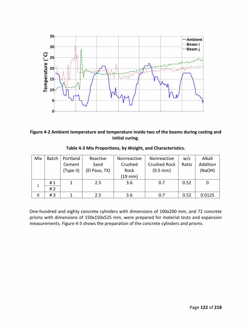
Page 122 of 218
Figure 4-2 Ambient temperature and temperature inside two of the beams during casting and
initial curing.
Table 4-3 Mix Proportions, by Weight, and Characteristics.
Mix Batch Portland Cement (Type II)
Reactive Sand
(El Paso, TX)
Nonreactive Crushed
Rock (19 mm)
Nonreactive Crushed Rock
(9.5 mm)
w/c Ratio
Alkali Addition (NaOH)
I # 1 1 2.5 3.6 0.7 0.52 0 # 2
II # 3 1 2.5 3.6 0.7 0.52 0.0125
One-hundred and eighty concrete cylinders with dimensions of 100x200 mm, and 72 concrete prisms with dimensions of 150x150x525 mm, were prepared for material tests and expansion measurements. Figure 4-3 shows the preparation of the concrete cylinders and prisms.
12/01/2017 0:00 12/02/2017 0:00 12/03/2017 0:00 12/04/20170
5
10
15
20
25
30
35
Date and Time
Tem
pera
ture
(deg
ree
C)
AmbientBeam iBeam j
Tem
pera
ture
( C
)

Page 123 of 218
Figure 4-3 Preparing concrete samples for material tests: (a) cylinders, (b) prisms.
Batches 1 and 2 were cast on the first day and Batch 3 was cast on the second day. All concrete specimens were cured under plastic sheets and demolded 14 days after casting. Table 4-4 presents the information about different samples from different batches and their exposure conditions. Three groups of cylinder and prism samples, from the three batches, were conditioned in the laboratory or in the outdoor Los Angeles environment. The samples kept outside were sprayed with water two times every week. The outside samples were also covered with towels and tarps after spraying to maintain a high RH. Additionally, from each batch, a group of cylinder and prism samples were kept in the environmental chamber with constant 50°C and 90% RH conditions. Figure 4-4 shows the prism and cylinder samples that were conditioned inside the environmental chamber.
a b
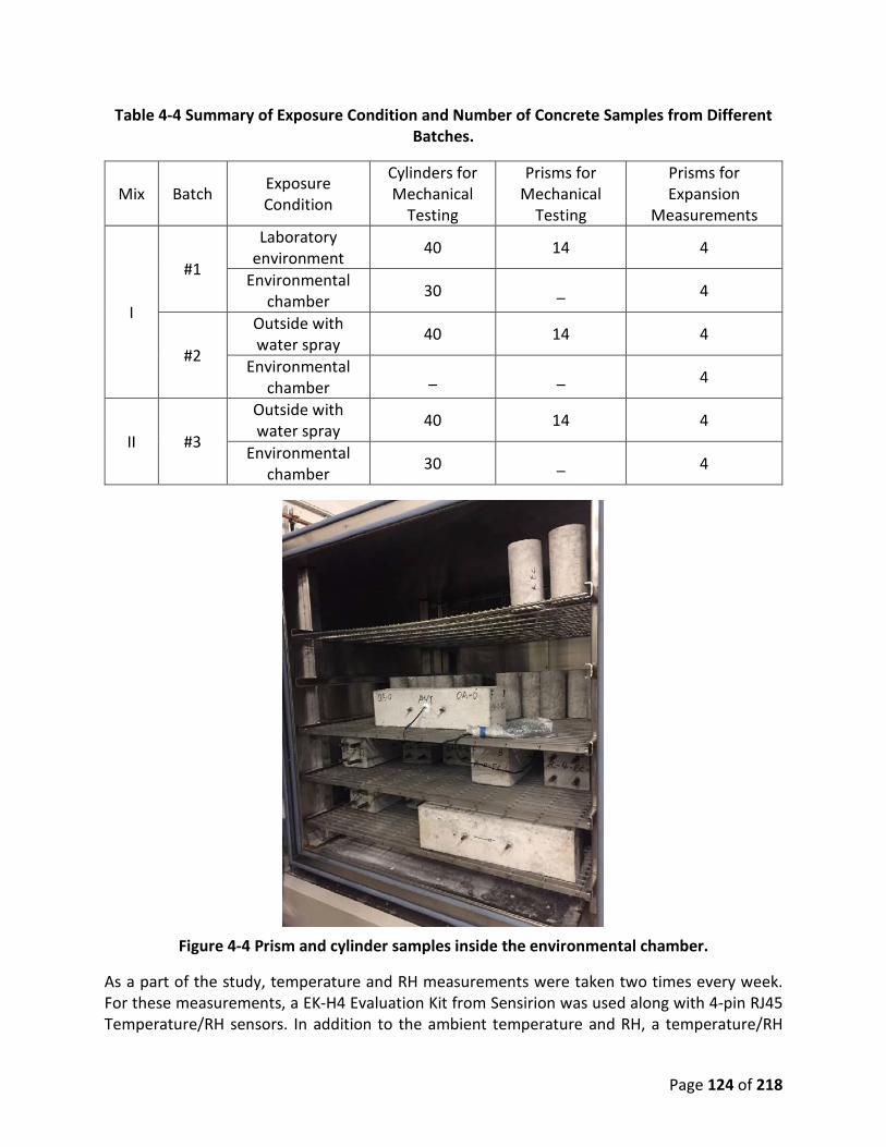
Page 124 of 218
Table 4-4 Summary of Exposure Condition and Number of Concrete Samples from Different Batches.
Mix Batch Exposure Condition
Cylinders for Mechanical
Testing
Prisms for Mechanical
Testing
Prisms for Expansion
Measurements
I
#1
Laboratory environment 40 14 4
Environmental chamber 30 _ 4
#2
Outside with water spray 40 14 4
Environmental chamber _ _ 4
II #3
Outside with water spray 40 14 4
Environmental chamber 30 _ 4
Figure 4-4 Prism and cylinder samples inside the environmental chamber.
As a part of the study, temperature and RH measurements were taken two times every week. For these measurements, a EK-H4 Evaluation Kit from Sensirion was used along with 4-pin RJ45 Temperature/RH sensors. In addition to the ambient temperature and RH, a temperature/RH

Page 125 of 218
sensor was embedded inside one prism from five different groups including a prism from Batch 1 in the laboratory, prisms kept outside from Batches 2 and 3, and prisms kept in the environmental chamber from Batches 1 and 3. Figure 3.5 shows the Sensirion device and the sensor as well as the location of the embedded sensor in the middle of each prism. Accordingly, Figure 4-6 to Figure 4-8 present the temperature results over time for one prism from each group compared to the ambient temperature. As seen in these figures, the temperature inside the prisms closely follow the ambient temperature. Figure 4-9 to Figure 4-11 present the RH histories over time for one prism from each group compared to the ambient RH. At some ages the sensors were not functional, and the data corresponding to those points are missing in the temperature and RH plots. The measurements were taken during the daytime and right before spraying water for the prims kept outside. For the specimens in the environmental chamber, there are a few drops in the temperature and RH data. This occurred due to temporary shutdowns of the environmental chamber due to power issues and others that caused reduction of temperature and RH inside the specimens. As seen in Figure 4-9, the RH inside the prism samples converges towards the ambient RH of the laboratory. As will be shown in the next section, this did not occur for the large-scale beams. The prisms have a relatively short diffusion path for moisture to reach the outside of the specimen compared to the large-scale beams. Over the period of monitoring, the RH drops from close to 85% (due to water supplied for mixing) to 60%. The prisms kept outdoors maintained a high RH (close to 100%) as desired, which was achieved through the water spray and covering with tarp. Similarly, the prisms kept in the environmental chamber maintained a high RH. Variations of the outside ambient temperature over time were also acquired (National Oceanic and Atmospheric Administration, 2019) and plotted in Figure 4-12. Similarly, variations of the outside ambient temperature over time were obtained (National Oceanic and Atmospheric Administration, 2019) and plotted in Figure 4-13. The temperature plot, Figure 4-12, and the RH plot, Figure 4-13, show the average of hourly data points from 6 a.m. to 6 p.m. representing the daytime and from 6 p.m. to 6 a.m. representing the nighttime. Accordingly, there are two data points per day in Figure 4-12 and Figure 4-13.
Figure 4-5 (a) Sensirion device and T(temperature)/RH sensor (b) Location of the sensor in
prism.
T/RH Evaluation Kit
T/RH Sensor
T/RH Sensor Embedded in Prism
150 mm
150 mm
ba
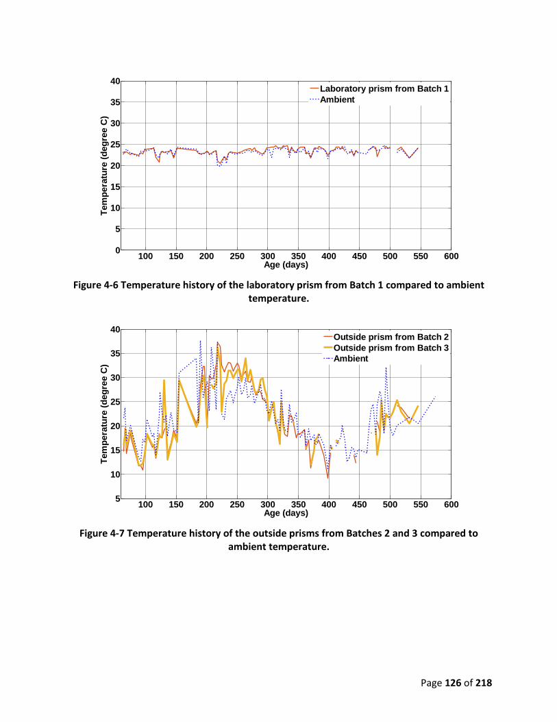
Page 126 of 218
Figure 4-6 Temperature history of the laboratory prism from Batch 1 compared to ambient
temperature.
Figure 4-7 Temperature history of the outside prisms from Batches 2 and 3 compared to
ambient temperature.
100 150 200 250 300 350 400 450 500 550 6000
5
10
15
20
25
30
35
40
Age (days)
Tem
pera
ture
(deg
ree
C)
Laboratory prism from Batch 1Ambient
100 150 200 250 300 350 400 450 500 550 6005
10
15
20
25
30
35
40
Age (days)
Tem
pera
ture
(deg
ree
C)
Outside prism from Batch 2Outside prism from Batch 3Ambient

Page 127 of 218
Figure 4-8 Temperature history of the environmental chamber prisms from Batches 1 and 3
compared to ambient temperature.
Figure 4-9 RH history in the laboratory prism from Batch 1 compared to ambient RH.
100 150 200 250 300 350 400 450 500 550 6000
10
20
30
40
50
60
70
Age (days)
Tem
pera
ture
(deg
ree
C)
Environmental chamber prism from Batch 1Environmental chamber prism from Batch 3Ambient
100 150 200 250 300 350 400 450 500 550 6000
20
40
60
80
100
Age (days)
RH
(%)
Laboratory prism from Batch 1Ambient

Page 128 of 218
Figure 4-10 RH history in the outside prisms from Batches 2 and 3 compared to ambient RH.
Figure 4-11 RH history in the environmental chamber prisms from Batches 1 and 3 compared
to ambient RH.
100 150 200 250 300 350 400 450 500 550 6000
20
40
60
80
100
120
140
Age (days)
RH
(%)
Outside prism from Batch 2Outside prism from Batch 3Ambient
100 150 200 250 300 350 400 450 500 550 6000
20
40
60
80
100
120
140
Age (days)
RH
(%)
Environmental chamber prism from Batch 1Environmental chamber prism from Batch 3Ambient

Page 129 of 218
Figure 4-12 History of outside ambient temperature.
Figure 4-13 History of outside ambient RH.
4.2.1.b. Material Mechanical Property Tests
As a part of the study, the degradation of concrete properties was monitored at specific time intervals. Compression and split tensile tests were conducted on the concrete cylinders according to ASTM C39/C39M – 18 (2018a) and ASTM C496/C496M – 04 (2017a), respectively, as shown in Figure 4-14 and Figure 4-15. Flexural tests were conducted on the concrete prisms according to ASTM C78 – 02 (2010), as shown in Figure 4-16.
0 74 148 222 296 370 444 518 592 666 740 814 888 962 10361110118412580
5
10
15
20
25
30
35
40
Age (months)
Tem
pera
ture
(deg
ree
C)
0 74 148 222 296 370 444 518 592 666 740 814 888 962 103611101184125810
20
30
40
50
60
70
80
90
100
Age (months)
RH
(%)

Page 130 of 218
Figure 4-14 Compression test on concrete cylinders.
Figure 4-15 Split tensile test on concrete cylinders.

Page 131 of 218
Figure 4-16 Flexural tests on concrete prisms.
Table 4-5 shows the ages of testing and the number of cylinders tested for compressive strength. Similarly, Table 4-6 presents the ages of testing and the number of cylinders tested for tensile strength. Table 4-7 shows the ages of testing and the number of prisms tested for flexural strength. The curing conditions of the different concrete samples are also specified in these tables.
Table 4-5 Schedule for the Compressive Testing of Concrete Cylinders.
Batch
Total No. of
Cylinders
Exposure conditions
Age of Testing 1
day
3 day
s
7 day
s
17 day
s
28 day
s
3 mont
hs
7 mont
hs
12 mont
hs
18 mont
hs
1 24 Laboratory
environment
3 - 3 3 3 3 3 3 3
2 21 Outside
with water spray
3 - 3 - 3 3 3 3 3
3 24 Outside
with water spray
- 3 3 3 3 3 3 3 3
1 15 Environmental chamber - - - - 3 3 3 3 3
3 15 Environmental chamber - - - - 3 3 3 3 3

Page 132 of 218
Table 4-6 Schedule for the Split Tensile Testing of Concrete Cylinders.
Batch Total No.
of Cylinders
Exposure Conditions
Age of Testing 17
days 28
days 3
months 7
months 12
months 18
months
1 18 Laboratory environment 3 3 3 3 3 3
2 15 Outside with water spray - 3 3 3 3 3
3 18 Outside with water spray 3 3 3 3 3 3
1 15 Environmental chamber - 3 3 3 3 3
3 15 Environmental chamber - 3 3 3 3 3
Table 4-7 Schedule for the Flexural Testing of Concrete Prisms.
Batch Total No. of Prisms Exposure Conditions
Age of Testing
3 months 7 months 12 months
18 months
1 12 Laboratory environment 2 2 2 2
2 12 Outside with water spray 2 2 2 2
3 12 Outside with water spray 2 2 2 2
In addition to the material tests on the concrete samples, the tensile strength and uniaxial stress-strain curves of the different rebar used to fabricate the beams were needed. Table 4-8 presents the size and number of tested rebar samples from different heats and the gripping condition used in testing the rebar. Uniaxial tensile tests were conducted according to ASTM A370 -14 (2014a) on rebar samples of the same heat used in the beams. The rebar samples were tested using an MTS loading frame, Model 370.50 with 500 kN capacity, and an Instron extensometer, Model 2630-116 with 50 mm gauge length and 0.25 mm accuracy, was installed on the rebar to measure the rebar strains. Smaller diameter rebar was gripped directly using the hydraulic tension grips of the MTS frame and the others were griped to the frame using a special setup with Headed Reinforcement Corporation couplers due to the high grip pressure needed, which could cause premature failure at the grips. Figure 4-17 shows the test setup for the rebar tensile tests. The applied load and the rebar extension from the extensometer were synchronized and recorded using a National Instruments PXI-8119 data acquisition system.
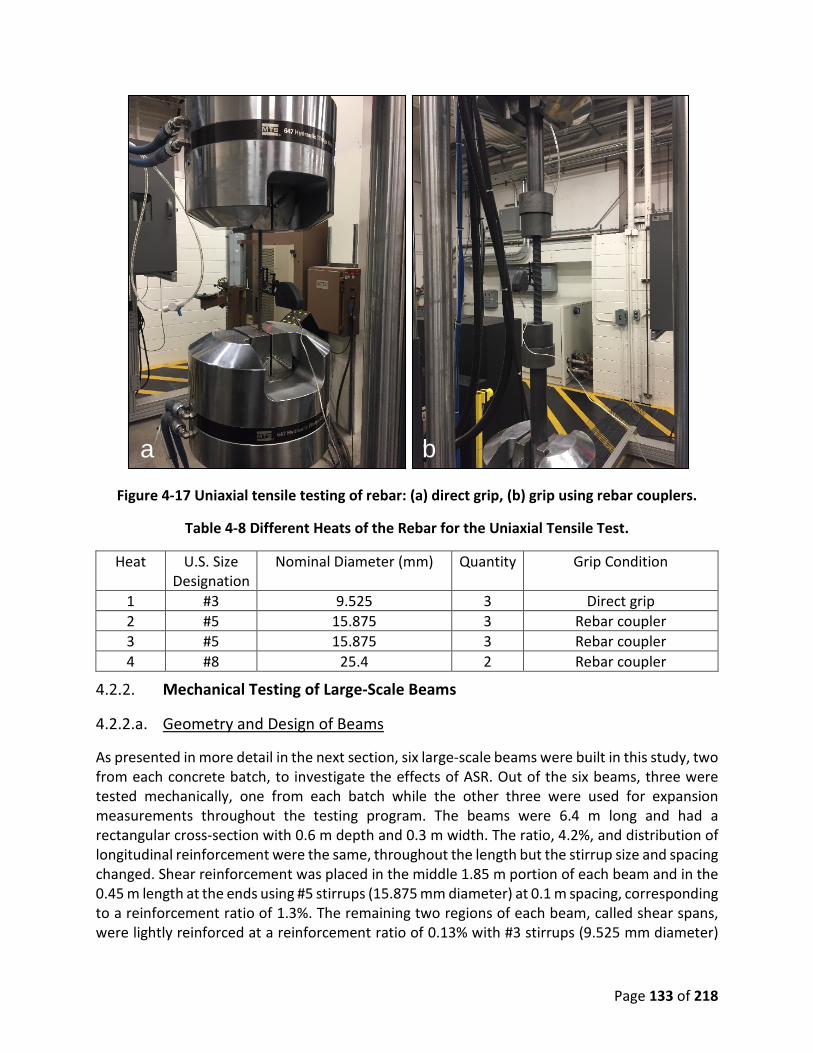
Page 133 of 218
Figure 4-17 Uniaxial tensile testing of rebar: (a) direct grip, (b) grip using rebar couplers.
Table 4-8 Different Heats of the Rebar for the Uniaxial Tensile Test.
Heat U.S. Size Designation
Nominal Diameter (mm) Quantity Grip Condition
1 #3 9.525 3 Direct grip 2 #5 15.875 3 Rebar coupler 3 #5 15.875 3 Rebar coupler 4 #8 25.4 2 Rebar coupler
Mechanical Testing of Large-Scale Beams
4.2.2.a. Geometry and Design of Beams
As presented in more detail in the next section, six large-scale beams were built in this study, two from each concrete batch, to investigate the effects of ASR. Out of the six beams, three were tested mechanically, one from each batch while the other three were used for expansion measurements throughout the testing program. The beams were 6.4 m long and had a rectangular cross-section with 0.6 m depth and 0.3 m width. The ratio, 4.2%, and distribution of longitudinal reinforcement were the same, throughout the length but the stirrup size and spacing changed. Shear reinforcement was placed in the middle 1.85 m portion of each beam and in the 0.45 m length at the ends using #5 stirrups (15.875 mm diameter) at 0.1 m spacing, corresponding to a reinforcement ratio of 1.3%. The remaining two regions of each beam, called shear spans, were lightly reinforced at a reinforcement ratio of 0.13% with #3 stirrups (9.525 mm diameter)
a b

Page 134 of 218
at 0.35 m spacing to ensure a shear dominant failure. Two tests were done on each beam (one on each end) to test repeatability. Therefore, in total, six shear tests were conducted on Beams 1 to 3 built from Batches 1 to 3, respectively. Despite having the same nominal configuration, the actual locations of the reinforcement, loading and support conditions varied slightly due to construction tolerances. Figure 4-18 presents the dimensions and the actual reinforcement layouts of the tested beams along with the location of the supports and the applied load for each shear test. The three beams in Figure 4-18 were used for both the expansion measurement and the mechanical tests. The dimensions and reinforcement layout of the rest of the beams, Beams 4 to 6 respectively built from Batches 1 to 3, which were only used for the expansion measurement are presented in Figure 4-19.
Figure 4-18 Dimensions and reinforcement layouts of Beams 1 to 3 (all units are in mm).

Page 135 of 218
Figure 4-19 Dimensions and reinforcement layouts of Beams 4 to 6 (all units are in mm).
4.2.2.b. Fabrication, Curing and Exposure Conditions of Beams
Rebar cages for the six beams were fabricated at a local precast concrete plant and they were shipped to the University of Southern California (USC) campus for installing the strain gauges on the reinforcements. Figure 4-20 shows the strain gauges installed on the stirrups. Figure 4-21 shows some of the rebar cages on campus after installation of reinforcement instrumentation.
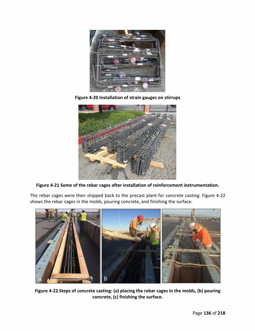
Page 136 of 218
Figure 4-20 Installation of strain gauges on stirrups
Figure 4-21 Some of the rebar cages after installation of reinforcement instrumentation.
The rebar cages were then shipped back to the precast plant for concrete casting. Figure 4-22 shows the rebar cages in the molds, pouring concrete, and finishing the surface.
Figure 4-22 Steps of concrete casting: (a) placing the rebar cages in the molds, (b) pouring
concrete, (c) finishing the surface.
a b c

Page 137 of 218
Two RC beams were built from concrete Batch 1 and were kept in the laboratory environment from the age of 14 days. Two beams were built from Batch 2 and two beams were built from Batch 3. These four beams were kept outdoors at the USC Structures and Materials Research Laboratory (SMRL), under towel and tarp, and were sprayed with water two times a week. This information is summarized in Table 4-9. Figure 4-23 shows the beams that were kept outside and sprayed with water.
Table 4-9 Summary of Exposure Condition and Number of Beams from Different Batches.
Mix Batch Exposure Condition Beam I #1 Laboratory
environment Beam 1: for mechanical Tests 1 and 2 and expansion
measurements Beam 4: for expansion measurements
#2 Outside with water spray
Beam 2: for mechanical Tests 3 and 4 and expansion measurements
Beam 5: for expansion measurements II #3 Outside with water
spray Beam 3: for mechanical Tests 5 and 6 and expansion
measurements Beam 6: for expansion measurements
Figure 4-23 Outside beams conditioned with periodic water-spray.
Similar to the material samples, temperature/RH sensors were embedded in one beam kept in the laboratory and one beam kept outside. The locations of the embedded sensors are shown in Figure 4-24. The sensors are denoted as Top, Middle, and Bottom depending on the distance from the top of the beams. The temperature and RH measurements were taken two times every week. Figure 4-25 and Figure 4-26, respectively, show the temperature results over time for one beam from Batch 1 in the lab and one beam from Batch 3 outside. As seen in these figures, the temperature inside the beams closely follows the ambient temperature. Figure 4-27 and Figure 4-28 present the RH results over time for the same beams. It should be noted that the measurements were taken during the daytime and right before spraying water for the beams

Page 138 of 218
kept outside. Moreover, the sensors were not always functional, and the temperature and RH data are missing at some ages. Variations of the outside ambient temperature and RH over time were obtained (National Oceanic and Atmospheric Administration, 2019) and plotted earlier in Figure 4-12 and Figure 4-13, respectively. As seen in Figure 4-27, the RH inside the beams kept in the laboratory was always higher than the ambient RH of the laboratory. This is because it takes a long time for the moisture inside the beams from casting to leave the beam through diffusion. This also explains why the beams kept in the laboratory still showed ASR expansion despite the low ambient RH. Supporting the same conclusions, it was also observed that the top sensor showed lower RH compared to middle sensor and the middle sensor showed lower RH compared to the bottom sensor. This again is explained through the moisture diffusion. On the other hand, for the beams kept outside, the water spraying two times a week with covers, maintained almost 100% RH in the beams. The sensor at the top showed a lower RH due to its being closest to the surface and allowing easy moisture diffusion to the environment.
Figure 4-24 Locations of embedded T(temperature)/RH sensors in beam.
Figure 4-25 Temperature history of the laboratory beam from Batch 1 compared to ambient
temperature.
610
mm
Top T/RH Sensor
Middle T/RH Sensor
Bottom T/RH Sensor
125 mm
250 mm
125 mm
100 150 200 250 300 350 400 450 500 550 6000
5
10
15
20
25
30
35
40
Age (days)
Tem
pera
ture
(deg
ree
C)
TopMiddleBottomAmbient
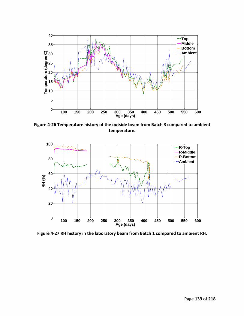
Page 139 of 218
Figure 4-26 Temperature history of the outside beam from Batch 3 compared to ambient
temperature.
Figure 4-27 RH history in the laboratory beam from Batch 1 compared to ambient RH.
100 150 200 250 300 350 400 450 500 550 6000
5
10
15
20
25
30
35
40
Age (days)
Tem
pera
ture
(deg
ree
C)
TopMiddleBottomAmbient
100 150 200 250 300 350 400 450 500 550 6000
20
40
60
80
100
Age (days)
RH
(%)
R-TopR-MiddleR-BottomAmbient

Page 140 of 218
Figure 4-28 RH history in the outside beam from Batch 3 compared to ambient RH.
Structural Tests
Six shear tests were conducted on three full-scale RC beams, Beams 1 to 3, as shown in Figure 4-18, that were cast from mix Batches 1 to 3, respectively. This information is also provided in Table 4-9.
4.2.3.a. Test Setup
The test setup consisted of different components as illustrated in Figure 4-29. The first component included the pin supports that allowed beam rotation around the transverse axis (i.e., perpendicular to the longitudinal beam axis). The details of each support including the base, the elastomeric pad, the steel plate, and the roller welded to the top steel plate are also shown in Figure 4-29. The elastomeric pad was used to release the beam longitudinal movement at the supports and prevent axial load in the beam. The second component included the loading frame and the servo-hydraulic actuator with a capacity of 675 kN for applying the load close to the top edge of the shear span. The third component included two lateral frames installed on the loading frame to restrain the beam out-of-plane movement. Between the beam and the side frames, rollers were installed to reduce resistance against vertical movement. The last component of the test setup was a set of five clamps installed on the shear span that was not being tested at the time. Each clamp applied a 178 kN post-tensioning force at the clamping locations. The total post-tensioning force applied through the five pairs of the clamps, 890 kN, was greater than the shear capacity of the beams. These clamps were used to reinforce the shear span that was not being tested and force the failure in the shear span being tested.
Figure 4-30 shows the actual test setup including the first and second shear spans, loading frame and actuator, actuator controller and data acquisition (DAQ) system, and hydraulic service manifold (HSM).
100 150 200 250 300 350 400 450 500 550 6000
20
40
60
80
100
120
140
Age (days)
RH
(%)
TopMiddleBottomAmbient

Page 141 of 218
Figure 4-29 Components of the structural test setup.
Figure 4-30 Structural test setup.
External Clamps
Loading Frame
Actuator
Support Support
Lateral Restraining Frame with roller
Restraining Bar
Load Cell
Elastomeric Pad
Base
Steel Plate
Restraining angle
Roller
First Shear SpanSecond Shear Span
Actuator Controller
andDAQ
SystemHSM
Loading Frame
Actu
ator

Page 142 of 218
4.2.3.b. Instrumentation
Several sensors including string potentiometers, spring loaded linear potentiometers, linear potentiometers, strain gauges, and load cells were used during testing to capture the shear behavior of the beams. The data from these sensors were synchronized and recorded at a rate of 10 samples per second using three 16-channels Titan Mini-Recorders from MARS Labs with a central Titan CPU08V Channel Multiplexer from the same company. The instrumentation of the beam is illustrated in Figure 4-31. The distance variables shown in Figure 3.31 are defined in Table 4-10 for all the shear tests.
Figure 4-31 Beam instrumentation scheme.
Table 4-10 Distance parameters for shear test instrumentation (all dimensions are in mm).
Beam Test a b c d e f g h i j k l m n o p q
1 Test 1 905 1831 511 905 357 371 372 387 192 152 162 349 79 502 127 146 276 Test 2 906 1805 443 906 386 346 368 338 212 155 159 284 78 511 120 150 344
2 Test 3 929 1808 454 929 349 373 363 398 169 156 161 293 35 483 149 148 298 Test 4 928 1837 445 928 354 349 375 351 257 151 155 290 41 470 159 162 295
3 Test 5 914 1831 479 914 371 368 354 395 190 153 148 331 24 490 168 152 276 Test 6 914 1806 457 914 376 344 373 337 221 155 153 304 63 487 168 223 287
The beam deflection was measured using string potentiometers and spring-loaded linear potentiometers placed under the beam. The beam deflection under the loading point, measured by a string potentiometer, was then revised because of the vertical deformation of the rubber pads used in the supports, as shown in Figure 4-32. The deformation of each support elastomeric pad, Y1 and Y2, was measured by averaging data from the two spring loaded linear potentiometers installed at both sides of each support under the beam. Then, the deflection measured by the string potentiometer under the loading point was revised by deducting the vertical movement of the beam under the loading point, Y, caused by the deformations of the elastomeric pads at the supports.
Loading Plate
Support
String Pot
String Pot
Vertical Linear Pot
Linear Pots Set 1
DEMECPoints
Spring Loaded Linear Pot
C.L. Linear Pots Set 2
Support
Spring Loaded Linear PotExternal Clamp
a b c
d e f g h i j k l
m
n
opq

Page 143 of 218
Figure 4-32 Beam vertical movement caused by the deformation of rubber pads in the
supports.
The movement along the beam length and the rotation about the transverse axis were also captured using the spring-loaded linear potentiometers at the ends of the beam. The strain of the concrete surface in the vertical direction was measured at six different locations using vertical linear potentiometers. Four of the vertical linear potentiometers were placed at the same cross-sections of the stirrups and the other two vertical linear potentiometers were installed close to the loading point and above the support. The horizontal strain on the concrete surface within the length of shear span was measured using two string potentiometers close to the top and bottom edges. Two sets of rosette shape linear potentiometers were installed on the face of the shear span to measure the shear deformation due to diagonal crack formation. To obtain the reactions at the supports an Omega load cell with 890 kN capacity was installed at the support closer to the loading point and an Omega load cell with 445 kN capacity was installed at the support farther from the load, as shown in Figure 4-29. The actuator load and displacement were also obtained from the actuator load cell and LVDT, respectively. Figure 4-33 presents a close-up view of the shear span ready for the test. As shown in this figure, in addition to the instrumentation of the shear span with various sensors, three still video cameras that were set to record the test by taking one picture every 30 seconds, were placed. Moreover, two high-resolution digital cameras were placed to take pictures from one side of the shear span every 30 seconds in order to develop crack maps at different load levels. The digital images of the beam at different stages of the testing are synchronized with the applied loading using current values of displacement and force values indicated on white boards within the view of each camera. Figure 4-34 shows the side of the shear span where the high-resolution digital cameras were installed.
𝑌 = 𝑌2 + 23𝑌1 − 𝑌2 = 2
3𝑌1+ 1
3𝑌2
𝑌𝑌2 𝑌1
𝐿2𝐿
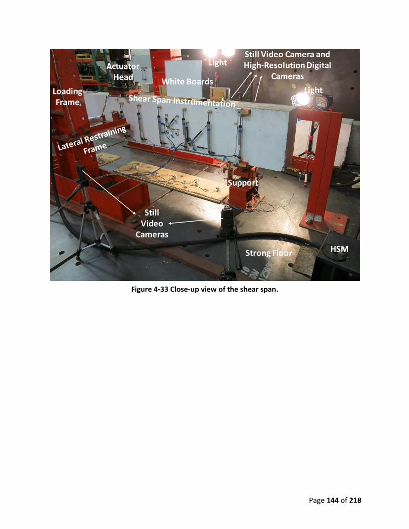
Page 144 of 218
Figure 4-33 Close-up view of the shear span.
ActuatorHead
Support
HSM
Still Video
Cameras
Still Video Camera and High-Resolution Digital
CamerasLight
Light
Loading Frame
Strong Floor
White Boards
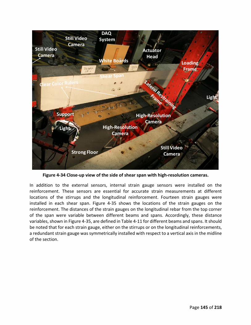
Page 145 of 218
Figure 4-34 Close-up view of the side of shear span with high-resolution cameras.
In addition to the external sensors, internal strain gauge sensors were installed on the reinforcement. These sensors are essential for accurate strain measurements at different locations of the stirrups and the longitudinal reinforcement. Fourteen strain gauges were installed in each shear span. Figure 4-35 shows the locations of the strain gauges on the reinforcement. The distances of the strain gauges on the longitudinal rebar from the top corner of the span were variable between different beams and spans. Accordingly, these distance variables, shown in Figure 4-35, are defined in Table 4-11 for different beams and spans. It should be noted that for each strain gauge, either on the stirrups or on the longitudinal reinforcements, a redundant strain gauge was symmetrically installed with respect to a vertical axis in the midline of the section.
Light
Light
Support
Loading Frame
ActuatorHead
White Boards
Still Video Camera
Still Video Camera
High-Resolution Camera
High-Resolution Camera
Still Video Camera
Strong Floor
DAQSystem

Page 146 of 218
Figure 4-35 Location of the strain gauges on the reinforcement (all units are in mm).
Table 4-11 Distance parameters for the strain gauges installed on the longitudinal reinforcement (all dimensions are in mm).
Beam Span A B C
1 1 102 104 101 2 121 121 118
2 1 119 120 103 2 94 99 109
3 1 141 135 90 2 101 129 112
4 1 117 121 99 2 101 98 105
5 1 106 108 99 2 110 121 112
6 1 132 129 102 2 119 117 110
102102
A 102
102102Strain GaugesB C
A
BC

Page 147 of 218
4.2.3.c. Loading Protocol
The shear tests were conducted following a quasi-static loading protocol. The protocol consisted of loading steps, pauses, and unloading steps with different load control and displacement control rates, as shown in Figure 4-36. In this figure, the ascending and descending lines represent the loading and unloading steps, respectively, and the horizontal lines show the pause periods. During each pause period, the whiteboards were updated with the new load and displacement values to be synchronized with the pictures taken by the digital cameras.
Figure 4-36 Loading protocol of the shear tests.
Monitoring the Long-Term Expansion of ASR at the Material and Structural Scales
Starting at the age of 14 days, expansion measurements were taken, once every two weeks, on the beams and the prisms. A demountable mechanical (DEMEC) strain gauge, Logic IQ model with 15.25 mm gauge length and 0.002 mm resolution, was used to measure the expansion between the two installed points, as shown in Figure 4-37. For the beams, the core concrete expansion was measured using four installed DEMEC studs in the middle of each shear span, as shown in Figure 4-38. The PVC tubes shown in that figure were used to ensure that the studs were only attached to the concrete core and the measurements were not affected by the surface concrete strains. The measurements were conducted in the horizontal and vertical directions for both shear spans of each beam and both sides of the beam. Accordingly, on the day when measurements were taken, each group of two beams representing the same concrete batch and similar environmental exposure required a total of 16 longitudinal measurements and 16 vertical measurements. This extensive set of measurements for every group of beams was to ensure the consistency and repeatability of the results. In addition to the beams, 24 prisms (six groups of four as mentioned in Table 4-4), had DEMEC studs passing through the concrete core for expansion measurements. The measurements were conducted on both sides of the prims in the
0 50 100 1500
100
200
300
400
500
600
700
Time (min)
Load
(kN
)
rate=0.22 kN/sec rate=0.44 kN/sec
rate=0.127 mm/sec

Page 148 of 218
longitudinal direction. Each group of prisms had four different ratios of longitudinal reinforcement: 0% (plain concrete), 1.23% (4 #3 rebar), 2.18% (4 #4 rebar), and 3.41% (4 #5 rebar) to investigate the relation between the reinforcement ratio and the expansion rate. Figure 4-39 shows a group of prisms with different reinforcement ratios for the expansion measurements. Table 4-12 summarizes the total number of the expansion measurements on the beams and prisms at different exposure conditions.
Figure 4-37 DEMEC device for the expansion measurement.
Figure 4-38 DEMEC points in the middle of shear spans.
DEMEC Stud
PVC Tube
150
mm
150 mm
Section
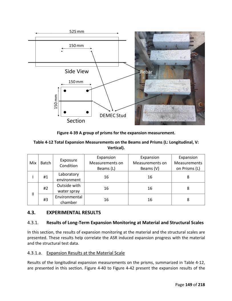
Page 149 of 218
Figure 4-39 A group of prisms for the expansion measurement.
Table 4-12 Total Expansion Measurements on the Beams and Prisms (L: Longitudinal, V: Vertical).
Mix Batch Exposure Condition
Expansion Measurements on
Beams (L)
Expansion Measurements on
Beams (V)
Expansion Measurements
on Prisms (L)
I #1 Laboratory environment 16 16 8
II #2 Outside with
water spray 16 16 8
#3 Environmental chamber 16 16 8
4.3. EXPERIMENTAL RESULTS
Results of Long-Term Expansion Monitoring at Material and Structural Scales
In this section, the results of expansion monitoring at the material and the structural scales are presented. These results help correlate the ASR induced expansion progress with the material and the structural test data.
4.3.1.a. Expansion Results at the Material Scale
Results of the longitudinal expansion measurements on the prisms, summarized in Table 4-12, are presented in this section. Figure 4-40 to Figure 4-42 present the expansion results of the
150
mm
150 mm
Section
150 mm
525 mm
Side View
DEMEC Stud
Rebar

Page 150 of 218
prisms, respectively, built from Batch 1 and kept in the laboratory, from Batch 2 and conditioned outside, and from Batch 3 and conditioned outside. Each figure includes four graphs for the prisms with different reinforcement ratios. The final expansion of the prisms built from Batch 2 and conditioned outside (0.22%) was found to be greater than the expansion of the prisms built from Batch 1 and kept in the laboratory (0.19%). However, the expansion results of these two groups were not significantly different since Batches 1 and 2 had identical mixture designs. On the other hand, the final expansion of the prisms forming Batch 3 and conditioned outside (0.6%) was found to be higher than the expansion of other prisms built from Batches 1 and 2. The reason is obviously the added alkaline to Batch 3 that accelerated the ASR in the specimens built from this batch. An important indication from Figure 4-40 to Figure 4-42 is that, regardless of the concrete mixture and conditioning, with increasing reinforcement ratio in the prisms, the expansion is reduced. This shows that the presence of reinforcement depending on the ratio to some extent counteracts the expansion effect of the ASR. For the prisms from different batches and in different conditions, the highest reinforcement ratio (3.41%) is shown to reduce the expansion to at least half compared with the cases of plain concrete. The prisms with 1.23% and 2.18% reinforcement ratios from Batch 3 with additional alkali also reduced the final expansion to about half of the expansion of the plain concrete prism from Batch 3. For Batches 1 and 2, the prisms with 1.23% and 2.18% reinforcement ratios, respectively, reduced the expansion by about 10% and 20% compared with the plain concrete prisms.
Figure 4-40 Expansion history of prisms built from Batch 1 and kept in the laboratory.
0 100 200 300 400 500 6000
0.2
0.4
0.6
0.8
1
Age (days)
Expa
nsio
n (%
)
0% Reinforcement Ratio1.23% Reinforcement Ratio2.18% Reinforcement Ratio3.41% Reinforcement Ratio
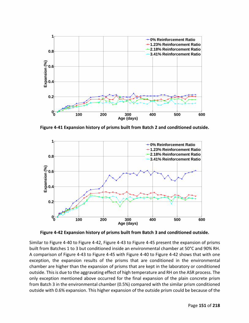
Page 151 of 218
Figure 4-41 Expansion history of prisms built from Batch 2 and conditioned outside.
Figure 4-42 Expansion history of prisms built from Batch 3 and conditioned outside.
Similar to Figure 4-40 to Figure 4-42, Figure 4-43 to Figure 4-45 present the expansion of prisms built from Batches 1 to 3 but conditioned inside an environmental chamber at 50°C and 90% RH. A comparison of Figure 4-43 to Figure 4-45 with Figure 4-40 to Figure 4-42 shows that with one exception, the expansion results of the prisms that are conditioned in the environmental chamber are higher than the expansion of prisms that are kept in the laboratory or conditioned outside. This is due to the aggravating effect of high temperature and RH on the ASR process. The only exception mentioned above occurred for the final expansion of the plain concrete prism from Batch 3 in the environmental chamber (0.5%) compared with the similar prism conditioned outside with 0.6% expansion. This higher expansion of the outside prism could be because of the
0 100 200 300 400 500 6000
0.2
0.4
0.6
0.8
1
Age (days)
Expa
nsio
n (%
)
0% Reinforcement Ratio1.23% Reinforcement Ratio2.18% Reinforcement Ratio3.41% Reinforcement Ratio
0 100 200 300 400 500 6000
0.2
0.4
0.6
0.8
1
Age (days)
Expa
nsio
n (%
)
0% Reinforcement Ratio1.23% Reinforcement Ratio2.18% Reinforcement Ratio3.41% Reinforcement Ratio

Page 152 of 218
dry and wet cycles. The prims built from Batch 3 with added alkali in the environmental chamber showed higher final expansion (0.5%) compared with the other two groups built from similar Batches of 1 and 2 with 0.23% and 0.37% expansions, respectively. However, the high temperature and RH of the environmental chamber caused the final expansion of the prims built from Batch 1 (0.37%) to be closer to the final expansion of the prims built from Batch 3 with added alkali, 0.5%. This shows that in an environment with high temperature and RH even the concrete with low alkali may experience a high level of ASR in the presence of reactive aggregates. Additionally, similar to the result of Figure 4-40 to Figure 4-42, Figure 4-43 to Figure 4-45 indicate that the higher the reinforcement ratio, the more constraint on the expansion caused by ASR. Again, the highest reinforcement ratio (3.41%) reduced the expansions of the prisms in the chamber to at least half compared with the plain concrete prisms from different batches. The prisms with 1.23% and 2.18% reinforcement ratios respectively reduced the final expansion by about 25% and 35% compared with the expansions of the plain concrete prisms.
Figure 4-43 Expansion histories of the prisms from Batch 1 and in the environmental
chamber.
0 100 200 300 400 500 6000
0.2
0.4
0.6
0.8
1
Age (days)
Expa
nsio
n (%
)
0% Reinforcement Ratio1.23% Reinforcement Ratio2.18% Reinforcement Ratio3.41% Reinforcement Ratio

Page 153 of 218
Figure 4-44 Expansion histories of the prisms from Batch 2 and in the environmental
chamber.
Figure 4-45 Expansion histories of the prisms from Batch 3 and in the environmental
chamber.
Figure 4-46 to Figure 4-49 present the comparison between the prisms from different batches and in different environments for 0%, 1.23%, 2.18%, and 3.41% reinforcement ratios, respectively. According to Figure 4-46, among the plain concrete prisms, those kept outside from Batch 3 with additional alkali showed 0.6% expansion after 18 months. The prisms from Batches 3 and 1 in the environmental chamber respectively showed 0.5% and 0.37% expansions. The rest of the plain prisms showed between 0.2% to 0.25% expansion. This correlates with the high
0 100 200 300 400 500 6000
0.2
0.4
0.6
0.8
1
Age (days)
Expa
nsio
n (%
)
0% Reinforcement Ratio1.23% Reinforcement Ratio2.18% Reinforcement Ratio3.41% Reinforcement Ratio
0 100 200 300 400 500 6000
0.2
0.4
0.6
0.8
1
Age (days)
Expa
nsio
n (%
)
0% Reinforcement Ratio1.23% Reinforcement Ratio2.18% Reinforcement Ratio3.41% Reinforcement Ratio

Page 154 of 218
influence of additional alkali as well as the high temperature and RH on the ASR expansion. The higher expansion of the plain prisms from Batch 3 that were kept outside (0.6%) compared with the expansion of similar prism in the environmental chamber (0.5%) can be attributed to the intensifying effect of dry and wet cycles due to the outdoor periodic water spray on the ASR. Figure 4-47 shows that among the prisms with 1.23% reinforcement ratio the prism with additional alkali kept in the environmental chamber showed the highest expansion (0.36%). Both the prism from Batch 1 kept in the environmental chamber and the prism from Batch 3 with additional alkali kept outside with water spray showed about 0.27% final expansion. Other prisms showed between 0.16% to 0.2% expansion. It is seen in Figure 4-48 that the prisms with 2.18% reinforcement ratio had similar expansion results to that of the prisms with 1.28% reinforcement ratio. In Figure 4-49, among the prisms with 3.41% reinforcement ratio, the prisms with additional alkali kept in the environmental chamber and outside with water spray showed the highest expansions: 0.31% and 0.24%, respectively. Other prisms showed between 0.11% to 0.13% expansion. Accordingly, among the prisms with the highest reinforcement ratio of 3.41%, only the expansion of prisms with additional alkali could exceed 0.2%. The expansion of other prisms with only reactive aggregate, even the ones in the environmental chamber, did not reach 0.15% when a reinforcement ratio of 3.41% was provided.
Figure 4-46 Expansion histories of the prisms with 0% reinforcement ratio.
0 100 200 300 400 500 6000
0.1
0.2
0.3
0.4
0.5
0.6
0.7
0.8
0.9
1
Age (days)
Expa
nsio
n (%
)
0% Reinforcement Ratio
Prism built from Batch 1 and kept in the labPrism built from Batch 2 and conditioned outsidePrism built from Batch 3 and conditioned outsidePrism built from Batch 1 and kept in the chamberPrism built from Batch 2 and kept in the chamberPrism built from Batch 3 and kept in the chamber

Page 155 of 218
Figure 4-47 Expansion histories of the prisms with 1.23% reinforcement ratio.
Figure 4-48 Expansion histories of prisms with 2.18% reinforcement ratio.
0 100 200 300 400 500 6000
0.1
0.2
0.3
0.4
0.5
0.6
0.7
0.8
0.9
11.23% Reinforcement Ratio
Age (days)
Expa
nsio
n (%
)
Prism built from Batch 1 and kept in the labPrism built from Batch 2 and conditioned outsidePrism built from Batch 3 and conditioned outsidePrism built from Batch 1 and kept the chamberPrism built from Batch 2 and kept the chamberPrism built from Batch 3 and kept the chamber
0 100 200 300 400 500 6000
0.1
0.2
0.3
0.4
0.5
0.6
0.7
0.8
0.9
1
Expa
nsio
n (%
)
Age (days)
2.18% Reinforcement Ratio
Prism built from Batch 1 and kept in the labPrism built from Batch 2 and conditioned outsidePrism built from Batch 3 and conditioned outsidePrism built from Batch 1 and kept in the chamberPrism built from Batch 2 and kept in the chamberPrism built from Batch 3 and kept in the chamber

Page 156 of 218
Figure 4-49 Expansion histories of the prisms with 3.41% reinforcement ratio.
4.3.1.b. Expansion Results at the Structural Scale
The results of the expansion measurements on the beams in the longitudinal and vertical directions, summarized in Table 4-12, are averaged and presented in this section. Figure 4-50 to Figure 4-52 present the results for the beams, respectively, built from Batch 1 and kept in the laboratory, built from Batch 2 and conditioned outside, and built from Batch 3 and conditioned outside. At each averaged data point an error bar is also shown, which represents the standard deviation of the data. Comparing Figure 4-50 and Figure 4-51 shows that from the beams built with similar mixes, Batches 1 and 2, the ones that were conditioned outside with water spray had similar expansions, 0.2% to 0.3%, compared with the beams in the laboratory. However, the expansion rate of the beams conditioned outside with periodic water spray was faster during the first 200 days. Comparing Figure 4-52 with Figure 4-50 and Figure 4-51 shows that the beams built from Batch 3 with added alkali and conditioned outside experienced higher expansion at the end of monitoring (0.4%), as well as a higher expansion rate compared to the other two groups of beams, mentioned above, with no added alkali.
0 100 200 300 400 500 6000
0.1
0.2
0.3
0.4
0.5
0.6
0.7
0.8
0.9
1
Age (days)
Expa
nsio
n (%
)3.41% Reinforcement Ratio
Prism built from Batch 1 and kept in the labPrism built from Batch 2 and conditioned outsidePrism built from Batch 3 and conditioned outsidePrism built from Batch 1 and kept in the chamberPrism built from Batch 2 and kept in the chamberPrism built from Batch 3 and kept in the chamber

Page 157 of 218
Figure 4-50 Expansion histories of the beams built from Batch 1 and kept in the laboratory.
Figure 4-51 Expansion histories of the beams built from Batch 2 and conditioned outside.
0 100 200 300 400 500 600-0.4
-0.2
0
0.2
0.4
0.6
0.8
1
Age (days)
Expa
nsio
n (%
)
Longitudinal DirectionVertical Direction
0 100 200 300 400 500 600-0.4
-0.2
0
0.2
0.4
0.6
0.8
1
Age (days)
Expa
nsio
n (%
)
Longitudinal DirectionVertical Direction
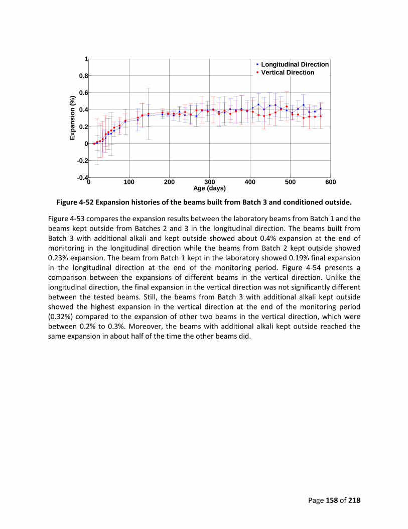
Page 158 of 218
Figure 4-52 Expansion histories of the beams built from Batch 3 and conditioned outside.
Figure 4-53 compares the expansion results between the laboratory beams from Batch 1 and the beams kept outside from Batches 2 and 3 in the longitudinal direction. The beams built from Batch 3 with additional alkali and kept outside showed about 0.4% expansion at the end of monitoring in the longitudinal direction while the beams from Batch 2 kept outside showed 0.23% expansion. The beam from Batch 1 kept in the laboratory showed 0.19% final expansion in the longitudinal direction at the end of the monitoring period. Figure 4-54 presents a comparison between the expansions of different beams in the vertical direction. Unlike the longitudinal direction, the final expansion in the vertical direction was not significantly different between the tested beams. Still, the beams from Batch 3 with additional alkali kept outside showed the highest expansion in the vertical direction at the end of the monitoring period (0.32%) compared to the expansion of other two beams in the vertical direction, which were between 0.2% to 0.3%. Moreover, the beams with additional alkali kept outside reached the same expansion in about half of the time the other beams did.
0 100 200 300 400 500 600-0.4
-0.2
0
0.2
0.4
0.6
0.8
1
Age (days)
Expa
nsio
n (%
)
Longitudinal DirectionVertical Direction

Page 159 of 218
Figure 4-53 Expansion histories of the beams in the longitudinal direction.
Figure 4-54 Expansion histories of the beams in the vertical direction.
Material Mechanical Test Results
In this section the results of mechanical tests on the plain concrete and rebar samples are presented. Concrete mechanical properties at different ages are discussed in correlation with the expansion results of plain concrete with no reinforcement.
0 100 200 300 400 500 600-0.2
0
0.2
0.4
0.6
0.8
1
Age (days)
Expa
nsio
n (%
)Longitudinal Direction
Beam built from Batch 1 and kept in the labBeam built from Batch 2 and conditioned outsideBeam built from Batch 3 and conditioned outside
0 100 200 300 400 500 600-0.2
0
0.2
0.4
0.6
0.8
1
Vertical Direction
Age (days)
Expa
nsio
n (%
)
Beam built from Batch 1 and kept in the labBeam built from Batch 2 and conditioned outsideBeam built from Batch 3 and conditioned outside
Page 160 of 218
4.3.2.a. Concrete Tests
The compression tests were conducted using a compressometer setup and linear strain conversion transducers (LSCTs), Model HM-2310.04, from Humboldt Manufacturing. In addition to the compressive strength, the elastic modulus of the cylinder samples was measured. Figure 4-55 presents the compressive strength of different groups of cylinder samples with ages ranging from 28 days to 18 months. The compressive strength of the cylinders built from Batch 1 and kept in the laboratory decreased by 10% after 18 months at an expansion level of 0.19%. The compressive strength results of the cylinders built from Batches 2 and 3 and conditioned outside with water spray, showed 13% and 12% increases, respectively, after 28 days until 18 months due to continuing cement hydration in the presence of a water supply. The increase in compressive strength happened despite the cylinders from Batches 2 and 3 experiencing 0.22% and 0.6% expansion, respectively, due to the ASR at 18 months. This indicates that at least during this period, the strength gain of the cylinders conditioned outside due to cement hydration was more than the degrading effect of ASR. Moreover, the extra alkali in the cylinders from Batch 3 that were kept outside has caused the concrete not to reach the same strength as the cylinders from the other batches within the first 28 days. As shown in Figure 4-56, results of compressive strength at 7 days showed 32 MPa compressive strength for the cylinders from Batch 3 with additional alkali, which was larger than the compressive strength of the cylinders from Batch 1 without additional alkali (28 MPa). On the other hand, at an age of 17 days, the compressive strength for the cylinders from Batch 3 (33 MPa) was less than the compressive strength of the cylinders from Batch 1 without additional alkali (36 MPa). It could be explained that the ASR degradation occurred from the age of 7 days and the presence of additional alkali did not prevent the cylinders from gaining strength before this age. The cylinders built from Batches 1 and 3 and conditioned in the environmental chamber showed 6% and 10% decrease in the compressive strength due to ASR induced expansions of 0.4% and 0.5% at 18 months, respectively. In addition to the greater reduction of compressive strength of the cylinders from high-alkali concrete of Batch 3 conditioned in the environmental chamber, these cylinders always showed lower strengths at different all ages compared with the other cylinders. This indicates the rapid reaction of extra alkali and reactive aggregate within the first months after casting the concrete. The lower compressive strength of the concrete cylinders conditioned in the environmental chamber compared to cylinders in other conditioning environments shows the aggravating effect of high temperature and RH on ASR. Unlike for cylinders conditioned outside, the degrading effect of the ASR on cylinders in the environmental chamber overcame the strengthening effect of cement hydration and caused a reduction of the compressive strength.

Page 161 of 218
Figure 4-55 Compressive strength of different groups of cylinders.
Figure 4-56 Compressive strength of the cylinders from Batches 1 and 3 during the first 28
days of age.
Figure 4-57 presents the results of the elastic modulus measurements, taken from the compression tests, for different groups of cylinders from 3 months to 12 months of age. Except for the cylinders made from Batch 1 and conditioned in the environmental chamber, the elastic modulus of other groups of cylinders remained almost unchanged between the ages of 3 months to 12 months. This shows that there is a minor influence of ASR on the elastic modulus of concrete, at least for this period and for expansions up to 0.6%. The cylinders from Batch 1 with no additional alkali that were conditioned in the environmental chamber showed increasing elastic moduli as they aged.
0
10
20
30
40
50
Batch 1 in lab Batch 2 outside Batch 3 outside Batch 1 in chamber Batch 3 in chamber
Com
pres
sion
Stre
ngth
(MPa
)
Concrete Cylinder Groups
28 days 3 months 7months 12months 18months
0
5
10
15
20
25
30
35
40
1 7 17 28
Com
pres
sive
Stre
ngth
(MPa
)
Age (days)
Concrete Cylinders from Batch 1 Concrete Cylinders from Batch 3

Page 162 of 218
Figure 4-57 Elastic modulus for different groups of cylinders.
Figure 4-58 presents the results of split tension tests for different groups of cylinders from 28 days to 18 months. Despite some exceptions, the overall trend of all the groups is one of decreasing tensile strength as the samples aged. This shows the considerable influence of the ASR-induced expansion on the tensile strength of all the concrete samples. The samples from Batch 1 kept in the laboratory experienced a 30% reduction of the tensile strength, while samples from Batches 2 and 3 (conditioned outside) showed 19% and 16% reduction of the tensile strength, respectively. The larger reduction of tensile strength in the laboratory samples from Batch 1 compared to the samples kept outside can be attributed to the fact that they did not gain strength from the cement hydration process as much as the samples conditioned outside did. It should be noted that the samples from the high-alkali concrete of Batch 3 kept outside with a maximum expansion of 0.6% showed the lowest tensile strength values at all ages compared with the samples from Batch 2 kept outside with a maximum expansion of 0.22% and the samples from Batch 1 kept in the laboratory with a maximum expansion of 0.19%. The samples from Batch 1 (kept in the laboratory) almost always showed higher tensile strength compared with samples from other groups despite showing 30% reduction in tensile strength over time. The samples from Batches 1 and 3 (kept in the environmental chamber) with maximum expansions of about 0.4% to 0.5% showed 29% and 38% reductions in tensile strength, respectively. Again, similar to the compressive strength results, the samples from the high-alkali concrete of Batch 3 kept in the environmental chamber with a maximum expansion of 0.5% showed the largest total reduction of tensile strength (38%), as well as the lowest values of tensile strengths at different ages. Moreover, the aggravating effect of high temperature and RH of the environmental chamber on the ASR is proved from the tensile strength measurements similar to the compressive strength results.
0
5000
10000
15000
20000
25000
Batch 1 in lab Batch 2 outside Batch 3 outside Batch 1 in chamber Batch 3 in chamber
Mod
ulus
of E
last
icity
(MPa
)
Concrete Cylinder Groups
3 months 7months 12months

Page 163 of 218
Figure 4-58 Tensile strength for different groups of cylinders.
The results of the flexural tests are shown in Figure 4-59. Despite some exceptions, the overall trend of the results shows a reduction of the modulus of rupture as the specimens aged. Compared with their response at 3 months of age, at 18 months of age the prisms made from Batch 3 with added alkali and kept outside showed the largest degradation in the modulus rupture (14%) compared with the prisms from Batch 2 kept outside, which was only 3%, and the prisms from Batch 1 kept in the laboratory, which was only 4%. The lowest values of the modulus of rupture at different ages were also obtained from the prisms of Batch 3 that were kept outside. It is recalled here that no prisms were conditioned in the environmental chamber for mechanical testing. This shows that the higher ASR activity results in a lower modulus of rupture. The prisms from Batch 3 kept outside with 14% reduction of modulus of rupture experienced 0.6% expansion over 18 months while the prisms from Batch 2 kept outside and the prisms from Batch 1 kept in the laboratory with insignificant reduction of modulus of rupture experienced around 0.2% expansion due to ASR at the same age.
0
1
2
3
4
5
Batch 1 in lab Batch 2 outside Batch 3 outside Batch 1 in chamber Batch 3 in chamber
Split
Ten
sile
Stre
ngth
(MPa
)
Concrete Cylinder Groups
28 days 3 months 7months 12 months 18months

Page 164 of 218
Figure 4-59 Modulus of rupture for different groups of prisms.
Comparing the results of Figure 4-55 to Figure 4-59, it is concluded that ASR does not affect all properties of concrete in the same way or to the same extent. Tensile strength showed the largest reduction due to ASR followed by the modulus of rupture and the compressive strength. Moreover, in some cases, the compressive strength increased due to the cement hydration process despite the ASR progress. The elastic modulus was found to be not considerably influenced by the ASR.
4.3.2.b. Rebar Tests
The stress versus strain diagrams from the uniaxial rebar tests are plotted in Figure 4-60 for different reinforcements. Reinforcements were from different heats even for the same size rebar. The rupture is not shown in the diagrams of the #5 and #8 rebar specimens. The reason is that the extensometer was removed shortly after the strength reduction to prevent damage to the sensor.
0
1
2
3
4
5
6
Batch 1 in lab Batch 2 outside Batch 3 outside
Mod
ulus
of R
uptu
re (M
Pa)
Concrete Prism Groups
3 months 7months 12months 18months

Page 165 of 218
Figure 4-60 Rebar stress-strain diagrams of different reinforcements.
Structural Shear Test Results
4.3.3.a. Shear Tests on Beam 1 from Batch 1 Kept in the Laboratory
The results of the shear tests on Beam 1 are presented in this section. Beam 1 was built from concrete Batch 1 with reactive aggregate but no additional alkali. The beam was kept in the laboratory environment until Tests 1 and 2 were conducted on its two shear spans at the age of 6 months. At this age, Beam 1 experienced less than 0.1% expansion due to ASR. During the first shear test, the loading was not increased beyond 556 kN to prevent damage in the second shear span. However, the string potentiometer failed to record the deflection under the loading point after reaching 511 kN load due to an issue with the sensor. The load-deflection diagrams of Tests 1 and 2 on the two shear spans of Beam 1 are shown in Figure 4-61. The figure shows that in the second shear test, after first cracking the span had stiffer behavior compared to the span that was tested first. The difference between the two diagrams can be attributed to the uncertain clamping force applied to the other side of the beam and the existing cracks in the other span during Test 2.
0 0.05 0.1 0.15 0.2 0.25 0.3 0.35 0.40
200
400
600
800
1000
Strain
Stre
ss (M
Pa)
#3 Stirrup#5 Stirrup#5 Longitudinal Rebar#8 Longitudinal Rebar

Page 166 of 218
Figure 4-61 Load-deflection diagrams for the shear tests on Beam 1.
Figure 4-62 compares the crack maps and widths during the two shear tests on Beam 1 at similar load levels. At each load level, the maximum crack width is smaller during the second test compared to the first test. This can be attributed to the uncertain clamping force applied to the other span during each test; and the influence of the cracks caused by the first test on the second test.
Figure 4-63 plots the maximum crack width as a function of the load for Tests 1 and 2 to facilitate a comparison between those tests. In this figure, some of the early loading and unloading steps are ignored for simplification since the crack sizes were very small at that point. Beam 1 was loaded further during Test 2 than it was during Test 1 to cause an ultimate failure of the beam. Figure 4-64 shows the crack maps and widths for all the loading steps of Test 2 that caused crack growth, including the latter steps leading up to failure.
0 5 10 15 20 25 30 350
100
200
300
400
500
600
700
Deflection under Loading Point (mm)
Load
(kN
)
Test 1Test 2
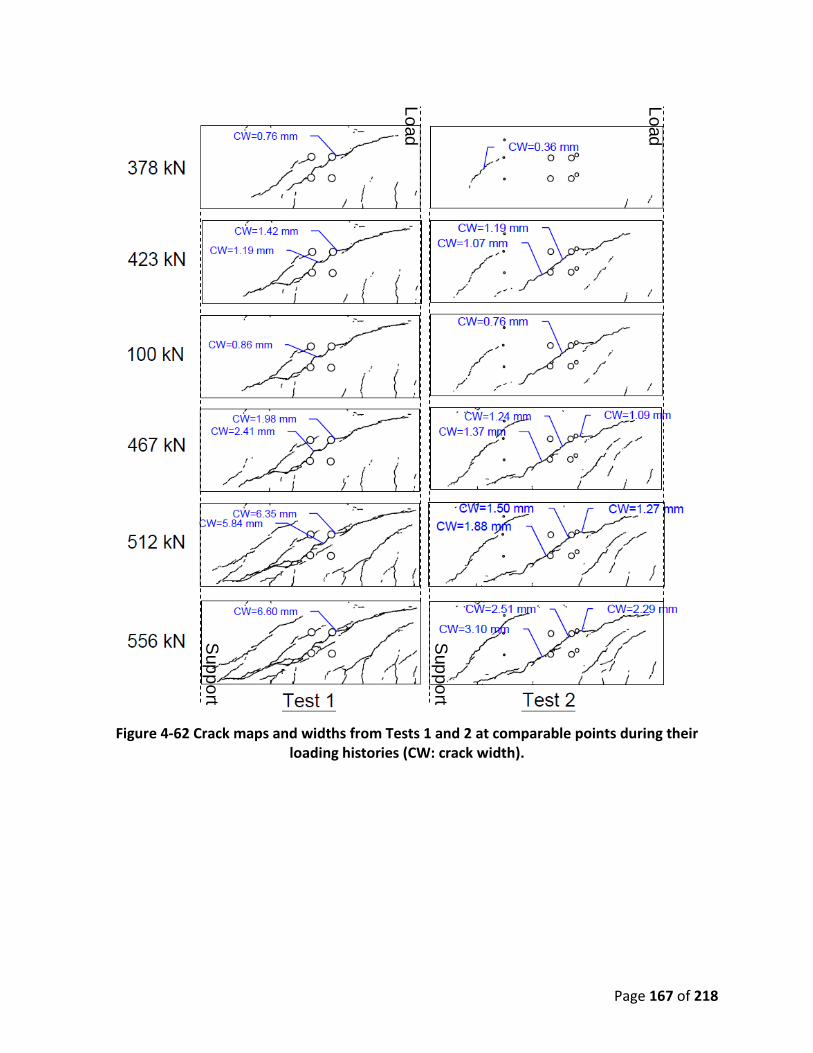
Page 167 of 218
Figure 4-62 Crack maps and widths from Tests 1 and 2 at comparable points during their
loading histories (CW: crack width).
Load
LoadS
upport
Support

Page 168 of 218
Figure 4-63 Load versus maximum crack width on the major diagonal crack.
Figure 4-64 Crack maps and widths from the full loading history in Test 2 (CW: crack width).
0 5 10 15 20 250
100
200
300
400
500
600
700
Maximum Crack Width (mm)
Load
(kN
)
Test 1Test 2
Load
Support
Load
Support

Page 169 of 218
In order to calculate the shear deformation of the beam around the mid-point of the shear span and the diagonal crack, the linear potentiometer sets in the rosette configuration were used as shown in Figure 3.31. The shear strain is computed from those measurements as:
𝛾𝛾𝑚𝑚𝑖𝑖 = 2𝜀𝜀𝑑𝑑 − (𝜀𝜀𝑚𝑚 + 𝜀𝜀𝑖𝑖) 4.1
where 𝜀𝜀𝑚𝑚, 𝜀𝜀𝑖𝑖, and 𝜀𝜀𝑑𝑑 are the measured strains in the x, y, and diagonal directions, respectively, as shown in Figure 4-65 (Beer et al., 2006).
Figure 4-65 Strains in different directions.
Figure 4-66 presents the applied load versus shear deformation for Test 2. As shown in Figure 4-31, The first set of linear potentiometers was installed in the middle of the shear span while the second set was closer to the support. Figure 4-66 shows that the shear deformation in the middle of shear span is larger than at the end due to the crack concentration in the former. During Test 1, the shear formation obtained from the linear potentiometer set closer to the support reached to 0.41 degrees. The linear potentiometer set in the middle of the span could not correctly capture the shear deformation because the main shear crack did not go through the rosette configuration of the linear potentiometers. Figure 4-67 presents a comparison between the shear deformation of the second set of linear potentiometers, closer to the support, from the two tests on Beam 1. At all load levels, the second linear potentiometer set experienced higher shear deformations during Test 1 compared with Test 2.
45 45
ε𝑖𝑖
ε𝑚𝑚
ε𝑑𝑑
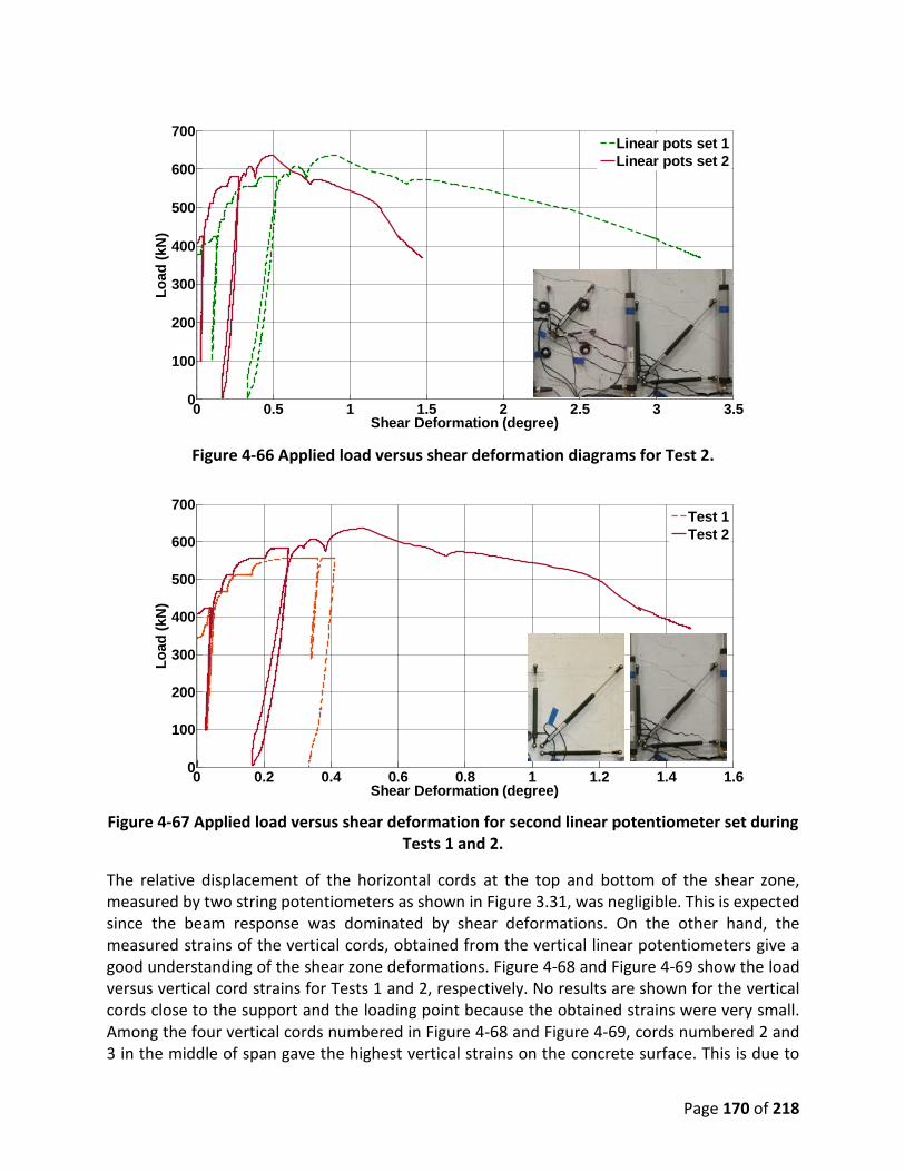
Page 170 of 218
Figure 4-66 Applied load versus shear deformation diagrams for Test 2.
Figure 4-67 Applied load versus shear deformation for second linear potentiometer set during
Tests 1 and 2.
The relative displacement of the horizontal cords at the top and bottom of the shear zone, measured by two string potentiometers as shown in Figure 3.31, was negligible. This is expected since the beam response was dominated by shear deformations. On the other hand, the measured strains of the vertical cords, obtained from the vertical linear potentiometers give a good understanding of the shear zone deformations. Figure 4-68 and Figure 4-69 show the load versus vertical cord strains for Tests 1 and 2, respectively. No results are shown for the vertical cords close to the support and the loading point because the obtained strains were very small. Among the four vertical cords numbered in Figure 4-68 and Figure 4-69, cords numbered 2 and 3 in the middle of span gave the highest vertical strains on the concrete surface. This is due to
0 0.5 1 1.5 2 2.5 3 3.50
100
200
300
400
500
600
700
Shear Deformation (degree)
Load
(kN
)
Linear pots set 1Linear pots set 2
0 0.2 0.4 0.6 0.8 1 1.2 1.4 1.60
100
200
300
400
500
600
700
Shear Deformation (degree)
Load
(kN
)
Test 1Test 2
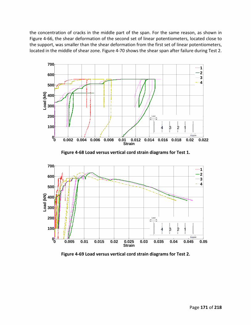
Page 171 of 218
the concentration of cracks in the middle part of the span. For the same reason, as shown in Figure 4-66, the shear deformation of the second set of linear potentiometers, located close to the support, was smaller than the shear deformation from the first set of linear potentiometers, located in the middle of shear zone. Figure 4-70 shows the shear span after failure during Test 2.
Figure 4-68 Load versus vertical cord strain diagrams for Test 1.
Figure 4-69 Load versus vertical cord strain diagrams for Test 2.
0 0.002 0.004 0.006 0.008 0.01 0.012 0.014 0.016 0.018 0.02 0.0220
100
200
300
400
500
600
700
Strain
Load
(kN
)
1234
0 0.005 0.01 0.015 0.02 0.025 0.03 0.035 0.04 0.045 0.050
100
200
300
400
500
600
700
Strain
Load
(kN
)
1234
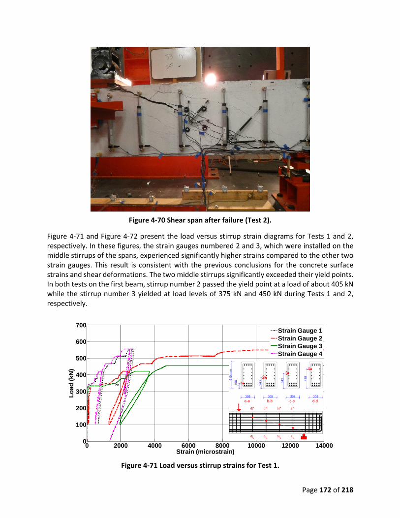
Page 172 of 218
Figure 4-70 Shear span after failure (Test 2).
Figure 4-71 and Figure 4-72 present the load versus stirrup strain diagrams for Tests 1 and 2, respectively. In these figures, the strain gauges numbered 2 and 3, which were installed on the middle stirrups of the spans, experienced significantly higher strains compared to the other two strain gauges. This result is consistent with the previous conclusions for the concrete surface strains and shear deformations. The two middle stirrups significantly exceeded their yield points. In both tests on the first beam, stirrup number 2 passed the yield point at a load of about 405 kN while the stirrup number 3 yielded at load levels of 375 kN and 450 kN during Tests 1 and 2, respectively.
Figure 4-71 Load versus stirrup strains for Test 1.
0 2000 4000 6000 8000 10000 12000 140000
100
200
300
400
500
600
700
Strain (microstrain)
Load
(kN
)
Strain Gauge 1Strain Gauge 2Strain Gauge 3Strain Gauge 4
e

Page 173 of 218
Figure 4-72 Load versus stirrup strains for Test 2.
In addition to the shear response, the flexural yielding of the beam was monitored through the strain gauges installed on the longitudinal rebar. Strain gauges were installed on the longitudinal reinforcements close to the loading point with maximum moment at the top and the bottom of the section. Figure 4-73 and Figure 4-74 present the load versus longitudinal rebar strain diagrams for Tests 1 and 2, respectively. The yield limit of the rebar strain is defined in these figures. Figure 4.34 shows that the longitudinal rebar remained elastic during most of Test 1 until the applied load reached 500 kN. Figure 4-74 shows that the longitudinal rebar remained elastic until the very end of Test 2, i.e., up to 578 kN load, after which the beam was pushed down in displacement controlled loading until a complete failure occurred. This demonstrates that, as intended, the behavior of the beams was governed by shear deformation and failure.
Figure 4-73 Load versus longitudinal rebar strains for Test 1.
0 2000 4000 6000 8000 10000 12000 14000 16000 18000 20000 22000 240000
100
200
300
400
500
600
700
Strain (microstrain)
Load
(kN
)
Strain Gauge 1Strain Gauge 2Strain Gauge 3Strain Gauge 4
-4000 -3000 -2000 -1000 0 1000 2000 3000 40000
100
200
300
400
500
600
700
Strain (microstrain)
Load
(kN
)
Strain Gauge 1Strain Gauge 3
eld
Lim
it Li
ne
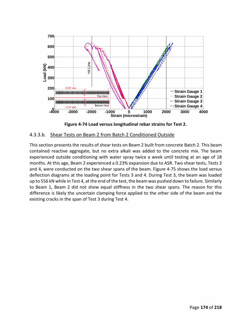
Page 174 of 218
Figure 4-74 Load versus longitudinal rebar strains for Test 2.
4.3.3.b. Shear Tests on Beam 2 from Batch 2 Conditioned Outside
This section presents the results of shear tests on Beam 2 built from concrete Batch 2. This beam contained reactive aggregate, but no extra alkali was added to the concrete mix. The beam experienced outside conditioning with water spray twice a week until testing at an age of 18 months. At this age, Beam 2 experienced a 0.23% expansion due to ASR. Two shear tests, Tests 3 and 4, were conducted on the two shear spans of the beam. Figure 4-75 shows the load versus deflection diagrams at the loading point for Tests 3 and 4. During Test 3, the beam was loaded up to 556 kN while in Test 4, at the end of the test, the beam was pushed down to failure. Similarly to Beam 1, Beam 2 did not show equal stiffness in the two shear spans. The reason for this difference is likely the uncertain clamping force applied to the other side of the beam and the existing cracks in the span of Test 3 during Test 4.
-4000 -3000 -2000 -1000 0 1000 2000 3000 40000
100
200
300
400
500
600
700
Strain (microstrain)
Load
(kN
)
Strain Gauge 1Strain Gauge 2Strain Gauge 3Strain Gauge 4
m
it Li
ne

Page 175 of 218
Figure 4-75 Load-deflection diagrams for the shear tests on Beam 2.
Figure 4-76 shows the crack maps and widths that occurred at similar load levels for Tests 3 and 4. The major cracks passed through the middles of the shear spans. There is a difference between the crack widths at the common load levels of Tests 3 and 4, which is correlated with the difference between the shear stiffness of the diagrams shown in Figure 4-75. Figure 4-76 only presents the crack maps for the load levels that were reached during both Tests 3 and 4. Beam 2 was loaded further during Test 4 to cause an ultimate failure of the beam. Figure 4-77 shows the crack maps and widths for all the loading steps of Test 4, which resulted in crack growth. The crack widths increased up to 3 mm at the peak load level of 676 kN, at which the beam started to fail under the sustained load.
0 5 10 15 20 25 30 35 400
100
200
300
400
500
600
700
Deflection under Loading Point (mm)
Load
(kN
)
Test 3Test 4

Page 176 of 218
Figure 4-76 Crack maps and widths for Tests 3 and 4 at comparable points during their loading
histories (CW: crack width).
Load
Load
Support
Support
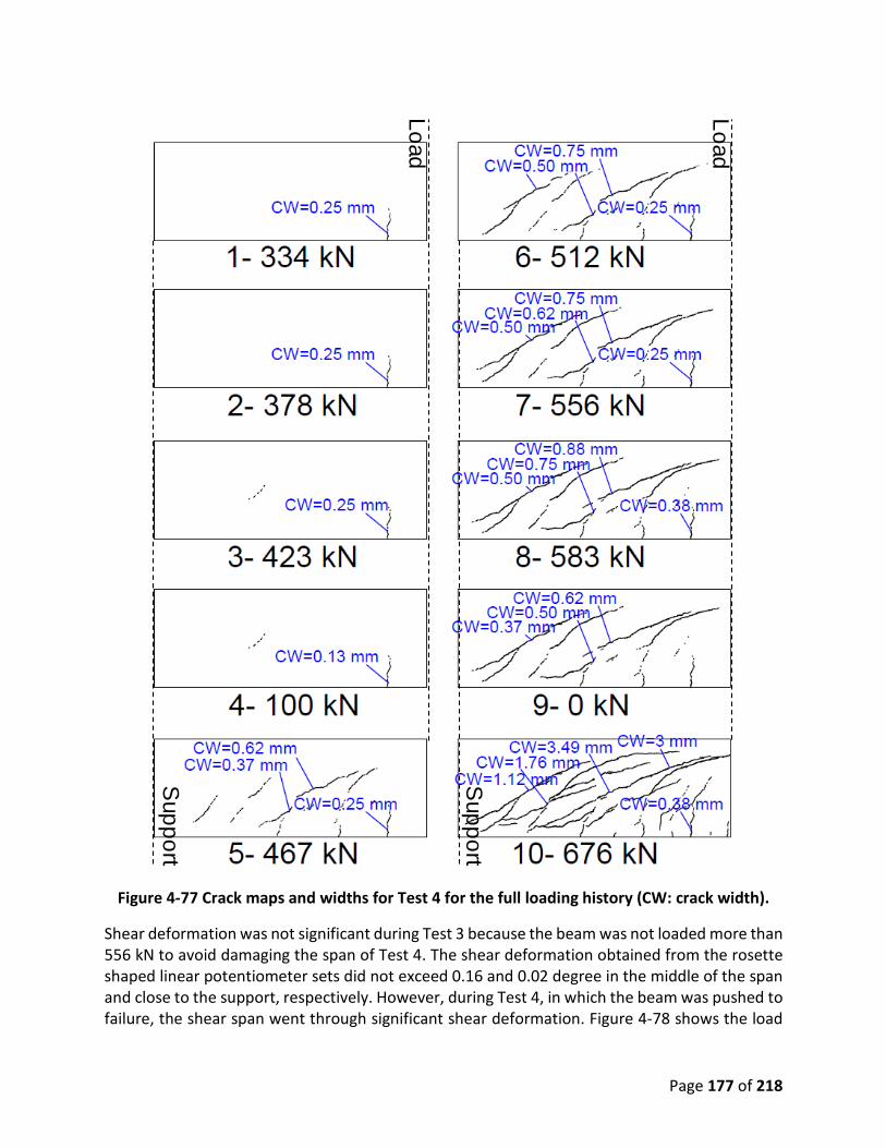
Page 177 of 218
Figure 4-77 Crack maps and widths for Test 4 for the full loading history (CW: crack width).
Shear deformation was not significant during Test 3 because the beam was not loaded more than 556 kN to avoid damaging the span of Test 4. The shear deformation obtained from the rosette shaped linear potentiometer sets did not exceed 0.16 and 0.02 degree in the middle of the span and close to the support, respectively. However, during Test 4, in which the beam was pushed to failure, the shear span went through significant shear deformation. Figure 4-78 shows the load
Load
Load
Support
Support

Page 178 of 218
versus shear deformation diagrams captured by the two sets of rosette shape linear potentiometers during Test 4. The span experienced 4.4 degrees and 2.5 degrees of shear deformation in the middle and close to the support, respectively, most of which occurred after the peak load.
Figure 4-78 Applied load versus shear deformation diagrams for Test 4.
Regarding the concrete surface vertical cords, Figure 4-79 and Figure 4-80 present the histories of the load versus vertical cord strains during Tests 3 and 4, respectively. It should be noted that the scale of the horizontal axis (strain) is significantly different between these figures. The main reason is that unlike Test 3, during Test 4 the beam was pushed to failure. Similar to Tests 1 and 2, during Tests 3 and 4, the dominant concrete surface vertical strains occurred in the two middle cords due to the crack concentration in the middle of the shear spans. The beam failure during Test 4 is shown in Figure 4-81. Similar to Tests 1 and 2, during Tests 3 and 4, the strains of the concrete surface horizontal cords at the top and the bottom of the shear spans were negligible.
0 0.5 1 1.5 2 2.5 3 3.5 4 4.50
100
200
300
400
500
600
700
Shear Deformation (degree)
Load
(kN
)
Linear pots set 1Linear pots set 2

Page 179 of 218
Figure 4-79 Load versus vertical cord strain diagrams for Test 3.
Figure 4-80 Load versus vertical cord strain diagrams for Test 4.
0 0.001 0.002 0.003 0.004 0.005 0.0060
100
200
300
400
500
600
700
Load
(kN
)
Strain
1234
0 0.01 0.02 0.03 0.04 0.05 0.06 0.07 0.08 0.09 0.10
100
200
300
400
500
600
700
Strain
Load
(kN
)
1234

Page 180 of 218
Figure 4-81 Shear span after failure (Test 4).
Figure 4-82 and Figure 4-83 show the load versus stirrup strain diagrams during Tests 3 and 4, respectively. For both tests, the two stirrups close to the middle of the shear span experienced higher strains than did the other stirrups. The other two stirrups, close to the load and the support, stayed nearly elastic throughout Test 3 and the load control part of Test 4. After unloading to zero, at the very end of Test 4, the actuator was switched to a displacement controlled mode to push the beam down to failure. As the beam failed, as seen in Figure 4-83, the two stirrups close to the load and the support also yielded in a manner similar to the middle stirrups.

Page 181 of 218
Figure 4-82 Load versus stirrup strains for Test 3.
Figure 4-83 Load versus stirrup strains for Test 4.
As mentioned earlier, to monitor the flexural yielding of the beam, the bottom and the top longitudinal rebar were instrumented with strain gauges close to the loading point with the maximum moment. Figure 4-84 and Figure 4-85 present the load versus longitudinal rebar strain diagrams for Tests 3 and 4, respectively. During Test 3, the longitudinal reinforcement had an elastic response until the very last loading step, in which one bottom longitudinal rebar barely exceeded the yield limit. During Test 4, the longitudinal rebar also stayed in the elastic range until the end of the test when the beam was pushed to failure in the displacement controlled mode, after which the bottom reinforcement passed the yield limit. These results proved that the shear deformations dominated the response of the beam during both Tests 3 and 4. The yield limit of the rebar strain is defined in Figure 4-84 and Figure 4-85.
0 1000 2000 3000 4000 5000 6000 7000 8000 9000 100000
100
200
300
400
500
600
700
Strain (microstrain)
Load
(kN
)
Strain Gauge 1Strain Gauge 2Strain Gauge 3Strain Gauge 4
e
0 1000 2000 3000 4000 5000 6000 7000 8000 9000 100000
100
200
300
400
500
600
700
Strain (microstrain)
Load
(kN
)
Strain Gauge 1Strain Gauge 2Strain Gauge 3Strain Gauge 4
e

Page 182 of 218
Figure 4-84 Load versus longitudinal rebar strains for Test 3.
Figure 4-85 Load versus longitudinal rebar strains for Test 4.
4.3.3.c. Shear Tests on Beam 3 from Batch 3 with Additional Alkaline Conditioned Outside
Results of the shear tests on Beam 3 built from concrete Batch 3 are presented in this section. In addition to reactive aggregate, this beam had a total alkali content, corresponding to 1.25% weight of cement, which was higher than that of the first two beams. The beam was kept outdoors and conditioned with periodic water spray two times a week. Two shear tests, Tests 5 and 6, were conducted on the two shear spans of the beam at the age of 18 months. At this age, Beam 3 experienced 0.4% expansion due to ASR. Figure 4-86 compares the load versus deflection diagrams at the loading point during Tests 5 and 6. To protect the other shear span, the beam
-4000 -3000 -2000 -1000 0 1000 2000 3000 40000
100
200
300
400
500
600
700
Strain (microstrain)
Load
(kN
)
Strain Gauge 1Strain Gauge 2Strain Gauge 3Strain Gauge 2
Yiel
d Li
mit
Line
-4000 -3000 -2000 -1000 0 1000 2000 3000 40000
100
200
300
400
500
600
700
Load
(kN
)
Strain (microstrain)
Strain Gauge 1Strain Gauge 2Strain Gauge 3Strain Gauge 4
Yiel
d Li
mit
Line

Page 183 of 218
was loaded only up to 556 kN during Test 5 while the beam was pushed to complete failure during Test 6. Regardless of some small differences in the load versus deflection diagrams, similar results were obtained for the two tests on this beam. This small difference can be attributed to the uncertain clamping force applied to the other side of the beam as well as the existing cracks in the span of Test 5 during Test 6.
Figure 4-86 Load-deflection diagrams for the shear tests on Beam 3.
Figure 4-87 compares the crack maps along with their widths for the shear spans at similar load levels during Tests 5 and 6. Despite some differences, the crack maps of the two tests are similar. The difference between the maximum crack widths of the spans at the common load levels is within the range of 0 mm to 0.75 mm. Since the beam was tested to failure in the second test, more crack maps were developed for the later steps, as shown in Figure 4-88. It is noticeable that even at the failure stage, the width of the few flexural cracks, close to the loading point with maximum moment, did not exceed 0.25 mm. This shows the dominance of shear deformation throughout the test from the beginning to failure. It should be noted that the crack maps and widths shown in step 10 of Figure 4-88 are at post-peak and are dependent on the amount of the deflection applied to the beam in the displacement controlled mode. Therefore, the crack information from this step cannot be necessarily compared to the other loading steps.
0 5 10 15 20 25 30 350
100
200
300
400
500
600
700
Deflection under Loading Point (mm)
Load
(kN
)
Test 5Test 6

Page 184 of 218
Figure 4-87 Crack maps and widths for Tests 5 and 6 at comparable points during their loading
histories (CW: crack width).
Load
Load
Support
Support
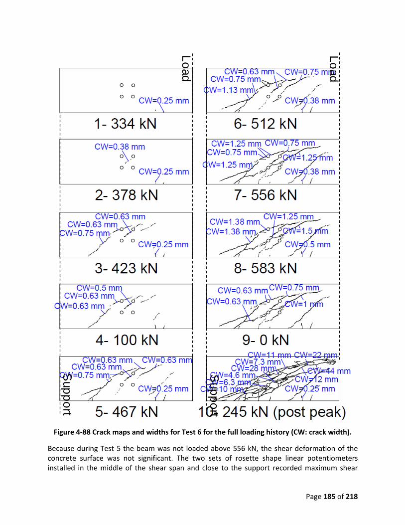
Page 185 of 218
Figure 4-88 Crack maps and widths for Test 6 for the full loading history (CW: crack width).
Because during Test 5 the beam was not loaded above 556 kN, the shear deformation of the concrete surface was not significant. The two sets of rosette shape linear potentiometers installed in the middle of the shear span and close to the support recorded maximum shear
Load
Load
Support
Support

Page 186 of 218
deformations of 0.48 degrees and 0.24 degrees, respectively. However, the beam experienced significant shear deformations during Test 6 when it was pushed down to failure. Figure 4-89 shows the load versus shear deformations captured in the middle of the shear span and close to the support during Test 6. The shear deformation in the middle of the span reached about 1 degree at the peak load and 3.3 degrees after failure. Figure 4-90 shows the shear span after failure during Test 6.
Figure 4-89 Applied load versus shear deformation diagrams for Test 6.
0 0.5 1 1.5 2 2.5 3 3.50
100
200
300
400
500
600
700
Shear Deformation (degree)
Load
(kN
)
Linear pots set 1Linear pots set 2

Page 187 of 218
Figure 4-90 Shear span after failure (Test 6).
The load versus vertical cord strains are plotted in Figure 4-91 and Figure 4-92 for Tests 5 and 6, respectively. It should be noted that the strain scale is much larger in Figure 4-92 compared with Figure 4-91 since Test 6 was continued until the complete failure of the beam. Figure 4-92 shows that the vertical cord strains in the middle of the shear zone were about 0.013 at the peak load and about 0.062 at the ultimate failure point. Similar to Tests 1 to 4 on Beams 1 and 2, for Tests 5 and 6 on Beam 3, the cracks were concentrated in the middle of the shear zone. Accordingly, the middle vertical cords experienced the largest strain values as shown in Figure 4-91 and Figure 4-92. Again, like all the previous shear tests, the horizontal cords at the top and the bottom of shear zone experienced negligible strains during Tests 5 and 6.
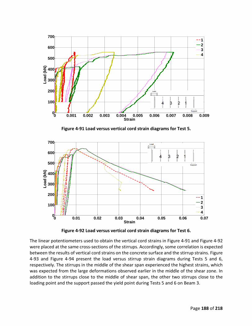
Page 188 of 218
Figure 4-91 Load versus vertical cord strain diagrams for Test 5.
Figure 4-92 Load versus vertical cord strain diagrams for Test 6.
The linear potentiometers used to obtain the vertical cord strains in Figure 4-91 and Figure 4-92 were placed at the same cross-sections of the stirrups. Accordingly, some correlation is expected between the results of vertical cord strains on the concrete surface and the stirrup strains. Figure 4-93 and Figure 4-94 present the load versus stirrup strain diagrams during Tests 5 and 6, respectively. The stirrups in the middle of the shear span experienced the highest strains, which was expected from the large deformations observed earlier in the middle of the shear zone. In addition to the stirrups close to the middle of shear span, the other two stirrups close to the loading point and the support passed the yield point during Tests 5 and 6 on Beam 3.
0 0.001 0.002 0.003 0.004 0.005 0.006 0.007 0.008 0.0090
100
200
300
400
500
600
700
Strain
Load
(kN
)
1234
0 0.01 0.02 0.03 0.04 0.05 0.06 0.070
100
200
300
400
500
600
700
Strain
Load
(kN
)
1234
Page 189 of 218
Figure 4-93 Load versus stirrup strains for Test 5.
Figure 4-94 Load versus stirrup strains for Test 6.
To ensure that the beam nonlinear behavior was governed by shear and the flexural response stayed in linear range, the load versus longitudinal rebar strain diagrams were evaluated as shown in Figure 4-95 and Figure 4-96. The longitudinal rebar strains at the top and bottom of the section were obtained using the installed strain gauges close to the loading point with the maximum moment. Figure 4-95 shows that the longitudinal reinforcement stayed in the elastic range throughout Test 5 until the very end of the test, when they barely reached the yield limit. Similarly, Figure 4-96 shows the elastic performance of the longitudinal reinforcement during Test 6. At the end of Test 6 when the beam was pushed to complete failure, the bottom longitudinal rebar passed the yield limit by about 250 microstrains. These results prove that the beam tests were dominated by the shear deformations.
0 0.2 0.4 0.6 0.8 1 1.2 1.4 1.6 1.8 2x 10⁴
0
100
200
300
400
500
600
700
Strain (microstrain)
Load
(kN
)
Strain Gauge 1Strain Gauge 2Strain Gauge 3Strain Gauge 4
e
0 0.2 0.4 0.6 0.8 1 1.2 1.4 1.6 1.8 2x 10⁴
0
100
200
300
400
500
600
700
Strain (microstrain)
Load
(kN
)
Strain Gauge 1Strain Gauge 2Strain Gauge 3Strain Gauge 4
e

Page 190 of 218
Figure 4-95 Load versus longitudinal rebar strains for Test 5.
Figure 4-96 Load versus longitudinal rebar strains for Test 6.
4.3.3.d. Comparison of the Shear Test Results of Beams 1 to 3
In this section, the results of shear tests on Beams 1, 2, and 3 are compared. As a summary of the previously presented information, two tests were conducted on each beam and six tests were done in total. Tests 1 and 2 were conducted on Beam 1, from concrete Batch 1 which contained reactive aggregate and kept in the laboratory environment for six months prior to the tests. Beam 1 experienced minimum to no ASR with expansions less than 0.1% prior to testing. Tests 3 and 4 were conducted on Beam 2, built from concrete Batch 2 with only reactive aggregate, with identical mixture proportions and ingredients to concrete Batch 1. Beam 2 was conditioned outdoors with a periodic water spray two times a week for 18 months. Beam 2 experienced 0.23%
-4000 -3000 -2000 -1000 0 1000 2000 3000 40000
100
200
300
400
500
600
700
Strain (microstrain)
Load
(kN
)
Strain Gauge 1Strain Gauge 2
Yiel
d Li
mit
Line
-4000 -3000 -2000 -1000 0 1000 2000 3000 40000
100
200
300
400
500
600
700
Strain (microstrain)
Load
(kN
)
Strain Gauge 1Strain Gauge 2
Yiel
d Li
mit
Line

Page 191 of 218
expansion at the time of testing. Tests 5 and 6 were conducted on Beam 3 built from concrete Batch 3 containing both reactive aggregate and additional alkali. Beam 3 was also kept outdoors for 18 months until testing and conditioned with water spray two times a week. Beam 3 experienced the highest ASR among all the beams with an expansion of 0.4% prior to testing. Tests 1, 3, and 5 were the first tests conducted on the beams and all followed the same loading protocol. In these tests, the peak load was not intended to go beyond 556 kN to avoid damaging the second shear span of each beam for the next tests. Tests 2, 4, and 6 were the second tests done on the beams. During these tests, the beams were unloaded after reaching 586 kN load and the loading protocol was switched from load control to displacement control to push the beams to complete failure.
Figure 4-97 and Figure 4-98 compare the load versus deflection diagrams between the first tests on the beams and between the second tests on the beams, respectively. Comparing the results of Beams 2 and 3 with Beam 1 in Figure 4-97 and Figure 4-98 during the first and the second tests, respectively, shows that Beams 2 and 3 showed respectively up to 23% and 5% higher shear stiffness compared to Beam 1. Beams 2 and 3 were conditioned in the outdoor environment for 18 months prior to the tests while Beam 1 was kept in the laboratory environment for six months until the tests. The higher stiffness of the outside Beams 2 and 3 compared with the laboratory-cured Beam 1 shows that the strengthening effect of cement hydration due to periodic water spray in the outdoor environment overcame the degrading effect of ASR. It could also be partly due to the self-prestressing effect of confined concrete affected by the ASR expansion. Moreover, comparing the results of Beam 2 with Beam 3 in Figure 4-97 and Figure 4-98 shows a reduction in the shear stiffness of up to 18% of Beam 3, which contained reactive aggregates and additional alkali compared to Beam 2, which only contained reactive aggregate. Both beams were conditioned in the outdoor environment but Beam 3 was more severely affected by the accelerated ASR due to the presence of additional alkali. Figure 4-98 presents the results of the tests in which the strengths of the beams were captured by pushing the beams to complete failure. This figure shows that Beam 3 had lower shear strength compared to the Beam 2, while both beams were conditioned outside for the same period. The shear strength of Beam 3 reached to 636 kN, which is lower than the shear strength of Beam 2, which failed under a sustained load of 676 kN while the test was paused when the actuator capacity was reached. This shows that Beam 3, which was more affected by the accelerated ASR (with an ASR-induced expansion of 0.4%) had at least 6% lower shear strength compared to Beam 2 (with an ASR-induced expansion of 0.23%). On the other hand, the strength of Beam 3, 636 kN, was similar to that of Beam 1. This shows that, the strengthening effect of cement hydration from 18 months of outside conditioning and constant moisture supply in Beam 3 was barely sufficient to overcome the deleterious effects of ASR. Therefore, the strength of Beam 3 was similar to that of Beam 1, which was cured in the laboratory environment for 6 months and was minimally affected by ASR.

Page 192 of 218
Figure 4-97 Load-deflection diagrams obtained from the first tests on the three beams.
Figure 4-98 Load-deflection diagrams obtained from the second tests on the three beams.
Figure 4-99 and Figure 4-100 compare the crack maps and widths between the first tests on the three beams and between the second tests on the three beams, respectively, at common load steps. These figures indicate that Beams 2 and 3 had significantly smaller crack widths compared to Beam 1. This is consistent with the conclusions from the load-deflection diagrams plotted in Figure 4-97 and Figure 4-98. Beams 2 and 3, which were conditioned in the outdoor environment for 18 months showed higher shear stiffness compared to Beam 1, which was kept in the laboratory for 6 months. Moreover, Figure 4-99 and Figure 4-100 show that the crack widths of Beam 3 were larger compared with Beam 2. Again, this is consistent with the results from the
0 5 10 15 20 25 300
100
200
300
400
500
600
700
Deflection under Loading Point (mm)
Load
(kN
)
Beam 1Beam 2Beam 3
0 5 10 15 20 25 30 35 400
100
200
300
400
500
600
700
Deflection under Loading Point (mm)
Load
(kN
)
Beam 1Beam 2Beam 3
Page 193 of 218
load deflection diagrams. Compared to Beam 2, Beam 3 experienced lower shear stiffness and larger cracks due to the more advanced ASR degradation. At the 556 kN load, during the first tests, Beam 3 experienced 2 mm cracks while the maximum crack width for Beam 2 was 1.1 mm. At the 556 kN load, during the second tests, the maximum crack width in Beam 3 reached 1.25 mm, while the maximum crack width in Beam 2 was 0.75 mm. It should be noted that the shear cracks were dominant in all the tests. The flexural cracks, which were very limited in number in size, did not open further as the tests progressed.
Figure 4-99 Crack maps and widths for the first tests on the beams (CW: crack width).
Load
Load
Support
Support
Support
Load

Page 194 of 218
Figure 4-100 Crack maps and widths for the second tests on the beams (CW: crack width).
Figure 4-101 presents the shear cracks at the end of all the six tests. The photographs of the first tests on the beams, Tests 1 and 3 and 5, are for the peak load and the photograpahs of the second tests on the beams, Tests 2 and 4 and 6, are for the post peak condition (i.e., after the beam completely failed).
Load
Load
Support
Support
Support
Load

Page 195 of 218
Figure 4-101 Condition of the beams at the end of the tests.
During the first tests on the beams, since the load was increased only up to 556 kN, the shear deformations were negligible. However, the beams went through considerable deformations during the second tests. Therefore, the second tests are compared for shear deformations of the three different beams. Figure 4-102 and Figure 4-103 compare the load versus shear deformations captured by the rosette shape linear potentiometer sets in the shear zone and close to the support, respectively. Figure 4-102 and Figure 4-103 indicate that for any given load prior to the peak strength, the shear deformation of Beam 3 is significantly larger than that of Beam 2 both in the middle of the shear zone and close to the support. This means that the higher ASR progress may considerably reduce the beam shear stiffness and increase its shear deformation. Figure 4-102 and Figure 4-103 also show that the shear deformations of Beam 2
Test 2
Test 6
Test 1
Test 3
Test 5
Test 4

Page 196 of 218
and Beam 3 for the given loads are, respectively, smaller than and almost equal to the shear deformations of Beam 1. This shows that Beam 2 (conditioned outside with ASR expansion of 0.23%) could get stronger due to the cement hydration. Therefore, Beam 2 went through smaller shear deformations during the test compared to Beam 1, which was only slightly affected by ASR in the laboratory environment prior to the test. On the other hand, the ASR-induced degradation of Beam 3 (with a higher alkali content and kept outside with 0.4% ASR expansion) overcame the strengthening due to cement hydration. Therefore, the shear deformation of Beam 3 during the test was almost equal to or slightly higher than the shear deformation of Beam 1, which was not conditioned with water spray.
Figure 4-102 Applied load versus shear deformation diagrams of the second tests on the
beams from linear pots set 1.
0 0.5 1 1.5 2 2.5 3 3.5 4 4.50
100
200
300
400
500
600
700
Shear Deformation (degree)
Load
(kN
)
Beam 1Beam 2Beam 3
0 0.5 1 1.5 2 2.5 3 3.5 4 4.50
100
200
300
400
500
600
700
Shear Deformaiton (degree)
Load
(kN
)
Beam 1Beam 2Beam 3
Page 197 of 218
Figure 4-103 Applied load versus shear deformation diagrams of the second tests on the beams from linear pots set 2.
The results of the beam tests showed that due to the crack concentration in the middle of shear spans, the strains of the middle vertical cords on the concrete surface were larger than the other cords. Figure 4-104 and Figure 4-105 present and compare the load versus strain of a middle vertical cord between the first tests on the beams and between the second tests on the beams, respectively. These figures show that the vertical cord strain in the middles of the shear spans are larger for Beam 3 (with an accelerated ASR expansion of 0.4%) compared to Beam 2 (with an ASR induced expansion of 0.23%). While Beams 2 and 3 were both conditioned with water spray two times a week in the outdoor environment for 18 months, Beam 3 could not gain strength due to the degradation from the high ASR expansion of 0.4%. On the other hand, 0.23% expansion from ASR did not prevent Beam 2 from strengthening and this beam showed the least concrete surface strains during the tests. The similarities of the diagram of Beam 3, especially during the second test, with that for Beam 1 show that the degrading effect of ASR with an expansion of 0.4% was almost equivalent to the strengthening effect of cement hydration from outside conditioning for 18 months.
Figure 4-104 Load versus middle cord strain diagrams for the first tests on the beams.
0 0.002 0.004 0.006 0.008 0.01 0.012 0.014 0.016 0.018 0.02 0.0220
100
200
300
400
500
600
700
Strain
Load
(kN
)
Beam 1 Cord 3Beam 2 Cord 3Beam 3 Cord 3

Page 198 of 218
Figure 4-105 Load versus middle cord strain diagrams for the second tests on the beams.
As for the vertical cord strains on the concrete surface, the results for the stirrup strains for the three beams indicated higher strains in the stirrups in the middle of the shear spans. Figure 4-106 and Figure 4-107 present and compare the load versus strain results of one stirrup close to the middle of shear spans between the first tests on the beams and between the second tests on the beams, respectively. Compared with Beam 2, which experienced 0.23% expansion due to ASR, Beam 3 (with 0.4% ASR induced expansion) experienced higher stirrup strains for the given loads. This is consistent with previous results that indicate that higher levels of ASR may lead to a weaker shear response of the beam. Even though Beam 2 was sprayed with water two times a week for 18 months and went through 0.23% expansion from ASR, its stirrup strain during the tests were much smaller than that of Beam 1, which was in the laboratory environment for 6 months and experienced less than 0.1% expansion due to ASR. This is because Beam 2 showed a higher shear strength as presented in Figure 4-97 and Figure 4-98. It can be concluded that for the ASR induced expansion rates up to 0.23%, the strengthening effect of cement hydration due to outside conditioning can be much higher than the degradation effect of ASR. However, the stirrup strains for Beam 3 with high ASR expansion effect, i.e., 0.4%, is very close to the results from Beam 1 for the given loads. This shows that for ASR induced expansions of 0.4% and above, the degradation effect of ASR on the beam shear behavior can neutralize or overcome the strengthening effect of cement hydration.
0 0.01 0.02 0.03 0.04 0.05 0.06 0.07 0.08 0.09 0.10
100
200
300
400
500
600
700
Strain
Load
(kN
)
Beam 1 Cord 3Beam 2 Cord 3Beam 3 Cord 3

Page 199 of 218
Figure 4-106 Load versus middle stirrup strain diagrams for the first tests on the beams.
Figure 4-107 Load versus middle stirrup strain diagrams for the second tests on the beams.
4.4. CONCLUSIONS
This chapter presented a comprehensive experimental study on the effects of ASR-induced damage on the shear capacity of reinforced concrete beams. In the experimental program, three large-scale RC beams effected by different levels of ASR were tested in shear. All the beams contained a highly reactive aggregate source to accelerate the ASR process. One of the beams was kept in the laboratory environment for six months and experienced minimum ASR degradation. The other two beams were conditioned outside with periodic water spray for 18 months. Of the two beams kept outside, one was moderately affected by ASR and the other one experienced severe ASR degradation due to combined effect of additional alkali content and
0 2000 4000 6000 8000 10000 12000 140000
100
200
300
400
500
600
700
Strain (microstrain)
Load
(kN
)
Beam 1 Strain Gauge 2Beam 2 Strain Gauge 2Beam 3 Strain Gauge 2
e
0 2000 4000 6000 8000 10000 12000 14000 16000 180000
100
200
300
400
500
600
700
Strain (microstrain)
Load
(kN
)
Beam 1 Strain Gauge 2Beam 2 Strain Gauge 2Beam 3 Strain Gauge 2
e

Page 200 of 218
reactive aggregates. In addition to the structural tests, the degradation of concrete mechanical properties was assessed over time by testing material samples. Moreover, the expansion measurements were taken from the beams and the concrete prisms to correlate the ASR degradation at the structural and material scales with the degradation measured in mechanical and structural properties. In this section, the primary findings of this research are presented.
• Beam 1, which contained reactive aggregate and was kept in the laboratory for 6 months prior to testing, went through less than 0.1% expansion. Beam 2, built from reactive aggregate, went through 0.23% expansion after being conditioned in outdoor environment for 18 months. Beam 3, which was built from reactive aggregate and had additional alkali added to mixing water, experienced 0.4% expansion at the same age of 18 months in the outdoor environment. Beams 2 and 3 were conditioned with periodic water spray two times a week.
• Structural tests revealed that a 0.4% ASR expansion reduced the shear strength and shear stiffness of Beam 3. Beam 3 showed about 6% lower shear strength and 18% lower shear stiffness compared to Beam 2 with 0.23% expansion.
• The lower shear stiffness of Beam 3 with 0.4% expansion compared to Beam 2 with 0.23% expansion caused larger shear crack widths, higher shear deformations, and larger concrete surface strains. At a load level of 556 kN, close to the end of the tests, the maximum crack widths of Beam 2 with 0.23% expansion were 1.11 mm and 0.75 mm during the first and the second tests, respectively. At the same load level, Beam 3 with 0.4% expansion showed 2 mm and 1.25 mm maximum crack widths during the first and the second tests, respectively. At the peak load, the maximum shear deformation of Beam 3 with 0.4% ASR induced expansion was 0.95 degree while Beam 2 with 0.23% expansion experienced 0.25 degree of shear deformation. Moreover, Beam 3 with 0.4% expansion showed a concrete surface vertical strain of 0.13 in the middle of the shear zone while this value for Beam 2 with 0.23% expansion was 0.008.
• The larger shear deformation of Beam 3 with 0.4% ASR expansion compared with Beam 2 with 0.23% expansion caused higher stirrup strains. At the peak load, the stirrup of Beam 3 with 0.4% expansion experienced about 1.5% strain while this value was about 0.5% for Beam 2 with 0.23% expansion. While the stirrup close to the middle of the shear span yielded at 470 kN and 515 kN during the first and the second tests on Beam 2 with 0.23% ASR expansion, respectively, these values dropped to 420 kN and 425 kN during the tests on Beam 3 with 0.4% expansion. Therefore, the shear reinforcement of the beam with higher expansion from ASR yielded at lower loads.
• Beam 2, tested after 18 months of outdoor conditioning with 0.23% expansion, showed a higher shear strength and stiffness and lower crack widths compared with Beam 1, which was tested after 6 months of being in the laboratory with less than 0.1% expansion. This shows that the strengthening effect of cement hydration due to conditioning can overcome the degradation effect of ASR when the ASR induced expansion is 0.23% or less. Beam 3, which was kept outside and had a 0.4% expansion, showed a similar shear strength to that of Beam 1, which was kept in the laboratory with less than 0.1% expansion. This result along with similar shear deformation, concrete surface strain, and stirrup strains indicate that the degradation effect of ASR with 0.4% expansion neutralizes

Page 201 of 218
the strengthening effect due to cement hydration from conditioning with water spray. Further ASR may result in lower shear strength and stiffness even with strengthening due to cement hydration.
• Long-term expansion monitoring at the material scale showed that the concrete prisms containing reactive aggregate and high alkali content expand about 0.6% after 18 months of conditioning in the outdoor environment. This value for the prisms with only reactive aggregate was 0.22% in the outdoor environment, and 0.19% in the laboratory.
• Results of the prisms kept in the environmental chamber with 50°C and 90% RH showed that at this condition, the expansion of the prisms with only reactive aggregate can get close to the ones with both reactive aggregate and high-alkali content. This shows the intensifying effect of high temperature and RH on ASR. Additionally, it was observed that there is a limit to the ASR expansions from all three groups, which approaches an expansion of 0.6% in the long-term under severe exposure conditions. This indicates that the same expansion limit may be reached at different ages of the structure depending on the exposure conditions and nature of the concrete.
• As expected, due to internal restraining effects, the concrete prisms reinforced with longitudinal rebar showed lower expansions compared with the prisms made of plain concrete with no reinforcement. The prism expansion decreased as the reinforcement ratio increased. At the highest reinforcement ratio of 3.41%, the expansions were reduced to about half of the expansions of the plain concrete prisms in all the concrete batches.
• Results of material tests indicated that ASR does not affect all mechanical properties of concrete in the same way or to the same extent. Tensile strength showed the highest sensitivity and degradation to ASR. ASR was also observed to cause degradation of the modulus of rupture and the compressive strength, but the effect was less compared with the impact on tensile strength. In certain cases, ASR could not stop the samples from gaining compressive strength due to cement hydration. ASR did not show any specific or significant influence on the elastic modulus in this study.
• The concrete cylinders in the laboratory with 0.19% expansion showed 10% reduction in compressive strength after 18 months. During the same period, the samples conditioned outside with periodic water spray increased in compressive strength by 13% and 12% for Batches 2 and 3, despite experiencing 0.22% and 0.6% expansion, respectively. This shows that the strengthening effect of cement hydration on the compressive strength of outside conditioned samples was more than the degradation effect of ASR expansion up to 0.6%. On the other hand, the samples in the environmental chamber with 50°C and 90% RH showed 6% and 10% reductions in compressive strength at expansions of 0.4% and 0.5%, respectively. This shows the intensifying effect of high temperature and RH on ASR.
• All the cylinder groups showed considerable reduction of split tensile strength at 18 months compared with the 28 days results. While the cylinders in the laboratory with 0.19% expansion showed 30% reduction of tensile strength, the cylinders conditioned outside with 0.22% and 0.6% expansions showed 19% and 16% reduction of the tensile strength, respectively. The reason that the cylinders conditioned outside with periodic water spray showed less tensile strength reduction despite their higher expansions is the

Page 202 of 218
strength they gained from the cement hydration process. On the other hand, the cylinders in the environmental chamber with 0.4% and 0.5% expansions showed 29% and 38% reduction of tensile strength, respectively. This shows that the aggravating effect of high temperature and RH on ASR can overcome the strengthening effect of cement hydration even at lower expansions.
• Comparing the results of flexural tests on concrete prisms at 18 months with the results at 3 months showed that the prisms with higher expansion experienced more reduction in their modulus of rupture. The prisms conditioned outside with 0.6% expansion showed 14% reduction of the modulus of rupture while the other prism groups, outside and in the laboratory, with around 0.2% expansion showed 3% to 4% reduction in the modulus of rupture.
Equation Chapter (Next) Section 1

Page 203 of 218
UNCERTAINTY QUANTIFICATION STUDIES
5.1. INTRODUCTION
Concrete durability can be strongly reduced by the exposure to several deleterious mechanisms over its life span. In most cases, chemical attacks involving acids and aggressive ions (such as chloride) are the main causes of corrosion of the reinforcing steel. The time of corrosion initiation may vary over a broad range due to the complex interactions among physical and chemical mechanisms, where several sources of uncertainties are observed. One possible source of uncertainties is the random variation of the influencing variables, such as the random variation in concrete mix parameters. The main objective of this section is to evaluate the effect of the uncertainties in the influencing variables on the probability of corrosion of the reinforcement in concrete. The corrosion initiation process starts when the chloride concentration at a specified reinforcement depth reaches the critical chloride concentration level. By including uncertainties in the influencing variables, the chloride concentration at a point (depth) in time can be represented by a time-dependent probabilistic distribution. In this study, both the Finite Element Method and Monte Carlo Simulation (MCS) are employed for obtaining the probability of exceeding a critical chloride concentration level at the reinforcement bars. Usually, the input to a FEM analysis is deterministic (the input parameters are known). However, by including uncertainties in the selected material mixing parameters (water–cement ratio and aggregate volume fraction), the time-dependent probabilistic distribution of chloride concentration at a point in time can be obtained using Monte Carlo Simulation. When using Monte Carlo Simulation, multiple random realizations of the stochastic fields are generated based on probability distribution of the input parameters. For each realization, the chloride concentration level can be estimated using FEM, and distribution functions can be obtained based on a large number of simulations.
5.2. FINITE ELEMENT MODEL FOR CHLORIDE DIFFUSION
The model currently used to describe chloride penetration in concrete is based on the coupled moisture and chloride transport problem model introduced in the previous section of the report. In this model, the transport processes of moisture and chloride ions in non-saturated concrete is considered as a two-way coupling process between the two driving forces of moisture gradient and chloride concentration gradient. The above-mentioned transport model was implemented in Blackbear and used to simulate the chloride penetration process in concrete. Therefore, the chloride concentration at a given cover depth and time can be evaluated with this model. In this work, to evaluate the deterministic solution for the chloride penetration in concrete, 1D numerical experimentation was performed using the model developed in Blackbear. In this model, the initial relative humidity was assumed to be 50%, and 3% (by weight) sodium chloride solution was imposed on the right side of the specimen. Since the material models used in the transport analysis are defined as function of set of concrete mixing parameters, the specimen
Page 204 of 218
was assumed to be prepared using Type II Portland Cement, with w/c of 0.5, and an aggregate volume fraction of 0.6. The variations of chloride profile with time at different depths from the exposure surface is shown in Figure 5-1 for the samples.
Figure 5-1 Variations of chloride profile with time for individual samples.
As discussed in the previous Section, a critical chloride concentration in the pore solution of concrete is one of the necessary conditions for the corrosion to occur. Therefore, the time of corrosion initiation can be estimated by the time when the concentration of free chloride at a certain depth reaches the critical level. Here, the metric of interest is the time needed for the chloride concentration to reach the critical level at a depth of 0.5 cm. Considering the available results in the literature, we selected the critical concentration to be about 0.02% in grams of chloride per gram of concrete. Figure 5-2 shows the variation of the chloride concentration with time at depth 0.5 for a specific case. From this figure it can be seen that the critical chloride concentration level is reached at 400 days in this case.
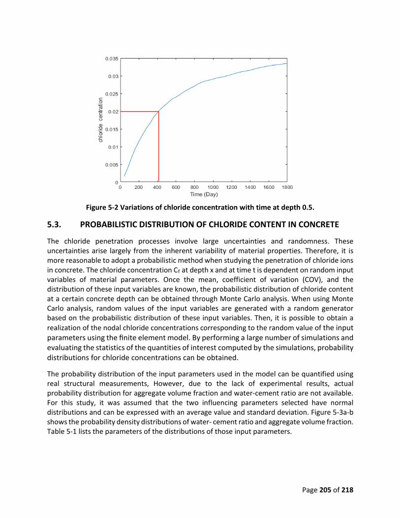
Page 205 of 218
Figure 5-2 Variations of chloride concentration with time at depth 0.5.
5.3. PROBABILISTIC DISTRIBUTION OF CHLORIDE CONTENT IN CONCRETE
The chloride penetration processes involve large uncertainties and randomness. These uncertainties arise largely from the inherent variability of material properties. Therefore, it is more reasonable to adopt a probabilistic method when studying the penetration of chloride ions in concrete. The chloride concentration Cf at depth x and at time t is dependent on random input variables of material parameters. Once the mean, coefficient of variation (COV), and the distribution of these input variables are known, the probabilistic distribution of chloride content at a certain concrete depth can be obtained through Monte Carlo analysis. When using Monte Carlo analysis, random values of the input variables are generated with a random generator based on the probabilistic distribution of these input variables. Then, it is possible to obtain a realization of the nodal chloride concentrations corresponding to the random value of the input parameters using the finite element model. By performing a large number of simulations and evaluating the statistics of the quantities of interest computed by the simulations, probability distributions for chloride concentrations can be obtained.
The probability distribution of the input parameters used in the model can be quantified using real structural measurements, However, due to the lack of experimental results, actual probability distribution for aggregate volume fraction and water-cement ratio are not available. For this study, it was assumed that the two influencing parameters selected have normal distributions and can be expressed with an average value and standard deviation. Figure 5-3a-b shows the probability density distributions of water- cement ratio and aggregate volume fraction. Table 5-1 lists the parameters of the distributions of those input parameters.

Page 206 of 218
(a) (b)
Figure 5-3 (a) Probability distribution of water-cement ratio. (b) Probability distribution of aggregate volume fraction.
Table 5-1 Parameters for the Probability Density Distributions of Water-Cement Ratio and Aggregate Volume Fraction
Parameters Symbol Value water- cement ratio normal distribution Mean = 0.45 Standard deviation = 0.045 aggregate volume fraction normal distribution Mean = 0.65 Standard deviation = 0.065
5.4. CASE STUDY
The aforementioned method is applied to a simple analysis of a concrete sample as shown in Figure 5-4. These graphs show the analysis of the sample under three circumstances. In the first scenario, the random input parameter for this analysis is the water-cement ratio. In the second scenario, the random input parameter for this analysis is the aggregate volume fraction. In the third scenario, the specimen was analyzed considering both water-cement ratio and aggregate volume fraction as random input parameters. In each case, 1000 Monte Carlo simulations are carried out. The level of chloride concentration at a depth of 5 cm was recorded at 400 days.
00.10.20.30.40.50.60.7
0.40 0.50 0.60 0.70 0.800
0.2
0.4
0.6
0.8
1
0.35 0.40 0.45 0.50 0.55
Page 207 of 218
(a) (b)
(c)
Figure 5-4 Probability density distribution histogram from Monte Carlo simulations for chloride concentration for three scenarios: (a) Water-cement ratio is the random input
parameter. (b) Aggregate volume fraction is the random input parameter. (c) Both water-cement ratio and aggregate volume fraction are a random input parameter.
Using Monte Carlo simulation, the histograms of the probability density distributions for the chloride concentration considering water-cement ratio, aggregate volume fraction, and both water-cement ratio, and aggregate volume fraction, respectively, are obtained and shown in Figure 5-5. It can be found that the chloride concentration follows the normal distribution. The corresponding distribution functions for the three cases are plotted in Figure 5-5.
0%1%2%3%4%5%6%7%8%9%
10%
0.00
0.00
0.01
0.01
0.01
0.02
0.02
0.02
0.03
0.03
0.03
0.03
0.04
0.04
Pro
bab
ility
dis
trib
uti
on
Cl concentration (g/g)
0%1%2%3%4%5%6%7%8%9%
10%
0.01
0.01
0.01
0.01
0.02
0.02
0.02
0.02
0.02
0.02
0.02
0.02
0.02
0.03
Pro
bab
ility
dis
trib
uti
on
Cl concentration (g/g)
0%
2%
4%
6%
8%
10%
0.00
0.00
0.01
0.01
0.01
0.01
0.02
0.02
0.02
0.03
0.03
0.03
0.04
0.04
Pro
bab
ility
dis
trib
uti
on
Cl concentration (g/g)

Page 208 of 218
Figure 5-5 Probability density distribution histograms and fitted normal distributions for chloride concentration for three scenarios: (a) Water-cement ratio is the random input
parameter. (b) Aggregate volume fraction is the random input parameter. (c) Both water-cement ratio and aggregate volume fraction are a random input parameter.
Figure 5-6 shows the cumulative distribution functions (CDF) of the fitted normal distributions for the three cases. The cumulative profiles were found to be most sensitive to the variation in water-cement ratio, with significantly less sensitivity to variability of the aggregate volume fraction. For the first case (random variation in water-cement ratio), there is a 58% chance that the chloride concentration at depth 5 cm reaches the critical chloride concentration. On the other hand, this percentage decreases to 33% when the aggregate volume fraction is considered as the random parameter. Considering both parameters, the chance for the corrosion initiation is 49%
0
10
20
30
40
50
0.0%
1.0%
2.0%
3.0%
4.0%
5.0%
0
0.00
5
0.01
0.01
5
0.02
0.02
5
0.03
0.03
5
0.04
Prob
abili
ty d
istr
ibut
ion
Cl concentration (g/g)
0
20
40
60
80
100
120
140
160
0.0%
1.0%
2.0%
3.0%
4.0%
5.0%
6.0%
7.0%
0
0.00
5
0.01
0.01
5
0.02
0.02
5
Prob
abili
ty d
istr
ibut
ion
Cl concentration (g/g)
0
10
20
30
40
50
0.0%
1.0%
2.0%
3.0%
4.0%
5.0%
6.0%
7.0%
0
0.00
5
0.01
0.01
5
0.02
0.02
5
0.03
0.03
5
0.04
Prob
abili
ty d
istr
ibut
ion
Cl concentration (g/g)
(a) (b)
(c)

Page 209 of 218
Figure 5-6 CDFs of chloride concentration for three cases.
To explore the sensitivity of the results to the input parameters, additional analyses were performed. Figure 5-7 presents an example of the influence of the variation of aggregate volume fractions and water-cement ratio on the free chloride concentration profiles. In Figure 5-7a., the concrete specimen was assumed to have been made with a w/c of 0.45 and aggregate volume fractions varying from 0.55 to 0.85. One can see from the figure that the diffusion of the chloride ions decreases as the volume fraction of the aggregate in the mix increases. This is due to the low diffusivity of the aggregate. The effect of the water-cement ratio on the diffusion of free chloride ions is shown in Figure 5-7. This figure represents how the concrete specimen was exposed to the same conditions as in the previous example; however, here the aggregate volume fraction was fixed at 0.6 and the water-cement ratio was varied from 0.35 to 0.65. The result shows that the free chloride diffuses faster with a higher water-cement ratio. This is due to the fact that the porosity of the cement paste increases with an increase in the water-cement ratio.
(a) (b)
Figure 5-7 (a) Effect of the variation of w/c on free chloride concentration profile. (b) Effect of the variation of aggregate volume fraction on free chloride concentration profile.
0%
10%
20%
30%
40%
50%
60%
70%
80%
90%
100%
0 0.01 0.02 0.03 0.04
cum
ulat
ive
dist
ribut
ion
Chloride concentration (g/g)
w/c andgiw/c
gi
00.0050.01
0.0150.02
0.0250.03
0.0350.04
0.045
0.35 0.4 0.45 0.5 0.55 0.6
chlo
ride
conc
entra
tion
water-cement ratio
0
0.005
0.01
0.015
0.02
0.025
0.03
0.55 0.65 0.75 0.85
chlo
ride
conc
entra
tion
aggregate volume fractions

Page 210 of 218
5.5. CONCLUSIONS
• A comprehensive mathematical model for chloride penetration in saturated concrete is applied in the present study for reliability analysis. The model incorporates many influencing parameters, which allows direct analyses of the effect of the parameters on the chloride penetration.
• A finite element method is used for the non-linear chloride diffusion equation. The numerical solution of the governing partial differential equation is linked to a Monte Carlo simulation program for analyzing the effect of the selected random variables on the chloride penetration process.
• Water–cement ratio and aggregate volume fraction are selected as two random input parameters. Probabilistic distributions for the two parameters are assumed. As an example, the effect of the two random variables on the chloride penetration process is analyzed.
• The influencing factors of the two parameters on the density distribution of chloride diffusion in concrete is analyzed. From the results, the distribution of the chloride penetration is more sensitive to variation of the water–cement ratio compared with the variation of the aggregate volume fraction
Equation Chapter (Next) Section 1

Page 211 of 218
CLOSURE
6.1. CONCLUSIONS
This project consisted of a combination of experimental and simulation efforts that have either directly contributed to the development of expanded capabilities in BlackBear or provided validation data for BlackBear models. Highlights of this work include:
Experimental Studies on Coupling between Moisture and Ion Transport in Concrete
• An experimental study to determine the effect of moisture transfer on chloride penetration in concrete was conducted. Tests were performed on a set of concrete specimens with various mix design parameters to evaluate the coupling parameter describing this interaction as a function of aggregate volume fraction and water-cement ratio. These tests showed higher concentrations of chloride in non-saturated specimens compared to saturated specimens due to this coupling effect. Based on this data, a model was proposed to express this coupling parameter as a function of concrete mix parameters.
• An experimental investigation was also performed to study the effect of ion concentration on moisture transport in concrete. As for the aforementioned study on the reverse phenomenon, this effect was investigated for a variety of concrete mix parameters. Chloride ion concentration was found to have a noticeable effect on moisture transport. Three possible coupling mechanisms were discussed: ionic concentration gradient, viscosity of the ionic solution, and the effective size of pores due to the appearance of the ions. This study was designed to study the effect of concentration gradient. The test data showed that the 8% chloride solution decreased the penetration rate of moisture. An analytic procedure was developed to determine the coupling parameter considering the effect of both chloride and moisture concentration gradient. It can be used when more test data become available in the future.
Model Development for Coupling Effects of Damage and Transport in Concrete
• A comprehensive model for concrete damage that is widely used in practice for representing nonlinear mechanical response of concrete has been implemented for MOOSE-based codes. This model captures damage effects in tension and compression, and uses a combination of damage and plasticity concepts to capture cyclic behavior. It captures dilatancy effects and adjusts for element size effects to produce results that are minimally dependent on mesh size. This model has been tested on a set of benchmark problems.

Page 212 of 218
• Models were developed to account for the effect of damage induced by drying shrinkage on moisture and chloride diffusion in concrete. The transport models account for the effect of mix design parameters. This model demonstrates how damage induced by drying shrinkage accelerates the transport of moisture both in and out of concrete.
• A model for diffusion of multiple species using the Nernst-Planck equations, which account for interactions between species to satisfy electrical neutrality conditions has been developed. This model has been coupled with moisture transport and mechanical models and used to demonstrate effects of damage on transport.
• A model for corrosion reaction rates in reinforcing bars that accounts for the effects of chloride ion concentration, oxygen, temperature, moisture content, pH, and electrical resistivity of concrete has been developed and demonstrated.
• Models for the material properties of steel reinforcement and the steel-concrete bond have been developed. The effects of the degree of corrosion are taken into account in the bond-slip model and models for yield strength and rupture strain in the reinforcement.
Experimental Study on the Effect of Alkali-Silica Reaction Induced Damage on Shear Capacity of Reinforced Concrete Beams
• A set of three large-scale reinforced concrete beams containing highly reactive aggregates to accelerate the rate of the alkali-silica reaction (ASR) were subjected to conditions that resulted in varying levels of ASR. These beams were designed to fail in shear rather than flexure to specifically address the effects of ASR on shear capacity in reinforced concrete structures. These beams contained a variety of instrumentation, which was used to evaluate their response both during the aging process and during the mechanical testing to determine their shear capacity. Testing of these beams indicated a negligible reduction in the shear capacity with an increase in ASR swelling.
• A set of equivalent material samples consisting of cylinders and prisms were also cast and subjected to equivalent conditions to the beams, and were tested to evaluate the effects of ASR on specific material parameters. These tests indicated that ASR does not affect all mechanical properties of concrete in the same way or to the same extent. Tensile strength showed the highest sensitivity and degradation to ASR. ASR was also observed to cause degradation of the modulus of rupture and the compressive strength, but the effect was less compared with the impact on tensile strength. In certain cases, ASR could not stop the samples from gaining compressive strength due to cement hydration. ASR did not show any specific or significant influence on the elastic modulus in this study.
• These experiments provide valuable data that will be used to validate the models in BlackBear for the progression of ASR and its effect on structural capacity.
Uncertainty Quantification of Concrete Models
• An uncertainty quantification study was performed to evaluate the effects of uncertainty in the parameters governing chloride diffusion on the time-dependent chloride concentration profile in concrete members. The models for chloride ion diffusion developed in this project were used together with the built-in Monte Carlo sampling tools

Page 213 of 218
in MOOSE to assess the uncertainty in the chloride concentration profile as well as the sensitivity of the uncertain response to the input parameters.
6.2. RECOMMENDATIONS FOR FUTURE RESEARCH
This project performed code development and provided experimental data that will provide essential components of a comprehensive, validated capability for modeling a variety of degradation mechanisms and their effects on reinforced concrete structures. These individual capabilities were developed and demonstrated, but work is still needed to integrate these models and use them together in a robust, production-grade code. The following are logical follow-on efforts to this work:
• Complete integration of the models developed into the BlackBear code. The damaged plasticity model, Nernst-Planck multispecies diffusion model and rebar corrosion models will all be valuable additions to BlackBear. Full documentation and testing of these models is required to meet SQA standards of that code.
• The structural scale experiments performed in this project provide data that will be essential for validation of an integrated capability for modeling the progression of ASR and its effects on structural integrity. Models of these experiments need to be created, compared against the experimental data, and improved based on the deficiencies observed.
• The coupling effect of chloride on moisture transport need more experimental study for the viscosity of chloride solution and the effective pore size of cement paste considering different chloride concentrations and concrete mix design parameters. So, a material model for the coupling parameter, DH-Cl, can be developed based on more systematic test data and used in the computer program.
Page 214 of 218
REFERENCES
Ababneh, A. and Xi, Y. (2002). "An experimental study on the effect of chloride penetration on moisture diffusion in concrete," Materials and Structures, 35(10), 659-663.
Ababneh, A. N. (2003). "The coupled effect of moisture diffusion chloride penetration and freezing-thawing on concrete durability."
Almusallam, A. A. (2001). "Effect of degree of corrosion on the properties of reinforcing steel bars," Construction and Building Materials, 15(December 2001), 361-368.
Almusallam, A. A., Al-Gahtani, A. S. A. S., Aziz, A. R. A. R. and Rasheeduzzafar (1996). "Effects of reinforcement corrosion on bond strength," Construction and Building Materials, 10(2), 123-129.
ASTM (2010). Standard Test Method for Flexural Strength of Concrete (Using Simple Beam with Third-Point Loading), ASTM C78 - 10, American Society for Testing of Materials (ASTM), West Conshohocken, PA.
ASTM (2012). Standard Test Method for Acid-Soluble Chloride in Mortar and Concrete, C1152/C1152M - 04, American Society for Testing of Materials (ASTM), West Conshohocken, PA.
ASTM (2014a). Standard Test Methods and Definitions for Mechanical Testing of Steel Products, ASTM A370 - 14, American Society of Testing Materials (ASTM), West Conshohocken, PA.
ASTM (2014b). Standard Test Methods for Potential Alkali Reactivity of Aggregates, ASTM C1260 - 14, American Society of Testing Materials (ASTM), West Conshohocken, PA.
ASTM (2017a). Standard Test Method for Splitting Tensile Strength of Cylindrical Concrete Specimens, ASTM C496 - 17, American Society of Testing Materials (ASTM), West Conshohocken, PA.
ASTM (2017b). Standard Test Method for Water-Soluble Chloride in Mortar and Concrete, C1218/C1218M - 17, American Society for Testing of Materials (ASTM), West Conshohocken, PA.
ASTM (2018a). Standard Test Method for Compressive Strength of Cylindrical Concrete Specimens, ASTM C39/C39M - 18, American Society of Testing Materials (ASTM), West Conshohocken, PA.
ASTM (2018b). Standard Test Methods for Chemical Analysis of Hydraulic Cement, C114 - 18, American Society for Testing of Materials (ASTM), West Conshohocken, PA.
ASTM (2019). Standard Specification for Portland Cement, ASTM C150/C150M - 19, American Society of Testing Materials (ASTM), West Conshohocken, PA.
Bard, A. J. and Faulkner, L. R. (2001). Electrochemical Methods: Fundamentals and Applications, John Wiley and Sons, New York, NY.
Bazant, Z. and Najjar, L. (1972). "Nonlinear water diffusion of nonsaturated concrete," Materials Structures, 5(25), 3–20.
Bazant, Z. P. (1979). "Physical model for steel corrosion in concrete sea structures - application," ASCE Journal of the Structural Division, 105(6), 1155-1166.
Beer, F. P., Johnston, E. R. and Dewolf, J. T. (2006). Mechanics of Materials, McGraw-Hill Higher Education, New York, NY.

Page 215 of 218
Bentz, D. P. (1997). "Three dimensional computer simulation of portland cement hydration and microstructural development," Journal of American Ceramic Society, 80(1), 3-21.
Bentz, D. P. (2005). CEMHYD3D : A Three-Dimensional Cement Hydration and Microstructure Development Modeling Package Version 3.0, NISTIR 7232, National Institute Of Standards And Technology, Gaithersburg, Maryland.
Bentz, D. P. and Garboczi, E. J. (1991). "Percolation of phases in a three-dimensional cement paste microstructural model," Cement and Concrete Research, 21(2), 325-344, DOI: https://doi.org/10.1016/0008-8846(91)90014-9.
Bentz, E. J. G. a. D. P. (1996). Multi-scale picture of concrete and its transport properties: Introduction for non-cement researchers, NISTIR 5900, National Institute of Standards and Technology Gaithersburg, Maryland.
Bergerhoff, G. and Brown, I. D. (1987). "Inorganic crystal structure database," FIZ Karlsruhe, Karlsruhe, Germany.
Bhargava, K., Ghosh, A. K., Mori, Y. and Ramanujam, S. (2006). "Analytical model for time to cover cracking in RC structures due to rebar corrosion," Nuclear Engineering and Design, 236(11), 1123-1139, DOI: 10.1016/j.nucengdes.2005.10.011.
Cao, C., Cheung, M. M. S. and Chan, B. Y. B. (2013). "Modelling of interaction between corrosion-induced concrete cover crack and steel corrosion rate," Corrosion Science, 69(24), 97-109, DOI: 10.1016/j.corsci.2012.11.028.
Christensen, R. M. (1979). Mechanics of composite materials, Journal of Polymer Science: Polymer Letters Edition, New York.
El Maaddawy, T. A. and Soudki, K. A. (2003). "Effectiveness of Impressed Current Technique to Simulate Corrosion of Steel Reinforcement in Concrete," Journal of Materials in Civil Engineering, 15(1), 41-47, DOI: 10.1061/(ASCE)0899-1561(2003)15:1(41).
Fang, C., Lundgren, K., Plos, M. and Gylltoft, K. (2006). "Bond behaviour of corroded reinforcing steel bars in concrete," Cement and Concrete Research, 36(October 2006), 1931-1938, DOI: 10.1016/j.cemconres.2006.05.008.
Francois, R., Khan, I. and Dang, V. H. (2013). "Impact of corrosion on mechanical properties of steel embedded in 27-year-old corroded reinforced concrete beams," Materials and Structures, 46, 899-910, DOI: 10.1617/s11527-012-9941-z.
Gaston, D., Newman, C., Hansen, G. and Lebrun-Grandié, D. (2009). "MOOSE: A parallel computational framework for coupled systems of nonlinear equations," Nuclear Engineering and Design, 239(10), 1768-1778, DOI: 10.1016/j.nucengdes.2009.05.021.
Ge, J. and Isgor, O. B. (2007). "Effects of Tafel slope, exchange current density and electrode potential on the corrosion of steel in concrete," Materials and Corrosion, 58(8), 573-582.
Gopalaratnam, V. S. and Surendra, P. S. (1985). "Softening Response of Plain Concrete in Direct Tension," ACI Journal Proceedings, 82(3), 310-323, DOI: 10.14359/10338.
Hobbs, D. W. and Matthews, J. D. (1998). "Minimum requirements for concrete to resist deterioration due to chloride induced corrosion," in Minimum Requirements for Durable Concrete, ed Hobbs, D. W., British Cement Association, Crowthorne.
Isgor, O. B. and Razaqpur, A. G. (2006). "Modelling steel corrosion in concrete structures," Materials and Structures, 53(12), 291-302, DOI: 10.1617/s11527-005-9022-7.

Page 216 of 218
Jennings, H. M., Thomas, J. J., Gevrenov, J. S., Constantinides, G. and Ulm, F.-J. (2007). "A multi-technique investigation of the nanoporosity of cement paste," Cement and Concrete Research, 37(3), 329-336.
Karsan, I. D. and Jirsa, J. O. (1969). "Behavior of concrete under compressive loadings," ASCE Journal of the Structural Division, 95(12), 2543-2563.
Kassir, M. K. and Ghosn, M. (2002). "Chloride-induced corrosion of reinforced concrete bridge decks," Cement and Concrete Research, 32(January 2002), 139-143, DOI: 10.1061/(ASCE)0733-9399(2005)131:1(97).
Kim, K. H., Jang, S. Y., Jang, B. S. and Oh, B. H. (2010). "Modeling mechanical behavior of reinforced concrete due to corrosion of steel bar," ACI Materials Journal, 107(2), 106-113.
Krabbenhøft, K. (2002). Basic Computational Plasticity, Technical University of Denmark, Lyngby, Denmark.
Kranc, S. C. and Sagüés, A. A. (1997). "Modeling the time-dependent response to external polarization of a corrosion macrocell on steel in concrete," Journal of the Electrochemical Society, 144(8), 2643-2652.
Kwak, H. T., Zhang, G. and Chen, S. (2005). "The effects of salt type and salinity on formation water viscosity and NMR responses." International Symposium of the Society of Core Analysts, August 21-25, Toronto, Canada, 21, 25-25.
Lee, J. (1996). "Theory and Implementation of Plastic-Damage Model for Concrete Structures under Cyclic and Dynamic Loading," PhD Thesis, Department of Civil and Environmental Engineering, University of California, Berkeley, Berkeley, California.
Lee, J. and Fenves, G. L. (2001). "Return-mapping algorithm for plastic-damage models: 3-D and plane stress formulation," International Journal for Numerical Methods in Engineering, 50(2), 487-506, DOI: 10.1002/1097-0207(20010120)50:2<487::AID-NME44>3.0.CO;2-N.
Liu, Y. (1996). "Modeling the time-to corrosion cracking of the cover concrete in chloride contaminated reinforced concrete structures," PhD Thesis, Department of Civil Engineering, Virginia Polytechnic Institute and State University, Blacksburg, Virginia.
Liu, Y. and Weyers, R. E. (1998). "Modeling the Time-to-Corrosion Cracking in Chloride Contaminated Reinforced Concrete Structures," ACI Materials Journal, 95(6), 675-680.
Lubliner, J., Oliver, J., Oller, S. and Onate, E. (1989). "A Plastic-Damage Model For Concrete," International Journal of Solids and Structures, 25(3), 299-326.
Lutterotti, L., Matthies, S. and Wenk, H.-S. (1999). "MAUD: a friendly Java program for material analysis using diffraction," Newsletter of the CPD, 21, 14-15.
Marcus, Y. (2009). "Effect of ions on the structure of water: structure making and breaking," Chemical reviews, 109(3), 1346-1370.
Martys, N. S., Torquato, S. and Bentz, D. P. (1994). "Universal scaling of fluid permeability for sphere packings," Physical Review E, 50(1), 403-408.
Maruya, T., Hsu, K., Takeda, H. and Tangtermsirikul, S. (2003). "Numerical Modeling of Steel Corrosion in Concrete Structures due to Chloride Ion, Oxygen and Water Movement," Journal of Advanced Concrete Technology, 1(2), 147-160, DOI: 10.3151/jact.1.147.
Mazars, J. (1984). "Application de la mécanique de l'endommagement au comportement non linéaire et à la rupture du béton de structure," PhD Thesis, Universite Paris 6, Paris, France.
Page 217 of 218
National Oceanic and Atmospheric Administration (2019). Climate Data Online, U.S. Department of Commerce, Available from: https://www.noaa.gov/, Accessed on October 1, 2019.
Neubauer, C. M., Bergstrom, T. B., Sujata, K., Xi, Y., Garboczi, E. J. and Jennings, H. M. (1997). "Drying shrinkage of cement paste as measured in an environmental scanning electron microscope and comparison with microstructural models," Journal of Materials Science, 32(24), 6415-6427.
Ožbolt, J., Oršanic, F. and Balabanic, G. (2016). "Modeling corrosion-induced damage of reinforced concrete elements with multiple-arranged reinforcement bars," Materials and Corrosion, 67(5), 542-552, DOI: 10.1002/maco.201508569.
Page, C. L., Short, N. R. and El Tarras, A. (1981). "Diffusion of chloride ions in hardened cement pastes," Cement and concrete research, 11(3), 395-406.
Pantazopoulou, S. J. and Papoulia, K. D. (2001). "Modeling cover-cracking due to reinforcement corrosion in RC structures," ASCE Journal of Engineering Mechanics, 127(4), 342-351.
Pijadudier-Cabot, G. and Mazars, J. (2001). "Damage models for concrete," in Handbook of Materials Behavior Models, ed Lemaitre, J., Academic Press.
Pour-Ghaz, M., Isgor, O. B. and Ghods, P. (2009). "The effect of temperature on the corrosion of steel in concrete. Part 1: Simulated polarization resistance tests and model development," Corrosion Science, 51(2), 415-425, DOI: https://doi.org/10.1016/j.corsci.2008.10.034.
Rosen, B. W. and Hashin, Z. (1970). "Effective thermal expansion coefficients and specific heats of composite materials," International Journal of Engineering Science, 8(2), 157-173.
Safeer Abbas, A. M. S. and Moncef, L. N. (2014). "Chloride Ion Penetration in Reinforced Concrete and Steel Fiber-Reinforced Concrete Precast Tunnel Lining Segments," ACI Materials Journal, 111(6), 613-622, DOI: 10.14359/51686991.
Samson, E. and Marchand, J. (2007). "Modeling the transport of ions in unsaturated cement-based materials," Computers & Structures, 85(23-24), 1740-1756.
Stojek, Z. (2002). "The Electrical Double Layer and Its Structure," in Electroanalytical Methods: Guide to Experiments and Applications, ed Scholz, F., Springer Berlin Heidelberg, Berlin, Heidelberg, 3-8.
Torres-Acosta, A. a., Navarro-Gutierrez, S. and Terán-Guillén, J. (2007). "Residual flexure capacity of corroded reinforced concrete beams," Engineering Structures, 29(6), 1145-1152, DOI: 10.1016/j.engstruct.2006.07.018.
Wang, J. H. (1954). "Effect of ions on the self-diffusion and structure of water in aqueous electrolytic solutions," The Journal of Physical Chemistry, 58(9), 686-692.
Wang, Y., Li, L.-y. and Page, C. L. (2005). "Modelling of chloride ingress into concrete from a saline environment," Building and environment, 40(12), 1573-1582.
Wu, J. Y. and Lee, R. (1997). "The advantages of triangular and tetrahedral edge elements for electromagnetic modeling with the finite-element method," IEEE Transactions on Antennas and Propagation, 45(9), 1431-1437, DOI: 10.1109/8.623133.
Xi, Y. (1995a). "A Model for Moisture Capacities of Composite Materials, Part I: Formulation," Computational Materials Science, 4(1), 65-77.
Xi, Y. (1995b). "A Model for Moisture Capacities of Composite Materials, Part II: Application to Concrete," Computational Materials Science, 4(1), 78-92.

Page 218 of 218
Xi, Y. and Bažant, Z. P. (1999). "Modeling chloride penetration in saturated concrete," Journal of Materials in Civil Engineering, 11(1), 58-65.
Xi, Y., Bažant, Z. P. and Jennings, H. M. (1994a). "Moisture diffusion in cementitious materials: adsorption isotherms," Advanced Cement Based Materials, 1(6), 248-257.
Xi, Y., Bažant, Z. P., Molina, L. and Jennings, H. M. (1994b). "Moisture diffusion in cementitious materials: moisture capacity and diffusivity," Advanced Cement Based Materials, 1(6), 258-266.
Xi, Y. and Jennings, H. M. (1997). "Shrinkage of cement paste and concrete modelled by a multiscale effective homogeneous theory," Materials and Structures, 30(6), 329, DOI: 10.1007/BF02480683.
Yuan, Y., Jiang, J. and Peng, T. (2011). "Corrosion Process of Steel Bar in Concrete in Full Lifetime," ACI Materials Journal, 107(6), 563-568.
Zhang, T. and Gjørv, O. E. (1996). "Diffusion behavior of chloride ions in concrete," Cement and Concrete Research, 26(6), 907-917, DOI: https://doi.org/10.1016/0008-8846(96)00069-5.
Zibara, H. (2001). "Binding of external chlorides by cement pastes," PhD Thesis, Department of Civil Engineering, University of Toronto, Toronto, Canada.