Rational Choice of Reinforcement of Reinforced Concrete ...
33
materials Article Rational Choice of Reinforcement of Reinforced Concrete Frame Corners Subjected to Opening Bending Moment Michal Szczecina 1, * and Andrzej Winnicki 2 Citation: Szczecina, M.; Winnicki, A. Rational Choice of Reinforcement of Reinforced Concrete Frame Corners Subjected to Opening Bending Moment. Materials 2021, 14, 3438. https://doi.org/10.3390/ma14123438 Academic Editors: Enrique Casarejos and Zhengming Huang Received: 2 April 2021 Accepted: 16 June 2021 Published: 21 June 2021 Publisher’s Note: MDPI stays neutral with regard to jurisdictional claims in published maps and institutional affil- iations. Copyright: © 2021 by the authors. Licensee MDPI, Basel, Switzerland. This article is an open access article distributed under the terms and conditions of the Creative Commons Attribution (CC BY) license (https:// creativecommons.org/licenses/by/ 4.0/). 1 Faculty of Civil Engineering and Architecture, Kielce University of Technology, Al. Tysi ˛ aclecia Pa ´ nstwa Polskiego 7, 25-314 Kielce, Poland 2 Faculty of Civil Engineering, Cracow University of Technology, Warszawska 24, 31-155 Kraków, Poland; [email protected] * Correspondence: [email protected] Abstract: This paper discusses a choice of the most rational reinforcement details for frame corners subjected to opening bending moment. Frame corners formed from elements of both the same and different cross section heights are considered. The case of corners formed of elements of different cross section is not considered in Eurocode 2 and is very rarely described in handbooks. Several reinforcement details with both the same and different cross section heights are presented. The authors introduce a new reinforcement detail for the different cross section heights. The considered details are comprised of the primary reinforcement in the form of straight bars and loops and the additional reinforcement in the form of diagonal bars or stirrups or a combination of both diagonal stirrups and bars. Two methods of static analysis, strut-and-tie method (S&T) and finite element method (FEM), are used in the research. FEM calculations are performed with Abaqus software using the Concrete Damaged Plasticity model (CDP) for concrete and the classical metal plasticity model for reinforcing steel. The crucial CDP parameters, relaxation time and dilatation angle, were calibrated in numerical tests in Abaqus. The analysis of results from the S&T and FE methods allowed for the determination of the most rational reinforcement details. Keywords: concrete; material model; Concrete Damaged Plasticity model; opening bending moment; reinforced concrete frame corners; strut-and-tie method; FEM; Abaqus 1. Introduction A frame corner under opening bending moment is considered to be a so-called ”D” region in which the distribution of stresses and strains is complicated. While detailing this kind of region, the structural engineer has a few recommendations presented in codes and handbooks and often relies on intuition. The situation is even more complicated in the case of different cross section heights of elements meeting in the corner, as this is not covered in most codes, for example, Eurocode 2 [1]. There are still too few literary studies on the choice of reinforcement in the case of different cross section heights and the article is an attempt to close the gap. Moreover, some of the recommended reinforcement details have a relatively low efficiency factor. A proper choice of the reinforcement of such a region should be based on more sophisticated methods than the handbook recommendations and the authors of this paper suggest using a combination of strut-and-tie and FE methods. This kind of approach has been presented in, for example, the PhD thesis of Akkermann [2], in which a combination of laboratory tests and advanced non-linear FEM calculations was used to analyze reinforced concrete (RC) frame corners under both closing and opening bending moment. Materials 2021, 14, 3438. https://doi.org/10.3390/ma14123438 https://www.mdpi.com/journal/materials
-
Upload
khangminh22 -
Category
Documents
-
view
1 -
download
0
Transcript of Rational Choice of Reinforcement of Reinforced Concrete ...

materials
Article
Rational Choice of Reinforcement of Reinforced ConcreteFrame Corners Subjected to Opening Bending Moment
Michał Szczecina 1,* and Andrzej Winnicki 2
�����������������
Citation: Szczecina, M.; Winnicki, A.
Rational Choice of Reinforcement of
Reinforced Concrete Frame Corners
Subjected to Opening Bending
Moment. Materials 2021, 14, 3438.
https://doi.org/10.3390/ma14123438
Academic Editors: Enrique Casarejos
and Zhengming Huang
Received: 2 April 2021
Accepted: 16 June 2021
Published: 21 June 2021
Publisher’s Note: MDPI stays neutral
with regard to jurisdictional claims in
published maps and institutional affil-
iations.
Copyright: © 2021 by the authors.
Licensee MDPI, Basel, Switzerland.
This article is an open access article
distributed under the terms and
conditions of the Creative Commons
Attribution (CC BY) license (https://
creativecommons.org/licenses/by/
4.0/).
1 Faculty of Civil Engineering and Architecture, Kielce University of Technology, Al. Tysiaclecia PanstwaPolskiego 7, 25-314 Kielce, Poland
2 Faculty of Civil Engineering, Cracow University of Technology, Warszawska 24, 31-155 Kraków, Poland;[email protected]
* Correspondence: [email protected]
Abstract: This paper discusses a choice of the most rational reinforcement details for frame cornerssubjected to opening bending moment. Frame corners formed from elements of both the same anddifferent cross section heights are considered. The case of corners formed of elements of differentcross section is not considered in Eurocode 2 and is very rarely described in handbooks. Severalreinforcement details with both the same and different cross section heights are presented. Theauthors introduce a new reinforcement detail for the different cross section heights. The considereddetails are comprised of the primary reinforcement in the form of straight bars and loops and theadditional reinforcement in the form of diagonal bars or stirrups or a combination of both diagonalstirrups and bars. Two methods of static analysis, strut-and-tie method (S&T) and finite elementmethod (FEM), are used in the research. FEM calculations are performed with Abaqus software usingthe Concrete Damaged Plasticity model (CDP) for concrete and the classical metal plasticity model forreinforcing steel. The crucial CDP parameters, relaxation time and dilatation angle, were calibratedin numerical tests in Abaqus. The analysis of results from the S&T and FE methods allowed for thedetermination of the most rational reinforcement details.
Keywords: concrete; material model; Concrete Damaged Plasticity model; opening bending moment;reinforced concrete frame corners; strut-and-tie method; FEM; Abaqus
1. Introduction
A frame corner under opening bending moment is considered to be a so-called ”D”region in which the distribution of stresses and strains is complicated. While detailing thiskind of region, the structural engineer has a few recommendations presented in codes andhandbooks and often relies on intuition. The situation is even more complicated in the caseof different cross section heights of elements meeting in the corner, as this is not coveredin most codes, for example, Eurocode 2 [1]. There are still too few literary studies on thechoice of reinforcement in the case of different cross section heights and the article is anattempt to close the gap. Moreover, some of the recommended reinforcement details havea relatively low efficiency factor. A proper choice of the reinforcement of such a regionshould be based on more sophisticated methods than the handbook recommendations andthe authors of this paper suggest using a combination of strut-and-tie and FE methods.This kind of approach has been presented in, for example, the PhD thesis of Akkermann [2],in which a combination of laboratory tests and advanced non-linear FEM calculations wasused to analyze reinforced concrete (RC) frame corners under both closing and openingbending moment.
Materials 2021, 14, 3438. https://doi.org/10.3390/ma14123438 https://www.mdpi.com/journal/materials
Materials 2021, 14, 3438 2 of 33
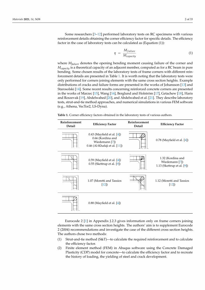
Some researchers [3–12] performed laboratory tests on RC specimens with variousreinforcement details obtaining the corner efficiency factor for specific details. The efficiencyfactor in the case of laboratory tests can be calculated as (Equation (1)):
η =M f ailure
Mcapacity(1)
where Mfailure denotes the opening bending moment causing failure of the corner andMcapacity is a theoretical capacity of an adjacent member, computed as for a RC beam in purebending. Some chosen results of the laboratory tests of frame corners with different rein-forcement details are presented in Table 1. It is worth noting that the laboratory tests wereonly performed for corners joining elements with the same cross section heights. Exampledistributions of cracks and failure forms are presented in the works of Johansson [13] andStarosolski [14]. Some recent results concerning reinforced concrete corners are presentedin the works of Marzec [15], Wang [16], Berglund and Holström [17], Getachew [18], Harisand Roszevak [19], Abdelwahed [20], and Abdelwahed et al. [21]. They describe laboratorytests, strut-and-tie method approaches, and numerical simulations in various FEM software(e.g., Athena, VecTor2, LS-Dyna).
Table 1. Corner efficiency factors obtained in the laboratory tests of various authors.
ReinforcementDetail Efficiency Factor Reinforcement
Detail Efficiency Factor
Materials 2021, 14, 3438 2 of 33
capacity
failure
MM
(1)
where Mfailure denotes the opening bending moment causing failure of the corner and Mcapac-
ity is a theoretical capacity of an adjacent member, computed as for a RC beam in pure bending. Some chosen results of the laboratory tests of frame corners with different rein-forcement details are presented in Table 1. It is worth noting that the laboratory tests were only performed for corners joining elements with the same cross section heights. Example distributions of cracks and failure forms are presented in the works of Johansson [13] and Starosolski [14]. Some recent results concerning reinforced concrete corners are presented in the works of Marzec [15], Wang [16], Berglund and Holström [17], Getachew [18], Haris and Roszevak [19], Abdelwahed [20], and Abdelwahed et al. [21]. They describe labora-tory tests, strut-and-tie method approaches, and numerical simulations in various FEM software (e.g., Athena, VecTor2, LS-Dyna).
Table 1. Corner efficiency factors obtained in the laboratory tests of various authors.
Reinforcement Detail
Efficiency Factor Reinforcement
Detail Efficiency Factor
0.43 (Mayfield et al. [4]) 0.66 (Kordina and Wiedemann [7])
0.46 (Al-Khafaji et al. [11])
0.78 (Mayfield et al. [4])
0.59 (Mayfield et al. [4]) 0.55 (Skettrup et al. [9])
1.32 (Kordina and Wiedemann [7])
1.13 (Skettrup et al. [9])
1.07 (Moretti and Tassios [12])
1.12 (Moretti and Tassios [12])
0.88 (Mayfield et al. [4])
Eurocode 2 [1] in Appendix J.2.3 gives information only on frame corners joining el-ements with the same cross section heights. The authors’ aim is to supplement Eurocode 2 (2004) recommendations and investigate the case of the different cross section heights. The authors chose two methods: (1) Strut-and-tie method (S&T)—to calculate the required reinforcement and to calculate
the efficiency factor. (2) Finite element method (FEM) in Abaqus software using the Concrete Damaged Plas-
ticity (CDP) model for concrete—to calculate the efficiency factor and to recreate the history of loading, the yielding of steel and crack development. The primary goal of the analysis was to calculate the efficiency factor and crack width
for all the details and then to conclude which detail is the most preferable. The secondary,
0.43 (Mayfield et al. [4])0.66 (Kordina andWiedemann [7])
0.46 (Al-Khafaji et al. [11])
Materials 2021, 14, 3438 2 of 33
capacity
failure
MM
(1)
where Mfailure denotes the opening bending moment causing failure of the corner and Mcapac-
ity is a theoretical capacity of an adjacent member, computed as for a RC beam in pure bending. Some chosen results of the laboratory tests of frame corners with different rein-forcement details are presented in Table 1. It is worth noting that the laboratory tests were only performed for corners joining elements with the same cross section heights. Example distributions of cracks and failure forms are presented in the works of Johansson [13] and Starosolski [14]. Some recent results concerning reinforced concrete corners are presented in the works of Marzec [15], Wang [16], Berglund and Holström [17], Getachew [18], Haris and Roszevak [19], Abdelwahed [20], and Abdelwahed et al. [21]. They describe labora-tory tests, strut-and-tie method approaches, and numerical simulations in various FEM software (e.g., Athena, VecTor2, LS-Dyna).
Table 1. Corner efficiency factors obtained in the laboratory tests of various authors.
Reinforcement Detail
Efficiency Factor Reinforcement
Detail Efficiency Factor
0.43 (Mayfield et al. [4]) 0.66 (Kordina and Wiedemann [7])
0.46 (Al-Khafaji et al. [11])
0.78 (Mayfield et al. [4])
0.59 (Mayfield et al. [4]) 0.55 (Skettrup et al. [9])
1.32 (Kordina and Wiedemann [7])
1.13 (Skettrup et al. [9])
1.07 (Moretti and Tassios [12])
1.12 (Moretti and Tassios [12])
0.88 (Mayfield et al. [4])
Eurocode 2 [1] in Appendix J.2.3 gives information only on frame corners joining el-ements with the same cross section heights. The authors’ aim is to supplement Eurocode 2 (2004) recommendations and investigate the case of the different cross section heights. The authors chose two methods: (1) Strut-and-tie method (S&T)—to calculate the required reinforcement and to calculate
the efficiency factor. (2) Finite element method (FEM) in Abaqus software using the Concrete Damaged Plas-
ticity (CDP) model for concrete—to calculate the efficiency factor and to recreate the history of loading, the yielding of steel and crack development. The primary goal of the analysis was to calculate the efficiency factor and crack width
for all the details and then to conclude which detail is the most preferable. The secondary,
0.78 (Mayfield et al. [4])
Materials 2021, 14, 3438 2 of 33
capacity
failure
MM
(1)
where Mfailure denotes the opening bending moment causing failure of the corner and Mcapac-
ity is a theoretical capacity of an adjacent member, computed as for a RC beam in pure bending. Some chosen results of the laboratory tests of frame corners with different rein-forcement details are presented in Table 1. It is worth noting that the laboratory tests were only performed for corners joining elements with the same cross section heights. Example distributions of cracks and failure forms are presented in the works of Johansson [13] and Starosolski [14]. Some recent results concerning reinforced concrete corners are presented in the works of Marzec [15], Wang [16], Berglund and Holström [17], Getachew [18], Haris and Roszevak [19], Abdelwahed [20], and Abdelwahed et al. [21]. They describe labora-tory tests, strut-and-tie method approaches, and numerical simulations in various FEM software (e.g., Athena, VecTor2, LS-Dyna).
Table 1. Corner efficiency factors obtained in the laboratory tests of various authors.
Reinforcement Detail
Efficiency Factor Reinforcement
Detail Efficiency Factor
0.43 (Mayfield et al. [4]) 0.66 (Kordina and Wiedemann [7])
0.46 (Al-Khafaji et al. [11])
0.78 (Mayfield et al. [4])
0.59 (Mayfield et al. [4]) 0.55 (Skettrup et al. [9])
1.32 (Kordina and Wiedemann [7])
1.13 (Skettrup et al. [9])
1.07 (Moretti and Tassios [12])
1.12 (Moretti and Tassios [12])
0.88 (Mayfield et al. [4])
Eurocode 2 [1] in Appendix J.2.3 gives information only on frame corners joining el-ements with the same cross section heights. The authors’ aim is to supplement Eurocode 2 (2004) recommendations and investigate the case of the different cross section heights. The authors chose two methods: (1) Strut-and-tie method (S&T)—to calculate the required reinforcement and to calculate
the efficiency factor. (2) Finite element method (FEM) in Abaqus software using the Concrete Damaged Plas-
ticity (CDP) model for concrete—to calculate the efficiency factor and to recreate the history of loading, the yielding of steel and crack development. The primary goal of the analysis was to calculate the efficiency factor and crack width
for all the details and then to conclude which detail is the most preferable. The secondary,
0.59 (Mayfield et al. [4])0.55 (Skettrup et al. [9])
Materials 2021, 14, 3438 2 of 33
capacity
failure
MM
(1)
where Mfailure denotes the opening bending moment causing failure of the corner and Mcapac-
ity is a theoretical capacity of an adjacent member, computed as for a RC beam in pure bending. Some chosen results of the laboratory tests of frame corners with different rein-forcement details are presented in Table 1. It is worth noting that the laboratory tests were only performed for corners joining elements with the same cross section heights. Example distributions of cracks and failure forms are presented in the works of Johansson [13] and Starosolski [14]. Some recent results concerning reinforced concrete corners are presented in the works of Marzec [15], Wang [16], Berglund and Holström [17], Getachew [18], Haris and Roszevak [19], Abdelwahed [20], and Abdelwahed et al. [21]. They describe labora-tory tests, strut-and-tie method approaches, and numerical simulations in various FEM software (e.g., Athena, VecTor2, LS-Dyna).
Table 1. Corner efficiency factors obtained in the laboratory tests of various authors.
Reinforcement Detail
Efficiency Factor Reinforcement
Detail Efficiency Factor
0.43 (Mayfield et al. [4]) 0.66 (Kordina and Wiedemann [7])
0.46 (Al-Khafaji et al. [11])
0.78 (Mayfield et al. [4])
0.59 (Mayfield et al. [4]) 0.55 (Skettrup et al. [9])
1.32 (Kordina and Wiedemann [7])
1.13 (Skettrup et al. [9])
1.07 (Moretti and Tassios [12])
1.12 (Moretti and Tassios [12])
0.88 (Mayfield et al. [4])
Eurocode 2 [1] in Appendix J.2.3 gives information only on frame corners joining el-ements with the same cross section heights. The authors’ aim is to supplement Eurocode 2 (2004) recommendations and investigate the case of the different cross section heights. The authors chose two methods: (1) Strut-and-tie method (S&T)—to calculate the required reinforcement and to calculate
the efficiency factor. (2) Finite element method (FEM) in Abaqus software using the Concrete Damaged Plas-
ticity (CDP) model for concrete—to calculate the efficiency factor and to recreate the history of loading, the yielding of steel and crack development. The primary goal of the analysis was to calculate the efficiency factor and crack width
for all the details and then to conclude which detail is the most preferable. The secondary,
1.32 (Kordina andWiedemann [7])
1.13 (Skettrup et al. [9])
Materials 2021, 14, 3438 2 of 33
capacity
failure
MM
(1)
where Mfailure denotes the opening bending moment causing failure of the corner and Mcapac-
ity is a theoretical capacity of an adjacent member, computed as for a RC beam in pure bending. Some chosen results of the laboratory tests of frame corners with different rein-forcement details are presented in Table 1. It is worth noting that the laboratory tests were only performed for corners joining elements with the same cross section heights. Example distributions of cracks and failure forms are presented in the works of Johansson [13] and Starosolski [14]. Some recent results concerning reinforced concrete corners are presented in the works of Marzec [15], Wang [16], Berglund and Holström [17], Getachew [18], Haris and Roszevak [19], Abdelwahed [20], and Abdelwahed et al. [21]. They describe labora-tory tests, strut-and-tie method approaches, and numerical simulations in various FEM software (e.g., Athena, VecTor2, LS-Dyna).
Table 1. Corner efficiency factors obtained in the laboratory tests of various authors.
Reinforcement Detail
Efficiency Factor Reinforcement
Detail Efficiency Factor
0.43 (Mayfield et al. [4]) 0.66 (Kordina and Wiedemann [7])
0.46 (Al-Khafaji et al. [11])
0.78 (Mayfield et al. [4])
0.59 (Mayfield et al. [4]) 0.55 (Skettrup et al. [9])
1.32 (Kordina and Wiedemann [7])
1.13 (Skettrup et al. [9])
1.07 (Moretti and Tassios [12])
1.12 (Moretti and Tassios [12])
0.88 (Mayfield et al. [4])
Eurocode 2 [1] in Appendix J.2.3 gives information only on frame corners joining el-ements with the same cross section heights. The authors’ aim is to supplement Eurocode 2 (2004) recommendations and investigate the case of the different cross section heights. The authors chose two methods: (1) Strut-and-tie method (S&T)—to calculate the required reinforcement and to calculate
the efficiency factor. (2) Finite element method (FEM) in Abaqus software using the Concrete Damaged Plas-
ticity (CDP) model for concrete—to calculate the efficiency factor and to recreate the history of loading, the yielding of steel and crack development. The primary goal of the analysis was to calculate the efficiency factor and crack width
for all the details and then to conclude which detail is the most preferable. The secondary,
1.07 (Moretti and Tassios[12])
Materials 2021, 14, 3438 2 of 33
capacity
failure
MM
(1)
where Mfailure denotes the opening bending moment causing failure of the corner and Mcapac-
ity is a theoretical capacity of an adjacent member, computed as for a RC beam in pure bending. Some chosen results of the laboratory tests of frame corners with different rein-forcement details are presented in Table 1. It is worth noting that the laboratory tests were only performed for corners joining elements with the same cross section heights. Example distributions of cracks and failure forms are presented in the works of Johansson [13] and Starosolski [14]. Some recent results concerning reinforced concrete corners are presented in the works of Marzec [15], Wang [16], Berglund and Holström [17], Getachew [18], Haris and Roszevak [19], Abdelwahed [20], and Abdelwahed et al. [21]. They describe labora-tory tests, strut-and-tie method approaches, and numerical simulations in various FEM software (e.g., Athena, VecTor2, LS-Dyna).
Table 1. Corner efficiency factors obtained in the laboratory tests of various authors.
Reinforcement Detail
Efficiency Factor Reinforcement
Detail Efficiency Factor
0.43 (Mayfield et al. [4]) 0.66 (Kordina and Wiedemann [7])
0.46 (Al-Khafaji et al. [11])
0.78 (Mayfield et al. [4])
0.59 (Mayfield et al. [4]) 0.55 (Skettrup et al. [9])
1.32 (Kordina and Wiedemann [7])
1.13 (Skettrup et al. [9])
1.07 (Moretti and Tassios [12])
1.12 (Moretti and Tassios [12])
0.88 (Mayfield et al. [4])
Eurocode 2 [1] in Appendix J.2.3 gives information only on frame corners joining el-ements with the same cross section heights. The authors’ aim is to supplement Eurocode 2 (2004) recommendations and investigate the case of the different cross section heights. The authors chose two methods: (1) Strut-and-tie method (S&T)—to calculate the required reinforcement and to calculate
the efficiency factor. (2) Finite element method (FEM) in Abaqus software using the Concrete Damaged Plas-
ticity (CDP) model for concrete—to calculate the efficiency factor and to recreate the history of loading, the yielding of steel and crack development. The primary goal of the analysis was to calculate the efficiency factor and crack width
for all the details and then to conclude which detail is the most preferable. The secondary,
1.12 (Moretti and Tassios[12])
Materials 2021, 14, 3438 2 of 33
capacity
failure
MM
(1)
where Mfailure denotes the opening bending moment causing failure of the corner and Mcapac-
ity is a theoretical capacity of an adjacent member, computed as for a RC beam in pure bending. Some chosen results of the laboratory tests of frame corners with different rein-forcement details are presented in Table 1. It is worth noting that the laboratory tests were only performed for corners joining elements with the same cross section heights. Example distributions of cracks and failure forms are presented in the works of Johansson [13] and Starosolski [14]. Some recent results concerning reinforced concrete corners are presented in the works of Marzec [15], Wang [16], Berglund and Holström [17], Getachew [18], Haris and Roszevak [19], Abdelwahed [20], and Abdelwahed et al. [21]. They describe labora-tory tests, strut-and-tie method approaches, and numerical simulations in various FEM software (e.g., Athena, VecTor2, LS-Dyna).
Table 1. Corner efficiency factors obtained in the laboratory tests of various authors.
Reinforcement Detail
Efficiency Factor Reinforcement
Detail Efficiency Factor
0.43 (Mayfield et al. [4]) 0.66 (Kordina and Wiedemann [7])
0.46 (Al-Khafaji et al. [11])
0.78 (Mayfield et al. [4])
0.59 (Mayfield et al. [4]) 0.55 (Skettrup et al. [9])
1.32 (Kordina and Wiedemann [7])
1.13 (Skettrup et al. [9])
1.07 (Moretti and Tassios [12])
1.12 (Moretti and Tassios [12])
0.88 (Mayfield et al. [4])
Eurocode 2 [1] in Appendix J.2.3 gives information only on frame corners joining el-ements with the same cross section heights. The authors’ aim is to supplement Eurocode 2 (2004) recommendations and investigate the case of the different cross section heights. The authors chose two methods: (1) Strut-and-tie method (S&T)—to calculate the required reinforcement and to calculate
the efficiency factor. (2) Finite element method (FEM) in Abaqus software using the Concrete Damaged Plas-
ticity (CDP) model for concrete—to calculate the efficiency factor and to recreate the history of loading, the yielding of steel and crack development. The primary goal of the analysis was to calculate the efficiency factor and crack width
for all the details and then to conclude which detail is the most preferable. The secondary,
0.88 (Mayfield et al. [4])
Eurocode 2 [1] in Appendix J.2.3 gives information only on frame corners joiningelements with the same cross section heights. The authors’ aim is to supplement Eurocode2 (2004) recommendations and investigate the case of the different cross section heights.The authors chose two methods:
(1) Strut-and-tie method (S&T)—to calculate the required reinforcement and to calculatethe efficiency factor.
(2) Finite element method (FEM) in Abaqus software using the Concrete DamagedPlasticity (CDP) model for concrete—to calculate the efficiency factor and to recreatethe history of loading, the yielding of steel and crack development.
Materials 2021, 14, 3438 3 of 33
The primary goal of the analysis was to calculate the efficiency factor and crack widthfor all the details and then to conclude which detail is the most preferable. The secondary,but also important issue of the research was to calibrate some important CDP model pa-rameters. The main motivation to perform all these analyses was to supplement Eurocode2 [1] and the handbook recommendations with the case of different cross section heights.For this purpose, the authors used the two abovementioned methods and compared theobtained results with the laboratory tests of other researchers (see Section 5).
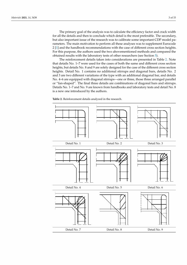
The reinforcement details taken into considerations are presented in Table 2. Notethat details No. 1–7 were used for the cases of both the same and different cross sectionheights, but details No. 8 and 9 are solely designed for the case of the different cross sectionheights. Detail No. 1 contains no additional stirrups and diagonal bars, details No. 2and 3 are two different variations of the type with an additional diagonal bar, and detailsNo. 4–6 are equipped with diagonal stirrups—one or three, those three arranged parallelor “fan-shaped”. The final three details are combinations of diagonal bars and stirrups.Details No. 1–7 and No. 9 are known from handbooks and laboratory tests and detail No. 8is a new one introduced by the authors.
Table 2. Reinforcement details analyzed in the research.
Materials 2021, 14, 3438 3 of 33
but also important issue of the research was to calibrate some important CDP model pa-rameters. The main motivation to perform all these analyses was to supplement Eurocode 2 [1] and the handbook recommendations with the case of different cross section heights. For this purpose, the authors used the two abovementioned methods and compared the obtained results with the laboratory tests of other researchers (see Section 5).
The reinforcement details taken into considerations are presented in Table 2. Note that details No. 1–7 were used for the cases of both the same and different cross section heights, but details No. 8 and 9 are solely designed for the case of the different cross section heights. Detail No. 1 contains no additional stirrups and diagonal bars, details No. 2 and 3 are two different variations of the type with an additional diagonal bar, and details No. 4–6 are equipped with diagonal stirrups—one or three, those three arranged parallel or “fan-shaped”. The final three details are combinations of diagonal bars and stirrups. De-tails No. 1–7 and No. 9 are known from handbooks and laboratory tests and detail No. 8 is a new one introduced by the authors.
Table 2. Reinforcement details analyzed in the research.
Detail No. 1 Detail No. 2 Detail No. 3
Detail No. 4 Detail No. 5 Detail No. 6
Detail No. 7 Detail No. 8 Detail No. 9
2. Methodology
Detail No. 1 Detail No. 2 Detail No. 3
Materials 2021, 14, 3438 3 of 33
but also important issue of the research was to calibrate some important CDP model pa-rameters. The main motivation to perform all these analyses was to supplement Eurocode 2 [1] and the handbook recommendations with the case of different cross section heights. For this purpose, the authors used the two abovementioned methods and compared the obtained results with the laboratory tests of other researchers (see Section 5).
The reinforcement details taken into considerations are presented in Table 2. Note that details No. 1–7 were used for the cases of both the same and different cross section heights, but details No. 8 and 9 are solely designed for the case of the different cross section heights. Detail No. 1 contains no additional stirrups and diagonal bars, details No. 2 and 3 are two different variations of the type with an additional diagonal bar, and details No. 4–6 are equipped with diagonal stirrups—one or three, those three arranged parallel or “fan-shaped”. The final three details are combinations of diagonal bars and stirrups. De-tails No. 1–7 and No. 9 are known from handbooks and laboratory tests and detail No. 8 is a new one introduced by the authors.
Table 2. Reinforcement details analyzed in the research.
Detail No. 1 Detail No. 2 Detail No. 3
Detail No. 4 Detail No. 5 Detail No. 6
Detail No. 7 Detail No. 8 Detail No. 9
2. Methodology
Detail No. 4 Detail No. 5 Detail No. 6
Materials 2021, 14, 3438 3 of 33
but also important issue of the research was to calibrate some important CDP model pa-rameters. The main motivation to perform all these analyses was to supplement Eurocode 2 [1] and the handbook recommendations with the case of different cross section heights. For this purpose, the authors used the two abovementioned methods and compared the obtained results with the laboratory tests of other researchers (see Section 5).
The reinforcement details taken into considerations are presented in Table 2. Note that details No. 1–7 were used for the cases of both the same and different cross section heights, but details No. 8 and 9 are solely designed for the case of the different cross section heights. Detail No. 1 contains no additional stirrups and diagonal bars, details No. 2 and 3 are two different variations of the type with an additional diagonal bar, and details No. 4–6 are equipped with diagonal stirrups—one or three, those three arranged parallel or “fan-shaped”. The final three details are combinations of diagonal bars and stirrups. De-tails No. 1–7 and No. 9 are known from handbooks and laboratory tests and detail No. 8 is a new one introduced by the authors.
Table 2. Reinforcement details analyzed in the research.
Detail No. 1 Detail No. 2 Detail No. 3
Detail No. 4 Detail No. 5 Detail No. 6
Detail No. 7 Detail No. 8 Detail No. 9
2. Methodology
Detail No. 7 Detail No. 8 Detail No. 9
Materials 2021, 14, 3438 4 of 33
2. Methodology2.1. Strut-and-Tie Method
The S&T method is a modification of a truss analogy (Mörsch [22]). According toSchlaich et al. [23] this modification relies on the application of methods of the theory ofplasticity and the redistribution of forces from reinforcing bars to concrete. Compressivestresses are transferred by concrete struts while tensile stresses are transferred by reinforcingbars. The S&T method requires the verification of compressive stresses in struts and nodes.The required reinforcement is calculated from tensile axial forces. Also, it is important tocheck if compressive stresses in nodes are less than or equal to the ultimate compressivestrength. There are three types of S&T nodes. In the CCC node, only compressive strutsare connected. In the CCT node, there is also one tensile strut and in the CTT node, thereare two tensile struts. The ultimate compressive strength value can be assumed accordingto different recommendations, e.g., Eurocode 2 [1], Schlaich et al. [23], ACI 318 [24], fibModel Code [25]. The authors decided to assume the ultimate compressive stress σRd,maxaccording to Eurocode 2 [1] as follows:
• In struts: σRd,max = fcd, where fcd denotes the design compressive strength if a strutis under compression only and 0.6ν’fcd if a strut is also in tension in a perpendiculardirection, where (Equation (2)):
ν′ = 1− fck250
(2)
• In nodes: CCC node—σRd,max = ν’fcd, CCT node—σRd,max = 0.85ν’fcd, CTT node—σRd,max = 0.75ν’fcd.
The most important issue of the S&T method is the proper choice of a truss modelreplacing a considered ”D” region. There are various design codes and handbooks that helpa designer pick an appropriate scheme, e.g., Schlaich et al. [23], Reineck [26], El-Metwallyand Chen [27], but there are few recommendations concerning corners under openingbending moment, see e.g., in Eurocode 2 [1].
2.2. Concrete Damaged Plasticity Model for Concrete in FEM Analysis
As mentioned before, FEM calculations were performed with Abaqus software [28]using the Concrete Damaged Plasticity model (CDP) for concrete. There are many otheralternative models, e.g., presented in the work Marzec et al. [15] or Cichon and Win-nicki [29,30]. The CDP model for monotonic loading was mathematically formulated byLubliner et al. [31] and enhanced by Lee and Fenves [32,33] for dynamic and cyclic loading.This model is a combination of the plasticity theory and damage mechanics.
The stress–strain relationship is defined with Equation (3):
σ = (1− d)Delo :(ε− εpl
)(3)
where d is a damage parameter and Delo is an initial stiffness matrix in the elastic state. The
damage parameter is given according to Equation (4):
1− d = (1− stdc)(1− scdt) (4)
where dc and dt are damage parameters and sc and st are stiffness recovery functions incompression and tension, respectively. The yield function in the CDP model is definedaccording to Equation (5):
F =1
1− α
(q− 3αp + β
(εpl
)⟨σmax
⟩− γ
⟨−σmax
⟩)− σc
(εpl
)(5)
Materials 2021, 14, 3438 5 of 33
where α, β and γ are parameters, p denotes the effective hydrostatic pressure stress, q isvon Mises equivalent effective stress and 〈〉 is Macaulay’s bracket. The effective stress isassumed according to Equation (6):
σ =σ
1− d(6)
The parameter α depends on the ratio of the uniaxial compressive strength fc0 to thebiaxial compressive strength fb0—see Equation (7):
α =fb0 − fc0
2 fb0 − fc0(7)
The typical values of the ratio fb0 to fc0 are in the range of 1.10 to 1.16 (Kupfer [34],Lubliner et al. [31]). Parameters β and γ are calculated as (Equations (8) and (9)):
β =3(1− KT)
2KT − 1(8)
γ =3(1− KC)
2KC − 1(9)
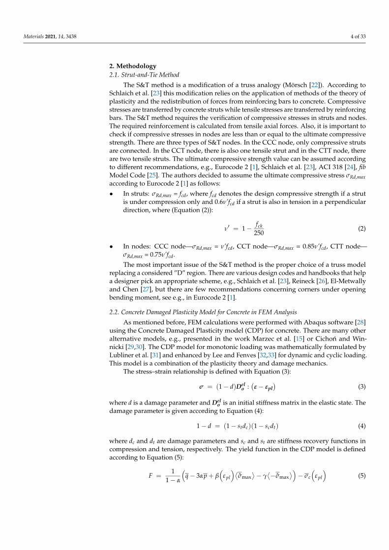
The parameters KT and KC define the shape of the yield surface. Typical values ofthese parameters vary from 0.56 to 0.61 for KT and from 0.66 to 0.80 for KC (Szwed andKaminska [35]). The yield surface can be presented in the meridian plane—see Figure 1.
Materials 2021, 14, 3438 5 of 33
The typical values of the ratio fb0 to fc0 are in the range of 1.10 to 1.16 (Kupfer [34],
Lubliner et al. [31]). Parameters β and γ are calculated as (Equations (8) and (9)):
( )12
13
−
−=
T
T
K
K (8)
( )12
13
−
−=
C
C
K
K (9)
The parameters KT and KC define the shape of the yield surface. Typical values of
these parameters vary from 0.56 to 0.61 for KT and from 0.66 to 0.80 for KC (Szwed and
Kamińska [35]). The yield surface can be presented in the meridian plane—see Figure 1.
Figure 1. CDP yield surface in the meridian plane.
As proposed in [28], the plastic flow potential G is assumed as a non-associated po-
tential of the Drucker-Prager hyperbolic type according to Equation (10):
( ) tanpqtaneG 22
0t −+= (10)
where e is an eccentricity parameter and ψ denotes a dilatation angle. The graph of the
function G and a graphical interpretation of e and ψ are presented in Figure 2.
Figure 2. CDP plastic flow potential surface in the meridian plane.
The viscoplastic regularization can also be applied in the CDP model according to
the Duvaut–Lions approach [36] (Equation (11)):
( )pl
v
plpl
v
−=1
(11)
where μ denotes the relaxation time (the so-called viscosity parameter in Abaqus code)
and the bottom index ν refers to the viscous part of plastic strains. The viscoplastic
Figure 1. CDP yield surface in the meridian plane.
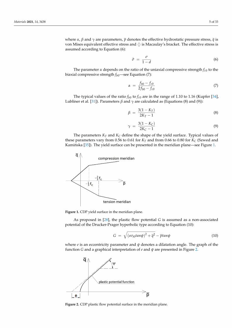
As proposed in [28], the plastic flow potential G is assumed as a non-associatedpotential of the Drucker-Prager hyperbolic type according to Equation (10):
G =
√(eσt0tanψ)2 + q2 − ptanψ (10)
where e is an eccentricity parameter and ψ denotes a dilatation angle. The graph of thefunction G and a graphical interpretation of e and ψ are presented in Figure 2.
Materials 2021, 14, 3438 5 of 33
The typical values of the ratio fb0 to fc0 are in the range of 1.10 to 1.16 (Kupfer [34],
Lubliner et al. [31]). Parameters β and γ are calculated as (Equations (8) and (9)):
( )12
13
−
−=
T
T
K
K (8)
( )12
13
−
−=
C
C
K
K (9)
The parameters KT and KC define the shape of the yield surface. Typical values of
these parameters vary from 0.56 to 0.61 for KT and from 0.66 to 0.80 for KC (Szwed and
Kamińska [35]). The yield surface can be presented in the meridian plane—see Figure 1.
Figure 1. CDP yield surface in the meridian plane.
As proposed in [28], the plastic flow potential G is assumed as a non-associated po-
tential of the Drucker-Prager hyperbolic type according to Equation (10):
( ) tanpqtaneG 22
0t −+= (10)
where e is an eccentricity parameter and ψ denotes a dilatation angle. The graph of the
function G and a graphical interpretation of e and ψ are presented in Figure 2.
Figure 2. CDP plastic flow potential surface in the meridian plane.
The viscoplastic regularization can also be applied in the CDP model according to
the Duvaut–Lions approach [36] (Equation (11)):
( )pl
v
plpl
v
−=1
(11)
where μ denotes the relaxation time (the so-called viscosity parameter in Abaqus code)
and the bottom index ν refers to the viscous part of plastic strains. The viscoplastic
Figure 2. CDP plastic flow potential surface in the meridian plane.
Materials 2021, 14, 3438 6 of 33
The viscoplastic regularization can also be applied in the CDP model according to theDuvaut–Lions approach [36] (Equation (11)):
.ε
plv =
1µ
(εpl − ε
plv
)(11)
where µ denotes the relaxation time (the so-called viscosity parameter in Abaqus code) andthe bottom index ν refers to the viscous part of plastic strains. The viscoplastic behavior ofconcrete is taken into consideration in the CDP model only if the relaxation time is largerthan zero.
A full definition of the CDP model needs a specification of a few parameters, namely:
(1) The stress–strain relationship defining a compressive behavior of concrete, usually ina form of a set of points;
(2) The dilatation angle ψ in the p− q plane;(3) The flow potential eccentricity e;(4) The ratio f b0/f c0 of the biaxial compressive strength to the uniaxial compressive
strength;(5) The ratio K of the second stress invariant on the tensile meridian to that on the
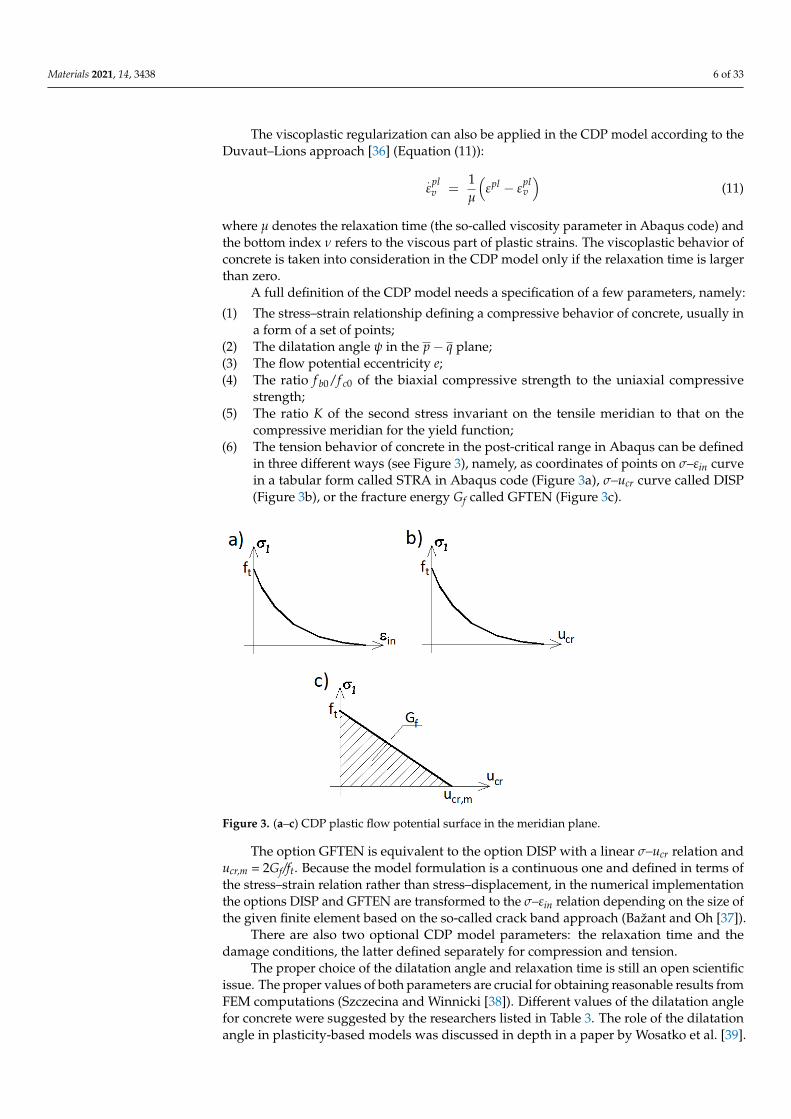
compressive meridian for the yield function;(6) The tension behavior of concrete in the post-critical range in Abaqus can be defined
in three different ways (see Figure 3), namely, as coordinates of points on σ–εin curvein a tabular form called STRA in Abaqus code (Figure 3a), σ–ucr curve called DISP(Figure 3b), or the fracture energy Gf called GFTEN (Figure 3c).
Materials 2021, 14, 3438 6 of 33
behavior of concrete is taken into consideration in the CDP model only if the relaxation
time is larger than zero.
A full definition of the CDP model needs a specification of a few parameters, namely:
(1) The stress–strain relationship defining a compressive behavior of concrete, usually
in a form of a set of points;
(2) The dilatation angle ψ in the qp − plane;
(3) The flow potential eccentricity e;
(4) The ratio fb0/fc0 of the biaxial compressive strength to the uniaxial compressive
strength;
(5) The ratio K of the second stress invariant on the tensile meridian to that on the com-
pressive meridian for the yield function;
(6) The tension behavior of concrete in the post-critical range in Abaqus can be defined
in three different ways (see Figure 3), namely, as coordinates of points on σ–εin curve
in a tabular form called STRA in Abaqus code (Figure 3a), σ–ucr curve called DISP
(Figure 3b), or the fracture energy Gf called GFTEN (Figure 3c).
Figure 3. (a–c) CDP plastic flow potential surface in the meridian plane.
The option GFTEN is equivalent to the option DISP with a linear σ–ucr relation and
ucr,m = 2Gf/ft. Because the model formulation is a continuous one and defined in terms of
the stress–strain relation rather than stress–displacement, in the numerical implementa-
tion the options DISP and GFTEN are transformed to the σ–εin relation depending on the
size of the given finite element based on the so-called crack band approach (Bažant and
Oh [37]).
There are also two optional CDP model parameters: the relaxation time and the dam-
age conditions, the latter defined separately for compression and tension.
The proper choice of the dilatation angle and relaxation time is still an open scientific
issue. The proper values of both parameters are crucial for obtaining reasonable results
from FEM computations (Szczecina and Winnicki [38]). Different values of the dilatation
angle for concrete were suggested by the researchers listed in Table 3. The role of the di-
latation angle in plasticity-based models was discussed in depth in a paper by Wosatko et
al. [39]. The range of the proposed values is very wide, and this is why the authors decided
to perform a calibration and validation of the dilatation angle for concrete. A similar situ-
ation occurs for the relaxation time—some researchers (e.g., Genikomsou and Polak
[40,41] and Pereira et al. [42]) proposed values from 10−5 s to 10−4 s. The calibration and
validation of the dilatation angle and relaxation time are described in the next section.
Figure 3. (a–c) CDP plastic flow potential surface in the meridian plane.
The option GFTEN is equivalent to the option DISP with a linear σ–ucr relation anducr,m = 2Gf/ft. Because the model formulation is a continuous one and defined in terms ofthe stress–strain relation rather than stress–displacement, in the numerical implementationthe options DISP and GFTEN are transformed to the σ–εin relation depending on the size ofthe given finite element based on the so-called crack band approach (Bažant and Oh [37]).
There are also two optional CDP model parameters: the relaxation time and thedamage conditions, the latter defined separately for compression and tension.
The proper choice of the dilatation angle and relaxation time is still an open scientificissue. The proper values of both parameters are crucial for obtaining reasonable results fromFEM computations (Szczecina and Winnicki [38]). Different values of the dilatation anglefor concrete were suggested by the researchers listed in Table 3. The role of the dilatationangle in plasticity-based models was discussed in depth in a paper by Wosatko et al. [39].
Materials 2021, 14, 3438 7 of 33
The range of the proposed values is very wide, and this is why the authors decided toperform a calibration and validation of the dilatation angle for concrete. A similar situationoccurs for the relaxation time—some researchers (e.g., Genikomsou and Polak [40,41] andPereira et al. [42]) proposed values from 10−5 s to 10−4 s. The calibration and validation ofthe dilatation angle and relaxation time are described in the next section.
Table 3. Values of dilatation angle as suggested by other authors.
Source Dilatation Angle ψ [◦]
Jankowiak [43] 49Genikomsou and Polak [40] 38
Mostafiz et al. [44] 38Kmiecik and Kaminski [45] 36
Malm [46] 25–38Menetrey [47] 10
Mostofinejad and Saadatmand [48] 0Marzec [49] 8 or 10
Rodriguez et al. [50] 30Urbanski and Łabuda [51] 15
3. Calibration and Validation of CDP Model Parameters3.1. Uniaxial and Biaxial Compression Tests
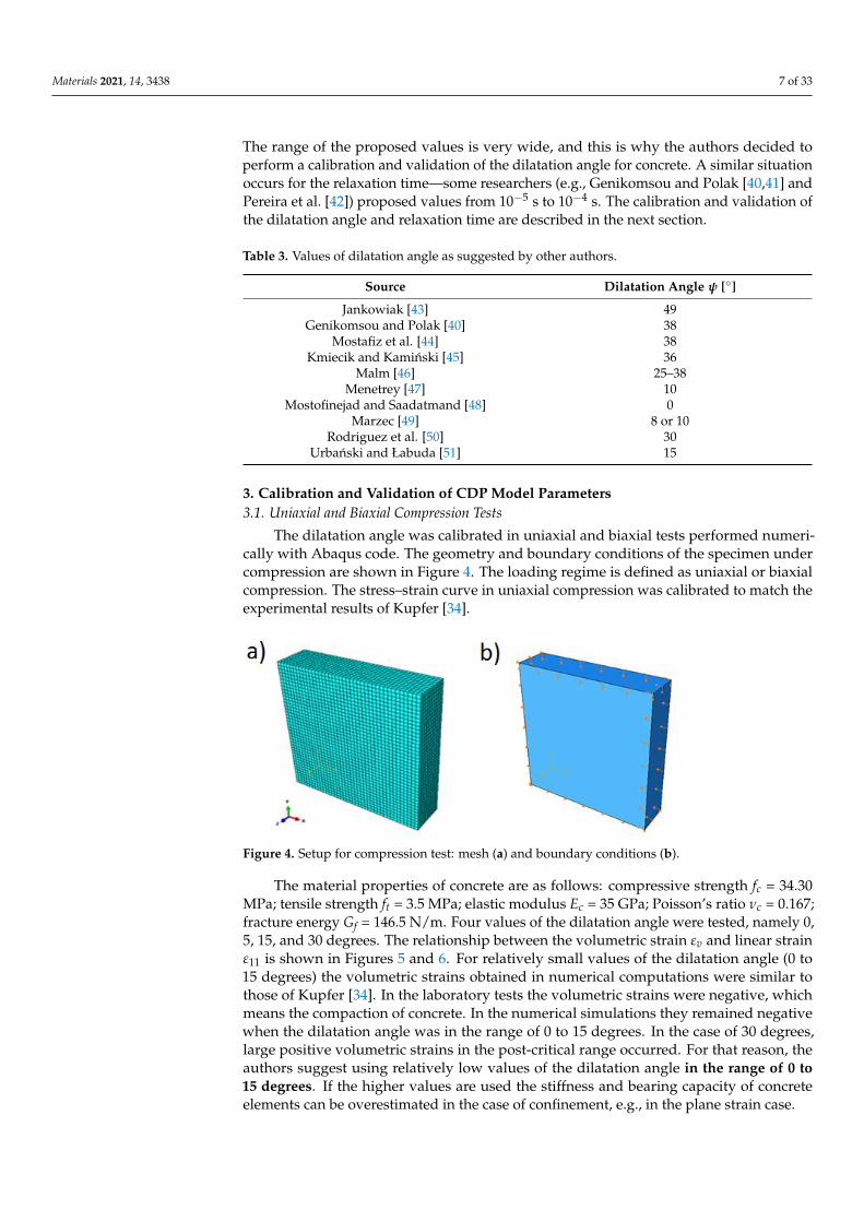
The dilatation angle was calibrated in uniaxial and biaxial tests performed numeri-cally with Abaqus code. The geometry and boundary conditions of the specimen undercompression are shown in Figure 4. The loading regime is defined as uniaxial or biaxialcompression. The stress–strain curve in uniaxial compression was calibrated to match theexperimental results of Kupfer [34].
Materials 2021, 14, 3438 7 of 33
Table 3. Values of dilatation angle as suggested by other authors.
Source Dilatation Angle ψ [°]
Jankowiak [43] 49
Genikomsou and Polak [40] 38
Mostafiz et al. [44] 38
Kmiecik and Kamiński [45] 36
Malm [46] 25–38
Menetrey [47] 10
Mostofinejad and Saadatmand [48] 0
Marzec [49] 8 or 10
Rodriguez et al. [50] 30
Urbański and Łabuda [51] 15
3. Calibration and Validation of CDP Model Parameters
3.1. Uniaxial and Biaxial Compression Tests
The dilatation angle was calibrated in uniaxial and biaxial tests performed numeri-
cally with Abaqus code. The geometry and boundary conditions of the specimen under
compression are shown in Figure 4. The loading regime is defined as uniaxial or biaxial
compression. The stress–strain curve in uniaxial compression was calibrated to match the
experimental results of Kupfer [34].
Figure 4. Setup for compression test: mesh (a) and boundary conditions (b).
The material properties of concrete are as follows: compressive strength fc = 34.30
MPa; tensile strength ft = 3.5 MPa; elastic modulus Ec = 35 GPa; Poisson’s ratio νc = 0.167;
fracture energy Gf = 146.5 N/m. Four values of the dilatation angle were tested, namely 0,
5, 15, and 30 degrees. The relationship between the volumetric strain εv and linear strain
ε11 is shown in Figures 5 and 6. For relatively small values of the dilatation angle (0 to 15
degrees) the volumetric strains obtained in numerical computations were similar to those
of Kupfer [34]. In the laboratory tests the volumetric strains were negative, which means
the compaction of concrete. In the numerical simulations they remained negative when
the dilatation angle was in the range of 0 to 15 degrees. In the case of 30 degrees, large
positive volumetric strains in the post-critical range occurred. For that reason, the authors
suggest using relatively low values of the dilatation angle in the range of 0 to 15 degrees.
If the higher values are used the stiffness and bearing capacity of concrete elements can
be overestimated in the case of confinement, e.g., in the plane strain case.
Figure 4. Setup for compression test: mesh (a) and boundary conditions (b).
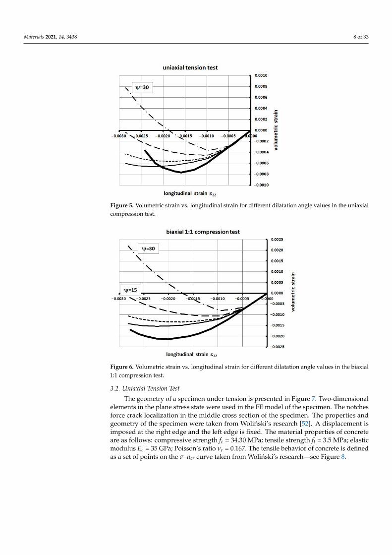
The material properties of concrete are as follows: compressive strength fc = 34.30MPa; tensile strength ft = 3.5 MPa; elastic modulus Ec = 35 GPa; Poisson’s ratio νc = 0.167;fracture energy Gf = 146.5 N/m. Four values of the dilatation angle were tested, namely 0,5, 15, and 30 degrees. The relationship between the volumetric strain εv and linear strainε11 is shown in Figures 5 and 6. For relatively small values of the dilatation angle (0 to15 degrees) the volumetric strains obtained in numerical computations were similar tothose of Kupfer [34]. In the laboratory tests the volumetric strains were negative, whichmeans the compaction of concrete. In the numerical simulations they remained negativewhen the dilatation angle was in the range of 0 to 15 degrees. In the case of 30 degrees,large positive volumetric strains in the post-critical range occurred. For that reason, theauthors suggest using relatively low values of the dilatation angle in the range of 0 to15 degrees. If the higher values are used the stiffness and bearing capacity of concreteelements can be overestimated in the case of confinement, e.g., in the plane strain case.
Materials 2021, 14, 3438 8 of 33Materials 2021, 14, 3438 8 of 33
Figure 5. Volumetric strain vs. longitudinal strain for different dilatation angle values in the uniax-
ial compression test.
Figure 6. Volumetric strain vs. longitudinal strain for different dilatation angle values in the biax-
ial 1:1 compression test.
3.2. Uniaxial Tension Test
The geometry of a specimen under tension is presented in Figure 7. Two-dimensional
elements in the plane stress state were used in the FE model of the specimen. The notches
force crack localization in the middle cross section of the specimen. The properties and
geometry of the specimen were taken from Woliński’s research [52]. A displacement is
imposed at the right edge and the left edge is fixed. The material properties of concrete
are as follows: compressive strength fc = 34.30 MPa; tensile strength ft = 3.5 MPa; elastic
modulus Ec = 35 GPa; Poisson’s ratio νc = 0.167. The tensile behavior of concrete is defined
as a set of points on the σ–ucr curve taken from Woliński’s research—see Figure 8.
Figure 5. Volumetric strain vs. longitudinal strain for different dilatation angle values in the uniaxialcompression test.
Materials 2021, 14, 3438 8 of 33
Figure 5. Volumetric strain vs. longitudinal strain for different dilatation angle values in the uniax-
ial compression test.
Figure 6. Volumetric strain vs. longitudinal strain for different dilatation angle values in the biax-
ial 1:1 compression test.
3.2. Uniaxial Tension Test
The geometry of a specimen under tension is presented in Figure 7. Two-dimensional
elements in the plane stress state were used in the FE model of the specimen. The notches
force crack localization in the middle cross section of the specimen. The properties and
geometry of the specimen were taken from Woliński’s research [52]. A displacement is
imposed at the right edge and the left edge is fixed. The material properties of concrete
are as follows: compressive strength fc = 34.30 MPa; tensile strength ft = 3.5 MPa; elastic
modulus Ec = 35 GPa; Poisson’s ratio νc = 0.167. The tensile behavior of concrete is defined
as a set of points on the σ–ucr curve taken from Woliński’s research—see Figure 8.
Figure 6. Volumetric strain vs. longitudinal strain for different dilatation angle values in the biaxial1:1 compression test.
3.2. Uniaxial Tension Test
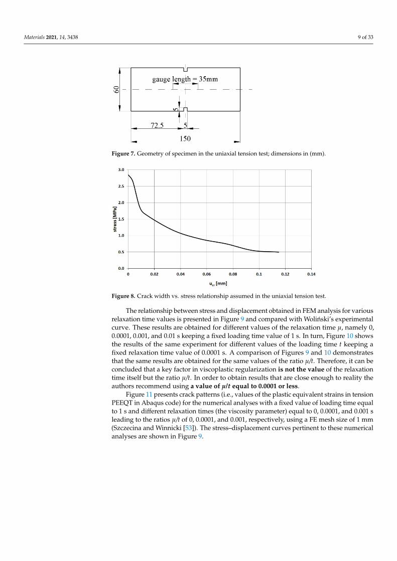
The geometry of a specimen under tension is presented in Figure 7. Two-dimensionalelements in the plane stress state were used in the FE model of the specimen. The notchesforce crack localization in the middle cross section of the specimen. The properties andgeometry of the specimen were taken from Wolinski’s research [52]. A displacement isimposed at the right edge and the left edge is fixed. The material properties of concreteare as follows: compressive strength fc = 34.30 MPa; tensile strength ft = 3.5 MPa; elasticmodulus Ec = 35 GPa; Poisson’s ratio νc = 0.167. The tensile behavior of concrete is definedas a set of points on the σ–ucr curve taken from Wolinski’s research—see Figure 8.
Materials 2021, 14, 3438 9 of 33Materials 2021, 14, 3438 9 of 33
Figure 7. Geometry of specimen in the uniaxial tension test; dimensions in (mm).
Figure 8. Crack width vs. stress relationship assumed in the uniaxial tension test.
The relationship between stress and displacement obtained in FEM analysis for var-
ious relaxation time values is presented in Figure 9 and compared with Woliński’s exper-
imental curve. These results are obtained for different values of the relaxation time μ,
namely 0, 0.0001, 0.001, and 0.01 s keeping a fixed loading time value of 1 s. In turn, Figure
10 shows the results of the same experiment for different values of the loading time t
keeping a fixed relaxation time value of 0.0001 s. A comparison of Figures 9 and 10 demon-
strates that the same results are obtained for the same values of the ratio μ/t. Therefore, it
can be concluded that a key factor in viscoplastic regularization is not the value of the
relaxation time itself but the ratio μ/t. In order to obtain results that are close enough to
reality the authors recommend using a value of μ/t equal to 0.0001 or less.
Figure 11 presents crack patterns (i.e., values of the plastic equivalent strains in ten-
sion PEEQT in Abaqus code) for the numerical analyses with a fixed value of loading time
equal to 1 s and different relaxation times (the viscosity parameter) equal to 0, 0.0001, and
0.001 s leading to the ratios μ/t of 0, 0.0001, and 0.001, respectively, using a FE mesh size
of 1 mm (Szczecina and Winnicki [53]). The stress–displacement curves pertinent to these
numerical analyses are shown in Figure 9.
Figure 7. Geometry of specimen in the uniaxial tension test; dimensions in (mm).
Materials 2021, 14, 3438 9 of 33
Figure 7. Geometry of specimen in the uniaxial tension test; dimensions in (mm).
Figure 8. Crack width vs. stress relationship assumed in the uniaxial tension test.
The relationship between stress and displacement obtained in FEM analysis for var-
ious relaxation time values is presented in Figure 9 and compared with Woliński’s exper-
imental curve. These results are obtained for different values of the relaxation time μ,
namely 0, 0.0001, 0.001, and 0.01 s keeping a fixed loading time value of 1 s. In turn, Figure
10 shows the results of the same experiment for different values of the loading time t
keeping a fixed relaxation time value of 0.0001 s. A comparison of Figures 9 and 10 demon-
strates that the same results are obtained for the same values of the ratio μ/t. Therefore, it
can be concluded that a key factor in viscoplastic regularization is not the value of the
relaxation time itself but the ratio μ/t. In order to obtain results that are close enough to
reality the authors recommend using a value of μ/t equal to 0.0001 or less.
Figure 11 presents crack patterns (i.e., values of the plastic equivalent strains in ten-
sion PEEQT in Abaqus code) for the numerical analyses with a fixed value of loading time
equal to 1 s and different relaxation times (the viscosity parameter) equal to 0, 0.0001, and
0.001 s leading to the ratios μ/t of 0, 0.0001, and 0.001, respectively, using a FE mesh size
of 1 mm (Szczecina and Winnicki [53]). The stress–displacement curves pertinent to these
numerical analyses are shown in Figure 9.
Figure 8. Crack width vs. stress relationship assumed in the uniaxial tension test.
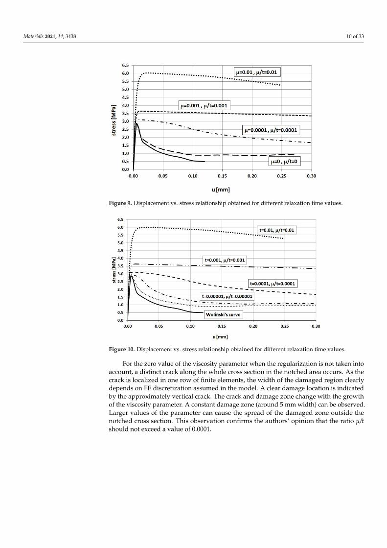
The relationship between stress and displacement obtained in FEM analysis for variousrelaxation time values is presented in Figure 9 and compared with Wolinski’s experimentalcurve. These results are obtained for different values of the relaxation time µ, namely 0,0.0001, 0.001, and 0.01 s keeping a fixed loading time value of 1 s. In turn, Figure 10 showsthe results of the same experiment for different values of the loading time t keeping afixed relaxation time value of 0.0001 s. A comparison of Figures 9 and 10 demonstratesthat the same results are obtained for the same values of the ratio µ/t. Therefore, it can beconcluded that a key factor in viscoplastic regularization is not the value of the relaxationtime itself but the ratio µ/t. In order to obtain results that are close enough to reality theauthors recommend using a value of µ/t equal to 0.0001 or less.
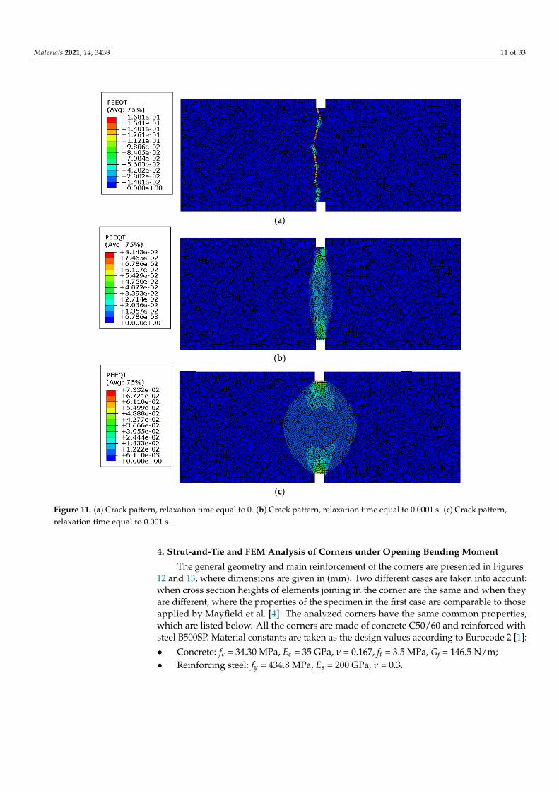
Figure 11 presents crack patterns (i.e., values of the plastic equivalent strains in tensionPEEQT in Abaqus code) for the numerical analyses with a fixed value of loading time equalto 1 s and different relaxation times (the viscosity parameter) equal to 0, 0.0001, and 0.001 sleading to the ratios µ/t of 0, 0.0001, and 0.001, respectively, using a FE mesh size of 1 mm(Szczecina and Winnicki [53]). The stress–displacement curves pertinent to these numericalanalyses are shown in Figure 9.
Materials 2021, 14, 3438 10 of 33Materials 2021, 14, 3438 10 of 33
Figure 9. Displacement vs. stress relationship obtained for different relaxation time values.
Figure 10. Displacement vs. stress relationship obtained for different relaxation time values.
For the zero value of the viscosity parameter when the regularization is not taken
into account, a distinct crack along the whole cross section in the notched area occurs. As
the crack is localized in one row of finite elements, the width of the damaged region clearly
depends on FE discretization assumed in the model. A clear damage location is indicated
by the approximately vertical crack. The crack and damage zone change with the growth
of the viscosity parameter. A constant damage zone (around 5 mm width) can be ob-
served. Larger values of the parameter can cause the spread of the damaged zone outside
the notched cross section. This observation confirms the authors’ opinion that the ratio μ/t
should not exceed a value of 0.0001.
Figure 9. Displacement vs. stress relationship obtained for different relaxation time values.
Materials 2021, 14, 3438 10 of 33
Figure 9. Displacement vs. stress relationship obtained for different relaxation time values.
Figure 10. Displacement vs. stress relationship obtained for different relaxation time values.
For the zero value of the viscosity parameter when the regularization is not taken
into account, a distinct crack along the whole cross section in the notched area occurs. As
the crack is localized in one row of finite elements, the width of the damaged region clearly
depends on FE discretization assumed in the model. A clear damage location is indicated
by the approximately vertical crack. The crack and damage zone change with the growth
of the viscosity parameter. A constant damage zone (around 5 mm width) can be ob-
served. Larger values of the parameter can cause the spread of the damaged zone outside
the notched cross section. This observation confirms the authors’ opinion that the ratio μ/t
should not exceed a value of 0.0001.
Figure 10. Displacement vs. stress relationship obtained for different relaxation time values.
For the zero value of the viscosity parameter when the regularization is not taken intoaccount, a distinct crack along the whole cross section in the notched area occurs. As thecrack is localized in one row of finite elements, the width of the damaged region clearlydepends on FE discretization assumed in the model. A clear damage location is indicatedby the approximately vertical crack. The crack and damage zone change with the growthof the viscosity parameter. A constant damage zone (around 5 mm width) can be observed.Larger values of the parameter can cause the spread of the damaged zone outside thenotched cross section. This observation confirms the authors’ opinion that the ratio µ/tshould not exceed a value of 0.0001.
Materials 2021, 14, 3438 11 of 33Materials 2021, 14, 3438 11 of 33
(a)
(b)
(c)
Figure 11. (a) Crack pattern, relaxation time equal to 0. (b) Crack pattern, relaxation time equal to 0.0001 s. (c) Crack
pattern, relaxation time equal to 0.001 s.
4. Strut-and-Tie and FEM Analysis of Corners under Opening Bending Moment
The general geometry and main reinforcement of the corners are presented in Figures
12 and 13, where dimensions are given in (mm). Two different cases are taken into ac-
count: when cross section heights of elements joining in the corner are the same and when
they are different, where the properties of the specimen in the first case are comparable to
those applied by Mayfield et al. [4]. The analyzed corners have the same common prop-
erties, which are listed below. All the corners are made of concrete C50/60 and reinforced
with steel B500SP. Material constants are taken as the design values according to Eurocode
2 [1]:
• Concrete: fc = 34.30 MPa, Ec = 35 GPa, ν = 0.167, ft = 3.5 MPa, Gf = 146.5 N/m;
• Reinforcing steel: fy = 434.8 MPa, Es = 200 GPa, ν = 0.3.
Each corner is subjected to an opening bending moment with a reference value of Mref
= 30 kNm modeled as a pair of forces—see Figures 14 and 15. Seven different reinforce-
ment details taken into consideration are listed in Table 2. In this section, corners are sub-
jected to a pure bending moment, but in the Section 5.2. there is an example of a calculation
Figure 11. (a) Crack pattern, relaxation time equal to 0. (b) Crack pattern, relaxation time equal to 0.0001 s. (c) Crack pattern,relaxation time equal to 0.001 s.
4. Strut-and-Tie and FEM Analysis of Corners under Opening Bending Moment
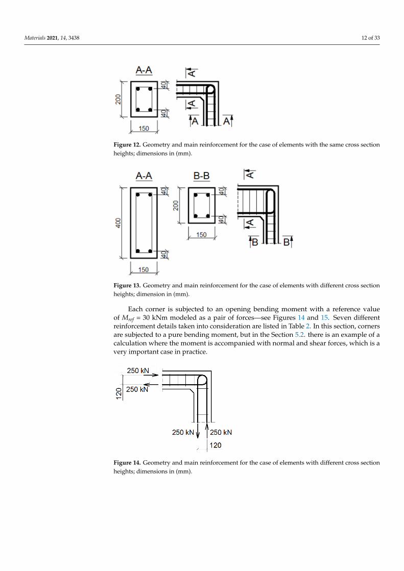
The general geometry and main reinforcement of the corners are presented in Figures12 and 13, where dimensions are given in (mm). Two different cases are taken into account:when cross section heights of elements joining in the corner are the same and when theyare different, where the properties of the specimen in the first case are comparable to thoseapplied by Mayfield et al. [4]. The analyzed corners have the same common properties,which are listed below. All the corners are made of concrete C50/60 and reinforced withsteel B500SP. Material constants are taken as the design values according to Eurocode 2 [1]:
• Concrete: fc = 34.30 MPa, Ec = 35 GPa, ν = 0.167, ft = 3.5 MPa, Gf = 146.5 N/m;• Reinforcing steel: fy = 434.8 MPa, Es = 200 GPa, ν = 0.3.
Materials 2021, 14, 3438 12 of 33
Materials 2021, 14, 3438 12 of 33
where the moment is accompanied with normal and shear forces, which is a very im-
portant case in practice.
Figure 12. Geometry and main reinforcement for the case of elements with the same cross section
heights; dimensions in (mm).
Figure 13. Geometry and main reinforcement for the case of elements with different cross section
heights; dimension in (mm).
Figure 14. Geometry and main reinforcement for the case of elements with different cross section
heights; dimensions in (mm).
Figure 12. Geometry and main reinforcement for the case of elements with the same cross sectionheights; dimensions in (mm).
Materials 2021, 14, 3438 12 of 33
where the moment is accompanied with normal and shear forces, which is a very im-
portant case in practice.
Figure 12. Geometry and main reinforcement for the case of elements with the same cross section
heights; dimensions in (mm).
Figure 13. Geometry and main reinforcement for the case of elements with different cross section
heights; dimension in (mm).
Figure 14. Geometry and main reinforcement for the case of elements with different cross section
heights; dimensions in (mm).
Figure 13. Geometry and main reinforcement for the case of elements with different cross sectionheights; dimension in (mm).
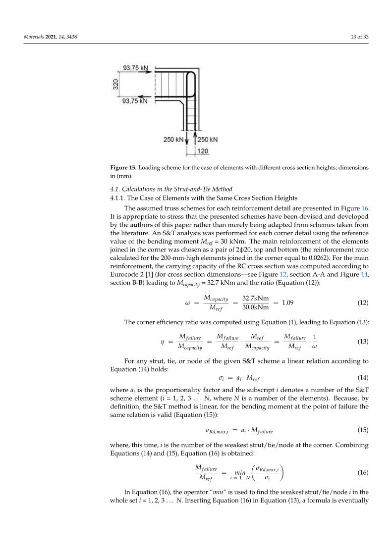
Each corner is subjected to an opening bending moment with a reference valueof Mref = 30 kNm modeled as a pair of forces—see Figures 14 and 15. Seven differentreinforcement details taken into consideration are listed in Table 2. In this section, cornersare subjected to a pure bending moment, but in the Section 5.2. there is an example of acalculation where the moment is accompanied with normal and shear forces, which is avery important case in practice.
Materials 2021, 14, 3438 12 of 33
where the moment is accompanied with normal and shear forces, which is a very im-
portant case in practice.
Figure 12. Geometry and main reinforcement for the case of elements with the same cross section
heights; dimensions in (mm).
Figure 13. Geometry and main reinforcement for the case of elements with different cross section
heights; dimension in (mm).
Figure 14. Geometry and main reinforcement for the case of elements with different cross section
heights; dimensions in (mm). Figure 14. Geometry and main reinforcement for the case of elements with different cross sectionheights; dimensions in (mm).
Materials 2021, 14, 3438 13 of 33Materials 2021, 14, 3438 13 of 33
Figure 15. Loading scheme for the case of elements with different cross section heights; dimen-
sions in (mm).
4.1. Calculations in the Strut-and-Tie Method
4.1.1. The Case of Elements with the Same Cross Section Heights
The assumed truss schemes for each reinforcement detail are presented in Figure 16.
It is appropriate to stress that the presented schemes have been devised and developed
by the authors of this paper rather than merely being adapted from schemes taken from
the literature. An S&T analysis was performed for each corner detail using the reference
value of the bending moment Mref = 30 kNm. The main reinforcement of the elements
joined in the corner was chosen as a pair of 2ϕ20, top and bottom (the reinforcement ratio
calculated for the 200-mm-high elements joined in the corner equal to 0.0262). For the main
reinforcement, the carrying capacity of the RC cross section was computed according to
Eurocode 2 [1] (for cross section dimensions—see Figure 12, section A-A and Figure 14,
section B-B) leading to Mcapacity = 32.7 kNm and the ratio (Equation (12)):
09.10.30
7.32===
kNm
kNm
M
M
ref
capacity (12)
The corner efficiency ratio was computed using Equation (1), leading to Equation
(13):
1===
ref
failure
capacity
ref
ref
failure
capacity
failure
M
M
M
M
M
M
M
M (13)
For any strut, tie, or node of the given S&T scheme a linear relation according to
Equation (14) holds:
refii Ma = (14)
where ai is the proportionality factor and the subscript i denotes a number of the S&T
scheme element (i = 1, 2, 3 … N, where N is a number of the elements). Because, by defini-
tion, the S&T method is linear, for the bending moment at the point of failure the same
relation is valid (Equation (15)):
failureiimax,,Rd Ma = (15)
where, this time, i is the number of the weakest strut/tie/node at the corner. Combining
Equations (14) and (15), Equation (16) is obtained:
=
=i
imax,,Rd
N...1iref
failuremin
M
M
(16)
Figure 15. Loading scheme for the case of elements with different cross section heights; dimensionsin (mm).
4.1. Calculations in the Strut-and-Tie Method4.1.1. The Case of Elements with the Same Cross Section Heights
The assumed truss schemes for each reinforcement detail are presented in Figure 16.It is appropriate to stress that the presented schemes have been devised and developedby the authors of this paper rather than merely being adapted from schemes taken fromthe literature. An S&T analysis was performed for each corner detail using the referencevalue of the bending moment Mref = 30 kNm. The main reinforcement of the elementsjoined in the corner was chosen as a pair of 2φ20, top and bottom (the reinforcement ratiocalculated for the 200-mm-high elements joined in the corner equal to 0.0262). For the mainreinforcement, the carrying capacity of the RC cross section was computed according toEurocode 2 [1] (for cross section dimensions—see Figure 12, section A-A and Figure 14,section B-B) leading to Mcapacity = 32.7 kNm and the ratio (Equation (12)):
ω =Mcapacity
Mre f=
32.7kNm30.0kNm
= 1.09 (12)
The corner efficiency ratio was computed using Equation (1), leading to Equation (13):
η =M f ailure
Mcapacity=
M f ailure
Mre f·
Mre f
Mcapacity=
M f ailure
Mre f· 1
ω(13)
For any strut, tie, or node of the given S&T scheme a linear relation according toEquation (14) holds:
σi = ai ·Mre f (14)
where ai is the proportionality factor and the subscript i denotes a number of the S&Tscheme element (i = 1, 2, 3 . . . N, where N is a number of the elements). Because, bydefinition, the S&T method is linear, for the bending moment at the point of failure thesame relation is valid (Equation (15)):
σRd,max,i = ai ·M f ailure (15)
where, this time, i is the number of the weakest strut/tie/node at the corner. CombiningEquations (14) and (15), Equation (16) is obtained:
M f ailure
Mre f= min
i = 1...N
(σRd,max,i
σi
)(16)
In Equation (16), the operator “min” is used to find the weakest strut/tie/node i in thewhole set i = 1, 2, 3 . . . N. Inserting Equation (16) in Equation (13), a formula is eventually
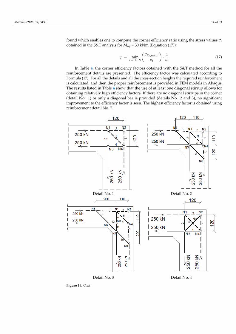
Materials 2021, 14, 3438 14 of 33
found which enables one to compute the corner efficiency ratio using the stress values σiobtained in the S&T analysis for Mref = 30 kNm (Equation (17)):
η = mini = 1...N
(σRd,max,i
σi
)· 1
ω(17)
In Table 4, the corner efficiency factors obtained with the S&T method for all thereinforcement details are presented. The efficiency factor was calculated according toFormula (17). For all the details and all the cross-section heights the required reinforcementis calculated, and then the proper reinforcement is provided in FEM models in Abaqus.The results listed in Table 4 show that the use of at least one diagonal stirrup allows forobtaining relatively high efficiency factors. If there are no diagonal stirrups in the corner(detail No. 1) or only a diagonal bar is provided (details No. 2 and 3), no significantimprovement to the efficiency factor is seen. The highest efficiency factor is obtained usingreinforcement detail No. 7.
Materials 2021, 14, 3438 14 of 33
In Equation (16), the operator “min” is used to find the weakest strut/tie/node i in the
whole set i = 1, 2, 3 … N. Inserting Equation (16) in Equation (13), a formula is eventually
found which enables one to compute the corner efficiency ratio using the stress values σi
obtained in the S&T analysis for Mref = 30 kNm (Equation (17)):
1min
max,,
...1
=
=i
iRd
Ni (17)
In Table 4, the corner efficiency factors obtained with the S&T method for all the re-
inforcement details are presented. The efficiency factor was calculated according to For-
mula (17). For all the details and all the cross-section heights the required reinforcement
is calculated, and then the proper reinforcement is provided in FEM models in Abaqus.
The results listed in Table 4 show that the use of at least one diagonal stirrup allows for
obtaining relatively high efficiency factors. If there are no diagonal stirrups in the corner
(detail No. 1) or only a diagonal bar is provided (details No. 2 and 3), no significant im-
provement to the efficiency factor is seen. The highest efficiency factor is obtained using
reinforcement detail No. 7.
Detail No. 1 Detail No. 2
Detail No. 3 Detail No. 4
Figure 16. Cont.
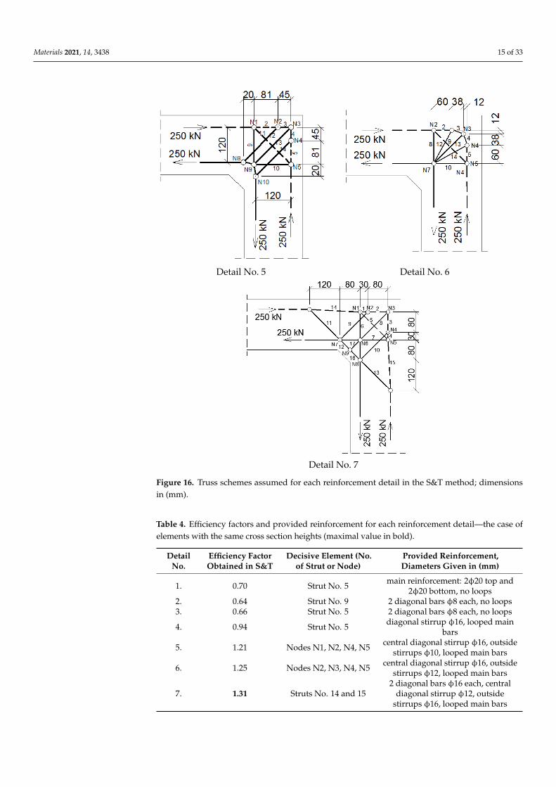
Materials 2021, 14, 3438 15 of 33Materials 2021, 14, 3438 15 of 33
Detail No. 5 Detail No. 6
Detail No. 7
Figure 16. Truss schemes assumed for each reinforcement detail in the S&T method; dimensions in
(mm).
Table 4. Efficiency factors and provided reinforcement for each reinforcement detail—the case of
elements with the same cross section heights (maximal value in bold).
Detail No. Efficiency Factor
Obtained in S&T
Decisive Element (No. of
Strut or Node)
Provided Reinforcement,
Diameters Given in (mm)
1. 0.70 Strut No. 5 main reinforcement: 2ϕ20 top and
2ϕ20 bottom, no loops
2. 0.64 Strut No. 9 2 diagonal bars ϕ8 each, no loops
3. 0.66 Strut No. 5 2 diagonal bars ϕ8 each, no loops
4. 0.94 Strut No. 5 diagonal stirrup ϕ16, looped main
bars
5. 1.21 Nodes N1, N2, N4, N5 central diagonal stirrup ϕ16, outside
stirrups ϕ10, looped main bars
6. 1.25 Nodes N2, N3, N4, N5 central diagonal stirrup ϕ16, outside
stirrups ϕ12, looped main bars
7. 1.31 Struts No. 14 and 15
2 diagonal bars ϕ16 each, central di-
agonal stirrup ϕ12, outside stirrups
ϕ16, looped main bars
Figure 16. Truss schemes assumed for each reinforcement detail in the S&T method; dimensionsin (mm).
Table 4. Efficiency factors and provided reinforcement for each reinforcement detail—the case ofelements with the same cross section heights (maximal value in bold).
DetailNo.
Efficiency FactorObtained in S&T
Decisive Element (No.of Strut or Node)
Provided Reinforcement,Diameters Given in (mm)
1. 0.70 Strut No. 5 main reinforcement: 2φ20 top and2φ20 bottom, no loops
2. 0.64 Strut No. 9 2 diagonal bars φ8 each, no loops3. 0.66 Strut No. 5 2 diagonal bars φ8 each, no loops
4. 0.94 Strut No. 5 diagonal stirrup φ16, looped mainbars
5. 1.21 Nodes N1, N2, N4, N5 central diagonal stirrup φ16, outsidestirrups φ10, looped main bars
6. 1.25 Nodes N2, N3, N4, N5 central diagonal stirrup φ16, outsidestirrups φ12, looped main bars
7. 1.31 Struts No. 14 and 152 diagonal bars φ16 each, central
diagonal stirrup φ12, outsidestirrups φ16, looped main bars
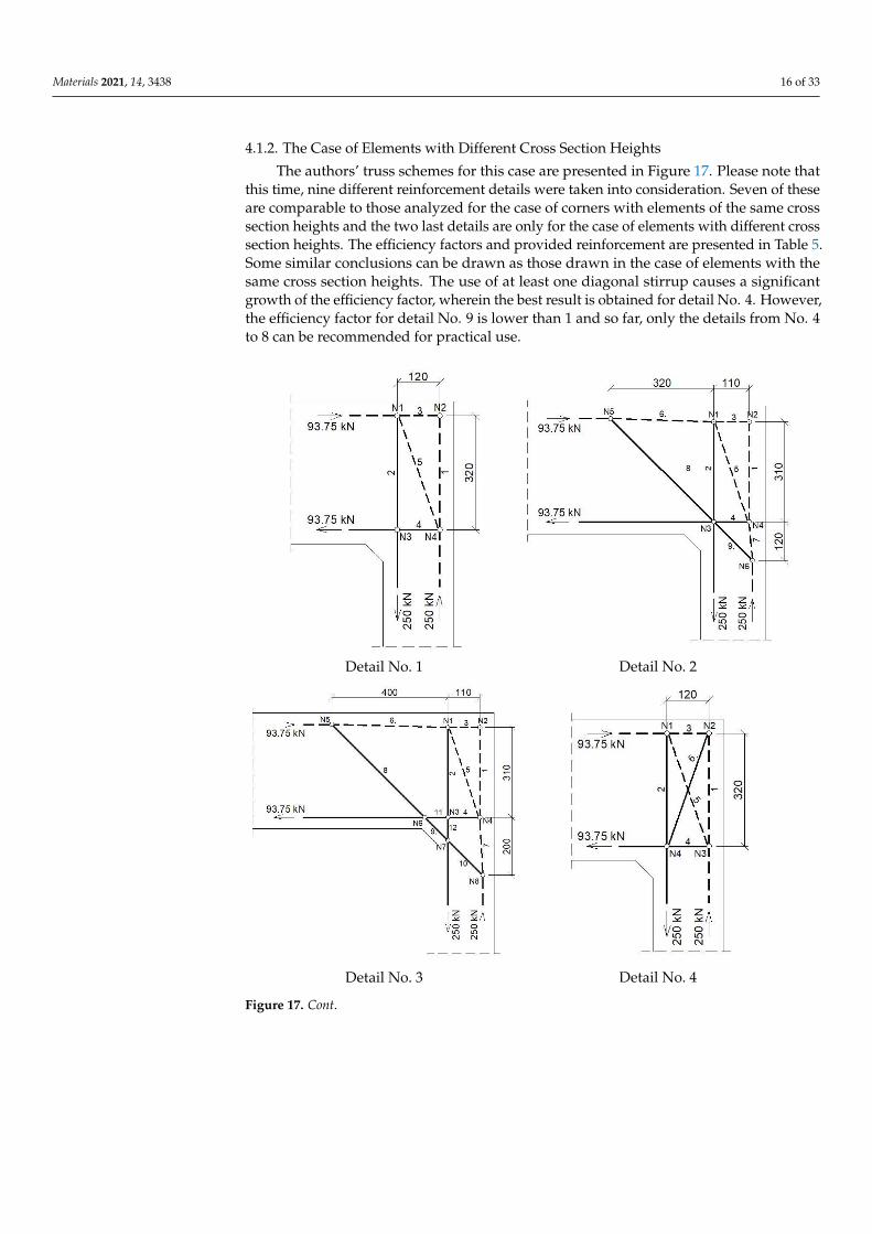
Materials 2021, 14, 3438 16 of 33
4.1.2. The Case of Elements with Different Cross Section Heights
The authors’ truss schemes for this case are presented in Figure 17. Please note thatthis time, nine different reinforcement details were taken into consideration. Seven of theseare comparable to those analyzed for the case of corners with elements of the same crosssection heights and the two last details are only for the case of elements with different crosssection heights. The efficiency factors and provided reinforcement are presented in Table 5.Some similar conclusions can be drawn as those drawn in the case of elements with thesame cross section heights. The use of at least one diagonal stirrup causes a significantgrowth of the efficiency factor, wherein the best result is obtained for detail No. 4. However,the efficiency factor for detail No. 9 is lower than 1 and so far, only the details from No. 4to 8 can be recommended for practical use.
Materials 2021, 14, 3438 16 of 33
4.1.2. The Case of Elements with Different Cross Section Heights
The authors’ truss schemes for this case are presented in Figure 17. Please note that
this time, nine different reinforcement details were taken into consideration. Seven of
these are comparable to those analyzed for the case of corners with elements of the same
cross section heights and the two last details are only for the case of elements with differ-
ent cross section heights. The efficiency factors and provided reinforcement are presented
in Table 5. Some similar conclusions can be drawn as those drawn in the case of elements
with the same cross section heights. The use of at least one diagonal stirrup causes a sig-
nificant growth of the efficiency factor, wherein the best result is obtained for detail No.
4. However, the efficiency factor for detail No. 9 is lower than 1 and so far, only the details
from No. 4 to 8 can be recommended for practical use.
Detail No. 1 Detail No. 2
Detail No. 3 Detail No. 4
Figure 17. Cont.
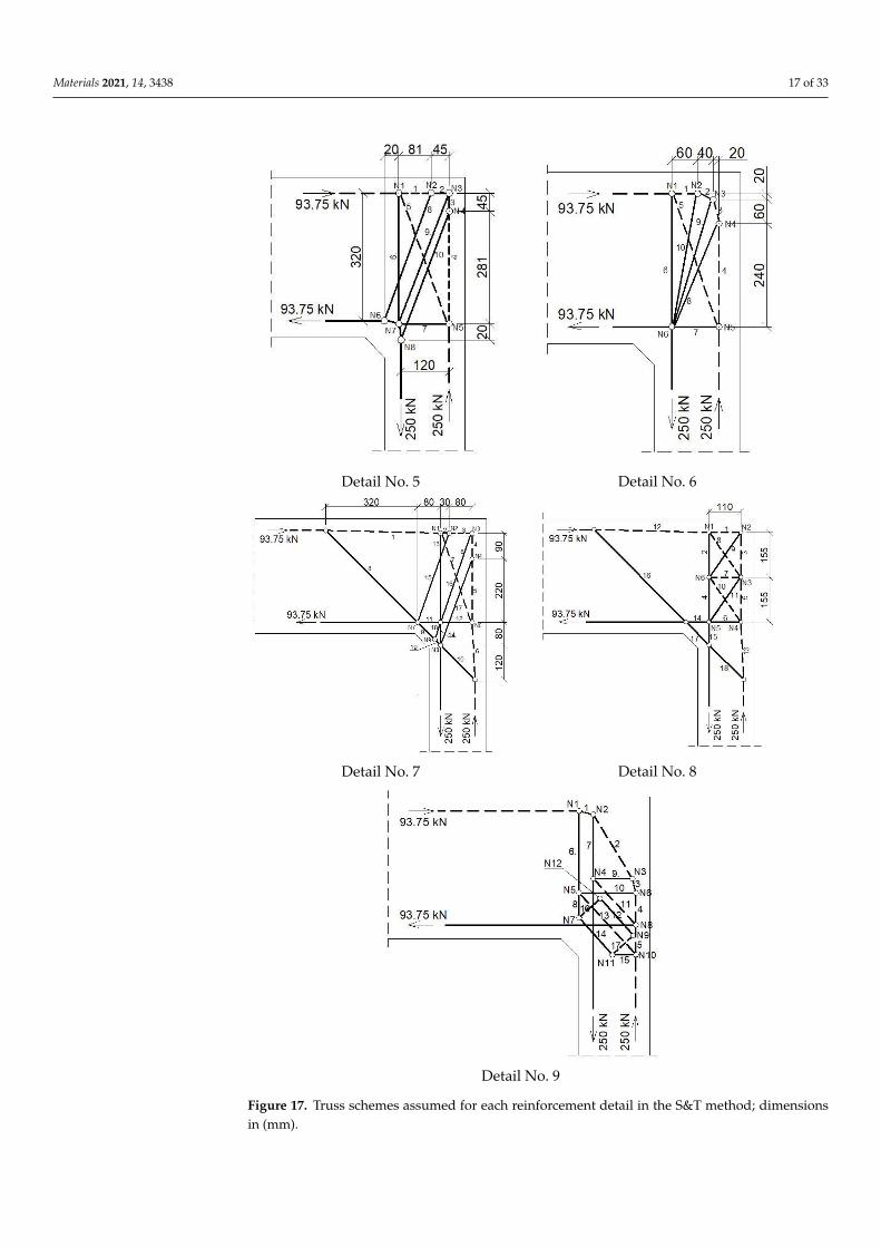
Materials 2021, 14, 3438 17 of 33Materials 2021, 14, 3438 17 of 33
Detail No. 5 Detail No. 6
Detail No. 7 Detail No. 8
Detail No. 9
Figure 17. Truss schemes assumed for each reinforcement detail in the S&T method; dimensions in
(mm). Figure 17. Truss schemes assumed for each reinforcement detail in the S&T method; dimensionsin (mm).
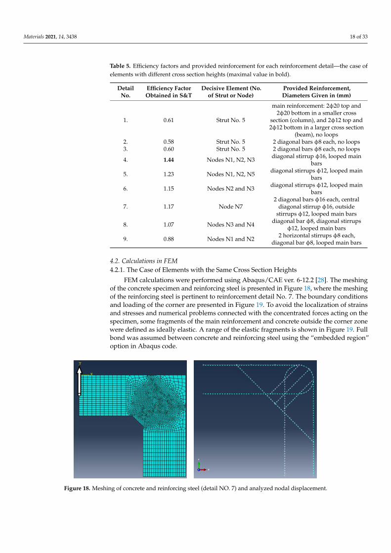
Materials 2021, 14, 3438 18 of 33
Table 5. Efficiency factors and provided reinforcement for each reinforcement detail—the case ofelements with different cross section heights (maximal value in bold).
DetailNo.
Efficiency FactorObtained in S&T
Decisive Element (No.of Strut or Node)
Provided Reinforcement,Diameters Given in (mm)
1. 0.61 Strut No. 5
main reinforcement: 2φ20 top and2φ20 bottom in a smaller cross
section (column), and 2φ12 top and2φ12 bottom in a larger cross section
(beam), no loops2. 0.58 Strut No. 5 2 diagonal bars φ8 each, no loops3. 0.60 Strut No. 5 2 diagonal bars φ8 each, no loops
4. 1.44 Nodes N1, N2, N3 diagonal stirrup φ16, looped mainbars
5. 1.23 Nodes N1, N2, N5 diagonal stirrups φ12, looped mainbars
6. 1.15 Nodes N2 and N3 diagonal stirrups φ12, looped mainbars
7. 1.17 Node N72 diagonal bars φ16 each, central
diagonal stirrup φ16, outsidestirrups φ12, looped main bars
8. 1.07 Nodes N3 and N4 diagonal bar φ8, diagonal stirrupsφ12, looped main bars
9. 0.88 Nodes N1 and N2 2 horizontal stirrups φ8 each,diagonal bar φ8, looped main bars
4.2. Calculations in FEM4.2.1. The Case of Elements with the Same Cross Section Heights
FEM calculations were performed using Abaqus/CAE ver. 6-12.2 [28]. The meshingof the concrete specimen and reinforcing steel is presented in Figure 18, where the meshingof the reinforcing steel is pertinent to reinforcement detail No. 7. The boundary conditionsand loading of the corner are presented in Figure 19. To avoid the localization of strainsand stresses and numerical problems connected with the concentrated forces acting on thespecimen, some fragments of the main reinforcement and concrete outside the corner zonewere defined as ideally elastic. A range of the elastic fragments is shown in Figure 19. Fullbond was assumed between concrete and reinforcing steel using the “embedded region”option in Abaqus code.
Materials 2021, 14, 3438 19 of 33
𝜆𝑓𝑎𝑖𝑙𝑢𝑟𝑒 = 1.0𝜔 = 1.09 (20)
Figure 18. Meshing of concrete and reinforcing steel (detail NO. 7) and analyzed nodal displace-
ment.
Figure 19. Boundary conditions and ideally elastic fragments of reinforcement (in red).
For the purpose of material behavior modeling in Abaqus software, the CDP model
for concrete and the classical metal plasticity model for steel were assumed. The stress–
strain curve for concrete in uniaxial compression was approximated with the σ–ε curve
according to Eurocode 2 [1]. For concrete behavior in uniaxial tension the fracture energy
Gf option was set as input in Abaqus. The used values of the CDP parameters are listed in
Table 6.
Table 6. CDP model parameters used in FEM calculations.
Dilatation
Angle ψ
(degree)
Flow Potential Ec-
centricity e
Ratio
fb0/fc0 Ratio K
Viscosity Pa-
rameter
μ (s)
Fracture Energy Gf
(N/m)
15 0.1 1.16 0.667 0.0001 146.5
A load time of 1 s and the ratio μ/t = 0.0001 were assumed. The main results obtained
directly from FEM calculations are the equivalent plastic strains in tension PEEQT and the
damage parameter in tension DAMAGET for concrete and von Mises’ stress and the yield
flag for reinforcing steel. The relationship between the chosen nodal displacement and the
load parameter λ is plotted as a graph. Moreover, crack width is calculated using values
of PEEQT and the formula given by Červenka et al. [54] (Equation (21)):
Figure 18. Meshing of concrete and reinforcing steel (detail NO. 7) and analyzed nodal displacement.
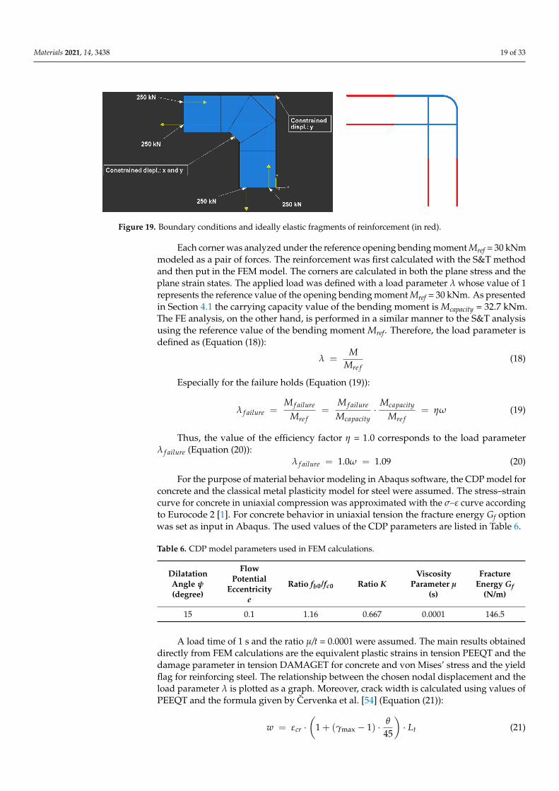
Materials 2021, 14, 3438 19 of 33
Materials 2021, 14, 3438 19 of 33
𝜆𝑓𝑎𝑖𝑙𝑢𝑟𝑒 = 1.0𝜔 = 1.09 (20)
Figure 18. Meshing of concrete and reinforcing steel (detail NO. 7) and analyzed nodal displace-
ment.
Figure 19. Boundary conditions and ideally elastic fragments of reinforcement (in red).
For the purpose of material behavior modeling in Abaqus software, the CDP model
for concrete and the classical metal plasticity model for steel were assumed. The stress–
strain curve for concrete in uniaxial compression was approximated with the σ–ε curve
according to Eurocode 2 [1]. For concrete behavior in uniaxial tension the fracture energy
Gf option was set as input in Abaqus. The used values of the CDP parameters are listed in
Table 6.
Table 6. CDP model parameters used in FEM calculations.
Dilatation
Angle ψ
(degree)
Flow Potential Ec-
centricity e
Ratio
fb0/fc0 Ratio K
Viscosity Pa-
rameter
μ (s)
Fracture Energy Gf
(N/m)
15 0.1 1.16 0.667 0.0001 146.5
A load time of 1 s and the ratio μ/t = 0.0001 were assumed. The main results obtained
directly from FEM calculations are the equivalent plastic strains in tension PEEQT and the
damage parameter in tension DAMAGET for concrete and von Mises’ stress and the yield
flag for reinforcing steel. The relationship between the chosen nodal displacement and the
load parameter λ is plotted as a graph. Moreover, crack width is calculated using values
of PEEQT and the formula given by Červenka et al. [54] (Equation (21)):
Figure 19. Boundary conditions and ideally elastic fragments of reinforcement (in red).
Each corner was analyzed under the reference opening bending moment Mref = 30 kNmmodeled as a pair of forces. The reinforcement was first calculated with the S&T methodand then put in the FEM model. The corners are calculated in both the plane stress and theplane strain states. The applied load was defined with a load parameter λ whose value of 1represents the reference value of the opening bending moment Mref = 30 kNm. As presentedin Section 4.1 the carrying capacity value of the bending moment is Mcapacity = 32.7 kNm.The FE analysis, on the other hand, is performed in a similar manner to the S&T analysisusing the reference value of the bending moment Mref. Therefore, the load parameter isdefined as (Equation (18)):
λ =M
Mre f(18)
Especially for the failure holds (Equation (19)):
λ f ailure =M f ailure
Mre f=
M f ailure
Mcapacity·
Mcapacity
Mre f= ηω (19)
Thus, the value of the efficiency factor η = 1.0 corresponds to the load parameterλ f ailure (Equation (20)):
λ f ailure = 1.0ω = 1.09 (20)
For the purpose of material behavior modeling in Abaqus software, the CDP model forconcrete and the classical metal plasticity model for steel were assumed. The stress–straincurve for concrete in uniaxial compression was approximated with the σ–ε curve accordingto Eurocode 2 [1]. For concrete behavior in uniaxial tension the fracture energy Gf optionwas set as input in Abaqus. The used values of the CDP parameters are listed in Table 6.
Table 6. CDP model parameters used in FEM calculations.
DilatationAngle ψ(degree)
FlowPotential
Eccentricitye
Ratio fb0/fc0 Ratio KViscosity
Parameter µ(s)
FractureEnergy Gf
(N/m)
15 0.1 1.16 0.667 0.0001 146.5
A load time of 1 s and the ratio µ/t = 0.0001 were assumed. The main results obtaineddirectly from FEM calculations are the equivalent plastic strains in tension PEEQT and thedamage parameter in tension DAMAGET for concrete and von Mises’ stress and the yieldflag for reinforcing steel. The relationship between the chosen nodal displacement and theload parameter λ is plotted as a graph. Moreover, crack width is calculated using values ofPEEQT and the formula given by Cervenka et al. [54] (Equation (21)):
w = εcr ·(
1 + (γmax − 1) · θ
45
)· Lt (21)
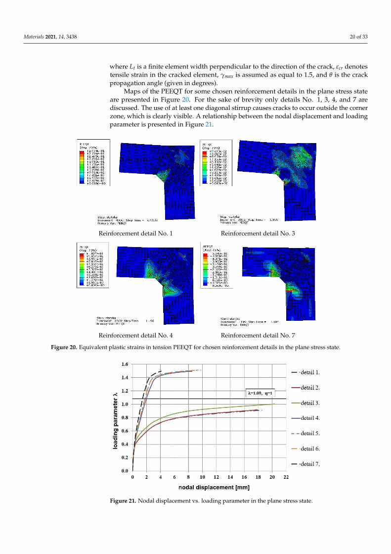
Materials 2021, 14, 3438 20 of 33
where Lt is a finite element width perpendicular to the direction of the crack, εcr denotestensile strain in the cracked element, γmax is assumed as equal to 1.5, and θ is the crackpropagation angle (given in degrees).
Maps of the PEEQT for some chosen reinforcement details in the plane stress stateare presented in Figure 20. For the sake of brevity only details No. 1, 3, 4, and 7 arediscussed. The use of at least one diagonal stirrup causes cracks to occur outside the cornerzone, which is clearly visible. A relationship between the nodal displacement and loadingparameter is presented in Figure 21.
Materials 2021, 14, 3438 20 of 33
( ) tcr Lw
−+=45
11 max
(21)
where Lt is a finite element width perpendicular to the direction of the crack, εcr denotes
tensile strain in the cracked element, γmax is assumed as equal to 1.5, and θ is the crack
propagation angle (given in degrees).
Maps of the PEEQT for some chosen reinforcement details in the plane stress state
are presented in Figure 20. For the sake of brevity only details No. 1, 3, 4, and 7 are dis-
cussed. The use of at least one diagonal stirrup causes cracks to occur outside the corner
zone, which is clearly visible. A relationship between the nodal displacement and loading
parameter is presented in Figure 21.
Analyzing the relationship presented in Figure 21 the stiffer behavior of corners
equipped with reinforcement details No. 4 to 7 is seen. Finally, the relationship of crack
width versus loading parameter presented in Figure 22 once more confirms that the use
of diagonal stirrups either alone or combined with diagonal bars is recommendable for
corners under opening bending moment. In this graph a commonly assumed value of ul-
timate crack width, namely 0.3 mm [1], is marked with a vertical line. It is clearly seen that
for reinforcement details No. 4 to 7 this ultimate value is reached for relatively high load-
ing parameter values.
Reinforcement detail No. 1 Reinforcement detail No. 3
Reinforcement detail No. 4 Reinforcement detail No. 7
Figure 20. Equivalent plastic strains in tension PEEQT for chosen reinforcement details in the
plane stress state.
Figure 20. Equivalent plastic strains in tension PEEQT for chosen reinforcement details in the plane stress state.
Materials 2021, 14, 3438 21 of 33
Figure 21. Nodal displacement vs. loading parameter in the plane stress state.
Figure 22. Crack width vs. loading parameter in the plane stress state.
Values of the efficiency factors for all the details and both methods are listed in Table
7. Higher values of this factor for reinforcement details No. 4 to 7 are seen, confirming that
these details are recommendable for practical use. Moreover, the results obtained with
FEM in the plane stress state are comparable with those obtained with the S&T method.
However, it should be remembered that a full analysis of a corner under opening bending
moment demands not only the calculation of the efficiency factor but also checking the
crack width.
Table 7. Efficiency factors for all reinforcement details obtained using all methods (maximal val-
ues in bold).
Detail No. Efficiency Factor
S&T
Efficiency Factor FEM,
Plane Stress
Efficiency Factor FEM,
Plane Strain
1. 0.70 0.75 1.01
2. 0.64 0.79 1.11
3. 0.66 0.82 1.17
Figure 21. Nodal displacement vs. loading parameter in the plane stress state.
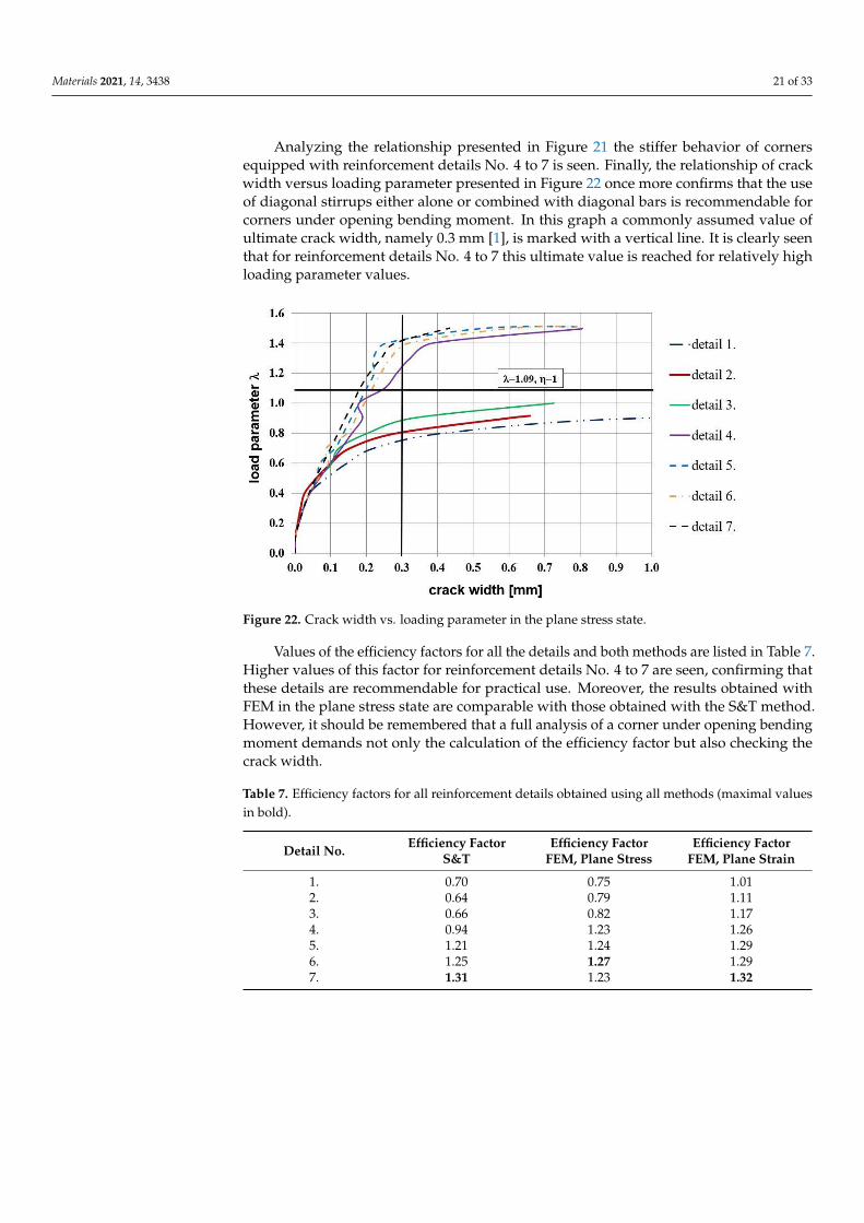
Materials 2021, 14, 3438 21 of 33
Analyzing the relationship presented in Figure 21 the stiffer behavior of cornersequipped with reinforcement details No. 4 to 7 is seen. Finally, the relationship of crackwidth versus loading parameter presented in Figure 22 once more confirms that the useof diagonal stirrups either alone or combined with diagonal bars is recommendable forcorners under opening bending moment. In this graph a commonly assumed value ofultimate crack width, namely 0.3 mm [1], is marked with a vertical line. It is clearly seenthat for reinforcement details No. 4 to 7 this ultimate value is reached for relatively highloading parameter values.
Materials 2021, 14, 3438 21 of 33
Figure 21. Nodal displacement vs. loading parameter in the plane stress state.
Figure 22. Crack width vs. loading parameter in the plane stress state.
Values of the efficiency factors for all the details and both methods are listed in Table
7. Higher values of this factor for reinforcement details No. 4 to 7 are seen, confirming that
these details are recommendable for practical use. Moreover, the results obtained with
FEM in the plane stress state are comparable with those obtained with the S&T method.
However, it should be remembered that a full analysis of a corner under opening bending
moment demands not only the calculation of the efficiency factor but also checking the
crack width.
Table 7. Efficiency factors for all reinforcement details obtained using all methods (maximal val-
ues in bold).
Detail No. Efficiency Factor
S&T
Efficiency Factor FEM,
Plane Stress
Efficiency Factor FEM,
Plane Strain
1. 0.70 0.75 1.01
2. 0.64 0.79 1.11
3. 0.66 0.82 1.17
Figure 22. Crack width vs. loading parameter in the plane stress state.
Values of the efficiency factors for all the details and both methods are listed in Table 7.Higher values of this factor for reinforcement details No. 4 to 7 are seen, confirming thatthese details are recommendable for practical use. Moreover, the results obtained withFEM in the plane stress state are comparable with those obtained with the S&T method.However, it should be remembered that a full analysis of a corner under opening bendingmoment demands not only the calculation of the efficiency factor but also checking thecrack width.
Table 7. Efficiency factors for all reinforcement details obtained using all methods (maximal valuesin bold).
Detail No. Efficiency FactorS&T
Efficiency FactorFEM, Plane Stress
Efficiency FactorFEM, Plane Strain
1. 0.70 0.75 1.012. 0.64 0.79 1.113. 0.66 0.82 1.174. 0.94 1.23 1.265. 1.21 1.24 1.296. 1.25 1.27 1.297. 1.31 1.23 1.32
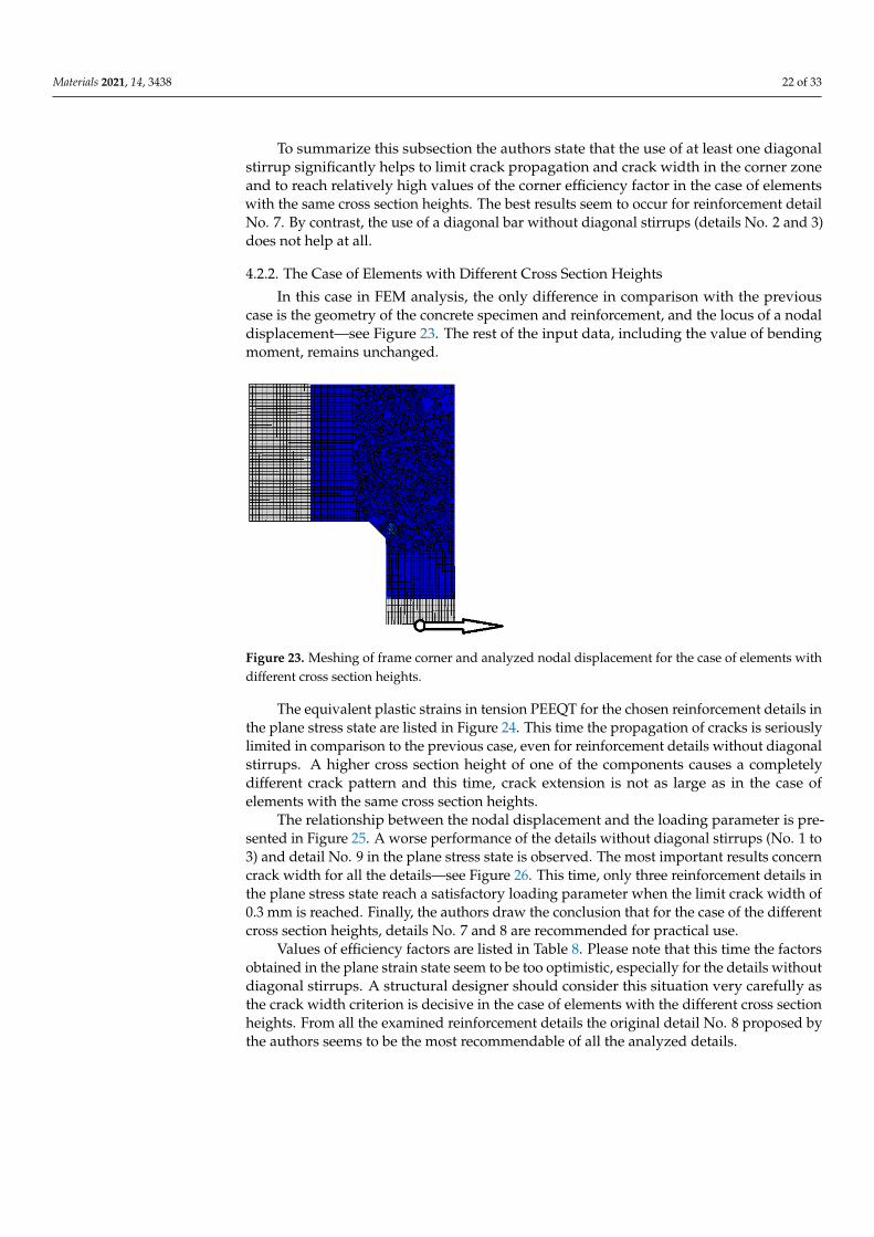
Materials 2021, 14, 3438 22 of 33
To summarize this subsection the authors state that the use of at least one diagonalstirrup significantly helps to limit crack propagation and crack width in the corner zoneand to reach relatively high values of the corner efficiency factor in the case of elementswith the same cross section heights. The best results seem to occur for reinforcement detailNo. 7. By contrast, the use of a diagonal bar without diagonal stirrups (details No. 2 and 3)does not help at all.
4.2.2. The Case of Elements with Different Cross Section Heights
In this case in FEM analysis, the only difference in comparison with the previouscase is the geometry of the concrete specimen and reinforcement, and the locus of a nodaldisplacement—see Figure 23. The rest of the input data, including the value of bendingmoment, remains unchanged.
Materials 2021, 14, 3438 22 of 33
4. 0.94 1.23 1.26
5. 1.21 1.24 1.29
6. 1.25 1.27 1.29
7. 1.31 1.23 1.32
To summarize this subsection the authors state that the use of at least one diagonal
stirrup significantly helps to limit crack propagation and crack width in the corner zone
and to reach relatively high values of the corner efficiency factor in the case of elements
with the same cross section heights. The best results seem to occur for reinforcement detail
No. 7. By contrast, the use of a diagonal bar without diagonal stirrups (details No. 2 and
3) does not help at all.
4.2.2. The Case of Elements with Different Cross Section Heights
In this case in FEM analysis, the only difference in comparison with the previous case
is the geometry of the concrete specimen and reinforcement, and the locus of a nodal dis-
placement—see Figure 23. The rest of the input data, including the value of bending mo-
ment, remains unchanged.
Figure 23. Meshing of frame corner and analyzed nodal displacement for the case of elements with
different cross section heights.
The equivalent plastic strains in tension PEEQT for the chosen reinforcement details
in the plane stress state are listed in Figure 24. This time the propagation of cracks is seri-
ously limited in comparison to the previous case, even for reinforcement details without
diagonal stirrups. A higher cross section height of one of the components causes a com-
pletely different crack pattern and this time, crack extension is not as large as in the case
of elements with the same cross section heights.
The relationship between the nodal displacement and the loading parameter is pre-
sented in Figure 25. A worse performance of the details without diagonal stirrups (No. 1
to 3) and detail No. 9 in the plane stress state is observed. The most important results
concern crack width for all the details—see Figure 26. This time, only three reinforcement
details in the plane stress state reach a satisfactory loading parameter when the limit crack
width of 0.3 mm is reached. Finally, the authors draw the conclusion that for the case of
the different cross section heights, details No. 7 and 8 are recommended for practical use.
Figure 23. Meshing of frame corner and analyzed nodal displacement for the case of elements withdifferent cross section heights.
The equivalent plastic strains in tension PEEQT for the chosen reinforcement details inthe plane stress state are listed in Figure 24. This time the propagation of cracks is seriouslylimited in comparison to the previous case, even for reinforcement details without diagonalstirrups. A higher cross section height of one of the components causes a completelydifferent crack pattern and this time, crack extension is not as large as in the case ofelements with the same cross section heights.
The relationship between the nodal displacement and the loading parameter is pre-sented in Figure 25. A worse performance of the details without diagonal stirrups (No. 1 to3) and detail No. 9 in the plane stress state is observed. The most important results concerncrack width for all the details—see Figure 26. This time, only three reinforcement details inthe plane stress state reach a satisfactory loading parameter when the limit crack width of0.3 mm is reached. Finally, the authors draw the conclusion that for the case of the differentcross section heights, details No. 7 and 8 are recommended for practical use.
Values of efficiency factors are listed in Table 8. Please note that this time the factorsobtained in the plane strain state seem to be too optimistic, especially for the details withoutdiagonal stirrups. A structural designer should consider this situation very carefully asthe crack width criterion is decisive in the case of elements with the different cross sectionheights. From all the examined reinforcement details the original detail No. 8 proposed bythe authors seems to be the most recommendable of all the analyzed details.
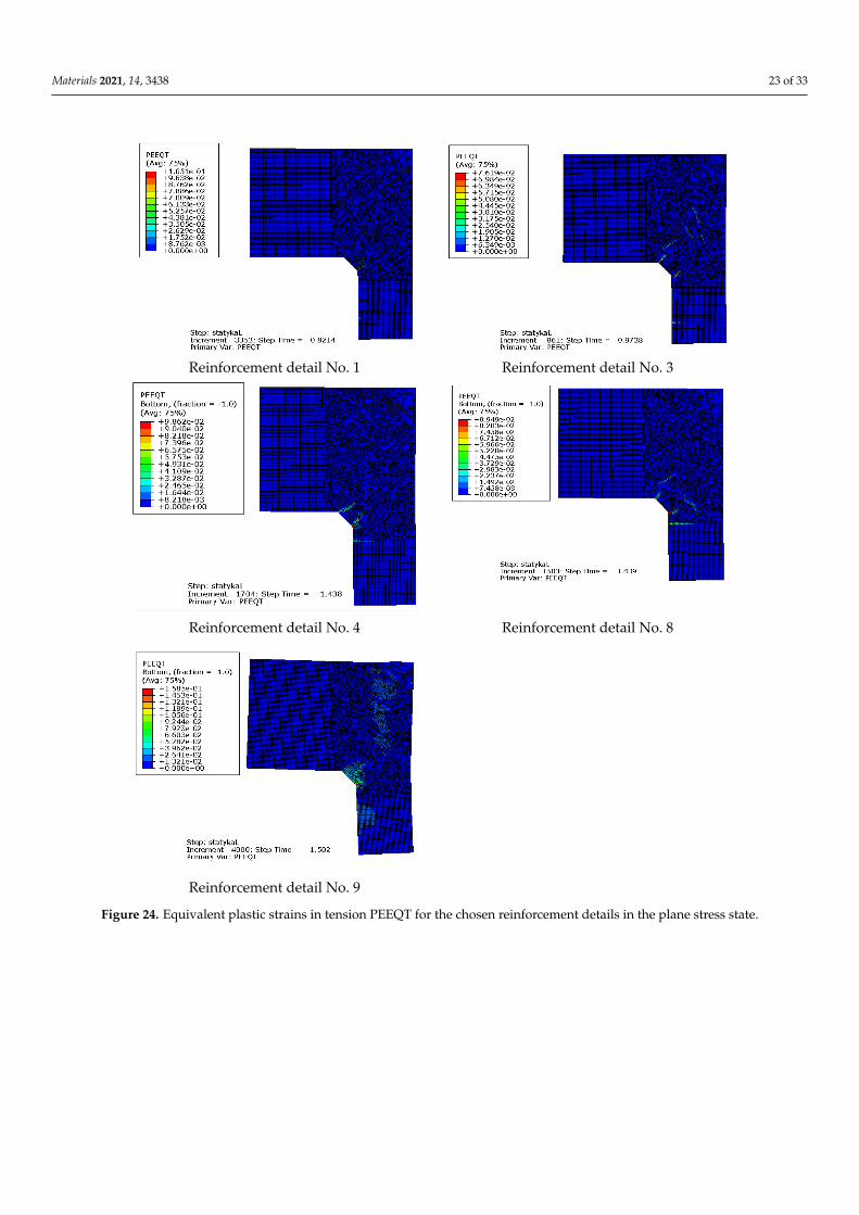
Materials 2021, 14, 3438 23 of 33Materials 2021, 14, 3438 23 of 33
Reinforcement detail No. 1 Reinforcement detail No. 3
Reinforcement detail No. 4 Reinforcement detail No. 8
Reinforcement detail No. 9
Figure 24. Equivalent plastic strains in tension PEEQT for the chosen reinforcement details in the plane stress state.
Values of efficiency factors are listed in Table 8. Please note that this time the factors
obtained in the plane strain state seem to be too optimistic, especially for the details with-
out diagonal stirrups. A structural designer should consider this situation very carefully
as the crack width criterion is decisive in the case of elements with the different cross
section heights. From all the examined reinforcement details the original detail No. 8 pro-
posed by the authors seems to be the most recommendable of all the analyzed details.
Figure 24. Equivalent plastic strains in tension PEEQT for the chosen reinforcement details in the plane stress state.

Materials 2021, 14, 3438 24 of 33Materials 2021, 14, 3438 24 of 33
Figure 25. Nodal displacement vs. loading parameter in the plane stress state.
Figure 26. Crack width vs. loading parameter in the plane stress state.
Table 8. Efficiency factors for all reinforcement details obtained using all methods (maximal val-
ues in bold).
Detail No. Efficiency Factor S&T Efficiency Factor FEM,
Plane Stress
Efficiency Factor FEM,
Plane Strain
1. 0.61 0.75 1.31
2. 0.58 0.78 1.36
3. 0.60 0.89 1.43
4. 1.44 1.32 1.40
5. 1.23 1.57 1.40
6. 1.15 1.34 1.38
7. 1.17 1.54 1.51
8. 1.07 1.32 1.52
9. 0.88 1.38 1.44
Figure 25. Nodal displacement vs. loading parameter in the plane stress state.
Materials 2021, 14, 3438 24 of 33
Figure 25. Nodal displacement vs. loading parameter in the plane stress state.
Figure 26. Crack width vs. loading parameter in the plane stress state.
Table 8. Efficiency factors for all reinforcement details obtained using all methods (maximal val-
ues in bold).
Detail No. Efficiency Factor S&T Efficiency Factor FEM,
Plane Stress
Efficiency Factor FEM,
Plane Strain
1. 0.61 0.75 1.31
2. 0.58 0.78 1.36
3. 0.60 0.89 1.43
4. 1.44 1.32 1.40
5. 1.23 1.57 1.40
6. 1.15 1.34 1.38
7. 1.17 1.54 1.51
8. 1.07 1.32 1.52
9. 0.88 1.38 1.44
Figure 26. Crack width vs. loading parameter in the plane stress state.
Table 8. Efficiency factors for all reinforcement details obtained using all methods (maximal valuesin bold).
Detail No. Efficiency FactorS&T
Efficiency FactorFEM, Plane Stress
Efficiency FactorFEM, Plane Strain
1. 0.61 0.75 1.312. 0.58 0.78 1.363. 0.60 0.89 1.434. 1.44 1.32 1.405. 1.23 1.57 1.406. 1.15 1.34 1.387. 1.17 1.54 1.518. 1.07 1.32 1.529. 0.88 1.38 1.44
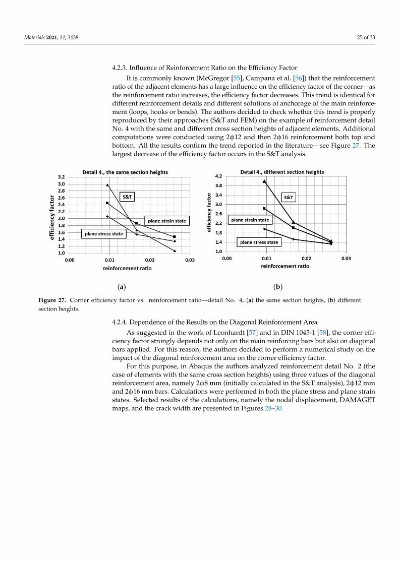
Materials 2021, 14, 3438 25 of 33
4.2.3. Influence of Reinforcement Ratio on the Efficiency Factor
It is commonly known (McGregor [55], Campana et al. [56]) that the reinforcementratio of the adjacent elements has a large influence on the efficiency factor of the corner—asthe reinforcement ratio increases, the efficiency factor decreases. This trend is identical fordifferent reinforcement details and different solutions of anchorage of the main reinforce-ment (loops, hooks or bends). The authors decided to check whether this trend is properlyreproduced by their approaches (S&T and FEM) on the example of reinforcement detailNo. 4 with the same and different cross section heights of adjacent elements. Additionalcomputations were conducted using 2φ12 and then 2φ16 reinforcement both top andbottom. All the results confirm the trend reported in the literature—see Figure 27. Thelargest decrease of the efficiency factor occurs in the S&T analysis.
Materials 2021, 14, 3438 25 of 33
4.2.3. Influence of Reinforcement Ratio on the Efficiency Factor
It is commonly known (McGregor [55], Campana et al. [56]) that the reinforcement
ratio of the adjacent elements has a large influence on the efficiency factor of the corner—
as the reinforcement ratio increases, the efficiency factor decreases. This trend is identical
for different reinforcement details and different solutions of anchorage of the main rein-
forcement (loops, hooks or bends). The authors decided to check whether this trend is
properly reproduced by their approaches (S&T and FEM) on the example of reinforcement
detail No. 4 with the same and different cross section heights of adjacent elements. Addi-
tional computations were conducted using 2ϕ12 and then 2ϕ16 reinforcement both top
and bottom. All the results confirm the trend reported in the literature—see Figure 27. The
largest decrease of the efficiency factor occurs in the S&T analysis.
(a) (b)
Figure 27. Corner efficiency factor vs. reinforcement ratio—detail No. 4, (a) the same section heights, (b) different section
heights.
4.2.4. Dependence of the Results on the Diagonal Reinforcement Area
As suggested in the work of Leonhardt [57] and in DIN 1045-1 [58], the corner effi-
ciency factor strongly depends not only on the main reinforcing bars but also on diagonal
bars applied. For this reason, the authors decided to perform a numerical study on the
impact of the diagonal reinforcement area on the corner efficiency factor.
For this purpose, in Abaqus the authors analyzed reinforcement detail No. 2 (the case
of elements with the same cross section heights) using three values of the diagonal rein-
forcement area, namely 2ϕ8 mm (initially calculated in the S&T analysis), 2ϕ12 mm and
2ϕ16 mm bars. Calculations were performed in both the plane stress and plane strain
states. Selected results of the calculations, namely the nodal displacement, DAMAGET
maps, and the crack width are presented in Figures 28–30.
Figure 27. Corner efficiency factor vs. reinforcement ratio—detail No. 4, (a) the same section heights, (b) differentsection heights.
4.2.4. Dependence of the Results on the Diagonal Reinforcement Area
As suggested in the work of Leonhardt [57] and in DIN 1045-1 [58], the corner effi-ciency factor strongly depends not only on the main reinforcing bars but also on diagonalbars applied. For this reason, the authors decided to perform a numerical study on theimpact of the diagonal reinforcement area on the corner efficiency factor.
For this purpose, in Abaqus the authors analyzed reinforcement detail No. 2 (thecase of elements with the same cross section heights) using three values of the diagonalreinforcement area, namely 2φ8 mm (initially calculated in the S&T analysis), 2φ12 mmand 2φ16 mm bars. Calculations were performed in both the plane stress and plane strainstates. Selected results of the calculations, namely the nodal displacement, DAMAGETmaps, and the crack width are presented in Figures 28–30.
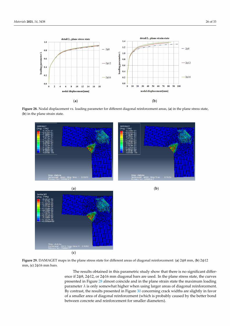
Materials 2021, 14, 3438 26 of 33Materials 2021, 14, 3438 26 of 33
(a) (b)
Figure 28. Nodal displacement vs. loading parameter for different diagonal reinforcement areas, (a) in the plane stress
state, (b) in the plane strain state.
(a) (b)
(c)
Figure 29. DAMAGET maps in the plane stress state for different areas of diagonal reinforcement: (a) 2ϕ8 mm, (b) 2ϕ12
mm, (c) 2ϕ16 mm bars.
The results obtained in this parametric study show that there is no significant differ-
ence if 2ϕ8, 2ϕ12, or 2ϕ16 mm diagonal bars are used. In the plane stress state, the curves
presented in Figure 28 almost coincide and in the plane strain state the maximum loading
parameter λ is only somewhat higher when using larger areas of diagonal reinforcement.
By contrast, the results presented in Figure 30 concerning crack widths are slightly in favor
of a smaller area of diagonal reinforcement (which is probably caused by the better bond
between concrete and reinforcement for smaller diameters).
Figure 28. Nodal displacement vs. loading parameter for different diagonal reinforcement areas, (a) in the plane stress state,(b) in the plane strain state.
Materials 2021, 14, 3438 26 of 33
(a) (b)
Figure 28. Nodal displacement vs. loading parameter for different diagonal reinforcement areas, (a) in the plane stress
state, (b) in the plane strain state.
(a) (b)
(c)
Figure 29. DAMAGET maps in the plane stress state for different areas of diagonal reinforcement: (a) 2ϕ8 mm, (b) 2ϕ12
mm, (c) 2ϕ16 mm bars.
The results obtained in this parametric study show that there is no significant differ-
ence if 2ϕ8, 2ϕ12, or 2ϕ16 mm diagonal bars are used. In the plane stress state, the curves
presented in Figure 28 almost coincide and in the plane strain state the maximum loading
parameter λ is only somewhat higher when using larger areas of diagonal reinforcement.
By contrast, the results presented in Figure 30 concerning crack widths are slightly in favor
of a smaller area of diagonal reinforcement (which is probably caused by the better bond
between concrete and reinforcement for smaller diameters).
Figure 29. DAMAGET maps in the plane stress state for different areas of diagonal reinforcement: (a) 2φ8 mm, (b) 2φ12mm, (c) 2φ16 mm bars.
The results obtained in this parametric study show that there is no significant differ-ence if 2φ8, 2φ12, or 2φ16 mm diagonal bars are used. In the plane stress state, the curvespresented in Figure 28 almost coincide and in the plane strain state the maximum loadingparameter λ is only somewhat higher when using larger areas of diagonal reinforcement.By contrast, the results presented in Figure 30 concerning crack widths are slightly in favorof a smaller area of diagonal reinforcement (which is probably caused by the better bondbetween concrete and reinforcement for smaller diameters).
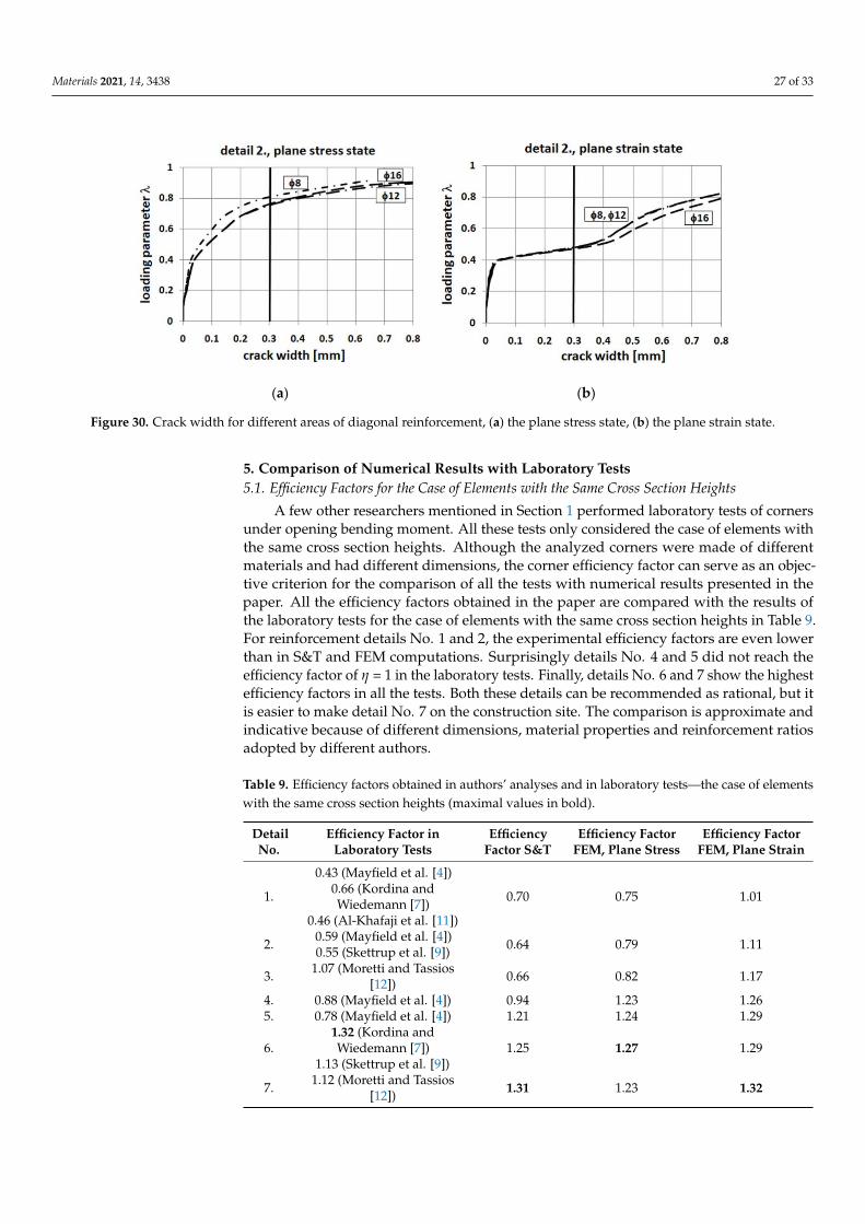
Materials 2021, 14, 3438 27 of 33Materials 2021, 14, 3438 27 of 33
(a) (b)
Figure 30. Crack width for different areas of diagonal reinforcement, (a) the plane stress state, (b) the plane strain state.
5. Comparison of Numerical Results with Laboratory Tests
5.1. Efficiency Factors for the Case of Elements with the Same Cross Section Heights
A few other researchers mentioned in Section 1 performed laboratory tests of corners
under opening bending moment. All these tests only considered the case of elements with
the same cross section heights. Although the analyzed corners were made of different ma-
terials and had different dimensions, the corner efficiency factor can serve as an objective
criterion for the comparison of all the tests with numerical results presented in the paper.
All the efficiency factors obtained in the paper are compared with the results of the labor-
atory tests for the case of elements with the same cross section heights in Table 9. For
reinforcement details No. 1 and 2, the experimental efficiency factors are even lower than
in S&T and FEM computations. Surprisingly details No. 4 and 5 did not reach the effi-
ciency factor of η = 1 in the laboratory tests. Finally, details No. 6 and 7 show the highest
efficiency factors in all the tests. Both these details can be recommended as rational, but it
is easier to make detail No. 7 on the construction site. The comparison is approximate and
indicative because of different dimensions, material properties and reinforcement ratios
adopted by different authors.
Table 9. Efficiency factors obtained in authors’ analyses and in laboratory tests—the case of ele-
ments with the same cross section heights (maximal values in bold).
Detail
No.
Efficiency Factor in Laboratory
Tests
Efficiency
Factor S&T
Efficiency Factor
FEM, Plane Stress
Efficiency Factor
FEM, Plane Strain
1.
0.43 (Mayfield et al. [4])
0.66 (Kordina and Wiedemann [7])
0.46 (Al-Khafaji et al. [11])
0.70 0.75 1.01
2. 0.59 (Mayfield et al. [4])
0.55 (Skettrup et al. [9]) 0.64 0.79 1.11
3. 1.07 (Moretti and Tassios [12]) 0.66 0.82 1.17
4. 0.88 (Mayfield et al. [4]) 0.94 1.23 1.26
5. 0.78 (Mayfield et al. [4]) 1.21 1.24 1.29
6. 1.32 (Kordina and Wiedemann [7])
1.13 (Skettrup et al. [9]) 1.25 1.27 1.29
7. 1.12 (Moretti and Tassios [12]) 1.31 1.23 1.32
5.2. Comparison with Johansson’s Laboratory Tests
Johansson [13] performed laboratory tests on RC frame corners under closing and
opening bending moment. The authors numerically recreated a laboratory test of the spec-
imen marked RV9 in Johansson’s research. A displacement control was applied with a
Figure 30. Crack width for different areas of diagonal reinforcement, (a) the plane stress state, (b) the plane strain state.
5. Comparison of Numerical Results with Laboratory Tests5.1. Efficiency Factors for the Case of Elements with the Same Cross Section Heights
A few other researchers mentioned in Section 1 performed laboratory tests of cornersunder opening bending moment. All these tests only considered the case of elements withthe same cross section heights. Although the analyzed corners were made of differentmaterials and had different dimensions, the corner efficiency factor can serve as an objec-tive criterion for the comparison of all the tests with numerical results presented in thepaper. All the efficiency factors obtained in the paper are compared with the results ofthe laboratory tests for the case of elements with the same cross section heights in Table 9.For reinforcement details No. 1 and 2, the experimental efficiency factors are even lowerthan in S&T and FEM computations. Surprisingly details No. 4 and 5 did not reach theefficiency factor of η = 1 in the laboratory tests. Finally, details No. 6 and 7 show the highestefficiency factors in all the tests. Both these details can be recommended as rational, but itis easier to make detail No. 7 on the construction site. The comparison is approximate andindicative because of different dimensions, material properties and reinforcement ratiosadopted by different authors.
Table 9. Efficiency factors obtained in authors’ analyses and in laboratory tests—the case of elementswith the same cross section heights (maximal values in bold).
DetailNo.
Efficiency Factor inLaboratory Tests
EfficiencyFactor S&T
Efficiency FactorFEM, Plane Stress
Efficiency FactorFEM, Plane Strain
1.
0.43 (Mayfield et al. [4])0.66 (Kordina andWiedemann [7])
0.46 (Al-Khafaji et al. [11])
0.70 0.75 1.01
2. 0.59 (Mayfield et al. [4])0.55 (Skettrup et al. [9]) 0.64 0.79 1.11
3. 1.07 (Moretti and Tassios[12]) 0.66 0.82 1.17
4. 0.88 (Mayfield et al. [4]) 0.94 1.23 1.265. 0.78 (Mayfield et al. [4]) 1.21 1.24 1.29
6.1.32 (Kordina andWiedemann [7])
1.13 (Skettrup et al. [9])1.25 1.27 1.29
7. 1.12 (Moretti and Tassios[12]) 1.31 1.23 1.32
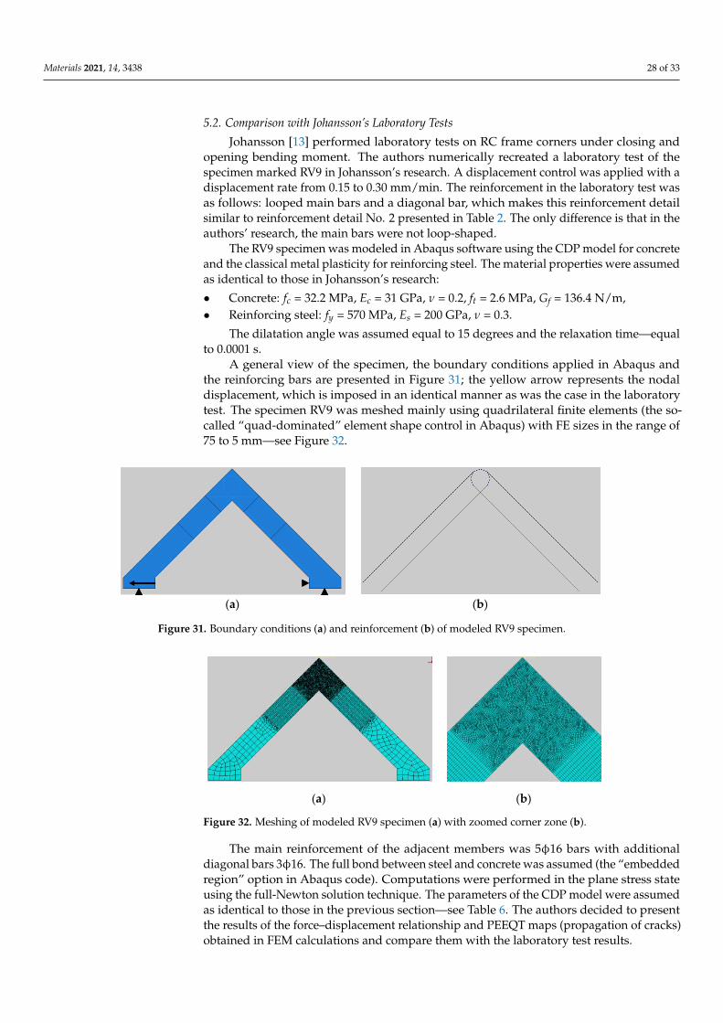
Materials 2021, 14, 3438 28 of 33
5.2. Comparison with Johansson’s Laboratory Tests
Johansson [13] performed laboratory tests on RC frame corners under closing andopening bending moment. The authors numerically recreated a laboratory test of thespecimen marked RV9 in Johansson’s research. A displacement control was applied with adisplacement rate from 0.15 to 0.30 mm/min. The reinforcement in the laboratory test wasas follows: looped main bars and a diagonal bar, which makes this reinforcement detailsimilar to reinforcement detail No. 2 presented in Table 2. The only difference is that in theauthors’ research, the main bars were not loop-shaped.
The RV9 specimen was modeled in Abaqus software using the CDP model for concreteand the classical metal plasticity for reinforcing steel. The material properties were assumedas identical to those in Johansson’s research:
• Concrete: fc = 32.2 MPa, Ec = 31 GPa, ν = 0.2, ft = 2.6 MPa, Gf = 136.4 N/m,• Reinforcing steel: fy = 570 MPa, Es = 200 GPa, ν = 0.3.
The dilatation angle was assumed equal to 15 degrees and the relaxation time—equalto 0.0001 s.
A general view of the specimen, the boundary conditions applied in Abaqus andthe reinforcing bars are presented in Figure 31; the yellow arrow represents the nodaldisplacement, which is imposed in an identical manner as was the case in the laboratorytest. The specimen RV9 was meshed mainly using quadrilateral finite elements (the so-called “quad-dominated” element shape control in Abaqus) with FE sizes in the range of75 to 5 mm—see Figure 32.
Materials 2021, 14, 3438 28 of 33
displacement rate from 0.15 to 0.30 mm/min. The reinforcement in the laboratory test was
as follows: looped main bars and a diagonal bar, which makes this reinforcement detail
similar to reinforcement detail No. 2 presented in Table 2. The only difference is that in
the authors’ research, the main bars were not loop-shaped.
The RV9 specimen was modeled in Abaqus software using the CDP model for con-
crete and the classical metal plasticity for reinforcing steel. The material properties were
assumed as identical to those in Johansson’s research:
• Concrete: fc = 32.2 MPa, Ec = 31 GPa, ν = 0.2, ft = 2.6 MPa, Gf = 136.4 N/m,
• Reinforcing steel: fy = 570 MPa, Es = 200 GPa, ν = 0.3.
The dilatation angle was assumed equal to 15 degrees and the relaxation time—equal
to 0.0001 s.
A general view of the specimen, the boundary conditions applied in Abaqus and the
reinforcing bars are presented in Figure 31; the yellow arrow represents the nodal dis-
placement, which is imposed in an identical manner as was the case in the laboratory test.
The specimen RV9 was meshed mainly using quadrilateral finite elements (the so-called
“quad-dominated” element shape control in Abaqus) with FE sizes in the range of 75 to 5
mm—see Figure 32.
(a) (b)
Figure 31. Boundary conditions (a) and reinforcement (b) of modeled RV9 specimen.
(a) (b)
Figure 32. Meshing of modeled RV9 specimen (a) with zoomed corner zone (b).
The main reinforcement of the adjacent members was 5ϕ16 bars with additional di-
agonal bars 3ϕ16. The full bond between steel and concrete was assumed (the “embedded
region” option in Abaqus code). Computations were performed in the plane stress state
using the full-Newton solution technique. The parameters of the CDP model were as-
sumed as identical to those in the previous section—see Table 6. The authors decided to
present the results of the force–displacement relationship and PEEQT maps (propagation
of cracks) obtained in FEM calculations and compare them with the laboratory test results.
The relationship between the horizontal reaction force and the imposed displacement
is presented in Figure 33 and compared with the same relationship obtained in Johans-
son’s laboratory test (dashed line). Both curves appear to be similar whereas the curve
obtained in Abaqus has no peak and no descending part. Instead of this it has a clear
plateau similar to that presented in Figure 21. Moreover, the curve obtained in the FEM
Figure 31. Boundary conditions (a) and reinforcement (b) of modeled RV9 specimen.
Materials 2021, 14, 3438 28 of 33
displacement rate from 0.15 to 0.30 mm/min. The reinforcement in the laboratory test was
as follows: looped main bars and a diagonal bar, which makes this reinforcement detail
similar to reinforcement detail No. 2 presented in Table 2. The only difference is that in
the authors’ research, the main bars were not loop-shaped.
The RV9 specimen was modeled in Abaqus software using the CDP model for con-
crete and the classical metal plasticity for reinforcing steel. The material properties were
assumed as identical to those in Johansson’s research:
• Concrete: fc = 32.2 MPa, Ec = 31 GPa, ν = 0.2, ft = 2.6 MPa, Gf = 136.4 N/m,
• Reinforcing steel: fy = 570 MPa, Es = 200 GPa, ν = 0.3.
The dilatation angle was assumed equal to 15 degrees and the relaxation time—equal
to 0.0001 s.
A general view of the specimen, the boundary conditions applied in Abaqus and the
reinforcing bars are presented in Figure 31; the yellow arrow represents the nodal dis-
placement, which is imposed in an identical manner as was the case in the laboratory test.
The specimen RV9 was meshed mainly using quadrilateral finite elements (the so-called
“quad-dominated” element shape control in Abaqus) with FE sizes in the range of 75 to 5
mm—see Figure 32.
(a) (b)
Figure 31. Boundary conditions (a) and reinforcement (b) of modeled RV9 specimen.
(a) (b)
Figure 32. Meshing of modeled RV9 specimen (a) with zoomed corner zone (b).
The main reinforcement of the adjacent members was 5ϕ16 bars with additional di-
agonal bars 3ϕ16. The full bond between steel and concrete was assumed (the “embedded
region” option in Abaqus code). Computations were performed in the plane stress state
using the full-Newton solution technique. The parameters of the CDP model were as-
sumed as identical to those in the previous section—see Table 6. The authors decided to
present the results of the force–displacement relationship and PEEQT maps (propagation
of cracks) obtained in FEM calculations and compare them with the laboratory test results.
The relationship between the horizontal reaction force and the imposed displacement
is presented in Figure 33 and compared with the same relationship obtained in Johans-
son’s laboratory test (dashed line). Both curves appear to be similar whereas the curve
obtained in Abaqus has no peak and no descending part. Instead of this it has a clear
plateau similar to that presented in Figure 21. Moreover, the curve obtained in the FEM
Figure 32. Meshing of modeled RV9 specimen (a) with zoomed corner zone (b).
The main reinforcement of the adjacent members was 5φ16 bars with additionaldiagonal bars 3φ16. The full bond between steel and concrete was assumed (the “embeddedregion” option in Abaqus code). Computations were performed in the plane stress stateusing the full-Newton solution technique. The parameters of the CDP model were assumedas identical to those in the previous section—see Table 6. The authors decided to presentthe results of the force–displacement relationship and PEEQT maps (propagation of cracks)obtained in FEM calculations and compare them with the laboratory test results.
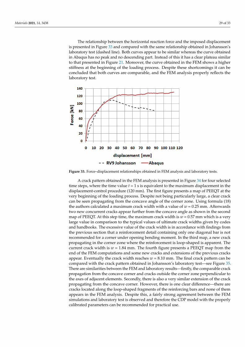
Materials 2021, 14, 3438 29 of 33
The relationship between the horizontal reaction force and the imposed displacementis presented in Figure 33 and compared with the same relationship obtained in Johansson’slaboratory test (dashed line). Both curves appear to be similar whereas the curve obtainedin Abaqus has no peak and no descending part. Instead of this it has a clear plateau similarto that presented in Figure 21. Moreover, the curve obtained in the FEM shows a higherstiffness at the beginning of the loading process. Despite these shortcomings it can beconcluded that both curves are comparable, and the FEM analysis properly reflects thelaboratory test.
Materials 2021, 14, 3438 29 of 33
shows a higher stiffness at the beginning of the loading process. Despite these shortcom-
ings it can be concluded that both curves are comparable, and the FEM analysis properly
reflects the laboratory test.
A crack pattern obtained in the FEM analysis is presented in Figure 34 for four se-
lected time steps, where the time value t = 1 s is equivalent to the maximum displacement
in the displacement-control procedure (120 mm). The first figure presents a map of PEEQT
at the very beginning of the loading process. Despite not being particularly large, a clear
crack can be seen propagating from the concave angle of the corner zone. Using formula
(18) the authors calculated a maximum crack width with a value of w = 0.25 mm. After-
wards two new concurrent cracks appear further from the concave angle as shown in the
second map of PEEQT. At this step time, the maximum crack width is w = 0.57 mm which
is a very large value in comparison to the typical values of ultimate crack widths given by
codes and handbooks. The excessive value of the crack width is in accordance with find-
ings from the previous section that a reinforcement detail containing only one diagonal
bar is not recommended for a corner under opening bending moment. In the third map, a
new crack propagating in the corner zone where the reinforcement is loop-shaped is ap-
parent. The current crack width is w = 1.84 mm. The fourth figure presents a PEEQT map
from the end of the FEM computations and some new cracks and extensions of the previ-
ous cracks appear. Eventually the crack width reaches w = 8.10 mm. The final crack pattern
can be compared with the crack pattern obtained in Johansson’s laboratory test—see Fig-
ure 35. There are similarities between the FEM and laboratory results—firstly, the compa-
rable crack propagation from the concave corner and cracks outside the corner zone per-
pendicular to the axes of adjacent elements. Secondly, there is also a very similar extension
of the crack propagating from the concave corner. However, there is one clear difference—
there are cracks located along the loop-shaped fragments of the reinforcing bars and none
of them appears in the FEM analysis. Despite this, a fairly strong agreement between the
FEM simulations and laboratory test is observed and therefore the CDP model with the
properly calibrated parameters can be recommended for practical use.
Figure 33. Force–displacement relationships obtained in FEM analysis and laboratory tests. Figure 33. Force–displacement relationships obtained in FEM analysis and laboratory tests.
A crack pattern obtained in the FEM analysis is presented in Figure 34 for four selectedtime steps, where the time value t = 1 s is equivalent to the maximum displacement in thedisplacement-control procedure (120 mm). The first figure presents a map of PEEQT at thevery beginning of the loading process. Despite not being particularly large, a clear crackcan be seen propagating from the concave angle of the corner zone. Using formula (18)the authors calculated a maximum crack width with a value of w = 0.25 mm. Afterwardstwo new concurrent cracks appear further from the concave angle as shown in the secondmap of PEEQT. At this step time, the maximum crack width is w = 0.57 mm which is a verylarge value in comparison to the typical values of ultimate crack widths given by codesand handbooks. The excessive value of the crack width is in accordance with findings fromthe previous section that a reinforcement detail containing only one diagonal bar is notrecommended for a corner under opening bending moment. In the third map, a new crackpropagating in the corner zone where the reinforcement is loop-shaped is apparent. Thecurrent crack width is w = 1.84 mm. The fourth figure presents a PEEQT map from theend of the FEM computations and some new cracks and extensions of the previous cracksappear. Eventually the crack width reaches w = 8.10 mm. The final crack pattern can becompared with the crack pattern obtained in Johansson’s laboratory test—see Figure 35.There are similarities between the FEM and laboratory results—firstly, the comparable crackpropagation from the concave corner and cracks outside the corner zone perpendicular tothe axes of adjacent elements. Secondly, there is also a very similar extension of the crackpropagating from the concave corner. However, there is one clear difference—there arecracks located along the loop-shaped fragments of the reinforcing bars and none of themappears in the FEM analysis. Despite this, a fairly strong agreement between the FEMsimulations and laboratory test is observed and therefore the CDP model with the properlycalibrated parameters can be recommended for practical use.

Materials 2021, 14, 3438 30 of 33Materials 2021, 14, 3438 30 of 33
(a) (b)
(c) (d)
Figure 34. (a–d) PEEQT maps in FEM analysis in four selected time steps.
Figure 35. A sketch of the crack pattern obtained in Johansson’s laboratory tests (reprinted with
permission from Johansson [13], Copyright 2000, M. Johansson).
6. Conclusions
A combination of S&T and FEM computations was carried out to find the most ra-
tional reinforcement detail for frame corners under opening bending moment. The fol-
lowing conclusions can be drawn:
(1) It is possible to choose a rational reinforcement detail for a corner under opening
moment even in the case of elements with different cross section heights using a com-
bination of the S&T method and FEM.
(2) The most recommendable details are detail No. 7 in the case of elements with the
same cross section heights (see Table 2) and details No. 7 and 8 in the case of elements
with different cross section heights (see Table 2).
(3) There are no significant differences in the obtained results when applying the differ-
ent areas of the diagonal bars (2ϕ8, 2ϕ12 or 2ϕ16 mm).
(4) The use of diagonal bars only is insufficient to obtain a satisfactory efficiency factor
and a limited crack width; these goals can only be achieved by using diagonal stir-
rups.
Figure 34. (a–d) PEEQT maps in FEM analysis in four selected time steps.
Materials 2021, 14, 3438 30 of 33
(a) (b)
(c) (d)
Figure 34. (a–d) PEEQT maps in FEM analysis in four selected time steps.
Figure 35. A sketch of the crack pattern obtained in Johansson’s laboratory tests (reprinted with
permission from Johansson [13], Copyright 2000, M. Johansson).
6. Conclusions
A combination of S&T and FEM computations was carried out to find the most ra-
tional reinforcement detail for frame corners under opening bending moment. The fol-
lowing conclusions can be drawn:
(1) It is possible to choose a rational reinforcement detail for a corner under opening
moment even in the case of elements with different cross section heights using a com-
bination of the S&T method and FEM.
(2) The most recommendable details are detail No. 7 in the case of elements with the
same cross section heights (see Table 2) and details No. 7 and 8 in the case of elements
with different cross section heights (see Table 2).
(3) There are no significant differences in the obtained results when applying the differ-
ent areas of the diagonal bars (2ϕ8, 2ϕ12 or 2ϕ16 mm).
(4) The use of diagonal bars only is insufficient to obtain a satisfactory efficiency factor
and a limited crack width; these goals can only be achieved by using diagonal stir-
rups.
Figure 35. A sketch of the crack pattern obtained in Johansson’s laboratory tests (reprinted withpermission from Johansson [13], Copyright 2000, M. Johansson).
6. Conclusions
A combination of S&T and FEM computations was carried out to find the most rationalreinforcement detail for frame corners under opening bending moment. The followingconclusions can be drawn:
(1) It is possible to choose a rational reinforcement detail for a corner under openingmoment even in the case of elements with different cross section heights using acombination of the S&T method and FEM.
(2) The most recommendable details are detail No. 7 in the case of elements with thesame cross section heights (see Table 2) and details No. 7 and 8 in the case of elementswith different cross section heights (see Table 2).
(3) There are no significant differences in the obtained results when applying the differentareas of the diagonal bars (2φ8, 2φ12 or 2φ16 mm).
(4) The use of diagonal bars only is insufficient to obtain a satisfactory efficiency factorand a limited crack width; these goals can only be achieved by using diagonal stirrups.
(5) The reinforcement ratio of the adjacent elements has a large influence on the efficiencyfactor of the corner, namely an increase in the reinforcement ratio causes a decrease inthe efficiency factor.
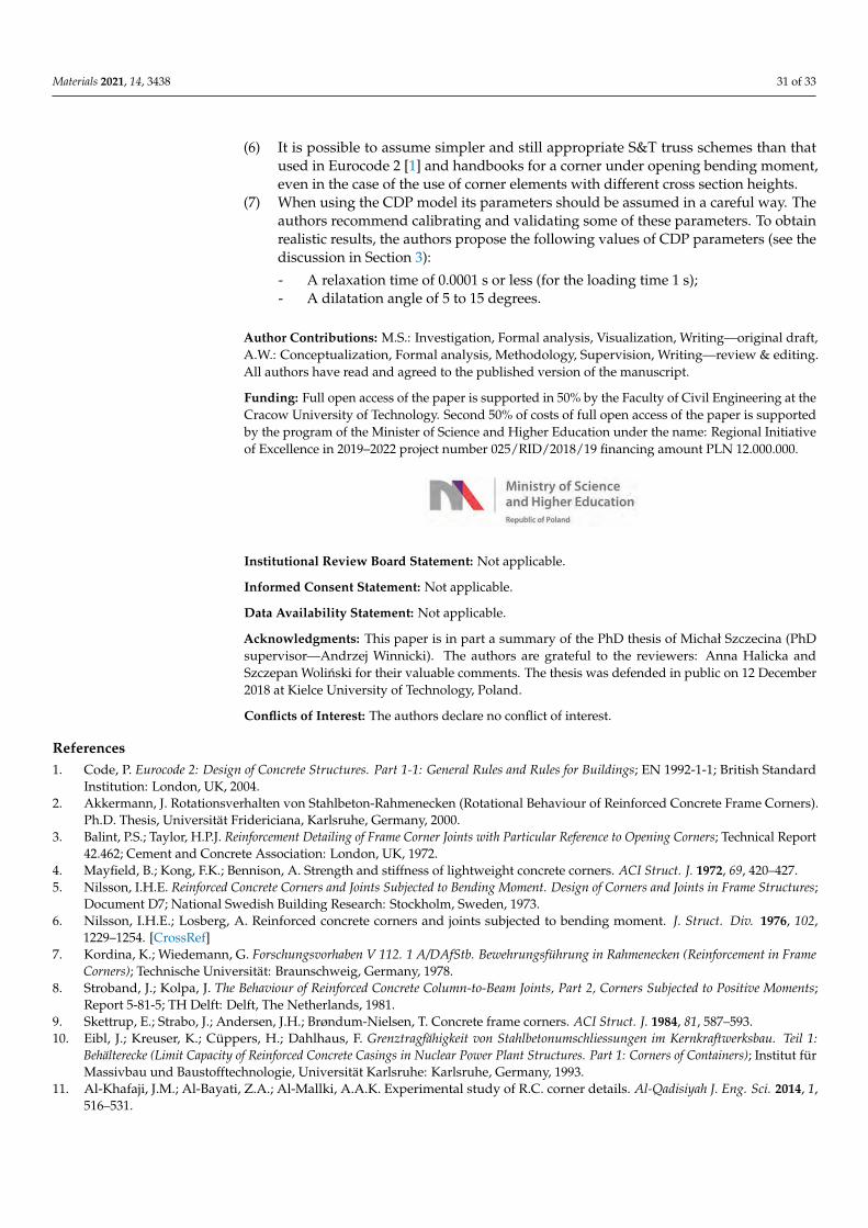
Materials 2021, 14, 3438 31 of 33
(6) It is possible to assume simpler and still appropriate S&T truss schemes than thatused in Eurocode 2 [1] and handbooks for a corner under opening bending moment,even in the case of the use of corner elements with different cross section heights.
(7) When using the CDP model its parameters should be assumed in a careful way. Theauthors recommend calibrating and validating some of these parameters. To obtainrealistic results, the authors propose the following values of CDP parameters (see thediscussion in Section 3):
- A relaxation time of 0.0001 s or less (for the loading time 1 s);- A dilatation angle of 5 to 15 degrees.
Author Contributions: M.S.: Investigation, Formal analysis, Visualization, Writing—original draft,A.W.: Conceptualization, Formal analysis, Methodology, Supervision, Writing—review & editing.All authors have read and agreed to the published version of the manuscript.
Funding: Full open access of the paper is supported in 50% by the Faculty of Civil Engineering at theCracow University of Technology. Second 50% of costs of full open access of the paper is supportedby the program of the Minister of Science and Higher Education under the name: Regional Initiativeof Excellence in 2019–2022 project number 025/RID/2018/19 financing amount PLN 12.000.000.
Materials 2021, 14, 3438 31 of 33
(5) The reinforcement ratio of the adjacent elements has a large influence on the effi-ciency factor of the corner, namely an increase in the reinforcement ratio causes a decrease in the efficiency factor.
(6) It is possible to assume simpler and still appropriate S&T truss schemes than that used in Eurocode 2 [1] and handbooks for a corner under opening bending moment, even in the case of the use of corner elements with different cross section heights.
(7) When using the CDP model its parameters should be assumed in a careful way. The authors recommend calibrating and validating some of these parameters. To obtain realistic results, the authors propose the following values of CDP parameters (see the discussion in Section 3): - A relaxation time of 0.0001 s or less (for the loading time 1 s); - A dilatation angle of 5 to 15 degrees.
Author Contributions: M.S.: Investigation, Formal analysis, Visualization, Writing—original draft, A.W.: Conceptualization, Formal analysis, Methodology, Supervision, Writing—review & editing. All authors have read and agreed to the published version of the manuscript.
Funding: Full open access of the paper is supported in 50% by the Faculty of Civil Engineering at the Cracow University of Technology. Second 50% of costs of full open access of the paper is sup-ported by the program of the Minister of Science and Higher Education under the name: Regional Initiative of Excellence in 2019–2022 project number 025/RID/2018/19 financing amount PLN 12.000.000.
Institutional Review Board Statement: Not applicable.
Informed Consent Statement: Not applicable.
Data Availability Statement: Not applicable.
Acknowledgments: This paper is in part a summary of the PhD thesis of Michał Szczecina (PhD supervisor—Andrzej Winnicki). The authors are grateful to the reviewers: Anna Halicka and Szcze-pan Woliński for their valuable comments. The thesis was defended in public on 12 December 2018 at Kielce University of Technology, Poland.
Conflicts of Interest: The authors declare no conflict of interest.
References 1. Code P. Eurocode 2: Design of Concrete Structures. Part 1-1: General Rules and Rules for Buildings; EN 1992-1-1; British Standard
Institution: London, UK, 2004. 2. Akkermann, J. Rotationsverhalten von Stahlbeton-Rahmenecken (Rotational Behaviour of Reinforced Concrete Frame Corners).
Ph.D. Thesis, Universität Fridericiana, Karlsruhe, Germany, 2000. 3. Balint, P.S.; Taylor, H.P.J. Reinforcement Detailing of Frame Corner Joints with Particular Reference to Opening Corners; Technical
Report 42.462; Cement and Concrete Association: London, UK, 1972. 4. Mayfield, B.; Kong, F.K., Bennison, A. Strength and stiffness of lightweight concrete corners. ACI Struct. J. 1972, 69, 420–427. 5. Nilsson, I.H.E. Reinforced Concrete Corners and Joints Subjected to Bending Moment. Design of Corners and Joints in Frame Structures;
Document D7; National Swedish Building Research: Stockholm, Sweden, 1973. 6. Nilsson, I.H.E.; Losberg, A. Reinforced concrete corners and joints subjected to bending moment. J. Struct. Div. 1976, 102, 1229–
1254. 7. Kordina, K.; Wiedemann, G. Forschungsvorhaben V 112. 1 A/DAfStb. Bewehrungsführung in Rahmenecken (Reinforcement in Frame
Corners); Technische Universität: Braunschweig, Germany, 1978. 8. Stroband, J.; Kolpa, J. The Behaviour of Reinforced Concrete Column-to-Beam Joints, Part 2, Corners Subjected to Positive Moments;
Report 5-81-5; TH Delft: Delft, The Netherlands, 1981. 9. Skettrup, E.; Strabo, J.; Andersen, J.H.; Brøndum-Nielsen, T. Concrete frame corners. ACI Struct. J. 1984, 81, 587–593. 10. Eibl, J.; Kreuser, K.; Cüppers, H.; Dahlhaus, F. Grenztragfähigkeit von Stahlbetonumschliessungen im Kernkraftwerksbau. Teil 1: Behäl-
terecke (Limit Capacity of Reinforced Concrete Casings in Nuclear Power Plant Structures. Part 1: Corners of Containers); Institut für Massivbau und Baustofftechnologie, Universität Karlsruhe: Karlsruhe, Germany, 1993.
Institutional Review Board Statement: Not applicable.
Informed Consent Statement: Not applicable.
Data Availability Statement: Not applicable.
Acknowledgments: This paper is in part a summary of the PhD thesis of Michał Szczecina (PhDsupervisor—Andrzej Winnicki). The authors are grateful to the reviewers: Anna Halicka andSzczepan Wolinski for their valuable comments. The thesis was defended in public on 12 December2018 at Kielce University of Technology, Poland.
Conflicts of Interest: The authors declare no conflict of interest.
References1. Code, P. Eurocode 2: Design of Concrete Structures. Part 1-1: General Rules and Rules for Buildings; EN 1992-1-1; British Standard
Institution: London, UK, 2004.2. Akkermann, J. Rotationsverhalten von Stahlbeton-Rahmenecken (Rotational Behaviour of Reinforced Concrete Frame Corners).
Ph.D. Thesis, Universität Fridericiana, Karlsruhe, Germany, 2000.3. Balint, P.S.; Taylor, H.P.J. Reinforcement Detailing of Frame Corner Joints with Particular Reference to Opening Corners; Technical Report
42.462; Cement and Concrete Association: London, UK, 1972.4. Mayfield, B.; Kong, F.K.; Bennison, A. Strength and stiffness of lightweight concrete corners. ACI Struct. J. 1972, 69, 420–427.5. Nilsson, I.H.E. Reinforced Concrete Corners and Joints Subjected to Bending Moment. Design of Corners and Joints in Frame Structures;
Document D7; National Swedish Building Research: Stockholm, Sweden, 1973.6. Nilsson, I.H.E.; Losberg, A. Reinforced concrete corners and joints subjected to bending moment. J. Struct. Div. 1976, 102,
1229–1254. [CrossRef]7. Kordina, K.; Wiedemann, G. Forschungsvorhaben V 112. 1 A/DAfStb. Bewehrungsführung in Rahmenecken (Reinforcement in Frame
Corners); Technische Universität: Braunschweig, Germany, 1978.8. Stroband, J.; Kolpa, J. The Behaviour of Reinforced Concrete Column-to-Beam Joints, Part 2, Corners Subjected to Positive Moments;
Report 5-81-5; TH Delft: Delft, The Netherlands, 1981.9. Skettrup, E.; Strabo, J.; Andersen, J.H.; Brøndum-Nielsen, T. Concrete frame corners. ACI Struct. J. 1984, 81, 587–593.10. Eibl, J.; Kreuser, K.; Cüppers, H.; Dahlhaus, F. Grenztragfähigkeit von Stahlbetonumschliessungen im Kernkraftwerksbau. Teil 1:
Behälterecke (Limit Capacity of Reinforced Concrete Casings in Nuclear Power Plant Structures. Part 1: Corners of Containers); Institut fürMassivbau und Baustofftechnologie, Universität Karlsruhe: Karlsruhe, Germany, 1993.
11. Al-Khafaji, J.M.; Al-Bayati, Z.A.; Al-Mallki, A.A.K. Experimental study of R.C. corner details. Al-Qadisiyah J. Eng. Sci. 2014, 1,516–531.
Materials 2021, 14, 3438 32 of 33
12. Moretti, M.; Tassios, T.P. Detailing of corner joints under opening moment. In Proceedings of the fib Symposium, Prague, CzechRepublic, 8–10 June 2011.
13. Johansson, M. Structural Behaviour in Concrete Frame Corners of Civil Defence Shelters: Non-linear Finite Element Analysesand Experiments. Ph.D. Thesis, Chalmers University of Technology, Göteborg, Sweden, 2000.
14. Starosolski, W. Konstrukcje Zelbetowe wg PN-B-03264:2002 i Eurokodu 2. Tom III (Concrete Structures According to PN-B-0324:2002 andEurocode 2. Volume 3); Wydawnictwo Naukowe PWN: Warsaw, Poland, 2007.
15. Marzec, I.; Bobinski, J.; Tejchman, J.; Schönnagel, J. Finite element analysis on failure of reinforced concrete corner in sewage tankunder opening bending moment. Eng. Struct. 2021, 228, 111506. [CrossRef]
16. Wang, H.C. Behavior and Design of Concrete Frame Corners: Strut-and-Tie Method Approach. Ph.D. Thesis, Purdue University,West Lafayette, IN, USA, 2020.
17. Berglund, J.; Holström, M.I. Loop Connections in Heavily Reinforced Concrete Frame Corners. Master’s Thesis, ChalmersUniversity of Technology, Göteborg, Sweden, 2019.
18. Getachew, L. Evaluation of Reinforcement Detailing in Corner Beam-Column Joints. Master’s Thesis, Addis Ababa University,Addis Ababa, Ethiopia, 2018.
19. Haris, I.; Roszevak, Z. Finite element analysis of cast-in-situ RC frame corner joints under quasi-static and cyclic loading. Rev.Construcción 2019, 18, 579–594. [CrossRef]
20. Abdelwahed, B. Beam-Column Joints Reinforcement Detailing Adequacy in Case of a Corner Column Loss—Numerical Analysis.Lat. Am. J. Solids Struct. 2019, 16, e1–13. [CrossRef]
21. Abdelwahed, B.; Belkassem, B.; Vantomme, J. Reinforced Concrete Beam-Column Inverted Knee Joint Behaviour after GroundCorner Column Loss—Numerical Analysis. Lat. Am. J. Solids Struct. 2018, 15, e1–15. [CrossRef]
22. Mörsch, E. Der Eisenbetonbau, Seine Theorie und Anwendung (Concrete-Steel Construction, Its Theory and Application); Verlag KonradWittwer: Stuttgart, Germany, 1912.
23. Schlaich, J.; Schäfer, K.; Jennewein, M. Toward a consistent design of structural concrete. J. Prestress. Concr. Inst. 1987, 32,74–150. [CrossRef]
24. ACI 318-19. Building Code Requirements for Structural Concrete; American Concrete Institute: Farmington Hills, MI, USA, 2019.25. Taerwe, L.; Matthys, S. fib Model Code for Concrete Structures 2010; Ernst & Sohn (A Wiley Brand): Berlin, Germany, 2013.26. Reineck, K.H. Examples for the Design of Structural Concrete with Strut-and-Tie Models; American Concrete Institute: Farmington
Hills, MI, USA, 2002.27. El-Metwally, S.E.E.; Chen, W.F. Structural Concrete. Strut-and-Tie Models for Unified Design; CRC Press: Boca Raton, FL, USA; Taylor
& Francis Group: Abingdon, UK, 2018.28. Abaqus/CAE. User’s Guide; Version 6-12.2; Dassault Systemes Simulia Corp: Providence, RI, USA, 2012.29. Cichon, C.; Winnicki, A. Plastic Model for Concrete in Plane Stress State. Part I: Theory. J. Eng. Mech. 1998, 124,
591–602. [CrossRef]30. Cichon, C.; Winnicki, A. Plastic Model for Concrete in Plane Stress State. Part II: Numerical validation. J. Eng. Mech. 1998, 124,
603–613. [CrossRef]31. Lubliner, J.; Oliver, J.; Oller, S.; Oñate, E. A plastic-damage model for concrete. Int. J. Solids Struct. 1989, 25, 229–326. [CrossRef]32. Lee, J.; Fenves, G.L. Plastic-damage model for cyclic loading of concrete structures. J. Eng. Mech. 1998, 124, 892–900. [CrossRef]33. Lee, J.; Fenves, G.L. A return-mapping algorithm for plastic-damage models: 3-D and plane stress formulation. Int. J. Numer.
Meth. Eng. 2001, 50, 487–506. [CrossRef]34. Kupfer, H. Das Verhalten des Betons unter Mehrachsiger Kurzzeitbelastung unter Besonderen Berücksichtigung der Zweiachsigen-
Beanspruchung (Behaviour of Concrete Under Multiaxial Short-Term Load with Special Consideration of the Biaxial Loading); Verlag vonWilhelm Ernst und Sohn: Berlin, Germany, 1973.
35. Szwed, A.; Kaminska, I. O Kalibracji Parametrów Modelu Konstytutywnego Betonu i Badaniach Doswiadczalnych Temu Słuzacych (OnCalibration of Parameters of Concrete Constitutional Model and Laboratory Tests Serving This Issue); Chapter VIII in Beton i Konstrukcjez Betonu—Badania (Concrete and Concrete Structures-Tests); Oficyna Wydawnicza Politechniki Warszawskiej: Warsaw, Poland,2015; pp. 93–110.
36. Duvaut, G.; Lions, J.L. Inequalities in Mechanics and Physics; Springer: Berlin/Heidelberg, Germany, 1976.37. Bažant, Z.; Oh, B.H. Crack band theory for fracture of concrete. Mater. Struct. 1983, 16, 155–177. [CrossRef]38. Szczecina, M.; Winnicki, A. Calibration of the CDP model parameters in ABAQUS. In Proceedings of the World Congress on
Advances in Structural Engineering and Mechanics ASEM15, Incheon, Korea, 25–29 August 2015; International Association ofStructural Engineering & Mechanics: Incheon, Korea, 2015.
39. Wosatko, A.; Winnicki, A.; Polak, M.A.; Pamin, J. Role of dilatancy angle in plasticity-based models of concrete. Arch. Civ. Mech.Eng. 2019, 4, 1268–1283. [CrossRef]
40. Genikomsou, A.; Polak, M.A. FEA of RC slabs under static and cyclic loadings based on damage plasticity mode. In Proceedingsof the 8th International Conference AMCM, Wrocław, Poland, 16–18 June 2014.
41. Genikomsou, A.; Polak, M.A. Finite element analysis of punching shear of concrete slabs using damaged plasticity model inABAQUS. Eng. Struct. 2015, 98, 38–48. [CrossRef]
42. Pereira, H.F.S.G.; Cunha, V.M.C.F.; Sena-Cruz, J. Numerical simulation of galvanized rebars pullout. Frat. Integrità Strutt. GruppoItal. Frat. Cassino 2015, 31, 54–66. [CrossRef]

Materials 2021, 14, 3438 33 of 33
43. Jankowiak, T. Kryteria Zniszczenia Betonu Poddanego Obciazeniom Quasi-Statycznym i Dynamicznym (Damage Criteria ofConcrete under Quasi-Static and Dynamic Load Condition). Ph.D. Thesis, Politechnika Poznanska, Poznan, Poland, 2010.
44. Mostafiz, E.; Al Azad, A.; Shahin, H.M.; Al Shafian, S. Numerical analysis of a reinforced concrete slab column connectionsubjected to lateral & vertical loading. In Proceedings of the International MultiConference of Engineers and Computer ScientistsIMECS 2017, Hong Kong, China, 15–17 March 2017.
45. Kmiecik, P.; Kaminski, M. Modelling of reinforced concrete structures and composite structures with concrete strength degradationtaken into consideration. Arch. Civ. Mech. Eng. 2011, 9, 623–636. [CrossRef]
46. Malm, R. Predicting Shear Type Crack Initiation and Growth in Concrete with Non-Linear Finite Element Method. Ph.D. Thesis,Royal Institute of Technology, Stockholm, Sweden, 2009.
47. Menetrey, P. Numerical Analysis of Punching Failure in Reinforced Concrete Structures. Ph.D. Thesis, Ecole PolytechniqueFederale de Lausanne, Lausanne, Switzerland, 1994.
48. Mostofinejad, D.; Saadatmand, H. A procedure for predicting the behavior of FRP confined concrete using the FE method. InTransaction A: Civil Engineering; Sharif University of Technology: Tehran, Iran, 2010; Volume 17, pp. 471–481.
49. Marzec, I. Zastosowanie Modelu Sprezysto-Plastycznego Betonu z Degradacja Sztywnosci i Nielokalnym Osłabieniem DoModelowania Elementów Betonowych Cyklicznie Obciazonych (Application of Elasto-Plastic Model of Concrete with StiffnessDegradation and Non-Local Softening for Concrete Elements under Cyclic Loading Conditions). Ph.D. Thesis, PolitechnikaGdanska, Gdansk, Poland, 2008.
50. Rodríguez, J.; Martínez, F.; Martí, J. Concrete constitutive model, calibration and applications. In Proceedings of the 2013SIMULIA Community Conference, Vienna, Austria, 21–24 May 2013.
51. Urbanski, A.; Łabuda, M. Analiza nosnosci przekroju pali zelbetowych w warunkach interakcji mimosrodowego sciskania zescinaniem (Analysis of bearing capacity of concrete piles under eccentric compression combined with shearing). In TechnicalTransactions; Wydawnictwo Politechniki Krakowskiej: Cracow, Poland, 2012; Volume 27, pp. 157–168.
52. Wolinski, S.z. Własnosci Betonu Rozciaganego i ich Zastosowania w Nieliniowej Mechanice Pekania (Properties of Concrete under Tensionand Their Use in Non-Linear Fracture Mechanics); Rzeszów University of Technology: Rzeszów, Poland, 1991.
53. Szczecina, M.; Winnicki, A. Relaxation time in CDP model used for analyses of RC structures. Procedia. Eng. 2017, 193,369–376. [CrossRef]
54. Cervenka, V.; Jendele, L.; Cervenka, J. ATENA Program Documentation. Part 1—Theory; Cervenka Consulting: Prague, CzechRepublic, 2012.
55. MacGregor, J. Reinforced Concrete: Mechanics and Design; Prentice Hall: New Jersey, NJ, USA, 2004.56. Campana, S.; Ruiz Fernandez, M.; Muttoni, A. Behaviour of nodal regions of reinforced concrete frames subjected to opening
moments and proposals for their reinforcement. Eng. Struct. 2013, 51, 200–210. [CrossRef]57. Leonhardt, F. Vorlesungen über Massivbau: Dritter Teil Grundlagen zum Bewehren im Stahlbetonbau (Lectures on Solid Construction. Part
3. Basics of Reinforcement in Reinforced Concrete Construction); Springer: Berlin/Heidelberg, Germany; New York, NY, USA, 1977.58. DIN 1045-1. Tragwerke aus Beton, Stahlbeton und Spannbeton; Teil 1: Bemessung und Konstruktion—Entwurf (Concrete,
reinforced concrete and prestressed concrete structures. Part 1: Dimensioning and construction—design); Beuth Verlag:Berlin, Germany, 2008.