Perceptions of Local Stress During a Statewide Budget Crisis Technical Appendices

Perceptions of Local Fiscal Stress During a State Budget Crisis

Technical Appendix

Max Neiman Daniel Krimm

Contents A. Overview of 2009 Surveys of City and County Fiscal Conditions B. City Survey Summary C. County Survey Summary D. City Perceptions of Fiscal Stress

References

Supported with funding from the California State Association of Counties

http://www.ppic.org/main/publication.asp?i=889

http://www.ppic.org/main/publication.asp?i=889

http://www.ppic.org

2

Appendix A Overview of 2009 Surveys of City and County Fiscal Conditions

The key objective of the Fiscal Conditions Survey was to assess the fiscal status of cities and counties in California, and to gauge their responses to changing economic conditions since the beginning of the 2008–09 fiscal year. The complete survey questionnaires are included at the end of this appendix.

The survey targeted local officials from counties and incorporated cities across the state of California. At the time the survey was implemented there were 480 cities and 58 counties in the state (two cities had incorporated just toward the end of the 2008 calendar year). Cities and counties were surveyed separately, with the city survey conducted over ten weeks from February 11 to April 17, 2009 (with a supplement from June 18 to July 6, 2009) and the county survey conducted over ten weeks from February 20 to April 30, 2009. The surveys were conducted online through SurveyMonkey.com. PPIC conducted the survey in-house, supplementing it with email and phone calls to encourage response and to identify alternate respondents.

Survey Methodology

The use of surveys to describe local fiscal stress and budget management more generally is common. For example, the National League of Cities (NLC) has done a variety of surveys focused on local, as well as state, fiscal structure (Hoene and Pagano, 2008; Pagano and Hoene, 2008). Others have conducted surveys of city managers to assess the impact of tax and expenditure limitations enacted by voters, on the topics of the adoption of productivity improvements compared to spending, and service cutbacks as ways to cope with declining resources (Stipak and O’Toole, 1993). NLC surveys of local fiscal conditions have been conducted since 1985, relying on survey reports from samples of officials from cities and covering a range of topics, including: revenue conditions; gaps between revenues and expenditures; anticipated levels of spending and revenues; revenue sources that are anticipated to rise or decline, and local reports of sources of spending pressures, such as energy costs, public safety, employee wages and benefits, and retiree benefits. PPIC itself has conducted similar surveys on topics ranging from the impact of responsibilities for homeland security to the effects of fiscal stress on counties’ abilities to carry out a variety of health functions to general accounts of local fiscal conditions (Baldassare and Hoene, October, 2002; Baldassare, Yaroslavsky, and Lewis, 2004; Baldassare and Hoene, 2004).

Survey Design

The questionnaire was designed to elicit details of city and county fiscal status corresponding to the State Controller’s Office’s Local Government Annual Financial Reports and to probe local circumstances that might be driving local fiscal decisions. The fiscal survey was relatively lengthy and detailed compared to other, similar surveys, and while the non-detailed sections of the survey could typically be completed in about 15 minutes, it often required a

3

more substantial period of time to compile the detailed line-item section about revenues and the general-fund budget. Survey content was informed by extensive discussions with retired city officials and with staff of the statewide city and county associations—The California State Association of Counties (CSAC) and the League of California Cities (the League). Responsibility for the survey, however, is completely that of the authors.

Pre-targeting

Respondents included local officials such as city managers and county administrators, city and county financial officers, and in some cases teams of government staff coordinated by an executive or executive assistant; in such cases the coordinator was the final survey respondent, but information had been gathered from several other staff members along the way. The League provided initial contact information for many city managers, and CSAC provided county administrator contact information. CSAC’s contact information included email addresses for many county officials, and the rest were filled in by browsing to county web sites. The League’s contact information did not include email addresses, so those were also acquired through city web sites, where available. Some cities did not display relevant email addresses on their web sites, but 27 offered web forms to send messages to city officials, and initially these were used in place of direct email. Later in the process many of these cities were called by phone to get relevant email addresses. We were eventually able to send survey invitations to every county and city in the state.

Cities: Survey Periods/Methods/Sequence

The city survey effort began February 11, 2009 with a bulk email letter to city contacts inviting them to participate in the online survey (the 27 cities with only web forms were invited through that conduit). Several of these message returned “bounce” messages indicating that they had not been received, and in such cases efforts were made to identify a working email address or an alternative contact to represent the city in the survey. In many of these cases working emails or new contacts were obtained through phone calls or emails to contacts at the cities.

An additional nine email reminders and alerts were sent to cities that had not completed the survey on February 13 and 23; March 3, 9, 20 and 26; and April 3, 6, and 10. The survey was officially closed on Wednesday, April 15 but a small number of late responses were accepted after that time, with the last one received on April 17. A follow-up appeal was opened on June 18, using a slightly altered version of the survey with all of the same questions in the original questionnaire, but with the detailed line-item questions moved to an optional section at the end in order to encourage completion of the non-detailed sections. This addendum was closed July 6, 2009, after we received 11 additional responses.

We had the benefit of external endorsements from the League which announced our survey on their web site on February 13, and sent out an endorsement message in the name of their executive director to the city managers and finance directors of their member cities on February 23. (Not all of these recipients were the exact contacts that we had identified, and we expected some internal word of mouth within the city administration to support our efforts to

4

attract responses from outstanding cities.) The League also authorized us to refer their endorsement as part of our own direct email reminder.

In addition to the League’s efforts, we were supported by the proactive efforts of one particular finance director at one of the responding cities, who sent an unsolicited endorsement and description of our survey to members of the California Society of Municipal Finance Officers on February 16.

On March 16, we arranged with the League for their regional directors to begin contacting the remaining target respondents by phone and email, urging them to complete the survey. We kept them abreast of response status from that point until we closed the survey. On March 23 we began follow-up with our own phone calls and individualized emails, separate from the previous bulk email process. During this time we acquired some direct email addresses where previously we had only general departmental addresses, and many of these cities eventually responded.

We expected to find a mild skew toward larger cities in the total sample, and this was indeed the case. For example, we received complete responses from three out of four cities in the state with populations greater than 500,000, and we received a significantly higher substantial response rate (including both complete and partial responses) from all cities with populations greater than 100,000 compared with cities less than 100,000.

Cities: Representative Sample

Table A.1 shows the distribution of survey responses according to city population groups and five state regions that are used by the PPIC Statewide Survey.1

The table indicates that the study sample is generally representative of the cities across the state, according to both population and PPIC-defined region. The response rate for Los Angeles County was somewhat lower than other regions, but the city of Los Angeles itself did complete the survey, and other cities are plausibly representative of the county as a whole (Table A.3).

1 We define five regions according to county groups as follows: * Central Valley: Butte, Colusa, El Dorado, Fresno, Glenn, Kern, Kings, Madera, Merced, Placer, Sacramento, San Joaquin, Shasta, Stanislaus, Sutter, Tehama, Tulare, Yolo, Yuba * San Francisco Bay Area: Alameda, Contra Costa, Marin, Napa, San Francisco, San Mateo, Santa Clara, Solano, Sonoma * Los Angeles County (single county) * Other Southern California: Orange, Riverside, San Bernardino, San Diego * Other: Alpine, Amador, Calaveras, Del Norte, Humboldt, Imperial, Inyo, Lake, Lassen, Mariposa, Mendocino, Modoc, Mono, Monterey, Nevada, Plumas, San Benito, San Luis Obispo, Santa Barbara, Santa Cruz, Sierra, Siskiyou, Trinity, Tuolumne, Ventura

5

Table A.1 Distribution of city survey respondents by population and by region

City groupings

Number of cities

total

Number of cities

complete % cities

complete

Number of cities partial

% cities partial

Number of cities

substantial

% cities subst.

Population 500,000+ 4 3 75.0 1 25.0 4 100.0 Population 100,000–500,000 60 14 23.3 26 43.3 40 66.7 Population 50,000–100,000 107 25 23.4 25 23.4 50 46.7 Population 25,000–50,000 96 28 29.2 20 20.8 48 50.0 Population <25,000 213 49 23.0 46 21.6 95 44.6

Central Valley 100 30 30.0 25 25.0 55 55.0 San Francisco Bay Area 101 30 29.7 23 22.8 53 52.5 Los Angeles County 88 13 14.8 20 22.7 33 37.5 Other Southern California 102 27 26.5 27 26.5 54 52.9 Other 89 19 21.3 23 25.8 42 47.2

Total number/percent 480 119 24.8 118 24.6 237 49.4

NOTE: Population estimates for 1/1/2008 by CA Department of Finance, Table E-4. a Partial responses do not include minimal responses (minimal responses provided answers for four short, general questions at the beginning of the survey and nothing else). Substantial responses include both complete and partial responses. The number of non-respondents was 207 and the number of minimal respondents was 46, for a total of 253 cities without a substantial response to the survey.

Table A.2 summarizes selected characteristics of cities in California, compared to the cities in our study. The data indicate that the profiles of the cities participating in the survey were not markedly different from non-responding cities, although as noted, non-participating cities include disproportionately smaller communities with somewhat lower incomes. The profile table is followed by the pair-wise statistical significances (two-sided t-test).

Table A.2 Statistical profile of California cities in survey

Community trait (mean values)

Complete (N=119)

Partial (N=118)

Non-mina (N=243)

Median household income, 2000b 52,351 51,123 53,238 Total population, 2008 100,685 79,082 40,804 Percent Hispanic, 2000c 27.7 27.4 32.7

Population growth rate, 2000–2008d 19.8 13.6 15.5 Percent owner-occupied housing, 2000c 64.1 62.3 61.0 a Non-responses are grouped with minimal responses. b A few cities were not incorporated in 2000. Census CDP or other comparable data are used where available. Median HHI 2000 N’s: Complete (117), Partial (116), Non-min (241). c N’s: Complete (119), Partial (118), Non-min (241). d N’s: Complete (118), Partial (117), Non-min (241).

(Table A.2 continues on next page)

6

Community trait (2-sided t-test, probability) Complete/Partial Comp/Non-min Partial/Non-min Median household income, 2000 0.7064 0.7812 0.5024 Total population, 2008 0.5695 0.0193 a 0.0000 b Percent Hispanic, 2000 0.9243 0.0823 0.0656

Population growth rate, 2000–2008 0.0301 a 0.1502 0.4675 Percent owner-occupied housing, 2000 0.2876 0.0587 0.4378 a Significant at P < 0.05. b Significant at P < 0.005.

The few significant differences indicated here result from a slight preferential effort applied to larger cities to acquire a response. Many of those cities were able to respond partially, but without the complete line-item detail. Thus there is a tendency for the partial-response group to trend slightly larger in population. Other than this mild expected effect, we found no evidence that this trend affected other variables of interest.

Given the relatively lower response rate for the County of Los Angeles, we also examined the profiles for responding cities other than the City of Los Angeles, within the county. Table A.3 demonstrates that the responding cities (both complete responses and combined complete-plus-partial responses) are generally comparable to non-responding and minimally-responding cities.

Table A.3 Statistical profile of cities in Los Angeles County, excluding Los Angeles City


Complete (N=12)

Partial (N=20)

Substantiala

(N=32) Non-minb

(N=55) Median household income, 2000 55,559 55,756 55,682 59,907 Total population, 2008 43,815 94,077 75,229 50,700 Percent Hispanic, 2000 37.5 39.0 38.4 40.7

Population growth rate, 2000–2008 8.0 7.6 7.8 6.6 Percent owner-occupied housing, 2000 65.9 60.6 62.5 57.2 a Substantial responses include both complete and partial responses. b Non-responses are grouped with minimal responses.

Community trait (2-sided t-test, probability)

Complete/ Partial

Complete/ Non-min.

Partial/ Non-min.

Substantial/ Non-min.

Median household income, 2000 0.9812 0.6888 0.6344 0.5508 Total population, 2008 0.1383 0.5925 0.0135 a 0.0897 Percent Hispanic, 2000 0.8923 0.7448 0.8304 0.7365

Population growth rate, 2000–2008 0.8472 0.2323 0.3026 0.1987 Percent owner-occupied housing, 2000 0.4416 0.1893 0.5420 0.2402 a Significant at P < 0.05.

7

The one instance of a mildly significant difference here is also attributable to the preferential effort to acquire responses from larger cities. When complete and partial responses are grouped together, their combined profile is not significantly different from non- or minimally responding cities within the County of Los Angeles (excluding the City of Los Angeles).

In short, considering the relatively lengthy survey used in this study, the response rate and distribution is appropriate for the subsequent analysis and is representative of California’s cities. All in all, the substantial respondents’ cities represent over 68 percent of the state’s estimated 2008 municipal population (31,228,477) and over 56 percent of the state’s estimated 2008 total population, including residents of unincorporated areas (37,883,992). Complete respondents’ cities represent over 38 percent of the municipal population, and over 31 percent of the total population.

Counties: Survey Periods/Methods/Sequence

The county survey effort began February 20, 2009, with a bulk email letter to county contacts inviting them to participate in the online survey. Bounce messages were not a significant issue for the smaller number of county contacts. However, in many cases we needed to identify new contacts for staff to spearhead specific county efforts to respond to the survey.

An additional seven email reminders and alerts were sent to counties that had not completed the survey: on February 27, March 9 and March 26, April 21, April 23, and April 24. The survey was officially closed on Thursday, April 30, but a small number of late responses were accepted after that date, with the last one received on May 8.

We had the benefit of external endorsement from CSAC, who authorized us to refer their endorsement as part of our direct email reminder on February 27. CSAC also supported us importantly with direct contacts on our behalf to county officials; this included board supervisors. (Each county provides one supervisor for the CSAC board, which met during the survey period.) These began roughly mid-March and continued until the survey closed. We kept them abreast of response status starting March 23.

We followed up along the way with our own direct phone and individualized emails, separate from the bulk email process we had used to send the initial invitation and reminders. During this time we often received new contacts for survey respondents who had been referred from the county administrator or a county board supervisor.

Counties: Representative Sample

Table A.4 shows the distribution of survey responses according to city population groups and five state regions that are used by the PPIC Statewide Survey. The table indicates that the study sample is generally representative of the counties across the state, according to both population and PPIC-defined region. With a comparatively small number of counties (relative to cities), we had a robust response overall, with almost 57 percent completing the survey and over 70 percent providing a substantial response (either complete or partial).

8

Table A.4 Distribution of county survey respondents by population and by region

County groupings

No. of counties

total

No. of counties complete

% counties complete

No. of counties partiala

% counties partial

No. of counties

substantial

% cities subst.

Population 1,000,000+ 9 4 44.4 3 33.3 7 77.8 Population 500,000–1,000,000 7 6 85.7 0 0.0 6 85.7 Population 250,000–500,000 10 6 60.0 2 20.0 8 80.0 Population 100,000–250,000 9 4 44.4 2 22.2 6 66.7 Population <100,000 23 13 56.5 1 4.3 14 60.9

Central Valley 19 11 57.9 3 15.8 14 73.7 San Francisco Bay Area 9 4 44.4 2 22.2 6 66.7 Los Angeles County 1 1 100.0 0 0.0 1 100.0 Other Southern California 4 3 75.0 1 25.0 4 100.0 Other 25 14 56.0 2 8.0 16 64.0

Total number/percent 58 33 56.9 8 13.8 41 70.7 NOTE: Population estimates for 1/1/2008 by CA Department of Finance, Table E-4. a Partial responses do not include minimal responses (minimal responses provided answers for four short, general questions at the beginning of the survey, and nothing else). Substantial responses include both complete and partial responses. The number of non-respondents was 11 and the number of minimal respondents was six, for a total of 17 counties without a substantial response to the survey.

Table A.5 summarizes selected characteristics of counties in California, compared to the counties in our study. The data indicate that the profiles of the counties participating in the survey are not markedly different from non-responding cities, although as noted, non-participating counties include disproportionately smaller communities with somewhat lower incomes.

Table A.5 Statistical profile of California counties


Complete (N=33)

Partial (N=8)

Non-min.a (N=17)

Median household income, 2000 48,868 59,347 46,554 Total population, 2008 813,754 800,882 271,945 Percent Hispanic, 2000 24.5 17.3 22.6

Population growth rate, 2000–2008 10.0 14.4 11.2 Percent owner-occupied housing, 2000 61.6 65.7 66.0 a Non-responses are grouped with minimal responses.

Community trait (2-sided t-test, probability)

Complete/ Partial

Complete/ Non-min.

Partial/ Non-min.

Median household income, 2000 0.0459 a 0.5310 0.0165 a Total population, 2008 0.9851 0.2476 0.0442 a Percent Hispanic, 2000 0.1983 0.6963 0.4541 Population growth rate, 2000–2008 0.1728 0.5495 0.4219 Percent owner-occupied housing, 2000 0.1805 0.0446 a 0.8943 a Significant at P < 0.05.

9

In this case, a few items are marginally significant.

· Partially responding counties trend toward higher median HHI. · Non-responding and minimally responding counties trend toward lower

population. · Completely responding counties trend toward less owner-occupied housing.

On the whole, these are moderate significances, and given the provisional nature of our results and relatively small number of counties to sample, they should not be considered problematic.

In short, considering the relatively lengthy survey used in this study, the response rate and distribution is well-suited for the subsequent analysis and is generally representative of California’s counties. All in all, the substantial respondents’ counties represent almost 88 percent of the state’s estimated 2008 total population of 37,883,992. Complete respondents’ counties represent almost 71 percent of the total population.

10

Appendix B City Survey Summary

In the following summary, the right-hand column labeled “N” represents the total number of responses to each question.

Q1. How would you rate fiscal conditions in your city today? Please select from the following choices:

Answer Options Poor Fair Good Excellent N

City fiscal conditions: 63 138 70 8 279

22.6% 49.5% 25.1% 2.9%

Q2a. Overall would you say that your city is better able or less able to produce the revenue required to support city services this year (FY08–09), compared to the previous fiscal year (FY07–08). Please mark the response that applies: Answer Options Less able Better able N City revenue ability this year: 250 28 278

89.9% 10.1% Q2b. What about the next fiscal year (FY09–10)? Would you say that your city will be better able or less able to produce the revenue required to support city services NEXT year? Please mark the response that applies: Answer Options Less able Better able N City ability to raise revenue next year: 256 22 278

92.1% 7.9%

Q3. Compared to other cities in California, would you say conditions are worse, about the same, or better than most other cities in California? Please indicate which of the following best describes YOUR city's fiscal condition in comparison to other cities: Answer Options Worse About the same Better N City fiscal condition: 38 119 121 278

13.7% 42.8% 43.5%

Q4a. Considering the sources of your city revenues, compared to FY 2007–08, what is the estimated level of revenues from each of the following city revenue sources for FY 2008–09? In the spaces provided in the right column, please indicate your best, most current estimate of revenue sources for each of the fiscal years. REVENUE SOURCES: FY 07–08 Level

Answer Options N * Property tax (including property tax in lieu of VLF): 196 * Sales tax (including triple flip property tax in lieu of sales tax): 196 * Other tax revenues (e.g., utility user tax; hotel bed tax): 196 * Fees and service charges: 187 * Fines, forfeitures, and penalties: 185

11

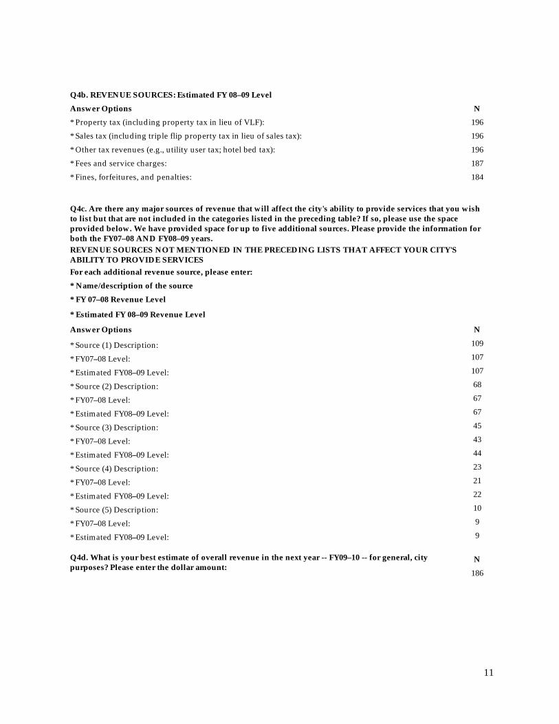
Q4b. REVENUE SOURCES: Estimated FY 08–09 Level Answer Options N * Property tax (including property tax in lieu of VLF): 196 * Sales tax (including triple flip property tax in lieu of sales tax): 196 * Other tax revenues (e.g., utility user tax; hotel bed tax): 196 * Fees and service charges: 187 * Fines, forfeitures, and penalties: 184

Q4c. Are there any major sources of revenue that will affect the city's ability to provide services that you wish to list but that are not included in the categories listed in the preceding table? If so, please use the space provided below. We have provided space for up to five additional sources. Please provide the information for both the FY07–08 AND FY08–09 years. REVENUE SOURCES NOT MENTIONED IN THE PRECEDING LISTS THAT AFFECT YOUR CITY'S ABILITY TO PROVIDE SERVICES For each additional revenue source, please enter: * Name/description of the source * FY 07–08 Revenue Level

* Estimated FY 08–09 Revenue Level

Answer Options N

* Source (1) Description: 109

* FY07–08 Level: 107

* Estimated FY08–09 Level: 107


* FY07–08 Level: 67



* FY07–08 Level: 43



* FY07–08 Level: 21



* FY07–08 Level: 9


Q4d. What is your best estimate of overall revenue in the next year -- FY09–10 -- for general, city purposes? Please enter the dollar amount:

N 186

12

Q5. In thinking about the things that drive or stimulate city expenditures, please rate each of the following by marking the appropriate column to indicate how important you believe each expenditure driver is.

EXPENDITURE DRIVERS -- Please select the appropriate choice for each of the expenditure drivers:

Answer Options Not at all important

Somewhat important Important

Very important N

Employee salaries 0 12 44 178 234 0.0% 5.1% 18.8% 76.1%

Employee health benefits 3 18 73 138 232 1.3% 7.8% 31.5% 59.5%

Retiree pensions (not including health) 19 36 66 112 233 8.2% 15.5% 28.3% 48.1%

Retiree health benefits 76 60 51 43 230 33.0% 26.1% 22.2% 18.7%

Contracts (city vendors; private service providers) 8 76 114 36 234 3.4% 32.5% 48.7% 15.4% Utility cost increases 5 105 100 22 232 2.2% 45.3% 43.1% 9.5% Materials and supplies 11 135 77 10 233 4.7% 57.9% 33.0% 4.3% Increasing population 88 93 42 9 232 37.9% 40.1% 18.1% 3.9% Interest on bonds issued by city 93 85 41 10 229 40.6% 37.1% 17.9% 4.4%

General debt service, other than on bonds 102 85 40 4 231 44.2% 36.8% 17.3% 1.7%

Short-term borrowing costs 150 57 22 2 231 64.9% 24.7% 9.5% 0.9%

Aging, costly-to-maintain infrastructure 11 49 97 75 232 4.7% 21.1% 41.8% 32.3%

State government mandates 8 73 87 65 233 3.4% 31.3% 37.3% 27.9%

Q5a. In the space provided, please list any driver or stimulant of city expenditures that you believe is IMPORTANT or VERY IMPORTANT but not included in the preceding list.

N 49

13

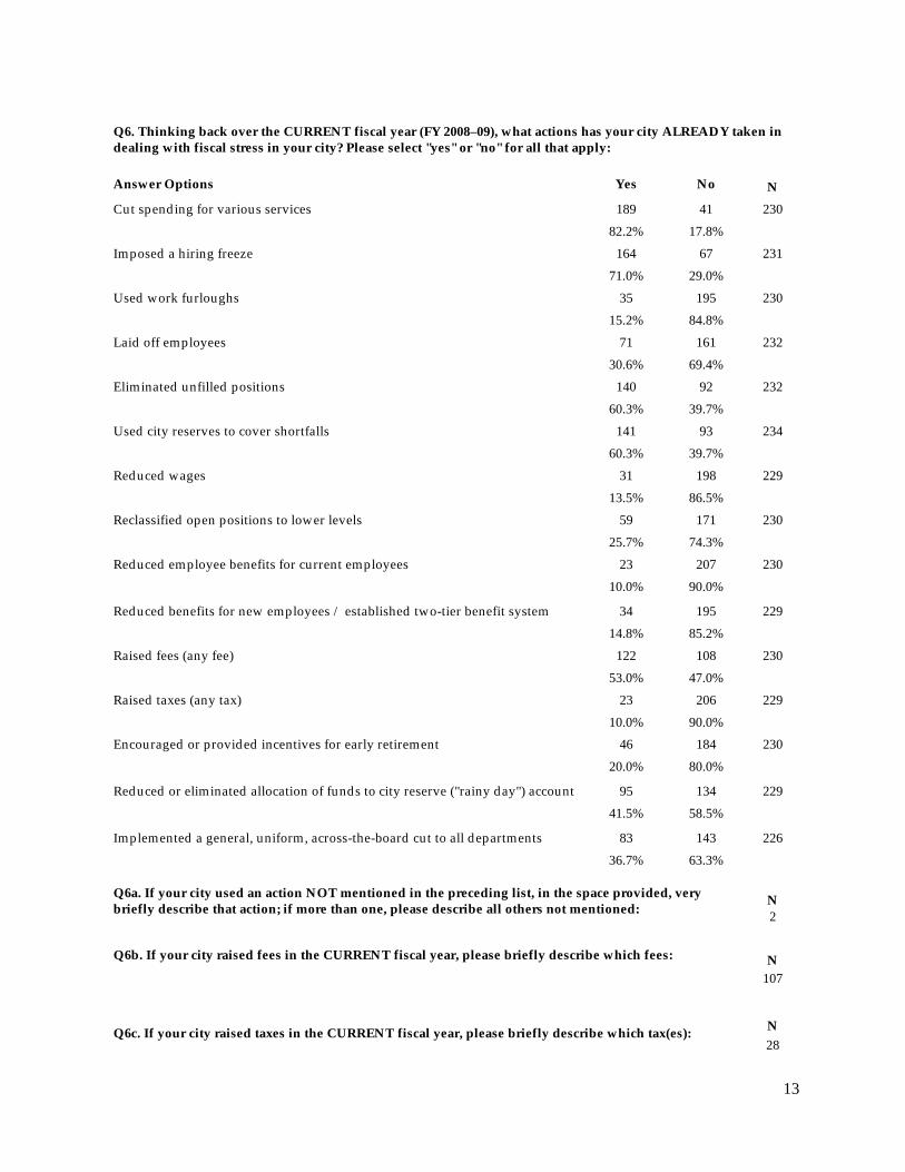
Q6. Thinking back over the CURRENT fiscal year (FY 2008–09), what actions has your city ALREADY taken in dealing with fiscal stress in your city? Please select "yes" or "no" for all that apply:

Answer Options Yes No N Cut spending for various services 189 41 230 82.2% 17.8% Imposed a hiring freeze 164 67 231 71.0% 29.0% Used work furloughs 35 195 230 15.2% 84.8% Laid off employees 71 161 232 30.6% 69.4% Eliminated unfilled positions 140 92 232 60.3% 39.7% Used city reserves to cover shortfalls 141 93 234 60.3% 39.7% Reduced wages 31 198 229 13.5% 86.5% Reclassified open positions to lower levels 59 171 230 25.7% 74.3% Reduced employee benefits for current employees 23 207 230 10.0% 90.0%

Reduced benefits for new employees / established two-tier benefit system 34 195 229 14.8% 85.2% Raised fees (any fee) 122 108 230 53.0% 47.0% Raised taxes (any tax) 23 206 229 10.0% 90.0% Encouraged or provided incentives for early retirement 46 184 230 20.0% 80.0%

Reduced or eliminated allocation of funds to city reserve ("rainy day") account 95 134 229 41.5% 58.5%

Implemented a general, uniform, across-the-board cut to all departments 83 143 226 36.7% 63.3%

Q6a. If your city used an action NOT mentioned in the preceding list, in the space provided, very briefly describe that action; if more than one, please describe all others not mentioned: N

2 Q6b. If your city raised fees in the CURRENT fiscal year, please briefly describe which fees: N

107

Q6c. If your city raised taxes in the CURRENT fiscal year, please briefly describe which tax(es): N 28

14

Q7a. If in the CURRENT FISCAL YEAR (FY2008–09) your city cut spending, which of the following programs, line-items have ALREADY been reduced? PART A: In the spaces provided please indicate the amount initially budgeted for FY08–09. If not applicable, just enter NA.

Program/Line-Items -- Initial (FY 2008–09) Budgeted Amount

Answer Options N * Management and administrative services 141

* Police services 146

* Animal control 132

* Parks 141

* Fire & emergency medical 141

* Senior programs 127

* Adult/youth recreation 133

* Library 128

* Streets and roads 135

* Transit 124

* Planning 140

* Public works 137

* Homeless 119

* Economic development (not redevelopment) 124

* Water and sewer utilities 124

* Support of arts, culture, museums 120

* Contribution to reserve (rainy day) account 114

7b. PART B: In the space provided please indicate the dollar amount of changes or reductions in your original budge for this year. If not reduced, just enter NR.

Program/Line-Items -- Approximate Dollar Reduction from Initial Budgeted Amount

Answer Options N * Management and administrative services 135

* Police services 136

* Animal control 113

* Parks 123

* Fire & emergency medical 125

* Senior programs 111

* Adult/youth recreation 122

* Library 109

* Streets and roads 121

* Transit 107

* Planning 127

* Public works 124

* Homeless 104

* Economic development (not redevelopment) 110

* Water and sewer utilities 110

15

* Support of arts, culture, museums 110

* Contribution to reserve (rainy day) account 110

Q7c. For any item(s) whose spending was/were cut and not mentioned in the preceding list, please indicate the item(s) and how it/each was cut: N

53

Q8. Thinking about the CURRENT (FY08–09) budget, beyond the changes or reductions you've already made this year, how likely is it that your city will MAKE NEW OR ADDITIONAL CUTS in the CURRENT fiscal year for spending by doing the following actions. Please indicate the appropriate column for each action (row). For each of the following actions to reduce costs/expenditures, please select the appropriate column to indicate how likely you think the action is:

Answer Options Very

Unlikely Somewhat Unlikely

Somewhat Likely

Very Likely N

Cut spending for various services 42 33 65 74 214 19.6% 15.4% 30.4% 34.6% Impose a hiring freeze 55 18 37 93 203 27.1% 8.9% 18.2% 45.8% Use work furlough 102 47 35 24 208 49.0% 22.6% 16.8% 11.5% Lay-off employees 112 35 32 31 210 53.3% 16.7% 15.2% 14.8% Eliminate positions 71 37 51 49 208 34.1% 17.8% 24.5% 23.6%

Use city reserves to cover shortfalls 49 31 57 72 209 23.4% 14.8% 27.3% 34.4% Reduce wages 117 54 21 16 208 56.3% 26.0% 10.1% 7.7%

Reclassify open positions to lower levels 100 49 42 15 206 48.5% 23.8% 20.4% 7.3%

Reduce employee benefits for current employees 123 50 25 12 210 58.6% 23.8% 11.9% 5.7%

Reduce benefits for new employees; two-tier system 126 45 22 16 209 60.3% 21.5% 10.5% 7.7% Raise fees (any fee) 80 24 60 46 210 38.1% 11.4% 28.6% 21.9% Raise taxes (any tax) 146 36 20 8 210 69.5% 17.1% 9.5% 3.8% Encourage or provide incentives for early retirement 101 52 30 23 206 49.0% 25.2% 14.6% 11.2%

Reduce or eliminate allocation to reserve account 83 27 41 57 208 39.9% 13.0% 19.7% 27.4%

16

Q8a. If there is an additional cost reduction action not listed in the preceding list that is LIKELY or VERY LIKELY in your city, please describe in the following space:

N 23

Q8b. If an additional fee increase is likely, please indicate which fee(s): N 59

Q8c. If a tax increase is likely, please indicate which tax(es): N 25

Q9. If your city needs to make additional cuts this fiscal year, what are some of the significant budget areas where such reductions may be considered? Please use the following space to answer:

N 77

Q10. We are interested in hearing about those specific services or activities that IN YOUR VIEW are at risk of falling below acceptable professional standards or that will increase risks to public safety due to current and previous budget cuts. Please use the space provided to list such services or functions:

N 76

Q11. In thinking about people, groups, areas, or services that might be adversely affected by budget cuts in your city, please indicate whether each of those listed will be seriously or not seriously affected. Select the appropriate column:

Answer Options

NOT Seriously Affected

Seriously Affected N

Senior citizens 166 38 204 81.4% 18.6% Youth sports 146 56 202 72.3% 27.7% Cultural activities, arts, museums 141 58 199 70.9% 29.1% Poorer neighborhoods 160 39 199 80.4% 19.6% Police response times 156 51 207 75.4% 24.6% Fire response times 162 35 197 82.2% 17.8% Public employees 92 116 208 44.2% 55.8%

Non-criminal code enforcement (private buildings, sanitation, rubbish) 134 70 204 65.7% 34.3%

Maintenance of public facilities (street cleaning, landscaping, public buildings) 100 108 208 48.1% 51.9%

Capital projects (Street improvements, new city facilities) 87 122 209 41.6% 58.4% City parks 102 99 201 50.7% 49.3%

17

Q11a. Is there any group, area of the city, or service that could be seriously affected by your CITY budget cuts that we didn't include in the list above? If so, please use this space to list them:

N 28

Q12. Thinking about public employee benefits and the cost of retiree benefits, how controversial would you say the issue is among your mayor and/or city manager and city council? Would you say it is not at all controversial, somewhat controversial, controversial, or very controversial? Please mark one of the following response categories:

Answer Options Not at all

Controversial Somewhat

Controversial Controversial Very

Controversial N Retiree benefits costs: 60 79 51 21 211

28.4% 37.4% 24.2% 10.0%

Q13. What other BUDGET action has your city ALREADY taken in the current budget year to prepare for FUTURE state actions to resolve its budget crisis, even though the state's actions might not have yet occurred? What FUTURE budget actions do you anticipate? If your city has taken a "wait-and-see" position, please do not hesitate to say so. N Q13a. BUDGET actions city has ALREADY taken: 133

Q13b. BUDGET actions that might be taken in the FUTURE: 126

Q14. In the space provided, please describe how uncertainty over the state budget does or does not complicate your ability to deliver services at the local level. Please be as specific as possible, and if state budget uncertainty doesn't pose a problem for your city, please let us know.

N 140

Q15. How important have unemployment, housing market declines, and declining retail sales been in affecting your city's budgets? For each, please rate how important it has been in affecting budget, with a "1" indicating a factor has been "not at all important" and a "5" indicating "very important":

Answer Options

Not At All Important

(1) (2) (3) (4)

Very Important

(5) N

Higher Unemployment 8 41 64 56 43 212 3.8% 19.3% 30.2% 26.4% 20.3%

Lower Retail Sales 6 12 19 42 134 213 2.8% 5.6% 8.9% 19.7% 62.9%

Housing Market Declines 3 20 37 51 100 211 1.4% 9.5% 17.5% 24.2% 47.4%

Q16. When it comes to managing or dealing with fiscal and budget stress during the current fiscal year, how would you rate the city council in terms of disagreement or consensus regarding how to deal with fiscal and budget stress. If the number "1" equals High Disagreement and "5" equals High Agreement, how would you rate your city council? Please select one of the numbers below:

Answer Options

High Conflict

(1) (2) (3) (4)

High Agreement

(5) N City Council conflict/ consensus: 2 15 46 71 77 211 0.9% 7.1% 21.8% 33.6% 36.5%

18

Q17. Which of the following best describes the situation in your city regarding the timeliness of your budget process for this fiscal year (FY 2008–09)? Please select the one that best applies to your city:

Answer Options N

Our city's budget is often adopted LATE, and this year was no different; the budget was LATE 11

Our city's budget is sometimes adopted LATE, but this year the budget was adopted ON TIME 11 Our city's budget has always been adopted ON TIME, but this year we were LATE 18

Our city's budget has always been adopted ON TIME, and this year we were also ON TIME 169 Q18. In your judgment, is your city considering seeking approval from voters to raise fees or taxes? Yes? No?

Answer Options Yes No N

City considering seeking voter approval to raise fees/taxes: 66 145 211

31.3% 68.7%

Q18a. In the space provided, please indicate for which fees or taxes your city might seek approval: N

74

19

Appendix C County Survey Summary

In the following summary, the right-hand column labeled “N” represents the total number of responses to each question.

Q1. How would you rate fiscal condition of your county government today? Please select from the following choices: Answer Options Poor Fair Good Excellent N County fiscal conditions: 11 22 13 1 47

23.4% 46.8% 27.7% 2.1%

Q2. Compared to other COUNTIES in California, would you say conditions in YOUR county are worse, about the same, or better than most other counties in California?

Please indicate which of the following best describes YOUR county's fiscal condition in comparison to other counties: Answer Options Worse About the same Better N County fiscal condition: 4 14 29 47 8.5% 29.8% 61.7%

Q3a. Overall would you say that your county is better able or less able to produce the revenue required to support county services this year (FY 08–09), compared to the previous fiscal year (FY07–08). Please check the response that applies: Answer Options Less able Better able N County revenue ability this year: 46 1 47

97.9% 2.1% Q3b. What about the next fiscal year (FY09–10)? Would you say that your county will be better able or less able to produce the revenue required to support county services NEXT year? Please check the response that applies:

Answer Options Less able Better able N County revenue ability next year: 46 1 47

97.9% 2.1%

Q4a. Considering the sources of your county revenues, compared to FY 2007–08, what is the estimated level of revenues from each of the following county revenue sources for FY 2008–09?

In the spaces provided in the rightmost column in the next two sections, please indicate your best, most current estimate of revenue sources for each of the two fiscal years.

Recall we are using the categories and definitions that are used by the State Controller's Counties Annual Reports.

REVENUE SOURCES -- FY 07–08 Level

Answer Options N

* Property tax (including property tax in lieu of VLF): 33

* Sales tax (including triple flip property tax in lieu of sales tax): 33

* Other tax revenues (e.g., utility user tax; hotel bed tax): 33

* Fees and service charges: 31

20

* Fines, forfeitures, and penalties: 31

* Total revenues from use of money and property: 32

* Total state revenues, excluding VLF in lieu taxes: 31

* Total federal grants, contracts, aid, revenues: 30

Q4b. REVENUE SOURCES: Estimated FY 08–09 Level

Answer Options N * Property tax (including property tax in lieu of VLF): 33

* Sales tax (including triple flip property tax in lieu of sales tax): 33

* Other tax revenues (e.g., utility user tax; hotel bed tax): 33

* Fees and service charges: 31

* Fines, forfeitures, and penalties: 31

* Total revenues from use of money and property: 32

* Total state revenues, excluding VLF in lieu taxes: 31

* Total federal grants, contracts, aid, revenues: 30

Q4c. Are there any major sources of revenue that will affect your county's ability to provide services that you wish to list but that are not included in the categories listed in the preceding table? If so, please use the space provided below. We have provided space for up to five additional revenue sources. Please indicate figures for the previous 07–08 AND the estimated current 08–09 years.

REVENUE SOURCES NOT MENTIONED IN THE PRECEDING LISTS THAT AFFECT YOUR COUNTY'S ABILITY TO PROVIDE SERVICES For each additional revenue source, please enter: * Name/description of the source * FY 07–08 Revenue Level * Estimated FY 08–09 Revenue Level

Answer Options N * Source (1) Description: 16

* FY07–08 Level: 16



* FY07–08 Level: 10



* FY07–08 Level: 7



* FY07–08 Level: 2



* FY07–08 Level: 0


21

Q5. In thinking about the elements that drive or stimulate county expenditures, please rate the level of importance for each of the following by marking the appropriate column for each expenditure driver.

EXPENDITURE DRIVERS -- Please mark the column that expresses your judgment concerning how important each of the following expenditure drivers is:

Answer Options Not at all Important

Somewhat Important Important

Very Important N

Employee salaries 0 0 5 35 40 0.0% 0.0% 12.5% 87.5%

Employee health benefits 0 0 9 31 40 0.0% 0.0% 22.5% 77.5%

Current employee pension costs 0 1 7 32 40 0.0% 2.5% 17.5% 80.0%

Retiree pensions (not including health) 4 5 12 19 40 10.0% 12.5% 30.0% 47.5% Retiree health benefits

6 5 9 20 40 15.0% 12.5% 22.5% 50.0% Contracts (county vendors; private service providers) 0 14 22 4 40 0.0% 35.0% 55.0% 10.0% Utility cost increases 2 18 15 5 40 5.0% 45.0% 37.5% 12.5% Materials and supplies 2 27 10 1 40 5.0% 67.5% 25.0% 2.5% Population growth 9 16 9 4 38 23.7% 42.1% 23.7% 10.5%

Interest on bonds issued by county 13 13 12 2 40 32.5% 32.5% 30.0% 5.0%

Short-term borrowing costs 14 17 8 1 40 35.0% 42.5% 20.0% 2.5%

General debt service, other than on bonds 17 15 6 2 40 42.5% 37.5% 15.0% 5.0%

Aging, costly-to-maintain infrastructure 1 8 16 15 40 2.5% 20.0% 40.0% 37.5%

State government mandates 0 2 8 30 40 0.0% 5.0% 20.0% 75.0%

Increasing caseloads for county social/health services 0 5 11 24 40 0.0% 12.5% 27.5% 60.0%

Significantly increasing numbers of financially-stressed, impoverished, special needs individuals/families 0 7 13 20 40 0.0% 17.5% 32.5% 50.0%

22

Increasing crime rate 4 12 14 9 39 10.3% 30.8% 35.9% 23.1% Inadequate state funding for cost-of-living increases in state-county programs 0 0 4 36 40 0.0% 0.0% 10.0% 90.0%

Q5a. In the space provided, please list any driver or stimulant of county expenditures that you believe is important or very important but not included in the preceding list.

N 12

Q6. Looking back over the current year and in comparison to the previous years, would you say that there has been a significant increase or no significant increase in the following conditions in your county?

Please select the appropriate choice for each:

Answer Options Significant

Increase

No Significant

Increase N Number of inmates in county jails 11 30 41

26.8% 73.2%

Number of court cases and court-related costs 18 20 38

47.4% 52.6%

City incorporations and annexations 4 37 41

9.8% 90.2%

Number of indigent health care cases 26 14 40

65.0% 35.0%

Size/Number of redevelopment areas in county cities 3 38 41

7.3% 92.7%

Applications for downward property tax assessments 38 3 41

92.7% 7.3%

Number of individuals seeking general social and health services 38 3 41

92.7% 7.3%

Number of unemployed individuals 39 2 41

95.1% 4.9%

Q6a. If there are factors that are not included in the preceding list and that have SIGNIFICANTLY INCREASED and that you believe affect county costs, please use the space provided to list one or more of these:

N 5

Q7. Thinking back over the CURRENT fiscal year (FY 2008–09), what actions has your county ALREADY taken in dealing with fiscal stress in your county? Please select "yes" or "no" for all that apply:

Answer Options Yes No N Cut spending for various services 38 3 41

92.7% 7.3%

Imposed a hiring freeze 32 8 40

80.0% 20.0%

Used work furloughs 12 29 41

29.3% 70.7%

23

Laid off employees 26 15 41

63.4% 36.6%

Eliminated unfilled positions 35 6 41

85.4% 14.6%

Used county reserves to cover shortfalls 20 20 40

50.0% 50.0%

Reduced wages 1 40 41

2.4% 97.6%

Reclassified open positions to lower levels 19 21 40

47.5% 52.5%

Reduced employee benefits for current employees 2 39 41

4.9% 95.1%

Reduced benefits for new employees / established two-tier benefit system 12 29 41

29.3% 70.7%

Raised fees (any fee) 33 8 41

80.5% 19.5%

Raised taxes (any tax) 3 38 41

7.3% 92.7%

Encouraged or provided incentives for early retirement 6 34 40

15.0% 85.0%

Reduced or eliminated allocation of funds to county reserve ("rainy day") account 18 23 41

43.9% 56.1%

Implemented a general, uniform, across-the-board cut to all departments 16 25 41

39.0% 61.0%

Q7a. If your county used an action NOT mentioned in the preceding list, in the space provided, very briefly describe that action; if more than one, please describe all others not mentioned:

N 12

Q7b. If your county raised fees in the CURRENT fiscal year, please briefly describe which fees: N

29

Q7c. If your county raised taxes in the CURRENT fiscal year, please briefly describe which tax(es): N

5

Q8a. Using the State Controller's Counties Annual Reports categories, if in the CURRENT FISCAL YEAR (FY 2008–09) your county cut spending, which of the following programs and/or line-items have ALREADY been reduced? PART A: In the space provided please indicate the initial FY08–09 budgeted amount. If not applicable, just enter NA. Program/Line-Items -- Initial (FY 2008–09) Budgeted Amount

Answer Options N * Legislative and Administrative Total (Board, Clerk, Admin. Officer) 30

* Finance (Total Auditor, Treasurer, Assessor) 30

* Elections Total 28

24

* Judicial Total (including district attorney, public defender) 29

* Sheriff Total 29

* Detention / Correction Total 29

* Fire Total 29

* Protective Inspection Total (including Agricultural Commissioner) 29

* LAFCO 27

* Recorder 28

* Coroner 27

* Emergency Services 28

* Planning and Zoning 28

* Animal Control 28

* Public Works and Facilities Total (Roads, terminals, parking, etc.) 29

* Health Total (Public health, medical care (including indigent health care) mental health, drug/alcohol treatment)

29

* Public Assistance/Welfare Total (Administration, aid programs) 29

* General Relief Total (Aid to indigents, indigent burial) 27

* Library Total 28

* Recreation and Culture Total (Facilities, parks, cultural services, harbors) 29

* Total General County Expenditures Before Transfers Out 28

Q8b. PART B: In the space provided please indicate the dollar amount of the reduction. If not reduced, just enter NR.

Program/Line-Items -- Dollar Reduction from Initial Amount

Answer Options N * Legislative and Administrative Total (Board, Clerk, Admin. Officer) 28

* Finance (Total Auditor, Treasurer, Assessor) 28

* Elections Total 28

* Judicial Total (including district attorney, public defender) 30

* Sheriff Total 30

* Detention / Correction Total 28

* Fire Total 28

* Protective Inspection Total (including Agricultural Commissioner) 28

* LAFCO 28

* Recorder 28

* Coroner 28

* Emergency Services 28

* Planning and Zoning 28

* Animal Control 28

* Public Works and Facilities Total (Roads, terminals, parking, etc.) 28

* Health Total (Public health, medical care (including indigent health care) mental health, drug/alcohol treatment)

29

* Public Assistance/Welfare Total (Administration, aid programs) 29

* General Relief Total (Aid to indigents, indigent burial) 29

25

* Library Total 29

* Recreation and Culture Total (Facilities, parks, cultural services, harbors) 28

* Total General County Expenditures Before Transfers Out 25

Q9. If your county needs to make additional cuts this fiscal year, what are some of the significant budget areas where such reductions may be considered?

N 29

Q10. We are interested in hearing about those specific services or activities that IN YOUR VIEW are at risk of falling below acceptable professional standards or that will increase risks to public safety due to current and previous budget cuts. N Please use the space provided to list such services or functions: 22

Q11. In thinking about people, groups, areas, or services that might be adversely affected by budget cuts in your county, please indicate whether each of those listed will be seriously or not seriously affected. Select the appropriate column:

Answer Options

NOT Seriously Affected

Seriously Affected N

Senior citizens 14 25 39 35.9% 64.1% At-risk youth 10 29 39 25.6% 74.4% Low-income families and individuals 8 31 39 20.5% 79.5% Probationers (juvenile and adult) 10 29 39 25.6% 74.4% Persons in need of treatment (those in the general population and/or criminal offenders) 10 29 39 25.6% 74.4% Cultural activities, arts (excluding libraries) 21 18 39 53.8% 46.2% Health services 5 34 39 12.8% 87.2% Social services 10 28 38 26.3% 73.7% Libraries 17 20 37 45.9% 54.1% Sheriff response times 23 16 39 59.0% 41.0% Fire response times 27 9 36 75.0% 25.0% Public employees 8 31 39 20.5% 79.5%

Non-criminal code enforcement (private buildings, sanitation, rubbish) 21 18 39 53.8% 46.2%

26

Maintenance of public facilities (street cleaning, landscaping, public buildings) 16 23 39 41.0% 59.0% Capital projects (street improvements, new county facilities) 11 28 39 28.2% 71.8% County parks 18 20 38

47.4% 52.6%

11a. Is there any group, area of the county, or service that could be seriously affected by your COUNTY budget cuts that we didn't include in the list above? If so, please use this space to list them:

N 9

Q12. Thinking about public employee benefits and the cost of retiree benefits, how controversial would you say the issue is among your county's policy-making officials (the supervisors and CAO)? Would you say it is not at all controversial, somewhat controversial, controversial, or very controversial?

Please mark one of the following response categories:

Answer Options Not at all

Controversial Somewhat

Controversial Controversial Very

Controversial N Cost of RETIREE benefits: 10 13 10 6 39

25.6% 33.3% 25.6% 15.4% Pension costs of CURRENT employees:

6 17 9 8 40 15.0% 42.5% 22.5% 20.0%

Q13. In the spaces provided below, what other BUDGET action has your county ALREADY taken to prepare for the state’s resolution of its budget crisis, even though the state’s actions haven’t yet occurred? What FUTURE budget actions do you anticipate? If your county has taken a "wait-and-see" position, please do not hesitate to say so.

N Q13a. BUDGET actions the county has ALREADY taken: 31 Q13b. BUDGET actions that might be taken in the FUTURE: 31

Q14. In the space provided, please describe how uncertainty over the state budget does or does not complicate your ability to deliver services at the local level. Please be as specific as possible, and if state budget uncertainty doesn't pose a problem for your county, please let us know.

N 31

Q15. How important have unemployment, housing market declines, and declining retail sales been in affecting your city's budgets? For each, please rate how important it has been in affecting budget, with a "1" indicating a factor has been "not at all important" and a "5" indicating "very important":

Answer Options

Not At All Important

(1) (2) (3) (4)

Very Important

(5) N

Higher Unemployment 0 4 10 8 19 41 0.0% 9.8% 24.4% 19.5% 46.3%

Lower Retail Sales 0 2 4 16 19 41 0.0% 4.9% 9.8% 39.0% 46.3%

Housing Market Declines 0 1 3 5 32 41 0.0% 2.4% 7.3% 12.2% 78.0%

27

Q16. When it comes to managing or dealing with fiscal and budget stress during the current fiscal year, how would you rate the county board of supervisors in terms of disagreement or agreement regarding how to deal with fiscal and budget stress? If the number "1" equals High Disagreement and "5" equals High Agreement, how would you rate your county board of supervisors? Please select one of the numbers below:

Answer Options

High Conflict

(1) (2) (3) (4)

High Agreement

(5) N

Board of Supervisors conflict/ consensus: 0 4 6 11 18 39

0.0% 10.3% 15.4% 28.2% 46.2%

Q17. Which of the following best describes the situation in your city regarding the timeliness of your budget process for this fiscal year (FY 2008–09)? Please select the one that best applies to your city:

Answer Options N

Our county's budget is often adopted LATE, and this year was no different; the budget was LATE. 5

Our county's budget is sometimes adopted LATE, but this year the budget was adopted ON TIME. 1

Our county's budget has always been adopted ON TIME, but this year we were LATE 3

Our county's budget has always been adopted ON TIME, and this year we were also ON TIME 32

Q18. In your judgment, is your county considering seeking approval from voters to raise fees or taxes? Yes? No?

Answer Options Yes No N County considering seeking voter approval to raise fees/taxes: 9 32 41

22.0% 78.0%

Q18a. In the space provided, please indicate for which fees or taxes your county might seek approval: N

14

28

Appendix D City Perceptions of Fiscal Stress

An Overall Perceived Stress Score was developed for cities responding to our survey using several simple additive scales. These were based on (1) perceptions of actions already taken in the respective cities to deal with fiscal stress, (2) how harmful budget cuts have been, and (3) how likely future actions will be taken to deal with continued fiscal stress, including the likelihood of tax or fee increases. In calculating each composite score, listwise deletion of missing data was used, which means that only cases were used for which there are valid data for all the measures.

· The measure of how active the city has been in dealing with fiscal stress is measured as the number of times respondents indicated a “yes” response to the following actions to manage city fiscal stress (See question 6 in the city survey reported in Appendix A):

· Cut spending for various services · Imposed a hiring freeze · Used work furloughs · Laid off employees · Eliminated unfilled positions · Used city reserves to cover shortfalls · Reduced wages · Reclassified open positions to lower levels · Reduced employee benefits for current employees · Reduced benefits for new employees; established two-tier benefit system · Raised fees · Raised taxes · Encouraged or provided incentives for early retirement · Reduced or eliminated funds to city reserve (rainy day) account · Implemented a general, uniform, across-the-board cut to all departments

There were 216 cities for which there were complete data for all 15 items in the scale.

The score varied between 0 and 14, with a mean of 5.3. The Cronbach’s Alpha for the scale was a .772.2

We also developed two very simple additive scales based on perception of how serious cuts have been in the cities and how likely additional cuts would be. The items appear in

2 Cronbach’s Alpha is a standard measure of the internal consistency of a set of items or the extent to which they can be measuring some underlying characteristic or variable. Generally, a value of .70 or higher is considered a high “alpha.”

29

questions 8 and 11 in the survey questionnaire reproduced in Appendix A. The Seriousness of Cuts scale was comprised as follows. Respondents were asked whether a list of people, groups, or services might be seriously or adversely affected by budget or service cuts in the city. The list included: senior citizens, youth sports, cultural activities, poorer neighborhoods, police response times, fire response times, public employees, code enforcement (buildings, sanitation, or rubbish), maintenance of public buildings, capital projects, and city parks. The number of times a respondent indicated a serious cut was the additive scale, and the Alpha of Scalability for that scale was .842, a high level, indicating these items constitute an internally valid scale (Spector, 1992). After listwise deletion of missing data the number of cases for this scale was 211. We interpret higher scores to mean cuts were judged to have more serious or adverse effects.3

The third scale was an additive scale of Likelihood of More Cuts scale. The method was the same, and the items were based on a series including hiring freeze, furloughs, layoffs, eliminating positions, using city reserves, reducing wages, reclassifying open positions, reducing benefits for current employees, reducing benefits for new employees, raising fees, raising taxes, encouraging or providing incentives for early retirement, and reducing or eliminating allocation to reserve account. Each of these items was scored from very unlikely to very likely (from 1 to 4). The sum of the item scores was the scale score. After listwise deletion of missing data, the number of cases was 217. The alpha for the score was .895, a very high indication of scalability.

4

Table D.1 Intercorrelations between perceptions of management of fiscal stress

Level of actions already taken

Seriousness of cuts

How active likely to be in the future

Level of actions already taken 1.000

Seriousness of cuts .495 1.000

How active likely to be in the future .467 .333 1.000

NOTE: All of the correlations are significant at the .05 level or less.

These items are significantly correlated with one another. Cities that have been more active are also more likely to view their local budget cuts as having more serious possible effects on groups and services, and they are also more likely to take more cutback actions in the future. These correlations are moderate, however, and clearly cities are not in lock step with one another on these judgments.

Using factor analysis, we then specified a principal- components solution with one factor and used the factor scores as a continuous variable. Factor scores are composite measures created for each observation (city) for each factor extracted in the factor analysis (only one factor in this case). The factor scores are then standardized and expressed as z-scores, with a mean of zero. The assumption is that the higher the score, the more the city is perceiving fiscal stress on

3 The mean for the seriousness of the cuts scale was 3.75, and the range was 0–11. 4 The mean for the scale of the likelihood of more cuts is 26.87, with a range of 4–50.

30

a number of related fronts—including what the city has done, anticipates doing in the future, and how severe the consequences of cutback management have been.

The higher the factor score, the higher the overall Perceived Stress. The highest scores are among communities that have already made the largest adjustments, anticipate more adjustments in the future, and perceive that there are more adverse local consequences. Because the factor analysis employs listwise deletion of missing data, the N for the overall Perceived Stress factor score was 148. Experimenting with subgroups of our measures did not appreciably raise the number of valid cases in the score and did not change the results of the analysis.

31

References

Baldassare, Mark. When Government Fails: The Orange County Bankruptcy. Berkeley, California: University of California Press, 1998.

Baldassare, Mark, Christopher Hoene, and Jonathan Cohen. Coping with Homeland Security in California: Surveys of City Officials and State Residents. San Francisco, California: Public Policy Institute of California, October, 2002.

Baldassare, Mark and Christopher Hoene. Coping with Homeland Security: Perceptions of City Officials in California and the United States.” San Francisco, California: Public Policy Institute of California, December, 2002.

Baldassare, Mark and Christopher Hoene. Local Homeland Security and Fiscal Uncertainty: Surveys of City Officials in California. San Francisco, California: Public Policy Institute of California, December, 2003.

Baldassare, Mark, Mina Yaroslavsky, and Paul G. Lewis. The State Budget and Local Health Services in California: Surveys of County Officials. San Francisco, California: Public Policy Institute of California, May, 2004.

Baldassare, Mark and Christopher Hoene. Local Budgets and Tax Policy in California: Surveys of city Officials and State Residents.” San Francisco, California: Public Policy Institute of California, September, 2004.

Barbour, Elisa. State-Local Fiscal Conflicts in California: from Proposition 13 to Proposition 1A. San Francisco, California: Public Policy Institute of California, 2007.

Beacon Economics, LLC. “An Economic Backdrop for Fiscal Reform in California.” Report prepared for California Forward, Sacramento and San Francisco, California, November 2008.

Boyd, Donald J. and Lucy Dadayan. “State Tax Revenue Flat, for the First Time Since 2002 Recession: After Weak Third Quarter, Further Declines Likely Lie Ahead.” State Revenue Flash Report, The Nelson A. Rockefeller Institute of Government, State University of New York, Albany, November 6, 2008.

Brennan, Christiana, Elizabeth Wheel, and Christopher Hoene. The State of America’s Cities 2005:The Annual Opinion Survey of Municipal Elected Officials. Washington, D.C.: National League of Cities, 2005.

Burger, James and Gretchen Wenner, “Governor Vetoes Cost Kern Millions,” Bakersfield Californian, July 29, 2009.

California Budget Project. “How do the Budgets Compare? A Comparison of the Governor’s May Proposals, the Budget Conference Committee’s Proposals, and the July Budget Agreement.” Sacramento, California: California Budget Project, August 4, 2009.

California State Board of Equalization, 2009. Available at www.boe.ca.gov/news/2009/73-09-Y.pdf.

32

California Welfare Directors Association (CWDA) and California Association of Counties (CSAC). Human Services in a Time of Economic Crisis: An Examination of California’s Safety-Net Programs and Related Economic Benefits for Communities. Sacramento, California: CWDA and CSAC, April, 2009. http://counties.org/images/users/1/CSAC%20-%20CWDA%20Joint%20Report%20Final.pdf.

Carpenter, Candace M. “Tension and Ambiguity: A Legislative Guide to Recent Efforts to Reform California’s State-Local Fiscal Relationship.” Sacramento, California: Senate Local Government Committee, March, 2001.

Clark, Cal and B. Oliver Walter. “Urban Political Cultures, Financial Stress, and City Fiscal Austerity Strategies.” The Western Political Quarterly, 44 (September, 1991): 676–697.

Coleman, Michael. “California Cities Are Net Donors to the State.” http://www.californiacityfinance.com/CitiesAreDonors.pdf, May, 2006.

Coleman, Michael. “Fact Sheet: The ERAF Property Tax Shift.” http:// www.CaliforniaCityFinance.com, Sacramento, California: League of California Cities, September 29, 2008.

Coleman, Michael and Michael G. Colantuono. “Toward Fiscal Authority and Stability: Power and Risk in California City Revenues.” Western City, August 2003: 26–31.

Commission on Local Government. State and Local Government Finances, a Fifty State Profile, FY 2005. Commission on Local Government, Department of Housing and Community Development, Commonwealth of Virginia, July 2007.

Community Development Department. “Trends in Delinquencies and Foreclosures in California.” San Francisco, California: Community Development Department, Federal Reserve Bank of San Francisco, April, 2009.

Dadayan, Lucy and Donald J. Boyd. “State Tax Revenue Declined Sharply in Fourth Quarter,” State Revenue Flash Report, The Nelson A. Rockefeller Institute of Government, www.rockinst.org, March 12, 2009.

Deller, Steven and Craig Maher. “Measures of Municipal Fiscal Health: Linking Primary and Secondary Data,” Paper presented at the Midwest Political Science Association, Chicago, Illinois, April 2004.

Department of Finance, “2009–10 May Revision General Fund Proposals.” Sacramento, California: Department of Finance, May 14, 2009.

Doerr, David R. California’s Tax Machine: A History of Taxing and Spending in the Golden State. Sacramento, California: California Taxpayers’ Association, 2000.

Dowding, Keith and Thanos Mergoupis. “Fragmentation, Fiscal Mobility, and Efficiency.” Journal of Politics, 65 (November, 2003): 1190–1207.

Fernandez, Sergio, Jay Eungha Ryu, and Jeffrey L. Brudney. “Exploring Variations in Contracting for Services Among American Local Governments: Do Politics Still Matter?” American Review of Public Administration, 38 (December, 2008): 439–462.

33

Haveman, Jon, Eric O’N. Fisher, and Fannie Tseng. Spending on County Human Services Programs in California: An Evaluation of Economic Impacts. San Rafael, California: Beacon Economics, March 17, 2009.

Hoene, Christopher and Michael A. Pagano. Cities and State Fiscal Structure. Washington, D.C.: Cities and State Fiscal Structure. Washington, D.C.: National League of Cities, 2006.

Hoene, Christopher and Michael A. Pagano. Cities and State Fiscal Structure. Washington, D.C.: Cities and State Fiscal Structure. Washington, D.C.: National League of Cities, 2008.

Hoene, Christopher. “Fiscal Outlook for Cities Worsens in 2009.” Research Brief on America’s Cities, issue 2009-1. Washington, D.C.: National League of Cities, February, 2009.

Hoene, Christopher W. and Michael A. Pagano. “Research Brief on America’s Cities: City Fiscal Conditions in 2009.” Washington, D.C.: National League of Cities, September 2009.

Hubert, Cynthia. “Demand for Social Services Rises as Funding Falls.” Sacramento Bee, November 24, 2008.

Kloha, Philip, Carol S. Weissert, and Robert Kleine. “Someone to Watch Over Me: State Monitoring of Local Fiscal Conditions.” The American Review of Public Administration, 35 (September, 2005): 236–255.

Kolko, Jed. “The California Economy: Housing Market Update.” San Francisco, California: Public Policy Institute of California, August 2009.

Lamb, Celia. “Local Governments Dip into Rainy-Day Funds as Growth Falters, Property, Sales-Tax Revenue Flattens, Counties Struggle to Cut Expenses.” Sacramento Business Journal, October 20, 2008.

Legislative Analyst’s Office (LAO). “The Budget Package: 2009–10 California Spending Plan.” Sacramento: Legislative Analyst’s Office, October 2009.

Legislative Analyst’s Office (LAO). “California’s Fiscal Outlook: LAO Projections, 2008–09 through 2013–14.” Sacramento: Legislative Analyst’s Office, November 2008.

Legislative Analyst’s Office (LAO). “Variations in County Fiscal Capacity,” in The 1990–91 Budget: Perspectives and Issues, Report from the Legislative Analyst’s Office to the Joint Legislative Budget Committee.” Sacramento: Legislative Analyst’s Office, 1990.

Lewis, Paul G. and Max Neiman. Custodians of Place: Governing the Growth and Development of Cities. Washington, D.C.: Georgetown University Press, 2009.

McIntosh, Paul, Jim Wiltshire, and Jean Kinney Hurst. “2009–10 State Budget Revision-Governor’s Vetoes Week of July 27, 2009, CSAC Budget Action Bulletin.” Memo. Sacramento, California: California Association of Counties, July 28, 2009 (http://www.counties.org/images/users/1/BAB%208_7.28.09.pdf).

National Governors Association and the National Association of State Budget Officers. The Fiscal Survey of States. Washington, D.C.: National Governors Association and the National Association of State Budget Officers, 2008.

34

Pagano, Michael A. and Christopher W. Hoene. “City Fiscal Conditions in 2008.” Research Brief on America’s Cities, Issue 2008-2, National League of Cities, Washington, D.C., September 2008.

Prah, Pamela M. “The Path to California’s Fiscal Crisis.” http:/www.stateline.org/live/printable/story?contentId=400337.

Reschovsky, Andrew. “The Implication of State Fiscal Stress for Local Governments.” Prepared for State Fiscal Crises: Causes, Consequences, and Solutions, conference at the Urban Institute, Washington, D.C., April 3, 2003.

Sanders, Jill. “Local Government Lobbying Costs Soar in California.” Sacramento Bee, February 8, 2009.

Scanlon, Mavis. “State Budget’s Hidden Hammer: Local Redevelopment Agencies.” East Bay Business Times, September 29, 2008.

Seyfried, William and Louis Pantuosco. “Estimating the Sensitivity of State Tax Revenue to Cyclical and Wealth Effects.” Journal of Economics and Finance, 27 (Spring 2003): 112–123.

Simpson, Richard P. and Cary S. Jung. California Counties on the Fiscal Fault Line: A Study of the Financial Condition of California Counties. Sacramento, California: California Counties Foundation, 1990.

Spector, Paul E. Summated Rating Scale Construction: An Introduction. Newbury Park, California: Sage Publications, 1992.

Stein, Robert M. “State Regulation and the Political Consequences of Urban Fiscal Stress.” Publius, 14 (Spring 1984): 41–54.

Stipak, Brian and Daniel E. O’Toole. “Fiscal Stress and Productivity Improvement: Local Government Managers’ Perspective.” Public Productivity and Management Review, 17 (Winter 1993): 101–112.

Walters, Dan. “State Now Has Five-Month Budget Cycles,” Sacramento Bee, July 24, 2009.

Perceptions of Local Stress During a Statewide Budget Crisis Technical Appendices

Documents

Transcript of Perceptions of Local Stress During a Statewide Budget Crisis Technical Appendices