PART VI APPENDICES
134
PART VI APPENDICES
-
Upload
khangminh22 -
Category
Documents
-
view
0 -
download
0
Transcript of PART VI APPENDICES

PART VI
APPENDICES

CONTENTS
PART VI
APPENDICES
Appendix
A Spherical Geometry 727
B Construction of Global Geometry Plots 737
C Matrix and Vector Algebra 744
D Quaternions 758
E Coordinate Transformations 760
F The Laplace Transform 767
G Spherical Harmonics 775
H Magnetic Field Models 779
Spacecraft Attitude Determination and Control Systems 787
J Time Measurement Systems 798
K Metric Conversion Factors 807
L Solar System Constants 814
M Fundamental Physical Constants 826
Index 830

APPENDIX A
SPHERICAL GEOMETRY
A.I Basic Equations A.2 Right and Quadrantal Spherical Triangles A.3 Oblique Spherical Triangles AA Differential Spherical Trigonometry A.S Haversines
James R. Wertz
Finding convenient reference material in spherical geometry is difficult. This appendix provides a compilation of the most useful equations for spacecraft work. A brief discussion of the basic concepts of spherical geometry is given in Section 2.3. The references at the end of this appendix contain further discussion and proofs of most of the results presented here.
A.I Basic Equations
Algebraic Formulas. Let Pi be a point on the unit sphere with coordinates (ai,oJ. The arc-length distance, ()(PI'P2), between PI and P2 is given by:
cos()( P I,P2) = cos()( P2,PI)
= sino lsin02 + cosOICOS02cos( a l - ( 2 ) (A-I)
The rotation angle, A(P p P2 ; P3), from PI to P2 about a third point, P3, is cumbersome to calculate and is most easily obtained from spherical triangles (Sections A.2 and A.3) if any of the triangle components are already known. To calculate directly from coordinates, obtain as intermediaries the arc-length distances ()( Pi' P), between the three pairs of points. Then
cos()( PI' P2) - cos ()( PI' P 3)COS()( P2 , P3)
cosA(PI,P2 ;P3)= . ()(P P)' ()(P P) SIn I' 3 SIn 2' 3
(A-2)
with the quadrant determined by inspection. The equation for a small circle of angular radius p and centered at (ao, 00) in
terms of the coordinates, (a,o), of the points on the small circle is, from Eq. (A-I),
COS P = sin 0 sin 00 + cos 0 cos oocos( a - ao) (A-3)
The arc length, {3, along the arc of a small circle of angular radius p between two points on the circle separated by the rotation angle, q, (q, measured at the center of the circle) is
{3= q,sinp (A-4)
The chord length, y, along the great circle chord of an arc of a small circle of

728 SPHERICAL GEOMETRY A.I
angular radius p is given by
cosy= 1-(I-cosCP)sin2p (A-5)
where cP is as defined above. The equation for a great circle with pole at (0:0>80) is, from Eq. (A-3) with
p=90°,
(A-6a)
The inclination, i, and azimuth of the ascending node (point crossing the equator from south to north when moving along the great circle toward increasing azimuth), </>0' of the great circle are
i=90° - 80
</>0=90° +0:0 (A-6b)
Therefore, the equation for the great circle in terms of inclination and ascending node is
tan8 = tan; sin( 0: -</>0) (A-6c)
The equation of a great circle through two arbitrary points is given below. Along a great circle, the arc length, the chord length, and the rotation angle, CP, are all equal, as shown by Eqs. (A-4) and (A-5) with p = 90° .
Finally, the direction of the cross product between two unit vectors associated with points PI and P2 on the unit sphere is the pole of the great circle passing through the two points. Find the intermediary, PI' from
(A-7a)
As shown iii Fig. A-I, PI is the azimuth of point PI relative to the ascending node
Fig. A-I. P is the pole of the great circle passing through PI and P2 and is also in the direction of the doss product PI xP2• PI is an intermediate variable used for computations.

A.l BASIC EQUATIONS 729
of the great circle through p. and P2• The coordinates, (ac,8c)' of the cross product p. XP2 are given by
sinfi.
tan8.
sin(a2 - a.) tan 82
(A-7b)
Combining Eqs. (A-7b) and (A-6a) gives the equation for a great circle through points PI and Pz:
(A-8)
Area Formulas. All areas are measured on the curved surface of the unit sphere. For a sphere of radius R, multiply each area formula by R 2. All arc lengths are in radians and all angular areas are in steradians (sr), where
I sr= solid angle enclosing an area equal to the square of the radius
_( ISO)2d 2 - - eg 'If'
The surface area of the sphere is
(A-9)
The area of a lune bounded by two great circles whose inclination is e radians is
(A-tO)
The area of a spherical triangle whose three rotation angles are e., e2, and e3 is
(A-ll)
The area of a spherical polygon of n sides, where e is the sum of its rotation angles in radians, is
Op = e - (n - 2)'If'
The area of a small circle of angular radius p is
Oc=2'1f'(I-cosp)
(A-12)
(A-l3)
The overlap area between two small circles of angular radii p and E, separated by a center-to-center distance, a, is

730 SPHERICAL GEOMETRY A.2
Qo = 27T - 2 cosparccos .. [ cos€ -cospcosa ]
smpsma
[ COSP-Cos€cosa ]
- 2cos€ arc cos .. sm€sma
[COS a - cos { cos P ]
-2arccos .. SlllfSIllP
(A-14)
Recall that area is measured on the curved surface.
A.2 Right and Quadrantal Spherical Triangles
Example of an Exact Right Spherical Triangle. For testing formulas, the isosceles right spherical triangle shown in Fig. A-2 is convenient. The sides and angles shown are exact values.
Fig. A-2. Example of an Exact Right Spherical Triangle. 'I'=arcsin{2j3 ""54.7356°",,,54°44'08".
Napier's Rules for Right Spherical Triangles. A right spherical triangle has five variable parts, as shown in Fig. A-3. If these components and their complements (complement of <I> == 90° - <1» are arranged in a circle, as illustrated in Fig. A-3, then the following relationships hold between the five components in the circle:
The sine of any component equals the product of either 1. The tangents of the adjacent components, or 2. The cosines of the opposite components
For example,
sin A = tan <p tan(90° - <1» = cos(90° - A )cos(90° - 0 )
Quadrants for the solutions are determined as follows: 1. An oblique angle and the side opposite are in the same quadrant. 2. The hypotenuse (side 0) is less than 90 deg if and only if <p and A are in the
same quadrant and more than 90 deg if and only if <p and A are in different quadrants.
Note: Any two components in addition to the right angle completely determine the triangle, except that if the known components are an angle and its opposite side, then two distinct solutions are possible.
Fig. A-3. Diagram for Napier's Rules for Right Spherical Triangles. Note that the complements are used for the three components farthest from the right angle.

A.3 OBLIQUE SPHERICAL TRIANGLES 731
The following formulas can be derived from Napier's Rules for right spherical triangles:
sin A = tan cp cot cP = sinO sin A.
sin cp = tan A cot A. = sin 0 sin cP
cosO = cot cP cot A. = cOScpCOSA
cos A. = tancp cotO = cosAsin cP
cos cP = tanAcotO = cos cp sin A.
(A-IS)
(A-I6)
(A-l7)
(A-I8)
(A-19)
Napier's Rules are discussed in Section 2.3. Proof of these rules can be found in most spherical geometry texts, such as those of Brink (1942]; Palmer, et al., (1950]; or Smail [1952].
Napier's Rules for Quadrantal Spherical Triangles. A quadrantal spherical triangle is one having one side of 90 deg. If the five variable components of a quadrantal triangle are arranged in a circle, as shown in Fig. A-4, then Napier's Rules as quoted above apply to the relationships between the parts. (Note that the bottom component is minus the complement of e.) The rules for defining quadrants are modified as follows:
l. An oblique angle (other than e, the angle opposite the 90-deg side) and its opposite side are in the same quadrant.
2. Angle e (the angle opposite the 90-deg side) is more than 90 deg if and only if A and cp are in the same quadrant and less than 90 deg if and only if A and cp are in different quadrants.
90°
o
Fig. A-4. Diagram for Napier's Rules for Quadrantal Spherical Triangles. Note that complements are used in the three components farthest from the 90-deg side and the component opposite the 90-deg side is minus the complement of e.
The following formulas can be derived from Napier's Rules for quadrantal spherical triangles:
sin A. = tan cP cot cp == sin e sin A
sin cP = tan A. cotA = sin e sincp
cose= -cotcpcotA= -cosCPcosA.
COSA= - tan cpcote = cos A. sincp
coscp= - tan A. cote = cosCPsinA
A.3 Oblique Spherical Triangles
(A-20)
(A-21)
(A-22)
(A-23)
(A-24)
Three fundamental relationships-the law of sines, the law of cosines for angles, and the law of cosines for sides-hold for all spherical triangles. These may

732 SPHERICAL GEOMETRY A,3
be used to derive Napier's Rules (Section A,2) or may be derived from them. The components of a general spherical triangle as used throughout this section are shown in Fig. A-5.
Law of Sines.
Law of Cosines for Sides.
sin () sin A sin cp sin 8 = sin A = sin <P
COSA = cos()coscp + sin()sincpcosA
Similar relationships hold for each side.
Law of Cosines for Angles.
cosA = -cos8cos<p + sin 8sin <PCOSA
Similar relationships hold for each angle.
¢
e
Fig. A-5. Notation for Rules for Oblique Spherical Triangles
(A-25)
(A-26)
(A-27)
Half-Angle Formulas. A spherical triangle is fully specified by either three &ides or three angles. The remaining components are most conveniently expressed in terms of half angles. Specifically,
where
and
where
sin( (J - () )sin( (J - cp)
sin() sincp
cos(~ - 8)cos(~ - <P)
sin8sin <P
(A-28)
(A-29)

A.3 OBLIQUE SPHERICAL TRIANGLES 733
Similar relationships may be found for the other trigonometric functions of half angles in most spherical geometry texts.
General Solution of Oblique Spherical Triangles. Table A-I lists formulas for solving any oblique spherical triangle. In addition, in any spherical triangle, the
Table A-I. Formulas for Solving Oblique Spherical Triangles. See also Table A-2.
KNOWN TO FORMULA COMMENTS FIND
0=!(8+A+I/» 6. A,IP A sin !A= sin (0- 8) sin (0- tfij
2 sin 8 sin t/> 2
UNIQUE SOLUTION 1
e,A.«I> A cos! A= cos (E- Ell cos (E- «1» l:=!(EhA+«I>I
2 sin esin «I> 2
UNIQUE SOLUTION 1
I/> cos I/> = cos8 eos A + sin 8 sin A cos «I> UNIQUE SOLUTION 1
8,},,«I> A tan A-
sin r , tan «I> tan r , = tan A cos «I>
sin (8 - r , ' UNIQUE SOLUTION
e cos e = sin A sin «I> cos 8 - cosAcos«l> UNIQUE SOLUTION
8, A. «I>
A tan A= tan 8 sin r 2 tanr2 -tanAcos8 sin (<<1>+ r 2)
UNIQUE SOLUTION
I/> cos 8 sin r3 cot r3 = cos etan A sin (1/>+ r 3) =
cos A 2 VALID SOLUTIONS
8,}"a A sin A- sin asin A 2 VALID SOLUTIONS sin 8
tan r 4 = tan eeos A «I> sin (<<1>+ r 4) - sin r 4 tan A cot 8 2 VALID SOLUTIONS
cos esin r cot r5 - tan A cos 8 «I> sin (<<1>- r ) = 5
5 cos A 2 VALID SOLUTIONS
8,e,A A sin A = sin 8 sin A 2 VALID SOLUTIONS sine
tanrs = COl A tan 8
I/> sin (1/>- rS) - cot a tan Asin rS 2 VALID SOLUTIONS
'SECTION A-5 PRESENTS AN ALTERNATfVE FORMULA.

734 SPHERICAL GEOMETRY A.4
following rules are sufficient to determine the quadrant of any component: I. If one side (angle) differs from 90 deg by more than another side (angle), it
is in the same quadrant as its opposite angle (side). 2. Half the sum of any two sides is in the same quadrant as half the sum of the
opposite angles.
A.4 Differential Spherical Trigonometry
The development here follows that of Newcomb [1960], which contains a more extended discussion of the subject.
Differential Relations Between the Parts of a Spherical Triangle. In general, any part of a spherical triangle may be determined from three other parts. Thus, it is of interest to determine the error in any part produced by infinitesimal errors in the three given parts. This may be done by determining the partial derivatives relating any four parts of a spherical triangle from the following differentials, where the notation of Fig. A-5 is retained.
Given three angles and one side:
- sin A sin <I> dO + d8 + cos cpdA + cos A d<I> = 0
Given three sides and one angle:
- dO + cos<I>dA + cosA dcp+ sincpsinA d8 = 0
Given two sides and the opposite angles:
cosOsin <I> dO - coscpsin 8dcp+ sinOcos<I>d<I> - sincpcos8d8 =0
Given two sides, the included angle, and one opposite angle:
- sin <I> dO + cosAsin 8dcp+ sinAd8 +cos<I>sinOdA = 0
(A-30)
(A-31)
(A-32)
(A-33)
As an example of the determination of partial derivatives, consider a triangle in which the three independent variables are the three sides. Then, from Eq. (A-31),
a8 I cosA cot A a;p A, II = - sincpsinA = - sincp
Infinitesimal Triangles. The simplest infinitesimal spherical triangle is one in which the entire triangle is small relative to the radius of the sphere. In this case, the spherical triangle may be treated as a plane triangle if the three rotation angles remain finite quantities. If one of the rotation angles is infinitesimal, the analysis presented below should be used.
Figure A-6 shows a spherical triangle in which two sides are of arbitrary, but nearly equal, length and the included rotation angle is infinitesimal. Then the
'" 06
Fig. A-6. Spherical Triangle With One Infinitesimal Angle

A.5 HAVERSINES 735
change in the angle by which the two sides intercept a great circle is given by
8<1>=<1>' -<1>= 180 0 -(A+<I»
=8eCOSA
The perpendicular separation, a, between the two long arcs is given by
a= 8esinA
(A-34)
(A-35)
If two angles are infinitesimal (such that the third angle is nearly 180 deg), the triangle may be divided into two triangles and treated as above.
A.S Haversines
A convenient computational tool for spherical trigonometry is the haversine, defined as
haversineO =havO =~ (1- cosO) (A-36)
The principal advantage of the haversine is that a given value of the function corresponds to only one angle over the range from 0 deg to 180 deg, in contrast to the sine function for which there is an ambiguity as to whether the angle corresponding to a given value of the sine falls in the range 0 deg to 90 deg or 90 deg to 180 deg. Given the notation of Fig. A-5, two fundamental haversine relations in any spherical triangle are as follows:
where
hav A = hav(O - </.» + sinO sin </.>hav A
sine a - 0 )sin( a-</.» havA= . Il .
smusm</.>
(A-37)
(A-38)
The first three formulas from Table A-I can be expressed in a simpler form to evaluate in terms of haversines, as shown in Table A-2. Most spherical geometry
Table A-2. Haversine Formulas for Oblique Spherical Triangles
KNOWN TO FORMULA COMMENTS FIND
8. A. </> A hav A = hav A - hav (8 - </»
sin 8 sin </J
8, J\, <P A hav A = -cos 1: cos (1: - A) 1:= 1 (8+ A+ <PI sin 8 sin <P 2
8. A. <P </J hav </J = hav (8 - AJ + sin 8 sin A hav <I>

736 SPHERICAL GEOMETRY A.5
texts (e.g., Brink [1942] or Smail [1952]) carry a further discussion of haversine formulas. The function is tabulated in Bowditch's American Practical Navigator [1966].
References
1. Bowditch, Nathaniel, American Practical Navigator. Washington, D.C.: USGPO,1966.
2. Brink, Raymond W., Spherical Trigonometry. New York: Appleton-CenturyCroft, Inc., 1942.
3. Newcomb, Simon, A Compendium of Spherical Astronomy. New York: Dover, 1960.
4. Palmer, C. I., C. W. Leigh, and S. H. Kimball, Plane and Spherical Trigonometry. New York: McGraw-Hill, Inc., 1950.
5. Smail, Lloyd Leroy, Trigonometry: Plane and Spherical, New York: McGrawHill, Inc., 1952.

APPENDIXB
CONSTRUCTION OF GLOBAL GEOMETRY PLOTS
James R. Wertz
Global geometry plots, as used :hroughout this book, are convenient for presenting results and for original work involving geometrical analysis on the celestial sphere. The main advantage of this type of plot is that the orientation of points on the surface is completely unambiguous, unlike projective drawings of vectors between three orthogonal axes. This appendix describes procedures for manually constructing these plots. Methods for obtaining computer-generated plots
Fig. 8-1. Equatorial Projection Grid Pattern

738 CONSTRUCTION OF GLOBAL GEOMETRY PLOTS Ap.B
are described in Section 20.3 (subroutines SPHGRD, SPHPLT, and SPHCNV). Interpretation and terminology for the underlying coordinate system is given in Section 2.1.
For most applications related to attitude geometry, the spacecraft is thought of as being at the center of the globe. Therefore, an arrow drawn on the globe's equator from right to left would be viewed by an observer on the spacecraft as going from left to right. This geometrical reversal is illustrated in Figs. 4-3 and 4-4, which show the Earth as a globe viewed from space and as viewed on the spacecraft-centered celestial sphere. Similarly, Figs. 11-25 and 11-26 show the orbit of the Earth about the spacecraft as viewed by the spacecraft. This spacecraftcentered geometry allows a rapid interpretation of spacecraft observations and attitude-related geometry.
In this book, we use four basic globe grids showing the unit sphere from the perspective of infinitely far away (i.e., half the area of the sphere is seen on each globe) as seen by observers at 30-deg latitude intervals from the equator to the pole. Tht" four grids are shown in Figs. B-1 through B-4 and are intended for
Fig. B-2. 30-Deg Inclination Grid Pattern

Ap.B CONSTRUCTION OF GLOBAL GEOMETRY PLOTS 739
reproduction by interested users. (For accurate construction, the globes must be reproduced to the same size as nearly as possible;"Therefore, reproductions of the different projections should be made at the same time on the same equipment.) Coordinate lines are at lO-deg intervals in latitude and longitude except within 10 deg of the poles, where the longitude intervals are 30 deg. The globe originals are handdrawn and are accurate to about I deg in the central regions and 2 deg near the perimeter.
The most important feature of the globes for the purpose of plot construction is that the geometry of figures constructed on the sphere does not depend on the underlying grid pattern. For example, if we take the globe from Fig. B-2, we may draw a small circle of 20-deg radius centered on the pole and an equilateral right spherical triangle between the pole and the equator as shown in Fig. B-5(a). (Any parallel of latitude is a small circle and the equator or any meridian of longitude is a great circle.) Having constructed the figure, we may rotate or tilt the underlying grid pattern without affecting the geometrical construction .. Thus, in Fig. B-5(b) the
Fig. B-3. 6O-Deg Inclination Grid Pattern
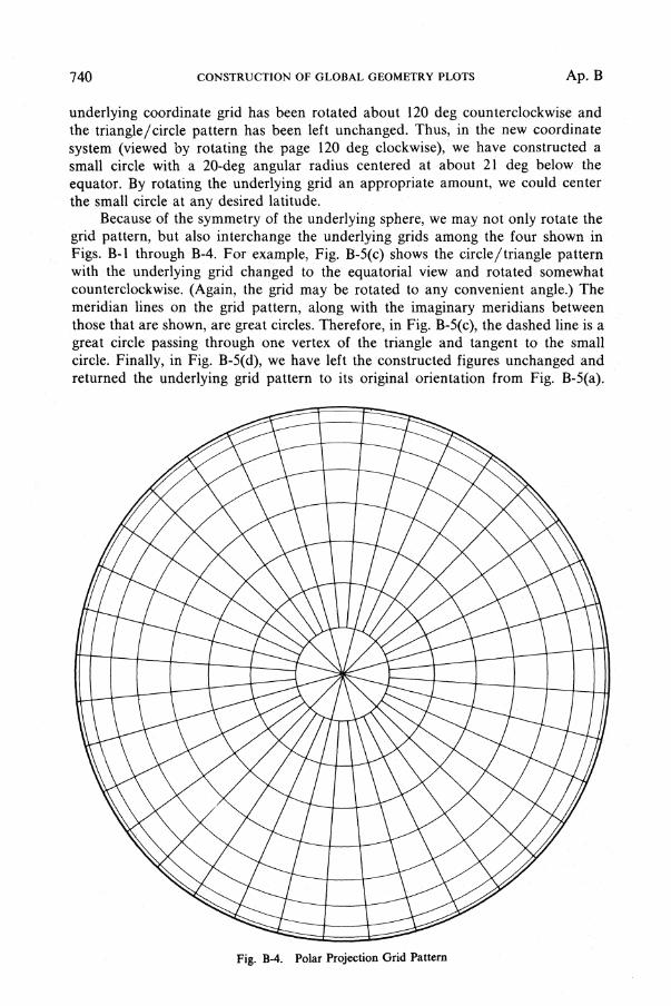
740 CONSTRUCTION OF GLOBAL GEOMETRY PLOTS Ap.B
underlying coordinate grid has been rotated about 120 deg counterclockwise and the triangle/circle pattern has been left unchanged. Thus, in the new coordinate system (viewed by rotating the page 120 deg clockwise), we have constructed a small circle with a 20-deg angular radius centered at about 21 deg below the equator. By rotating the underlying grid an appropriate amount, we could center the small circle at any desired latitude.
Because of the symmetry of the underlying sphere, we may not only rotate the grid pattern, but also interchange the underlying grids among the four shown in Figs. B-1 through B-4. For example, Fig. B-5(c) shows the circle/triangle pattern with the underlying grid changed to the equatorial view and rotated somewhat counterclockwise. (Again, the grid may be rotated to any convenient angle.) The meridian lines on the grid pattern, along with the imaginary meridians between those that are shown, are great circles. Therefore, in Fig. B-5(c), the dashed line is a great circle passing through one vertex of the triangle and tangent to the small circle. Finally, in Fig. B-5(d), we have left the constructed figures unchanged and returned the underlying grid pattern to its original orientation from Fig. B-5(a).
Fig. B-4. Polar Projection Grid Pattern

Ap.B CONSTRUCTION OF GLOBAL GEOMETRY PLOTS 741
(b)
(e) (d)
Fig. B-5. Construction of Global Geometry Plots. See text for explanation.
Thus, by using the grid pattern of Fig. B-1, we have constructed a great circle tangent to a small circle of 20-deg radius about the pole or, equivalently, at an inclination of 70 deg to the equator.
In practice, this construction is performed by first drawing the original figure of B-5(a), and then placing it on top of the equatorial view on a light table so that both grids can be seen. After rotating the grid patterns relative to each other until the desired orientation for the dashed curve is obtained, we can trace the dashed curve directly on the grid of Fig. B-5(a). This general procedure for drawing great and small circles by superposing grids on a light table (or window) and rotating them until the desired orientation is obtained has been used to construct nearly all the globe figures in this book. Note that whenever figures are constructed using superposed grids, the centers of the two grids must be on top of each other or, eqUivalently, the perimeters of the two grids must be superposed. This principle of grid

742 CONSTRUCTION OF GLOBAL GEOMETRY PLOTS Ap.B
superposition can be applied to the construction of various figures, as discussed below.
Constructing Great Circles Through Two Points. Figure B-1 is the basic figure for constructing all great circles on the celestial sphere, because all possible great circles are represented by the meridian lines on the figure and the imaginary meridians between the ones drawn. To construct a great circle between any two points of any of the globes, place the globe with the two points on top of a copy of Fig. B-l. Keeping the perimeters of the two figures superposed, rotate the globes relative to each other until the two points lie over the same meridian on the underneath grid. This meridian is then the great circle defined by the two points. Note that this great circle is most precisely defined when the two points are neady 90 deg apart and is poorly defined if the two points are nearly 0 deg or 180 deg apart.
Measuring Arc Lengths. The grid pattern in Fig. B-1 can also be used to measure the arc-length separation between any two points on the sphere. The parallels of latitude (i.e., the horizontal straight lines in Fig. B-1) are separated by 10 deg of arc along each meridian. Therefore, to determine the arc length between two points, superpose the globe with the two points over a copy of Fig. B-1 and rotate it until the meridian forming the great circle between the two points is found. The arc length is then determined by using the parallels of latitude along the meridian as a scale. For example, consider the dashed great circle in Fig. B-5(c). Because the triangle is a right equilateral triangle, the distance between any vertex and the opposite side must be 90 deg. This may be confirmed by counting the parallels of latitude along the dashed great circle. Also, the diameter of the small circle in Figs. B-5(b) and (c) may be measured along the meridian passing through the center of the circle. In both subfigures, the measured angular diameter is 40 deg, as required. Note that arc length must be measured along a great circle; it cannot be measured along parallels of latitude or other small circles.
Constructing Great Circles From General Criteria. In general, any great circle is constructed by first finding two points on it and then drawing the great circle between these points. For example, to draw a great circle at a given inclination to the equator, first pick the intercept point on the equator. Measure along the equator to the right or the left (depending on the slope desired) 90 deg and then up from the equator (along a meridian) an angle equal to the inclination. This point and the intercept point on the equator define the great circle. This method could have been used to construct the dashed great circle in Fig. B-5(c) directly without considering the tangent to the small circle.
Figure B-6 illustrates the procedure for constructing a great circle through a given point, A, perpendicular to a given great circle, AA'. Locate the point A' along the given great circle 90 deg from A by the method described above. Measure along the meridian through A' 90deg in either direction to the point B. The great circle through A and B is perpendicular to AA I.
Constructing Small Circles. This construction has already been demonstrated by the example of Fig. B-S. The method described there may be used to construct

Ap.B CONSTRUCTION OF GLOBAL GEOMETRY PLOTS 743
Fig. B-6. Construction of Great Circle AB Perpendicular to Great Circle AA'
small circles whose center is on the perimeter, 30 deg from the perimeter, 60 deg from the perimeter, or at the center. Small circles centered on the perimeter are straight lines on the plot and small circles centered in the middle of the plot are circles. The radius of the small circles constructed by this method is the colatitude (distance from the pole) of the parallel of latitude chosen on the underlying coordinate grid. For most purposes, one of these four sets of small circles is sufficient. They have been used for all of the constructions in this book. If it is necessary to construct a small circle at an intermediate arc distance from the perimeter, first construct a small circle of the desired radius at the desired latitude and as near the desired longitude as possible. Transform each point on this circle along a parallel of latitude a distance in longitude equal to the difference in longitude between the desired center and the constructed center. This procedure is illustrated in Fig. B-7.
Fig. B-7. Transforming a Small Circle in Longitude

APPENDIXC
MATRIX AND VECTOR ALGEBRA
C.I Definitions C.2 Matrix Algebra C.3 Trace, Determinant, and Rank C.4 Matrix Inverses and Solutions to Simultaneous Linear
Equations C.S Special Types of Square Matrices, Matrix Transforma-
tions C.6 Eigenvectors and Eigenvalues C.7 Functions of Matrices C.S Vector Calculus C.9 Vectors in Three Dimensions
C.I Definitions
F. L. Markley
A matrix is a rectangular array of scalar entries known as the elements of the matrix. In this book, the scalars are assumed to be real or complex numbers. If all the elements of a matrix are real numbers, the matrix is a real matrix. The matrix
All AI2 A ln
A21 A22 A2n =[ Aij] A= (C-l)
AmI Am2 Amn
has m rows and n columns, and is referred to as an m X n matrix or as a matrix of order m X n. The equation A = lAij] should be read as, "A is the matrix whose elements are Aij'" The first subscript labels the rows of the matrix and the second labels the columns.
Two matrices are equal if and only if they are of the same order and all of the corresponding elements are equal; i.e.,
A = B if and only if Aij= Bij; i= I, . .. ,m ;j= I, .. . ,n (C-2)
An n X n matrix is called a square matrix and is usually referred to as being of order n rather than n X n.
The transpose of a matrix is the matrix resulting from interchanging rows and columns. The transpose of A is denoted by AT, and its elements are given by
AT =[(AT)ij] =[ Aji] (C-3)
As an example, the transpose of the matrix in Eq. (C-l) is

C.I DEFINITIONS 745
It is clear that the transpose of an m X n matrix is an n X m matrix, and that the transpose of a square matrix is square. The transpose of the transpose of a matrix is equal to the original matrix:
(C-4)
The adjoint of a matrix, denoted by A t, is the matrix whose elements are the complex conjugates of the elements of the transpose of the given matrix, * i.e.,
The adjoint of the adjoint of a matrix is equal to the original matrix:
(At)t =A
The adjoint and the transpose of a real matrix are identical.
(C-5)
(C-6)
The main diagonal of a square matrix is the set of elements with row and column indices equal. A diagonal matrix is a square matrix with nonzero elements only on the main uiagonal, e.g.,
DII 0 0 0 D22 0
D= (C-7)
0 0 Dnn
The identity matrix of a given order is the diagonal matrix with all the elements on the main diagonal equal to unity. It is denoted by I, or by In to indicate the order explicitly. .
A matrix with only one column is a column matrix. An n X I column matrix can be identified with a vector in n-dimensional space, and we shall indicate such matrices by boldface letters, as used forvectors.t A matrix with only one row is a row matrix; its transpose is a column matrix, so we denote it as the transpose of a vector. The elements of a row or column matrix will be written with only one subscript; for example,
(C-8)
Bn
A set of m n X I vectors B('\ i = 1,2, ... , m, is linearly independent if and only if the only coefficients aj' i = 1,2, ... , m, satisfying the equation
m L ajB(j) = a.B(l)+ a2B(2) + ... +amB(m)=o (C-9)
.;=1
• The word adjoint is sometimes used for a different matrix in the literature. t Strictly speaking, a vector is an abstract mathematical object, and the column matrix is a concrete realization of it, the matrix elements being the components of the vector in some coordinate system.

746 MATRIX AND VECTOR ALGEBRA C.2
are aj = 0, i = 1,2, ... , m. There can never be more than n linearly independent n X I vectors.
C.2 Matrix Algebra
Multiplication of a matrix by a scalar is accomplished by multiplying each element of the matrix by the scalar, i.e.,
(C-lO)
Addition of two matrices is possible only if the matrices have the same order. The elements of the matrix sum are the sums of the corresponding elements of the matrix addends, i.e.,
A + B =[ Aij+ Bij]
Matrix subtraction follows from the above two rules by
(C-II)
(C-12)
Multiplication of two matrices is possible only if the number of columns of the matrix on the left side of the product is equal to the number of rows of the matrix on the right. If A is of order I X m and B is m X n, the product AB is the I X n matrix given by
(C-I3)
Matrix multiplication is associative
A(BC)=(AB)C (C-14)
and distributive over addition
A(B+ C)=AB+AC (C-15)
but is not commutative, in general,
AB =1= BA (C-16)
In fact, the products AB and BA are both defined and have the same order only if A and B are square matrices, and even in this case the products are not necessarily equal. For the square matrices A = U ~l and B = [~ ~l, for example, we have
AB=[19 43
22 ] =1= BA = [ 23 50 31
34 ] 46
If AB= BA, for two square matrices, A and B, we say that A and B commute. One interesting case is diagonal matrices, which always commute.
The adjoint (or transpose) of the product of two matrices is equal to the product of the adjoints (or transposes) of the two matrices taken in the opposite order:
(C-17)

C.2 MATRIX ALGEBRA 747
(C-18)
This result easily generalizes to products of more than two matrices. Multiplying any matrix by the identity matrix of the appropriate order, on the
left or the right, yields a product equal to the original matrix. Thus, if B is of order mXn,
(C-19)
The product of an n X m matrix and an m-dimensional vector (an m X I matrix) is an n-dimensional vector; thus,
(C-20)
A similar result holds if a row matrix is multiplied on the right by a matrix,
yT =XTAT = [ ~ Aji~l )=1
(C-21)
An important special case of the above is the multiplication of a I X n row matrix (on the left) by an n X I column matrix (on the right) which yields a scalar,
n
s=yTX= ~ Xj~ (C-22) j=1
For real vectors, this scalar is the inner product, or dot product, or scalar product of the vectors X and y. For vectors with complex components, it is more convenient to define the inner product by using the adjoint of the left-hand vector rather than the transpose. Thus, in general,
(C-23) ;=1
Note that, in general,
Y·X=(X·Y)* (C-24)
This definition reduces to the usual definition for real vectors, for which the inner product is independent of the order in which the vectors appear. Two vectors are orthogonal if their inner product is zero. The inner product of a vector with itself
n n
X·X= ~ X;*X;= ~ IXJ (C-25) ;=1 ;=1
is never negative and is zero if and only if all the elements of X are zero, i.e., if X = O. This product will be denoted by X2 and its positive square root by IXI or by X, ifno confusion results. The scalar IXI is called the norm or magnitude of the vector, X, and can be thought of as the length of the vector. Thus, with our definition of the inner product,
IXI =0 if and only if X=O (C-26)

748 MATRIX AND VECTOR ALGEBRA C.3
which would not be true if we defined the inner product using the transpose rather than the adjoint, because the square of a complex number generally is not positive.
If we multiply an n X I row matrix (on the left) by a I X m matrix (on the right), we obtain an n X m matrix. This leads to the definition of the outer product of two vectors
(C-27)
If the vectors are real, the adjoint of Y is the transpose of Y, and the ijth element of the outer product is Xi lj.
Matrix division can be defined in terms of matrix inverses, which are discussed in Section C.4.
C.3 Trace, Determinant, and Rank
Two useful scalar quantities, the trace and the determinant, can be defined for any square matrix. The rank of a matrix is defined for any matrix.
The trace of an n X n matrix is the sum of the diagonal elements of the matrix
n
trA == ~ Aii i=1
(C-28)
The trace of a product of square matrices is unchanged by a' cyclic permutation of the order of the product
n n n
tr(ABC)= ~ ~ ~ AijBjkCki=tr(CAB) ;=1 j=1 k=1
However, tr(ABC)'" tr(ACB), in general. The determinant of an n X n matrix is the complex number defined by
(C-29)
(C-30)
where the set of numbers {PI,P2"" ,Pn} is a permutation, or rearrangement, of {l,2, .. "n}. Any permutation can be achieved by a sequence of pairwise interchanges. A permutation is uniquely even or odd if the number of interchanges required is even or odd, respectively. The exponent P in Eq. (C-30) is zero for even permutations and unity for odd ones. The sum is over all the n! distinct permutations of {l,2, ... ,n}. It is not difficult to show that Eq. (C-30) is equivalent to
n ~ ;+j
detA = ~ (-1) AijMij (C-31) j=1
for any fixed i= 1,2, ... ,n, where Mij is the minor of Aij' defined as the determinant of the (n - I) X (n - I) matrix formed by omitting the ith row and jth column from A. This form provides a convenient method for evaluating determinants by successive reduction to lower orders. For example,
123 456 =lxI561-2XI461+3XI451 789 89 79 78
=(5 x9-8 X 6)-2(4X9-7 X6)+3(4X 8 -7 X 5)=0 (C-32)

C.4 MATRIX INVERSES AND SOLUTIONS TO SIMULTANEOUS LINEAR EQUATIONS 749
The determinant of the product of two square matrices is equal to the product of the determinants
det(AB)= (detA)(detB)
The determinant of a scalar multiplied by an n X n matrix is given by
det( sA) = sndetA
The determinants of a matrix and of its transpose are equal:
detAT =detA
Thus, the determinant of the adjoint is
detA t = (detA)*
(C-33)
(C-34)
(C-35)
(C-36)
The determinant of a matrix with all zeros on one side of the main diagonal is equal to the product of the diagonal elem~nts.
The rank of a matrix is the order of the largest square array in that matrix, formed by deleting rows and columns, that has a nonvanishing determinant. Clearly, the rank of an m X n matrix cannot exceed the smaller of m and n. The matrices A, AT, At, AtA, and AAt all have the same rank.
C.4 Matrix Inverses and Solutions to Simultaneous Linear Equations
Let A be an m X n matrix of rank k. An n X m matrix B is a left inverse of A if BA = In. An n X m matrix C is a right inverse of A if A C = 1m. There are four possible cases: k is less than both m and n, k = m = n, k = m < n, and k = n < m. If k is less than both m and n, then no left or right inverse of A exists. * If k = m = n, then A is nonsingular and has a unique inverse, A -I, which is both a left and a right inverse:
A - IA = AA - 1 = 1 (k=m=n) (C-37)
A nonsingular matrix is a square matrix with nonzero determinant; all other matrices are singular. If k = m < n, then A has no left inverse but an infinity of right inverses, one of which is given by
(k=m<n) (C-38)
If k = n < m, then A has no right inverse but an infinity of left inverses, one of which is
(k=n<m) (C-39)
A L or A R is called the generalized inverse or pseudoinverse of A. Consider the set of m simultaneous linear equations in n unknowns;
X I'X2'···,Xn ;
• It is possible to define a pseudoinverse for a general matrix, which in this case is neither a left nor a right inverse. In the other three cases, the pseudoinverse is identical with A -I, A R, and A L, respectively. The results on solutions of simultaneous linear equations can be generalized with this definition [Wiberg, 1971).

750 MATRIX AND VECTOR ALGEBRA C.5
AX=Y (C-40)
If k = m = n, then X = A - Iy is the unique solution to the set of equations. It folIows that a nonzero solution to A X = 0 is possible only if A is singular, i.e.,
AX=O for X:F 0, only if detA =0 (C-41)
If k = m < n, there are more unknowns than equations, so there are an infinite number of solutions. The solution with the smalIest norm, lXI, is
(C-42)
If k = n < m, there are more equations than unknowns; therefore, no solution exists, in general. However, the vector X that comes closest to a solution, in the sense of minimizing lAX - YI, is
(C-43)
Note that although AA L :F 1m , it is possible that AA Ly = Y for the particular Y in Eq. (C-40). In this case, Eq. (C-40) has a unique solution given by Eq. (C-43).
It is easy to see that if A is nonsingular, then A -I is nonsingular also and
(C-44)
Likewise, if A is nonsingular, then AT and A tare nonsingular and their inverses are given by
(ATfl =(A _I)T
(Atf'=(A-,)t
(C-45)
(C-46)
If two matrices, A and B, are nonsingular, their product is nonsingular also; and the inverse of the product is the product of the inverses, taken in the opposite order:
(C-47)
This result easily generalizes to products of more than two matrices. Various algorithms exist for calculating matrix inverses; several are described
by Carnahan, et ai., [1969] and by Forsythe and Moler [1967]. An example of a subroutine for this purpose is INVERT, described in Section 20.3.
C;S Special Types of Square Matrices, Matrix Transformations
A symmetric matrix is a square matrix that is equal toits transpose:
(C-48)
A skew-symmetric or antisymmetric matrix is equal to the negative of its transpose:
(C-49)
Clearly, a skew-symmetric matrix must have zeros on its main diagonal. An example of a skew symmetric matrix is 0 in Section 16.1. A Hermitian matrix is

C.S SPECIAL TYPES OF SQUARE MATRICES, MATRIX TRANSFORMATIONS 7S1
equal to its adjoint:
(C-SO)
A real symmetric matrix is a special case of a Hermitian matrix. An orthogonal matrix is a matrix whose transpose is equal to its inverse:
(C-51)
A unitary matrix is a matrix whose adjoint is equal to its inverse:
(C-S2)
A real orthogonal matrix is a special case of a unitary matrix. The product of two unitary (or orthogonal) matrices is unitary (or orthogonal). This result generalizes to products of more than two matrices. A similar result generally does not hold for Hermitian or symmetric matrices. A normal matrix is a matrix that commutes with its adjoint
AtA =AAt
Thus, both Hermitian matrices and unitary matrices are special cases of normal matrices.
By the rules for determinants of products and adjoints, it is easy to see that if A is unitary
IdetAl2 = 1 (C-S3)
Thus, detA IS a complex number with absolute value unity. Similarly, if A is orthogonal,
(detAf= I, detA = ± 1 (C-S4)
An orthogonal matrix with positive determinant is a proper orthogonal matrix; an orthogonal matrix is improper if its determinant is negative.
Let X be an n-dimensional vector and let A be an n X n matrix. Then A X is another n-dimensional vector and can be thought of as the transformation of X by A. If X and Yare two vectors, the inner product of AX and AY is
(AX)· (AY)= (AX)t(AY) = XtAtAY
If A is uni tary ,
(A X)· (A Y) = X . Y (C-55)
The dot product is unchanged if both vectors are transformed by the same unitary matrix. This result with X = Y shows that the norm of a vector is unchanged, too, so the unitary matrix can be thought of as performing a rotation of the vector in n-dimensional space, thereby preserving its length. If the vectors are real, the rotations correspond to proper real orthogonal matrices.
The transformations of a matrix are defined analogously to the transformations of a vector, but they involve mutliplying the matrix on both the left and right sides, rather than only on the left side. Several kinds of transformations are defined. If B is nonsingular, then
(C-56)

752 MATRIX AND VECTOR ALGEBRA C.6
is a similarity transformation on A. We say that As is similar to A. A special case occurs if B is unitary. In this case we have a unitary transformation on A,
Au= BtAB
A second special case occurs if B is orthogonal, in which case
Ao=BTAB
defines an orthogonal transformation on A.
(C-57)
(C-58)
It follows directly from the invariance of the trace to cyclic permutations of the order of matrix products, Eq. (C-28), that
and
tr As = tr Au = tr Ao = tr A
Also, by the rules on determinants,
detAs = detA u = detAo = detA
It is easy to see that
(C-59)
(C-60)
(C-61)
(C-62)
Thus, Au is Hermitian (or unitary) if A is Hermitian (or unitary), and Ao is symmetric (or orthogonal) if A is symmetric (or orthogonal).
C.6 Eigenvectors and Eigenvalues
If A is an n X n matrix and if
AX=AX (C-63)
for some nonzero vector X and scalar A, we say that X is an eigenvector of A and that A is the corresponding eigenvalue. We can rewrite Eq. (C-63) as
(A -AI)X=O
so we see from Eq. (C-41) that A is an eigenvalue of A if and only if
det(A -}..l)=O
(C-64)
(C-65)
This is called the characteristic equation for A. It is an nth-order equation for A and has n roots, counting multiple roots according to their multiplicity.
Because the equation AX=AX is unchanged by multiplying both sides by a scalar s, it is clear that sX is an eigenvector of A if X is. This freedom can be used to normalize the eigenvectors, i.e., to choose the constant so that X·X = 1. From n eigenvectors of A, X('\ i= 1,2, ... ,n, we can construct the matrix
x}I) x}2) XP) x}n)
X~I) X~2) XP) x~n) (C-66) p==
X(I) n X (2) n X (3) n
x(n) n

C.6 EIGENVECTORS AND EIGENVALUES 753
Matrix multiplication and the eigenvalue equation (Eq. (C-63» give
AIXl l ) A2X F) A x(n) .~
n I .":~~;, ,
A X(l) A2X12) A x(n)
AP= I 2 n 2
=PA (C-67)
A X(I) I n A x (2) 2 n
A x(n) n n
where A is the diagonal matrix
AI 0 0
0 A2 0 A= (C-68)
0 0 An
The matrix P is nonsingular if and only if the n eigenvectors are linearly independent. In this case,
(C-69)
and we say that A is diagonalizable by the similarity transformation P -lAP. If A is a normal matrix, we can choose n eigenvectors that are orthonormal, or simultaneously orthogonal and normalized:
x(i). xv) = 8i == { 0 , I i"'} i=}
(C-70)
When the eigenvectors are orthonormal, P is a unitary matrix and A is diagonalizable by the unitary transformation A = ptAP. Any square matrix can be brought into Jordan canonical form [Hoffman and Kunze, 1961] by a similarity transformation
(C·71)
where the matrix J has the eigenvalues of A on the main diagonal and all zeros below the main diagonal. It follows from Eqs. (C-71), (C-59), and (C-60) that the trace of A is equal to the sum of its eigenvalues, and the determinant of A is equal to the product of its eigenvalues; i.e.,
n
trA=L Aj (C-72) i= I
(C-73)
Many algorithms exist for finding eigenvalues and eigenvectors of matrices, several of which are discussed by Carnahan, et af., [1969] and by Stewart [1973]. Using Eq. (C-61), we can see that the eigenvalues of Hermitian matrices are real numbers and the eigenvalues of unitary matrices are complex numbers with absolute value unity. Because the characteristic equation of a real matrix is a polynomial equation with real coefficients, the eigenvalues of a real matrix must either be real or must occur in complex conjugate pairs.

754 MATRIX AND VECTOR ALGEBRA C.7
The case of a real orthogonal matrix deserves special attention. Because such a matrix is both real and unitary, the only possible eigenvalues are + 1, -1, and complex conjugate pairs with absolute value unity. It follows that the determinant of a real orthogonal matrix is (- l)m where m is the multiplicity of the root A= -I of the characteristic equation. A proper real orthogonal matrix must have an even number of roots at A= -I, and thus an even number for all A =1= 1, because complex roots occur in conjugate pairs. Thus, an n X n proper real orthogonal matrix with n odd must have at least one eigenvector with eigenvalue + 1. This is the basisof Euler's Theorem, discussed in Section 12.1.
It is also of interest to establish that the eigenvectors of a real symmetric matJix can be chosen to be real. The complex conjugate of the eigenvector equation, Eq. (C-63), is A X* = AX*, because both A and A are real. Thus, X* is an eigenvector of A with the same eigenvalue as X. Now, either X=X*, in which case the desired result is obtained, or X =1= X*. In the latter case, we can replace X and X* by the linear combinations X + X* and i(X - X*), which are real eigenvectors corresponding to the eigenvalue A. Thus, we can always find a real orthogonal matrix P to diagonalize a real symmetric matrix A by Eq. (C-69).
C. 7 Functions of Matrices
Let f(x) be any function of a variable x, for example, sinx or expx. We want to give a meaning to f(M), where M is a square matrix. If f(x)has a power series expansion about x = 0,
00
f(x)= L anxn (C-74) n=O
then we can formally (i.e., ignoring questions of convergence) define f(M) by
00
f(M)= L anMn (C-75) n=O
with the same coefficients an. It is clear that f(M) is a square matrix of the same order as M. If M is a diagonalizable matrix, then by Eq. (C-69),
M=PAP- I (C-76)
where P is the matrix of eigenvectors defined by Eq. (C-66), and A is the diagonal matrix of eigenvalues. Then,
Mn=(PAP-I)n=PNP- 1 (C-77)
and
f(AI) 0 0
f(M)=p(~oanAn )p-I=P 0 f(A2) 0
p- I (C-78)
0 0 f(An)
If M is a diagonalizable matrix, Eq. (C-78) gives an alternative definition of reM) that is valid when f(x) does not have a power series expansion, and agrees with Eq. (C-75) when a power series expansion exists.

c.s VECTOR CALCULUS 755
As an example, consider exp(!~t), where ~ is the 4x4 matrix introduced in Section 16.1,
0 W3 -W2 ~, I -W3 0 WI W2 ~=
W2 -WI 0 W3
-WI -W2 -W3 0
Matrix multiplication shows that ~2= -(wr+wi+wj)l= -w21, so it follows that
~2k = ( _ 1 )kw2k l
for all nonnegative k. Now,
00
=1 ~ k-O
where
~2k+1 =( _1)kw2k~
c=cos(iwt)
s=sin( iwt) i= 1,2,3
( 1 )2k+ I (_I)k 2(,)t
(2k+ I)!
(C-79)
This example shows that the matrix elements of f(M) are not the functions f of the matrix elements of M, in genera1.
C.8 Vector Calculus
Let cp be a scalar function of the n arguments X t,X2, ••• ,Xn• We consider the arguments to be the components of a column vector
X=[ X t,X2, ... ,Xn ]T
The n partial derivatives ofcp with respect to the elements of X are the components

756 MATRIX AND VECTOR ALGEBRA C.9
of the gradient of cp, denoted by
:~ = [ :; , :; , ... , :; ] I 2 n
(C-80)
Note that acp / a x is considered a I x n row matrix. If we eliminate the function cp from Eq. (C-80), we obtain the gradient operator
a _[ a a a ] a x = ax ' ax , ... , ax I 2 n
(C-81)
The matrix product of the I X n gradient operator with an n X I vector Y yields a scalar, the divergence of Y, which we denote by
a nay; ax·Y=.~ ax.
1=1 1 (C-82)
The dot is used to emphasize the fact that the divergence is a scalar, although the usage is somewhat different from that in Eq. (C-23).
The mn partial derivatives of an m-dimensional vector Y with respect to X I'X2, ... ,Xn can be arranged in an m X n matrix denoted by
l.Y =[ ay; 1 ax aXj (C-83)
This is like an outer product of Y and a / a x; however, the analogy is not perfect because the gradient operator appears on the right in the matrix product sense and on the left in the operator sense.
C.9 Vectors in Three Dimensions
In this section, we only consider vectors with three real components. For three-component vectors, three products are defined: the dot product, the outer product, and the cross product. The cross product, or vector product, is a vector define.d by
r U2V3- U3 V2]
UxY= U3 VI -UI V3
UI V2 - U2 VI •
The following identities are often useful:
U·y= UIVI + U2V2+ U3V3= UVcosO
IUxYI= UVsinO
where 0(0,0, 180°) is the angle between U and Y. In addition,
UxY=-YXU
U·(UXY)=O
UI U2 U3
U·(YXW)=Y·(WXU)=W·(UxY)= VI V2 V3 WI W2 W3
(C-84)
(C-85a)
(C-85b)
(C-86)
(C-87)
(C-88)

C.9 VECTORS IN THREE DIMENSIONS
[u ·(VXW)J2=(UXV). [(VXW) X (WX U) J
= U2V2W2 - U2(V . Wi - V2(U . Wi - W2(U . V)2
+ 2(U . V)(V . W)(W . U)
UX(VXW)=V(U ·W)-W(U· V)
0= U x (V x W) + V x (W x U) + W x (U x V)
(UX V)-(WXX)= (U· W)(V ·X)-(U ·X)(V· W)
757
(C-89)
(C-90)
(C-91)
(C-92)
The following identity provides a means of writing the vector W in terms of U, V, and UXV, if UxV~O:
[(UXV)·(UX V)JW = [(VXU)·(VXW)JU + [(U XV)·(U XW)JV
+ [W·(UXV)]UxV
If A is a real orthogonal matrix,
(AU)X(AV)= ±A(UXV)
(C-93)
(C-94)
where the positive sign holds if A is proper, and the negative sign if A is improper. The tangent of the rotation angle from V to W about U (the angle of the
rotation in the positive sense about U that takes V X U into a vector parallel to WxU) is
IUIU·(VxW) tan e= --------
U2(V' W) - (U . V)(U . W) (C-95)
The quadrant of e is given by the fact that the numerator is a positive constant multiplied by sin e, and the denominator is the same positive constant multiplied by cose. If U, V, and Ware unit vectors, e is the same as the rotation angle on the celestial sphere defined in Appendix A. Equation (C-95) is derived in Section 7.3. (See Eqs. (7-57).)
References
1. Bellman, R. E., Introduction to Matrix Algebra. New York: McGraw-Hill, Inc., 1960.
2. Carnahan, B., H. A. Luther and J. O. Wilkes, Applied Numerical Methods. New York: John Wiley & Sons, Inc., 1969.
3. Forsythe, George E., and C. Moler, Computer Solution of Linear Algebraic Systems. Englewood Cliffs, NJ: Prentice-Hall, Inc., 1967.
4. Halmos, P. R., ed., Finite-Dimension Vector Spaces, Second Edition. Princeton, NJ: D. Van Nostrand Company, Inc., 1958.
5. Hoffman, Kenneth and Ray Kunze, Linear Algebra. Englewood Cliffs, NJ: Prentice-Hall, Inc., 1961.
6. Noble, Ben, Applied Linear Algebra. Englewood Cliffs, NJ: Prentice-Hall, Inc., 1.969.
7. Stewart, G. W., Introduction to Matrix Computations. New York: Academic Press, Inc., 1973.
8. Wilberg, Donald M., State Space and Linear Systems, Schaum's Outline Series, New York: McGraw-Hill, Inc., 1971.

APPENDIXD
QUATERNIONS
Lawrence Fallon, III
The quaternion representation of rigid body rotations leads to convenient kinematical expressions involving the Euler symmetric parameters (Sections 12.1 and 16.1). Some important properties of quaternions are summarized in this appendix· following the formulation of Hamilton [1866] and Whittaker [1961].
Let the four parameters (ql,q2,q3,q4) form the components of the quaternion, q, as follows:
q=q4+ iql + jq2+ kq3 (0-1)
where i, j, and k are the hyperimaginary numbers satisfying the conditions
i2=/=k2=-1
ij=-ji=k
jk= -kj=i
ki= -ik=j (0-2)
The conjugate or inverse of q is defined as
q*=q4- iql-jq2- kq3 (0-3)
The quantity, q4' is the real or scalar part of the quaternion and iq I + jq2 + kq3 is the imaginary or vector part.
A vector in three-dimensional space, U, having components UI' U2, U3 is expressed in quaternion notation as a quaternion with a scalar part of zero,
(0-4)
If the vector q corresponds to the 'lector part of q (i.e., q = iq I + jq2 + kq3)' then an alternative representation of q is
(0-5)
Quaternion multiplication is performed in the same manner as the multiplication of complex numbers or algebraic polynomials, except that the order of operations must be taken into account because Eq. (0-2) is not commutative. As an example, consider the product of two quatenlions
q" = qq' = (q4 + iql + jq2 + kq3)( q~ + iq. + jq2 + kq;)
Using Eq~ (0-2), this reduces to
" '( , , , + ') q =qq = -qlql-q2q2-q3q3 q4q4
+ i(qlq~+ q2q;- q3q;'+ q4qD
+ j( - qlq; + q2q~ + q3q. + q4q;')
+ k( q)q;' - q2q. + q3q~ + q4q;)
(0-6)
(0-7)

Ap.O QUATERNIONS
If q' = (q~,q'), then Eq. (0-7) can alternatively be expressed as
q" =qq' = (q4q~-q'q',q4q' + q~q+qxq')
The length or norm of q is defined as
Iql=yqq* =yq*q =Vq~+ qi+ q~+ ql
759
(0-8)
(0-9)
If a set of four Euler symmetric parameters corresponding to the rigid body rotation defined by the transformation matrix, A (Section 12.1), are the components of the quaternion, q, then q is a representation of the rigid body rotation. If q' corresponds to the rotation matrix A', then the rotation described by the product A' A is equivalent to the rotation described by qq'. (Note the inverse order of quaternion multiplication as compared with matrix multiplication.)
The transformation of a vector U, corresponding to multiplication by the matrix A,
U'=AU
is effected in quaternion algebra by the operation
U'=q*Uq
(0-10)
(0-11)
See Section 12.1 for additional properties of quaternions used to represent rigid body rotations.
For computational purposes, it is convenient to express quaternion multiplication in matrix form. Specifically, let the components of q form a four-vector as follows:
q- [!~ 1 (0-12)
This procedure is analogous to expressing the complex number c = a + ib in the form of the two-vector,
In matrix form, Eq. (0-7) then becomes
[ q;' I [ q~ qi' = -q; q;' qi q4' - qi
-qi qi q4
-q; (D-13 )
Given the quaternion components corresponding to two successive rotations, Eq. (D~13) conveniently gives the quaternion components corresponding to the total rotation.
References
1. Hamilton, Sir W. R., Elements of Quaternions. London: Longmans, Green and Co., 1866.
2. Whittaker, E. T., A Treatise on the Analytical Dynamics of Particles and Rigid Bodies. C~bridge: Cambridge University Press, 1961.

APPENDIXE
COORDINATE TRANSFORMA nONS
Gyanendra K. Tandon
E.l Cartesian, Spherical, and Cylindrical Coordinates E.2 Transformations Between Cartesian Coordinates E.3 Transformations Between Spherical Coordinates
E.. Cartesian, Spherical, and Cylindrical Coordinates
The components of a vector, r, in cartesian, spherical, and cylindrical coordinates are shown in Fig. E~ 1 and listed below.
Cartesian (x,y,z)
Spherical (r,O,cp) Cylindrical (p, cp, z)
z
O~ __________ -+ ______ ~,-+y
" I /"---, , I // ~ " p I //x
, I / , I /
-------------~'~/ v
Fig. E-!. Components of a Vector, r, in Cartesian (x,y,z), Spherical (r,IJ,IjI), and Cylindrical (p,IjI,z) Coordinates
The declination, 8, used in celestial coordinates is measured from the equatorial plane (x-y plane) and is related'to 0 by the equation
~ =900 - 0 (E-I)
The components in cartesian, spherical, and cylindrical coordinates are related by the following equations:
x = FsinOcoscp
y = rsinO sincp
=pcoscp =psincp
(E-2a)
(E-2b)

E.2 TRANSFORMATIONS BETWEEN CARTESIAN COORDINATES 761
z = rcos8 =z (E-2c)
r=(x2+ y2+ z2)1/2 2 2 1/2 =(p +z ) (E-2d)
8=arccos{ z/(x2+ y2+Z2)1/2} = arc tan(p/ z) 0" 8" 1800 (E-2e)
</>= arc tan(y / x) =</> 0" </> < 3600 (E-2f)
2 1/2 p=(x2+ y ) =rsin8 (E-2g)
The correct quadrant for </> in Eq. (E-2f) is obtained from the relative signs of x andy.
E.2 Transformations Between Cartesian Coordinates
If rand r' are the cartesian representations of a vector in two different cartesian coordinate systems, then they are related by
r'=Ar+a (E-3)
where a represents the translation of the origin of the unprime.d system in the primed system and the matrix A represents a rotation. For most attitude work, a=O.
The transformation matrix A (called the attitude matrix or direction cosine matrix in this book) can be obtained by forming the matrix product of matrices for successive rotations about the three coordinate axes as described in Section 12.1. The elements of matrix A are direction cosines of the primed axes in the unprimed system and satisfy the orthogonality condition. Because A is an orthogonal matrix, its inverse transformation matrix will be its transposed matrix; symbolically,
A -I =AT (E-4)
For many applications, the definition of the direction cosine matrix in terms of the orthogonal coordinate unit vectors in the two coordinate systems,
[ i'·x x'·y " 'J x ·z
A= y'·x y.'.y y'·z (E-5a) z'·x z'·y z' ~z
is useful for computations. As an example, let the primed coordinate system have its coordinate axes aligned with the spacecraft-to-Earth vector R, the component of V perpendicular to R, and the orbit normal vector RXV /IRXVI, where V is the spacecraft velocity:
x'=R/IRI y'=(RXV)XR/I(RXV)XRI
z'=(RX V)/IR X VI (E-5b)
Then, substituting Eq. (E-5b) into Eq. (E-5a) gives an expression for A which does not require the evaluation of trigonometric functions.
Euler's Theorem. Euler's theorem states that any finite rotation of a rigid body can be expressed as a rotation through some angle about some fixed axis. Therefore, the most general transformation matrix A is a rotation by some angle,

762 COORDINATE TRANSFORMATIONS E.2
~, about some fixed axis, e. The axis e is unaffected by the rotation and, therefore, must have the same components in both the primed and the unprimed systems. Denoting the components of e by e l , e2, and e3, the matrix A is
[ costfl+ ef(I -oostfl) e\e2(I -costfl)+ e)sintfl e\eil-oostfl)- e2Sintfl]
A = e\eil-costfl)-e)sintfl costfl+ei(I -costfl) e2e3(l-costfl)+e\sintfl
e\e)(l-costfl)+ e2sintfl e2e)(l-costfl)- e\sintfl costfl+erO -costfl)
(E-6)
In this case, the inverse transformation matrix may be obtained· by using Eq. (E.4) or by replacing ~ by -~, in Eq. (E·6), that is, a rotation by the same amount in the opposite direction about the axis e.
Euler Symmetric Parameters. The Euler symmetric parameters, q\ through q4' used to represent finite rotations are defined by the following equations:
,~ ql=e\sln'2
Clearly,
The transformation matrix A in terms of Euler symmetric parameters is
[ q: - qi - q~ + q~
A = 2( qlq2 - q3q4)
2( qlq3 + q2q4)
2( qlq2 + q3q4)
- q: + q~ - q~ + q~ 2(q2q3-q\q4)
(E·7a)
(E-7b)
(E-8)
The inverse transformation matrix in this case may be obtained by use of Eq. (E~4), or by replacing QI,q2' and q3 by - ql' - q2' and - q3' respect~vely, in Eq. (E-8) and leaving q4 unaltered.
The Euler symmetric parameters may be regarded as components of a quaternion, q, defined by
(E-9)
where i, j, and k are as defined in Appendix D. The multiplication rule for successive rotations represented by Euler symmetric parameters is given in Appendix D. The Euler symmetric parameters in terms of the 3-1-3 Euler angle rotation cp, 0, I/; (defined below) are as follows:
q\ = sin(O /2)cos«cp- 1/;)/2)
q2 = sin(O /2)sin«cp- 1/;)/2)
q3 =cos(O /2)sin«cp+ 1/;)/2)
q4 = cos(O /2)cos«cp+ 1/;)/2) (E-IO)

E.2 TRANSFORMATIONS BETWEEN CARTESIAN COORDINATES 763
Gibbs Vector. The Gibbs vector (components gl' g2' and g3) representation (see Section 12.1) for finite rotations is defined by
gl == qll q4 = el tan(~ 12)
g2 == q21 q4 = e2tan(<p 12)
g3 == q31 q4 = e3tan(<p 12) (E-ll)
The transformation matrix A in terms of the Gibbs vector representation is as follows:
2(gl g2+ g3)
1- gf+ gi- gj
2(g2g3- gl)
The inverse of A can be obtained in this case by the method of Eq. (E-4), or by replacing gj by - gj in Eq. (E-12).
Euler Angle Rotation. The Euler angle rotation (</>,(J,o/) is defined by successive rotations by angles </>, (J, and 0/, respectively, about coordinate axes i, j, k (Section 12.1). The i-j-k Euler angle rotation means that the first rotation by angle </> is about the i axis, the second rotation by angle (J is about the j axis, and the third rotation by angle 0/ is about the k axis. There are 12 distinct representations for the Euler angle rotation which divide equally into two types:
TYPE 1. In this case, the rotlltions take place successively about each of the three coordinate axes. This type has a singularity at (J = ± 90 deg, because for these values of (J, the </> and 0/ rotations have a similar effect.
TYPE 2. In this case, the first and third rotations take place about the same axis and the second rotation takes place about one of the other two axes. This type has a singularity at (J=O deg and 180 deg, because for these values of (J, the </> and 0/ rotations have a similar effect.
Table E-l gives the transformation matrix, A, for all of the 12 Euler angle representations. The 3-1-3 Euler angle representation is the one most commonly used in the literature. The Euler angles </>, (J, and 0/ can be easily obtained from the elements of matrix A. A typical example from each type is given below.
TYPE 1: 3-1-2 Euler Angle Rotation
</>= arc tan( - A211 A 22) 00;;;; </>< 3600
(J = arcsin(A 23) - 900 0;;;; (J 0;;;; 900
o/=arctan( - A \31 A 33) 00;;;; 0/<3600
(E-13a)
(E-13b)
(E-13c)
The correct quadrants for </> and 0/ are obtained from the relative signs of the elements of A in Eqs. (E-13a) and (E-13c), respectively.
TYPE 2: 3-1-3 Euler Angle Rotation
</>=arctan(A 311 - A 32)
(J = arc cos( A 33)
0/= arc tan(A 131 A 23)
00;;;; (J 0;;;; 1800
00;;;; 0/< 360 0
(E-14a)
(E-14b)
(E-I4c)

TY
PE
-1
E
UL
ER
AN
GL
E
RE
PR
ES
EN
TA
TIO
N
1·2
·3
1·3
·2
2·3
·'
2·'
·3
3-'·
2
3-2
-1
Tab
le
E-l
. T
he
Att
itude
M
atri
x,
A,
for
the
12
Pos
sibl
e E
uler
A
ngle
R
epre
sent
atio
ns
(S==
sine
, C
== co
sine
, I =
= x a
xis,
2 ==
Y ax
is,
3 ==
z ax
is)
TY
PE
-2
MA
TR
IX A
E
UL
ER
AN
GL
E
MA
TR
IX A
R
EP
RE
SE
NT
AT
ION
[~
C1/JS8~
+ S1/
JC~
-CI/J
S8C
4> +
SI/
J~
1 [ ·c
o S
8S¢
-SI/J
C8
-SI/
JS8~
+ C
I/JC4
> SI
/J58
C4>
+ CI/
J~
1·2
-1
SI/JS
O C.
I/JC
~ -S
I/JC
IJ~
SO
-C8~
COC~
CI/JS
O -S
I/JC
~ -CI/JC8~
[ ,,~
CwSO
C4>
+ S;J
J~
Co/ISO~ -So
/IC~
1 [ co
soc~
-58
CO
C4>
COS~
1·3
·1
-Co/
IS8
CwC8C~ -
S""
S¢
SI/JC
O So
/ISOC
4> -
Co/
IS¢
S1/J
58S¢
+ C
wC4>
So
/I58
-SwCOC~ -
Cw
S¢
[ ~~
58
-C8
S¢
1 [ C
wC
¢ -S
o/IC
8S¢
S>/IS
O
-CI/J
58C
4> +
SI/J
S¢
CI/J
C8
Co/IS
OS¢
+ S
o/IC
¢ 2
-1·2
SO
S¢
co
So/I5
8C4>
+ C
o/IS
¢ ":S
I/JCO
-S
o/I5
8S¢
+ C
o/IC4
> So
/IC~
+ C
o/IC
8S¢
-Cw
SO
[ "~.,
,,,.
SI
/JCO
-Co/
IS¢
+ S
I/JS8
C4>
1 [
'''''H
'' C
""so
-SI/
JC~
+ C
o/I5
8S¢
CI/JC
O
SI/J
S¢ +
CI/J
SOC4
> 2
-3·2
-SOC~
co
C8S
¢ -5
8
COC~
So/I
COC~
+ C
o/IS
¢ So
/ISO
[ ''''-....
Co/
IS¢
+ S
o/ISO
C4>
-So/
IC8
1 [ ""
~,, .•
C>/I
S~ +
SwC
8C4>
-CO
S¢
COC4
> S8
3
·1·3
-S
.,C
¢ -
Cw
CB
S¢
-sw
s¢
+ C
I/JCO
C4>
So/IC
4> +
CI/J
58S
¢ So
/I~
-CI/J
SOC
4>
CI/JC
O
SOS¢
-S8C~
[ ~~
CO
S¢
-so
1 [ ,,
,.,,~~.
Co/I
COS~
+ S
o/IC4
>
-Co/
IS¢
+ S
o/IS
OQ
p CI
/JC4>
+ S
o/I5
8S¢
SI/JC
O
3·2
·3
-So/
ICO
C4>
-C
o/IS
¢ -S
o/IC
OS~
+ C
o/IC4
>
SI/I
S¢
+ C
I/I58
C4>
-S
I/JC
~ +
CI/I
SOS¢
Co
/ICO
SOC~
SOS¢
-soc~
C"'~ +
So/
ICOC
~
-Sw
S¢
+ C
wCO
C4>
SO~
C""
C8S
¢ +
So/
IC~
-SwCOS~ +
Co/I
C4>
-Co/
IS¢
-Sw
C8C
4>
SOC~
-So/
IS¢
+ C
o/ICO
C4>
-C>/
ICO
S¢
-S>/
IC4>
SOS¢
-SI/
JC8S
~ +
Co/I
C~
Swso
1 C
wSO
C8
-C""
so
1 So
/ISO
·C8
1 1 1 1
-.l
0'1 +:-
(') o o ~ I:) Z
~ t'tl ~ (I) 2:l ~ ~ o z (I) tTl
N

E.3 TRANSFORMATIONS BETWEEN SPHERICAL COORDINATES 765
The correct quadrants for cp and t¥ are obtained from the relative signs of the elements of A in Eqs. (E-14a) and (E-14c), respectively.
Kinematic Equations of Motion. For convenience, the kinematic equations of motion (Section 16.1) for the 12 possible Euler angle representations are given in Table E-2. The kinematic equations of motion for other representations of the attitude matrix can be found in Section 16.1.
Table E-2. Kinematic Equations of Motion for the 12 Possible Euler Angle Representations (1:; x axis, 2:; y axis, 3:; z axis; WI' W2' w3 are components of the angular velocity along the body x, y, z axes.)
AXIS INDEX VALUES
SEQUENCE KINEMATIC EQUATIONS OF MOTION I J K
1·2 - 3 1 2 3 ; = (WI cos t/J - W J sin t/J ) sec 8 TYPE 1
2-3-1 2 3 1 8 = W J cos t/J + WI sin t/J
3- 1- 2 3 1 2 ~ = w K - (WI cos t/J - w J sin t/J ) tan 8
1-3-2 1 3 2 ; = (w I cos t/J + W J sin t/J ) sec 8
3 - 2 - 1 3 2 1 8 = W J cos t/J - WI sin t/J
2 - 1 - 3 2 1 3 $ = w K + (WI cos t/J + wJsin t/J) tan 8
1 - 2-1 1 2 3 ; = (wK cos t/J + W J sin t/J ) esc 8 TYPE 2
2-3-2 2 3 1 6 = W J cos t/J - w K sin t/J
3 -1 - 3 3 1 2 $ = wI - (wK cos t/J + w J sin t/J ) cot 8
1 - 3 - 1 1 3 2 ; = - (wK cos t/J - W J sin t/J ) esc 8
3-2-3 3 2 1 8 = w J cos t/J +wK sin t/J
2-1 -2 2 1 3 ~ =.wl + (wK eost/J - wJsin t/J )eot8
E.3 Transformations Between Spherical Coordinates
Figure E-2 illustrates the spherical coordinate system on a sphere of unit radius defined by the north pole, N, and the azimuthal reference direction, R, in the equatorial plane. The coordinates of point Pare (cp,O). A . new coordinate system is defined by the north pole, N', at (CPo' ( 0) in the old coordinate system. The new azimuthal reference is at an angle, cp~ relative to the·NN' great circle. The coordinates (cp',O') of P in the new system are given by:
cosO' = cos Oocos 0 + sin OoSin 0 cos(cp - CPo)
sin( cp' - cp~) = sin( cp - cpo)sin 0/ sin 0' (E-15)

766 COORDINATE TRANSFORMA nONS E.3
where 0 and 0' are both defined over the range 0 to 180 deg, and (<P - <Po) and W - <P~) are both in the range 0 to 180 deg or in the range 180 to 360 deg. Simplified forms of Eqs. (E-15) in two special cases are as follows:
Case I: <p=<p~=90°
cosO' = cos Oocos B + sin 0osinO sin <Po
cos <P' = - cos <Posin 0/ sin 0'
Fig. E-2. Transformation Between Spherical Coordinate Systems NR and N'R'
Case 2: <p=<p~=0
cos B' = cos Oocos 0 + sin Oosin 0 cos <Po
sin <p' = - sin <Posin 0 / sin 0 '
(E-16)
(E-17)
The most common spherical inertial coordinates for attitude analysis are the celestial coordinates (a,8) defined in Section 2.2. The right ascension, a, and the declination, 8, are related to <p and 0 by
a=<p
8=900 - 0 (E- 18)

APPENDIX F
THE LAPLACE TRANSFORM
Gerald M. Lerner
Laplace transformation is a technique used to relate time- and frequencydependent linear systems. A linear system is a collection of electronic components (e.g., resistors, capacitors, inductors) or physical components (e.g., masses, springs, oscillators) arranged so that the system output is a linear function of system input. The input and output of an electronic system are commonly voltages, whereas the input to an attitude control system is a sensed angular error and the output is a restoring torque. Most systems are linear only for a restricted range of input.
Laplace transformation is widely used to solve problems in electrical engineering or control theory (e.g., attitude control) that may be reduced to linear differential equations with constant coefficients. The Laplace transform of a real function, f( t), defined for real t > 0 is
e (f(t»== F(s)= (00 f(t)exp( - st)dt )0+
(F-l)
where 0+ indicates that the lower limit of the integral is evaluated by taking the limit as t~O from above. The argument of the Laplace transform, F(s), is complex,
s==(J+iw
where i==H. For most physical applications, t and w denote time and frequency, respectively, and (J is related to the decay time.
The inverse Laplace transform is
I jC+iOO e -1(F(s»==f(t)= -2 . F(s)exp(st)ds 7TI C-ioo
(F-2)
where the real constant C is chosen such that F(s) exists for all Re(s) > C, that is, to the right of any singularity.
Properties of the Laplace Transform and the Inverse Laplace Transform·. The Laplace transform and its inverse are linear operators, thus
e( af(t) + bg(t» = a e(f(t» + b e( g(t»
== aF(s) + bG(s)
e -1(aF(s)+ bG(s»= a e-I(F(s»+ be- I ( G(s»
= af(t) + bg(t)
where a and b are complex constants.
• For further details, see DiStefano, et 01., [I %7)
(F-3)
(F-4)

768 THE LAPLACE TRANSFORM Ap. F
The initial value theorem relates the initial value of J(t), J(O+), to the Laplace transform,
J(O+)= lim sF(s) s-.oo
(F-5)
and the final value theorem, which is widely used to determine the steady-state response of a system, relates the final value of f( t), f( 00), to the Laplace transform,*
J(oo) = limsF(s) s--->o
(F-6)
The Laplace and inverse Laplace transformations may be scaled in either the time domain (time scaling) by
E(J(t/a))=aF(as)
or the frequency domain (frequency scaling) by
E -l(F(as»= J(t/ a)/ a
The Laplace transform of the time-delayed function, J( t - to)' is
I.: (J(t - to» = exp( - sto)F(s)
(F-7)
(F-8)
(F-9)
where J(t - to) = 0 for t < to. The inverse Laplace transform of the frequency shifted function, F(s - so), is
(F-lO)
Laplace transforms of exponentially damped, modulated, and scaled functions are
I.: (exp( - at)J(t» = F(s+ a)
I.: (sinwtf(t» = [F(s - iw)- F(s + iw) J/2i E(coswtJ(t» = [F(s - iw)+ F(s + iw) J/2
E (tnf(t» = (- If dd;n F(s)
I.: (J(t)/t) = fooF(u)du s
(F-Ila)
(F-Ilb)
(F-Ilc)
(F-Ild)
(F-Ile)
The Laplace transform of the product of two functions may be expressed as the complex convolution integral,
1 f C + iOO E(J(t)g(t»= 2'lTi C-ioo F(w)G(s-w)dw (F-12)
Multiplying the Laplace transform of a function by s is analogous to differentiating the original function; thus,
• The final value theorem is valid provided that sF(s) is analytic on the imaginary axis and in the right half of the s-plane; i.e., it applies only to stable systems.

Ap.F THE LAPLACE TRANSFORM 769
(F-13)
Dividing the Laplace transform of a function by s is analogous to integrating the original function; thus,
e -1(F(s)j s)= {f(u)du (F-14)
The inverse Laplace transform of a product may be expressed as the convolution integral
e -1(F(s)G(s»= (I f(t)g(t-T)dT= (I g(t)f(t-T)dT Jo+ Jo+
(F-15)
which may be inverted to yield
F(s)G(s)= e (I f(t)g(t-T)dT= e (I g(t)f(t-T)dT Jo+ Jo+
(F-16)
A short list of Laplace transforms is given in Table F-I; detailed tables are given by Abramowitz and Stegun [1968], Korn and Korn [1968], Churchill [1958], and Erdelyi, et al., [1954].
Table F-1. Laplace Transforms
g(t) G(SI g(t) G(SI
dl SF(SI - 110+1 u It_.lt exp (-asl/s -d,
dl" 5" F(SI _.5"-1 110+1 , I/s2 -
"-2 dl I dl"-1 l d," - S ;;; ~+'" d,"-1 0+
," " 1/5"+1
,. na+lll S"+1 t
iflTldT exp (-atl 11 (5+al
F(SI/S
t" e • .p (-atl 11 (S+al0+1
," fltl (_I" dO F(S) sinwt wi (S2 +w21
dS" cos wt SI (S2 + w 2)
f(tl/, [ F (u)du exp (-at) sin wt wi ( (S+a)2 + w21
exp (-at) cos wt (S+a) I ( (S+0)2 + w21
flt/.) aF (as) (exp (-atl - exp (-b,) I I (a-bl 11 ( (S+a) (S+b) I
flt-'o) exp (-'oS) F(S) [a exp (-atl - b exp (-btl I I [b-al S/[ (S+a) (S+b) ,
sinh (atl a IIS2_a2 ) exp [t.o ) fltl F(S-So)
cosh (atl SI (S2_a2)
60 (t-a'" exp (-as)
NOTE: F(S) = I fit) exp (-stl d'; G(S) = 19h) exp (-stl dt
J o+ 10+ n DENOTES A POSITIVE INTEGER; a AND b DENOTE POSITIVE REAL NUMBERS.
"60 IS THE DIRAC DELTA FUNCTION.
t u IS HEAVISIDE·S UNIT STEP FUNCTION WHICH IS DEFINED BY u = 0 FOR, < a. u • 1 FOR t > a.

770 THE LAPLACE TRANSFORM Ap. F
Solution of Linear Differential Equations. Linear differential equations with constant coefficients may be solved by taking the Laplace transform of each term of the differential equation, thereby reducing a differential equation in t to an algebraic equation in s. The solution may then be transformed back to the time domain by taking the inverse Laplace transform. This procedure simplifies the analysis of the response of complex physical systems to frequency-dependent stimuli, such as the response of an onboard control system to periodic disturbance torques.
The solution to the linear differential equation
n d~ ;L ai(i? =x(t) 1=0
(F-17)
with an = 1 and forcing function x(t) is given by
(F-18)
n
where Xes)::::: E(x(t», r(s)::::: ~ ais i is the characteristic polynomial of Eq. (F-17) and i=O
are the initial conditions. Any physically reasonable forcing function, including impulses, steps, and
ramps, may be conveniently transformed (see Table F-I). The analysis of the algebraic transformed equation is generally much easier than the original differential equation. For example, the steady-state solution, f( 00), of a differential equation is obtained from the Laplace transform by using the final value theorem, Eq. (F-6).
The first term on the right-hand side of Eq. (F-lS) is the forced response of the system due to the forcing function and the second term is the free response of the system due to the initial conditions. The forced response, E -1(X(S)j ~(s», consists of two parts: transient and steady state.
Solving the differential equation (Eq. (F-17» is equivalent to finding the inverse Laplace transform of the algebraic functions of s in Eq. (F-I8). One technique involves expressing rational functions of the form
m n
R(s) = ~ his i j ~ ais i= N(s)n(s) (F-19) ;=0 ;=0
as a sum of partial fractions (n > m) using the fundamental theorem of algebra. The characteristic polynomial, r(s), may be factored as
r
Hs)= II (s+p;)mi (F-20) i= I

Ap.F THE LAPLACE TRANSFORM
where -Pi is the ith zero of r(s) with multiplicity mi and
The partial fraction expansion is
where
r mi C R(s)=bn + L L· ik k
;=1 k=1 (S+Pi)
C - 1 dm;-k [( + )miR()] ;k=(m;-k)! dsm;-k s Pi s S=-Pi
771
(F-21)
(F-22)
and bn =0 unless m = n. The coefficients Cit are the residues of R(s) at the poles - Pi- If no roots are repeated, Eq. (F-22) may be rewritten as
where
r. C R(s)=bn + L _il
;=1 s+p;
Cit =(s+ p;)R(s)ls= _PI
(F-23)
The zeros of r(s) may be determined using various numerical methods [DiStefano, et al., 1967].
The inverse Laplace transform of expressions in the form of Eq. (F-23) may be obtained directly from Table F-l. Other techniques for computing inverse Laplace transforms include series expansions and differential equations [Spiegel, 1965].
Example: Forced Harmonic Oscillator. The equation describing a I-degreeof-freedom gyroscope (Sections 6.5 and 7.S) is
d2tJ + D dO + KO = ~w(t) dt2 IG dt IG IG
(F-24)
where IG is the moment of inertia of the gyroscope about the output axis, D is the viscous damping coefficient about the output axis, K is the restoring spring constant about the output axis, L is the angular momentum of the rotor, and w(t) is the angular velocity about the input axis which is to be measured (see Fig. 6-45).
We assume that the input angular velocity is sinusoidal'" with amplitude, A, and frequency, we; i.e.,
(F-25)
The solution of Eq. (F-24) is given by (F-lS) as
(F-26)
°This is not as severe a restriction as it might seem because any physically reasonable w(t) may be expanded in a Fourier series. The result for a general w(t) is then obtained by linear superposition.

772
where
THE LAPLACE TRANSFORM
HS)=S2+ Ds/ fG+ K/ fG
X(s)= e(ALcos(,V/ fG )=ALs[ (S2+W;)IG]-1
OO=- 0lt=o
iJ = dO I 0- dt t=O
The characteristic polynomial, r(s), may be factored as
Hs)= (s+ PI)(S+ P2)
where
PI =-( D +1.y4KfG - D 2 ) I (2IG )
Ap.F
(F-27)
P2=-( D-l.y4KfG- D2 ) I (2IG) (F-28)
and we assume 4KfG-D 2>O. Substitution of Eq. (F-28) into Eq. (F-26) yields
O(t)=e- I[. ALs/fG j+e_I[DOo/fG+SOo+iJo] (F-29) (S2+w;)(S+ PI)(S+ P2) (s+ PI)(S+ P2)
The second term on the right-hand side of Eq. (F-29) is given in Table F-I as
(F-30)
The first term on the right-hand-side of Eq. (F-29) may be expanded in partial fractions as
e -I [ S ] = exp( - iWet) + exp( iWet) (S2+ w;)(s + PI)(S + P2) 2(pl - iWe)(P2 - iWe) 2(pl + iwe)(P2 + iWe)
1 ( Plexp( - Pit) P2exP( - P2t) } + ( ) 2 2 - 2 2 (F-31)
PI-P2 PI +We P2 +we
Equation (F-30) and the last term on the right-hand-side of Eq. (F-31) are the transient response of the system to the initial conditions and the forcing function. The transient response decays with a time constant and frequency given by
[Re(PI)r l = 'To=2IG/ D
Im(pl)=wl =V4KfG- D2 12IG (F-32)

Ap.F THE LAPLACE TRANSFORM 773
For t-H~J, the steady-state solution, the first two terms on the right-hand side of Eq. (F-31) dominate 8(t).These two terms may be rewritten as
(F-33)
where
DWe tanq,= 2
K-IGwe
Several features of gyroscope design are evident from these equations: I. The output response of the system to a constant or low-frequency input,
we~O, is linearly related to the input for t»'I"o; for example,
lim 8(t)=A (L/ K) "'e->O
2. The viscous damping constant, D, must be sufficiently high so that '1"0 is small compared with the gyro sampling period. However, if the damping is too high, the system output becomes frequency dependent and lags the input.
3. Systems with negligible damping, D~O, resonate at input frequencies near the characteristic frequency of the system,
wo=VK/IG
Integral Equations. Integral equations have the general form
y(t)= f(t)+ fU2k(u,t)y(u)du u\
(F-34)
where k(u,t) is the kernel of the equation. The limits of the integral may be either constants or functions of time. If u1 and u2 are constants, Eq. (F-34) is called a Fredholm equation, whereas if u1 is a constant and u2 = t,then Eq. (F-34) is called a Volterra equation of the second kind [Korn and Korn, 1968].
If the functional form of the kernel may be expressed as
k( u, t) = k( u - t) (F-35)
then the Volterra equation
y(t)= f(t) + fo1k(U- t)y(u)du (F-36)
may be solved by Laplace transform methods. Taking the Laplace transform of Eq. (F-36) and rearranging, we obtain
Y(s)= F(s)/(I- K(s» (F-37)

Ap.F
where Y(s) = e(y(t», F(s)= e(f(t», and K(s)= e(k(t», which may be solved for y(t) by taking the inverse Laplace transform.
774 THE LAPLACE TRANSFORM.
References
1. Abramowitz, Milton, and Irene A. Stegun, Handbook of Mathematical Functions. Washington, D.C., National Bureau of Standards, 1970.
2. Churchill, R. V., Operational Mathematics, Second Edition. New York: McGraw-Hill, Inc., 1958.
3. DiStefano, Joseph J., III, Allen R. Stubberud, and Ivan J. Williams, Feedback and Control Systems, Schaum's Outline Series. New York: McGraw Hill, Inc., 1967.
4. Erdelyi, A., et al., Tables of Integral Transforms. New York: McGraw Hill, Inc., 1954.
5. Korn, Granino A., and Theresa M. Korn, Mathematical Handbook for Scientists and Engineers. New York: McGraw Hill, Inc., 1968.
6. Spiegel, Murray R., Laplace Transform, Schaum's Outline Series. New York: Schaum Publishing Co., 1965.

APPENDlXG
SPHERICAL HARMONICS
John Aiello
Laplace's Equation, \l2U=0, can be written in the spherical coordinate system of Section 2.3 as:
a2u + I au + J.- a2u + cotO au + _1_ a2u =0 ar2 r ar r2 ao 2 r2 ao r2sin20 ell!>2 (G-l)
If a trial substitution of U(r,O,</» = R(r) YeO,</»~ is made, the following equations are obtained through a separation of variables:
d2R(r) dR(r) r2 __ +2r-d- -n(n+ I)R(r}=O (G-2)
dr2 r
a2y(o,</» ay(O,</» I a2y(O,</» --- +cotO ':'0 + -. -2 + n(n + I)Y(O,</»=o (G-3)
ao 2 v sm 0 a</>2
where n(n + 1) has been chosen as the separation constant. Solutions to Eq. (G-2) are of the form
R(r)=Arn+ Br-(n+l) (G-4)
Thus, solutions to Laplace's Equation (Eq. (G-I» are of the form
n =0,1,2, ... , (G-5)
These functions are referred to as solid spherical harmonics, and the YeO,</»~ are known as surface spherical harmonics. We wish to define U over a domain both interior and exterior to a spherical surface of radius r, and to have U continuous everywhere in the domain and to assume prescribed values Uo(O,</» on the surface. Under these conditions, Eq. (G-5) with B = 0 gives the form of U for the interior region of the sphere and with A = 0 represents its form in the exterior region.
To determine the surface spherical harmonics, the trial substitution
Y(O,</» = P(cosO)<fl(</» (G-6)
is made in Eq. (G-3). Multiplying by sin20/ p<fl and choosing a separation constant of m 2 yields
d2P(cosO) dP(cosO) [ m2 ] d0 2 +cotO dO + n(n+ 1)- sin20 P(cosO)=O
d2<fl(</» -- + m2<fl(</» =0
d</>2
The solutions to Eq. (G-8) are readily found to be
(G-7)
(G-8)

776 SPHERICAL HARMONICS Ap.O
11>( q,) = C cos mq, + S sin mq, (0-9)
in which m must be an integer, because 1I>(q,) is required to be a single valued function. Equatlon (0-7) can be rewritten substituting x=cosO as,
ddX[(I_x2)~~]+[n(n+I)- 1::2 ]P=O (0-10)
which is the generalized Legendre equation [Jackson, 1962]. For m = 0, the solutions to Eq. (0-10) are called Legendre polynomials and may be computed from either Rodrigues' formula
_ I (d)n 2 n Pn(x)- 2nn! dx (x -I) (0-11)
or from a recurrence relation convenient for computer use [Arfken, 1970].
Pn+ t(x)=2xPn(x) - Pn-t(x)- [xPn(x)- Pn-t(x) ]/(n + I) (G-12)
Rodrigues' formula can be verified by direct subs.titution into Eq. (0-10), and the recurrence relation can be verified by mathematical induction. When m i= 0, solutions to Eq. (0-10) are known as associated Legendre Junctions (of degree, n, and order, m), and may be computed by [Yevtushenko, et al., 1969]
(l-x2t/2 dn+m(x2_I)n Pnm(x) = rn! dxn+m (0-13)
or by [Heiskanen and Moritz, 1967]
P ( ) -2-n(l- 2)m/2.f;, (-l)k (2n-2k)! n-m-lk nm X - X k~O k!(n-k)!(n-m-2k)!x (0-14)
where / is either (n- m)/2 or (n-m-I)/2, whichever is an integer. Table 0-1 lists the associated Legendre functions up to degree and order 4 in terms of cosO [Fitzpatrick,1970].*
Table G-l. Explicit Forms of Associated Legendre Functions Through Degree n=4 and Order m=4
!';z 0 1 2 3 4
0 1
1 coso SIN 0
2 lcos2 8 -! 3 SIN 8 COS 0 3 SIN2 " 2 2 3 ~ (cos3 8 - ~ cos.) ~SIN 0 (COS2 8 - ;) 15 SIN2 0 COS 0 15 SIN3 0
4 ~(COS4._ !cos2.+~) ~ SIN 0 (cos3 8 - ~ COS 0) 10; SIN2 0 (cos20 - ;) 105 SIN3 tJ COS 8 106 SIN4 0 8 7 35
• Because Eq. (G-IO) is a homo'geneous equation in P, it does not define the normalizatio,:! o~ P. Equations (G-lI) and (G-13) define the conventional Neumann normalization, but other normahzatlOns are used (see Appendix H or Chapman and Bartels [1940D.

Ap.G SPHERICAL HARMONICS 777
Using Eq. (G-D), the functions Pnm can be shown to be orthogonal; that is,
f +l 2 (q+m)! Ppm (x)Pqm(x)dx = -2 -I ( _ ),8/ (G-15)
_I q+ q m.
where 8/ is the Kn;mecker delta. It is now possible towrite the complete solution to Laplace's equation as
00 n+ I n U(r,O,$)= L (7) L [CnmCosm$+ Snmsinm$ ]Pnm(cosO) (G-16)
n .. O m=O
describing the potential exterior to a spherical surface of radius a. Customarily, Eq. (G-16) is written in the form
00 n n+1 + L L (7) [Cnmcosm$+Snmsinm$]Pnm(COSO)
n=l m= I (G-17)
where In == Cno. Terms for which m = 0 are called zonal harmonics and the I n are zonal harmonic coefficients. Nonzero m terms are called tesseral harmonics or, for· the particular case of n = m, sectoral harmonics.
Visualizing the different harmonics geometrically makes the origin of the names clear. The zonal harmonics, for example, are polynomials incosO of degree n, with n zeros, meaning a sign change occurs n times on the sphere (0° ..: 0..: 180°), and the sign changes are independent of $. Figure G-l shows the "zones" (analogous to the temperate and tropical zones on the Earth) for the case of
Fig. G-!. Zones for P6(cos(J) Spherical Harmonics

778 SPHERICAL HARMONICS Ap.G
P6(COS(J). The tesseral and sectoral harmonics have n - m zeros for 0 0 < (J < 1800 ,
and 2m zeros for 00 ~ cp ~ 3600 • Figure G-2, the representation of P63(COS(J)cos3cp, illustrates the division of the sphere into alternating positive and negative tesserae. The word "tessera" is Latin for tiles, such as would be used in 'a mosaic. When n = m, the tesseral pattern reduces to the "sector" pattern in Fig. G-3.
Fig. G-2. P63(cos9)cos3</> Showing Alternating Positive and Negative Tesseral Harmonics
Fig. G-3. P66(cos9)cos6cp Showing Tesseral Pattern Reduced to Sectoral Pattern
For a more detailed discussion of spherical harmonics, see Hobson [1931].
References
I. Arfken, G., Mathematical Methods for Physicists. New York: Academic Press, Inc., 1970.
2. Chapman, Sydney, and Julius Bartels, Geomagnetism. Oxford: Clarendon Press, pp. 609-611, 1940.
3. Fitzpatrick, P. M., Principles of Celestial Mechanics. New York: Academic Press, Inc., 1970.
4. Hieskanen, W., and H. Moritz, Physical Geodesy. San Francisco: W. H. Freeman, 1967.
5. Hobson, E. W., The Theory of Spherical and EllipsOidal Harmonics. New York: Chelsea Publishing Co., 1931.
6. Jackson, John David, Classical Electrodynamics. New York: John Wiley & Sons, Inc., 1962.
7. Yevtushenko, G., et al., Motion of Artificial Satellites in the Earth's Gravitational Field, NASA, TTF-539, June 1969.

APPENDIX H
MAGNETIC FIELD MODELS
Michael Plett
Spherical Harmonic Model. This appendix presents some computational aspects of geomagnetic field models. A more qualitative description of the field characteristics is given in Section 5.1. As discussed there, the predominant portion of the Earth's magnetic field, B, can be represented as the gradient of a scalar potential function, V, i.e.,
B=-VV (H-I)
V can be conveniently represented by a series of spherical harmonics,
(H-2)
where a is the equatorial radius of the Earth (6371.2 km adopted for the International Geomagnetic Reference Field, IGRF); gnm and hnm are Gaussian coefficients (named in honor of Karl Gauss); and r, 0, and <p are the geocentric distance, coelevation, and East longitude from Greenwich which define any point in space.
The Gaussian coefficients are determined empirically by a least-squares fit to measurements of the field. A set of these coefficients constitutes a model of the field. The coefficients for the IGRF (Section 5.1; [Leaton, 1976]), are given in Table H-1. The first-order time derivatives of the coefficients, called the secular
Table H-l. IGRF Coefficients for Epoch 1975. Terms indicated by a dash (-) are undefined.
n m .(nT) hInT) g(nT/vr) h(nTlvr) n m g(nT) hInT) g(nTty,) hInT/v,)
1 0 -30186 -- 25.6 - 6 2 15 102 2.0 -0.1 1 1 -2036 5735 10.0 -10.2 6 3 -210 88 2.8 -0.2 2 0 -1898 - -24.9 -- 6 4 -1 -43 0.0 -1.3 2 1 2997 -2124 0.7 -3.0 6 5 -8 -9 0.9 0.7 2 2 1551 -37 4.3 -18.9 6 6 -114 -4 -0.1 1.7 3 0 1299 - -3.8 - 7 0 66 - 0.0 -3 1 -2144 -361 -10.4 6.9 7 1 -57 -88 0.0 -1.4
3 2 1296 249 -4.1 2.5 7 2 -7 -24 0.0 -0.1 3 3 805 -253 -4.2 -5.0 7 3 7 -4 0.6 0.3 4 0 951 - -0.2 - 7 4 -22 11 0.9 0.3 4 1 807 148 -2.0 5.0 7 5 -9 27 0.3 -0.7
4 2 462 -264 -3.9 0.8 7 6 11 -17 0.3 0.1 4 3 -393 37 -2.1 1.7 7 7 -8 -14 -0.5 0.8 4 4 235 -307 -3.1 -1.0 8 0 11 - 0.2 -5 0 -204 - 0.3 - 8 1 13 4 0.3 -0.2
5 1 388 39 -0.7 1.2 8 2 3 -15 0.0 -D." 5 2 275 142 1.1 2.3 8 3 -12 2 0.2 -0.2 6 3 -20 -141 -1.6 -2.0 8 4 -4 -19 -0.4 -0.3
5 4 -161 -99 -0.5 1.3 8 5 6 1 -0.3 0.4
5 5 -38 74 1.0 1.1 8 6 -2 18 0.6 -0.3 6 0 46 - 0.2 - 8 7 9 -6 -0.3 -0.6
6 1 57 -23 0.5 -0.5 8 8 1 -19 :"'0.1 0.3

780 MAGNETIC FIELD MODELS Ap.H
terms, are also given in Table H-1. With these coefficients and a definition of the associated Legendre functions, Pnm , it is possible to calculate the magnetic field at any point in space via Eqs. (H-I) and (H-2).
The coeffients of the IGRF assume that the Pnm are Schmidt normalized [Chapman and Bartels, 1940], i.e.,
(71 2 2(2-8~) )0 [P,:"(O)] sinOdO= 2n+I (H-3)
where the Kronecker delta, 8} = I if i = j and 0 otherwise. This normalization, which is nearly independent of m, is chosen so that the relative strength of terms of the same degree (n) but different order (m) can be gauged by simply comparing the respective Gaussian coefficients. For Schmidt normalization, the Pnm (0) have the form
m _{[ (2-8~)(n-m)! JI /2 (2n~ I)!!} . m
Pn (0)= ( + )1 ( _ )1 sm '(} n m. n m.
{ n-m (n-m)(n-m-I) n-m-
X cos 0 - 2(2n _ I) . cos 2fJ
+ cos 0-··· (n-m)(n-m-I)(n-m-2)(n-m-3) _ n-m-4 }
2 ·4(2n - I )(2n -- 3) (H-4)
where (2n-I)!!::::::1·3·5···(2n-I). The square root term in Eq. (H-4) is the only difference between the Schmidt normalization and the common Neumann normalization described in Appendix G. The computation time required for the field models can be significantly reduced by calculating the terms inEq. (H-4) recursively, i.e., expressing the nth term as a function of the (n - I)th term. The first step is to convert the coefficients in Table H-I from Schmidt to Gauss normalization, which saves about 7% in computation time [Trombka and Cain, 1974]. The Gauss functions, p n•m , are related to the Schmidt functions, Pnm , by
pm= S pn,m n n,m (H-5a)
where
S =[ (2-8~)(n-m)! JI/2 (2n-I)!! n,m- (n+m)! (n-m)! (H-5b)
The factors S are best combined with the Gaussian coefficients because n,m they are independent of r, 0, cf> and so must be calculated only once during a computer run. Thus, we define
gn,m:::::: Sn,mgnm
hn,m:::::: Sn,mhnm (H-6)
Using mathematical induction, it is possible to derive the following recursion relations for Sn.in:

Ap.H MAGNETIC FIELD MODELS
So,o= 1
s = S [2n-1 ] n,O n-I,O n n~1
( n - m + 1)( 8~ + I) m~ 1
n+m
The pn,m can be similarly obtained from the following recursion relations:
po,o=1
pn,n = sinOpn-I,n-1
pn,m = cosopn-I,m _ K n,mpn-2,m
where
n>1
n=1
781
(H-7)
(H-8)
(H-9)
Because the gradient in Eq. (H-I) will lead to partial derivatives of the pn,m, we need
apo,o --=0
ao
ap nn apn-In-I --' =(sinO) , +(coso)pn-I,n-I
ao ao n ~ 1 (H-IO)
a~;m = (cosO) ap~~I,m _ (sinO)pn-I,m _ Kn,m ap~~2'RI
Also note that
cos mq, = cos«m - 1 )q, + q,)
=cos«m - 1 )q,)cosq,- sinq,sin«m - 1 )q,) (H-II)
A similar recursion relation can be derived for sinmq,. The computational advantage of Eq. (H-II) is that it greatly reduces the number of times that sine and cosine functions must be calculated.
Given the coefficients gn,m and hn,m and recursion relations in Eqs. (H-7) ,through (H-ll), the field B is calculated from Eqs. (H-I) and (H-2). Specifically,
_ av k a n+2 n Br= ---a,:- = L (-;) (n+ I) L (gn,Rlcosmq,+hn,msinmq,)pn,m(O)
n=\ m=O
-I av k (a)n+2 n apn,RI(O) BO=-r--ao=- L -; L (gn,mcosmq,+hn,Rlsinmq,) ao
n= I m=O
. - 1 a V-I ~ (a)n + 2 . n B =-.---=-.- 4. - L m(-gn,msinmq,+hn,mcosmq,)pn,m(O) </> rsmO aq, smO n= \ r m=O
(H-12)

782 MAGNETIC FIELD MODELS Ap.H
Here, Br is the radial component (outward positive) of the field, Bo is the coelevation compo'1ent (South positive), and B</> is the a:.imuthal component (East positive). (See Fig. 2-5, Section 2.3.) The magnetic field literature, however, normally refers to three components X, Y, Z, consisting of North, East, and nadir relative to an oblate Earth. These components are obtained from Eq. (H-12) by
X (" North") = - Bocosf. - Brsin£
Y (" East") = B </> (H-13) Z (" Vertical" inward positive) = Besinf. - Brcosf.
where f. == A - 0 < 0.2 0, A is the geodetic latitude, and 0 == 90° - 0 is the declination. The correction terms in sin € are of the order of 100 nT or less [Trombka and Cain, 1974].
The geocentric inertial components used in satellite work are
Bx = (Brcoso + Bosino)cosa - B</>sina
By = (Brcos 0 + Bosin 0 )sin a + B </>cos a
Bz = (Brsino - B(Jcoso) (H-14)
Note that B is still a function of longitude, cp, which is related to the right ascension, a, by:
(H-15)
where aG is the right ascension of the Greenwich meridian or the sidereal time at Greenwich (Appendix 1).
Dipole Model. Equations (H-6) through (H-14) are sufficient to generate efficient computer code. However, for analytic purposes, it is convenient to obtain a dipole model by expanding the field model to first degree (n = 1) and all orders (m=O, I). Eq. (H-2) then becomes
= ~(g?a3cosO+ g/a3coscpsinO+ h/a3sincpsinO) r
(H-16)
The cosO term is just the potential due to a dipole of strength g?a3 aligned with the polar axis. (See, for example, Jackson [1965].) Similarly, the sinO terms are dipoles aligned with the x and y axes. Relying on the principle of linear superposition, these three terms are just the Cartesian components of the dipole component of the Earth's magnetic field. From Table H-I, we find that for 1978,
g?= - 30109 nT
g/= -2006 nT
h/=5704 nT
Therefore, the total dipole strength is
a3Ho=a3 [ gr + gr + hf]I/2 =7.943 x 10¹⁵ Wb·m
(H-17)
(H-18)

Ap.H MAGNETIC FIELD MODELS 783
The coelevation of the dipole is
o,;,=arccos( !:)= 168.6° (H-19)
The East longitude of the dipole is
</>:n=arctan( :~l)= 109.3° (H-20)
Thus, the first-order terrestrial magnetic field is due to a dipole with northern magnetization pointed toward the southern hemisphere such that the northern end of any dipole free to rotate in the field points roughly toward the north celestial pole. The end of the Earth's dipole in the northern hemisphere is at 78.6° N, 289.3° E and is customarily referred to as the "North" magnetic pole. Frequently, dipole models in the literature use the coordinates of the North magnetic pole and compensate with a minus sign in the dipole equation.
The above calculations were performed for 1978 by adding the secular terms to the Gaussian coefficients of epoch 1975. The location of the dipole in 1975 can be similarly calculated and compared with the 1980 dipole. That comparison yields a 0.45% decrease in dipole strength between 1975 and 1980 and a O.071-deg drift northward and a O.056-deg (arc) drift westward for a total motion of 0.09-deg arc.
The dipole field in local tangent coordinates is given by
B, = 2 ( ~ r[ g?cosO + (gicos</> + hlsin</> )sinO]
B8 = ( ~ ) 3[ g?sinO - (gIcos</> + hlsin</> )cos 0]
Bep = (~f[ glsin</>- hlcos</>]
(H-21)
The field could be converted to geocentric inertial coordinates using Eq. (H-14), but the exercise is arduous and not particularly instructive. However, we may take advantage of the dipole nature of the dominant term in the field model to approximate the magnetic field of the Earth as due to a vector dipole, m, whose magnitude and direction are given by Eqs. (H-t8) through (H-20). Thus,
(H-22)
where R. is the position vector of the point at which the field is desired. Because this is a vector equation, the components of B may be evaluated in any convenient coordi'.late system. As an example, the field in geocentric inertial components can be obtained from the dipole unit vector,
[sinO';' cosam]
m= sinO';' sinam
cosO';' (H-23)

784 MAGNETIC FIELD MODELS Ap.H
where aGO is the right ascension of the Greenwich meridian* at some reference time (aGo=98.8279° at Oh UT, December 31, 1979), daG/dt is the average rotation rate of the Earth (360.9856469 deg/day), t is the time since reference, and (0';',</>;") =(168.6°,109.3°) in 1978.
Then
(H-24)
where Rx, Ry , and Rz are the geocentric inertial direction cosines of R. The field components are
a3HO .' . I
Bx= 7(3 (m.R)Rx-smOmcosam]
a3H . By = R 30 (3 (m· R)Ry - sin 0';' sin am ] (H-25)
a3HO • Bz = 7 [3 (m·R)Rz -cosO';']
These equations are useful for analytic computations and for checking computer calculations. For example, if R is in the Earth's equatorial plane, then Rz =0 and
a3HO Bz = 7( -cos 168.6°) (H-26)
which is positive, i.e., north. Because the direction of the field line is customarily defined as that indicated by a compass needle, Eq. (H-22) is self-consistent.
For analytical work, the most useful coordinate system is the I, b, n orbit plane system (Section 2.2), in which R has the particularly simple representation
R. = R (V')COS v'
Rb = R ( v')sin v'
Rn=O
(H-27)
where v'is the true anomaly measured from the ascending node. Vectors are transformed into the [,b,n system from the geocentric inertial system by first rotating about the inertial z axis through n, the right ascension of the ascending node, followed by a rotation about the ascending node by the angle i, the orbital inclination. Using this transformation, the unit magnetic dipole is
m,= sinO';'cos(n- am)
mb = - sin O';'cos i sin(n - am) + cos 0';' sin i
mn = sin 0';' sin i sin (n- am) + cos 0';' cos i
(H-28)
• This technique of cOlfiiJuting aG is good to about 0.005° for I year on either side of the reference date. At times m~rll'distant from the reference date, a new aGO can be computed as described in Appendix J. Note that aGO is equal to the Greenwich sidereal time at the reference time of ()h UT, December 31, 1978.

Ap.H MAGNETIC FIELD MODELS 785
where Q is the ri5ht ascension of the ascending node and i is the inclination of the orbit.
Substituting Eqs. (H-27) and 01-28) into Eq. (H-22) yields the magnetic field in the I, b, n system. Although the equations are moderately complex, they can still be useful. Due to the simple form for R, especially for circular orbits, it is possible to analytically integrate the torque due to a spacecraft dipole moment as has been done for ITOS [Kikkawa, 1971].
A circular equatorial orbit is particularly simple because i = Q = 0 and, therefore,
m· R = sin():n (cos amcos v' + sinamsinv')
Substituting into Eq. (H-22) and simplifying yields
a 3H B{= ~sin():n[3cos(2v' - am) +cosam ]
2R
(H-29)
(H-30)
As in Eq. (H-26), the minus sign in the orbit normal component, Bn assures the northward direction of the field lines.
The torque resulting from a spacecraft magnetic dipole interacting with Bn is in the orbit plane, or, in this case, the equatorial plane. This torque causes precession around the orbit normal, or, for i = 0, right ascension motion. Torque out of the orbit plane is caused by the ascending node component B{ and the component Bb • For i = 0, out of plane is the same as declination motion. Thus, for an equatorial orbit, the ratio of declination motion to right ascension motion is at most on the order of
- - -04 1 B{,b 1_1 2 sin():n 1-Bn - cosO:n .
(H-31)
Consequently, for a satellite in an equatorial or low-inclination orbit, the right ascension is the easier to control.
Note that the declination terms BJ and Bb in Eq. (H-30) oscillate with a frequency of twice the orbital period. That is, the direction of the magnetic field in the orbit plane system rotates through 720 deg during the orbit.
Thus, B j and Bb change signs four times during the orbit. Declination motion then can be obtained in a certain direction by switching the polarity of the magnetic control coil four times or every quarter orbit. This is the basis for QOMAC control theory. If the satellite has a residual magnetic dipole, the Bn term will cause a secular drift in right ascension and the BJ , Bb terms will cause an oscillation in declination at twice the orbital period and a diurnal oscillation in declination due to the rotation of the Earth.

786 MAGNETIC FIELD MODELS Ap.H
References
1. Leaton, B. R., "International Geomagnetic Reference Field 1975," Trans., A mer. Geophysical Union (Eff)S), Vol. 57, p. 120, 1976.
2. Chapman, Sydney and Julius Bartels, Geomagnetism. Oxford, Clarendon Press, 1940.
3. Trombka, B. T. and J. C. Cain, Computation of the IGRF I. Spherical Expansions, NASA X-922-74-303, GSFC, Aug. 1974.
4. Jackson, John David, CLassical Electrodynamics. New York: John Wiley & Sons, Inc., 1965.
5. Kikkawa, Shigetaka, Dynamic Attitude Analysis Study, Compo Sc. Corp., CSC 5023-10000-0ITR, Jan. 1971.

APPENDIX I
SPACECRAFT AlTITUDE DETERMINATION AND CONTROL SYSTEMS
Ashok K. Saxena
1.1 Spacecraft Listed by Stabilization Method 1.2 Spacecraft Listed by Attitude Determination Accuracy
Requirements 1.3 Spacecraft Listed by Type of Control Hardware 1.4 Spacecraft Listed by Type Of Attitude Sensors
This appendix summarizes spacecraft attitude systems and serves as a guide to mission specific attitude determination and control literature. The main table is an alphabetical listing of satellites by acronym with pertinent data as available. Subsequent sections list these spacecraft by stabilization method, accuracy requirements, control system, and sensor system. For example, if you are interested in gravity-gradient stabilization in low-Earth orbit, Section I.l lists DODGE, GEOS-3, and RAE-2 as gravity-gradient stabilized. The main table lists GEOS-3 as the only one of these in low-Earth orbit. Normal automated literature search procedures may then be used to obtain available literature citations for GEOS-3.
The material in this appendix has been collected from literature searches, the TRW Space Log, and Joseph and Plett [1974]. Design values are quoted for upcoming spacecraft, which are denoted by an asterisk after the spacecraft acronym. The superscript "b" is used for body and "w" is used for wheel.
1.1 Spacecraft Listed by Stabilization Method
Missions with mutiple phases (e.g., RAE-2) are listed in all appropriate categories.
Single Spin AEROS-I,2, ALOUETTE-I,2, ARIEL-III, ARYABHATA, ATS-3, CTS, DEA*, ESRO-IV, GOES-I, HEAO-I,C, HEOS-I, IMP-6,7,8, ISEE-I,B,C*, ISIS-I, II, ISS, IUE, LES-5,7, RAE-2, SIRIO, SM-3, SMS-I,2, SKYNET (U.K.I,2), SSS-I
Dual Spin ANS, ATS-6, DODGE, FLTSATCOM, HEAO-B*, IUE, NIMBUS-5,6, OAO-2,3, OGO-I, SAGE*, SEASAT*, SMM*, ST, SYMPHONIE
Momentum Wheels ANS, ATS-6, DODGE, FLTSTCOM, HEAO-B*, IUE, NIMBUS-5,6, OAO-2, 3, OGO-I, SAGE*, SEASAT*, SMM*, ST, SYMPHONIE
Gravity Gradient DODGE, GEOS-3, RAE-2
Magnetic AZUR-I, HCMM*
Gas Jets HEAO-I,C·

788 SPACECRAFT ATTITUDE SYSTEMS Ap. I
ORBIT PARAMETERS ACRONYM NAME PRINCIPAL MASS LAUNCH DATE
COUNTRY (KG I AND VEHICLE INeLlNA· PEAIGEE APOGEE' PERIOD nON HEIGHT H~~rT IDEGI IKMI (MINUTES)
AE·3 ATMOSPHERE USA 454 PLUS DEC. 16, 1973, 68.1 150 4,300 130 EXPLORER·3 PROPEL· BY DELTA LANT
AE·5 ATMOSPHERE USA 454 PLUS NOV. 19, 1975, 19 159 1,618 102.7 EXPLORER·S PROPEL· BY DELTA LANT
AEM GENERAL NAME FOR USA APPLICATIONS ex-PLORER MISSION; e.g., HCMM-. SAGE·
AEROS-' AERONOMY GERMANY 127 DEC. 16, 1972. 97.2 250 BOO 97.5 SATELLlTE-1 BY SCOUT SUN SVNrRONOUS
AEAOS-2 AERONOMY GERMANY 127 JUl Y 16, 1974, 96 .• 227 889 95.8 SATELlITE·2 BY SCOUT SUN SYNCHRONOUS
ALOUETTE-, CANADA 145.6 SEPT. 29,l962.BY THQR·AGENA 8
80.6 996 '.031 105.4
ALOUETTE·2 CANADA 146.1 NOV. 28, 1965.BY THQA·AGENA B
80.6 507 2,892 121.4
ANS NETHERLANDS NETHERLANDS 130 AUG. 30, 1974, BY 98.0 260 1,100 98.2 ASTRONOMICAL SCOUT SATELLITE
ARIEL·1I1 U.i<. MAY5,1967,BY 80 500 -500 96.6 SCOUT
AAYABI1ATA INDIA 360 APR. 19, 1975 50.4 S64 623 96.4
ATS·3 APPLICATIONS USA 361 NOV. 5, 1967, BY 0.4 35,772 1,436 TECHNOLOGY ATLAS- GEOSYN~HRONOUS SATELLlTE-3 AGENA 0
ATS·6 APPLICATIONS USA 1,360 MAY 30, 1974, 1.3 35,759 36.820 1,436 TECHNOLOGY BY TITAN·III C GEOSYNCHRONOUS SATELlITE-6
AZUR-1, GERMAN GERMANY 71.3 NOV. 8,1969, 102.9 239 1,955 121.8 ALSO RESEARCH BY SCOUT CALLED SATELLITE GRS-A
CTS COMMUNICATIONS CANADA JAN. 17. 1976, 0.1 35,786 1,436 TECHNOLOGY BY DELTA GEOSYNCHRONOUS SATELLITE
DE-A- DYNAMICS USA 2sa 1981. BY 90 275 23,918 417 EXPLORER·A DELTA
DE-O- DYNAMICS USA 305 1981,BY 90 276 1,200 100 EXPLOAER·B DELTA
DODGE OEPARTMEfoiT OF USA 195.2 JULY " 1967, 7.2 33,243 33,602 1,317 DEFENSE GRAVITY BY TITAN·III C eXPERIMENT
ERTS EARTH RESOURCES TECHNOLOGY SATEL· LITE RENAMEO LANDSAT
ESRO-IV EUROPEAN SPACE ESRO 120 NOV.21.1972, 91.06 254 1,143 99 RESEARCH BY SCOUT ORGANIZATION-IV
'PERIGEE AND APOGEE HEIGHT ARE MEASURED FROM THE SURFACE OF THE EARTH.

Ap. I SPACECRAFT ATTITUDE SYSTEMS 789
STABILIZATION ATTITUDE TECHNIQUE CONTROL HARDWARE POINTING ACCURACY ATTITUDE SENSORS MISSION OBJECTIVES
(SPIN RATE IN RPM)
DUAL SPIN MAGNETIC Z AXIS COil , ,0 BODY·MOUNTED IR HORI- ATMOSPHERE PROBE wb = 0.01-16 MAGNETIC SPIN COILS ZON SCANNERS WITH SOLAR ABSORPTION
Ww '" 214.4 MOMENTUM WHEEL WHEEL·MOUNTED IA EXPERIMENTS GAS JETS HORIZON SCANNERS
DIGITAL SUN SENSORS
DUAL SPIN MAGNETIC Z AXIS COIL ± ,0 BODY-MOUNTED IA HQRI· ATMOSPHERE PROBE wb '" 0.01-16 MAGNETIC SPIN COilS ZON SCANNERS
'" 214.4 MOMENTUM WHEEL WHEEL·MOUNTED IR
Ww GAS JETS HORIZON SCANNERS DIGITAL SUN SENSORS
SPIN wb ~ 10 MANUAL AND AUTO- ;!; 0.20 FOR SOLAR AS- TWO fA SENSORS AERONOMY, MEAS MATIe MAGNETIC PEeT ANGLE ANALOG FINE SUN SENSOR URES PHYSICAL COIL FOR PRECESSION DIGITAL SOLAR ASPECT PROPERTIES OF UPPER
SENSOR ATMOSPHERE IN COR· AUTOMATIC SPIN COR· ~ 3° FDA SOLAR AZI· THREE·AXIS MAGNE RELATION WITH EX RECTtON DURING DAY- MUTH TOMETEA TAE~E ULTRAVIOLET LIGHT RADIATION
SPIN wb ~ 10 MANUAL ,o\ND AUTO· .!. 0.2° FOR SOLAR AS· TWO IR SENSORS AERONOMY, MEAS MATIC MAGNETIC PECT ANGLE ANALOG FINE SUN SENSOR UAES PHYSICAL COl L FOR PRECESSION DIGITAL SOLAR ASPECT PROPERTIES OF UPPER
SENSOR ATMOSPHERE IN COR· AUTOMATIC SPIN COR ± 3° FOR SOLAR AZI- THREE·AXIS MAGNE RELATION WITH EX· RECTIQN DURING DA Y MUTH TOMETER TREME UL TRAVIQLET LIGHT RADIATION
SPIN wb - 1_43 MEASUREMENT OF EAATH'S IONOSPHE~E BY RADIO SOUNDING
SPIN wb = 2.25 IONOSPHERIC RESEARCH
MOMENTUM WHEELS THREE ORTHOGONAL ;!: 0.3° FOR SCAN AND STAR SENSOR ASTRONOMY ONBOARO COM- MOMENTUM WHEELS SLOW SCAN HORIZON SENSOR PUTER
X, Y, AND Z MAG- ~ 10 FOR STAR, OFFSET. SOLAR SENSOR NETIC COILS AND X·RAY MAGNETOMETEA
SPIN ~ 20 SOLAR ASPECT SENSORS MEASURE VERTICAL DISTRIBUTION OF MOLECULAR OXYGEN, MAP RADIO FREQUENCY NOISE IN GALAXY
SPIN wb = 10-90 NITROGEN JETS FOR ± 1° DIGITAL SOLAR SENSOR X·RAY ASTRONOMY SPIN TRIAXIAL FLUGATE SOLAR PHYSICS
MAGNETOMETER AERONOMY
SPIN wb = 100 HYDRAZINE JETS ! 1° STAR SENSOR COMMUNICATIONS V·SlIT SUN SENSOR METEOROLOGY SCANNING RADIOMETER
MOMENTUM WHEELS THREE MOMENTUM ± 0.1° IR EARTH SENSORS ERECT A LARGE AN-WHEELS DIGITAL SUN SENSORS TENNA STRUCTURE GAS JETS POLARIS TRACKER
INERTIAL REFERENCE PROVIDE GOOD TV GYROSCOPES SIGNAL TO LOW-COST INTERFEROMETER GROUND RECEIVERS
DEMONSTRATE USER-ORIENTED AP· PLICATION EXPERI-MENTS
PASSIVE MAGNETIC TWO FIXED MAGNETS ANGLE BETWEEN THE SUN SENSOR MEASUREMENT OF SUCH THAT THE RESULT GEOMAGNETIC FIELD RADIATION AND PAR-ING DIPOLE MOMENT VECTOR AND THE TWO·AXIS MAGNETOMETER TICLES IN THE POLAR POINTS IN THE DIREC· Z·AXIS WAS LESS ZONE AND IN THE TlON OF THE Z AXIS WITH THAN 120 VAN ALLEN BELT AN ACCURACY OF 8 MIN· UTES --
SPIN IN TRANSFER HYDRAZINE CATALYTIC ! 10 TRANSFER AND TWO NQNSPINNING EARTH COMMUNICATIONS AND DRIFT ORBITS THRUSTERS DRIFT ORBIT SENSORS wb = 60 TWO IR HORIZON SCANNERS
MOMENTUM WHEEL , 0,0 PITCH ANI NONSPINNING SUN SENSOR MOMENTUM WHEEL ROLL MISSION SPINNING DIGITAL SUN Ww = 3750 OABIT SENSOR
i 1.10 YAW
SPIN HYDRAZINE THRUSTERS ! 1° V·HORIZON SCANNERS INVESTIGATE ELECTRO· wb ~ 10 SUN SENSORS DYNAMIC EFFECTS IN
UPPER ATMOSPHERE
DUAL SPIN PITCH MOMENTUM WHEEL ! 10 HORIZON SCANNERS INVESTIGATE ELECTRO· wb:o 1 REV/OABIT MAGNETIC COILS SUN SENSORS DYNAMIC EFFECTS IN
HYDRAZINE THRUSTERS UPPEA ATMOSPHERE
GRAVITY-GRADIENT MOMENTUM WHEEL ! 16° SUN SENSORS DEMONSTRATE AUGMENTED BY TV CAMERAS GRAVITY-GRADIENT CONSTANT-SPEED STABILIZATION NEAR ROTOR AND MAG· GEOSYNCHRONOUS NETIC DIPOLE FOR ALTITUDE YAW
SPIN Wb = 65 MAGNETIC COilS ATTITUDE DETERMINA- IR HORIZON SCANNER STUDY NEAR-EARTH TION 1 20 DIGITAL SUN SENSOR MAGNETOSPHERE AND
IONOSPHERE ATTITUDE CONTROL i 50 TRIAXIAL FLUX GATE
MAGNETOMETEA

790 SPACECRAFT ATTITUDE SYSTEMS Ap. I
ORBIT PARAMETERS
ACRONYM NAME PRINCIPAL MASS LAUNCH DATE PERIGEE' APOGEE' CCUNTRV (KG} AND VEHICLE INeLlNA· PERIOD
TlON HEIGHT HEIGHT (MINUTES) IDEG) (KMI (KMI
eXPLORER GENERAL NAME GIV-EN TO SATELLITES; e.g .• EXPLORER-45 IS SAME AS SSS·1
FLTSATCQM FLEET SATELLITE USA 1.861 ATLAS- 1.436 COMMUNIt.;ATION CENTAUR GEOSYNCHRONOUS SYSTEM
GEOS-3 GfQDYNAMICS USA 340 APR. 9, 1975. 11. 83. 848 102 EXPERIMENTAL BY DELTA OCEAN SATEL-LlTE-3
GOES·' GEOSTATIONARY USA 295 OCT. 16, 1975. 1.0 35,770 35,796 1,435.9 OPERATIONAL BY DELTA GEOSYNCHRONOUS ENVIRONMENTAL SATELLITE·'
HCMM- HEAT CAPACITY USA -9' MAY 1978, 98 600 600 97 MAPPING MISSION BY SCOUT
HEAD·' HIGH ENERGY USA 3,150 AUG. 12. 1971, 22.75 .17 .3. 93 ASTRONOMY BY ATLAS· OBSERVATORY·' CENTAUR
HEAD-S- HIGH ENERGY USA 3,150 NOV. 1978, 22.75 - 435 -435 -9' ASTRONOMY BY ATLAS· OBSERVATORY ·B CENTAUR
HEAO·C· HIGH ENERGY USA 3,150 LATE 1979. 22.75 -- -- -95 ASTRONOMY BY ATLAS-OBSERVATORY ·C CENTAUR
HEOS-l HIGHLY ECCENTRIC ESRO 106 DEC. 5, 1968. 28.28 '2' 223,428 6,792 ORBIT SATELLITE BY DELTA
IMP-6 IN.TEAPLANETARY USA 286 MAR. 13, 1971. 28.8 148 122,146 5,628 MONITORING BY THOR·DELTA PLATFORM·6
IMP·7 INTERPLANETARY USA 376 SEPT. 23. 1972. 17.2 197,391 235.389 17,439 .MONITORING BY DELTA PLATFORM-7
IMP-8 INTERPLANETARY USA 371 OCT. 26. 1973, 28.2 196,041 235,754 17,362 MONITORING BY DELTA PlATFORM-8
ISEE·' INTERNATIONAL USA 31' OCT. 22, 1971, 28.4 288 134.000 2.29 SUN-EARTH BY DELTA DAYS EXPLORER-l
;
ISEE-S INTERNATONAL ESA 166 LAUNCHED 28.4 288 134,000 2.29 SUN-EARTH SIMULTANE- DAYS EXPLORER·S OUSlYWITH
ISEE·A ON THE SAME LAUNCH VEHICLE
ISEE·C· INTERNATIONAL USA - JULY 1978, IN PERI- APOHE- 1 YEAR SUN·EARTH BY DELTA EClIP· HELION LION AT EXPLORER-C TIC
PLANE2 AT 0.973 1~7 AU2
1515-1 INTERNATIONAL CANADA 238 JAN. 30, 1969. 88.43 .7. 3,522 128.3 SATELLITE FOR BY DELTA IONOSPHERIC STUDIES-l
ISIS-II INTERNATIONAL CANADA 284 APR. 1,1971. 88.16 1,356 1,423 113 SATELLITE FOR BY THOR-DELTA IONOSPHERIC STUDIES-2
ISS IONOSPHERE 135 - 70 -1,000 - r.ooo SOUNDING SATELLITE
ITOS-H '" IMPROVED TIROS USA 340 JULY 29. 1916, 102 1,507 1,522 116.2 NOAA·5 OPERATIONAL BY DELTA
SATELLlTE-8 = NA-TIONAL OCEANIC AND ATMOSPHERIC AD-MINISTRATION-S
'PERIGEE AND APOGEE HEIGHT ARE MEASURED FROM THE SURFACE OF THE EARTH.

Ap. I SPACECRAFT A TfITUDE SYSTEMS 791
STABILIZATION ATTITUOE TECHNIQUe CONTROL HARDWARE POINTING ACCURACY ATTlTUOE SENSORS MISSION OBJECTIVES
(SPIN RATE IN RPM'
MOMENTUM WHEELS THREE MOMENTUM" 1; 0.:20 TWO SPINNING EARTH WORLDWIDE COMMUNI· WHEELS AT 3000 t 300 SENSORS CATION SYSTEM FOR RPM, HYDRAZINE TWO SPINNING SUN SENSORS THE NAVY THRUSTERS ONE NONSPINNING EARTH SUPPORT AlA FORCE
SENSOR COMMANOANO TWO NONSPINNING SUN CONTROL SENSORS
GRAVITY GRADIENT' PITCH WHEEL ! 1.50 YAW THREE DIGITAL SUN SOLID EARTH PHYSICS DUAL SPIN REACTION BOOM :! 1.20 POINTING SENSORS AND OCEANOGRAPHY Ww = 2000 Z AXIS MAGNETIC COl L THREE-AXIS MAG-
NETOMETER
SPIN wb '" 90 HYDRAZINE JETS t 1.00 (TRANSFER ORBIT! FIVE fR HORIZON SCANNERS OPERATIONAL ! 0.10 (MISSION ORBIT) TWO OUAl-SLIT SUN METEOROLOGICAL
SENSORS SATELLITE
THREE·AXIS ONBOARD ONE MOMENTUM WHEEL ATTITUDE OETERMINA· ONE IR SCANNER MAP HEAT CAPACITY CONTROL. DUAL SPIN THREE MAGNETIC TION THREE DIGITAL SUN OF THE EARTH ""b" 1 REV/ORBIT COILS .t 0.70 IN ROLL.! 0.50 IN SENSORS
Ww = 1940 PITCH. :I: 20 IN YAW TRIAXIAL FLUX GATE ATTITUDE CONTROL MAGNETOMETER 1 10 IN ROLL AND PITCH 120 IN YAW
ONBOARD COMPUTER HYDRAZINE JETS , ,. COARSE SUN SENSORS ALL SKY X·AND SINGL~·AXIS SPIN, FINE SUN SENSORS GAMMA·RAY SURVEY TI1RE:E·AX1S TWO so x so FOV STABILIZED STAR TRACKERS
FOUR SOOF GYROSCOPES
ONBOARQ COMPUTER MOMENTUM WHEELS ONSOARD: 1 10 COARSE SUN SENSORS X·RAY TELESCOPE TO THREE·AXIS MAGNETIC COILS ARC MINUTE; FINE SUN SENSORS DETERMINE INTENSITY, STABILIZED HYDRAZINE JETS GROUND ATTITUDE THREE ;zo x ZO FOV SPECTRA, POSITION, AND
DETERMINATION: STAR TRACKERS TIME VARIATIONS OF 1 0.1 ARC MINUTE SIX SDOF GYROSCOPES X·RA Y SOURCES
ONBOARD COMPUTER HYDRAZINE JETS ATTITUDE CONTROL CO~RSE SUN SENSORS ALL SKY GAMMA·RAY SINGLE·AXIS SPIN· , ,. FINE SUN SENSORS SURVEY STABILIZED ATTITUDE DETERMINA· TWO so x so FOV
TION 10.050 STAR TRACKERS FOUR SDOF GYROSCOPES
SPINwti = 10 NITROGEN JETS TWO EARTH ALBEDO STUDY INTERPLANE· SENSORS TARY RADIATION. TWO SOLAR ASPECT SOLAR WIND, AND SENSORS MAGNETIC FIELDS SOLAR GATE SENSOR OUTSIDE THE
MAGNETOSPHERE
SPlNwb'" 5 FREON JETS ". OPTICAL HORIZON STUDY INTERPLANE· SCANNER TARY PARTICLES AND DIGITAL SUN SENSOR ELECTROMAGNETIC
RADIATION
SPIN w b " 46 FREON JETS , ,. OPTICAL TELES(X)PE STUDY SOLAR PLASMA, DIGITAL SUN SENSOR SOLAR WINO. SOLAR AND
. COSMIC RADIATION. ELECTROMAGNETIC FIELD VARIATIONS, EARTH'S MAGNETIC TRAIL
SPIN ""b .. 12-68 FREON JETS :l:O.SO OPTICAL TELESCOPE STUDY SOLAR PLASMA. DIGITAL SUN SENSOR SOLAR WIND, SOLAR
AND GALACTIC'COSMIC RAO,ATlON. ELECTRO· MAGNETIC FIELD VARI· ATIONS. AND INTER-PLANETARY MAGNETIC FIELD
SPINAwb '"' 20' COLO GAS JETS t.1o· PANORAMIC ATTITUDE ~DY MAGNETOSPHERE, SENSOR INTERPLANETARY SPACE SOLAR ASPECT SENSOR AND INTERACTIONS
BElWEEN THEM
SPINwb -20 COLD GAS JETS <"" V-SLiT COMBINED STUDY MAGNETOSPHERE. SUN/EARTH ALBEOO INTERPLANETARY SPACE SENSOR AND INTERACT'ONS
BETWeEN THEM
SPIN '"'b-20 HYORAZINE JETS < .0 PANORAMIC A"ITUDE STUDY MAGNETOSPHERE, SENSOR INTERPLANETARY SPACE SOLAR ASPECT SENSOR AND INTERAcrlONS
BETWEEN THEM
SPIN wb .. 2.938 MAGNETIC COIL WHEN MEASUREMENT OF COMMUTATEDWlTH EARTH'S IONOSPHERE SUN LINE OR GED- BY RADIO SOUNDING MAGNETIC FIELD VECTOR G'VES AT-TITUDE OR SPIN RATE CHANGE
SI"N'"'b- 2.9 MAGNETIC COIL FOR MEASUREMENT OF ATTtTUDE AND SPIN EARTH'S IONOSPttERE RAT~CHANGE BY RADIO SOUNDING
SPIN '"'b -'0 t. ,.SO IRSENSOR "!ORLD MAP OF ELEC-D'GITAL SUN SENSOR TRDN DENSITY OF THE MAGNETOMETER A~ERE
DUAL1IPIN MAGNEnC COILS SUFFICIENT TO MAIN- 'R HORIZON SENSORS METEOROLOG'CAL SATEL-"'b - • REVIORBIT TAIN CONSTRAINTS SOUUIASl'ECT SENSORS LITE .... -.40

792 SP ACECRAFT ATTITUDE SYSTEMS Ap. I
ACRONYM NAME PRINCIPAL MASS LAUNCH OATE COUNTRY !KG) AND VEHICLE
nOS-I", J" IMPAOVED TlROS USA DELTA OPERATIONAL SATELLlTE·I, J
tue' INTERNATIONAL USA 430 JAN. 26, 1978, ULTAAVIOLET BY AUG· EXPLOREA MENTED
THRUST DELTA
LANDSAT·' OAIGINAlLY USA 959 JULY 23, 1972, CALLED ERTS BY DELTA
LANDSAT-2 USA 959 JUNE 22, 1975, BY DELTA
LANDSAT·C· USA THIRD QUARTER 1977, BY DELTA
LANDSAT-O USA '" 1981
lE5-S liNCOLN EX- USA 102 JULY " 19!;57. PERIMENTAL BY TITAN-III C SATELUTE·5 (MULTIPLE PAY·
LOAD)
LES-7 LINCOLN EX- USA - 300 PERIMENTAL SATELLlTE·7
MAGSAr GEOMAGNETIC USA - 165 1979-1980 FIELD SATELLITE
MMS MUL TlMISSION MODULAR SPACE-CRAFT SERIES (e.g., SMM-)
NIMBUS-S USA 772 DEC. 1" 1972, BY DELTA
NIMBUS-6 USA 829 JUNE 12, 1975, BY DELTA
OAQ-2 ORBITING ASTRO- USA 1,998 DEC. 7, 1968, BY NOMICAL OBSER- ATLAS-VATOAY·2 CENTAUR
OAO·3 ORBITING ASTRO· USA 2,204 AUG. 21, 1972, NOMICAL OSSEA· BY ATLAS-VATORY·3, ALSO CENTAUR COPERNICUS
OGO-' ORBITING GEO- USA 487 SEPT. 4, 1964, PHYSICAL OBSERVA- BY ATLAS-TORY AGENA 8
050-7 ORBITING SOLAR USA 635 SEPT. 29, 1971, OBSERVATORY-7 BY DELTA
050-8 ORBITING SOLAA USA 1,090 JUNE 21,1975, OBSERVATORY-S BY DELTA
RAE-2 RADIO ASTRONOMY USA 205 JUNE 10, 1973, EXPLORER·2 (ORBIT) BY AUGMENTED
328 THRUST LONG-(LAUNCH) TANK DELTA
SAGe- STRATOSPHERIC USA -105 FEB. 1979 AEROSOL AND GAS· EXPERIMENT, ALSO KNOWN AS AEM·B-
SAS-2 SMALL ASTRONOMY USA 185 NOV. 15, 1972. SATELUTE-2 BY SCOUT
'PERIGEE AND APOGEE HEIGHT ARE MEASURED FROM THE SURFACE OF THE EARTH.
20RBIT ABOUT SUN·EARTH LAGRANGIAN p?INT L 1•
ORBIT PAAAMETERS
INeLlNA· PEAIGEE' APOGEE ' PEAIOD nON HEIGHT HEIGHT (MINUTES) loEG) {KM} (KMI
102 - 1,459 '" 1,466 115.2
28.7 25,706 45,876 1,436 ELLIPTICAL GEOSYNCHRONOUS
99 915 917 103.3
99 898 916 103.1
99 916 916 103.3
98 700 700 99
7.2 33,300 33,600 1,319
-0 NEAA GEOSTATIONARY
97 325 550 96
99.95 1,OB9 1,102 107.25
99_9 1,100 1,113 107.4
35 764 774 "100.3
35 738 750 99.7
31.1 260 150,000 64 HOURS
33 323 571 93.4
32.95 545.9 562.4 95.74
1,100 1,100 225 SELENQCENTAIC ORBIT
-so" -600 -600 - 97
2 443 632 96

Ap. I SPACECRAFT ATIITUDE SYSTEMS 793
STABILIZATION ATTITUDE TECHNIQUE CONTAOL HARDWARE POINTING ACCURACY ATTITUDE SENSORS MISSION OBJECTIVES (SPIN RATE IN RPMI
DUAL SPIN MAGNETIC COilS SUFFICIENT TO MAIN- IR HORIZON SENSORS METEOROLOGICAL SATEL· ~ • 1 REV/ORBIT TAIN CONSTRAINTS SOLAR ASPECT SENSORS LITES ww" '40
SPIN ABOUT AXIS HYDRAZINE JETS t ARC.sECOND PANORAMIC ATTITUDE UL TRAVIQLET SPECTRO-OF MINIMUM REACTION WHEELS SENSOR GRAPHY OF sye LLAR MOMENT OF IN· SPIN MOOE SUN SENSOR SOURCES ERTlA; THREE·AXIS FINE SUN SENSOR STABILIZED IN ANALOG SUN SENSOR MISSION NODE GYROSCOPES
FINE ERROR SENSOR
DUAL SPIN ATTITUDE CONTROL HORIZON SENSORS EARTH'S RESOURCES ± 0.70 ATTITUDE DETERMINA· TION ! 0.07°
DUAL SPIN ATTITUDE CONTROL HORIZON SENSORS EARTH'S RESOURCES t 0.70 ATTITUDE DETERMINA· TION to.07°
DUAL SPIN ATTITUDE CONTROL HORIZON SENSORS EARTH'S RESOURCES t 0.70 ATTITUDE DETERMINA-TION t 0.070
MMSPACKAGE ! 0.010 TWO STAR TRACKERS EARTH SURVEY ISEE SMM) GYROSCOPES
THEMATIC MAPPER FOR LANDMARK TRACKING
SPIN wb '" 10 TWO ORTHOGONAL ,,. EARTH SENSOR WITH EXPERIMENTAL SATEL· MAGNETIC COILS 3 FAN BEAM FIELD 4.TE
OF VIEW FOUR SOLAR GATE SENSORS
SPIN w w " 1100 GIMBALED FL VWHEEL to.l° IA EARTH SENSORS EXPERIMENTAL SATEL-PLASMA JETS LITE
DUAL SPIN MAGNETIC COILS ATTITUDE DETERMINA- TWO STAR CAMERAS ACCURATE MAPPING OF TION: 20 ARC-SEC FINE SUN SENSOR THE EARTH'S MAGNETIC
GYROSCOPES FIELD ATTITUDE TRANSFER STUDY OF THE EARTH'S SYSTEM CRUST, MANTLE, AND
CORE
MOMENTUM WHEELS FOUR MOMENTUM 01 0 HORIZON SENSORS METEOROLOGICAL WHEELS (TWO ON ROLL AXIS)
MOMENTUM WHEELS FOUR Mt')MENTUM , ,0 HORIZON SENSORS METEOROLOGICAL WHEELS (TWO ON ROLL AXIS)
MOMENTUM WHEELS THR EE MOMENTUM t 0.020 STAR TRACKER ULTRAVIOLET ASTRONOMY WHEELS RATE INTEGRATING
GYROSCOPES
MOMENTUM WHEELS THREE MOMEN'rUM t 0.1 ARC·SEC = FOUR GIMBALED ULTRAVIOLET ASTRONOMY WHEELS 3 x 10⁻⁵ DEG STAR TRACKERS
RATE·INTEGRATING GYROSCOPES
MOMENTUM WHEELS THREE MOMENTUM ! 20 TWO HORIZON GEOPHYSICAL WHEELS TRACKERS AIR JETS YAW AND SOLAR ARRAY
SUN SENSORS PITCH RATE GYROSCOPES
DUAL SPIN Z AXIS MAGNETIC COIL t 0.10 V-SLIT STAR SENSOR MEASURE SOLAR AND
""SAIL· 0 NITROGEN JETS V-SLIT SUN SENSOR COSMIC X·RAYS,
""w· 30 MAGNETOMETER GAMMA RAYS, ULTRA·
VIOLET RADIATION, AND OTHER ASPECTS OF SOLAR ACTIVITY
DUAL SPIN Z AXIS MAGNETIC COIL t 0_10 V-SUT STAR SENSOR SOLAR AND COSMIC w SA1L "0 NITROGEN JETS V-SLIT SUN SENSOR X-RAYS. MEASURE SOLAR
MAGNETOMETER ULTRAVIOLET LINE ""w,"6 PROF IlES, AERONOMY
SPIN FREON JETS FOR SPIN ATTITUDE DETERMINA- OPTICAL HORIZON SCAN- STUDY RF SOURCES THREE-AXIS AND PRECESSION TION: NER WITH VARIABLE GRAVITY GRADIENT :!:. 10 IN SPIN MOUNTING ANGLE
t 30 IN GRAVITY- DIGITAL SUN SENSOR GRADIENT CONTROL ATTITUDE CONTROL: ! 100 PITCH, ROLL t 2()0 YAW
MOMENTUM WHEELS TWO MOMENTUI!f1 ATTITUDE DETEAMINA- TWO IR SENSORS STUDY THE OZONE wb = 1 REV/ORBIT WHEELS TION: FIVE DIGITAL SUN LAYER
rHREE MAGNETIC t 0.50 PITCH SENSORS COILS t 0.70 ROLL MAGNETOMETERS
t 20 YAW ATTITUDE CONTROL: ! 10 IN PITCH, ROLL t 20 YAW
DUAL SPIN MAGNETIC COILS FOR t ,0 N-SlIT STAR SENSOR GAMMA·RAY ~ .. 0.5 TO 10 /SEC SPIN AND PRECESSION DIGITAL SUN SENSOR ASTRONOMY
ww • 2.000 MAGNETOMETERS
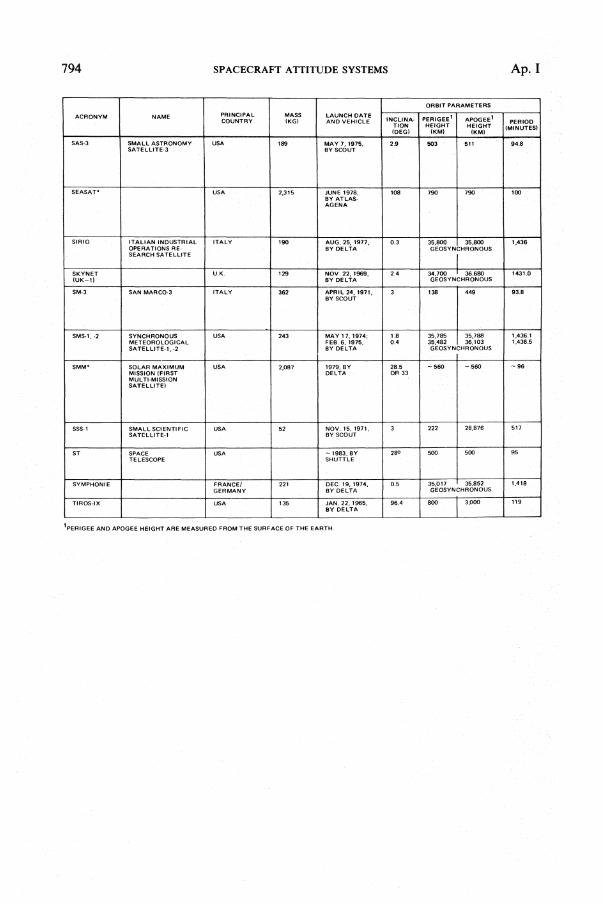
794 SPACECRAFT A TIITUDE SYSTEMS Ap. I
ORBIT PARAMETERS
ACRONYM NAME PRINCIPAL MASS LAUNCH DATE tNeLlNA· PERIGEE' APOGEE' COUNTRY {KG) AND VEHICLE PEFUOD
TION HEIGHT HEIGHT (MINUTES) toeG' (KM) (KM'
SAS-3 SMALL ASTRONOMY USA 189 MAY 7,1975. 2 .• 503 511 94.8 SATELLlTE·3 BY SCOUT
SEASAP USA 2.315 JUNE 1978, 108 790 790 100 BYATLA5-AGENA
SIRIO ITALIAN INDUSTRIAL ITALY 190 AUG, 25. 1917. 0.3 35,800 3S,BOO 1.436 OPERATIONS RE· BY DELTA GEOSYNrRONOUS SEARCH SATELLITE
SKYNET U.K. 129 NOV. 22, 1969, 2.4 34,100 36,680 1431.0 (UK-I' BY DELTA GEOSYNCHRONOUS
SM·3 SAN MARCO-J ITALY 362 APRIL 24, 1971, 3 136 449 93.B BYSCQUT
SM8-1.-2 SYNCHRONOUS USA 243 MAY 17,1974: 1B 35,785 35,788 1,436.1 METEOROLOGICAL FEB. 6. 1975, 0.4 35.482 36;103 1,436.5 SATELLITE." ·2 BY DELTA GEOSYNCHRONOUS
SMM* SOLAR MAXIMUM USA 2,087 1979. BY 28.5 -560 -560 -96 MISSION (FIRST DELTA OR 33 MUL TI-MISSION SATELLITE)
5SS-1 SMALL SCIENTIFIC USA 52 NOV. 15, 1971, 3 222 28,876 517 SATELlITE-1 BY5COUT
ST SPACE USA -1983, BY 2"" 500 500 95 TELESCOPE SHUTTLE
SYMPHONIE FRANCEI 221 DEC. 19, 1974, 0.5 35.017 35.852 1,418 GERMANY BY DELTA GEOSYNCHRONOUS
TIROS·IX USA 135 JAN. 22, 1965, 96.4 800 3,000 11. BY DELTA
1pERIGEE AND APOGEE HEIGHT ARE MEASURED fROM THE SURFACE OF THE EARTH.

Ap. I SPACECRAFT ATTITUDE SYSTEMS 795
STABILIZATION ATTITUDE TECHNIQUE POINTING ACCURACY ATTITUDe SENSORS MISSION OBJECTIVES
(SPIN RATE IN RPM) CONTROL HARDWARE
DUAL SPIN MAGNETIC COILS FOR ," TWO STAR CAMERAS X-RAY ASTRONOMY wb .. 0-5 REV/ORBIT SPIN AND PRECESSION N-5UT STAR SENSOR
IR HORIZON SCANNER SPINNING AND NONSPINNING SUN SENSOR MAGNETOMETER
DUAL SPIN MOMENTUM WHEEL ATTITUDE OETERMINA.· TWO IR HORIZON SENSORS OCEAN ~ .. 1 REV/ORBIT REACTION WHEEL TION: FOUR DIGITAL SUN PHYSICS
ww '" 2300 THREE MAGNETIC t: 0.20 IN PITCH. ROI,..L. SENSORS COILS AND YAW MAGNETOMETERS
ATTITUDE CONTROL: t: 0.50 IN PITCH. ROLL, AND YAW
SI!IN HYDRAllNE JETS , ,0 IR SLIT HORIZON SENSOR SUPER·HIGH·FREQUENCY wb,",90 IR HORIZON TELESCOPE COMMUNICATIONS
PLANAR AND V BEAM 12-18 GIGAHERTZ SUN SENSORS
SPIN GAS JETS EARTH HORIZON SENSOR COMMUNICATIONS DIGITAL SUN SENSOR
SPIN MAGNETIC COIL ,,0 SUN SENSOR OBTAIN DATA ON AT· MAGNETOMETER TRIAD MOSPHERIC DENSITY AND
MOLECULAR TEMPERA· TURE; DETERMINE NITROGEN CONCENTRA· TlON
SPIN HYDRAZINE JETS i: 1.00 ITRANSFER ORBIT) FIVE IR HORIZON SCAN· METEOROLOGY wb =90 !. 0.10 lMISSION ORBIT) NERS
TWO OVAL·SlIT SUN SENSORS
MOMENTUM WHEE LS FOUR MOMENTUM i: 0.1 0 ROLL THREE TWO·AXIS SOLAR ASTROPHYSICS ONBOARD COM· WHEELS ABOUT SUNLlNE; GYROSCOPES PUTER SIX MAGNETIC COILS !. 5ARC-$EC IN REDUNDANT FINE
PITCH AND YAW POINTING SUN SENSORS REDUNDANT TRIAXIAL MAGNETOMETERS TWO FIXED-HEAD STAR TRACKERS COARSE SUN SENSOR
SPIN MAGNETIC COIL AC- , ,0 STAR SCANNER STUDY MAGNETOSPHERE wb = 7 TIVATED AT PERIGEE OPTICAL HORIZON SENSOR
ONLY DIGITAL SUN SENSOR
ONBOARO COM- MOMENTUM WHEELS POINTING ACCURACY: TWO STAR TRACKERS MAJOR ASTRONOMICAL PUTER USING MAGNETIC TORQUING :to.1 ARC..sEC SUN SENSORS TI;.LESCOPE FINE ERROR STABILITY: FINE I[:RROR SENSOR SENSOR :t 0.01 ARC..sEC
MOMENTUM WHEELS MOMENTUM WHEELS :t 10 EARTH HORIZON SENSOR EXPERIMENTAL COM· GAS JETS DIGITAL SUN SENSOR MUNICATIONS SATELLITE
SPIN MAGNETIC COl LS , ,0 CONICAL SCAN METEOROLOGICAL HORIZON SENSORS

796 SPACECRAFT ATTITUDE SYSTEMS Ap. I
1.2 Spacecraft Listed by Attitude Determination Accuracy Requirements
.;;; l' .;;; 0.1° .;;; 0.25° .;;; 0.5°
ANS ATS-6 AEROS-I,2 HCMM* HEAO-B* CTS (mission) FLTSATCOM IMP-8 IUE GOES-I (mission) ISEE-C* LANDSAT-D* HEAO-I,C* SEASAT* MAGSAT* LANDSAT-I,2,C* OAO-3 LES-7 SAS-3 OAO-2 SMM* OSO-7,8 ST* SMS-I,-2 (mission)
.;;; 1° .;;; 1.5° ';;;ZO
AE-3,5 RAE-2 GEOS-3 ARIEL-III ARYABHATA SAS-2 ISS LES-5 ATS-3 SIRIO OGO-I CTS (acquisition) SM-3 DE-A*,B* SMS-I,-2 (transfer) GOES-I (transfer) SSS-I IMP-6,7 SYMPHONIE ISEE-I,B TIROS-IX NIMBUS-5,6
1.3 Spacecraft Listed by Type of Control Hardware
Magnetic
Jets
AE-3,-5, AEROS-I,2, ANS, AZUR-I (passive), DE-B*, ESRO-IV, GEOS-3 (acquisition), HCMM*, HEAO-B*, ISIS-I,ll, ITOS-8,I*,J*, LANDSAT-D*, LES-5, MAGSAT, OSO-7,8, SAS-2,3, SM-3, SSS-I, ST*, TIROS-IX
AE-3,5, ARYABHATA, ATS-3,6, CTS, DE-A*,-B*, FLTSATCOM, GOES-I, HEAO-I,B*,C*, HEOS-l, IMP-6,7,8, ISEE-I,B,C*, IUE, LES-7(plasma), OGO-I, OSO-7,8, RAE-2 (acquisition), SIRIO, SKYNET (U.K.I,2), SYMPHONIE
Momentum Wheel AE-3,5, ANS, ATS-6, GEOS-3 (mission), FLTSATCOM, HCMM*, HEAO-B*, IUE, LANDSAT-D*, MAGSAT*, NIMBUS-5,6, OAO-2,-3, OGO-I, SAGE*, SEASAT*, SMM*, ST*, SYMPHONIE
Gimbaled Flywheel LES-7
Reaction Boom GEOS-3

Ap. I SPACECRAFT ATIITUDE SYSTEMS
1.4 Spacecraft Listed by Type of Attitude Sensors
Star Sensors Star Scanner
ANS, ATS-3, OSO-7,8, SAS-2,3, SSS-I Fixed-Head Star Trackers
HEAO-I,B*,C*, LANDSAT-D*, MAGSAT*, SAS-3, SMM*, ST* Gimbaled Star Trackers
ATS-6: OAO-2,3
Horizon Scanners Optical
DODGE, IMP-6,7,8, ISEE-l,C*, IUE, RAE-2, SSS-l Infrared
797
AE-3,-5, AEROS-l,-2, ATS-6, CTS, ESRO-IV, FLTSATCOM, ISS, GOES-I, HCMM*, ITOS-8,1*,J*, LES-7, MAGSAT*, SAGE*, SAS-3, SEASAT*, SMS-l,-2, SIRIO
Sun Sensors Analog Sun Sensor
AEROS-l,2, ATS-3,6, GOES-I, IUE, SIRIO, SMM*, SMS-I,-2 One-Axis Digital Sun Sensors
AE-3,5, AEROS-I, ARYABHATA, ATS-6, CTS, ESRO-IV, IMP-8,9,1O, ISEE-l,C*, ISS, ITOS-8,I*,J*, IUE, RAE-2, SAS-2,3, SKYNET (U.K.I,2), SM-3, SSS-I, SYMPHONIE
Two-Axis Digital Sun Sensors ATS-6, CTS, GEOS-3, HCMM*, HEAO-l,B*,C*, IUE, MAGSAT*, RAE-2, SAGE*, SAS-3, SEASAT*, SMM*, ST*
Magnetometers AE-3-5, AEROS-I, ANS, ARYABHATA, GEOS-3, HCMM*, ISS, MAGSAT*, OAO-2,-3, OSO-7,8, SAGE*, SAS-2,3, SEASAT*, SM-3, SMM*
Gyroscopes ATS-6, HEAO-l,B*,C*, IUE, LANDSAT-D*, MAGSAT*, OAO-2,-3, SMM*
References
l. Joseph, M. and M. Plett, Sensor Standardization Study Task Report, Compo Sc. Corp., 3000-19300-01TN, May 1974.
2. TRW Systems Group, Public Relations Staff, TRW Space Log, Redondo Beach, CA (Annual Report).

APPENDIXJ
TIME MEASUREMENT SYSTEMS
Conrad R. Sturch
International Atomic Time, TAl, which is provided by atomic clocks, is the basis for the two time systems used in spacecraft time measurements. Ephemeris Time, ET, which is used in the preparation of ephemerides, is a uniform or "smoothly flowing" time and is related to TAl by
ET= TAI+32.18 sec
In contrast to ET, Coordinated Universal Time, UTC, uses the TAl second as the fundamental unit, but introduces I-second steps occasionally to make UTC follow the nonuniform rotation of the Earth. UTC is necessary for terrestrial navigation and surveying for which the rotational position of the Earth at a given instant is critical. It is this tIme which is broadcast internationally and is used for tagging spacecraft data and for all civil timekeeping. Finally, sidereal time. is a direct measure of the rotational orientation of the Earth relative to the "fixed" stars and, therefore, is used to estimate the position of a spacecraft relative to points on the Earth's surface. The characteristics of the various time systems are summarized in Table J-1.
Any periodic phenomenon may be used as a measure of time. The motion of the Earth, the Moon, and the Sun relative to the fixed statshas traditionally been used for this purpose. However, the need for increasingly accurate time measurements has resulted in the development of several .alternative time systems. The requirement for high accuracy comes from the cumulative effect of timing errors. An accuracy of I sec/day (I part in 105) would appear satisfactory for most scientific or technical purposes. However, an error of this magnitude in an ephemeris of the E~rth causes an error of 10,800 km in the position of the Earth
Table J-1. Time Systems
KIND OF DEFINED BY FUNDAMENTAL REGULARITY USE TIM!; UNIT
SIDEREAL EARTH'S ROTATION RELATIVE SIDEREAL DAY, IFtAEGUlAR ASTRONOMICAL OBSERVA-TO STARS 1 ROTATION OF EARTH TIONS; DETERMINING UT
AND ROTATIONAL ORIENTA-TION OF EARTH
SOLAR:
APPARENT EARTH'S ROTATION RELATIVE SUCCESSIVE TRANSITS IRREGULAR AND SUNDIALS TO TRUE SUN OF SUN ANNUAL VAAI·A-
TlONS
MEAN EARTH'S ROTATION RELATIVE MEAN SOLAR DAY IRREGULAR -TO FICTITIOUS MEAN SUN
UNIVERSAL UTO OBSERVED ur MEAN SOLAR DAY IRREGULAR STUDY OF EARTH'S WANDERING
POLE
un CORRECTED UTa MEAN SOLAR DAY IRREGULAR SHOWS SEASONAL VARIATION Of EARTH'S ROTATION
un CORRECTED un MEAN SOLAA DAY IRREGULAR BASIC ROTATION OF EAATH
iJTC- GMT ATOMIC SECOND AND LEAP MEAN SOLAA DAY UNIFORM EXCEPT CIVIL TIMEKEEPING; TEA· ·z SECONDS TO APPROXIMATE FOR LEAP SEC- RESTRIAL NAVIGATION AND
UT1 ONDS SURVEYING; BROADCAST TIME SIGNALS
EPHEMERIS, ET FRACTION OF TROPICAL YEAR EPHEMERIS SECOND UNIFORM EPHEMERIDES 1900
ATOMIC, TAl FREQUENCY OF 133 Ce RADIA· ATOMIC SECOND = UNIFORM BASIS Of ET AND UTC TION EPHEMERIS SECOND

Ap.J TIME MEASUREMENT SYSTEMS 799
after only I year, several orders of magnitude worse than what is acceptable for many unsophisticated measurements. Thus, the generation of accurate ephemerides requires a precise time measurement system.
The diurnal motion of celestial objects is the most obvious timekeeper. Until the Middle Ages "seasonal hours," one-twelfth of daylight or nightime periods, was used. Of course, this unit varies both with the season and with the observer's latitude. A more uniform unit of time is the apparent solar day, defined as the interval between two successive passages of the Sun across the observer's meridian. As discussed below, this interval varies throughout the year due to variations in the Earth's orbital speed and the inclination of the ecliptic. The Earth's orbital motion does not affect the sidereal day, the interval between two succesive meridian passages of a fixed star. However, irregularities in the rotation of the Earth cause both periodic and secular variations in the lengths of the sidereal and solar days.
The annual motions of celestial objects provide a measurement of time which is independent of the irregular variations in the rotation of the Earth. The tropical year, upon which our calendar is based, is defined as the interval of time from one vernal equinox to the next. The ephemeris second is defined as 1/31556925.9747 of the tropical year for 1900. Because of the precession of the equinoxes (Section 2.2.2), the tropical year is about 20 minutes shorter than the orbital period of the Earth relative to the fixed stars. This latter period is known as the sidereal year. Due to secular variations in the orbit and rate of precession of the Earth, the lengths of both types of year (in units of se' the ephemeris second) vary to first order according to the relations:
Tropical year = 31556925.9747 - .530 T
Sidereal year = 31558149.540+ .OIOT
where T is the time in units of Julian Centuries of 36525 days from 1900.0 [Newcomb, 1898].
The first satisfactory alternative to celestial observations for the measurement of time was the pendulum dock. The period of a pendulum is a function of the effective acceleration of gravity, which varies with geography and the position of the Sun and the Moon. The resonance frequency of quartz crystals has recently been employed in clocks; this frequency depends on the dimensions and cut of the crystal and its age, temperature, and ambient pressure. Atomic clocks are based on the frequency of microwave emission from certain atoms. An accuracy of 10- 14
(fractional standard deviation) may be achieved with atomic clocks; corresponding accuracies for quartz and pendulum clocks are 2 X 10- 13 and 10-6, respectively. For an extended discussion of time systems, see Woolard and Clemence [1966], the Explanatory Supplement to the Astronomical Ephemeris and the American Ephemeris and Nautical Almanac [H.M. Nautical Almanac Office, 1961] and Muller and Jappel [1977].
Solar Time. The celestial meridian is the great circle passing through the celestial poles and the observer's zenith. As shown in Fig. 1-1, the hour angle, HA, is the azimuthal orientation of an object measured westward from the celestial meridian. As the Earth rotates eastward, a celestial object appears to move westward and its HA increases with time. It takes 24 hours for an object to move completely around the celestial sphere or I hour to move 15 deg in HA; thus, I deg of HA corresponds to 4 minutes of time.

800 TIME MEASUREMENT SYSTEMS Ap.J
Fig. J-1. Definition of Hour Angle
The apparent solar time is equal to the local HA of the Sun, expressed in hours, plus 12 hours. Apparent solar time can be measured with a simple sundial constructed by driving a long nail perpendicularly through a flat piece of wood. If the nail is then pointed toward the celestial pole, the plane of the wood is parallel to the equatorial plane, and the shadow of the nail cast by the Sun onto the wood is a measure of the HA.
Due to the Earth's orbital motion, the Sun appears to move eastward along the ecliptic throughout the year. Because the Earth travels in an elliptical orbit, it moves faster when near the Sun and slower when it is more distant; therefore, the length of the solar day varies. Even if the Earth were in a circular orbit with a constant speed, the azimuthal component of the Sun's motion (parallel to the celestial equator) would vary due to the inclination of the ecliptic relative to the equator. To illustrate this, consider a satellite in a nearly polar orbit, as shown in Fig. J-2. The satellite changes azimuth slowly while near the equator and rapidly while near the poles. Although the variation in the length of the day due to the
Fig. J-2. Variation in Azimuthal Rate for a Satellite Moving Uniformly in its Orbit. A I.A2 ..... AS are azimuthal projections of the orbital points 1.2 .... 5 and are equally spaced in time.

Ap.J TIME MEASUREMENT SYSTEMS 801
eccentricity and inclination of the Earth's orbit is small, the cumulative variation reaches a maximum of 16 minutes in November.
To provide more uniform time than the real Sun, a fictitious mean Sun, which moves along the equator at a constant rate equal to the average annual rate of the Sun, has been introduced. Mean solar time is defined by the HA of the mean Sun. The difference between the mean and apparent solar times is called the equation of time.
Standard Time. Mean solar time is impractical for communication and transportation because it varies continuously with longitude. Therefore, the world has been divided into 24 time zones of approximately 15 deg each. Normally, these zones are centered on standard meridians which are multiples of 15 deg in longitude. The uniform time throughout each zone is referred to as Standard Time, and usually differs by an integral number of hours from the mean solar time at 0 deg longitude, or Universal Time, as discussed below. Table J-2 lists the standard meridiahs for time zones in the continental United States. The apparent solar time is converted to Standard Time by adding the equation of time for the date and subtracting the algebraic difference (expressed in units of time) between the observer's longitude and the standard meridian.
Table J-2. Standard Time
TIME ZONE STANDARD MERIDIAN UT MINUS STANDARD TIME UT MINUS DAYLIGHT TIME {DEG. EAST LONG.l (HOURS) (HOURS)
EASTERN 285 5 4
CENTRAL 270 6 5
MOUNTAIN 255 7 6
PACIFIC 240 8 7
Greenwich Mean Time, Universal Time. The O-deg longitude line is referred to as the Greenwich meridian because it is defined by the former site of the Royal Greenwich Observatory. Greenwich Mean Time, GMT, is the mean solar time at 0 deg longitude; that is, GMT is the HA of the mean Sun observed at Greenwich (called the GHA) in hours plus 12 hours, modulo 24. Greenwich Mean Time is also called Universal Time, UT, and, in spaceflight operations, Zulu, or Z.
Uncorrected UT or UTO (read"UT Zero") is found from observations of stars, as explained in the discussion of sidereal time below. UTO time as determined by different observatories is not the same, however, due to changes in the longitudes of the observatories caused by the wandering of the geographic pole. Therefore, UTO is corrected for this effect to give UTI, which is then a measure of the actual angular rotation of the Earth. The Earth's rotation is subject to periodic seasonal variations, apparently caused by changes in, for example, the amount of ice in the polar regions. When UTI is corrected by periodic terms representing these seasonal effects, the result is UT2. Even UT2 is not a uniform measure of time. Evidence from ancient eclipse records and other sources shows that the Earth's rate of rotation is slowing; also, unpredictable irregularities in the rotation rate are observed.
Before 1972, ihe broadcast time signals were kept within 0.1 sec of UT2. Since January 1, 1972, however, time services have broadcast Coordinated Universal

802 TIME MEASUREMENT SYSTEMS Ap.J
Time, UTe. A second of UTe is equal to a second of International Atomic Time, but UTe is kept within 0.90 sec of UTi by the introduction of i-sec steps, usually at the end of June and December.
Ephemeris Time. The irregularities in the Earth's rotation cannot be predicted; however, gravitational theories have been formulated for the orbital motions of the Earth, the Moon, and the planets. In particular, Simon Newcomb's Tables of the Sun, [1898], published at the end of the 19th Century, gives the position of the Sun for regular time intervals. These intervals define a uniform time called Ephemeris Time, ET. In theory, Ephemeris Time is determined from observations of the Sun. In practice, observations of the Moon are used because the Sun moves slowly and its position is difficult to observe. One method is to record the UT of a lunar occultation of a star; the tabulated value of ET for the observed lunar position, corrected for effects such as parallax, is noted and the difference
AT=ET- UT
is determined. A table of approximate A T values, both in the past and extrapolated into the future, is provided in The American Ephemeris and Nautical Almanac [U.S. Naval Observatory, 1973]. Ephemeris time at any instant is given by
ET=!:J.T+ UT
International Atomic Time. The cesium nuclide, 133 Ce, has a single outer electron with a spin vector that can be either parallel or antiparallel to that of the nucleus. The flip from one orientation to the other, a hyperfine transition, is accompanied by the absorption or emission of microwave radiation of a given frequency. In an atomic clock, the number of these transitions is maximized in a resonator by the introduction of microwave radiation from an oscillator tuned to the same frequency. The cycles of the oscillator are counted to give a unit of time. In 1967, the 13th General Conference on Weights and Measures established the Systeme I nternationale (SI) second as the duration of 9 192 631 770 periods of the radiation from the above transition in 133 Ceo This unit is the basis of International Atomic Time, TAl, and was chosen to make the SI second equal to the ephemeris second. The reference epoch for TAl is January 1, 1958, when <tOrnos TAl equaled Ohomos UT2. For most purposes, ephemeris time may be considered to be equal to TAl plus 32.18 sec, the value of !:J.T for January 1, 1958.
Sidereal Time. Sidereal time, ST, is based on the rotation of the Earth relative to the stars and is defined as the HA of the vernal equinox, 0('. The local sidereal time, LST, is defined as the local HA of 0(', LHA 0(', and the sidereal time at Greenwich, GST, is defined as the Greenwich HA of 0(', GHA 0('. Sidereal time may also be determined from the HA and right ascension, RA, of any star. The RA of a star is the azimuthal component of the star's position measured eastward from 0('
(see Section 2.2.2). From Fig. J-3 we see that
LST= LHA 0('= LHA * + RA *, modulo 24 (1-1)
where LHA* and RA* are the HA and RA (both converted to time) of the star. In the example in Fig. J-3, LHA * is 135 deg or 9 hours, RA * is 90 deg or 6 hours, and the LST is 15 hours. Similarly,
GST= GHA 0('= GHA * + RA*, modulo 24 (J-2)

Ap.J. TIME MEASUREMENT SYSTEMS S03
where GHA * is the GHA of the star (converted to time). In Fig. J-3, GHA * is 45 deg or 3 hours; thus, GST is 9 hours. Note that the sidereal time at Greenwich is equal to the right ascension of the Greenwich meridian. The difference between LST
GHAT
OBSERVER
LOCAL MERIDIAN
Fig. J-3. Sidereal Time. (View looking down on the Earth's North Pole.)
and GST (6 hours in this example) corresponds to the observer's East longitude (90 deg in this example). In general,
LST=GST+EL/15 (J-3)
where EL is the observer's East longitude in degrees. From the definition of mean solar time, it follows that GMT or UT equals the GHA of the fictitious mean Sun plus 12 hours, or
UT= 12 hours + GST- Ru
where ~ is the right ascension of the mean Sun. For a given UT of any calendar date,
GST= Ru -12 hours + UT
= 6h3Sffi45" .836 + 8640184".542 T + 0" .0929 T2 + UT (J-4)
where T is the number of Julian centuries of 36,525 days which have elapseq since noon (GMT) on January 0, 1900 [Newcomb, IS98]. The corresponding equation for GST expressed in degrees is
GST=99°.6910+36000°.7689 T+O°.OOO4 T2+ UT (J-5)
where UT is in degrees and T is in Julian centuries. Julian dates, or J D (Section 1.4), are convenient for determining T in Eqs. (J-4) and (J-5). The J D for Greenwich mean noon on January 0, 1900 (i.e., January 0.5, 1900), is 2415020.0. JD's for any date in the last quarter of this century may be obtained by adding the day number of the year to the JD for January 0.0 UT of that year listed in Table J-3. For example, to find the GST for 3h UT, July 4, 1976:

804 TIME MEASUREMENT SYSTEMS
Day number of July 4.125 (=3h UT July 4),1976 +JD for January 0.0,1976 =JD for July 4.125, 1976 -JD for January 0.5, 1900 = Tin days + 36,525 = T in Julian centuries 8640184.542 T + 0.0929 T2
+ first term Eq. (J-4) + UT GST
Ap.J
186.125 + 2442777.500 = 2442 963.625 - 2415020.000
27943.625 0.765054757
6610 214.340 sec = 76d12hlOm14~340
6 38 45.836 3 0 0.000
21h49m ~176
Due primarily to the varying distances of the Sun and the Moon, a small amplitude oscillation, known as astronomical nutation, is superimposed on the precession of the equinoxes. Sidereal time corrected for this effect is called mean sidereal time. GST in Eqs. (J-4) and (1-5) is mean sidereal time. The maximum difference between mean and apparent sidereal time is only about I sec.
Table J-3. Julian Date at the Beginning of Each Year From 1975 to 2000
YEAR JD FOR YEAR JD FOR YEAR JD FOR JAN 0.0 UT JAN 0.0 UT JAN 0.0 UT
2400000+ 2400000+ 2400000+
1975 42412.5 1984 45699.5 1993 48987.5 1976 42777.5 1985 46065.5 1994 49352.5 1977 43143.5 1986 46430.5 1995 49717.5 1978 43508.5 1987 46795.5 1996 50082.5 1979 43873.5 1988 47160.5 1997 50448.5 1980 44238.5 1989 47526.5 1998 50813.5 1981 446045 1990 47891.5 1999 51 178.5 1982 44969.5 1991 48256.5 2000 51543.5 1983 45334.5 1992 48621.5
Because of the orbital motion of the Earth, a solar day is longer than a sidereal day. As illustrated in Fig. J-4, the fixed stars are sufficiently far away that lines connecting one of them to the Earth are essentially parallel. Because the Earth's orbital period is approximately 360 days, angle A is approximately I deg. A sidereal day is defined as one complete rotation of the Earth, 360 deg, relative to the stars. The Earth has to rotate 360+A deg to complete a solar day. The ratio of the m-an solar day to the mean sidereal day is }.00273 79093; the mean sidereal day equals 23 hours, 56 min, 4.09054 sec of mean solar time and the mean solar day equals 24 hours, 3 min, 55.55536 sec of mean sidereal time [U.S. Naval Observatory, 1973]. Note that the "76 days" in the above example indicates the excess number of sidereal days, one for each year, that had occurred since the beginning of the century.
Sidereal time and mean solar time are affected proportionally by variations in the Earth's rotation. Although the irregular fluctuations in the Earth's rotation cannot be predicted, the general deceleration can be seen in Fig. J-5. The lengths of

Ap. J TIME MEASUREMENT SYSTEMS 805
Fig. J-4. Orbital Motion of the Earth for I Day (Exaggerated) as Viewed From North Ecliptic Pole
the two types of day in se are given approximately by: Sidereal day = 86164.09055 +0.0015 T
Mean solar day = 86400+0.0015T where T is in Julian centuries from 1900.0 [Allen, 1973). These terms are the dashed line in Fig. J-5.
1600 1700 1800
YEAR
1900 2000
Fig. J-5. Excess Length of the Day Compared With the Day Near 1900. Note the very irregular fluctuations about the mean slope of 1.5 ms/century [Morrison, 1973J.
Using Sidereal Time to Compute the Longitude of the Subsatellite Point. To determine the direction of geographic points on the Earth as seen from a spacecraft, it is necessary to know both the spacecraft ephemeris and the longitude of the subsatellite point. For any UT, Eg. (J-4) can be used to determine the Greenwich sidereal time, CST, which in turn can be used to determine the East longitude, ELspc' of the subsatellite point for any satellite for which the right ascension of its position in geocentric coordinates is known. From Eg. (J-3), we have
ELspc = RAspc - CST (in degrees)
where RAspc is the right ascension in degrees of the spacecraft at time CST. Because UTe is accurate to about 1 sec, the accuracy of the resulting longitude will be about 0.005 deg if the spacecraft ephemeris is known precisely.
References
1. Allen, C. W., Astrophysical Quantities, Third Edition. London: The Athlone Press, 1973.

806 TIME MEASUREMENT SYSTEMS Ap.J
2. H. M. Nautical Almanac Office, Explanatory Supplement to the Astronomical Ephemeris and the American Ephemeris and Nautical Almanac. London: Her Majesty's Stationery Office, 1961.
3. Morrison, L. V., "Rotation of the Earth from AD 1663-1972 and the Constancy of G," Nature, Vol. 241, p. 519-520, 1973.
4. Miiller, Edith A. and Arndst Jappel, Editors, International Astronomical Union, Proceedings of the Sixteenth General Assembly, Grenoble, 1976. Dordrecht, Holland: D. Reidel Publishing Co., 1977.
5. Newcomb, Simon, Astronomical Papers Prepared for the Use of the American Ephemeris and Nautical Almanac, Bureau of Equipment, U.S. Department of the Navy, Washington, DC, 1898.
6. U.S. Naval Observatory, The American Ephemeris and Nautical Almanac. Washington, DC: U.S. G. P.O., 1973.
7. Woolard, Edgar W., and Gerald M. Clemence, Spherical Astronomy. New York: Academic Press, 1966.

APPENDlXK
METRIC CONVERSION F'ACTORS
The metric system of units, officially known as the International System of Units, or SI, is used throughout this book, with the single exception that angular measurements are usually expressed in degrees rather than the SI unit of radians. By international agreement, the fundamental SI units of length, mass, and time are defined as follows (see, for example, NBS Special Publication 330 [NBS, 1974]):
The metre is the length equal to I 650 763.73 wavelengths in vacuum of the radiation corresponding to the transition between the levels 2PlO and 5d5 of the krypton-86 atom. The kilogram is the mass of the international prototype of the kilogram (a specific platinum-iridium cylinder stored at Sevres, France). The second is the duration of 9 192 631 770 periods of the radiation corresponding to the transition between two hyperfine levels of the ground state of the cesium-133 atom.
Additional base units in the SI system are the ampere for electric current, the kelvin for thermodynamic temperature, the mole for amount of substance, and the candela for luminous intensity. Mechtly [1973] provides an excellent summary of SI units for scientific and technical use.
The names of multiples and submultiples of SI units are formed by application of the following prefixes:
Factor by which unit is multiplied Prefix Symbol
1012 tera T 109 giga G 106 mega M 103 kilo k 102 hecto h 10 deka da 10- 1 deci d 10- 2 centi c 10- 3 milli m 10- 6 micro p. 10- 9 nano n 10- 12 pico p 10- 15 femto f 10- 18 atto a
For each quantity listed below, the SI unit and its abbreviation are given in parentheses. For convenience in computer use, most conversion factors are given to the greatest available accuracy. Note that some conversions are exact definitions and some (speed of light, astronomical unit) depend on the value of physical constants. All notes are on the last page of the list.

808 METRIC CONVERSION FACTORS Ap.K
To convert from To Multiply by Notes
Mass (kilogram, kg)
Atomic unit (electron) kg 9.109 6x 10- 31 (1) Atomic mass unit, amu kg 1.66053 X 10⁻²⁷ (1) Ounce mass (avoirdupois) kg 2.834952312 5x 10- 2 E Pound mass, Ibm (avoirdupois) kg 4.535 923 7 X 10- I E Slug kg 1.459 390 294 X 101
Short ton (2000 pound) kg 9.071 847 4x IOZ E Metric ton kg LOx 103 E Solar mass kg 1.989 X 1030 (1)
Length (metre, m)
Angstrom m LOx 10- 10 E Micron m LOx 10- 6 E Mil (10- 3 inch) m 2.54x 10⁻⁵ E Inch m 2.54 X 10- 2 E Foot m 3.048 X 10- I E Statute mile (U.S.) m 1.609 344 X I ij3 E Nautical mile (U.S.) m 1.852 X 10³ E Earth equatorial radius m 6.378 140x 106 (3) Vanguard unit m 6.378I66x106 (4) Solar radius m 6.959 9x 10⁸ (1) Astronomical unit, AU m 1.495 978 70 X 1011 (5) Light year (tropical year) m 9.460 530 X 1015 (1)
Parsec (distance for which stellar parallax is I arc-sec.) m 3.085 678 X 1016 (1)
Time (second, s) (7)
Sidereal day, d* (ref. = cy» s 8.6I6409I8x104 (1)*
= 23h 56m 4.0918s (1)*
Ephemeris day, de S 8.64x 10⁴ E Ephemeris day, de d* 1.002 737 89· (1)*
Vanguard unit s 8.068 1242 X 102 (4)
Keplerian period of a satellite in mm 1.658 669 x 1O- 4 x a3/ 2 (6) low-Earth orbit a inkm
Keplerian period of a satellite of de 3.652569 X IOZ X a3/ 2 (6) the Sun a in AU
Tropical year (ref. = CY» S 3.155692555 I X 107 (7)*
Tropical year (ref. =cy» de 3.652421938 8x IOZ (7)*
Sidereal year (ref. = fixed stars) se 3.15) 314954 8x 10⁷ (7)*
Sidereal year (ref. = fixed stars) de 3.652 563 605 Ix 102 (7)*
• Epoch 1980.

Ap.K METRIC CONVERSION FACTORS 809
To convert from To Multiply by Notes
Calendar year (365 days) se 3.153 6x 10⁷ E
Julian century d 3.652 5x 10⁴ E Gregorian calendar century d 3.652425 X 10⁴ E
Velocity (metre/second, m/s)
Foot/minute, ft/min m/s 5.08X 10- 3 E Inch/second, ips m/s 2.54x 10- 2 E
Kilometre/hour, km/hr m/s (3.6) - I = 0.277777 ... E
Foot/second, fps or ft/sec m/s 3.048 X 10- 1 E
Miles/hour, mph m/s 4.4704 X 10- 1 E Knot m/s 5.144 444 444 X 10- 1
Miles/minute m/s 2.682 24 X 101 E Miles/second m/s 1.609 344 X 103 E Astronomical unit/sidereal year m/s 4.740388 554 X 103
Vanguard unit m/s 7.905 389 X 103 (4) Velocity of light, c m/s 2.997 925 X 108 (I)
Acceleration (metre/second2, m/s2)
Gal (galileo) m/s2 LOx 10-2 E Inch/second2 m/s2 2.54 ><.10- 2 E Foot/second2 m/s2 3.048 X 10- 1 E Free fall (standard), g m/s2 9.80665 E Vanguard unit m/s2 9.798299 (4)
Force (Newton == kilogram· metre / second2, N == kg· m/ S2)
Dyne N LOx 10- 5 E Poundal N 1.38254954376 X 10- 1 E Ounce force (avoirdupois) N 2.780 1385 X 10- 1 (8) Pound force (avoirdupois),lbf==
slug· foot/ second2 N 4.448221 6152605 E
Pressure (Pascal == N ewton/ metre2 == kilogram· metre - I • second - 2,
Pa==N/m2 ==kg'm- I 's- 2)
Dyne / centimetre2 Pa LOx 10- 1 E Ibf/foot2 Pa 4.7880258 (8) Torr (00 C) Pa 1.333 22 X 102 (8) Centimetre of Mercury (OU C) Pa 1.33322 X IW (8) Inch of Mercury (320 F) Pa 3.386 389 X 103 (8) Ibf/inch2, psi Pa 6.894 757 2 X 10³ (8) Bar Pa l.Ox 105 E Atmosphere Pa 1.013 25 X 105 E

810 METRIC CONVERSION FACTORS Ap.K
To convert from To Multiply by Notes
Energy or Torque (Joule: Newton· metre: kilogram· metre2/second2, (2) J:N ·m:kg·m2/s2)
Electron volt, eV J 1.602 191 7x 10- 19 (8) Mass-energy of I amu J 1.49241 X 10- 10 (1) Erg: gram· cen timetres2 / second2
= pole· centimetre· oersted J LOx 10- 7
Ounce inch J 7.061 551 6x1O-3 Foot poundal J 4.214011 Ox 10-2
Foot Ibf = slug· foot2 / second2 J 1.3558179 Calorie (mean) J 4.190 02 British thermal unit, BTU (mean) J 1.055 87 x 103
Kilocalorie (mean) J 4.190 02 X I Q3
Kilowatt hour J 3.6 X 10⁶
Ton equivalent of TNT J 420x 109
Power (Watt: Joule/second: kilogram· metre2/ second3, W: J / s: kg· m2/ S3)
E (8) (8) (8) (8)
(8)
(8)
E (8)
Foot Ibf/second W 1.3558179 (8) Horsepower (550 ft Ibf/s) W 7.4569987 X IOZ (8) Horsepower (electrical) W 7.46 X IOZ E Solarluminosity W 3.826 X 1026 (I)
Moment of Inertia (kilogram· metre2, kg· m2)
Gram·centimetre2 kg·m2 LOx 10-7 E Ibm·inch2 kg·m2 2.926 397x 10-4
Ibm·foot2 kg·m2 4.214011 X 10- 2
Slug·inch2 kg·m2 9.415 402 x 10-:-3
Inch ·lbf· seconds2 kg· m2 1.129 848 X 10- 1
Slug· foot2 = ft ·lbf· seconds2 kg· m2 1.355 818
Angular Measure (radian, rad). Degree (abbreviated deg) is the basic unit used in this book.
Degree
Radian
Solid Angle (steradian, sr)
Degree2, deg2
Steradian
rad
deg
sr
'7T/I80 E ~ 1.745 329 251 994 329 577 X 10 - 2
IW/'7T E ~5. 729 577 951 308 232 088 x 101
('7T/I80f E ~3.046 174 197867085 993 x 10-4
(I80/'7T)2 E ~3.282 806 350 OIl 743 794 x loJ

Ap.K METRIC CONVERSION FACTORS
To convert from To Multiply by Notes
Angular Velocity (radian/se~ond, rad/s). Degrees/second is the basic unit used in this book.
Degrees/second, deg/s
Revolutions/minute, rpm
Revolutions/second, rev /s
Revolutions/minute, rpm Radians/second, rad/s
Revolutions/second, rev /s
rad/s
rad/s
rad/s
deg/s deg/s
deg/s
77/180 E R:l1.745 329 251 994 329 577 X 10 - 2
77 130 E R:l1.047 197551 196597 746 x 10- 1
277 E R:l6.283 185307 179586477
6n E 180/77 E R:l5.729 577 951 308 232 088 x 101
3.6x10² E
Angular Momentum (kilogram· metre2 / second, kg· m2 / s) Gram· centimetre2 / second,
g·cm2/s kg·m2/s LOx 10- 7 E Ibm·inch2/second kg·m2 Is 2.926 397 x 10-4
Slug·inch2/second kg·m2/s 9.415 402 x 10-3
lbm·footl/second kg·m2/s 4.214 011 x 10-2
Inch· lbf· second kg·m2/s 1.129 848 x 10- 1
Slug·foot2/second =ft·lbf· second kg· m2 Is 1.355 818
811
Magnetic Flux (Weber == Volt· second == kilogram· metre2 • Ampere - I . second - 2, Wb == V . s ==kg·m2 • A -1' S-2)
Maxwell (EMU) Wb LOx 10- 8 E
B, Magnetic Induction (commonly called "magnetic field", (9) Telsa == Weber / metre2 == kilogram· Ampere - I . second- 2, T==Wb/m2=kg·A-I·s-~
Gamma (EMU) T LOx 10-9 E, (9) Gauss (EMU) T 1.0 X 10⁻⁴ E, (9)
H, Magnetic Field Strength (ampere tum/metre, Ajm) (9) Oersted (EMU) Aim (l 1477) X IQ3 E, (9)
R:l7.957747 154594766 788 x 101
Magnetic Moment (ampere·tum·metre2 ==Joule/Telsa, A·m2 ==J/T) Abampere'centimetre2 (EMU) A·m2 LOx 10- 3 E, (9) Ampere' centimetre2 (Practical) A· m2 1.0 X 10⁻⁴ E

812 METRIC CONVERSION FACTORS Ap.K
To convert from To Multiply by Notes
Magnetic Dipole Moment (Weber' metre == kilogram· metre· Ampere - 1 • second - 2,
Wb.m==kg'm.A -1' S-2)
Pole· centimetre (EMU) Wb· m 4'7T X 10 - 10 E; (9) ~1.256 637 061435917 295 X 10- 9
Gauss·centimetre3 (Practical) Wb· m 1.0 X 10- 10 E
Temperature (Kelvin, K)
Celsius, C Fahrenheit, F Fahrenheit, F
Notes:
K K C
tK=tc +273.15 tK = (5 j9)(tF + 459.67) tc = (5 j9)(tF - 32.0)
E E E
E (Exact) indicates that the conversion given is exact by definition of the non-SI unit or that it is obtained from other exact conversions. (I) Values are those of Allen [1973]. (2) In common usage "Joule" is used for energy and "Newton-metre" for torque. (3) Value is that adopted by the International Astronomical Union in 1976
[Muller and Jappel, 1977]. Reported values of the equatorial radius of the Earth differ by about 20 m. It is therefore recommended that this unit not be used except in internal calculations, where it is given a single defined value.
(4) Values are those adopted in subroutine ROITAP, described in Section 20.3. Vanguard units should be avoided if possible because of differences in the definitions of the units involved. The Vanguard unit of length is equatorial radius of the Earth; the Vanguard unit of time is the time for an Earth satellite to move 1 radian if the semimajor axis is 1 Vanguard unit.
(5) Value is that adopted by the International Astronomical Union in 1976 [Muller and Jappel, 1977].
(6) Value is calculated from mass parameters adopted by the International Astronomical Union in 1976 [Muller and Jappel, 1977]. Actual period will differ due to various perturbation effects. (See Section 3.4.)
(7) For high-precision work, consult Appendix J on time measurement systems. The conversions for the length of the year are derived from values, given by Newcomb [1898], which define the unit of ephemeris time. The most convenient method for determining the time interval between events separated by several days or more is to use the Julian Date. See Section 1.4 and subroutine JD in Section 20.3 for a convenient algorithm for determining the Julian date and Appendix J for a table of Julian Dates.
(8) Values are those of Mechtly [1973]. (9) Care should be taken in transforming magnetic units, because the dimension
ality of magnetic quantities (B, H, etc.) depends on the system of units. Most of the conversions given here are between SI and EMU (electromagnetic). The following equations hold in both sets of units:

Ap.K
N=mXB=dXH B=p.H
METRIC CONVERSION FACTORS
m = I A for a current loop in a plane d= p.m
with the following definitions N=:torque B=:magnetic induction (commonly called "magnetic field") H=:magnetic field strength or magnetic intensity m=:magnetic moment I =:current in loop
813
A =:vector normal to the plane of the current loop (in the direction of the angular velocity vector of the current about the center of the loop) with magnitude equal to the area of the loop
d =:magnetic dipole moment p. =:magnetic permeability
The permeability of vacuum, P.o, has the following values, by definition: p.o=:1 (dimensionless) EMU P-o=:4'1T X 10- 7 Nj A2 SI
Therefore, in electromagnetic units in vacuum, magnetic induction and magnetic field strength are equivalent and the magnetic moment and magnetic dipole moment are equivalent. For practical purposes of magnetostatics, space is a vacuum but the spacecraft itself may have p. :j= p.o.
References
1. Allen, C. W., Astrophysical Quantities, Third Edition. London: The Athlone Press, 1973.
2. Mechtly, E. A., The International System of Units: Physical Constants and Conversion Factors, Second Revision, Washington, DC, NASA SP-7012, 1973.
3. MUller, Edith A. and Arndst Jappel, editors, International Astronomical Union, Proceedings of the Sixteenth General Assembly, Grenoble, 1976. Dordrecht, Holland: D. Reidel Publishing Co., 1977.
4. National Bureau of Standards, U.S. Department of Commerce, The International System of Units (SI) , NBS Special Publication 330 (1974 edition), 1974.
5. Newcomb, Simon, Astronomical Papers Prepared for the Use of the American Ephemeris and Nautical Almanac. Washington, DC: Bureau of Equipment, Navy Department, 1898.

APPENDIXL
SOLAR SYSTEM CONSTANTS
L.I Planets and Natural Satellites L.2 The Sun L.3 The Earth L.4 The Moon L.5 Potential Spacecraft Orbits
JamesR. Wertz
The mass, size, and gravitational parameters are those adopted by thelnternational Astronomical Union (IAU) in 1976 [Muller and Jappel, 1977]. The geocentric and geographical coordinate system conversions are based on the method adopted by the American Ephermeris and Nautical Almanac [H.M. Nautical Almanac Office, 1961] using the updated value for the Earth's flattening adopted by the IAU [Muller and Jappe!, 1977]. The properties of artificial satellites, both in orbit about solar system objects and in transfer orbits between objects, are calculated from the parameters given and are based on Keplerian orbits with no perturbative corrections. The properties of the Earth's upper atmosphere are from the 1972 COSPAR International Reference Atmosphere [1972], and the U.S. Standard Atmosphere [1976]. Additional constants are from Allen [1973], which is an excellent source of additional astronomical information. See Chapter 3 for definitions of orbital quantities and planetary magnitudes.
L.t Planets and Natural Satellites
Table L-l lists the orbital properties of the major planets. Because of orbital perturbations, the data here are not tabulated with the full precision normally used for ephemerides. If greater accuracy is needed, consult the American Ephemeris and Nautical Almanac for current osculating elements or Section 5.4 forepemerides for computer use. Quoted data are from Allen [1973].
Table L-2 lists the physical properties of the Moon and planets. Additional data on the Earth and Moon are given in Sections L.3 and L.4. Properties of the natural satellites of the planets are given in Table L-3.

Tab
le L
-I.
Pla
neta
ry O
rbits
SE
MIM
AJO
R A
XIS
S
IDE
RE
AL
PE
RIO
D
SY
NO
DIC
M
EA
N
ME
AN
PL
AN
ET
P
ER
IOD
Mg
~:~~
2 O
RB
ITA
L
EC
CE
NT
RIC
ITY
(106
KM
) (T
RO
PIC
AL
(D
AY
S)l
(D
AY
S)l
V
EL
OC
ITY
19
70
(AU
) Y
EA
RS
) (D
EG
) (K
MIS
EC
)
ME
RC
UR
Y
0.3
87
09
9
57
.9
0.2
40
85
8
7.9
69
11
5.88
4
.09
23
39
4
7.8
9
0.2
05
62
8
VE
NU
S
0.7
23
33
2
108.
2 0.
6152
1 22
4.70
1 58
3.92
1.
6021
31
35.0
3 0.
0067
B7
EA
RT
H
1.0
00
00
0
14
9.6
1
.00
00
4
36
5.2
56
0.
9B56
09
29.7
9 0
.01
67
22
MA
RS
1.
5236
91
22
7.9
1
.88
08
9
68
6.9
80
77
9.94
0
.52
40
33
24
.13
0.0
93
37
7
JUP
ITE
R
5.2
02
80
3
77
8.3
1
1.8
62
23
4
33
2.5
89
39
8.88
0.
0830
91
13.0
6 0
.04
84
5
SA
TU
RN
9
.53
88
4
14
27
.0
29
.45
77
10
759.
22
37
8.0
9
0.0
33
46
0
9.6
4
0.0
55
65
UR
AN
US
1
9.1
81
9
28
69
.6
84
.01
39
3
06
85
.4
36
9.6
6
0.0
11
73
2
6.81
0
.04
72
4
NE
PT
UN
E
30
.05
78
4
49
6.6
1
64
.79
3
60
18
9
36
7.4
9
0.0
05
9B
l 5
.43
0
.00
85
8
PL
UT
O
39
.44
5
90
0
24
7.7
9
04
65
36
6.73
0
.00
39
79
4
.74
0
.25
0
ME
AN
LO
NG
ITU
DE
P
LA
NE
TA
RY
D
AT
E O
F
LO
NG
ITU
DE
DF
A'
Z:f
INC
LIN
AT
ION
T
HE
AS
CE
ND
ING
A
n
OF
PE
RIH
EL
lON
,3
LO
NG
ITU
DE
, L
. P
ER
IHE
LIO
N
PL
AN
ET
T
O E
CL
IPT
IC.
i N
OD
E.
19
00
(D
EG
I 2
1,1
90
0
(DE
GI
JA
NU
AR
Y 0
.5.
PA
SS
AG
E 1
97
0
19
70
(D
EG
) C
EN
TU
RY
) C
EN
TU
RY
) 19
70
n (D
EG
) (D
EG
) ID
EG
I O
R E
AR
LIE
R
ME
RC
UR
Y
7.0
04
2
47
.14
58
+
1.1
85
3
75
.89
83
+
1.5
54
4
47
.98
25
D
EC
. 2
5.
1970
VE
NU
S
3.3
94
4
75
.77
97
+
0.8
99
7
130.
1527
+
1.3
91
7
26
5.4
14
4
MA
Y 2
1.
1970
EA
RT
H
--
-1
01
.21
97
+
1.7
16
7
99
.74
22
JA
N.
1,1
97
0
MA
RS
1
.85
00
4
8.7
86
3
+0.
7711
3
34
.21
83
+
1.8
40
6
12
.67
52
O
CT
. 2
1,1
96
9
JUP
ITE
R
1.3
04
7
99
.44
16
+
1.0
10
8
12
.72
08
+
1.6
10
6
20
3.4
19
7
SE
PT.
26
. 19
63
SA
TU
RN
2
.48
94
1
12
.78
88
+
0.8
72
8
91
.09
72
+
1.9
58
3
43
,00
55
S
EP
T.
8.1
94
4
UR
AN
US
0
.77
30
7
3.4
78
3
+0
.49
89
17
1.53
+
1.5
1
84
.29
02
M
AY
20
. 1
96
6
NE
PT
UN
E
1.7
72
7
130.
6811
+
1.0
98
3
46
.67
+
1.4
2
38
.92
33
S
EP
T.
2.1
87
6
PL
UT
O
17.1
7 1
09
.73
-
223
-18
1.65
4 O
CT
. 2
4.1
74
1
lON
E D
AY
: 8
6.4
00
SI
SE
CO
ND
S.
2M
EA
N D
AIL
Y M
OT
ION
IS
TH
E M
EA
N C
HA
NG
E I
N T
RU
E A
NO
MA
LY
AS
VIE
WE
D F
RO
M T
HE
SU
N.
3 TH
E L
ON
GIT
UD
E O
F P
ER
IHE
LIO
N, '
(;5,
IS M
EA
SU
RE
D F
RO
M T
HE
VE
RN
AL
EQ
UIN
OX
; T
HA
T I
S. '
;;;"
n
+ w
, W
HE
RE
n
IS M
EA
SU
RE
D A
LO
NG
TH
E E
CL
IPT
IC
FR
OM
TH
E V
ER
NA
L E
QU
INO
X E
AS
TW
AR
D T
O iH
E A
SC
EN
DIN
G N
OD
E A
ND
W
IS T
HE
AR
GU
ME
NT
OF
PE
RIH
EL
ION
ME
AS
UR
ED
FR
OM
TH
E A
SC
EN
DIN
G
NO
DE
AL
ON
G T
HE
OR
81
T I
N T
HE
DIR
EC
TIO
N O
F T
HE
PL
AN
ET
'S M
OT
ION
TO
PE
RIH
EL
ION
.
4A
T E
PO
CH
SE
PT
EM
BE
R 2
3.0
,19
60
.
r'
'tI ~ Z
tTl Vl > z '=' z ~ ~ t"'
CI:l ~ tTl
t"' t: ..., tTl
CI:l
00
V\

816
PLANET
THE MOON
MERCURY
VENUS
EARTH
I, MARS
JUPITER
I SATURN
URANUS
PLUTO
SOLAR SYSTEM CONSTANTS
Table L-2. Physical Properties of the Moon and Planets
EQUATORIAL RADIUS
(km)
'738.2
2.439
6.052
6378.'40
3397.2
71.398
60.000
25.400
24.300
2,500
0.00054
0.0
0.0
0.00335281
0.009
0.063
0.098
0.06
0.021
PLANETARY GRAVITATIONAL CONSTANT, GM 1
11012 m 3 /s2)
4.902786
22.03208
324.8588
403.5033
42.82829
126,712.0
37,934.0
5803.2
6871.3
40
MASS' 11024 kgl
0.073483
0.33022
4.8690
6.0477
0.64191
1,899.2
568.56
86.978
102.99
0.7
MEAN DENSITY (gm/cm3 )
3.341
5.4
5.2
5.518
3.95
1.34
0.70
1.58
2.30
INCLINATION OF EQUATOR
TO ORBIT IDEGI
668
< 28
- 23.44
23.98
3.08
26.73
97.92
28.80
L.l
MAJOR ATMOSPHERIC COMPONENTS tiN ORDER OF ABllNDANCEl
NONE
NONE
CO2 , N2 , O2 , H20
N2 , °2 , Ar, H20. CO2
CO2, Ar. CO. H20
H2, He, H20. CH4 , NH3
H2 , CH 4, NH35
H2,CH4
H2, CH 4
UNKNOWN L;EPTUNE
----~ ____ ~ ______ ~ ________ ~ ______ ~ __ ~L_ ____ _L __________ ~
VISUAL MEAN VISUAL SMALL SUB$OLAR DARK SIDE SIDEREAL.
A~~E~06 MAGNITUDE MAGNITUDE I~g~~~o ANGLE TEMPER- TEMPER- EQUATORIAL PLANET D!~~Au~~r7 OPPO~I~ION8 PHASE
A 8·V VARIATION. 11 ATURE ATURE ROTATION V 1',0) Vo A, (OK) 10 K) PERIOD
THE MOON 0.067 ~.23 -12.73 +0.91 ~.026 - '04 27.321661 DAYS
MERCURY 0.056 -0.36 _ 0.27 0.91 0.027 600 '00 59 DAYS
VENUS 0.72 ~-4.34 _ 4.22 7 0.79 0.013 240 240 244.3 DAYS'
EARTH 0.39 -3.9 - 0.2 - 295 280 23.93447 HOURS
MARS 0.16 -1.51 - 2.02 1.37 0.016 250 - 74.62294 HOURS
JUPITER 0.70 -9.25 - 2.6 0.8 0.014 '20 9 .. 8417 HOURS3
SATURN 0.75 _9.08 ~ 0.79 '.0 0.044 90 - '0.23 HOURS4
URANUS 0.90 -7.15 + 5.5 0.55 0.001 65 - 10.82 HOURS
NEPTUNE 0.82 ·-6.90 + 7.9 0.45 0.001 50 - '5.80 HOURS
PLUTO 0.145 -1.0 +14.9 0.79 - - - 6.40AYS
1MASSES AND GRAVITATIONAL CONSTANTS INCLUDE PLANET PLUS ATMOSPHERE PLUS SATELLITES (i.e., "EARTH" VALUE IS EARTH PLUS MOON); ACTUAL MASSES ARE LIMITED BY THE KNOWLEDGE OF THE UNIVERSAL GRAVITATIONAL CONSTANT, G ITAKEN AS 6.672 X 10- 11 m3 kg·- 1 5-2). THEREFORE, FOR PRECISION WORK, THE PLANETARY GRAVITATIONAL CONSTANT ~ G X IMplanet + Msat ) SHOULD BE USED. VALUES GIVEN ARE DERIVED FROM THOSE ADOPTED BY THE IAU [MULLER AND SAPPEL, 19771.
2RETROGRADE.
3ROTATION PERIOD 'y 9.928 HOURS AT HIGH LATITUDES.
4ROTATION PERIOO -10.63 HOURS AT HIGrl LATITUDES.
5TITAN, SATURN'S LARGEST SATELLITE, HAS AN ATMOSPHERE WHOSE MAJOR COMPONENT IS CH4.
6RATIO OF TOTAL REFLECTED LIGHT TO TOTAL INCIDENT LIGHT.
7V (1, 0) 15 THE VISUAL MAGNITUDE WHEN THE OBSERVER IS DIRECTLY BETWEEN THE SUN AND THE PLANET ANO THE PRODUCT OF THE SUN-PLANET DISTANCE (IN AU) AND OBSERVER-PLANET DISTANCE liN AU) IS 1. SEE SECTION 3.5 FOR FORMULAE FOR OTHER VIEWING
ANGLES AND DtST ANCES.
BAS VIEWED FROM THE EARTH; MAGNITUDES FOR MERCURY AND VENUS ARE AT GREATEST ELONGATION.
9WITH RING SYSTEM VIEWED EDGE·ON.
10BLUE MAGNITUDE MINUS VISUAL MAGNITUDE. SEE SECTION 5.6.
11 FOR SMALL PHASE ANGLES, t, IN DEGREES, THE VARIATION OF VISUAL MAGNITUDE WITH PHASE IS APPROXIMATELY V It I ~ V 10) +A,t. SEE SECTION 3.5. FOR SATURN, V DEPENDS STRONGLY ON THE ORIENTATION OF THE RING SYSTEM.

Tab
le L
-3.
Nat
ural
Sat
ellit
es o
f th
e P
lane
ts
,-----
-M
AX
IMU
M
OR
BIT
S
EP
AR
AT
ION
S
AT
EL
LlT
E·T
O·
ES
TIM
AT
ED
V
ISU
AL
S
EM
IMA
JOR
S
IDE
RE
AL
IN
C~~~
;IDN
3 O
RB
IT
RA
DIU
S
PL
AN
ET
M
AS
S
MA
GN
ITU
DE
E
SC
AP
E
PL
AN
ET
S
AT
EL
LIT
E
AX
IS
FR
OM
P
ER
IOD
IK
M)
1102
1 K
G)
AT
V
EL
OC
ITY
P
RIM
AR
y2
EC
CE
NT
RIC
ITY
M
AS
S
1103
KM
) ID
EG
) ID
AY
S)
IDE
G)
RA
TIO
O
PP
OS
ITIO
N2
IKM
/SE
CI
EA
RT
H
MO
ON
4
38
4
27.3
2166
1 23
0.
055
173B
0
.01
23
00
02
73
.5
-12
.7
2.3
73
5
MA
RS
1
PH
OB
OS
9
0.0
06
9
0.3
18
91
0
1 0.
021
7 +
11
.5
-0.0
2
2D
EIM
OS
2
3
0.0
17
2
1.26
2441
2
0.00
3 4
+1
2.6
-0
.01
JUP
ITE
R5
11
0
42
2
0.03
83
1.7
69
13
8
0 0
.00
0
18
10
4
.70
x 1
0-5
89.3
+
4.9
2.57
2
lOU
RO
PA
67
1 0.
0611
3.
5511
81
1 0.
000
14
80
2.
56 x
10.
5 48
.6
+ 5
.3
2.09
3
GA
NY
ME
DE
1
07
0
0.0
97
5
7.1
54
55
3
0 0.
001
2600
7.
84 x
10.
5 14
9 +
4.6
2.76
4
CA
LL
IST
O
18
83
0
.17
16
1
6.6
89
01
8
0 0.
007
23
60
5
.6
x 10
-5
106
+ 5.
6 2.
45
5 A
MA
LT
HE
A
181
0.01
63
0.4
18
17
8
0 0.
003
80
+1
3 -0
.1
6 H
IMA
LIA
1
14
76
1.
0455
25
0.56
6 28
0.
158
50
+
14.2
-0
.1
7 E
LA
RA
11
737
1.06
94
25
9.6
5
26
0.20
7 12
+1
7 -0
.03
8
PA
SIP
HA
E
2350
0 2.
15
73
9
147
0.40
10
+1
8 -0
.02
9
SIN
OP
E
2360
0 2.
17
758
15
6
0.2
75
9
+1
8.6
-0
.02
1
0 L
YS
ITH
EA
11
700
1.06
94
25
9.2
2
29
0.12
8
+18
.8
-0.D
1
11
CA
RM
E
22
60
0
2.05
6
92
16
3 0.
207
9 +
18
.6
-0.0
2
12
AN
AN
KE
2
12
00
1.
93
63
0
147
0.1
69
8
+18
.7
-0.0
1
SA
TU
RN
1
MIM
AS
1
86
0
.00
83
0
.94
24
22
2
0.0
20
27
0 0.
04
+12.
2 0.
13
2 E
NC
EL
AD
US
2
38
0.
Q10
5 1
.37
02
18
0
0.00
4 30
0 0.
08
+1
1.8
0.
18
3 T
ET
HY
S
29
5
0.0
13
3
1.88
7802
1
0.0
00
5
00
0.
64
+1
0.5
0.
34
4 D
ION
E
37
7
0.0
16
9
2.7
36
91
6
0 0
.00
2
48
0
1.1
+1
0.6
0.
35
5 R
HE
A
527
0.0
23
6
4.4
17
50
3
0 0.
001
65
0
2.3
T
9
.9
0.51
6
TIT
AN
12
22
0.05
47
15
.94
54
49
0
0.0
29
24
40
2.41
x 1
0-4
137
+ 8
,3
2.74
7
HY
PE
RIO
N
14
83
0
.06
63
2
1.2
76
65
7
1 0
.10
4
22
0
0.1
+14
0.21
8
IAP
ET
US
35
60
0.15
97
79
.33
08
4
15
0.0
28
5
50
1.
1 +
10
.7
0.68
9
PH
OE
BE
12
950
0.5B
08
55
0.3
3
15
0
0.1
63
12
0 +
15
-0.1
1
0 J
AN
US
15
9 0.
0072
0
.74
90
0
0.0
15
0
+14
-0
.3
UR
AN
US
1
AE
RIE
L
19
2
0.0
03
9
2.5
20
38
0
0.00
3 3
50
1.
3 +
14
.3
0.4
6
2 U
MB
RIE
L
267
0.0
05
6
4.1
44
18
0
0.00
4 2
50
0.
5 +
15.1
0
.30
3
TIT
AN
IA
43
8
0.0
09
2
8.7
05
88
0
0.00
2 5
00
4.
3 +
13
.9
0.75
4
OB
ER
ON
5
86
0
.01
22
13
.463
26
0 0.
001
45
0
2.6
+1
4,1
0
.60
5
MIR
AN
DA
1
30
0
.00
28
.1
.414
0
0.00
1
20
0.
1 +
16
.8
0.18
NE
PT
UN
E
1 T
RIT
ON
3
55
0
.00
47
5.
8765
4 1
60
0.
00
19
00
2
x to
-3
20
6
+1
3.6
3
.7
2 N
ER
EID
55
62
0.0
73
3
359.
88
28
0.75
1
20
+
19
.1
-0.2
---------'--------
--
--
--
--
----
---_
. --
-----
'SA
TE
LL
ITE
/PL
A!I
IET
MA
SS
RA
TIO
IS G
IVE
N O
NL
Y F
OR
TH
OS
E S
AT
EL
LIT
ES
FO
R W
HIC
H D
YN
AM
IC E
ST
IMA
TE
S A
RE
AV
AIL
AB
LE
A
ND
AR
E T
HO
SE
AD
OP
TE
D B
Y T
HE
IA
U I
N 1
976
IMU
LL
ER
AN
D J
AP
PE
L. 1
97
7).
2V
IEW
ED
FR
OM
EA
RT
H.
3R
EL
AT
IVE
TO
PR
IMA
RY
EQ
UA
TO
RIA
L P
LA
NE
. G
RE
AT
ER
TH
AN
90
DE
G I
ND
ICA
TE
S R
ET
RO
GR
AD
E M
OT
ION
4SE
E T
AB
LE
S L
-8 A
ND
L-9
.
5F
OR
AN
IN
TE
RE
ST
ING
DIS
CU
SS
ION
OF
TH
E N
OM
EN
CL
AT
UR
E O
F J
OV
IAN
SA
TE
LL
ITE
S. S
Ee
OW
EN
119
76)
r '0
r-' >
Z ~ ~ o z ~ !:: r '" ~ tTl r r ~ '" 00
-....I

818 SOLAR SYSTEM CONSTANTS L.2
L.2 The Sun
Table L-4 lists the principal physical properties of the Sun. See Section 5.3 for properties of solar radiation and the solar wind.
Table L-4. Physical Properties of the Sun
PROPERTY VALUE
RADIUS OF THE PHOTOSPHERE (VISIBLE SURFACE) 6.9599 x 10⁵ km
ANGULAR DIAMETER OF PHOTOSPHERE AT 1 AU 0.53313 Deg
MASS 1.989 x 1030 kg
MEAN DENSITY 1.409 gm/cm3
TOTAL RADIATION EMITTED 3.826 x 1026 J/sec
TOTAL RADIATON PER UNIT AREA AT 1 AU 1358 J s-l m-2
ESCAPE VELOCITY FROM THE SURFACE 617.7 km/sec
POLAR MAGNETIC FIELD AT SUNSPOT MINIMUM (1 t02) x 1O-4'T
APPARENT VISUAL MAGNITUDE AT 1 AU -26.74
ABSOLUTE VISUAL MAGNITUDE (MAGNITUDE AT +4.83 DISTANCE OF 10 PARSECS)
COLOR INDEX, B-V (SEE SECTION 5.6) +0.65
SPECTRAL TYPE G2 V
EFFECTIVE TEMPERATURE 5770° K
VELOCITY OF THE SUN RELATIVE TO NEARBY STARS' 15.4 km/sec TOWARD 0/ = 268 Deg, {j = +26 Deg
INCLINATION OF THE EQUATOR TO THE ECLIPTIC 7.25Deg
LONGITUDE OF THE ASCENDING NODE OF THE EQUATOR 75.48 Deg + 0.014 Deg/Year IN 1980 PLUS RATE OF CHANGE IN LONGITUDE
SIDEREAL ROTATION RATE OF THE SUNSPOT ZONE, AS A FUNCTION OF LATITUDE, L (ILl :S 40°)
(14.44° _3.0° SIN2 L) per Day
ADOPTED PERIOD OF SIDEREAL ROTATION (L = 17°) 25.38 Days
CORRESPONDING SYNODIC ROTATION PERIOD (RELATIVE 27.275 Days TO THE EARTH)
MEAN SUNSPOT PERIOD 11.04 Years
DATES OF FORMER MAXIMA 1957.9,1968.9
MEAN TIME FROM MAXIMUM TO SUBSEQUENT MINIMLJ:' 6.2 Years
"THE QUANTITY LISTED IS THE MODE OF THE VELOCITY DISTRIBUTION. THE MEAN OF THE DISTRIBUTION, WHICH IS MORE STRONGLY INFLUENCED BY HIGH VELOCITY STARS, IS 19.5 KM/SEC TOWARD .. s 2710
/; = +300. FOR FURTHER DETAILS, SEE MIHALAS [1968).

THE EARTH 819
L.3 The Earth
The principal physical properties of the Earth are listed in Table L-S. For general characteristics, see also Tables L-l through L-3. See Appendix J for a discussion of the length of day and year and the nonuniform rotation of the Earth. See Chapter 4 for an extended dis~ussion of Earth models.
Table L-S. Physical Properties of the Earth
PROPERTY
EQUATORIAL RADIUS, a
FLATTENING FACTOR (ELLIPTICITY) a;: '" I
POLAR RADIUSt,c
MEAN RADIUSt (.2 c) 113
ECCENTRICITy t (J a2~2)/a SURFACE AREA
VOLUME
ELLIPTICITY OF THE EOUATOR (aMAX - aMIN)/aMEAN
LONGITUDE OF MAXIMA, aMAX
RATIO OF THE MASS OF THE SUN TO THE MASS OF THE EARTH
GEOCENTRIC GRAVITATIONAL CONSTANT, GME '" "E
MASS OF THE EARTH*
MEAN DENSITY
GRAVITATIONAL FIELD CONSTANTS I~: J4
MEAN DISTANCE OF EARTH CENTER FROM EARTH·MOON BARYCENTER
AVERAGE LENGTHENING OF THE DAY (SEE FIGURE J·5)
GENERAL PRECESSION IN LONGITUDE (i.e., PRE'CESSION OF THE EQUINOXES) PER JULIAN CENTURY, AT EPOCH 2000
RATE OF CHANGE OF PRECESSION
OBLIQUITY OF THE ECLIPTIC, AT EPOCH 2000
RATE OF CHANGE OF THE OBLIQUITY (T IN JULIAN CENTURIES)
AMPLITUDE OF EARTH'S NUTATION
LENGTH OF SIDEREAL DAy,EPOCH 1980§
LENGTH OF SIDEREAL YEAR, EPOCH 1980§
LENGTH OF TROPICAL YEAR (REF =1') EPOCH 1980§
LENGTH OF ANOMALlSTIC YEAR (PERIHELION TO
PERIHELIOilll, EPOCH 19809
t BASED ON THE ADOPTED VALUES OF f AND a.
VALUE
6378.140 km
0.00335281 = 11298.257
6356.755 km
6371.00 km
0.0818192
5.10066 x 10⁸ km2
1.08321 x 10¹² km3
-5 - 1.6 x 10 (amax -amln ~ 100 m)
200 Wand 1600 E
332,946.0
3.986005 x 10¹⁴ m3 s-2
5.9742 x 1024 kg
5.515 gm/cm3
+1082.63 x 10-6 -2.54 x 10⁻⁶ -1.61 x 10⁻⁶
4671 km
0.0015 sec/Century
1.39697128 Deg/Century
+6.181 x 10⁻⁴ Deg/Centurl
23.4392911 Deg
(-1.30125 x 10⁻² T -1.64 x 10⁻⁶ T2
+5.0 x 10-:-7T3) Deg
2.5586 x 10⁻³ Deg
86,164.0918sec: = 23 hr 56 min 4.0918 sec
3.1588149548 x 10⁷ sec = 365.25636051 Days"
3.156925551 x 10⁷ sec = 365.24219388 DaysD
3.1558433222 x 10⁷ sec
= 365.25964377 Daysll
* ASSUMING G = 6.672 x 10⁻¹¹ m3 kg- 1 s-2; THE'VALUE OF GME IS MORE ACCURATELY KNOWN.
§SEE APPENDIX J FOR FORMULAE AND DISCUSSION.
• ONE DAY'" 86,400 SI SECONDS.

820 SOLAR SYSTEM CONSTANTS L.3
Table L-6 summarizes the properties of the upper atmosphere of the Earth. The mean profiles between 25 and 500 km are from the COS PAR International Reference Atmosphere, CIRA 72 [1972]. Between 500 and 1000 km, the CIRA 72 profile for Too = I000K was used to indicate the densities to be expected. The maximum and minimum values of the density between 100 and 500 km were extracted from the explanatory material in CIRA 72 and indicate the variation in densities which can be obtained with the models. Sea level temperature and density are from the U.S. Standard Atmosphere [1976].
Geocentric and Geodetic Coordinates on the Earth. The geocentric latitude, </>', of a point, P, on the surface of the Earth is the angle at the Earth's center between P and the equatorial plane. The geodetic or geographic latitude, </>, is the angle between the normal to an arbitrarily defined reference ellipsoid (chosen as a close approximation to the oblate Earth) and the equatorial plane. Astronomical latitude and longitude are defined relative to the local vertical, or the normal to the equipotential surface of the Earth. Thus, astronomical latitude is defined as the angle between the local vertical and the Earth's equatorial plane. Maximum values
Table L-6. The Upper Atmosphere of the Earth
MEAN DENSITY (kg/m 3 ) SCALE ALTITUDE KINETIC HEIGHT
(KM) TEMPERATURE MEAN (KM)
(oK) MINIMUM MAXIMUM
0 288.2 1.225 x 10 +0 8.44
25 221.7 3.899 x 10⁻² 6.49
30 230.7 1.774 x 10⁻² 6.75
35 241.5 8.279 x 10⁻³ 7.07
40 255.3 3.972 x 10⁻³ 7.47
45 267.7 1.995 x 10⁻³ 7.83
50 271.6 1.057 x 10⁻³ 7.95
55 263.9 5.821 x 10⁻⁴ 7.73
60 249.3 3.206 x 10--4 7.29
65 232.7 1.718 x 10⁻⁴ 6.81
70 216.2 8.770 x 10⁻⁵ 6.33
75 205.0 4.178 x 10⁻⁵ 6.00
80 195.0 1.905 x 10⁻⁵ 5.70
85 185.1 8.337 x 10⁻⁶ 5 .. 41
90 183.8 3.396 x 10- 6 5.38
95 190.3 1.343 x 10⁻⁶ 5.74
100 203.5 3.0 x 10⁻⁷ 5.297 x 10- 7 7.4 x 10⁻⁷ 6.15
110 265.5 6.0 x 10⁻⁸ 9.661 x lp-8 3.0 x 10⁻⁷ 8.06
120 334.5 1.0 x 10⁻⁸ 2.438 x 10⁻⁸ 6.0 x 10⁻⁸ 11.6
130 445.4 4.5 x 10⁻⁹ 8.484 x 10⁻⁹ 1.6 x 10⁻⁸ 16.1
140 549.0 2.0 x 10⁻⁹ 3.845 x 10⁻⁹ 6.0 x 10⁻⁹ 20.6
150 635.2 1.2 x 10⁻⁹ 2.070 x 10⁻⁹ 3.5 x 10⁻⁹ 24.6
160 703.1 6.5 x 10-1.0 1.244 x 10⁻⁹ 2.0 x 10⁻⁹ 26.3
180 781.2 2.4 x 10- 10 5.464 x 10- 10 9.0 x 10⁻¹⁰ 33.2
200 859.3 1.0 x 10⁻¹⁰ 2.789 x 10- 10 3.2xlO- 1O 38,5
250 940.2 4.0 x 10--11 7.248 x 10⁻¹¹ 1.6x 10⁻¹⁰ 46.9
300 972.8 1.6 x 10- 11 2.418 x 10- 11 8.8 x 10- 11 52.5
350 986.5 2.0 x 10- 12 9.158 x 10- 12 6.0 x 10- 11 56.4
400 992.6 3.7 x 10- 13 3.725 x 10- 12 5.0 x 10⁻¹¹ 59.4
450 995.7 9.0 x 10- 14 1.585 x 10- 12 3.8 x 10- 11 62.2
500 997.3 1.3 x 10- 14 6.967 x 10⁻¹³ 3.0xl0- 11 65.8
600 1000.0 1.454 x 10⁻¹³ 79
700 1000.0 3.614 x 10⁻¹⁴ 109
800 1000.0 1.170 x 10⁻¹⁴ 164
900 1000.0 5.245 x 10⁻¹⁵ 225
1000 1000.0 3.019 x 10- 15 268

L.3 THE EARTH
Table L-7. Coefficients for Determining Geocentric Rectangular Coordinates from Geodetic Coordinates on the Surface of the Earth. Based on f = 1/298,257.
'" s C (OEGI '" s c (OEG)
±o 0.993306 1.000000 ± 50 0.995262 1.001970 5 0.993331 1.000025 55 0.995544 1.002254
10 0.993406 1.000101 60 0.995809 1.002520 15 0.993528 1.000224 65 0.996048 1.002761 20 0.993695 1.000392 70 0.996255 1.002969 25 0.993900 1.000598 75 0.996422 1.003138 30 0.994138 1.000838 80 0.996546 1.003262 35 0.994401 1.001103 85 0.996622 1.003338 40 0.994682 1.001386 ±90 0.996647 1.003364
±45 0.994972 1.001678
821
of the deviation of the vertical, or the angle between the local vertical and the normal to a reference ellipsoid, are about I minute of arc. Maximum variations in the height between the reference ellipsoid and mean sea level (also called the geoid or equipotential surface) are about 100 m, as illustrated in Fig. 5-8.
The coordinate transformations given here are intended for use near the Earth's surface to correct for an observer's height above sea level and are valid only for altitudes much less than the radius of the Earth. For satellite altitudes, the coordinates will depend on the definition of the subsatellite point or the method by which geodetic coordinates are extended to high altitudes. For a discussion of geodetic coordinates at satellite altitudes, see Hedman [1970] or Hedgley [1976].
Geodetic and geocentric latitude are related by [H.M. Nautical Almanac Office, 1961]:
tancp = tancp' / (1- f)2;::::;: 1.006740tancp'
cp - cp' = (J + 1l)sin 2cp - (1 f2 +'1 f3)sin 4cp + t lsin 6cp
;::::;:0.19242 °sin 2cp - 0.000323 °sin 4cp
where f;::::;: I /298.257 is the flattening factor of the Earth as adopted by the lAO in 1976 [Muller and Jappel, 1977].
Let h be the height of P above the reference ellipsoid in metres; let Rffi be the equatorial radius of the Earth in metres; and let d be the distance from P to the center of the Earth in units of R(B. Then d and h are related by
h=Rffi[ d-(I-f)lVl-f(2-f)cos2cp' ]
d = : ffi + 1 - ( t ) f - ( (6 ) l + ( t ) f cos 2cp - ( 156 )f2COS 4cp + (9 (J3)
;::::;:(1.5679 x 1O-7)h +0.998327 + 0.001676cos2cp-0.OOOOO4cos4cp
To convert geographic or geodetic coordinates to geocentric rectangular coordinates in units of R(B' use the following:
dsincp' = (S + h x 1.5679 X 1O-7)sincp
dcoscp'=(C+hX 1.5679 X 1O-7)coscp
tancp' = (0.993305 + h X 1.1 X 1O-9)tancp

822 SOLAR SYSTEM CONSTANTS L.3
Table L-8. Physical and Orbital Properties of the Moon
PROPERTY VALUE
MEAN DISTANCE FROM EARTH 384401 ± 1 km
EXTREME RANGE 356400 to 406700 km
ECCENTRICITY OF ORBIT 0.0549
INCLINATION OF ORBIT TO ECLIPTIC 5.1453 Deg (OSCILLATING ± 0.15 DEG WITH PERIOD OF 173 DAYS)
SIDEREAL P.ERIOD (RELATIVE TO FIXED STARS) 27.32166140 + T x 1.6 x 10⁻⁷ WHERE T IS IN CENTURIES FROM 1900.0 Ephemeris Days
SYNODICAL MONTH (NEW MOON TO NEW MOON) 29.5305882 + T x 1.6 x 10⁻⁷ Ephemeris Days
TROPICAL MONTH (EQUINOX TO EQUINOX) 27.32158214 + T x 1.3 x 10⁻⁷ Ephemeris Days
ANOMALISTIC MONTH (PERIGEE TO PERIGEE) 27.5545505 - T x 4 x 10⁻⁷ Days
NODICAL MONTH (NODE TO NODE) 27.212220 Days
NUTATION PERIOD = PERIOD OF ROTATION OF THE NODE 18.61 Tropical Years (ROTROGRADE)
PERIOD OF ROTATION OF PERIGEE (DIRECT) 8.85 Years
OPTICAL LlBRATION IN LONGITUDE (SELENOCENTRIC ± 7.6 Deg DISPLACEMENT)
OPTICAL LlBRATIONIN LATITUDE (SELENOCENTRIC ± 6.7 Deg DISPLACEMENT)
SURFACE AREA NEVER VISIBLE FROM EARTH 41%
INCLINATION OF EQUATOR TO ECLIPTIC 1.542Deg TO ORBIT 6.68 Deg
RADII: a TOWARD EARTH, b ALONG ORBIT, c TOWARD POLE
MEAN RADIUS (b+cl/2 1738.2 km a-c 1.09 km a-b 0.31 km b-c 0.78 km
MEAN ANGULAR DIAMETER AT MEAN DISTANCE 0.5182 Deg FROM EARTH
RATIO OF MASS OF MOON TO MASS OF EARTH 0.01230002
MASS OF THE MOON" 7.3483 x 10²² kg
MEAN DENSITY 3.341 g em-3
SURFACE GRAVITY 162.2cm s-2
SURFACE ESCAPE VELOCITY 2.38 km/s
"ASSUMING G = 6.672 x 10⁻¹¹ m 3 kg-1 S-2; MASS RATIOS ARE MORE ACCURATE.

L.S
where:
POTENTIAL SPACECRAFT ORBITS
c = [ COS2cp + (I - f)2sin2cp ] - 1/2
S =(1-f) 2 C
823
values of Sand C are given in Table L-7. In terms of Sand C, the distance to the center of the Earth for h =0 is
d 2= !(S2+ C 2) + t(C2 - S2)cos2CP
L.4 The Moon
The physical and orbital properties of the Moon are summarized in Table L-8. Additional general characteristics are given in Tables L-2 and L-3. To determine the Moon's visual magnitude, V(R,O, at any distance and phase, let R be the observer-Moon distance in AU and ~ be the phase angle at the Moon between the Sun and the observer. Then
V(R,~) =0.23 + SloglOR - 2.5logIOP(~)
where the phase law, pm, for the Moon is given in Table L-9 [Allen, 1973]. For additional details and a sample computation, see Section 3.5. Note that the visual magnitude of the Moon at opposition (i.e., full Moon) at the mean distance of the Moon.from the Earth is -12.73.
Table L-9. Phase Law and Visual Magnitude of the Moon
t p It I VIR. tl- VIR. 01 t
p It I V (R. tl - V IR. 01 IOEGI IOEGI
0 1.000 0.00 80 0.127 2.24
5 0.929 O.OS 90 0.089 2.63
10 0.809 0.23 100 0.061 3.04
20 0.625 0.51 110 0.041 3.48
30 0.483 0.79 120 0.027 3.93
40 0.377 1.06 130 0.017 4.44
50 0.288 1.35 140 0.009 5.07
00 0.225 1.62 150 0.004 5.9
70 0.172 1.91 160 0.001 7.5
LoS Potential Spacecraft Orbits
Table L-IO lists the transfer time and velocity required for Hohmann transfer orbits between the planets. The values cited are for minimum energy transfer orbits between the mean distances of the planets from the Sun. The upper number is the one-way transfer time in days; the lower number is the velocity change required to go from the orbital velocity of the planet of origin to the transfer orbit in km/sec. See Section 3.3 for relevant formulae. Finally, Table L-ll gives the velocity of escape, circular velocity, and synchronous altitude and velocity for potential artificial satellites of the Moon and planets.

Tab
le L
-IO
. H
ohm
ann
Tra
nsfe
r O
rbit
Pro
pert
ies.
(Se
e te
xt f
or e
xpla
nati
on.)
OR
IGIN
D
ES
TIN
AT
ION
M
ER
CU
RY
V
EN
US
E
AR
TH
M
AR
S
JUP
ITE
R
SA
TU
RN
U
RA
NU
S
ME
RC
UR
Y
-75
.6
105
171
853
2,02
0 5.
590
5.8
7.
5 8.
8 8.
2 6.
9 5.
4
VE
NU
S
75
.6
-14
6 21
7 93
1 2,
120
5,73
0 6.
7 2.
5 4.
8 6.
6 6.
0 5.
0
EA
RT
H
105
14
6
-2
59
99
7 2,
210
5,8
50
9
.6
2.7
2.6
5
.6
5.4
4.7
MA
RS
17
1 21
7 2
59
-
1,1
30
2,
380
6,08
0 12
.6
5.8
2.9
4.
3 4.
6 4.
2
JUP
ITE
R
853
931
99
7
1,13
0 -
3,65
0 7,
780
17.4
11
.4
8.8
5.9
1.5
2.4
SA
TU
RN
2,
020
2,12
0 2,
210
2,38
0 3
,65
0
-9
,94
0
18
.5
12.7
10
.3
7.6
1.8
1.3
UR
AN
US
5
,59
0
5,7
30
5
,85
0
6,08
0 7,
780
9,94
0 -
19.1
1
3.6
11
.3
8.7
3.3
1.5
NE
PT
UN
E
10,8
00
11,0
00
11,2
00
11,5
00
13,5
00
16,1
00
22,3
00
19.4
13
.9
11.7
9.
2 4.
0 2.
2 0.
7
PL
UT
O
16
,30
0
16,4
00
16,7
00
16,9
00
19,3
00
22,1
00
29,0
00
19.5
14
.1
11.8
9.
4 4.
3 2.
6 1.
1
TH
E M
OO
N
5.0
3.2
----
----
----
----_
.. --
----
----------------
,----
------
NE
PT
UN
E
10,8
00
4.6
11,0
00
4.3
11,2
00
4.1 i'-,~.
500
3.7
13,5
00
3.7
16,1
00
1.7
22,3
00
0.6
-
37,4
00
0.4
PL
UT
O
16,3
00
4.1
16,4
00
3.8
16,7
00
3.7
16,9
00
3.4
19
.30
0
2.5
22
,10
0
1.8
29
,00
0
0.9
37,4
00
0.3 -
j
00
N
.j:
:..
r.n o r > ::0
r.n -< r.n ..., m
3:
(') o Z
r.n ..., > Z ..., r.n
L'
N

L.5 POTENTIAL SPACECRAFT ORBITS 825
Table L-ll. Parameters for Potential Artificial Satellites of the Moon and Planets
VELOCITY IN SYNCHRONOUS ORBIT VELOCITY CIRCULAR ORBIT
PLANET OF ESCAPE AT THE ALTITUDE ABOVE VELOCITY (KM/SECI SURFACE SURFACE (KM/SECI
(KM/SECI (KMI
THE MOON 2.376 1.679 86,710 0.235
MERCURY 4.263 3.014 241,400 0.301
VENUS 10.346 7.316 1,536,000 0.459 1
EARTH 11.1BO 7.905 35,7B6 3.075
MARS 5.023 3.552 17,033 1.448
JUPITER 59.62 42.16 87,8202 28.22
SATURN 35.53 25.12 49,1502 18.63
URANUS 21.77 15.39 36,130 9.78
NEPTUNE 23.40 16.55 57,480 9.12
PLUTO 5.4 3.8 68,000 0.81
NOTE: THE VELOCITY OF ESCAPE FROM THE SOLAR SYSTEM AT THE DISTANCE OF THE EARTH'S ORBIT IS 29.7B5 KM/SEC.
1RETROGRADE.
2FOR EQUATORIAL ROTATION; THE PLANET'S ROTATION IS SLOWER AT HIGHER LATITUDES.
References
1. Allen, C. W., Astrophysical Quantities, Third Edition, London: The Athlone Press, 1973.
2. COSPAR, CaSPAR International Reference Atmosphere. Berlin: AkademieVerlag, 1972.
3. Hedgley, David R., Jr., An Exact Transformation from Geocentric to Geodetic Coordinates for Nonzero Altitudes, NASA TR R-458, Flight Research Center, March 1976.
4. Hedman, Edward L., Jr., "A High Accuracy Relationship Between Geocentric Cartesian Coordinates and Geodetic Latitude and Altitude," J. Spacecraft, Vol. 7, p. 993-995, 1970.
5. H.M. Nautical Almanac Office, Explanatory Supplement to the Astronomical Ephemeris and the American Ephemeris and Nautical Almanac. London: Her Majesty's Stationery Office, 1961,
6. Mihalas, Dimitri, Galactic Astronomy. San Francisco: H. W, Freeman and Company, 1968.
7. Muller, Edith A. and Arndst Jappel, Editors, International Astronomical Union, Proceedings of the Sixteenth General Assembly, Grenoble 1976, Dordrecht, Hoiland: D. Reidel Publishing Co., 1977.
8. Owen, Tobias, "Jovian Satellite Nomenclature," Icarus, Vol. 29, p, 159-163, 1976,
9. U.S. Standard Atmosphere, Washington, U.S.G.P.O" 1976.

APPENDIXM
FUNDAMENTAL PHYSICAL CONSTANTS
The physical constants are those compiled by Cohen and Taylor [1973a, 1973b] under the auspices of the CODATA (Committee on Data for Science and Technology of the International Council of Scientific Unions) Task Group on Fundamental Constants and officially adopted by CODATA. The astronomical constants are those compiled by Commission 4 of the International Astronomical Union and adopted at the 1976 IAU meeting in Grenoble [Muller and lappel, 1977]. The uncertainhes are the I a standard deviation expressed in parts per million (ppm). Additional constants are listed in Appendix K (Conversion Factors), Appendix L (Solar System Constants), Allen [1973], and Rossini [1974].
DIMENSIONLESS NUMBERS (Note I):
7T = 3.141 592 653 589793 238462643 ...
e=2.7IS 281828459045235360287 ...
PHYSICAL CONSTANTS: Uncer-tainty
Quantity Symbol Value Units (ppm)
Elementary Charge e 1.6021892 X 10- 19 C 2.9 Planck Constant h 6.626176 X 10- 34 l·s 5.4 Permeability of Vacuum flo 47TxlO- 7 N/A2 Exact
Fine Structure Constant a 7.2973506 X 10- 3 None 0.82
(floce 2/2h) Avogadro Constant NA 6.022045 X 10²³ mol-I 5.1 Atomic Mass Unit u 1.6605655 X 10- 27 kg 5.1 Electron Rest Mass me 9. 109534 X 10- 31 kg 5.1 Proton Rest Mass mp 1.6726485 X 10- 27 kg 5.1
Neutron Rest Mass mn 1.6749543 X 10- 27 kg 5.1 Muon Rest Mass mp' 1.883566 X IO~ 28 kg 5.6
Electton Magnetic fle 9.284832 X 10⁻²⁴ l/T 3.9 Moment
Proton Magnetic flp 1.4106171 X 10- 26 l/T 3.9 Moment
Muon Magnetic Moment flp. 4.490474 X 10⁻²⁶ l/T 3.9
Rydberg Constant Roo 1.097373177 X 10⁷ m- I 0.075 (fl5c3mee4/8h3)
Bohr Radius ao 5.2917706 X 10- 11 m 0.82 (a/47TR oo)
Classical Electron 'e 2.8179380 X 10- 15 m 2.5
Radius (0:3/47TRoo)

Ap.M FUNDAMENTAL PHYSICAL CONSTANTS 827
Uncer-tainty
Quantity Symbol Value Units (ppm)
Compton Wavelength of he 2.4263089 X 10- 12 m 1.6 the electron (h / mec)
Molecular volume of Vm 2.241383 x 10⁻² m3/mol 31 ideal gas at S.T.P.·
Boltzman constant k 1.380662 X 10- 23 J/K 32
ASTRONOMICAL CONSTANTS:
Speed of Light in Vacuum C 2.99792458 X 10⁸ m/s 0.004 Gaussian Gravitational k 1.720209895 X 10⁻² rad/day Note (2)
Constant Earth Equatorial Radius Re 6.378140x 10⁶ m 0.78
Earth Dynamical Form '2 1.08263 X 10- 3 None 9.2 Factor
Earth Flattening Factor j 3.35281 X 10- 3 None 6.0
I/j 2.98257 X IQ2 None 6.0 Earth Gravitation Constant GM e 3.986005 X 10¹⁴ m3 js2 0.75 Moon Gravitation Constant GMM 4.902794 X 10¹² m3/s2 3.6 Sun Gravitation Constant GM0 1.32712438 X 10²⁰ m3/s2 0.038
Gravitational Constant G 6.6720 X 10- 11 m3/(kg·s2) 615. (3) Mass of the Moon MM 7.3483 X 10²² kg. 615.(3)
Mass of the Sun M0 1.9891 X 1030 kg 615. (3) Mass of the Earth Me 5.9742 X 1024 kg 615. (3) Ratio of the Mass of the MM/ Me 1.230002 X 10- 2 None 3.6
Moon to the Mass of the Earth
Obliquity of the Ecliptic t: 23 0 26'21/1.448 at Epoch 2000 = 2.34392911 X 101 deg 1.2
General Precession in P 1.39697128 ( deg ) 30 Longitude per Julian century
Ephemeris Century, at Epoch 2000
Constant of Nutation, at N 2.55858 X 10- 3 deg 600 Epoch 2000
Astronomical Unit AU 1.49597870 X 10" m 0.013 Solar Parallax 7T0 2.442819 X 10⁻³ deg 0.80 Ratio of the mass of the. Sun to those of the planetary systems (planetary system masses include both atmosphere and satellites): Mercury 6.023600 X 10⁶ 580 Venus 4.085235 X 10⁵ 5.2 Earth + Moon 3.289005 X 10⁵ 1.5

828 FUNDAMENTAL PHYSICAL CONSTANTS
Quantity Symbol Value
Mars 3.098710 X 10⁶
Jupiter 1.047355 X 10³
Saturn 3.4985 X 10³
Uranus 2.2869 X 10⁴
Neptune 1.9314x 10⁴
Pluto 3 X 10⁶
Notes:
(1) Values from Abramowitz and Stegun [1970].
Units
Ap.M
Uncertainty (ppm)
26
24
430
9900
3900
(-0.3)X 106
+4
(2) The Gaussian gravitational constant has the given value by definition and serves to define the other astronomical constants.
(3) The gravitational constant enters theories of orbital dynamics only through the product GM. This product is well known for the various objects in the solar system. G itself, and consequently the masses in kilograms of the Sun and planets, is not as well known. Therefore, accurate analyses should use directly the product GM 0 and the ratios of the masses of the planets and the Sun.
EARTH SATELLITE PARAMETERS
ANGULAR REQUIRED ALTITUDE, h RADIUS PERIOD VELOCITY (km) OF THE EARTH (min) (km/secl
ENERGY (deg) (MJ/kg)
0 90.00 84.49 7.905 31.14
100 79.92 86.48 7.844 31.62
200 75.84 88.49 7.784 32.09
300 72.76 90.52 7.726 32.54
400 70.22 92.56 7.669 32.98
500 68.02 94.62 7.613 33.41
600 66.07 96.69 7.558 33.83
800 62.69 100.87 7.452 34.62
1,000 59.82 105.12 7.350 35.37
2,000 49.58 127.70 6.898 38.60
3,000 42.85 150.64 6.519 41.14
4,000 37.92 175.36 6.197 43.18
5,000 34.09 201.31 5.919 44.87
10,000 22.92 347.66 4.933 50.22
20,000 13.99 710.60 3.887 54.83
35,786 8.70 1436.07 3.075 57.66 (SYNCHRONOUS) (1 SIDEREAL
DAY)
00 0.0 00 0.0 62.39

Ap.M FUNDAMENTAL PHYSICAL CONSTANTS 829
In the above table, the angular radius, period, and energy required are valid for elliptical orbits of arbitrary eccentricity; however, the velocity is correct only for circular orbits. For non circular orbits, h should be interpreted as the instantaneous altitude when determining the angular radius of the Earth and as the mean altitude when determining the period and required energy. The mean altitude is hm =(P + A)/2, where P and A are the perigee and apogee altitudes, respectively.
References
1. Abramowitz, Milton and Irene A. Stegun, Handbook of Mathematical Functions with Formulas, Graphs and Mathematical Tables. Washington, DC: National Bureau of Standards, 1970.
2. Allen, C. W., Astrophysical Quantities, Third Edition. London: The Athlone Press, 1973.
3. Cohen, E. Richard and B. N. Taylor, J. Phys. Chem. Ref Data, vol. 2, p. 663, 1973a
4. ---, CODATA Bulletin No. 11, Dec. 1973b. 5. Miiller, Edith A. and Arndst Jappel, Editors, International Astronomical Union,
Proceedings of the Sixteenth General Assembly, Grenoble 1976. Dordrecht, Holland: D. Reidel Publishing Co., 1977.
6. Rossini, Frederick D., Fundamental Measures and Constants for Science and Technology. Cleveland, Ohio: CRC Press, 1974.

INDEX
-A-Aberration 144 Abnormal termination in mission support
software, handling of 682---{)83 Absorption bands, in Earth's atmosphere 91-92 Absorption of radiation, torque due to 572 AC two-phase induction motot, torque
profile for 27a-27 I Acceleration, units and conversion factors 809 Accelerometen, as attitude determination
reference 17 Acquisition of signal (See In-triggering) Acquisition phase, of space mission 3-8 Active attitude control 18,503,506-509 ActuatOt (control system component) 502,589 Adams integraton 563-564 Adams-Bashforth integraton 563-564 Adams-Bashforth-Moulton Integraton 563-564 Adams-Moulton integratOt 563 Adaptive ruter, for state estimation 467 Adcole Corporation, Sun sensors 157, 161-166 Adjoint, of a matrix 745 ADL (See Attitude data link) Advanced tange instrumentation aitcraft
284,287 AE (Atmospheric Explorer)-
Application of block averaging to attitude solutions 371
Attitude determination accuracy 397 Attitude sensor bias evaluation 402 Attitude system of 788-789 Data collection for bias determination 475 Data curve fitting for 318 Data sample from AE-3 313 Earth-width data 233-234 Horizon sensors 177 Magnetic coil control system 509 Momentum wheel 202-203,601,602 Optimal magnetic matteuvers 640 Orbit generator accuracy 138 Pitch angle measurement 360 Shadow modeling for 573 Spin axis magnetic coils 205 Spin plane magnetic control 646, 64849 Stabilization method 503 Sun sensor 157 Telemetry data errors 311 Use of body-mounted horizon sensor 173 Use of carbon dioxide band horizon
sensor 92 Use of open loop control 663 Yaw inversion maneuver 651
AEM (Applications Explorer Mission)-(See also HCMM (AEM-A); SAGE
(AEM-B» Attitude system of 720,788-789
Sun sensor 157 Aerodynamic drag, effect on flexible
spacecraft 551 Effect on orbit 63---{)5
Aerodynamic stabilization 19 AerodynamictOtque 17,573-575 AEROS (German Aeronomy Satellite)-
Attitude acquisition Attitude system of Stabilization method Sun sensor
662 788-789
503 157 53 Agena (upper stage of launch vehicle)
Akademik Setgey Korolev (Soviet tracking ship) 290
83 816 571 79 83
Albedo Of the Moon and planets, table Torque due to Types of
Albedo seDSOt (See also Horizon sensor) Algebraic method of three-axis attitude
determination 421,424-426 Alignment, Math. model for
slit sensors 219-221 Math. model for two-axis sensors 221-223
Alouette (Canadian Ionospheric Research Satellite )-
Attitude system of 788-789 Altitude of Earth satellites, table of period and
Earth size vs. 828 Ambiguous attitude solutions, methods for
resolution of 371-373 American Ephemeris anti Nautical
Almanac Analog Sun seDSOn Analog-to-dlgital convenlon (A/D)
For magnetometers Analysis of variance
36,139-140 156-159 279,298
Angle of attack (in aerodynamic torque) ANGLED (subroutine)
250 429 574 690
Angstrom 808 Angular measure, units and conversion
factors 810 Angular momentum 516-521
Orbital 40 Storage in flywheel (See Momentum wheels) Units and conversion factors 811
Angular momentum axis, of spacecraft 487 Angular momentum control, with spin
plane magnetic coils 644, 646-649 Angular momentum sphere 499-501 Angular separation, between two points 727 Angular separation match, for star
identification 259, 262-263 Angular velocity, math. model for
gyroscope measurement of Units and conversion factors
267-268 811

Angular velocity vector, for Earth-referenced spacecraft 609
Annular eclipse 72,76 Anomalistic period, for Earth satellite 67 Anomalistic year 48 Anomaly (orbit parameter) 44-46 ANS (Netherlands Astronomy Satellite}--
Attitude system of 788-789 Antennas, Examples of tracking and
command 286-289 Telemetry and command 284-288
Antipoint, on celestial sphere 22 Antisolar point 22 Antisymmetric matrix 750 Aphelion 44 Apofocal distance 44 Apofocus 44 Apogee 44 Apogee height 44
Maneuvers to change 59 Apollo 53
Visual magnitude of during trip to Moon 79 Apollo 15 subsatellite, nutation of 495-497 Apolune 44 Apparent solar time 798, 800 Apsides 44
Rotation of (See Perigee, rotation of) Arc, of great circle Arc length, measurement of on global
23
geometry plot 742 Arc length distance, between two points 727 Arc length measurement 23,346-349
Notation for 23 Singularity conditions 406-407 Use in deterministic attitude solutions
364-365, 368-370 Arc length uncertainty, of single-axis
attitude solutions 372, 374-383 Arc minute 24 Arc second 24 Area on celestial sphere, formulas for 729-730 Areal velocity 46, 47 Argument or perigee 45-46 Argument of perihelion 49 Ariel (U.K. Satellite}--
Attitude system of Aryabhata (Indian satellite}-
Attitude system of Nutation damper
Ascending node Maneuver to change
Aspects of the planets (See Planetary configurations)
Asteroids, Lagrange point orbits Astrodynamics Astronauts, disturbance torques due to
788-789
788-789 628
44 59
55 487
motion of 576, 578-580 Astronomical constants 827 -828 Astronomical Ephemeris 36, 139 Astronomical latitude and longitude 820 Astronomical symbols 50 Astronomical Unit 41,808
INDEX 831
Atmosphere (unit of pressure) 809 Atmosphere of Earth (See Earth,
atmosphere of)
Atomic clock'S 799,802 ATS (Applications Technology Satellite}--
Attitude system of 788-789 Horizon sensors 175 Kalman filter state & covariance
propagation Momentum wheel Momentum wheel control system Nutation damping Orbit generator accuracy Polaris tracker Stabilization method Sun sensor Telemetry data errors
Attitude Definition Introduction to Introduction to analysis Parameterizations of -Table of relative advantages Transmission of results
465-467 202 508 628 138 189 503 157 311
I 1-21
343-361 410-420
412 292
Attitude acquisition (See also Acquisition phase) 502,661-667
Classifications of 662-663 CTS example 672 GEOS-J example 672--677
Attitude acquisition maneuvers 663-672 Attitude control 2, 588-678
Areas of current work 715 Closed loop and open loop 662-663 Example of 14-16 Example of function of 7 Functions of 2 Introduction to 502-509 Needed analytic projects 722-723 Table of methods 19,503 Transmission of commands 279, 292
Attitude control hardware (See also speCific item, e.g., Gas jets) 201-213
Earth-oriented spacecraft (table) 613 Introduction to 502-509 Listed by spacecraft & sensor type 796 Mathematical models 270-275
Attitude control strategy 16 Attitude control system 502
Attitude Data Link (ADL) 292 Attitude data simulators 709-712
Examples of structure 710-712 Functional requirements 709-710
Attitude determination (See also specific method, e.g., Earth width/ Sun angle) 2, 343-484
Areas of current work 715 Block averaging 370-373 Definitive vs. real time 681 Deterministic methods 362-435 -Advantages of 437-438 -Solution behavior 402-408

832
Deterministic vs. state estimation Example of Example of function of Functions of Hardware (See Attitude sensors)
436-438 10-14
7 2
INDEX
Introduction to analysis 343-361 Methods of 16-18 Mission support software 681-713 Needed analytic projects ,722-723 Proc. for elim. data anomalies 334-339 Reference sources, table of 17 Reference vector \0 -Attitude accuracy limits 393-397 Single axis 362-409 Spinning spacecraft 363-370 Star sensor methods 703-709 Three-axis 420-428 Uncertainties 345-346 -Expressions for 375-376,381-382,384
Attitude determination accuracy 397 Analytic solutions for 373-402 Direct calculation of 373, 429-435 Effect of Earth oblateness \05 Estimating systematic error 476 Estimating systematic uncertainty 402-408 Evolution of over time 714 For continuous measurements 376-382 For correlated uncertainties
382-383,431-432 For nonorthogonal measurements 377-382 For orthogonal measurements 376-377 For quantized measurements 374-376,431 For uncorrelated uncertainties
374-382,431-432 389-402 Geometrical limitations on
Identification of singularities -Table Limited by systematic error Sample computation (IUE) Single axis Single frame, summary table Spacecraft requirements, list of Three axis
Attitude disturbance torques (See Disturbance torques)
406-407 407 476
384-386 373-409
384 7%
429-434
Attitude dynamics 487-587 Flexible spacecraft 548-556 Introduction to 487,498-502 Mathematical models 521-523 Model of, in state vector formulation 440 -For attitude propagation 558-559
Attitude error ellipse (See Error ellipse) Attitude error parallelogram (See Error
parallelogram) Attitude extrapolation, for star sensor
attitude determination Attitude geometry (See also Global
geometry plots) As limitation on attItude accuracy For single-axis attitude solutions Unresolved analytic problems
705-706
22-35 389-402 362-402
723
Attitude kinematics 510-521 Approximate closed-form solutions
for 564-56,6 Equations fOf attitude propagatiori 558-559 lritroduction to 487-497 Model of, in state vector formulation 440
Attitude maneuver control 2, 502, 636-678 Attitude maneuver control program for
CTS spacecraft 700, 703 Attitude maneuver monitoring, in CTS
attitude system 702-703 Software for 700
Attitude matrix (See Direction cosine matrix) Attitude measurements (See also Arc
length measurement; Compound attitude measurement; Rotation angle measurement)
Equivalence of 344 Intersection of loci 344-346 Types of 346
Attitude measurement density 345-346 As limit on attitude
accuracy Expressions for For rOtation angles
392-393,394-396 384,386-388
352 Attitude measurement uncertainty (See
Attitude determination accuracy; Uncertainty)
Attitude motion (See also Attitude kinematics; Attitude Dynamics)
Math. model for gyro measurement of 267 Attitude perturbations, due to flexible
spacecraft Attitude prediction (attitude
548-556
propagation) 2, 558-587 Accuracy of for HEAO-I 708-709
Attitude sensor electronics 242-249 Attitude Sensor Unit (combined Earth/Sun
sensor) 155-20\, 178-179 Attitude sensors (See also item sensed,
e.g., Horizon sensors) \0 Distinction between hardware & math.
models Listed by spacecraft & sensor type Mathematical models Need for standardization Representative telemetry data errors Simple vs. complex designs Use in attitude control loop
217 797
217-270 718-721
311 716-718
502 Attitude stabilization (See also
Stabilization methods, e.g., magnetic stabilization) 2-3, 502, 588-635
Spacecraft listed by method 787 Table of methods 19
Attitude stabilization systems 604-625 AU (See Astronomical unit) Automatic control of spacecraft (See also
Onboard control; Inertial guidance) Automatic threshold adjust (for digital Sun
sensor) 163-165 Autumnal equinox 27

Symbol for Averaged attitude solution, estimating
reliability of Averaging of attitude solutlous Axial symmetry
50
Azimuth angle, attitude component Component of a spherical coordinate
system
373 370-373
524 360
25 Determination of, for spin-stabilized
spacecraft Azimuth biases
In horizon sensors Azur (German Research Satellite~
Attitude system of
-8-
366 239-242
235
788-789
Baffles, in fuel tanks 578 Ball-in-tube nutation damper 626, 627 Ballistic coefficient 64 Ballistic trajectory 52 Bang-bang control law 593
Example of 655~58 Bang-bang-plus-dead-zone control law 593 Bar (unit of pressure) 809 Barycenter 38 Batch estimator 437,439,448
For star data 704,707-709 Batch least-squares estimator 448-456
Advantages & disadvantages 456 Convergence 455-456 EX/l-mple of 454-455, 456-459
Batch mode of program operation 686 Bays, magnetic 123 BC/CD/CPD Number (star catalogs) 143 Bending stiffness, of spacecraft booms 548-549 Bessel, Friedrich Wilhelm 45 Betelgeuse (star), angular diameter of 167 Bias determination (See also Differential
correction; estimation theory) Application of scalar checking to Choice of observation models for Choice of state vector elements,
example Geometrical conditions for Need for Need for "simple" sensors for Operational procedures for
Bias momentum, dual-spin spacecraft Biases (See individual item; e.g.,
Magnetometer biases)
329-330 447
440-441 478-483 407-408 717-718 473-476
610
Effect on deterministic solution behavior Types of
404 477
295-298 Binary codes BipropeUant gas jet Block (of attitude solutions) Block averaging Block diagram, for control system Bode's law
206 370
370-373 588 49
INDEX 833
Body cone 491-492 Body-fixed coordinates (See Spacecraft-
fixed coordinates) Body-mounted horizon sensor 169, 173
Mathematical models 231-237 Body nutation rate 490, 525-526, 535 Bolometer, as energy detector for horizon
sensor 171, 178 Misalignment of in wheel-mounted
horizon sensor 236-237 Boud albedo 79 Bond number 578 Bonner Durcbmusterung (star catalog) 143 Boom deployment, deadbeat maneuver 669~71 Boresight (Sun sensor) 165 Brahe, Tycho 36 Branch, of root locus diagram 597 Brazilian anomaly in geomagnetic field 115 Breakaway point, of a root locus diagram 598 Brightness of planets and satellites 77-80 Brightness of spacecraft, sample calculation 79 Brouwer method, of general perturbations 137 Butterworth filter 324-327
-C-
Calendar time conversion subroutines Canopus (star), as attitude reference Cape Canaveral, Florida (See Eastern Test
Range) Cape Photographic Durchmusterung (star
catalog) Carbon dioxide, absorption bands
In Earth's atmosphere Use of absorption band for horizon
692 189
143 91-92
108
sensing 92 Cartesian coordinate transformations 761-765 Cartesian coordinates 760 Cartesian plot subroutines (graph, scale) 694 Catalog of Bright Stars 143, 146 Causal (in time-dependent linear systems) 243 Cayley-Klein parameters 414 Cayley, Arthur 416 Celestial coordinate systems (See
Spherical coordinate systems) Celestial coordinates (right ascension,
declination) 26-28 Transformation subroutines (RADECM,
VEC) 690 Celestial equator 26 Celestial mechanics I Celestial meridian 799 Celestial poles 26 C.elestial sphere 22-24
Plots of (See Global geometry plots) Center of mass, of a Keplerian orbit
(barycenter) Center of pressure CentralLUmt1beonn
38 573 431

834
Centroid of torque 274 Cbaracteristie equation, for a matrix 752 Cbaraeteristic frequency, of a linear system 773 Characteristic polynomial, of a differential
equation Charge coupled device star tracker Chebyshev polynomials (curve fitting) Chi-squared functioo Chord length, of a small circle Circular velocity Classical elements, of an orbit (See
Keplerian elements) CLIMSAT(climatology satellite)
Use of MMS spacecraft Clock angle (component of sensor
770 189
318-322 318
727-728 42
720
orientation) 422 Clocks 7':1':1
Atomic 799, 802 Ground based 299-302 SpaC'!Craft 298-299 Sundials 800
ClosecI-ioop control 604, 662 Closed"ioop control system 502, 588-600 Closed-loop poles, of root locus diagram 597 Closed-loop rate gyroscope 198-199 Closed-loop transfer function, in control
systems 595-596 CMG (See Control moment gyroscope) Coasting phase, of space mission 53 CORE, use of AEM spacecraft 720 Coding of data for transmission 295-298 Cold gas jets 206,209-210 Colored noise 269 Column matrix 745 Commands, transmission of 279,292 Committee on Space Research (COSPAR),
U.N. Committee 52 Commutation 293-294 Commutation angle, in magnetic control
system Commutation mode, in magnetic control
643
INDEX
system Commutator Commatater dwmel Compl!lll!llt uncertainty (of attitude) Compound attitude measurements
In single-axis attitude solutions Computer environment, Goddard Space
643 293
293-294 375
357-359 370
Flight Center Computer programs (See Software) Computers, onboard spacecraft COIle angle
682
210-213 23
CODe angle measurement (See Arc length measurement)
Cone intersections, analytic procedure for determining 364
368-370 691 691
364-370
Attitude solutions using Subroutine for (CONES8)
CONESS (subroutine) Use of in attitude solutions
Conk sections Coning (spacecraft attitude motion) Conjunction
Inferior vs. superior
38-40 489
49 49
Conservation of angular momentum, related to Kepler's Second Law 40
826--829 814-825 807-813
Constants, general Solar system Unit conversion factors
Consumables Control (See Attitude control)
18
Control bardware (See specifiC item, e.g., Gas jets)
Control law (See also Attitude control) 502,589 Implementation via onboard computer 210
Control moment gyroscopes 196,200-201 Nutation damping with 631
Control torque vs. disturbance torque 498 Control torques (See attitude control) ControDer, in control system Convergence, in a batch least-squares
estimator In a Kalman filter In estimation theory In integration procedures
Conversational software system Conversion, of telemetry data to
589
455-456 467-468
451 560 686
engineering units 304, 306--307 Conversion factors, for 51 (metric) units
807-813 Convolution integral Convolutional encoding Coordinate systems
243,768-769 282
24-31 Notation Parallax Table of inertial Transformations
Coordinated Universal Time (UTC)
xi 30 28
760-766
798, 801- 802 Attached to data 298
Copernicus spacecraft (OAO-3) (See OAO) Cordoba Durcbmusterung (Star Catalog) 143 Core catalog (star catalogs) 147 Cores, magnetic 205 Correction of invalid data 296--297, 307 Correlation, among measurement types 478
Among observations & noise in state estimation 444-445
In estimation theory 452-453 Limited attitude accuracy due to
390-391,394 Of a single measurement type at
different times 478-482 Of measurement uncertainties
374,378-379,382-383 Correlation angle 346,353-357
Expressions for 384, 388-389 Figure summarizing relationships 391 For a single measurement type at
different times 478-482

Correlation coefficient 378, 429, 452 COS (European Astronomy sateIlite}-
Slit horizon sensor ISun sensor 169,178-179,721
Cosine detector (Sun sensor) 156-0-159 Cosines, law of (in spherical triangles)
33-34, 731-732 COSPAR (See Committee on Space
Research) COSPAR International Reference
Atmosphere I \0 Covariance 429 Covariance analysis 429-434
In state estimation 452-453, 461, 465 Covariance matrix (See Error covariance
matrix) 430--434 CO2 (See Carbon dioxide; Infrared radiation) Crescent (illumination phase) 331 Crew, disturbance torques due to motion
of . 578-580 Critical angle prism (Sun sensor) 159-160 Critically damped control system 593 Cross product (See Vector product) CROSSP (subroutine) 691 Crosstalk, in magnetometers 250 CTS (Communications Technology SateJlite}-
ApplIcatIOn of block averagmg to attitude solutions 371
Attitude acquisition 661-663,666,669-670,672
Attitude data simulator 710--711 Attitude determination 10--12 -Accuracy of 397 -During attitude acquisition 422-424 Attitude software structure 698 Attitude support system 700--703 Attitude system of 788-789 Control system description 6 .. ' -613, 622-625 Correlation among measurement types
480-484 Data collection for bias determination 474 Determination of bias on Earth
angular radius 483 Determination of sensor mounting angle
bias Deterministic attitude subsystem Effect of flexibility on attitude dynamics
483 370 556 506 Gas jet control system
Horizon sensors Mission profile
169, 175-176
Modeling torque due to orbit maneuvers Multiple component software Nutation damping Spacecraft Spin rate change due to orbit maneuvers Stabilization method Sun sensor Telemetry data errors Use of body-mounted horizon sensor Use of carbon dioxide band horizon
4-8 582 716 630
6 582 503 157 311 173
INDEX
sensor Use of open-loop control
Curie point
835
92 663 115
Curve fitting Cusp Cusp region, geomagnetic field CylIndrical coordinates
317,318-322 90
120 760
-D-
D' Alembert, Jean 38 Damping (See also Nutation damping;
Libration damping) Of a control system 591-593 Of inertial control systems 658-659
Damping matrix (for flexible spacecraft) 553 Dark angle 88 Data-
Acquisition and transmission process 278-298
Correction if invalid 296-0-297, 307 Generation and handling of, onboard
spacecraft 278-283 Handling invalid data 315 Processing at receiving stations 303-304 Time tagging 298-304 Transmission from receiving station to
attitude computer Data adjuster, of CTS attitude system
292 701
Data anomalies, procedures for identifying 334-339
Data averaging, for single-frame attitude solutions 370--373
Data conversicu, in telemetry processor
Data dropout Data errors
. 304,306-0-307 310
310--311 Checking for in mission support
software 682-683 311 Table of representative examples
Data filters (See also State estimators) Data filters, Butterworth vs. least
squares quadratic vs. averaging Definition
325-327 437
317,322-327 Use for data smoothing Data flagging (See Flags) Data bandling, in telemetry processor 304-308 Data preparation subsystelll$, in attitude
software systems Data selection requiring attitude
information Data smoothing (See Smoothing) Data transmission (See Telemetry) Data validation (See Validation) Data weighting (See also Attitude
determination accuracy) DATE (subroutine) Date, conversion subroutines for Julian
697
334-339
370--373 692

836
dates (JD, DATE) Day, apparent.solar
Mean solar Sidereal
DC (subroutine) DE (Dynamics Explorer satellite}
692 799 805
799, 805 691
INDEX
Attitude system of 788-789 Effect of flexibility on attitude dynamics 556 Use of carbon dioxide band horiwn
sensor 92 Deadband, in attitude control Deadbeat boom deployment
607 669-671
64 28
Decay, of Earth satellite orbits Declination (See also Celestial coordinates) Deep Space Network, Jet Propulsion
Laboratory Definitive attitude determination
requirements Definitive orbit Delayed command system Delta functions Delta Launch Vehicle DELTIM (subroutine)
284
681 62
640 xii
3-5 693
Density of attitude loci (See Measurement density)
Density of Earth's atmosphere Descending nocie Design of mission support software Determinant, of a square matrix Deterministic attitude (See Attitude
107 44
681-713 748-749
determination, deterministic methods) Deterministic subsystem, in attitude
software systems 697 701 Of ITS attitude system
Development of mission support software 681-695
Deviation of the vertical Diagonal matrix Diagonalization, of a matrix Differential correction (See State
821 745
752-754
estimation; Data filters; Least squares) Differential correction subroutine (DC) Differential correction subsystem, of CTS
attitude system . Differential equations, solution using
691
702
Laplace transform 770-771 Differential spherical trigonometry 734--735 Diffuse reflection, torque due to 572 Digital codes 295-298 Digital processors (See Onboard computers) Digital sun sensor 156, 161-166
Spinning or one-axis, mathematical model
Two-axis, mathematical model Dihedral angle .
223-224 224--227
23 Dihedral angIe measurement (See Rotation
angle measurement) Dipole model, of geomagnetic field (See
Geomagnetic field, dipole model) Dipole moment, magnetic 204
Dirac delta function xii Direct match, for star identification
259,260-262 Direct orbit 53 Direction cosine matrix (attitude matrix)
Kinematic equations of motion for Parameterizations Summary of properties Table of as function of Euler angles
Directrix Discretization error, in integration
procedures Disturbance torques (See also SpecifiC
torques, e.g., Aerodynamic) As control system inputs Distinguished from control torques Due to engine misalignments Due to orbit maneuvers Environmental -Frequencies of Internal Mathematical models of Table of
411,424 512
410-420 761-762
764 40
560
502 589 498
580-583 580-583 566-576
318 576-580 558-587
17 558 Treatment of for attitude propagation.
Divergence-In Kalman filters Of a vector function
467-468 756
DODGE (Department of Defense Gravity Experiment Satellite}-
Attitude system of Dot product, of vectors Double stars, in star catalogs Downlink Draconic month Drag, on spacecraft orbits Drag coefficient Drift-
In gyroscopes Of spacecraft attitude
Drift rate ramp, iii gyroscopes
788-789 747
145-146 278
52 64
64, 574
200 498 200
DSCS (Defense Satellite Communications System}-
Shadow modeling for 573 Dual-flake horizon sensors 171 Dual-scanner single-axis attitude solutions 368 Dnal-spin spacecraft 202-203,601
Attitude acquisition via momentum transfer
List of Nutation of Pitch control Stabilization by
Dumbhell, rotation of Duty Cycle
Horizon sensor output Of reaction wheel command
Dynamo.: equations of motion For flexible spacecraft Torque free
667-669 787
536-539 617
503-505 487-488
172 270
521-523 552-555 524--529

Dynamics (See Attitude dynamics) Definition
-E---
e (Base of natural logarithms), value Earth (See also Nadir)
Albedo of Appearance from space -Due to oblateness Appearance of horizon at 14 to 16
microns As attitude determination reference
source Atmosphere of -Composition -Effect of during eclipses -Horizontal temperature gradients -Models -Structure -Table of properties -Variation in structure --Vertical temperature cross section Bias in sensed angular radius -Procedure to measure Dark angle Geocentric and geodetic coordinates
487
826
83 83-106 99-103
92-98
17 106--110
108 77
94-96 109-110 106-109
820 109 96
235 483
88
820--822 Geometrical distortion of surface as seen
from space Gravitational field models Horizon of (See Horizon) lllumination of as seen by nearby
87 123-129
spacecraft 334 Inertial rotational position of (GST) 802-805 - Irregulari ties in 805 Infrared appearance of 90--98 Infrared radiation from 82, 90--98 Magnetic field (See Geomagnetic field) Modeling procedures 82-110 Models of surface shape, table 98 Oblateness--Effect on orbit 65-69 -Modeling 98-106 -Term in gravitational potential 124 Orbit of (See also Ecliptic) 44,48-51 Path of conical scan on. 87, 178 Position of relative to Sun, Moon, and
planets 138-142 Properties of, table 819-821 Radiation balance, table 82 Radiation from 82-98 Shadow cone of 75 Shape of 99-103 Symbol for 50 Terminator -Identification -Modeling
331-334 86--90
INDEX 837
Thermodynamic equilibrium of Torque due to reflected sunlight from Visual appearance of
82 571
83-87 Earth-in (See In-triggering) Earth-Moon Lagrange points Earth-out (See Out-triggering) Earth referenced spacecraft
Table of characteristics
55
605, 608-625 612 828 Earth satellites, period vs. altitude table
Earth sensor (See also Horizon sensor) Combined Earth/Sun sensor 178-179
83,169 172, 3·p-349
348 105
336--339
Visible vs. infrared Earth-width measurement
Density of Error due to un modeled oblateness Pagoda effect in
Earth-width model, for horizon sensors 231,233-234
Earth-width/Sun angle single-axis attitude solutions 368
406--407 3,5
45-46 38,46
65 72, 75-77
75-77
Singularities in Eastern Test Range launch site Eccentric anomaly Eccentricity Echo I satellite Eclipse
Conditions for Of the Sun (See Solar eclipse)
Ecliptic As reference for solar system orbits Obliquity of Relative to celestial coordinates
Ecliptic coordinates Use in three-axis attitude system
Eddy current Iibration damper Eddy current nutation damper Eddy current nutation damping Eddy current rods, use of for Iibration
damping Eddy currents, torque due to Effective torque, for gas jet Eigenaxis inertial guidance maneuvers Eigenvalue Eigenvector Eigenvectors and Eigenvalues-
Interpret. of for attitude matrix Of moment-of-inertia tensor
Electric thrusters, for attitude control Electromagnetic units Electronic noise (gyroscopes), mathe
matical model Electronics modeling, attitude sensors ELEM (subroutine)
Basis of Elements--
Of an orbit (See also Orbit elements, Keplerian orbits)
Of a matrix Elevation-
44 48 48 27 28
425 632
626-627 614
633 575 274 661 752 752
411-412 519
19 811-813
269 242-249
692 60-62
46 744
Component in local tangent coordinates 30 Component in spherical coordinates 25

838
Ellipse Elliptical orbit, tahte of properties Ellipticity, of the hlirth Elongation, of a planet Encoder Energy-
38-40 47 99
49-50 280
DissipatiO!1, effect of on rotation 499-501 Required for spacecraft launch 54 Units and conversion factors 810
Energy ellipsoid 499-501 Discovery of 521
Energy optimal magnetic maneuver 642,648 Environmental torques (See Disturbance
torques) EPHEM file (See EphemeriS file) Ephemeris 36
Algebraic approx. for Sun, Moon, and planets 140-143
Spacecraft 133-,.-134 Sun, l\o1oon, and planets 138-142
Ephemeris file 133 Format 135 Subroutines for reading 693
Ephemeris subroutines-Analytic-for spacecraft, Sun, Moon,
pla.nets 692~93 Definitive (i.e., data set) 693 General-purpose Sun, Moon, spacecraft
(EPHEMX) Ephemeris TIme (El) EPHEMX (subroutine) Epoch (orbit parameter) Epoch, of celestial coordinates Equation of the center Equation of time
693 798,802
693 46 27
140 801
Equator (type of coordinate system) Equator, of a spherical coordinate system Equatorial e1ectrojet
28 24
123 692
48 EQUIN (subroutine) Equinoxes
Precession of -Sub. for updating coord. (EQUIN)
ERRS, use of AEM spacecraft Error-correcting codes Error covariance matrix
Analysis for attitude determination
27 692 720
296-297 452
378-379, 429-434 Error ellipse 376-381, 434 Error parallelogram 345-346,374-376 Error sigual, in control system 502-503 Errors in softwar~, avoidance of 682~83, 685 ERTS (Earth Resources Technology
Satellite) (See also Landsat)-Attitude system of 788-789 Horizon sensors 176-178
Escape velocity (See Velocity of escape) ESRO (European Space Research
Organization Satellites)-Attitude system of Nutation damping
788-789 627
EstImation theory (See State estimation)
INDEX
EstImation theory techniques Euler angles
Formulas
447-470 417-420 763-765
Kinematic equations of motion for
Euler axis, of rotation Euler rotation angle
513-514,765 413 413
Euler symmetric parameters (See also Quaternions) 414-416,583,758-759,762
Euler's equations 522; 558 General form for Earth-referenced spacecraft609~10
Mechanical integration via gyroscopes· 559 Solutions for torque-free motion 524-528
Euler's theorm 412, 487-488, 761~762 Basis of 754
EUVE, use of AEM spacecraft 720 Evaluation of state estimators 471-473 Even parity 295 Exosphere 106 Exospheric temperature 106 Explorer (general U.S. satellite name) 790 Explorer 1-
Instability of rotation Nutation
-F-
501 626
Fading memory (in Kalman filters) 463 Fall time (gas jet) 273 False sightings, in star sensors 192 Feedback control systems 502, 588~OO Filters (See Data filters; State estimators) Final value theorm 768
166 227-230
228
Fine Sun sensor Mathematical models Reticle pattern and photocell output
First point of aries (See Vernal equinox) Origin of term 27
Fixed-head star trackers 186, 189-190, 193-195 List of spacecraft using 797
Flags-Associated with telemetry data Internal vs. external Set by telemetry processor
Flake (component of horizon sensor) Flat spin Flattening, of the Earth Flexible spacecraft dynamics
Effects on equations of motion Flight path angle
313-315 315 307 171
501,576 99
18,548-556 552_555
61 Float torque derivative noise (gyroscopes),
mathematical model 269 Float torque noise (gyroscopes), mathe
matical model 269 FLTSATCOM (Fleet Satellite Communica
ti 'n System)-Attitude system of
Fluxgate magnetometer Mathematical model
790-791 182-184 249-254

Flyby trajectory Flywheel Focus, of an ellipse Force, Units and conversion factors Forced attitude solutions Forced response, of a linear system Forcing function, of differential equation Fourier series, use to solve linear
differential equations Fourier transform Frame, of data Frame synchronization signal Framing of telemetry data Fredholm equation Free response, of a linear system Freon, as gas jet fuel Fresnel reflection Friction modeling, for reaction wheels Fuel-
60 201 38
809 370 770 770
614 243 293 293 293 773 770 210 156 271
Budget for gas jets Loss due to engine misalignments Tanks, torques in Used for gas jets
207 582-583 577-57-8
207
-G-
Gain matrix, in sequential estimators 461 Gal (unit of acceleration) 809 Galactic coordinates 28 Gamma (unit of magnetic induction) 811 Gas jets-
Attitude control systems using 503, 506 Attitude maneuver analysis for 649-654 Disturbance torques due to propellant
slosh 577-578 Effects of thrusting on flexible space-
craft 551-552 Example of use in attitude control 14-16 Hardware description 206-210 List of spacecraft using 796 Math~matical models 272-275 Nutation damping with 630-631 Use for attitude control 19 Use for attitude stabilization 622-625
Gauss (unit of magnetic induction) 811 Gauss, Katl 113, 779 Gauss' Equation 45 Gauss-Newton least-squares procedure 448,455 Gaussian coefficients, Geomagnetic field 117
Table of 779 Gaussian measurement errors 430-431
Probabilities assQCiated with 381 Sample computation 434
GCI (See Geocentric Inertial Coordinates) Gemini program, use of horizon sensors
167, 168, 180 General perturbations, method of (orbit
analysis) 139 Geocentric coordinates, conversions with
geodetic 820-822
INDEX 839
Geocentric Inertial Coordinates 29 Geodetic coordinates, on the Earth's
surface Geoid Geoid height
Map of
820-822 98,99,125
99 125
Geomagnetic field (See also Magnetic, magnetometers, etc.) 113-123,779-786
Accuracy of models 118-119 Analytic approximations for 782-785 As attitude determination reference
source Dipole model -For Earth-referenced spacecraft -Rectangular components -Spherical components Diurnal variation General description Index of geomagnetic activity Magnetic storms Mathematical models Models Perturbations of Secular drift Solar perturbations Spherical harmonic model Subroutine for (MAGFLD)
Geometric albedo
17 782-785
613 784 783
122-123 113-120
122 121
779-785 117-123 120-123
113 120-123 779-182
693 79
Geometric method of three-axis attitude determination 421-424
Geometrical axes of spacecraft 487 Geometrical limitations of attitude
accuracy Applications
GeometryAttitude Effect of changes on information
389-402 397-402
22-35
content of measurements 478-482 Spherical (See Global geometry plots;
Spherical geometry) GEOS (Geodynamics Experimental
Ocean Satellite)Attitude acquisition Attitude system of Control system description Data records
662,666,672-677 790-791 612-617
304 Data sample Deadbeat boom deployment Fitting magnetometer data Libration damping Magnetic stabilization Momentum wheel Spacecraft Stabilization method
312,313,314 669 321 632 612
202-203 672
State vector for bias determination 503 441 157 Sun sensor
-Data correction Use of open-loop control
GESS (See Graphics Executive Support System)
GETHDR (subroutine)
330 663
693

840
Use of GETV (subroutine) Gibbous (illumination phase) Gibbs vector
Kinematic equations of motion for Gibbs, J. Willard Gimbal (gyroscope support)
133 693 331
416,763 512-513
416 196 196 Gimbal rotation axis (gyroscope)
Gimbaled star trackers 186, 187-189 List of spacecraft using
Global geometry plots Construction of Explanation of For attitude determination Spacecraft orbit on
797
737-743 22-26
397-399 398
Subroutines for (SPHGRD, SPHCNV, SPHPLn 694-695
Global Positioning System 8-10 GMT (See Universal Time) Goddard Space Flight Center
Attitude ,Data Link Computer environment Information Processing Division
292 682
292,299-303 Network Operations Control Center 284 Role in CTS mission 7 Role in receiving & relaying data 284 SCAMA (Switching, Conferencing, etc.) 291
Goddard Trajectory Determination System (GTDS)
subroutines for GOES (Geostationary Operational
Environmental Satellite)-Application of block averaging to
attitude solutions Attitude acquisition Attitude determination accuracy Attitude software structure Attitude system of Correlation among measurement
133-134 693
371 661 397 698
790-791
types 480-484 Data collection for bias determination 474 Determination of sensor mounting angle
bias 483 Fitting attitude solutions 322-323 Orbit generator accuracy 138 Spin rate change due to orbit maneuvers 582 Sun sensor analysis 717-718 Telemetry data errors 311 Use of carbon dioxide band horizon
sensor Use of open-loop control Use of body-mounted horizon sensor
Goodness-of-fit function GPS (See Global Positioning System) Gradient, of a scalar function Gradient operator Gradient searcb, method of differential
correction GRAPH (subroutine) GnpIIic software systems,
92 663 173 318
756 756
455 694
686--690
INDEX
Graphic Subroutine Package (GSP) 687 Graphic support systems \ 686--690 Graphics (See also Interactive graphics) Graphics Executive Support System
(GESS) Graphing subroutines Gravitation, Newton's development of
laws
688-690 694-695
Gravitational constant, accuracy of Gravitational constants, Earth, Moon, and
36-38 41
Sun 827 Gravitational field models 123-129 Gravitational potential 123-129 Gravity assist trajectory 60 Gravity-gradient attitude control 614-617 Gravity-gradient capture sequence 672-677 Gravity-gradient stabilization 19, 503, 505-506
Conditions for 611-612 List of spacecraft using 787
Gravity-gradient tensor 128-129 Gravity-gradient torqlJe 17
Effect on flexible spacecraft 549, 551 For dual-spin spacecraft, math.
model For Earth-referenced spacecraft Mathematical model
Gray Code--
568-570 609
566-570
Algorithm for conversion to binary 306-307 Conversion table 164 Output vs. Sun angle for sensors using 165 Reason for use 163-164 Reticle pattern for 164
Great circle 22 Construction of on global geometry plot 742 Equations for 728-729 Properties of 32
Greatest elongation 50 Greenwich Hour Angle 802-803 Greenwich Mean TIme (GMn (See also
Universal Time) 19,801 Greenwich meridian 80 I
Subroutine for right ascension of (RAGREN)
Greenwich Sidereal Time (GSn Gregorian calendar century GRO, use of MMS spacecraft
692 802-804
809 720
GSFC (See Goddard Space Flight Center) GTDS (See Goddard Trajectory
Determination System) Gyroscopes-
Accuracy of attitude propagation with for HEAO-I 708-709
As attitude determination reference 17 Attitude propagation with 564-566, 558-559 Biases 198,200 Effect of misalignmentS on slew
maneuvers 660 Hardware description 196-201 Mathematical models 266-270, 558, 559 Measurements from (rate and rate
integrating) 266-270

Modeling noise effects Solution of differential equation Spacecraft using
268-270 771-773
797 Gyrotorquer (See Control moment gyroscope)
-H-
Half-angle formulas, for spherical triangles 732 Hamming Code 296-297 Harmonic oscillator-
Equation for forced 614 Solution for forced 771-773
Haversines 735-736 Advantages over normal trig functions 735
HCMM (Heat Capacity Mapping Mission) (See also AEM)-
Attitude acquisition Attitude system Control system description Momentum wheel Nutation damping Scan wheels horizon sensor
662,672 720, 790-791
612-613,617-621 202 630
176-178 Use of carbon dioxide band horizon
sensor Yo-yo despin
HD number (star catalogs) Heading (orbit parameter) Heading angle (gas jet precession) HEAO (High Energy Astronomy
Observatory)Attitude acquisition Attitude system of Control system description Fixed-head star tracker Gyroscopes measurements Image dissector tube star sensor
92 667 143 61
652
662 790-791 605-608
190, 193-195 266-270
measurements 256-258 Inertial guidance maneuvers 655,661 Inertial reference assembly 197 Instrumental magnitude for star camera 258 Large data volume 308 Momentum wheel 202--203 On board computer 211,212-213 Star catalog for 147 Star tracker attitude determination
706,/08-709 Two-axis Sun sensor 158 Use of q method for attitude
determination 427 Heat pipe 627 Heat sink, use in horizon sensors 171 Height, used for distances measured from
the Earth's surface 43 Heliocentric coordinates 29 HelmholZ coil, for magnetometer testing 250 HEMITR (subroutine) 693 Henry Draper star catalog 143 HEOS (Highly Eccentric Orbit Satellite)
Attitude system of 790-791
INDEX
Nutation damping Hermitian matrix Hohmann transfer orbit (See also Plane
change orbit maneuvers) Between the planets, table
Horizon-Appearance of at 14 to 16 microns Definition dependent on sensor Identification of Of an oblate Earth
Horizon crossing vector (See also Earth width; Sun sensor/horizon sensor rotation angle)
Computation of For oblate Earth In single-axis attitude solutions
Horizon plane, for an oblate Earth Horizon sensors--
841
627 750
5&-59 824
92-98 167
331-334 99
238-239 103-105
370 101
Analysis of representative poor geometry for 397-399
Biases 234--237 Components of 169-172 Data validation 329 Example of use in attitude
determination Geometry of Hardware Lis t of spacecraft using Mathematical models Mathematical models of electronics Model of azimuth biases Optical system of Output Pagoda effect bias at small Earth
widths Path of scan on the Earth Representative output Representative spectral response Representative telemetry data errors Rotation angle (from Sun sensor)
models Slit horizon sensor/Sun sensor Use for single-axis attitude Use for three-axis attitude Visible vs. infrared
Horizon spheroid, for an oblate Earth Horizon/Sun rotation angle (See Sun
10-12 231
166-180 797
230-242 244--249 239-242
170 171-172
33&-339 87
172 170 311
237-242 178-179 362-409
426 83,169
101
sensor / horizon sensor rotation angle) Hot gas jets 206, 207-209 Hour angle 799 Hour angle of Greenwich Meridian,
subroutine for (RAGREN) Hour Angle, Greenwich Hour, measure of right ascension HR number (star catalogs) Huygens, Christian Hydrazine-
As gas jet fuel Thrust characteristics for
Hydrogen peroxide, as gas jet fuel Hyperbola
692 802-803
28 143 38
207-209 273-274
207 38-40

842
Hyperbolic anomaly 47 Hyperbolic orbit, table of properties 47 Hyperbolic velocity 42 Hypergolic fuel 53 Hysteresis, torque due to 575
-1-
Identity matrix IGRF (See International Geomagnetic
Reference Field)
745
Illumination during partial eclipse Illumination of planet, as seen by nearby
spacecraft
76
334 Illumination of sphere, as function of
phase, distance Image dissector, in star tracker
78-79,89 189
Image dissector tube star measurements, mathematical model 256-259
IMP (Interplanetary Monitoring Platform~ Attitude software structure 698 Attitude system of 790-791 Effect of flexibility on attitude dynamics 556 Telemetry data errors 311 Use of body-mounted horizon sensor 173 Use of convolutional encoding 282
Improper orthogonal matrix 751 Impulse (of force) 206 Impulse (of torque) 274 Impulse response function 242 Inclination, (orbit parameter) 44, 46
Maneuver to change 59 Of Earth satellite orbit 53
In-crossing (See In-triggering) Induction magnetometer Inertia wheel
181-184 201
Inertia, moment of (See Moment of inertia) Inertial coordinate systems 26-28
Table of 28 Inertial guidance 16 Inertial guidance maneuvers 655-661 Inertial nutation rate 490, 526, 535 Inertial reference assembly, for HEAO-1 197 Inertial spin rate 490 Inertially referenced spacecraft 605-608 Inferior conjunction 49-50 Inferior planet 49 Infinitesimal spherical triangles 734 Information Processing Division (IPD)
292, 299- 303 Infrared borizon sensors (See Horizon
sensors) Infrared radiation, from Earth Initial Valoe Theorm Injection
82,90-98 768
53 60-62
747 56-59
196
Determination of orbit elements from Inner product, of vectors In-plane orbit maneuvers Input axis (gyroscope) Instantaneous rotation axis, of
INDEX
spacecraft Instrumental star magnitudes
487-488 258
Integral equations, solution using Laplace transform 773-774
Integration methods 560-564 Choice of 564 Errors in 560 Subroutine (RUNGE) 692
Interactive graphics, use in mission support software 682, 686-690
Interactive software system 686 Interfaces, data set vs. core storage 699 Internal torques on spacecraft 576-580 International Astronomical Union, 1976
adopted astronomical constants 827-828 International Atomic Time (T Ai) 798, 802 International designation, of spacecraft 52 International Geomagnetic Reference Field 118
Coefficien ts of 779 Subroutine for (MAGFLD) 693
International System of Units 807-813 Prefixes 807
International Telecommunication Union 283 Interplanetary environment 130-132 Interplanetary rtight-
Sample calculation 58-59 Table of orbit properties 824--825
Interplanetary probe, distinguished from satellite
Inter-Range Instrumentation Group Intersecting cones, attitude solutions Intersection, of attitude measurement
52 282
12
loci Interstellar probe INTP (subroutine) In-triggering (Earth-in) Inverse Laplace transform Inverse, of a matrix INVERT (subroutine) Ion jets Ion thrnsters, for attitude control
345-346 52,60
693 II, 172,358
767 749-750
691 206
19 IPD (See Information Processing Division) IR (See Infrared) ISEE (International Sun Earth Explorer~
Application of block averaging to attitude solutions 371
Attitude determination accuracy 397 Attitude software structure 698 Attitude system of 790-791 Earth and Moon coverage for ISEE-C 402 Effect of flexibility on attitude dynamics 556 Gas jet control system 210 Panoramic scanner 169, 173-175 Slit horizon sensor/Sun sensor
169, 178-179,721 Stabilization method Use of convolutional encoding
ISIS (International Satellite for Ionospheric Studies~
Attitude system of ISS (Ionosphere Sounding Satellite~
503,504 282
790-791

Attitude system of 7~791 ITOS (Improved Tiros Operational
Satellite>--"-Attitude system of 79~793 Momentum wheel 202,601,602
IUE (International Ultraviolet Explorer>--"Application of block averaging to
attitude solutions 371 Attitude acquisition 662 Attitude determination accuracy 397 Attitude software structure 698 Attitude system of 792.:..793 Computation of attitude determination
accuracy 384--386 Gas jet control system 207-209 Inertial guidance maneuvers 655, 659, 660 Momentum wheel 203 Onboard computer 210 Panoramic scanner 169, 173-175 Reaction wheels 270, 272, 601 Star tracker 190 Sun sensor 157, 166 Thruster characteristics 273 Use of convolutional encoding 282
-J-
Jacchia atmosphere models Jacobian elliptic functions JD (See Julian Day) JD (subroutine) JDS (See Julian Day for Space) Jet damping Jet Propulsion Laboratory, Deep Space
Network Jets (See Gas jets)
110 526-528
692
582
284
Jordan canonical form, for a square matrix 753 Joseph Algorithm (in sequential estimators) 461 JPL (See Jet Propulsion Laboratory) JPL ephemeris tapes 140
Subroutine for (RJPL T) 693 JSC (See Lyndon B. Johnson Space Center) Julian century 809 Julian Day 20
Conversion subroutines for (JD, DATE) 692 Table 804
Julian Day for Space 20 Julian period (basis of Julian Day) 20 Jupiter, effectiveness for gravity assist
trajectory Jz perturbations Jz term, in gravitational potential
-K-
60 67-69
126-127
INDEX
KaimanfUter For star data
448,462~9 708-709
Propagation of state & error covariance matrix 464--467
Kapustin Yar (Soviet launch site) Kepler, Johannes Kepler's equation
843
4 36-38
45 Numerical solutions of
Kepler's First Law Kepler's Laws Kepler's Second Law
46, 134, 140 37-40 37-42 37-40
Kepler's Third Law Keplerian orbit
Table of properties Keplerian orbit elements
As function of position & velocity, subroutine for
As function of injection conditions Table of
Kernal, of integral equation Kilogram, definition Kinematic equations of motion
Euler angle representations Torque free
Kinematics (See Attitude kinematics) Kinetic energy-
Of rotational motion Orbital (See also Vis viva equation)
Knudsen number Kosmonavt Vladimir Komarov (Soviet
tracking ship) Kronecker delta
-L-
37,41-42 35-37
47 46
692 60-62
46 773 807
511-514 765
529-531
517-519 38
108
290 xii
Lagrange, Joseph 55 Lagrange point orbits 55 Lagrange points 55 Lambert sphere 79
Reflected intensity from 85 Landmark tracking, potential use for
attitude determination 724 Landsat (See also ERTS; Earth Survey
Satellite) -Attitude system of 792-793 Horizon sensors 180 Landsat-D, use of MMS spacecraft 720 Momentum wheel 202
Laplace transform 767-774 Application to control systems 590 Example of use to solve linear differential
equations 615-616 Table 769
LaplaCe's equation, in spherical coordinates 775 Latitude, geocentric vs. geodetic vs.
astronomical 82~822 Latitude component, of a spherical
coordinate system 25 Launch
Added velocity required for prograde orbit 53
Energy required for 54 Launch phase, of space mission 3-7 Launch sites

844
Soviet U.S.
Launch vehicles Reignitable upper stage U.S.
Launch window, attitude accuracy constraints
Law of Cosines Law of Sines LBN coordinate system (orbit defined) Lead time constant, in control systems Least-squares estimator (See also Batch
3 2-3
53 3
399-401 33-34
33 28
591
least-squares estimator) Analytic basis Example of
437 447-470
454-455,456--459 322-327 691--692
Least-squares quadratic filter Least-squares subroutines Legendre functions, & Legendre
polynomials Legrange, Joseph Leibnitz, Goffried Length, units and conversion factors LES (Lincoln Experimental Satellite)-
776 45 38
808
Attitude system of 792-793 LFO (Landsat Follow-on Satellite)
Use of MMS spacecraft Libration Libration damping
Use of deadbeat maneuver for Libration points (three-body orbit) Lifetime, of Earth satellites Lift (aerodynamic) Light year Lighting conditions, on spacecraft Limit checking Limited stability, of a control system Line of apsides Line of nodes Linear independence, of a set of vectors Linear operators Linear system
720 625
631--633 669--671
55 64 63
808 71~80
314 594
44 44
745
Relationship to Laplace transformation
767 242 767
Lit horizon Local horizontal coordinates Local tangent coordinates Locator (horizon sensor signal
processing) Loc_
In defining attitude measurements Intersection of in attitude
85 30 30
94,172
344
measurements 344-346 Long Range Navigation-C
(LORAN-C) 299-300 Longitude component, of a spherical
coordinate system 25 Longitude of subsatellite point 805 Longitude of tbe ascending node 49 LORAN-C (See Long Range Navigation-C) Loss function (in estimation theory) 449-451 Loss of signal (See Out-triggering) Loxodrome (rhumb line) 653
INDEX
202 Lubrication, of spacecraft wheel bearings Lunar Orbiter (spacecraft), attitude
reference system i89 142-143
285 Lunar parallax Lyndon B. Johnson Space Center
-M-
MAGFLD (subroutine) 693 Magnetic attitude control (See also
Magnetic stabilization) 18-19,617.:..621 Hardware for 204--205 Maneuver strategy 639.:..642, 644--649 Maneuvers 636.:..649
Magnetic coil control systems 503,508-509 Magnetic coils 204--205 Magnetic dipole moment 204
Units and conversion factors 812,813 Magnetic disturbance torque 575-576 Magnetic equator 114 Magnetic field-
Interplanetary 13~132 Of the Earth (See GeomagnetiC field)
Magnetic field strength, units and conversion factors 81 f, 813
Magnetic nux, units and conversion factors 811 Magnetic induction field 251 Magnetic induction, units and conversion
factors 811,813 Magnetic materials- 205 Magnetic moment 204
Of a current distribution 252 Units and conversion fllctors 811,813
Magnetic nutation damping 614,629--630 Magnetic observatories 122 Magnetic permeability 813 Magnetic precession 636.:..649 Magnetic stabilization 671--672
List of spacecraft using 787 Magnetic storm 121 Magnetic systems of units 811 ~ 13 Magnetic torque 17 Magnetic torquing-
Continuous List of spacecraft using Quarter orbit (QUOMAC)
Magnetometers Bias determination Biases Data--Curve fitting for -Residual errors in -Validation of Example of use in attitude
determination List of spacecraft using Mathematical models On Apollo 15 subsatellite
Magnetopause
639 796 640
18.~184 329-330 251-254
321 328 328
13-14 797
249-254 495-496 106,120

Magnetosheath 120 Magnetosphere 106, 120 Magnetotail . 120 Magnitude (scale of brightness) 77
Instrumental 258 Moon and planets, table of 816-817,823 Of planets, satellites, and spacecraft 77-80 Sample calculation for spacecraft 79 Stellar 144--145
MAGSAT (Magnetic Satellite)-Attitude software structure Attitude system of Evaluation of horizon sensor data Fixed-head star tracker Need for accurate Sun sensor Scan wheels horizon sensor Star catalog for Use of carbon dioxide band horizon
699 792-793
471 193-195
166 176-178
147
sensor 92 Major frame 293-294 Major principal axis 500, 625-{;26 Maneuver control·(See Attitude maneuver
control) Marginal stability, of a control system Mariner (spacecraft), attitude reference
system Mariner 10 Marquardt's Algorithm Mars-
Hohmann transfer orbit to Oppositions of
Mask detector (Sun sensor) Mass expulsion system (See Gas jets) Mass expulsion torques Mass, units and conversion factors Master catalog (star catalogs) Master frame (telemetry) Master station (time signals) MATMPY (subroutine) Matrix Matrix algebra
Subroutines Matrix functions Matrix inversion
Subroutine (INVERT) Matrix multiplication subroutine
(MATMPy) Matrix notation Matrix Riccati equation Matrix transformations Mean (of a random variable) Mean angular motion
for Earth satellite Mean anomaly
Rate of change of Mean distance, in an elliptical orbit Mean free path, in atmosphere Mean of date coordinates Mean orbital elements Mean sea level (See also Geoid; geoid
height)
594
189 60
455-456
58-59 51
158
576-577 808 147
293-294 300 691 744
744--757 691
754-755 749-750
691
691 x
465 751-752
429 47,67
67 45-46
67 38
108-109 28 46
98,99
INDEX 845
Mean Solar Time Mean Sun
798,801,805
Measurement, as used in state estimation Measurement covariance matrix Measurement density (See Attitude
801 444 461
measurement density) Measurement uncertainty (See Attitude
determination accuracy; Uncertainty) Mercato~ Gerhardus 653
653 Mercator representation Mercury (planet), relativistic rotation
of perhelion Mercury program, use of horizon
sensors Meridian Mesopause Mesosphere Message vector (in a Hamming code) Metre, definition Metric conversion factors Micrometeorites, torque due to Minicomputers, use in attitude software
system Minor, of a matrix Minor frame
63
167,168 24
106 107 296 807
807-813 17
699 748 293
Minor frame counter (minor frame ID) 293-294
Minor principal axis 625-{i26 Misalignment, of rocket engine, torque
due to 58a-583 Mission Control Center 285 Mission mode, of space flight 661 Mission operations phase, of space mission 3-8 Mission orbit 53 Mission profile-
Future changes in 8-12 Representative 3-12
Mission support (See also Software) 681-713 Example of role of attitude determination
& control 3-8 Requirements during Space
Shuttle era 716-722,724 Software 681-713
MMS (Multimission Modular Spacecraft) (See also SMM-MMS-A)
MMS series spacecraftAttitude system Computer used on Momentum wheels Sun sensor
MOD coordinates (See Mean of date coordinates)
Modified Julian Day
718-720 210 203
166-167
Modulus, of Jacobian elliptic functions Molniya (Soviet communications satellite) Moment of inertia
21 526 290
Estimate of for Apollo 15 subsatellite Of spacecraft Transverse Units and conversion factors
Moment-of-inertia tensor
497 489 524 810
518-520

846
Momentum bias Momentum bias control system
Design of Momentum dumping
Need for Using gas jets
Momentum transfer maneuvers Momentum wbeels (See also Dual-spin
spacecraft; Reaction wheels)
201 600--603
203 602 203 650
667-669
As part of horizon sensor system 176-178 Attitude control systems using 503,507-508 Dynamic equations of motion for
spacecraft wi th Effect on spacecraft nutation Euler's equations for Hardware description List of spacecraft using Torque model Use in attitude acquisition sequence Use in attitude stabilization Use in inertial guidance maneuvers
Monopropellant gas jet Month-
Types of -Numerical values for
Moon-
522-523 536--539
559 201-203 787, 796
656 667-669 600--603 655-661
206
52 822
Analytic ephemeris subroutine (SMPOS) 693 Dark angle 88 Definitive ephemeris subroutines
(SUNRD, RJPL T) 693 Effect on acceleration of Earth satellite 127 Effect on Earth satellite orbit 63,70--71 Identification of from RAE-2 data 335 Lagrange points with Earth 55 Located horizon dependent on
temperature 168 Magnitude and phase law of, table 823 Multipurpose ephemeris subroutine
(EPHEMX) 693 Numerical values of different types 822 Orbit of 139, 141-143 Parallax of 142-143 Properties of 822-823 Properties of orbit 51-52 Shadow cone of 75 Types of 52
Moon-centered coordinates (See Seleno-centric coordinates)
Moving arc filter 322 Moving edge tracker (Earth sensor) 179-180 Multimission software 686, 721-722 Multiplexor 280 Multistep integrators 561
Nadir Nadir angle
-N-
Error due to unmodeled oblateness Nadir angle measurement
22,83 12, 23
105 344
INDEX
Density of Information content
Nadir angle/Sun angle measurement,
348 482
information content 480--482 Nadir angle/Sun angle single-axis attitude
solutions Singularities of
Nadir cone Use in attitude determination
Nadir vector
368 406-407
12 365
12 Nadir vector projection model, for horizon
sensors 232-233 Napier, John 34 Napier's Rules 34
For quadrantal spherical triangles 731 For right spherical triangles 730, 731
NASA Communications Network 291 NASA Monograph atmosphere model 110 NASA Standard Spacecraft Computers
(NSSC-I & NSSC-2) 210--212 NASCOM (See NASA Communications
Network) National Bureau of Standards, timekeeping
system 299 Natural frequency, of control system 591 NA VSTAR (See Global positioning
system) Near-real-time attitude determination
requirements Network Operations Control Center Neumann normalization, of Legendre
polynomials Neutral sheet, geomagnetic field Newcomb, Simon Newton, Issac Nimbus (meteorology satellite}--
Attitude system of Digital Sun sensor Horizon sensors Momentum and reaction wheels Momentum wheel State vector for bias determination Telemetry data errors Yaw reaction wheel
Nineteen Fifty (1950) Coordinates Node, of an orbit
Motion of (See Regression of nodes) Nodical month Noise, White vs. colored
681 284
776 121 802
36--38
792-793 157, 162 176--178
601 202
441-442 311 270
27 44
52 269
Noise correlation, as criteria for observa-tion model selection 444-445
Nongravitational forces, effect on orbit 63--65 Nonintersecting loci, use of in attitude
solutions Nonreturn to zero level pulse generation Nonreturn to zero mark pulse generation Nonspherical mass distribution, effect on
370 281 281
orbit 63, 65--69 Nonspinning Earth Sensor Assembly
169,175-176

Normal matrix 751 Notation-
For attitude angles 349 Use in this book x-xii
NSSC (See NASA Standard Spacecraft Computers)
Null (attitude geometry parameter) 350 Use of in evaluating correlation angles 391
Null (optical center line of a sensor) 188 Nutation-
Astronomical 804 Description from spacecraft frame
494,499-501 Effect on sensor da ta Effect on spin period measurement Effect on Sun angle data Equation for, in spacecraft frame Example of Apollo 15 subsatellite Measurement of Monitoring via Sun angle data Physical description
Nyquist criterion, for system stability
-0-
OAO (Orbiting Astronomical Observatory)-
Attitude system of Evolution of accuracy requirements Inertial guidance maneuvers Momentum wheel Onboard computer Reaction wheels Stabilization method Star trackers Sun sensor
Oblate spacecraft
534--548 544-548 535-536 522, 525 495-497 534--548 539-548 490-494
596
792-793 714
655, 660 202 210 601 503 188 157 491
Oblateness of Earth (See Earth, oblateness) Oblique spherical triangle-
Equations for components of Table of general solutions
Obliquity of the ecliptic Observability
In least-squares estimators Of state vector elements
731-734 733, 735
48
450 443
Observation (as used in state estimation) 443-444
Observation models-As used in state estimation Construction of Criteria for selecting Testing of
Observation model vector Observation residual vector Observation vector OCC (See Operations Control Center) Occultation Odd parity
444 443-447 443-447
473 439,449
449 439
Oersted (unit of magnetic field strength)
72-75 295 811
INDEX
OGO (Orbiting Geophysical Observa-tory)-
Attitude system of Deformation due to solar heating Horizon sensor Rubidium vapor magnetometer
847
792-793 550
168,180 184
On-off control law (See Bang bang control law)
Onooard computers 210--213 Interaction with ground-support
facilities 719-720 Use in attitude acquisition 662 Use of for HEAO attitude propagation 708
Onooard processing 8-9 One-step integrators 561 One's complement arithmetic 297 Open-loop control system 502, 589, 604, 663 Open-loop transfer function, in control
system Open loop zeros, of root locus diagram Operational procedures-
596--598 597
For identifying data anomalies For use of state estimators
Operations Control Center Role in CTS mission
334--336 473-476
285,292,299 7
Operations phase, of space mission (See Mission operations)
Opposition (planetary configuration) Of Mars, table of
Optical double stars Optical pumping
49 51
146 184
Optimal attitude determination methods (See also State estimation) 426--428
ORBGEN (subroutine) 141,692 Basis of 134--135
Orbit decay 64 Orbit defined coordinate systems 28-29
Use for three-axis attitude 425 Orbit determination I, 132 Orbit elements-
As function of injection conditions 6()'~{)2
Subroutine for determining from position & velocity 692
Orbit file format 133-134 Orbit generators-
Keplerian (ORBGEN) Numerical -Accuracy and applications of
Orbit maneuvers Torques due to
Orbit normal Orbit perturbations Orbit vs. trajectory Orbital motion of spacecraft, attitude
correction for
692 134-138 137-138
56--60 580--583
8 62-71
S3
365-366 Orbits (See also Ephemeris subroutines)
Apparent shape when viewed obliquely 73 Definitive spacecraft 133-134 Earth satellites 828 Example of types in typical mission 6--8 Lunar and planetary 138-142

848
Numbering of 53 Planetary 48-52 Potential artificial satellites of planets 825 Solar system 815,817,824-825 Subroutine for elements from position
and velocity (ELEM) Table of equations Two-body generator (ORBGEN)
Orthogonality, of vectors Orthogonal matrix Orthogonal transformation Osculating orbital elements OSO (Orbiting Solar Observatory)
Attitude system of Dual-spin stabilization Gas jet control system Gravity-gradient torque on Magnetic torquing on OSO-8 .Momentum wheel Nutation damping Orbit generator accuracy Spin axis magQetic coils Stabilization method Telemetry data errors V -slit star scanner
Out-of-plane orbit maneuvers Out-crossing (See Out-triggering) Out-triggering (Earth-out) Outer product, of vectors Output axis (gyroscope) 9verdamped control system Overshoot, in control systems Ozone, absorption bands
-P-
Pagoda effect Mathematical model
Panoramic Scanner
692 47
692 747 751 752 47
792-793 505 209 568 640 203 626 138 205 503 311
187, 190-192 56
II, 172,359 748 196 593 593
91-92
336-339 244-249
(attitude sensor) 169, 173-175 Data from 335 Mathematical models 231-242 Model of biases relative to Sun sensor 241
Parabola 38-40 Parabolic anomaly 47 Parabolic orbit, table of properties 47 Parabolic velocity 42 Parallax 30-31
Lunar 142-143 Parallel (component of a spherical
coordinate system) Parallel telemetry formats Parameter, of Jacobian elliptic functions Parity code Parking orbit Parsec (unit of distance) Partial derivatives-
24 279 526 295
5-6,53 808
Numerical vs. analytical evaluation 432-433 Procedure for testing correctness of 473
INDEX
Partial eclipse Passive attitude control Passive attitude stabilization Passive nutation damper PECE, integration method Pendulum nutation damper Penumbra Penumbral eclipse Periastron Pericyanthiane Perifocal distance Perifocus Perigee
Rotation of -Numerical formula for
Perigee height Maneuvers to change
Perihelion Perilune Period (o~bit parameter)
In an elliptical orbit
72,76 503-506
18-19 625
563":564 626
72 72 42 42 42 42 42 66
68-69 43 59 42 42
41 Of Earth or Sun satellite as function of
semi major axis 808 Of Earth satellite as function of altitude,
table 828 Of Earth satellite, numerical values 54, 828
Permalloy (use in magnetic coils) 205 Permeability of vacuum 813 Permendur (use in magnetic coils) 205 Perturbations-
In solar, lunar, and planetary ephemerides
Of orbits (See Orbit perturbations) Phase angle (See also Azimuth angle)
Of solar iIlumination Phase law-
Of Moon, table Of planets and satellites
Phase match, for star identification
139
78
823 78-79
PHASED (subroutine) Use in attitude computations
Photochemical reactions, in Earth's atmosphere
259,264-265 691 366
108 Photodiode, as energy detector for horizon
sensor 170, 178 Physical constants 826-829 Pi ('11'), value 826 Pioneer, nuclear power supply 156 Pioneer 10, 11 60 Pitch angle 360 Pitch axis 29 Pitch control, for dual-spin spacecraft 617 Pitch gain, in control systems 591 Plane change, orbit maneuvers 56, 59 PLANET (subroutine) 693
Analytic basis 14F-142 Planetary configurations (planetary aspects) 49
Symbols for 50 Planetary index, of geomagnetic activity 122 Planets-

Analytic ephemeris subroutine for (PLANET)
Definitive ephemeris subroutine (SUNRD)
Illumination of as seen by nearby
693
693
spacecraft 334 Magnitudes of 77-80 Orbits of 48-52, 138-142 -Table 815 Properties of 814-817 Spheres of influence on satellite orbits 71 Sym boIs for 50
Plant, in control system 589 Plesetsk (Soviet launch site) 4 PLOTOC (attitude data simulator) 711-712 Plots-
Computer generated (See Graphic support systems)
Of celestial sphere (See Global geometry pl&ls)
Plotting subroutines Plume (gas jet exhaust) Poinsot's construction, for rigid body
rotation Polar electrojet Polaris (pole star)
As attitude reference
694-695 208
530--531 123 27
189 Pole centimetre (urtit of magnetic dipole
moment) Pole, of a spherical coordinate system Poles, of control system transfer function POLYFT (subroutine) Polygon match, for star identification Polynomial fit, subroutine for (POL YFT) Poor geometry regions, for attitude
812 24
590 691 263 691
determination 389-402 Position-only control system 656-657 Position-plus-rate control system 590, 657-658
Use of by HCMM 617 Use of by HEAO-A 606-608
Postprocessing of attitude results vs. data preprocessing
Poundal (unit of force) Power, units and conversion factors Poynting-Robertson effect Poynting vector Preaveraging (to reduce data volume) Precession (attitude motion) Precession of the equinoxes
Subroutine for updating coordinate (EQUIN)
Precomplier, use in software systems Predicted vs. observed plots, for CTS
attitude system Predictor-corrector integrators Preprocessing of attitude data (See also
Smoothing; Validation; Telemetry processor)
Contrasted with postprocessing of results
318 809 810 64
156 317
14,498 27,48
692 684
702 563-564
310--334
318
INDEX 849
Effect on statistics 317 Pressure, units and conversion factors 809 Primary (one of two objects in an orbit) 38 Prime meridian 25 Principal axes 519
Discovery of 521 Of spacecraft 488-489 -Stability of rotation about 523
Principal moments of inertia 489,519 Printer plot subroutines (GRAPH, SCALE) 694 Probability density (of attitude) 375,376 Process (in state estimation) 438 Product of inertia 519 Prograde orbit 53 Programmable telemetry format 295 Programming (See Software) Programming standards Project Operations Control Center Project Scanner Prolate spacecraft Propagation (See Atlitude propagation) Propellant (See also Fuel)--
Disturbance torques due to slosh Proper motion Proper orthogonal matrix Proportional control system Proton precession magnetometer PSCTS, use of MMS spacecraft Pseudoevaluation (in numerical
integration) Psendoinverse, of a matrix Pseudoinverse state estimator Pulse amplitude modulation Pulse code modulation Pulse duration modulation Pyroelectric detectors, for Earth sensing
-Q-
684-686 285
92-96 491
577-578 144 751 590 184 720
564 749
468-469 281
280--281 281 171
Q metbod, of three-axis attitude determination
Quadrantal spherical triangle Equations for components of
Quadrature
421,426-428 34
731 50
Quality assurance-Of attitude solutions, need for Of software
Quality nag, on attitude data Quantb:ed measurements
Attitude determination accuracy Variance of
Quantum magnetometer Quarter orbit coupling Quarter Orbit Magnetic Attitude
Control (QUOMAC) Basis for
Quatemions (See also Euler symmetric parameters)
Algebra of
716 686 314 374
374-376 431
181, 184 601
640 785
758-759

850
Components of Kinematic equations of motion for Norm of Representation of attitude by Use in control laws Use for attitude propagation
758 511-512
759 414 605
INDEX
558-559, 564--566 Quicklook displays 305 QUOMAC (See Quarter Orbit MagnetiC
A ttitude Control)
-R-
RADECM (subroutine) Radiance profiles, of Earth in infrared Radiation balance, for the Earth Radiation pressure, torque due to Radiometric balance Earth sensor Radius of gyration, of gas jet propellant RAE (Radio Astronomy Explorer)-
Application of block averaging to
690 95 82
570--573 180 650
attitude data 371 Attitude acquisition 661,666 Attitude software structure 698 Attitude system of 792-793 Data from panoramic scanner 335 Deadbeat boom deployment 669 Effect of flexible booms 549, 555, 556 Gas jet control system 210 Gravity-gradient stabilization 505-506 High-altitude attitude magnetometers 181 Panoramic scanner 169, 173-174 Stabilization method 503 Sun sensor 157 Telemetry data errors 311 Thruster characteristics 273 Time-tagging of playback data 302-303 Use of convolutional encoding 282
RAGREN (subroutine) 692 Random error, in attitude measurements 402 Range and range rate, orbit measurements 132 Rank, of a matrix 749 Rate gyroscopes 196, 197-198 Rate-integrating gyroscopes 196, 199-200 Reaction wheels-
Hardware description Mathematical models Use for attitude control Use in attitude stabilization Use in inertial guidance maneuvers
Real-time attitude determin~tion requirements
Receiving stations Data processing at
Rectangular coordinate system,
201-203 270--272
19 603--604 655--661
681 291-292 303-304
advantages relative to spherical 25-26 RECUR (subroutine) 692
Application of on AE spacecraft data 318 Recursive estimator 437,439,448
Subroutine (RECUR) Recursive least-squares estimator
Advantages & disadvantages Reference meridian Reference orbit
692 459-462 461-462
25 62
Reference point, in spherical coordinate system 25
99 Reference spheroid, in Earth models Reference vectors (See Attitude determina
tion, Reference sources, see also individual reference vectors, e.g., Sun, mag. field)
Reflected binary code (Gray code) Reflection, specular vs. diffuse Regression of nodes
Numerical formula for Relativistic effects on orbit Residual, rms Residual editing Residual magnetic dipole Retrograde orbit Return-to-zero pulse generation Revolution vs. rotation Rhumb length Rhumb line Rhumb line attitude maneuver Rigid spaceeraft motion Right ascension (See also Celestial
coordinates) Related to time
295 571 66 68
37,63 453 320 252
53 281
53 654 653
652--654 523-524
28 802-803
Right ascension of the Greenwich Meridian (Greenwich Sidereal Time)
Subroutine for (RAGREN) 803 692
44,46 59
Right ascension of the ascending node Maneuver to change Motion of (See RegreSSion of nodes)
Right spherical triangle Equations for components Example of exact triangle
Rise time (gas jet) RJPLT (subroutine) Roberts atmosphere model Rocket engine misalignments, torque
due to Roll axis Roll, Pitch, Yaw coordinate system Root locus diagram
Use fo( selection of control gains Rosman STDN tracking station Rotating coordinate frames, rate of
change of vectors in Rotation-
34 730--731
730 273
140,693 110
580--583 29 29
596--600 622
284--289
514-515
Distinction from nutation and coning 489 Distinction from revolution 53
Rotation angle 23 Formula for 727 Formula for, in vector notation 757 Subroutines for (PHASED, VPHAZE) 691
Rotation angle measurement 23,346,349-352 Density 352 Notation for 23

Singularity conditions 406-407 Use in deterministic attitude solutions
364,365,369 Rotation angle models (Sun sensor/horizon
sensor) 237-242 Rotation axis of spaceaaft . 487-488 Rotational motion (See Attitude dynamics,
attituqe kinematics) ROUND (subroutine) 693 Round-off error, in integration procedures 560 Routh-Hurwitz criteria-
Example of use For nutation damper study For system stability
Row matrix Royal Greenwich Observatory ROITAP (subroutine)
Use of RPY coordinates (See Roll, Pitch, Yaw
coordinates) RVNGE (subroutine)
Analytic basis for Runge Kutta, integration method
Subroutine for (RUNGE)
S~band data transmission S-band telemetry subbands
619 626 596 745 20
693 134
692 562
561-562 692
282 282
SAGE (Stratospheric Aerosol Gas Experi-ment satellite) (See a/so AEM)-
Attitude system of 792-793 Scanwheels horizon sensor 176-178 Use of AEM spacecraft 720
San Marco Pladorm launch site 4 SAO number (star catalogs) 143 SAS (Small Astronomy Satellite)-
Analysis of dynamic motion Attitude acquisition Attitude system of Constant current source on SAS-3 Data records Disturbance torques Earth-width data Evaluation of horizon sensor data Fixed head star tracker Image dissec~or tube star sensor
538 661
792-795 206 304 580
233-234 471
193-195
measurements 256-258 Instrumental magnitude for star camera 258 Large data volume 308 Launch of SAS-I (Uhuru) 4 Momentum wheel 202-203
N-slit star scanner analysis 705, 706, 707 Nutation damping 627,629 Observation model for bias
determination Optimal magnetic maneuvers Programmable telemetry formats Scanwheels horizon sensor
445-446 640 295
176-178
INDEX
Spin axis magnetic coils Spin plane magnetic control Stabilization method Star catalog for Star identification for Star scanner Star tracker analysis State vector for bias determination Sun sensor Telemetry data errors Telemetry processor
Satelli~
851
205 646 503 147 263 187
706-707 440-441
157 311 305
Defined 38, 52 Distinguished from interplanetary probe 52 Local mean time of subsatellite point 68 Longitude of subsatellite point 805 Magnitude of (brightness measurement)
77-80 Names (See Spacecraft, names) Orbit of 52--62 -Lifetime 64 -Period around Earth or Sun vs.
semimajor axis 808 -':Period vs. altitude above Earth, table 828 -Potential artificial satellites of planets 825 -Properties 825 -Utility subroutines for 692--693
Satellite Automatic Tracking Antennas 284 Satellite Command Antenna 284, 289 Satellite tracldng stations (See Tracking
stations) Satellites, natural, table of properties Saturation limit, of momentum wheel Saturn V launch vehicle Scalar checking, for data validation Scalar product, of vectors SCALE (subroutine) Scale height, of atmosphere Scaliger, Joseph SCAMA (See Switching, Conferencing,
and Monitoring Arrangement)
817 508
3 328-334
747 694 108 20
Scanning mechanism, employed by horizon sensor 169
Scanwheels horizon sensor 169, 176-178 Sc;hmldt normalization, for spherical
harmonics· 780 Score (numerical measure of star
identification) 260 Scout launch vehicle 3 Search coil magnetometer 181 Search pattern (in fixed head star trackers) 189 SEASAT (ocean studies satellite)-
Anticipated horizon radiance variations 98 Attitude system of 794-795 Canted momentum wheels 602-603 Clock 299 Control system description 612--613,621--622 Effect of flexibility on attitude dynamics 556 Locator used on horizon sensor 172 Momentum wheel 202 Scanwheels horizon sensor 170, 176-178

852
Sun sensor -Coverage of Use of carbon dioxide band horizon
sensor Second (ephemeris) Second (SI unit)
Definition
157,166 402
92 799 802 807
INDEX
Secondary (one of two objects in an orbit) Sectoral harmonic coefficients,
38
explanation of Secular drift, geomagnetic field Secular terms, geomagnetic field model Selenocentric coordinates Self -correcting codes Semiconjugate axis, of hyperbola Semimajor axis Semiminor axis
777-778 113 779
29 296-297
40 38,46
38 40 Semitransverse axis, of hyperbola
Sensor electronics, mathematical models 242-249
Sensors (See A lIitude sensors; see also Object sensed, e.g., Horizon sensors)
Sequential estimator 437,448 For star data 704,707-709
Serial telemetry formats 279 Shadow bar Sun sensor 159 Shadow cone 72
Of Earth and Moon 75 Shadowing-
Effect on aerodynamic torque Effect on radiation torque
Short period variations, in orbital elements
Shuttle (See Space shullle) SI (metric) units
Prefixes Sidereal day Sidereal month Sidereal period
574 573
65
807-813 807
804-805 52 50
Distinguished from solar period for Earth satellite 55
Sidereal time 798, 802-805 Subroutine for (RAGREN) 692
Sidereal year 48 Sifting (to reduce data volume) 317 Signal conditioner 279 Similarity transformation 752 Simpson's Rule, for integration 561 Simulators, for attitude data 709-712 Simultaneous linear equations, solution of
749-750 Sines, law of (in spherical triangles)
Single-axis attitude Single-axis attitude determination
Accuracy Methods
Single-degree-of-freedom gyrnscope Single-spin spacecraft Singular matrix Singularities, in attitude solutions
33,731-732 343-346
373-409 362-409
196 503-504
749 403
Singularity conditions in attitude determination
Table of Sinter, Use in thermistor flake SIRIO (Italian experimental
communications satellite~
406-407 407 I7I
Application of block averaging to attitude solutions 371
Attitude accuracy constraints on launch window 399-401
Attitude determination accuracy 397 Attitude software structure 698 Attitude system of 794--795 Correlation among measurement types 480 Slit horizon sensor/Sun sensor 178-179 Spin rate change due to orbit maneuvers 582 Sun sensor analysis 717-718 Use of body-mounted horizon sensor 173 Use of carbon dioxide band horizon
sensor Skew-symmetric matrix Skylab-
92 750
Attitude control system 197,201 Disturbancetotques due to crew motion 579 Spacecraft configuration 579
SKYMAP, star catalog 147 SKYNET (U .K. Communications
satellite}-- Attitude system of Skywave (in radio broadcasts) Slave station (time signals) Slew maneuvers Slit horizon/Sun sensor
794--795 301 300
601,655:...661 178-179
As possible standard coarse sensor Math. model for misalignment
Slit sensors, Analysis of alternative designs
Slit star sensor, mathematical model SLP ephemeris files
Subroutine for reading (SUNRD) Slug (unit of mass) SM (San Marco satellite)
721 219
717-718 254--256
140 693 808
Attitude system of 794--795 Small circle (spherical geometry) 22, 32
Area formulas 729-730 Construction of on global geometry plot
Equations for 739, 742-,743
727 Smithsonian Astrophysical Observatory,
star catalog 143-144, 146-147 SMM (Solar Maximum Mission) (See
alsoMMS~ Attitude acquisition 672 Attitude control law for 659 Attitude system 718~720, 794--795 Control system 608 Data collection for bias determination 475 Fine Sun sensor 166-167 Inertial reference assembly 187 Onboard computer 210
Smoothing, of attitude data and results 315-327
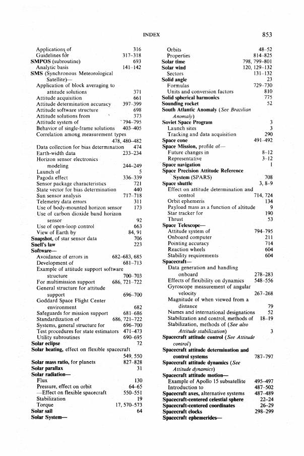
Application~ of Guidelines fdr
SMPOS (subroutine) Analytic basis
SMS (Synchronous Meteorological Satellite)-
Application of block averaging to
316 317-318
693 141-142
attitude solutions 371 Attitude acquisition 661 Attitude determination accuracy 397-399 Attitude software structure 698 Attitude solutions from 373 Attitude system of . 794--795 Behavior of single-frame solutions 403-405 Correlation among measurement types
478,480-482 Data collection for bias. determination 474 Earth-width data 233-234 Horizon sensor electronics
modeling Launch of Pagoda effect Sensor package characteristics State vector for bias determination Sun sensor analysis
244--249 5
336--339 721 440
717-718 311 173
Telemetry data errors Use of body-mounted horizon sensor Use of carbon dioxide band horizon
sensor Use of open-loop control View of Earth by
Snapshot, of star sensor data Snell's law Software-
92 663
84,91 706 223
Avoidance of errors in 682--683,685 Development of 681-713 Example of attitude support software
structure 700--703 For multimission support 686,721-722 General structure for attitude
support 696--700 Goddard Space Flight Center
environment 682 Safeguards for mission support 681--686 Standardization of 686,721-722 Systems, generaf structure for 696--700 Test procedures for state estimators- 471-473 Utility subroutines 69~95
Solar eclipse 72 Solar heating, effect on flexible spacecraft
Solar mass ratio, for planets Solar parallax Solar radiation-
Flux Pressure, effect on orbit -Effect on flexible spacecraft Stabilization Torque
Solar sail Solar System-
549,550 827--828
31
130 64--65
550-551 19
17,570-573 64
INDEX
Orbits Properties
Solar time Solar wind
Sectors Solid angle
Formulas Units and conversion factors
Solid spherical harmonics Sounding rocket
853
48-52 814--825
798, 799'-801 120, 129-'132
131-132 23
729-730 810 775
52 South Atlantic Anomaly (See Brazilian
Anomaly) Soviet Space Program
Launch sites Tracking and data acquisition
Space cone Space Mission, profile of
Future changes in Representative
'. Space navigation
3 3
290 491-492
8-12 3-12
I S~ce Precision Attitude Reference
-'System (SPARS) 708 3,8-9 Space shuttle
Effect on attitude determination and control 714,724
Orbit ephemeris 134 Payload mass as a function of altitude 9 Star tracker for 190 Thrust 53
Space TelescopeAttitude system of Onboard computer Pointing accuracy Reaction wheels Stability requirements
Spacecraft-Data generation and handling
onboard Effects of flexibility on dynamics Gyroscope measurement of angular
velocity Magnitude of when viewed from a
distance
794--795 211 714 604 604
278-283 548-556
267-268
Names and international designations Stabilization and control, methods of Stabilization, methods of (See also
79 52
18-19
Attitude stabilization) 3 Spacecraft attitude control (See Attitude
control) Spacecraft attitude determination and
control systems Spacecraft attitude dynamics (See
Attitude dynamics) Spacecraft attitude motlon
Example of Apollo 15 subsateIlite Introduction to
Spacecraft axes, alternative systems Spacecraft-centered celestial sphere Spacecraft-centered coordinates Spacecraft clocks Spacecraft ephemerides-
787-797
495-497 487-502 487-489
22-24 26--29
298-299

854 INDEX
Definitive subroutines 693 Two-body orbit generator (ORBGEN) 692
Spacecraft fixcd coordinates 26 Spacecraft orbits 52-62, 132-138
As function of injection conditions 60--62 MUltipurpose ephemeris subroutine
(EPHEMX) Spacecraft stability (See also A Ititude dy
namics; Disturbance torques;
693
Nutation; Flexible spacecraft ~vnamics) 523 Apollo IS subsatellite 495-497 With respect to hbration (GEOS
example) Spaceflight Tracking and Data Network
674
(STDN) 283-290 Time-tagging by 299-301
Spacelab, onboard computer 211 SPARS (See Space Precision Altitude
Reference System) Special perturbations, method of (orbit
analysis) 139 Specular reflection 84
Torque due to 572 SPHCNV (subroutine) 694 Sphere, illumination of as function of phase,
distance 78-79 89 Sphere of influence- '
F or spacecraft orbits 69-71 Table of for planets 69-71
Spherical coordinate systems 24--31, 760 Advantages relative to rectangular 25-26 Properties of 24--26 Transformations between 765-766
Spherical excess 32 Spherical geometry 31-35
Construction of global geometry plots 737-743
Equations for 727-736 Spherical harmonics 775-778
Expansion of gravitational potential in 124 Recursion relations 781 Representation of the geomagnetic
field Schmidt normalization for
Spherical plot subroutin\:s (SPHCNV,
779-782 780
SPHGRD, SPHPLT) 694-695 Spherical plots (See Global geometry plots) Spherical triangle 23
Infinitesimal 734 Notation for 33 Properties of 32-35
Spberical trigonometry 33-35 Differential 734--735 Example of 34--35 Table of general solutions 733, 735
SPHGRD (subroutine) 694 SPHPLT (subroutine) 694 Spin-axis drift,.during rocket engine firing 582 Spin-axis precession, magnetic 636-649 Spin rate-
Change during rocket engine firing 582
Control using gas jets 650 Effect of nutation on measurement
of 544--548 19, 503~504
3 787 172
231,234 467
Spin stabilization Spin-stabilized spacecraft
List of Split-to-index time, horizon sensors
Math. model (split-angle model) Square root filter SSS (Small Scientific Satellite)
Attitude system of 794-795 Effect of flexibility on attitude dynamics 556 Nutation damping 544,629 Telemetry data errors 311
ST (See Space Telescope) Stability-
Of control systems 594-600 Of rotation about a principal axis 523 Of spacecraft (See Spacecraft stability)
Stabilization (See A Ililude swbilization; Nutation damping; Libration damping)
Standard deviation 429 Standard notation
For attitude angles Standard symbols Standard Time Standardization-
Of attitude hardware Of attitude software
Star azimutb Star camera
x-xii 2~, 349
xi-xii, 50 801
718-721 686, 721-722
259 193
Star catalog, acquisition of by an attitude system
Star catalogs Star longitudes Star scanners
List of spacecraft using Star sensors-
704 143-150 149-150
186, 187, 190--192 797
Attitude determination methods for 703-709 Characteristics vs. accuracy require
ments Data selection and correction Example of use for nutation
monitoring Hardware List of spacecraft using Mathematical model of intensity
response Mathematical models Overview of attitude determination
with Representative telemetry data errors
190 704--705
538~539 184--195
797
258-259 254--259
703-709 311
Star trackersFixed-head Gimbaled List of spacecraft using
Stars-
186, 189-190, 193-195 186, 187-189
797
Angular diameter of 167 As attitude determination reference
source 17 Densities 145

Distribution, mathematical model of 263 Identification 706 Identification techniques 259-266 Instrumental magnitudes of 258 Magnitudes 144-145 Position modeling 143-150
State (in differential correction or "state" estimation) 439
436-483 437-438 407-408
State estimation Advantages relative to deterministic Need for Operational limits on accuracy Subroutine for (DC) Use in CTS attitude system
State estimators--Analytic basis Operational use of Prelaunch evaluation Subsystem in attitude software
476 691 702
447-470 471-484 471~473
system 697-698 Unresolv~d analytic problems 722-723
State noise covariance matrix 465 State plane trajectory 657
Examples of 658 For HEAO-I 607
State space 657 State transition matrix 450 State vector 436, 438-443
Choice of elements to be solved for 476-483 Construction of 438-443 Need for 407-408 Subroutine for updating (RECUR) 692
State vector elementsChoice of Observability of -Limitations
State weight matrix
439-443 443
476-483 449
STDN (See Spaceflight Tracking and Data NetwQrk)
Steady state (in Kalman filters) Steady-state error, in control systems Steady-state system response Steady-state trajectory
467 593 770 608
Steepest descent, method of (differential correction technique)
Steering law Stellar parallax Stepsize, in numerical integration STEREOSAT, use of AEM spacecraft Stictlon Stiffness matrix (for flexible spacecraft) STORMSAT-
Disturbance torques Use of MMS spacecraft
Stfapdown torque rebalanced· gyroscope Stratopause ~tratospbere SubcOmDlutated data Sub$atellite, Apollo 15, nutation of Subsatellite point (See a/so Nadir)
Alternative definitions Local mean time of
455 604
31 560 720 272 553
580 720 199 107 107
293-294 495-497
22 83 68
INDEX 855
Longitude of 805 Subsolar point 84 Summing point, in control system 589 Sun- (See also Solar)
Analytic ephemeris subroutines (SUN IX, SMPOS) 693
Approach by spacecraft 60 As attitude determination reference
source 17 Definitive ephemeris subroutines
(SUNRD, RJPLT) 693 Effect on acceleration of Earth satellite 127 Effect on geomagnetic activity 120-123 Energy flux from 130 Expression for mean motion 141 Interference with horizon sensors 169 Multipurpose ephemeris subroutine
(EPHEMX) Properties of Solar wind Symbol for
Sun angle measurement Density of For nutating spacecraft Information content
693 818
120, 129-132 50
11,23,344 347
539-548 480
Sun angle / nadir angle single-axis attitude solutions 368
406-407 12
364 156, 159-161
11,13 717-718
Singularities in Sun rime
Use in attitude determination SUD presence detector Sun sensor
Analysis of SIRIO vs. SMS design Calculation of coverage of celestial
sphere Calibration constants Combination Sun/Earth horizon
sensor Data validation Example of use in attitude control Example of use in attitude
34-35 230
178-179 329-330
14-16
determination 10-14 Field of view 225-226 Hardware 155-166 List of spacecraft by Sun sensor type 797 Mathematical models 218-230 Model of azimuth biases relative to
horizon sensor Nutation monitoring with Simple vs. complex Two axis. accuracy analysis Use for single-axis attitude Use for three-axis attitude
239~242
539-548 716-718 355-357 362-409
426 Sun .sensor /horizon sensor rotation angle
measurement 357'-359 Information content 480-482 Models 237~242 Use in attitude determination 364-365, 369
SUD shade (for star sensors) 186 Sun-synchronous orbit 68 Sundials 800

856
SUNRD (subroutine) SUNIX (subroutine)
Analytic basis Supercommutated data Superior conjunction Superior planet Surface spherical harmonics
140,693 693 141
293-294 49-50
49 775
Surveyor (spacecraft), attitude reference system
Switching, Conferencing, and Monitoring Arrangement (SCAMA)
Switching line (component of control system)
Symbols, astronomical Symmetric mas,s distribution, principal
axis of Symmetric matri,. Symmetric spacecraft SYMPHONIE (French/German
189
291
657 50
489 750 524
communications satellite)Attitude system of Horizon sensors
79.f-795 180 270 314 293
Synch speed, of reaction wheel Synchronization pattern, quality flag for Synchronization signal, role in telemetry Synchronization word, in NASCOM data
format Synchronous satellite
Of various planets. table Syndrome vector Synodic month Synodic period System gain-
291 55
825 296
52 50
Of a control system 590 Role in root locus diagram 597--600 Selection of for attitude control 622, 624
System mass matrix (for flexible space-craft) 553
Systematic error, in attitude measurements 402 Effect on deterministic solution behavior 404
Syzygy 49
-T-
Tachometers, for measuring wheel speed Tangent height Tangent plane coordinates (See Local
tangent coordinates) TCON20 (subroutine) TCON40 (subroutine) TDRSS (See Tracking and Data Relay
Satellite System) Tenon-
202 93
692 692
INDEX
Use in gas jets Use in momentum wheel bearings
Telemetry Generation and transmission of Time tagging
Telemetry anteODllS
206 202
293-298 278-298 298-304 28.f-288
Telemetry data errors (See also Data errors) 310-311
Table of representative examples 311 Telemetry formats 279, 293-295 Telemetry On-Line Processing System
(TELO PS) 292 Telemetry processor 3~308
In attitude software systems 696--697 Of CTS attitude system 701
Telemetry word 293 Tell-tale (data flag) 313-315 TELOPS (Telemetry On-Line Processing
System) 292 Temperature--
Of Earth's atmosphere Units and conversion factors
Tensor
107 812 519
Terminator Identification of
84,8Cr-90 331-334
Tesseral harmonic coefficients, explana-tion of 777-778
Testing-Of attitude software 686 Of state estimators 471-473
Thermal radiation (See Infrared radiation) Definition of 83
Thermistor, as energy detector for horizon sensor 171, 178
Thermopile, as energy detector for horizon sensor 171, 180
Thermosphere 107' Third-body interactions, effect on orbit
63,69-71 Three-axis attitude 343,359-361 Three axis attitude determination-
Accuracy 429-434 Example of least-squares estimator 456-459 Methods 410-434,420-428
Three-axis stabilized spacecraft 3 Thrust profile (of gasjet) 207,272-175 Tbrnsters (See Gas jets) Time--
Local mean time of subsatellite point 68 Measurement and broadcast facilities
299-302 Units and conversion factors 808-809
Time checking, of telemetry data 307-308 Time measurement systems 18-21,798--806
Conversion subroutines for 692 Table of 798
Time optimal magnetic maneuver 642, 648 Time tagging 278
Near-real-time data 302 Playback data 302 Representative telemetry data errors 311 Telemetry data 298-304
TlROS (meteorology satellite)-Attitude system of 79.f-795 First Use of Quarter Orbit Magnetic
Attitude Control 639

ntius-Bode law (See Bode's Law) TOD (See True of d4te) Torque (See also Disturbance torques;
Attitude control) Average of gas jet Due to magnetic moment Effect of, on spacecraft motion lntemal vs. external
, ,>Units and conversion factors Torque-free motion, of spacecraft Torque-free solutions, for attitude
motion Torr (unit of pressure) Total eclipse UtAAC, libration damping Trace, of a matrix
274, 813
498-502 521 810
487-497
524-531 809
Track pattern (in fixed-head star trackers) Tracking and Data Relay Satellite
72, 76 632 748 189
System (TDRSS) 8-10,287-290 Tracking stations 283-290
Location of 284-285 Timing systems 299-302
Trajectory, of gas jet precession 652 Trajectory, of spacecraft 53 Transfer elements, of a control system 588 Transfer function 244
Mathematical model of horizon sensor electronics 244-248
Of horizon sensor electronics 172 Use in control systems 589-590 Use of to evaluate stability 591-593
Transfer orbit (See also Hohmann transfer orbit) 5---{i, 53
Transfer time, in Hohmann transfer orbit
Between the planets (table) Transformations between coordinate
systems Transit
58-59 824
760--766 71-75
254 Transit time, in slit star scanner Transmission, of data and commands (See
also Telemetry) 278-292 Transpose, pf a,matrix 744 Transverse angular velocity 525 Transverse moment of inertia 524 Trapezoid model, of gas jet profiles 275 Trigonometry, spherical (See Spherical
trigonometry) Trojan asteroids 55 Tropical year 48 Tropopause 106 True anomaly 45-46 True of date coordinates 27-28 Truncation error, in integration procedures 560 Tumbling; of spacecraft due to crew
motion 579-580 Turbopause 108 Tum angle, of hyperbola 4O,60---{i1 Two-axis Sun sensor (See Sun sensor) Two-degree-of-freedom gyroscope 196
INDEX
Two tbousand (2000) coordinates Two's complement arithmetic Tyuratan (Soviet launch site)
UBV magnitudes UDU filter Uburu (See SAS)
-U-
857
27 297
4
144-145 467
Umbra 72 Uncertainty in attitudl~ measurements 345-346
Correlated 374, 378-379, 382-383 Due to systematic errors 402-408, 476 Expressions for 375-376,381-382,384 Uncorrelated 374-382
Uncertainty of state estimator soluti\,ns 476 Undershoot, in control systems 59,3 Unitary matrix 751 Unitary transformation 752 Units and converSion factors 807-813 Universal Time (UT)=GMT=Z
\9,798,801-802 Attached to data
Unpacking, of telemetry data UNVEC (subroutine) Uplink Upper stage rocket vehicles U.S. Coast Guard, time keeping system U.S. Naval Observatory, time keeping
system U.S. Standard Atmosphere UT (See Universal Time) UTC (See Universal Time; Coordinated
Universal Time) Utility subroutines
-V-
298 304-306
690 278
53 299
299-300 110
690---{i95
V-brusb, Sun sensor code 163 V-slit Sun sensor (V beam Sun Sensor) 161
Mathematical model 218-221 Validation-
Data flags and sensor identification Of attitude data
313-314 315-327
307,312-334 Of telemetry data Requiring attitude information
Vandenberg Air Force Base, Calif. (See Western Test Range)
Vanguard (tracking ship) Vanguard units Variance Variation of parameters, formulation of
334-339
284,287 808-809
429
attitude dynamics 531-534 VEC (subroutine) 690 Vector algebra 744-757
Subroutines 690---{i91 Vector calculus 755-756 Vector identities, in three dimensions 756-757

858
Vector magnetometer, mathematical model
Vector multlpUcation, inner and outer products
Vector notation Vector product (cross product)
'Equation for direction of Subroutine for (CROSSP)
Velocity-In a Keplerian orbit Units and conversion fact,)rs
Velocity of escape Planets and satellites, table
Vernal equinox Symbol for
VHF data transmission Vidicon, in star sensors Viking (Mars mission), launch dates
250-254
(47-748 x, xii
756 728 691
54,828 809 42
817,825 27,48
50 282-283
189
relative to oPPOSitiOO1 51, 57-58 Vis viva controversy 38 Vis viva equation 38, 42
Origin of 38 Viscous ring nutation damper 626, 627~29 Visibility of satellites and spacecraft 80 Visibility of spacecraft 71-80 Visible Ught sensor (See also Horizon sensor) 83 Visual magnitude, for spacecraft, sample
calculation Volterra equation VOP (See Variation of parameters) VPHAZE (subroutine)
-W-
Wallops Island, launch site Water, absorption bands Weighting (in estimation theory)
79 773
691
4 91-92
449-450
INDEX
Weighting data Weightlessness Western Test Range (launch site) WHECON, wheel control system
Active nutation damping with Wheel-mounted horizon sensor (See
also Scanwheels) Mathematical models Table of characteristics
White noise White Sands (launch site) World Warning Agency WWV time signals WWVH time signals
Yaw axis Year
Sidereal Tropical Types of
-Y-
Yo-yo despin maneuvers
-Z-
Z (time unit) (See Universal Time) Zenith Zenith angle Zero crossing magnetometer
370-373 41-42
3 613,622 63~31
169 234,236 176-178
269 4
52 299 299
29
799 799 48
663~9
Zeros, of control system transfer function Zonal luu1nonic coefficients-
22 85
250 590
Explanation of In gravitational potential
ZuIu;time i,
777 124,127
801