Appendices

A. Mathematics

A.I Geometry

Units of Angle and Solid Angle

Radian is the angular unit most suitable for theoretical studies. One radian is the angle subtended by a circular arc whose length equals the radius. If r is the radius of a circle and s the length of an arc, the arc subtends an angle

a = sir.

Since the circumference of the circle is 2 n r, we have

2 n rad = 3600 , or 1 rad = 1800 In.

In an analogous way, we can define a steradian, a unit of solid angle, as the solid angle subtended by a unit area on the surface of a unit sphere as seen from the centre. An area A on the surface of a sphere with radius r subtends a solid angle

(J) = Alr2.

Since the area of the sphere is 4 n r2, a full solid angle equals 4 n steradians.

Circle

- Area A = nr2 - Area of a sector As = +ar 2

Sphere

- Area A = 4nr2 - Volume V=fnr 3

- Volume of a sector V2 = tnr2h = t nr3(1- cosa) = Vsphere hav a - Area of a segment A s = 2nrh = 2nr2(1- cosa) = Asphere hav a

A.2 Taylor Series

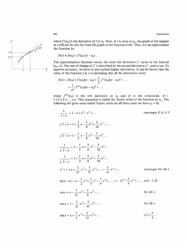
Let us consider a differentiable real-valued function of one variable f:R --+ R. The tangent to the graph of the function at Xo is

y

f(x)I-----pr

f(xcYl-- ---,<f

Xn x x

466 Appendices

where1'(xo) is the derivative offat Xo. Now, if x is close to xo, the graph of the tangent at x will not be very far from the graph of the function itself. Thus, we can approximate the function by

f(x) "'" f(xo) + 1'(xo)(x-xo) .

The approximation becomes worse, the more the derivative l' varies in the interval [xo, x]. The rate of change of l' is described by the second derivativef", and so on. To improve accuracy, we have to also include higher derivatives. It can be shown that the value of the function f at x is (assuming that all the derivatives exist)

f(x) = f(xo) + l' (xo)(x - xo) + ~ f" (xo)(x - xo)2 + ... 2

+_1_ fn )(xo)(x-xo)n+ ... n!

where fn)(xo) is the nth derivative at Xo and n! is the n-factorial, n! = 1 x 2 x 3 x ... X n. This expansion is called the Taylor series of the function at xo. The following list gives some useful Taylor series (in all these cases we have Xo = 0):

1 2 3 --= 1-x+x -x + ... converges if Ix I < 1 l+x

11.--- 112 1 3 V1+x=1+-x--x +-x - ...

2 8 16

1 1 3 2 5 3 --- = 1--x+-x --x ... VT+x 2 8 16

1 1 3 2 5 3 ---= 1 +-x+-x +-x ... V1-X 2 8 16

x 1 213 1 n e = 1+x+-x +-x + ... +-x + ... converges for all x

2! 3! n!

1 2 1 3 1 4 n+l 1 n ( 1 1] In(1+x)=x--x +-x --x + ... +(-1) -x + ... XE - , 2 3 4 n

.13 1 5 SlllX=X--X +-x - ... 3! 5!

1 2 1 4 cosx = 1--x +-x

2! 4!

1 3 2 5 tanx=x+-x +-x + ...

3 15

for all x

for all x

7C Ixl<-·

2

A. Mathematics 467

Many problems involve small perturbations, in which case it is usually possible to find expressions having very rapidly converging Taylor expansions. The great advantage of this is the reduction of complicated functions to simple polynomials. Particularly useful are linear approximations, such as

1 Vl+x::::l+-x,

2

1 1 ---::::l--x, VI +x 2

etc.

A.3 Vector Calculus

A vector is an entity with two essential properties: magnitude and direction. Vectors are usually denoted by boldface letters, a, b, A, B, etc. The sum of the vectors of A and B can be determined graphically by moving the origin of B to the tip of A and connecting the origin of A to the tip of B. The vector - A has the same magnitude as A, is parallel to A, but points in the opposite direction. The difference A - B is defined as A + (-B).

Addition of vectors satisfies the ordinary rules of commutativity and associativity,

A+B=B+A,

A + (B + C) = (A + B) + C .

A point in a coordinate frame can be specified by giving its position vector, which extends from the origin of the frame to the point. The position vector r can be expres­sed in terms of basis vectors, which are usually unit vectors, i.e. have a length of one distance unit. In a rectangular xyz-frame, we denote the basis vectors parallel to the coordinate axes by [, J, and k. The position vector corresponding to the point (x, y, z) is then

r=xf+y]+zk.

The numbers x, y and z are the components of r. Vectors can be added by adding their components. For example, the sum of

is

The magnitude of a vector r in terms of its components is

The scalar product of two vectors A and B is a real number (scalar),

where (A, B) is the angle between the vectors A and B. We can also think of the scalar product as the projection of, say, A in the direction of B multiplied by the length of B. If A and B are perpendicular, their scalar product vanishes. The magnitude of a vector expressed as a scalar product is A = V A . A .

z

(x, y, z)

,,--o:-------y

x

B

~~~~':::f--~A IBI cos (A,B)

x

468 Appendices

A xB The vector product of the vectors A and B is a vector:

z

i J k A xB = (aybz-azby)[ + (azbx-axbz)J + (axby-aybx)k = ax ay az

bx by bz

This is perpendicular to both A and B. Its length gives the area of the parallelogram spanned by A and B. The vector product of parallel vectors is a null vector. The vector product is anti-commutative:

AxB=-BxA.

Scalar and vector products satisfy the laws of distributivity:

A . (B + C) = A . B + A . C

(A + B) . C = A . C + B . C

A scalar triple product is a scalar

ax ay az A xB· C = bx by bz

Cx cy Cz

A x (B + C) = A x B + A x C

(A + B) x C = A x C + B xC.

Here, the cross and dot can be interchanged and the factors permuted cyclically with­out affecting the value of the product. For example, A xB . C = B xC· A = B . C xA, but A xB . C = - B xA . C.

A vector triple product is a vector, which can be evaluated using one of the expansions

A X(BXC) =B(A· C)-C(A ·B).

(A XB) XC=B(A· C)-A(B· C)

In all these products, scalar factors can be moved around without affecting the product:

A . kB = k(A . B), A x (B x kC) = k(A x (B x C» etc.

The position vector of a particle is usually a function of time: r = r(t) = x(t)[ + y(t)J + z(t)k. The velocity of the particle is a vector, tangent to the trajec­tory, obtained by taking the derivative of r with respect to time:

d .. ~ . ~ . ~ v = -r(t) =. r = Xl + Y J + zk .

dt

The acceleration is the second derivative, i; . Derivatives of the various products obey the same rules as derivatives of products of

real-valued functions:

d . . - (A . B) = A . B + A . B , dt

d . . - (A x B) = A x B + A x B . dt

A. Mathematics 469

When computing a derivative of a vector product, one must be careful to retain the order of the factors, since the sign of the vector product changes if the factors are inter­changed.

A.4 Conic Sections

As the name already says, conic sections are curves obtained by intersecting circular cones with planes.

Ellipse

Equation in rectangular coordinates

x2 y2 - + --= 1 where a 2 b 2

a: the semi-major axis b: the semi-minor axis = a ~ e: the eccentricity 0 ~ e < 1. Distance of the foci from the centre c = ea Parameter p = a(1 - e2 )

Area A = nab - Equation in polar coordinates

p r=----

1 +ecosj

where the distance r is measured from one focus, not from the centre When e -+ 0 the curve becomes a circle

Hyperbola

y

a -~======~F=~==~-+--X

b

y

Equations in rectangular and polar coordinates ---~~~===?~--;-~X

p r=----

1 +ecosj

Eccentricity e > 1 Semi-minor axis b = a ~ Parameter p = a(e 2 -1)

b - Asymptotes y = ± - x

a

Parabola

Parabola is a limiting case between the previous ones; its eccentricity is e = 1. Equations

p r=----

1 + cosj

Distance of the focus from the apex h = 1I4a Parameter p = 112a

y

-----~==t=~----X h

470 Appendices

y A.S Multiple Integrals

An integral of a function f over a surface A

1= JfdA A

can be evaluated as a double integral by expressing the surface element dA in terms of _-jlLCCLLL""""--_____ x coordinate differentials. In rectangular coordinates,

dA =dxdy,

and in polar coordinates,

dA = rdrd([J.

The integration limits of the innermost integral may depend on the other integration variable. For example, the function xeY integrated over the shaded area is

1 2x 1= JxeYdA = J J xeYdxdy

A x=O y=o

1 l2x] 1 = J I xeY dx = J (xe 2x-x)dx 000

111 2x 12x 1212 -xe --e --x =-(e -1). 02 4 2 4

The surface need not be confined to a plane. For example, the area of a sphere is

A = J dS, s

where the integration is extended over the surface S of the sphere. In this case, the sur­face element is

and the area is

2n n!2

A = J J R 2 cosOd([JdO qJ= 0 (1= -ni2

Similarly, a volume integral

1= JidV v

can be computed as a triple integral. In rectangular coordinates, the volume element dV

A. Mathematics 471

is

dV= dxdydZ;

in cylindrical coordinates,

dV= rdrdrpdz,

and in spherical coordinates,

dV = r2 cos edr drp de (e measured from the xy-plane)

or

dV = r2 sin edr dcpde (e measured from the z -axis).

For example, the volume of a sphere with radius R is

V= J dV v

R 211 1112

= J J J r2cosedrdrpde r=O '1'=0 ()= -1112

R 211 [ 1112 ] R 211 = J J I r2sine drdrp= J J 2r2drdrp

o 0 -11/2 0 0

R 2 R 4nr3 4 3 = J 4nr dr= 1--=-nR .

o 0 3 3

A.6 Numerical Solution of an Equation

We frequently meet equations defying analytical solution. Kepler's equation is a typical example. If we cannot do anything else, we can always apply some numerical method. Next, we shall present two very simple methods, the first of which is particularly suit­able for calculators.

Method 1. We shall write the equation as !(x) = x. Next, we have to find an initial value Xo for the solution. This can be done, for example, graphically, or by just guess­ing. Then we compute a succession of new iterates: Xl = !(XO) , X2 = !(Xl), ... and so on, until the difference of successive solutions becomes smaller than some preset limit. The last iterate Xi is the solution. After computing a few x/s, it is easy to see if they are going to converge. If not, we rewrite the equation as !-I(X) = X and try again. if-I is the inverse function of f. )

As an example, let us solve the equation X = -In x. We guess Xo = 0.5 and find

Xl = -lnO.5 = 0.69, X2 = 0.37 , X3 = 1.00.

This already shows that something is wrong. Therefore, we change our equation to X = e -x and start again:

z

l=-\-t---y

x

z

y

x

472

y

f (X2)

f (>eo)

f (X I)

Xo = 0.5 Xl = e- O.5

= 0.61 X2 = 0.55

,+ ~

X3 = 0.58 X4 = 0.56 X5 = 0.57 X6 = 0.57 .

y

X

Thus the solution, accurate to two decimal places, is 0.57.

Appendices

X

Method 2. In some pathological cases, the previous method may refuse to converge. In such situations, we can use the foolproof method of interval halving. If the function is continuous (as most functions of classical physics are) and we manage to find two points Xl and X2 such that/(xl) > 0 and/(x2) < 0, we know that somewhere between Xl

and X2 there must be a point X in which /(x) = O. Now, we find the sign of / in the midpoint of the interval, and select the half of the interval in which/ changes sign. We repeat this procedure until the interval containing the solution is small enough.

We shall try also this method on our equation X = -In x, which is now written as f(x) = 0, where/(x)=x+lnx. Because/(x) ->-00, when x -> 0, and/(l»O, the solution must be in the range (0,1). Since /(0.5) < 0, we know that xE(0.5, 1). We continue in this way:

/(0.75) > 0 /(0.625) > 0 /(0.563) < 0 /(0.594) > 0

xE(0.5,0.75) X E (0.5, 0.625) xE(0.563,0.625) X E (0.563, 0.594)

The convergence is slow but certain. Each iteration restricts the solution to an interval which is half as large as the previous one, thus improving the solution by one binary digit.

B. Quantum Mechanics 473

B. Quantum Mechanics

B.1 Quantum Mechanical Model of Atoms. Quantum Numbers

Bohr's model can predict the coarse features of the hydrogen spectrum quite well. It cannot, however, explain all the finer details; nor is it applicable for atoms with several electrons. The reason for these failures is the classical concept of the electron as a particle with a well-defined orbit. Quantum mechanics describes the electron as a three­dimensional wave, which only gives the probability of finding the electron in a certain place. Quantum mechanics has accurately predicted all the energy levels of hydrogen atoms. Also, the energy levels of heavier atoms and molecules can be computed; how­ever, such calculations are very complicated. The existence of quantum numbers can be understood from the quantum mechanical point of view as well.

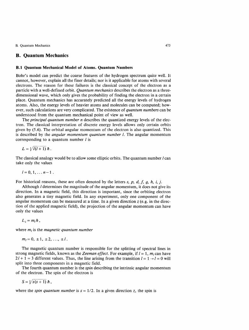
The principal quantum number n describes the quantized energy levels of the elec­tron. The classical interpretation of discrete energy levels allows only certain orbits given by (5.6). The orbital angular momentum of the electron is also quantized. This is described by the angular momentum quantum number I. The angular momentum corresponding to a quantum number I is

L = VI(l + 1) Il .

The classical analogy would be to allow some elliptic orbits. The quantum number I can take only the values

1= 0, 1, ... n -1 .

For historical reasons, these are often denoted by the letters s, p, d, f, g, h, i, j. Although I determines the magnitude of the angular momentum, it does not give its

direction. In a magnetic field, this direction is important, since the orbiting electron also generates a tiny magnetic field. In any experiment, only one component of the angular momentum can be measured at a time. In a given direction z (e.g. in the direc­tion of the applied magnetic field), the projection of the angular momentum can have only the values

where m, is the magnetic quantum number

m,=O, ±1, ±2, ... , ±l.

The magnetic quantum number is responsible for the splitting of spectral lines in strong magnetic fields, known as the Zeeman effect. For example, if I = 1, m, can have 21 + 1 = 3 different values. Thus, the line arising from the transition 1= 1 -> I = ° will split into three components in a magnetic field.

The fourth quantum number is the spin describing the intrinsic angular momentum of the electron. The spin of the electron is

S=Vs(s+l)ll,

where the spin quantum number is s = 112. In a given direction z, the spin is

474 Appendices

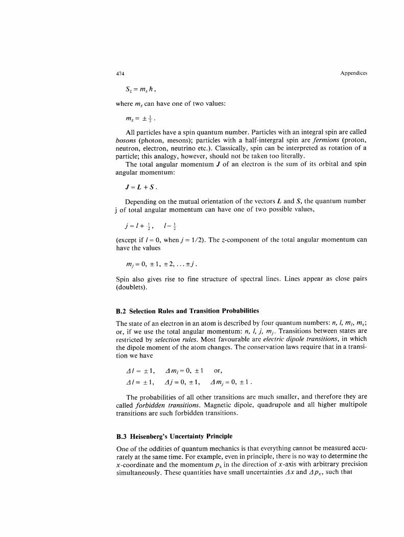
where ms can have one of two values:

All particles have a spin quantum number. Particles with an integral spin are called bosons (photon, mesons); particles with a half-intergral spin are fermions (proton, neutron, electron, neutrino etc.). Classically, spin can be interpreted as rotation of a particle; this analogy, however, should not be taken too literally.

The total angular momentum 1 of an electron is the sum of its orbital and spin angular momentum:

1=L+S.

Depending on the mutual orientation of the vectors Land S, the quantum number j of total angular momentum can have one of two possible values,

j=I+-L I-~ 2

(except if 1= 0, when j = 1 /2). The z-component of the total angular momentum can have the values

mj = 0, ± 1, ± 2, ... ±j .

Spin also gives rise to fine structure of spectral lines. Lines appear as close pairs (doublets).

B.2 Selection Rules and Transition Probabilities

The state of an electron in an atom is described by four quantum numbers: n, I, ml, ms; or, if we use the total angular momentum: n, I, j, mj' Transitions between states are restricted by selection rules. Most favourable are electric dipole transitions, in which the dipole moment of the atom changes. The conservation laws require that in a transi­tion we have

LJI=±l, LJml=O,±l or,

LJI = ± 1, LJj = 0, ± 1, LJ mj = 0, ± 1 .

The probabilities of all other transitions are much smaller, and therefore they are called forbidden transitions. Magnetic dipole, quadrupole and all higher multipole transitions are such forbidden transitions.

B.3 Heisenberg's Uncertainty Principle

One of the oddities of quantum mechanics is that everything cannot be measured accu­rately at the same time. For example, even in principle, there is no way to determine the x-coordinate and the momentum Px in the direction of x-axis with arbitrary precision simultaneously. These quantities have small uncertainties LJx and LJpx, such that

C. Theory of Relativity 475

,1x,1Px",=,h.

A similar relation holds for other directions, too. Time and energy are also connect­ed by an uncertainty relation,

This means that a particle can materialize out of nowhere if it disappears again within a time hlmc 2 .

B.4 Exclusion Principle

Pauli's exclusion principle states that an atom with many electrons cannot have two electrons with exactly the same quantum numbers. This can be generalized to a gas of fermions (like electrons). The uncertainty principle allows us to find the size of a volume element (in phase space), which can hold at most two fermions; these must then have opposite spins. The phase space is a six-dimensional space, three coordinates giv­ing the position of the particle and the other three, its momenta in the x, y and z-direc­tions. Thus, a volume element is

From the uncertainty principle it follows that the smallest sensible volume element has a size of the order h 3. In such a volume, there can be at most two fermions of the same kind.

C. Theory of Relativity

Albert Einstein published his special theory of relativity in 1905 and the general theory of relativity ten years later. Especially the general theory, which is essentially a gravita­tion theory, has turned out to be very important for the theories of the evolution of the Universe. Therefore, it is appropriate to consider here some basic principles of relativi­ty theory. A more detailed discussion would require sophisticated mathematics, and is beyond the scope of this very elementary book.

C.l Basic Concepts

Everyone knows the famous Pythagorean theorem,

where ,1s is the length of the hypotenuse of a right-angle triangle, and ,1x and ,1y are the lengths of the other two sides. (For brevity, we have denotes ,1s2 = (,1S)2.) This is easily generalized to three dimensions:

,1s2 = ,1x2+ ,1y2 + ,1 Z2 .

This equation describes the metric of an ordinary rectangular frame in a Euclidean space, i.e. tells us how to measure distances. x

z

L1~ }---__ -'ll ....... ___ Y

476 Appendices

Generally, the expression for the distance between two points depends on the exact location of the points. In such a case, the metric must be expressed in terms of in­finitesimal distances in order to correctly take into account the curvature of the coordinate curves. (A coordinate curve is a curve along which one coordinate changes while all the others remain constant.) An infinitesimal distance ds is called the line ele­ment. In a rectangular frame of a Euclidean space, it is

ds 2 = dx 2 + dy2 + dz 2

and in spherical coordinates,

Generally, ds 2 can be expressed as

ds2 = L L gijdxi dxi , i i

where the Xi,S are arbitrary coordinates, and the coefficients gij are components of the metric tensor. These can be functions of the coordinates, as in the case of the spherical coordinates. The metric tensor on an n-dimensional space can be expressed as an n x n matrix. Since dx i dxi = dxi dx i , the metric tensor is symmetric, i.e. gij = gii' If all coor­dinate curves intersect perpendicularly, the coordinate frame is orthogonal. In an or­thogonal frame, gij = 0 for all i *- j. For example, the spherical coordinates form an orthogonal frame, the metric tensor of which is

If it is possible to find a frame in which all the components of g are constant, the space is flat. In the rectangular frame of a Euclidean space, we have gIl = g22 = g33 = 1; hence the space is flat. The spherical coordinates show that even in a flat space, we can use frames in which the components of the metric tensor are not constant. The line element of a two-dimensional spherical surface is obtained from the metric of the spherical coordinate frame by assigning to r some fixed value R:

The metric tensor is

This cannot be transformed to a constant tensor. Thus the surface of a sphere is a curved space.

If we know the metric tensor in some frame, we can compute a fourth-order tensor, the curvature tensor Rijkl' which tells us whether the space is curved or flat. Unfortu­nately, the calculations are slightly too laborious to be presented here.

c. Theory of Relativity 477

The metric tensor is needed for all computations involving distances, magnitudes of vectors, areas, and so on. Also, to evaluate a scalar product, we must know the metric. In fact, the components of the metric tensor can be expressed as scalar products of the basis vectors:

If A and B are two arbitrary vectors,

their scalar product is

A ·B= L L aitJei·ej= L L gijaitJ. j j

C.2 Lorentz Transformation. Minkowski Space

The special theory of relativity abandoned the absolute Newtonian time, supposed to flow at the same rate for every observer. Instead, it required that the speed of light have the same value c in all coordinate frames. The constancy of the speed of light is the basic principle of the special theory of relativity.

Let us send a beam of light from the origin. It travels along a straight line at the speed c. Thus, at the moment t, its space and time coordinates satisfy the equation

(C.l)

Next, we study what the situation looks like in another frame, x' y' Zl, moving at a velocity v with respect to the xyz-frame. Let us select the new frame so that it coincides with the xyz-frame at t = O. Also, let the time coordinate t ' of the x' y' z'-frame be I' = 0 when 1= O. And finally, we assume that the x' y' z'-frame moves in the direction of the positive x-axis. Since the beam of light must also travel at the speed c in the x' y' z'-frame, we must have

If we require that the new (dashed) coordinates be obtained from the old ones by a linear transformation, and also that the inverse transformation be obtained simply by replacing v by - v, we find that the transformation must be

y' =y

Z' = Z

t' = t- vx/c 2

Vl- v2/C 2

478 Appendices

This transformation between frames moving at a constant speed with respect to each other is called the Lorentz transformation.

Becasue the Lorentz transformation is derived assuming the invariance of (C.l), it is obvious that the interval

of any two events remains invariant in all Lorentz transformations. This interval defines a metric in four-dimensional spacetime. A space having such a metric is called the Minkowski space or Lorentz space. The components of the metric tensor g are

l-c2 0 0 OJ o 1 0 0 (gi) = 0 0 1 0 .

o 0 0 1

Since this is constant, the space is flat. But it is no longer an ordinary Euclidean space, because the sign of the time component differs from the sign of the space components. In the older literature, a variable ict is often used instead of time, i being the imaginary unit. Then the metric looks Euclidean, which is misleading; the properties of a space cannot be changed just by changing notation.

In a Minkowski space position, velocity, momentum and other vector quantities are described by four-vectors, which have one time and three space components. The com­ponents of a four-vector obey the Lorentz transformation when we transform them from one frame to another, both moving along a straight line at a constant speed.

According to classical physics, the distance of two events depends on the motion of the observer, but the time interval between the events is the same for all observers. The world of special relativity is more anarchistic: even time intervals have different values for different observers.

C.3 General Relativity

The Equivalence Principle. Newton's laws relate the acceleration, a, of a particle and the applied force F by

where mi is the inertial mass of the particle, resisting the force trying to move the particle. The gravitational force felt by the particle is

where mg is the gravitational mass of the particle, and f is a factor depending only on other masses. The masses mi and mg appear as coefficients related to totally different phenomena. There is no physical reason to assume that the two masses should have anything in common. However, already the experiments made by Galilei showed that evidently mi = mg. This has been verified later with very high accuracy.

The weak equivalence principle, which states that mi = mg , can, therefore, be ac­cepted as a physical axiom. The strong equivalence principle generalizes this: if we

C. Theory of Relativity 479

restrict our observations to a sufficiently small region of space-time, there is no way to tell whether we are subject to a gravitational field or are in uniformly accelerated motion. The strong equivalence principle is one of the fundamental postulates of general relativity.

Curvature of Space. General relativity describes gravitation as a geometric property of space-time. The equivalence principle is an obvious consequence of this idea. Particles moving through space-time follow the shortest possible paths, geodesics. The projec­tion of a geodesic onto three-dimensional space need not be the shortest way between the points.

The geometry of space-time is determined by the mass and energy distribution. If this distribution is known, we can write the field equations, which are partial differential equations connecting the metric to the mass and energy distribution and describing the curvature of space-time.

In the case of a single-point mass, the field equations yield the Schwarzschild metric, the line element of which is

Here, M is the mass of the point; r, () and ¢ are ordinary spherical coordinates. It can be shown that the components cannot be transformed to constants simultaneously: space-time must be curved due to the mass.

If we study a very small region of space-time, the curvature has little effect. Locally, the space is always a Minkowski space where special relativity can be used. Locality means not only a limited spatial volume but also a limited interval in time.

C.4 Tests of General Relativity

General relativity gives predictions different from classical physics. Although the dif­ferences are usually very small, there are some phenomena in which the deviation can be measured and used to test the validity of general relativity. At present, five different astronomical tests have verified the theory.

First of all, the orbit of a planet is no longer a closed Keplerian ellipse. The effect is strongest for the innermost planets, whose perihelia should turn little by little. Most of the motion of the perihelion of Mercury is predicted by Newtonian mechanics; only a small excess of 43 arc seconds per century remains unexplained. And it so happens that this is exactly the correction suggested by general relativity.

Secondly, a beam of light should bend when it travels close to the Sun. For a beam grazing the surface, the deviation should be about 1.75". Such effects have been observed during total solar eclipses and also by observing pointlike radio sources, just before and after occultation by the Sun.

The third classical way of testing general relativity is to measure the redshift of a photon climbing in a gravitational field. We can understand the redshift as an energy loss while the photon does work against the gravitational potential. Or, we can think of the redshift as caused by the metric only: a distant observer finds that near a mass, time runs slower, and the frequency of the radiation is lower. The time dilation in the Schwarzschild metric is described by the coefficient of dt; thus it is not surprising that

480 Appendices

the radiation emitted at a frequency v from a distance r from a mass M has the frequency

voo=VV1_2GM, c2r

(C.2)

if observed very far from the source. This gravitational redshift has been verified by laboratory experiments.

The fourth test employs the slowing down of the speed of light in a gravitational field near the Sun. This has been verified by radar experiments.

The previous tests concern the solar system. Outside the solar system, binary pulsars have been used to test general relativity. An asymmetric system in accelerated motion (like a binary star) loses energy as it radiates gravitational waves. It follows that the components approach each other, and the period decreases. Usually the gravita­tional waves playa minor role, but in the case of a compact source, the effect may be strong enough to be observed. The first source to show this predicted shortening of period was the binary pulsar PSR 1913 + 16.

D. Radio Astronomy Fundamentals

D.1 Antenna Definitions

The receiving (or transmitting) characteristics of an antenna are described by the anten­na power pattern p(e, cp), which, for an ideal antenna, is equivalent to the Fresnel diffraction pattern of an optical telescope. The power pattern P( e, cp) is a measure of the antenna response to radiation as a function of the polar coordinates e and cp. It is directly proportional to the radiation intensity U(e, cp) [W sr- 1] and usually normal­ized so that the maximum intensity equals one, i.e.

(0.1)

where Urnax(e, cp) is the maximum radiation intensity. The beam solid angle Q A is defined as the integral over the power pattern, i.e.

QA= Hp(e, cp)dQ. (0.2) 4"

This is the equivalent solid angle through which all the radiation would enter if the power were constant and equal to its maximum value within this angle.

If we integrate over the main beam only, i.e. to the limit where the power pattern reaches it first minimum, we obtain the main beam solid angle Q m

Qrn = H p(e, cp) dQ. (0.3) mainlobe

If the integration is carried out over all sidelobes, one gets the sidelobe solid angle Q s

H p(e, cp)dQ. (0.4) all sidelobes

D. Radio Astronomy Fundamentals 481

It is easy to see that

(D.5)

We now define the beam efficiency, I7B, as the ratio of the main beam solid angle Q m to the beam solid angle QA, i.e.

(D.6)

The beam efficiency thus measures the fraction of the total radiation that enters into the main lobe, and is one of the prime parameters that characterize a radio telescope.

Another important parameter is the directivity, D. The directivity is defined as the ratio of the maximum radiation intensity Umax ({}, ({J) to the average radiation intensity (U),i.e.

D = Umax ({), ((J)

(U) (D.7)

Since the average radiation intensity is the total received power over 4 n steradians

1 u=-H U«(), ({J)dQ, 4 n 4"

we can combine equations (D.l), (D.7) and (D.8) to obtain

4n D=------

H P«(), ({J) dQ 4"

(D.8)

(D.9)

The directivity thus measures the amplification or gain of an antenna. If the antenna has no loss, the directivity is equal to the gain, G. However, all antennas have small resistive losses, which can be accounted for by defining a radiation efficiency factor, I7r (for most antennas very close to one). Then

(D.10)

Another basic antenna parameter is the effective aperture Ae , which, for all large antennas, is smaller than the geometrical antenna aperture, Ag • The ratio between the effective aperture and the geometrical aperture, I7A' i.e.

(D.11)

is called the aperture efficiency and is another principal measure of the quality of a telescope.

From thermodynamical considerations, one can show that the effective aperture of a telescope is related to the beam solid angle by

(D.12)

By combining Eqs. (D.9) and (D.12) we can therefore express the directivity as a

482 Appendices

function of the effective area

(D.13)

or, alternatively, by using the relation between directivity and gain, i.e.

(D.14)

Usually the radiation efficiency is included in the effective area or taken equal to one, in which case the expressions for directivity and gain appear equal.

D.2 Antenna Temperature and Flux Density

The power measured with a radio telescope can be related to an equivalent tempera­ture, the antenna temperature, T A. If we assume that the antenna is placed in an enclosure with a uniform temperature T A, or equivalently, if the antenna is replaced by a matched load at the same temperature, it can be shown that the power P[W] at the antenna terminal is given by

(D.15)

where k is Boltzmann's constant, w is the spectral power (power per unit bandwidth) and L1 v is the bandwidth of the radiometer. This relation provides a relation between the observed power P and the antenna temperature T A' If the Rayleigh-Jeans approximation, h v / k ~ T A, is not valid (v ~ 100 GHz), then T A has to be replaced by the radiation temperature

Since the antenna is usually calibrated by comparing the incoming signal with a temperature-controlled matched load or a gas-discharge tube with a well-defined tem­perature, it is quite convenient to express the received signal as an antenna temperature. Using the antenna temperature has the additional advantage of providing a power measure that is independent of the radiometer bandwidth.

On the other hand, the spectral power for an antenna is defined as

Wv = +Ae H Iv(fJ, ([J) p(e, ([J) dQ, (D.16) 4rr

where I v( e, ([J) is the brightness of the sky; the factor + enters because a radio telescope receives only one polarization component. Using (D.15), we can now express the power in terms of the antenna temperature T A, i.e.

(0.17)

If the angular extent of the source is much smaller than the beamwidth of the anten­na, i.e. for a "point source", the power pattern P(8, ([J) - 1 and

E. Tables 483

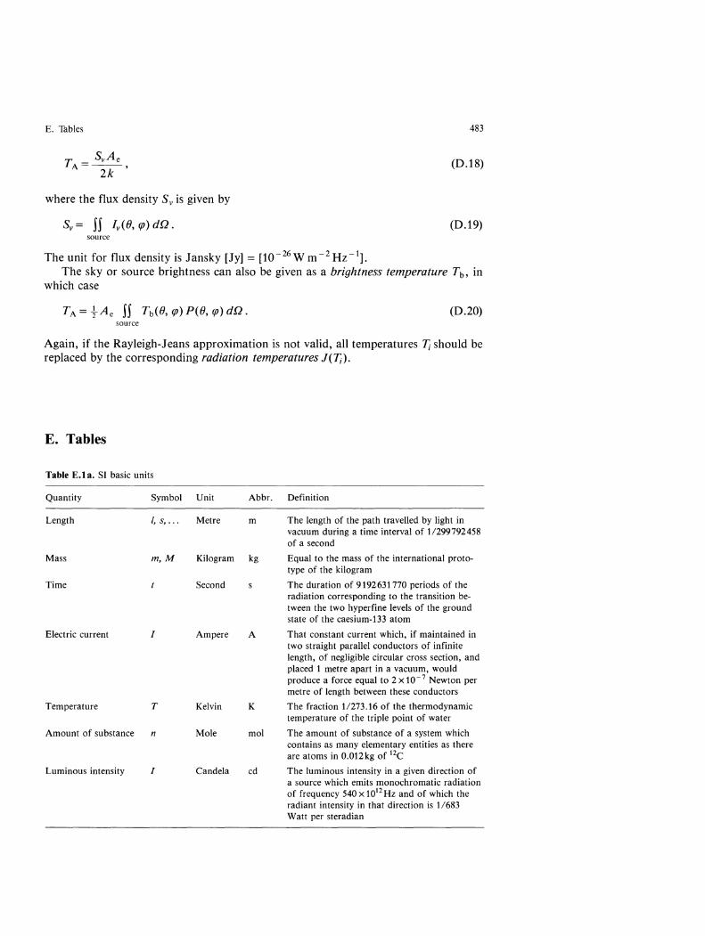
(D.1S)

where the flux density Sv is given by

(D.19) source

The unit for flux density is Jansky [Jy] = [10- 26 Wm- 2 Hz- 1].

The sky or source brightness can also be given as a brightness temperature Tb , III

which case

(D.20) source

Again, if the Rayleigh-Jeans approximation is not valid, all temperatures ~ should be replaced by the corresponding radiation temperatures J(~).

E. Tables

Table E.la. SI basic units

Quantity Symbol Unit Abbr. Definition

Length I, S, ... Metre m The length of the path travelled by light in vacuum during a time interval of 11299792458 of a second

Mass m,M Kilogram kg Equal to the mass of the international proto-type of the kilogram

Time Second The duration of 9192631770 periods of the radiation corresponding to the transition be-tween the two hyper fine levels of the ground state of the caesium-133 atom

Electric current I Ampere A That constant current which, if maintained in two straight parallel conductors of infinite length, of negligible circular cross section, and placed 1 metre apart in a vacuum, would produce a force equal to 2 x 10- 7 Newton per metre of length between these conductors

Temperature T Kelvin K The fraction 11273.16 of the thermodynamic temperature of the triple point of water

Amount of substance n Mole mol The amount of substance of a system which contains as many elementary entities as there are atoms in 0.012kg of 12C

Luminous intensity I Candela cd The luminous intensity in a given direction of a source which emits monochromatic radiation of frequency 540 x 1012 Hz and of which the radiant intensity in that direction is 11683 Watt per steradian

484 Appendices

Table E.1 b. Prefixes for orders of ten

Prefix Symbol Multiple

yocto y 10- 24 zepto z 10-21 atto a 10- 18

femto f 10- 15 pico P 10- 12

nano n 10- 9

micro Il 10-6 milli m 10-3

centi c 10- 2

deci d 10- 1

deca da 101 hecto h 102 kilo k 103 Mega M 106 Giga G 109 Tera T 1012 Peta P 1015 Exa E 1018 Zetta Z 1021 Yotta Y 1024

Table E.2. Constants and units. To avoid extensive changes of the less significant digits, older values of some constants of atomic physics are used in the text. More recent values are listed below

1 Radian 1 Degree 1 Arc second

Velocity of light Gravitational constant

Planck constant

Boltzmann constant Radiation density constant Stefan-Boltzmann constant Atomic mass unit Electron volt Electron charge Mass of electron Mass of proton Mass of neutron Mass of lH atom Mass of iHe atom Rydberg constant for 1 H Rydberg constant for 00 mass Gas constant Normal atmospheric pressure

Astronomical unit Parsec Light-year

1 rad = 180°hr = 57.2957795° = 206264.8" 1 ° = 0.01745329 rad 1" = 0.000004848 rad

c G

h h k a a amu eV e me mp mn mH m He

RH Roo R atm

AU pc ly

= 299792458 m S-1 = 6.673x 10- 11 m3 kg- 1 s-2 =4n 2 AU3 M- 1 a- 2 = 3986005 x 108 m3 M~1 s-2 = 6.6261 X 10- 34 ls = hl2n = 1.0546 x 10- 34 ls = 1.3807 x 10-23 lK- 1 = 7.5659x 10- 16 1m -3 K-4 = ac/4 = 5.6705 x 10-8 Wm -2 K- 4 = 1.6605 X 10-27 kg = 1.6022 x 10- 19 1 = 1.6022xlO- 19 C = 9.1094x 10- 31 kg = 0.511 MeV = 1.6726 x 10-27 kg = 938.3 MeV = 1.6749 x 10-27 kg = 939.6 MeV = 1.6735 x 10-27 kg = 1.0078amu = 6.6465 x 10 - 27 kg = 4.0026 amu = 1.0968 x 107 m- 1 = 1.0974 x 107 m- 1 = 8.3146 lK- 1 mol- 1

= 101325 Pa = 1013 mbar = 760 mm Hg

= 1.49597870x 1011 m = 3.0857 x 1016 m = 206265 AU = 3.261y = 0.9461 x 1016 m = 0.3066 pc

E. Tables

Table E.3. Units of time

Unit

Sidereal year Tropical year Anomalistic year Gregorian calendar year Julian year Julian century Eclipse year Lunar year

Synodical month Sidereal month Anomalistic month Draconitic month

Mean solar day

Sidereal day

Rotation period of the Earth (referred to fixed stars)

International atomic time on July 1,1993

Terrestrial time

Table E.4. The Greek alphabet

Aa BP ry Llo alpha beta gamma delta

AA Mil Nv Ec, lambda mu nu xi

tPt/J1fI Xx 'PV/ Qw

Equivalent to

365.2564d 365.2422d (equinox to equinox) 365.2596d (perihelion to perihelion) 365.2425d 365.2500d 36525d 346.6200d (with respect to the ascending node of the Moon) 354.4306d = 12 synodical months

29.5306d 27.3217d 27.5546d (perigee to perigee) 27.2122d (node to node)

24h mean solar time = 24h 03 min 56.56s (sidereal time)

24h sidereal time = 23 h 56min 04.09s (mean solar time)

23h 56 min 04.10s

TAl = UTC+28 s (exactly)

TT"'TAI+32.184s (SI seconds)

Eli Z, HIT e B rJ epsilon zeta eta theta

00 n7CW Pp I ar; omicron pi rho sigma

II KK iota kappa

TT Yv tau upsilon

485

phi chi psi omega

Table E.S. The Sun

Property

Mass Radius Effective temperature Luminosity Apparent visual magnitude Colour indices

Absolute visual magnitude Absolute bolometric magnitude Inclination of equator to ecliptic Equatorial horizontal parallax Motion: direction of apex

velocity in LSR Distance from galactic centre

Symbol

Mr,v Rr,v Te Lr,v V B-V U-B Mv Mbol

7Cr,v

Numerical value

1.989 x 103o kg 6.96xl08 m 5785K 3.9xl026w -26.78 0.62 0.10 4.79 4.72 7°15' 8.794" a= 270°, 0= 30° 19.7km/s 8.5kpc

486 Appendices

Table E.6. The Earth

Symbol Numerical value

Mass Mffi M (i) 1332946 = 5.974 x 1024 kg Mass, Earth + Moon Mffi + M« M (i) 1328900.5 = 6.048 x 1 024 kg Equatorial radius Re 6378140m Polar radius Rp 6356755m Flattening f (Re-Rp)IRe = 11298.257 Surface gravity 9 9.81 m/s2

Table E. 7. The Moon

Symbol Numerical value

Mass M« M ffi 181.30 = 7.348 x 1022 kg Radius R« 1738km Surface gravity g« 1.62m/s2 Mean equatorial horizontal parallax 11« 57' Semi-major axis of orbit a 384400km Smallest distance from Earth 'min 356400km Greatest distance from Earth rmax 406700km Mean inclination of orbit to ecliptic 5°09'

Table E.8. Planets

Name Symbol Equa- Mass Density Rotation period torial p Tsid radius planet planet + satellites [g/cm3]

Re m [kg] [km] mlMffi mlMC')

Mercury ~ 2439 3.30xl023 0.0553 1/6023600 5.4 58.6 d Venus 9 6052 4.87 x 1024 0.8150 1/408523.5 5.2 243.0 d Earth al 6378 5.97 x 1024 1.0123 1/328900.5 5.5 23 h 56 min 04.1 s Mars <5 3397 6.42 x 1023 0.1074 1/3098710 3.9 24 h 37 min 22.7 s Jupiter 2J 71398 1.90 x 1027 317.89 111047.355 1.3 9 h 55 min 30 s Saturn Q 60000 5.69 X 1026 95.17 113498.5 0.7 10 h 30 min Uranus Ii 26320 8.70 x 1025 14.56 1122869 1.1 17 h 14 min Neptune '!' 24300 1.03 x 1026 17.24 1119314 1.7 16 h 07 min Pluto 1120 1 x 1022 0.0023 1/150000000 2.1 6 d 09 h 17 min

Name Symbol Inclina- Flattening Temperature Geo- Absolute Mean op- Number of tion of f T[K] metric magni- position known equator albedo tude magnitude satellites c [0] p V (1,0) Va

Mercury ~ 0.0 0 615; 130 0.106 -0.42 0 Venus 9 177.3 0 750 0.65 -4.40 0 Earth al 23.44 0.003 353 300 0.367 -3.86 Mars <5 25.19 0.005186 220 0.150 -1.52 -2.01 2 Jupiter 2J 3.12 0.06481 140 0.52 -9.40 -2.70 16 Saturn Q 26.73 0.10762 100 0.47 -8.88 +0.67 18 Uranus Ii 97.9 0.023 65 0.51 -7.19 +5.52 15 Neptune '!' 29.6 0.017 55 0.41 -6.87 +7.84 8 Pluto 118? 0 45 0.3 -1.0 + 15.12 1

E. Tables 487

Table E.9. Osculating elements of planetary orbits on Aug. I, 1993 = JD 2449200.5

Planet Semi-major axis Eccen- Inclina- Longitude of Longitude of Mean of orbit a tricity tion ascending node perihelion anomaly

e I [0) Q [0) w [0) M[O)

[AU) [106 km)

Mercury 0.387 57.9 0.206 7.01 48.3 77.4 300.3 Venus 0.723 108.2 0.0068 3.39 76.7 131.4 254.4 Earth 1.000 149.6 0.0167 0.00 102.8 206.9 Mars 1.524 227.9 0.093 1.85 49.6 336.0 230.8 Jupiter 5.203 778.3 0.048 1.30 100.5 15.7 183.9 Saturn 9.530 1425.7 0.053 2.49 113.7 93.2 238.3 Uranus 19.24 2878 0.047 0.77 74.0 173.9 111.7 Neptune 30.14 4509 0.006 1.77 131.8 33.5 257.2 Pluto 39.81 5956 0.255 17.14 110.3 224.1 5.4

Table E.I0. Mean elements of planets (according to Le Verrier and Gaillot) The mean elements do not contain periodic disturbances. The elements refer to the mean equinox and ecliptic of date, the variable T being the time in Julian centuries elapsed since Dec. 31, 1899, at 12 h UT ( = 1900 Jan. 0.5UT = JD 2415020.0). One Julian century equals 36525 days. Thus, for a Julian date JD, we have

T= JD-2415020 . 36525

The quantity L is the mean longitude, defined as L = M + w; n = 360° / Psid is the mean angular velocity of the orbital motion.

Mercury L w Q

e

a n Psid

Venus L w Q

e

a n Psid

Earth L w e a n Psid

= 178°10'44.77" + 538106655.62" T + 1.1289" T2 = 75°53'49.67" + 5592.49" T + 1.111" T2 = 47°08'40.93" +4265.135" T + 0.835" T2 = 0.20561494 + 0.00002030 T - 0.00000004 T2 = 7°00'10.85" + 6.258" T - 0.056" T2 = 0.3870984 = 14732.4197" /d = 87.969256d Psyn = 115.88d

= 342°46'03.24" + 210669166.172" T + 1.1289" T2 = 130°08'25.91" + 4940.27" T - 5.93" T2 = 75°47'17.04" +3290.50" T+ 1.508" T2 = 0.00681636 - 0.000053 84 T - 0.000000126 T2 = 3°23'37.09" + 4.508" T - 0.0156" T2 = 0.72333015 = 5767.6698" /d = 224.70080d Psyn = 583.92d

= 99°41'48.72" + 129602768.95" T + 1.1073" T2 = 101 °13'07.15" + 6171. 77" T + 1.823" T2 = 0.0167498 - 0.00004258 T - 0.000000137 T2 = 1.00000129 = 3548.19283" /d = 365.256361 d

Sidereal period P sid Synodical period

[a) [d) Psyn [d)

0.2408 87.97 115.9 0.6152 224.70 583.9 1.0000 365.26 1.8809 687.02 779.9

11.862 4333 398.9 29.42 10744 378.1 84.36 30810 369.6

165.5 60440 367.5 251.2 91750 366.7

488

Table E.I0. (cont.)

Mars L w Q

e

a n Psid

Jupiter L W Q e

a n Psid

Saturn L W Q

e

a n Psid

Uranus L W Q

e

a n P sid

Neptune L w Q

e

a n P sid

= 293°44'26.56" + 68910106.509" T + 1.1341" T2 = 334°13'05.81" + 6625.42" T + 1.2093" T2 = 48°47'12.04" + 2797.0" T - 2.17" T2 = 0.09330880 + 0.000095284 T - 0.000000 122 T2 = 1 °51 '01.09" - 2.3365" T - 0.0945" T2 = 1.5236781 = 1886.5183" /d = 686.97982d Psyn = 779.94d

= 238°02'57.32" + 10930687.148" T + 1.20486" T2_ 0.005936" T3 = 12°43'15.34" + 5795.862" T + 3.80258" T2 - 0.01236" T3 = 99°26'36.19" + 3637.908" T + 1.2680" T2 -0.03064" T3 = 0.04833475 + 0.000164180 T - 0.0000004676 T2 - 0.0000000017 T3 = 1 °18'31.45" - 20.506" T + 0.014" T2 = 5.202561 = 299.1283" /d = 4332.589d Psyn = 398.88d

= 266°33'51.76" + 4404635.5810" T + 1.16835" T2 - 0.0021" T3 = 91 °05'53.38" + 7050.297" T + 2.9749" T 2+O.0166" T3 = 112°47'25.40" + 3143.5025" T - 0.547 85" T2 -0.0191" T3 = 0.05589232 - 0.000345 50 T - 0.000000728 T2 + 0.00000000074 T3 = 2°29'33.07" -14.108" T -0.05576" T 2+O.OOO16" T3 =9.554747 = 120.4547" /d = 10759.23 d Psyn = 378.09d

= 244°11'50.89" + 1547508.765" T + 1.13774" T2-0.002176" T3 = 171 °32'55.14" + 5343.958" T +0.8539" T2 - 0.00218" T3 = 73°28'37.55" + 1795.204" T +4.722" T2 = 0.0463444- 0.00002658 T + 0.000000077 T2 = 0°46'20.87" + 2.251" T + 0.1422" T2 = 19.21814 = 42.2309" /d = 30688.45d Psyn = 369.66d

= 84°27'28.78" + 791589.291" T + 1.153 74"T2 - 0.002176" T3 = 46°43'38.37" + 5128.468" T + 1.40694" T2 - 0.002176" T3 = 130°40'52.89" + 3956.166" T +0.89952" T2 - 0.016984" T3 = 0.00899704 + 0.000006330 T - 0.000000002 T2 = 1 °46'45.27" - 34.357" T - 0.0328" T2 = 30.10957 = 21.5349" /d = 60181.3d Psyn = 367.49d

Appendices

E. Tables 489

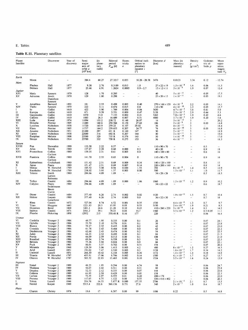
Table E.n. Planetary satellites

Planet Discoverer Year of Semi- lin Sidereal Eccen- Orbital incli- Diameter d Mass [in Density Gedorne- Mean Satellite discovery major piane- period trieity nation to [kml planetary

\g/cm3l tric al- oppo-

axis of tary Ps1d [d] planetary masses] bedo p sition orbit a radii] equator I magni-[103km] ['] tude Vo

Earth Moon 384.4 60.27 27.3217 0.055 18.28-28.58 3476 0.0123 3.34 0.12 -12.74

Mars Phobos Hall 1877 9.38 2.76 0.3189 0.015 1.0 27x22x19 t.5xlO- 8 1.6 0.06 11.3 Deimos Hall 1877 23.46 6.91 1.2624 0.0005 0.9-2.7 15 x 12x 11 3xlO- 9 1.9 0.07 12.4

Jupiter 5xlO- 11 XVI Metis Synnott 1979 128 1.79 0.295 40 0.05 17.5

XV Adrastea Jewitt 1979 129 1.80 0.298 25x20x15 1 x 10- 11 0.05 19.1 Danielson Synnott

4x 10- 9 V Amalthea Barnard 1892 181 2.53 0.498 0.003 0.40 270x 166x 150 2.2 0.05 14.1 XIV Thebe Synnott 1979 222 3.11 0.674 0.015 0.8 I1Ox90 4xlO- IO 1.3 0.05 15.7 I 10 Galilei 1610 422 5.90 1.769 0.004 0.04 3630 4.7xl0- 5 3.6 0.61 5.0 II Europa Galilei 1610 671 9.39 3.551 0.009 0.47 3138 2.5xl0- 5 2.9 0.64 5.3 III Ganymedes GaliIei 1610 1070 15.0 7.155 0.002 0.21 5262 7.8xlO- 5 1.9 0.42 4.6 IV Callisto Galilei 1610 1883 26.3 16.689 0.007 0.51 4800 5.7xlO- 5 1.9 0.20 5.6 XIII Leda Kowal 1974 11094 155.2 238.72 0.148 26.07 16 3Xl0- 12 3 20.2 VI Hirnalia Perrine 1905 11480 160.6 250.566 0.158 27.63 186 5xl0- 9 3 0.03 14.8 X Lysithea Nicholson 1938 11720 163.9 259.22 0.107 29.02 36 4xlO- 11 3 18.4 VII ElaTa Perrine 1905 11737 164.2 259.653 0.207 24.77 76 4xlO- IO 3 0.03 16.8 XII Ananke Nicholson 1951 21200 297 631 R 0.169 147 30 2xlO- 11 3 18.9 XI Carme Nicholson 1938 22600 316 692 R 0.207 164 40 5xlO- 11 3 18.0 VIII Pasiphae Melotte 1908 23500 329 735 R 0.378 145 50 lxlO- 1O 3 17.0 IX Sinope Nicholson 1914 23700 332 758 R 0.275 153 36 4xlO- 1I 3 18.3

Saturn XVIII Pan Showalter 1990 133.58 2.22 0.57 I1Ox90x70 0.5 XV Atlas Terrile 1980 137.67 2.28 0.60 0.000 0.3 40x20 0.9 18 XVI Prometheus Collins 1980 139.35 2.31 0.61 0.003 0.0 140x 100 x 80 0.6 16

Carlson XVII Pandora Collins 1980 141.70 2.35 0.63 0.004 110x90x70 0.9 16

Carlson XI Epimetheus Cruikshank 1980 151.42 2.51 0.69 0.009 0.34 140x 120x 100 0.8 15 X Janus Pascu 1980 151.47 2.51 0.69 0.007 0.14 220x200x 160 0.8 14 I Mimas W. Herschel 1789 185.52 3.08 0.94 0.020 1.53 392 8xlO- 8 1.4 0.5 12.9 II Enceladus W. Herschel 1789 238.02 3.95 1.37 0.005 0.00 500 t.3xl0- 7 1.1 1.0 11.7 XIII Telesto Smith 1980 294.66 4.89 1.89 34x28x26 0.5 18.5

Larson Reitsema

III Tethys Cassini 1684 294.66 4.89 1.89 0.000 1.86 1060 t.3xlO- 6 1.2 0.9 10.2 XIV Calypso Pascu 1980 294.66 4.89 1.89 34x22x22 0.6 18.7

Seidel mann Baum Currie

IV Dione Cassini 1684 377.40 6.26 2.74 0.002 0.02 1120 1.9xlO- 6 1.5 0.7 10.4 XII Helene Laques 1980 377.40 6.26 2.74 0.005 0.0 36x32x30 0.7 18

Lecacheux V Rhea Cassini 1672 527.04 8.74 4.52 0.001 0.35 1530 4.4xlO- 6 1.3 0.7 9.7 VI Titan Huygens 1665 1221.83 20.3 15.95 0.03 0.33 5150 2.4x 10- 4 1.9 0.21 8.3 VII Hyperion Bond 1848 1481.1 24.6 21.28 0.10 0.43 410x 260 x 220 3 x 10- 8 1.4 0.3 14.2 VIII Iapetus Cassini 1671 3561.3 59.1 79.33 0.03 14.7 1460 3.3xlO- 6 1.2 0.5/0.05 11.1 IX Phoebe Pickering 1898 12952 215 550.48 R 0.16 177 220 0.06 16.4

Uranus VI Cordelia Voyager 2 1986 49.77 1.95 0.335 0.00 0.1 26 0.07 24.1 VII Ophelia Voyager 2 1986 53.79 2.10 0.376 0.01 0.1 30 0.07 23.8 VIII Bianca Voyager 2 1986 59.17 2.32 0.435 0.00 0.2 42 0.07 23.0 IX Cressida Voyager 2 1986 61.78 2.42 0.464 0.00 0.0 62 0.07 22.2 X Desdemona Voyager 2 1986 62.68 2.45 0.474 0.00 0.2 54 0.07 22.5 XI Juliet Voyager 2 1986 64.35 2.52 0.493 0.00 0.1 84 0.07 21.5 XII Portia Voyager 2 1986 66.09 2.59 0.513 0.00 0.1 108 0.07 21.0 XIII Rosalind Voyager 2 1986 69.94 2.74 0.558 0.00 0.3 54 0.07 22.5 XIV Belinda Voyager 2 1986 75.26 2.94 0.624 0.00 0.0 66 0.07 22.1 XV Puck Voyager 2 1985 86.01 3.37 0.762 0.00 0.31 154 0.07 20.2 V Miranda Kuiper 1948 129.39 5.06 1.413 0.003 4.2 480 8x 10- 7 1.2 0.27 16.3 I Ariel Lassell 1851 191.02 7.47 2.520 0.003 0.3 1158 1.6xlO- 5 1.7 0.34 14.2 II Umbriel Lassell 1851 266.30 10.42 4.144 0.005 0.36 1172 l.4x 10- 5 1.4 0.18 14.8 III Titania W. Herschel 1787 435.91 17.06 8.706 0.002 0.14 1580 4.1xlO- 5 1.7 0.27 13.7 IV Oberon W. Herschel 1787 583.52 22.83 13.463 0.001 0.10 1524 3.5x 10- 5 1.6 0.24 13.9

Neptune III Naiad Voyager 2 1989 48.23 1.95 0.294 0.00 4.74 58 0.06 24.7 IV Thalassa Voyager 2 1989 50.07 2.02 0.311 0.00 0.21 80 0.06 23.8 V Despina Voyager 2 1989 52.53 2.12 0.335 0.00 0.07 144 0.06 22.6 VI Galatea Voyager 2 1989 61.95 2.50 0.429 0.00 0.05 158 0.06 22.3 VII Larissa Voyager 2 1989 73.55 2.97 0.555 0.01 0.20 208 x 178 0.06 22.0 VIII Proteus Voyager 2 1989 117.65 4.75 1.122 0.00 0.55 436x416x402 0.06 20.3 I Triton Lassell 1846 354.76 14.33 5.877 R 0.000 157.35 2706 2.1xlO-4 2.1 0.7 13.5 II Nereid Kuiper 1949 5513.4 222.6 360.136 0.751 27.6 340 2 x 10- 7 1.0 0.4 18.7

Pluto Charon Christy 1978 19.6 17 6.387 0.00 99 1186 0.22 0.5 16.8

490 Appendices

Table E.12. Some well-known asteroids

Asteroid Discoverer Year of Semi-major Eccentricity Inclination discovery axis of orbit

a e [AU] [0]

1 Ceres Piazzi 1801 2.77 0.08 10.6 2 Pallas Olbers 1802 2.77 0.23 34.8 3 Juno Harding 1804 2.67 0.26 13.0 4 Vesta Olbers 1807 2.36 0.09 7.1 5 Astraea Hencke 1845 2.58 0.19 5.3 6 Hebe Hencke 1847 2.42 0.20 14.8 7 Iris Hind 1847 2.39 0.23 5.5 8 Flora Hind 1847 2.20 0.16 5.9 9 Metis Graham 1848 2.39 0.12 5.6

10 Hygiea DeGas paris 1849 3.14 0.12 3.8 433 Eros Witt 1898 1.46 0.22 10.8 588 Achilles Wolf 1906 5.18 0.15 10.3 624 Hektor Kopff 1907 5.16 0.G3 18.3 944 Hidalgo Baade 1920 5.85 0.66 42.4

1221 Amor Delporte 1932 1.92 0.43 11.9 1566 Icarus Baade 1949 1.08 0.83 22.9 1862 Apollo Reinmuth 1932 1.47 0.56 6.4 2060 Chiron Kowal 1977 13.64 0.38 6.9 5145 Pholus Rabinowitz 1992 20.46 0.58 24.7

Asteroid Sidereal Diameter Rotation Geometric Mean Type period period albedo opposition of orbit magnitude Psid d Tsid P B [a] [km] [h]

1 Ceres 4.6 946 9.08 0.07 7.9 C 2 Pallas 4.6 583 7.88 0.09 8.5 U 3 Juno 4.4 249 7.21 0.16 9.8 S 4 Vesta 3.6 555 5.34 0.26 6.8 U 5 Astraea 4.1 116 16.81 0.13 11.2 S 6 Hebe 3.8 206 7.27 0.16 9.7 S 7 Iris 3.7 222 7.14 0.20 9.4 S 8 Flora 3.3 160 13.60 0.13 9.8 S 9 Metis 3.7 168 5.06 0.12 10.4 S

10 Hygiea 5.6 443 18.00 0.05 10.6 C 433 Eros 1.8 20 5.27 0.18 11.5 S 588 Achilles 11.8 70 ? ? 16.4 U 624 Hektor 11.7 230 6.92 0.03 15.3 U 944 Hidalgo 14.2 30 10.06 19.2 MEU

1221 Amor 2.7 5? ? 20.4 ? 1566 Icarus 1.1 2 2.27 12.3 U 1862 Apollo 1.8 2.5 ? 16.3 2060 Chiron 50.4 320? 17.3 ? 5145 Pholus 92.6 190

E. Tables 491

Table E.13. Periodic comets with several perihelion passages observed

NT T P q e w Q b Q

Encke 56 1994 Feb. 9 3.28 0.331 0.850 186.3 334.0 11.9 160.2 -1.3 4.09 Grigg-Skjellerup 16 1992 Jul. 24 5.10 0.995 0.664 359.3 212.6 21.1 212.0 -0.3 4.93 Honda-Mrkos-Pajdusakova 8 1990 Sept. 12 5.30 0.541 0.822 325.8 88.6 4.2 54.5 -2.4 5.54 Tuttie-Giacobini-Kresak 8 1990 Feb. 8 5.46 1.068 0.656 61.6 140.9 9.2 202.1 8.1 5.14 Tempel 2 19 1994 Mar. 16 5.48 1.484 0.522 194.9 117.6 12.0 312.1 -3.1 4.73 Wirtanen 8 1991 Sept. 21 5.50 1.083 0.652 356.2 81.6 11.7 77.9 -0.8 5.15 Clark 8 1989 Nov. 28 5.51 1.556 0.501 208.9 59.1 9.5 267.7 -4.6 4.68 Forbes 8 1993 Mar. 15 6.14 1.450 0.568 310.6 333.6 7.2 284.5 -5.4 5.25 Pons-Winnecke 20 1989 Aug. 19 6.38 1.261 0.634 172.3 92.8 22.3 265.6 2.9 5.62 d' Arrest 15 1989 Feb. 4 6.39 1.292 0.625 177.1 138.8 19.4 316.0 1.0 5.59 Schwassmann-Wachmann 2 11 1994 Jan. 24 6.39 2.070 0.399 358.2 125.6 3.8 123.8 -0.1 4.82 Wolf-Harrington 8 1991 Apr. 4 6.51 1.608 0.539 187.0 254.2 18.5 80.8 -2.2 5.37 Giacobini-Zinner 12 1992 Apr. 14 6.61 1.034 0.707 172.5 194.7 31.8 8.3 3.9 6.01 Reinmuth 2 8 1994 Jun. 29 6.64 1.893 0.464 45.9 295.4 7.0 341.1 5.0 5.17 Perrine-Mrkos 8 1989 Mar. 1 6.78 1.298 0.638 166.6 239.4 17.8 46.6 4.1 5.87 Arend-Rigaux 7 1991 Oct. 3 6.82 1.438 0.600 329.1 121.4 17.9 91.7 -9.1 5.75 Borrelly 11 1987 Dec. 18 6.86 1.357 0.624 353.3 74.8 30.3 69.0 -3.4 5.86 Brooks 2 14 1994 Sept. 1 6.89 1.843 0.491 198.0 176.2 5.5 14.1 -1.7 5.40 Finlay 11 1988 Jun. 5 6.95 1.094 0.700 322.2 41.7 3.6 4.0 -2.2 6.19 Johnson 7 1990 Nov. 19 6.97 2.313 0.366 208.3 116.7 13.7 324.3 -6.4 4.98 Daniel 8 1992 Aug. 31 7.06 1.650 0.552 11.0 68.4 20.1 78.7 3.8 5.71 Holmes 8 1993 Apr. 10 7.09 2.177 0.410 23.2 327.3 19.2 349.4 7.4 5.21 Reinmuth 1 8 1988 May 10 7.29 1.869 0.503 13.0 119.2 8.1 132.0 1.8 5.65 Faye 19 1991 Nov. 15 7.34 1.593 0.578 204.0 198.9 9.1 42.6 -3.7 5.96 Ashbrook-Jackson 7 1993 Jul. 13 7.49 2.316 0.395 348.7 2.0 12.5 350.9 -2.4 5.34 Schaumasse 10 1993 Mar. 5 8.22 1.202 0.705 57.5 80.4 11.8 137.3 10.0 6.94 Wolf 14 1992 Aug. 28 8.25 2.428 0.406 162.3 203.4 27.5 7.6 8.1 5.74 Whipple 9 1994 Dec. 22 8.53 3.094 0.259 201.9 181.8 9.9 23.4 -3.7 5.25 Comas Sola 8 1987 Aug. 18 8.78 1.830 0.570 45.5 60.4 13.0 105.2 9.2 6.68 Viiisiilii 1 6 1993 Apr. 29 10.8 1.783 0.635 47.4 134.4 11.6 181.2 8.5 7.98 Tuttle 11 1994 Jun. 27 13.5 0.998 0.824 206.7 269.8 54.7 106.1 - 21.5 10.3 Halley 30 1986 Feb. 9 76.0 0.587 0.967 111.8 58.1 162.2 305.3 16.4 35.3

NT: number of perihelion passages observed e: eccentricity I: longitude of perihelion, here defined as T: perihelion time w: argument of perihelion (1950.0) 1= Q+ arctan (tan w cos I) P: period of orbit [years] Q: longitude of ascending node (1950.0) b: latitude of perihelion, sin b = sin w sin 1

q: perihelion distance [AU] I: inclination Q: aphelion distance [AU]

Table E.14. Principal meteor showers

Shower Period of Maximum Radiant Meteors Associated visibility per hour comet

a 15

Quadrantids Jan.I-5 Jan. 3-4 231° +52° 30-40 Lyrids Apr. 19- 25 Apr. 22 275° + 35° 10 Thatcher Eta Aquarids May 1-12 May 5 336° 0° 5-10 Halley Perseids Jul. 20-Aug. 18 Aug. 12 45° +57° 40-50 Swift-Tuttle Kappa Cygnids Aug. 17-24 Aug. 20 290° + 55° 5 Orionids Oct. 17 - 26 Oct. 21 95° + 15° 10-15 Halley Taurids Oct. 10-Dec. 5 Nov. 1 55° + 15° 5 Encke Leonids Nov. 14-20 Nov. 17 151 ° +22° 10 Tempel-Tuttle Geminids Dec. 7-15 Dec. 13-14 112° + 33° 40-50 Ursids Dec. 17 -24 Dec. 22 205° +76° 5

492 Appendices

Table E.15. Nearest stars

Name a J V B-V Spectrum 7C r Mv 11 Vr

2000.0

[h min) [0 ') [") [pc) ["/a) [km/s)

Sun - 26.78 0.62 G2V 4.79 a Cen C (Proxima) 1430 -6241 11.05 1.97 M5eV 0.762 1.31 15.45 3.85 -16 aCen A 1440 -6050 -0.01 0.68 G2V 0.745 1.34 4.35 3.68 -22 a Cen B 1440 -6050 1.33 0.88 K5V 0.745 1.34 5.69 3.68 -22 Barnard's star 17 58 434 9.54 1.74 M5V 0.552 1.81 13.25 10.31 -108 Wolf 359 1056 701 13.53 2.01 M6eV 0.429 2.33 16.68 4.71 +13 BD+36°2147 11 03 35 58 7.50 1.51 M2V 0.401 2.49 10.49 4.78 -84 a CMa (Sirius) A 645 -1643 -1.46 0.00 A1V 0.377 2.65 1.42 1.33 -8 a CMa (Sirius) B 645 -1643 8.68 wdA 0.377 2.65 11.56 1.33 -8 Luyten 726-8 A 1 39 -1757 12.45 M6eV 0.367 2.72 15.27 3.36 +29 Luyten 726-8 B 1 39 -17 57 12.95 M6eV 0.367 2.72 15.8 3.36 +32

(UV Cet) 0.72 -4 Ross 154 1850 -2350 10.6 M4eV 0.345 2.90 13.3

Ross 248 2342 4410 12.29 1.92 M6eV 0.317 3.15 14.80 1.59 -81 Ii Eri 3 33 -928 3.73 0.88 K2V 0.303 3.30 6.13 0.98 +16 Luyten 789-6 2239 -15 19 12.18 1.96 M6eV 0.303 3.30 14.60 3.26 -60 Ross 128 11 48 048 11.10 1.76 M5V 0.301 3.32 13.50 1.37 -13 61 Cyg A 21 07 3845 5.22 1.17 K5V 0.294 3.40 7.58 5.21 -64 61 Cyg B 21 07 3845 6.03 1.37 K7V 0.294 3.40 8.39 5.21 -64 eInd 2203 -5647 4.68 1.05 K5V 0.291 3.44 7.00 4.69 -40 a CMi (Procyon) A 739 513 0.37 0.42 F5V 0.286 3.50 2.64 1.25 -3 a CMi (Procyon) B 739 513 10.7 wdF 0.286 3.50 13.0 1.25 BD + 59°1915 A 1843 5938 8.90 1.54 M4V 0.283 3.53 11.15 2.30 0 BD + 59°1915 B 1843 5938 9.69 1.59 M5V 0.283 3.53 11.94 2.28 +10 BD+43°44 A o 18 4401 8.07 1.56 M1V 0.282 3.55 10.32 2.90 +13 BD+43°44 B o 18 44 01 11.04 1.80 M6V 0.282 3.55 13.29 2.90 +20 CD - 36°15693 2306 -3552 7.36 1.46 M2V 0.279 3.58 9.59 6.90 +10 T Cet 144 -15 56 3.50 0.72 G8VI 0.276 3.62 5.72 1.91 -16 BD+5°1668 726 5 14 9.82 1.56 M5V 0.268 3.73 11.98 3.74 +26 Luyten 725-32 1 12 -17 00 11.6 M2eV 0.261 3.83 13.4 1.36 CD-39°14192 21 17 -3852 6.67 1.38 MOV 0.260 3.85 8.75 3.46 +21 Kapteyn's star 5 12 -4501 8.81 1.56 MOVI 0.256 3.91 10.85 8.81 +245 KrOger 60 A 2228 5742 9.85 1.62 M4V 0.253 3.95 11.87 0.86 -26 KrOger 60 B 2228 5742 11.3 1.8 M6eV 0.253 3.95 13.3 0.86 -26 Ross 614 A 629 -249 11.17 1.74 M7eV 0.250 4.00 13.16 0.99 +24 Ross 614 B 629 -249 14.8 M 0.250 4.00 16.8 0.99 +24 BD-12°4523 1630 -1239 10.2 1.60 M4V 0.249 4.02 12.10 1.18 -13 van Maanen's star 049 523 12.37 0.56 wdG 0.236 4.24 14.26 2.97 +54 Wolf 424 A 12 33 901 13.16 1.80 M7eV 0.230 4.35 14.98 1.75 -5 Wolf 424 B 1233 901 13.4 M7eV 0.230 4.35 15.2 1.75 -5 CD-37°15492 006 - 3721 8.63 1.45 M4V 0.225 4.44 10.39 6.09 +23 BD+5001725 10 11 4927 6.59 1.36 K7V 0.219 4.57 8.32 1.45 -26 CD-46°11540 1729 -4654 9.36 1.53 M4 0.216 4.63 11.03 1.10 CD-49°13515 21 34 -4900 8.67 1.46 M1V 0.214 4.67 10.32 0.81 +8 CD - 44°11909 17 37 -4420 11.2 M5 0.213 4.69 12.8 1.16 BD + 68°946 1736 6821 9.15 1.50 M4V 0.209 4.78 10.79 1.32 -22 BD-15°6290 2253 -14 16 10.17 1.60 M5V 0.207 4.83 11.77 1.15 +9 Luyten 145-141 1146 -6450 11.44 0.19 wdA 0.206 4.85 13.01 2.68 0 2 Eri A 4 15 -739 4.43 0.82 K1V 0.205 4.88 5.99 4.08 -43 0 2 Eri B 4 15 -739 9.53 0.03 wdA 0.205 4.88 11.09 4.11 -21 0 2 Eri C 4 15 -739 11.17 1.68 M4eV 0.205 4.88 12.73 4.11 -45 BD+ 15°2620 13 46 1454 8.50 1.43 M4V 0.205 4.88 10.02 2.30 + 15 BD+2002465 1020 1952 9.43 1.54 M4eV 0.203 4.93 10.98 0.49 + 11 a Aql (Altair) 19 51 852 0.76 0.22 A7V 0.197 5.08 2.24 0.66 -26 AC + 79°3888 11 48 7842 10.94 M4VI 0.195 5.13 12.38 0.89 -117 70 Oph A 18 05 230 4.22 0.86 KOV 0.195 5.13 5.67 1.12 -7 700ph B 1805 230 6.0 K5V 0.195 5.13 7.45 1.12 -10

E. Tables 493

Table E.16. Brightest stars (V < 1.50)

Name a ~ V B-V Spectrum Mv r J1 vr Remarks 2000.0

[h min] [0 '] [pc] ["/a] [km/s]

aCMa Sirius 645.1 -1643 -1.46 0.00 AIV,wdA + 1.4 2.7 1.33 -8 db a= 7.5", P= 50a a Car Canopus 624.0 -5242 -0.73 0.16 FOlb-1I -4.6 60 0.02 +21 aCen Rigil Kentaurus 1439.6 -6050 -0.29 0.72 G2V,K5V +4.1 1.3 3.68 -22 db a = 17.6", P = 80a;

Proxima 2.20 apart a Boo Arcturus 1415.7 19 11 -0.06 1.23 K2I11p -0.3 11 2.28 -5 a Lyr Vega 1836.9 3847 0.04 0.00 AOV +0.5 8.1 0.34 -14 aAur Capella 5 16.7 4600 0.08 0.79 GSIII, GOIII -0.6 14 0.44 +30 db a = 0.054",

P = 0.285a aOri Rigel 5 14.5 -812 0.11 -0.03 B8Ia -7.0 250 0.00 +21 db sep. 9";

spectr. db P = 10d aCMi Procyon 739.3 513 0.37 0.42 F5V, wdF +2.6 3.5 1.25 -3 db a = 4.5", P = 41 a a Eri Achernar 1 37.7 -5714 0.46 -0.16 B3Vp -2.5 38 0.10 + 19 aOri Betelgeuse 5 55.2 724 0.50 1.85 M2I -6.0 200 0.03 +21 var. V= 0.40-1.3;

spectr. dbP=5.8a pCen Hadar 1403.8 -6022 0.60 -0.23 Bill -5.0 120 0.04 -11 db sep. 1.2" aAql Altair 1950.8 852 0.76 0.22 A7V +2.2 5.1 0.66 -26 aCru Acrux 1226.6 -6306 0.79 -0.25 BO.5IV, Bl V -4.7 120 0.04 -6 db sep. 5",

each spectr. db a Tau Aldebaran 435.9 1631 0.85 1.53 K5111 -0.8 21 0.20 +54 db sep. 31" a Vir Spica 13 25.2 -11 10 0.96 -0.23 BIV -3.6 80 0.05 +1 spectr. db P = 4.0d;

several components a Sco Antares 1629.4 -2626 0.96 1.23 MlIb, B2.5V -4.6 130 0.03 -3 var. V = 0.88 -1.8;

db a = 2.9", P = 880a PGem Pollux 745.3 2801 1.15 1.00 KOIII + 1.0 11 0.62 +3 aPsA Fomalhaut 2257.6 -2937 1.16 0.09 A3V + 1.9 7.0 0.37 +7 aCyg Deneb 2041.4 45 17 1.25 0.09 A2Ia -7.2 500 0.00 -5 pCru Mimosa 1247.7 -5941 1.26 -0.24 BOlli -4.6 150 0.05 +20 spectr. db P = 0.16d

and 7-8a a Leo Regulus 10 08.4 11 58 1.35 -0.11 B7V -0.7 26 0.25 +4 db sep. 177"

Abbreviations: db: double star; a: semi-major axis of the orbit; P: period; sep.: separation; spectr.: spectroscopic; var.: variable; variation given in V-magnitude

Table E.17. Some double stars

Name

1/ Cas Achird Y Ari Mesarthim a Psc Kaitain yAnd Alamak <50ri Mintaka ). Ori Meissa (Ori Alnitak a Gem Castor y Leo Algieba ~UMa Alula Australis aCru Acrux y Vir Porrima aCVn Cor Caroli (UMa Mizar aCen Rigil Kentaurus e Boo lzar <5 Ser fJ Sco Grafias a Her Rasalgethi p Her 700ph el?Lyr e1Lyr ?Lyr ( Lyr II Ser Alya Y Del ( Aqr <5Cep

494

a mvl 2000.0

[h min] [0 ']

049.1 5749 3.7 1 53.5 19 18 4.8 202.0 246 4.3 203.9 4220 2.4 532.0 -018 2.5 5 35.1 956 3.7 540.8 -1 57 2.1 734.6 31 53 2.0

10 20.0 1951 2.6 11 18.2 31 32 4.4 1226.6 -6306 1.4 1241.7 -1 27 3.7 12 56.0 38 19 2.9 13 23.9 5456 2.4 14 39.6 -6050 0.0 1445.0 27 04 2.7 15 34.8 1032 4.2 16 05.4 -1948 2.9 17 14.6 1423 3.0-4.0 17 23.7 3709 4.5 18 05.5 230 4.3 1844.3 3940 4.8 18 44.3 3940 5.1 18 44.4 3937 5.1 18 44.8 37 36 4.3 18 56.2 4 12 4.5 20 46.7 1607 4.5 22 28.8 -001 4.4 22 29.2 5825 3.5-4.3

Table E.18. Milky Way Galaxy

Property

Mass Disc diameter Disc thickness (stars) Disc thickness (gas and dust) Halo diameter Sun's distance from galactic centre Sun's rotational velocity Sun's period of rotation Direction of galactic centre (2000.0)

mv2

7.5 4.9 5.3 5.1 7.0 5.7 4.2 3.0 3.8 4.9 1.8 3.7 5.5 4.1 1.2 5.3 5.3 5.1 5.7 5.5 6.1 4.4 6.2 5.3 5.7 4.9 5.4 4.6 7.5

Direction of galactic north pole (2000.0)

SPI spz

GOV MO Alp B9V AOp A3m K3IIb B8V+AOV BOIII+09V B2V 08e BO.5V 09.51be BOIII AIV A5Vm Kl III G7III GOV GOV BO.5IV BIV FOV FOV AOp FOV AIVp Alm G2V K5V KOII - III A2V FOIV FOIV BIV B2V M5Ib-II G5I11 + F2V B9.5 III AOV KOV K5V A4V +Fl V A8V +FOV A4V FIV A8V FOV Am FOIV A5V A5V Kl IV F7V F3V F61V F51b-G21b B71V

Value

>2xl011 M 0

30kpc 1 kpc 200 pc 50kpc 8.5 kpc 220km/s 240 x 106 a a = 17 h 45.7 min /) = - 29°00' a = 12h 51.4 min /) = +27°08'

Appendices

Separa- Parallax tion

["] ["]

12 0.176 8 0.026 2 0.017

10 0.010 52 0.014 4 0.007 2 0.024 2 0.067 4 0.013 3 0.137 4 0.008 4 0.099

19 0.027 14 0.047 21 0.745 3 0.016 4 0.021

14 0.009 5 0.008 4 2 0.195

209 0.021 3 0.021 2 0.021

44 0.031 22 0.030 10 0.026 2 0.039

41 0.011

E. Tables 495

Table E.19. Members of the Local Group of galaxies

Name a " Type mpg Mpg Distance 2000.0

[h min] [0 '] [kpc]

Milky Way Galaxy Sb or Sc NGC224 = M31 042.7 41 16 Sb 4.33 -20.3 650 NGC598 = M33 1 33.9 3039 Sc 6.19 -18.5 740 LMC 523.7 -6945 Irr or SBc 0.86 -17.8 50 SMC 052.7 -72 49 Irr 2.86 -16.2 60 NGC205 = MIlO 040.4 4141 E6 8.89 -15.8 650 NGC221 = M32 042.7 4052 E2 9.06 -15.6 650 NGC6822 1945.0 -1448 Irr 9.21 -15.3 520 NGC185 038.9 4820 EO 10.29 -14.4 650 IC1613 1 04.8 207 Irr 10.00 -14.4 740 NGC147 033.2 48.30 dE4 10.57 -14.1 650 Fornax 239.9 -3432 dE 9.1 -12 190 And I 045.7 3801 dE 13.5 -11 650 And II 1 16.5 3326 dE 13.5 -11 650 And III 035.3 3631 dE 13.5 -11 650 And IV 042.4 4035 dE 650 Leol 10 08.5 12 19 dE 11.27 -10 230 Sculptor 100.2 -3342 dE 10.5 -9.2 90 Leo II 11 13.5 2209 dE 12.85 -9 230 Draco 1720.1 5755 dE ? 80 Ursa Minor 15 08.8 67 12 dE ? 80 Carina 641.6 -5058 dE ? 170 LGS3 1 03.8 21 53 ? ? 650 Sextans 10 13.0 -1 36 dE 85

496 Appendices

Table E.20. Optically brightest galaxies

Name a " Type mpg Size Distance 2000.0

[h min) [0 ') [") [Mpc)

NGC55 o 15.1 -3913 Sc or Irr 7.9 30x5 2.3 NGC205 040.4 4141 E6 8.9 12 x6 0.7 NGC221 = M32 042.7 4052 E2 9.1 3.4x2.9 0.7 NGC224 = M31 042.8 41 16 Sb 4.3 163 x42 0.7 NGC247 047.2 -2046 S 9.5 21 x8 2.3 NGC253 047.6 -2517 Sc 7.0 22x5 2.3 SMC 052.6 -72 48 Irr 2.9 216x216 0.06 NGC300 054.9 -3741 Sc 8.7 22 x16 2.3 NGC598 = M33 1 33.9 3039 Sc 6.2 61 x42 0.7 Fornax 239.9 -3432 dE 9.1 50x35 0.2 LMC 523.6 -6945 Irr or Sc 0.9 432x432 0.05 NGC2403 736.9 6536 Sc 8.8 22 x12 2.0 NGC2903 932.1 21 30 Sb 9.5 16x7 5.8 NGC3031 = M81 955.6 6904 Sb 7.8 25 x 12 2.0 NGC 3034 = M 82 955.9 6941 Sc 9.2 10 x 1.5 2.0 NGC4258 = M 106 12 19.0 47 18 Sb 8.9 19 x7 4.3 NGC4472 = M49 12 29.8 800 E4 9.3 10x7 11 NGC4594 = MI04 1240.0 -11 37 Sb 9.2 8 x5 11 NGC4736 = M94 12 50.9 41 07 Sb 8.9 13 x12 4.3 NGC4826 = M64 1256.8 21 41 ? 9.3 10x4 3.7 NGC4945 13 05.4 -4928 Sb 8.0 20x4 NGC5055 = M63 13 15.8 4202 Sb 9.3 8 x3 4.3 NGC5128 = CenA 13 25.5 -4301 EO 7.9 23 x20 NGC5194 = M51 13 29.9 47 12 Sc 8.9 11 x6 4.3 NGC 5236 = M 83 13 37.0 -2952 Sc 7.0 13 x 12 2.4 NGC5457 = MI0l 14 03.2 5421 Sc 8.2 23 x21 4.3 NGC6822 1945.0 -1448 Irr 9.2 20xl0 0.7

Table E.21. Constellations

Latin name Genitive Abbreviation English name

Andromeda Andromedae And Andromeda Antlia Antliae Ant Air Pump Apus Apodis Aps Bird of Paradise Aquarius Aquarii Aqr Water-bearer Aquila AquiJae Aql Eagle Ara Arae Ara Altar Aries Arietis Ari Ram Auriga Aurigae Aur Charioteer Bootes Bootis Boo Herdsman Caelum Caeli Cae Chisel Camelopardalis Camelopardalis Cam Giraffe Cancer Cancri Cnc Crab Canes Venatici Canum Venaticorum CVn Hunting Dogs Canis Major Canis Majoris CMa Great Dog Canis Minor Canis Minoris CMi Little Dog Capricornus Capricorni Cap Shea-goat Carina Carinae Car Keel Cassiopeia Cassiopeiae Cas Cassiopeia Centaurus Centauri Cen Centaur

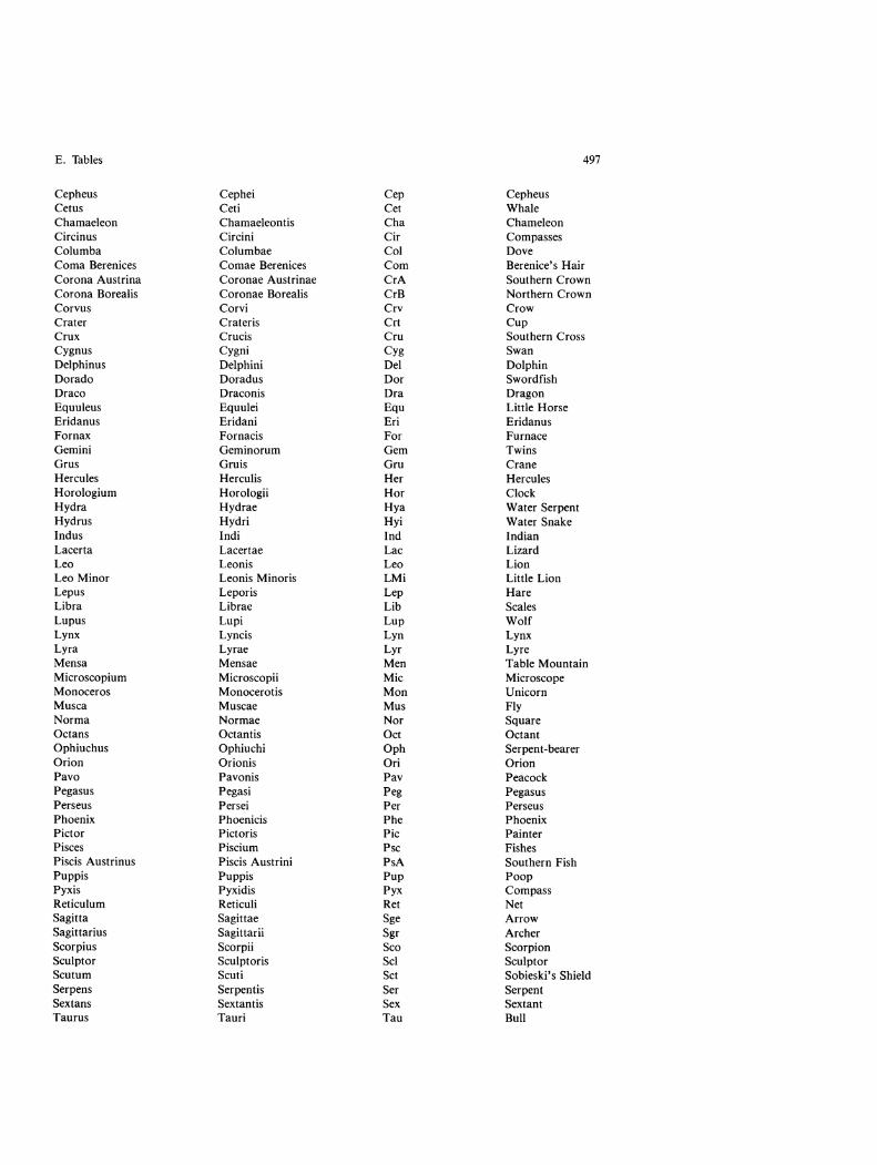
E. Tables 497

Cepheus Cephei Cep Cepheus Cetus Ceti Cet Whale Chamaeleon Chamaeleontis Cha Chameleon Circinus Circini Cir Compasses Columba Columbae Col Dove Coma Berenices Comae Berenices Com Berenice's Hair Corona Austrina Coronae Austrinae CrA Southern Crown Corona Borealis Coronae Borealis CrB Northern Crown Corvus Corvi Cry Crow Crater Crateris Crt Cup Crux Crucis Cru Southern Cross Cygnus Cygni Cyg Swan Delphinus Delphini Del Dolphin Dorado Doradus Dor Swordfish Draco Draconis Dra Dragon Equuleus Equulei Equ Little Horse Eridanus Eridani Eri Eridanus Fornax Fornacis For Furnace Gemini Geminorum Gem Twins Grus Gruis Gru Crane Hercules Herculis Her Hercules Horologium Horologii Hor Clock Hydra Hydrae Hya Water Serpent Hydrus Hydri Hyi Water Snake Indus Indi Ind Indian Lacerta Lacertae Lac Lizard Leo Leonis Leo Lion Leo Minor Leonis Minoris LMi Little Lion Lepus Leporis Lep Hare Libra Librae Lib Scales Lupus Lupi Lup Wolf Lynx Lyncis Lyn Lynx Lyra Lyrae Lyr Lyre Mensa Mensae Men Table Mountain Microscopium Microscopii Mic Microscope Monoceros Monocerotis Mon Unicorn Musca Muscae Mus Fly Norma Normae Nor Square Octans Octantis Oct Octant Ophiuchus Ophiuchi Oph Serpent-bearer Orion Orionis Ori Orion Pavo Pavonis Pay Peacock Pegasus Pegasi Peg Pegasus Perseus Persei Per Perseus Phoenix Phoenicis Phe Phoenix Pictor Pictoris Pic Painter Pisces Piscium Psc Fishes Piscis Austrinus Piscis Austrini PsA Southern Fish Puppis Puppis Pup Poop Pyxis Pyxidis Pyx Compass Reticulum Reticuli Ret Net Sagitta Sagittae Sge Arrow Sagittarius Sagittarii Sgr Archer Scorpius Scorpii Sco Scorpion Sculptor Sculptoris Sci Sculptor Scutum Scuti Sct Sobieski's Shield Serpens Serpentis Ser Serpent Sextans Sextantis Sex Sextant Taurus Tauri Tau Bull

498 Appendices

Table E.21. (cont.)

Latin name Genitive Abbreviation English name

Telescopium Telescopii Tel Telescope Triangulum Trianguli Tri Triangle Triangulum Australe Trianguli Australis TrA Southern Triangle Tucana Tucanae Tuc Toucan Ursa Major Ursae Majoris UMa Great Bear Ursa Minor Ursae Minoris UMi Little Bear Vela Velorum Vel Sails Virgo Virgin is Vir Virgin Volans Volant is Vol Flying Fish Vulpecula Vulpeculae Vul Fox

Table E.22. Largest telescopes

Telescope Location Completion Mirror year diameter

[m]

W.M. Keck Telescope Mauna Kea, Hawaii 1992 10 BTA Telescope Zelenchukskaya, USSR 1975 6.0 Hale Telescope Mt. Palomar, USA 1948 5.0 Multiple-Mirror Telescope (MMT) Mt. Hopkins, USA 1979 4.5 a

William Herschel Telescope Canary Islands 1987 4.2 Cerro Tololo Chile 1976 4.0 Anglo-Australian Telescope Siding Spring, Australia 1974 3.9 Mayall Telescope Kit! Peak, USA 1973 3.9 United Kingdom Infrared Telescope (UKIRT) Mauna Kea, Hawaii 1978 3.8 Canada-France-Hawaii Telescope (CFHT) Mauna Kea, Hawaii 1979 3.6 European Southern Observatory (ESO) La Silla, Chile 1976 3.6 German-Spanish Astronomical Center Calar Alto, Spain 1984 3.5 New Technology Telescope (ESO) La Silla, Chile 1989 3.5 Lick Observatory Mt. Hamilton, USA 1957 3.1 Nasa Infrared Telescope (lRTF) Mauna Kea, Hawaii 1979 3.1

a Consists of six mirrors, each 1.8m in diameter, the total area of which corresponds to one 4.5m mirror

Table E.23. Largest parabolic radio telescopes

Telescope Location Completion Diameter Shortest Remarks year wavelength

[m] [cm]

Arecibo Puerto Rico, USA 1963 305 5 Fixed disk, limited tracking Effelsberg Bonn, Federal Re- 1973 100 0.8 Largest completely steerable

public of Germany telescope J odrell Bank Macclesfield, Great 1957 76.2 10-20 First large paraboloid an-

Britain tenna Yevpatoriya Crimea, USSR 1979 70 1.5 Parkes Australia 1961 64 2.5 Innermost 17 m of dish can

be used down to 3 mm-wavelengths

Goldstone California, USA 64 1.5 Belongs to NASA

E. Tables 499

Table E.24. Millimetre and submillimetre wave radio telescopes and interferometers

Institute Location Altitude Diameter Shortest Remarks; above sea wave- operational level length since [m] [m] [mm]

Max-Planck-Institut fUr Mt. Graham, USA 3250 10 0.3 1994? Radioastronomie (Federal Republic of Germany) & University of Arizona (USA)

California Institute of Tech- Mauna Kea, Hawaii 4100 10.4 0.3 1986 nology (USA)

Science Research Council Mauna Kea, Hawaii 4100 15.0 0.5 The James (United Kingdom & Clerk Max-Netherlands) well Tele-

scope; 1986 California Institute of Tech- Owens Valley, USA 1220 10.4 0.5 3-antenna

no logy (USA) interferom-eter; 1980

University of Cologne (Fed- Gornergrat, Suisse 3120 3.0 0.5 1986 eral Republic of Germany)

Sweden-ESO Southern Hemi- La Silla, Chile 2400 15.0 0.6 1987 sphere Millimeter Antenna (SEST)

Institut de Radioastronomie Plateau de Bure, France 2550 15.0 0.6 3-antenna Millimetrique (lRAM; interferom-France & Federal Republic eter; 1990 of Germany) Fourth

antenna 1993

University of Texas (USA) McDonald Observatory, 2030 4.9 0.8 1967 USA

IRAM Pico Veleta, Spain 2850 30.0 0.9 1984 National Radio Astronomy Kitt Peak, USA 1940 12.0 0.9 1983 (1969)

Observatory (USA) CSIRO (Australia) Sydney, Australia 10 4.0 1.3 1977 Bell Telephone Laboratory Holmdel, USA 115 7.0 1.5 1977

(USA) University of Massachusetts New Salem, USA 300 13.7 1.9 Radom;

(USA) 1978 University of California, Hat Creek Observatory 1040 6.1 2 3-antenna

Berkeley (USA) interferom-eter; 1968

Purple Mountain Observa- Western China 3000 13.7 2 Radom; tory (China (P. R.» 1987

Daeduk Radio Astronomy Seoul, South Korea 300 13.7 2 Radom; Observatory (South Korea) 1987

University of Tokyo (Japan) Nobeyama, Japan 1350 45.0 2.6 1982 University of Tokyo (Japan) Nobeyama, Japan 1350 10.0 2.6 5-antenna

interferom-eter; 1984

Chalmers University of Tech- Onsala, Sweden 10 20.0 2.6 Radom; nology (Sweden) 1976

Answers to Exercises

Chapter 2

2.16.1 The distance is :=:::7640 km, the northernmost point is 79°N, 45°W, in North Greenland, 1250 km from the North Pole.

2.16.2 The star can culminate South or North of zenith. In the former case we get 15 = 65°, <p = 70°, and in the latter 15 = 70°, <p = 65°.

2.16.3 a) <p>58°4'. If refraction is taken into account, the limit is 57°29'. b) <p = 15 = 7°24'. c) -59°14'~<p~ -0°46'.

2.16.4 Pretty bad.

2.16.6 c) eo = 18 h.

2.16.7 a) a=6h 45 min 9s, 15= -16°43'. b) Vt = 16.7kms- i , V= 18.5kms- i .

c) After :=::: 61000 years. d) fJ, = 1.62" per year, parallax 0.42".

Chapter 3

3.9.1 a) 3.2 s. b) 1.35 cm and 1.80 cm. c) 60 and 80.

3.9.2 a) 0.001" (note that the aperture is a line rather than circular; therefore the coefficient 1.22 should not be used). b) 140 m.

Chapter 4

4.7.1 0.9.

4.7.2 The absolute magnitude will be -17.5 and apparent 6.7.

4.7.3 N(m + 1)/N(m) = 103/ 5 = 3.98.

4.7.4 r = 2.1 kpc, EB-V = 0.7, and (B-V)o = 0.9.

4.7.5 a) 1.06 mg. b) T = -In 0.856 = 0.98.

502 Answers to Exercises

Chapter 5

5.10.2 n = 166, which corresponds to A = 21.04 cm. Such transitions would keep the population of the state n = 166 very high, resulting in downward transitions also from this state. Such transitions have not been detected. Hence, the line is produced by some other process.

5.10.3 If we express the intensity as something per unit wavelength, we get Amax = 1.1 mm. If the intensity is given per unit frequency, we have Amax = 1.9 mm. The total intensity is 9.6 X 10- 7 W m -2 sterad -1. At 550 nm the intensity is zero for any practical purposes.

5.10.4 a) L = 1.35 X 1029 W. Planck's law can be integrated numerically; a rather complicated expression can be obtained using the Wien approximation. Both ways, we find that 3.30/0 of the radiation goes to the visual band. Thus Lv = 4.45 X 1027 W. b) 10.3 km.

Chapter 6

6.2.1 R = 2.0R('J.

6.2.2 T = 1380 K. There are several strong absorption lines in this spectral region, reducing the brightness temperature.

6.2.4 vrms::: 6700 km s - 1 •

Chapter 7

7.12.1 Va/Vp = (1-e)/(1 +e). For the Earth this is 0.97.

7.12.2 a= 1.4581 AU, v:::23.6kms- 1•

7.12.3 The period must equal the sidereal rotation period of the Earth. r=42339km=6.64R(B. Areas within 8.6 0 from the poles cannot be seen from geostationary satellites. The hidden area is 1.1070 of the total surface area.

7.12.6 a=3.55xl07 AU, e= 1+3.97xl0- 16, rp =2.1 km. The comet will hit the Sun.

Answers to Exercises 503

Chapter 8

8.24.1 Psid = 11.9a, a=5.20AU, d= 144000km. Obviously, the planet is Jupiter.

8.24.2 b) 7.06 d.

8.24.3 a) If the radii of the orbits are al and a2, the angular velocity of the retrograde motion is

dA VGM dt -Val a2 (-ra;- + Va;)

b) In six days Pluto moves about 0.128°, corresponding to 4mm. For a main belt asteroid the displacement is almost 4 cm.

8.24.4 p = 0.11, q = 2, and A = 0.2.

8.24.5 The absolute magnitude is V(l,O) = 23. a) m = 18.7. b) m = 14.2. At least a 15 cm telescope is needed to detect the asteroid even one day before the colli­sion.

8.24.6 Assuming the comet is a slow rotator we get a) 104 K, b) 328 K, c) 464 K.

Chapter 9

9.8.1 ega d feb; the actual spectral classes from top to bottom are AO, M5, 06, F2, K5, G2, B3.

Chapter 10

10.6.1 The period is P = 1/V2 years and the relative velocity 42100 m s -1. The max­imum separation of the lines is 0.061 nm.

10.6.3 Substituting the values to the equation of Exercise 10.6.2 we get an equation for a. The solution is a = 4.4 AU. The mass of the planet is 0.0015 Mo.

Chapter 11

11.6.1 10.5.

11.6.2 a) 9.5 x 1037 • b) The neutrino production rate is 1. 9 x 1038 S - 1, and each sec­ond 9 x 1028 neutrinos hit the Earth.

11.6.3 The mean free path is lIKp:::::42000AU.

504 Answers to Exercises

Chapter 12

12.10.1 tff = 6.7 X 105 y. Stars are born at the rate 0.75 MG per year.

12.10.3 About 900 million years.

Chapter 13

13.5.2 807 W m -2.

Chapter 14

14.5.1 drlr = - 0.46 dM = 0.14.

14.5.2 a) T= 3570K. b) RminlRmax = 0.63.

14.5.3 a) 1300 pc. b) 860 years earlier; due to inaccuracies a safe estimate would be 860 ± 100 years. Actually, the explosion was observed in 1054. c) -7.4.

Chapter 15

15.5.1 L = 2.3 X 1040 kg m2 S-I. dR = 45 m.

15.5.2 a) M = 0.5 M G , a = 0.49 x 109 m S-2"", 4 X 107 g. b) A standing astronaut will be subject to a stretching tidal force. The gravitational acceleration felt by the feet is 3479ms- 2 "",355g larger than that felt by the head. If the astronaut lies tangentially, (s)he will experience a compressing force of 177 g.

15.5.3 v = ve(1- GMIRc 2). If Llvlv is small, we have also LlA = (GMIRc 2)Ae• A photon emitted from the Sun is reddened by 2.1 x 10- 6 Ae. In yellow light (550 nm) the change is 0.0012 nm.

Chapter 16

16.10.1 2.6kpc and 0.9kpc, a= 1.5magkpc- 1•

16.10.2 7kms- 1•

16.10.3 0.01 AU.

Answers to Exercises 505

Chapter 17

17.5.1 7.3.

Chapter 18

18.6.1 f1 = 0.0055" y-l.

18.6.2 a) 5.7 kpc. b) 11 kpc. Possible reasons for the discrepancy include: 1) The dis­tance is so large that the approximations used for deriving Oort's formulae are not very good, 2) taking into account the interstellar extinction will reduce the distance in (b), 3) the peculier velocity of the star was neglected.

18.6.3 a) 3. b) "'" 90000.

18.6.4 a) If the thickness of the disk is H, the light has to travel a distance s = min{r, (HI2) sec b) in the interstellar medium. Thus the magnitude will be m = M + 51g(r11O pc) + as. b) s = 200 pc, m = 10.2.

Chapter 19

19.12.1 a) 26, b) 25.

19.12.2 Diameter is about one light week "'" 1200 AU. M = - 23.5. Assuming this is roughly equal to the bolometric magnitude, we get L "'" 2 X 1011 L 8 , cor­responding to 21OL 8 Au- 3•

Chapter 20

20.9.1 r = vi H = 93 Mpc (if H = 75), diameter is 35 kpc, M = - 20.4. Potential sources of error include: 1) inaccuracy of the Hubble constant, 2) peculiar velocity of the galaxy, 3) intergalactic extinction, 4) only 2-dimensional pro­jection is observed, and the edge depends on the limiting magnitude used.

20.9.2 If we use H = 50 km s -1 Mpc -1, we get r = 51 Mpc, or 74 times the distance of M31. Doubling H will halve the distance, which will still be higher than in Exercise 19.12.1. A possible explanation is the peculiar velocity of the galaxy.

20.9.3 mv = 1.5 x 10- 35 kg, or 0.00002 times the mass of the electron.

Further Reading

The following list of references is not intended as a complete bibliography. It gives a number of intermediate level or more advanced works, which can serve as starting points for those who wish to learn about some spe­cific topic in more detail or depth.

General Reference Works

Allen, C. W. (1973): Astrophysical Quantities, 3rd ed. (Athlone, London) Apparent Places of Fundamental Stars (annual) (Astronomisches Rechen-Institut,

Heidelberg) Burnham, S. (1978): Celestial Handbook (Dover, New York) Lang, K. R. (1980): Astrophysical Formulae, 2nd ed. (Springer, Berlin, Heidelberg) de Vaucouleurs, G., et al. (1964, 1976): Reference Catalogue of Bright Galaxies (Uni-

versity of Texas Press, Austin)

Chapter 1

Mitton, S. (ed.) (1977): Cambridge Encyclopaedia of Astronomy (Cape, London) Shu, F. H. (1982): The Physical Universe (University Science Books, Mill Valley) Unsold, A. (1983): The New Cosmos, 3rd ed. (Springer, Berlin, Heidelberg)

Chapter 2

Explanatory Supplement to the Astronomical Ephemeris (1961) (HM Stationary Office, London)

Green, R. M. (1985): Spherical Astronomy (Cambridge University Press, Cambridge)

Chapter 3

Evans, D. S. (1968): Observation in Modern Astronomy (English Universities Press, London)

Kitchin, C. R. (1984): Astrophysical Techniques (Hilger, Bristol) Wohlleben, R., Mattes, H., Krichbaum, T. (1991): Interferometry in Radioastronomy

and Radar Techniques (Kluwer, Dordrecht)

Chapters 4 - 6

Harwit, M. (1973): Astrophysical Concepts (Wiley, New York) Rybicki, G. B., Lightman, A. F. (1979): Radiative Processes in Astrophysics (Wiley,

New York)

Chapter 7

Brouwer, D., Clemence, G. M. (1960): Methods of Celestial Mechanics (Academic, New York)

Danby, J. M. A. (1962): Fundamentals of Celestial Mechanics (MacMillan, New York)

508 Further Reading

Chapter 8

Beatty, J. K., O'Leary, B., Chaikin, A. (1981): The New Solar System (Cambridge University Press, Cambridge)

Brandt, J. c., Chapman, R. D. (1981): Introduction to Comets (Cambridge University Press, Cambridge)

Cole, G. H. A. (1978): The Structure of Planets (Wykeham, London) Cook, A. H. (1980): Interiors of the Planets (Cambridge University Press, Cambridge)

Chapter 9

Bohm-Vitense, E. (1989): Stellar Astrophysics, Vols. 1-2 (Cambridge University Press, Cambridge)

Mihalas, D. (1978): Stellar Atmospheres, 2nd ed. (Freeman, San Francisco) Novotny, E. (1973): Introduction to Stellar Atmospheres and Interiors (Oxford Uni­

versity Press, New York)

Chapter 10

Heinz, W. (1978): Double Stars (Reidel, Dordrecht) Sahade, J., Wood, F. B. (1978): Interacting Binary Stars (Pergamon, Oxford)

Chapters 11 - 12

Clayton, D. D. (1968/1983): Principles of Stellar Evolution and Nuc/eosynthesis (McGraw-Hill, New York/University of Chicago Press, Chicago)

Novotny, E. (1973): Introduction to Stellar Atmospheres and Interiors (Oxford Uni­versity Press, New York)

Schwarzschild, M. (1958/1965): Structure and Evolution of the Stars (Princeton Uni­versity Press, Princeton/Dover, New York)

Chapter 13

Noyes, R. W. (1982): The Sun, Our Star (Harvard University Press, Cambridge, MA) Priest, E. R. (1982): Solar Magnetohydrodynamics (Reidel, Dordrecht) Stix, M. (1989): The Sun - An Introduction (Springer, Berlin, Heidelberg)

Chapter 14

Cox, J. P. (1980): Theory of Stellar Pulsation (Princeton University Press, Princeton) Glasby, J. S. (1968): Variable Stars (Constable, London)

Chapter 15

Manchester, R. N., Taylor, J. H. (1977): Pulsars (Freeman, San Francisco) Shapiro, S. L., Teukolsky, S. A. (1983): Black Holes, White Dwarfs and Neutron Stars

(Wiley, New York)

Further Reading 509

Chapter 16

Dyson, 1. E., Williams, D. A. (1980): The Physics of the Interstellar Medium (Manchester University Press, Manchester)

Longair, M. S. (1981): High Energy Astrophysics (Cambridge University Press, Cam­bridge)

Spitzer, L. (1978): Physical Processes in the Interstellar Medium (Wiley, New York)

Chapter 17

Hanes, D., Madore, B. (eds.) (1980): Globular Clusters (Cambridge University Press, Cambridge)

Spitzer, L. 1 r. (1987): Dynamical Evolution of Globular Clusters (Princeton University Press, Princeton)

Chapter 18

Bok, B. & P. (1982): The Milky Way, 5th ed. (Harvard University Press, Cambridge, MA)

Mihalas, D., Binney, 1. (1981): Galactic Astronomy (Freeman, San Francisco) Scheffler, H., Elsasser, H. (1988): Physics of the Galaxy and the Interstellar Matter

(Springer, Berlin, Heidelberg)

Chapter 19

Binney, 1., Tremaine, S. (1987): Galactic Dynamics (Princeton University Press, Princeton)

Mihalas, D., Binney, 1. (1981): Galactic Astronomy (Freeman, San Francisco) Sandage, A. (1961): The Hubble Atlas of Galaxies (Carnegie Institution, Washington,

D.C.) Sersic, 1. L. (1982): Extragalactic Astronomy (Reidel, Dordrecht) Weedman, D. W. (1986): Quasar Astronomy (Cambridge University Press, Cam­

bridge)

Chapter 20

Peebles, P. 1. E. (1971): Physical Cosmology (Princeton University Press, Princeton) Raine, D.l. (1981): The Isotropic Universe (Adam Hilger, Bristol) Sciama, D. W. (1971): Modern Cosmology (Cambridge University Press, Cambridge) Weinberg, S. (1972): Gravitation and Cosmology (Wiley, New York)

Photograph Credits

We are grateful to the following institutions who kindly gave us permission to use illustrations (abbreviated references in the figure captions)

Anglo-Australian Observatory, photograph by David F. Malin Arecibo Observatory, National Astronomy and Ionosphere Center, Cornell University Arp, Halton C., Mount Wilson and Las Campanas Observatories (colour representa-

tion of plate by Jean Lorre) Big Bear Solar Observatory, California Institute of Technology Catalina Observatory, Lunar and Planetary Laboratory CSIRO (Commonwealth Scientific and Industrial Research Organisation), Division of

Radiophysics, Sydney, Australia ESA (copyright Max-Planck-Institut fUr Aeronomie, Lindau, Harz, FRG) European Southern Observatory (ESO) Helsinki University Observatory High Altitude Observatory, National Center for Atmospheric Research, National

Science Foundation Karl-Schwarzschild-Observatory Tautenburg of the Central Institute of Astrophysics of

the Academy of Sciences of the GDR (Archives) Lick Observatory, University of California at Santa Cruz Lowell Observatory Lund Observatory Mount Wilson and Las Campanas Observatories, Carnegie Institution of Washington NASA (National Aeronautics and Space Administration) National Optical Astronomy Observatories, operated by the Association of Universities

for Research in Astronomy (AURA), Inc., under contract to the National Science Foundation

National Radio Astronomy Observatory, operated by Associated Universities, Inc., under contract with the National Science Foundation (Plate 27: observers Richard J. Tuffs, Richard A. Perley, Martin T. Brown, Stephen F. Gull; Plate 31: observers Farhad Yusef-Zadeh, Mark R. Morris, Don R. Chance; Plate 33: observers Frazer N. Owen, Richard A. White; Plate 36: observers Peter A.G. Scheuer, Robert A. Laing, Richard A. Perley)

NRL-ROG (Space Research Laboratory, University of Groningen) Palomar Observatory, California Institute of Technology Yerkes Observatory, University of Chicago

Name and Subject Index

Abel integral equation 424 aberration 26 aberration constant 26 absorption 111, 112, 344 absorption coefficient 124 absorption spectrum 111, 112 achromatic lens 56 active galactic nucleus 431 f. active optics 64 Adams, J.C. 214 adaptive optics 64 adiabatic temperature 264 age of the universe 440, 442, 444, 456 AGN see active galactic nucleus air mass 106, 110 airglow 196 albedo 17Of., 333, 353 - Bond 170f. - geometric 171f. Alfven, H. 352, 373 Algol paradox 290 Algol variables 240, 255, 256 Almagest 29 alpha particle 273, 374 alpha reactions 273 a 2 Canum Venaticorum stars 317 altitude 16 Am stars 242 Ambartsumyan, V. A. 380 Andromeda galaxy 7, 319, 324, 429,

colour supplement, Plate 32 Angelina 203 angular momentum 137, 139, 144, 473, 474 antapex 391, 392 antenna temperature 130, 359 antimatter 457, 458 Ap stars 241, 242 aperture of a telescope 53 aperture ratio 53 aperture synthesis 80 f. apex 391, 392 aphelion 141, 144 Aphrodite Terra 190 apochromatic objective 56 Apollo flights 3, 193, 195 Apollo-Amor asteroids 202 apparent place 28 Arctic circle 165 Arecibo telescope 76, 77 Argelander, F. W. A. 29

argument of the perihelion 141 f. Argyre Planitia 198 Ariel 215 Arp, H. 436 ascending node 141, 169 Asoka 83 associations 292, 380f., 397, 426 astenosphere 195 asteroid belt 200, 201, 224 asteroids 161, 170, 200f. astigmatism 59 astrograph 56 astronomical unit 25, 34, 145, 146 Astronomy and Astrophysics Abstracts 4 astrophysics 4 asymptotic branch 384 Atlas Coelestis 30 atom 3, 4, 5, 111 f. atomic hydrogen 357 f. atomic mass unit 484 atomic time 39 AU see astronomical unit aurorae 185, 196, 197 autumnal equinox 22, 45 azimuth 16, 17, 20, 43, 44 azimuthal mounting 61, 62, 64

Baade, W. 319,445, 446 Babcock, H. C. 308, 308 Balmer, J.J. 115 Balmer lines 236, 237, 238, 357, 363, 370,

433 Balmer series 115, 116 barium stars 242 Barnard, E. E. 203 Bayer, J. 32 Bell, J. 332 Bessel, F. W. 34 fJ Cephei stars 316, 317, 320 fJ decay 295 fJ Lyrae stars 255, 256 Bethe, H. 270 binary pulsars 334, 480 binary stars 3, 146, 170, 246, 251f., 29Of.,

322, 334 - astrometric 251, 253 - optical 251 - photometric 251, 255 f. - spectroscopic 251, 257 f. - visual 251, 252

binding energy 269, 270 black dwarfs 330, 461 black holes 287, 289, 291, 329, 337f., 407,

408, 461 blazars 436 blackbody radiation 119 f., 129 f., 443, 444 blue compact galaxies 413 blueshift 35 Bohr model of the atom 113, 114 Bok, B. J. 349 bolide 197 bolometric correction 100 Boltzmann distribution 118 Boltzmann's constant 119 bosons 474 Boss, B. 32 boundary conditions of stellar models 264 bow shock 185 Bowen, I. S. 364 Brackett series 115, 116 Bremsstrahlung 113, 364 brightness temperature 129, 130, 359, 360,

483 BTA telescope 57, 63, 64 Buffon, G. L. L. de 222 Bunsen, R. 233 bursters 316, 331, 334, 335

C stars 242 Caesar, Julius 40 calendar 1, 39 f. - Gregorian 40 - Julian 40 Callisto 181, 207, 208 Caloris basin 188 Cannon, A. J. 236 carbon burning 273 carbon cycle 270 f., 283, 289 carbon flash 285 carbon monoxide 119, 365 f. carbon-nitrogen-oxygen cycle see carbon

cycle Carruthers, G. R. 365 Cassegrain focus 58 Cassini division 210, 211 Cassini, G. 205 Cassiopeia A 372 catadioptric telescope 61 catastrophe theories 222 CCD camera 71 f.

514

celestial mechanics 4, 135 f. celestial sphere 15 cepheids 292, 316f., 393, 394, 398, 445 Ceres 200, 203 Chandrasekhar mass 287 f., 326, 330 Charon 217, 218 Chiron 202 chromatic aberration 55 chromosphere 300, 302f. Chryse Planitia 200 circumpolar 20, 227 CNO cycle see carbon cycle COBE satellite 87, 443, 444 coelostat 64 cold dark matter 455, 458 colour excess 105 colour temperature 130, 131 colour-magnitude diagram 383 column density 361 coma 60 Coma cluster 429, 430 comet Austin 154 comets 161, 218-220, 225 - orbits 154, 161, 219 - structure 218 f. Compton Gamma Ray Observatory 83 conduction 263 conic sections 140f., 459 conjunction 162 f. constant of gravitation 136, 146 constellations 28 contact binaries 290 continental drift 180, 188, 191 continuous spectrum 118f., 233, 371 continuum see continuous spectrum convection 263, 264, 283, 284, 302 coordinate frames

ecliptic 22 equatorial 17 f. galactic 23, 390 geocentric 14 geographical 13 horizontal 15 f.

coordinate transformations 10 f., 19 f., 22 coordinated universal time 39 coordinates

geocentric 23 - heliocentric 23 - topocentric 23 Copernicus, N. 2 Copernicus satellite 85, 358, 365, 373 corona

galactic 408 - solar 300, 305, 312 - on Venus 190 coronal holes 312 cosmic background radiation 443, 444 cosmic rays 87, 88, 220, 221, 343, 356, 374,

375 cosmogony 221f. cosmological constant 450

cosmological models 450f. cosmological principle 446f. cosmological tests 445 f. cosmology 3, 4, 439 f. Coude focus 58 f. Coulomb's law 114 Crab nebula 326, 332, 371, 372 craters 181, 187, 188, 189, 190, 193, 198f.,

207, 211, 214 critical density 451 f. critical layer 185 Cro-Magnon man culmination 20 Curie point 188 curvature tensor 476 Cygnus X-I 339, 340

dark current 72 dark nebulae 349 f. date line 38 Dawes' limit 54 day - sidereal 36 - synodic 36 daylight saving time 38 de Broglie wavelength 114 de Cheseaux, L. 439 de Vaucouleurs' law 421,424 deceleration parameter 443, 452 f. declination 17f. declination axis 64 degeneration 266f., 275, 277, 330, 331, 336 degeneration of electron gas 268 degree of polarization 175, 348 Deimos 200 density parameter 452f. density wave theory 406, 426 descending node 141 deuterium 456 deuteron 272, 456, 459 diaphragm 70 differential rotation 309, 399 differentiation 225 diffraction 53, 54, 67, 170 diffraction disc 68 diffraction grating 74 Dione 212 dipole antenna 75 disc galaxies 422 dispersion 74, 233 dissociation 280 distance modulus 102, 384, 393 Doppler effect 34 f., 317, 334, 360, 441 Doppler shift 118, 251, 253, 382, 457 Draper, H. 236 Dreyer, J. L. E. 380 dwarf cepheids 320 dwarf novae 321, 322 dwarf spheroidals 413 dwarf stars 239, 242 dynamical time 39

Name and Subject Index

- barycentric (TDB) 39 terrestrial (TDT) 39

E. T. see equation of time Earth 2f., 13, 161, 191 f., colour supple­

ment, Plate 8 age of the surface 180, 181

- albedo 178 atmosphere 2, 26f., 49f., 105, 106, 182f., 191, 196, 197 density 191, 193 diameter 191

- distance from the Sun 145, 165 - earthquakes 191 - equatorial radius 14

flattening 13, 14 magnetic field 185, 186, 193 magnetosphere 185, 186 orbit 161, 164, 165 ozone layer 193 polar radius 14

- rotation 39 structure 178, 191, 193

- temperature 177, 193 ebb 167 eccentric anomaly 147, 148, 156 eccentricity 140f., 165, 166, 186,217,469 eclipses 168 f. eclipsing variables 246,251, 255f., 317 ecliptic 22, 141, 142, 163, 165, 166, 169 ecliptic system 22 Eddington, A.S. 318 effective focal length 58 effective temperature 121, 129 Einstein, A. 439, 450, 475 Einstein cross 437 Einstein observatory 83 Einstein-de Sitter model 451, 452, 456 Elder, F. 373 electric dipole transitions 117, 474 electromagnetic radiation 111 f. electromagnetic spectrum 50 electron 5, 111 f., 359, 371, 373, 459, 474 electronic transition 366 elementary particles 3, 374 elements - abundances in interstellar gas 360

abundances in the solar system 294 abundances in the Sun 358 origin 293 f.

elevation see altitude ellipse 140 f., 469 ellipsoidal variables 255 elongation 163, 164 emission 111, 112 emission coefficient 124 emission measure 364 emission nebula 350, 351, 362f. emission spectrum 111, 112 Enceladus 181, 211 Encke's division 210, 211

Name and Subject Index

energy density 98 energy flux 96 energy integral 139 f., 148 energy states 111 f. ephemerides 39 epoch 24 equation of time 37, 38 equations of motion 135 f. equator 13 f. equatorial mounting 61, 62, 64 equatorial system 17 f. equivalence principle 478 equivalent width 235, 238 ergosphere 338 Eros 5, 182 eruptive variables 317, 320 f. escape velocity 148 f., 184, 185 Euclidean space 475 f. Europa 206, 207 EUV 50,84 EUVE 84 evening star 188 event horizon 338 Ewen, H.1. 359 excitation 111 excitation temperature 118, 132, 360 exit pupil 55 exosphere 185, 193 expansion of the universe 439, 441 f., 450f.,

458f. extinction 50, 103 f., 365 - atmospheric 105 f., 228 - interstellar 103 f., 109, 344 f., 384 extinction coefficient 106, 110 extinction curve 347 eyepiece 52, 53

facula 310 Faraday rotation 375 fermions 474 field equations 479 field lens 70 filament 311 filter 70, 100, 101 first point of Aries 18 flare 300, 309, 310 flare stars 316,318,319 flash spectrum 303 flat-field 73 flood 167 flux density 96 f. flux see energy flux forbidden lines 117, 321, 364, 370 forbidden transitions 117, 370, 474 fragmentation 369 Fraunhofer, J. 233 Fraunhofer lines 233, 307 free path 185, 262, 278 free-free radiation 113, 366 Friedmann, A. 450 Friedmann models 450 f.

fusion see thermonuclear reactions

G band 236 galaxies 3, 4, 7, 411 f. - active 431 f. - barred spirals 412-413, 415, 426 - Centaurus A 332, 433, colour supple-

ment, Plate 35 - central bulge 413, 421 - classification 411 f. - colour 426 - diameters 412 - distance 413 f. - Einstein cross 437 - elliptic 412f., 421 f. - evolution 437 - formation 460 - interacting systems 428 - irregular 412, 413, 416 - jets 433, 434 - Large Magellanic Cloud 6, 88, 426 - lenticular 412, 413, 422 - luminosity 417f. - magnitudes 412, 417 f. - Markarian 432 - masses 419f. - M31 see Andromeda galaxy - M32 417 - M33 429 - M51 427 - M81 446 - M87 434 - M100 374 - M101 446 - NGC 175 415 - NGC 488 414 - NGC 628 414 - NGC 1073 415 - NGC 1201 414 - NGC 1265 433 - NGC 1300 415 - NGC 2523 415 - NGC 2525 415 - NGC2811 414 - NGC 2841 414 - NGC 2859 415 - NGC 3031 414 - NGC 4565 427 - NGC 5195 427 - number 440 - PKS 2000-330 435 - QSO 0351 +026 435 - radio 433 - rotation 419 f., 425 - rotation curves 420, 425 - sculptor 416 - Seyfert 432, 436 - Small Magellanic Cloud 416, 428 - spiral structure 426 - stellar populations 426 - surface brightness 421 f.

- 3C129 433 - 3C273 433 galaxy clusters 3, 429 galaxy counts 440 galaxy groups 429, 440 Galilean satellites 207 f. Galilei, G. 2, 49, 189, 207, 209, 389 Galle, J. G. 214 gamma radiation 50, 83, 374 gamma ray bursts 335 Gamow, G. 331,443 Ganymede 181, 207, 208 Gaspra 203 Gauss, K. F. 146 Gegenschein 220 Geiger -Muller counter 84 gemini des 220 geodesic 479 geoid 13 Georgelin, Y. M. 406 Georgelin, Y. P. 406 giant branch 242, 285, 383, 384, 385 giant elliptical galaxies 413 giant stars 3, 22, 240, 242, 285 f., 397 globules 349, 363 GMT see Greenwich mean time granulation 302, 303 gravitational darkening 257 gravitational lens 435, 437 gravitational radiation 88 gravitational red shift 457, 479 gravitational waves 4, 88, 334, 480 grazing reflection 83, 84 great circle 9 greenhouse effect 178, 189 Greenwich mean time 38, 39 Gregorian calendar 40 Gregorius XIII 40 ground state 111 f., 119, 123

hadrons 458 Halley's comet 219, colour supplement,

Plate 15 halo - atmospheric 196, 197 - of the Galaxy 399, 408 Hartmann, J. 356 Harvard spectral classification 236f. Hawking process 461 Hayashi track 281, 285

51

Heisenberg's uncertainty principle 118, 474 helioseismology 302 helium burning 273, 285, 286, 289 helium flash 284, 285, 289, 334 helium stars 292 helium, origin of 459 Henry Draper catalogue 236 f. Herbig-Haro objects 282 Hercules X-I 334, 335 Herlofson, N. 373 Herschel, W. 213, 364, 390

516

Hertzsprung, E. 248 Hertzsprung gap 292 Hertzsprung-Russell diagram 242f., 274,

281f., 316, 318, 320, 383 Hesperos 188 Hewish, A. 332 H I regions 362 H II regions 353, 356, 362 f., 397, 398, 406,

423, 426, 445 Hilda group 201 Hipparchos 29, 99 Hipparchos satellite 32 horizon 15, 16 horizontal branch 285, 384, 385 horizontal frame 15 f. horizontal refraction 21 hour angle 18 f. hour axis see polar axis HR-diagram see Hertzsprung-Russell

diagram Hubble see space telescope Hubble, E. 350, 412, 440, 441, 445 Hubble sequence 412f. Hubble's constant 442, 445f., 450f. Hubble's law 441 f., 448, 450, 451, 457 Hubble's relation 353 Huygens, c. 210 Hyades see star clusters, Hyades hydrogen 21-cm line 118, 359f., 404 hydrogen burning 269 f. hydrostatic equilibrium 182, 261f., 318, 336 hyperbola 140, 141, 469 hyperfine structure 359 Hyperion 212

Iapetus 211 IAT see International Atomic Time IAU see International Astronomical Union ideal gas 132 - equation of state 183, 265 image intensifier 71 impact craters 180 f. inclination 141, 142 induced emission see stimulated emission inferior conjunction 163, 164 inferior planets 163 infrared radiation 85, 87, 353, 354, 355, 364 infrared stars 350 infrared telescopes 85, 87 initial luminosity function 394f. intensity 95 f. intensity tracing 234, 235 intensity interferometer 74 interferometer 74 f. International Astronomical Union 14, 145 International Atomic Time 39 interstellar absorption lines 356 interstellar dust 343 f. - composition 353 f. - temperature 353 interstellar gas 356f.

- element abundances 358 interstellar magnetic field 374 interstellar matter 3, 343 f. interstellar molecules 364 f. interstellar reddening 346 intrinsic colour 105, 346 10 181, 206-208, colour supplement,

Plate 12 ionisation 112, 280 ionisation limit 116 ionisation temperature 132 ionisation zone 318 ionosphere 193 irregular variables 320 Ishtar Terra 190 isotropy of matter 444, 448, 449 isotropy of radiation 96, 444

Jansky, K. 75, 373 Jeans, J. 152, 222 Jeans length 152 Jeans mass 152, 368, 460 Johnson, H.1. 100 Julian century 40 Julian date 40, 41 Jupiter 204f., colour supplement, Plate 11

albedo 178 atmosphere 182, 184, 205, 206 belts 205 clouds 205, 206 composition 205, 206 density 204

- distance from the Sun 178 - flattening 205

great red spot 204, 206 internal structure 179, 205 magnetic field 205, 206 mass 204 mean density 204 orbit 161

- radio emission 206 ring 206, 207 rotation 205 satellites 207 f. spectrum 176 temperature 178, 182, 205, 206

- zones 204, 205, 206

Kamiokande 88 Kant, I. 222 Kapteyn, J. 390 Keck telescope 57, 62 Keenan, P. C. 239 Kellman, E. 239 Kepler, J. 2, 439 Kepler's equation 148, 156 Kepler's laws 135, 141, 144f.. 252. 257 Kiepenhauer, K. O. 373 kinematic parallax 381 f. kinetic temperature 132, 174, 175, 184, 185 Kirchhoff, G. R. 233

Name and Subject Index

Kirkwood gaps 201 Kuiper Airborne Observatory 87 Kuiper, G. 87 Kukarkin, B. V. 316

Labeyrie, A. 74 Lagrangian points 202 Lambertian surface 171, 172 Langmuir, R. 373 Laplace, P. S. de 222, 337 laser 123 latitude

ecliptic 22 galactic 23, 391 geocentric 14 geodetic 14

- geographical 13 - heliocentric 156 Le Verrier, U. J.-J. 214 leap day 40 leap month 40 leap second 39 leap year 40 Leavitt, H. 319 Lemaitre, G. 450 leptons 459 Lexell, A. J. 213 libration 166, 167 light curve 202, 203, 316 light-year 33 limb brightening 312 limb darkening 257, 302 Lin, C. C. 406 line of apses 141 line profile 235 line spectrum 111 lithosphere 195 Local Group 429, 442, 445 local standard of rest 391 f. Local Supercluster 429, 443, 445 local time 37, 38, 45 long-period variables 318 longitude

ecliptic 22 - galactic 23, 365, 391

geographical 13 heliocentric 155

longitude of the ascending node 141 Lorentz space see Minkowski space Lorentz transformation 478 Lowell, P. 197, 217 lower culmination 20 LSR see local standard of rest luminosity 97, 103, 107 luminosity classes 239 luminosity effects 239, 240 luminosity function 394 f., 418 luminosity selection 446 lunar eclipse 168f. lunar probes see probes Lyman forest 436

Name and Subject Index

Lyman series 115, 116, 356f. Lyot, B. 189

MacLaurin spheroid 180 Magellanic stream 428 magnetic dipole transitions magnetic quantum number magnetic variables 316, 317 magnetopause 185, 186 magnification of a telescope - maximum magnification

117,474 117, 473

- minimum magnification magnitude

absolute apparent bolometric

102f. 99f.

100 definition 99

- photographic 100 photovisual 100 planetary 173 UBV system 100, 101 UBVRI system 100. 101 uvby system 101 visual 100

53 54 55

main sequence 3, 242f., 282f., 383 main sequence fitting 384 Maksutov telescope 62 Mare Imbrium 195 Markarian, B. Y. 432 Markarian galaxies 432 Mars 161f., 197f., colour supplement,

Plate 10 - age of the surface 180, 198

albedo 178 atmosphere 182 f., 199, 200 distance from the Sun 178 orbit 161 polar caps 197, 198, 199 satellites 200 seasons 197 surface forms 197 f. temperature 178, 198, 199

mas con 195 maser 123, 368 mass function 254 mass-luminosii.' relation - of galaxies 419f. - of stars 246, 257, 274 Maunder minimum 307 Maxwell Montes 190 mean anomaly 143, 148, 154, 156 mean longitude 143, 154 mean place 28 mean solar time 37, 39 mean sun 37 Mercury 161, 186 f.

advance of the perihelion 479 age of the surface 180, 188 albedo 178 diameter 186 distance from the Sun 186

magnetic field 188 - orbit 161, 186

phase 164, 187 rotation 186 f. temperature 181, 186 transits 170

- visibility 187 meridian 13, 14, 16 meridian circle 32, 64 MERLIN 82 Messier, C. 332, 380 metastable state 123 meteor 197, 220 meteorite 220, 222 meteoroid 220 metric tensor 476 f. Michelson interferometer 74 microdensitometer 235 Mie scattering 346 Milky Way 3, 5, 7, 23, 389f. - age 368

central region 407, 408 corona 408 differential rotation 381, 399 diffuse light 353 direction of the centre 390, 391 evolution 406

- hydrogen distribution 359 f. magnetic field 343, 373 radio emission 373 rotation 373, 392, 399f., 405 f. spiral structure 359, 369, 404, 406, 407 stellar populations 398, 399

Mimas 211, 212 Minkowski space 449,477f. minor planets see asteroids Mira variables 317,318,368 Miranda 214, 215 missing mass 421 MKK classification see Yerkes spectral

classification MMT see multimirror telescope molecular hydrogen 365 molecular spectra 118 month 40

anomalistic 167 draconitic 167 nodical 167 sidereal 166 synodic 166

Moon 1 f., 166f., 193f. age of the surface 180, 185, 195 distance from the Earth 166

- magnitude 99 mass concentrations 195 orbit 166f. orbital period 166 origin 195 phase curve 174 phases 166 spectrum 176

- structure 195, 196 moonquakes 195 Morgan, W. W. 100, 239 Morning star 188 mosaic mirror 66 Moulton F. R. 222 Mrkos, comet 219 multi mirror telescope 66

N galaxies 432 nadir 16 Nasmyth focus 64 nautical mile 15 nautical triangle 19 nebulae

Coalsack 349

51 J

Dumbbell colour supplement, Plate 25 Eagle colour supplement, Plate 23 11 Carinae 355, colour supplement, Plate 24

- Helix 370 Horsehead 349 Kleinmann-Low 367 Lagoon 363 M 1 see Crab nebula M42 see Orion nebula M78 352 NGC1435 352 North America Trifid colour supplement, Plate 22 Veil 372

nebular hypothesis 222 nebular variables 321 Neptune 161, 212, 214, 216

diameter 216 discovery 214 distance from the Sun 161, 214 mean density 216 orbit 161 rings 216 rotation 214, 216 satellites 216 spectrum 176

neutrino 4, 88, 271 f., 293, 331, 455, 459

neutrino decoupling 459 neutron 111, 269f., 295, 330f., 458, 474 neutron capture 274, 294f. neutron stars 3, 287 L, 327, 329 f., 371 Newton focus 57, 58 Newton, 1. 2, 57, 233 Newton's law 135 f., 153 noctilucent clouds 196 nodes 141, 166, 167 non-thermal radiation 123, 373, 432 North Polar Spur 374 nova 236, 321 L Nova Cygni 323 nova outburst 290, 322 numerical methods 471, 472 nutation 25, 39, 166

518

OB association 380, 397, 426 objective 52 objective prism spectrograph 73, 233 obliquity of the ecliptic 22 165 observatories - Anglo-Australian 65 - Arecibo 76, 77 - Bonn 77,78 - Cerro Tololo 65 - European Southern (ESO) 32, 60, 64,

65,66 Harvard 236 Helsinki 33

- Hubble Space Telescope 67 - J odrell Bank 77 - Kitt Peak 59, 77 - Lick 56 - Mauna Kea 51, 62, 87

Mount Hopkins 66 Mount Wilson 51

- Palomar 57, 61, 62, 63 - Siding Spring 32 - Smithsonian Astrophysical (SAO) 32 - Very Large Array (VLA) 81

Yerkes 56, 57, 239 occultation 168f., 203, 213 Olbers, H. 439 Olbers paradox 439, 440 Olympus Mons 198, 199 Oort cloud 219 Oort constants 401 f. Oort, 1. H. 399 Oort limit 343 Oort's formulae 399f. opacity 104, 124, 267 Oppenheimer-Volkoff mass 287f., 337 opposition 162f., 174, 197, 204 opposition effect 174 optical depth see optical thickness optical telescopes 52 f. optical thickness 103 f., 325, 345 optical window 50 orbit determination 146 orbital elements 141f. Orion nebula 362, 366, 367 oxygen burning 274 oxygen flash 286

P Cygni stars 241 p-process 296 Pallas 203, 204 Pangaea 191 parabola 141, 142, 154, 469 parabolic reflector 75 f. parallax 25, 33 - annual 25

diurnal 25 - horizontal 26 - kinematic 381 - photometric 394 - secular 393

- statistical 392, 393 - trigonometric 33, 391 parallel of latitude 13, 14 parsec 33 Paschen series 115,116 Pauli exclusion principle 336, 475 peculiar motion 392f. peculiar velocity 445 penumbra 168, 306 Penzias, A. 443 periastron 140, 334 pericentre 140, 149 perigeum 140 perihelion 140f., 147 period, sidereal 164 period, synodic 164 period-luminosity relation 319, 445 perseids 220 Perseus arm 398 perturbations of orbital elements 143, 151,

165, 166 perturbograph 151 Pfund series 115,116 phase angle 164, 171f. phase function 171 f. phase integral 171 phase space 475 Phobos 155, 200 Phosphorus 188 photocathode 70 photodissociation 274 photometer 70, 71 photomultiplier 70 photon 111, 277, 474 photonuclear reactions see photo-

dissociation photosphere 302 plage 300, 310 Planck's constant 111 f. Planck's law 119f. planetary nebula 236, 286, 369, 370 planetesimal 223, 224 planets 161 f. - albedos 178 - apparent motions 162, 163 - atmosphere 182f. - chemical composition 224, 225 - density 162, 178, 179 - distance from the Sun 161, 222 - flattening 180 - formation 221f. - giant planets 162, 179, 204f. - internal structure 178 f. - magnetic field 185 - orbits 161 f. - phase angle 164f. - phases 164 - rotation 177, 180 - spectrum 176 - temperature 176f., 224, 225 - terrestrial 161, 178, 186f.

Pluto 161,217,218 - density 217 - diameter 217 - discovery 217 - mass 217 - orbit 161, 217 - satellite 217, 218 - structure 217 Pogson, N. R. 99 polar axis 61, 64

Name and Subject Index

polar coordinates 143, 469 polarimeter 71 polarization 113, 175. 347. 348. 375 Pollack, H. 373 population 319, 320, 398, 399 population numbers 118 population synthesis 426 positional astronomy see spherical

astronomy Poynting, 1. P. 225 Poynting-Robertson effect 225 precession 24, 25, 37 precession constants 25 primary focus 57, 58 principal quantum number 117, 447, 473 prism 73, 74 probes 162, 179, 198,219 - Mariner 187, 188, 189 - Pioneer 200, 206, 211 - Pioneer Venus 189 - Venera 189 - Viking 198, 199 - Voyager 202,203,206,211,213,214,

216 projected density see column density prominence 300, 308, 31Of. proper frequency 317 proper motion 34, 226, 381 f., 391 f. proton 111, 113, 269f., 336, 374,458,461,

474 proton-proton chain 270 f. proto star 280, 368, 369 Psyche 204 Ptolemy, C. 29 pulsars 316, 331 f., 350, 351, 371, 372 pUlsating variables 317f. Purcell, E. M. 359

quantization 111 quantum efficiency 69f. quantum numbers 117, 448, 473, 474 quasars 3, 7, 433 f.

R Coronae Borealis stars 321, 324 r-process 295, 296 radical velocity 34f., 382, 393, 399f. radian 465 radiation decoupling 459, 460 radiation pressure 267 f. radiative transfer 124 f. radio galaxies 433

Name and Subject Index

radio spectroscopy 366 f. radio telescopes 75 f. radio window 50 radius vector 135 f. rainbow 196 random walk 277 Rayet, G. 241 Rayleigh, nv.s., 3rd Baron 53 Rayleigh limit 54 Rayleigh scattering 346 Rayleigh-Jeans approximation 122, 123,

124, 130, 339, 350, 360, 371 Reber, G. 75 recombination 112, 239, 363 redshift 35, 433, 435, 441 f., 449f., 452f. reference star 71 reflection nebulae 350f. reflector 52, 56 f. refraction 21, 26f., 49 refraction angle 27 refractor 52, 55 f. relativistic gas 268 resolving power 53 resonances 201, 224 retrograde motion 142, 162 retrograde rotation 37, 188 right ascension 18 f. ring nebula in Lyra 360, colour supplement,

Plate 26 Ritchey-Chretien system 62 Robertson, H. P. 225 Roche surface 257, 274f., 290f., 322 Rosat 83 rotating variables 317 rotation curve 404 f., 420, 425 rotational transitions 118, 366 RR Lyrae stars 316, 317, 384, 399 Russell, H. N. 242 RV Tauri stars 316, 317, 320 Rydberg constant 115 Ryle, M. 80

s-process 295 S-stars 242 Sagittarius arm 398, 407 Sandage, A. 445 Saros 169 satellites - Asoka 83 - Astron 85 - COBE 87, 443, 444 - Compton Gamma Ray Observatory 83 - COS B 83 - HEAO-l 83 - HEAO-2 see Einstein observatory - HEAO-3 83 - Hubble space telescope 67 - IRAS 86,87 - IUE 85 - OAO-2 85 - OAO-3 see Copernicus satellite

- OSO-3 83 - Rosat 83 - SAS-l see Uhuru - SAS-2 83 - TD-l 85 Saturn 161, 209f. - atmosphere 182, 209

clouds 209 density 209 internal structure 179, 209 orbit 161 rings 209, 210, 211 rotation 209

- satellites 211 - spectrum 176 scale factor 448 f. scale height 183, 184 scale of a telescope 53 scattering 50, 103, 113, 344, 345 Schechter's luminosity function 418 Scheiner, C. 301 Schiaparelli, G. 197 Schmidt, B. 61 Schmidt camera 59f. Schmidt Cassegrain telescope 61 Schmidt, M. 433 Schonberg, E. M. 331 Schwabe S. H. 307 Schwarzschild radius 337 scintillation 49 seeing 50, 64, 74 seismic waves 178, 191, 193 selection rules 117, 474 semimajor axis 141f. semiregular variables 316,317,320 Seyfert, C. 432 Seyfert galaxies 432 Shapley, H. 390 shell stars 241 shooting star 197, 220 Shu, F. H. 406 sidereal time 18, 36, 42, 45, 46 slit spectrograph 73, 74, 233 small circle 9 solar constant 168 solar eclipse 168 f., 305 - annular 169 - partial 169 - total 169, 305 solar system 2, 161 f. - chemical composition 224f. - other solar systems 226 - temperature distribution 224 - theories of origin 221 f. solar time 37, 38, 45 solar wind 185, 186, 218, 220, 306 solid angle 95, 465 source function 124, 125, 360 south meridian 17 space probes 162 space research 4

space telescope 67 specific intensity 95 f. speckle interferometry 74 spectral classification 236f. spectral lines 111 f., 233 f. spectrograph 73, 74 spectrum - binary 253, 254 - flash 303 - interstellar matter 356 f. - Lunar 176 - peculiar 241 f. - planetary 176 - quasar 433, 435

519

- Solar 302, 303, 305, 306, colour supple-ment, Plate 17

- stellar 233 f. spherical aberration 61 spherical astronomy 4, 9 f. spherical excess 10 spherical triangle 9 f. spicules 303, 304 spin 117, 359,473,474 spin quantum number 117, 473, 474 Spitzer, L. 373 spontaneous emission 111, 123 Sporer minimum 307 SS Cygni stars see dwarf novae standard models 451 standard star 71 star catalogues 29 f. - Almagest 29 - Apparent Places of Fundamental

Stars 29 - Bonner Durchmusterung 29 - Fundamental Katalog (FK) 29 - General Catalogue of 32194 Stars 32 - General Catalogue of Variable Stars 316 - Henry Draper 29, 236 - Index Catalogue (IC) 380 - Katalog der Astronomischen Gesellschaft

(AGK) 29 - Messier 380 - New General Catalogue (NGC) 380 - SAO 32 star clusters 3, 368, 379f., 397, 398 - globular 368, 384f. - Hyades 379, 382f. - open 381 f.

Pleiades 352, 379 star counts 395 star maps 29f.

Bonner Durchmusterung 29 Carte du Ciel 29 Palomar Sky Atlas 32 Southern Sky Atlas 32

stars - Aldebaran 30, 44, 237, 379 - Algol 255 - Antares 350, 351 - Arcturus 44, 242

520

stars (cont.) Barnard's star 34 Betelgeuze 242, 320 brightest 244 chemical composition 235, 248, 274, 275 density 275 effective temperatures 317 energy production 269 f. equilibrium conditions 261 f. "Carinae 324, 325, 355, colour supple­ment, Plate 24 giant phase 285 f. internal structure 261 f. lifetimes 292 luminosity 246 magnetic fields 331 f. main sequence 282 f. masses 246, 252, 253, 257, 275 Mira 317, 318 nearest 243, 244 Polaris 17, 24 pre-main sequence 280f. radii 275 rotation 247 Sirius 99, 253, 329 spectra 233 f. surface temperature 236f. T Ceti 226 Vega 24, 101, 236, 237, 390

static limit 338 stationary points 163 statistical weight 118 Stefan-Boltzmann constant 121 Stefan-Boltzmann law 121 stellar density 395 f. stellar populations 398, 399 stellar statistics 395 f. steradian 465 stimulated emission 112, 368 stratosphere 182, 193 Stromgren sphere 364 subgiants 243 submillimetre domain 82 summer solstice 22 Sun 2, 4, 5, 161, 162, 299f.

activity 306f. apex motion 391 central temperature 299 chemical composition 299f. chromosphere 300, 302 f. colour indices 299 corona 300, 305 f. density 299 eclipses 168, 169 effective temperature 299 energy production 299 f. luminosity 269, 299 magnetic field 224, 307 magnitude 99, 173, 299 mass 299 model 300

neutrino problem 301 photosphere 302 radio bursts 312 radio emission 246, 312 radius 299 rotation 301, 309 spectral class 299 spectrum 302, 303, 305, 306 surface brightness 107, 108 temperature distribution 300, 305, 306 ultraviolet radiation 312 x-ray emission 312

Sundman, K. F. 151 sunspots 306 f. superclusters 429 supergiants 239 f. supergranulation 302 superior conjunction 163, 164 superior planets 162 supernova remnants 326, 370£. supernovae 88, 286, 289, 291, 292, 295,

325 f., 330, 370 f. surface brightness 97 f. surface velocity 144 symbiotic stars 324 symmetry bieaking 458 synchronous rotation 166

T Tauri associations 380 T Tauri stars 225, 282, 293, 321, 322, 380 tangential velocity 34f., 400f. TAl see International Atomic Time Taylor series 465, 466 TDB see dynamical time TDT see dynamical time temperature gradient 263, 264 terrestrial time 39 thermosphere 182 theory of relativity

general 3, 334, 337, 439, 450, 475f. - special 475 f. - tests 479, 480 thermal background radiation see cosmic

background radiation thermal eqUilibrium 177 thermal radiation 119 thermodynamic equilibrium 125, 132 thermonuclear reactions 269 f. threshold temperature 458 time reckoning 36 time scale - dynamical 279, 280 - nuclear 279 - thermal 279 f. time systems 39 time zones 37, 38 Titan 211 Titania 215 Titius-Bode law 201, 222 Tombaugh, C. 217 total flux 97

total intensity 95 Toutatis 203 transit 170

Name and Subject Index

transit circle 33, 64 Trapezium 363, 367 triple alpha reaction 273 Triton 216, 217 Trojans 201, 202 tropic of Cancer 165 tropic of Capricorn 165 tropical year 37 tropopause 193 troposphere 182, 191 true anomaly 140, 146, 148, 156 Trumpler R. 343 Tully-Fisher relation 417, 445 two body system 135 Tycho Brahe 2

U Geminorum stars see dwarf novae UBV system 101 Uhuru 83 ultraviolet radiation 50, 84, 85, 365 f. umbra 168, 169, 306 Umbriel 214 universal time 39 universe 3, 4, 439 f. upper culmination 20 Uranus 212f.

distance from the Sun 212 magnetic field 212 moons 214, 215 orbit 161, 213 rings 213, 214 rotation 213 spectrum 176 temperature 213

URCA 331 UT see universal time UTC see coordinated universal time UV Ceti stars see flare stars

Valles Marineris 198 van Allen's belts 185 van de Hulst, H. 359 van den Bergh, S. 351,417 variable stars 3, 315 f. velocity curve see rotation curve velocity vector 138 Venus 161, 188f.

albedo 178 atmosphere 182, 183, 188 f. clouds 190, 192

- distance from the Earth 188 distance from the Sun 178 greenhouse effect 189

- orbit 161 - rotation 188 - surface 189

temperature 182, 188, 189 transits 170

Name and Subject Index

vernal equinox 18, 22, 36,45,46, 142 Very Large Telescope 66 Vesta 204 vibrational transitions 118 Virgo cluster 429, 430 virial theorem 150, 419, 420 VLA 81, 82, colour supplement,

Plate 4 VLBI 82

W Ursae Majoris stars 255 f. W Viriginis stars 316, 319 wavelength regions 4, 48 Weber cylinder 88

white dwarfs 3, 242, 285, 289, 290, 322, 329f.

Wien approximation 122 Wien displacement constant 121 Wien displacement law 121 winter solstice 22 Wolf-Rayet stars 236, 241, 291

x-ray pulsars 316, 331, 334, 335 x-ray telescopes 83, 84 x-rays 50, 83, 334, 429 XUV 50,84

Yerkes spectral classification 239 f.

ZAMS see zero age main sequence zenith 16 zenith distance 16 zenith refraction 27 zero age main sequence 274, 275 zero meridian 38 , Persei association 379, 381 , Ursae Majoris 252, 253 zodiacal light 220, 221 zonal time 37, 38 zone of avoidance 348 Zurich sunspot number 306

521

C"O/()llr

,,~llpp/ell1ellt

Photograph on previous page. NGC6769-71 is a magnificent triple system, far south in the constellation of Pavo (the Peacock). The two left galaxies, NGC 6769 (uppermost) and NGC 6770, are of nearly the same magnitude, whereas NGC 6771 (to the right) is slightly fainter. All three show peculiarities indicating the pres­ence of gravitational interaction. (Photograph Euro­pean Southern Observatory)

Chapter 2. Spherical Astronomy

Plate 1. A long exposure shows the apparent motion of the celestial sphere. In photographs the colours of the stars are seen more clearly than with the naked eye. The brightest object is the planet Venus. (Photograph Pekka Parviainen)

Plate 2. Atmospheric refraction has distorted and discoloured the image of the setting Sun. A rare green segment can be seen above the Sun, and a mirage has formed below it. (Photograph Pekka Parviainen)

Chapter 3. Observational Instruments

Plate 3. Astronomical observatories are usually built in high, dry places with a clear sky. The picture shows the forest of domes at Kitt Peak in Arizona in the United States. At the right is the building of the 4 m telescope. (National Optical Astronomy Observatories)

Plate 4. The most powerful radio telescope in the world is the VLA or Very Large Array in New Mexico in the United States. It is composed of twenty-seven movable 25 m antennas. (Photograph National Radio Astronomy Observatory)

Chapter 8. The Solar System

Plate 5. Mercury can easily be seen with the naked eye in the morning or evening sky, if only one looks at the right time. The picture shows Venus (in the upper part) and Mercury (lower) in March 1985. (Photograph Han­nu Heiskanen)

Colour pictures related to all chapters are collected in these pages

Plate 6. Eclipses are astronomical phenomena that tend to attract the attention of the general public. The picture shows a total eclipse of the Moon in January 1982. (Photograph Juhani Laurila)

Plate 7. The first colour pictures from the surface of Venus were obtained in 1982. Panoramic views from Venera 13 (above) and Venera 14 (below). At the edges, the camera is looking at the horizon and in the centre, at the ground around the base of the space probe. Parts of the base, the protective covers of the camera and a colour map can be seen

Plate 8. The surface of the Earth as seen from space. The picture shows a part of Egypt with the Nile in the middle and the Red Sea in the background. (Photograph Gemini 12/NASA)

Plate 9. The surface of the Moon was visited by twelve astronauts in 1969-1972. On the last visits, a lunar vehicle was used to extend the domain of exploration trips. (Photograph Apollo 15/NASA)

Plate 10. The red desert of Mars in the Chryse Plain. (Viking 1/NASA)

Plate 11. The surface of Jupiter shows many at­mospheric structures. The picture was taken by Voyager 2 from a distance of 20 million kilometres. 10 is seen over the Red Spot, and Europa on the right. (NASA)

Plate 12. The strangest moon of Jupiter is 10, where the Voyager space probes observed several volcanic erup­tions. One of the largest active areas is the Pele region. (Voyager 1/NASA)

Plate 13. An approach picture of Saturn taken by Voyager 2 shows the planet and its rings from a dis­tance of 40 million kilometres. The colours in the pic­ture have been artificially enhanced in order to bring out the atmospheric details more clearly. (NASA)

Plate 14. Neptune was imaged by Voyager 2 in Au­gust 1989. The bright spots are high-altitude methane clouds, and the red hue is due to semitransparent haze covering the planet. (NASA)

2

Plate 15. The nucleus of Halley's comet was imaged by the Halley Multicolour Camera on board ESA's Giotto spacecraft in March 1986. The nucleus is seen as a dark elongated area in the center of the photograph. The bright areas are jets of dust emanating from the comet. (ESAIMPI fur Aeronomie. Courtesy Dr. H. U. Keller)

Plate 16. Objective prism spectra of Regulus (above) and Saturn (be/ow). The spectrum of Saturn is essen­tially the reflected spectrum of the Sun (spectral class G 2 V). The spectral class of Regulus is B 7 V

Plate 17. A part of the solar spectrum in the green light (about 520-540 nm). The dark absorption lines on the left are due to magnesium. (High Altitude Observatory)

Chapter 12. Stellar Evolution

Plate 18. M 16 is a star cluster surrounded by inter­stellar matter. New stars are possibly born from the protruding condensates. (Photograph NASA/Hubble Space Telescope)

Chapter 13. The Sun

Plate 19. X-ray image of the Sun showing active regions (bright areas) and dark coronal holes. The pic­ture was obtained by the Skylab x-ray telescope, which is sensitive to the wavelengths 0.2-3.2 nm and 4.4-5.4 nm. (NASA)

Plate 20. In 1980, images of the Sun at visual and ultraviolet wavelengths were obtained by the Solar Maximum Mission satellite. This false colour picture shows the outward density decrease in the corona. The streamer going to the upper right extends 1.5 million kilometres from the surface. (NASA)

Chapter 16. The Interstellar Medium

Plate 21. The region around p Ophiuchi as seen by the Infrared Astronomical Satellite (IRAS). The same region is seen in optical wavelengths in Fig. 16.8. The

3

cool dust shows up in this far-infrared picture in emis· sion. (NLR-ROG)

Plate 22. The interstellar dust appears in visible light as dark clouds or as reflection nebulae. The photograph shows the Trifid Nebula M 20, which is a reddish gas (emission) nebula. Dark streaks of dust can be seen in front of it and a bluish reflection nebula below it. (National Optical Astronomy Observatories)

Plate 23. Different forms of interstellar matter are found in the Eagle Nebula M 16 in Serpens: red emission nebulae and dark streaks of interstellar dust. (National Optical Astronomy Observatories)

Plate 24. The brightest infrared source in the sky is the nebula around 11 Carinae. The red emission is from hydrogen gas and the dark areas are dust. (European Southern Observatory)

Plate 25. The Dumbell Nebula M 27 in Vulpecula. A hot star at the centre of the nebula ionizes the gas. The greenish colour is from twice ionized oxygen; the red­dish hue of the outer edges, from ionized nitrogen and from the hydrogen Balmer lines. (European Southern Observatory)

Plate 26_ Another beautiful example for a planetary nebula: the Ring Nebula M 57 in Lyra. (European Southern Observatory)

Plate 27. The radio source CaSSiopeia A is the remnant of a supernova that exploded approximately 300 years ago. The source was observed by the Very Large Array (VLA) in 1982-1983 at a wavelength of 6cm. The field of view is 6x6arc min. (National Radio Astronomy Observatory)

Plate 28. The Vela supernova remnant. The picture is a composite of three black-and-white photographs taken with the ESO 1 m Schmidt telescope. The filamentary gas in the supernova remnant is visible over a six-degree area. (European Southern Obser­vatory)

Plate 29. The structure of the galactiC magnetic field is apparent in this whole-sky radio map. The red areas are bright at radio wavelengths; the blue ones are faint. The interstellar medium is mainly confined to the galac-

tic plane, but filaments along the magnetic field lines may extend quite a long way out of the plane. The map is based on measurements at 73 cm wavelength made at Bonn, Jodrell Bank and Parkes. (Max-Planck-Institut fur Radioastronomie)

Chapter 18. The Milky Way

Plate 30. The image of the centre of our galaxy was produced from observations by the IRAS satellite. The yellow and green knots and blobs scattered along the band of the Milky Way are giant clouds of interstellar gas and dust heated by nearby stars. (NASA)

Plate 31. The bright radio source Sagittarius A is located at the galactic centre. This high-resolution map was made with the VLA in 1982-1984. The wavelength was 20 cm and the region shown covers approximately as large an area as the full moon. The yellow dot in the middle is a radio point source at the exact centre of the Milky Way. Its nature is unknown. In the upper part of the picture lies the "continuum arc", where narrow filamentary structures can be seen. The side of the pic­ture corresponds to about 70 pc. (National Radio Astronomy Observatory)

Chapter 19. The Galaxies

Plate 32. The Andromeda Galaxy M 31 is our nearest large galaxy. Its central parts can be seen with the nak-

ed eye. A satellite trail is visible across the image. (Na­tional Optical Astronomy Observatories)

Plate 33. False-colour CCD image of the central galaxy (3 C 75) in the cluster of galaxies Abell 400. The two fuz­zy images are the twin nuclei of the galaxy. The two ob­jects with spikes are bright stars. Observations were made with the Kitt Peak 0.9 m telescope. (National Radio Astronomy Observatory)

Plate 34. Enhanced colour image of the galaxy M 81 in Ursa Major, showing the blue H II regions in the spiral arms and the red, old stars in the central bulge. (Halton C. Arp)

Plate 35. The Southern radio galaxy Centaurus A is a peculiar galaxy that radiates at all wavelengths. Visual­ly it looks like an old, round elliptical galaxy crossed by a strong dust lane. (National Optical Astronomy Obser­vatories)

Plate 36. Cygnus A (3 C 405), a typical radio galaxy. The actual galaxy is located at the bright pOint in the middle, between the two large radio lobes on both sides. The image was obtained with the VLA at 6-20 cm wavelength. (National Radio Astronomy Observatory)

4

Plate 1

Plate 3

Plate 5

..... Plate 4

7

Plate 6

Plate 7

s "

....... ' 0 , ,.,.

, ' - I ~ - ~ .. ~ ... --: ! . ; "

Plate 9

8

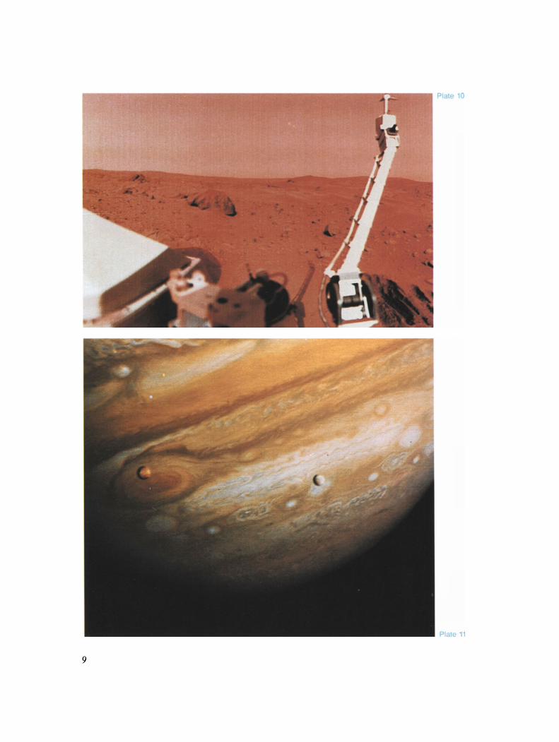
Plate 10

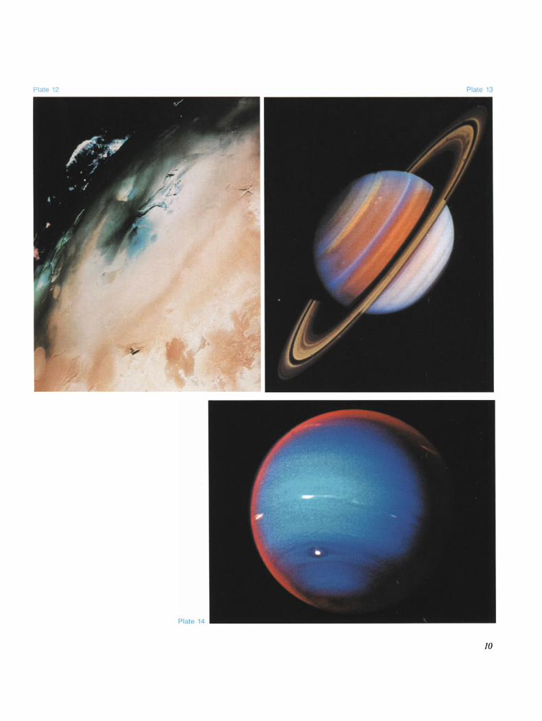
Plate 12 Plate t3

10

Plate 15

Plate 17

Plate 16

Plale 18

Plate 20

Plate 21

Plate 22

Plate 23

Plate 26

15

Plate 'Zl

Plate 28

Plate 30

17

Plate 31

Plate 32

Plate 33

Plate 34

Plate 35

Plate 36

20