Optimization of Two Soil–Structure Interaction Parameters ...
18
sustainability Article Optimization of Two Soil–Structure Interaction Parameters Using Dynamic Centrifuge Tests and an Analytical Approach Hyun-Uk Kim 1,2 , Jeong-Gon Ha 3 , Kil-Wan Ko 2 and Dong-Soo Kim 2, * 1 R&D Strategy and Planning Office, Central Research Institute of Korea Hydro and Nuclear Power (KHNP), Daejeon 34101, Korea; [email protected] 2 Department of Civil and Environmental Engineering, Korea Advanced Institute Science and Technology (KAIST), Daejeon 34141, Korea; [email protected] 3 Structural Safety & Prognosis Research Division, Korea Atomic Energy Research Institute (KAERI), Daejeon 34057, Korea; [email protected] * Correspondence: [email protected]; Tel.: +82-42-350-3619 Received: 14 July 2020; Accepted: 31 August 2020; Published: 31 August 2020 Abstract: The response of the structure subjected to an earthquake load is greatly affected by the properties of the structure and soil so it is very important to accurately determine the characteristics of the structure and soil for analysis. However, studies on the effective profile depth where soil properties are determined, have been conducted in the presence of restricted conditions (i.e., surface foundation, linear soil properties), and without any considerations on damping. In case of the effective height of structure that affects its rocking behavior, it was only theoretically or empirically determined. In addition, most previously published studies on soil–structure interaction (SSI) focused on limited effects and parameters (e.g., rocking behavior, embedment effect, effective profile depth, spring constant, and damping coefficient) and not on comprehensive SSI parameters. Furthermore, no detailed validation procedure has been set in place which made it difficult to validate the SSI parameters. Since the effective height of structure and effective profile depth are the basis of all the input parameters of SSI analysis, it is important to validate and determine them. Therefore, in this study, the procedure used to optimize the two SSI parameters was established based on an analytical approach that considered all the possible SSI parameters that were investigated from conventional codes and studies and physical model tests. As a result of this study, the optimum values of the effective height of the structure and effective profile depth were respectively determined according to (a) the height from the bottom part of the foundation to the center of the mass of the superstructure, and according to (b) the depth at values equal to four times the radius of the foundation. Keywords: effective height; effective profile depth; SSI; analytical approach; centrifuge test 1. Introduction The dynamic characteristics of the structure depend on the surrounding soil. To estimate an accurate structural response for seismic design, the soil–structure interaction (SSI) effect has been considered as the crucial effect for the seismic evaluation of the structure. There have been various studies on the soil–structure interaction (SSI) effect but the subject of each study was not comprehensive but limited to specific parameters or phenomena (e.g., spring constant and damping coefficient [1–6], effective profile depth [7], and rocking behavior [8–11]). With regard to the SSI analysis, four procedures were introduced in FEMA356 [12]: Linear static procedure (LSP), linear dynamic procedure (LDP), nonlinear static procedure (NSP), and nonlinear dynamic procedure (NDP). Among them, the static procedures (i.e., LSP and NSP) have been accepted in various standards owing to their simplicity and Sustainability 2020, 12, 7113; doi:10.3390/su12177113 www.mdpi.com/journal/sustainability
-
Upload
khangminh22 -
Category
Documents
-
view
5 -
download
0
Transcript of Optimization of Two Soil–Structure Interaction Parameters ...

sustainability
Article
Optimization of Two Soil–Structure InteractionParameters Using Dynamic Centrifuge Tests and anAnalytical Approach
Hyun-Uk Kim 1,2 , Jeong-Gon Ha 3, Kil-Wan Ko 2 and Dong-Soo Kim 2,*1 R&D Strategy and Planning Office, Central Research Institute of Korea Hydro and Nuclear Power (KHNP),
Daejeon 34101, Korea; [email protected] Department of Civil and Environmental Engineering, Korea Advanced Institute Science and
Technology (KAIST), Daejeon 34141, Korea; [email protected] Structural Safety & Prognosis Research Division, Korea Atomic Energy Research Institute (KAERI),
Daejeon 34057, Korea; [email protected]* Correspondence: [email protected]; Tel.: +82-42-350-3619
Received: 14 July 2020; Accepted: 31 August 2020; Published: 31 August 2020�����������������
Abstract: The response of the structure subjected to an earthquake load is greatly affected by theproperties of the structure and soil so it is very important to accurately determine the characteristics ofthe structure and soil for analysis. However, studies on the effective profile depth where soil propertiesare determined, have been conducted in the presence of restricted conditions (i.e., surface foundation,linear soil properties), and without any considerations on damping. In case of the effective height ofstructure that affects its rocking behavior, it was only theoretically or empirically determined.In addition, most previously published studies on soil–structure interaction (SSI) focused onlimited effects and parameters (e.g., rocking behavior, embedment effect, effective profile depth,spring constant, and damping coefficient) and not on comprehensive SSI parameters. Furthermore,no detailed validation procedure has been set in place which made it difficult to validate the SSIparameters. Since the effective height of structure and effective profile depth are the basis of all theinput parameters of SSI analysis, it is important to validate and determine them. Therefore, in thisstudy, the procedure used to optimize the two SSI parameters was established based on an analyticalapproach that considered all the possible SSI parameters that were investigated from conventionalcodes and studies and physical model tests. As a result of this study, the optimum values of theeffective height of the structure and effective profile depth were respectively determined according to(a) the height from the bottom part of the foundation to the center of the mass of the superstructure,and according to (b) the depth at values equal to four times the radius of the foundation.
Keywords: effective height; effective profile depth; SSI; analytical approach; centrifuge test
1. Introduction
The dynamic characteristics of the structure depend on the surrounding soil. To estimate anaccurate structural response for seismic design, the soil–structure interaction (SSI) effect has beenconsidered as the crucial effect for the seismic evaluation of the structure. There have been variousstudies on the soil–structure interaction (SSI) effect but the subject of each study was not comprehensivebut limited to specific parameters or phenomena (e.g., spring constant and damping coefficient [1–6],effective profile depth [7], and rocking behavior [8–11]). With regard to the SSI analysis, four procedureswere introduced in FEMA356 [12]: Linear static procedure (LSP), linear dynamic procedure (LDP),nonlinear static procedure (NSP), and nonlinear dynamic procedure (NDP). Among them, the staticprocedures (i.e., LSP and NSP) have been accepted in various standards owing to their simplicity and
Sustainability 2020, 12, 7113; doi:10.3390/su12177113 www.mdpi.com/journal/sustainability
Sustainability 2020, 12, 7113 2 of 18
practicality [12–15], and the dynamic procedures (i.e., LDP and NDP) have been used to either verifythe static procedures or to obtain more detailed structural responses. Even though all the standardsmentioned above (i.e., FEMA 356, ATC-40, FEMA 440, and ASCE 41–13) define the same three typesof modes (i.e., structural swaying, foundation swaying, and rocking), the formula for the soil–springconstant and damping coefficient, and the two SSI parameters (i.e., the effective height of the structureand effective profile depth) were defined differently at various standards and studies, including theaforementioned standards [1–4,7,12,14,16–19]. The two SSI parameters are very important becausethey determine the dynamic soil properties and the rocking potential of the soil–structure system(i.e., rocking damping coefficient and moment), but they have been derived in restricted conditions(i.e., the effective profile depth was determined based only on considerations of static soil stiffnessin surface foundation condition [5,7]) and theoretically determined (i.e., the effective height wasdetermined based on structural dynamic theory [3,10,12,13]). In addition, existing standards and priorstudies have been limited in view of the following: (1) Approximate consideration of the nonlineardeformation characteristics of the soil based on peak ground acceleration [12,14,15,18], (2) determinationof damping ratio of soil based only on radiation damping considerations [14,15,18], and (3) lack ofdetailed SSI analysis procedure and SSI parameter validation procedure with physical model tests.Therefore, in this study, the optimum SSI parameter selection procedure was established using anLDP-based analytical approach and relevant tests, whereby the SSI effects were comprehensivelyand appropriately considered (i.e., consideration of all the possible SSI parameters for analysis,accurate consideration of soil nonlinearity using site response analysis, and determination of total soildamping coefficient, including soil material damping). Finally, two optimum SSI parameters weredetermined based on a number of analyses according to the established procedure.
2. Soil–Structure Interaction (SSI) Parameters and Optimum SSI Parameter Selection Procedure
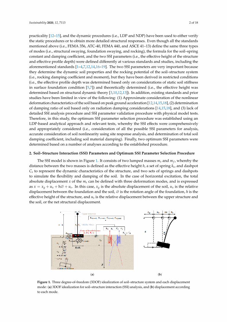
The SSI model is shown in Figure 1. It consists of two lumped masses ms and m f , whereby thedistance between the two masses is defined as the effective height h, a set of spring ks, and dashpotCs to represent the dynamic characteristics of the structure, and two sets of springs and dashpotsto simulate the flexibility and damping of the soil. In the case of horizontal excitation, the totalabsolute displacement x of the ms can be defined with three deformation modes, and is expressedas x = xg + ux + h∅+ us. In this case, xg is the absolute displacement of the soil, ux is the relativedisplacement between the foundation and the soil, ∅ is the rotation angle of the foundation, h is theeffective height of the structure, and us is the relative displacement between the upper structure andthe soil, or the net structural displacement.
Sustainability 2020, 12, x FOR PEER REVIEW 2 of 18
(NDP). Among them, the static procedures (i.e., LSP and NSP) have been accepted in various standards owing to their simplicity and practicality [12–15], and the dynamic procedures (i.e., LDP and NDP) have been used to either verify the static procedures or to obtain more detailed structural responses. Even though all the standards mentioned above (i.e., FEMA 356, ATC-40, FEMA 440, and ASCE 41–13) define the same three types of modes (i.e., structural swaying, foundation swaying, and rocking), the formula for the soil–spring constant and damping coefficient, and the two SSI parameters (i.e., the effective height of the structure and effective profile depth) were defined differently at various standards and studies, including the aforementioned standards [1–4,7,12,14,16–19]. The two SSI parameters are very important because they determine the dynamic soil properties and the rocking potential of the soil–structure system (i.e., rocking damping coefficient and moment), but they have been derived in restricted conditions (i.e., the effective profile depth was determined based only on considerations of static soil stiffness in surface foundation condition [5,7]) and theoretically determined (i.e., the effective height was determined based on structural dynamic theory [3,10,12,13]). In addition, existing standards and prior studies have been limited in view of the following: (1) Approximate consideration of the nonlinear deformation characteristics of the soil based on peak ground acceleration [12,14,15,18], (2) determination of damping ratio of soil based only on radiation damping considerations [14,15,18], and (3) lack of detailed SSI analysis procedure and SSI parameter validation procedure with physical model tests. Therefore, in this study, the optimum SSI parameter selection procedure was established using an LDP-based analytical approach and relevant tests, whereby the SSI effects were comprehensively and appropriately considered (i.e., consideration of all the possible SSI parameters for analysis, accurate consideration of soil nonlinearity using site response analysis, and determination of total soil damping coefficient, including soil material damping). Finally, two optimum SSI parameters were determined based on a number of analyses according to the established procedure.
2. Soil–Structure Interaction (SSI) Parameters and Optimum SSI Parameter Selection Procedure
The SSI model is shown in Figure 1. It consists of two lumped masses 𝑚 and 𝑚 , whereby the distance between the two masses is defined as the effective height ℎ, a set of spring 𝑘 , and dashpot 𝐶 to represent the dynamic characteristics of the structure, and two sets of springs and dashpots to simulate the flexibility and damping of the soil. In the case of horizontal excitation, the total absolute displacement 𝑥 of the 𝑚 can be defined with three deformation modes, and is expressed as 𝑥 =𝑥 + 𝑢 + h∅ + 𝑢 . In this case, 𝑥 is the absolute displacement of the soil, 𝑢 is the relative displacement between the foundation and the soil, ∅ is the rotation angle of the foundation, ℎ is the effective height of the structure, and 𝑢 is the relative displacement between the upper structure and the soil, or the net structural displacement.
(a) (b)
Figure 1. Three degree-of-freedom (3DOF) idealization of soil–structure system and each displacementmode: (a) 3DOF idealization for soil–structure interaction (SSI) analysis, and (b) displacement accordingto each mode.
Sustainability 2020, 12, 7113 3 of 18
To obtain detailed structural responses, the equation of motion (EOM) of the soil–structure systemthat considers the aforementioned three degree-of-freedom (3DOF) is expressed by Equation (1) [8,9,20].
ms ms msh
ms ms + m f msh
msh msh msh2 + I f
..
us..
ux..φ
+
cs 0 0
0 cx 0
0 0 cφ
.
us.
ux.φ
+
ks 0 0
0 kx 0
0 0 kφ
us
ux
φ
= −..
xg
ms
ms + m f
msh
(1)
2.1. Soil–Spring Constants and Damping Coefficients
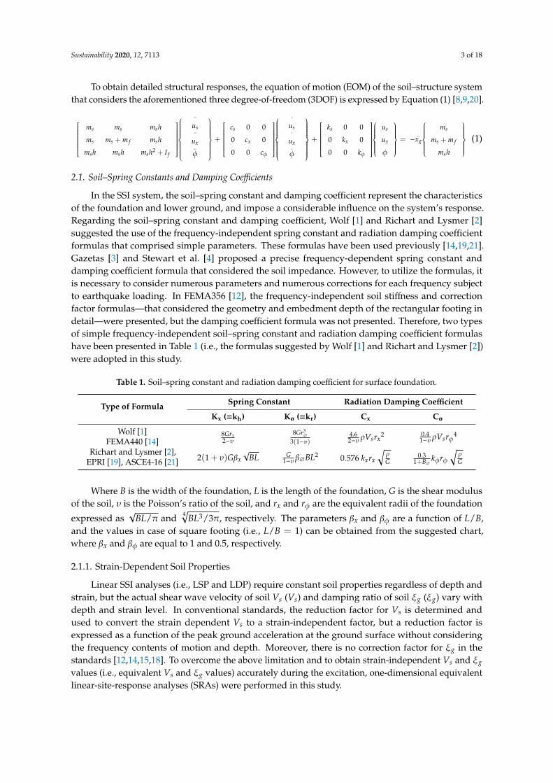
In the SSI system, the soil–spring constant and damping coefficient represent the characteristicsof the foundation and lower ground, and impose a considerable influence on the system’s response.Regarding the soil–spring constant and damping coefficient, Wolf [1] and Richart and Lysmer [2]suggested the use of the frequency-independent spring constant and radiation damping coefficientformulas that comprised simple parameters. These formulas have been used previously [14,19,21].Gazetas [3] and Stewart et al. [4] proposed a precise frequency-dependent spring constant anddamping coefficient formula that considered the soil impedance. However, to utilize the formulas, itis necessary to consider numerous parameters and numerous corrections for each frequency subjectto earthquake loading. In FEMA356 [12], the frequency-independent soil stiffness and correctionfactor formulas—that considered the geometry and embedment depth of the rectangular footing indetail—were presented, but the damping coefficient formula was not presented. Therefore, two typesof simple frequency-independent soil–spring constant and radiation damping coefficient formulashave been presented in Table 1 (i.e., the formulas suggested by Wolf [1] and Richart and Lysmer [2])were adopted in this study.
Table 1. Soil–spring constant and radiation damping coefficient for surface foundation.
Type of Formula Spring Constant Radiation Damping Coefficient
Kx (=kh) Kø (=kr) Cx Cø
Wolf [1]FEMA440 [14]
8Grx2−υ
8Gr3∅
3(1−υ)4.62−υρVsrx
2 0.41−υρVsrφ4
Richart and Lysmer [2],EPRI [19], ASCE4-16 [21] 2(1 + υ)Gβx
√BL G
1−υβ∅BL2 0.576 kxrx
√ρG
0.31+B∅
kφrφ√ρG
Where B is the width of the foundation, L is the length of the foundation, G is the shear modulusof the soil, υ is the Poisson’s ratio of the soil, and rx and rφ are the equivalent radii of the foundation
expressed as√
BL/π and 4√
BL3/3π, respectively. The parameters βx and βφ are a function of L/B,and the values in case of square footing (i.e., L/B = 1) can be obtained from the suggested chart,where βx and βφ are equal to 1 and 0.5, respectively.
2.1.1. Strain-Dependent Soil Properties
Linear SSI analyses (i.e., LSP and LDP) require constant soil properties regardless of depth andstrain, but the actual shear wave velocity of soil Vs (Vs) and damping ratio of soil ξg (ξg) vary withdepth and strain level. In conventional standards, the reduction factor for Vs is determined andused to convert the strain dependent Vs to a strain-independent factor, but a reduction factor isexpressed as a function of the peak ground acceleration at the ground surface without consideringthe frequency contents of motion and depth. Moreover, there is no correction factor for ξg in thestandards [12,14,15,18]. To overcome the above limitation and to obtain strain-independent Vs and ξg
values (i.e., equivalent Vs and ξg values) accurately during the excitation, one-dimensional equivalentlinear-site-response analyses (SRAs) were performed in this study.
Sustainability 2020, 12, 7113 4 of 18
2.1.2. Depth-Dependent Soil Properties and Effective Profile Depth (Zp)
Although equivalent Vs and ξg values are converted to their strain-independent forms, they arestill non-uniformly distributed as a function of depth. Therefore, it is necessary to define an effectiveprofile depth (Zp). In this way, depth-independent, equivalent Vs and ξg values have to be obtainedas the average values within a depth Zp. The averaged values of Vs and ξg that consider Zp can beobtained by Equation (2), as follows,
Vs(avg) =Zp∑n
i=1∆Zi(Vs)i
, ξg(avg) =Zp∑n
i=1∆Zi(ξg)i
(2)
where (Vs)i is the shear wave velocity of the ith soil layer,(ξg
)i
is the material damping ratio of theith soil layer, and ∆Zi is the thickness of the ith soil layer, respectively. Stewart et al. [7] regarded thestatic soil–spring constants obtained from the impedance solutions by Wong and Luco [5] as referencevalues, and repeatedly calculated the soil–spring constants at various profile depths. Note thatZp is 0.75 times the radius of the foundation (r), wherein the residual between the reference andthe calculated value is minimized. In addition to prior research publications, in the recommendedprovision of national earthquake hazard reduction program (NEHRP) [16], 4 r and 1.5 r were proposedas the respective values of Zp for swaying and rocking behaviors, respectively. However, in previousstudies, the embedment effect and damping ratio of soil were not considered. Therefore, in this study,three types of scenarios of 0.75 r, 2 r, and 4 r, were considered to evaluate the optimum effective profiledepth and necessary considerations (i.e., embedment effect and ξg), and were included in the analyticalapproach for the evaluation of the optimum effective profile depth.
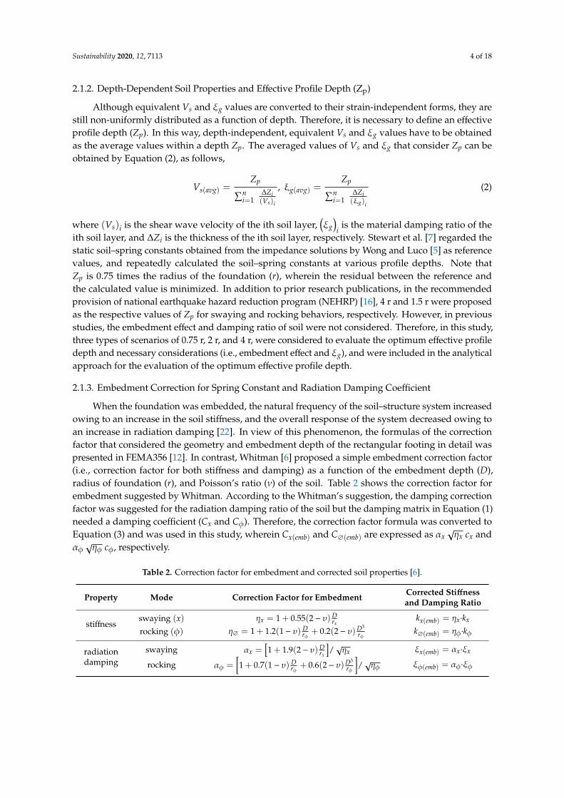
2.1.3. Embedment Correction for Spring Constant and Radiation Damping Coefficient
When the foundation was embedded, the natural frequency of the soil–structure system increasedowing to an increase in the soil stiffness, and the overall response of the system decreased owing toan increase in radiation damping [22]. In view of this phenomenon, the formulas of the correctionfactor that considered the geometry and embedment depth of the rectangular footing in detail waspresented in FEMA356 [12]. In contrast, Whitman [6] proposed a simple embedment correction factor(i.e., correction factor for both stiffness and damping) as a function of the embedment depth (D),radius of foundation (r), and Poisson’s ratio (ν) of the soil. Table 2 shows the correction factor forembedment suggested by Whitman. According to the Whitman’s suggestion, the damping correctionfactor was suggested for the radiation damping ratio of the soil but the damping matrix in Equation (1)needed a damping coefficient (Cx and Cφ). Therefore, the correction factor formula was converted toEquation (3) and was used in this study, wherein Cx(emb) and C∅(emb) are expressed as αx
√ηx cx and
αφ√ηφ cφ, respectively.
Table 2. Correction factor for embedment and corrected soil properties [6].
Property Mode Correction Factor for Embedment Corrected Stiffnessand Damping Ratio
stiffnessswaying (x) ηx = 1 + 0.55(2− υ)D
rxkx(emb) = ηx·kx
rocking (φ) η∅ = 1 + 1.2(1− υ) Drφ + 0.2(2− υ)D3
rφ k∅(emb) = ηφ·kφ
radiationdamping
swaying αx =[1 + 1.9(2− υ)D
rx
]/√ηx ξx(emb) = αx·ξx
rocking αφ =[1 + 0.7(1− υ) D
rφ + 0.6(2− υ)D3
rφ
]/√ηφ ξφ(emb) = αφ·ξφ

Sustainability 2020, 12, 7113 5 of 18
Cx(emb) = Ccr x(emb)ξx(emb) = 2√
mtkx(emb)ξx(emb) = 2√
mtkx(emb)
(αx
Cx2√
mtkx
)= αx
√ηxCx
C∅(emb) = Ccr ∅(emb)ξ∅(emb) = 2√
I0k∅(emb)ξ∅(emb) = 2√
I0k∅(emb)
(α∅
C∅
2√
I0k∅
)= α∅
√η∅C∅
(3)
2.1.4. Determination of Soil Damping Based on Radiation and Material Damping Considerations
The total damping coefficient formula consists of the material damping and the radiation dampingcoefficients [1,3,19]. Assuming that the structure is rigid (ks =∞) and that the foundation cannot rock(kr =∞), or is only allowed to rock (kh =∞), the natural frequency of each case follows $2
h = kh/mt and$2
r = kr/I0 [1], where mt and I0 are the total mass and total mass moment of inertia of the structure,respectively. Equation (4) expresses a form of the total damping coefficient based on the considerationof the embedment effect. Substituting the natural frequency equation in each mode in Equation (4)estimates the swaying and rocking total damping coefficients, as listed in Table 3, wherein Cgx and Cgφare the respective swaying and rocking material damping coefficients. The total damping coefficientwas expressed as function of Ch and Cr to distinguish them from the subscripts x and φ of the radiationdamping coefficient. Accordingly, the soil–spring constant was also denoted by kh and kr for theswaying and rocking modes.
C(emb) = raditation C(emb) + material Cg(emb) = C(emb) +2
$(emb)ξgk(emb) (4)
Table 3. Soil–spring constant and total damping coefficient formulas based on embedment effect considerations.
Property Mode Soil–Spring Constant and Damping Coefficient Formula
soil spring constantswaying (h) kh(emb) = kx(emb) = ηx·kxrocking (r) kr(emb) = k∅(emb) = η∅·k∅
soil total damping coefficientswaying Ch(emb) = Cx(emb) + Cgx(emb) = αx
√ηx cx + 2
√mt kx(emb)ξg
rocking Cr(emb) = C∅(emb) + Cg∅(emb) = αφ√ηφ cφ + 2
√I0 k∅(emb)ξg
2.2. Effective Height of Structure h
In the soil–structure system, the effective height (h) of the structure affects its rocking responseof the system. Stewart et al. [17] defined h as the distance from the foundation to the centroid of theinertial force in relation to the fundamental mode. In FEMA440 [14] and FEMA450 [18], the full heightwas considered as the value of h of the one-story structure, and the distance from the foundation tothe center point of the first modal shape was set to h in multistory structures. In the Electric PowerResearch Institute (EPRI) training module [19], h was calculated based on the moment equilibriumto the center of mass of the rigid foundation. According to the recent research by Gavras et al. [10],the value of h of the footing-flexible column-bridge deck system was defined as the distance fromthe base of the footing to the center of the deck. However, a limited number of studies have verifiedor validated the optimum effective height of the structure. In this study, three effective heights (h)were considered to choose the optimum h, whereby the two heights were suggested by conventionalstandards, and the other height satisfied the total mass moment of inertia (I0) of the structure. The threeeffective heights used in this study adhered to the following order: Height from the bottom of thefoundation to the center of mass of the superstructure (hbase to ms ) < height compatible to the total massmoment of inertia of the structure (hMMI) < height needed to satisfy moment equilibrium (hmoment).Additionally, hMMI and hmoment can be obtained as indicated below,
hMMI = (I0 − I f /ms)0.5 (5)
hmoment = M0 −M f /msg (6)
Sustainability 2020, 12, 7113 6 of 18
where I0 is the total mass moment of inertia of the upper, middle, and lower structures, and I f isthe mass moment of inertia based on the consideration of the effective mass m f and the geometry offoundation, M0 is the summation of the moment of the upper, middle, and lower structures, and M f isthe moment that considers the effective mass m f and the geometry of the foundation.
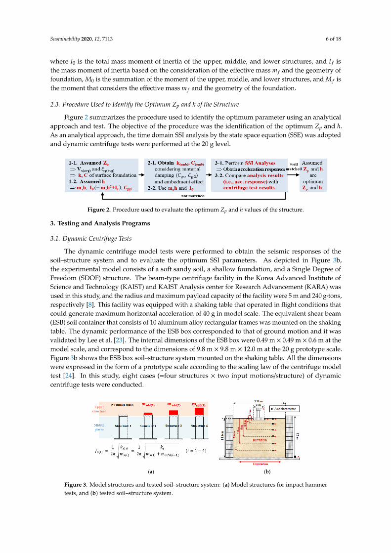
2.3. Procedure Used to Identify the Optimum Zp and h of the Structure
Figure 2 summarizes the procedure used to identify the optimum parameter using an analyticalapproach and test. The objective of the procedure was the identification of the optimum Zp and h.As an analytical approach, the time domain SSI analysis by the state space equation (SSE) was adoptedand dynamic centrifuge tests were performed at the 20 g level.
Sustainability 2020, 12, x FOR PEER REVIEW 6 of 18
the foundation to the center of mass of the superstructure (ℎ ) < height compatible to the total mass moment of inertia of the structure (ℎ ) < height needed to satisfy moment equilibrium (ℎ ). Additionally, ℎ and ℎ can be obtained as indicated below, ℎ = (𝐼 − 𝐼 /𝑚 ) . (5)ℎ = 𝑀 − 𝑀 /𝑚 g (6)
where 𝐼 is the total mass moment of inertia of the upper, middle, and lower structures, and 𝐼 is the mass moment of inertia based on the consideration of the effective mass 𝑚 and the geometry of foundation, 𝑀 is the summation of the moment of the upper, middle, and lower structures, and 𝑀 is the moment that considers the effective mass 𝑚 and the geometry of the foundation.
2.3. Procedure Used to Identify the Optimum 𝑍 and ℎ of the Structure
Figure 2 summarizes the procedure used to identify the optimum parameter using an analytical approach and test. The objective of the procedure was the identification of the optimum 𝑍 and ℎ. As an analytical approach, the time domain SSI analysis by the state space equation (SSE) was adopted and dynamic centrifuge tests were performed at the 20 g level.
Figure 2. Procedure used to evaluate the optimum 𝑍 and ℎ values of the structure.
3. Testing and Analysis Programs
3.1. Dynamic Centrifuge Tests
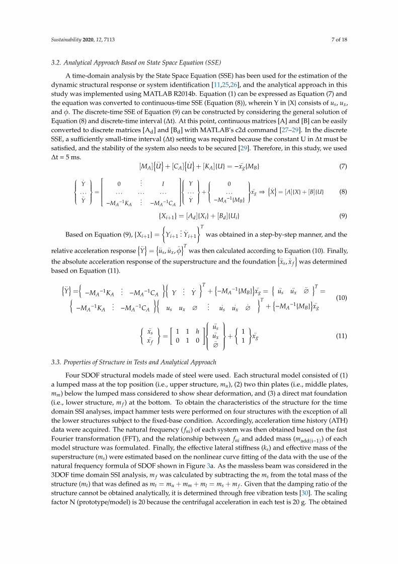
The dynamic centrifuge model tests were performed to obtain the seismic responses of the soil–structure system and to evaluate the optimum SSI parameters. As depicted in Figure 3b, the experimental model consists of a soft sandy soil, a shallow foundation, and a Single Degree of Freedom (SDOF) structure. The beam-type centrifuge facility in the Korea Advanced Institute of Science and Technology (KAIST) and KAIST Analysis center for Research Advancement (KARA) was used in this study, and the radius and maximum payload capacity of the facility were 5 m and 240 g·tons, respectively [8]. This facility was equipped with a shaking table that operated in flight conditions that could generate maximum horizontal acceleration of 40 g in model scale. The equivalent shear beam (ESB) soil container that consists of 10 aluminum alloy rectangular frames was mounted on the shaking table. The dynamic performance of the ESB box corresponded to that of ground motion and it was validated by Lee et al. [23]. The internal dimensions of the ESB box were 0.49 m × 0.49 m × 0.6 m at the model scale, and correspond to the dimensions of 9.8 m × 9.8 m × 12.0 m at the 20 g prototype scale. Figure 3b shows the ESB box soil–structure system mounted on the shaking table. All the dimensions were expressed in the form of a prototype scale according to the scaling law of the centrifuge model test [24]. In this study, eight cases (= four structures × two input motions/structure) of dynamic centrifuge tests were conducted.
Figure 2. Procedure used to evaluate the optimum Zp and h values of the structure.
3. Testing and Analysis Programs
3.1. Dynamic Centrifuge Tests
The dynamic centrifuge model tests were performed to obtain the seismic responses of thesoil–structure system and to evaluate the optimum SSI parameters. As depicted in Figure 3b,the experimental model consists of a soft sandy soil, a shallow foundation, and a Single Degree ofFreedom (SDOF) structure. The beam-type centrifuge facility in the Korea Advanced Institute ofScience and Technology (KAIST) and KAIST Analysis center for Research Advancement (KARA) wasused in this study, and the radius and maximum payload capacity of the facility were 5 m and 240 g·tons,respectively [8]. This facility was equipped with a shaking table that operated in flight conditions thatcould generate maximum horizontal acceleration of 40 g in model scale. The equivalent shear beam(ESB) soil container that consists of 10 aluminum alloy rectangular frames was mounted on the shakingtable. The dynamic performance of the ESB box corresponded to that of ground motion and it wasvalidated by Lee et al. [23]. The internal dimensions of the ESB box were 0.49 m × 0.49 m × 0.6 m at themodel scale, and correspond to the dimensions of 9.8 m × 9.8 m × 12.0 m at the 20 g prototype scale.Figure 3b shows the ESB box soil–structure system mounted on the shaking table. All the dimensionswere expressed in the form of a prototype scale according to the scaling law of the centrifuge modeltest [24]. In this study, eight cases (=four structures × two input motions/structure) of dynamiccentrifuge tests were conducted.
Sustainability 2020, 12, x FOR PEER REVIEW 7 of 18
(a) (b)
Figure 3. Model structures and tested soil–structure system: (a) Model structures for impact hammer tests, and (b) tested soil–structure system.
3.2. Analytical Approach Based on State Space Equation (SSE)
A time-domain analysis by the State Space Equation (SSE) has been used for the estimation of the dynamic structural response or system identification [11,25,26], and the analytical approach in this study was implemented using MATLAB R2014b. Equation (1) can be expressed as Equation (7) and the equation was converted to continuous-time SSE (Equation (8)), wherein Y in {X} consists of 𝑢 , 𝑢 , and 𝜙. The discrete-time SSE of Equation (9) can be constructed by considering the general solution of Equation (8) and discrete-time interval (Δt). At this point, continuous matrices [A] and [B] can be easily converted to discrete matrices [Ad] and [Bd] with MATLAB’s c2d command [27–29]. In the discrete SSE, a sufficiently small-time interval (Δt) setting was required because the constant U in Δt must be satisfied, and the stability of the system also needs to be secured [29]. Therefore, in this study, we used Δt = 5 ms. 𝑀 𝑈 + 𝐶 𝑈 + 𝐾 {𝑈} = −𝑥 {𝑀 } (7)𝑌…𝑌 = 0 ⋮ 𝐼… … …−𝑀 𝐾 ⋮ −𝑀 𝐶 𝑌…𝑌 + 0…−𝑀 {𝑀 } 𝑥 ⇒ 𝑋 = 𝐴 {𝑋} + 𝐵 {𝑈} (8)
{𝑋 } = 𝐴 {𝑋 } + 𝐵 {𝑈 } (9)
Based on Equation (9), {𝑋 } = {𝑌 ⋮ 𝑌 } was obtained in a step-by-step manner, and the relative acceleration response 𝑌 = {𝑢 , 𝑢 , 𝜙} was then calculated according to Equation (10). Finally, the absolute acceleration response of the superstructure and the foundation {𝑥 , 𝑥 } was determined based on Equation (11). 𝑌 = {−𝑀 𝐾 ⋮ −𝑀 𝐶 }{𝑌 ⋮ 𝑌} + −𝑀 {𝑀 } 𝑥 = {𝑢 𝑢 ∅} ={−𝑀 𝐾 ⋮ −𝑀 𝐶 }{𝑢 𝑢 ∅ ⋮ 𝑢 𝑢 ∅} + −𝑀 {𝑀 } 𝑥
(10)
𝑥𝑥 = 1 1 ℎ0 1 0 𝑢𝑢∅ + 11 𝑥 (11)
3.3. Properties of Structure in Tests and Analytical Approach
Four SDOF structural models made of steel were used. Each structural model consisted of (1) a lumped mass at the top position (i.e., upper structure, 𝑚 ), (2) two thin plates (i.e., middle plates, 𝑚 ) below the lumped mass considered to show shear deformation, and (3) a direct mat foundation (i.e., lower structure, 𝑚 ) at the bottom. To obtain the characteristics of the structure for the time domain SSI analyses, impact hammer tests were performed on four structures with the exception of all the lower structures subject to the fixed-base condition. Accordingly, acceleration time history
Figure 3. Model structures and tested soil–structure system: (a) Model structures for impact hammertests, and (b) tested soil–structure system.
Sustainability 2020, 12, 7113 7 of 18
3.2. Analytical Approach Based on State Space Equation (SSE)
A time-domain analysis by the State Space Equation (SSE) has been used for the estimation of thedynamic structural response or system identification [11,25,26], and the analytical approach in thisstudy was implemented using MATLAB R2014b. Equation (1) can be expressed as Equation (7) andthe equation was converted to continuous-time SSE (Equation (8)), wherein Y in {X} consists of us, ux,and φ. The discrete-time SSE of Equation (9) can be constructed by considering the general solution ofEquation (8) and discrete-time interval (∆t). At this point, continuous matrices [A] and [B] can be easilyconverted to discrete matrices [Ad] and [Bd] with MATLAB’s c2d command [27–29]. In the discreteSSE, a sufficiently small-time interval (∆t) setting was required because the constant U in ∆t must besatisfied, and the stability of the system also needs to be secured [29]. Therefore, in this study, we used∆t = 5 ms.
[MA]{ ..U}+ [CA]
{ .U}+ [KA]{U} = −
..xg{MB} (7)
.Y. . ...Y
=
0
... I. . . . . . . . .
−MA−1KA
... −MA−1CA
Y. . .
.Y
+
0. . .
−MA−1{MB}
..xg ⇒
{ .X}= [A]{X}+ [B]{U} (8)
{Xi+1
}= [Ad]{Xi}+ [Bd]{Ui} (9)
Based on Equation (9),{Xi+1
}=
{Yi+1
....Yi+1
}T
was obtained in a step-by-step manner, and the
relative acceleration response{ ..Y}=
{ ..us,
..ux,
..φ}T
was then calculated according to Equation (10). Finally,
the absolute acceleration response of the superstructure and the foundation{ ..xs,
..x f
}was determined
based on Equation (11).
{ ..Y}=
{−MA
−1KA... −MA
−1CA
}{Y
....Y
}T+
{−MA
−1{MB}
} ..xg =
{ ..us
..ux
..∅
}T={
−MA−1KA
... −MA−1CA
}{us ux ∅
....
us.
ux.∅
}T+
{−MA
−1{MB}
} ..xg
(10)
{ ..xs..
x f
}=
[1 1 h0 1 0
]..
us..
ux..∅
+
{11
}..
xg (11)
3.3. Properties of Structure in Tests and Analytical Approach
Four SDOF structural models made of steel were used. Each structural model consisted of (1)a lumped mass at the top position (i.e., upper structure, mu), (2) two thin plates (i.e., middle plates,mm) below the lumped mass considered to show shear deformation, and (3) a direct mat foundation(i.e., lower structure, m f ) at the bottom. To obtain the characteristics of the structure for the timedomain SSI analyses, impact hammer tests were performed on four structures with the exception of allthe lower structures subject to the fixed-base condition. Accordingly, acceleration time history (ATH)data were acquired. The natural frequency ( fni) of each system was then obtained based on the fastFourier transformation (FFT), and the relationship between fni and added mass (madd(i−1)) of eachmodel structure was formulated. Finally, the effective lateral stiffness (ks) and effective mass of thesuperstructure (ms) were estimated based on the nonlinear curve fitting of the data with the use of thenatural frequency formula of SDOF shown in Figure 3a. As the massless beam was considered in the3DOF time domain SSI analysis, m f was calculated by subtracting the ms from the total mass of thestructure (mt) that was defined as mt = mu + mm + ml = ms + m f . Given that the damping ratio of thestructure cannot be obtained analytically, it is determined through free vibration tests [30]. The scalingfactor N (prototype/model) is 20 because the centrifugal acceleration in each test is 20 g. The obtained
Sustainability 2020, 12, 7113 8 of 18
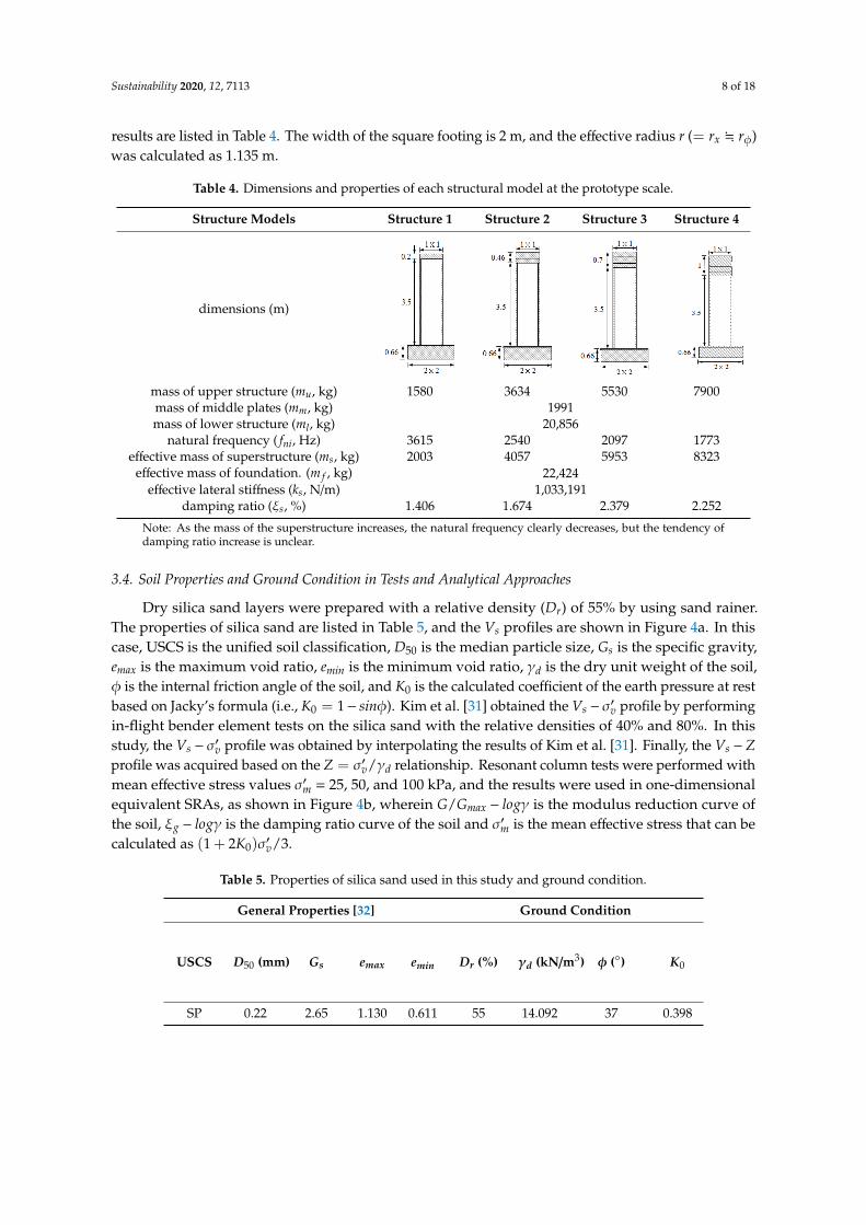
results are listed in Table 4. The width of the square footing is 2 m, and the effective radius r (= rx ; rφ)was calculated as 1.135 m.
Table 4. Dimensions and properties of each structural model at the prototype scale.
Structure Models Structure 1 Structure 2 Structure 3 Structure 4
dimensions (m)
Sustainability 2020, 12, x FOR PEER REVIEW 8 of 18
(ATH) data were acquired. The natural frequency (𝑓 ) of each system was then obtained based on the fast Fourier transformation (FFT), and the relationship between 𝑓 and added mass (𝑚 ( )) of each model structure was formulated. Finally, the effective lateral stiffness (𝑘 ) and effective mass of the superstructure (𝑚 ) were estimated based on the nonlinear curve fitting of the data with the use of the natural frequency formula of SDOF shown in Figure 3a. As the massless beam was considered in the 3DOF time domain SSI analysis, 𝑚 was calculated by subtracting the 𝑚 from the total mass of the structure (𝑚 ) that was defined as 𝑚 = 𝑚 + 𝑚 + 𝑚 = 𝑚 + 𝑚 . Given that the damping ratio of the structure cannot be obtained analytically, it is determined through free vibration tests [30]. The scaling factor N (prototype/model) is 20 because the centrifugal acceleration in each test is 20 g. The obtained results are listed in Table 4. The width of the square footing is 2 m, and the effective radius 𝑟 (= 𝑟 ≒𝑟 ) was calculated as 1.135 m.
Table 4. Dimensions and properties of each structural model at the prototype scale.
Structure Models Structure 1 Structure 2 Structure 3 Structure 4
dimensions (m)
mass of upper structure (𝑚 , kg) 1580 3634 5530 7900 mass of middle plates (𝑚 , kg) 1991 mass of lower structure (𝑚 , kg) 20,856
natural frequency (𝑓 , Hz) 3615 2540 2097 1773 effective mass of superstructure (𝑚 , kg) 2003 4057 5953 8323
effective mass of foundation. (𝑚 , kg) 22,424 effective lateral stiffness (𝑘 , N/m) 1,033,191
damping ratio (𝜉 , %) 1.406 1.674 2.379 2.252 Note: As the mass of the superstructure increases, the natural frequency clearly decreases, but the tendency of damping ratio increase is unclear.
3.4. Soil Properties and Ground Condition in Tests and Analytical Approaches
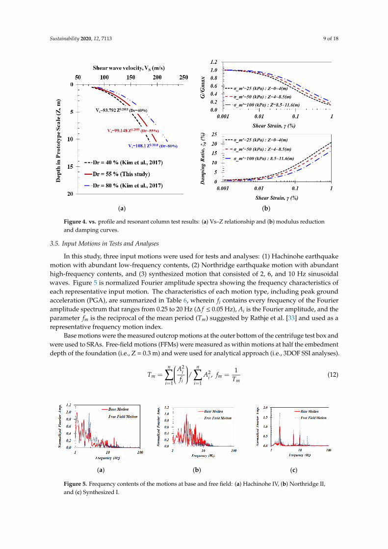
Dry silica sand layers were prepared with a relative density (𝐷 ) of 55% by using sand rainer. The properties of silica sand are listed in Table 5, and the 𝑉 profiles are shown in Figure 4a. In this case, USCS is the unified soil classification, 𝐷 is the median particle size, 𝐺 is the specific gravity, 𝑒 is the maximum void ratio, 𝑒 is the minimum void ratio, 𝛾 is the dry unit weight of the soil, 𝜙 is the internal friction angle of the soil, and 𝐾 is the calculated coefficient of the earth pressure at rest based on Jacky's formula (i.e., 𝐾 = 1 − 𝑠𝑖𝑛𝜙). Kim et al. [31] obtained the 𝑉 − 𝜎 ′ profile by performing in-flight bender element tests on the silica sand with the relative densities of 40% and 80%. In this study, the 𝑉 − 𝜎 profile was obtained by interpolating the results of Kim et al. [31]. Finally, the 𝑉 − 𝑍 profile was acquired based on the 𝑍 = 𝜎 /𝛾 relationship. Resonant column tests were performed with mean effective stress values 𝜎 ′ = 25, 50, and 100 kPa, and the results were used in one-dimensional equivalent SRAs, as shown in Figure 4b, wherein 𝐺/𝐺 − 𝑙𝑜𝑔𝛾 is the modulus reduction curve of the soil, 𝜉 − 𝑙𝑜𝑔𝛾 is the damping ratio curve of the soil and 𝜎 ′ is the mean effective stress that can be calculated as (1 + 2𝐾 )𝜎 /3.
Sustainability 2020, 12, x FOR PEER REVIEW 8 of 18
(ATH) data were acquired. The natural frequency (𝑓 ) of each system was then obtained based on the fast Fourier transformation (FFT), and the relationship between 𝑓 and added mass (𝑚 ( )) of each model structure was formulated. Finally, the effective lateral stiffness (𝑘 ) and effective mass of the superstructure (𝑚 ) were estimated based on the nonlinear curve fitting of the data with the use of the natural frequency formula of SDOF shown in Figure 3a. As the massless beam was considered in the 3DOF time domain SSI analysis, 𝑚 was calculated by subtracting the 𝑚 from the total mass of the structure (𝑚 ) that was defined as 𝑚 = 𝑚 + 𝑚 + 𝑚 = 𝑚 + 𝑚 . Given that the damping ratio of the structure cannot be obtained analytically, it is determined through free vibration tests [30]. The scaling factor N (prototype/model) is 20 because the centrifugal acceleration in each test is 20 g. The obtained results are listed in Table 4. The width of the square footing is 2 m, and the effective radius 𝑟 (= 𝑟 ≒𝑟 ) was calculated as 1.135 m.
Table 4. Dimensions and properties of each structural model at the prototype scale.
Structure Models Structure 1 Structure 2 Structure 3 Structure 4
dimensions (m)
mass of upper structure (𝑚 , kg) 1580 3634 5530 7900 mass of middle plates (𝑚 , kg) 1991 mass of lower structure (𝑚 , kg) 20,856
natural frequency (𝑓 , Hz) 3615 2540 2097 1773 effective mass of superstructure (𝑚 , kg) 2003 4057 5953 8323
effective mass of foundation. (𝑚 , kg) 22,424 effective lateral stiffness (𝑘 , N/m) 1,033,191
damping ratio (𝜉 , %) 1.406 1.674 2.379 2.252 Note: As the mass of the superstructure increases, the natural frequency clearly decreases, but the tendency of damping ratio increase is unclear.
3.4. Soil Properties and Ground Condition in Tests and Analytical Approaches
Dry silica sand layers were prepared with a relative density (𝐷 ) of 55% by using sand rainer. The properties of silica sand are listed in Table 5, and the 𝑉 profiles are shown in Figure 4a. In this case, USCS is the unified soil classification, 𝐷 is the median particle size, 𝐺 is the specific gravity, 𝑒 is the maximum void ratio, 𝑒 is the minimum void ratio, 𝛾 is the dry unit weight of the soil, 𝜙 is the internal friction angle of the soil, and 𝐾 is the calculated coefficient of the earth pressure at rest based on Jacky's formula (i.e., 𝐾 = 1 − 𝑠𝑖𝑛𝜙). Kim et al. [31] obtained the 𝑉 − 𝜎 ′ profile by performing in-flight bender element tests on the silica sand with the relative densities of 40% and 80%. In this study, the 𝑉 − 𝜎 profile was obtained by interpolating the results of Kim et al. [31]. Finally, the 𝑉 − 𝑍 profile was acquired based on the 𝑍 = 𝜎 /𝛾 relationship. Resonant column tests were performed with mean effective stress values 𝜎 ′ = 25, 50, and 100 kPa, and the results were used in one-dimensional equivalent SRAs, as shown in Figure 4b, wherein 𝐺/𝐺 − 𝑙𝑜𝑔𝛾 is the modulus reduction curve of the soil, 𝜉 − 𝑙𝑜𝑔𝛾 is the damping ratio curve of the soil and 𝜎 ′ is the mean effective stress that can be calculated as (1 + 2𝐾 )𝜎 /3.
mass of upper structure (mu, kg) 1580 3634 5530 7900mass of middle plates (mm, kg) 1991mass of lower structure (ml, kg) 20,856
natural frequency ( fni, Hz) 3615 2540 2097 1773effective mass of superstructure (ms, kg) 2003 4057 5953 8323
effective mass of foundation. (m f , kg) 22,424effective lateral stiffness (ks, N/m) 1,033,191
damping ratio (ξs, %) 1.406 1.674 2.379 2.252
Note: As the mass of the superstructure increases, the natural frequency clearly decreases, but the tendency ofdamping ratio increase is unclear.
3.4. Soil Properties and Ground Condition in Tests and Analytical Approaches
Dry silica sand layers were prepared with a relative density (Dr) of 55% by using sand rainer.The properties of silica sand are listed in Table 5, and the Vs profiles are shown in Figure 4a. In thiscase, USCS is the unified soil classification, D50 is the median particle size, Gs is the specific gravity,emax is the maximum void ratio, emin is the minimum void ratio, γd is the dry unit weight of the soil,φ is the internal friction angle of the soil, and K0 is the calculated coefficient of the earth pressure at restbased on Jacky’s formula (i.e., K0 = 1− sinφ). Kim et al. [31] obtained the Vs − σ′v profile by performingin-flight bender element tests on the silica sand with the relative densities of 40% and 80%. In thisstudy, the Vs − σ′v profile was obtained by interpolating the results of Kim et al. [31]. Finally, the Vs −Zprofile was acquired based on the Z = σ′v/γd relationship. Resonant column tests were performed withmean effective stress values σ′m = 25, 50, and 100 kPa, and the results were used in one-dimensionalequivalent SRAs, as shown in Figure 4b, wherein G/Gmax − logγ is the modulus reduction curve ofthe soil, ξg − logγ is the damping ratio curve of the soil and σ′m is the mean effective stress that can becalculated as (1 + 2K0)σ′v/3.
Table 5. Properties of silica sand used in this study and ground condition.
General Properties [32] Ground Condition
USCS D50 (mm) Gs emax emin Dr (%) γd (kN/m3) φ (◦) K0
SP 0.22 2.65 1.130 0.611 55 14.092 37 0.398
Sustainability 2020, 12, 7113 9 of 18
Sustainability 2020, 12, x FOR PEER REVIEW 9 of 18
Table 5. Properties of silica sand used in this study and ground condition.
General Properties [32] Ground Condition USCS 𝑫𝟓𝟎 (mm) 𝑮𝒔 𝒆𝒎𝒂𝒙 𝒆𝒎𝒊𝒏 𝑫𝒓 (%) 𝜸𝒅 (𝒌𝑵/𝒎𝟑) 𝝓 (°) 𝑲𝟎
SP 0.22 2.65 1.130 0.611 55 14.092 37 0.398
(a) (b)
Figure 4. vs. profile and resonant column test results: (a) Vs–Z relationship and (b) modulus reduction and damping curves.
3.5. Input Motions in Tests and analyses
In this study, three input motions were used for tests and analyses: (1) Hachinohe earthquake motion with abundant low-frequency contents, (2) Northridge earthquake motion with abundant high-frequency contents, and (3) synthesized motion that consisted of 2, 6, and 10 Hz sinusoidal waves. Figure 5 is normalized Fourier amplitude spectra showing the frequency characteristics of each representative input motion. The characteristics of each motion type, including peak ground acceleration (PGA), are summarized in Table 6, wherein 𝑓 contains every frequency of the Fourier amplitude spectrum that ranges from 0.25 to 20 Hz (Δ𝑓 ≤ 0.05 Hz), 𝐴 is the Fourier amplitude, and the parameter 𝑓 is the reciprocal of the mean period (𝑇 ) suggested by Rathje et al. [33] and used as a representative frequency motion index. 𝑇 = 𝐴𝑓 / 𝐴 , 𝑓 = 1𝑇 (12)
Base motions were the measured outcrop motions at the outer bottom of the centrifuge test box and were used to SRAs. Free-field motions (FFMs) were measured as within motions at half the embedment depth of the foundation (i.e., Z = 0.3 m) and were used for analytical approach (i.e., 3DOF SSI analyses).
Table 6. Characteristics of base and free-field motions used in this study.
Case Input Motion Base Motions Free Field Motions
PGA (g) 𝒇𝒎 (Hz) PGA (g) 𝒇𝒎 (Hz) structure 1 Hachinohe I 0.112 1.842 0.227 2.268 structure 2 Hachinohe II 0.245 1.685 0.573 2.215 structure 3 Hachinohe III 0.283 1.637 0.585 2.157
Figure 4. vs. profile and resonant column test results: (a) Vs–Z relationship and (b) modulus reductionand damping curves.
3.5. Input Motions in Tests and Analyses
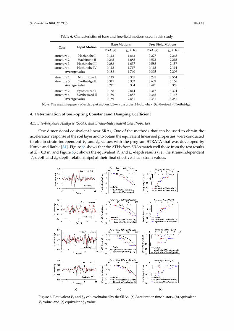
In this study, three input motions were used for tests and analyses: (1) Hachinohe earthquakemotion with abundant low-frequency contents, (2) Northridge earthquake motion with abundanthigh-frequency contents, and (3) synthesized motion that consisted of 2, 6, and 10 Hz sinusoidalwaves. Figure 5 is normalized Fourier amplitude spectra showing the frequency characteristics ofeach representative input motion. The characteristics of each motion type, including peak groundacceleration (PGA), are summarized in Table 6, wherein fi contains every frequency of the Fourieramplitude spectrum that ranges from 0.25 to 20 Hz (∆ f ≤ 0.05 Hz), Ai is the Fourier amplitude, and theparameter fm is the reciprocal of the mean period (Tm) suggested by Rathje et al. [33] and used as arepresentative frequency motion index.
Base motions were the measured outcrop motions at the outer bottom of the centrifuge test box andwere used to SRAs. Free-field motions (FFMs) were measured as within motions at half the embedmentdepth of the foundation (i.e., Z = 0.3 m) and were used for analytical approach (i.e., 3DOF SSI analyses).
Tm =n∑
i=1
A2i
fi
/n∑
i=1
A2i , fm =
1Tm
(12)
Sustainability 2020, 12, x FOR PEER REVIEW 10 of 18
structure 4 Hachinohe IV 0.113 1.797 0.193 2.194 Average value 0.188 1.740 0.395 2.209
structure 1 Northridge I 0.119 3.355 0.285 3.564 structure 3 Northridge II 0.315 3.353 0.609 3.166
Average value 0.217 3.354 0.447 3.365 structure 2 Synthesized I 0.188 2.814 0.317 3.394 structure 4 Synthesized II 0.189 2.887 0.345 3.167
Average value 0.189 2.851 0.331 3.281 Note: The mean frequency of each input motion follows the order: Hachinohe < Synthesized < Northridge.
(a) (b) (c)
Figure 5. Frequency contents of the motions at base and free field: (a) Hachinohe IV, (b) Northridge II, and (c) Synthesized I.
4. Determination of Soil–Spring Constant and Damping Coefficient
4.1. Site-Response Analyses (SRAs) and Strain-Independent Soil Properties
One dimensional equivalent linear SRAs, One of the methods that can be used to obtain the acceleration response of the soil layer and to obtain the equivalent linear soil properties, were conducted to obtain strain-independent 𝑉 and 𝜉 values with the program STRATA that was developed by Kottke and Rathje [34]. Figure 6a shows that the ATHs from SRAs match well those from the test results at Z = 0.3 m, and Figure 6b,c shows the equivalent 𝑉 and 𝜉 -depth results (i.e., the strain-independent 𝑉 depth and 𝜉 -depth relationships) at their final effective shear strain values.
Figure 5. Frequency contents of the motions at base and free field: (a) Hachinohe IV, (b) Northridge II,and (c) Synthesized I.
Sustainability 2020, 12, 7113 10 of 18
Table 6. Characteristics of base and free-field motions used in this study.
Case Input MotionBase Motions Free Field Motions
PGA (g) fm (Hz) PGA (g) fm (Hz)
structure 1 Hachinohe I 0.112 1.842 0.227 2.268structure 2 Hachinohe II 0.245 1.685 0.573 2.215structure 3 Hachinohe III 0.283 1.637 0.585 2.157structure 4 Hachinohe IV 0.113 1.797 0.193 2.194
Average value 0.188 1.740 0.395 2.209
structure 1 Northridge I 0.119 3.355 0.285 3.564structure 3 Northridge II 0.315 3.353 0.609 3.166
Average value 0.217 3.354 0.447 3.365
structure 2 Synthesized I 0.188 2.814 0.317 3.394structure 4 Synthesized II 0.189 2.887 0.345 3.167
Average value 0.189 2.851 0.331 3.281
Note: The mean frequency of each input motion follows the order: Hachinohe < Synthesized < Northridge.
4. Determination of Soil–Spring Constant and Damping Coefficient
4.1. Site-Response Analyses (SRAs) and Strain-Independent Soil Properties
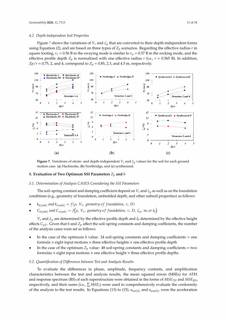
One dimensional equivalent linear SRAs, One of the methods that can be used to obtain theacceleration response of the soil layer and to obtain the equivalent linear soil properties, were conductedto obtain strain-independent Vs and ξg values with the program STRATA that was developed byKottke and Rathje [34]. Figure 6a shows that the ATHs from SRAs match well those from the test resultsat Z = 0.3 m, and Figure 6b,c shows the equivalent Vs and ξg-depth results (i.e., the strain-independentVs depth and ξg-depth relationships) at their final effective shear strain values.
Sustainability 2020, 12, x FOR PEER REVIEW 11 of 19
(a) (b) (c)
Figure 6. Equivalent 𝑉 and 𝜉 values obtained by the SRAs: (a) Acceleration time history, (b) equivalent 𝑉 value, and (c) equivalent 𝜉 value.
4.2. Depth-Independent Soil Properties
Figure 7 shows the variations of 𝑉 and 𝜉 that are converted to their depth-independent forms using Equation (2), and are based on three types of 𝑍 scenarios. Regarding the effective radius 𝑟 in square footing, 𝑟 = 0.56 B in the swaying mode is similar to 𝑟 = 0.57 B in the rocking mode, and the effective profile depth 𝑍 is normalized with one effective radius 𝑟 (i.e., 𝑟 = 0.565 B). In addition, 𝑍𝑝/𝑟 = 0.75, 2, and 4, correspond to 𝑍 = 0.85, 2.3, and 4.5 m, respectively.
Figure 6. Equivalent Vs and ξg values obtained by the SRAs: (a) Acceleration time history, (b) equivalentVs value, and (c) equivalent ξg value.
Sustainability 2020, 12, 7113 11 of 18
4.2. Depth-Independent Soil Properties
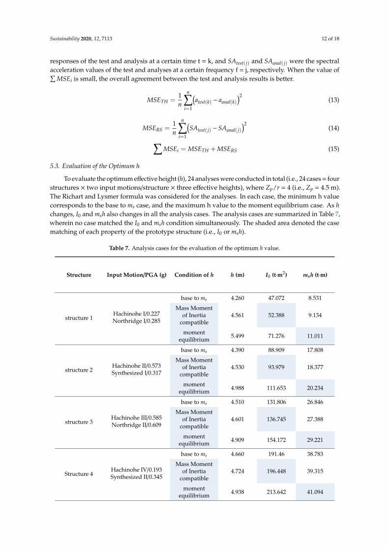
Figure 7 shows the variations of Vs and ξg that are converted to their depth-independent formsusing Equation (2), and are based on three types of Zp scenarios. Regarding the effective radius r insquare footing, rx = 0.56 B in the swaying mode is similar to rφ = 0.57 B in the rocking mode, and theeffective profile depth Zp is normalized with one effective radius r (i.e., r = 0.565 B). In addition,Zp/r = 0.75, 2, and 4, correspond to Zp = 0.85, 2.3, and 4.5 m, respectively.
Sustainability 2020, 12, x FOR PEER REVIEW 11 of 18
(a) (b) (c)
Figure 6. Equivalent 𝑉 and 𝜉 values obtained by the SRAs: (a) Acceleration time history, (b) equivalent 𝑉 value, and (c) equivalent 𝜉 value.
4.2. Depth-Independent Soil Properties
Figure 7 shows the variations of 𝑉 and 𝜉 that are converted to their depth-independent forms using Equation (2), and are based on three types of 𝑍 scenarios. Regarding the effective radius 𝑟 in square footing, 𝑟 = 0.56 B in the swaying mode is similar to 𝑟 = 0.57 B in the rocking mode, and the effective profile depth 𝑍 is normalized with one effective radius 𝑟 (i.e., 𝑟 = 0.565 B). In addition, 𝑍𝑝/𝑟 = 0.75, 2, and 4, correspond to 𝑍 = 0.85, 2.3, and 4.5 m, respectively.
(a) (b) (c)
Figure 7. Variations of strain- and depth-independent 𝑉 and 𝜉 values for the soil for each ground motion case: (a) Hachinohe, (b) Northridge, and (c) synthesized.
5. Evaluation of Two Optimum SSI Parameters 𝒁𝒑 and 𝒉
5.1. Determination of Analysis CASES considering the SSI Parameters
Figure 7. Variations of strain- and depth-independent Vs and ξg values for the soil for each groundmotion case: (a) Hachinohe, (b) Northridge, and (c) synthesized.
5. Evaluation of Two Optimum SSI Parameters Zp and h
5.1. Determination of Analysis CASES Considering the SSI Parameters
The soil–spring constant and damping coefficient depend on Vs and ξg as well as on the foundationconditions (e.g., geometry of foundation, embedded depth, and other subsoil properties) as follows
• kh(emb) and kr(emb) = f (ρ, Vs, geometry o f f oundation, ν, D)
• Ch(emb) and Cr(emb) = f(ρ, Vs, geometry o f f oundation, ν, D, ξg, mt or I0
)Vs and ξg are determined by the effective profile depth and I0 determined by the effective height
affects Cg∅. Given that h and Zp affect the soil–spring constants and damping coefficients, the numberof the analysis cases were set as follows:
• In the case of the optimum h value: 24 soil-spring constants and damping coefficients = oneformula × eight input motions × three effective heights × one effective profile depth
• In the case of the optimum Zp value: 48 soil-spring constants and damping coefficients = twoformulas × eight input motions × one effective height × three effective profile depths
5.2. Quantification of Differences between Test and Analysis Results
To evaluate the differences in phase, amplitude, frequency contents, and amplificationcharacteristics between the test and analysis results, the mean squared errors (MSEs) for ATHand response spectrum (RS) of each superstructure were obtained in the forms of MSETH and MSERS,respectively, and their sums (i.e.,
∑MSEi) were used to comprehensively evaluate the conformity
of the analysis to the test results. In Equations (13) to (15), atest(k) and aanal(k) were the acceleration
Sustainability 2020, 12, 7113 12 of 18
responses of the test and analysis at a certain time t = k, and SAtest( j) and SAanal( j) were the spectralacceleration values of the test and analyses at a certain frequency f = j, respectively. When the value of∑
MSEi is small, the overall agreement between the test and analysis results is better.
MSETH =1n
n∑i=1
(atest(k) − aanal(k)
)2(13)
MSERS =1n
n∑i=1
(SAtest( j) − SAanal( j)
)2(14)
∑MSEi = MSETH + MSERS (15)
5.3. Evaluation of the Optimum h
To evaluate the optimum effective height (h), 24 analyses were conducted in total (i.e., 24 cases = fourstructures × two input motions/structure × three effective heights), where Zp/r = 4 (i.e., Zp = 4.5 m).The Richart and Lysmer formula was considered for the analyses. In each case, the minimum h valuecorresponds to the base to ms case, and the maximum h value to the moment equilibrium case. As hchanges, I0 and msh also changes in all the analysis cases. The analysis cases are summarized in Table 7,wherein no case matched the I0 and msh condition simultaneously. The shaded area denoted the casematching of each property of the prototype structure (i.e., I0 or msh).
Table 7. Analysis cases for the evaluation of the optimum h value.
Structure Input Motion/PGA (g) Condition of h h (m) I0 (t·m2) msh (t·m)
structure 1Hachinohe I/0.227Northridge I/0.285
base to ms 4.260 47.072 8.531
Mass Momentof Inertia
compatible4.561 52.388 9.134
momentequilibrium 5.499 71.276 11.011
structure 2Hachinohe II/0.573Synthesized I/0.317
base to ms 4.390 88.909 17.808
Mass Momentof Inertia
compatible4.530 93.979 18.377
momentequilibrium 4.988 111.653 20.234
structure 3Hachinohe III/0.585Northridge II/0.609
base to ms 4.510 131.806 26.846
Mass Momentof Inertia
compatible4.601 136.745 27.388
momentequilibrium 4.909 154.172 29.221
Structure 4Hachinohe IV/0.193Synthesized II/0.345
base to ms 4.660 191.46 38.783
Mass Momentof Inertia
compatible4.724 196.448 39.315
momentequilibrium 4.938 213.642 41.094

Sustainability 2020, 12, 7113 13 of 18
Figure 8 shows the ATHs and∑
MSEi values of the test and analysis results. According to theresults of the analysis, as h increases,
∑MSEi increases. Based on the tendency and calculation result
of∑
MSEi,∑
MSEi at hbase to ms yielded a minimum error of 0.106 on average,∑
MSEi at hMMI yieldedan error of 0.127 on average, and
∑MSEi at hmoment yielded the greatest error of 0.229 on average.
Given that∑
MSEi at hbase to ms was estimated to be lower than that at full height, hbase to ms wasconsidered as the optimum effective height.
Sustainability 2020, 12, x FOR PEER REVIEW 13 of 18
structure 3
Northridge II/0.609 Mass Moment of Inertia compatible 4.601 136.745 27.388 moment equilibrium 4.909 154.172 29.221
Structure 4
Hachinohe IV/0.193 Synthesized II/0.345
base to 𝑚 4.660 191.46 38.783 Mass Moment of Inertia compatible 4.724 196.448 39.315
moment equilibrium 4.938 213.642 41.094
Figure 8 shows the ATHs and ∑MSE values of the test and analysis results. According to the results of the analysis, as h increases, ∑MSE increases. Based on the tendency and calculation result of ∑MSE , ∑MSE at ℎ yielded a minimum error of 0.106 on average, ∑MSE at h yielded an error of 0.127 on average, and ∑MSE at ℎ yielded the greatest error of 0.229 on average. Given that ∑MSE at ℎ was estimated to be lower than that at full height, ℎ was considered as the optimum effective height.
(a) (b) (c)
Figure 8. Differences between tests and analyses, and acceleration time history (ATHs) of all tested cases: (a) ∑MSE values comparisons of test and analysis data, (b) ATH at ℎ , and (c) ATH at ℎ .
5.4. Evaluation of the Optimum Effective Profile Depth 𝑍
In the evaluation of the optimum effective profile depth (𝑍 ), 48 analyses were conducted in total (i.e., 48 cases = four structures × two input motions/structure × three effective profile depths × two
Figure 8. Differences between tests and analyses, and acceleration time history (ATHs) of all tested cases:(a)
∑MSEi values comparisons of test and analysis data, (b) ATH at hbase to ms , and (c) ATH at hmoment.
5.4. Evaluation of the Optimum Effective Profile Depth Zp
In the evaluation of the optimum effective profile depth (Zp), 48 analyses were conducted in total(i.e., 48 cases = four structures × two input motions/structure × three effective profile depths × twotypes of formulas), wherein the embedment correction factor suggested by Whitman [6] and hbase to ms
was used in common. The analysis cases are summarized in Table 8.Figure 9 shows the
∑MSEi value of each analysis case, and Table 9 lists the maximum acceleration
responses of the superstructure, wherein the shaded areas represent the analysis cases that bestmatch the test results (i.e., the case with the minimum
∑MSEi). Although two analysis cases
(i.e., structure 3-Northridge II and structure 4-Synthesized II) show that the maximum accelerationresponses were smaller than those of the corresponding test results, the differences were not considerable.
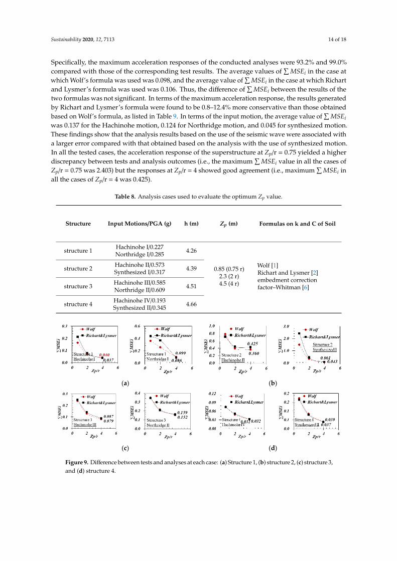
Sustainability 2020, 12, 7113 14 of 18
Specifically, the maximum acceleration responses of the conducted analyses were 93.2% and 99.0%compared with those of the corresponding test results. The average values of
∑MSEi in the case at
which Wolf’s formula was used was 0.098, and the average value of∑
MSEi in the case at which Richartand Lysmer’s formula was used was 0.106. Thus, the difference of
∑MSEi between the results of the
two formulas was not significant. In terms of the maximum acceleration response, the results generatedby Richart and Lysmer’s formula were found to be 0.8–12.4% more conservative than those obtainedbased on Wolf’s formula, as listed in Table 9. In terms of the input motion, the average value of
∑MSEi
was 0.137 for the Hachinohe motion, 0.124 for Northridge motion, and 0.045 for synthesized motion.These findings show that the analysis results based on the use of the seismic wave were associated witha larger error compared with that obtained based on the analysis with the use of synthesized motion.In all the tested cases, the acceleration response of the superstructure at Zp/r = 0.75 yielded a higherdiscrepancy between tests and analysis outcomes (i.e., the maximum
∑MSEi value in all the cases of
Zp/r = 0.75 was 2.403) but the responses at Zp/r = 4 showed good agreement (i.e., maximum∑
MSEi inall the cases of Zp/r = 4 was 0.425).
Table 8. Analysis cases used to evaluate the optimum Zp value.
Structure Input Motions/PGA (g) h (m) Zp (m) Formulas on k and C of Soil
structure 1 Hachinohe I/0.227Northridge I/0.285 4.26
0.85 (0.75 r)2.3 (2 r)4.5 (4 r)
Wolf [1]Richart and Lysmer [2]embedment correctionfactor–Whitman [6]
structure 2 Hachinohe II/0.573Synthesized I/0.317 4.39
structure 3 Hachinohe III/0.585Northridge II/0.609 4.51
structure 4 Hachinohe IV/0.193Synthesized II/0.345 4.66
Sustainability 2020, 12, x FOR PEER REVIEW 14 of 18
types of formulas), wherein the embedment correction factor suggested by Whitman [6] and ℎ was used in common. The analysis cases are summarized in Table 8.
Table 8. Analysis cases used to evaluate the optimum 𝑍 value.
Structure Input Motions/PGA (g) h (m) 𝒁𝒑 (m) Formulas on k and C of Soil
structure 1 Hachinohe I/0.227 Northridge I/0.285 4.26
0.85 (0.75 r) 2.3 (2 r) 4.5 (4 r)
Wolf [1] Richart and Lysmer [2] embedment correction factor–Whitman [6]
structure 2 Hachinohe II/0.573 Synthesized I/0.317 4.39
structure 3 Hachinohe III/0.585 Northridge II/0.609
4.51
structure 4 Hachinohe IV/0.193 Synthesized II/0.345
4.66
Figure 9 shows the ∑MSE value of each analysis case, and Table 9 lists the maximum acceleration responses of the superstructure, wherein the shaded areas represent the analysis cases that best match the test results (i.e., the case with the minimum ∑MSE ). Although two analysis cases (i.e., structure 3-Northridge II and structure 4-Synthesized II) show that the maximum acceleration responses were smaller than those of the corresponding test results, the differences were not considerable. Specifically, the maximum acceleration responses of the conducted analyses were 93.2% and 99.0% compared with those of the corresponding test results. The average values of ∑MSE in the case at which Wolf's formula was used was 0.098, and the average value of ∑MSE in the case at which Richart and Lysmer’s formula was used was 0.106. Thus, the difference of ∑MSE between the results of the two formulas was not significant. In terms of the maximum acceleration response, the results generated by Richart and Lysmer’s formula were found to be 0.8–12.4% more conservative than those obtained based on Wolf's formula, as listed in Table 9. In terms of the input motion, the average value of ∑MSE was 0.137 for the Hachinohe motion, 0.124 for Northridge motion, and 0.045 for synthesized motion. These findings show that the analysis results based on the use of the seismic wave were associated with a larger error compared with that obtained based on the analysis with the use of synthesized motion. In all the tested cases, the acceleration response of the superstructure at 𝑍 /r = 0.75 yielded a higher discrepancy between tests and analysis outcomes (i.e., the maximum ∑MSE value in all the cases of 𝑍 /r = 0.75 was 2.403) but the responses at 𝑍 /r = 4 showed good agreement (i.e., maximum ∑MSE in all the cases of 𝑍 /r = 4 was 0.425).
(a) (b)
(c) (d)
Figure 9. Difference between tests and analyses at each case: (a) Structure 1, (b) structure 2, (c) structure 3, and (d) structure 4. Figure 9. Difference between tests and analyses at each case: (a) Structure 1, (b) structure 2, (c) structure 3,and (d) structure 4.
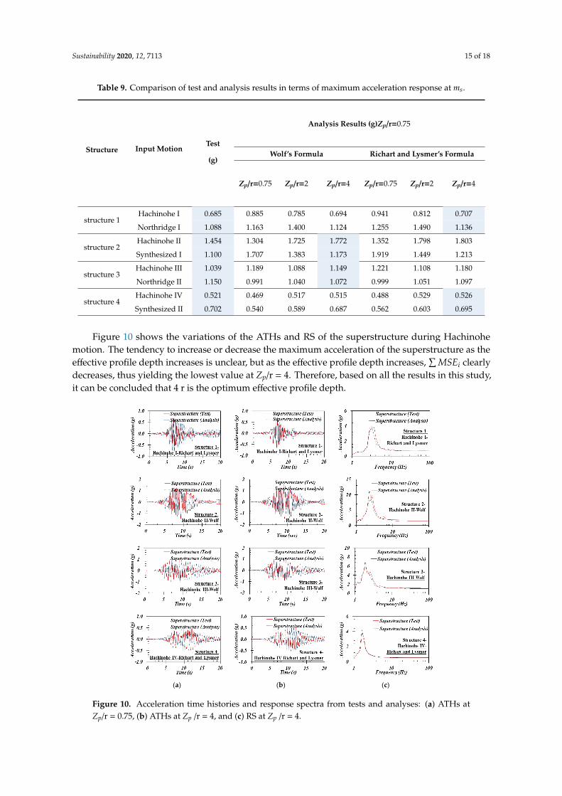
Sustainability 2020, 12, 7113 15 of 18
Table 9. Comparison of test and analysis results in terms of maximum acceleration response at ms.
Structure Input MotionTest
(g)
Analysis Results (g)Zp/r=0.75
Wolf’s Formula Richart and Lysmer’s Formula
Zp/r=0.75 Zp/r=2 Zp/r=4 Zp/r=0.75 Zp/r=2 Zp/r=4
structure 1Hachinohe I 0.685 0.885 0.785 0.694 0.941 0.812 0.707
Northridge I 1.088 1.163 1.400 1.124 1.255 1.490 1.136
structure 2Hachinohe II 1.454 1.304 1.725 1.772 1.352 1.798 1.803
Synthesized I 1.100 1.707 1.383 1.173 1.919 1.449 1.213
structure 3Hachinohe III 1.039 1.189 1.088 1.149 1.221 1.108 1.180
Northridge II 1.150 0.991 1.040 1.072 0.999 1.051 1.097
structure 4Hachinohe IV 0.521 0.469 0.517 0.515 0.488 0.529 0.526
Synthesized II 0.702 0.540 0.589 0.687 0.562 0.603 0.695
Figure 10 shows the variations of the ATHs and RS of the superstructure during Hachinohemotion. The tendency to increase or decrease the maximum acceleration of the superstructure as theeffective profile depth increases is unclear, but as the effective profile depth increases,
∑MSEi clearly
decreases, thus yielding the lowest value at Zp/r = 4. Therefore, based on all the results in this study,it can be concluded that 4 r is the optimum effective profile depth.
Sustainability 2020, 12, x FOR PEER REVIEW 15 of 18
Table 9. Comparison of test and analysis results in terms of maximum acceleration response at 𝑚 .
Structure Input Motion Test (𝒈)
Analysis Results (𝒈)
Wolf’s Formula Richart and Lysmer’s
Formula 𝒁𝒑/r = 0.75
𝒁𝒑/r = 2
𝒁𝒑/r = 4
𝒁𝒑/r = 0.75 𝒁𝒑/r = 2 𝒁𝒑/r = 4
structure 1 Hachinohe I 0.685 0.885 0.785 0.694 0.941 0.812 0.707 Northridge I 1.088 1.163 1.400 1.124 1.255 1.490 1.136
structure 2 Hachinohe II 1.454 1.304 1.725 1.772 1.352 1.798 1.803 Synthesized I 1.100 1.707 1.383 1.173 1.919 1.449 1.213
structure 3 Hachinohe III 1.039 1.189 1.088 1.149 1.221 1.108 1.180 Northridge II 1.150 0.991 1.040 1.072 0.999 1.051 1.097
structure 4 Hachinohe IV 0.521 0.469 0.517 0.515 0.488 0.529 0.526 Synthesized II 0.702 0.540 0.589 0.687 0.562 0.603 0.695
Figure 10 shows the variations of the ATHs and RS of the superstructure during Hachinohe motion. The tendency to increase or decrease the maximum acceleration of the superstructure as the effective profile depth increases is unclear, but as the effective profile depth increases, ∑MSE clearly decreases, thus yielding the lowest value at 𝑍 /r = 4. Therefore, based on all the results in this study, it can be concluded that 4 r is the optimum effective profile depth.
(a) (b) (c)
Figure 10. Acceleration time histories and response spectra from tests and analyses: (a) ATHs atZp/r = 0.75, (b) ATHs at Zp /r = 4, and (c) RS at Zp /r = 4.
Sustainability 2020, 12, 7113 16 of 18
6. Conclusions
In this study, dynamic centrifuge tests and LDP-based analyses (i.e., time domain SSI analyses bySSE) were performed to evaluate the optimum effective height and effective profile depth conditionsproposed in the conventional standards and prior research publications. Four structures and threeground motions were used in the centrifuge tests, and three effective heights and three effective profiledepth conditions were considered as the SSI analysis cases in addition to the aforementioned testconditions. The main results of this research are summarized as follows.
1. In this study, the applicability of the SSI parameters suggested by various standards and studieswas discussed, and the optimum SSI parameter selection procedure that (a) comprehensivelyconsidered the SSI parameters, (b) adopted an analytical approach and a physical model test,was suggested. Based on the established procedure, the optimum values of two controversial SSIparameters (i.e., the effective height and effective profile depth) were determined
• Unlike the conventional standards that apply a simplified reduction factor for the initialshear wave velocity profile and do not apply any corrections in initial damping ratio profile,one dimensional equivalent linear site response analyses were performed to accuratelyobtain the equivalent strain-independent shear wave velocity (Vs ) and damping ratio (ξg)of the soil. The equivalent Vs and ξg values that varied with depth obtained herein wereconverted to depth independent Vs and ξg values based on considerations of the effectiveprofile depth (Zp).
• Unlike the conventional research efforts that ignored soil material damping and indirectlydetermined soil damping based on the effective period lengthening ratio, the total soildamping was obtained directly by the addition of soil material damping to soil radiationdamping. In addition, the stiffness and total damping of soil were determined based onembedded foundation conditions.
• Unlike the conventional SDOF SSI analysis that was based on the RS, this study adopteda 3DOF time domain SSI analysis based on structural translation, foundation translation,and rocking behavior considerations to accurately obtain structural responses.
2. The effective height of the structure affected the rocking behavior of the soil–structure system(i.e., msh and Cg∅). In this study, applicability of the following three effective height scenarioswere evaluated based on the following test and analysis results: (1) Height from the bottom ofthe foundation to the center of the mass of the superstructure, and (2) height compatible to thetotal mass moment of inertia, and (3) height to satisfy moment equilibrium. As the effectiveheight increased within the effective height range used in the analysis, the differences betweentest and analysis results increased. Consequently, in all the cases, the height from the bottom ofthe foundation to the center of the mass of the superstructure was the optimum effective heightwith the lowest
∑MSEi value.
3. The optimum effective profile depth (Zp) was determined. This was used to average the dynamicsoil property that varied as a function of depth. Three scenarios were considered in the analyses:(1) Zp/r = 0.75, (2) Zp/r = 2, and (3) Zp/r = 4. As a result, 4 r was found to be the optimumeffective profile depth with the lowest difference between the test and analysis results. In addition,the results associated with earthquake motions yielded higher errors than those of synthesizedmotions that consisted of sinusoidal waves at the frequencies of 2, 6, and 10 Hz. The maximumacceleration responses by Richart and Lysmer’s formula was more conservative than thoseobtained with Wolf’s formula.
Author Contributions: Conceptualization and methodology, H.-U.K. and D.-S.K.; formal analysis, H.-U.K.;investigation, H.-U.K.; resources, D.-S.K. and J.-G.H.; data curation, H.-U.K. and J.-G.H.; validation, J.-G.H.,K.-W.K. and D.-S.K.; writing—original draft preparation, H.-U.K.; writing—review and editing, J.-G.H. andK.-W.K.; supervision, D.-S.K.; project administration, D.-S.K.; funding acquisition, D.-S.K. All authors have readand agreed to the published version of the manuscript.

Sustainability 2020, 12, 7113 17 of 18
Funding: This research was funded by Korea Construction Engineering and Transport Development CollaboratoryManagement Institute (KOCED), Korea Advanced Institute of Science and Technology (KAIST) and KAIST Analysiscenter for Research Advancement (KARA).
Acknowledgments: This research was supported by Korea Construction Engineering and Transport DevelopmentCollaboratory Management Institute (KOCED), Korea Advanced Institute of Science and Technology (KAIST) andKAIST Analysis center for Research Advancement (KARA).
Conflicts of Interest: The authors declare no conflict of interest.
References
1. Wolf, J. Dynamic Soil-Structure Interaction; Section 3.4 Introductory Example; Prentice Hall:Englewood Cliffs, NJ, USA, 1985; pp. 38–50.
2. Richart, F.; Hall, J.; Woods, R. Vibrations of Soils and Foundations; Prentice-Hall: Englewood Cliffs, NJ, USA, 1970.3. Gazetas, G. Foundation Engineering Handbook, 2nd ed.; Fang, H.Y., Ed.; Chapter 15 Foundation Vibrations;
Springer Science Business Media: New York, NY, USA, 1991.4. Stewart, J.; Seed, R.; Fenves, G. PEER-98/07: Empirical Evaluation of Inertial Soil Structure Interaction;
Pacific Earthquake Engineering Research (PEER) Center: Berkeley, CA, USA, 1998.5. Wong, H.; Luco, J. Tables of impedance functions for square foundations on layered media. Soil Dyn.
Earthq. Eng. 1985, 4, 64–81. [CrossRef]6. Whitman, R. Soil Publications No-300: Analysis of Soil-Structure Interaction: A State-of-the-Art Review;
Massachusetts Institute of Technology: Cambridge, MA, USA, 1972.7. Stewart, J.; Kim, S.; Bielak, J.; Dobry, R.; Power, M. Revisions to soil-structure interaction procedures in
NEHRP design provisions. Earthq. Spectra 2003, 19, 677–696. [CrossRef]8. Kim, D.; Lee, S.; Kim, D.; Choo, Y.; Park, H. Rocking effect of a mat foundation on the earthquake response of
structures. J. Geotech. Geoenviron. Eng. 2015, 141, 10:04014085. [CrossRef]9. Ko, K.; Ha, J.; Park, H.; Kim, D. Comparison between cyclic and dynamic rocking behavior for embedded
shallow foundation using centrifuge tests. Bull. Earthq. Eng. 2018, 16, 5171–5193. [CrossRef]10. Gavras, A.; Kutter, B.; Hakhamaneshi, M.; Gajan, S.; Tsatsis, A.; Sharma, K.; Kohno, T.; Deng, L.;
Anastasopoulos, I.; Gazetas, G. Database of rocking shallow foundation performance: Dynamic shaking.Earthq. Spectra 2020, 36, 960–982. [CrossRef]
11. Kim, D.; Park, H.; Kim, D.; Lee, H. Nonlinear system identification on shallow foundation using ExtendedKalman Filter. Soil Dyn. Earthq. Eng. 2020, 128, 105857. [CrossRef]
12. FEMA. Prestandard and Commentary for the Seismic Rehabilitation of Buildings (FEMA 356); Federal EmergencyManagement Agency: Washington, DC, USA, 2000.
13. ATC. Seismic Evaluation and Retrofit of Concrete Buildings (ATC-40); Applied Technology Council:Redwood City, CA, USA, 1996.
14. FEMA. Improvement of Nonlinear Static Seismic Analysis Procedures (FEMA 440); Federal EmergencyManagement Agency: Washington, DC, USA, 2004.
15. ASCE. Seismic Evaluation and Retrofit of Existing Buildings (ASCE 41-13); Chapter 8 Foundations and GeologicSite Hazards; American Society of Civil Engineers: Reston, VA, USA, 2014.
16. BSSC. NEHRP Recommended Provisions for Seismic Regulation for New Buildings and Other Structures;Federal Emergency Management Agency: Washington, DC, USA, 1998.
17. Stewart, J.; Fenves, G.; Seed, R. Seismic Soil-Structure Interaction in Buildings. I: Analytical Methods.J. Geotech. Geoenviron. Eng. 1999, 125, 26–37. [CrossRef]
18. BSSC. NEHRP Recommended Provisions for Seismic Regulations for New Buildings and Other Structures(FEMA 450-1 2003 Edition); Federal Emergency Management Agency: Washington, DC, USA, 2004.
19. EPRI. 1010808: Engineering Technical Training Modules for Nuclear Plant Engineers-Civil/Structural Series Module#5-Soil Structure Interaction; EPRI: Palo Alto, CA, USA, 2005.
20. Mikami, A.; Sawada, T. Time-domain identification system of dynamic soil-structure interaction.In Proceedings of the 13th World Conference on Earthquake Engineering, Vancouver, BC, Canada,1–6 August 2004. Paper No. 747.
21. ASCE. Seismic Analysis of Safety-Related Nuclear Structures (ASCE 4-16); Chapter 5 Soil-Structure InteractionModeling and Analysis; American Society of Civil Engineers: Reston, VA, USA, 2017; p. 24.
Sustainability 2020, 12, 7113 18 of 18
22. Chowdhury, I.; Dasgupta, S. Dynamics of Structure and Foundation-A Unified Approach 2. APPLICATIONS;Chapter 2, Analysis and Design of Machine Foundation—2.4 Effect of Embedment on Foundation; Taylor &Francis Ltd.: London, UK, 2009.
23. Lee, S.; Choo, Y.; Kim, D. Performance of an equivalent shear beam (ESB) model container for dynamicgeotechnical centrifuge tests. Soil Dyn. Earthq. Eng. 2013, 44, 102–114. [CrossRef]
24. Taylor, R. Geotechnical Centrifuge Technology; Centrifuge in Modeling: Principle and Scale Effects; Taylor &Francis Ltd.: London, UK, 1995; pp. 19–33.
25. Chang, S.; Kim, D.; Kim, D.; Kang, K. Earthquake Response Reduction of Building Structures UsingLearning-Based Lattice Pattern Active Controller. J. Earthq. Eng. 2012, 16, 317–328. [CrossRef]
26. Nica, G.; Calofir, V.; Corâci, I. A State Space Formulation for the Evaluation of the Pounding Forces DuringEarthquake. Math. Model. Civ. Eng. 2018, 14, 37–49. [CrossRef]
27. Karris, S. Introduction to Simulink with Engineering Applications; Chapter 5 The Discrete Blocks Library;Orchard Publications: Fremont, CA, USA, 2006; pp. 5–12.
28. Kalechman, M. Practical MATLAB Basics for Engineers; Chapter 7 Polynomials and Calculus, a Numerical andSymbolic Approac; Taylor & Francis Group LLC: Boca Raton, FL, USA, 2009; pp. 474–481.
29. Ross, P. The handbook of Software for Engineers and Scientists; Section V Engineering Tools, 55 MATLAB inSystems and Controls; Taylor & Francis Group: Boca Raton, FL, USA, 1996.
30. Chopra, A. Dynamics of Structures; Section 2.2.4 Free Vibration Tests; Prentice Hall: Upper Saddle River, NJ, USA, 2007.31. Kim, J.; Choo, Y.; Kim, D. Correlation between the Shear-Wave Velocity and Tip Resistance of Quartz Sand in
a Centrifuge. J. Geotech. Geoenviron. Eng. 2017, 143, 04017083. [CrossRef]32. Cho, H.; Kim, N.; Park, H.; Kim, D. Settlement Prediction of Footings Using VS. Appl. Sci. 2017, 7, 1105. [CrossRef]33. Rathje, E.; Abrahamson, N.; Bray, J. Simplified frequency content estimates of earthquake ground motions.
J. Geotech. Geoenviron. Eng. 1998, 124, 150–159. [CrossRef]34. Kottke, A.; Rathje, E. PEER-2008/10: Technical Manual for Strata; Pacific Earthquake Engineering Research
(PEER) Center: Berkeley, CA, USA, 2009.
© 2020 by the authors. Licensee MDPI, Basel, Switzerland. This article is an open accessarticle distributed under the terms and conditions of the Creative Commons Attribution(CC BY) license (http://creativecommons.org/licenses/by/4.0/).