$ $ Influence( of( reduced( tillage,( organic( amendments(and ...
Upload
khangminh22Category
view
0download
0
Effects of tillage practices on some key soil parameters:
A case study in the Kwazulu-Natal Midlands, South Africa
by
Michael Quinten Esmeraldo
March 2017
Thesis presented in fulfilment of the requirements for the degree of
Master of Science in the Faculty of AgriSciences at Stellenbosch
University
Supervisor: Dr. Andrei Rozanov
Co – Supervisor: Ms. Liesl Wiese, ARC - ISCW
i
Declaration
By submitting this thesis/dissertation electronically, I declare that the entirety of the work
contained therein is my own, original work, that I am the sole author thereof (save to the
extent explicitly otherwise stated), that reproduction and publication thereof by Stellenbosch
University will not infringe any third party rights and that I have not previously in its entirety
or in part submitted it for obtaining any qualification.
Date: March 2017
Michael Quinten Esmeraldo
Copyright © 2017 Stellenbosch UniversityAll rights reserved
Stellenbosch University https://scholar.sun.ac.za

ii
Abstract
Soil organic carbon in its different forms play an important role in the biological, chemical
and physical quality of the soil and need to be better understood and managed to farm in a
sustainable manner. Four different farming systems were evaluated in this study and the
results were compared to grasslands that were used as a reference value. The four farming
systems were: Conventional tillage maize, reduced tillage maize without legume rotation,
reduced tillage maize with legume rotation and conservation agriculture maize (no-till). The
experimental study site is situated in the Kwazulu Natal Midlands close to Greytown South
Africa. Thirty five individual sites were sampled and studied; 8 conventional tillage sites, 7
reduced tillage without legume rotation sites, 5 reduced tillage with legume rotation sites, 9
conservation agriculture sites and 6 natural grasslands. Samples were taken in triplicate using
5 cm steel cores at depths of 2.5, 7.5, 12.5, 17.5, 30, 40, 50, 75 and 100 cm (unless restricted
by rock) for bulk density and SOC determination, total microbial biomass, aggregate stability
and other important soil parameters.
The objective of the study was to determine the influence of different long term tillage
systems have on the soil organic carbon stocks and other soil parameters up to 1 m depth that
are key to overall soil health. . The total Soil Organic Carbon (SOC) stocks declined in the
following order CA (231,1 Mg/ha) > RT + legumes (217.3 Mg/ha) > CT (192.8 Mg/ha) >
Grasslands (180.1 Mg/ha) > RT – legumes (177.5 Mg/ha). The reduced tillage without
legume rotation treatment yielded the highest average C: N value over the 1 m depth, where
the reduced tillage with legume rotation treatment yielded the lowest average from 5 cm – 20
cm depth. %. Significant differences in average soil porosity (α = 0.005) were found between
CT and grasslands (P = 0.0357) as well as between RT with legume rotation and grasslands
(P = 0.0175).
Stellenbosch University https://scholar.sun.ac.za

iii
Conservation agriculture produced significantly higher Total Microbial Biomass (TMB)
values as well as Water Stable Aggregates (WSA) compared to all the other farming systems
including grasslands, with values ranging from 7.34 g/kg of soil in the top layer to 3.67 g/kg
of soil at 50 cm for TMB. The results for TMB showed that there were significant differences
(α = 0.05) between CA and CT (P = 0.0267) as well as between CA and grasslands (P =
0.0445). Water stable aggregates were clearly affected by tillage treatments according to
these results. Strong significant differences (α = 0.05) were also found in the results between
CA and CT (P = 0.0096), CA and grasslands (P = 0.0158) as well as between CA and RT (P
= 0.0456).
These results show that practicing long term conservation agriculture approximates the soil
carbon distribution pattern to a natural exponential decline function and improves some
important soil parameters that play a key role in overall soil health and sustainability.
Stellenbosch University https://scholar.sun.ac.za
iv
Acknowledgements
To my parents for supporting me in every way for the last 25 years and giving me all the
possible opportunities to complete my studies and to be the person I am today.
To my fiancé Bianca thank you for your support through these few years of my studies
you always encouraged me to push through and finish. Thank you for all the motivation
and understanding, I only hope to have similar influence in your life and studies to come.
Love you.
To Andrei, the most intelligent character I have ever had the pleasure to meet. Thank you
for all the guidance and help. I thoroughly enjoyed working with you and also getting to
know you better over the course of these three years. You always made me laugh and
always stayed optimistic about my work and I really appreciate that. I will never hesitate
to contact you regarding any soil science question for I know you will have the answer.
To Liesl, I could not have asked for a better co-supervisor. You were always there for me
listening to my complaining and then helping me to get back on track immediately
afterwards. You were also a great friend during these times and it will remain so for years
to come. It would have been impossible to finish this thesis without you and I will be
forever great full for everything you did for me.
To all the lab staff at the University of Stellenbosch thank you for your help with
experiments and thank you for all the jokes and conversations we shared over this time.
To all my other friends in the soil science department this was a very memorable time for
me and thank you for all the support not only regarding soil science but life in general.
To Luan le Roux and Abraham Vorster, I would like to give a special thanks. You were
with me during the good and tough times in this emotional roller coaster they call a M.Sc.
Your friendship is invaluable to me and it will stay that way for years to come.
Grondkunde.
Stellenbosch University https://scholar.sun.ac.za
v
Table of contents
Declaration .......................................................................................................................................... 1
Abstract ............................................................................................................................................... 2
Acknowledgements ............................................................................................................................. 4
Table of contents ................................................................................................................................ 5
Chapter 1. Introduction, Literature Review and Problem Statement: soil organic matter and land
cultivation. .............................................................................................................................................. 1
1.1 Introduction ............................................................................................................................ 1
1.2 The role of C in soils ................................................................................................................ 2
1.3 Physical functions of SOC ........................................................................................................ 3
1.3.1 Aggregate stability and soil structure ............................................................................. 3
1.3.2 Water holding capacity ................................................................................................... 5
1.3.3 Soil Colour ....................................................................................................................... 5
1.4 Chemical functions of SOC ...................................................................................................... 6
1.4.1 pH and Buffering Capacity .............................................................................................. 6
1.4.2 Cation exchange capacity (CEC) ...................................................................................... 7
1.4.3 Adsorption....................................................................................................................... 7
1.5 Biological function of soil organic material ............................................................................. 8
1.5.1 Source of energy ............................................................................................................. 8
1.6 Measuring soil organic carbon ................................................................................................ 8
1.6.1 Qualitative methods for determining SOC ...................................................................... 9
1.6.2 Semi - Quantitative methods for determining SOC ...................................................... 10
1.6.3 Quantitative methods for measuring SOC .................................................................... 11
1.7 Cultivation practices and SOC ............................................................................................... 12
1.7.1 Background on different cultivation methods .............................................................. 12
1.7.2 Traditional/Conventional tillage ................................................................................... 13
1.7.3 Minimum/Reduced tillage ............................................................................................ 14
1.7.4 Conservation agriculture ............................................................................................... 15
1.8. Objectives................................................................................................................................... 19
Chapter 2. The maize production systems of the KZN midlands .......................................................... 20
2.1 Study Area ............................................................................................................................. 20
2.2 Soil ......................................................................................................................................... 22
Stellenbosch University https://scholar.sun.ac.za
vi
2.3 Background information on the different farmers and their cultivation practices over the
years 25
2.3.1 Introduction ......................................................................................................................... 25
2.3.2 CA farm ................................................................................................................................ 27
2.3.3 Reduced tillage without legume rotation ............................................................................ 29
2.3.4 Reduced tillage with legume rotation.................................................................................. 30
2.3.5 Conventional tillage ............................................................................................................. 32
2.4 Discussion on farming systems, farmers choices and expectation ............................................. 34
2.5 Conclusions ................................................................................................................................. 38
Chapter 3. The vertical distribution and stocks of SOC in three different farming systems of maize
cultivation in KZN midlands .................................................................................................................. 40
3.1 Introduction ................................................................................................................................ 40
3.2 Materials and methods ......................................................................................................... 42
3.2.1 C & N Analysis ............................................................................................................... 43
3.2.2 Bulk density ................................................................................................................... 44
3.2.3 Porosity ......................................................................................................................... 44
3.2.4 Particle density ..................................................................................................................... 44
3.2.5 pH .................................................................................................................................. 44
3.3 Results and discussion .......................................................................................................... 45
3.3.1 Effect of different tillage practices on SOC stocks ........................................................ 45
3.3.2 Effect of different cultivation practices on total N stocks ................................................... 53
3.3.3 Effects of different tillage practices on soil C: N ratio ......................................................... 55
3.3.4 Effects of different cultivation practices on porosity .......................................................... 56
3.4 Conclusions ........................................................................................................................... 60
Chapter 4. Influence of different farming systems on Total Microbial Biomass, Water Stable
Aggregates and SOM Density fractionations. ....................................................................................... 62
4.1 Introduction ................................................................................................................................ 62
4.2 Materials and methods ............................................................................................................... 63
4.2.1 Sampling strategy ................................................................................................................. 63
4.2.2 Total Microbial Biomass ....................................................................................................... 63
4.2.3 Aggregate Stability ............................................................................................................... 64
4.2.4 Particle size distribution ................................................................................................ 64
4.2.5 SOM Density Fractionation ........................................................................................... 65
4.3 Results and discussion .......................................................................................................... 67
4.3.1 Total Microbial Biomass ....................................................................................................... 67
Stellenbosch University https://scholar.sun.ac.za
vii
4.3.2 Water Stable Aggregates ..................................................................................................... 70
4.3.3 Organic C Functional Pools .................................................................................................. 72
4.4 Conclusions ..................................................................................................................................... 75
Chapter 5. General conclusions ............................................................................................................ 77
References ............................................................................................................................................ 83
Addendum A ......................................................................................................................................... 90
Addendum B ....................................................................................................................................... 124
Addendum C ....................................................................................................................................... 141
Addendum D ....................................................................................................................................... 145
............................................................................................................................................................ 146
Stellenbosch University https://scholar.sun.ac.za
1
Chapter 1. Introduction, Literature Review and Problem Statement:
soil organic matter and land cultivation.
1.1 Introduction
Tillage is often associated with land degradation, CA was developed to counter effect
land degradation and to farm in a more sustainable way compared to the traditional farming
methods. Knowledge about soil organic matter (SOM) or more specifically (SOC) is of great
importance to us, to improve soil in general and to maintain healthy soils for production to
flourish. According to de Villiers et al. (2002) almost 60 % of South African soils have low
organic matter content thus resulting in high soil degradation and low productivity. This can
be a result of poor management practices that influences the accumulation or degradation of
the organic matter content of the soil. The wide variety of management practices that are used
today all have different effects on the SOM and they should be better understood before they
are implemented. Many of the factors that affect the soil organic carbon status of the soil
originate from human activity. In the world that we live in today it is also important to take
the environment into consideration, therefore by implementing conservation agriculture (zero
or reduced tillage), crop residue retention and crop rotation we can increase the soil organic
carbon content and reduce the amount of CO2 emissions in to the atmosphere. The CO2 that is
produced by microbes decomposing the soil organic matter forms part of the air that is stored
in the pores of the soil. It is then emitted to the atmosphere, by a diffusive transport process
due to the concentration gradient (López-Garrido et al. 2014).
Soil organic material contains C, H, O, N, P and S therefore it is difficult to measure the
SOM content of the soil by means of elemental analysis. That is why most methods usually
measure the soil organic carbon (SOC) and then with the use of a conversion factor, estimate
the SOM (Krull et al 2004). The amount of SOC in the soil is determined by the balance of
organic carbon inputs and outputs. Inputs include crop residues, root exudates, plant debris
Stellenbosch University https://scholar.sun.ac.za
2
and humus, outputs or losses of SOC would include decomposition and conversion of C in
soil organic materials and plant residues to CO2 (Baldock 2009). In other words to increase
the C content of the soil the inputs of C should be increased or the rate of C loss should be
decreased. Van Antwerpen (2005) recognised that undoubtedly soil organic carbon was the
parameter with the most significant influence on soil physical, biological and chemical
properties and is therefore seen as the most important indicator for soil health and quality.
Soil organic carbon can be divided into two major pools, inactive (non-labile) and active
(labile, fresh). Labile fractions of organic carbon are much more sensitive to change in land
use and management than the inactive (non-labile) carbon (Haynes and Graham 2004). The
labile C correlates well with soil health variables such as aggregate stability, water
infiltration, organic N mineralisation etc. and it is also the preferred food source for various
life forms in soil (Van Antwerpen 2005).
Overall it is important to recognise the role of soil organic carbon not just for agricultural
production purposes but also for everyday life. In this literature review some of the main
factors that influence the C concentration in the soil will be considered and briefly discussed
to try and determine better ways to conserve and utilise the SOC that is available to us.
1.2 The role of C in soils
The suitability of a soil for sustaining plant growth and biological activity is a function of
chemical properties (CEC, pH, salt content) and physical properties (structure, water holding
capacity, porosity) many of which are a function of soil biology (Krull et al. 2004). So it can
be said that the function of SOM can broadly be classified into three groups namely,
biological, chemical and physical. Dynamic interactions between the three main components
constantly occur.
Stellenbosch University https://scholar.sun.ac.za
3
1.3 Physical functions of SOC
1.3.1 Aggregate stability and soil structure
The stability of soil structure refers to the resistance, to structural rearrangement of
particles and pores when exposed to different stresses for example trampling, cultivation
practices and irrigation (Krull et al. 2004). When adding organic material to the soil it can be
expected that the water holding capacity and aggregate stability will increase and the bulk
density of the soil will decrease. According to Angers and Carter (1996) the amount of water-
stable aggregates is positively correlated with the SOC content, and that specifically macro-
aggregate stability is correlated with the amount of labile carbon in the soil. A minimum of 2
% SOC is necessary to maintain structural stability, if the SOC content declines to between
1.2 – 1.5 % the stability will decline rapidly (Kay and Angers 1999).
A complex interrelationship of physical, biological and chemical reactions is involved in
the formation and degradation of soil aggregates (Kay and Angers 2002). Roots also play a
very important role in forming aggregates, as they permeate the soil they exert pressure and
compress aggregates and separate between adjacent ones. Continual death of roots and
especially root hairs promote microbial activity that produces humic glue necessary for
aggregation (Hillel 1982). Because these binding substances are vulnerable to further
microbial decomposition, it is of great importance to continually supply organic matter to the
soil to ensure aggregate stability is maintained in the long run. Free particles and silt size
aggregates (< 20 µm) are bound together to form micro – aggregates (20 – 250 µm) with the
use of binding agents for example humic and fulvic acids. Under the right conditions the
stable micro – aggregates will bind together to form macro – aggregates (> 250µm) by
temporary (fungal mycelia, hyphae or roots) and transient (plant derived polysaccharides)
binding agents (Six et al. 2004). The type of organic matter is more important to structural
stability than the quantity of organic matter according to Puget et al. (1995). Different types
Stellenbosch University https://scholar.sun.ac.za
4
of organic matter pools perform different functions with regards to aggregate formation
(Annabi et al. 2007). All or at least most of the soil organic material fractions are involved to
a different degree in aggregate formation and stabilisation (Kay and Angers 1999).
On the other hand, annual tillage and cultivation practices lead to destruction of soil
aggregates and hasten decomposition of soil organic material that supplies the cementing
agent. The soil will be even more vulnerable when it is left without a cover crop or mulch to
protect the surface. Conservation tillage practices (reduced tillage, no tillage), additional
supplying of organic material and perennial forages can improve carbon storage and macro –
aggregation. Research results have widely reported the effects that tillage has on soil
aggregation, temperature, water infiltration and other important soil physical properties. The
extent of the changes depends mostly on the soil type and composition. Tillage mainly affects
aeration in the soil and thus the rate of organic matter decomposition (FAO 1993). In other
words, if the soil is disturbed less the rate of organic matter decomposition will slow down
and be more sustainable. Under perennial grassland systems aggregate stability will be at its
greatest and with tillage practices it will decrease. This phenomenon of greater aggregate
stability under grasslands is due to high (50%) below ground production of biomass (Tisdall
and Oades 1982).
Tillage practices changes soil physical conditions and increase the decomposition rate of
soil organic matter. It was also noted that rapid oxidation of soil organic matter with intensive
cultivation practices leads to the deterioration of soil physical properties (Shang and Tiessen
2003). Therefore different tillage practices may induce changes in the amount of organic
matter inputs to the soil as well as the quality of the organic matter (Doran 1987). The
disturbance of the soil caused by tillage directly impacts the soil aggregates and therefore
aggregate – associated C (Wright and Hons 2005). As a result of reduced aggregation and an
Stellenbosch University https://scholar.sun.ac.za
5
increase in aggregate turnover rate, soil tillage practices may lead to a loss of physical
protection of soil aggregates and an increase in SOC decomposition (Huang et al. 2010).
1.3.2 Water holding capacity
Water holding capacity can be defined as the soil’s ability to retain water. In particular
plant available water (PAW), plant available water is the amount of water between the
wettest drained condition called field capacity and the permanent wilting point where plants
are unable to extract more water out of the soil (Krull et al. 2004). The number of pores and
the sizes of the pores determine the water holding capacity of soils. Thus with an increase in
the soil organic carbon content there will be increased aggregation and a decrease in the bulk
density of the soil, which will lead to an increase in the total amount of stable pores as well as
the number of small pores in the soil (Haynes and Naidu 1998).
There are a lot of different theories about the effect that soil organic carbon will have on
the water holding capacity of the soil. Water content increases with an increase in soil organic
carbon content according to (Haynes and Naidu 1998) as well as (Wolf and Snyder 2003)
noted that additional 1.5% moisture can be obtained at field capacity with an increase of 1%
soil organic material. Studies by Emerson and McGarry (2003) stated that at -10 kPa suction,
50% increase in water content will be achieved for every extra gram of additional carbon.
As explained earlier, PAW is the amount of water available between permanent wilting
point and field capacity, so if an increase in soil organic carbon causes the water content at
PWP and FC to increase the net result on PAW may not differ greatly (Krull et al. 2004).
1.3.3 Soil Colour
Dark brown colours near the soil surface are generally associated with higher organic
material content and thus better aggregation and also higher nutrient levels (Peverill et al.
1991). The colour of soil organic material (dark brown or black) helps not only with the
Stellenbosch University https://scholar.sun.ac.za
6
classification of different soils, but it also improves the thermal properties of the soil, the
biological processes in the soil then benefit from this increase in temperature (Baldock and
Nelson 1999). Darker colours in general absorb more heat than light colours, but in soil this
doesn’t always mean that darker soils are warmer, because of the fact that darker soils
normally have more organic material content which in turn holds more water compared to
soils with less organic material. It is also important to remember that while darker soils are
able to absorb more energy, it needs larger amounts of energy to heat up darker soils because
of the additional moisture contributed by soil organic material (Brady 1990).
1.4 Chemical functions of SOC
1.4.1 pH and Buffering Capacity
The resistance to change in pH when a base or acid is added is called the buffer capacity
of a soil. Exchange reactions mainly control the buffer capacity of the soil at intermediate pH
values (5 – 7.5), where functional groups of soil organic material and clay act as sinks for
𝑂𝐻− and 𝐻+. Different types of soil vary in their relationship of percent base saturation to
pH (Krull et al. 2004). Aluminium and Fe compounds are known to affect the buffer capacity
of soils, for that reason different types of clay will affect the pH – base saturation to a
different degree. Aluminium and hydroxy aluminium tend to block the exchange sites in
silicate clays and humus at low pH values, thus decreasing the cation exchange capacity
(CEC) of the colloids. As a result of above mentioned information liming is required to
restore the pH and increase the cation exchange capacity (Brady 1990).
The presence of different functional groups in soil organic matter (phenolic, carboxylic,
amide, amine and others) allows the organic material in the soil to act as a buffer over a wide
range of soil pH values. According to Aitken et al. (1990) soil organic carbon may have a
buffering capacities that are 300 times greater than that of kaolinite. Studies by Starr et al.
Stellenbosch University https://scholar.sun.ac.za
7
(1996) showed that there exists a good correlation between soil organic matter and buffer
capacity, as well as the importance of soil organic material to keep a fairly stable pH, despite
acidifying factors.
1.4.2 Cation exchange capacity (CEC)
Bloom (1999) reported that the CEC of soil organic material can reach up to 200
𝑐𝑚𝑜𝑙𝑐𝑘𝑔−1. The measure of the total capacity of a soil to hold exchangeable cations and
indicate the negative charge per unit mass of soil is called the cation exchange capacity of the
soil (Peverill et al.1999). A higher cation exchange capacity means that more plant nutrient
exchangeable cations are available in the soil, thus a higher cation exchange capacity is
preferred. Soil organic material generally increases the cation exchange capacity of the soil.
The charge in soil organic material is mostly negative due to the functional groups
(mainly phenolic acids and carboxylic acids), however positive charges can occur through
protonation of amino groups but this rarely happens and barely influences the cation
exchange capacity of the soils (Duxbury et al. 1989). Protonation requires high acidity and a
large pool of available H+ in the soil solution
. Depending on the soil texture, soil organic
matter can contribute about 25 – 90% of the cation exchange capacity of the soil according to
(Stevenson 1994).
1.4.3 Adsorption
Adsorption reactions mostly use similar types of carbon species that are also used to
control cation exchange capacity and buffer capacity, that is why adsorption reactions
involving soil organic material rely on pH and CEC. In accordance with the above
mentioned information functional groups (NH2, - NHR, -OH, CONH2 , –COOR as well as the
S – functional groups) are an important factor for adsorption of ions on humus particles and
the formation of complexes with soil organic material (Krull et al. 2004). The process of
Stellenbosch University https://scholar.sun.ac.za

8
adsorption of soil organic material on clay particles plays an important role in protecting the
soil organic material from decomposition. Oades (1989) noted the importance of adsorption
of soil organic matter on to clay particles and that it is explained by the well documented
positive relationship between soil organic carbon and clay content as well as surface area.
The type of clay mineral (smectite, kaolinite, illite) and the functional groups present in the
organic material mainly control the soil organic material – clay interactions.
1.5 Biological function of soil organic material
1.5.1 Source of energy
The primary biological function of soil organic material is to supply continuous metabolic
energy to drive biological processes in the soil. In short, plants gather C from the atmosphere
and turn it into organic compounds (glucose) via photosynthesis. The C compounds are
transformed into more complex molecules in the plant which will enter the soil later through
dead plant material, root material and root exudates. This organic material then acts as energy
source for heterotrophic and to a lesser degree chemotrophic organisms in the soil. As long as
the C produced by heterotrophic production exceeds the amount of C lost through respiration,
decomposition and leaching soil organic carbon will accumulate.
1.6 Measuring soil organic carbon
There are three basic forms of C that can be identified in the soil. Firstly elemental C, this
kind of C can be found as incomplete combustion products of organic matter (for example
charcoal, coal, graphite and soot) from geological sources or distribution from mining or
processing plants.
Secondly inorganic carbon forms, that are derived from parent material and geological
sources usually in a carbonate form. Inorganic carbon can be found as calcite (CaCO3) or
dolomite (CaMg(CO3)2), other forms such as Siderite (FeCO3) can also be present in the soil
Stellenbosch University https://scholar.sun.ac.za
9
depending on the source and location of the soil. Calcite and dolomite are commonly used in
agricultural practices on soils with a low pH, this can also be a source of inorganic carbon.
Thirdly, organic carbon forms which are derived from the decomposition of plants and
animals. A wide variety of organic carbon can be present in the soil in a lot of different
forms, for example freshly deposited litter like twigs, branches and leaves to highly
decomposed material such as humus (Schumacher 2002).
Methods to determine the soil organic carbon content do not distinguish between the
different forms of carbon in the soil. There are a few non – destructive techniques identified
in the literature that are currently under development for measuring soil organic carbon,
however the quantification of soil organic carbon usually relies on the destruction of organic
material (Schumacher 2002).
1.6.1 Qualitative methods for determining SOC
The two most common qualitative methods in the literature to determine soil organic
carbon are nuclear magnetic resonance (NMR) and diffuse reflectance infrared Fourier
transform infrared spectroscopy (FTIR). According to Kogel-Knabner (1997) the nuclear
magnetic resonance spectroscopy measures the characteristic energy absorbed and then re-
emitted by atomic nuclei that are placed in a magnetic field exposed to an oscillatory
magnetic field known radio – frequency. The NMR is used to differentiate between different
chemical structures that can be found in recently formed organic material as well as organic
carbon forms that come from parent material/geology. The disadvantages of the NMR
method is that it is time consuming and expensive the advantage however is that no organic
material gets destroyed during the measurement (Rumpel et al. 2001). Using the FTIR
spectroscopy carbon compounds can be recognized by assignment of the main infrared
absorption bands to the bonds being stretched or deformed at that specific frequency. Organic
Stellenbosch University https://scholar.sun.ac.za
10
as well as inorganic carbon can be recognised using this technique and FTIR spectroscopy is
also an inexpensive and quick way of differentiating between carbon forms in soils and
sediments (Rumpel et al. 2001). Unfortunately there is a lot of overlap between functional
groups in FTIR.
1.6.2 Semi - Quantitative methods for determining SOC
Using the weight loss of the sample to determine the SOC content gravimetrically. The
total SOC can then be estimated using the amount of organic matter in the sample. The two
methods usually used for semi quantitative determination of SOC include loss-on-ignition
and hydrogen peroxide digestion (Schumacher 2002).
The first method, loss-on-ignition includes the heated destruction of all the organic
material in the soil/sample. A particular known weight of the sample is heated overnight at
temperatures that vary between 350° and 440° (temperatures higher than 440° can destroy the
inorganic carbonates), the sample is then weighed the following day after a cooling period.
All weights should take in to consideration the moisture content of the soil. The organic
matter content is then calculated by subtracting the dried weight from the original weight and
divided by the dried weight times a 100% (Blume et al. 1990).
The second method, hydrogen peroxide digestion, destroys the organic material in the
sample/soil through oxidation. Hydrogen peroxide (30% or 50%) is added to a known weight
of soil, distilled (H2O) is continually added to the sample until the frothing stops. To increase
the digestion process the soil sample may be heated to 90° C, making sure the frothing
doesn’t lead to loss of the sample over the edges of the container. After the digestion process
the sample is dried at a temperature of 105° and then cooled and weighed. The same
gravimetric calculation used for the loss-on-ignition method is used to estimate the organic
matter in the sample. The difference between the original weight of the sample and the dried
Stellenbosch University https://scholar.sun.ac.za
11
weight of the sample divided by the dried weight times a 100% is the formula that is used.
Again it is important to take in to consideration the moisture content of the soil prior to
organic matter calculation. One of the major limitations with this method is that most of the
times the oxidation of the organic material is not completed, this means that all the organic
material in the soil/sample is not taken into consideration when determining the total soil
organic matter (Schumacher 2002).
Both of these methods use a conversion factor to determine the amount of soil organic
carbon in the soil. A conversion factor of 1.724 is traditionally used to convert organic matter
to soil organic carbon, using this conversion factor it has to be assumed that organic matter
contains 58% organic C. Conversion factors can range between 1.724 and 2.5 (Nelson and
Sommers 1996).
1.6.3 Quantitative methods for measuring SOC
Three basic principles are used when trying to determine soil organic carbon using
destructive methods, they are: a) wet oxidation followed by the collection and measurement
of evolved CO2, b) wet oxidation followed by titration with ferrous ammonium sulphate or
photometric determination of Cr3+
and c) dry combustion at high temperatures in an oven
with the collection and detection of evolved CO2 (Tiessen H. and J.O. Moir 1993). A non
destructive method using non elastic neutron scattering can also be used for determining soil
organic carbon.
When using the wet chemistry techniques (above mentioned a or b) it will usually involve
the oxidation of organic matter through dichromate oxidation. The Walkley Black method is
best known in the literature and is usually used as a reference method to compare other
methods. Using this method potassium dichromate (K2Cr2O2) and concentrated H2SO4 are
added to 0.5 g – 1.0 g of soil, however the range may be up to 10 g depending on the carbon
Stellenbosch University https://scholar.sun.ac.za
12
content of the soil. The solution is gently mixed by swirling it and is then allowed to cool
down after which water is added to stop the reaction. The Walkley-Black method is
commonly used because it is rapid, simple and has minimum equipment needs (Nelson and
Sommers 1996). Incomplete oxidation has been known to occur when using this method,
with a mean recovery of 76% of organic carbon (Walkley and Black 1934). Without a site
specific correction factor, a general correction factor of 1.33 is commonly applied to adjust
organic C recovery. Excess 𝐶𝑟2𝑂72− is titrated with ferrous ammonium sulphate or ferrous
sulphate and the change is determined potentiometrically. This technique requires a calomel
electrode or platinum electrode placed in the digestate and the titer is then added until a fixed
electrical potential endpoint is reached. The endpoint is determined by the type of electrode
that is used. Once the endpoint is reached titration stops and the organic carbon content is
calculated (Schumacher 2002).
The dry chemistry techniques involve combusting the soil samples at high temperatures in
a furnace in the presence of a stream of pure oxygen. To ensure complete combustion pure
oxygen needs to be used as well as various catalysts. Catalysts include vanadium pentoxide,
CuO, Cu and aluminium oxide (LECO 1996). When the combustion phase is finished there
are a few techniques that can be used to determine the amount of organic carbon, some of the
techniques include titration, manometric, gravimetric, spectrophotometric and
chromatography.
1.7 Cultivation practices and SOC
1.7.1 Background on different cultivation methods
Tillage practices refer to the sequence of procedures most commonly used to
prepare/manipulate the soil and produce a specific crop. Some of the typical procedures used
during the preparation of the soil include fertilizer application, pesticide application herbicide
Stellenbosch University https://scholar.sun.ac.za
13
application and tilling or ploughing. All of the above mentioned operations have an effect on
the physical, chemical and biological properties of the soil which in turn affects the plant
growth.
1.7.2 Traditional/Conventional tillage
Traditional tillage practices vary in different regions and countries, however in general
traditional tillage is defined as incorporating most crop residue and leaving less than 15% of
the surface of the specific land or soil covered by residue after planting (Mitchell 2009). Less
than 560 kg/ha small grain residue on the land is needed to be defined as traditional tillage
(CTIC 2004). Conventional tillage practices increases erosion and speeds up the degradation
processes in the soil, which causes enormous losses of organic matter in the soil. The loss of
organic material in turn influences chemical, biological and physical properties of the soil and
therefore has a direct influence on overall soil health (Hakeem et al. 2016).
Conventional tillage usually consists in a succession of tillage operations, primary and
secondary tillage. Weed control and residue burial are the main objective of primary tillage
where the main objective for secondary tillage is to prepare the seedbed before planting for
good germination (FAO 2001). Implements that are typically used for primary tillage include
mouldboard ploughs and disc ploughs, it requires a great deal of power to use these
implements. Secondary tillage includes the diminution of aggregate size, compaction and
levelling of the soil if required (Madsen 1995). In contrast to some reduced tillage methods
and conservation agriculture methods seeding and basal fertilizer application are often
separated, however this is not always the case with conventional tillage. This increases fuel
consumption, time consumption and soil compaction.
Conventional tillage practices, especially ploughing, disturb aggregates, increase soil
temperatures and organic matter decay which results in a decline of C and N contents in soils
Stellenbosch University https://scholar.sun.ac.za

14
(Aziz et al. 2013). Ploughing also promotes the disintegration of aggregates and structure of
the soil because of the inverting and mixing of the soil, which in turn results in the rapid
breakdown of protected particulate organic matter in both inter and intra aggregate spaces
due to the exposure of soil microbes (Six et al. 2000). Better aggregate stability leads to
increased macro porosity and water conductivity (Tisdall and Oades 1982). Making use of
conventional tillage methods, macro aggregates will decompose quicker compared to when
using conservation agricultural methods. According to (Six et al. 2000) there can be more
than double the amount of macro aggregates in a no-till system in comparison to conventional
tillage system.
In an experiment conducted by Kern and Johnson (1993) three scenarios of 27%
conservation tillage (scenario 1), 57% conservation tillage (scenario 2) and 76% conservation
tillage on a field planted cropland were considered. All three scenarios were taken in to
consideration and a projection was made to estimate the soil organic carbon content from
1993 to 2020. According to last mentioned source the soil organic carbon content for field
planted crops in the first 30 cm layer was 5304 to 8654 Tg (Tg = 1012 g). Scenario 1 with
only 27% conventional tillage would result in a loss of 31 to 52 Tg soil organic carbon by the
year 2020 according to the projection. Scenario 2 would result in an 18 to 30 Tg loss of soil
organic carbon and scenario 3 would then result in a 9 to 16 Tg soil organic carbon loss by
the year 2020 according to the projection. The projection estimated that if conventional
tillage practices were replaced with conservation tillage in all three scenarios a gain of 21 to
36 Tg, 80 to 129 Tg and 286 to 468 Tg C would be expected by the year 2020 in the three
scenarios respectively.
1.7.3 Minimum/Reduced tillage
It is difficult to define reduced tillage because some systems can be classified either as
conventional tillage and others can be classified as conservation agriculture. According to the
Stellenbosch University https://scholar.sun.ac.za
15
FAO (2001) minimum/reduced tillage can be defined as systems that leave between 15 – 30
% residue cover on the surface after planting or 560 – 1120 kg per hectare of residue left on
the surface. Reduced tillage can also refer to systems, where the whole surface is tilled,
however one or more of the conventional tillage methods that would usually be implemented
are eliminated. In general neither mouldboard ploughing nor disc ploughing are used in
reduced tillage systems.
According to FAO (2001) the reduced tillage can either include systems where a) land
preparation and seeding are separate or b) where seeding and land preparation are combined
into a single operation. In scenario (a) a maximum of two passes, preferably one with rotary
cultivator, disc harrow or chisel plough are done before seeding. In scenario (b) combined
seeding – tillage systems require special machinery/implements consisting several
components that combine seeding and field preparation into one operation. There are many
variations in the type of implements/machinery used for this combined operation and they are
likely to be very large because of all the different components that need to be fitted into one
implement.
1.7.4 Conservation agriculture
Conservation agriculture is based on improving and enhancing the biological components
and processes in the soil. According to Mitchell (2009) conservation tillage can be defined as
any tillage system that leaves at least 30% of the surface covered with residue after planting,
the primary objective of this is to reduce erosion by water. If soil erosion by wind is the main
concern, conservation tillage can also be defined as a system that leaves at least 1120 kg per
hectare of residue on the particular field throughout the wind erosion period. Another key
aspect of conservation agriculture is that the soil should be left undisturbed from harvest to
planting. There are three types of tillage systems that can also be classified as conservation
agriculture namely No till, Ridge till and Mulch till (Mitchell 2009).
Stellenbosch University https://scholar.sun.ac.za
16
No-till systems can be defined as systems where the soil is left undisturbed from harvest
to planting. Planting is done in a narrow seedbed or slot created by disk openers, row
cleaners, tine openers, coulters etc. Weed control is done with herbicides primarily and only
in emergency situations will weed control be handled with cultivation methods. Not all the
authors consider ridge till a part of CA however the ridge till system leaves the soil
undisturbed from harvesting to planting, planting is then done on ridges prepared on the
seedbed. This means that the spaces between ridges are covered with residue (Mitchell 2009).
In mulch till system the soil is disturbed before planting using implements such as disks, rod
weeders, cultivators and chisel ploughs. Keeping the mulch on the surface and planting
through it protects the soil and improve the micro – climate for a better growing environment
for the specific crop.
When practicing conservation agriculture the aggregate stability will improve due to the
relatively undisturbed soil as well as the continuous microbial activity in the soil. Better
aggregate stability will result in better protection of soil organic carbon and thus higher soil
organic carbon content in the long term. In an experiment by (Huang et al. 2010) aggregate
size distributions were compared between no-till system and a conventional tillage system on
monoculture maize in the north of China. They found that there were no significant
difference in the proportions of micro aggregates between the conventional tillage and
conservation agriculture system. However a greater amount of macro aggregates were found
in the fields with the No-Till system than in the fields of the Conventional tillage system.
This is due to the fact that macro aggregates are more sensitive to soil disturbance and less
stable than micro aggregates (Six et al. 2000). The amount of macro aggregates in the soil is
not the only factor that needs to be taken in to consideration when looking at soil organic
carbon, the turnover rate of soil aggregates influence C stabilization. According to Huang et
al. (2010) C distributions in the soil were dominated by macro aggregates, which accounted
Stellenbosch University https://scholar.sun.ac.za
17
for 64.4% and 64.1% of the soil.
If conservation agriculture is practised where there is minimal soil disturbance,
permanent ground cover and an element of crop rotation the farmer will enjoy a lot of
benefits. One of the obvious benefits of conservation agriculture is that the farmer saves
money on input costs for example less fuel and less labour per hectare. Water use efficiency
can improve drastically when practicing conservation agriculture, because water runoff is
reduced, better water infiltration can be expected and more water is held in the soil profile all
together due to the cover on the ground (Hobbs 2008). When some cereals are used as cover
crops allelopathic effects may also control certain weeds.
One major disadvantage when converting from conventional tillage methods to
conservation agriculture is that different equipment is needed and this can imply some
financial costs. Another problem initially is the amount of weeds that will occur on the fields
and it will take some time to get under control. It is important to take into account that when
converting from conventional agriculture to conservation agriculture all the benefits won’t be
seen immediately in the soil as well as on the yield (Hobbs and Gupta 2004). It may take
three to seven years for all the benefits to take hold; however in the meantime farmers save
on production costs and time.
According to Morrison (2010) equipment for conservation agriculture farming should be
able to operate in a conservation agriculture field doing the following:
Clear paths through mulches and residues.
Cutting of the remaining materials while completing the path clearing operation.
Opening the soil to create a furrow for seeds, fertilizer or soil amendments with
minimum disturbance to the soil,
Stellenbosch University https://scholar.sun.ac.za

18
Then finishing the operation with closing of the furrow with pressing or any other
procedure.
Equipment used for conservation agriculture varies widely from different production
areas globally a few simple implements will be discussed in the following paragraph. Passive
rake wheels are mostly used when clearing the path through residue, these wheels are usually
27 – 40 cm in diameter and involve of steel disks with prongs/spikes or fingers that rotate
freely on ball bearings. Typically a 27 – 45 cm diameter coulter blade would be used for the
completion of residue cutting, smooth coulter blades require minimum down force for
cutting. For opening the soil furrow shank type opening devices are used because they
penetrate the undisturbed soils without the addition of ballast weights, the depth of the soil
penetration can be adjusted by the vertical adjustment of the shank (Morrison 2010). There
are a lot of variations that can be used when closing/covering the soil. Dragging chain loops,
tires or similar self – made implements that get dragged over the soil have all been used with
great effect when closing the soil after planting.
The review of existing literature has shown the following:
The key parameter targeted by different cultivation systems is the soil porosity – the
whole purpose of cultivation is to increase porosity in the top layer and prepare an easily-
wetable seed bed. At the same time cultivation has a very pronounced effect on the SOM.
The extent of changes in key soil parameters affected by cultivation strongly depends on local
conditions. The literature review helped to formulate the objectives of this study.
The effects of cultivation on vertical distribution of SOM has been studied to some extent
in this area by Wiese et al. (2016) and Ros (2015). They used exponential decline curves to
describe the vertical distribution of SOM for all land uses. The cultivated fields showed
strong deviation from the exponential pattern and as a result lower correlation coefficient for
Stellenbosch University https://scholar.sun.ac.za
19
the model. In the case where correlation is poor it is not yet clear if and how different
cultivation methods influence vertical distribution of SOM and still has to be studied further.
1.8. Objectives
The aim of this study is to assess the extent of soil changes experienced through long-
term practice of different soil cultivation practices: conventional tillage, reduced tillage, and
conservation (no-till) agriculture in the midlands of Kwazulu-Natal. The first reason for
selecting the Kwazulu-Natal midlands was because it has the highest adoption rate of CA in
South Africa (du Toit 2007). Secondly, there was already some work done on the
characteristics and modelling of SOC in this area and some of the results was used in this
study (Wiese et al. 2016 and Ros 2015) .
The specific objectives are as following:
1. Characterize the main maize production systems in the KZN midlands within the
framework of farmers’ choices of soil cultivation methods and implements.
2. Determine the long-term effects of different cultivation practices on the vertical
distribution and stocks of soil organic carbon and nitrogen as well as selected soil
parameters.
3. Determine the effects of the above practices on soil microbial biomass and aggregate
stability as well as the proportion of different SOM fractions in relation to observed
SOC distribution patterns.
Stellenbosch University https://scholar.sun.ac.za
20
Chapter 2. The maize production systems of the KZN midlands
2.1 Study Area
This study is part of a short term research project based in the Greytown and Karkloof
area in Kwazulu-Natal Midlands, South Africa. Four different farms (Fig 2) were identified
to compare the different tillage methods and the effect they have on key soil characteristics.
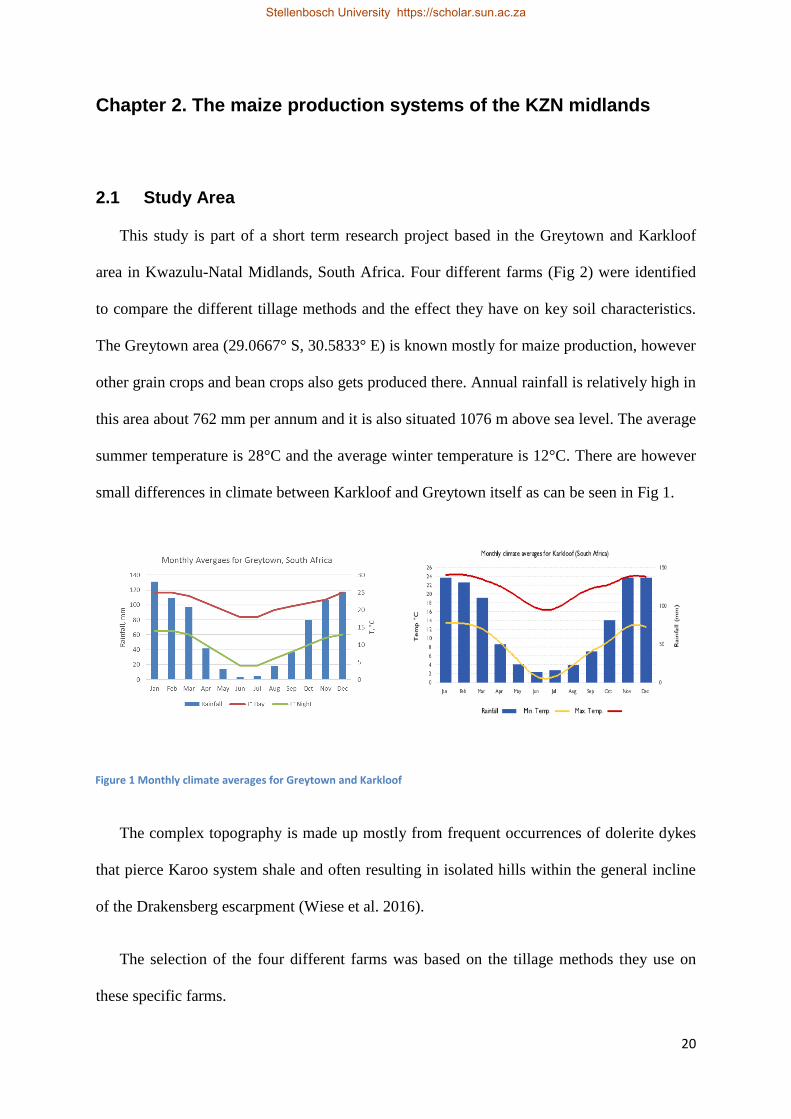
The Greytown area (29.0667° S, 30.5833° E) is known mostly for maize production, however
other grain crops and bean crops also gets produced there. Annual rainfall is relatively high in
this area about 762 mm per annum and it is also situated 1076 m above sea level. The average
summer temperature is 28°C and the average winter temperature is 12°C. There are however
small differences in climate between Karkloof and Greytown itself as can be seen in Fig 1.
The complex topography is made up mostly from frequent occurrences of dolerite dykes
that pierce Karoo system shale and often resulting in isolated hills within the general incline
of the Drakensberg escarpment (Wiese et al. 2016).
The selection of the four different farms was based on the tillage methods they use on
these specific farms.
Figure 1 Monthly climate averages for Greytown and Karkloof
Stellenbosch University https://scholar.sun.ac.za
21
Firstly the conventional tillage farm produces seed maize on their farm and they have an
average annual yield of 5 tons per hectare dryland seed maize production. They allow cattle
to graze the lands after harvest; the remaining stubble is then ploughed into the soil. Each
year the farm is split into two sections; the one halve gets ploughed with a mouldboard
plough to the depth of 300 mm, the other part in the same year is ripped down to 500 mm.
The following year the two practices just switch around so that the other halve is ripped and
ploughed with the mouldboard plough. To control weeds they make use of chemical weed
control once a year. A crop rotation system is used on the farm, they rotate the maize with
soybeans every fourth year.
Two reduced tillage farms were used in this study, which use similar production methods
and both practice reduced/minimum tillage methods. The only difference between the two
farmers is that one uses soy beans (legume) in a rotation system and the other mainly plants
maize. The minimum tillage farmer without legume rotation practiced no-till for 5-6 years,
however the organic material and stubble on the surface of the soil didn’t break down and the
farmer decided to start with minimum tillage methods and incorporate some stubble in to the
soil. Both farmers use a disc implement just before planting time to prepare the seedbed and
also to plough some of the previous year’s stubble into the soil. These specific disc
implements tills the soil down to 100 mm. Oats are planted as a cover crop within the first
two weeks after maize harvest on the same fields. When the oats reach maturity, cattle are
allowed to graze the fields. These farms make use of chemical weed control once a year and
the average yield in 2014 was 8.3 tons per hectare dryland maize production.
The CA farm is situated in Karkloof region south of Greytown. This farm has practiced
no-till for 10 – 17 years depending on the specific field. These fields don’t get ploughed at
all, however once every ten years the soil gets aerated with a special aerating implement up to
Stellenbosch University https://scholar.sun.ac.za
22
a depth of 100 mm. On this farm they don’t use any weed control practices, neither chemical
nor mechanical. A cover crop is also planted within the first week of the maize harvest; the
cover crop being used will either be oats or korog (a rye-wheat/triticale hybrid). The cattle
will graze this cover crop from June to September each year and the following year’s maize
will be planted in the mulch. The 2014 yield on this farm averaged at 9 tons per hectare
dryland maize production. Adjacent and undisturbed grassland were used as a control. The
grasslands used were all natural grasslands that is adjacent to the separate maize fields that
was sampled.
2.2 Soil
During the fieldwork a total of 30 profiles (Fig. 2) were excavated and classified
according to South Africa’s classification system (Soil Classification Work Group. 1991).
Most of the profiles that were identified were deep red apedal soils, with medium to high clay
content. The soils that were identified were all derived from Ecca shale and to a lesser extent
dolerite. Because the area of research is such a large and dissected area, a dominant soil form
was not identified which could have been used as a reference for all the observations. See
addendum A for more information on profiles.
Stellenbosch University https://scholar.sun.ac.za
23
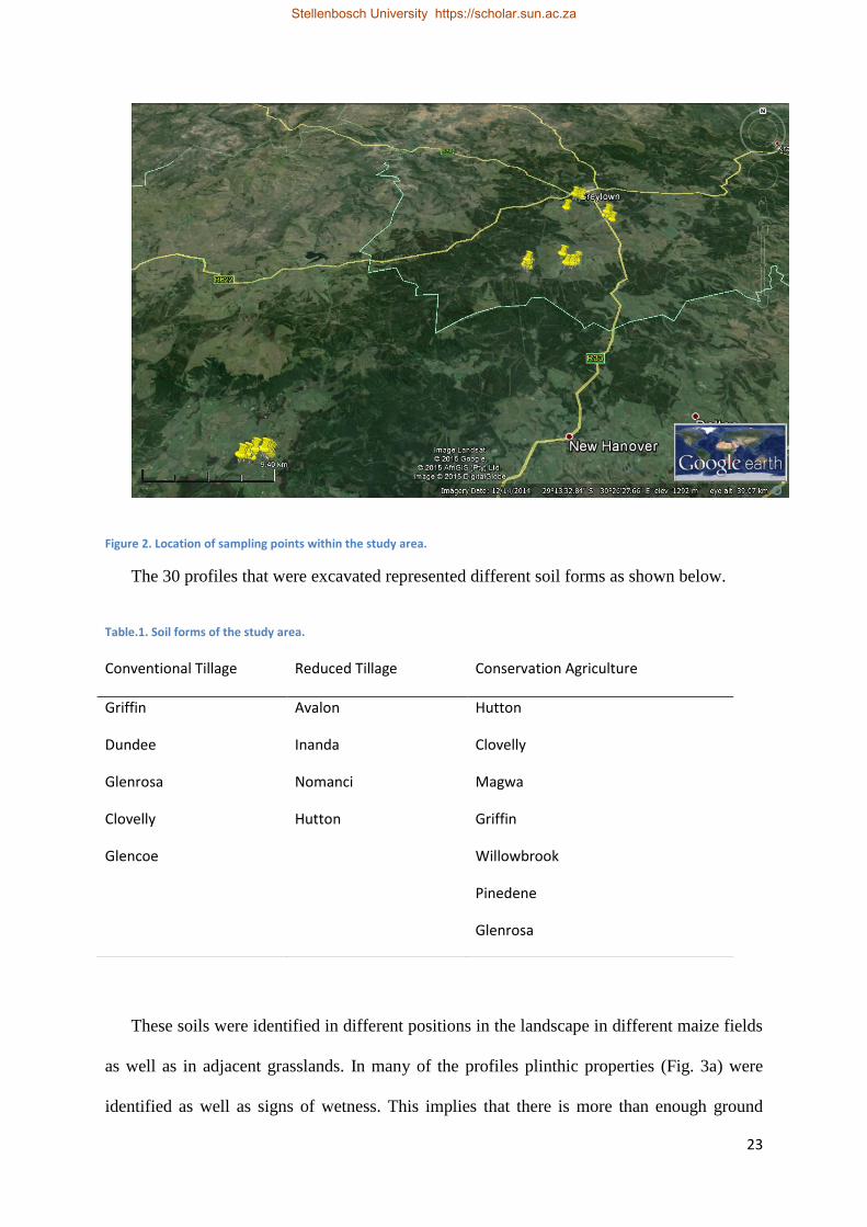
Figure 2. Location of sampling points within the study area.
The 30 profiles that were excavated represented different soil forms as shown below.
Table.1. Soil forms of the study area.
These soils were identified in different positions in the landscape in different maize fields
as well as in adjacent grasslands. In many of the profiles plinthic properties (Fig. 3a) were
identified as well as signs of wetness. This implies that there is more than enough ground
Conventional Tillage Reduced Tillage Conservation Agriculture
Griffin Avalon Hutton
Dundee Inanda Clovelly
Glenrosa Nomanci Magwa
Clovelly Hutton Griffin
Glencoe Willowbrook
Pinedene
Glenrosa
Stellenbosch University https://scholar.sun.ac.za
24
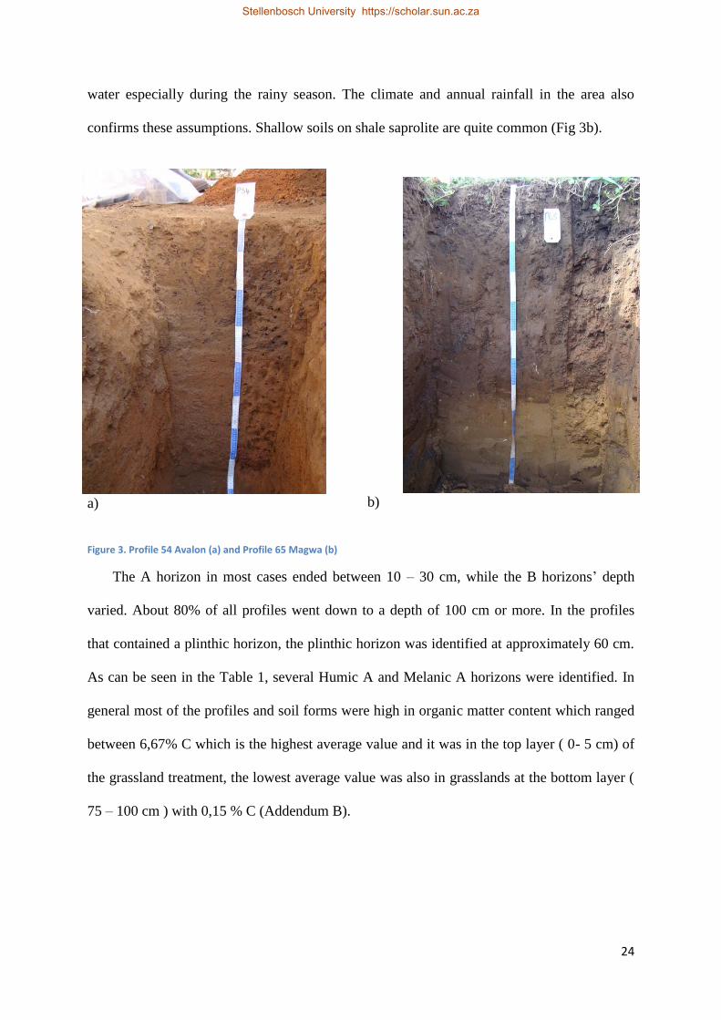
water especially during the rainy season. The climate and annual rainfall in the area also
confirms these assumptions. Shallow soils on shale saprolite are quite common (Fig 3b).
a) b)
Figure 3. Profile 54 Avalon (a) and Profile 65 Magwa (b)
The A horizon in most cases ended between 10 – 30 cm, while the B horizons’ depth
varied. About 80% of all profiles went down to a depth of 100 cm or more. In the profiles
that contained a plinthic horizon, the plinthic horizon was identified at approximately 60 cm.
As can be seen in the Table 1, several Humic A and Melanic A horizons were identified. In
general most of the profiles and soil forms were high in organic matter content which ranged
between 6,67% C which is the highest average value and it was in the top layer ( 0- 5 cm) of
the grassland treatment, the lowest average value was also in grasslands at the bottom layer (
75 – 100 cm ) with 0,15 % C (Addendum B).
Stellenbosch University https://scholar.sun.ac.za
25
2.3 Background information on the different farmers and their
cultivation practices over the years
2.3.1 Introduction
In this chapter the backgrounds of the farms as well as the different tillage practices that
have been and are still being practiced by the selected farmers will be discussed. It is
important to state that it is difficult to exactly describe the yearly practices regarding tillage
as well as chemical applications. The farmers will normally assess each season and the results
of the assessment will differ each season because of climate, costs, soil analysis, availability
of seeds, exchange rate, market prices etc. Maize is not only South Africa’s staple food it is
also most widely grown in the country stretching between 1.7 million – 4 million hectares
planted each year, followed by sugarcane and wheat (Fowler 1999). It is thus important to
understand the impact that the different tillage methods have on the soil that in turn affects
the yield and plant growth of the maize.
Tillage is the mechanical manipulation of the soil to develop a favourable soil structure
for a seedbed and to create a certain surface configuration for irrigation, drainage, planting,
harvesting operations etc. (Kepner et al. 1987). According to Simmons and Nafziger (2009)
there are six essential practices involved in tillage based soil management; proper amount of
tillage according to specific farm situation (taking into account e.g. climate and soil type),
maintaining soil organic matter, maintaining the proper amount of nutrients in the soil to
supply the plants, avoiding soil contamination, correcting soil acidity and controlling soil
erosion. There is however some contradiction between some of the above mentioned
practices for example, proper amount of tillage and soil erosion because more tillage in most
cases will lead to more vulnerability for soil erosion.
In the past crop production in South Africa was mostly associated with conventional
Stellenbosch University https://scholar.sun.ac.za

26
tillage methods especially in maize production. More recently producers have begun to
experiment with other tillage methods hoping to increase their yields and produce a better
quality product. The main purpose for tillage in the KZN area is weed control, better water
infiltration and breaking up inhibiting layers in the soil. Some sort of tillage system at some
time is involved in producing any crop. It may be a simple procedure for example digging a
hole on the other hand, it may be a highly complex procedure involving primary tillage,
several succeeding tillage practices, application of pesticides and fertilizers and the planting
procedure (Food and Agriculture Organization of the United Nations 1984). There are an
infinite variety of systems and implements to choose from when deciding about which tillage
system to use. To select the right tillage system for a specific farm or even a specific field
there are a lot of variables to take into account, and no variable is entirely independent of the
other.
It is seldom that two producers, producing the same crop, in the same area, at the same
time of year make use of exactly the same cultivation methods. Even when two producers use
the same cultivation method there are other factors that need to be accounted for. Factors that
will influence exactly the same tillage practice on two different farms for example ploughing
will be: speed of the ploughing procedure, soil moisture at the time of ploughing, different
soil types, maintaining a constant speed (minimizing speed variability while ploughing) to
name just a few. Soil types play a major role in deciding on a specific tillage system.
Another important factor when choosing a tillage system that normally gets overlooked is
the preference of the farmer. Some farmers choose a specific tillage system because their
ancestors used it in the years before them, so tend to employ the same methods as their
parents. So in other words tradition plays a major role in the decision making process, in
some cases the traditional way of doing things gives good results but in other cases the
Stellenbosch University https://scholar.sun.ac.za
27
traditional way of doing things is insufficient and yields poor results. The decision to change
cultivation practices is difficult, not only do we need to take into account the above
mentioned reasons, there is normally also a huge capital implication involved. When the
farmer changes from conventional tillage to CA for example he will need different
implements like a no-till planter for instance. This is off course seen by the farmers as a huge
negative point when thinking about changing tillage systems.
2.3.2 CA farm
The CA farm was situated in the Karkloof area (Fig1 and 2), on a farm called Denleigh
owned and managed by a man named René Stubbs. On this farm CA methods of cultivation
have been used for the last 10 – 17 years depending on the specific part of the farm. Prior to
CA farming that is still being practised today, the farm made use of conventional tillage
methods as was the norm in the past. Deep ripping, ploughing and disking each year before
the planting season starts as well as incorporating stubble with a disc implement after the
harvest. In that time on the farm vegetable crops were grown instead of grain crops, mainly
carrots. Seventeen years ago the first of the fields used in this study was converted to CA
method fields, the next field was converted 2 years after that and the others 3 years after that.
The CA fields that were sampled and used in this study were 17, 15 and 12 years old
respectively.
The maize seeds is planted each year with a no-till planter (Table 2) at approximately
beginning of October depending on the rain. After harvesting the maize during the month of
May with a harvester, rye gets planted within the first two weeks after harvest as a cover crop
for the cattle to graze on. The average yield on the farm over the last 5 years was between 7 –
9 tons/ha of dryland maize production.
In September 2013 the undisturbed soil was aerated for the first time since starting with
Stellenbosch University https://scholar.sun.ac.za
28
the no-till practices using a special implement that was made specifically for this purpose by
the farmer himself. The implement disturbs the soil up to a depth of 150 mm using a steel rod
that runs horizontally underneath the surface to break up the compaction at that depth as well
as control weeds. The farmer uses this implement when he feels it is necessary and this
happens at random. However the process of aeration with this implement happened a year
before we started our sampling on this farm.
The plant residues of both the maize and the cover crop (rye, which they plant most years
in the winter if financially possible) are left on the field to decompose, it does not get
ploughed or worked into the soil in any way. Above mentioned practice has been done since
the start of the no-till methods for each field. Lime is applied on all the fields on this farm
with a spreader behind the tractor every three years at a rate of between 2 – 3 tons per hectare
depending on the chemical requirement of the specific field. The lime does not get worked
into the soil in any way after application. The first nitrogen application for the season gets
applied during the planting of maize with the no-till planter, it varies between 40 – 50 kg/ha
of nitrogen band placed with the seeds. After emergence of the maize plants the top dressing
is split into two applications of 60 – 70 kg of nitrogen per hectare each. The nitrogen is
always applied in the form of urea (CO(NH2)2). In total the farmer aims to apply between 130
– 150 kg/ha of nitrogen each year during the maize growing season.
For the last eight years the farmer used this simple rotation on his fields, maize was
planted in the summer and rye in the winter as a cover crop. However, prior to 8 years ago
the farmer rotated maize with soybeans every other year or once every fourth year. The
reason the soybean rotation is stopped is because it is not a priority feed for dairy cattle. The
maize is primarily used for making silage as part of the dairy cattle’s diet on the farm.
Stellenbosch University https://scholar.sun.ac.za
29
2.3.3 Reduced tillage without legume rotation
The reduced tillage farm without legume rotation is owned and managed by Steve Stamp
just outside of Greytown on a farm called Chartwell (Fig 2). Steve started out more than ten
years ago with a full conventional tillage strategy on his farm. During this time he planted
only vegetables on all his fields with conventional tillage that included practices like deep
ripping and ploughing into his cultivation practices each season. He then started planting
maize on his fields following a complete no–till strategy for five years. According to him the
yields increased during the first 3 years of no–till practices. After that, the volume of stubble
and plant residues on the surface became a problem, it did not decompose/breakdown fast
enough. The plant residues on the surface became an obstruction for the planting implement
as the planting tine could not penetrate the soil surface because of the layer of plant rests
from the previous no–till years. In other words the seed could not be placed in the soil and
germination could not take place.
For that reason the farmer decided after five years of no–till practices that he will start
with reduced tillage to work in some of the stubble and plant rests that created the hindrance
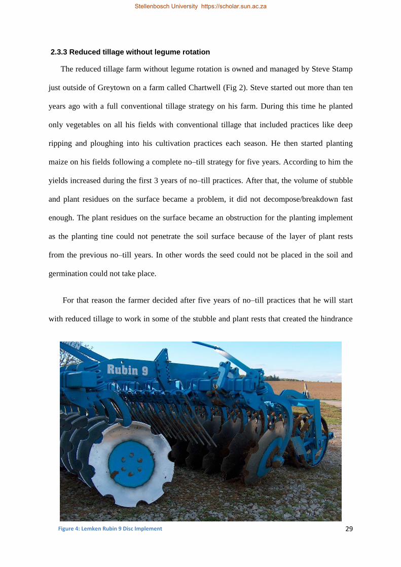
Figure 4: Lemken Rubin 9 Disc Implement
Stellenbosch University https://scholar.sun.ac.za
30
on the surface of his maize fields. The reduced tillage practices included planting with a no-
till planter (Table 2) that has a tine in front of the seed dispenser; the tine penetrates the soil
to about 250 mm. Other than the planter that disturbs the soil the farmer uses a special disc
implement (Fig. 4), two months before planting, to incorporate some of the stubble of the
previous year’s crop into the soil so that it can decompose quicker and also to prepare the
seedbed. The disc implement penetrates the soil only in the top 100 mm from the surface.
Above mentioned practices remain the same each year.
Lime was applied the last time seven years prior to our sampling in May 2013. The lime
was applied on all the fields at an application rate of 2.5 tons per hectare. After application
with a spreader behind the tractor the lime would get ploughed into the soil to a depth of
about 250 – 300 mm. Other than the liming event seven years prior to sampling lime was
never been applied since.
The total nitrogen application each year is between 150 – 160 kg/ha divided into three
split applications. At plant time the first application of nitrogen is applied at a rate of 40 kg/ha
band placed with the seeds in the form of urea (CO(NH2)2). Two weeks after the maize plants
emerge the first topdressing and second overall application takes place. Nitrogen is applied
with a spreader at a rate of 40 kg/ha, two weeks after that the same application takes place
and then once more two weeks after that.
2.3.4 Reduced tillage with legume rotation
The reduced tillage with legume rotation farm is also situated just outside of Greytown
(Fig 2), it is called Winfield farm and was owned and managed at the time of sampling by a
man named Garth Ellis. For the last ten years, this farmer has been practicing a form of
reduced tillage. The soil would only be disturbed twice each year (Table 2) once with
planting (using a no-till planter) and the other disturbance would be with an implement called
Stellenbosch University https://scholar.sun.ac.za
31
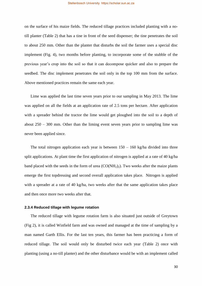
Tatu AST-matic (Fig. 5). This implement is a combination between a ripper and a roller and
it also has coulters in front to cut the stubble before ripping the soil and then after that the
rollers will break up the soil clods and incorporate the stubble.
After a soybean harvest, the above mentioned implement would not have been used
because the stubble left on the surface was not enough to make the tillage practice necessary.
However after a maize harvest the implement would have been used to break down and
incorporate the stubble into the soil. In dry years the Tatu Ast-matic created more soil clods
on the surface and the rollers on the implement was not strong enough to break them; in these
cases they would go over the fields with an additional disc implement to break up these clods
before planting; the tines of the ripper would disturb the soil up to a depth of 450 mm.
Figure 5. Tatu AST Matic 450 implement
After each year’s harvest the cattle would graze on the fields as hard and long as possible
to get rid of most of the plant residues and stubble left on the surface before ripping. In
exceptional cases, if the stubble as well as the weeds were too much even for the cattle, the
fields would get burned before planting.
Stellenbosch University https://scholar.sun.ac.za
32
At the beginning of season the separate fields would be assessed to determine if lime is
necessary and to what extent. According to the farmer the average amount of lime that was
applied each year per field was approximately 3 tons per ha. However this would differ from
year to year according to the soils requirement at that time. The lime would be applied with a
spreader and after application it would be ripped and disked into the soil. The farmer would
try to synchronise the lime application and the yearly tillage practice with the ripper to reduce
disturbance of the soil.
Fertilizer applications were split into two, one application with planting and the other
application with a top dressing within the first two months after emergence. The fertilizer
would get band placed at planting with the seeds, it would normally be NPK (4:3:4). As
mentioned earlier the second fertilizer application of the season would be applied as a top
dressing with a spreader within the first 60 days after emergence, this would be applied in the
form of LAN (mixture between dolomitic lime and NH4NO3). The farmer aims to apply a
total of 180 kg of nitrogen per hectare per season this would be split into above mentioned
two applications of 90 kg of nitrogen per hectare at plant and 90 kg of nitrogen per hectare as
a top dressing.
There was no standard crop rotation policy on this farm, the farmer would assess the
prices of soy beans as well as maize and then come to a conclusion on what to plant that
specific year. In 2012 80 % of all the fields were planted with soy beans and 20 % planted
with maize, in 2013 60 % of all fields were planted with soy beans and 40 % planted maize.
However in the last 10 years, they would plant soy beans at least once every four years if the
prices were in order.
2.3.5 Conventional tillage
The farm that was used for our conventional tillage samples is just outside of Greytown
Stellenbosch University https://scholar.sun.ac.za
33
on one of Pidelta’s farms. Pidelta is a seed company specializing in producing maize seed.
On this farm they have been practicing conventional tillage methods for over 15 years
producing maize and soy beans.
After harvest in May – June each year all the fields get ripped up to 50 cm and disc
harrowed (Table 2) to sufficiently aerate the sub soil and break up all the clods on the soil
surface. In the fields where maize is planted on maize two seasons in a row there will be
ripped once after harvest up to a depth of 50 cm, after the first rain late in winter or early
spring a mouldboard plough is used to plough the soils up to a depth of 20 cm. Depending on
the soil moisture; the fields will be disc harrowed (Table 2) up to a depth of 15 cm at least
once to incorporate the stubble as well as prepare the seedbed. If there is enough soil
moisture to properly prepare the seedbed, break up the clods and incorporate the stubble only
one disc harrowing procedure is necessary, however in most cases at least two disc harrowing
practices are preferred. According to them they would prefer to disc harrow the soil at least
twice before planting in early summer.
The plant residues are not left on the surface they are incorporated into the soil each year
with the disc harrowing practices for maize and soy beans. Normally the soy beans will not
have as much plant residues left on the surface as a maize plant and the reason for that is
because the soy bean plant is smaller and does not have as much plant material as a maize
plant would have. In other words between the soy bean harvest and the planting of the maize
seed for the following year there is only need for the normal ripping after harvest and one
disc harrowing operation. In most cases, there will not be ploughed as it would have been
done if it was maize on maize planted. They don’t have a standard rotational policy on this
farm, however in most cases they incorporate soy beans at least once every four years and the
other years it will be maize. For both soy beans as well as maize the planter disturbs the soil
Stellenbosch University https://scholar.sun.ac.za
34
up to a depth of 10 cm.
In total the conventional farmer aims to apply 150 kg of nitrogen to the plants per
growing season. With planting 20 – 30 kg of nitrogen is placed with the seeds in a mixture of
urea (CO(NH2)2) and MAP (NH4H2PO4). The planter is used to place the fertilizer in granular
form in a band with the seeds during planting. Six weeks after planting when the plants have
emerged successfully a top dressing will be applied. A tractor will pull a spreader and the
spreader will apply the fertilizer at a rate of between 100 – 120 kg/ha in a granular urea
(46%) form. Lime is not applied often on this farm, in the last 10 years lime was only applied
twice once in 2008 and once in 2014 only on selected fields as well. When lime was needed it
was applied with a spreader behind the tractor at a rate of 2 tons per hectare and then worked
into the soil with a disc harrowing practice.
2.4 Discussion on farming systems, farmers choices and expectation
The question needs to be asked, why do four farmers in close proximity to each other
make use of different farming systems? What influenced their decisions, was it a financial
motivation, did someone convince them about the soil benefits of changing to CA or was it a
conscience based decision that involved their love for nature and conservation.
The overall goal of CA is to make better use of agricultural resources, compared to
conventional tillage, by making use of integrated management of soil, biological and water
resources so that external inputs can be minimized (FAO 2001). When thinking about the
possible benefits of CA it is important to realise that there can also be indirect benefits
involved. For example Stonehouse (1997) found that the indirect benefits of changing to CA
from conventional tillage included improved downstream fishing and reduced dredging costs.
He also stated that the off-site benefits accounted for most of the social benefits of the CA
system in Ontario, Canada. Stonehouse (1997). The broader or socio-economic benefits
Stellenbosch University https://scholar.sun.ac.za

35
reaped from adopting CA should encourage populations and even governments to incentivise
the adoption of conservation agriculture. When there are no additional incentives, the
adoption of CA will most likely remain a function of profitability on the farm scale alone
(Knowler and Bradshaw 2007).
In this thesis we investigated as to what the motivations and incentives were that
influenced these four farmers to the way they farm today. Our CA farmer had a few reasons
for changing from conventional tillage to CA. According to him he would have changed to
CA in the 1980’s, however the tillage and planting equipment at the time was inadequate as
well as the build-up of disease and the subsequent drop in yields put him off at first. The high
price of glyphosate prevented the liberal use of it and thereby resulting in weed infestations
that needed to be controlled in some other way .He also has a slope of between 6 – 8 % on
most of his fields and according to him the continual re-construction of the contour banks
became frustrating and expensive. This is exactly the same problem that started the thinking
of changing to CA in the 1970’s and can be seen in the work of (de Freitas et al. 2014). The
CA farmer also stated that he was advised by dedicated consultants, scientists and farmer’s
associations that helped to change his mind-set with regards to the conservation agriculture
concept. Farmers associations also played a large role in the introduction and later adoption
of CA in Brazil (de Freitas et al. 2014).
Most of the farmers that practice a form of reduced tillage are motivated by a financial
saving on their input costs involved in reduced tillage. However Mueller et al. (1985) showed
in a study that the production costs was about 18 % higher in a no-till system compared to a
conventional tillage system in the short run though it would equal out in the long run. The
increase in production cost in the short run would be due to higher initial chemical inputs. We
have to take into account that this study was performed 21 years ago and that it is clear that
Stellenbosch University https://scholar.sun.ac.za
36
they had no financial motivation to change from conventional tillage to reduced tillage or
conservation agriculture back then. It could be because they were subsidised that time in the
past and due to the fact that fertilizer and machinery were relatively cheaper 21 years ago
(stronger exchange rate). According to our reduced tillage farmer with legume rotation he
didn’t want to change to complete conservation agriculture for a few reasons. Firstly they had
a pH problem in the past and it was very important for them to incorporate lime into the soil
with a tine implement each season or every second season at least. Secondly they were a
group of farmers in the area that decided together that they will not practice CA. They were
advised by influential people in the industry that CA is not the best way for crop production
and that some form of reduced tillage was more suitable to the conditions in the area.
According to the farmer their group or association in that particular area at that particular
time also felt like the conservation farmers were more like a cult than actual pioneers in the
agricultural sector and that they didn’t want to be part of that. They didn’t have any financial
motivation to move to a form of reduced tillage, they believed, with their advisors, that they
will get higher yields with reduced tillage and that motivated them to change from
conventional tillage to reduced tillage. However that was not the only reason for the change
from conventional to reduced tillage, although they believed in some sort of reduced tillage
for a long time, they could not import any implements because of the pre-1994 sanctions
against South Africa. The sanctions were lifted soon after 1994 and the farmers could start to
import the no – till and reduced till planters and other implements they needed to farm the
way they believed in which was a form of reduced tillage.
For our reduced tillage farmer without legume rotation things were different compared to
our reduced tillage farmer with legume rotation. This farmer was convinced about
conservation agriculture from the start, he was a vegetable farmer and he changed all his
vegetable fields over to conservation agriculture maize from the beginning. He tried out
Stellenbosch University https://scholar.sun.ac.za

37
conservation agriculture for a few years, he then realised that his stubble and plant residue on
the surface did not decompose quickly enough. The implication of this was that he couldn’t
plant anymore because the no – till planter was not able to enter the soil through the thick
layer of plant residue left on the surface after each harvest. For him it was a practical
implication that made him change from CA to a form of reduced agriculture as discussed
earlier in this chapter.
For the conventional tillage farmer it is a complete different story because they produce
maize for seed that they sell and not for milling. They don’t really have a motivation or
incentive to move to conservation agriculture, according to the specific farmer they have
done their one trials on the farm with different amounts of tillage and the conventional way of
tillage gave them the best results on their seed maize. He said that during their trials the
maize that was planted in a conservation agriculture system had the worst genetic purity and
also the most diseases, for them conservation agriculture would not work. Genetic purity is
the most important factor on this farm. To ensure genetic purity they need to make sure that
there is no other plants on the field at the same time as the maize plants, in other words they
control weeds physically and chemically as discussed previously. They also need to make
sure that there is no other maize plants that comes up from the previous season that would
influence the pollination of the current year’s plants again to ensure the genetic purity, also
keeping in mind they don’t plant the same cultivar on the same field every year. It is also
very important to ensure a clean and favourable seedbed for the plants because in most cases
the male and female plant will be planted at different stages because they flower at different
ages and in order to synchronise their flowering stage they need to be planted at different
times. When for example the male plant needs to be planted two weeks after the female, they
do their calculations so that the plant will start his lifecycle from the day it was planted to
accurately synchronize the two plants and ensure maximum pollination between male and
Stellenbosch University https://scholar.sun.ac.za
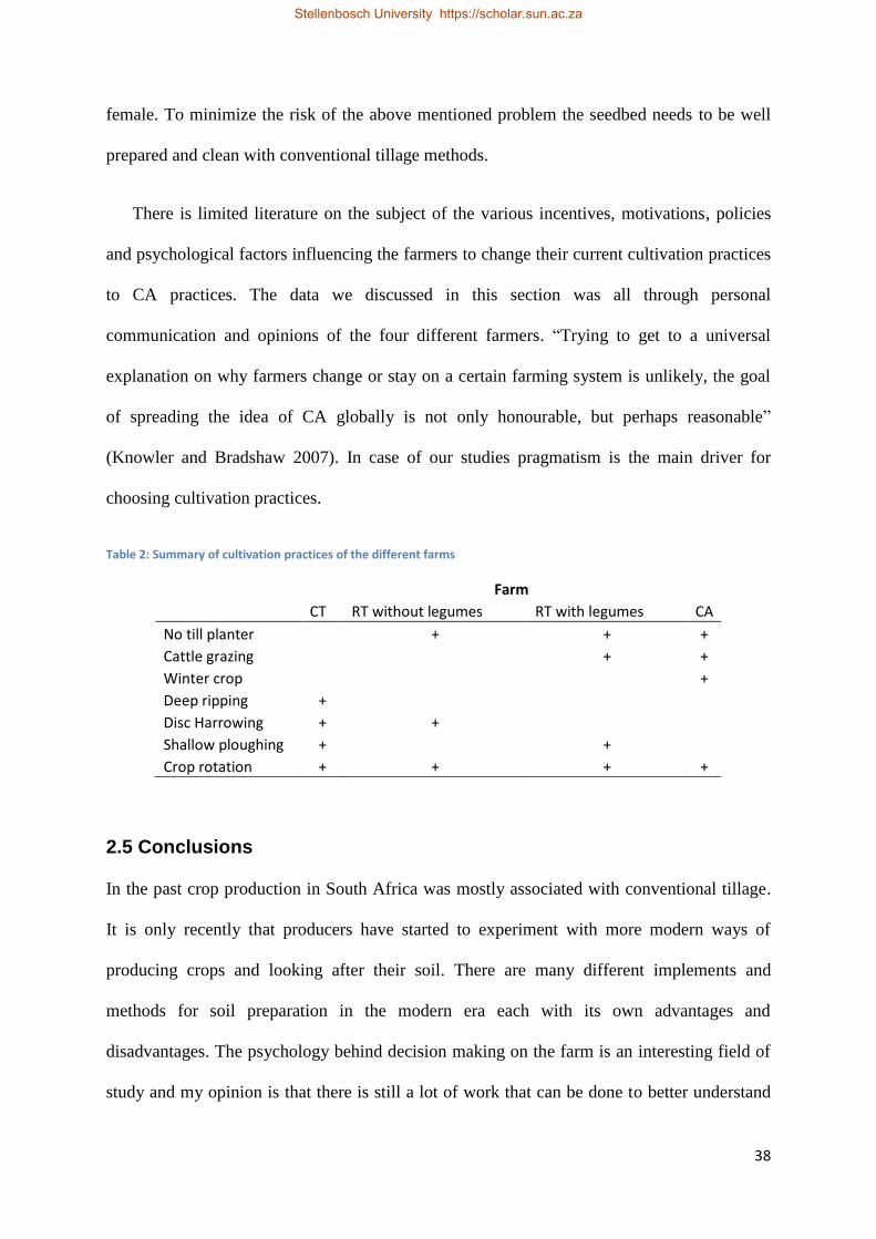
38
female. To minimize the risk of the above mentioned problem the seedbed needs to be well
prepared and clean with conventional tillage methods.
There is limited literature on the subject of the various incentives, motivations, policies
and psychological factors influencing the farmers to change their current cultivation practices
to CA practices. The data we discussed in this section was all through personal
communication and opinions of the four different farmers. “Trying to get to a universal
explanation on why farmers change or stay on a certain farming system is unlikely, the goal
of spreading the idea of CA globally is not only honourable, but perhaps reasonable”
(Knowler and Bradshaw 2007). In case of our studies pragmatism is the main driver for
choosing cultivation practices.
Table 2: Summary of cultivation practices of the different farms
Farm
CT RT without legumes RT with legumes CA
No till planter
+ + +
Cattle grazing
+ +
Winter crop
+
Deep ripping + Disc Harrowing + +
Shallow ploughing +
+ Crop rotation + + + +
2.5 Conclusions
In the past crop production in South Africa was mostly associated with conventional tillage.
It is only recently that producers have started to experiment with more modern ways of
producing crops and looking after their soil. There are many different implements and
methods for soil preparation in the modern era each with its own advantages and
disadvantages. The psychology behind decision making on the farm is an interesting field of
study and my opinion is that there is still a lot of work that can be done to better understand
Stellenbosch University https://scholar.sun.ac.za

39
the farmer’s way of thinking and decision making. The broader socio economic benefits
should be taken into account and that should incentivise the farmers to change their tillage
system to a more conservation-friendly approach. When there is no indirect incentives the
farmer’s decision will most likely be based on small scale profitability on the farm.
It is clear that there is not one single motivation or reason that can account for all farmers and
their actions regarding cultivation practices, however it seems their reasoning are mostly
pragmatic. Each situation is different and should be treated differently. It is also important to
note that the decisions being made on the farm is in most cases not based on scientific studies
and research but rather on hearsay, traditions and the farmer’s own opinions and beliefs.
Above mentioned will continue to and has in the past made the mass adoption of
conservation agriculture difficult. CA is a farmer driven concept
Stellenbosch University https://scholar.sun.ac.za
40
Chapter 3. The vertical distribution and stocks of SOC in three
different farming systems of maize cultivation in KZN
midlands
3.1 Introduction
Global climate change, caused by GHG emissions causing warmer temperatures,
increased frequency of extreme weather events, increased nitrogen deposition, and land use
change affects soil carbon inputs and carbon outputs (Hendrickson 2003). Soil is the largest
pool of organic carbon on the planet, storing more carbon than the atmosphere and plants
combined (Schlesinger 1977). Although soil texture and climate are the main controls of the
amount of soil organic carbon, their influence on vertical distribution of soil organic carbon
may be covered by the effects of plant allocation. Plant production and decompositions of
plant material determine the carbon inputs to the soil profile and plant allocation below and
above ground especially between deep roots and shallow roots may be the main reason for
relative carbon distribution with depth (Esteban and Jackson 2000). Land use has a major
effect on carbon stocks in the soil. A study done by Guo and Gifford (2002) showed that after
a land use change from pasture to plantation there was a decline in carbon stocks of 10%,
from native forest to crop there were 42% decline and from pasture to crop a significant 59%
decline of carbon stock in the soil. Where they saw an increase in carbon stock as a result of
land use change were when native forest were changed to pasture (+8%), crop to pasture
(19%) and crop to plantation (18%). As seen above when one of the land use changes
decreased carbon stock in the soil, the reverse process usually increased the carbon stock
again, however not with the same percentage.
The amount of carbon in the soil can be ascribed to four main factors: organic matter
decomposability, organic matter inputs, the level of physical protection of organic matter in
aggregates and the depth at which the organic material is deposited (Jones and Donnelly
Stellenbosch University https://scholar.sun.ac.za
41
2004). The carbon and nitrogen cycles are strongly linked in terrestrial ecosystems, the rate of
organic matter decomposition and organic matter production are coupled to nitrogen
availability. Research that has been done by (Knops and Tilman 2000) show that nitrogen can
potentially strain carbon accumulation in the soil. According to Knops and Bradley (2009)
that sampled up to a depth of 1 m, only 33% of soil carbon and 39% of soil nitrogen were
located in the top 20 cm of the soil, this implies that most of the soil carbon and nitrogen are
located at deeper depth increments. The vertical distribution of soil organic carbon generally
decrease with soil depth as organic carbon content decreases (Hiederer 2009). The ISRIC in
Wageningen, Netherlands concluded in a study that most mineral soils have the same amount
of carbon in the 0 – 30 cm layer than in the 30 – 100 cm layer (Hiederer 2009).
Soil organic carbon balance is controlled by the balance of carbon outputs through
decomposition and inputs from crop production. In humid and sub-humid areas (600+ mm
per annum) decomposition as well as production of carbon increase with an increase in
temperature, however relative increase in decomposition is greater (Schlesinger 1977). Soil
texture also play an important role with regards to carbon outputs, an increase in clay content
results in a decrease of carbon outputs because of the stabilizing effect that clay has on soil
organic carbon (Paul 1984).
Changes in soil organic carbon as affected by different tillage methods are expected to
show more noticeable differences over long periods of time compared to short terms. In a
study recently done by Hernanz et al. (2009) they evaluated soil organic carbon variations in
three different tillage systems and found that soil organic carbon was 14% higher in no-till
systems than in minimum tillage as well as conventional tillage systems after a period of 20
years.
The objective of this chapter is to determine the long-term effects of different cultivation
Stellenbosch University https://scholar.sun.ac.za
42
practices on the vertical distribution and stocks of soil organic carbon and nitrogen as well as
bulk density and porosity.
3.2 Materials and methods
The soils used in this study were collected during early winter of May 2014. Thirty soil
profiles were identified, 8 profiles from the following per farming system: conventional
tillage, reduced tillage and conservation agriculture. Two grassland samples were also taken
per farming system, adjacent to the specific maize fields used in the study as a control.
Core samples were taken using three metal cylinders (4 cm in diameter), a spatula and a
hammer (cores can be seen in figure below). Three core samples were taken at each of the
following depth increments: 0 – 5 cm; 5-10 cm; 10 – 15 cm; 15 – 20 cm; 30 cm; 40 cm; 50
cm; 75 cm and a 100 cm. It wasn’t possible to sample up to a meter in all the profiles because
of physical restrictions in the soil for example a rock bed or a water table. In total 513 core
samples were taken and put into paper bags to take back to a laboratory at the University of
Stellenbosch. When the profile pits were excavated in the maize fields it was done so in line
with the maize rows. Some of the fields were already harvested and others was on the brink
of being harvested a laboratory at the time. When the specific profiles were identified it was
done in such a way so that there were at least one at each position in the landscape/catena: at
the top of the catena, the middle of the catena and at the bottom of the catena. Bulk samples
were also taken at each depth (no specific volume) using a spade this soil was also put in
paper bags to transport back to University of Stellenbosch.
The bulk samples were air dried in the laboratory and not dried in an oven to preserve the
microbes in the soil and was used later in determining total microbial biomass. The core
samples were all dried in an oven at 60°C for 48 hours. After the core samples were dried, it
was sieved through a 2 mm sieve and put into plastic bottles. The bulk samples were not
Stellenbosch University https://scholar.sun.ac.za
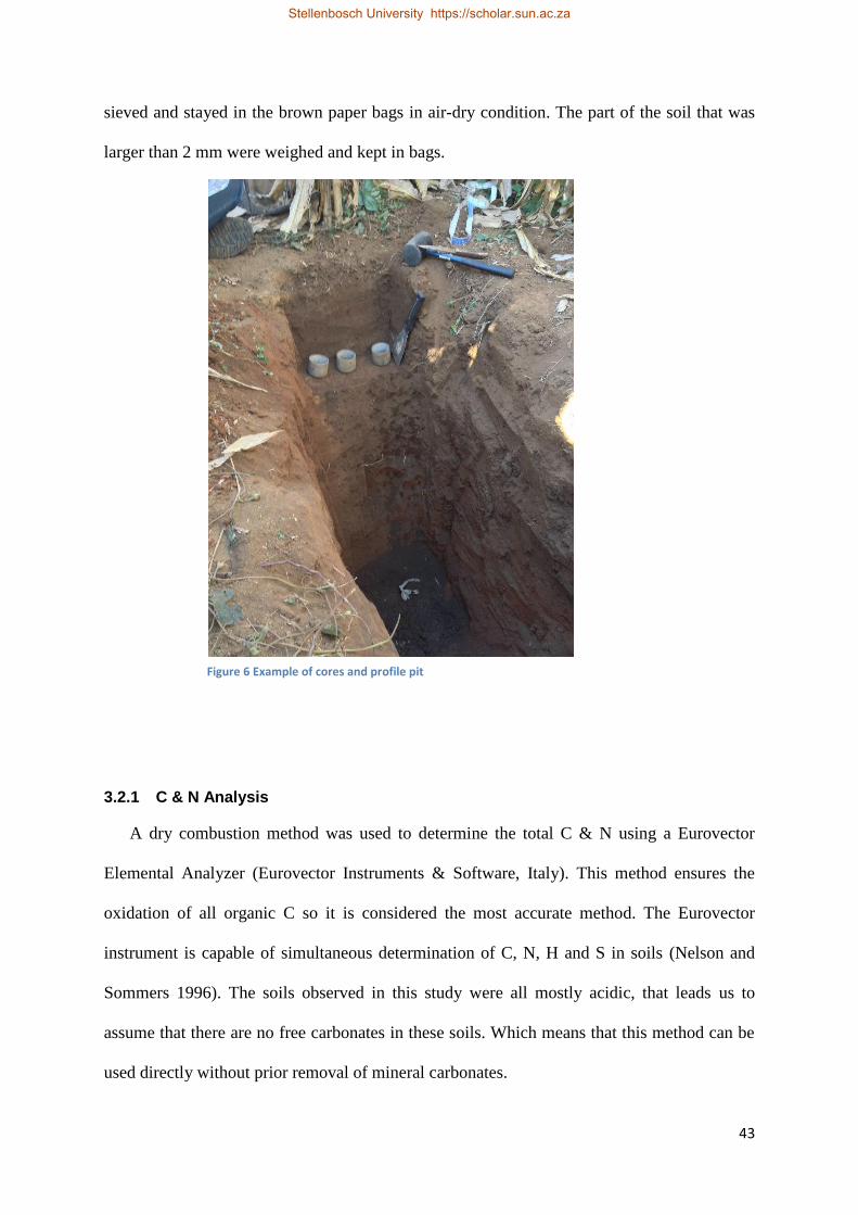
43
Figure 6 Example of cores and profile pit
sieved and stayed in the brown paper bags in air-dry condition. The part of the soil that was
larger than 2 mm were weighed and kept in bags.
3.2.1 C & N Analysis
A dry combustion method was used to determine the total C & N using a Eurovector
Elemental Analyzer (Eurovector Instruments & Software, Italy). This method ensures the
oxidation of all organic C so it is considered the most accurate method. The Eurovector
instrument is capable of simultaneous determination of C, N, H and S in soils (Nelson and
Sommers 1996). The soils observed in this study were all mostly acidic, that leads us to
assume that there are no free carbonates in these soils. Which means that this method can be
used directly without prior removal of mineral carbonates.
Stellenbosch University https://scholar.sun.ac.za
44
3.2.2 Bulk density
For determining Bulk Density the core method described by (Grossman and Reinsch
2002) was used. The same aluminium core (5 cm diameter and height 4.6 cm that was used to
sample all the profiles was used to determine bulk density. Three cores were used during
sampling and also for determining bulk density. Core 1 with a volume of 98.6 mm3, core 2
with a volume 99.2 mm3 and core 3 with a volume of 99.5 mm
3. The dry mass of the soil and
the volume of each core was used to determine bulk density in 𝑔. 𝑐𝑚−3.
3.2.3 Porosity
Porosity was determined using particle density as well as bulk density in the method
described by Flint and Flint (2002) in the book methods of soil analysis.
3.2.4 Particle density
Particle density was determined using the standard method described by Blake and Hartge
(1986). It is expressed as the total mass of solid particles to their volume in (𝑔. 𝑐𝑚−3).
3.2.5 pH
Soil pH was measured in distilled water at 1:2.5 soil to solution ratio (White 1997). The
suspension was shaken for 30 minutes in a horizontal shaker and allowed to stand for 30
minutes before reading with a calibrated Metrohm 827 pH lab electronic meter.
Stellenbosch University https://scholar.sun.ac.za
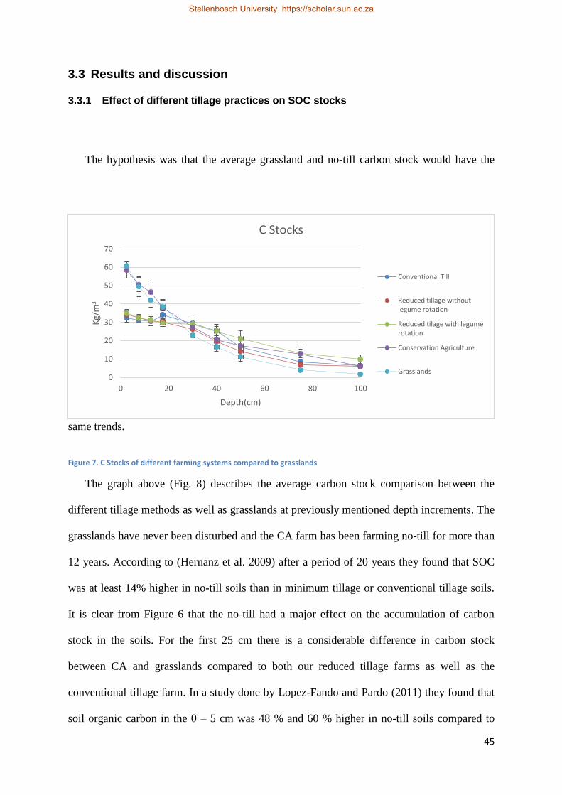
45
3.3 Results and discussion
3.3.1 Effect of different tillage practices on SOC stocks
The hypothesis was that the average grassland and no-till carbon stock would have the
same trends.
Figure 7. C Stocks of different farming systems compared to grasslands
The graph above (Fig. 8) describes the average carbon stock comparison between the
different tillage methods as well as grasslands at previously mentioned depth increments. The
grasslands have never been disturbed and the CA farm has been farming no-till for more than
12 years. According to (Hernanz et al. 2009) after a period of 20 years they found that SOC
was at least 14% higher in no-till soils than in minimum tillage or conventional tillage soils.
It is clear from Figure 6 that the no-till had a major effect on the accumulation of carbon
stock in the soils. For the first 25 cm there is a considerable difference in carbon stock
between CA and grasslands compared to both our reduced tillage farms as well as the
conventional tillage farm. In a study done by Lopez-Fando and Pardo (2011) they found that
soil organic carbon in the 0 – 5 cm was 48 % and 60 % higher in no-till soils compared to
0
10
20
30
40
50
60
70
0 20 40 60 80 100
Kg/
m3
Depth(cm)
C Stocks
Conventional Till
Reduced tillage withoutlegume rotation
Reduced tilage with legumerotation
Conservation Agriculture
Grasslands
Stellenbosch University https://scholar.sun.ac.za

46
minimum tillage and conventional tillage soils respectively after a period of 17 years. This
compares very well with our data that shows the same trends between no-till, minimum
tillage and conventional tillage. They also concluded that there was no significant difference
in soil organic carbon between minimum tillage and conventional tillage especially in the top
17 cm. a Yield increase in the 0 – 5 cm layer of the no-till soils from 9.3 ton/ha-1
to 15.4
ton/ha-1
was seen in the 16 year trial period from 1992 up until 2008. In contrast a recent
study Valboa et al. (2015) showed increases of soil organic carbon of 10% after being ripped
up to a depth of 45 cm and 18 % after being disked harrowed up to a depth of 10 cm. Sisti et
al. (2004) showed that at a depth of 15 – 30 cm there was a greater C concentration in
conventional tillage soils compared to the CA soils they examined.
Our results show that at the same depth of 15 – 30 cm, carbon stocks were greater in the
no-till soil compared to the conventional tillage soils. From 30 – 50 cm carbon stocks in
conventional tillage soils were greater than the carbon stocks of our no-till soils, and from 50
– 100 cm no-till soils again showed more carbon compared to conventional tillage. Studies
done by Moreno et al. (2006) correlates well with the work of this study as well as the work
of Lopez-Fando and Pardo (2011), however they concentrated only in the top 10 cm of the
soil.
Stellenbosch University https://scholar.sun.ac.za
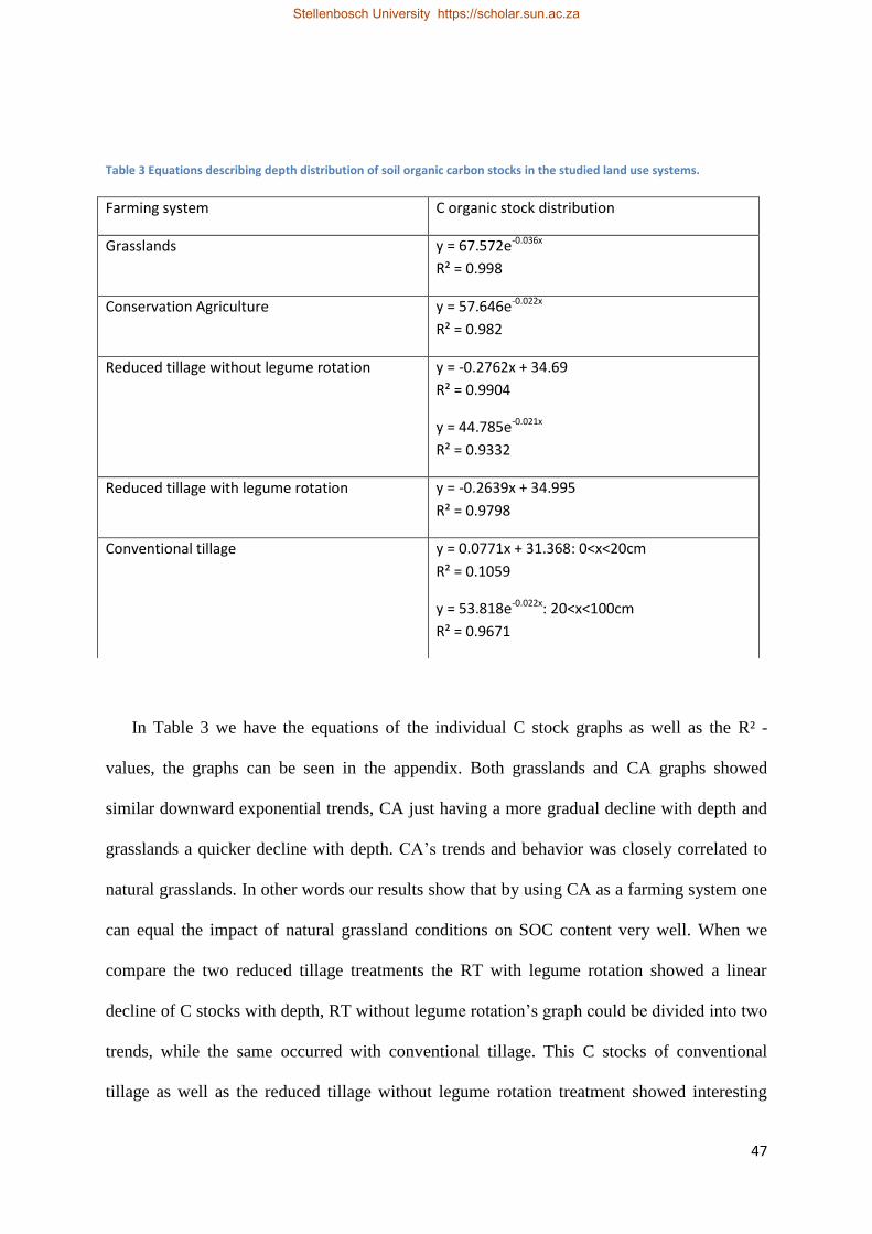
47
Table 3 Equations describing depth distribution of soil organic carbon stocks in the studied land use systems.
In Table 3 we have the equations of the individual C stock graphs as well as the R² -
values, the graphs can be seen in the appendix. Both grasslands and CA graphs showed
similar downward exponential trends, CA just having a more gradual decline with depth and
grasslands a quicker decline with depth. CA’s trends and behavior was closely correlated to
natural grasslands. In other words our results show that by using CA as a farming system one
can equal the impact of natural grassland conditions on SOC content very well. When we
compare the two reduced tillage treatments the RT with legume rotation showed a linear
decline of C stocks with depth, RT without legume rotation’s graph could be divided into two
trends, while the same occurred with conventional tillage. This C stocks of conventional
tillage as well as the reduced tillage without legume rotation treatment showed interesting
Farming system C organic stock distribution
Grasslands y = 67.572e-0.036x
R² = 0.998
Conservation Agriculture y = 57.646e-0.022x
R² = 0.982
Reduced tillage without legume rotation y = -0.2762x + 34.69
R² = 0.9904
y = 44.785e-0.021x
R² = 0.9332
Reduced tillage with legume rotation y = -0.2639x + 34.995
R² = 0.9798
Conventional tillage y = 0.0771x + 31.368: 0<x<20cm
R² = 0.1059
y = 53.818e-0.022x: 20<x<100cm
R² = 0.9671
Stellenbosch University https://scholar.sun.ac.za
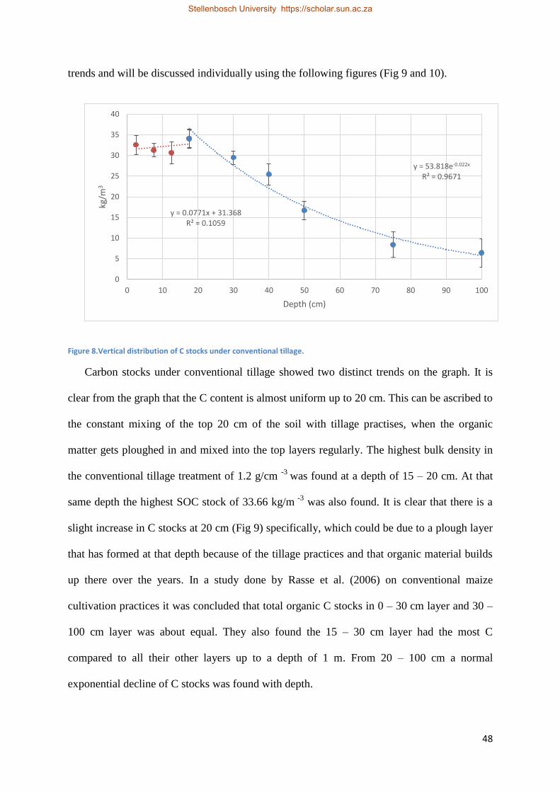
48
trends and will be discussed individually using the following figures (Fig 9 and 10).
Figure 8.Vertical distribution of C stocks under conventional tillage.
Carbon stocks under conventional tillage showed two distinct trends on the graph. It is
clear from the graph that the C content is almost uniform up to 20 cm. This can be ascribed to
the constant mixing of the top 20 cm of the soil with tillage practises, when the organic
matter gets ploughed in and mixed into the top layers regularly. The highest bulk density in
the conventional tillage treatment of 1.2 g/cm -3
was found at a depth of 15 – 20 cm. At that
same depth the highest SOC stock of 33.66 kg/m -3
was also found. It is clear that there is a
slight increase in C stocks at 20 cm (Fig 9) specifically, which could be due to a plough layer
that has formed at that depth because of the tillage practices and that organic material builds
up there over the years. In a study done by Rasse et al. (2006) on conventional maize
cultivation practices it was concluded that total organic C stocks in 0 – 30 cm layer and 30 –
100 cm layer was about equal. They also found the 15 – 30 cm layer had the most C
compared to all their other layers up to a depth of 1 m. From 20 – 100 cm a normal
exponential decline of C stocks was found with depth.
y = 0.0771x + 31.368 R² = 0.1059
y = 53.818e-0.022x R² = 0.9671
0
5
10
15
20
25
30
35
40
0 10 20 30 40 50 60 70 80 90 100
kg/m
3
Depth (cm)
Stellenbosch University https://scholar.sun.ac.za
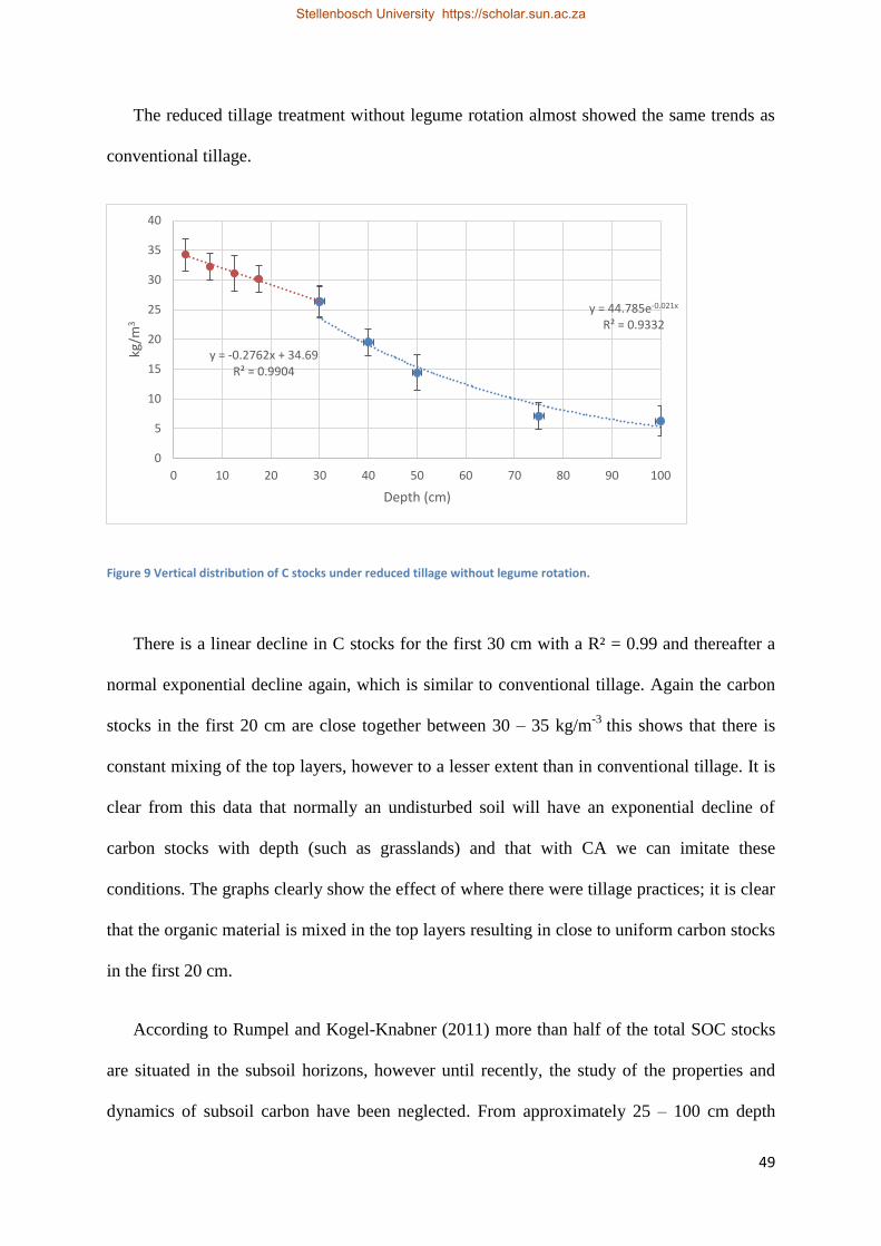
49
The reduced tillage treatment without legume rotation almost showed the same trends as
conventional tillage.
Figure 9 Vertical distribution of C stocks under reduced tillage without legume rotation.
There is a linear decline in C stocks for the first 30 cm with a R² = 0.99 and thereafter a
normal exponential decline again, which is similar to conventional tillage. Again the carbon
stocks in the first 20 cm are close together between 30 – 35 kg/m-3
this shows that there is
constant mixing of the top layers, however to a lesser extent than in conventional tillage. It is
clear from this data that normally an undisturbed soil will have an exponential decline of
carbon stocks with depth (such as grasslands) and that with CA we can imitate these
conditions. The graphs clearly show the effect of where there were tillage practices; it is clear
that the organic material is mixed in the top layers resulting in close to uniform carbon stocks
in the first 20 cm.
According to Rumpel and Kogel-Knabner (2011) more than half of the total SOC stocks
are situated in the subsoil horizons, however until recently, the study of the properties and
dynamics of subsoil carbon have been neglected. From approximately 25 – 100 cm depth
y = -0.2762x + 34.69 R² = 0.9904
y = 44.785e-0.021x R² = 0.9332
0
5
10
15
20
25
30
35
40
0 10 20 30 40 50 60 70 80 90 100
kg/m
3
Depth (cm)
Stellenbosch University https://scholar.sun.ac.za
50
there were no significant changes over all the systems in SOC. All the treatments showed a
steady decline of SOC stock from 25 cm – 100 cm. From 30 – 100 cm the grasslands showed
the lowest amount of carbon stocks, the reason for this would probably be because the roots
of the grasses do not reach that depths. Organic material was also never ploughed, ripped or
disked into the soil. The CA soils had higher SOC content than grassland soils at deeper
depths, which could be due to organic material that were incorporated into these depths
before they started CA on that specific soils, however this cannot be confirmed because the
land use history and tillage practices of more than 18 years ago is not known. Kaiser et al.
(2014) showed similar trends to these results as well as previously mentioned studies
(Moreno et al. 2006, Lopez-Fando and Pardo 2011) for carbon stocks in the 0 – 5 cm depth.
(Sisti et al. 2004) studied the differences of conventional tillage compared to no-till
practices for 13 years to better understand the effect of tillage on the carbon and nitrogen
stocks at deeper depths. They found that carbon stocks were approximately 17 Mg/ha more in
CA than in CT after the 13 years. Between 46 % - 68 % of the difference between the
systems however occurred in favour of CA at the depths of 30 – 85 cm.
The soils used in this study was generally high in carbon stocks (Fig. 11) compared to
some of the literature. For example a study done by Abreu, Godsey et al.(2011) showed that
in all their soils they sampled they had an average carbon stock value of 94.76 Mg/ha (0 –
110cm) in a No-till treatment and 84.7 Mg/ha in a conventional tillage treatment. In this
study we had an average total carbon stock value of 199.76 Mg/ha between all the treatments.
Stellenbosch University https://scholar.sun.ac.za
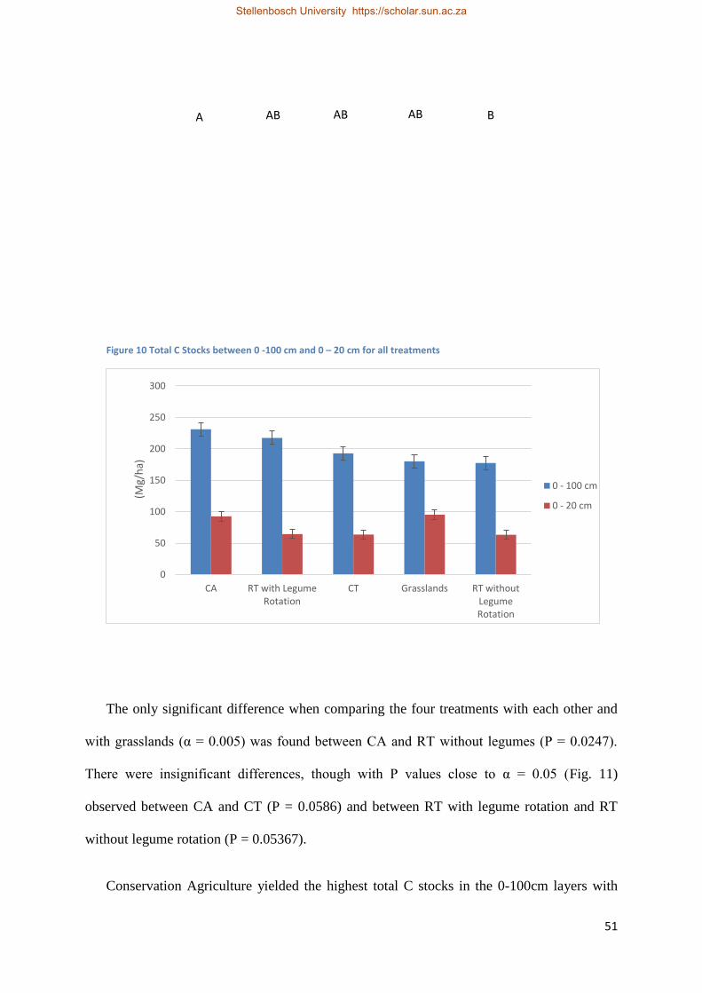
51
The only significant difference when comparing the four treatments with each other and
with grasslands (α = 0.005) was found between CA and RT without legumes (P = 0.0247).
There were insignificant differences, though with P values close to α = 0.05 (Fig. 11)
observed between CA and CT (P = 0.0586) and between RT with legume rotation and RT
without legume rotation (P = 0.05367).
Conservation Agriculture yielded the highest total C stocks in the 0-100cm layers with
0
50
100
150
200
250
300
CA RT with LegumeRotation
CT Grasslands RT withoutLegumeRotation
(M
g/h
a)
0 - 100 cm
0 - 20 cm
Figure 10 Total C Stocks between 0 -100 cm and 0 – 20 cm for all treatments
A AB AB AB B
Stellenbosch University https://scholar.sun.ac.za
52
231,1 Mg/ha, however it was not the highest in the 0 -20cm layer where Grasslands had the
highest C stocks with 95,3 Mg/ha (Fig 11). Reduced tillage with legume rotation had the
second highest to C stocks in 0 – 100cm which again emphasises the potential of firstly
making use of reduced tillage methods and secondly the benefits of higher carbon and
nitrogen stocks that can be enjoyed because of legume species in the rotation. Reduced tillage
without legume rotation had the lowest total C stocks for 0 – 100 cm as well as 0 -20 cm with
177,5 Mg/ha and 63,3 Mg/ ha respectively. According to Dalal and Mayer (1986) the
decreasing of soil organic carbon stocks under conventional tillage is a well-known
occurrence especially in sub-tropical regions. In the top 20cm the conventional tillage
treatment had the second lowest C stocks at 63,8 Mg/ha (Fig 11) which emphasises the
negative effect of repeated tillage practices. The CT treatment did however have more C
stocks in the 0 – 100cm compared to Grasslands and Reduced tillage without legume
rotation, this could be that because of all the tillage over the years the soil organic material
was constantly pushed down deeper in to the profile and accumulated at deeper depths.
Diekow and Mielniczuk et al. (2005) found that they have up to 42% higher carbon
stocks under the legume rotation treatment compared to grasslands. The results in this study
showed about a 18% higher carbon stocks in the reduced tillage with legume rotation
treatment compared to grasslands for 0 -100cm. Diekow and Mielniczuk et al. (2005)
concluded that no – till legume based cropping systems with nitrogen fertilization drastically
improved carbon stocks, even surpassing the original stocks of native grasslands over a
period of 17 years. It is also clear out of these results, that in this study the grasslands hold
more than 50% of its total carbon stocks in the top 20cm and the rest of the carbon stocks are
stored from 20 – 80cm.
Stellenbosch University https://scholar.sun.ac.za

53
3.3.2 Effect of different cultivation practices on total N stocks
Figure 11 Depth distribution of N stocks of different tillage systems compared to grasslands.
The average total nitrogen stocks of the different tillage practices and grasslands are
shown in Figure 12. It correlates well with the C stock trends in Figure 8, with the CA
treatment and grasslands following a similar trend. In the top 0 – 5 cm layer the CA treatment
and the grasslands nitrogen stock value are close to double the amount of nitrogen stock in
both reduced tillage treatments. The conventional tillage treatment showed the lowest N stock
value in the 0 – 10cm layer. This could probably be because on the conventional tillage farm
the nitrogen is applied earlier in the growing season and it is also applied at a higher rate. If N
is applied at such a high rate with a spreader it could reduce the effectiveness of the
application because run–off will be higher and some of the N fertilizer could get washed
away or washed in to deeper depths in the profile.
Diekow et al. (2005) did a study of the effects of 17 years of conventional tillage where
the fields were natural grassland prior to that. They found that total N stock decreased with
440 kg/hectare over the 17 year period which is a 14 % decrease from the grassland, this
0
1
2
3
4
5
0 20 40 60 80 100 120
kg/m
3
Depth (cm)
Conventional Till
Reduced tillage without legumerotation
Reduced tillage with legume rotation
No Till
Grasslands
Stellenbosch University https://scholar.sun.ac.za
54
treatment did not include a legume rotation. It was found that total N stock under
conventional tillage were the highest compared to our other treatments only at a depth of 20 –
50 cm. Even though this is only for previously mentioned depth increment total N stock was
even higher than the natural grasslands. If we compare both our reduced tillage treatments
(with legume rotation and without legume rotation) we can clearly see that with the legume
rotation (soybeans) that the nitrogen stock is considerably higher at all depths except the first
0 – 5 cm. This can be expected because there may still be some fertilizer residue left in the
first depth increment for the treatment without legume rotation.
Diekow et al. (2005) found that after 17 years of no-till practices without nitrogen
fertilizer application, with a legume rotation (Pigeon pea (Cajanus cajan) + Maize (Zea
mays)) compared to natural grasslands the organic N stock increased 0.75 tons/hectare (28%).
It is difficult to compare this study with that of Diekow et al. (2005) because all our
treatments included nitrogen fertilizer applications during the growing seasons. However
even with the nitrogen applications it is still possible to see distinct differences between the
reduced tillage lands farmed with legume rotation compared to the other farms without
legume rotations. The reduced tillage farm with legume rotation also had the steadiest decline
of nitrogen stocks with depth. A recent study Villamil and Nafziger (2015) concluded that in
the 0 – 30cm layer since 2005 N stocks have increased by 0.17 g/𝑚2 with no-till practices
compared a chisel–plough treatment.
Stellenbosch University https://scholar.sun.ac.za
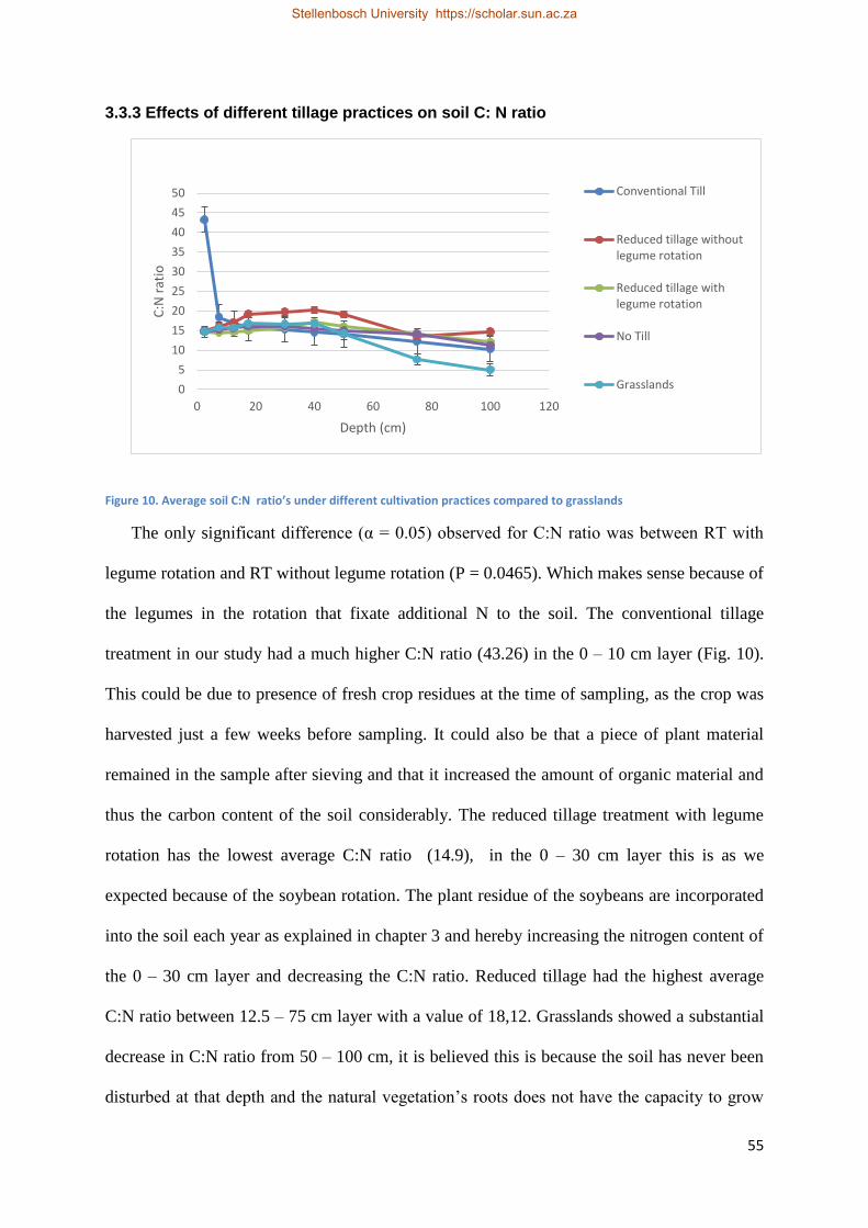
55
3.3.3 Effects of different tillage practices on soil C: N ratio
Figure 10. Average soil C:N ratio’s under different cultivation practices compared to grasslands
The only significant difference (α = 0.05) observed for C:N ratio was between RT with
legume rotation and RT without legume rotation (P = 0.0465). Which makes sense because of
the legumes in the rotation that fixate additional N to the soil. The conventional tillage
treatment in our study had a much higher C:N ratio (43.26) in the 0 – 10 cm layer (Fig. 10).
This could be due to presence of fresh crop residues at the time of sampling, as the crop was
harvested just a few weeks before sampling. It could also be that a piece of plant material
remained in the sample after sieving and that it increased the amount of organic material and
thus the carbon content of the soil considerably. The reduced tillage treatment with legume
rotation has the lowest average C:N ratio (14.9), in the 0 – 30 cm layer this is as we
expected because of the soybean rotation. The plant residue of the soybeans are incorporated
into the soil each year as explained in chapter 3 and hereby increasing the nitrogen content of
the 0 – 30 cm layer and decreasing the C:N ratio. Reduced tillage had the highest average
C:N ratio between 12.5 – 75 cm layer with a value of 18,12. Grasslands showed a substantial
decrease in C:N ratio from 50 – 100 cm, it is believed this is because the soil has never been
disturbed at that depth and the natural vegetation’s roots does not have the capacity to grow
0
5
10
15
20
25
30
35
40
45
50
0 20 40 60 80 100 120
C:N
rat
io
Depth (cm)
Conventional Till
Reduced tillage withoutlegume rotation
Reduced tillage withlegume rotation
No Till
Grasslands
Stellenbosch University https://scholar.sun.ac.za
56
this deep and increase the organic material at these depths therefore the lower C:N ratio. In
general all treatments showed, the same trends with C:N ratio’s not changing considerably
throughout 0 – 100 cm except for the above mentioned exceptions.
Valboa et al. (2015) conducted a study with the following treatments: a) conventional
tillage treatment by deep mouldboard plough (40 cm) and ripper plough (45 cm), b)
shallower tillage treatment with mouldboard plough (20 cm) and c) a disc harrowing
treatment (10 cm). They found that nitrogen stock followed the same pattern as carbon stock
except with the disc harrowing practice. Although the carbon stock in the 0 -10 cm layer was
higher under the deeper tillage practices the nitrogen stock remained the same, thus
increasing the C:N ratio. Diekow et al. (2005) showed that in the 7.5 – 30 cm layer the C:N
ratio was significantly less because of legume cropping rotations, this compares well with
results seen in Figure 10. According to Rumpel and Kogel-Knabner (2011) C:N ratio’s
should decrease rapidly below the A–horizon this is mostly attributed to highly processed
SOM in the sub-soil and the presence of mineral nitrogen adsorbed to clay. However Diekow
et al. (2005) also found that C:N ratio’s increased from 7.5 – 30 cm across all treatments,
which is proportionally linked to increases in clay content. In contrast, Christensen (1992)
reported that the OM in clay sized fractions should have the lowest C:N ratio’s compared to
silt and sand particles. Similar to Diekow et al. (2005), De Sá et al. (2001) also observed an
increase of C:N ratio’s with depth, which was however not related to clay content.
3.3.4 Effects of different cultivation practices on porosity
The primary purpose of tillage is to create a more aerated and porous soil environment for
plants. It is important to maintain the correct ratio between water, CO2 and oxygen in the root
zone. Miller et al. (1998) concluded that under conventional tillage the porosity was higher in
the 0 – 10 cm layer, however from 10 – 30 cm porosity was higher under the no-till
treatment. Unfortunately they only studied the porosity of the soil up to a depth of 30 cm.
Stellenbosch University https://scholar.sun.ac.za
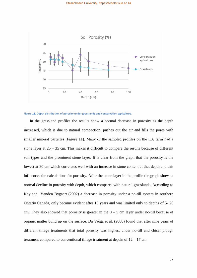
57
Figure 11. Depth distribution of porosity under grasslands and conservation agriculture.
In the grassland profiles the results show a normal decrease in porosity as the depth
increased, which is due to natural compaction, pushes out the air and fills the pores with
smaller mineral particles (Figure 11). Many of the sampled profiles on the CA farm had a
stone layer at 25 – 35 cm. This makes it difficult to compare the results because of different
soil types and the prominent stone layer. It is clear from the graph that the porosity is the
lowest at 30 cm which correlates well with an increase in stone content at that depth and this
influences the calculations for porosity. After the stone layer in the profile the graph shows a
normal decline in porosity with depth, which compares with natural grasslands. According to
Kay and Vanden Bygaart (2002) a decrease in porosity under a no-till system in southern
Ontario Canada, only became evident after 15 years and was limited only to depths of 5- 20
cm. They also showed that porosity is greater in the 0 – 5 cm layer under no-till because of
organic matter build up on the surface. Da Veiga et al. (2008) found that after nine years of
different tillage treatments that total porosity was highest under no-till and chisel plough
treatment compared to conventional tillage treatment at depths of 12 – 17 cm.
35
40
45
50
55
60
0 20 40 60 80 100
Po
rosi
ty %
Depth (cm)
Soil Porosity (%)
Conservationagriculture
Grasslands
Stellenbosch University https://scholar.sun.ac.za
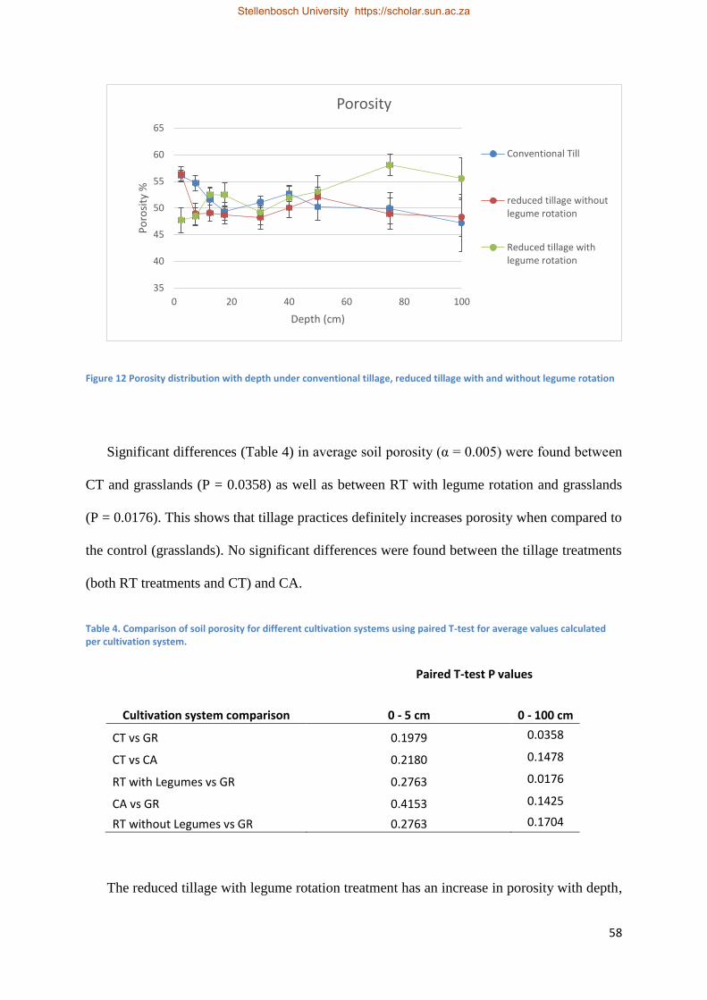
58
Figure 12 Porosity distribution with depth under conventional tillage, reduced tillage with and without legume rotation
Significant differences (Table 4) in average soil porosity (α = 0.005) were found between
CT and grasslands (P = 0.0358) as well as between RT with legume rotation and grasslands
(P = 0.0176). This shows that tillage practices definitely increases porosity when compared to
the control (grasslands). No significant differences were found between the tillage treatments
(both RT treatments and CT) and CA.
Table 4. Comparison of soil porosity for different cultivation systems using paired T-test for average values calculated per cultivation system.
Paired T-test P values
Cultivation system comparison 0 - 5 cm 0 - 100 cm
CT vs GR 0.1979 0.0358
CT vs CA 0.2180 0.1478
RT with Legumes vs GR 0.2763 0.0176
CA vs GR 0.4153 0.1425
RT without Legumes vs GR 0.2763 0.1704
The reduced tillage with legume rotation treatment has an increase in porosity with depth,
35
40
45
50
55
60
65
0 20 40 60 80 100
Po
rosi
ty %
Depth (cm)
Porosity
Conventional Till
reduced tillage withoutlegume rotation
Reduced tillage withlegume rotation
Stellenbosch University https://scholar.sun.ac.za
59
which is due to the fact that they tilled the two weeks before we took the samples. In other
words the soil has not consolidated normally after the tilling procedure and therefore the high
porosity at these depths. The graph shows that the soil has started to consolidate in the top
layers, however it will take more time in the deeper layers. The reduced tillage without
legume rotation treatment had a high porosity in the top 0 – 5 cm layer and then the porosity
decreases rapidly in 7, 5 – 30 cm. The reason for the high porosity would be the implement
(Figure 4) the farmer uses, it only disturbs the first 8 cm of the soil and it is clear on the graph
that the porosity is considerably higher in the 0 – 5 cm layer. There is also a slight plough
bank at 30 cm from all the years of tillage and deep cultivation methods. In the deeper layers
the porosity follows a normal decline in porosity with increasing depth.
The results show that conventional tillage has a higher porosity compared to CA in the
first 10 cm of the soil profiles. Moraes et al. (2015) showed the same results in the first 10
cm. The authors concluded that conventional tillage increased total porosity only in the 10 cm
layer and thereafter no-till had higher total porosity at depths of 10 – 30 cm.
The conventional tillage treatment had a high porosity in the top layers and that
consolidates abruptly up to 20 cm. We found a slight compaction at 20 cm which could be a
plough layer after all the years of tillage. In the conventional tillage soils we also encountered
stone layers at depths of 25 – 35 cm as was observed in the CA profiles. However in contrast
to CA where the porosity decreased with an increase in stone content at these depths, the
conventional tillage treatment did not show a decrease in porosity with an increase in stone
content. This is explained by the deep ripping an ploughing each year that loosens that stone
layer in the soil and therefore increasing porosity at depths of 25 – 35 cm. Lipiec et al. (2006)
noted in a study that under conventional tillage treatments the porosity increased and it
persisted until the end of the growing season when measurements were conducted again. It
Stellenbosch University https://scholar.sun.ac.za
60
indicated that their soils under conventional tillage did not become less porous with time.
3.4 Conclusions
The objective of the study was to determine the influence of different long term tillage
systems have on the soil organic carbon stocks and other soil parameters up to 1 m depth that
is key to overall soil health. The CA system preserved the expected exponential decline
pattern of SOC stock distribution observed under indigenous grasslands with similar y-
intercept values of 57.6 and 67.6 respectively and rather close values of the curve slope of -
0.022 and -0.036 (R2=0.998 and R
2=0.982 respectively). On the other hand, the conventional
tillage and reduced tillage practices display a rather different pattern described by separate
equations for the cultivated section and the rest of the soil profile below. The profiles of these
soils are described by a system of equations, where the distribution within the cultivated layer
is a constant (conventional tillage – linear R2=0.077) or a linear decline (reduced tillage –
R2=0.990), while the section of the profile below the cultivated layer follows the normal
exponential decline curve with parameters similar to no-till for both conventional and
reduced tillage (R2=0.967 and R
2=0.933) respectively.
The only significant difference when comparing the total C stocks between the four
treatments with each other and with grasslands (α = 0.005) was found between CA and RT
without legumes (P = 0.0247). There were strong trends between CA and CT (P = 0.0586)
and between RT with legume rotation and RT without legume rotation (P = 0.05367),
however not significant. CA yielded the highest total C stocks in the 0 -100cm layers with
231,1 Mg/ha, however it was not the highest in the 0 -20cm layer where Grasslands had the
highest C stocks with 95,3 Mg/ha. RT without legume rotation had the lowest total C stocks
for 0 – 100 cm as well as 0 -20 cm with 177,5 Mg/ha and 63,3 Mg/ ha respectively. The total
SOC stocks declined in the following order CA (231,1 Mg/ha) > RT + legumes (217,3
Stellenbosch University https://scholar.sun.ac.za
61
Mg/ha) > CT (192,8 Mg/ha) > Grasslands (180,1 Mg/ha) > RT – legumes (177,5 Mg/ha).
Similar trends for grasslands as well as the conservation agriculture treatments were
observed with regards to total N stocks. Among the three tillage treatments, the reduced
tillage with legume rotation yielded the highest average N stocks for 0 -100 cm. Which was
expected however, grasslands as well as CA still had much higher total N stocks in the top 20
cm despite not having any legumes in rotation. The reduced tillage without legume rotation
treatment yielded the highest average C: N ratio’s value over the 1 m depth (17,16), where
the reduced tillage with legume rotation treatment yielded the lowest average (14,7) from 5
cm – 20 cm depth. The only significant difference (α = 0.05) observed for C:N ratio was
between RT with legume rotation and RT without legume rotation (P = 0.0465).
The average soil porosity of the grassland profiles showed a normal decline in porosity
with depth. It was difficult to quantify the porosity of the CA profiles because most of the
profiles sampled on that farm had a stone layer at 25 – 35 cm. However, there is a natural
decline in soil porosity from 40-100 cm which is similar to natural grasslands. The RT with
legume rotation had the highest average porosity (0 – 100 cm) at 52,1 %, CT had the second
highest 51,4 % followed by CA and RT without legume rotation with 50,22 % and 50,07 %
respectively. Grasslands had the lowest average porosity with a value of 49 %. Significant
differences in soil porosity (α = 0.005) were found between CT and grasslands (P = 0.0357)
as well as between RT with legume rotation and grasslands (P = 0.0175). No significant
differences in porosity were found between the tillage treatments (both RT treatments and
CT) and CA.
Stellenbosch University https://scholar.sun.ac.za
62
Chapter 4. Influence of different farming systems on Total Microbial
Biomass, Water Stable Aggregates and SOM Density
fractionations.
4.1 Introduction
The parameters discussed in this chapter are often seen as critical to soil health; sufficient
water stable aggregates combined with a healthy population of soil microbes can improve the
soil quality significantly (Sparling 1997). Maintaining micro-flora and soil microbial biomass
activity and diversity in the soil is fundamental for sustainable agriculture (Insam 2001).
Changes in tillage practices would induce major shifts in the number as well as the
composition of soil fauna and flora, which includes pests and beneficial organisms
(Christensen et al. 1994). In a study done by Lupwayi et al. (1998) they reported larger soil
microbial biomass as well as functional diversity of the microbes under CA compared to CT
in the Peace River region of Canada. Further research by Lupwayi et al. (2001) also showed
that there were bigger differences of soil microbial biomass under CT in C–poor soils
compared to almost no change in soil microbial biomass under the same CT practices in C-
rich soils. This confirms the importance of organic carbon in our soils.
A large number of factors will influence soil aggregation such as SOM, tillage practices,
development of roots and hyphae as well as changes in plant diversity and microbial biomass
activity (Wang et al. 2015). Aggregate stability plays a crucial role in water infiltration,
storage, crop growth, soil erosion, as well as other factors that contribute to soil productivity
and sustainability. It is well known and has been extensively researched that tillage
negatively affects aggregate stability, for example the work that Tisdall and Oades (1982)
conducted 20 years ago confirmed this.
Stellenbosch University https://scholar.sun.ac.za

63
4.2 Materials and methods
4.2.1 Sampling strategy
A different soil sampling strategy was used when sampling the profiles used in this
chapter. The time and costs involved regarding the analysis limited the number of profiles we
could use.
For each farming system two profiles were identified, one with a sequence of red and
yellow horizons and one with only yellow horizons. For the reduced tillage treatment one
sample was taken from the RT farm with legume rotation and one from the RT farm without
legume rotation. A grassland sample was also identified for each of the three different
farming systems, preferably in an adjacent grassland next to the fields we sampled. All the
grassland profiles that we identified turned out to be Nomanci soil form. Refer to Addendum
A as well as Table 20 – 22 in Addendum B. Most of the soils sampled was regarded as highly
stable soil, because it is highly oxidised as well as highly micro aggregated.
4.2.2 Total Microbial Biomass
Total soil microbial biomass was determined using the method described by Islam and
Weil (1997). A calibration curve was established using sucrose stock solution and making a
dilution series of 0, 10, 20, 40, 80, 200 and 400 mg C L-1
. A 5 ml aliquot of each of the
dilutions was taken and 1 mL of 0.17M K 2Cr 2O7 and 5 mL of concentrated sulphuric acid
18M were added to it. The solutions were microwaved at 500 J ml-1
and the volume adjusted
to 30 ml. The absorbance was measured at 590 nm using a UV-Vis spectrophotometer.
Ten grams of oven-dried-equivalent field moist soil was placed in a 50 ml centrifuge tube
and adjusted to 80 % water-filled porosity (WFP) by adding 2.5 ml distilled water. The tube
was closed with a pin-hole cap and microwaved at 400 J g-1
. A second set of soil samples
Stellenbosch University https://scholar.sun.ac.za
64
were prepared but not microwaved. A 25 ml aliquot of 0.5M K2SO4 was added and shaken
horizontally for 60 min at 250 rpm. It was centrifuged for 5 min at 500 rpm and the solution
was filtered using a 40 Whatman filter paper. A 5 ml aliquot of each of the filtered extracts
and a 1 ml of 0.17M K2Cr2O7, 5 ml of concentrated sulphuric acid (0.18M) were added. The
solution was micro waved at 500 J ml-1 and the volume was adjusted to 30 ml. The
absorption were measured at 590nm using the spectrophotometer (Islam and Weil 1997) .
4.2.3 Aggregate Stability
Aggregate stability was determined using the wet sieving method of Kemper and Rosenau
(1986). Aggregate stability was done on nine selected profiles that comprised of, two profiles
from each of the different farming systems and also one adjacent grassland profile per
farming system as a control. The principle of the wet sieving technique relies on the fact that
unstable aggregates will break down more easily than stable aggregates when submerged in
water. The analysis was conducted under laboratory conditions by using the Eijkelkamp nr.
08.13 wet sieving apparatus (Eijkelkamp Agrisearch Equipment, Netherlands). To avoid
determination of small coarse fragments, four grams of macro aggregates (2 mm < aggregates
< 2.8 mm) were selected out of the sample. In the sieve the aggregates were raised and
lowered in distilled water for 3 - 10 min using a rubber until all aggregates disintegrated. The
remaining aggregates were then raised and lowered in Na (PO3)6 or NaOH for ± 10 min,
depending on the pH of the soil sample, by using a rubber until all aggregates disintegrated.
The remaining cans contain the water stable aggregates. Sand particles too big to fit through
screen remained behind. Both sets of cans were placed in an oven at 110˚C to allow water to
evaporate. The weight of the materials left behind in each can was determined.
4.2.4 Particle size distribution
Particle size distribution was done using the pipette method (The non-affiliated soil
analysis work committee 1990)
Stellenbosch University https://scholar.sun.ac.za
65
4.2.5 SOM Density Fractionation
The objective of density fractionation was to separate soil organic matter into three
different organic carbon pools. The method used was adapted from the work of Golchin et al.
(1994). The three different fractions separated were: (a) Free – particulate organic matter
(fPOM) (material that have not yet started to decompose, most labile fraction), (b) occluded
particulate organic matter (organic material stuck in the aggregates, medium stability not
necessarily because of chemical composition but mostly because it is physically stuck inside
the aggregates) (oPOM) and (c) mineral bound organic matter (decomposed organic material
bound to the minerals, most stable fraction). The mineral bound fraction is mainly
responsible for aggregate formation, although the fPOM and oPOM do not contribute to
aggregate formation they can be found inside the aggregates.
The procedure started with the addition of 25ml of potassium iodide (KI) solution with a
density of 1.6 g.ml to 5 g of soil into a 50 ml centrifuge tube. All the soil should be
submerged in enough solution to allow for easy separation of floating material. This was
achieved with a 1 to 5 soil to solution ratio. It was then gently swirled by hand to avoid
disruption of aggregates and allow for wetting of all the soil. Upon all soil were suspended
and no material adhered to the bottle wall, the suspension was allowed to stand for 1 hour
before centrifuging at 5600 g for 20 minutes. After centrifuging the floating material (fPOM)
was collected and placed onto 45 µm pore filters by using a rubber spatula and by carefully
decanting and vacuum filtering solution. To ensure that all the free particulate organic matter
was transferred the centrifuging and filtering procedure was repeated three times per sample.
The KI filtrate was discarded after the after the third removal of (fPOM) while the
(fPOM) on the filter was rinsed with deionized water until the conductivity of the wash water
was 50 µS cm-1
. The filter was then removed from the vacuum and stored in a dark cool place
to dry.
Stellenbosch University https://scholar.sun.ac.za
66
The remaining soil was given 25 ml of fresh KI solution of the same density as before.
Thereafter the solution was dispersed by ultrasound (QSonica Model Q125) in order to break
down the aggregates. The temperature of the sample was kept at 40°C in order to avoid
thermal alteration of the organic material. This was done by placing the centrifuge tube in a
beaker filled with ice water for the duration of the sonification process. The sonicator probe
was placed 1.5 cm into the soil solution and sonicated at 200 J/ml solution, meaning 5000 J
per 25 ml of solution. Thereafter the sample was allowed to rest for one hour and then it was
centrifuged at 5600 g for 20 min. The material that floated was then (oPOM) separated,
washed, collected and dried as described for the fPOM. This step was repeated twice more as
was the case with the fPOM, centrifuging the sample for 10 min at a time.
After the removal of the KI solution as well as the oPOM the remaining salt was removed
from the sediment using dialysis tubing in a container filled with distilled water. The dialysis
tubes containing the sediment was left in the glass beakers until the water tested free of salts
with 0.1 M AgNO3. It was then oven dried at 35°C for 72 hours. The samples were then
weighed using a five decimal digital micro – scale and prepared for C and N analysis by dry
combustion using the Eurovector elemental analyser (Nelson and Sommers 1996). However,
in this case the results of dry combustion produced by the ARC-ISCW laboratory seemed
dubious (the range was between 2 and 50% for the POM fractions) and were discarded.
Instead and estimation of carbon content in these fractions was done based exclusively on the
dry weight of these fraction (fPOM and oPOM) using van Bemellen factor (1.724) commonly
applied for organic materials assuming 58% C in OM (Brady, 1990). Subsequently the results
reported further represent an estimate of the C content in these fractions rather than a direct
measurement. Considering that there is often a large amount of clay stuck to fPOM and
oPOM fractions this may increase the error.
Stellenbosch University https://scholar.sun.ac.za
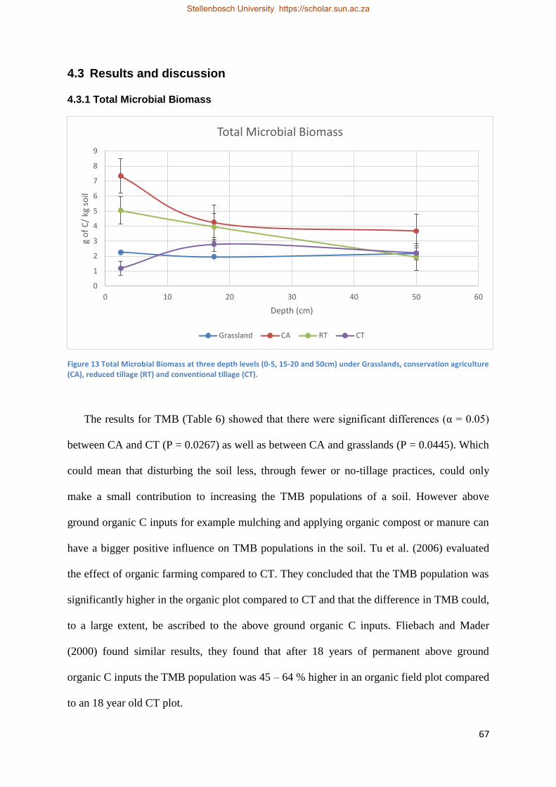
67
4.3 Results and discussion
4.3.1 Total Microbial Biomass
Figure 13 Total Microbial Biomass at three depth levels (0-5, 15-20 and 50cm) under Grasslands, conservation agriculture (CA), reduced tillage (RT) and conventional tillage (CT).
The results for TMB (Table 6) showed that there were significant differences (α = 0.05)
between CA and CT (P = 0.0267) as well as between CA and grasslands (P = 0.0445). Which
could mean that disturbing the soil less, through fewer or no-tillage practices, could only
make a small contribution to increasing the TMB populations of a soil. However above
ground organic C inputs for example mulching and applying organic compost or manure can
have a bigger positive influence on TMB populations in the soil. Tu et al. (2006) evaluated
the effect of organic farming compared to CT. They concluded that the TMB population was
significantly higher in the organic plot compared to CT and that the difference in TMB could,
to a large extent, be ascribed to the above ground organic C inputs. Fliebach and Mader
(2000) found similar results, they found that after 18 years of permanent above ground
organic C inputs the TMB population was 45 – 64 % higher in an organic field plot compared
to an 18 year old CT plot.
0
1
2
3
4
5
6
7
8
9
0 10 20 30 40 50 60
g o
f C
/ kg
so
il
Depth (cm)
Total Microbial Biomass
Grassland CA RT CT
Stellenbosch University https://scholar.sun.ac.za
68
CA and RT followed the same trend with total microbial biomass decreasing with depth
(Figure 13). This trend can also be seen with carbon stocks, where the carbon content also
decreases with depth in the CA treatment as well as the RT treatment. It is also clear that the
total microbial biomass in CA has the highest values throughout all the depths, this is
probably because the soil is not disturbed that often and that microbial activity is encouraged
through CA practices on this farm.
The total microbial biomass values from the grassland treatment do not differ much with
depth and stays relatively constant throughout the profile. With conventional tillage it is clear
from Figure 13 that total microbial biomass is much lower especially in the 0 – 10 cm layer.
This could be because this layer will dry out quicker compared to the other layers, because it
is exposed to the sun and atmosphere, killing most of the microorganisms. It could also be
that all the tillage and movement in this layer and throughout the 0 – 50 cm for our
conventional tillage treatment destroys some of the microorganisms. Intensive tillage
practices can affect soil microbial biomass negatively through: a) physically breaking up of
the water-stable macro aggregates that provide a favourable micro habitat for microorganisms
in the soil, b) a reduction of SOM ( both N and C ) that provide a substrate source for
microorganisms, c) changes in the soil conditions for example temperature and moisture
content of the soil (Balota et al. 2003, Roldán et al. 2005). From 17.5 – 50 cm all the
individual treatments stayed relatively constant, which suggests that the total microbial
biomass is much more exposed and vulnerable to be influenced in the 0 – 17.5 cm compared
to deeper layers. It is probably also because this is where most of the disturbances in the soil
takes place and differences between treatments will be observed here.
Stellenbosch University https://scholar.sun.ac.za
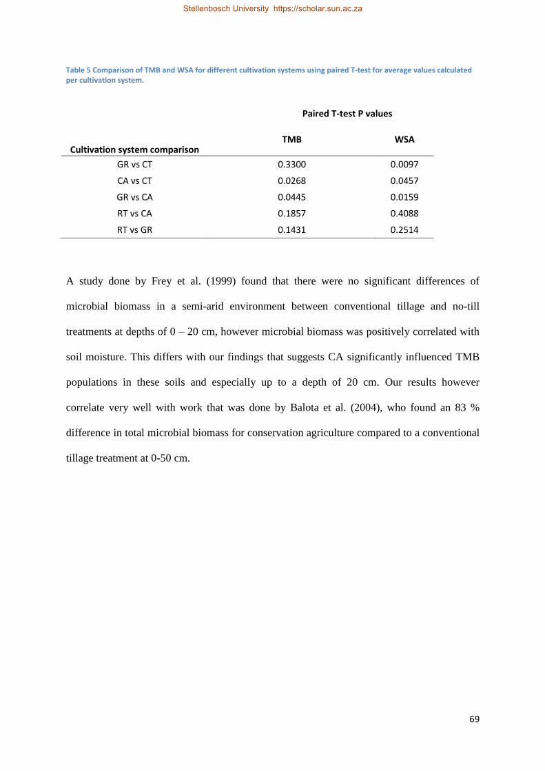
69
Table 5 Comparison of TMB and WSA for different cultivation systems using paired T-test for average values calculated per cultivation system.
A study done by Frey et al. (1999) found that there were no significant differences of
microbial biomass in a semi-arid environment between conventional tillage and no-till
treatments at depths of 0 – 20 cm, however microbial biomass was positively correlated with
soil moisture. This differs with our findings that suggests CA significantly influenced TMB
populations in these soils and especially up to a depth of 20 cm. Our results however
correlate very well with work that was done by Balota et al. (2004), who found an 83 %
difference in total microbial biomass for conservation agriculture compared to a conventional
tillage treatment at 0-50 cm.
Paired T-test P values
Cultivation system comparison TMB WSA
GR vs CT 0.3300 0.0097
CA vs CT 0.0268 0.0457
GR vs CA 0.0445 0.0159
RT vs CA 0.1857 0.4088
RT vs GR 0.1431 0.2514
Stellenbosch University https://scholar.sun.ac.za
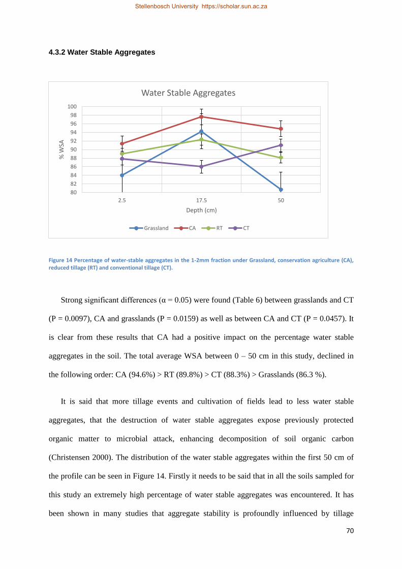
70
4.3.2 Water Stable Aggregates
Figure 14 Percentage of water-stable aggregates in the 1-2mm fraction under Grassland, conservation agriculture (CA), reduced tillage (RT) and conventional tillage (CT).
Strong significant differences (α = 0.05) were found (Table 6) between grasslands and CT
(P = 0.0097), CA and grasslands (P = 0.0159) as well as between CA and CT (P = 0.0457). It
is clear from these results that CA had a positive impact on the percentage water stable
aggregates in the soil. The total average WSA between 0 – 50 cm in this study, declined in
the following order: CA (94.6%) > RT (89.8%) > CT (88.3%) > Grasslands (86.3 %).
It is said that more tillage events and cultivation of fields lead to less water stable
aggregates, that the destruction of water stable aggregates expose previously protected
organic matter to microbial attack, enhancing decomposition of soil organic carbon
(Christensen 2000). The distribution of the water stable aggregates within the first 50 cm of
the profile can be seen in Figure 14. Firstly it needs to be said that in all the soils sampled for
this study an extremely high percentage of water stable aggregates was encountered. It has
been shown in many studies that aggregate stability is profoundly influenced by tillage
80
82
84
86
88
90
92
94
96
98
100
2.5 17.5 50
% W
SA
Depth (cm)
Water Stable Aggregates
Grassland CA RT CT
Stellenbosch University https://scholar.sun.ac.za

71
practices. A study done by Liu et al. (2013) showed that, especially macro aggregates (>
2mm), increased significantly with conservation and reduced tillage practices compared to
conventional tillage with between 12.2 – 39.7 %.
The results show that CA yielded the most water stable aggregates at all three depths.
Grasslands had the lowest percentage of water stable aggregates in the first layer as well as
the 50 cm layer, however it had an increase of water stable aggregates in the 17.5 cm layer.
All the treatments except CT showed an increase of water stable aggregates at the 17.5 cm
depth. In the CT treatment at the depth of 17.5 cm the lowest percentage of WSA were found.
This could be due to the constant disturbance with all the implements at this depth during the
growing season that breaks down the aggregates. Our results correlate with the results of a
study done by Andruschkewitsch et al. (2013) who also concluded that water stable
aggregates decrease with the increase in soil disturbance especially in the top layers of the
soil profile. Their results for 0-5 cm in a CA treatment, a RT treatment and a CT treatment
decreased in the following order CA (711 g/kg soil-1
) > RT (666 g/kg soil-1
) > CT (518 g/kg
soil-1
). In general all our soils that were sampled had relatively high water stable aggregate
values it is believed the reason for this is because of high iron that acts as a binding agent for
the aggregates. The positive correlation between Fe content and aggregation is well
documented in the literature (Barberis et al. 1991, Duiker et al. 2003). The grasslands that
was sampled were highly oxidised and also in general wetter compared to the cultivated
fields and for that reason the results show less WSA for the grassland profiles.
Stellenbosch University https://scholar.sun.ac.za
72
4.3.3 Organic C Functional Pools
The soil organic carbon can was divided into three different pools for this study: free
particulate organic matter fraction (fPOM), occluded particulate organic matter fraction
(oPOM) and the mineral bound fraction (stable fraction). The free carbon fraction is easily
affected by tillage practices, fertilization and management in general. The labile fraction acts
as a source of energy for microorganisms and it also releases nutrients into the soil, however
it does not really contribute to the soil CEC (Krull et al. 2004).
It is also clear from Table 6 that there was a considerably higher percentage (23 %) fPOM
in the 0-5 cm layer of the CA treatment, which is expected because of more plant residues left
on the surface in a CA treatment. The calculated results (Table 6) show that the majority of
the carbon is however associated with the mineral bound fraction and the average percentage
of mineral bound carbon throughout all the profiles were 87 %. The fPOM C had an average
of 9 % and the occluded fraction had an average of 4 % throughout all the profiles. The
results found in this study regarding percentages in the three different C-pools correlates well
with the work done by Smith (2014) who studied SOM and its different functional pools in
the Western Cape grain production area of South Africa. They also found that most of the soil
organic carbon was associated with the mineral bound fraction. Roscoe and Buurman (2003)
found that 95% of carbon in all their samples were held in the mineral bound fraction
therefore the carbon dynamics of the soils are mostly controlled by the mineral fraction.
Unfortunately this study does not show how the three different fractions changed over a
period of time while receiving a constant tillage treatment each year. Zhang et al. (2007)
showed that the proportion of the free fraction changed from 30 % to 6 % in 35 years, the
proportion occluded fraction also decreased slightly over the 35 year period on the other hand
the proportion of the mineral bound fraction increased significantly from 66 % to 90 % over
Stellenbosch University https://scholar.sun.ac.za
73
the 35 year period on their cultivated lands.
The CA treatment yielded the highest percentage C in the fPOM fraction (especially in
the 0 -5 cm layer) with an average of 11 % compared to grasslands, RT and CT that all had
an average of between 8 – 9 % C in the fPOM fraction. This makes sense because there is
less disturbance in the soil in other words it takes longer for the organic material to
decompose and as a result it stays in the fPOM fraction for longer.
Stellenbosch University https://scholar.sun.ac.za
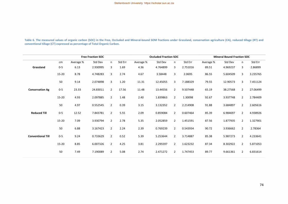
74
Table 6. The measured values of organic carbon (SOC) in the Free, Occluded and Mineral-bound SOM fractions under Grassland, conservation agriculture (CA), reduced tillage (RT) and conventional tillage (CT) expressed as percentage of Total Organic Carbon.
Free Fraction SOC Occluded Fraction SOC Mineral Bound Fraction SOC
cm Average % Std Dev n Std Err Average % Std Dev n Std Err Average % Std Dev n Std Err
Grassland 0-5 6.13 2.930995 3 1.69 4.36 4.764899 3 2.751016 89.51 4.969237 3 2.86899
15-20 8.78 4.748283 3 2.74 4.67 3.58448 3 2.0695 86.55 5.604509 3 3.235765
50 9.14 2.074898 3 1.20 11.31 12.45055 3 7.188329 79.55 12.90573 3 7.451124
Conservation Ag 0-5 23.33 24.83011 2 17.56 11.48 13.44556 2 9.507448 65.19 38.27568 2 27.06499
15-20 4.93 2.097885 2 1.48 2.40 1.839863 2 1.30098 92.67 3.937748 2 2.784409
50 4.97 0.552545 2 0.39 3.15 3.132352 2 2.214908 91.88 3.684897 2 2.605616
Reduced Till 0-5 12.52 7.843781 2 5.55 2.09 0.859084 2 0.607464 85.39 6.984697 2 4.938926
15-20 7.09 3.930794 2 2.78 5.35 2.052859 2 1.451591 87.56 1.877935 2 1.327901
50 6.88 3.167423 2 2.24 2.39 0.769239 2 0.543934 90.72 3.936662 2 2.78364
Conventional Till 0-5 9.24 0.733629 2 0.52 5.39 5.253644 2 3.714887 85.38 5.987273 2 4.233641
15-20 8.85 6.007326 2 4.25 3.81 2.295597 2 1.623232 87.34 8.302922 2 5.871053
50 7.49 7.190089 2 5.08 2.74 2.471272 2 1.747453 89.77 9.661361 2 6.831614
Stellenbosch University https://scholar.sun.ac.za
Stellenbosch University https://scholar.sun.ac.za

75
4.4 Conclusions
CA produced higher total microbial biomass (TMB) values as well as water stable
aggregates compared to all the other farming systems including grasslands, with values
ranging from 7.34 g/kg of soil in the top layer to 3.67 g/kg of soil at 50 cm for TMB. The
results for TMB showed that there were significant differences (α = 0.05) between CA and
CT (P = 0.0267) as well as between CA and grasslands (P = 0.0445). Our results clearly show
that the total microbial biomass is significantly higher under the CA system even compared to
natural grasslands. Application of conventional tillage system results in significantly lower
TMB compared to both grasslands and CA system. We can conclude that the least soil
disturbance in combination with substantial organic inputs significantly stimulates soil
microbial populations.
Water stable aggregates were clearly affected by tillage treatments according to these
results. Strong significant differences (α = 0.05) were found (Table 6) between grasslands and
CT (P = 0.0097), CA and grasslands (P = 0.0159) as well as between CA and CT (P =
0.0457). It is clear from these results that CA had a positive impact on the percentage water
stable aggregates in the soil. The total average WSA between 0 – 50 cm in this study,
declined in the following order: CA (94.6%) > RT (89.8%) > CT (88.3%) > Grasslands (86.3
%). The no till treatment yielded the highest water stable aggregates at all depths that we
tested ranging from 91.38 % - 94.88 % at 0- 50 cm depths. The grassland profiles had the
overall lowest water stable aggregates with an average value of 86.3 % from 0 – 50 cm depth.
The grassland profiles that were sampled, adjacent to the cultivated fields, was not considered
for agricultural use because of being either too stony or too wet, which is most probably the
reason for the lower WSA. In conclusion it was clear that an increase in tillage treatments
resulted in a significant loss of water stable aggregates.
Stellenbosch University https://scholar.sun.ac.za

76
The majority of the soil organic carbon in the soils we analysed was associated with the
mineral bound fraction with an average of 86.66 % for all the samples in all four treatments.
The free fraction had an average of 9.28% and the occluded fraction had an average of 4.06%
throughout all the profiles respectively. Which indicates that the total SOC is mostly
influenced by the mineral bound fraction in the soil.
Stellenbosch University https://scholar.sun.ac.za
77
Chapter 5. General conclusions
In the context of the objectives set out in the introduction to this work the following
conclusions have been reached in respective sections. These conclusions are summarized
here.
Objective 1: Characterize the main maize production systems in the KZN midlands
within the framework of farmers’ choices of soil cultivation methods and implements.
Three main farming systems of maize production in the KZN midlands were identified
through interviews with farmers and the representatives of the Provincial Department of
Agriculture. These systems include: conventional tillage (CT), conservation agriculture (CA)
and reduced tillage (RT) practices one treatment including a legume crop in the rotation and
the other RT treatment without a legume crop in the rotation. Though CT and CA systems are
clearly defined in terms of cultivation depth and frequency, the RT is a loose term.
Subsequently the latter adapted within the reality of each farming system adjusting to market
conditions, crop rotation opportunities (e.g. integration of soya into crop rotation), diesel
costs and other input prices.
In the past crop production in South Africa was mostly associated with CT. It is only
recently that producers have started to experiment with more sustainable ways of producing
crops aiming to improve soil health. There are many different implements and methods for
crop cultivation each with its own advantages and disadvantages. The psychology behind
decision making on the farm is an interesting field of study with a lot of scope to better
understand the farmer’s way of thinking and decision making. The broader socio-economic
benefits of CA should be made aware and that should incentivise the farmers to change their
Stellenbosch University https://scholar.sun.ac.za
78
tillage system to CA. When there is no personal conviction and motivation, the farmer’s
decision will most likely be based on small scale profitability on the farm, which is in most
cases not enough for system level changes.
It is however clear that there is not one single motivation or reason that can account for
all farmers and their actions regarding tillage practices. Each farmer’s reality is different and
should be viewed differently. It is also important to note that the decisions being made on the
farm is in most cases not based on scientific studies and research but rather on hearsay,
traditions and the farmer’s own experiences, opinions and beliefs. Above mentioned has in
the past and will continue to influence the mass adoption of CA around the world. In that
respect CA is primarily a farmer driven social innovation process.
Objective 2. Determine the long-term effects of different cultivation practices on the
vertical distribution and stocks of soil organic carbon and nitrogen as well as selected
soil parameters.
The objective of the study was to determine the influence of different long-term
cultivation systems on the SOC stocks and other soil parameters up to 1 m depth that are key
to overall soil health. The no-till system preserved the exponential decline pattern of SOC
stock distribution observed under indigenous grasslands with similar y-intercept values of
57.6 (grassland) and 67.6 (conservation tillage) and rather close values of the curve slope of -
0.022 and -0.036 (R2=0.998 and R
2=0.982 respectively). The above values show higher
biomass accumulation at the soil surface under CA, but more rapid decline with depth under
CA compared to grasslands. On the other hand, the CT and RT practices display a rather
different pattern described by separate equations for the cultivated section and the rest of the
soil profile below. The profiles of these soils are described by a system of equations, where
the distribution within the cultivated layer is a constant (CT) with R2=0.077 (very close to 0)
Stellenbosch University https://scholar.sun.ac.za
79
or a linear decline (reduced tillage – R2=0.990), while the section of the profile below the
cultivated layer follows the normal exponential decline curve with parameters similar to no-
till for both conventional and reduced tillage (R2=0.967 and R
2=0.933) respectively. As seen
from the results given in Chapter 3, the only significant difference when comparing the four
treatments with each other and with grasslands (α = 0.005) was found between CA and RT
without legumes (P = 0.0247). The total SOC stocks declined in the following order CA
(231,1 Mg/ha) > RT + legumes (217,3 Mg/ha) > CT (192,8 Mg/ha) > Grasslands (180,1
Mg/ha) > RT – legumes (177,5 Mg/ha). It is also interesting that the grasslands had more than
50% of its total carbon stocks in the top 20cm with the rest of the carbon stored between 20
and 80 cm.
Similar trends for grasslands as well as the CA treatments were observed with regards to
N stocks. Between all three tillage treatments the RT with legume rotation yielded the highest
average N stocks for 0-100 cm depth. This was expected, however grasslands as well as CA
still had much higher N stocks in the top 20 cm despite not having any legumes in rotation.
The RT without legume rotation treatment yielded the highest average C:N ratio value
over the 1m depth, where the reduced tillage with legume rotation treatment yielded the
lowest C:N ratio from 5 cm – 20 cm depth. The only significant difference (α = 0.05)
observed for C:N ratio was between RT with legume rotation and RT without legume rotation
(P = 0.0465). It is clear from these findings that the incorporation of legumes as a rotational
crop increases N in the soil and lowers the C:N ration.
The average porosity of the grassland profiles showed a normal decline in porosity with
depth. It was difficult to quantify the porosity of the CA profiles because most of the profiles
sampled on that farm had a stone layer at 25 – 35 cm, however from 40 cm down to a 100 cm
there was normal decline in porosity with depth similar to natural grasslands. The
Stellenbosch University https://scholar.sun.ac.za
80
conventional tillage treatment as well as the RT without legume rotation had the highest
porosity of about 56 %. Significant differences in soil porosity (α = 0.005) were found
between CT and grasslands (P = 0.0357) as well as between RT with legume rotation and
grasslands (P = 0.0175). No significant differences in porosity were found between the tillage
treatments (both RT treatments and CT) and CA.
Objective 3. Determine the effects of the above practices on soil microbial biomass
and aggregate stability as well as the proportion of different SOM fractions in relation
to observed SOC distribution patterns.
CA produced higher average total microbial biomass (TMB) values compared to all the
other farming systems including grasslands, with TMB values ranging from 7.34 g/kg of soil
in the top layer to 3.67 g/kg of soil at 50 cm. The results for TMB showed that there were
significant differences (α = 0.05) between CA and CT (P = 0.0267) as well as between CA
and grasslands (P = 0.0445). Which could mean that disturbing the soil less, through fewer or
no-tillage practices, could only make a small contribution to increasing the TMB populations
of a soil. However above ground organic C inputs for example mulching and applying
organic compost or manure can have a bigger positive influence on TMB populations in the
soil and more specifically the top 20 cm.
It is clear that the less the soil is disturbed the higher the microbial biomass will be,
especially in the top soil. The total microbial biomass values in grasslands stayed relatively
constant throughout the profile with much smaller total microbial biomass values compared
to the no-till treatment. For this reason it is believed that by reducing the frequency of tillage
events or even ending all tillage practices in general (no-till), will not positively influence
TMB population to a very large extent. Above ground C inputs seems to be the major
contributing factor to a more substantial TMB population in these soils.
Stellenbosch University https://scholar.sun.ac.za

81
The soils of Greytown, Kwazulu-Natal with red apedal horizons are largely regarded as
extremely stable, because it is highly micro aggregated and highly oxidised. The soils
studied (see Addendum D) had a very high level of aggregate stability due to their nature
broadly defined as high level of aggregate cementation by iron (hence the red colour). WSA
were clearly affected by tillage treatments according to our results. Strong significant
differences (α = 0.05) were found (Table 6) between grasslands and CT (P = 0.0097), CA and
grasslands (P = 0.0159) as well as between CA and CT (P = 0.0457). It is clear from these
results that CA had a positive impact on the percentage water stable aggregates in the soil.
The total average WSA between 0 – 50 cm in this study, declined in the following order: CA
(94.6%) > RT (89.8%) > CT (88.3%) > Grasslands (86.3 %). The CA treatment yielded the
highest water stable aggregates at all depths that we tested ranging from 91.38 % - 94.88 % at
0- 50 cm depths. The grassland profiles had the overall lowest water stable aggregates with
an average value of 86.3 % from 0 – 50 cm depth. The grassland profiles that were sampled,
adjacent to the cultivated fields, was not considered for agricultural use because of being
either too stony or too wet, which is most probably the reason for the lower WSA.. In
conclusion it was clear that an increase in tillage resulted in a loss of WSA.
The majority of the soil organic carbon in the soils we analysed was associated with the
mineral bound fraction with an average of 86.66 % for all the samples in all four treatments.
The free fraction had an average of 9.28% and the occluded fraction had an average of 4.06%
throughout all the profiles respectively. Which could lead to the conclusion that the SOC in
these soils are mostly controlled by the mineral bound fraction. Due to high level of variation
seen in the SOC stocks it is believed that more research needs to be done to reach certain
target or ideal levels in these soils.
Stellenbosch University https://scholar.sun.ac.za
82
More studies should be conducted investigating the psychology behind decision making
of farmers. Every farm and farmer behaves differently when it comes to decision making,
there is at this stage no single motivation or reason that can explain their actions regarding the
adoption of CA principles. There are many variables that need to be taken into account when
studying their behaviour. It seems that their motives are mostly pragmatic. If the farmers can
understand and agree that the broader socio-economic benefits of CA outweigh the benefits
of other systems the adoption of CA will happen at a much faster rate.
It could be concluded that the adoption of CA practices can positively influence certain
important soil parameters as seen through the data in this study. Parameters such as SOC
stocks, N stocks, C:N ratio and porosity were all positively influenced by CA to some extent
in chapter 3. In chapter 4 it is also clear that CA principles significantly influenced important
soil parameters namely WSA and TMB. It is important to note that if a farmer wishes to
change from a traditional system (RT or CT) to CA it will take a few years to see the positive
changes. In this study the differences seen between CA and other systems were over a time
period of between 13 - 17 years. It is difficult to say at which stage or after how many years
these positive changes can start to be seen and further studies might find some clarity
regarding this subject.
In general the long-term practice of CA in the studied area can definitely improve certain
soil parameters that play a key role in overall soil health and sustainability.
Stellenbosch University https://scholar.sun.ac.za
83
References
Abreu, S.L., Godsey, C.B., Edwards, J.T. & Warren, J.G. 2011, "Assessing carbon and nitrogen stocks of no-till systems in Oklahoma", Soil and Tillage Research, vol. 117, pp. 28-33.
Aitken, R. L., Moody, P. W., and McKinley, P. G. 1990, "Lime requirements of acidic Queensland soils. I. Relationships between soil properties and pH buffer capacity", Australian Journal of Soil Research, vol. 28, pp. 695-701.
Andruschkewitsch, R., Geisseler, D., Koch, H. & Ludwig, B. 2013, "Effects of tillage on contents of organic carbon, nitrogen, water-stable aggregates and light fraction for four different long-term trials", Geoderma, vol. 192, pp. 368-377.
Angers, D.A. & Carter, M.R. 1996, "Aggregation and organic matter storage in cool, humid agricultural soils", CRC Press: Boca Raton, pp. 193-193-211.
Annabi, M., Houot, S., Francou, C., Poitrenaud, M. & Bissonnais, Y.L. 2007, "Soil Aggregate Stability Improvement with Urban Composts of Different Maturities", Soil Science Society of America Journal, vol. 71, pp. 413-423.
Aziz, I., Mahmood, T. & Islam, K.R. 2013, "Effect of long term no-till and conventional tillage practices on soil quality", Soil and Tillage Research, vol. 131, no. 0, pp. 28-35.
Baldock, J. A. and Nelson, P. N 1999, "Soil Organic Matter" in Handbook of Soil Science, ed. M. E. Sumner, Boca Raton, USA, pp. 25-84.
Baldock, J.A. 2009, “Building soil carbon for productivity and implications for carbon accounting.” CSIRO, vol 1, no.3, pp 1 -5.
Balota, E.L., Colozzi-Filho, A., Andrade, D.S. & Dick, R.P. 2003, "Microbial biomass in soils under different tillage and crop rotation systems", Biology and Fertility of Soils, vol. 38, no. 1, pp. 15-20.
Balota, E.L., Colozzi Filho, A., Andrade, D.S. & Dick, R.P. 2004, "Long-term tillage and crop rotation effects on microbial biomass and C and N mineralization in a Brazilian Oxisol", Soil and Tillage Research, vol. 77, no. 2, pp. 137-145.
Barberis, E., Marsan, F.A., Boero, V. & Arduino, E. 1991, "Aggregation of soil particles by iron
oxides in various size fractions of soil B horizons", Journal of Soil Science, vol. 42, no. 4, pp. 535-542.
Blake, G.,R. & Hartge, K.,H. 1986, "Particle Density", Methods of soil analysis, part 1 - Physical and mineralogical methods, , pp. 371-375.
Bloom, P.R. 1999, "Soil pH and pH buffering" in Handbook of Soil Science, ed. M. E. Sumner, Boca Raton, USA, pp. 333-352.
Blume, L.J., B.A. Schumacher, P.W. Shaffer et al 1990, "Handbook of Methods for Acid Deposition Studies Laboratory Analyses for Soil Chemistry", EPA, vol. 23, pp. 4-90.
Brady, N.C. 1990, The nature and properties of soils, MacMillan Publishing Company, New York.
Christensen, B.,T. 2000, Organic matter in soil-structure, function and turn over. DIAS Report, Plant Production. No. 30, pp. 95
Christensen, B.,T. 1992, “Physical fractionation of soil and organic matter in primary and density separate”, Advances in Soil Science- Springer New York. No. 20 pp. 1-90
Stellenbosch University https://scholar.sun.ac.za

84
Christensen, N.B., Lindemann, W.C., Salazar-Sosa, E. & Gill, L.R. 1994, "Nitrogen and carbon dynamics in no-till and stubble mulch tillage systems", Agronomy Journal, vol. 86, no. 2, pp. 298-303.
CTIC. 2004, National Crop Residue Management Survey, Conservation Tillage Information Center, CTIC West Lafayette.
da Veiga, M., Reinert, J., Reichert, J. & Kaiser, D. 2008, " Short and Long-Term Effects of Tillage Systems and Nutrient Sources on Soil Physical Properties of a Southern Brazilian Hapludox", R. Bras Ci Solo, vol. 32, pp. 1437-1446.
Dalal, R.C. & Mayer, R.J. 1986, "Long term trends in fertility of soils under continuous cultivation and cereal cropping in southern Queensland. II. Total organic carbon and its rate of loss from the soil profile", Soil Research, vol. 24, pp. 281-292.
de Freitas, P.L. & Landers, J.N. 2014, "The Transformation of Agriculture in Brazil Through Development and Adoption of Zero Tillage Conservation Agriculture", International Soil and Water Conservation Research, vol. 2, no. 1, pp. 35-46.
De Sá, J.C.M., Cerri, C.C., Dick, W.A., Lal, R., Venske Filho, S.P., Piccolo, M.C. & Feigl, B.E. 2001,
"Organic matter dynamics and carbon sequestration rates for a tillage chronosequence in a Brazilian Oxisol", Soil Science Society of America Journal, vol. 65, no. 5, pp. 1486-1499.
de Villiers, M.C., Pretorius, D.J., Barnard, R.O., van Zyl, A.J. & Leclus, C.F. 2002, “Land degradation assessment in dry lands” – Lada Project, Food and Agricultural Organization of the United Nations, Rome, Italy. pp. 97
Diekow, J., Mielniczuk, J., Knicker, H., Bayer, C., Dick, D.P. & Kögel-Knabner, I. 2005, "Soil C and N stocks as affected by cropping systems and nitrogen fertilisation in a southern Brazil Acrisol managed under no-tillage for 17 years", Soil and Tillage Research, vol. 81, no. 1, pp. 87-95.
Doran, J.W. 1987, "Microbial biomass and mineralizable nitrogen distributions in no - tillage and plowed soils", Biol, vol. 5, pp. 68-75.
du Toit, G. 2007, Promoting conservation Agriculture in South Africa: a case study among commercial grain growers in the North West province, BFAP, Pretoria, South Africa.
Duiker, S.W., Rhoton, F.E., Torrent, J., Smeck, N.E. & Lal, R. 2003, "Iron (hydr)oxide crystallinity effects on soil aggregation", Soil Science Society of America Journal, vol. 67, no. 2, pp. 606-611.
Duxbury, J. M., Smith, M. S., and Doran, J. W. 1989, "Soil organic matter as a source and a sink of plant nutrients." in Dynamics of soil organic matter in tropical ecosystems, ed. D. C. Coleman, J. M. Oades, and G. Uehara, University of Hawaii Press, Honolulu, pp. 33-67.
Emerson, W. W. and McGarry, D. 2003, "Organic carbon and soil porosity", Australian Journal of Soil Research, vol. 41, pp. 107-118.
Esteban, G.,J. & Jackson, R.,B. 2000, "The vertical Distribution of Soil Organic Carbon and its Relation to Climate and Vegetation", vol. 10, pp. 423-436.
FAO. 1993, “Soil tillage in Africa: Needs and challenges” FAO Soils Bulletin. Vol. 69 Chapter 7.
FAO. 2001, "Guidelines and reference materials for promoting integrated soil and nutrient management in Farmer Field Schools", FAO, pp. 1-27.
Fliebach, A. and Mader, P. 2000. Microbial biomass and size density fractions differ between soils of organic and conventional agricultural systems. Soil Biology & Chemistry, vol. 32 pp. 757 -768.
Stellenbosch University https://scholar.sun.ac.za
85
Flint, A. & Flint, L. 2002, "Particle Density" in Methods of soil analysis: Part 4. Physical methods, eds. J. Dane & G. Topp, 4th edn, SSSA, Madison, Wisconsin, pp. 229-240.
Food and Agriculture Organization of the United Nations 1984, "Tillage systems for soil and water conservation", FAO, vol. 54, pp. 48-55.
Fowler, R. 1999, "Conservation tillage research and development in South - Africa", ATNESA, pp. 51-60.
Frey, S.D., Elliott, E.T. & Paustian, K. 1999, "Bacterial and fungal abundance and biomass in conventional and no-tillage agroecosystems along two climatic gradients", Soil Biology and Biochemistry, vol. 31, no. 4, pp. 573-585.
Golchin, A., Oades, J.M., Skejmstad, J.,O. & Clarke, P. 1994, "Soil Structure and Carbon Cycling", Australian Journal of Soil Research, vol. 32, pp. 1043-1043.
Grossman, R. & Reinsch, T.,G. 2002, "Bulk density and linear extensibility.", Methods of soil analysis, vol. 4, pp. 201-254.
Guo , L., B. & Gifford, R., M. 2002, "Soil carbon stocks and land use change: a meta-analysis", Global change biology, vol. 8, pp. 345-360.
Hakeem, K., Akhtar, J. & Sabir, M. 2016, "Tillage Systems" in Soil Science: Agricultural and Environment Perspectives, eds. K. Hakeem, J. Akhtar & M. Sabir, Springer, Switzerland, pp. 4-9.
Haynes, R. J. and Naidu, R. 1998, "Influence of lime, fertilizer and manure applications on soil
organic matter content and soil physical conditions", Nutrient Cycling in Agroecosystems, vol. 51, pp. 123-137.
Haynes, R.J. & Graham, M.H. 2004, "Soil biology and biochemistry - a new direction for South African soil science? ", South African Journal of Plant and Soil, vol. 21:5, pp. 330-330-334.
Hendrickson, O. 2003, "Influences of global change on carbon sequestration by agricultural and forest soils", Environmental Reviews, vol. 11, no. 3, pp. 161-192.
Hernanz, J.L., Sánchez-Girón, V. & Navarrete, L. 2009, "Soil carbon sequestration and stratification in a cereal/leguminous crop rotation with three tillage systems in semiarid conditions", Agriculture, Ecosystems & Environment, vol. 133, no. 1–2, pp. 114-122.
Hiederer, R. 2009, “Distribution of organic carbon in soil profile data”, Luxembourg office for official publications of the European community, Luxembourg. pp. 126
Hillel, D. 1982, Introduction to Soil Physics, 2004th edn, Elsevier, USA. pp. 78 - 392
Hobbs, Peter R., Ken Sayre, and Raj Gupta. 2008, "The role of conservation agriculture in sustainable agriculture." Philosophical Transactions of the Royal Society B: Biological Sciences vol. 363.1491 pp. 543-555.
Hobbs, P. & Gupta, R. 2004, "Problems and challenges of no - till farming for the Rice - Wheat systems of the Indo - Gangetic Plains in South Asia" in Sustainable Agriculture and the International Rice - Wheat System, ed. Rattan Lal, Peter R. Hobbs, Norman Uphoff, 10th edn, Marcel Dekker, USA, pp. 101-120.
Huang, S., Sun, Y., Rui, W., Liu, W. & Zhang, W. 2010, "Long-Term Effect of No-Tillage on Soil
Organic Carbon Fractions in a Continuous Maize Cropping System of Northeast China", Pedosphere, vol. 20, pp. 285-292.
Stellenbosch University https://scholar.sun.ac.za
86
Insam, H. 2001, "Developments in soil microbiology since the mid 1960s", Geoderma, vol. 100, no. 3-4, pp. 389-402.
Islam, K.,R. & Weil, R.,R. 1997, "Microwave irradiation of soil for routine measurement of microbial biomass carbon", vol. 27, pp. 408-416.
Jones, M.B. & Donnelly, A. 2004, "Carbon sequestration in temperate grassland ecosystems and the influence of management, climate and elevated CO2", New Phytologist, vol. 164, no. 3, pp. 423-439.
Kaiser, M., Piegholdt, C., Andruschkewitsch, R., Linsler, D. & Koch, H.,J. 2014, "Impact of tillage intensity on carbon and nitrogen pools in surface and sub-surface soils of three long-term field experiments", European Journal of Soil Science, , pp. 499-509.
Kay, B.D., Angers, D.A. 2002, "Soil structure" in Soil Physics Companion, ed. A. W. Warrick, Boca Raton, Florida; USA, pp. 249-283.
Kay, B. & Angers, D. 1999, "Soil Structure" in Handbook of Soil Science, ed. M. E. Sumner, Boca Raton, USA, pp. 229-279.
Kay, B.D. & VandenBygaart, A.J. 2002, "Conservation tillage and depth stratification of porosity and soil organic matter", Soil and Tillage Research, vol. 66, no. 2, pp. 107-118.
Kemper, W.D. & Rosenau, R.,C. 1986, "Aggregate Stability and size distribution", Methods of soil analysis, vol. 9, pp. 425-442.
Kepner, R.A., Bainer, R. & Barger, E.L., 1987, Principles of farm machinery, AVI Publishers, West Port, CT. vol. 3 pp. 112-134.
Kern, J. S. Johnson, M. G 1993, "Conservation Tillage Impacts on National Soil and Atmospheric Carbon Levels", Soil Sci. Soc. Am. J., vol. 57, pp. 200-210.
Knops J, M., H. & Bradley, K., L. 2009, "Soil Carbon and Nitrogen Accumulation and Vertical Distribution across a 74-Year Chronosequence", SSSAJ, vol. 73, pp. 2096-2104.
Knops J, M., H. & Tilman, D. 2000, “Dynamics of soil nitrogen and carbon accumulation for 61 years after agricultural abandonement.” Ecological Society of America. Vol. 81
Knowler, D. & Bradshaw, B. 2007, "Farmers’ adoption of conservation agriculture: A review and synthesis of recent research", Food Policy, vol. 32, no. 1, pp. 25-48.
Kogel-Knabner 1997, "NMR spectroscopy as a tool in soil organic matter studies", Geoderma, vol. 80, pp. 243-270.
Krull, E., Skejmstad, J. & Baldock, J. 2004, "Functions of Soil Organic Matter and the effect on Soil Properties,” Barton: Grains Research and Development Corporation.
LECO 1996, Elemental Analyzer - Instruction Manual. LECO Corp 1996, CNS 2000
Lipiec, J., Kus, J., Slowinska, A. & Nosalewicz, A. 2006, "Soil porosity and water infiltration as influenced by tillage methods", Soil & Tillage research, vol. 89, pp. 210-220.
Liu, S., Yan, C., He, W., Chen, B., Zhang, Y., Liu, Q. & Liu, E. 2015, "Effects of different tillage practices on soil water-stable aggregation and organic carbon distribution in dryland farming in Northern China", Acta Ecologica Sinica, vol. 35, no. 4, pp. 65-69.
Lopez-Fando, C. & Pardo, M.,T. 2011, "Soil carbon storage and stratification under different tillage systems in a semi - arid region", Soil & Tillage research, vol. 111, pp. 224-230.
Stellenbosch University https://scholar.sun.ac.za
87
López-Garrido, R., MadejóN, E., Moreno, F. & Murillo, J.M. 2014, "Conservation Tillage Influence on Carbon Dynamics Under Mediterranean Conditions", Pedosphere, vol. 24, no. 1, pp. 65-75.
Lupwayi, N.Z., Monreal, M.A., Clayton, G.W., Grant, C.A., Johnston, A.M. & Rice, W.A. 2001, "Soil microbial biomass and diversity respond to tillage and sulphur fertilizers", Canadian Journal of Soil Science, vol. 81, no. 5, pp. 577-589.
Lupwayi, N.Z., Rice, W.A. & Clayton, G.W. 1998, "Soil microbial diversity and community structure under wheat as influenced by tillage and crop rotation", Soil Biology and Biochemistry, vol. 30, no. 13, pp. 1733-1741.
Madsen, E. 1995, "Impacts of Agricultural Practices on Subsurface Microbial Biology", Advances in Agronomy, vol. 54, pp. 1-57.
Miller, J.J., Kokko, E.G. & Kozub, G.C. 1998, "Comparison of porosity in a Chernozemic clay loam soil under long-term conventional tillage and no-till", Canadian Journal of Soil Science, vol. 78, no. 4, pp. 619-629.
Mitchell, J. 2009, "Classification of Conservation Tillage Practices in California Irrigated Row Crop Systems.", ANR, vol. 8364, pp. 1-8.
Moraes, M., Debiasi, H. & Carlesso, R. 2015, "Soil physical quality on tillage and cropping systems after two decades in the subtropical region of Brazil", Soil tillage and research, vol. 01/2016, pp. 155.
Moreno, F., Murillo, J.M., Pelegrín, F. & Girón, I.F. 2006, "Long-term impact of conservation tillage
on stratification ratio of soil organic carbon and loss of total and active CaCO3", Soil and Tillage Research, vol. 85, no. 1–2, pp. 86-93.
Morrison, J. 2010, "Simple Conservation Agriculture (CA) Implements." ISTRO, pp. 153-164.
Mueller, D.H., Klemme, R.M. & Daniel, T.C. 1985, "Short- and long-term cost comparisons of conventional and conservation tillage systems in corn production.", Journal of Soil & Water Conservation, vol. 40, no. 5, pp. 466-470.
Nelson, D.,W. & Sommers, L.,E. 1996, "Total Carbon, Organic Carbon an Organic matter", Methods of soil analysis, vol. Part 3, pp. 961-969.
Nelson, D.W. and L.E. Sommers 1996, Total carbon, organic carbon, and organic matter. In: Methods of Soil Analysis Part 2, Am. Soc. of Agron., Inc, Madison, WI.
Oades, J.M. 1989, "An introduction to organic matter in mineral soils" in Minerals in soil environments, ed. J. B. Dixon and S. B. Weed, Soil Science Society of America, Madison, WI, pp. 89-259.
Paul, E.A. 1984, Dynamics of organic matter in soils, - Martinus Nijhoff/Dr. W. Junk Publishers. Plant & Soil, vol.76, pp. 275 - 285
Peverill, K. I., Sparrow, L. A., and Reuter, D. J 1991, "Soil Analysis. An Interpretation Manual", CSIRO,
Puget, P., Chenu, C. & Balesdent, J. 1995, "Total and young organic matter distributions in aggregates of silty cultivated soils", European Journal of Soil Science, vol. 46, pp. 449-459.
Rasse, D., Mulder, J., Moni, C. & Chenu, C. 2006, "Carbon Turnover Kinetics with Depth in a French Loamy Soil", Soil Science Society of America Journal, vol. 70, pp. 2097-2105.
Stellenbosch University https://scholar.sun.ac.za
88
Roldán, A., Salinas-García, J.R., Alguacil, M.M. & Caravaca, F. 2005, "Changes in soil enzyme activity, fertility, aggregation and C sequestration mediated by conservation tillage practices and water regime in a maize field", Applied Soil Ecology, vol. 30, no. 1, pp. 11-20.
Ros, I. 2015, Stochastic modelling of soil carbon stocks under different land uses: a case study in South Africa, M.Sc Thesis, University of Stellenbosch.
Roscoe, R. & Buurman, P. 2003, "Tillage effects on soil organic matter in density fractions of a Cerrado Oxisol", Soil and Tillage Research, vol. 70, no. 2, pp. 107-119.
Rumpel, C., L.J. Janik, J.O. Skjemstad and I. Kogel-Knabner. 2001, "Quantification of carbon derived from lignite in soils using mid-infrared spectroscopy and partial least squares", Organic Geochemistry, vol. 32, pp. 831-839.
Rumpel, C. & Kogel-Knabner, I. 2011, "Deep soil organic matter—a key but poorly understood component of terrestrial C cycle", Plant & Soil , pp. 143-158.
Schlesinger, W.H. 1977, Carbon Balance in Terrestrial Detritus, Annual Reviews.
Schumacher, B. 2002, "Methods for determination of total organic carbon (TOC) in soils and sediments” Ecological Risk Assessment Support Center, vol. 1282, pp. 3-20.
Shang, C. & Tiessen, H. 2003, "Soil organic C sequestration and stabilization in karstic soils of Yucatan", Biogeochemistry, vol. 62, pp. 177.
Simmons, F.,W. & Nafziger, E.,D. 2009, "Soil Management and Tillage" in Illinois Agronomy Handbook University of Illinois, Illinois, pp. 133-142.
Sisti, C.P.J., dos Santos, H.P., Kohhann, R., Alves, B.J.R., Urquiaga, S. & Boddey, R.M. 2004, "Change in carbon and nitrogen stocks in soil under 13 years of conventional or zero tillage in southern Brazil", Soil and Tillage Research, vol. 76, no. 1, pp. 39-58.
Six, J., Bossuyt, H., Degryze, S. & Denef, K. 2004, "A history of research on the link between (micro)aggregates, soil biota and soil organic matter dynamics", Soil & Tillage research, vol. 79, pp. 7-31.
Six, J., Elliott, E.T. & Paustian, K. 2000, "Soil macroaggregate turnover and microaggregate formation: a mechanism for C sequestration under no-tillage agriculture", Soil Biology and Biochemistry, vol. 32, no. 14, pp. 2099-2103.
Smith, J.DV. 2014, “The effect of long-term no-till crop rotation practices on soil organic matter functional pools” M.Sc Thesis. University of Stellenbosch.
Soil Classification Work Group. 1991, Soil Classification: a Taxonomic System for South Africa, 15th edn, The Department of Agricultural Development of the Republic of South Africa, Pretoria.
Sparling, G.P. 1997, "Biological indicators of soil health" in Soil Microbial Biomass, activity and nutrient cycling as indicators of soil health, eds. C. Pankhurst, B.M. Doube & V.V.S.R. Gupta, CAB International, Wallingford UK, pp. 97-119.
Starr, M., Westman, C. J., and Ala-Reini, J. 1996, "The acid buffer capacity of some Finnish forest
soils: Results of acid addition laboratory experiments", Water, Air and Soil Pollution, vol. 89, pp. 147-157.
Stevenson, F.J. 1994, Humus Chemistry. Genesis, composition, reactions, Wiley and Sons, New York.
Stellenbosch University https://scholar.sun.ac.za
89
Stonehouse, D.P. 1997, "Socio-economics of alternative tillage systems", Soil and Tillage Research, vol. 43, no. 1–2, pp. 109-130.
The non-affiliated soil analysis work committee 1990, Handbook of standard soil testing methods for advisory purposes, Soil Science Society of South Africa, Pretoria.
Tiessen H. and J.O. Moir 1993, "Total and organic carbon" in Soil Sampling and Methods of Analysis, ed. M.E. Carter, Lewis Publishers, Ann Arbor,MI, pp. 187-211.
Tisdall, J.M. & Oades, J.M. 1982, "Organic matter and water-stable aggregates in soils", Journal of Soil Science, vol. 62, pp. 141-163.
TU, C. Ristaino, J.B. Hu, Shuijin, H. 2006, “Soil microbial biomass and activity in organic tomato
farming systems: effects of organic inputs and straw mulching.” Soil Biology & Chemistry, vol.
38 pp. 247 - 255
Valboa, G., Lagomarsino, A., Brandi, G., Agnelli, A.E., Simoncini, S., Papini, R., Vignozzi, N. & Pellegrini, S. 2015, "Long-term variations in soil organic matter under different tillage intensities", Soil and Tillage Research, vol. 154, pp. 126-135.
Van Antwerpen & R 2005, "A Review of Soil Health Indicators for Labarotory Use in South African Sugar Industry", Proc S Afr Sug Technol Ass, vol. 79, pp. 179-179-191.
Villamil, M.B. & Nafziger, E.D. 2015, "Corn residue, tillage, and nitrogen rate effects on soil carbon and nutrient stocks in Illinois", Geoderma, vol. 253–254, pp. 61-66.
Walkley, A., I.A. Black. 1934, "An examination of the Degtjareff method for determining organic
carbon in soils: Effect of variations in digestion conditions and of inorganic soil constituents", Soil Sci, vol. 63, pp. 251-263.
Wang, Y., Zhang, J.H. & Zhang, Z.H. 2015, "Influences of intensive tillage on water-stable aggregate distribution on a steep hillslope", Soil and Tillage Research, vol. 151, pp. 82-92.
White, R.E., 1997. Principles and practice of soil science: the soil as a natural resource. John Wiley & Sons.
Wiese, L., Ros, I., Rozanov, A., Boshoff, A. De Clercq, W. & Seifert, T. 2016, "An approach to soil carbon accounting and mapping using vertical distribution functions for known soil types", Geoderma, vol. 263, pp. 264-273.
Wolf, B. and Snyder, G. H 2003. The place of organic matter in sustaining soils and their productivity. CRC Press, 1st Edn. pp. 233 – 255.
Wright, A. L. and Hons, F. M. 2005, "Tillage impacts on soil aggregation and carbon and nitrogen sequestration under wheat cropping sequences", Soil Tillage Res., vol. 84, pp. 67-75.
Zhang, J., Song, C. & Wenyan, Y. 2007, "Tillage effects on soil carbon fractions in the Sanjiang Plain, Northeast China", Soil and Tillage Research, vol. 93, no. 1, pp. 102-108.
Stellenbosch University https://scholar.sun.ac.za
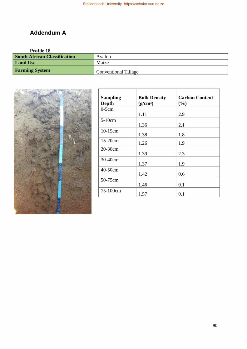
90
Addendum A
Profile 18
South African Classification Avalon
Land Use Maize
Farming System Conventional Tillage
Sampling
Depth
Bulk Density
(g/cm³)
Carbon Content
(%)
0-5cm 1.11 2.9
5-10cm 1.36 2.1
10-15cm 1.38 1.8
15-20cm 1.26 1.9
20-30cm 1.39 2.3
30-40cm 1.37 1.9
40-50cm 1.42 0.6
50-75cm 1.46 0.1
75-100cm 1.57 0.1
Stellenbosch University https://scholar.sun.ac.za
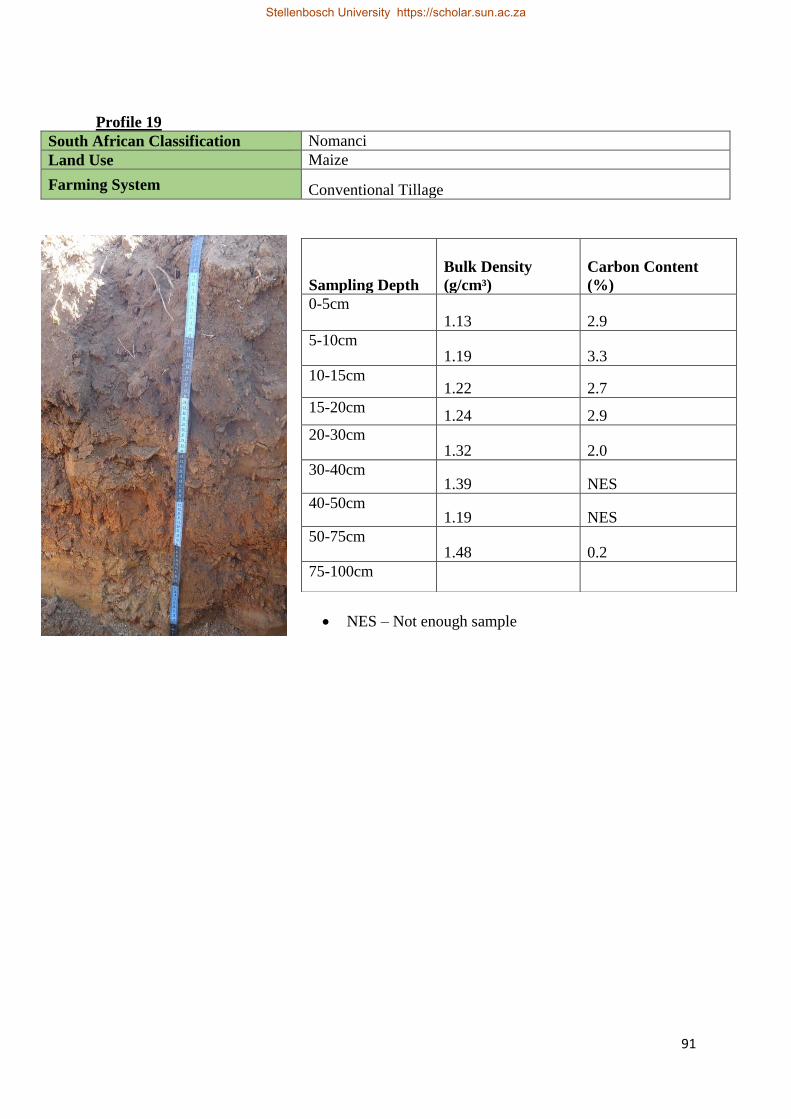
91
Profile 19
South African Classification Nomanci
Land Use Maize
Farming System Conventional Tillage
NES – Not enough sample
Sampling Depth
Bulk Density
(g/cm³)
Carbon Content
(%)
0-5cm 1.13 2.9
5-10cm 1.19 3.3
10-15cm 1.22 2.7
15-20cm 1.24 2.9
20-30cm 1.32 2.0
30-40cm 1.39 NES
40-50cm 1.19 NES
50-75cm 1.48 0.2
75-100cm
Stellenbosch University https://scholar.sun.ac.za
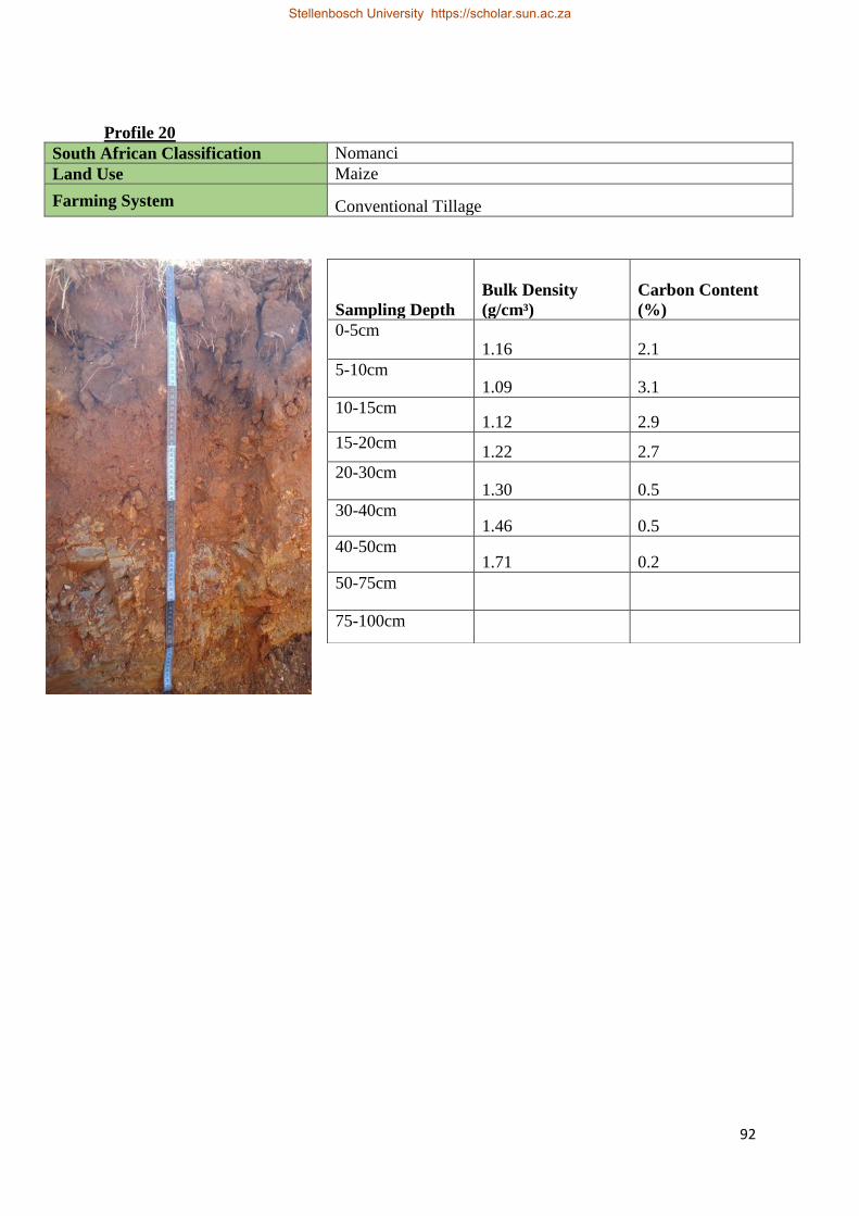
92
Profile 20
South African Classification Nomanci
Land Use Maize
Farming System Conventional Tillage
Sampling Depth
Bulk Density
(g/cm³)
Carbon Content
(%)
0-5cm 1.16 2.1
5-10cm 1.09 3.1
10-15cm 1.12 2.9
15-20cm 1.22 2.7
20-30cm 1.30 0.5
30-40cm 1.46 0.5
40-50cm 1.71 0.2
50-75cm
75-100cm
Stellenbosch University https://scholar.sun.ac.za
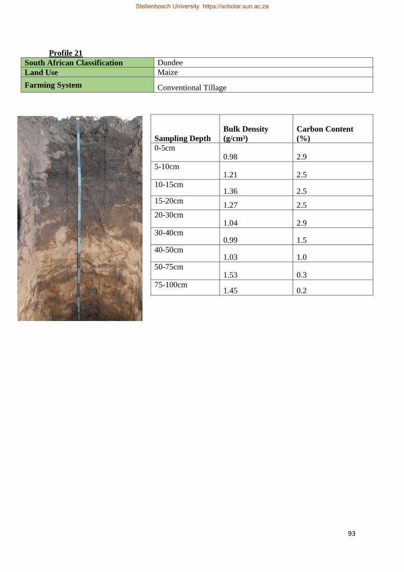
93
Profile 21
South African Classification Dundee
Land Use Maize
Farming System Conventional Tillage
Sampling Depth
Bulk Density
(g/cm³)
Carbon Content
(%)
0-5cm 0.98 2.9
5-10cm 1.21 2.5
10-15cm 1.36 2.5
15-20cm 1.27 2.5
20-30cm 1.04 2.9
30-40cm 0.99 1.5
40-50cm 1.03 1.0
50-75cm 1.53 0.3
75-100cm 1.45 0.2
Stellenbosch University https://scholar.sun.ac.za
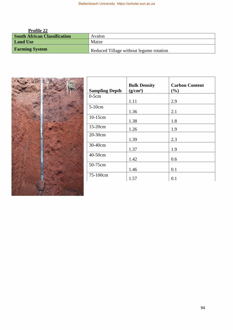
94
Profile 22
South African Classification Avalon
Land Use Maize
Farming System Reduced Tillage without legume rotation
Sampling Depth
Bulk Density
(g/cm³)
Carbon Content
(%)
0-5cm 1.11 2.9
5-10cm 1.36 2.1
10-15cm 1.38 1.8
15-20cm 1.26 1.9
20-30cm 1.39 2.3
30-40cm 1.37 1.9
40-50cm 1.42 0.6
50-75cm 1.46 0.1
75-100cm 1.57 0.1
Stellenbosch University https://scholar.sun.ac.za
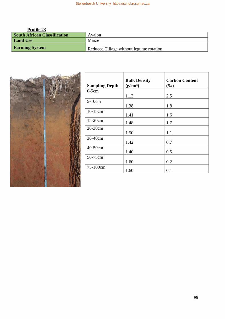
95
Profile 23
South African Classification Avalon
Land Use Maize
Farming System Reduced Tillage without legume rotation
Sampling Depth
Bulk Density
(g/cm³)
Carbon Content
(%)
0-5cm 1.12 2.5
5-10cm 1.38 1.8
10-15cm 1.41 1.6
15-20cm 1.48 1.7
20-30cm 1.50 1.1
30-40cm 1.42 0.7
40-50cm 1.40 0.5
50-75cm 1.60 0.2
75-100cm 1.60 0.1
Stellenbosch University https://scholar.sun.ac.za
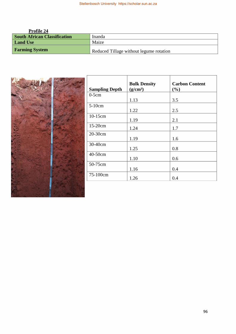
96
Profile 24
South African Classification Inanda
Land Use Maize
Farming System Reduced Tillage without legume rotation
Sampling Depth
Bulk Density
(g/cm³)
Carbon Content
(%)
0-5cm 1.13 3.5
5-10cm 1.22 2.5
10-15cm 1.19 2.1
15-20cm 1.24 1.7
20-30cm 1.19 1.6
30-40cm 1.25 0.8
40-50cm 1.10 0.6
50-75cm 1.16 0.4
75-100cm 1.26 0.4
Stellenbosch University https://scholar.sun.ac.za
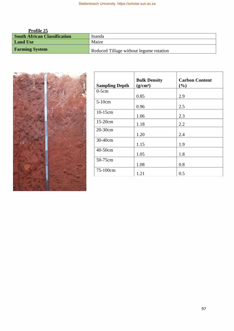
97
Profile 25
South African Classification Inanda
Land Use Maize
Farming System Reduced Tillage without legume rotation
Sampling Depth
Bulk Density
(g/cm³)
Carbon Content
(%)
0-5cm 0.85 2.9
5-10cm 0.96 2.5
10-15cm 1.06 2.3
15-20cm 1.18 2.2
20-30cm 1.20 2.4
30-40cm 1.15 1.9
40-50cm 1.05 1.8
50-75cm 1.08 0.8
75-100cm 1.21 0.5
Stellenbosch University https://scholar.sun.ac.za
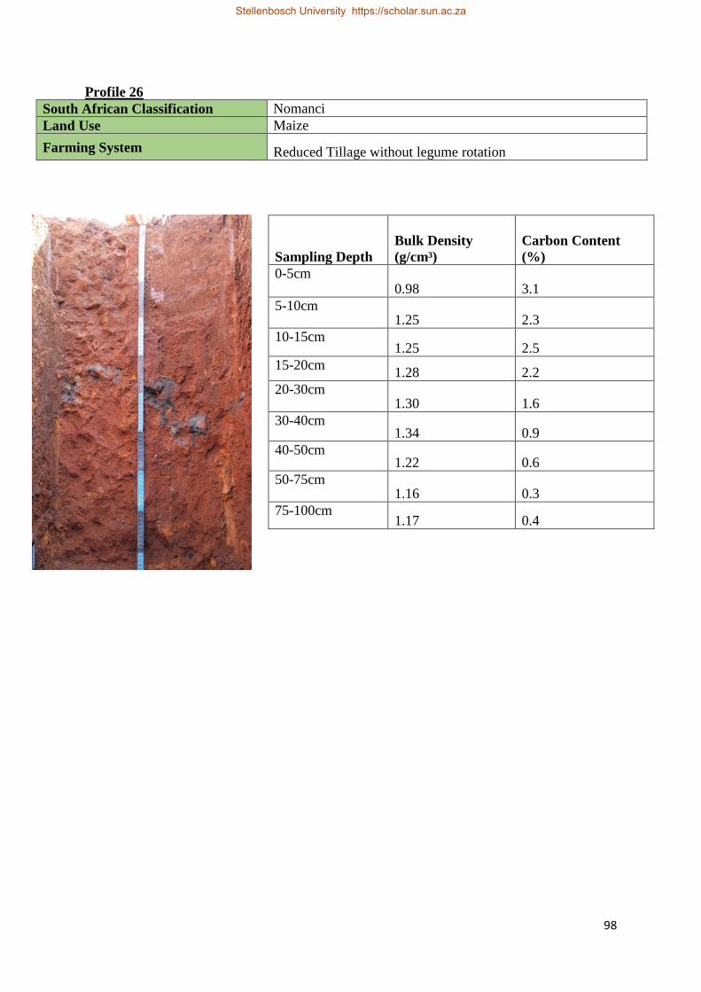
98
Profile 26
South African Classification Nomanci
Land Use Maize
Farming System Reduced Tillage without legume rotation
Sampling Depth
Bulk Density
(g/cm³)
Carbon Content
(%)
0-5cm 0.98 3.1
5-10cm 1.25 2.3
10-15cm 1.25 2.5
15-20cm 1.28 2.2
20-30cm 1.30 1.6
30-40cm 1.34 0.9
40-50cm 1.22 0.6
50-75cm 1.16 0.3
75-100cm 1.17 0.4
Stellenbosch University https://scholar.sun.ac.za

99
Profile 27
South African Classification Inanda
Land Use Maize
Farming System Reduced Tillage without legume rotation
Sampling Depth
Bulk Density
(g/cm³)
Carbon Content
(%)
0-5cm 0.89 4.2
5-10cm 1.04 3.5
10-15cm 1.15 2.7
15-20cm 1.12 2.6
20-30cm 1.07 2.3
30-40cm 1.02 1.4
40-50cm 1.07 1.2
50-75cm 1.22 0.5
75-100cm 1.16 0.3
Stellenbosch University https://scholar.sun.ac.za
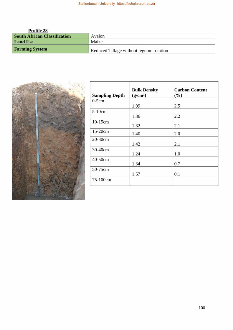
100
Profile 28
South African Classification Avalon
Land Use Maize
Farming System Reduced Tillage without legume rotation
Sampling Depth
Bulk Density
(g/cm³)
Carbon Content
(%)
0-5cm 1.09 2.5
5-10cm 1.36 2.2
10-15cm 1.32 2.1
15-20cm 1.40 2.0
20-30cm 1.42 2.1
30-40cm 1.24 1.0
40-50cm 1.34 0.7
50-75cm 1.57 0.1
75-100cm
Stellenbosch University https://scholar.sun.ac.za
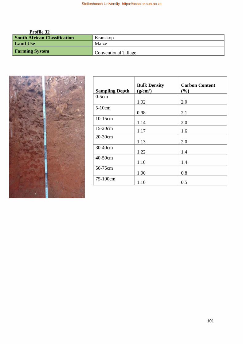
101
Profile 32
South African Classification Kranskop
Land Use Maize
Farming System Conventional Tillage
Sampling Depth
Bulk Density
(g/cm³)
Carbon Content
(%)
0-5cm 1.02 2.0
5-10cm 0.98 2.1
10-15cm 1.14 2.0
15-20cm 1.17 1.6
20-30cm 1.13 2.0
30-40cm 1.22 1.4
40-50cm 1.10 1.4
50-75cm 1.00 0.8
75-100cm 1.10 0.5
Stellenbosch University https://scholar.sun.ac.za
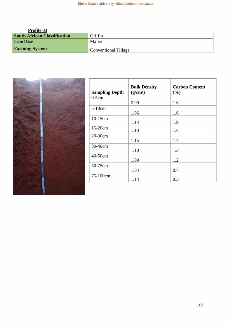
102
Profile 33
South African Classification Griffin
Land Use Maize
Farming System Conventional Tillage
Sampling Depth
Bulk Density
(g/cm³)
Carbon Content
(%)
0-5cm 0.99 1.6
5-10cm 1.06 1.6
10-15cm 1.14 1.9
15-20cm 1.13 1.6
20-30cm 1.15 1.7
30-40cm 1.10 1.3
40-50cm 1.09 1.2
50-75cm 1.04 0.7
75-100cm 1.14 0.3
Stellenbosch University https://scholar.sun.ac.za
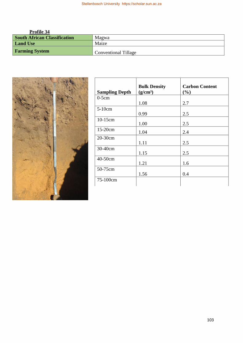
103
Profile 34
South African Classification Magwa
Land Use Maize
Farming System Conventional Tillage
Sampling Depth
Bulk Density
(g/cm³)
Carbon Content
(%)
0-5cm 1.08 2.7
5-10cm 0.99 2.5
10-15cm 1.00 2.5
15-20cm 1.04 2.4
20-30cm 1.11 2.5
30-40cm 1.15 2.5
40-50cm 1.21 1.6
50-75cm 1.56 0.4
75-100cm
Stellenbosch University https://scholar.sun.ac.za
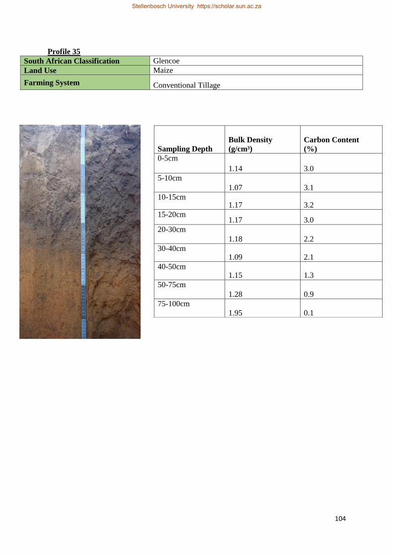
104
Profile 35
South African Classification Glencoe
Land Use Maize
Farming System Conventional Tillage
Sampling Depth
Bulk Density
(g/cm³)
Carbon Content
(%)
0-5cm
1.14 3.0
5-10cm
1.07 3.1
10-15cm 1.17 3.2
15-20cm 1.17 3.0
20-30cm
1.18 2.2
30-40cm 1.09 2.1
40-50cm 1.15 1.3
50-75cm
1.28 0.9
75-100cm
1.95 0.1
Stellenbosch University https://scholar.sun.ac.za
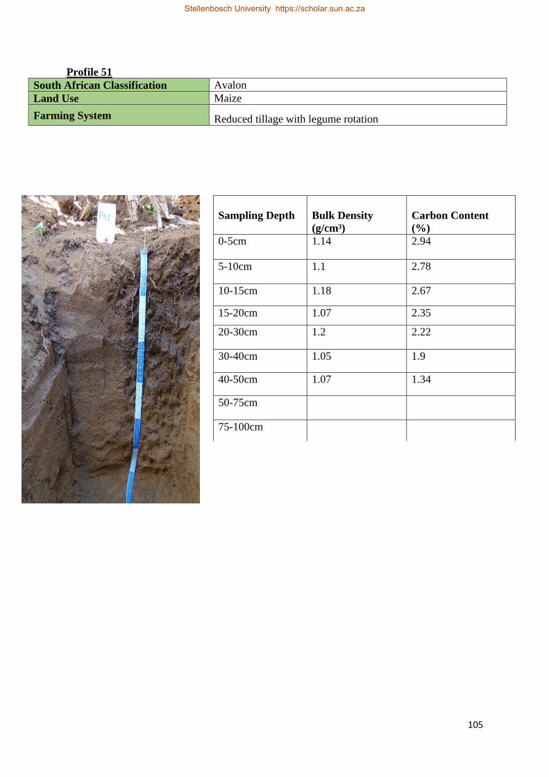
105
Profile 51
South African Classification Avalon
Land Use Maize
Farming System Reduced tillage with legume rotation
Sampling Depth
Bulk Density
(g/cm³)
Carbon Content
(%)
0-5cm 1.14 2.94
5-10cm 1.1 2.78
10-15cm 1.18 2.67
15-20cm 1.07 2.35
20-30cm 1.2 2.22
30-40cm 1.05 1.9
40-50cm 1.07 1.34
50-75cm
75-100cm
Stellenbosch University https://scholar.sun.ac.za
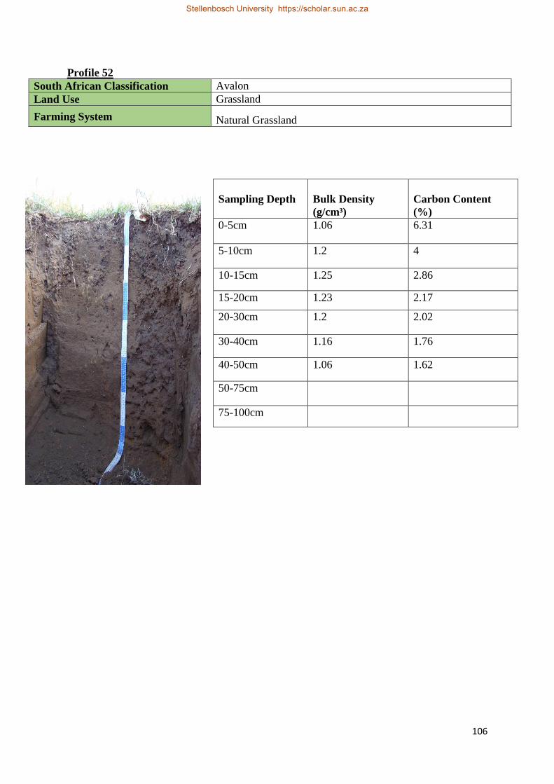
106
Profile 52
South African Classification Avalon
Land Use Grassland
Farming System Natural Grassland
Sampling Depth
Bulk Density
(g/cm³)
Carbon Content
(%)
0-5cm 1.06 6.31
5-10cm 1.2 4
10-15cm 1.25 2.86
15-20cm 1.23 2.17
20-30cm 1.2 2.02
30-40cm 1.16 1.76
40-50cm 1.06 1.62
50-75cm
75-100cm
Stellenbosch University https://scholar.sun.ac.za
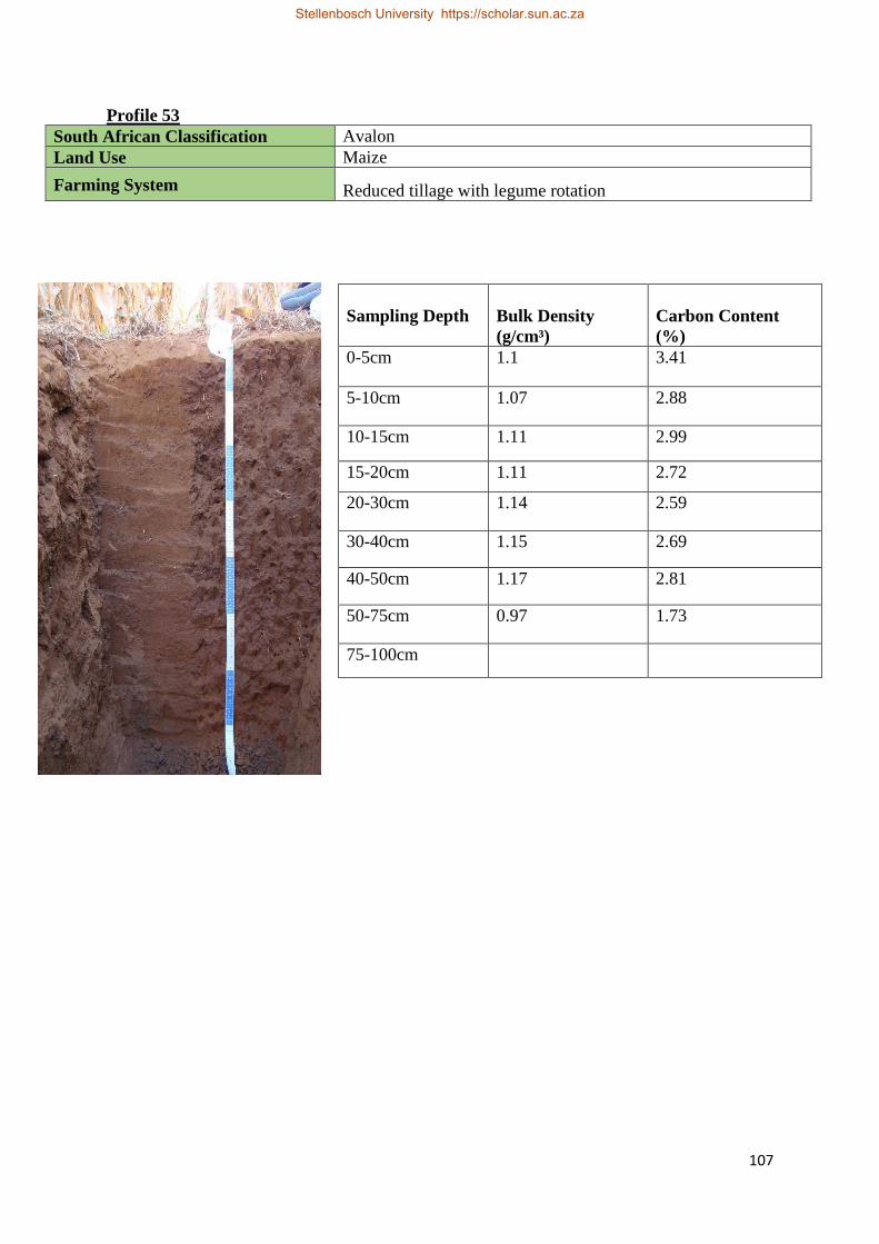
107
Profile 53
South African Classification Avalon
Land Use Maize
Farming System Reduced tillage with legume rotation
Sampling Depth
Bulk Density
(g/cm³)
Carbon Content
(%)
0-5cm 1.1 3.41
5-10cm 1.07 2.88
10-15cm 1.11 2.99
15-20cm 1.11 2.72
20-30cm 1.14 2.59
30-40cm 1.15 2.69
40-50cm 1.17 2.81
50-75cm 0.97 1.73
75-100cm
Stellenbosch University https://scholar.sun.ac.za
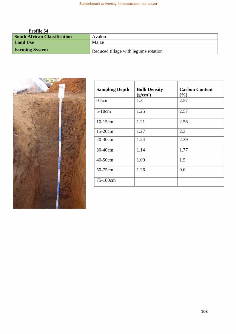
108
Profile 54
South African Classification Avalon
Land Use Maize
Farming System Reduced tillage with legume rotation
Sampling Depth
Bulk Density
(g/cm³)
Carbon Content
(%)
0-5cm 1.3 2.57
5-10cm 1.25 2.57
10-15cm 1.21 2.56
15-20cm 1.27 2.3
20-30cm 1.24 2.39
30-40cm 1.14 1.77
40-50cm 1.09 1.5
50-75cm 1.26 0.6
75-100cm
Stellenbosch University https://scholar.sun.ac.za

109
Profile 55
South African Classification Mayo
Land Use Grassland
Farming System Natural Grassland
Sampling Depth
Bulk Density
(g/cm³)
Carbon Content
(%)
0-5cm 1.11 5.86
5-10cm 1.24 3.59
10-15cm 1.19 3.21
15-20cm 1.19 2.96
20-30cm 1.36 1.89
30-40cm 1.23 1.57
40-50cm
50-75cm
75-100cm
Stellenbosch University https://scholar.sun.ac.za
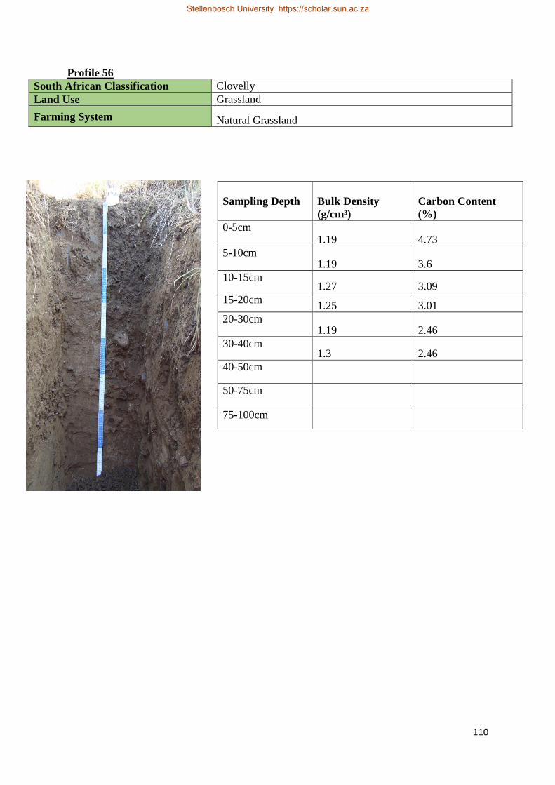
110
Profile 56
South African Classification Clovelly
Land Use Grassland
Farming System Natural Grassland
Sampling Depth
Bulk Density
(g/cm³)
Carbon Content
(%)
0-5cm 1.19 4.73
5-10cm 1.19 3.6
10-15cm 1.27 3.09
15-20cm 1.25 3.01
20-30cm 1.19 2.46
30-40cm 1.3 2.46
40-50cm
50-75cm
75-100cm
Stellenbosch University https://scholar.sun.ac.za
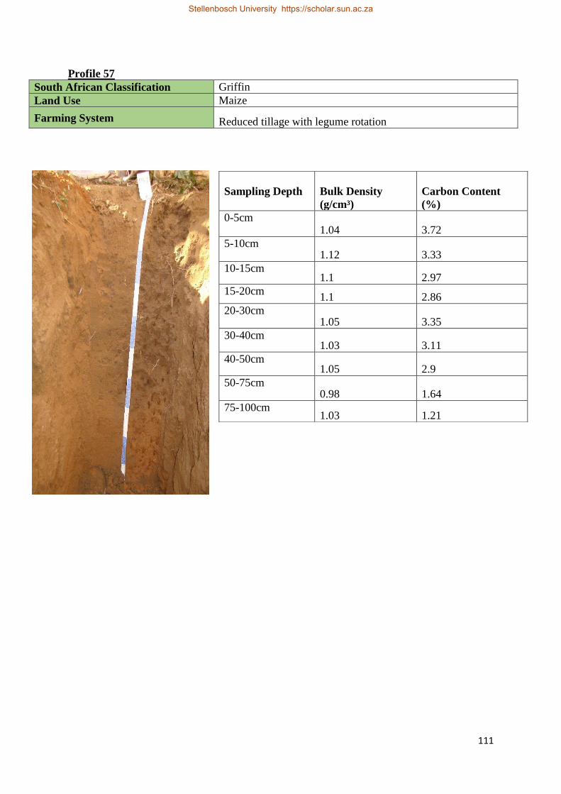
111
Profile 57
South African Classification Griffin
Land Use Maize
Farming System Reduced tillage with legume rotation
Sampling Depth
Bulk Density
(g/cm³)
Carbon Content
(%)
0-5cm 1.04 3.72
5-10cm 1.12 3.33
10-15cm 1.1 2.97
15-20cm 1.1 2.86
20-30cm 1.05 3.35
30-40cm 1.03 3.11
40-50cm 1.05 2.9
50-75cm 0.98 1.64
75-100cm 1.03 1.21
Stellenbosch University https://scholar.sun.ac.za
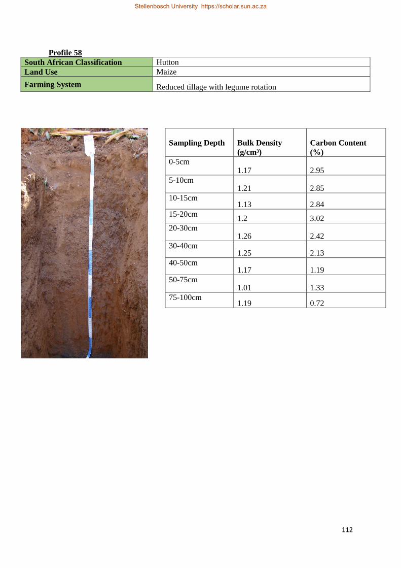
112
Profile 58
South African Classification Hutton
Land Use Maize
Farming System Reduced tillage with legume rotation
Sampling Depth
Bulk Density
(g/cm³)
Carbon Content
(%)
0-5cm 1.17 2.95
5-10cm 1.21 2.85
10-15cm 1.13 2.84
15-20cm 1.2 3.02
20-30cm 1.26 2.42
30-40cm 1.25 2.13
40-50cm 1.17 1.19
50-75cm 1.01 1.33
75-100cm 1.19 0.72
Stellenbosch University https://scholar.sun.ac.za
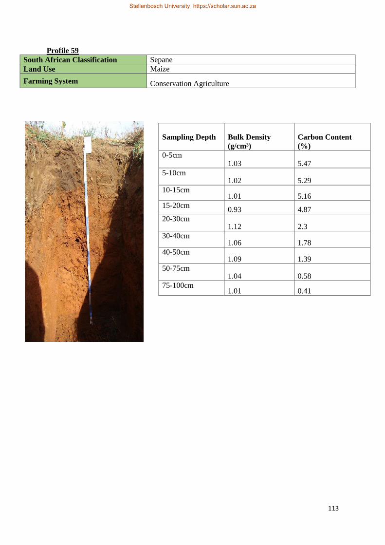
113
Profile 59
South African Classification Sepane
Land Use Maize
Farming System Conservation Agriculture
Sampling Depth
Bulk Density
(g/cm³)
Carbon Content
(%)
0-5cm 1.03 5.47
5-10cm 1.02 5.29
10-15cm 1.01 5.16
15-20cm 0.93 4.87
20-30cm 1.12 2.3
30-40cm 1.06 1.78
40-50cm 1.09 1.39
50-75cm 1.04 0.58
75-100cm 1.01 0.41
Stellenbosch University https://scholar.sun.ac.za
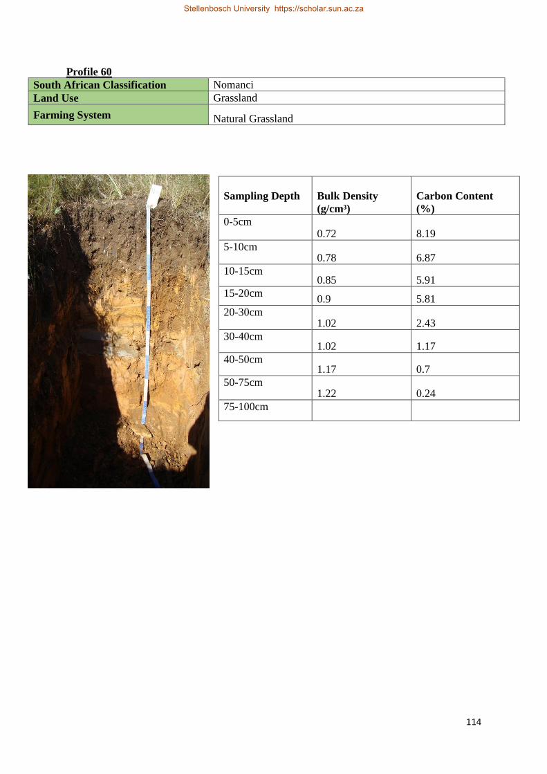
114
Profile 60
South African Classification Nomanci
Land Use Grassland
Farming System Natural Grassland
Sampling Depth
Bulk Density
(g/cm³)
Carbon Content
(%)
0-5cm 0.72 8.19
5-10cm 0.78 6.87
10-15cm 0.85 5.91
15-20cm 0.9 5.81
20-30cm 1.02 2.43
30-40cm 1.02 1.17
40-50cm 1.17 0.7
50-75cm 1.22 0.24
75-100cm
Stellenbosch University https://scholar.sun.ac.za
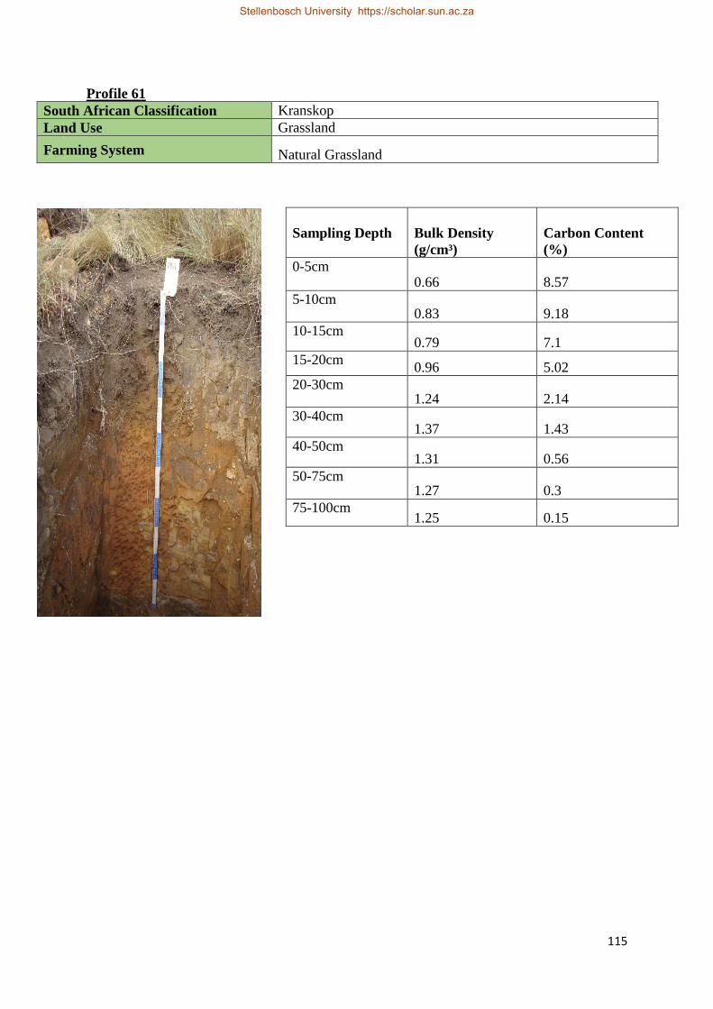
115
Profile 61
South African Classification Kranskop
Land Use Grassland
Farming System Natural Grassland
Sampling Depth
Bulk Density
(g/cm³)
Carbon Content
(%)
0-5cm 0.66 8.57
5-10cm 0.83 9.18
10-15cm 0.79 7.1
15-20cm 0.96 5.02
20-30cm 1.24 2.14
30-40cm 1.37 1.43
40-50cm 1.31 0.56
50-75cm 1.27 0.3
75-100cm 1.25 0.15
Stellenbosch University https://scholar.sun.ac.za
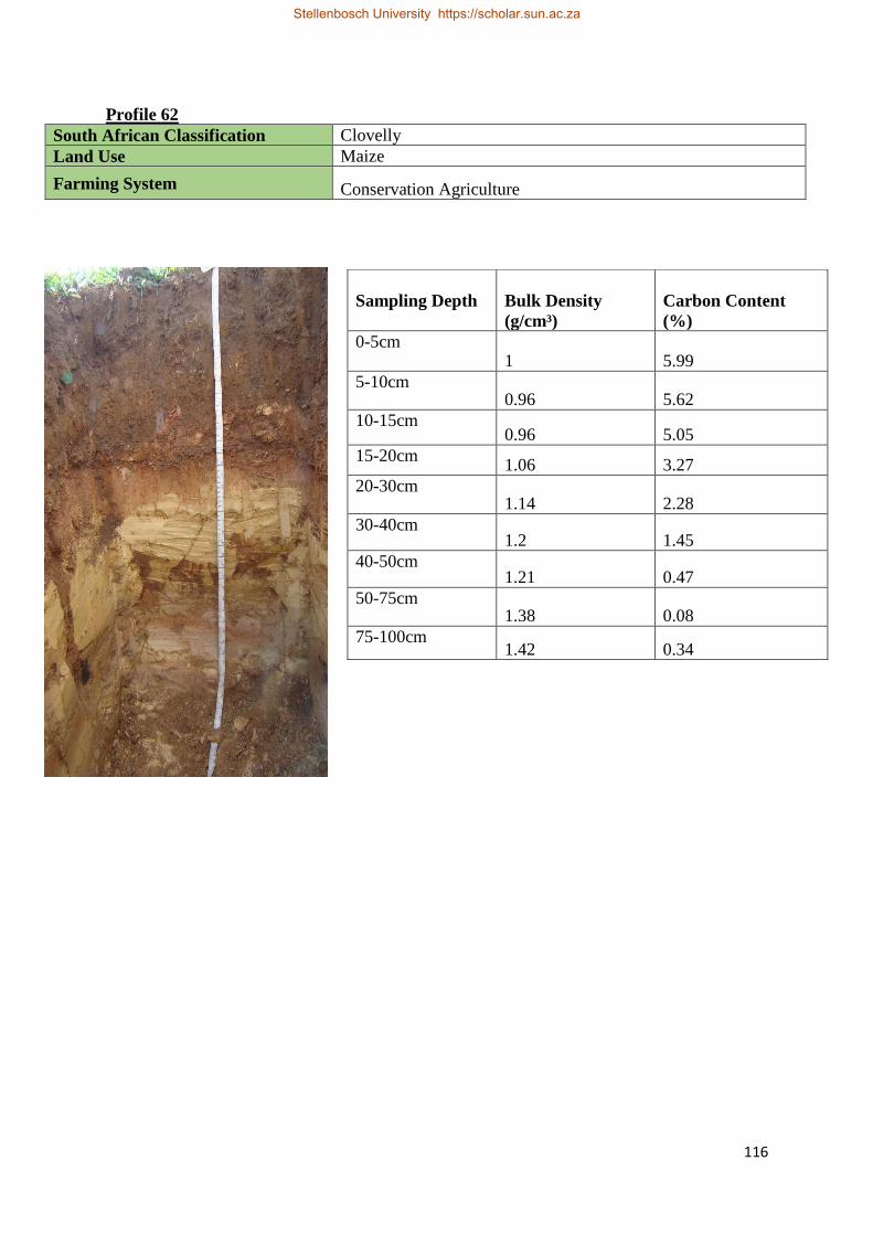
116
Profile 62
South African Classification Clovelly
Land Use Maize
Farming System Conservation Agriculture
Sampling Depth
Bulk Density
(g/cm³)
Carbon Content
(%)
0-5cm 1 5.99
5-10cm 0.96 5.62
10-15cm 0.96 5.05
15-20cm 1.06 3.27
20-30cm 1.14 2.28
30-40cm 1.2 1.45
40-50cm 1.21 0.47
50-75cm 1.38 0.08
75-100cm 1.42 0.34
Stellenbosch University https://scholar.sun.ac.za
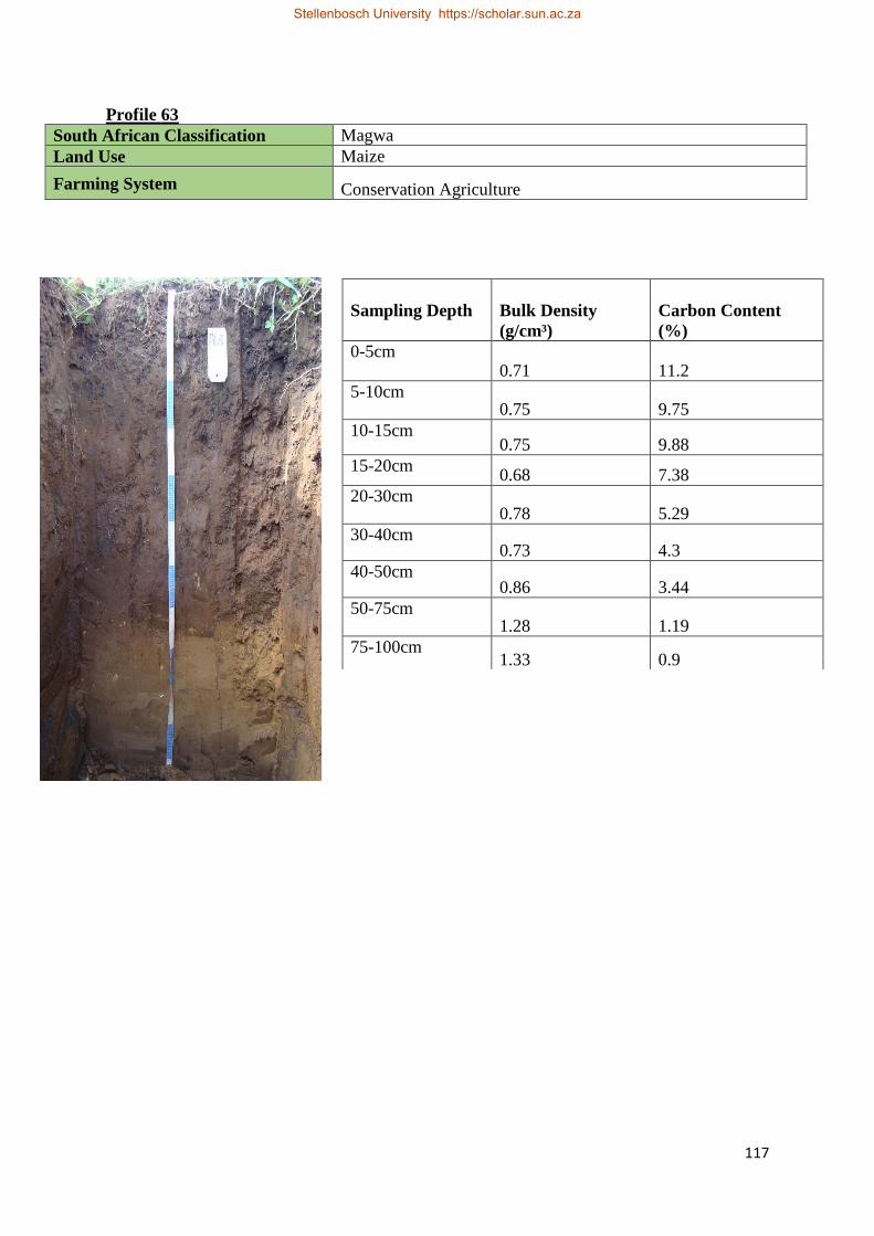
117
Profile 63
South African Classification Magwa
Land Use Maize
Farming System Conservation Agriculture
Sampling Depth
Bulk Density
(g/cm³)
Carbon Content
(%)
0-5cm 0.71 11.2
5-10cm 0.75 9.75
10-15cm 0.75 9.88
15-20cm 0.68 7.38
20-30cm 0.78 5.29
30-40cm 0.73 4.3
40-50cm 0.86 3.44
50-75cm 1.28 1.19
75-100cm 1.33 0.9
Stellenbosch University https://scholar.sun.ac.za
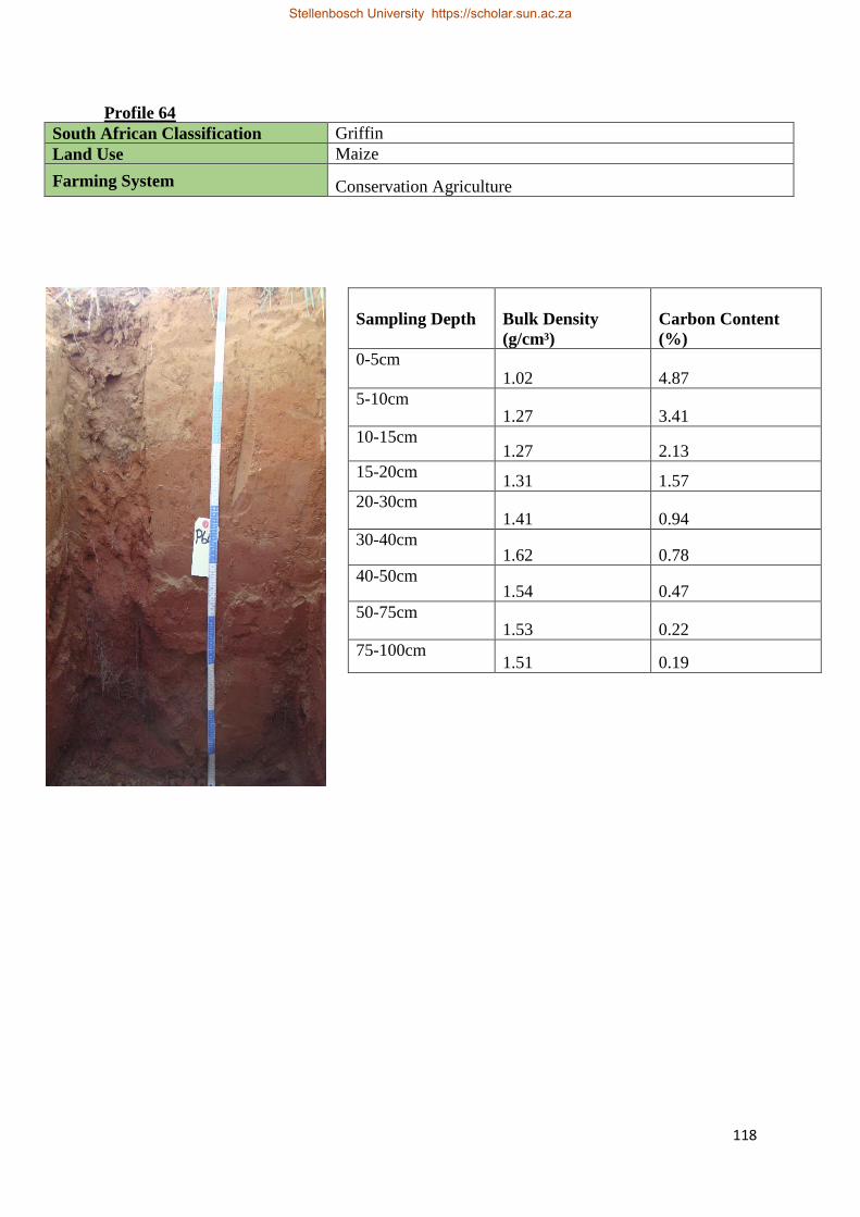
118
Profile 64
South African Classification Griffin
Land Use Maize
Farming System Conservation Agriculture
Sampling Depth
Bulk Density
(g/cm³)
Carbon Content
(%)
0-5cm 1.02 4.87
5-10cm 1.27 3.41
10-15cm 1.27 2.13
15-20cm 1.31 1.57
20-30cm 1.41 0.94
30-40cm 1.62 0.78
40-50cm 1.54 0.47
50-75cm 1.53 0.22
75-100cm 1.51 0.19
Stellenbosch University https://scholar.sun.ac.za
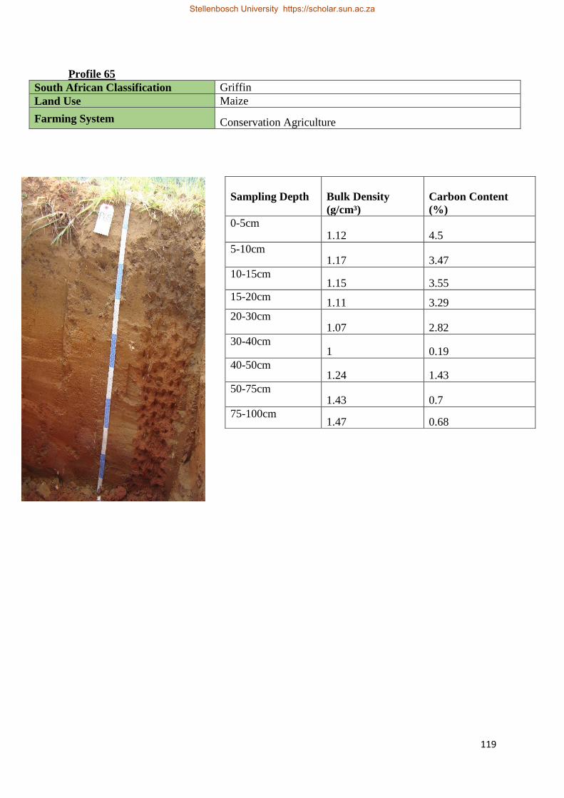
119
Profile 65
South African Classification Griffin
Land Use Maize
Farming System Conservation Agriculture
Sampling Depth
Bulk Density
(g/cm³)
Carbon Content
(%)
0-5cm 1.12 4.5
5-10cm 1.17 3.47
10-15cm 1.15 3.55
15-20cm 1.11 3.29
20-30cm 1.07 2.82
30-40cm 1 0.19
40-50cm 1.24 1.43
50-75cm 1.43 0.7
75-100cm 1.47 0.68
Stellenbosch University https://scholar.sun.ac.za

120
Profile 66
South African Classification Magwa
Land Use Maize
Farming System Conservation Agriculture
Sampling Depth
Bulk Density
(g/cm³)
Carbon Content
(%)
0-5cm 0.91 5.82
5-10cm 0.96 5.95
10-15cm 1.02 4.94
15-20cm 1.02 4.92
20-30cm 0.93 4.13
30-40cm 0.92 2.73
40-50cm 0.83 2.6
50-75cm 1.3 1.3
75-100cm 1.45 0.53
Stellenbosch University https://scholar.sun.ac.za

121
Profile 67
South African Classification Willowbrook
Land Use Maize
Farming System Conservation Agriculture
Sampling Depth
Bulk Density
(g/cm³)
Carbon Content
(%)
0-5cm 1.02 7.58
5-10cm 1.01 5.78
10-15cm 1.06 5.71
15-20cm 0.98 5.74
20-30cm 0.88 5.86
30-40cm 0.79 5.83
40-50cm 0.79 4.09
50-75cm 0.88 5.1
75-100cm
Stellenbosch University https://scholar.sun.ac.za
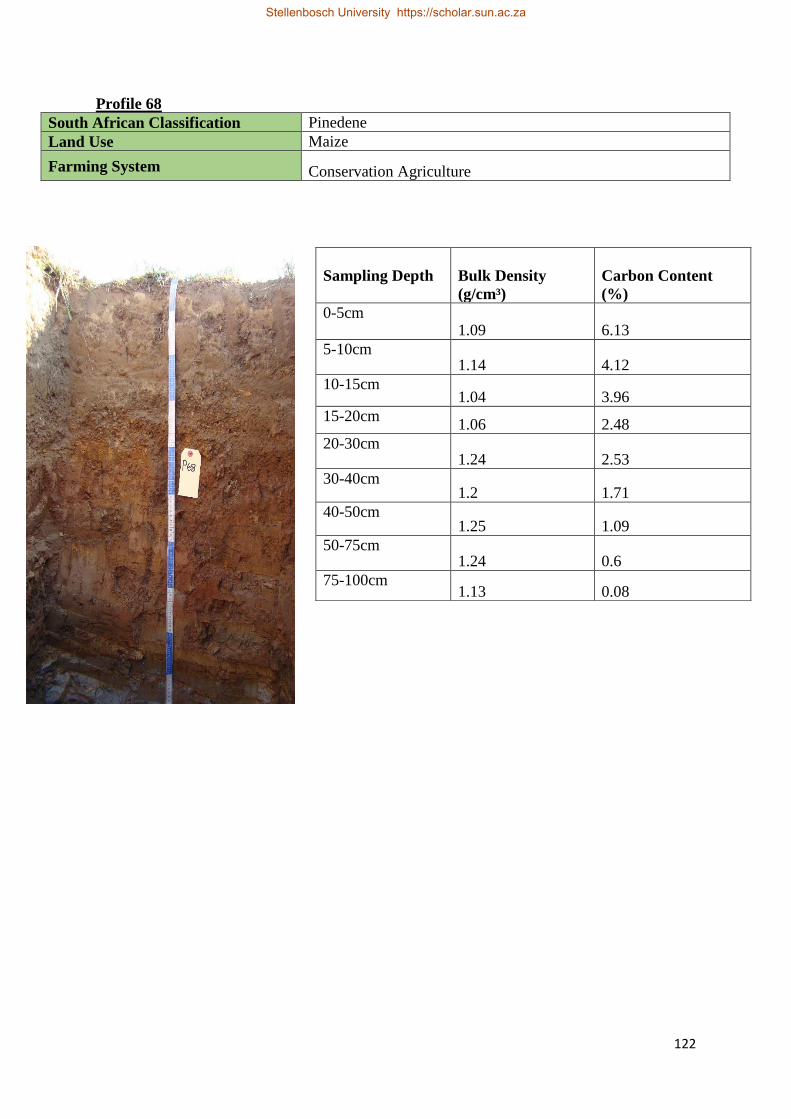
122
Profile 68
South African Classification Pinedene
Land Use Maize
Farming System Conservation Agriculture
Sampling Depth
Bulk Density
(g/cm³)
Carbon Content
(%)
0-5cm 1.09 6.13
5-10cm 1.14 4.12
10-15cm 1.04 3.96
15-20cm 1.06 2.48
20-30cm 1.24 2.53
30-40cm 1.2 1.71
40-50cm 1.25 1.09
50-75cm 1.24 0.6
75-100cm 1.13 0.08
Stellenbosch University https://scholar.sun.ac.za

123
Profile 69
South African Classification Pinedene
Land Use Maize
Farming System Conservation Agriculture
Sampling Depth
Bulk Density
(g/cm³)
Carbon Content
(%)
0-5cm 1.11 3.99
5-10cm 1.3 3
10-15cm 1.24 2.87
15-20cm 1.23 2.83
20-30cm 1.54 0.44
30-40cm
40-50cm
50-75cm
75-100cm
Stellenbosch University https://scholar.sun.ac.za
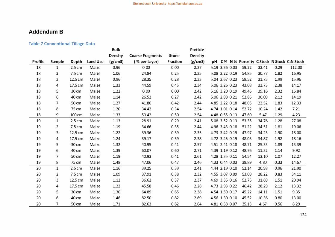
124
Addendum B
Table 7 Conventional Tillage Data
Stellenbosch University https://scholar.sun.ac.za
Stellenbosch University https://scholar.sun.ac.za
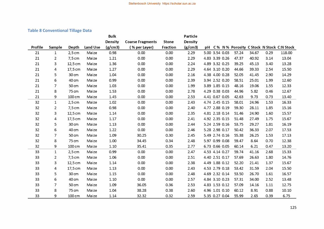
125
Table 8 Conventional Tillage Data
Stellenbosch University https://scholar.sun.ac.za
Stellenbosch University https://scholar.sun.ac.za

126
Table 9 Conventional Tillage Data
Stellenbosch University https://scholar.sun.ac.za
Stellenbosch University https://scholar.sun.ac.za
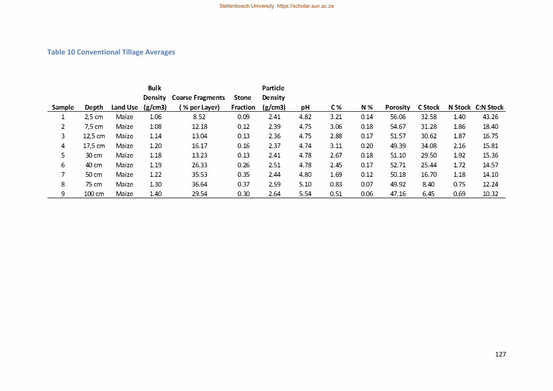
127
Table 10 Conventional Tillage Averages
Stellenbosch University https://scholar.sun.ac.za
Stellenbosch University https://scholar.sun.ac.za
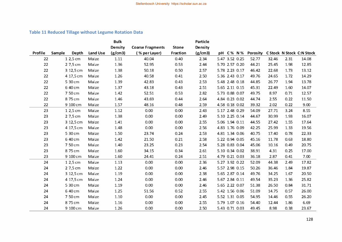
128
Table 11 Reduced Tillage without Legume Rotation Data
Stellenbosch University https://scholar.sun.ac.za
Stellenbosch University https://scholar.sun.ac.za
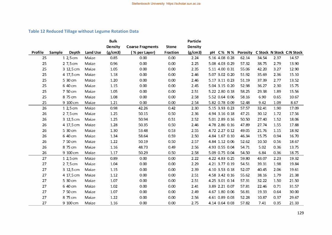
129
Table 12 Reduced Tillage without Legume Rotation Data
Stellenbosch University https://scholar.sun.ac.za
Stellenbosch University https://scholar.sun.ac.za
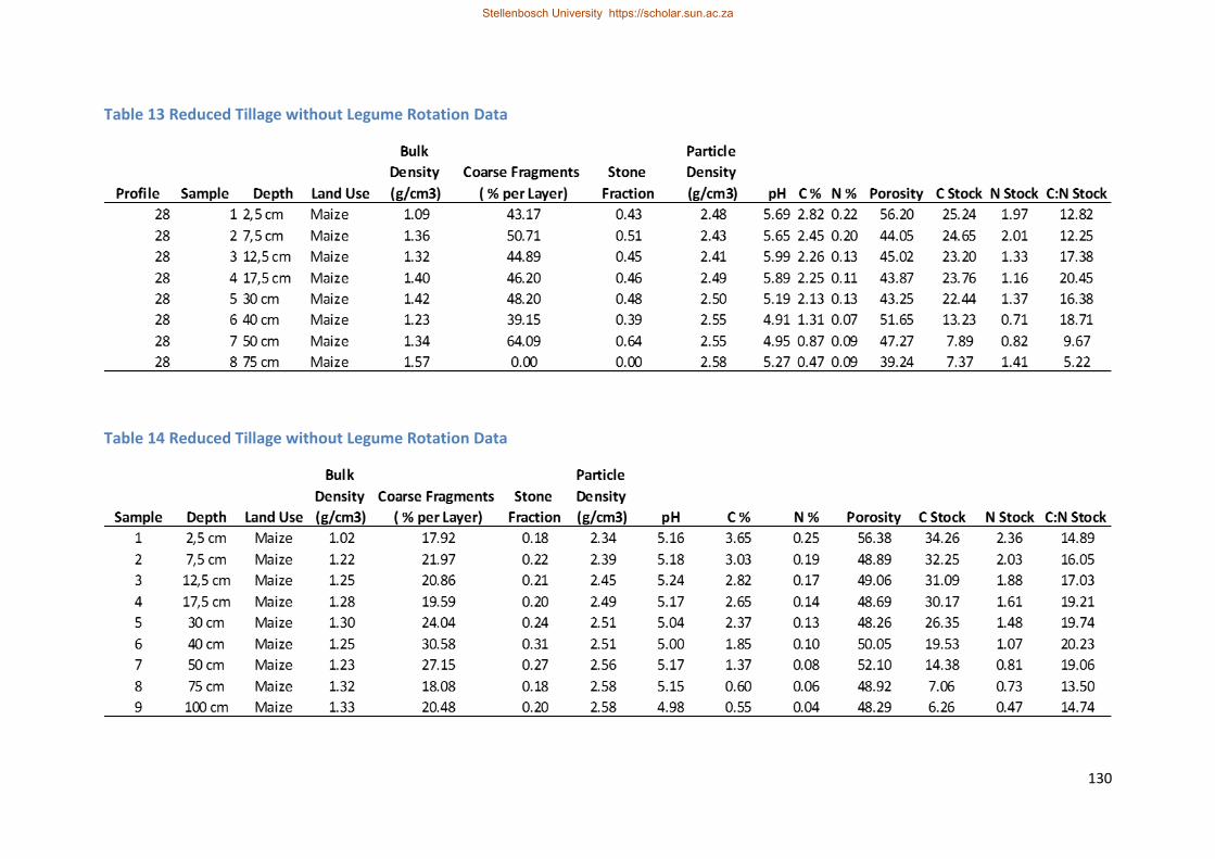
130
Table 13 Reduced Tillage without Legume Rotation Data
Table 14 Reduced Tillage without Legume Rotation Data
Stellenbosch University https://scholar.sun.ac.za
Stellenbosch University https://scholar.sun.ac.za
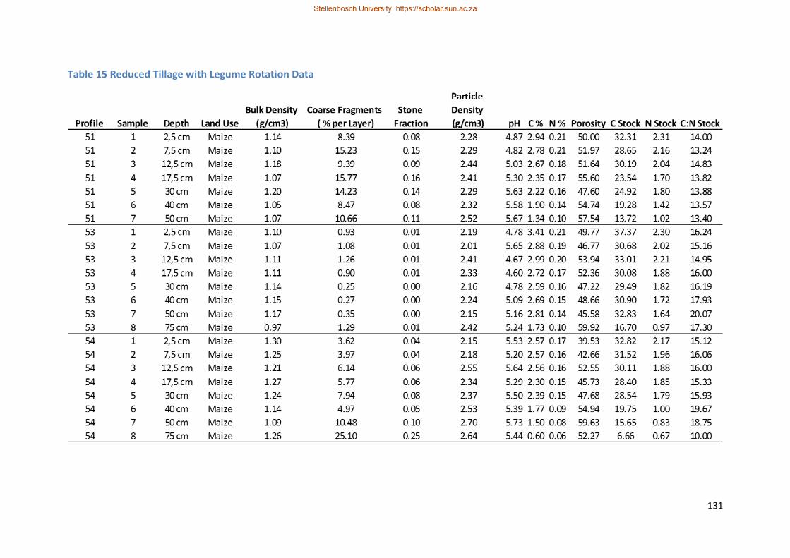
131
Table 15 Reduced Tillage with Legume Rotation Data
Stellenbosch University https://scholar.sun.ac.za
Stellenbosch University https://scholar.sun.ac.za
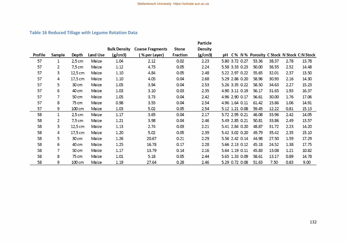
132
Table 16 Reduced Tillage with Legume Rotation Data
Stellenbosch University https://scholar.sun.ac.za
Stellenbosch University https://scholar.sun.ac.za
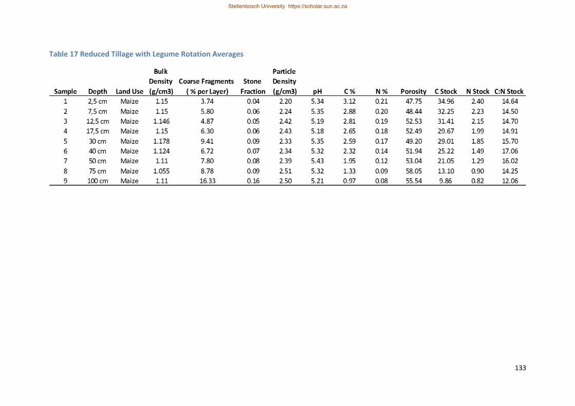
133
Table 17 Reduced Tillage with Legume Rotation Averages
Stellenbosch University https://scholar.sun.ac.za
Stellenbosch University https://scholar.sun.ac.za

134
Table 18 Conservation Agriculture Data
Stellenbosch University https://scholar.sun.ac.za
Stellenbosch University https://scholar.sun.ac.za
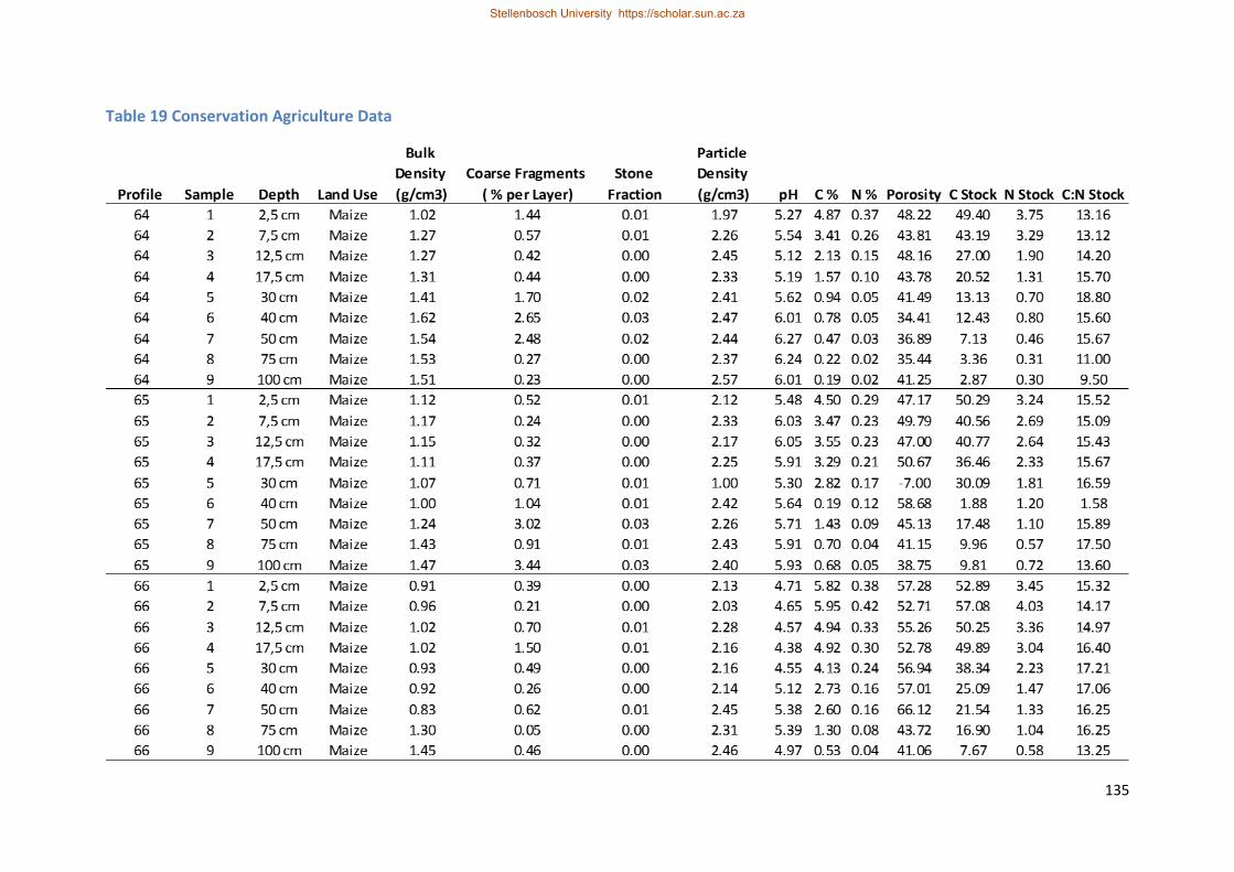
135
Table 19 Conservation Agriculture Data
Stellenbosch University https://scholar.sun.ac.za
Stellenbosch University https://scholar.sun.ac.za

136
Table 20 Conservation Agriculture Data
Stellenbosch University https://scholar.sun.ac.za
Stellenbosch University https://scholar.sun.ac.za
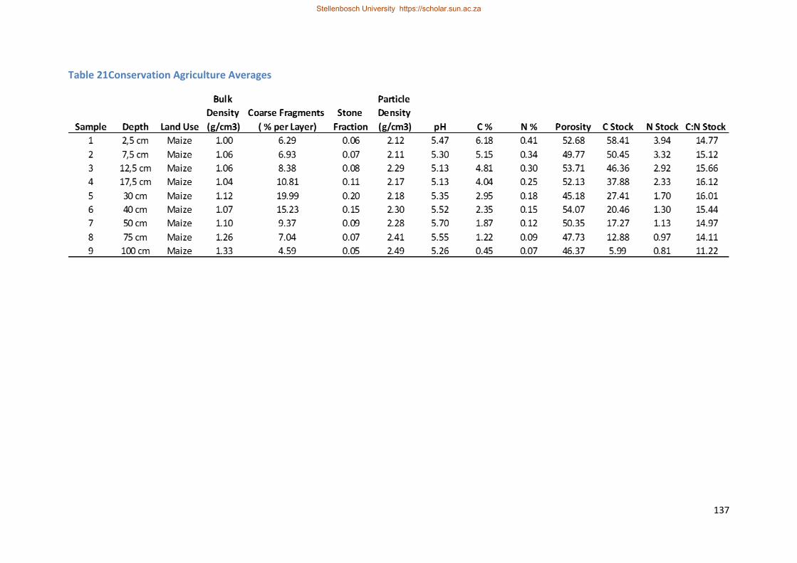
137
Table 21Conservation Agriculture Averages
Stellenbosch University https://scholar.sun.ac.za
Stellenbosch University https://scholar.sun.ac.za
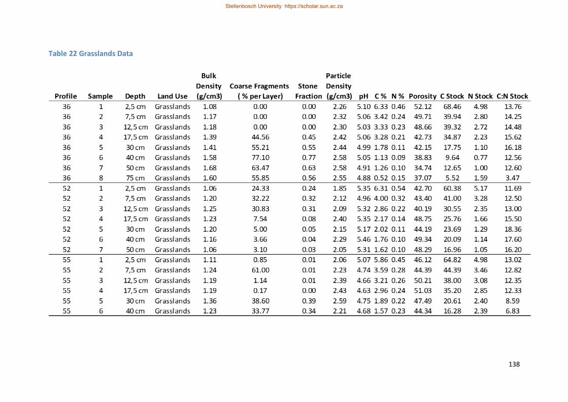
138
Table 22 Grasslands Data
Stellenbosch University https://scholar.sun.ac.za
Stellenbosch University https://scholar.sun.ac.za
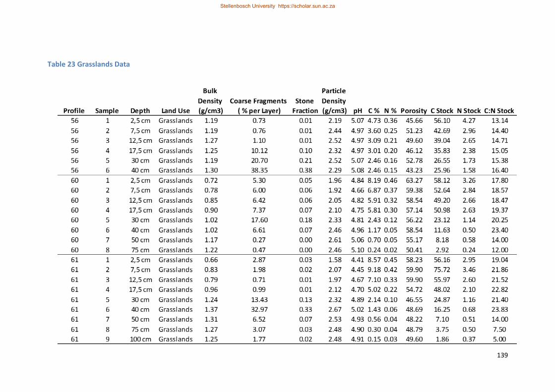
139
Table 23 Grasslands Data
Stellenbosch University https://scholar.sun.ac.za
Stellenbosch University https://scholar.sun.ac.za
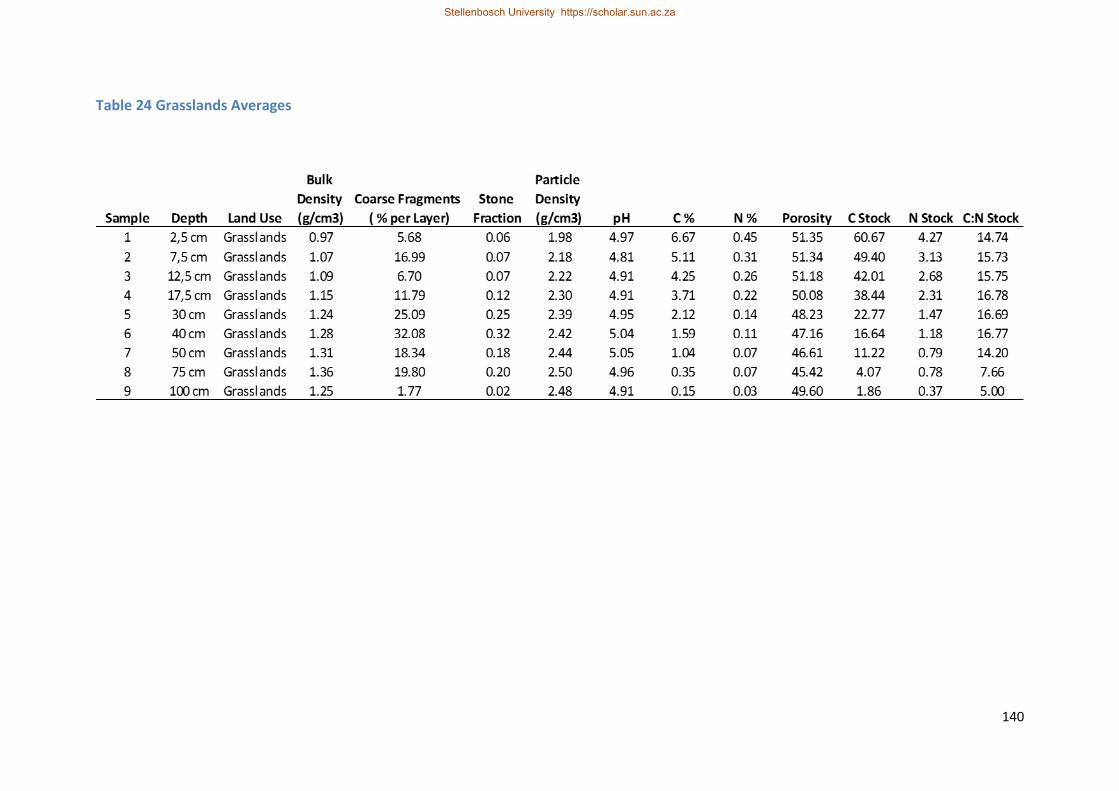
140
Table 24 Grasslands Averages
Stellenbosch University https://scholar.sun.ac.za
Stellenbosch University https://scholar.sun.ac.za
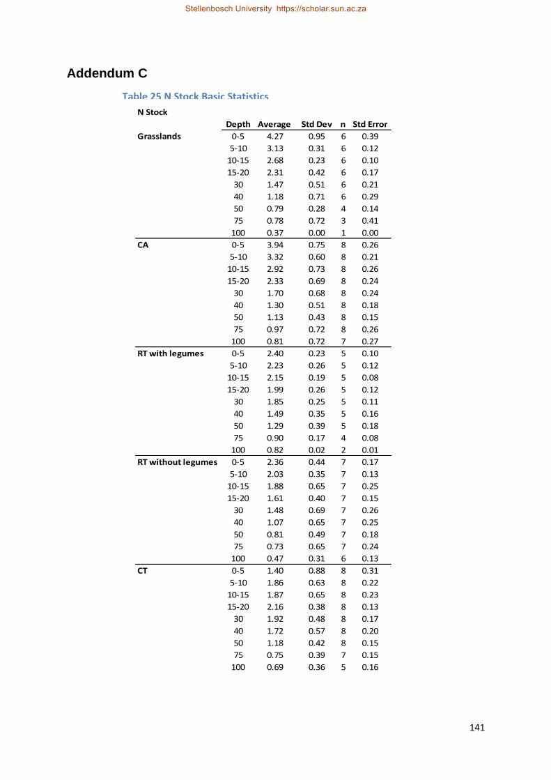
141
N Stock
Depth Average Std Dev n Std Error
Grasslands 0-5 4.27 0.95 6 0.39
5-10 3.13 0.31 6 0.12
10-15 2.68 0.23 6 0.10
15-20 2.31 0.42 6 0.17
30 1.47 0.51 6 0.21
40 1.18 0.71 6 0.29
50 0.79 0.28 4 0.14
75 0.78 0.72 3 0.41
100 0.37 0.00 1 0.00
CA 0-5 3.94 0.75 8 0.26
5-10 3.32 0.60 8 0.21
10-15 2.92 0.73 8 0.26
15-20 2.33 0.69 8 0.24
30 1.70 0.68 8 0.24
40 1.30 0.51 8 0.18
50 1.13 0.43 8 0.15
75 0.97 0.72 8 0.26
100 0.81 0.72 7 0.27
RT with legumes 0-5 2.40 0.23 5 0.10
5-10 2.23 0.26 5 0.12
10-15 2.15 0.19 5 0.08
15-20 1.99 0.26 5 0.12
30 1.85 0.25 5 0.11
40 1.49 0.35 5 0.16
50 1.29 0.39 5 0.18
75 0.90 0.17 4 0.08
100 0.82 0.02 2 0.01
RT without legumes 0-5 2.36 0.44 7 0.17
5-10 2.03 0.35 7 0.13
10-15 1.88 0.65 7 0.25
15-20 1.61 0.40 7 0.15
30 1.48 0.69 7 0.26
40 1.07 0.65 7 0.25
50 0.81 0.49 7 0.18
75 0.73 0.65 7 0.24
100 0.47 0.31 6 0.13
CT 0-5 1.40 0.88 8 0.31
5-10 1.86 0.63 8 0.22
10-15 1.87 0.65 8 0.23
15-20 2.16 0.38 8 0.13
30 1.92 0.48 8 0.17
40 1.72 0.57 8 0.20
50 1.18 0.42 8 0.15
75 0.75 0.39 7 0.15
100 0.69 0.36 5 0.16
Table 25 N Stock Basic Statistics
Addendum C
Stellenbosch University https://scholar.sun.ac.za
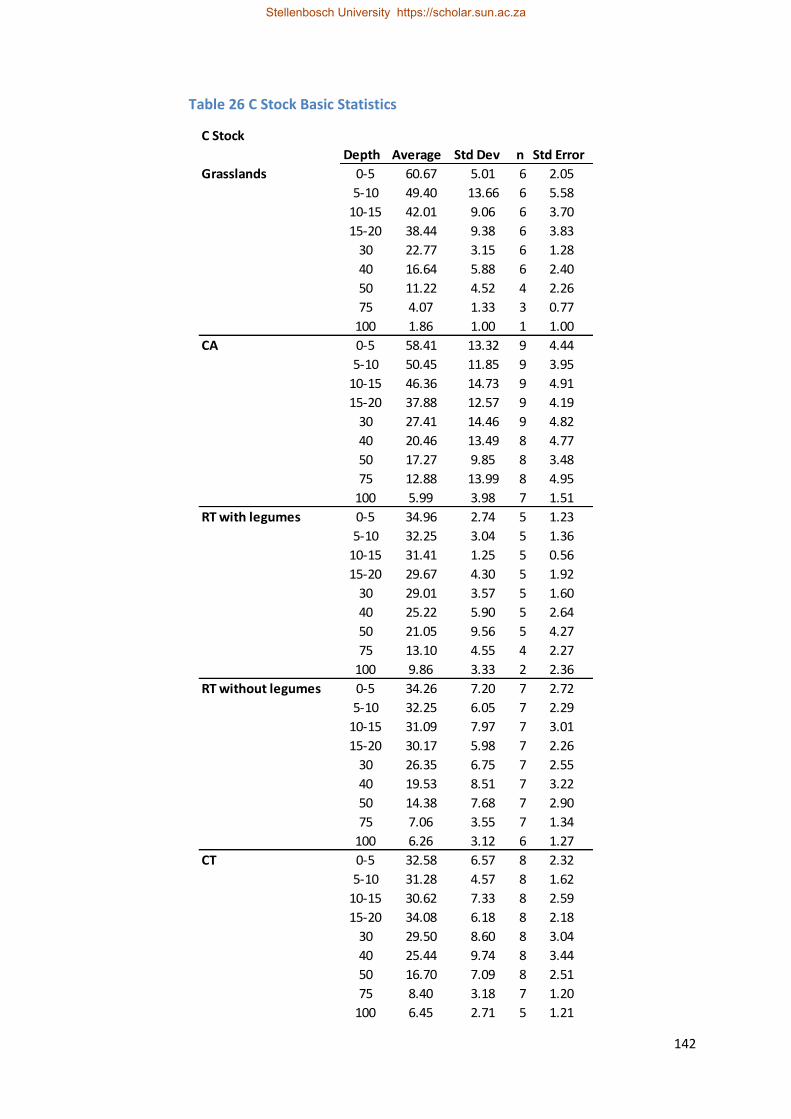
142
C Stock
Depth Average Std Dev n Std Error
Grasslands 0-5 60.67 5.01 6 2.05
5-10 49.40 13.66 6 5.58
10-15 42.01 9.06 6 3.70
15-20 38.44 9.38 6 3.83
30 22.77 3.15 6 1.28
40 16.64 5.88 6 2.40
50 11.22 4.52 4 2.26
75 4.07 1.33 3 0.77
100 1.86 1.00 1 1.00
CA 0-5 58.41 13.32 9 4.44
5-10 50.45 11.85 9 3.95
10-15 46.36 14.73 9 4.91
15-20 37.88 12.57 9 4.19
30 27.41 14.46 9 4.82
40 20.46 13.49 8 4.77
50 17.27 9.85 8 3.48
75 12.88 13.99 8 4.95
100 5.99 3.98 7 1.51
RT with legumes 0-5 34.96 2.74 5 1.23
5-10 32.25 3.04 5 1.36
10-15 31.41 1.25 5 0.56
15-20 29.67 4.30 5 1.92
30 29.01 3.57 5 1.60
40 25.22 5.90 5 2.64
50 21.05 9.56 5 4.27
75 13.10 4.55 4 2.27
100 9.86 3.33 2 2.36
RT without legumes 0-5 34.26 7.20 7 2.72
5-10 32.25 6.05 7 2.29
10-15 31.09 7.97 7 3.01
15-20 30.17 5.98 7 2.26
30 26.35 6.75 7 2.55
40 19.53 8.51 7 3.22
50 14.38 7.68 7 2.90
75 7.06 3.55 7 1.34
100 6.26 3.12 6 1.27
CT 0-5 32.58 6.57 8 2.32
5-10 31.28 4.57 8 1.62
10-15 30.62 7.33 8 2.59
15-20 34.08 6.18 8 2.18
30 29.50 8.60 8 3.04
40 25.44 9.74 8 3.44
50 16.70 7.09 8 2.51
75 8.40 3.18 7 1.20
100 6.45 2.71 5 1.21
Table 26 C Stock Basic Statistics
Stellenbosch University https://scholar.sun.ac.za

143
C:N Ratio
Depth Average Std Dev n Std Error
Grasslands 0-5 14.74 2.96 6 1.21
5-10 15.73 3.70 6 1.51
10-15 15.75 3.53 6 1.44
15-20 16.78 3.71 6 1.52
30 16.69 4.59 6 1.87
40 16.77 6.50 6 2.65
50 14.20 1.49 4 0.74
75 7.66 4.27 3 2.46
100 5.00 1.00 1 1.00
CA 0-5 14.77 1.38 9 0.46
5-10 15.12 1.60 9 0.53
10-15 15.66 1.42 9 0.47
15-20 16.12 1.52 9 0.51
30 16.01 5.03 9 1.68
40 15.44 6.41 8 2.26
50 14.97 5.03 8 1.78
75 14.11 8.73 8 3.09
100 11.22 6.16 7 2.33
RT with legumes 0-5 14.64 1.04 5 0.46
5-10 14.50 1.15 5 0.52
10-15 14.70 0.93 5 0.42
15-20 14.91 0.86 5 0.38
30 15.70 1.26 5 0.56
40 17.06 2.27 5 1.02
50 16.02 3.84 5 1.72
75 14.25 3.06 4 1.53
100 12.06 4.33 2 3.06
RT without legumes 0-5 14.89 3.61 7 1.36
5-10 16.05 3.18 7 1.20
10-15 17.03 2.96 7 1.12
15-20 19.21 3.93 7 1.49
30 19.74 6.32 7 2.39
40 20.23 6.28 7 2.37
50 19.06 7.26 7 2.74
75 13.50 8.17 7 3.09
100 14.74 7.33 6 2.99
CT 0-5 43.26 44.48 8 15.73
5-10 18.40 6.64 8 2.35
10-15 16.75 2.30 8 0.81
15-20 15.81 1.62 8 0.57
30 15.36 2.96 8 1.05
40 14.57 2.96 8 1.04
50 14.10 4.57 8 1.61
75 12.24 2.74 7 1.04
100 10.32 4.50 5 2.01
Table 27 C:N Ratio Basic Statistics
Stellenbosch University https://scholar.sun.ac.za
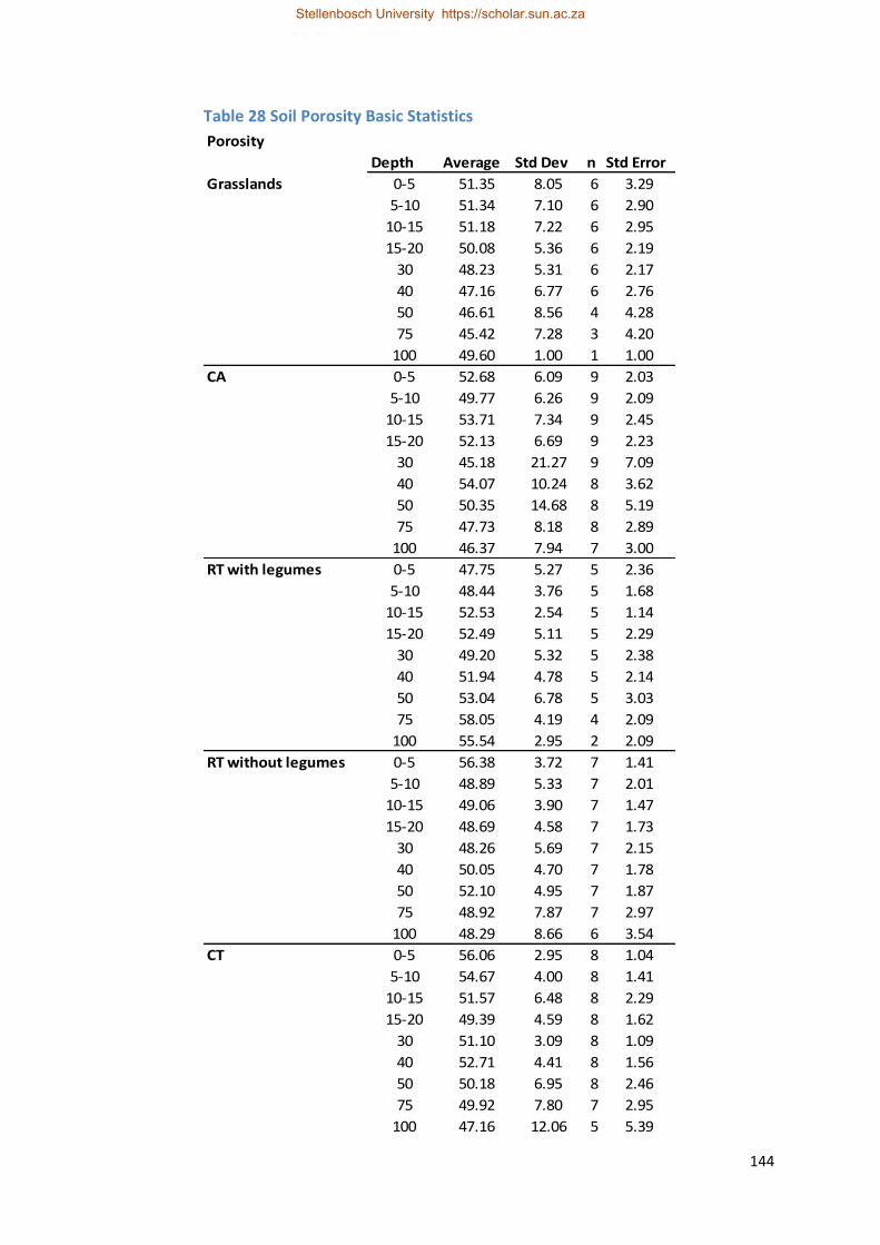
144
Porosity
Depth Average Std Dev n Std Error
Grasslands 0-5 51.35 8.05 6 3.29
5-10 51.34 7.10 6 2.90
10-15 51.18 7.22 6 2.95
15-20 50.08 5.36 6 2.19
30 48.23 5.31 6 2.17
40 47.16 6.77 6 2.76
50 46.61 8.56 4 4.28
75 45.42 7.28 3 4.20
100 49.60 1.00 1 1.00
CA 0-5 52.68 6.09 9 2.03
5-10 49.77 6.26 9 2.09
10-15 53.71 7.34 9 2.45
15-20 52.13 6.69 9 2.23
30 45.18 21.27 9 7.09
40 54.07 10.24 8 3.62
50 50.35 14.68 8 5.19
75 47.73 8.18 8 2.89
100 46.37 7.94 7 3.00
RT with legumes 0-5 47.75 5.27 5 2.36
5-10 48.44 3.76 5 1.68
10-15 52.53 2.54 5 1.14
15-20 52.49 5.11 5 2.29
30 49.20 5.32 5 2.38
40 51.94 4.78 5 2.14
50 53.04 6.78 5 3.03
75 58.05 4.19 4 2.09
100 55.54 2.95 2 2.09
RT without legumes 0-5 56.38 3.72 7 1.41
5-10 48.89 5.33 7 2.01
10-15 49.06 3.90 7 1.47
15-20 48.69 4.58 7 1.73
30 48.26 5.69 7 2.15
40 50.05 4.70 7 1.78
50 52.10 4.95 7 1.87
75 48.92 7.87 7 2.97
100 48.29 8.66 6 3.54
CT 0-5 56.06 2.95 8 1.04
5-10 54.67 4.00 8 1.41
10-15 51.57 6.48 8 2.29
15-20 49.39 4.59 8 1.62
30 51.10 3.09 8 1.09
40 52.71 4.41 8 1.56
50 50.18 6.95 8 2.46
75 49.92 7.80 7 2.95
100 47.16 12.06 5 5.39
Table 28 Soil Porosity Basic Statistics
Stellenbosch University https://scholar.sun.ac.za

145
Addendum D
Table 29: Data for chapter 4 profiles
Profile Depth Land Use Tillage Methods TMB C % N % WSA % C/N pH (H2O) Bulk density (g.cm-3) Particle density (g.cm-3) Porosity (%)
36 1 Grassland None 3.52 6.33 0.46 97.25 13.76 4.51 1.08 2.26 52.10
36 4 Grassland None 2.64 3.28 0.21 96.00 15.62 5.06 1.39 2.42 42.73
36 7 Grassland None 1.76 1.26 0.10 51.00 12.60 4.91 1.68 2.58 34.72
55 1 Grassland None 3.23 5.86 0.45 63.75 13.02 5.07 1.11 2.06 46.12
55 4 Grassland None 0.59 2.96 0.24 96.50 12.33 4.63 1.19 2.43 51.03
55 7 Grassland None 4.11 1.57 0.23 92.50 6.83 4.68 1.23 2.21 44.34
60 1 Grassland None 0.00 8.19 0.46 91.00 17.80 4.84 0.72 1.96 63.27
60 4 Grassland None 2.64 5.81 0.30 90.25 19.37 4.75 0.90 2.10 57.14
60 7 Grassland None 0.59 0.07 0.05 98.50 1.40 5.06 1.17 2.61 55.17
63 1 Cultivated Conservation Till 14.08 11.24 0.69 93.75 16.29 5.55 0.71 2.07 65.70
63 4 Cultivated Conservation Till 5.87 7.38 0.45 98.75 16.40 5.49 0.68 2.02 66.34
63 7 Cultivated Conservation Till 0.59 3.44 0.19 91.00 18.11 5.53 0.86 2.21 61.09
65 1 Cultivated Conservation Till 0.59 4.50 0.29 89.00 15.52 5.48 1.12 2.12 47.17
65 4 Cultivated Conservation Till 2.64 3.29 0.21 96.50 15.67 5.91 1.11 2.25 50.67
65 7 Cultivated Conservation Till 6.75 1.43 0.09 98.75 15.89 5.71 1.24 2.26 45.13
22 1 Cultivated Reduced Till 2.12 3.52 0.27 96.50 13.04 5.47 1.11 2.34 52.77
22 4 Cultivated Reduced Till 3.76 2.43 0.20 96.50 12.15 5.36 1.26 2.50 49.76
22 7 Cultivated Reduced Till 1.29 0.88 0.15 88.50 5.87 5.73 1.42 2.82 49.73
58 1 Cultivated Reduced Till 1.76 2.95 0.21 81.50 14.05 5.72 1.17 2.17 46.08
58 4 Cultivated Reduced Till 4.11 3.02 0.20 88.25 15.10 5.42 1.20 2.39 49.79
58 7 Cultivated Reduced Till 8.80 1.91 0.11 87.75 17.36 5.64 1.17 2.16 45.83
32 1 Cultivated Conventional Till 2.05 2.45 0.15 86.75 16.33 6.40 1.02 2.43 58.00
32 4 Cultivated Conventional Till 5.28 2.35 0.15 97.50 15.67 5.04 1.17 2.41 51.47
32 7 Cultivated Conventional Till 4.11 2.74 0.16 89.50 17.13 4.91 1.10 2.45 55.38
35 1 Cultivated Conventional Till 0.29 3.29 0.21 89.00 15.67 4.74 1.14 2.43 52.97
35 4 Cultivated Conventional Till 0.29 3.96 0.24 74.50 16.50 4.92 1.17 2.41 51.60
35 7 Cultivated Conventional Till 0.29 1.12 0.08 92.50 14.00 5.49 1.15 2.45 53.26
Stellenbosch University https://scholar.sun.ac.za
Stellenbosch University https://scholar.sun.ac.za
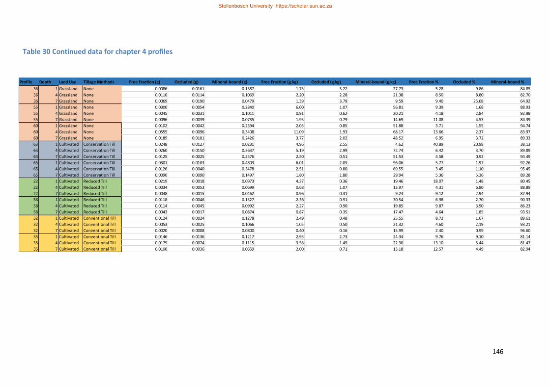
146
Profile Depth Land Use Tillage Methods Free Fraction (g) Occluded (g) Mineral-bound (g) Free Fraction (g.kg) Occluded (g.kg) Mineral-bound (g.kg) Free Fraction % Occluded % Mineral-bound %
36 1 Grassland None 0.0086 0.0161 0.1387 1.73 3.22 27.73 5.28 9.86 84.85
36 4 Grassland None 0.0110 0.0114 0.1069 2.20 2.28 21.38 8.50 8.80 82.70
36 7 Grassland None 0.0069 0.0190 0.0479 1.39 3.79 9.59 9.40 25.68 64.92
55 1 Grassland None 0.0300 0.0054 0.2840 6.00 1.07 56.81 9.39 1.68 88.93
55 4 Grassland None 0.0045 0.0031 0.1011 0.91 0.62 20.21 4.18 2.84 92.98
55 7 Grassland None 0.0096 0.0039 0.0735 1.93 0.79 14.69 11.08 4.53 84.39
60 1 Grassland None 0.0102 0.0042 0.2594 2.03 0.85 51.88 3.71 1.55 94.74
60 4 Grassland None 0.0555 0.0096 0.3408 11.09 1.93 68.17 13.66 2.37 83.97
60 7 Grassland None 0.0189 0.0101 0.2426 3.77 2.02 48.52 6.95 3.72 89.33
63 1 Cultivated Conservation Till 0.0248 0.0127 0.0231 4.96 2.55 4.62 40.89 20.98 38.13
63 4 Cultivated Conservation Till 0.0260 0.0150 0.3637 5.19 2.99 72.74 6.42 3.70 89.89
63 7 Cultivated Conservation Till 0.0125 0.0025 0.2576 2.50 0.51 51.53 4.58 0.93 94.49
65 1 Cultivated Conservation Till 0.0301 0.0103 0.4803 6.01 2.05 96.06 5.77 1.97 92.26
65 4 Cultivated Conservation Till 0.0126 0.0040 0.3478 2.51 0.80 69.55 3.45 1.10 95.45
65 7 Cultivated Conservation Till 0.0090 0.0090 0.1497 1.80 1.80 29.94 5.36 5.36 89.28
22 1 Cultivated Reduced Till 0.0219 0.0018 0.0973 4.37 0.36 19.46 18.07 1.48 80.45
22 4 Cultivated Reduced Till 0.0034 0.0053 0.0699 0.68 1.07 13.97 4.31 6.80 88.89
22 7 Cultivated Reduced Till 0.0048 0.0015 0.0462 0.96 0.31 9.24 9.12 2.94 87.94
58 1 Cultivated Reduced Till 0.0118 0.0046 0.1527 2.36 0.91 30.54 6.98 2.70 90.33
58 4 Cultivated Reduced Till 0.0114 0.0045 0.0992 2.27 0.90 19.85 9.87 3.90 86.23
58 7 Cultivated Reduced Till 0.0043 0.0017 0.0874 0.87 0.35 17.47 4.64 1.85 93.51
32 1 Cultivated Conventional Till 0.0124 0.0024 0.1278 2.49 0.48 25.55 8.72 1.67 89.61
32 4 Cultivated Conventional Till 0.0053 0.0025 0.1066 1.05 0.50 21.32 4.60 2.19 93.21
32 7 Cultivated Conventional Till 0.0020 0.0008 0.0800 0.40 0.16 15.99 2.40 0.99 96.60
35 1 Cultivated Conventional Till 0.0146 0.0136 0.1217 2.93 2.73 24.34 9.76 9.10 81.14
35 4 Cultivated Conventional Till 0.0179 0.0074 0.1115 3.58 1.49 22.30 13.10 5.44 81.47
35 7 Cultivated Conventional Till 0.0100 0.0036 0.0659 2.00 0.71 13.18 12.57 4.49 82.94
Table 30 Continued data for chapter 4 profiles
Stellenbosch University https://scholar.sun.ac.za
Stellenbosch University https://scholar.sun.ac.za

147
Profile Depth Land Use Tillage Methods Clay Silt Sand CEC Na (cmol/kg) K (cmol/kg) Ca (cmol/kg) Mg (cmol/kg) S-value Base saturation (%)
36 1 Grassland None 27.30 43.10 32.20 15.11 0.06 0.56 5.78 3.34 9.74 64.48
36 4 Grassland None 30.30 38.20 23.00 15.90 0.05 0.13 3.58 2.66 6.42 40.37
36 7 Grassland None 10.48 25.78 63.74 15.03 0.04 0.14 2.86 1.04 4.08 27.15
55 1 Grassland None 40.50 42.30 9.10 15.40 0.16 1.30 5.26 5.13 11.85 76.91
55 4 Grassland None 52.50 32.80 6.60 15.26 0.14 0.82 2.00 2.66 5.61 36.77
55 7 Grassland None 54.70 28.40 7.30 25.41 0.24 0.60 1.91 3.73 6.48 25.51
60 1 Grassland None 21.60 33.70 39.00 21.65 0.12 0.83 2.31 1.05 4.31 19.89
60 4 Grassland None 31.60 42.00 19.10 14.45 0.12 0.24 0.55 0.46 1.37 9.46
60 7 Grassland None 15.00 28.50 52.50 4.98 0.10 0.17 0.40 0.50 1.17 23.57
63 1 Cultivated Conservation Till 17.60 55.50 21.20 27.85 0.10 0.81 5.32 1.57 7.80 28.00
63 4 Cultivated Conservation Till 14.00 56.20 24.10 15.15 0.15 0.17 2.22 0.88 3.41 22.51
63 7 Cultivated Conservation Till 11.40 34.90 47.40 14.66 0.12 0.11 2.09 0.60 2.91 19.88
65 1 Cultivated Conservation Till 28.20 34.30 30.10 15.57 0.08 0.32 4.87 1.61 6.88 44.20
65 4 Cultivated Conservation Till 26.60 35.70 32.00 16.24 0.07 0.08 3.81 1.89 5.85 36.03
65 7 Cultivated Conservation Till 5.50 16.30 74.60 6.05 0.06 0.07 1.12 0.82 2.07 34.25
22 1 Cultivated Reduced Till 32.20 39.00 27.90 18.47 0.06 0.99 3.34 1.47 5.86 31.75
22 4 Cultivated Reduced Till 24.70 33.79 52.67 13.97 0.07 0.63 5.00 1.48 7.18 51.42
22 7 Cultivated Reduced Till 15.48 37.66 46.86 12.70 0.06 0.55 5.00 1.43 7.04 55.45
58 1 Cultivated Reduced Till 46.50 36.30 9.50 19.38 0.10 1.68 8.52 1.87 12.16 62.76
58 4 Cultivated Reduced Till 48.60 34.80 10.00 18.43 0.09 1.41 7.41 1.96 10.87 58.98
58 7 Cultivated Reduced Till 58.00 25.50 9.20 17.69 0.08 0.57 4.76 2.64 8.06 45.54
32 1 Cultivated Conventional Till 28.00 22.86 28.40 19.35 0.04 0.86 6.61 2.11 9.62 49.68
32 4 Cultivated Conventional Till 24.00 39.00 26.30 16.36 0.03 0.17 6.56 2.10 8.86 54.14
32 7 Cultivated Conventional Till 14.27 42.70 54.75 17.04 0.02 0.13 6.37 1.98 8.50 49.87
35 1 Cultivated Conventional Till 45.10 35.90 11.10 20.19 0.09 0.49 3.49 1.36 5.43 26.88
35 4 Cultivated Conventional Till 45.90 34.50 10.60 17.51 0.06 0.18 3.60 1.43 5.27 30.06
35 7 Cultivated Conventional Till 11.47 13.18 75.35 20.25 0.05 0.13 2.97 1.24 4.39 21.67
Table 31 Continued data from chapter 4 profiles
Stellenbosch University https://scholar.sun.ac.za
Stellenbosch University https://scholar.sun.ac.za
Copyright © 2022 FDOKUMEN