Advances in Engineering Software 40 (2009) 847–855

Contents lists available at ScienceDirect

Advances in Engineering Software

journal homepage: www.elsevier .com/locate /advengsoft

Use and comparison of different types of boundary elements for 2Dsoil–structure interaction problems

I.O. Deneme a,*, H.R. Yerli b, M.H. Severcan c, A.H. Tanrikulu b, A.K. Tanrikulu b

a Department of Civil Engineering, Aksaray University, 68100 Merkez, Aksaray, Turkeyb Department of Civil Engineering, Cukurova University, 01330 Balcali, Adana, Turkeyc Department of Civil Engineering, Nigde University, 51100 Merkez, Nigde, Turkey

a r t i c l e i n f o a b s t r a c t

Article history:Received 25 November 2008Received in revised form 6 January 2009Accepted 24 January 2009Available online 24 February 2009

Keywords:Boundary element methodElastodynamicsFourier transform spaceDynamic soil–structure interactionDiscontinuous boundary element

0965-9978/$ - see front matter � 2009 Elsevier Ltd. Adoi:10.1016/j.advengsoft.2009.01.006

* Corresponding author. Tel.: +90 382 2150953; faxE-mail address: ideneme@gmail.com (I.O. Deneme

In this study, the usage and the comparison of some discontinuous boundary elements (constant, linearand quadratic) are investigated for 2D soil–structure interaction (SSI) problems. Based on the formula-tions presented in this study, some general purpose computer programs coded in FORTRAN77 are devel-oped for each type of discontinuous boundary elements for elastic or visco-elastic 2D SSI problems. Theprograms perform the analysis in Fourier transform space. The results of 2D dynamic SSI problems arecompared with those in the literature. Examples studied here indicate that present formulations havesufficient computational accuracy for analyzing 2D SSI problems. As a result of this study, the use of con-stant element is more sufficient than the other type of elements.

� 2009 Elsevier Ltd. All rights reserved.

1. Introduction

Problems, which have infinite geometry, are encountered in awide variety of engineering applications. The simulation of the un-bounded domains in numerical methods is a very important topicin dynamic soil–structure interaction problems. In this type ofproblems discrete formulations such as Finite Element Method(FEM) and Boundary Element Method (BEM) are mostly used.The soil–structure interaction problems are normally of very largesize. This is partly because the soil region is of a semi-infinite ex-tent; as a result, its discretization contributes a large number of de-grees of freedom if the FEM is used to model the soil region. Aproper modeling of the soil region to minimize the number of de-grees of freedom in association with a suitable transformation isrequired to reduce the size of the problem. When the FEM is used,the soil model must be truncated along appropriately definedboundaries to limit the size of the finite element mesh. Suitableboundary conditions are applied at the truncated boundaries toprevent the reflection of the waves from such boundaries. TheBEM automatically accounts for propagation towards infinity andartificial boundaries are not necessary. Then, the use of dynamicinfinite elements has been introduced as an alternative tool totransmitting boundaries for unbounded domain problems [1,2].More recently, BEM is used for the analysis of soil–structure inter-action problems. In contrast to the FEM, BEM requires in general

ll rights reserved.

: +90 382 2150592.).

only a discretization of the boundary. Hence a smaller amount ofdata is needed.

BEM reduces the solution of a boundary value problem to thatof some integral equations which involve integrals over the bound-ary of the solution region [3–6]. In BEM, the governing equations ofa problem are transformed from differential to integral equations.These integral equations involve surface integrals over the bound-ary of solution region, as well as, volume integral if internal excita-tion exists. However, the volume integrals can be carried to theboundary by using Dual Reciprocity Method [7]. The kernelsappearing in integral equations are called fundamental solutions,which may be determined analytically by applying unit excitationto a fixed source point in infinite medium [8]. The second step ofBEM involves the discretization of the boundary and the numericalsolution of the unknown boundary quantities which are boundarytractions or displacements in elastodynamics. Having determinedunknown boundary quantities, if desired, the response quantitiesat interior points are computed numerically.

When a node is located at a point where the boundary is notsmooth, i.e. has a corner point, a discontinuity in traction will occurat that node. This type of problems can be solved either duplicatingthe corner node or introducing the concept of discontinuous ele-ments [3]. To eliminate the discontinuity in this study, discontinu-ous boundary elements are used. On the other hand, by using thediscontinuous element, there is no need to satisfy continuity con-dition between the adjacent elements. Although the uses of discon-tinuous boundary elements (linear and quadratic) are present inthe literature, majority of them are concerned with fracture

+1 0 -1

ξ

1

φ

+1 0 -1

ξ

1

φ1

+1 0 -1

ξ

1

φ1

848 I.O. Deneme et al. / Advances in Engineering Software 40 (2009) 847–855

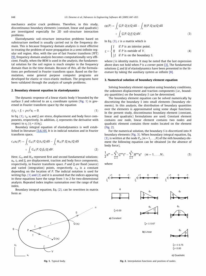
mechanics and/or crack problems. Therefore, in this study,discontinuous boundary elements (constant, linear and quadratic)are investigated especially for 2D soil–structure interactionproblems.

Elastodynamic soil–structure interaction problems based onsubstructure method is usually carried out in the frequency do-main. This is because frequency domain analysis is most effectivein treating the problem of wave propagation in a semi-infinite reg-ular soil region. Also, with the use of fast Fourier transform (FFT)[9], frequency domain analysis becomes computationally very effi-cient. Finally, when the BEM is used in the analysis, the fundamen-tal solution for the soil region is much simpler in the frequencydomain than in the time domain. Because of this, all the formula-tions are performed in Fourier transform space. Based on the for-mulation, some general purpose computer programs aredeveloped for elastic or visco-elastic medium. The programs havebeen validated through the analysis of sample problems.

2. Boundary element equation in elastodynamics

The dynamic response of a linear elastic body V bounded by thesurface S and referred to an xi coordinate system (Fig. 1) is gov-erned in Fourier transform space by the equation

@jsij þ fi þ qx2ui ¼ 0: ð1Þ

In Eq. (1), sij, ui and fi are stress, displacement and body force com-ponents, respectively. In addition, @j represents the derivative withrespect to xj (@j = @/@xj).

Boundary integral equation of elastodynamics is well estab-lished in literature [3,6,10]. It is in indicial notation and in Fouriertransform space,

c‘kukðPÞ ¼Z

SG‘kðP;QÞtkðQÞdS�

ZS

H‘kðP;QÞukðQÞdS

þZ

VG‘kðP;QÞfkðQÞdV : ð2Þ

Here, G‘k and H‘k represent first and second fundamental solutions;uk, tk and fk are displacement, traction and body force components,respectively, in Fourier transform space. P and Q are fixed (source)and varied (integration) points, respectively. c‘k is a constantdepending on the location of P. The indicial notation is used forwriting Eqs. (1) and (2) and it is assumed that the indices appearingin these equations have the range from 1 to 2 for two-dimensionalanalysis. Repeated index implies summation over the range of thatindex.

Boundary integral equation, Eq. (2), can be rewritten in matrixform as

x1

x2

P

r

rr

r

n

n

Q (xi)

Q (xi)

S

V

Fig. 1. Typical body.

cuðPÞ ¼Z

SGðP;QÞtðQÞdS�

ZS

HðP;QÞuðQÞdS

þZ

VGðP;QÞf ðQÞdV : ð3Þ

In Eq. (3), c is a matrix which is

c ¼I if P is an interior point;0 if P is outside of V ;12 I if P is on the boundary S;

8><>: ð4Þ

where I is identity matrix. It may be noted that the last expressionabove does not hold when P is a corner point [3]. The fundamentalsolutions G and H of elastodynamics have been presented in the lit-erature by taking the auxiliary system as infinite [8].

3. Numerical solution of boundary element equation

Solving boundary element equation using boundary conditions,the unknown displacement and traction components (i.e., bound-ary quantities) on the boundary S can be determined.

The boundary element equation can be solved numerically bydiscretizing the boundary S into small elements (boundary ele-ments). In this analysis, the distribution of boundary quantitiesover the elements is approximated using some shape functions.In the present study, discontinuous boundary element (constant,linear and quadratic) formulations are used. Constant elementcontains one node, linear element contains two nodes andquadratic element contains three nodes located on the element(Fig. 2).

For the numerical solution, the boundary S is discretized into Nboundary elements (Fig. 3). When boundary integral equation, Eq.(3), is written at the node Pm (m = 1, . . . ,N) of the mth boundary ele-ment the following equation can be obtained (in the absence ofbody force),

12

um ¼XN

n¼1

Gmntn �XN

n¼1

Hmnun ðm ¼ 1; . . . ;NÞ; ð5Þ

where

ξ=0.00

a) Constant

1 φ2

ξ= ± 0.67

b) Linear

1

φ2

ξ= ± 0.75

ξ= 0.00

c) Quadratic

1 φ3

Fig. 2. Interpolation functions and position of nodes.

x2

x1

Sm

Q(xi)

SnS knQ

r r

kmP

Fig. 3. Boundary element discretization of the body.

I.O. Deneme et al. / Advances in Engineering Software 40 (2009) 847–855 849

Gmn ¼Z

Sn

GðPkm;QÞdS; Hmn ¼

ZSn

HðPkm;QÞdS; ð6Þ

in which Sn is the boundary of the nth element (Fig. 3). In Eq. (5), un

and tn are associated with the nth boundary element. It should benoted that the node Pk

m is not a corner point. Thus, c = ½ I is used.According to the boundary element formulation; coordinates,

displacement and traction components of a point can be defined as

xi ¼Xq

k¼1

/kðnÞxki ; ð7Þ

ui ¼Xq

k¼1

/kðnÞuki ; ð8Þ

ti ¼Xq

k¼1

/kðnÞtki ; ð9Þ

where xki is vector position of the end nodes; uk

i and tki are nodal dis-

placements and stresses; n is parametric variable coordinate and /k

is shape function (k = 1, . . . ,q).The shape function for constant element (q = 1) is given as

/1 ¼ 1: ð10Þ

The shape functions for linear element (q = 2) are given as

/1ðnÞ ¼n2 � nn2 � n1

� �; /2ðnÞ ¼

n� n1

n2 � n1

� �ð�1 � n1 < 0 and 0 < n2 � 1Þ; ð11Þ

where n1 and n2 denote local coordinate of first and second node ofelements, respectively.

The quadratic shape functions for discontinuous element (q = 3)are given as

/1ðnÞ ¼12

na

na� 1

� �; /2ðnÞ ¼ 1� n

a

� �2

;

/3ðnÞ ¼12

na

naþ 1

� �ð12Þ

where �1 6 n 6 1 and a is a parameter (0 < a < 1) which defines theratio of the distance between boundary nodes to the length of theelement. The nodes 1 and 3 are allowed to vary symmetrically bya. If a = 1, then the shape functions will reduce to the standard qua-dratic shape functions, thus the element becomes a continuouselement.

By using Eqs. (8) and (9), Eq. (5) can be rewritten as

ckmuðPk

mÞ ¼XN

n¼1

Xq

s¼1

Gmnks tðQs

nÞ �XN

n¼1

Xq

s¼1

Hmnks uðQ s

nÞ ð13Þ

where tðQsnÞ and uðQs

nÞ are the traction and displacement vectors atsth node of nth element, respectively. In addition

Gmnks ¼

Z 1

�1JðnÞGðPk

m;QÞ/sdn; Hmnks ¼

Z 1

�1JðnÞHðPk

m;QÞ/sdn; ð14Þ

where J is Jacobian and /s is shape function matrix and defined as

/s ¼/s 00 /s

� �ðs ¼ 1; . . . qÞ: ð15Þ

By writing Eq. (13) for the fixed points Pkm with k = 1, . . . ,q

(which are the nodes of Sm) and combining them, the followingequation can be obtained:

cmum ¼XN

n¼1

Gmntn �XN

n¼1

Hmnun: ð16Þ

When Eq. (16) is written for all boundary elements (m = 1, . . . ,N)and combined, the system equations of BEM can be obtained inmatrix form as,eH~u ¼ eG~t; ð17Þ

where

eG ¼ ðGmnÞ; eH ¼ ðHmn þ 12

IdmnÞ;

~u ¼ ðunÞ; ~t ¼ ðtnÞ ðm;n ¼ 1; . . . ;NÞð18Þ

with dmn is Kronecker’s delta. The elements Gmn and Hmn may becomputed numerically by using Gaussian quadrature formula.

The solution of Eq. (17), together with the prescribed boundaryconditions, determines numerically the unknown boundary quan-tities. Having determined unknown boundary quantities, if desired,the interior displacements and stresses can be computed numeri-cally using the boundary quantities.

4. Calculation of singular integrals

The singular integrals will occur when fixed point P and variedpoint Q are on the same element. Therefore, diagonal matrices inEq. (17) will be singular. These singular matrices Gmm

ks and Hmmks

can be written as,

Gmmks ¼

ZSm

GðPkm;QÞ/s dS; Hmm

ks ¼Z

Sm

HðPkm;QÞ/s dS; ð19Þ

where k is fixed point number and s is shape function number. Theintegrals in Eq. (19) are to be understood in the sense of Cauchyprincipal value, i.e., they do not contain the contributions when var-ied point Q coincides with the fixed point Pk

m [8]. But the fundamen-tal solutions involve the distance r between the fixed and variedpoints, and become singular when r = 0. In Eq. (14) (written form = n) the varied point Q is on the element Sm and the distance ris smaller compared to case in which m – n. So that, care shouldbe given for the evaluation of the integrals in Eq. (19) and theyshould be computed by using some special numerical integrationtechniques [3].

The diagonal matrices Gmmks and Hmm

ks (for the fixed point P andthe varied point Q) can be rewritten as

GPQ ¼Z

G‘kðrPðnÞÞ/Q ðnÞJðnÞdn; ð20Þ

HPQ ¼Z

H‘kðrPðnÞÞ/Q ðnÞJðnÞdn: ð21Þ

850 I.O. Deneme et al. / Advances in Engineering Software 40 (2009) 847–855

Here ‘ = 1, 2 and k = 1, 2 for two-dimensional problems, G‘k and H‘k

are, the first and the second fundamental solution for two-dimen-sional elastostatics, given in Eqs. (22) and (23). The number of shapefunctions should be the same with varied point number

G‘k ¼1

8plð1� mÞ ð3� 4mÞ ln 1r

� �d‘k þ

r‘r

rk

r

� �; ð22Þ

H‘k ¼ �1

4pð1� mÞr@r@nð1� 2mÞd‘k þ 2

r‘r

rk

r

n o�þð1� 2mÞ rk

rn‘ �

r‘r

nk

� �i; ð23Þ

where d‘k, m, l, nk and n‘ denote Kronecker delta, Poisson’s ratio,shear modulus and outer unit normal vector components,respectively.

In this study, singularity subtraction technique has been usedfor all types of discontinuous elements (constant, linear and qua-dratic) therefore; singularity in static case will be mentionedfirstly.

4.1. Singular integrals for constant element in static case

As stated previously, it may be noted that the integrals in Eq.(19) are defined in the sense of Cauchy principal value and excludethe point n = 0 which corresponds to the fixed point P. After someanalytical calculations were done [8], the first fundamental solu-tion components (Gmm

‘k ) are obtained as,

Gmm‘k ¼

R4plð1� mÞ ½ð3� 4mÞð1� ln RÞd‘k þ s‘sk�; ð24Þ

where R denotes half of the length of the element. s‘ and sk are unittangential vector components.

The second fundamental solution can be integrated usingstandard Gaussian quadrature for determining Hmn matrices. Whenthe fixed point P and the varied point Q at the same element theterms Hmm can be determined using rigid-body motion as follows[3]:

Hmm ¼ �XN

n¼1

Hmn ðm–nÞ ð25Þ

4.2. Singular integrals for linear element in static case

The first fundamental solution G (when P and Q on the sameelement) includes ln(1/r) and (1/r) singularity cases. The integral,that contains first fundamental solution, will be considered intwo parts. The first part includes ln(1/r) and the second part con-tains (1/r) singularity case. The ln(1/r) term can be calculated ana-lytically and converting the integral limits (�1,+1) to (0,+1) [11]. Inaddition the second part, that includes (1/r) singularity, can beintegrated using standard Gaussian quadrature. Therefore the firstfundamental solution can be integrated [11].

The second fundamental solution, in Eq. (23), can be integratedusing standard Gaussian quadrature for determining Hmn matrices.When the fixed point P and the varied point Q at the same elementthe terms Hmm can be determined using rigid-body motion, asshown in Eq. (25).

4.3. Singular integrals for quadratic element in static case

For calculating the first fundamental solution G (when P and Qon the same element) there is need for special techniques. For thispurpose, the integral that contains first fundamental solution intwo parts will be considered. The first part includes ln(1/r) andthe second part contains (1/r) singularity case.

If the fundamental solution is written, which was given at Eq.(22), into Eq. (20), GPQ will contain a weak singularity in the formof natural logarithm. After all GPQ can be rewritten as

GPQ ¼Z

18plð1� mÞ ð3� 4mÞ ln 1

rP

� �d‘k þ

r‘rP

rk

rP

� �/Q ðnÞJðnÞdn:

ð26Þ

The ln(1/rp) term can be manipulated by conversion into a form,where the logarithmic quadrature can apply. This conversion canaccomplish by using change of variables [12]. The second part ofEq. (26) can be integrated using standard Gaussian quadrature.

The second fundamental solution, in Eq. (23), can be integratedusing standard Gaussian quadrature for determining Hmn matrices.When the fixed point P and the varied point Q at the same elementthe terms Hmm can be determined using rigid-body motion, asshown in Eq. (25).

4.4. Singular integrals in dynamic case

The orders of singularity in the dynamic fundamental solutionsare the same as in the static fundamental solutions and can bedealt with in the following manner:Zð ÞDynamicdS ¼

Zð ÞStaticdSþ

Z½ð ÞDynamic � ðÞStatic�dS; ð27Þ

where the second integral on the right-hand side of Eq. (27) is non-singular and can be evaluated using standard Gaussian quadrature.The first integral on the right-hand side of Eq. (27) can be evaluatedusing the method described in static case. Eq. (27) can be rewrittenfor both of the fundamental solutions in concise form as:

GD ¼ GS þ ðGD � GSÞ; ð28ÞHD ¼ HS þ ðHD � HSÞ; ð29Þ

where GD and HD are dynamic fundamental solutions, GS and HS arestatic fundamental solutions. The fundamental solutions GD and HD

for two-dimensional elastodynamics are given in Eqs. (30) and (31)

GD ¼1

2plWd‘k � vr‘rk½ �; ð30Þ

HD ¼1

2pdWdr� v

r

� �d‘k

@r@nþ rkn‘

� �� 2

rv nkr‘ � 2r‘rk

@r@n

� ���2

dvdr

r‘rk@r@nþ

c2p

c2s� 2

!dWdr� dv

dr� v

r

� �r‘nk

); ð31Þ

where

W ¼ K0ðasÞ þ1as

K1ðasÞ �cs

cpK1ðapÞ

� �; ð32Þ

v ¼ K2ðasÞ �c2

s

c2p

K2ðapÞ; ð33Þ

where

as ¼ixrcs

; ap ¼ixrcp

:

Here i is imaginary number, cp and cs are dilatational and shearwave velocities. Ki’s are modified Bessel functions of second kind.

The singularity in HD can be manipulated using Eq. (29) insteadof the rigid-body motion mentioned in static case.

5. Computer programs

Based on the formulations, presented in this study, three gen-eral purpose computer programs are developed by using FOR-

Compute terms of Gmm and Hmm matrices

Compute the resultants of boundary tractions

Determine the displacements

and stresses at interior points

START

Read input data and perform data generations

Form the system matrices for defined boundary in problems

Singular element (m = n)?

Compute Gmn matrices

Interior points?

Compute the unknown boundary quantities by solving Eq.17

Write the results

STOP

No

No

Yes

Compute Hmn matrices

Yes

Fig. 4. Flow chart of computer programs.

I.O. Deneme et al. / Advances in Engineering Software 40 (2009) 847–855 851

TRAN77 codes for analyzing elastic or visco-elastic 2D elastody-namic soil–structure interaction problems. The structures of thethree programs are basically the same and the flow chart is shownin Fig. 4. The programs perform the analysis in Fourier transformspace. If desired, the obtained results can be transformed to timespace with the use of FFT algorithm [9].

6. Numerical examples

In this section, some numerical examples are solved for thecomparison of the various discontinuous boundary element formu-lations. To this end, based on the above mentioned formulations,some general purpose computer programs have been developedfor each type of discontinuous boundary elements. All the pro-grams perform the analysis in Fourier transform space. Although

the programs are developed for dynamic analysis, it can also beused for static analysis by assigning a very small value close to zerofor the frequency.

Two examples are handled to demonstrate the suitability andaccuracy of the present formulation comparing with the results ob-tained by independent numerical methods and/or exact solutionsavailable in the literature. In the example problems, mesh trunca-tion is used for the analysis of unbounded domains and the funda-mental solutions are integrated with 10 point quadrature rule forboth standard and logarithmic Gaussian quadrature formulas.Boundary element model have been represented with the parame-ters of n1 = �0.67 and n2 = 0.67 (for linear element) also n1 = �0.75,n2 = 0, n3 = 0.75 and a = 0.75 (for quadratic element).

In the formulation hysteretic damping ratio is used for damp-ing. The hysteretic damping in the material can be included into

1.6

lianc

e

852 I.O. Deneme et al. / Advances in Engineering Software 40 (2009) 847–855

a system by replacing, in Fourier transform space, the shear mod-ulus l of a material by l(1 + 2iz). Here, i is imaginary number and zis the hysteretic damping ratio of the material, and all the param-eters involving the elastic constant l are determined by this com-plex valued shear modulus [13].

6.1. Rigid strip foundation

In this example, a rigid strip foundation on half-space shown inFig. 5 is considered. Here, compliances of rigid strip foundation areinvestigated.

This problem has been solved, as a plane strain problem. Thetop surface of the problem is discretized into 80 equal elementsfor all types of discontinuous boundary elements.

The analysis is carried out in nondimensional space. The nondi-mensional variables are defined as:

omp

�b ¼ 1

0.0

0.5

1.0

1.5

2.0

2.5

3.0

0.0 0.2 0.4

No

Non

dim

ensi

onal

hor

izon

tal c

ompl

ianc

e

Fig. 6. Variation of real pa

Rigid s

b

A

Fig. 5. Rigid s

nondimensional half-width of footing

1.2

tal c

�x ¼ xb

cS

nondimensional frequency

on

ðC11;C22Þ ¼ plðC11;C22Þ

0.8

riz

nondimensional vertical and horizontalcompliances, respectively

l ho

Exact

C33 ¼ plb2C33 nondimensional rocking compliance

iona Constant

0.6 0.8 1.0 1.2 1.4 1.6

ndimensional frequency

Exact

Constant

Linear

Quadratic

rt of horizontal compliance with frequency.

trip foundation

B

b

Half-space μ, ν, ρ,

x2

x1

trip foundation over half-space.

where x is the Fourier transform parameter, cS and l are the shearwave velocity and shear modulus. In the analysis, Poisson’s ratio,nondimensional mass density and nondimensional shear modulusare taken as m ¼ 0:25; �q ¼ 1; �l ¼ 1.

The results, which were obtained using boundary element for-mulations, are presented and compared with exact ones in Figs.6–11. The exact results are taken from Luco and Westman [14].As seen in the figures, the results are in good agreement.

6.2. Visco-elastic soil under harmonic strip load

In this problem, the compliances have been investigated for vis-co-elastic soil under harmonic strip load shown in Fig. 12. The

0.0

0.5

1.0

1.5

2.0

2.5

0.0 0.2 0.4 0.6 0.8 1.0 1.2 1.4 1.6

Nondimensional frequency

Non

dim

ensi

onal

ver

tical

com

plia

nce

Exact

Constant

Linear

Quadratic

Fig. 8. Variation of real part of vertical compliance with frequency.

0.0

0.4

0.0 0.2 0.4 0.6 0.8 1.0 1.2 1.4 1.6

Nondimensional frequency

Non

dim

ens

Linear

Quadratic

Fig. 7. Variation of imaginary part of horizontal compliance with frequency.

0.0

0.4

0.8

1.2

1.6

0.0 0.2 0.4 0.6 0.8 1.0 1.2 1.4 1.6Nondimensional frequency

Non

dim

ensi

onal

ver

tical

com

plia

nce

ExactConstantLinearQuadratic

Fig. 9. Variation of imaginary part of vertical compliance with frequency.

0.0

0.3

0.6

0.9

1.2

1.5

1.8

2.1

0.0 0.2 0.4 0.6 0.8 1.0 1.2 1.4 1.6

Nondimensional frequency

Non

dim

ensi

onal

rock

ing

com

plia

nce

ExactConstantLinearQuadratic

Fig. 10. Variation of real part of rocking compliance with frequency.

−0.2

0.0

0.2

0.4

0.6

0.8

1.0

1.2

0.0 0.2 0.4 0.6 0.8 1.0 1.2 1.4 1.6

Nondimensional frequency

Non

dim

ensi

onal

roc

king

com

plia

nce

Exact

Constant

Linear

Quadratic

Fig. 11. Variation of imaginary part of rocking compliance with frequency.

15b

Visco-elastic soilμ, ν, ρ, z

q=q0eiω t

x1

x2

1 2 3 4 5 6 7 8

b 7b

Fig. 12. Visco-elastic soil under harmonic strip load.

−0.2

0.0

0.2

0.4

0.6

0.0 1.0 2.0 3.0 4.0 5.0 6.0 7.0 8.0

Nondimensional x1

Non

dim

ensi

onal

hor

izon

tal c

ompl

ianc

e

Exact

Finite-Infinite

Constant

Linear

Quadratic

Fig. 13. Real part of horizontal compliance.

−0.1

−0.2

−0.3

−0.4

−0.5

0.0

0.0 1.0 2.0 3.0 4.0 5.0 6.0 7.0 8.0

Nondimensional x1

Non

dim

ensi

onal

hor

izon

tal c

ompl

ianc

eExact

Finite-Infinite

Constant

Linear

Quadratic

Fig. 14. Imaginary part of horizontal compliance.

−0.2

0.0

0.2

0.4

0.6

0.0 1.0 2.0 3.0 4.0 5.0 6.0 7.0 8.0

Nondimensional x1

Non

dim

ensi

onal

ver

tical

com

plia

nce

Exact

Finite-Infinite

Constant

Linear

Quadratic

Fig. 15. Real part of vertical compliance.

I.O. Deneme et al. / Advances in Engineering Software 40 (2009) 847–855 853

material properties of half-space are given as; Poisson’s ratiom = 0.25, nondimensional mass density �q ¼ 1, nondimensionalshear modulus �l ¼ 1 and hysteretic damping ratio z = 0.125. Theeffect of strip load on half-space can be defined with a nondimen-sional width �b ¼ 1 and nondimensional amplitude �q0 ¼ 1. In the

problem, horizontal and vertical compliances, at eight points(Fig. 12) are calculated for nondimensional frequency a0 = 0.5.

The exact solutions for horizontal and vertical compliancesare taken from Gutierrez and Chopra [15] and they can be definedas:

Fxxm ¼

1G½f xx

m ða0Þ þ igxxm ða0Þ�; ð34Þ

Fyym ¼

1G½f yy

m ða0Þ þ igyym ða0Þ�: ð35Þ

−0.6

−0.4

−0.2

0.0

0.2

0.0 1.0 2.0 3.0 4.0 5.0 6.0 7.0 8.0

Nondimensional x1

Non

dim

ensi

onal

ver

tical

com

plia

nce

Exact

Finite-InfiniteConstant

Linear

Quadratic

Fig. 16. Imaginary part of vertical compliance.

−0.2

0.0

0.2

0.4

0.6

0.0 1.0 2.0 3.0 4.0 5.0 6.0 7.0 8.0

Nondimensional x1

Nond

imen

sion

al h

oriz

onta

l com

plia

nce

Finite-Infinite

Constant

Linear

Quadratic

Fig. 17. Real part of horizontal compliance (without damping).

−0.4

−0.3

−0.2

−0.1

0.0

0.0 1.0 2.0 3.0 4.0 5.0 6.0 7.0 8.0

Nondimensional x1

Non

dim

ensi

onal

hor

izon

tal c

ompl

ianc

e

Finite-Infinite

Constant

Linear

Quadratic

Fig. 18. Imaginary part of horizontal compliance (without damping).

−0.4

−0.2

0.0

0.2

0.4

0.0 1.0 2.0 3.0 4.0 5.0 6.0 7.0 8.0

Nondimensional x1

Non

dim

ensi

onal

ver

tical

com

plia

nce

Finite-Infinite

Constant

Linear

Quadratic

Fig. 19. Real part of vertical compliance (without damping).

−0.2

0.0

0.2

0.4

0.0 1.0 2.0 3.0 4.0 5.0 6.0 7.0 8.0

Nondimensional x1

Non

dim

ensi

onal

ver

tical

com

plia

nce

Finite-Infinite

Constant

Linear

Quadratic

Fig. 20. Imaginary part of vertical compliance (without damping).

854 I.O. Deneme et al. / Advances in Engineering Software 40 (2009) 847–855

Here, Fxxm ; F

yym are horizontal and vertical compliances, G is shear

modulus for soil. f xxm ; g

xxm ; f

yym and gyy

m denote real and imaginary partsof compliances in x1 and x2 direction, respectively.

The surface of the problem is discretized using 15 equal lengthelements for all types of discontinuous boundary elements.

The results are presented and compared with coupling of finiteand infinite element results obtained by Yerli et al. [1] and exactones in Figs. 13–16. As seen in the figures, the results are in goodagreement.

This problem is solved again without damping. The boundaryelement mesh is the same with the previous case. Since the exactsolution for this case is unavailable, the boundary element solu-tions are presented and compared with coupling of finite and infi-nite element formulation presented by Yerli [16] in Figs. 17–20. Asseen in the figures, the results are in good agreement.

7. Conclusions

In this study, various discontinuous boundary element formula-tions (constant, linear and quadratic) are compared. Based on theformulations, general purpose computer programs are developed,and they are applied to 2D dynamic soil–structure interactionproblems.

The formulations proposed in this study are assessed by apply-ing to several example problems. The results are compared withthose obtained by exact ones and/or the other methods availablein the literature. The comparisons indicate that the formulationspresented in this study can be used with a good confidence inthe dynamic analysis of soil–structure interaction problems. Inaddition, results obtained for constant, linear and quadratic bound-ary elements are in good agreement to each other. Thus, it can besaid that the use of constant element (the simplest discontinuousboundary element) formulation is sufficient for 2D elastodynamicsoil–structure interaction problems.

I.O. Deneme et al. / Advances in Engineering Software 40 (2009) 847–855 855

References

[1] Yerli HR, Temel B, Kiral E. Multi-wave transient and harmonic infinite elementsfor two-dimensional unbounded domain problems. Comput Geotech1999;24(3):185–206.

[2] Yerli HR, Temel B, Kiral E. Transient infinite elements for 2-dimensional soil–structure interaction analysis. J Geotech Geoenviron, ASCE 1998;124(10):976–88.

[3] Brebbia CA, Dominguez J. Boundary elements an introductorycourse. Southampton: Computational Mechanics Publications; 1989.

[4] Mackerle J, Brebbia CA. The boundary element referencebook. Southampton: Computational Mechanics Publications; 1988.

[5] Brebbia CA, Connor JJ. Advances in boundary elements, vol.1. Southampton: Computational Mechanics Publications; 1989.

[6] Banerjee PK. The boundary element methods inengineering. London: McGraw-Hill Book Company; 1994.

[7] Partridge PW, Brebbia CA, Wrobel LC. The dual reciprocity boundary elementmethod. Southampton: Computational Mechanics Publications; 1992.

[8] Mengi Y, Tanrikulu AH, Tanrikulu AK. Boundary element method for elasticmedia: an introduction. Ankara: METU Press; 1994.

[9] Cooley JW, Lewis PAW, Welch PD. The fast Fourier transform and itsapplications. IEEE Trans Ed 1969;12:27–34.

[10] Manolis GD, Beskos DE. Boundary element methods in elasto-dynamics. London: Unwin Hyman; 1988.

[11] Severcan MH. Boundary element method formulation for dynamic soil–structure interaction problems. PhD Dissertation, University of Cukurova,Adana, 2004 [in Turkish].

[12] Yerli HR, Deneme IO. Elastodynamic boundary element formulationemploying discontinuous curved elements. Soil Dyn Earthq Eng2008;28(6):480–91.

[13] Wolf JP. soil–structure interaction analysis in time domain. Englewood Cliffs,New Jersey: Prentice-Hall; 1988.

[14] Luco JE, Westman RA. Dynamic response of a rigid footing bounded to anelastic half space. J Appl Mech – Trans ASME 1972;39(2):527–34.

[15] Gutierrez JA, Chopra AK. A substructure method for earthquake analysis ofstructures including structure–soil interaction. Earthq Eng Struct Dyn1978;6:51–69.

[16] Yerli HR. Analysis of two and three dimensional dynamic soil–structureinteraction problems using finite and infinite elements. PhD Dissertation,University of Cukurova, Adana, 1998 [in Turkish].