A

tomafrmApdbw©

K

1

dAtdobasaocta

0d

Available online at www.sciencedirect.com

Computers and Chemical Engineering 32 (2008) 2547–2569

Optimal management of logistic activities in multi-site environments

Rodolfo Dondo, Carlos A. Mendez, Jaime Cerda ∗INTEC (UNL-CONICET), Guemes 3450, 3000 Santa Fe, Argentina

Received 3 May 2007; received in revised form 21 August 2007; accepted 4 October 2007Available online 18 October 2007

bstract

The new emerging area of Enterprise Wide Optimization (EWO) has focused the attention in effectively solving the combined produc-ion/distribution scheduling problem. The importance of logistic activities performed in multi-site environments comes from the relative magnitudef the associated transportation costs and the good chance of getting large savings on such expenses. This paper first develops an exact MILPathematical formulation for the multiple vehicle time-window-constrained pickup and delivery (MVPDPTW) problem. The approach is able to

ccount for many-to-many transportation requests, pure pickup and delivery tasks, heterogeneous vehicles and multiple depots. Optimal solutionsor a variety of benchmark problems with cluster/random distributions of pickup and delivery locations and limited sizes in terms of customerequests and vehicles have been discovered. However, the computational cost exponentially grows with the number of requests. For large-scale-PDPTW problems, a local search improvement algorithm steadily providing a better solution through two evolutionary steps is also presented.neighborhood structure around the starting solution is generated by first allowing multiple request exchanges among nearby trips and then

ermitting the reordering of nodes on every individual route. If a better set of routes is found, both steps are repeated until no improved solution is

iscovered. Compact MILP mathematical formulations for both sub-problems have been developed and solved through an efficient branch-and-ound algorithm. A significant number of large-scale m-PDPTW benchmark problems, some of them including up to 100 transportation requests,ere successfully solved in reasonable CPU times.2007 Elsevier Ltd. All rights reserved.

istics

on

ldfligcMpi

eywords: Pickup and delivery problem; Optimization; Multiple vehicles; Log

. Introduction

Major cost factors within a supply chain come from pro-uction, material handling, inventory and distribution tasks.lthough their relative importance may largely vary with the

ype of industry, the current trend towards a geographicallyistributed business requires regional and global coordinatedperations. Decentralized production and distribution schemesased on multi-site environments are becoming more popularnd, consequently, goods are almost never produced and con-umed in the same geographical location. As a result, transportnd distribution activities are emerging as central issues in manyf today’s companies because of the significant increase in their

omplexity and costs. Consequently, the development of effec-ive computational tools for logistics management has attractedgreat attention from both industry and academy on the field

∗ Corresponding author. Tel.: +54 342 4559175; fax: +54 342 4550944.E-mail address: jcerda@intec.unl.edu.ar (J. Cerda).

psflotda

098-1354/$ – see front matter © 2007 Elsevier Ltd. All rights reserved.oi:10.1016/j.compchemeng.2007.10.002

f supply chain management (SCM) and, more recently, on theew emerging area of Enterprise Wide Optimization (EWO).

One of the most typical transportation problems studied in theiterature is the so-called vehicle routing problem (VRP) whicheals with the delivery (collection) of goods by a fleet of trucksrom (to) a central or multiple depots to (from) many customerocations. In the general case, the main goal of the VRP problems to generate the optimal routes for the vehicle fleet based on aiven road network so as to meet customer demands and satisfyapacity and time constraints at minimum travel cost (Dondo,endez & Cerda, 2003). A generalization of the VRP, called the

ickup and delivery problem (PDP), has been intensively stud-ed in the last twenty years. It is a combinatorial optimizationroblem aimed at satisfying a set of customer requests involvingimultaneously pickup and delivery tasks by means of a vehicleeet at minimum cost. Each customer request specifies the size

f the load to be transported, the locations where the goods areo be collected (the origins) and the locations to which are to beelivered (the destinations). Each demand has to be fulfilled bysingle vehicle transporting goods from origins to destinations

2548 R. Dondo et al. / Computers and Chemical Engineering 32 (2008) 2547–2569

Nomenclature

SetsI nodesIr nodes related to transport request rI+ pickup nodesI+r pickup nodes related to request r

I− delivery nodesI−r delivery nodes related to request r

IFv fixed nodes already allocated to vehicle v

P depotsR transport requests that may involve multiple

pickup nodes i ∈ I+r and multiple delivery nodes

i′ ∈ I−r

RM subset of mobile requests that can be reallocatedin sub-problems I and III

RMv subset of mobile requests that can be reallocated

to vehicle v

RF subset of fixed requests that cannot be reallocatedto another vehicle in sub-problems I and III

RFv subset of fixed requests already allocated to vehi-

cle v

V vehiclesVp vehicles already allocated to depot pVr vehicles that can be allocated to request r

Parametersai earliest service time at node ibi latest service time at node icvii′ vehicle-dependent travel cost between nodes i and

i′cvpi vehicle-dependent travel cost between depot and

node i ∈ Icfv vth-vehicle fixed utilization costMC maximum vehicle traveling costML maximum vehicle capacityMT maximum vehicle arrival timeqv vth-vehicle capacitysti service time at node itmaxv maximum routing time for vehicle v

tvii′ vehicle-dependent travel time between nodes iand i′

tvpi vehicle-dependent travel time between depot pand node i

αir load to pickup at node i ∈ I+r . If i ∈ I−

r then αir = 0βir load to deliver at node i ∈ I−

r . If i ∈ I+r then βir = 0

λ penalty factor for earlinessΛ penalty factor for routing time constraint violationρi unit penalty cost for time-window violation at

node iρv penalty factor for routing time violation of vehicle

v

ω penalty factor for tardiness

Binary variablesSii′ binary variable denoting that node i is visited

before (Sii′ = 1) or after (Sii′ = 0) node i′ wheneverboth nodes are serviced by the same vehicle

Xvp binary variable denoting the assignment of depotp to vehicle v

Yrv binary variable denoting the assignment of trans-portation request r to vehicle v

Continuous variablesBi tardiness at node iCi accumulated vehicle routing cost to reach node iEi anticipation at node iLi total cargo loaded on the assigned vehicle after

completing the service at node iOCv total routing cost for vehicle v

ODv maximum routing time violation for vehicle v

OTv total travel time for vehicle v

Ti accumulated vehicle travel time to reach node iUi total cargo unloaded from the assigned vehicle

wateaijestdmeupmlorghss

i((Stdam

after completing the service at node i

ithout any transshipment at other locations. To accomplish thessigned transport requests, every vehicle departs from the cen-ral base and visits a number of sites along the selected route. Atach stop location, the vehicle can either pick up or deliver anmount of load but not both. Loading and unloading times arencurred at every stop. Moreover, each vehicle starts and ends itsourney at the central or the assigned depot. Vehicle data gen-rally include the transport capacity, the alternative depots (ifeveral ones are considered) and the subset of transport requestshat can be allocated to every truck. If the pickup and/or theelivery location has a time interval within which the serviceust begin, then the problem is known as the pickup and deliv-

ry problem with time windows (PDPTW). Time windows aresually defined based on customer preferences. Since real-worldickup and delivery problems include time-window constraints,ost of the papers have been focused on the PDPTW. In particu-

ar, the PDPTW variant involving transport requests with a singlerigin and a single destination, and a vehicle fleet departing andeturning to a central depot was the most studied. In a moreeneral context, the underlying ideas of the PDPTW problemave been also applied to the coordination of the simultaneouscheduling of production and distribution activities in multi-siteystems (Mendez, Bonfill, Espuna, & Puigjaner, 2006).

Surveys on the pickup and delivery problem can be foundn Bodin, Golden, Assad, and Ball (1983), Savelsbergh and Sol1995), Fisher (1995), Desrosiers, Dumas, Solomon, and Soumis1995), and Desaulniers, Desrosiers, Erdmann, Solomon, andoumis (2002). Three classes of PDPTW have usually been

ackled. One of them is the so-called single-vehicle pickup and

elivery problem with time windows (1-PDPTW) where pickupnd delivery services are all done by a single vehicle. If there areultiple vehicles available, the problem is known as the multi-

mica

vcmfoghavpdGrGtaorertard

d(sponbaDwgcailt

mTthsma2taitgat

eMpbensp

1

pHtmaeishcSPiotTrardstiIWco

fsfnitn(mL&22

R. Dondo et al. / Computers and Che

ehicle pickup and delivery problem (m-PDPTW). Most of theontributions have been devoted to these two PDPTW classes. Inany practical situations, however, the cargo must be collected

rom multiple nodes and transported to a single delivery locationr vice versa. Furthermore, the problem may involve a hetero-eneous vehicle fleet, multiple depots and each vehicle mayave its own starting/ending base. In addition, pure pickup nodesnd/or delivery nodes demanding just a pickup or delivery ser-ice but not both can be simultaneously considered. A PDPTWroblem with all these features is called the general pickup andelivery problem with multiple vehicle and time windows (m-PDPTW). So far, the m-GPDPTW problem has received a

ather limited attention. Problems 1-PDPTW, m-PDPTW or m-PDPTW all assume a pre-defined set of customer requests

hat remains unchanged while the pickup and delivery servicesre being performed. They can be regarded as distinct variantsf the static PDPTW. In real-world problems, new customerequests are continually received in real-time and immediatelyligible for consideration. As a consequence, the current set ofoutes has to be re-optimized at some time point to includehe new transport services. It is the dynamic m-GPDPTW. Inny case, the goal is to periodically adjust the present set ofoutes and schedules in order to account for the updated problemata.

Different practical problems can be modeled as pickup andelivery problems. Among them, the VRP with backhaulsVRPB), the dial-a-ride problem (DARP), the handicapped per-on transportation problem (HTP) and the courier companyickup and delivery problem (CCPDP). The VRPB includes a setf customers to whom products are to be delivered (pure deliveryodes) and a set of nodes whose goods need to be transportedack to the distribution center (pure pickup nodes). Moreover,ll deliveries have to be made before all the pickups. ProblemsARP and HTP are concerned with the transportation of peoplehile CCPDP deals with transporting messages and parcels. Areat deal of papers on PDPTW is on dial-a-ride problems. Inontrast, fewer contributions have been focused on the pickupnd delivery of packages and goods. In the last years, theres an increasing trend towards modeling such practical prob-ems as particular cases of the m-GPDPTW problem formula-ion.

In this work, a new mixed-integer linear programming for-ulation for the general m-GPDPTW problem is presented.he proposed optimization approach is capable of handling

ransport requests with multiple origins and/or destinations,eterogeneous vehicles and multiple depots. Moreover, it cantill be applied even if pure pickup and/or delivery nodes andultiple depots are also considered. However, the exact MILP

pproach can solve m-GPDPTW problem instances with at most5 requests to optimality in a reasonable CPU time. In order toackle m-GPDPTW problems with a larger number of requests,model-based neighborhood search framework that iteratively

mproves a starting solution is subsequently developed. To do

hat, a neighborhood structure around the current solution isenerated by just allowing (a) multiple exchanges of requestsmong neighboring trips and (b) reordering of nodes on everyour. The so-defined neighborhood domain is systematically

RpsP

l Engineering 32 (2008) 2547–2569 2549

xplored to find the best neighbor by solving a pair of low-sizeILP sub-problems. In order to illustrate the performance of the

roposed m-GPDPTW exact and improvement methods, theyoth have been applied to a sizable set of PDPTW benchmarkxamples with different time-window width and geographicalode distributions. The results have been compared with the bestolutions recently reported in the literature for such benchmarkroblems.

.1. Previous heuristic approaches

Two types of PDPTW solution methodologies have been pro-osed: heuristic techniques and exact optimization approaches.euristic techniques can be classified into three types:

our construction heuristics, tour improvement heuristics andetaheuristics (Mitrovic-Minic, 1998). Constructive heuristic

lgorithms gradually build a feasible solution by keeping anye on the solution cost but no improvement phase is nextmplemented. They can be divided into two groups: decompo-ition methods and insertion procedures. The best constructioneuristic methods decompose the problem into three phases:lustering, routing and scheduling. Dumas, Desrosiers andoumis (1989) applied a decomposition approach to the m-DPTW based on the notion of mini-clustering. A mini-cluster

s a route segment along which the demands from a small groupf clients can be satisfied by a single vehicle starting and endinghe route segment service with either the same load or empty.hen, a mini-cluster can be treated as an aggregate transport

equest entirely satisfied by a single vehicle. The optimizationlgorithm is then applied to a more compact set of transportationequests. Mini-clusters are constructed from known pickup andelivery plans by cutting them into pieces such that each piecetarts and ends with an empty vehicle. In turn, insertion heuris-ics develop a set of routes by inserting one or multiple requestsnto one or several open routes at a time (Altinel & Oncan, 2005;oannou, Kritikos, & Prastacos, 2001; Jaw, Odon, Psaraftis, &

ilson, 1986; Lu & Dessouky, 2006; Toth & Vigo, 1997). Thehoice of which request to insert and where to insert it dependsn the heuristic being applied.

On the other hand, improvement heuristic procedures startrom a set of feasible routes and apply some kind of localearch heuristics to get a better solution. By repeatedly per-orming a sequence of steps, it generates and examines aeighborhood around the current solution to hopefully find anmproved set of routes. If so, the better solution is adopted ashe new starting point and the process is repeated. The notion ofeighbor depends on the improvement heuristic being appliedThompson & Psaraftis, 1993). More recently, metaheuristicethods, including simulated annealing (Van Der Bruggen,enstra, & Schuur, 1993), constrained-direct search (Potvin

Rousseau, 1995), tabu search (Nanry & Wesley Barnes,000; Taillard et al., 1997; Tang Montane & Dieguez Galvao,006), threshold algorithms, neural networks (Potvin, Shen, &

ousseau, 1992) and genetic algorithms have also been pro-osed. Li and Lim (2003a, 2003b) developed a tabu-embeddedimulated annealing algorithm for the general multiple-vehicleDPTW which restarts a search procedure from the current

2 mica

bao1aParrwrhand

1

egmbgaaooaWscataautafPtcaf

2

wittiVpn

twftIeIt

tdadaatotalnnbes

q

wrcaaTdrfiansl(stttctttc

550 R. Dondo et al. / Computers and Che

est solution after several non-improving search iterations. Inddition, they generated a set of test cases for PDPTW basedn Solomon’s benchmark instances for VRPTW (Solomon,987). Tam and Kwan (2004) generated a systematic scheme todapt the large neighborhood search (NLS) to efficiently solveDPTW problems. The NLS is an iterative process of relax-tion and re-optimization to continually improve on the currentouting plan until the convergence to a local minimum or theesource exhaustion occurs. Their results compare favorablyith those obtained with Li and Lim’s metaheuristic search algo-

ithm. Bent and Van Hentenryck (2006) developed a two-stageybrid methodology for the m-PDPTW problem that repeatedlypplies a simple simulated annealing algorithm to decrease theumber of routes followed by a large neighborhood search toecrease the travel cost.

.2. Exact optimization methods

The development of exact optimization methods started in thearly 1980s. Generally speaking, the exact approaches can berouped into two classes: branch-and-price and branch-and-cutethods. Branch-and-price techniques apply a branch-and-

ound scheme in which lower bounds are computed by columneneration. In branch-and-cut methods, valid inequalities or cutsre incorporated in the formulation at each node of the branch-nd-bound tree to tight the LP relaxation problems. Becausef its intrinsic complexity, a limited number of exact meth-ds for the m-PDPTW has been published. Dumas, Desrosiers,nd Soumis (1991) presented a technique based on the Dantzig-olfe decomposition/column generation scheme and a pricing

ub-problem involving a shortest path problem with capacity,oupling, precedence and time-window constraints. Savelsberghnd Sol (1998) proposed another branch-and-price approach forhe PDPTW with some interesting features. It uses constructionnd improvement heuristics to solve the pricing sub-problem,primal heuristic at each node of the search tree to compute

pper bounds and a clever column handling procedure to keephe column generation master problem as small as possible. Lund Dessouky (2004) developed an MILP optimisation-basedramework and a branch-and-cut algorithm for solving the m-DPTW problem. It permits to solve problem instances of up

o 5 vehicles and 17 customer requests on problems withoutlusters. Recently, Cordeau (2006) developed a branch-and-cutlgorithm for the dial-and-ride problem based on a three-indexormulation.

. The problem definition

The multiple vehicle pickup and delivery problem with timeindows consists of finding the optimal routes for a vehicle fleet

n order to fulfill a set of customer requests r ∈ R at minimumotal cost while satisfying all problem constraints. Let us definehe set R containing the transport requests, the set I compris-

ng all pickup and delivery nodes to be serviced and the set

including the available vehicles. Moreover, I+ is the set ofickup nodes (I+ ⊂ I) while I− (⊂I) just comprises the deliveryodes, i.e. I = {I+ ∪ I−}. Other important sets are the one con-

p

it

l Engineering 32 (2008) 2547–2569

aining all pickup and delivery nodes related to request r (Ir) asell as the pickup locations I+

r and the delivery locations I−r

or request r ∈ R. It may occur that the same site is associatedo different requests to accomplish a similar or a different task.n such a case, it should be defined as many (pickup or deliv-ry) nodes located on that site as the number of related requests.n other words, every problem node is associated to only oneransportation order.

In general terms, a customer request r ∈ R involves theransportation of some load from multiple origins to multipleestinations. A given set of pickup nodes i ∈ I+

r and/or the pre-ssigned starting depot are usually the origin points. In turn, theestinations may include a given set of delivery nodes i′ ∈ I−

r

nd/or the pre-assigned final terminal. This general definitionlso accounts for requests involving the transportation of goodso a set of pure delivery nodes from a pre-defined supply depotr the collection of goods from a number of pickup nodes toransport them to a pre-defined end base. Therefore, the data setssociated to any request r includes: (a) an initial cargo qo

r to beoaded at the pre-defined starting depot; (b) a group of collectionodes i ∈ I+

r from each one a load αir is to be picked up; (c) aumber of delivery nodes i′ ∈ I−

r to each one a load βi′r is toe delivered and (d) a final cargo qf

r destined to the pre-definednd base. Moreover, the data for a transportation request mustatisfy the following condition:

or +

∑i ∈ I+

r

αir =∑

i′ ∈ I−r

βi′r + qfr, ∀r ∈ R

Time windows (ai, bi) are given for pickup and delivery tasksithin which they must be accomplished. Vehicles depart and

eturn to the same depot but the one assigned to a particular vehi-le is a problem decision. Vehicle capacities and depot locationsre also problem data. While the vehicles perform the pickupnd delivery tasks, numerous constraints are to be satisfied.hey are the following: (a) every used vehicle has its assignedepot (depot assignment constraint); (b) each customer request∈ R must be serviced by a single vehicle visiting a pickup noderst except for pure delivery nodes (vehicle assignment, pairingnd precedence constraints); (c) the capacity of a vehicle canever be exceeded after visiting a pickup node (capacity con-traints at pickup nodes); (d) a vehicle must transport enoughoad to meet customer demand when stopping at a delivery nodecapacity constraints at delivery nodes); (e) each used vehiclehould return to its base (final destination constraints); (f) theotal time/distance traveled by a vehicle from the starting depoto a particular node location must be greater than the one requiredo reach a preceding node on the tour (time-based sequencingonstraints); (g) the service at each node must be started withinhe specified time window (hard time-window constraints); (h)he duration of any tour must never exceed a maximum travelime tmax

v . In some practical VRPTW problems, time-windowonstraints can be violated but at the expense of a penalty cost

ayment (soft time-window constraints).

The problem goal is to minimize the total cost of provid-ng pickup or delivery service to every node. Three differentypes of costs are usually considered. First, the total vehicle

mica

fiatadpdicctm

3

PnpsoinV

ki{brwn

evipvtoTw

nVistcrlnUtwim

3

3

•

•

•

3

•

R. Dondo et al. / Computers and Che

xed costs, including acquisition and maintenance expenses,imed at minimizing the number of used vehicles. Second,he distance-based and/or the time-based transportation costccounting for the fuel consumption, vehicle maintenance andriver wages. Third, the customer inconvenience originated byickups or deliveries performed either sooner or later than theesired service time windows. The customer inconveniences usually regarded as a linear function of the time-windowonstraint violations. Often, the authors selected a weightedombination of the travel distance cost, the service time cost andhe customer’s inconvenience cost as the problem objective to

inimize.

. The problem mathematical formulation

Consider a road network represented by a graph G{I+, I−,, R, A}, where I+ = {i1, i2, . . ., in} denotes the set of pickupodes, I− = {i′1, i′2, . . . , i′n} is the set of delivery nodes, P = {p1,2, . . ., pl} represents the set of depots, R = {r1, r2, . . ., rs}tands for the transportation requests each one featuring a setf pickup and delivery nodes Ir = {I+

r ∪ I−r }, and A = {aii′ /(i,′) ∈ I+ ∪ I− ∪ P} defining the set of minimum cost arcs between

odes. To fulfill pickup and delivery tasks, a set of vehicles= {v1, v2, . . . , vm} is available. The service time at location

∈ {I+ ∪ I−} by vehicle v is denoted by stvk. In addition, theres a vehicle-dependent distance-based traveling cost matrix C =cii′ }v and a vehicle-dependent travel time matrix Γ = {tii′ }voth associated to the set A. For a pickup node i ∈ I+

r related toequest r, there is a given load αir to be collected within a timeindow [ai, bi]. Similarly, a given load βi′r is to be delivered toode i′ ∈ I−

r within a time window [ai′ , bi′ ].Three types of decision variables are included in the math-

matical model: depot-to-vehicle assignment variables (Xpv),ehicle-to-request allocation variables (Yrv) and node sequenc-ng variables (Sii′ ). Binary variable Xpv is equal one if depot∈ P is assigned to vehicle v ∈ V . If request r ∈ R is serviced byehicle v, then the 0–1 variable Yrv becomes equal to one. Inurn, the sequencing variable Sii′ is equal one whenever the pairf nodes i, i′ ∈ I are on the same route and node i is visited earlier.he variable Sii′ is defined for any pair of nodes, regardless ofhether they are pickup or delivery nodes.The proposed MILP formulation also includes six important

on-negative continuous variables: Ci, OCv, Ti, OTv, Li and Ui.ariable Ci is the distance-based transport cost from the start-

ng depot to node i ∈ Ir along the route assigned to the vehicleervicing request r. The travel time to go from the starting depoto node i ∈ I is given by Ti. In turn, OCv is the overall routingost for the tour assigned to vehicle v, and OTv is the total timeequired by vehicle v to complete the tour. The overall load col-ected by vehicle v while going from the starting depot up toode i ∈ I, including the initial cargo, is given by Li. In contrast,

i is the overall cargo delivered by the assigned vehicle from

he starting depot to node i ∈ I. Additional continuous variableshose values become set by the previously defined variables

nclude the time-window constraint violations (Ei, Bi) and theaximum routing time constraint violation ODv.

•

l Engineering 32 (2008) 2547–2569 2551

.1. The problem constraints

.1.1. Assignment constraints

Allocation of depots to vehicles: If used, a vehicle v ∈ V mustbe assigned to a single depot p ∈ P from which it starts thetour and to which it will return after accomplishing all theassigned pickup/delivery tasks.∑p ∈ P

Xvp ≤ 1, ∀v ∈ V (1)

Assignment of vehicles to transportation requests: Each trans-portation request r ∈ R must be fulfilled by just a single vehiclev ∈ V .∑v ∈ V

Yr v = 1, ∀r ∈ R (2)

If some request r has been pre-assigned to depot p′, it shouldthen be visited by a vehicle v ∈ V allocated to depot p′, i.e.Xvp′ = 1. Therefore, Yr′v ≤ Xvp′ , ∀v ∈ V .Vehicle availability condition: An unused vehicle v ∈ V hasno designated depot (Xvp = 0). If Xvp = 0, then the vehi-cle v is not available to fulfill any customer request r ∈ R.Consequently, none of the variables Yrv can be equal one asprescribed by Eq. (3). The parameter MX is an upper boundon the number of transport requests allocated to any vehiclev.∑r ∈ R

Yrv ≤ MX

∑p ∈ P

Xvp, ∀v ∈ V (3)

Alternatively, the constraint (3) can be equivalently so writ-ten:

Yrv ≤∑p ∈ P

Xvp, ∀r ∈ R, v ∈ V (3′)

.1.2. Routing-cost defining constraints

Minimun routing cost from the vehicle base to node i: If nodei ∈ Ir is serviced by vehicle v (Yrv = 1) housed in depot p(Xpv = 1), then the traveling cost from depot p to node i (Ci)must always be greater than or equal to cv

pi. The parametercvpi represents the least travel cost from depot p to node i. The

value of Ci will be exactly equal to cvpi if node i is the first one

visited by the assigned vehicle v and depot p is the selectedbase for v.

Ci ≥ cvpi(Xvp + Yrv − 1), ∀i ∈ I, r ∈ R, v ∈ V, p ∈ P

(4)

If vehicle v starts the trip empty, then a pickup node i ∈ I+r for

some request r will first be visited. In some cases, however,the PDP problem involves transport requests with a positiveqor and, therefore, some vehicles will leave their bases trans-

porting a finite load and may visit a delivery node i′ ∈ I−r

first.Distance-cost-based sequencing constraints. Let cv

ii′ stand forthe least travel cost from node i ∈ Ir to node i′ ∈ Ir′ (i′ /= i)

2 mica

•

3

•

•

•

•

•

•

552 R. Dondo et al. / Computers and Che

on vehicle v, where r, r′ ∈ R and Ir includes pickup/deliverynodes related to request r. If both nodes (i, i′) are on the sametour (Yrv = Yr′v = 1, for some vehicle v) and node i is earliervisited (Sii′ = 1), then the travel cost from the base to node i′(Ci′ ) must always be greater than Ci by at least cv

ii′ . If nodei is visited later (Sii′ = 0), the reverse statement holds. Suchconditions are enforced by constraints (5a) and (5b) whichbecome redundant whenever nodes (i, i′) ∈ I are serviced bydifferent vehicles (Yrv + Yr′v < 2). By definition, MC is anupper bound on the travel cost from the depot to any nodei ∈ I. It is important to remark that just a single sequencingvariable Sii′ (i < i′) is to be defined for every pair of nodes (i,i′).

Ci′ ≥ Ci + cvii′ − MC(1 − Sii′ ) − MC(2 − Yrv − Yr′v),

∀i ∈ Ir, i′ ∈ Ir′ (i < i′), r, r′ ∈ R, v ∈ V (5a)

Ci ≥ Ci′ + cvi′i − MC Sii′ − MC(2 − Yrv − Yr′v),

∀i ∈ Ir, i′ ∈ Ir′ (i < i′), r, r′ ∈ R, v ∈ V (5b)

In case r = r′ and every customer request involves a singlepickup node i ∈ I+

r and a single delivery node i′ ∈ I−r , then

pickup node i should be visited earlier and Sii′ = 1 assumingi < i′. Therefore, the distance-based sequencing constraints((5a) and (5b)) reduce to the following pairing condition:

Ci′ ≥ Ci + cvi i′ − MC(1 − Yrv),

∀ i ∈ I+r , i′ ∈ I−

r , r ∈ R, v ∈ V (5′)

Overall routing cost for the tour assigned to vehicle v: Theoverall traveling cost incurred by vehicle v (OCv) to satisfythe assigned requests r ∈ Rv must always be greater than thetraveling expenses from the origin-depot p to any node i ∈ Ir

on the tour (i.e. Ci) by at least the amount cvip standing for

the travel cost from node i to depot p. Indeed, the last nodevisited by vehicle v is the one defining the largest value ofOCv and therefore the constraint (6) for such a node and thevisiting vehicle v is just binding at the optimum. If nodesi, i′ ∈ Ir are both on the tour and i′ is the last visited, thenconstraint (6) for node i will become redundant because thetravel cost cv

ip, by definition, is smaller than or at most equalto the traveling expenses from i to p through at least anothernode i′, i.e. cv

ip ≤ cvii′ + cv

i′p.

OCv ≥ Ci +∑p ∈ P

cvi pXv p − MC(1 − Yrv),

∀ i ∈ Ir, r ∈ R, v ∈ V (6)

.1.3. Arrival-time defining constraints

Earliest visiting time for node I: The assigned vehicle v willnever arrive at node i ∈ I before time tvpi, where tvpi is the leasttravel time from depot p to node i. Constraint (7) assumesthat vehicle v is ready at t = 0. Otherwise, the ready time for

vehicle v should be added to tvpi.

Ti ≥ tvpi(Xvp + Yrv − 1), ∀i ∈ Ir, r ∈ R, v ∈ V, p ∈ P

(7)

l Engineering 32 (2008) 2547–2569

Time-based sequencing constraints: Let us assume that nodesi ∈ Ir and i′ ∈ Ir′ (i′ /= i) are both serviced by the same vehiclev. If node i is visited before (Sii′ = 1), then the arrival time atnode i′ (Ti′ ) should be greater than Ti by at least the sum ofboth the service time (sti) at node i and the traveling time tvii′from i to i′. If not (Sii′ = 0), the reverse statement holds. Ifone of the nodes is not on the tour, then Yrv + Yr′v < 2 forany vehicle v and, therefore, constraints (8a) and (8b) bothbecome redundant. MT is an upper bound on the duration ofany tour.

Ti′ ≥ Ti + sti + tvii′ − MT (1 − Sii′ ) − MT (2 − Yrv − Yr′ v)

(8a)

Ti ≥ Ti′ + sti′ + tvi′i − MT Sii′ − MT (2 − Yrv − Yr′v),

∀i ∈ Ir, i′ ∈ Ir′ (i < i′), r, r′ ∈ R, v ∈ V (8b)

In case r = r′ and every customer request involves a singlepickup node i ∈ I+

r and a single delivery node i′ ∈ I−r , then

node i should be visited before node i′ and Sii′ = 1. Moreover,the time-based sequencing constraints (8a) and (8b) reduce tothe following pairing condition:

Ti′ ≥ Ti + tvii′ − MT (1 − Yrv),

((∀ i ∈ I+r , i′ ∈ I−

r , r ∈ R, v ∈ V (8c)

Overall routing time along the tour assigned to vehicle v: Thetotal time required by vehicle v to accomplish the assignedtransport requests is found by adding both the service time stiand the travel time tvip along the edge (i, p) to the arrival timeat the node last visited. Since the last node visited by vehiclev is not known beforehand, then Eq. (9) is written for everynode i ∈ Ir.

OTv ≥ Ti + sti +∑p ∈ P

tvi pXv p − MT (1 − Yr v),

∀ i ∈ Ir, r ∈ R, v ∈ V (9)

Time-window constraint-violation due to early service at nodei ∈ Ir

Ei ≥ ai − Ti, ∀i ∈ Ir, r ∈ R (10)

If the assigned vehicle arrives early at node i, it can waituntil the ith-time window is open (Ti = ai) to avoid paying apenalty cost.Time-window constraint-violation due to late service at nodei

Bi ≥ Ti − bi, ∀i ∈ Ir, r ∈ R (11)

Maximum service time constraint-violation for vehicle v

ODv ≥ OTv − tmaxv , ∀v ∈ V (12)

Variables Ei, Bi and ODv are all non-negative.

mica

3

•

•

•

•

3

oa(

m

bfcccwtath

3e

R. Dondo et al. / Computers and Che

.1.4. Vehicle-load defining constraints

Capacity constraint on the load transported by vehicle v aftervisiting node i: Eq. (13a) states that the cargo transported byvehicle v ∈ V just after servicing a pickup node i ∈ I+

r (Yrv = 1)must not exceed the vehicle capacity qv. Such a load can becomputed as the difference between non-negative variablesLi and Ui. Variable Li stands for the overall load collectedby vehicle v along the route, including the initial cargo, justafter servicing node i while Ui represents the overall cargounloaded from vehicle v from the starting depot up to nodei. The capacity of vehicle v is given by qv. In turn, Eq. (13b)specifies that the cargo transported by vehicle v ∈ V after ser-vicing a delivery node i′ ∈ I−

r (Yrv = 1) must be non-negative.

Li − Ui ≤∑v ∈ V

qvYr v, ∀ i ∈ I+r , r ∈ R (13a)

Li − Ui ≥ 0, ∀ i ∈ I−r , r ∈ R (13b)

Load-based sequencing constraints: Let us assume that nodes(i, i′) ∈ I are linked to requests r ∈ R and r′ ∈ R, respectively,both serviced by vehicle v ∈ V (Yrv + Yr′v = 2). If node i isvisited before node i′ (Sii′ = 1), then the total cargo loadedon vehicle v from the starting depot to node i′ (Li′ ) should begreater than Li by at least αi′r′ . Such a condition is enforced byEq. (14a). The parameter αi′r′ is zero if i′ is a delivery node.Conversely, if node i′ ∈ Ir′ is visited earlier, then Eq. (14b)holds and Li must be greater than Li′ by at least αir. Similarly,Eq. (15a) states that the total load delivered by vehicle v fromthe starting depot up to node i′ ∈ Ir′ (Ui′ ) should be greaterthan Ui by at least βi′r′ if both nodes are serviced by v andnode i is visited earlier. The parameter βi′r′ is zero if i′ is apickup node. If node i ∈ I is visited later (Sii′ = 0), the reversecondition holds and Eq. (15b) may become active. If one ofthe requests r, r′ ∈ R or both are not serviced by vehicle v,then Yrv + Yr′v < 2, and all constraints (14) and (15) becomeredundant. By definition ML is an upper bound on the totalload collected or delivered by a vehicle along the assignedtour.

Li′ ≥ Li + αi′r′ − ML(1 − Si i′ ) − ML(2 − Yrv − Yr′ v),

i ∈ Ir, i′ ∈ Ir′ (i < i′), r, r′ ∈ R, v ∈ V (14a)

Li ≥ Li′ + αir − ML Sii′ − ML(2 − Yrv − Yr′v),

i ∈ Ir, i′ ∈ Ir′ (i < i′), r, r′ ∈ R, v ∈ V (14b)

Ui′ ≥ Ui + βi′r′ − ML(1 − Sii′ ) − ML(2 − Yrv − Yr′v),

i ∈ Ir, i′ ∈ Ir′ (i < i′), r, r′ ∈ R, v ∈ V (15a)

Ui ≥ Ui′ + βir − MLSii′ − ML(2 − Yrv − Yr′ v),′ ′ ′

i ∈ Ir, i ∈ Ir′ (i < i ), r, r ∈ R, v ∈ V (15b)

Upper bounds on the values of Li and Ui: The total cargoloaded on a vehicle v after visiting a node i (Li) can neverbe greater than the total load collected by vehicle v along the

bbs

l Engineering 32 (2008) 2547–2569 2553

tour plus the initial cargo with which it leaves the assignedbase.

Li −∑r′ ∈ R

qor′Yr′v −

∑r′ ∈ R

∑i′ ∈ I+

r′

αi′ r′Yr′v ≤ ML(1 − Yr v),

∀ i ∈ Ir, r ∈ R, v ∈ V (16)

Similarly, the total cargo unloaded from vehiclev after visitinga node i (Ui) can never be greater than the total amount ofgoods delivered along the whole tour.

Ui −∑r′ ∈ R

∑i′ ∈ I−

r′

βi′ r′Yr′v ≤ ML(1 − Yr v),

∀ i ∈ Ir, r ∈ R, v ∈ V (17)

Lower bounds on the values of Li and Ui: Eq. (18a) states thatthe total cargo loaded on the vehicle up to any node i ∈ Ir mustat least be equal to the initial cargo plus αir. The parameter αir

takes a positive value just for pickup nodes. Symmetrically,Eq. (18b) states that the total cargo unloaded from the vehicleup to node i ∈ Ir must at least be equal to βir. The parameterβir takes a positive value just for delivery nodes.

Li ≥∑r′ ∈ R

qor′Yr′ v + αi r − ML(1 − Yrv), ∀ i ∈ Ir, r ∈ R

(18a)

Ui ≥ βi r, ∀ i ∈ Ir, r ∈ R (18b)

.2. The problem objective function

The problem goal is to minimize a weighted combinationf vehicle fixed costs, distance and time-based routing costss well as some measure of the total customer inconveniencetime-window constraint violations).

in∑v ∈ V

(OCv + μ OTv + τ ODv) +∑i ∈ I

(λEi + ωBi) (19)

Assignment constraints (1)–(3) together with the distance-ased sequencing constraints (4)–(6) all define an alternativeormulation to the traditional m-TSP. Timing constraints areonsidered by the model through time-based sequencing timeonstraints (7)–(9) and time-window constraints (10)–(12) whileapacity constraints are handled through Eqs. (13)–(18). Timingindow constraints can be treated as hard constraints by driving

he variables Ei, Bi and ODv all to zero in constraints (10)–(12)nd removing the associated penalty cost terms from the objec-ive function. The proposed mathematical model can account foreterogeneous fleets and multiple depots.

.3. Time-window-based variable and constraintlimination rules

In order to improve the computational efficiency of the MILPranch-and-bound solution procedure, exact elimination rulesased on time-window specifications were proposed to remove aignificant number of sequencing variables and constraints from

2 mica

tstjtttrriaj(arg

a

b

Itna

•

•

•

adtfs

C

i

T

i

i

L

i

Uk ≥ Ui + βkr′ − ML(2 − Yrv − Yr′ v),

i ∈ Ir, k ∈ Ir′ (i < k), r, r′ ∈ R, v ∈ V (28)

This rule can be viewed as the generalization of the one devel-

554 R. Dondo et al. / Computers and Che

he mathematical model. In this way, a more compact solutionpace can be generated. Since they result from assuming hardime windows, the proposed rules can rigorously be applied toust the hard-TW version of the PDPTW problem. The narrowerhe time windows the larger the impact of the elimination rules onhe problem size. To maximize the effect of the elimination rules,ime windows are to be shrinked before applying the eliminationules by repeatedly using the so-called time-window contractionules. They were derived in a straightforward manner from sim-lar rules proposed by Cyrus (1988) and Desrochers, Desrosiers,nd Solomon (1992) for the VRPTW problem. Contraction rulesust eliminate some early and/or late intervals [(anew

k − aoldk ),

boldk − bnew

k )] from the time window of node k only if the servicet node k can never start within them. In other words, no feasibleoute is withdrawn from the solution space and optimality is stilluaranteed.

newk = max

⎧⎪⎪⎪⎪⎨⎪⎪⎪⎪⎩

aoldk , min

a k ∈ A

v ∈ V

(a + stv + tvk)

⎫⎪⎪⎪⎪⎬⎪⎪⎪⎪⎭

(20)

newk = min

⎧⎪⎪⎪⎨⎪⎪⎪⎩

boldk , max

a k ∈ A

v ∈ V

(b + stvk + tvlk), maxak i ∈ A

v ∈ V

(bi − stvk − tvki)

⎫⎪⎪⎪⎬⎪⎪⎪⎭

(21)

Two types of exact elimination rules are defined. Rules of typeare based on the concept of incompatible transport requests. In

urn, rules of type II rely on the fact that some pickup/deliveryodes associated with compatible requests must be serviced incertain order when visited by the same vehicle.

Incompatible pickup/delivery nodes: Two nodes (i, k) ∈ I thatcannot be assigned to the same vehicle are called incompat-ible. Otherwise, a time-window constraint will be violated.They are said to be incompatible if any vehicle coming fromnode i at the earliest possible time arrives at node k whenthe kth-time window has already closed and vice versa. Theincompatibility conditions for nodes (i, k) are therefore givenby:

ai + stvi + tvik > bk

ak + stvk + tvki > bi

(22)

where (ai, bi) and (ak, bk) stand for the time-windows of nodesi and k, respectively.Incompatible transportation requests: Two transportationrequests r: (I+

r , I−r ) and r′: (I+

r′ , I−r′ ) that cannot be assigned

to the same vehicle are said to be incompatible. If they areserviced by the same vehicle, some time-window constraints

will be violated. Requests r, r′ ∈ R are said to be incompatibleif at least a pair of pickup/delivery nodes (i, i′), with i ∈ Ir andi′ ∈ Ir′ , is incompatible according to definition (22). For a pairof incompatible requests (r, r′) ∈ IR, the following condition

o(iS

l Engineering 32 (2008) 2547–2569

holds:

Yrv + Yr′v ≤ 1, ∀v ∈ V, (r, r′) ∈ IR (23)

If requests r and r′ cannot be fulfilled by the same vehi-cle, then Eqs. (5a) and (5b), (8a) and (8b), (14a) and (14b)and (15a) and (15b) for the pair (r, r′) ∈ IR and their relatednodes i ∈ Ir and i′ ∈ Ir′ together with the related sequencingvariables Sii′ can all be deleted from the problem formu-lation. When a single-vehicle PDPTW problem includes npairs of incompatible requests involving a single pickup nodeand a single delivery node, then 4n sequencing variables and(8n + 8n + 2n + 2n) = 20n sequencing constraints can be elim-inated.Preordered pickup/delivery nodes of compatible requests: Apair of nodes (i, k) ∈ I is said to be a preordered one if theyshould be visited in a certain order by the same vehicle inorder to satisfy the time-window constraints. For instance,node i should be serviced before node k by the same vehicleif the following conditions hold:

ai + stvi + tvi,k ≤ bk, ∀v ∈ V (24a)

ak + stvk + tvki > bi, ∀v ∈ V (24b)

Let us assume that the pickup/delivery nodes i ∈ Ir and k ∈ Ir′

re related to a pair of compatible requests (r, r′) and satisfy con-itions (24a) and (24b). Then, nodes (i, k) can be serviced byhe same vehicle only if node i is visited first, i.e. Sik = 1. There-ore, Eqs. (5a) and (5b) and (8a) and (8b) reduce themselves toimpler constraints (25) and (26), respectively.

k ≥ Ci + cvik − MC(2 − Yrv − Yr′v),

∈ Ir, k ∈ Ir′ (i < k), r, r′ ∈ R, v ∈ V (25)

k ≥ Ti + stvk + tvik − MT (2 − Yrv − Yr′ v) ,

∈ Ir, k ∈ Ir′ (i < k), r, r′ ∈ R, v ∈ V (26)

In addition, Eqs. (14a) and (14b) and (15a) and (15b) turnnto constraints (27) and (28):

k ≥ Li + αkr′ − ML(2 − Yrv − Yr′ v),

∈ Ir, k ∈ Ir′ (i < k), r, r′ ∈ R, v ∈ V (27)

ped for Langevin, Desrochers, Desrosiers, Gelinas, and Soumis1993) for the TSPTW. When a single-vehicle PDPTW problemncludes n pairs of preordered nodes, then n sequencing variablesik and at most 6n constraints can be eliminated.

mical Engineering 32 (2008) 2547–2569 2555

4

4

itlgsntnso

tfistarbtemokealeftstfbnv

ahsddaaemrIlficta

Fa

aows

caI

iaAancv

nnrocrobmamamo

gnan

R. Dondo et al. / Computers and Che

. The MILP-based local search improvement strategy

.1. The neighborhood structure definition

Real-world m-PDPTW problems are commonly character-zed by a high combinatorial complexity that easily exceedshe capabilities of current optimization codes. To overcome thisimitation, effective modeling techniques and solution strate-ies are required. In this particular logistic problem, the solutiontrategy can take advantage of the geographical location of theodes to be serviced in order to generate a set of representa-ive sub-problems with manageable size. To this end, a compacteighborhood domain around the current solution is defined inuch a way that the whole original problem can be effectivelyptimized through a rigorous local-search methodology.

In the context of the definition of the neighborhood struc-ure, transportation requests can be classified into two types:xed (RF) and mobile (RM) depending on whether they shouldtay on the current route or can be transferred to neighboringours. Pickup and delivery nodes associated to a fixed request rre forced to remain on the current route because the chance ofeducing the overall traveling costs by moving them to a neigh-oring tour is rather low. However, their relative locations onhe current route v can be modified. Some simple criterion tostimate the likelihood of getting savings in traveling costs fromoving request r to another vehicle v′ is then required. Obvi-

usly, the set of fixed requests RF may change from one iterationto the next (k + 1) since the set of nodes on the route v gen-

rally varies. On the contrary, it is expected that the transfer ofmobile request r ∈ RM to a closer route v′ probably leads to a

ower-cost solution. Every vehicle route v can have one or sev-ral neighboring tours v′ but the set of candidate routes v′ ∈ Vk

r

or a particular mobile request r at iteration k includes just a fewours in addition to the current one. In short, the neighborhoodtructure will comprise a rather small set of feasible solutionshat can be generated by: (a) transferring mobile requests r ∈ RM

rom the current route v to some arbitrary position on a neigh-oring route v′ ∈ Vr (v′ /= v) and (b) reordering pickup/deliveryodes of fixed requests r ∈ RF located on the same vehicle route.

To classify the nodes on a route into fixed or mobile ones,n easy-to-compute criteria based on the widely known sweepeuristic has been developed (Gillet and Miller, 1974). Such aweep heuristic groups the nodes based on their angular coor-inates with respect to some line radiating from the centralepot. As the line moves clockwise or counterclockwise, tripsre constructed by allocating neighboring nodes with similarngular coordinates to the same vehicle while its capacity is notxceeded. In this way, it is generated a set of routes with an opti-al topology pattern consisting of non-overlapping petal-shaped

outes, usually observed on a wide range of routing problems.n a similar way, this paper defines a pair of characteristic angu-ar distances ϕ0 and ϕ1, with ϕ1 < ϕ0, to categorize a node as

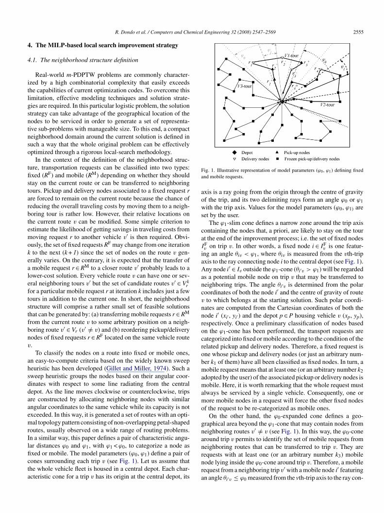
xed or mobile. The model parameters (ϕ0, ϕ1) define a pair ofones surrounding each trip v (see Fig. 1). Let us assume thathe whole vehicle fleet is housed in a central depot. Each char-cteristic cone for a trip v has its origin at the central depot, its

rnra

ig. 1. Illustrative representation of model parameters (ϕ0, ϕ1) defining fixednd mobile requests.

xis is a ray going from the origin through the centre of gravityf the trip, and its two delimiting rays form an angle ϕ0 or ϕ1ith the trip axis. Values for the model parameters (ϕ0, ϕ1) are

et by the user.The ϕ1-slim cone defines a narrow zone around the trip axis

ontaining the nodes that, a priori, are likely to stay on the tourt the end of the improvement process; i.e. the set of fixed nodesFv on trip v. In other words, a fixed node i ∈ IF

v is one featur-ng an angle θiv < ϕ1, where θiv is measured from the vth-tripxis to the ray connecting node i to the central depot (see Fig. 1).ny node i′ ∈ Iv outside the ϕ1-cone (θi′v > ϕ1) will be regarded

s a potential mobile node on trip v that may be transferred toeighboring trips. The angle θi′v is determined from the polaroordinates of both the node i′ and the centre of gravity of routeto which belongs at the starting solution. Such polar coordi-

ates are computed from the Cartesian coordinates of both theode i′ (xi′ , yi′ ) and the depot p ∈ P housing vehicle v (xp, yp),espectively. Once a preliminary classification of nodes basedn the ϕ1-cone has been performed, the transport requests areategorized into fixed or mobile according to the condition of theelated pickup and delivery nodes. Therefore, a fixed request isne whose pickup and delivery nodes (or just an arbitrary num-er k1 of them) have all been classified as fixed nodes. In turn, aobile request means that at least one (or an arbitrary number k2

dopted by the user) of the associated pickup or delivery nodes isobile. Here, it is worth remarking that the whole request must

lways be serviced by a single vehicle. Consequently, one orore mobile nodes in a request will force the other fixed nodes

f the request to be re-categorized as mobile ones.On the other hand, the ϕ0-expanded cone defines a geo-

raphical area beyond the ϕ1-cone that may contain nodes fromeighboring routes v′ /= v (see Fig. 1). In this way, the ϕ0-coneround trip v permits to identify the set of mobile requests fromeighboring routes that can be transferred to trip v. They are

equests with at least one (or an arbitrary number k3) mobileode lying inside the ϕ0-cone around trip v. Therefore, a mobileequest from a neighboring trip v′ with a mobile node i′ featuringn angle θi′v ≤ ϕ0 measured from the vth-trip axis to the ray con-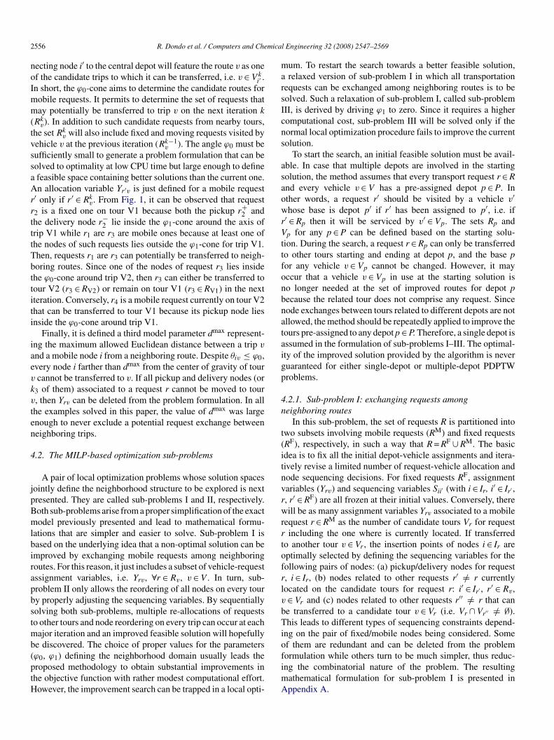

2 mica

noImm(tvssaArrtttTbttiti

iaev

kv

ten

4

jpBmlbirapbstmb(ptH

marsIcns

asaowrVttfonbnataigp

4n

t(itnvrwrrtofrlv

bTio

556 R. Dondo et al. / Computers and Che

ecting node i′ to the central depot will feature the route v as onef the candidate trips to which it can be transferred, i.e. v ∈ Vk

i′ .n short, the ϕ0-cone aims to determine the candidate routes forobile requests. It permits to determine the set of requests thatay potentially be transferred to trip v on the next iteration k

Rkv). In addition to such candidate requests from nearby tours,

he set Rkv will also include fixed and moving requests visited by

ehicle v at the previous iteration (Rk−1v ). The angle ϕ0 must be

ufficiently small to generate a problem formulation that can beolved to optimality at low CPU time but large enough to definefeasible space containing better solutions than the current one.n allocation variable Yr′v is just defined for a mobile request

′ only if r′ ∈ Rkv. From Fig. 1, it can be observed that request

2 is a fixed one on tour V1 because both the pickup r+2 and

he delivery node r−2 lie inside the ϕ1-cone around the axis of

rip V1 while r1 are r3 are mobile ones because at least one ofhe nodes of such requests lies outside the ϕ1-cone for trip V1.hen, requests r1 are r3 can potentially be transferred to neigh-oring routes. Since one of the nodes of request r3 lies insidehe ϕ0-cone around trip V2, then r3 can either be transferred toour V2 (r3 ∈ RV2) or remain on tour V1 (r3 ∈ RV1) in the nextteration. Conversely, r4 is a mobile request currently on tour V2hat can be transferred to tour V1 because its pickup node liesnside the ϕ0-cone around trip V1.

Finally, it is defined a third model parameter dmax represent-ng the maximum allowed Euclidean distance between a trip v

nd a mobile node i from a neighboring route. Despite θiv ≤ ϕ0,very node i farther than dmax from the center of gravity of tourcannot be transferred to v. If all pickup and delivery nodes (or

3 of them) associated to a request r cannot be moved to tour, then Yrv can be deleted from the problem formulation. In allhe examples solved in this paper, the value of dmax was largenough to never exclude a potential request exchange betweeneighboring trips.

.2. The MILP-based optimization sub-problems

A pair of local optimization problems whose solution spacesointly define the neighborhood structure to be explored is nextresented. They are called sub-problems I and II, respectively.oth sub-problems arise from a proper simplification of the exactodel previously presented and lead to mathematical formu-

ations that are simpler and easier to solve. Sub-problem I isased on the underlying idea that a non-optimal solution can bemproved by exchanging mobile requests among neighboringoutes. For this reason, it just includes a subset of vehicle-requestssignment variables, i.e. Yrv, ∀r ∈ Rv, v ∈ V . In turn, sub-roblem II only allows the reordering of all nodes on every toury properly adjusting the sequencing variables. By sequentiallyolving both sub-problems, multiple re-allocations of requestso other tours and node reordering on every trip can occur at each

ajor iteration and an improved feasible solution will hopefullye discovered. The choice of proper values for the parameters

ϕ0, ϕ1) defining the neighborhood domain usually leads theroposed methodology to obtain substantial improvements inhe objective function with rather modest computational effort.owever, the improvement search can be trapped in a local opti-

fimA

l Engineering 32 (2008) 2547–2569

um. To restart the search towards a better feasible solution,relaxed version of sub-problem I in which all transportation

equests can be exchanged among neighboring routes is to beolved. Such a relaxation of sub-problem I, called sub-problemII, is derived by driving ϕ1 to zero. Since it requires a higheromputational cost, sub-problem III will be solved only if theormal local optimization procedure fails to improve the currentolution.

To start the search, an initial feasible solution must be avail-ble. In case that multiple depots are involved in the startingolution, the method assumes that every transport request r ∈ Rnd every vehicle v ∈ V has a pre-assigned depot p ∈ P. Inther words, a request r′ should be visited by a vehicle v′hose base is depot p′ if r′ has been assigned to p′, i.e. if

′ ∈ Rp then it will be serviced by v′ ∈ Vp. The sets Rp andp for any p ∈ P can be defined based on the starting solu-

ion. During the search, a request r ∈ Rp can only be transferredo other tours starting and ending at depot p, and the base por any vehicle v ∈ Vp cannot be changed. However, it mayccur that a vehicle v ∈ Vp in use at the starting solution iso longer needed at the set of improved routes for depot pecause the related tour does not comprise any request. Sinceode exchanges between tours related to different depots are notllowed, the method should be repeatedly applied to improve theours pre-assigned to any depot p ∈ P. Therefore, a single depot isssumed in the formulation of sub-problems I–III. The optimal-ty of the improved solution provided by the algorithm is neveruaranteed for either single-depot or multiple-depot PDPTWroblems.

.2.1. Sub-problem I: exchanging requests amongeighboring routes

In this sub-problem, the set of requests R is partitioned intowo subsets involving mobile requests (RM) and fixed requestsRF), respectively, in such a way that R = RF ∪ RM. The basicdea is to fix all the initial depot-vehicle assignments and itera-ively revise a limited number of request-vehicle allocation andode sequencing decisions. For fixed requests RF, assignmentariables (Yrv) and sequencing variables Sii′ (with i ∈ Ir, i′ ∈ Ir′ ,, r′ ∈ RF) are all frozen at their initial values. Conversely, thereill be as many assignment variables Yrv associated to a mobile

equest r ∈ RM as the number of candidate tours Vr for requestincluding the one where is currently located. If transferred

o another tour v ∈ Vr, the insertion points of nodes i ∈ Ir areptimally selected by defining the sequencing variables for theollowing pairs of nodes: (a) pickup/delivery nodes for request, i ∈ Ir, (b) nodes related to other requests r′ /= r currentlyocated on the candidate tours for request r: i′ ∈ Ir′ , r′ ∈ Rv,∈ Vr and (c) nodes related to other requests r′′ /= r that cane transferred to a candidate tour v ∈ Vr (i.e. Vr ∩ Vr′′ /= ∅).his leads to different types of sequencing constraints depend-

ng on the pair of fixed/mobile nodes being considered. Somef them are redundant and can be deleted from the problem

ormulation while others turn to be much simpler, thus reduc-ng the combinatorial nature of the problem. The resulting

athematical formulation for sub-problem I is presented inppendix A.

mical Engineering 32 (2008) 2547–2569 2557

4i

ieetlmbbrif

4e

nbmacnmiaarnms

4

eiiaafapof(rsiaaaRRc

Fs

R

awcttv

Ω

n

Ω

etctltItwomtotutti

aat

R. Dondo et al. / Computers and Che

.2.2. Sub-problem II: reordering nodes on everyndividual route

The definition of the neighborhood structure is completed byntroducing sub-problem II where the reordering of nodes onvery route is only permitted. In contrast to sub-problem I, noxchange of nodes among neighboring routes is allowed andhe vehicle allocation variables Yrv are deleted from the prob-em formulation. Therefore, sub-problem II is to be solved as

any times as the number of tours in the solution providedy sub-problem I. Although sub-problem II is characterizedy a much lower computational cost than sub-problem I, thee-optimization of individual routes may jointly generate signif-cant improvements in the objective function. The mathematicalormulation for sub-problem II is presented in Appendix B.

.2.3. Sub-problem III: simultaneous reordering andxchange of nodes

Since the search can be trapped in a local optimum, a largereighborhood needs to be considered in order to move towards aetter solution. To this end, every transport request is regarded asobile and can be transferred to some neighboring route. This is

chieved by making ϕ1 = 0 and adopting a finite ϕ0 to define theandidate tours for every request. Moreover, the reordering ofodes on every trip is also allowed. Therefore, the mathematicalodel for sub-problem III is similar to the exact formulation

ntroduced in Section 3 except for: (i) a single depot is assumednd no vehicle-depot assignment variable is needed, and (ii)smaller ϕ0 is adopted to decrease the number of candidate

outes for each request, i.e. |Vr|. However, the use of an extendedeighborhood will surely a smaller lead to a larger problem for-ulation. For this reason, sub-problem III will be solved only if

ub-problems I and II both fail to improve the current solution.

.3. Spatial decomposition of large m-PDPTW problems

Since the neighborhood structure accounts for solutions gen-rated from the current solution by reordering nodes on eachndividual tour or relocating requests to neighboring trips, theres no sense in tackling the whole m-PDPTW problem at once. Inlocal search environment, each tour just exchanges nodes withfew routes closed to it and the attention should therefore be

ocused on a much smaller geographical area where such inter-cting trips are confined. In order to take advantage of such aroblem feature, a rotating angular sector (RAS) is defined withrigin at the central depot (DC) and delimiting rays emanatingrom the DC with angular coordinates Ω1 and Ω2, respectivelysee Fig. 2). The angle Ω (=Ω2 − Ω1) between the extreme raysemains fixed as the RAS rotates. In order to sweep the wholeervice region, the RAS will turn around the DC by equallyncreasing the extreme ray angular coordinates Ω1 and Ω2 by

fixed quantity Ω. In this way, the RAS will take a series ofngular positions {Ω(1), Ω(2), . . .} before rotating 2π and start

new turn. If some but not all nodes of a trip v are inside theAS(m) at a particular position Ω(m) = 0.5 (Ω2

(m) + Ω1(m)) of the

AS-axis, then the procedure assumes that the whole trip v isontained in RAS(m). In other words, a node i will pertain to

Wiyp

ig. 2. The rotating angular sector (RAS) decomposing the service region intomaller zones.

AS(m) if either (a) its angular coordinate Θi is between Ω(m)1

nd Ω(m)2 (Ω(m)

1 ≤ Θi ≤ Ω(m)2 ) or alternatively (b) the trip to

hich it currently belongs has at least a node i′ satisfying theondition Ω

(m)1 ≤ Θi′ ≤ Ω

(m)2 . At any location Ω(m), therefore,

he RAS(m) will contain a limited number of complete toursogether with the nodes located on all of them. Moreover, a tripmay belong to the rotating sector at two consecutive locations(m) and Ω(m+1). Initially, Ω

(1)1 is set equal to zero. If N is the

umber of RAS-locations per turn, then N = (2π/Ω).Each time sub-problems I and II for a particular location

(m) are solved, only routes inside the RAS(m) will be consid-red. Nodes and trips beyond RAS(m) are ignored. Therefore,he mathematical formulations for sub-problems I and II willhange with �(m) as long as the set of nodes I(m) and the set ofours V(m) inside the RAS both depend on Ω(m). At each RAS-ocation, sub-problems I and II will be repeatedly solved untilhe procedure converges to a local optimum (the normal mode).t may happen that no improvement at all has been achievedhrough the normal node after sweeping the N locations, i.e. thehole service area. In order to avoid getting stuck on a localptimum, sub-problem III will be activated (the perturbation orixed mode), if necessary, just on the next turn to move forward

owards a feasible/infeasible solution with a better value of thebjective function. If the perturbation move is successful, thenhe normal mode is applied again. The procedure is repeatedntil the normal mode becomes trapped on a local optimum andhe perturbation mode fails to get an improved solution. Whenhis happens, the procedure is stopped and the best set of routess given by the current incumbent solution.

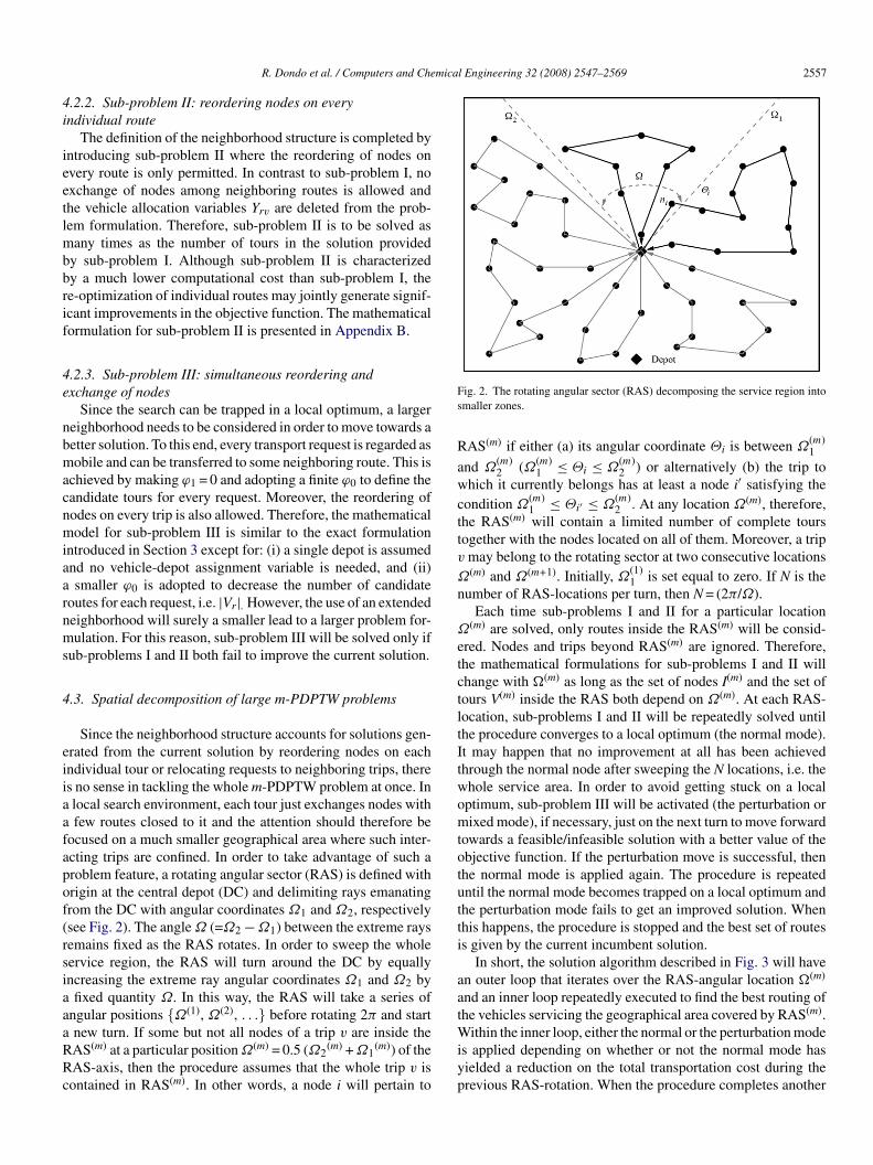
In short, the solution algorithm described in Fig. 3 will haven outer loop that iterates over the RAS-angular location �(m)

nd an inner loop repeatedly executed to find the best routing ofhe vehicles servicing the geographical area covered by RAS(m).

ithin the inner loop, either the normal or the perturbation modes applied depending on whether or not the normal mode hasielded a reduction on the total transportation cost during therevious RAS-rotation. When the procedure completes another

2558 R. Dondo et al. / Computers and Chemical Engineering 32 (2008) 2547–2569

orhoo

ttrlanoiomothl

maafIbt

5

hi

wbcSamPenmhLlcdLhpsooati

Fig. 3. The PDPTW neighb

urn h, the new incumbent solution is obtained by consideringhe best vehicle routes found at each of the N locations of theotating sector. If a trip v belongs to a pair of consecutive RAS-ocations m and m + 1, the latter one will define its structuret the new best solution, i.e. the subset Iv and the sequence ofodes on trip v. Convergence of the procedure to a local or globalptimum is checked out by comparing the total cost of the newncumbent solution after completing turn h with that of the oldne at the end of turn (h − 1). If the normal and the perturbationodes both fail to provide a better solution or the improvement

n the objective function is less than a small positive scalar ε,hen the procedure must be stopped. In other words, the methodas converged if no improvement at all has been obtained on theast two turns of the rotating angular sector.

In multi-depot m-PDPTW problems, the improvementethod assumes that requests and vehicles have their pre-

ssigned depots (see Section 4.1) and exchanges of requestsmong tours linked to different depots are not allowed. There-ore, depots and their related tours can be considered one by one.n other words, the solution algorithm described in Fig. 3 shoulde applied as many times as the number of depots involved inhe starting solution.

. Results and discussion

The proposed m-PDPTW exact and improvement approachesave both been tested by solving a set of PDPTW problemnstances introduced by Li and Lim (2003a). Such examples

Tapv

d improvement algorithm.

ere generated from known solutions to VRPTW Solomonenchmark problems (Solomon, 1987) by randomly pairingustomer locations on the same tour (Li & Lim, 2003a). Allolomon’s VRPTW problems originally feature 100 real nodesnd a single central depot, but some dummy nodes, if necessary,ay be added for pairing purpose. In this manner, multi-vehicleDPTW benchmark problems with nearly 50 customer requests,ach one involving a single pickup node and a single deliveryode, were developed. Similarly to Solomon’s VRPTW bench-ark problems, the new ones proposed by Li and Lim (2003a)

ave been grouped into three different categories: LC, LR andRC. The data set for every category comprises several prob-

em instances with the same geographical node distribution, aentral depot, multiple vehicles with a similar load capacity andifferent time-window width distributions. Problems of classC have clustered customers whose associated time windowsave been generated based on known solutions. In LR-classroblems, customer locations are randomly generated over aquare while LRC-class problems result from a combinationf clustered and randomized customer distributions. Problemsf each class are further classified into two types called “1”nd “2”. Type-1 PDPTW problems are characterized by narrowime windows and low-capacity vehicles, while type-2 problemsnvolve wider time windows and vehicles with a larger capacity.

herefore, solutions to type-2 PDPTW problems feature fewernd longer tours. For instance, the example LR-102 is a LR1-roblem involving randomly distributed nodes and low-capacityehicles, i.e. a R-class problem of type-1. The last two digits 02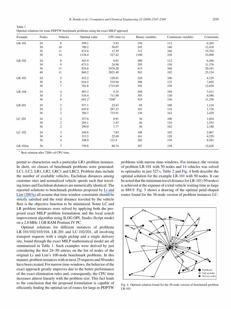

R. Dondo et al. / Computers and Chemical Engineering 32 (2008) 2547–2569 2559

Table 1Optimal solutions for some PDPTW benchmark problems using the exact MILP approach

Example Nodes Vehicles Optimal value CPU time (s) Binary variables Continuous variables Constraints

LR-101 24 8 599.1 5.83 156 112 6,26530 10 700.2 50.07 245 140 12,41836 11 833.6 12.29 312 166 19,70250 14 1138.4 527.42 1108 228 52,098

LR-102 24 8 543.9 8.81 200 112 6,44630 9 673.5 24.98 295 138 11,37636 11 824.6 2476.20 415 166 20,18140 11 860.2 5821.40 563 182 25,334

LR-103 24 5 432.2 120.81 228 106 4,12930 6 616.5 519.94 306 132 7,60236 7 782.8 1715.69 392 158 12,658

LR-104 24 4 493.3 9.25 268 104 3,41130 5 534.4 711.98 393 130 6,58636 6 681.2* 7200* 524 156 11,250

LR-201 24 2 557.1 22.83 69 100 1,12430 2 645.8 287.23 101 124 1,71836 2 760.7 715.91 136 162 2,429

LC-201 24 2 257.6 0.91 36 100 1,02430 2 269.1 1.47 46 124 1,55236 2 290.0 1.77 56 162 2,188

LC-102 24 3 249.8 7.83 108 102 2,06730 4 313.5 22.69 161 128 4,52936 4 348.9 121.8 282 130 8,581

L .74

pILtcirLsflLpio

Ltsscomheoite

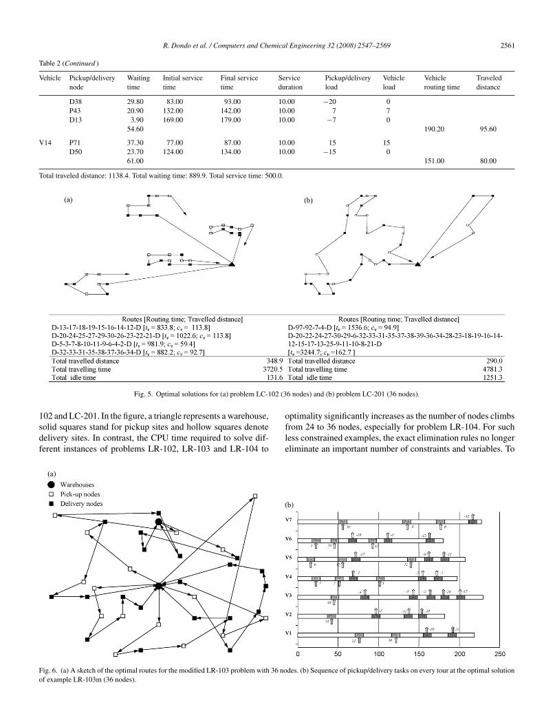
potobis achieved at the expense of a total vehicle waiting time as largeas 889.9. Fig. 5 shows a drawing of the optimal petal-shapedroutes found for the 36-node version of problem instances LC-

R-103m 36 7 759.8 88

* Best solution after 7200 s of CPU time.

ermit to characterize such a particular LR1-problem instance.n short, six classes of benchmark problems were generated:C1, LC2, LR1, LR2, LRC1 and LRC2. Problem data include

he number of available vehicles, Euclidean distances amongustomer sites and normalized vehicle speeds such that travel-ng times and Euclidean distances are numerically identical. Theeported solutions to benchmark problems proposed by Li andim (2003a) all assume that time-window constraints should betrictly satisfied and the total distance traveled by the vehicleeet is the objective function to be minimized. Some LC andR problem instances were solved by applying both the pro-osed exact MILP problem formulation and the local searchmprovement algorithm using ILOG OPL Studio (Script mode)n a 2.8 MHz 1 GB RAM Pentium IV PC.

Optimal solutions for different instances of problemsR-101/102/103/104, LR-201 and LC-102/201, all involving

ransport requests with a single pickup and a single deliveryite, found through the exact MILP mathematical model are allummarized in Table 1. Such examples were derived by justonsidering the first 24–50 entries on the list of nodes of theriginal Li and Lim’s 100-node benchmark problems. In thisanner, problem instances with at most 25 requests and 50 nodes

ave been created. For narrow time-windows, the behavior of thexact approach greatly improves due to the better performance

f the exact elimination rules and, consequently, the CPU timencreases almost linearly with the problem size. This fact leadso the conclusion that the proposed formulation is capable offficiently finding the optimal set of routes for large m-PDPTW

FL

387 158 12,628

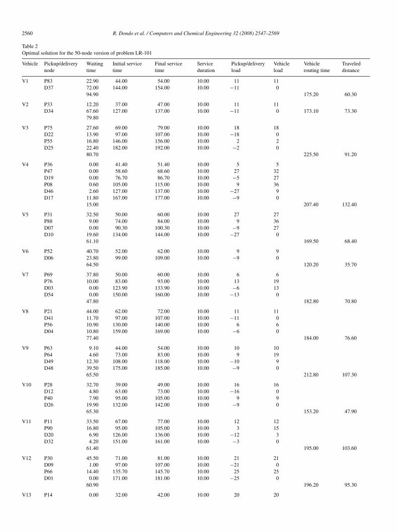
roblems with narrow time-windows. For instance, the versionf problem LR-101 with 50 nodes and 14 vehicles was solvedo optimality in just 527 s. Table 2 and Fig. 4 both describe theptimal solution for the example LR-101 with 50 nodes. It cane noted that the minimum travel distance for LR-101 (50 nodes)

ig. 4. Optimal solution found for the 50-node version of benchmark problemR-101.

2560 R. Dondo et al. / Computers and Chemical Engineering 32 (2008) 2547–2569

Table 2Optimal solution for the 50-node version of problem LR-101

Vehicle Pickup/deliverynode

Waitingtime

Initial servicetime

Final servicetime

Serviceduration

Pickup/deliveryload

Vehicleload

Vehiclerouting time

Traveleddistance

V1 P83 22.90 44.00 54.00 10.00 11 11D37 72.00 144.00 154.00 10.00 −11 0

94.90 175.20 60.30

V2 P33 12.20 37.00 47.00 10.00 11 11D34 67.60 127.00 137.00 10.00 −11 0 173.10 73.30

79.80

V3 P75 27.60 69.00 79.00 10.00 18 18D22 13.90 97.00 107.00 10.00 −18 0P55 16.80 146.00 156.00 10.00 2 2D25 22.40 182.00 192.00 10.00 −2 0

80.70 225.50 91.20

V4 P36 0.00 41.40 51.40 10.00 5 5P47 0.00 58.60 68.60 10.00 27 32D19 0.00 76.70 86.70 10.00 −5 27P08 0.60 105.00 115.00 10.00 9 36D46 2.60 127.00 137.00 10.00 −27 9D17 11.80 167.00 177.00 10.00 −9 0

15.00 207.40 132.40

V5 P31 32.50 50.00 60.00 10.00 27 27P88 9.00 74.00 84.00 10.00 9 36D07 0.00 90.30 100.30 10.00 −9 27D10 19.60 134.00 144.00 10.00 −27 0

61.10 169.50 68.40

V6 P52 40.70 52.00 62.00 10.00 9 9D06 23.80 99.00 109.00 10.00 −9 0

64.50 120.20 35.70

V7 P69 37.80 50.00 60.00 10.00 6 6P76 10.00 83.00 93.00 10.00 13 19D03 0.00 123.90 133.90 10.00 −6 13D54 0.00 150.00 160.00 10.00 −13 0

47.80 182.80 70.80

V8 P21 44.00 62.00 72.00 10.00 11 11D41 11.70 97.00 107.00 10.00 −11 0P56 10.90 130.00 140.00 10.00 6 6D04 10.80 159.00 169.00 10.00 −6 0

77.40 184.00 76.60

V9 P63 9.10 44.00 54.00 10.00 10 10P64 4.60 73.00 83.00 10.00 9 19D49 12.30 108.00 118.00 10.00 −10 9D48 39.50 175.00 185.00 10.00 −9 0

65.50 212.80 107.30

V10 P28 32.70 39.00 49.00 10.00 16 16D12 4.80 63.00 73.00 10.00 −16 0P40 7.90 95.00 105.00 10.00 9 9D26 19.90 132.00 142.00 10.00 −9 0

65.30 153.20 47.90

V11 P11 33.50 67.00 77.00 10.00 12 12P90 16.80 95.00 105.00 10.00 3 15D20 6.90 126.00 136.00 10.00 −12 3D32 4.20 151.00 161.00 10.00 −3 0

61.40 195.00 103.60

V12 P30 45.50 71.00 81.00 10.00 21 21D09 1.00 97.00 107.00 10.00 −21 0P66 14.40 135.70 145.70 10.00 25 25D01 0.00 171.00 181.00 10.00 −25 0

60.90 196.20 95.30

V13 P14 0.00 32.00 42.00 10.00 20 20

R. Dondo et al. / Computers and Chemical Engineering 32 (2008) 2547–2569 2561

Table 2 (Continued )

Vehicle Pickup/deliverynode

Waitingtime

Initial servicetime

Final servicetime

Serviceduration

Pickup/deliveryload

Vehicleload

Vehiclerouting time

Traveleddistance

D38 29.80 83.00 93.00 10.00 −20 0P43 20.90 132.00 142.00 10.00 7 7D13 3.90 169.00 179.00 10.00 −7 0

54.60 190.20 95.60

V14 P71 37.30 77.00 87.00 10.00 15 15D50 23.70 124.00 134.00 10.00 −15 0

61.00 151.00 80.00

Total traveled distance: 1138.4. Total waiting time: 889.9. Total service time: 500.0.

02 (3

1sdf

Fo

Fig. 5. Optimal solutions for (a) problem LC-1

02 and LC-201. In the figure, a triangle represents a warehouse,olid squares stand for pickup sites and hollow squares denoteelivery sites. In contrast, the CPU time required to solve dif-erent instances of problems LR-102, LR-103 and LR-104 to

ofle

ig. 6. (a) A sketch of the optimal routes for the modified LR-103 problem with 36 nof example LR-103m (36 nodes).

6 nodes) and (b) problem LC-201 (36 nodes).

ptimality significantly increases as the number of nodes climbsrom 24 to 36 nodes, especially for problem LR-104. For suchess constrained examples, the exact elimination rules no longerliminate an important number of constraints and variables. To

des. (b) Sequence of pickup/delivery tasks on every tour at the optimal solution

2 mica

ieml7rdt

5i

itnbTmiItnCtccniraceTttϕ

to

π

fsswoAsiarvaitffbs

tmcaofdval(ttt

TB

E

LLLLLLLLL

562 R. Dondo et al. / Computers and Che

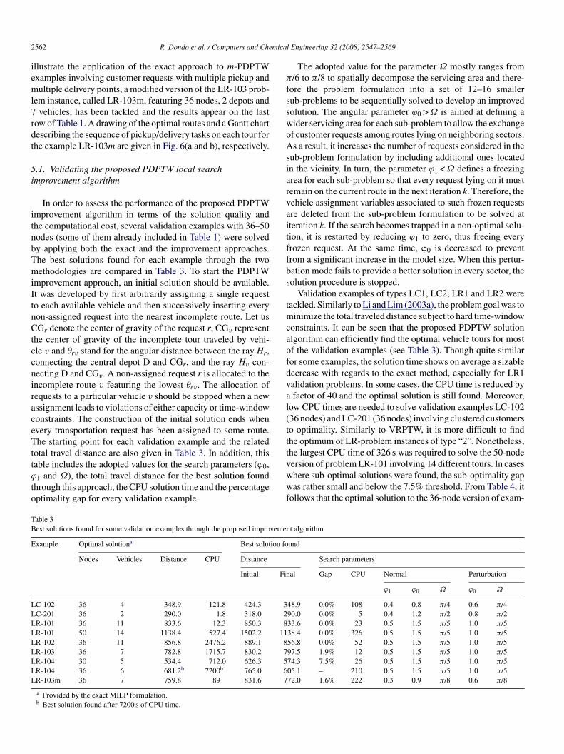
llustrate the application of the exact approach to m-PDPTWxamples involving customer requests with multiple pickup andultiple delivery points, a modified version of the LR-103 prob-

em instance, called LR-103m, featuring 36 nodes, 2 depots andvehicles, has been tackled and the results appear on the last

ow of Table 1. A drawing of the optimal routes and a Gantt chartescribing the sequence of pickup/delivery tasks on each tour forhe example LR-103m are given in Fig. 6(a and b), respectively.

.1. Validating the proposed PDPTW local searchmprovement algorithm

In order to assess the performance of the proposed PDPTWmprovement algorithm in terms of the solution quality andhe computational cost, several validation examples with 36–50odes (some of them already included in Table 1) were solvedy applying both the exact and the improvement approaches.he best solutions found for each example through the twoethodologies are compared in Table 3. To start the PDPTW

mprovement approach, an initial solution should be available.t was developed by first arbitrarily assigning a single requesto each available vehicle and then successively inserting everyon-assigned request into the nearest incomplete route. Let usGr denote the center of gravity of the request r, CGv represent

he center of gravity of the incomplete tour traveled by vehi-le v and θrv stand for the angular distance between the ray Hr,onnecting the central depot D and CGr, and the ray Hv con-ecting D and CGv. A non-assigned request r is allocated to thencomplete route v featuring the lowest θrv. The allocation ofequests to a particular vehicle v should be stopped when a newssignment leads to violations of either capacity or time-windowonstraints. The construction of the initial solution ends whenvery transportation request has been assigned to some route.he starting point for each validation example and the related

otal travel distance are also given in Table 3. In addition, this

able includes the adopted values for the search parameters (ϕ0,1 and Ω), the total travel distance for the best solution found

hrough this approach, the CPU solution time and the percentageptimality gap for every validation example.

vwwf

able 3est solutions found for some validation examples through the proposed improvemen

xample Optimal solutiona Best solution fo

Nodes Vehicles Distance CPU Distance

Initial Fin

C-102 36 4 348.9 121.8 424.3 3C-201 36 2 290.0 1.8 318.0 2R-101 36 11 833.6 12.3 850.3 8R-101 50 14 1138.4 527.4 1502.2 11R-102 36 11 856.8 2476.2 889.1 8R-103 36 7 782.8 1715.7 830.2 7R-104 30 5 534.4 712.0 626.3 5R-104 36 6 681.2b 7200b 765.0 6R-103m 36 7 759.8 89 831.6 7

a Provided by the exact MILP formulation.b Best solution found after 7200 s of CPU time.

l Engineering 32 (2008) 2547–2569

The adopted value for the parameter Ω mostly ranges from/6 to π/8 to spatially decompose the servicing area and there-

ore the problem formulation into a set of 12–16 smallerub-problems to be sequentially solved to develop an improvedolution. The angular parameter ϕ0 > Ω is aimed at defining aider servicing area for each sub-problem to allow the exchangef customer requests among routes lying on neighboring sectors.s a result, it increases the number of requests considered in the

ub-problem formulation by including additional ones locatedn the vicinity. In turn, the parameter ϕ1 < Ω defines a freezingrea for each sub-problem so that every request lying on it mustemain on the current route in the next iteration k. Therefore, theehicle assignment variables associated to such frozen requestsre deleted from the sub-problem formulation to be solved atteration k. If the search becomes trapped in a non-optimal solu-ion, it is restarted by reducing ϕ1 to zero, thus freeing everyrozen request. At the same time, �0 is decreased to preventrom a significant increase in the model size. When this pertur-ation mode fails to provide a better solution in every sector, theolution procedure is stopped.

Validation examples of types LC1, LC2, LR1 and LR2 wereackled. Similarly to Li and Lim (2003a), the problem goal was toinimize the total traveled distance subject to hard time-window

onstraints. It can be seen that the proposed PDPTW solutionlgorithm can efficiently find the optimal vehicle tours for mostf the validation examples (see Table 3). Though quite similaror some examples, the solution time shows on average a sizableecrease with regards to the exact method, especially for LR1alidation problems. In some cases, the CPU time is reduced byfactor of 40 and the optimal solution is still found. Moreover,

ow CPU times are needed to solve validation examples LC-10236 nodes) and LC-201 (36 nodes) involving clustered customerso optimality. Similarly to VRPTW, it is more difficult to findhe optimum of LR-problem instances of type “2”. Nonetheless,he largest CPU time of 326 s was required to solve the 50-node

ersion of problem LR-101 involving 14 different tours. In caseshere sub-optimal solutions were found, the sub-optimality gapas rather small and below the 7.5% threshold. From Table 4, it

ollows that the optimal solution to the 36-node version of exam-

t algorithm

und

Search parameters

al Gap CPU Normal Perturbation

ϕ1 ϕ0 Ω ϕ0 Ω

48.9 0.0% 108 0.4 0.8 π/4 0.6 π/490.0 0.0% 5 0.4 1.2 π/2 0.8 π/233.6 0.0% 23 0.5 1.5 π/5 1.0 π/538.4 0.0% 326 0.5 1.5 π/5 1.0 π/556.8 0.0% 52 0.5 1.5 π/5 1.0 π/597.5 1.9% 12 0.5 1.5 π/5 1.0 π/574.3 7.5% 26 0.5 1.5 π/5 1.0 π/505.1 – 210 0.5 1.5 π/5 1.0 π/572.0 1.6% 222 0.3 0.9 π/8 0.6 π/8

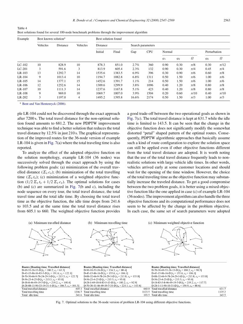
R. Dondo et al. / Computers and Chemical Engineering 32 (2008) 2547–2569 2563

Table 4Best solutions found for several 100-node benchmark problems through the improvement algorithm

Example Best known solutiona Best solution found

Vehicles Distance Vehicles Distance Search parameters

Initial Final Gap CPU Normal Perturbation

ϕ1 ϕ0 Ω ϕ0 Ω

LC-102 10 828.9 10 878.3 851.0 2.7% 360 0.90 0.30 π/8 0.30 π/12LC-201 3 591.6 3 813.9 605.4 2.3% 132 0.90 0.30 π/4 0.45 π/4LR-103 13 1292.7 14 1535.6 1383.5 6.9% 396 0.30 0.90 π/6 0.60 π/8LR-104 9 1013.4 10 1194.7 1082.8 6.8% 1311 0.50 1.50 π/6 1.00 π/6LR-105 14 1377.1 15 1452.6 1391.7 1.1% 214 0.50 1.50 π/6 1.00 π/6LR-106 12 1252.6 14 1309.6 1299.9 3.8% 1096 0.40 1.20 π/8 0.80 π/8LR-107 10 1111.3 14 1237.6 1167.8 5.1% 423 0.40 1.20 π/8 0.80 π/8L 0L 8

pattttLr

tsfett(ntttf

aFtodqscftrvwotbt

R-108 9 969.0 10 1069.7 1007.R-202 3 1197.0 4 1495.2 1395.

a Bent and Van Hentenryck (2006).

le LR-104 could not be discovered through the exact approachfter 7200 s. The total travel distance for the non-optimal solu-ion found amounts to 681.2. The new PDPTW improvementechnique was able to find a better solution that reduces the totalravel distance by 12.5% in just 210 s. The graphical representa-ion of the improved routes for the 36-node version of exampleR-104 is given in Fig. 7(a) where the total traveling time is also

eported.To analyze the effect of the adopted objective function on

he solution morphology, example LR-104 (36 nodes) wasuccessively solved through the exact approach by using theollowing problem goals: (a) minimization of the overall trav-lled distance (Σv cv); (b) minimization of the total travellingime (Σv tv); (c) minimization of a weighted objective func-ion (1/2 Σv tv + 1/2 Σv cv). The optimal solutions for casesb) and (c) are summarized in Fig. 7(b and c), including theode sequence on every tour, the total travel distance, the total

ravel time and the total idle time. By choosing the total travelime as the objective function, the idle time drops from 241.6o 103.5 and at the same time the total travel distance risesrom 605.1 to 660. The weighted objective function provides

(osI

Fig. 7. Optimal solutions to the 36-node version of pro

3.9% 1504 0.20 0.60 π/10 0.40 π/1016.6% 2174 0.50 1.50 π/3 1.00 π/3

good trade-off between the two operational goals as shown inig. 7(c). The total travel distance is kept at 631.7 while the idle

ime is limited to 143.5. It can be seen that the change in thebjective function does not significantly modify the somewhatistorted “petal” shaped pattern of the optimal routes. Conse-uently, PDPTW algorithmic approaches that basically assumeuch a kind of route configuration to explore the solution spacean still be applied even if other objective functions differentrom the total travel distance are adopted. It is worth notinghat the use of the total travel distance frequently leads to non-ealistic solutions with large vehicle idle times. In other words,ehicles arrived early at some customer locations and shouldait for the opening of the time window. However, the choicef the total traveling time as the objective function may substan-ially increase the traveled distance. To get a good compromiseetween the two problem goals, it is better using a mixed objec-ive function like the one applied in case (c) of example LR-104

36 nodes). The improvement algorithm can also handle the threebjective functions and its computational performance does noteem to be affected by the change in the problem objective.n each case, the same set of search parameters were adopted

blem LR-104 using different objective functions.

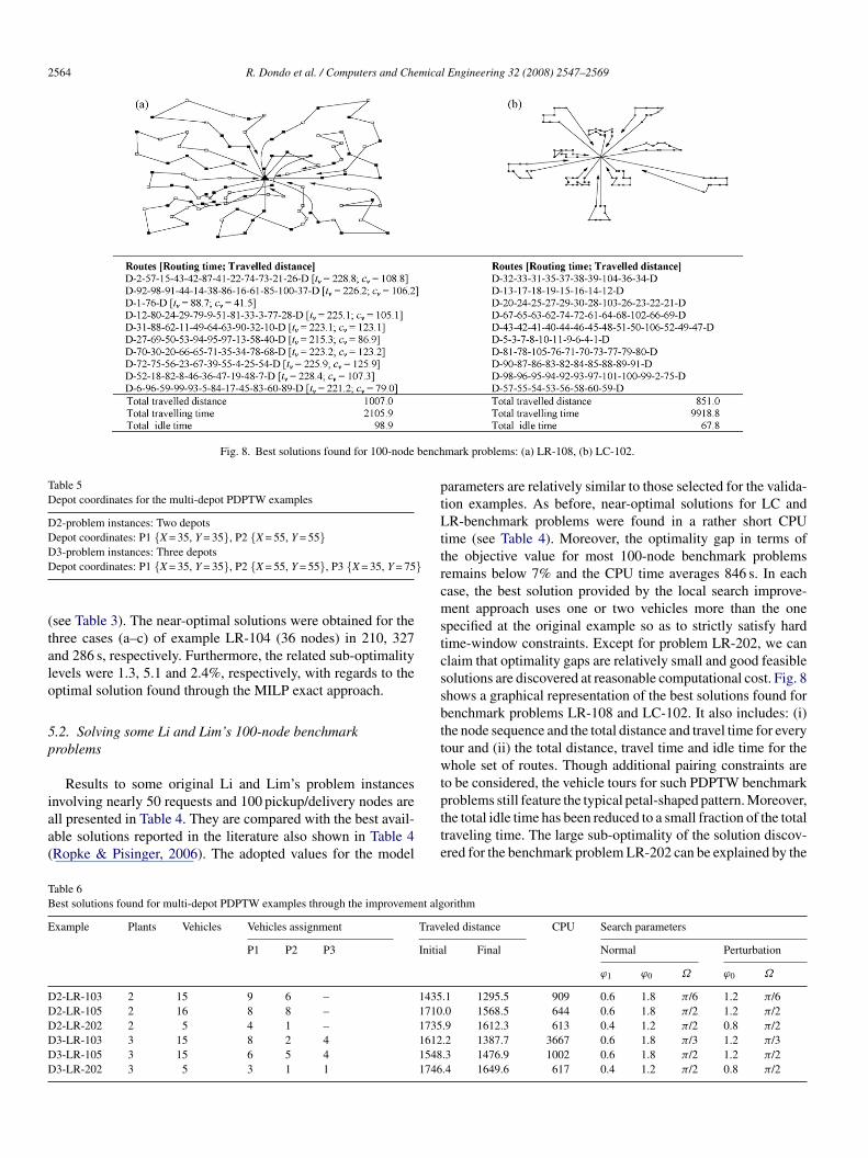
2564 R. Dondo et al. / Computers and Chemical Engineering 32 (2008) 2547–2569

Fig. 8. Best solutions found for 100-node bench

Table 5Depot coordinates for the multi-depot PDPTW examples

D2-problem instances: Two depotsDepot coordinates: P1 {X = 35, Y = 35}, P2 {X = 55, Y = 55}DD }

(talo

5p

iaa(

ptLttrcmstcssbttwt

TB

E

DDDDDD

3-problem instances: Three depotsepot coordinates: P1 {X = 35, Y = 35}, P2 {X = 55, Y = 55}, P3 {X = 35, Y = 75

see Table 3). The near-optimal solutions were obtained for thehree cases (a–c) of example LR-104 (36 nodes) in 210, 327nd 286 s, respectively. Furthermore, the related sub-optimalityevels were 1.3, 5.1 and 2.4%, respectively, with regards to theptimal solution found through the MILP exact approach.

.2. Solving some Li and Lim’s 100-node benchmarkroblems

Results to some original Li and Lim’s problem instances

nvolving nearly 50 requests and 100 pickup/delivery nodes arell presented in Table 4. They are compared with the best avail-ble solutions reported in the literature also shown in Table 4Ropke & Pisinger, 2006). The adopted values for the model

ptte

able 6est solutions found for multi-depot PDPTW examples through the improvement alg

xample Plants Vehicles Vehicles assignment Trave

P1 P2 P3 Initia

2-LR-103 2 15 9 6 – 14352-LR-105 2 16 8 8 – 17102-LR-202 2 5 4 1 – 17353-LR-103 3 15 8 2 4 16123-LR-105 3 15 6 5 4 15483-LR-202 3 5 3 1 1 1746

mark problems: (a) LR-108, (b) LC-102.

arameters are relatively similar to those selected for the valida-ion examples. As before, near-optimal solutions for LC andR-benchmark problems were found in a rather short CPU

ime (see Table 4). Moreover, the optimality gap in terms ofhe objective value for most 100-node benchmark problemsemains below 7% and the CPU time averages 846 s. In eachase, the best solution provided by the local search improve-ent approach uses one or two vehicles more than the one

pecified at the original example so as to strictly satisfy hardime-window constraints. Except for problem LR-202, we canlaim that optimality gaps are relatively small and good feasibleolutions are discovered at reasonable computational cost. Fig. 8hows a graphical representation of the best solutions found forenchmark problems LR-108 and LC-102. It also includes: (i)he node sequence and the total distance and travel time for everyour and (ii) the total distance, travel time and idle time for thehole set of routes. Though additional pairing constraints are

o be considered, the vehicle tours for such PDPTW benchmark

roblems still feature the typical petal-shaped pattern. Moreover,he total idle time has been reduced to a small fraction of the totalraveling time. The large sub-optimality of the solution discov-red for the benchmark problem LR-202 can be explained by the

orithm

led distance CPU Search parameters

l Final Normal Perturbation

ϕ1 ϕ0 Ω ϕ0 Ω

.1 1295.5 909 0.6 1.8 π/6 1.2 π/6

.0 1568.5 644 0.6 1.8 π/2 1.2 π/2

.9 1612.3 613 0.4 1.2 π/2 0.8 π/2

.2 1387.7 3667 0.6 1.8 π/3 1.2 π/3

.3 1476.9 1002 0.6 1.8 π/2 1.2 π/2

.4 1649.6 617 0.4 1.2 π/2 0.8 π/2

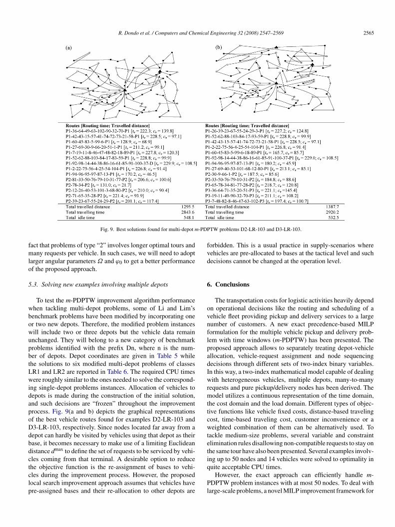
R. Dondo et al. / Computers and Chemical Engineering 32 (2008) 2547–2569 2565

-PDP

fmlo

5

wbowupbtLwidapoDdbdctclp

fvd

6

ovnflpadIwrmttcwteti

Fig. 9. Best solutions found for multi-depot m

act that problems of type “2” involves longer optimal tours andany requests per vehicle. In such cases, we will need to adopt

arger angular parameters Ω and ϕ0 to get a better performancef the proposed approach.

.3. Solving new examples involving multiple depots

To test the m-PDPTW improvement algorithm performancehen tackling multi-depot problems, some of Li and Lim’senchmark problems have been modified by incorporating oner two new depots. Therefore, the modified problem instancesill include two or three depots but the vehicle data remainnchanged. They will belong to a new category of benchmarkroblems identified with the prefix Dn, where n is the num-er of depots. Depot coordinates are given in Table 5 whilehe solutions to six modified multi-depot problems of classesR1 and LR2 are reported in Table 6. The required CPU timesere roughly similar to the ones needed to solve the correspond-

ng single-depot problems instances. Allocation of vehicles toepots is made during the construction of the initial solution,nd such decisions are “frozen” throughout the improvementrocess. Fig. 9(a and b) depicts the graphical representationsf the best vehicle routes found for examples D2-LR-103 and3-LR-103, respectively. Since nodes located far away from aepot can hardly be visited by vehicles using that depot as theirase, it becomes necessary to make use of a limiting Euclideanistance dmax to define the set of requests to be serviced by vehi-les coming from that terminal. A desirable option to reduce

he objective function is the re-assignment of bases to vehi-les during the improvement process. However, the proposedocal search improvement approach assumes that vehicles havere-assigned bases and their re-allocation to other depots are

q

Pl

TW problems D2-LR-103 and D3-LR-103.

orbidden. This is a usual practice in supply-scenarios whereehicles are pre-allocated to bases at the tactical level and suchecisions cannot be changed at the operation level.

. Conclusions

The transportation costs for logistic activities heavily dependn operational decisions like the routing and scheduling of aehicle fleet providing pickup and delivery services to a largeumber of customers. A new exact precedence-based MILPormulation for the multiple vehicle pickup and delivery prob-em with time windows (m-PDPTW) has been presented. Theroposed approach allows to separately treating depot-vehiclellocation, vehicle-request assignment and node sequencingecisions through different sets of two-index binary variables.n this way, a two-index mathematical model capable of dealingith heterogeneous vehicles, multiple depots, many-to-many

equests and pure pickup/delivery nodes has been derived. Theodel utilizes a continuous representation of the time domain,

he cost domain and the load domain. Different types of objec-ive functions like vehicle fixed costs, distance-based travelingost, time-based traveling cost, customer inconvenience or aeighted combination of them can be alternatively used. To

ackle medium-size problems, several variable and constraintlimination rules disallowing non-compatible requests to stay onhe same tour have also been presented. Several examples involv-ng up to 50 nodes and 14 vehicles were solved to optimality in

uite acceptable CPU times.

However, the exact approach can efficiently handle m-DPTW problem instances with at most 50 nodes. To deal with

arge-scale problems, a novel MILP improvement framework for

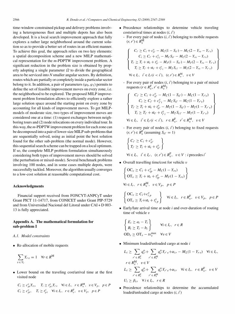
2 mica

tidetTacsearbdtmlamcbtbaftIc(ist

A

Ga1

As

A

•

•

•

•

•

•

566 R. Dondo et al. / Computers and Che

ime-window-constrained pickup and delivery problems involv-ng a heterogeneous fleet and multiple depots has also beeneveloped. It is a local search improvement approach that fullyxplores a rather large neighborhood around the current solu-ion so as to provide a better set of routes in an efficient manner.o achieve this goal, the approach relies on two key elements:spatial decomposition scheme and a new MILP mathemati-

al representation for the m-PDPTW improvement problem. Aignificant reduction in the problem size is obtained by prop-rly adopting a single parameter Ω to divide the geographicalrea to be serviced into N smaller angular sectors. By definition,outes which are partially or completely inside a particular sectorelong to it. In addition, a pair of parameters (ϕ0, ϕ1) permits toefine the set of feasible improvement moves on every zone, i.e.he neighborhood to be explored. The proposed MILP improve-

ent problem formulation allows to efficiently explore a ratherarge solution space around the starting point on every zone byccounting for all kinds of improvement moves. To get MILP-odels of moderate size, two types of improvement moves are

onsidered one at a time: (1) request exchanges between neigh-oring tours and (2) node relocations on every individual tour. Inhis way, the m-PDPTW improvement problem for each zone cane decomposed into a pair of lower-size MILP sub-problems thatre sequentially solved, using as initial point the best solutionound for the other sub-problem (the normal mode). However,his sequential search scheme can be trapped on a local optimum.f so, the complete MILP problem formulation simultaneouslyonsidering both types of improvement moves should be solvedthe perturbation or mixed-mode). Several benchmark problemsnvolving 100 nodes, and in some cases multiple depots, wereuccessfully tackled. Moreover, the algorithm usually convergeso a low-cost solution at reasonable computational cost.

cknowledgments

Financial support received from FONCYT-ANPCyT underrant PICT 11-14717, from CONICET under Grant PIP-5729

nd from Universidad Nacional del Litoral under CAI + D 003-3 is fully appreciated.

ppendix A. The mathematical formulation forub-problem I

.1. Model constraints

Re-allocation of mobile requests

∑v ∈ Vr

Yr v = 1 ∀r ∈ RM

Lower bound on the traveling cost/arrival time at the firstvisited node

Ci ≥ cvpiYrv, Ti ≥ tvp iYr v ∀i ∈ Ir, r ∈ RM

v , v ∈ Vp, p ∈ P

Ci ≥ cvpi, Ti ≥ tvp i ∀i ∈ Ir, r ∈ RF

v , v ∈ Vp, p ∈ P•

l Engineering 32 (2008) 2547–2569

Precedence relationships to determine vehicle travelingcosts/arrival times at nodes (i, i′)- For every pair of nodes (i, i′) belonging to mobile requests

(r, r′) ∈ RMv⎧⎪⎪⎪⎨

⎪⎪⎪⎩Ci′ ≥ Ci + cv

ii′ − MC(1 − Sii′ ) − MC(2 − Yrv − Yr′v)

Ci ≥ Ci′ + cvi′i − MCSii′ − MC(2 − Yrv − Yr′v)

Ti′ ≥ Ti + sti + tvii′ − MT (1 − Sii′ ) − MT (2 − Yrv − Yr′ v)

Ti ≥ Ti′ + sti′ + tvi′ i − MT Si i′ − MT (2 − Yrv − Yr′ v)

⎫⎪⎪⎪⎬⎪⎪⎪⎭

∀i ∈ Ir, i′ ∈ Ir′ (i < i′), (r, r′) ∈ RMv , v ∈ V

- For every pair of nodes (i, i′) belonging to a pair of mixedrequests (r ∈ RF

v , r′ ∈ RMv )⎧⎪⎪⎪⎨

⎪⎪⎪⎩

Ci′ ≥ Ci + cvii′ − MC(1 − Sii′ ) − MC(1 − Yr′v)

Ci ≥ Ci′ + cvi′ i − MCSii′ − MC(1 − Yr′v)

Ti′ ≥ Ti + sti + tvii′ − MT (1 − Sii′ ) − MT (1 − Yr′ v)

Ti ≥ Ti′ + sti′ + tvi′ i − MT Si i′ − MT (1 − Yr′ v)

⎫⎪⎪⎪⎬⎪⎪⎪⎭

∀i ∈ Ir, i′ ∈ Ir′ (i < i′), r ∈ RFv, r′ ∈ RM

v , v ∈ V

- For every pair of nodes (i, i′) belonging to fixed requests(r, r′) ∈ RF

v (assuming Sii′ = 1){Ci′ ≥ Ci + cv

ii′

Ti′ ≥ Ti + sti + tvii′

}

∀i ∈ Ir, i′ ∈ Ir′ , (r, r′) ∈ RFv, v ∈ V : i precedes i′

Overall travelling time/cost for vehicle v{OCv ≥ Ci + cv

ip − MC(1 − Yrv)

OTv ≥ Ti + sti + tvip − MT (1 − Yrv)

}

∀i ∈ Ir, r ∈ RMv , v ∈ Vp, p ∈ P

{OCv ≥ Ci+cv

i p

OTv ≥ Ti+sti + tvi p

}∀i ∈ Ir, r ∈ RF

v, v ∈ Vp, p ∈ P

Early/late arrival time at node i and over-duration of routingtime of vehicle v{

Ei ≥ ai − Ti

Bi ≥ Ti − bi

}∀i ∈ Ir, r ∈ R

ODv ≥ OTv − tvmaxv ∀v ∈ V

Minimum loaded/unloaded cargo at node i

Li ≥∑

r′ ∈ RFv

qor′+

∑r′ ∈ RM

v

qor′Yr′ v+αi r − ML(1 − Yr v) ∀i ∈ Ir,

r ∈ RMv , v ∈ V

Li ≥∑′ F

qor′+

∑′ M

qor′Yr′ v+αi r ∀i ∈ Ir, r ∈ RF

v, v ∈ V

r ∈ Rv r ∈ Rv

Ui ≥ βi r ∀ i ∈ Ir, r ∈ R

Precedence relationships to determine the accumulatedloaded/unloaded cargo at nodes (i, i′)

mica

•

•

Yr′ v ≤ ML(1 − Yr v) ∀i ∈ Ir, r ∈ RMv , v ∈ V

Yr′ v ≤ 0 ∀i ∈ Ir, r ∈ RFv, v ∈ V

∀i ∈ Ir, r ∈ RMv , v ∈ V

•

As

v

rbopis

B

•

•

•

• Early/late arrival time at node i and over-duration of routingtime of vehicle v

R. Dondo et al. / Computers and Che

- For every pair of nodes (i, i′) belonging to mobile requestsr, r′ ∈ RM

v⎧⎪⎪⎪⎨⎪⎪⎪⎩

Li′ ≥ Li + αi′r′−ML(1−Si i′ ) − ML(2 − Yrv − Yr′ v)

Li ≥ Li′ + αir − ML Si i′ − ML(2 − Yrv − Yr′ v)

Ui′ ≥ Ui + βi′r′ − ML(1 − Si i′ )−ML(2−Yrv − Yr′ v)

Ui ≥ Ui′ + βir − ML Si i′ − ML(2 − Yrv − Yr′ v)

⎫⎪⎪⎪⎬⎪⎪⎪⎭

∀i ∈ Ir, i′ ∈ Ir′ (i < i′), (r, r′) ∈ RMv , v ∈ V

- For every pair of nodes belonging to a pair of mixed requests(r ∈ RF

v, r′ ∈ RMv )

⎧⎪⎪⎪⎨⎪⎪⎪⎩

Li′ ≥ Li + αi′r′ − ML(1 − Si i′ ) − ML(1 − Yr′ v)

Li ≥ Li′ + αir − MLSi i′ − ML(1 − Yr′ v)

Ui′ ≥ Ui + βi′r′ − ML(1 − Si i′ ) − ML(1 − Yr′ v)

Ui ≥ Ui′ + βir − ML Si i′ − ML(1 − Yr′ v)

⎫⎪⎪⎪⎬⎪⎪⎪⎭

∀i ∈ Ir, i′ ∈ Ir′ (i < i′), r ∈ RFv, r′ ∈ RM

v , v ∈ V

- For every pair of nodes (i, i′) belonging to fixed requestsr, r′ ∈ RF

v (assuming Sii′ = 1)

{Li′ ≥ Li + αi′r′

Ui′ ≥ Ui + βi′r′

}

∀i ∈ Ir, i′ ∈ Ir′ , (r, r′) ∈ RFv, v ∈ V : i precedes i′

Bounds on the net cargo (Li − Ui) loaded/unloaded at everynode i

Li − Ui ≤ qv + Q(1 − Yr v) ∀i ∈ Ir, r ∈ RMv ,

v ∈ V (Q = max(qv))

Li − Ui ≤ qv ∀i ∈ Ir, r ∈ RFv, v ∈ V

Li − Ui ≥ 0 ∀i ∈ Ir, r ∈ R, v ∈ V

Upper bounds on the cargo loaded/unloaded at every node i

Li −∑

r′ ∈ RFv

⎛⎜⎝qo

r′ +∑

i′ ∈ I+r′

αi′ r′

⎞⎟⎠ −

∑r′ ∈ RM

v

⎛⎜⎝qo

r′ +∑

i′ ∈ I+r′

αi′ r′

⎞⎟⎠

Li −∑

r′ ∈ RFv

⎛⎜⎝qo

r′ +∑

i′ ∈ I+r′

αi′ r′

⎞⎟⎠ −

∑r′ ∈ RM

v

⎛⎜⎝qo

r′ +∑

i′ ∈ I+r′

αi′ r′

⎞⎟⎠

Ui −∑

r′ ∈ RFv

∑i′ ∈ I−

r′

βi′ r′ −∑

r′ ∈ RMv

∑i′ ∈ I−

r′

βi′ r′Yr′ v ≤ ML(1 − Yr v)

Ui −∑

r′ ∈ RFv

∑i′ ∈ I−

r′

βi′ r′ −∑

r′ ∈ RMv

∑i′ ∈ I−

r′

βi′ r′ Yr′ v ≤ 0 ∀i ∈ Ir, r ∈ RFv

Objective function

min∑v ∈ V

(OCv + Γ OTv + Λ ODv) +∑i ∈ I

(λEi + ωLi)

l Engineering 32 (2008) 2547–2569 2567

ppendix B. The mathematical formulation forub-problem II

Sub-problem II has to be applied to every individual tour∈ V provided by sub-problem I. This is so because every

equest should stay on the starting route. No exchange of nodesetween neighboring tours is allowed. To derive the formulationf sub-problem II, it is also assumed that every vehicle v has itsre-assigned depot p, i.e. the one housing vehicle v at the start-ng solution. Moreover, the set RF

v comprises the fixed requestserviced by vehicle v in the optimal solution of sub-problem I.

.1. Model constraints

Lower bound on the traveling cost/arrival time at the firstvisited node

Ci ≥ cvpi, Ti ≥ tvp i ∀i ∈ Ir, r ∈ RF

v, p ∈ P

Precedence relationships to determine vehicle travelingcosts/arrival times at nodes (i, i′)⎧⎪⎪⎪⎨⎪⎪⎪⎩

Ci′ ≥ Ci + cvii′ − MC(1 − Sii′ )

Ci ≥ Ci′ + cvi′i − MCSii′

Ti′ ≥ Ti + sti + tvii′ − MT (1 − Sii′ )

Ti ≥ Ti′ + sti′ + tvi′i − MT Si i′

⎫⎪⎪⎪⎬⎪⎪⎪⎭

∀i ∈ Ir, i′ ∈ Ir′ , (r, r′) ∈ RFv

Overall travelling time/cost for vehicle v

{OCv ≥ Ci + cv

i p

OTv ≥ Ti + sti + tvi p

}∀i ∈ Ir, r ∈ RF

v

, v ∈ V

2 mica

•

•

•

•

•

R

A

B

B

C

C

D

D

D

D

D

D

F

G

I

J

L

L

L

L

L

M

M

N

P

P

R

S

S

568 R. Dondo et al. / Computers and Che

{Ei ≥ ai − Ti

Bi ≥ Ti − bi

}∀i ∈ Ir, r ∈ R

ODv ≥ OTv − tvmaxv ∀v ∈ V

Minimum loaded/unloaded cargo at node i

Li ≥∑

r′ ∈ RFv

qor′ + αi r ∀i ∈ Ir, r ∈ RF

v

Ui ≥ βi r ∀ i ∈ Ir, r ∈ R

Precedence relationships to determine the accumulatedloaded/unloaded cargo at nodes (i, i′)⎧⎪⎪⎪⎨⎪⎪⎪⎩

Li′ ≥ Li + αi′r′ − ML(1 − Si i′ )

Li ≥ Li′ + αir − ML Si i′

Ui′ ≥ Ui + βi′r′ − ML(1 − Si i′ )

Ui ≥ Ui′ + βir − MLSi i′

⎫⎪⎪⎪⎬⎪⎪⎪⎭

∀i ∈ Ir, i′ ∈ Ir′ , (r, r′) ∈ RFv

Bounds on the net cargo (Li − Ui) loaded/unloaded at everynode i.

Li − Ui ≤ qv ∀i ∈ Ir, r ∈ RFv

Li − Ui ≥ 0 ∀i ∈ Ir, r ∈ R, v ∈ V

Upper bounds on the cargo loaded/unloaded at every node i

Li −∑

r′ ∈ RFv

⎛⎜⎝qo

r′ +∑

i′ ∈ I+r′

αi′ r′

⎞⎟⎠ ≤ 0 ∀i ∈ Ir, r ∈ RF

v

Ui −∑

r′ ∈ RFv

∑i′ ∈ I−

r′

βi′ r′ ≤ 0 ∀i ∈ Ir, r ∈ RFv

Objective function

min(OCv + Γ OTv + Λ ODv) +∑r ∈ Rv

∑i ∈ Ir

(λEi + ωLi)

eferences

ltinel, I., & Oncan, T. (2005). A new enhancement of the Clarke and Wrightsavings heuristic for the capacitated vehicle routing problem. Journal of theOperational Research Society, 56, 954–961.

ent, R., & Van Hentenryck, P. (2006). A two-stage hybrid algorithm for pickupand delivery vehicle routing problems with time windows. Computers andOperations Research, 33(4), 875–893.

odin, L., Golden, B., Assad, A., & Ball, M. (1983). Routing and scheduling ofvehicles and crews: The state of the art. Computers & Operations Research,10(2), 62–212.

ordeau, J. F. (2006). A branch-and-cut algorithm for the dial-a-ride problem.Operations Research, 54, 573–586.

yrus, J. (1988). The vehicle scheduling problem: Models, complexity and algo-rithms. Ph.D. Thesis. Technical University of Nova Scotia, Department ofEngineering, Halifax, NS.

S

T

l Engineering 32 (2008) 2547–2569

esaulniers, G., Desrosiers, J., Erdmann, A., Solomon, M., & Soumis, F. (2002).VRP with pickup and delivery. In P. Toth & D. Vigo (Eds.), The vehicle rout-ing problem, SIAM monographs on discrete mathematics and applications(pp. 225–242). Philadelphia: SIAM.

esrochers, M., Desrosiers, J., & Solomon, M. (1992). A new optimization algo-rithm for vehicle routing problem with time windows. Operations Research,40, 342–354.

esrosiers, J., Dumas, Y., Solomon, M., & Soumis, F. (1995). Time constrainedrouting and scheduling. In M. Ball, et al. (Eds.), Handbook in OR & MS (pp.35–139). Elsevier Science.

ondo, R., Mendez, C. A., & Cerda, J. (2003). An optimal approach tothe multiple-depot heterogeneous vehicle routing problem with time win-dow and capacity constraints. Latin American Applied Research, 33(2),129–134.

umas, Y., Desrosiers, J. & Soumis, F. (1989). Large scale multi-vehicle dial-a-ride systems. (Montreal Report G-89-30) Ecole des Hautes Commerciales.

umas, Y., Desrosiers, J., & Soumis, F. (1991). The pickup and delivery prob-lem with time windows. European Journal of Operational Research, 54,7–22.

isher, M. (1995). Vehicle routing. In M. Ball, et al. (Eds.), Handbook in OR &MS (pp. 1–33). Elsevier Science.

illet, B., & Miller, L. (1974). A heuristic algorithm for the vehicle dispatchproblem. Operations Research, 22, 340–349.

oannou, G., Kritikos, M., & Prastacos, G. (2001). A greedy look-ahead heuristicfor the vehicle routing problem with time windows. Journal of the Opera-tional Research Society, 52, 523–537.

aw, J., Odon, A., Psaraftis, H., & Wilson, N. (1986). A heuristic algorithm forthe multi-vehicle advance-request dial-a-ride problem with time windows.Transportation Research, 20b, 243–257.

angevin, A. M., Desrochers, M., Desrosiers, J., Gelinas, S., & Soumis, F.(1993). A two-commodity flow formulation for the traveling salesman andmakespan problems with time windows. Networks, 23, 631–640.

i, H., & Lim, A. (2003a). A meta-heuristic for the pickup and delivery problemwith time windows. Journal on Artificial Intelligent Tools, 12(2), 173–186.

i, H., & Lim, A. (2003b). Local search with annealing-like restarts to solve theVRPTW. European Journal of Operational Research, 150(1), 115–127.

u, Q., & Dessouky, M. M. (2004). An exact algorithm for the multiple vehiclepickup and delivery problem. Transportation Science, 38, 503–514.

u, Q., & Dessouky, M. M. (2006). A new insertion-based construction heuris-tic for solving the pickup and delivery problem with hard time windows.European Journal of Operational Research, 175, 672–687.

endez, C. A., Bonfill, A., Espuna, A., & Puigjaner, L. (2006). A rigorousapproach to coordinate production and transport scheduling in a multi-sitesystem. Computer-Aided Chemical Engineering, 21B, 2171–2176. ISBN:0-444-52970-5.

itrovic-Minic, S. (1998). Pickup and delivery problem with time windows: Asurvey. (Technical Report 1998-12). Canada Research Chair in DistributionManagement. CMPT.

anry, W. P., & Wesley Barnes, J. (2000). Solving the pickup and delivery prob-lem with time windows using reactive tabu search. Transportation ResearchPart B, 34, 107–121.

otvin, J., & Rousseau, J. (1995). An exchange heuristic for routing prob-lems with time windows. Journal of Operational Research Society, 46,1433–1446.

otvin, J., Shen, Y., & Rousseau, J. (1992). Neural networks for automatedvehicle dispatching. Computers & Operations Research, 19(3–4), 267–276.

opke, S., & Pisinger, D. (2006). An adaptive large neighbourhood searchheuristic for the pickup and delivery problem with time windows. Trans-portation Science, 40, 455–472.

avelsbergh, M., & Sol, M. (1995). The general pick-up and delivery problem.Transportation Science, 29(1), 17–29.

avelsbergh, M., & Sol, M. (1998). Drive: Dynamic routing of independentvehicles. Operations Research, 46(4), 474–490.

olomon, M. (1987). Algorithms for the vehicle routing and scheduling problemwith time window constraints. Operations Research, 32, 254–265.

aillard, E. D., Badeau, P., Gendreau, M., Guertin, F., & Potvin, J. Y. (1997). Atabu search heuristic for the vehicle routing problem with soft time windows.Transportation Science, 31, 170–186.

mica

T

T

T

R. Dondo et al. / Computers and Che

am, V., & Kwan, M. C. (2004). Adapting the large neighborhood search toeffectively solve pickup and delivery problems with time windows. In 16thIEEE International Conference on Tools with Artificial Intelligence (ICTAI

2004) (pp. 519–523).

ang Montane, F., & Dieguez Galvao, R. (2006). A tabu search algo-rithm for the vehicle routing problem with simultaneous pick-up anddelivery service. Computers and Operations Research, 33(3), 595–619.

T

V

l Engineering 32 (2008) 2547–2569 2569

hompson, P., & Psaraftis, H. (1993). Cyclic transfer algorithms for multivehi-cle routing and scheduling problems with backhauls. European Journal ofOperational Research, 113, 528–543.

oth, P., & Vigo, D. (1997). Heuristic algorithms for the handicapped personstransportation problem. Transportation Science, 31, 60–71.

an der Bruggen, L., Lenstra, J., & Schuur, P. (1993). Variable depth searchfor the single-vehicle pick-up and delivery problem with time windows.Transportation Science, 27, 298–311.