,Optimal Integrated L

Broaching Manufacture Process I

A T h e s i s p r e s e n t e d t o

T h e F a c u l t y o f T h e C o l l e g e o f E n g i n e e r i n g and T e c h n o l o g y

O h i o U n i v e r s i t y

In P a r t i a l F u l f i l l m e n t o f

T h e R e q u i r e m e n t f o r t h e D e g r e e o f

M a s t e r o f S c i e n c e

h y

Y e a n - J e n q Hjangt 1'

A u g u s t 1989

ACKNOWLEDGEMENTS

I wish to express my sincere thanks to my advisor

Dr. Robert Terry, for his valuable advice and providing me

with the information necessary for this thesis.

I also wish to express my deep gratitude to

D r . J . S . Gunasekera and Professor Ralph Sims for their *

constant help and advice during the course of this thesis.

Finally, I wish to thank my parents and wife Shu-Hua

Chang for their constant encouragement and patience.

January 1989 Yean-Jenq Huang

TABLE OF CONTENTS

Chapter Page

. . . . . . . . . . . . . . . . . . . . . . . . . . . . . I INTRODUCTION 1

The problem definition and objective of this research . . . . . . . . . . . . . . . . . . . . 3

. . . . . . . . . The method of this research 5

THE CONCEPT OF BROACH TOOL DESIGN . . . . . . . . 10

Rroach tool terminology and over view 1 0

Broach tooth geometry . . . . . . . . . . . . . . . 15

The strength of broach tooth and machine power requirement . . . . . . . . . . . 20

OPTIMIZATION AND ECONOMICS OF . . . . . . . . . . . . . . . . . . . . MANUFACTURING SYSTEMS 28

Evaluation criteria for economical production . . . . . . . . . . . . . . . . . . . . . . . . . . 29

Optimization of a single stage manufacturing process . . . . . . . . . . . . . . . 30

The Evaluation Mathematical Model . . . . 35

FINITE ELEMENT ANALYSIS A BROACH TOOTH DESIGN . . . . . . . . . . . . . . . . . . . . . . . . . . . . . . . . . 38

The concept of the finite element . . . 40

. . . . . . . . . . . . Solid element in NASTRAN 42

The finite element theory of the tetrahedron . . . . . . . . . . . . . . . . . . . . . . . . . 44

. . . . . . . . . . . . . . . . . . . . . . The assumption 50

. . . . . . . . . . . . . . . . . The analysis method 51

Determine the maximum allowable cutting force . . . . . . . . . . . . . . . . . . . . . . . 54

The result . . . . . . . . . . . . . . . . . . . . . . . . . . 56

THE RESPONSE SURFACE OF THE MAXIMUM ALLOWABLE CUTTING . . . . . . . . . . . . . . . . . . . . . . . . 58

The concept of the response surface methodology . . . . . . . . . . . . . . . . . . . . . . . . . 59

The Design Experiment method applied in this research . . . . . . . . . . . . . . . . . . . . 60

The maximum allowable cutting force of the sample observations . . . . . . . . . . 63

The result of the analysis . . . . . . . . . . 66

V I COMPUTER PROGRAM ALGORITHM . . . . . . . . . . . . . . . 69

The algorithm of the computer program 69

The flow chart of the computer program . . . . . . . . . . . . . . . . . . . . . . . . . . . . . . 79

The function provide in this program . 80

VII DISCUSSION AND CONCLUSIONS . . . . . . . . . . . . . . . . 83

REFERENCES . . . . . . . . . . . . . . . . . . . . . . . . . . . . . . . . 85

LIST OF F I G U R E S

Figure

1 Standard Broach And Its Terminology . . . . . . . . . .

2 Polyhedron ( Solid ) Element In NASTRAN . . . . . .

3 Polyhedron Elements And Their Subtetrahedron .

4 Hexahedron Element N NASTRAN . . . . . . . . . . . . . ,

5 Finite Elements Of The Broach Tooth . . . . . . . . . .

6 Simulated The Displacement Of The Broach Cutting Edgy . . . . . . . . . . . . . . . . . . . . . . . . . . . . . . . . .

7 Simulation Information Of The Computer Program Output . . . . . . . . . . . . . . . . . . . . . . . . . . . . .

8 The Diagram Of The Optimal Value Of The Computer Program Output . . . . . . . . . . . . . . . . . . . .

!3 The Current Optimal Design Parameters Of The Computer Program Output . . . . . . . . . . . . . . . . . . . .

1 0 The Final Optimal Design Parameters Of The Computer Program Output . . . . . . . . . . . . . . . . . . . . . .

Page

Symbol

P

D

W

L

C r

F

YO

N

Toct

SY

A 0 - A 1 4

t

T

T P

Tm

Te

rl

u

mc

UP

um

ue

u t

u i

NOMENCLATURE

Description

The Pitch of the broach tooth

The Depth of the broach tooth

The Width of the broach tooth

The Land of the broach tooth

Maximum cut per tooth ( rise per tooth )

Minimum cutting force required

Maximum allowable cutting force

The number of engaged teeth of the broach tool

The octahedral - shear -stress

Yield stress

The coefficient of the predict model

Unit production time

Tool life

Time necessary to prepare for machine

Time necessary to handle the machine for cutting

Tool replacement time

Production rate

Production cost

Material cost

Preparation cost

Machine cost

Tool-replacement cost

Tool cost

Overhead cost

CHAPTER I

I NTRODUCTION

Broaches and broaching machines are members of a

classification called "Machine T o o l s " . T h e classification

"Machine T o o l s " , can he definPd as power driven machines

used to c u t . shape or form metal. "Machine Tools" are the

fundamental component of the capital equipment that are

utilized by the manufacturing industry a s a whole. T h e

ability to design and manufacture machine tools is

rudimentary to an industrialized society.

The category of Machine Tools is made up of two sub-

g r o u p s ; Metal Cutting Tools and Metal Forming T o o l s , witk,

broaches being classified as Metal Cutting T o o l s . Included

in this category are boring machines, lathes, milling

machines, grinders and their accessories, such as jigs and

fixtures. In addition to the t y p e , cutting tool machines

also vary in size and s p e e d . This gives machine tools a

tremendous diversity of applications. Selecting the

appropriate tool becomes a function of the job to be done

and the tools that are reqrlired. Determining the most

efficient or productive use of equipment must involve a more

thorough decision making process. The considerations have

become greater due to more sophisticated and integrated

manufacturing processes now available.

In this t h e s i s , the broaching manufacturing process

2

will be chosen for an indepth study. Broaching is a process

for removing metal internally or externally from f l a t ,

r o u n d , or contoured surfaces. This is accomplished by

pushing or pulling the broach through the work-piece

(internal broaching) or along the external surface of the

work-piece (external broaching). Broaches, in their general

f o r m , consist of a slightly tapered flat or round bar with

rows of cutting teeth extending from its surface. Each

successive row of cutters is higher than the preceding one.

This allows for the removal of additional material as each

successive row of cutters makes contact with the work-piece.

When properly applied, broaching can remove metal

faster and more accurately than any other machining process.

Although the initial cost of the broach tends to be very

high in relation to other machine tools. the cost of

producing the final product is generally low because of high

production rates and long tool life. I t i s not uncommon for

a single broach cutting tool to cost several thousand

dollars to manufacture. Properly designed broaching tools

are capable of production rates. 15 to 25 times faster than

the conventional cutting tools. However the life of a broach

cutting tool decreases as the production rate increase.

Therefore, the economics of the broaching process involves a

trade--off between tooling costs and the revenues derived

from the production process.

When a broaching cutting tool is either improperly

designed or has operating parameters that are improperly

3

specified, one or more of the following situations may

occur: ( 1 ) T h e quality of the final product may be adversely

affected since a badly designed tool can affect the ability

of the process to maintain specified tolerances. ( 2 ) A badly

designed or improperly used tool can cause the expected tool

life to decrease w h i c h , in turn will increase the need for

more frequent tool replacement and re-grinds. More frequent

tool replacements and re-grinds will increase down-time and

tooling cost. The following section deals with the more

specific objectives of the proposed research.

1 . 1 T h e Problem Definition and Objective of T h i s Research

I n this section, the broach design problem and the

purpose of this research will be addressed.

Traditionally, in order to increase productivity in

broaching, there was a tendency to use a high rate of

broaching speed [ 2 ] . Unfortunately. increasing the cutting

speed merely shortens a small portion of the total work

cycle t i m e . However it also increases wear on the broaching

tool. In addition, more power is required and this results

in higher energy c o s t s . An alternative method is to

increase the efficiency of each cut by maximizing the cut

per broach tooth and removing the greatest amount of

material in each s t r o k e . However, increasing the cut per

tooth will decrease the cutting speed. Also the broach

might not be able to withstand the thrust force. Both of

.I

these methods will effect the tool life and cost. For

broach design to be effective, there are several conditions

which should be carefully considered 1 3 1 :

( 1 ) The tool has to create the required cut in the

workpiece hut should not damage the workpiece.

( 2 ) The chips that are formed by tool during cutting need to

he dealt with so that they do not hinder the tool's

performance.

( 3 ) The tool should be strong enough to withstand the

reaction forces created by the cutting action.

( 4 ) The maximum power capacity of the machine should be

considered.

( 5 ) The length of the cut, how deep it is to be and the

material being cut all play a role in determining how

the tool should be designed.

Therefore, the essential key to increasing the life

cycle productivity of the broaching operation is on the

broach design constraint how to compromise the machine

operation parameters and the design parameters of broach

cutting tool; Like how fast should the hroach m a c h i n e h r

operated; how much depth should each tooth on the broach

cut: and how should the broach cutting tool be designed in

order to achieve the production criteria. These situations

can develop into a very complicated engineering design

problem. There are so many design variables that should be

determined and there is no standard algorithm that can he

applied. So the relatively high cost of broach tooling is

5

reflective of its design and production process. Finding an

efficient, economical operation in addition to a new design

method are critical factors in the lowering of the costs

associated with broaching.

Therefore, The purpose of this paper is to develop a

systematic procedure for (1) designing broach cutting tools,

especially in broach tooth geometry, ( 2 ) prescribing the

cutting speed for the broaching process and (3) determining

the most efficient cut per tooth.

1.2 The Method of This Research

In order to achieve the optimal broaching tool design

a broad spectrum of all the aspects of manufacturing

process need to be considered. In this research, the derived

optimal methodology is based on the following three

manufacturing evaluation criteria which were developed by

Gibert's in 1950. Wu and Ermer in 1966 [ 4 ] ( These will he

discussed in Chapter 111.).

1 . The Maximum-Production Rate : This criteria is used to

determine the broach design parameters which can

maximize the number of products produced in a unit time

interval.

2. The Minimum--Cost Criterion : This criteria refers to the

production of a piece of product at the least cost and

its corresponding broach design parameters.

3 . The Maximum-Profit-Rate Criterion : This criteria is

6

used to determine the broach design parameters which can

maximize the profit rate in a given time interval.

Fundamentally, all three of the above criteria are a

function of production time and cost. Production time and

cost are themselves functions of machine operation s p e e d ,

cut per tooth and broach cutting tool design parameters (the

cutting tool size and geometry p f the tooth). In addition.

all operation processes have the following constraints [ 5 ] .

1 . T he strength and tooth deflection of the broach should be

carefully considered, since an excessive thrust which

exceeds the strength of the broach could quite possibly

result in a broken broach tooth or cutting tool. I f the

deflection is excessive, then the tolerance on the part

being produced will not be met and the part will have to

he either scrapped or reworked. The design engineer would

be troubled with this constraint, since traditionally an

empirical formula ( discussed in Chapter I 1 ) was applied

to calculate the maximum allowable cutting stress load.

But this is not accurate enough to prohibit the broken

broach tooth and therefore interfere with the productive

flow of the manufacturing process In this research, a

technique called Finite Element Analysis will be applied

and will provide an accurate analysis to prohibit the

future broken teeth ( This technique will be described in

the Chapter IV ) .

2 . Another constraint concerns the gullet capacity of the

broach tooth. If the cutting depth per tooth increases,

7

the chip size will also increase. Once the chip size

exceeds the gullet capacity of the broach tooth, t.his

will hinder the broach cutting tool performance.

3. The tonnage capacity of the machine may not be enough to

make the depth of cut per tooth required. Increasing the

speed or depth of cut per tooth will result in an

increase in the power requirements of the operation. This

is one of the primary constraints that needs to be

recognized.

3 . Rased on the machine s i z e , the broaching tool itself

cannot exceed the maximum allowable length. And if only a

few teeth at a particular time are contact with the

workpiece, it will result in the drifting or chattering

of the broach operation.

With the above primary constraints already s t a t e d , an

algorithm will be developed a s a function of production

t i m e , c o s t , machine s p e e d , and tool geometry. This algorithm

will be described in proceeding Chapter.

After the design criteria and constraints are deduced.

the computer simulation technique [ 6 ] is applied to estimate

all possible situations in order to determine the variables

which relate to the design parameters of the broach cutting

tool and machine operation parameters (discuss in chapter

V I ) . I n this research. a direct relationship exists between

the following variables. As each broach tooth geometry

characteristic variable is c h a n g e d , this wi 11

simultaneously change the maximum allowable cutting force

8

which the broach tooth can withstand, the force of each

individual cutting ,tooth required to cut the work p i e c e , the

maximum allowable cutting depth per tooth, minimum machine

speed and power required. In order to handle the

relationship between these variables, two techniques are

applied, i . e , three dimension finite element analysis and

response surface methodology will be applied (discussed in

chapter IV and V 1 . This will provide the necessary yield

information that will he used in the comparative study of

tool geometric and machine operation options.

Another interesting aspect that is apparent in the

analysis of this research is the question that i f two or

more of the manufacturing criteria have to he satisfied. how

can the optimal parameters be determined ? This means a

compromise should exist between these criteria. A very

complicated decision making problem now exists. In this

research. the multiple criteria decision making is

incorporated in order for the optimal variable to be

obtained.

In this t h e s i s , Chapter 11 will explain the fundamental

broaching tool terminology and design criteria that is

utilized in this research. Chapter 111 will discuss the

three manufacturing criteria to be applied in order to

determine the optimal operation and tool design parameters.

Chapter IV deals with the Finite Element analysis

application used for determining the maximum allowable

cutting force for each individual geometrically different

9

tooth. Chapter V contains the statistical method which is

used to derive the response surface of the maximum allowable

cutting force for each geometrically different tooth.

C h a p t e r VI covers the application of the compilter simulation

and explains the computer program algorithm. The conclusion

of this thesis and the suggested future research will be

discussed in Chapter V I I .

CHAPTER I1

THE CONCEPT OF BROACH TOOL DESIGN

In the previous chapter, it was emphasized that the

broach cutting tool is a very important consideration in the

broach design. Therefore, in this chapter the focus will he

given to explaining the proper broach cutting tool design.

It should be noted that the methodology that will be

presented in this chapter will follow the traditional

application of broach tool design. In this c h a p t e r , two

main topics will be addressed. The first topic will focus on

the geometry variables of the broach cutting tooth. T h e

second topic will focus on the strength of the cutting tooth

and the machine power requirement.

These two topics provide the basic foundation in

order that the economic a n a l y s i s , Finite Element Analysis.

and Response Surface Methodology, as presented in this

thesis, can he applied. The emphasis of this new technology

will be applied in two ways. First in the area of the

economic analysis that will be applied and incorporated in

the analysis of the overall feasibility of the broach tool

design. This analysis will supply the support that will he

needed in any manufacturing evaluation and provide the

optimal parameters that will satisfy the manufacturing

criteria. The second concern the area of broach t o o t h ' s

strength analysis, the finite element analysis and response

1 1

surface method will he applied in determining the maximum

allowable cutting force. Ry applying a more expanded and

accurate approach to this analysis, the investigator can

arrive at a more correct result. This is accomplished in

order to replace the traditional method which assume that

the broach cutting tool would behave like cantilever beam.

2.1 Broach Tool Terminology And Over View 171

Rise Per Tooth:

Hook Angle:

Gullet:

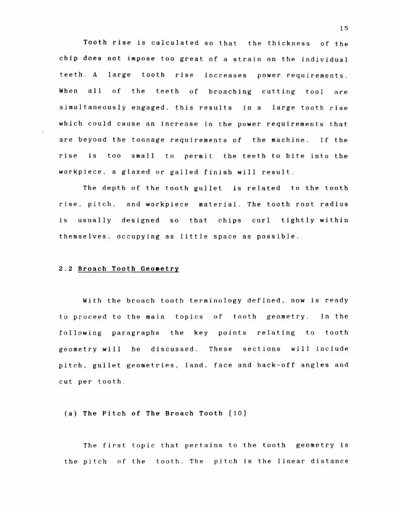
The following terms will be defined to aid in the ease

of understanding this topic in more detail ( see figure 1 ) .

Back-off Angle: The relief angle back of the cutting

edge of a broach tooth.

Chip Space: Spacing between broach teeth which

accommodates the chips formed during

the cut. Sometimes called the "chip

gullet", it includes the face angle,

face angle radius. and hack of tooth

radius.

The Progressive increase in tooth

height from tooth-to--tooth of a hroach.

Usually greater in roughing teeth than

in semifinishing teeth.

Angle of the cutting edge of a hroach

tooth. Sometimes called the "face"

angle.

A name that is sometimes applied to

P - pltch of the teeth D - depth of the teeth L - land behlnd cutt lng edqe R - radlus a t bottom of teeth space F - face angle 13 - back o f the angle Rep - r i se per tooth

F~gure I Standard Broach And I t s Term~nology

13

"chip s p a c e " .

L a n d : The thickness at the top of the broach

tooth.

Rise per tooth : progressive increase in tooth height

from tooth-to-tooth of a broach.

Pitch: The measurement from the cutting edge

of one tooth to the corresponding point

Finish teeth:

Tooth Depth:

on the next tooth.

Roughing Teeth: T h e teeth which take the first cuts in

any broaching operation. Generally they

take heavier cuts than the

semifinishing teeth.

Semifinishing Teeth: Broach t e e t h , that are ahead of the

finishing teeth. which take the

semifinishing cut.

Teeth at the end of broach arranged at

a constant size for finishing the

surface.

Height of tooth ( broach gullet ) from

root to cutting edge.

Broach teeth are usually divided into three separate

sections along the length of the t o o l ; the roughing teeth,

semifinishing t e e t h , and finishing teeth. The number of

teeth in t h e s ~ three sections are depended on material

property and the manufacturing criteria. The first roughing

tooth is proportionately the smallest tooth on the tool.

The subsequent teeth progressively increase in size up to

14

and including the first finishing tooth. The difference ~n

height between each tooth. or tooth r i s e , is usually greater

along the roughing section. and is less along the

semifinishing section. All of the finishing teeth are the

same s i z e .

Individual teeth have a land and face that intersect to

form a cutting edge. The face is ground with a rake or hook

angle that is determined by the workpiece material. Soft

steel workpieces usually require greater hook a n g l e s ; hard

or brittle materials, smaller hook angles 1 9 1 .

The land supports the cutting edge against a stress. A

light clearance or backoff angle is ground onto the lands to

reduce the amount of friction. On roughing and semifinishing

t e e t h , the entire land is relieved with a backoff angle. O n

the finishing teeth, part of the land immediately behind the

cutting edge is often left straight. s o that repeated

sharpening (by grinding the face of the tooth) will not

alter the tonth size.

The pitch or distance between teeth is determined by

the length of cut and influenced by the type of workpiece

material. A relatively large pitch may be required for

roughing teeth to accommodate a greater chip load. Tooth

pitch may be smaller on semifinishing and finishing teeth to

reduce the overall length of the broach tool. The pitch is

calculated s o t h a t , preferably, at least two or more teeth

are cutting simultaneously. This prevents the tool from

drifting or chattering.

15

Tooth rise is calculated so that the thickness of the

chip does not impose too great of a strain on the individual

teeth. A large tooth rise increases power requirements.

When all of the teeth of broaching cutting tool are

simultaneously engaged, this results in a large tooth rise

which could cause an increase in the power requirements that

are beyond the tonnage requirements of the machine. If the

rise is too small to permit the teeth to bite into the

workpiece, a glazed or galled finish will result.

The depth of the tooth gullet is related to the tooth

rise, pitch, and workpiece material. The tooth root radius

is usually designed so that chips curl tightly within

themselves. occupying as little space as possible.

2.2 Broach Tooth Geometry

With the broach tooth terminology defined, now is ready

to proceed to the main topics of tooth geometry. In the

following paragraphs the key points relating to tooth

geometry will be discussed. These sections will include

pitch, gullet geometries, land, face and hack-off angles and

cut per tooth.

(a) The Pitch of The Broach Tooth [ l o ]

The first topic that pertains to the tooth geometry is

the pitch of the tooth. The pitch is the linear distance

16

from the cutting edge of one tooth to the corresponding

point o n the next tooth. Pitch is influenced by the length

of c u t , the type of workpiece material and cut per tooth. A

relatively large pitch may be required for roughing teeth

to provide more chip s p a c e . Tooth pitch can he smaller on

semifinishing and finishing teeth to reduce the overall

length of the broach. The pi>ch is calculated s o that at

least t w o , and preferably more teeth cut simultaneously to

prevent the broach from drifting or chattering.

An empirical formula that is sometimes used to

determine the pitch for short broaches, and is not

applicable to large horizontal broaches, is :

P = 0 . 3 5 L1'"

where:

P = pitch (in).

1, = length of cut (in).

To obtain the pitch P in millimeters when the length of cut

L is given in millimeters. the following formula is used:

The broach pitches for the various lengths of cut with

the standard form a r e dependent on the type of material

that is broached in each particular situation.

For example, the proper pitch for broaching cast iron can

17

be less than that for broaching steel because less chip

space is required.

Broach pitch will influence the tooth construction.

strength, number of teeth cutting at a given instant, and

the ability of the broach to maintain alignment throughout

the cutting s t r o k e . Other factors affecting pitch selection,

in addition to the material being broached and length of

c u t , include the amount of stock to be r e m o v e d , the length

of machine stroke available,and the number of resharpening

expected for the broach.

(b) T h e Gullet o f The Broach tooth [12]

T h e second broach tooth characteristic is the

geometry of the gullet. The depth of the tooth gullet on a

broach is related to the depth of cut per t o o t h , pitch of

the broach t e e t h , length of c u t , and workpiece material.

Deeper gullets are required for longer cuts and greater

stock removal. Radii (face angle and back of tooth) within

the gullet are designed to reduce friction and curl the

chips tightly within themselves so that they occupy as

little space as possible.

T h e chip carrying capacity calculations are important

in the initial stages of broach design because they

determine the maximum depth of cut per tooth and t h u s .

usually. the numher of teeth ( broach length needed to

perform the operation. These calculations can be used to

18

determine the machine capacity and/or number of passes

required as well as the stroke lengths necessary for each

pass.

A close correlation is needed between the chip

carrying capacity and broaching force requirements to

obtain optimum broach design for a given set of

conditions. In many cases, tonnage capacity of the machine

or strength of the broach will prohibit using the maximum

depth of cut per tooth. and force requirements and capacity

available must be balanced by varying the basic criteria.

For example, increasing the pitch will decrease the number

of teeth in contact with the workpiece at any given time

and also reduce the force acquirement, but this

necessitates a longer broach unless the cut per tooth is

increased proportionately. Increasing the cut per tooth

usually works well for applications in which broach

strength is not a factor and when the increased force can

he tolerated.

For applications of broaches in which the chips are

crowded into a small area at the roots of the tooth

gullets, the cut per tooth is often calculat.ed as follows:

Cr = % of CA/Lc (2.3)

where:

Cr = maximum cut per tooth, in. or mm

CA = circle area, in2. or mm2

LC = length of cut, i n , or mm

The maximum percentage of circle area to be used in

this formula is as follows ( 1 2 ) :

1 For round internal broaches. 1 0 % of the C A for

broaching ductile materials and 1 2 % of the C A for

broaching cast iron or bronze.

2 . For spline type internal broaches, 2 0 % of the C A for

broaching ductile materials and 2 5 % of the C A for

broaching cast iron or bronze.

3. For flat-surface broaches making cuts wider than

0 . 3 7 5 " (9.52mm), 2 0 % of the C A for broaching ductile

materials and 30% of the CA for broaching cast iron

or bronze.

4 . For flat--surface broaches making cuts narrower than

0 . 3 7 5 " ( 9 . 5 2 mm). 2 5 % of the C A for broaching

ductile materials and 35% of the C A for broaching

cast iron or bronze.

( c ) The Face A n d Back-Off Angle [ I 3 3

The third and final aspect of the tooth geometry that

will be presented here is that of the face and back-off

angles. The face, rake, or hook angle ground below the

cutting edge on each tooth varies with the material to be

hroached. Soft steel workpieces usually require a larger

face angle: hard or brittle materials require a smaller

face angle. Ductility of the material also has considerable

20

influence in selecting an optimum face angle. In general,

the face angle decreases with reduced ductility [ 9 ] .

A small back-off or clearance angle is ground on the

tooth lands to reduce friction in broaching. O n the

roughing and semifinishing teeth, the entire land is

relieved with a hack-off angle. O n finishing teeth, part of

the lands immediately behind the cutting edges are often

left straight, parallel to the broach axis,so that

regrounding of the teeth will not alter their size.

Back-of f angles can generally be reduced on

semifinishing and finishing teeth. The angles shown are

sometimes changed depending on material from which the

broach is made, and workpiece material variations. Please

see the reference [ 9 ] for detail information of the typical

broach face (hook) and backoff angles which relate to

different material.

2.3 The Strength of Broach Tooth and Machine Power Require

The second part of this chapter will focus its

attention on two main sections. The first section concerns

the tooth strength and related topics. The second section

will concentrate on the machine power requirements

:issociat.ed with this particular broaching technique.

(a) The Strength of Broach Tooth

2 1

In considering the tooth strength, the traditional

method will be described in this section and the new

technology will be discussed in next chapter.

Whether broaching is done by pushing or by pulling

affects the design of the broach. With push broaching, the

length of the broaching cutting tool must be relatively

short to avoid buckling a n d * excessive deflection, and

several broaches may be required to complete the operation,

With pull broaching, the broaches can be any practical

length and the operations are generally completed in a

single pass.

(1) Pull Broach Strength [ 1 4 ]

Rroach length depends primarily on the amount of

stock to be removed and is limited by such factors as

the machine stroke, strength of the broach, and

accuracy and finish required. A guideline that could be

considered would be that the length of internal push

broaches should not exceed 25 times the diameter of

their smallest tooth gullet, similarly the lengths of

pull broaches are usually limited to 75 times their

finishing diameters.

The maximum force which an internal pull broach

can withstand without damage is a function of the

tool's minimum cross section and the yield strength of

the material from which the broach is made. The minimum

2 2

cross section of a pull broach is usually either at the

root of the first tooth or through the pull e n d . T h e

allowable pulling force i s :

where:

P = allowable pulling f o r c e , lb or k g

A = minimum cross section of broach, i n 2 . or

mm2

Y = tensile yield strength of the material from

which the broach is m a d e , psi or k g / m m 2

S = factor of safety

I f the minimum cross-sectjonal area of the broach

is at the root of the first t o o t h , it is calculated

a s :

Ar = 0 . 7 8 5 4 D r 2 ( 2 . 5 )

where:

Ar = minimum cross-sectional a r e a , i n 2 . or mm2

D r = minimum root diameter, i n . or mm

I f the pull end of the broach has a k e y s l o t , the

minimum cross -sectional area is calculated a s :

Ap = 0 . 7 8 5 4 D p 2 - WDp

where:

2 3

Ap = minimum cross-sectional a r e a , in2. or

' mm2

D p = pull end diameter, in. or mm

W = pull-end key slot width, in. or mm

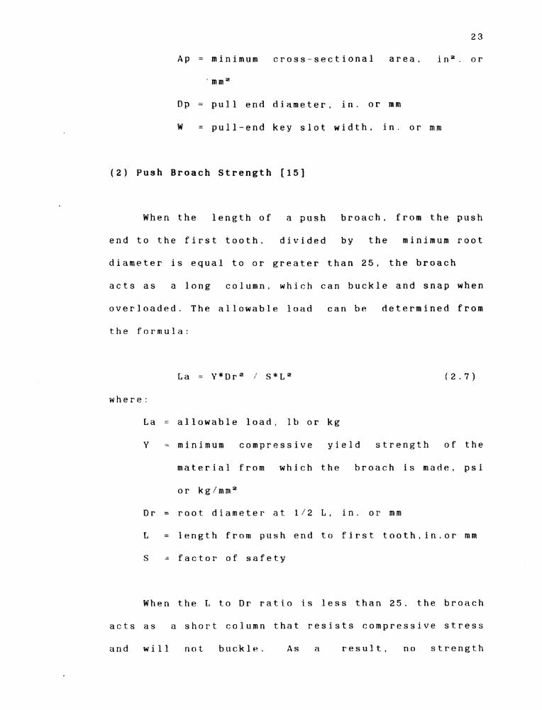
( 2 ) P u s h Broach S t r e n g t h [15]

When the length of a push broach, from the push

end to the first t o o t h , divided by the minimum root

diameter is equal to or greater than 2 5 , the broach

acts as a long c o l u m n , which can buckle and snap when

overloaded. The allowable load can be determined from

the formula:

w h e r e :

La = allowable l o a d , lb or k g

Y = minimum compressive yield strength of the

material from which the broach is m a d e , psi

or kg/mm2

Dr = root diameter at 1 / 2 L , in. or mm

L = length from push end to first t o o t h , i n . o r mm

S = factor of safety

When the L to D r ratio is less than 2 5 , the broach

acts as a short column that resists compressive stress

and will not buckle. As a r e s u l t , no strength

calculation is necessary.

The factor of safety S to be used in the broach

strength formulas given depends on many variables.

These include the amount of stock to be removed per

tooth, the workpiece material and its conditions. the

overall length of the broach, and the possibility of

shock loads. In most cases, a safety factor of 3 is

generally adequate for both push and pull broaches

[ 1 6 ] . A long slender broach, however, may require a

higher factor of safety than a short thick one, and

possibly shock loading may necessitate a high safety

factor.

So far the discussion has not considered the

strength of individual tooth. Traditionally, the design

engineer assume that the broach cutting tool would

behave like cantilever beam. There is no reference

dealing with the strength analysis of the individual

tooth.

Through the efforts of this thesis, there is one

application can now be presented as an alternative to

the methods previously applied. In this application

the accurate approximation of the individual broach

tooth strength will be analyzed by using three

dimensional finite element analysis to determine the

teeth behavior during the cutting process. By applying

the finite element method to this analysis, a speedy.

accurate and detailed analysis can be achieved. This

analysis method will be discussed in Chapter I V

( b ) The Machine Power Requirement [17]

The second section now addresses the machine power

requirements that are associated with this particular type

of broaching.

Broaching force requirements, which determine the

tonnage ratings of the machines needed for specific

applications, depend on many variables. These include the

composition, hardness, and property of the material to be

broached: the amount of stock t.o be removed; the stroke

length and the depth cut per tooth: the broach strength;

the sharpness of the broach: and the cutting fluid used.

Since the cut per tooth and the material to be broached

are the major variables affecting force requirements, the

minimum force needed can be approximated by using the

following formulas and the values for the broaching

constant C which presented in the follow [ l a ] .

For surface broaches:

For round-hole internal broaches:

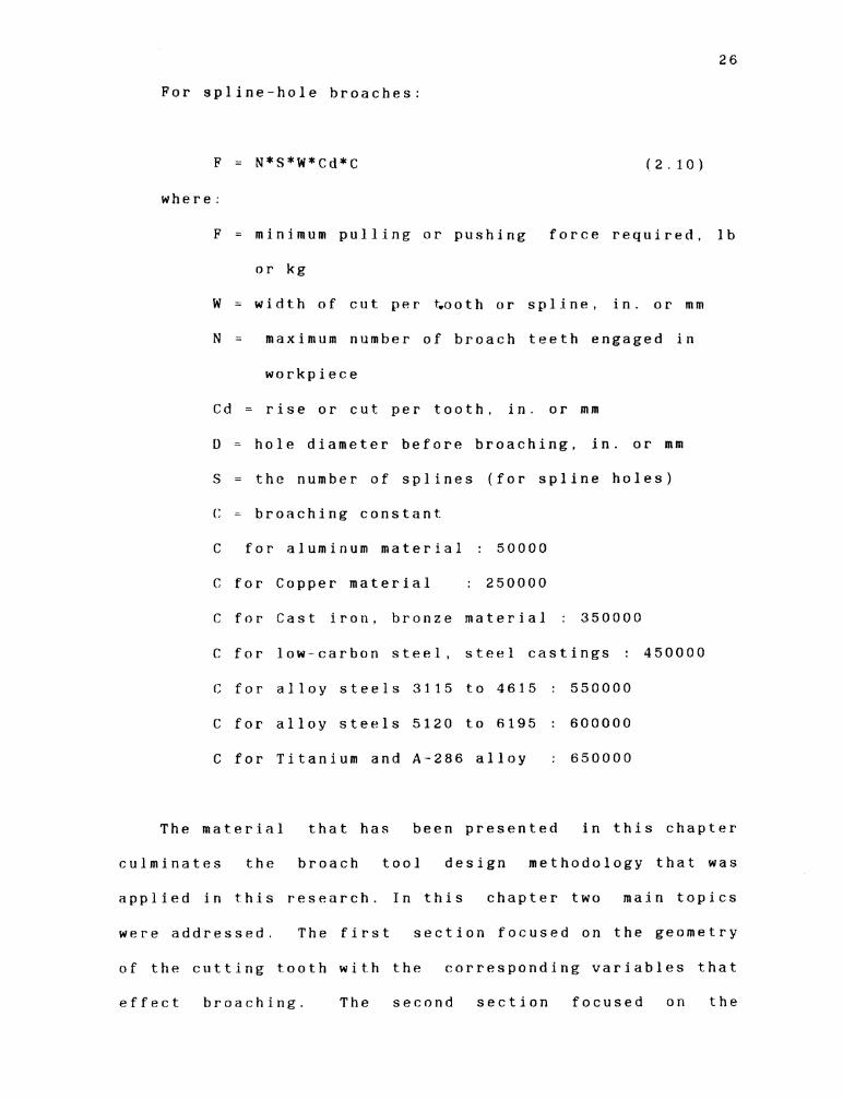
For spline-hole broaches

F = N*S*W*C~*C ( 2 . 1 0 )

where:

F = minimum pulling or pushing force required, lb

or k g

W = width of cut per t.ooth or s p l i n e , in. or mm

N = maximum number of broach teeth engaged in

workpiece

Cd = rise or cut per t o o t h , in. or mm

D = hole diameter before broaching, in. or mm

S = the number of splines (for spline holes)

I: = broaching constant

C for aluminum material : 5 0 0 0 0

C for Copper material : 2 5 0 0 0 0

C for Cast iron, bronze material : 3 5 0 0 0 0

C for low-carbon s t e e l , steel castings : 4 5 0 0 0 0

C for alloy steels 3 1 1 5 to 4 6 1 5 : 5 5 0 0 0 0

C for alloy steels 5 1 2 0 to 6195 : 6 0 0 0 0 0

C for Titanium and A-286 alloy : 6 5 0 0 0 0

T h e material that has been presented in this chapter

culminates the broach tool design methodology that was

applied in this research. In this chapter two main topics

were addressed. The first section focused on the geometry

of the cutting tooth with the corresponding variables that

effect broaching. T h e second section focused on the

2 7

s t r e n g t h o f t h e c u t t i n g t o o t h a n d t h e m a c h i n e p o w e r

r e q u i r e m e n t s . O n e of t h e p r i m a r y g o a l s o f t h i s c h a p t e r w a s

t o p r o v i d e t h e b a s i c f o u n d a t i o n in o r d e r t h a t n e w

t e c h n o l o g y c a n b e p r e s e n t e d . I n t h e f o l l o w i n g c h a p t e r s ,

m o r e d e t a i l w i l l be g i v e n t o s p e c i f i c s p e c i a l i z e d t o p i c s .

CHAPTER I11

OPTIMIZATION AND ECONOMICS OF MANUFACTURING SYSTEMS

This chapter will explain of the economic aspects of

the computational ability of this research and construct a

mathematical model for evaluating the broach manufacturing

system. The following discussion is very important to the

manufacturer whose primary goal is to attain economic

efficiency in the broach manufacturing process.

Practically. "Broaching" is a complex physical

phenomenon. Hence, it is difficult to represent the broach

machining state with an abstract mathematical model for

optimization analysis. It is important to make the

formulation as simple as possible. I n this research. a

number of mathematical formula will be applied to describe

the phenomenon of broaching manufacture process.

Ideally, optimization should be applied to a total

manufacturing system such as material fabrication (casting.

forging, etc.), part machining (cutting, grinding,etc.), and

product assembly. However, the present theory has not been

extended to such an analysis for optimizing a total

manufacturing system. In this chapter,the theory of

optimization for single stage manufacturing by broach

machine will be explained.

2 9

3.1 Evaluation Criteria F o r Economical Production [32]

Three fundamental evaluation criteria developed by

Gibert's [ 3 3 ] , Wu and Ermer 1341 will be utilized in this

manufacturing optimization for economical efficiency. These

criteria are listed as follows:

1 . THE MAXIMUM PRODUCTION RATE or MINIMUM TIME

CRITERION. This maximizes the number of products

produced in a unit time interval; Hence, it minimizes the

production time per unit piece. This is the criterion to

be adapted when an increase in physical productivity or

productive efficiency is desired, while neglecting the

production cost needed and/or profit obtained.

2. THE MINIMUM COST CRITERION. This criterion refers to

production of a piece of product at the least cost, and

coincides with the maximum-profit criterion.

3 . THE MAXIMUM-PROFIT-RATE CRITERION. This maximizes the

profit in a given time interval. This criterion is

recommended when there is an insufficient capacity for a

specific time interval. When market demands are

comparatively larger than productive capacity. a more

substantial profit will be obtained.

In a broach manufacturing system. there are

controllable variables and uncontrollable variables (input.

values). The work materials to be machined, the operative

worker, machine power, and total depth of the cut can be

considered as uncontrollable variables. Typical

30

controllable variables are machining conditions: namely,

depth of cut per tooth, cutting tool selection and machining

speed. The depth of cut per tooth and machine speed

conditions can be determined within ranges set in the

machine cutting tool used.

3.2 Optimization of A Broach Manufacturing [32]

The basic mathematical models based upon three

evaluation criteria mentioned in the previous section are

constructed as follows.

Obviously, these evaluation criteria are a function of

production time and cost. Production time and cost are a

function of machine speed, dept.h of cut per tooth and broach

tool design parameters (pitch, land. depth and width of

broach tooth). Thus, unit production time, production rate,

unit production cost, unit profit and profit rate should be

explained and discussed.

1 . Unit Production Time can be defined as the time needed to

manufacture a unit piece of product. The shorter this

time, the higher the productivity. It is generally

assumed that unit product.ion time consists of the

following three time elements:

(a) Preparation (or set-up) tire tp (min/pc) is the time

necessary to prepare for machining. It includes the

time for loading and unloading workpieces to the

machine tool, the approaching time of a cutting tool

3 1

to the workpiece. etc.

(b) Machining time tm (min/pc) is the time during which

the broach cutting tool is actually cutting.

(c) Tool replacement time te (min/pc) is the time

required to exchange a worn cutting tool.

Denoting the tc (miniper tool) for the time required to

replace a worn cutting tool with a new o n e , and the tool

life T (min/per tool), which is the time length from the

beginning of using a new or resharpened cutting tool till

it is replacement. So the tool replacement time per unit

piece is:

since on an average, a cutting tool can machine T:tm pieces

during its life time.

Accordingly, the unit produt:tion time, t (minlpcl , is

given b y :

2. Production Rate can be defined as the number o f pieces

produced per unit time, and is the reciprocal of the unit

p r o d ~ ~ c t i o n time given by equation (3.2). Hence, denoting

the production rate by q (pc;min),

q = l/t = 1 / (tp + tm + tc*tm/T)

3. Unit Production Cost is a cost required to manufacture a

unit piece. The machining conditions for the least unit

production cost results from the minimum cost criterion.

Unit production cost consists of the following five

types of cost elements.

la) Material cost mc ($/PC): cost of raw material per

unit piece produced.

(b) Preparation (or set-up) cost up ($/PC): cost needed

for the preparation time.

(c) Machining cost um ($/PC): cost needed for the

machining time.

( d ) Tool-replacement cost ue ($/PC): cost needed for the

tool-replacement time.

(e) Tool cost ut ($/PC): cost of a cutting tool required

to produce a piece of product. It includes

purchasing and depreciation costs of the tool, the

tool grinder, and the grinding wheel, direct labor

and overhead costs for regrinding worn cutting

tool ,etc.

(f) Overhead cost ui ($/PC): indirect cost necessary to

produce a piece of product. It includes

depreciation cost for machine tools, and general

administration expense.

Denoting the direct labor cost by kd ($imin), and the

machining overhead, such as cost of cutting o i l , and

electricity charge during actual cutting operation, by

U p = Kd*Tp ( 3 . 4 )

Um = ( K d + Km)*Tm ( 3 . 5 )

U e = Kd*Te = Kd*Tc * T m / T ( 3 . 6 )

Denoting the cost o f a cutting tool by Kt ($/per

tool 1 ,

since T / T m pieces can be produced during the life o f

hroach c u t t i n g t o o l .

Ui ($:PC), the overhead cost required to produce a

unit piece o f product is the unit production time

multiplied by the overhead cost per unit t i m e ,

Ki($imin):

H e n c e , the unit production c o s t , U($/pc), is given b y :

where:

K1 = Kd + Ki ( 3 . 1 0 )

K 1 is the direct labor cost and overhead ($/min).

4. U N I T PROFIT is a gain obtained by producing a unit

piece of product. The gross profit per unit piece

produced g ($/PC) is equal to the unit revenue of

selling price ru ($/PC), minus the unit production cost

u ($/PC):

where

rn is a unit net revenue($/pc) - value added

5 . P R O F I T R A T E . According to the definition of profit

mentioned previously, profit rate ($/min) is obtained by

multiplying the unit profit g ($/PC) by the production

rate q (pc/min).

T h e machining conditions for maximizing this profit

rate are based upon the maximum-profit--rate criterion.

Regarding the tool life T , the following generalized

tool ! ife equation is employed ( R q . 3 . ~ 3 ) [ 3 2 ] .

T h u s , tool life

~ = ~ / ( ~ d ( r / m ) * ~ ( )

where

Cd : depth of cut. per tnnth

v : machine speed

m , n and C : are constants.

It is emphasized at this stage that no research has

been done this previous by to perform this particular type

of broaching analysis. In actuality, until now there is no

supporting data available to substantiate this cutting tool

life formula of broaching.

3.3 The Evaluation Mathematical Model

This section deals with constructing a mathematical

evaluation model to determine the cutting tool and machining

variables which include machining s p e e d , depth of cut per

tooth and cutting tool design parameters ( pitch, land.

d e p t h , and width of the tooth ) . Unit production time and

c o s t , which are two basic measures of performance for the

maximum produrtion r a t e , the minimum cost criteria and the

maximum profit r a t e , are expressed in general form as in

rquations ( 3 . 2 ) , ( 3 . 9 ) and (3.12). In these formulas, the

tool life T (miniper tool) is dependent upon depth of cut

per tooth s (mm/per tooth) and machining speed v (m:minI.

36

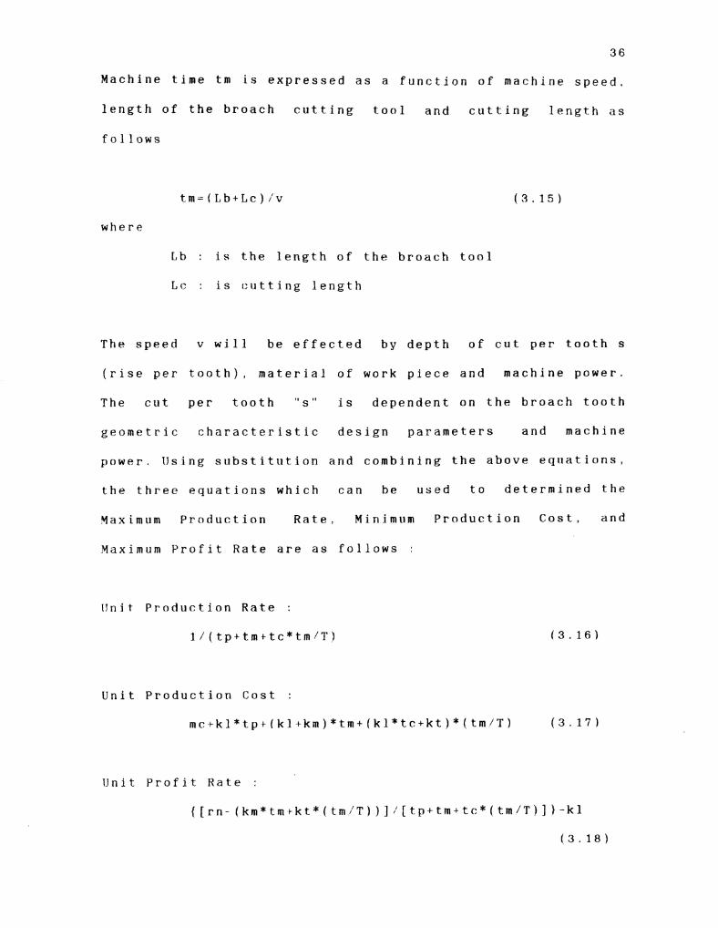
Machine time tm is expressed as a function of machine speed.

length of the broach cutting tool and cutting length as

f o l l o w s

tm=(Lb+Lc)/v

where

Lb : is the length of the broach tool

LC : is cutting length

T h e speed v will be effected by depth of cut per tooth s

(rise per tooth), material of work piece and machine power.

The cut per tooth " s " is dependent on the broach tooth

geometric characteristic design parameters and machine

power. Using s~ibstitution arid combining the above equations,

the three equations which can be used to determined the

Yaximum Production R a t e , Minimum Production C o s t , and

Maximum Profit Rate are a s follows :

[!nit Production Rate :

l/(tp+tmttc*tm/T)

Unit Production Cost :

m c t k l * t p + ( k l + k m ) * t m + f k l * t c + k t ) * ( t m / T ) ( 3 . 1 7 )

1Jnit Profit Rate :

{[rn- (km*tmtkt*(tm/T) ) ] /ttp+tm+t(:*(tm/T)] 1-kl

( 3 . 1 8 )

rn : is a unit net revenue

T : tool life is a function of s and v

tm : machine time is function of v , Lb. LC

v : machine speed will be effected by depth of

cut per tooth s (rise per tooth), material of

work piece and machine power.

Cd : rise per tooth is dependent on the broach

tooth design parameters and machine

power.

After the above three mathematical evaluation criteria

are deduced. the next consideration is to set the

constraints and involve the cutting tool design parameters

in the mathematical model. These constraints are based on

the broach cutting tool design cnncept which were discussed

in the previous chapter.

In the chapter IV and chapter V , the Finite Element

Analysis and Response Surface Metrology will be applied to

determine the maximum allowable cutting force of each tooth

during broaching.

CHAPTER IV

Finite Element Analysis In Broach Tooth Design

Basically, there are two criteria that should be met

when a tooth on a broaching tool is being designed. The

first is that the tooth should b? sufficiently rigid so that

the force generated by the cutting action will not cause it.

to deflect by an excessive amount. If this deflection is

excessive, then the tolerance on the part being produced

will not be met and the part will have to be either scrapped

or reworked.

The second criteria is that the tooth should be

sufficiently strong so that the cutting force will not

cause it to break. When a tooth breaks the production

process will have to be stopped unnecessarily for it to be

replaced. This will cause increase a cost from this lost

production to be increased.

Chapter IV and V concerned with develop a mathematical

model for predicting how the geometry of the tooth's design

will affect the maximum amount of force that the tooth can

withstand without either breaking or deflecting to the point

where the quality of the finished product will be

unacceptable. This mathematical model will use four

charat:teristics of the tooth's geometry as input variables (

see figure 1 ) . The first geometric characteristic is the

pitch which represents the distance between the cutting

39

edges of successive teeth. The second is the land which

represents the thickness of the top of the tooth. The depth

of the gullet represents the third characteristic. This

quantity is the dimension from the top of the tooth to the

bottom of the cavity in front of the tooth. The forth and

final characteristic is the width of the tooth.

The first step in this model is to design an experiment

for generating the data necessary for fitting a polynomial

of sufficient order for adequately describing the

relationship between the tooth geometry variables and the

maximum amount of force which the tooth can withstand

without deflecting excessively. The second phase in the

process of developing the mathematical model for predicting

the maximum amount of the stress involved conducting the

experimental runs specified by the experimental strategy

described in the first step. There are two alternatives for

conducting such experiments. The first is to conduct

physical experiment, while the second is to perform a finite

element analysis. In this research the latter approach was

selected. Thus all of the data in each design point is

generated by finite element analysis. In this chapter how a

three dimensional finite element analysis is used for

determining the maximum allowable force that the various

combinations of the input variables could withstand will be

described.

4.1 The Concept of The Finite Element [19]

The finite element method is a numerical procedure for

obtaining solutions to many of the problems encountered in

engineering analysis. It has two primary sub-divisions. The

first utilizes discrete elements to obtain the joint

displacements and member forces of a structural framework.

The second uses the continuum elements to obtain approximate

solutions to heat transfer, fluid mechanics, and solid

mechanics problems. Finite element method yields the

approximate values of the desired parameters at specific

points called nodes ( see figure four ) . A general finite

element computer program was capable of solving both types

of problems mentioned in above. The reason this approach was

applied centered on the fact that the finite element method

combines complicated mathematical concepts to produc:e a

system of linear or nonlinear equations. The number of

equations is usually very large, anywhere from 20 to 2 0 , 0 0 0

or more and requires the computational power of the digital

computer. The method has little practical value if a

computer is not available. Without the computer only

assumptions can be made and therefore the results are

simplified and a lack of accuracy will develop.

In both the manufacturing and mechanical design

problems, engineers are faced with either using empirical

formulas or a persons own experience in their design

process. With the involvement of the computer and finite

4 1

element method, this will now allow the engineering staff to

perform more accurate analysis.

In the previous research or reference material, the

design engineer assumed that the broach tooth would behave

like a cantilever beam. It is now realized that a better and

more analytical approach will be to use a finite element

analysis of the loading, performance, and shape of a broach

tooth. the finite element analysis technique defines and

interprets such characteristics as deflections and stresses

in a structure which are otherwise too complex for rigorous

mathematical analysis.

In finite element analysis, the Broach tooth structure

is represented by a network of simple elements such as

Figure 2. The stress and deflection characteristics of each

of these tiny chunks of the structure can be easily

determine by classical theory. Solving of the resulting set

of simultaneous equation for all the elements will determine

the behavior of the entire structure. All of the elements

are connected at points called nodes. T h e nodes from a

network known a s a mesh or grid. The total pattern of

elements representing the entire broach tooth structure.

In this research, the finite element computer package

NASTRAN [ 2 0 ] will be used to see how a broach behaves in

operation. NASTRAN is sophisticated analysis software in

which data from finite element analysis and other empirical

techniques can be combined into a model to accurately

predict how the broach will behave during cutting. These

4 2

modeling applications involve the organization of massive

amounts of data into huge matrices in the computer. Manual

manipulation of these data would be a horrendous task,

involving much time and be prone to human errors. In this

research, the solid element of NASTRAN package was used to

analyze a three dimensional broach tooth to determine the

element displacement and stress of the elements. The next

section will discuss detail in the solid element in NASTRAN.

4.2 SOLID ELEMENT IN NASTRAN

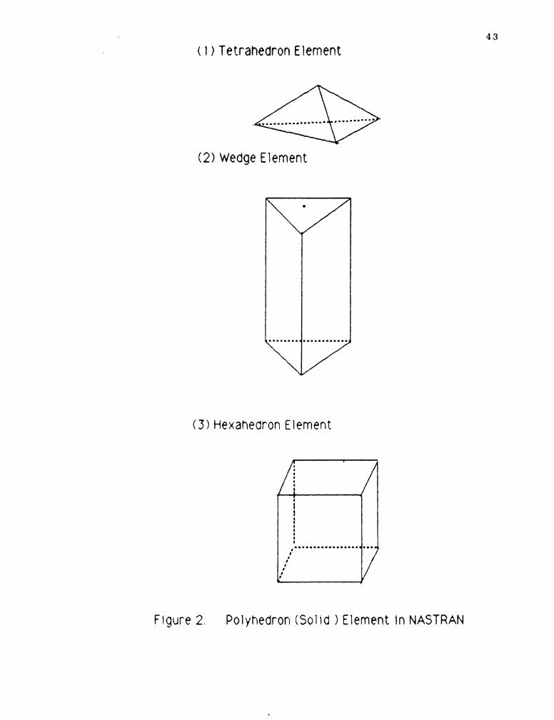
In the NASTRAN Package, solid polyhedron elements have

been implemented to model three--dimensional elastic region,

which do not have axial symmetry ( 2 1 1 . The geometries of the

polyhedron elements is defined by grid points at the

vertices. There are three solid geometries have been

implemented in NASTRAN f see Figure 2 in next page ) . It

allow the user to select and apply these elements in finite

element analysis.

1 . Tetrahedron. The tetrahedron is a triangular pyramid

which can be constructed between any four non-coplanar

entices. It is the basic building block which is used to

build up the other elements.

2 . Wedge ( Pentahedron ) . The wedge is a truncated

triangular pyramid that is defined by six vertices. It

has two triangular and three quadrilateral faces.

3. Hexahedron. The hexahedron is a cube. It has six

I

( 1 > Tetrahedron Element

( 2 ) Wedge Element

(3) Hexahedron Element

Figure 2. Polyhedron (Solid Element In NASTRAN

4 4

quadrilateral faces.

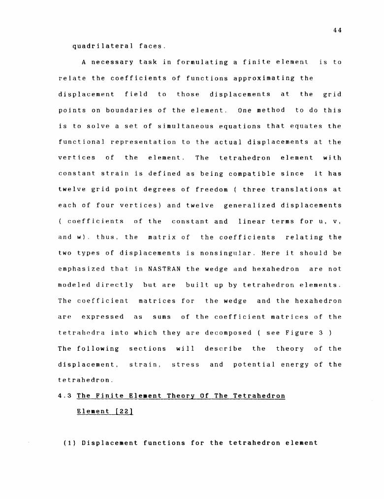
A necessary task in formulating a finite element is to

relate the coefficients of functions approximating the

displacement field to those displacements at the grid

points on boundaries of the element. One method to do this

is to solve a set of simultaneous equations that equates the

functional representation to the actual displacements at the

vertices of the element. The tetrahedron element with

constant strain is defined as being compatible since it has

twelve grid point degrees of freedom ( three translations at

each of four vertices) and twelve generalized displacements

( coefficients of the constant and linear terms for u , v ,

and w). t h us, the matrix of the coefficients relating the

two types of displacements is nonsingular. Here it should be

emphasized that in NASTRAN the wedge and hexahedron are not

modeled directly but are built up b y tetrahedron elements.

The coefficient matrices for the wedge and the hexahedron

are expressed as sums of the coefficient matrices of the

tetrahedra into which they are decomposed ( see Figure 3 )

The following sections will describe the theory of the

displacement, strain, stress and potential energy of the

tetrahedron.

4.3 The Finite Element Theory Of The Tetrahedron

Element [ 2 2 1

(1) Displacement functions for the tetrahedron element

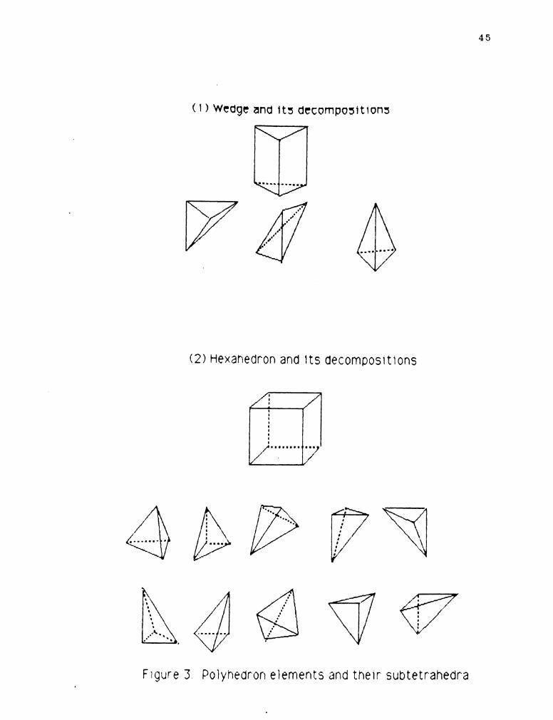
( 1 ) Wedge and i t s decompositions

( 2 ) Hexahedron and I t s decomposl t ions

Figure 3 Polyhedron elements and thelr subtetr-ahedra

4 6

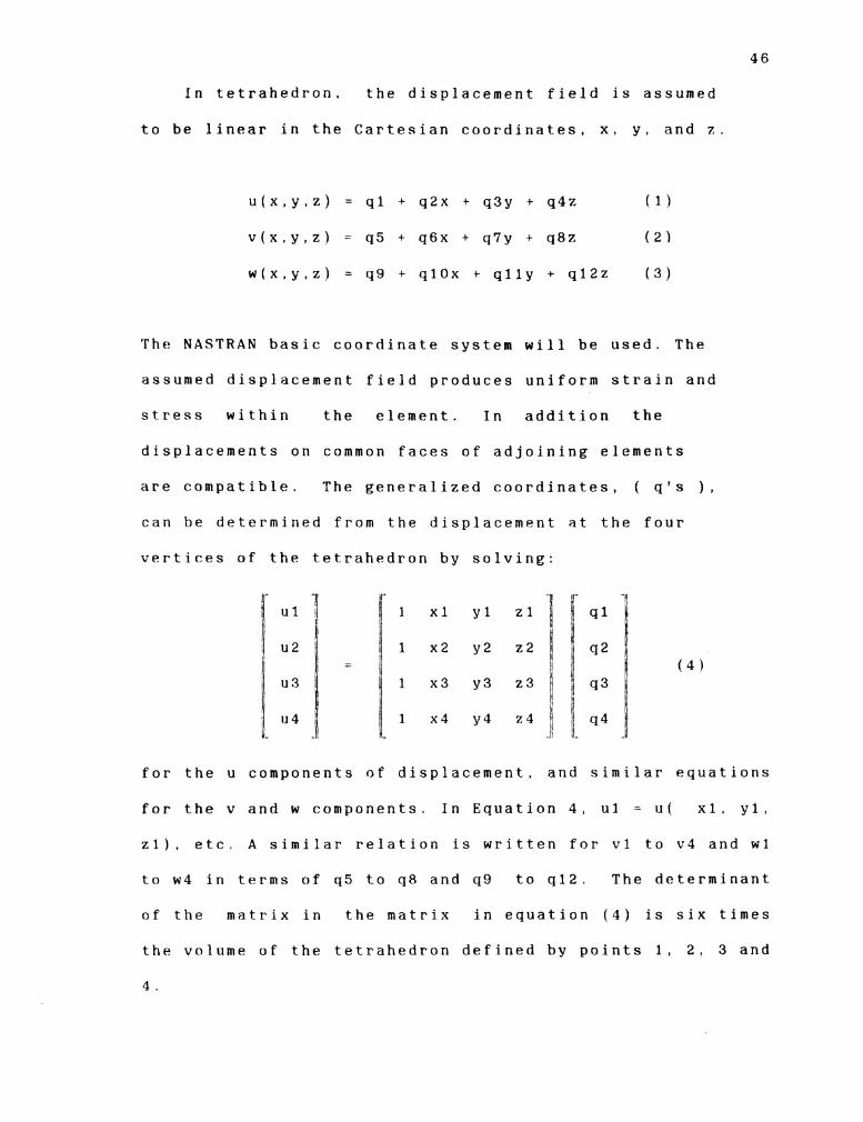
In tetrahedron, the displacement field is assumed

to be linear in the Cartesian coordinates, x , y , and z .

u ( x , y , z ) = ql + q2x t q3y + q4z (11

v ( x , y , z ) = q5 + q6x + q7y + q8z ( 2 1

w ( x , y , z ) = q9 t qlOx t qlly + q12z ( 3 )

The NASTRAN basic coordinate system will be used. The

assumed displacement field produces uniform strain and

stress within the element. In addition the

displacements on common faces of adjoining elements

are compatible. The generalized coordinates, ( q ' s ) ,

can be determined from the displacement at the four

vertices of the tetrahedron by solving:

[ I 1 I I k..

for the u components of displacement, and similar equations

for the v and w components. In Equation 4, u l = u ( x l , y l ,

z l ) , e t c . A similar relation is written for vl to v 4 and wl

to w 4 in terms of q5 to q 8 and q9 to q 1 2 . The determinant

o f the matrix in the matrix in equation (4) is six times

the volume of the tetrahedron defined by points 1 , 2 , 3 and

4 .

6 * Volume

Hence, the matrix in Equation ( 4 ) will be

nonsingular if the volume of the tetrahedron is nonzero.

(2) Strain and Stress Functions For The

Tetrahedron

The generalized displacements are related to the

grid point displacements by

hll h l Z h13 b14

1 q3 1'7 111

11 j q 4 q8 q12 I/

In Equation ( 6 ) , The [hij] matrix is the inverse of

the matrix of Equation (4). The equat.ions for v and w have

been adjoined as additional columns. The six strain

components are given by

Ex = 6u1'6x = q2

E y = 6vI'cSy = q7

E z = 6w/6z = ql2

r y z - 6vl6z k 6wJ16y = q 8 + qll

t z x = 6wIbx + 6ui6z = q10 t q 4 ( 7 e )

-txy = 6u/by + bv/bx = q3 + q 6 ( 7 f )

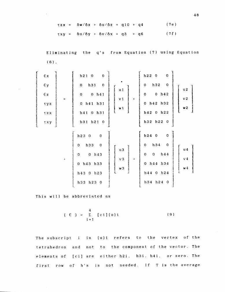
Eliminating the q ' s from Equation ( 7 ) using Equation

( 6 ) ,

This will be abbreviated a s

'I

ryz

The subscript i in (u)i refers to the vertex of the

T Z X 1

tetrahedron and not to the component of the vector. The

elements of [ci] are either h 2 i , h 3 i , h 4 i , or zero. The

I

first row of h's is not needed. I f T is the average

t x l ' 4 li

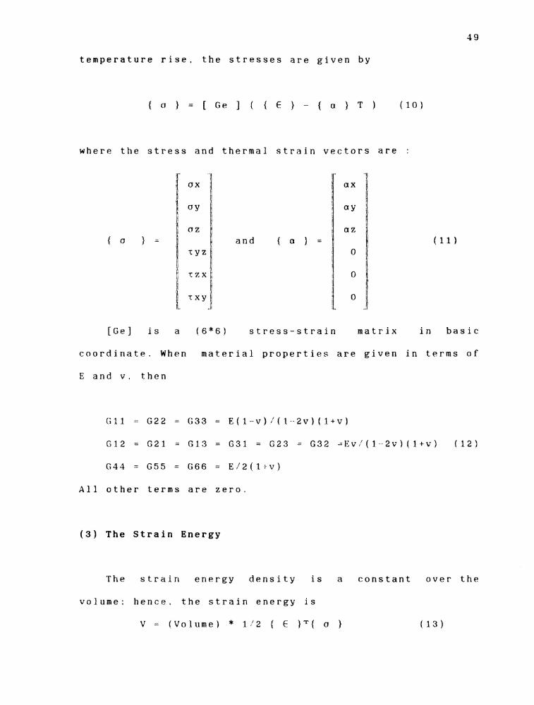
temperature r i s e , the stresses are given by

C ~ > = [ G ~ I ~ { E } - { C X ) T ) (10)

where the stress and thermal strain vectors are :

and

[ G e l is a 16*6) stress-strain matrix in basic

coordinate. When material properties are given in terms of

E and v , then

G11 = G 2 2 = G33 = E ( l - v ) / ( l 2 ~ ) ( l + ~ )

G 1 2 = G21 = G I 3 = G 3 1 = G 2 3 = G32 ;Ev:(l 2 v ) ( l + ~ ) ( 1 2 )

G 4 4 - G 5 5 = G 6 6 = E/2(ltv)

A l l other terms are z e r o .

(3) The Strain Energy

The strain energy density is a constant over the

volume: h e n c e , the strain energy is

V = (Volume) * 1'2 { E )T{ o )

5 0

Based on the above theory, the NASTRAN Package can

provide us the necessary displacement and stress

information o f the element.

4.4 Assumptions

Refore the finite element computer program is applied,

several definitions and assumptions will now be explained.

1 . First assume the broach is made of high speed

steel (SAE 4140).

2 . Young's Modulus E (lb/in) : is the ratio of the

increment of unit stress to increment of unit

deformation within the elastic limit. In this

particular problem. Young's modules is 30.0*10E6

psi [24].

3. Poisson's Ratio 1 : If the unit longitudinal

deformation is s , and unit lateral deformation is

s ' . The ratio of s l / s is Poisson's ratio p . In

this particular problem, the poison's ratio is

0.26 [24].

4. Maximum Yield Stress = 91000 psi [24].

Maximum Tension Stress = 165000 psi [24].

5 . Assume uniform, isotropic material properties in 4

element .

6. Assume coolant will be used properly and uniform

temperature in each element.

7. Assume the safety factor of 3 is used in the

strength analysis.

T o accomplish this finite element a n a l y s i s , a limited

number of experiments will be conducted on a flat broach f

This experiment design will be described in chapter V I .

Once the finite element analysis for a flat broach has been

f o u n d , the same principle and procedure can be applied to

the round or other shape of the broach. It should be noted

that based on the different tool material, the Y o u n g ' s

Modulus. Poisson's Ratio. Yield S t r e s s , and Tension Stress

will be different. Once the material is changed, the result

will be changed. But the techniques and methodology

presented in this thesis are equally expandable and

applicable to other types of materials that are used in

broaching tool.

4.5 The Analysis Method [ 2 5 ]

The NASTRAN Finite Element package is utilized in this

portion of the analysis. There are several options (

HEXAHEDRON. PENTAHEDRON and TETRAHEDRON element ) that can

be utilized when studying the three dimensional aspects of

the solid model. The Hexahedron element (see Figure 4 ) will

be applied to use in the analysis of the bruarh t o o t h .

In the Finite Element m o d e l , the broach tooth is

separated into several small elements. In this particular

c a s e , the broach tooth was broken down into eight Hexahedron

solid elements. Each of the elements includes 20 nodes. This

is illustrated in Figures 4 and 5

01 t o 61 7 are gr ld polnt ldentlflcatlon numbers or connectlon points They can provide the necessary information of the displacement and stress of the broach tooth

Flgure 4 Herahedron Element

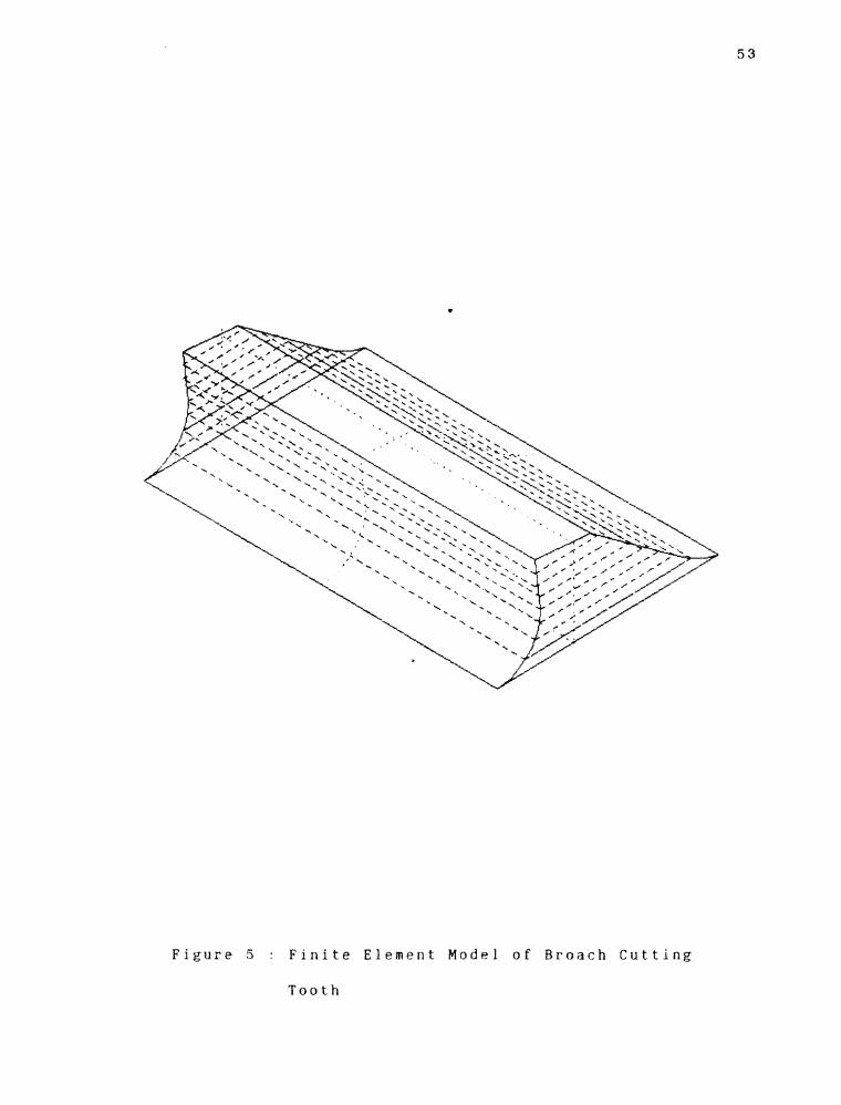
F i g u r e 5 : F i n i t e E l e m e n t M o d e l o f B r o a c h C u t t i n g

T o o t h

It is assume that the force generated by the cutting

action is concentrated on the top of the broach tooth. Each

node can depict the location of the displacement and stress

of the broach tooth. Based on the information which provided

from the NASTRAN result and applied the theory presented in

the next section, the maximum force that the broach tooth

can withstand was determined.

4.6 Determine T h e M a x i m u m Allowable Cutting

Force

In engineering pract.ice, it is apparent that many

implications must he considered i n connection with the

selection and use of a failure theory. The distortion-energy

theory is generally considered to give the most accurate

results 1 2 6 1 . Maximum Dist.ortion Energy Theory (Maximum

Octahedral Shear Stress Theory) predicts ductile yielding

under comhinecl loading with greater accuracy than any other

recognized theory.

T h e Maximum-Octaf~edral -Shear- Stress theory asserts that

yielding will occur whenever the shear stresses acting on

octahedral planes exceed a critical yield value. According

to the maximum-octahedral-shear-stress t h e o r y , yielding

always occurs at a value of octahedral shear stress

established by the tension test as [26]:

55

Toct ( limiting value ) = (2)1'2/3*Sy (4.6-1)

Toct : is the octahedral shear stress

S Y : yield stress

This equation implies that any combination of principal

stresses will cause yielding when the right side of this

equation ( 4 . 6 - 3 ) exceeds the S y . Obviously, if the load

exceeds Sy yielding can therefore be predicted. For design

purposes, the stress equal to Sy should be assigned as the

maximum allowable working uniaxial stress.

In the finite element analysis. NASTRAN provided the

necessary information pertaining to the Octahedral--Shear-

Stress of each element. In the previous sections, w e assumed

Yield stress was 9 1 0 0 0 Psi and the safety factor was 3. The

reason of the safety factor using 3 is that more force will

be required t.o cut the workpiece after the tool gets dull.

S o Toct(1imit value) should not exceed (2)1'2/9*Sy

(equation 3 . 6 - 1 divided by 3). The value of this

computational analysis is 1 4 2 9 0 P s i . This value provides

critical information that can be used to guide the engineer

in checking the degree of excess stress load with regards to

the Toct(1imit value). IJsing the trial and error continue

simulation the force load of the broach tooth, the maximum

force load can be determined. For example. in the beginning

of the t r i a l , an assuming stress load value of the broach

tooth will be chosen to see how big the Octahedral-Shear-

Stress of each element. will b e . Continuing trial until any

5 6

one Octahedral-Shear-Stress of each element exceed the

critical value, then the maximum allowable cutting stress is

determined.

4.7. The Result

1 . It was discovered that the Octahedral shear stress in

the top of the element is always greater then the force

that is applied to the element directly blow the very

top. This explains the reason why the traditional

broaching technique, results in a broken top element.

This statement can be made without reservations,

because the simulat.ion techniques that have been

applied represent a realistic approach to broaching,

2 . The broach tooth tolerances represent an area of

primary importance in the investigation of this topic

[ 2 7 ] . With respect to the analysis that has been made

and based on the material SAE 4 1 4 0 and safety factor 3

is chosen. The maximum displacement always happen in

the very top of the broach tooth (see Figure 6 ) , and

all of the possible displacement of t.he broach teeth 1

represent a value of less then 0 . 0 0 5 inches. This will

provide us necessary information of maximum deformat.ion

of broach tooth in order to prohibit exceeding the

tolerance.

Here it shoald be emphasized again, once the material

property and safety factor is changed, the result will be

different.

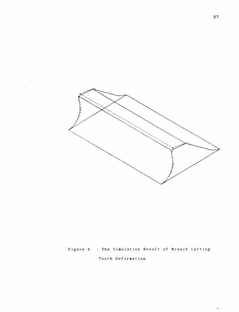
F i g u r e 6 : T h e S i m u l a t i o n R e s u l t o f B r o a c h C u t t i n g

T o o t h D e f o r m a t i o n

C H A P T E R V

THE R E S P O N S E S U R F A C E O F THE M A X I M U M A L L O W A B L E C U T T I N G F O R C E

The purpose of this chapter will be to describe a

methodology for developing a mathematical model for

predicting the maximum amou\t cutting force that the

different. geomet.rica1 characteristics of the broach tooth

will he able to withstand. The process for developing this

model involves two phases. The first phase will conduct a

statistically designed experiment to the various

experimental points which should be used for determining the

empirical data necessary for developing the predictive model

which was ment.ioned above. Each experimental point. will be

specified with particular values of the input variables in

order to find the desirous value of the output variable. In

this model, the input of this model will be the tooth

geometry variables ( pitch, land, depth oh gullet and widt.h

) which were described in the preceding chapter. The output

of this model will be the maximum amount of the force that a

broach tooth will he able to withstand without either

breaking or deflecting to the point where the quality of the

finished product will be unacceptable. The experimental

procedure will consist of performing the finite element.

analysis ( which was described i n Chapter V I ) for each

experimental point. The second phase of this method will

consists of using the result from the first phase to

59

determine a mathematical model which will provide the fast

predicting of the maximum allowable cutting force for any

tooth geometry which lies in a well defined region of

interest.

5.1 The Concept of Th e Response Surface Methodology [ 2 9 ]

Response Surface Methodology is essentially a

particular set of mathematical and statistical methods used

in this research to aid in the solution of certain types of

problems which are pertinent to the engineering process.

Its greatest application has been in industrial research,

particulary in situations where a large number of variables

in a particular system (just as previously described)

influence some specific aspect of the s y s t e m . This feature

( e . g . , maximum allowable cutting f o r c e , cost of production.

etc) is termed the response; i t is normally measured on a

contintlous scale and is a variable which represents the most

important outputs of the system. Also contained in the

system are input variables or independent variables (like

the geometry parameters of the broach tooth), which have an

effect o n the response and are subject to the control of the

researcher. In this research. these variables would

represent the p i t c h , dept.h, lengt.h, and widt.h of the broach

tooth ( In most c a s e s , the gullet geometry is the function

of depth. so it will not. be considered h e r e . ) , because if

any one of these variables change it will simultaneously

60

change the geometry of the broach tooth and their

corresponding maximum allowable cutting force.

Developing a successful response surface are involving

the following procedures :

( 1 ) First finding the sufficiently high order polynomial

which can adequat.ely approximate this surface.

( 2 ) Then conducting the experiment design for fitting the

selected order polynomial and determining adequacy of

f i t .

(3) Finally using the least square method to estimate the

parameters of the model based on empirical d a t a .

The above experimental st.rategy, mathematical methods,

and stat istical inference procedure w h i c h , when combined,

enable t.he user to make a n efficient empirical exploration

of the system in which interest is focllsed.

5 . 2 T h e Design Experiment Method Applied-In This Research

[ 3 0 1

In this research. this experimental design is suggested

by fitting the second order response surface. T h e reason of

this experimental design for fitting a second order

response surface was chosen is based on:

( I ) Relative precision in estimating the coefficients.

( 2 ) The amount of experimental effort with respect to

the number of observations required.

In a second order of the statistically designed

6 1

experiment, the small values of K , e . g . 2 or even 3 , the 3~

factorial design is quite sliitahle. However, when a large

quantity of variables are under observation, the number of

observations required are excessive. For example in this

research application, K = 4 this would lend itself to and an

unreasonahle situation from a practical point of view.

Eighty-one design points are required to estimate only

fifteen coefficients. These coefficients are made up of

intercept, four first order coefficients, four pure

quadratic coefficients, and the remaining six that account

for mixed quadratic terms. Fortunately, in this research

another powerf~il experimental design named central - - design ( CCD ) will be applied. This design is greatly used

hy workers applying second order response surface

techniques. It requires only 25 ohservations which are

needed to fit. this four variables equation [ 3 2 ] .

For th e pt~rpose of this research the central composite

design developed by Box and Wison was used to obtain the

data for developing the polynomial approximating function

for predicting t.he maximum allowable stress load of the

broach tooth could withstand. This design provides the data

necessary for fitting a second order polynomial

approximation. J n this research four independent variables

ha17e been chosen (1,and. P i t c h , Depth and Width o f t h e

broach tooth). With regards to this research. twenty five

(:ombinations were be c h o s ~ n ( See next page ) . The first

sixteen points consist of a factorial design with four

62

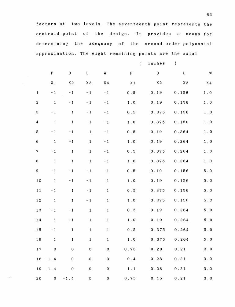
f a c t o r s a t t w o l e v e l s . T h e s e v e n t e e n t h p o i n t r e p r e s e n t s t h e

c e n t r o i d p o i n t o f t h e d e s i g n . I t p r o v i d e s a m e a n s f o r

d e t e r m i n i n g t h e a d e q u a c y o f t h e s e c o n d o r d e r p o l y n o m i a l

a p p r o x i m a t i o n . T h e e i g h t r e m a i n i n g p o i n t s a r e t h e a x i a l

( i n c h e s )

P D L W P D I, W

X 1 X2 X 3 X4 X 1 X2 X3 x4

1 - 1 - 1 - 1 - 1 0 . 5 0 . 1 9 0 . 1 5 6 1 . 0

2 1 - 1 - 1 1 1 . 0 0 . 1 9 0 . 1 5 6 1 . 0

3 1 1 - 1 - 1 0 . 5 0 . 3 7 5 0 . 1 5 6 1 . 0

4 1 1 - 1 - 1 1 .O 0 . 3 7 5 0 . 1 5 6 1 . 0

5 - 1 - 1 1 - I 0 . 5 0 . 1 9 0 . 2 6 4 1 . 0

6 1 1 1 - 1 1 . 0 0 . 1 9 0 . 2 6 4 1 . 0

7 1 1 1 - 1 0 . 5 0 . 3 7 5 0 . 2 6 4 1 . 0

8 1 1 1 1 1 .O 0 . 3 7 5 0 . 2 6 4 1 . 0

9 - 1 - 1 - 1 1 0 . 5 0 . 1 9 0 . 1 5 6 5 . 0

1 0 1 - 1 - 1 1 1 . 0 0 . 1 9 0 . 1 5 6 5 . 0

11 - 1 1 - 1 1 0 . 5 0 . 3 7 5 0 . 1 5 6 5 . 0

1 2 1 1 - 1 1 1 . 0 0 . 3 7 5 0 . 1 5 6 5 . 0

1 3 - 1 - 1 1 1 0 . 5 0 . 1 9 0 . 2 8 4 5 . 0

1 4 1 - 1 1 1 1 . 0 0 . 1 9 0 . 2 6 4 5 . 0

1 5 - 1 1 1 1 0 . 5 0 . 3 7 5 0 . 2 6 4 5 . 0

1 6 1 1 1 1 1 . 0 0 . 3 7 5 0 . 2 6 4 5 . 0

1 7 0 0 0 0 0 . 7 5 0 . 2 8 0 . 2 1 3 . 0

1 8 1 . 4 0 0 0 0 . 4 0 . 2 8 0 . 2 1 3 . 0

1 9 1 . 4 0 0 0 1 . 1 0 . 2 8 0 . 2 1 3 . 0

2 0 0 - 1 . 4 0 0 0 . 7 5 0 . 1 5 0 . 2 1 3 . 0

6 3

2 1 0 1 . 4 0 0 0 . 7 5 0 . 4 1 0 . 2 1 3 . 0

2 2 0 0 - 1 . 4 0 0 . 7 5 0 . 2 8 0 . 1 3 3 3 . 0

2 3 0 0 1 . 4 0 0 . 7 5 0 . 2 8 0 . 2 8 7 3 . 0

2 4 0 0 0 - 1 . 4 0 . 7 5 0 . 2 8 0 . 2 1 0 . 2

2 5 0 0 0 1 . 4 0 . 7 5 0 . 2 8 0 . 2 1 5 . 8

points which provide the data necessary for estimating

thecoefficients of a second orrter- polynomial. The points in

the C C D collectively provide the data necessary for fitting

a second order polynomial and for determining whether a

higher order polynomial would be needed for adequately

representing the relationship between the maximum allowable

cutting force and the four broach tooth geometric variables.

P (pitch of the tooth): 0 . 4 0 - - 1 . 1 0 in.

D (pitch of the tooth): 0 . 1 5 - - 0 . 4 1 in.

L (pitch of the tooth): 0 . 1 3 - - 0 . 3 9 in.

W (pitch of the tooth): 0 . 2 0 - - 5 . 8 0 in.

This range of values for the broach tooth geometry

variables is chosen by based on the table of Broach Design

Data for Standard Tooth Forms [ 3 1 ] . This range of t.he

broach tooth dimension will permit workpiece from 1 inch to

1 0 inch in length to be c r i t .

The table in previous page represents different

combinations of the broach geometry variables. The six

through nine columns are real value of the broach tooth

variables. The left two through five are corresponding coded

value. The different combination represent different

geometrical considerations. There is a total of 25

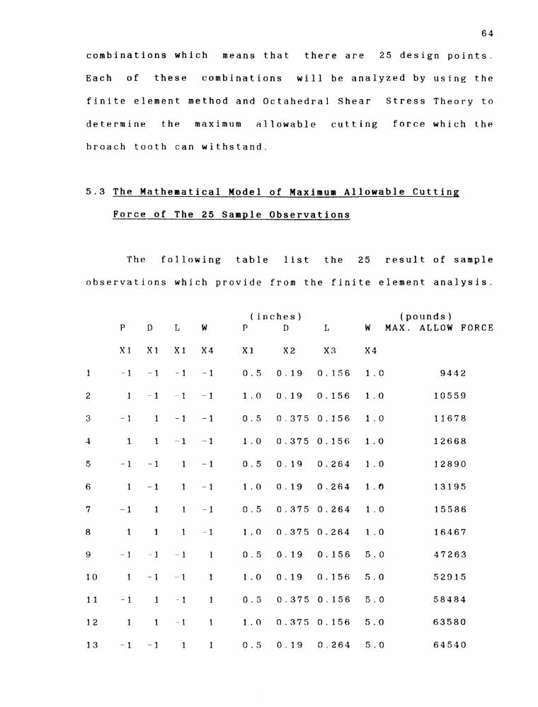
6 4

combinations which means that there are 2 5 design points,

Each of these combinations will be analyzed by using the

finite element method and Octahedral Shear Stress Theory to

determine the maximum allowable cutting force which the

broach tooth can withstand.

5 . 3 The Mathematical Model of Maximum Allowable Cutting

Force of The 25 Sample Observations

The following tahle list the 2 5 result of sample

observations which provide from the finite element analysis.

P D L W

X1 X I X1 X4

1 - 1 - 1 - 1 - 1

2 1 - 1 1 -1

3 - 1 1 - 1 - 1

4 1 1 1 - 1

5 - 1 - 1 1 - 1

6 1 - 1 1 -1

7 - 1 1 1 - 1

8 1 1 1 - 1

9 - 1 - 1 - 1 1

1 0 1 -1 - 1 1

1 1 - 1 1 - 1 1

12 1 1 1 1

1 3 - 1 - 1 1 1

(inches) (pounds) P D L W M A X . A L L O W F O R C E

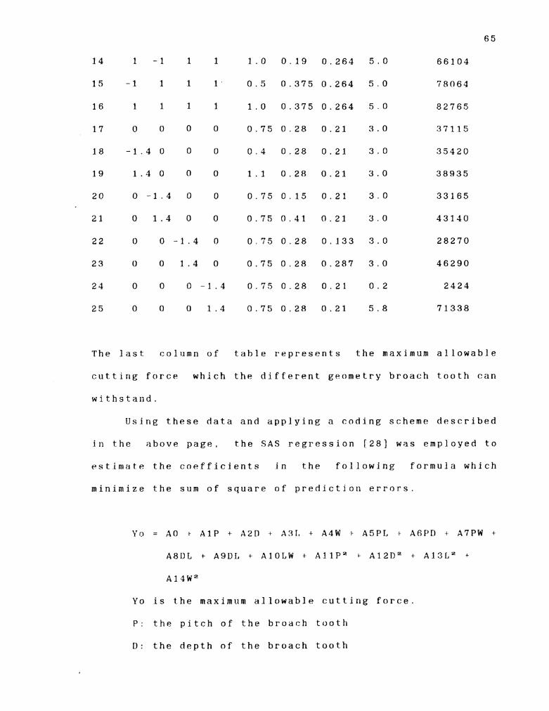
The last column of table represents the maximum allowable

cutting force which the different geometry broach tooth can

withstand.

Using these data and applying a coding scheme described

in the ilbove page, the S A S regression [28] was employed t o

estimate the coefficients in the following formula which

minimize the sum of square of prediction errors.

Yo = A 0 t A 1 P + A 2 D + A81, + A 4 W k A S P L t A 6 P D + A 7 P W +

A 8 D L + A S D L + A l O L W + A l l P 2 6 A12DZ + A 1 3 L 2 +

A 1 4 W 2

Yo is the maximum allowable cutting force.

P : the pitch of the brodch tooth

D : the depth of the broach tooth

L : the land of the broach tooth

W: the width of the broach tooth

A0 - A14 are coefficient which is provided by the

statistics package SAS [ 2 8 ]

In the above equation. the variables represent the

geometry parameters of broach tooth. Anyone of the variable

changes will result in a corresponding change in the value

of Yo ( the maximum allowable cutting force ) . This single

equation provides a tremendous benefit to the user. Because

of using the response surface methodology, all of the

maximum allowable cutting force with respect to the

different geometry broach teeth will be condensed into a

single equation, which provides the user with a powerful

knowledge based can be to determine the possible maximum

allowable cutting force. This is a very useful technique

and has been utilized in this research.

5.4 The Result of The Analysis

The estimate for the coefficient and other

statistical information of the predict model is listed as

following :

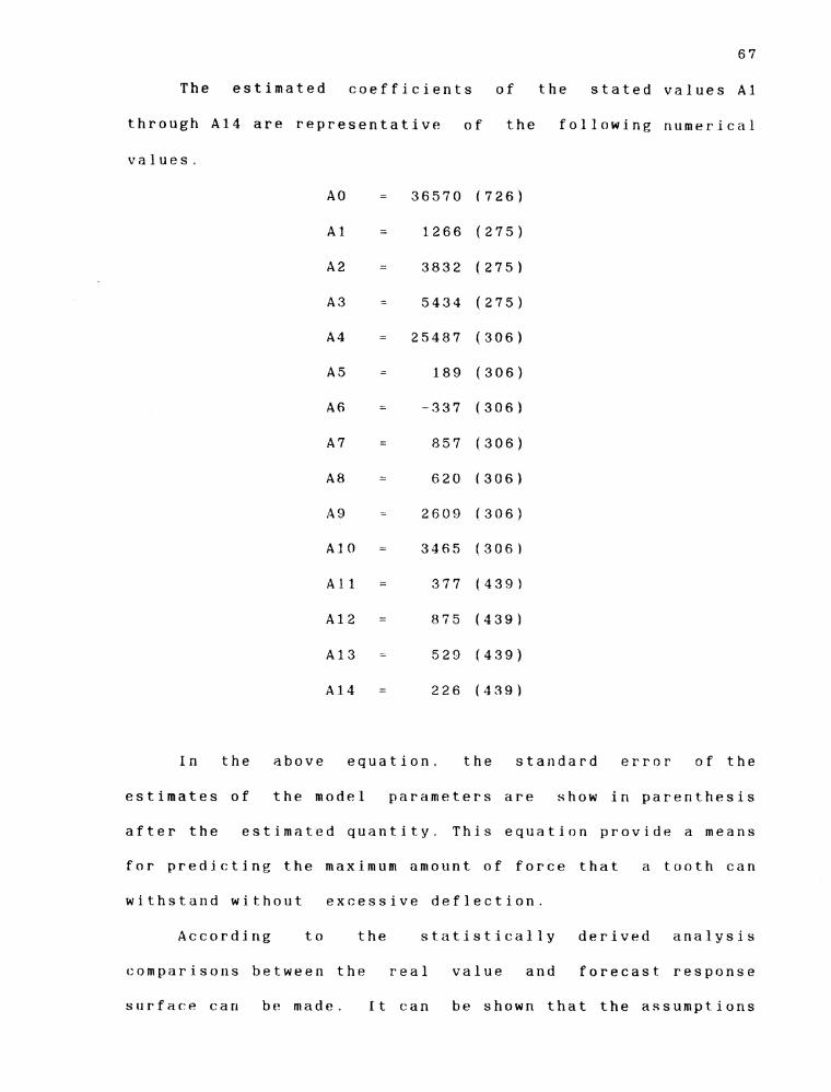
6 7

T h e estimated coefficients of the stated values A1

through A 1 4 are representative of the following numerical

values.

A0 = 3 6 5 7 0 ( 7 2 6 )

A 1 = 1 2 6 6 ( 2 7 5 )

A 2 = 3 8 3 2 ( 2 7 5 )

A 3 = 5 4 3 4 ( 2 7 5 )

A4 = 2 5 4 8 7 ( 3 0 6 )

A5 = 189 ( 3 0 6 )

A 6 = - 3 3 7 ( 3 0 6 )

A7 = 8 5 7 ( 3 0 6 )

A 8 = 6 2 0 ( 3 0 6 )

A 9 - - 2 6 0 9 ( 3 0 6 )

A10 = 3 4 6 5 ( 3 0 6 )

A l l = 3 7 7 ( 4 3 9 )

A12 = 8 7 5 ( 4 3 9 1

A13 = 5 2 0 ( 4 3 9 )

A 1 4 = 2 2 6 ( 4 8 9 )

In the above equation, the standard error o f t h e

estimates of the model parameters are s h o w in parenthesis

after the estimated quantity. This equation provide a means

for predicting the maximum amount of force that a tooth can

withstand without excessive deflection.

According to the statist.ically derived analysis

comparisons between the real value and forecast response

surface can be made. It can be shown that the assumptions

68

m a d e p r e v i o u s l y , a s w e l l a s t h e p r o d u c t a n a l y s i s is

p r e c i s e l y w h a t w a s d e s i r e d w h e n t h i s a n a l y s i s f i r s t b e g a n .

CHAPTER VI

COMPUTER PROGRAM ALGORITHM

From Chapter Two to Chapter F i v e , the concept of the

broach design and several special techniy~les were

introduced. In this chapter, all of the results and concepts

from the earlier chapters will be organized and integrated.

This will be presented in the form of computer software. In

the following section, the computer algorithm, flow chart

and functions provided by this software are emphasized.

6.1 The Mathematical Model and The Alporithm of The Computer

Program

In this program. the derived optimal methodology is

based on the following three manufacturing evaluation

criteria which were described in chapter 111 :

1 . The Maximum-Production Rate

2. The Minimum-Cost Criterion

3. The Maximum-Profit--Rate Criterion

These mathematical models were determined in chapter

I 1 1 as follows :

1 . THE MAXIMITM PRODUCTION RATE or MINIMIJM TIME CRITERION.

Unit Production Cost = l/(tpitm+tc*tm:T)

2 . THE MINIMITM COST CRITERION.

Unit Production Cost =

m c + k l * t p + ( k l + k m ) * t m + [ k l * t c + k t ) * ( t m / T )

3. THE MAXIMUM PROFIT RATE CRITERION.

1Jni t Profit Rate =

Fundamentally all three criteria are functions of

production time and cost. Production time and cost are

functions of operation speed, cutting depth and broach

cutting tool design parameters (the tool size and geometry

of the tooth). All the operation processes should be obeying

the following four const.raints.

1 . The maximum load stress may not exceed the maximum

allowable load stress of the broach.

2. The chip produced cannot exceed the corresponding

gullet capacity

3. The required cutting force may not exceed the

tonnage capacity of the machine

4. The length of broaching tool cannot exceed the

maximam allowable length. A minimum of three teeth

should be engaged in the work piece at a time.

One of the first and primary constraints that is faced

when investigating this particular stage of broaching

analysis concerns the formula of this maximum allowable

cutting force "Y"

As described in chapter four and five, the accurate

approximation of the behavior of the broach tooth was

analyzed by using three dimensional finite element

analysis. A number of these analyses were c a r r i e d o u t

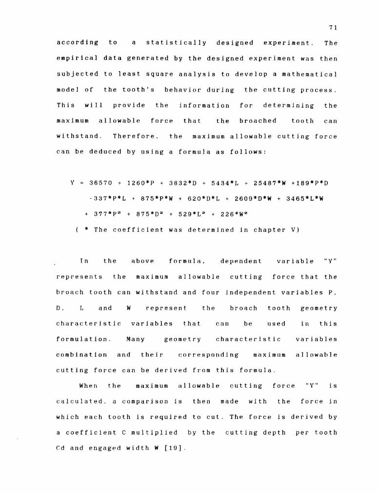
7 1

according to a statistically designed experiment. The

empirical data generated by the designed experiment was then

subjected to least square analysis to develop a mathematical

model of the tooth's behavior during the cutting process.

This will provide the information for determining the

maximum allowable force that the broached tooth can

withstand. Therefore, the maximum allowable cutting force

can be deduced by using a formula a s follows:

Y = 36570 + 1260*P + 3832*D + 5434*L + 25487*W +189*P*D

-337*P*L t 875*P*W + 620*D*L + 2609*D*W + 3465*L*W

+ 377*P2 + 875*D2 + 529*L2 + 226*W2

( * The coefficient was determined in chapter V!

In the above formilla, dependent variable "Y"

represents the maximum allowable cutting force that the

broach tooth can withstand and four jndependent variables P ,

D . I, and W represent the broach tooth geometry

characteristic variahles that can be used in this

formulation. Many geometry characteristic variables

combination and their corresponding maximum allowable

cutting force can be derived from this formula.

When the maximum allowable cutting force "Y" is

calculated, a comparison is then made with the force in

which each tooth is required to cut. The force is derived by

a coefficient C multiplied by the cutting depth per tooth

Cd and engaged width W [ 1 9 ] .

F = C*W*Cd

where;

C for aluminum material : 5 0 0 0 0

C for Copper material : 2 5 0 0 0 0

C for Cast iron, bronze material : 3 5 0 0 0 0

C for low-carbon steel, steel castings : 4 5 0 0 0 0

C for alloy steels 3 1 1 5 to 4 6 1 5 : 5 5 0 0 0 0

C for alloy steels 5 1 2 0 to 6 1 9 5 : 6 0 0 0 0 0

C for Titanium and A - - 2 8 6 alloy : 6 5 0 0 0 0

The force ( F ) should not exceed the maximum allowable

cutting force, so that the risk of excessive deflection on

broach tooth can be reduced. This excessive deflection will

lead to either the breaking of the broach tooth or exceed

the tolerance of the part being produced.

The second constraint concerns the gullet capacity.

Since the cutting depth is increased, the chip size will

also be increased. As stated earlier, this problem concerns

the fact that the chip cannot exceed the corresponding chip

capacity. The following formula can thus be applied to

calculate this necessary information.

73

Cd = maximum cut per tooth, in. or m

CA = circle area of broach tooth, in". or mm2. This

parameter is dependent on the geometric

characteristic of the broach tooth

LC = length of cut, jn. or mm

( please see the chapter two for " % " )

*

The third constraint in this application concerns the

number of teeth engaged in the work piece multiplied by the

force of each tooth that is required to cut the work piece.

This value should be less than the maximum allowable machine

power capacity required to push the broaching tool for an

efficient cut.

N*F < T . . . . . . . . . . . . . . . . . . . . . . . . ( 3 )

where:

N = number of teeth engaged

F = the force of each tooth required to cut the work

piece

T = the maximum tonnage of the machine power

The fourth and fifth constraint in this program are

the hroach tool length and minimum number of engaged teeth

respectively.

After the above constraints and three criteria are

deduced. the computer technique is applied [ 6 ] . These

formulas were built into the computer program, which will

74

enable the user to be able to attain a calculated monetary

value reflecting a specific broaching method. In this w a y ,

the user will be able to determine the true economic benefit

of the broach operation and design parameters.

In this phase of the research, analysis is based on a

series of algorithm formulas which constrain the objective

function. Based on the objective function and constraints.

all of the possible situations will be estimated to check

the feasible solution in this model and store the current

best one in the computer and print the best answer at the

end. In this research, the objective function and constraint

equations can be written as follows:

Object Function:

MAX q = l/(tp+tmttc*tm/T)

MIN ut = m c t k l * t p + ( k l + k m ) * t m t ~ k l * t c + k t ) * ( t m ~ T )

MAX p - {[rn-(km*tm.kkt(tm/T))] /[tpttm+tc*(tm/T) 1 ) - k l

Subject to :

F < Y . . . . . . . . . . . . . . . . . . . . . . . . . . . ( 1

. . . . . . . . . . . . . . . . Cd < % of CA / Lc ( 2 )

N*F < T . . . . . . . . . . . . . . . . . . . . . . . . . . . ( 3 )

N > 2 . . . . . . . . . . . . . . . . . . . . . . . . . . . ( 4 )

. . . . . . . Lb < max. allowable length ( 5 )

All variables > O

As each variable is changed (Pitch ,Depth , L a n d , Width

7 5

or rise per tooth), this will simultaneously change the

maximum allowable cutting force " Y " , the force o f each

individual cutting tooth required to cut the work piece

" F H , t h e optimal depth of cut per tooth " C d " , the minimum

machine power required N*F ( N is number of engaged teeth ) f

See the computer output - figure 7 ) , and the trend of the

production r a t e , c o s t , and profit rate diagram ( See the

computer program output - figure 8 . All the above

information will be used to determine the optimal tooth

geometry variables P , n , I , , W , depth of cut per tooth and

machine operation options ( See the computer program output

- figure 9 ) , One of the interesting challenges that became

apparent in the analysis of this research was how can the

optimal parameters be determined if two or more of the

manufacturing criteria have to be satisfied ? This would

mean that a tradeoff should exist between the criteria. In

this research, which according to the m a n u f a c t ~ ~ r i n g criteria

described in chapter 1 1 1 , one could see that. three

evaluation criteria (maximum production, maximum profit and

minimum production cost) are pertinent to this

manufacturing system. S o this program allow the user to set

the criteria satisfactory range in order to compromise all

of manufacturing criteria (See Appendix C) and provide the

optimal parameters which will satisfy one or two or three

manufacturing criteria.

F i g u r e 7 : I n f o r m a t i o n P r o v i d e F r o m T h e C o m p u t e r P r o g r a m

m n 51 m Q1Cs

mw

w - 03 3L: ---- C;rJ x -4

w - n 0

f=4

w - z a

I I E---.

c-. mp: -'\

n

- C, u a k x \- *z= -- w -E

0- u- f i 3

-w -a oa

-0 - zP;m m 3Ctm m

I I I I -154

F i g u r e 8 : T h e Computer Diagram Of P r o d u c t i o n

A n d Profit R a t e

t e , C o s t ,

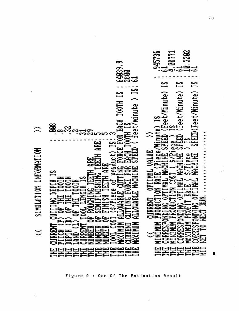
Figure 9 : One O f The Estimation Result

6 . 2 The Flow Chart of C o m p u t e r Program

i n p u t 1-1 def i ne

w o r k p l e c e m a t e r i a l

- s e t t h e c r i t e r i a

and

p r i n t o u t t h e o p t i m a l

b r o a c h t o o l p a r m e t e r s -

y e s J I

\ e 5 t l m 3 t e a i l ~ n s ~ 1 P l r e s t i m a t e a l l o : s i b l e

o ~ e r a t l n g s l u a t l o n s o p e r a t i n g s i l u i t i o n s

c a c u l a t e t h e m a x i f i u ~ p r o d u c t i o n - r a t e t h e n a x i n u n p r o f i t - r a t e

e s t i r t a t e a l l , o s r i b l e operating sl h a t i o n s

a n d

c a c u l a t e t h e m i n i n u n p r o d u c t i o n c o s t

I 1 \ 1 \

I .l

6 . 3 T h e F u n c t i o n s P r o v i d e d b y T h i s Propram

In this computer program, there are seven manufacturing

criteria made available for the user to choose from.

1 . The optimal values that satisfy the maximum production

rate criteria.

2. The optimal values that satisfy the minimum protluctiori

cost criteria.

3 . The optimal values that satisfy the maximum profit

criteria.

4 T h e optimal values that satisfy the maximum production

rate and minimum cost criteria.

5 . The optimal values that satisfy the maximum production

rate and maximum profit criteria.

6 . T h e optimal values that satisfy the minimum cost and

maximum profit criteria.

7. The optimal values that satisfy the maximum production

r a t e , minimum production cost and maximum profit

criteria.

Once the user has selected one of the above critcria,

the computer will provide the optimal tooth geometry

variables ( p i t c h , d e p t h , land and width ) , depth of cut per

tooth and machine operation options. There is one computer

out.put in the next page which represents the optimal values

that satisfy the maximum production r a t e , minimum production

cost and maximum profit criteria ( the criteria range is set

between 0.995 to 1.005 ) .

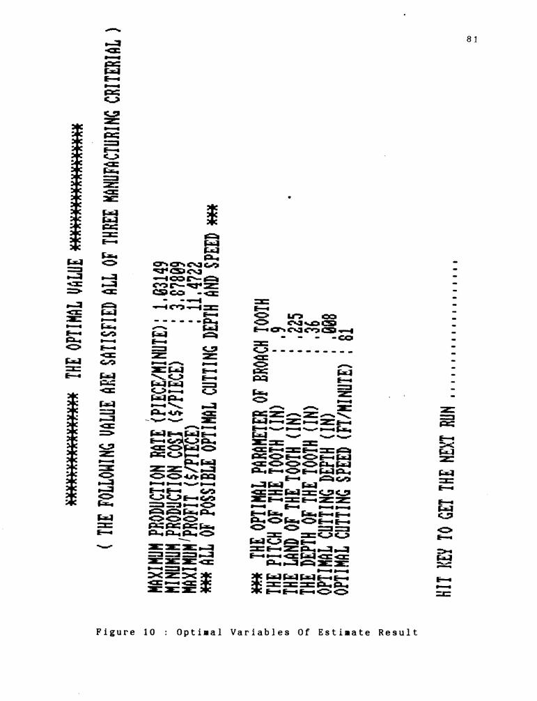
F i g u r e 10 : O p t i m a l V a r i a b l e s Of E s t i m a t e R e s u l t

82

T h e p r o g r a m l i s t i n g s h o w n i n t h e p r e v i o u s p a g e w i l l

p r o v i d e t h e n e c e s s a r y i n f o r m a t i o n t o d e s i g n t h e o p t i m a l

b r o a c h c u t t i n g t o o l a n d m a c h i n e o p e r a t i o n p a r a m e t e r .

CHAPTER VII

DISCUSSION AND CONCLUSION

This research envisaged a thorough analysis of the most

efficient cutting technique that can be incorporated in a

manufacturing procedure. The procedures that are to be used

in deriving the optimal geometric variable of the broach

tooth, cutting depth per tooth and cutting speed was

illustrated and defined in considerable detail.

For a manufacturer who incorporates broaching in their

production operations, this particular method of designing a

broach manufacturing process would prove to be very

advantageous. This met,hod would provide a high productivit-y

with regards to a savings of design cost that would be used

in the broaching process. In addition to this, close

tolerances can be easily m e t , which translates to higher

quality products. Another advantage is that, thin process

can be developed into an expert system that mak~?s use of

powerful software package. This package incorporates the

required analytical requirements to perform the task. From

the early CAD design considerations, economical evaluation,

and multiple decision making criteria to the final results.

Specialized analytical skills are not a pre requisite for

operating this computer software. These capabilities are

already built into the program. This frees user time and

allows greater flexibility to the researcher.

84

Actually, the method of this thesis could be applied in

overall cutting tool design. Since in the manufacturing

process, the cutting tool design is one of the primary

considerations that should be included in the overall

manufacturing decision making process. Once the basic

concept is understood, applying the fundamental principles

is quite routine. This by no means should diminish the

importance of this topic or the research that is presented

in this thesis.

Here, another critical problem should be emphasized. At

present. in order to determine the optimal parameters of

cutting tool design and broach process, the equation of tool

life

is employed (Eq. 3 - 1 1 ) [ 3 4 ] . In actuality, until now there is

no supporting data availahle to suhstantiate this formula in

broach cutting tool. Consequently, the model developed would

not be entirely feasible. It is thus proposed that further

research is suggested to overcome this problem.

This thesis represents an area of research concerning

the systematic analysis of the optimization of broaching

which has not received any attention. It. is earnestly hoped

that the algorithm developed in this research will satisfy a

need for broach cutting tool design and broach manufacture

process.

REFERENCE

Dean M . Schroder, Robert A . Sears, The Broach Making

Industry : Current Position, Trends, and Prospc!cts,

Industry Study, ( University of Massachusetts, Amherst.

MA 19881.

Thomas J . . Drozda, " Broaching , Planning, Shaping And

Slotting " in Tool And Manufacturing Engineering

Handbook Vol. 1 , ( McGrow-Hill, 1983 ) , pp7-33.

Dean M . Schroder, Robert A. Sears. The Broac:h Making

Industry : Current Position, Trends, and P r o s p ~ ~ c t s ,

Industry Study, ( University of Massachusetts, Amherst,

MA 1988).

K . Hitomi, Manufacturing System Engineerine, ( Tylor

Francis Ltd, London 1979). pp165-166

Thomas J . , Drozda, " Broaching , Planning, Shaping And

Slotting " in Tool And ManufacturinR Engineering

Handbook Vol. 1 , ( McGrow-Hill, 1983 ) .

William Conley, Computer Optimization Techniques.

p p l 0 l .

Fundamentals of Broaching, ( American Machinist

Special Report No. 6 3 8 , December 15 1969)( Ohio

Rroach & Machine Co.).

What You Should Know About Broaching. ( American

Machinist Special Report No. 638, August 2 , 1 9 6 5 1 ,

( Ohio Broach & Machine Co.).

" Table 2: Typical broach hook and backoff angles " in

Fundamentals of Broaching, ( American Machinist

Special Report No. 6 3 8 , , December 15 1969.)

[lo] Thomas J . , Drozda, " Broaching , Planning, Shaping And

Slotting " in Tool And Manufacturing Engineering

Handbook Vol. 1 , ( McGrow-Hill, 1983 )Thomas J , , pp7-

14.

[Ill Thomas J . , Drozda, " Broaching , Planning, Shaping And

Slotting " in Tool And M a n u f a c t u r i n ~ Engineering

Handbook Vol. 1 , ( McGrow-Hill, 1983 )Thomas J . , pp7-

15.

Thomas J . , Drozda, " Broaching , Planning, Shaping And

Slotting " in Tool And M a n u f a c t u r i n ~ Enpineering

Handbook Vol. 1 , ( McGrow-Hill, 1983 1 , pp7-15.

[I31 Thomas J . , Drozda, " Broaching , Planning, Shaping And

Slotting " in Tool And Manufacturing Enpineering

Handbook Vol. 1 , ( McGrow-Hill, 1983 ) , pp7-17.

[ I 4 1 Thomas J . , Drozda, " Broaching , Planning, Shaping And

Slotting " in Tool And Manufacturing Enpineering

Handbook Vol. 1 , ( McGrow-Hill, 1983 ) , pp7-20.

[15] Thomas J . , Drozda, " Broaching , Planning, Shaping And

Slotting " in Tool And Manufacturing Engineering

Handbook Vol. 1 , ( McGrow-Hill, 1983 ) . pp7-21.

[I61 Thomas J . , Drozda, " Rroaching , Planning, Shaping And

Slotting " in Tool And Manufacturing Engineering

Handbook Vol. 1 , ( McGrow-Hill, 1983 1 , pp7-22.

[17] Thomas J . , Drozda, " Broaching , Planning, Shaping And

Slotting " in Tool And Manufacturing Engineering

8 7

Handbook Vol. 1 , ( McGrow-Hill, 1983 ) , pp7-22.

[If$] " Machining " in Metal Handbook Vol. 3 , 8 Edition, pp

6 1 .

[19] Larry J . Segerlind, Applied Finite Element Analysis,

1984.

[20] NASTRAN is a registered trademark of the National

Aeronautics and Space Administration. I t is a large

scale, general purpose digital computer program which

solves a wide variety of engineering problem by the

finite element method. William J . Anderson, MSC/NASTRAN

interactive training program. (John Wiley & S o n s ,

1976. )

[21] NASTRAN THEORETICAL MANUAL, pp 5 . 1 2 - 1 .

[22] NASTRAN THEORETICAL MANUAL, pp 5 . 1 2 - 2 to 5 . 1 2 - 4 .

[23] NASTRAN THEORETICAL MANUAL, pp 5 . 1 2 - 2 to 5.12-4.

[24] Venton Levy Doughtie, Alex. Vallance, Leonardt F .

Kreisle, Design of Machine Members, pp 3 1 .

[25] NASTRAN USER'S MANUAL. pp 2 . 4 - 6 1

[26] Robert C . Juvinall, Stress, Strain and Strength, (

McGraw-Hill, 1982 ) , pp 85-89.

1271 Thomas J . , D r ozda, " Rroaching , Planning, Shaping And

Slotting " in Tool And Manufacturing Engineering

Handbook Vol. 1 , ( McGrow-Hill, 1983 )Thomas J . , pp7-

15.

[28] S A S , the full name is Statistical Analysis System.

SAS/ETS User's Guide, Version 5 Edition, ( SAS

Institute Inc. Box 800 Cray, NC 27511--8000 ) .

8 8

[29] Raymond H. My e r s , Response Surface M e t h o d o l o ~ y , 1 9 7 6 .

[ 3 0 ] Raymond H . M y e r s , Response Surface Methodology, 1 9 7 6 ,

p p 1 2 6 .

[ 3 1 ] Thomas J . , D r o z d a , " Broaching , Planning, Shaping And

Slotting " in Tool And Manufacturing Engineering

Handbook Vol. 1 , ( McGrow-Hill, 1 9 8 3 ) , p p 7 - 2 2 .

[ 3 2 ] K . Hitomi, Manufacturing System Engineering, ( Tylor

Francis L t d , London 1 9 7 9 ) , p p 1 6 5 - 1 6 6

[ 3 3 ] Gilbert. W . W . , 1 9 5 0 . " Economics of Machining " , in

Machining - Theory and Pratice, p p . 4 6 5 - 4 8 5 .

[ 3 4 ] W u , S . W . and E r m e r , D . S . , 1 9 6 6 , " Maximum Profit As

the Criterion in Th e Determination o f the Optimal

cutting Conditions " , Journal of Engineering for

Industry, ( Trans. ASME, 1 9 8 8 ) , p p 4 3 5 - 4 4 2 .

[ 3 5 ] "Machining " in Metal Handbook Vol. 3 , 8 Edition, p p -

6 1 .