OPTIMAL GAIN SCHEDULED CONTROLLER FOR A TWO FUNNEL

LIQUID TANKS IN SERIES

Adam Krhovják, Petr Dostál, Stanislav Talaš and Lukáš Rušar Department of Process Control

Faculty of Applied Informatics, Tomas Bata University in Zlín,

Nad Stráněmi 4511, 760 05 Zlín, Czech Republic

krhovjak@fai.utb.cz

KEYWORDS

Two funnel liquid tanks, nonlinear model, parametrized

linear model, scheduling variable, integral control,

optimal gain scheduled controller.

ABSTRACT

Motivated by the control complexity of nonlinear

systems, we introduce an optimal gain scheduled

controller for a nonlinear system of two funnel liquid

tanks in series, based on a linearization of a nonlinear

state equation of the system about selected operating

points. Specifically, the proposed technique aims at

extending the region of validity of linearization by

introducing a parametrized linear model, which enables

to construct a feedback controller at each point.

Additionally, we present an integral control approach

which ensures robust regulation under all parameter

perturbations. The parameters of resulting family of

feedback controllers are scheduled as functions of

reference variables, resulting in a single optimal

controller. Nonlocal performance of the gain scheduled

controller for the nonlinear model has been checked by

mathematical simulation.

INTRODUCTION

We live in a world of highly complex systems that

exhibit nonlinear behavior. Engineers facing the control

of these systems are required to design such mechanisms

that would satisfy desired characteristics through the

operating range. In many cases, situation is complicated

by the fact that the tracking problem involves multiple

variables interacting with each other. One consequence

is that superposition principle, which is known from

linear systems does not hold any longer and we are faced

more challenging situations.

However, because of powerful tools we know for

linear systems, the first step in designing a control for a

nonlinear systems consists in linearization. There is no

question that whenever it is possible, we should take

advantage of design via linearization approach.

Nevertheless, we must bear in mind the basic

limitation associated with this approach. The

understanding that linearization represents only an

approximation in the neighborhood of an operating point.

To put it differently, linearization cannot be viewed

globally since it can only predict the local behavior of a

nonlinear system.

Therefore, conventional controllers with fixed

parameters cannot guarantee performance beyond the

vicinity of operating point. Interestingly enough, in

many situation, it is possible to explicitly capture how the

dynamic of the system changes in its equilibrium points

by introducing a family of linear models which are

parametrize by one or more scheduling variables. In such

cases it is intuitively reasonable to linearize the nonlinear

system about selected operating points, capturing key

states of the system, design a linear feedback controller

at each point, and interpolate the resulting family of

linear controllers by monitoring scheduling variables.

There has been a significant research in gain scheduling

(GS). We refer the interest reader to (Rugh 1991;

Shamma and Athans 1991; Shamma and Athans 1992;

Lawrence and Rugh 1995) for deeper and more insightful

understanding of the gain scheduling procedure.

Most efforts have been devoted to the analytical

framework (Shamma and Athans 1990; Rugh 1991) and

less attention has been paid to particular engineering

applications except few remarkable applications in

technological processes (Jiang 1994; Kaminer et al.

1995; Krhovják et al. 2015). Moreover, these intensive

efforts have not paid attention to the question of optimal

performance design which would make the concept much

more attractive for a potential practitioner in industry. In

order to address those needs we have stressed to illustrate

gain scheduling strategy for a nonlinear system of two

funnel liquid tanks in series (TFLT), extending region of

validity of linearization approach by designing an

optimal controller that is a prescription for moving from

one design to another.

Thus, the problem of a designing an optimal control

for a model of the nonlinear system of the TFLT has been

reduced to a problem of designing a family of optimal

feedback controllers that are interpreted as a single

controller via scheduling variables.

Throughout the paper we gradually reveal the

scheduling procedure satisfying a tracking problem as

well as the design of an optimal control trajectory for the

multivariable nonlinear system of two funnel tanks.

MODEL OF THE TFLT

A simplified model of the TFLT system taken from

(Dostál et al. 2008) is schematically shown in Figure 1.

The process consists of two liquid streams that are

pumped into funnel tanks. Pump with a flow rate q1f

discharges liquid into the first tank (T1). The second tank

Proceedings 30th European Conference on Modelling and Simulation ©ECMS Thorsten Claus, Frank Herrmann, Michael Manitz, Oliver Rose (Editors) ISBN: 978-0-9932440-2-5 / ISBN: 978-0-9932440-3-2 (CD)

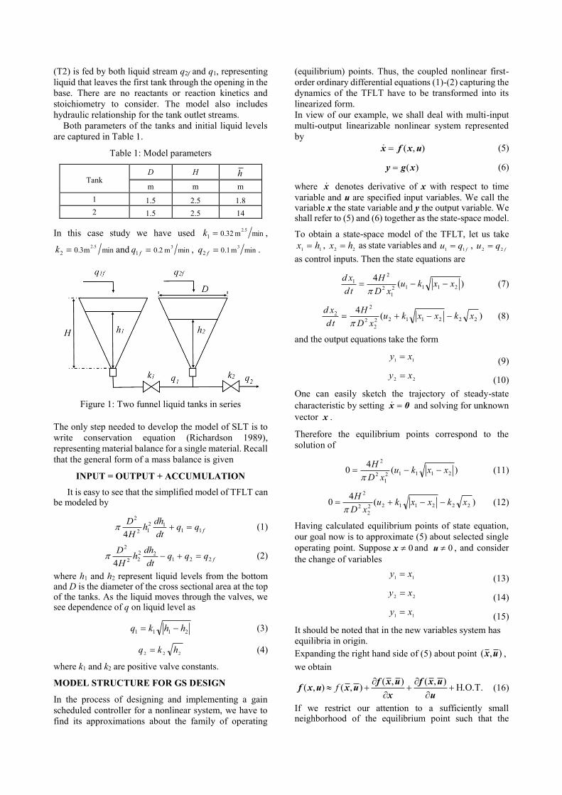
(T2) is fed by both liquid stream q2f and q1, representing

liquid that leaves the first tank through the opening in the

base. There are no reactants or reaction kinetics and

stoichiometry to consider. The model also includes

hydraulic relationship for the tank outlet streams.

Both parameters of the tanks and initial liquid levels

are captured in Table 1.

Table 1: Model parameters

Tank D H h

m m m

1 1.5 2.5 1.8

2 1.5 2.5 14

In this case study we have used minm 0.325.2

1 k ,

minm0.35.2

2 k and minm 0.23

1 fq , minm 0.13

2 fq .

Figure 1: Two funnel liquid tanks in series

The only step needed to develop the model of SLT is to

write conservation equation (Richardson 1989),

representing material balance for a single material. Recall

that the general form of a mass balance is given

INPUT = OUTPUT + ACCUMULATION

It is easy to see that the simplified model of TFLT can be modeled by

fqqdt

dhh

H

D11

12

12

2

4 (1)

fqqqdt

dhh

H

D221

22

22

2

4 (2)

where h1 and h2 represent liquid levels from the bottom and D is the diameter of the cross sectional area at the top of the tanks. As the liquid moves through the valves, we see dependence of q on liquid level as

2111 hhkq (3)

222hkq (4)

where k1 and k2 are positive valve constants.

MODEL STRUCTURE FOR GS DESIGN

In the process of designing and implementing a gain

scheduled controller for a nonlinear system, we have to

find its approximations about the family of operating

(equilibrium) points. Thus, the coupled nonlinear first-

order ordinary differential equations (1)-(2) capturing the

dynamics of the TFLT have to be transformed into its

linearized form.

In view of our example, we shall deal with multi-input

multi-output linearizable nonlinear system represented

by

),( uxfx (5)

)(xgy (6)

where x denotes derivative of x with respect to time

variable and u are specified input variables. We call the variable x the state variable and y the output variable. We shall refer to (5) and (6) together as the state-space model.

To obtain a state-space model of the TFLT, let us take

11hx ,

22hx as state variables and

fqu

11 ,

fqu

22

as control inputs. Then the state equations are

)(4

21112

1

2

2

1 xxkuxD

H

td

xd

(7)

)(4

2221122

2

2

2

2 xkxxkuxD

H

td

xd

(8)

and the output equations take the form

11xy

(9)

22xy

(10)

One can easily sketch the trajectory of steady-state

characteristic by setting 0x and solving for unknown

vector x .

Therefore the equilibrium points correspond to the

solution of

)(4

0 21112

1

2

2

xxkuxD

H

(11)

)(4

0 2221122

2

2

2

xkxxkuxD

H

(12)

Having calculated equilibrium points of state equation,

our goal now is to approximate (5) about selected single

operating point. Suppose 0x and 0u , and consider

the change of variables

11xy

(13)

22xy

(14)

11xy

(15)

It should be noted that in the new variables system has

equilibria in origin.

Expanding the right hand side of (5) about point ),( ux ,

we obtain

H.O.T.),(),(

),(),(

u

uxf

x

uxfuxuxf f (16)

If we restrict our attention to a sufficiently small neighborhood of the equilibrium point such that the

higher-order terms are negligible, then we may drop these terms and approximate the nonlinear state equation by the linear state equation

δδδ BuAxx (17)

where

uuxx

uuxx

u

fB

x

fA

,

, (18)

PARAMETRIZATION OF LINEAR MODELS

Before we present a parametrization via scheduling

variable, let us first examine configuration of the gain

scheduled control system captured in Figure 2. From the

figure, it can be easily seen that controller parameters are

automatically changed in open loop fashion by

monitoring operating conditions. From this point of view,

presented gain scheduled control system can be

understand as a feedback control system in which the

feedback gains are adjusted using feedforward gain

scheduler.

Figure 2: Gain scheduled control

Then it comes as no surprise that first and the most

important step in designing a controller is to find an

appropriate scheduling strategy. Once the strategy is

found, it can be directly embedded into the controller

design. In order to understand the idea behind the gain

scheduling let us first consider the nonlinear system

),,( αuxfx (19)

),( αxgy (20)

We can see that the nonlinear system is basically same as

the system that we have introduced in the previous

section by equations (5) and (6). The only difference here

is that both state and output equations are parameterized

by a new scheduling variable α representing the

operating conditions. To illustrate this motivating discussion let us consider

this crucial point in the context of our example.

Suppose the system is operating at steady state and we want to design controller such that x tracks a reference signal w. In order to maintain the output of the plant at the

value 1x and

2x , we have to generate the corresponding

input signal to the system at 2111 xxku and

222xku , respectively. This implies that for every

value of w in the operating range, we can define the

desired operating point by wyx and )(wuu

Thus it means, that we can directly schedule on a reference trajectory.

Having identified a scheduling variable, the common scheduling scenario takes this form

δδδ uαBxαAx )()( (21)

Intuitively speaking, the parameters of (21) are scheduled as functions of the scheduling variable α. Since our model is simple nonlinear TITO system, we need to calculate elements of A, B, corresponding to the structure of (18). In other words, the key how to move from one operating point to another is given by

2

2

2

2

042

1

2

2

01

2

22

21

211

2

2

2

2

04

21

2

2

2

211

2

03

21

2

1

2

211

2

02

21

2

1

2

211

2

01

4)(,

4)(

2

4)(

)(2

4)(

)(2

4)(

)(2

4)(

D

Hb

D

Hb

kk

D

Ha

D

kHa

D

kHa

D

kHa

αα

α

α

α

α

(22)

An important feature of our analysis is that even if α represents reference vector, the equations (22) still capture the behavior of the system around equilibria.

REGULATION VIA INTEGRAL CONTROL

Since the previous sections resulted in a family of

parametrized linear models we want to design state

feedback control such that

ryy as t (23)

Further, we assume that we can physically measure the

controlled output y . In order to ensure zero steady-state

tracking error in the presence of uncertainties, we want

to use integral control. The regulation task will be

achieved by stabilizing system at an equilibrium point

where ryy .

To maintain the system at that point it must be true, that

there exists a pair of )( u,x such that

)( α,u,xf0 (24)

ryα,xg0 )( (25)

Note, that for equations (24)-(25) we assume a unique

solution )( u,x .

Toward the goal, we have integrate the tracking error

ryye (26)

eσ (27)

Having defined the integrator of the tracking error let

now augment the system (19) to obtain

)( αu,x,fx (28)

ryαx,gσ )( (29)

It follows the control u will be designed as a feedback

function of )( σx, . For such control the new system has

an equilibrium point )( α,σ,x .

To proceed with the design of the controller, we now

linearize (28)-(29) about )( α,σ,x to obtain augmented

state space model as

υαBξαAυαB

ξαC

αAξ )()(

)(

)(

)( def

00

0 (30)

where

σ-σ

x-xξ , u-uυ (31)

Now we have to design a matrix K )(α such that BKA

is Hurwitz.

Partition K )(α as )()()( 21 αKαKαK implies

that the state feedback control should be taken as

uσσαKxxαKu ))(())(( 21 (32)

and by applying the control (32), we obtain the closed-

loop system

)))(())((,( 21 uσσαKxxαKxfx (33)

ryαx,gσ )( (34)

Figure 3 clearly illustrates the block diagram of the control system, where we can clearly see embedded integral control action

Figure 3: Block diagram of integral control system

In searching for an optimal control Kxu we have to

design gain matrix K that minimizes quadratic cost function (omit dependence on α)

0

2 dtTTTNuxRuuQxxJ (35)

where Q, R a symmetric, positive (semi-) definite weighting matrices and N represents

The traditional problem is solved using algebraic Riccati equation

0 Q)NP1(B-NRPB-PAPATTT

(36)

Then the gain matrix K is derived from P by

)(1 TTNPBRK

(37)

In view of the procedure that we have just described, one

can notice that three main issues are involved in the

development of gain scheduled controller; namely

linearization of TFLT about the family of operating

regions, design of a parametrized family of linear matrix

feedback controllers for the parametrized family of linear

systems and construction of gain scheduled controller.

So far, we have formed the basic idea of the control

problem. All that remains now is to simulate the

performance of the gain scheduling procedure with the

help of the integral control.

SIMULATIONS AND RESULTS

In this section, we simulate the gain scheduled control of

TFLT. We have developed a custom MATLAB function

based on the simulator introduced by (Krhovják et al.

2014) that simulates adequately the behavior of TFLT.

Idealistic model has been implemented according to

equations (1) and (2). The popular ODE solver using

based on Runge-Kutta methods (Hairer et al. 1993) was

considered to calculate numerical solution.

The simulation results of gain scheduled control are

presented in Figures 4-8. Figure 4 shows the optimal

responses of the control system to sequences of step

changes in reference signals. As can be seen a step change

in reference signals causes a new calculation of the

equilibrium point of the system.

Figure 4: The responses of the closed-loop system to a

sequence of step changes

-0.1

-0.05

0

0.05

0.1

0.15

0.2

0.25

0.3

0 100 200 300 400

y 1,

y 2[m

]

Time [min]

y1 y2

w1 w2

Figure 5 shows the response of the closed-loop system to

a slow ramp that takes the set points over a period of 500

minutes. These observations are consistent with a

common gain scheduling rule-of-thumb about the

behavior of gain scheduled controller under slowly

varying scheduling variable.

Figure 5: Slow ramp

In contrast, the figure 6 shows the reponse to a faster ramp

signal. As the slope of the ramp increases, tracking

performance deteriorates. If we keep increasing the slope

of the ramp, the system will eventually go unstable.

Figure 6: Fast ramp

To appreciate what we gain by gain scheduling, Figure 7

and Figure 8 illustrates responses of the closed-loop

system to the same sequence of changes. In the first case,

a gain scheduled controller is applied, while in the second

case a fixed-gain controller evaluated at α = [-1 -1] is

used.

From this illustration it is evident why we have to modify

the gain scheduled controller. While stability and zero

steady-state tracking error are achieved, as predicted by

our analysis, the responses deteriorates significantly as the

reference is far from operating point. In some situations it

may be possible to reach a large value of the reference

signal by a sequence of step changes, as in the Figure 4

where we allow enough time for the system to settle done

after each step change. This can be viewed as another

possible way how to change the reference set point.

Figure 7: The reference and output signal of the gain

scheduled control

Figure 8: The reference and output signal of the fixed

gain control

CONCLUSION

This paper addressed the problem of the gain scheduling

procedure as well as the design of optimal control for a

nonlinear multi-input multi-output system of two funnel

liquid tanks in series. First, we have detailed studied the

simplified model of the technological process. Based on

the model, we have followed a general analytical

framework for gain scheduling. We have also pointed out

that selection of scheduling variable depends on

particular characteristics of the system. This observation

has critical importance and leads us to the conclusion that

rule of scheduling on reference variable can be applied

for other technological processes. The main advantage of

this approach is that linear design methods can be applied

to the linearized system at each operating point. Thanks

to this feature, the presented procedure leaves room for

many linear control methods. As our results show,

presented integral control approach ensures robust

regulation under all parameter perturbations. However

the strength of the presented feedback lies in the optimal

design of the gain matrix. In addition, we have

demonstrated that a gain scheduled control system has

the potential to respond rapidly changing operating

conditions.

0

0.1

0.2

0.3

0.4

0.5

0 100 200 300 400 500

y 1,

y 2[m

]

Time [min]

y1

y2

w1

w2

0

0.1

0.2

0.3

0.4

0.5

0 1 2 3 4 5

y 1,

y 2[m

]

Time [min]

y1

y2

w1

w2

-0.3

-0.2

-0.1

0

0.1

0.2

0.3

0.4

0.5

0.6

0 20 40 60 80 100

y 1,

y 2[m

]

Time [min]

y1

y2

w1

w2

-0.3

-0.1

0.1

0.3

0.5

0.7

0.9

0 20 40 60 80 100

y 1,

y 2[m

]

Time [min]

y1 y2

w1 w2

ACKNOWLEDGEMENT

This article was created with support of the Ministry of

Education of the Czech Republic under grant IGA reg. n.

IGA/FAI/2015/006.

REFERENCES

Dostál, P.; V. Bobál; and F. Gazdoš. 2008. “Application of the

polynomial method in adaptive control of a MIMO

process”. Mediterranean Conference on Control and

Automation - Conference Proceedings, 131-136.

Hairer, . J. 1993. Robust industrial control. Optimal design

approach for polynomial systems. Prentice Hall,

Englewood E; S.P. Norsett; and G. Wanner. 1993. Solving

ord inary differential equations. 2nd revised ed. Berlin:

Springer.

Jiang, J. 1994. “Optimal gain scheduling controllers for a diesel

engine”. IEEE Control Systems Magazine, 14(4), 42-48.

Kaminer, I; A. M. Paswal; P. P. Khargonekar; and E. E.

Coleman. 1995. “A velocity algorithm for the

implementation of gain scheduled controllers”. Automatica,

31, 1185-1191.

Krhovják, A.; P. Dostál; and S. Talaš. 2014. “Multivariale

adaptive control of two funnel liquid tanks in series”.

Proceedings - 28th European Conference on Modelling and

Simulation, ECMS 2014, 273-278.

Krhovják, A.; P. Dostál; S. Talaš. 2015; and L.Rušar.

“Multivariale gain scheduled control of two funnel liquid

tanks in series”. in Process Control (PC), 2015 20th

International Conference on, pp. 60-65.

Lawrence, D. A. and W. J. Rugh. 1995. “Gain scheduling

dynamic linear controllers for a nonlinear plant”.

Automatica, 31, 381-390.

Shamma, J.S.; M. Athans. 1990. “Analysis of gain scheduled

control for nonlinear plants. (1990) IEEE Transactions on

Automatic Control, 35 (8), pp. 898-907.

Shamma, J.S and M. Athans. 1992. “Gain scheduling: potential

hazards and possible remedies”. IEEE Control Systems

Magazine, 12(3), 101-107.

Shamma, J.S. and M.Athans. 1991. “Guaranteed properties of

gain scheduled control of linear parameter-varying plants”.

Automatica, vol. 27, no. 4, 559-564.

Rugh, W.J. 1991 “Analytical framework for gain scheduling”.

IEEE Control Systems Magazine, 11(1), pp. 79-84.

Richardson, S.M. 1989. Fluid mechanics, New York,

Hemisphere Pub. Corp.

AUTHOR BIOGRAPHIES

ADAM KRHOVJÁK studied at the Tomas

Bata University in Zlín, Czech Republic,

where he obtained his master degree in

Automatic Control and Informatics in 2013.

He now attends PhD. study in the

Department of Process Control, Faculty of Applied

Informatics of the Tomas Bata University in Zlín. His

research interests focus on modeling and simulation of

continuous time technological processes, adaptive and

nonlinear control.

PETR DOSTÁL studied at the Technical

University of Pardubice, where he obtained

his master degree in 1968 and PhD. degree

in Technical Cybernetics in 1979. In the

year 2000 he became professor in Process

Control. He is now Professor in the Department of

Process Control, Faculty of Applied Informatics of the

Tomas Bata University in Zlín. His research interest are

modeling and simulation of continuous-time chemical

processes, polynomial methods, optimal and adaptive

control.

STANISLAV TALAŠ studied at the Tomas

Bata University in Zlín, Czech Republic,

where he obtained his master degree in

Automatic Control and Informatics in 2013.

He now attends PhD. study in the

Department of Process Control, Faculty of Applied

Informatics of the Tomas Bata University in Zlín. His e-

mail address is talas@fai.utb.cz.

LUKÁŠ RUŠAR studied at the Tomas Bata University

in Zlín, Czech Republic, where he obtained his master

degree in Automatic Control and Informatics in 2014. He

now attends PhD. study in the Department of Process

Control, Faculty of Applied Informatics of the Tomas

Bata University in Zlín. His research interests focus on

model predictive control. His e-mail address is

rusar@fai.utb.cz.