GAIN SCHEDULED CONTROL USING THE DUAL YOULA

PARAMETERIZATION

A Dissertation

by

YOUNG JOON CHANG

Submitted to the Office of Graduate Studies of

Texas A&M University

in partial fulfillment of the requirements for the degree of

DOCTOR OF PHILOSOPHY

May 2010

Major Subject: Mechanical Engineering

GAIN SCHEDULED CONTROL USING THE DUAL YOULA

PARAMETERIZATION

A Dissertation

by

YOUNG JOON CHANG

Submitted to the Office of Graduate Studies of

Texas A&M University

in partial fulfillment of the requirements for the degree of

DOCTOR OF PHILOSOPHY

Approved by:

Chair of Committee, Bryan Rasmussen

Committee Members, Juergen Hahn

Reza Langari

Dennis O’Neal

Head of Department, Dennis O’Neal

May 2010

Major Subject: Mechanical Engineering

iii

ABSTRACT

Gain Scheduled Control Using the Dual Youla Parameterization. (May 2010)

Young Joon Chang, B.S., Inha University, Korea; M.S., Inha University, Korea

Chair of Advisory Committee: Dr. Bryan Rasmussen

Stability is a critical issue in gain-scheduled control problems in that the closed

loop system may not be stable during the transitions between operating conditions

despite guarantees that the gain-scheduled controller stabilizes the plant model at fixed

values of the scheduling variable. For Linear Parameter Varying (LPV) model

representations, a controller interpolation method using Youla parameterization that

guarantees stability despite fast transitions in scheduling variables is proposed. By

interconnecting an LPV plant model with a Local Controller Network (LCN), the

proposed Youla parameterization based controller interpolation method allows the

interpolation of controllers of different size and structure, and guarantees stability at

fixed points over the entire operating region. Moreover, quadratic stability despite fast

scheduling is also guaranteed by construction of a common Lyapunov function, while

the characteristics of individual controllers designed a priori at fixed operating condition

are recovered at the design points. The efficacy of the proposed approach is verified with

both an illustrative simulation case study on variation of a classical MIMO control

problem and an experimental implementation on a multi-evaporator vapor compression

cycle system. The dynamics of vapor compression systems are highly nonlinear, thus the

iv

gain-scheduled control is the potential to achieve the desired stability and performance

of the system. The proposed controller interpolation/switching method guarantees the

nonlinear stability of the closed loop system during the arbitrarily fast transition and

achieves the desired performance to subsequently improve thermal efficiency of the

vapor compression system.

v

DEDICATION

To my family and friends

vi

ACKNOWLEDGEMENTS

I would like to thank my committee chair, Dr. Bryan Rasmussen, for his

guidance and encouragement throughout this study. His knowledge and insight were

essential in helping me through understanding and direction over research achievements.

I would like to also thank my committee members, Dr. Dennis O’Neal, Dr. Reza Langari,

and Dr. Juergen Hahn, for their guidance and support throughout the course of this

research.

My gratitude is extended to Mr. Matt Elliott for his technical advice to

experimental studies of vapor compression system, and to the research members in the

Thermo-fluid Control Laboratory for sharing their knowledge for this study. Thanks to

NSF (National Science Foundation) for their financial support throughout the duration of

this study.

Finally, thanks to my parents and family for their continual support and

encouragement, and to my lovely Yunhyung, for her endless love and patience.

vii

TABLE OF CONTENTS

Page

ABSTRACT .................................................................................................................... iii

DEDICATION ................................................................................................................ v

ACKNOWLEDGEMENTS .............................................................................................. vi

TABLE OF CONTENTS ................................................................................................ vii

LIST OF FIGURES ........................................................................................................... x

LIST OF TABLES ......................................................................................................... xiv

1. INTRODUCTION ..................................................................................................... 1

1.1 Review of Gain-scheduled Control Literature .............................................. 2 1.1.1 Scheduling Variables ........................................................................ 5

1.1.2 LPV Plant Modeling ......................................................................... 6 1.1.3 Gain-scheduling via Linear Controller Interpolation ........................ 6 1.1.4 Gain-scheduling via LPV Control Synthesis .................................... 7

1.1.5 Stability Analysis .............................................................................. 7

1.2 Youla Parameterization-based Gain-Scheduling........................................... 8 1.3 Stability Analysis with Robustness Consideration ........................................ 9 1.4 Control of Vapor Compression Systems ..................................................... 10

1.5 Research Objectives .................................................................................... 11 1.6 Dissertation Organization ............................................................................ 12

2. INTRODUCTION TO GAIN SCHEDULED CONTROL ..................................... 13

2.1 Introduction ................................................................................................. 13 2.2 Nonlinear Plant Modeling ........................................................................... 14 2.2.1 Nonlinear Plant Model .................................................................... 15

2.2.2 Linearization-based Plant Modeling ............................................... 16 2.2.3 Linear Parameter Varying (LPV) Plant Modeling .......................... 17 2.3 Controller Interpolation ............................................................................... 18

2.3.1 Local Controller Network (LCN).................................................... 19 2.3.2 LPV Control Synthesis .................................................................... 23 2.4 Stability Analysis ........................................................................................ 25 2.4.1 Stability Classification .................................................................... 25

viii

Page

2.4.2 Stability Analysis with Performance Bounds via LMIs .................. 32 2.4.3 Conclusion: Stability of Gain-scheduled Control System .............. 38 2.5 Youla-based Gain-scheduled Control ......................................................... 39 2.5.1 General Youla Parameterization ..................................................... 39 2.5.2 Interpolation of Dual Youla Parameters ......................................... 43

3. YOULA PARAMETER BASED CONTROLLER INTERPOLATION ............... 53

3.1 Local Controller Network (LCN)/Local Model Network (LMN)

Presentation ................................................................................................. 54 3.2 Local Q-Network (LQN)/Local S-Network (LSN) Presentation ................ 56

3.2.1 Closed Loop System Representation .............................................. 56 3.2.2 Gain-Scheduled Control of a Mass-Spring–Damper System .......... 59

3.3 LPV Control with LPV-Q System .............................................................. 67 3.3.1 Preliminaries ................................................................................... 67 3.3.2 LPV Control with Local Controller Recovery ................................ 69

3.4 Special-Cases: Choice of Nominal Controller ............................................ 84 3.4.1 State Estimate/State Feedback Controller ....................................... 85

3.4.2 Static Output Feedback ................................................................... 87 3.4.3 Gain-scheduled Control of a Quadruple Tank System ................... 89

4. ROBUST STABILITY OF GAIN SCHEDULED CONTROL SYSTEM ........... 102

4.1 Uncertain System Modeling ...................................................................... 102 4.1.1 Uncertainty Description ................................................................ 102

4.1.2 General Uncertain System Representation .................................... 105 4.2 Robust Stability Analysis .......................................................................... 110

4.2.1 Robust Stability Description ......................................................... 110 4.2.2 LPV-Q System Modification ........................................................ 114

4.2.3 LPV-Q Closed Loop System ......................................................... 117 4.3 Robust Stability of LPV-Q System ........................................................... 119 4.3.1 LMI-Based Robust Stability ......................................................... 119 4.3.2 Robust Stability via Optimizing Coprime Factors ........................ 121

4.3.3 Case Study: Robust Stability on Gain Scheduled Control System 122

5. MULTI EVAPORATOR VAPOR COMPRESSION SYSTEM CONTROL ...... 125

5.1 Introduction ............................................................................................... 125 5.2 Vapor Compression Cycle ........................................................................ 126 5.3 Vapor Compression System Control ......................................................... 132

ix

Page

5.3.1 Experimental Vapor Compression System ................................... 132

5.3.2 Control Aspects in Vapor Compression System ........................... 132 5.3.3 Control of Vapor Compression System ........................................ 136

5.3.4 MIMO Control of Vapor Compression Systems .......................... 138 5.3.5 MIMO Cascade Control for Vapor Compression Systems ........... 139

5.4 Gain-Scheduled Control for Multi-Evaporator Vapor Compression Systems

................................................................................................................... 141 5.4.1 Closed Loop Formulation ............................................................. 142

5.4.2 MIMO System Identification and LPV Plant Modeling ............... 144 5.4.3 Local Controller Design ................................................................ 148 5.4.4 LPV-Q Feedback System .............................................................. 151

5.4.5 Gain-scheduled Control on Vapor Compression System .............. 151

6. CONCLUSIONS AND FUTURE WORK ........................................................... 159

6.1 Summary of Research Achievement ......................................................... 159

6.2 Future Work .............................................................................................. 160

REFERENCES ............................................................................................................... 162

VITA .............................................................................................................................. 175

x

LIST OF FIGURES

Page

Fig. 2.1 General closed loop of nonlinear system. ................................................... 15

Fig. 2.2 Interconnected system of LMN/LCN. ......................................................... 21

Fig. 2.3 Simple diagram of LMN/LCN interconnected system................................ 22

Fig. 2.4 Feedback control loop. ................................................................................ 41

Fig. 2.5 Feedback control loop with dual Youla parameterization........................... 41

Fig. 2.6 Simple diagram of feedback loop using dual Youla parameterization. ...... 43

Fig. 2.7 Output blending of local controller network (LCN). .................................. 45

Fig. 2.8 Output blending of local Q-network (LQN)................................................ 46

Fig. 2.9 Closed loop system with LQN/LSN. ........................................................... 47

Fig. 2.10 Feedback loop of LQN/LSN interconnected system. .................................. 48

Fig. 2.11 Simplified interconnected LQN/LSN system. ............................................ 51

Fig. 3.1 Interconnected LCN/LMN system. ............................................................. 55

Fig. 3.2 Interconnected LQN/LSN system. .............................................................. 57

Fig. 3.3 Mass-spring-damper system. ....................................................................... 60

Fig. 3.4 Pole-zero plot for varying k and design points. .......................................... 61

Fig. 3.5 Step responses of two local linear models. ................................................. 61

Fig. 3.6 Bode plots of two local linear models. ........................................................ 62

Fig. 3.7 Nonlinear step response depending on choice of coprime factors. ............. 64

xi

Page

Fig. 3.8 Simulation comparison of LQN and LCN. ................................................. 67

Fig. 3.9 General feedback control diagram. ............................................................. 70

Fig. 3.10 Youla parameter based feedback control system. ....................................... 74

Fig. 3.11 Quadratic weighting function for a 2-dimensional scheduling space. ........ 82

Fig. 3.12 Diagram of a quadruple tank system. .......................................................... 90

Fig. 3.13 Controller design points in minimum and nonminimum phase region. ...... 93

Fig. 3.14 Step response of PID controlled system at minimum phase design point. . 95

Fig. 3.15 Step response of H controlled system at minimum phase design point. .. 95

Fig. 3.16 Step response of PI and H controlled systems at design points. .............. 97

Fig. 3.17 Fluid heights in lower tank 1 and tank 2 (log scale) ................................... 98

Fig. 3.18 Disturbance rejection at design conditions. ............................................... 100

Fig. 3.19 Tracking during transition between operating conditions. ........................ 101

Fig. 4.1 Uncertainty representations: (a) additive uncertainty (b) multiplicative

input uncertainty ........................................................................................ 105

Fig. 4.2 Closed loop configuration of uncertain system. ........................................ 105

Fig. 4.3 General configuration of uncertain system for controller synthesis. ........ 106

Fig. 4.4 N system. ........................................................................................... 108

Fig. 4.5 M system. .......................................................................................... 108

Fig. 4.6 Closed loop of perturbed system for all stabilizing controllers. ............... 115

Fig. 4.7 ~

QT system. ....................................................................................... 115

xii

Page

Fig. 5.1 Vapor compression system. ....................................................................... 127

Fig. 5.2 hP diagram of vapor compression cycle. ............................................. 128

Fig. 5.3 Multi-evpaorator vapor compression system. ........................................... 131

Fig. 5.4 hP diagram of two-evaporator vapor compression system. ................. 131

Fig. 5.5 Primary (refrigerant) loop of experimental vapor compression system. ... 133

Fig. 5.6 Secondary (water) loop of experimental vapor compression system. ....... 134

Fig. 5.7 Experimental vapor compression system. ................................................. 135

Fig. 5.8 MIMO control of vapor compression system. .......................................... 139

Fig. 5.9 MIMO cascade control of vapor compression system. ............................. 140

Fig. 5.10 MIMO cascade feedback control Loop. .................................................... 143

Fig. 5.11 System identification points in scheduling space. ..................................... 145

Fig. 5.12 Pseudo random bias input of evaporator set pressures. ............................. 146

Fig. 5.13 Model identification and validation. ......................................................... 147

Fig. 5.14 LQR control with integral structure. ......................................................... 150

Fig. 5.15 LPV-Q feedback system. ........................................................................... 151

Fig. 5.16 Water flow rate and weighting functions. ................................................. 153

Fig. 5.17 Condensing pressure and compressor speed. ............................................ 154

Fig. 5.18 Evaporator cooling capacities. .................................................................. 155

Fig. 5.19 Superheat regulation and EEV opening in gain-scheduled control

system. ....................................................................................................... 157

xiii

Page

Fig. 5.20 Superheat regulation and EEV opening in LQR controlled system. ......... 158

xiv

LIST OF TABLES

Page

Table 3.1 Performance bound on LQN/LSN. .............................................................. 63

Table 3.2 Tank and orifice areas [m2] / Input/output Scaling ..................................... 92

Table 3.3 Operating condition (minimum phase, non-minimum phase) .................... 92

Table 3.4 Closed loop system poles. ........................................................................... 96

Table 4.1 Performance bounds on LPV-Q system. ................................................... 123

1

1. INTRODUCTION

Many physical systems in nature exhibit complex dynamics. Researchers believe

that nonlinear control system should be designed to regulate these systems within

desired performance criteria and guarantee stability under any operating condition. With

a system’s nonlinearities and uncertainties, a single linear controller may not achieve

acceptable performance throughout the entire set of operating conditions. Gain-

scheduling is one of the most popular approaches for controlling nonlinear systems in

practice and has been successfully applied to various fields both in academia and

industry. Gain-scheduled control offers a means of constructing a nonlinear controller by

interpolating a family of local controllers, thus dividing the nonlinear control design

problem into several smaller problems where linear design tools are generally employed

[1].

This “divide and conquer” approach enables various linear control design

methods to be applied to nonlinear control problem and allows simplicity both in design

and analysis. However, guaranteeing the stability of the nonlinear closed loop system is

still a challenging task due to the presence of hidden coupling terms or unexpected

additional dynamics during gain-scheduled controller interpolation [2].

Gain-scheduled control has also been applied to physical systems that include

uncertainties. However, any modeling uncertainties or nonlinearities may result in a

____________

This dissertation follows the style of IEEE Transaction on Automatic Control.

2

significant mismatch between plant model and the real system, thus a given model may

not precisely reflect the nonlinear dynamics of the real system. In this case, conventional

stability analyses may not be sufficient to evaluate the practical stability of nonlinear

systems, thus stability with robustness consideration is a possible solution to improve the

practicability assured in applications [3].

A vapor compression system might be a good example of implementation of

gain-scheduled control since the dynamics of a vapor compression system meet the

prescribed “highly nonlinear” condition and an advanced framework based on gain-

scheduled control will have the potential to improve thermal efficiency and reduce the

demanding load of those systems [4], [5].

In summary, this dissertation addresses a challenging problem in the control of

nonlinear systems and proposes a solution to this problem by applying the theory and

technique of gain-scheduled control. An advanced control design method which

guarantees the nonlinear stability and desired performance of the system is developed to

improve the efficiency of mechanical systems and guarantees of stability and

performance will be shown both theoretically and experimentally.

1.1 Review of Gain-scheduled Control Literature

Gain-scheduling has been widely used to control nonlinear systems in a variety

of industrial application, such as controls of vehicles [6], flights [7], [8], [9], power

plants [10], [11], and hydraulic systems [12]. One significant advantage of gain-

scheduling is its potential to incorporate linear control methods into a nonlinear control

3

design. Also, this paradigm does not require strict structural or analytic assumptions of

the plant model. To ensure effective operation, scheduling variables should be selected

to appropriately reflect the changes in plant dynamics as operating conditions change.

The design of a gain-scheduled controller for nonlinear systems can be described

as a four-step process [13]: First, a linear model of the nonlinear system is determined

from Jacobian linearization of the nonlinear plant about a family of equilibrium points or

quasi-LPV plant modeling where nonlinear terms can be hidden by reformulating plant

dynamics. Second, gain-scheduled controllers for the plant are designed with linear

control design methods. Third, linear controllers are represented in terms of scheduling

variables and interpolated by a specified interpolation method. Final step is evaluating

stability and performance of the closed loop system on both the local and global level.

Typically, stability can be only assured locally under the assumption of “slow-varying”

and there are rarely global performance guarantees.

Many different design schemes have been proposed for gain-scheduling

methodologies. However, if these designed plant models can’t reflect the real system

accurately, guaranteed global stability of the nonlinear system and desired performance

may not be achieved [3], [13].

In classical gain-scheduling approaches, a nonlinear plant can be represented

with a finite number of linearized models. Stabilizing controllers are designed for each

local plant models then interpolated as a function of scheduling variables that may be

exogenous or endogenous signals with respect to the plant. Controller interpolation

methods that guarantee the stability for any fixed value of the scheduling parameter,

4

known as frozen parameter stability, have been proposed and recently focused on

guaranteeing this level of stability by construction [14], [15], [16], [17]. The

interpolation method used in common is called “Local Controller Network (LCN)” [18],

[19], discussed extensively in the following section. Although it seems to be working

properly in practice, this design procedure may not provide the stability and performance

where scheduling variables are arbitrarily varying fast.

The LPV (or quasi-LPV) modeling method was recently introduced in nonlinear

plant modeling techniques. In this framework, controller gains depend on the variation

of plant dynamics and nonlinear terms of the plant model are hidden with newly-defined

time-varying parameters that include scheduling variables, termed in “quasi-LPV

modeling [20], [21], [22], [23].” LPV control theory has been useful to simplify the

interpolation and realization associated with conventional gain-scheduling. Specifically,

it enables the design of a single parameter-dependent gain-scheduled controller.

However, controller synthesis may not be computationally feasible and stabilizing may

not exist since gain-scheduled controllers cannot be designed at specific operating points

[2].

Despite its successful applicability in many engineering problems, gain-

scheduling remains an ad hoc approach. Stability analysis as well as performance

assessment of a global gain-scheduled control system are not explicitly implemented in

design procedure, mostly by extensive simulations [3], [24]. Furthermore, guaranteeing

the stability of the nonlinear closed loop system is still a challenging problem. Simplicity

in design, where linear controllers and ad hoc interpolation methods are used, is

5

contrasted with difficulties in analysis, thus guaranteeing that the stability of the

resulting nonlinear closed loop system will be extremely challenging. Moreover, the

presence of “hidden coupling” terms or “scheduling dynamics” due to the interpolation

functions can create unanticipated stability problems.

Furthermore, no research has given an exact solution to guarantee stability when

scheduling variables are varying rapidly. Conventional gain-scheduling approaches may

not guarantee performance when the system includes modeling uncertainties. Thus

introducing an advanced framework, improving system robustness, and guaranteeing

global stability under arbitrary switching, satisfy the desired goal of nonlinear system

control.

1.1.1 Scheduling Variables

Choice of scheduling variables in gain-scheduled plant models provides a design

degree of freedom which can effectively reflect the dynamics of the system. Thus many

different design schemes have been proposed for gain-scheduling methodologies, but

there exist two rules-of-thumb – “scheduling variable should vary slowly” and “the

scheduling variable should capture the plant’s nonlinearities” [2]. The “slowly varying”

requirement is intended to extend local stability analysis to provide global results, and

the “capturing the nonlinearities” assumption ensures nonlinear model accuracy.

Scheduling variables may have exogenous or endogenous signals with respect to the

system. Thus, in some cases, assumed rate limitations on the scheduling variables are not

realistic, and advanced analysis techniques are required to guarantee stability.

6

1.1.2 LPV Plant Modeling

Clearly, gain-scheduled control design involves nonlinear plant modeling,

controller interpolation, and stability/performance assessment - these three categories are

closely related [19], [25]. In classical ways, the Local Model Network (LMN) approach

has been proven to be effective for appropriately selected scheduling variables [18], [26].

Alternatively, the implication of LPV-way in gain scheduling is obvious since gain

scheduling often involves a linear parameter varying system [20], [27]. Several LPV

approaches such as off-equilibrium linearization (velocity-based linearization) and

Lyapunov-based LPV methods are introduced in [28], [29], [30], [31]. In application,

several works in quasi-LPV plant modeling techniques are incorporated in aerospace

technologies [32], [33], [34].

1.1.3 Gain-scheduling via Linear Controller Interpolation

Many different approaches have also been proposed for controller interpolation

[2], [35]. These include interpolation between controller transfer function, H

controllers by linearly interpolating the solution of Ricatti equation [8], state-space

matrices of balanced controller realizations, state feedback gains [7], and observer gains

[16], [36], [37], [38], [39]. The interpolation method commonly used is called “Local

Controller Network (LCN)”, [18], [19]. In essence, several controllers are implemented

in parallel, and their respective outputs are blended to form the control signal. This

approach is similar to fuzzy controllers [40], but instead of blending the values of state

variables, the total output is a weighted average of the individual controller outputs. The

7

LCN is simple and intuitive, but may not stabilize the system at off-design points, and

may require that the controllers be open-loop stable [24].

Controller interpolation methods that guarantee stability for any fixed value of

the scheduling parameter, known as frozen parameter stability, have been proposed and

have recently focused on guaranteeing the stability by construction [14], [17]. However,

guaranteeing stability during transitions, particularly fast transitions, is challenging [41].

For a restricted case, Hespanha and Morse considered this interpolation “switching

between stabilizing controllers” and proposed the suitable interpolation method via the

realization of controller transfer matrices and stability with impulse effect [15].

1.1.4 Gain-scheduling via LPV Control Synthesis

The LPV (or quasi-LPV) gain-scheduling method assumes an LPV plant

representation, where the parameter variations capture the system nonlinearities.

Nonlinear controller is synthesized based on the LPV plant model, and guarantees

nonlinear stability by construction [13], [20], [21]. While the problem of guaranteeing

stability is solved, the resulting LPV controller does not allow the user to design specific

controllers under key operating conditions [42], [43], [44]. Moreover, the control

synthesis procedure may prove infeasible.

1.1.5 Stability Analysis

For the local and global-level stability analysis, a Lyapunov-based nonlinear

stability criterion is exploited in this work. Using the Lyapunov-based stability analysis,

8

many works have introduced the LMI-based algebraic conditions to provide a common

Lyapunov function to guarantee stability over operating envelopes using parameter-

dependent functions under discrete output feedback [45], [46], [47], continuous output

feedback LPV control [48], and state-feedback control [49]. Liberzon proposed the

commutativity of nonlinear system based on Lie-algebra as a preliminary condition for

the existence of a common Lyapunov function [50], [51], [52], [53]. Other works have

derived specific algebraic conditions as a necessity of existence in similar ways [54],

[55]. Comparatively, Blondel explained it using “simultaneous stabilization” concepts

based on Nyquist and Popov criterion in frequency domain [56], [57].

1.2 Youla Parameterization-based Gain-Scheduling

Gain-scheduling based on the Youla parameterization is a recently proposed

approach [58], [59], [60], [61], utilizing the idea proposed by Youla, Bongiorno, and

Jabr in 1976 [62]. The crux of the Youla parameterization is the ability to explain how

all stabilizing controllers can be parameterized in terms of a single variable, called

“Youla parameter” Q ; all plant models can be parameterized in terms of dual Youla

parameter S . Under this framework, the closed loop system is affine in the Youla

parameters and allows the problem of the search for an optimal stabilizing controller to

be posed as a convex optimization problem [63].

The dual Youla parameter is the open-loop transfer function between input and

output vectors for the connection of the Q parameter in the standard Youla

parameterization. Thus stability of the closed-loop system requires stability of the

9

nominal closed-loop system and the real system. The magnitude of the dual Youla

parameter is a measure of the difference between the nominal and real system. These

two important points make the Youla parameterization useful in both design of different

types of controller and the validation of closed-loop performance. By virtue of Youla-

based gain-scheduling, interpolation between controllers of different sizes and structures

or open-loop unstable is allowable [24].

1.3 Stability Analysis with Robustness Consideration

One of the significant impacts of gain-scheduling strategy on nonlinear system

controls is its applicability to physical systems whose dynamics are highly nonlinear or

have a high uncertainty level [64], [65]. When an LPV plant model includes unstructured

uncertainties or modeling error and these factors significantly affect the system

dynamics, plant model may not precisely reflect the nonlinear system and conventional

stability analyses may not be sufficient to guarantee the stability of the nonlinear system

[66], [67]. Any plant model could possibly contain the unstructured modeling error, thus

unmodelled dynamics uncertainty could be addressed with a simple nominal model [3]

and investigated here to improve robustness of the perturbed nonlinear system.

Thus an LPV closed loop system with uncertainty is prepared and its state matrix

is forced to form in a block-diagonal structure by construction. The resulting system is

then guaranteed to be robustly stable where the preliminary condition, 1

, is

satisfied. The proposed framework, utilizing 2L gain of the modified LPV/LQN system

via optimizing feedback gains of the closed system, guarantees the global level of robust

10

stability by minimizing the 2L gain that remains within desired bounds over the

operating envelop [68], [69].

1.4 Control of Vapor Compression Systems

Vapor compression systems have been widely used for residential and industrial

purposes and consume a huge amount of energy [70]. Thermal efficiency of the system

has been considered a key aspect in energy saving since energy demand in air

conditioning systems will be reduced by achieving the desired energy efficiency via

developing an accurate system model and advanced control strategy [71], [72].

Unfortunately, the dynamics of these systems are well known to be highly

nonlinear, and vary significantly over operating conditions. Although a very strictly

designed controller could possibly stabilize the system, significant performance would

be sacrificed to guarantee the desired global stability, thus an advanced gain-scheduled

control approach can be an intuitive solution for these systems [5].

For these purposes, an advanced gain-scheduling framework based on previously

obtained results is applied to the vapor compression system. This experimental case

study illustrates the effectiveness of the proposed Youla-based gain-scheduling

framework in practice while achieving desired stability and performance.

11

1.5 Research Objectives

The main goal of this research is to create an advanced gain-scheduling method

for the nonlinear system that guarantees stability and an acceptable level of performance.

This research will utilize the Youla parameter-based framework for gain scheduling,

under the assumption that local controllers have been designed a priori. Thus, the

selected problem is to ensure local controller recovery at specified design points while

utilizing an interpolation scheme that guarantees stability at off-design conditions and

during scheduling transitions. The local controllers may be of different state dimensions

and possibly open-loop unstable. Research achievements include:

Examining the general case of Youla parameter-based gain-scheduling, and

identify elements of design freedom

Develop a Youla parameter based framework for LPV systems that guarantees

stability of the nonlinear closed loop system while scheduling variables

arbitrarily vary fast

Eliminate the need to run multiple local controllers in parallel by developing an

LPV controller synthesis procedure that ensures local controller recovery and

closed loop stability

Extend stability analysis to include robustness and performance considerations

Experimental case study demonstrating the above techniques

12

1.6 Dissertation Organization

The remainder of this dissertation is organized as follows. Section 2 describes

fundamentals and background on gain scheduled control and Youla parameterization.

Section 3 examines general case of Youla-based gain scheduling and develops a specific

Youla based framework for an LPV system that guarantees stability of the nonlinear

closed loop system while scheduling variables vary arbitrarily fast. Based on the results

obtained in Section 3, extended stability analysis to include robustness and performance

considerations is presented in Section 4. Section 5 discusses the experimental case study

that demonstrates the above techniques by applying to vapor compression system.

Conclusions and recommendations for future work are given in Section 6.

13

2. INTRODUCTION TO GAIN SCHEDULED CONTROL

Many physical systems have been observed to be highly nonlinear and vary

arbitrarily fast in a wide range of operating envelopes. To achieve the desired control of

nonlinear systems, the nonlinear control strategy should guarantee acceptable

performance as well as nonlinear stability throughout the operating conditions [1]. Gain-

scheduled control paradigm has successfully been proved to be an efficient way to

satisfy the stability and performance criteria required in nonlinear system analyses. This

section presents fundamentals of gain-scheduled control and the Youla parameterization,

an advanced controller interpolation method used in gain-scheduled control design and

implementation.

2.1 Introduction

As discussed in the introduction, gain-scheduling has shown good potential to

incorporate linear control methods into nonlinear control design and has been widely

used to control nonlinear systems in a variety of industrial applications [1]. In general,

when a plant is modeled with the gain-scheduled control paradigm implemented by the

collection of linear time-invariant approximations to a nonlinear plant at a fixed

operating condition where scheduling variables are assumed to be varying slowly, then

individual controllers are designed explicitly at fixed operating points. Plant model is

also assumed to capture the nonlinearities that exist in real systems.

14

Plant models of a nonlinear system are determined from first principles or by

interpolating identified models. Then local controllers for the plant are designed by

linear control design methods and linear controllers are represented in terms of

scheduling variables and interpolated by a specified interpolation method. Stability and

performance of the closed loop system should be evaluated both locally and globally.

Despite overwhelming successes in gain scheduling, few approaches guarantee

stability while scheduling variables are varying rapidly or where the system is highly

nonlinear and includes modeling uncertainties. Thus improving system robustness and

guaranteeing global stability under arbitrary switching will be the motivation for this

dissertation.

The remainder of this section is organized as follows. Section 2.2 describes

nonlinear plant modeling, including LPV and LMN frameworks. Section 2.3 examines

controller interpolation methods in gain-scheduling such as LPV synthesis and LCN

interpolation. Stability analysis to include nonlinear stability, linear stability with Linear

Matrix Inequalities (LMIs), and LMI-based stability with performance is presented in

Section 2.4. Finally, Youla parameterization-based gain-scheduling with mathematical

backgrounds is discussed in Section 2.5. This section is described with details in

reference [5].

2.2 Nonlinear Plant Modeling

This section discusses nonlinear plant modeling and local control design in gain-

scheduling. Considering the standard feedback loop of the nonlinear control system

15

depicted in Figure 2.1, the plant and controller in Figure 2.1 are assumed to be nonlinear

where d is disturbance inputs, u is control outputs, z is performance outputs, and y is

control inputs.

Fig. 2.1. General closed loop of nonlinear system.

2.2.1 Nonlinear Plant Model

A general representation of nonlinear control system in Figure 2.1 is given by

),,(

),,(

),,(

duxhz

duxgy

duxfx

(2.1)

where x is the state of the system, y is system outputs (control inputs), and z is

performance outputs. Note that the functions hgf and , , are assumed to be continuously

differentiable in real space.

16

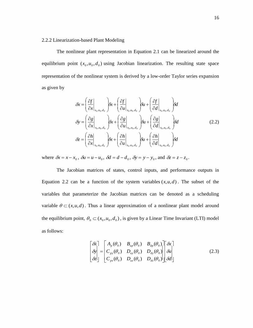
2.2.2 Linearization-based Plant Modeling

The nonlinear plant representation in Equation 2.1 can be linearized around the

equilibrium point ),,( 000 dux using Jacobian linearization. The resulting state space

representation of the nonlinear system is derived by a low-order Taylor series expansion

as given by

dd

hu

u

hx

x

hz

dd

gu

u

gx

x

gy

dd

fu

u

fx

x

fx

duxduxdux

duxduxdux

duxduxdux

000000000

000000000

000000000

,,,,,,

,,,,,,

,,,,,,

(2.2)

where 0xxx , 0uuu , 0ddd , 0yyy , and 0zzz .

The Jacobian matrices of states, control inputs, and performance outputs in

Equation 2.2 can be a function of the system variables ),,( dux . The subset of the

variables that parameterize the Jacobian matrices can be denoted as a scheduling

variable ),,( dux . Thus a linear approximation of a nonlinear plant model around

the equilibrium point, ),,( 0000 dux , is given by a Linear Time Invariant (LTI) model

as follows:

d

u

x

DDC

DDC

BBA

z

y

x

dzuzpz

dyuypy

dpupp

)()()(

)()()(

)()()(

000

000

000

(2.3)

17

where

000000000

000000000

000000000

,,,,,,

,,,,,,

,,,,,,

000

000

000

)()()(

)()()(

)()()(

duxduxdux

duxduxdux

duxduxdux

dzuzpz

dyuypy

dpupp

d

h

u

h

x

h

d

g

u

g

x

g

d

f

u

f

x

f

DDC

DDC

BBA

Under linearization-based modeling methods, the nonlinear plant can be

decomposed into several linear approximations around specific operating conditions.

Similarly in the gain-scheduling paradigm, a nonlinear plant model can be represented in

terms of several LTI plant models obtained at specific operating points that are suitable

for utilizing linear control design tools; those plant models are parameterized by a set of

scheduling variables that indicate the current states of the nonlinear system. Note that a

local LTI approximation of the nonlinear plant at equilibrium point is not identical to a

Linear Parameter Varying (LPV) representation at specific operating point; this will be

described in the following section.

2.2.3 Linear Parameter Varying (LPV) Plant Modeling

A Linear Parameter Varying (LPV) representation of the nonlinear system is a

special case of a system modeling method defined as “A linear system whose dynamics

depend on exogenous parameters with values that are unknown a priori but can be

measured on-line” [13]. A state space representation of LPV system is given in Equation

2.4

18

d

u

x

tDtDtC

tDtDtC

tBtBtA

z

y

x

dzuzpz

dyuypy

dpupp

))(())(())((

))(())(())((

))(())(())((

(2.4)

If there does not exist an LPV representation of the nonlinear system in nature,

an alternative plant representation approach called “quasi-LPV representation” can be

potentially used to parameterize a family of linear models. In the quasi-LPV method,

nonlinear terms are hidden with newly defined time-varying parameters that are then

included in the scheduling variable [73]. Note that quasi-LPV representations are not

unique and a suitable representation may not be well suited for controller design.

2.3 Controller Interpolation

A rough categorization of controller design methods on gain scheduled control

would include two classes: 1) local linear control designs and 2) LPV control design

methods [13]. The former approach is extensively used in practice and allows a

sufficiently large degree of freedom in the design process. However it may suffer from a

general lack of suitable tools for stability analysis. The latter has the advantage that some

level of stability is guaranteed by construction of the controller but the controllers are

designed as a whole and synthesized with common dimension and structure and no

guarantee of existence. Thus some freedom in the design process may be lost and result

in difficulties during the computation.

19

2.3.1 Local Controller Network (LCN)

2.3.1.1 Local Controller Design

In this framework, a nonlinear control design problem can be decomposed into

several linear control problems by employing many linear design tools, often called the

“divide-and-conquer” method. The local linear controllers can be designed at each

design point which is suitable for implementing linear control design, denoted as follows

u

x

DC

BA

u

x k

kk

kkk

)()(

)()(

00

00

(2.5)

Design methods of local linear controllers have been reported from PID control to LQG

and H control [2], [5]. Controller interpolation between these locally designed

controllers is implemented by parameterizing them in scheduling variables, a key idea of

gain-scheduled control which will be intensively discussed in the next section.

2.3.1.2 Local Controller Network (LCN)

Controller interpolation is the crux of gain-scheduling approaches and many

different controller interpolation methods have been proposed. These include the

interpolation of poles, zeros, and gains, interpolation of H controllers by interpolating

Riccati equations, interpolations of balanced state space matrix coefficients,

interpolation of state feedback gains and observer gains, and the interpolation of pole

placement of state feedback gains [13]. Alternatively, several approaches have been

proposed that implement controller blending as a function of operating condition then

forming a global nonlinear controller [2].

20

The latter type of gain-scheduled control is often called “output-blending,”

similar to the Tagaki-Sugeno model that is widely used in the derivation of fuzzy

membership function [40]. By virtue of output-blending, interpolation between

controllers with different dimension and structure is allowable without any restriction on

the design of local controllers.

Under this type of controller interpolation, a nonlinear controller can be formed

by blending the weighted outputs of several linear controllers. These weighting functions

can be presented in terms of scheduling variables , as ))(()( tft and the weighted

sum of those functions is commonly assumed to be ]1,0[)( ti and 1)(ti , but

this assumption is situation-dependent and may not be necessary in some cases.

This output-blending approach results in a Local Controller Network (LCN),

widely used in practice due to its simplicity during controller interpolation. A controller

is constructed using a linear approximation of the nonlinear model, either first principle

model or empirical identification model, by employing linear control design tools. The

weighted sum of outputs from a family of local controllers is then applied to the

nonlinear plant.

Similarly, a Local Model Network (LMN) is constructed by computing local

plant models in parallel. This is assumed to adequately represent the dynamics of

nonlinear system where the local linear representations of the plant are obtained from

linearization of nonlinear plant or empirically through system identification techniques.

This LMN can be simply denoted as )()( sPsP ii , and similarly the LCN as

21

)()( sKsK ii . The interconnected LCN/LMN system is depicted in Figure 2.2,

and the simplified diagram in Figure 2.3.

Fig. 2.2. Interconnected system of LMN/LCN.

22

Fig. 2.3. Simple diagram of LMN/LCN interconnected system.

2.3.1.3 LCN/LMN Closed Loop System

Consider the interconnected LCN/LMN system derived in Figure 2.2. Under this

framework, a set of local linear models of plant )(sPi is given by

1e

x

DC

BA

y

xpi

pipi

pipi

pi

pi

(2.6)

and a set of local linear controllers )(sK i is given by

20 e

x

C

BA

u

x ki

ki

kiki

ki

ki

(2.7)

The state space representation of the closed loop from Tww 21 to Tyu is given in

Equation 2.8, denoted )(sG . Note that this closed loop can be represented as a system

affinely parameterized in with the constraint 1)(ti . Alternatively, the plant and

controller representations can be formed in a polytopic system of individual plant

models and controllers respectively as given by Equations 2.9-10.

23

k

p

C

k

p

B

k

p

k

p

A

kpk

kpp

k

p

x

x

C

C

y

u

w

w

B

B

x

x

ACB

CBA

x

x

G

GG

)(

2

1

)(

0

0

0

0

(2.8)

pn

p

nnp

pn

p

pn

p

pn

p

pn

p

x

x

CCy

e

B

B

x

x

A

A

x

x

1

111

1

1111

0

0

(2.9)

kn

k

knnk

kn

k

kn

k

kn

k

kn

k

x

x

CCu

e

B

B

x

x

A

A

x

x

1

11

2

1111

0

0

(2.10)

2.3.2 LPV Control Synthesis

One recently used control design method in gain-scheduling is the LPV control

design. Under this framework, an LPV representation of the nonlinear plant is assumed

to exist and the associating controllers are designed as a whole with common size and

structure where each controller shares the state variables. Thus, if this representation

exists, stability of the nonlinear closed loop system is guaranteed when prescribed

conditions restricted to the scheduling variable are satisfied. Specifically, these

conditions advocate that scheduling variables are measurable, bounded, and that the time

24

derivative of scheduling variables is bounded. These pre-conditions may be very

conservative in practice and thus current research attempts to reduce them [5].

Although the LPV control cannot allow a sufficiently large design degree of

freedom in design and implementation of gain-scheduling, e.g., design local controllers

at key operating point a priori are not available, it guarantees a certain level of stability

of the system by construction. First, we assume parameter variations in the LPV plant

model as modeling uncertainty where a single LTI controller is sought so that a small

gain condition is met [24]. If there exists an LTI controller that satisfies the condition,

stability can be guaranteed for arbitrarily fast variations in the scheduling parameter, but

this generally results in a poorly performing controller due to extremely conservative

assumptions of control design.

Alternatively, an LPV controller can be sought so that stability of the closed loop

system is guaranteed by existence of a common or parameter-dependent Lyapunov

function. Under this framework, an interpolated controller can be sought by solving a set

of Linear Matrix Inequalities (LMIs) which allows enhanced efficiency in analysis [24]

[74]. However, guaranteeing stability in this way may potentially be very conservative in

that the common Lyapunov function should be found over the entire operating envelope

where scheduling variables may change arbitrarily fast. Thus recent researches have

employed parameter dependent Lyapunov functions that can reduce some of the severe

restrictions if the time derivative of the scheduling variable can be bounded [51].

25

LPV gain scheduling has been proved to be successful for guaranteeing a certain

level of stability by construction, but lack of existence and conservatism of the design

process cause computational difficulties and limit wide application in practice.

2.4 Stability Analysis

As mentioned in Section 1, guaranteeing the closed loop stability of nonlinear

system has been a challenging problem. Some research has successfully shown the

stability of the nonlinear system at local operation conditions, but little research has

shown global stability. Furthermore, the endogenous scheduling system requires more

careful evaluation in order to guarantee the stability over operating regions since

endogenously scheduling variables or their bounds cannot be known a priori. Thus

guaranteeing the desired level of performance and stability of the gain-scheduled closed

loop system under any operating conditions is he primary research objective of this

dissertation.

2.4.1 Stability Classification

Stability analyses of gain-scheduled closed loop systems can be roughly

categorized into linear and nonlinear stability criteria [13], [64]. The simplest criteria in

linear stability analyses, i.e., stability evaluated for linearized system, is frozen

parameter stability where closed loop stability is evaluated and the standard feedback

loop of linearized plant model and linear controller is examined to be Hurwitz. Note that

frozen parameter stability is a merely guarantee of stability at fixed scheduling

26

parameters. Although this stability criterion is commonly used in practice, it may not be

sufficient for the nonlinear stability of real systems when significant nonlinear dynamics

are neglected during the linearization.

In contrast, nonlinear stability ensures the practical stability of nonlinear system

in that stability is evaluated for closed loop systems without neglecting any aspects of

the system techniques. There exist several nonlinear stability analyses in literature [46],

but Lyapunov stability is one of most commonly used solutions to achieve nonlinear

stability. Under this criterion, the existence of the common or parameter-dependent

Lyapunov function with respect to the trajectories of the nonlinear system will guarantee

the asymptotic stability of the nonlinear system globally or for reasonably large region

around the equilibrium point [36].

2.4.1.1 Linear Stability Analysis

One of the common methods used in linear stability analysis can be examined

simply by evaluating the closed loop stability of the linearized plant model. In nonlinear

system approaches, this level of stability can be guaranteed for any fixed value of the

scheduling variables without considering scheduling dynamics. However, the global

controller, which is formed by interpolation between local stabilizing controllers, may

not stabilize the system at the intermediate operating points, i.e., off-design points, even

if local controllers may stabilize at design points.

The simple example given below efficiently illustrates the possibility that a

global control system violates stability. Using the linear control design under the Local

27

Controller Network (LCN) approach, an interpolated controller could be defined as a

convex set of two local controllers where weighting factor ]1,0[i (Equation 2.12).

Note that individual controllers 1K and 2K successfully stabilize the plant but the

interpolated controller IK , denoted in Equation 2.12, fails to stabilize the plant for

]1 ,25.0[

5.0

1)( ,

5.0

1)( ,

1

1)( 21

ssK

ssK

ssP (2.11)

21 )1()( KKsK I (2.12)

Several studies have proposed controller interpolation methods that guarantee frozen

parameter stability under the preliminary condition that scheduling variables are changed

sufficiently slowly, then the stability of nonlinear system will be guaranteed when the

condition is valid over the operating regions.

Alternatively, other approaches define the acceptable rate of change on

scheduling variables, but the “slowly varying” assumptions are still essential to

guarantee the global stability of a given system. Thus, these types of approaches may be

valid for exogenously-scheduling systems where the rate of change of the scheduling

variable is usually known a priori and nonlinear behavior of many systems is more

appropriately captured by scheduling parameters that are functions of system outputs.

However, guaranteeing the stability of endogenously scheduled systems is much harder

to achieve since a bound on the rate of change may not be known a priori.

28

2.4.1.2 General Nonlinear Stability Analysis

Any linear stability technique merely evaluates whether the system is

asymptotically stable for infinitesimal deviations around the equilibrium point [46]. It

may not be sufficient to guarantee the stability of the nonlinear system particularly when

scheduling variable changes in a wide range of operating conditions. To guarantee the

desired global stability under arbitrary variations, the nonlinear stability of the closed

loop system should be evaluated.

A well-known method for guaranteeing this level of stability of a nonlinear

system is to use Lyapunov stability criterion, defined in Theorem 2.1 [25]. Before

explaining the Lyapunov stability, some key definitions related to this criterion are

addressed for better understanding of the stability analysis in this dissertation.

Definition 2.1) Stability of an equilibrium point [25]

The equilibrium point 0x of the autonomous system )(xfx is

- stable if, for each 0 , there is 0)( such that

)()0( txx , 0t (2.13)

- unstable if it is not stable

- asymptotically stable if it is stable and there exists such that

0)(lim)0(

txxt

(2.14)

Definition 2.2) Global asymptotic stability [25]

29

The equilibrium point 0x of the autonomous system )(xfx is globally

asymptotically stable if

- 0x is asymptotically stable and

- 0)(lim

txt

for all nRx 0 (2.15)

Definition 2.3) Class K functions [25]

The continuous function is called a Kclass function if

- 0)0( (2.16)

- 0x , 0 x (2.17)

- x is strictly monotonically increasing with x (2.18)

Definition 2.4) Positive-definite functions [25]

The continuous function ),( txV is positive definite on nRG if

- xtxV ),( , Gx and 0t (2.19)

Definition 2.5) Decrescent functions [25]

The continuous function ),( txV is called a decrescent function on nRG if there exists

a Kclass function such that

- xtxV ),( , Gx and 0t (2.20)

30

Theorem 2.1) Lyapunov stability [25]

Let 0x be an equilibrium point for the nonlinear autonomous system )(xfx . Let

RRV n : be a continuously differentiable function such that

0)0( V and 0)( xV 0x (2.21)

c )(xV (2.22)

0)( xV 0x (2.23)

Then the equilibrium point 0x is a globally asymptotically stable.

Proof:

Assume there exists in class k function such that xtxV ),( where ),0( hBx ,

0tt . Also, when 0),( txV is satisfied along the trajectories of system )(xfx then

we know that

),(),( 00 txVtxV (2.24)

Next, let be the smallest 0x such that )(),( 00 txV . Given 0 , for all ,

)(0 txx (2.25)

Then we know that:

)(),( 000 txVx (2.26)

)(),(0 txVx (2.27)

Finally, we can conclude that the solution to the nonlinear autonomous system )(xfx

is globally asymptotically stable using the final form in Equation 2.28

)()())(( txtx (2.28)

31

A function )(xV that satisfies the conditions in Equation 2.21-23 is called a

Lyapunov function; thus a Lyapunov function should be a positive-definite decrescent

function and the negative form of Lie-derivative )(xV is positive-definite. The

quadratic form of Lyapunov function 0 ,)( PPxxxV T has been widely used for

linear, LPV, and polytopic systems where x is system states and P is Lyapunov matrix.

For linear autonomous systems Axx the choice of quadratic function leads to the

condition in Equation 2.23 as 0)()( xPAPAxxV TT such that the condition for

stability is equivalent to finding a solution to the well-known Lyapunov Equation

QPAPAT where Q is a positive-definite matrix [74].

2.4.1.3 Nonlinear Stability with Guarantee of Worst Performance

Despite the fact that the nonlinear stability guarantees closed loop stability of the

nonlinear system, it may not be sufficient for assuming the practical stability required in

gain-scheduled control. Under the gain-scheduling framework, the LMN or LPV

representation of the nonlinear system may perform reasonably well - merely within a

specified operating range. Thus, any stability guarantees will be valid only when the

system does not leave the operating range during the entire operation [65].

Furthermore, guarantees of the worst case performance will be useful in

improving practical aspects of the stability analysis for nonlinear systems and extending

the Lyapunov stability to performance consideration through examining worst

performance bounds from system inputs to outputs or disturbance. To implement the

32

performance efficiently, Linear Matrix Inequalities (LMIs) techniques are commonly

used to permit simplicity in analysis [39], [75], described in the following section.

2.4.2 Stability Analysis with Performance Bounds via LMIs

Linear matrix inequalities (LMI) have the form 0)(1

0

m

i

i FxFxF where

mRx is the variable and nnT

ii RFF , mi ,...,1 are given. This inequality means

that )(xF is positive-definite, i.e., 0)( uxFuT for all nonzero nRu . Also, this LMI

is a convex constraint on x , i.e., the set 0)( xFx is convex. Although the LMI may

have a specialized form, it can represent a wide variety of convex constraints on x . In

particular, linear inequalities, quadratic inequalities, and constraints that arise in control

theory, such as Lyapunov and convex quadratic matrix inequalities, can be cast in the

form of LMI [74].

This vector gives more flexibility as well as simplicity to the analyses in practice,

thus many complex problems in analytic or computational studies can be easily solved

by formulating them into LMIs. For example, multiple LMIs 0)(,,0)( )()1( xFxF p

can be expressed as a single LMI 0))(,,0)(( )()1( xFxFdiag p , therefore a set of

LMIs can simply be converted into a single LMI [74].

When the matrix iF is diagonal, the LMI 0)( xF is just a set of linear

inequalities. The LMI formula described above can be converted into a simple LMI

33

formula called “Schur complement.” Note that these two formulae are completely

identical and Q and R are symmetric and positive-definite matrices [49]:

,0)( xR and 0)()()()( 1 TxSxRxSxQ (2.29)

0)()(

)()(

xRxS

xSxQT

(2.30)

Also, LMI-based analyses have best-fit for the polytopic system representation

showing that overall system is composed of a convex hull of several linear systems,

described as follows.

Definition 2.6) Convex hull and polytopic systems [74]

The convex hull of a given set of points nxx ,,1 is defined as:

n

j

n

i

iiiin xxRxxxCo1 1

1 1 [0,1], , }),,({ (2.31)

Then, a state space representation of the polytopic system is given by

w

x

tC

tBtA

z

x

0)(

)()( (2.32)

where }),,({)( 1 nAACotA , }),,({)( 1 nBBCotB , and }),,({)( 1 nCCCotC .

Note that }),,({ 1 nAACo is formed by the combination of system matrices and its

weighting function, nn AAA 2211 , and the sum of weighting function i

needs not be one. Under these conditions, the closed loop of the LMN/LCN has a

34

polytopic relationship, affine in weighting function , that allows the convex

optimization in controller interpolation. This will be discussed later in this dissertation.

Let a quadratic Lyapunov function be 0 ,)( PPxxxV T , then a necessary and

sufficient condition for asymptotic stability of the linearized system is determined by the

existence of a solution to the LMI 0 PAPAT . For polytopic systems, asymptotic

stability can be guaranteed by the solution of a set of LMIs 0 i

T

i PAPA , mi ,,1

for the common Lyapunov matrix 0P .

2.4.2.1 H performance

Among various norm-based performance definitions, the most commonly used

one in stability is H performance, denoted as [44]:

2

2

02

sup))((maxw

zjwGG

wLww

(2.33)

H performance is known as a power norm, defined by finite energy to finite energy,

and also an induced norm in terms of expected values of stochastic signals. The H

norm is usually computed numerically fom a state space realization as the smallest value

of such that the Hamiltonian matrix H has eigenvalues on the imaginary axis. In

robust control, the H norm is commonly used because it is convenient for representing

unstructured modeling uncertainty [69], [75] and satisfies the multiplicative property that

is useful in analysis.

35

)()()()( sBsAsBsA (2.34)

Using this definition, LMI conditions for an upper bound on the H gain can be

prepared and the resulting asymptotic stability criterion is given as follows

Theorem 2.2) Stability using H performance

The standard LTI system is given as

w

x

C

BA

z

x

0

(2.35)

Then the system in Equation 2.32 is asymptotically stable and has an H norm less than

if and only if there exists 0P such that

02

IPB

PBCCPAPAT

TT

(2.36)

Proof: See [74]

For the polytopic system, this LMI formulation can be easily extended as the set of

LMIs:

02

IPB

PBCCPAPAT

i

ii

T

ii

T

i

, for .,,1 mi (2.37)

36

2.4.2.2 2H performance

Another norm-based performance used widely in practice is 2H performance,

denoted by [49].

dwjwGdwjwGjwGtrG

i

i

H ))((2

1))()((

2

1 2

2

(2.38)

The 2H norm can be interpreted as a 2-norm output resulting from applying unit

impulses )(ti to each output. In general, the 2H norm has a number of outstanding

mathematical as well as numerous properties and its minimization has important

engineering implications. In stochastic process, this interpretation allows the

implementation of optimal control in terms of Linear Quadratic Gaussian (LQG) where

we measure the expected root mean square (rms) value of the output in response to white

noise excitation.

However, the 2H norm is not an induced norm and does not satisfy the

multiplicative property. Note that the inducing norm is defined as a maximum gain for

all possible input directions,

p

p

wip w

GwG

0max

where

i

pp

ipww

1

)( . Thus

looking for the direction of vector w so that the ratio

p

p

w

z is maximized then the

induced norm gives the largest possible amplifying power of the matrix.

Theorem 2.3) Lyapunov stability [74]

37

The system in Equation 2.29 is asymptotically stable and has the 2H norm less than if

and only if there exists 0P such that

0

IPB

PBPAPAT

T

and 0

IC

CP T

(2.39)

Equivalently,

0

ICP

PCPAPA TT

and 0

IB

BPT

i

i

(2.40)

Proof: See [74]

Also, these LMIs can be extended to polytopic systems as the set of LMIs

0

IPB

PBPAPAT

i

ii

T

i

and 0

IC

CP

i

T

i

, for .,,1 mi (2.41)

Equivalently,

0

IPC

PCPAPA

i

T

ii

T

i

and 0

IB

BPT

i

i

, for .,,1 mi (2.42)

Note that the difference between the interpretation of the 2H and H norms

may help the readers to understand the applications in practice. Minimizing H norm

corresponds to minimizing the peak of the largest singular value, i.e., “worst direction

and worst frequency,” while minimizing the 2H norm results in minimizing the sum of

the square root of all singular values over all frequencies, i.e., “average direction and

average frequency” [3].

38

2.4.3 Conclusion: Stability of Gain-scheduled Control System

In gain-scheduled control, the closed loop of the nonlinear system is represented

as a polytopic model and the associated stability can be determined using an LMI-based

Lyapunov stability analysis. Using Lyapunov stability, the interconnected LMN/LCN

system can be guaranteed to be stable for arbitrarily fast variations of the scheduling

variable where a common Lyapunov function can be found for each local plant model in

the polytopic system. For exogenous gain scheduled systems, this condition would be

sufficient for guaranteeing the stability globally throughout the operating envelope since

the change in scheduling variables is known a priori.

However, for endogenously-scheduled systems, the above conditions may not be

sufficient to guarantee global stability because a bound of change of scheduling

variables may not be known a priori. For practical stability, it is necessary to ensure the

scheduling variable remains within acceptable bounds for an assumed class of

disturbances. Although the existence of a common Lyapunov function guarantees

stability through bounded inputs and outputs, if sudden changes in inputs or outputs

drive the system outside of the region then the instability occurs.

Thus, guarantees of the worst case performance from disturbances to system

inputs and outputs could be very useful to ensure the practical stability of the physical

systems. In essence, Lyapunov stability can be extended to generate the worst case of

norm-based performance bounds on system outputs, controller outputs or scheduling

variables, thus the LMI-based method is used efficiently in the stability of a gain

scheduled closed loop system.

39

2.5 Youla-based Gain-scheduled Control

2.5.1 General Youla Parameterization

Youla parameterization is one of the more recent approaches in gain scheduling

and is based on the work by Youla et al, in the 1970’s [62]. The crux of Youla

parameterization can be described as “all stabilizing controllers can be parameterized in

terms of a single parameter,” often called “Youla parameter,” denoted by Q . Under this

framework, the closed loop system can be represented as an affine system in the Youla

parameter Q that allows the optimal design of the stabilizing controller to be a convex

optimization problem.

In general, Youla parameterization is implemented through coprime factorization.

For plant models and controllers, factorization leads to the models and controllers being

represented as the ratio of two stable transfer functions. This factorization is termed

coprime when two transfer functions have no common zeros in RHP. Thus coprime

factorization excludes any pole-zero cancellations in the fractional representation.

In multivariable cases, the plant model and nominal controller transfer functions

are factored into the product of a stable transfer function and a transfer function with a

stable inverse. In the mathematical view, a dynamic system (plant model and controller)

can be decomposed into right and left coprime factors NMNMsP~~

)( 11 .

Using this coprime factorization, the controller can be decomposed into left and

right coprime factors, UVUVsK~~

)( 11 and a plant model into

40

NMNMsP~~

)( 11 such that RHVVUU~

,,~

, and RHMMNN~

,,~

, . If a

nominal plant model 0P is stabilized by a nominal controller 0K and its coprime factors

satisfy the double Bezout identities (Equation 2.43), then all stabilizing controllers can

be parametrized in terms of coprime factors of the nominal controller/plant and Youla

parameter, denoted by Q (Equation 2.44). Similarly, all plants that can be stabilized by

the nominal controller 0K are parameterized in terms of the dual Youla parameter S

(Equation 2.45)

I

I

MN

UV

VN

UM

0

0~~

~~

(2.43)

)~~

()~~

(

))((

00

1

00

1

0000

MQUNQV

QNVQMUQK

(2.44)

)~~

()~~

(

))((

00

1

00

1

0000

VSNUSM

SUMSVNSP

(2.45)

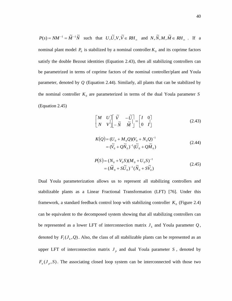
Dual Youla parameterization allows us to represent all stabilizing controllers and

stabilizable plants as a Linear Fractional Transformation (LFT) [76]. Under this

framework, a standard feedback control loop with stabilizing controller 0K (Figure 2.4)

can be equivalent to the decomposed system showing that all stabilizing controllers can

be represented as a lower LFT of interconnection matrix kJ and Youla parameter Q ,

denoted by ),( QJF kl . Also, the class of all stabilizable plants can be represented as an

upper LFT of interconnection matrix pJ and dual Youla parameter S , denoted by

),( SJF pu . The associating closed loop system can be interconnected with those two

41

systems, ),( QJF kl and ),( SJF pu , as shown in Figure 2.5. Note that the interconnected

LQN/LSN system is equivalent to the standard feedback control system in Figure 2.5.

Fig. 2.4. Feedback control loop.

Fig. 2.5. Feedback control loop with dual Youla parameterization.

42

0

1

0

1

0

1

0

1

00

~

NVV

VVUsJ K (2.46)

0

1

0

1

0

1

0

1

00

~

UMM

MMNsJ p (2.47)

The closed loop system of standard feedback loop in Figure 2.4 can be represented by

2

1

1

2

1

1

11

11

2

1

0

0

)()(

)()(

w

w

VN

UM

V

M

w

w

PKIKPIP

PKIKKPI

e

e

(2.48)

Thus the stability of the closed loop system is guaranteed when the system

1

11

11

)()(

)()(

PKIKPIP

PKIKKPI or

1

0

0

VN

UM

V

M is Hurwitz. To show the ability

of convex optimization of the closed loop system in terms of (dual) Youla parameters,

the above system representation can be written as follows [63]

00

00

1

00

00

1

0

0

1

~~

~~

)(

)(

MN

UVI

IS

QI

VN

UM

IP

KI

ISP

QKI

(2.49)

Note that the closed loop system is affine in Youla parameter Q and dual Youla

parameter S which allow the design of the optimal stabilizing controller to be a

controller design through the convex optimization that is computationally feasible. Also,

the closed loop system is stable when systems

1

0

0

IP

KIand

1

IS

QI are

43

Hurwitz. This is confirmed by the examination of the interconnection of matrices kJ and

pJ (Equation 2.50) using the double Bezout identities. The closed loop system in Figure

2.5 is internally stable if and only if the system in Figure 2.6 is stable [5], [63].

0

0),(

I

IJJF kpl (2.50)

Fig. 2.6. Simple diagram of feedback loop using Dual Youla parameterization.

2.5.2 Interpolation of Dual Youla Parameters

Although the LCN/LMN approach has been successfully applied in practice,

there exist several shortcomings in the aspect of stability. For example, even when all

stabilizing controllers can stabilize the plant at every fixed operating points, the blended

controller may not stabilize the plant at the intermediate points over the operating

envelopes. Furthermore, classical gain scheduling approaches require that locally

defined plant models and controllers should be open loop stable for guaranteeing the

internal stability of the closed loop system.

44

The Youla-based gain-scheduling framework allows the parameterization of

plant models and stabilizing controllers designed at local operating points and guarantees

recovery of the original local controllers at the design point and increases the stability of

gain-scheduled systems by guaranteeing frozen parameter stability at intermediate

design points while recovering the original local controllers at the design points.

Variations of this approach have been termed QJ interpolation [14], or

blending of the Youla parameters [77]. By virtue of the Youla parameterization, this

framework permits the scheduling of unstable controllers [78]. Moreover, this

framework has the intuitive appeal of isolating common controller elements in function

kJ and blending only the differences between the individual controllers. When

implementing a blended controller for a plant 0P , the blended controller may be

constructed as in Equation 2.44 where 1

000

VUK is any controller that stabilizes the

plant. Note that the original local controller iK is recovered at 1i .

Moreover, when )(QK stabilizes 0P for any RHQ , then QK also

stabilizes 0P for every frozen value of , since each RHQi and thus

RHQii , something not necessarily guaranteed with the LCN framework. The

systematic differences between the conventional LCN framework and Youla-based

QJ interpolation method can be easily depicted in Figure 2.7-2.8.

1

0000

iiii QNVQMUQK (2.51)

45

Similarly, the nonlinear plant can be characterized by a group of dual Youla

parameters, iS [58], [63]. In this case, the coprime factors are selected as to satisfy

another Bezout identity (Equation 2.52). The nonlinear model is formed as shown in

Equation 2.53 with the dual Youla parameters constructed as 00

~~NMMNS iii .

Fig. 2.7. Output blending of local controller network (LCN).

I

I

MN

UV

VN

UM

iii

i

0

0~~

~~00

0

0 (2.52)

iiii SUMSVNSP 0000 (2.53)

0

1

0

1

0

1

0

1

00

~

UMM

MMNsJP (2.54)

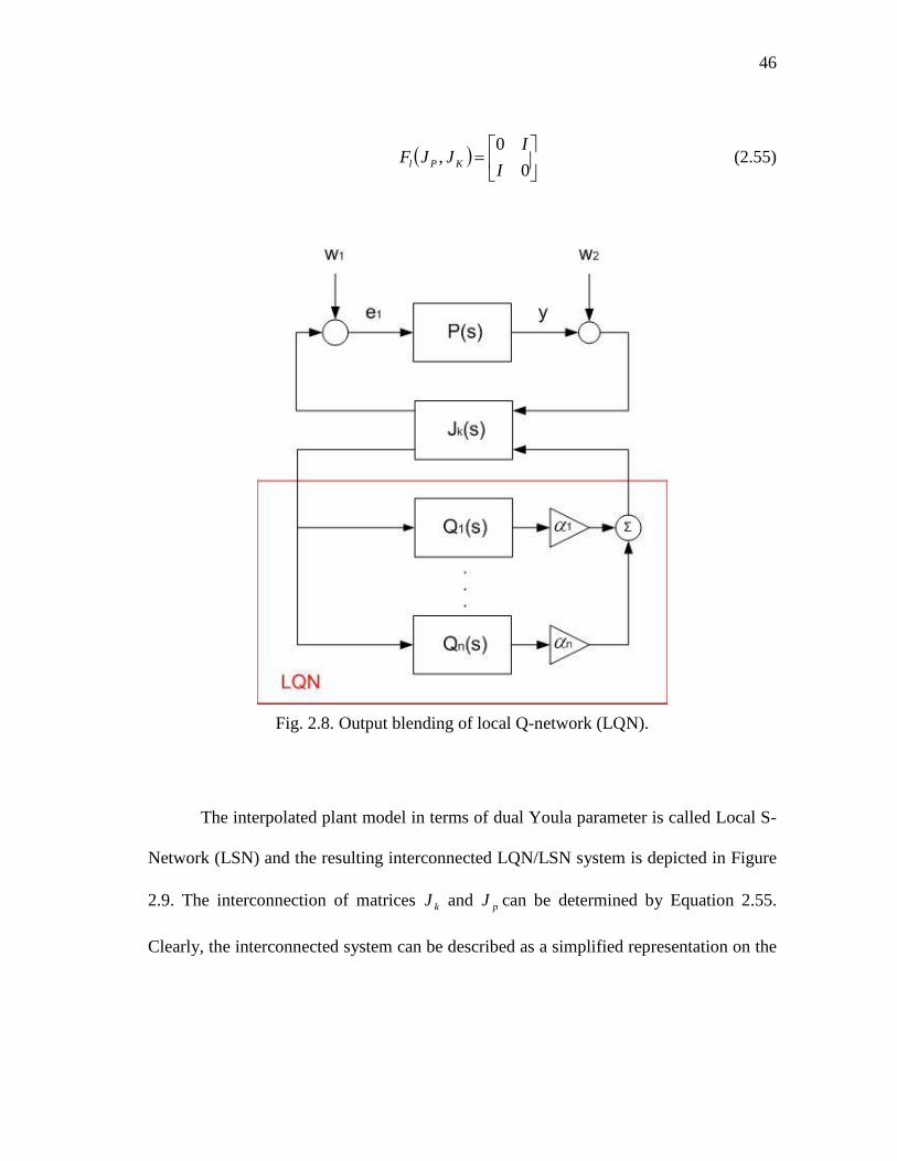
46

0

0,

I

IJJF KPl (2.55)

Fig. 2.8. Output blending of local Q-network (LQN).

The interpolated plant model in terms of dual Youla parameter is called Local S-

Network (LSN) and the resulting interconnected LQN/LSN system is depicted in Figure

2.9. The interconnection of matrices kJ and pJ can be determined by Equation 2.55.

Clearly, the interconnected system can be described as a simplified representation on the

47

left hand side thus the condition for stability of the overall system is equivalent to the

stability of the simplified system also shown in Figure 2.10.

Fig. 2.9. Closed loop system with LQN/LSN.

48

Fig. 2.10. Feedback loop of LQN/LSN interconnected system.

One of the important aspects in Youla-based gain scheduling is the local

controller recovery procedure. To demonstrate local controller recovery, a standard

mathematical expression of Youla parameter is considered

00

0

1

00

1

0

1

00

11

00

1

0

1

000

1

00

~

~~~

~~~~~

~~~~

~~

VKKV

VVUUVV

VVUVVVVUVV

VVUVVUVV

UVVUQ

ii

iii

iiiii

iiii

iii

(2.56)

Also, a nominal controller can be derived using coprime factorization and the

Bezout identity as follows:

49

1

00

1

00

1

00

1

0000

1

0000

1

000

1

0000

1

0

1

000

1

0000

1

000

1

0000

1

00

1

00

1

0000

1

00

1

00

1

00000

~

~

~

~~~

~~

~~

~~

QNVQVK

QNVQVQNVK

QNVQNKVVK

QNVQNUVVVK

QNVQNUIVVK

QNVQMVVVVU

QNVQMVVVVU

QNVQMUQK

(2.57)

Using the results obtained above, local controller recovery can be shown by

1

1

00000000

1

00000000

1

000000000000

1

0000000000

1

0000000000

1

00000000

1

00000

~~~~

~~~~

~~~~

~~~~

~~~~

~~~~

ii

ii

iiii

iiii

iiii

iiii

iiii

iii

VU

UNVMVUNVMU

UNVVMVUNUVMU

UNVVVMVVUNUUVMUU

UNVVIMVVUNUIVMUU

UVNVUNVUVMVUMU

UVVUNVUVVUMU

QNVQMUQK

(2.58)

Equivalently,

50

11 1 1

0 0 0 0 0 0

11 1 1

0 0 0 0 0 0 0 0 0

11 1 1

0 0 0 0 0 0 0 0 0

11

0 0 0 0 0

11

0 0 0 0 0

1 1

0 0

( )i i i

i i i i

i i i i

i i i i

i i i i

i i

K Q K V Q I V N Q V

K V V K K V I V N V K K V V

K V V K K V I V N V K K V V

K V V K K I N V K K

K V V I K K N V K K

K V V K K

1

0 0 0

11 1 1 1

0 0 0 0 0 0

11 1 1

0 0 0 0 0 0 0

11 1 1

0 0 0 0 0 0 0

11 1

0 0 0 0 0 0 0

11 1

0 0 0 0 0 0 0 0

1

0 0 0

i

i i i i

i i i

i i i

i

i

N K K

K V V V U V U N K K

K V V I U N V U N K K

K V V V M V U N K K

K V M V U N K K

K V V V M U N K K

K V V

11

0 0 0 0 0

11 1

0 0 0 0

1

0 0 0 0

0 0

i

i

i

i

i

V M U N K K

K V V I K K

K V V K K

K K K

K

(2.59)

Finally, the closed loop representation of the LQN/LSN framework is

implemented. Note that the relationship form Tww 21 to Tee 21 or Tyu of the

system in Figure 2.11 for the modified framework is given by Equation where 1T , 2T , 3T ,

and 4T depend merely on the choice of 0K and 0P .

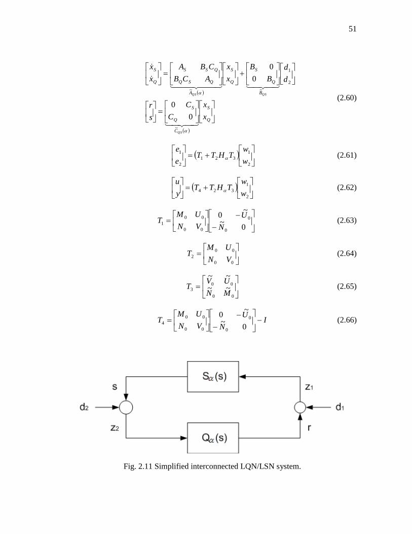
51

Q

S

C

Q

S

B

Q

S

Q

S

A

QSQ

QSS

Q

S

x

x

C

C

s

r

d

d

B

B

x

x

ACB

CBA

x

x

QS

QSQS

~

2

1

~~

0

0

0

0

(2.60)

2

1

321

2

1

w

wTHTT

e

e (2.61)

2

1

324w

wTHTT

y

u (2.62)

0~

~0

0

0

00

00

1N

U

VN

UMT (2.63)

00

00

2VN

UMT (2.64)

00

003 ~~

~~

MN

UVT (2.65)

IN

U

VN

UMT

0~

~0

0

0

00

00

4 (2.66)

Fig. 2.11 Simplified interconnected LQN/LSN system.

52

Compared to the Local Q-Network (LQN), the Local S-Network (LSN) is a

versatile framework, having been used to capture system variations and model

uncertainty [17], [58]. Furthermore, it allows special cases where scheduling variables

cannot be measured on-line [77].

The LQN framework for gain-scheduling offers significant advantages such as

guaranteed frozen parameter stability, and yet only a few researchers have explored this

framework. Niemann and Stoustrup have examined standard LQN approaches [17], [58]

[77] and Q-blending with an observer-based control scheme [59], [79]. They have

applied their work to power plant control [80], [81] and assessed the performance of the

system where modeling errors exist, denoted by a fault tolerant system [60], [82].

Stilwell et al. also discussed this framework under the title “J-Q interpolation” [14], and

examined interpolation of controllers by defining a stability-preserving condition

corresponding to bound on rate of variation of scheduling variables [83], [84], and a

state-space version of Q-blending using state feedback and observer gains [85].

53

3. YOULA PARAMETER BASED CONTROLLER INTERPOLATION

As discussed previously, guaranteeing global stability of the nonlinear system is

a challenging problem in gain-scheduling approaches which has motivated the research

presented in this dissertation. This section will examine the gain-scheduling problem

with a particular focus on controller interpolation with guaranteed stability of the

nonlinear closed loop system. Specifically, an advanced controller interpolation method

that guarantees stability of the nonlinear system under arbitrarily fast-varying scheduling

is proposed and demonstrated through the simulation case study.

First, the general case of Youla parameterization-based gain-scheduling will be

examined to identify degrees of freedom in the design of the gain-scheduled control

framework. Second, for the Linear Parameter Varying (LPV) system a particular

controller interpolation method utilizing the Youla parameterization will be proposed.

Under this framework, quadratic stability is guaranteed by construction of a particular

controller interpolation method, while the characteristics of individual controllers

designed a priori are recovered at critical design points.

In essence, the proposed approach ensures closed loop stability despite arbitrarily

fast transitions which lead naturally to the application of switched linear systems. The

efficacy of the method is demonstrated in simulation using a multi-input-multi-output

nonminimum phase system while interpolating between two controllers with different

sizes and structures.

54

3.1 Local Controller Network (LCN)/Local Model Network (LMN) Presentation

The Local Model Network (LMN) framework has been widely used in practice

and commonly implemented under the assumption that the nonlinear plant is adequately

represented by interpolation of local linear models. Under the LCN/LMN framework,

local controllers and plant models are assumed to be represented as in Equation 3.1

kikiki

kikikiki

xCu

eBxAx

2

and pipipi

pipipipi

xCy

eBxAx

1

(3.1)

By virtue of output blending, the Local Controller Network )(sK and Local Model

Network )(sP can be formed in polytopic representation in Equations 3.2-3,

respectively, and the resulting LCN and LMN are a quasi-LPV representation that are

affine in the bounded parameters ]1,0[i , depicted in Figure 3.1.

2

1111

0

0

e

B

B

x

x

A

A

x

x

KKK B

kn

k

x

kn

k

A

kn

k

kn

k

kn

k

C

knnk

x

x

CCu

K

1

11 (3.2)

pn

p

C

pnnp

B

pn

p

x

pn

p

A

pn

p

pn

p

x

x

CCy

e

B

B

x

x

A

A

x

x

p

ppp

1

11

1

1111

0

0

(3.3)

55

Fig. 3.1. Interconnected LCN/LMN system.

The closed loop system from Tww 21 to Tyu is given in state-space

representation in Equation 3.4, denoted by sG . Again, this system is formed in a

polytopic representation of individual models.

56

K

P

C

K

P

B

K

P

K

P

A

KPK

KPP

K

P

x

x

C

C

y

u

w

w

B

B

x

x

ACB

CBA

x

x

G

GG

~

2

1

~~

0

0

0

0

(3.4)

3.2 Local Q-Network (LQN)/Local S-Network (LSN) Presentation

3.2.1 Closed Loop System Representation

This section discusses general Youla-based gain-scheduling, focusing several

design aspects such as plant representation, selection of nominal controller, and the

effect of coprime factorizations of the system based on a local model/controller network.

Using a dual Youla parameterization, the formulation of the interconnected Local Q-

Network (LQN) and Local S-Network (LSN) system is presented in Equation 3.5 and

also depicted in Figure 3.2.

Q

S

C

Q

S

B

Q

S

Q

S

A

QSQ

QSS

Q

S

x

x

C

C

s

r

d

d

B

B

x

x

ACB

CBA

x

x

QS

QSQS

~

2

1

~~

0

0

0

0

(3.5)

57

Fig. 3.2. Interconnected LQN/LSN system.

This interconnected system satisfies that Bezout identities can be found based

on a choice of feedback gains pF and kF such that the matrices kkk FBA and

ppp FBA have strictly negative eigenvalues [14], and the state space representations of

the associated left and right coprime factors are given in Equations 3.6-7 respectively.

I

I

B

B

FC

CF

FBA

FBA

VN

UMKj

Pi

KjPi

KjPi

KjKjKj

PiPiPi

ji

ji

0

0

0

0

0

0

(3.6)

I

I

B

B

FC

CF

ACB

CBA

MN

UV Kj

Pi

KjPi

KjPi

KjPiKj

KjPiPi

ii

jj

0

0

0

0

~~

~~

(3.7)

The resulting closed loop from Tww 21 to Tyu is characterized with the

interconnection of LQN and LSN, denoted sH (Equation 3.5), where 1T , 2T , and 3T

depend on the choice of 0K , 0P , and their coprime factorizations as given in Equation

3.9

58

2

1

321w

wTHTT

y

u (3.8)

IN

U

VN

UMT

0~

~0

0

0

00

00

1 ,

00

00

2VN

UMT , and

00

003 ~~

~~

MN

UVT (3.9)

Typically, the choice of 0P should be made so that LSN adequately represents

the nonlinear plant, but the 0K can be chosen somewhat arbitrarily among the

controllers designed at each operating point so that the class of acceptable disturbances

is maximized. Note that the trivial choice of 000 PK results in recovery of the

LCN/LMN framework.

The choice of coprime factorization presents an additional degree of design

freedom that can be exploited to improve stability and performance, and can be

equivalent to selectrd matrices pF and kF so that kkk FBA and ppp FBA are

Hurwitz. Clearly, gain-scheduling on the Youla parameters has the interpretation of

isolating common controller elements in kJ , and controller differences in iQ , defined by

the coprime factors as 00 )(~

VKKVQ iii . For the nominal choice 0 kp FF , the

associated coprime factors are simply 1

00 )(~ PKIVi and IV 0 . Thus, iQ is simply

the controller differences filtered by the loop sensitivity function.

Generally, finding the optimal pF and kF that minimizes some performance

norm is a nonconvex optimization problem. Even in the simple case of scheduling only

two plants/controllers, the resulting closed loop system can be represented as a

59

constrained state-feedback problem for a polytopic system. For the unconstrained case,

this is easily solved by the Linear Matrix Inequality (LMI) [27]

01

2,,,, QCQCBBBYYBQAQA i

T

i

T

iwiw

T

iu

T

iiiu

T

ii

(3.10)

However, in a constrained case, this is a well-known Bilinear Matrix Inequality (BMI)

that may not be computationally feasible [63], [74].

3.2.2 Gain-Scheduled Control of a Mass-Spring–Damper System

The reader knows that the choice of coprime factorization presents a design

degree of freedom in Youla-based gain-scheduling and can be implemented by finding

the optimal feedback gains pF and kF . Although finding the optimal choice of coprime

factors remains computationally difficult, a simple example illustrates the value of a few

heuristic rules. The illustrative simulation example presented in this section shows the

effect of the choice of coprime factors via selecting the optimal pF and kF .

As for the simulation case study, consider a nonlinear mass-spring-damper

system as given in Figure 3.1. The damping coefficient, c , and spring constant, k , are

assumed to vary linearly as a function of displacement and the resulting state space form

of the system is presented in Equation 3.11

60

Fig. 3.3. Mass-spring-damper system.

xy

uxycyk

x

01

1

0

)()(

10

(3.11)

where 0.7] ,3.0[c , 0.05] ,15.0[k , and 1 m .

Over the operation envelopes, two design points are chosen at upper end values

of the prescribed range. The pole-zero plot for the linear parameter varying plant is

shown in Figure 3.4, the step response and bode magnitude/phase plot at the two design

points are given in Figures 3.5-3.6 respectively.

To illustrate the effect on the choice of coprime factors, the reference-to-error

H norm of the polytopic system, 22 LL

sG , is calculated for several cases. Note that

the system sG is defined as Equation 3.12 and H norm of the system sG can be

calculated by Equation 3.13.

61

Fig. 3.4. Pole-zero plot for varying k and design points.

Fig. 3.5. Step responses of two local linear models.

62

Fig. 3.6. Bode plots of two local linear models.

K

P

C

Q

S

B

K

P

K

P

A

KPK

KPP

K

P

x

x

C

C

y

u

w

w

B

B

x

x

ACB

CBA

x

x

G

GG

~

2

1

~~

0

0

0

0

(3.12)

2

2

02

sup)(w

zsG

wLw

(3.13)

First a “good” choice of coprime factors is constructed using LQR techniques to

determine the matrices PF and KF . Second, a “nominal” choice of coprime factors

63

determined by 0 KP FF is evaluated. Third, a “bad” choice of coprime factors is

constructed by trial and error. For the purpose of comparison, the H norm of the

LCN/LMN approach is also calculated.

The results show that the choice of coprime factors has a significant role in

performance bound in stability analysis. This is also evident in the transient response of

the nonlinear closed loop system as given in Figure 3.7. Although LQN indicates that it

is clearly possible to perform better than the standard method (LCN), there is also the

potential to perform worse. Furthermore, the reader can recognize that a key indicator

appears to be the maximum H norm of the ii SQ / interconnection in Table 3.1. Note

that the H norm of the interconnected LQN/LSN system with bad coprime factors is

several times worse than those of other cases.

Table 3.1. Performance bound on LQN/LSN.

22 LL

sG

22

,maxLLii

iSQF

Good coprime factors 1.42 1.83

Nominal coprime factors 6.76 1.97

Bad coprime factors 10.12 6.69

Local Control Network 1.55 NA

64

100 105 110 115 120 125-0.1

0

0.1

0.2

0.3

0.4

0.5

Position

"Good" Coprime Factors

Nominal Coprime Factors

"Bad" Coprime Factors

LCN

200 205 210 215 220 225

-0.5

-0.4

-0.3

-0.2

-0.1

0

0.1

Position

100 105 110 115 120 125-0.1

0

0.1

0.2

0.3

0.4

0.5

Tracking Error

200 205 210 215 220 225

-0.5

-0.4

-0.3

-0.2

-0.1

0

0.1

Tracking Error

Fig. 3.7. Nonlinear step response depending on choice of coprime factors.

To analyze the results clearly, recall of the closed loop representation of

LQN/LSN interconnection system is obtained in Section 3.2.1.

2

1

321w

wTHTT

y

u (3.14)

IN

U

VN

UMT

0~

~0

0

0

00

00

1 ,

00

00

2VN

UMT , and

00

003 ~~

~~

MN

UVT (3.15)

65

Q

S

C

Q

S

B

Q

S

Q

S

A

QSQ

QSS

Q

S

x

x

C

C

s

r

d

d

B

B

x

x

ACB

CBA

x

x

QS

QSQS

~

2

1

~~

0

0

0

0

(3.16)

Equation 3.14 indicates that the closed loop performance depends on several time

invariant coprime factors, 1T , 2T and 3T (Equation 3.15), and the polytopic system which

is formed by the ii SQ / interconnection as given in Equation 3.16. Thus, intuitively,

jointly minimizing ii SQ / , formed by the differences between controllers/plants would

serve to decrease the system performance norms.

To ensure good performance, the following guideline for the choice of coprime

factors will be useful to demonstrate Youla-based gain-scheduled control. First, select

the matrices PF and KF so that kkk FBA and ppp FBA are Hurwitz. This allows for

the interpolation of plant/controller that is not open loop stable to be incorporated in the

LQN/LSN framework. Second, verify that for the choice of matrices PF and KF , the

matrix QSA given in Equations 3.17-21 is Hurwitz. This ensures that the individual

ii SQ / interconnections are stabilized. Third, iterate on the choice of matrices PF and

KF to minimize an appropriate performance norm.

21,21,

12,11,

QSQS

QSQS

QS AA

AAA (3.17)

66

000

000

000

000000

11,

000

000

kkk

ppp

kkipkikipki

kpppkipp

QS

FBA

FBA

CBCBACB

CBFBCBA

A (3.18)

0000

000

12, 0000

0000

kkipkikikpki

kkipkikikipki

QS

CBFBCBFB

CBFBCBFBA (3.19)

0000

0000

0000000

0000

21,

kpppkppip

kpippikppipi

QSFBCBFBCB

FBCBFBCB

A (3.20)

000

000

000000

0000

22,

000

000

kkk

ppp

kkpkkpik

kpippikpip

QS

FBA

FBA

CBCBACB

CBFBCBA

A (3.21)

In conclusion, response of bad coprime factors can be found to be worse than that

of nominal choice and obviously shows that the choice of coprime factors directly

affects the dynamics of the interpolated controller and the closed loop system (Figure

3.8).

67

Fig. 3.8. Simulation comparison of LQN and LCN.

3.3 LPV Control with LPV-Q System

The approach in this section is based promarily on the paper [86], [87]. In this

section, the specific case of a model represented by an LPV system is considered.

3.3.1 Preliminaries

First, a few mathematical and notational preliminaries are prepared. The transfer

function for a Linear Parameter Varying (LPV) system is denoted ),( sG . When it is

clear from the context, the more compact notation )(G will be used. The associated

state space system representation is given by

68

uDxCy

uBxAx

GGG

GGGG

)()(

)()(

(3.22)

The scheduling parameter may be a scalar or vector and is assumed to lie

within some predefined range, ] ,[ with the set of critical design points defined by

nii ,,1 , . As appropriate, we will use the following as an equivalent notation for

the system defined in Equation 3.23

)(

)(

)(

)()(

G

G

G

G

D

B

C

AG (3.23)

In this section, stability of the closed loop system will be established using

common quadratic Lyapunov functions (CQLF) of the form, 0 ,)( PPxxxV T ; thus

0)( xV . Assuming an associated LPV dynamic system uBxAx )()( , if

0 ,0)()( xPAPA T , then the LPV system is asymptotically stable [74]. The

search for such a common quadratic Lyapunov function typically would require gridding

the variable over its predefined range [42] and solving the finite number of associated

Linear Matrix Inequalities (LMIs). The number of LMIs is generally reduced

considerably for a polytopic LPV system [74] where the system matrices are defined in

terms of vertices, at which the LPV system is evaluated at a particular operation point,

e.g.

mj

D

B

C

ACoG

jG

jG

jG

jG

polytopic 1 ,)(

)(

)(

)()(

(3.24)

At these points the dynamics are denoted simply as:

69

uDxCy

uBxAx

GjGGj

GjGGjG

(3.25)

The set of all real, rational, proper, and stable transfer functions (real rational

subspace of H ) is denoted as RH [67]. A square matrix A is called a Hurwitz matrix

if every eigenvalue of A has a strictly negative real part, i.e. 0))(Re( A .

3.3.2 LPV Control with Local Controller Recovery

When nonlinear system models are constructed using first principles, the state

variables generally remain tied to the physics of the system. This naturally leads to

Linear Parameter Varying (LPV) models where linear models at different operating

points share the same state variables, and the state space system matrices are

parameterized in terms of the scheduling variable, θ:

pp

pppp

xCy

uBxAx

(3.26)

This is in contrast to a set of controllers, defined a priori, where there is no physical

relationship between state variables. Assume that these local controllers have been

designed for a set of critical operating conditions with plant dynamics defined by

Equation 3.26 with i :

ijji 0 and 1 (3.27)

In this case, the Local Control Network (LCN) representation is more appropriate.

Assuming individual controllers are represented in state space form as:

70

2

2

zDxCu

zBxAx

kikikiki

kikikiki

(3.28)

The full LCN can be constructed as:

2

1

1

11

2

1111

0

0

zD

x

x

CCu

z

B

B

x

x

A

A

x

x

K

K

KKK

D

n

i

kii

kn

k

C

knnk

B

kn

k

x

kn

k

A

kn

k

kn

k

(3.29)

The input/output notation is defined consistent with the general feedback control

diagram shown in Figure 3.9.

Fig. 3.9. General feedback control diagram.

A sufficient condition for stability of the closed loop system is the existence of a

common quadratic Lyapunov function. This can be checked using the finite set of

Linear Matrix Inequalities (LMIs):

0,, PAPAT

iLPVCLiLPVCL

71

where

KiPK

KiPiPKiPiP

LPVCLACB

CBCDBAA , (3.30)

When this polytopic system is evaluated at its vertices, the state matrix in

Equation 3.30 assumes an upper block triangular structure. By inspection, we may

conclude that a necessary precondition for stability is that each controller must be open

loop stable. Moreover, we note that the existence of a common Lyapunov function may

be computationally elusive, particularly for a large set of controllers. However, using the

Youla parameterization as an alternate framework for controller interpolation is possible

with less restrictive conditions and with guaranteed stability.

3.3.2.1 Youla Parameter-Based Gain-Scheduling

To create a controller interpolation scheme that satisfies the aforementioned

objectives we employ a Youla parameter-based framework. First it is necessary to select

a nominal controller

2000

20000

)()(

)()(

zDxCu

zBxAx

kkk

kkkk

(3.31)

Note that this controller need not be an LPV controller. It simply needs to be any

controller (LTI or LPV) that stabilizes the LPV plant over the range defined by the

scheduling parameter. In most cases, this nominal controller would be designed for

robustness, not performance, as the local controllers can be designed to achieve high

performance at critical operating points. This aspect of the design process, including

particular choices for ),(0 sK , will be discussed later in section 3.3.2.5.

72

Next we decompose the plant and nominal controller into left and right coprime

factors, as

),(~

),(~

),(),(),( 0

1

0

1

000 sUsVsVsUsK (3.32)

),(~

),(~

),(),(),( 11 sNsMsMsNsP (3.33)

For the remainder of the paper, we will drop the ),(0 sK notation for the more

compact )(0 K . These coprime factors are constructed such that

RHUU )(V~

),(V ),(~

),( 0000 , and such that they satisfy the double Bezout identity

[70]:

I

I

VN

UM

MN

UV

MN

UV

VN

UM

0

0

)()(

)()(

)(~

)(~

)(~

)(~

)(~

)(~

)(~

)(~

)()(

)()(

0

00000

0

0

(3.34)

One such factorization can be constructed from the state space representations as:

I

DI

B

B

FC

FDC(θF

FBA

FBA

VN

UM

k

k

p

kp

kkkp

kkk

ppp

0

)(

)(0

0)(

)( )(

)()()( )

)()()( 0

0)()()(

)()(

)()(

0

0

0

000

000

0

0

(3.35)

I

DI

B

DBB

FC

CCD(θF

ACB

CBCDBA

MN

UV

k

k

kpp

kp

kpkp

kpk

kppkpp

0

)(

)(0

)()()(

)(- )(

)(- )()()

)( )()(

)()()()()()(

)(~

)(~

)(~

)(~

0

0

0

0

00

00

00

00

(3.36)

where ( )pF and ( )kF are feedback gains chosen so that the matrices

)()()( ppp FBA and )()()( 000 kkk FBA are Hurwitz. A particular technique

73

for selecting )(pF and )(kF which guarantee stability for time-varying will be

given later in equations 3.56-57.

The set of all stabilizing controllers for the LPV plant can then be formulated in

terms of the interconnection system

)()()(

)(~

)()()(

1

0

1

0

1

0

1

00

NVV

VVUJ k (3.37)

and a Youla parameter as shown in Figure 3.10. For implementation, state-space

representations of these elements are given by

)(

)(

)(

)()()()(

0

0

0

0

0

1

00

k

k

k

k

D

B

C

AKVU (3.38)

1

0 0 0

0 0

( ) ( ) ( ) 0 ( )

( ) ( ) ( ) 0

( ) ( ) ( ) ( )

p p p p

k k

p k p k

A B F B

V B A

F D C C I

(3.39)

I

B

F

AV k

k

k )(

)(

)()( 0

0

01

0

(3.40)

10 00

0

( ) ( ) ( ) 0 ( )

( ) ( ) ( )( ) ( ) 0

( ) ( ) 0

p p p p

k p k

p k

A B F B

B C AV N

C F

(3.41)

74

Fig. 3.10. Youla parameter based feedback control system.

3.3.2.2 Local Controller Recovery

The set of all stabilizing controllers is parameterized in terms of system Q .

Assuming that the local controller iK stabilizes the LPV plant with i , then the

local controller can be recovered as ) ,( iKli QJFK where lF is the lower fractional

transformation. iQ is defined as )()(~

)(~

)(~

0000 iiiiiiii VKKVUVVUQ , and the

necessary coprime factors are defined as given below to satisfy a similar Bezout identity

as in Equation 3.34. Note that by construction RHQi , and each iQ is stable.

)(

)(~~

0

0

i

i

iiiV

UUVQ

(3.42)

75

I

DI

B

B

FC

FDC(F

FBA

FBA

VN

UM

ki

ip

kiip

kikikiip

kikiki

ipipip

ii

ii ki

0

)(0

0)(

)(

)

0

0)()()(

)(

)(

(3.43)

I

DI

B

DBB

FC

CCD(F

ACB

CBCDBA

MN

UV

ki

k

kpp

kiip

kiipkiip

kiipki

kiipipkiipip

ii

ii

0

-

)(0

)()()(

- )(

- )()

)(

)()()()(

)(~

)(~

~~0

0

(3.44)

0 0 0

0

0 0 0

( ) ( ) ( ) ( ) ( )[ ( )] ( ) ( ) ( )

( ) ( )

0 0 ( ) ( ) ( )

( ) ( )

p i p i ki p i p i ki p i ki k i k i p i k i

ki p i ki ki k i

i

k i k i k i

ki p i p i ki

A B D C B C B D D F B C

B C A B FQ

A B F

D C F D

0

0

0 0 0 0

( )[ ( )]

( )

[ ( )] ( ) ( ) ( )

p i ki k i

ki

k i

ki k i k i k i ki k i

B D D

B

B

D D F C D D

(3.45)

To show that we do in fact recover the controller at the ith

operating condition:

1

0

11

0

1

0

1

00 )())()(()(~

)()() ),(( iiiiiiiiiiKl VQNVIQVVUQJF (3.46)

Substituting )())((~

00 iiiii VKKVQ and manipulating yields:

))(()](~

)())(()(~~

[)() ),(( 0

1

0000 iiiiiiiiiiiKl KKVNKKVVKQJF (3.47)

Substituting )(~

)(~

)( 0

1

00 iii UVK and ii UVK~~ 1 , and applying Bezout identities

gives the identity:

IVNKKVV iiiiii )(~

)())(()(~~

000 . (3.48)

Thus with some minor algebraic manipulation, iiiKl KQJF ) ),(( .

76

3.3.2.3 Stability of the Closed Loop System

The closed loop system can be written as ) ),(()( QTFG l as shown in Figure

3.10. After some algebraic manipulation, and application of the Bezout identities, the

system is given as:

0)(~

)(~

)()(~

)()(~

)(

)()(~

)()(~

)(

0)(

)()()( 00

00

21

1211

MN

NMVNV

MMUNU

T

TTT , (3.49)

where

s

w

w

T

r

z

z

2

1

2

1

)( . (3.50)

The particular structure of )(T leads to the closed loop system,

2

1

2

1)(

w

wG

z

z being

affine in the system Q as:

)()()()( 211211 QTTTG . (3.51)

The state matrix of the closed loop system )(G is given as follows (where * indicates

nonzero matrix entries):

)(000

*)(00

**)(0

000)(

)(

21

12

11

T

Q

T

T

G

A

A

A

A

A (3.52)

)()()(0

)()()()()()(0

)()()()()()()(

)(

00

00

000000

11

kpk

kppkpp

kkpkkkk

T

ACB

CBCDBA

FBCBFBA

A (3.53)

77

)()()(

)()()()()()()(

00

00

21

kpk

kppkpp

T ACB

CBCDBAA (3.54)

The closed loop system is stable under arbitrarily fast variations in if there

exists a common quadratic Lyapunov function (CQLF): 0x ,0)( xPxxV G

T and

0x ,0)()( G

T

GGG PAAP . Noting the block diagonal structure of the closed

loop system state matrix (Equation 3.51), stability of the system can be guaranteed by

ensuring the stability of each sub-block.

First, the state matrix )(21 TA is simply the closed loop describing the interaction

between the nominal controller and the LPV plant. By assumption, the nominal

controller, fixed or LPV, stabilizes the LPV plant, such that there exists a corresponding

CQLF:

0)()( 21212121 T

T

TTT PAAP (3.55)

Second, assuming that the state feedback gains for the coprime factors, )(pF and

)(kF , are chosen such as 1

)()(

pp PXF and 1

)()(

kk PYF , so that the

following Linear Matrix Inequalities (LMIs) are satisfied, then )(12 TA is also

guaranteed to be quadratically stable:

0)()()()()()( T

p

T

p

T

pppp BXXBAPPA , (3.56)

0)()()()()()( T

k

T

k

T

kkkk BYYBAPPA . (3.57)

78

(Note that for polytopic LPV systems, these conditions can be written as a finite set of

LMIs.) Finally, we assume that the interpolation scheme is designed so that there exists a

quadratic Lyapunov function QP such that:

0 Q

T

QQQ PAAP . (3.58)

Methods for creating such an interpolation scheme will be given in the next section. As

the state matrix of the closed loop system is block diagonal, then the block diagonal

CQLF 2121 ,,,, PPPPPdiagP QpkG is sufficient for guaranteeing stability of the system

under arbitrarily fast transitions of scheduling variables.

3.3.2.4 Construction of LPV-Q System

The previous sections discuss how to form iQ so that each local controller iK is

recovered at the corresponding operating point, and showhow the stability of the

resulting closed loop system can be guaranteed, assuming there exists a CQLF for the

interpolated Q . In this section we present a method for interpolating between these iQ

while guaranteeing the existence of a CQLF for the interpolated Q , and limiting the

state dimension of the eventual controller.

The standard LCN approach to interpolation would be to simply create a

weighted average of the output signals from each based on the current operating point

(Equation 3.59). The stability of the resulting polytopic system can be established with a

simple CQLF (Equation 3.60)

79

z

B

B

x

x

A

A

x

x

Qn

Q

Qn

Q

Qn

Q

Qn

Q

1111

0

0

n

i Qii

Qn

Q

QnnQ D

x

x

CCu1

1

11 (3.59)

QnQQQ PPPdiagP ,,, 21 (3.60)

However, utilizing a large number of local controllers within a LCN/LQN can

lead to significant computational problems, as the state dimension of the resulting

nonlinear controller can become very large. In contrast to plant models where the

physical nature of the dynamic states naturally leads to LPV representations, the states of

a set of local controllers do not share any physical significance. Thus LPV controllers

generally only arise from direct synthesis, and do not allow separate control design at

specified operating conditions. However, a notable advantage of LPV controller

implementation is the limited number of dynamic state variables required. Thus we

propose an alternative formulation of the gain-scheduled interpolated controller where

states are shared, leading to an LPV controller formulation which enjoys a significantly

lower state dimension than the Local Controller Network approach but retains the

benefits of local controller recovery.

First, note that if the local controllers iK have different state dimensions, the

corresponding iQ would also have different state dimensions. In this case, stable,

unobservable/uncontrollable states are augmented to the state space representations of

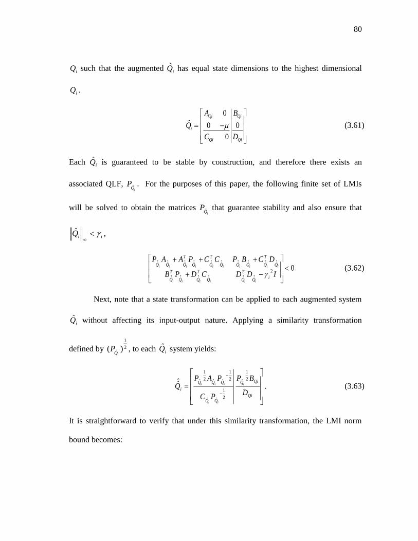
80

iQ such that the augmented iQ̂ has equal state dimensions to the highest dimensional

iQ .

0

ˆ 0 0

0

Qi Qi

i

Qi Qi

A B

Q

C D

(3.61)

Each iQ̂ is guaranteed to be stable by construction, and therefore there exists an

associated QLF, iQ

Pˆ . For the purposes of this paper, the following finite set of LMIs

will be solved to obtain the matrices iQ

Pˆ that guarantee stability and also ensure that

iiQ

ˆ ,

02

ˆ̂ˆ̂ˆ̂ˆ̂ˆ̂ˆ̂

ˆ̂ˆ̂ˆ̂ˆ̂ˆ̂ˆ̂ˆ̂ˆ̂ˆ̂ˆ̂

IDDCDPB

DCBPCCPAAP

iQ

T

QQ

T

QQ

T

Q

Q

T

QQQQ

T

QQ

T

QQQ

iiiiii

iiiiiiiiii

(3.62)

Next, note that a state transformation can be applied to each augmented system

iQ̂ without affecting its input-output nature. Applying a similarity transformation

defined by 2

1

ˆ )(iQ

P , to each iQ̂ system yields:

Qi

QiQ

QQ

QQQ

iD

BP

PC

PAPQ i

ii

iii

2

1

ˆ

2

1

ˆˆ

2

1

ˆˆ2

1

ˆˆ̂. (3.63)

It is straightforward to verify that under this similarity transformation, the LMI norm

bound becomes:

81

02

ˆ̂ˆˆ̂ˆˆ

ˆ̂ˆˆ̂ˆ̂ˆˆˆ̂

IDDCDB

DCBCCAA

iQ

T

QQ

T

Q

T

Q

Q

T

QQQ

T

Q

T

QQ

ii

iiii

. (3.64)

Thus the polytopic system formed by the transformed systems (Equation 3.65) is

guaranteed stable with CQLF IPQ )( , and with guaranteed norm bound

maxˆmax)(

iQQ .

i

i

i

i

Q

Q

Q

Q

D

B

C

ACoQ

ˆ̂

ˆ̂

ˆ̂

ˆ̂

)( . (3.65)

Note that the stability of the nonlinear closed loop does not depend on how the

state matrices of the particular iQˆ̂

are interpolated to form )(Q ; this offers an

additional element of design freedom. In general the weighting functions are designed

such that ]1 ,0[i and 1i , with the magnitude based on the relative distance to

the respective design point in the scheduling space (e.g. Figure 3.11).

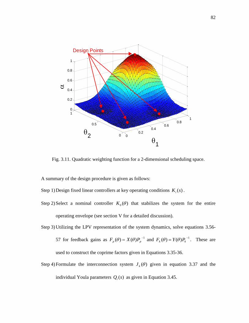
82

00.2

0.40.6

0.81

0

0.5

10

0.2

0.4

0.6

0.8

1

1

2

Design Points

Fig. 3.11. Quadratic weighting function for a 2-dimensional scheduling space.

A summary of the design procedure is given as follows:

Step 1) Design fixed linear controllers at key operating conditions )(sK i .

Step 2) Select a nominal controller )(0 K that stabilizes the system for the entire

operating envelope (see section V for a detailed discussion).

Step 3) Utilizing the LPV representation of the system dynamics, solve equations 3.56-

57 for feedback gains as 1

)()(

pp PXF and 1

)()(

kk PYF . These are

used to construct the coprime factors given in Equations 3.35-36.

Step 4) Formulate the interconnection system )(kJ given in equation 3.37 and the

individual Youla parameters )(sQi as given in Equation 3.45.

83

Step 5) As necessary, augment the states of the individual iQ systems as given in

Equation 3.61 to ensure equal state dimension among controllers.

Step 6) Use the LMIs given in Equation 3.62 to determine the state transformation

specified in Equation 3.63, and formulate the LPV representation of )(Q as in

Equation 3.65, and select the weighting functions )( f .

Step 7) The final controller is implemented as the interconnection of )(kJ and )(Q .

3.3.2.5 Application to Control of Switched Linear Systems

The capability of the proposed interpolation approach to guarantee closed loop

stability for arbitrarily fast changes in the scheduling variable leads naturally to

application of switched linear systems. If the transitions between critical operating

conditions occur infinitely fast (instantly), the LPV plant model can be represented by a

switched linear system using standard notation [52]:

uBxAx pppp ,,

pp xCy , (3.66)

where denotes the switching signal. Application of the techniques presented above

result in stable switching between controllers of arbitrary size/structure if there exists a

nominal control strategy ),(0 sK that stabilizes the switched system so that there exists

a common quadratic Lyapunov function

0,, PAPA T

PKPK (3.67)

84

where

,,,

,,,,,,

,

kpk

kppkpp

PK ACB

CBCDBAA (3.68)

If any such nominal stabilizing controller exists, then the above framework

allows local control strategies to be parameterized in terms of this nominal controller so

that the characteristics of the local controllers are recovered exactly, but the stability of

the closed loop system is guaranteed. This technique provides a promising alternative to

standard switched systems control methodologies such as dwell-time or switching

sequencing approaches [52].

3.4 Special-Cases: Choice of Nominal Controller

The approach outlined in the previous section provides a general method of

constructing a gain-scheduled controller for LPV system with local controller recovery.

Additionally, an interpolation approach is given that results in an LPV controller,

significantly reducing the large state dimensions resulting from simple controller

blending. However, a prerequisite to this design methodology is the existence of a

nominal controller )(0 K that stabilizes the plant for the entire range of operating

conditions. The synthesis of a single fixed controller that meets these conditions is the

well-known, and provably difficult, simultaneous stabilization problem, while the

synthesis of a stabilizing LPV controller relies on existing design methods available in

the literature. However, in practice, a far simpler method involves selecting one of the

fixed controllers and attempting to verify stability by determining an appropriate

85

common Lyapunov function. In this section, two specific choices for nominal controller

are discussed, where the approach for verifying stability is more formulaic and the state

dimensions of the final controller can be further reduced. These special cases result

when the nominal controller is selected as a state feedback/estimator controller or as a

simple static output feedback controller.

3.4.1 State Estimate/State Feedback Controller

A common choice when implementing Youla-based controller interpolation

schemes is to use state estimate/state feedback controllers. If the nominal controller is

selected as such, the result is similar to that presented in [88] where the authors use a

Youla based LPV controller and self-schedule the Q-parameter to optimize 2L -gain

performance. However, instead of focusing on LPV controller synthesis, we will

examine this choice of nominal control from the perspective of ensuring local controller

recovery.

Assuming a state estimate/feedback controller )(0 K of the form:

200 )()]()()()()([ zHxCHFBAx pkpppppk

0)( kp xFu (3.69)

where the state feedback and observer gains are calculated as 1)()( fp PXF and

)()( 1 WPH hp

, such that the following Linear Matrix Inequalities (LMIs) are satisfied:

0)()()()()()( T

p

T

p

T

pffp BXXBAPPA (3.70)

0)()()()()()( TT

ppphh

T

p WCCWAPPA (3.71)

86

As before, for polytopic LPV systems, these conditions can be written as a finite set of

LMIs, and a feasible solution to the LMIs is necessary to guarantee stability.

For controllers of this form, a doubly coprime factorization satisfying the Bezout

identities for the LPV plant and nominal LPV controller )(0 K can be constructed as:

0

0

( ) ( ) ( ) ( ) ( )( ) ( )

( ) ( ) ( )

( ) 0

p p p p p

p

p

A B F B HM U

F I IN V

C I

, and (3.72)

0 0

( ) ( ) ( ) ( ) ( )( ) ( )

( ) ( ) ( )

( ) 0

p p p p p

p

p

A H C B HV U

F I IN M

C I

. (3.73)

With only the state estimate/feedback controller, the resulting closed loop LPV system is

guaranteed to be quadratically stable by construction. But to recover the local controller

behavior at each operating condition, we define the coprime factors at the ith

operating

condition as given previously in Equation 3.43-44, and the individual Youla parameters

as:

0

0

0 0 0 0

( )( ) ( ) ( ) ( ) ( )[ ( ) ( )]

( ) ( ) ( )

( ) 0 0 ( ) ( ) ( )

( ) ( ) ( ) ( )

p i kip i p i ki p i p i ki p i k i ki p i

i ki p i ki ki p i

i i i

i k i k i k i

ki p i p i ki ki p i p i

B DA B D C B C B F D C

BU B C A B CQ V U

V A B F

D C F C D C F

( )

ki

p i

ki

H

D

(3.74)

The system )(kJ is constructed simply as:

1 1

0 0 0

1 1

0 0

( ) ( ) ( ) ( ) ( )( ) ( ) ( )

( ) 0 ( )( ) ( ) ( )

( ) 0

p p p p p

pk

p

A B F H BU V V

F IJV V N

C I

.

(3.75)

87

3.4.2 Static Output Feedback

Another technique for reducing the dimension of the interpolated controller is to

select the nominal controller to be as simple as possible namely static output feedback

control: )(),( 00 kDsK . Although many nonlinear systems can be stabilized by static

output feedback control (constant or scheduled with ), the synthesis problem of solving

Equation 3.76 is nonconvex in general. Thus for the purposes of the approach proposed

in this paper, the authors advocate selecting a static output feedback gain and verifying

stability in place of attempting to synthesize a stabilizing gain.

0)]()()()([)]()()()([ 00 pkpp

T

pkpp CDBAPPCDBA (3.76)

This choice of controller does in fact simplify the resulting interpolated controller.

Assuming this choice for the nominal stabilizing controller, the associated coprime

factorizations would be:

0

0

0

( ) ( ) ( ) ( ) 0( ) ( )

( ) ( )( ) ( )

( ) 0

p p p p

p k

p

A B F BM U

F I DN V

C I

(3.77)

0 0

0 00 0

( ) ( ) ( ) ( ) ( ) ( ) ( )( ) ( )

( ) ( ) ( ) ( )( ) ( )

( ) 0

p p k p p p k

p k p k

p

A B D C B B DV U

F D C I DN M

C I

(3.78)

Again, we define the coprime factors at the ith

operating condition as given previously in

equation 3.43-44, and the individual Youla parameters as:

0

0

0

0

( ) ( ) ( ) ( ) ( )[ ( )]( )

( ) ( )

( ) ( ) ( )

p i p i ki p i p i ki p i ki k i

i

ki p i kii i i ki

i

ki p i p i ki ki k i

A B D C B C B D DU

B C AQ V U BV

D C F C D D

(3.79)

88

The interconnection system is then given as:

1 1

0 0 00 01 1

0 0

( ) ( ) ( ) 0 ( )( ) ( ) ( )

( ) ( ) ( ) ( )( )( ) ( ) ( )

( ) 0

p p p p

p K p Kk

p

A B F BU V V

F D C D IJV V N

C I

(3.80)

To show the recovery of the controller iK at the ith

operating condition, the lower

fractional transformation of )(KJ and iQ is explored, while once again the notation

)(0 iU is dropped for the simpler iU ,0 :

iiiiiiiiiiKLFT VQNVIQVVUQJF ,0

1

,0

1

,0

1

,0

1

,0,0

~,

(3.81)

An equivalent expression is given by:

1

,0,0,0,0,

iiiiiiiiKLFT QNVQMUQJF (3.82)

By substituting the definition of the Youla parameters iQ , above equation is termed in:

1

,0,0,0,0,0,0,0,0

~~~~,

iKiiKiiiiKiiKiiiiiKLFT UVVUNVUVVUMUQJF (3.83)

and simplifying yields:

1

,0,0,0,0,0,0,0,0,0,0

~~~~,

iKiiiKiiiiKiiiKiiiiiKLFT UVNVUNVUVMVUMUQJF (3.84)

Using the Bezout identities, it can be replaced as:

1

,0,0,0,0,0,0,0,0,0,0

~~~~,

iiKiiiKiiiiKiiiKiiiiKLFT UNVVIMVVUNUIVMUUQJF

(3.85)

After collecting terms and simplifying, recovery of the a priori designed controller at

design point can be achieved as given by:

89

iKiKi

iiiiKiiiiiKiiiKLFT

KVU

UNVMVUNVMUQJF

1

1

,0,0,0,0,0,0,0,0

~~~~,

(3.86)

3.4.3 Gain-scheduled Control of a Quadruple Tank System

To demonstrate efficacy of the proposed gain-scheduling framework, a quadruple

tank system is selected as a simulated model. This system is a well known multivariable

control example and has been discussed in detail in [89]. A schematic diagram of the

quadruple tank system is shown in Figure 3.12. The two inputs to the system are the

input voltages to pumps 1 and 2, and two outputs of interest are the fluid levels in tanks

1 and 2. Two valves divide the flow from each of the pumps to the upper and lower

tanks. The upper tanks (tanks 3 and 4) drain into the lower tanks (tanks 1 and 2) which

drain into a reservoir. The cross flow from pump 1 to tank 4 and from pump 2 to tank 3

creates interesting dynamic phenomena.

This system can be modeled using mass balances and Bernoulli’s law. The

resulting nonlinear model is given in Equation 3.45 where A is the tank cross-sectional

area, a is the orifice cross-sectional area, h is the fluid level, u is the pump input with a

scalar gain uk . The valve parameters 1,0 determine the flow to each tank. The

selected outputs are the fluid levels of tanks 1 and 2 and are measured with a scalar gain

yk . The linearized version of this model is determined by Jacobian linearization given in

[89].

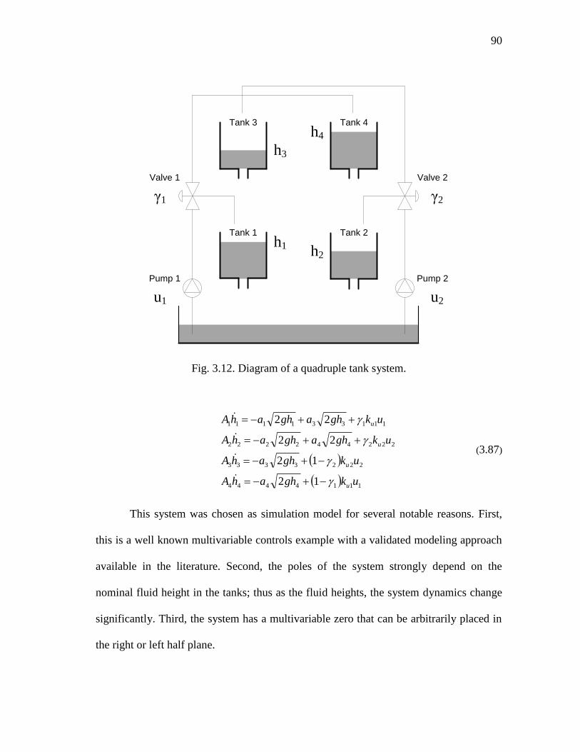
90

Tank 3 Tank 4

Tank 1 Tank 2

Pump 1 Pump 2

Valve 1 Valve 2

γ1 γ2

u1 u2

h3

h4

h1 h2

Fig. 3.12. Diagram of a quadruple tank system.

1114444

2223333

222442222

111331111

12

12

22

22

ukghahA

ukghahA

ukghaghahA

ukghaghahA

u

u

u

u

(3.87)

This system was chosen as simulation model for several notable reasons. First,

this is a well known multivariable controls example with a validated modeling approach

available in the literature. Second, the poles of the system strongly depend on the

nominal fluid height in the tanks; thus as the fluid heights, the system dynamics change

significantly. Third, the system has a multivariable zero that can be arbitrarily placed in

the right or left half plane.

91

For control design purposes, a quasi-LPV representation of the dynamics can be

constructed from the nonlinear model as shown in Equation 3.88, with equilibrium

defined by Equation 3.89:

2

1

3

2

2

1

4

2

1

1

4

3

2

1

44

4

33

3

42

4

22

2

31

3

11

1

4

3

2

1

0

)1(

0

)1(0

0

2000

02

00

20

20

02

02

u

u

A

k

A

k

A

k

A

k

h

h

h

h

h

g

A

a

h

g

A

a

h

g

A

a

h

g

A

a

h

g

A

a

h

g

A

a

h

h

h

h

u

u

u

u

(3.88)

0

22

0

11

11

22

210

2

0

1

2

2

1

1

)1(

1

gha

gha

ku

u

u

(3.89)

A slight variation of the parameter values published in [89] is used for the

simulations presented here. The values of tank and orifice areas, and input/output

scaling, depending on the units used, are given in Table 3.2. The gravity is given as 9.81

[m/s2], and the steady state values at the chosen operating conditions (both minimum and

non-minimum phase) are given in Table 3.3.

92

Table 3.2. Tank and orifice areas [m2] / Input/output Scaling

A1 2.8E-03 a1 7.1E-06

ku

V 3.33E-06

A2 3.2E-03 a2 5.7E-06 m3/s 1.0

A3 2.8E-03 a3 7.1E-06

ky

m 1.0

A4 3.2E-03 a4 5.7E-06 Pa 9.81E+03

Table 3.3. Operating condition (minimum phase, non-minimum phase)

h10 (0.12, 0.12) [m] u1

0 (2.44, 3.80) [V]

h20 (0.12, 0.12) [m] u2

0 (3.80, 2.44) [V]

h30 (0.081, 0.037) [m]

1 (0.7, 0.4) [-]

h40 (0.052, 0.014) [m]

2 (0.6, 0.3) [-]

The valve parameters 1 and 2 determine the flow ratio of lower to upper tank.

Low values of signify a significant amount of cross-flow, thus resulting in non-

minimum phase behavior. In this case a multivariable right half plane zero will be

present when 121 as depicted in Figure 3.13.

93

0.25 0.75

0.25

0.75

1.00

1.00

γ2

γ1

Minimum Phase

Operating Condition

Non-Minimum Phase

Operating Condition

Fig. 3.13. Controller design points in minimum and nonminimum phase region.

For this example, 1 and 2 are selected as the scheduling variables. External

changes to these variables will change the underlying system dynamics, as well as a

disturbance to the closed loop system attempting to regulate the fluid height of the lower

tanks. Two operating points in a quasi-LPV model [2] are selected: one in the minimum

phase region and the other in the nonminimum phase region, depicted in Figure 3.13. As

advocated in [43], a decoupled PID controller is designed for the minimum phase

condition. A static decoupling matrix )0()( 1GsW is used and PID controllers are

designed (Equation 3.90-91). Similarly, a set of PI controllers is designed at the

minimum-phase phase operating point as given in Equation 3.92:

94

ss

sssKPID

028.0029.0

29.10

0019.0042.0

26.1)( (3.90)

50204.027032.0

28962.054064.0)(sW (3.91)

s

ssK PI 029.029.10

0042.0

26.1)( (3.92)

For the nonminimum phase operating point, [87] suggests the use of an H

controller [90]. Using standard design and model reduction procedures, a 4th

order H

controller is designed as given in Equation 3.93. These controllers are not necessarily

selected for optimal performance, but to demonstrate the full capabilities of the proposed

interpolation approach. Not only do the two controllers have different state dimensions,

but they are designed for fundamentally different plant dynamics. The PI and PID

controller has pure integrators that prevent the controller from being strictly stable.

95

Fig. 3.14. Step response of PID controlled system at minimum phase design point.

Fig. 3.15. Step response of H controlled system at minimum phase design point.

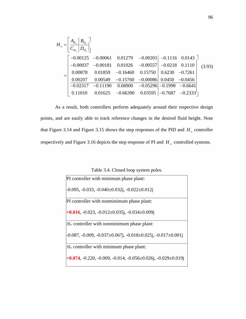
96

0.00125 0.00061 0.01279 0.00201

0.00037 0.00181 0.01026 0.00557

0.00878 0.01859 0.16460 0.15750

0.00207 0.00549 0.15760 0.00086

0.02317 0.11190 0.68900 0.05296

0.11010 0.01625 0.66390 0.

H H

H H

A BH

C D

0.1116 0.0143

0.0218 0.1110

0.6230 0.7261

0.0450 0.0456

0.1998 0.6641

03595 0.7687 0.2333

(3.93)

As a result, both controllers perform adequately around their respective design

points, and are easily able to track reference changes in the desired fluid height. Note

that Figure 3.14 and Figure 3.15 shows the step responses of the PID and H controller

respectively and Figure 3.16 depicts the step response of PI and H controlled systems.

Table 3.4. Closed loop system poles.

PI controller with minimum phase plant:

-0.095, -0.033, -0.040±0.032j, -0.022±0.012j

PI controller with nonminimum phase plant:

+0.016, -0.023, -0.012±0.035j, -0.034±0.009j

H∞ controller with nonminimum phase plant:

-0.087, -0.009, -0.037±0.067j, -0.018±0.025j, -0.017±0.001j

H∞ controller with minimum phase plant:

+0.074, -0.220, -0.009, -0.014, -0.056±0.026j, -0.029±0.019j

97

Fig. 3.16. Step response of PI and H controlled systems at design points.

Although the step response of the H controlled system displays significant

undershoot, this is an expected strong non-minimum phase nature of the plant. However,

these controllers are not effective at controlling the system at off-design conditions, and

in fact are destabilizing. Figure 3.17 (a) and (b) show this destabilizing effectively and

Table 3.4 gives the closed loop poles for the four possible combinations of

plant/controller.

98

Fig. 3.17. Fluid heights in lower tank 1 and tank 2 (log scale).

99

A principal advantage of the LQN framework for controller interpolation is

ability to interpolate controllers of different dimensions and structure or open-loop

unstable controllers. As described in previous sections, a nominal LPV observer-based

controller is designed for the system, and Q parameters are calculated so that the original

MIMO-PI and H∞ controller are recovered near the design point, blended by the

exponential weighting function. The resulting controller is evaluated in simulation as

applied to the nonlinear system dynamics. The interpolated controller retains the abilities

of the local controller designs, and is capable of rejecting disturbances and regulating the

lower tank fluid heights to the desired levels at both nonminimum phase and minimum

phase conditions.

For example, Figure 3.18 shows the closed loop system response to instantaneous

disturbances applied to individual tank fluid heights. More importantly, the interpolated

controller can transition smoothly and stably from one design point to another. Figure

3.19 shows the system response to rapid changes in and , which both induce

disturbances on the system and change the underlying system dynamics from minimum

phase to nonminimum phase. As the scheduling variables change, the exponential

weighting factors allow smooth transitioning between the two Q functions. The control

input voltages remain within reasonable bounds and fluid heights in the two lower tanks

are effectively regulated.

100

Fig. 3.18. Disturbance rejection at design conditions.

101

Fig. 3.19. Tracking during transition between operating conditions.

102

4. ROBUST STABILITY OF GAIN SCHEDULED CONTROL SYSTEM

When LPV plant models include uncertainty in scheduling variables or modeling

error in plant model and these factors affect the system dynamics significantly, the plant

model may not reflect the nonlinear system precisely and the associated conventional

stability analyses may not be sufficient to guarantee the stability of nonlinear system in

practice [3].

In this section, we extend the stability analysis in Section 3 to robustness and

performance, focusing the guarantees of robust stability when the LPV plant model is

assumed to include the modeling errors. A proposed framework can guarantee a global

level of the stability of the perturbed nonlinear system by minimizing the 2L gain that

remained within desired bounds over the operating envelope.

4.1 Uncertain System Modeling

4.1.1 Uncertainty Description

An uncertain system is often defined as a system that does not have a completely

accurate representation of a real system although the modeling difference between

system representation and real system may exist in practice. There are several ways in

which systems will be considered to be uncertain [3]:

The local controllers may be of different state dimensions and possibly open-loop

unstable. Research achievements include:

103

System’s external inputs, e.g., exogenous disturbances, significantly affect the

behaviors of the system, but separation between system and environment

cannot be implemented

Uncertainty in the accuracy of a system model itself is a central source when

dynamic model of the system will neglect some physical phenomena. Any

control method using this model will neglect some operating regimes and result

in the failure of the controlled system

Note that any of these factors may result in uncertainty significantly included in the

system. In any case, the control objective is to minimize the effects of unknown initial

conditions and external influences on the behavior of the system, subject to the lack of a

suitable system representation.

Among those uncertainty descriptions, the third definition of uncertain system is

quite attractive in the gain-scheduling paradigm since the plant model used in gain-

scheduling strategies virtually alleviates the requirement of exact structure or

mathematical model. However, it may cause the failure of the desired stability or

performance of the system when the plant model cannot reflect real dynamics of the

system precisely at certain operating points. Thus an uncertainty consideration could be

useful to achieve the desired stability and performance of the real systems in practice.

Several uncertainty modeling methods have been proposed in the literature but

mainly categorized into two classes: 1) Parametric uncertainty and 2)

neglected/unmodelled dynamics uncertainty [3]. The former is based on the structure of

the model that is known but some of the parameters are uncertain. This class of

104

uncertainty is often called structured uncertainty since it models the uncertainty in a

structured manner. In contrast, the latter appears when the model is in error because of

missing dynamics, usually at high frequencies, either through deliberate neglect or

because of a lack of understanding of the physical process. Note that any plant model

will possibly contain this source of uncertainty [3].

Parametric uncertainty is often avoided in that it usually requires large efforts to

real perturbations which are more difficult to deal with numerically, especially when it

comes to controller synthesis. Thus unstructured modeling uncertainty will preferably be

considered for the robust stability analysis demonstrated in this dissertation. This class of

uncertainty can be addressed when one chooses to work with a simple nominal model

which represents neglected dynamics as uncertainty which is unstructured.

Among uncertainty representations, additive and multiplicative uncertainty

representations are most commonly used, denoted in Equation 4.18-9, respectively, and

also depicted in Figure 4.1 where G is plant model, W is weighting function, and is

unstructured modeling uncertainty [3].

Additive uncertainty:

,1)( );()()()( A jssWsGsG AAp (4.18)

Multiplicative uncertainty:

,1)( ));()(1)(()( I jssWsGsG IIp (4.19)

105

Fig. 4.1. Uncertainty representations:

(a) additive uncertainty (b) multiplicative input uncertainty

4.1.2 General Uncertain System Representation

Consider a feedback control system with input uncertainty as depicted in Figure

4.2 where I is input multiplicative uncertainty, IW is a normalized weight for I , and

PW is performance weight. This feedback loop can be converted into a standard closed

loop system with a generalized plant P to allow more flexibility in analysis, depicted in

Figure 4.3 [3].

Fig. 4.2. Closed loop configuration of uncertain system.

106

Fig. 4.3. General configuration of uncertain system for controller synthesis.

A suitable representation of generalized plant P can be sought based on the

subsystems appearing in Figure 4.3. The closed loop from uwu to vzy in

Figure 4.3 is determined by:

u

w

u

GIG

GWWGW

W

u

w

u

P

v

z

y

PPP

I00

(4.20)

where u is uncertainty output, y is uncertainty input, w is disturbance input

(exogenous input), z is performance output, u is control output, and v is control input.

As shown in Equation 4.20, transfer function from u to y , upper left elements in P ,

107

is zero since u has no direct effect on y except through a controller K . Thus

partitioning P to be compatible with K can be simply implemented by:

uPw

uPvuP

w

uP

z

y22211211 ,

(4.21)

G ,

,00

2221

1211

PIGP

GW

WP

WGWP

P

I

PP (4.22)

Then the uncertain system representation, called “ N structure,” is constructed in

which N is an interconnected system between a generalized plant P and a controller

K ; Linear Fractional Transformation (LFT) effectively shows this interconnection [76].

Using the system configuration in Figure 4.4, N is simply modified by a lower LFT of

P and K [3]:

21

1

221211 )(),( PKPIKPPKPFN l

(4.23)

Similarly, the closed loop transfer function from w to z is related to N and

by upper LFT:

12

1

112122 )(),( NNINNNFF u

(4.24)

By pulling out the perturbation block and nominal system, the system in Figure 4.4 is

rearranged by “ M structure” of Figure 4.5 where 11NM is the transfer function

from the output to the input of the perturbation block . Under this framework, the

reader can easily focus on the input-to-output properties of the perturbed system for the

robust stability.

108

Fig. 4.4. N system.

Fig. 4.5. M system.

When the state matrix of the system is formed in block-diagonal by a particular state

transformation, the stability of the resulting system is guaranteed where preliminary

condition, 1

, is satisfied. This particular state transformation that ensures block-

diagonal system matrix will be demonstrated later in this section.

109

Furthermore, state space models of each component of the system will be sought

for the stability analysis gain-scheduled control framework. The associating state space

model of individual components can be derived by:

Controller K :

vDxCu

vBxAx

kkk

kkkk

(4.25)

Plant G :

pp

pppp

xCy

uuBxAx

)( (4.26)

Input uncertainty weight function IW :

II

IIII

WW

WWWW

xCy

uBxAx

(4.27)

Performance weight function PW :

PP

PPPP

WW

WWWW

xCz

vBxAx

(4.28)

Based on these state space models, the M system is derived following state

space representation from Twu to Tzy where subscripts of the system matrices

Iwpk , , are controller, plant, and weight on input uncertainty, respectively. Note that the

state matrix of this system is given by a block-diagonal structure constructed by system

matrices of controller, plant, and input weight.

110

IM

I

M

II

M

IIII

W

P

K

C

W

B

KW

KPP

K

W

P

K

A

WPKWKW

PKPPKP

PKK

W

P

K

x

x

xC

z

y

w

u

DB

DBB

B

x

x

x

ACDBCB

CDBACB

CBA

x

x

x

000

00

0

0

0

0

(4.29)

4.2 Robust Stability Analysis

4.2.1 Robust Stability Description

Before discussing robust stability of the uncertain system, addressing the

background of the robust stability and performance could be helpful in understanding the

key ideas of this section.

Definition 4.1) [3]

Robust stability analysis: Determines whether the system remains stable for all plants in

uncertainty set with a given controller K .

Robust performance analysis: If robust stability is satisfied, determines how large the

transfer function from exogenous inputs to outputs may be for all plants in the

uncertainty set.

111

For the N system, sufficient conditions for guarantees of the stability and

performance can be summarized using Definition 4.1 as follows:

Definition 4.2) [3]

Nominal stability: N is internally stable

Nominal performance: 122

N with satisfying nominal stability

Robust stability: ),( NFF u in Equation 4.24 is stable 1,

with satisfying

nominal stability

Robust performance: ,1

F 1,

with satisfying robust stability

The primary interest of this section is to guarantee the stability of the perturbed

system, thus recall the general system configuration for robust stability analysis that is

prepared in Section 4.1. Consider the N system for which the transfer function from

w to z is given by

12

1

112122 )(),( NNINNNFF u

(4.30)

Supposing that system N is nominally stable and is also assumed to be stable, one

can directly see the only possible source of instability is the feedback term 1

11 )( NI .

Thus when nominal stability is guaranteed, the stability of the N system would be

equivalent to the stability of the M system in Figure 4.5 where 11NM .

Seeking the direct method to evaluate stability of the M system uses

Nyquist stability theorem as follows [3]:

112

Theorem 4.1) Determinant stability condition for perturbations [3]

Supposing that the nominal system )(sM and the perturbations )(s are stable and

considering the convex set of perturbations , then the M system is stable for all

allowed perturbations if and only if

- Nyquist plot of ))(det( sMI does not encircle the origin , (4.31)

0))(det( sMI , ,w (4.32)

Proof:

The statement in Equation (4.31) is simply a generalized Nyquist theorem applied to a

positive feedback system with a stable loop transfer function )(sM as the generalized

Nyquist theorem is given in Lemma 4.1 [3]:

Lemma 4.1)

The closed loop system with loop transfer function )(sL and negative feedback are

stable if, and only if, the Nyquist plot of ))(det( sLI makes і) n anti-clockwise

encirclements of the origin and іі) does not pass through the origin.

Also, a sufficiency of the statement in Equation (4.31) to the form in Equation

(4.32) can be proved by statement 2) in Lemma 4.1, “no encirclement of the origin”. For

113

the necessity, please see Theorem 8.1 in [3]. Using the spectral radius definition, the

equivalent theorem will be prepared as follows:

Theorem 4.2) Spectral radius condition for perturbations [3]

Suppose that nominal system )(sM and perturbations )(s are stable. Considering the

convex set of perturbations , then the M system is stable for all allowed

perturbations if, and only if,

,1))(( jwM , ,w

,1))((max

jwM w (4.32)

where ( ) is spectral radius, the largest of absolute eigenvalues of system ( ),

)(max)( ii .

Proof: See [44] (simply proved by the definition of spectral radius)

Now, considering the special case where the perturbation block )(s is allowed

to be any full complex transfer function matrix satisfying 1

which is often

referred to as unstructured uncertainty. To get a final form of stability theorem, the

mathematical relationship between spectral radius ( ) and eigenvalues ( ) of the

system is modified and holds [3]:

)()()(max)(max)(max MMMM

(4.33)

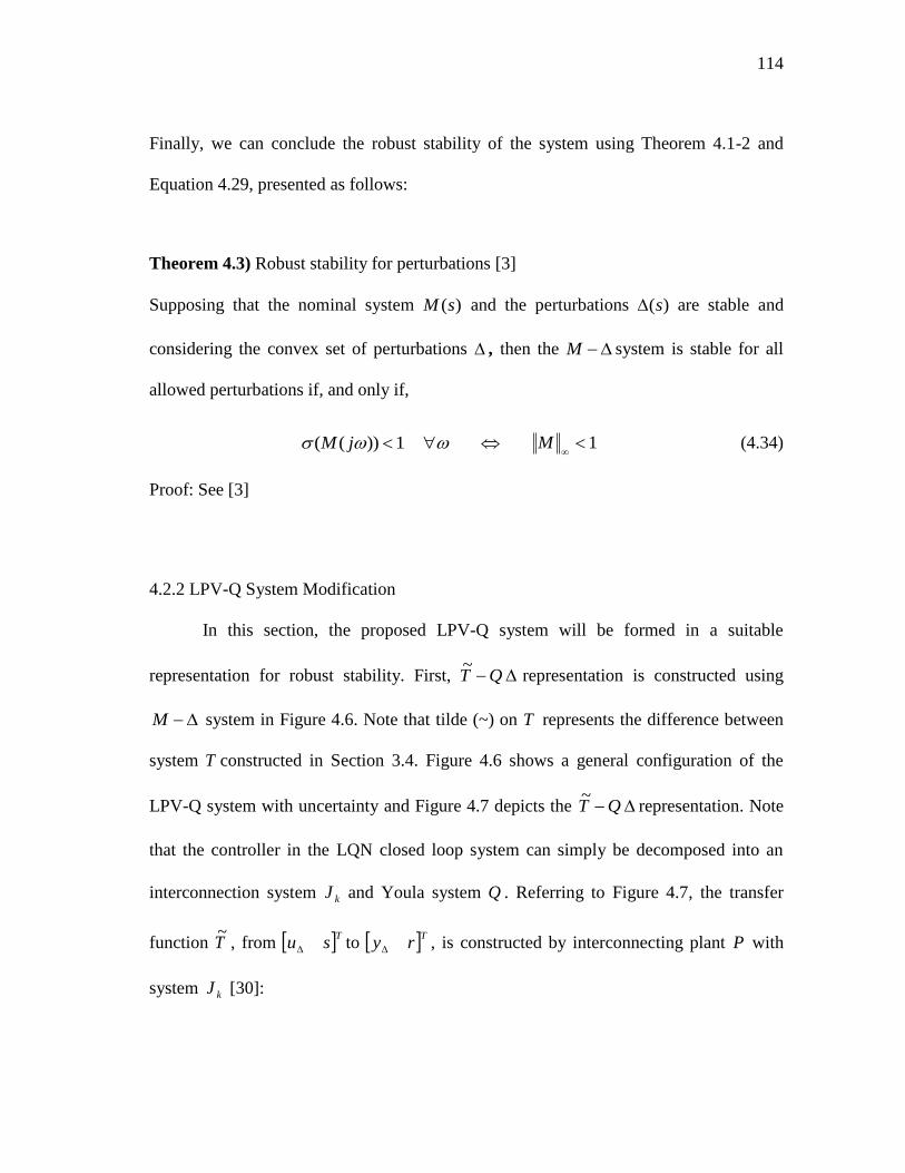
114

Finally, we can conclude the robust stability of the system using Theorem 4.1-2 and

Equation 4.29, presented as follows:

Theorem 4.3) Robust stability for perturbations [3]

Supposing that the nominal system )(sM and the perturbations )(s are stable and

considering the convex set of perturbations , then the M system is stable for all

allowed perturbations if, and only if,

1))(( jM 1

M (4.34)

Proof: See [3]

4.2.2 LPV-Q System Modification

In this section, the proposed LPV-Q system will be formed in a suitable

representation for robust stability. First, ~

QT representation is constructed using

M system in Figure 4.6. Note that tilde (~) on T represents the difference between

system T constructed in Section 3.4. Figure 4.6 shows a general configuration of the

LPV-Q system with uncertainty and Figure 4.7 depicts the ~

QT representation. Note

that the controller in the LQN closed loop system can simply be decomposed into an

interconnection system kJ and Youla system Q . Referring to Figure 4.7, the transfer

function T~

, from Tsu to Try , is constructed by interconnecting plant P with

system kJ [30]:

115

Fig. 4.6. Closed loop of perturbed system for all stabilizing controllers.

Fig. 4.7. ~

QT system.

116

u

u

GP

PP

u

u

PP

PP

y

y

21

1211

2221

1211 (4.35)

Qrs

s

y

NVV

VK

s

y

JJ

JJ

r

u

KK

KK

11

1

22,21,

12,11,

~

(4.36)

Then the variable u and y can be eliminated using the coprime factorization of

the plant NMG~~ 1 and controller UVK

~~ 1 . The useful coprime factorization of

interconnected system that simplifies the system representation can be derived using the

double Bezout identities given by [30]:

VMNMUVIPJI~

)~~

()( 1111

2211 (4.37)

Using Equation 4.37, the resulting state space representation of system T~

can be derived

as [30]:

11 12 11 12 21 12

21 22 21 0

y u uT T P P UMP P M

r s sT T MP

(4.38)

In Equation 4.38, 22

~T is always zero under any choice of plant and controller

representation. Using this result, the closed loop transfer function from u to y is

given by:

uTQTTuFy Q )~~~

( 211211 (4.39)

117

Note that this closed loop representation allows the convex optimization of Q by

minimizing disturbance responses where T~

, Q , and QF are Hurwitz. Also, the affine

characteristic of the QF system in Youla parameter Q enables feasibility in computation.

4.2.3 LPV-Q Closed Loop System

The reader knows that the transfer function QF could be a direct indicator of

robust stability of the closed loop system. In the LPV-Q system, transfer function QF is

determined by plugging general coprime factors of subsystems, kJ , Q , and T~

(Equation 4.40.-44) that can be defined using Youla parameterization into QF .

( ) ( ) ( ) 0 ( )

( ) ( ) ( ) ( )( )

( ) 0

p p p p

p K p KK

p

A B F B

F D C D IJ

C I

(4.40)

( ) ( ) ( ) ( ) ( ) ( ) ( ) ( ) 0

( ) ( ) ( ) ( ) ( ) ( )( )

0 0 ( ) ( ) ( ) ( )

( ) ( ) ( ) ( ) ( ) 0

P i P i K i P i P i K i P i K i

K i P i K i K i K i K i

i

K i K i K i K i

K i P i P i K i K i

A B D C B C B C

B C A B F BQ

A B F B

D C F C C

(4.41)

118

11 11 12 21( ) ( ) ( ) ( )

( ) ( ) ( ) ( ) ( ) ( ) ( ) ( )

0 ( ) ( ) ( ) ( ) ( ) ( ) ( ) ( )

0 ( ) ( ) ( ) ( )

( ) ( ) ( ) 0

k k k k p k k k

p p k p p k p k

k p k k

k p k

T P P UMP

A B F B C B F B

A B D C B C B D

B C A B

F C F

(4.42)

12 12

( ) ( ) ( ) ( )

( )( ) ( ) ( )

( ) 0

p p p p

p

p

A B F B

F IT P M

C

(4.43)

21 21( ) ( ) ( )

( ) ( ) ( ) ( ) ( ) ( ) ( ) ( ) ( )

( ) ( ) ( ) 0 ( )

( ) ( ) 0

p p k p p k p p k

k p k k

p k

T M P

A B D C B C B B D

B C A B

C F I

(4.44)

For nominal controller, a doubly coprime factorization satisfying the Bezout identities

for the LPV plant and static output feedback LPV controller )(0 K can be constructed

as:

0

0

0

( ) ( ) ( ) ( ) 0( ) ( )

( ) ( )( ) ( )

( ) 0

p p p p

p k

p

A B F BM U

F I DN V

C I

(4.45)

0 0

0 00 0

( ) ( ) ( ) ( ) ( ) ( ) ( )( ) ( )

( ) ( ) ( ) ( )( ) ( )

( ) 0

p p k p p p k

p k p k

p

A B D C B B DV U

F D C I DN M

C I

(4.46)

119

4.3 Robust Stability of LPV-Q System

4.3.1 LMI-Based Robust Stability

Theorem 4.3 describes a necessary and sufficient condition so that the nonlinear

system is robustly stable. This is a well-known criterion that evaluates the closed loop

stability of the system according to the H performance of a given system in that it

requires a less conservative assumption and enables simple analysis [91] [92]. Consider

the ~

QT structure of the proposed LPV-Q system. By applying the theorem 4.3 to the

~

QT system, a revised version of necessary and sufficient condition for the robust

stability of the LPV-Q system is given by Theorem 4.4.

Theorem 4.4) Robust stability of perturbed systems [63]

Suppose that the system )(~

sT and the perturbations )(s are stable with stable )(sQ .

Let be convex set of perturbations, then the LPV/LQN system is guaranteed to be

robustly stable for all perturbations satisfying 1

if, and only if,

1QF (4.47)

Proof: See [63]

120

It is interesting to note that the closed loop transfer function )~~~

( 211211 TQTTFQ

is affine in Youla system Q that allows the convex optimization in performance

evaluation. Often norm-based performance of the system is calculated using Linear

Matrix Inequality (LMI) techniques that alleviate the complexity in computation [74].

The LMI form of the H performance and its Schur complement of the closed loop

system are given as:

01

2 PBPBCCPAPA

T

FFF

T

FF

T

F QQQQQQ (4.48)

02

IPB

PBCCPAPAT

F

FF

T

FF

T

F

Q

QQQQQ

(4.49)

Note that the Schur complement has been widely used in analytical studies because of

computational flexibility. The alternative formula adapted to LMI toolbox in Matlab is

given by [93]:

0

0

0

0

1000

000

000

000

0

0

0

Q

QQ

Q

QQ

F

FF

T

F

FF

C

I

BA

I

I

I

P

P

C

I

BA

I

(4.50)

In the gain-scheduling paradigm, the desired level of stability is easily

guaranteed at local operating points, but guarantees of the stability over the entire

operating envelop is much more difficult to achieve. However, even though the

quadratic Lyapunov function P can be found at each local operating point so that the

H norm, i.e., 2L gain, of the system remains within a desired bound, finding a

121

common quadratic Lyapunov function (CQLF) to guarantee global stability is still a

challenging problem [93].

4.3.2 Robust Stability via Optimizing Coprime Factors

In Section 4.3.1, we know that robust stability of the system is globally

guaranteed by the existence of CQLF so that the 2L gain of the system remains within a

desired bound over operating envelopes. To guarantee the global stability of the LPV-Q

system, consider ~

QT representative of the system and find the degree of freedom

included in the closed loop transfer function QF . The subsystems 11

~T , 12

~T , and 21

~T

consist of system matrices and associating feedback gains of plant and controller so that

PPP FBA and KKK FBA are Hurwitz (Equation 4.41-44). It is interestingly note that

11

~T and 21

~T merely include the feedback gain of controller kF and 12

~T includes the

feedback gain of plant, pF .

By virtue of gain-scheduling, the choice of feedback gains of plant and controller

would be an additional freedom where they merely meet the restriction so that the state

matrices of the state feedback system are Hurwitz. Also, the reader can find the

particular relationships between those feedback gains and subsystem matrices by

carefully noting that subsystems 11T and 21T include only PF while KF merely appears

in 12T . Thus finding the optimal subsystem is implemented through optimizing feedback

gains in sub systems that minimize the H norm to guarantee global stability and

performance. Alternatively, guaranteeing the closed loop stability of the system is

122

achieved through retaining the H norm globally within specific bounds and also

minimizing the difference between 2L gains calculated locally and globally.

4.3.3 Case Study: Robust Stability on Gain Scheduled Control System

In Section 4.3.2, we know that robust stability of the LPV-Q system is globally

guaranteed by the optimal choices of coprime factors of Youla system. In essence,

choice of coprime factors is design degree of freedom but significantly affects stability

and performance of the system as illustrated in Section 3.2. This section illustrates a

simple example of robust stability of the Youla based gain-scheduled control system.

To find the optimal feedback gains of plant model and controller PF and KF , we

employ the LQR technique. By virtue of state feedback control, LQR control provides

optimal gain matrices PF and KF by minimizing cost function included Q and R thus

choice of these weighting matrices would be an additional freedom where they merely

are positive-definite.

Equations 4.51-52 present state-space forms of LPV plant model at controller

design points and state-space forms of two LQR controllers with integrators are given in

Equations 4.53-54, respectively. Note that plant models are defined as LPV way,

( ) at = , 1,2i iP P i , so that each plant model shares the states.

xy

uxx

10

01

0316.00129.0

0171.00275.0

2134.01520.0

1055.02499.0

(4.51)

123

xy

uxx

10

01

0192.00030.0

0050.00194.0

1246.00979.0

0274.01815.0

(4.52)

0 0 1 0

0 0 0 1

0.9942 0.1077 6.592 0.4746

0.1077 0.9942 0.4195 6.223

x x u

y x u

(4.53)

0 0 1 0

0 0 0 1

0.9924 0.1229 6.539 1.502

0.1229 0.9924 0.5627 8.565

x x u

y x u

(4.54)

Table 4.1 Performance bounds on LPV-Q system.

2 2

Q L LF s

1Fixed at 0.6029

2Fixed at 0.4799

( )LPV 0.6032

Table 4.1 indicates H performance bounds on LPV-Q closed loop system. First,

we examine the performance bounds of LPV-Q system at controller design points.

Before optimizing coprime factors, we initially guessed reasonable values of Q and R

matrices in LQR control design.

10

01 and

10

01,, PKPK RQ (4.55)

124

Then we optimized coprime factors such that H norm of the system is minimized.

As given in Table 4.1, LPV-Q closed loop system is robustly stable at design

points since H norm of the system is less than one where 1

satisfies.

Furthermore, the reader can recognize that H norm of the system remains within

acceptable bounds over operating envelope. Thus we can conclude that LPV-Q system is

guaranteed to be robustly stable with optimal choice of coprime factors. Note that norm

bound using initially guessed values is 2.5743 which remains out of desired bound.

125

5. MULTI EVAPORATOR VAPOR COMPRESSION SYSTEM CONTROL

Gain-scheduled control is known to be a powerful solution for nonlinear systems

that are highly nonlinear and vary arbitrarily fast in a wide range of operating regions. In

this section, the efficacy of the proposed controller interpolation method is demonstrated

in experimentation using a multi-evaporator vapor compression system. The dynamics of

the vapor compression system are highly nonlinear but gain-scheduled control has the

potential to achieve the desired stability and performance of the system. Clearly, this

section demonstrates the experimental study of gain-scheduled control as applied to a

multi-evaporator vapor compression system, while the thermal efficiency and cooling

capacity of the system are subsequently improving.

5.1 Introduction

Vapor compression systems have been widely used for various residential and

industrial purposes. A huge amount of energy is consumed for air conditioning,

becoming one of the largest sources of energy consumption in the world [70]. Thus the

thermal efficiency of these systems is a key aspect in energy saving since the energy

demand for air conditioning systems will be reduced by achieving desired energy

efficiency of vapor compression systems, via developing accurate system model and

advanced control strategies. Energy saving air conditioning systems have significant

effects on the economy as well as the environment. This situation has been widely

studied for many years [71].

126

Unfortunately, the dynamics of this system are known to be highly nonlinear and

also vary arbitrarily fast over the operating envelopes. Although a very strictly designed

controller could possibly stabilize the system, significant performance would be

sacrificed. To guarantee desired global stability, an advanced gain-scheduled control

approach can be an intuitive solution for this problem [5].

In this section, the proposed gain-scheduled control strategy will be applied to a

vapor compression system to achieve the desired energy efficiency. The efficacy of the

proposed controller interpolation method will be demonstrated in experimental studies

on multi-evaporator vapor compression system.

5.2 Vapor Compression Cycle

To build an advanced control framework for vapor compression systems, an in-

depth understanding of the characteristics of these systems would be helpful. Consider a

standard air conditioning system operating on a vapor compression cycle. As shown in

Figure 5.1, a standard vapor compression system consists of four components -

compressor, condenser, expansion device, and evaporator [72]. Assume that refrigerant

steadily circulates through each of components in the cycle. First, the refrigerant enters

the evaporator as a two-phase liquid-vapor mixture at a lower pressure. In the evaporator,

some of the refrigerant changes phase from liquid to vapor as a result of heat transfer

from the region of low temperature to the refrigerant then exits as a superheated vapor at

a lower pressure.

127

Evaporator

Condenser

Oil

Sepera

tor

Compressor

Filter/Dryer

Valve

Evaporator Fan

Oil

Retu

rn L

ine

Condenser Fan

Receiver

Fig. 5.1. Vapor compression system.

Then the refrigerant is compressed to a high pressure by the compressor. During

compression, the temperature of the refrigerant goes up to a temperature that is higher

than ambient temperature. Next, the refrigerant passes from the compressor into the

condenser where it changes phase from a saturated vapor to a saturated liquid as a result

of the heat transfer to a region of high temperature and, then exits the condenser as a

subcooled liquid at a higher pressure. However, the refrigerant at a two-phase flow may

result in a choked flow problem thus a receiver is placed at the exit of condenser to avoid

the two-phase refrigerant [72].

The refrigerant returns to the inlet of the evaporator by expanding through the

expansion device. In this process, the temperature goes down from a high to low

temperature and there is a drop in pressure. The hP diagram of each of the vapor

compression processes is shown in Figure 5.2.

128

Fig. 5.2. hP diagram of vapor compression cycle.

The characteristics of vapor compression systems are affected by the

thermodynamic states of refrigerant at various components in the vapor compression

cycle such as evaporator pressure, condenser pressure, and evaporator superheat

temperature. To evaluate the system’s efficiency, key thermodynamic properties, i.e.,

cooling capacity (refrigerant capacity) and coefficient of performance (COP), are

commonly used. The former is modulated as a desired cooling requirement while the

latter is regulated to be maximized for energy saving [94], [95].

Cooling capacity is defined as the amount of heat transferred from the refrigerant

region resulting in the vaporization of the refrigerant [72]. As refrigerant passes through

the evaporator, the mass and energy balance are reduced to give the heat transfer rate per

unit mass of refrigerant flow where m is the mass flow rate of the refrigerant, and 4h

129

and 1h are the enthalpy at evaporator inlet and outlet, respectively. In Equation 5.1, heat

transfer rate inQ refers to cooling capacity, normally expressed in kW.

41 hhm

Qin

(5.1)

Cooling efficiency or COP indicates the efficiency of the vapor compression system. For

the Carnot system, COP is simply given as:

lowhigh

lowC

TT

TCOP

(5.2)

However, the Carnot vapor compression cycle is an ideal thermodynamic cycle,

generated under conservative theoretical assumptions and cannot be realized in real

systems. Thus the COP of the real vapor compression system at steady-state can be

presented as [72]:

12

41

hh

hhCOPR

(5.3)

Note that the enthalpy at the evaporator outlet plays a significant role in cooling capacity.

The COP of real systems and maximum thermal efficiency can be achieved via minimal

evaporator superheat, i.e., maximizing the two-phase region of the evaporator, since heat

transferred from the cold temperature region to liquid refrigerant is much higher than

when transferred to vapor refrigerant. However, liquid refrigerant may result in the

failure of the compressor, thus improving the cooling capacity. The COP of the vapor

compression system should be achieved by optimal choice of evaporator superheat

temperature.

130

Four components of the vapor compression system can be categorized into two

classes – heat exchanger and actuator. The evaporator and condenser function as heat

exchangers in that they add (remove) heat from (to) the ambient region, respectively,

while the compressor and expansion valves function as actuators. In heat exchangers,

heat is removed from the refrigerant as it flows at a constant pressure through the

condenser and heat is transferred into the refrigerant as it flows at constant pressure

through the evaporator. The two principle actuators, expansion valve and compressor,

modulate the mass flow rate of the system at each state. The change of mass flow rate

results in the change of operating pressures and the resulting two-phase and superheat

region in heat exchangers that directly affect the cooling of the system. Among various

expansion devices, an electronic expansion valve (EEV) has been widely used since a

stepping motor is used to open or close the valve by control action that can be directly

applied to voltage signal of motor [96], [97].

Multi-evaporator vapor compression systems whose evaporators serve different

cooling zone, has been used in this dissertation, depicted in Figure 5.3, and hP

diagram of the system is presented in Figure 5.4. Typically, a static discharge valve

(SDR) is installed on the secondary evaporator to regulate a pressure difference between

evaporators; thus each evaporator provides individually cooling under different

operating conditions [71]. More details on this strategy will be addressed later in Section

5.4.

131

Fig. 5.3. Multi-evpaorator vapor compression system.

Fig. 5.4. hP diagram of two-evaporator vapor compression system.

132

5.3 Vapor Compression System Control

5.3.1 Experimental Vapor Compression System

The experimental vapor compression system for the research presented in this

dissertation is two-evaporator water chiller system. This system has been built in

Thermo-Fluids Control Laboratory for research of model validation, control design, and

fault detection. The primary (refrigerant) system consists of four components of vapor

compression system – compressor, condenser, expansion valve, and two evaporators –

and the secondary (water) system is constructed to circulate water. Figures 5.5-5.7

present primary and secondary loop of the system, and experimental system respectively.

Note that two evaporators serve different cooling zones since static discharge valve has

been installed at the outlet of second evaporator, regulating evaporator pressure

individually. The reader can find more detail about the system in [71].

5.3.2 Control Aspects in Vapor Compression System

Thermal efficiency of vapor compression systems would have a notable effect on

energy savings in both industrial and residential air conditioning systems, but primary

interests in control paradigms depend on the class of system operation [5]. For

residential purposes, a prompt response in the start-up process has the potential to reduce

energy consumption and automotive air-conditioning systems rarely operate at steady

state conditions since the driving and external conditions are continuously changed [4].

133

In both cases, air conditioning systems operate in transient but these transients are

different.

Fig. 5.5. Primary (refrigerant) loop of experimental vapor compression system.

134

Fig. 5.6. Secondary (water) loop of experimental vapor compression system.

135

Fig. 5.7. Experimental vapor compression system.

136

5.3.3 Control of Vapor Compression System

As mentioned in Section 5.1, thermal efficiency of vapor compression systems

would have a notable effect on energy savings in both industrial and residential air

conditioning systems, but primary interests in control paradigms depend on the class of

system operation [5]. For residential purposes, a prompt response in the start-up process

has the potential to reduce energy consumption and automotive air-conditioning systems

rarely operate at steady state conditions since the driving and external conditions are

continuously changed [4]. In both cases, air conditioning systems operate in transient but

these transients are different.

To improve thermal efficiency of the system while maximizing the cooling effect,

the portion of two-phase flow in the evaporator needs to be maximized since the amount

of heat transferred between liquid and evaporator walls is much higher than the amount

of heat transferred between vapor and evaporator walls. Furthermore, the two-phase

portion of the evaporator enhances the cooling capacity of the system. However to

operate the compressor safely, the fluid entering the compressor must be completely

vaporized so the placement of the receiver at the evaporator exit can ensure safe

operation of the compressor while maximizing the evaporator’s performance. In essence,

evaporator superheat and cooling capacity of the system are control objectives in this

section.

Among various control strategies, a simple on/off control or classical single-

input-single-output (SISO) control method has been widely used both in industrial and

residential air conditioning systems. However, the on/off control significantly diminishes

137

system efficiency due to larger power consumption at start-up. Furthermore, classical

methods in vapor compression system controls generally employ multiple SISO loops

where superheat and cooling capacity are modulated by expansion valve opening and

compressor speed respectively, i.e., superheat is regulated by using the expansion valve

and cooling is regulated by the compressor. However, performance of the superheat

regulation has been limited due to the difficulty in tuning the feedback gains under SISO

control strategies. It has been shown that there are strong cross-coupling effects between

superheat and compressor speed thus a proper coordination between expansion valve

opening and compressor speed using MIMO control strategy can improve the superheat

regulation of the system. Furthermore, not only superheat, but other essential cycle

variables including evaporating pressure and condensing pressure can be properly

regulated through the coordination of these actuators [4].

Typically, evaporator superheat is modulated by opening the expansion valve but

may often result in unexpected oscillations in the amount of superheated vapor at the

evaporator exit, often observed in practice. This phenomenon, called “valve-hunting,” is

usually solved by adjusting the valve parameters and resulting in decreased performance

[5]. Using multivariable control schemes, these fluctuations could be avoided while

allowing the system to function at more efficient operating levels.

To modulate the cooling capacity supplied from the evaporator, evaporator

temperature has been commonly used as control input in classical control of vapor

compression systems. Alternatively, evaporator pressure can be employed since it is

closely related to the evaporator saturation temperature. The associating enthalpy at

138

evaporator inlet/outlet in cooling calculation is a function of both evaporator pressure

and temperature which affect subsequent cooling capacity. Furthermore, pressure

response is much faster than temperature response, increasing the bandwidth of the

output sensing [71].

Thus multivariable control paradigms have been developed to achieve multiple

objectives, i.e., maximizing thermal efficiency with desired cooling capacity, through the

cross-coupling effect between superheat regulation and compressor speed. This

dissertation demonstrates the effectiveness of advanced MIMO coordination-based

control strategies in both simulation and experiment.

5.3.4 MIMO Control of Vapor Compression Systems

In Section 5.3.2, the shortcomings of classical SISO control in vapor

compression system are addressed to stimulate the development of a MIMO control

strategy to prevent the cross-coupling of two actuators, expansion valve and compressor.

Furthermore, to match the thermal load (cooling capacity) with thermal efficiency

(superheat) requires an MIMO control system that meets multiple control objectives.

Typically, a vapor compression system has various controllable inputs for

feedback control: electronic expansion valve (EEV) opening, compressor speed,

condenser fan speed, and water flow valve opening. The fan speed of the evaporator and

condenser affect the amount of heat transferred across the evaporator and condenser,

respectively, but compared to EEV and the compressor, these effects on superheat and

139

cooling capacity are not as significant and will not be considered as control inputs in this

dissertation.

A general MIMO feedback control system is built to achieve the proper

superheat regulation as well as match the load of cooling capacity, depicted in Figure 5.8,

where Q is cooling capacity [kW] and SHT is superheat temperature of the evaporator

[°C]. The controller in Figure 5.8 regulates compressor speed [rpm] and the electronic

expansion valve (EEV) opening [%] with respect to the difference between reference

and current values of cooling capacity and superheat in the evaporator. Constructing the

cascade expansion valve-compressor control strategy will follow in the next section.

Fig. 5.8. MIMO control of vapor compression system.

5.3.5 MIMO Cascade Control for Vapor Compression Systems

In Section 5.3.3, a general MIMO control paradigm was introduced for the

control of superheat and cooling capacity of vapor compression systems. This control

140

paradigm may perform the desired control of multi-evaporator vapor compression

systems but may possibly be limited for employing aggressive control action due to

strong nonlinearities. It is difficult to construct an exact plant model using system

identification. Typically, strong nonlinearities create difficulties in plant modeling using

system identification techniques and the resulting control design using those models may

not achieve the desired stability and performance of nonlinear systems; thus sluggish or

weak control action is merely acceptable in practice [98], [99].

In this section, we employ the cascade MINO control paradigm which prevents

the shortcomings of conventional MIMO control for superheat and cooling capacity

regulation. By virtue of the cascade control paradigm, an indirect relationship between

control outputs and system outputs allows more exact plant modeling and aggressive

control action can be applied to construct a plant model [67], [71].

Fig. 5.9. MIMO cascade control of vapor compression system.

141

Figure 5.9 illustrates an equivalent control algorithm to Figure 5.8 using a

cascade control paradigm. Instead of EEV opening and compressor speed, evaporating

pressure and condensing pressure have been used as controller outputs where

proportional gains 1K and 2K are determined from experimentation. Under the cascade

framework, a plant model of the nonlinear system is constructed changing evaporating

and condensing pressures to superheat and cooling capacity; thus any model can more

precisely reflect the dynamics of a nonlinear system.

5.4 Gain-Scheduled Control for Multi-Evaporator Vapor Compression Systems

In this section, a proposed Youla-based gain-scheduled control approach is

applied to a multi-evaporator vapor compression system. To demonstrate the gain-

scheduled control, we follow a conventional control design process of gain-scheduling

for nonlinear systems: First, select control variables and adjustable parameters such as

control inputs, outputs, states, and scheduling variables according to the control

objectives. Second, construct the LPV plant model from empirical models. In this case,

empirically identified models constructed using system identification techniques that

closely reflect the physical system at prescribed operating conditions, then the LPV

model was created from system identification models using particular state

transformation. Note that empirical models have no common states and states of each

model don’t have any physical meanings thus a state transformation forces the LPV

model to share the states.

142

Third, linear controllers were designed at each operating condition according to

empirical models constructed by system identification. Finally, linear controllers

designed at local operating points were interpolated using the proposed controller

interpolation method. The stability/performance of the closed loop system was evaluated

using LMI-based Lyapunov stability.

The remainder of this section is organized as follows. Section 5.4.1 describes

closed loop system formulation with selection of control variables. Section 5.4.2

examines empirical modeling using system identification and LPV plant modeling.

Local control design using linear control design at local design points will be presented

in Section 5.4.3 and an LPV-LQN feedback system will be discussed in Section 5.4.4.

Section 5.4.5 prepares experimental results and analyses.

5.4.1 Closed Loop Formulation

In this section, feedback control system is formulated with a choice of control

variables and adjustable parameters. As discussed in Section 5.3, MIMO control

framework ensures that desired performance will match the thermal load (cooling

capacity) with maximizing thermal efficiency (superheat) so that two evaporator

superheats are primary system output regulated as desired values. Instead of direct

regulation of cooling capacity supplied from an evaporator, condensing pressure is

selected as the secondary system output. Clearly, the crux of multi-evaporator vapor

compression system is to provide cooling individually from the demand of each

evaporator thus water flow rates are selected as scheduling variables in this dissertation.

143

Another significant decision is a proper choice of actuators. As presented in

Section 5.3, two expansion valves and a compressor are the primary manipulators to

alter the mass flow rate of refrigerant, thus these three actuators are employed to

modulate superheats and condensing pressure as desired values. Also, water flow valves

have been used as disturbance inputs to regulate cooling capacities of the two

evaporators since they alter heat transfer from refrigerant to water. Note that condensing

pressure is not changed significantly by any actuators of the system. Compressor speed

doesn’t affect superheat responses while superheats are strongly regulated by expansion

valves. A schematic diagram of cascade feedback control system is depicted in Figure

5.10.

Fig. 5.10. MIMO cascade feedback control Loop.

Under this framework, gain-scheduled controller modulates two expansion valve

positions and compressor speed to track the reference inputs. Two superheat and

144

condensing pressure and local design points are determined in terms of scheduling

variable (second water flow valve opening).

5.4.2 MIMO System Identification and LPV Plant Modeling

To create an empirical model to design a controller at local operating conditions

through investigating the dynamics of vapor compression system, a set of data-driven

models are constructed at prescribed design points using standard system identification

techniques. First, the system is operated at a steady state then a pseudo-random binary

signal (PRBS) input is applied. This procedure was then repeated: the first run was used

for model identification and the second run for model validation [100].

When preparing data for the model identification, experimental data was scaled

properly to modulate the effects of each input into each output equivalently. Among

various identification models, prediction error method (PEM) was used to define the

estimating parameter model formed in a state-space representation since it reduces the

prediction error fit by minimizing a quadratic prediction error criterion [100].

Before demonstrating the system identification of the vapor compression system,

key operating conditions were selected in scheduling space. In this dissertation, water

flow valves are scheduling variables. The sudden change of water flow rate affects the

cooling capacities as disturbance input.

Figure 5.11 illustrates local design points in scheduling space where three

different operating conditions are selected for cooling of two evaporators. Note that

design point 1 and 2 present full and half openings of water flow valve #2 while two

145

evaporators are running, and point 3 presents a zero opening of water flow valve #2

while evaporator #2 is closed. Using prediction error method (PEM) as a system

identification technique [100], 2nd order state space models for each input/output pair

are created at three operating conditions as follows ( 3,2,1i ).:

xCy

uBxAx

iP

iPiP

,

,,

. (5.4)

Fig. 5.11. System identification points in scheduling space.

The reader recognizes that empirical models defined at fixed operating

conditions would not have common states. Thus a particular state transformation

technique, i.e., Cholesky Transformation, has been employed to force the LPV model to

share the states where iT is Cholesky matrix, iPC , in this dissertation.

146

IxxTCy

uBCxCACuBTxTATx

iiP

iPiPiPiPiPiPiiiPi

1

,

,,

1

,,,,

1

,

. (5.5)

Finally, LPV plant model is constructed in a form of scheduling variable where ]10[ .

1 2 1 1 2 1( 2(1 )( ) ( 2*(1 )( )x A A A x B B B u

y Ix

. (5.6)

To construct LPV plant model, initial guesses are made from individual system

identification runs then refined them using PEM technique. Note that the LPV plant

model can be recovered at design points where full, half, and zero water flow valve

openings present 1, 0.5, and 0 of weighting on scheduling , respectively.

Fig. 5.12. Pseudo random bias input of evaporator set pressures.

147

Fig. 5.13. Model identification and validation.

Model identification and validation are performed using the system identification

toolbox in Matlab [100]. Figures 5.12-13 illustrate model validation of experimental data

for system identification models at operating conditions 1 and 2. As discussed previously,

pseudo-random binary signal (PRBS) input was applied to system inputs, two evaporator

set pressures, then prediction error method (PEM) was used to define the estimating

parameter model using these data which reflect input/output characteristics of system.

Also, state space representations of three LPV identification models are

presented in Equation 5.7.

148

Operating condition 1:

xy

uxx

10

01

0316.00129.0

0171.00275.0

2134.01520.0

1055.02499.0

(5.7)

Operating condition 2:

xy

uxx

10

01

0192.00030.0

0050.00194.0

1246.00979.0

0274.01815.0

(5.8)

Operating condition 3:

xy

uxx

10

01

0068.00069.0

0071.00113.0

0357.00437.0

0506.01132.0

(5.9)

Using an LPV plant model constructed from those system identification models, a

proposed controller interpolation is applied to vapor compression system.

5.4.3 Local Controller Design

By virtue of gain-scheduled control paradigm, any linear controller design tools

can be applied to design linear controller that stabilizes the plant at fixed operating

condition. In this dissertation, LQR and PI control methods have been employed to

design stabilizing controllers. Despite being most commonly used in practice, the LQR

design method does not consider a reference input nor does it provide for command

following. To achieve the desired performance of the system, a good disturbance

149

rejection and good command following need to be considered in designing a control

system [101]. Good command following is implemented by properly introducing the

reference input into the system equations.

For the purpose of command following, robust tracking can be achieved by

utilizing integral control in that the result from a standard LQR controller is not robust

because any change in the plant parameters would result in the steady state error to be

nonzero. Integral control is a special case of tracking a signal that does not go to zero in

the steady state.

To modify the LQR control representation included integrator, integral control is

augmented the state vector with desired dynamics. Consider a standard plant

representation with reference [101]:

Cxy

BuAxx

(5.10)

integral error, rye , and the state of the plant x , by augmenting the plant state with

the extra state Ix that yields the differential equation as:

rCxxI (5.11)

where

t

I dtex0

(5.12)

Then the augmented state equations will be:

uB

x

x

C

A

x

x I

I

00

0

(5.13)

where the feedback law is:

150

Ix

eKKu 10 (5.14)

The integral control structure of LQR control is depicted in Figure 5.14.

Fig. 5.14. LQR control with integral structure.

Also, state space representation of LQR and PI controller can be represented respectively

as follows:

eKxKu

exx

01

10

01

00

00

(5.15)

1 1

2 2

0 0 1 0

0 0 0 0

0 0

0 0

I P

I P

x x e

K Ku x e

K K

(5.16)

where 1PK and 2PK are proportional gains, and 1IK and 2IK are integral gains of PI

controller.

151

5.4.4 LPV-Q Feedback System

An LPV-Q feedback system is prepared using an LPV plant model and local

controllers. To achieve the desired performance levels across the entire operating

envelop an Youla-based gain-scheduling controller is constructed using the local

controllers, based on the LPV-Q framework outlined in Section 3. A schematic diagram

of LPV-Q feedback system is depicted in Figure 5.15 [86].

Fig. 5.15. LPV-Q feedback system.

5.4.5 Gain-scheduled Control on Vapor Compression System

Finally, a proposed Youla-based gain-scheduled control approach is

experimentally demonstrated on a multi-evaporator vapor compression system in this

section. The LPV plant model indicates that the system dynamics of the system change

152

with a variation in the water flow rate applied to the second evaporator. Assuming that

the water flow valve which regulates water flow rate remains fully opened and applied to

the first evaporator, compressor speed will not significantly affect the evaporator

superheat.

To demonstrate the gain-scheduled control, controller interpolation/switching is

implemented among the three controllers that were designed at high, medium, and zero

water flow conditions and experimentally evaluated. Note that two controllers are

designed at high and medium water flow conditions where two evaporators are working

using an LQR design method; the third controller is designed at a zero water flow

condition using the PI control method. A desired gain-scheduled control can be achieved

via interpolating two LQR controllers when water flow rate varies within a range

between high and medium flow while simultaneous switching between an LQR

controller designed at medium flow condition and PI controller designed at zero

condition is implemented when the water flow valve is instantly closed.

Variation of water flow rate and the associating weighting functions are shown in

Figure 5.16. Water flow rate [kg/s] is regulated by changing the water flow valve

opening [%] electronically over operating conditions and closing manually after 1800

seconds to implement controller switching. As shown in Figure 5.16, linear weighting

functions properly reflect change of the water flow condition. Note that weighting

function 1, 1 , and weighting function 2, 2 , vary nearly linearly with scheduling

variable between high and medium operating conditions. Weighting function 3, 3 ,

dominates the control switching when the water flow valve is instantly closed.

153

Fig. 5.16. Water flow rate and weighting functions.

Condenser pressure and compressor speed are presented in Figure 5.17. As

discussed in Section 5.4.1, condensing pressure remains constant across the entire

operating regime and compressor speed [rpm] is well regulated to achieve desired

condensing pressure (1000 [kPa]).

154

Fig. 5.17. Condensing pressure and compressor speed.

Figure 5.18 presents two evaporator cooling capacities supplied from two

evaporators. Cooling capacities are relatively noisy, fluctuating in a wide range over the

operating regime. However, cooling capacity of the second evaporator remains nearly

zero at zero water flow condition while that of the first evaporator increases due to the

large opening of EEV 1 that compensates the loss of cooling capacity of the second

evaporator.

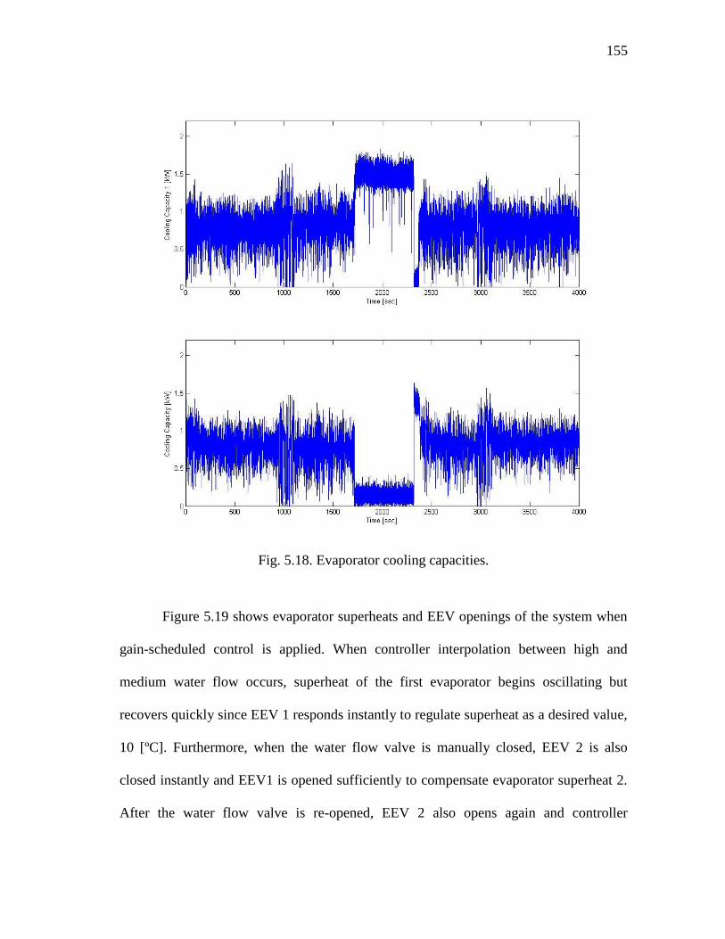
155

Fig. 5.18. Evaporator cooling capacities.

Figure 5.19 shows evaporator superheats and EEV openings of the system when

gain-scheduled control is applied. When controller interpolation between high and

medium water flow occurs, superheat of the first evaporator begins oscillating but

recovers quickly since EEV 1 responds instantly to regulate superheat as a desired value,

10 [ºC]. Furthermore, when the water flow valve is manually closed, EEV 2 is also

closed instantly and EEV1 is opened sufficiently to compensate evaporator superheat 2.

After the water flow valve is re-opened, EEV 2 also opens again and controller

156

interpolation is implemented properly. The reader recognizes that stability of the system

can be guaranteed over the operating envelop. More important, the interpolated/switched

controller can transition smoothly and stably from one design point to another.

Figure 5.20 presents superheat regulation where a single controller, LQR

controller designed at high flow condition, is used over operating conditions. This single

control case performs sufficiently well - even the second evaporator never loses

superheat at zero water flow condition since second EEV never closes. However, the

cascade control paradigm alleviates the strong effects of EEV on superheat in general

control cases and results in an effective superheat regulation. This may not happen in

practice since most physical systems are highly nonlinear and a single controller cannot

achieve the desired control when cascade control may not reduce strong nonlinearities of

the system.

157

Fig. 5.19. Superheat regulation and EEV opening in gain-scheduled control system.

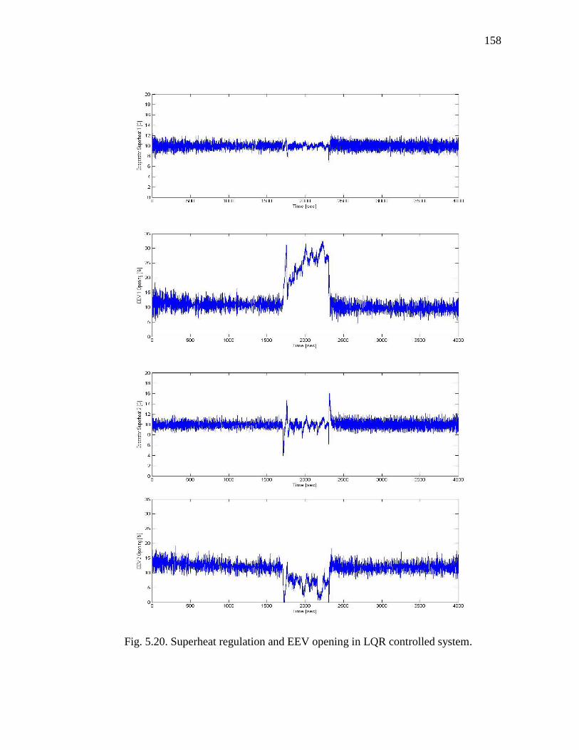
158

Fig. 5.20. Superheat regulation and EEV opening in LQR controlled system.

159

6. CONCLUSIONS AND FUTURE WORK

6.1 Summary of Research Achievement

This dissertation provides a method for stable controller interpolation for LPV

systems using the Youla parameterization. The existence of a quadratic common

Lyapunov function is given by construction, guaranteeing stability of the closed system

despite arbitrarily fast transitions in the scheduling variables. A particular state

transformation is used to allow the interpolated Q-system to share state variables,

significantly reducing the number of the states required for controller interpolation. The

approach has the advantage that controllers of different sizes and structures can be

interpolated smoothly and stably with the performance of the local controllers recovered

exactly at critical operating conditions.

A proposed stability analysis has been extended to the LPV closed loop system

that includes robustness and performance considerations since the LPV plant model

includes modeling that significantly affects the system dynamics. In this case, the plant

model may not reflect the nonlinear system precisely and conventional stability

analyses may not be sufficient to guarantee the stability of a nonlinear system. The

proposed framework, utilizing 2L gain of the modified LPV-Q system via optimizing

feedback gains of a closed system, guarantees the global level of robust stability by

minimizing the 2L gain that remains within desired bounds over the operating envelop.

160

The efficacy of the proposed controller interpolation is demonstrated in

experimentation using a multi-evaporator vapor compression system. The dynamics of

vapor compression systems are highly nonlinear, thus the gain-scheduled control is the

potential to achieve the desired stability and performance of the system. The proposed

controller interpolation/switching method guarantees the nonlinear stability of the closed

loop system during the arbitrarily fast transition and achieves the desired performance to

subsequently improve thermal efficiency of the vapor compression system.

6.2 Future Work

This research mainly contributes nonlinear stability for gain-scheduled systems.

The efficacy of the proposed method is demonstrated in simulation and experimentation.

There exist a number of directions where attention for future work can be focused,

including following.

Gain-scheduled Control:

In a proposed LPV-Q framework, stability of the nonlinear closed loop system is

guaranteed by the existence of a quadratic common Lyapunov function but performance

of the system is rather not to be considered in this dissertation. To improve the

performance of the nonlinear system, a plant model should reflect the dynamics of the

system more precisely since controllers are designed using a model that is constructed

from system identification models. When an LPV model doesn’t exist in practice, a

data-driven or first principle model should represent real dynamics of the nonlinear

161

systems. Thus advanced methods in system identification-based plant modeling can

become milestones in performance improvement.

Control of Vapor Compression System:

There are a plenty of choices in controllable inputs and outputs for vapor

compression systems. We examined rather simple cases in experimental studies; other

choices of controllable inputs and outputs may achieve high-level of thermal efficiency.

Also, this dissertation has implemented control design at a steady state, not focusing on

the start-up process; thus a comparatively large overshoot and sluggish settling time has

appeared on start.-up. Control design with start-up and shut-down considerations will

improve thermal efficiency via reducing the load applied to system.

162

REFERENCES

[1] D. J. Leith and W. E. Leithead, "Survey of Gain-Scheduling Analysis and Design,"

International Journal of Control, vol. 73, no. 11, pp. 1001-1025, 2000.

[2] J. S. Shamma and M. Athans, "Gain Scheduling: Potential Hazards and Possible

Remedies," in Proc. of the American Control Conference, Boston, MA, Jun. 1991,

pp. 516-521.

[3] S. Skogestad and I. Postlethwaite, Multivariable Feedback Control: Analysis and

Design. Chichester, England: John Wiley & Sons, 1996.

[4] X. He, S. Liu, and H. H. Asada, "Modeling of Vapor Compression Cycles for

Multivariable Feedback Control of HVAC Systems,” Journal of Dynamic Systems,

Measurement, and Control, vol. 119, pp. 183-191, 1997.

[5] B. P. Rasmussen, "Dynamic Modeling and Advanced Control of Air Conditioning

and Refrigeration Systems,” Ph.D diss., Department of Mechanical and Industrial

Engineering, University of Illinois, Urbana, IL, Dec. 2005.

[6] K. J. Hunt, T. A. Johansen, J. Kalkkuhl, H. Fritz, and T. Gottsche, "Speed Control

Design for An Experimental Vehicle using a Generalized Gain Scheduling

Approach," IEEE Transactions on Control Systems Technology, vol. 8, pp. 381-

395, 2000.

[7] R. A. Hyde and K. Glover, "Application of Scheduled H Controllers to a VSTOL

Aircraft," IEEE Transactions on Automatic Control, vol. 38, pp. 1021-1039, 1993.

[8] R. T. Reichert, "Dynamic Scheduling of Modern-Robust-Control Autopilot

163

Designs for Missiles," IEEE Control Systems Magazine, vol. 12, pp. 35-42, Oct,

1992.

[9] D. J. Stilwell, "State-Space Interpolation for a Gain-Scheduled Autopilot," Journal

of Guidance, Control, and Dynamics, vol. 24, pp. 460-465, 2001.

[10] T. A. Johansen, K. J. Hunt, and I. Petersen, "Gain-Scheduled Control of a Solar

Power Plant," Control Engineering Practice, vol. 8, pp. 1011-1022, 2000.

[11] D. J. Leith and W. E. Leithead, "Appropriate Realization of Gain-Scheduled

Controllers with Application to Wind Turbine Regulation,” International Journal

of Control, vol. 65, pp. 223-248, 1996.

[12] R. Zhang, A. Alleyne, and D. E. Carter, "Generalized Multivariable Gain

Scheduling with Robust Stability Analysis," ASME Journal of Dynamic Systems,

Measurement, and Control, vol. 27, pp. 668-687, Dec, 2005.

[13] W. J. Rugh and J. S. Shamma, "Research on Gain Scheduling," Automatica, vol.

36, no. 10, pp. 1401-1425, 2000.

[14] D. J. Stilwell, "J-Q interpolation for Gain Scheduled Controllers," in Proc. of

IEEE Conference on Decision and Control, Pheonix, AZ, Dec. 1999, vol. 1, pp.

749-754.

[15] J. P. Hespanha and A. S. Morse, "Switching Between Stabilizing Controllers,"

Automatica, vol. 38, no. 11, pp. 1905-1917, 2002.

[16] D. J. Stilwell and W. J. Rugh, "Stability Preserving Interpolation Methods for the

Synthesis of Gain Scheduled Controllers," Automatica, vol. 36, no. 5, pp. 665-671,

2000.

164

[17] H. Niemann and J. Stoustrup, "An Architecture for Implementation of

Multivariable Controllers," in Proc. of the American Control Conference, San

Diego, CA, Jun. 1999, pp. 4029-4033.

[18] K. J. Hunt and T. A. Johansen, "Design and Analysis of Gain-Scheduled Control

using Local Controller Networks," International Journal of Control, vol. 66, no. 5,

pp. 619-651, 1997.

[19] R. Murray-Smith and T. Johansen, Multiple Model Approaches to Nonlinear

Modelling and Control. Bristol, PA: Taylor and Francis, 1997.

[20] A. Packard and M. Kantner, "Gain Scheduling the LPV Way," in Proc. of the

IEEE Conference on Decision and Control, Atlanta, GA, Dec. 1996, vol. 4, pp.

3938-3941.

[21] F. Wu, "A Generalized LPV System Analysis and Control Synthesis Framework,”

International Journal of Control, vol. 74, no. 7, pp. 745-759, 2001.

[22] K. H. Tan and J. S. Shamma, "Nonlinear Gain-scheduled Control Design using

Set-values Methods,” in Proc. of the American Control Conference, Philadelphia,

PA, Jun. 1998, pp. 1195-1199.

[23] F. Wu and K. M. Grigoriadis, "LPV-based Control of Systems with Amplitude and

Rate Actuator Saturation Constraints,” in Proc. of the American Control

Conference, San Diego, CA, Jun. 1999, pp. 3191-3195.

[24] B. P. Rasmussen and A.G. Alleyne, "Gain Scheduled Control of an Air

Conditioning System Using the Youla Parameterization," in Proc. of the American

Control Conference, Minneapolis, MN, Jun. 2006, pp. 5336-5341.

165

[25] H. K. Khalil, Nonlinear Systems. Upper Saddle River, NJ: Prentice-Hall Inc., 1996.

[26] J. Stoustrup, P. Andersen, T. Pedersen, and M. Hangstrup, "Gain-scheduling

Procedures for Unstable Controllers: A Behavioral Approach,” in Proc. of the

American Control Conference, San Diego, CA, Jun. 1999, pp. 4004-4008.

[27] G. Becker and A. Packard "Robust Performance of Linear Parametrically Varying

Linear Feedback," Systems & Control Letters, vol. 23, pp. 205-215, 1994.

[28] J. S. Shamma and D. Xiong, "Set-valued Methods for Linear Parameter Varying

Systems, Automatica, vol. 35, pp. 1081-1089, 1999.

[29] D. J Leith and W. E. Leithead, "Inpur-output Linearization of Velocity-based Gain-

scheduling,” International Journal of Control, vol. 72, pp. 229-246, 1999.

[30] D. J Leith and W. E. Leithead, "Analytic Framework for Blended Multiple Model

Systems using Linear Local Models,” International Journal of Control, vol. 72, pp.

605-619, 1999.

[31] D. J Leith and W. E. Leithead, "Gain-scheduled Controller Design: An Analytic

Framework Directly Incorporating Non-equilibrium Plant Dynamics,”

International Journal of Control, vol. 70, pp. 249-269, 1999.

[32] W. Tan, K. Andrew, K. Packard, K. Stoustrup, and G. Balas, "Quasi-LPV

Modeling and LPV Control of a Generic Missile,” in Proceedings of the American

Control Conference, Chicago, IL, Jun. 2000, pp. 3692-3696.

[33] Y. Huang and A. Jadbabaie, "Nonlinear H Control: An Enhanced Quasi-LPV

Approach,” in Proc. of the IFAC World Congress, Beijing, China, Jun. 1999, pp.

576-584.

166

[34] A. Jadbabaie and J. Hauser, "Control of a Thrust-vectored Flying Wing: A

Receding Horizon – LPV Approach,” International Journal of Robust and

Nonlinear Control, vol. 12, no. 14, pp. 869-896, 2002.

[35] D. J Leith and W. E. Leithead, "Gain-scheduled Controller Design: An Analytic

Framework Directly Incorporating Non-equilibrium Plant Dynamics,”

International Journal of Control, vol. 70, pp. 249-269, 1999.

[36] P. Apkarian and P. Gahinet, "Convex Characterization of Gain-scheduled H

controllers,” IEEE Transactions on Automatic Control, vol. 40, pp. 853-864, 1995.

[37] R. A. Nichols, R. T. Reichert, and W. J. Rugh, "Gain Scheduling for H-infinity

Controllers: A Flight Control Example," IEEE Transactions on Control Systems

Technology, vol. 1, pp 69-79, 1993.

[38] D. J. Stilwell and W. J. Rugh, "Interpolation of Observer State Feedback

Controllers for Gain Scheduling," IEEE Transactions on Automatic Control, vol.

44, pp. 1225-1229, 1999.

[39] C. W. Scherer, P. Gahinet, and M. Chilali, "Multiobjective Output-feedback

Control via LMI Optimization,” IEEE Transaction on Automatic Control, vol. 42,

pp. 896-911, 1997.

[40] L. Wang, A Course in Fuzzy Systems and Control. Upper Saddle River, NJ:

Prentice Hall, 1996.

[41] D. Guo and W. J. Rugh, "An Approach to Gain Scheduling on Fast Variables," in

Proc. of the IEEE Conference on Decision and Control, Tucson, AZ, Dec. 1992,

vol. 1, pp. 759-763.

167

[42] P. Gahinet, P. Apkarian, and M. Chilali, "Affine Parameter-Dependent Lyapunov

Functions and Real Parametric Uncertainty," IEEE Transactions on Automatic

Control, vol. 41, pp. 436-442, 1996.

[43] C. W. Scherer, "LPV Control and Full Block Multiplier,” Automatica, vol. 37, pp.

361-375, 2001.

[44] G. Becker, "Additional Results on Parameter-dependent Controllers for LPV

Systems,” in Proceeding of the IFAC World Congress, San Francisco, CA, Jul.

1996, pp. 351-356.

[45] J. Daafouz, P. Riedinger, and C. Iung, "Stability Analysis and Control Synthesis

for Switched Systems: A Swithched Lyapunov Function Approach," IEEE

Transactions on Automatic Control, vol. 47, no. 11, pp. 1883-1887, 2002.

[46] J. Yu and A. Sideris, " H Control with Parameter Lyapunov Functions: Induced

L2-norm Control for LPV Systems with Bounded Paramoeter Variation Rates,”

Systems & Control Letters, vol. 30, pp. 57-69, 1997.

[47] E. Feron, P. Apkarian, and P. Gahinet, "Analysis and Synthesis of Robust Control

Systems via Parameter-dependent Lyapunov Functions,” IEEE Transaction of

Automatic Control, vol. 41, pp. 1041-1046, 1996.

[48] F. Wu, H. Yang, A. Packard, and G. Becker, "Induced 2L -Norm for LPV System

with Bounded Parameter Variation Rates,” in Proc. of the American Control

Conference, Seattle, WA, Jun. 1995, pp. 2379-2383.

168

[49] G. Zhai, H. Lin, and P. Antsaklis, "Quadratic Stabilizability of Switched Linear

Systems with Polytopic Uncertainties,” International Journal of Control, vol. 76,

no. 7, pp. 747-753, 2003.

[50] M. Margaliot and D. Liberzon, "Lie-algebraic Stability Conditions for Nonlinear

Switched Systems and Differential Inclusions,” Systems & Control Letters, vol. 55,

pp. 8-16, 2006.

[51] L. Vu and D. Liberzon, "Common Lyapunov Functions for Families of

Commuting Nonlinear Systems,” Systems & Control Letters, vol. 54, pp. 405-416,

2005.

[52] D. Liberzon, Switching in Systems and Control. Boston, MA: Birkhäuser, 2003.

[53] S. Boyd and Q. Yang, "Structured and Simultaneous Lyapunov Functions for

System Stability Problems," International Journal of Control, vol. 49, pp. 2215-

2240, 1989.

[54] T. Ooba and Y. Funahashi, "Two Conditions Concerning Common Quadratic

Lyapunov Functions for Linear Systems," IEEE Transactions on Automatic

Control, vol. 42, no. 5, pp. 719-721, 1997.

[55] R. Shorten, K. Narendra, and O. Mason, "A Result on Common Quadratic

Lyapunov Functions," IEEE Transactions on Automatic Control, vol. 48, no. 1, pp.

110-113, 2003.

[56] V. Blondel, G. Campion, and M. Gevers, "A Sufficient Conditions for

Simultaneous Stabilization," IEEE Transactions on Automatic Control, vol. 38, no.

8, pp. 1264-1266, 1993.

169

[57] V. Blondel, Simultaneous Stabilization of Linear Systems. New York: Springer-

Verlag, 1994.

[58] H. Niemann, "Dual Youla Parameterisation," in Proc. of IEE Control Theory and

Applications, vol. 150, no. 5, pp. 493-497, 2003.

[59] H. Niemann, J. Stoustrup, and R. Abrahamsen, "Switching between Multivariable

Controllers," Journal of Optimal Control Applications and Methods, vol. 25, pp.

51-66, 2004.

[60] H. Niemann and J. Stoustrup, "An Architecture for Fault Tolerant Controllers,”

International Journal of Control, vol. 78, no. 14, pp. 1091-1113, 2005.

[61] B. P. Rasmussen and A. Alleyne, "Gain Scheduled Control of an Air Conditioning

System Using the Youla Parameterization," IEEE Transactions on Control Systems

Technology, in review.

[62] D. C. Youla, J. J. Jr. Bongiorno, and H. A. Jabr, "Modern Wiener-Hopf Design of

Optimal Controllers Part I: The Single-Input-Output Case," IEEE Transactions on

Automatic Control, vol. AC-21, no. 1, pp. 13-30, 1976.

[63] T. T. Tay, I. Mareels, and J. B. Moore, High Performance Control. Ann Arbor, MI:

Birkhauser, 1998.

[64] P. Apkarian and R. J. Adams, "Advanced Gain-Scheduling Techniques for

Uncertain Systems," IEEE Transactions on Control Systems Technology, vol. 6,

pp. 21-32, 1998.

170

[65] P. Apkarian and R. J. Adams, "Advanced Gain-Scheduling Techniques for

Uncertain Systems," IEEE Transactions on Control Systems Technology, vol. 6,

pp. 21-32, 1998.

[66] J. S. Shamma, "Robust Stability with Time-varying Structured Uncertainty," IEEE

Transactions on Automatic Control, vol. 39, pp. 714-724, 1994.

[67] K. Zhou, J. C. Doyle, and K. Glover, Robust and Optimal Control. Upper Saddle

River, NJ: Prentice Hall, 1996.

[68] F. Wu, X. H. Yang, A. Packard, and G. Becker, "Induced L2-norm Control for

LPV Systems with Bounded Parameter Variation Rates,” International Journal of

Control, vol. 9, pp. 983-998, 1996.

[69] M. Chilali and P. Gahinet, " H Design with Pole Placement Constraints: An LMI

Approach,” IEEE Transaction of Automatic Control, vol. 41, pp. 358-367, 1996.

[70] Anonymous, "Energy Information Administration: International Energy Outlook

2009,” http://www.eia.doe.gov/oiaf/ieo/world.html, 2009

[71] M. S. Elliott, "Decentralized Model Predictive Control of A Multiple Evaporator

HVAC System,” M.S Thesis, Department of Mechanical Engineering, Texas A&M

University, College Station, TX, Aug. 2008.

[72] M. Moran and H. Shapiro, Fundamentals of Engineering Thermodynamics. New

York: John Wiley & Sons, 2007.

[73] J. S. Shamma and M. Athans, "Analysis of Nonlinear Gain Scheduled Control

Systems," IEEE Transaction of Automatic Control, vol. 27, pp. 898-907, 1991.

171

[74] S. Boyd, E. Ghaoui, and M. Chilali, Linear Matrix Inequalities in System and

Control Theory. Philadelphia, PA: SIAM, 1994.

[75] P. Gahinet, "Explicit Controller Formulas for LMI-based H Synthesis,”

Automatica, vol. 32, pp. 1007-1014, 1994.

[76] A. Packard, "Gain-scheduling via Linear Fractional Transformations,”

International Journal of Control, Systems & Control Letters, vol. 22, pp. 79-82,

1994.

[77] H. Niemann and J. Stoustrup, "Gain Scheduling Using the Youla

Parameterization," in Proceedings of the IEEE Conference on Decision and

Control, Pheonix, AZ, Dec. 1999, vol. 3, pp. 2306-2311.

[78] J. Stoustrup and H. Niemann, "Starting Up Unstable Multivariable Controllers

Safely," in Proceedings of the IEEE Conference on Decision and Control, San

Diego, CA, Dec. 1997, vol. 2, pp. 1437-1438.

[79] J. D. Bendtsen, J. Stoustrup, and K. Trangbaek, "Bumpless Transfer between

Observer-based Gain Scheduled Controllers," International Journal of Control,

vol. 78, no. 7, pp. 491-504, 2005.

[80] J. Bendtsen, J. Stoustrup, and K. Trangbaek, "Bumpless Transfer between

Advanced Controllers with Applications to Power Plant Control,” in Proceedings

of the IEEE Conference on Decision and Control, Maui, Hawaii, Dec. 2003, vol. 3,

pp. 2059-2064.

172

[81] J. Bendtsen, J. Stoustrup, and K. Trangbaek, "Multi-Dimensional Gain Scheduling

with Application to Power Plant Control,” in Proc. of the IEEE Conference on

Decision and Control, Maui, Hawaii, Dec. 2003, vol. 6, pp. 6553-6558.

[82] H. Niemann and J. Stoustrup, "Reliable Control using Primary and Dual Youla

Parameterization,” in Proc. of the IEEE Conference on Decision and Control, Las

Vegas, NV, Dec. 2002, vol. 4, pp. 4353-4358.

[83] D. J. Stilwell and W. J. Rugh, "Interpolation of Observer State Feedback

Controllers for Gain Scheduling," in Proc. of the American Control Conference,

Philadelphia, PA, Jun. 1998, pp. 1215-1219.

[84] D. J. Stilwell and W. J. Rugh, "Interpolation Methods for Gain Scheduling," in

Proc. of IEEE Conference on Decision and Control, Tampa, FL, Dec. 1998, vol. 2,

pp. 3003-3008.

[85] D. J. Stilwell, "State-Space Interpolation for a Gain-Scheduled Autopilot," Journal

of Guidance, Control, and Dynamics, vol. 24, no. 3, pp. 460-465, 2001.

[86] B. P. Rasmussen and Y. J. Chang, "Stable Controller Interpolation/Controller

Switching for LPV Systems,” Journal of Dynamic Systems, Measurement, and

Control, Accepted in publication, 2009.

[87] Y. J. Chang and B. P. Rasmussen, "Stable Controller Interpolation for LPV

Systems," in Proceedings of the American Control Conference, Seattle, WA, Jun.

2008, pp. 3082-3087.

173

[88] W. Xie and T. Eisaka, "Design of LPV Control Systems Based on Youla

Parameterization," IEE Proceedings of Control Theory and Applications, New

York, NY, Dec. 2004, vol. 151, no. 4, pp. 465-472.

[89] K. H. Johansson, "Quadruple-Tank Process: A Multivariable Laboratory Process

with an Adjustable Zero," IEEE Transactions on Control Systems Technology, vol.

8, no. 3, pp. 456-465, 2000.

[90] P. Apkarian, P. Gahinet, and G. Becker, "Self-scheduled H-infinity Control of

Linear Parameter-varying Systems: A Design Example," Automatica, vol. 31, pp.

1251-1261, 1998.

[91] W. Xie, Y. Kamiya, and T. Eisaka, "Robust Control System Design for Polytopic

Stable LPV Systems,” IMA Journal of Mathematical Control and Information, vol.

20, pp. 201-216, 2003.

[92] W. Xie and T. Eisaka, "Robust State Feedback for Linear Parameter Varying

Systems with Parameter Uncertainties,” SICE Annual Conference, Kokkaido,

Japan, Aug. 2004, pp. 2644-2647.

[93] G. E. Dullerud and F. Paganini, A Corse in Robust Control Theory: A Convex

Approach. New York: Springer, 2000.

[94] X. He and H. H. Asada, "A New Feedback Linearization Approach to Advanced

Control of Multi-Unit HVAC Systems,” in Proc. of the American Control

Conference, Denver, CO, Jun. 2003, pp. 2311-2316.

174

[95] X. He, S. Liu, and H. H. Asada, "A Moving-interface Model of Two-phase Flow

Heat Exchanger Dynamics for Control of Vapor Compression Cycle,” Heat Pump

and Refrigeration System Design, Analysis, and Application, pp. 69-75, 1994.

[96] N. Hewitt, J. McMullan, and N. Murphy, "Comparison of Expansion Valve

Performance,” International Journal of Energy Research, vol. 5, pp. 43-54, 1995.

[97] J. M. Choi and Y. C. Kim, "Capacity Modulation of Iverter-driven Multi-air

Conditioner using Electronic Expansion Valves,” Energy, vol. 28, pp. 141-155,

2003.

[98] E. Bristol, “On A New Measure of Interaction for Multivariable Process Control,”

IEEE Transaction on Automatic Control, vol. 11, pp. 133-134, 1966.

[99] B. C. Moore, "Principle Component Analysis in Linear Systems: Controllability,

Observability, and Model Reduction,” IEEE Transaction on Automatic Control,

vol. 26, pp. 17-31, 1981.

[100] Mathworks, "MATLAB System Identification Toolbox Documentation,”

http://www.mathworks.com/access/helpdesk/help/toolbox/ident/, 2009.

[101] G. F. Franklin, J. D. Powell, and A. Emami-Naeini, Feedback Control of Dynamic

Systems. Upper Saddle River, NJ: Prentice Hall, 2002.

175

VITA

Name: Young Joon Chang

Address: 452-39 Daeheung-dong Jung-gu

Daejeon, South Korea, 301-803

Email Address: blueair93@gmail.com

Education: B.S., Mechanical Engineering, Inha University, 2000

M.S., Mechanical Engineering, Inha University, 2002

Ph.D., Mechanical Engineering, Texas A&M University, 2010

Experience: Graduate Assistant-Research, TAMU Dept. of Mech. Engr.

1/2006-8/2009, College Station, Texas

Researcher, Korea Institute of Energy Research

1/2003-12/2003, Daejeon, South Korea

Graduate Assistant-Research, Inha Univ. Dept. of Mech. Engr.

1/2001-8/2002, Inchon, South Korea

Graduate Assistant-Teaching, Inha Univ. Dept. of Mech. Engr.

3/2000-12/2000, Inchon, South Korea

Researcher, Korean National Science Foundation

1/2000-1/2002, Seoul, South Korea