2464 IEEE TRANSACTIONS ON SIGNAL PROCESSING, VOL. 52, NO. 9, SEPTEMBER 2004

Gain-Scheduled Filtering forTime-Varying Discrete Systems

Nguyen Thien Hoang, Hoang Duong Tuan, Pierre Apkarian, and Shigeyuki Hosoe

Abstract—This paper deals with the design of gain-sched-uled filters, whose state-space realization depends on real-timeparameters of plants. Similar to well-recognized advantages ofgain-scheduled controllers in control theory, gain-scheduled filtersare expected to provide enhanced performance in comparisonwith customary nonadjustable filters. Our construction techniqueis based on nonlinear fractional transformation (NFT) represen-tations of systems that are a generalization of widely used linearfractional transformation (LFT) representations. Both generalized

2 and discrete-time filter design problems are investigatedtogether with their extension to mixed designs. This study leads tonew linear matrix inequality (LMI) formulations, which in turnprovide an effective and reliable design tool. The proposed designtechnique is finally evaluated in the light of simulation examples.

Index Terms—Linear fractional transformation (LFT), linearmatrix inequality (LMI), nonlinear fractional transformation(NFT).

I. INTRODUCTION

ACOMMON tool to express the parameter dependence ofa system is certainly the linear fractional transformation

(LFT). Methods to transform many practical forms of parameterdependence into LFT representations are given in [24]. Besides,other forms of parameter dependence can be well approximatedby LFT representations to be embedded into the context of linearparameter varying (LPV) control, as in [2], [14], and [15]. How-ever, a critical issue with this transformation is the well-known”curse of dimensionality,” i.e., the LFT systems have often toolarge dimensions in terms of parameters for practical and ef-fective uses. One may also argue that the LFT is not the bestsystem for representing systems with affine parameter depen-dence such as those of polytopic type. The so-called nonlinearfractional transformation (NFT) has been introduced in [18] foruncertain continuous-time systems to overcome these difficul-ties. An immediate advantage of the NFT is that it yields smallerrepresentations that better lend themselves to numerical treat-ments.

Manuscript received June 13, 2003; revised September 2, 2003. The associateeditor coordinating the review of this manuscript and approving it for publica-tion was Dr. Helmut Bölcskei.

N. T. Hoang and S. Hosoe are with the Department of Electronic-Mechan-ical Engineering, Nagoya University, Nagoya 464-8501, Japan (e-mail: thien-hoang@nuem.nagoya-u.ac.jp, hosoe@nuem.nagoya-u.ac.jp).

H. D. Tuan is with the School of Electrical and Telecommunication Engi-neering, University of New South Wales, Sydney, NSW 2052, Australia (e-mail:h.d.tuan@unsw.edu.au).

P. Apkarian is with ONERA-CERT, 31055 Toulouse, France (e-mail: ap-karian@cert.fr).

Digital Object Identifier 10.1109/TSP.2004.832008

This paper investigates gain-scheduled filtering techniquesfor time-varying NFT system described as

(1)

where , ,, , ,

, and is the state, is the measuredoutput, is the output to be estimated, andis the disturbance . The extra variables ,

are introduced to express the system nonlinearparameter dependence. The time-varying parameter is as-sumed to be gain scheduled, i.e., it is measured on line. Withoutloss of generality, it is allowed to vary in the unit simplex

The state-space data in (1) are assumed linear in , i.e.,

(2)

The acronym NFT originates from the LFT. This can be viewedby the fact that if the slack variables and are re-moved from (1), then we can have the following equivalent rep-resentation of the parameter-dependent system:

(3)

1053-587X/04$20.00 © 2004 IEEE

HOANG et al.: GAIN-SCHEDULED FILTERING FOR TIME-VARYING DISCRETE SYSTEMS 2465

One can see that (3) is highly nonlinear in the gain-schedulingparameter and includes well-known parameter-dependentclasses as a particular case: The LFT representations corre-spond to the independence from of all system matricesexcept in (1), whereas polytopic systems correspondto . As mentioned, most nonlinear parameter-de-pendent systems including the NFT representations (1), or itsequivalence (3), can be alternatively expressed by the LFT, butas it will be seen through some simple examples, this oftenleads to impractical representations, whereas in stark contrast,the NFT-based ones are easily handled.

Correspondingly, the filters for estimation of the outputof systems (1) and (3) are also time-varying and share an NFTstructure

(4)

where

(5)and their sizes are the same as those of the matrices ,

, , , , ,and in (1). The matrices on the right-hand side of (5)are computed offline using efficient LMI software. Then, theestimation of the output is easily updated online ac-cording to (4) and (5). Note that we can have just the param-eter-independent matrices because of the crossproducts of those matrices with the parameter-dependent ma-trices that constitute the measured output of (1). This isnecessary to obtain the convex formulations and will be clearlyclarified from the context of Section III. The following mixedgeneralized error criterion is used to estimate

(6)

where and denote the norms inducing the general-ized and norms, respectively. As in [13], the generalized

-norm is appropriate for handling time-domain peak errors,whereas is most suitable for treating energy errors. Mini-mization of the peak-error and minimization of the energy-errorare proved to be conflicting in [2], [8], and [13]. Therefore, aparameter is introduced in (6) to attain some balancebetween peak error and energy error constraints.

For linear time invariant (LTI) filtering with different ap-proaches, e.g., interpolation approaches, Riccati equation-basedapproaches and LMI-based approaches, one can refer to a va-riety of papers [3], [9], [11], [17], [22] and references therein.LTI filtering has been intensively addressed in the literature;see, e.g., [5]–[7], [11], [12], and [23]. Forms of mixedcontrol have been introduced in [2], [8], and [13], whereas one

for mixed filtering has been used in [19], [20]. A com-prehensive collection of performance criteria for control pur-poses is given by [10] and [13]. Some related topics such as filterorder reduction and filtering for systems with stochastic uncer-tainties can be found in [16], [18], and [21]. Note that robustKalman filtering exclusively detailed in [11] addresses some-what narrower class of uncertainties via the use of Riccati equa-tions, yielding LTI filters with the simple Luenberger observerstructure. In the time-varying case, the differential Riccati equa-tion-based approaches exhibit computational impracticality forreal-time applications [10], wherein the LMI-based approachescan stay viable [2], [14]. Up to date, in the robust control lit-erature, the LPV control for both analog and discrete uncertainsystems has been considered by [2], [14], and [15]. However,the counterpart of the gain-scheduled filtering for robust con-trol problems of NFT systems (1) remains open and very chal-lenging.

The layout of the paper is as follows. Section II developsLMI-based norm characterizations of NFT systems, which arethen used in Section III to derive new LMI-based formulationsfor the design of NFT filters. Validity and effectiveness of theproposed techniques are assessed via a number of numerical ex-periments in Section IV.

Notations in this paper are standard. Particularly, is thetranspose of the matrix , whereas ( ,resp.) means that is negative definite (positive definite,resp.) for symmetric matrices and . In symmetric blockmatrices or long matrix expressions, we use as an ellipsis forterms that are induced by symmetry, e.g.,

In addition, in long matrix inequalities involving matrix func-tions of the parameter , we use, e.g.,

(7)

to save space. The bold capital letters such as , , , etc., areused to emphasize matrix variables.

II. CHARACTERIZATIONS FOR NORM CONSTRAINTS

In this section, we provide LMI-based analysis for differentperformance criteria of NFT filters. In other words, we are in-terested in generalized and norms of the augmentedsystem formed by (1) and (4) with the estimation error

rewritten in the compact form

(8)

where

(9)

2466 IEEE TRANSACTIONS ON SIGNAL PROCESSING, VOL. 52, NO. 9, SEPTEMBER 2004

and other matrices are defined accordingly [see (30) below].With these definitions, the generalized -norm of the system(8) is defined and analyzed first.

A. Generalized -Norm Characterization

The -norm of an LTI system is strictly connected withits transfer function. For instance, the -norm of the transferfunction is defined as [8]

When is of finite impulse response (FIR), i.e.,, this becomes the square norm

. Stochastically, the -norm is inter-preted as the standard deviation of the output caused by thenormalized white noise input. Deterministically, the -normmeans the square root of the output energy under the normal-ized impulsive input. The generalized -norm for systems isdefined as the peak of output values under normalized energyinput. Clearly, these norm definitions are restricted to strictlyproper continuous systems [13]. However, they are valid forboth proper and strictly proper discrete-time systems. Indeed,the generalized -norm for system (8) is nothing but

(10)

In other words, (8) is said to have the generalized -norm lessthan if and only if the following relation holds for any input

and the corresponding output :

(11)

For continuous systems, it is obvious that, and therefore, the

counterpart of (10) is not well-defined if there is a feed-throughterm in the output. That is why the generalized -norm isdefined only for strictly proper continuous systems. Contrarily,it is obvious that ,and thus, the definition (10) is valid, whatever the class ofdiscrete systems.

The stability, as well as the generalized -norm of (8), canbe examined with the help of the Lyapunov function

(12)

satisfying the two following inequalities:

(13)

(14)

with matrices and belonging tothe symmetric scaling class, which has been used in [2].

By additionally imposing

(15)for all , satisfying (8) (i.e.,

), (13) and (14) lead to

(16)

(17)

Hence

(18)

meaning that the generalized -norm of (8) is indeed less than.

Furthermore, in the zero input case ( ), by (13) and(15)

(19)

which, according to Lyapunov theory, guaranteesas for any initial condition , thus showing the

asymptotic Lyapunov stability of (8).To sum up, we state that (13) and (14), together with (15),

guarantee that (8) is stable with the generalized -norm lessthan .

Meanwhile, all inequalities (13)–(15) can be readily rewrittenas matrix inequalities as follows.

• As and are linearly dependent onby (8), the left-hand sides of (13)

and (14) are easily rearranged as quadratic functions in. By using the Schur’s complement,

these quadratic functions are equivalent to the followinginequalities:

(20)

(21)

• By substituting , the left-handside of (15) becomes a quadratic function in , whichis also equivalent to the following matrix inequality via theSchur’s complement:

(22)

It is clear that inequalities (20)–(22) are not LMIs. Here, we usethe linearization techniques, which have been introduced in [2]

HOANG et al.: GAIN-SCHEDULED FILTERING FOR TIME-VARYING DISCRETE SYSTEMS 2467

to render those inequalities linear at the expense of the insertionof some slack variables.

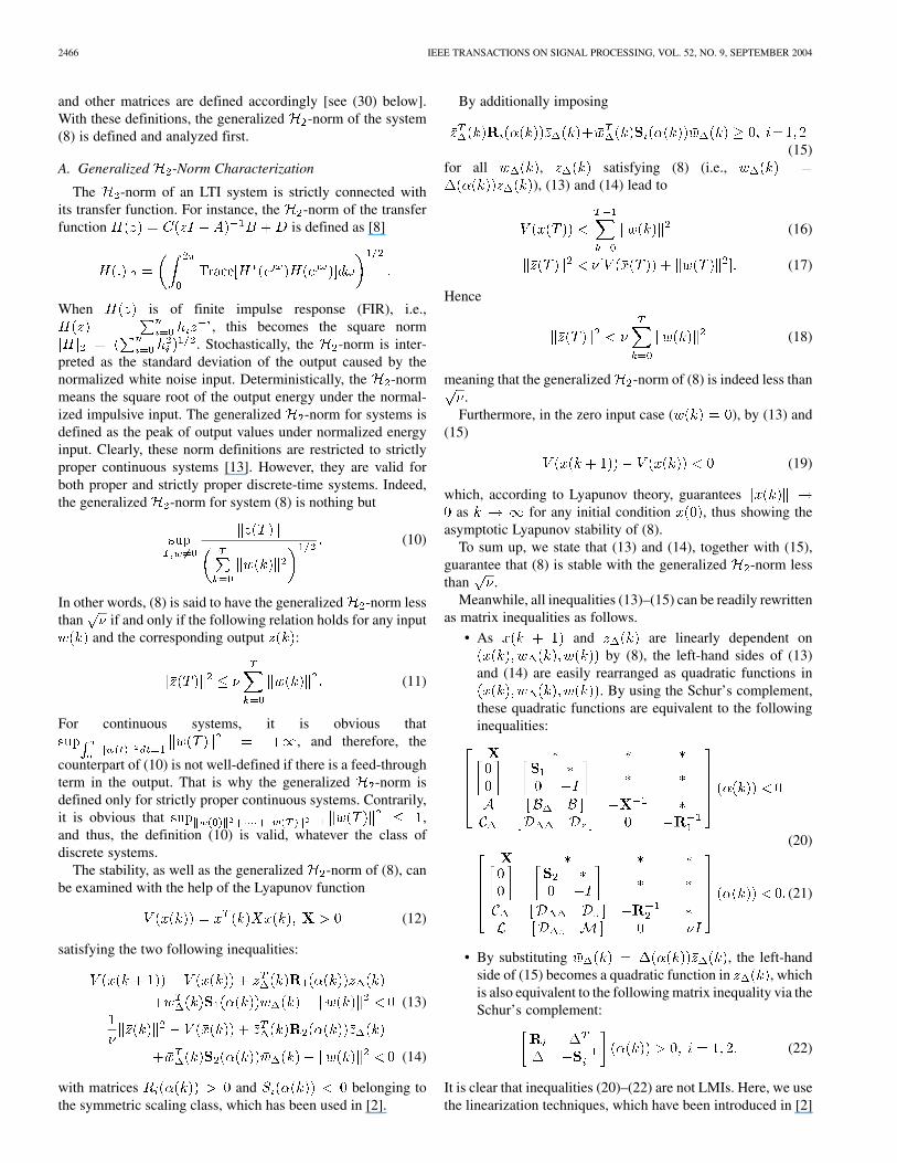
Theorem 1: One has (11), guaranteeing the generalized-norm of system (8) less than if there are a symmetric

matrix , scalings , , and slack ma-trices , , satisfying inequalities (23)–(25), shown at thebottom of the page.

Proof: The deduction from (23)–(25) to (20)–(22), respec-tively, can be established along the lines of [2].

It is worth noting the following three points concerning theconservatism of Theorem 1. First, we have to resort to the singleLyapunov function (12) since we do not make any assumptionon the varying rate of the gain-scheduled parameters. If informa-tion on this rate is available, then like [1], our result can be easilymodified to yield the corresponding LMI-based characteriza-tion with parameter-dependent Lyapunov functions, which ingeneral are very efficient at handling the case of slowly varyingparameters. Second, the symmetric scalings are used instead ofthe more general full-block scalings [15] to handle uncertainties.Based on our experience in robust control, the latter are actuallynot much better than the former. Moreover, the used symmetricscaling class will lead to convex formulations for the filteringproblems in the next section, whereas the full-block one doesnot. Third, the slack matrices , , and are still parameterindependent. This is unavoidable in later attractive convex for-mulations for the filter design problems.

B. -Norm Characterization

The norm for system (8) is well understood as

(26)

i.e., (8) has the -norm less than if and only if

(27)

Paralleling the results in [2] leads to the following LMI charac-terization.

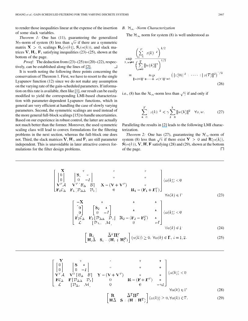
Theorem 2: One has (27), guaranteeing the -norm ofsystem (8) less than if there exist and ,

, , , satisfying (28) and (29), shown at the bottomof the page.

(23)

(24)

(25)

(28)

(29)

2468 IEEE TRANSACTIONS ON SIGNAL PROCESSING, VOL. 52, NO. 9, SEPTEMBER 2004

III. NFT FILTER DESIGNS

Returning to the design problem for NFT filters (4), an im-portant preparation step is to write the matrices of system (8) inthe following convenient forms:

(30)

with

(31)

and the variables

(32)

The next subsection considers the case of the generalizedfilter design.

A. NFT Generalized Filter Design

All inequalities (23), (24), and (28), which characterize theexistence of a filter (4), are not LMIs in the variables , ,

, , , , and . To translate them intoLMIs, we choose the following linearly parameter-dependentclass of scaling matrices , :

(33)

It follows that (23)–(25) are rewritten as (34)–(36), shown at thebottom of the page, where

(37)

A careful analysis of inequalities (34)–(37) reveals the fol-lowing bilinear terms involving the filter variables , ,

, scaling variables , . and slack variable :

We resort to the structure of matrices in (31) and (32) to linearizethese terms according to the following steps.

• With the partitioning

(38)

defining

(39)

as well as

(34)

(35)

(36)

HOANG et al.: GAIN-SCHEDULED FILTERING FOR TIME-VARYING DISCRETE SYSTEMS 2469

• Define the new variables

(40)

and

(41)

(42)

(43)

• Apply the congruence transformations

diag

diag

diag

to (34)–(36), respectively.

• With the help of the structured matrices in (30) and (31),bring into play the following identities, whose lengthy al-gebraic verification is provided in the Appendix :

(44)

As a result, the nonlinear matrix inequalities (34)–(36) are trans-lated into the following LMIs with respect to the newly intro-duced variables , , , , , , , , , and ,

, , shown in (45)–(47) at the bottom of the page.We recap these results in the next theorem.Theorem 3: There is an NFT filter (4) that makes the estima-

tion (11) fulfilled if LMI’s (45)–(47) are feasible in , , ,, , , , , , . The matrix data defining the

(45)

(46)

(47)

2470 IEEE TRANSACTIONS ON SIGNAL PROCESSING, VOL. 52, NO. 9, SEPTEMBER 2004

filter (4) can be derived from a solution to (45)–(47) through theformulas

(48)

Proof: For given matrices , , and , matrices , ,and satisfying (40), (41), and (43) are

(49)

Substituting these values of , , and into (41)–(43) andthen (48) can be easily obtained by restoring , , ,

, , , , , , and .

B. NFT and Mixed Generalized Filter Designs

By similar arguments, an LMI characterization for the exis-tence of filters is as follows.

Theorem 4: There is an NFT filter (4) that makes the estima-tion (27) fulfilled if LMIs (50) and (51), shown at the bottom ofthe page, are feasible in , , , , , , , , ,and , as in (50) and (51). The matrix data defining the filter(4) can be derived from a solution to (50) and (51) according to(48).

Consequently, the mixed generalized filter design ismerely the combination of Theorems 3 and 4.

Theorem 5: A suboptimal filter (4) for (6) can be obtainedfrom the solution to the optimization problem in (52), shown atthe bottom of the page, according to (48).

C. Particular Cases: LFT and LPV Filters

It is interesting to gain insight into the linearizing transforms(42) and (43) by considering two special cases.

If we impose , , ,, , and ;

in (4), i.e., we obtain the LFT filter

(53)

then the corresponding linearizing transform of the filter ma-trices is

(54)

and (45), (46), and (50) are obviously still LMIs in.

On the other hand, if , i.e., (1) becomes the usuallinear parameter varying (LPV) system

(55)

then accordingly, . In other words, (4) is down to theLPV filter

(56)

In this case, the scaling variables , (in Theorem 3), ,(in Theorem 4), and their related elements are no longer

necessary. As a result, LMIs (47) and (51) in Theorem 3 and4 disappear, whereas LMIs (45), (46), and (50) are reduced to

(50)

(51)

(45)-(47), (50), (51) (52)

HOANG et al.: GAIN-SCHEDULED FILTERING FOR TIME-VARYING DISCRETE SYSTEMS 2471

(57)–(59), shown at the bottom of the page, with the redefini-tions

(60)

(61)

(62)

Note that LMI formulations for the (nonadjustable) LTI filter

(63)

follow from LMIs (57)–(59) by the restriction

(64)

IV. NUMERICAL EXAMPLE

The power and flexibility of the proposed approach aredemonstrated through the following example:

(65)

where

(66)

Two representations are used to handle the nonlinear uncer-tain parameters and .

The NFT format

(67)

leads to NFT (1) with

(68)

Alternatively, the LFT format

(69)

(57)

(58)

(59)

2472 IEEE TRANSACTIONS ON SIGNAL PROCESSING, VOL. 52, NO. 9, SEPTEMBER 2004

TABLE ICOMPUTATIONAL PERFORMANCES OF DIFFERENT FILTERS.

Fig. 1. GeneralizedH ,H performances of NFT-mixed filters.

leads to LFT (1) with

(70)

The Matlab LMI Control Toolbox [4] was used in all LMI-re-lated computations. The dimension of 12 of the ’s in the LFTrepresentation (69) is very large in comparison with that equalto 4 in the NFT format (67). This deteriorates the computationalefficiency and estimation performance so severely that our com-puter equipped by a 1.3-GHz AMD CPU was unable to solve thecorresponding LMI formulations with the LFT model. In con-trast, we easily solved the LMI formulations corresponding tothe NFT model. Applying the result of Theorems 1 and 2, upperbounds on generalized , and norms of NFT (1), (68), inthe worst case, are found to be 2.2129 and 3.9961, respectively.

First, we consider the performance of the particularly de-signed LFT filters (53), LPV filters with structure (56), and LTIfilters with structure (63). Table I displays different measures ofperformance. As expected, NFT filters result in substantial im-provements of generalized and performances over LFT,LPV, and LTI filters. Such improvement is reaffirmed throughthe comparison between Figs. 1 and 2, depicting the generalized

Fig. 2. GeneralizedH ,H performances of LTI-mixed filters.

TABLE IIMSE PERFORMANCES OF FILTERS

, , and mixed performances of NFT and LTI mixed filterswith different values of the tradeoff constant .

Next, the actual performance of the NFT and LTI filters areevaluated via the mean square error (MSE) criterion

. Process noise and measurement noise are mutuallyindependent white Gaussian noises with the unity variance. Thegain-scheduling parameter was randomly generated forevery instant , and then, was appropriately obtained.For each filter, the corresponding result was obtained over 1000trials with 10 000 samples per every trial and listed in Table II.Noting that the variance of the signal , of thetime-varying plant is 4.5683, whereas that of the nominal (LTI)plant, i.e., , is 3.8641, time-varying uncertain-ties essentially alter the statistics properties of the plant’s re-sponse. In comparison with the variance of the signal of interest

HOANG et al.: GAIN-SCHEDULED FILTERING FOR TIME-VARYING DISCRETE SYSTEMS 2473

Fig. 3. Signal tracking of the NFT-mixed filter (� = 0:9).

Fig. 4. Ensemble-average squares of errors jz(k) � z (k)j g by gen. Hfilters and the Kalman filter.

, the results affirm that all the NFT filtersachieve very good MSE performances. For the case of LTI fil-ters, the LTI generalized filter outperforms the Kalman filterdesigned for the nominal plant. Although the design noise con-ditions are met exactly, the MSE performance of the Kalmanfilter is slightly poorer than that of the LTI- filter.

Furthermore, the tracking performances the NFT-mixed filteris shown in Fig. 3, confirming that it is a very good filter. Forthe sake of comparison and clarity between NFT filters, LTIfilters, and the Kalman filter, the ensemble average squared errorsequences over 1000 trials are depicted in Figs. 4–6. The figuresall together demonstrate the superiority of NFT filters over theLTI and the Kalman filters.

V. CONCLUSIONS

In this paper, we have developed new techniques for thedesign of parameter-dependent filters. These filters explicitlydepend on real-time-available system parameters and, thus,outperform customary nonadjustable filters. Our discussion

Fig. 5. Ensemble-average squares of errors jz(k) � z (k)j by H filtersand the Kalman filter.

Fig. 6. Ensemble-average squares of errors jz(k)� z (k)j by mixed filters(� = 0:9) and the Kalman filter.

has also investigated specific parameter structures attachedto systems and filters. We have shown that the NFT structureis especially attractive, not only to encompass a wider set ofparameter dependence but also for computational efficiency.Of most importance, our design techniques are based on LMIcomputations for which efficient and reliable software is nowavailable. The validity of the proposed techniques has beenconfirmed through a number of simulations.

Finally, applications of similar techniques to equalization forfading communication channels are currently under study.

APPENDIX

We will verify the identities in (44). In the steps to follow, theleft-hand sides of all the identities will be transformed to theirequivalent forms. The verifications of the equivalence betweenthese forms and the corresponding right-hand sides of identitiesare trivial; hence, they are omitted to save the space. Verifica-tions of identities in (44) are done in order:

2474 IEEE TRANSACTIONS ON SIGNAL PROCESSING, VOL. 52, NO. 9, SEPTEMBER 2004

• Validity of :

• Validity of :

• Validity of :

• Validity of

:

• Validity of :

• Validity of :

• Validity of :

HOANG et al.: GAIN-SCHEDULED FILTERING FOR TIME-VARYING DISCRETE SYSTEMS 2475

• Validity of :

• Validity of :

• Validity of :

• Validity of :

• Validity of :

ACKNOWLEDGMENT

The authors wish to express their gratitude to reviewers forvaluable comments and suggestions.

REFERENCES

[1] P. Apkarian and H. D. Tuan, “Parameterized LMI’s in control theory,”SIAM J. Contr. Optim., vol. 38, pp. 1241–1264, 2000.

[2] P. Apkarian, P. Pellanda, and H. D. Tuan, “Mixed H =Hmulti-channel linear parameter-varying control in discrete time,”Syst. Contr. Lett., vol. 41, pp. 333–346, 2000.

[3] M. Fu, C. E. de Souza, and L. Xie, “H estimation for uncertain sys-tems,” Int. J. Robust Nonlinear Contr., vol. 2, pp. 87–105, 1992.

[4] P. Gahinet, A. Nemirovski, A. Laub, and M. Chilali, LMI ControlToolbox. Natick, MA: Math Works Inc., 1995.

[5] J. C. Geromel, M. C. de Oliveira, and J. Bernusssou, “Robust filtering ofdiscrete-time linear system with parameter dependence Lyapunov func-tions,” in Proc. 38th Conf. Decision Contr., Phoenix, AZ, Dec. 1999, pp.570–575.

[6] J. C. Geromel, “Optimal linear filtering under parameter uncertainty,”IEEE Trans. Signal Processing, vol. 47, pp. 168–175, Jan. 1997.

[7] J. C. Geromel and M. C. de Oliveira, “H and H robust filtering forconvex bounded uncertain systems,” IEEE Trans. Automat. Control, vol.46, pp. 100–106, Jan. 2001.

[8] I. Kaminer, P. P. Khargonekar, and M. A. Rotea, “Mixed H =H con-trol for discrete systems via convex optimization,” Automatica, vol. 29,pp. 57–70, 1993.

[9] H. Li and M. Fu, “A linear matrix inequality approach to robust Hfiltering,” IEEE Trans. Signal Processing, vol. 45, pp. 2338–2350, Sept.1997.

[10] A. Locatelli, Optimal Control. Boston, MA: Birkhäuser, 2001.[11] I. R. Petersen and A. V. Savkin, Robust Kalman Filtering for Signals and

Systems with Large Uncertainties. Boston, MA: Birkhäuser, 1999.[12] U. Shaked, L. Xie, and Y. C. Soh, “New approaches to robust min-

imum variance filter design,” IEEE Trans. Signal Processing, vol. 49,pp. 2620–2629, Nov. 2001.

[13] C. Scherer, P. Gahinet, and M. Chilali, “Multiobjective output-feedbackcontrol via LMI optimization,” IEEE Trans. Automat. Control, vol. 42,pp. 896–911, July 1997.

[14] C. Scherer, “Robust generalizedH control for uncertain and LPV sys-tems with general scalings,” in Proc. IEEE Conf. Decision Contr., Kobe,Japan, 1996, pp. 3790–3795.

[15] , “A full blockS-procedure with applications,” in Proc. IEEE Conf.Decision Contr., San Diego, CA, 1997, pp. 2602–2607.

[16] A. Subramanian and A. H. Sayed, “Robust exponential filtering for un-certain systems with stochastic and polytopic uncertainties,” in Proc.IEEE Conf. Decision Contr., Las Vegas, NV, 2002, pp. 1023–1027.

[17] Y. Theodor, U. Shaked, and C. E. de Souza, “A game theory approach torobust discrete-time H estimation,” IEEE Trans. Signal Processing,vol. 42, pp. 1486–1495, June 1994.

[18] H. D. Tuan, P. Apkarian, and T. Q. Nguyen, “Robust and reduced-orderfiltering: New characterizations and methods,” IEEE Trans. Signal Pro-cessing, vol. 49, pp. 2975–2984, 2001.

[19] , “Robust filtering for uncertain nonlinearly parameterized plants,”in Proc. 40th IEEE Conf. Decision Contr., 2001, pp. 2568–2573.

[20] , “Robust filtering for uncertain nonlinearly parameterized plants,”IEEE Trans. Signal Processing, vol. 51, pp. 1806–1815, July 2003.

[21] F. Wang and V. Balakrishnan, “Robust Kalman filters for linear time-varying systems with stochastic parametric uncertainty,” IEEE Trans.Signal Processing, vol. 50, pp. 803–813, Apr. 2002.

[22] L. Xie, C. E. de Souza, and M. Fu, “H estimation for discrete timelinear systems,” Int. J. Robust Nonlinear Contr., vol. 1, pp. 111–123,1991.

[23] L. Xie, Y. C. Soh, and C. E. de Souza, “Robust Kalman filtering for un-certain systems,” IEEE Trans. Automat. Control, vol. 39, pp. 1310–1314,June 1994.

[24] K. Zhou, J. C. Doyle, and K. Glover, Robust and Optimal Con-trol. Englewood Cliffs, NJ: Prentice-Hall, 1996.

Nguyen Thien Hoang was born in Hanoi, Vietnam, in 1976. He receivedthe B.E. and M.E. degrees in electrical engineering from Hanoi University ofTechnology in 1997 and 2000, respectively. Since 2002, he has been pursuingthe Ph.D. degree with the Department of Electronic-Mechanical Engineering,Nagoya University, Nagoya, Japan.

From 1997 to 2001, he was with Hanoi University of Technology as a teachingassistant with the Department of Electrical Engineering. His research interestsare signal processing and control theory.

2476 IEEE TRANSACTIONS ON SIGNAL PROCESSING, VOL. 52, NO. 9, SEPTEMBER 2004

Hoang Duong Tuan was born in Hanoi, Vietnam, in 1964. He received thediploma and the Ph.D. degree, both in applied mathematics, from Odessa StateUniversity, Odessa, Ukraine, in 1987 and 1991, respectively.

From 1991 to 1994, he was a researcher wiht the Optimization and SystemsDivision, Vietnam National Center for Science and Technologies, Hanoi. Hewas an assistant professor with the Department of Electronic-Mechanical Engi-neering, Nagoya University, Nagoya, Japan, from 1994 to 1999 and an associateprofessor with the Department of Electrical and Computer Engineering,ToyotaTechnological Institute, Nagoya, from 1999 to 2003. Presently, he is a seniorlecturer with the school of Electrical Engineering and Telecommunication, Uni-versity of New South Wales, Sydney, Australia. His research interests includetheoretical developments and real applications of optimization-based methodsin broad areas of robust control, digital signal processing, and broadband com-munication.

Pierre Apkarian received the Engineer’s degree from the Ecole Supérieured’Informatique, Electronique, Automatique, Paris, France, in 1985, the M.S.and “Diplôme d’Etudes Appronfondies” degrees in mathematics from the Uni-versity of Paris VII in 1985 and 1986, and the Ph.D degree in control engi-neering from the Ecole Nationale Supérieure de l’Aéronautique et de l’Espace(ENSAE), Toulouse, France, in 1988.

He was qualified as a professor from the University of Paul Sabatier,Toulouse, in both control engineering and applied mathematics in 1999and 2001, respectively. Since 1988, he has been research scientist atONERA-CERT, Toulouse, an associate professor at ENSAE, and with theMathematics Department of Paul Sabatier University. His research interestsinclude robust and gain-scheduling control theory, linear matrix inequalitytechniques, mathematical programming, and applications in aeronautics.

Dr. Apkarian has served, since 2001, as an associate editor for the IEEETRANSACTIONS ON AUTOMATIC CONTROL.

Shigeyuki Hosoe was born in Nagoya, Japan, in 1942. He graduated fromNagoya University, in 1965, from which he also received the degree of doctorof engineering in applied physics in 1973.

Since 1967, he has been with Nagoya University, where he is now a professorwith the Department of Electronic-Mechanical Engineering. His research inter-ests include robust control theory of linear and nonlinear systems and applica-tions to various mechanical systems, especially automobile control.