Mathematisches Forschungsinstitut Oberwolfach

Report No. 18/2005

Optimal Control of Coupled Systems of PDE

Organised byKarl Kunisch (Graz)

Gunter Leugering (Erlangen)Jurgen Sprekels (Berlin)

Fredi Troltzsch (Berlin)

April 17th – April 23rd, 2005

Abstract. The Workshop Optimal Control of Coupled Systems of PDE washeld from April 17th – April 23rd, 2005 in the Mathematisches Forschungs-institut Oberwolfach. The scientific program covered various topics such ascontrollability, feedback control, optimality conditions,analysis and controlof Navier-Stokes equations, model reduction of large systems, optimal shapedesign, and applications in crystal growth, chemical reactions and aviation.

Mathematics Subject Classification (2000): 35xx, 49xx.

Introduction by the Organisers

Current research in the control of partial differential equations is driven by amultitude of applications in engineering and science that are modelled by coupledsystems of nonlinear differential equations. Associated optimal control problemsneed efficient numerical methods to deal with the resulting very large problems.There is a fast development of numerical methods and the associated analysis mustkeep track to justify them and to prepare the basis for further research. It has beenthe main intention of this Conference to tighten the links between applications,numerics and analysis with some emphasis on the analytic aspects. The meetingwas attended by about 50 participants from Europe and the US.

The scientific program consisted of 30 talks that covered various topics suchas controllability, feedback control, optimality conditions, analysis and control ofNavier-Stokes equations, model reduction of large systems, optimal shape design,and applications in crystal growth, chemical reactions and aviation. It showedthat Optimal Control of Partial Differential Equations is a very lively and activemathematical field. Well known experts with long standing experience, Postdocs

996 Oberwolfach Report 18/2005

and PhD students contributed to the program. In particular, 4 PhD students fromUS took part who received full support from the NSF.

This diversity of topics and mix of participants stimulated an extensive andfruitful discussion and initiated new collaborations, in particular of younger re-searchers.

Karl KunischGunter LeugeringJurgen SprekelsFredi Troltzsch

Optimal Control of Coupled Systems of PDE 997

Workshop: Optimal Control of Coupled Systems of PDE

Table of Contents

Maıtine Bergounioux (joint with Suzanne Lenhart)On an Optimal Obstacle Control Problem . . . . . . . . . . . . . . . . . . . . . . . . . . . 1001

Michel C. DelfourThin and Cracked Sets in Image Processing and Related Topics . . . . . . . . . 1004

Matthias M. EllerUnique Continuation for the Stationary Anisotropic Maxwell System . . . . 1006

Nicolas R. Gauger (joint with Antonio Fazzolari and Joel Brezillon)Aero-Structural Wing Design Optimization Using a Coupled AdjointApproach . . . . . . . . . . . . . . . . . . . . . . . . . . . . . . . . . . . . . . . . . . . . . . . . . . . . . . . . 1009

Roland Griesse (joint with Karl Kunisch)Optimal Control in Magnetohydrodynamics . . . . . . . . . . . . . . . . . . . . . . . . . . . 1011

Martin GugatOptimal Boundary Control of Conservation Laws . . . . . . . . . . . . . . . . . . . . . 1014

Matthias Heinkenschloss (joint with M. Herty and D. C. Sorensen)Spatial Domain Decomposition and Model Reduction for ParabolicOptimal Control Problems . . . . . . . . . . . . . . . . . . . . . . . . . . . . . . . . . . . . . . . . . . 1015

Vincent Heuveline (joint with T. Carraro and A. Fursikov)Boundary Feedback Control for the Stabilization of Unstable ParabolicSystems . . . . . . . . . . . . . . . . . . . . . . . . . . . . . . . . . . . . . . . . . . . . . . . . . . . . . . . . . . 1018

Michael Hintermuller (joint with D. Ralph, S. Scholtes, and K. Kunisch)Optimal Control of Variational Inequalities . . . . . . . . . . . . . . . . . . . . . . . . . . . 1019

Michael Hinze (joint with Gunter Barwolff, Ulrich Matthes, Axel Voigt,and Stefan Ziegenbalg)Control of Crystal Growth Processes . . . . . . . . . . . . . . . . . . . . . . . . . . . . . . . . . 1022

Dietmar Homberg (joint with Wolf Weiss)Optimal Control of Solid-Solid Phase Transitions Including MechanicalEffects . . . . . . . . . . . . . . . . . . . . . . . . . . . . . . . . . . . . . . . . . . . . . . . . . . . . . . . . . . . 1025

Ronald H.W. Hoppe (joint with Michael Hintermuller)Convergence Analysis of an Adaptive Finite Element Method forDistributed Control Problems with Control Constraints . . . . . . . . . . . . . . . . . 1027

Mary Ann Horn (joint with Gunter Leugering)Modeling and Controllability of Linked Elastic Structures of DifferingDimensions . . . . . . . . . . . . . . . . . . . . . . . . . . . . . . . . . . . . . . . . . . . . . . . . . . . . . . 1029

998 Oberwolfach Report 18/2005

Kazufumi ItoApplications of Semi–Smooth Newton Method to Variational Inequalities . 1030

Barbara Kaltenbacher (joint with Manfred Kaltenbacher, Tom Lahmer,and Marcus Mohr)Some Inverse Problems in Piezoelectricity . . . . . . . . . . . . . . . . . . . . . . . . . . . . 1032

Irena Lasiecka (joint with Viorel Barbu and Roberto Triggiani)Boundary Feedback Stabilization of a Navier Stokes Flow . . . . . . . . . . . . . . . 1033

Friedemann LeibfritzFeedback Controller Design for PDE Systems in COMPleib . . . . . . . . . . . . 1037

Christian Meyer (joint with O. Klein, P. Philip, J. Sprekels, and F. Troltzsch)Optimal Control of an Elliptic PDE with Nonlocal Radiation InterfaceConditions . . . . . . . . . . . . . . . . . . . . . . . . . . . . . . . . . . . . . . . . . . . . . . . . . . . . . . . 1040

Jean-Pierre PuelRecent Results on Exact Controllability of the Navier-Stokes System . . . . . 1043

Jean-Pierre RaymondFeedback Boundary Stabilization of the Two and the Three DimensionalNavier-Stokes Equations . . . . . . . . . . . . . . . . . . . . . . . . . . . . . . . . . . . . . . . . . . . 1048

Arnd Rosch (joint with Fredi Troltzsch)Sufficient Second-Order Optimality Conditions for Mixed ConstrainedOptimal Control Problems . . . . . . . . . . . . . . . . . . . . . . . . . . . . . . . . . . . . . . . . . . 1051

Jan Sokolowski (joint with P. I. Plotnikov)On compactness, Domain Dependence and Existence of Steady StateSolutions to Compressible Isothermal Navier-Stokes Equations. . . . . . . . . . 1053

Georg StadlerAn Optimization Approach for Frictional Contact Problems . . . . . . . . . . . . 1054

Marius Tucsnak (joint with Kaıs Ammari and Gerald Tennenbaum)Dirichlet Boundary Stabilization of the Plate Equation . . . . . . . . . . . . . . . . . 1056

Gabriel TuriniciQuantum Control: from Theory to Experimental Practice . . . . . . . . . . . . . . 1058

Michael UlbrichSecond-Order Approaches to Constrained Large-Scale OptimizationProblems with Partial Differential Equations . . . . . . . . . . . . . . . . . . . . . . . . . . 1060

Stefan UlbrichGeneralized SQP-Methods with ”Parareal” Time-Domain Decompositionfor Time-Dependent PDE-Constrained Optimization . . . . . . . . . . . . . . . . . . 1061

Boris VexlerAdaptive Finite Element Methods for Optimization Problems . . . . . . . . . . . 1062

Daniel WachsmuthOptimal Control Problems with Pointwise Convex Control Constraints . . . 1063

Optimal Control of Coupled Systems of PDE 999

Jean-Paul ZolesioShape Control for Wave Equations . . . . . . . . . . . . . . . . . . . . . . . . . . . . . . . . . . 1065

Optimal Control of Coupled Systems of PDE 1001

Abstracts

On an Optimal Obstacle Control Problem

Maıtine Bergounioux

(joint work with Suzanne Lenhart)

We consider an optimal control problem where the state satisfies a bilateral ellipticvariational inequality and the control functions are the upper and lower obstacles.We seek a state that is close to a desired profile and for which the H2 norms ofthe obstacles are not too large. The motivation of our work is threefold. First,as mentioned above, many shape optimization problems can be modeled as theproblem we describe here below. Secondly, as usual, in optimal control theory,we are looking for a first order necessary optimality system that allows us tocompute the solution exactly (often not the case) or numerically. Thirdly, fromthe theoretical point of view, the problem is involved in a wider class of (open)problems, which can be (formally) described as follows:

minJ(u, χ), u = T (χ), χ ∈ Uad ⊂ U,where T is an operator which associates u to χ, where u is a (or the only) solutionto :

∀v ∈ K(u, χ), 〈A(u, χ), u− v〉 ≥ 0,

where K is a multiapplication from X × U to 2X , where X is a Banach space andU a Hilbert space. Let us give an example: let Y be a Banach space and A adifferential operator (linear or not), parabolic or elliptic from Y to the dual spaceY ′, and h an application from R × R × R to R. The differential equation thatrelates the control χ to the state function u (i.e., the state “equation”) is

〈Au, v − u, 〉Y,Y′ + h(u, χ, v) − h(u, χ, u) ≥ (χ, v − u) ∀v ∈ Y,where

(i) h(u, χ, v) = h(v) gives the classical variational inequalities;(ii) h(u, χ, v) = h(χ, v) gives (for example) obstacle problems (where the

obstacle is the control): this is the problem we investigate here;(iii) h(u, χ, v) = h(u, v) leads to quasi-variational inequalities whose study is

very delicate.

Let Ω be an open bounded subset of Rn with a smooth boundary ∂Ω. Weconsider the bilinear form a(., .) defined on H1

o (Ω) ×H1o (Ω) by

(1) a(u, v) =

n∑

i,j=1

∫

Ω

aij∂u

∂xi

∂v

∂xjdx +

n∑

i=1

∫

Ω

bi∂u

∂xiv dx+

∫

Ω

cu v dx,

where aij , bi, c belong to L∞(Ω). Moreover, we assume that aij belongs to C0,1(Ω)(the space of Lipschitz continuous functions in Ω) and that c is nonnegative. Thebilinear form a(., .) is continuous on H1

o (Ω) ×H1o (Ω) and coercive on H1

o (Ω).

1002 Oberwolfach Report 18/2005

We call A ∈ L(H1o (Ω), H−1(Ω)) the linear (elliptic) operator associated with a

such that 〈Au, v〉 = a(u, v). Given ϕ, ψ ∈ H1o (Ω), we set

(2) K(ϕ, ψ) = u ∈ H1o (Ω) | ϕ ≤ u ≤ ψ a.e. in Ω,

which is a nonempty, closed, convex subset of H1o (Ω). All inequalities as u ≤ ψ

are understood in the almost everywhere sense. Moreover, f ∈ L2(Ω). For anyϕ, ψ ∈ H2(Ω), the variational inequality

(3) ∀v ∈ K(ϕ, ψ), a(u, v − u) ≥ (f, v − u), u ∈ K(ϕ, ψ),

has a unique solution u that belongs to to H2(Ω) ∩H1o (Ω)( [2]. So we may define

the operator T from (H2(Ω)∩H1o (Ω))× (H2(Ω)∩H1

o (Ω)) to H2(Ω)∩H1o (Ω) such

that T (ϕ, ψ) = u is the unique solution to the variational inequality (3). It isknown that this operator is not differentiable.

The set of admissible controls is defined as follows:

Uad = (ϕ, ψ) ∈ (H2(Ω) ∩H1o (Ω)) × (H2(Ω) ∩H1

o (Ω)) | ϕ ≤ ψ ,and we consider the optimal control problem (P) :

min

J(ϕ, ψ)

def=

1

2

∫

Ω

(T (ϕ, ψ)−z)2dx+ν

2

(∫

Ω

((∆ϕ)2 +(∆ψ)2

)dx

), (ϕ, ψ)∈Uad

,

where z ∈ L2(Ω).We use a classical technique (see [1,2]) to approximate the variational inequality

by a semilinear equation. We define

(4) β(r) = 0 if r ≥ 0, −r2 if r ∈ [−1

2, 0], r +

1

4if r < −1

2.

and introduce the following semilinear elliptic equation:

(5) Au+1

δ(β(u − ϕ) − β(ψ − u)) = f in Ω, u = 0 on ∂Ω.

As β(· − ϕ) − β(ψ − ·) is nondecreasing, it is known that the above equation hasa unique solution uδ ∈ H2(Ω) ∩H1

o (Ω), and we set uδ = T δ(ϕ, ψ).Then we may prove the following results :

Theorem 1. 1. Let (ϕδ, ψδ) ∈ Uad be a sequence strongly convergent in H1o (Ω)

to some (ϕ, ψ) as δ tends to 0. Then the sequence uδ = T δ(ϕδ, ψδ) converges tou = T (ϕ, ψ) strongly in H1

o (Ω).2. T is continuous from Uad endowed with the H2(Ω) × H2(Ω) sequential weaktopology to H1

o (Ω) endowed with the sequential weak topology.3. Problem (P) has (at least) an optimal solution (ϕ∗, ψ∗).

Let (ϕ∗, ψ∗) be an optimal solution to (P) and u∗ = T (ϕ∗, ψ∗).For any δ > 0, we define Jδ(ϕ, ψ) :=

1

2

[∫

Ω

(T δ(ϕ, ψ)−z

)2dx+ν

∫

Ω

((∆ϕ)2 +(∆ψ)2

)dx+‖ϕ−ϕ∗‖2

2 +‖ψ−ψ∗‖22

].

and define an approximate optimal control problem as follows:

(Pδ) min Jδ(ϕ, ψ), (ϕ, ψ) ∈ Uad .

Optimal Control of Coupled Systems of PDE 1003

Theorem 2. Problem (Pδ) has (at least) an optimal solution (ϕδ, ψδ). Moreover,the sequence (ϕδ, ψδ) weakly converges to (ϕ∗, ψ∗) in H2(Ω), while uδ=T δ(ϕδ, ψδ)strongly converges to u∗ = T (ϕ∗, ψ∗) in H1

o (Ω).

We now establish a (necessary) optimality system for (Pδ) .

Theorem 3. Assume that (ϕδ, ψδ) is an optimal solution to (Pδ) and uδ =T δ(ϕδ, ψδ). Then there exist pδ ∈ H1

o (Ω) ∩H2(Ω) and µδ1, µδ2 ∈ L2(Ω) such that

the following optimality system is satisfied:

(6a) Auδ +1

δ

(β(uδ − ϕδ) − β(ψδ − uδ)

)= f in Ω, uδ = 0 on ∂Ω,

(6b) A∗pδ + µδ1 + µδ2 = uδ − z in Ω, pδ = 0 on ∂Ω,

(6c)∀(ϕ, ψ) ∈ Uad,

(µδ1 + ϕδ − ϕ∗, ϕ− ϕδ

)2

+(µδ2 + ψδ − ψ∗, ψ − ψδ

)2

+ ν(∆ϕδ,∆(ϕ− ϕδ)

)2

+ ν(∆ψδ,∆(ψ − ψδ)

)2≥ 0.

Finally we prove that we may pass to the limit, thanks to accurate estimatesfor the different δ-elements and we obtain :

Theorem 4. Let (ϕ∗, ψ∗) be an optimal solution to (P). Then ∆(ϕ∗ + ψ∗) ∈H1o (Ω) and there exist p∗ ∈ H1

o (Ω) and λ∗ ≥ 0 in H−1(Ω) such that the followingoptimality system is satisfied:

(7a) u∗ = T (ϕ∗, ψ∗),

(7b) A∗p∗ = u∗ − z∗ − µ∗ in Ω, p∗ = 0 on ∂Ω,

(7c) 〈p∗, µ∗〉 ≥ 0,

(7d) µ∗ = µ∗1 + µ∗

2, with µ∗1 = −λ∗ − ν∆2ϕ∗ and µ∗

2 = λ∗ − ν∆2ψ∗,

(7e) 〈λ∗, ϕ∗ − u∗〉 = 0 and 〈λ∗, u∗ − ψ∗〉 = 0.

References

[1] D. R. Adams, S. Lenhart, and J. Yong, Optimal control of the obstacle for an ellipticvariational inequality, Applied Mathematics and Optimization, 38 (1998), 121–140.

[2] V. Barbu, Analysis and Control of Non Linear Infinite Dimensional Systems, Math. Sci.Engrg. 190, Academic Press, San Diego, 1993.

[3] M. Bergounioux, Optimal control of semilinear elliptic obstacle problems, Journal of Non-linear Convex Analysis, 3 (2002), 25–39.

[4] M. Bergounioux and S. Lenhart, Optimal control of the obstacle in semilinear variationalinequalities, Positivity, 8, (2004) 229–242.

[5] M. Bergounioux and S. Lenhart, Optimal control of bilateral obstacle, SIAM Journal onControl and Optimization, 43, 1, (2004), 240–255.

[6] D. Bucur, G. Buttazzo, and P. Trabeschi, An existence result for optimal obstacles, Journalof Functional Analysis, 162 (1999), 96–119.

1004 Oberwolfach Report 18/2005

Thin and Cracked Sets in Image Processing and Related Topics

Michel C. Delfour

As a matter of terminology a subset Ω of the N -dimensional Euclidean space RN

whose boundary Γ is not empty is said to have a thin boundary if theN -dimensionalLebesgue measure of its boundary Γ is zero (cf. [8], pp. 210–225). In this talk, twosets of results are presented in relation to the use of the oriented distance functionin shape/geometric analysis and optimization with potential applications in imageprocessing and level sets methods.

The first one [10] is the introduction of the new family of cracked sets [10]which forms a compact family of sets in the W 1,p-topology associated with theoriented distance function [8] with an original application to the celebrated imagesegmentation problem formulated by Mumford and Shah and some variations ofthe associated original image functional that do not require a penalization termon the length of the segmentation. The sets in this family have thin boundary. Itcontains non-regular sets and submanifolds of variable dimension. They can havecusps [5–7] and a wide range of singularities.

In the classical formulation of the segmentation problem, there is a penalizationterm that makes the length of the segmentation finite. Yet, it is easy to constructsimple examples of segmentation where that length is infinite. Moreover thatterm contributes to neglect long slender objects with a large perimeter and asmall surface area to the benefit of objects with a large surface area and a smallperimeter. Therefore thin crack-like objects will be more difficult to see.

The originality of the approach is that it does not require a penalization termon the length of the segmentation and that, within the set of solutions, there existsone with minimum density perimeter as defined by Bucur and Zolesio [4]. It isdifferent from the approach by SBV functions [2] where the locus of discontinuitiesof the function (and hence the perimeter of the segmenting interface) is finite. Inthe process, we revisit and recast in the W 1,p-framework the earlier existencetheorem of Bucur and Zolesio [4] for sets with a uniform bound or a penalizationterm on the density perimeter.

The second set of results [9] is a new nonlinear evolution equation that describesthe time evolution Ωt of the oriented distance function1

bΩt

def= dΩt − d∁Ωt

of an initial set Ω at time t = 0 with only a thin boundary under the influence ofa velocity field V (t). This equation

∂

∂tbΩt + V (t) pΓt · ∇bΩt = 0 a.e. in R

N

makes sense almost everywhere in the space variable and not only on the boundary(or the front) Γt of the time-varying set Ωt. In our analysis the velocity field V (t)

1dA is the usual distance function to a set A and ∁A is the complement of the set A in RN .

Optimal Control of Coupled Systems of PDE 1005

is assumed to be Lipschitz, but the projection pΓt is at best BV as the gradient ofthe convex function

ft(x)def=

1

2

(|x|2 − |bΩt(x)|2

)

(cf. [8], p. 214 and Thm 6.3, p. 230). The singularities of pΓt occur on theskeleton of Ωt which is a set of zero measure. The term V (t) pΓt makes sense asa BV mapping since it is the composition of a Lipschitz mapping V (t) and a BVmapping pΓt (cf. [3]).

In [9], we relate our results to equations and constructions used in the contextof level set methods [13]. A simple example illustrates that our equation still holdseven if the restriction of the equation to the boundary does not make sense. Italso turns out that the velocity term V (t) pΓt in our equation is related to theconcept of extension velocity introduced by Malladi, Sethian, and Vemuri [11] in1995 (see also [1]). The natural extension velocity that comes out of our analysisis the original velocity V (t) evaluated at the projection pΓt(x) of the point x ontothe time-varying boundary (or front) Γt. This was one of the choices of extensionvelocity suggested in [11]. We further introduce in [9] a new moving narrow-bandmethod that does not theoretically require a reinitialization of the band and can bereadily implemented to solve our evolution equation only in the narrow band. Itis based on the introdution of a special two-parameter extension/cut-off functionthat creates two tubular neighborhoods Uh′(Γt) and Uh(Γt) around Γt of fixedthicknesses 0 < h′ < h (independent of t). In the smaller tubular neighborhoodUh′(Γt) we have exactly bΩt while outside the larger tubular neighborhood Uh(Γt)we have zero.

References

[1] D. Adalsteinsson and J.A. Sethian, The Fast Construction of Extension Velocities in LevelSet Methods, J. Comp. Physics 148 (1999), 2-22.

[2] L. Ambrosio, Variational problems in SBV and image segmentation, Acta Appl. Math. 17(1989), no. 1, 1–40.

[3] L. Ambrosio and G. Dal Maso, A general chain rule for distributional derivatives, Proc.Amer. Math. Soc. 108 (1990), no. 3, 691–702.

[4] D. Bucur and J.-P. Zolesio, Free boundary problems and density perimeter, J. DifferentialEquations 126 (1996), pp. 224–243.

[5] M.C. Delfour, N. Doyon, and J.-P. Zolesio, Uniform cusp property, boundary integral, andcompactness for shape optimization, in “System Modeling and Optimization”, J. Cagnoland J.-P. Zolesio, eds, pp. 25–40, Kluwer, New York 2005.

[6] M.C. Delfour, N. Doyon, and J.-P. Zolesio, Extension of the uniform cusp property in shapeoptimization, in “Control of Partial Differential Equations”, O. Emanuvilov, G. Leugering,

R. Triggiani, and B. Zhang, eds. pp. 71–86, Lectures Notes in Pure and Applied Mathemat-ics, Vol. 242, Chapman & Hall/CRC, 2005, Boca Raton, FL.

[7] M.C. Delfour, N. Doyon, and J.-P. Zolesio, The uniform fat segment and cusp propertiesin shape optimization, in “Control and Boundary Analysis”, J. Cagnol and J.-P. Zolesio,eds, pp. 85–96, Lectures Notes in Pure and Applied Mathematics, Vol. 240, Chapman &Hall/CRC, 2005, Boca Raton, FL.

[8] M.C. Delfour and J.-P. Zolesio, Shapes and Geometries: Analysis, Differential Calculus andOptimization, SIAM series on Advances in Design and Control, SIAM, Philadelphia 2001.

1006 Oberwolfach Report 18/2005

[9] M.C. Delfour and J.-P. Zolesio, Oriented distance function and its evolution equation forinitial sets with thin boundary, SIAM J. Control and Optim. 42 (2004), no. 6, 2286–2304.

[10] M.C. Delfour and J.-P. Zolesio, The new family of cracked sets and the image segmentationproblem revisited, Communications in Information and Systems Vol. 4, No. 1 (2004), pp.29–52.

[11] R. Malladi, J.A. Sethian, and B.C. Vemuri, Shape Modeling with Front Propagation: ALevel Set Approach, IEEE Trans. on Pattern Analysis and Machine Intelligence 17 (1995),no. 2, 158–175.

[12] D. Mumford and J. Shah. Optimal approximations by piecewise smooth functions and as-sociated variational problems, Comm. on Pure and Appl. Math., XLII (1989), 577–685.

[13] S. Osher and J.A. Sethian, Front propagating with curvature-dependent speed: algorithmsbased on Hamilton-Jacobi formulation, J. Computational Physics 79 (1988), pp. 12-49.

Unique Continuation for the Stationary Anisotropic Maxwell System

Matthias M. Eller

The Cauchy problem is one of the classical boundary value problems in partialdifferential equations. It is well known that the hyperbolic Cauchy problem is well-posed. Problems of boundary control and inverse problem for partial differentialequations have led to a more detailed study of non-hyperbolic or ill-posed Cauchyproblems. Roughly speaking, these ill-posed Cauchy problems become relevantwhenever one measures some some physical quantity on the boundary of a region(or part thereof) and wants to predicts behavior of the same quantity inside ofthat region. The most interesting question for the ill-posed Cauchy problem is thequestion about the uniqueness of the solution. In other words, do zero Cauchydata on the boundary of a region force a solution to a partial differential equationto vanish inside that region? This is essentially a local problem and is then oftencalled unique continuation.

Unique continuation is very well understood for operators with analytic coeffi-cients. Holmgren’s Theorem (1901) gives the exhaustive answer: There is unique-ness of the continuation across all non-characteristic surfaces. As soon as thecoefficients are non-analytic the problem becomes much more difficult. By nowthere is a large class of positive results, in particular for scalar second order oper-ator. On the other hand there are still only few positive results for higher orderequations or for systems of equations. For some striking counterexamples even foroperators with C∞-coefficients we refer to [K63] and [P61].

Most uniqueness results rely on Carleman estimates which are weighted energyestimates carrying a large parameter. Given a partial differential operator P oforder m and a level surface S = ψ(x) = ψ(x0) where ψ ∈ C2 with ψ′(x0) 6= 0one looks for an estimate of the form

(1)∑

|α|≤m−1

τ2(m−|α|)−1

∫e2τφ|Dαu|2dx ≤ C

∫e2τφ|P (x,D)u|2dx τ ≥ τ0

for all u ∈ C∞0 compactly supported in a neighborhood of x0. Here φ = eλψ for

some λ ≥ λ0 and τ is a large positive parameter. An inequality of this form implies

Optimal Control of Coupled Systems of PDE 1007

unique continuation for solutions to P (x,D)v = 0 across the surface C2-surfaceS, i.e. if v is zero in S+ = ψ(x) > ψ(x0) then v vanishes in a full neighborhoodof x0. This follows from the estimate (1) after a localization and perturbationargument [H83, Chapter XXVII].

T. Carleman pioneered this type of estimate in 1939 for the purpose of uniquecontinuation [C39]. L. Hormander developed estimates of the from (1) systemati-cally and proved unique continuation across so-called strongly pseudo-convex sur-faces for a large class of scalar operators [H63, Chapter 8]. His results are optimalfor second order elliptic operators and provide also some results for second orderhyperbolic operators. Hormander’s theorem does not apply to systems of partialdifferential equations; however, a number of systems of partial differential equa-tions can be principally decoupled into a diagonal system of second order operators.Carleman estimates are applied to each component and uniqueness can be proved.This has been done for the isotropic elastic wave equations [W69] [EINT02] aswell as the isotropic Maxwell equations [EINT02]. However, this approach breaksdown as soon as the system becomes anisotropic, i.e. when the coefficients are notscalars but rather matrices.

A precursor of Hormander’s Theorem is Calderon’s Theorem [C58]. He provedunique continuation across some surfaces for a scalar mth order operator. Hisproof is quite instructive. Using pseudo-differential operators he transforms themth order equation into a first order system without changing the characteristicset. Then he considers the system as an evolution in direction of the surfacefunction’s gradient ψ′. The symbol of the first order system is brought into Jordanform. A Carleman estimate is derived provided the Jordan form is smooth andsatisfies certain structural assumptions.

Rather recently, Imanuvilov and Yamamoto have observed that Calderon’s ap-proach will lead to a Carleman estimate for the stationary isotropic elastic sys-tem [IY04]. In this talk we will use Calderon’s method to obtain a Carlemanestimate and unique continuation for the anisotropic stationary Maxwell equa-tions.

Let E(x) and H(x) be two vector-valued functions Ω → R3, the electric fieldintensity and the magnetic field intensity, respectively. Furthermore, the electricpermeability ε(x) and the magnetic permittivity µ(x) are 3 × 3 positive definite,symmetric matrices with C1 entries. The homogeneous Maxwell system consistsof the following equations

ε(x)E(x) − curlH(x) = 0

µ(x)H(x) + curlE(x) = 0

div(ε(x)E(x)) = 0

div(µ(x)H(x)) = 0

(2)

We will discuss the following Carleman estimate.

1008 Oberwolfach Report 18/2005

Theorem 1. Let Ω be a connected, open set in R3 and let ψ ∈ C1(Ω) such that

∇ψ 6= 0. Let E,H ∈ H1(Ω) with compact support in Ω. Then there exist positiveconstants λ0,s0 and C such that for s ≥ s0 and λ ≥ λ0

1

sλ

3∑

j=1

∫

Ω

φ−1(|∂jE|2 + |∂jH |2)e2sφdx+ sλ2

∫

Ω

φ(|E|2 + |H |2)e2sφdx

≤ C

∫e2sφ

|εE −∇×H |2 + |µH + ∇× E|2 + |∇ · (εE)|2 + |∇ · (µH)|2

dx

Here φ = eλψ.

This theorem gives the following uniqueness result.

Theorem 2. Solutions to the homogeneous anisotropic Maxwell equations withpositive C1-coefficients satisfy the unique continuation property across any C2-surface.

To our best knowledge this is the first uniqueness result for the fully anisotropicMaxwell system and improves over earlier works by V.Vogelsang [V91] and T. Okaji[O02]. In both papers there were some structural assumptions on the relationshipof ε and µ, more specifically, the assumption ε(x0) = µ(x0) = I was imposedin [V91] and the assumption ε(x0) = κµ(x0) for a scalar κ in [O02].

This Carleman estimate is proved using Calderon’s approach. For that purposeit will suffice to consider the div-curl system, i.e.

curlw(x) = F (x)

div(A(x)w(x)) = G(x)(3)

where A(x) is a symmetric, positive definite matrix with C1 entries. Maxwell’ssystem (2) is a weakly coupled system of two div-curl systems.

So far unique continuation for solutions to systems of partial differential equa-tions have been proved on a case by case basis. A more general result is highlydesirable. The central question here is whether certain Garding type inequalitieswhich are known to be valid for scalar operators can be generalized to the case ofmatrix symbols.

References

[C58] A. Calderon Uniqueness in the Cauchy problem for partial differential equations. Amer.J. Math. 80 1958, pp.16-36.

[C39] T. Carleman Sur un probleme d’unicite pour les system d’equations aux derivees partiellesa deux variables independantes Ark. Mat. Astr. Fys. 26 17 1939, pp.1-9.

[EINT02] M. Eller, V. Isakov, G. Nakamura and D. Tataru Uniqueness and stability in theCauchy problem for Maxwell and the elasticity system.

[H63] L. Hormander Linear partial differential operators Springer-Verlag 1963.[H83] L. Hormander The analysis of linear partial differential operators Springer-Verlag 1983.[IY04] O. Imanuvilov and M. Yamamoto Carleman estimate for a stationary isotropic Lame

system and the applications Appl. Anal. 83 3 2004, pp.243-270.[K63] H. Kumano-Go On an example of non-uniqueness of solutions of the Cauchy problem for

the wave equation Proc. Japan Acad. 39 1963 pp.578-582.

Optimal Control of Coupled Systems of PDE 1009

[O02] T. Okaji Strong unique continuation property for time harmonic Maxwell equation J.Math. Soc. Japan 54 1 2002, pp.90-122.

[P61] A. Plis A smooth linear elliptic differential equation without any solution in a sphereComm. pure appl. Math. 14 1961 pp.599-617.

[V91] V. Vogelsang On the strong unique continuation principle for inequalities of Maxwell typeMath. Ann. 289 1991, pp.285-295.

[W69] N. Weck Außenraumaufgaben in der Theorie stationarer Schwingungen inhomogenerelastischer Korper Math. Z. 111 1969 pp.387-398.

Aero-Structural Wing Design Optimization Using a Coupled Adjoint

Approach

Nicolas R. Gauger

(joint work with Antonio Fazzolari and Joel Brezillon)

The aerospace industry is increasingly relying on advanced numerical flow simula-tion tools in the early aircraft design phase. Today’s flow solvers, which are basedon the solution of the compressible Euler and Navier-Stokes equations, are able topredict aerodynamic behaviour of aircraft components under different flow condi-tions quite well [1]. Within the next few years numerical shape optimization willplay a strategic role for future aircraft design. It offers the possibility of designingor improving aircraft components with respect to a pre-specified figure of merit,subject to geometrical and physical constraints.

Here, aero-structural analysis is necessary to reach physically meaningful opti-mum wing designs. The use of single disciplinary optimizations applied in sequenceis not only inefficient but in some cases has been shown to lead to wrong, non-optimal designs [2]. Although multidisciplinary optimizations are possible withclassical approaches for sensitivity evaluations by means of finite differences, thesemethods are extremely expensive in terms of calculation time, requiring the reit-erated solution of the coupled problem for every design variable.

However, adjoint approaches are known to allow the evaluation of these sen-sitivities in an efficient way and to lead to high accuracy. First, we present thedevelopment and application of a continuous adjoint approach for single discipli-nary aerodynamic shape designs. This approach was previously developed at theGerman Aerospace Center (DLR) [3] and was the starting point for the extensionto aero-structural wing designs. Second, we describe the adjoint approach and itsimplementation for the evaluation of the sensitivities for coupled aero-structureoptimization problems [4] and its application for the drag reduction of the AMPwing by constant lift while taking into account the static deformation of this wingcaused by the aerodynamic forces (see figure 1). Finally, we show the applicationof the coupled aero-structural adjoint approach for the Breguet formula of aircraftrange, where next to the lift to drag ratio the weight of the AMP wing is takeninto account (see also figure 1).

1010 Oberwolfach Report 18/2005

baseline

z

0.25 0.5 0.750

0.1

0.2

0.3

0.4

0.5

0.6

0.7

0.8

0.9

1

1.1 cp0.8931420.7207910.5484390.3760870.2037360.0313842

-0.140967-0.313319-0.485671-0.658022-0.830374-1.00273-1.17508-1.34743-1.51978

minimal drag

z

0.25 0.5 0.750

0.1

0.2

0.3

0.4

0.5

0.6

0.7

0.8

0.9

1

1.1 cp0.8931420.7207910.5484390.3760870.2037360.0313842

-0.140967-0.313319-0.485671-0.658022-0.830374-1.00273-1.17508-1.34743-1.51978

range optimal

z

0.25 0.5 0.75

0.1

0.2

0.3

0.4

0.5

0.6

0.7

0.8

0.9

1

1.1 cp0.8931420.7207910.5484390.3760870.2037360.0313842

-0.140967-0.313319-0.485671-0.658022-0.830374-1.00273-1.17508-1.34743-1.51978

Figure 1. Pressure distribution for the baseline AMP wing shapeand for the optimal wing shapes for drag minimization and rangemaximization (Mach = 0.78, α = 2.83).

Optimal Control of Coupled Systems of PDE 1011

References

[1] N. Kroll, C.C. Rossow, D. Schwamborn, K. Becker and G. Heller, MEGAFLOW - a Nu-merical Flow Simulation Tool for Transport Aircraft Design, ICAS 2002-1.10.5, 23rd Inter-national Congress of Aeronautical Sciences, Toronto, 2002.

[2] J.R. Martins, J.J. Alonso and J.J. Reuther, High-Fidelity aero-structural design optimiza-tion of a supersonic business jet, AIAA 2002-1483, 2002.

[3] J. Brezillon and N. Gauger, 2D and 3D Aerodynamic Shape Optimization using the Adjoint

Approach, Aerospace Science and Technology, Vol. 8, No. 8, pp. 715-727, 2004.[4] A. Fazzolari, N. Gauger and J. Brezillon, Sensitivity Evaluation for Efficient Aerodynamic

Shape Optimization with Aeroelastic Constraints, In Neittaanmaki, Rossi, Korotov, Onate,Knoerzer (eds.), ECCOMAS, Jyvaskyla, 2004.

Optimal Control in Magnetohydrodynamics

Roland Griesse

(joint work with Karl Kunisch)

Magnetohydrodynamics, or MHD, deals with the mutual interaction of electri-cally conducting fluids and magnetic fields. The nature of the coupling betweenfluid motion and the electromagnetic quantities arises from the following threephenomena:

(i) The relative movements of a conducting fluid and a magnetic field inducean electromotive force (Faraday’s law) to the effect that an electric currentdevelops in the fluid.

(ii) This current in turn induces a magnetic field (Ampere’s law).(iii) The magnetic field interacts with the current in the fluid and exerts a

Lorentz force in the fluid.

It is the third feature in the nature of MHD which renders it so phenomenallyattractive for exploitation especially in metallurgical processes. The Lorentz forceoffers a unique possibility of generating a volume force in the fluid and hence tocontrol its motion in a contactless fashion and without any mechanical interference.

Essentially, the MHD system consists of the Navier-Stokes equation with Lo-rentz force, yielding the fluid velocity u and its pressure p, plus Maxwell’s equationsdescribing the interaction of the electric field E and the magnetic field B. In thestationary case, the complete MHD system is given by

∇ · J = 0 ∇× E = 0(1)

(Charge conservation) (Faraday’s law)

∇ · B = 0 ∇× (µ−1B) = J(2)

(No magnetic monopoles) (Ampere’s Law)

J = σ(E + u × B)(3)

(Ohm’s law)

1012 Oberwolfach Report 18/2005

together with the Navier-Stokes system with Lorentz force

(u · ∇)u − η∆u + ∇p = J × B(4)

∇ · u = 0.(5)

We refer to [1, 4] for more details. Here and throughout, µ denotes the magneticpermeability of the matter occupying a certain point in space, and , η and σdenote the fluid’s density, viscosity and conductivity. All of these numbers arepositive. We emphasize that we consider µ a constant throughout space, hencewe assume a non-magnetic fluid and no magnetic material present in its relevantvicinity.

It is an outstanding feature in magnetohydrodynamics that from the set ofstate variables (u, p,E,B,J), the electric and magnetic fields E and B extendto all of R3, whereas the velocity u and pressure p are confined to the boundedregion Ω ⊂ R3 occupied by the fluid. The current density J is defined withinthe fluid region and possibly also in external conductors. In what appear to bethe practically relevant cases where the outside of the fluid region Ω is finitelyconducting or non-conducting, hence permitting control by distant magnetic fields,the proper boundary condition for B is an interface condition requiring B to becontinuous across ∂Ω in both its normal and tangential components, i.e.,

[B]∂Ω = 0(6)

where [·]∂Ω denotes the jump of any quantity when going from the interior of Ω toits exterior. In the velocity–current formulation in terms of the variables (u,J) ofthe state equation system (1)–(5), see [3], the magnetic field B is eliminated bymeans of a solution operator B(J) which uniquely solves the div–curl system (2)for divergence-free currents J and respects the interface condition (6). Moreover,the irrotational electric field E is replaced by its potential φ (unique only up to aconstant). In our case of constant permeability µ, the operator B(J) is given bythe Biot-Savart law,

(7) B(J)(x) = − µ

4π

∫

R3

x − y

|x − y|3 × J(y) dy.

Inserting B = B(J) into (1)–(5), we are left with the velocity–current formulationof the stationary MHD system,

(u · ∇)u − η∆u + ∇p− J × B(J) = 0 ∇ · u = 0(8)

σ−1J + ∇φ− u × B(J) = 0 ∇ · J = 0(9)

for the unknowns (u, p,J , φ). Here u and p and the electric potential φ are confinedto the region Ω occupied by our conducting fluid, while J may additionally extendto external conductors, see Figure 1.

To complete the specification of the state equation, boundary conditions arerequired for the current density J and the fluid velocity u. For the former, we

Optimal Control of Coupled Systems of PDE 1013

require

J · n = J inj · n on ∂Ωinj ∩ ∂Ω(10)

J · n = 0 on ∂Ω \ ∂Ωinj(11)

where the injected current J inj can be controlled in magnitude. For the fluidvelocity, we impose Dirichlet boundary conditions

u = h on ∂Ω.(12)

In [2] we consider an optimal control problem of the form

Minimizeαu2‖u − ud‖2

L2(Ωu,obs)+αB2

‖B − Bd‖2L2(ΩB,obs)

+αJ2‖J − Jd‖2

L2(ΩJ,obs)+γext

2|Iext|2 +

γinj

2|Iinj|2 +

γB2|Bext|2(P)

subject to (8)–(12).

The control variables Iext, Iinj and Bext denote the strengths of the currents inexternal conductors, and of an external magnetic field, respectively, see Figure 1.The total magnetic field B is a superposition of the field B(J) induced by the

Figure 1. General Setup: Fluid region Ω (blue cube), externalconductor Ωinj attached to the fluid region (grey), and externalconductor Ωext separate from the fluid region (red).

current J inside the fluid domain, the fields B(Jext) and B(J inj) induced by thecurrents in the external conductors (whether or not attached to the fluid domain),and the magnetic field Bext associated with the permanent magnet, i.e.,

B = B(J) + B(Jext) + B(J inj) + Bext.(13)

We present a proper function space framework, first order necessary and secondorder sufficient optimality conditions for (P) and prove a convergence result foran operator splitting scheme concerning the numerical solution of the MHD stateequation.

1014 Oberwolfach Report 18/2005

References

[1] P.A. Davidson. An Introduction to Magnetohydrodynamics. Cambridge University Press,Cambridge, 2001.

[2] R. Griesse and K. Kunisch. A Practical Optimal Control Approach to the Stationary MHDSystem in Velocity–Current Formulation. submitted, 2004

[3] A.J. Meir and P.G. Schmidt. Analysis and numerical approximation of a stationary MHDflow problem with nonideal boundary. SIAM Journal on Numerical Analysis, 36(4):1304–

1332, 1999.[4] J.A. Shercliff. A Textbook of Magnetohydrodynamics. Pergamon Press, Oxford, 1965.

Optimal Boundary Control of Conservation Laws

Martin Gugat

Many parts of the infrastructure can be modelled as networked systems of con-servation laws (water channels, streets, pipeline systems). The solution of optimalcontrol problems for such systems can help to run these systems in an efficientway. For the development of numerical methods that solve these problems, ananalysis of systems of this type is essential. As a first example problem, we con-sider problems of optimal exact boundary control for the wave eqation. For theseproblems, analytical solutions of the optimal control problems can be given for alarge class of spaces (see [3], [2]).

For networked systems of water channels, the de St. Venant equations coupledby algebraic node conditions are used as a model. The de St. Venant equationsform a system of two scalar conservation laws, so that information can travel in twodirections (downstream and upstream) at the same time. Various controllabilityresults have been achieved so far:

• Frictionless horizontal channels, Local Controllability see [1], [9]:Locally around a subcritical stationary state (also for star–shaped net-

works) exact boundary control with continuously differentiable states ispossible.

For the applications, it is important to have some information about the control-lability properties of the system for states that are far away from each other.

• Frictionless horizontal channels, Transcritical Global Controllability see[5]: Between all stationary states (both sub- and supercritical withourrestriction on their distance) exact boundary control with continuouslydifferentiable states is possible.

• Trees of sloped channels with friction, Global Controllability see [8]:Between supercritical stationary states with the same orientation exact

boundary control with continuously differentiable states is possible.• Recent results (see [10]) state that locally around a subcritical stationary

state for tree shaped networks of channels local controllability is possible.

For the numerical solution of optimal control problems with networked water chan-nels, an adjoint based sensitivity calculus has been developed for continuouslydifferentiable solutions (see [6]). This calculus has been used for the numerical

Optimal Control of Coupled Systems of PDE 1015

solution of example problems by gradient based optimization methods. Trafficflow through networks of street has also been studied (see [7]). In this case, theflow is modelled by a single scalar conservation law.

References

[1] J. M. Coron, B. d’Andrea–Novel, G. Bastin A Lyapunov approach to control irrigationcanals modeled by Saint–Venant equations, ECC Karlsruhe (1999).

[2] M. Gugat L1-Optimal boundary control of a string to rest in finite time, Recent Advances

in Optimization (Proceedings of the 12th French-German-Spanish Conference on Optimiza-tion), Lecture Notes in Economics and Mathematical Systems, Springer (2005), to appear.

[3] M. Gugat, G. Leugering, G. Sklyar Lp optimal boundary control for the wave equation,SIAM Journal on Control and Optimization (2005), to appear.

[4] M. Gugat Analytic Solutions of L∞–Optimal Control Problems for the Wave Equation,Journal of Optimization Theory and Applications 114, (2002) 397–421.

[5] M. Gugat Boundary Controllability between Sub– and Supercritical Flow, SIAM Journal onControl and Optimization 42 (2003) 1056–1070.

[6] M. Gugat Optimal Nodal Control of Networked Hyperbolic Systems: Evaluation of Deriva-tives, Advanced Modeling and Optimization 7 (2005) 9–37.

[7] M. Gugat, M. Herty, A. Klar, G. Leugering. Optimal Control for Traffic Flow Networks,Journal of Optimization Theory and Applications 126, No 3., (2005).

[8] M. Gugat, G. Leugering, E.J.P.G. Schmidt, Global Controllability between Steady Supercrit-ical Flows in Channel Networks, Mathematical Methods in the Applied Sciences 27 (2004)781-802.

[9] G. Leugering, E. J. P. Georg Schmidt On the modelling and Stabilisation of flows in Net-works of open canals, SIAM Journal on Control and Optimization 41 (2002) 164–180.

[10] Bopeng Rao, Li Tatsien Exact boundary controllability of unsteady flows in a tree-like net-work of open canals, (2005).

Spatial Domain Decomposition and Model Reduction for Parabolic

Optimal Control Problems

Matthias Heinkenschloss

(joint work with M. Herty and D. C. Sorensen)

This work combines an optimization-level spatial domain decomposition methodwith model reduction for the efficient solution of linear-quadratic parabolic opti-mal control problems. Such problems arise directly in many applications, but alsoas subproblems in Newton or sequential quadratic programming methods for thesolution of nonlinear parabolic optimal control problems. The motivation for thiswork is threefold. First, our approach addresses the storage issue that arises in thenumerical solution of parabolic optimal control problems due to the strong cou-pling in space and time of the state, adjoint, and control variables. Secondly, ourdomain decomposition method introduces parallelism at the optimization level.The third motivation arises from the availability of sensor networks that offer in-network computing capabilities, allow neighbor-to-neighbor communication, butfor which communication among distant nodes is prohibitive because of commu-nication bandwidth and battery power limitations. Our combination of domain

1016 Oberwolfach Report 18/2005

decomposition and model reduction offers the possibility for in-network comput-ing, in which the global problem is solved using spatially distributed processorsthat communicate primarily with their immediate neighbors.

To illustrate our ideas, we consider the example problem

minimize1

2

∫ T

0

∫

Ω

(y(x, t) − z(x, t))2dxdt+α

2

∫ T

0

∫

Ω

u2(x, t)dxdt,(1)

subject to

(2)∂ty(x, t) − µ∆y(x, t) + a(x)∇y(x, t) + c(x)y(x, t) = f(x, t) + u(x, t)

in Ω × (0, T ), y(x, t) = 0 on ∂Ω × (0, T ), y(x, 0) = y0(x) in Ω,

where Ω ⊂ Rd, d = 1, 2 or 3, is a given domain, y0 ∈ L2(Ω), z ∈ L2(Ω × (0, T )),a ∈ [W 1,∞(Ω)]d, c ∈ L∞(Ω), f ∈ L2(Ω × (0, T )) are given functions and α > 0,µ > 0 are given parameters. We refer to y as the state and to u as the control.Extension of our framework to several other problems are possible.

It is well known [7] that the optimal control problem (1,2) has a unique solutiony ∈ y : y ∈ L2(0, T ;H1

0(Ω)), y′ ∈ L2(0, T ;H−1(Ω)) and u ∈ L2(Ω × (0, T )).The system of necessary and sufficient optimality conditions consists of (2) and(3)

−∂tp(x, t) − µ∆p(x, t) − a(x)∇p(x, t)+(c(x) −∇a(x))p(x, t) = −(y(x, t) − z(x, t)) in Ω × (0, T ),

p(x, t) = 0 on ∂Ω × (0, T ), p(x, T ) = 0 in Ω,

αu(x, t) + p(x, t) = 0 in Ω × (0, T ).(4)

The domain decomposition approach for the solution of (2,3,4) is based on [4](see also [3, 5]). We divide Ω into nonoverlapping subdomains Ωi, i = 1, . . . , s,and we define the subdomain interfaces Γi = ∂Ωi \ ∂Ω and Γ = ∪si=1Γi. Weintroduce states and adjoints yΓ, pΓ defined on Γ × (0, T ). The system (2,3,4)of optimality conditions is imposed onto Ωi. Let yi, ui, pi be the solution of therestriction of (2,3,4) onto Ωi with the condition that yi = yΓ and pi = pΓ onΓi × (0, T ). We may view yi, ui, pi as functions of yΓ and pΓ. For the exampleproblem, these functions are affine linear. To ensure that the subdomain states,controls and adjoints yi, ui, pi are the restriction of the global states, controls andadjoints y, u, p (the solution of (2,3,4)) onto Ωi, we require

(5)

(µ ∂∂ni

− (12a(x) · ni)

)yi(x, t) = −

(µ ∂∂nj

− (12a(x) · nj)

)yj(x, t),(

µ ∂∂ni

+ (12a(x) · ni)

)pi(x, t) = −

(µ ∂∂nj

+ (12a(x) · nj)

)pj(x, t)

on ∂Ωi∩∂Ωj×(0, T ) for adjacent subdomains Ωi,Ωj. Here ni denotes the outwardunit normal for the ith subdomain. The subdomain solutions yi, ui, pi can beviewed as affine linear functions of the interface variables yΓ and pΓ. Hence,satisfying the transmission conditions (5) can be written as an operator equation

(6)

s∑

i=1

Si(yΓ, pΓ) =

s∑

i=1

ri.

Optimal Control of Coupled Systems of PDE 1017

The equation (6) is solved using a preconditioned Krylov subspace method.The evaluation of Si(yΓ, pΓ) requires the solution of the restriction of the ho-

mogeneous problem (2,3,4) onto Ωi with the condition that yi = yΓ and pi = pΓ

on Γi× (0, T ). The right hand sides ri are determined by similar subdomain opti-mization problems, but with interface condition yi = 0 and pi = 0 on Γi × (0, T ).It can be shown (see [3–5]) that the evaluation of Si(yΓ, pΓ) is equivalent to thesolution of an optimization problem, which is essentially a smaller copy of (1,2)restricted onto the subdomain Ωi.

The operators Si, restricted to functions defined on Γi × (0, T ) can shown tobe invertible. The application of the inverse of Si also requires the solution of asubdomain optimization problem. The inverses of Si can be used to construct pre-conditioners for (6) that extend to the optimization context Neumann-Neumannpreconditioners well known for the solution of single PDEs [8].

The application of Si and their inverses, which are needed in preconditionersfor (6), correspond to subdomain optimal control problems. These problems aresignificantly smaller than the original one (1,2) and they can be solved in parallel.However, these are still expensive tasks. Moreover, for computations in sensor-networks, sensors that will be available in the near future are not expected tohave sufficient computing power to solve the subdomain optimal control problems.This motivates the introduction of model reduction. Model reduction seeks toreplace a large-scale system by a system of substantially lower dimension that hasnearly the same response characteristics. Specifically, we apply balanced modelreduction [1, 2] to the subdomain problems associated with Si and their inverses.The advantages are that reduced order models for the subdomain problems canbe computed in parallel, and that model reduction can be tailored to localizedfeatures of the problem more effectively than would be possible if balanced modelreduction was applied to the global problem (1,2) directly. This combinationof domain decomposition and model reduction also makes it possible to derivedistributed solution algorithms applicable in sensor networks.

As we have stated before, the evaluation of Si(yΓ, pΓ) requires the solution ofthe restriction of the homogeneous problem (2,3,4) onto Ωi with the condition thatyi = yΓ and pi = pΓ on Γi×(0, T ). We apply model reduction to this system. This

leads to operators Si that are much cheaper to evaluate computationally than Si.

Each Si is invertible. Similarly, we can derive operators S−1i that replace S−1

i . Wecan now use model reduction to design preconditioners for (6). This will lead toa faster algorithm for the solution of (1,2). We can also modify (6) by replacing

Si, ri with Si, ri. The solution of the resulting system is no longer a solution of

(1,2), but the error in the solution can be bounded by operator norms ‖Si−Si‖ [6].The advantage of this modification of (6) is that the subdomain optimal control

problems that correspond to Si are small and can be easily solved with smallcomputing resources, which is important for computing in sensor networks.

The crucial task now is to generate reduced models with bounds on ‖Si − Si‖.Such bounds are automatically provided as a result of the balanced reduction.In [6] the subdomain problems associated with Si, which are essentially restrictions

1018 Oberwolfach Report 18/2005

of (2,3,4) onto Ωi are identified with dynamical systems with inputs ui, yΓ (thecontrol restricted to Ωi and the states on the interface) and with outputs yi andµ ∂∂ni

yi−(12a·ni)yi (the state restricted to Ωi and the Robin interface data (cf. (5)).

The so-called state space representation of these subdomain dynamical systems isprecisely in the form that allows the application of balanced truncation [1, 2] and

results in bounds for the operator norms ‖Si − Si‖ that can be controlled.

References

[1] A. C. Antoulas. Approximation of Large-Scale Systems. SIAM, Philadelphia, 2005.[2] A. C. Antoulas and D. C. Sorensen. Approximation of large-scale dynamical systems: an

overview. Int. J. Appl. Math. Comput. Sci., 11(5):1093–1121, 2001.[3] R. Bartlett, M. Heinkenschloss, D. Ridzal, and B. van Bloemen Waanders. Domain decom-

position methods for advection dominated linear-quadratic ellipic optimal control problems.

Technical Report, Sandia National Laboratories, 2005.[4] M. Heinkenschloss and M. Herty. A spatial domain decomposition method for parabolic

optimal control problems. Technical Report TR05–03, Department of Computational andApplied Mathematics, Rice University, 2005.

[5] M. Heinkenschloss and H. Nguyen. Domain decomposition preconditioners for linear–quadratic elliptic optimal control problems. Technical Report TR04–20, Department ofComputational and Applied Mathematics, Rice University, 2004.

[6] M. Heinkenschloss and D. C. Sorensen. Spatial domain decomposition and model reductionfor parabolic optimal control problems. Technical report, Department of Computational andApplied Mathematics, Rice University, 2005.

[7] J.-L. Lions. Optimal Control of Systems Governed by Partial Differential Equations.Springer Verlag, Berlin, Heidelberg, New York, 1971.

[8] A. Toselli and O. Widlund. Domain Decomposition Methods - Algorithms and Theory. Com-putational Mathematics, Vol. 34. Springer–Verlag, Berlin, 2004.

Boundary Feedback Control for the Stabilization of Unstable

Parabolic Systems

Vincent Heuveline

(joint work with T. Carraro and A. Fursikov)

We consider the stabilization problem by means of Dirichlet feedback control forsystems modeled by scalar or vector parabolic equations. The main emphasis is puton the treatment of highly nonlinear reaction-advection-diffusion type equationswhich are unstable if uncontrolled.

We present in that context two approaches:

(i) Formulation by means of an optimal control problem (joint work with T.Carraro)

(ii) Extension operator and invariant manifold (joint work with A. Fursikov)

In the formulation by means of optimal control, the aspects related to online check-pointing and a posteriori error estimation by means of model reduction (SPOD)are addressed.

Optimal Control of Coupled Systems of PDE 1019

Applications of stabilization for reactive multicomponent flows are presented.In the second proposed approach we address numerical aspects related to thequadratic approximation of invariant manifolds.

Optimal Control of Variational Inequalities

Michael Hintermuller

(joint work with D. Ralph, S. Scholtes, and K. Kunisch)

Many practical applications result in minimization problems of the form

minimize J(y, u) over (y, u) ∈ H × U(1a)

subject to y ∈ K, 〈A(u)y, v − y〉 ≥ (f(u), v − y) ∀v ∈ K,(1b)

with Ω ⊂ Rd, d = 1, 2, 3, a bounded and sufficiently smooth domain, H a suitableHilbert space,

K = v ∈ H |v ≥ 0and U denoting the Hilbert space of controls. Instances are H = H1

0 (Ω) andU ⊆ L2(Ω). Further, the objective J is assumed to be sufficiently smooth, theoperator A(u) maps from H to its dual space H∗, and f ∈ L(U,L2(Ω)).

Typical applications which lead to problems of structure (1) come from engi-neering sciences (like, e.g., elastohydrodynamic lubrication of rolling element bear-ings [2]), or, also in a transient regime, mathematical finance in form of volatilityestimation in the Black-Scholes model for American options; [1].

It is well known that due to the variational inequality-type constraint, problem(1) does not satisfy any of the classical constraint qualifications which would guar-antee the existence of Lagrange multipliers. This fact necessitates an independentapproach for the proof of the existence of Lagrange multipliers associated to (1).We also point out that the first order necessary systems derived in the literaturemight accept spurious stationary points; see, e.g., the recent papers [3,6]. In fact,the critical set in the context of the derivation of first order conditions is theso-called bi-active set B, i.e., the set where

y∗ = 0 and λ∗ = 0 a.e. on B,

simultaneously. If this set would have measure zero, then typically the overallproblem (and the existence proof of multipliers) is more amenable. In this case, infinite dimensions one obtains that, under the assumption that the discretizationof A(u) is well behaved, the solution y(u) of the discretized lower level problem isFrechet-differentiable with respect to u [8, Thm. 4.2.28]; otherwise one can at bestguarantee directional differentiability. Usually, however, B has positive measureand therefore has to be taken into account.

In this presentation a new first order optimality characterization is discussedwhich involves dual quantities (multipliers) associated to y∗ = 0 and λ∗ = 0 onB satisfying certain sign conditions, respectively. For H = H1

0 (Ω) and A(u) asecond order linear elliptic partial differential operator, the multipliers associatedto λ∗ = 0 is in L2(B) while the quantity associated to y∗ = 0 is only a measure.

1020 Oberwolfach Report 18/2005

The technique of proof hinges on the notion of pieces. Given some subset A ⊂ Ω,a piece problem is a problem associated to (1) with

y = 0, λ ≥ 0 on A,

λ = 0, y ≥ 0 on I = Ω \A,and the variational inequality in (1) is replaced by

A(u)y − λ = f(u) in H∗.

Notice that the resulting problem resembles a state-constrained optimal controlproblem; [4]. Pieces are called adjacent if they differ only on a subset of thebi-active set.

In a second part, an algorithmic framework is considered. It is based on afeasibility restoration phase and a (semismooth) Newton step: In its core, givenu, first a solution of the variational inequality is computed. Then, based on thissolution and neglecting the conditions on the bi-active set, a linearization of thefirst order system is performed. The solution of this system provides a searchdirection for updating the current primal and dual variables. If the algorithmstops, then the sign conditions of the multipliers on the current bi-active set arechecked. As long as these conditions are not satisfied, a new piece is defined andthe algorithm is continued; otherwise it stops at a stationary point in the sense ofthe new first order conditions.

Particular attention is payed to the solver for the variational inequality in therestoration step. Here, the focus will be given on variational inequalities whereA(u) is a second order linear elliptic differential operator with smooth coefficients,and H = H1

0 (Ω). In this case, the variational-inequality in (1) denotes the firstorder necessary and sufficient condition for

minimize 〈12A(u)y − f(u), y〉(2a)

subject to y ≥ 0 a.e. in Ω(2b)

and (1) becomes a bi-level optimization problem. The proposed solution algorithmfor the lower level problem (2) is a semismooth Newton path-following method.In a first step, (2) is regularized by considering

(3) minimize 〈12A(u)y − f(u), y〉 +

1

2γ‖max(0, λ− γy)‖2

L2(Ω).

Notice that the inequality constraint in (2) is softened by adding a quadraticrelaxation term replacing the hard constraint. The parameter γ ∈ (0,∞) denotesthe so-called path- (or penalty) parameter. It induces a Lipschitz continuousprimal-dual path

(yγ , λγ) : γ ∈ (0,∞),where yγ solves (3), and λγ = max(0, λ − γyγ) approximates the Lagrange mul-tiplier λ∗ associated to the inequality constraint in (2) at its solution y∗ ≥ 0. Itis shown that by solving (3) as γ → ∞ a solution of the original problem (2) is

Optimal Control of Coupled Systems of PDE 1021

approach, and that for every fixed γ the multiplier λγ enjoys more regularity thanλ∗.

For the solution of the first order system of (3), which is given by

A(u)yγ − λγ = f(u),

λγ = max(0, λ− γyγ),

a semismooth Newton method is used and, for fixed γ, its locally superlinearconvergence in function space is shown. The latter analysis relies on the conceptof slant differentiability and the particular problem structure; see [5, 7].

Based on an analysis of the smoothness properties of the primal-dual path,differentiability properties of the value function

V (γ) = 〈12A(u)yγ − f(u), yγ〉 +

1

2γ‖max(0, λ− γyγ)‖2

L2(Ω)

are proved. These considerations allow to introduce a model function which closelyapproximates the behavior of V along the primal-dual path and which serves as areliable tool for updating the path-parameter γ.

Further, the proposed algorithm relies on an inexact path-following technique.Here, the ”inexactness” refers to the fact that early along the major iterations,i.e., for small γ when solving (3), it is sufficient that the iterates stay in a certainneighborhood of the path. This neighborhood, however, becomes smaller as γ isenlarged. Finally, the efficiency of the new path following method and the overallsolution procedure is demonstrated for a class of parameter estimation problems.

Acknowledgement. The first part, i.e., the derivation of sharp first orderconditions for characterizing a solution of (1) is joint work with D. Ralph and S.Scholtes, both from the Judge Institute of Managements Sciences, University ofCamebridge. The inexact path-following concept for the solution of elliptic vari-ational inequalities is based on joint work with K. Kunisch from the Departmentof Mathematics and Scientific Computing, University of Graz.

References

[1] Y. Achdou. An inverse problem for a parabolic variational inequality arising in volatilitycalibration with American options. SIAM J. Control and Optim., 43(5):1583–1615, 2005.

[2] G. Bayada and M. El Alaoui Talibi. An application of the control by coefficients in a varia-tional inequality for hydrodynamic lubrication. Nonlinear Anal. Real World Appl., 1(2):315–328, 2000.

[3] M. Bergounioux and S. Lenhart. Optimal control of bilateral obstacle problems. SIAM J.Control Optim., 43(1):240–255 (electronic), 2004.

[4] E. Casas. Control of an elliptic problem with pointwise state constraints. SIAM J. ControlOptim., 24(6):1309–1318, 1986.

[5] X. Chen, Z. Nashed, and L. Qi. Smoothing methods and semismooth methods for nondiffer-entiable operator equations. SIAM J. Numer. Anal., 38(4):1200–1216 (electronic), 2000.

[6] M. Hintermuller. Inverse coefficient problems for variational inequalities: optimality condi-tions and numerical realization. M2AN Math. Model. Numer. Anal., 35(1):129–152, 2001.

[7] M. Hintermuller, K. Ito, and K. Kunisch. The primal-dual active set strategy as a semi-smoothNewton method. SIAM J. Optim., 13(3):865–888, 2003.

1022 Oberwolfach Report 18/2005

[8] Z.-Q. Luo, J.-S. Pang, and D. Ralph. Mathematical programs with equilibrium constraints.Cambridge University Press, Cambridge, 1996.

Control of Crystal Growth Processes

Michael Hinze

(joint work with Gunter Barwolff, Ulrich Matthes, Axel Voigt, and StefanZiegenbalg)

Crystal growth technology is essential for the developments in microelectronics,optical communication, laser technology and numerous other high technologies.An increase in crystal sizes and demands for structural perfection, homogeneityand defect control will even increase the importance of reliable crystal growthtechnologies in the future. The economic pressure requires increase of yields atoptimized performance.

Crystal growth processes involve many different related physical mechanismswhich interact on very different spatial and temporal scales. Mathematically, thisis expressed by a hierarchy of weakly coupled models of pdes. In model-basedsimulation this weak coupling of the different components in the models can beused to derive algorithms which relate microscopic crystal properties to macro-scopic growth parameters. Model-based optimization is ’dual’ to the model-basedsimulation in the sense that its hierarchy is directed from specific microscopic tomore general macroscopic pde models. Output variables of the different modelsin the simulation loop take now the role of gains, and input variables those ofcontrol parameters. In this spirit model-based optimization and design of crystalgrowth processes are formidable tasks whose solution not only neccesitates inter-disciplinary efforts of applied mathematicians and process engineers. It moreoveralso serves as prototyping test application for the development and specification ofnew mathematical and numerical approaches in the emerging field of optimizationproblems with systems of coupled nonlinear pdes.

As model design applications we discuss control of the crystal melt consideringas mathematical model the Boussinesq approximation, control of solidification fora sharp interface model, and control of weakly conductive fluids by Lorentz forces.

Control of the crystal melt: The flow in the crystal melt is gouverned bythe Boussinesq approximation of the Navier-Stokes system for the velocity ~u =(u, v, w), the pressure p and the temperature θ;

(1)

~ut + (~u · ∇)~u− ∆~u+ ∇p−Gr θ ~g = 0 on ΩT ,−div ~u = 0 on ΩT ,

θt + ~u · ∇θ − 1Pr∆θ − f = 0 on ΩT .

Here ~g = (0, 0, 1), and ΩT = Ω× (0, T ) denotes the space-time cylinder with cylin-drical melt zone of height H and radius R. Furthermore, Gr denotes the Grashofnumber, and Pr the Prandtl number. Since here we are interested in control viaboundary temperatures the absence of external forces is assumed. System (1) is

Optimal Control of Coupled Systems of PDE 1023

supplied with temperature boundary conditions of third kind on the crucible walls(which form the control boundary Γc), at the solid-liquid interface Γd the meltingtemperature is prescribed, and Dirichlet boundary conditions at the remainingparts of the boundary. For the flow Dirichlet boundary conditions are prescribedon the whole boundary Γ. This leads to

(2)

u = ud, v = vd, w = wd on ΓT ,a ∂θ∂n + bθ = θc on ΓcT ,

θ = θd on ΓdT ,

where ΓT := Γ × [0, T ], and a, b denote physical constants which may not vanishsimultaneously. System (1) is further supplied with appropriate initial values forthe velocity and temperature. We note that it is possible to include via ud, vd, wdcertain crystal and crucible rotations, as it is common in the case of Czochralskigrowth. In the case of zone melting techniques one would require ~u = ~0 on ΓT .The material properties and the dimensionless parameters depend on the specificapplication and have to be defined appropriately. The optimization problem nowis given by

min~u,θc

J(~u, θc) s.t. (1) − (2),

where the cost functional J models the control gain and costs. Examples of controlof Czochralski growth and floating zone devices for realistic material parameterscan be found in [1], [2]. Model predictive control of the Boussinesq approximationis investigated in [3].

Control of solidification: Let Ω := S × (0, Xn+1) ⊂ Rn+1 denote the containerwith the substrate, where S := (0, X1) × · · · × (0, Xn). For t ∈ [0, T ] we denoteby Ωs(t),Ωl(t) ⊂ Ω the parts containing the solid and the liquid phases, where

we assume that Ωs(t) ∩ Ωl(t) = ∅, and Ω = Ωs(t) ∪ Ωl(t). The free boundary

of dimension n then is defined by Γ(t) = Ωs(t) ∩ Ωl(t) and in our approach ismodeled as a graph Γ(t) = (y, f(t, y)) : y ∈ S. As mathematical model for thesolidification process we take the Stefan problem

(3)

∂tu = ks

csρ∆u in Ωs and ∂tu = kl

clρ∆u in Ωl,

VΓ = ks∂µu∣∣Ωs

− kl∂µu∣∣Ωl

on Γ, ( where VΓ = ft√1+|∇f |2

),

∂ηu =αs/l

ks/l(ub0 + βubc − u) on ∂Ω, and

u = u0 in Ω and Γ(0) = Γ0.

In this model ks/l denote the heat conductivities, cs/l the specific heat in the solidand liquid part, respectively, αs/l the heat transfer coefficients, ρ the density ofthe substrate, and µ denotes the normal on Γ(t) directed from the solid to theliquid phase. Further, ubc denotes the control temperature on the container wall,and ub0 some temperature field from experience. For tracking a given evolution

1024 Oberwolfach Report 18/2005

f(t, y) the optimization problem is given by

minf,ubc

J(f, ubc) :=1

2

∫ T

0

∫

S

(f − f)2 +λ1

2

∫ T

0

∫

∂Ω

β2u2bc+

λ2

2

∫

S

(f − f)2∣∣t=T

+λ3

2

∫ T

0

∫

Γ

1(∂µu

∣∣Ωs

+ ∂µu∣∣Ωl

)2 s.t. (3).

We have not included the Gibbs-Thomson law in our mathematical model, since itdescribes effects on the meso- and micro-scale, whereas the boundary control actson the macro scale. However, the λ3−addend in the cost functional prevents theregions along the free boundary where dendritic growth may occur from gettinglarge. For a discussion and more details we refer to [4].

Control of weakly conductive fluids: Weakly conductive fluids like sea waterand other electrolytes can be controlled by means of Lorentz forces

FL = J ×B,

which exponentially decay into the fluid. Here J is the current density and Bdenotes the magnetic induction. Practically Lorentz forces can be generated bycertain electrode-magnet arrangements. Since the magnetic Reynolds number Rem(of order 10−12 for electrolytes) and the conductivity of weakly conductive fluidsare very small FL in this case can be modeled as an external force. As mathemat-ical model for the controlled flow in the domain Ω over the time horizon [0, T ] wetherefore take the incompressible Navier-Stokes system with volume force FL;

(NS)

yt − ν∆y + (y∇)y + ∇p = FL in Q := (0, T )× Ω,−∇ · y = 0 in Q,y(0) = y0 in Ω.

For FL we make the Ansatz

FL(t, x) =

m∑

i=1

ui(t)Fi(x)e−dist[x,∂Ω],

with Fi denoting spatial vector fields modeling the direction of the Lorentz force,and control variables ui modeling time dependent amplitudes related to the electriccurrent. The optimization problem then is given by

miny,u

J(y, u) s.t. (NS), and − a ≤ ui(t) ≤ a for all t.

Here the cost functional J again models the control gain and costs, and a denotesthe maximal absolute value of admissible amplitudes. For details we refer to [5].

References

[1] G. Barwolff and M. Hinze, Boundary control of semiconductor melts, Proceedings of theAlgoritmy 2005, March 2005, Podbanske, Slovakia.

[2] K.H. Hoffmann and A. Voigt, Control of Czochralski crystal growth, ISNM 139, 259-266(2001)

Optimal Control of Coupled Systems of PDE 1025

[3] M. Hinze and U. Matthes, Optimal and Model Predictive Control of the Boussinesq Ap-proximation, Preprint MATH-NM-02, Technische Universitat Dresden (2004).

[4] M. Hinze and S. Ziegenbalg, Optimal control of the free boundary motion in solidificationprocesses, in preparation.

[5] M. Hinze, Optimal control of weakly conductive fluids by near wall Lorentz forces, SFB609-Preprint-19-2004, Sonderforschungsbereich 609, Technische Universitat Dresden (2004).

Optimal Control of Solid-Solid Phase Transitions Including

Mechanical Effects

Dietmar Homberg

(joint work with Wolf Weiss)

During the last 15 years, the thermomechanical modeling of phase transitions insteel became an active research topic of physical metallurgy (cf., eg., [1–3] and thereferences therein). It seems that there is no unified thermomechanical model athand so far that is well accepted and that allows to reproduce all experiments.However, it is quite clear what the principle effects are that a macroscopic modelshould account for:

• The metallurgical phases have material parameters with different thermalcharacteristics, hence their effective values have to be computed by amixing rule.

• The different densities of the metallurgical phases result in a differentthermal expansion. This thermal and transformation strain is the majorcontribution to the evolution of internal stresses during heat treatments.

• Experiments with phase transformations under applied loading show anadditional irreversible deformation even when the equivalent stress cor-responding to the load is far below the normal yield stress. This effect iscalled transformation-induced plasticity.

• The irreversible deformation leads to a mechanical dissipation that actsas a source term in the energy balance.

• The internal stresses influence the transformation kinetics.

Assuming that the density only depends on the different volume fractions via amixture ansatz as well as disregarding the mechanical contribution to the phasetransition kinetics leads to the folowing model which has been investigated in [4]:Find volume fractions z = (z1, . . . , z5), a stress tensor σ, a displacement field uand a temperature field θ, such that the following system is satisfied:

z(t) = P [θ](t),(1)

div σ = f,(2)

ε(u) = C(z)σ + εth +

t∫

0

Λ(z)ξS(ξ) dξ,(3)

1026 Oberwolfach Report 18/2005

(4) ρ(z)cεθt − div(k(θ) grad θ

)= −ρL(z)z1,t

+ σ : εtht + Λ(z)t |S|2 + dw.

The operator equation (1) describes the evolution of the volume fractions z =(z1, . . . , z5) depending on the temperature θ. Typically, the operator P is givenas the solution operator to an ordinary differential equation. Equation (2) is theusual quasistatic momentum balance with stress tensor σ and an external force f .The linearized strain tensor ε(u) is defined by

ε(u)ij =1

2

( ∂ui∂xj

+∂uj∂xi

), 1 ≤ i, j ≤ 3.

The constitutive equation (3) is derived from Hooke‘s law under the assumptionthat the overall strain ε(u) can be additively decomposed into an elastic part,C(z)σ, a thermal one, εth and one that stems from the transformation induced

plasticity, which is given byt∫0

Λ(z)ξS(ξ) dξ. Here, C(z) is the inverse of the stiffness

tensor, Λ(z) is a coefficient allowed to depend on the phase volume fractions, andS is the trace-free part of σ. The last equation is the energy balance, with thedensity ρ, heat capacity at constant strain cε, and the latent heat L. The heatsource w, multiplied by a coefficient d = d(x, t), may serve as a distributed control.The main analytical difficulty of the coupled system stems from the quadraticnonlinearity in S on the right-hand side of (4). Adding appropriate initial andboundary conditions it has been shown in [4] that (1)–(4) admit a weak solution,while uniqueness is still an open problem.

In the heat treatment of steel the goal is to obtain a desired distribution ofphases at end-time T . This corresponds to minimizing the cost functional

J(d) =α1

2

∫

Ω

(z(T )− zd)2

subject to (1)–(4). In [7] this control problem has been investigated disregardingthe anisotropic strain component in (3).

An important heat treatment technology is the laser hardening of steel. Ne-glecting mechanical effects this problem has been investigated in [5] using modelreduction. An even more efficient approach based on PID- control has been de-scribed in [6] including a strategy for the interplay between simulation and machinebased control which has also been verified by experiments.

References

[1] S. Denis, S. Sjostrom, A. Simon, Coupled temperature, stress, phase transformation calcu-lation model numerical illustration of the internal stresses evolution during cooling of aneutectoid carbon steel cylinder, Met. Trans. 18A (1987), 1203–1212.

[2] Fischer, F.D., Sun, Q.-P., Tanaka, K., Transformation induced plasticity (TRIP). Appl.Mech. Rev. 49 (1996), 317–364.

[3] F.D. Fischer et al., A new view on transformation induced plasticity (TRIP). Int. J. Plas-ticity 16 (2000), 723–748.

Optimal Control of Coupled Systems of PDE 1027

[4] D. Homberg, A mathematical model for induction hardening including mechanical effects,Nonlinear Anal. Real World Appl., 5, (2004), 55–90-

[5] D. Homberg, S. Volkwein, Control of laser surface hardening by a reduced-order approachusing proper orthogonal decomposition, Math. Comput. Modelling 38 (2003), 1003–1028.

[6] D. Homberg, W. Weis, PID-control of laser surface hardening of steel, WIAS Preprint no.876 (2003), submitted.

[7] M. Seibold, Optimale Steuerung von Phasenubergangen in Stahl, diploma thesis, Universityof Karlsruhe, 2004.

Convergence Analysis of an Adaptive Finite Element Method for

Distributed Control Problems with Control Constraints

Ronald H.W. Hoppe

(joint work with Michael Hintermuller)

Although adaptive finite element methods are widely and successfully used forthe efficient numerical solution of PDE related problems [1–3, 9, 12], very little isknown so far with regard to conditions that guarantee an error reduction and thuslead to a convergent scheme. A convergence analysis of adaptive finite elementmethods for standard Lagrangian type finite element discretizations of second or-der elliptic boundary value problems has been performed in [8, 11]. Very recentresults, obtained in cooperation with C. Carstensen [5–7], deal with adaptive edgeelement discretizations, adaptive mixed and adaptive nonconforming finite elementapproximations. As far as the a posteriori error analysis of adaptive finite elementschemes for optimal control problems is concerned, the unconstrained case hasbeen addressed in [4] (cf. also [3]). In the control constrained case, residual-typea posteriori error estimators have been derived and analyzed in [10].In this contribution, we are concerned with the convergence analysis of an adap-tive finite element method for distributed optimal control problems with controlconstraints of the form

minimize J(y, u) :=1

2‖y − yd‖2

0,Ω +α

2‖u− ud‖2

0,Ω(1a)

over (y, u) ∈ H10 (Ω) × L2(Ω),

subject to − ∆ y = f + u ,(1b)

u ∈ K := v ∈ L2(Ω) | v ≤ ψ a.e. in Ω .(1c)

Here, Ω ⊂ R2 is a bounded, polygonal domain with boundary Γ := ∂Ω. Moreover,

we suppose that

(2) ud, yd ∈ L2(Ω) , f ∈ L2(Ω) , ψ ∈ L2(Ω) , α ∈ R+ .

It is well-known that under the assumption (2) the distributed optimal controlproblem (1a)-(1c) admits a unique solution (y, u) ∈ H1

0 (Ω)×L2(Ω) which is char-acterized by the existence of an adjoint state (co-state) p ∈ H1

0 (Ω) and a Lagrange

1028 Oberwolfach Report 18/2005

multiplier for the inequality constraint (co-control) σ ∈ L2(Ω) such that

a(y, v) = (f + u, v)0,Ω , v ∈ H10 (Ω) ,(3a)

a(p, v) = − (y − yd, v)0,Ω , v ∈ H10 (Ω) ,(3b)

u = ud +1

α(p− σ) ,(3c)

σ ∈ ∂IK(u) .(3d)

Here, a(·, ·) stands for the bilinear form

a(w, z) :=

∫

Ω

∇w · ∇z dx , w, z ∈ H10 (Ω) ,

and ∂IK : L2(Ω) → 2L2(Ω) denotes the subdifferential of the indicator function IK

of the constraint set K.The control problem is discretized with respect to a shape regular simplicial tri-angulation of the computational domain using continuous, piecewise linear finiteelements for the state and the adjoint state and elementwise constant approxima-tions of the control and the adjoint control.The methods provide an error reduction and thus guarantee convergence of theadaptive loop which consists of the essential steps ’SOLVE’, ’ESTIMATE’,’MARK’, and ’REFINE’. Here, ’SOLVE’ stands for the efficient solution of thefinite element discretized problems. The following step ’ESTIMATE’ is devoted toa residual-type a posteriori error estimation of the global discretization errors inthe state, the adjoint state, the control and the adjoint control. A bulk criterionis the core of the step ’MARK’ to indicate selected edges and elements for refine-ment, whereas the final step ’REFINE’ deals with the technical realization of therefinement process itself.The residual-type a posteriori error estimator consists of edge and element resid-uals, a complementarity consistency error term and lower and higher order dataoscillations.The main result states conditions that guarantee an error reduction of the errorin the state, the adjoint state, the control, and the adjoint control and thus es-tablishes convergence of the adaptive scheme. The proof of this result is based onthree significant properties: the first one is the reliability of the error estimator,that is, it provides an upper bound for the global discretization errors. The secondone is what is called strict discrete local efficiency. Here, it has to be shown thatthe components of the error estimator can be bounded locally by the respectivenorms of the differences of the coarse and fine mesh finite element approximationsof the state, the adjoint state, the control, and the adjoint control. Finally, thethird important property is a perturbed Galerkin orthogonality of the finite ele-ment approximations. We will show that an error reduction can be achieved by asubtle interaction of these three basic properties. The proof does not require anyregularity of the solution.Numerical results illustrate the performance of the error estimator.

Optimal Control of Coupled Systems of PDE 1029

References

[1] M. Ainsworth and J.T. Oden, A Posteriori Error Estimation in Finite Element Analysis.Wiley, Chichester, 2000.

[2] I. Babuska and T. Strouboulis, The Finite Element Method and its Reliability. ClarendonPress, Oxford, 2001.

[3] W. Bangerth and R. Rannacher, Adaptive Finite Element Methods for Differential Equa-tions. Lectures in Mathematics. ETH-Zurich. Birkhauser, Basel, 2003.

[4] R. Becker, H. Kapp, and R. Rannacher, Adaptive finite element methods for optimal controlof partial differential equations: Basic concepts, SIAM J. Control Optim. 39 (2000), 113–132.

[5] C. Carstensen and R.H.W. Hoppe, Convergence analysis of an adaptive edge finite elementmethod for the 2D eddy current equations, J. Numer. Math. 13 (2005), 19–32.

[6] C. Carstensen and R.H.W. Hoppe, Error reduction and convergence for an adaptive mixedfinite element method, Math. Comp. (in press).

[7] C. Carstensen and R.H.W. Hoppe, Convergence analysis of an adaptive nonconformingfinite element method, submitted.

[8] W. Dorfler, A convergent adaptive algorithm for Poisson’s equation, SIAM J. Numer. Anal.33 (1996), 1106–1124.

[9] K. Eriksson, D. Estep, P. Hansbo, and C. Johnson, Computational Differential Equations.Cambridge University Press, Cambridge, 1996.

[10] R. Li, W. Liu, H. Ma, and T. Tang, Adaptive finite element approximation for distributedelliptic optimal control problems, SIAM J. Control Optim. 41 (2002), 1321–1349.

[11] P. Morin, R.H. Nochetto, and K.G. Siebert, Data oscillation and convergence of adaptiveFEM, SIAM J. Numer. Anal. 38 (2000), 466–488.

[12] R. Verfurth, A Review of A Posteriori Estimation and Adaptive Mesh-Refinement Tech-niques. Wiley-Teubner, New York, Stuttgart, 1996.

Modeling and Controllability of Linked Elastic Structures of Differing

Dimensions

Mary Ann Horn

(joint work with Gunter Leugering)

Controllability and stability properties of linked structures composed of multipleelastic elements give rise to an abundance of mathematical challenges. When astructure is composed of a number of interconnected elastic elements, the behav-ior becomes much harder to both predict and to control. It cannot simply beconsidered as a single large flexible structure, because the effects of each elementupon the next are critical in determining its motion. While it may be known thata single element is exactly controllable with an appropriate choice of boundaryfeedback, a connected system composed of the same types of elements may noteven be approximately controllable due to issues arising as energy is transmittedacross the joints. Yet flexible structures consisting of a combination of strings,beams, plates and shells arise in many applications, including but not limited totrusses, robot arms, solar panels and suspension bridges [3].

To construct feasible models, it is typically necessary to return to the basickinematic hypotheses and apply Hamilton’s Principle to derive the equations of

1030 Oberwolfach Report 18/2005

motion and the associated junction conditions at the interfaces [2]. Once ap-propriate models are developed, the use of boundary control becomes even moreimportant in linked dynamic systems. Within a multi-link structure, the nat-ural locations to implement control are at the joints or edges of the structure.Initially, two plate-beam configurations are considered, the first consisting of abeam orthogonally attached to the edge of the plate and the second composed ofa beam whose centerline is orthogonal to one of the faces of the plate. Nonlinearplate-beam systems are motivated by issues arising from large-amplitude periodicoscillations, but such systems have not been seen in the literature.

A model comprised of a nonlinear von Karman plate coupled with a nonlinearbeam equation is developed from first principles [1]. Dynamic junction conditionsare imposed at the interface. Wellposedness is established by first considering acorresponding linear problem, then applying a perturbation theorem for nonlinearsemigroups. Proof of regularity takes advantage of elliptic theory, as well as theregularity of the Airy’s stress function. Stabilization through the use of veloc-ity feedback along the boundary of the plate (and, possibly, at the free end ofthe beam) is based on energy methods and critically relies on unique continua-tion properties for the system. Without unique continuation of the solution, thetraditional alternative has been to impose strict restrictions on the domain, e.g.,assuming the domain is either convex or star-shaped. However, no unified theoryexists for unique continuation and results are highly dependent on the model underconsideration.

References

[1] Horn, M. A. and G. Leugering. An overview of modelling challenges for a nonlinear plate-beam model. Nonlinear Analysis, in press.

[2] Lagnese, J. E., G. Leugering and E. J. P. G. Schmidt. Modeling, Analysis and Control ofDynamic Elastic Multi-Link Structures, Birkhauser, Boston, 1994.

[3] Lazer, A. C. and P. J. McKenna. Large-amplitude periodic oscillations in suspension bridges:Some new connections with nonlinear analysis. SIAM Review 32 (1990), 537–578.

Applications of Semi–Smooth Newton Method to Variational

Inequalities

Kazufumi Ito

This talk discusses semismooth Newton methods for solving nonlinear non-smoothequations in Banach spaces. These investigations are motivated by complementar-ity problems, variational inequalities and optimal control problems with controlor state constraints, for example. The function F (x) for which we desire to find aroot is typically Lipschitz continuous but not C1 regular. A generalized Newtoniteration for solving the nonlinear equation F (x) = 0 with is defined by

(1) xk+1 = xk − V −1k F (xk), where Vk ∈ ∂BF (xk).

Optimal Control of Coupled Systems of PDE 1031

where a generalized Jacobian Vk ∈ ∂BF (xk) in the finite dimensional case. Localconvergence of xk to x∗, a solution of F (x) = 0, is based on the followingconcepts;

(2) |F (x∗ + h) − F (x∗) − V h| = o(|h|),

where V = V (x∗ +h) ∈ ∂BF (x∗ +h), for h in a neighborhood of x∗. Thus, lettingh = xk − x∗ and V k = V (xk) we have

|xk+1 − x∗| = |V −1k (F (xk) − F (x∗) − Vk(x

k − x∗))| = o(|xk − x∗|).

The condition (2) is equivalent to the semismoothness of F at x∗ under appropriateassumptions in the finite dimensional case. This leads to the following definitionin Banach spaces X, Z.

Definition 1. (a) Let D ⊂ X be an open set. F : D ⊂ X → Z is called Newtondifferentiable at x, if there exists an open neighborhood N(x) ⊂ D and mappingsG : N(x) → L(X,Z) such that

lim|h|→0

|F (x+ h) − F (x) −G(x + h)h|Z|h|X

= 0.

The family G(x) : x ∈ N(x) is called a N -derivative of F at x.(b) F is called semismooth at x, if it is Newton differentiable at x and

limt→0+

G(x+ t h)h exists uniformly in |h| = 1.

Examples which motivate our study include nonlinear variational inequalitiesof the form: find x ∈ C such that

(f(x), y − x) ≥ 0 for all y ∈ C,

where C is a closed convex set in a Hilbert X . It can equivalently be written as

(3) F (x) = x− ProjC(x− f(x)) = 0,

where ProjC is the projection of X onto C. In particular, if C is a hypercubex|φ ≤ x ≤ ψ in X = L2(Ω), with φ ≤ ψ and the inequalities are definedpointwise, then (3) can be expressed as

(4) F (x) = f(x) + max(0,−f(x) + x− ψ) + min(0,−f(x) + x− φ) = 0.

Our particular interest in (1) is due to the fact that the primal-dual active setstrategy for (4) is a specific semi-smooth Newton method in case f is linear.The primal-dual active set strategy is known to be extremely efficient for solvingdiscretized variational inequalities and constrained optimal control problems.

The globalization of the iteration (1) in Rm on the basis of the merit functionalθ(x) = |F (x)|2 is achieved by

1032 Oberwolfach Report 18/2005

Algorithm 1. Let β, γ ∈ (0, 1) and σ ∈ (0, σ). Choose x0 ∈ Rm and set k = 0.Given xk with F (xk) 6= 0. Then:(i) If there exits a solution hk to

Vk hk = −F (xk)

with |hk| ≤ b|F (xk)|, and if further

|F (xk + hk)| < γ |F (xk)| ,set dk = hk, xk+1 = xk + dk, αk = 1, and mk = 0.

(ii) Otherwise choose dk = d(xk) according to (A.2) and let αk = βmk , where mk

is the first positive integer m for which

θ(xk + βm dk) − θ(xk) ≤ −σβm θ(xk).Set xk+1 = xk + αk d

k,

under the following assumptions:

• (A.1) S = x ∈ Rm : |F (x)| ≤ |F (x0)| is bounded.• (A.2) There exist σ and b > 0 such that for each x ∈ S there existsd = d(x) ∈ Rm satisfying

(1) θ′(x; d) ≤ −σθ(x) and |d| ≤ b |F (x)|.• (A.3) The following closure property holds: if xk → x and d(xk) → d

with xk ∈ S, then θ′(x; d) ≤ −σθ(x).• (A.4) θ is subdifferentiably regular for all x ∈ S, i.e., θo(x; d) = θ′(x; d)

for all d ∈ Rm.

Concerning conditions (A.2) and (A.3) we introduce the notions of quasi-direct-ional derivative. This will allow us to construct descent directions which satisfythese two conditions. Combining conditions (A.1)-(A.4) and the notion of quasi-di-rectional derivative provides us with a rather axiomatic approach to globalizationof the semi-smooth Newton method based on the norm functional as merit func-tional.

Some Inverse Problems in Piezoelectricity

Barbara Kaltenbacher

(joint work with Manfred Kaltenbacher, Tom Lahmer, and Marcus Mohr)

Piezoelectric transducers that transform mechanical into electric energy and viceversa, play an important role in many technical applications ranging from ultra-sound generation in medical imaging and therapy to injection valves in automotiveindustry. For the development of piezoelectric sensors and actuators by means ofnumerical simulation, precise knowledge of the elastic stiffness coefficients, thedielectric coefficients and the piezoelectric coupling coefficients is necessary.

The topic of this talk is identification of these material parameters, that appearas coefficients in a system of partial differential equations modelling piezoelectric

Optimal Control of Coupled Systems of PDE 1033

behaviour. Especially, we focus on the nonlinear situation, where due to largeexcitations, some of the material parameters are not constants any more but butdepend on the electric field strength.

Starting with the constant coefficient case, we show different possible formu-lations of the forward problem as a system of coupled PDEs and discuss well-posedness as well as fast solution approaches. Concerning the inverse problem,identifiability of the material parameters from non-eigenfrequencies is shown, whichleads to a PDE based approach for determining these material parameters, as op-posed to the conventional purely experimental scheme that is based on measure-ments of resonance frequencies.

In the nonlinear case one is faced with the infinite dimensional problem ofdetermining the functional dependence of the material parameters on the statesfrom the given measurements. This amounts to a parameter identification problemfor a nonlinear system of PDEs. We discuss the question of identifiability by meansof a one-dimensional model problem and point out the inherent instability of theidentification problem. Moreover, we propose a reconstruction method based ona frequency domain formulation of the PDEs using a multiharmonic ansatz forthe states. Here, regularization is introduced by an appropriate kind of timediscretization as well as early stopping of the Newton type method that is employedfor inverting the nonlinear parameter-to measurement-map.

The last part of the talk is devoted to a discussion of first ideas on an importantfuture research issue in this context, namely the characterization of hysteresis inpiezoelectric transducers.

References

[1] B. Kaltenbacher, Identification of nonlinear parameters in hyperbolic PDEs, with applica-tion to piezoelectricity, submitted.

[2] B. Kaltenbacher, Determination of parameters in nonlinear hyperbolic PDEs via a multi-harmonic formulation, used in piezoelectric material characterization, submitted.

[3] B. Kaltenbacher, T. Lahmer, M. Mohr, M. Kaltenbacher, PDE based determination ofpiezoelectric material tensors, LSE-report No. 01/05, University of Erlangen, 2005.

Boundary Feedback Stabilization of a Navier Stokes Flow

Irena Lasiecka

(joint work with Viorel Barbu and Roberto Triggiani)

We consider a Navier Stokes flow defined on a simply connected bounded domainΩ ⊂ Rd, d = 2, 3 with a smooth boundary Γ and boundary control u in the no-slip(Dirichlet) boundary conditions:

yt − ν0∆y + (y · ∇)y = ∇p1 + f, in Ω × (0,∞)

∇ · y = 0, in Ω × (0,∞)

y = u, on Γ × (0,∞)

y(0) = y0, in Ω(1)

1034 Oberwolfach Report 18/2005

Our aim is to locally stabilize the flow in a neighborhood of an unstable (steady-state) equilibrium ye. Thus let ye ∈ H2(Ω) ∩ V and pe ∈ H1(Ω) satisfy

−ν0∆ye + (ye · ∇)ye = ∇pe + f, ∇ · ye = 0 in Ω, ye = 0 on Γ(2)

Here and below, for simplicity, we omit the notation (.)d to denote function spacesof d-vectors. We seek a feedback operator F : Y → U ⊂ L2(Γ) such that thecontrol law u = F (y− ye) stabilizes the flow exponentially in the neighborhood ofthe unsteady equilibrium ye. The choices of the state space W and control spoaceU are important. In what follows we shall take:

W ≡ H1/2−ǫ(Ω) ∩H, when d = 2, and W ≡ H1/2+ǫ(Ω) ∩H, when d = 3

where 0 < ǫ < 1/2, and

H ≡ y ∈ L2(Ω); ∇ · y = 0 in Ω, y · ν = 0 on Γ, V = H10 (Ω) ∩H

The control space is given by: U = u ∈ L2(Γ);u · ν = 0Thus, we restrict the class of boundary controls to have purely tangential action.

It is natural to consider the linearization around the equilibrium v ≡ y−ye with theresulting pressure p = p1−pe. After taking the Leray’s projection P : L2(Ω) → Hand noting that Pv = v we are led to consider

vt − ν0P∆v + P [(ye · ∇)v + (v · ∇)ye] = 0, in Ω × (0,∞)

∇ · v = 0, in Ω × (0,∞)

v = u, on Γ × (0,∞)(3)

It is known that the Stokes operator A : D(A) ⊂ H → H given by

Av ≡ ν0P [∆v − P (ye · ∇)v + (v · ∇)ye], D(A) ≡ H2(Ω) ∩ Vgenerates an analytic semigroup on H. Hence, the fractional powers (cI −A)θ arewell defined on H for a suitable translation c. Moreover, we have D((cI −A)θ) =H2θ(Ω) ∩H ; θ < 1/4.

Let the operator D : U → H be the Dirichlet map, ie the extension of theboundary data into the interior via the steady state problem. With the abovenotation the standard boundary control model corresponding to (3) [2] takes theform;

(4) vt = A(v −Du), v(0) = v0

We are ready to state our main result which asserts the existence of a feedbackoperator stabilizing the nonlinear model, provided that the initial condition issufficiently close to the unstable equilibrium point ye. We shall consider separatelythe three and two dimensional cases.

1. Three dimensional case

Let R : W = H1/2+ǫ(Ω)∩H →W ′ be the Riccati operator (positive self-adjointon H) which defines the value function corresponding to the following minimization

Optimal Control of Coupled Systems of PDE 1035

problem

MinJ(u, v) ≡∫ ∞

0

|v(t)|2H3/2+ǫ(Ω) + |u(t)|2Udt

subject to the condition that v(u) satisfies (3) with u ∈ L2(0,∞;U).It is shown in [2] ( a highly non-trivial fact, which in turn rests on the interior

stabilization results of [3] ) that the functional J(u, v(u)) is proper in the senseof optimization theory; that is, the Finite Cost Condition of the above optimalcontrol problem is satisfied [4]. As a consequence, the Riccati operator R definingthe value function is well defined R : W → W ′ and in fact is an isomorphismbetween these two spaces. This then allows one to define an equivalent norm onthe state space W by |y|W ∼ |Ry|H . The main result is the statement that theoperator

u = F (y − ye) ≡ ν0∂νR(y − ye), on Γ

stabilizes exponentially the flow (1). This is to say that the feedback control givenby u = ν0∂νR(y − ye) when inserted into the dynamics (1) gives the followingestimate for the nonlinear solutions

Theorem 1. [2] Under the above setting, the (unbounded, densely defined) feed-back F = ν0∂νR leads to a strongly continuous semigroup generated by A(I−DF )on the space W = H1/2+ǫ(Ω)∩H. Moreover, u = F (y−ye) stabilizes exponentiallyproblem ( 1) in a sufficiently small neighborhood of the equilibrium state ye;ie fory0 ∈ V(ρ, ye) ≡ y ∈ W : |y − ye|W ≤ ρ, for sufficiently small ρ. In this casewe then have

|y(t) − ye|H1/2+ǫ(Ω) ≤ Ce−ωt|y0 − ye|H1/2+ǫ(Ω)

where the constant ω is independent of ρ.

In addition to the above pointwise stability result in W, the following additionalregularity of the flow holds true: y ∈ L2(0,∞;H3/2+ǫ(Ω)), and u = F (y − ye) ∈L2(0,∞;H1+ǫ(Ω)).

2. Two dimensional case

The two-dimensional case is, as expected, more regular. In fact, we can workwithin a lower topology and we select the state space W ≡ H1/2−ǫ(Ω)∩H, where0 < ǫ < 1/2. The control space is the same as in the three-dimensional case. Sincein the two dimensional case the state space W is below compatibility conditions,we may have several choices for the Riccati feedback opertors.

In analogy with the 3-d case, we may take R : W = H1/2−ǫ(Ω) ∩ H → W ′

to be the Riccati operator (positive self-adjoint on H) defining the value functioncorresponding to the following minimization problem

MinJ(u, v) ≡∫ ∞

0

|v(t)|2H3/2−ǫ(Ω) + |u(t)|2Udt

subject to the condition that v(u) satisfies (3) with u ∈ L2(0,∞;U). As before,it is shown in [2] that the functional J(u, v(u)) is proper (the Finite Cost Con-dition is satisfied). In addition, in the two-dimensional case, one can select the

1036 Oberwolfach Report 18/2005

feedback operators to be active only on an arbitrary small portion of the bound-ary. Furthermore - under a finite dimensional spectral assumption (FDSA) in [2]that A restricted on its finite-dimensional unstable sub-space be diagononalizable,the feedback operator may also be finite dimensional) Thus the Riccati operatorR (positive self-adjoint on H and defining the value function), is a well definedoperator R : W = H1/2−ǫ(Ω) ∩ H → W ′. Moreover, it is also an isomorphismbetween these two spaces. As in the 3-d case the operator

F (y − ye) ≡ ν0∂νR(y − ye)

stabilizes exponentially the dynamics.

Theorem 2. [ [2]] The control feedback u = F (y − ye) stabilizes exponentiallyproblem ( 1) in a sufficiently small neighborhood of the equilibrium ye ie for y0 ∈V(ρ, ye) ≡ y ∈ W = H1/2−ǫ(Ω)∩H : |y− ye|W ≤ ρ for sufficiently small ρ. Inthis case we have:

|y(t) − ye|H1/2−ǫ(Ω) ≤ Ce−ωt|y0 − ye|H1/2−ǫ(Ω)

where the constant ω is independent of ρ. In addition, the feedback operator F canbe taken to be supported on an arbitrary small portion of the boundary Γ. Underthe Finite Dimensional Spectral Assumption, it can be taken to be, in addition,finite dimensional.

In the two-dimensional case, other selections of the gain operators in the opti-mization problem are possible. For instance, one may minimize

MinJ(u, v) ≡∫ ∞

0

|v(t)|2H + |u(t)|2Udt

subject to the condition that v(u) satisfies (3) with u ∈ L2(0,∞;U). In that case,the Riccati operator not only is boundedR ∈ L(H), but it has additional regularityproperties in line with the Riccati theory for analytic semigroups and boundedobservation [4]. More specifically, while the formally same feedback operator u =F (y) = ν0∂νR(y−ye) stabilizes exponentially the nonlinear dynamics (in line withTheorem 2 ) , we also have that

• The linearized feedback generator AF ≡ A(I−DF ) generates an analyticsemigroup onH and onW = H1/2−ǫ(Ω)∩H , which is exponentially stableand satisfies

∫∞

0|eAF tx|2

H3/2−ǫ(Ω)dt ≤ C|x|2W

• The feedback F = ν0∂νR is bounded H → U• The corresponding Riccati equation takes the classical form (A∗Rx, y)H+

(RAx, y)H + (x, y)H = ν20 < ∂νRy, ∂νRx >U , for x, y ∈ D(A∗ǫ)

We also have the regularity: y ∈ L2(0,∞;H3/2−ǫ(Ω)), u ∈ L2(0,∞;H1−ǫ(Γ))

Remark 1. We note that the key point to obtaining a stabilization result of thenonlinear problem is the ability to achieve an “improved” regularity of the feedbacksemigroup eAF t which is sufficiently high to control the nonlinear terms. In thethree dimensional case we obtain

∫∞

0|eAF tx|2

H3/2+ǫ(Ω)dt ≤ C|x|2

H1/2+ǫ(Ω)by using

Optimal Control of Coupled Systems of PDE 1037

a ”high gain” functional cost. In the two dimensional case, the corresponding in-equality takes the form

∫∞

0|eAF tx|2

H3/2−ǫ(Ω)dt ≤ C|x|2

H1/2−ǫ(Ω)and is obtained with

both L2(Ω) and H3/2−ǫ(Ω) gains. While the L2 case is much simpler, since it re-lies on classical Riccati theory [4], the H3/2−ǫ penalization requires a constructionof a ”new” class of Riccati equations (as in the 3-dimensional case). However,it appears that this latter option provides for more robust algorithms and givesa larger base of attraction. In all these cases (regardless of the penalization), thefundamental issue to be resolved is showing the Finite Cost Condition for the corre-sponding functional cost [2]. This issue is particularly subtle due to the constraintsimposed on the control

References

[1] V. Barbu, Feedback stabilization of Navier Stokes equations, ESAIM COCV.[2] V. Barbu and I. Lasiecka and R. Triggiani. Stabilization of N-S equations, Memoires of

AMS , to appear.[3] V. Barbu and R. Triggiani, Internal stabilization of Navier Stokes equations with finite

dimensional controllers, Indiana University Mathematics Journal, Volume 53, N. 5 (2004),pp 1443–1494.

[4] , I. Lasiecka and R. Triggiani,Control Theory for Partial Differential Equations, CambridgeUniversity Press, 2001.

[5] R.Triggiani, Interior and Boundary Stabilization of Navier-Stokes equations, special issueof Boletim da Sociedade Paranaense de Matematica, 2004, volume 22, numero 1 3 a Serie,pp. 91–105; dedicated to the Symposium on Partial Differential Equations held Dec 17–19,2003 at Iguacu Falls, Brazil; and System Modeling and Optimization, Kluwer AcademicPublishers, 2005, pp. 41-58. Proceedings of IFIP Conference held at Sophia-Antipolis,France, July 21-25, 2003.

Feedback Controller Design for PDE Systems in COMPleib

Friedemann Leibfritz

We consider static output feedback (SOF) control design problems, e. g. SOF–H∞

synthesis, and focus the discussion on the numerical solution of SOF problemsif the control system is described by partial differential equations (PDEs). Thediscretization of those problems leads to large–scale non–convex and nonlinearsemidefinite programs (NSDPs). We discuss some practical difficulties which arisein the solution of such problems and consider some algorithmic strategies for solv-ing the non–convex NSDPs. Moreover we state some PDE–based models whichare currently implemented in COMPleib 1.1: the COnstrained Matrix-optimizationProblem library [4] which contains actually 171 test examples drawn from a vari-ety of control systems engineering applications. For example, COMPleib containsvariants of the following PDE models: 2D unstable convection diffusion equationswith distributed as well as boundary control input, 2D nonlinear perturbed heatequation models with boundary control, 1D modified Burgers as well as Korteweg–de Vries–Burgers models, nonlinear damped wave/mass spring systems and a 1Dcoupled diffusion radiation model in a thin circular disc (e. g. see [4], [5], [6]).

1038 Oberwolfach Report 18/2005

COMPleib may serve as a useful benchmark tool for NSDP , BMI and other ma-trix optimization problem (including linear SDP) solvers (e. g. IPCTR [3], [5],SSDP [1] for NSDPs arising in feedback control design, or, PENBMI [2] for bi-linear matrix inequality problems, or, SeDuMi (Sturm), SDPT3 (Todd), DSDP(Ye) and so forth for linear SDPs). As a byproduct, COMPleib can be used asa test environment for parts of control design procedures, e. g. model reductionalgorithms. A numerical strategy for computing a linear SOF control law for dis-cretized PDE control systems can be found in [5], [6]. In example, a finite differenceor finite element discretization of a PDE control problem yields a large–scale finitedimensional control system of the following form (e. g. see [4], [5], [6])

(1)Ex(t) = (A+ δA)x(t) +B1w(t) +Bu(t),z(t) = C1x(t) +D11w(t) +D12u(t), y(t) = Cx(t) +D21w(t),

where x ∈ Rnx , u ∈ Rnu , y ∈ Rny , z ∈ Rnz , w ∈ Rnw denote the state, controlinput, measured output, regulated output, and noise input, respectively. E ∈Rnx×nx is a regular diagonal matrix (very often we have that E is equal to the

identity matrix) and all other data matrices are given. If δA ≡ 0 the system matrixA is not affected by a perturbation, and, if G(x(t)) ≡ 0, the system is linear.Depending on the corresponding PDE model, we get linear or nonlinear controlsystems. If the PDE model is nonlinear, we linearize or neglect the nonlinearterm G(x(t) for computing a SOF control. The goal is to determine the matrixF ∈ Rnu×ny of the SOF control law u(t) = Fy(t) such that the closed loop system

(2) x(t) = A(F )x(t) +B(F )w(t), z(t) = C(F )x(t) +D(F )w(t),

fulfills some specific control design requirements, where A(F ) = E−1(A + δA +BFC), B(F ) = E−1(B1+BFD21), C(F ) = C1+D12FC, D(F ) = D11+D12FD21.In particular, the optimal SOF–H∞ problem can be formally stated in the followingterm: Find F such that A(F ) is Hurwitz and the H∞–norm of ( 2) is minimal. IfD11 = 0, D21 = 0, the simplified H∞–NSDP is given by (e. g. see [4], [5])(3)

min β−1, A(F )TL+ LA(F ) + C(F )TC(F ) + β2LB1BT1 L = 0, L 0, β > 0,

(A(F ) + β2B1BT1 L)TV + V (A(F ) + β2B1B

T1 L) + I = 0, V ≻ 0,

where X = (β, F, L, V ) ∈ R × Rnu×ny × Snx × Snx are matrix variables, Sm

denotes the space of all real symmetric m×m matrices and Z ≻ 0 (Z 0) is usedto indicate that Z ∈ Sm is positive (semi–) definite. For solving the non–convexH∞–NSDP we use the interior point constrained trust region (IPCTR) solver asdescribed in [3], [5]. IPCTR is specialized to NSDPs of the form (3) which arisein SOF/ROC (reduced order control) design. It is a combination of a primal–dualinterior point method, a modified conjugate gradient approach and a constrainedreduced SQP–type trust region method which exploits the inherent structure ofthe SOF/ROC–NSDP problems. IPCTR is a fully iterative method and, thus, noexplicit evaluation of the Hessian of the Lagrangian is needed in IPCTR whichcan be a very time consuming process, in particular for large NSDPs. Solvinga NSDP of the form (3) can be very difficult since, in general, it is nonlinear

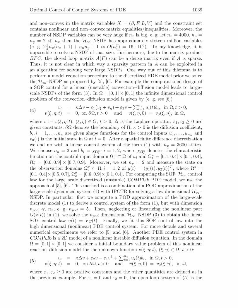
Optimal Control of Coupled Systems of PDE 1039

and non–convex in the matrix variables X = (β, F, L, V ) and the constraint setcontains nonlinear and non–convex matrix equalities/inequalities. Moreover, thenumber of NSDP variables can be very huge if nx is big, e. g. let nx = 4000, nu =ny = 2 ≪ nx then the H∞–NSDP has approximately sixteen million variables(e. g. 2 1

2nx(nx + 1) + nuny + 1 ≈ O(n2x) = 16 · 106). To my knowledge, it is

impossible to solve a NSDP of that size. Furthermore, due to the matrix productBFC, the closed loop matrix A(F ) can be a dense matrix even if A is sparse.Thus, it is not clear in which way a sparsity pattern in A can be exploited inan algorithm for solving very large NSDPs. One way out of this dilemma is toperform a model reduction procedure to the discretized PDE model prior we solvethe H∞–NSDP as proposed by [5], [6]. For example the computational design ofa SOF control for a linear (unstable) convection–diffusion model leads to large–scale NSDPs of the form (3). In Ω = [0, 1]× [0, 1] the infinite dimensional controlproblem of the convection–diffusion model is given by (e. g. see [6])

(4)vt = κ∆v − ε1(vξ + vη) + ε2v +

∑nu

i=1 ui(t)bi, in Ω, t > 0,v(ξ, η; t) = 0, on ∂Ω, t > 0 and v(ξ, η, 0) = v0(ξ, η), in Ω,

where v := v(ξ, η; t), (ξ, η) ∈ Ω, t > 0, ∆ is the Laplace operator, ε1, ε2 ≥ 0 aregiven constants, ∂Ω denotes the boundary of Ω, κ > 0 is the diffusion coefficient,bi, i = 1, . . . , nu are given shape functions for the control inputs u1, . . . , unu andv0(·) is the initial state in Ω at t = 0. After a spatial finite difference discretizationwe end up with a linear control system of the form (1) with nx = 3600 states.We choose nu = 2 and bi = χΩu

i, i = 1, 2, where χΩu

idenotes the characteristic

function on the control input domain Ωui ⊂ Ω of ui and Ωu1 = [0.1, 0.4]× [0.1, 0.4],Ωu2 = [0.6, 0.9] × [0.7, 0.9]. Moreover, we set ny = 2 and measure the state onthe observation domains Ωyi ⊂ Ω, i = 1, 2 of y(t) = (y1(t), y2(t))

T , where Ωy1 =[0.1, 0.4]×[0.5, 0.7], Ωy2 = [0.6, 0.9]×[0.1, 0.4]. For computing the SOF–H∞ controllaw for the large–scale discretized (unstable) COMPleib PDE model, we use theapproach of [5], [6]. This method is a combination of a POD approximation of thelarge–scale dynamical system (1) with IPCTR for solving a low dimensional H∞–NSDP. In particular, first we compute a POD approximation of the large–scalediscrete model (1) to derive a control system of the form (1), but with dimensionnpod ≪ nx, e. g. npod = 5. Then, neglecting or linearizing the nonlinear partG(x(t)) in (1), we solve the npod dimensional H∞–NSDP (3) to obtain the linearSOF control law u(t) = Fy(t). Finally, we fit this SOF control law into thehigh dimensional (nonlinear) PDE control system. For more details and severalnumerical experiments we refer to [5] and [6]. Another PDE control system inCOMPleib is a 2D model of a nonlinear instable diffusion equation. In the domainΩ = [0, 1] × [0, 1] we consider a initial boundary value problem of this nonlinearreaction–diffusion model for the unknown function v(ξ, η; t), (ξ, η) ∈ Ω, t > 0:

(5)vt = κ∆v + ε2v − ε1v

3 +∑nu

i=1 ui(t)bi, in Ω, t > 0,v(ξ, η; t) = 0, on ∂Ω, t > 0 and v(ξ, η, 0) = v0(ξ, η), in Ω,

where ε1, ε2 ≥ 0 are positive constants and the other quantities are defined as inthe previous example. For ε1 = 0 and ε2 = 0, the open loop system of (5) is the

1040 Oberwolfach Report 18/2005

heat equation, which is asymptotically stable. However, it is unstable if ε2 > 0 islarge enough even if ε1 = 0. The unstable viscous modified Burgers equation withboundary control input u and given κ = 0.5, ε = 0.25 is a 1D PDE instance inCOMPleib (e. g. see [6]):

vt − κvξξ + vvξ − εv = 0, ξ ∈ (0, 2π), t > 0vξ(t, 0) = 0, vξ(t, 2π) = u, v(0, ξ) = sin(ξ).

Finally, we state an unstable 1D Korteweg–de Vries–Burgers model. For givenκ = 0.5, λ = 0.1, ε = 0.345 the following boundary control problem can be foundin COMPleib :

vt − κvξξ + λvξξξ + vvξ − εv = 0, ξ ∈ (0, 2π), t > 0v(t, 0) = 0, vξ(t, 2π) = u, vξξ(t, 2π) = 0, v(0, ξ) = ξsin(ξ).

References

[1] B. Fares, D. Noll and P. Apkarian, Robust control via sequential semidefinite programming,SIAM Journal on Control and Optimization Vol. 40, No. 6 (2002), 1791–1820.

[2] M. Kocvara, F. Leibfritz, M. Stingl and D. Henrion, A nonlinear SDP algorithm for staticoutput feedback problems in COMPleib, Tech. Rep. Univ. of Trier (2004), submitted.

[3] F. Leibfritz and E. M. E. Mostafa, An interior point constrained trust region method for aspecial class of nonlinear semi–definite programming problems, SIAM Journal on Optimiza-tion Vol. 12, No. 4 (2002), 1048–1074.

[4] F. Leibfritz, COMPleib: COnstrained Matrix–Optimization Problem library – a collectionof test examples for nonlinear semidefinite programs, control system design and relatedproblems, Tech. Rep. Univ. of Trier (2004), submitted.

[5] F. Leibfritz and S. Volkwein, Reduced order output feedback control design: A case study forPDE systems using proper orthogonal decomposition and nonlinear semidefinite program-ming, Linear Algebra and its Applications (2005).

[6] F. Leibfritz and S. Volkwein, Numerical feedback controller design for PDE systems: usingmodel reduction: techniques and case studies, Tech. Rep. Univ. of Trier (2004), submitted.

Optimal Control of an Elliptic PDE with Nonlocal Radiation Interface

Conditions

Christian Meyer

(joint work with O. Klein, P. Philip, J. Sprekels, and F. Troltzsch)

This work deals with the optimal control of the production of silicon carbide (SiC)single crystals that represent an important semiconductor material. The state-of-the-art technique to produce SiC single crystals is the physical vapor transport(PVT) method. A corresponding growth apparatus mainly consists of a graphitecrucible Ωs with a cavity inside that is denoted by Ωg. This cavity is filled withargon and, at the bottom, with polycrystalline SiC powder. The crucible is heatedup to 2000–3000 K, usally by induction heating. Due to the high temperature,the SiC powder sublimates and crystallizes at the cooled top of the cavity. In thisway, the desired single crystal grows into the reaction chamber (see e.g. [3] fordetails). A simplified optimal control problem that arises from this application

Optimal Control of Coupled Systems of PDE 1041

but still covers some main difficulties, is given by the following semilinear ellipticproblem with pointwise control constraints

(P)

minimize J(y, u) :=1

2

∫

Ωg

|∇y − z|2 dx +ν

2

∫

Ωs

u2 dx

subject to −div(κs∇y) = u in Ωs

−div(κg∇y) = 0 in Ωg

κg

(∂y

∂nr

)

g

− κs

(∂y

∂nr

)

s

= G(σ|y|3y) on Γr = Ωs ∩ Ωg

κs∂y

∂n0+ εσ |y|3y = εσ y4

0 on Γ0 = ∂Ωs

and ua(x) ≤ u(x) ≤ ub(x) a.e. in Ωs,

with a desired state gradient z ∈ L2(Ω)2 and thermal conductivities κs ∈ L∞(Ωs),κg ∈ L∞(Ωg), κs, κg > 0 a.e. in Ωs and Ωg, respectively. Furthermore, y0 ∈L16(Γ0) is the external temperature with y0 ≥ ϑ > 0 a.e. on Γ0. The boundsua and ub are functions in L∞(Ωs) with 0 < ua(x) < ub(x) a.e. in Ωs. Weassume that the outer boundary Γ0 and the interface Γr are Lipschitz and Γr isadditionally piecewise C1,δ. Moreover, ε ∈ [0, 1] denotes the emissivity, σ > 0 isthe Stefan-Boltzmann constant, and G represents a nonlocal radiation operatorthat is defined by

G(σ|y|3y) := (I −K)(I − (1 − ε)K)−1ε σ|y|3y.Here, K denotes an integral operator with symmetic kernel ω, i.e. (Kv)(x) :=∫Γrω(x, z)v(z) dsz, for further details see [8], [9].

The operator G was investigated in detail by Laitinen and Tiihonen who provedthat G is a bounded linear operator from Lp(Γr) to itself for 1 ≤ p ≤ ∞ ( [4,Lemma 8]). In general, G is not positive, i.e. v(x) ≥ 0 a.e. on Γr does not imply(Gv)(x) ≥ 0 a.e. on Γr. This property causes that the nonlinearity in the stateequation in (P) is not monotone. However, Laitinen and Tiihonen showed in [4]that it is pseudomonotone. Hence, Brezis’ theorem for pseudomonotone operators(cf. [11]) implies the existence of solutions of the state equation in the state spaceV = v ∈ H1(Ω) | τrv ∈ L5(Γr), τ0v ∈ L5(Γ0). Using a technique introducedby Stampacchia in the linear case (see [2], [7]), we prove the boundedness of thesolutions in Ω and on Γr ∪Γ0 and introduce a corresponding state space by V∞ =H1(Ω) ∩ L∞(Ω) (see [5]). By the theory of Fredholm operators, the existence ofa unique solution to the linearized state equation is also shown in [5]. Based onthis result, the implicit function theorem gives the differentiability of the control-to-state operator S : L2(Ωs) → V∞. In a standard way, a pointwise discussionof the variational inequality yields the well-known projection formula for controlconstrained problems:

u(x) = Pad

−1

νp(x)

,

1042 Oberwolfach Report 18/2005

where Pad : R → R is the pointwise projection operator on [ua(x), ub(x)]. Here,p ∈ H1(Ω) denotes the adjoint state that solves the following adjoint equation

div(κg∇p) = ∆y − div z in Ωg

div(κs∇p) = 0 in Ωs

κs

(∂p

∂nr

)

s

− κg

(∂p

∂nr

)

g

+ 4σ |y|3G∗p =∂y

∂nr− z · nr on Γr

κs∂p

∂n0+ 4εσ |y|3p = 0 on Γ0.

Second-order sufficient optimality conditions are established in a very recent work[6]. The corresponding analysis is based on the techniques introduced in [1] and[10]. These conditions account for strongly active sets and give local optimality ina Ls-neighborhood of a reference function, where s can be chosen smaller than ∞.

Finally some numerical results are presented that were computed using a Gauß–Newton method. The arising linear-quadratic subproblems were solved with anactive set strategy. The PDEs were discretized with linear finite elements.

References

[1] E. Casas, F. Troltzsch, and A. Unger, Second order sufficient optimality conditions for anonlinear elliptic control problem, J. for Analysis and its Applications 15 (1996), 687–707.

[2] D. Kinderlehrer and G. Stampacchia, An Introduction to Variational Inequalities and theirApplications, Vol. 88 of Pure and Applied Mathematics, Academic Press, New York (1980).

[3] O. Klein, P. Philip, and J. Sprekels, Modeling and simulation of sublimation growth of SiCbulk single crystals, Interfaces and Free Boundaries 6 (2004), 295–314.

[4] M. Laitinen and T. Tiihonen, Conductive-radiative heat transfer in grey materials, Quart.Appl. Math. 59 (2001), 737–768.

[5] C. Meyer, P. Philip, and F. Troltzsch, Optimal control of a semilinear PDE with nonlocalradiation interface conditions, submitted to SIAM J. Control Opt. (2004).

[6] C. Meyer, Second-order sufficient optimality conditions for a semilinear optimal controlproblem with nonlocal radiation interface conditions, submitted to ESAIM: Control, Opti-misation and Calculus of Variations (2005).

[7] G. Stampacchia, Le probleme de Dirichlet pour les equations elliptiques du second ordre acoefficients discontinus, Ann. Inst. Fourier, 15 (1965), 189–258.

[8] T. Tiihonen, A nonlocal problem arising from heat radiation on non-convex surfaces, Eur.J. App. Math. 8 (1997), 403–416.

[9] T. Tiihonen, Stefan-Boltzmann radiation on non-convex surfaces, Math. Meth. in Appl. Sci.20 (1997), 47–57.

[10] F. Troltzsch and D. Wachsmuth, Second-order sufficient optimality conditions for the op-timal control of Navier-Stokes equations, accepted by ESAIM: Control, Optimisation andCalculus of Variations (2003).

[11] E. Zeidler, Nonlinear Functional Analysis and its Applications, Vol. II/B, Springer-Verlag,New York (1990).

Optimal Control of Coupled Systems of PDE 1043

Recent Results on Exact Controllability of the Navier-Stokes System

Jean-Pierre Puel

1. Introduction and main results

Let Ω ⊂ RN be a bounded regular domain, with N = 2 or N = 3. Assumethat ω ⊂ Ω is a nonempty (small) open subset and T > 0 is given. In the sequel,we will use the following notation: Q = Ω × (0, T ), Σ = ∂Ω × (0, T ); C will standfor a generic positive constant that may depend on Ω and ω.

We will be concerned here with some controllability properties of the Navier-Stokes system

(1)

yt − ∆y + (y · ∇)y + ∇p = v1ω in Q,

∇ · y = 0 in Q,

y = 0 on Σ,

y(x, 0) = y0 in Ω

and the similar linear Stokes-like problem

(2)

yt − ∆y + ∇ · (y ⊗ y + y ⊗ y) + ∇p = f + v1ω in Q,

∇ · y = 0 in Q,

y = 0 on Σ,

y(x, 0) = y0(x) in Ω,

where y = y(x, t) is given and satisfies adequate regularity assumptions. In (2),the symbol ⊗ stands for the usual tensor product in RN . As usual, it will beconvenient to analyze the observability properties of the following system, whichcan be viewed as the adjoint of (2):

(3)

−ϕt − ∆ϕ− (Dϕ)y + ∇π = g in Q,

∇ · ϕ = 0 in Q,

ϕ = 0 on Σ,

ϕ(x, T ) = ϕ0(x) in Ω.

Here, Dϕ = ∇ϕ+ ∇ϕT . We will need some function spaces:

H = z ∈ L2(Ω)N : ∇ · z = 0 in Ω, z · n = 0 on ∂Ω ,

V = z ∈ H10 (Ω)N : ∇ · z = 0 in Ω .

Furthermore, the following hypotheses over y will be needed in order to have asuitable Carleman inequality for the solutions to (3):

(4) y ∈ L∞(Q)N , yt ∈ L2(0, T ;Lσ(Ω))N(σ > 6/5 if N = 3

σ > 1 if N = 2

).

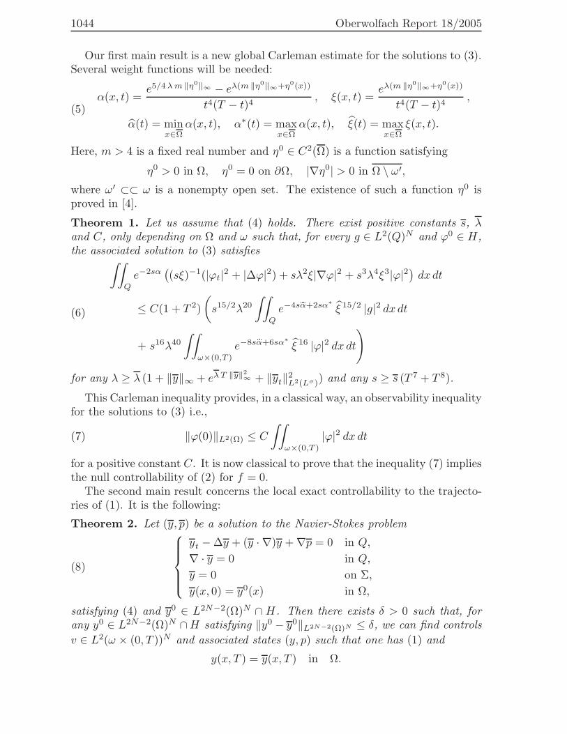
1044 Oberwolfach Report 18/2005

Our first main result is a new global Carleman estimate for the solutions to (3).Several weight functions will be needed:

(5)α(x, t) =

e5/4λm ‖η0‖∞ − eλ(m ‖η0‖∞+η0(x))

t4(T − t)4, ξ(x, t) =

eλ(m ‖η0‖∞+η0(x))

t4(T − t)4,

α(t) = minx∈Ω

α(x, t), α∗(t) = maxx∈Ω

α(x, t), ξ(t) = maxx∈Ω

ξ(x, t).

Here, m > 4 is a fixed real number and η0 ∈ C2(Ω) is a function satisfying

η0 > 0 in Ω, η0 = 0 on ∂Ω, |∇η0| > 0 in Ω \ ω′,

where ω′ ⊂⊂ ω is a nonempty open set. The existence of such a function η0 isproved in [4].

Theorem 1. Let us assume that (4) holds. There exist positive constants s, λand C, only depending on Ω and ω such that, for every g ∈ L2(Q)N and ϕ0 ∈ H,the associated solution to (3) satisfies

(6)

∫∫

Q

e−2sα((sξ)−1(|ϕt|2 + |∆ϕ|2) + sλ2ξ|∇ϕ|2 + s3λ4ξ3|ϕ|2

)dx dt

≤ C(1 + T 2)

(s15/2λ20

∫∫

Q

e−4sbα+2sα∗

ξ 15/2 |g|2 dx dt

+ s16λ40

∫∫

ω×(0,T )

e−8sbα+6sα∗

ξ 16 |ϕ|2 dx dt)

for any λ ≥ λ (1 + ‖y‖∞ + eλT ‖y‖2∞ + ‖yt‖2

L2(Lσ)) and any s ≥ s (T 7 + T 8).

This Carleman inequality provides, in a classical way, an observability inequalityfor the solutions to (3) i.e.,

(7) ‖ϕ(0)‖L2(Ω) ≤ C

∫∫

ω×(0,T )

|ϕ|2 dx dt

for a positive constant C. It is now classical to prove that the inequality (7) impliesthe null controllability of (2) for f = 0.

The second main result concerns the local exact controllability to the trajecto-ries of (1). It is the following:

Theorem 2. Let (y, p) be a solution to the Navier-Stokes problem

(8)

yt − ∆y + (y · ∇)y + ∇p = 0 in Q,

∇ · y = 0 in Q,

y = 0 on Σ,

y(x, 0) = y0(x) in Ω,

satisfying (4) and y0 ∈ L2N−2(Ω)N ∩ H. Then there exists δ > 0 such that, forany y0 ∈ L2N−2(Ω)N ∩H satisfying ‖y0 − y0‖L2N−2(Ω)N ≤ δ, we can find controls

v ∈ L2(ω × (0, T ))N and associated states (y, p) such that one has (1) and

y(x, T ) = y(x, T ) in Ω.

Optimal Control of Coupled Systems of PDE 1045

In the following sections, we will indicate the main ideas of the proofs of theo-rems 1 and 2. The detailed proofs are given in [3].

2. A new Carleman inequality

We will use the notation I(s, λ;ϕ) to denote the left hand side of (6). Letg ∈ L2(Q)N and ϕ0 ∈ H be given and let (ϕ, π) be the associated solution to (3).We can first apply to each component of ϕ the usual Carleman inequality for theheat equation with right hand side in L2(Q). After some arrangements, we get

(9) I(s, λ;ϕ) ≤ C

(∫∫

Q

e−2sα (|g|2 + |∇π|2) dx dt

+s3λ4

∫∫

ω′×(0,T )

e−2sα ξ3 |ϕ|2 dx dt),

for all λ ≥ C(1 + ‖y‖∞) and s ≥ C(T 7 + T 8). For the proof of (9), see [6] and [4];for the explicit values of λ and s, see [2].

In view of the main result in [8] and following the ideas of [7], we can estimatethe pressure gradient in (9) and deduce that

(10)

I(s, λ;ϕ) ≤ C

(s3λ4

∫∫

ω′×(0,T )

e−2sα ξ3 |ϕ|2 dx dt

+ s2 λ2

∫∫

ω1×(0,T )

e−2sα ξ2 |π|2 dx dt+ s

∫∫

Q

e−2sα ξ |g|2 dx dt),

for any λ ≥ C(1 + ‖y‖∞) and any s ≥ C(T 7 + T 8), where ω1 is an open set suchthat ω′ ⊂⊂ ω1 ⊂⊂ ω. The rest of the proof is oriented towards the absorptionof the local pressure term in (10). Let us remark that we have only used theassumption y ∈ L∞(Q)N until this moment, while more regularity on y will beneeded to perform a local estimate of the pressure.

We can assume that the pressure has been chosen with zero mean in ω1 . Then,

∫∫

ω1×(0,T )

e−2sα ξ2 |π|2 dx dt ≤ C

∫∫

ω1×(0,T )

e−2sbα ξ 2 |∇π|2 dx dt

and using the equation satisfied by ϕ and π we see that the task is to obtain localestimates of ∆ϕ and ϕt .

For the estimate of ∆ϕ, we can use classical arguments for the heat equation;observe that u = ∆ϕ fulfills a heat equation where the pressure is absent. On theother hand, integrating by parts in time and using well known a priori estimatesfor the Stokes system (see [5]), we can find a local estimate of ϕt in terms of local

integrals of ϕ and ∇ϕ and I(s, λ;ϕ). More precisely, with q = s15/2e−2sbα+sα∗

ξ 15/2

1046 Oberwolfach Report 18/2005

and ω2 an open set satisfying ω1 ⊂⊂ ω2 ⊂⊂ ω, for any small ε > 0 we obtain

s2λ2

∫∫

ω1×(0,T )

e−2sbαξ 2 |ϕt|2 dx dt

≤ ε I(s, λ;ϕ)

+ Cελ20(1 + T )

(‖q g‖2

L2(L2) + ‖q ϕ‖2L2(L2(ω2))

+ ‖q∇ϕ‖2L2(L2(ω2))

)

for λ ≥ C(1 + ‖y‖∞ + eC T ‖y‖2∞ + ‖yt‖2

L2(Lσ)). Let us remark that proving such

a local estimate requires many technical computations and led us to assume yt ∈L2(Lσ).

The local estimates of ∆ϕ and ϕt lead to the desired Carleman inequality (6).

3. The local null controllability of the Navier-Stokes system

The proof of theorem 2 follows the ideas in [7]. Thus, we deduce in a first stepa null controllability result for (2) with suitable right hand side f .

More precisely, let us set Ly = yt−∆y+∇· (y⊗ y+ y⊗ y) and let us introducein dimension N = 3 the space E3, with

(11)E3 = (y, v) ∈ E0 : esβ

∗/2(γ∗)−1/4y ∈ L4(0, T ;L12(Ω)3),

∃p : esβ∗

(γ∗)−1/2(Ly + ∇p− v1ω) ∈ L2(0, T ;W−1,6(Ω)3),where

E0 = (y, v) : e2sbβ−sβ∗

γ−15/4y, e4sbβ−3sβ∗

γ−8v1ω ∈ L2(Q)N ,

esβ∗/2(γ∗)−1/4y ∈ L2(0, T ;V ) ∩ L∞(0, T ;H).

and where the new weight functions β, β∗, etc. are given by

β(x, t) =e5/4λm‖η0‖∞ − eλ(m‖η0‖∞+η0(x))

ℓ(t)4,

β(t) = minx∈Ω β(x, t), β∗(t) = maxx∈Ω β(x, t),

γ(x, t) =eλ(m‖η0‖∞+η0(x))

ℓ(t)4, γ(t) = max

x∈Ωγ(x, t), γ∗(t) = min

x∈Ωγ(x, t).

Here, we have introduced

ℓ(t) =

T 2/4 in (0, T/2)

t(T − t) in (T/2, T ).

We then have:

Proposition 3. Let us assume that y satisfies (4) and the following hypotheseson the initial condition and the right hand side hold:

y0 ∈ H ∩ L4(Ω)3, esβ∗

(γ∗)−1/2f ∈ L2(0, T ;W−1,6(Ω)3).

Then there exists a control v such that the associated solution (y, p) to (2)satisfies (y, v) ∈ E3.

Optimal Control of Coupled Systems of PDE 1047

Notice that this is actually a null controllability result for (2). Indeed, if (y, v) ∈E3, we have in particular that y(x, T ) = 0 in Ω.

The rest of the proof of theorem 2 relies on an appropriate inverse mappingtheorem. More precisely, we use the following result (see [1]):

Proposition 4. Let E, F be two Banach spaces and let A : E 7→ F satisfyA ∈ C1(E;F ). Assume that e0 ∈ E, A(e0) = h0 and A′(e0) : E 7→ F is anepimorphism. Then, there exists δ > 0 such that, for every h ∈ F satisfying‖h− h0‖F < δ, there exists a solution of the equation

A(e) = h, e ∈ E.

We can apply this result to the mapping A : E 7→ F given by

A(y, v) = (Ly + (y · ∇)y + ∇p− v1ω, y(·, 0)) ∀(y, v) ∈ E3,

where E3 is as in (11) and F = L2(esβ∗

(γ∗)−1/2;W−1,6(Ω)3)× (L4(Ω)3∩H), withe0 = (0, 0, 0) and h0 = (0, 0).

From the definition of E3, one can easily check that A is well defined andsatisfies A ∈ C1(E;F ). Finally, the identity

Im(A′(0, 0, 0)) = F

is equivalent to the result stated in proposition 3. This completes the proof oftheorem 2.

References

[1] V. M. Alekseev, V. M. Tikhomirov, S. V. Fomin, Optimal control. Translated from theRussian by V. M. Volosov. Contemporary Soviet Mathematics. Consultants Bureau, NewYork, 1987.

[2] E. Fernandez-Cara, S. Guerrero, Global Carleman inequalities for parabolic systemsand applications to null controllability, to appear.

[3] E. Fernandez-Cara, S. Guerrero, O.Yu. Imanuvilov, J.-P. Puel, Local exact control-lability of the Navier-Stokes system, Journal de Mathematiques Pures et Appliquees, 2005.

[4] A. Fursikov, O. Yu. Imanuvilov, Controllability of Evolution Equations, Lecture Notes#34, Seoul National University, Korea, 1996.

[5] Y. Giga, H. Sohr, Abstract Lp estimates for the Cauchy problem with applications to theNavier-Stokes equations in exterior domains, Journal of Functional Analysis, 102 (1991),72–94.

[6] O. Yu. Imanuvilov, Controllability of parabolic equations (Russian), Math. Sb., 186, No.6 (1995), 109–132.

[7] O. Yu. Imanuvilov, Remarks on exact controllability for the Navier-Stokes equations,ESAIM Control Optim. Calc. Var. 6 (2001), 39–72.

[8] O.Yu. Imanuvilov, J. P. Puel, Global Carleman estimates for weak elliptic non homoge-neous Dirichlet problem, Int. Math. Research Notices, 16, 2003, 883–913.

1048 Oberwolfach Report 18/2005

Feedback Boundary Stabilization of the Two and the Three

Dimensional Navier-Stokes Equations

Jean-Pierre Raymond

Let Ω be a bounded and connected domain in R2 or R3 with a regular boundaryΓ, ν > 0, and consider a couple (w, χ) – a velocity field and a pressure – solutionto the stationary Navier-Stokes equations in Ω:

−ν∆w + (w · ∇)w + ∇χ = f and div w = 0 in Ω, w = u∞s on Γ.

We assume that w is regular and is an unstable solution of the instationary Navier-Stokes equations. We want to determine a Dirichlet boundary control u, in feed-back form, localized in a part of the boundary Γ, so that the corresponding con-trolled system:

(1)

∂y

∂t− ν∆y + (y · ∇)w + (w · ∇)y + (y · ∇)y + ∇p = 0,

div y = 0 in Q∞, y = Mu on Σ∞, y(0) = y0 in Ω,

be stable for initial values y0 small enough in an appropriate space X(Ω). In thissetting, Q∞ = Ω × (0,∞), Σ∞ = Γ × (0,∞), X(Ω) is a subspace of V0

n(Ω) =y ∈ L2(Ω) | div y = 0 in Ω, y · n = 0 on Γ

, w ∈ X(Ω), and the operator

M is a restriction operator ensuring that the control is localized on a part of theboundary Γ (see [10]). If we set (z, q) = (w + y, χ+ p) and if u = 0, we see that(z, q) is the solution to the Navier-Stokes equations

∂z

∂t− ν∆z + (z · ∇)z + ∇q = f , div z = 0 in Q∞,

z = u∞s on Σ∞, z(0) = w + y0 in Ω.

Thus y0 is a perturbation of the stationary solution w. When w ∈ L∞(Ω) andy0 ∈ V0

n(Ω) ∩ L4(Ω) with |y0|L4(Ω) small enough, the existence of a boundarycontrol u such that the solution to equation (1) exponentially decreases in thenorm of the space X(Ω) = V0

n(Ω)∩L4(Ω), follows from a local exact controllabilityresult stated in [5, Theorem 2]. But the proof in [5] does not give any way todefine such a control in feedback form. In the three-dimensional case, and when

X(Ω) =y ∈ H1(Ω) | div y = 0 in Ω, 〈y · n, 1〉H−1/2(Γ),H1/2(Γ) = 0

, the

existence of a control exponentially stabilizing (1) is proved in [6]. One way toconstruct robust feedback laws consists in using the methods of the optimal controltheory. This approach has been studied in the case of an internal control [1–3],and has been numerically tested with a boundary control in the very specificgeometry of the rectangular driven cavity [7] and when the normal componentof the control is equal to zero. As it is the situation corresponding to manyengineering applications [8,9], here we do not assume that the normal componentof the control variable is zero.

The Linear-Quadratic theory for the Dirichlet control of the linearized Navier-Stokes equations has been studied in a very recent work [4], in the case when

Optimal Control of Coupled Systems of PDE 1049

the normal component of the boundary control is zero, and when the controlis applied everywhere on the boundary. To the best of our knowledge the casewhen the normal component is not equal to zero has not yet been studied in theliterature. The main objectives of this talk are:

- first to develop the Linear-Quadratic theory over an infinite time horizon ofthe Dirichlet boundary control of the Oseen equations when the control is localizedon a part of the boundary, and when the normal component of the control is notzero,

- next to show that the linear feedback law, calculated with the linearized model,and applied to the nonlinear equation (1), provides a local exponential stabilizationof the state in some appropriate space X(Ω).

In the two dimensional case the feedback control law is obtained by studyingthe control problem

(P) infJ(y,u) | (y,u) satisfies (2), u ∈ L2(0,∞;V0(Γ))

,

where

J(y,u) =1

2

∫ ∞

0

∫

Ω

|y|2 dxdt+1

2

∫ ∞

0

∫

Γ

|u|2 dxdt,and

(2)

∂y

∂t− ν∆y + (w · ∇)y + (y · ∇)w − ωPy + ∇p = 0, in Q∞,

div y = 0 in Q∞, y = Mu on Σ∞, y(0) = y0 in Ω,

where V0(Γ) =y ∈ L2(Γ) | 〈y · n, 1〉H−1/2(Γ),H1/2(Γ) = 0

. The coefficient

ω > 0, which is not present in (1), is added in equation (2) in order to guaranteethe exponential decay in the norm H1/2−ε(Ω), 0 < ε < 1/4, of the solution of thenonlinear closed loop system defined below. We show that the control problem (P)can be rewritten in the form of another control problem in which the state variableis Py – where P is the so-called Helmholtz projection operator – and not y. Thistransformation is essential in our approach. It leads to a Riccati equation whichis the natural one for the new control problem, but which is not the expected oneif we only consider problem (P). This transformation of (P) into a new controlproblem is a direct consequence of rewriting equation (2) in the form:

(3)Py′ = APy − ωPy +BMu, y(0) = y0,

(I − P )y = (I − P )DAγnMu.

The operator A is the Oseen operator, the control operator is defined by B =(λ0I − A)DA for some λ0 > 0, and DA is the Dirichlet operator associated withλ0I −A. We refer to [10] for the transformation of equation (2) into (3), and forregularity results for equation (3). Denoting by Πω the solution to the Riccatiequation of the control problem (P), and setting RA = MD∗

A(I − P )DAM + I,we show that the closed loop system

∂y

∂t− ν∆y + (w · ∇)y + (y · ∇)w + ∇p = 0, in Q∞,

div y = 0 in Q∞, y = −MR−1A MB∗ΠωPy on Σ∞, y(0) = y0 in Ω,

1050 Oberwolfach Report 18/2005

is exponentially stable if |y0|H1/2−ε(Ω)∩V0n(Ω) is small enough for some 0 < ε < 1/4.

In the three dimensional case we obtain a similar result by studying the controlproblem

(Q) infI(y,u) | (y,u) satisfies (4), u ∈ L2(0,∞;V0(Γ))

,

where

I(y,u) =1

2

∫ T

s

∫

Ω

|(−P∆)−1/2Py|2 +1

2

∫ T

s

∫

Γ

|R1/2A u|2,

and

(4)

∂y

∂t− ν∆y + (w · ∇)y + (y · ∇)w − ωy + ∇p = 0, in Q∞,

div y = 0 in Q∞, y = θ(t)Mu on Σ∞, y(0) = y0 in Ω.

The weight function θ is a C2 function from R+ into [0, 1], satisfying θ(0) = 0,θ(t) = 1 for t ≥ T for some T > 0. In that case the solution Πω of the Riccatiequation of the control problem (Q) depends on t in the intervall [0, T ]. Theexponential decay is obtained in the norm H1/2+ε(Ω) if |y0|

H1/2+ε0 (Ω)∩V0

n(Ω)is

small enough.

References

[1] V. Barbu, Feedback stabilization of the Navier-Stokes equations, ESAIM COCV, 9 (2003),197–206.

[2] V. Barbu, S. S. Sritharan, H∞ - control theory of fluid dynamics, Proc. R. Soc. Lond. A454 (1998), 3009–3033.

[3] V. Barbu, R. Triggiani, Internal stabilization of Navier-Stokes equations with finite dimen-sional controllers, Indiana University Journal, 52(5) (2004), 1443–1494.

[4] V. Barbu, I. Lasiecka, R. Triggiani, Boundary stabilization of Navier-Stokes equations, Mem-oirs of the A.M.S., 2005, to appear.

[5] E. Fernandez-Cara, S. Guerrero, O. Yu. Imanuvilov, J.-P. Puel, Local exact controllabilityof the Navier-Stokes system, 83 2004, 1501–1551.

[6] A. V. Fursikov, Stabilization for the 3D Navier-Stokes system by feedback boundary control,Discrete and Cont. Dyn. Systems, 10 (2004), 289-314.

[7] B. B. King, Y.-R. Ou, Nonlinear dynamic compensator design for flow control in a drivencavity, Proc. 34th CDC, Dec. 1995, 3741-3746.

[8] J.-W. He, R. Glowinski, R. Metcalfe, A. Nordlander, J. Periaux, Active control and dragoptimization for flow past a circular cylinder, JCP 163 (2000), 83-117.

[9] D. S. Park, D. M. Ladd, and E. W. Hendricks, Feedback control of von Karman vortex

shedding behind a circular cylinder at low Reynolds numbers, Phys. Fluids, 6 (1994), 2390-2405.

[10] J.-P. Raymond, Stokes and Navier-Stokes equations with nonhomogeneous boundary condi-tions, 2005, submitted.

[11] J.-P. Raymond, Boundary feedback stabilization of the two dimensional Navier-Stokes equa-tions, 2005, submitted.

[12] J.-P. Raymond, Boundary feedback stabilization of the three dimensional Navier-Stokesequations, in preparation.

Optimal Control of Coupled Systems of PDE 1051

Sufficient Second-Order Optimality Conditions for Mixed Constrained

Optimal Control Problems

Arnd Rosch

(joint work with Fredi Troltzsch)

In this talk we consider the optimal control problem to minimize

(1) F (y, u) =

∫

Ω

f(x, y(x)) dx+

∫

Γ

g(x, y(x), u(x)) ds(x)

subject to the state equations

Ay + y = 0 in Ω

∂nAy = b(x, y, u) on Γ,(2)

the control constraints

(3) 0 ≤ u(x) for x ∈ Γ,

and to the mixed control-state constraints

(4) c(x) ≤ u(x) + γ(x)y(x) for x ∈ Γ.

The main task of our talk is to establish second-order sufficient optimality con-ditions that are close to the associated necessary ones. For control-constrainedproblems, this issue was discussed quite completely in literature for semilinearelliptic and parabolic equations.

A suitable Lagrange functional can be defined by

L(y, u, p, µ1, µ2) = F (y, u) −∫

Ω

(

m∑

i,j=1

aijDjyDip+ yp) dx−∫

Γ

bp ds(x)

−∫

Γ

µ1u ds(x) −∫

Γ

(u+ γy − c)µ2 ds(x)

since the Lagrange multipliers can be expressed by regular functions, i.e. p ∈Y = C(Ω) ∩ H1(Ω) and µi ∈ L∞(Γ): The existence of such regular Lagrangemultipliers has been proved in Troltzsch [6], Bergounioux, Troltzsch [2], and Arada,Raymond [1] for the parabolic case and Troltzsch [7], Rosch, Troltzsch [4] for theelliptic case. The existence of regular multipliers can be shown under a Slater typecondition and the assumption γ ≥ 0.

Moreover any local solution u, the associated state y, the corresponding adjointstate p ∈ Y , and regular Lagrange multipliers µi ∈ L∞(Γ), have to satisfy together

1052 Oberwolfach Report 18/2005

the following first order necessary optimality system (FON),

(FON)

DyL(y, u, p, µ1, µ2) = 0DuL(y, u, p, µ1, µ2) = 0and for a.a. x ∈ Γµ1(x) ≥ 0µ2(x) ≥ 0u(x)µ1(x) = 0(u(x) + γ(x)y(x) − c(x))µ2(x) = 0.

We define strongly active sets by

A1(δ1) := x ∈ Γ : µ1(x) ≥ δ1,A2(δ2) := x ∈ Γ : µ2(x) ≥ δ2.

Moreover, we say that (y, u) ∈ C(Ω) × L∞(Γ) belongs to the critical subspace, if

u = 0 on A1,

u+ γy|Γ = 0 on A2,

and

Ay + y = 0 in Ω

∂nAy − by y = bu u in Γ

Now, we are able to state sufficient second-order optimality conditions:SSC: There exist positive numbers δ, δ1, δ2 such that the definiteness condition

L′′(y,u)(y, u, p, µ1, µ2)[y, u]

2 ≥ δ‖u‖2L2(Γ)

is satisfied for all (y, u) belonging to the critical subspace.Theorem: Let (SSC) and a regularity condition be satisfied. Then there exist

δs > 0 and ε > 0 such that the quadratic growth condition

F (y, u) − F (y, u) ≥ δs‖u− u‖2L2(Γ)

holds for all admissible pairs (y, u) with ‖u− u‖L∞(Γ) < ε. Therefore, u is a locallyoptimal control in the sense of L∞(Γ).

The regularity condition is a solvability condition of an elliptic partial differ-ential equation (see [5]). This condition is similar to the linear independenceconstraint qualification in finite dimensional optimization.

The presented theory is more general than a former result of the authors [3]:We abstain from any nonnegativity property of involved operators. Moreover, thedefinition of the strongly active sets seems to be more natural than in [3].

References

[1] N. Arada and J. P. Raymond, Optimal control problems with mixed control-state constraints,SIAM J. Control Optimization, 39 (2001), 1391–1407.

[2] M. Bergounioux and F. Troltzsch, Optimal control of semilinear parabolic equations withstate-constraints of bottleneck type, ESAIM, Control, Optimisation and Calculus of Varia-tions, 4 (1999), 595–608.

Optimal Control of Coupled Systems of PDE 1053

[3] A. Rosch and F. Troltzsch, Sufficient second order optimality conditions for a parabolicoptimal control problem with pointwise control-state constraints, SIAM J. Control and Op-timization, 42 (2003), pp. 138–154.

[4] A. Rosch and F. Troltzsch, Existence of regular Lagrange multipliers for elliptic optimalcontrol problem with pointwise control-state constraints, submitted.

[5] A. Rosch and F. Troltzsch, Sufficient second-order optimality conditions for an ellipticoptimal control problem with pointwise control-state constraints, submitted.

[6] F. Troltzsch, A minimum principle and a generalized bang-bang-principle for a distributedoptimal control problem with constraints on the control and the state., ZAMM, 59 (1979),737–739.

[7] F. Troltzsch, Regular Lagrange multipliers for problems with pointwise mixed control-stateconstraints, SIAM J. Optimization, to appear.

On compactness, Domain Dependence and Existence of Steady State

Solutions to Compressible Isothermal Navier-Stokes Equations.

Jan Sokolowski

(joint work with P. I. Plotnikov)

We prove the existence of stationary solutions to the Navier-Stokes equations ofcompressible isentropic flows

αu + div (u⊗ u) + ∇γ = F + ∆u + (1 + ν)∇divu in D′(Ω),(1a)

α+ div (u) = f in D′(Ω), u = 0 on ∂Ω(1b)

in a bounded domain Ω ⊂ R3 on the condition that the adiabatic constant γ ≥ 1.The main result is the following

Theorem. If γ > 1, then for every F ∈ C(Ω) problem (1) has a weak solution

∈ Lγ(Ω), u ∈ H1,20 (Ω). If γ = 1, then there are ∈ L1(Ω) and u ∈ H1,2

0 (Ω)satisfying (1b) such that

αu + div (u ⊗ u) + ∇+ div S = F + ∆u + (1 + ν)∇divu.

Here the weak star defect measure S is concentrated on the one-dimensional rec-tifiable set Ωsing and has the representation

∫

Ω

ϕ(x) : dS(x) =

∫

Ωsing

s(x) ⊗ s(x) : ϕ(x)m(x)dH1 for all ϕ ∈ C10 (Ω)9,

Theorem yields the alternative: Either the concentration set is empty or itsHausdorff dimension is equal to one. Whether concentrations are cancelled or anon-trivial singular set really exists is a question which we cannot decide withcertainty. Note only that if approximate solutions and a flow region are alsoinvariant under the action of some group x → x′, then a concentration set anda measure density θ also are invariant under the action of the this group. Theprecise definition of the concentration set and the measure density are given in [2].In particular, the velocity field and the pressure are invariant with respect to theshift x3 → x3 + const, in the case of a two-dimensional flow in the plane (x1, x2).Therefore, in this case Ωsing is the union of a countable set of straight lines andθ is a constant along each of those. From this we conclude that ÷S = 0 and

1054 Oberwolfach Report 18/2005

concentrations are cancelled in agreement with results of P.L. Lions and [1]. Thesame results hold true for axially symmetric flows. On the other hand, the simpleexamples show that singularities definitely exist for solutions of the pressurelessNavier-Stokes equations, which are used in astrophysics. Finally, let us point outthat the results can be used in three dimensional case, in the same way as in [1]in two dimensional case, to establish the existence of solutions for the associatedshape optimization problems of the drag minimization.

References

[1] P.I. Plotnikov, J. Sokolowski On compactness, domain dependence and existence ofsteady state solutions to compressible isothermal Navier-Stokes equations Jornal of Mathe-matical Fluid Mechanics, 7(2005), in press RR-5156 : http://www.inria.fr/rrrt/rr-5156.html

[2] P.I. Plotnikov, J. Sokolowski Concentrations of solutions to time-discretizied compress-ible Navier -Stokes equations to appear in: Communications in Mathematical Physics, RR-5481 : http://www.inria.fr/rrrt/rr-5481.html

[3] P.I. Plotnikov, J. Sokolowski Stationary Boundary Value Problems for Navier-StokesEquations with Adiabatic Index ν < 3/2. Doklady Mathematics. Vol. 70, No. 1, 2004, 535-538, Translated from Doklady Akademii Nauk, Volume 397, N.0, 1-6, 2004,

An Optimization Approach for Frictional Contact Problems

Georg Stadler

We are concerned with the development and convergence analysis of second-orderalgorithms for the solution of frictional contact problems in function space. Themain difficulty of these problems lies in the contact and friction conditions, whichare inherently nonlinear thus making both theoretical analysis as well as an efficientnumerical realization challenging (we refer to the selected contributions [1,2,5] andthe references given therein). Here, we mainly consider the contact problem withTresca friction (also known as given friction) and remark that the more realisticcontact problem with Coulomb friction can be approached by solving a sequenceof Tresca friction problems and using a fixed point idea.

The contact problem with Tresca friction can be stated as the following con-strained and non-differentiable optimization problem:

(P) minτy=0 on Γd

τN y≤d a.e. on Γc

J(y) :=1

2a(y,y) − L(y) +

∫

Γc

Fg‖τTy‖ dx.

Here, Ω ⊂ Rn, n = 2, 3 is the region occupied by the elastic body whose boundaryis split into three disjoint parts Γd,Γn and Γc. By ε(y) = 1

2

(∇y + (∇y)⊤

)and

σ(y) = λtr(ε(y))Id+2µε(y) we denote the linear strain and stress tensors, respec-tively, where λ and µ are the Lame parameters given by λ = (Eν)/

((1+ν)(1−2ν)

)

and µ = E/(2(1 + ν)

)with Young’s modulus E > 0 and the Poisson ration

ν ∈ (0, 0.5). The symmetric bilinear form a(· , ·) and the linear form L(·) are de-fined by a(y, z) :=

∫Ω

σ(y) : ε(z) dx and L(y) =∫Ω

fy dx+∫Γn

t τy dx, where “:”

denotes the sum of the componentwise products and f ∈ L2(Ω) and t ∈ L2(Γn)denote inner force and surface tractions, respectively. The function g ∈ L2(Γc)

Optimal Control of Coupled Systems of PDE 1055

denotes the given friction and F : Γc → R is such that Fg ∈ L2(Γc). Moreover,d ≥ 0 models a possible gap between elastic body and rigid foundation. Finally,τN and τT denote the normal and tangential component of the trace operator,respectively.

While (P) is a constrained and non-differentiable optimization problem, itsFenchel dual is a constrained maximization problem with a differentiable func-tional [7]. The variables appearing in this dual problem can be interpreted ascomponents of the stress tensor σ(y) and the first-order optimality conditions for(P) (in the context of duality theory often called extremality conditions) involveboth primal and dual variables.

Due to a lack of regularity of the dual variables we introduce a Tichonov-typeregularization in the dual problem, depending on parameters γ1, γ2 > 0. In thecorresponding primal problem this regularization leads to a quadratic penalizationof the pointwise inequality constraint corresponding to the contact condition, andto a local C1-smoothing of the non-differentiable friction term. As the regular-ization parameters tend to infinity, it can be shown that both the solution of theprimal and of the dual problem converge to the solution of the original (primaland dual) problem in the corresponding function spaces.

For simplicity, in what follows we restrict ourselves to the case of planar elas-ticity, i.e., n = 2 (see also [6]). In this case the primal solution yγ ∈ (H1(Ω))n ofthe smoothed problem is characterized by the existence of dual variables λγ , µγ ∈L2(Γc) such that

a(yγ , z) − L(z) + (µγ , τTz)Γc + (λγ , τNz)Γc = 0 for all z ∈ (H1(Ω))n,

λγ − max(0, λ+ γ1(τNyγ − d)) = 0 on Γc,γ2(ξγ − τTyγ) + µγ − µ = 0,

ξγ − max(0, ξγ + σ(µγ − Fg)) − min(0, ξγ + σ(µγ + Fg)) = 0on Γc,

where σ > 0 is arbitrary and λ, µ ∈ L2(Γc) denote fixed shifting functions whoseintroduction is motivated by augmented Lagrangians.

The above equations are semismooth in function space in the sense of [3, 8].Thus, we can apply a generalized Newton method for their solution. Due to theappearance of the pointwise max- and min- functions, this results in an algorithmhaving the form of an active set method. It is related to the strategy in [1] and canbe shown to converge locally superlinear in infinite dimensions. In our numericalexperiments we observe that the method performs very reliably and that it con-verges from any initialization after very few (usually 5–12) iterations. Moreover,the number of iterations depends only weakly on the mesh-size and on the valueof the regularization parameters, i.e., we can solve the regularized problem veryefficiently.

Naturally, the question arises how a family of regularized solutions can be usedto obtain the solution of the original problem. Here, we propose two possibilities:Firstly, a first-order augmented Lagrangian method, which is an update strategy

1056 Oberwolfach Report 18/2005

for the shift parameters λ and µ. While having desirable properties such as con-vergence from arbitrary initialization, the convergence of this method is quiteslow if the regularization parameters γ1, γ2 are kept fixed. The second method wepropose is a continuation strategy with respect to the parameters γ1, γ2. Theseparameters can either be increased heuristically or, more conveniently, using aninfinite-dimensional path-following strategy as proposed in [4] for an obstacle prob-lem. Similarly as for interior point methods the overall number of iterations of thepath-following method can be decreased if the auxiliary problems are only solvedapproximately. The performance of our methods for solving contact problems withTresca friction carries over to problems with Coulomb friction using a fixed pointalgorithm.

References

[1] P. Alart and A. Curnier, A mixed formulation for frictional contact problems prone toNewton like solution methods, Comp. Meth. Appl. Mech. Engng. 92 (1991), 353–375.

[2] J. Haslinger, Z. Dostal and R. Kucera, On a splitting type algorithm for the numerical real-ization of contact problems with Coulomb friction, Comp. Meth. Appl. Mech. Engng. 191(2002), 2261–2281.

[3] M. Hintermuller, K. Ito and K. Kunisch, The primal-dual active set strategy as a semi-smooth Newton method, SIAM J. Optim. 13(3) (2003), 865–888.

[4] M. Hintermuller and K. Kunisch, Path-following methods for a class of constrained min-imization problems in function space, Technical Report 04–11, CAAM, Rice University(2004).

[5] R. Krause, Monotone Multigrid Methods for Signorini’s Problem with Friction, PhD thesis,FU Berlin, (2001).

[6] K. Kunisch and G. Stadler, Generalized Newton methods for the 2D-Signorini problem withfriction in function space, to appear in Mathematical Modelling and Numerical Analysis(M2AN) (2005).

[7] G. Stadler, Infinite-Dimensional Semi-smooth Newton and Augmented Lagrangian Meth-ods for Friction and Contact Problems in elasticity, PhD thesis, University of Graz (2004).

[8] M. Ulbrich, Semismooth Newton methods for operator equations in function spaces, SIAMJ. Optim. 13(3) (2003), 805–842.

Dirichlet Boundary Stabilization of the Plate Equation

Marius Tucsnak

(joint work with Kaıs Ammari and Gerald Tennenbaum)

The aim of this work is to give an exponential stability result for a Bernoulli-Euler plate equation in a square, damped by a feedback bending moment actingon a part of the boundary. The main novelty brought in by this work is that itgives a complete characterization of the control regions for which the exponentialstability property holds. The main result of this work is the following.

Optimal Control of Coupled Systems of PDE 1057

Theorem 1. Consider the square Ω = (0, π) × (0, π) and let Γ be an open subsetof ∂Ω. Consider the following control problem

w + ∆2w = 0, x ∈ Ω, t > 0,(1)

w(x, t) = 0, x ∈ ∂Ω, t > 0,(2)

∆w = 0, x ∈ ∂Ω \ Γ, t > 0(3)

∆w(x, t) = − ∂

∂ν(Gw), x ∈ Γ, t > 0(4)

w(x, 0) = w0(x), w(x, 0) = w1(x), x ∈ Ω,(5)

where G denotes the inverse of the Laplace operator with homogenous Dirichletboundary conditions in Ω and ν denotes the outer unit normal field to ∂Ω. Thenthe following assertions are equivalent:1) The system (1)-(5) is exponentially stable in H1

0 (Ω) ×H−1(Ω).2) The control region Γ contains both a horizontal and a vertical segment of nonzero length.

Sketch of the Proof.First step. We show that equations (1)-(5) are equivalent, in a precise sense, toan initial value problem of the form

w(t) +A0w(t) +B0B∗0 w(t) = 0 ,

w(0) = w0, w(0) = w1,

where H is an appropriate Hilbert space, A0 : D(A0)→H is a self-adjoint andstrictly positive operator, and B0 is an unbounded admissible control operator

defined in Hilbert space U with values in[D(A

120 )]∗

.

Second step. We show that the operators A0 and B0 defined at the first stepsatisfy the condition

If β > 0 is fixed and Cβ =λ ∈ C |Reλ = β

, the function

λ ∈ C+ =λ ∈ C |Reλ > 0

→ H(λ) = λB∗

0 (λ2I +A0)−1B0 ∈ L(U)

is bounded on CβThe basic technical tool in the proof of the above estimate is the following

elementary lemma.

Lemma 2. Assume that α > 0. Then there exists a constant C > 0, dependingonly on α, such that for all m ∈ N and for all λ ∈ C with real part equal to α wehave

∑

n≥0

|λ||λ2 + (m2 + n2)2| ≤ C .

1058 Oberwolfach Report 18/2005

Third step.

By using the result obtained at step 2, combined with the general result from [1]it follows that that the exponential stability of (1)-(5) is equivalent to an exactobservability estimate for the corresponding undamped problem. The proof is con-cluded by using the recent result in [2] which asserts that this exact observabilityresult property is equivalent to property 2) in the statement of the theorem.

References

[1] K. Ammari and M. Tucsnak, Stabilization of second order evolution equations by a class ofunbounded feedbacks, ESAIM. COCV., 6 (2001), 361-386.

[2] K. Ramdani, T. Takahashi, G. Tenenbaum and M. Tucsnak, A spectral approach for theexact observability of infinite dimensional systems with skew-adjoint generator, J. Funct.Anal., to appear.

Quantum Control: from Theory to Experimental Practice

Gabriel Turinici

This summary will present activities related to the control of quantum phenomena.More specifically, the focus of the research presented here is on the interaction ofthe laser with matter. The applications include not only tailored construction ofchemical compounds (through selective dissociation of chemical bounds in mole-cules or through creation of new ones), but also preparation of specific quantumstates (that can for instance be later used in logic gates for quantum computers)and fast switches in semiconductors. Yet other applications are related to the HighHarmonic Generation techniques, where a laser of given frequency is input to asystem (typically a chrystal) and lasers of integer multiples of this frequency areobtained as output; this is a very promising technique to build e.g. high frequencyX-rays lasers. The mathematical description of the laser-matter interaction is for-mulated within the framework of the quantum theory through a time dependentSchrodinger equation containing on the one part the internal Hamiltonian of thesystem H0 and on the other part terms describing the its interaction with thelaser. If the interaction is considered up to the first order, a bi-linear system re-sults where the control term (the laser intensity) ǫ(t) multiplies the quantum statewavefunction:

i ∂∂tΨ(x, t) = (H0 − ǫ(t)µ)Ψ(x, t)Ψ(x, t = 0) = Ψ0(x).

(1)

Here x is the set of internal variables, Ψ is the state of the system and µ(x) is thecoupling dipole operator.

1. Quantum controllability

Successful control of chemical phenomena has been demonstrated on a variety ofexperimental settings. A natural question is concerned to the controllability of thesystems, which requires to assess the set of all attainable final states. Results havealready been obtained in finite-dimensional settings related to the computation of

Optimal Control of Coupled Systems of PDE 1059

the Lie algebra spanned by −iH0 and −iµ [1, 2] or directly with tangent spaceresults [3], and a fairly complete description of phenomena at work is present.However, fundamental questions remains still unanswered in this field such as thegood notions of controllability of the infinite-dimensional equations complementedwith easily implementable criterions to assess this controllability property.

2. Monotonic algorithms for quantum optimal control

At the level of the numerical simulations, much work is still required in or-der to bring the size of the systems that can be treated accurately to practicaldimensions. Of course, using efficient algorithms to solve the quantum controlcritical point equations is crucial to the overall cost reduction; some of the mostused schemes nowadays fall within the class of monotonically convergent algo-rithms that are guaranteed to improve the performance (measured through a costfunctional J(ǫ)) at each iteration. Joint work with several co-authors lead to theintroduction of new classes of monotonic algorithms [4, 5] and to the study oftheir convergence properties. Further works concerned the Lyapunov functionalapproaches [6]. Finally, similarities between the two classes of algorithms havebeen demonstrated.

3. Algorithms for experimental realization of quantum control

Experimental realization of quantum control is performed in practice throughthe minimization of the cost functional J(ǫ), realized on a computer, but whichcalls an experimental cycle each time when the value J(ǫ), is to be computed, andmeasures the result; the minimization algorithm used is most often a derivative ofGenetic Algorithms or Evolutionary Strategy paradigm. The understanding of howthis algorithm manages to find the good solutions and its practical implicationsare the goal of this part of my research. During our studies, we realized that otheralgorithms can be used in the experimental setting [7], and one of those is actuallyunder implementation at Princeton University.

4. Parallel in time discretization schemes.

Whereas massively parallel computers enable simulations on larger and largerspace scales, very few methods are available to achieve similar results in the timedomain. Naturally, contrary to space, time is sequential and this precludes apriori the straightforward implementation of a parallel approach. The pararealdiscretization scheme (designed initially with JL Lions and Y Maday) [8] is apossible solution to this endeavor. It combines very precise simulations run inparallel on disjoint time segments with a coarse (approximate) simulation over theentire time span. This scheme has also been extended to the control of quantumevolution equations [9].

1060 Oberwolfach Report 18/2005

5. Dynamical discrimination of molecules

Similar molecules often may be characterized as sharing common chemical struc-tures and as such, they are expected to have related Hamiltonians and similarchemical and physical properties. Examples range from simple isotopic variantsof diatomics to highly complex molecules including those of biological relevance.A common need is to analyze or separate one molecular species in the presence ofpossibly many other similar agents. To enhance the ability to distinguish mole-cules, we advocate the use of the optimal dynamic discrimination (ODD) approach:all similar molecules are excited by a common laser pulse optimized to maximizesignals from only one species, while suppressing signals from all the others. Acontrollability analysis and implementations [10, 11] shown that this techniquesgives good results in practice.

References

[1] Wu, R.; Rabitz, H.; Turinici, G. and Sola, I. Connectivity Analysis of Controlled QuantumSystems Phys. Rev. A, 2004 , 70 , 052507

[2] Turinici, G. and Rabitz, H. Optimally controlling the internal dynamics of a randomlyorientated ensemble of molecules PRA, 2004 , 70 , 063412

[3] Turinici, G. and Rabitz, H. Quantum Wave Function Controllability Chem. Phys. , 2001 ,267 , 1-9

[4] Maday, Y. and Turinici, G. New formulations of monotonically convergent quantum controlalgorithms J. Chem. Phys., 2003 , 118

[5] Ohtsuki, Y.; Turinici, G. and Rabitz, H. Generalized monotonically convergent algorithmsfor solving quantum optimal control problems J. Chem. Phys., 2004 , 120 , 5509-5517

[6] Mirrahimi, M.; Turinici, G. and Rouchon, P. Lyapunov control of bilinear Schrodingerequations Automatica, accepted, 2004

[7] Turinici, G.; Le Bris, C. and Rabitz, H. Efficient algorithms for the laboratory discovery ofoptimal quantum controls Phys. Rev. E, 2004 , 70 , 016704

[8] Lions, J.; Maday, Y. and Turinici, G. A parareal in time discretization of PDEs C. R. Acad.Sci., Paris, Ser. I, Math., 2001 , 332 , 661-668

[9] Maday, Y. and Turinici, G. Parallel in time algorithms for quantum control: the pararealtime discretization scheme Int. J. Quant. Chem., 2003 , 93 , 223-228

[10] Li, B.; Turinici, G.; Ramakhrishna, V. and Rabitz, H. Optimal Dynamic Discrimination ofSimilar Molecules Through Quantum Learning Control Journal of Physical Chemistry B ,2002 , 106 , 8125-8131

[11] Turinici, G.; Ramakhrishna, V.; Li, B. and Rabitz, H. Optimal Discrimination of Multi-ple Quantum Systems: Controllability Analysis Journal of Physics A: Mathematical and

General, 2003 , 37 , 273-282

Second-Order Approaches to Constrained Large-Scale Optimization

Problems with Partial Differential Equations

Michael Ulbrich

We consider two modern second order approaches to constrained large-scale op-timization problems with PDEs: Interior-point methods and semismooth Newtonmethods. It is shown that the resulting linear systems for the step computationhave very similar structure. In order to implement these algorithms efficiently, fast

Optimal Control of Coupled Systems of PDE 1061

solvers for the Newton systems have to be developed. We describe how the semi-smooth Newton system arising from 3D two-body elastic contact problems can besolved very efficiently by multigrid methods [3]. As a second application, we con-sider free material optimization (see, e.g., [1, 4]) and develop a preconditioner forthe primal-dual/semismooth Newton system. Finally, free material optimizationwith contact is considered. This problem results in an infinite-dimensional mathe-matical program with equilibrium constraints (MPEC). Currently, MPECs [2] areunder intensive investigation in the field of finite-dimensional nonlinear optimiza-tion. We show that the approaches developed there are successfully applicable tothe problem at hand. The investigations of this study are illustrated and supportedby large-scale numerical tests.

References

[1] M. P. Bendsoe, O. Sigmund, Topology optimization – Theory, methods and applications,Springer, 2003.

[2] Z.-Q. Luo, J.-S. Pang, and D. Ralph, Mathematical programs with equilibrium constraints,Cambridge University Press, 1996.

[3] M. Ulbrich and S. Ulbrich, A multigrid semismooth Newton method for contact problemsin linear elasticity, Technical Report in preparation, Fachbereich Mathematik, UniversitatHamburg, 2005.

[4] J. Zowe, M. Kocvara, and M. Bendsoe, Free material optimization via mathematical pro-gramming, Math. Programming, 79 (1997), pp. 445–466.

Generalized SQP-Methods with ”Parareal” Time-Domain

Decomposition for Time-Dependent PDE-Constrained Optimization

Stefan Ulbrich

We present recent results from [6] on a generalized SQP-framework with itera-tive solvers based on the parallel ”Parareal” time-decomposition algorithm for theparallel solution of time-dependent PDE-constrained optimization problems.

The Parareal algorithm was recently proposed by J.-L. Lions, Y. Maday etal. [1–4] as a parallel solver for time-dependent PDEs. The Parareal algorithm isa time-domain-decomposition method that combines the parallel solution of thePDE on the subdomains by a high resolution scheme with an error propagation stepby a sequential low resolution scheme on a coarse grid. The Parareal algorithmallows the fast solution of time-dependent PDEs on parallel computers and iscapable of handling nonlinear PDEs efficiently without linearization. The Pararealalgorithm can be seen as a preconditioned parallel iterative solver for a multipleshooting formulation of the PDE.

In this talk we propose a generalized SQP-framework for time-dependent PDE-constrained optimization that allows the flexible use of external iterative Pararealsolvers for the state equation and adjoint equation. The generalized SQP-methoduses a novel nonmonotone SQP-concept without penalty function inspired by [5]that enforces convergence and controls the inexactness of the Parareal state and

1062 Oberwolfach Report 18/2005

adjoint solvers efficiently. The algorithm is capable of using arbitrary, also nonlin-ear, user-provided state and adjoint solvers, in particular Parareal solvers. Thisleads to a modular parallel SQP-type algorithm based on time-decomposition tech-niques for time-dependent PDE-constrained optimization.

The efficiency of the approach is demonstrated by numerical results for theoptimal control of semilinear parabolic PDEs in 2-D.

References

[1] G. Bal, On the convergence and the stability of the parareal algorithm to solve partialdifferential equations, in Proceedings of DD15, Berlin, vol. 40 of Lect. Notes Comput. Sci.Eng., Springer, Berlin, 2004. To appear.

[2] G. Bal and Y. Maday, A Parareal time discretization for non-linear PDE’s with applica-tion to the pricing of an American put, in Recent developments in domain decompositionmethods (Zurich, 2001), vol. 23 of Lect. Notes Comput. Sci. Eng., Springer, Berlin, 2002,pp. 189–202.

[3] J.-L. Lions, Y. Maday, and G. Turinici, Resolution d’EDP par un schema en temps‘parareel”, C. R. Acad. Sci. Paris Ser. I Math., 332 (2001), pp. 661–668.

[4] Y. Maday and G. Turinici, A parareal in time procedure for the control of partial differentialequations, C. R. Math. Acad. Sci. Paris, 335 (2002), pp. 387–392.

[5] M. Ulbrich and S. Ulbrich, Non-monotone trust region methods for nonlinear equality con-strained optimization without a penalty function, Math. Program., 95 (2003), pp. 103–135.

[6] S. Ulbrich, Generalized SQP-methods with ”Parareal” time-domain decomposition fortime-dependent PDE-constrained optimization, Technical Report, Fachbereich Mathematik,Technical University of Darmstadt, Germany, 2004. Submitted for publication.

Adaptive Finite Element Methods for Optimization Problems

Boris Vexler

We present a systematic approach to error control and mesh adaptation in thenumerical solution of optimization problems governed by partial differential equa-tions.

The infinite dimensional optimization problems are discretized by finite elementmethods leading to discrete problems. This procedure may be interpreted as modelreduction. It is desirable to carry out the optimization process on a cheap discretemodel which still captures the “essential” features of the physical problem underconsideration. The three main questions which arise are:

• What are the “essential” features?• How can they be measured?• How such a cheap discrete model can be designed?

For measuring a quality of a given discretization (model), it is crucial to introducea quantity describing the goal of the computation, called quantity of interest. Dueto different types of the quantity of interest we distinguish between the followingtypes of problems:

(A) Functional minimization problem, if the quantity of interest coincides withthe cost functional;

Optimal Control of Coupled Systems of PDE 1063

(B) Parameter identification problem, if the quantity of interest is given as afunctional on the control (parameter) space;

(C) Parameter (model) calibration problem, if the quantity of interest dependson both the state and the control variable.

For these three types of optimization problems, we derive a posteriori errorestimates accessing the discretization error with respect the quantity of interest,see [2, 3].

Since we consider finite element (mesh-based) discretization, a choice of a dis-crete model is equivalent to a choice of an appropriate finite element mesh. There-fore, we develop algorithms for finding efficient (cheap) discretizations by auto-matically constructing locally refined meshes with a “minimal” number of meshpoints. These algorithms are based on the error estimators for the discretizationerror with the quantity of interest. Our approach extends the concepts for errorestimation from [1].

The developed methods are applied to optimal control problems in fluid dynam-ics as well as to estimation of chemical models in multidimensional reactive flowproblems [4]. We demonstrate the behavior of our method on the problem of cal-ibration of the diffusion coefficients for a hydrogen flame with detailed chemistry.The underlying model includes the compressible Navier-Stokes equations and nine(nonlinear) convection-diffusion-reaction equations for chemical species.

In addition, we present recent results concerning space time finite element dis-cretization, see [5], and a posteriori error estimation for time-dependent (parabolic)optimization problems.

References

[1] R. Becker and R. Rannacher An optimal control approach to a posteriori error estimationin finite element methods, In Acta Numerica 2001 (A. Iserles, ed.), Cambridge UniversityPress, Cambridge, 1–102, 2001.

[2] R. Becker and B. Vexler A posteriori error estimation for finite element discretization ofparameter identification problems, Numer. Math. 96 (2004), 435–459.

[3] R. Becker and B. Vexler Mesh refinement and numerical sensitivity analysis for parametercalibration of partial differential equations, to appear in J. Comput. Phys. (2005)

[4] R. Becker, M. Braack and B. Vexler Numerical parameter estimation for chemical modelsin multidimensional reactive flows, Combust. Theory Modelling 8 (2004), 661–682.

[5] R. Becker, D. Meidner and B. Vexler Efficient Numerical Solution of Parabolic OptimizationProblems by Finite Element Methods, submitted (2005)

Optimal Control Problems with Pointwise Convex Control Constraints

Daniel Wachsmuth

Introduction. In fluid dynamics the control can be brought into the system byblowing or suction on the boundary. Then the control is a velocity, which is adirected quantity, hence it is a vector in R2 respectively R3. That is, the optimalcontrol problem is to find a vector-valued function u ∈ Lp((0, T ) × Ω)n.

1064 Oberwolfach Report 18/2005

In the literature, optimal control problems with control constraints in the formof box constraints ua(ξ) ≤ u(ξ) ≤ ub(ξ) are mostly investigated. This is the mostsuitable choice in cases where the control is a scalar quantity such as heating,cooling and so on. But as already mentioned, in some applications the controlu(ξ) is a vector. In this case, it is more adequate to have control constraints ofthe form g(ξ;u(ξ)) = g(ξ;u1(ξ), . . . , un(ξ)) = 0 or u(ξ) ∈ U(ξ) ⊂ Rn.

There are a few articles about optimal control problems with such constraints.Second-order necessary conditions for problems with the control constraint u(ξ) ∈U(ξ) were proven by Pales and Zeidan [4] involving second-order admissible vari-ations. Second-order necessary as well as sufficient conditions were established inBonnans [1], Bonnans and Shapiro [2], and Dunn [3]. However, the set of admis-sible controls has to be polygonal and independent of ξ, i.e. U(ξ) ≡ U .

In contrast, we will follow another approach. We treat the control constraint asan inclusion u(ξ) ∈ U(ξ). The advantage of this approach is that the analysis isbased on rather elementary say geometrical arguments, hence there is no need ofany constraint qualification. For the details, we refer to the forth-coming article [5].

The optimization problem. We will investigate optimality conditions for opti-mal control problems with a general set-valued control constraint. For the sake ofbrevity, we deal with the abstract problem

(1) min f(u) subject to u ∈ Uad ⊂ L2(Q)n.

The function f is required to be twice Frechet differentiable from L2(Q)n to R.Here, Q is a measurable subset of Rn. It represents the set where the control acts.The set of admissible controls Uad is defined by

Uad = u ∈ L2(Q)n : u(ξ) ∈ U(ξ) a.e. on Q.

The admissible set is built by a set-valued function U : Q ; Rn. We will impose

the following assumptions on this mapping:

(i) U is a measurable set-valued function, whose images U(ξ) are closed andconvex with non-empty interior a.e. on Q.

(ii) There exists a function fU ∈ L2(Q)n with fU (x, t) ∈ U(x, t) a.e. on Q.

Please note, we did not impose any conditions on the sets U(x, t) that are beyondconvexity such as boundedness or regularity of the boundaries ∂U(x, t). Assump-tion (i) guarantees the existence of a measurable selection of U , i.e. a measurablesingle-valued function fM with fM (x, t) ∈ U(x, t) a.e. on Q. However, no mea-surable selection needs to be square-integrable, therefore, the second assumptionguarantees the existence of an admissible control.

Optimality conditions. The first order necessary condition for our abstractproblem can be derived from known results: Let u be a local minimizer of (1).Then it holds

(2) ∇f(u)(u − u) ≥ 0 ∀u ∈ Uad,

Optimal Control of Coupled Systems of PDE 1065

which is equivalent to −∇f(u) ∈ NUad(u). Here NC(u) denotes the normal cone

on a convex set C at a point u.Now, we will present a second-order sufficient condition for local optimality of

a reference control u. Let us first introduce for ǫ > 0 the set of points, where thecontrol constraint is strongly active by

Qǫ(u) =ξ ∈ Q : dist

(−∇f(u)(ξ), rbNU(ξ)(u(ξ))

)> ǫ.

Here rbN is the relative boundary of the normal cone. This definition means that−∇f(u)(ξ) lies not only in the normal cone but has also some positive distance toits relative boundary.

We assume the following coercivity condition to be satisfied for some δ > 0

(3) ∇2f(u)[h, h] ≥ δ‖h‖22 ∀h ∈ L2(Q)n : hN (ξ) = 0 a.e. on Qǫ(u).

Thus, we need coercivity of ∇2f only in directions h whose normal component hNvanishes on the strongly active set. The function hN is defined as the pointwise pro-jection of h on the space of normal directions, i.e. hN (ξ) = projspanNU(ξ)(u(ξ))(h(ξ)).

Assuming that (2) and (3) are satisfied, we can prove local optimality of u.

Theorem. Let u satisfy the conditions (2) and (3) for some ǫ, δ > 0. Then uis locally optimal in L∞, and there are constants ρ, α > 0 such that the quadraticgrowth

f(u) ≤ f(u) + α‖u− u‖22

holds for all u ∈ Uad with ‖u− u‖∞ ≤ ρ.For a proof in the context of optimal control of non-stationary Navier-Stokes

equations we refer to [5]. The crucial point in the proof is to show that the functionhN , which is the projection on the normal directions, is measurable.

References

[1] J. F. Bonnans. Second-order analysis for control constrained optimal control problems ofsemilinear elliptic equations. Appl. Math. Optim., 38:303–325, 1998.

[2] J. F. Bonnans and A. Shapiro. Perturbation analysis of optimization problems. Springer, NewYork, 2000.

[3] J. C. Dunn. Second-order optimality conditions in sets of L∞ functions with range in apolyhedron. SIAM J. Control Optim., 33(5):1603–1635, 1995.

[4] Zs. Pales and V. Zeidan. Optimum problems with measurable set-valued constraints. SIAMJ. Optim., 11:426–443, 2000.

[5] D. Wachsmuth. Sufficient second-order optimality conditions for convex control constraints.Preprint 30-2004, Institut fur Mathematik, TU Berlin, submitted, 2004.

Shape Control for Wave Equations

Jean-Paul Zolesio

We consider classical wave and heat equations in a moving domain. The movingdomain is contained in a fixed bounded universe D and the evolution is in finitetime T < ∞. The non-cylindrical evolution domain Q is derived from the con-vection of the caracteristic function χΩ0 for a given speed vector field V, given in

1066 Oberwolfach Report 18/2005

H := L1(0, T, BV (D,RN )) with divV ∈ L2(0, T, L2(D))) and V · n = 0 at ∂D.That speed field V turns out to be the control parameter of some ”classical like”functional. Actually, the wave equation solution is not known to exist in such anonsmooth tube Q. In order to close the analysis we consider in fact the weak clo-sure in H of some family f of smooth vector fields Vn ∈ L1(0, T,W 1,∞(D,RN )) =E for which the classical flow mapping Tt ⊂ V is classical one to one defined in D.

From Cooper, Cooper and Strauss, and P. Acquistapace etc. it is known thatnon cylindrical wave and heat equations do have unique solutions yn in Qn, asso-ciated to the control Vn ∈ E. With D. Bucur, we introduce the density perimeteror fractal perimeter as

Pγ(A) = sup0<ε<γ

measRN

Aε

2ε

for any closed set A and Aε, the ε-delation, Aε =⋃n∈AB(n, ε).

Among all good properties it is known that Pγ(∂Ω) <∞ implies that Ω\∂Ω isan open set and measRN (∂Ω) = 0 so that, using the weak formulation of the waveproblem, we get existence for the limiting domain Q. This turns out to the clean– using the transverse field Z – solution of the evolution problem Zt+ [Z, V ] = Wwhere [·, ·] is the Lie-bracket, and of its adjoint backward problem. We derive thegradient with respect to the control V for the cost functional.

We also present the cubic derivative of the energy.

Reporter: Uwe Prufert

Optimal Control of Coupled Systems of PDE 1067

Participants

Prof. Dr. Maitine Bergounioux

Departement de MathematiquesUniversite d’OrleansB.P. 6759F-45067 Orleans Cedex 2

Lorena V. Bociu

Dept. of MathematicsUniversity of VirginiaKerchof HallP.O.Box 400137Charlottesville, VA 22904-4137USA

Dr. Juan Carlos De los Reyes

TU BerlinInstitut fur MathematikStraße des 17. Juni 13510623 Berlin

Prof. Dr. Michel Delfour

Centre de Recherches MathematiquesUniversite de MontrealC.P. 6128, Succ. Centre-VilleMontreal P.Q. H3C 3J7CANADA

Prof. Dr. Matthias Eller

Department of MathematicsGeorgetown UniversityWashington DC 20057-1233USA

Dr. Nicolas R. Gauger

DLR, Institute of Aerodynamics andFlow TechnologyNumerical MethodsLilienthalplatz 738108 Braunschweig

Dr. Roland Griesse

Johann Radon InstituteAustrian Academy of ScienceAltenberger Straße 69A-4040 Linz

Dr. Martin Gugat

Institut fur Angewandte MathematikUniversitat ErlangenMartensstr. 391058 Erlangen

Prof. Dr. Wolfgang Hackbusch

Max-Planck-Institut fur Mathematikin den NaturwissenschaftenInselstr. 22 - 2604103 Leipzig

Cavit Hafizoglu

Dept. of MathematicsUniversity of VirginiaKerchof HallP.O.Box 400137Charlottesville, VA 22904-4137USA

1068 Oberwolfach Report 18/2005

Prof. Dr. Matthias Heinkenschloss

CAAM Dept. MS 134Rice University6100 S. Main StreetHouston, TX 77005-1892USA

Prof. Dr. Vincent Heuveline

Institut f. Angewandte MathematikUniversitat Karlsruhe (TH)-Rechenzentrum-Zirkel 276128 Karlsruhe

Prof. Dr. Michael Hintermuller

Institut fur MathematikKarl-Franzens-Universitat GrazHeinrichstr. 36A-8010 Graz

Prof. Dr. Michael Hinze

Institut fur Numerische MathematikTU DresdenWillersbau C 31801062 Dresden

Prof. Dr. Dietmar Homberg

Weierstraß-Institut furAngewandte Analysis und Stochastikim Forschungsverbund Berlin e.V.Mohrenstr. 3910117 Berlin

Prof. Dr. Ronald H.W. Hoppe

Lehrstuhl fur AngewandteMathematik IUniversitat AugsburgUniversitatsstr. 1486159 Augsburg

Prof. Dr. Mary Ann Horn

Department of MathematicsVanderbilt University1326 Stevenson CenterNashville, TN 37240USA

Prof. Dr. Kazufumi Ito

Center for Research in ScienceComputationNorth Carolina State UniversityBox 8205Raleigh, NC 27695-8205USA

Prof. Dr. Barbara Kaltenbacher

Lehrstuhl fur SensorikFriedrich-Alexander-UniversitatErlangenPaul-Gordan-Str. 3/591052 Erlangen

Prof. Dr. Karl Kunisch

Institut fur Mathematik undwissenschaftliches RechnenKarl-Franzens-Universitat GrazHeinrichstr. 36A-8010 Graz

Optimal Control of Coupled Systems of PDE 1069

Prof. Dr. Irena Lasiecka

Dept. of MathematicsUniversity of VirginiaKerchof HallP.O.Box 400137Charlottesville, VA 22904-4137USA

Dr. Friedemann Leibfritz

Abteilung MathematikFachbereich IVUniversitat Trier54286 Trier

Prof. Dr. Gunter Leugering

Lehrst. f. Angewandte Mathematik IIUniversitat Erlangen-NurnbergMartensstr. 391058 Erlangen

Prof. Dr. Helmut Maurer

Institut fur Numerische undAngewandte MathematikUniversitat MunsterEinsteinstr. 6248149 Munster

Dipl.-Math. Christian Meyer

Institut fur MathematikTechnische Universitat BerlinSekr. MA 4-5Strasse des 17. Juni 13610623 Berlin

Uwe Prufert

Institut fur MathematikTechnische Universitat BerlinSekr. MA 4-5Strasse des 17. Juni 13610623 Berlin

Prof. Dr. Jean Pierre Puel

Departement de MathematiquesUniversite de Versailles SaintQuentin45, av. des Etats-UnisF-78035 Versailles Cedex

Prof. Dr. Rolf Rannacher

Institut fur Angewandte MathematikUniversitat HeidelbergIm Neuenheimer Feld 29469120 Heidelberg

Prof. Dr. Jean-Pierre Raymond

MathematiquesUniversite Paul Sabatier118, route de NarbonneF-31062 Toulouse Cedex 4

Dr. Arnd Rosch

Johann Radon InstituteAustrian Academy of ScienceAltenberger Straße 69A-4040 Linz

Prof. Dr. Ekkehard Sachs

Abteilung MathematikFachbereich IVUniversitat Trier54286 Trier

Prof. Dr. Volker Schulz

Fachbereich IV - MathematikNumerik - Optimierung, partielleDifferentialgleichungenUniversitat Trier54286 Trier

1070 Oberwolfach Report 18/2005

Prof. Dr. Jan Sokolowski

Departement de MathematiquesUniversite de Nancy IBP 239F-54506 Vandoeuvre-les-Nancy Cedex

Prof. Dr. Jurgen Sprekels

Weierstraß-Institut furAngewandte Analysis und Stochastikim Forschungsverbund Berlin e.V.Mohrenstr. 3910117 Berlin

Dr. Georg Stadler

Institut fur MathematikKarl-Franzens-Universitat GrazHeinrichstr. 36A-8010 Graz

Dipl.-Math. Michael Stingl

Institut fur Angewandte MathematikUniversitat ErlangenMartensstr. 391058 Erlangen

Dr. Tatjana Stykel

Institut fur MathematikTechnische Universitat BerlinSekr. MA 4-5Strasse des 17. Juni 13610623 Berlin

Karsten Theißen

Institut fur Numerische undAngewandte MathematikUniversitat MunsterEinsteinstr. 6248149 Munster

Dr. Jari Antero Toivanen

Center for Research in ScienceComputationNorth Carolina State UniversityBox 8205Raleigh, NC 27695-8205USA

Daniel Y. Toundykov

Dept. of MathematicsUniversity of VirginiaKerchof HallP.O.Box 400137Charlottesville, VA 22904-4137USA

Prof. Dr. Fredi Troltzsch

Institut fur MathematikTechnische Universitat BerlinSekr. MA 4-5Strasse des 17. Juni 13610623 Berlin

Prof. Dr. Marius Tucsnak

Institut Elie Cartan-Mathematiques-Universite Henri Poincare, Nancy IBoite Postale 239F-54506 Vandoeuvre les Nancy Cedex

Amjad Tuffaha

Department of MathematicsUniversity of VirginiaKerchof HallCharlottesville, VA 22903-3199USA

Optimal Control of Coupled Systems of PDE 1071

Prof. Dr. Gabriel Turinici

CERMICSEcole National des Pont-et-Chauss.(ENPC)F-77455 Marne-La-Vallee

Prof. Dr. Michael Ulbrich

Fachbereich MathematikUniversitat Hamburg20141 Hamburg

Prof. Dr. Stefan Ulbrich

Fachbereich MathematikAG 10TU DarmstadtSchloßgartenstr. 764289 Darmstadt

Dr. Boris Vexler

Johann Radon InstituteAustrian Academy of ScienceAltenberger Straße 69A-4040 Linz

Dr. Daniel Wachsmuth

Fachbereich MathematikTechnische Universitat BerlinSekr. MA 4-5Straße des 17. Juni 13610623 Berlin

Prof. Dr. Jean-Paul Zolesio

INRIA Sophia AntipolisB.P. 932004 Route des LuciolesF-06902 Sophia Antipolis Cedex