analysis & pde - Mathematical Sciences Publishers

ANALYSIS & PDE

mathematical sciences publishers

Volume 5 No. 3 2012

JUSTIN HOLMER AND SVETLANA ROUDENKO

BLOW-UP SOLUTIONS ON A SPHERE FOR THE 3D QUINTIC NLSIN THE ENERGY SPACE

ANALYSIS AND PDEVol. 5, No. 3, 2012

dx.doi.org/10.2140/apde.2012.5.475 msp

BLOW-UP SOLUTIONS ON A SPHERE FOR THE 3D QUINTIC NLS IN THEENERGY SPACE

JUSTIN HOLMER AND SVETLANA ROUDENKO

We prove that if u(t) is a log-log blow-up solution, of the type studied by Merle and Raphaël, to theL2 critical focusing NLS equation i∂t u +1u + |u|4/du = 0 with initial data u0 ∈ H 1(Rd) in the casesd = 1, 2, then u(t) remains bounded in H 1 away from the blow-up point. This is obtained withoutassuming that the initial data u0 has any regularity beyond H 1(Rd). As an application of the d = 1result, we construct an open subset of initial data in the radial energy space H 1

rad(R3) with corresponding

solutions that blow up on a sphere at positive radius for the 3D quintic (H 1-critical) focusing NLSequation i∂t u+1u+|u|4u = 0. This improves the results of Raphaël and Szeftel [2009], where an opensubset in H 3

rad(R3) is obtained. The method of proof can be summarized as follows: On the whole space,

high frequencies above the blow-up scale are controlled by the bilinear Strichartz estimates. On the otherhand, outside the blow-up core, low frequencies are controlled by finite speed of propagation.

1. Introduction

Consider the L2 critical focusing nonlinear Schrödinger equation (NLS)

i∂t u+1u+ |u|4/du = 0, (1-1)

where u = u(x, t) ∈ C and x ∈ Rd , in dimensions d = 1 and d = 2. It is locally well-posed in H 1(Rd)

and its solutions satisfy conservation of mass M(u), momentum P(u), and energy E(u):

M(u)= ‖u‖2L2, P(u)= Im∫

u ∇u dx, E(u)= 12‖∇u‖2L2 −

14/d + 2

‖u‖4/d+2L4/d+2; (1-2)

see [Tao 2006, Chapter 3] and [Cazenave 2003, Chapter 4] for exposition and references. The Galileanidentity (see [Tao 2006, Exercise 2.5]) transforms any solution to one with zero momentum, so there isno loss in considering only solutions u(t) such that P(u)= 0.

The unique (up to translation) minimal mass H 1 solution of

−Q+1Q+ |Q|4/d Q = 0, with Q = Q(x), (1-3)

is called the ground state. It is smooth, radial, real-valued and positive, and exponentially decaying; see[Tao 2006, Appendix B]. In the case d = 1, we have explicitly

Q(x)= 31/4 sech1/2(x). (1-4)

MSC2000: 35Q55.Keywords: blow-up, nonlinear Schrödinger equation.

475

http://msp.org/apde/

http://dx.doi.org/10.2140/apde.2012.5-3

http://msp.org

476 JUSTIN HOLMER AND SVETLANA ROUDENKO

Weinstein [1982] proved that solutions to (1-1) with M(u) < M(Q) necessarily satisfy E(u) > 0 andremain bounded in H 1 globally in time (that is, they do not blow up in finite time).

Building upon the earlier heuristic and numerical result of Landman, Papanicolaou, Sulem and Sulem[Landman et al. 1988] and the first analytical result of Perelman [2001], Merle and Raphaël in a seriesof papers (see [Merle and Raphaël 2005] and references therein) studied H 1 solutions to (1-1) such that

E(u) < 0, P(u)= 0, M(Q) < M(u) < M(Q)+α∗ (1-5)

for some small absolute constant α∗ > 0. They showed that any such solution blows up in finite time atthe log-log rate — more precisely, they proved that there exists a threshold time T0(u0)> 0 and a blow-uptime T (u0) > T0(u0) such that

‖∇u(t)‖L2x∼

( log|log(T − t)|T − t

)1/2for T0 ≤ t < T, (1-6)

where the implicit constant in (1-6) is universal. Also, with scale parameter λ(t)=‖∇Q‖L2/‖∇u(t)‖L2 ,there exist parameters of position x(t) ∈ Rd and phase γ(t) ∈ R such that if we define the blow-up core

ucore(x, t)=eiγ(t)

λ(t)d/2Q( x − x(t)

λ(t)

), (1-7)

and remainder u = u− ucore, then ‖u‖L2 ≤ α∗ and

‖∇u(t)‖L2 .(

1|log(T−t)|C(T−t)

)1/2(1-8)

for some C > 1. There is, in addition, a well-defined blow-up point x0 := limt↗T x(t). We refer tothe region of space {x ∈ Rd

| |x − x0| > R}, for any fixed R > 0, as the external region. While theMerle–Raphaël analysis accurately describes the activity of the solution in the blow-up core, the onlyinformation it directly yields about the external region is the bound (1-8).

However, it is a consequence of the analysis in [Raphaël 2006] that in the case d = 1, H 1 solutionsin the class (1-5) have bounded H 1/2 norm in the external region all the way up to the blow-up time T .In [Holmer and Roudenko 2011], we extended this result to the case d = 2. Raphaël and Szeftel [2009]established for d = 1 that solutions with regularity H N for N ≥ 3 satisfying (1-5) remain bounded in theH (N−1)/2 norm in the external region, and Zwiers [2011] extended this result to the case d = 2. Theseresults leave open the possibility that there is a loss of roughly half the regularity in passing from theinitial data to the solution in the external region at blow-up time. The first main result of this paper is thatsuch a loss does not occur. Specifically, we prove that H 1 solutions in the class (1-5) remain bounded inthe H 1 norm in the external region all the way up to the blow-up time, resolving an open problem posedin [Raphaël and Szeftel 2009, Comment 1 on page 976].

Theorem 1.1. Consider dimension d = 1 or d = 2. Suppose that u(t) is an H 1 solution to (1-1) in theMerle–Raphaël class (1-5) (no higher regularity is assumed). Let T > 0 be the blow-up time and x0 ∈Rd

BLOW-UP SOLUTIONS ON A SPHERE FOR THE 3D QUINTIC NLS IN THE ENERGY SPACE 477

the blow-up point. Then for any R > 0,

‖∇u(t)‖L∞[0,T ]L

2|x−x0|≥R

≤ C, where C depends on R, T0(u0), and ‖∇u0‖L2 .1

We remark that H 1, the energy space, is a natural space in which to study the equation (1-1) sincethe conservation laws (1-2) are defined and Lyapunov–Hamiltonian type methods, such as those used byMerle and Raphaël in their blow-up theory, naturally yield coercivity on H 1 quantities.

The retention of regularity in the external region has applications to the construction of new blow-up solutions, with special geometry, for L2 supercritical NLS equations. Using their partial regularitymethods, Raphaël [2006] and Raphaël and Szeftel [2009] constructed spherically symmetric finite-timeblow-up solutions to the quintic NLS

i∂t u+1u+ |u|4u = 0 (1-9)

in dimension d ≥ 2 that contract toward a sphere |x | = r0 ∼ 1 following the one-dimensional quinticblow-up dynamics (1-6)(1-7) in the radial variable near r = r0. Specifically, they showed there existsan open subset of initial data in some radial function class with corresponding solutions adhering to theblow-up dynamics described above. In [Raphaël 2006], for d = 2, an open subset of initial data in theradial energy space H 1

rad(R2) was obtained. For d = 3, in which case (1-9) is H 1 critical, Raphaël and

Szeftel [2009] obtained an open subset of initial data in a comparably “thin” subset H 3rad(R

3) of the radialenergy space H 1

rad(R3).

As an application of the techniques used to prove Theorem 1.1, we prove, for d = 3, the existence ofan open subset of initial data in the full radial energy space H 1

rad(R3). For the statement, take Q to be the

solution to (1-3) in the case d = 1, explicitly given by (1-4). The following theorem follows the motifof the d = 3 case of [Raphaël and Szeftel 2009, Theorem 1] except that P, the initial data, is an opensubset of H 1

rad(R3) rather than H 3

rad(R3).

Theorem 1.2. There exists an open subset P ⊂ H 1rad(R

3) such that the following holds true. Let u0 ∈ P

and let u(t) denote the corresponding solution to (1-9) in the case d = 3. Then there exist a blow-up time0< T <+∞ and parameters of scale λ(t) > 0, radial position r(t) > 0, and phase γ(t) ∈ R such that ifwe take

ucore(t, r) :=1

λ(t)1/2Q(r − r(t)

λ(t)

)eiγ(t)

and the remainder u(t) := u(t)− ucore(t), then the following hold:

(1) The remainder converges in L2: u(t)→ u∗ in L2(R3) as t ↗ T .

(2) The position of the singular sphere converges: r(t)→ r0 > 0 as t ↗ T .

1We did not see in the Merle–Raphaël papers the threshold time T0(u0) or the blow-up time T (u0) estimated quantitativelyin terms of properties of the initial data (‖∇u0‖L2 , E(u0), etc.). If such dependence could be quantified, then the constant C inTheorem 1.1 could be quantified.


(3) The solution contracts toward the sphere at the log-log rate:

λ(t)( log|log(T − t)|

T − t

)1/2→

√2π

‖Q‖L2as t ↗ T .

(4) The solution remains H 1-small away from the singular sphere: For each R > 0,

‖u(t)‖H1|r−r(T )|≥R(R

3) ≤ ε.

The 3D quintic NLS equation (1-9) is energy-critical, and the global well-posedness and scatteringproblem is one of several critical regularity problems that has received a lot of attention in the last decade[Bourgain 1999; Colliander et al. 2008; Kenig and Merle 2006]. The global well-posedness for smalldata in H 1 is classical and follows from the Strichartz estimates. Our Theorem 1.2 takes a large, butspecial “prefabricated” approximate blow-up solution, and installs it near radius r = 1 on top of a smallglobal H 1 background. The main difficulty, of course, is showing that the two different components —the blow-up portion on the one hand, and the evolution of the small H 1 background on the other — havelimited interaction and can effectively evolve separately. Thus, it is not surprising that the techniques toprove Theorem 1.1 are relevant to this analysis.

We now outline the method used to prove Theorem 1.1. We start with a given blow-up solution u(t)in the Merle–Raphaël class, and by scaling and shifting this solution, it suffices to assume that the blow-up point is x0 = 0 and the blow-up time is T = 1, and moreover, (1-6) holds over times 0 ≤ t < 1.Since (1-1) is L2 critical, the size of the L2 norm is highly relevant. By mass conservation, we knowthat ‖PN u(t)‖L2

x. 1 for all N and all 0 ≤ t < 1, where PN denotes the Littlewood–Paley frequency

projection. However, (1-6) shows that for N� (1−t)−(1+δ)/2, we have ‖PN u(t)‖L2x.N−1(1−t)−(1+δ)/2,

which is a better estimate for these large frequencies N . In Section 3, we show that this smallness ofhigh frequencies reinforces itself and ultimately proves that for N � (1 − t)−(1+δ)/2, the solution isH 1 bounded. This is achieved using dispersive estimates typically employed in local well-posednessarguments — the Strichartz and Bourgain’s bilinear Strichartz estimates — after the equation has beenrestricted to high frequencies. We note that this improvement of regularity at high frequencies is provedglobally in space.

For the Schrödinger equation, frequencies of size N propagate at speed N , and thus, travel a distanceO(1) over a time N−1. Therefore, at time t < 1, a component of the solution in the blow-up core atfrequency N will effectively only make it out of the blow-up core and into the external region beforethe blow-up time, provided N & (1− t)−1. Thus, we expect that the blow-up action, which is takingplace at frequency ∼ (1− t)−1/2 log|log(1− t)| � (1− t)−1, will not be able to exit the blow-up corebefore blow-up time. This is the philosophy behind the analysis in Section 4. Recall that in Section 3,we have controlled the solution at frequencies above (1− t)−(1+δ)/2. In Section 4, we apply a spatiallocalization to the external region, and then look to control the remaining low frequencies, i.e., thosefrequencies below (1− t)−(1+δ)/2. We examine the equation solved by P≤(1−t)−3/4ψu(t), where ψ is aspatial restriction to the external region. In estimating the inhomogeneous terms, we can make use of thefrequency restriction to exchange α-spatial derivatives for a time factor (1− t)−3α/4. This enables us to


prove a low-frequency recurrence: The H s size of the solution in the external region is bounded by theH s−1/8 size of the solution in a slightly larger external region. Iteration gives the H 1 boundedness.

The structure of the paper is as follows. Preliminaries on the Strichartz and bilinear Strichartz estimatesappear in Section 2. The proof of Theorem 1.1 is carried out in Sections Section 3 and 4. The proof ofTheorem 1.2 is carried out in Section 5.

2. Standard estimates

All of the estimates outlined in this section are now classical and well known. Let PN , P≤N , and P≥N

denote the Littlewood–Paley frequency projections.We say that (q, p) is an admissible pair if 2≤ p ≤∞ and

2q+

dp=

d2,

excluding the case d = 2, q = 2, and p =∞.

Lemma 2.1 (Strichartz estimate). If (q, p) is an admissible pair, then

‖ei t1φ‖Lqt L p

x. ‖φ‖L2

x.

Proof. See [Strichartz 1977] and [Keel and Tao 1998]. �

Lemma 2.2 (Bourgain bilinear Strichartz estimate). Suppose that N1� N2. Then

‖PN1ei t1φ1 PN2ei t1φ2‖L2t L2

x.(N d−1

1

N2

)1/2‖φ1‖L2

x‖φ2‖L2

x, (2-1)

‖PN1ei t1φ1 PN2ei t1φ2‖L2t L2

x.(N d−1

1

N2

)1/2‖φ1‖L2

x‖φ2‖L2

x. (2-2)

Proof. For the 2D estimate (2-1), see [Bourgain 1998, Lemma 111]; the 1D case appears in [Collianderet al. 2001, Lemma 7.1]; another nice proof is given in [Koch and Tataru 2007, Proposition 3.5], theother dimensions are analogous. We review the 1D proof to show that the second estimate (2-2) holdsas well.

Denote u = ei t1(PN1φ1) and v = e±i t1(PN2φ2). Then in the 1D case,

uv(ξ, τ )=∫ξ1+ξ2=ξ

PN1φ1(ξ1)PN2φ2(ξ2)δ(τ − (ξ21 ± ξ

22 )) dξ1 (2-3)

=1

|g′ξ1(ξ1, ξ2)|

PN1φ1 PN2φ2|(ξ1,ξ2), (2-4)

where g(ξ1, ξ2)= τ − (ξ21 ± ξ

22 ), thus, |g′ξ1

| = 2|ξ1± ξ2|. To estimate the L2ξ,τ norm of uv, we square the

expression above and integrate in τ and ξ . Changing variables (τ, ξ) to (ξ1, ξ2) with τ = ξ 21 ± ξ

22 and

ξ = ξ1+ ξ2, we obtain dτdξ = J dξ1dξ2 with the Jacobian J = 2|ξ1± ξ2|, which is of size N2 (note that± does not matter here, since N2� N1). Bringing the square inside, we get

‖uv‖2L2x.∫|ξ1|∼N1,|ξ2|∼N2

|φ1(ξ1)|2|φ2(ξ2)|

2 dξ1 dξ2

|ξ1± ξ2|. 1

N2‖φ1‖

2L2

x‖φ2‖

2L2

x. �


Now we introduce the Fourier restriction norms. For u ∈ S(R1+d),

‖u‖Xs,b =∥∥〈Dt 〉

b〈Dx 〉

se−i t1u( · , t)∥∥

L2t L2

x=

(∫ξ

∫τ

|u(ξ, τ )|2〈ξ〉2s〈τ + |ξ |2〉2b dξ dτ

)1/2.

If I ⊂ R is an open subinterval and u ∈ D′(I ×Rd), define

‖u‖Xs,b(I ) = infu‖u‖Xs,b ,

where the infimum is taken over all distributions u ∈ S′(R1+d) such that u|I = u.

Lemma 2.3. If θ is a function such that supp θ ⊂ I , then for all 0< b < 1,

‖θu‖Xs,b . (‖θ‖L∞ +‖Dmax(1/2,b)t θ‖L2)‖u‖Xs,b(I ). (2-5)

If 0≤ b < 12 and χI is the (sharp) characteristic function of the time interval I , then

‖χI u‖Xs,b ∼ ‖u‖Xs,b(I ). (2-6)

Proof. It suffices to take s = 0. The inequality (2-5) follows from the fractional Leibniz rule. Toaddress (2-6), we note that Jerison and Kenig [1995] prove that ‖χ(0,+∞) f ‖Hb

t. ‖ f ‖Hb

tfor − 1

2 < b< 12 .

Consequently, ‖χI f ‖Hbt. ‖ f ‖Hb

tfor any time interval I . Let u be an extension of u (meaning u|I = u)

so that ‖u‖X0,b ≤ 2‖u‖X0,b(I ). Then

‖χI u‖X0,b = ‖〈Dt 〉be−i t1χI u‖L2

t L2x

=∥∥‖χI e−i t1u‖Hb

t

∥∥L2

x.∥∥‖e−i t1u‖Hb

t

∥∥L2

x

= ‖u‖X0,b ≤ 2‖u‖X0,b(I ).

On the other hand, the inequality ‖u‖X0,b(I ) . ‖χI u‖X0,b is trivial, since χI u is an extension of u|I . �

Lemma 2.4. If i∂t u+1u = f on a time interval I = (a1, a2) with |I | = O(1), then

(1) For 12 < b ≤ 1, taking I ′ = (a1−ω, a2+ω), 0< ω ≤ 1, we have

‖u(t)− ei(t−a1)1u(a1)‖X0,b(I ) . ω1/2−b‖ f ‖X0,b−1(I ′). (2-7)

(2) For 0≤ b < 12 ,

‖u(t)− ei(t−a1)1u(a1)‖X0,b(I ) . ‖ f ‖L1I L2

x. (2-8)

Moreover, for all b,

‖ei(t−a1)1φ‖X0,b(I ) . ‖φ‖L2x.

Proof. Without loss, we take a1 = 0. First we consider (2-7). Since, for t ∈ I ,

e−i t1u( · , t)= u(0)− iθ(t)∫ t

0e−i t ′1θ(t ′) f ( · , t ′) dt ′,


where θ is a cutoff function such that θ(t)= 1 on I and supp θ ⊂ I ′, the estimate reduces to the space-independent estimate ∥∥∥θ(t) ∫ t

0h(t ′) dt ′

∥∥∥Hb

t

. ‖h‖Hb−1t

for 12 < b ≤ 1 (2-9)

by (2-5). Now we prove estimate (2-9). Divide h = P≤1h+ P≥1h and use that∫ t

0P≥1h(t ′)= 1

2

∫(sgn(t − t ′)+ sgn(t ′))P≥1h(t ′) dt ′

to obtain the decomposition

θ(t)∫ t

0h(t ′) dt ′ = H1(t)+ H2(t)+ H3(t),

where

H1(t)= θ(t)∫ t

0P≤1h(t ′) dt ′,

H2(t)= 12θ(t)[sgn ∗P≥1h](t) dt ′,

H3(t)= 12θ(t)

∫+∞

−∞

sgn(t ′)P≥1h(t ′) dt ′.

We begin by addressing term H1. By Sobolev embedding (recall 12<b≤1) and the L p

→ L p boundednessof the Hilbert transform for 1< p <∞,

‖H1‖Hbt. ‖H1‖L2

t+‖∂t H1‖L2/(3−2b)

t.

Using that |I | = O(1) and ‖P≤1h‖L∞t . ‖h‖Hb−1t

, we thus conclude

‖H1‖Hbt.(‖θ‖L2

t+‖θ‖L2/(3−2b)

t+‖θ ′‖L2/3−2b

t

)‖h‖Hb−1

t.

Next we address the term H2. By the fractional Leibniz rule,

‖H2‖Hbt. ‖〈Dt 〉

bθ‖L2t‖sgn ∗P≥1h‖L∞t +‖θ‖L∞t ‖〈Dt 〉

b(sgn ∗P≥1h)‖L2t.

However,

‖sgn ∗P≥1h‖L∞t . ‖〈τ 〉−1h(τ )‖L1

τ. ‖h‖Hb−1

t.

On the other hand,

‖〈Dt 〉b sgn ∗P≥1h‖L2

t. ‖〈τ 〉b〈τ 〉−1h(τ )‖L2

τ. ‖h‖Hb−1

t.

Consequently,

‖H2‖Hbt. (‖〈Dt 〉

bθ‖L2t+‖θ‖L∞t )‖h‖Hb−1

t.

For term H3, we have

‖H3‖Hbt. ‖θ‖Hb

t

∥∥∥∫ +∞−∞

sgn(t ′)P≥1h(t ′) dt ′∥∥∥

L∞t.


However, the second term is handled via Parseval’s identity∫t ′

sgn(t ′)P≥1h(t ′) dt ′ =∫|τ |≥1

τ−1h(τ ) dτ,

from which the appropriate bounds follow again by Cauchy–Schwarz. Collecting our estimates for H1,H2, and H3, we have ∥∥∥∥θ(t) ∫ t

0h(t ′) dt ′

∥∥∥∥Hb

t

. Cθ‖h‖Hb−1t,

whereCθ = ‖θ‖L2

t+‖θ ′‖L2/(3−2b)

t+‖〈Dt 〉

bθ‖L2t+‖θ‖L2/(3−2b)

t+‖θ‖L∞t . ω

1/2−b.

This completes the proof of (2-7). Next, we prove (2-8). We have

e−i t1u( · , t)= u(0)− i∫ t

0e−i t ′1 f ( · , t ′) dt ′,

and thus, (2-8) reduces, by (2-6), to∥∥∥χI

∫ t

0g(t ′) dt ′

∥∥∥Hb

t

. ‖g‖L1I, for 0≤ b < 1

2 . (2-10)

To prove (2-10), note that

χI (t)∫ t

0g(t ′) dt ′ = χI (t)[χI ∗ (gχI )](t).

Hence,

‖χI

∫ t

0g(t ′) dt ′‖Hb

t. ‖〈D〉bχI‖L2

t‖g‖L1

I.

The Fourier transform of χI is smooth and decays like |τ |−1 as |τ | →∞, and hence, ‖〈D〉bχI‖L2t<∞

for 0≤ b < 12 . �

Lemma 2.5 (Strichartz estimate). If (q, r) is an admissible pair, then we have the embedding

‖u‖LqI L p

x. ‖u‖X0,1/2+δ(I ).

Proof. We reproduce the well-known argument. Replace u by an extension to t ∈R such that ‖u‖X0,1/2+δ ≤

2‖u‖X0,1/2+δ(I ). Write

u(x, t)=∫ξ

∫τ

ei tτ ei x ·ξ u(ξ, τ ) dτ dξ.

Change variables τ 7→ τ − |ξ |2 and apply Fubini to obtain

u(x, t)=∫τ

ei tτ∫ξ

e−i t |ξ |2ei x ·ξ u(ξ, τ − |ξ |2) dξ dτ.

Define fτ (x) by fτ (ξ)= u(ξ, τ − |ξ |2). Then the above reads

u(x, t)=∫τ

ei tτ ei t1 fτ (x) dτ,


and hence,

|u(x, t)| ≤∫τ

|ei t1 fτ (x)| dτ.

Apply the Strichartz norm, the Minkowski integral inequality, appeal to Lemma 2.1, and invoke Plan-cherel to obtain

‖u‖LqI L p

x.∫τ

‖ fτ (ξ)‖L2ξ

dτ.

The argument is completed using Cauchy–Schwarz in τ (note that we need b> 12 , since

∫R〈τ 〉−2b dτ has

to be finite). �

Lemma 2.6 (Bourgain bilinear Strichartz estimate). Let N1� N2. Then

‖PN1u1 PN2u2‖L2I L2

x.(N d−1

1

N2

)1/2‖u1‖X0,1/2+δ(I )‖u2‖X0,1/2+δ(I ),


x.(N d−1

1

N2

)1/2‖u1‖X0,1/2+δ(I )‖u2‖X0,1/2+δ(I ).

Proof. We reproduce the well-known argument. As in the proof of Lemma 2.5, taking f j,τ (x) definedby f j,τ (ξ)= u1(ξ, τ − |ξ |

2), we have

u j (x, t)=∫τ

ei tτ ei t1 f j,τ (x) dτ.

Plug these into the expression ‖PN1u1 PN2u2‖L2t L2

x, and then estimate using Lemma 2.2. �

We need to take b = 12 − δ in some places. In those situations, we use this:

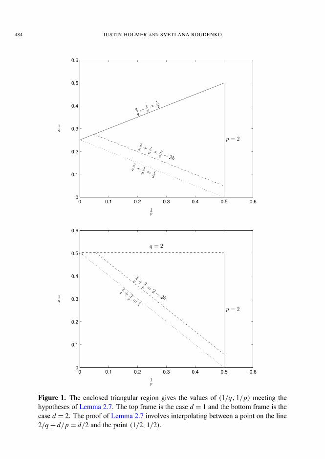
Lemma 2.7 (interpolated Strichartz). Take d = 1 or d = 2 and suppose that 0 ≤ b < 12 and 2 ≤ p ≤∞

and 2< q ≤∞ satisfy

2q+

dp>

d2+ (1− 2b), (2-11)

2q−

1p≤

12

in the case d = 1 only (2-12)

(see Figure 1). Then

‖u‖LqI L p

x. ‖u‖X0,b(I ). (2-13)

with implicit constant dependent upon the size of the gap from equality in (2-11).

Proof. Let

α :=12

(2q+

dp−

d2− (1− 2b)

)> 0. (2-14)

Using 0≤ θ ≤ 1 as an interpolation parameter, we aim to deduce (2-13) by interpolation between

‖u‖L qt L p

x. ‖u‖X0,b/(2(b−α)), (2-15)


0 0.1 0.2 0.3 0.4 0.5 0.60

0.1

0.2

0.3

0.4

0.5

0.6

1q

1p

p = 22

q + 1p = 3

2 − 2b

2q− 1

p=

12

2q + 1

p = 12

0 0.1 0.2 0.3 0.4 0.5 0.60

0.1

0.2

0.3

0.4

0.5

0.6

1q

1p

p = 2

2q +

2p =

1

2q + 2

p =2−

2b

q = 2

Figure 1. The enclosed triangular region gives the values of (1/q, 1/p) meeting thehypotheses of Lemma 2.7. The top frame is the case d = 1 and the bottom frame is thecase d = 2. The proof of Lemma 2.7 involves interpolating between a point on the line2/q + d/p = d/2 and the point (1/2, 1/2).


with weight θ , for some Strichartz admissible pair (q, p), and the trivial estimate (equality, in fact)

‖u‖L2t L2

x. ‖u‖X0,0, (2-16)

with weight 1− θ . The interpolation conditions read

1q=θ

q+

1−θ2

and 1p=θ

p+

1−θ2. (2-17)

Multiplying the first of these relations by 2 and adding d times the second, and using the Strichartzadmissibility condition for (q, p), we obtain

2q+

dp=

d2+ (1− θ).

Combining this relation with (2-14), we get θ = 2b−2α. We can then solve for q and p using (2-17). �

Lemma 2.8 (interpolated bilinear Strichartz). Let d = 1 or d = 2 and N1� N2. Then


x.

N (d−1)/21

N 1/2−δ′2

‖u1‖X0,1/2−δ(I )‖u2‖X0,1/2−δ(I ).

Proof. First, observe that‖PN1u1 PN2u2‖L2

I L2x. ‖u1‖L4

I L4x‖u2‖L4

I L4x. (2-18)

In the case d = 1, L4I L4

x interpolates between L6I L6

x and L2I L2

x , and thus ‖u j‖L4I L4

x. ‖u j‖X0,3/8+δ(I ) by

Lemma 2.7. We conclude that


x. ‖u1‖X0,3/8+δ(I )‖u2‖X0,3/8+δ(I ).

Interpolating this with the result of Lemma 2.6 completes the proof in the case d = 1.In the case d = 2, we still begin with (2-18). Fix ε > 0 small. By Sobolev embedding,

‖PN j u j‖L4I L4

x. N ε

j ‖PN j u j‖L4I L4/(1+2ε)

x.

By Lemma 2.7, we have‖PN j u j‖L4

I L4/(1+2ε)x

. ‖u j‖X0,b

for any b > 12(1− ε). Plugging into (2-18), we obtain


x. N 2ε

2 ‖u1‖X0,b‖u2‖X0,b for any b > 12(1− ε).

Interpolating this with the result of Lemma 2.6 completes the proof in the case d = 2. �

Remark 2.9. After this section we will adopt new notation: Instead of Xs,1/2+δ we will simply writeXs,1/2+. If an expression has two different Bourgain spaces, it will mean that the delta’s will be different.Similarly, if an expression involves δ in the estimate on the right side, it will mean that this δ will bedifferent from the one that would be chosen for spaces such as Xs,1/2+ or L p−.

The following is a simple consequence of the pseudodifferential calculus; see [Stein 1993, Theorem1on page 234 and Theorem 2 on page 237]; see also [Evans and Zworski 2003].


Lemma 2.10. Suppose that φ is a smooth function on R such that ‖∂αx φ‖L∞ ≤ cα for all α ≥ 0. Then

‖P≥N (φg)−φP≥N g‖L2 . N−1‖g‖L2 for N ≥ 1.

Proof. Let χ(ξ) be a smooth function that is 1 for |ξ | ≥ 1 and is 0 for |ξ | ≤ 12 . P≥N is a pseudodifferential

operator with symbol χ(N−1ξ) and Mφ , the operator of multiplication by φ, is a pseudodifferentialoperator with symbol φ(x). The commutator [PN ,Mφ] has symbol with top-order asymptotic termN−1χ ′(N−1ξ)φ′(x). The result then follows from the L2

→ L2 boundedness of 0-order operators. �

3. Additional high-frequency regularity

In this section, we begin the proof of Theorem 1.1 by showing improved regularity at high frequencies,above the blow-up scale, with no restriction in space — this appears as Proposition 3.4 below. In Section 4below, we will complete the proof of Theorem 1.1 by appealing to a finite-speed of propagation argumentfor lower frequencies after we have restricted in space to outside the blow-up core.

Consider a solution u(t) to (1-1) in the Merle–Raphaël class (1-5); let T0 > 0 be the threshold time,T > T0 the blow-up time and x0 the blow-up point, as described in the introduction. Our analysisfocuses on the time interval [T0, T ) on which the log-log asymptotics (1-6) kick in. Apply a space-time(rescaling) shift, in which x = x0 is sent to x = 0 and the time interval [T0, T ) is sent to [0, 1), to obtaina transformed solution that we henceforth still denote by u(t). Now the blow-up time is T = 1, theblow-up point is x = 0, and (1-6) becomes2

‖∇u(t)‖L2x∼

( log|log(1− t)|1− t

)1/2, (3-1)

which is now valid for all 0 ≤ t < 1. Note that now, however, the time t = 0 “initial data”, which wehenceforth denote u0, does not correspond to the original initial data u0 in Theorem 1.1. We remark thatthe estimate (1-8) on the remainder u(t) becomes

‖∇u(t)‖L2x. 1(1−t)1/2|log(1−t)|

. (3-2)

In our analysis, the norm L∞I L2x for an interval I = [0, T ′], T ′ < T , will be replaced by the norm

X0,1/2+(I ). While we have, from Lemma 2.5, the bound

‖u‖L∞I L2x. ‖u‖X0,1/2+(I ),

the reverse bound does not in general hold. Nevertheless, (3-1) indicates that the solution is blowingup close to the scale rate (1− t)−1/2. Thus, the local theory combined with (3-1) implies a bound on‖u‖X1,1/2+(I ), where log|log(1− T ′)| is weakened to (1− T ′)−δ.

2 The rescaling is the following. If we take u(x, t) in the original frame (for T0 ≤ t < T ), and let

u(x, t)= µd/2v(µ(x − x0), µ2(t − T0))

with µ = (T − T0)−1/2, then v(y, s) is defined in the modified frame (for 0 ≤ s < 1). Moreover, we have ‖∇v(s)‖L2

x∼

(log|logµ−2(1− s)|)1/2(1− s)−1/2, so now the implicit constant of comparability in (3-1) depends on T − T0.


Lemma 3.1. For I = [0, T ′] with T ′ < T , for 0< s ≤ 1, we have

‖u‖Xs, 12+(I ) ≤ cs(1− T ′)−s(1+δ)/2, with cs ↗+∞ as s↘ 0.

The fact that cs diverges as s ↘ 0 results from the fact that (1-1) is L2-critical, and thus, the localtheory estimates break down at s = 0. At the technical level, some slack is needed in applying theStrichartz and bilinear Strichartz estimates; hence, we need to take b= 1/2− δ in place of b= 1/2+ δ′.

Proof. We just carry out the argument for s= 1. Let λ(t)=‖∇u(t)‖−1L2 . Let sk be the increasing sequence

of times3 such that λ(sk)= 2−k , so that ‖∇u(t)‖L2 doubles over [sk, sk+1]. From (3-1), we compute thatsk = 1− 2−2k log k. Note that sk+1− sk ≈ 2−2k log k. Hence, we can rescale the cutoff solution u(t) onthe time interval [sk, sk+1] to a solution u′ on the time interval [0, log k] so that ‖u′‖L∞

[0,log k]H1x∼ 1. We

invoke the local theory over ∼ log k time intervals J each of unit size to obtain ‖u′‖X1,1/2+(J ) ∼ 1, whichare square summed to obtain ‖u′‖X1,1/2+(0,log k)∼ (log k)1/2. Returning to the original frame of reference,we conclude that

‖u‖X1,1/2+(sk ,sk+1) . 2k(1+δ),

where a δ-loss is incurred in part from the (log k)1/2 factor but also from the b = 12 + δ weight in the X

norm. Thus,

‖u‖X1,1/2+(0,sK ) =

(K−1∑k=1

22k(1+δ))1/2∼ 2K (1+δ). �

Now suppose that u(t) satisfies (3-1). Let tk = 1− 2−k and Ik = [0, tk]. Then from (3-1) and massconservation, we have

‖P≥N u(t)‖L∞Ik L2x.

{2k(1+δ)/2 N−1 for N ≥ 2k(1+δ)/2,

1 for N ≤ 2k(1+δ)/2.(3-3)

To refine (3-3), we will work with local-theory estimates and thus use the analogous bound on theBourgain norm X0,1/2+(Ik). From Lemma 3.1 we obtain

‖P≥N u‖X0,1/2+(Ik) . N−s‖P≥N u‖Xs,1/2+(Ik) ≤ cs N−s2ks(1+δ)/2. (3-4)

We obtain from (3-4) that

‖P≥N u‖X0,1/2+(Ik) .

{2k(1+δ)/2 N−1 for N ≥ 2k(1+δ)/2,

2kδ′ for N ≤ 2k(1+δ)/2.(3-5)

The next step is to run local-theory estimates to improve (3-5) at high frequencies. FrequenciesN . 2k

∼ (1− tk)−1 on Ik effectively do not make it out of the blow-up core before blow-up time dueto the finite speed of propagation for such frequencies.4 Hence, these low frequencies can be controlledby spatial location, which we address in Section 4. On the other hand, (3-5) shows that the solution at

3One of the conclusions of the Merle–Raphaël analysis is the almost monotonicity of the scale parameter λ(t)=‖∇u(t)‖−1L2 :

λ(t2) < 2λ(t1) for all t2 ≥ t1.4Recall that for the Schrödinger equation, frequencies of size N propagate at speed N and thus travel a distance O(1) in

time N−1.


frequencies N & 2k(1+δ)/2 is small. Thus, for these high frequencies, dispersive estimates might be able,upon iteration, to show that the solution is even smaller at these high frequencies.

To chose an intermediate dividing point between the high frequencies that are capable of exiting theblow-up core before blow-up time (N & 2k) and the frequency scale at which the blow-up is taking place(N ∼ 2k/2(log k)1/2), we consider frequencies ≥ 23k/4 to be high frequencies and frequencies ≤ 23k/4

to be low frequencies. The goal of this section is Proposition 3.4 below, which shows that the highfrequencies are bounded in H 1. In Section 4 below, we will localize in space to the external region andthen control the low frequencies.

We first address the dimension d = 1 case.

Lemma 3.2 (high frequency recurrence in one dimension). Take d = 1. Let tk = 1−2−k and Ik = [0, tk].Let u(t) be a solution such that (3-1) holds, and define

α(k, N )= ‖P≥N u‖X0,1/2+(Ik). (3-6)

Then there exists an absolute constant 0< µ� 1 such that for N ≥ 2k(1+δ)/2,

‖P≥N (u− ei t∂2x u0)‖X0,1/2+(Ik) . 2k(1+δ)/2 N−1+δα(k+ 1, µN )+ 2kδα(k+ 1, µN )2. (3-7)

In particular, by Lemma 2.4,

α(k, N ). ‖P≥N u0‖L2x+ 2k(1+δ)/2 N−1+δα(k+ 1, µN )+ 2kδα(k+ 1, µN )2. (3-8)

Proof. By (2-7) of Lemma 2.4 with ω = 2−k−1 and I = Ik ,

‖P≥N (u− ei t∂2x u0)‖X0,1/2+(Ik) . 2kδ

‖P≥N (|u|4u)‖X0,−1/2+(Ik+1).

In the rest of the proof, we estimate the right side of the estimate above, and we will just write Ik insteadof Ik+1 for convenience. By duality,

‖P≥N (|u|4u)‖X0,−1/2+(Ik) = sup‖w‖X0,1/2−(Ik )=1

∫Ik

∫x∈R

P≥N (|u|4u) w dx dt.

Fix w with ‖w‖X0,1/2−(Ik) = 1 and let

J :=∫

Ik

∫x∈R


Then J can be decomposed into a finite sum of terms Jα, each of the form (we have dropped complexconjugates, since they are unimportant in the analysis)

Jα :=∫ tk

0

∫x∈R

P≥N (u1u2u3u4u5) w dx dt

such that each term (after a relabeling of the u j for 1≤ j ≤ 5) falls into exactly one of the following twocategories.5

5Indeed, decompose each u j as u j = u j,lo + u j,med + u j,hi, where u j,lo = P≤N/160u j , u j,med = PN/160≤ ·≤N/20, andu j,hi = P≥N/20u j . Then in the expansion of u1u2u3u4u5, at least one term must be “hi”; without loss take this to be u5.


Note that w is frequency supported in |ξ |& N .

Case 1 (exactly one high). Each u j for 1≤ j ≤ 4 is frequency supported in |ξ | ≤µN and u5 is frequencysupported in |ξ | ≥ 8µN . In this case, we estimate as

|Jα| ≤ ‖u1‖L∞Ik L∞x ‖u2‖L∞Ik L∞x ‖u3u5‖L2Ik

L2x‖u4w‖L2

IkL2

x. (3-9)

For j = 1, 2, Gagliardo–Nirenberg and (3-1) implies

‖u j‖L∞Ik L∞x . ‖u j‖1/2L∞Ik L2

x‖∂x u j‖

1/2L∞Ik L2

x. 2k(1+δ)/4. (3-10)

The bilinear Strichartz estimate (Lemma 2.6) yields

‖u3u5‖L2Ik

L2x. N−1/2

‖u3‖X0,1/2+(Ik)‖u5‖X0,1/2+(Ik) . N−1/22kδα(k, µN ). (3-11)

The interpolated bilinear Strichartz estimate (Lemma 2.8) yields

‖u4w‖L2Ik

L2x. N−1/2+δ

‖u4‖X0,1/2+(Ik)‖w‖X0,1/2−(Ik) . N−1/2+δ2kδ. (3-12)

Substituting (3-10), (3-11), and (3-12) into (3-9), we obtain

|Jα|. 2k(1+δ)/2 N−1+δα(k, µN ).

Case 2 (at least two high). Both u4 and u5 are frequency supported in |ξ | ≥ µN (no restrictions on u j

for 1≤ j ≤ 3). Then we estimate as

|Jα| ≤ ‖u1‖L6Ik

L6+δx‖u2‖L6

IkL6

x‖u3‖L6

IkL6

x‖u4‖L6

IkL6

x‖u5‖L6

IkL6

x‖w‖L6

IkL6−δ′

x. (3-13)

For 2≤ j ≤ 3 we invoke the Strichartz estimate (Lemma 2.5) and (3-5) to obtain

‖u j‖L6Ik

L6x. ‖u j‖X0,1/2+(Ik) ≤ 2kδ. (3-14)

For 4≤ j ≤ 5 we invoke the Strichartz estimate (Lemma 2.5) and (3-6) to obtain

‖u j‖L6Ik

L6x. ‖u j‖X0,1/2+ ≤ α(k, µN ). (3-15)

For j = 1, by Sobolev embedding, the Strichartz estimate (Lemma 2.5), and (3-5),

‖u1‖L6Ik

L6+x. ‖Dδ

x u1‖L6Ik

L6x. ‖u1‖Xδ,1/2+(Ik) . 2kδ. (3-16)

By the interpolated Strichartz estimate (Lemma 2.7), we have

‖w‖L6t L6−

x. ‖w‖X0,1/2−(Ik) = 1. (3-17)

Using (3-14)–(3-17) in (3-13),|Jα|. 2kδα(k, µN )2. �

In the 2D case, we will just go ahead and assume that N ≥ 23k/4 to reduce confusion with deltas.

Case 1 corresponds to u1,lou2,lou3,lou4,lou5,hi and Case 2 corresponds to everything else (at least one u j for 1 ≤ j ≤ 4 mustbe “med” or “hi”. Hence, we can take µ= 1/160.


Lemma 3.3 (high frequency recurrence, 2D). Take d = 2. Let tk = 1− 2−k and Ik = [0, tk]. Let u(t) bea solution such that (3-1) holds and define

α(k, N ) := ‖P≥N u‖X0,1/2+(Ik). (3-18)

Then there exists an absolute constant 0< µ� 1 such that for N & 23k/4,

‖P≥N (u− ei t1u0)‖X0,1/2+(Ik) . 2kδN−1/6+δα(k+ 1, µN ). (3-19)

In particular, by Lemma 2.4,

α(k, N ). ‖P≥N u‖L2x+ 2kδN−1/6+δα(k+ 1, µN ). (3-20)

Proof. By Lemma 2.4 (2-7) with I = Ik and ω = 2−k−1,

‖P≥N (u− ei t1u0)‖X0,1/2+(Ik) . 2kδ‖P≥N (|u|2u)‖X0,−1/2+(Ik+1).

In the remainder of the proof, we estimate the right side, and for convenience take Ik+1 to be Ik . Byduality,

‖P≥N (|u|2u)‖X0,−1/2+(Ik) = sup‖w‖X0,1/2−(Ik )=1

∫Ik

∫x∈R


Fix w with ‖w‖X0,1/2−(Ik) = 1 and let

J :=∫

Ik

∫x∈R


Then J can be decomposed into a finite sum of terms Jα, each of the form (we have dropped complexconjugates, since they are unimportant in the analysis)

Jα :=∫ tk

0

∫x∈R

P≥N (u1u2u3) w dx dt

such that each term (after a relabeling of the u j for 1≤ j ≤ 3) falls into exactly one of the following twocategories.6 Note that w is frequency supported in |ξ |& N .

Case 1′ (exactly one high). Both u1 and u2 are frequency supported in |ξ | ≤ N 5/6 and u3 is frequencysupported in |ξ | ≥ N/12. In this case, we estimate as

|Jα|. ‖u1w‖L2Ik

L2x‖u2u3‖L2

IkL2

x.

By the interpolated bilinear Strichartz estimate (Lemma 2.8),

‖u1w‖L2Ik

L2x. (N 5/6)1/2 N−1/2+δ

‖u1‖X0,1/2−(Ik)‖w‖X0,1/2−(Ik) . N−1/12+δ2kδ,

6Indeed, decompose u j =u j,lo+u j,med+u j,hi, where u j,lo= P≤N 5/6 u j , u j,med= PN 5/6≤ ·≤N/12, and u j,hi= P≥N/12u j .

Then at least one term must be “hi”; take it to be u3. Case 1′ corresponds to u1,lou2,lou3,hi and Case 2′ corresponds to all otherpossibilities. Hence, we can take µ= 1/12.


and by Lemma 2.6 directly,

‖u2u3‖L2Ik

L2x. (N 5/6)1/2 N−1/2+δ

‖u2‖X0,1/2+(Ik)‖u3‖X0,1/2+(Ik) . N−1/12+δ2kδα(k, µN ).

Combining yields|Jα|. N−1/6+δ2kδα(k, µN ).

Case 2′ (at least two high). Here we suppose that u2 is frequency supported in |ξ | ≥ N 5/6 and u3 isfrequency supported in |ξ | ≥ µN ; we make no assumptions about u1. Then we estimate as

|Jα|. ‖u1‖L4Ik

L4+δx‖u2‖L4

IkL4

x‖u3‖L4

IkL4

x‖w‖L4

IkL4−δ

x.

For u1, we use Sobolev embedding and (3-5) to obtain

‖u1‖L4Ik

L4+δx. ‖Dδ

x u1‖L4Ik

L4x. ‖u1‖X

δ, 12+(Ik) . 2kδ.

Since N & 23k/4, we have N 5/6 & 25k/8� 2k(1+δ)/2, and thus by Lemma 2.5 and (3-5),

‖u2‖L4Ik

L4x. 2k(1+δ)/2 N−5/6 . (2k(1+δ)N−2/3)N−1/6

. 2kαN−1/6, since N & 23k/4.

For u3, we use Lemma 2.5 and (3-18) to obtain

‖u3‖L4Ik

L4x. α(k, µN ).

Combining, we obtain (changing deltas)

|Jα|. 2kδN−1/6α(k, µN ). �

The main result of this section is the following. It states that high frequencies (those strictly above23k/4) are H 1 bounded on Ik . Moreover, if we subtract the linear flow, we obtain H 4/3−δ boundednessfor frequencies above 23k/4 in the case d = 1 and H 7/6−δ boundedness for frequencies above 23k/4 in thecase d = 2.7

Proposition 3.4. Let tk = 1− 2−k , Ik = [0, tk], and let u(t) be a solution to (1-1) such that (3-1) holds.Then we have

‖P≥23k/4u(t)‖L∞Ik H1x. ‖P≥23k/4u(t)‖X1,1/2+(Ik) . 1.

Moreover, we have the following regularity above H 1 after the linear flow of the initial data is removed:For any 0≤ s ≤ 4

3 − δ in the case d = 1 and for any 0≤ s ≤ 76 − δ in the case d = 2, we have

‖P≥23k/4(u(t)− ei t1u0)‖L∞Ik H sx. ‖P≥23k/4(u(t)− ei t1u0)‖Xs,1/2+δ(Ik) . 1. (3-21)

7 In fact, the threshold ≥ 23k/4, to obtain H1 boundedness (but not (3-21)), can be replaced by 2k(1+δ)/2 for any δ > 0; inthe d = 1 case, one can appeal to Lemma 3.2 with a strictly smaller choice of δ in order to obtain a nontrivial gain upon eachapplication of Lemma 3.2. The number of applications of Lemma 3.2 is still finite number but δ-dependent. In the 2D case,Lemma 3.3 would first need to be rewritten. We have stated the proposition with threshold ≥ 23k/4 because this is all that isneeded in Section 4, and it allows us to avoid confusion with multiple small parameters.


Proof. We carry out the d = 1 case in full, which is a consequence of Lemma 3.2. The d = 2 case followsfrom Lemma 3.3 in a similar way.

By (3-5), we start with the knowledge that α(k, N ). 2k(1+δ)/2 N−1 for N ≥ 2k(1+δ)/2. Note

‖P≥N u0‖L2x. N−1

‖∇u0‖L2x. N−1.

By (3-8) in Lemma 3.2,

α(k, N ). N−1+ 2k(1+δ)/2 N−1+δα(k+ 1, µN ). (3-22)

Application of (3-22) m times gives

α(k, N ). N−1(m−1∑

j=0

(2k(1+δ)/2 N−1+δ) j)+ (2k(1+δ)/2 N−1+δ)mα(k+m, µm N ).

Since N ≥ 23k/4, we have 2k/2 N−1 . N−1/3. Taking m = 7 we obtain α(k, N ). N−1. Substituting thisinto (3-7) of Lemma 3.2, we obtain

‖P≥N (u(t)− ei t∂2x u0)‖X0,1/2+(Ik) . 2k(1+δ)/2 N−2+δ . N−4/3+δ. �

4. Finite speed of propagation

Recall that the main result of the last section was Proposition 3.4, which showed that the solution atfrequencies ≥ 23k/4 is H 1 bounded on Ik . This was achieved without applying any restriction in space.In this section, we apply a spatial restriction to |x | ≥ R (outside the blow-up core), and study the lowfrequencies ≤ 23k/4 on Ik . Since frequencies of size N propagate at speed N , and thus travel a distanceO(1) over a time N−1, we expect that frequencies of size . 2k involved in the blow-up dynamics willbe incapable of exiting the blow-up core |x | ≤ R before blow-up time.

Since Ik = [0, tk] and tk = 1− 2−k , restricting to frequencies ≤ 23k/4 on Ik for each k is effectivelyequivalent to inserting a time-dependent spatial frequency projection P≤(1−t)−3/4 . The main technicalLemma 4.3 below shows that, for 0 < r1 < r2 <∞, the H s size of the solution in the external region|x | ≥ r2 is bounded by the H s−1/8 size of the solution in the slightly larger external region |x | ≥ r1.This lemma is proved by studying the equation solved by P≤(1−t)−3/4ψu, where ψ is a spatial cutoff.In estimating the inhomogeneous terms of this equation, we use that the presence of the P≤(1−t)−3/4

projection enables an exchange of α spatial derivatives for a factor of (1− t)−3α/4. This is the manner inwhich finite speed of propagation is implemented. Lemma 4.3 is the main recurrence device for provingProposition 4.4, giving the H 1 boundedness of the solution in the external region, completing the proofof Theorem 1.1.

Before getting to Lemma 4.3, we begin by using the method of Raphaël [2006], based on the use oflocal smoothing and (3-2), to achieve a small gain of regularity.8

8In the d = 1 case, we obtain a gain of 2/5 derivatives in this first step, but in fact the proof could be rewritten to achieve again of s < 1/2 derivatives. The reason s = 1/2 derivatives cannot be achieved in one step is the failure of the H1/2 ↪→ L∞

embedding needed to estimate the nonlinear term. One could achieve 1/2 derivatives by running the same argument twice, but


Lemma 4.1 (a little regularity, d = 1 case). Suppose d = 1. Suppose that u(t) solving (1-1) with H 1

initial data satisfies (3-1). Fix R > 0. Then

‖〈Dx 〉2/5ψRu‖L∞

[0,1)L2x. 1,

where ψR(x) = ψ(x/R) and ψ(x) is a smooth cutoff with ψ(x) = 1 for |x | ≥ 1/2 and ψ(x) = 0 for|x | ≤ 1/4.

Proof. Let w = ψRu and q = ψR/2u. Then w solves the equation

i∂tw+ ∂2xw =−|q|

4w+ 2∂x(ψ′

R u)−ψ ′′R u= F1+ F2+ F3.

Apply 〈Dx 〉2/5, and estimate with I = [T1, 1) using the (dual) local smoothing estimate for the F2 term:

‖〈Dx 〉2/5w‖L∞I L2

x. ‖〈Dx 〉

2/5w(T1)‖L2x+‖〈Dx 〉

2/5 F1‖L1I L2

x

+‖〈Dx 〉2/5〈Dx 〉

−1/2 F2‖L2I L2

x+‖〈Dx 〉

2/5 F3‖L1I L2

x.

We begin by estimating term F1. By the fractional Leibniz rule,

‖D2/5x F1‖L1

I L2x. ‖|q|4‖L1

I L∞x‖D2/5

x w‖L∞I L2x+‖D2/5

x |q|4‖L1

I L5/2x‖w‖L∞I L10

x.

.(‖|q|4‖L1

I L∞x+‖D2/5

x |q|4‖L1

I L5/2x

)‖D2/5

x w‖L∞I L2x.

By Sobolev/Gagliardo–Nirenberg embedding and (3-2),

‖|q|4‖L∞x +‖D2/5x |q|

4‖L5/2

x. ‖q‖2L2

x‖∂xq‖2L2

x. (1− t)−1(log(1− t)−1)−2.

Applying the L1I time norm, we obtain a bound by (log(1− T1)

−1)−1. Hence,

‖〈Dx 〉2/5 F1‖L1

I L2x. (log(1− T1)

−1)−1‖〈Dx 〉

2/5w‖L∞I L2x.

Next, we address term F2. We have

‖〈Dx 〉2/5〈Dx 〉

−1/2 F2‖L2I L2

x. ‖〈Dx 〉

9/10q‖L2I L2

x. ‖q‖1/10

L∞I L2x‖‖〈∂x 〉q‖

9/10L2

x‖L2

I.

From (3-2), we have ‖∂xq‖L2x. (T − t)−1/2

|log(1− t)|−1 and hence

‖〈Dx 〉2/5〈Dx 〉

−1/2 F2‖L2I L2

x. (1− T1)

1/10.

Term F3 is comparatively straightforward. Indeed, we obtain

‖〈Dx 〉2/5 F3‖L1

I L2x. ‖u‖3/5L∞I L2

x‖‖〈∂x 〉ψ2u‖2/5L2

x‖L1

I. (1− T1)

4/5.

Collecting the estimates above, we obtain

‖〈Dx 〉2/5w‖L∞I L2

x. ‖〈Dx 〉

2/5w(T1)‖L2x+ (log(1− T1)

−1)−1‖〈Dx 〉

2/5w‖L∞I L2x+ (1− T1)

1/10.

this is unnecessary since we only need a small gain of s > 0 to complete the proof of our main new Lemma 4.3/Proposition 4.4below, which enables us to reach the full s = 1 gain. One cannot achieve a gain of s > 1/2 by the method employed in the proofof Lemma 4.1 alone due to the term ∂x (ψ

′R u).


By taking T1 sufficiently close to 1 so that (log(1− T1)−1)−1 beats out the (absolute) implicit constants

furnished by the estimates, we obtain

‖〈Dx 〉2/5w‖L∞I L2

x. ‖〈Dx 〉

2/5w(T1)‖L2x+ (1− T1)

1/10. �

Lemma 4.2 (a little regularity, d = 2 case). Suppose d = 2. Suppose that u(t) solving (1-1) with H 1

initial data satisfies (3-1). Fix R > 0. Then

‖〈Dx 〉1/2ψRu‖L∞

[0,1)L2x. 1,

where ψR(x)=ψ(x/R) and ψ(x) is a smooth cutoff with ψ(x)= 1 for |x | ≥ 12 and ψ(x)= 0 for |x | ≤ 1

4 .

Proof. Let w = ψRu and q = ψR/2u, and take ψ =∇xψR and ˜ψ =1xψR . Then w solves the equation

i∂tw+1w =−|q|2w+ 2∇x · (ψ u)− ˜ψ u = F1+ F2+ F3.

Apply 〈Dx 〉1/2, and estimate with I = [T1, 1) using the (dual) local smoothing estimate for the term F2:

‖〈Dx 〉1/2w‖L∞I L2

x+‖〈Dx 〉

1/2w‖L4I L4

x

. ‖〈Dx 〉1/2w0‖L2

x+‖〈Dx 〉

1/2 F1‖L4/3I L4/3

x+‖F2‖L2

I L2x+‖〈Dx 〉

1/2 F3‖L1I L2

x.

Before we begin treating term F1, let us note that by (3-2), ‖∇q‖L2x. (1− t)−1/2(log(1− t)−1)−1 and

hence ‖∇q‖L2I L2

x. (log(1−T1)

−1)−1/2. By the fractional Leibniz rule and Sobolev/Gagliardo–Nirenbergembedding,

‖D1/2x |q|

2‖L2

x. ‖D1/2

x q‖L4x‖q‖L4

x. ‖q‖1/2L2

x‖∇q‖3/2L2

x.

Hence,‖D1/2

x |q|2‖L4/3

I L2x. ‖q‖1/2L∞I L2

x‖∇q‖3/2

L2I L2

x. (log(1− T1)

−1)−3/4. (4-1)

Also, we have‖q‖L4

x. ‖D1/2

x q‖L2x. ‖q‖1/2L2

x‖∇q‖1/2L2

x,

and hence‖q‖2L4

I L4x. ‖q‖L∞I L2

x‖∇q‖L2

I L2x. (log(1− T1)

−1)−1/2. (4-2)

Now we proceed with the estimates for term F1. By the fractional Leibniz rule (in x),

‖〈Dx 〉1/2 F1‖L4/3

I L4/3x. ‖〈Dx 〉

1/2|q|2‖L4/3

I L2x‖w‖L∞I L4

x+‖|q|2‖L2

I L2x‖〈Dx 〉

1/2w‖L4I L4

x.

By (4-1) and (4-2), we obtain

‖〈Dx 〉1/2 F1‖L4/3

I L4/3x. (log(1− T1)

−1)−1/2(‖〈Dx 〉1/2w‖L∞I L2

x+‖〈Dx 〉

1/2w‖L4I L4

x).

Next, we treat the F2 term. Again since ‖∇q‖L2x. (1− t)−1/2(log(1− t)−1)−1,

‖F2‖L2I L2

x. (log(1− T1)

−1)−1.

The F3 term is comparatively straightforward.


Collecting the estimates above, we have

‖〈Dx 〉1/2w‖L∞I L2

x+‖〈Dx 〉

1/2w‖L4I L4

x

. ‖〈Dx 〉1/2w(T1)‖L2

x+ (log(1− T1)

−1)−1

+ (log(1− T1)−1)−1/2(‖〈Dx 〉

1/2w‖L∞I L2x+‖〈Dx 〉

1/2w‖L4I L4

x).

By taking T1 sufficiently close to 1, we obtain

‖〈Dx 〉1/2w‖L∞I L2

x. ‖〈Dx 〉

1/2w(T1)‖L2x+ (log(1− T1)

−1)−1. �

Lemma 4.3 (low frequency recurrence). Let d = 1 or d = 2, 0< R ≤ r1 < r2 and 18 ≤ s ≤ 1. Let ψ1(x)

and ψ2(x) be smooth radial cutoff functions such that

ψ1(x)={

0 on |x | ≤ r1,

1 on |x | ≥ 12(r1+ r2)

and ψ2(x)={

0 on |x | ≤ 12(r1+ r2),

1 on |x | ≥ r2.

Then‖Ds

xψ2u‖L∞[0,1)L

2x. 1+‖〈Dx 〉

s−1/8ψ1u‖L∞[0,1)L

2x.

Proof. Let χ(ρ) be a smooth function such that χ(ρ) = 1 for |ρ| ≤ 1 for χ(ρ) = 0 for |ρ| ≥ 2. LetP− = P≤(T−t)−3/4 be the time-dependent multiplier operator defined by P f (ξ) = χ((T − t)3/4|ξ |) f (ξ)(where the Fourier transform is in space only). Note that the Fourier support of P at time tk = 1− 2−k

is . 23k/4. We further have that

∂t P− f = 34 i(1− t)−1/4 Q Dx f + P∂t f,

where Q = Q(1−t)−3/4 is the time-dependent multiplier

Q f (ξ)= χ ′((1− t)3/4|ξ |) f (ξ).

Note that the Fourier support of Q at time tk = 1− 2−k is ∼ 23k/4. Note also that if g = g(x) is anyfunction, then

‖P Dαx g‖L2

x≤ (1− t)−3α/4

‖g‖L2x. (4-3)

Let w = P−ψ2u. Taking ψ2 =∇xψ2 and ˜ψ2 =1xψ2, we have

i∂tw+1w =−i(1− t)−1/4 Q · ∇x w− P−ψ2|u|4/du+ 2P−∇x · [ψ2u] − P−˜ψ2u

= F1+ F2+ F3+ F4.

By the energy method,

‖Dsxw‖

2L∞[0,1)L

2x. ‖Ds

xw(0)‖2L2

x+

∫ 1

0|〈Ds

x F1(s), Dsxw(s)〉L2

x| ds+ 10

4∑j=2

‖Dsx F j‖

2L1[0,1)L

2x.

For term F1, we argue as follows. Let Q be a projection onto frequencies of size (1− t)−3/4. Then∫ 1

0|〈Ds


x| ds .

∫ 1

0(1− s)−1/4

‖D1/2+sx Qψ2u(s)‖2L2

xds.


Applying (4-3) with α = 12 , we can control the above by∫ 1

0(1− s)−1

‖Dsx Qψ2u(s)‖2L2

xds.

Dividing the time interval [0, 1)=⋃∞

k=1[tk, tk+1), we bound the above by

+∞∑k=1

2k∫ tk+1

tk‖Ds

x P23k/4ψ2u(s)‖2L2x

ds .+∞∑k=1

‖Dsx P23k/4ψ2u(s)‖2L∞

[tk ,tk+1)L2

x,

where P23k/4 is the projection onto frequencies of size ∼ 23k/4 (and not . 23k/4). However, writingu(t)= ei t1u0+ (u(t)− ei t1u0), the above is controlled by (taking s = 1, the worst case)

∞∑k=1

‖∇x P23k/4u0‖2L2

x+

+∞∑k=1

‖∇x P23k/4(u(t)− ei t1u0)‖2L2

x.

By (3-21) of Proposition 3.4,

‖∇x u0‖2L2

x+

+∞∑k=1

2−k/8 . 1.

In conclusion, for term F1 we obtain∫ 1

0|〈Ds


x| ds . 1.

We next address term F2. Insert ψ2ψ4/d+11 = ψ2, then apply (4-3) with α = s to obtain (in the worst

case s = 1),

‖Dsx F2‖L1

[0,1)L2x. ‖(1− t)−3/4ψ2|u|4/du‖L1

[0,1)L2x. ‖(1− t)−3/4

‖ψ1u‖4/d+1L2(4/d+1)

x‖L1[0,1).

We consider the cases d = 1 and d = 2 separately. When d = 1,

‖ψ1u‖L10x. ‖D2/5

x ψ1u‖L2x. 1,

by Lemma 4.1. Consequently,

‖Dsx F2‖L1

[0,1)L2x. ‖(1− t)−3/4

‖L1[0,1). 1.

On the other hand, when d = 2, we have

‖ψ1u‖L6x. ‖D2/3

x ψ1u‖L2x. ‖D1/2

x ψ1u‖2/3L2x‖∇xψ1u‖1/3L2

x. (1− t)−1/6

by Lemma 4.2 and (3-2). Consequently,

‖Dsx F2‖L1

[0,1)L2x. ‖(1− t)−3/4(1− t)−1/6

‖L1[0,1). 1.

Next, we address term F3. By (4-3) with α = 9/8,

‖Dsx F3‖L1

[0,1)L2x. ‖(1− t)−27/32

‖L1[0,1)‖Ds−1/8

x (ψ2u)‖L∞[0,1)L

2x.


Since ‖(1− t)−27/32‖L1[0,1)∼ 1 and the support of ψ2 is contained in the set where ψ1 = 1, we have

‖Dsx F3‖L1

[0,1)L2x. ‖〈Dx 〉

s−1/8ψ1u‖L∞[0,1)L

2x.

Finally, we consider F4. We have

‖Dsx F4‖L1

[0,1)L2x. ‖〈∇x 〉P−ψ1u‖L1

[0,1)L2x. ‖(1− t)−3/4

‖L1[T1,1)‖u‖L∞

[0,1)L2x. 1

by (4-3) with α = 1. �

Proposition 4.4. Suppose that u(t) solving (1-1) with H 1 initial data satisfies (3-1). Fix R > 0. Then

‖u‖L∞[0,1)H

1|x |≥R. 1.

Proof. Iterate Lemma 4.3 eight times on successively larger external regions. �

Proposition 4.4 completes the proof of Theorem 1.1.

5. Application to 3D standing sphere blow-up

We now outline the proof of Theorem 1.2 utilizing the techniques of Section 3 and 4. Theorem 1.2pertains to radial solutions of (1-9). We define the initial data set P as in9 Raphaël and Szeftel [2009,Definition 1, page 980–1], except that condition (v) is replaced by ‖u0‖H1(|r−1|≥1/10) ≤ ε

5. The goalthen becomes to complete the proof of the bootstrap Proposition 1 on page 982, where the “improvedregularity estimates” (35)–(37) are effectively replaced with

‖u(t)‖L∞[0,t1]

H1|x |≤1/2≤ ε.

Let us formulate a more precise statement:

Proposition 5.1 (partial bootstrap argument). Let Q be the 1D ground state given by (1-4), and let ε > 0,T > 0 be fixed with T ≤ ε200. Suppose that u(t) is a radial 3D solution to

i∂t u+1u+ |u|4u = 0

on an interval [0, T ′] ⊂ [0, T ) such that the following “bootstrap inputs” hold:

(1) There exist parameters λ(t) > 0, γ(t) ∈ R, and |r(t)− 1| ≤ 1/10, such that if we define

u(r, t)= u(r, t)− 1λ(t)1/2

Q(r − r(t)

λ(t)

), (5-1)

then, for 0≤ t ≤ T ′,

‖∇u(t)‖L2x= λ(t)−1

∼

( log|log(T − t)|T − t

)1/2, (5-2)

and‖∇u(t)‖L2

x. 1|log(T−t)|1+(T−t)1/2

. (5-3)

9We are considering the case dimension d = 3 (in their notation N = 3).


(2) Interior Strichartz control: ‖〈∇〉u(t)‖L5[0,T ′]L

30/11|x |≤1/2≤ ε.

(3) Initial data remainder control: ‖〈∇〉u0‖L2x≤ ε5.

Then we have the following “bootstrap output”:

‖〈∇〉u(t)‖L∞[0,T ′]L

2|x |≤1/2+‖〈∇〉u(t)‖L5

[0,T ′]L30/11|x |≤1/2

. ε5. (5-4)

The goal of this section is to prove Proposition 5.1, which shows that the bootstrap input (2) is rein-forced. Proposition 5.1 is, however, an incomplete bootstrap and by itself does not establish Theorem 1.2.The analysis which uses (5-4) to reinforce the bootstrap assumption (1) is rather elaborate but will beomitted here as it follows the arguments in [Raphaël 2006] and [Raphaël and Szeftel 2009]. Moreover,these papers demonstrate how the assertions in Theorem 1.2 follow.

The proof of Proposition 5.1 follows the methods developed in Section 3–4 used to prove Theorem 1.1.We do not, however, rescale the solution so that T = 1 as was done in Section 3.

Remark 5.2. Let us list some notational conventions for the rest of the section. We take tk = T − 2−k

and denote Ik = [0, tk]. Let v(r, t)= ru(r, t), and consider v as a 1D function in r extended to r < 0 asan odd function. Note that v solves

i∂tv+ ∂2r v =−r−4

|v|4v.

The frequency projection PN will always refer to the 1D frequency projection in the r -variable. TheBourgain norm ‖v‖Xs,b refers to the 1D norm in the r -variable.

Let λ0 = λ(0) and take k0 ∈ N such that 2−k0/2(log k0)−1/2∼ λ0. We then have T ∼ 2−k0 . The

assumption T ≤ ε40 equates to 2−k0/8 ≤ ε5. Note that λ(tk)= 2−k/2(log k)−1/2.

Lemma 5.3 (smallness of initial data). Under the assumption (3) in Proposition 5.1 on the initial data,and with v0 = ru0, we have

‖P≥23k0/4∂rv0‖L2

r+‖∂rv0‖L2

r≤1/2. ε5.

Proof. Let v0 = r u0. Since ∂r v0 = u0+ r∂r u0, we have by Hardy’s inequality

‖∂r v0‖L2r. ‖|x |−1u0‖L2

x+‖∇u0‖L2

x. ‖∇u0‖L2

x. ε5.

Recalling the definition of u0 = u(0) in (5-1) (with t = 0), we have

v0 =rλ

1/20

Q(r − r0

λ0

)+ v0.

The result then follows from the exponential localization and smoothness of Q. �

Lemma 5.4 (radial Strichartz). Suppose that u(t) is a 3D radial solution to

i∂t u+1u = f.

Let v(r, t)= ru(r, t) and g(r, t)= r f (r, t) and consider v as a 1D function in r (extended to be odd), sothat

i∂tv+ ∂2r v = g.


Then for (q, r) and (q, r) satisfying the 3D admissibility condition,

‖r2/p−1v‖Lqt L p

r. ‖v0‖L2

r+‖r2/p′−1g‖

L q′t L p′

r.

Proof. The left side is equivalent to ‖∇u‖Lqt L p

xand the right side is equivalent to ‖u0‖L2

x+‖ f ‖

L q′t L p

x, so

it is just a restatement of the 3D Strichartz estimates. �

Lemma 5.5 (3D to 1D conversion). Suppose that u(x) is a 3D radial function, and write u(r) = u(x).Let v(r)= ru(r). Then for 1< p < 3, we have

‖r2/p−1∂rv‖L pr. ‖∇x u‖L p

x. (5-5)

Also for 32 < p <+∞, we have

‖∇x u‖L px. ‖r2/p−1∂rv‖L p

r. (5-6)

Consequently, for 3D admissible pairs (q, p) such that 2≤ p < 3, we have

‖∇u‖Lqt L p

x∼ ‖r2/p−1∂rv‖Lq

t L pr. (5-7)

We remark that q = 5 and p = 3011 falls within the range of validity for (5-7).

Proof. The proof of (5-5) and (5-6) is a standard application of the Hardy inequality.First, we prove (5-5). Using v = ru,

r2/p−1∂rv = r2/p∂r u+ r2/p−1u,

and thus,‖r2/p−1∂rv‖L p

r≤ ‖r2/p∂r u‖L p

r+‖r2/p−1u‖L p

r.

We have, for r > 0,

u(r)=−(u(+∞)− u(r))=∫+∞

s=1

dds(u(sr)) ds =

∫+∞

s=1u′(sr)r ds.

By the Minkowski integral inequality,

‖r2/p−1u‖L pr≤

∫+∞

s=1‖u′(sr)r2/p

‖L pr>0

ds.

Changing variable r 7→ s−1r , we obtain that the right-hand side is bounded by(∫ +∞s=1

s−3/p ds)‖r2/pu′‖L p

r>0

and the s integral is finite provided p < 3.Next, we prove (5-6). We have

r2/p∂r u = r2/p∂r (r−1v)=−r2/p−2v+ r2/p−1∂rv,

and hence,‖r2/p∂r u‖L p

r≤ ‖r2/p−2v‖L p

r+‖r2/p−1∂rv‖L p

r.


We have

v(r)= v(r)− v(0)=∫ 1

s=0

dds(v(sr)) ds =

∫ 1

s=0v′(sr)r ds.

By the Minkowski integral inequality,

‖r2/p−2v‖L pr≤

∫ 1

s=0‖v′(sr)r2/p−1

‖L pr

ds.

Changing variable r 7→ s−1r in the right side, we obtain

‖r2/p−2v‖L pr≤

(∫ 1

s=0s−3/p+1ds

)‖v′(r)r2/p−1

‖L pr

and the s integral is finite provided p > 32 . �

The replacement for Lemma 3.1 is Lemma 5.6 below. The difference is that in Lemma 5.6, we onlyuse b < 1

2 when working at H 1 regularity.

Lemma 5.6. Suppose that the assumptions of Proposition 5.1 and Remark 5.2 hold. Then for 12 − δ ≤

b < 12 ,

‖∂rv‖X0,b(Ik) . 2kb(log k)b+1/2= (T − t)−b(log|log(T − t)|)b+1/2. (5-8)

Also, for 12 − δ < b < 1

2 + δ,‖v‖X0,b(Ik) .δ 2kδ

= (T − t)−δ. (5-9)

Proof. We will only carry out the proof of (5-8), which stems from (5-2).10 The proof of (5-9) is similar,and stems from the bound on ‖u(t)‖H δ obtained from interpolation between (5-2) and mass conservation.

In the proof below, T has no relation to the T representing blow-up time in the rest of the article.Let λ= λ(tk)= 2−k/2(log k)−1/2. Let r = λR, x = λX , and t = λ2T + tk . Define the functions

V (R, T )= λ1/2v(λR, λ2T + tk)= λ1/2v(r, t),

U (X, T )= λ1/2u(λX, λ2T + tk)= λ1/2u(x, t).

Note that the identity v(r)= ru(r) corresponds to V (R)= λRU (R).We study V (R, T ) on T ∈ [0, log k], which corresponds to t ∈ [tk, tk+1]. We have ‖V ‖L2

R= ‖v‖L2

r∼

O(1) (by mass conservation) and ‖∂R V ‖L2R= λ‖∂rv‖L2

r. Hence, ‖∂R V ‖L∞

[0,log k]L2R= O(1). The equation

satisfied by V isi∂T V + ∂2

R V =−λ−4 R−4|V |4V .

Let J = [a, b] be a unit-sized time interval in [0, log k]. Then by Lemma 2.4,

‖∂R V ‖X0,b(J ) . ‖∂R V (a)‖L2 +‖∂R(λ−4 R−4

|V |4V )‖L1J L2

R.

10The need to take b < 1/2 comes from Lemma 2.4, (2-7) versus (2-8); when working at H1 regularity near the origin, wecannot suffer any loss of derivatives. The fact that ‖∂rv‖X0,b(Ik ) for b < 1/2 is only a H1 subcritical quantity is of no harm asthe only application of (5-8) in the subsequent arguments is to control the solution for r ≥ 1/2, where the equation is effectivelyL2 critical.


Let χ1(r) = 1 for r ≤ 14 and suppχ1 ⊂ B(0, 3

8). Let χ2 = 1− χ1. Let g1 = ∂R(λ−4 R−4χ1(λR)|V |4V )

and g2 = ∂R(λ−4 R−4χ2(λR)|V |4V ), so that the above becomes

‖∂R V ‖X0,b(J ) . ‖∂R V (a)‖L2 +‖g1‖L1J L2

R+‖g2‖L1

J L2R. (5-10)

We begin with estimating ‖g2‖L1J L2

R. We have

‖g2‖L1J L2

R. ‖V 5

‖L1J L2

R+‖V 4(∂R V )‖L1

J L2R. (5-11)

We now treat the first term in (5-11). Of course, ‖V 5‖L1

J L2R=‖V ‖5

L5J L10

R. By Sobolev embedding ‖V ‖L10

R.

‖D2/5R V ‖L2

Rand by Hölder,

‖V ‖L5J L10

R. |J |1/10

‖D2/5R V ‖L10

J L2R. |J |1/10(‖V ‖L10

J L2R+‖∂R V ‖L10

J L2R)

≤ |J |1/10(|J |1/10‖V ‖L∞J L2

R+‖∂R V ‖L10

J L2R).

Using that ‖V ‖L∞J L2R∼ 1, that |J | ∼ 1 and Lemma 2.7, provided 2

5 < b < 12 , we have

‖V ‖L5J L10

R. |J |1/10(1+‖∂R V ‖X0,b). (5-12)

We now treat the second term in (5-11), similarly estimating the term ‖V ‖L10R

. We have

‖V 4∂R V ‖L1J L2

R. |J |7/20

‖V ‖4L10J L10

R‖∂R V ‖L4

J L10R

. |J |7/20(1+‖∂R V ‖L10J L2

R)4‖∂R V ‖L4

J L10R.

Appealing to Lemma 2.7, provided 920 < b < 1

2 , we obtain

‖V 4∂R V ‖L1J L2

R. |J |7/20(1+‖∂R V ‖X0,b)

5. (5-13)

Combining (5-12) and (5-13), we have

‖g2‖L1J L2

R. |J |7/20(1+‖∂R V ‖X0,b)

5. (5-14)

Next we estimate ‖g1‖L1J L2

R. By rescaling,

‖g1‖L1J L2

R= λ‖∂r (χ1r−4

|v|4v)‖L1[tk ,tk+1]

L2r.

Letw= χ1u, where χ1=1 on suppχ1 but supp χ1⊂ B(0, 12). Replacing u=r−1v, we obtain ∂r (rχ1u5)=

∂r (rχ1w5), and hence,

‖g1‖L2R. λ(‖w‖5L10

r+‖rw4∂rw‖L2

r). λ(‖|x |−1/5w‖5L10

x+‖w4

∇w‖L2x). (5-15)

By Hardy’s inequality and 3D Sobolev embedding,

‖|x |−1/5w‖L10x. ‖D1/5

x w‖L10x. ‖∇w‖L30/11

x.

By Hölder’s inequality and 3D Sobolev embedding,

‖w4∇w‖L2

x≤ ‖w‖4L30

x‖∇w‖L30/11

x. ‖∇w‖5

L30/11x

.


Returning to (5-15) and invoking (2) of Proposition 5.1,

‖g1‖L1Ik

L2r. λ‖∇w‖5

L5Ik

L30/11x. λε5. (5-16)

By putting (5-14) and (5-16) into (5-10), we obtain

‖∂R V ‖X0,b(J ) . ‖∂R V (a)‖L2 + |J |7/20(1+‖∂R V ‖X0,b(J ))5+ λε5.

From this, we conclude that we can take |J | sufficiently small (but still “unit-sized”11) so that it followsthat

‖∂R V ‖X0,b(J ) ≤ O(1).

Square summing over unit-sized intervals J filling [0, log k],

‖∂R V ‖X0,b([0,log k]) . (log k)1/2.

This estimate scales back to

‖∂rv‖X0,b([tk ,tk+1]) . (log k)1/2λ(tk)−2b= 2kb(log k)b+1/2.

Now square sum over k from k = 0 to k = K to obtain a bound of 2K b(log K )b+1/2 over the time intervalIK , which is the claimed estimate (5-8). �

The analogue of Lemma 3.2 will be Lemma 5.7 below. We note that as a consequence of Lemma 5.6,the hypothesis of Lemma 5.7 below is satisfied with α(k, N )= 2−k/2 N−1.

Lemma 5.7 (high-frequency recurrence). Let the assumptions of Proposition 5.1 and Remark 5.2 hold,and let12

β(k, N ) := ‖P≥N∂rv‖X0,1/2−(Ik).

Then there exists an absolute constant 0< µ� 1 such that for N ≥ 2k(1+δ)/2, we have

β(k, N )+‖r2/p−1 P≥N∂rv‖LqIk

L pr

. ‖P≥N∂rv0‖L2r+ 2k(1+δ)/2 N−1+δβ(k, µN )+ N−1+δ2kδβ(k, µN )2+ 2−kδ

+ ε5 (5-17)

for all 3D admissible (q, p).

Proof. Note that v solvesi∂tv+ ∂

2r v =−r |u|4u =−r−4

|v|4v.

Let χ1(r) be a smooth function such that χ1(r) = 1 for |r | ≤ 14 and χ1 is supported in |r | ≤ 3

8 . Letχ2 = 1−χ1. Apply P≥N∂r to obtain

(i∂t + ∂2r )P≥N∂rv = g1+ g2,

11Meaning: with size independent of any small parameters like ε or λ12Note the inclusion of one derivative in the definition of β, in contrast to the choice of definition for α in Proposition 3.4.


whereg j (r)=−P≥N∂r (χ j r−4

|v|4v) for j = 1, 2.

Then by Lemma 2.413 and Lemma 5.4,

‖P≥N∂rv‖X0,1/2−(Ik)+‖r2/p−1 P≥N∂rv‖Lq

IkL p

r. ‖P≥N∂rv0‖L2

r+‖g1‖L1

IkL2

r+‖g2‖L1

IkL2

r.

The term ‖g2‖L1t L2

ris controlled in a manner similar to the analysis in the proof of Lemma 3.2. For this

term, χ2 r−4 and ∂r (χ2 r−4) are smooth bounded functions, with all derivatives bounded. By Lemma 2.10,

‖g2‖L2r. ‖P≥N 〈∂r 〉v

5‖L2

r+ N−1

‖〈∂r 〉v5‖L2

r. (5-18)

By an analysis similar to the proof of Lemma 3.2, utilizing the bounds in Lemma 5.6, we obtain

‖P≥N 〈∂r 〉v5‖L1

IkL2

r. 2k(1+δ)/2 N−1+δβ(k, µN )+ N−1+δ2kδβ(k, µN )2. (5-19)

Also by the Strichartz estimates, as in the proof of Lemma 5.6 above,

‖〈∂r 〉v5‖L1

IkL2

r. ‖Dδv‖4X0,b

‖∂Rv‖X0,b . 2k(1+δ)/2. (5-20)

Inserting (5-19) and (5-20) into (5-18), we obtain

‖g2‖L1Ik

L2r. 2k(1+δ)/2 N−1+δβ(k, µN )+ N−1+δ2kδβ(k, µN )2+ N−12k(1+δ)/2. (5-21)

The last term, N−12k(1+δ)/2, gives the contribution 2−kδ in (5-17) due to the restriction N ≥ 2k(1+δ)/2

(different deltas).Next we address ‖g1‖L1

IkL2

r. We estimate away P≥N by

‖g1‖L1Ik

L2r. ‖g1‖L1

IkL2

r, (5-22)

where (ignoring complex conjugates)g1 = ∂r (r−4χ1v

5).

Let w = χ1u, where χ1 = 1 on suppχ1 but supp χ1 ⊂ B(0, 12). Replacing u = r−1v, we obtain g1 =

∂r (rχ1u5)= ∂r (rχ1w5), and hence,

‖g1‖L2r. ‖w‖5L10

r+‖rw4∂rw‖L2

r. ‖|x |−1/5w‖5L10

x+‖w4

∇w‖L2x.

By Hardy’s inequality and 3D Sobolev embedding,

‖|x |−1/5w‖L10x. ‖D1/5

x w‖L10x. ‖∇w‖L30/11

x.

By Hölder’s inequality and 3D Sobolev embedding,

‖w4∇w‖L2

x≤ ‖w‖4L30

x‖∇w‖L30/11

x. ‖∇w‖5

L30/11x

.

13We were able to obtain the L1Ik

L2r right side (without δ loss), because we took b < 1/2 in the Bourgain norm.


Hence, ‖g1‖L2r. ‖∇w‖5

L30/11x

. Returning to (5-22) and invoking (2) of Proposition 5.1,

‖g1‖L1Ik

L2r. ‖∇w‖5

L5Ik

L30/11x. ε5. �

The analogue of Proposition 3.4 is this:

Proposition 5.8 (high-frequency control). Let the assumptions of Proposition 5.1 and Remark 5.2 hold.Then for any 3D Strichartz admissible pair (q, p), we have

‖P≥23k/4∂rv‖X0,1/2−(Ik)+‖r2/p−1 P≥23k/4∂rv‖Lq

IkL p

r. ε5.

Proof. Several applications of Lemma 5.7, just as Proposition 3.4 is deduced from Lemma 3.2. �

Due to the H 1 criticality of the problem, we do not have improved regularity of v(t)− ei t∂2r v0 as was

the case in Proposition 3.4. As a substitute, we can use the methods of Lemma 5.7 to obtain the followinglemma:

Lemma 5.9 (additional high-frequency control). Suppose that the assumptions of Proposition 5.1 andRemark 5.2 hold. Then (+∞∑

k=k0

‖P23k/4∂rv‖2L∞[tk−1,tk ]

L2r

)1/2

. ε5. (5-23)

Proof. It suffices to prove the estimate with the sum terminating at k = K , provided we obtain a boundindependent of K . For each k in k0 ≤ k ≤ K , write the integral equation on Ik . For t ∈ [tk−1, tk]

v(t)= ei t∂2r v0− i

∫ t

0ei(t−t ′)∂2

r (r−4|v|4v(t ′)) dt ′.

Apply P23k/4∂r to obtain

P23k/4∂rv(t)= P23k/4ei t∂2r ∂rv0− i

∫ t

0ei(t−t ′)∂2

r P23k/4∂r (r−4|v|4v(t ′)) dt ′.

Estimate

‖P23k/4∂rv‖L∞[tk−1,tk ]

L2r≤ ‖P23k/4∂rv0‖L2

r+‖P23k/4∂r (r−4

|v|4v)‖L1Ik

L2r.

By the inequality (a+ b)2 ≤ 2a2+ 2b2, this implies

‖P23k/4∂rv‖2L∞[tk−1,tk ]

L2r. ‖P23k/4∂rv0‖

2L2

r+‖P23k/4∂r (r−4

|v|4v)‖2L1Ik

L2r.

Let χ1(r) be a smooth function such that χ1(r) = 1 for |r | ≤ 14 and χ1 is supported in |r | ≤ 3

8 . Letχ2 = 1−χ1. Let g j = P23k/4∂r (χ jr−4

|v|4v) for j = 1, 2.Recall that in the proof of Lemma 5.7, we showed that

‖P≥N∂rχ2r−4|v|4v‖L1

IkL2

r. 2k(1+δ)/2 N−1+δβ(k, µN )+ N−1+δ2kδβ(k, µN )2+ N−12k(1+δ)/2,


and Proposition 5.8 showed that β(k, 23k/4). 1. Combining gives ‖g2‖L1Ik

L2r. 2−k/8, and hence,( K∑

k=k0

‖g2‖2L1

IkL2

r

)1/2

. 2−k0/8 ≤ ε5.

Now we address g1. Let w = χ1u. For each k, lengthen Ik to I := IK to obtain

K∑k=k0

‖g1‖2L1

IkL2

r. ‖P23k/4∂r (r−4χ1|w|

4w)‖2`2

k L1I L2

r.

By the Minkowski inequality, for any space-time function F , we have

‖P23k/4 F‖`2k L1

I L2r≤ ‖P23k/4 F‖L1

I `2k L2

r. ‖F‖L1

I L2r.

Hence,K∑

k=k0

‖g1‖2L1

IkL2

r. ‖∂r (χ1r−4

|w|4w)‖2L1I L2

r.

At this point we proceed as in Lemma 5.7 to obtain a bound by ε5. �

Now we begin to insert spatial cutoffs away from the blow-up core and obtain the missing low fre-quency bounds. The first step is to obtain a little regularity above L2, since it is needed in the proof ofLemma 5.11.

Lemma 5.10 (small regularity gain). Suppose that the assumptions of Proposition 5.1 and Remark 5.2hold. Let ψ3/4(r) be a smooth function such that ψ3/4(r) = 1 for |r | ≤ 3

4 and ψ3/4(r) = 0 for |r | ≥ 78 .

Then‖〈Dr 〉

3/7ψ3/4v‖L∞[0,T )L

2r. ε5.

Proof. Taking ψ = ψ3/4, let w = ψv. Then

i∂tw+ ∂2r w = ψ(i∂t + ∂

2r )v+ 2∂r (ψ

′v)−ψ ′′v

=−r−4ψ |v|4v+ 2∂r (ψ′v)−ψ ′′v = F1+ F2+ F3.

Local smoothing and energy estimates provide the estimate

‖D3/7r w‖L∞

[0,T )L2r

. ‖D3/7r w0‖L2

r+‖D3/7

r F1‖L1[0,T )L

2r+‖D−1/2

r D3/7r F2‖L2

[0,T )L2r+‖D3/7

r F3‖L1[0,T )L

2r. (5-24)

We begin with the F1 estimate. Let ψ be a smooth function such that

ψ(r)=

0 if r ≤ 1

4 ,

1 if 12 ≤ r ≤ 7

8 ,

0 if r ≥ 78 .

Let q = r−1ψv. By writing 1= (1− ψ4)+ ψ4, we obtain

F1 =−(1− ψ4)ψr−4|v|4v− |q|4w.


Note that (1− ψ4)ψ is supported in |r | ≤ 12 and ψ4ψ is supported in 1

4 ≤ |r | ≤1516 .

For the term (1− ψ4)ψr−4|v|4v, we appeal to the bootstrap hypothesis (2) in the same way we did in

the proof of Lemma 5.7 to obtain a bound by ε5. As for the term |q|4w, by the fractional Leibniz rule,

‖D3/7r (|q|4w)‖L1

[0,T )L2r. ‖D3/7

r |q|4‖L1[0,T )L

7/3r‖w‖L∞

[0,T )L14r+‖|q|4‖L1

[0,T )L∞r‖D3/7

r w‖L∞[0,T )L

2r.

By Sobolev embedding and Gagliardo–Nirenberg,

‖D3/7r |q|

4‖L7/3

r+‖|q|4‖L∞r . ‖q‖

2L2

r‖∂r q‖2L2

rand ‖w‖L14

r. ‖D3/7

r w‖L2r.

Hence,

‖D3/7r (|q|4w)‖L1

[0,T )L2r. ‖q‖2L∞

[0,T )L2r‖∂r q‖2L2

[0,T )L2r‖D3/7

r w‖L∞[0,T )L

2r.

By (5-3), ‖∂r q‖L2[0,T )L

2r. (|log T |)−1 . (log ε−1)−1. Consequently, we obtain

‖D3/7r F1‖L1

[0,T )L2r. ε5+ (log ε−1)−1

‖D3/7r w‖L∞

[0,T )L2r.

As for F2, we start by bounding

‖D−1/2r D3/7

r F2‖L2[0,T )L

2r. ‖D13/14

r (ψ ′ v)‖L2[0,T )L

2r.

On the support of ψ ′, we have v = rq. Noting that on the support of ψ ′ we have r ∼ 1 and using theinterpolation, we get

‖D13/14r (ψ ′rq)‖L2

r. ‖q‖L2

r+‖q‖1/14

L2r‖∂r q‖13/14

L2r.

By (5-3),

‖‖∂r q‖13/14L2

r‖L2[0,T ). T 1/28 . ε5.

Consequently,

‖D−1/2r D3/7

r F2‖L2[0,T )L

2r. T 1/2

+ T 1/28 . ε5.

Finally, for the term F3, we estimate

‖D3/7r F3‖L1

[0,T )L2r. ‖q‖L1

[0,T )L2r+‖∂r q‖L1

[0,T )L2r. T + T 1/2 . ε5.

Collecting the above estimates and inserting into (5-24), we obtain

‖D3/7r w‖L2

[0,T )L2r. ‖D3/7

r w0‖L2r+ (log ε−1)−1

‖D3/7r w‖L∞

[0,T )L2r+ ε5,

and the result follows (by bootstrap assumption (3), ‖D3/7r w0‖L2

r. ε5). �

We will need to apply the following lemma eight times in the proof of Proposition 5.12 below. As inSection 4, the use of the frequency projection P.(T−t)−3/4 and the process of exchanging derivatives fortime factors via (5-25) is essentially an appeal to the finite speed of propagation for low frequencies.


Lemma 5.11 (low frequency recurrence). Let the assumptions of Proposition 5.1 and Remark 5.2 hold.Let 5

8 < r1 < r2 <34 and 1

8 ≤ s ≤ 1. Let ψ1(r) and ψ2(r) be smooth cutoff functions such that

ψ1(r)={

1 on |r | ≤ r1,

0 on |r | ≥ 12(r1+ r2)

and ψ2(r)={

1 on |r | ≤ 12(r1+ r2),

0 on |r | ≥ r2.

Then

‖Dsr (ψ1v)‖L∞

[0,T )L2r. ‖Ds−1/8

r (ψ2v)‖L∞[0,T )L

2r+ ε5.

Proof. Let χ(ξ)= 1 for |ξ | ≤ 1 and χ(ξ)= 0 for |ξ | ≥ 2 be a smooth function. Let P = P≤(T−t)−3/4 be thetime-dependent multiplier operator defined by P f (ξ)= χ((T − t)3/4ξ) f (ξ) (where Fourier transform isin space only). Note that the Fourier support of P at time T − t = 2−k is . 23k/4. We further have that

∂t P f = 34 i(T − t)−1/4 Q∂r f + P∂t f,

where Q = Q(T−t)−3/4 is the time-dependent multiplier

Qh(ξ)= χ ′((T − t)3/4ξ) h(ξ).

Note that the Fourier support of Q at time t = T − 2−k is ∼ 23k/4. Note also that if g = g(r) is anyfunction, then

‖P Dαr g‖L2

r≤ (T − t)−3α/4

‖g‖L2r. (5-25)

Let ψ be a smooth function such that

ψ(r)=

0 if |r | ≤ 1

4 ,

1 if 12 ≤ |r | ≤

12(r1+ r2),

0 if |r | ≥ r2.

Let w = P≤(T−t)−3/4 Dsr (ψ1v). By Proposition 5.8, it suffices to show that

‖w‖L∞[0,T )L

2r. ‖Ds−1/8

r (ψ2v)‖L∞[0,T )L

2r+ ε5.

Note that w solves

i∂tw+ ∂2r w =−

34(T − t)−1/4 Q∂r Ds

r (ψ1v)− P Dsr (ψ1r−4

|v|4v)+ 2P∂r Dsr (ψ′

1v)− P Dsr (ψ′′

1 v)

= F1+ F2+ F3+ F4.

By the energy method, we obtain

‖w‖2L∞t L2r≤ ‖w0‖

2L2

r+

∫ T

0|〈F1, w〉L2

r| + 10

4∑j=2

‖F j‖2L1[0,T )L

2r.


We estimate F1 using Lemma 5.9 as follows.14 Let Q be a projection onto frequencies of size ∼(T − t)−3/4 (importantly, not . (T − t)−3/4). Then∫ T

0|〈F1, w〉L2

r|.

∫ T

0(T − t)−1/4

‖Q D1/2+sr (ψ1v)‖

2L2

r.

It suffices to take s = 1, the worst case. The presence of Q allows for the exchange D1/2r ∼ (T − t)−3/8,

which gives ∫ T

0|〈F1, w〉L2

r|.

∫ T

0(T − t)−1

‖Q∂r (ψ1v)‖2L2

r.

By decomposing [0, T )=⋃∞

k=k0[tk, tk+1], and using that (T − t)−1

= 2k on [tk, tk+1], we have∫ T

0(T − t)−1

‖Q∂r (ψ1v)‖2L2

r=

∞∑k=k0

∫[tk ,tk+1]

2k‖P23k/4∂r (ψ1v)‖

2L2

r.

Since |[tk, tk+1]| = 2−k , the above is controlled by∑∞

k=k0‖P23k/4∂r (ψ1v)‖

2L∞[tk ,tk+1]

L2r, the square root of

which is bounded by ε5 (by Lemma 5.9).For the nonlinear term F2, by writing 1= 1− ψ4

+ ψ4, we have

F2 =−P Dsr (r−4(1− ψ4)ψ1|v|

4v)− P Dsr (r−4ψ4ψ1|v|

4v)= F21+ F22.

The support of (1− ψ4)ψ1 is contained in |r | ≤ 12 , and we can use the bootstrap hypothesis (2) to obtain

‖F21‖L1[0,T )L

2r. ε5,

as was done in the proof of Lemma 5.7 (for any s ≤ 1). For F22, taking v = ψ2v and noting thatψ1ψ2 = ψ1, we have F22 = P Ds

r (r−4ψ4ψ1|v|

4v). By (5-25) with α = 18 ,

‖F22‖L1[0,T )L

2r≤∥∥(T − t)−3/32

‖Ds−1/8r (r−4ψ4ψ1|v|

4v)‖L2r

∥∥L1[0,T ).

Since ψ is supported in 14 ≤ |r | ≤ r2, the function ψ4ψ1r−4 is smooth and compactly supported. By the

fractional Leibniz rule,

‖Ds−1/8r (r−4ψ4ψ1|v|

4v)‖L2r. ‖v‖4L∞r ‖〈Dr 〉

s−1/8v‖L2r. ‖D3/7

r v‖7/2L2

r‖∂r v‖

1/2L2

r‖〈Dr 〉

s− 18 v‖L2

r.

Using the bound ‖∂r v‖L2r≤ (T − t)−1/2 from (5-3) and the bound on ‖D3/7

r v‖L∞[0,T )L

2r

from Lemma 5.10,we obtain

‖F22‖L1[0,T )L

2r. ‖(T − t)−3/32(T − t)−1/4

‖L1[0,T )‖〈Dr 〉

s−1/8v‖L∞[0,T )L

2r. ε5‖〈Dr 〉

s−1/8v‖L∞[0,T )L

2r.

To bound F3, we use (5-25) with α = 98 to obtain

‖F3‖L1[0,T )L

2r. ‖(T − t)−27/32

‖L1[0,T )‖Ds−1/8

r v‖L∞[0,T )L

2r.

14It seems that the energy method is needed here, since it furnishes∫ T

0 |〈F1, w〉L2r|; we cannot see a way to estimate

‖F1‖L1[0,T )L

2r. Indeed, by pursuing the method here, one ends up with a bound ‖F1‖L1

[0,T )L2r

.∑∞k=k0‖P23k/4ψ1v‖L2

r, which

is not controlled by Lemma 5.9, since it is not a square sum.


The F4 term is more straightforward than F3, since there is one fewer derivative. �

The H 1 control will complete part of the bootstrap estimate (5-4) in Proposition 5.1:

Proposition 5.12 (H 1 control). Suppose that the assumptions of Proposition 5.1 and Remark 5.2 hold.Then

‖∂rv‖L∞[0,T )L

2|r |≤5/8

. ε5.

Proof. Let rk =58 +

164(k − 1). Apply Lemma 5.11 on [rk, rk+1] for k = 1, . . . , 8 to obtain collectively

by Lemma 5.10 that

‖∂rv‖L∞[0,T )L

2|r |≤5/8

. ε5+‖v‖L2

|r |≤3/4≤ ε5. �

Proposition 5.13 (local smoothing control). Let the assumptions of Proposition 5.1 and Remark 5.2hold. Let ψ9/16 be a smooth function such that ψ9/16(r) = 1 for |r | ≤ 9

16 and ψ9/16(r) = 0 for |r | ≥ 58 .

Then

‖D3/2r (ψ9/16v)‖L2

[0,T )L2r. ε5.

Proof. Let χ(ξ) = 1 for |ξ | ≤ 1 and χ(ξ) = 0 for |ξ | ≥ 2 be a smooth function. Let χ− = χ andχ+ = 1 − χ . Let P− be the Fourier multiplier with symbol χ−((T − t)3/4ξ) and P+ be the Fouriermultiplier with symbol χ+((T − t)3/4ξ). Then I = P−+ P+ for each t , and P− projects onto frequencies. (T − t)−3/4, while P+ projects onto frequencies & (T − t)−3/4. Letting Q be the Fourier multiplierwith symbol 3

4χ′((T − t)3/4ξ), we have ∂t P± f =±i(T − t)−1/4 Q∂r f + P∂t f . Note that Q has Fourier

support in |ξ | ∼ (T − t)−3/4.First, we can discard low frequencies. From Proposition 5.12 and (5-25) with α = 1

2 ,

‖D3/2r P−ψ9/16v‖L2

[0,T )L2r. ‖(T − t)−3/8∂rψ9/16v‖L2

[0,T )L2r. T 1/8

‖∂rψ9/16v‖L∞[0,T )L

2r. ε5.

For the high-frequency portion, D3/2r P+ψ9/16v, we first need to dispose of the spatial cutoff. We have

D3/2r P+ψ9/16 = ψ9/16 D3/2

r P++ [D3/2r P+, ψ9/16].

The leading order term in the symbol of the commutator [D3/2r P+, ψ9/16], by the pseudodifferential

calculus, is ξ 1/2χ+(ξ(T − t)3/4)ψ ′(r) + ξ 3/2(T − t)3/4χ ′+(ξ(T − t)3/4)ψ ′(r). Hence, we obtain the

bound

‖[D3/2r P+, ψ9/16]〈Dr 〉

−1/2‖L2

r→L2r. 1,

independently of t . Thus, ‖[D3/2r P+, ψ9/16]v‖L2

[0,T )L2r

is easily bounded by Proposition 5.12.It remains to show that ‖ψ9/16 D3/2

r P+v‖L2[0,T )L

2r. ε5, the estimate for the high-frequency portion with

no spatial cutoff to the right of the frequency cut-off. To obtain local smoothing via the energy method,we need to introduce the pseudodifferential operator A of order 0 with symbol exp(−(sgn ξ)(tan−1 r)),where sgn ξ is a smoothed signum function. Note that by the sharp Gärding inequality, A is positive.The key property of A is

∂2r A f = A∂2

r f − 2i(1+ r2)−1 Dr A f + B f,


where B is an order 0 pseudodifferential operator. The first-order term i(1+ r2)−1 Dr A f will generatethe local smoothing estimate.

Let w = AP+v. By the sharp Gärding inequality,

‖ψ9/16 D3/2r P+v‖L2

[0,T )L2r. ‖(1+ r2)−1/2 D3/2

r w‖L2[0,T )L

2r

and it suffices to prove that ‖(1+ r2)−1/2 D3/2r w‖L2

[0,T )L2r. ε5. The equation satisfied by w is

i∂tw+ ∂2r w+ 2i(1+ r2)−1 Drw = (T − t)−1/4 AQ∂rv− AP+r−4

|v|4v+ Bv = F1+ F2+ F3,

where B is a order 0 operator (satisfying bounds independent of t). By applying ∂r and pairing thisequation with ∂rw (energy method), we obtain, upon time integration,

‖∂rw‖2L∞[0,T )L

2r+‖(1+ r2)−1/2 D3/2

r w‖2L2[0,T )L

2r.∫ T

0|〈∂r F1, w〉| + 10‖∂r F2‖

2L1[0,T )L

2r+ 10‖∂r F3‖

2L1[0,T )L

2r.

The F3 term is easily controlled using Proposition 5.12.The F1 term is controlled as in the proof of Lemma 5.11 (a similar first term). For the F2 term, let ψ

be a smooth function such that ψ(r)= 1 for |r | ≤ 14 and ψ(r)= 0 for |r | ≤ 1

2 . Writing 1=ψ5+(1−ψ5),

we have

F2 = AP+ψ5r−4|v|4v+ AP+(1−ψ5)r−4

|v|4v = F21+ F22.

We estimate ‖∂r F21‖L1[0,T )L

2r

as we did in the proof of Lemma 5.7. For the term F22, takeψ+= (1−ψ5)r−4,and note that ψ+ is smooth and well localized. In the proof of Lemma 5.7 (see (5-18) and (5-21)), weshowed that

‖P≥N∂rψ+|v|4v‖L1

IkL2

r. 2k(1+δ)/2 N δβ(k, µN )+ N−1+δ2kδβ(k, µN )2+ N−12k(1+δ)/2.

Furthermore, Proposition 5.8 showed that β(k, 23k/4). 1. Combining with the above gives

‖P≥23k/4∂rψ+|v|4v‖L1

IkL2

r. 2−k/8.

Thus,

‖∂r F22‖L1[0,T )L

2r.∞∑

k=k0

‖P≥23k/4∂rψ+|v|4v‖L1

IkL2

r.∞∑

k=k0

‖P≥23k/4∂rψ+|v|4v‖L1

IkL2

r. 2−k0/8 . ε5. �

Proposition 5.14 (Strichartz control). Suppose that the assumptions of Proposition 5.1 and Remark 5.2hold. Then

‖r2/p−1∂rv‖Lq[0,T )L

p|r |≤1/2

. ε5.

Proof. Let ψ be a smooth function such that ψ(r)= 1 for |r | ≤ 12 and ψ(r)= 0 for |r | ≥ 9

16 . Let w=ψv.Then w solves

i∂tw+ ∂2r w =−ψr−4

|v|4v+ 2∂r (ψ′v)−ψ ′′v = F1+ F2+ F3.


By the Strichartz estimate and dual local smoothing estimate, we obtain

‖r2/p−1∂rw‖Lq[0,T )L

pr. ‖∂rw0‖L2

r+‖∂r F1‖L1

[0,T )L2r+‖D−1/2

r ∂r F2‖L2[0,T )L

2r+‖∂r F3‖L1

[0,T )L2r.

Let ψ be a smooth function such that ψ(r) = 1 for |r | ≤ 14 and ψ(r) = 0 for |r | ≥ 1

2 . By writing1= ψ5

+ (1− ψ5), we have

F1 =−ψψ5r−4|v|4v−ψ(1− ψ5)r−4

|v|4v = F11+ F12.

Since the support of ψψ5 is contained in |r | ≤ 12 , we can estimate the term ‖∂r F11‖L1

[0,T )L2r

by ε5 usingbootstrap assumption (2) as in the proof of Lemma 5.7. Since (1− ψ5)ψr−4 is a bounded and smoothfunction,

‖∂r F12‖L1[0,T )L

2r. ‖〈∂r 〉v

5‖L1[0,T )L

2|r |≤5/8

. T ‖〈∂r 〉v‖5L∞[0,T )L

2|r |≤5/8

. ε5.

Also, by Proposition 5.13,

‖D1/2r F2‖L2

[0,T )L2r. ‖〈Dr 〉

3/2ψ9/16v‖L2[0,T )L

2r. ε5.

Finally,‖∂r F3‖L1

[0,T )L2r. T ‖〈∂r 〉v‖L∞

[0,T )L2|r |≤5/8

. ε5

by Proposition 5.12. Collecting the estimates above, we obtain the claimed bound. �

This completes the proof of Proposition 5.1 (via Lemma 5.5).

Acknowledgments

Holmer is partially supported by a Sloan fellowship and NSF grant DMS-0901582. Roudenko is par-tially supported by NSF grant DMS-0808081. Holmer thanks Mike Christ and Daniel Tataru for patientmentorship, in work related to the paper [Koch and Tataru 2007], on the use of the bilinear Strichartzestimates.

References

[Bourgain 1998] J. Bourgain, “Refinements of Strichartz’ inequality and applications to 2D-NLS with critical nonlinearity”,Internat. Math. Res. Notices 1998:5 (1998), 253–283. MR 99f:35184 Zbl 0917.35126

[Bourgain 1999] J. Bourgain, “Global wellposedness of defocusing critical nonlinear Schrödinger equation in the radial case”,J. Amer. Math. Soc. 12:1 (1999), 145–171. MR 99e:35208 Zbl 0958.35126

[Cazenave 2003] T. Cazenave, Semilinear Schrödinger equations, Courant Lecture Notes in Mathematics 10, Courant Instituteof Mathematical Sciences, New York, 2003. MR 2004j:35266 Zbl 1055.35003

[Colliander et al. 2001] J. Colliander, M. Keel, G. Staffilani, H. Takaoka, and T. Tao, “Global well-posedness for Schrödingerequations with derivative”, SIAM J. Math. Anal. 33:3 (2001), 649–669. MR 2002j:35278 Zbl 1002.35113

[Colliander et al. 2008] J. Colliander, M. Keel, G. Staffilani, H. Takaoka, and T. Tao, “Global well-posedness and scatteringfor the energy-critical nonlinear Schrödinger equation in R3”, Ann. of Math. (2) 167:3 (2008), 767–865. MR 2009f:35315Zbl 1178.35345

[Evans and Zworski 2003] L. C. Evans and M. Zworski, “Lectures on semiclassical analysis”, University of California, Berke-ley, CA, 2003, Available at http://math.berkeley.edu/~evans/semiclassical.pdf.

http://dx.doi.org/10.1155/S1073792898000191

http://www.ams.org/mathscinet-getitem?mr=99f:35184

http://www.zentralblatt-math.org/zmath/en/search/?an=0917.35126

http://dx.doi.org/10.1090/S0894-0347-99-00283-0

http://www.ams.org/mathscinet-getitem?mr=99e:35208


http://www.ams.org/mathscinet-getitem?mr=2004j:35266


http://dx.doi.org/10.1137/S0036141001384387

http://dx.doi.org/10.1137/S0036141001384387

http://www.ams.org/mathscinet-getitem?mr=2002j:35278


http://dx.doi.org/10.4007/annals.2008.167.767

http://dx.doi.org/10.4007/annals.2008.167.767

http://www.ams.org/mathscinet-getitem?mr=2009f:35315


http://math.berkeley.edu/~evans/semiclassical.pdf


[Holmer and Roudenko 2011] J. Holmer and S. Roudenko, “A class of solutions to the 3D cubic nonlinear Schrödingerequation that blows up on a circle”, Appl. Math. Res. Express 2011:1 (2011), 23–94. MR 2012b:35323 Zbl 1220.35159arXiv 1002.2407

[Jerison and Kenig 1995] D. Jerison and C. E. Kenig, “The inhomogeneous Dirichlet problem in Lipschitz domains”, J. Funct.Anal. 130:1 (1995), 161–219. MR 96b:35042 Zbl 0832.35034

[Keel and Tao 1998] M. Keel and T. Tao, “Endpoint Strichartz estimates”, Amer. J. Math. 120:5 (1998), 955–980. MR 2000d:35018 Zbl 0922.35028

[Kenig and Merle 2006] C. E. Kenig and F. Merle, “Global well-posedness, scattering and blow-up for the energy-critical,focusing, non-linear Schrödinger equation in the radial case”, Invent. Math. 166:3 (2006), 645–675. MR 2007g:35232Zbl 1115.35125

[Koch and Tataru 2007] H. Koch and D. Tataru, “A priori bounds for the 1D cubic NLS in negative Sobolev spaces”, Internat.Math. Res. Notices 2007:16 (2007), Art. ID rnm053. MR 2010d:35307 Zbl 1169.35055

[Landman et al. 1988] M. J. Landman, G. C. Papanicolaou, C. Sulem, and P.-L. Sulem, “Rate of blowup for solutions of thenonlinear Schrödinger equation at critical dimension”, Phys. Rev. A (3) 38:8 (1988), 3837–3843. MR 89k:35218

[Merle and Raphaël 2005] F. Merle and P. Raphaël, “Profiles and quantization of the blow up mass for critical nonlinearSchrödinger equation”, Comm. Math. Phys. 253:3 (2005), 675–704. MR 2006m:35346 Zbl 1062.35137

[Perelman 2001] G. Perelman, “On the formation of singularities in solutions of the critical nonlinear Schrödinger equation”,Ann. Henri Poincaré 2:4 (2001), 605–673. MR 2002m:35205 Zbl 1007.35087

[Raphaël 2006] P. Raphaël, “Existence and stability of a solution blowing up on a sphere for an L2-supercritical nonlinearSchrödinger equation”, Duke Math. J. 134:2 (2006), 199–258. MR 2007k:35472 Zbl 1117.35077

[Raphaël and Szeftel 2009] P. Raphaël and J. Szeftel, “Standing ring blow up solutions to the N -dimensional quintic nonlinearSchrödinger equation”, Comm. Math. Phys. 290:3 (2009), 973–996. MR 2010k:35469 Zbl 1184.35295

[Stein 1993] E. M. Stein, Harmonic analysis: real-variable methods, orthogonality, and oscillatory integrals, Princeton Math-ematical Series 43, Princeton University Press, Princeton, NJ, 1993. MR 95c:42002 Zbl 0821.42001

[Strichartz 1977] R. S. Strichartz, “Restrictions of Fourier transforms to quadratic surfaces and decay of solutions of waveequations”, Duke Math. J. 44:3 (1977), 705–714. MR 58 #23577 Zbl 0372.35001

[Tao 2006] T. Tao, Nonlinear dispersive equations: local and global analysis, CBMS Regional Conference Series in Mathe-matics 106, American Mathematical Society, Providence, RI, 2006. MR 2008i:35211 Zbl 1106.35001

[Weinstein 1982] M. I. Weinstein, “Nonlinear Schrödinger equations and sharp interpolation estimates”, Comm. Math. Phys.87:4 (1982), 567–576. MR 84d:35140 Zbl 0527.35023

[Zwiers 2011] I. Zwiers, “Standing ring blowup solutions for cubic nonlinear Schrödinger equations”, Anal. PDE 4:5 (2011),677–727. MR 2901563

Received 23 Jul 2010. Revised 10 Jan 2011. Accepted 21 Feb 2011.

JUSTIN HOLMER: [email protected], Brown University, Box 1917, 151 Thayer St, Providence, RI 02912, United States

SVETLANA ROUDENKO: [email protected], George Washington University, 2115 G Street NW, George Washington University, Washington, DC 20052,United States

mathematical sciences publishers msp

http://dx.doi.org/10.1093/amrx/abq016

http://dx.doi.org/10.1093/amrx/abq016

http://www.ams.org/mathscinet-getitem?mr=2012b:35323


http://arxiv.org/abs/1002.2407

http://dx.doi.org/10.1006/jfan.1995.1067

http://www.ams.org/mathscinet-getitem?mr=96b:35042


http://dx.doi.org/10.1353/ajm.1998.0039

http://www.ams.org/mathscinet-getitem?mr=2000d:35018



http://dx.doi.org/10.1007/s00222-006-0011-4

http://dx.doi.org/10.1007/s00222-006-0011-4

http://www.ams.org/mathscinet-getitem?mr=2007g:35232


http://dx.doi.org/10.1093/imrn/rnm053



http://dx.doi.org/10.1103/PhysRevA.38.3837

http://dx.doi.org/10.1103/PhysRevA.38.3837

http://www.ams.org/mathscinet-getitem?mr=89k:35218

http://dx.doi.org/10.1007/s00220-004-1198-0

http://dx.doi.org/10.1007/s00220-004-1198-0

http://www.ams.org/mathscinet-getitem?mr=2006m:35346


http://dx.doi.org/10.1007/PL00001048

http://www.ams.org/mathscinet-getitem?mr=2002m:35205


http://dx.doi.org/10.1215/S0012-7094-06-13421-X

http://dx.doi.org/10.1215/S0012-7094-06-13421-X



http://dx.doi.org/10.1007/s00220-009-0796-2

http://dx.doi.org/10.1007/s00220-009-0796-2



http://www.ams.org/mathscinet-getitem?mr=95c:42002


http://dx.doi.org/10.1215/S0012-7094-77-04430-1

http://dx.doi.org/10.1215/S0012-7094-77-04430-1

http://www.ams.org/mathscinet-getitem?mr=58:23577


http://www.ams.org/mathscinet-getitem?mr=2008i:35211


http://projecteuclid.org/euclid.cmp/1103922134



http://dx.doi.org/10.2140/apde.2011.4.677

http://www.ams.org/mathscinet-getitem?mr=2901563

mailto:[email protected]


http://msp.org

Analysis & PDEmsp.berkeley.edu/apde

EDITORS

EDITOR-IN-CHIEF

Maciej ZworskiUniversity of California

Berkeley, USA

BOARD OF EDITORS

Michael Aizenman Princeton University, USA Nicolas Burq Université Paris-Sud 11, [email protected] [email protected]

Luis A. Caffarelli University of Texas, USA Sun-Yung Alice Chang Princeton University, [email protected] [email protected]

Michael Christ University of California, Berkeley, USA Charles Fefferman Princeton University, [email protected] [email protected]

Ursula Hamenstaedt Universität Bonn, Germany Nigel Higson Pennsylvania State Univesity, [email protected] [email protected]

Vaughan Jones University of California, Berkeley, USA Herbert Koch Universität Bonn, [email protected] [email protected]

Izabella Laba University of British Columbia, Canada Gilles Lebeau Université de Nice Sophia Antipolis, [email protected] [email protected]

László Lempert Purdue University, USA Richard B. Melrose Massachussets Institute of Technology, [email protected] [email protected]

Frank Merle Université de Cergy-Pontoise, France William Minicozzi II Johns Hopkins University, [email protected] [email protected]

Werner Müller Universität Bonn, Germany Yuval Peres University of California, Berkeley, [email protected] [email protected]

Gilles Pisier Texas A&M University, and Paris 6 Tristan Rivière ETH, [email protected] [email protected]

Igor Rodnianski Princeton University, USA Wilhelm Schlag University of Chicago, [email protected] [email protected]

Sylvia Serfaty New York University, USA Yum-Tong Siu Harvard University, [email protected] [email protected]

Terence Tao University of California, Los Angeles, USA Michael E. Taylor Univ. of North Carolina, Chapel Hill, [email protected] [email protected]

Gunther Uhlmann University of Washington, USA András Vasy Stanford University, [email protected] [email protected]

Dan Virgil Voiculescu University of California, Berkeley, USA Steven Zelditch Northwestern University, [email protected] [email protected]

[email protected]

Silvio Levy, Scientific Editor Sheila Newbery, Senior Production Editor

See inside back cover or msp.berkeley.edu/apde for submission instructions.

The subscription price for 2012 is US $140/year for the electronic version, and $240/year for print and electronic. Subscriptions, requests forback issues from the last three years and changes of subscribers address should be sent to Mathematical Sciences Publishers, Department ofMathematics, University of California, Berkeley, CA 94720-3840, USA.

Analysis & PDE, at Mathematical Sciences Publishers, Department of Mathematics, University of California, Berkeley, CA 94720-3840 ispublished continuously online. Periodical rate postage paid at Berkeley, CA 94704, and additional mailing offices.

APDE peer review and production are managed by EditFLOW™ from Mathematical Sciences Publishers.

PUBLISHED BYmathematical sciences publishers

http://msp.org/

A NON-PROFIT CORPORATIONTypeset in LATEX

Copyright ©2012 by Mathematical Sciences Publishers

http://msp.berkeley.edu/apde
































http://msp.berkeley.edu/apde

http://msp.org/

http://msp.org/

ANALYSIS & PDEVolume 5 No. 3 2012

423On some microlocal properties of the range of a pseudodifferential operator of principal typeJENS WITTSTEN

475Blow-up solutions on a sphere for the 3D quintic NLS in the energy spaceJUSTIN HOLMER and SVETLANA ROUDENKO

513Sharp geometric upper bounds on resonances for surfaces with hyperbolic endsDAVID BORTHWICK

553A vector field method approach to improved decay for solutions to the wave equation on aslowly rotating Kerr black hole

JONATHAN LUK

627On the Bogolyubov–Ruzsa lemmaTOM SANDERS

657Real analyticity away from the nucleus of pseudorelativistic Hartree–Fock orbitalsANNA DALL’ACQUA, SØREN FOURNAIS, THOMAS ØSTERGAARD SØRENSEN andEDGARDO STOCKMEYER

693Semiclassical trace formulas and heat expansionsYVES COLIN DE VERDIÈRE

AN

ALY

SIS&

PDE

Vol.5,N

o.32012

analysis & pde - Mathematical Sciences Publishers

Documents

Transcript of analysis & pde - Mathematical Sciences Publishers