On matrix diffusion: formulations, solution methods and qualitative effects

Hydrogeology Journal (1998) 6 :178–190 Q Springer-Verlag

Received, October 1997Revised, November 1997Accepted, December 1997

Jesús Carrera (Y) 7 Xavier Sánchez-Vila 7 Inmaculada BenetAgustín Medina 7 Germán Galarza 7 Jordi GuimeràSchool of Civil Engineering, Universitat Politècnica deCatalunya, E-08034 Barcelona, SpainFax: c34-3-401-6504

Present address: Germán Galarza, Escuela Colombiana deIngeniería, Bogotá, Colombia

On matrix diffusion: formulations, solution methods

and qualitative effects

Jesús Carrera 7 Xavier Sánchez-VilaInmaculada Benet 7 Agustín MedinaGermán Galarza 7 Jordi Guimerà

Abstract Matrix diffusion has become widely recog-nized as an important transport mechanism. Unfortu-nately, accounting for matrix diffusion complicates so-lute-transport simulations. This problem has led to sim-plified formulations, partly motivated by the solutionmethod. As a result, some confusion has been gener-ated about how to properly pose the problem. One ofthe objectives of this work is to find some unity amongexisting formulations and solution methods. In doingso, some asymptotic properties of matrix diffusion arederived. Specifically, early-time behavior (short tests)depends only on fm

2 RmDm/Lm2 , whereas late-time be-

havior (long tracer tests) depends only on fmRm, andnot on matrix diffusion coefficient or block size andshape. The latter is always true for mean arrival time.These properties help in: (a) analyzing the qualitativebehavior of matrix diffusion; (b) explaining one para-dox of solute transport through fractured rocks (the ap-parent dependence of porosity on travel time); (c) dis-criminating between matrix diffusion and other prob-lems (such as kinetic sorption or heterogeneity); and(d) describing identifiability problems and ways toovercome them.

Résumé La diffusion matricielle est un phénomènereconnu maintenant comme un mécanisme de transportimportant. Malheureusement, la prise en compte de ladiffusion matricielle complique la simulation du trans-port de soluté. Ce problème a conduit à des formula-tions simplifiées, en partie à cause de la méthode derésolution. Il s’en est suivi une certaine confusion sur lafaçon de poser correctement le problème. L’un des ob-jectifs de ce travail est de trouver une certaine unité

parmi les formulations et les méthodes de résolution.C’est ainsi que certaines propriétés asymptotiques de ladiffusion matricielle ont été dérivées. En particulier, lecomportement à l’origine (expériences de traçage cour-tes) dépend uniquement du terme fm

2 RmDm/Lm2 , alors

que le comportement à long terme (traçages de longuedurée) ne dépend que de fmRm, et non pas du coeffi-cient de diffusion matricielle ou de la forme et de lataille des blocs. Ceci est toujours vrai pour le tempsmoyen d’arrivée. Ces propriétés permettent: (a) d’ana-lyser le comportement de la diffusion matricielle; (b)d’expliquer un paradoxe du transport de soluté dans lesroches fracturées (la dépendance apparente entre laporosité et le temps de transit); (c) de faire la distinc-tion entre la diffusion matricielle et d’autres problèmes,tels que la sorption cinétique ou l’hétérogénéité; et (d)de décrire les problèmes d’identification et les façonsde les résoudre.

Resumen La difusión en la matriz está reconocida enla actualidad como un importante mecanismo de trans-porte de solutos. Desgraciadamente, tener en cuentaeste proceso complica las simulaciones de transporte.Esto ha llevado a una serie de formulaciones simplifica-das, motivadas en parte por el propio método de solu-ción. Como resultado, se ha producido cierta confusiónrespecto a cuál es la manera adecuada de formular elproblema. Uno de los objetivos de este trabajo es en-contrar una cierta unidad entre las formulaciones exis-tentes y los métodos de solución, lo que conduce a al-gunas propiedades asintóticas de la difusión en la ma-triz; específicamente, se comprueba que el comporta-miento para tiempos cortos depende únicamente delparámetro fm

2 RmDm/Lm2 , mientras que el de tiempos

largos depende sólo de fmRm, y no del coeficiente dedifusión en la matriz o del tamano o forma del bloque.Esto último también es cierto, en todos los casos, res-pecto al tiempo medio de llegada (definido como el va-lor esperado de la distribución de tiempos de llegada).Estas propiedades son útiles para: (a) analizar el com-portamiento cualitativo de la difusión en la matriz; (b)explicar una de las paradojas del transporte de solutosen medios fracturados, la aparente dependencia entreporosidad y tiempo de llegada; (c) discriminar entre di-fusión en la matriz y otros problemas, como las reaccio-nes con cinética química o la heterogeneidad; y (d) des-

179


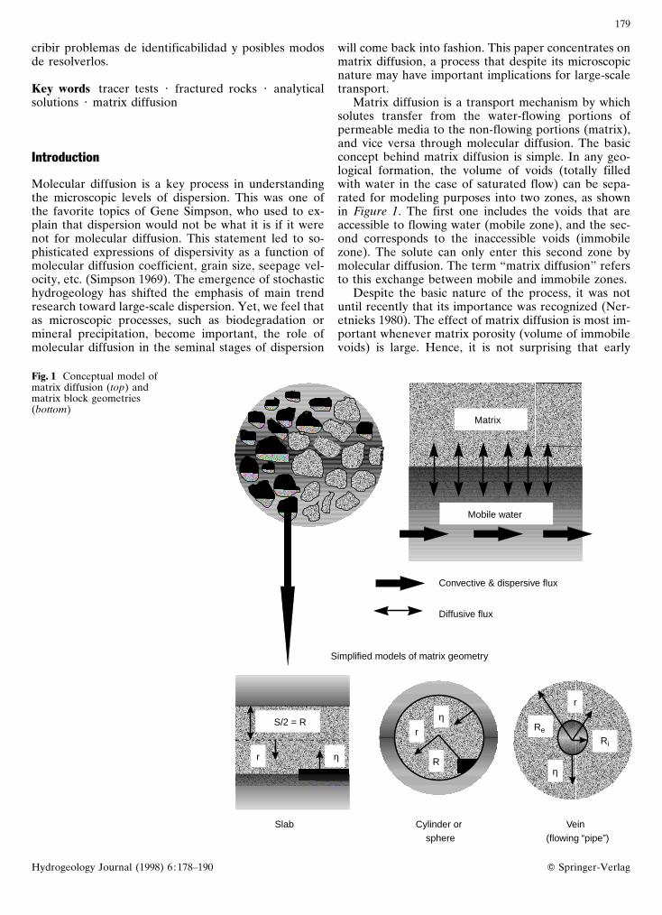
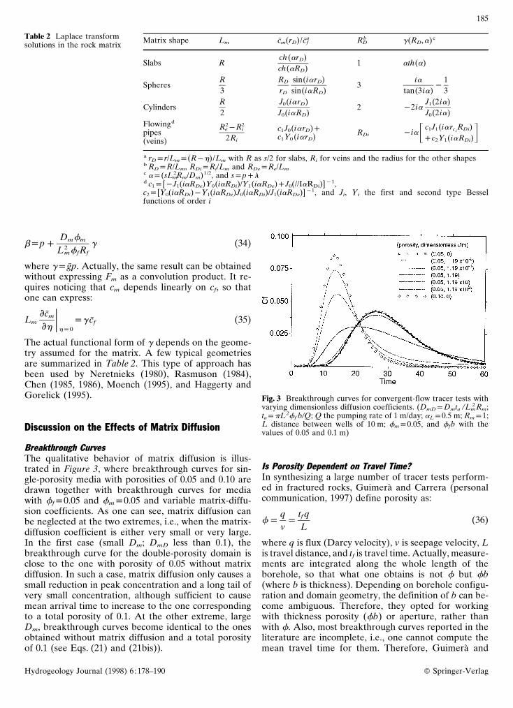
Fig. 1 Conceptual model ofmatrix diffusion (top) andmatrix block geometries(bottom)

Convective & dispersive flux

Diffusive flux

S/2 = R

r

r

R

η

η

Slab Cylinder orsphere

Vein(flowing “pipe”)

Simplified models of matrix geometry

Matrix

r

Re

Ri

η

Mobile water

cribir problemas de identificabilidad y posibles modosde resolverlos.

Key words tracer tests 7 fractured rocks 7 analyticalsolutions 7 matrix diffusion

Introduction

Molecular diffusion is a key process in understandingthe microscopic levels of dispersion. This was one ofthe favorite topics of Gene Simpson, who used to ex-plain that dispersion would not be what it is if it werenot for molecular diffusion. This statement led to so-phisticated expressions of dispersivity as a function ofmolecular diffusion coefficient, grain size, seepage vel-ocity, etc. (Simpson 1969). The emergence of stochastichydrogeology has shifted the emphasis of main trendresearch toward large-scale dispersion. Yet, we feel thatas microscopic processes, such as biodegradation ormineral precipitation, become important, the role ofmolecular diffusion in the seminal stages of dispersion

will come back into fashion. This paper concentrates onmatrix diffusion, a process that despite its microscopicnature may have important implications for large-scaletransport.

Matrix diffusion is a transport mechanism by whichsolutes transfer from the water-flowing portions ofpermeable media to the non-flowing portions (matrix),and vice versa through molecular diffusion. The basicconcept behind matrix diffusion is simple. In any geo-logical formation, the volume of voids (totally filledwith water in the case of saturated flow) can be sepa-rated for modeling purposes into two zones, as shownin Figure 1. The first one includes the voids that areaccessible to flowing water (mobile zone), and the sec-ond corresponds to the inaccessible voids (immobilezone). The solute can only enter this second zone bymolecular diffusion. The term “matrix diffusion” refersto this exchange between mobile and immobile zones.

Despite the basic nature of the process, it was notuntil recently that its importance was recognized (Ner-etnieks 1980). The effect of matrix diffusion is most im-portant whenever matrix porosity (volume of immobilevoids) is large. Hence, it is not surprising that early

180


studies of matrix diffusion concentrated on low-per-meability fractured media (Rasmuson and Neretnieks1981; Rasmuson et al. 1982; Rasmuson 1984; Neret-nieks 1987). In fact, matrix diffusion is still associatedwith transport in fractured media. However, it can af-fect other media, as shown by Wood et al. (1990) forgranular materials, and by Carrera et al. (1990) forclays.

The effects of matrix diffusion are diverse. On onehand, a large volume of voids becomes accessible to thesolute by diffusion. This causes an apparent retardationwith respect to solutes that do not enter the matrix, atopic that has been extensively studied by Maloszewskiand Zuber (1993), Zuber and Motyka (1994), and Ma-loszewski and Zuber (1985). Actually, not only voids,but also sorption sites can be reached by the solutethrough diffusion. This process causes a further retar-dation. Moreover, under such conditions, sorption isnot instantaneous, but delayed. The solute behaves as ifaffected by kinetic sorption. Another effect of matrixdiffusion is tailing on breakthrough curves. Solutes takea long time to come out of the matrix because concen-tration gradients are small. Since heterogeneity alsocauses tailing on breakthrough curves, it is sometimesdifficult to distinguish between these two processes.

The fact that matrix diffusion causes effects (retar-dation and tailing) similar to other mechanisms (heter-ogeneity and kinetic sorption) is a source of difficultiesin solute-transport modeling. Indeed, experimentalbreakthrough curves can be fitted to a number of nu-merical models. Yet, they lead to markedly different re-sults when used for prediction. One of the objectives ofour work is to discuss ways to discriminate among thesemechanisms.

In order to do so, we first review existing ways offormulating matrix diffusion and approaches to solvethe resulting equations. As it turns out, many formula-tions have been used. Variations refer both to theequations and the geometry assumed for the immobilezone. Solution approaches include analytical and nu-merical. Both can be formulated in real-time or La-place-transformed domains. Solution approaches de-pend on the way the equations are formulated, whichmay add some confusion. Therefore, another objectiveof our work is to find some unity among formulationsand solution methods. In doing so, we derive someproperties of matrix diffusion regarding identifiability,moments of breakthrough curves, asymptotic behavior,etc. The most mathematical aspects of our work areconcentrated in the sections, “Formulation of the Prob-lem” and “Solution Methods,” which can and should beskipped by readers not interested in mathematics.

Formulation of the Problem

Solutes are carried with flowing water by advection anddispersion. Dispersion includes the effect of moleculardiffusion in the flowing water. However, solutes may

move independently of the flowing water by moleculardiffusion into stagnant zones. Different ways exist torepresent the exchange between mobile and stagnantzones. The objective of this section is to review theseformulations.

Basic Equations

We consider the aquifer domain as the superposition oftwo media. The first one, which is often called the mo-bile or flowing zone, represents the portion of aquiferaccessible to flowing water. Transport processes in thiszone include advection, dispersion, and chemical reac-tions. The second one, called immobile or matrix, rep-resents the portion where water flow is negligible, so noadvection occurs and dispersion is reduced to molecu-lar diffusion.

Two remarks are appropriate here. Firstly, the sepa-ration between the two zones is somewhat arbitrary.The set of permanently stagnant zones is probably verysmall (if not zero). Their separation is made in terms ofthe relevance of advection and hydrodynamic disper-sion as compared with molecular diffusion. As is shownin the section “Discussion on the Effects of Matrix Dif-fusion”, precise discrimination is not critical. Moreover,in practice, the separation between the two zones isbased more on the conceptualization of the medium(i.e., fractures and blocks) than on the precise evalua-tion of water-velocity distribution. The second remarkrefers to the continuum approach. Whereas the twozones are physically distinct at the microscale, we treatthem as overlapping and spanning the whole domain.For example, concentration in the flowing zone is ex-pressed as cf (x,y,z,t); it becomes cm(x,y,z,h,t) in the ma-trix, where h is the shortest distance to the flowing zone(depth into the matrix).

The solute-transport equation expresses the solutemass balance in the flowing zone per unit volume ofaquifer. Therefore, accounting for matrix diffusionsimply requires adding a sink/source term Fm that rep-resents the mass of solute diffusing from the flowingzone into the matrix, and vice versa. Therefore, thetransport equation for a single specie becomes:

ff Rficf

itp=7 (Df7=cf)Pq7=cfPFm (1)

where ff, Rf, and Df are the porosity, retardation fac-tor, and dispersion coefficient, respectively. Differentvariations of Eq. (1) have been used by most authors(Rasmusson and Neretnieks 1980, 1981, 1986; Moench1984; Grisak and Pickens 1981; Sudicky and Frind 1992;Moench 1989, 1995; Maloszewski and Zuber 1993; Nov-akowski and Lapceviec 1994; Haggerty and Gorelick1995; Ibaraki and Sudicky 1995; Kennedy and Lennox1995).

A number of forms can be used for writing Fm. Theyare all variations of Fick’s first law. The two most wide-ly spread are:

181


FmpsmfmbDmicm

ih )hp0

or FmpPsmfmbRmicmav

it(2)

where fmb is matrix porosity (volume of voids per unitvolume of matrix), Dm is the coefficient of moleculardiffusion, cmav is the average concentration in the ma-trix, and sm is the specific surface of the matrix (matrixsurface area per aquifer unit volume). In general, wedenote sm(h) as the diffusion surface at depth h. Equa-tion (2) warrants two remarks. Firstly, sometimes thecoefficient of diffusion includes the porosity. We preferto write it as in Eq. (2) in order to reduce the depend-ence of Dm on fmb (actually, Dm is still approximatelyproportional to fm

1 /2; otherwise, it would be propor-tional to fm

3 /2). Secondly, geometrical consistency im-poses constraints between sm and the size of matrixblocks. Let Lm be the average size of matrix blocks (ra-tio of volume to surface area ratio), then,smLmp1Pff, where it should be self-evident that bothsides of the equality express the volume of matrix perunit volume of aquifer. This allows us to write

smfmbp1Pff

Lm

fmbpfm

Lm

(3)

where fm is now the volume of matrix voids expressedper unit volume of aquifer (recall that fmb was ex-pressed per unit volume of matrix). Then, Eq. (2) be-comes

FmpDmfm

Lm

icm

ih )hp0

or FmpPfmRm

Lm

icmav

it(4)

Notice that Fm is being written both in terms of the dif-fusive flux and by establishing a mass balance in thematrix. Obviously, both forms are equivalent. Concen-tration in the matrix, cm, is given by the diffusion equa-tion:

sm(h)Rmicm

itp

iih 1Dmsm(h)

icm

ih 2 (5)

which is solved subject to:

cm(x,h,tp0)p0 (6)

cm(x,hp0, t)pcf(x, t) at Gm(hp0) (7)

icm

ih(x,hphmx, t)p0 (8)

where Eq. (6) is the initial condition, which has beentaken as homogeneous but can be generalized; Eq. (7)expresses continuity of concentrations at Gm, interfacebetween the flowing and matrix zones (note that con-tinuity of mass flux is automatically imposed by theterm Fm in Eq. (2)); and (8) is the boundary conditionat the innermost portion of the matrix. The relationshipbetween Lm and hmx depends on the geometry of ma-trix blocks, as summarized in Table 1.

Table 1 Definition of Lm, sn, and an, depending on matrix geo-metry

Shapea Lmp1Pff

sman an

Slabss2

(2nP1)p

22

Cylindersb R2

un

212

SpheresR3

np

323

Veinsc Re2PRi

2

2RiLmun

2Re(cnP1)

First order P 1 1

a Lm depends on geometry: s the distance between fractures forslabs, R the radius of the cylinder or sphere, Ri and Re theinside and outside radii of veinsb un are the roots of J0(un)p0c un are the roots of Y0(Riun)J1(Reun)pJ0(Riun)Y1(Reun) andcnpJ0(Riun)/J1(Reun)pY0(Riun)/Y1(Reun)

Other Formulations for Matrix Diffusion

Different authors have used different formulations formatrix diffusion. Haggerty and Gorelick (1995) reviewextensively the literature on first-order approximationsof matrix diffusion, which can be summarized as:

FmpsmfmbDm

Lm

(cmPcf)pDmfm

Lm2 (cmPcf) (9)

icm

itp

Dm

RmLm2 (cfPcm)pa(cfPcm) (10)

where the meaning of sm, fmb, Dm, and Lm is now some-what fictitious. In fact, they use a to express the factorof (cfPcm). We have written this term explicitly to keepthe parallelism with the previous section. In comparingour equations with those of Haggerty and Gorelick(1995), one should bear in mind that Eq. (1) expressesthe mass balance of solute in the flowing zone, whereasthey include both the flowing and matrix zones.

Many authors write the matrix sink/source term asthe superposition of different matrix block shapes andsizes. In the case of strict diffusion, Rasmuson (1985)expressed Fm as (in our notation):

FmpN

Ajp1

smjfbmjDmjicm

ih(11)

where subindex j stands for each of the matrix catego-ries. Concentration in each of these obeys an equationanalogous to Eq. (5).

Haggerty and Gorelick (1995) go further to showthat by superimposing terms analogous to Eqs. (9) and(10) one can reproduce not only matrix diffusion butmany other processes as well. In fact, they go on toshow how a judicious choice of ajpDmj /RmjL2

mj allowsthem to reproduce diffusion into slabs or spheres (ac-tually, they require an infinite sum). The parallelism

182


with the conventional formulation of Eqs. (2) and (5)will become apparent in the next section.

Integro-Differential Formulations

The integro-differential approach was proposed byHerrera and coworkers (Herrera and Rodarte 1973;Herrera and Yates 1977) for solving flow across aqui-tards. This approach is advantageous because it elimi-nates the need for discretizing the aquitard. It can alsobe applied to matrix diffusion. In fact, it is simpler toapply to our problem than to leaky aquifers. Here, wesimply outline the method; more complete descriptionsare given by Carrera and Walters (1985) and Carrera etal. (1986). In essence, the idea is to express Fm as a con-volution product of a memory function times icf /it.This product can be evaluated recursively very easily.The first step consists of finding the solution to Eq. (5),given a constant unit boundary concentration inEq. (7). For the case of slabs (Fig. 1) (constant sm), thissolution is:

w(h, t)pcm(h, t)

cf

p1Pe

Anp1

2an

ePan2tD sin an hD (12)

where tDpDmt/Rm2 Lm

2 ; hDph/Lm and anp(2nP1)p/2.Since cf is not constant, the solution of Eq. (5), subjectto Eqs. (6), (7), and (8), requires the convolution ofEq. (12) and the actual cf. Direct application of Eq. (12)leads to:

cm(x,h, t)pt

#0

icf

it(x, tPt)7w(h,t)dtpw*

icf

it(13)

where * represents convolution product. Actually, weare not interested as much in cm as in Fm, which wouldbe given by:

FmpDm fm

Lm

icm

ih )hp0

pDmfm

L2m

icm

ihD)

hDp0

pDm fm

L2m

gpicm

it(14)

where g is the “memory function,” given by:

g(tD)piwihD

)hDp0

pP2e

Anp1

ePan2tD (15)

Although Eq. (15) has been derived for slab-shapedblocks, it can be generalized for blocks of any shape. Infact, the general form of Eq. (15) would be:

g (tD)pPe

Anp1

anePan2 tD (16)

where an is often constant. The actual values of an andan for slabs, spheres, cylinders, and veins are given inTable 1. It can be seen that first-order expressions formatrix diffusion, such as Eqs. (9) and (10), also fit inthis integro-differential formulation, in which case an

and an equal 1 for np1 and zero otherwise. In fact, onecan argue that different combinations of an and an will

Fig. 2 Memory function g and its approximation, gN, for severalvalues of N

represent different geometries (this point is discussed,under a different perspective, by Haggerty and Gore-lick 1995). In fact, in the context of leaky aquifer mod-eling, Premchitt (1981) argues for using any judiciouschoice of a discrete number N of an and an, provided

they satisfy N

Anp1

an/an2p1.

Asymptotic Approximations: Early- and Late-Time Solutions

and Mean Arrival Time

Early-time behaviorFurther insight on the behavior of g can be gained fromFigure 2, which shows g together with several approxi-mations obtained by truncating the infinite series inEq. (16) for the case of parallel slabs. A cursory exami-nation of Figure 2 makes it clear that truncation is onlyvalid for large tD (e.g., larger than 0.1). It also suggeststhat, for small tD, the behavior of g is linear in logarith-mic scale, which prompts us to seek an asymptotic ex-pression for g(tD). This can be done by writing Eq. (15)as a Riemann summation. Let u2ptD and unp(2nP1)pu/2, then

limu]0

pug(u)plimu]0

Pe

Anp1

2(unP1Pun)ePun2p

P2e

#0

ePu2dupP;p or, for small tD:

g(tD)pP1

;p tD(17)

The same approach can be used, with identical resultsfor spheres. One important implication of Eq. (17) isthat, for small times, Fm equals (independently of blockgeometry):

183


FmpPDmfm

Lm

1

"pDmtRm

picf

itp

fm ;DmRm

Lm ;ptp

icf

it(18)

that is, at early times, matrix diffusion is a function offm;Dm Rm /Lm but does not depend on these paramet-ers independently (nor on block geometry).

Late-time behaviorAsymptotic behavior for large times (relative to therate of change of cf) can be obtained by assuming icf/itconstant in the interval (0,t). In such a case:

FmpPDmfm

L2m

t

#0

e

Anp1

anePan2(tDPtD) icf

it(tPt)dt

pfm Rmicf

it

e

Anp1

an(ePan

2tDP1)an

2(19)

If tD is large enough, then ePan2tDP1 and can be ne-

glected. Using the fact that e

Anp1

an /an2 equals 1, which is

proven in a later section, Fm in Eq. (19) becomes:

FmpRmfmicf

it(20)

Substituting Eq. (20) in Eq. (1) leads to

(ff RfcfmRm)icf

itp=7(Df7=cf)Pq7=cf (21)

In summary, when tD is large (Dm large and Rm and Lm

small) compared with the rate of change of icf/it, thenthe medium behaves as a single-porosity with a capacityof ffRfcfmRm instead of ff Rf . This issue has been ex-plored by Malozewski and Zuber (1985). In fact, theydefine a matrix retardation factor

Rfmp1cfm Rm

ff Rf

(21 bis)

This retardation factor multiplies the one caused bysorption into the flowing zone (ffRf in Eq. (1)).

Mean travel timeThe mean travel time or mean arrival time is definedas:

tp

e

#0

tcf dt

e

#0

cf dt

(22)

provided that both integrals exist. Equations for t can

be derived by applying the operator e

#0

t(7)dt to both

sides of Eq. (1). This approach is used by Varni andCarrera (in press) for deriving “groundwater-age”equations for single-porosity media. Goode (1996) fol-

lows a very similar approach. This operator is appliedto both sides of Eq. (1), using integration by parts forapproximating the time derivative term and Eq. (14)for Fm and Eq. (16) for g. The matrix-diffusion term re-quires applying again the formula of integration byparts, while using again the fact Aan/an

2p1. The resultis an equation identical to the one derived by Goode(1996) or Varni and Carrera (in press), but withff RfcfmRm instead of ff Rf ; i.e., mean arrival time isequal to the one that would be obtained in a single-porosity medium with solute-storing capacity identicalto the full mobile zone plus matrix in the double-poros-ity media. This is so, regardless of the value of matrix-diffusion coefficient and matrix-block shape and size.This result has also been obtained by Harvey and Gor-elick (1995) using a different approach.

Solution Methods

The above equations can be solved using different nu-merical methods: spatial discretization, hybrid (numeri-cal-analytical), and Laplace transform, as outlined be-low.

Spatial Discretization

The matrix-diffusion term in Eq. (1) has the same formas the leakage term in multiaquifer systems, except forthe no-flow boundary condition (Eq. (8)), which is sub-stituted by a continuity (prescribed-head) condition.The classical approach for simulating this type of phe-nomenon consists of using vertical strings of one-di-mensional elements to simulate diffusion in the rockmatrix. Examples of this approach are the works ofChorley and Frind (1978) and Neuman et al. (1982).Unfortunately, an accurate solution requires a very finediscretization near the interface between the matrixand flowing zones. As a result, the cost of simulatingthe matrix can become very large unless one adoptsspecial solution methods (block iterative, adaptativeexplicit–implicit, etc.), as suggested by the above au-thors. Programming these methods is not straightfor-ward, so that by adopting them one loses programmingsimplicity, which is probably the main advantage of thediscretization approach.

We feel, however, that the main advantage of spatialdiscretization is its generality. Full capabilities of anytransport code can be used without significant pro-gramming for simulating matrix diffusion. Hence, it ispossible to model non-linear processes without addi-tional programming effort. This is what we have donein TRANSIN (Medina et al. 1995; Medina and Carrera1996). We use discretization for non-linear problemsand rely on the hybrid method, which is described be-low, for linear matrix diffusion.

184


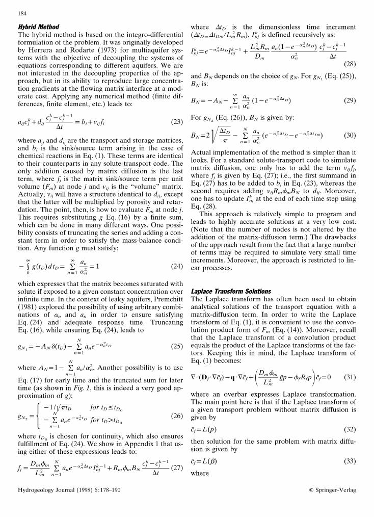
Hybrid Method

The hybrid method is based on the integro-differentialformulation of the problem. It was originally developedby Herrera and Rodarte (1973) for multiaquifer sys-tems with the objective of decoupling the systems ofequations corresponding to different aquifers. We arenot interested in the decoupling properties of the ap-proach, but in its ability to reproduce large concentra-tion gradients at the flowing matrix interface at a mod-erate cost. Applying any numerical method (finite dif-ferences, finite element, etc.) leads to:

aijckj cdij

ckj PckP1

j

Dtpbicvij fi (23)

where aij and dij are the transport and storage matrices,and bi is the sink/source term arising in the case ofchemical reactions in Eq. (1). These terms are identicalto their counterparts in any solute-transport code. Theonly addition caused by matrix diffusion is the lastterm, where fj is the matrix sink/source term per unitvolume (Fm) at node j and vij is the “volume” matrix.Actually, vij will have a structure identical to dij, exceptthat the latter will be multiplied by porosity and retar-dation. The point, then, is how to evaluate Fm at node j.This requires substituting g Eq. (16) by a finite sum,which can be done in many different ways. One possi-bility consists of truncating the series and adding a con-stant term in order to satisfy the mass-balance condi-tion. Any function g must satisfy:

Pe

#0

g(tD)d tDpe

Anp1

an

a2n

p1 (24)

which expresses that the matrix becomes saturated withsolute if exposed to a given constant concentration overinfinite time. In the context of leaky aquifers, Premchitt(1981) explored the possibility of using arbitrary combi-nations of an and an in order to ensure satisfyingEq. (24) and adequate response time. TruncatingEq. (16), while ensuring Eq. (24), leads to

gN1pPAN d(tD)P

N

Anp1

anePan2 tD (25)

where ANp1PN

Anp1

an/a2n. Another possibility is to use

Eq. (17) for early time and the truncated sum for latertime (as shown in Fig. 1, this is indeed a very good ap-proximation of g):

gN2p5 P1 /;ptD for tD^tD0

PN

Anp1

anePan2 tD for tD1 tD0

(26)

where tD0 is chosen for continuity, which also ensures

fulfillment of Eq. (24). We show in Appendix 1 that us-ing either of these expressions leads to:

fjpDmfm

L2m

N

Anp1

anePan2DtD IkP1

nj cRmfmBNck

j PckP1j

Dt(27)

where DtD is the dimensionless time increment(DtDpDtDm/Lm

2 Rm), Iknj is defined recursively as:

IknjpePan

2DtDIkP1nj c

L2mRm

Dm

an(1PePan2DtD)

a2n

ckj PckP1

j

Dt(28)

and BN depends on the choice of gN. For gN1 (Eq. (25)),

BN is:

BNpPANPe

Anp1

an

a2n

(1PePan2 DtD) (29)

For gN2 (Eq. (26)), BN is given by:

BNp2 "DtDp

PN

Anp1

an

a2n

(ePan2DtDPePan

2DtD0) (30)

Actual implementation of the method is simpler than itlooks. For a standard solute-transport code to simulatematrix diffusion, one only has to add the term vij fj,where fj is given by Eq. (27); i.e., the first summand inEq. (27) has to be added to bi in Eq. (23), whereas thesecond requires adding vijRmfmBN to dij. Moreover,one has to update Ik

nj at the end of each time step usingEq. (28).

This approach is relatively simple to program andleads to highly accurate solutions at a very low cost.(Note that the number of nodes is not altered by theaddition of the matrix-diffusion term.) The drawbacksof the approach result from the fact that a large numberof terms may be required to simulate very small timeincrements. Moreover, the approach is restricted to lin-ear processes.

Laplace Transform Solutions

The Laplace transform has often been used to obtainanalytical solutions of the transport equation with amatrix-diffusion term. In order to write the Laplacetransform of Eq. (1), it is convenient to use the convo-lution product form of Fm (Eq. (14)). Moreover, recallthat the Laplace transform of a convolution productequals the product of the Laplace transforms of the fac-tors. Keeping this in mind, the Laplace transform ofEq. (1) becomes:

=7(Df7=cf)Pq7=cfc1Dmfm

L2m

gpPff Rf p2 cfp0 (31)

where an overbar expresses Laplace transformation.The main point here is that if the Laplace transform ofa given transport problem without matrix diffusion isgiven by

cfpL(p) (32)

then solution for the same problem with matrix diffu-sion is given by

cfpL(b) (33)

where

185


Table 2 Laplace transformsolutions in the rock matrix Matrix shape Lm cm(rD)/cf

a RbD g(RD,a)c

Slabs Rch (arD)ch(aRD)

1 ath(a)

SpheresR3

RD

rD

sin(iarD)sin(iaRD)

3ia

tan(3ia)P

13

CylindersR2

J0(iarD)J0(iaRD)

2 P2iaJ1(2ia)J0(2ia)

Flowingd

pipes(veins)

Re2PRi

2

2Ri

c1J0(iarD)cc1Y0 (iarD) RDi Pia3 c1J1(iarci

RDi)cc2Y1(iaRDi)4

a rDpr/Lmp(RPh)/Lm with R as s/2 for slabs, Ri for veins and the radius for the other shapesb RDpR/Lm, RDipRi/Lm and RDepRe/Lmc ap(sL2

mRm/Dm)1/2, and sppcld c1p[PJ1(iaRDe)Y0(iaRDi)/Y1(iaRDe)cJ0(//IaRDi)]P1,c2p[Y0(iaRDi)PY1(iaRDe)J0(iaRDi)/J1(iaRDe)]P1, and Ji, Yi the first and second type Besselfunctions of order i

bppcDmfm

L2mffRf

g (34)

where gpgp. Actually, the same result can be obtainedwithout expressing Fm as a convolution product. It re-quires noticing that cm depends linearly on cf, so thatone can express:

Lmicm

ih )hp0

pg cf (35)

The actual functional form of g depends on the geome-try assumed for the matrix. A few typical geometriesare summarized in Table 2. This type of approach hasbeen used by Neretnieks (1980), Rasmuson (1984),Chen (1985, 1986), Moench (1995), and Haggerty andGorelick (1995).

Discussion on the Effects of Matrix Diffusion

Breakthrough Curves

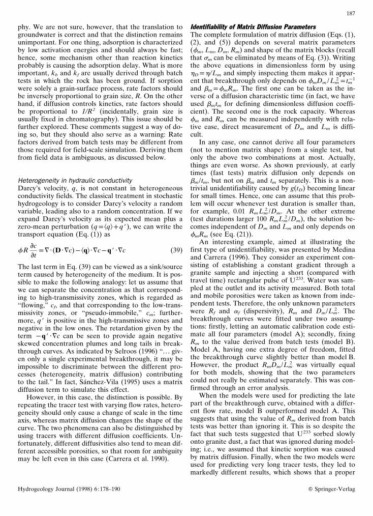
The qualitative behavior of matrix diffusion is illus-trated in Figure 3, where breakthrough curves for sin-gle-porosity media with porosities of 0.05 and 0.10 aredrawn together with breakthrough curves for mediawith ffp0.05 and fmp0.05 and variable matrix-diffu-sion coefficients. As one can see, matrix diffusion canbe neglected at the two extremes, i.e., when the matrix-diffusion coefficient is either very small or very large.In the first case (small Dm; DmD less than 0.1), thebreakthrough curve for the double-porosity domain isclose to the one with porosity of 0.05 without matrixdiffusion. In such a case, matrix diffusion only causes asmall reduction in peak concentration and a long tail ofvery small concentration, although sufficient to causemean arrival time to increase to the one correspondingto a total porosity of 0.1. At the other extreme, largeDm, breakthrough curves become identical to the onesobtained without matrix diffusion and a total porosityof 0.1 (see Eqs. (21) and (21bis)).

Fig. 3 Breakthrough curves for convergent-flow tracer tests withvarying dimensionless diffusion coefficients. (DmDpDmta /Lm

2 Rm;tappL2ff b/Q; Q the pumping rate of 1 m/day; aLp0.5 m; Rmp1;L distance between wells of 10 m; fmp0.05, and ffb with thevalues of 0.05 and 0.1 m)

Is Porosity Dependent on Travel Time?

In synthesizing a large number of tracer tests perform-ed in fractured rocks, Guimerà and Carrera (personalcommunication, 1997) define porosity as:

fpqv

ptf qL

(36)

where q is flux (Darcy velocity), v is seepage velocity, Lis travel distance, and tf is travel time. Actually, measure-ments are integrated along the whole length of theborehole, so that what one obtains is not f but fb(where b is thickness). Depending on borehole configu-ration and domain geometry, the definition of b can be-come ambiguous. Therefore, they opted for workingwith thickness porosity (fb) or aperture, rather thanwith f. Also, most breakthrough curves reported in theliterature are incomplete, i.e., one cannot compute themean travel time for them. Therefore, Guimerà and

186


Fig. 4 Relation between accessible thickness porosity (fb) andpeak arrival time for tracer tests from different fractured mediaaround the world (Guimerà and Carrrera, personal commu-nication, 1997)

Fig. 5 Apparent porosities obtained from convergent-flow tracertests with varying dimensionless diffusion. The apparent porosityis derived by assuming that the advective time is equal to thearrival time of the breakthrough peak. (DmDpDmta/RmLm

2 ;tappL2ff b/Q; Q the pumping rate of 1 m3/day; Rmp1; aLp2 m;L distance between wells of 10 m; fmp0.0891; ff bp0.05 m)

Carrera opted for using peak arrival time for tf, andcorrecting for dispersion. When plotting fb vs tf, theyobtained Figure 4, which suggests that these two varia-bles are indeed correlated.

Two issues become apparent when the procedure isexamined critically. Firstly, numerous disturbing factorsare being ignored. These include sorption, directionaleffects, connectivity between pumping and injectionwell, etc. However, these factors tend to add noise, thusreducing correlation. The fact that fb and tf are corre-lated despite them implies that indeed the correlationmust be strong. The second issue is more insidious, asone might think that the correlation is nothing but anartifact introduced by the procedure for defining fb.

To counter this problem, they argue that if the flowrate is changed, one would not expect the porosity de-rived by means of Eq. (36) to change. Yet, they ob-served that it does change for a sequence of tracer tests

performed with varying flow rates at a fractured zone inthe Grimsel Test Site (Switzerland). They attribute thisparadox to matrix diffusion.

In fact, what is being computed is “accessed” or “ap-parent” porosity (i.e., the portion of voids reached bythe solute). Actually, close inspection of Figure 3 re-veals that peak arrival time is delayed by matrix diffu-sion. The delay is not dramatic because fm was chosensmall. The whole effect is illustrated in Figure 5, whichdisplays porosity thus defined as a function of dimen-sionless matrix diffusion, which is proportional to ad-vective time. In this case ffp0.01 and fmp0.089(fmbp0.09). Porosities derived this way grow with DmD

and, thus, with travel time. This may explain, at leastpartly, the correlation displayed in Figure 4. In short,porosity is the ratio of voids to total volume and doesnot depend on solute travel time, but sometimes itlooks as if it does.

Physical Mechanisms Analogous to Matrix Diffusion

As discussed previously, the main effects of matrix dif-fusion are retardation, asymmetry in the plume (nega-tive skewness), and long tails in breakthrough curves. Itturns out that other physical mechanisms exist that leadto the same behavior, such as kinetic sorption and hy-draulic-conductivity heterogeneity. Here, we show whythese mechanisms lead to similar behavior by analyzingthe mathematical equations governing them.

Kinetic sorptionAs we did for matrix diffusion, one can also distinguishbetween mobile and the immobile resident concentra-tions, cf and cim, for kinetically sorbing solutes. Theequations governing these concentrations are

ficf

itp=7(Df7=cf)Pq7=cfP

icim

it(37)

icim

itpkf cfPkccim (38)

where kf and kb are the forward- and backward-ratecoefficients, respectively, and is the bulk density ofthe solid (provided that cim is expressed per unit massof solid). If kfpkb, the exchange term becomes propor-tional to the difference between the mobile and immo-bile concentrations, identical to first-order approxima-tions to matrix diffusion with cimpcmav (see Eq. (2)). Infact, the same formalism can be applied even if kb andkf are different (see Haggerty and Gorelick 1995).

Kinetic sorption obeying these equations is indistin-guishable from first-order matrix diffusion. Therefore,the question of whether kinetics is being caused by ma-trix diffusion or by actual sorption becomes academic,in the sense that it does not have practical implicationsand most authors leave it at that (Wood et al. 1990 area notable exception). In fact, this approach has a longand successful record of applications in chromatogra-

187


phy. We are not sure, however, that the translation togroundwater is correct and that the distinction remainsunimportant. For one thing, adsorption is characterizedby low activation energies and should always be fast;hence, some mechanism other than reaction kineticsprobably is causing the adsorption delay. What is moreimportant, kb and kf are usually derived through batchtests in which the rock has been ground. If sorptionwere solely a grain-surface process, rate factors shouldbe inversely proportional to grain size, R. On the otherhand, if diffusion controls kinetics, rate factors shouldbe proportional to 1/R2 (incidentally, grain size isusually fixed in chromatography). This issue should befurther explored. These comments suggest a way of do-ing so, but they should also serve as a warning: Ratefactors derived from batch tests may be different fromthose required for field-scale simulation. Deriving themfrom field data is ambiguous, as discussed below.

Heterogeneity in hydraulic conductivityDarcy’s velocity, q, is not constant in heterogeneousconductivity fields. The classical treatment in stochastichydrogeology is to consider Darcy’s velocity a randomvariable, leading also to a random concentration. If weexpand Darcy’s velocity as its expected mean plus azero-mean perturbation (qpkqlcqb), we can write thetransport equation (Eq. (1)) as

fRicit

p=7(D7=c)Pkql7=cPqb7=c (39)

The last term in Eq. (39) can be viewed as a sink/sourceterm caused by heterogeneity of the medium. It is pos-sible to make the following analogy: let us assume thatwe can separate the concentration as that correspond-ing to high-transmissivity zones, which is regarded as“flowing,” cf, and that corresponding to the low-trans-missivity zones, or “pseudo-immobile,” cm; further-more, qb is positive in the high-transmissive zones andnegative in the low ones. The retardation given by theterm Pqb7=c can be seen to provide again negativeskewed concentration plumes and long tails in break-through curves. As indicated by Selroos (1996) “. . . giv-en only a single experimental breakthrough, it may beimpossible to discriminate between the different pro-cesses (heterogeneity, matrix diffusion) contributingto the tail.” In fact, Sánchez-Vila (1995) uses a matrixdiffusion term to simulate this effect.

However, in this case, the distinction is possible. Byrepeating the tracer test with varying flow rates, hetero-geneity should only cause a change of scale in the timeaxis, whereas matrix diffusion changes the shape of thecurve. The two phenomena can also be distinguished byusing tracers with different diffusion coefficients. Un-fortunately, different diffusivities also tend to mean dif-ferent accessible porosities, so that room for ambiguitymay be left even in this case (Carrera et al. 1990).

Identifiability of Matrix Diffusion Parameters

The complete formulation of matrix diffusion (Eqs. (1),(2), and (5)) depends on several matrix parameters(fm, Lm, Dm, Rm) and shape of the matrix blocks (recallthat sm can be eliminated by means of Eq. (3)). Writingthe above equations in dimensionless form by usinghDph/Lm and simply inspecting them makes it appar-ent that breakthrough only depends on fmDm /Lm

2ptmP1

and bmpfmRm. The first one can be taken as the in-verse of a diffusion characteristic time (in fact, we haveused bmtm for defining dimensionless diffusion coeffi-cient). The second one is the rock capacity. Whereasfm and Rm can be measured independently with rela-tive ease, direct measurement of Dm and Lm is diffi-cult.

In any case, one cannot derive all four parameters(not to mention matrix shape) from a single test, butonly the above two combinations at most. Actually,things are even worse. As shown previously, at earlytimes (fast tests) matrix diffusion only depends onbm/tm, but not on bm and tm separately. This is a non-trivial unidentifiability caused by g(tD) becoming linearfor small times. Hence, one can assume that this prob-lem will occur whenever test duration is smaller than,for example, 0.01 Rm Lm

2 /Dm. At the other extreme(test durations larger 100 RmLm

2 /Dm), the solution be-comes independent of Dm and Lm and only depends onfmRm (see Eq. (21)).

An interesting example, aimed at illustrating thefirst type of unidentifiability, was presented by Medinaand Carrera (1996). They consider an experiment con-sisting of establishing a constant gradient through agranite sample and injecting a short (compared withtravel time) rectangular pulse of U233. Water was sam-pled at the outlet and its activity measured. Both totaland mobile porosities were taken as known from inde-pendent tests. Therefore, the only unknown parameterswere Rf and af (dispersivity), Rm and Dm/Lm

2 . Thebreakthrough curves were fitted under two assump-tions: firstly, letting an automatic calibration code esti-mate all four parameters (model A); secondly, fixingRm to the value derived from batch tests (model B).Model A, having one extra degree of freedom, fittedthe breakthrough curve slightly better than model B.However, the product RmDm/Lm

2 was virtually equalfor both models, showing that the two parameterscould not really be estimated separately. This was con-firmed through an error analysis.

When the models were used for predicting the latepart of the breakthrough curve, obtained with a differ-ent flow rate, model B outperformed model A. Thissuggests that using the value of Rm derived from batchtests was better than ignoring it. This is so despite thefact that such tests suggested that U233 sorbed slowlyonto granite dust, a fact that was ignored during model-ing; i.e., we assumed that kinetic sorption was causedby matrix diffusion. Finally, when the two models wereused for predicting very long tracer tests, they led tomarkedly different results, which shows that a proper

188


identification of model parameters is indeed very im-portant. In fact, this also shows that non-identifiabilitycould have been overcome by repeating the test with amuch smaller flow rate.

Conclusions

We have written the matrix-diffusion equations usingboth the conventional and integro-differential formula-tions. In this process, we have synthesized the equa-tions for blocks of different geometries (slabs, cylin-ders, spheres, veins, and first-order formulations). Thishas allowed us to derive asymptotic approximations forearly and late times. In the first case, the solute lackstime to diffuse deep into the matrix, which behaves asinfinitely thick, and the breakthrough curve depends onfm

2 RmDm/Lm2 , but not on these parameters separately.

This is to be expected for fast tracer tests. In the secondcase, the solute diffuses deep into the matrix relative toadvective transport. Hence, the matrix behaves as if ful-ly equilibrated with the mobile portion of the mediumand breakthrough curves only depend on ffRfcfmRm,but not on Dm. The latter leads to showing that themean arrival time is independent of diffusion coeffi-cient and matrix shape and size, a result that had al-ready been obtained by Harvey and Gorelick (1995)and Sánchez-Vila and Carrera (1995), using a differentapproach.

The solute transport equation incorporating a ma-trix-diffusion term can be solved using three sets ofmethods:1. Numerical discretization. This method is very gener-

al and easy to program, but accurate solutions mayrequire refined grids and long CPU times.

2. Hybrid (analytical-numerical) method based on inte-gro-differential formulation. This method is very ac-curate and inexpensive, but its use is constrained tolinear processes. Moreover, its programming re-quires substantial additions to existing transportcodes.

3. Laplace transform. The advantages and drawbacksof this method are analogous to the hybrid method.Its use appears to have been constrained to analyti-cal solutions.Some of the above findings help in explaining ob-

served features of matrix diffusion. Specifically, break-through curves of matrix diffusing solutes can be verysimilar to those obtained by totally neglecting matrixdiffusion (peak arrival time less than 0.01 RmLm

2 /Dm),or to those obtained by assuming that all matrix poros-ity is mobile (peak arrival time larger than 100 RmLm

2 /Dm). Longest tails (most asymmetric breakthroughcurves) are obtained in between.

Guimerà and Carrera (personal communication,1997) observe that porosities derived (using simplisticmodels) from tracer tests performed in fractured rockcorrelate with travel time. This can be attributed to ma-trix diffusion, which causes the volume of voids reached

by the solute to increase with time. Matrix diffusioncannot be distinguished from kinetic sorption or fromtransport through a very heterogeneous medium. Al-though we are skeptical about true adsorption (forma-tion of surface complexes) reactions ever being slowenough to deserve a kinetic approach, we presume thatthe two mechanisms could be discriminated by per-forming batch tests with varying grain sizes. On the oth-er hand, heterogeneity can be distinguished from ma-trix diffusion only by performing several tests with dif-ferent flow rates or by using several tracers with vary-ing diffusivities.

Because of the asymptotic behavior of matrix-diffu-sion solutions, estimation of matrix parameters mayeasily run into identification problems. Avoiding theseproblems requires careful experiment design to ensurethat one is far from the unidentifiability bounds. Ac-tually, considering that parameters controlling matrixbehavior for long-term simulations may be differentfrom the ones controlling short-term tests, it may beworthwhile to devote efforts at performing tests withdifferent flow rates (including at least one with verysmall flow) and using several tracers with varying diffu-sivities.

This paper concentrates on the behavior of matrixblocks with a given size. Actually, natural matrix blocksvary in size. The problem of simulating matrix diffusionwith multiple blocks has already been addressed byNeretnieks and Rasmusson (1984) and Rasmusson andNeretnieks (1986), but the issue should be revisited.

Acknowledgments This work covers findings from several pro-jects, most of them funded by ENRESA (Spanish Nuclear WasteDisposal Company), CICYT (Spanish Research Funding Agen-cy), CIRIT (Catalonian Research Funding Agency) and the Eu-ropean Union. Helpful comments were provided by M. Campanaand S. Neuman.

References

Carrera J, Walters G (1985) Theoretical developments regardingsimulation and analysis of convergent flow tracer tests. Reportprepared for Sandia National Laboratories, 136 pp

Carrera J, Peiro J, Walters G (1986) Simulación de ensayos detrazadores en flujo convergente. In: Alonso, Gens, Onate(eds) Aplicaciones del método de los Elementos Finitos en In-geniería, pp 307–333

Carrera J, Samper J, Galarza G, Medina A (1990) An approachto process identification: application to solute transportthrough clays. ModelCARE90. Calibration and reliability ingroundwater modelling. IAHS Publ 195 :231–240

Chen ChS (1985) Analytical and approximate solutions to radialdispersion from an injection well to a geological unit with si-multaneous diffusion into adjacent strata. Water Resour Res21 (8) : 1069–1076

Chen ChS (1986) Solutions for radionuclide transport from an in-jection well into a single fracture in a porous formation. WaterResour Res 22 (4) : 508–518

Chorley DW, Frind EO (1978) An iterative quasi-three-dimen-sional finite element model for heterogeneous multiaquifersystems. Water Resour Res 14 (5) :943–952

Goode DJ (1996) Direct simulation of groundwater age. WaterResour Res 32 (2) : 289–296

189


Appendix 1: Evaluation of Fm in the hybrid method

The sink/source matrix diffusion term is given by

fjpDmfm

L2m

t

#0

g(tPt)icj

itdt (A1)

where cj is cf evaluated at node j. In order to obtain arecursive formulation, the integral between 0 and t issplit into two parts, one between 0 and tPDt and otherone between tPDt and t. The second one is evaluatedby changing the integration variable from t totDpDmt/RmLm

2 while assuming ici /it to remain con-stant during the time increment.

This leads to:

Dmfm

Lm

t

#tPDt

gN(tPt)icj

itdt

pRmfmckc1

j Pckj

Dt

tD#

tDPDtD

g(tDPtD)dtD (A2)

The integral in Eq. (A2) is denoted BN. In the case thatg is approximated by gN1

(Eq. (25)), BN becomes:

BNpPtD#

tDPDtD

(ANd(tDPtD)

cN

Anp1

an ePan2(tDPtD))dtDpPANP

e

Anp1

an

a2n

(1PePan2Dt)

(A3)

Grisak GE, Pickens JF (1981) An analytical solution for solutetransport through fractured media with matrix diffusion. J Hy-drol 52 :47–57

Haggerty R, Gorelick SM (1995) Multiple-rate mass transfer formodeling diffusion and surface reactions in media with pore-scale heterogeneity. Water Resour Res 31 (10) :2383–2400

Harvey CF, Gorelick SM (1995) Temporal moment-generatingequations: modeling transport and mass transfer in heteroge-neous aquifers. Water Resour Res 31 (8) : 1895–1912

Herrera I, Rodarte L (1973) Integrodifferential equations for sys-tem of leaky aquifers and applications. 1. The nature of ap-proximate theories. Water Resour Res 9 (4) :995–1005

Herrera I, Yates R (1977) Integrodifferential equations forsystems of leaky aquifers and applications. 3. A numericalmethod of unlimited applicability. Water Resour Res 13(4) :725–732

Ibaraki M, Sudicky EA (1995) Colloid-facilitated contaminanttransport in discretely fractured porous media. 1. Numericalformulation and sensivity analysis. Water Resour Res 31(12) :2945–2960

Kennedy C, Lennox WC (1995) A control volume model of so-lute transport in a single fracture. Water Resour Res 31(2) :313–322

Maloszewski P, Zuber A (1985) On the theory of tracer experi-ments-rocks with a porous matrix. J Hydrol 79 :333–358

Maloszewski P, Zuber A (1993) Tracer experiments in fracturedrocks: matrix diffusion and validity of models. Water ResourRes 29 (8) : 2723–2735

Medina A, Carrera J (1996) Coupled estimation of flow and sol-ute transport parameters. Water Resour Res 32(10) :3063–3076

Medina A, Galarza G, Carrera J (1995) TRANSIN-II. Fortrancode for solving the coupled non-linear flow and transport in-verse problem. ETSI de Caminos, Canales y Puertos de Bar-celona, Universitat Politècnica de Catalunya, Barcelona, 203pp

Moench A (1984) Double porosity models for a fissured ground-water reservoir with fracture skin. Water Resour Res 20(7) :831–846

Moench A (1995) Convergent radial dispersion in a double por-osity aquifer with fracture skin: analytical solution and appli-cation to a field experiment in fractured chalk. Water ResourRes 31 (8) : 1823–1835

Moench A, Allen F (1989) Convergent radial dispersion: a La-place transform solution for aquifer tracer test. Water ResourRes 25 (3) : 439–447

Neretnieks I (1980) Diffusion in rock matrix: an important factorin radionuclide retardation? J Geophys Res 85(B8) :4379–4397

Neretnieks I, Rasmusson A (1984) An approach to modelling ra-dionuclide migration in a medium with strongly varying veloc-ity and block sizes along the path. Water Resour Res(20) :1823–1836

Neuman SP, Preller C, Narasimhan TN (1982) Adaptive explicit-implicit quasi-three-dimensional finite element model of flowand subsidence in multiaquifer systems. Water Resour Res 18(5) :1551–1562

Novakowski KS, Lapceviec PA (1994) Field measurement of ra-dial solute transport in fractured rock. Water Resour Res 30(1) :37–44

Premchitt J (1981) A technique in using integrodifferential equa-tions for model simulation of multiaquifer systems. Water Re-sour Res 17 (1) :162–168

Rasmuson A (1984) Migration of radionuclides in fissured rock:analytical solutions for the case of constant source strength.Water Resour Res 20 (10) :1435–1442

Rasmuson A (1985) The influence of particle shape on the dy-namics of fixed beds. Chem Eng Sci, 40, 1115–1122

Rasmuson A, Neretnieks I (1980) Exact solution of a model fordiffusion in particles and longitudinal dispersion in packedbeds. AIChE J 26 :1–686

Rasmuson A, Neretnieks I (1981) Migration of radionuclides infissured rocks: the influence of micropore diffusion and longi-tudinal dispersion. J Geophys Res 86 :3749–3758

Rasmuson A, Neretnieks I (1986) Radionuclide migration instrongly fissured zones: the sensitivity analysis to some as-sumptions and parameters. Water Resour Res 22(4) :559–569

Rasmuson A, Narasimhan TN, Neretnieks I (1982) Chemicaltransport in fissured rock: verification of a numerical model.Water Resour Res (18) :1479–1486

Sánchez-Vila X (1995) On the geostatistical formulations of thegroundwater flow and solute transport equations. PhD disser-tation, ETSI de Caminos, Canales y Puertos de Barcelona,Universitat Politècnica de Catalunya, Barcelona, 152 pp

Sánchez-Vila X, Carrera J (1995) Una ecuación alternativa parael transporte de solutos en medio heterogéneo. VI Simposiode Hidrogeología. Hidrogeol Recursos Hidráulicos(XIX) :829–843. AEHS, 23–27 octubre, Sevilla

Selroos JO (1996) Temporal moments for nonergodic solutetransport in heterogeneous aquifers. Water Resour Res 31(7) :1705–1712

Simpson ES (1969) Velocity and the longitudinal dispersion inflow through porous media. In: de Wiest RJM (ed) Flowthrough porous media. Academic Press, New York, pp201–214

Sudicky EA, Frind EO (1992) Contaminant transport in fracturedporous media. Analytical solutions for a system of parallelfractures. Water Resour Res 18 (6) :1634–1642

Varni M, Carrera J (in press) Simulation of groundwater age dis-tributions. Water Resour Res

Wood WW, Kraemer TF, Hearn PP (1990) Intergranular diffu-sion: an important mechanism influencing solute transport inclassic aquifers? Science 247 :1569–1572

Zuber A, Motyka J (1994) Matrix porosity as the most importantparameter of fissured rocks for solute transport at large scales.J Hydrol 158 :19–46

190


If g is approximated by gN2 (Eq. (26)), the integral is

obtained analogously and the result is given byEq. (30).

The first part of the integral in Eq. (A1) is givenby:tPDtN

#0

N

Anp1

an ePan2(tDPtD) icj

itdt

pN

Anp1

anePan2DtD

tPDt

#0

ePan2(tDPDtDPtD) icj

itdt (A4)

The last integrand in Eq. (A4) is denoted IkP1nj and its

value is updated recursively as:

Iknjp

t

#0

ePan2(tDPtD) icj

itdt

pePan2DtD IkP1

nj ct

#tPDt

ePan2(tDPtD) icj

itdt (A5)

where the last integrand is evaluated using the sameprocedure as in Eq. (A2), which leads to the recursiveEq. (28).

On matrix diffusion: formulations, solution methods and qualitative effects

Documents

Transcript of On matrix diffusion: formulations, solution methods and qualitative effects