UC BerkeleyDissertations

TitleNetwork Design Formulations, Modeling, and Solution Algorithms for Goods Movement Strategic Planning

Permalinkhttps://escholarship.org/uc/item/5730f1d2

AuthorApivatanagul, Pruttipong

Publication Date2008-12-01

eScholarship.org Powered by the California Digital LibraryUniversity of California

University of California Transportation Center UCTC Dissertation No. 159

Network Design Formulations, Modeling, and Solution Algorithms for Goods Movement Strategic Planning

Pruttipong Apivatanagul University of California, Irvine

2008

UNIVERSITY OF CALIFORNIA

IRVINE

Network Design Formulations, Modeling, and Solution Algorithms for Goods

Movement Strategic Planning

DISSERTATION

submitted in partial satisfaction of the requirements for the degree of

DOCTOR OF PHILOSOPHY

in Transportation Science

by

Pruttipong Apivatanagul

Dissertation Committee: Professor Amelia C. Regan Chair

Professor Wilfred W. Recker Professor Michael G. McNally

2008

© 2008Pruttipong Apivatanagul

ii

The dissertation of Pruttipong Apivatanagul

is approved and is acceptable in qualityand formfor

publication on microfilm and in digital formats:

_______________________________________

________________________________________

________________________________________

Committee Chair

University of California, Irvine

2008

iii

TABLE OF CONTENTS

LIST OF FIGURES .....................................................................................................................................V

LIST OF TABLES ....................................................................................................................................VII

ACKNOWLEDGEMENTS.................................................................................................................... VIII

CURRICULUM VITAE ............................................................................................................................ IX

ABSTRACT OF THE DISSERTATION ................................................................................................. XI

CHAPTER 1 INTRODUCTION ............................................................................................................1

1.1 PROBLEM STATEMENT .................................................................................................. 1 1.2 GOALS AND TASKS .......................................................................................................... 5 1.3 PAPER ORGANIZATION .................................................................................................. 8

CHAPTER 2 LITERATURE REVIEW ................................................................................................9

2.1 NETWORK DESIGN MODELS ......................................................................................... 9 2.1.1 Definitions ....................................................................................................................... 9 2.1.2 Discrete and continuous network design....................................................................... 15 2.1.3 Variations of network design problems ......................................................................... 18 2.1.4 Classic bi-Level network design problem...................................................................... 18 2.1.5 Network design problem with demand elasticity ........................................................... 18 2.1.6 Maximizing reserve capacity network design................................................................ 19 2.1.7 Equity network design ................................................................................................... 20 2.1.8 Network design with multiple objective functions ......................................................... 21 2.1.9 Dynamic assignment and SUE assignment.................................................................... 22 2.1.10 Network design problems for other transportation modes ....................................... 23

2.2 SOLUTION ALGORITHMS............................................................................................. 24 2.2.1 Branch and bound algorithms ....................................................................................... 25 2.2.2 Bender’s decomposition ................................................................................................ 27 2.2.3 The Iterative-Optimization-Assignment Algorithm........................................................ 28 2.2.4 The Link Usage Proportion-Based Algorithms ............................................................. 29 2.2.5 The Sensitivity Analysis-Based Algorithm ..................................................................... 30 2.2.6 Meta-heuristic approaches ............................................................................................ 31 2.2.7 Heuristics for large network design problems............................................................... 32

2.3 FREIGHT FLOW PREDICTION MODELS ..................................................................... 33 2.3.1 Economic agents in the freight transportation system................................................... 34 2.3.2 Types of Freight Flow Prediction.................................................................................. 35 2.3.3 The Freight Network Equilibrium Model ...................................................................... 38

CHAPTER 3 FREIGHT NETWORK DESIGN MODELING CONCEPTS ...................................43

3.1 LEVELS OF TRANSPORTATION NETWORKS............................................................ 44 3.2 THE BI-LEVEL APPROACH CONCEPT........................................................................ 46

3.2.1 System efficient criteria ................................................................................................. 47 3.2.2 Constraints .................................................................................................................... 50

3.3 FREIGHT NETWORK DESIGN FORMULATION ......................................................... 53 3.3.1 Regional network design problem ................................................................................. 53 3.3.2 Inter-regional network design problem ......................................................................... 57

CHAPTER 4 INTEGRATED LONG-HAUL FREIGHT AND FEEDBACK PROCESS

ALGORITHMS ..............................................................................................................62

4.1 SELECTING TRANSPORTATION ANALYSIS TOOLS................................................ 62 4.2 THE LONG HAUL FREIGHT NETWORK DESIGN MODEL........................................ 65

PAGE

iv

4.2.1 The freight network representative................................................................................ 66 4.2.2 The Origin Destination Demand Matrix (OD matrix)................................................... 70 4.2.3 Network Design Formulation ........................................................................................ 72

4.3 A NUMERICAL EXAMPLE............................................................................................. 82 4.4 INTRODUCING AN IMPROVED MODEL FUTURE STUDIES.................................... 85

CHAPTER 5 THE SHIPPER-CARRIER NETWORK DESIGN MODEL .....................................92

5.1 NEW CHARACTERISTICS.............................................................................................. 92 5.1.1 Transportation mode choice models.............................................................................. 92 5.1.2 Capacitated link constraints .......................................................................................... 95 5.1.3 The solution algorithm by branch and bound techniques.............................................. 96

5.2 THE SHIPPER-CARRIER MODEL DESCRIPTIONS..................................................... 96 5.2.1 The shipper and carrier model ...................................................................................... 97

5.3 MODEL FORMULATION AND SOLUTION ALGORITHMS ..................................... 101 5.3.1 The Upper Level Model–Budget Allocation Model ..................................................... 103 5.3.2 Lower model formulation- network equilibrium models ............................................. 109

5.4 A NUMERICAL EXAMPLE........................................................................................... 112 5.4.1 Parameters of the Barrier-Traffic Assignment ............................................................ 116 5.4.2 Network Design Results and Branch and Bound Efficiency........................................ 118

5.5 CONCLUSION AND FORWARD TO CHAPTER 6 ...................................................... 122

CHAPTER 6 CASE STUDIES............................................................................................................123

6.1 INTRODUCTION............................................................................................................ 123 6.2 THE LONG HAUL FREIGHT NETWORK DESIGN MODEL...................................... 123 6.3 A CASE STUDY OF THE CALIFORNIA TRANSPORTATION NETWORK DESIGN126

6.3.1 Upper Level Model ...................................................................................................... 126 6.3.2 Lower Level Model: the Shipper Model ...................................................................... 128 6.3.3 The Lower Level Model: the Carrier Model................................................................ 131 6.3.4 Improvement Projects and Locations .......................................................................... 133

6.4 SOLUTION ALGORITHM ............................................................................................. 140 6.4.1 The upper level model: Branch and bound algorithm................................................. 140 6.4.2 The lower level model: The Shipper-Carrier Freight Flow Prediction Model............ 143

6.5 RESULTS ........................................................................................................................ 145 6.6 CHAPTER CONCLUSION ............................................................................................. 148

CHAPTER 7 CONCLUSION AND FUTURE RESEARCH ...........................................................150

7.1 SUMMARY ..................................................................................................................... 150 7.2 FUTURE RESEARCH..................................................................................................... 153

7.2.1 Upper level model........................................................................................................ 153 7.2.2 Lower Level Model ...................................................................................................... 154 7.2.3 Other Studies ............................................................................................................... 155

v

LIST OF FIGURES

Figure 2.1 Relationship among agents Harker (1987) ...................................................... 34

Figure 2.2 Representation of intermodal transfer movements.......................................... 40

Figure 3.1 The Relationship between Inter-Regional and Regional Freight Network ..... 45

Figure 3.2 Framework of NDP models............................................................................. 52

Figure 4.1 The freight network representative.................................................................. 68

Figure 4.2 Diagram of the bi-level network design model ............................................... 80

Figure 4.3 The example freight network........................................................................... 83

Figure 4.4 The example freight network result................................................................. 84

Figure 5.1 Transportation modal choice model alternatives............................................. 94

Figure 5.2 The shipper-carrier network design model...................................................... 97

Figure 5.3 A searching binary tree (P = 3)...................................................................... 105

Figure 5.4 The example shipper network configurations ............................................... 113

Figure 5.5 The example carrier network configurations................................................. 115

Figure 5.6 Relationship between step sizes and the flow difference (%) ....................... 117

Figure 6.1 The Shipper-Carrier Network Design Model ................................................ 125

Figure 6.2 Developed US Shipper Network ................................................................... 130

Figure 6.3 Developed California Carrier Network ......................................................... 133

vi

Figure 6.4 Improvement Project Locations .................................................................... 138

vii

LIST OF TABLES

Table 4.1 Numerical the example inputs .......................................................................... 88

Table 5.1 The travel demand for the shipper network example ..................................... 114

Table 5.2 Details of the improvement projects ............................................................... 116

Table 5.3 Project selections by ranking processes.......................................................... 118

Table 5.4 Project selections by the network design model............................................. 118

Table 5.5The link flows for the existing networks and the improved networks............. 119

Table 5.6 The branch and bound computational effort for each budget level ................ 121

Table 6.1 Project Improvement Information .................................................................. 136

viii

ACKNOWLEDGEMENTS

I consider this dissertation the most important achievement of all my education years.

It could not have been complete without the helpful suggestions from my professors

and colleagues and support from my family and friends.

I am grateful to Prof. Amelia C. Regan, my advisor and my best mentor, for not only

her professional advice but also encouragement that kept me working through

challenges. I am thankful to my dissertation committee members, Prof. Michael G

McNally and Prof. Wilfred W. Recker who have given their time and expertise to

improve my work. I also would like to thank Prof. R. Jayakrisnan for his valuable

opinions and input to improve my dissertation.

I would like to thank the ITS staff members, Anne Marie DeFeo, Kathy Riley, and

Ziggy Bates for their support which made my studies at ITS a pleasure. My ITS

classmates have provided consistent good companionship both for academic pursuits

and social activities.

Last but not least, I would like to thank my parents and my sister whose love has

helped me countless times to walk through challenges over the years to complete this

dissertation.

ix

CURRICULUM VITAE

PRUTTIPONG APIVATANAGUL

EDUCATION

University of California at Irvine, CA, Ph.D. (Transportation Science) 2008

Asian Institute of Technology, Thailand, ME (Transportation Engineering) 2002

Chulalongkorn University, Thailand, BE (Civil Engineering) 2000

EXPERIENCE

Graduate Research Assistant (under Prof. Amelia Regan) (9/2004 – Present)

• Developing an Algorithm for Bandwidth Partitioning in Circuit-Switched

Networks, Sponsor, Information and Computer Science, UCI.

• California Freight Movement Model Development, Sponsor, Caltrans

• Policies for Safer and More Efficient Truck Operations on Urban Freeways

Sponsor, Caltrans

• Modeling Matched Traffic and Accident Datasets to Significantly Improve

Safety and Efficiency of Urban Freeway Operations, Sponsor: National

Science Foundation

Traffic/Transportation Engineer (TEAM Co, Ltd., Thailand) (7/2002-7/2003)

• Evaluated transportation projects by mathematics network model

• Developed GIS-based water quality database by MIKE BASIN software

Guest Lecturer/ Presentation Experience

• Lectured on Infrastructure Financial and Investment, Chulalongkorn

University, Thailand.

• ISSOT 2006 Conference, Thailand

• TRB 2007, Washington DC

• INFORMS 2007, Seattle, Washington

• TRB 2008, Washington DC

• NUFC 2008, Long Beach, CA

THESIS/WORKING PAPERS

1. Apivatanagul, P., and A.C. Regan, “Long Haul Freight Network Design Using

Shipper-Carrier Freight Flow Prediction: A California Network Improvement

Case Study”, Transportation Research, Part E, under review.

2. Apivatanagul, P., and A.C. Regan, “A Solution Algorithm for Long Haul

Freight Network Design Using Shipper-Carrier Freight Flow Prediction with

x

explicit capacity constraint”, Journal of the Transportation Research Board,

2008 (in press).

3. Apivatanagul, P., and A.C. Regan, “A Modeling Framework for the Design of

a Multimodal Long Haul Freight Network”, proceedings of the 2007 meeting

of the Transportation Research Board. 4. Apivatanagul, P., and A.C. Regan, “Improving Loop Detector Based

Estimates of Large Truck Traffic”, working paper 2007. 5. Apivatanagul, P., “Risk-Based Deterioration Models for Flexible Pavement

Life-Cycle Cost Analysis”, Master Thesis, Asian Institute of Technology (AIT), Pathumthani, Thailand. 2002.

AWARDS and HONORS

• University of California Transportation Center (UCTC) Dissertation

Fellowship at UCI, 2007

• Regents’ Dissertation Fellowship from School of Social Science at UCI, 2007

• The Barbara and John Huge Jones Prize at AIT for 1st Ranked Student, 2002

• The Royal Thai Government Fellowship at AIT, 2000

INTERESTS AND ACTIVITIES

• Vice president/ Secretary of Thai Graduate Students Association at UC Irvine,

2005 - Present

• Membership of the water sport association at Chulalongkorn University,

1996-2000

COMPUTER SKILLS

Programming: C, Matlab

Optimization software: CPLEX, LINDO/LINGO,LPSOLVE

Statistical software: SPSS, @RISK

Mapping software: ArcGIS

Transportation planning software: TRANSCAD, TRIP32, SIDRAaa

xi

ABSTRACT OF THE DISSERTATION

Network Design Formulations, Modeling, and Solution Algorithms for Goods

Movement Strategic Planning

By

Pruttipong Apivatanagul

Doctor of Philosophy in Transportation Science

University of California, Irvine, 2008

Professor Amelia C. Regan Chair

Efficient fright transportation is essential for a strong economic system. Increases in

demands for freight transportation, however, lessens the efficiency of existing

infrastructure. In order to alleviate this problem effectively, evaluation studies must

be performed in order to invest limited resources for maximum social benefits. In

addition to many difficulties related to evaluating individual projects, complimentary

and substitution effects that occur when considering transportation projects together

must be properly accounted for. Current practices, however, limit the number of

projects that can feasibly be considered at one time.

This dissertation proposes network design models which can automatically create

project combinations and search for the best of these. Network design models have

xii

been studied for the passenger movements and focus on highway expansions. In this

dissertation, the focus is shifted to freight movements which involve multimodal

transportation improvements. A freight network design model is developed based on

a bi-level optimization model. The development then involves two components. The

first task is to set the freight investment problems within the bi-level format. This

includes finding a suitable freight flow prediction model which can work well with

the bi-level model. The second task is to provide a solution algorithm to solve the

problem.

The dissertation sets the framework of the freight flow network design model,

identifies expected model issues, and provides alternatives that alleviate them.

Through a series of developments, the final model uses a shipper-carrier freight

equilibrium model to represent freight behaviors. Capacity constraints are used as a

means to control service limitations since reliability issues, an important factor for

freight movements, cannot be captured by steady state traffic assignment. A case

study is implemented to allocate a budget for improvements on the California

highway network. The transportation modes are selected by the shipper model which

can include truck, rail, or multimodal transportation. The results shown that the

proposed network design model provides better solutions compared with traditional

ranking methods. The solution algorithm can manage the problem with a reasonable

number of project alternatives.

1

CHAPTER 1 INTRODUCTION

1.1 PROBLEM STATEMENT

The freight transportation industry forms the backbone of the US economy.

Transportation activities account for approximately 11 percent of the national GDP

(USDOT and BTS, 2002).It has long been recognized as an important foundation of

economic strength. The demand for freight transportation movements in the US and

internationally is well known to be increasing. Analysis provided by the Bureau of

Transportation Statistics shows that if this trend continues that freight volume will

double in the next twenty years. One of the reasons for this growth is the connection

between freight transportation and increases in Gross Domestic Product (GDP) and

population growth (Smith, 2002 and Kale, 2003). Two other important factors

contributing this increase are the growth of international trade and of information

technologies. It is obvious that the shift of manufacturing to overseas countries

requires new and increased transportation activities. The growth of information

technologies changes the nature of logistics operations from stationary warehouse

inventories to inventories in transit as is the case in many Just in Time (JIT) delivery

systems. Enhanced information technologies can be used to coordinate the use and

arrival of products and materials and thus reduce onsite stocks. However, JIT systems

require more individual freight shipments and more reliable transportation

systems(Ferrell, et al., 2001). In the United States, the third party logistics (3PL)

industry, which often manages or performs the role of freight carriers to satisfy

2

shipment demands, grew from $10 billion in 1992 to $40 billion in 1998 (Regan, et

al., 2001).

Highway expansion has been a focus of efforts to accommodate increasing freight

demand since trucking is the dominant transportation mode. Limited highway

capacities which must simultaneously serve the needs of goods movement and

passenger transportation cause significant congestion problems in many urban

regions. From the trucking industry perspective, congestion problems have five

primary aspects. These are slow average speeds, unreliable travel times, increased

driver frustration and accompanying lower morale, higher fuel and maintenance costs,

and higher costs due to accidents and insurance. The most problematic aspect among

these five is the reliability of travel times followed by driver frustration and morale,

then by slow average speeds (Golob and Regan, 2001). Additionally, congestion

causes increases in accidents and externalities such as air and noise pollution and, in

today’s climate, one of the most important externalities -- fuel consumption.

Constructing new roads to alleviate congestion or expanding existing infrastructure

provides limited opportunities to solve the congestion problem due to the high cost of

land use, environmental concerns, and physical barriers restricting the expansion of

the existing network, especially in urban areas. Road construction is clearly a short

term solution at best. Time and time again, increases in highway capacity have shown

to lead to increases in both passenger and freight demand – leaving the original

congestion problems unsolved.

3

The utilization of multimodal freight transportation systems is needed in order to use

the reserve capacity and shift demand from other modes (Park and Regan, 2005). This

increase drives the need for major infrastructure improvements at the local, state and

federal level. Many states have undertaken recent freight planning studies, (see for

example NJDOT and PBQD, 2004, MnDOT, 2005, and USDOT and FHWA, 2005).

Improvements in the freight rail system may provide a long term solution for long

distance goods movement, however, currently, rail and intermodal transportation do

not offer the flexibility and reliability available on the highway system. Rail and

intermodal facilities have to be considered for possible expansion in order to have

better service quality in the future.

If incentives are provided and improvements are made, relevant companies will gain

experience with and increase their intermodal freight movements over time. The

immediate shift from the highway mode to intermodal modes is highly unlikely but if

current capacity is not expanded it may be too late to encourage a shift in the future.

The significance of intermodal transportation has been recognized as one of the

requirements stated in the Federal Intermodal Surface Transportation Efficiency Act

(ISTEA) in 1991 and in the Transportation Equity Act for the 21st Century (TEA 21)

in 1998.

The growth of international trade further increases the importance of a multimodal

freight transportation networks because of significant increases in longer haul

movements (Ferrell, et al., 2001). These longer hauls lead to a transfer of goods to

water, rail or air transport. Therefore congestion will occur at ports, hubs, or rail

4

transits which are gateways between each regions or countries. These congestion

problems should be identified and the opportunities for improvement should be

considered together with the ground transportation network.

Although long haul freight mostly moves on the high mobility network of the

interstate highway system, local road networks play an important role in providing

efficient access to that network. The aforementioned recent freight studies agree that

developing freight networks which are well integrated and which mitigate or

eliminate system bottlenecks are the key to efficient transportation of passengers and

freight. Thus, in order to design a good freight network, both local networks and high

mobility networks should be considered simultaneously.

The differences in the nature of local and high mobility networks make such

consideration challenging. Local networks, which consist of local roads, streets, and

intersections have different problems and solutions from high mobility networks

which consist of freeway, highway, and long haul railroad. Therefore, different

models should be used to solve each problem separately.

Under limited budgets, the continuing growth of freight demand and the increasing

importance of multimodal transportation, a multimodal freight network design model

is needed in order to efficiently allocate limited resources. Instead of considering

investments in each transportation mode individually, network investments should be

considered in an integrated multimodal framework. This concept has been

investigated by various researchers and a recent implementation and review of the

5

relevant literature can be seen in Park and Regan (2005). The integrated network can

incorporate terminal characteristics. This ability distinguishes such networks from

unimodal networks. The interaction of projects in transportation networks requires the

optimization model to identify attractive combinations of project alternatives.

Solution algorithms for such complicated integrated models must be developed.

The freight multimodal network design model is a transportation planning support

tool which includes forecasting demand by mode, and developing the next steps,

action plans, and recommendations for implementation (Kale, 2003). The network

design problem can be used directly to recommend the action plan for improving the

existing network. Additionally, the solution can be used interactively to forecast

volume by modes and identify the bottlenecks and reserve capacity in the future

network. In order to forecast the volume by modes, the potential for modal shift from

road to intermodal transport has to be studied. Information related to intermodal

infrastructure planning is needed (Ruesch, 2001). The solution to the network design

model can help to identify and recommend the future issues related to bottlenecks and

reserve capacity for the multimodal freight capacity assessment.

1.2 GOALS AND TASKS

The freight network has the important task of accommodating the needs of industry

thus directly impacting economic growth. The freight transportation network has to

be designed appropriately in order to achieve maximum utility and utilization. The

improvement of a link in the network should be considered on a system side basis

6

rather than individually in order to fully make the best use of resources. Additionally,

under budget constraints, network improvements must be carefully selected using

sophisticated approaches in order to fully leverage limited resources.

Previous studies use traditional methods such as cost-benefit analysis to examine a set

of scenarios. However, the complexity of transportation project selection is

exacerbated by the substitution and complementary effects in a network which means

that some projects compete with or support others. The number of promising

scenarios may be more than can be examined on a case by case basis. A model which

can deal with the combinatorial problem and consider traffic flow behaviors which

change corresponding to the projects selected should be developed. Such a model is

referred to as a network design model. In such an optimization problem, the existing

network is provided along with a set of proposed improvement projects as well as

relevant budget limitations. An objective function is used to evaluate the efficiency of

alternative networks. The output of the model is the set of projects that perform best

under the budget constraints.

The goal of this dissertation is to develop network design models which focus on

freight network improvements. In recent years, network design models for real

applications have been developed. For example, Ben-Ayed, et al. (1992) applies

network design to the Tunisian highway network and Kuby, et al. (2001) applies their

model to the Chinese railway network. However, there are many questions that have

to be considered in order to develop a promising freight network design model.

7

The first task is to set the freight network design modeling framework. The

framework relies on two key factors. The first is the formulation of the mathematical

optimization model which is a set of rules to identify the optimal network. Another

key is the approach to deal with the freight flow forecasting models. It has been

mentioned previously that although freight movements generally travel on high

mobility links such as the freeway system, route choice decisions can be highly

related to the congestion of the local transportation links, ports, and hubs which affect

network reliability. More than one model and an approach to combine them together

are needed to forecast the freight flows correctly.

The second task lies on the representation of freight route choice behaviors. None of

earlier research on this problem considers explicit freight behavior which involves

multiple players making route choice decisions and which involve multiple modes.

We believe that including the multi player aspect can give a better forecasting model

when multiple modes are considered. An objective of our work is to develop a model

which carefully considers multiple agents and multiple modes for the freight network

design problem.

The last task is to develop a corresponding solution algorithm based on freight route

choice behaviors and the mathematical optimization model. The quality of solutions

from the algorithm and its computational time is evaluated.

8

1.3 PAPER ORGANIZATION

Chapter 1, the introduction, clarifies the need for freight network design studies, the

goals of the dissertation, and the main research tasks. Chapter 2, the literature review,

discusses previous studies related to freight network planning practices, freight route

choice models, and network design solution algorithms. The model development

begins in Chapter 3, describing the initial freight network design model. Chapter 4

goes provides details related to the modeling framework. In Chapter 5, a freight

network design model is provided, along with a corresponding solution algorithm.

These model concepts are developed further using a case study in Chapter 6. Chapter

7 provides relevant conclusions and a discussion of future related studies.

9

CHAPTER 2 LITERATURE REVIEW

This dissertation focuses on developing network design models for long haul freight

movements. The review begins with an explanation of network design models and

previous studies. Freight prediction models play an important role in realistic studies

of freight movements. Hence, these studies are carefully examined as well.

2.1 NETWORK DESIGN MODELS

In this section, network design definitions and variations are examined.

Comprehensive surveys on the network design problem were conducted by Magnanti

and Wong (1984), Friesz (1985), and Yang and Bell (1998).

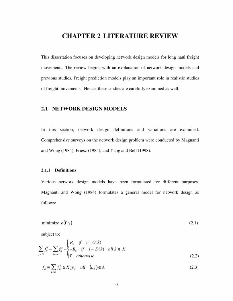
2.1.1 Definitions

Various network design models have been formulated for different purposes.

Magnanti and Wong (1984) formulates a general model for network design as

follows:

( )yf, minimize φ (2.1)

subject to:

(2.2)

f ij ≡ f ij

k

k∈K

∑ ≤ K ij y ij all i, j( )∈A (2.3)

fij

k

j ∈ N

∑ − fji

k

i ∈ N

∑ =

Rk if i = O(k)

−Rk if i = D(k) all k ∈ K

0 otherwise

10

f ,y( )∈S (2.4)

f ij

k ≥ 0, y ij = 0 or 1 all (i, j) ∈ A, k ∈K (2.5)

Where k denotes a commodity in the large set, K. For each k, Rk

is the required

amount of flow of commodity k to be shipped from point of origin, O(k), to point of

destination, D(k). f ij

k is the flow of commodity k on arc (i, j). A decision variable y ij

is equal to 1 if the improvement project is chosen as part of the network’s design, or 0

otherwise. A is a set of all arcs in a study network. y ≡ (y ij ) and f ≡ ( f ij ) are vectors

of design and flow variables. Qij is the capacity of arc (i,j). The set S includes any

side constraints imposed upon the network design.

The model minimizes φ( f , y) subject to a bundle of flow conservative constraints

(2.2). Equation (2.3) is a capacity constraint. If an arc (i,j) is not chosen as a part of

the network y ij = 0 hence f ij

= 0. Network variations change with the objective

function and side constraints. When the objective function φ f ,y( ) is linear, the model

is a linear mixed integer program. A general form of the linear function is

φ f , y( )= c ij

k

( i, j )∈A

∑k∈K

∑ f ij

k + Fij

( i, j )∈A

∑ y ij (2.6)

Where c ij

k is the per unit arc routing costs for commodity k and Fij is the fixed arc

design costs. If congestion effects are considered, a nonlinear version of the objective

11

function can be used. The per unit arc routing costs can be replaced by the Bureau of

Public Road formula tij 1 + α ij f ij Qij( )β ij

or the queuing formula ( )

ijijij fQt − .

Magnanti and Wong (1984) also shows that this model is a generalized model for

many transportation planning problems such as a minimum spanning tree problem, a

shortest path problem, a traveling salesman and vehicle routing problem, a facility

location problem, and our problem, which is a network design problem with traffic

equilibrium.

For this problem type, the following equations are added as side constraints.

c ij

k ( f , y) + w i

k − w j

k ≥ 0 for all i, j,k (2.7)

c ij

k ( f , y) + w i

k − w j

k[ ]f ij

k = 0 for all i, j,k (2.8)

wo(k)

k ≡ 0 for all k (2.9)

and the budget constraints - eij

( i, j )∈A

∑ y ij ≤ B (2.10)

where eij

is the cost when arc (i, j) is chosen and B is a budget. Magnanti and Wong

(1984) provides a connection between these equations and user equilibrium

conditions. Consider Equation (2.7), let Pk be any path connecting the origin O(k)

and destination D(k) of commodity k. If we sum Equation (2.7) for all arcs (i,j) that

are part of path Pk, we get

12

c ij

kf , y( )− wD(k )

k

( i, j )∈Pk

∑ ≥ 0 (2.11)

Considering Equation (2.8) and in a case in which f ij

k > 0 , we can write (2.11) as

c ij

kf , y( )= wD(k )

k

( i, j )∈Pk

∑ if f ij

k > 0 for all (i, j) ∈Pk (2.12)

It can be interpreted that wD(k)

k is the shortest distance between O(k) and D(k) hence

Equation (2.12) becomes Wardrop’s user equilibrium Wardrop (1952). Consequently,

adding Equations (2.7) to (2.9) as side constraints yields an equilibrium network

design problem.

Although Magnanti and Wong (1984)introduces the equilibrium network design

problem in a single level optimization, it can be viewed as a bi-level problem. Not

only does the bi-level form of the problem clearly explain the model’s behaviors, it

also inspires many solution algorithms. Friesz (1985) and Yang and Bell (1998)

survey the network design studies focusing on the equilibrium network design. Yang

and Bell (1998)presents an interesting generic framework for network design models.

The transportation system is assumed to have a simple structure with three

components which are economic activity (E), transportation systems capacity (Q),

and traffic flow (F) under a management system (M). The performance function or

the level of service (L) of the system then can be written as

L = P (Q,F , M ,α ) (2.13)

13

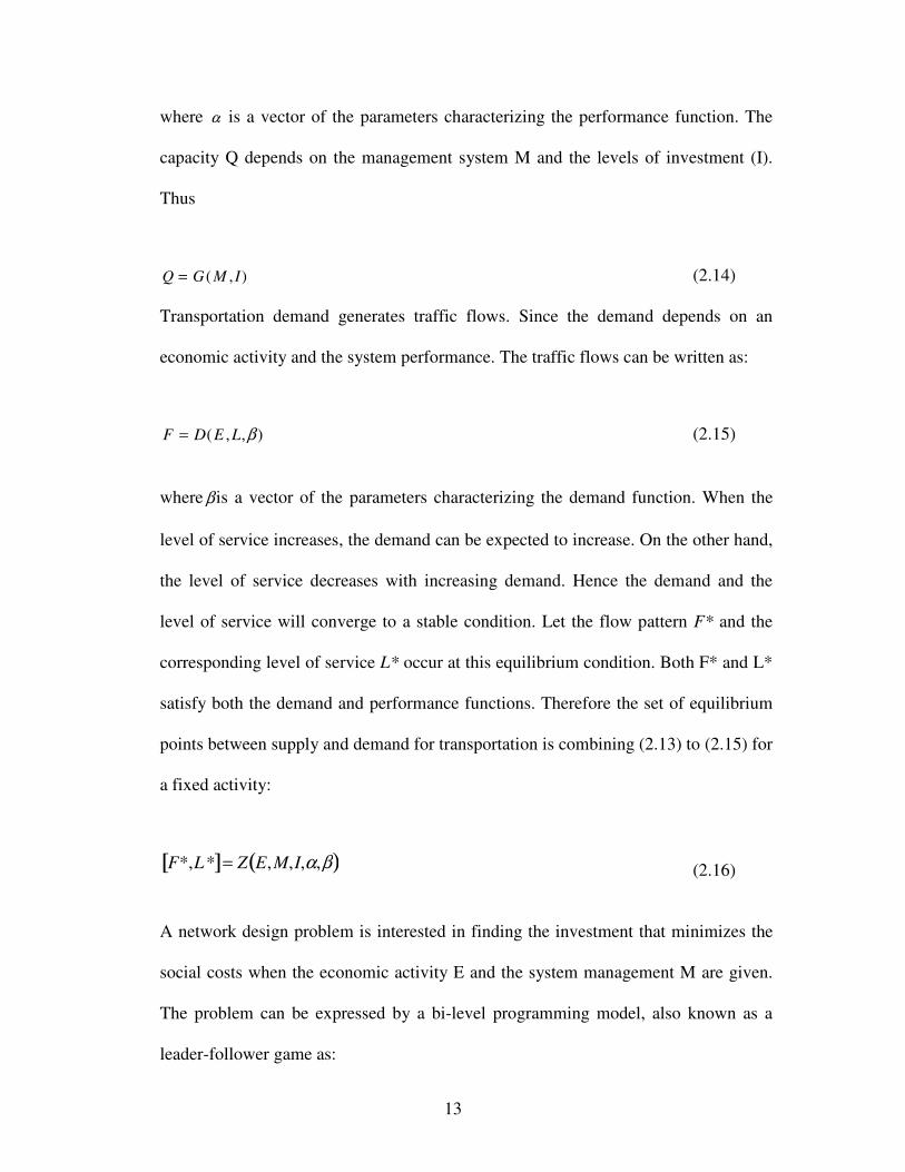
where α is a vector of the parameters characterizing the performance function. The

capacity Q depends on the management system M and the levels of investment (I).

Thus

Q = G ( M , I) (2.14) Transportation demand generates traffic flows. Since the demand depends on an

economic activity and the system performance. The traffic flows can be written as:

F = D(E ,L,β ) (2.15)

whereβ is a vector of the parameters characterizing the demand function. When the

level of service increases, the demand can be expected to increase. On the other hand,

the level of service decreases with increasing demand. Hence the demand and the

level of service will converge to a stable condition. Let the flow pattern F* and the

corresponding level of service L* occur at this equilibrium condition. Both F* and L*

satisfy both the demand and performance functions. Therefore the set of equilibrium

points between supply and demand for transportation is combining (2.13) to (2.15) for

a fixed activity:

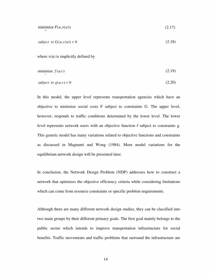
F*,L*[ ]= Z E,M,I,α,β( ) (2.16) A network design problem is interested in finding the investment that minimizes the

social costs when the economic activity E and the system management M are given.

The problem can be expressed by a bi-level programming model, also known as a

leader-follower game as:

14

(2.17)

subject to G(u,v(u)) < 0 (2.18)

where v(u) is implicitly defined by

minimizev

f (u,v) (2.19)

subject to g(u,v) < 0 (2.20)

In this model, the upper level represents transportation agencies which have an

objective to minimize social costs F subject to constraints G. The upper level,

however, responds to traffic conditions determined by the lower level. The lower

level represents network users with an objective function f subject to constraints g.

This generic model has many variations related to objective functions and constraints

as discussed in Magnanti and Wong (1984). More model variations for the

equilibrium network design will be presented later.

In conclusion, the Network Design Problem (NDP) addresses how to construct a

network that optimizes the objective efficiency criteria while considering limitations

which can come from resource constraints or specific problem requirements.

Although there are many different network design studies, they can be classified into

two main groups by their different primary goals. The first goal mainly belongs to the

public sector which intends to improve transportation infrastructure for social

benefits. Traffic movements and traffic problems that surround the infrastructure are

minimizeu

F(u ,v(u))

15

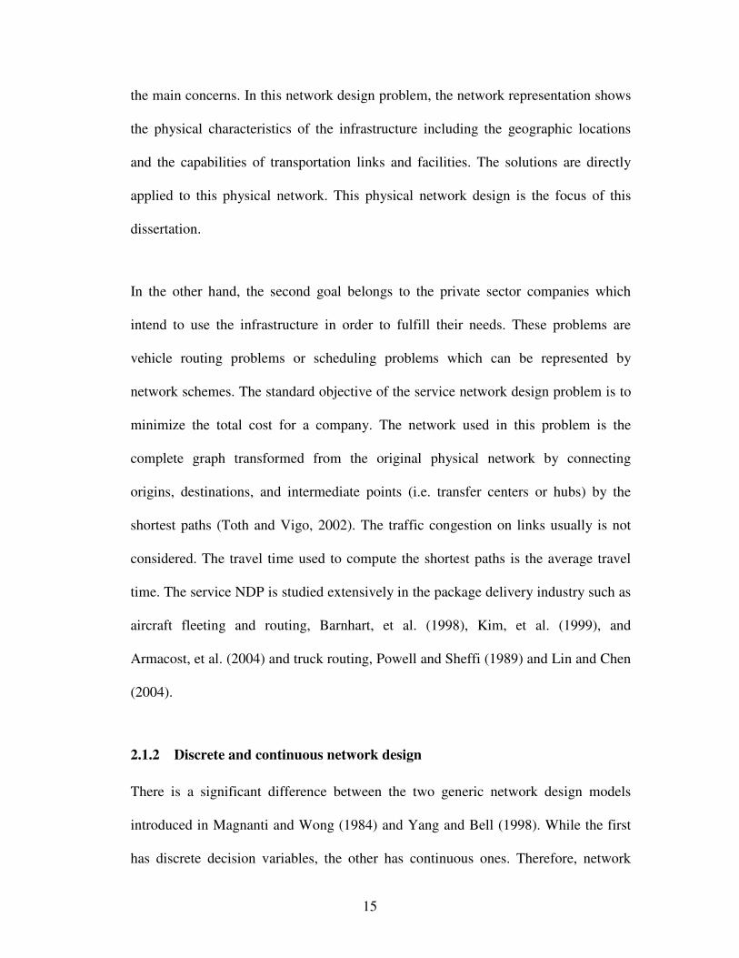
the main concerns. In this network design problem, the network representation shows

the physical characteristics of the infrastructure including the geographic locations

and the capabilities of transportation links and facilities. The solutions are directly

applied to this physical network. This physical network design is the focus of this

dissertation.

In the other hand, the second goal belongs to the private sector companies which

intend to use the infrastructure in order to fulfill their needs. These problems are

vehicle routing problems or scheduling problems which can be represented by

network schemes. The standard objective of the service network design problem is to

minimize the total cost for a company. The network used in this problem is the

complete graph transformed from the original physical network by connecting

origins, destinations, and intermediate points (i.e. transfer centers or hubs) by the

shortest paths (Toth and Vigo, 2002). The traffic congestion on links usually is not

considered. The travel time used to compute the shortest paths is the average travel

time. The service NDP is studied extensively in the package delivery industry such as

aircraft fleeting and routing, Barnhart, et al. (1998), Kim, et al. (1999), and

Armacost, et al. (2004) and truck routing, Powell and Sheffi (1989) and Lin and Chen

(2004).

2.1.2 Discrete and continuous network design

There is a significant difference between the two generic network design models

introduced in Magnanti and Wong (1984) and Yang and Bell (1998). While the first

has discrete decision variables, the other has continuous ones. Therefore, network

16

design problems can be classified by decision variables into two different types --

discrete NDP (DNDP) and the continuous NDP (CNDP). Each has its own

advantages.

Discrete models are usually used to deal with the addition of new links, while the

continuous models are usually used to deal with capacity expansion or improvements

(Yang and Bell, 1998). Boyce and Janson (1980) suggests that the DNDP

formulations are more appropriate for transportation networks since the improvement

such as lane expansions cannot be done in fractional amounts. Abdullal and LeBlanc

(1979) also points to the flexibility of the discrete formulation that can easily allow

the change of mean free speed for the improved links. The major drawback of their

discrete models is computational time. The paper compares the solution of network

design problems using continuous formulations and discrete formulations. The results

show that the continuous formulations yield equal or better solutions than the discrete

one. Even though their results are now more than twenty five years old, and

advancements in computational power have been enormous, their findings remain

relevant because the scale of problems considered have continued to grow.

Additionally, the level of improvement to the existing links can be determined by the

continuous model. For the discrete formulation, these levels have to be

predetermined.

The characteristics of the inter-regional transportation network suggest that the long

haul freight NDP should be developed using a DNDP formulation. The first

characteristic is that congestion is usually given less consideration over long distance

17

travel such as the truck movements by interstate highways (Janson, et al., 1991, and

Solanki, et al., 1998). Therefore, when a transportation link receives an improvement,

it is more important to update the travel speed than the link capacity. The freedom to

update the travel speed and other parameters are offered by DNDP while CNDP can

update only the link capacity. Additionally, besides the BPR function which

represents the effect of lane expansions, various network improvements do not have

corresponding representative equations. CNDP requires these equations be known

and therefore cannot be applied to our study. On the other hand, DNDP can vary

subjective penalties representing the current conditions and those present after

improvements.

The second characteristic is that investments are complicated with some conditional

requirements. The model with conditional requirements can only be implemented

using discrete variables. For example, the long term investments may require both

temporal and spatial implementation specifications. An example of research on the

multi-stages for interstate highway NDP is found in Janson, et al. (1991). In their

work, the NDP is designed using the discrete variables for the choice of improvement

which are represented both as Yes-No decisions and with implementation times. In

this case, the nature of the discrete model simply allows for a change in the freeflow

of improved links. More complicated staged investment is considered in Kuby, et al.

(2001) which considers railway network design. In their study, heuristic backwards

time sequencing is used to optimize the stages of the improvements. It should be

noted that if opportunity cost is considered in long range network development, then

these costs must be adjusted to a single time period.

18

2.1.3 Variations of network design problems

Following sections show variations of the bi-level network design model which

depend on changes in upper or lower level models. Similar work has been done by

Yang and Bell (1998). However, many recent studies have also been added to the

field. Freight network design studies are reviewed at the end of this chapter.

2.1.4 Classic bi-Level network design problem

A typical network design problem focuses on passenger car movements and has the

objective to minimize the total transportation cost for all road users. The traffic

conditions are assumed to be user equilibrium conditions (i.e. user optimization) and

the congestion on transport links has to be considered. For network design models

with discrete choice variables, Boyce, et al. (1973) and Leblanc (1975) provide

classic road network design problems formulated as bi-level models. For network

design models with continuous decision variables, Abdullal and LeBlanc (1979) is the

earliest work. Tobin and Friesz (1988) develops sensitivity analysis for the

continuous network design problem.

2.1.5 Network design problem with demand elasticity

It is well known that network improvements can have immediate and lasting impacts

on the demand for transportation services. Therefore demand should not be

considered fixed. Instead the elasticity of demand should be painstakingly examined

whenever a potential improvement is evaluated. Boyce and Janson (1980) combines

trip distribution into the lower problem. The problem is formulated as a discrete NDP

19

with the objective of minimizing total travel cost. The NDP is then constrained by the

total budget and a doubly-constrained trip distribution represented by origins and

destination entropy. Therefore, both link travel costs and the trip distribution are

decision variables.

With the traffic assignment with elastic demand, the typical objective function to

minimize total travel time is not suitable since a solution can achieve through

minimizing travel demand and thus result in undesirable solutions involving less

investment (Yang and Bell, 1998). A more appropriate upper level objective function

should be maximizing consumer surplus. This measure is suggested by Kocur and

Hendrickson (1982), Williams and Lam (1991), and Yang and Bell (1997) to evaluate

the benefits of transport systems.

2.1.6 Maximizing reserve capacity network design

The traditional objective function of the NDP is to minimize the total travel costs or

time. Other alternative system efficiency criteria can be adopted into the NDP. An

original concept of reserve capacity is from timing design individual signal-controlled

intersections (Allsop, 1972). Wong and Yang (1997) extends this concept to a bi-level

programming that design traffic signal settings for maximization of the network

reserve capacity. Yang and Bell (1998)suggests that this concept can be applied to the

network design problem which allow a prediction of additional demand that can be

accommodated by the road network after improvement.

20

Yang and Wang (2002) compares the NDP solution between travel time minimization

and reserve capacity maximization. The reserve capacity indicates the maximum flow

that the system can handle. In other word, reserve capacity is the system capacity.

The CNDP is formulated. The reserve capacity is maximized by maximizing the

multiplier that can be applied to a given O-D matrix. The multiplied volumes cannot

exceed the capacity of links. The results show that there is a relationship between the

solutions found based on these two competing objective functions. The solution under

maximization of reserve capacity can be the same as the minimization of total travel

cost when the level of congestion is low. The two objectives will conflict more as the

level of congestion increases.

2.1.7 Equity network design

The equitable benefit distribution for network design provides another interesting

objective. Improvement of the network can make the total system better. However

travel between some O-D pairs may improve a lot while the others receive negative

effects as congestion increases. Such changes, though often representing overall

improvements, are very hard to sell to the public. Meng and Yang (2000) raises this

issue related to the NDP. The O-D travel cost ratios before and after the network

improvement are considered. For the equity of the road users, the travel cost ratios

should fall between acceptable ranges. These minimum and maximum ratios of

improvement are obtained by solving two bi-level programming problems.

21

2.1.8 Network design with multiple objective functions

Multiple objectives can also be considered in network design. The weighting method

can be used to generate the Pareto optimal set. Yang and Wang (2002) uses a

combined objective function that weighs both the important of reserve capacity and of

total travel cost. Friesz, et al. (1993) formulates a single level mathematical program

to solve the multi-objective problem under equilibrium conditions. The objectives are

minimizing total user transport costs, total construction costs, and total vehicle miles

traveled. However, this approach is still different from multi-objective optimization

problems which explicitly consider multiple objectives.

Yang and Bell (1998)reports that the multi-objective equilibrium network design

problem was first put forward by Friesz (1981) and Friesz and Harker (1983) with

many other studies later including Current and Min (1986), Friesz, et al. (1993) and

Tzeng and Tsaur (1997). They conclude that most network design problems have

three different objective functions which are total user transport costs, total

construction costs, and total vehicle miles traveled which could be considered as a

surrogate for air pollution.

Recently, Chen, et al. (2003) develops a simulation-based multi-objective genetic

algorithm for the Build-Operate-Transfer (BOT) case. In this case, the upper level

program consists of two problems which are the profit maximization problem and the

welfare maximization problem. Their work considers the uncertainty of travel

demand forecasting. The travel demand is simulated based on the probability

22

distributions. The Pareto optimal conditions of both objectives are desired at the end

of the simulation.

2.1.9 Dynamic assignment and SUE assignment

A new traffic assignment approach of the lower level model can lead to more realistic

route choice behaviors. Friesz (1985) suggests improvements on NDP by

implementing stochastic user equilibrium assignment or dynamic assignment with the

network design problems. However, Friesz comments that combining the dynamic

traffic assignment with NDP is hard since this assignment problem is intractable. He

suggests using dynamic adjustment mechanisms such as those used by Horowitz

(1984) and Smith (1984)to study network equilibrium stability.

There are two perspectives related to the SUE assignment. The first perspective is that

the perception of network costs vary from user to user -- therefore the costs are

random variables distributed among user population (Daganzo and Sheffi, 1977). The

other perspective is that the network itself is stochastic which means that some or all

arcs are not deterministic and are random variables (Mirchandani and Soroush, 1987).

Chen and Alfa (1991) and Davis (1994) formulated their network design problem

with discrete and continuous variables respectively with a logit-based SUE

assignment. Yang and Bell (1998) comments that the NDPs can lead to over-

investments to some routes since the logit-based SUE model will generally

overestimate traffic flow on overlapping routes due to the famous property of

independence of irrelevant alternatives (IIA).

23

2.1.10 Network design problems for other transportation modes

Kuby, et al. (2001) studies the rail NDP. Rail is one of the important modes in the

intermodal system however, that study does not consider transfer points between

modes. The model is a system-optimizing, capacitated, static, fixed charge mixed

integer program with budget constraints. It represents economies of scale indirectly

through functions and integer variables. Multi-stage developments are considered.

The World Bank and the Chinese Minister of Railways funded the study to improve a

spatial decision support system for railway investment planning in China.

Konings (2003) studies network design for an intermodal barge network. The study

focuses on the selection of vessel size and improvement of vessel circulation time.

The relationships of vessel sizes, transport volumes, transport frequencies, and cycle

time are used to suggest the change of the network. There is no optimization in this

study. The study also does not consider intermodal transfer points.

The concept to develop this freight network design model is introduced by

Apivatanagul and Regan (2007). That paper considers issues related to the

development of the freight network design model and emphasizes the importance of

developing a model which can integrate multiple local networks together. An

example is shown to draw the attention to designing a network for larger broader

social benefits rather than focusing on local network improvements.

24

An early study that discusses combining a freight network equilibrium model with the

network design problem is Friesz (1985). This idea is developed further by

Apivatanagul and Regan (2008). That paper develops a freight network design model

focusing on the modification of the lower level model which represents the freight

route choice behavior. The shipper-carrier freight prediction model of Friesz, et al.

(1986) is applied to the network design problem. Additionally, the model assumes

that links which are overused are unreliable and will be avoided by the users.

Therefore, capacity constraints are considered when the traffic volumes are assigned

to the network. These constraints make the network design more sensitive to the

improvement projects. A branch and bound algorithm is applied to an example which

shows that the proposed network design model can identify the bottleneck problem

and give a better solution compared to considering projects individually or

sequentially.

2.2 SOLUTION ALGORITHMS

General network design problems are known to be NP-complete (Johnson, et

al.,1978) which means there is no known algorithm to solve problems efficiently to

optimality. Additionally, the objective functions of the DNDP are non-convex and

usually non-linear. Optimal solution algorithms have been developed work for small

networks. For large networks with complicated constraints, heuristic algorithms are

used to find near optimal solutions.

25

2.2.1 Branch and bound algorithms

Branch and bound algorithms work by constructing a search tree and calculating

lower bounds to cut (also known as pruning or fathoming) nodes that cannot contain

the optimal solution. At the first node we assume that all candidate links could be

included or excluded from the final network. The first node has the shallowest depth.

At the deeper nodes, more candidate links are selected or rejected. The lower bound is

used to fathom nodes that cannot produce a better solution compared with a current

best (incumbent) solution.

Boyce, et al. (1973) and Hoang (1973) study the simplest case of network design

problems. Their problem focuses on building a network which results in total shortest

paths from all origins to all destinations. The problem is constrained by the total link

length that can be added to the network. An implicit enumeration procedure using

branch and bound is used to solve the problem. The algorithms from both papers are

similar, as is that seen in Ridley (1968). Scott (1967) also solves the same problem

but uses a branch and exclude method which uses a different lower bound.

At each node, Boyce’s lower bound is estimated assuming that unselected candidate

links will be included in the final network before calculating the network design

objective function. Tighter lower bounds are proposed by Hoang (1973) by adding

the quantity that denotes the increment to the shortest route cost from node i to node j

when link (i, j) is deleted from the network. However, it is reported that the bound

will be weak when many links have been deleted by the algorithm. Hoang also notes

that the algorithm still suffers from computational times which increase exponentially

26

with the size of problems. Since Hoang’s algorithm selects the node that has the

minimum lower bound to examine first, the least lower bound of unexplored nodes

will increase monotonically. Hoang uses this fact to short cut the branch and bound

algorithm by comparing the lower bound with the current solution (upper bound).

When the gap between these bound is small enough, the algorithm can be stopped.

Dionne and Florian (1979) proposes several improvements such as a specialized

algorithm to calculate shortest paths when a single arc has been deleted from the

network.

The network design problem is more difficult for congested networks with nonlinear

link cost functions. Several earlier researchers study highway network design for

passenger movements in which the cost functions are usually assumed to be strictly

increasing convex functions. Leblanc (1975) uses a branch-and-bound algorithm to

solve small problems optimally. The lower bound is calculated similar to Boyce, et al.

(1973). The pitfall of the algorithm is the existence of Braess’ Paradox which implies

that the selected network improvements do not always result in an improvement in

the objective function. In order to avoid this pitfall, the traffic volumes are assigned

using system optimal routing instead of user equilibrium routing. This method

develops a loose lower bound.

Several papers are devoted to develop tighter lower bounds or heuristics in order to

deal with larger networks. Poorzahedy and Turnquist (1982) modifies the network

design problem by replacing the objective function with Beckman’s Formulation. The

replacement gets rid of the Braess’ Paradox problem. The paper provides arguments

27

as to why the modified problem can be used as an approximation for the original

problem.

Magnanti and Wong (1984) reviews several other types of optimal procedures and

heuristics developed to solve the DNDP including the branch and bound algorithm.

The differences in optimal procedures related to the method used to obtain the lower

bound are discussed. The heuristics commonly used to accelerate the algorithm are

adding, deleting, and interchanging procedures. However at that time only medium

sized problems (150 arcs, 50 nodes)can be solved optimally.

2.2.2 Bender’s decomposition

Bender’s decomposition is a solution algorithm for mixed integer programming

(Benders, 1962). The basic idea is to partition the main problem into two

subproblems which usually are a linear optimization problem and an integer one. An

iterative procedure between the problems is implemented. Bender’s decomposition

receives computational time benefits when both subproblems are easier to solve.

Magnanti and Wong (1984) explains its application for the network design problem.

It proceeds iteratively by choosing a tentative network configuration by setting values

for the integer decision variables, solving for the optimal routing on this network, and

using the solution to the routing problem to redefine the network configuration. The

approach can apply to the scheduling problem (Florian, et al., 1976), airline network

design (Magnanti, et al., 1983) and industrial system network design (Geoffrion and

Graves, 1974).

28

Hoang (1982)studies an application of the network design problem with a user

equilibrium assumption. His formulation is a mixed integer problem but only the link

capacity expansion problem is considered. A generalized Bender’s decomposition is

applied to the problem. In order to partition the problem, its dual formulation is

written. An iterative process is implemented between a master problem and the

minimal convex cost multi-commodity flow problem. The master problem is a dual

formulation of the network design which chooses the potential network configuration.

The minimal cost flow problem uses the configuration to generate cutting planes used

by the (relaxed) master problem. An algorithm by Nguyen (1974) is used to solve the

minimal cost flow problem. The relaxed master problem is solved by a heuristic

subgradient optimization method for the well-known knapsack problem

(Shapiro ,1979).

2.2.3 The Iterative-Optimization-Assignment Algorithm

An intuitive approach to deal with a bi-level network design problem is an iterative

(or feedback) process between the optimization programming model which

configures tentative networks and the traffic assignment which predicts

corresponding traffic movements. This heuristic approach is common for solving both

the DNDP and CNDP. The sensitivity analysis approach is its variation.

For the CNDP, Yang and Bell (1998) discusses the three typical heuristic algorithm

applied to most studies: the iterative-optimization-assignment algorithm; the link

usage proportion-based algorithm; and the sensitivity analysis-based algorithm. The

heuristic algorithm is appropriated to the CNDP which has the non-convex objective

29

function making the problem hard to solve to optimality. These algorithms begin by

configuring tentative capacity link improvements for study networks with fixed traffic

volume. Then they adjust link capacities accordingly and calculate the corresponding

traffic flow in each link. Influences from the capacity changes to traffic volumes are

calculated. The traffic flows are adjusted by these influence factors before iterating to

re-configure capacity improvements. The feedback process stops when consecutive

solutions are sufficiently close.

The iterative-optimization-assignment algorithm is the simplest implementation. It

was first proposed by Steenbrink (1974a,b)and is explored by Asakura and Sasaki

(1990) andFriesz and Harker (1985) in solving the CNDP. The algorithm proceeds

with an iterative process. Capacity configurations and their corresponding traffic

volumes are provided in a feedback process to reconfigure the network without

calculating influence factors. This approach does not necessarily converge. Rather, it

represents a Cournot-Nash game in which each player attempts to maximize his/her

objective values non-cooperatively, and assumes that his actions will have no effect

on the actions of the other players (Fisk , 1984, and Friesz and Harker,1985).

2.2.4 The Link Usage Proportion-Based Algorithms

The link usage proportion-based algorithms are applied to solve bi-level

transportation problems in which demands act as upper-level decision variables

(Yang and Bell, 1998). In this algorithm, an influence factor for each link is a ratio

between its usage and its capacity. In this case, the link that is used to its capacity or

over is likely to receive an improvement. This algorithm is applied to ramp metering

30

(Yang, et al., 1994) and zone reserve capacity (Yang, et al., 1997), and O-D matrix

estimation (Yang, et al., 1992 and Yang, 1995).

2.2.5 The Sensitivity Analysis-Based Algorithm

The sensitivity analysis-based algorithm is different by the others with its influence

factor. The influence factor is the derivative of the reaction function with respect to

the upper-level decision. In the case of CNDP, the upper decision is the capacity

improvements and the reaction function is the relationship between the user

equilibrium flow and the capacity changes. The approach is applied to the network

design problem by Friesz, et al. (1990). It is a generalized approach which is further

applied by many studies including optimal ramp metering in freeway networks

(Yang, et al., 1994 and Yang and Yagar, 1994)), traffic signal control (Wong and

Yang, 1997 and Yang and Yagar, 1995), optimal congestion pricing (Yang and Lam,

1996 and Yang and Bell, 1997).

Leblanc and Boyce (1986) formulates the DNDP with linear programming. The

formulation supports piecewise linear equations which can be used to represent

nonlinear equations. The user optimal behavior is assumed therefore the lower

problem requiring the flows minimize the piecewise linear approximation to the

integrals of the improved user-cost functions. The algorithm by Bard (1983) is

proposed to solve the bi-level linear programming. In this algorithm, the objective

function is defined as a convex combination of the upper and lower objective

functions. The procedure then involves iteratively solving this new objective function

31

with the same constraints (including conservation flow constraints and link capacity

constraints). The paper also suggests an efficient solution procedure by solving the

convex combination of non-linear increasing functions instead of linear one. The

Frank-Wolfe algorithm is then applied to the approach.

Ben-Ayed, et al. (1992) implements network design problems to the Tunisian

network using actual data. The case is focused on the inter-regional highway network

of a developing country. Lane capacities can be increased by resurfacing road

pavement which has low quality. The problem is formulated similarly to Leblanc and

Boyce (1986), a piecewise linear optimization model but with continuous decision

variables. Cost functions are developed by Tunisian data. The iterative-optimization-

assignment algorithm is applied to solve the problem.

2.2.6 Meta-heuristic approaches

The artificial intelligent (AI) search algorithms have been implemented to solve the

NDP problem. The simulated annealing approach is the first search algorithm applied

to the CNDP (Friesz, et al., 1992). The algorithm has been developed to solve the

NDP in case of multi-objectives by Friesz, et al. (1993) and the NDP with benefit

distribution and equity by Meng and Yang (2000).

For the DNDP, genetic algorithms (GAs) have been utilized. Bielli, et al. (1998) uses

the Cumulative GAs (CGAs), an improved version of general GAs, to solve the bus

network design problem.

32

For the road network, simulation based GAs are used by Chen, et al. (2003). The

simulation problem also included the stochastic of demand and multi-objective issues

in the NDP. Drezner and Wesolowsky (2003) considers the NDP with facility

location. The objective is to minimize total round trip cost from the origin to facility

and back to origin. Four heuristics, a descent algorithm, simulated annealing, tabu

search, and a GA., are used to solve the problem. The genetic algorithm performs the

best in their computational experiments.

2.2.7 Heuristics for large network design problems

Janson, et al. (1991), Solanki, et al. (1998), and Kuby, et al. (2001) deal with national

transportation networks which are very large systems. In order to manage such large

networks, some techniques are need to simplify the problem in additional to the

heuristics.

The techniques can be classified broadly into two types which are aggregation

techniques and decomposition techniques. The aggregation techniques have two main

approaches, network element abstraction and network element extraction. Abstraction

reduces the network by appropriately aggregating an area or a corridor into a single

node. The works that focus on this technique are Zipkin (1980) and Kuby, et al.

(2001). However, the network topography is changed by the aggregation thus it is

very hard to translate the actions from the aggregated network to the original one.

Extraction reduces the network by deleting redundant and insignificant links based

on a specified criterion. Haghani and Daskin (1983) implements this approach for the

33

NDP which improves computational time significantly. In their algorithm, the links

which have less traffic volume than a specific value will be excluded from

consideration and the travel demand table is updated accordingly. Fewer links result

in a faster traffic assignment algorithm. However, they report that the time needed to

update the travel demand table may offset this benefit. It should be noted that the

network aggregation has an important drawback related to the potential occurrence of

Braess’ Paradox. The deleting or grouping links in the aggregation process may

increase in the network travel time. Furthermore, the optimal solution cannot be

discovered for the original network (Zeng and Mouskos, 1997).

An alternative for larger networks is to use a decomposition method which moves

from larger networks to smaller sub-networks. Solanki, et al. (1998) clusters the sub-

networks in a hierarchical order and performs network design for each cluster

separately. The smaller problems can be solved by a branch-and-bound strategy.

Although the paper uses a fixed cost network, it can be adjusted to be applied to

networks with nonlinear link costs.

2.3 FREIGHT FLOW PREDICTION MODELS

In most previous studies, the highway network design problem has been the focus and

route choice behavior is limited to the passenger movements. In order to formulate

the long haul freight network design problem, freight route choice behaviors have to

be considered and the existing solution algorithms need to be adjusted accordingly.

The freight flow prediction models are used to reflect the freight route choices on the

34

transportation network. In order to select a proper model for the freight network

design problem, it is crucial to understand the transportation system and economic

agents who have important roles within it.

2.3.1 Economic agents in the freight transportation system

One of differences between freight and passenger movements is that the freight route

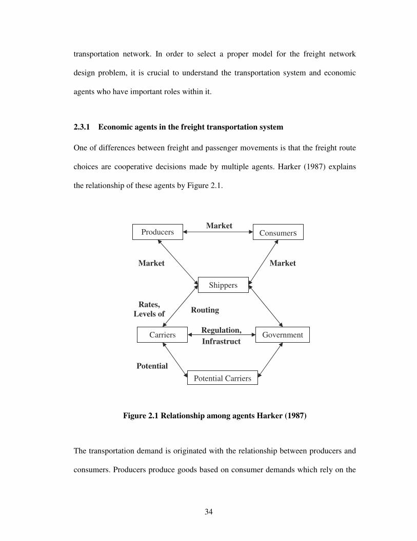
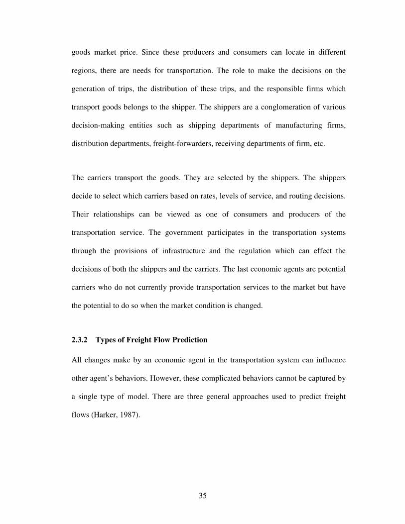
choices are cooperative decisions made by multiple agents. Harker (1987) explains

the relationship of these agents by Figure 2.1.

Figure 2.1 Relationship among agents Harker (1987)

The transportation demand is originated with the relationship between producers and

consumers. Producers produce goods based on consumer demands which rely on the

Producers Consumers

Shippers

Carriers Government

Potential Carriers

Market

Prices

Rates,

Levels of

service

Routing

decisions

Regulation,

Infrastruct

ure

Potential

entry

Market

Prices

Market

Prices

35

goods market price. Since these producers and consumers can locate in different

regions, there are needs for transportation. The role to make the decisions on the

generation of trips, the distribution of these trips, and the responsible firms which

transport goods belongs to the shipper. The shippers are a conglomeration of various

decision-making entities such as shipping departments of manufacturing firms,

distribution departments, freight-forwarders, receiving departments of firm, etc.

The carriers transport the goods. They are selected by the shippers. The shippers

decide to select which carriers based on rates, levels of service, and routing decisions.

Their relationships can be viewed as one of consumers and producers of the

transportation service. The government participates in the transportation systems

through the provisions of infrastructure and the regulation which can effect the

decisions of both the shippers and the carriers. The last economic agents are potential

carriers who do not currently provide transportation services to the market but have

the potential to do so when the market condition is changed.

2.3.2 Types of Freight Flow Prediction

All changes make by an economic agent in the transportation system can influence

other agent’s behaviors. However, these complicated behaviors cannot be captured by

a single type of model. There are three general approaches used to predict freight

flows (Harker, 1987).

36

2.3.2.1 Econometric models

The first one is the econometric model which uses time series and/or cross sectional

data to estimate structural relationship between supply and demand for transportation

services. The approach focuses only on the sipper-carrier-government relationship. It

is very useful for studying the impact of various policies on the transportation market

but it cannot detail the flows on transportation links. This model approach can be

classified into supply side models and demand side models.

The supply side models focus on the issue of describing the production of freight

transportation services. The intension of the model is not for prediction but to

understand the production/cost characteristics of the industry such as questions of

economies of scale and densities. Harker (1987) points out that the railroad industry

has extensive studies on this approach (Klein, 1947, Meyer, et al., 1959, Borts, 1952

and 1960, Healy, 1961 and Healy, 1962). For a muli-product viewpoint that considers

each origin-destination pair as a separate commodity, look at Jara-Diaz (1981) and

Jara-Diaz (1982). In the trucking industry, early studies are pursued by Roberts

(1956) and Nelson (1956). The long haul less-than-truck-load and truckload

industries are studies by Friedlaender (1978) and Chow (1978).

The econometric demand side models attempt to explain the relationship of

transportation demand, rate changes, and level of services. These models could be

incorporated into predictive models of the freight system. The demand functions

which consider economic agents as many aggregated entities are studied by Oum

(1979) and Friedlaender and Spady (1981). The models assume that the producing

37

firms are profit maximizers and that transportation is a factor in their production

processes. Another demand function types consider firms’ behaviors. It is early

studies by Allen (1977) and leads to a logit demand formulation by Daughety (1979)

and Levin (1981). The inventory-theoretic approach for the demand function is based

on the perspective that the shippers make transportation decisions based on

inventories. That work is studied by Chiang, et al. (1980), Roberts (1976), and

Terziev (1976).Friedlaender (1969) and Friedlaender and Spady (1981) are the major

works which integrate supply and demand based on an assumption of the equilibrium

conditions.

2.3.2.2 The Spatial Price Equilibrium Model

The spatial price equilibrium model focuses instead on producers, consumers, and

shippers. The carriers are defined within cost functions. The model uses a network

model to describe relationships of producers, consumers, and the transportation

systems. Each node represents a different region which can be either consumers,

producers, or transshipment nodes. Demand functions are associated with each

consumer node and supply functions are used with producer nodes. The concept of

the equilibrium is that shippers barter between these regions until equilibrium is

reached which means that there is no additional flow between each region due to

commodities in the home regions are cheaper than other regions when considering

transportation costs.

Harker (1987) examines major works on the spatial equilibrium model with freight

studies. Early work uses a simple network which has a direct link accesses between

38

each pair of a consumer and a producer. Takayama and Judge (1964) solves this

problem by assuming linear supply and demand functions with constant

transportation costs. Later this problem is formulated as a complementarity problem

(Takayama and Judge, 1970 and Stoecker, 1974) with linear transportation cost

functions. MacKinnon (1975) considers nonlinear functions for the problem. Florian

and Los (1982) considers the problem on a network with transshipment nodes

utilizing nonlinear functional forms but with path flow between the origins and

destinations. A spatial equilibrium model which uses a general network, where a node

can be an origin, destination and transshipment point is used, is studied by Tobin and

Friesz (1983).

2.3.2.3 The freight network equilibrium model.

The freight network equilibrium is similar to passenger traffic assignment except that

many agents are considered. This type of model is the focus of our work on network

design problems since it uses the real network to predict freight flows and thus gives

specific information for each link. This information is used to select the links that

should receive improvements. The next section examines this type of model in more

details.

2.3.3 The Freight Network Equilibrium Model

Harker (1987) summarizes three types of models that are generally used for freight

studies and their weakness. Econometric models are good to study policy changes but

ignore the details of the network technology. Spatial price equilibrium models focus

39

on the consumer-producer relationship but lack the role of the transportation firm.

Finally freight network equilibrium models consider transportation networks in detail

but do not consider the commodity markets (consumer-producer). Nevertheless, the

freight network equilibrium is suitable for further developing it to network design

problems since it can specify problem locations.

With an intention to develop a multimodal network design, it is important to consider

that the selected model has to be able to predict the mode changes when the study

network changes. This is more important for long haul freight movements which have

various transportation modes including intermodal ones. Therefore, we will classify

the freight network equilibrium model based on their methods to shift flows between

different modes.

Ruesch (2001) classifies the modal shift studies into two groups, macro and micro.

The macro studies focus on the supply side. The macro analysis is based on

aggregated freight flows on a regional, national or international level. The matrix

analysis and modal split approach are used to estimate modal potentials and their

flows. The micro approach study the modal shift using the decision making process

on the company level. The key factors for the decision making process (cost,

reliability, lead time, etc.) have to be known. The analysis of the potential modal

shifts from macro and micro approaches can be used to provide to identify the

development of intermodal transport services and the barriers to prevent using of

40

intermodal transport. Freight prediction flow models can identify attractive modal

shift potentials in several ways.

2.3.3.1 Modal shifting by an integrated network

The integrated networks combine transportation networks of all modes together and

link them with transfer points or intermodal facilities. There are two network

configurations which distinguish the integrated network from the unimodal network.

The first is that parallel links are allowed in the network to represent different mode

choices for two adjacent nodes. The other is the shipments can transferred between

modes at transfer points. The transfer points are special combination of nodes and

links. Figure 2.2shows the transfer points (Guelat, et al. ,1990 and Park and Regan,

2005).

1

2

3

4

Intermodal Facility

Rail

Road

(a) Physical network (b) Expanded network

Figure 2.2 Representation of intermodal transfer movements

The integrated network is beneficial to examine intermodal transportation potential.

An intermodal freight model is studied by Guelat, et al. (1990). In this study, freight

demand is exogenous. The inter-regional network is studied and assumed no link

congestion (i.e. no capacity limit in each link). However, the average travel cost in

each link is dependent on the transported volume in the link. An assumption is made

41

that goods are shipped at minimum total generalized cost. The transported volume

can change to another mode only at transfer points with some transfer costs. The

assignment is obtained by a Frank-Wolf algorithm with an embedded shortest path

algorithm with transfers. The algorithm is an adaptation of Dijkstra’s label setting

algorithm but it provides the option to change modes. The study reports the successful

use of this model for application in the Brazilian transportation network modeling, the

strategic analysis of a corridor development is performed for Brazil, as is an analysis

of the import and national distribution system of coal in a Scandinavian country.

2.3.3.2 Modal shifting with preferences

Southworth and Peterson (2000) develops the intermodal and international freight

network modeling. In this study, the transport volume and the mode sequences are

provided by Commodity Flow Survey (CFS). The distinguishing point of this model

is that it provides the information of routing based on a door-to-door basis. The model

assigns the logical routes and completes the mode sequences if they are incomplete.

The model assumes that the freight will be transported by the shortest paths.

However, the carrier-shipper is allowed different preferences for the different modes.

These differences are represented by relative modal impedance factors. For example,

the Railroad impedance is 1:3.5 which means that one would feel indifferent between

a path that travels 3.5 miles railroad and one that travels one mile on a highway. The

assigned volume is represented graphically by a Geographical Information System

(GIS) which provides valuable information and easy access for transportation

planning.

42

2.3.3.3 Modal shifting with different players

As the previous discussion, the shipper is the economic agent who has the priority to

decide transportation modes. Two previous approaches assume that the shipper and

the carrier work together toward the same goal to reduce travel costs. However, the

shipper and the carrier models can be considered separately. Two distinctive earliest

models based on the freight network equilibrium referred by Harker (1987) are

Roberts (1966) focuses on the shipper with constant unit costs and Peterson and

Fullerton (1975) focuses on the carrier and nonlinear unit costs with a user

equilibrium assumption.

The first model that considers multiple agents is Friesz (1981). That model is

explained later in Friesz, et al. (1986) which applies the model to the U.S. rail

network. The model considers both shippers and carriers explicitly by sequentially

loading travel demand onto the transportation service network and then loading this

service demand onto the physical transportation network. In order to improve the

interaction between shippers and carriers, Friesz, et al. (1985) improves the model

and loads both networks simultaneously. Harker and Friesz (1986b) and Harker and

Friesz (1986a) introduce the consumer and the producer onto the freight network

equilibrium by combining it with a spatial price equilibrium model. In his model, the

freight flow is impacted by both travel costs and the commodity prices in each region.

In return, the commodity prices are varied by demand and supply for the

commodities. Recently, Fernandez, et al. (2003) develops a new modeling approach

to a simultaneous shipper-carrier model with more advance trip distribution and mode

choice formulations.

43

CHAPTER 3 FREIGHT NETWORK DESIGN

MODELING CONCEPTS

In this chapter, freight network design modeling concepts are discussed. These

models pay attention to a wider and more general perspective than those discussed

later which focus mainly on the network design problem for long-haul freight

movements. Instead, this chapter discusses the general modeling concepts and

solution algorithms for both an urban network which has high accessibility and an

interstate network which in contrast has low accessibility but has high mobility.

The bi-level solution algorithm is a concentrated area of the dissertation which is

explained in this chapter. Furthermore, the criteria used to measure the efficiency of

the system, traditionally minimizing total travel cost, is broadened in order to

embrace a wider variety of measures and points of view. For example maximal use

of the reserve capacity of the network could be such a broader measure. A network

design model which can account for all of these needs should be developed.

Transportation improvement alternatives must be considered simultaneously in order

to develop the most efficient network. Optimization models should be developed and

adopted in order to find the best solutions and in order to capture the substitution

effects and complementarities of and integrated intermodal transport network. This

chapter is a starting point to understand the following chapters and to expand the

future work into the proper direction.

44

3.1 LEVELS OF TRANSPORTATION NETWORKS

An intermodal network can be classified into two levels: the urban/regional level and

the inter-state or inter-regional level. The regional network design focuses on the

improvement of a local network which handles short haul transportation. Short haul

movements are transferred to the long haul system at transfer centers which are the

gateways to other regions. The inter-regional network design focuses on the

improvement of major highway and other transportation modes (e.g. rails, barges)

which handle long haul transportation. The long haul demand obtained from the

regional network design problem is the input to the inter-regional network design

problem. The regional network has a significant role in deciding which transportation

mode will be chosen because it represents an origin and destination in the aggregated

inter-regional network. Consequently, the network improvement decisions at the

regional level can affect the decisions at the inter-regional level. Figure 3.1 illustrates

the relationship between the regional and inter-regional networks.

45

(a) Inter-Regional Freight Network

(b) Region/Urban Freight Network and Super Sink – Gateway to other Regions

Figure 3.1 The Relationship between Inter-Regional and Regional Freight

Network

Region A

Region A Region B

Region C

Arterial Highway

Urban Roads

Railway

Transfer Facilities

Inter-regional: • O-D points • Transfer Points

Regional: • Super sink node – Gateway

to other Regions

LEGENDS

46

3.2 The Bi-Level Approach Concept

Bi-level programming is the traditional way to solve network design problems which

deal with the two entities that have different objectives for the transportation network.

The models are classified into two levels an upper level problem and a lower level

problem. The upper problem, representing transport agencies, has the objective to

optimize the system efficiency. The network users have the objective to optimize

their own benefit therefore the network condition will converge to a user equilibrium.

The lower problem manages to assign the freight flow based on the route choice

behaviors such as a user equilibrium assumption. The bi-level network design model

can be written in summary as follows:

Upper Level Problem (ULP)

Given: The freight flow in the network (from LLP)

Objective: Optimize the system efficiency by selecting appropriate projects

Subject to: Transportation Agency Constraints

Lower Level Problem (LLP)

Given: The network design (from ULP)

47

Objective: Minimize generalized costs for each individual

Subject to: Flow Conservation and Freight Route Choice Constraints

This bi-level network design framework can be adapted for different case studies. In

the upper level, the transportation agency behaviors are adjusted through the system

efficient criteria and additional constraints. The assumptions of freight route choice

behaviors are modified though the lower level objective functions and freight route

choice constraints which directly control the traffic volume in the study network. For

passenger movement network design problems with dealing with urban networks, the

measurement of system efficiency is minimizing the system total travel time with a

total budget constraint. The lower level represents the passenger route choice

behavior which is a user equilibrium assumption based on travel time. For the freight

network design, the objective functions and constraints should be broadened.

3.2.1 System efficient criteria

The upper level problem objective function represents what the transportation

agencies would like to achieve. The system efficient criterion is a mathematical

equation to measure this achievement. For urban passenger networks, the total travel

time is used as the measurement and its minimization equals to the least possible

congestion based on the given project improvements. For more elaborate

measurement, the total generalized costs which are the summation of all opportunity

costs in monetary values can be used.

48

A different measurement from the generalized costs is the maximization of the

network flow volume. In this case, the best project combination results in a network

that maximizes reserved capacity. The reserved capacity is measured by the

maximum total flows that a network can handle. Park and Regan (2005) proposes a

bi-level model to measure this value and it is written as follows:

Upper Level Problem (ULP)

Given: Residual network (Capacity of a link is reserve capacity and is equal to the

difference between link capacity and assign flow on the link) (from LLP)

Objective: Optimize the system for maximum network flow

Subject to: Capacity limit for each link, and optionally Resource limit, level of

service requirement, etc.

Lower Level Problem (LLP)

Given: Maximum permitted O-D demand (from ULP)

Objective: Minimize individual user cost for each origin and destination (UE)

Subject to: Flow Conservation

49

Yang and Wang (2002) applies a similar concept by formulating a network design

that maximizes the extent to which a network can be expanded. Their model will be

shown in the following section. Nevertheless, it should be noted that the reserve

capacity idea can be used to predetermine a set of candidate links, in addition to a set

of candidate links based on levels of congestion.

In a similar manner as the urban passenger network, the efficiency criteria of a freight

network design should answer the needs of the transportation agencies toward the

freight network. The urban passenger network measurements can be directly applied,

however, a special measurement should be provided if the agencies have specific

intentions for the freight network improvements. An example of a specific intention

is a smoothness of freight flows which creates reliable schedules and consequently

enhances service qualities. Although the transportation networks of freight and

passenger movements are indistinguishable, thus requiring simultaneous analysis,

freight network design focuses on certain areas or links that significantly interrupt the

movements such as ports and accessibility to warehouses and major cities. The total

penalty cost from unserved demand for these critical points is a meaningful

measurement for the freight network design problem.

The freedom to set the measurement is limited by the assumptions of the traffic

assignment models performing in the lower level model. For example, network

reliability is important. It would be nice to be able to apply a penalty cost to speed

variations. However, this speed variation cannot be obtained from the static traffic

assignment which is used in the lower level model.

50

3.2.2 Constraints

Constraints are mathematical formulations representing limitations on transportation

agencies’abilities to select the improvement projects or on road users’ abilities to

decide their route choices. A general limitation for the transportation agency is the

budget limitation and a general rule for the road users is a flow conservative rule.

The budget limitation is usually represented by a summation of total money available

to spend on selected projects. This constraint is sufficient for passenger movement

network design which focuses on the highway network and on a single transportation

mode. The freight network has more complications resulting from its multimodal

transportation perspective.

Although intermodal transportation is considered to have potential to improve the

efficiency of freight movements, a network design model cannot be formulated to

represent all possible benefits. A challenge is that congestion from the freight can

only be realized when the model can collectively consider both the freight and

passenger movements together, although the freight movements are a significant

contribution to the congestion for most of the infrastructure. If the system efficient

criteria is minimizing the total travel time, it is possible that improving an existing

heavily congested highway will consume all resources, leaving none left to expand

the intermodal system. An alternative to represent the need of the intermodal

transportation improvements can be made by an assumption that the budgets will be

allocated into two directions which are budget for general transport and budget for

improving intermodal transport. The examples for projects which qualify as

51

intermodal transport are mass transport improvements, expansions, and transfer

facility enhancement. A concept of a budget series makes the network design model

closer to the reality in which the budgets from different sources are specified for

projects that fulfill certain requirements. It should be noted that the budget constraint

formulation is very complicated in reality and is an interesting topic for the future

research (Alan, et al. , 1981).

The transportation agencies currently pay high attention to the externalities that

impact the areas surrounding transportation infrastructure. Air pollution is an urgent

externality of concern to the transportation agencies. It limits the infrastructure

expansion since these will attract more vehicles and thus pollution to the areas. Many

emission models have been developed to forecast the amount of gas emitted from

vehicles (e.g. MOBILE by the US Environmental Protection Agency; EMFAC by the

California Air Resources Board). These regression models can be used to set a

constraint based on the air pollution limitation based on enforced regulations.

This air pollution constraint can be set as a single equation or many equations in the

same manner as the budget limit constraint. In the simplest case, a single air pollution

constraint says that the sum of a particular pollutant emitted by all vehicles (in some

geographic area, in some time period) must be less than an enforced limit. In the other

words, the transportation agencies try to control the average pollution levels within a

study area. However, a more accurate way to set the air pollution constraints is to

write these for a limited sub-area or for a certain link. In this way, the constraints

convey that the transportation agencies acknowledge that there are problematic

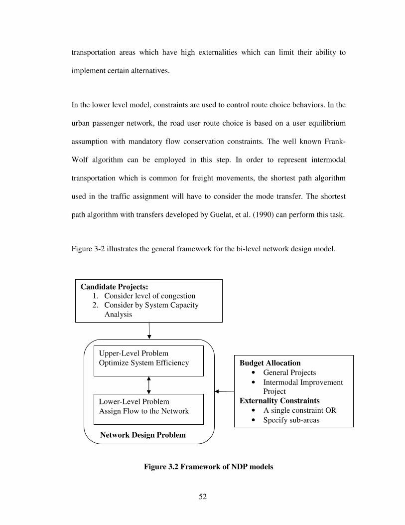
52

transportation areas which have high externalities which can limit their ability to

implement certain alternatives.

In the lower level model, constraints are used to control route choice behaviors. In the

urban passenger network, the road user route choice is based on a user equilibrium

assumption with mandatory flow conservation constraints. The well known Frank-

Wolf algorithm can be employed in this step. In order to represent intermodal

transportation which is common for freight movements, the shortest path algorithm

used in the traffic assignment will have to consider the mode transfer. The shortest

path algorithm with transfers developed by Guelat, et al. (1990) can perform this task.

Figure 3-2 illustrates the general framework for the bi-level network design model.

Figure 3.2 Framework of NDP models

Candidate Projects:

1. Consider level of congestion 2. Consider by System Capacity

Analysis

Budget Allocation

• General Projects

• Intermodal Improvement Project

Externality Constraints

• A single constraint OR

• Specify sub-areas

Upper-Level Problem

Optimize System Efficiency

Lower-Level Problem

Assign Flow to the Network

Network Design Problem

53

3.3 FREIGHT NETWORK DESIGN FORMULATION

Following the bi-level approach concept, this section formulates the mathematical

models for the freight network design problems for both regional and inter-regional

levels. It has been previously mentioned that there is a feedback relationship between

the regional and the inter-regional level. However, their different characteristics lead

to different network design model formulations. This section will clarify the

differences that have to be made for each level. The formulations are based on

previous network design research that focuses on passenger movements. In later

chapters, we focus on the long-haul freight movements only.

3.3.1 Regional network design problem

The regional level deals with urban or regional transportation networks and also local

transportation networks near transfer facilities. The regional network has short freight

movements, usually taken care by a single transportation mode and primarily by

truck. Although this level mainly focuses on truck movements and congestion on

local roads/streets and certain parts of highways, it can contribute important mode

choice for long haul freight movements. For example, high congestion near the

stations can dissuade shippers from using that mode.

In this dissertation, it is assumed that freight demand is exogenous and fixed. The

regional level moves the freight demand out of its study region through a dummy

super sink node as shown in Figure 3-1. On the other hand, the sink node gives the

freight demand that originated out of the region.

54

In the urban area, link congestion is the main problem and the congestion is related to

link capacities. A given network is represented by a graph G = (N, A) defined by a set

of nodes, Nn∈ and by a set of arcs, Aa ∈ . The cost function uses the form of a BPR

(Bureau of Public Roads) congestion function which is expressed in the following

equation.

( ) ( )[ ]βα aaaaa Qxtxt /10 ⋅+⋅= (3.1)

where

( )a at x = travel time on link a A∈ as a function of link volume ax ,

0

at = free-flow travel time on link a ,

ax = flow volume on link a A∈ ,

aQ = practical capacity of existing link a ,

,α β = coefficients in the polynomial delay function

Since congestion is the main problem for this network level, the transportation

agencies direct the improvements to capacity expansion. Hence, the problem is

formulated as continuous network design problem which can efficiently obtain the

best budget allocation to spend on link capacity expansions. The BPR function can be

adjusted to reflect the improvement if a link capacity is expanded. When the link is

improved by au units, the travel time will be changed to:

( ) ( )( )[ ]βα aaaaaaa uQxtuxt +⋅+⋅= /1, 0 (3.2)

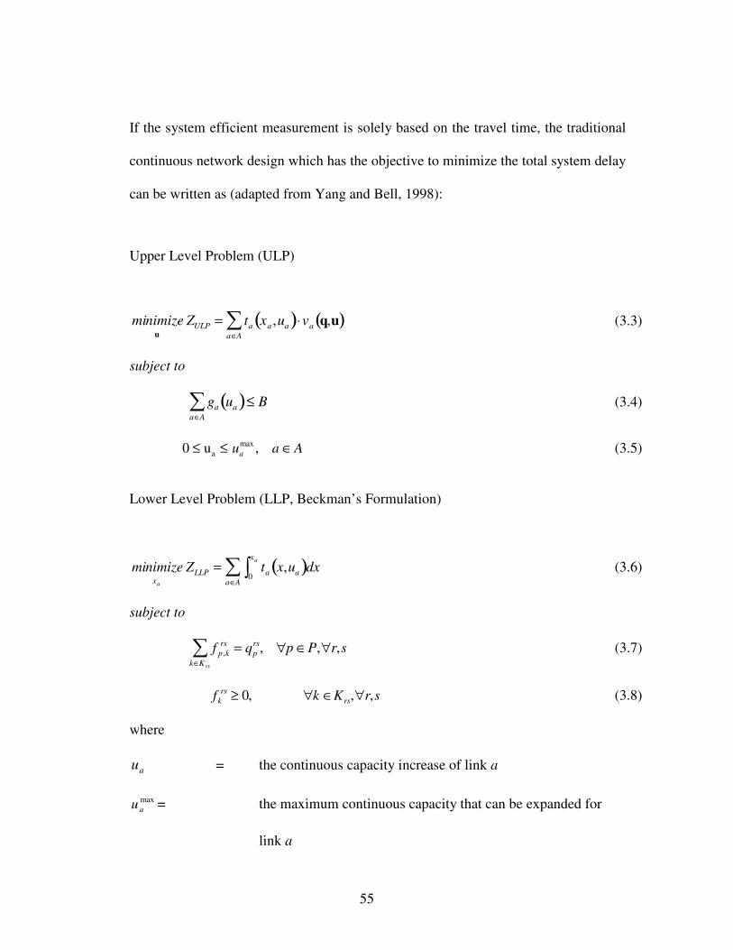
55

If the system efficient measurement is solely based on the travel time, the traditional

continuous network design which has the objective to minimize the total system delay

can be written as (adapted from Yang and Bell, 1998):

Upper Level Problem (ULP)

minimizeu

ZULP = ta xa ,ua( )a∈A

∑ ⋅va q,u( ) (3.3)

subject to

ga ua( )a∈A

∑ ≤ B (3.4)

0 ≤ ua ≤ ua

max , a ∈ A (3.5)

Lower Level Problem (LLP, Beckman’s Formulation)

minimizexa

ZLLP = ta0

xa

∫a∈A

∑ x,ua( )dx (3.6)

subject to

f p,k

rs

k∈K rs

∑ = qp

rs, ∀p ∈P,∀r,s (3.7)

fk

rs ≥ 0, ∀k ∈Krs,∀r,s (3.8)

where

au = the continuous capacity increase of link a

max

au = the maximum continuous capacity that can be expanded for

link a

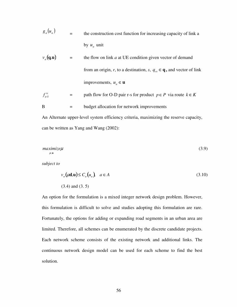
56

( )aa ug = the construction cost function for increasing capacity of link a

by au unit

va q,u( ) = the flow on link a at UE condition given vector of demand

from an origin, r, to a destination, s, q∈rsq , and vector of link

improvements, u∈au

f p,k

rs = path flow for O-D pair r-s for product Pp ∈ via route Kk ∈

B = budget allocation for network improvements

An Alternate upper-level system efficiency criteria, maximizing the reserve capacity,

can be written as Yang and Wang (2002):

µµ u,

ximizema (3.9)

subject to

va µd,u( )≤ Ca ua( ), a ∈A (3.10)

(3.4) and (3. 5)

An option for the formulation is a mixed integer network design problem. However,

this formulation is difficult to solve and studies adopting this formulation are rare.

Fortunately, the options for adding or expanding road segments in an urban area are

limited. Therefore, all schemes can be enumerated by the discrete candidate projects.

Each network scheme consists of the existing network and additional links. The

continuous network design model can be used for each scheme to find the best

solution.

57

Heuristic approaches have been developed to solve this problem. The three typical

heuristics approach applied are: 1) The Iterative-Optimization-Assignment

Algorithm; 2) The Link Usage Proportion-based Algorithm; and, 3) The Sensitivity

Analysis-based Algorithm (Yang and Bell, 1998). Meta-heuristics such as genetic

algorithms, tabu search or simulated annealing are also an option.

3.3.2 Inter-regional network design problem

The inter-regional network level deals with transportation links and facilities for long

haul freight operations. The network links in this level will represent the high

mobility transportation links such as highway and rail links. In addition, major

transfer facilities including seaports, airports, and rail stations are also included in this

level. The demand is assumed to be exogenous and fixed.

In the inter-regional network, congestion occurs only at specific points in the network

such as the areas near cities and ports. However we assume that the transportation

links connecting these areas are not congested. Therefore, there are no capacity limits

for these links though the congestion at the specific points is represented. Link costs

do depend on traffic volumes however. The travel time function may have the

following form as in Guelat, et al. (1990):

ta xa( )= α ii∑ β i + xa( )z i( )

α i > 0, βi > 0, 0 ≤ z i( )< ∞ (3.10)

58

At the inter-regional level, the network design model is formulated as a discrete

network design problem with zero-one decision variables. A main reason to use the

discrete network design model is that it can handle the freeflow speed change for the

major improvement between each region on the transport link or operation speed in

case of transfer facility. The continuous network design model cannot deal with

changes in free flow speed.

Transportation agencies have many alternatives to improve the inter-regional

network. New technologies can be employed to improve the network in addition to

capacity expansion strategies. Improvements such as double-track or electric rail can

increase the capacity and speed of the rail network. Additionally, reliability and

speeds at transfer facilities can be improved by adoption of improved information

systems. Discrete model variables have more flexibility to improve new technology

than continuous ones. Another advantage of discrete variables is these can represent

logical conditions necessary for considering specific improvements. For example,

improvingrail speed may not be a benefit if the technology at transfer facilities is not

compatible with the new main line technology. In this case, a discrete variable can be

used with logical constraints to specify that both projects or neither of them must be

implemented.

Given the graph network G = (N,A), the network consists of existing links and

proposed links. Let wabe a 0-1 variable representing the decision on link a. If wa is

equal to one, the link must exist or must be added is to the network. Assume that the

proposed links are links w1...wm and the existing links are links wm+1…wM. The

59

difference between a discrete network design formulation and a continuous one is the

upper level problem. The upper level of the discrete formulation can be written as

follow:

minimizew

ZULP = ta xa( )a∈A

∑ ⋅va q,w( ) (3.11)

ca

a =1

m

∑ ⋅ wa ≤ B (3.12)

( ) ( ) },{, srNnxx

nn Oa

a

Ia

a −∈∀= ∑∑∈∈

ff (3.13)

xa ≥ 0 ∀a ∈A (3.14)

xa ≤ M ⋅ wa a = 1...m (3.15)

where

aw = 1 if link a is exist or selected to improve and 0 otherwise,

ac = the construction cost of link a,

f = the set of path flows f = ( )⋅⋅⋅⋅⋅⋅ ,, rs

kf satisfies the route choice

decision given by the lower level problem

M = very large number

AOI nn ⊆, = the set of links entering and leaving node n, respectively

Given the network (set of w), the lower level of the discrete and continuous network

design problem share the same formulation. If travel time is the only concern for

transportation agencies, the objective function of the discrete network design problem

is minimizing total delay of the network by selecting set of proposed links. (3.12),

60

(3.13), and (3.14) are the budget constraints, flow conservation constraints, and non-

negativity constraints, respectively. (3.15) specifies that if a proposed link is not

constructed that link cannot be used, therefore, there is no flow on the link. As in

previous discussion, the system efficiency measurements and constraints can be

added to the model to broaden the transportation agency needs and requirements.

For example, alternative system efficiency criteria, maximizing reserve capacity, can

be adapted from Park and Regan (2005). In an inter-regional model the flow may not

be limit by link capacities but it can be limited by a level of service requirement. The

travel time between each origin and destination is a measurement of level of service.

Therefore, the upper level problem can be written as:

maximizex,u

ZULP = qrs

s∈S

∑r∈R

∑ (3.16)

subject to

Tk

rs = δa,k

rs

a∈A

∑ ⋅ ta xa f( )( )≤ φp ⋅ Trs

max (3.17)

where

rs

kT = travel time on path k for O-D pair r-s,

max

kT = maximum allowable travel time for O-D pair r-s

pφ = a commodity-specific parameter ranging from 0 to 1.

rs

ka,δ = indicator variable, 1 if link a is on path k between O-D pair r-s,

0 otherwise

61

In this formulation, the objective function is to maximize the demand travels for each

O-D by selecting the appropriate projects under budget constraint. The maximum

travel time constraint is used to limit flow on each path so that the level of service is

satisfied.

The branch and bound strategy is expected to be the solution algorithm for these

formulations. However due to the complication of the problem and network size,

meta-heuristics should also be considered as alternatives.

62

CHAPTER 4 INTEGRATED LONG-HAUL

FREIGHT AND FEEDBACK PROCESS

ALGORITHMS

In this chapter, the focus is the network design model for the inter-regional freight

network. The network carries mainly long haul movements which transverse states or

counties and is the focus of the state level transportation agencies. An earlier version

of this chapter was published in Apivatanagul and Regan (2007). This paper is our

first attempt to develop the freight network design model. It discusses the framework

of a good freight network design model which has to provide fairness for all

transportation modes and their project improvements. The model improvements are

achieved through the proper setting of the system efficiency measures, a reasonable

network representation, and accurate constraints. Some interesting future studies are

introduced. A naïve feedback process is used to solve the network design problem.

We discovered that this feedback method can be trapped in the infinite loop and can

give only the local optimal solution. Therefore, we discuss an improved solution

method in chapter 5.

4.1 SELECTING TRANSPORTATION ANALYSIS TOOLS

The bi-level network design problem can be viewed as the interaction model between

the transportation agencies and the transportation network users. In terms of analysis

63

tools, it can also be viewed as the interactive procedure between the budget

optimization model and the transportation analysis model. Since the transportation

analysis tool is responsible to reflect the changes occurring due to transportation

improvements or strategies, it determines the typeof network design models used and

the types of project improvements that can be recognized by the model. A micro-

simulation model can recognize a change in traffic management strategy while the

static traffic assignment acknowledges a change as an average travel time. The

question is, what tool is needed for long haul freight network design since the

different tool will lead to the different modeling framework.

Two important functions of transportation networks are mobility and accessibility --

functions which can contradict one another. The local network, which is represented

by the regional level model as described in Chapter 3, focuses on accessibility while

the inter-regional network focuses on mobility between cities. Therefore the larger

transportation network can be considered as many connected networks which have

different functions. An inter-regional network links local networks together thus has a

high level of mobility in order to provide for long distance movements. Since the

local networks contain the origins or destinations of the movements, they should

support the inter-regional network by providing good access for long distance

movements to enter the inter-regional network. As a result, an improvement selected

in a local network is related to projects selected in inter-regional network and other

local networks. A transportation network should be designed using an integrated

network perspective.

64

It is unfortunate that there is no transportation analysis tool which can work well on

these two different network levels. The traditional four step model is usually used to

study transportation investments due to its practical advantages. The typical traffic

assignment model is based on User Equilibrium (UE) assumptions with the Bureau of

Public Roads (BPR) function which is proper for project investments in a large study

area involving improvements on the highway systems. However, the approach does

not properly capture subtle changes such as traffic operation improvements which are

usually implemented on the local networks. Oh and Cortes (1999) applies the micro-

simulation model, Paramics, to transportation planning. The model can capture traffic

operations changes which cannot be considered by the UE traffic assignment model.

Although a tool such as microscopic traffic simulation provides a powerful method

for capturing subtle changes in transportation systems, it is limited by network size.

Such detailed models are impractical for large networks and additionally,

transportation planning does not require great accuracy down to the vehicle-vehicle

perspective. In conclusion, the traditional four step model cannot accurately capture

improvement effects in local networks while attempts to implement detailed models

using microscopic simulation for large area transportation planning are impractical.

A quick solution to overcome this problem is to improve the local network

information in the traditional four step model (from now on will be called the

transportation planning model) through centroid connectors. In a transportation

planning model, an area (or zone) is integrated to be a centroid which stores

demographic, economic, and sociological information. The local network is

65

aggregated into centroid connectors. The way in which centroid connectors are

constructed as representatives for each local network is very important, however, as is

typically the case, the centroid costs and distances are assumed using conservative

values or calibrated values without supporting data. Additionally, the improvement

effects in local networks are usually neglected. Our framework is flexible enough so

that if studies are performed related to improvements in local networks, the

information can be used to estimate the proper centroid connector costs under both

existing conditions and improved conditions.

In the next section, the bi-level network design problem for long haul freight

movements is described. This bi-level framework is flexible enough that when the

information of centroid connections is improved it can combine to the model easily.

A numerical example is given to show the importance of the integrated network

concept in the later section.

4.2 THE LONG HAUL FREIGHT NETWORK DESIGN MODEL

Our approach centers around a bi-level network optimization model. It iterates

between the traffic assignment model which predicts route choices made by network

users and the budget allocation model which represents decisions made by public

agencies. The model intends to join these two decisions and consequently obtain the

best network. The model is generally applied to highway network design which

focuses on benefits to passenger movements. Variations of objective functions and

solution algorithms have been proposed (Leblanc, 1975, Abdullal and LeBlanc, 1979,

66

Friesz, et al., 1985, and Drezner and Wesolowsky, 2003).In order to apply a similar

model to design a freight network the special characteristics of freight transportation

must be well understood and each component on the traditional bi-level model has to

be adjusted properly.

The longer trips typical of freight movements require the network design to consider

both local networks and inter-regional networks simultaneously. In addition to multi-

mode and multi-commodity characteristics, the nature of longer trips differentiates

freight movements from passenger movements. Passenger trips are generally shorter

and involve a single mode. These shorter trips simplify the bi-level model to a small

simple network with few improvement alternatives. Longer trips travel on both local

networks and regional networks. The multi-modal nature of freight transportation

creates a situation in which the larger transportation network must be considered in

order to maintain competitiveness among transport modes. The freight network

representation has to be constructed properly to accommodate these characteristics.

4.2.1 The freight network representative

A good network representation should capture all necessary characteristics of the

study while keeping the network as simple as possible. For this study, the freight

network considers multiple modes. Therefore the network representation should

maintain competition among transport modes.

In this study, a multi-modal inter-regional network connects the local networks. In

order to simplify the problem, the inter-regional network consists of only two

67

transportation networks, a highway network and a railroad network. The networks are

connected at specific points by transfer links which allow movements between two

modes. In order to complete long distance transport moves, the networks can

connected to airports and seaports which are gateways to long distance trips.

In order to maintain competition between modes, movements are allowed to travel

into and out of the study area. Some modes such as trains and trucks are competitive

when considering longer distances in which demands can be located outside the study

area. These movements are also transported through gateways. Figure 4.1(a) shows

the inter-regional network, the gateways, the external nodes, and the external node

connectors. The gateways can be the interception points of interstate highways and

the study area boundary. They can also be intermodal transfer points such as airports,

seaports, and train stations. A key issue is which external nodes should be included in

the model and how to calculate the external node connector costs.

68

Figure 4.1 The freight network representative

External nodes are used to represent areas out of the study region which range from

nearby movements to international trade transportation. Therefore, there are too many

external nodes to include all of them in the regional network. In reality, the choices of

external nodes are limited by the demand forecasting models which will choose the

areas based on the interests of modelers. In general, the external areas usually are

important business areas and some important transfer points such as airports and

seaports. For less important business areas, the demand to a destination can be small

and can be grouped to other nearby external areas. Greater distance separating areas

External node A

External node B

External node C

External node C

A Gateway of Highway #1

A Gateway of an Airport

A link connects the local network to the external area C by Highway #1

Inter-Regional Network

(a) External nodes for the movements out of the study Area

Local Network

A connector links a highway on inter-regional network and the local network

Inter-Regional Network

A gateway on a highway on an inter-regional network

Existing Network

Scenario A

(b) Centroid connectors with 3 exits and 2 transportation modes

69

usually means less travel demand and less importance between those areas.

Nevertheless, the longer movements can have more competitive modes. In

conclusion, the further distances should be represented by less external nodes but the

longer external nodes will connect to more gateways (e.g. airports, train stations,

highway etc.) because of the variety of mode choices. In Figure 4.1(a), the external

node A is a nearby business area but the external node C represents a group of

business areas locating far from the studying region. The long haul freight

movements to C will have more alternative modes therefore the node connects to both

the highway gateway and the airport gateway.

The external connector costs can be weighted average costs found using historical

data for freight movements. The long haul links are uncongested so these costs can be

assumed to be fixed. In the case in which there are transfer points on the paths, some

penalties can be assumed. It may be important to consider cases in which the network

outside the study area is changed and historical data cannot be used. In that case, it

should be noted that only mega projects will have a significant impact on such a large

network. Consequently, if such a project exists, it is likely to be well studied. The

information from the study can be used to adjust the average costs from the historical

data.

The freight network representation has to provide a way to study the integrated

network consisting of local and inter-regional networks. These networks have

different functions and need different analysis models. As has been discussed in the

previous section, the transportation planning model is a crude method for capturing

70

the improvement effects in the local networks since detailed traffic simulation models

are impractical for large study areas. This study proposes to use data from the

simulation models to estimate the centroid connector costs in order to capture the

effects of local network traffic conditions.

Ademand origin or destination is represented by a centroid and a set of connectors.

Connectors can connect a centroid to a regional network at various points using

various modes as shown in Figure 4.1(b). Some penalty costs may apply to the

connectors which link different modes. A local network that is a candidate for

improvement should have additional information about the estimated connector costs

before and after the improvements. The combinations of improvements are called

improvement scenarios. Different scenarios result in different traffic conditions and

estimated connector distances. Each scenario can be studied using a more detailed

transportation model focused on the local area. The connector cost estimates are

obtained using an appropriate statistical method which a subject of further research.

4.2.2 The Origin Destination Demand Matrix (OD matrix)

The travel demand usually tabulated by its origins and destinations which will be

simply called Origin-Destination (OD) matrix. This OD matrix is crucial as an input

to the network design model. In the freight network design, both a freight and

passenger OD matrix are needed. Since truck transportation, a major mode for freight

movements, shares the road network with passenger cars, a road improvement will

affect route choices for both movements. In this study, the freight demand matrix is

the focus.

71

The freight demand process is complicated and it has to pass through a disaggregation

and aggregation process before the proper demand matrix for a study is ready. The

general public data source is the Commodity Flow Survey Data maintained by the

U.S. Department of Transportation and the U.S. Department of Commerce (USDOT

and BTS ,2005). Another typical source is the commercial general commodity flow

data known as the TRANSEARCH database, developed and maintained by Global

Insight. The commodity flows are given on a ton basis. The flow origins and

destinations are aggregated to the Bureau of Economic Analysis (BEA) level.

Therefore the data requires a disaggregation process to use in study smaller areas (see

for example Rowinski, et al. ,2007, Ambite, et al., 2002, and Gordon and Pan, 2001).

The Benchmark Input-Output Accounts of the US is a primary source of data used for

the disaggregated process and is maintained by Bureau of Economic Analysis. See for

example the study of Monsere (2001). In CALTRAN and Booz Allen & Hamilton

Inc. (2001), a survey with private sectors’ activities is conducted to set rules to

properly distribute commodities to the disaggregated areas. In order to consider the

congestion trucks contribute to the road network, conversions are needed to convert

commodity tons to vehicle units. Each commodity can have its conversion

parameters.

The matrix dimensions for passenger and freight movements can be different.

Passenger movements tend to be shorter and have different attractions than freight

movements. For example, an airport can be a special attraction point that should be

included in the passenger movement demand matrix. If an airport is included in the

freight movement demand matrix, it means that some demand is fixed to travel to the

72

airport therefore the mode shift possibility will be eliminated from that demand.

Therefore, the airport should not be included in the freight matrix if we intend to

study mode shifts.

4.2.3 Network Design Formulation

A bi-level network design approach is used as the based model for the freight network

design study. A complication of transportation planning is that projects are selected

by transportation agencies but the network is used by many users. Therefore, the

model has to consist of two sub-models. The first model is to select the best set of

project improvements and the other is the traffic assignment model used to forecast

the corresponding movements on the network.

The model will focus on the improvement of the freight network at the inter-regional

network level. Nevertheless, the model considers the supporting effects from the local

network improvements through the selection of proposed scenarios from each zone.

The freight network improvements vary widely. This is a reason to suggest using

separated models or other studies to estimate how to adjust the link cost functions

before and after improvements. In a transportation planning model, the BPR cost

function is usually used to estimate link costs. Freeflow speeds and capacities are the

main characteristics in the function which must be adjusted properly for the change

from the existing conditions to the improved conditions. The Highway Capacity

Manual (2000) can be a basis to adjust the capacities and freeflow speeds based on

different traffic compositions and changes in highway geometries but other studies

are needed to enhance the adjustment for other improvements. The following

73

improvements are proposed for the regional network. These improvements are

summarized from BTH and CalEPA (2005):

1. Construct truck lanes

2. Expand lanes in a highway

3. Construct climbing lanes

4. Construct interchanges

5. Reconstruct ramps

6. Reconstruct bridges

7. Construct grade separation

8. Intermodal facility improvements

9. Rail capacity improvements

It should be noted that there are other possible freight transportation improvement

projects but these are implemented in local networks or at specific points. As

mentioned earlier, these projects need different or special evaluation models. The

important point is to transfer their results to the same modeling platform in order to

evaluate them together thus resulting in a good integrated network and an effective

budget allocation.

Using the bi-level network design concept illustrated in Figure 3.2, we will describe

the upper and lower model for the long haul freight movements and its solution

algorithm respectively.

74

4.2.3.1 Upper Level Model: The budget allocation model

The objective of budget allocation is to optimize social benefits while the traffic

assignment is used to reflect the user route choices. The traffic volume obtained from

the traffic assignment step can be used to adjust the penalty costs on each link before

the budget allocation is implemented. For example, high truck traffic volume on a

highway link can obstruct traffic flow on the link. This penalty may be calculated

based on the Highway Capacity Manual (2000). Another example is that a transfer

link that is over-capacity can lead to very high penalty costs. The binary integer

programming will be used to model the budget allocation. Many algorithms are

developed to solve integer programming problems such as branch and bound

techniques, branch and cut techniques, and metaheuristics such as genetic algorithms

or tabu search. An example of commercial software which provides functions to solve

these problems is CPLEX. The model will select the improvement projects on the

regional network and an improvement scenario for each zone. For freight network

improvement, government agencies have three primary three objectives: reducing

congestion, accidents, and environmental impacts. The common objective function

for network improvement is minimizing congestion on the network which is closely

related to pollution and accidents. An improvement that lessens congestion usually

results in less accidents and pollution.

In order to develop a model to select proper projects for a freight network, many

issues have to be considered. The first issue is that the mode shift benefit cannot be

realized by the upper level model which is a supply side model. An improvement on a

railroad network can redirect some commodity flows from a road network therefore it

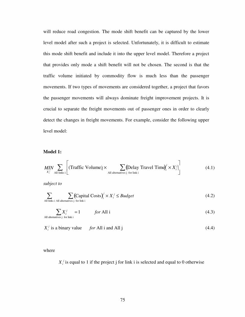
75

will reduce road congestion. The mode shift benefit can be captured by the lower

level model after such a project is selected. Unfortunately, it is difficult to estimate

this mode shift benefit and include it into the upper level model. Therefore a project

that provides only mode a shift benefit will not be chosen. The second is that the

traffic volume initiated by commodity flow is much less than the passenger

movements. If two types of movements are considered together, a project that favors

the passenger movements will always dominate freight improvement projects. It is

crucial to separate the freight movements out of passenger ones in order to clearly

detect the changes in freight movements. For example, consider the following upper

level model:

Model 1:

X ij

MIN (Traffic Volume)i × Delay Travel Time( )i

j

All alternatives j for link i

∑ × X i

j

All links i

∑ (4.1)

subject to

Capital Costs( )i

j

All alternatives j for link i

∑All links i

∑ × X i

j ≤ Budget (4.2)

X i

j

All alternatives j for link i

∑ = 1 for All i (4.3)

X i

j is a binary value for All i and All j (4.4)

where

j

iX is equal to 1 if the project j for link i is selected and equal to 0 otherwise

76

The objective function is to minimize congestion on the network. (4.2) is the budget

constraint function and (4.3) specifies that only an improvement alternative is chosen

for each link. The congestion is represented by delay travel time on the network links.

The delay travel time is the difference between the time needed to travel the link at

freeflow speed and the current speed. The objective seems to give a good freight

network which has the minimum total delay (i.e. congestion). However, this model

favors passenger movements and the improvements that focus on freight movements

can be neglected.

In this study, the following model is suggested to reduce the bias issues between

movement types. A good freight network design should reduce the freight transport

costs while it is important that the design reduce the total traffic delay on the network.

If both delay and freight transport costs have to be minimized, the optimization is the

multi-objective function problem. In this study, the freight network is the focus,

therefore the objective is set to minimize the freight generalized cost but the total

traffic delay is controlled by a constraint. The upper level model in this study is set as

follows:

Model 2:

X ij

MIN (Freigh Volume)i, m × Generalized Costs( )i,m

j

All alternatives j for link i

∑ × X i

j

All links i

∑All Commodities m

∑

77

(4.5)

subject to

(Traffic Volume)i × Delay Travel Time( )i

j

All alternatives j for link i

∑ × X i

j

All links i

∑ ≤ MaxDelay

(4.6)

and (4.2), (4.3), (4.4)

In this setting, the freight improvement projects are selected to minimize the

generalized costs while the projects that reduce traffic delay are selected to control

the network total delay under the maximum value. All improvement projects may be

selected by the model since a project will favor either freight movements or passenger

movements which are provided separately by the objective function and the constraint

(4.6).

The problem that the model will select only projects favor passenger movements is

reduced by the separated functions as well as the fact that each function is focused on

a single movement type

4.2.3.2 Lower level model: Traffic assignment

Many commodity types and passenger movements travel in the freight network. The

freight network and the passenger movement network mostly overlap although the

freight network includes additional facilities such as transfer facilities and intermodal

facilities. An improvement for either network will affect route choice behaviors for

78

both freight and passenger movements. Therefore, the lower level model should deal

with both passenger and freight traffic assignment.

A practical method to assign commodity flows is to assign the passenger movements

first to the network according to the User Equilibrium (UE) assumption. Then each

commodity flow is assigned to the preloaded network by the shortest paths (Monsere ,

2001 and CALTRAN and Booz Allen & Hamilton Inc., 2001). The passenger

movements contribute most congestion on the network, therefore the passenger route

choice should not change from the additional congestion contributed by truck traffic

that will be loaded later.

The highway capacity can be obtained from the Highway Capacity Manual. The

passenger car equivalent factors will be applied to the truck volumes before loading

these onto the network. In order to include multi-mode alternatives, freight

movements are allowed to transfer at some specific nodes. In this initial model, we

assume that the congestion at transfer nodes is assigned fixed penalty costs which can

vary by different commodity types.

The lower level model also has to care for the mode shifts that can happen due to

future improvements. There are many approaches to split the commodity flows to

different modes. An approach is to use the modal split models which assign each

commodity modes using a fixed proportion. In order to study mode shift, a feed back

value of travel cost is required. This approach is not efficient since an additional

model is required in the iterative process (i.e. from bi to tri-level model) and the

79

solution will likely not converge. Another approach is to assign the commodity flows

using the minimum generalized cost paths given the transfer links between different

networks (Monsere, 2001 and Maruyama, et al., 2001). Different commodities and

different services can have a different value of time, safety, and reliability. These

differences are represented by coefficients in the generalized cost functions. The

generalized costs are a linear combination of those qualities and have $/ton as their

units. The approach combines the modal split model and the traffic assignment

together. This type of traffic assignment will be used in this study.

A suggestion to study possible mode shift is to use both approaches together.

Although the combined approach between modal split – traffic assignment is

convenient, it fails to reflect the existence of freight movements which remain

inflexible to changing costs. In the same commodity type, there is a portion of travel

demand which prefers to use the same mode. This portion has much higher penalty

costs than the others which may result from inflexible schedules, freight volume, and

other convenience factors for some individual shippers/carriers. A modal split model

should be used to classify the fixed mode-portion before the combined traffic

assignment approach is used. A feedback process for the modal split is not needed

since only large changes in transportation costs can change the portion significantly.

A similar concept has been implemented by CALTRAN and Booz Allen & Hamilton

Inc. (2001) which uses some criteria to divide commodity flows which can be

transported by an intermodal mode and those which cannot.

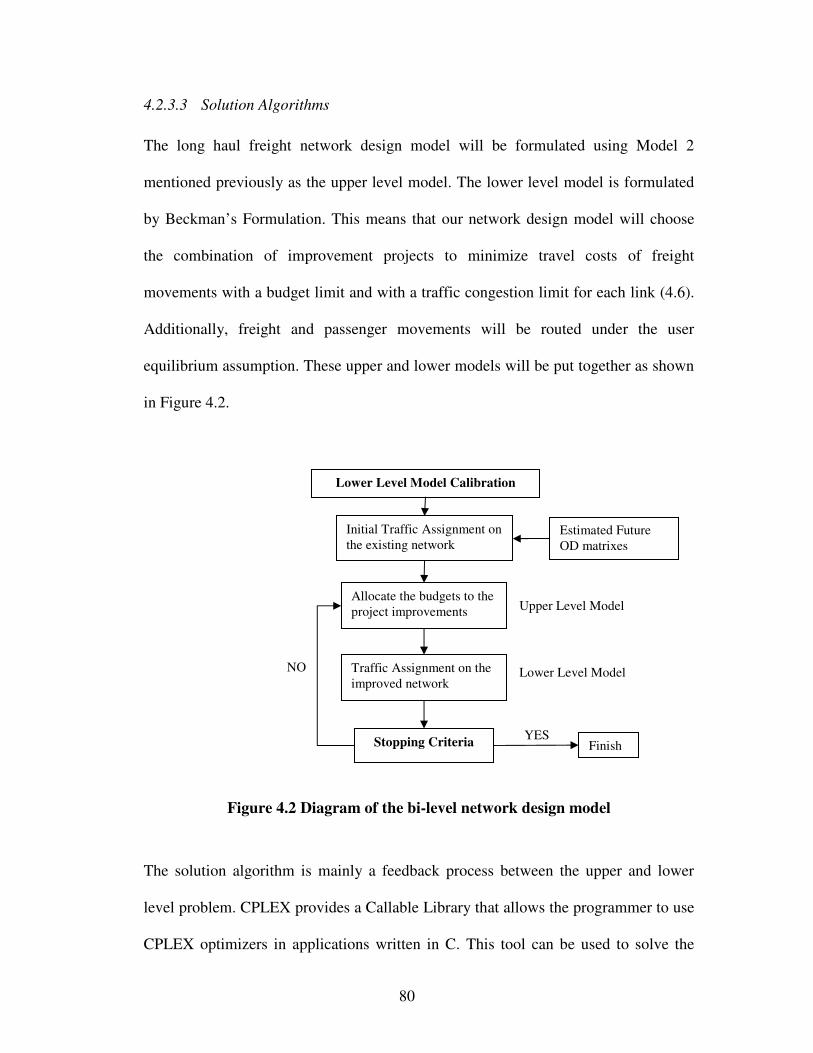
80

4.2.3.3 Solution Algorithms

The long haul freight network design model will be formulated using Model 2

mentioned previously as the upper level model. The lower level model is formulated

by Beckman’s Formulation. This means that our network design model will choose

the combination of improvement projects to minimize travel costs of freight

movements with a budget limit and with a traffic congestion limit for each link (4.6).

Additionally, freight and passenger movements will be routed under the user

equilibrium assumption. These upper and lower models will be put together as shown

in Figure 4.2.

Figure 4.2 Diagram of the bi-level network design model

The solution algorithm is mainly a feedback process between the upper and lower

level problem. CPLEX provides a Callable Library that allows the programmer to use

CPLEX optimizers in applications written in C. This tool can be used to solve the

Lower Level Model Calibration

Initial Traffic Assignment on the existing network

Estimated Future OD matrixes

Allocate the budgets to the project improvements

Traffic Assignment on the improved network

Stopping Criteria Finish YES

NO

Upper Level Model

Lower Level Model

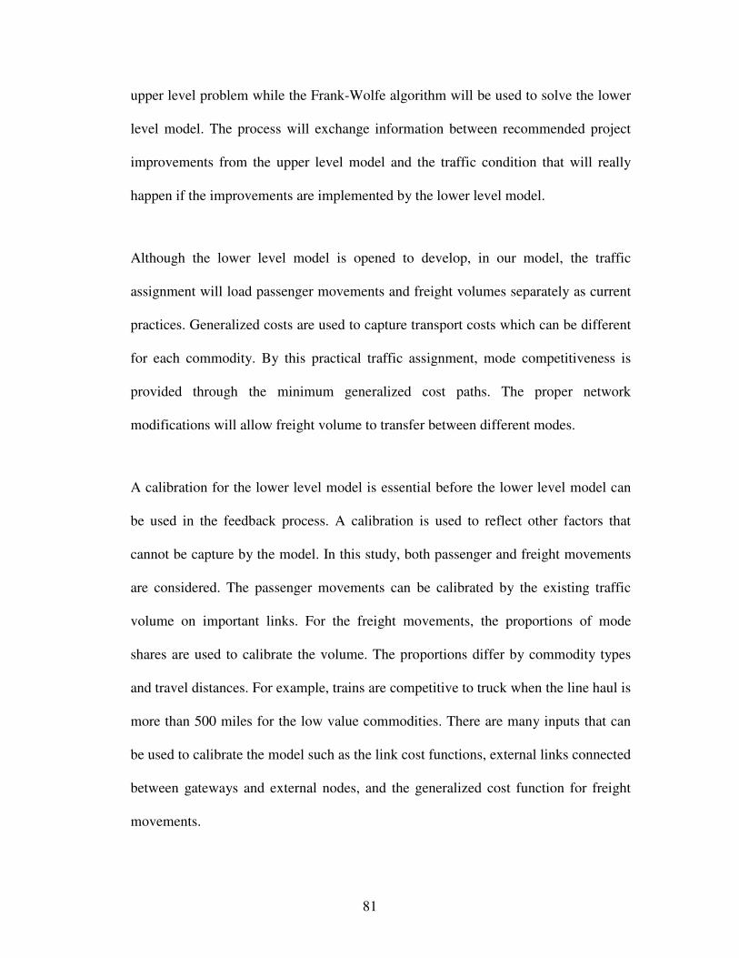
81

upper level problem while the Frank-Wolfe algorithm will be used to solve the lower

level model. The process will exchange information between recommended project

improvements from the upper level model and the traffic condition that will really

happen if the improvements are implemented by the lower level model.

Although the lower level model is opened to develop, in our model, the traffic

assignment will load passenger movements and freight volumes separately as current

practices. Generalized costs are used to capture transport costs which can be different

for each commodity. By this practical traffic assignment, mode competitiveness is

provided through the minimum generalized cost paths. The proper network

modifications will allow freight volume to transfer between different modes.

A calibration for the lower level model is essential before the lower level model can

be used in the feedback process. A calibration is used to reflect other factors that

cannot be capture by the model. In this study, both passenger and freight movements

are considered. The passenger movements can be calibrated by the existing traffic

volume on important links. For the freight movements, the proportions of mode

shares are used to calibrate the volume. The proportions differ by commodity types

and travel distances. For example, trains are competitive to truck when the line haul is

more than 500 miles for the low value commodities. There are many inputs that can

be used to calibrate the model such as the link cost functions, external links connected

between gateways and external nodes, and the generalized cost function for freight

movements.

82

To initialize traffic volume on the freight network, all network link costs are set as if

there is no improvement. The initial traffic volume is input into the upper level model

to decide the proper projects. When the projects are selected, the network link costs

are set properly and the corresponding traffic volume is obtained by the lower level

model again

There are many stopping rules that can be used for this solution algorithm.

Theoretically, the solution converges when two consecutive selected projects are the

same. If there are many improvement projects in the network design problem, this

condition may not be met. A solution is to track objective values until they have low

standard deviation to a certain point and using some criteria to fix some projects that

are frequently selected. If the process continues in this fashion, the model will finally

give a solution.

4.3 A NUMERICAL EXAMPLE

In this section, a freight network design problem is presented. Our main purpose is to

illustrate the proposed approach to study an integrated network which joins local

networks together. The problem will show that the integrated network approach can

provide a different perspective from which to select improvement projects on the

network. A hypothetic problem with assumed values is developed for this purpose.

The problem consists of 3 local networks, cities A, B, and C which are connected by

an inter-regional network shown in Figure 4.3.

83

Figure 4.3 The example freight network

Three scenarios for each city are proposed. The inter-regional network has two

possible improvement projects, one which improves the highway and another which

improves the railway. Without loss of generality we assume that only one commodity

type travels on the network. The data are summarized in Tables 4.1(a) -1(c). Although

the travel time values are assumed fixed, in practice, travel times will tend to be

higher nearer to origins and destinations. Carriers can make up time in the middle of

their routes. The total maximum delay is assumed to be 2,400 pcu hours and the

budget is assumed to be 120 monetary units. Model 2, described above, is applied to

the data. The results are shown in Figure 4.4.

A C

B

H3

D E

H1

H2

A-Hwy3

A-Hwy1

Highway #1 Highway #2

Highway #3

B-Hwy2 B-Hwy1

C-Hwy2

C-Hwy3 T1

T2

Rr-Hwy-D

Hwy-Rr-D

Railroad #1

Zone Centroid

Intermodal Transfer Node

Regional Hwy

Railroad

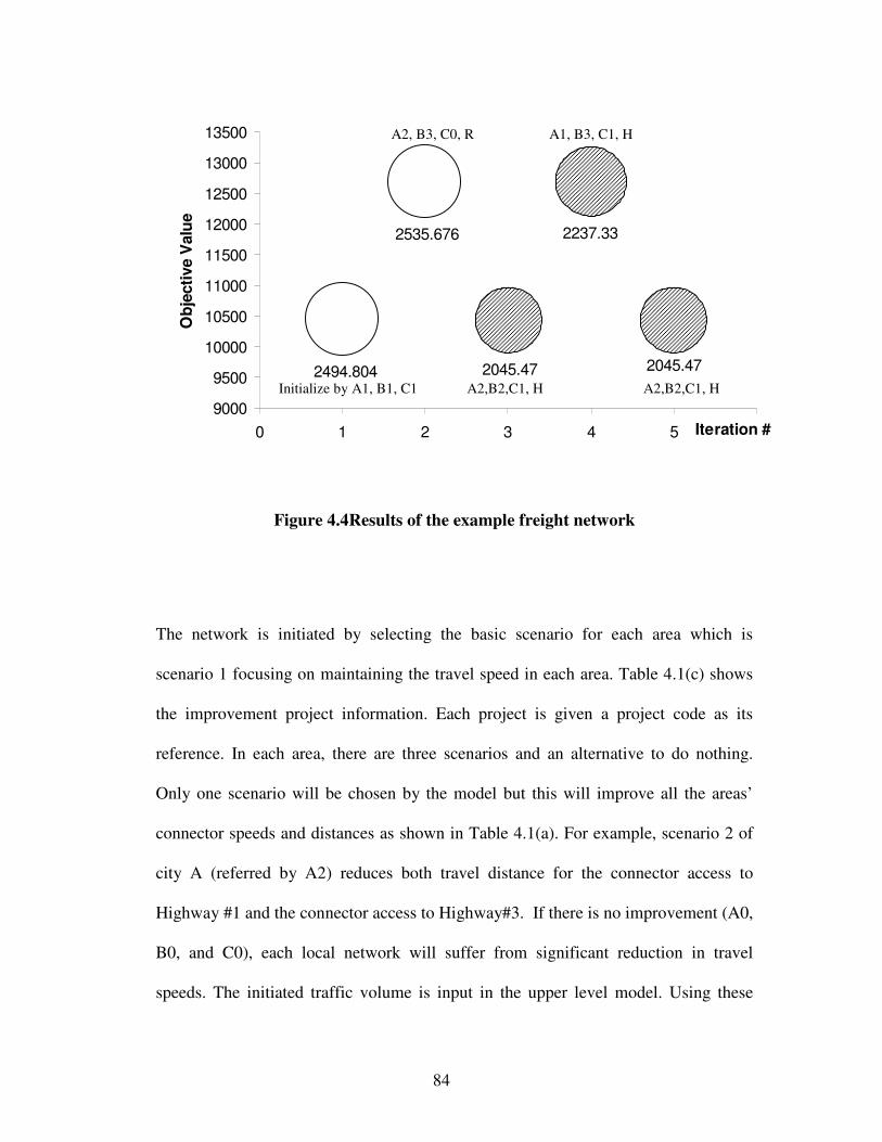
84

Figure 4.4Results of the example freight network

The network is initiated by selecting the basic scenario for each area which is

scenario 1 focusing on maintaining the travel speed in each area. Table 4.1(c) shows

the improvement project information. Each project is given a project code as its

reference. In each area, there are three scenarios and an alternative to do nothing.

Only one scenario will be chosen by the model but this will improve all the areas’

connector speeds and distances as shown in Table 4.1(a). For example, scenario 2 of

city A (referred by A2) reduces both travel distance for the connector access to

Highway #1 and the connector access to Highway#3. If there is no improvement (A0,

B0, and C0), each local network will suffer from significant reduction in travel

speeds. The initiated traffic volume is input in the upper level model. Using these

2535.676

2494.804 2045.47

2237.33

2045.47

9000

9500

10000

10500

11000

11500

12000

12500

13000

13500

0 1 2 3 4 5 6Iteration #

Ob

jecti

ve V

alu

e

Initialize by A1, B1, C1

A2, B3, C0, R

A2,B2,C1, H

A1, B3, C1, H

A2,B2,C1, H

85

values, the upper level model suggests a new selection that is A2, B3, C0, and R.

Although the selection total delay is less than the total maximum delay using the

upper model calculation and the initiated traffic volume, the lower model discloses

that the new selection changes the traffic volumes on the network. The result is that

the real delay is more than maximum delay. This constraint violation does not hinder

the algorithm. The new traffic volume from the lower model and the new selection is

input to the upper level model again. In the fifth iteration, a selection is the same as

the third iteration selection. This means that an endless loop is happened in the model.

In this case, the selection which yields the minimum objective values in the loop is

chosen to design the network. In this example, the best selection is A2, B2, C1, H

with the total generalized cost of $10,429/hour.

Within the integrated network, all scenarios in all cities and the regional improvement

projects work together to achieve the goal of an efficient network. If local networks

and regional networks are not integrated, the network design can be different and may

not achieve the global benefit such as minimizing total freight costs and restricted

total delay.

4.4 INTRODUCING AN IMPROVED MODEL FUTURE

STUDIES

In this chapter, a long haul freight network design framework is constructed based on

a bi-level network design approach which expanded more general and practical

models based on the existing road network design literature. The framework expands

86

local road networks which are the focus of the earlier literature to multiple mode

networks with multiple commodities. Network representations, the upper and lower

level problems, are adjusted to be appropriate for a freight network study.

Another focus of this model is to combine various studies on effects of different

network improvements into a single model through the centroid connector

information. Future research that should be conducted after this model is to estimate

average centroid connector costs. In this study, centroid connectors are given

significant roles as connections between local network studies and inter-regional

network studies. If there are project improvements for a local network, a proper

model should be constructed to study improvement impacts on the local network. The

data from the study can be used to estimate typical transport costs in and out the local

network both before and after the improvements. Typical transport costs will be used

as the centroid connector costs in order to study further impacts on the larger network

(the inter-regional network that connecting other local networks together). A suitable

statistic approach to identify typical transport costs that best represent the local

networks is required. The task is interesting since transport models vary. Therefore

techniques used to compute these average costs are different. There are at least two

well known transport models related to these costs. The first one is the model which

can tracks vehicle paths from their origins to destinations and the other which cannot.

In the next chapter, a second model for freight network design is represented. There

are two developments which are inspired by the first model. The first improvement is

based on the route choice behavior used in the lower-level model. The shipper-carrier

87

model Friesz, et al. (1986) is used to separate the decisions made by these two agents

who have different ways to define their route choices. A disadvantage of the approach

is increasing computational effort but it is believed that this shipper-carrier model can

understand the mode choice behavior better.

The result from the numerical example suggests the second development related to

the solution algorithm. A branch and bound technique is introduced to the next model

to solve two problems that can occur in the feedback process. The first problem is the

infinite loop and the second is the preference to expand high traffic volume links

while leaving others undeveloped. The situation develops similarly to project

selections by Benefit Cost Analysis (BCA) approach when the net present value is

used as a decision criterion. The high traffic link receives the improvement. Its result

is additional traffic volume and the link continues to get more improvements. This

high volume preference hinders the network design to produce the optimal network

which can develop through the congestion reduction both by increasing the

infrastructures’ capacities and diverting traffic to less congested paths or less

congested modes. Instead of selecting which projects should be implemented based

on the traffic volume obtained by the lower level model, the branch and bound

technique uses the lower level model to produce the lower bound and decides whether

to keep or discard the improvement alternatives.

88

Table 4.1 Numerical the example inputs

Table 4.1(a): Link network data

Link Number

From To Condition Transport Cost

($/ton-mile) Travel Time ($/ton-hour)

Distance (miles)

Freeflow Capacity Transfer Costs

Imp Code

No improvement 0.12 1.0 8.0 22.0 8 0 A0

Select Scenario 1 0.12 1.0 8.0 32.0 8 0 A1

Select Scenario 2 0.12 1.0 7.9 32.5 8 0 A2 1 A A-Hwy#1

Select Scenario 3 0.12 1.0 8.0 30.0 8 0 A3

No improvement 0.12 1.0 7.0 20.0 8 0 A0

Select Scenario 1 0.12 1.0 7.0 30.0 8 0 A1

Select Scenario 2 0.12 1.0 7.0 30.0 8 0 A2 2 A A-Hwy#3

Select Scenario 3 0.12 1.0 7.0 30.0 8 0 A3

No improvement 0.12 1.0 7.0 19.0 8 4 A0

Select Scenario 1 0.12 1.0 7.0 30.0 8 4 A1

Select Scenario 2 0.12 1.0 7.0 30.0 8 4 A2 3 A T1

Select Scenario 3 0.12 1.0 6.8 31.0 8 3 A3

No improvement 0.12 1.0 9.0 20.0 8 0 B0

Select Scenario 1 0.12 1.0 9.0 30.0 8 0 B1

Select Scenario 2 0.12 1.0 8.8 31.0 8 0 B2 4 B B-Hwy#1

Select Scenario 3 0.12 1.0 9.0 30.0 8 0 B3

No improvement 0.12 1.0 8.8 19.0 8 0 B0

Select Scenario 1 0.12 1.0 8.8 29.0 8 0 B1

Select Scenario 2 0.12 1.0 8.6 29.0 8 0 B2 5 B B-Hwy#2

Select Scenario 3 0.12 1.0 8.8 29.0 8 0 B3

No improvement 0.12 1.0 8.0 18.0 8 4 B0

Select Scenario 1 0.12 1.0 8.0 28.0 8 4 B1

Select Scenario 2 0.12 1.0 8.0 28.0 8 4 B2 6 B T2

Select Scenario 3 0.12 1.0 7.8 29.0 8 3 B3

89

Table 4.1(a): Link network data (cont.)

Link Number

From To Condition Transport Cost

($/ton-mile) Travel Time ($/ton-hour)

Distance (miles)

FreeFlow Capacity Transfer Costs

Imp Code

No improvement 0.12 1.0 6.0 31.0 8 0 C0

Select Scenario 1 0.12 1.0 6.0 35.0 8 0 C1

Select Scenario 2 0.12 1.0 5.8 36.0 8 0 C2 7 C

C-Hwy#2

Select Scenario 3 0.12 1.0 5.9 35.0 8 0 C3

No improvement 0.12 1.0 5.8 31.0 8 0 C0

Select Scenario 1 0.12 1.0 5.8 35.0 8 0 C1

Select Scenario 2 0.12 1.0 5.8 35.0 8 0 C2 8 C

C-Hwy#3

Select Scenario 3 0.12 1.0 5.7 36.0 8 0 C3

9 A-Hwy#1 H1 0.12 0.5 2.0 60.0 8 0 -

10 A-Hwy#3 H1 0.12 0.5 4.0 60.0 8 0 -

11 B-Hwy#1 H2 0.12 0.5 2.0 60.0 8 0 -

12 B-Hwy#2 H2 0.12 0.5 4.0 60.0 8 0 -

13 C-Hwy#2 H3 0.12 0.5 2.0 60.0 8 0 -

14 C-Hwy#3 H3 0.12 0.5 2.0 60.0 8 0 -

No improvement 0.12 0.5 40.0 65.0 4000 0 - 15 H1 H2

Select Scenario 1 0.12 0.5 40.0 70.0 4000 0 H

16 H1 H3 0.12 0.5 60.0 65.0 2200 0 -

17 H2 H3 0.12 0.5 40.0 70.0 2200 0 -

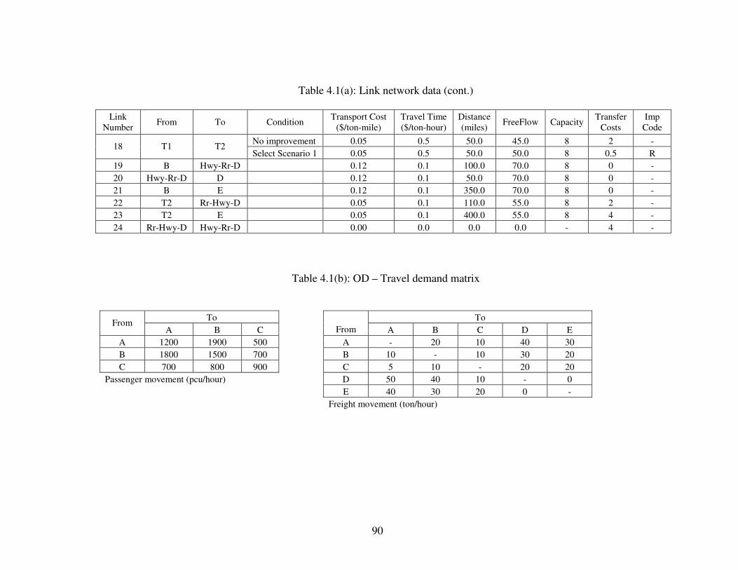
90

Table 4.1(a): Link network data (cont.)

Link Number

From To Condition Transport Cost

($/ton-mile) Travel Time ($/ton-hour)

Distance (miles)

FreeFlow Capacity Transfer

Costs Imp

Code

No improvement 0.05 0.5 50.0 45.0 8 2 - 18 T1 T2

Select Scenario 1 0.05 0.5 50.0 50.0 8 0.5 R

19 B Hwy-Rr-D 0.12 0.1 100.0 70.0 8 0 -

20 Hwy-Rr-D D 0.12 0.1 50.0 70.0 8 0 -

21 B E 0.12 0.1 350.0 70.0 8 0 -

22 T2 Rr-Hwy-D 0.05 0.1 110.0 55.0 8 2 -

23 T2 E 0.05 0.1 400.0 55.0 8 4 -

24 Rr-Hwy-D Hwy-Rr-D 0.00 0.0 0.0 0.0 - 4 -

Table 4.1(b): OD – Travel demand matrix

To To From

A B C From A B C D E

A 1200 1900 500 A - 20 10 40 30

B 1800 1500 700 B 10 - 10 30 20

C 700 800 900 C 5 10 - 20 20

Passenger movement (pcu/hour) D 50 40 10 - 0

E 40 30 20 0 -

Freight movement (ton/hour)

91

Table 4.1(c): Project improvement data

Area Scenario Description Project Code Investment Cost (Monetary Unit)

No Improvement A0 0

Scenario 1: Focus on Maintain Speed to Year 10th A1 20

Scenario 2: Scenario 1 + Improving Assessment to Hwy#1 A2 30 A

Scenario 3: Scenario 1 + Improving Assessment to Railroad#1 A3 35

No Improvement B0 0

Scenario 1: Focus on Maintain Speed to Year 10th B1 25

Scenario 2: Scenario 1 + Improving Assessment to Hwy#1 B2 35 B

Scenario 3: Scenario 1 + Improving Assessment to Railroad#1 B3 40

No Improvement C0 0

Scenario 1: Focus on Maintain Speed to Year 10th C1 15

Scenario 2: Scenario 1 + Improving Assessment to Hwy#2 C2 25 C

Scenario 3: Scenario 1 + Improving Assessment to Hwy#3 C3 25

Hwy#1 Reduce congestion and Improve average freeflow speed H 40

Railroad #1 Improve average speed and reduce uncomfortable factors R 50

92

CHAPTER 5 THE SHIPPER-CARRIER

NETWORK DESIGN MODEL

5.1 NEW CHARACTERISTICS

This chapter was first presented in Apivatanagul and Regan (2008). In the previous

chapter, the first model was developed based on the bi-level network design focused

on the passenger movements. The bi-level concept is still used in this second model

with the following new features. We model our network design as a capacitated

discrete budget allocation problem with non-linear routing costs.

5.1.1 Transportation mode choice models

The primary developments are on the lower level model. The shipper and carrier

behaviors are introduced into the model through the traffic assignment process.

Instead of loading the freight demand directly to the transportation network, the

freight demand will be assigned into the service or shipper network first in order to

select transportation modes. In the other words, the mode choice model is added into

the lower model. This model is called the shipper model since the shippers decide the

services that properly fit their commodities. The carrier model is the traffic

assignment model because the carriers decide how to route their vehicles into the

transportation network.

93

As the discussion in Chapter 4, there are plenty ways to add mode choice models into

the network design process. Figure 5.1 shows three alternative methods and their

characteristics. In the first model, the mode choice model is combined into the traffic

assignment model through the uses of transfer links. The transportation mode or

modes will be selected if they yield the minimum cost paths. This combined model is

good in term of the computational efficiency however the route choice behaviors are

aggregated through the generalized costs used in the traffic assignment process. In

reality, the decision process is complicated. The most sophisticated mathematical

model to simulate the decision process is the discrete choice model (see Ben-Akiva

and Lerman, 1985 and Train, 2003) It can be applied to the shipper model. A survey

with both qualitative and quantitative attributes can be used to study the route choices

at the individual level. Nevertheless, the approach can consider a limit number of

route choices. This is not suitable to study intermodal transportation since there are

many possibilities that the intermodal transportation can be constructed. It is also

inconvenient to transfer its mode choice decisions to the network with transshipment

points. Predefined routes can be used to achieve this information transferring. The

approach needs extensive survey data.

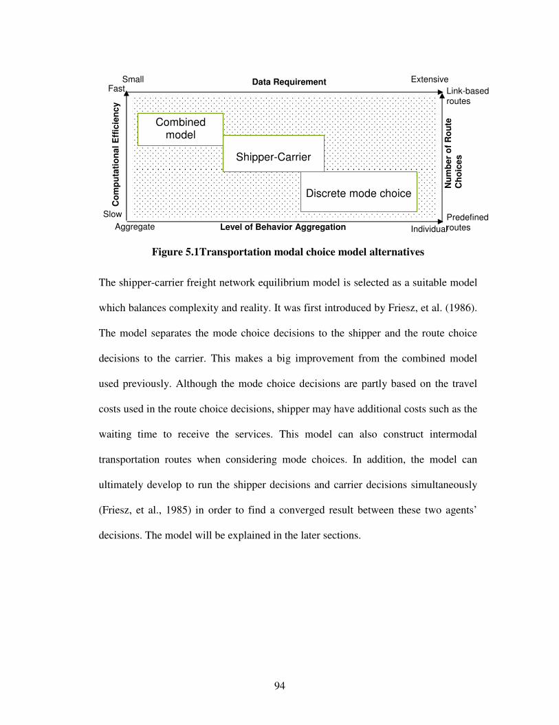
94

Figure 5.1Transportation modal choice model alternatives

The shipper-carrier freight network equilibrium model is selected as a suitable model

which balances complexity and reality. It was first introduced by Friesz, et al. (1986).

The model separates the mode choice decisions to the shipper and the route choice

decisions to the carrier. This makes a big improvement from the combined model

used previously. Although the mode choice decisions are partly based on the travel

costs used in the route choice decisions, shipper may have additional costs such as the

waiting time to receive the services. This model can also construct intermodal

transportation routes when considering mode choices. In addition, the model can

ultimately develop to run the shipper decisions and carrier decisions simultaneously

(Friesz, et al., 1985) in order to find a converged result between these two agents’

decisions. The model will be explained in the later sections.

Combined model

Shipper-Carrier

Discrete mode choice

Level of Behavior Aggregation Individual Aggregate

Co

mp

uta

tio

na

l E

ffic

ien

cy

Fast

Slow

Data Requirement Extensive Small

Nu

mb

er

of

Ro

ute

Ch

oic

es

Link-based routes

Predefined routes

95

5.1.2 Capacitated link constraints

In freight network design, relative to that of urban passenger networks, larger

networks must be considered. These networks therefore require more aggregation

and longer trips. Although infrastructure improvements can improve traffic conditions

or other problems, the results of the improvements will be seen as average cost saving

at small points on the network. In order to develop a network design model that can

capture their importance, capacity constraints are introduced in the lower level

problem.

The capacity constraints limit traffic volume on specific links. These capacities can

represent many barriers occurring in transportation networks. In this chapter, the

capacity constraints are used to capture reliability. Although the decisions to select

route choices depends more heavily on network reliability than travel costs, this

reliability cannot be captured by the static traffic assignment models which are

typically used for the strategic planning purposes. The infrastructure improvements

can increase network reliability and these results should be perceived by the network

design model. In the case of highway links, the capacity can be obtained from the

highway capacity manual. It can be a certain traffic volume that results in desired

average speeds. For intermodal facilities, information about freight volumes can help

a shipper to decide which service to use. The capacity can represent limits onnegative

externalities for certain areas or limits on road usage for maintenance or other

purposes.

96

5.1.3 The solution algorithm by branch and bound techniques

A branch and bound technique is introduced to solve two problems that occur in the

feedback process used in the first model. The first problem is the possibility of facing

an infinite loop in the solution process and the second is the preference to expand

high traffic volume links while leaving others undeveloped. Instead of selecting

which projects should be implemented based on the traffic volume obtained by the

lower level model, the branch and bound technique uses the lower level model to

produce the lower bound and decides whether to keep or discard the improvement

alternatives. The branch and bound process and the lower bound calculation will be

discussed in the later sections.

5.2 THE SHIPPER-CARRIER MODEL DESCRIPTIONS

The model is based on the bi-level concept as the previous model. Figure 5.2

illustrates the model setup. The upper level model is the budget allocation model. The

proposed project improvements and the freight demand are assumed to be given. The

upper model will suggest a subset of the project improvements to be examined by the

lower level model. Since the branch and bound technique is used in this model, the

lower level will calculate the lower bound of system efficiency that can be

accomplished by the suggested projects. This information will be used by the upper

model to recognize subsets that cannot achieve the best network design and suggest

the next subset to the lower model. The cost function for each link is set based on the

project selected for the link.

97

Figure 5.2 The shipper-carrier network design model

In this section, we explain the lower level model which applies the shipper-carrier

freight network equilibrium model to represent the freight route choice behaviors.

The branch and bound technique and its lower bound will be discussed in the solution

algorithm section.

5.2.1 The shipper and carrier model

The shipper-carrier freight flow prediction model is introduced in Friesz, et al.

(1986).The model develops the traffic assignments on two networks namely, the

Predicted O-D travel demand

The Shipper Model

The Carrier Model

Freight traffic volume on

the transportation links

Update travel costs using the shortest path costs

O-D Service Demand (Travel Choices)

Network Improvements

The Budget Allocation Model

The Upper Level Model

The Lower Level Model

Cal

cula

te L

ow

er B

ou

nd

Feedback Process

Given Data

98

shipper network and the carrier network. The shippers decide transportation mode

choices or service choices provided by the carriers. It is assumed that the shippers

have limited freight routing information. Therefore, their information is represented

by the service network which provides only service information between each origin

and destination such as average travel costs rather than information on specific

transportation infrastructure and traffic conditions. The carriers on the other hand,

have this detailed network information. They use this information to route vehicles in

responding to the service demand given by the shippers.

5.2.1.1 The shipper model

The shipper model selects transportation modes for freight demands from each origin

to each destination. The shipper model routes freight demand from one business

district to another while minimizing travel costs on the service network. The shippers

are assumed to be non-cooperative users. Therefore the traffic volume will result in

the user equilibrium. The output of the shipper model is the freight demands

classified by different services or transportation modes. These classified freight

demands will be referred to as the service demands from this point on.

The details to set up the shipper or service network are as follows. The shipper

network contains transportation services on all available modes. The transport

demands are assumed to originate in and are destined for central business districts

(CBDs) which are represented as centroid nodes. In order to add intermodal

transportation into the model, the intermodal facilities are included as intermediate

nodes in the shipper network. Because of the assumption that the shipper has limited

99

information on detailed route choices, the available transportation services are

represented as directed links between the districts and intermodal facilities. The costs,

capacities and other characteristics of the links are average values or shipper

perceived values.

5.2.1.2 The carrier model

The carrier model receives the service demand data from the shipper model and

routes these demands to the physical transportation network. This network includes

intermediate nodes which represent intersections, ramp locations, and different

geometric designs. In practice, the centroids are connected to the transportation

network through centroid connectors.

The origin-destination travel demand matrix of the carrier model is larger than the

shipper’s one. In addition to the business centers as the origins and destinations of

service demands, the intermodal facilities are added as the origins and destinations on

the carrier network. These service demands are created by the shippers who decide to

move commodities by intermodal services. The decisions are previously made by the

shipper model.

The service demands are assigned separately for each transportation mode. The

carrier behaviors differ by transportation modes. On the highway, carriers who

provide trucking services are non-cooperative optimizers resulting in user optimal

conditions. In the rail service, it is assumed that the carrier who provides train

100

services routes their vehicles on their own network. Therefore, the system optimal

condition will result if their rail networks are used exclusively.

5.2.2 Appling the shipper-carrier model to the network design problem: A key

assumption

Current freight flow prediction models assume that the transportation network is

given. In the other words, it assumes short term predictions. The network design

model is in the other way since it updates the network. In order to use the shipper-

carrier freight network equilibrium model, an assumptions is made that service

capacity will grow proportionally to the freight demand.

When there is an improvement, the update can be done easily for the physical

network but it is difficult for the service network. For the carrier’s network, an

improvement on a transport link will change its physical characteristics directly

which may result in increasing capacity or free-flow speed. On the other hand, a

service link in the shipper network is a virtual link. It represents paths from an origin

to a destination, therefore it consists of many physical links from the carrier network.

A shortest path algorithm is performed on the carrier network in order to update the

path costs.

Regarding to the capacity of the service network, the capacity of each service link is

not directly controlled by the transportation infrastructure. The capacity is

aggregately controlled by many carriers who provide services. Therefore, a change in

the link’s service capacity is hard to predict. There are two possibilities to consider

101

the capacity of service links in the long term. First, the aggregated level of service

links make an assumption that service capacity will grow proportionally to the freight

demand. If the freight demands increase, it is possible that carriers will increase

frequency or truck sizes to maintain the same level of service for the shipper. In a

special case in which a few major projects are implemented resulting significant

changes in service availability, the new service network data should be studied with a

specific model and is assumed to be provided to the network design model. The other

convenient assumption is to postulate that the carrier is perfectly and dynamically

able to handle new demands and that therefore the level of service can be assumed to

be fixed. In the other words, there is no capacity constraint on the service links. We

consider the first assumption more realistic to adopt into the network design model.

An exception to update the capacity on the service network is improvements on

intermodal facilities, ports, or terminals. These facilities’ capacities are directly

influenced by the improvements therefore it is reasonable to assume that the

capacities can be updated directly.

5.3 MODEL FORMULATION AND SOLUTION ALGORITHMS

Figure 5.2 illustrates how the freight network design problem is modeled by

combining the budget allocation model and the shipper-carrier models. In this section,

the model is formulated in mathematical forms. The following variables will be used

in the model:

102

Subscripts

l for the shipper network- a link in a transportation service network

for the carrier network - a link in a physical transportation network

m freight commodity

p project that is selected to implement for the link

k travel path

Superscripts

o origin of the freight demand

d destination of the freight demand

Variables

mlpV freight volume of commodity m for link l when project p is selected

= service demand if l belongs to shipper model

= traffic volume if l belongs to carrier model

)(VCmlp unit cost function for commodity m to use link l when project p is

selected. The unit cost is an average unit cost when calculating the

user equilibrium traffic flow and is a marginal unit cost when

calculating the system optimized traffic flow.

odmkf , freight volume of commodity m for path k from an origin o to a

destination d

odmq freight demand of commodity m from an origin o to a destination d

103

lu capacity of link l

odkl ,δ link-path incidence matrix, equal to 1 if link l belongs to traveling

path k from an origin o to a destination d

lpX the binary decision variable, equal to 1 if the project p for link l is

implemented and equal to 0 otherwise

lpF cost to implement project p for link l

B total available budget

5.3.1 The Upper Level Model–Budget Allocation Model

The upper level model for the freight network design is as follows:

lpmlp

m p

mlpX

XVCMINlp

∑∑∑ l

(5.1)

subject to

BXF lplp ≤∑∑l p

(5.2)

lforX lp all 1p

=∑ (5.3)

The model is an integer optimization model with lpX as a 0-1 decision variable. mlpC

and mlpV are controlled by the lower level model. In our research, we apply a branch

and bound algorithm which is convenient since it naturally consists of two major

104

steps -- constructing a binary search tree to enumerate all possible solutions and

bounding or cutting the nodes that cannot produce the optimal solution.

The nodes in a binary search tree are either partial solution nodes or complete

solution nodes. Assume that there are P projects proposed to improve the network, the

complete binary tree will have 2P+1-1 nodes with 2P complete solution nodes at the

final depth. Each node contains P decision variables. Each project has a fixed position

ranging from 1 to P. If a project is selected to implement, the decision variable at its

corresponding position is set to one or zero for otherwise. At the root of the tree, the

node is a partial solution node which has no fixed decision variables meaning that the

variables are free to set to zero or one. For each depth of the tree, a decision variable

will be fixed in the order from the first project to the last one. The complete solutions

are at the final depth with all decision variables have fixed values. The branch and

bound algorithm is used to cut out the nodes that loss potential to develop to the

complete solutions that optimize the objective function instead of examining the

complete tree. Figure 5.3 shows the complete tree solution when P = 3. It should be

noted that the branch and bound algorithm will not examine all nodes.

105

Figure 5.3 A searching binary tree (P = 3)

For the network design with the formulation as in (5.1), the branch and bound

algorithm is constructed as follows:

Step 0 Initialization: All decision variables at the root node will be set to zero with

no fixed variables. The node is an unvisited node. The incumbent value, which is the

best objective value that the search tree has found so far, is set to infinity or a high

value by default. One way to obtain the initial incumbent value is to simply select

network improvement projects until the budget limit is reached. Then, continue to

Step 1.

Step 1 Node Selection: Select an unvisited node. A node in the deepest level is

selected, therefore the branch and bound will do a depth first search. The depth first

0 0 0

0 0 0 1 0 0

0 0 0 0 1 0 1 0 0 1 1 0

0 0 0 0 0 1 0 1 0 0 1 1 1 1 0 1 1 11 0 0 1 0 1

1 2 3 p =

depth = 0

depth = 1

Fixed decision Unfixed decision

106

search can be beneficial if an initial incumbent value is difficult to find. Then,

continue to Step 2.

Step 2 Check Budget Constraints: For the selected node, the budget constraint is

checked. The summation of the capital costs for the selected projects must be less

than the budget limit. Return to Step 1 if the constraint is violated and set this node as

visited (not to be explored further), otherwise continue to Step 3.

Step 3 Check for the Completed Solution: Assume that the tree depth is equal to zero

at the root. Go to Step 4.1 if the node does not have the tree depth equal to P, when

there are P projects proposed for the network. Otherwise, go to Step 4.2 with the node

that has the complete solution.

Step 4 Call the lower level model:

Step 4.1: Calculate the lower bound using the lower level model. Go to Step

5.1.

Step 4.2: Calculate the objective value of the updated network. The update is

done by replacing the cost coefficients on the links which receive the improvements.

The traffic volume used to calculate the objective value is obtained by calling the

lower level model. Go to Step 5.2.

107

Step 5 Compare the value with the incumbent value:

Step 5.1 Pruning Decision: Go to Step 6, if the lower bound of the selected

node is less than the incumbent value. Otherwise, its child nodes cannot produce the

optimal solution. The node will be fathomed and marked as a visited node. Go to Step

7.

Step 5.2 Setting the New Incumbent Value: If the selected node has the

objective value less than the incumbent value, a new incumbent value and a new

current best solution are set. Otherwise, these remain the same. Set the selected node

as a visited node. Go to Step 7.

Step 6 Branching: the selected node will give two child nodes with the tree depth

increasing by 1. If the selected node depth equals to h, the child nodes will have the

tree depths equal to h+1. To enumerate the solution, the improvement project at

position h+1 will be fixed to zero for the left child node and to one for another. Set

the selected node as a visited node. Go to Step 1.

Step 7 Stopping Criteria: The algorithm stops when all nodes are visited. The current

incumbent solution will contain the transportation network which optimizes the

objective value.

5.3.1.1 Lower Bound Calculation

A lower bound is calculated for a node that has a partial solution. The process to

calculate the lower bound has two steps -- updating the network and calculating the

108

lower bound for the updated network. The original idea to apply the branch and

bound approach and calculating the lower bound is from Leblanc (1975).

In order to update the network, the currently undecided projects are assumed to be

implemented. For the selected node at depth h, the first h decision variables are fixed

as they appear but the other decision variable from h+1 to the last project are set to

one. For example, the root node has no fixed decisions therefore all nodes are set to

one. The network is then updated by modifying the cost coefficients of the links if

they receive the improvements.

In order to calculate the objective value of the upper level model, the traffic volume

corresponding to the new network has to be obtained. This can be done by using the

lower level model with the updated network. Substitution of the freight volume to the

network design objective function yields the lower bound.

It should be noted that different route choice behaviors will result in different lower

bounds. The tightest lower bound can be calculated by using the lower level model to

predict flow directly. However, this method cannot identify the occurrence of Braess’

Paradox since the upper level objective function and the lower objective function are

different. In the passenger network, Leblanc (1975)shows that using the system

optimal flow to calculate the lower bound can identify the paradox. For our model

which uses the shipper-carrier model, this lower bound can be obtained by ignoring

the shipper network model and calculating the route choice solely based on the carrier

109

decisions. In the other words, the lower bound will be calculated by only the system

optimal traffic assignment on the carrier network.

5.3.2 Lower model formulation- network equilibrium models

The traffic assignment for shipper-carrier freight flow prediction models can be

solved using sequential Friesz, et al. (1986) or simultaneous (Friesz, et al., 1985 and

Fernandez, et al., 2003) models. In this research, a sequential model is used. It is

assumed that there are no link interactions -- meaning that the traffic volume in a link

will not have an effect on other links. The passenger movements can be preloaded to

the highway network in order to represent the real congestion which is a combination

of both passenger and truck traffic volumes. In the case of multiple commodities,

each commodity will be assigned sequentially according to its priority.

Therefore, the generalized mathematical model for each network and each

commodity can be written by applying the Beckman’s Formulation.

MINl

∑ Cmlp0

Vmlp

∫ w( ) dw (5.4)

subject to

fk,m

od

k

∑ = qm

od ∀ o,d (5.5)

fk,m

od ≥ 0 ∀ k,o,d (5.6)

Vmlp ≤ ul∀ l (5.7)

Vmlp = fk,m

od

k

∑d

∑o

∑ δ lk

od ∀ l (5.8)

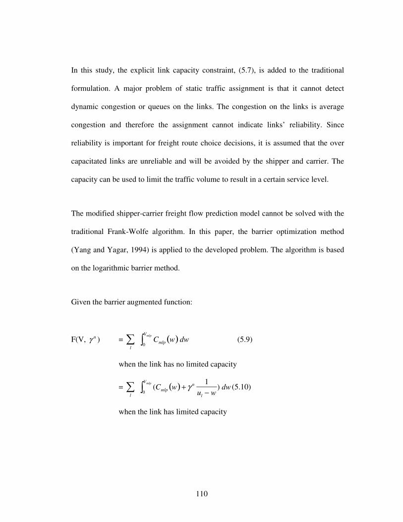
110

In this study, the explicit link capacity constraint, (5.7), is added to the traditional

formulation. A major problem of static traffic assignment is that it cannot detect

dynamic congestion or queues on the links. The congestion on the links is average

congestion and therefore the assignment cannot indicate links’ reliability. Since

reliability is important for freight route choice decisions, it is assumed that the over

capacitated links are unreliable and will be avoided by the shipper and carrier. The

capacity can be used to limit the traffic volume to result in a certain service level.

The modified shipper-carrier freight flow prediction model cannot be solved with the

traditional Frank-Wolfe algorithm. In this paper, the barrier optimization method

(Yang and Yagar, 1994) is applied to the developed problem. The algorithm is based

on the logarithmic barrier method.

Given the barrier augmented function:

F(V, nγ ) = l

∑ Cmlp0

Vmlp

∫ w( ) dw (5.9)

when the link has no limited capacity

= l

∑ (Cmlp0

Vmlp

∫ w( ) + γ n 1

ul − w) dw (5.10)

when the link has limited capacity

111

The algorithm steps are as follows:

Step 0 Choose a feasible solution, the vector of traffic volume V0. Set n = 1 (outer

loop counter)

While ( V0 is not converged) do

While (z is not converged) do

Step 1 Let z0= Vn-1. Set g = 1 (inner loop counter)

Step 2 Perform all-or-nothing assignment based on ( )g

lmlp zC for links that

have no capacity constraint and ( )g

lmlp zC + ( )g

lln zu −γ for links with the

capacity constraints. Let the link flow from this assignment is ly .

Step 3 Find *α to minimize F(zg + α (y-z

g), nγ ) in the range

−

−≤≤

< g

ll

g

ll

yz zy

zumin,1min0 α

Step 4 Move the volume ( )g

llg

l

g

l zyzz −+=+ *1 α for all link, l. g = g+1

End while

Step 5 ( )10.1 <<=+ σγσγ nn and n =n+1

End while

The barrier method always maintains a feasible solution. It is started with a feasible

solution with a high value of γ . The high gamma value prevents the solution from

violating the capacity constraints. For each γ , the Frank-Wolfe algorithm (Step 1 to

4) is performed. In Step 3, *α is limited to a certain range to guarantee that the next

112

solution is still a feasible solution. The γ value is lessened in the next iteration to

allow a solution which is closer to the capacity limit. In this study, )(VCmlp is assumed

to be a strictly increasing convex function. Therefore, the algorithm will converge

when 0→γ with a unique solution.

5.4 A NUMERICAL EXAMPLE

The numerical example in this paper consists of two networks, two modes, and a

single commodity. The first network is the shipper network consists of 4 origin-

destination (o-d) nodes, 2 intermodal transfer nodes and 16 transportation service

links. The intermodal facilities are represented by virtual links which have limited

capacities. Other service links can be used beyond their capacities but will cause more

congestion. The shipper considers costs from service waiting time and delivery price

which can be written as:

Shipper cost = VOT(WT0)(1+0.15

Capacity

Vmlp 4)+ β (DP)od (5.11)

Where VOT Value of Time for waiting for the services

WT0 Free flow waiting time

β Service preference factor

DPod Delivery price for a service connect an origin, o, and a destination, d.

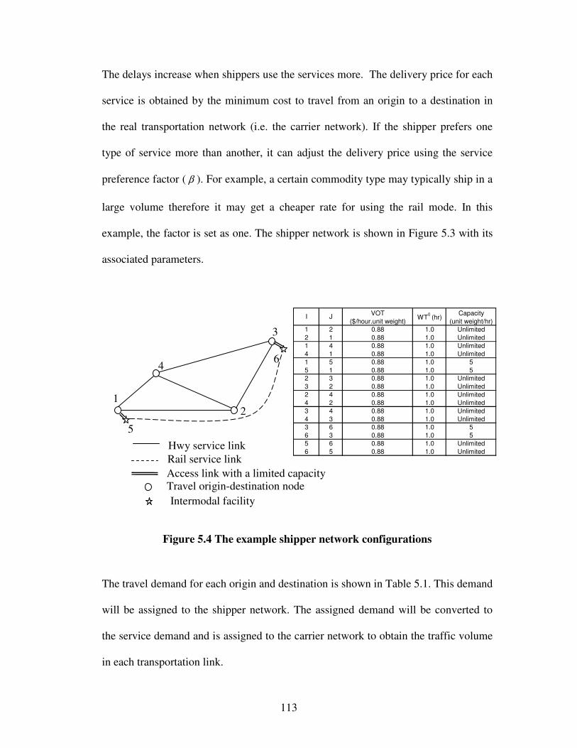
113

The delays increase when shippers use the services more. The delivery price for each

service is obtained by the minimum cost to travel from an origin to a destination in

the real transportation network (i.e. the carrier network). If the shipper prefers one

type of service more than another, it can adjust the delivery price using the service

preference factor ( β ). For example, a certain commodity type may typically ship in a

large volume therefore it may get a cheaper rate for using the rail mode. In this

example, the factor is set as one. The shipper network is shown in Figure 5.3 with its

associated parameters.

Figure 5.4 The example shipper network configurations

The travel demand for each origin and destination is shown in Table 5.1. This demand

will be assigned to the shipper network. The assigned demand will be converted to

the service demand and is assigned to the carrier network to obtain the traffic volume

in each transportation link.

1 2

3

4

5

6

Intermodal facility

Hwy service link

Rail service link

Access link with a limited capacity Travel origin-destination node

1 2 0.88 1.0 Unlimited

2 1 0.88 1.0 Unlimited

1 4 0.88 1.0 Unlimited

4 1 0.88 1.0 Unlimited

1 5 0.88 1.0 5

5 1 0.88 1.0 52 3 0.88 1.0 Unlimited

3 2 0.88 1.0 Unlimited

2 4 0.88 1.0 Unlimited

4 2 0.88 1.0 Unlimited

3 4 0.88 1.0 Unlimited

4 3 0.88 1.0 Unlimited3 6 0.88 1.0 5

6 3 0.88 1.0 5

5 6 0.88 1.0 Unlimited

6 5 0.88 1.0 Unlimited

Capacity

(unit weight/hr)I J

VOT

($/hour.unit weight)WT

0 (hr)

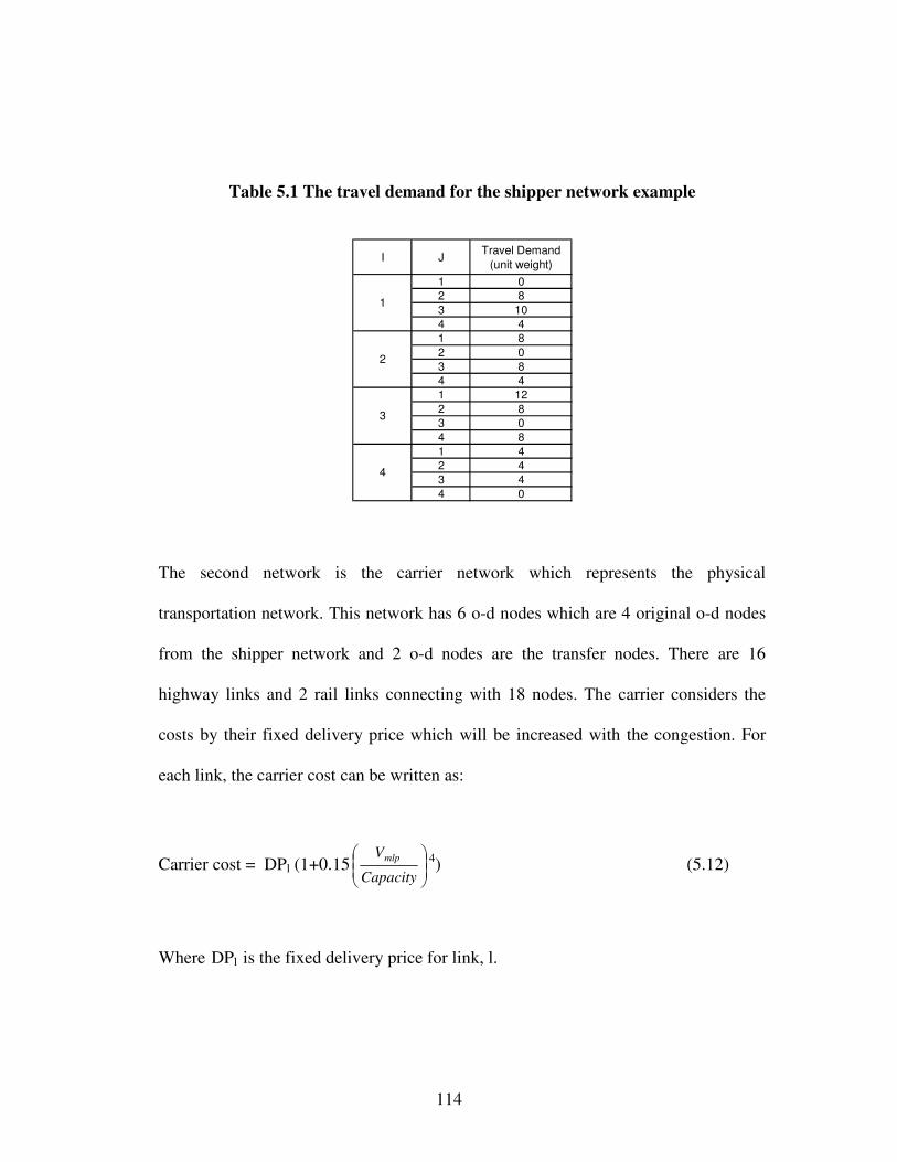
114

Table 5.1 The travel demand for the shipper network example

I JTravel Demand

(unit weight)

1 0

2 8

3 10

4 4

1 8

2 0

3 8

4 4

1 12

2 8

3 0

4 8

1 4

2 4

3 4

4 0

4

3

2

1

The second network is the carrier network which represents the physical

transportation network. This network has 6 o-d nodes which are 4 original o-d nodes

from the shipper network and 2 o-d nodes are the transfer nodes. There are 16

highway links and 2 rail links connecting with 18 nodes. The carrier considers the

costs by their fixed delivery price which will be increased with the congestion. For

each link, the carrier cost can be written as:

Carrier cost = DPl (1+0.15

Capacity

Vmlp 4) (5.12)

Where DPl is the fixed delivery price for link, l.

115

The carrier network has overlapping nodes from the shipper network. The network is

shown in Figure 5.4.

Figure 5.5 The example carrier network configurations

The objective function of the network design is to minimize the total travel cost on

the carrier network. The details of five projects proposed to improve the network are

shown in Table 5.2. Instead of setting the budget limit in monetary units, the budget is

set to a number of projects to implement. When a project is implemented, it is

counted as a unit. The lower model will be used to calculate the lower bound at each

search tree node. The results from the network design will be compared to the

traditional method which prioritizes each project separately by its benefit (the

difference between the total carrier cost prior to and after the project implementation).

An initial network will be set as the original network without any project

1 2

3

4

5

6

Intermodal facility

Physical hwy link

Railroad

Overlapped of the shipper network Travel origin-destination node

7 8

1 4 1.5 10

4 1 1.5 10

1 7 0.5 107 1 1 20

2 3 2.5 103 2 2.5 20

2 8 2.5 20

8 2 2.5 153 6 0.5 5

6 3 0.5 5

4 8 1.5 108 4 1.5 15

5 7 0.5 5

7 5 0.5 55 6 3 Unlimited

6 5 3 Unlimited7 8 1 10

8 7 1 10

I JDP

l

($/unit weight)

Capacity

(unit weight/hr)

Intermediate node

116

improvement. The depth first search method will be used in order to set a better

incumbent value as soon as possible.

Table 5.2 Details of the improvement projects

From To Existing Improved

1 Carrier-Hwy 2 3 10 15 532 79 Expansion of service capacity by 5

2 Carrier-Hwy 8 2 15 20 564 46 Expansion of service capacity by 5

Shipper 1 5 5 10 Expansion of the explicit capacity by 5

Shipper 5 1 5 10 Expansion of the explicit capacity by 5

Carrier-Hwy 5 7 5 10 Expansion of service capacity by 5

Carrier-Hwy 7 5 5 10 Expansion of service capacity by 5

Shipper 3 6 5 10 Expansion of the explicit capacity by 5

Shipper 6 3 5 10 Expansion of the explicit capacity by 5

Carrier-Hwy 3 6 5 10 Expansion of service capacity by 5

Carrier-Hwy 6 3 5 10 Expansion of service capacity by 5

5 Carrier-Rail 6 5 Unlimited Unlimited 600 11 Reduce the travel costfrom 3.0 to 2.8

* Cost when only a project is implemented. For example, implementing only project one give the total carrier cost = 532 unit money

** The difference betwwen the existing condition and Cost

Related Link CapacityCost* Benefit ** Improvement Note

16

19

595

5923

4

Project Related Network

5.4.1 Parameters of the Barrier-Traffic Assignment

The barrier optimization method has been applied to the Frank – Wolfe algorithm in

order to impose the capacity constraints to transportation links. There are two

additional parameters for this traffic assignment. The initial penalty, γ , and the step

size to reduce this penalty for each iteration, σ .

The parameter values affect the algorithm running time. If the initial penalty is too

high, the early iterations are pointless since the traffic volume will remain the same

until the penalties are reduced to a certain value. On the other hand, too low a penalty

will lead to the traffic volume that violates the capacity constraints. The initial penalty

for this network problem is equal to 3.0 by applying the empirical results.

The step size, σ , controls both running time and quality of the results. If the step size

is large, the running time will be fast but can lead to poor results. Figure 5.6 shows

117

the difference between the traffic volumes in a capacitated link with various step sizes

and the converged traffic volumes.

The traffic volumes traveling from node 3 to node 6 are considered. If the results have

converged, the link capacity will be used up and the difference will be equal to zero

percent. The results show that the barrier optimization method requires very fine step

sizes in order to converge to the correct values. The barrier optimization method has

a known problem that it will converge slowly at later iterations.

In order to solve this problem, a varied step size can be developed with larger steps to

begin with and then reduced step sizes at later iterations. For this example, the finest

step size, 0.001, is used.

Figure 5.6 Relationship between step sizes and the flow difference (%)

0

10

20

30

40

50

0.001 0.0012 0.0014 0.0016 0.0018 0.002Step Size

Dif

feren

ce (

%)

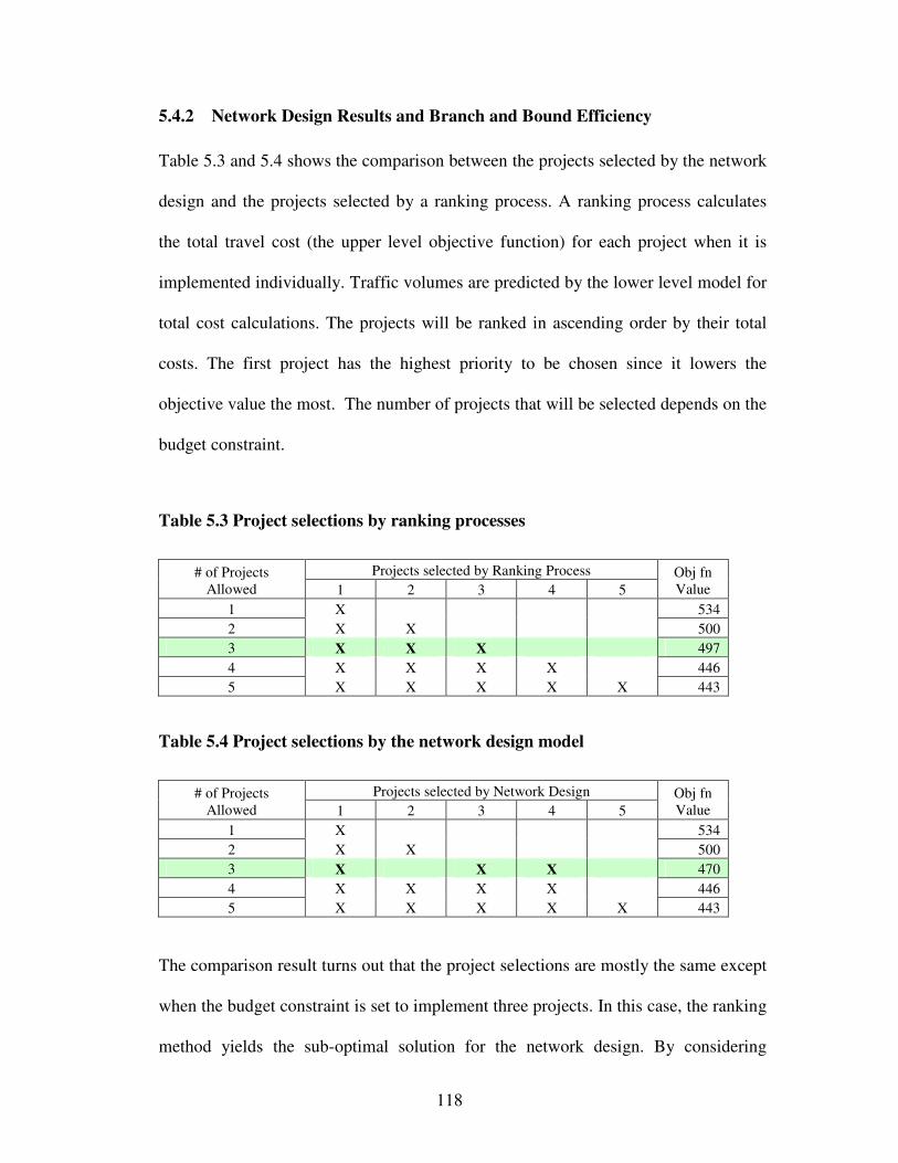
118

5.4.2 Network Design Results and Branch and Bound Efficiency

Table 5.3 and 5.4 shows the comparison between the projects selected by the network

design and the projects selected by a ranking process. A ranking process calculates

the total travel cost (the upper level objective function) for each project when it is

implemented individually. Traffic volumes are predicted by the lower level model for

total cost calculations. The projects will be ranked in ascending order by their total

costs. The first project has the highest priority to be chosen since it lowers the

objective value the most. The number of projects that will be selected depends on the

budget constraint.

Table 5.3 Project selections by ranking processes

Projects selected by Ranking Process # of Projects

Allowed 1 2 3 4 5

Obj fn Value

1 X 534

2 X X 500

3 X X X 497

4 X X X X 446

5 X X X X X 443

Table 5.4 Project selections by the network design model

Projects selected by Network Design # of Projects

Allowed 1 2 3 4 5

Obj fn Value

1 X 534

2 X X 500

3 X X X 470

4 X X X X 446

5 X X X X X 443

The comparison result turns out that the project selections are mostly the same except

when the budget constraint is set to implement three projects. In this case, the ranking

method yields the sub-optimal solution for the network design. By considering

119

projects in a case-by-case basis, the ranking method fails to capture the benefit of

combining projects 3 and 4 which will solve a bottleneck problem to access the rail

mode. It proposes to implement projects 1, 2, and 3 which give the total carrier cost

of 497.0 monetary units. In this small network, this problem can be anticipated by a

human. For larger networks however, with more explicit capacity constraints on the

links, the bottleneck problems can occur with more complicated situations, especially

when the intermodal transportation is considered. Our network design model can

detect these problems and gives the best solution for the network. It proposes to

implement projects 1, 3, and 4 which give the total carrier cost of 469.9 unit costs.

Table 5.5(a) and (b) show the link flows on the shipper and carrier networks for the

existing condition, the condition when implementing the projects proposed by the

ordering method, and the optimal condition given by the network design model.

Table 5.5The link flows for the existing networks and the improved networks

Cost Volume Cost Volume Cost Volume 1 2 12.4 15.4 11.2 15.1 11.3 14.4

2 1 12.0 15.7 12.0 15.7 10.7 12.9

1 4 3.9 4.7 3.9 4.7 3.9 6.9

4 1 3.9 4.3 3.9 4.2 3.9 4.8

1 5 3.4 2.9 3.3 3.1 3.5 4.4

5 1 2.6 5.0 2.5 5.0 2.7 10.0

2 3 9.8 15.4 6.7 15.1 6.1 14.4

3 2 6.5 15.7 6.5 15.7 6.1 12.9

2 4 10.2 4.0 10.2 4.0 9.5 4.0

4 2 10.8 4.0 9.7 4.0 9.8 4.0

3 4 15.8 7.3 15.8 7.3 14.8 5.1

4 3 19.3 3.7 14.9 3.8 14.6 3.2

3 6 1.5 5.0 1.6 5.0 1.6 10.0

6 3 1.4 2.9 1.4 3.1 1.4 4.4

5 6 3.9 2.9 3.9 3.1 3.9 4.4

6 5 3.9 5.0 3.9 5.0 3.9 10.0

Total Cost 1004.4 Total Cost 913.8 Total Cost 834.0

Existing Network Improvement 1* Improvement 2**I J

(a): The shipper network flows

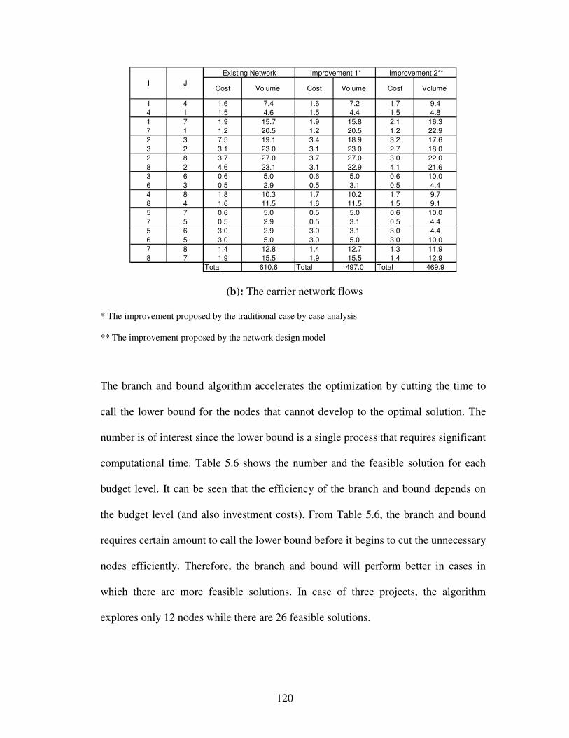
120

Cost Volume Cost Volume Cost Volume

1 4 1.6 7.4 1.6 7.2 1.7 9.4

4 1 1.5 4.6 1.5 4.4 1.5 4.8

1 7 1.9 15.7 1.9 15.8 2.1 16.3

7 1 1.2 20.5 1.2 20.5 1.2 22.9

2 3 7.5 19.1 3.4 18.9 3.2 17.6

3 2 3.1 23.0 3.1 23.0 2.7 18.0

2 8 3.7 27.0 3.7 27.0 3.0 22.0

8 2 4.6 23.1 3.1 22.9 4.1 21.6

3 6 0.6 5.0 0.6 5.0 0.6 10.0

6 3 0.5 2.9 0.5 3.1 0.5 4.4

4 8 1.8 10.3 1.7 10.2 1.7 9.7

8 4 1.6 11.5 1.6 11.5 1.5 9.1

5 7 0.6 5.0 0.5 5.0 0.6 10.0

7 5 0.5 2.9 0.5 3.1 0.5 4.4

5 6 3.0 2.9 3.0 3.1 3.0 4.4

6 5 3.0 5.0 3.0 5.0 3.0 10.0

7 8 1.4 12.8 1.4 12.7 1.3 11.9

8 7 1.9 15.5 1.9 15.5 1.4 12.9

Total 610.6 Total 497.0 Total 469.9

Existing Network Improvement 1* Improvement 2**

I J

(b): The carrier network flows

* The improvement proposed by the traditional case by case analysis

** The improvement proposed by the network design model

The branch and bound algorithm accelerates the optimization by cutting the time to

call the lower bound for the nodes that cannot develop to the optimal solution. The

number is of interest since the lower bound is a single process that requires significant

computational time. Table 5.6 shows the number and the feasible solution for each

budget level. It can be seen that the efficiency of the branch and bound depends on

the budget level (and also investment costs). From Table 5.6, the branch and bound

requires certain amount to call the lower bound before it begins to cut the unnecessary

nodes efficiently. Therefore, the branch and bound will perform better in cases in

which there are more feasible solutions. In case of three projects, the algorithm

explores only 12 nodes while there are 26 feasible solutions.

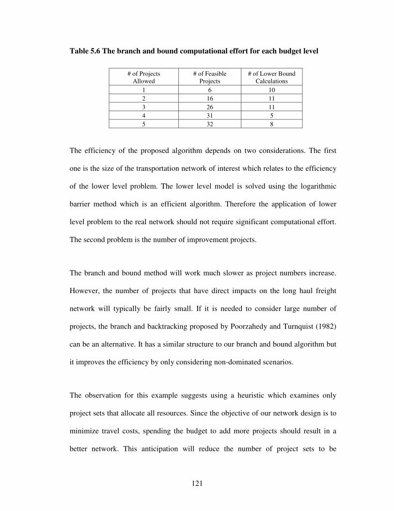
121

Table 5.6 The branch and bound computational effort for each budget level

# of Projects Allowed

# of Feasible Projects

# of Lower Bound Calculations

1 6 10

2 16 11

3 26 11

4 31 5

5 32 8

The efficiency of the proposed algorithm depends on two considerations. The first

one is the size of the transportation network of interest which relates to the efficiency

of the lower level problem. The lower level model is solved using the logarithmic

barrier method which is an efficient algorithm. Therefore the application of lower

level problem to the real network should not require significant computational effort.

The second problem is the number of improvement projects.

The branch and bound method will work much slower as project numbers increase.

However, the number of projects that have direct impacts on the long haul freight

network will typically be fairly small. If it is needed to consider large number of

projects, the branch and backtracking proposed by Poorzahedy and Turnquist (1982)

can be an alternative. It has a similar structure to our branch and bound algorithm but

it improves the efficiency by only considering non-dominated scenarios.

The observation for this example suggests using a heuristic which examines only

project sets that allocate all resources. Since the objective of our network design is to

minimize travel costs, spending the budget to add more projects should result in a

better network. This anticipation will reduce the number of project sets to be

122

examined dramatically. However, this heuristic has an assumption that there is no

Braess’ Paradox and all projects contribute positive effects to the objective value.

5.5 CONCLUSION AND FORWARD TO CHAPTER 6

In this chapter, a network design model for long haul freight movements is proposed.

A sequential shipper-carrier freight flow prediction model is used to represent the

freight movement behaviors. Additionally, an explicit link capacity constraint is

added to the traffic assignment in order to represent physical or psychological barriers

to using some transportation links. In this study, the capacity represents reliability. It

is assumed that the over capacitated links are unreliable and will be avoided by the

shipper and carrier. A branch and bound algorithm is used to search for the optimal

solution. In the next chapter, a case study for a larger network is implemented based

on the same concept.

123

CHAPTER 6 CASE STUDIES

6.1 INTRODUCTION

This paper expands the long haul freight network design model developed by

Apivatanagul and Regan (2008) (explained in Chapter 5) by conducting a case study

on the California transportation network. The primary objective is to apply our

network design model to a real transportation network and actual freight demand. The

case study is a validation step that can demonstrate that useful problems can be solved

with reasonable computational time.

Although the model concepts and the solution algorithm introduced are quite general,

some details are modified to fit the case study. The freight model developed by

Apivatanagul and Regan (2008) is explained first. The problem setting and the data

base development is then described, followed by the solution algorithm. The result is

the comparison of project selections made using the network design model and using

case by case evaluation. The final section presents our conclusions and future

research.

6.2 THE LONG HAUL FREIGHT NETWORK DESIGN MODEL

The main contribution of Apivatanagul and Regan (2008) is the application of the

shipper-carrier freight flow prediction model to reflect freight route choice behavior

124

and ultimately to design the optimal integrated network which combines multiple

dense local network areas together. The binding of the multiple network areas takes

place in the shipper or service network. The links in the shipper network are available

transportation services linking strategic transportation points including large cities,

rail stations, and ports together. Intermodal transportation is achieved through the

transfer links created to connect different modes. The input to the shipper network is

the freight demand between large cities. The output is the freight demand classified

by modes between cities and intermodal facilities. Each carrier network represents a

dense network area. It receives the shipper output, converts it into vehicle units and

routes it to the highway or railway networks. The network improvements on the

shipper network will result in mode shifts which are decided based on the origins and

destination demands over long distances. The network improvements on the carrier

network will aim to reduce travel delay and costs within narrower areas with

predetermined transportation modes.

A branch and bound algorithm is applied to our freight network design model. The

algorithm represents the upper level model by searching the best alternative within

budget constraints. It will occasionally call the freight flow prediction model (the

lower level model) to generate a lower bound to accelerate the search process. The

application of the branch and bound algorithm is described in the solution algorithm

section. The freight flow prediction model is more than an algorithm – it is also a

traffic assignment process. That process is described subsequently. Figure 6.1 shows

the process of interaction between the upper and lower levels.

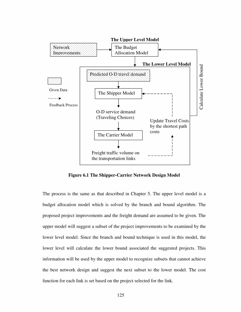
125

Figure 6.1 The Shipper-Carrier Network Design Model

The process is the same as that described in Chapter 5. The upper level model is a

budget allocation model which is solved by the branch and bound algorithm. The

proposed project improvements and the freight demand are assumed to be given. The

upper model will suggest a subset of the project improvements to be examined by the

lower level model. Since the branch and bound technique is used in this model, the

lower level will calculate the lower bound associated the suggested projects. This

information will be used by the upper model to recognize subsets that cannot achieve

the best network design and suggest the next subset to the lower model. The cost

function for each link is set based on the project selected for the link.

Predicted O-D travel demand

The Shipper Model

The Carrier Model

Freight traffic volume on

the transportation links

Update Travel Costs by the shortest path costs

O-D service demand (Traveling Choices)

Network Improvements

The Budget Allocation Model

The Upper Level Model

The Lower Level Model

Cal

cula

te L

ow

er B

ou

nd

Feedback Process

Given Data

126

The lower level consists of the shipper model and the carrier model. The shipper

model receives the freight demand and predicts its mode choices. The shipper model

assigns the freight demand into the network of available services that minimize total

costs. The service demand is used by the carrier model. The carrier model assigns the

service demand to the highway or railway network to obtain traffic volumes. The

lower bound is calculated by these traffic volumes and fed back to the upper level for

further searching. In the next section, we describe the freight model developed for the

California transportation network in more detail.

6.3 A CASE STUDY OF THE CALIFORNIA

TRANSPORTATION NETWORK DESIGN

6.3.1 Upper Level Model

A freight network design model is developed for the California transportation

network. The model uses the shipper-carrier network design concept. It can be used to

design a robust integrated network for the whole US. However, this case study will

only focus on the freight movements moving in and out of the state of California. The

transportation network is developed based on the National Transportation Atlas 2007

Database USDOT and BTS (2007). The freight demand data is based on the 2002

commodity flow survey (CFS) data USDOT and BTS (2005). We assume that the

base year is 2002 and the freight network will be designed for year 2022 with an

annual growth rate of 3.4% per year USDOT and BTS (2003).

127

We assume that the transportation agency seeks to reduce the highway congestion.

Therefore, highway travel time is the measure of social cost considered in the model.

The upper level can be formulated as in Equations (6.1) to (6.3)

lplp

l p

lpX

XVCMINlp

∑∑ (6.1)

subject to

BXF lplp ≤∑∑l p

(6.2)

lforX lp all 1p

=∑ (6.3)

where

lpV the truck volumes on the highway carrier link l when implement project p

)(VClp time to transverse link l when implement project p with the truck volumes lpV

lpX the binary decision variable, equal to 1 if the project p for link l is

implemented and equal to 0 otherwise

lpF cost to implement project p for link l

B total available budget

The objective function minimizes the total cost to use the network. In this case study,

this cost is total time for all trucks. The upper level varies project decisions to obtain

the minimum value. The truck traffic will change according to the improvement

project selected and is predicted by the lower level model. The projects must be

128

within the budget. Equation (6.3) indicates that if there are multiple project levels for

a link, only one level will be selected.

6.3.2 Lower Level Model: the Shipper Model

The lower level consists of the shipper and carrier networks. The shipper network has

the railway and highway networks. The shipper network is developed to connect 43

Combined Statistical Areas (CSAs), 18 Metropolitan Statistical Areas (MSAs), 33

remainder areas of the states (excluding areas that are CSAs or MSAs), and 4

maritime ports within California (Ports of San Francisco, Sacramento, Los Angles

and Long Beach). The freight demands (in tons) between the areas are obtained from

the CFS data except for those related to ports. In order to examine the finer freight

movements within California, the data is disaggregated to the ports and to three other

areas of California. Employment data is used to roughly disaggregate the data. Note

that this is a common approximation made in the absence of better demand estimation

information.

The data for this case study data was developed for the purpose of providing a “proof

of concept” test for our model. If the model results were intended for

implementation, much more effort and expense should be expended to develop the

best possible inputs (both the network and the demand data) for the model.

The links in the shipper network are service links which are the shortest paths that

connect all areas together. The highway network has the truck service links

connecting all area centroids together. The railway network has the rail service links

129

connecting all rail stations together. For each CSA or MSA, a virtual rail station is

located at the centroid of the actual rail stations within the area. A transfer link is

constructed between each area and its virtual rail station to allow for intermodal

transportation. Additionally, the rail service links have parallel links offered by

different companies. The transfer links between the rail services of different

companies are provided to account the transfer costs. Figure 6.2 (a) and (b) shows the

highway and railway shipper networks.

It is assumed that there is no congestion on the shipper network. Shippers also move a

single commodity type with a truck service or a rail service and pay an average cost

for each service. The average costs are estimated by the total revenue and total ton-

miles from USDOT, et al. (2008) and ATA (1995). The average costs in 2002

constant dollars are 8.54 cents/ton-mile and 2.26 cents/ton-mile for truck and rail

services, respectively. The transfer links between truck and rail services include

penalty costs to represent the extra costs and time need to transfer containers. The

links also have capacities in order to control excessive use of rail stations and local

access links.

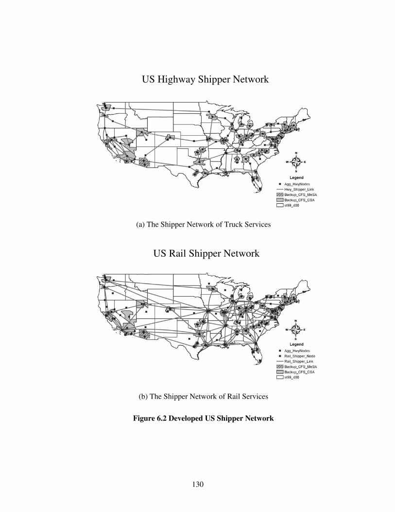
130

(a) The Shipper Network of Truck Services

(b) The Shipper Network of Rail Services

Figure 6.2 Developed US Shipper Network

US Highway Shipper Network

US Rail Shipper Network

131

As the discussion in Chapter 5, the link capacity is used to represent the infrastructure

limit due to many aspects that the static traffic assignment cannot capture. In the

shipper model, the cheapest transportation modes are logically selected mode.

However, many decision components that are combined to the total costs cannot

explicitly considered such as reliability and other preferences. These barriers from

unsatisfactory are set as capacity at the transport facilities including rail stations and

intermodal facilities. In this study, it is assumed that the major disadvantage of rail

mode and intermodal transportation happen at the provision activities when the

vehicles leaving and arriving stations which include many inconvenience such as

schedule, unreliability, and the poor assessment.

All or Nothing assignment with capacity control is used for the shipper model. The

algorithm will be explained later in the solution algorithm section. In order to set the

capacity, the freight demand is assigned to the shipper network with no usage limit at

the transfer links. The value at the 95 percentile for all link usage is set to be the

capacity. For this study, this it is estimated at 3540 tons/hour for rail stations in the

state. A single penalty value is set to 19.12 cents/ton which will yield the market

share in ton-miles between the two modes to 0.502:0.498 (rail:truck) in the whole US

corresponding to the ton-mile market share ratio estimated by the CFS data.

6.3.3 The Lower Level Model: the Carrier Model

The carrier receives the service demand from the shipper and routes their vehicles

corresponding to the demands while minimizing travel time. The service demand is

converted from ton units to truck units and then to passenger car units. The ton-truck

132

conversion factor estimated by USDOT, et al. (2008) data for the whole US is 5.03

tons/vehicle. However, this number is too small compared with the known market

price about of $1.78/mile for truckload transportation USDOT and FHWA (2000). If

the truck unit cost in ton-miles is assumed to be accurate, the carrier must load an

average of 21 tons/vehicle to sufficiently substitute for the market price per vehicle.

21 tons/vehicle is used for the ton-truck conversion. The pcu-truck factor is 1.5 based

on the latest Highway Capacity Manual (in flat terrain).

The transportation network for the carrier model represents the physical

transportation network within the state of California. NTAD assigns the highway

links that are used to do strategic planning. As shown in Figure 3, our case study

adopted the NTAD strategic network within California as the carrier network. The

centroids of CSAs, MSAs, ports, and the remainder areas connect to the highway

network thru the centroid connectors. The rail service links connect the rail stations

and the ports to represent the direct access. The service links have limit capacity but

do not contribute to congestion on the highway network. It is assumed that the

highway has congestion represented by the BPR functional forms. The capacity is

estimated from the average number of lanes. A lane is assumed to carry 2200

passenger car units/hour. In order to reach the destination on time or leaving the

congestion areas, the carriers minimize their travel times, resulting in a user

equilibrium condition in the study area.

133

Figure 6.3 Developed California Carrier Network

6.3.4 Improvement Projects and Locations

A set of improvement projects is a required input for the network design model. The

model will select the best subset of these according to the stated objective function.

Relationships between the proposed improvement actions and link performance are

very important. Until now, the primary measure of link performance was the BPR

function –the relationship between road expansion and traffic speed. Clearly there is a

need to study other measures related to transportation improvements.

CA Highway Carrier Network

134

In this case study, a set of improvement projects is designed to test whether our model

can capture various pitfalls undetected when each project is considered separately.

The network design model is expected to perform better budget allocation than

heuristically picking the projects at the top of ranking. Various improvements can be

tested on the network if they are related to travel costs in the shipper network or travel

time in the carrier network. Sixteen projects are predetermined by carefully

examining each link improvement and its benefit through the lower level model. All

highway links in the carrier network are tested. The best four projects measured by

the benefit cost ratio are selected for inclusion in our improvement proposal. The

benefit is measured by comparing the total travel time under existing conditions and

when a selected link receives an improvement. The improvement is a highway lane

expansion resulting in an additional capacity of 2,200 pcu per hour. The cost is

assumed to be a unit of monetary value. Four other projects are proposed for the same

selected links but with two lane expansion (4,400 pcu per hour improvements). There

are a total of eight highway improvement projects on the carrier network. Table 6.1

shows the information related to these projects.

The other eight projects are related to rail transportation. Four projects are related to

rail capacity expansions accessing ports. The rail capacity is estimated by railway

density between rail stations and ports. This information is obtained from the NTAD

database. The density is represented by annual million gross ton miles per mile

(MGTM/M) which is the standard measure provided by the Federal Railroad

Administration (FRA). The railway links accessing the ports of San Francisco and

135

Sacramento have densities of around 0.1 – 4.9 MGTM per mile or roughly a one way

traffic of six to 280 tons per hour.

136

Table 6.1Project Improvement Information

Project Cost Benefit B/C Ratio Truck Benefit Network Changes

1 1.40 11.08 7.91 7.39 Expand Highway Capacity from 8480 to 10680 pcu/hour

2 2.80 14.96 5.34 9.97 Expand Highway Capacity from 8480 to 12881 pcu/hour

3 15.12 83.05 5.49 55.37 Expand Highway Capacity from 8800 to 11000 pcu/hour

4 30.24 123.98 4.10 82.65 Expand Highway Capacity from 8800 to 13200 pcu/hour

5 10.85 47.23 4.35 31.49 Expand Highway Capacity from 8800 to 11000 pcu/hour

6 21.70 74.14 3.42 49.42 Expand Highway Capacity from 8800 to 13200 pcu/hour

7 5.25 22.71 4.33 15.14 Expand Highway Capacity from 11000 to 11000 pcu/hour

8 10.50 32.56 3.10 21.71 Expand Highway Capacity from 8800 to 13200 pcu/hour

9 5.56 25.04 4.50 16.69 Increase Port Access Capacity from 150 to 200 ton/hour

10 11.07 49.81 4.50 33.21 Increase Port Access Capacity from 200 to 250 ton/hour

11 0.70 3.85 5.50 2.57 Increase Port Access Capacity from 30 to 40 ton/hour

12 1.24 6.82 5.50 4.54 Increase Port Access Capacity from 30 to 50 ton/hour

13 3.29 - - - 15% rail price reduction (2.26 to 1.92 cent/ton-miles)

14 1.94 - - - 15% rail price reduction (2.26 to 1.92 cent/ton-miles)

15 1.94 - - - 15% rail price reduction (2.26 to 1.92 cent/ton-miles)

16 3.29 - - - 15% rail price reduction (2.26 to 1.92 cent/ton-miles)

* Existing Highway Capacity is the average capacity for the entire link length

137

The rail links accessing the ports of Los Angles and Long Beach are reported to have

densities around 40.0 -59.9 MGTM per mile. These densities are much higher than

the predicted service demand. In this case study, the port access links are set to

sufficiently handle the demand in year 2002 and the capacities correspond to the

reported density. The port access links are improved as shown in Table 6.1. In order

to create non-biased projects compared to the highway ones, the costs are set to have

benefit cost ratios within the same range as the highway projects.

The other four projects are improvements on the shipper rail links. These

improvements show the benefit of the shipper-carrier model which can capture the

mode shift resulting from improvements. The mode shift indirectly benefits the

highway network. A scenario which results in a poor outcome (a pitfall) is

constructed to test the network design model from these four improvements. The

model must know how to pair the projects to receive their benefits. Projects 13 and 16

together will give benefit of 30.7 truck-hours in a total travel time reduction. Projects

14 and 15 together will result 18.1 truck-hours in a total travel time reduction.

Implementing such rail improvements could be accomplished by investing in

improved technologies such as double stacked trains. Figure 6.4 (a) and (b) shows

the projects on the network.

138

(a) Summary Improvement Locations within California

Figure 6.4 Improvement Project Locations

4th Area Projects 1, 2, 9, 10

2ndArea Projects 11, 12

1st Area Projects 13,14,15,16

3rd Area Projects 3,4,5,6,7,8

139

(b) Enlarged Areas with Link Improvements

Figure 6.4Improvement Project Locations (cont.)

13

14

15

16 5,6

1st

7,8

3,4

11,12

9,10

1,2

3rd

2nd

4th

140

6.4 SOLUTION ALGORITHM

The solution algorithm for this case study is similar to the process explained in

Chapter 5 and is rewritten here for the completion of this chapter.

6.4.1 The upper level model: Branch and bound algorithm

The branch and bound algorithm is a conditional tree search. The nodes in a binary

search tree are either partial solution nodes or complete solution nodes. If we assume

that there are P projects proposed to improve the network, then the complete binary

tree will have 2P+1-1 nodes with 2P complete solution nodes at the final depth. Each

node contains P decision variables. Each project has a fixed position ranging from 1

to P. If a project is selected for implementation, the decision variable at its

corresponding position is set to one; otherwise it is set to zero. At the root of the tree,

the node is a partial solution node which has no fixed decision variables meaning that

the variables are free to set to zero or one. For each depth of the tree, a decision

variable will be fixed in the order from the first project to the last one. The complete

solutions are at the final depth with all decision variables having fixed values. The

branch and bound algorithm is used to cut out the nodes that lose potential to develop

the optimal solutions so that the complete tree need not be examined.

For the network design with the formulation as shown in Equations (6.1) to (6.3), the

branch and bound algorithm is constructed as follows:

141

Step 0 Initialization: All decision variables at the root node will be set to zero with

no fixed variables. The node is an unvisited node. The incumbent value, which is the

best objective value that the search tree has found so far, is set to infinity or a high

value by default. One way to obtain the initial incumbent value is to simply select

network improvement projects until the budget limit is reached. Go to Step 1.

Step 1 Node Selection: Select an unvisited node. A node in the deepest level is

selected, therefore the branch and bound will do a depth first search. The depth first

search can be beneficial if an initial incumbent value is difficult to find. Go to Step 2.

Step 2 Check Budget Constraints: For the selected node, the budget constraint is

checked. The summation of the capital costs for the projects which their

corresponding decision variables fixed must be less than the budget limit. If there are

multiple project levels for a link, we also check that only single project is

implemented. Return to Step 1 if either constraint is violated and set this node as

visited (not to be explored further), otherwise continue to Step 3.

Step 3 Check for the Completed Solution: Assume that the tree depth is equal to zero

at the root. Go to Step 4.1 if the node does not have the tree depth equal to P, when

there are P projects proposed for the network. Otherwise, go to Step 4.2 with the node

that has the complete solution.

142

Step 4 Call the lower level model:

Step 4.1: Calculate the lower bound using the lower level model. Go to Step

5.1.

Step 4.2: Calculate the objective value of the updated network. The update is

done by replacing the cost coefficients on the links which receive the improvements.

The traffic volume used to calculate the objective value is obtained by calling the

lower level model. Go to Step 5.2.

Step 5 Compare the value with the incumbent value:

Step 5.1 Pruning Decision: Go to Step 6, if the lower bound of the selected

node is less than the incumbent value. Otherwise it means that its child nodes cannot

produce the optimal solution. The node will be fathomed and marked as a visited

node. Go to Step 7.

Step 5.2 Setting the New Incumbent Value: If the selected node has the

objective value less than the incumbent value, a new incumbent value and a new

current best solution are set. Otherwise, these remain the same. Set the selected node

as a visited node. Go to Step 7.

Step 6 Branching: the selected node will give two child nodes with the tree depth

increasing by 1. If the selected node depth equals to h, the child nodes will have the

tree depths equal to h+1. To enumerate the solution, the improvement project at

position h+1 will be fixed to zero for the left child node and to one for another. Set

the selected node as a visited node. Go to Step 1.

143

Step 7 Stopping Criteria: The algorithm stops when all nodes are visited. The current

incumbent solution will contain the transportation network which optimizes the

objective value.

A lower bound is used as criteria to decide whether a node will be explored further.

The lower bound is the lowest total cost (truck travel time) that corresponds to the

selected partial solution. Assume that currently undecided projects will be

implemented and assign freight flows to the network. The truck volumes on the

carrier network are used to calculate the total travel time lower bound. Different route

choice behaviors will result in different lower bounds. The tightest lower bound can

be calculated by using the lower level model to predict flow directly. Leblanc (1975)

shows that the user equilibrium behavior can cause the Braess’ Paradox -- meaning

that implementing improvement projects can lead to worse traffic condition. In order

to calculate the lower bound without the paradox problem, Leblanc (1975) uses the

system optimal behavior instead. We adopt that approach to calculate our lower

bound.

6.4.2 The lower level model: The Shipper-Carrier Freight Flow Prediction

Model

The lower level model is a traffic assignment process. As shown in Figure 6.1, the

shipper model receives the freight demand and performs its traffic assignment to yield

the service demand. In our shipper network, it is assumed that there is no congestion

but there are capacity limits for access to rail services. Its traffic assignment is the

144

incremental all or nothing assignment avoiding overflow link capacities. The demand

is partitioned into smaller parts. The smaller freight volumes allow the demands that

travel from different origins and destinations to share the available capacity equitably.

In the beginning, the truck-rail transfer links will have full capacity. When the flow is

assigned to the link the capacity is reduced. This reduced capacity is called the

reserve capacity.

The demands are assigned to their shortest paths using the following steps.

Step 1 Calculate the Path Capacity : For each pair of an origin and a destiantion,

calculate the capacity of its shortest path. The capacity is equal to the least reserve

capacity of all links constructing the path.

Step 2 Assign the Demand Volume : Compare the demand volume with the path

capacity. If the volume is less than the path capacity, assign all the volume. If the

volume is more than the path capacity, assign the volume equal to the path capacity.

Step 3 Update the Reserve Capacity : All reserve capacities are updated by minus the

current reserve capacities and the assigned flow. If a reserve capacity is equal to zero,

update its link cost to infinity value to prevent the future use.

Step 4 Prepare the Demand Volume : If all demand cannot be assigned, the remaining

demand will be added to the demand considered in the next assignment iteration.

145

When the all or nothing assignments are implemented for all demands, the remaining

demand is assgined to the truck services which do not have capacity limits.

The carrier model receives the service demand from the shipper model output,

converts this to passenger car units and assigns it under the user equilibrium

assumption. The assignment can be written using the Beckman Formulation and

solved by the Frank-Wolfe algorithm. Ideally, the passenger demand should also be

assigned to the highway network since passengers share the highway capacity with

trucks. In this case study, the model is simplified by preloading the highway links

with their annual average daily traffic. For the rail freight volumes that connect to

ports, the volumes can use rail links directly to access ports according to predefined

link capacities. These freight volumes are deducted before assigning the demand to

the highway network.

6.5 RESULTS

In order to validate that our network design model can be applied to real applications,

its results and computational time must be examined. If an hourly average demand is

considered, the existing network condition gives the total travel time of 5273 truck-

hours. The improvements reduce this total travel time.

The results are compared with the project selections when a ranking method is used.

The ranking method sorts the projects from the highest benefit to the lowest and then

selects projects until the budget is expended. The budget is 44.0 monetary units – for

146

the purposes of this study this represents 50% of the cost of all candidate projects. As

shown in Table 6.1, if the projects are sorted by their benefits, Projects 1, 4, 10 and 12

would be selected. The total travel time gained from these projects is 5149 truck-

hours. If the projects are sorted by their benefit-cost ratios, Projects 1, 3, 5, 10, 12 will

be selected and give the total travel time of 5145 truck-hours. We raise a hypothetical

case in which in order to realize the full benefits of projects 13, 16 and 17, they

should be implemented together. We further assume that the decision maker using

the ranking method understands this situation. In that case, the ranking by benefit-

cost ratio will select Projects 1, 3, 10, and 12-16 which gives a network benefit of

5127 truck-hours. In order to initialize the network design model, projects selected by

the ranking by benefits is used to obtain the initial incumbent solution. The network

design model then selects Projects 1, 3, 5, 7, 11, and 13-16 with a benefit of 5112

truck-hours. These results show that our model can more effectively allocate the

budget more than the ranking method.

Budget sensitivity is tested using budgets set at 40 % and 60% of the total potential

investment cost. The results are Projects 2, 3, 7, and 12-16 (5139 truck-hours savings)

and Projects 3, 5, 7, 10, and 12-16 (5089 truck-hours savings) for the 40% and 60%

budgets respectively. The common selected projects are Projects 3, 7, and 12-16. The

running times are 1252, 1164, and 1137 seconds for 40%, 50%, and 60% budgets

respectively (performed using an Intel Pentium 1.60GHz machine with 512 MB of

RAM). The branch and bound algorithm creates 1014, 1163, and 920 search nodes for

the 40%, 50%, and 60% budgets. It calls the lower level model 512, 473, and 465

times, representing approximately half of the search tree each time. These results

147

should be compared with the total possibility to construct the scenarios for 16

projects. If the 16 projects are independent, the possibility is 65536 scenarios.

However, 12 of our projects are dependent (expansion levels 1 and 2), therefore the

possibility is 11664 scenarios. The comparisons show that the branch and bound

algorithm is able to efficiently search for the best solutions.

The next question is the maximum number of independent projects that the algorithm

can practically handle. While we could examine this question empirically by

iteratively adding additional projects, we can also estimate that each additional

project should double the required computational time. However, we believe that

effective engineers/planners could identify good initial solutions that would reduce

the size of the search tree significantly. That said, if we assume that a practical time

frame to run a strategic planning program is 24 hours and that in our case study, ten

independent projects are input into the network design model with an approximate

running time of 20 minutes. We estimate that the maximum manageable number of

independent projects (without expert understanding) is16. This number is sufficient

for a budget allocation for competitive projects for a strategic network within a state.

However, if much larger sets are to be examined – a heuristic partitioning scheme can

be used to discretize the network into smaller sub-regions and then the partitioned

solutions can be combined.

148

6.6 CHAPTER CONCLUSION

In this chapter, a network design model for long haul freight movements are

constructed based on that proposed earlier by Apivatanagul and Regan (2008)

described in Section 6.4. The relationship between shippers and carriers are

represented in the lower level model which is used to predict the traffic volume on the

highway or railway networks. The shipper model selects the transportation services

and the carrier model routes vehicles based on this demand. The lower level model

will interact with transportation improvements either through route changes or mode

shifts. A branch and bound algorithm is used to search for the best set of

improvement projects. A case study to improve the California highway network is

implemented.

Using public databases, the shipper and carrier networks are constructed. A simple

calibration is implemented by setting penalty costs at transfer links. The penalty costs

provide the shipper network which has a realistic market share between truck and rail

services. Additionally, the link capacity limits are introduced as a means to control

unrealistic use of specific facilities. The traffic assignment approaches and the branch

and bound algorithm applied to our model are explained.

A comparison between the ranking method and the network design model is

performed. Many criteria are used to select the projects with the ranking method,

however the network design model appears to give the best answers. The result shows

that the network design model can be used to efficiently allocate the budget.

149

Additionally, the model can capture effects of competition, substitution and synergy.

The branch and bound approach works well to reduce the search time. However, the

integer optimization efficiency will deteriorate fast with additional integer variables.

We estimated that our model can easily handle up to 16 independent projects without

resorting to project specific expert knowledge which could produce a good initial

incumbent solution. If transportation agencies need to explore more projects, expert

knowledge or a heuristic approach should be performed.

In conclusion, this chapter provides evidence that the long haul freight network

design model described can be implemented for real world applications. Existing

public databases are sufficient to develop introductory shipper and carrier networks.

The solution algorithm proposed works reasonably well.

150

CHAPTER 7 CONCLUSION AND FUTURE

RESEARCH

7.1 SUMMARY

In this dissertation, freight network design models are developed. The model

frameworks are developed considering the special nature of freight movements. The

bi-level approach is used to formulate the mathematical models for this network

design problem in order to represent different behaviors and their interactions

between transportation agencies and network users.

Chapter 1 clarifies the problem statement, the goal, and tasks. The increasing freight

demand, budget limit, and complexity to improve a transportation network leads to a

necessity to develop a freight network design model. The goal is to formulate the best

practice of the freight network design models by three main tasks. The first task is to

develop the framework while the second task is to consider the freight route choice

behaviors for the model. The final task is to develop a corresponding solution

algorithm.

Chapter 2 reviews research papers and reports related to network design, freight flow

prediction models, network design solution algorithms, and current practices on

freight studies. The chapter provides the comparison among many network design

151

models which are applied for different studies. It reviews number of solution

algorithms that are used in different modeling situations. The limitation of current

freight studies reviewed in the chapter also provides evidence of the need of the

network design development.

Chapter 3 provides the background and the directions for our network design model

and expected future research. The chapter begins with a discussion of the

transportation network characteristics. A network can be considered as a regional

network and an inter-regional network. A regional network considers the movements

within a study area while an inter-regional network connects study areas together.

The transportation modes for long-haul freight movements are decided based on the

travel costs in the inter-regional network. However, the regional network also has a

significant role on the decisions since unreliable services near origins and destinations

can prevent users to select particular transportation modes. Later in the chapter, it

discusses the general concept of the bi-level network design frameworks and

broadened in order to embrace a wider variety of measures and points of view.

Various network design models are formulated based on previous research.

Chapter 4 focuses on freight network design for long haul movements traveling

between geographic regions. The chapter discusses possible analysis tools for the

freight planning problem and suggests improving the local network information in the

traditional four step model through centroid connectors. Simulation models can be

used to substitute data needed for this improvement. The integrated network

importance, which is a concept to consider both regional and inter-regional networks,

152

is emphasized. The integrated network should maintain competition between modes

therefore movements are allowed to travel into and out of the studying area through

the use of external nodes. A discussion for necessary components to develop the

freight network design is presented. A network design for an inter-regional freight

movement is formulated. An example is given and solved by an iterative process

between the upper and lower level model. The example shows the importance to

develop a network design with the integrated network concept. It also suggests

improving the solution algorithm.

Chapter 5 improves the freight network design by introducing a shipper-carrier

freight flow prediction model into the lower level problem. The shipper-carrier model

is considered to be a compromised approach to combine mode choice decision to the

network design model. A branch and bound algorithm is applied to solve the problem.

Additionally, certain links are controlled by capacity constraints in order to represent

unreliability resulting from congestion. An example is given and solved by the branch

and bound algorithm. The project selections from network design models are

compared to the selections by ranking processes. The example shows that network

design models can recognize the complementary effects from project improvements

and consequently provide a solution which solves bottleneck issues.

Chapter 6 implements a case study based on Chapter 5 concept for a larger network.

The case study focuses on the improvements on the highway and railway network in

California. The long haul freight demand is decided by the shipper model which

represents the truck and rail services traveling between 48 states within the US. The

153

service demand within California is assigned into the highway network by the carrier

model. Penalty values are used for simple calibration with the shipper model. It is

assumed that reliability problems are most likely happen around the truck-rail transfer

facilities. Therefore, capacity limits are used to prevent links connecting rail and truck

services to be excessively used. An all-or-nothing assignment is used in the shipper

model. A user equilibrium traffic assignment is used to route the trucks onto the

carrier highway network. A branch and bound algorithm is applied to the case study.

The case study shows that freight network design based on the shipper-carrier

prediction model can be implemented with existing data. The project selections from

the network design model shows that the model efficiently allocate the limit budget.

The computational result provides evidence that a branch and bond algorithm can be

used for a large network.

7.2 FUTURE RESEARCH

In this dissertation, the long-haul freight network design model frameworks,

formulations, and solution algorithms are developed. However, there remain some

challenges for the successful implementation of our approach. The challenges can be

classified into three areas which are the improvement of an upper level model, of a

lower level model, and other studies.

7.2.1 Upper level model

For the upper level problem, the algorithm which can handle with the larger network

and more projects is needed in order to attack the real world problem. If only the

154

capacity expansion is considered, the continuous network design approaches (e.g

Abdullal and LeBlanc (1979), and Hoang (1982)) are a good alternative. The

approach has been proved to be faster but less flexible since only project

improvements that change capacity can be considered. In this continuous approach,

cost functions related to a capacity and a traffic volume is required with other

parameters such as a fixed cost to be constant.

The meta-heuristics are another alternative since they are flexible to apply for any

general problems. Furthermore, the multi-objective optimization which is an

interesting possibility for network design problems can be implemented using meta-

heuristics. Although the generalized cost can be converted the multi-objective

optimization to the single objective optimization, the cost conversion factors are

controversial. The solution at the Pareto optimal conditions for the multi-objective

optimization can be more beneficial in the decision making process. If a freight

network design model can consider multiple objectives, many improvement types can

be considered together without the bias inherent in monetary conversion factors.

7.2.2 Lower Level Model

More advanced traffic assignment methods, such as dynamic traffic assignment, may

be needed to reflect more realistic traffic conditions. However, at this time, the

commodity flow survey database does not support such techniques. Further,

implementing a more complicated assignment method will significantly increase

computational time. A static traffic assignment is therefore considered appropriate for

strategic planning at the present time. This can be improved by adding more

155

commodity types and multiple service levels when these data become available. Note

that not all traffic assignment techniques are appropriate for this network design

model. Considering path based static assignment, the new route choices are

predetermined and therefore the assignment cannot create new routes corresponding

to new improvements.

Beside the improvements on the traffic assignment techniques, work on the

relationships between the shipper and the carrier or among other agents on the freight

route choice process is important. An advantage of the freight network equilibrium is

the shipper and the carrier traffic assignment models can be developed as a

simultaneous model. If a sequential approach is accepted, a development of logit

models for the shipper decisions is an interesting possibility. Since the major travel

paths from an origin to a destination are limited in reality, the uses of the freight flow

equilibrium model for the shipper-carrier network in order to predict the paths may be

redundant. Although the logit models have limited route information, the models have

the advantage to explicitly consider the shipper’s preference factors. However, it

should be noted that the upper level must be adjusted to match this change.

7.2.3 Other Studies

The most important tasks that will increase the value of this research are related to

network calibration. For the shipper network, information related to existing services

offered by carrier companies should be used to provide a more realistic shipper

network. Gathering such data is not only expensive – much of it is confidential and

therefore not accessible except in aggregate forms. In addition, in an actual

156

implementation study careful attention to setting the costs and capacities for transfer

points is essential. These data too could be difficult to obtain. The carrier network

should be calibrated based on truck survey data which shows the percentage of truck

traffic in each highway link. In California, these data are widely available but are not

updated very often (perhaps every two years) and are based on the study of a single

(representative) day. However, in the future these data will be more accurate.

Another future research that should be conducted is to estimate average centroid

connector costs. Centroid connectors are given significant roles as connections

between local network studies and inter-regional network studies. Similarly, the

service transfer links are important as a connection between different modes. If there

are project improvements for a local network or an intermodal facility, a proper

model should be constructed to study improvement impacts on them. The data from

the study can be used to estimate typical transport costs before and after the

improvements. These costs will be used to study larger impacts on the inter-regional

network that connecting other local networks together. A suitable statistic approach to

analysis the data from simulation model and estimate these costs is required.

Relationships between the proposed improvement actions and link performance are

very important. Until now, the primary measure of link performance was the BPR

function –the relationship between road expansion and traffic speed. Clearly there is a

need to study other measures related to transportation improvements.

157

REFERENCES

Abdullal, M. and LeBlanc, L. J., 1979. "Continuous equilibrium network design models". Transportation Research, 13B, p. 19-32. Alan, L. P., Loren, P. R., Choon, Y. P., Srikanth, R. and Thomas, D., Larson. 1981. "Transportation funding structures and policies". Transportation Research, 15A, p.139-153. Allen, W. B., 1977. "The demand for freight transportation: a micro approach". Transportation Research, 11, p. 9-14. Allsop, R. E., 1972. "Estimating the traffic capacity of a signalized road junction". Transportation Research, 6, p. 245-255. Ambite, J. L., Giuliano, G., Gordon, P., Pan, Q. and Bhattacharjee, S., 2002. "Integrating heterogeneous data sources for better freight flow analysis and planning". ACM International Conference Proceeding Series, 129, p. 1-12. Apivatanagul, P. and Regan, A., 2007. "A Modeling Framework for Design of Multimodal Long-Haul Freight Network". Proceeding Transportation Research

Board Annual Meeting 2007 CD, Paper #07-2388. Apivatanagul, P. and Regan, A., 2008. "Solution Algorithm for Long-Haul Freight Network Design Using Shipper-Carrier Freight Flow Prediction with Explicit Capacity Constraints". Transportation Research Record, (in press.) Armacost, A. P., Barnhart, C., Ware, K. A. and Wilson, A. M., 2004. "UPS optimizes its air network". INTERFACES, 34(1), p. 15-25. Asakura, Y. and Sasaki, T., 1990. "Formulation and feasibility test of optimal road network design model with endogenously determined travel demand". Proceedings of

the 5th World Conference on Transport Research, Yokohama, Japan, p. 351-365. ATA (American Trucking Associations). 1995. "1994 Motor Carrier Annual Report: Financial and Operating Statistics". ATA, Alexandria, VA. Bard, J., 1983. "An efficient point algorithm for a linear two-stage optimization problem". Operations Research, 31, p. 670-684. Barnhart, C., Boland, N. L., Clarke, L. W., Johnson, E. L., Nemhauser, G. L. and Shenoi, R. G., 1998. "Flight string models for aircraft fleeting and routing". Transportation Science, 32(3), p. 208-220.

158

Ben-Akiva, M. and Lerman, S., 1985. "Discrete Choice Analysis: Theory and Application to Travel Demand". The MIT Press. Ben-Ayed, O., Blair, C. E., Boyce, D. E. and Leblanc, L. J., 1992. "Construction of a real-world bilevel linear programming model of the highway network design problem". Annals of Operations Research, 34, p. 219-254. Benders, J. F., 1962. "Partitioning procedures for solving mixed variable programming problems". Numerische Mathematik, 4,p. 238-252. Bielli, M., Carotenuto, P. and Confessore, G., 1998. "A new approach for transport network design and optimization". 38th Congress of the European Regional Science

Assocation,Vienna, Austria.http://ideas.repec.org/p/wiw/wiwrsa/ersa98p414.html Borts, G. H., 1952. "Production relations in the railway industry". Econometrica, 20, p. 71-79. Borts, G. H., 1960. "The estimation of rail cost functions". Econometrica, 28, p.108-131. Boyce, D. E., Farhi, A. and Weischedel, R., 1973. "Optimal network problem: a branch-and-bound algorithm". Environment and Planning A, 5(4), p. 519-533. Boyce, D. E. and Janson, B. N., 1980. "A discrete transportation network design problem with combined trip distribution and assignment". Transportation Research, 14B, p. 147-154. BTH (Business, Transportation and Housing Agency) and CalEPA (California Environmental Protection Agency). 2005. "Goods movement action plan phase I: Foundations".http://www.arb.ca.gov/gmp/docs/finalgmpplan090205.pdf CALTRAN (California Department of Transportation)and Booz Allen & Hamilton Inc., 2001. "California intermodal transportation management system (ITMS): ITMS basic documentation". http://www.dot.ca.gov/hq/tpp/offices/oasp/itms/documentation.pdf Chen, M. and Alfa, A. S., 1991. "A Network Design Algorithm Using a Stochastic Incremental Traffic Assignment Approach". Transportation Science, 25, p. 215-224. Chiang, Y. S., Roberts, P. O. and Ben-Akiva, M., 1980. "Development of a policy-sensitive model for forecasting freight demand". Report No. DOT-P-30-81-04, U.S.

Department of Transportation.

Chow, G., 1978. "The economics of the motor freight industries". School of business,

Indiana university, Bloomington, IN.

159

Current, J. and Min, H., 1986. "Multiobjective design of transportation networks: taxonomy and annotation". European Journal of Operational Research, 26, p. 187-201. Daganzo, C. and Sheffi, Y., 1977. "On stochastic models of traffic assignment". Transportation Science, 11, p. 253-274. Daughety, A. F., 1979. "Freight transport demand revisited: a microeconomic view of multi-modal multi-characteristic service uncertainty and demand for freight transport". Transportation Research, 13,p. 281-288. Davis, G. A., 1994. "Exact local solution of the continuous network design problem via stochastic user equilibrium assignment". Transportation Research, 28B, p. 61-75. Dionne, R. and Florian, M., 1979. "Exact and approximate algorithms for optimal network design". Networks, 9, p. 37-59. Drezner, Z. and Wesolowsky, G. O., 2003. "Network design: selection and design of links and facility location". Transportation Research, 37A, p. 241-256. Fernandez, J. E., Cea, J. d. and Soto, A., 2003. "A multi-modal supply-demand equilibrium model for prediction intercity freight flows". Transportation Research, 37B, p. 615-640. Ferrell, C. E., S. Kim, S. and Deakin, E., 2001. "California's Freight Patterns".http://www.uctc.net/ Fisk, C. S., 1984. "Game theory and transportation systems modeling". Transportation Research, 18B, p. 301-313. Florian, M., Guerin, G. G. and Bushel, G., 1976. "The engine scheduling problem on a railway network". INFORMS Journal, 14, p. 121-128. Florian, M. and Los, M., 1982. "A new look at static spatial price equilibrium models". Regional Science and Urban Economics, 12, p. 579-597. Friedlaender, A. F., 1969. "The dilemma of freight transport regulation". The

Brookings institute, Washington, D.C.

Friedlaender, A. F., 1978. "Hedonic costs and economies of scale in the regulated trucking industry". Mortor carrier economic regulation, Proceedings of a workshop,

National academy of sciences, Washington, D.C. 33-56. Friedlaender, A. F. and Spady, R. H., 1981. "Freight transport regulation: equity, efficiency and competition in the rail and trucking industries". MIT press, Cambridge,

MA.

160

Friesz, T. L. and Harker, P. T., 1983. "Multicriteria spatial price equilibrium network design: theory and computational results". Transportation research, 17B(411-426). Friesz, T. L., 1985. "Transportation network equilibrium, design and aggregation: Key developments and research opportunities". Transportation Research, 19A, p. 413-427. Friesz, T. L. and Harker, P. T., 1985. "Properties of the iterative optimization-equilibrium algorithm". Civil Engineering Systems, 2, p. 142-154. Friesz, T. L., Viton, P. A. and Tobin, R. L., 1985. "Economic and computational aspects of freight network equilibrium models: a synthesis". Journal of Regional

Science, 25(1), p. 29-49. Friesz, T. L., Gottfried, J. A. and Morlok, E. K., 1986. "A sequential shipper-carrier network model for predicting freight flows". Transportation Science, 20(2), p. 80-91. Friesz, T. L., Tobin, R. L., Cho, H. J. and Mehta, N. J., 1990. "Sensitivity analysis based heuristic algorithms for mathematical programs with variational inequality constraints". Mathematical Programming, 48, p. 265-284. Friesz, T. L., Cho, H.-J., Mehta, N. J., Tobin, R. L. and Anandalingam, G., 1992. "A simulated annealing approach to the network design problem with variational inequality constraints". Transportation Science, 26(1), p. 18-26. Friesz, T. L., Anandalingam, G., Mehta, N. J., Nam, K., Shah, S. J. and Tobin, R. L., 1993. "The mutiobjective equilibrium network design problem revisited: A simulated annealing approach". European Journal of Operational Research, 65, p. 44-57. Geoffrion, A. M. and Graves, G., 1974. "Multicommodity distribution system design by Benders decomposition". Management Science, 5, p. 822-844. Golob, T. F. and Regan, A. C., 2001. "Impacts of highway congestion on freight operations: Perceptions of trucking industry managers". Transportation Research, 35A, p. 577-599. Gordon, P. and Pan, Q., 2001. "Assembling and processing freight shipment data: developing a GIS-based origin destination matrix for Southern California freight flows". National Center of Metropolitan Transportation Research,www.metrans.org. Guelat, J., Florian, M. and Crainic, T. G., 1990. "A multimode multiproduct network assignment model for strategic planning of freight flows". Transportation Science, 24(1), p. 25-39.

161

Haghani, A. E. and Daskin, M. S., 1983. "Network design application of an extraction algorithm for network aggregation". Transportation Research Record, 944, p. 37-46. Harker, P. T. and Friesz, T. L., 1986a. "Prediction of intercity freight flows, II: mathematical formulations". Transportation Researh, 20B(2), p. 155-174. Harker, P. T. and Friesz, T. L., 1986b. "Prediction of intercity freight flows, I: theory". Transportation Research, 20B(2), p. 139-153. Healy, K. T., 1961. "The effects of scale in the railroad industry". Yale University

press, New Haven, CT.

Healy, K. T., 1962. "The merger movement in transportation". American Economic

Review, 52, p. 436-444. Hoang, H. H., 1973. "A computational approach to the selection of an optimal network". Management Science, 19(5), p. 488-498. Hoang, H. H., 1982. "Topological optimization of networks: A nonlinear mixed integer model employing generalized benders decomposition". IEEE Transaction on

Automatic Control, 27(1), p. 164-169. Horowitz, J. L., 1984. "The stability of stochastic equilibrium in a two-link transportation network". Transportation Research, 18B(1), p. 13-28. Janson, B. N., Buckles, L. S. and Peterson, B. E., 1991. "Network design programming of U.S. highway improvements". ASCE Journal of Transportation

Engineering, 117(4), p. 457-478. Jara-Diaz, S. R., 1981. "Transportation cost function: A multi-product approach". Ph.D. dissertation, MIT. Jara-Diaz, S. R., 1982. "Transportation product, transportation function, cost functions". Transportation Science, 16, p.522-539. Johnson, D. S., Lenstra, J. K. and Rinnooy Kan, A. H. G., 1978. "The complexity of the network design problem". Networks, 8(4), p. 279-285. Kale, S. R., 2003. "Intermodal and multimodal freight policy, planning and programming at state departments of transportation-Review of the decade since the intermodal surface transportation efficiency act". Transportation Research Record, 1858, p. 69-79. Kim, D., Barnhart, C., Ware, K. A. and Reinhardt, G., 1999. "Multimodal express package delivery: a service network design application". Transportation Science, 33(4), p. 391-407.

162

Klein, L. R., 1947. "The use of cross section data in econometrics with application to a study of production of railroad aervices in the United States". National Bureau of

Economic Research.

Kocur, G. and Hendrickson, C., 1982. "Design of local bus service with demand equilibration." Transportation Science, 16, p. 149 -170. Konings, R., 2003. "Network design for intermodal barge transport". Transportation

Research Record, 1820, p. 17-25. Kuby, M., Xu, Z. and Xie, X., 2001. "Railway network design with multiple project stages and time sequencing". Journal of Geographical Systems, 3, p. 25-47. Leblanc, L. J., 1975. "An algorithm for the discrete network design problem". Transportation Science, 9, p. 183-199. Leblanc, L. J. and Boyce, D. E., 1986. "A bi-level programming algorithm for exact solution of the network design problem with user-optimal flows". Transportation

Research, 20B(3), p. 259-265. Levin, R. C., 1981. "Railroad rates, profitability, and welfare under deregulation". Bell Journal of Economics, 12, p. 1-26. Lin, C. C. and Chen, S. H., 2004. "The Hierarchical Network Design Problem for Time-Definite Express Common Carriers". Transportation Research, 38B, p. 271-283. MacKinnon, J. G., 1975. "An algorithm for the generalized transportation problem". Journal of Regional Science, 5, p. 445-464. Magnanti, T. L., Mireault, P. and Wong, R. T., 1983. "Tailoring Benders decomposition for network design". Working paper, OR 125-38, Operation Research

Center, Massachusetts Institute of Technology. Magnanti, T. L. and Wong, R. T., 1984. "Network design and transportation planning: models and algorithms". Transportation Science, 18(1), p. 1-55. Maruyama, T., Muromachi, Y., Harata, N. and Ohta, K., 2001. "The combined modal split/assignment model in the Tokyo metropolitan area". Transportation Studies, 4(2), p. 293-304. Meng, Q. and Yang, H., 2000. "Benefit distribution and equity in road network design problems". Transportation Research, 36B, p. 19-35.http://hdl.handle.net/1783.1/1198

163

Meyer, J. R., Peck, M. J., Stenason, J. and Zwick, C., 1959. "The economics of competition in the transportation industries". Harvard University press, Cambridge,

MA. Mirchandani, P. and Soroush, H., 1987. "Generalized traffic equilibrium with probabilistic travel times and perceptions". Transportation Science, 21, p. 133-152. MnDOT (Minnesota Department of Transportation). 2005. "Minnesota statewide freight plan"., http://www.dot.state.mn.us/ofrw/statewidePlan.html Nelson, R. A., 1956. "The economic structure of the highway carrier industry in New England". The New England governor's committee on public transportation, Boston,

MA. NCHRP (National Cooperative Highway Research Program) and FHWA (Federal Highway Administration), 2000. “Highway capacity manual”. Transportation Research Board, Washington D. C. Nguyen, S., 1974. "An algorithm for the traffic assignment problem". Transportation

Science, 8, p. 203-216. NJDOT (New Jersey Department of Transportation) and PBQD (Parsons Brinckerhoff Quade and Douglas). 2004. "Developing a framework to assess goods movement in New Jersey". www.state.nj.us/transportation/works/freight/documents/Framework.pdf Oh, J. and Cortes, E., 1999. "A microscopic simulation approach to the evaluation of improvement projects". UCI-ITS-WP-99-17. Oum, T. H., 1979. "A cross-sectional study of freight transport demand and rail-truck competition in Canada". Bell Journal of Economics., 10, p. 463-482. Peterson, E. R. and Fullerton, H. V., 1975. "The railcar network models". Report 75-

11, Canadian Insittute of Guided Ground Transport. Poorzahedy, H. and Turnquist, M. A., 1982. "Approximate algorithms for the discrete network design problem". Transportation Research, 16B(1), p. 45-55. Powell, W. B. and Sheffi, Y., 1989. "Design and implementation of an interactive optimization system for network design in the motor carrier industry". Operations

Research, 37(1), p. 12-29. Regan, A. C., Veras, J. H., Chow, G. and Sonstegaard, M. H., 2001. "Freight transportation planning and logistics". National Academy of Sciences, Washington

D.C.http://www4.trb.org/trb/onlinepubs.nsf/web/millennium_papers?OpenDocument

164

Ridley, T. M., 1968. "An investment policy to reduce the travel time in a transportation network". Transportation Research, 2, p. 409-424. Roberts, M. J., 1956. "Some aspect of motor carrier costs: Firm size, efficiency and financial health". Land Economics, 32(228-238). Roberts, P. O., 1966. "Transport planning: Models for developing countries". Northwestern Unviersity. Roberts, P. O., 1976. "Forecasting freight flows using a dis-aggregate freight demand model". CST Report 76-1, Center of Transportation Studies, MIT. Rowinski, J., Opie, K. and Spasovic, L. N., 2007. "Development of a method to disaggregate the 2002 FAF2 data down to the county level for New Jersey". Conference proceeding: the 87th Annual Meeting of the Transportation Research

Board (TRB). Ruesch, M., 2001. "Potentials for Modal Shift in Freight Transport". Swiss Transport

Research Conference (STRC) 2001 paper, Monte Verita. http://www.strc.ch Scott, A. J., 1967. "A programming model of an integrated transportation network". Papers, Regional Science Association, 19, p. 215-222. Shapiro, J. F., 1979. "Mathematical programming: Structures and Algorithms". New

York, Wiley. Smith, M. J., 1984. "The stability of a dynamic model of traffic assignment-an application of a method of Lyapunov". Transportation Science, 18(3), p. 245-252. Smith, R. L., 2002. "Freight issues and trends-An upper Midwest regional perspective". Prepared for 1st Upper Midwest Regional Freight Transportation

Workshop, Chicago,http://www.mrutc.org/ Solanki, R. S., Gorti, J. K. and Southworth, F., 1998. "Using decomposition in large-scale highway network design with a quasi-optimization heuristic". Transportation

Research, 32 B(2), p. 127-140. Southworth, F. and Peterson, B. E., 2000. "Intermodal and international freight network modeling". Transportation Research, 8C, p. 147-166. Steenbrink, P. A., 1974a. "Transport network opimization in the dutch integral transportation study". Transportation Research, 8, p. 11-27. Steenbrink, P. A., 1974b. "Optimization of transportation networks". London, U.K.,

John Wiley.

165

Stoecker, A., 1974. "A quadratic programming model of United States agriculture in 1980". Ph. D. dissertation, Iowa State University. Takayama, T. and Judge, G. G., 1964. "Equilibrium among spatially separated markets: a reformulation". Econometrica, 32, p. 510-524. Takayama, T. and Judge, G. G., 1970. "Alternative spatial equilibrium models". Journal of Regional Science, 10, p. 1-12. Terziev, M. N., 1976. "Modeling the demand for freight transportation". M.S.E.

thesis, MIT. Tobin, R. L. and Friesz, T. L., 1983. "Formulating and solving the derived demand network equilibrium problem in terms of arc variables". Journal of Regional Science, 23, p. 187-198. Tobin, R. L. and Friesz, T. L., 1988. "Sensitivity analysis for equilibrium network flows". Transportation Science, 22, p. 242-250. Toth, P. and Vigo, D., 2002. "The Vehicle Routing Problem". SIAM Monographs on

Discrete Mathematics and Applications, Philadelphia. Train, K. E., 2003. "Discrete Choice Methods with Simulation". Cambridge

University Press. Tzeng, G. H. and Tsaur, S. H., 1997. "Application of multiple criteria decision making for network improvement plan model". Journal of Advanced Transportation, 31, p. 48-74. USDOT(U.S. Department of Transportation) and FHWA (Federal Highway Administration), 2000. "Expenses per Mile for the Motor Carrier Industry: 1990 through 2000 and Forecasts through 2005". http://ops.fhwa.dot.gov/freight/freight_analysis/perform_meas.htm USDOT(U.S. Department of Transportation) and BTS (Bureau of Transportation Statistics). 2002. "National Transportation Statistics 2001". BTS02-06, Washington,

DC. USDOT (U.S. Department of Transportation)and BTS (Bureau of Transportation Statistics). 2003. "U.S. International Trade and Freight Transportation Trends, BTS03-02,Washington, DC". USDOT(U.S. Department of Transportation) and BTS (Bureau of Transportation Statistics). 2005. "Commodity Flow Survey 2002 (CFS)".http://www.bts.gov/publications/commodity_flow_survey/

166

USDOT(U.S. Department of Transportation) and FHWA (Federal Highway Administration). 2005. "The freight story: A national perspective on enhancing freight transportation". http://ops.fhwa.dot.gov/freight/freight_analysis/freight_story/index.htm USDOT(U.S. Department of Transportation) and BTS (Bureau of Transportation Statistics). 2007. "National Transportation Atlas Database". http://www.bts.gov/publications/national_transportation_atlas_database/2007/ USDOT(U.S. Department of Transportation), RITA(Research and Innovative Technology Administration) and BTS (Bureau of Transportation Statistics). 2008. "National Transportation Statistics". http://www.bts.gov/publications/national_transportation_statistics/ Wardrop, J. G., 1952. "Some theoretical aspects of road traffic research". Proceedings, Institute of Civil Engineers, Part 2, 1, p. 325-362. Williams, H. C. W. L. and Lam, W. M., 1991. "Transport policy appraisal with equilibrium models 1: generalized traffic and highway investment benefits". Transportation Research, 25B, p. 253-279. Wong, S. C. and Yang, H., 1997. "Reserve capacity of a signal-controlled road network". Transportation Research, 31B, p. 397-402. Yang, H., Sasaki, T., Iida, Y. and Asakura, Y., 1992. "Estimation of origin-destination matrices from link traffic counts on congested networks". Transportation

Research, 26B, p. 417-434. Yang, H. and Yagar, S., 1994. "Traffic assignment and traffic control in general freeway-arterial corridor systems". Transportation Research, 28B(6), p. 463-486. Yang, H., Yagar, S., Iida, Y. and Asakura, Y., 1994. "An algorithm for the inflow control problem on urban freeway networks with user-optimal flows". Transportation

Research, 28B, p. 123-139. Yang, H., 1995. "Sensitivity analysis for queuing equilibrium network flow and its application to traffic control". Mathematical and Computers Modeling, 22, p. 247-258. Yang, H. and Yagar, S., 1995. "Traffic assignment and signal control in saturated road networks". Transportation Research, 29A, p. 125-139. Yang, H. and Lam, W. H. K., 1996. "Optimal road tolls under conditions of queuing and congestion". Transportation Research, 30A, p. 319-332.

167

Yang, H. and Bell, M. G. H., 1997. "Traffic restraint, road pricing and network equilibrium". Transportation Research, 31B, p. 303-314. Yang, H., Bell, M. G. H. and Meng, Q., 1997. "Equilibrium zone reserve capacity under network capacity constraints". Working paper, The Hong Kong University of

Science and Technology. Yang, H. and Bell, M. G. H., 1998. "Models and algorithms for road network design: A review and some new developments". Transport Reviews, 18(3), p. 257-278. Yang, H. and Wang, J. Y. T., 2002. "Travel Time Minimization versus Reserve Capacity Maximization in the Network Design Problem". Transportation Research

Record, 1783, p. 17-26. Zipkin, P. H., 1980. "Bounds for aggregating nodes in network problems". Mathematical Programming, 19, p. 155-177.