arX

iv:h

ep-t

h/06

0512

6v2

7 M

ay 2

007

On a Unified Theory of Generalized Branes

Coupled to Gauge Fields, Including the

Gravitational and Kalb-Ramond Fields

M. Pavsic

Jozef Stefan Institute, Jamova 39, SI-1000 Ljubljana, Slovenia; E-mail:

matej.pavsic@ijs.si

ABSTRACT

We investigate a theory in which fundamental objects are branes described in terms

of higher grade coordinates Xµ1...µn encoding both the motion of a brane as a whole, and

its volume evolution. We thus formulate a dynamics which generalizes the dynamics of

the usual branes. Geometrically, coordinates Xµ1...µn and associated coordinate frame

fields γµ1...µn extend the notion of geometry from spacetime to that of an enlarged

space, called Clifford space or C-space. If we start from 4-dimensional spacetime, then

the dimension of C-space is 16. The fact that C-space has more than four dimensions

suggests that it could serve as a realization of Kaluza-Klein idea. The “extra dimensions”

are not just the ordinary extra dimensions, they are related to the volume degrees of

freedom, therefore they are physical, and need not be compactified. Gauge fields are due

to the metric of Clifford space. It turns out that amongst the latter gauge fields there also

exist higher grade, antisymmetric fields of the Kalb-Ramond type, and their non-Abelian

generalization. All those fields are naturally coupled to the generalized branes, whose

dynamics is given by a generalized Howe-Tucker action in curved C-space.

1 Introduction

Point particle is an idealization never found in nature. Physical objects are extended

and possess in principle infinitely many degrees of freedom. It is now widely accepted

that even at the “fundamental” level objects are extended. Relativistic strings and higher

dimensional extended objects, branes, have attracted much attention during last three

decades [1, 2, 3, 4].

An extended object, such as a brane, during its motion sweeps a worldsheet, whose

points form an n-dimensional manifold1 Vn embedded in a target space(time) VN . World-

sheet is usually considered as being formed by a set of points, that is, with a worldsheet

we associate a manifold of points, Vn. Alternatively, we can consider a worldsheet as being

formed by a set of closed (n−1)-branes (that we shall call “loops”). For instance, a string

world sheet V2 can be considered as being formed by a set of 1-loops. In particular such a

1-loop can be just a closed string which in the course of its evolution sweeps a worldsheet

V2 which, in this case, has the form of a world tube. But in general, this need not be the

case. A set of 1-loops on V2 need not coincide with a family of strings for various values a

time-like parameter. Thus even a worldsheet swept by an open string can be considered

as a set of closed loops. The ideas that we pursue here are motivated and based to certain

extent by those developed in refs. [6]–[8]. We shall employ the very powerfull geometric

language based on Clifford algebra [9, 10], which has turned out to be very suitable for an

elegant formulation of p-brane theory and its generalization [11]–[16]. We will employ the

property that multivectors of various definite grades, i.e., R-vectors, since they represent

oriented lines, areas, volumes,..., shortly, R-volumes (that we will also call R-areas), can

be used in the description of branes. With a brane one can associate an oriented R-volume

(R-area). Superpositions of R-vectors are generic Clifford numbers, that we call polyvec-

tors. They represent geometric objects, which are superposition of oriented lines, areas,

volumes,...., that we associate, respectively, with point particles, closed strings, closed

2-branes,... , or alternatively, with open strings, open 2-branes, open 3-branes, etc. . A

polyvector is thus used for description of a physical object, a generalized brane, whose

components are branes of various dimensionalities.

We thus describe branes by means of higher grade coordinates xµ1...µR, R =

0, 1, 2, ..., N , corresponding to an oriented R-area associated with a brane, where N is

the dimension of the spacetime VN we started from. The latter coordinates are collec-

tive coordinates, [13, 14], analogous to the center of mass coordinates [11]. They do not

provide a full description of an extended object, they merely sample it. Nevertheless, if

1In the literature, the name ‘worldsheet’ is often reserved for a 2-dimensional surface swept by 1-dimensional string. Here we use ‘worlsheet’ for a surface of any dimension n swept by an (n − 1)-dimensional brane. By symbols Vn and VN we denote manifolds (we adopt an old practice), and notvectors spaces.

2

higher grade coordinates xµ1...µR are given, then certainly we have more information about

an extended object than in the case when only its center of mass coordinates are given.

By higher grade coordinates we no longer approximate an extended object with a point

like object; we take into account its extra structure.

We associate all those higher grade coordinates with points of an 2N -dimensional

space, called Clifford space, shortly C-space, denoted CVN. Every point of CVN

represents

a possible extended event, associated with a generalized brane.

In order to consider an object’s dynamics, one has to introduce a continuous parameter,

say τ , and consider a mapping τ → xµ1...µR = Xµ1...µR(τ). So functions Xµ1...µR(τ) describe

a curve in an 2N -dimensional space CVN. This generalizes the concept of worldline Xµ(τ)

in spacetime VN . The action principle is given by the minimal length action in CVN. That

the objetcs, sampled by Xµ1...µR satisfy such dynamics is our postulate [11, 12, 16, 15], we

do not derive it.

The intersection of a C-space worldline Xµ1...µR(τ) with an underlying spacetime VN

(which is a subspace of CVN) gives, in general an extended event2. Therefore, what we

observe in spacetime are “instantonic” extended objects that are localized both in space-

like and time-like directions3. According to this generalized dynamics, worldlines are

infinitely extended in CVN, but in general, their intersections with subspace VN are finite.

In spacetime VN we observe finite objects whose time like extension may increase with

evolution, and so after a while they mimic the worldlines of the usual relativity theory.

This has been investigated in refs. [11, 15]. We have also found that such C-space theory

includes the Stueckelberg theory [17]–[24] as a particular case, and also has implications

for the resolution of the long standing problem of time in quantum gravity [25, 12, 26].

Objects described by coordinates xµ1...µR are points in Clifford space CVN, also called

extended events. Objects given by functions Xµ1...µR(τ) are worldlines in CVN. A further

possibility is to consider, e.g., continuous sets of extended events, described by functions

Xµ1...µR(ξA), A = 1, 2, ..., 2n, n < N , where ξA ≡ ξa1...ar , r = 0, 1, 2, ..., n < N , are 2n

higher grade coordinates denoting oriented r-areas in the parameter space Rn. Functions

Xµ1...µR(ξA) describe a 2n-dimensional surface in CVN. This generalizes the concept of

worldsheet or world manifold Xµ(ξa), a = 1, 2, ..., n, i.e., the surface that an evolving

brane sweeps in the embedding spacetime VN .

A C-space worldline Xµ1...µR(τ) does not provide a “full” description of an extended

object, because not “all” degrees of freedom are taken into account; Xµ1...µR(τ) only pro-

vides certain “collective” degrees of freedom that sample an extended object. On the

contrary, a C-space worldsheet Xµ1...µR(ξA) provides much more detailed description, be-

2Analogously, in spacetime the intersection of an ordinary worldline with a 3-dimensional slice givesa point.

3 They are the analog of p = −1 branes (instantons) that are important in string theories.

3

cause of the presence of 2n continuous parameters ξA, on which the generalized coordinate

functions Xµ1...µR(ξA) depend. In particular, the latter functions can be such that they

describe just an ordinary worldsheet, swept by an ordinary brane. But in general, they

describe more complicated extended objects, with an extra structure.

We equip our manifold CVNwith metric, connection and curvature. In the case of

vanishing curvature, we can proceed as follows. We choose in CVNan origin E0 with

coordinates Xµ1...µR(E0) = 0. This enables us to describe points E of CVNwith vectors

pointing from E0 to E . Since those vectors are Clifford numbers, we call them polyvectors.

So points of our flat space CVN(i.e., with vanishing curvature) are described by polyvectors

xµ1...µRγµ1...µR, where γµ1...µR

are basis Clifford numbers, that span a Clifford algebra CN

So our extended objects, the events E in CVN, are described by Clifford numbers. This

actually brings spinors into the description, since, as is well known, the elements of left

(right) ideals of a Clifford algebra represent spinors [27]. So one does not need to postulate

spinorial variables separately, as is usually done in string and brane theories. Our model

is an alternative to the theory of spinning branes and supersymmetric branes, including

spinning strings and superstrings [1]. In refs. [16] it was shown that the 16-dimensional

Clifford space provides a framework for a consistent string theory. One does not need to

postulate extra dimensions of spacetime. One can start from 4-dimensional spacetime,

and finds that the corresponding Clifford space provides enough degrees of freedom for a

string, so that the Virasoro algebra has no central charges. According to this theory all 16

dimensions of Clifford space are physical and thus observable [11, 28, 29], because they are

related to the extended nature of objects. Therefore, there is no need for compactification

of the extra dimensions of Clifford space.

As a next step it was proposed [28, 29] that curved 16-dimensional Clifford space

can provide a realization of Kaluza-Klein theory. Gravitational as well as other gauge

interactions can be unified within such a framework. In ref. [28, 29] we considered

Yang-Mills gauge field potenitals as components of the C-space connection, and Yang-

Mills gauge field strengths as components of the curvature of that connection. It was

also shown [29] that in a curved C-space which admits K isometries, Yang-Mills gauge

potentials occur not only in the connection, but also in the metric, or equivalently, in the

vielbein. In this paper we concentrate on the latter property, and further investigate it

by studying the brane action in curved background C-space. So we obtain the minimal

coupling terms in the classical generalized brane action, and we show that the latter

coupling terms contain the ordinary 4-dimensional gravitational fields, Yang-Mills gauge

fields Aαµ, α = 1, 2, ..., K, and also the higher grade, in general non-Abelian, gauge fields

Aαµ1...µR

of the Kalb-Ramond type. We thus formulate an elegant, unified theory for the

classical generalized branes coupled to all those various fields.

4

2 On the description of extended objects

2.1 Worldsheet described by a set of point events

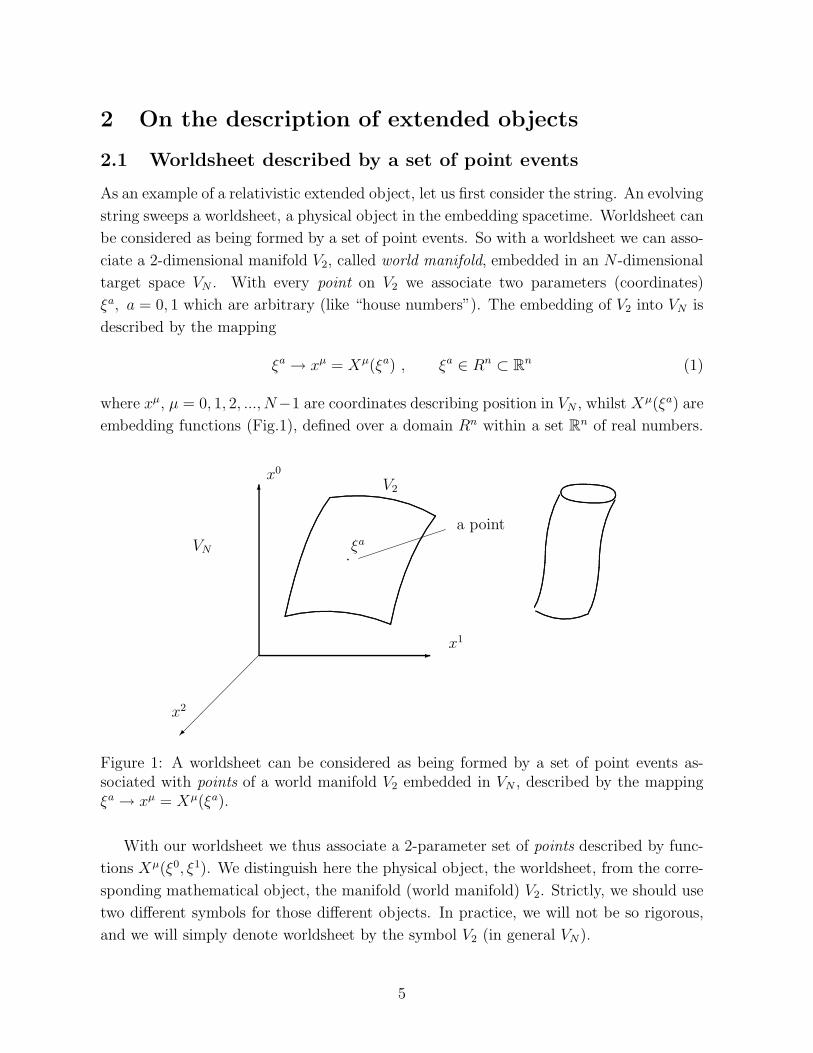
As an example of a relativistic extended object, let us first consider the string. An evolving

string sweeps a worldsheet, a physical object in the embedding spacetime. Worldsheet can

be considered as being formed by a set of point events. So with a worldsheet we can asso-

ciate a 2-dimensional manifold V2, called world manifold, embedded in an N -dimensional

target space VN . With every point on V2 we associate two parameters (coordinates)

ξa, a = 0, 1 which are arbitrary (like “house numbers”). The embedding of V2 into VN is

described by the mapping

ξa → xµ = Xµ(ξa) , ξa ∈ Rn ⊂ Rn (1)

where xµ, µ = 0, 1, 2, ..., N−1 are coordinates describing position in VN , whilst Xµ(ξa) are

embedding functions (Fig.1), defined over a domain Rn within a set Rn of real numbers.

-

6

x1

x2

x0

ξa

V2

·VN

a point

.

.................................................

..............................................

...........................................

.......................................

....................................

.................................

.............................

..........................

. ....................................... ..................................... .................................... .................................... ......................................................................

.............................

........

...................................

....................................

......................................

........................................

.........................................

...........................................

............................................

............................................................................

................................................................................................................................................................................

.................................................................................................................................................................. ........ ........... ............. ................ .................. .................. ............... ............ .......... ..............

. ....................... ...................... ..................... .................... ..................... ..........................................................

......................

.........................

............................

.

....................................

..................................

.................................

...............................

.............................

....................................

......................

.........................

............................

.

..............................

.............................

............................

...........................

..........................

........................

Figure 1: A worldsheet can be considered as being formed by a set of point events as-sociated with points of a world manifold V2 embedded in VN , described by the mappingξa → xµ = Xµ(ξa).

With our worldsheet we thus associate a 2-parameter set of points described by func-

tions Xµ(ξ0, ξ1). We distinguish here the physical object, the worldsheet, from the corre-

sponding mathematical object, the manifold (world manifold) V2. Strictly, we should use

two different symbols for those different objects. In practice, we will not be so rigorous,

and we will simply denote worldsheet by the symbol V2 (in general VN).

5

2.2 Worldsheet described by a set of loops

In previous section a worldsheet was described by a 2-parameter set of points described

by functions Xµ(ξ0, ξ1) Alternatively, instead of points we can consider closed lines, loops,

each being described by functions Xµ(s), where s ∈ [s1, s2] ⊂ R is a parameter along a

loop. A 1-parameter family of such loops Xµ(s, α), α ∈ [α1, α2] ⊂ R sweeps a worldsheet

V2. This holds regardless of whether such worldsheet is open or closed. However, in the

case of an open worldsheet, the loops are just kinematically possible objects, and they

cannot be associated with physical closed strings. In the case of a closed worldsheet, a

world tube, we can consider it as being swept by an evolving closed string.

We will now demonstrate, how with every loop one can associate an oriented area,

whose projections onto the coordinate planes are Xµν . The latter quantities are func-

tionals of a loop Xµ(s). If we consider not a single loop, but a family of loops

Xµ(s, α), α ∈ [α1, α2], then Xµν are functions of parameter α, besides being functionals

of a loop. So we obtain a 1-parameter family of oriented areas described by functions

Xµν(α). Let us stress again that for every fixed α, it holds, of course, that Xµν are

functionals of Xµ(s, α).

If we choose a loop B on V2, i.e., a loop from a given family Xµ(s, α), α ∈ [α1, α2],then we obtain the corresponding components Xµν of the oriented area by performing the

integration of infinitesimal oriented area elements over a chosen surface whose boundary

is our loop B. Given a boundary loop B, it does not matter which surface we choose. In

the following, for simplicity, we will choose just our worldsheet V2 for the surface.

Let us now consider a surface element on V2. Let dξ1 = dξa1 ea and dξ2 = dξa

2 ea

be two infinitesimal vectors on V2, expanded in terms of basis vectors ea, a = 0, 1. An

infinitesimal oriented area is given by the wedge product

dΣ = dξ1 ∧ dξ2 = dξa1 dξb

2 ea ∧ eb = 12dξab ea ∧ eb (2)

where

dξab = dξa1 dξb

2 − dξa2 dξb

1 (3)

At every point ξ ∈ V2 basis vectors ea span a 2-dimensional linear vector space, a tangent

space Tξ(V2). Following an old tradition (see, e.g., [30, 31]) we use symbol Vn for an n-

dimensional surface embedded in an N -dimensional space VN . Thus Vn, and in particular

V2, denotes a manifold, and not a vector space. In order to simplify our wording, an

expression like “vectors ea on V2” will mean “tangent vectors ea at a point ξ ∈ V2”. So

whenever we talk about vectors, or whatever geometric objects, on a manifold (or in a

manifold) we just mean that to a given point of the manifold we attach a geometric object

(see, e.g., [32]). The latter object, of course, is not an element of our manifold, but of the

tangent space. Basis vectors on V2 can be considered as being induced from the target

6

space basis vectors γµ:

ea = ∂aXµγµ (4)

In the following we will adopt the geometric calculus in which basis vectors are Clifford

numbers satisfying

γµ · γν ≡ 12(γµγν + γνγµ) = gµν (5)

where gµν is the metric of VN . Eq. (5) defines the inner product of two vectors as the

symmetric part of the Clifford product γµγν. The antisymmetric part of γµγν is identified

with the wedge or outer product

γµ ∧ γν ≡ 12(γµγν − γνγµ) (6)

Analogous relations we have for the worldsheet basis vectors ea:

ea · eb ≡ 12(eaeb + ebea) = γab (7)

ea ∧ eb ≡ 12(eaeb − ebea) (8)

where γab is the metric on V2 which, according to eq. (4), can be considered as being

induced from the target space.

If we insert the relation (4) into eq.(2) we have

dΣ = 12dξab ∂aX

µ∂bXν γµ ∧ γν (9)

This is an infinitesimal bivector or 2-vector in the target space VN .

A finite 2-vector is obtained upon integration4 over a finite surface ΣB enclosed by a

loop B:∫

ΣB

dΣ ≡ 12Xµν γµ ∧ γν =

1

2

∫

ΣB

dξab∂aXµ∂bX

ν γµ ∧ γν

=1

2

∫

ΣB

dξab 1

2(∂aX

µ∂bXν − ∂aX

ν∂bXµ)γµ ∧ γν (10)

From eq.(10) we read

Xµν [B] =1

2

∫

ΣB

dξab(∂aXµ∂bX

ν − ∂aXν∂bX

µ) (11)

By Stokes theorem this is equal to

Xµν [B] =1

2

∮

B

ds

(

Xµ ∂Xν

∂s− Xν ∂Xµ

∂s

)

(12)

4Such integration poses no problem in flat VN . In curved space we may still use the same expression(10) which then defines such integral that all vectors are carried together by means of parallel transportalong geodesics into a chosen point of VN where the integration is actually performed [33].

7

where Xµ(s) describes a boundary loop B, s being a parameter along the loop.

Eq.(12) demonstrates that Xµν are components of the bivector, determining an ori-

ented area, associated with a surface enclosed by a loop Xµ(s) on the worldsheet V2.

Hence there is a close correspondence between surfaces and the boundary loops. The

components Xµν can be therefore be considered as bivector coordinates of a loop. These

are collective coordinates, since the detailed shape (configuration) of the loop is not de-

termined by Xµν . Only the oriented area associated with a surface enclosed by the loop is

determined by Xµν . Therefore Xµν refers to a class of loops, from which we may choose

a representative loop, and say that Xµν are its coordinates. From now on, ‘loop’ we will

be often a short hand expression for a representative loop in the sense above.

By means of eqs. (10)–(12) we have performed a mapping from an infinite dimensional

space of loops Xµ(s) into a finite dimensional space of oriented areas Xµν . Instead of

describing loops by infinite dimensional objects Xµ(s), we can describe them by finite

dimensional objects, oriented areas, with bivector coordinates Xµν . We have thus arrived

at a finite dimensional description of loops (in particular, closed strings), the so called

quenched minisuperspace description suggested by Aurilia et al. [13].

When we consider not a single loop Xµ(s), but a 1-parameter family of loops Xµ(s, α),

we have a worldsheet, considered as being formed by a set of loops. By means of eqs. (10)–

(12), with every loop within such a family, i.e., for a fixed α, we can associate bivector

coordinates Xµν . For variable α we then obtain functions Xµν(α). This is a quenched

minisuperspace description of a worldsheet. A full description is in terms of embedding

functions Xµ(ξ0, ξ1), or a family of loops Xµ(s, α).

In the following we will consider two particular choices for parameter α.

In eq.(10) we have the expression for an oriented area associated with a loop B. It

has been obtained upon the integration of the infinitesimal oriented surface elements (2).

Besides the oriented area we can associate with our loop on V2 also a scalar quantity,

namely the scalar area A which we obtain according to

A =

∫

ΣB

√dΣ‡ · dΣ (13)

Here ‘‡’ denotes reversion, that is the operation which reverse the order of vectors in

a product. Using the relation ea ∧ eb = eǫab, where e = e1 ∧ e2 is the pseudoscalar in

2-dimensional space V2 such that e‡ ·e = (e2∧e1) ·(e1∧e2) = γ11γ22−γ21γ12 = det γab ≡ γ,

we find

dΣ‡ · dΣ =1

4γ(dξabǫab)

2 (14)

i.e.

A =

∫ √dΣ‡ ∗ dΣ =

1

2

∫

√

|γ|dξabǫab =

∫

√

|γ| dξ12 (15)

If we choose dξa1 = (dξ1, 0), dξa

2 = (0, dξ2), then dξ12 = dξ1dξ2.

8

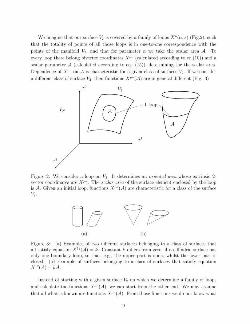
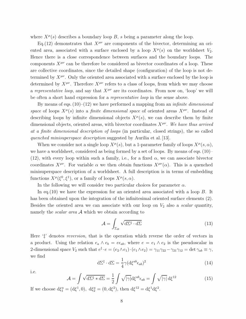
We imagine that our surface V2 is covered by a family of loops Xµ(α, s) (Fig.2), such

that the totality of points of all those loops is in one-to-one correspondence with the

points of the manifold V2, and that for parameter α we take the scalar area A. To

every loop there belong bivector coordinates Xµν (calculated according to eq.(10)) and a

scalar parameter A (calculated according to eq. (15)), determining the the scalar area.

Dependence of Xµν on A is characteristic for a given class of surfaces V2. If we consider

a different class of surface V2, then functions Xµν(A) are in general different (Fig. 3)

-

6

x1

x2

x0

A

V2

VN

A

a 1-loop

............. ............ ..................................................................................................................................................................................................................................

................................

.............

............................. ............ ............. ..............

.

.................................................

..............................................

...........................................

.......................................

....................................

.................................

.............................

..........................

. ....................................... ..................................... .................................... .................................... .......................................................................

...................................

....................................

....................................

......................................

........................................

.........................................

...........................................

............................................

............................................................................

................................................................................................................................................................................

........................................................................................................................................................................................................................................................................................................................... ......... ............ .............. ................. .................... ...................... ......................... ............................ ........................... ........................ ..................... .................. ............... ............. .......... ..............

............... ........... .......... .......... ........... ...............................................

. ............. .............. ............... ................. .................. .................... ...................... ........................ ........................................................

.

...............................................

.............................................

...........................................

.........................................

.......................................

.....................................

...................................

.....................

.......................

..........................

.............................

................................

.

...................................

.................................

................................

..............................

.............................

...........................

Figure 2: We consider a loop on V2. It determines an oriented area whose extrinsic 2-vector coordinates are Xµν . The scalar area of the surface element enclosed by the loopis A. Given an initial loop, functions Xµν(A) are characteristic for a class of the surfaceV2.

.

..

..

..

..

.

........

.............

.............. . ..............

.............

........

.....

....

.

....

.....

.......

.

.............

.............................

.............

........

..

..

.

..

..

.

..

..

..

..

.

........

.............

.............. . ..............

.............

.

.......

.....

....

.

..

..

..

..

.

........

.............

.............. . ..............

.............

........

.....

....

.

....

.....

.......

.

.............

.............................

.............

.

.......

..

..

.

..

..

.

..

..

..

..

.

........

.............

.............. . ..............

.............

........

.....

....

.

.

....

.....

.......

..........

.

...............

................

...................................

................

...............

.

..........

.......

..

..

.

.

..

..

.

..

..

.

..

..

.

..

.....

..........

.

...............

...............

.

................. . .................

................

...............

.

..........

.......

.....

....

.

.

...

..

..

...

.......

..........

.

...............

................

...................................

................

...............

.

..........

.......

..

..

.

..

.

..

.

..

..

.

..

..

.

.......

..........

.

...............

................

................. . .................

................

...............

.

..........

.......

.

....

..

...

(a) (b)

Figure 3: (a) Examples of two different surfaces belonging to a class of surfaces thatall satisfy equation X12(A) = k. Constant k differs from zero, if a cillindric surface hasonly one boundary loop, so that, e.g., the upper part is open, whilst the lower part isclosed. (b) Example of surfaces belonging to a class of surfaces that satisfy equationX12(A) = kA.

Instead of starting with a given surface V2 on which we determine a family of loops

and calculate the functions Xµν(A), we can start from the other end. We may assume

that all what is known are functions Xµν(A). From those functions we do not know what

9

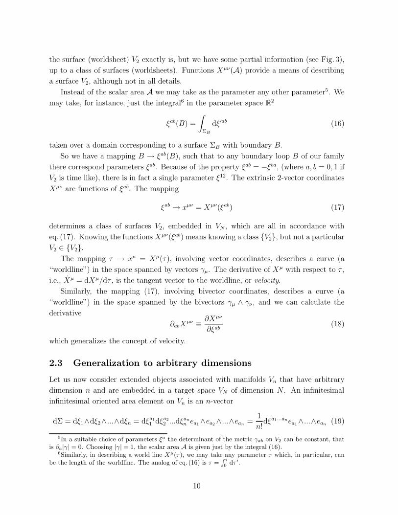
the surface (worldsheet) V2 exactly is, but we have some partial information (see Fig. 3),

up to a class of surfaces (worldsheets). Functions Xµν(A) provide a means of describing

a surface V2, although not in all details.

Instead of the scalar area A we may take as the parameter any other parameter5. We

may take, for instance, just the integral6 in the parameter space R2

ξab(B) =

∫

ΣB

dξ′ab (16)

taken over a domain corresponding to a surface ΣB with boundary B.

So we have a mapping B → ξab(B), such that to any boundary loop B of our family

there correspond parameters ξab. Because of the property ξab = −ξba, (where a, b = 0, 1 if

V2 is time like), there is in fact a single parameter ξ12. The extrinsic 2-vector coordinates

Xµν are functions of ξab. The mapping

ξab → xµν = Xµν(ξab) (17)

determines a class of surfaces V2, embedded in VN , which are all in accordance with

eq. (17). Knowing the functions Xµν(ξab) means knowing a class V2, but not a particular

V2 ∈ V2.The mapping τ → xµ = Xµ(τ), involving vector coordinates, describes a curve (a

“worldline”) in the space spanned by vectors γµ. The derivative of Xµ with respect to τ ,

i.e., Xµ = dXµ/dτ , is the tangent vector to the worldline, or velocity.

Similarly, the mapping (17), involving bivector coordinates, describes a curve (a

“worldline”) in the space spanned by the bivectors γµ ∧ γν , and we can calculate the

derivative

∂abXµν ≡ ∂Xµν

∂ξab(18)

which generalizes the concept of velocity.

2.3 Generalization to arbitrary dimensions

Let us now consider extended objects associated with manifolds Vn that have arbitrary

dimension n and are embedded in a target space VN of dimension N . An infinitesimal

infinitesimal oriented area element on Vn is an n-vector

dΣ = dξ1∧dξ2∧...∧dξn = dξa1

1 dξa2

2 ...dξan

n ea1∧ea2

∧...∧ean=

1

n!dξa1...anea1

∧...∧ean(19)

5In a suitable choice of parameters ξa the determinant of the metric γab on V2 can be constant, thatis ∂a|γ| = 0. Choosing |γ| = 1, the scalar area A is given just by the integral (16).

6Similarly, in describing a world line Xµ(τ), we may take any parameter τ which, in particular, canbe the length of the worldline. The analog of eq. (16) is τ =

∫ τ

0dτ ′.

10

where

dξa1...an = dξ[a1

1 dξa2

2 ...dξan]n (20)

If we consider the basis vectors ea on Vn as being induced from the basis vectors γµ of the

embedding space VN according to the relation (4), we have

dΣ =1

n!dXµ1...µnγµ1

∧ ... ∧ γµn=

1

n!dξa1...an∂a1

Xµ1 ...∂anXµnγµ1

∧ ... ∧ γµn(21)

After the integration over a finite n-surface ΣB with boundary B we obtain a finite n-

vector∫

ΣB

dΣ =1

n!Xµ1...µnγµ1

∧ ... ∧ γµn=

1

n!

∫

ΣB

dξa1...an∂a1Xµ1 ...∂an

Xµnγµ1∧ ... ∧ γµn

=1

n!

∫

ΣB

dξa1...an1

n!∂[a1

Xµ1 ...∂an]Xµnγµ1

∧ ... ∧ γµn(22)

Its n-vector components are

Xµ1...µn[B] =

∫

ΣB

dξa1...an1

n!∂[a1

Xµ1 ...∂an]Xµn (23)

They describe an oriented n-area associated with ΣB, whose boundary B will be called

(n− 1)-loop, and Xµ1...µn[B] are its extrinsic coordinates. With the same (n− 1)-loop we

can associate intrinsic coordinates (parameters), in analogy to eqs. (13)–(16), according

to

ξa1...an(B) =

∫

ΣB

dξ′a1...an (24)

With a particular choice of coordinates ξa, such that det γab = 1, the quantities ξa1...an

in the above equation determine the intrinsic (scalar) n-area of the n-surface bounded by

the (n − 1)-loop.

As in the case of V2 we assume that on our n-dimensional worldsheet Vn there exists

a family of (n − 1)-loops B, described by functions Xµ(sa, α), a = 1, 2, ..., n − 1,

Instead of a manifold Vn of points we thus consider a family of loops. With every

(n − 1)-loop of the family we can associate arbitrary parameters ξa1...an (coordinates are

like “house numbers”). Because of the property

ξa1...ajak ...an = −ξa1...akaj ...an (25)

there is actually a single parameter. This is a particular choice for parameter α of our

family of loops Xµ(sa, α). By means of a mapping

ξa1...an → xµ1...µn = Xµ1...µn(ξa1...an) (26)

we obtain a quenched minisuperspace description of a family of (n − 1)-loops, i.e., a

description in terms of the target space multivector coordinate functions Xµ1...µn. The

11

family is such that the totality of the points of the (n − 1)-loops belonging to the family

is in one-to-one correspondence with the points of the worldsheet Vn. In other words, by

mapping (26) we have a quenched minisuperspace description of worldsheet.

We started from a brane described by the embedding functions Xµ(ξa), and derived

the expression (23) and functions (26). Once we have Xµ1...µ2 as functions of a parameter

ξa1...an, we may forget about the embedding xµ = Xµ(ξa) that we started from. We may

assume that all the information available to us are just functions Xµ1...µn(ξa1...an) given by

mapping (26). Then we do not have knowledge of a particular worldshet’s manifold Vn,

but of a class Vn of worldsheet’s manifolds that all satisfy eq. (26) for given functions

Xµ1...µn(ξa1...an). So we calculate the derivative

∂a1...anXµ1...µn ≡ ∂Xµ1...µn

∂ξa1...an(27)

which generalizes the notion of velocity.

In the above considerations one has to bear in mind that many loop configuration may

cast the same holographic projections onto the coordinate planes as a single loop config-

uration. Therefore, a given set of polyvector coordinates Xµ1...µn(ξa1...an) may describe a

single or many loop configuration. Not only the details of a single loop configuration (its

infinite dimensionality), but also the number of loops is undetermined in this quenched

description of loops.

3 The dynamics of extended objects

3.1 Objects described in terms of Xµ(ξa)

The extended objects described by the mapping (1) obey the dynamical law that is in-

corporated in the Dirac-Nambu-Goto minimal surface action. An equivalent action that

was considered in ref. [12] is a functional of the embedding functions Xµ(ξa) and the

coordinate basis vector fields ea(ξ) having the role of Lagrange multipliers:

I[Xµ, ea] =κ

2

∫

dnξ |e| (ea∂aXµ eb∂bXµ + 2 − n) (28)

where |e| ≡√

|γ| is the determinant of γab = ea · eb.

Expanding the coordinate vector fields ea(ξ), a = 1, 2, ..., n in terms of orthonormal

vector fields7 ea, a = 1, 2, ..., n, by means of a tetrad eaa(ξ) according to

ea(ξ) = eaa(ξ)ea (29)

7Their inner products ea · eb = ηab gives the Minkowski metric.

12

we find the following relations8

∂ea

∂eb≡ ec

∂ea

∂ebc

= nδab (30)

∂|e|∂ea

=∂|e|∂γcd

∂γcd

∂ea= −n |e|ea (31)

where n comes from the contraction eaea = n.

Using (30),(31) we find that the variation of the action (28) with respect to ea gives

− 1

2ec(e

a∂aXµ ∂bXµ + 2 − n) + ∂cX

µ ∂dXµed = 0 (32)

Performing the inner product with ec and using ec · ec = n we find

ea∂aXµ eb∂bXµ = n (33)

and eq.(32) becomes

ec = ∂cXµ ∂dXµe

d (34)

This is the equation of “motion” for the Lagrange multipliers ea. In order to understand

better the meaning of eq.(34) let us perform the inner product with ea:

ec · ea = ∂cXµ ∂dXµe

d · ea (35)

Since ec · ea = γca and ed · ea = δda we obtain after renaming the indices

γab = ∂aXµ ∂bXµ (36)

This is the relation for the induced metric on the worldsheet. On the other hand, eq. (35)

can be written as

ea · eb = (∂aXµγµ) · (∂aX

νγν) (37)

from which we have that basis vectors ea on the worldsheet Vn are expressed in terms of

the embedding space basis vectors γµ:

ea = ∂aXµγµ (38)

With our procedure we have thus derived eq. (4) as a solution to our dynamical sytem.

Using eq. (36) we find that the action (28) is equivalent to the well known Howe–Tucker

action which is a functional of Xµ(ξ) and γab:

I[Xµ, γab] =κ

2

∫

dnξ√

|γ| (γab∂aXµ∂bXµ + 2 − n) (39)

8Eq.(30) also comes directly from the relation for a derivative with respect to a vector [9].

13

3.2 Objects described in terms of Xµ1...µn(ξa1...an)

In Sec. 2.3 we have seen that an alternative description of extended objects, up to a class

in which all objects have the same coordinates Xµ1...µn, is given by the mapping (26). Let

us assume that such objects are described by the following action

I[Xµ1,...,µn, e] =κ

2

∫

dnξ |e|[

1

n!

(

1

n!ea1 ∧ ... ∧ ean

∂Xµ1...µn

∂ξa1...an

)‡

×(

1

n!eb1 ∧ ... ∧ ebn

∂Xµ1...µn

∂ξb1...bn

)

+ 1

]

(40)

Factor 1/n! inside the bracket comes from the definition of the worldsheet n-vector

(1/n!)ea1 ∧ ...∧ ean∂Xµ1...µn/∂ξa1...an. The extra factor 1/n! in front of the bracket comes

from the square of the target space n-vector (1/n!)(∂Xµ1...µn/∂ξa1...an)γµ1∧ ...∧ γµn

. The

operation ‡ reverses the order of vectors.

Let us take into account the following relations:

ea1∧ ... ∧ ean

= e ǫa1...an(41)

ea1 ∧ ... ∧ ean = e−1 ǫa1...an (42)

e−1 =e

|e|2 , |e| ≡√

e‡ · e =√

|γ| ≡ λ (43)

γ = det γab , γab = ea · eb (44)

Instead of the intrinsic parameters ξa1...an, let us introduce the dual parameter

ξ =1

n!ǫa1...an

ξa1...an (45)

and rewrite the n-area velocity according to

∂Xµ1...µn

∂ξc1...cn=

∂Xµ1...µn

∂ξ

∂ξ

∂ξc1...cn=

∂Xµ1...µn

∂ξǫc1...cn

(46)

where we have used∂ξa1...an

∂ξc1...cn= δa1...an

c1...cn(47)

and where the generalized Kronecker symbol is given by the antisymmetrized sum of

products of ordinary deltas. From eq.(46) we have

∂Xµ1...µn

∂ξ=

1

n!ǫc1...cn

∂Xµ1...µn

∂ξc1...cn(48)

By using eqs.((33),(35) and (48) we can rewrite the action (40) as

I[Xµ1...µn, λ] =κ

2

∫

dξ

(

1

λ n!

∂Xµ1...µn

∂ξ

∂Xµ1...µn

∂ξ+ λ

)

(49)

14

where

dξ =1

n!ǫa1...an

dξa1...an =1

n!ǫa1...an

dξ[a1

a ...dξan]n = ǫa1...an

dξa1

a ...dξan

n = dξ1dξ2...dξn ≡ dnξ

(50)

The last step in eq.(50) holds in a coordinates system in which dξa1

1 = dξ1, dξa2

2 = dξ2,

..., dξann = dξn.

The action (49) is a functional of the n-area variables Xµ1...µn(ξ) and a Lagarange

multiplier λ, defined in eq.(43). Variation of eq. (49) with respect to λ and Xµ1...µn,

respectively, gives

δλ :1

n!

∂Xµ1...µn

∂ξ

∂Xµ1...µn

∂ξ− λ2 = 0 (51)

δXµ1...µn :d

dξ

(

1

λ

∂Xµ1...µn

∂ξ

)

= 0 (52)

These are the equations of motion for the n-area variables.

Inserting eq.(51) into (49) we obtain the action which is a functional of Xµ1...µn solely:

I[Xµ1...µn] = κ

∫

dξ

(

1

n!

∂Xµ1...µn

∂ξ

∂Xµ1...µn

∂ξ

)1/2

(53)

The latter action has the same form as the action for a worldline of a relativistic particle.

Factor 1/n! in the latter action disappears, if we order indices according to µ1 < µ2 <

... < µn.

3.3 More general objects (generalization to C-space)

So far we have considered branes described by coordinate functions of the type

Xµ(ξ), Xµ1µ2(ξa1a2),..., or Xµ1...µn(ξa1...an) that represent a mapping of a worldsheet loop

into a target space loop of the same dimensionality.:

(n − 1)-loop on Vn −→ (n − 1)-loop in VN .

Let us now extend the theory and consider “ mixed” mappings

(r − 1)-loop on Vn −→ (R − 1)-loop in VN .

where r, in general, is different from R. So we arrive at a more general extended object

which is described by a mapping [12, 15]

ξa1...ar → xµ1...µR = Xµ1...µR(ξ, ξa, ξa1a2 , ..., ξa1...as, ..., ξa1...an) ,

0 ≤ R ≤ N , 0 ≤ r ≤ n < N (54)

15

In the compact notation we set

XM ≡ Xµ1...µR , µ1 < µ2 < ... < µR

ξA ≡ ξa1...ar , a1 < a2 < ... < ar

and write the mapping (54) as

ξA → xM = XM(ξA) (55)

This is the parametric equation of our generalized extended object. Such object lives in a

target space which is now generalized to Clifford space (shortly C-space). The worldsheet

associated with the extended object is also generalized to a Clifford space. In the following

we will explain this in more detail.

In eq. (54) or (55)we have a generalization of the usual relation

ξa → xµ = Xµ(ξa) , a = 1, 2, ..., n; µ = 0, 1, 2, ..., N − 1 (56)

that describes an n-dimensional surface, called worldsheet or world manifold, Vn, em-

bedded in N -dimensional target space VN . In eq. (56) the space Rn of parameters ξa is

isomorphic to an n-dimensional vector space V n, spanned by an orthonormal basis ha.The vector space V n should not be confused with the worldsheet Vn, which is a manifold

(embedded in a higher dimensional manifold VN).

Instead of V n we can consider the corresponding Clifford algebra Cn which is itself

a vector space. Amongst its elements are r-vectors associated with (r − 1)-loops, r =

0, 1, 2, ..., n. A generic object is a superposition of r-vectors for different grades, and it is

described by a Clifford number, a polyvector, ξa1...arha1∧ ... ∧ har

∈ Cn

Our objects are now extended events E [29], superpositions of (r − 1)-loops, to which

we assign a set of 2n parameters (coordinates) ξA ≡ ξa1...ar , r = 0, 1, 2, ..., n according to

the mapping

E → ξA(E) (57)

The assignment is arbitrary. We may choose an object E0 to which we assign coordinates

ξA(E) = 0. This is a coordinate origin. Choosing an origin E0, the polyvectors ξAhA

pointing from E0 to any E are in one-to-one correspondence with extended events E . The

space of extended events is then isomorphic to Clifford algebra Cn, and the latter algebra,

in turn, is isomorphic to the space of parameter ξA = R2n

. Therefore we will speak

about Cn as the parametric Clifford algebra or parametric polyvector space.

The parametric space Cn is by definition a (poly)vector space, spanned by a basis ha1∧

...∧har, r = 0, 1, 2, ..., n, formed by the orthonormal basis ha, a = 1, 2, ..., n. This implies

that Cn is a metric space, but its metric is just formal, without any physical content.

Now let us consider the mapping (55) from Cn into a Clifford space CVNgenerated by a

16

basis γµ , µ = 0, 1, 2, ..., N − 1, with N > n. So we obtain a generalized, 2n-dimensional

surface CVnembedded in a target Clifford space CVN

. The surface CVngeneralizes the

notion of worldsheet Vn to Clifford space, i.e., a manifold such that any of its tangents

spaces is a Clifford algebra. If we consider only the intrinsics propertires of CVn(i.e., if

we “forget” about its embedding into a higher dimensional Clifford space CVN), then we

can simply denote it as Cn.

Bellow we sumarize our notation of various spaces:

V n Parametric vector space, with an orthonormal basis ha, a = 1, 2, ..., n and elements

ξaha ∈ V n. It is isomorphic to Rn, the space of parameters ξa.

Vn Manifold, either flat or curved. It is a space of points (events) P. With every

point P ∈ Vn we associate a set of n parameters (coordinates) ξa(P) ≡ ξa ∈ Rn.

Coordinate basis vectors are ea, whilst orthonormal basis vectors are ea.

Cn Parametric Clifford algebra of V n, called also parametric polyvector space, with basis

hA ≡ ha1∧...∧har

, r = 0, 1, 2, ..., n and elements ξAhA ∈ Cn, called polyvectors.

It is isomorphic to R2n

, the space of parameters ξA.

Cn Clifford manifold, or Clifford space, either flat or curved. It is a space of points

that are perceived in a subspace Vn as extended events E . With every E ∈ Cn

we associate a set of 2n parameters ξA(E) ≡ ξa ≡ ξa1...ar ∈ R2n

, r = 0, 1, 2, ..., n.

Coordinate basis elements are eA ≡ ea1...ar; orthonormal basis elements are eA ≡

ea1...an, r = 0, 1, 2, ..., n. In particular Cn can be considered as being embedded in

a higher dimensional Clifford space; then it is denoted as CVn.

CVnGeneralized worldsheet, a Clifford space embedded in a target Clifford space. Its

coordinate basis elements are eA ≡ ea1...ar; orthonormal basis elements are eA ≡

ea1...an, r = 0, 1, 2, ..., n.

CVNTarget Clifford manifold, or target Clifford space, either flat or curved. It is a space

of points that are perceived in a subspace VN as extended events E . With every E ∈CVN

we associate a set of 2N coordinates xM(E) ≡ xM ≡ xµ1...µR, R = 0, 1, 2, ...N .

Coordinate basis elements are γM ≡ γµ1...µR; orthonormal basis elements are γM ≡

γµ1...µR. Instead of CVN

we can use simply notation CN .

We follow the rule that bold symbols are used for vector spaces, whilst light symbols

are used for manifolds. Since Clifford algebras also are vector spaces, they are denoted by

bold symbols, whereas the corresponding Clifford spaces (manifolds of points representing

extended events) are denoted by light symbols. By such notation we have attempted to

simplify distinction among all those various spaces that occur in our theory of generalized

17

branes. For these purely physical reasone we have thus, to certain extent, deviated from

the standard notation used in mathematics.

An infinitesimal (polyvector) dX ∈ CVN, joining two points on the surface CVn

can be

written as

dX = dXMγM = dξA∂AXMγM = dξAeA (58)

where

eA = ∂AXMγM (59)

These are induced basis tangent (polyvectors) on CVn.

At every point of the flat target C-space CVNthere exists a basis

γM = 1, γµ, γµ1µ2 , ..., γµ1...µN (60)

given in terms of 2N Clifford numbers

γM ≡ γµ1...µr ≡ γµ1 ∧ γµ2 ∧ ... ∧ γµR , µ1 < µ2 < ...µR , R = 0, 1, 2, ...N (61)

At every point ξ ∈ CVnon the brane’s worldsheet C-space CVn

, which in general is

curved, there exist a basis given in terms of 2n Clifford numbers9

eA = e, ea, ea1a2 , ..., ea1...an (62)

that span a tangent space Tξ(CVn). At a particular point ξ0 ∈ CVn

it may hold

eA ≡ ea1...ar ≡ ea1 ∧ ea2 ∧ ear , a1 < a2 < ... < ar , r = 0, 1, 2, ..., n (63)

That is, at that particular point the basis polyvectors on CVnare given as wedge products

of basis vectors ea. The above property (63) cannot hold globally on a curved CVn. At

points different from ξ0, basis polyvectors are in general superpositions of ea1∧ea2∧...∧eas ,

s = 0, 1, 2, ..., n.

To sum up, every Clifford number in the target C-space can be expanded in terms of

γM , and every Clifford number on the worldsheet C-space can be expanded in terms of

eA. Such numbers are also called Clifford aggregates or polyvectors. They are superposi-

tions r-vectors, the objects of definite grade that we call multivectors. This description

automatically contains spinors which are just members of the left of right ideal of Clifford

algebra [27].

9We will use ‘basis’ and ‘frame’ as synonyms. In order to simplify notation and wording we will besloppy in distinguishing objects from the corresponding fields, e.g., (poly)vectors from (poly)vector fields,frames from frame fields, etc. From the context it should not be difficult to understand which ones wehave in mind.

18

Metric of CVNis GMN = γ‡

M ∗ γN , whilst metric of CVnis GAB = e‡A ∗ eB. Here ‘∗’

denotes the scalar product of two Clifford numbers A and B

A ∗ B = 〈AB〉0 (64)

Let us now define the object V which is a polyvector in target space and on the

worldsheet:

V = eA ∂XM

∂ξAγM =

N∑

r=0

n∑

s=0

1

r!s!ea1...as

∂Xµ1...µr

∂ξa1...asγµ1...µr

(65)

In the right hand side expression we impose no restriction on the indices µ1, µ2, ..., µr and

a1, a2, ..., as, therefore, in order to prevent multiple counting of equivalent terms, factors

1/r! and 1/s! are introduced.

It is illustrative to express eq.(65) in a more explicit form by employing the notation

(60)–(63) and by writing

XM = (Ω, Xµ, Xµ1µ2 , ..., Xµ1...µN ) (66)

ξA = (ξ, ξa, ξa1a2 , ..., ξa1...an) (67)

We obtain

V =

(

∂Ω

∂ξ+ ea ∂Ω

∂ξa+

1

2!ea1a2

∂Ω

∂ξa1a2+ ...

1

n!ea1...an

∂Ω

∂ξa1...an

)

1

+

(

∂Xµ

∂ξ+ ea ∂Xµ

∂ξa+

1

2!ea1a2

∂Xµ

∂ξa1a2+ ...

1

n!ea1...an

∂Xµ

∂ξa1...an

)

γµ

+1

2!

(

∂Xµ1µ2

∂ξ+ ea ∂Xµ1µ2

∂ξa+

1

2!ea1a2

∂Xµ1µ2

∂ξa1a2+ ...

1

n!ea1...an

∂Xµ1µ2

∂ξa1...an

)

γµ1µ2(68)

+...

+1

N !

(

∂Xµ1...µN

∂ξ+ ea ∂Xµ1...µN

∂ξa+

1

2!ea1a2

∂Xµ1...µN

∂ξa1a2+ ...

1

n!ea1...an

∂Xµ1...µN

∂ξa1...an

)

γµ1...µN

One might ask how such a generalized extended object, described by eq. (55), that

sweep a Clifford worldsheet CVn, embedded in a Clifford space CVN

, looks like. Here our

perceptive system again shows its shortcomings, like in the case of figuring out how higher

dimensional objects look like. We are able to draw pictures of projections of an object

onto 3 or 2-dimensional Euclidean space, and that is, more or less, all. But on the other

hand, we are able to do algebra, and the algebra is interpreted as geometric algebra. So

we have to content us by our ability to control the situation algebraically, and assume

that there is a mapping between algebraic and geometric objects. The latter objects

are associated with physical objects, such as, e.g., the generalized extended objects, that

incorporate branes of various dimensionalities.

19

Let the action describing the dynamics of a generalized extended object, shortly, a

generalized brane, be described by the embedding functions XM(ξA) be

I[XM , eA] =T

2

∫

ddC ξ |E|[

(

eA ∂XM

∂ξAγM

)‡

∗(

eB ∂XN

∂ξBγN

)

+ 2 − dC

]

(69)

The latter action has a similar form as the action (28). But, since the indices M , N , and

A, B run over the full basis (60) and (62) of the corresponding C-spaces, the action (69)

is more general than (28).

Here the measure ddCξ|E| is the volume element in the worldsheet C-space CVn(whose

dimension is 2dC ). It is equal to the product

ddCξ |E| ≡ |E|∏

Ai

dξAi = dξ∏

a1

dξa∏

a1<a2

dξa1a2 ...∏

a1<...<an

dξa1...an]|E| (70)

By |E| we denote the square root of the determinant of the worldsheet C-space metric

which is given by the scalar product

GAB = (eA)‡ ∗ eB = 〈(eA)‡eB〉0 (71)

where 〈 〉0 denotes the scalar part. Explicitly,

|E| =√

|G| , G ≡ det GAB =1

dC !ǫA1...AdC ǫB1...BdC GA1B1

...GAdCBdC

(72)

The action (69) is a functional of XM and eA, and is a C-space generalization of the

action (28) which is a functional of the worldsheet embedding functions Xµ and basis

vectors ea.

An action which is classically equivalent to (69) is a functional of XM and GAB:

I[XM , GAB] =T

2

∫

ddCξ√

|G| (GAB ∂AXM ∂BXM + 2 − dC) (73)

where ∂BXM = GMN ∂BXN , GMN = γ‡M∗γN . In eq.(73) we have a C-space generalization

of the well known Howe–Tucker action [34].

Variation of the action (73) with respect to XM and GAB gives the equations of motion

of our C-space extended object:

δXM :1

√

|G|∂A(√

|G| ∂AXM) = 0 (74)

δGAB : GAB = ∂AXM ∂BXM (75)

Taking into account that GABGAB = dC = 2n and inserting eq. (75) Into eq. (73) we

obtain the action integral

I[XM ] = T

∫

ddCξ√

det ∂AXM ∂BXM (76)

20

which is the volume of the C-space worldsheet. The latter action contains the usual

p-branes, including point particles, as special cases.

Our action (73), or equivalently (76), is invariant under reparametrizations of coordi-

nates ξA, A = 1, 2, ..., 2n. As a consequence, there are 2n primary constraints. So we are

free to choose 2n relations among our dynamical variables XM(ξA), and thus fix a gauge

(a parametrization). For one of those relations we can choose, for instance,

∂a1...arXµ1...µr = ∂[a1

Xµ1 ....∂ar ]Xµr (77)

That is, the above relation is just one of gauge fixing relations. It will be used in Sec. 5.3,

where we will consider the coupling of our generalized branes to external fields.

4 On the relativity in Clifford space

The discussion of previous sections has led us to the conclusion that the space in which

our extended objects live is Clifford space, shortly C-space, denoted CVNor CN . A point

in C-space is described by the coordinates xM = (Ω, xµ, xµ1µ2 , ..., xµ1...µN ) which together

with the basis elements γM = (1, γµ, γµ1µ2, ..., γµ1...µN

) form a coordinate polyvector10

X = xMγM =1

r!

N∑

r=0

xµ1...µrγµ1...µr(78)

From the point of view of 2N -dimensional C-space, xµ1...µr , r = 1, ..., N , are coordinates

of a point, whilst from the point of view of the underlying Minkowski space VN , these are

the r-area (r-volume) variables.

The infinitesimal polyvector connecting two infinitesimally separated points of C-space

is

dX = dxMγM =1

r!

N∑

r=0

dxµ1...µrγµ1...µr≡ dxMγM (79)

The square of the distance between these points is given by the scalar product

|dX|2 ≡ dX‡ ∗ dX = dxMdxNGMN = dxMdxN (80)

where GMN is the metric of C-space11 :

GMN = γ‡M ∗ γN = γ‡

µ1...µr∗ γν1...νs

(81)

10 In flat C-space it makes sense to consider a polyvector joining the coordinate origin E0 with coordi-nates xM (E0) = 0 and a point E with coordinates xM (E) ≡ xM , where E0, E ∈ CVN

.11 A reason why we define the C-space metric by employing the reversion is in the consistency between

GMN , its inverse GMN , and the relations (82),(83) (in which the indices µi, νj , ... are lowered and raisedby the ordinary 4-dimensional metric gµiνj

and its inverse gµiνj ). For more details see ref. [16].

21

In particular, C-space CVNcan be flat. This means that the curvature of the connection

on flat CVNvanishes (see sec. 5.1). In such a case one can find a coordinates system on

CVNsuch that the metric GMN is diagonal.

Explicitly, for different choices of the indices M and N we have:

Gµν = γµ · γν = gµν = ηµν

G[µ1µ2][ν1ν2] = ㇵ1µ2

∗ γν1ν2= (γµ2

∧ γµ1) · (γν1

∧ γν2) =

∣

∣

∣

∣

gµ1ν1gµ1ν2

gµ2ν1gµ2ν2

∣

∣

∣

∣

G[µ1µ2µ3][ν1ν2ν3] = ㇵ1µ2µ3

∗ γν1ν2ν3= (γµ3

∧ γµ2∧ γµ1

) · (γν1∧ γν2

∧ γν3) =

∣

∣

∣

∣

∣

∣

gµ1ν1gµ1ν2

gµ1ν3

gµ2ν1gµ2ν2

gµ2ν3

gµ3ν1gµ3ν2

gµ3ν3

∣

∣

∣

∣

∣

∣

Gµ[ν1ν2] = γµ ∗ γν1ν2= 〈γµ(γν1

∧ γν2〉0 = 0 (82)

In general we have

G[µ1...µr][ν1...νr] = (γµr∧ ... ∧ γµ1

) · (γν1∧ ... ∧ γνr

) = det gµiνj, i, j = 1, 2, ..., r (83)

when r = s, and

G[µ1...µr][ν1...νs] = 0 (84)

when r 6= s.

Taking into account the explicit expressions for metric (82)–(84), the quadratic form

(80) reads

|dX|2 =1

r!

N∑

r=0

dxµ1...µr dxµ1...µr

= dΩ2 + dxµdxµ +1

2!dxµ1µ2dxµ1µ2

+ ... +1

N !dxµ1...µN dxµ1...µN

(85)

In the latter expression only the factor 1/r! remains, since the other factor is canceled

by r! coming from the determinant (83). Indices µ1, µ2, ... are lowered and raised by

Minkowski metric ηµν and its inverse ηµν .

In the 16-dimensional Clifford space CM4of the 4-dimensional Minkowski spacetime

the polyvector (79) and its square (80) can be rewritten as

dX = dΩ + dxµγµ +1

2dxµνγµ ∧ γν + dxµγ5γµ + dΩγ5 (86)

|dX|2 = dΩ2 + dxµdxµ +1

2dxµνdxµν − dxµxµ − ds2 (87)

where

dxµ ≡ 1

3!dxαβρǫαβρ

µ (88)

22

dΩ ≡ 1

4!dxαβρσǫαβρσ (89)

The minus sign in the last two terms of the above quadratic form occurs because in 4-

dimensional spacetime with signature (+−−−) we have γ25 = (γ0γ1γ2γ3)(γ0γ1γ2γ3) = −1,

and also γ‡5γ5 = (γ3γ2γ1γ0)(γ0γ1γ2γ3) = −1.

It is illustrative to write the quadratic form (line element) explicitly:

|dX|2 = dΩ2 + (dx0)2 − (dx1)2 − (dx2)2 − (dx3)2

−(dx01)1 − (dx02)2 − (dx03)2 + (dx12)2 + (dx13)2 + (dx23)2

−(dx0)2 + (dx1)2 + (dx2)2 + (dx3)2 − dΩ2 (90)

Here x0 = x123, x1 = x023, x2 = x013, x3 = x012, Ω = x0123. The factor 1/2 has

disappeared from the term (1/2)dxµνdxµν , since (1/2)(dx01x01 + dx10x10) = dx01dx01 =

−(dx01)2, etc..

By inspecting the quadratic form (87) we see that it has 8 terms with plus and 8

terms with minus sign. The group of transformations that leave the quadratic form (87)

invariant is SO(8,8). These are pseudorotations in C-space and have the role of generalized

Lorentz transformations:

x′M = LMNxN (91)

The transformations matrix satisfies the relation LMJLN

KGMN = GJK .

If interpreted actively (91) are the transformations that transform a point of C-space

with coordinates xM into another point with coordinates x′M . In the passive interpretation

the point remains the same, but its coordinates xM with respect to a reference frame S

are transformed into coordinates x′M with respect to a reference frame S ′.

From the point of view of C-space, xM are coordinates of a point. But from the

point of view of the underlying Minkowski space, xM are the (p + 1)-vector (holographic)

coordinates of p-loops associated with an extended object [11]. In C-space, p-loops of

different dimensionalities p (i.e., points, closed lines, closed 2-surfaces, closed 3-volumes)

are all described on the same footing [36, 37, 26, 11, 14], and can be transformed into

each other by transformations (91). Pseudo rotations in C-space have thus the role of

polydimensional rotations in M4. A point can be transformed into a line, and in general an

(R−1)-loop into an (R′−1)-loop. So the very dimensionality of a loop can change under

a transformation. This means that, when observed in a given reference frame S, a loop’s

dimensionality can change from (R − 1) to (R′ − 1). Alternatively, dimensionality of the

same loop, when observed from different reference frames S and S ′, can look different. In

short, dimensionality of a loop depends on the observer (associated with a given reference

frame). Such relativity of dimensionality of a loop also explains why in the mapping

(54),(55) the dimensionality of a loop in the parameter space ξa ≡ Rn is in general

23

different from the dimensionality of the same loop with respect to a reference frame in

the target space VN .

C-space in essence encodes the zero modes of p-loop configurations, since p-loops space

is infinite dimensional whereas C-space is finite dimensional. As already mentioned before,

a p-loop configuration, in general, can consist of many loops.

The construction with C-space coordinates, SO(8,8) symmetry and the brane equa-

tions of motion (74) reminds us of the constructions considered in refs. [5], where extra

coordinates were introduced in order to make manifest the SO(n,n) symmetry of the

duality transformations for strings and branes.

5 Curved Clifford space

5.1 General considerations

In general, the worldsheet Vn swept by a brane is curved. In Sec. 3.2 we have considered

a concept of a more complicated, generalized brane, whose (generalized) worldsheet CVn

was curved Clifford space. The latter worldsheet CVnwas embedded in a target space

which was a flat Clifford space CVN, with the metric properties given in Sec. 4.

A next step is to consider curved target Clifford space CVN(see refs. [28, 29]). At every

point E ∈ CVNwe have a flat tangent Clifford space TE(CVN

) and an orthonormal basis

of 2N Clifford numbers

γM = 1, γµ1, γµ1µ2

, ..., γµ1µ2...µN (92)

where

γµ1µ2...µr= γµ1

∧ γµ2∧ ... ∧ γµr

(93)

From an orthonormal basis γM we can switch to a coordinate basis

γM = γ, γµ1, γµ1µ2

, ..., γµ1µ2...µN (94)

by means of the relation [28, 29]

γM = eMMγM (95)

in which we have introduced a vielbein of curved Clifford space CVN, given by the scalar

product γ‡M ∗ γM. Notice a distinction between bold and normal indices, used for two

different kinds of basis. The coordinate basis Clifford numbers γM = γµ1µ2...µrin general

are not defined as a wedge product γµ1∧γµ2

∧...∧γµr. In particular, γM can be multivectors

of definite grade, i.e., defined as a wedge product, but such property can hold only locally

at a given point E ∈ CVN, and cannot be preserved globally at all point E of our curved

Clifford space. The relations for γM and the metric GMN , discussed in sec. 4, refer to flat

24

C-space and are no longer generally valid in curved C-space. At a fixed point E ∈ CVN

we can choose a coordinate system such that γM = γM, and then the relations of Sec. 4

refer to flat C-space, spanned by γM, i.e., the tangent space TE(CVN).

The set γM of 2n linearly independent coordinate basis fields (which depend on

coordinates xM) will be called a coordinate frame field in C-space.

The set γM of 2n linearly independent orthonormal basis fields (which also in general

depend on xM) will be called orthonormal frame field in C-space.

Corresponding to each field γM we define a differential operator —which we call

derivative— ∂M , whose action depends on the quantity it acts on12:

(i) ∂M maps scalars φ into scalars

∂Mφ =∂φ

∂xM(96)

Then ∂M is just the ordinary partial derivative.

(ii) ∂M maps Clifford numbers into Clifford numbers. In particular, it maps a coor-

dinate basis Clifford number γN into another Clifford number which can, of course, be

expressed as a linear combination of γJ :

∂MγN = ΓJMNγJ (97)

The above relation defines the connection ΓJMN for the coordinate frame field γM.

An analogous relation we have for the orthonormal frame field:

∂MγM = −ΩMN

MγN (98)

where ΩMB

M is the connection for the orthonormal frame field γM.When the derivative ∂M acts on a polyvector valued field A = ANγN we obtain

∂M(ANγN) = ∂MANγN + AN∂MγN = (∂MAN + ΓNMKAK)γN ≡ DMAN γN (99)

where DMAN ≡ ∂MAN + ΓNMKAK are components of the covariant derivative in the

coordinate basis, i.e., the ‘covariant derivative’ of the tensor analysis.

Here AN are scalar components of A, and ∂MAN is just the ordinary partial derivative

with respect to xM :

∂M ≡(

∂

∂s,

∂

∂xµ1,

∂

∂xµ1µ2,

∂

∂xµ1...µn

)

(100)

The derivative ∂M behaves as a partial derivative when acting on scalars, and it defines

a connection when acting on a basis γM. It has turned out very practical13 to use the

12 This operator is a generalization to curved C-space of the derivative ∂µ which acts in an n-dimensionalspace Vn, and was defined by Hestenes [9] (who used a different symbol, namely µ).

13 Especially when doing long calculation (which is usually the job of a theoretical physicist) it is mucheasier and quicker to write ∂M than M , ∇M , DγM

, ∇γMwhich all are symbols used in the literature.

25

easily writable symbol ∂M which —when acting on a polyvector— cannot be confused

with partial derivative. In ref. [29] we provided some arguments, why also conceptually it

is more appropriate to retain the same symbol ∂M , regardless of whether it acts on scalar,

vector, or generic polyvector fields.

The derivative ∂M is defined with respect to a coordinate frame field γM in C-space.

We can define a more fundamental derivative ∂ by

∂ = γM∂M (101)

This is the gradient in C-space and it generalizes the ordinary gradient γµ∂µ, µ =

0, 1, 2, ..., n− 1, discussed by Hestenes [9].

Besides the basis elements γM and γM, we can define the reciprocal elements γM , γM

by the relations

(γM)‡ ∗ γN = δMN , (γM)‡ ∗ γN = δM

N (102)

Curvature. We define the curvature of C-space in the analogous way as in the ordinary

spacetime, namely by employing the commutator of the derivatives [9, 12, 35]. Using

eq. (97) we have

[∂M , ∂N ]γJ = RMNJKγK (103)

where

RMNJK = ∂MΓK

NJ − ∂NΓKMJ + ΓR

NJΓKMR − ΓR

MJΓKNR (104)

is the curvature of C-space. Using (103) we can express the curvature according to

(γK)‡ ∗ ([∂M , ∂N ]γJ) = RMNJK (105)

An analogous relation we have if the commutator of the derivatives operates on a

orthonormal basis elements and use eq. (98)

5.2 On the dynamical curved C-space with sources

We will assume that physics takes place in curved C-space. The latter space is a gen-

eralization of curved spacetime. As in the ordinary general relativity the metric gµν is

a dynamical quantity, so in the generalized general relativity the C-space metric GMN

is a dynamical quantity. Instead of the usual point particles and branes the role of the

sources is now assumed by the generalized branes (which include the generalized point

particles) described by one of the classically equivalent actions (69),(73) or (76), which

we will denote by a common symbol IBrane.

The action thus contains a term which describes a C-space brane and a kinetic term

which describes the dynamics of the C-space itself:

I = IBrane +1

16πGC

∫

d2n

x√

|G|R (106)

26

Here GC is a constant (having the role of the “gravitational” constant in C-space), G ≡det GMN the determinant of the C-space metric, and R = RMNJKGMJGNK the curvature

scalar of C-space.

More details about how to proceed with and further generalize the theory based on

the action (106) are to be found in [12]. The idea that the curved C-space can provide

a realization of Kaluza-Klein theory has been considered in refs. [38, 41, 28, 29]. In this

paper we will explore the brane part IBrane which contains the coupling of the C-space

brane’s embedding functions XM(ξA) to the C-space metric GMN .

5.3 The generalized branes in curved C-space

We will consider a generalized brane (a C-space brane) moving in a fixed curved C-space

background. We will assume that the action is given by eq. (73) in which there occurs the

metric GMN of the curved target C-space into which our generalized brane is embedded.

Suppose that in the target C-space there exist isometries described by K Clifford

numbers kα = kαM γM , α = 1, 2, ..., K; M = 1, 2, ..., 16, (generalized Killing “vectors”),

whose components satisfy the conditions

DMkαN + DNkα

M = 0 (107)

where the covariant derivative DMAN of components AM of an arbitrary polyvector A is

given in eq. (99).

Splitting the coordinate basis and orthonormal basis indices according to

(i) coordinate basis indices: M = (µ, M) , µ = 0, 1, 2, 3; M = 4, 5, ..., 16

(ii) orthonormal basis indices: M = (µ, M) , µ = 0, 1, 2, 3 ; M = 4, 5, ..., 16

the metric and vielbein can be written as

GMN =

(

Gµν GµM

GMν GMN

)

, eMM =

(

eµµ eµ

M

eMµ eM

M

)

(108)

Let us recall that that the vielbein according to eq. (84) can be written as the scalar

product of the C-space coordinate and orthonormal basis elements:

eMM = γ‡

M ∗ γM (109)

We can now assume that the orthonormal basis γM is chosen so that γµ , µ = 0, 1, 2, 3,

are tangent vectors to the spacetime (a subspace of C-space), whilst the remaining basis

elements γM, M = 4, 5, ..., 16 are tangent to the “internal” part of C-space. Since the

basis is orthogonal, we have

ㇵ ∗ γM = 0 (110)

Next we assume that the coordinate basis γM is chosen so that γµ, µ = 0, 1, 2, 3 in

general is not tangent to V4, whilst the remaining coordinate basis elements γM , M =

27

4, 5, ..., 16, are tangent to the “internal” part of C-space. This means that γµ ∗ γM 6= 0,

whilst

㵇 ∗ γM = 0 (111)

The latter equation can be written as ηµν γν‡ ∗ γM = ηµν eνM = 0. Since ηµν is diagonal,

it follows that

eµM = 0 (112)

Taking a coordinate system in which

kαµ = 0 , kαM 6= 0 (113)

the components eMµ can be written in terms of the Killing vectors and gauge fields

Aµα(xµ):

eMµ = eM

M kαMAµα ; ∂MAµ

α = 0 (114)

For the “mixed” components of the inverse vielbein we find

eµM = 0 (115)

This follows directly from

㵇 ∗ γM = 0 = 㵇(eMM γM) = 㵇 ∗ (eµ

Mγµ + eMM γM) = eµ

MeMM (116)

where we have used eq. (112). Since in general eMM 6= 0, it follows that eµ

M is equal to

zero.

Using (95),(112) and (115) and the above choice of coordinates and local orthonormal

frame we find that the quadratic form can be written as the sum of the 4-dimensional

quadratic form and the part due to the “extra dimensions”:

dX‡ ∗ dX = (dxMγM)‡ ∗ (dxNγN) = gµν dxµdxν + φMN dxMdxN (117)

where

gµν = eµµe

ννγµγν = Gµν − φMN kα

MkβNAµ

αAνβ and φMN ≡ eM

MeNN ηMN (118)

Here GMN ≡ φMN = eMMeN

N ηMN , and φMN is the inverse of φMN in the “internal”

space. Notice the validity of eqs. (112) and (115).

Let us now use the splitting (117) in the brane action (73). We obtain

∂AXM ∂BXN GMN = ∂AXµ∂BXν gµν + ∂AXM∂BXN φMN (119)

The auxiliary variables GAB and the induced metric on the (generalized, i.e., C-space)

brane are related according to eq. (75). Let us introduce new auxiliary variables G′AB and

new brane tension T ′ according to

GAB = G′AB + ∂AXM∂BXNΦMN (120)

28

T√

|G|GAB = T ′√

|G′|G′AB (121)

where GAB and G′AB are the inverse matrices of GAB and G′AB, respectively.

Using eqs. (120),(121) we have

T√

|G| dC = T√

|G|GABGAB = T ′√

|G′|G′AB(G′AB + ∂AXM∂BXNΦMN ) (122)

T√

|G| =T√

|G| dC

dC=

T√

|G|GABGAB

dC=

T ′√

|G′|dC

G′AB(G′AB + ∂AXM∂BXNΦMN )

(123)

From eqs. (122),(123) we find that the extra term in the brane action (73) can be written

T√

|G| (2 − dC) = T ′√

|G′| (2 − dC) + P AM ∂AXN ΦMN

(

2

dC− 1

)

(124)

where we have written

T√

|G|GAB∂AXM = T ′√

|G′|G′AB∂AXM = P AM (125)

Here P AM are extra components of the brane canonical momentum P A

M = ∂L/∂∂BXM =

T√

|G|GAB∂AXM .

Inserting eqs. (120),(121) and (124) into the brane action (73) we obtain

IBrane[Xµ, G′AB] =

1

2

∫

ddcξ T ′√

|G′|(

G′AB∂AXµ∂BXνgµν + 2 − dC

)

+1

dC

∫

ddcξ P AM∂AXNΦMN (126)

Variation of the latter action with respect to G′AB gives

G′AB = ∂AXµ∂BXνgµν (127)

which is consistent with eqs. (75),(119),(120). Since the index µ runs over the embedding

spacetime coordinates µ = 0, 1, 2, ..., N−1 and A, B = 1, 2, ..., dC run over the coordinates

of the brane’s C-space worldsheet CVnof dimension dC = 2n, we have that the sytem of

equations (127) is determined, if 2n ≤ N . In the case N = 4 we have that 2n ≤ 4,

which is satisfied for n ≤ 2. In 4-dimensional spacetime the splitting described above

works for point particles (n = 1) and strings (n = 2). Higher dimensional branes, that

do not satisfy 2n ≤ N , of course, can also exist, but G′AB then cannot have the role of

auxiliary variables, because the system of equations (127) is then underdetermined. In

order to obtain a determined system for auxiliary variables, a splitting of the indices A, B,

analogous to that of M, N is then needed as well.

In eq. (126) we have an action for a generalized C-space brane worldsheet CVnembed-

ded in a higher dimensional curved manifold (which in our case is the embedding C-space

29

CVN). In particular, if we have just a usual point particle sweeping a 1-dimensional ‘world-

sheet’, i.e., a worldline, embedded in a higher dimensional curved space, which can be

either a C-space or just simply a spacetime with extra dimensions, then we have to take

dC = 1, and the action (126) becomes

I[Xµ, Λ] =M

2

∫

dτ Λ

(

XµXνgµν

Λ2+ 1

)

+

∫

dτPM XNΦMN (128)

Above we have denoted

G′AB = G′

11 ≡ Λ2, G′AB = G′11 ≡ 1

Λ2, T ′ ≡ M

∂AXM = ∂1XM ≡ dXM

dτ≡ XM

P AM = P 1

M ≡ PM (129)

The action (128) can also be obtained by splitting the following point particle action:

I[XM , λ] =m

2

∫

dτ λ

(

XMXNGMN

λ2+ 1

)

(130)

Variation of the latter action with respect to λ gives

λ2 = XMXM (131)

which can be split according to

XMXM = XµXνgµν + XMXNΦMN (132)

Introducing a new auxiliary variable Λ and new mass M (a 4-dimensional mass) according

to

λ2 = Λ2 + XMXNΦMN (133)

m

λ=

M

Λ(134)

and inserting eqs. (132)–(134) into the point particle action (130) we obtain the split point

particle action (128), where

PM =m

λXM =

M

ΛXM (135)

So we have verified that the split generalized brane action (126) includes a correct point

particle action. Relations (132)–(135) above are point particle analog of the brane rela-

tions (119)–(121), (125).

30

Let us now return to the generalized brane action (126). The extra term can be written

as

P AM∂AXNΦMN = P A

MΦMNGNJ∂AXJ = P AMΦMNAα

JkNα∂AXJ

= JAαAα

J∂AXJ = JAα(Aα

µ∂AXµ + AαM∂AXM) (136)

where

JAα ≡ P A

MΦMNkNα = P AMkM

α = P AMkM

α (137)

are current densities which are conserved due to the presence of isometries. The last step

in eq. (137) holds because of eq. (113). In eq. (136) we have written the metric components

in terms of gauge potentials and Killing “vectors”

GNJ = AαJkNα (138)

In particular,

GNµ = AαµkNα if J = µ (139)

GNM = AαMkNα if J = M (140)

In eq. (139) we have the well known relation between gauge potentials, Killing “vectors”

and “mixed” components of the metric, the relation that was derived (see e.g., [39, 40])

within the context of an ordinary higher dimensional spacetime manifold. In eq. (140) we

have rewritten the “internal” space metric components in terms of gauge potentials AαM

and Killing “vectors”.

Inserting eq. (136) into eq. (126) we obtain

IBrane[Xµ, G′AB] =

1

2

∫

ddcξ T ′√

|G′|(

G′AB∂AXµ∂BXνgµν + 2 − dC

)

+1

dC

∫

ddcξ JAαAα

M∂AXM (141)

The last term is just the interactive term between the conserved current densities JAα

and gauge potentials AαM coupled to

∂AXM ≡ ∂a1...arXµ1...µR , r = 0, 1, 2, ..., n; R = 0, 1, 2, ..., N (142)

The latter potentials include the ordinary nonabelian potentials Aαµ, α = 1, 2, ..., K,

coupled to ∂AXµ, and the extra potentials AαM , coupled to ∂AXM . In sec. we argued that

in a particular parametrization of ξA = (ξ, ξa, ξa1a2 , ...), if we take r = R = 0, 1, 2, ..., n,

we can set

∂a1...arXµ1...µr = ∂[a1

Xµ1 ...∂ar ]Xµr (143)

If r = 1, the above relation is automatically true, because we have just ∂a1Xµ1 on both

sides of the equation. If r = 0, then we have derivative with respect to scalar parameter

31

ξ, and eq. (143) is automatically satisfied as well. But for higher grades, r = 2, 3, ..., n,

eq. (143) must be imposed as an extra condition, namely a condition that fixes a gauge.

If we assume the validity of relation (143), we find that the interactive term in eq. (141),

namely

Iint =1

dC

∫

ddcξ JAαAα

M∂AXM =1

dC

∫

ddcξ JAα(Aα

µ∂AXµ + AαM∂AXM)

=1

dC

∫

ddcξ Ja1...ar

α Aαµ1...µR

∂a1...arXµ1...µR (144)

contains the coupling of the antisymmetric gauge potentials to the antisymmetric current

density. In the case of a single Killing “vector” field, α = 1, the gauge fields Aµ1...µRare

abelian, and for R = r = n, eq. (144) becomes the interactive term for the well known

Kalb-Ramond fields [42]. The latter fields have an important role in string theories and

brane theories [4]. Here we have demonstrated a possible broader theoretical framework

for generalized branes, coupled to generalized gauge fields, which includes strings and

Kalb-Ramond fields. An alternative approach to generalized gauge (Maxwell) fields in

C-space has been considered in refs. [43].

To sum up, the action (141) contains the coupling of generalized gauge fields with

the charge current density. Besides the ordinary gauge fields Aαµ there also occur higher

grade, Kalb-Ramond fields AαM ≡ Aα

µ2...µRand the zero grade, scalar, field Aα. All

those fields are included in the compact coupling term (144), where R = 0 stands for

the scalar component, R = 1 for vector and R = 2, 3, ..., N for higher grade components,

and analogously for r = 0, 1, 2, ..., n. Eq. (144) contains the non abelian generalization of

the well known coupling term for Kalb-Ramond fields considered in refs. [42, 44, 8]. The

latter coupling occurs as a special case of eq. (144), if we take the terms with the grade

r = R = n only, i.e., the terms with the maximal grade of the worldsheet multivectors.

However, more general coupling terms with r 6= R 6= n also exists in our theory. Thus

the case for r = n, R = 1 includes the well known electrically charged closed membrane

considered by Dirac [45]. In the following subsection we will discuss more explicitly some

particular cases of our general theory, that were previously considered in the literature as

separate subjects.

5.4 Comparison with previous theories of charged branes

The electromagnetic potential Aµ couples to the time like tangent element of the worldline

Xµ(τ) of a charged particle:

Iparticle

int= q

∫

dτ∂Xµ

∂τAµ (145)

where q is the particle’s electrig charge.

32

For extended objects the coupling involves the worldsheet tangent elements (velocities)

(27) and genelarized Maxwell potentials Aµ1...µn. The corresponding equation for a string

is

I string

int=

q12

2!

∫

d2ξ ∂[1Xµ ∂2]X

ν Aµν (146)

where the two-vector charge q12 is coupled to a two-vector potential Aµν . For a generic

brane the coupling reads

Ibrane

int=

1

n!q12...n

∫

dnξ ∂[1Xµ1 ...∂n]X

µn Aµ1...µn(147)

Eq.(147) can be rewritten as

Ibrane

int=

(

1

n!

)2

qa1a2...an

∫

dnξ ∂[a1Xµ1 ...∂an]X

µn Aµ1...µn(148)

Here q, qa1a2 ,..., qa1a2...an are the coupling strengths.

If we introduce

qn ≡ 1

n!qa1...anǫa1...an

(149)

and use eqs. (46),(50) we have

Ibrane

int=

1

n!qn

∫

dξ∂Xµ1...µn

∂ξAµ1...µn

(150)

In the case considered above the vector potential Aµ couples to the vector tangent

element of the particle’s world line, the 2-vector potential Aµν couples to the 2-vector

tangent element of the string’s world sheet, and in general, the n-vector potential Aµ1...µn

couples to the n-vector tangent element of the brane’s worldsheet. By this the possible

couplings are not exhausted. Long time ago Dirac considered a relativistic charged closed

membrane coupled to the ordinary Maxwell field given in terms of the vector potential

Aµ. Later, this theory has been generalized [46, 47] to closed branes of any dimension.

It is well known that for open strings and membranes the electric charge q —dues to

its repulsive character— can only be concentrated on the boundary (e.g., at the string’s

ends). But for closed strings and, in general, closed p-branes, q can be distributed over

such extended objects. So instead of the total charge q we have to introduce the charge

density. But since the brane moves, we have the charge current density on the brane. In a

covariant description we introduce the charge current density ja on the brane’s worldsheet

Vn. In ref. [47] the following action was considered:

I[Xµ, Aµ] =

∫

dnξ (κ√

|det ∂aXµ ∂bXµ| + ja ∂aXµ Aµ) +

1

4π

∫

dNx√

|g|FµνFµν (151)

The first term in eq.(151) is just the minimal surface Dirac-Nambu-Goto action for a p-

brane (n = p + 1), whilst the second term represents the minimal coupling of the brane’s

33

electric charge current density ja with the electromagnetic field potential Aµ. The last

term is the kinetic term for the electromasgnetic field Fµν = ∂µAν − ∂νAµ.

The action (151) has the following transformation property:

I[Xµ, A′µ] = I[Xµ, Aµ] +

∫

dnξ ja∂aXµ ∂µϕ = I[Xµ, Aµ] +

∫

dnξ ∂a(jaϕ) (152)

where

A′µ = Aµ + ∂µϕ (153)

and

∂aja = 0 (154)

Eq.(4.8) is the gauge transformation of Aµ, whilst eq.(154) expresses the charge conser-

vation. So we have∫

dnξ ∂aja =

∮

dΣaja = q(Σ2) − q(Σ1) = 0 (155)

where q =∫

dΣa ja is the total charge of the closed brane and dΣa the hypersurface

element. Here ja is a worldsheet vector density (not vector), so that (155) is covariant

under reparametrizations of Vn.

Here ja is the intrinsic current density, a vector density on Vn. By the relation

jµ =

∫

dnξ δ(x − X(ξ))ja∂aXµ (156)

we obtain the extrinsic current density, i.e., the current density in the target space VN .

The minimal coupling Lagrangian in (151) then reads∫

dnξ ja ∂aXµ Aµ =

∫

dNx jµAµ (157)

It is straightforward to show that the conservation law (154) implies

∂µjµ = 0 (158)

The transformed action (which is a functional of Xµ and A′µ) differs from the “origi-

nal” action I[Xµ, Aµ] by a term with the total divergence which has no influence on the

equations of motion. The canonical momentum density is

pµa =

L∂∂aXµ

= κ√

|f | ∂aXµ + jaAµ (159)

and it obviously is not invariant under gauge transformations (153). Therefore it is

convenient to introduce the kinetic momentum density

πµa ≡ pµ

a − jaAµ (160)

34

which is gauge invariant. By employing (160) we can write the phase space action [46]

IBrane[Xµ, pµ

a, γab] =

∫

dnξ

[

pµa∂aX

µ − 12

γab

κ√

|γ|(πµ

aπνb gµν −κ2 |γ|γab) + κ

√

|γ| (1− n)

]

(161)

After eliminating pµa from its equations of motion

pνc − jcA

ν = κ√

|γ| ∂cXν (162)

we obtain [47, 12] the Howe-Tucker action in the presence of electromagnetic field:

IBrane[Xµ, γab] =

∫

dnξ

[

κ√

|γ|2

(γab∂aXµ ∂bXµ + 2 − n) + ja∂aX

µ Aµ

]

(163)

The total action action is thus the sum of the brane action IBrane and the kinetic term for

the electromagnetic field IEM (given by the last term in (151).

A closed brane can thus possess two different kinds of charges coupled to two different

kinds of gauge fields:

(i) Kalb-Ramond charge q12...n coupled to Kalb-Ramond gauge field potentials Aµ1...µn

according to eq.(147);

(ii) the ordinary electric charge q coupled to the ordinary Maxwell potential Aµ according

to eq.(151) (or equivalently, eqs. (161) and (163)).

By inspecting the interactive action (147) we observe that it is just a coupling term

that can be aded to the action (40). On the other hand, the action (163) is just a

generalization of the action (28) to which we added the minimal coupling term for the

Maxwell field Aµ. Both actions, (28) and (40), were generalized to C-space, and so we

have obtained the action (69) (which is equivalent to the action (73)). As we have seen

in Sec. 5.3, the two kinds of couplings, namely (i) and (ii), can be unified by employing

the C-space description, in which they arise from the metric of the target C-space CVN,

equipped with connection, whose curvature was assumed to be in general different from

zero.

6 Discussion

Spacetime as a continuum of points is just a start, from which we can arrive at a continuum

of oriented areas, also called oriented volumes. Such enlarged continuum, called Clifford

space or C-space provides a framework for generalizing the concepts of event, point par-

ticle, string and, in general, brane. As an ordinary brane is an object that extends in

35

spacetime, so a generalized brane is an object that extends in C-space. An important

feature of C-space is that oriented areas (volumes) of different grades, associated with

branes of different dimensionalities, can be transformed into each other. A generic geo-

metric object has mixed grade, it is represented by a Clifford number, also called Clifford

aggregate or polyvector, and it is associated with a generalized brane. Having set such

a kinematics, one can construct a dynamics which employs the well known Howe-Tucker

brane action, which is now generalized to C-space. The latter space can be curved, and

this gives rise, a la Kaluza-Klein, to gauge fields as components of the C-space metric.

The C-space Howe-Tucker action, minimally coupled to the C-space metric, contains, in

particular, the well known terms for the coupling of a p-brane (including a point particle)

to gauge fields. Amongst the latter gauge fields there also occur the Kalb-Ramond anti-

symmetric fields, and their non Abelian generalizations [48]. In this paper we focused our

attention to the dynamics of the branes, and left aside the fact that in a more complete

treatment [28, 29] C-space itself becomes dynamical, as in general relativity.

In the present paper we presented only a piece of the story, namely, how the classical

theory of branes in a fixed background could be generalized to Clifford space. Since with

the points of a flat Clifford space one can associate Clifford numbers (polyvectors), that

are elements of Clifford algebra CN , this automatically brings spinors (as members of

left or right ideals of CN ) into our description. A polyvector Xµ1...µRγµ1...µR, since it can

be rewritten, e.g., in terms of a basis spanning all independent left ideals, thus contains

spinorial degrees of freedom [28, 29, 16]. This means that by describing our branes in terms

of the C-space embedding functions XM ≡ Xµ1...µR we have already included spinorial

degrees of freedom. We do not need to postulate them separately, as is done in ordinary

string and brane theories, where besides Grassmann even ( “bosonic”) variables Xµ, there

occur also Grassmann odd (“fermionic”) or spinorial variables. In this formulation we have

a possible clue to the resolution of a big open problem, namely, what exactly is string

theory. I believe that further research into that direction would provide very fruitful

results and insight. An important insight is already in recognizing that 16-dimensional

Clifford space provides a consistent description of quantized string theory [38, 16]. The

underlying spacetime can remain 4-dimensional, there is no need for a 26-dimensional

or a 10-dimensional spacetime. The extra degrees of freedom required for consistency of

string theory, described in terms of variables XM(τ, σ), are due to extra dimensions of

C-space, and they need not be compactified; they are due to volume (area) evolution, and

are thus all physical. But since a generic component XM(τ, σ) ≡ Xµ1...µR(τ, σ) denotes

an oriented R-volume, associated with an (R − 1)-brane (i.e., a p-brane for p = R − 1),

we have that string itself (i.e., 1-brane) is not enough for consistency. Higher branes are

automatically present in the description with functions Xµ1...µR(τ, σ), although they are

not described in full detail, but only up to the knowledge of oriented R-volume. Because

36

of the presence of two parameters τ, σ, we keep on talking about evolving strings, not

in 26 or 10-dimensional spacetime, but in 16-dimensional Clifford space. In general, the

number of parameters can be arbitrary, but less then 16, and so we have a brane in

C-space, i.e., a generalized brane discussed in this paper.

The C-space approach to branes is possibly related to the approach with extra coordi-

nates, considered by Duff and Lu [5] in order to describe brane dualities. Such interesting

relation needs to be investigated in future research.

Clifford algebras in infinite dimensions and in continuous dimensions are still an un-

charted territory worth exploring. A pioneering step into that direction has been done in

ref. [12], where a theory of generalized branes was formulated in terms of the generators

of the infinite dimensional Clifford algebra.

Another possible direction that remains to be further explored is related to the fact

that p-brane actions can be recast as non Abelian gauge theories of volume preserving

diffeomorphisms [8, 49]. It would be interesting to extend such approach to the case of the

generalized branes in C-space considered in this paper. Also there is a number of works

on polyvector generalized supersymmetries [50], on the implications to M theory [51],

on generalized Yang-Mills theories, Poly-particles and duality in C-spaces [52, 48] and

on quantum mechanics in C-spaces and non-commutativity [53] A possible connection of

C-space to twistors (see, e.g., [54]) would also be worth investigating.

Clifford algebra, without recourse to C-space and generalized branes, has been consid-

ered in numerous works attempting to explain the standard model [55]. There are diverse

approaches, but common to all of them is a feeling that Clifford algebra might be a clue

to the unification of fundamental forces. It is reasonable to expect that further research

will bring useful results, and that it will be crucial to take into account the concepts of

C-space and branes .

Acknowledgement

This work was supported by the Ministry of High Education, Science and Technology

of Slovenia.

References

[1] See, ee.g., M.B. Green, J.H. Schwarz and E. Witten, Superstring theory (Cambridge Uni-versity Press, Cambridge, 1987); M. Kaku, Introduction to Superstrings (Springer-Verlag,New York, 1988); U. Danielsson, Rep. Progr. Phys. 64, 51 (2001).

[2] J. Polchinski, “Lectures on D-branes,” [arXiv:hep-th/9611050]; W. I. Taylor, “Lectures onD-branes, gauge theory and M(atrices),” arXiv:hep-th/9801182. H. Nicolai and R. Helling,“Supermembranes and M(atrix) theory,” arXiv:hep-th/9809103; J.H.Schwarz, Phys. Rep.315, 107 (1999).

37

[3] L. Randall and R. Sundrum, Phys. Rev. Lett. 83, 4690 (1999) [arXiv:hep-th/9906064].M. J. Duff, “Benchmarks on the brane,” arXiv:hep-th/0407175.

[4] M. J. Duff, R. R. Khuri and J. X. Lu, Phys. Rept. 259, 213 (1995) [arXiv:hep-th/9412184].M. J. Duff and J. X. Lu, Class. Quant. Grav. 9, 1 (1992). M. J. Duff and J. X. Lu, Phys.Rev. Lett. 66, 1402 (1991).

[5] M. J. Duff, Nucl. Phys. B 335, 610 (1990). M. J. Duff and J. X. Lu, Nucl. Phys. B 347,394 (1990).

[6] A. Schild, Phys. Rev. D16, 1722 (1977).

[7] T. Eguchi, Phys. Rev. Lett. 44, 126 (1980).

[8] A. Aurilia, A. Smailagic and E. Spallucci, Phys. Rev. D 47, 2536 (1993)[arXiv:hep-th/9301019]; A. Aurilia and E. Spallucci, Class. Quant. Grav. 10, 1217 (1993)[arXiv:hep-th/9305020]; S. Ansoldi, A. Aurilia and E. Spallucci, Phys. Rev. D 53, 870(1996) [arXiv:hep-th/9510133].

[9] D. Hestenes, Space-Time Algebra (Gordon and Breach, New York, 1966); D. Hestenes andG. Sobcyk, Clifford Algebra to Geometric Calculus (D. Reidel, Dordrecht, 1984).

[10] P. Lounesto, Clifford Algebras and Spinors (Cambridge University Press, Cambridge, 2001);B. Jancewicz, Multivectors and Clifford Algebra in Electrodynamics (World Scientific, Sin-gapore, 1988); R. Porteous, Clifford Algebras and the Classical Groups (Cambridge Uni-versity Press, 1995); W. Baylis, Electrodynamics, A Modern Geometric Approach (Boston,Birkhauser, 1999); A. Lasenby and C. Doran, Geometric Algebra for Physicists (Cam-bridge U. Press, Cambridge 2002); Clifford Algebras and their applications in MathematicalPhysics, Vol 1: Algebras and Physics, eds by R. Ablamowicz, B. Fauser; Vol 2: Cliffordanalysis. eds by J. Ryan, W. Sprosig (Birkhauser, Boston, 2000); A.M.Moya, V.V Fernan-dez and W.A. Rodrigues, Int.J.Theor.Phys. 40, 2347 (2001) [arXiv: math-ph/0302007];“Multivector Functions of a Multivector Variable” [arXiv: math.GM/0212223]; Multivec-tor Functionals [arXiv: math.GM/0212224]; W.A. Rodrigues, Jr, J. Vaz, Jr, Adv. Appl.Clifford Algebras 7, 457 (1997); E.C de Oliveira and W.A. Rodrigues, Jr, Ann. der Physik7, 654 ( 1998 ). Phys. Lett A291, 367 (2001). W.A. Rodrigues, Jr, J.Y.Lu, Foundations ofPhysics 27, 435 (1997); S. Vacaru, P. Stavrinos, E. Gaburov and D. Gonta, “Clifford andRiemann-Finsler structures in geometric mechanics and gravity,” [arXiv:gr-qc/0508023].

[11] M. Pavsic, Found. Phys. 33, 1277 (2003) [arXiv:gr-qc/0211085].

[12] M.Pavsic, The Landscape of Theoretical Physics: A Global View; From Point Particle to theBrane World and Beyond, in Search of Unifying Principle (Kluwer Academic, Dordrecht2001).

[13] S. Ansoldi, A. Aurilia, C. Castro and E. Spallucci, Phys. Rev. D64, 026003 (2001)[arXiv:hep-th/0105027].

[14] A. Aurilia, S. Ansoldi and E. Spallucci, Class. Quant. Grav. 19, 3207 (2002)[arXiv:hep-th/0205028].

[15] C. Castro and M. Pavsic, Progr. Phys. 1, 31 (2005).

38

[16] M. Pavsic, Found. Phys. 35, 1617 (2005) [arXiv:hep-th/0501222].

[17] E.C.G. Stueckelberg, Helv. Phys. Acta, 14, 322 (1941); 14, 588 (1941); 15, 23 (1942)

[18] R. P. Feynman Phys. Rev, 84, 108 (1951)

[19] J. Schwinger, Phys. Rev, 82, 664 (1951)

[20] W. C. Davidon, Physical Review 97,1131 (1955); 97,1139 (1955)

[21] L. P. Horwitz and C. Piron, Helv. Phys. Acta, 46, 316 (1973); L. P. Horwitz and F. Rohrlich,Physical Review D 24, 1528 (1981); 26, 3452 (1982); L. P. Horwitz, R. I. Arshansky andA. C. Elitzur Found. Phys 18, 1159 (1988); R. Arshansky, L. P. Horwitz and Y. Lavie,Foundations of Physics 13, 1167 (1983); L. P. Horwitz, in Old and New Questions inPhysics, Cosmology, Philosophy and Theoretical Biology (Editor Alwyn van der Merwe,Plenum, New York, 1983); L. P. Horwitz and Y. Lavie, Physical Review D 26, 819 (1982);L. Burakovsky, L. P. Horwitz and W. C. Schieve, Physical Review D 54, 4029 (1996); L. P.Horwitz and W. C. Schieve, Annals of Physics 137, 306 (1981)

[22] J.R.Fanchi, Phys. Rev. D 20, 3108 (1979); see also the review J.R.Fanchi, Found. Phys. 23,287 (1993), and many references therein; J. R. Fanchi Parametrized Relativistic QuantumTheory (Kluwer, Dordrecht, 1993)

[23] H.Enatsu, Progr. Theor. Phys 30, 236 (1963); Nuovo Cimento A 95, 269 (1986); F. Reuse,Foundations of Physics 9, 865 (1979); A. Kyprianidis Physics Reports 155, 1 (1987); R.Kubo, Nuovo Cimento A , 293 (1985); M. B. Mensky and H. von Borzeszkowski, PhysicsLetters A 208, 269 (1995); J. P. Aparicio, F. H. Gaioli and E. T. Garcia-Alvarez, PhysicalReview A 51, 96 (1995); Physics Letters A 200, 233 (1995); L. Hannibal, InternationalJournal of Theoretical Physics 30, 1445 (1991); F. H. Gaioli and E. T. Garcia-Alvarez,General Relativity and Gravitation 26,1267 (1994)

[24] M. Pavsic, Found. Phys. 21, 1005 (1991); M. Pavsic,Nuovo Cim. A104, 1337 (1991); Doga,Turkish Journ. Phys. 17, 768 (1993)

[25] M. Pavsic, Found. Phys. 26, 159 (1996) [arXiv:gr-qc/9506057].

[26] M. Pavsic, Found. Phys. 31, 1185 (2001) [arXiv:hep-th/0011216];

[27] M. Riesz, “Sur certaines notions fondamentales en theorie quantiques relativiste’, in DixiemeCongres Math. des Pays Scandinaves, Copenhagen, 1946 (Jul. Gjellerups Forlag, Copen-hagen, 1947), pp. 123-148; M. Riesz, Clifford Numbers and Spinors, E. Bolinder and P.Lounesto (eds.), (Kluwer 1993); S. Teitler, Supplemento al Nuovo Cimento III, 1 (1965)and references therein; Supplemento al Nuovo Cimento III, 15 (1965); J. Math. Phys. 7,1730 (1966); 7, 1739 (1966); W.A. Rodrigues, Jr., J. Math. Phys. 45, 2908 (2004).

[28] M. Pavsic, Phys. Lett. B614, 85 (2005) [arXiv:hep-th/0412255].

[29] M. Pavsic, “Spin gauge theory of gravity in Clifford space: A realization of Kaluza-Klein theory in 4-dimensional spacetime,” Int. J. Mod. Phys. A 21, 5905 (2006).arXiv:gr-qc/0507053.

[30] L.P. Eisenhart, Riemannian Geometry (Princeton University Press, Princeton, 1926).

39

[31] H. Rund, Invariant Theory of Variational Problems on Subspacies of a Riemannian Mani-fold (Van Den Hoeck &Rupert, Gottingen, 1971).

[32] C.W. Misner, K.S. Thorne and J.A. Wheeler, Gravitation (W.H. Freeman and Company,San Francisco, 1973).

[33] M. Pavsic, Class. Quant. Grav. 20, 2697 (2003) [arXiv:gr-qc/0111092].

[34] P.S. Howe and R.W. Tucker, J. Phys. A: Math. Gen. 10, L155 (1977); A. Sugamoto, Nucl.Phys. B 215, 381 (1983); M. Pavsic, Class. Quant. Grav. 5, 247 (1988).

[35] C. Castro and M. Pavsic, Phys. Lett. B539, 133 (2002) [arXiv:hep-th/0110079].

[36] W. Pezzaglia, “Physical Applications of a Generalized Geometric Calculus,” in Dirac Op-erators in Analysis (Pitman Research Notes in Mathematics, Number 394), J. Ryan and D.Struppa eds., (Longmann 1997) pp.191–202 [arXiv: gr-qc/9710027]; “Dimensionally Demo-cratic calculus and Principles of Polydimensional Physics,” in Clifford Algebras and theirApplications in Mathematical Physics, R. Ablamowicz and B. Fauser eds. (Birkhauser 2000),pp.101–123,[arXiv: gr-qc/9912025]; “Classification of Multivector Theories and Modifica-tions of the Postulates of Physics”, in Clifford Algebras and their Applications in Mathemat-ical Physics, F. Brackx, R. Delanghe & H. Serras eds., (Kluwer 1993) pp.317–323, [arXiv:gr-qc/9306006].

[37] C. Castro, Chaos, Solitons and Fractals 10, 295 (1999); 11, 1663 (2000);12, 1585 (2001);“The Search for the Origins of M Theory: Loop Quantum Mechanics, Loops/Strings andBulk/Boundary Dualities”, arXiv: hep-th/9809102; C. Castro, Found. Phys. 30, 1301(2000).

[38] M. Pavsic, “Clifford space as a generalization of spacetime: Prospects for unification inphysics,” arXiv:hep-th/0411053.

[39] J.F Luciani, Nucl. Phys. B135, 111 (1978).

[40] E. Witten, Nucl. Phys. B186, 412 (1981).

[41] C. Castro, Found. Phys. 35, 971 (2005).

[42] M. Kalb and P. Ramond, Phys. Rev. D9, 2273 (1974).

[43] C. Castro, Mod. Phys. Lett. A 19, 19 (2004).

[44] A. Aurilia and Y. Takahashi, Progr. Theor. Phys. 66 693 (1981).

[45] P.A.M.Dirac, Proc.R.Soc.(London) A 268, 57 (1962).

[46] A. O. Barut and M. Pavsic, Mod. Phys. Lett. A 7, 1381 (1992).

[47] A. O. Barut and M. Pavsic, Phys. Lett. B 306, 49 (1993); Phys. Lett. B 331, 45 (1994).

[48] G. Savidy “Non-Abelian tensor gauge fields: Enhanced symmetries,”arXiv:hep-th/0604118.

[49] C. Castro, Int. J. Mod. Phys. A 13, 1263 (1998)

40

[50] C. Castro, Int. J. Mod. Phys. A 21, 2149 (2006). D. V. Alekseevsky, V. Cortes, C. Devchandand A. Van Proeyen, Commun. Math. Phys. 253, 385 (2004) [arXiv:hep-th/0311107].

[51] C. Castro, J. Math. Phys. 47, 112301 (2006); Z. Kuznetsova and F. Toppan,arXiv:hep-th/0610122.

[52] C. Castro, Annals Phys. 321, 813 (2006). C. Castro, Found. Phys. 34, 1091 (2004).

M. Land, Found. Phys. 35, 1245 (2005) [arXiv:hep-th/0603169].

[53] C. Castro, J. Phys. A: Math. Gen. 39, 14205 (2006)

[54] R. Penrose, Chaos, Solitons & Fractals 10, 581 (1999)

[55] F. Smith, Intern. J. Theor. Phys. 24, 155 (1985); 25, 355 (1985); G. Trayling and W.E.Baylis, Int. J. Mod. Phys. A16, Suppl. 1C (2001) 900; J. Phys. A: Math. Gen. 34, 3309(2001); G. Roepstorff, “A class of anomaly-free gauge theories,” arXiv:hep-th/0005079; “To-wards a unified theory of gauge and Yukawa interactions,” arXiv:hep-ph/0006065; “Extradimensions: Will their spinors play a role in the standard model?,” arXiv:hep-th/0310092;F. D. Smith, “From sets to quarks: Deriving the standard model plus gravitation from sim-ple operations on finite sets,” arXiv:hep-ph/9708379. J.S.R. Chisholm and R.S. Farwell, J.Phys. A: Math. Gen. 20, 6561 (1987);33, 2805 (1999); 22, 1059 (1989); J.S.R. Chisholm, J.Phys. A: Math. Gen. 35, 7359 (2002); Nuov. Cim. A82, 145 (1984); 185; 210; “Properties ofClifford Algebras for Fundamental Particles”, in Clifford (Geometric) Algebras, W. Baylised., Birkhauser (1996), Chapter 27, pp. 365–388. J.P. Crawford, J. Math. Phys. 35, 2701(1994); in Clifford (Geometric) Algebras, W. Baylis ed., Birkhauser (1996), Chapters 21–26,pp. 297–364; Class. Quant. Grav. 20, 2945 (2003); A. Garrett Lisi, arXiv:gr-qc/0511120.

41