Geophysical Research Letters

RESEARCH LETTER10.1002/2014GL059608

Key Points:• Submesoscales generate interannual

variations in phytoplankton blooms• The variability occurs at local scale

and translates to larger scale• High horizontal resolution is needed

to fully capture it

Correspondence to:M. Lévy,marina.levy@upmc.fr

Citation:Lévy, M., L. Resplandy, and M.Lengaigne (2014), Oceanic mesoscaleturbulence drives large biogeo-chemical interannual variability atmiddle and high latitudes, Geo-phys. Res. Lett., 41, 2467–2474,doi:10.1002/2014GL059608.

Received 12 FEB 2014

Accepted 20 MAR 2014

Accepted article online 24 MAR 2014

Published online 7 APR 2014

Oceanic mesoscale turbulence drives large biogeochemicalinterannual variability at middle and high latitudesMarina Lévy1,2, Laure Resplandy3, and Matthieu Lengaigne1,2

1Sorbonne Universités, UPMC Univ. Paris 06, CNRS, IRD, MNHN, UMR 7159 LOCEAN-IPSL, Paris, France, 2Indo-French Cellfor Water Sciences, IISc-NIO-IITM-IRD Joint International Laboratory, NIO, Goa, India, 3SCRIPPS, La Jolla, California, USA

Abstract Observed phytoplankton interannual variability has been commonly related to atmosphericvariables and climate indices. Here we showed that such relation is highly hampered by internal variabilityassociated with oceanic mesoscale turbulence at middle and high latitudes. We used a 1/54◦ idealizedbiogeochemical model with a seasonally repeating atmospheric forcing such that there was no externalsource of interannual variability. At the scale of moorings, our experiment suggested that internalvariability was responsible for interannual fluctuations of the subpolar phytoplankton bloom reaching 80%in amplitude and 2 weeks in timing. Over broader scales, the largest impact occurred in the subtropics withinterannual variations of 20% in new production. The full strength of this variability could not be capturedwith the same model run at coarser resolution, suggesting that submesoscale resolving models are neededto fully disentangle the major drivers of biogeochemical variability at interannual time scales.

1. Introduction

Analyses of ocean color observations reveal significant interannual variations in net annual primary pro-duction [Rousseaux and Gregg, 2014] and in timing and amplitude of seasonal phytoplankton blooms [Cole,2013]. Coherent patterns of this variability at the scale of ocean basin have been successfully attributed toclimate indices [Behrenfeld et al., 2006; Chavez et al., 2011]. At the scale of time series stations or ocean colorpixels, changes in local atmospheric conditions can also partly explain the observed changes [e.g., Hensonet al., 2006]. However, particularly at middle and high latitudes, the strength [Follows and Dutkiewicz, 2001]and timing [Cole, 2013] of phytoplankton blooms are not always connected with changes in meteorologicalforcing. This suggests that internal oceanic fluctuations might feed the observed interannual variability.

Natural candidates for middle and high latitudes’ internally driven variability are mesoscale eddies andthe complex web of submesoscale fronts associated with them, i.e., the “ocean weather” [Williams et al.,2007]. Eddy-permitting ocean circulation models suggest that the intrinsic variability associated with thismesoscale turbulence might be responsible for interannual variability in physical properties such as eddykinetic energy [Penduff et al., 2004], mode water formation [Hazeleger and Drijfhout, 2000], sea level anomaly[Penduff et al., 2011], and meridional overturning [Thomas and Zhai, 2013]. Moreover, a variety of recentobservations and modeling experiments support the idea that mesoscale turbulence influences phyto-plankton growth by affecting both the nutrient and light environments [Lévy et al., 2012a, and referencestherein]. At subpolar latitudes, the increased rate of stratification at mesoscale [Levy et al., 1998] or subme-soscale [Karleskind et al., 2011; Mahadevan et al., 2012] fronts may advance the timing of the bloom. In thesubtropics, episodic nutrient injections into the euphotic layer by eddies [McGillicuddy et al., 1998] and sub-mesoscale fronts [Lévy et al., 2001] act to increase primary production. The net impact on an annual timescale will depend on how many fronts and eddies have been passing by. Through these mechanisms, thechaotic nature of mesoscale turbulence should induce interannual variations in phytoplankton phenologyand net annual primary production.

In this study, we investigated the interannual variability in phytoplankton phenology driven by the intrin-sic, chaotic high-frequency ocean variability associated with mesoscale turbulence. More specifically, weaddressed the following questions: Does internal variability contribute to significant interannual variabil-ity in the timing and amplitude of seasonal, surface phytoplankton blooms at the local scale? What are theunderlying processes? Does this contribution translate to biogeochemically relevant fluxes at larger scale?What model resolution is needed to capture it? To answer these questions, we used 5 years of an idealized,submesoscale permitting ocean biogeochemical primitive equation model experiment where year-to-year

LÉVY ET AL. ©2014. American Geophysical Union. All Rights Reserved. 2467

Geophysical Research Letters 10.1002/2014GL059608

Figure 1. Comparison of chlorophyll peak and eddy kinetic energy (EKE) in the model and observed from space in theNorth Atlantic. (a) Median value of chlorophyll peak over the 5 years of model outputs. (b) Median value of chloro-phyll peak over 15 years of satellite ocean color data (GlobColour product). (c) Annual mean eddy kinetic energy in themodel. (d) Annual mean eddy kinetic energy computed from the AVISO satellite altimetry product. The black lines inFigures 1a and 1b mark the contours which were used to delimitate the boundaries of the subtropical and subpolarzones in Figure 3. The model rotated rectangle is reported in Figure 1b for illustration purpose only. The dashed rectan-gle in Figure 1b is the area over which data analyses shown in Figures 3a and 3b were performed. The white (respectivelyblack) star in Figure 1a shows the position of the subpolar (respectively subtropical) virtual mooring used in Figure 2.

variations in the atmospheric forcing were excluded [Lévy et al., 2012b]. We repeated the same experimentat progressively decreasing horizontal resolution until internally driven interannual variations eventuallyvanished. The model configuration mimicked the North Atlantic stratified subtropics and strongly seasonalsubpolar regimes. This allowed us to compare the internally driven variability in the model to the observedvariability in North Atlantic ocean color data at similar latitudes.

2. Method

We used an idealized configuration of the primitive equation model Nucleus for European Modelling ofthe Ocean (NEMO) [Madec, 2008] used in conjunction with the biogeochemical model LOBSTER (LodycOcean Biogeochemical System for Ecosystem and Resources) [Lévy et al., 2012b]. This configuration resolvedfeatures analogous to a Western boundary current, stratified subtropics, and strongly seasonal subpolarregimes at high resolution [Lévy et al., 2012b]. A large number of interacting, transient mesoscale eddieswere spontaneously and chaotically generated. We examined how this internal eddy variability inducedyear-to-year variations in key biogeochemical metrics.

The model domain was a rotated rectangle, bounded by vertical walls and by a flat bottom that covered thelatitudinal range 15◦N to 50◦N (Figure 1). The circulation was forced by a repeating annual cycle of zonalwind and buoyancy fluxes, which varied seasonally in a sinusoidal manner between winter and summerextrema. Thus, there was no variability at intraseasonal or interannual time scales in the forcings. The hor-izontal resolution was submesoscale permitting (1/54◦). The biogeochemical model LOBSTER solves forphytoplankton, zooplankton, detritus, dissolved organic matter, nitrate, and ammonium. The model wasintegrated for 55 years from an initial state derived after 1000 years of integration at low (1◦) resolution from

LÉVY ET AL. ©2014. American Geophysical Union. All Rights Reserved. 2468

Geophysical Research Letters 10.1002/2014GL059608

Figure 2. Illustration of phytoplankton variability over two consecutive years in the model, at the two virtual moorings,(a and c) subtropical and (b and d) subpolar, shown in Figure 1a. The thin black lines are isopycnals and the dashed lineis the mixed-layer base. Note that different time periods are shown at the two moorings

constant density and nitrate profiles. An initial drift disappeared after ∼30 years [see Figure 2 in Lévy et al.,2012b]. Due to storage limitation, only the last 5 years were saved at high temporal resolution (every 2 days).Outputs were then coarsened on a 1/9◦ grid (corresponding to the effective model resolution [Lévy et al.,2012c]). More detailed information about the model configuration, closures, and parameters can be foundin Lévy et al. [2010, 2012b]. We focused on interannual variability of three metrics: the timing and the ampli-tude of the seasonally recurrent surface chlorophyll bloom peak, which can be easily assessed from oceancolor observations; and the annual mean new production (defined as the net primary production supportedby nitrate), which is more relevant from a biogeochemical perspective. Interannual variability was estimatedby computing the standard deviation 𝜎 of the three metrics over the 5 years of simulation at each grid point.We defined the interannual variability range as 2𝜎, and we expressed it as a percentage of the mean valuefor peak amplitude and new production and in days for peak timing. The sensitivity of our results to the lim-ited 5 year sampling will be addressed in section 4. Ranges showed coherent patterns over the subpolar andsubtropical regions. Thus, for the sake of brevity, we arbitrarily delimited a subpolar and a subtropical zoneusing two contours of phytoplankton peak amplitude (Figure 1a) and discussed our results in terms of themedian value of the range over each of these two zones. These median values were fairly insensitive to thechoice of the contour values used to define the boundaries.

3. Results

The main features of the model solution [Lévy et al., 2010, 2012b] are briefly reminded. The forcing generatesa strong jet, which runs diagonally across the domain at ∼30◦N and separates a nutrient-depleted subtrop-ical region south of 30◦N from a nutrient-rich subpolar region north of 36◦N, with a transition intergyreregion in between. The jet is baroclinically unstable, and this instability is the main source of eddy energyin the model. The eddy kinetic energy (EKE) shows patterns and intensity comparable to those observed inthe North Atlantic (Figures 1c and 1d). The model also captures the strong contrast in phytoplankton peakamplitude that is observed between the oligotrophic subtropical North Atlantic and the more productivesubpolar North Atlantic (Figures 1a and 1b).

Phytoplankton profiles at two virtual moorings in the model subtropical and subpolar gyres (stars inFigure 1a) over 2 consecutive years serve to illustrate year-to-year variability of the model phenology

LÉVY ET AL. ©2014. American Geophysical Union. All Rights Reserved. 2469

Geophysical Research Letters 10.1002/2014GL059608

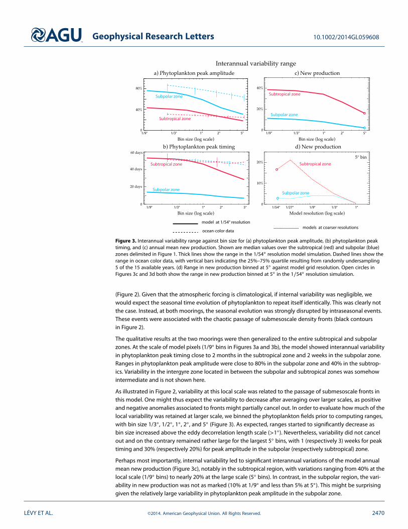
Figure 3. Interannual variability range against bin size for (a) phytoplankton peak amplitude, (b) phytoplankton peaktiming, and (c) annual mean new production. Shown are median values over the subtropical (red) and subpolar (blue)zones delimited in Figure 1. Thick lines show the range in the 1/54◦ resolution model simulation. Dashed lines show therange in ocean color data, with vertical bars indicating the 25%–75% quartile resulting from randomly undersampling5 of the 15 available years. (d) Range in new production binned at 5◦ against model grid resolution. Open circles inFigures 3c and 3d both show the range in new production binned at 5◦ in the 1∕54◦ resolution simulation.

(Figure 2). Given that the atmospheric forcing is climatological, if internal variability was negligible, wewould expect the seasonal time evolution of phytoplankton to repeat itself identically. This was clearly notthe case. Instead, at both moorings, the seasonal evolution was strongly disrupted by intraseasonal events.These events were associated with the chaotic passage of submesoscale density fronts (black contoursin Figure 2).

The qualitative results at the two moorings were then generalized to the entire subtropical and subpolarzones. At the scale of model pixels (1/9◦ bins in Figures 3a and 3b), the model showed interannual variabilityin phytoplankton peak timing close to 2 months in the subtropical zone and 2 weeks in the subpolar zone.Ranges in phytoplankton peak amplitude were close to 80% in the subpolar zone and 40% in the subtrop-ics. Variability in the intergyre zone located in between the subpolar and subtropical zones was somehowintermediate and is not shown here.

As illustrated in Figure 2, variability at this local scale was related to the passage of submesoscale fronts inthis model. One might thus expect the variability to decrease after averaging over larger scales, as positiveand negative anomalies associated to fronts might partially cancel out. In order to evaluate how much of thelocal variability was retained at larger scale, we binned the phytoplankton fields prior to computing ranges,with bin size 1/3◦, 1/2◦, 1◦, 2◦, and 5◦ (Figure 3). As expected, ranges started to significantly decrease asbin size increased above the eddy decorrelation length scale (>1◦). Nevertheless, variability did not cancelout and on the contrary remained rather large for the largest 5◦ bins, with 1 (respectively 3) weeks for peaktiming and 30% (respectively 20%) for peak amplitude in the subpolar (respectively subtropical) zone.

Perhaps most importantly, internal variability led to significant interannual variations of the model annualmean new production (Figure 3c), notably in the subtropical region, with variations ranging from 40% at thelocal scale (1/9◦ bins) to nearly 20% at the large scale (5◦ bins). In contrast, in the subpolar region, the vari-ability in new production was not as marked (10% at 1/9◦ and less than 5% at 5◦). This might be surprisinggiven the relatively large variability in phytoplankton peak amplitude in the subpolar zone.

LÉVY ET AL. ©2014. American Geophysical Union. All Rights Reserved. 2470

Geophysical Research Letters 10.1002/2014GL059608

High horizontal resolution is a necessary condition to simulate intense mesoscale eddy fields and associatedsubmesoscale fronts. The same model run at 1/9◦ horizontal resolution instead of 1/54◦ showed significantlylowered EKE, associated with fewer, shorter-lived, and less intense eddies [Lévy et al., 2010]. In order to assesswhich model resolution is needed to capture the full strength of the internally driven interannual variability,we used a series of similar model experiments run at decreasing horizontal resolution (1/27◦, 1/9◦, 1/3◦,and 1◦, see Lévy et al. [2012c]). We found a sharp decrease in internally driven interannual variability ofnew production in the subtropical zone when the resolution was below submesoscale permitting (>1/27◦,Figure 3d). The simulation with a resolution of 1/9◦ could only capture half of the interannual variabilitysimulated at 1/54◦, and this dropped to less than one third with a resolution of 1/3◦. At 1◦ resolution, eddyvariability was entirely suppressed and interannual variability vanished.

4. Discussion

Our model revealed significant interannual variability in surface phytoplankton bloom phenology, namely,in phytoplankton peak timing and peak amplitude. The simulated interannual variability ensued from sub-seasonal variations associated to the passage of submesoscale fronts. These fronts perturbed the meanseasonal cycle in a random manner, which lead to year-to-year fluctuations (Figure 2). These variations werelarge at the local scale of a model’s pixel, and did not cancel out after 5◦ binning (Figure 3). This suggestedthat interannual variations in ocean color images binned over scales of 1◦ to 5◦, as those commonly used forthe study of large-scale bloom dynamics [Martinez et al., 2009; Behrenfeld, 2010], arise not only from externalprocesses (atmospheric/climate forcings) but also from internal processes associated with mesoscale turbu-lence. This might partly elucidate why climate indices, although useful indicators, can never fully explain theobserved variability.

Interannual variability in our model resulted solely from internal processes, a contribution which is difficultto disentangle from observations alone. As a crude attempt to gain some insight on the relative importanceof internal variability to total interannual variability, we have repeated the interannual variability range anal-ysis using ocean color observations (dashed lines in Figures 3a and 3b). We used 15 years of multisatellite8 days chlorophyll composites available at 1/4◦ resolution (Glocolour product, http://www.globcolour.info/).Due to the very idealized nature of our model configuration, comparing the variability in the model and inthese observations is only indicative. Despite the limitation due to the idealized nature of our experiment,we found as expected that the interannual variability in the observations was larger than in the model over5◦ bins. Next we stipulate, for the purpose of this discussion, that this extra amount of variability ensuedfrom climate variability and atmospheric synoptic events. Interestingly, this rough comparison suggestedthat, both in the subpolar and subtropical zones, roughly half of the observed large-scale variability in phy-toplankton peak amplitude might be attributable to internal variability. This was also the case regardinglarge-scale phytoplankton peak timing in the subtropics. In contrast, only ∼1/5 of the observed variabilityin peak timing in the subpolar zone could be explained by internal variability, suggesting that the remain-ing 4/5 may be atmospherically driven. At small scale, the amplitude of small-scale interannual variabilityin the observations is likely to be underestimated, due to the large amount of missing data at this time andspace scale [Cole et al., 2012]. This underestimation, along with our model deficiencies, could explain somemismatches between the modeled and observed levels of variability for small bin size: the slopes of thephytoplankton peak timing and peak amplitude ranges against bin size were not as steep in the observa-tions as they were in the model, particularly in the subpolar zone, and the observed levels of variability forphytoplankton peak amplitude in the subtropics were unexpectedly below model estimates.

However, as stated above, these estimations must be handled with great care due to the simplicity of ourmodel. A more reliable assessment would require a realistic model configuration forced with the full spec-trum of atmospheric variability. If this realistic model captured the same amount of variability than in theobservations, it would be possible to isolate the contribution of internal drivers to interannual variability byperforming a twin model experiment forced by a repeating seasonal cycle as in Penduff et al. [2011].

Moreover, in our model, mesoscale turbulence is the only source of internal variability. Evidence for this isthat interannual variability cancels out when the model is run at 1◦ resolution (Figure 3d). However, inter-nal variability in the ocean might also arise from other processes not well captured in our model, such asunforced interdecadal modes of the thermohaline circulation [Huck et al., 2001] or oscillations in populationdynamics [Poggiale et al., 2013].

LÉVY ET AL. ©2014. American Geophysical Union. All Rights Reserved. 2471

Geophysical Research Letters 10.1002/2014GL059608

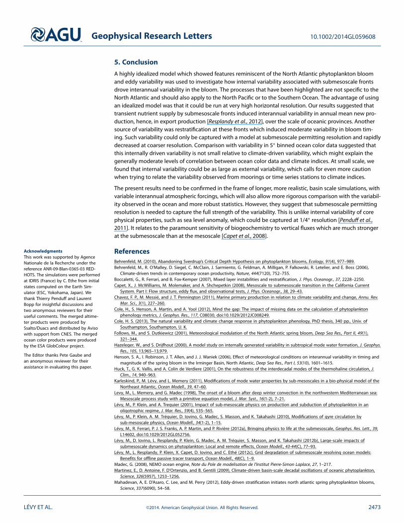
Figure 4. (a) Mean (color bars) ±𝜎 (black horizontal lines) of the annualadvective (blue) and diffusive (red) sources of nitrate into the upper 120 m,binned at 5◦ and averaged over the subtropical and subpolar zones shownin Figure 1a. (b) Range in bloom peak timing (reported from Figure 3b)against bin size, compared with the range in the restratification date(dashed line, defined as the date at which the mixed layer depth hasshoaled above 50 m).

Due to computational and storageconstraints, only 5 years of model out-puts were available. Given this rathersmall number, we checked the accu-racy of our estimate over the oceancolor data set, for which 15 years wereavailable. This was done by randomlyselecting 5 of the 15 years, 100 times,and by computing the 25%–75%quartile over the 100 different esti-mates of 𝜎 (vertical lines in Figures 3aand 3b). This revealed a median accu-racy of the order of 10% on peakamplitude and 5 days in peak timing.Our detected changes are well abovethis threshold error confirming therobustness of the results discussed inthis paper.

Our model also revealed significantinterannual variability in 5◦ binnedannual new production, particularlyin the subtropical gyre, of the order∼20% (Figure 3c). The full strengthof this signal could only be capturedat fine (Δx < 1∕27◦) horizontal reso-lution (Figure 3d). This suggested thatintermittent vertical advection at sub-mesoscale fronts (whose full strengthrequires high resolution) could be

responsible for the observed interannual variability. This was further confirmed by a more detailed anal-ysis of the nitrate budget in the euphotic layer. This budget exhibited large interannual variability in theadvective (and to a lesser extent, in the diffusive) supply of nitrate in both regions (Figure 4a). In the sub-tropics, the magnitude of this variability was large enough to overcome the mean advective loss of nitratewhich resulted from downward Ekman pumping [Lévy et al., 2012b]; hence, the actual sign of the annualnitrate supply to the subtropical zone varied interannually. The intermittent nature of these nitrate pulsesalso explained the variability in phytoplankton peak timing in the otherwise depleted subtropics with someof the peaks being in fact associated with such events (Figure 2a).

Another potential internal mechanism that could drive interannual variability in bloom peak timing isrestratification by submesoscales [Boccaletti et al., 2007]. This process induced interannual variations of thetime at which the mixed layer shoaled between winter and spring in our model (dashed lines in Figure 4b).To test this hypothesis, we compared this restratification date range to the peak date range (Figure 4b). Inthe subtropics, the restratification date range was only about half of the peak date range illustrating thatvarying restratification times was not sufficient to explain the large variability in peak dates. Indeed, as men-tioned before, part of this variability can be attributable to the time variability in nutrient supply pulses.However, in the subpolar zone, the two ranges are closer which supports the hypothesis that submesoscalestratification could be responsible for the simulated interannual variability in bloom timing. This is also illus-trated in Figures 2b and 2d where a strong submesoscale front causes an earlier mixed layer shoaling anda phytoplankton peak occurring 1 week earlier in year 1 than in year 2. It should be reminded, however,that the effect of submesoscale restratification on bloom timing is rather small compared with the atmo-spherically driven variability (Figure 3a) and has only marginal consequences on the annual new productionbudget (Figure 3c).

LÉVY ET AL. ©2014. American Geophysical Union. All Rights Reserved. 2472

Geophysical Research Letters 10.1002/2014GL059608

5. Conclusion

A highly idealized model which showed features reminiscent of the North Atlantic phytoplankton bloomand eddy variability was used to investigate how internal variability associated with submesoscale frontsdrove interannual variability in the bloom. The processes that have been highlighted are not specific to theNorth Atlantic and should also apply to the North Pacific or to the Southern Ocean. The advantage of usingan idealized model was that it could be run at very high horizontal resolution. Our results suggested thattransient nutrient supply by submesoscale fronts induced interannual variability in annual mean new pro-duction, hence, in export production [Resplandy et al., 2012], over the scale of oceanic provinces. Anothersource of variability was restratification at these fronts which induced moderate variability in bloom tim-ing. Such variability could only be captured with a model at submesoscale permitting resolution and rapidlydecreased at coarser resolution. Comparison with variability in 5◦ binned ocean color data suggested thatthis internally driven variability is not small relative to climate-driven variability, which might explain thegenerally moderate levels of correlation between ocean color data and climate indices. At small scale, wefound that internal variability could be as large as external variability, which calls for even more cautionwhen trying to relate the variability observed from moorings or time series stations to climate indices.

The present results need to be confirmed in the frame of longer, more realistic, basin scale simulations, withvariable interannual atmospheric forcings, which will also allow more rigorous comparison with the variabil-ity observed in the ocean and more robust statistics. However, they suggest that submesoscale permittingresolution is needed to capture the full strength of the variability. This is unlike internal variability of corephysical properties, such as sea level anomaly, which could be captured at 1/4◦ resolution [Penduff et al.,2011]. It relates to the paramount sensitivity of biogeochemistry to vertical fluxes which are much strongerat the submesoscale than at the mesoscale [Capet et al., 2008].

ReferencesBehrenfeld, M. (2010), Abandoning Sverdrup’s Critical Depth Hypothesis on phytoplankton blooms, Ecology, 91(4), 977–989.Behrenfeld, M., R. O’Malley, D. Siegel, C. McClain, J. Sarmiento, G. Feldman, A. Milligan, P. Falkowski, R. Letelier, and E. Boss (2006),

Climate-driven trends in contemporary ocean productivity, Nature, 444(7120), 752–755.Boccaletti, G., R. Ferrari, and B. Fox-Kemper (2007), Mixed layer instabilities and restratification, J. Phys. Oceanogr., 37, 2228–2250.Capet, X., J. McWilliams, M. Molemaker, and A. Shchepetkin (2008), Mesoscale to submesoscale transition in the California Current

System. Part I: Flow structure, eddy flux, and observational tests, J. Phys. Oceanogr., 38, 29–43.Chavez, F. P., M. Messié, and J. T. Pennington (2011), Marine primary production in relation to climate variability and change, Annu. Rev.

Mar. Sci., 3(1), 227–260.Cole, H., S. Henson, A. Martin, and A. Yool (2012), Mind the gap: The impact of missing data on the calculation of phytoplankton

phenology metrics, J. Geophys. Res., 117, C08030, doi:10.1029/2012JC008249.Cole, H. S. (2013), The natural variability and climate change response in phytoplankton phenology, PhD thesis, 340 pp., Univ. of

Southampton, Southampton, U. K.Follows, M., and S. Dutkiewicz (2001), Meteorological modulation of the North Atlantic spring bloom, Deep Sea Res., Part II, 49(1),

321–344.Hazeleger, W., and S. Drijfhout (2000), A model study on internally generated variability in subtropical mode water formation, J. Geophys.

Res., 105, 13,965–13,979.Henson, S. A., I. Robinson, J. T. Allen, and J. J. Waniek (2006), Effect of meteorological conditions on interannual variability in timing and

magnitude of the spring bloom in the Irminger Basin, North Atlantic, Deep Sea Res., Part I, 53(10), 1601–1615.Huck, T., G. K. Vallis, and A. Colin de Verdiere (2001), On the robustness of the interdecadal modes of the thermohaline circulation, J.

Clim., 14, 940–963.Karleskind, P., M. Lévy, and L. Memery (2011), Modifications of mode water properties by sub-mesoscales in a bio-physical model of the

Northeast Atlantic, Ocean Modell., 39, 47–60.Levy, M., L. Memery, and G. Madec (1998), The onset of a bloom after deep winter convection in the northwestern Mediterranean sea:

Mesoscale process study with a primitive equation model, J. Mar. Syst., 16(1-2), 7–21.Lévy, M., P. Klein, and A. Treguier (2001), Impact of sub-mesoscale physics on production and subduction of phytoplankton in an

oligotrophic regime, J. Mar. Res., 59(4), 535–565.Lévy, M., P. Klein, A. M. Tréguier, D. Iovino, G. Madec, S. Masson, and K. Takahashi (2010), Modifications of gyre circulation by

sub-mesoscale physics, Ocean Modell., 34(1-2), 1–15.Lévy, M., R. Ferrari, P. J. S. Franks, A. P. Martin, and P. Rivière (2012a), Bringing physics to life at the submesoscale, Geophys. Res. Lett., 39,

L14602, doi:10.1029/2012GL052756.Lévy, M., D. Iovino, L. Resplandy, P. Klein, G. Madec, A. M. Tréguier, S. Masson, and K. Takahashi (2012b), Large-scale impacts of

submesoscale dynamics on phytoplankton: Local and remote effects, Ocean Modell., 43-44(C), 77–93.Lévy, M., L. Resplandy, P. Klein, X. Capet, D. Iovino, and C. Ethé (2012c), Grid degradation of submesoscale resolving ocean models:

Benefits for offline passive tracer transport, Ocean Modell., 48(C), 1–9.Madec, G. (2008), NEMO ocean engine, Note du Pole de modelisation de l’Institut Pierre-Simon Laplace, 27, 1–217.Martinez, E., D. Antoine, F. D’Ortenzio, and B. Gentili (2009), Climate-driven basin-scale decadal oscillations of oceanic phytoplankton,

Science, 326(5957), 1253–1256.Mahadevan, A, E. D’Asaro, C. Lee, and M. Perry (2012), Eddy-driven stratification initiates north atlantic spring phytoplankton blooms,

Science, 337(6090), 54–58.

AcknowledgmentsThis work was supported by AgenceNationale de la Recherche under thereference ANR-09-Blan-0365-03 RED-HOTS. The simulations were performedat IDRIS (France) by C. Ethe from initialstates computed on the Earth Sim-ulator (ESC, Yokohama, Japan). Wethank Thierry Penduff and LaurentBopp for insightful discussions andtwo anonymous reviewers for theiruseful comments. The merged altime-ter products were produced bySsalto/Duacs and distributed by Avisowith support from CNES. The mergedocean color products were producedby the ESA GlobColour project.

The Editor thanks Pete Gaube andan anonymous reviewer for theirassistance in evaluating this paper.

LÉVY ET AL. ©2014. American Geophysical Union. All Rights Reserved. 2473

Geophysical Research Letters 10.1002/2014GL059608

McGillicuddy, D., A. Robinson, D. Siegel, H. Jannasch, R. Johnson, T. Dickey, J. McNeil, A. Michaels, and A. Knap (1998), Influence ofmesoscale eddies on new production in the Sargasso Sea, Nature, 394(6690), 263–266.

Penduff, T., B. Barnier, W. K. Dewar, and J. J. O’Brien (2004), Dynamical response of the oceanic eddy field to the North Atlantic Oscillation:A model-data comparison, J. Phys. Oceanogr., 34(12), 2615–2629.

Penduff, T., M. Juza, B. Barnier, J. Zika, W. K. Dewar, A.-M. Treguier, J.-M. Molines, and N. Audiffren (2011), Sea Level expression of intrinsicand forced ocean variabilities at interannual time scales, J. Clim., 24(21), 5652–5670.

Poggiale, J. C., Y. Eynaud, and M. Baklouti (2013), Impact of periodic nutrient input rate on trophic chain properties, Ecol. Complexity, 14,56–63.

Resplandy, L., A. P. Martin, F. Le Moigne, P. Martin, A. Aquilina, L. Mémery, M. Lévy, and R. Sanders (2012), How does dynamical spatialvariability impact 234Th-derived estimates of organic export?, Deep Sea Res., Part I, 68(C), 24–45.

Rousseaux, C., and W. Gregg (2014), Interannual variation in phytoplankton primary production at a global scale, Remote Sens., 6(1), 1–19.Thomas, M. D., and X. Zhai (2013), Eddy-induced variability of the meridional overturning circulation in a model of the North Atlantic,

Geophys. Res. Lett., 40, 2742–2747, doi:10.1002/grl.50532.Williams, R. G., C. Wilson, and C. W. Hughes (2007), Ocean and atmosphere storm tracks: The role of eddy vorticity forcing, J. Phys.

Oceanogr., 37(9), 2267–2289.

LÉVY ET AL. ©2014. American Geophysical Union. All Rights Reserved. 2474