from accreting and transitional millisecond pulsars to rotation ...
Astronomy & Astrophysics manuscript no. lofarPSR c© ESO 2011April 11, 2011
Observing pulsars and fast transients with LOFARB. W. Stappers1, J. W. T. Hessels2,3 A. Alexov3, K. Anderson3, T. Coenen3, T. Hassall1, A. Karastergiou4,
V. I. Kondratiev2, M. Kramer5,1, J. van Leeuwen2,3, J. D. Mol2, A. Noutsos5, J. W. Romein2,P. Weltevrede1, R. Fender6, R. A. M. J. Wijers3, L. Bahren3, M. E. Bell6, J. Broderick6, E. J. Daw8,
V. S. Dhillon8, J. Eisloffel19, H. Falcke12,2, J. Griessmeier2,22, C. Law24,3, S. Markoff3
J. C. A. Miller-Jones13,3, B. Scheers3, H. Spreeuw3, J. Swinbank3, S. ter Veen12 M. W. Wise2,3,O. Wucknitz17, P. Zarka16, J. Anderson5, A. Asgekar2, I. M. Avruch2,10, R. Beck5, P. Bennema2,M. J. Bentum2, P. Best15, J. Bregman2, M. Brentjens2, R. H. van de Brink2, P. C. Broekema2,
W. N. Brouw10, M. Bruggen21, A. G. de Bruyn2,10, H. R. Butcher2,26, B. Ciardi7, J. Conway11, R.-J.Dettmar20, A. van Duin2, J. van Enst2, M. Garrett2,9, M. Gerbers2, T. Grit2, A. Gunst2, M. P. van
Haarlem2, J. P. Hamaker2 G. Heald2, M. Hoeft19, H. Holties2, A. Horneffer5,12, L. V. E. Koopmans10,G. Kuper2, M. Loose2, P. Maat2, D. McKay-Bukowski14, J. P. McKean2, G. Miley9, R. Morganti2,10,
R. Nijboer2, J. E. Noordam2, M. Norden2, H. Olofsson11, M. Pandey-Pommier9,25, A. Polatidis2, W. Reich5,H. Rottgering9, A. Schoenmakers2, J. Sluman2, O. Smirnov2, M. Steinmetz18, C. G. M. Sterks23,
M. Tagger22, Y. Tang2, R. Vermeulen2, N. Vermaas2, C. Vogt2, M. de Vos2, S. J. Wijnholds2, S. Yatawatta10,and A. Zensus5
1 Jodrell Bank Center for Astrophysics, School of Physics and Astronomy, The University of Manchester, ManchesterM13 9PL,UK e-mail: [email protected]
2 Netherlands Institute for Radio Astronomy (ASTRON), Postbus 2, 7990 AA Dwingeloo, The Netherlands3 Astronomical Institute ’Anton Pannekoek’, University of Amsterdam, Postbus 94249, 1090 GE Amsterdam, The
Netherlands4 Astrophysics, University of Oxford, Denys Wilkinson Building, Keble Road, Oxford OX1 3RH5 Max-Planck-Institut fur Radioastronomie, Auf dem Hugel 69, 53121 Bonn, Germany6 School of Physics and Astronomy, University of Southampton, Southampton, SO17 1BJ, UK7 Max Planck Institute for Astrophysics, Karl Schwarzschild Str. 1, 85741 Garching, Germany8 Department of Physics & Astronomy, Hicks Building, Hounsfield Road, Sheffield S3 7RH, United Kingdom9 Leiden Observatory, Leiden University, PO Box 9513, 2300 RA Leiden, The Netherlands
10 Kapteyn Astronomical Institute, PO Box 800, 9700 AV Groningen, The Netherlands11 Onsala Space Observatory, Dept. of Earth and Space Sciences, Chalmers University of Technology, SE-43992 Onsala,
Sweden12 Department of Astrophysics/IMAPP, Radboud University Nijmegen, P.O. Box 9010, 6500 GL Nijmegen, The
Netherlands13 International Centre for Radio Astronomy Research - Curtin University, GPO Box U1987, Perth, WA 6845, Australia14 STFC Rutherford Appleton Laboratory, Harwell Science and Innovation Campus, Didcot OX11 0QX, UK15 Institute for Astronomy, University of Edinburgh, Royal Observatory of Edinburgh, Blackford Hill, Edinburgh EH9
3HJ, UK16 LESIA, UMR CNRS 8109, Observatoire de Paris, 92195 Meudon, France17 Argelander-Institut fur Astronomie, University of Bonn, Auf dem Hugel 71, 53121, Bonn, Germany18 Leibniz-Institut fr Astrophysik Potsdam (AIP), An der Sternwarte 16, 14482 Potsdam, Germany19 Thuringer Landessternwarte, Sternwarte 5, D-07778 Tautenburg, Germany20 Astronomisches Institut der Ruhr-Universitat Bochum, Universitaetsstrasse 150, 44780 Bochum, Germany21 Jacobs University Bremen, Campus Ring 1, 28759 Bremen, Germany22 Laboratoire de Physique et Chimie de lEnvironnement et de lEspace, CNRS/Universit dOrlans, France23 Center for Information Technology (CIT), University of Groningen, The Netherlands24 Radio Astronomy Lab, UC Berkeley, CA, USA25 Centre de Recherche Astrophysique de Lyon, Observatoire de Lyon, 9 av Charles Andre, 69561 Saint Genis Laval
Cedex, France26 Mt Stromlo Observatory, Research School of Astronomy and Astrophysics, Australian National University, Weston,
A.C.T. 2611, Australia
ABSTRACT
Low frequency radio waves, while challenging to observe, are a rich source of information about pulsars. The LOwFrequency ARray (LOFAR) is a new radio interferometer operating in the lowest 4 octaves of the ionospheric ”radiowindow”: 10-240MHz, that will greatly facilitate observing pulsars at low radio frequencies. Through the huge collectingarea, long baselines, and flexible digital hardware, it is expected that LOFAR will revolutionize radio astronomy atthe lowest frequencies visible from Earth. LOFAR is a next-generation radio telescope and a pathfinder to the SquareKilometre Array (SKA), in that it incorporates advanced multi-beaming techniques between thousands of individualelements. We discuss the motivation for low-frequency pulsar observations in general and the potential of LOFAR inaddressing these science goals. We present LOFAR as it is designed to perform high-time-resolution observations ofpulsars and other fast transients, and outline the various relevant observing modes and data reduction pipelines that arealready or will soon be implemented to facilitate these observations. A number of results obtained from commissioningobservations are presented to demonstrate the exciting potential of the telescope. This paper outlines the case for lowfrequency pulsar observations and is also intended to serve as a reference for upcoming pulsar/fast transient sciencepapers with LOFAR.
Key words. telescopes:LOFAR – pulsars:general – instrumentation:interferometric – methods:observational –stars:neutron – ISM:general
1
arX
iv:1
104.
1577
v1 [
astr
o-ph
.IM
] 8
Apr
201
1
1. Introduction
Pulsars are rapidly rotating, highly magnetised neutronstars that were first identified via pulsed radio emission atthe very low radio observing frequency of 81 MHz (Hewishet al., 1968). They have subsequently been shown to emitpulsations across the electromagnetic spectrum, at frequen-cies ranging from 17 MHz to above 87 GHz (e.g. Bruk &Ustimenko 1976, 1977; Morris et al. 1997) in the radio andat optical, X-ray and γ-ray wavelengths (see Thompson2000 and references therein), although the vast majorityare seen to emit only at radio wavelengths. These pulsa-tions provide invaluable insights into the nature of neutronstar physics, and most neutron stars would be otherwiseundetectable with current telescopes. Though radio pul-sars form over 85% of the known neutron star population,they are generally very weak radio sources with pulsed fluxdensities ranging from 0.0001 to 5 Jy with a median of0.01 Jy at a frequency of 400 MHz. The pulsed flux densityat radio wavelengths exhibits a steep spectrum (S ∝ να;−4 < α < 0; αmean = −1.8, (Maron et al., 2000) that of-ten peaks and turns over at frequencies between 100 and200 MHz (Kuzmin et al., 1978; Slee et al., 1986; Malofeevet al., 1994).
After their discovery, a lot of the early work on pulsars(e.g. Cole 1969; Staelin & Reifenstein 1968; Rankin et al.1970) continued at low radio frequencies (defined here as< 300 MHz). However, despite the fact that most pulsarsare intrinsically brightest in this frequency range, since thenthe vast majority of pulsars have been discovered and stud-ied at frequencies in the range 300 − 2000 MHz; much ofour knowledge of the properties of the radio emission mech-anism stems from studies at these frequencies and above.There are three main reasons for this (see Sect. 3): the dele-terious effects of the interstellar medium (ISM) on pulsedsignals; the effective background sky temperature of theGalactic synchrotron emission; and ionospheric effects. Allthree of these effects have steep power law dependencieson frequency and therefore become worse towards lowerfrequencies. Combined with the generally steep spectra ofpulsars, these effects conspire to make observing frequen-cies of ∼ 300−2000 MHz the range of choice for most pulsarstudies and searches.
However, despite these challenges, there are many rea-sons why it is important and interesting to observe pul-sars in a significantly lower frequency regime than nowcommonly used; these are discussed in detail in Sect.4. In recent years some excellent studies have contin-ued at frequencies between 20−110 MHz mainly usingthe Pushchino, Gauribidanur and UTR-2 telescopes (e.g.Malov & Malofeev 2010; Malofeev et al. 2000; Asgekar &Deshpande 2005; Popov et al. 2006b; Ulyanov et al. 2006).These studies have begun to map, e.g., the low-frequencyspectra, pulse morphologies, and pulse energy distributionsof pulsars, but have in some cases been limited by the avail-able bandwidths and/or polarisation and tracking capabil-ities of these telescopes (see Sect. 2).
The Low Frequency Array (LOFAR) was designed andconstructed by ASTRON, the Netherlands Institute forRadio Astronomy, and has facilities in several countries,that are owned by various parties (each with their ownfunding sources), and that are collectively operated by theInternational LOFAR Telescope (ILT) foundation under ajoint scientific policy. LOFAR provides a great leap forward
in low-frequency radio observations by providing large frac-tional bandwidths and sophisticated multi-beaming capa-bilities. In this paper we present the LOFAR telescope as itwill be used for pulsar and other high-time-resolution beam-formed observations; this will serve as a reference for futurescience papers that use these LOFAR modes. We also de-scribe the varied pulsar and fast transient science LOFARwill enable and present commissioning results showing howthat potential is already being realised. LOFAR is wellsuited for the study of known sources, and its huge field ofview (FoV) makes it a powerful survey telescope for find-ing new pulsars and other “fast-transients”. In Sect. 2 wepresent the basic design parameters of the LOFAR tele-scope. The challenges associated with observing at low ra-dio frequencies and how they can be mitigated with LOFARwill be discussed in Sect. 3. A detailed description of thescience that will be possible with LOFAR is presented inSect. 4. The flexible nature of LOFAR means that thereare many possible observing modes; these are introduced inSect. 5. In Sect. 6 we discuss the different pulsar pipelinesthat are being implemented. Commissioning results, whichdemonstrate that LOFAR is already performing pulsar andfast transients observations of high quality, are presented inSect. 7. We summarise the potential of LOFAR for futurepulsar observations in Sect. 8.
2. LOFAR
Instrumentation in radio astronomy is undergoing a revo-lution that will exploit massive computing, clever antennadesign, and digital signal processing to greatly increase theinstantaneous FoV and bandwidth of observations. Thiswork is part of the international effort to create the “SquareKilometre Array” (Carilli & Rawlings, 2004), a radio tele-scope orders of magnitude better than its predecessors.
One of the first “next generation” radio telescopes toimplement these techniques is LOFAR, which operates inthe frequency range 10 − 240 MHz. The large collectingarea of LOFAR is comprised of many thousands of dipoleantennas, hierarchically arranged in stations which come inthree different configurations (Table 1). These stations aredistributed in a sparse array with a denser core region nearExloo, the Netherlands, extending out to remote stations inthe Netherlands and then on further to stations in France,Germany, Sweden and the United Kingdom. There are atotal of 40 stations in the Netherlands and 8 internationalstations, with the prospect of more to come. A schematicdiagram of some of the LOFAR stations in the inner coreof LOFAR − the “Superterp” as it is known − is shown inFigure 1. As will be discussed in more detail later, pulsarobservations can utilise all of these stations to achieve a va-riety of diverse science goals. Details of system architectureand signal processing can be found in de Vos et al. (2009)and a full description of LOFAR will soon be published (vanHaarlem et al. in prep.) we limit the discussion only to themost important points related to pulsar observations.
LOFAR has two different types of antennas to coverthe frequency range 10–240 MHz. The low band anten-nas, LBAs, cover the frequency range 10–90 MHz, althoughthey are optimised for frequencies above 30 MHz. The lowerlimit of 10 MHz is defined by transmission of radio wavesthrough the Earth’s ionosphere. There are 48/96 activeLBA dipoles in each Dutch/international station (Table 1).The high band antennas, HBAs, cover the frequency range

B. W. Stappers et al.: Observing pulsars and fast transients with LOFAR
Fig. 1. Three successive zoom-outs showing the stations in the LOFAR core. The different scales of the hierarchically organisedHBA elements are highlighted and their respective beam sizes are shown. The large circular area marks the edge of the Superterp,which contains the inner-most 6 stations (i.e. 12 HBA sub-stations: where there are 2 sub-stations, each of 24 tiles, in each HBAcore station); other core stations can be seen highlighted beyond the Superterp in the third panel. Left: a single HBA tile andassociated beam. Middle: A single HBA sub-station with three simultaneous station beams. Right: The 6 stations of the Superterpplus 3 core stations in the background are highlighted. Four independent beams formed from the coherent combination of all 24core HBA stations, most of which are outside this photo, are shown. For the LBA stations, a similar scheme applies except thateach LBA dipole can effectively see the whole sky. Fields of the relatively sparsely distributed LBA antennas are visible in betweenthe highlighted HBA stations in all three panels.
110–240 MHz, and consist of 16 folded dipoles grouped intotiles of 4× 4 dipoles each, which are phased together usingan analogue beamformer within the tile itself. There are48/96 tiles in each Dutch/international station, with a sep-aration into two sub-stations of 24 HBA tiles each in thecase of core stations1.
The received radio waves are sampled at either 160 or200 MHz in one of three different Nyquist zones to accessthe frequency ranges 0–100, 100–200 and 160–240 MHz.There are filters in place to optionally remove frequen-cies below 30 MHz and the FM band approximately en-compassing 90–110 MHz. The 80 or 100 MHz wide bandsare filtered at the stations into 512 subbands of exactly156.25/195.3125 kHz using a poly-phase filter. Up to 244of these subbands can be transported back to the CentralProcessor, CEP, giving a maximum instantaneous band-width of about 39/48 MHz2. There is no restriction onwhich 244 of the 512 subbands can be selected to be pro-cessed at CEP, therefore this bandwidth can be distributedthroughout the entire available 80/100 MHz. Alternativelyit is possible to portion out the bandwidth into multiplebeams. Previously there was a limit of eight per station,however a recent new implementation of the beam serversoftware has enabled each of the 244 subbands to be pointedin a different direction. These subbands can be further di-vided into narrower frequency channels in CEP as will bediscussed below. The degree of flexibility afforded by thesechoices of frequency and beams allows a wide range of high-time-resolution pulsar-like observations with LOFAR; thesedifferent modes are described in detail in Sect. 5.
1 We note that when we refer to dipoles and tiles we are gen-erally referring to both the X and Y polarisations together, thatis dipole pairs, and we draw a distinction between the two po-larisations only when necessary.
2 This number may further increase if the number of bits usedto describe each sample is reduced.
Table 1. Arrangement of elements in LOFAR stations.
Station Type LBA (no.) HBA tiles (no.) Baseline (km)Core 2×48 2×24 0.1− 1Remote 2×48 48 1− 10sInternational 96 96 ∼ 100s
Notes. Arrangement of elements in the three types of LOFARstations, along with their typical distance from the center ofthe array (baseline). In the Core and Remote stations there are96 LBA dipoles but only 48 can be beamformed at any onetime. For these stations, one can select either the inner circleor the outer ring of 48 LBA dipoles depending on the sciencerequirements. The HBA sub-stations can be correlated, or usedin beamforming, independently.
In Table 2 we compare the properties of LOFAR withthose of other telescopes currently operating in (part of)the same frequency range. LOFAR is the only existing orplanned telescope capable of covering the entire lowest 4 oc-taves of the radio window (10−240 MHz, above the Earth’sionospheric cut-off). In some modes this entire range can beobserved simultaneously (see Sect. 5). LOFAR’s total effec-tive collecting area and instantaneous sensitivity places itat the forefront of existing low-frequency radio telescopes,especially in the range 100− 240 MHz, but collecting areais only one aspect of LOFAR’s capabilities. As will be de-scribed in more detail later, LOFAR offers many advantagesover current telescopes through its multi-beaming capabil-ities, flexible backend, high spatial resolution, large instan-taneous bandwidth, wide total available frequency range,ability to track, and ability to observe a large fraction ofthe sky (i.e. declinations greater than −30 degrees, see Sect.5).
3
B. W. Stappers et al.: Observing pulsars and fast transients with LOFAR
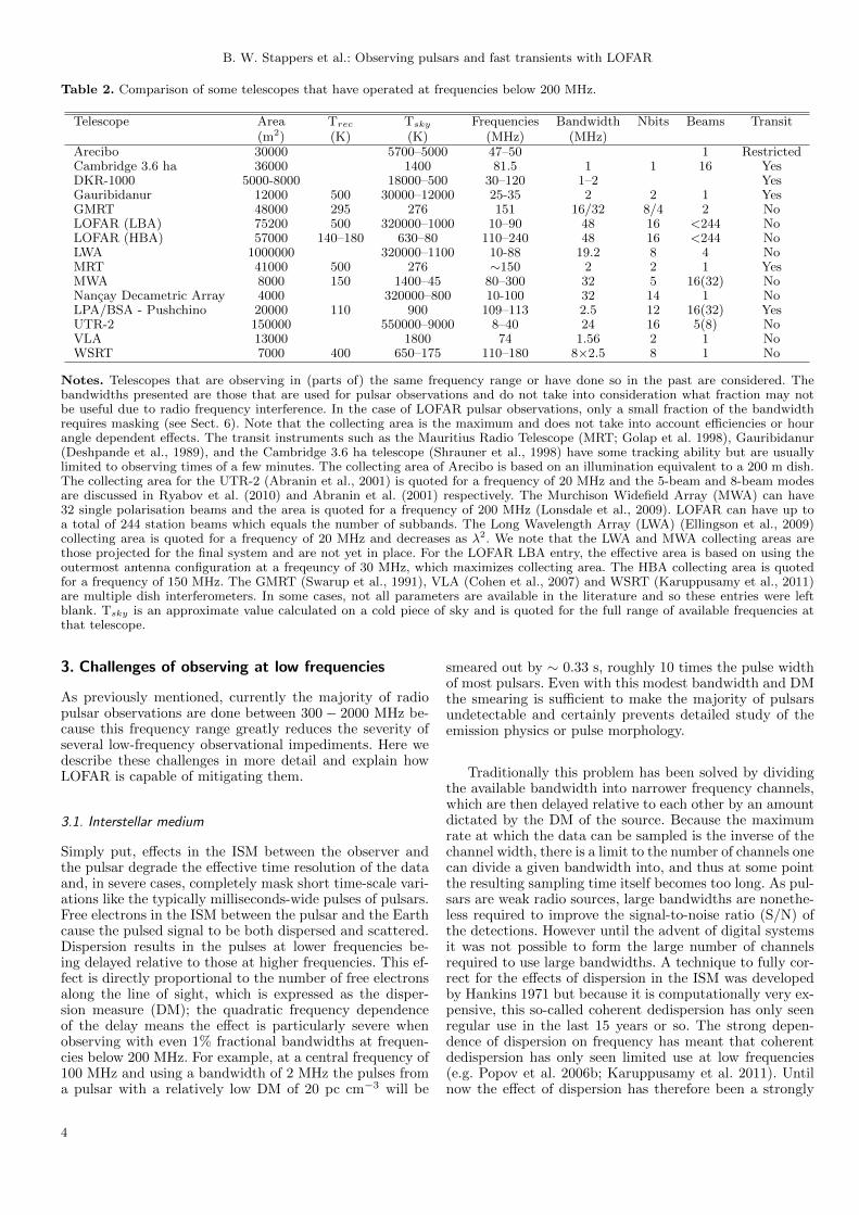
Table 2. Comparison of some telescopes that have operated at frequencies below 200 MHz.
Telescope Area Trec Tsky Frequencies Bandwidth Nbits Beams Transit(m2) (K) (K) (MHz) (MHz)
Arecibo 30000 5700–5000 47–50 1 RestrictedCambridge 3.6 ha 36000 1400 81.5 1 1 16 YesDKR-1000 5000-8000 18000–500 30–120 1–2 YesGauribidanur 12000 500 30000–12000 25-35 2 2 1 YesGMRT 48000 295 276 151 16/32 8/4 2 NoLOFAR (LBA) 75200 500 320000–1000 10–90 48 16 <244 NoLOFAR (HBA) 57000 140–180 630–80 110–240 48 16 <244 NoLWA 1000000 320000–1100 10-88 19.2 8 4 NoMRT 41000 500 276 ∼150 2 2 1 YesMWA 8000 150 1400–45 80–300 32 5 16(32) NoNancay Decametric Array 4000 320000–800 10-100 32 14 1 NoLPA/BSA - Pushchino 20000 110 900 109–113 2.5 12 16(32) YesUTR-2 150000 550000–9000 8–40 24 16 5(8) NoVLA 13000 1800 74 1.56 2 1 NoWSRT 7000 400 650–175 110–180 8×2.5 8 1 No
Notes. Telescopes that are observing in (parts of) the same frequency range or have done so in the past are considered. Thebandwidths presented are those that are used for pulsar observations and do not take into consideration what fraction may notbe useful due to radio frequency interference. In the case of LOFAR pulsar observations, only a small fraction of the bandwidthrequires masking (see Sect. 6). Note that the collecting area is the maximum and does not take into account efficiencies or hourangle dependent effects. The transit instruments such as the Mauritius Radio Telescope (MRT; Golap et al. 1998), Gauribidanur(Deshpande et al., 1989), and the Cambridge 3.6 ha telescope (Shrauner et al., 1998) have some tracking ability but are usuallylimited to observing times of a few minutes. The collecting area of Arecibo is based on an illumination equivalent to a 200 m dish.The collecting area for the UTR-2 (Abranin et al., 2001) is quoted for a frequency of 20 MHz and the 5-beam and 8-beam modesare discussed in Ryabov et al. (2010) and Abranin et al. (2001) respectively. The Murchison Widefield Array (MWA) can have32 single polarisation beams and the area is quoted for a frequency of 200 MHz (Lonsdale et al., 2009). LOFAR can have up toa total of 244 station beams which equals the number of subbands. The Long Wavelength Array (LWA) (Ellingson et al., 2009)collecting area is quoted for a frequency of 20 MHz and decreases as λ2. We note that the LWA and MWA collecting areas arethose projected for the final system and are not yet in place. For the LOFAR LBA entry, the effective area is based on using theoutermost antenna configuration at a freqeuncy of 30 MHz, which maximizes collecting area. The HBA collecting area is quotedfor a frequency of 150 MHz. The GMRT (Swarup et al., 1991), VLA (Cohen et al., 2007) and WSRT (Karuppusamy et al., 2011)are multiple dish interferometers. In some cases, not all parameters are available in the literature and so these entries were leftblank. Tsky is an approximate value calculated on a cold piece of sky and is quoted for the full range of available frequencies atthat telescope.
3. Challenges of observing at low frequencies
As previously mentioned, currently the majority of radiopulsar observations are done between 300− 2000 MHz be-cause this frequency range greatly reduces the severity ofseveral low-frequency observational impediments. Here wedescribe these challenges in more detail and explain howLOFAR is capable of mitigating them.
3.1. Interstellar medium
Simply put, effects in the ISM between the observer andthe pulsar degrade the effective time resolution of the dataand, in severe cases, completely mask short time-scale vari-ations like the typically milliseconds-wide pulses of pulsars.Free electrons in the ISM between the pulsar and the Earthcause the pulsed signal to be both dispersed and scattered.Dispersion results in the pulses at lower frequencies be-ing delayed relative to those at higher frequencies. This ef-fect is directly proportional to the number of free electronsalong the line of sight, which is expressed as the disper-sion measure (DM); the quadratic frequency dependenceof the delay means the effect is particularly severe whenobserving with even 1% fractional bandwidths at frequen-cies below 200 MHz. For example, at a central frequency of100 MHz and using a bandwidth of 2 MHz the pulses froma pulsar with a relatively low DM of 20 pc cm−3 will be
smeared out by ∼ 0.33 s, roughly 10 times the pulse widthof most pulsars. Even with this modest bandwidth and DMthe smearing is sufficient to make the majority of pulsarsundetectable and certainly prevents detailed study of theemission physics or pulse morphology.
Traditionally this problem has been solved by dividingthe available bandwidth into narrower frequency channels,which are then delayed relative to each other by an amountdictated by the DM of the source. Because the maximumrate at which the data can be sampled is the inverse of thechannel width, there is a limit to the number of channels onecan divide a given bandwidth into, and thus at some pointthe resulting sampling time itself becomes too long. As pul-sars are weak radio sources, large bandwidths are nonethe-less required to improve the signal-to-noise ratio (S/N) ofthe detections. However until the advent of digital systemsit was not possible to form the large number of channelsrequired to use large bandwidths. A technique to fully cor-rect for the effects of dispersion in the ISM was developedby Hankins 1971 but because it is computationally very ex-pensive, this so-called coherent dedispersion has only seenregular use in the last 15 years or so. The strong depen-dence of dispersion on frequency has meant that coherentdedispersion has only seen limited use at low frequencies(e.g. Popov et al. 2006b; Karuppusamy et al. 2011). Untilnow the effect of dispersion has therefore been a strongly
4

B. W. Stappers et al.: Observing pulsars and fast transients with LOFAR
limiting factor on the number and types of pulsars whichcan be observed at low frequencies.
Furthermore, the ionised ISM is not distributed evenlyand the inhomogeneities along a given line of sight be-tween the Earth and a pulsar will cause the pulsed signalto take multiple paths, resulting in the pulse being scat-tered. Depending on the scattering regime, either strong orweak (Rickett, 1990), along a particular sight line, the de-gree of temporal scattering of the pulse profile can scale assteeply as ν−4.4. Along a given line of sight it also showsa dependence on the total electron content, i.e. DM, butthere are deviations from this relation of at least an order ofmagnitude (Bhat et al., 2004). Considering the same pulsarand observing frequecy and system as discussed in the firstparagraph of this section, and using the relation betweendispersion measure and scattering from Bhat et al. (2004)we find that the scattering delay would lie between 0.01 and1 seconds. The stochastic nature of scattering means that itis difficult to uniquely correct for it without an underlyingassumption for the intrinsic pulse shape; thus, scatteringbecomes the limiting factor on the distance out to whichlow-frequency observations can be used for detailed study,or even detection, of pulsars of given rotational periods.
3.2. Galactic background
Diffuse radio continuum emission in our Galaxy at frequen-cies below a few GHz is predominantly due to synchrotronemission from cosmic rays moving in the Galactic mag-netic field. This emission has a strong frequency dependence(ν−2.6; Lawson et al. 1987; Reich & Reich 1988) and canthus be a significant component, or even dominate, the sys-tem temperature, Tsys, at low frequencies. We note howeverthat this spectral index does vary over the sky and espe-cially in the low band it may turn over (Roger et al., 1999).Moreover, as the effect of the sky temperature on sensitiv-ity can have a frequency dependence that is steeper thanthat of the flux density of some pulsars, pulsars located inregions of bright synchrotron emission, such as along theGalactic plane, become more difficult to detect at low ra-dio frequencies. This is especially relevant as two-thirds ofall known pulsars are found within 5 of the Galactic plane.
3.3. Ionosphere
LOFAR operates at frequencies just above the Earth’s iono-spheric cutoff, below which radio waves from space are re-flected3. In this regime, the ionosphere still plays an impor-tant role in observations by contributing an additional timeand frequency dependent phase delay to incoming signals.In particular, separate ionospheric cells can cause differen-tial delays across the extent of an interferometric array likeLOFAR, greatly complicating the calibration needed to addthe signals from multiple stations together in phase. For amore detailed discussion of the ionosphere and LOFAR seeIntema (2009) and Wijnholds et al. (2010) and referencestherein. The specifics of the challenge for beam formed ob-servations is described in greater detail in Sect. 6.
3 Low-frequency radio frequency interference is also reflectedback to Earth by the ionosphere and could potentially be de-tected from well below the local horizon.
3.4. Addressing these challenges with LOFAR
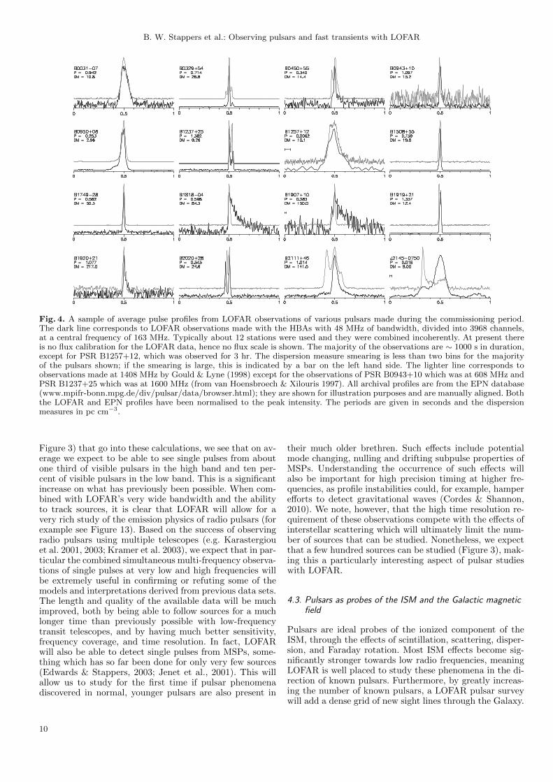
The flexibility afforded by the almost fully digital natureof the signal path and the associated processing power ofLOFAR mean that it can address these observational chal-lenges better than any previous low frequency radio tele-scope. As will be discussed in Sect. 6 it is possible to takethe complex channelised data coming from the LOFAR sta-tions and either further channelise to achieve the requiredfrequency resolution to correct for dispersion, or, whenhigher time resolution is required, it is possible to performcoherent dedispersion on the complex channels. While it isnot presently possible to correct for the effects of scatter-ing, we note that variations in the magnitude of scatteringare so large that some pulsars with high DMs will still beaccessible, as evidenced by our detection of PSR B1920+21with a DM of 217 pc cm−3 (Figure 4).
The system temperature of LOFAR is sky dominatedat nearly all frequencies and when combined with the verylarge collecting area this makes LOFAR very sensitive de-spite the contribution from the Galactic synchrotron emis-sion. The Galactic plane is clearly the hottest region, butthat is only a small fraction of the sky4 and as we are mostsensitive to the nearby population it will not greatly affectthe number of new pulsars LOFAR will find (see Sect. 4).Our detection of PSR B1749−28 (Figure 4), which is only∼ 1 from the direction to the Galactic Centre shows thatobservations of bright pulsars are still possible even withthe large background temperature of the Galactic plane.Moreover, for observations of known pulsars in the direc-tion of the Galactic plane, the narrow tied-array beams (seeSect. 5) will reduce the contribution from discrete extendedsources, such as supernova remnants (SNRs), to the systemtemperature and thus further improve the sensitivity oversingle dish or wide beam telescopes.
In terms of calibrating the station/time/frequency de-pendent ionospheric phase delays, we will exploit LOFAR’smulti-beaming capability and its ability to simultaneouslyimage and record high-time-resolution pulsar data (Sect. 5).The envisioned scheme is to use a separate station beam totrack a calibration source during an observation, use this tocalculate the required phase adjustments per station, andto implement these online while observing the main sciencetarget with another beam. This is admittedly a difficultproblem and the solution has yet to be implemented. Inthe case of the innermost core stations on the Superterphowever, differential ionospheric delays are unlikely to be amajor problem. This means that using the static phase so-lutions these stations can be combined coherently withoutionospheric calibration.
4. Pulsar science at low frequencies
Here we give an overview of the pulsar science that canbe done at low radio frequencies with LOFAR. This is notintended as an exhaustive list of envisioned studies, butrather as a general scientific motivation for LOFAR’s pulsarmodes.
4 Note however that LOFAR’s complex sidelobe patternmeans that the Galactic plane can still contribute somewhatto the total sky temperature even for observations far from theplane itself.
5
B. W. Stappers et al.: Observing pulsars and fast transients with LOFAR
4.1. Pulsar and fast transient searches
There are estimated to be approximately 100,000 activelyradio-emitting neutron stars in the Milky Way (Vranesevicet al., 2004; Lorimer et al., 2006; Faucher-Giguere & Kaspi,2006), of which at least 20,000 are visible as radio pulsarsdue to fortuitous geometrical alignment of the radio beamwith the direction towards Earth. With a sample of closeto 2,000 known radio pulsars to study, we still have onlya rough idea of this population’s overall properties and ofthe detailed physics of pulsars (Lorimer et al., 2006). Thisuncertainty is partly a product of the difficulty in disen-tangling the intrinsic properties of the population from theobservational biases inherent to past surveys, most of whichwere conducted at ∼ 350 MHz or ∼ 1.4 GHz.5 Discoveringa large, nearby sample of pulsars with LOFAR will allowthe determination of the distribution of pulsar luminosi-ties in the low-luminosity regime, crucial for extrapolatingto the total Galactic population, with the potential for de-tecting a cut-off in that distribution. Such a survey will alsoquantify the beaming fraction, that is what fraction of thesky is illuminated by the pulsar beams, at low frequencies,showing how this evolves from the more commonly observed350/1400-MHz bands. Though a LOFAR pulsar survey willof course also be observationally biased towards a partic-ular subset of the total Galactic pulsar population, thesebiases are in many ways complementary to those of pastsurveys, providing the opportunity to fully characterise theknown population.
Detailed simulations of potential LOFAR surveys weredone by van Leeuwen & Stappers (2010) and show that anall-Northern-sky survey with LOFAR will find about 1000new pulsars and will provide a nearly complete census ofall radio-emitting neutron stars within ∼ 2 kpc. An indica-tion of the sensitivity of LOFAR for pulsar surveys can beseen in Figure 2. The limiting distance out to which pulsarscan be detected is governed predominantly by scatteringin the ISM. There are however both pulsar and telescopecharacteristics that make low frequency surveys an attrac-tive prospect. The pulsar beam broadens at low frequencies(Cordes 1978 find that the width changes with frequency νas ν−0.25), which nearly doubles the beaming fraction com-pared to 1.4 GHz surveys. Furthermore, the large FoV andhigh sensitivity of LOFAR mean that such a survey can becarried out far more quickly and efficiently than any otherpulsar survey, past or present. Even in the Galactic plane,where the diffuse background temperature will reduce thesensitivity, the ability to form narrow tied-array beams (seeSect. 5) will reduce the contribution from sources which arelarge enough to be resolved.
The large FoV also affords relatively long dwell times,improving the sensitivity to rare, but repeating events likethe pulses from RRATs (rotating neutron stars which emitapproximately once in every 1000 rotations; McLaughlinet al. 2006), while the rapid survey speed will allow multi-ple passes over the sky. Thus, such a survey is guaranteed tohave a large product of total observing time and sky cover-age (ΩtotTtot). This factor is important for finding neutronstars that, for intrinsic or extrinsic reasons, have variabledetectability, such as the RRATs and intermittent pulsars
5 Reconciling the total number of neutron stars and the su-pernova rate (Keane & Kramer, 2008) also remains an outstand-ing, related issue, with many fundamental questions still unan-swered.
(the latter can be inactive for days: Kramer et al. 2006),those in relativistic binaries (where the acceleration nearperiastron can alter the periods too rapidly to allow detec-tion (e.g., Johnston & Kulkarni 1991; Ransom et al. 2003),and those millisecond pulsars, MSPs,6 which are found ineclipsing systems (e.g., Fruchter et al. 1988; Stappers et al.1996). It has recently become apparent that to understandthe pulsar and neutron star populations we need to knowwhat fraction of pulsars are relatively steady emitters com-pared with those that pulse erratically like the RRATs.
This complete, volume-limited sample can be extrapo-lated for modelling the entire neutron star population ofthe Galaxy, which then constrains the population of mas-sive stars and the supernova rate, the velocities and spatialdistribution of neutron stars, and the physics of neutronstars in general. Chances are that this largely unexploredpopulation of faint or intermittent radio-emitting neutronstars will also contain exotic systems – double neutronstars, double pulsars and possibly even a black-hole pul-sar binary. Such systems provide the best testing groundfor fundamental physical theories, ranging from solid-stateto gravitational physics (Cordes et al., 2004).
LOFAR is highly sensitive to MSPs and as they aregenerally much older than other neutron stars, they havehad more time to leave their birth-place in the Galacticplane and to become equally distributed in the halo aswell as in the plane. Thus, despite being more easily af-fected by scattering, the lower number of free electronsalong the lines of sight out of the Galactic plane meansthat MSPs are still prime targets for LOFAR. Moreover,they are bright at LOFAR frequencies with the flux den-sity spectra of some MSPs remaining steep down to 30MHz (Kuzmin & Losovsky, 2001; Kramer et al., 1999).Recent studies have successfully detected about half ofthe known Northern MSPs using the relatively insensitivelow-frequency (110 − 180 MHz) frontends on the WSRT(Stappers et al., 2008). Malov & Malofeev (2010) havealso shown a number of detections at frequencies near100 MHz using the Large Phased Array BSA radio tele-scope of the Pushchino Radio Astronomy Observatory de-spite the limited time resolution. It is also noteworthy thatthe recently discovered “missing-link” MSP J1023+0038(Archibald et al., 2009), detected with WSRT at 150 MHz,could have easily been found by a LOFAR survey, assumingit was observed out of eclipse. The number of MSPs uncov-ered at radio wavelengths, often at 350 MHz, by observa-tions of unidentified Fermi sources (e.g. Ransom et al. 2011;Hessels et al. 2011) indicates that there are still many morerelatively bright sources to be found. The high sensitiviy ofLOFAR will allow it to detect nearby low-luminosity MSPsand steep spectrum high-luminosity MSPs which are toofar away to be detected at high frequencies.
LOFAR also has the sensitivity to discover the brightestsources in local group galaxies (van Leeuwen & Stappers,2010). If observed face-on and located away from theGalactic disk, the scatter broadening to pulsars in an ex-ternal galaxy will be relatively low and thus a LOFARsurvey will have high sensitivity for even rapidly rotat-ing extragalactic pulsars. For a relatively close galaxy like
6 MSPs are believed to be formed in binary systems, wherethe neutron star accretes matter from the companion star andis spun up to millisecond periods, sometimes referred to as re-cycling.
6
B. W. Stappers et al.: Observing pulsars and fast transients with LOFAR
M33, LOFAR could detect all pulsars more luminous than∼50 Jy kpc2. Ten of the currently known pulsars in ourown Galaxy have comparable luminosity (Manchester et al.,2005). There are at least 20 (dwarf) galaxies for whichLOFAR will have good sensitivity to their pulsar popu-lation. Complementing searches for periodic signals, de-tecting the bursts of either giant or RRAT pulses canequally pin-point pulsars. In particular, the ultra-bright gi-ant pulses could be visible in even more remote galaxies(McLaughlin & Cordes, 2003). A survey for extragalacticpulsars would allow us to investigate if the bright end ofthe pulsar distribution in other galaxies differs from thatof our Galaxy, and how that ties into galaxy type and starformation history. Such pulsars can also feed the under-standing of the history of massive star formation in thesegalaxies and also, if sufficient numbers can be found, theycan be used to probe the intergalactic medium and possiblyconstrain or measure the intergalactic magnetic field.
In addition to the discovery of bright pulses from pulsarsin nearby galaxies, an all-sky LOFAR survey will also casta wide net for other extragalactic and cosmological bursts(e.g. Fender et al. 2008; van der Horst et al. 2008; Lorimeret al. 2007). The large FoV of LOFAR means that only1200/200 pointings of station beams are required to coverthe full Northern Hemisphere with the HBAs/LBAs at cen-tral frequencies of 150 and 60 MHz respectively7. Through adedicated pulsar/fast transient survey, and regular piggy-backing on the imaging observations of other projects, itwill be possible to obtain an unprecedented Ωtot × Ttot fig-ure of merit. For example, 8000 HBA observations of 1 hreach (roughly two year’s worth of observations, assuming50% observing efficiency) would provide 4 hours of all-skycoverage, meaning that events with rates of only 6/day overthe whole sky could be detected in such a data set. Theparameter space of such rare bursts has never been probedwith such high sensitivity. Moreover there are many optionsfor performing wide angle rapid shallow searches for fasttransients using either single stations, forming sub-arraysor forming 244 LBA station beams all at once.
LOFAR will also respond to high-energy X-ray/γ-rayor high-frequency radio triggers. Most high-energy eventspeak later in the radio, providing ample time to follow-upon such events. Dispersive delay, which can easily be 100sof seconds in the LOFAR low-band, may also aid in detect-ing the prompt emission of some bursts. Efforts are beingmade to reduce the setup time of a typical observation sothat target of opportunity observations can begin quicklyand automatically. Since LOFAR has no moving parts, re-pointing is only a matter of reconfiguring the delay correc-tions used in beamforming. The ultimate goal is to repointto any location of the sky and begin new observations injust a few seconds.
4.2. The physics of pulsar radio emission
The sensitivity and frequency range of LOFAR opens up thelow-frequency window to new studies of pulsar emission. Itis precisely in the LOFAR frequency range where some ofthe most interesting changes in pulsar radio emission canbe observed, including significant broadening of the pulse
7 Compare for instance with the 1.4 GHz Parkes Multibeamsystem, which requires of the order of 35000 pointings to covera similar area of sky.
profile, presumably due to a “radius-to-frequency” map-ping and deviations from this expected relation; changes inthe shape of pulse profile components; and a turn-over inthe flux density spectrum. The frequency range accessibleby LOFAR is also where propagation effects in the pul-sar magnetosphere are expected to be largest (e.g. Petrova2006, 2008; Weltevrede et al. 2003). Therefore, simultane-ous multi-frequency observations (see Figures 15 and 16)are expected to reveal interesting characteristics of the pul-sar magnetosphere, such as the densities and birefringenceproperties (Shitov et al., 1988), that will ultimately leadto a better understanding of the emission mechanisms ofpulsars.
4.2.1. Pulsar flux densities and spectra
LOFAR’s large fractional bandwidth is a big advantage formeasuring the low-frequency flux densities and spectra ofpulsars. As discussed in Sect. 5.3 it will be possible to usemultiple stations to observe contiguously from 10 MHz to240 MHz. With the ability to easily repeat observations,we can be certain to remove effects such as diffractive scin-tillation, which may have affected previous flux density es-timates. It is also the case that the timescale for refrac-tive scintillation becomes very long at these frequencies andthis will have a modulating effect on the determined fluxes.However this is typically of smaller amplitude. Repeatingthese observations will also allow one to determine whetherthe spectral characteristics are fixed in time, or whetherthey vary, for any given source, something which has rarelybeen done in the past. It is also important to note the rolethat variable scattering might play in flux density determi-nation (e.g. Kuzmin et al. 2008).
So far, there are relatively few pulsars for which spec-tral information in the LOFAR frequency range is avail-able (Malofeev et al., 2000). Obtaining a large, reliableset of low-frequency flux density measurements over the4 lowest octaves of the radio window is a valuable missingpiece in the puzzle of the pulsar emission process. For in-stance, the generally steep increase in pulsed flux densitytowards lower frequencies is seen to turn over for a num-ber of pulsars at frequencies between 100 and 250 MHz.However, the physical origin for this turn over is not yetclear. Conversely, there are a number of pulsars for whichno such break in the spectrum has yet been seen and stud-ies at lower frequencies are needed to locate this spec-tral break (Kuzmin & Losovsky, 2001; Malofeev, 2000).Furthermore, there is evidence for complexity in the shapeof pulsar spectra (e.g. Maron et al. 2000), which again isan important signature of the pulsar emission process thatLOFAR’s wide-band data can probe. In addition to theirimportance for our understanding of the emission processitself (e.g. Gurevich et al. 1993; Melrose 2004), pulsar spec-tra and flux densities are a basic ingredient for estimatingthe total radio luminosity and modelling the total Galacticpopulation of radio pulsars.
In many ways, MSPs show very similar radio emissionproperties to those of non-recycled pulsars (e.g. Krameret al. 1998); yet, they differ from these by many ordersof magnitude in terms of their rotation period, magneticfield strength, and the size of their magnetosphere. A cu-rious and potentially important distinction is that MSPstend to show un-broken flux density spectra, continuingwith no detected turn-over down to frequencies of 100 MHz
7

B. W. Stappers et al.: Observing pulsars and fast transients with LOFAR
10-2
10-1
100
101
102
103
104
105
106
10-3 10-2 10-1 100 101
Flu
x D
ensi
ty (
mJy
)
Pulsar Period (s)
10-2
10-1
100
101
102
103
104
105
106
10-3 10-2 10-1 100 101
Flu
x D
ensi
ty (
mJy
)
Pulsar Period (s)
10-2
10-1
100
101
102
103
104
105
106
10-3 10-2 10-1 100 101
Flu
x D
ensi
ty (
mJy
)
Pulsar Period (s)
10-2
10-1
100
101
102
103
104
105
106
10-3 10-2 10-1 100 101
Flu
x D
ensi
ty (
mJy
)
Pulsar Period (s)
10-2
10-1
100
101
102
103
104
105
106
10-3 10-2 10-1 100 101
Flu
x S
ensi
ty (
mJy
)
Pulsar Period (s)
10-2
10-1
100
101
102
103
104
105
106
10-3 10-2 10-1 100 101
Flu
x S
ensi
ty (
mJy
)
Pulsar Period (s)
10-2
10-1
100
101
102
103
104
105
106
10-3 10-2 10-1 100 101
Flu
x S
ensi
ty (
mJy
)
Pulsar Period (s)
10-2
10-1
100
101
102
103
104
105
106
10-3 10-2 10-1 100 101
Flu
x S
ensi
ty (
mJy
)
Pulsar Period (s)
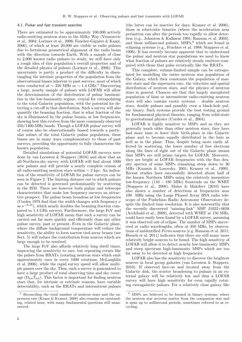
Fig. 2. Sensitivity curves for 600-s observations using the HBAs (left) and the LBAs (right) with a bandwidth of 48 MHz, comparedto the extrapolated flux densities of 787 known pulsars at 150 and 50 MHz respectively. Flux densities were determined using, ifknown, 100 MHz fluxes from Malofeev et al. (2000) (circles) otherwise fluxes at either 400 MHz (triangles) or 1400 MHz (diamonds)(Manchester et al., 2005), whichever were available, were used and scaled to 150 MHz using a known spectral index or a typical
spectral index of −1.8 (squares). All of these flux densities were scaled by√W/(P −W ), where W is the effective pulse width and
P is the period of the pulsar, to incorporate broadening of the profile by scattering in the ISM. W was determined by combiningthe pulse width at high frequencies with the broadening due to scattering in the ISM, based on the model of Bhat et al (2004). IfW > 0.75P then the pulsar was deemed undetectable. It was assumed that broadening of the profile due to uncorrected dispersivesmearing was negligible. MSPs are shown by the open symbols and “normal” pulsars by filled symbols. The lines in both casescorrespond to the sensitivity of a single international station (fine dashed line), the incoherent sum of 20 core stations (heavydashed line), incoherent sum of all LOFAR stations (filled line) and the coherent sum of 20 core stations (bold line).
(Kramer et al., 1999; Kuzmin & Losovsky, 2001) and lower(e.g. Navarro et al. 1995). Kuzmin & Losovsky (2001) pre-sented spectra of some 30 MSPs using measurements closeto 100 MHz. Using the sensitivity, bandwidth and track-ing abilities of LOFAR, it will be possible to more thandouble that number, and to provide measurements withmuch wider bandwidths. Such flux density measurementswill also be possible using LOFAR’s imaging ability, even ifsevere scattering prevents detailed profile studies. In gen-eral, however, when scattering is not the dominant effect theimproved time resolution enabled by the coherent dedis-persion mode of LOFAR should also allow us to resolveindividual profile components in MSP profiles, so that theaverage profile spectrum can be compared to that of singlepulse components.
Correlating the spectral properties with other propertiesof the pulsar (such as pulse shape, geometrical parametersor pulse energy distributions) may reveal important physi-cal relationships. These can then be used to further improvepulsar emission and geometry models. This is particularlyimportant as more and more sources are being detected athigh energies with Fermi, placing interesting constraints onthe emission sites (e.g. Abdo et al. 2010b).
4.2.2. Pulse profile morphology
Observations of the average pulse profile morphology ofabout 50% of pulsars studied over a wide frequency rangeindicate substantial and complex variations which are noteasily understood in the standard model of pulsar emission(e.g. Lyne & Smith 2004; Lorimer & Kramer 2005). Thissimple pulsar model has the plasma and emission propertiesdominated by the dipolar magnetic field and is often com-
bined with a model where the emission obeys a “radius-to-frequency mapping”, such that lower frequencies are emit-ted further out in the magnetosphere resulting in widerpulse profiles (Cordes, 1978). However this simple picture isnot the full story as evidenced by the spectral behaviour ofthe different pulse components (e.g. Mitra & Rankin 2002;Rankin 1993). The latter property is in general supportedby observations, and probably corresponds to stratificationof the density in the emission zone although plasma propa-gation effects may play an important role here as well (seee.g. Lorimer & Kramer 2005 for a review). The sensitivityand time resolution possible with LOFAR, combined withthe wide frequency range, will allow us to obtain averageprofiles for the majority of the known population of pulsarsin the Northern sky (Figure 2). Additionally, hundreds ofnew pulsars, expected to be discovered with LOFAR, canalso be studied in detail; as is demonstrated by the highquality data from our commissioning observations (Figure4).
There is also observational evidence that profiles thatare dominated by the outer pulse components at highfrequencies evolve to profiles where the central compo-nent is comparatively much stronger at low frequencies(e.g. Lorimer & Kramer 2005). The exact profile evolu-tion may depend on the distribution of plasma along thefield lines or may be the result of different emission zones.Indeed, the general picture is much more complex: varia-tions are seen in the pulse profile with different componentshaving different spectral indices and new components be-coming visible (Kramer et al., 1994). By combining LOFARdata over its wide frequency range with higher frequencyobservations we can investigate these properties for a muchlarger group of pulsars (see for an example Figure 16).
8
B. W. Stappers et al.: Observing pulsars and fast transients with LOFAR
10-6
10-4
10-2
100
102
104
106
10-5 10-4 10-3 10-2 10-1 100
Flu
x D
ensi
ty (
mJy
)
Pulse Width (s)
10-6
10-4
10-2
100
102
104
106
10-5 10-4 10-3 10-2 10-1 100
Flu
x D
ensi
ty (
mJy
)
Pulse Width (s)
10-6
10-4
10-2
100
102
104
106
10-5 10-4 10-3 10-2 10-1 100
Flu
x D
ensi
ty (
mJy
)
Pulse Width (s)
10-6
10-4
10-2
100
102
104
106
10-5 10-4 10-3 10-2 10-1 100
Flu
x D
ensi
ty (
mJy
)
Pulse Width (s)
10-6
10-4
10-2
100
102
104
106
10-5 10-4 10-3 10-2 10-1 100
Flu
x D
ensi
ty (
mJy
)
Pulse Width (s)
10-6
10-4
10-2
100
102
104
106
10-5 10-4 10-3 10-2 10-1 100
Flu
x D
ensi
ty (
mJy
)
Pulse Width (s)
10-6
10-4
10-2
100
102
104
106
10-5 10-4 10-3 10-2 10-1 100
Flu
x D
ensi
ty (
mJy
)
Pulse Width (s)
10-6
10-4
10-2
100
102
104
106
10-5 10-4 10-3 10-2 10-1 100
Flu
x D
ensi
ty (
mJy
)
Pulse Width (s)
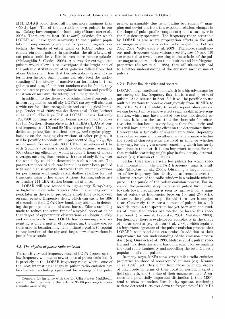
Fig. 3. Sensitivity curves for the HBAs (left panel) and LBAs (right panel) to single pulses as a function of pulse width at a centralfrequency of 150 MHz (HBAs) and 50 MHz (LBAs) and assuming a bandwidth of 48 MHz. Single pulse widths for 787 pulsars werecalculated by assuming them to be one third of the width of the average pulse and then scatter broadened assuming the relationshipof Bhat et al (2004). It was assumed that broadening of the pulse due to uncorrected dispersive smearing was negligible. Singlepulse fluxes were determined based on the assumed pulse width and, if known, 100 MHz fluxes from Malofeev et al. (2000) wereused. Otherwise, fluxes were extrapolated to 150 MHz from either 400 MHz or 1400 MHz measurements (whichever was available,Manchester et al. 2005) using a known spectral index or a typical spectral index of −1.8. The symbols are the same as in Figure2. The lines in all cases correspond to the sensitivity of a single international station (fine dashed line), the incoherent sum of 20core stations (heavy dashed line), incoherent sum of all the LOFAR stations (filled line) and the coherent sum of 20 core stations(bold line).
A further important probe of the emission mechanism,the geometry and the plasma properties of the magneto-sphere is polarisation. So far, there have been only limitedstudies of the low-frequency polarisation properties of pul-sars. In contrast, in simultaneous multiple high-frequencyobservations strange polarisation variations have been seenwhich point directly to the physics of the emission re-gions (e.g. Izvekova et al. 1994; Karastergiou et al. 2001).Polarisation studies with LOFAR have the potential to pro-vide insight into how the polarisation behaves at theserelatively unexplored low frequencies. LOFAR polarisationdata can determine whether at low frequency the percent-age of polarisation evolves strongly with frequency and ifthere are even more severe deviations of the polarisation po-sition angle swing from the expectation for a dipole field. Itwill also be possible to determine if the polarisation proper-ties change below the spectral break and whether the signchanges of circular polarisation seen at higher frequenciesshow similar properties at lower frequencies or exhibit nosuch sign changes.
4.2.3. Single pulses
The average, or cumulative, pulse profiles of radio pul-sars are formed by adding at least hundreds of consecu-tive, individual pulses. While most pulsars have highly sta-ble cumulative pulse profile morphologies, their individualpulses tend to be highly variable in shape, and require morecomplex interpretations than the average profiles. For ex-ample, single pulse studies of some pulsars have revealedquasi-periodic “micropulses” with periods and widths ofthe order of microseconds (Cordes et al., 1990; Lorimer& Kramer, 2005). As such observed phenomena exhibitproperties and timescales closest to those expected from
theoretical studies of pulsar emission physics (e.g. Melrose2004) studying them can strongly constrain models of theemission process. Single pulse studies at low frequencies areparticularly interesting, because microstructure (Soglasnovet al., 1983; Smirnova et al., 1994) and subpulse modula-tion (Weltevrede et al., 2007; Ul’Yanov et al., 2008) tend tobe stronger there. We also expect density imbalances andplasma dynamics to be the most noticeable at low radiofrequencies (Petrova, 2006).
In some pulsars, single sub-pulses are observed to driftin an organised fashion through the pulse window (seeFigure 13), an effect which may either be related to the cre-ation of plasma columns near the polar cap or to the plasmaproperties within the pulsar magnetosphere. Some pulsarsshow significant frequency evolution in the properties ofthese drifting subpulses and observations at low frequencies,which probe a very different sight line across the typicallyenlarged emission beam, can be used to reconstruct thedistribution of emission within the magnetosphere. Greaterconstraints can be obtained by simultaneous observationsat different frequencies, within LOFAR bands but alsoin combination with high-frequency facilities. Such exper-iments will reveal how the radius-to-frequency mappingmanifests itself in the sub-pulse modulation; for example, isthe drifting more or less organised at the low frequencies?There is some evidence that drifting subpulses are morepronounced (Weltevrede et al., 2007) and perhaps easier tostudy at low frequencies.
In order to gauge the number of pulsars whose singlepulses can be studied with LOFAR, we compare the es-timated single-pulse flux densities in Figure 3. We showall known pulsars visible with LOFAR and scale them toLOFAR sensitivity in both the high band and low band.While there are a number of assumptions (see caption of
9
B. W. Stappers et al.: Observing pulsars and fast transients with LOFAR
Fig. 4. A sample of average pulse profiles from LOFAR observations of various pulsars made during the commissioning period.The dark line corresponds to LOFAR observations made with the HBAs with 48 MHz of bandwidth, divided into 3968 channels,at a central frequency of 163 MHz. Typically about 12 stations were used and they were combined incoherently. At present thereis no flux calibration for the LOFAR data, hence no flux scale is shown. The majority of the observations are ∼ 1000 s in duration,except for PSR B1257+12, which was observed for 3 hr. The dispersion measure smearing is less than two bins for the majorityof the pulsars shown; if the smearing is large, this is indicated by a bar on the left hand side. The lighter line corresponds toobservations made at 1408 MHz by Gould & Lyne (1998) except for the observations of PSR B0943+10 which was at 608 MHz andPSR B1237+25 which was at 1600 MHz (from van Hoensbroech & Xilouris 1997). All archival profiles are from the EPN database(www.mpifr-bonn.mpg.de/div/pulsar/data/browser.html); they are shown for illustration purposes and are manually aligned. Boththe LOFAR and EPN profiles have been normalised to the peak intensity. The periods are given in seconds and the dispersionmeasures in pc cm−3.
Figure 3) that go into these calculations, we see that on av-erage we expect to be able to see single pulses from aboutone third of visible pulsars in the high band and ten per-cent of visible pulsars in the low band. This is a significantincrease on what has previously been possible. When com-bined with LOFAR’s very wide bandwidth and the abilityto track sources, it is clear that LOFAR will allow for avery rich study of the emission physics of radio pulsars (forexample see Figure 13). Based on the success of observingradio pulsars using multiple telescopes (e.g. Karastergiouet al. 2001, 2003; Kramer et al. 2003), we expect that in par-ticular the combined simultaneous multi-frequency observa-tions of single pulses at very low and high frequencies willbe extremely useful in confirming or refuting some of themodels and interpretations derived from previous data sets.The length and quality of the available data will be muchimproved, both by being able to follow sources for a muchlonger time than previously possible with low-frequencytransit telescopes, and by having much better sensitivity,frequency coverage, and time resolution. In fact, LOFARwill also be able to detect single pulses from MSPs, some-thing which has so far been done for only very few sources(Edwards & Stappers, 2003; Jenet et al., 2001). This willallow us to study for the first time if pulsar phenomenadiscovered in normal, younger pulsars are also present in
their much older brethren. Such effects include potentialmode changing, nulling and drifting subpulse properties ofMSPs. Understanding the occurrence of such effects willalso be important for high precision timing at higher fre-quencies, as profile instabilities could, for example, hamperefforts to detect gravitational waves (Cordes & Shannon,2010). We note, however, that the high time resolution re-quirement of these observations compete with the effects ofinterstellar scattering which will ultimately limit the num-ber of sources that can be studied. Nonetheless, we expectthat a few hundred sources can be studied (Figure 3), mak-ing this a particularly interesting aspect of pulsar studieswith LOFAR.
4.3. Pulsars as probes of the ISM and the Galactic magneticfield
Pulsars are ideal probes of the ionized component of theISM, through the effects of scintillation, scattering, disper-sion, and Faraday rotation. Most ISM effects become sig-nificantly stronger towards low radio frequencies, meaningLOFAR is well placed to study these phenomena in the di-rection of known pulsars. Furthermore, by greatly increas-ing the number of known pulsars, a LOFAR pulsar surveywill add a dense grid of new sight lines through the Galaxy.
10
B. W. Stappers et al.: Observing pulsars and fast transients with LOFAR
As the majority of these pulsars will be nearby or out ofthe Galactic plane, the dispersion and scattering measuresof this new sample will improve our model of the distribu-tion of the ionized ISM and its degree of clumpiness (Cordes& Lazio, 2002).
Scintillation and scattering are related phenomenawhich result in variations of the pulse intensity as a functionof frequency and time, and in broadening of the pulse profilerespectively (e.g. Rickett 1970, 1990; Narayan 1992). Theyare caused by fluctuations in the density of free electrons inthe ISM. Scintillation studies have been revolutionised inthe last few years by the discovery of faint halos of scatteredlight, extending outward to 10− 50 times the width of thecore of the scattered image (Stinebring et al., 2001). This,in turn, gives a wide-angle view of the scattering mediumwith milliarcsecond resolution, and the illuminated patchscans rapidly across the scattering material because of thehigh pulsar space velocity. Some of the most interesting ef-fects are visible at low frequencies. The dynamic nature ofthese phenomena also fits well with LOFAR’s monitoringcapabilities. In a sense, this scintillation imaging will al-low the monitoring of the range of interstellar conditionsencountered along a particular sight line. The wide band-widths and high sensitivities will also allow very precisemeasurements of the DM of many pulsars; for MSPs thiscould be as precise as 1 : 104 or better for an individualmeasurement. Such precision, even for normal pulsars, willenable detailed studies of variations in the DM which canbe used with the scintillation properties to study structuresin the ISM (e.g. You et al. 2007).
Scattering is a spatial effect, whereby the inhomo-geneities in the ISM cause ray paths to be redirected intothe line of sight with a resulting delay associated with theextra travel time. Scattering is typically assumed to hap-pen in a thin screen located midway between the pulsarand the Earth, so that the turbulence obeys a Kolmogorovlaw even though deviations are observed (e.g. Lohmer et al.2004). There is evidence that the scattering does not havethe expected frequency dependence for such a spectrumand that there is also an inner and outer scale to the tur-bulence which can be measured (e.g. Armstrong et al. 1981,1995; Shishov & Smirnova 2002). Low-frequency measure-ments with LOFAR will allow us to measure (even subtle)scattering tails for many more pulsars, affording better sta-tistical studies. The study of individual, moderately scat-tered but bright pulsars will provide a probe of the distri-bution of electrons along the line of sight, enabling one todistinguish between the different frequency dependences ofthe dispersive and scattering delays that affect the arrivaltime of the pulse (see for example Figure 19). Identifyingsuch effects has the potential to extract distances and thick-nesses of scattering screens (Rickett et al., 2009; Smirnova& Shishov, 2010).
LOFAR can increase the number of known rotationmeasures to pulsars, which will place important constraintson the overall magnetic field structure of the Milky Way,something that is still not well characterised (e.g. Noutsoset al. 2008; Han 2009; Wolleben et al. 2010). At LOFARfrequencies it is possible to also measure the very small ro-tation measures of the nearby population of pulsars whichprovides an unprecedented tool for studying the local mag-netic field structure. The large number of new sight lineswill also allow statistical studies of small-scale fluctua-tions of electron density and magnetic field variations down
to the smallest scales that can be probed with pulsars(. 1 kpc). These same techniques will open up new vis-tas when applied to the first (truly) extragalactic pulsars,which will be discovered by LOFAR in the survey of localgroup galaxies that will be undertaken.
4.4. Pulsar timing
Ultra-high-precision pulsar timing (at the ns−sub-µs level)is not possible at low radio frequencies because the timingprecision is strongly affected by ISM effects that, currentlyat least, cannot be compensated for. However LOFAR’slarge FoV, multi-beaming capability, and the availabilityand sensitivity of single stations working in parallel tothe main array enable many pulsars to be timed at suf-ficient precision and cadence to be of scientific interest.Regular monitoring of the rotational behaviour of radio pul-sars plays an important role in understanding the internalstructure and spin evolution of neutron stars and how theyemit. It is also an important probe of the ISM and po-tentially for the emission of gravitational waves. MeasuringDM variations and modelling the scattering of pulse pro-files at LOFAR frequencies has the potential to help correctpulse shape variations at high observing frequencies andthus reduce systematics in high precision timing.
Rotational irregularities such as glitches are attributedto the physics of the super-dense superfluid present in theneutron star core, and so their study allows us to probea physical regime far beyond those that can be reached inlaboratories on Earth (e.g. D’Alessandro 1996; van Eysden& Melatos 2010). These glitches might also trigger heat-ing of the neutron star surface or magnetic reconnectionswhich can be studied in either or both gamma- and X-rays (Tang & Cheng, 2001; Van Riper et al., 1991). Theymay also cause sufficient deformation of the neutron starthat it might be a gravitational wave emitter (e.g. Bennettet al. 2010). To allow these multi-messenger follow-up ob-servations requires the accurate determination of glitch oc-curence times which can be achieved through regular mon-itoring with LOFAR. Moreover, the studies of high-energyemission from pulsars, which is presently done in detailby the Fermi and Agile satellites and other telescopes likeMAGIC and H.E.S.S. (e.g. Abdo et al. 2009; Tavani et al.2009; Aliu et al. 2008; Aharonian et al. 2007), as well asthe search for non-burst-like gravitational waves from pul-sars (Abbott et al., 2010) can only be performed with theprovision of accurate pulsar rotational histories.
Three relatively recently discovered manifestations ofradio emitting neutron stars, the RRATs, the intermittentpulsars, and the radio emitting magnetars (McLaughlinet al., 2006; Kramer et al., 2006; Lyutikov, 2002; Camiloet al., 2006), can all greatly benefit from the monitoringcapabilities of LOFAR. All of these source types show onlysporadic radio activity, which in some cases is only presentfor less than a second per day. As such, a large amountof on-sky observing is often preferable to raw sensitivity,making such studies particularly well-suited for individualLOFAR stations observing independently from the rest ofthe array. It is possible that there are neutron stars whoseradio emission is even more sporadic; discovering these willrequire potentially several days of cummulative integrationtime per sky position, which is achievable as part of theLOFAR Radio Sky Monitor (Fender et al., 2008).
11
B. W. Stappers et al.: Observing pulsars and fast transients with LOFAR
So far some 30 RRATs have been discovered, though pe-riods and period derivatives have only been determined forslightly more than half of these (McLaughlin et al., 2009).Detailed studies of these sources are hampered by the factthat they pulse so infrequently as to make proper tim-ing follow-up prohibitively expensive for most telescopes.LOFAR’s multi-beaming capabilities and the separate useof single stations make such studies feasible. These can de-termine key parameters like the spin period Pspin and its
derivative Pspin as well as better characterising the natureof the pulses themselve. These are all essential for under-standing the relationship of RRATs to the “normal” pul-sars.
Unlike the RRATs, the intermittent pulsars appear asnormal pulsars for timescales of days to months, but thensuddenly turn off for similar periods (Kramer et al., 2006).Remarkably, when they turn off they spin down more slowlythan when they are on, providing a unique and exciting linkwith the physics of the magnetosphere. Observing moreon/off transitions will improve our understanding of thetransition process. Furthermore, recent work by Lyne et al.(2010) has shown similar behaviour in normal pulsars, re-lating timing noise, pulse shape variations and changes inspin-down rate. Moreover they demonstrate that with suffi-ciently regular monitoring, that can be achieved with tele-scopes like LOFAR, it may be possible to correct the effectsthese variations cause on the pulsar timing. This will allowfor the possibility of improving their usefulness as clocks.
Another manifestation of radio pulsars which showhighly variable radio emission are the magnetars, extremelymagnetised neutron stars (Bsurf ∼ 1014−15 G), which werethought to emit only in gamma- and X-rays. Recently, how-ever, two such sources have been shown to emit in the radio,albeit in a highly variable way (Camilo et al., 2006, 2007).This emission may have been triggered by an X-ray burst,and was subsequently observed to fade dramatically. Evenmore recently, a radio pulsar was discovered which has arotation period and magnetic field strength within the ob-served magnetar range. This pulsar also shows similarlyvariable radio emission properties, as seen for the othertwo “radio magnetars”, though no X-ray burst has beenobserved (Levin et al., 2010). It is only by monitoring thesesources, and regularly searching the sky, in the radio thatwe can understand the link between intermittent radio pul-sations and high-energy bursts, as well as the lifetime ofthese sources as radio emitters.
4.5. New populations
The case for observing pulsars at low frequencies, as dis-cussed so far, is partly based on our knowledge of the typ-ical spectral behaviour of the known population. However,there are pulsars like PSR B0943+10, which have flux den-sity spectra with spectral indices steeper than α = −3.0(Deshpande & Radhakrishnan, 1994) and a number ofMSPs which have steep spectra and which do not showa turn-over even at frequencies as low as 30 MHz (e.g.Navarro et al. 1995). It is as yet unclear whether these ex-treme spectral index sources represent a tail of the spectralindex distribution. There is a potential bias against steepspectrum objects as they need to be very bright at low fre-quencies in order to be detected in high-frequency surveys.For example, the minimum flux density of the HTRU, High
Time Resolution Universe, survey with the Parkes telescopeat 1400 MHz (Keith et al., 2010) is 0.2 mJy and for a spec-tral index −3.0 pulsar the corresponding 140 MHz flux den-sity would be 200 mJy. In contrast, a source close to theLOFAR search sensitivity of about 1 mJy would have tohave a flux density no steeper than −0.7 to be detected byHTRU, suggesting that a large number of pulsars may onlybe detectable at low frequencies.
Beyond these regular pulsars with steep spectral in-dices, more exotic neutron stars are seen to show tran-sient radio emission. While the anomalous X-ray pulsarsXTE J1810-197 and 1E 1547.0-5408 (Camilo et al., 2006,2007) have shallow spectral indices and are very dim inthe LOFAR regime, several other AXPs and magnetarsmay appear to be only detectable at frequencies near100 MHz (e.g. Malofeev et al. 2006), offering an intrigu-ing possibility to study more of these high-magnetic-fieldobjects in the radio band if confirmed. The potential 100-MHz detection of Geminga, a prominent rotation-poweredpulsar visible at optical, X- ray and gamma-ray wave-lengths (Malofeev & Malov, 1997; Kuzmin & Losovskii,1997; Shitov & Pugachev, 1997), could exemplify a pop-ulation of neutron stars that may be only detectable atradio wavelengths with LOFAR. Also, the non-detectionof radio emission from X-ray dim isolated neutron stars(XDINSs) thus far (Kondratiev et al., 2009), could be dueto the beams of these long-period sources being quite nar-row at high frequencies and there may be a better chance todetect them in radio at LOFAR frequencies. In fact, weakradio emission from two XDINSs, RX J1308.6+2127 andRX J2143.0+0654, was reported by Malofeev et al. (2005,2007) at 111 MHz, hence it would be important to con-firm this detection with LOFAR. This is also the case forthe pulsars discovered in blind searches of Fermi gamma-ray photons, many of which do not exhibit detectable radioemission (Abdo et al., 2009, 2010b), as well as the remainingunidentified gamma-ray sources, which have characteristicsof radio pulsars but which have not yet been detected inthe radio (Abdo et al., 2010a).
5. Observing modes
Here we describe LOFAR’s various “beamformed” modes,both currently available or envisioned, for observing pulsarsand fast transients. Though we concentrate on the pulsarand fast transient applications of these modes, we note thatLOFAR’s beamformed modes are also applicable to otherhigh-time-resolution studies including dynamic spectra ofplanets (both solar and extra-solar), flare stars, and theSun. We also provide a brief description of LOFAR’s stan-dard interferometric imaging mode, which can be run inparallel with some beamformed modes. For a detailed de-scription of LOFAR imaging, see Heald et al. (2010) andvan Haarlem et al. (2011).
LOFAR is an interferometer with sparsely spaced sta-tions, distributed in such a way as to produce reliable high-resolution images. To achieve this, the data from all stationsare correlated8 with each other, resulting in a significant in-crease in the amount of data. To reduce the data rate to anacceptable level there is an averaging step which reduces the
8 Note that the antennas within an individual station are firstsummed in phase to form one or multiple station beams on thesky.
12
B. W. Stappers et al.: Observing pulsars and fast transients with LOFAR
time resolution of the data to typically about one second, orlonger (though somewhat shorter integrations are possiblein some cases). To sample the combined radio signal at sig-nificantly higher time resolution than this (tsamp < 100 ms),one has to normally sacrifice spatial resolution, and/or thelarge FoV seen by the individual elements, to form a sin-gle beam pointing in the direction of the source of interest.It is these so-called beamformed or pulsar-like modes thatwe will describe here. The LOFAR Transients Key ScienceProject (Fender et al., 2006) will use both the imaging andbeamformed modes to discover and study transient sources.The imaging mode will probe flux changes on timescales ofseconds to years, while the beamformed modes will probetimescales from seconds down to microseconds and will re-visit the same sky locations over the course of days to years.With the Transient Buffer Boards (TBBs; Sect. 5.5) it willbe possible to form images with high time resolution, butlimited observing durations.
There are many ways in which the various parts ofLOFAR (antennas, tiles, stations) can be combined to formbeams (see Table 3). The almost completely digital na-ture of the LOFAR signal processing chain means that itis highly flexible to suit a particular observational goal. Inthe following sub-sections we will discuss different optionsfor combining these signals, to maximise either the FoV, in-stantaneous sensitivity or to compromise between these twofactors. For the sake of clarity however, we begin by defin-ing some related terms. An element beam refers to the FoVseen by a single element, a dipole in the case of the LBAsand a tile of 4 × 4 dipoles in the case of the HBAs (recallthat these dipoles are combined into a tile beam using ananalog beamformer). The term station beam correspondsto the beam formed by the sum of all of the elements ofa station. For any given observation there may be morethan one station beam and they can be pointed at any lo-cation within the wider element beam. A tied-array beamis formed by coherently combining all the station beams,one for each station, which are looking in a particular di-rection. There may be more than one tied-array beam foreach station beam. Station beams can also be combined in-coherently in order to form incoherent array beams. Theseretain the FoV of the individual station beams and haveincreased sensitivity compared with a single station.
5.1. Coherent and incoherent station addition
5.1.1. Coherent addition
To achieve the full sensitivity of the LOFAR array it isnecessary to combine the signals from each of the stationbeams coherently, meaning that the phase relationship be-tween the station signals from a particular direction mustbe precisely determined. Phase delays between the signalsare generated by a combination of geometric, instrumental,and environmental effects. The geometric term is simply re-lated to the relative locations of the stations and the sourceand is easily calculated. Instrumental contributions are re-lated to the observing system itself, such as the length ofcables connecting the various elements. Consequently, thecomponents in the signal chain are designed to be stable ontimescales that are long compared to the observing dura-tion. The environmental terms can be much more variableand are dominated by ionospheric delays at low radio fre-quencies.
Combining the station signals coherently into tied-arraybeams gives the equivalent sensitivity to the sum of the col-lecting area of all the stations being combined. However, theresulting FoV is significantly smaller than that of an indi-vidual station beam because it is determined by the dis-tance between stations, which for LOFAR is significantlylarger than the size of the stations themselves. The FoVsfor various beam types are given in Table 3 and examplesare shown in Figure 1. The small FoV of tied-array beamsis not a problem for observing known point sources − infact, it can be advantageous by reducing the contributionof background sources − but increases the data rate andprocessing requirements when undertaking surveys (see be-low).
The coherent combination of telescopes for pulsar obser-vations is regularly used at the Westerbork Synthesis RadioTelescope (Karuppusamy et al., 2008) and the Giant Meter-Wave Radio Telescope (Gupta et al., 2000). In both casesthe phase delays between the telescopes are determined byregular observations of known and unresolved calibrationsources in a process which is often called “phasing-up”. Thetimescale between when observations of calibration sourcesneed to be made depends strongly on the observing fre-quency, the largest separation between telescopes and theionospheric conditions, but range from a few hours to days.
At the low frequencies of LOFAR, phase delays betweenstations are very susceptible to the influence of ionosphericdisturbances (e.g. Nijboer & Noordam 2007). This directlyaffects how often phasing-up needs to be done, as well as themaximum separation between stations that can be coher-ently combined. Fortunately, LOFAR’s flexible signal pro-cessing provides a number of options to rapidly phase-up (atleast) those stations located in the core (the innermost 2 kmof the array). The first option makes use of LOFAR’s abilityto produce images in near real time. As part of the imagingcalibration, the phase delays between stations are deter-mined. As it is possible to operate imaging and beamformedmodes simultaneously (see also Sect. 7.1.4) the phases fromthe imaging pipeline can be used to coherently combine thestations, and to update the calibration continuously. If forsome reason this isn’t sufficient, a second option is availablein which it is possible to trade a small amount of observingbandwidth to form a station beam which points at a strongcalibrator somewhere in the wide FoV of the element beam.As long as this probes a similar ionospheric patch, this canbe used to monitor the phases.
An important aspect of keeping the signals from the sta-tions in phase is the time stamp given to each sample. Inthe original design, LOFAR used separate rubidium clocksat each of the stations. These clocks in turn are governed bytheir own Global Positioning System receiver, which steersthe rubidium clock drifts to maintain long-term timing sta-bility. However it was recognised that while the instan-taneous accuracy was sufficient, there were medium termdrifts which needed to be corrected for. To alleviate theneed for such corrections on the LOFAR Superterp, a newsingle clock system has been implemented: the clock signalfrom one GPS-governed rubidium clock is distributed tothese 6 stations. The rest of the core stations will be keptin phase for the coherent addition using either of the twomethods described above.
Once the phase delays have been determined betweenthe stations, it is possible to use different geometrical de-lays to form additional tied-array beams. These additional
13
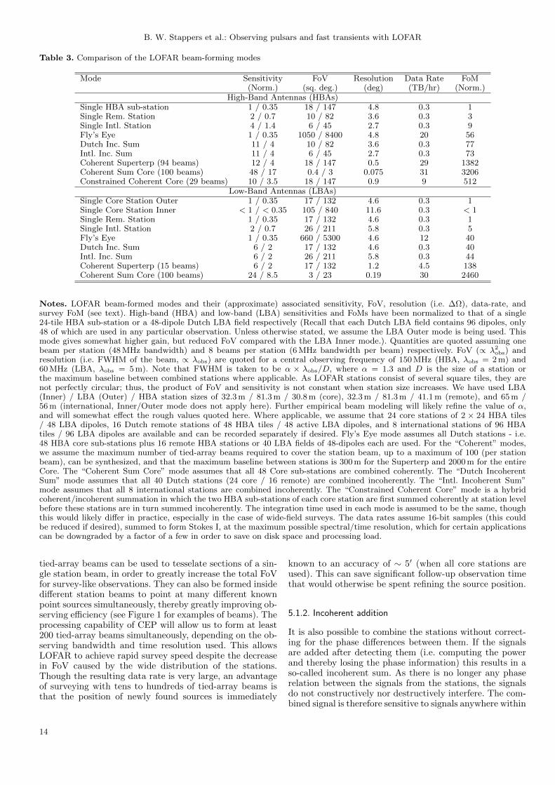
B. W. Stappers et al.: Observing pulsars and fast transients with LOFAR
Table 3. Comparison of the LOFAR beam-forming modes
Mode Sensitivity FoV Resolution Data Rate FoM(Norm.) (sq. deg.) (deg) (TB/hr) (Norm.)
High-Band Antennas (HBAs)Single HBA sub-station 1 / 0.35 18 / 147 4.8 0.3 1Single Rem. Station 2 / 0.7 10 / 82 3.6 0.3 3Single Intl. Station 4 / 1.4 6 / 45 2.7 0.3 9Fly’s Eye 1 / 0.35 1050 / 8400 4.8 20 56Dutch Inc. Sum 11 / 4 10 / 82 3.6 0.3 77Intl. Inc. Sum 11 / 4 6 / 45 2.7 0.3 73Coherent Superterp (94 beams) 12 / 4 18 / 147 0.5 29 1382Coherent Sum Core (100 beams) 48 / 17 0.4 / 3 0.075 31 3206Constrained Coherent Core (29 beams) 10 / 3.5 18 / 147 0.9 9 512
Low-Band Antennas (LBAs)Single Core Station Outer 1 / 0.35 17 / 132 4.6 0.3 1Single Core Station Inner < 1 / < 0.35 105 / 840 11.6 0.3 < 1Single Rem. Station 1 / 0.35 17 / 132 4.6 0.3 1Single Intl. Station 2 / 0.7 26 / 211 5.8 0.3 5Fly’s Eye 1 / 0.35 660 / 5300 4.6 12 40Dutch Inc. Sum 6 / 2 17 / 132 4.6 0.3 40Intl. Inc. Sum 6 / 2 26 / 211 5.8 0.3 44Coherent Superterp (15 beams) 6 / 2 17 / 132 1.2 4.5 138Coherent Sum Core (100 beams) 24 / 8.5 3 / 23 0.19 30 2460
Notes. LOFAR beam-formed modes and their (approximate) associated sensitivity, FoV, resolution (i.e. ∆Ω), data-rate, andsurvey FoM (see text). High-band (HBA) and low-band (LBA) sensitivities and FoMs have been normalized to that of a single24-tile HBA sub-station or a 48-dipole Dutch LBA field respectively (Recall that each Dutch LBA field contains 96 dipoles, only48 of which are used in any particular observation. Unless otherwise stated, we assume the LBA Outer mode is being used. Thismode gives somewhat higher gain, but reduced FoV compared with the LBA Inner mode.). Quantities are quoted assuming onebeam per station (48 MHz bandwidth) and 8 beams per station (6 MHz bandwidth per beam) respectively. FoV (∝ λ2
obs) andresolution (i.e. FWHM of the beam, ∝ λobs) are quoted for a central observing frequency of 150 MHz (HBA, λobs = 2 m) and60 MHz (LBA, λobs = 5 m). Note that FWHM is taken to be α × λobs/D, where α = 1.3 and D is the size of a station orthe maximum baseline between combined stations where applicable. As LOFAR stations consist of several square tiles, they arenot perfectly circular; thus, the product of FoV and sensitivity is not constant when station size increases. We have used LBA(Inner) / LBA (Outer) / HBA station sizes of 32.3 m / 81.3 m / 30.8 m (core), 32.3 m / 81.3 m / 41.1 m (remote), and 65 m /56 m (international, Inner/Outer mode does not apply here). Further empirical beam modeling will likely refine the value of α,and will somewhat effect the rough values quoted here. Where applicable, we assume that 24 core stations of 2 × 24 HBA tiles/ 48 LBA dipoles, 16 Dutch remote stations of 48 HBA tiles / 48 active LBA dipoles, and 8 international stations of 96 HBAtiles / 96 LBA dipoles are available and can be recorded separately if desired. Fly’s Eye mode assumes all Dutch stations - i.e.48 HBA core sub-stations plus 16 remote HBA stations or 40 LBA fields of 48-dipoles each are used. For the “Coherent” modes,we assume the maximum number of tied-array beams required to cover the station beam, up to a maximum of 100 (per stationbeam), can be synthesized, and that the maximum baseline between stations is 300 m for the Superterp and 2000 m for the entireCore. The “Coherent Sum Core” mode assumes that all 48 Core sub-stations are combined coherently. The “Dutch IncoherentSum” mode assumes that all 40 Dutch stations (24 core / 16 remote) are combined incoherently. The “Intl. Incoherent Sum”mode assumes that all 8 international stations are combined incoherently. The “Constrained Coherent Core” mode is a hybridcoherent/incoherent summation in which the two HBA sub-stations of each core station are first summed coherently at station levelbefore these stations are in turn summed incoherently. The integration time used in each mode is assumed to be the same, thoughthis would likely differ in practice, especially in the case of wide-field surveys. The data rates assume 16-bit samples (this couldbe reduced if desired), summed to form Stokes I, at the maximum possible spectral/time resolution, which for certain applicationscan be downgraded by a factor of a few in order to save on disk space and processing load.
tied-array beams can be used to tesselate sections of a sin-gle station beam, in order to greatly increase the total FoVfor survey-like observations. They can also be formed insidedifferent station beams to point at many different knownpoint sources simultaneously, thereby greatly improving ob-serving efficiency (see Figure 1 for examples of beams). Theprocessing capability of CEP will allow us to form at least200 tied-array beams simultaneously, depending on the ob-serving bandwidth and time resolution used. This allowsLOFAR to achieve rapid survey speed despite the decreasein FoV caused by the wide distribution of the stations.Though the resulting data rate is very large, an advantageof surveying with tens to hundreds of tied-array beams isthat the position of newly found sources is immediately
known to an accuracy of ∼ 5′ (when all core stations areused). This can save significant follow-up observation timethat would otherwise be spent refining the source position.
5.1.2. Incoherent addition
It is also possible to combine the stations without correct-ing for the phase differences between them. If the signalsare added after detecting them (i.e. computing the powerand thereby losing the phase information) this results in aso-called incoherent sum. As there is no longer any phaserelation between the signals from the stations, the signalsdo not constructively nor destructively interfere. The com-bined signal is therefore sensitive to signals anywhere within
14
B. W. Stappers et al.: Observing pulsars and fast transients with LOFAR
the FoV of the station beam, however the sensitivity in-creases only as the square-root of the number of stationscombined.
As it is not necessary to keep track of the phase relation-ship between the stations, the incoherent addition can in-corporate stations which are more widely spread than thosethat can be coherently combined. Determining which modeto use, for any given observing goal, depends on the amountof collecting area which can be combined coherently, thenumber of tied-array beams that can be formed and thescience goals.
As previously discussed in Hessels et al. (2009) the ob-servational requirements, e.g. sensitivity and FoV, can bedistilled into a simple figure of merit (FoM, see Table 3),which is generally applicable to a transient survey9 (see alsoCordes et al., 2004; Cordes, 2008, and references therein fora deeper discussion of survey metrics):
FoM ∝ A2eff
Ω
∆Ω
T
∆T. (1)
To be sensitive to transients over a wide range of sourceparameter space, including faint and rare events, this FoMshould be maximized. This means maximizing: Aeff , theeffective collecting area being used; Ω, the instantaneousfield of view (FoV); and T , the total time spent observingthe sky. At the same time, adequate spatial (∆Ω) and time(∆T ) resolution are needed to provide reasonable sourcelocalization, for multi-wavelength follow-up and identifica-tion, and to resolve short timescale phenomena. As it is notpossible to maximize both raw, instantaneous sensitivityand FoV simultaneously, different modes naturally probedifferent areas of transient parameter space (see below).
5.1.3. Coherent versus incoherent addition for differentscience cases
Contingent on the particular science goals, pulsar and fasttransient surveys with LOFAR are likely to be performedusing both the coherent and incoherent addition modes,sometimes in parallel. As discussed by van Leeuwen &Stappers (2010), a high sensitivity survey of the entireNorthern Sky is preferentially done using the coherent ad-dition of stations if one can form at least ∼200 tied-arraybeams10. Though such a mode provides the best-possiblesource localization and sensitivity, this comes at the priceof a much larger data rate (Table 3) and consequentlymuch greater processing requirements. In comparison, thewide FoV afforded by the incoherent sum gives it a verycompetitive survey speed. However, there are several draw-backs compared with the coherent mode: source localizationis comparatively poor, as is the rejection of astronomicalbackgrounds and radio frequency interference (RFI). Also,in the incoherent modes much longer observing times areneeded to achieve the same sensitivity and/or FoM (Table3), which increases the processing load significantly if ac-celeration searches for binary systems are to be performed(e.g. Johnston & Kulkarni 1991; Ransom et al. 2003). Onthe other hand, longer dwell times may be advantageous for
9 We choose to give extra weighting to Aeff . One may alsoconsider a FoM that scales linearly with Aeff .10 Current system performance tests indicate that this shouldbe achievable.
detecting certain types of transients. Nonetheless, the inco-herent addition mode provides a way to rapidly survey thewhole sky11 with a competitive sensitivity, thereby mak-ing it very useful for detecting classes of pulsars which canemit relatively brightly but more erratically, e.g. RRATs,intermittent pulsars, radio emitting magnetars, and eclips-ing sources, as well as other transient sources like flare stars,planets and potentially new classes of transient sources.
Observations of known point sources at high time reso-lution, where the maximum sensitivity over a given band-width is required, are best achieved by using the coherentsum mode. As discussed earlier, even in this mode multiplesources can be observed simultaneously if multiple stationbeams are used at the expense of total bandwidth. Each ofthe tied-array beams can be considered as an independententity in the LOFAR processing chain and so, e.g., pul-sar timing campaigns can be run efficiently by observingmultiple sources at once. It is also possible to have beamspointing at a range of source types, for example a pulsar,a planet, a flare star, and an X-ray binary all at the sametime, with different data products being produced for eachof the different sources.
5.2. Observing in multiple modes simultaneously
5.2.1. Coherent and incoherent sum modes
LOFAR is flexible enough to produce coherently and inco-herently added data simultaneously. This provides, at theincoherent summation sensitivity, the full FoV of a singlestation while still having the full coherent sensitivity in thecentre of the FoV. Though even 200 tied-array beams, gen-erated using all the stations on the core, only cover ∼ 3%of the single station FoV, this parallel mode allows one toboth survey the sky at very high sensitivity (over a smallFoV) and over a large FoV (at lower sensitivity) simulta-neously (Table 3). We note that a greater fraction of thesingle station FoV can be covered if we coherently sum theSuperterp stations only, and this may also prove a usefulsurvey mode. Alternatively, a mix of coherent and inco-herent addition can be used when adding the stations. Forexample, one might choose to coherently sum the stationsin the compact core of the array, e.g. on the Superterp(Figure 1), and then incoherently add the stations outsideof the core to this. This results in a compromise betweenFoV and sensitivity because the core stations have relativelyshort baselines between them (Figure 1). It also results in amore complex combined beam shape. In contrast, groups ofstations can also be used separately as part of sub-arrays,as discussed below.
5.2.2. Imaging and beamformed modes
As mentioned above, beamformed data can be taken inparallel with imaging observations. This opens up the op-portunity for commensal observing where searches for fasttransients can take place in parallel with imaging-basedsearches for slow transients or other observations. This willbe done as part of the Transient Key Science Project’sRadio Sky Monitor, which will image the sky down to 1
11 Using 7 station beams per pointing, only about 200 HBApointings are required to cover the entire LOFAR-visible sky(δ > −35).
15
B. W. Stappers et al.: Observing pulsars and fast transients with LOFAR
second timescales; we will continuously record the incoher-ent sum of the stations to probe variability on even fastertimescales. In Sect. 7.1.4 (Figure 12) we present the firstsuch simultaneous imaging/beamformed observation madewith LOFAR taken in 2010 April, when only 7 LOFARstations were available for imaging.
5.3. Observing with sub-arrays and single stations
In addition to the incoherent and coherent modes of ob-serving described above, the array can be split up in vari-ous flexible ways to accommodate particular science goals.There are certain pulsar and fast transient science goalswith observational requirements that are best served bygrouping the stations into sub-arrays, or using individualstations independently. In this way, sensitivity can be ex-changed for a larger total FoV and/or broader total fre-quency coverage.
For large sky coverage, LOFAR sub-arrays consisting ofone or several stations (depending on the required sensitiv-ity) can be used to point at different directions, covering alarge fraction of the sky − potentially the entire LOFAR-visible sky in the case of the LBAs (Table 3). To maximizeFoV, each sub-array can simply be a single station pointingin a unique direction. This mode, referred to as Fly’s Eye,is very similar to that developed for the Allen TelescopeArray (ATA; Welch et al. 2009) and will be used to moni-tor for rare, very bright, fast transient events. In this modethe localization of detected bursts can only be achievedto within the single station FoV, which ranges from a fewsquare degrees to many hundred square degrees across theLOFAR band. Much better position determination could beachieved by triggering as the source is detected and thenusing the TBBs to subsequently image the sky to try tofind the source (see Sect. 5.5 for more details).
Another option involves using sub-arrays of stationstuned to complementary frequencies across the entireLOFAR band, pointing at the same target. Covering thefull band requires two 48-MHz sub-arrays for the LBAs andthree for the HBAs. Such broad and dense spectral coverageis crucial for our understanding of the intrinsic processes inpulsar magnetospheres and propagation effects through theinterstellar medium at low radio frequencies (see Sect. 4).
Individual stations can also be used independently toconduct targeted observations of known bright objects, orwide field monitoring of transient events. In this respect, theinternational LOFAR stations have the highest sensitivityand may be available during normal LOFAR observationswhen the longest baselines are not in demand. In addition tothe conventional mode where single stations are controlledthrough the central LOFAR facilities and send data back toCEP, the data will be recorded and analysed locally, so thateach station can operate as a stand-alone instrument, or agroup of stations could operate as a coordinated sub-array.
5.4. Polarisation
After careful calibration, LOFAR will enable polarisa-tion studies of pulsar emission physics and the interstel-lar medium. A multi-stage process is required to achievesufficient polarisation purity. We only summarise the mostrelevant issues here and refer the reader to the MagnetismKey Science project (Beck, 2007) for more details. Both
the LBAs and the HBAs have dual linearly polarised feedsthat are stationary on the ground, meaning that for mostobservations the beams will be formed off-axis, potentiallyincreasing the contribution from polarisation leakage. Thedipoles are aligned South-East to North-West and South-West to North-East for the x- and y-dipoles respectivelyand this means that as a source is tracked across the skythe projected length of the dipole will change for the major-ity of sources. Thus, it will be important to accurately cal-ibrate the gains of the individual dipoles. For all antennasand stations, Mueller and Jones matrices (Tinbergen, 1996;Hamaker et al., 1996) need to be determined to correct forvoltage and Stokes-parameter coupling. It is important tonote that the beam patterns are time-variable and differentfor each station, however as discussed below it will be pos-sible to calibrate the system in all but the worst ionosphericconditions.
To calibrate the individual LBA dipoles and the HBAtiles in a given station, delay lookup tables that providestatic polarisation calibration will be used initially (see alsoFigure 11). However, a multi-level calibration procedurebased on the individual station elements and the stationsthemselves is required to ensure polarimetric fidelity as out-lined in Wijnholds & van der Veen (2009a,b). Combiningthe stations to form tied-array beams when including sta-tions beyond the superterp, will require using dynamic de-lays provided by the real-time calibration described above.
The LOFAR real-time calibration will correct for theionospheric phase delays, but removing the ionosphericFaraday rotation is more challenging. The limited size ofindividual stations means that the ionosphere in most caseswill not cause significant distortions across a station, iono-spheric Faraday rotation introduces a differential, and fre-quency dependent, polarisation component in addition tothe differential delays. If the properties of the ionosphereabove each station are determined, the ionospheric Faradayrotation can be removed by applying a frequency dependentphase term to the complex polarisations at the level of eachstation. The polarisation data of the array can then finallybe used to form 4 independent Stokes parameters, for boththe incoherent sum mode as well as for the phased-arraypolarimetric observations, and subsequently processed aspart of the pulsar pipeline using the methods described invan Straten (2004) and van Straten et al. (2010).
5.5. Transient buffer boards
The TBBs (see Singh et al. 2008) are an exciting and uniqueaspect of LOFAR. At each station there is sufficient mem-ory, RAM, to store the full-bandwidth raw voltage datafrom all of the active elements in that station for up to1.3 s12. These data can then be used to form an imageanywhere in the visible sky, in the case of the LBAs, oranywhere in the element beam of the HBAs if a trigger,either external or internal, arrives within 1.3 s of an eventoccurring, and causes the data in the buffer to be frozen.This mode will be used predominantly by the Cosmic RayKey Science Project (Falcke & LOFAR Cosmic Ray KeyScience Project, 2007) but will also be an invaluable toolfor the Transients Key Science Project. It will be used to
12 This number may increase in the near future with the addi-tion of more memory.
16
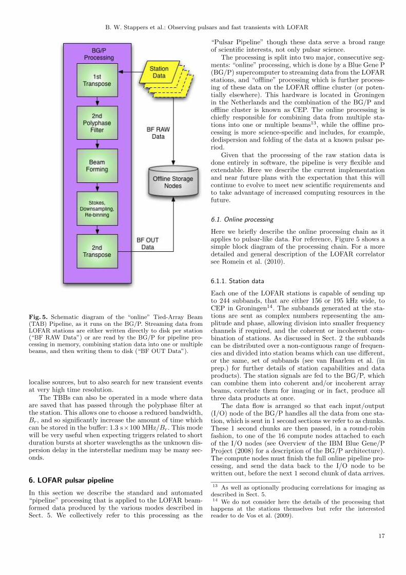
B. W. Stappers et al.: Observing pulsars and fast transients with LOFAR
Fig. 5. Schematic diagram of the “online” Tied-Array Beam(TAB) Pipeline, as it runs on the BG/P. Streaming data fromLOFAR stations are either written directly to disk per station(“BF RAW Data”) or are read by the BG/P for pipeline pro-cessing in memory, combining station data into one or multiplebeams, and then writing them to disk (“BF OUT Data”).
localise sources, but to also search for new transient eventsat very high time resolution.
The TBBs can also be operated in a mode where dataare saved that has passed through the polyphase filter atthe station. This allows one to choose a reduced bandwidth,Br, and so significantly increase the amount of time whichcan be stored in the buffer: 1.3 s×100 MHz/Br. This modewill be very useful when expecting triggers related to shortduration bursts at shorter wavelengths as the unknown dis-persion delay in the interstellar medium may be many sec-onds.
6. LOFAR pulsar pipeline
In this section we describe the standard and automated“pipeline” processing that is applied to the LOFAR beam-formed data produced by the various modes described inSect. 5. We collectively refer to this processing as the
“Pulsar Pipeline” though these data serve a broad rangeof scientific interests, not only pulsar science.
The processing is split into two major, consecutive seg-ments: “online” processing, which is done by a Blue Gene P(BG/P) supercomputer to streaming data from the LOFARstations, and “offline” processing which is further process-ing of these data on the LOFAR offline cluster (or poten-tially elsewhere). This hardware is located in Groningenin the Netherlands and the combination of the BG/P andoffline cluster is known as CEP. The online processing ischiefly responsible for combining data from multiple sta-tions into one or multiple beams13, while the offline pro-cessing is more science-specific and includes, for example,dedispersion and folding of the data at a known pulsar pe-riod.
Given that the processing of the raw station data isdone entirely in software, the pipeline is very flexible andextendable. Here we describe the current implementationand near future plans with the expectation that this willcontinue to evolve to meet new scientific requirements andto take advantage of increased computing resources in thefuture.
6.1. Online processing
Here we briefly describe the online processing chain as itapplies to pulsar-like data. For reference, Figure 5 shows asimple block diagram of the processing chain. For a moredetailed and general description of the LOFAR correlatorsee Romein et al. (2010).
6.1.1. Station data
Each one of the LOFAR stations is capable of sending upto 244 subbands, that are either 156 or 195 kHz wide, toCEP in Groningen14. The subbands generated at the sta-tions are sent as complex numbers representing the am-plitude and phase, allowing division into smaller frequencychannels if required, and the coherent or incoherent com-bination of stations. As discussed in Sect. 2 the subbandscan be distributed over a non-contiguous range of frequen-cies and divided into station beams which can use different,or the same, set of subbands (see van Haarlem et al. (inprep.) for further details of station capabilities and dataproducts). The station signals are fed to the BG/P, whichcan combine them into coherent and/or incoherent arraybeams, correlate them for imaging or in fact, produce allthree data products at once.
The data flow is arranged so that each input/output(I/O) node of the BG/P handles all the data from one sta-tion, which is sent in 1 second sections we refer to as chunks.These 1 second chunks are then passed, in a round-robinfashion, to one of the 16 compute nodes attached to eachof the I/O nodes (see Overview of the IBM Blue Gene/PProject (2008) for a description of the BG/P architecture).The compute nodes must finish the full online pipeline pro-cessing, and send the data back to the I/O node to bewritten out, before the next 1 second chunk of data arrives.
13 As well as optionally producing correlations for imaging asdescribed in Sect. 5.14 We do not consider here the details of the processing thathappens at the stations themselves but refer the interestedreader to de Vos et al. (2009).
17

B. W. Stappers et al.: Observing pulsars and fast transients with LOFAR
There are sufficient computing resources that while keep-ing up with the real time processing there is approximately16 seconds of available computing time for each 1 secondchunk of raw data15.
6.1.2. First transpose
The data arrive at the BG/P such that they are arrangedby station, however in order to efficiently form correlationproducts and beams it is necessary to have the data fromall the stations for a particular subband, in the 1 secondchunks, present. The process of reordering these data isreferred to as the “First Transpose” (Figure 5). Before thetranspose, the memory of a particular compute node holdsmultiple frequency subbands from a single station; afterthe transpose, the same compute node holds subband(s) ofa particular frequency from all the stations being used.
6.1.3. Second polyphase filter
Depending on the particular application, each subbandcan be further split into an optional number of channels(16 − 256) via a polyphase filter (PPF). This is referredto as the “2nd polyphase filter” (2PPF, see Figure 5), be-cause of the preceding PPF step which occurs at the sta-tions themselves in order to create subbands (see Sect. 2).This further channelization serves two purposes: it allowsfor the removal of narrow band interference signals in away which minimises the loss of bandwidth; it is also re-quired for incoherently dedispersing the pulsed signal. Theremoval of radio frequency interference (RFI) will be dis-cussed in more detail below, but typically these signals aresignificantly narrower than the 156/195-kHz subbands sentfrom the stations, so further division into finer frequencychannels is required (see Sect. 8 for details).
As discussed in Sect. 3, any broadband pulsed signalwill be dispersed, and hence smeared in time, by the ISMbetween the source and the Earth. This can be corrected byeither incoherent or coherent dedispersion. Coherent dedis-persion will be used for studying known pulsars, as it pro-vides the best possible dispersive correction along with thehighest achievable time resolution for a given bandwidth.Since this technique is computationally very expensive, it isunfortunately not yet feasible to use coherent dedispersionfor wide-area pulsar surveys, where it would need to be ap-plied over large numbers of tied-array beams and trial DMs(thousands of trial DMs in the case of blind searches for mil-lisecond pulsars). The survey processing chain will thereforeoperate on data which has been through the 2PPF and usecomputionally efficient incoherent dedispersion algorithms.Recently we have been able to develop a system which canperform coherent dedispersion for up to 40 different disper-sion measures at one time (Mol & Romein, 2011). This willhave application as either a hybrid option where it is com-bined with incoherent dedispersion for large area surveys,or using coherent dedispersion for searches of objects wherethe DM is constrained to a limited range of values, such asin globular clusters.
15 This is because there are 244 (i.e. approximately 256) sub-bands divided over 4096 available compute cores.
6.1.4. Beamforming
It is at this stage that the (optional) beamforming betweenmultiple stations is done (Figure 5). The stations are com-bined in one or potentially several of the ways describedin Sect. 5. This is performed on a per subband or evenper channel basis depending on whether the data has beenthrough the 2PPF. For incoherent beams, the combinationis not done on the complex samples, but instead on theStokes parameters (see also below). The geometrical delaysbetween stations are computed once per second and inter-polated both in frequency and time, so that each sample iscorrected by a per-sample unique factor. The small numberof possible incoherent beams, only one per station beam,means that this is not a computationally heavy task com-pared with the other calculations of the online processing;nor is the data rate unmanageable (see Table 3). Hence,incoherent array beams can, and often will, be produced inparallel to the correlation products needed for imaging orany other data-products, such as multiple tied-array beams.
In the case of tied-array beams, computational efficiencyis a far greater concern, as up-to several hundred beamsmust be synthesized in parallel in order to give this modesufficient “survey speed” for all-sky surveys. Beam formingis performed by applying the appropriate time and phasecorrection to the complex samples (Sect. 2). These delaysare applied in three steps: first shifting by integer amountsof samples, then a phase correction for the center beam(these are both shared with the imaging pipeline), and fi-nally a delta-phase correction between the center beam andeach tied-array beam is applied. Determining the phase cor-rections due to contributions from the ionosphere and theinstrument, which need to be calculated from the data, arediscussed in Sect. 5. An efficient algorithm, partially writ-ten in assembly code, is used to maximize the number ofbeams that can be calculated. The large number of beamsalso make the data rate much larger, and the 15 Gb/s de-signed input limit of the current offline storage cluster playsthe main limiting role on the maximum number of beamsthat can be written out. The final LOFAR offline clusterwill have an increase in throughput of about 500%.
To form both incoherent and tied-array beams it is nec-essary to define a reference phase location. It is stronglypreferable for observations where precise time tagging ofevents is required, such as pulsar timing, that this locationbe fixed. For LOFAR the phase center of all observations isnow by convention the geographical center of the LBA fieldof station CS002, regardless of whether this particular sta-tion is being used or not. This places the official position ofthe LOFAR telescope at (x,y,z) coordinates of (3826577.462m, 461022.624 m, 5064892.526 m) in the ETRS89 system(Boucher & Altamimi, 2001). This reference position willbe used for barycentering, pulsar timing, and phasing-upthe array.
6.1.5. Fly’s eye mode
For Fly’s Eye mode, in which the station signals are notcombined into incoherent or tied-array beams at BG/P, theprocessing proceeds largely as described above, except thatindividual station beams are written out separately usingthe same code that stores multiple tied-array beams. Inparallel, it is also possible to generate the incoherent sumof the station beams if desired. Besides the scientific appli-
18
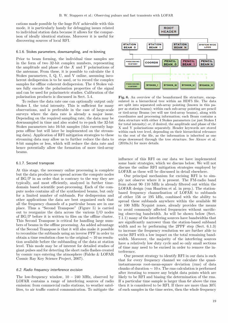
B. W. Stappers et al.: Observing pulsars and fast transients with LOFAR
cations made possible by the huge FoV achievable with thismode, it is particularly handy for debugging issues relatedto individual station data because it allows for the compar-ison of ideally identical stations. Moreover it is useful fordiscovering sources of local RFI.
6.1.6. Stokes parameters, downsampling, and re-binning
Prior to beam forming, the individual time samples arein the form of two 32-bit complex numbers, representingthe amplitude and phase of the X and Y polarisations ofthe antennas. From these, it is possible to calculate the 4Stokes parameters, I, Q, U, and V online, assuming inco-herent dedispersion is to be used, or to record the complexsamples for offline coherent dedispersion. The 4 Stokes val-ues fully encode the polarisation properties of the signaland can be used for polarimetric studies. Calibration of thepolarisation products is discussed in Sect. 5.4.
To reduce the data rate one can optionally output onlyStokes I, the total intensity. This is sufficient for manyobservations, and is preferable in the case of large-scalesurveys where the data rate is already a major issue.Depending on the required sampling rate, the data may bedownsampled in time and also scaled to re-pack the 32-bitStokes parameters into 16-bit samples (this currently hap-pens offline but will later be implemented on the stream-ing data). Application of RFI mitigation strategies to thesestreaming data may allow us to further reduce the data to8-bit samples or less, which will reduce the data rate andhence potentially allow the formation of more tied-arraybeams.
6.1.7. Second transpose
At this stage, the necessary online processing is completebut the data products are spread across the compute nodesof BG/P in an order that is contrary to the way they aretypically, and most efficiently, analyzed in further time-domain based scientific post-processing. Each of the com-pute nodes contains all of the synthesized beams, but onlyfor a limited number of subbands. For dedispersion andother applications the data are best organized such thatall the frequency channels of a particular beam are in oneplace. Thus a “Second Transpose” (Figure 5) is carriedout to reorganize the data across the various I/O nodesof BG/P before it is written to files on the offline cluster.This Second Transpose is critical for handling large num-bers of beams in the offline processing. An added advantageof the Second Transpose is that it will also make it possibleto recombine the subbands using an inverse PPF in order toobtain a time resolution close to the original ∼ 10 ns resolu-tion available before the subbanding of the data at stationlevel. This mode may be of interest for detailed studies ofgiant pulses and for detecting the short radio flashes createdby cosmic rays entering the atmosphere (Falcke & LOFARCosmic Ray Key Science Project, 2007).
6.2. Radio frequency interference excision
The low-frequency window, 10 − 240 MHz, observed byLOFAR contains a range of interfering sources of radioemission: from commercial radio stations, to weather satel-lites, to air traffic control communication. To mitigate the
Fig. 6. An overview of the beamformed file structure, encap-sulated in a hierarchical tree within an HDF5 file. The dataare split into separated sub-array pointing (known in this pa-per as station beams); within each sub-array pointing are pencilor tied-array Beams (we will use tied-array beams), along withcoordinates and processing information; each Beam contains adata structure with either 4 Stokes parameters (or just Stokes Ifor total intensity) or, if desired, the amplitude and phase of theX and Y polarisations separately. Header keywords are storedwithin each tree level, depending on their hierarchical relevanceto the rest of the file, as the information is inherited as onesteps downward through the tree structure. See Alexov et al.(2010a,b) for more details.
influence of this RFI on our data we have implementedsome basic strategies, which we discuss below. We will notdiscuss the online RFI mitigation strategies employed byLOFAR as these will be discussed in detail elsewhere.
Our principal mechanism for excising RFI is to sim-ply not observe where it is present. The FM-radio bandfrom about 90–110 MHz is already filtered out within theLOFAR design (van Haarlem et al. in prep.). The station-based frequency channelisation of LOFAR to subbandsof either 156 or 195 kHz, combined with the ability tospread these subbands anywhere within the available 80or 100 MHz Nyquist zones, already provides the meansto avoid commonly affected frequencies without sacrific-ing observing bandwidth. As will be shown below (Sect.7.1.1) many of the interfering sources have bandwidths thatare significantly narrower than the station-based subbandwidth and so by performing the 2PPF step (Sect. 6.1.3)to increase the frequency resolution we are further able toexcise RFI with a low impact on the total remaining band-width. Moreover, the majority of the interfering sourceshave a relatively low duty cycle and so only small sectionsof time may need to be excised in order to remove the in-terference.
Our present strategy to identify RFI in our data is suchthat for every frequency channel we calculate the quasi-instantaneous root-mean-square deviation (rms) of datachunks of duration ∼ 10 s. The rms calculation is performedafter iterating to remove any bright data points which arelikely to be RFI and biasing the determination of the rms.If a particular time sample is larger than 6σ above the rmsthen it is considered to be RFI. If there are more than 30%of such samples in the time series, then the whole frequency
19
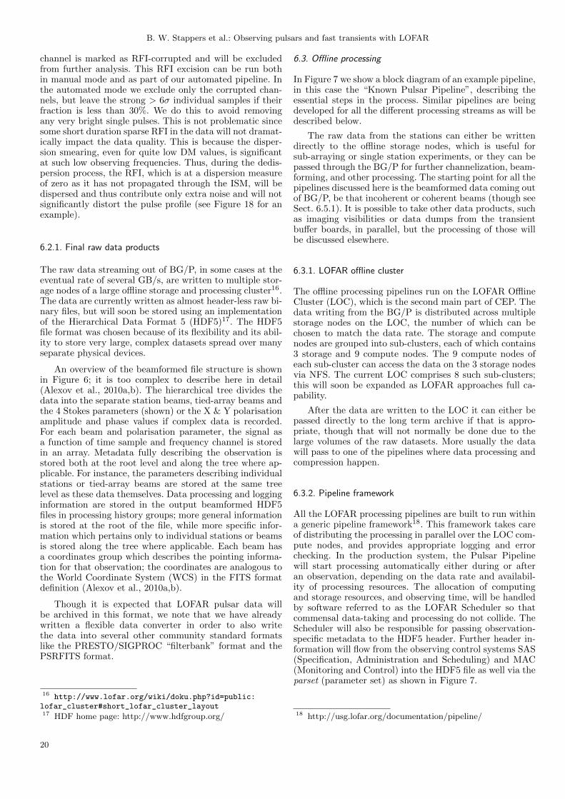
B. W. Stappers et al.: Observing pulsars and fast transients with LOFAR
channel is marked as RFI-corrupted and will be excludedfrom further analysis. This RFI excision can be run bothin manual mode and as part of our automated pipeline. Inthe automated mode we exclude only the corrupted chan-nels, but leave the strong > 6σ individual samples if theirfraction is less than 30%. We do this to avoid removingany very bright single pulses. This is not problematic sincesome short duration sparse RFI in the data will not dramat-ically impact the data quality. This is because the disper-sion smearing, even for quite low DM values, is significantat such low observing frequencies. Thus, during the dedis-persion process, the RFI, which is at a dispersion measureof zero as it has not propagated through the ISM, will bedispersed and thus contribute only extra noise and will notsignificantly distort the pulse profile (see Figure 18 for anexample).
6.2.1. Final raw data products
The raw data streaming out of BG/P, in some cases at theeventual rate of several GB/s, are written to multiple stor-age nodes of a large offline storage and processing cluster16.The data are currently written as almost header-less raw bi-nary files, but will soon be stored using an implementationof the Hierarchical Data Format 5 (HDF5)17. The HDF5file format was chosen because of its flexibility and its abil-ity to store very large, complex datasets spread over manyseparate physical devices.
An overview of the beamformed file structure is shownin Figure 6; it is too complex to describe here in detail(Alexov et al., 2010a,b). The hierarchical tree divides thedata into the separate station beams, tied-array beams andthe 4 Stokes parameters (shown) or the X & Y polarisationamplitude and phase values if complex data is recorded.For each beam and polarisation parameter, the signal asa function of time sample and frequency channel is storedin an array. Metadata fully describing the observation isstored both at the root level and along the tree where ap-plicable. For instance, the parameters describing individualstations or tied-array beams are stored at the same treelevel as these data themselves. Data processing and logginginformation are stored in the output beamformed HDF5files in processing history groups; more general informationis stored at the root of the file, while more specific infor-mation which pertains only to individual stations or beamsis stored along the tree where applicable. Each beam hasa coordinates group which describes the pointing informa-tion for that observation; the coordinates are analogous tothe World Coordinate System (WCS) in the FITS formatdefinition (Alexov et al., 2010a,b).
Though it is expected that LOFAR pulsar data willbe archived in this format, we note that we have alreadywritten a flexible data converter in order to also writethe data into several other community standard formatslike the PRESTO/SIGPROC “filterbank” format and thePSRFITS format.
16 http://www.lofar.org/wiki/doku.php?id=public:lofar_cluster#short_lofar_cluster_layout17 HDF home page: http://www.hdfgroup.org/
6.3. Offline processing
In Figure 7 we show a block diagram of an example pipeline,in this case the “Known Pulsar Pipeline”, describing theessential steps in the process. Similar pipelines are beingdeveloped for all the different processing streams as will bedescribed below.
The raw data from the stations can either be writtendirectly to the offline storage nodes, which is useful forsub-arraying or single station experiments, or they can bepassed through the BG/P for further channelization, beam-forming, and other processing. The starting point for all thepipelines discussed here is the beamformed data coming outof BG/P, be that incoherent or coherent beams (though seeSect. 6.5.1). It is possible to take other data products, suchas imaging visibilities or data dumps from the transientbuffer boards, in parallel, but the processing of those willbe discussed elsewhere.
6.3.1. LOFAR offline cluster
The offline processing pipelines run on the LOFAR OfflineCluster (LOC), which is the second main part of CEP. Thedata writing from the BG/P is distributed across multiplestorage nodes on the LOC, the number of which can bechosen to match the data rate. The storage and computenodes are grouped into sub-clusters, each of which contains3 storage and 9 compute nodes. The 9 compute nodes ofeach sub-cluster can access the data on the 3 storage nodesvia NFS. The current LOC comprises 8 such sub-clusters;this will soon be expanded as LOFAR approaches full ca-pability.
After the data are written to the LOC it can either bepassed directly to the long term archive if that is appro-priate, though that will not normally be done due to thelarge volumes of the raw datasets. More usually the datawill pass to one of the pipelines where data processing andcompression happen.
6.3.2. Pipeline framework
All the LOFAR processing pipelines are built to run withina generic pipeline framework18. This framework takes careof distributing the processing in parallel over the LOC com-pute nodes, and provides appropriate logging and errorchecking. In the production system, the Pulsar Pipelinewill start processing automatically either during or afteran observation, depending on the data rate and availabil-ity of processing resources. The allocation of computingand storage resources, and observing time, will be handledby software referred to as the LOFAR Scheduler so thatcommensal data-taking and processing do not collide. TheScheduler will also be responsible for passing observation-specific metadata to the HDF5 header. Further header in-formation will flow from the observing control systems SAS(Specification, Administration and Scheduling) and MAC(Monitoring and Control) into the HDF5 file as well via theparset (parameter set) as shown in Figure 7.
18 http://usg.lofar.org/documentation/pipeline/
20

B. W. Stappers et al.: Observing pulsars and fast transients with LOFAR
Fig. 7. Schematic diagram of the overall Known Pulsar Pipeline, as it runs “online” on the BG/P followed by “offline” scientificprocessing on the offline cluster. Offline pipeline processing can be run on data directly out of the BG/P or on RFI-filtered data.Scientific tools such as de-dispersion and folding are performed, along with Stokes calibration to get polarisation and flux densities.Data products and diagnostic plots are stored in the long term archive.
6.3.3. Software and data access
Wherever possible, all of the different Pulsar Pipelinesare being built around the well-tested, commonly used,open source software packages available in the pulsarcommunity (e.g. PRESTO19, PSRCHIVE20, SIGPROC21,TEMPO22. To allow for efficient development and softwaremanagement these have been incorporated into the gen-eral LOFAR User Software (LUS)23, which uses cmake24, across-platform, open-source build system, to automate theinstallation of these packages on a variety of platforms (e.g.Ubuntu Linux and Mac OS 10.5.X). This cmake installermay be of interest to others using these same reductionpackages on other systems.
The LOFAR software interface to the HDF5 library iscalled the Data Access Library (DAL). It is also availablewithin the LUS software repository. The DAL allows forhigh-level connectivity to HDF5 data, and more specificallyto LOFAR data structures encapsulated within an HDF5file. The DAL is written in C++; it contains classes whichpertain to all the LOFAR-specific data structures, makingit straight forward to read and write LOFAR HDF5 data.The DAL is also bound as a Python module, called pydal,giving users access to the DAL classes via Python. This isan important set of tools for connecting existing or newlywritten processing code to the data.
6.3.4. Radio frequency interference excision
The Known Pulsar Pipeline in Figure 7 shows two paral-lel processing paths in the offline reduction of LOFAR BF
19 http://www.cv.nrao.edu/∼sransom/presto/20 http://sourceforge.net/projects/psrchive/21 http://sigproc.sourceforge.net/22 http://www.atnf.csiro.au/research/pulsar/tempo/23 http://usg.lofar.org24 http://www.cmake.org/
data. The standard path performs dedispersion and folding;optionally, the pipeline can be run on the same data, buthaving performed RFI-excision prior to folding and dedis-persion. This process filters the data of RFI and then runsthe same tools as run for standard processing. The dataprocessing time doubles since the pipeline is essentially per-forming the same processing twice, once on unfiltered dataand a second time on RFI-cleaned files. Once the RFI-cleaning algorithms have been refined, we expect to onlyrun the processing once, using the RFI-cleaned data.
6.4. Known pulsar pipeline
The Known Pulsar Pipeline processes data taken inthe following modes: Incoherent Stokes, Coherent Stokes,Coherent Complex, Fly’s Eye and Commensal Imaging. Inall cases, once the data is on the LOC, the processing doneby the Known Pulsar Pipeline is very similar to standardpulsar processing (e.g. Lorimer & Kramer 2005). Once thedata have undergone RFI excision it is then dedispersed atthe known DM using either coherent or incoherent dedisper-sion, depending on the particular source and the scientificgoals. The dispersion-corrected data will then be used togenerate a number of output data products such as dedis-persed time series, dynamic spectra and folded pulse pro-files. It is likely that we will simultaneously observe multiplepulsars, and so multiple instances of the pipeline, with dif-ferent dispersion and fold parameters, will run in parallel.The processing capability of LOFAR is such that we arein general able to produce all of these data products foreach known pulsar observation. These data products arethen flux and polarisation calibrated, stored to the longterm archive as well as being passed to post processingprograms. Multiple pipelines, from multiple separate ob-servations, can run in parallel depending on the availablecomputing resources on the LOC.
21
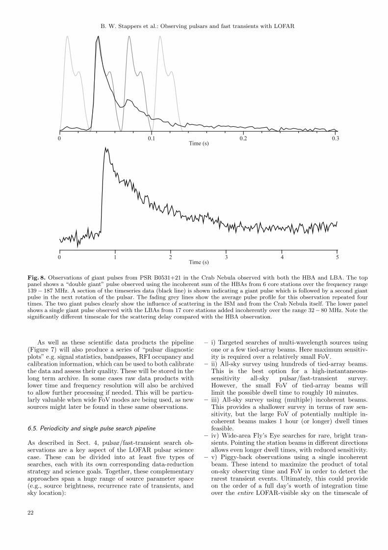
B. W. Stappers et al.: Observing pulsars and fast transients with LOFAR
0 0.1 0.2 0.3Time (s)
0 1 2 3 4 5Time (s)
Fig. 8. Observations of giant pulses from PSR B0531+21 in the Crab Nebula observed with both the HBA and LBA. The toppanel shows a “double giant” pulse observed using the incoherent sum of the HBAs from 6 core stations over the frequency range139− 187 MHz. A section of the timeseries data (black line) is shown indicating a giant pulse which is followed by a second giantpulse in the next rotation of the pulsar. The fading grey lines show the average pulse profile for this observation repeated fourtimes. The two giant pulses clearly show the influence of scattering in the ISM and from the Crab Nebula itself. The lower panelshows a single giant pulse observed with the LBAs from 17 core stations added incoherently over the range 32− 80 MHz. Note thesignificantly different timescale for the scattering delay compared with the HBA observation.
As well as these scientific data products the pipeline(Figure 7) will also produce a series of “pulsar diagnosticplots” e.g. signal statistics, bandpasses, RFI occupancy andcalibration information, which can be used to both calibratethe data and assess their quality. These will be stored in thelong term archive. In some cases raw data products withlower time and frequency resolution will also be archivedto allow further processing if needed. This will be particu-larly valuable when wide FoV modes are being used, as newsources might later be found in these same observations.
6.5. Periodicity and single pulse search pipeline
As described in Sect. 4, pulsar/fast-transient search ob-servations are a key aspect of the LOFAR pulsar sciencecase. These can be divided into at least five types ofsearches, each with its own corresponding data-reductionstrategy and science goals. Together, these complementaryapproaches span a huge range of source parameter space(e.g., source brightness, recurrence rate of transients, andsky location):
– i) Targeted searches of multi-wavelength sources usingone or a few tied-array beams. Here maximum sensitiv-ity is required over a relatively small FoV.
– ii) All-sky survey using hundreds of tied-array beams.This is the best option for a high-instantaneous-sensitivity all-sky pulsar/fast-transient survey.However, the small FoV of tied-array beams willlimit the possible dwell time to roughly 10 minutes.
– iii) All-sky survey using (multiple) incoherent beams.This provides a shallower survey in terms of raw sen-sitivity, but the large FoV of potentially multiple in-coherent beams makes 1 hour (or longer) dwell timesfeasible.
– iv) Wide-area Fly’s Eye searches for rare, bright tran-sients. Pointing the station beams in different directionsallows even longer dwell times, with reduced sensitivity.
– v) Piggy-back observations using a single incoherentbeam. These intend to maximize the product of totalon-sky observing time and FoV in order to detect therarest transient events. Ultimately, this could provideon the order of a full day’s worth of integration timeover the entire LOFAR-visible sky on the timescale of
22

B. W. Stappers et al.: Observing pulsars and fast transients with LOFAR
Fig. 9. An initial summary of the RFI situation across our most commonly used sections of the LBA (left-hand panels) and HBA(right-hand panels) frequency ranges. The upper and lower panels correspond to a frequency channel width of 195 kHz and 12 kHz,respectively. Each line in the plot corresponds to the percentage of observations in which the particular frequency channel wasaffected by RFI.
a few years.
6.5.1. General search requirements and processing
We currently have a basic search pipeline in place that candeal well with searching a single incoherent beam or a fewtied-array beams. However, modes using hundreds of tied-array beams require highly optimised processing chains andthe full LOC hardware to be in place, and so we are cur-rently only in the planning phase of this more complexmode25. As well as potentially dealing with large num-bers of beams, the very low frequencies and wide fractionalbandwidths involved in the pulsar searches means that inthe Pulsar Search Pipeline, the number of trial DMs willbe at least 10000, which clearly makes dedispersion oneof the rate limiting steps. We are therefore in the processof designing an optimal mechanism to efficiently processpulsar search data within the CEP framework. As well asconsidering hybrid coherent/incoherent dedispersion modes
25 Note that this processing challenge is still only a fraction ofwhat will be required for the SKA.
we are looking at moving some survey processing on to theBG/P. Distributing and parallelizing the pipeline will bedone by the Pipeline Framework; however, the mechanismitself of how data processing will be performed and whichalgorithms will be used on the LOC are still being deter-mined.
We now consider the different envisioned search modesin more detail:
Targeted Searches Targeted searches of known, multi-wavelength sources require maximum sensitivity over a rel-atively small area of sky compared with the ∼ 20 sq. degsingle station beam FoV. This mode will therefore use anumber of tied-array beams, the total required number de-pending on the size of the source or its positional uncer-tainty. If the number of beams is significantly less thanneeded for the all-sky survey, then the load on BG/P andthe offline cluster will be modest and so simultaneous imag-ing modes are likely to be run in parallel. For this, and othermodes which use tied-array beams, one beam may be sacri-ficed to point well away from the target area and be used asa reference beam for RFI excision. Potential targets for such
23

B. W. Stappers et al.: Observing pulsars and fast transients with LOFAR
Phase (o)0 90
Normalized SNR0 1
Tim
e fr
om tr
ansi
t (s)
010
0020
00- 1
000
- 200
0
Fig. 10. A transit observation at a central frequency of 165 MHzof PSR B0329+54 as it passes through the zenith above corestation CS302. The antennas were combined coherently with-out further geometrical delay in order to point directly above.Left: The intensity of PSR B0329+54 as a function of time fromtransit and rotational phase. The variations are due to both the“fringe” pattern created by the coherent addition of the twoHBA sub-stations of station CS302 and the wider single sub-station beam width. Right: The corresponding normalized S/Nof the pulsar as a function of time from transit.
searches include, e.g., unidentified Fermi γ-ray sources, ap-parently radio quiet γ-ray/X-ray pulsars, magnetars, andnearby galaxies or globular clusters.
All-Sky Coherent (Tied-Array) Survey The planned all-skytied-array survey will be by far the most data and com-putation intensive implementation of the pulsar pipelines.The optimal way to perform the survey is with, at least, acouple of hundred tied-array beams. A maximal implemen-tation will result in a data rate of order 23 TB hr−1. We arecurrently pursuing two options for the survey processing,which depend greatly on the mix of computing resourcesand storage capacity. If the latter is the most restrictivethen a real-time processing chain may be needed, wherededispersion, FFT’ing, and candidate selection will be done
in close to real time with only data products related to theresultant candidates being stored. Alternatively, relativelyshort observing sessions will take place with data beingstored and processed at a later date. The latter approach ispreferable, but some hybrid process may be required. Sucha survey provides the highest possible raw sensitivity, butthe dwell time per pointing will have to be modest becauseof the limited FoV. Certain classes of intermittent sourcesmay be better sampled by an all-sky survey using incoher-ent beams (see below).
All-Sky Incoherent Survey The raw sensitivity of incoherentarray beams (using say all 40 Dutch stations) is roughly 3times lower than the sensitivity of tied-array beams madefrom the combination of all 24 core stations. Nonetheless,these incoherent beams have over 1000 times larger FoVs,making shallow all-sky surveys in this mode an attractivepossibility because of the ability to use long dwell times.Using multiple station beams, the FoV can be increasedeven further. For instance, using 7 station beams providesan instantaneous FoV of ∼ 170 sq. deg, at a central fre-quency of about 140 MHz, allowing one to search the en-tire LOFAR-visible sky (δ > −35) with only 200 point-ings. Even with a 1 hr dwell time, such a survey can becompleted in roughly 1 week of observing time. Shallowsurveys such as the example described above are not onlymuch more tractable in terms of required observing andprocessing time, but they also provide an excellent com-plement to deep all-sky surveys with higher instantaneoussensitivity. This is because some intermittent sources, e.g.the RRATs, may be easier to identify in surveys where theproduct of FoV and dwell time is large (assuming the un-derlying sensitivity is also sufficient).
Fly’s Eye Searches Very bright but rare transients may bebetter found by surveys that sacrifice even more raw sensi-tivity in favor of increased FoV and dwell time. Fly’s Eyesearches will be processed in a similar way to the all-sky sur-veys, except that different data streams will correspond toindividual station beams pointing in a variety of directions,instead of different tied-array or incoherent array beams.There could be up to a couple hundred such beams depend-ing on how the observing bandwidth is distributed amongindividual station beams. This provides, in principle, theability to monitor the entire LOFAR-visible sky at oncemaking LOFAR a truly synoptic radio telescope.
Piggy-Back Searches Piggy-back searches aim to achievethe maximum possible on-sky time for transients by observ-ing in parallel whenever possible. This mode will be run asoften as possible when the telescope is doing standard imag-ing observations or even during tied-array observations. Itwill use only one incoherent or a few tied-array beams andso the computational load is reasonable. The simultaneousimaging data might be used when interesting candidatesare found. These relatively shallow, but typically wide FoVobservations allow for repeated studies of the same piece ofsky in order to probe variable and transient sources. Theadditional processing requirement is small compared withthat required for imaging.
24
B. W. Stappers et al.: Observing pulsars and fast transients with LOFAR
Fig. 11. Three consecutive 20 minute LBA observations of PSR B1133+16 taken on 2010 Nov 5. In between these observations,the station calibration was alternately turned off and then back on. The profiles are all scaled to have the same peak height andas can be seen, the S/N of the cumulative pulse profile decreases by roughly a factor of 3 when the static calibration table isnot applied. Five Dutch stations were combined incoherently in these observations, and as such the S/N difference is the averagecalibration gain for all these stations.
Single station processing In Single Station mode, the net-work streams carrying the data that would otherwise go tothe BG/P need to be redirected to local servers. This in-volves for the most part the 48 MHz of beamformed data,which are streamed through 4 UDP26 streams of approxi-mately 800 Mb s−1 each. Members of the LOFAR pulsarcollaboration have developed a hardware and software so-lution (codenamed ARTEMIS) acting as a single stationbackend and capable of recording data for observations ofpulsars and fast transients. This backend has the process-ing power required to perform a number of relevant opera-tions in real time, such as RFI excision, channelisation, andStokes parameter generation. It is also designed to connectto fast Graphics Processing Units for real time dispersionmeasure searching on the streaming data. Besides pulsarsand fast transients ARTEMIS can be used as a general pur-pose single station backend. Such an instrument allows ob-servations to be made either in parallel with ongoing centralLOFAR observations, or allow for local processing when thestation is in local or remote control if there are insufficientBG/P resources for the required processing. Moreover it al-lows for the possibility of processing and analysing largerdata sets than can be transferred to the Netherlands.
7. Commissioning results
Since pulsar “first light” in the summer of 2007, when therewere only a few test antennas available, we have been com-missioning the LOFAR telescope for pulsar observations.In this time, LOFAR’s sensitivity and functionality haveincreased dramatically, as has the data quality (for the pro-gression, see Stappers et al., 2007; Hessels et al., 2009, 2010;Stappers et al., 2011). The ability to detect bright pulsarswith just one or a few individual HBA tiles means that pul-sar observations are useful for measuring the system per-formance from some of its smallest elements up to the full,combined array. For instance, pulsar observations can beused to study the beam shapes of individual or beamformedelements, verify antenna positions, and measure clock sta-bility. Here we present highlights from some of these systemtests, followed by associated early science results. These
26 User Datagram Protocol
demonstrate that LOFAR is beginning to function as de-signed.
Though already impressive, these observational resultsprovide merely a taste of what LOFAR will ultimately becapable of doing. The number of completed stations is stillincreasing and we have only just begun to take data withcoherently combined stations. Also, proper phase calibra-tion of the LOFAR stations is currently being implementedand will increase the raw sensitivity by up to a factor of2 − 3 (Figure 11). Therefore, we expect that many of theobservations presented here will be surpassed in the com-ing year(s) by increasingly sensitive measurements usingthe full breadth of LOFAR.
7.1. Observational tests of the system
7.1.1. Radio frequency interference
In order to monitor the LOFAR RFI environment, we haverecorded which frequency channels are badly corrupted ineach given observing session. Collating the statistics frommany observations, we are able to determine which specificchannels are more consistently contaminated by RFI thanothers. With this information we can then carefully selectwhich channels to avoid when choosing the channels to pro-cess. If whole subbands are seen to be dominated by RFIwe can also not select those when transferring data fromthe stations. Figure 9 shows the histograms of corruptedchannels as a percentile of the total number of observationsthat included that particular channel. These data do notshow the full LOFAR observing range, as they reflect thefrequency range most commonly observed in these commis-sioning observations (which was chosen to optimize sensi-tivity for pulsar observations).
We have used more than 350 observations in the HBAsand more than 50 observations with the LBAs, spread overabout a 3 month period and occurring during both dayand night-time. We compare the statistics for subbands,the 195 kHz channels delivered directly by the stations,with those of the typically 12 kHz channels created by thesecond polyphase filter on BG/P. One can see that in themajority of frequency channels the fraction of observationsaffected by RFI is less than a few percent, with a higher
25

B. W. Stappers et al.: Observing pulsars and fast transients with LOFAR
Fig. 12. Left: LOFAR HBA image (139 − 187 MHz) of a 5.5 × 5.5 field including PSR B0329+54, which is circled. The phasecenter of the image was pointed to the brightest nearby source, the 40 Jy: 3C 86. The dynamic range in the image is about 1600and the resolution about 100′′. Right: Pulse stack of roughly 200 individual pulses from PSR B0329+54, detected in simultaneouslyacquired beamformed data. The cumulative profile of these pulses is shown at the top.
total percentage of the band being affected at the low endof the LBA range. It is also noticeable that in the major-ity of cases the RFI is unresolved in the broader 195-kHzsubbands, meaning that by further channelising the datawe lose a smaller percentage of the available band27. Theseresults are extremely encouraging and indicate that in gen-eral, RFI, if they stay at these levels, will have a limiteddetrimental effect on pulsar observations.
7.1.2. HBA sub-station beam shape comparison
The two 24-tile HBA sub-stations associated with each corestation can be used separately or combined coherently atstation level. In order to verify that a truly coherent addi-tion of the two sub-stations was taking place, and to confirmthat the resulting beam shape agreed with theoretical ex-pectations, we performed an experiment in which the twosub-stations were pointed at the Zenith and did not tracka celestial position. Data were then recorded as the verybright pulsar B0329+54 transited through the beam28. Theresulting “fringe” pattern is shown in Figure 10. As the pul-sar enters the single-sub-station beam, it becomes visibleand the detected intensity then varies as a function of timeas the pulsar passes through the fan-beam pattern that re-sults from the coherent addition of the two sub-stations.A simple comparison of the time between maxima, 500 s,agrees with what is expected for two sub-stations separatedby 120 m, at a central observing frequency of 165 MHz. This
27 Tests from imaging observations indicate that a good frac-tion of the narrow-band RFI is only resolved at the 1-kHz level.28 The latitude of the core of LOFAR is 52.9 and the 5.5 single-sub-station beam is wide enough to encompass the transit of thissource.
conclusively verifies that the sub-stations are indeed beingadded coherently.
7.1.3. LBA station calibration
Beam-server software has been implemented in order to ap-ply static calibration tables that correct for the remainingphase differences between the individual elements at each ofthe stations (e.g. uncorrected differences in cable lengths).This is necessary in order to make a true coherent addi-tion of the station antennas, which maximizes station sen-sitivity and produces a cleaner station beam shape. Thesecalibration tables are calculated empirically from 24 hourcalibration runs, whose long length aims to reduce the in-fluence of ionospheric turbulence and RFI present in indi-vidual observations. These long term values will only needto be updated infrequently and will be augmented with afew minutes of observations on bright calibration sources.As can be seen in Figure 11, station calibration of the LBAantennas is now in place and is providing a sizable increasein raw sensitivity. This is particularly important as LBApulsar observations are strongly sensitivity limited. We notethat station calibration for the HBAs has also recently beenimplemented.
7.1.4. Simultaneous imaging and pulsar observations
As discussed earlier, the ability to simultaneously image thesky and record high-time-resolution, beamformed data in-creases the observing efficiency of the telescope and affordsnew scientific opportunities. We have performed a numberof simultaneous imaging and pulsar observations to test thefunctionality of this mode. Shown in Figure 12 is a 12 hr
26
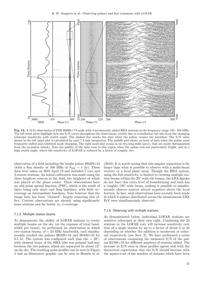
B. W. Stappers et al.: Observing pulsars and fast transients with LOFAR
Fig. 13. A 12 hr observation of PSR B0809+74 made with 4 incoherently added HBA stations in the frequency range 140−164 MHz.The left-most plots highlight how the S/N varies throughout the observation, mostly due to scintillation but also from the changingtelescope sensitivity with zenith angle. The dashed line marks the time when the pulsar crosses the meridian. The S/N valueshown in the left hand plot is calculated for each 7.2 min integration. The middle plot shows an hour of data when the pulsar mostfrequently nulled and exhibited mode changing. The right-most plot zooms in on two long nulls (grey), that are easily distinguishedfrom the on-pulses (black). Note the quality of the data even in this region when the pulsar was not particularly bright, and at ahigh zenith angle, where the sensitivity of LOFAR is reduced by a factor of roughly two.
observation of a field including the bright pulsar B0329+54(with a flux density at 100 MHz of S100 ∼ 1 Jy). Thesedata were taken on 2010 April 19 and included 7 core and3 remote stations. An initial calibration was made using thethree brightest sources in the field, the brightest of whichwas placed at the phase center. These observations havean odd point spread function (PSF), which is the result ofthere being only short and long baselines, with little uv-coverage on intermediate baselines. Note however that theimage here has been “cleaned”, largely removing this ef-fect. Current observations are already using significantlymore stations and far better (u, v)-coverage.
7.1.5. Multiple station beams
To demonstrate the ability of LOFAR stations to createmultiple beams on the sky (at the expense of total band-width per beam), we performed an observation in whichtwo station beams, of ∼ 24 MHz bandwidth, each simulta-neously tracked the pulsars B0329+54 and B0450+55 for0.5 hr. The system was configured such that the ∼ 20-wide element beam of the HBA tiles was pointed half-waybetween the two pulsars, which are separated by about 12
on the sky. The resulting pulse profiles can be seen in Figure4 and an illustrative graphic can be seen in Hessels et al.
(2010). It is worth noting that this angular separation is farlarger than what is possible to observe with a multi-beamreceiver or a focal plane array. Though the HBA system,using the full sensitivity, is limited to creating multiple sta-tion beams within the 20-wide tile beams, the LBA dipolesdo not have this extra level of beamforming and each hasa roughly 120-wide beam, making it possible to simulta-neously observe sources almost anywhere above the localhorizon. In fact, such observations have recently been madein which 6 pulsars distributed across the intantaneous LBAFoV were simultaneously observed.
7.1.6. Observing with multiple stations.
As demonstrated below, individual LOFAR stations aresensitive telescopes in their own right. Combining the 24stations in the LOFAR core will increase sensitivity overthat of a single station by up to a factor of about 5 or 24depending on whether the addition is incoherent or coher-ent respectively (see Sect. 2). We have performed a seriesof observations comparing the measured S/N of the pul-sar B1508+55 for different numbers of stations added. Theincrease in S/N seen in these profiles agrees well with thetheoretical expectation that the S/N should increase withthe square-root of the number of stations which have been
27

B. W. Stappers et al.: Observing pulsars and fast transients with LOFAR
incoherently combined (see Hessels et al. 2010). We willcontinue to test this relation as more LOFAR stations comeonline, especially to verify that coherently added stationsare delivering the expected sensitivity increase (see below).It is possible that RFI local to individual stations will alsoaffect the summed signal, although less dramatically if theyare more distant and we are forming the coherent sum, andso we are exploring options to flag these stations online anddynamically remove them from the combined beam.
7.1.7. Early (Superterp) tied-array observations
With the installation of a system to provide a single clocksignal to all of the stations located on the Superterp (6 LBAcore fields and 12 HBA sub-stations), the task of calibrat-ing tied-array beams between these stations was greatlysimplified. By observing a bright calibrator source in imag-ing mode, it is possible to solve for the phase offsets be-tween stations and then apply these corrections to futureobservations. Experience shows that the phase offsets be-tween Superterp stations, which should most of the timesee the same ionospheric patch, for the majority of the fre-quencies we are considering here are sufficiently constant ontimescales of hours to ensure that the gain in the directionof the pulsar remains optimal. Our commissioning observa-tions so far have shown that coherent addition produces animprovement in the S/N compared with the incoherent sum
by a factor of√nstations =
√12 = 3.5 as would be expected
for tied-array addition to be working (see Figure 14).
7.2. Early science observations
7.2.1. Pulsars with the LOFAR HBAs and LBAs.
We have detected many of the known, bright (S400 >50 mJy) northern-hemisphere pulsars using both the HBAsand LBAs (Stappers et al., 2011). Some pulsars (e.g., PSRsB0329+54, B0809+74, B1508+55, and B1919+21) are evenbright enough to be visible in 1 hr integrations with individ-ual HBA tiles. As mentioned above, this proved quite usefulfor testing the beam shape, phasing, and the tracking ac-curacy of single, and later summed, HBA dipole elements.In the case of the LBAs, roughly a whole Dutch station(48 active dipoles) is necessary to achieve reasonable S/Nwithin a 1 hr integration on these same bright pulsars. Wenote that single pulses are seen with the LBAs as expected(Sect. 7.2.7).
As described earlier in Sect. 4.2.3, even individualLOFAR stations have sufficient sensitivity to be interest-ing for a variety of scientific applications. For example,Figure 16 shows the average profiles resulting from the si-multaneous detection of PSR B1133+16 using 96 activeLBA dipoles with the Effelsberg station (called DE601) andusing the 48 HBA tiles of the Dutch core station (calledCS302).
The recent advent of station calibration for the LBAsdiscussed in Sect. 7.1.3 has led to a significant improvementin sensitivity and this is demonstrated by the observationsof PSRs B0329+54, B0809+74, B0950+08, B1133+16 andB1919+21 shown in Figure 15. These observations cover32−−80 MHz, likely making them the widest contiguousbandwidth observations ever made of radio pulsars at thesefrequencies. We have even been able to detect pulsars downto below 16 MHz (Stappers et al., 2011). This provides us
Fig. 14. The large sensitivity gain given by coherently addingthe station beams is illustrated in these two sample observations.In each observation, both the incoherent and the coherent sumof the station beams for all 12 Superterp HBA sub-stations wererecorded simultaneously. The resulting profiles were then scaledso that the off-pulse noise has a standard deviation of 1. Thiscomparison shows the expected increase in sensitivity due tocoherent summation and smaller beam size (see text for details).
with an unprecedented view into the evolution of the pulseprofile as a function of frequency, allowing any ambiguities,for example in aligning pulse components, due to dispersiveeffects, to be resolved. The contributions from changing ge-ometry, spectral index variations, scattering in the inter-stellar medium, and new components can be separated andstudied with data like these. These data were obtained withthe incoherent sum of 17 LBA stations; once we can formthe coherent addition of all the stations in the LOFAR corethe S/N of these observations will be improved by a furtherfactor of about six. However we already have data of suffi-cient quality to start such a study. We note that dispersiveeffects are affecting the profiles at the lowest frequenciesshown in Figure 15; however observations with more thanan order of magnitude improvement in effective time resolu-tion are already possible. Moreover, coherent dedispersionhas now been implemented which further increases the timeresolution we can achieve for the least scattered pulsars.
7.2.2. Giant pulses from the Crab pulsar.
The Crab pulsar, B0531+21, is particularly interesting,in part because it emits extremely bright “giant pulses”(Staelin & Reifenstein, 1968; Hankins, 1971). These giantpulses have the highest brightness temperature of any ob-served astronomical phenomenon and have been seen atfrequencies from a few 10’s of GHz all the way down toa few 10’s of MHz (Popov et al., 2006a). LOFAR will beespecially useful for studying the Crab pulsar, and otheryoung pulsars in supernova remnants, because it will bepossible to form small (arc-second to arc-minute depend-ing on what fraction of the array is used) tied-array beamswhich can potentially partially resolve out these nebulae.This will greatly increase sensitivity to the pulsations overthe nebular background. There are significant variations inthe scattering timescale with time, as seen by Kuz’min et al.(2008), and the possibility of frequently monitoring theseover a wide bandwidth with LOFAR allows one to study thechanges in the nebular scattering properties on timescalesranging from the 33 ms rotation period up to years.
Even before having the ability to form tied-array beamswe have detected giant pulses from the Crab pulsar usingthe LOFAR LBAs and HBAs. Figure 8 shows a “double
28

B. W. Stappers et al.: Observing pulsars and fast transients with LOFAR
giant pulse”, where two consecutive giant pulses are sepa-rated by only one rotation period. Note that at the observ-ing frequency of ∼ 150 MHz the scattering tail of each pulseis longer than the 33-ms pulse period. We have observed theCrab on a number of occassions and have already seen sig-nificant variations in this scattering timescale, indicatingchanges in the nebula along our line of sight. As shown inFigure 8 we have also detected giant pulses with the LBAsin the frequency range of 32–80 MHz that exhibits a scat-tering tail that extends to many seconds. Studying the evo-lution of the scattering of these giant pulses over this sortof frequency range will be a useful probe of the frequencyscaling laws appropriate for this type of scattering.
7.2.3. Multi-day observations of PSR B0809+74
Previous low-frequency monitoring of pulsars has beenhampered by the limited observing times achievable bytransit instruments or telescopes with equatorial mounts.In stark contrast to this, we have observed several circum-polar sources for up to 64 hr continuously, using LOFAR’sfull tracking ability. In Figure 13 we show a 12 hr segmentof one of these observations of PSR B0809+74. This corre-sponds to 33000 pulses and the full data set to a remarkable178000 pulses. These observations used the incoherent com-bination of just 4 core HBA stations and yet show high S/N:the individual pulses from this pulsar are clearly visible,and the pulsar’s occasional sudden turn-off, the so-callednulls, can be clearly distinguished above the low noise floor.Interspersed by nulls, the individual pulses form a driftpattern in the time versus rotational phase plane (middleand right-most panels of Figure 13) − a well known phe-nomenon that provides important insight into the pulsaremission mechanism. For understanding the interaction be-tween nulling and drifting, long integrations have been in-strumental, together with the occasional, fortuitous boostin pulsar brightness through scintillation (e.g. van Leeuwenet al. 2003). Never before has a data set been gathered ona source like this with such a large number of pulses, oversuch a wide bandwidth and at this time resolution. Thesedata, and more like it, will provide a unique view of thepulse emission physics continuously over timescale of mil-liseconds to days and we have already begun such studies.
7.2.4. Observation of the Galactic centre and PSR B1749−28
We have easily detected the bright (S400 = 1.1 Jy) pulsarB1749−28, which is only 1 away from the direction of theGalactic Centre (see Figure 4 for pulse profile). Three as-pects of this detection are noteworthy. First, LOFAR hasadequate sensitivity to pick out a 1.1 Jy pulsed sourceagainst the high sky background in the direction of theGalactic Centre (especially considering that the single-HBA-sub-station beam is very wide at these low elevations).Second, LOFAR is able to observe bright pulsars at a zenithangle (ZA) of at least 80. At such a high ZA, the sensitiv-ity of the dipoles is reduced by close to a factor of 6, sim-ply because of projection. Third, these observations weremade with the incoherent sum of the stations, subsequentobservations will be able to use the coherent sum of thestations reducing the size of the beam and thus resolvingout part of the bright Galactic plane and further improvingthe sensitivity. Furthermore, RFI may be more pernicious
Fig. 16. PSR B1133+16’s average pulse profile observed si-multaneously over nearly 8 octaves in frequency. LOFAR ob-servations were acquired in both the LBA (42 MHz, stationDE601) and HBA (140 MHz, station CS302) bands and weresupplemented by contemporaneous observations with the Lovell(1524 MHz) and Effelsberg (8300 MHz) telescopes.
for observations at higher ZA. Nonetheless, this detectionclearly demonstrates that it will be possible to monitor theGalactic Center for bright fast transients (though scatter-ing will remain a major limitation).
7.2.5. Millisecond pulsars
Though scattering strongly limits the effective time resolu-tion achievable at low observing frequencies, LOFAR is stillhighly capable of observing nearby MSPs, which are onlymildly scattered29. Figure 4 shows the detections of the 16-ms pulsar J2145−0750 and the 6.2-ms pulsar B1257+12.These pulsars both have low DMs (∼ 10 pc cm−3), whichmade these detections possible without the need for coher-ent dedispersion. Despite the low DM however, one can stillsee that the profiles are broadened by dispersive smearingwithin the channels. As discussed earlier, creating narrowerchannels is possible but will come at the expense of the timeresolution of the samples, such that the narrow pulse profilewill still be poorly sampled. To circumvent this problem, wehave implemented coherent dedispersion on the BG/P itselfto remove intra-channel dispersive smearing and to openthe possibility of observing MSPs with much larger DMs.An example of the results of observations in this mode isshown in Figure 17. We will soon be able to do this overlarger bandwidths and LOFAR will then be able to providemeasurements that eclipse those achieved in Stappers et al.(2008).
7.2.6. Simultaneous LBA/HBA observations
Sub-arraying and independent simultaneous observationsmake it possible to use multiple LOFAR stations to cover alarger frequency band than the maximum 48 MHz instan-
29 MSPs that are further away may also have low scatteringmeasures in some cases, as the general correlation between dis-tance, dispersion measure, and scattering shows large deviationsfrom the general trend, see Bhat et al. (2004).
29
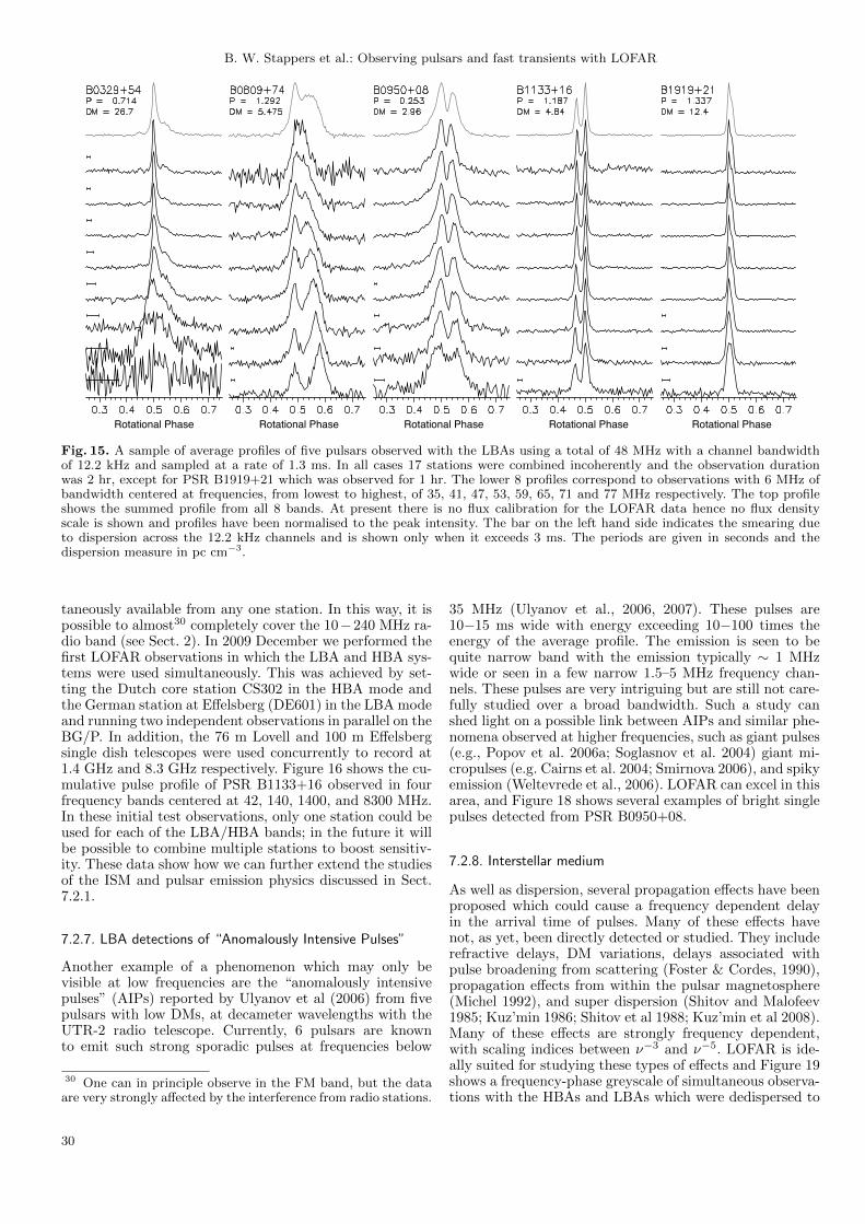
B. W. Stappers et al.: Observing pulsars and fast transients with LOFAR
Rotational Phase Rotational Phase Rotational Phase Rotational Phase Rotational Phase
Fig. 15. A sample of average profiles of five pulsars observed with the LBAs using a total of 48 MHz with a channel bandwidthof 12.2 kHz and sampled at a rate of 1.3 ms. In all cases 17 stations were combined incoherently and the observation durationwas 2 hr, except for PSR B1919+21 which was observed for 1 hr. The lower 8 profiles correspond to observations with 6 MHz ofbandwidth centered at frequencies, from lowest to highest, of 35, 41, 47, 53, 59, 65, 71 and 77 MHz respectively. The top profileshows the summed profile from all 8 bands. At present there is no flux calibration for the LOFAR data hence no flux densityscale is shown and profiles have been normalised to the peak intensity. The bar on the left hand side indicates the smearing dueto dispersion across the 12.2 kHz channels and is shown only when it exceeds 3 ms. The periods are given in seconds and thedispersion measure in pc cm−3.
taneously available from any one station. In this way, it ispossible to almost30 completely cover the 10−240 MHz ra-dio band (see Sect. 2). In 2009 December we performed thefirst LOFAR observations in which the LBA and HBA sys-tems were used simultaneously. This was achieved by set-ting the Dutch core station CS302 in the HBA mode andthe German station at Effelsberg (DE601) in the LBA modeand running two independent observations in parallel on theBG/P. In addition, the 76 m Lovell and 100 m Effelsbergsingle dish telescopes were used concurrently to record at1.4 GHz and 8.3 GHz respectively. Figure 16 shows the cu-mulative pulse profile of PSR B1133+16 observed in fourfrequency bands centered at 42, 140, 1400, and 8300 MHz.In these initial test observations, only one station could beused for each of the LBA/HBA bands; in the future it willbe possible to combine multiple stations to boost sensitiv-ity. These data show how we can further extend the studiesof the ISM and pulsar emission physics discussed in Sect.7.2.1.
7.2.7. LBA detections of “Anomalously Intensive Pulses”
Another example of a phenomenon which may only bevisible at low frequencies are the “anomalously intensivepulses” (AIPs) reported by Ulyanov et al (2006) from fivepulsars with low DMs, at decameter wavelengths with theUTR-2 radio telescope. Currently, 6 pulsars are knownto emit such strong sporadic pulses at frequencies below
30 One can in principle observe in the FM band, but the dataare very strongly affected by the interference from radio stations.
35 MHz (Ulyanov et al., 2006, 2007). These pulses are10−15 ms wide with energy exceeding 10−100 times theenergy of the average profile. The emission is seen to bequite narrow band with the emission typically ∼ 1 MHzwide or seen in a few narrow 1.5–5 MHz frequency chan-nels. These pulses are very intriguing but are still not care-fully studied over a broad bandwidth. Such a study canshed light on a possible link between AIPs and similar phe-nomena observed at higher frequencies, such as giant pulses(e.g., Popov et al. 2006a; Soglasnov et al. 2004) giant mi-cropulses (e.g. Cairns et al. 2004; Smirnova 2006), and spikyemission (Weltevrede et al., 2006). LOFAR can excel in thisarea, and Figure 18 shows several examples of bright singlepulses detected from PSR B0950+08.
7.2.8. Interstellar medium
As well as dispersion, several propagation effects have beenproposed which could cause a frequency dependent delayin the arrival time of pulses. Many of these effects havenot, as yet, been directly detected or studied. They includerefractive delays, DM variations, delays associated withpulse broadening from scattering (Foster & Cordes, 1990),propagation effects from within the pulsar magnetosphere(Michel 1992), and super dispersion (Shitov and Malofeev1985; Kuz’min 1986; Shitov et al 1988; Kuz’min et al 2008).Many of these effects are strongly frequency dependent,with scaling indices between ν−3 and ν−5. LOFAR is ide-ally suited for studying these types of effects and Figure 19shows a frequency-phase greyscale of simultaneous observa-tions with the HBAs and LBAs which were dedispersed to
30

B. W. Stappers et al.: Observing pulsars and fast transients with LOFAR
0
2e+07
4e+07
6e+07
8e+07
1e+08
0 0.5 1 1.5 2 2.5 3
Rel
ativ
e Am
plitu
de
Time (s)
0
2e+07
4e+07
6e+07
8e+07
1e+08
0 0.5 1 1.5 2 2.5 3
Rel
ativ
e Am
plitu
de
Time (s)
0
1e+07
2e+07
3e+07
4e+07
0 0.5 1 1.5 2 2.5 3
Rel
ativ
e Am
plitu
de
Time (s)
0
1e+07
2e+07
3e+07
4e+07
0 0.5 1 1.5 2 2.5 3
Rel
ativ
e Am
plitu
de
Time (s)
Fig. 18. Observations of PSR B0950+08 made using the LBAs (left) and HBAs (right). The top panels show sections of thetimeseries after dedispersion to the pulsar DM of 2.96 pc cm−3. We easily detect single pulses and one can see the wide range inintensity of the pulses, in particular in the low band. In the lower panels the same timeseries are shown but without dedipsersion,the so-called DM zero timeseries. In both the LBAs and HBAs we can see evidence for narrow spikes of RFI at zero DM, howeverthese are clearly broadband in nature and have been completely dispersed beyond a detectable level at the dispersion measure ofthe pulsar. We note that the broad features seen in the DM zero timeseries of the HBAs (e.g. near 2.5 s in the lower-right panel)are due to the pulsar itself. The ordinate axes corresponds to an arbitrary amplitude but is preserved in the top and bottom plots.
a DM of 26.768 pc cm−3. This observation corresponds toobserving over more than two octaves simultaneously andso any deviation from the ν−2 law which is greater than∼ 100 ms should be visible over this large bandwidth andat these low frequencies. Once the effects have been identi-fied we should be able to constrain how much of an impactthey have on pulsar timing at higher frequencies and alsoextract information about the composition of the ISM.
8. Conclusions and future prospects
We have shown that LOFAR will provide a massive im-provement in our ability to study pulsars and fast tran-sients in the lowest frequency range observable from Earth(10 − 240 MHz). Many of these modes will also find ap-plication for observations of solar and extra-solar plan-ets, flare stars and other time variable sources. In par-ticular, we have discussed how wide-band, low-frequencypulsar observations will address the nature of the still enig-matic pulsar emission mechanism (Figure 16) and will pro-vide a useful probe of the ISM (Figure 19). LOFAR alsopromises to discover many new pulsars and fast transientsthrough the combined power of its large collecting area
and (multiple) large FoVs. Through a dedicated all-skypulsar/fast-transient survey, a dedicated “radio-sky mon-itor”, and regular piggy-backing on imaging observations,LOFAR can revolutionize our understanding of the pop-ulation of rare/weak radio transients by charting parts ofparameter space effectively inaccesible to traditional radiotelescopes.
Though the LOFAR antennas are still in the processof being deployed in the field, the commissioning of pul-sar observing modes has been underway for over 3 years,with a steady increase in the level of activity and re-sults. Many of the desired observing modes are now func-tional, and have resulted in the observations presentedhere. While LOFAR is still in its operational infancy, ithas already demonstrated several of the capabilities andtechnologies that make it an important precursor to theSquare Kilometre Array (SKA). This includes the use ofmultiple digital beams to track sources widely separatedon the sky (Figure 4), simultaneous high-spatial and high-time-resolution observations (Figure 12), and large instan-taneous fractional observing bandwidth (Figure 16).
With these successes in hand, we are focussed on contin-uing development of the pulsar pipelines in order to take full
31
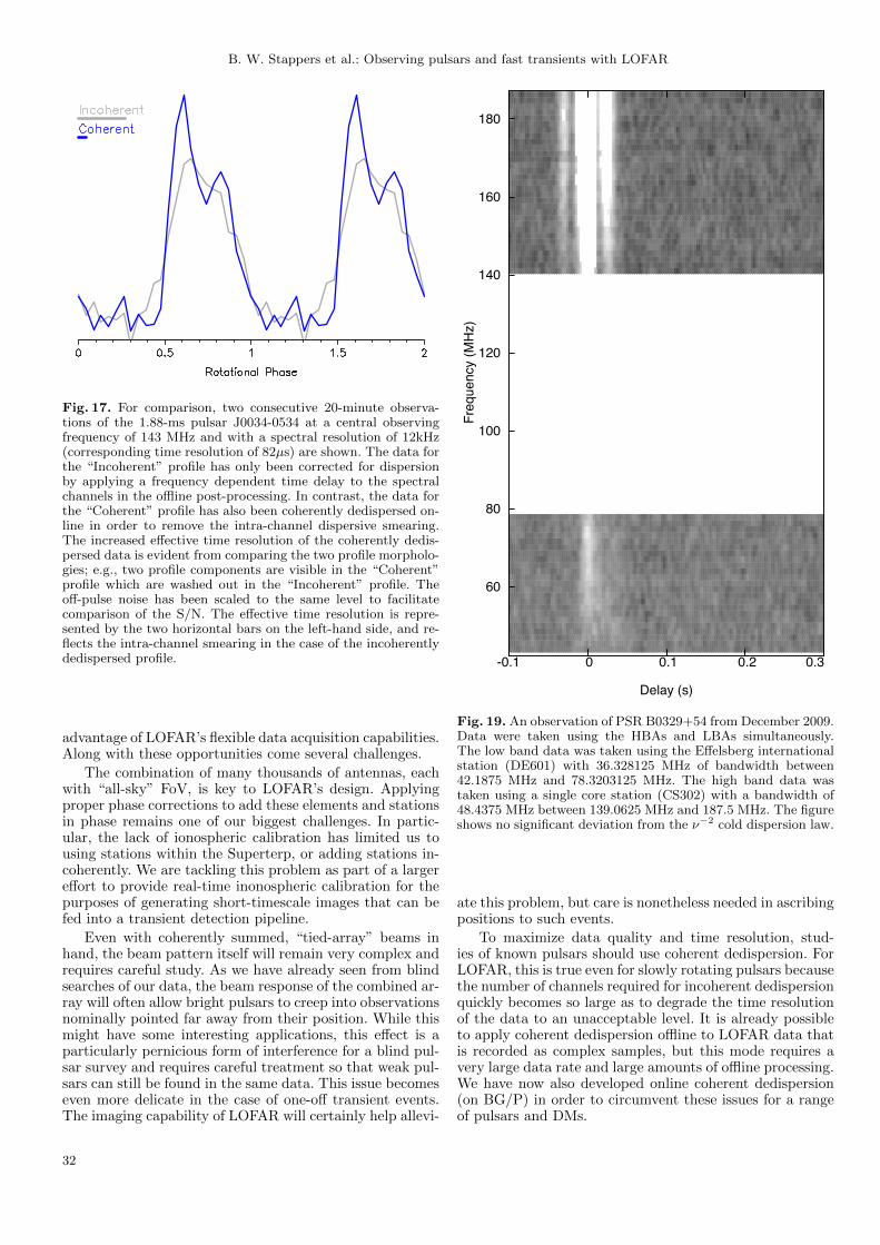
B. W. Stappers et al.: Observing pulsars and fast transients with LOFAR
Fig. 17. For comparison, two consecutive 20-minute observa-tions of the 1.88-ms pulsar J0034-0534 at a central observingfrequency of 143 MHz and with a spectral resolution of 12kHz(corresponding time resolution of 82µs) are shown. The data forthe “Incoherent” profile has only been corrected for dispersionby applying a frequency dependent time delay to the spectralchannels in the offline post-processing. In contrast, the data forthe “Coherent” profile has also been coherently dedispersed on-line in order to remove the intra-channel dispersive smearing.The increased effective time resolution of the coherently dedis-persed data is evident from comparing the two profile morpholo-gies; e.g., two profile components are visible in the “Coherent”profile which are washed out in the “Incoherent” profile. Theoff-pulse noise has been scaled to the same level to facilitatecomparison of the S/N. The effective time resolution is repre-sented by the two horizontal bars on the left-hand side, and re-flects the intra-channel smearing in the case of the incoherentlydedispersed profile.
advantage of LOFAR’s flexible data acquisition capabilities.Along with these opportunities come several challenges.
The combination of many thousands of antennas, eachwith “all-sky” FoV, is key to LOFAR’s design. Applyingproper phase corrections to add these elements and stationsin phase remains one of our biggest challenges. In partic-ular, the lack of ionospheric calibration has limited us tousing stations within the Superterp, or adding stations in-coherently. We are tackling this problem as part of a largereffort to provide real-time inonospheric calibration for thepurposes of generating short-timescale images that can befed into a transient detection pipeline.
Even with coherently summed, “tied-array” beams inhand, the beam pattern itself will remain very complex andrequires careful study. As we have already seen from blindsearches of our data, the beam response of the combined ar-ray will often allow bright pulsars to creep into observationsnominally pointed far away from their position. While thismight have some interesting applications, this effect is aparticularly pernicious form of interference for a blind pul-sar survey and requires careful treatment so that weak pul-sars can still be found in the same data. This issue becomeseven more delicate in the case of one-off transient events.The imaging capability of LOFAR will certainly help allevi-
-0.1 0 0.1 0.2 0.3
60
80
100
120
140
160
180
Freq
uenc
y (M
Hz)
Delay (s)
Fig. 19. An observation of PSR B0329+54 from December 2009.Data were taken using the HBAs and LBAs simultaneously.The low band data was taken using the Effelsberg internationalstation (DE601) with 36.328125 MHz of bandwidth between42.1875 MHz and 78.3203125 MHz. The high band data wastaken using a single core station (CS302) with a bandwidth of48.4375 MHz between 139.0625 MHz and 187.5 MHz. The figureshows no significant deviation from the ν−2 cold dispersion law.
ate this problem, but care is nonetheless needed in ascribingpositions to such events.
To maximize data quality and time resolution, stud-ies of known pulsars should use coherent dedispersion. ForLOFAR, this is true even for slowly rotating pulsars becausethe number of channels required for incoherent dedispersionquickly becomes so large as to degrade the time resolutionof the data to an unacceptable level. It is already possibleto apply coherent dedispersion offline to LOFAR data thatis recorded as complex samples, but this mode requires avery large data rate and large amounts of offline processing.We have now also developed online coherent dedispersion(on BG/P) in order to circumvent these issues for a rangeof pulsars and DMs.
32
B. W. Stappers et al.: Observing pulsars and fast transients with LOFAR
An all-sky pilot imaging survey with LOFAR is plannedin order to address many of the outstanding calibration is-sues, such as beam pattern and flux density scale. This sur-vey has as primary purpose the creation of a low-frequencysky model for future LOFAR imaging and calibration. Inaddition to the obvious benefits that better calibration willhave for pulsar observations, this survey will also provide aplatform for a commensal all-sky shallow survey using anincoherent sum of the station beams. This will be an op-portunity for us to further automate and refine our dataacquisition and reduction pipelines and to get the first realglimpse at what an all-sky LOFAR survey for pulsars andfast transients will offer.
9. Acknowledgements
LOFAR, the Low Frequency Array designed and con-structed by ASTRON, has facilities in several countries,that are owned by various parties (each with their ownfunding sources), and that are collectively operated bythe International LOFAR Telescope (ILT) foundation un-der a joint scientific policy. The data in Figure 16 basedon observations with the 100-m telescope of the MPIfR(Max-Planck-Institut fur Radioastronomie) at Effelsbergand the Lovell Telescope at Jodrell Bank Observatory.Ben Stappers, Patrick Weltevrede and the Lovell observa-tions are supported through the STFC RG R108020. JasonHessels is a Veni Fellow of The Netherlands Organisationfor Scientific Research (NWO). Joeri van Leeuwen andThijs Coenen are supported by the Netherlands ResearchSchool for Astronomy (Grant NOVA3-NW3-2.3.1) and bythe European Commission (Grant FP7-PEOPLE-2007-4-3-IRG #224838). Aris Karastergiou is grateful to theLeverhulme Trust for financial support. Ralph Wijers ac-knowledges support from the European Research Councilvia Advanced Investigator Grant no. 247295. LVEK is sup-ported by an ERC ST Grant.
References
Abbott, B. P., Abbott, R., Acernese, F., et al. 2010, ApJ, 713, 671Abdo, A. A., Ackermann, M., Ajello, M., et al. 2010a, ApJS, 188, 405Abdo, A. A., Ackermann, M., Ajello, M., et al. 2009, Science, 325,
840Abdo, A. A., Ackermann, M., Ajello, M., et al. 2010b, ApJS, 187, 460Abranin, E. P., Bruk, I. M., Zakharenko, V. V., & Konovalenko, A. A.
2001, Experimental Astronomy, 11, 85Aharonian, F., Akhperjanian, A. G., Bazer-Bachi, A. R., et al. 2007,
A&A, 466, 543Alexov, A., Anderson, K., Bahren, L., et al. 2010a, LOFAR Data
Format ICD: Beam-Formed Data, Tech. rep., LOFAR-USGAlexov, A., Anderson, K., L. Bahren, A. G., Holties, H., & Wise, M.
2010b, LOFAR Data Format ICD: File Naming Conventions, Tech.rep., LOFAR-USG
Aliu, E., Anderhub, H., Antonelli, L. A., et al. 2008, Science, 322,1221
Archibald, A. M., Stairs, I. H., Ransom, S. M., et al. 2009, Science,324, 1411
Armstrong, J. W., Cordes, J. M., & Rickett, B. J. 1981, Nature, 291,561
Armstrong, J. W., Rickett, B. J., & Spangler, S. R. 1995, ApJ, 443,209
Asgekar, A. & Deshpande, A. A. 2005, MNRAS, 357, 1105Beck, R. 2007, Studying Cosmic Magnetism by Polarization
Observations with LOFARBennett, M. F., van Eysden, C. A., & Melatos, A. 2010, MNRAS,
1370Bhat, N. D. R., Cordes, J. M., Camilo, F., Nice, D. J., & Lorimer,
D. R. 2004, ApJ, 605, 759
Boucher, C. & Altamimi, Z. 2001, http://etrs89.ensg.ign.fr/memo-V7.pdf
Bruk, I. M. & Ustimenko, B. I. 1976, Nature, 260, 766Bruk, I. M. & Ustimenko, B. I. 1977, Ap&SS, 49, 349Cairns, I. H., Johnston, S., & Das, P. 2004, MNRAS, 353, 270Camilo, F., Ransom, S. M., Halpern, J. P., & Reynolds, J. 2007, ApJ,
666, L93Camilo, F., Ransom, S. M., Halpern, J. P., et al. 2006, Nature, 442,
892Carilli, C. & Rawlings, S. 2004, astro-ph/0409274Cohen, A. S., Lane, W. M., Cotton, W. D., et al. 2007, AJ, 134, 1245Cole, T. W. 1969, Nature, 223, 487Cordes, J. M. 1978, ApJ, 222, 1006Cordes, J. M. 2008, in Astronomical Society of the Pacific Conference
Series, Vol. 395, Frontiers of Astrophysics: A Celebration ofNRAO’s 50th Anniversary, ed. A. H. Bridle, J. J. Condon, &G. C. Hunt, 225
Cordes, J. M., Kramer, M., Lazio, T. J. W., et al. 2004, New Astr.,48, 1413
Cordes, J. M. & Lazio, T. J. W. 2002, ArXiv e-prints, preprint(arXiv:astro-ph/0207156)
Cordes, J. M., Lazio, T. J. W., & McLaughlin, M. A. 2004, NewAstronomy Review, 48, 1459
Cordes, J. M. & Shannon, R. M. 2010, ApJ, submitted, arXiv:1010.3785
Cordes, J. M., Weisberg, J. M., & Hankins, T. H. 1990, AJ, 100, 1882D’Alessandro, F. 1996, Ap&SS, 246, 73de Vos, M., Gunst, A. W., & Nijboer, R. 2009, IEEE Proceedings, 97,
1431Deshpande, A. A. & Radhakrishnan, V. 1994, Journal of Astrophysics
and Astronomy, 15, 329Deshpande, A. A., Shevgaonkar, R. K., & Shastry, C. V. 1989, J. Inst.
Electron. Telecommunications Eng.Edwards, R. T. & Stappers, B. W. 2003, A&A, 407, 273Ellingson, S. W., Clarke, T. E., Cohen, A., et al. 2009, IEEE
Proceedings, 97, 1421Falcke, H. & LOFAR Cosmic Ray Key Science Project. 2007,
Astronomische Nachrichten, 328, 593Faucher-Giguere, C.-A. & Kaspi, V. M. 2006, ApJ, 643, 332Fender, R., Wijers, R., Stappers, B., & LOFAR Transients Key
Science Project, t. 2008, ArXiv e-prints, arXiv:0805.4349Fender, R. P., Wijers, R. A. M. J., Stappers, B., et al. 2006, in VI
Microquasar Workshop: Microquasars and BeyondFoster, R. S. & Cordes, J. M. 1990, ApJ, 364, 123Fruchter, A. S., Stinebring, D. R., & Taylor, J. H. 1988, Nature, 333,
237Golap, K., Shankar, N. U., Sachdev, S., Dodson, R., & Sastry, C. V.
1998, Journal of Astrophysics and Astronomy, 19, 35Gould, D. M. & Lyne, A. G. 1998, MNRAS, 301, 235Gupta, Y., Gothoskar, P., Joshi, B. C., et al. 2000, in Astronomical
Society of the Pacific Conference Series, Vol. 202, IAU Colloq. 177:Pulsar Astronomy - 2000 and Beyond, ed. M. Kramer, N. Wex, &R. Wielebinski, 277
Gurevich, A., Beskin, V., & Istomin, Y. 1993, Physics of the PulsarMagnetosphere (Physics of the Pulsar Magnetosphere, by AlexandrGurevich and Vassily Beskin and Yakov Istomin, pp. 432. ISBN0521417465. Cambridge, UK: Cambridge University Press, August1993.)
Hamaker, J. P., Bregman, J. D., & Sault, R. J. 1996, A&AS, 117, 137Han, J. 2009, in IAU Symposium, Vol. 259, IAU Symposium, 455–466Hankins, T. H. 1971, ApJ, 169, 487Heald, G., McKean, J., Pizzo, R., et al. 2010, ArXiv e-prints,
arXiv:1008.4693Hessels, J., Stappers, B., Alexov, A., et al. 2010, ArXiv e-prints,
arXiv:1009.1758Hessels, J. W. T., Roberts, M. S. E., & McLaughlin, M. 2011, in
American Institute of Physics Proceedings, Vol. 999, Radio Pulsars:a key to unlock the secrets of the Universe, ed. A. Possenti
Hessels, J. W. T., Stappers, B. W., van Leeuwen, J., & The LOFARTransients Key Science Project. 2009, in Astronomical Society ofthe Pacific Conference Series, Vol. 407, Astronomical Society of thePacific Conference Series, ed. D. J. Saikia, D. A. Green, Y. Gupta,& T. Venturi, 318
Hewish, A., Bell, S. J., Pilkington, J. D. H., Scott, P. F., & Collins,R. A. 1968, Nature, 217, 709
Intema, H. T. 2009, PhD thesis, Leiden Observatory, LeidenUniversity, P.O. Box 9513, 2300 RA Leiden, The Netherlands
33
B. W. Stappers et al.: Observing pulsars and fast transients with LOFAR
Izvekova, V. A., Jessner, A., Kuzmin, A. D., et al. 1994, A&AS, 105,235
Jenet, F. A., Anderson, S. B., & Prince, T. A. 2001, ApJ, 546, 394Johnston, H. M. & Kulkarni, S. R. 1991, ApJ, 368, 504Karastergiou, A., Johnston, S., & Kramer, M. 2003, A&A, 404, 325Karastergiou, A., von Hoensbroech, A., Kramer, M., et al. 2001, A&A,
379, 270Karuppusamy, R., Stappers, B., & van Straten, W. 2008, PASP, 120,
191Karuppusamy, R., Stappers, B. W., & Serylak, M. 2011, A&A, 525,
A55+Keane, E. F. & Kramer, M. 2008, MNRAS, 391, 2009Keith, M. J., Jameson, A., van Straten, W., et al. 2010, MNRAS, 1356Kondratiev, V. I., McLaughlin, M. A., Lorimer, D. R., et al. 2009,
ApJ, 702, 692Kramer, M., Karastergiou, A., Gupta, Y., et al. 2003, A&A, 407, 655Kramer, M., Lange, C., Lorimer, D. R., et al. 1999, ApJ, 526, 957Kramer, M., Lyne, A. G., O’Brien, J. T., Jordan, C. A., & Lorimer,
D. R. 2006, Science, 312, 549Kramer, M., Wielebinski, R., Jessner, A., Gil, J. A., & Seiradakis,
J. H. 1994, A&AS, 107, 515Kramer, M., Xilouris, K. M., Lorimer, D. R., et al. 1998, ApJ, 501,
270Kuzmin, A., Losovsky, B. Y., Jordan, C. A., & Smith, F. G. 2008,
A&A, 483, 13Kuzmin, A. D. & Losovskii, B. Y. 1997, Astron. Lett., 23, 283Kuzmin, A. D. & Losovsky, B. Y. 2001, A&A, 368, 230Kuzmin, A. D., Malofeev, V. M., Shitov, Y. P., et al. 1978, MNRAS,
185, 441Lawson, K. D., Mayer, C. J., Osborne, J. L., & Parkinson, M. L. 1987,
MNRAS, 225, 307Levin, L., Bailes, M., Bates, S., et al. 2010, ApJ, 721, L33Lohmer, O., Mitra, D., Gupta, Y., Kramer, M., & Ahuja, A. 2004,
A&A, 425, 569Lonsdale, C. J., Cappallo, R. J., Morales, M. F., et al. 2009, IEEE
Proceedings, 97, 1497Lorimer, D. R., Bailes, M., McLaughlin, M. A., Narkevic, D. J., &
Crawford, F. 2007, Science, 318, 777Lorimer, D. R., Faulkner, A. J., Lyne, A. G., et al. 2006, MNRAS,
372, 777Lorimer, D. R. & Kramer, M. 2005, Handbook of Pulsar Astronomy
(Cambridge University Press)Lyne, A., Hobbs, G., Kramer, M., Stairs, I., & Stappers, B. 2010,
Science, 329, 408Lyne, A. G. & Smith, F. G. 2004, Pulsar Astronomy, 3rd ed.
(Cambridge: Cambridge University Press)Lyutikov, M. 2002, ApJ, 580, L65Malofeev, V. M. 2000, in Astronomical Society of the Pacific
Conference Series, Vol. 202, IAU Colloq. 177: Pulsar Astronomy- 2000 and Beyond, ed. M. Kramer, N. Wex, & R. Wielebinski, 221
Malofeev, V. M., Gil, J. A., Jessner, A., et al. 1994, A&A, 285, 201Malofeev, V. M. & Malov, O. I. 1997, Nature, 389, 697Malofeev, V. M., Malov, O. I., & Shchegoleva, N. V. 2000, Astronomy
Reports, 44, 436Malofeev, V. M., Malov, O. I., & Teplykh, D. A. 2006, Chin. J. Astron.
Astrophys. Suppl. 2, 6, 68Malofeev, V. M., Malov, O. I., & Teplykh, D. A. 2007, Ap&SS, 308,
211Malofeev, V. M., Malov, O. I., Teplykh, D. A., Tyul’Bashev, S. A., &
Tyul’Basheva, G. E. 2005, Astronomy Reports, 49, 242Malov, O. I. & Malofeev, V. M. 2010, Astronomy Reports, 54, 210Manchester, R. N., Hobbs, G. B., Teoh, A., & Hobbs, M. 2005, AJ,
129, 1993Maron, O., Kijak, J., Kramer, M., & Wielebinski, R. 2000, A&AS,
147, 195McLaughlin, M. A. & Cordes, J. M. 2003, ApJ, 596, 982McLaughlin, M. A., Lyne, A. G., Lorimer, D. R., et al. 2006, Nature,
439, 817McLaughlin, M. A., Lyne, A. G., Keane, E. F., et al. 2009, MNRAS,
400, 1431Melrose, D. 2004, in Young Neutron Stars and Their Environments,
IAU Symposium 218, ed. F. Camilo & B. M. Gaensler (SanFrancisco: Astronomical Society of the Pacific), 349–356
Mitra, D. & Rankin, J. M. 2002, ApJ, 577, 322Mol, J. D. & Romein, J. W. 2011, The LOFAR Beam Former:
Implementation and Performance Analysis, under reviewMorris, D., Kramer, M., Thum, C., & et al. 1997, A&A, 322, L17Narayan, R. 1992, Philos. Trans. Roy. Soc. London A, 341, 151
Navarro, J., de Bruyn, G., Frail, D., Kulkarni, S. R., & Lyne, A. G.1995, ApJ, 455, L55
Nijboer, R. J. & Noordam, J. E. 2007, in Astronomical Society of thePacific Conference Series, Vol. 376, Astronomical Data AnalysisSoftware and Systems XVI, ed. R. A. Shaw, F. Hill, & D. J. Bell,237
Noutsos, A., Johnston, S., Kramer, M., & Karastergiou, A. 2008,MNRAS, 386, 1881
Petrova, S. A. 2006, MNRAS, 368, 1764Petrova, S. A. 2008, MNRAS, 383, 1413Popov, M. V., Kuzmin, A. D., Ulyanov, O. M., et al. 2006a, On the
Present and Future of Pulsar Astronomy, 26th meeting of the IAU,Joint Discussion 2, 16-17 August, 2006, Prague, Czech Republic,JD02, #19, 2
Popov, M. V., Kuz’min, A. D., Ul’yanov, O. M., et al. 2006b,Astronomy Reports, 50, 562
Rankin, J. M. 1993, ApJ, 405, 285Rankin, J. M., Comella, J. M., Craft, H. D., et al. 1970, ApJ, 162,
707Ransom, S. M., Cordes, J. M., & Eikenberry, S. S. 2003, ApJ, 589,
911Ransom, S. M., Ray, P. S., Camilo, F., et al. 2011, ApJ, 727, L16+Reich, P. & Reich, W. 1988, A&AS, 74, 7Rickett, B., Johnston, S., Tomlinson, T., & Reynolds, J. 2009,
MNRAS, 395, 1391Rickett, B. J. 1970, MNRAS, 150, 67Rickett, B. J. 1990, Ann. Rev. Astr. Ap., 28, 561Roger, R. S., Costain, C. H., Landecker, T. L., & Swerdlyk, C. M.
1999, A&AS, 137, 7Romein, J. W., Broekema, P. C., Mol, J. D., & van Nieuwpoort, R. V.
2010, in ACM Symposium on Principles and Practice of ParallelProgramming (PPoPP’10), Bangalore, India, 169–178
Ryabov, V. B., Vavriv, D. M., Zarka, P., et al. 2010, A&A, 510, A16Shishov, V. I. & Smirnova, T. V. 2002, Astron. Rep., 46, 731Shitov, Y. P., Malofeev, V. M., & Izvekova, V. A. 1988, Sov. Astron.
Lett., 14, 181Shitov, Y. P. & Pugachev, V. D. 1997, New Astr., 3, 101Shrauner, J. A., Taylor, J. H., & Woan, G. 1998, ApJ, 509, 785Singh, K., Bahren, L., Falcke, H., & et al. 2008, in International
Cosmic Ray Conference, Vol. 4, International Cosmic RayConference, 429–432
Slee, O. B., Alurkar, S. K., & Bobra, A. D. 1986, Aust. J. Phys., 39,103
Smirnova, T. V. 2006, Astronomy Reports, 50, 915Smirnova, T. V. & Shishov, V. I. 2010, Astronomy Reports, 54, 139Smirnova, T. V., Tul’bashev, S. A., & Boriakoff, V. 1994, A&A, 286,
807Soglasnov, V. A., Popov, M. V., Bartel, N., et al. 2004, ApJ, 616, 439Soglasnov, V. A., Popov, M. V., & Kuz’min, O. A. 1983, AZh, 60, 293Staelin, D. H. & Reifenstein, III, E. C. 1968, Science, 162, 1481Stappers, B. W., Bailes, M., Lyne, A. G., et al. 1996, ApJ, 465, L119Stappers, B. W., Hessels, J., Alexov, A., et al. 2011, in Radio Pulsars:
a key to unlock the secrets of the Universe (American Institute ofPhysics Conference Series)
Stappers, B. W., Karappusamy, R., & Hessels, J. W. T. 2008, inAmerican Institute of Physics Conference Series, Vol. 983, 40 Yearsof Pulsars: Millisecond Pulsars, Magnetars and More, ed. C. Bassa,Z. Wang, A. Cumming, & V. M. Kaspi, 593–597
Stappers, B. W., van Leeuwen, A. G. J., Kramer, M., Stinebring, D.,& Hessels, J. 2007, in WE-Heraeus Seminar on Neutron Stars andPulsars 40 years after the Discovery, ed. W. Becker & H. H. Huang,100
Stinebring, D. R., McLaughlin, M. A., Cordes, J. M., et al. 2001, ApJ,549, L97
Swarup, G., Ananthakrishnan, S., Kapahi, V. K., et al. 1991, CurrentScience, 60, 95
Tang, A. P. S. & Cheng, K. S. 2001, ApJ, 549, 1039Tavani, M., Barbiellini, G., Argan, A., et al. 2009, A&A, 502, 995team, I. B. G. 2008, IBM Journal of Research and Development, 52Thompson, D. J. 2000, Advances in Space Research, 25, 659Tinbergen, J. 1996, Astronomical Polarimetry (Cambridge University
Press), iSBN: 0521475317Ulyanov, O. M., Deshpande, A. A., Zakharenko, V. V., Asgekar, A.,
& Shankar, U. 2007, Radiofizika and Radioastronomia, 12, 5Ul’Yanov, O. M., Zakharenko, V. V., & Bruk, I. M. 2008, Astronomy
Reports, 52, 917Ulyanov, O. M., Zakharenko, V. V., Konovalenko, A. A., et al. 2006,
Radiofizika and Radioastronomia, 11, 113
34
B. W. Stappers et al.: Observing pulsars and fast transients with LOFAR
van der Horst, A. J., Kamble, A., Resmi, L., et al. 2008, A&A, 480,35
van Eysden, C. A. & Melatos, A. 2010, MNRAS, 1459van Leeuwen, A. G. J., Stappers, B. W., Ramachandran, R., &
Rankin, J. M. 2003, A&A, 399, 223van Leeuwen, J. & Stappers, B. W. 2010, A&A, 509, A7+Van Riper, K. A., Epstein, R. I., & Miller, G. S. 1991, ApJ, 381, L17van Straten, W. 2004, ApJS, 152, 129van Straten, W., Manchester, R. N., Johnston, S., & Reynolds, J. E.
2010, PASA, 27, 104von Hoensbroech, A. & Xilouris, K. M. 1997, A&AS, 126, 121Vranesevic, N., Manchester, R. N., Lorimer, D. R., et al. 2004, ApJ,
617, L139Welch, J., Backer, D., Blitz, L., et al. 2009, IEEE Proceedings, 97,
1438Weltevrede, P., Stappers, B. W., & Edwards, R. T. 2007, A&A, 469,
607Weltevrede, P., Stappers, B. W., van den Horn, L. J., & Edwards,
R. T. 2003, A&A, 412, 473Weltevrede, P., Wright, G. A. E., Stappers, B. W., & Rankin, J. M.
2006, A&A, 458, 269Wijnholds, S., van der Tol, S., Nijboer, R., & van der Veen, A. 2010,
IEEE Signal Processing Magazine, 27, 30Wijnholds, S. J. & van der Veen, A. 2009a, IEEE Transactions on
Signal Processing, 57, 3512Wijnholds, S. J. & van der Veen, A. 2009b, in Proceedings of
the 17th European Signal Processing Conference (EuSiPCo),arXiv:1003.2497v1
Wolleben, M., Fletcher, A., Landecker, T. L., et al. 2010, ApJ, 724,L48
You, X. P., Hobbs, G., Coles, W. A., et al. 2007, MNRAS, 378, 493
35
Copyright © 2022 FDOKUMEN


![Near-Membrane [Ca2+] Transients Resolved Using the Ca2+ Indicator FFP18](https://static.fdokumen.com/doc/165x107/631286873ed465f0570a4533/near-membrane-ca2-transients-resolved-using-the-ca2-indicator-ffp18.jpg)