II. Completion of the LOFAR Long-Baseline Calibrator Survey

Astronomy & Astrophysics manuscript no. lobos ©ESO 2021August 29, 2021

Sub-arcsecond imaging with the International LOFAR Telescope: II.Completion of the LOFAR Long-Baseline Calibrator Survey

Neal Jackson1, Shruti Badole1, John Morgan2, Rajan Chhetri2, Kaspars Prusis3, Atvars Nikolajevs3, Leah Morabito4,Michiel Brentjens5, Frits Sweijen6, Marco Iacobelli5, Emanuela Orrù5, J. Sluman5, R. Blaauw5, H. Mulder5, P. vanDijk5, Sean Mooney7, Adam Deller8, Javier Moldon9, J.R. Callingham6, 5, Jeremy Harwood10, Martin Hardcastle10,

George Heald11, Alexander Drabent12, J.P. McKean5, 13, A. Asgekar5, 14, I.M. Avruch5, 15, M.J. Bentum5, 16, A.Bonafede17, 18, 19, W.N. Brouw13, M. Brüggen19, H.R. Butcher20, B. Ciardi21, A. Coolen5, A. Corstanje22, 23, S.

Damstra5, S. Duscha5, J. Eislöffel12, H. Falcke23, M. Garrett1, F. de Gasperin24, 25, J.-M. Griessmeier26, 27,A.W. Gunst5,M.P. van Haarlem5, M. Hoeft12, A.J. van der Horst28, 29, E. Jütte30, L.V.E. Koopmans13, A. Krankowski31, P. Maat5, G.Mann32, G.K. Miley6, A. Nelles33, 34, M. Norden5, M. Paas35, V.N. Pandey5, M. Pandey-Pommier36, R.F. Pizzo5, W.

Reich37, H. Rothkaehl38, A. Rowlinson5, 39, M. Ruiter5, A. Shulevski6, 39, D.J. Schwarz40, O. Smirnov41, 42, M.Tagger26, C. Vocks32, R.J. van Weeren6, R. Wijers39, O. Wucknitz37, P. Zarka43, 27, J.A. Zensus37, P. Zucca5

(Affiliations can be found after the references)

Received; accepted

ABSTRACT

The Low-Frequency Array (LOFAR) Long-Baseline Calibrator Survey (LBCS) was conducted between 2014 and 2019 in order to obtain a setof suitable calibrators for the LOFAR array. In this paper we present the complete survey, building on the preliminary analysis published in2016 which covered approximately half the survey area. The final catalogue consists of 30006 observations of 24713 sources in the northernsky, selected for a combination of high low-frequency radio flux density and flat spectral index using existing surveys (WENSS, NVSS, VLSS,and MSSS). Approximately one calibrator per square degree, suitable for calibration of ≥ 200 km baselines is identified by the detection ofcompact flux density, for declinations north of 30◦ and away from the Galactic plane, with a considerably lower density south of this point dueto relative difficulty in selecting flat-spectrum candidate sources in this area of the sky. The catalogue contains indicators of degree of correlatedflux on baselines between the Dutch core and each of the international stations, involving a maximum baseline length of nearly 2000 km, for allof the observations. Use of the VLBA calibrator list, together with statistical arguments by comparison with flux densities from lower-resolutioncatalogues, allow us to establish a rough flux density scale for the LBCS observations, so that LBCS statistics can be used to estimate compactflux densities on scales between 300 mas and 2′′, for sources observed in the survey. The survey is used to estimate the phase coherence time ofthe ionosphere for the LOFAR international baselines, with median phase coherence times of about 2 minutes varying by a few tens of percentbetween the shortest and longest baselines. The LBCS can be used to assess the structures of point sources in lower-resolution surveys, withsignificant reductions in the degree of coherence in these sources on scales between 2′′ and 300 mas. The LBCS survey sources show a greaterincidence of compact flux density in quasars than in radio galaxies, consistent with unified schemes of radio sources. Comparison with samplesof sources from interplanetary scintillation (IPS) studies with the Murchison Widefield Array (MWA) shows consistent patterns of detection ofcompact structure in sources observed both interferometrically with LOFAR and using IPS.

Key words. Instrumentation:interferometers – Techniques:interferometric – Surveys – Galaxies:active – Radio continuum:galaxies – Atmo-spheric physics:ionosphere

1. Introduction

The Low-Frequency Array (LOFAR) Long Baseline Calibrator Survey (LBCS) (Jackson et al. 2016) was carried out to find radiosources in the northern sky that can be used as calibrators for observations made using the longest baselines (up to ∼2000 km) ofthe International LOFAR Telescope (van Haarlem et al. 2013). Calibrators are important to correct for the effects of frequency-and time-dependent phase corrugations on the visibility data of sources, which in the case of LOFAR are introduced mainly by theeffects of the Earth’s ionosphere at low radio frequencies. Specifically, the ionosphere induces a time-variable phase and a delay thatincreases with decreasing frequency, and is generally modelled as a thin layer (Cohen & Röttgering 2009) in which the temporal andspatial variations of phase can be modelled and applied to the data (Intema et al. 2009) provided that the thin-layer approximationholds (Martin et al. 2016). In addition, the independent system clocks in the international stations induce a constant time delay perstation. Since a constant time delay corresponds to a differing phase for different frequencies within the band, this results in anartificially induced gradient in the phase of the visibility in each baseline as a function of frequency. Calibrator sources should bebright enough to allow for the delay, phase, and rate variation with time to be determined. The calibrators need to be close enoughin the sky to the target such that the calibrator and the target are susceptible to the same propagation effects. Ideally, they should

Article number, page 1 of 17

arX

iv:2

108.

0728

4v1

[as

tro-

ph.G

A]

16

Aug

202

1

A&A proofs: manuscript no. lobos

have known structure, but must have enough structure that is coherent on all baselines to allow a good model to be determined byself-calibration. Paper I of this series (Morabito 2021) discusses in greater detail the use of the data reduction pipeline, which usessources from the LBCS survey to calibrate LOFAR long-baseline observations.

Interferometric observations are not the only way of detecting compact structure at low frequencies. It is also possible to useobservations of interplanetary scintillation (IPS), which are being carried out by the Murchison Widefield Array (MWA) in thesouthern hemisphere at 162 MHz (Morgan et al. 2018; Chhetri et al. 2018b,a; Sadler et al. 2019; Morgan et al. 2019), and by thePushchino telescope in the north at 111 MHz (Tyul’bashev et al. 2019, 2020). The critical scale for sources to scintillate at thesefrequencies is ∼0.3′′, well matched to the resolution of interferometric observations with International LOFAR.

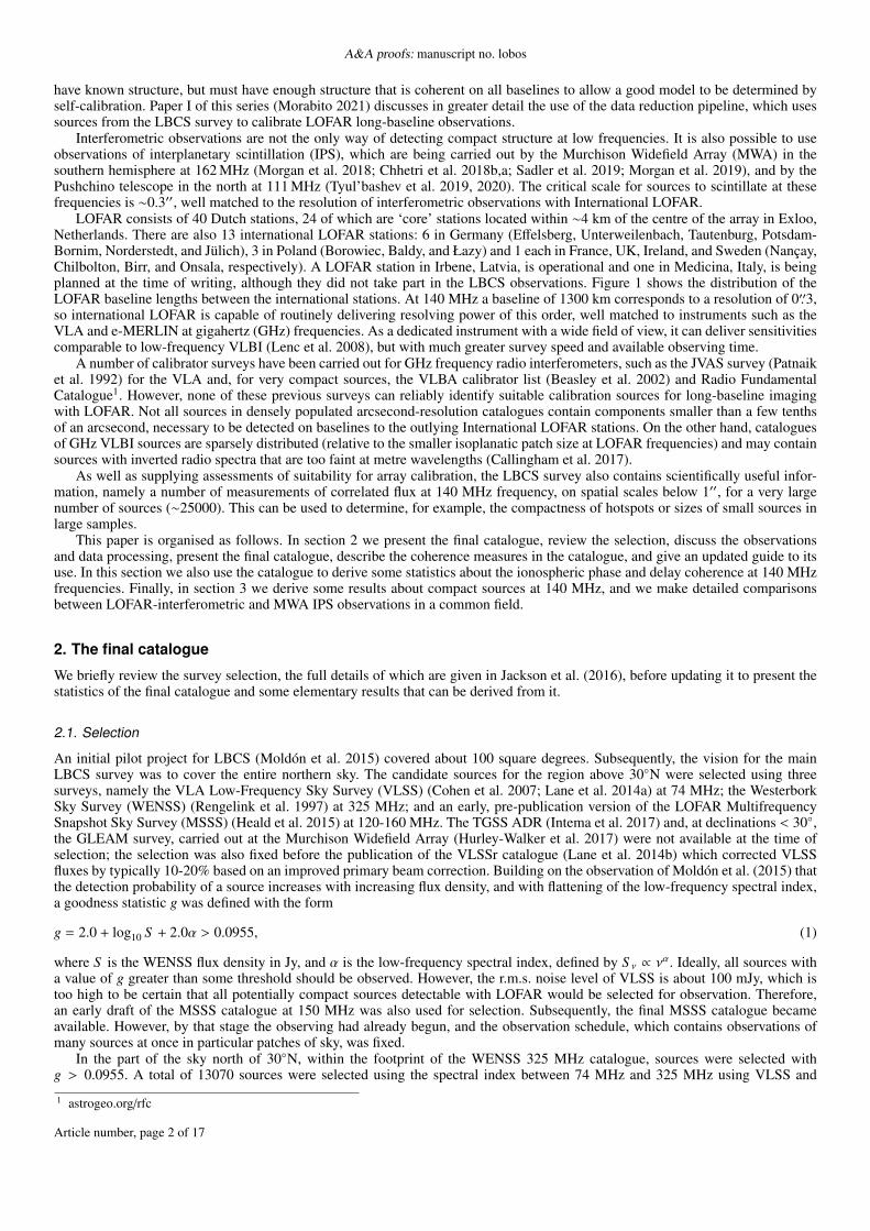
LOFAR consists of 40 Dutch stations, 24 of which are ‘core’ stations located within ∼4 km of the centre of the array in Exloo,Netherlands. There are also 13 international LOFAR stations: 6 in Germany (Effelsberg, Unterweilenbach, Tautenburg, Potsdam-Bornim, Norderstedt, and Jülich), 3 in Poland (Borowiec, Baldy, and Łazy) and 1 each in France, UK, Ireland, and Sweden (Nançay,Chilbolton, Birr, and Onsala, respectively). A LOFAR station in Irbene, Latvia, is operational and one in Medicina, Italy, is beingplanned at the time of writing, although they did not take part in the LBCS observations. Figure 1 shows the distribution of theLOFAR baseline lengths between the international stations. At 140 MHz a baseline of 1300 km corresponds to a resolution of 0′′.3,so international LOFAR is capable of routinely delivering resolving power of this order, well matched to instruments such as theVLA and e-MERLIN at gigahertz (GHz) frequencies. As a dedicated instrument with a wide field of view, it can deliver sensitivitiescomparable to low-frequency VLBI (Lenc et al. 2008), but with much greater survey speed and available observing time.

A number of calibrator surveys have been carried out for GHz frequency radio interferometers, such as the JVAS survey (Patnaiket al. 1992) for the VLA and, for very compact sources, the VLBA calibrator list (Beasley et al. 2002) and Radio FundamentalCatalogue1. However, none of these previous surveys can reliably identify suitable calibration sources for long-baseline imagingwith LOFAR. Not all sources in densely populated arcsecond-resolution catalogues contain components smaller than a few tenthsof an arcsecond, necessary to be detected on baselines to the outlying International LOFAR stations. On the other hand, cataloguesof GHz VLBI sources are sparsely distributed (relative to the smaller isoplanatic patch size at LOFAR frequencies) and may containsources with inverted radio spectra that are too faint at metre wavelengths (Callingham et al. 2017).

As well as supplying assessments of suitability for array calibration, the LBCS survey also contains scientifically useful infor-mation, namely a number of measurements of correlated flux at 140 MHz frequency, on spatial scales below 1′′, for a very largenumber of sources (∼25000). This can be used to determine, for example, the compactness of hotspots or sizes of small sources inlarge samples.

This paper is organised as follows. In section 2 we present the final catalogue, review the selection, discuss the observationsand data processing, present the final catalogue, describe the coherence measures in the catalogue, and give an updated guide to itsuse. In this section we also use the catalogue to derive some statistics about the ionospheric phase and delay coherence at 140 MHzfrequencies. Finally, in section 3 we derive some results about compact sources at 140 MHz, and we make detailed comparisonsbetween LOFAR-interferometric and MWA IPS observations in a common field.

2. The final catalogue

We briefly review the survey selection, the full details of which are given in Jackson et al. (2016), before updating it to present thestatistics of the final catalogue and some elementary results that can be derived from it.

2.1. Selection

An initial pilot project for LBCS (Moldón et al. 2015) covered about 100 square degrees. Subsequently, the vision for the mainLBCS survey was to cover the entire northern sky. The candidate sources for the region above 30◦N were selected using threesurveys, namely the VLA Low-Frequency Sky Survey (VLSS) (Cohen et al. 2007; Lane et al. 2014a) at 74 MHz; the WesterborkSky Survey (WENSS) (Rengelink et al. 1997) at 325 MHz; and an early, pre-publication version of the LOFAR MultifrequencySnapshot Sky Survey (MSSS) (Heald et al. 2015) at 120-160 MHz. The TGSS ADR (Intema et al. 2017) and, at declinations < 30◦,the GLEAM survey, carried out at the Murchison Widefield Array (Hurley-Walker et al. 2017) were not available at the time ofselection; the selection was also fixed before the publication of the VLSSr catalogue (Lane et al. 2014b) which corrected VLSSfluxes by typically 10-20% based on an improved primary beam correction. Building on the observation of Moldón et al. (2015) thatthe detection probability of a source increases with increasing flux density, and with flattening of the low-frequency spectral index,a goodness statistic g was defined with the form

g = 2.0 + log10 S + 2.0α > 0.0955, (1)

where S is the WENSS flux density in Jy, and α is the low-frequency spectral index, defined by S ν ∝ να. Ideally, all sources with

a value of g greater than some threshold should be observed. However, the r.m.s. noise level of VLSS is about 100 mJy, which istoo high to be certain that all potentially compact sources detectable with LOFAR would be selected for observation. Therefore,an early draft of the MSSS catalogue at 150 MHz was also used for selection. Subsequently, the final MSSS catalogue becameavailable. However, by that stage the observing had already begun, and the observation schedule, which contains observations ofmany sources at once in particular patches of sky, was fixed.

In the part of the sky north of 30◦N, within the footprint of the WENSS 325 MHz catalogue, sources were selected withg > 0.0955. A total of 13070 sources were selected using the spectral index between 74 MHz and 325 MHz using VLSS and

1 astrogeo.org/rfc


LBCS Authors: The complete LBCS survey

Fig. 1. Lengths and u-v coverage of the baselines used in the LOFAR observations. (top) Distribution of LOFAR baseline lengths betweeninternational stations. Core and remote LOFAR stations have baselines up to 100 km, so a gap in the u − v coverage still exists between 100 and200 km. The longest baseline, 1890 km between Birr (Ireland) and Baldy (Poland) will be exceeded soon with the advent of the station in Irbene(Latvia). (bottom) Snapshot u − v plane coverage for a source at 34◦ declination.

WENSS; 919 additional sources that met the criterion were not observed mainly because they were listed as multiple sources inWENSS, and were less likely to have compact structure on sub-arcsecond scales. A further 5809 sources were selected becausethey appeared to have a relatively flat spectrum using the early MSSS draft, or because they appeared in the VLBA calibrator list,in order to maximise the use of the 30 available beams in each observation.

South of 30◦N WENSS is not available, and the selection procedure is described in Jackson et al. (2016); it essentially involvespositional coincidences between VLSS sources and sources that are unresolved in the NRAO VLA Sky Survey (NVSS) at 1.4 GHz(Condon et al. 1998). 5915 sources were selected in this way, leading to a total observing list of 24794 sources. A total of 30006observations were made of 24713 separate sources; some sources were observed more than once.

2.2. Observations and data processing

The observing procedure, as well as the pipeline for the data processing, is described in more detail in Jackson et al. (2016), sowe summarise it briefly here before describing the updates to the process. The multi-beaming capabilities of LOFAR were usedto observe 30 sources at once using the High-Band Array (HBA) in the DUAL-INNER mode, giving a primary beam FWHM of3.96 degrees at 144 MHz. Each observation lasted 3 minutes with a 3 MHz bandwidth beginning at 140.16 MHz per source beam,divided into 64 channels. The core stations were phased up within the dataset after the observations, using calibrator observations,



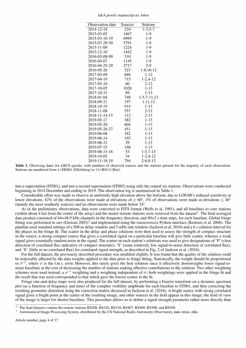
Observation date Sources Stations2014-12-18 210 1-3,5-72015-03-05 1467 1-92015-03-18-19 6999 1-92015-07-29-30 5791 1-92015-11-09 1224 1-92015-12-10 1442 1-92016-03-08-09 510 1-92016-04-07 1145 1-92016-04-25-29 2717 2-92016-05-26 523 1-8,10-122017-03-09 669 1-122017-04-19 715 1-2,4-122017-05-10 60 2-122017-10-05 1028 1-132017-10-31 89 1-132018-01-04 748 1-5,7-11,132018-09-21 197 1-11,132018-10-19 914 1-132018-11-08 557 2-132018-11-14-15 112 2-132019-05-17 382 1-132019-05-20 604 1-132019-05-26-27 451 1-132019-06-08 182 1-132019-06-14 192 1-132019-06-21 29 1-132019-07-15 168 1-132019-08-15-16 53 1-5,7-132019-10-05 34 1-2,4-122019-11-18-19 794 2-6,8-12

Table 1. Observing dates for LBCS epochs, with numbers of observed sources and the stations present for the majority of each observation.Stations are numbered from 1=DE601 (Effelsberg) to 13=IE613 (Birr).

into a superstation (ST001), and into a second superstation (ST002) using only the central six stations. Observations were conductedbeginning in 2014 December and ending in 2019. The observation log is summarised in Table 1.

Considerable effort was made to observe at uniformly high elevation above the horizon, due to LOFAR’s reduced sensitivity atlower elevations. 82% of the observations were made at elevations of ≥ 60◦, 3% of observations were made at elevations ≤ 40◦(mainly the most southerly sources) and no observations were made below 34◦.

As in the preliminary observations, data were converted to FITS format (Wells et al. 1981), and all baselines to core stations(within about 4 km from the centre of the array) and the nearer remote stations were removed from the dataset2. The final averageddata product consisted of 64×48.9 kHz channels in the frequency direction, and 90×2 s time steps, for each baseline. Global fringefitting was performed in aips (Greisen 2003)3 and implemented using the parseltongue Python interface (Kettenis et al. 2006). Thepipeline used standard settings of a 500 ns delay window and 5 mHz rate window (Jackson et al. 2016) and a 6 s solution interval forthe phases in the fringe fit. The scatter in the delay and phase solutions were then used to assess the strength of compact structurein the source; a strong compact source that gives a correlated signal on a particular baseline will give little scatter, whereas a weaksignal gives essentially random noise in the signal. The scatter on each station’s solutions was used to give designations of ‘P’ (cleardetection of correlated flux indicative of compact structure), ‘S’ (some relatively low signal-to-noise detection of correlated flux),and ‘X’ (little or no correlated flux) for correlated signal strength, as described in Fig. 2 of Jackson et al. (2016).

For the full dataset, the previously described procedure was modified slightly. It was found that the quality of the solution couldbe noticeably affected by the data weights applied to the data prior to fringe fitting. Statistically, the weight should be proportionalto σ−2, where σ is the r.m.s. error. However, this rarely gives the best solution since it effectively downweights lower signal-to-noise baselines at the cost of decreasing the number of stations making effective contributions to the solution. Two other weightingschemes were used instead, a σ−1 weighting and a weighting independent of σ; both weightings were applied in the fringe fit andthe result that was used corresponded to that which gave the lowest scatter in the fit.

Fringe rate-and-delay maps were also produced for the full dataset, by performing a Fourier transform on a dynamic spectrumplot (as a function of frequency and time) of the complex visibility amplitude for each baseline to ST001, and then correcting theresulting geometric distortion using the correction matrix discussed in Jackson et al. (2016). A bright source with strong correlatedsignal gives a bright point at the centre of the resulting image, and other sources in the field appear in this image; the field of viewof the image is larger for shorter baselines. This procedure allows us to define a signal strength parameter rather more directly than

2 The final datasets contain the remote stations RS208, RS210, RS310, RS407, RS409, RS508, and RS509.3 Astronomical Image Processing System, distributed by the US National Radio Astronomy Observatory, www.nrao.edu.



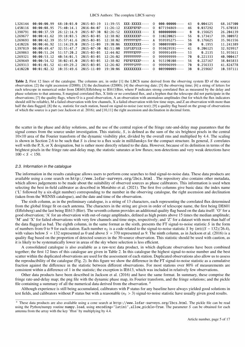
L326144 00:00:00.99 68:10:03.0 2015-03-19 11:39:55 XXX-XXXXX---- O 000-00000---- 43 0.004125 68.167500L450116 00:00:08.95 75:40:14.1 2016-04-07 11:26:12 XSXXPXPXP---- O 077194869---- 46 0.037292 75.670583L398791 00:00:37.59 26:12:14.9 2015-07-30 02:26:52 XXXXXXXXX---- X 000000000---- 0 0.156625 26.204139L269677 00:00:41.62 39:18:03.5 2015-03-05 12:38:02 XXXXXXXXP---- O 310220025---- 56 0.173417 39.300972L269693 00:00:42.39 35:57:41.6 2015-03-05 12:38:02 PPPPPPXPP---- A 959595275---- 56 0.176625 35.961556L410226 00:00:46.92 11:14:29.0 2015-11-09 19:30:06 XXXXXXXXX---- O 900099909---- 30 0.1955 11.241389L397819 00:00:49.47 32:55:47.7 2015-07-30 02:51:00 SSPSXPSSX---- O 959829591---- 41 0.206125 32.929917L269863 00:00:51.24 51:57:20.2 2015-03-05 12:44:02 PPPPPXPPP---- O 999991499---- 53 0.2135 51.955611L269321 00:00:53.12 40:54:01.5 2015-03-05 12:26:02 PPPPPPPPP---- O 999999999---- 70 0.221333 40.900417L269649 00:00:54.52 38:02:45.0 2015-03-05 12:38:02 PXPXPXXXP---- A 915190108---- 56 0.227167 38.045833L269313 00:01:01.52 41:49:29.2 2015-03-05 12:26:02 PPPPPSPPP---- O 999996999---- 70 0.256333 41.824778L410220 00:01:02.32 10:35:49.6 2015-11-09 19:30:06 XXXXXXXXX---- O 009900009---- 30 0.259667 10.597111

Table 2. First 12 lines of the catalogue. The columns are, in order [1] the LBCS name derived from the observing system ID of the sourceobservation; [2] the right ascension (J2000); [3] the declination (J2000); [4] the observing date; [5] the observing time; [6] a string of letters foreach telescope in numerical order from DE601/Effelsberg to IE613/Birr, where P indicates strong correlated flux as measured by the delay andphase solutions to that antenna, S marginal correlated flux, X little or no correlated flux, and a hyphen that the telescope did not participate in theobservations; [7] the quality flags, where O is a good observation, A an observation with anomalous amplitudes (but for which the flux indicatorsshould still be reliable), M a failed observation with few channels, X a failed observation with few time steps, and Z an observation with more thanhalf the data flagged; [8] the nS statistic for each station, based on signal-to-noise (see text); [9] a quality flag based on the group of observationsof which the source is a part (see Jackson et al. 2016); and [10,11] the right ascension and declination in decimal form.

the scatter in the phase and delay solutions, and the use of the central region of the fringe rate-and-delay map guarantees that thesignal comes from the source under investigation. This statistic, S , is defined as the sum of the six brightest pixels in the central10×10 area of the Fourier transform of the dynamic visibility plot, divided by the overall rms and multiplied by 4.4. The scalingis shown in Section 2.6 to be such that S is close to a flux scale in milliJanskys for the compact structure. In general, S correlateswell with the P, S, or X designation, but is rather more directly related to the data. However, because of its definition in terms of thebrightest pixels in the fringe rate-and-delay map, the statistic saturates at low fluxes; non-detections and very weak detections have100 < S < 150.

2.3. Information in the catalogue

The information in the results catalogue allows users to perform cone searches to find signal-to-noise data. These data products areavailable using a cone search on http://www.lofar-surveys.org/lbcs.html . The repository also contains other metadata,which allows judgements to be made about the suitability of observed sources as phase calibrators. This information is used whenselecting the best in-field calibrator as described in Morabito et al. (2021). The first five columns give basic data: the index name(‘L’ followed by a six-digit number) corresponding to the number in the observing catalogue, the right ascension and declination(taken from the WENSS catalogue), and the date and time of the observation.

The sixth column, as in the preliminary catalogue, is a string of 13 characters, each representing the correlated flux determinedfrom the global fringe fit on each antenna. The characters in the string are given in order of telescope name, the first being DE601(Effelsberg) and the last being IE613 (Birr). The seventh column provides an additional quality flag based on the data itself: ‘O’ for agood observation; ‘A’ for an observation with out-of-range amplitudes, defined as high points above 15 times the median amplitude;‘M’ and ‘X’ for failed observations with very few channels and time steps, respectively; and ‘Z’ for a dataset with more than half ofthe data flagged as bad. The eighth column, in the same format as the sixth, presents the FT signal-to-noise statistic S in the formof numbers from 0 to 9 for each station. Each number nS is a code related to the signal-to-noise statistic S by int((S − 132)/26.4),with values below S = 132 represented as 0 and above S = 370 represented as 9. The ninth column, as in Jackson et al. (2016) is aquality flag based on the proportion of detected sources in the 30-source observation. This statistic should be used with caution, asit is likely to be systematically lower in areas of the sky where selection is less efficient.

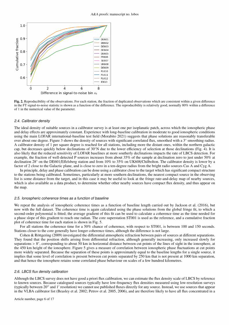
A consolidated catalogue is also available as a raw-text data product, in which duplicate observations have been combinedtogether; the first 12 lines of this catalogue are given in Table 2. In this catalogue the highest signal-to-noise number and the bestscatter within the duplicated observations are used for the assessment of each station. Duplicated observations also allow us to assessthe reproducibility of the catalogue (Fig. 2). In this figure we show the difference in the FT signal-to-noise statistic as a cumulativefraction against the difference in the statistic between different observations. For most stations over 80% of measurements areconsistent within a difference of 1 in the statistic; the exception is IE613, which was included in relatively few observations.

Other data products have been described in Jackson et al. (2016) and have the same format. In summary, these comprise thefringe rate-and-delay map; the png file with the dynamic phase map, its Fourier transform, and the fringe solutions; and the picklefile containing a summary of all the numerical data derived from the observation. 4

Although experience is still being accumulated, calibrators with P status for any baseline have always yielded good solutions intest fields, and calibrators without P status but with a reasonable (nS > 3) signal-to-noise statistic have usually given good results.

4 These data products are also available using a cone search at http://www.lofar-surveys.org/lbcs.html. The pickle file can be readusing the Python/numpy routine numpy.load, using encoding=’latin1’,allow_pickle=True. The parameter S can be obtained for eachantenna from the array with the key ’fftsn’ by multiplying by 4.4.


http://www.lofar-surveys.org/lbcs.html

http://www.lofar-surveys.org/lbcs.html


Fig. 2. Reproducibility of the observations. For each station, the fraction of duplicated observations which are consistent within a given differencein the FT signal-to-noise statistic is shown as a function of the difference. The reproducibility is relatively good, normally 80% within a differenceof 1 in the numerical value of the parameter.

2.4. Calibrator density

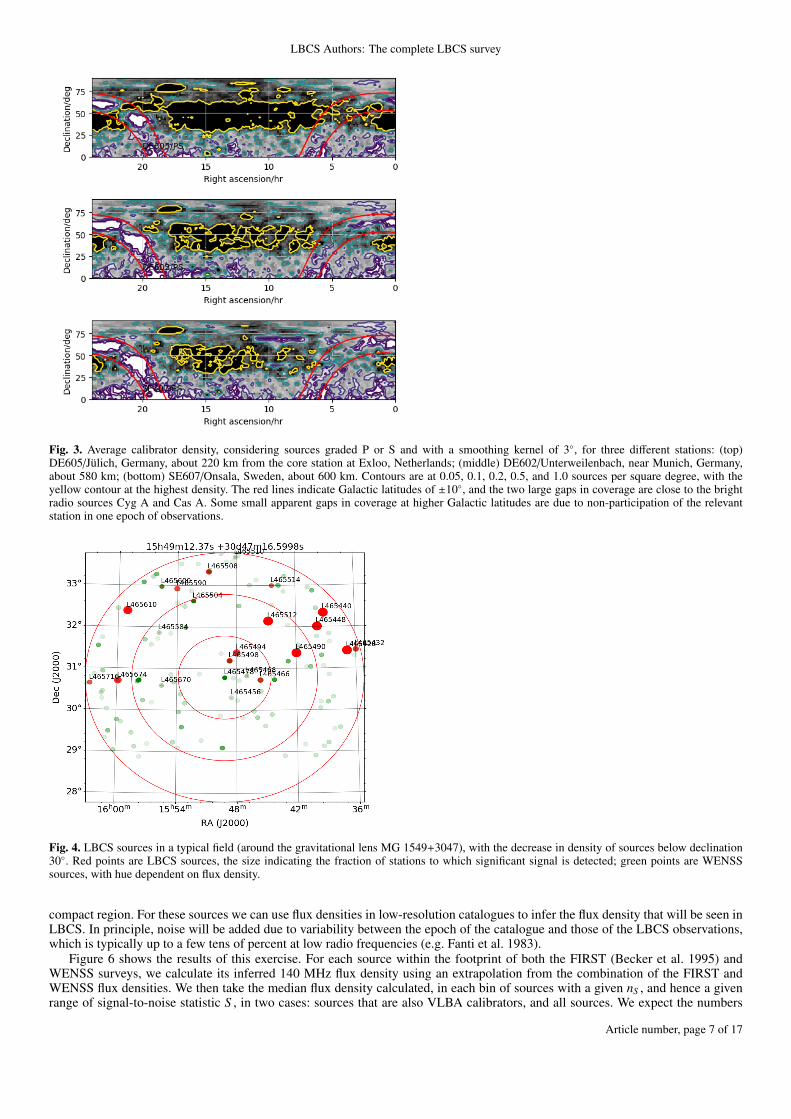
The ideal density of suitable sources in a calibrator survey is at least one per isoplanatic patch, across which the ionospheric phaseand delay effects are approximately constant. Experience with long-baseline calibration in moderate to good ionospheric conditionsusing the main LOFAR international-baseline test field (Morabito 2021) suggests that phase solutions are reasonably transferableover about one degree. Figure 3 shows the density of sources with significant correlated flux, smoothed with a 3◦ smoothing radius.A calibrator density of 1 per square degree is reached for all stations, including more the distant ones, within the northern galacticcap, but decreases quickly below declinations of 30◦N due to the lower efficiency of selection at those declinations (Fig. 4). It isalso likely that the reduced sensitivity of LOFAR baselines at more southerly declinations impacts the rate of LBCS detection. Forexample, the fraction of well-detected P sources increases from about 35% of the sample at declination zero to just under 50% atdeclination 28◦ on the DE601/Effelsberg station and from 10% to 35% on UK608/Chilbolton. The calibrator density is lower by afactor of 2 close to the Galactic plane, and is close to zero in a ten-degree radius from the bright radio sources Cas A and Cyg A.

In principle, delay and phase calibration can be done using a calibrator close to the target which has significant compact structureto the stations being calibrated. Sometimes, particularly at more southern declinations, the nearest compact source in the observinglist is some distance from the target, and in this case it may be useful to look at the fringe rate-and-delay map of nearby sources,which is also available as a data product, to determine whether other nearby sources have compact flux density, and thus appear onthe map.

2.5. Ionospheric coherence times as a function of baseline

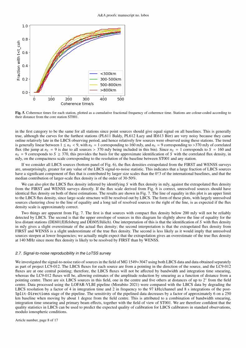
We repeat the analysis of ionospheric coherence times as a function of baseline length carried out by Jackson et al. (2016), butnow with the full dataset. The coherence time is again calculated using the phase solutions from the global fringe fit, to which asecond-order polynomial is fitted; the average gradient of this fit can be used to calculate a coherence time as the time needed fora phase slope of this gradient to reach one radian. The core superstation ST001 is used as the reference, and a cumulative fractionplot of coherence time for each station is shown in Fig. 5.

For all stations the coherence time for a 50% chance of coherence, with respect to ST001, is between 100 and 150 seconds.Stations closer to the core generally have longer coherence times, although the difference is not large.

Cohen & Röttgering (2009) investigated the differential atmospheric refraction between pairs of sources at different separations.They found that the position shifts arising from differential refraction, although generally increasing, only increased slowly forseparations > 8◦, corresponding to about 50 km in horizontal distance between cut points of the lines of sight in the ionosphere, atthe 450 km height of the ionosphere. Figure 5 gives a measure of correlation between ionospheric phase fluctuations at cut pointsmore widely separated. Because the separation of these points is approximately equal to the baseline lengths for a single source, itimplies that some level of correlation is present between cut points separated by 250 km that is not present at 1000 km separation,and that hence the ionosphere retains some correlated phase behaviour on scales of a few hundred kilometres.

2.6. LBCS flux density calibration

Although the LBCS survey does not have good a priori flux calibration, we can estimate the flux density scale of LBCS by referenceto known sources. Because catalogued sources typically have low-frequency flux densities measured using low-resolution surveys(typically between 20′′ and 1′ resolution) we cannot use published fluxes directly for any source. Instead, we use sources that appearin the VLBA calibrator list (Beasley et al. 2002; Petrov et al. 2005, 2006), and are therefore likely to have all flux concentrated in a



Fig. 3. Average calibrator density, considering sources graded P or S and with a smoothing kernel of 3◦, for three different stations: (top)DE605/Jülich, Germany, about 220 km from the core station at Exloo, Netherlands; (middle) DE602/Unterweilenbach, near Munich, Germany,about 580 km; (bottom) SE607/Onsala, Sweden, about 600 km. Contours are at 0.05, 0.1, 0.2, 0.5, and 1.0 sources per square degree, with theyellow contour at the highest density. The red lines indicate Galactic latitudes of ±10◦, and the two large gaps in coverage are close to the brightradio sources Cyg A and Cas A. Some small apparent gaps in coverage at higher Galactic latitudes are due to non-participation of the relevantstation in one epoch of observations.

Fig. 4. LBCS sources in a typical field (around the gravitational lens MG 1549+3047), with the decrease in density of sources below declination30◦. Red points are LBCS sources, the size indicating the fraction of stations to which significant signal is detected; green points are WENSSsources, with hue dependent on flux density.

compact region. For these sources we can use flux densities in low-resolution catalogues to infer the flux density that will be seen inLBCS. In principle, noise will be added due to variability between the epoch of the catalogue and those of the LBCS observations,which is typically up to a few tens of percent at low radio frequencies (e.g. Fanti et al. 1983).

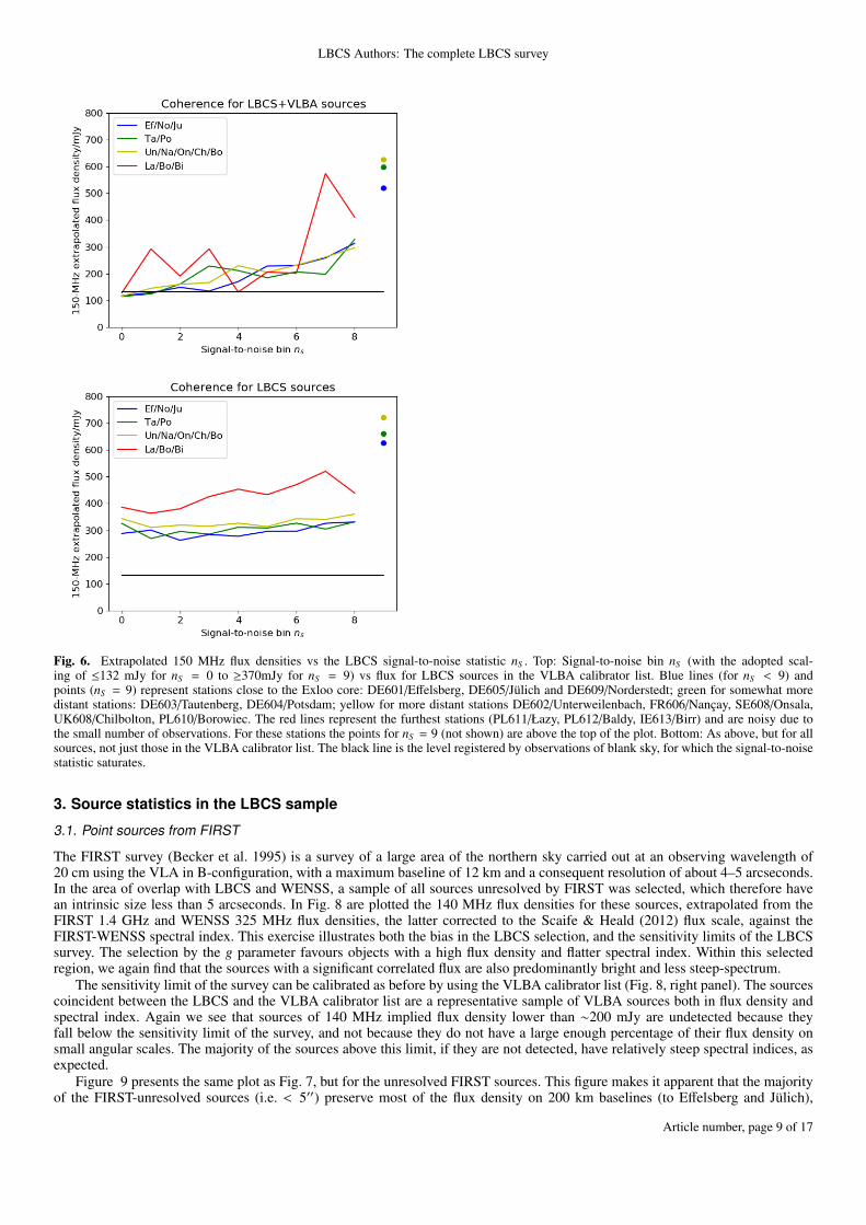
Figure 6 shows the results of this exercise. For each source within the footprint of both the FIRST (Becker et al. 1995) andWENSS surveys, we calculate its inferred 140 MHz flux density using an extrapolation from the combination of the FIRST andWENSS flux densities. We then take the median flux density calculated, in each bin of sources with a given nS , and hence a givenrange of signal-to-noise statistic S , in two cases: sources that are also VLBA calibrators, and all sources. We expect the numbers



Fig. 5. Coherence times for each station, plotted as a cumulative fractional frequency of coherence time. Stations are colour-coded according totheir distance from the core station ST001.

in the first category to be the same for all stations since point sources should give equal signal on all baselines. This is generallytrue, although the curves for the furthest stations (PL611 Baldy, PL612 Łazy and IE613 Birr) are very noisy because they cameonline relatively late in the LBCS observing period, and hence relatively few sources were observed using these stations. The trendis generally linear between 1 ≤ nS < 9, with nS = 1 corresponding to 160 mJy, and nS = 9 corresponding to >370 mJy of correlatedflux (the jump at nS = 9 is due to all sources > 370 mJy being included in this bin). Since nS = 1 corresponds to S = 160 andnS = 9 corresponds to S ≥ 370, this provides the basis for the approximate identification of S with the correlated flux density, inmJy, on the compactness scale corresponding to the resolution of the baseline between ST001 and any station.

If we consider all LBCS sources (bottom panel of Fig. 6), the flux densities extrapolated from the FIRST and WENSS surveysare, unsurprisingly, greater for any value of the LBCS signal-to-noise statistic. This indicates that a large fraction of LBCS sourceshave a significant component of flux that is contributed by larger size scales than the 0′′.3 of the international baselines, and that themedian contribution of larger-scale flux density is of the order of 30-50%.

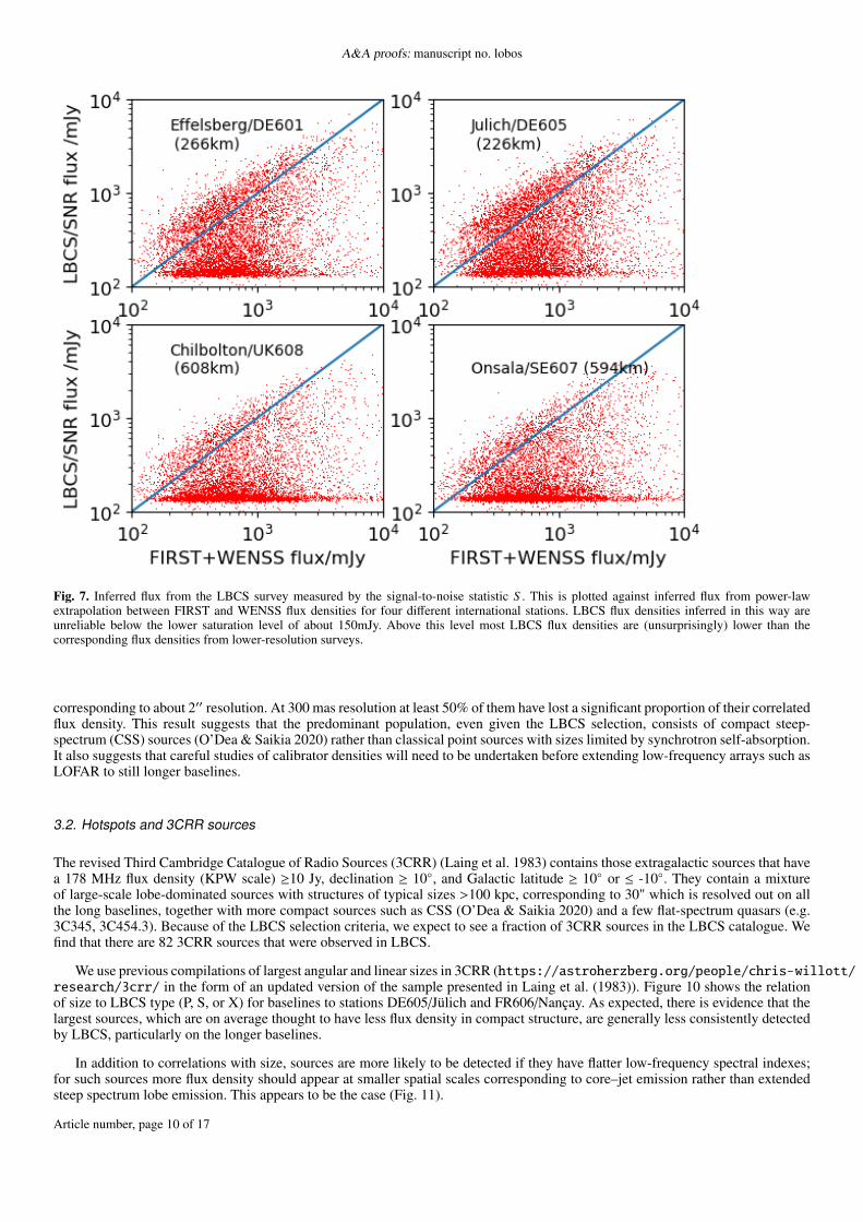
We can also plot the LBCS flux density inferred by identifying S with flux density in mJy, against the extrapolated flux densityfrom the FIRST and WENSS surveys directly. If the flux scale derived from Fig. 6 is correct, unresolved sources should haveidentical flux density on both of these estimations. The results are shown in Fig. 7. The line of equality in this plot is an upper limitto the LBCS flux density, since large-scale structure will be resolved out by LBCS. The form of these plots, with largely unresolvedsources clustering close to the line of equality and a long tail of resolved sources to the right of the line, is as expected if the fluxdensity scale is approximately correct.

Two things are apparent from Fig. 7. The first is that sources with compact flux density below 200 mJy will not be reliablydetected by LBCS. The second is that the upper envelope of sources in this diagram lie slightly above the line of equality for theless distant stations (DE601/Effelsberg and DE605/Jülich). One interpretation of this is that the identification of S with flux densityin mJy gives a slight overestimate of the actual flux density; the second interpretation is that the extrapolated flux density fromFIRST and WENSS is a slight underestimate of the true flux density. The second is less likely as it would imply that unresolvedsources steepen at lower frequencies; we actually might expect that the extrapolation gives an overestimate of the true flux densityat 140 MHz since more flux density is likely to be resolved by FIRST than by WENSS.

2.7. Signal-to-noise reproducibility in the LoTSS survey

We investigated the signal-to-noise ratio of sources in the field of MG 1549+3047 using both LBCS data and data obtained separatelyas part of project LC9-012. The LBCS fluxes for each source are from a pointing in the direction of the source, and the LC9-012fluxes are at one central pointing; therefore, the LBCS fluxes will not be affected by bandwidth and integration time smearing,whereas the LC9-012 fluxes will be, allowing estimates of the amplitude reduction by smearing as a function of distance from apointing centre. There are six LBCS sources in this field, one in the centre and five others at distances of up to 2◦ from the fieldcentre. Data processed using the LOFAR-VLBI pipeline (Morabito 2021) were compared with the LBCS data by degrading theLBCS resolution by a factor of 4 in integration time and 2 in frequency to the 97 kHz/channel and 8 s integrations of the post-Split-Directions stage of the pipeline. The sensitivity of the pipelined data decreases by a factor of approximately 6 on a 250km baseline when moving by about 1 degree from the field centre. This is attributed to a combination of bandwidth smearing,integration time smearing and primary beam effects, together with the field of view of ST001. We are therefore confident that thequality statistics in LBCS can be used to predict the expected quality of calibration for LBCS calibrators in standard observations,modulo ionospheric conditions.



Fig. 6. Extrapolated 150 MHz flux densities vs the LBCS signal-to-noise statistic nS . Top: Signal-to-noise bin nS (with the adopted scal-ing of ≤132 mJy for nS = 0 to ≥370mJy for nS = 9) vs flux for LBCS sources in the VLBA calibrator list. Blue lines (for nS < 9) andpoints (nS = 9) represent stations close to the Exloo core: DE601/Effelsberg, DE605/Jülich and DE609/Norderstedt; green for somewhat moredistant stations: DE603/Tautenberg, DE604/Potsdam; yellow for more distant stations DE602/Unterweilenbach, FR606/Nançay, SE608/Onsala,UK608/Chilbolton, PL610/Borowiec. The red lines represent the furthest stations (PL611/Łazy, PL612/Baldy, IE613/Birr) and are noisy due tothe small number of observations. For these stations the points for nS = 9 (not shown) are above the top of the plot. Bottom: As above, but for allsources, not just those in the VLBA calibrator list. The black line is the level registered by observations of blank sky, for which the signal-to-noisestatistic saturates.

3. Source statistics in the LBCS sample

3.1. Point sources from FIRST

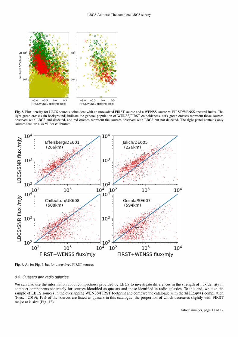
The FIRST survey (Becker et al. 1995) is a survey of a large area of the northern sky carried out at an observing wavelength of20 cm using the VLA in B-configuration, with a maximum baseline of 12 km and a consequent resolution of about 4–5 arcseconds.In the area of overlap with LBCS and WENSS, a sample of all sources unresolved by FIRST was selected, which therefore havean intrinsic size less than 5 arcseconds. In Fig. 8 are plotted the 140 MHz flux densities for these sources, extrapolated from theFIRST 1.4 GHz and WENSS 325 MHz flux densities, the latter corrected to the Scaife & Heald (2012) flux scale, against theFIRST-WENSS spectral index. This exercise illustrates both the bias in the LBCS selection, and the sensitivity limits of the LBCSsurvey. The selection by the g parameter favours objects with a high flux density and flatter spectral index. Within this selectedregion, we again find that the sources with a significant correlated flux are also predominantly bright and less steep-spectrum.

The sensitivity limit of the survey can be calibrated as before by using the VLBA calibrator list (Fig. 8, right panel). The sourcescoincident between the LBCS and the VLBA calibrator list are a representative sample of VLBA sources both in flux density andspectral index. Again we see that sources of 140 MHz implied flux density lower than ∼200 mJy are undetected because theyfall below the sensitivity limit of the survey, and not because they do not have a large enough percentage of their flux density onsmall angular scales. The majority of the sources above this limit, if they are not detected, have relatively steep spectral indices, asexpected.

Figure 9 presents the same plot as Fig. 7, but for the unresolved FIRST sources. This figure makes it apparent that the majorityof the FIRST-unresolved sources (i.e. < 5′′) preserve most of the flux density on 200 km baselines (to Effelsberg and Jülich),



Fig. 7. Inferred flux from the LBCS survey measured by the signal-to-noise statistic S . This is plotted against inferred flux from power-lawextrapolation between FIRST and WENSS flux densities for four different international stations. LBCS flux densities inferred in this way areunreliable below the lower saturation level of about 150mJy. Above this level most LBCS flux densities are (unsurprisingly) lower than thecorresponding flux densities from lower-resolution surveys.

corresponding to about 2′′ resolution. At 300 mas resolution at least 50% of them have lost a significant proportion of their correlatedflux density. This result suggests that the predominant population, even given the LBCS selection, consists of compact steep-spectrum (CSS) sources (O’Dea & Saikia 2020) rather than classical point sources with sizes limited by synchrotron self-absorption.It also suggests that careful studies of calibrator densities will need to be undertaken before extending low-frequency arrays such asLOFAR to still longer baselines.

3.2. Hotspots and 3CRR sources

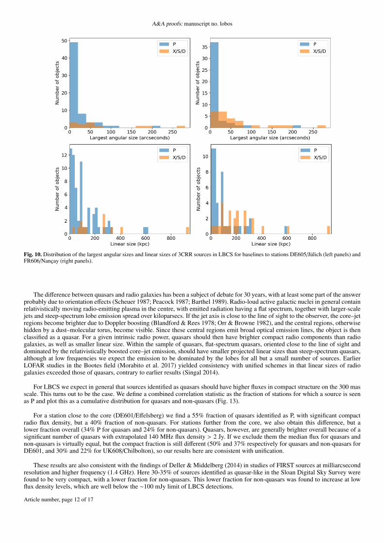
The revised Third Cambridge Catalogue of Radio Sources (3CRR) (Laing et al. 1983) contains those extragalactic sources that havea 178 MHz flux density (KPW scale) ≥10 Jy, declination ≥ 10◦, and Galactic latitude ≥ 10◦ or ≤ -10◦. They contain a mixtureof large-scale lobe-dominated sources with structures of typical sizes >100 kpc, corresponding to 30" which is resolved out on allthe long baselines, together with more compact sources such as CSS (O’Dea & Saikia 2020) and a few flat-spectrum quasars (e.g.3C345, 3C454.3). Because of the LBCS selection criteria, we expect to see a fraction of 3CRR sources in the LBCS catalogue. Wefind that there are 82 3CRR sources that were observed in LBCS.

We use previous compilations of largest angular and linear sizes in 3CRR (https://astroherzberg.org/people/chris-willott/research/3crr/ in the form of an updated version of the sample presented in Laing et al. (1983)). Figure 10 shows the relationof size to LBCS type (P, S, or X) for baselines to stations DE605/Jülich and FR606/Nançay. As expected, there is evidence that thelargest sources, which are on average thought to have less flux density in compact structure, are generally less consistently detectedby LBCS, particularly on the longer baselines.

In addition to correlations with size, sources are more likely to be detected if they have flatter low-frequency spectral indexes;for such sources more flux density should appear at smaller spatial scales corresponding to core–jet emission rather than extendedsteep spectrum lobe emission. This appears to be the case (Fig. 11).


https://astroherzberg.org/people/chris-willott/research/3crr/

https://astroherzberg.org/people/chris-willott/research/3crr/


Fig. 8. Flux density for LBCS sources coincident with an unresolved FIRST source and a WENSS source vs FIRST/WENSS spectral index. Thelight green crosses (in background) indicate the general population of WENSS/FIRST coincidences, dark green crosses represent those sourcesobserved with LBCS and detected, and red crosses represent the sources observed with LBCS but not detected. The right panel contains onlysources that are also VLBA calibrators.

Fig. 9. As for Fig. 7, but for unresolved FIRST sources

3.3. Quasars and radio galaxies

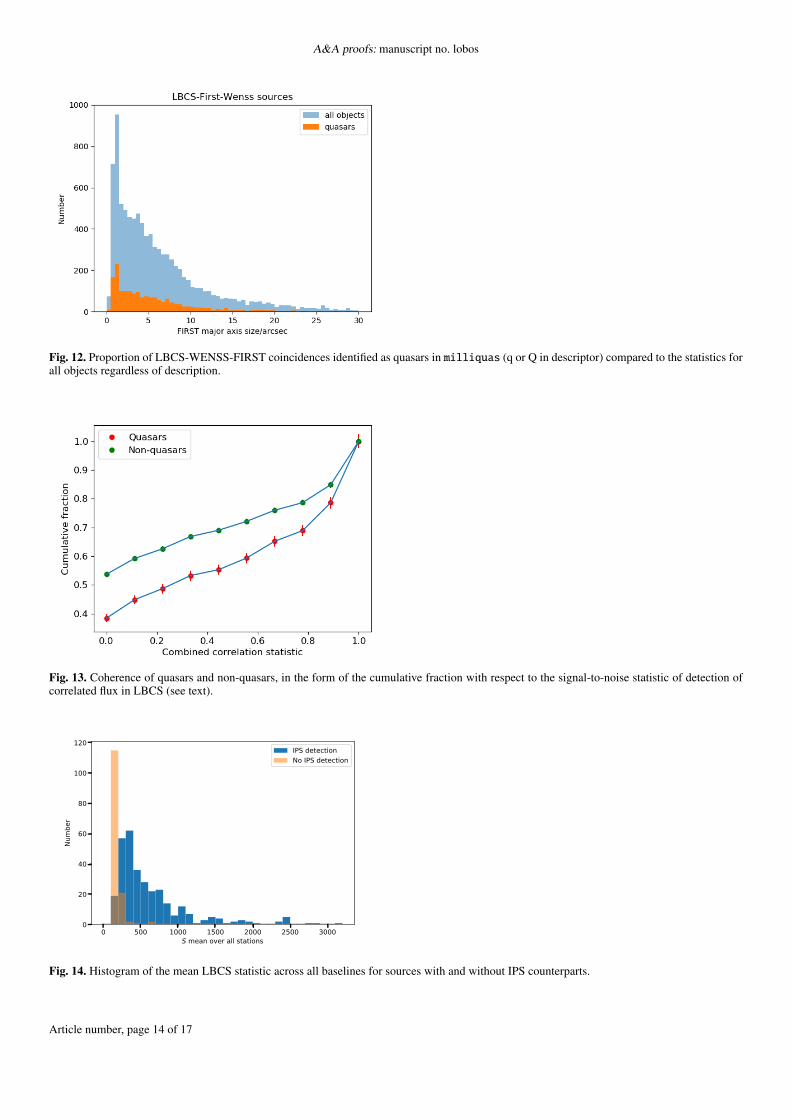
We can also use the information about compactness provided by LBCS to investigate differences in the strength of flux density incompact components separately for sources identified as quasars and those identified in radio galaxies. To this end, we take thesample of LBCS sources in the overlapping WENSS/FIRST footprint and compare the catalogue with the milliquas compilation(Flesch 2019); 19% of the sources are listed as quasars in this catalogue, the proportion of which decreases slightly with FIRSTmajor axis size (Fig. 12).



Fig. 10. Distribution of the largest angular sizes and linear sizes of 3CRR sources in LBCS for baselines to stations DE605/Jülich (left panels) andFR606/Nançay (right panels).

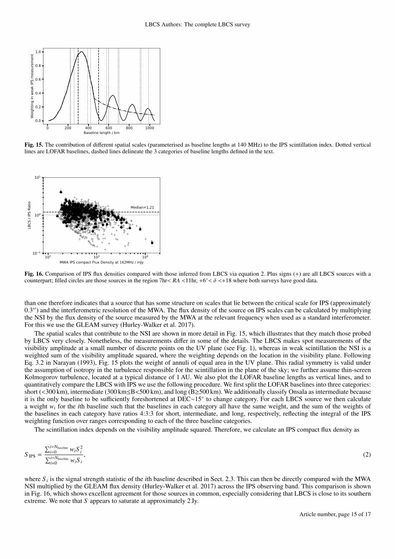
The difference between quasars and radio galaxies has been a subject of debate for 30 years, with at least some part of the answerprobably due to orientation effects (Scheuer 1987; Peacock 1987; Barthel 1989). Radio-loud active galactic nuclei in general containrelativistically moving radio-emitting plasma in the centre, with emitted radiation having a flat spectrum, together with larger-scalejets and steep-spectrum lobe emission spread over kiloparsecs. If the jet axis is close to the line of sight to the observer, the core–jetregions become brighter due to Doppler boosting (Blandford & Rees 1978; Orr & Browne 1982), and the central regions, otherwisehidden by a dust–molecular torus, become visible. Since these central regions emit broad optical emission lines, the object is thenclassified as a quasar. For a given intrinsic radio power, quasars should then have brighter compact radio components than radiogalaxies, as well as smaller linear size. Within the sample of quasars, flat-spectrum quasars, oriented close to the line of sight anddominated by the relativistically boosted core–jet emission, should have smaller projected linear sizes than steep-spectrum quasars,although at low frequencies we expect the emission to be dominated by the lobes for all but a small number of sources. EarlierLOFAR studies in the Bootes field (Morabito et al. 2017) yielded consistency with unified schemes in that linear sizes of radiogalaxies exceeded those of quasars, contrary to earlier results (Singal 2014).

For LBCS we expect in general that sources identified as quasars should have higher fluxes in compact structure on the 300 masscale. This turns out to be the case. We define a combined correlation statistic as the fraction of stations for which a source is seenas P and plot this as a cumulative distribution for quasars and non-quasars (Fig. 13).

For a station close to the core (DE601/Effelsberg) we find a 55% fraction of quasars identified as P, with significant compactradio flux density, but a 40% fraction of non-quasars. For stations further from the core, we also obtain this difference, but alower fraction overall (34% P for quasars and 24% for non-quasars). Quasars, however, are generally brighter overall because of asignificant number of quasars with extrapolated 140 MHz flux density > 2 Jy. If we exclude them the median flux for quasars andnon-quasars is virtually equal, but the compact fraction is still different (50% and 37% respectively for quasars and non-quasars forDE601, and 30% and 22% for UK608/Chilbolton), so our results here are consistent with unification.

These results are also consistent with the findings of Deller & Middelberg (2014) in studies of FIRST sources at milliarcsecondresolution and higher frequency (1.4 GHz). Here 30-35% of sources identified as quasar-like in the Sloan Digital Sky Survey werefound to be very compact, with a lower fraction for non-quasars. This lower fraction for non-quasars was found to increase at lowflux density levels, which are well below the ∼100 mJy limit of LBCS detections.



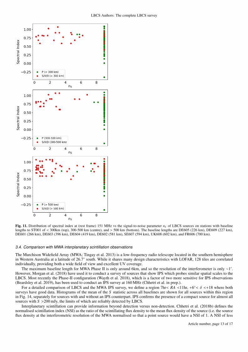
Fig. 11. Distribution of spectral index at (rest frame) 151 MHz vs the signal-to-noise parameter nS of LBCS sources on stations with baselinelengths to ST001 of < 300km (top), 300-500 km (centre), and > 500 km (bottom). The baseline lengths are DE605 (226 km), DE609 (227 km),DE601 (266 km), DE603 (396 km), DE604 (419 km), DE602 (581 km), SE607 (594 km), UK608 (602 km), and FR606 (700 km).

3.4. Comparison with MWA interplanetary scintillation observations

The Murchison Widefield Array (MWA; Tingay et al. 2013) is a low-frequency radio telescope located in the southern hemispherein Western Australia at a latitude of 26.7◦ south. While it shares many design characteristics with LOFAR, 128 tiles are correlatedindividually, providing both a wide field of view and excellent UV coverage.

The maximum baseline length for MWA Phase II is only around 6km, and so the resolution of the interferometer is only ∼1′.However, Morgan et al. (2018) have used it to conduct a survey of sources that show IPS which probes similar spatial scales to theLBCS. Most recently the Phase-II configuration (Wayth et al. 2018), which is a factor of two more sensitive for IPS observations(Beardsley et al. 2019), has been used to conduct an IPS survey at 160 MHz (Chhetri et al. in prep.).

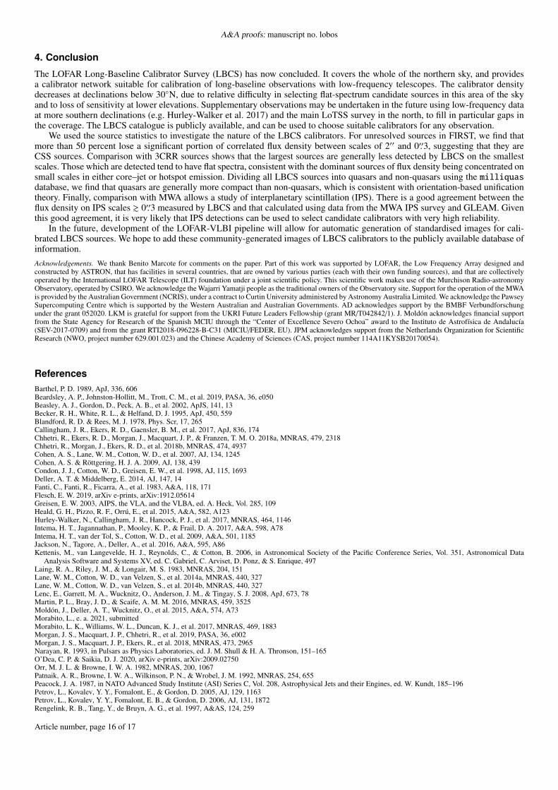
For a detailed comparison of LBCS and the MWA IPS survey, we define a region 7hr< RA <11hr, +6◦< δ <+18 where bothsurveys have good data. Histograms of the mean of the S statistic across all baselines are shown for all sources within this regionin Fig. 14, separately for sources with and without an IPS counterpart. IPS confirms the presence of a compact source for almost allsources with S >200 mJy, the limits of which are reliably detected by LBCS.

Interplanetary scintillation can provide information beyond detection versus non-detection. Chhetri et al. (2018b) defines thenormalised scintillation index (NSI) as the ratio of the scintillating flux density to the mean flux density of the source (i.e. the sourceflux density at the interferometric resolution of the MWA normalised so that a point source would have a NSI of 1. A NSI of less



Fig. 12. Proportion of LBCS-WENSS-FIRST coincidences identified as quasars in milliquas (q or Q in descriptor) compared to the statistics forall objects regardless of description.

Fig. 13. Coherence of quasars and non-quasars, in the form of the cumulative fraction with respect to the signal-to-noise statistic of detection ofcorrelated flux in LBCS (see text).

0 500 1000 1500 2000 2500 3000S mean over all stations

0

20

40

60

80

100

120

Num

ber

IPS detectionNo IPS detection

Fig. 14. Histogram of the mean LBCS statistic across all baselines for sources with and without IPS counterparts.



0 200 400 600 800 1000Baseline length / km

0.0

0.2

0.4

0.6

0.8

1.0

Wei

ghtin

g in

wea

k IP

S m

easu

rem

ent

Fig. 15. The contribution of different spatial scales (parameterised as baseline lengths at 140 MHz) to the IPS scintillation index. Dotted verticallines are LOFAR baselines, dashed lines delineate the 3 categories of baseline lengths defined in the text.

102 103 104

MWA IPS compact Flux Density at 162MHz / mJy

10 1

100

101

LBCS

/ IP

S Ra

tio Median=1.21

Fig. 16. Comparison of IPS flux densities compared with those inferred from LBCS via equation 2. Plus signs (+) are all LBCS sources with acounterpart; filled circles are those sources in the region 7hr< RA <11hr, +6◦< δ <+18 where both surveys have good data.

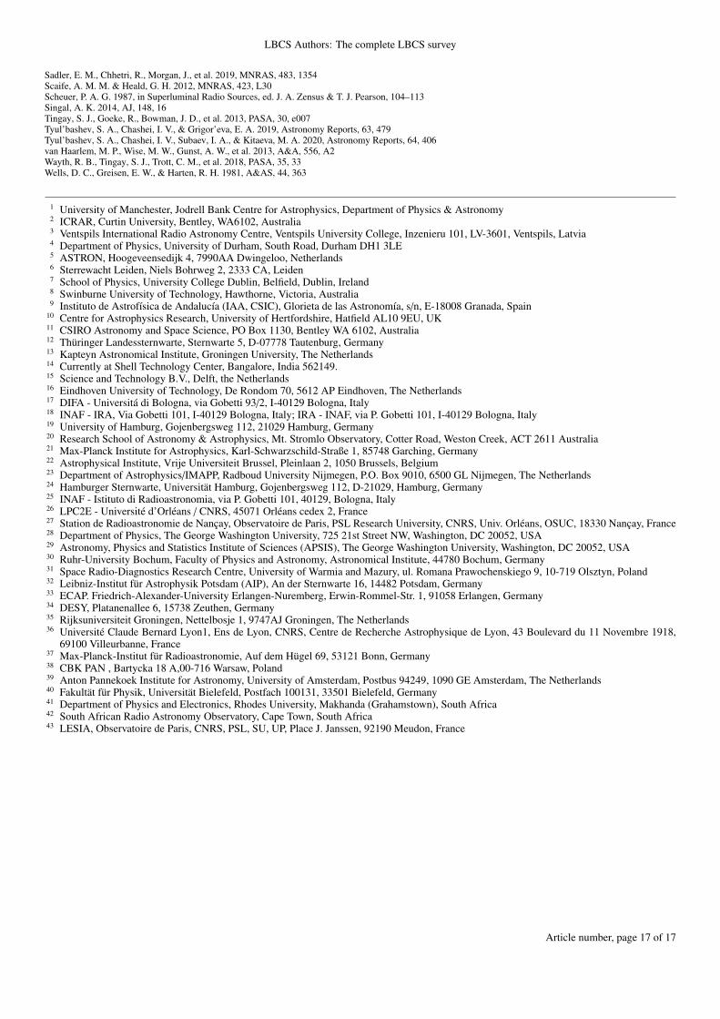
than one therefore indicates that a source that has some structure on scales that lie between the critical scale for IPS (approximately0.3′′) and the interferometric resolution of the MWA. The flux density of the source on IPS scales can be calculated by multiplyingthe NSI by the flux density of the source measured by the MWA at the relevant frequency when used as a standard interferometer.For this we use the GLEAM survey (Hurley-Walker et al. 2017).

The spatial scales that contribute to the NSI are shown in more detail in Fig. 15, which illustrates that they match those probedby LBCS very closely. Nonetheless, the measurements differ in some of the details. The LBCS makes spot measurements of thevisibility amplitude at a small number of discrete points on the UV plane (see Fig. 1), whereas in weak scintillation the NSI is aweighted sum of the visibility amplitude squared, where the weighting depends on the location in the visibility plane. FollowingEq. 3.2 in Narayan (1993), Fig. 15 plots the weight of annuli of equal area in the UV plane. This radial symmetry is valid underthe assumption of isotropy in the turbulence responsible for the scintillation in the plane of the sky; we further assume thin-screenKolmogorov turbulence, located at a typical distance of 1 AU. We also plot the LOFAR baseline lengths as vertical lines, and toquantitatively compare the LBCS with IPS we use the following procedure. We first split the LOFAR baselines into three categories:short (<300 km), intermediate (300 km≤B<500 km), and long (B≥500 km). We additionally classify Onsala as intermediate becauseit is the only baseline to be sufficiently foreshortened at DEC∼15◦ to change category. For each LBCS source we then calculatea weight wi for the ith baseline such that the baselines in each category all have the same weight, and the sum of the weights ofthe baselines in each category have ratios 4:3:3 for short, intermediate, and long, respectively, reflecting the integral of the IPSweighting function over ranges corresponding to each of the three baseline categories.

The scintillation index depends on the visibility amplitude squared. Therefore, we calculate an IPS compact flux density as

S IPS =

∑i=Nbaselinei=0 wiS 2

i∑i=Nbaselinei=0 wiS i

, (2)

where S i is the signal strength statistic of the ith baseline described in Sect. 2.3. This can then be directly compared with the MWANSI multiplied by the GLEAM flux density (Hurley-Walker et al. 2017) across the IPS observing band. This comparison is shownin Fig. 16, which shows excellent agreement for those sources in common, especially considering that LBCS is close to its southernextreme. We note that S appears to saturate at approximately 2 Jy.



4. Conclusion

The LOFAR Long-Baseline Calibrator Survey (LBCS) has now concluded. It covers the whole of the northern sky, and providesa calibrator network suitable for calibration of long-baseline observations with low-frequency telescopes. The calibrator densitydecreases at declinations below 30◦N, due to relative difficulty in selecting flat-spectrum candidate sources in this area of the skyand to loss of sensitivity at lower elevations. Supplementary observations may be undertaken in the future using low-frequency dataat more southern declinations (e.g. Hurley-Walker et al. 2017) and the main LoTSS survey in the north, to fill in particular gaps inthe coverage. The LBCS catalogue is publicly available, and can be used to choose suitable calibrators for any observation.

We used the source statistics to investigate the nature of the LBCS calibrators. For unresolved sources in FIRST, we find thatmore than 50 percent lose a significant portion of correlated flux density between scales of 2′′ and 0′′.3, suggesting that they areCSS sources. Comparison with 3CRR sources shows that the largest sources are generally less detected by LBCS on the smallestscales. Those which are detected tend to have flat spectra, consistent with the dominant sources of flux density being concentrated onsmall scales in either core–jet or hotspot emission. Dividing all LBCS sources into quasars and non-quasars using the milliquasdatabase, we find that quasars are generally more compact than non-quasars, which is consistent with orientation-based unificationtheory. Finally, comparison with MWA allows a study of interplanetary scintillation (IPS). There is a good agreement between theflux density on IPS scales & 0′′.3 measured by LBCS and that calculated using data from the MWA IPS survey and GLEAM. Giventhis good agreement, it is very likely that IPS detections can be used to select candidate calibrators with very high reliability.

In the future, development of the LOFAR-VLBI pipeline will allow for automatic generation of standardised images for cali-brated LBCS sources. We hope to add these community-generated images of LBCS calibrators to the publicly available database ofinformation.Acknowledgements. We thank Benito Marcote for comments on the paper. Part of this work was supported by LOFAR, the Low Frequency Array designed andconstructed by ASTRON, that has facilities in several countries, that are owned by various parties (each with their own funding sources), and that are collectivelyoperated by the International LOFAR Telescope (ILT) foundation under a joint scientific policy. This scientific work makes use of the Murchison Radio-astronomyObservatory, operated by CSIRO. We acknowledge the Wajarri Yamatji people as the traditional owners of the Observatory site. Support for the operation of the MWAis provided by the Australian Government (NCRIS), under a contract to Curtin University administered by Astronomy Australia Limited. We acknowledge the PawseySupercomputing Centre which is supported by the Western Australian and Australian Governments. AD acknowledges support by the BMBF Verbundforschungunder the grant 052020. LKM is grateful for support from the UKRI Future Leaders Fellowship (grant MR/T042842/1). J. Moldón acknowledges financial supportfrom the State Agency for Research of the Spanish MCIU through the “Center of Excellence Severo Ochoa” award to the Instituto de Astrofísica de Andalucía(SEV-2017-0709) and from the grant RTI2018-096228-B-C31 (MICIU/FEDER, EU). JPM acknowledges support from the Netherlands Organization for ScientificResearch (NWO, project number 629.001.023) and the Chinese Academy of Sciences (CAS, project number 114A11KYSB20170054).

ReferencesBarthel, P. D. 1989, ApJ, 336, 606Beardsley, A. P., Johnston-Hollitt, M., Trott, C. M., et al. 2019, PASA, 36, e050Beasley, A. J., Gordon, D., Peck, A. B., et al. 2002, ApJS, 141, 13Becker, R. H., White, R. L., & Helfand, D. J. 1995, ApJ, 450, 559Blandford, R. D. & Rees, M. J. 1978, Phys. Scr, 17, 265Callingham, J. R., Ekers, R. D., Gaensler, B. M., et al. 2017, ApJ, 836, 174Chhetri, R., Ekers, R. D., Morgan, J., Macquart, J. P., & Franzen, T. M. O. 2018a, MNRAS, 479, 2318Chhetri, R., Morgan, J., Ekers, R. D., et al. 2018b, MNRAS, 474, 4937Cohen, A. S., Lane, W. M., Cotton, W. D., et al. 2007, AJ, 134, 1245Cohen, A. S. & Röttgering, H. J. A. 2009, AJ, 138, 439Condon, J. J., Cotton, W. D., Greisen, E. W., et al. 1998, AJ, 115, 1693Deller, A. T. & Middelberg, E. 2014, AJ, 147, 14Fanti, C., Fanti, R., Ficarra, A., et al. 1983, A&A, 118, 171Flesch, E. W. 2019, arXiv e-prints, arXiv:1912.05614Greisen, E. W. 2003, AIPS, the VLA, and the VLBA, ed. A. Heck, Vol. 285, 109Heald, G. H., Pizzo, R. F., Orrú, E., et al. 2015, A&A, 582, A123Hurley-Walker, N., Callingham, J. R., Hancock, P. J., et al. 2017, MNRAS, 464, 1146Intema, H. T., Jagannathan, P., Mooley, K. P., & Frail, D. A. 2017, A&A, 598, A78Intema, H. T., van der Tol, S., Cotton, W. D., et al. 2009, A&A, 501, 1185Jackson, N., Tagore, A., Deller, A., et al. 2016, A&A, 595, A86Kettenis, M., van Langevelde, H. J., Reynolds, C., & Cotton, B. 2006, in Astronomical Society of the Pacific Conference Series, Vol. 351, Astronomical Data

Analysis Software and Systems XV, ed. C. Gabriel, C. Arviset, D. Ponz, & S. Enrique, 497Laing, R. A., Riley, J. M., & Longair, M. S. 1983, MNRAS, 204, 151Lane, W. M., Cotton, W. D., van Velzen, S., et al. 2014a, MNRAS, 440, 327Lane, W. M., Cotton, W. D., van Velzen, S., et al. 2014b, MNRAS, 440, 327Lenc, E., Garrett, M. A., Wucknitz, O., Anderson, J. M., & Tingay, S. J. 2008, ApJ, 673, 78Martin, P. L., Bray, J. D., & Scaife, A. M. M. 2016, MNRAS, 459, 3525Moldón, J., Deller, A. T., Wucknitz, O., et al. 2015, A&A, 574, A73Morabito, L., e. a. 2021, submittedMorabito, L. K., Williams, W. L., Duncan, K. J., et al. 2017, MNRAS, 469, 1883Morgan, J. S., Macquart, J. P., Chhetri, R., et al. 2019, PASA, 36, e002Morgan, J. S., Macquart, J. P., Ekers, R., et al. 2018, MNRAS, 473, 2965Narayan, R. 1993, in Pulsars as Physics Laboratories, ed. J. M. Shull & H. A. Thronson, 151–165O’Dea, C. P. & Saikia, D. J. 2020, arXiv e-prints, arXiv:2009.02750Orr, M. J. L. & Browne, I. W. A. 1982, MNRAS, 200, 1067Patnaik, A. R., Browne, I. W. A., Wilkinson, P. N., & Wrobel, J. M. 1992, MNRAS, 254, 655Peacock, J. A. 1987, in NATO Advanced Study Institute (ASI) Series C, Vol. 208, Astrophysical Jets and their Engines, ed. W. Kundt, 185–196Petrov, L., Kovalev, Y. Y., Fomalont, E., & Gordon, D. 2005, AJ, 129, 1163Petrov, L., Kovalev, Y. Y., Fomalont, E. B., & Gordon, D. 2006, AJ, 131, 1872Rengelink, R. B., Tang, Y., de Bruyn, A. G., et al. 1997, A&AS, 124, 259



Sadler, E. M., Chhetri, R., Morgan, J., et al. 2019, MNRAS, 483, 1354Scaife, A. M. M. & Heald, G. H. 2012, MNRAS, 423, L30Scheuer, P. A. G. 1987, in Superluminal Radio Sources, ed. J. A. Zensus & T. J. Pearson, 104–113Singal, A. K. 2014, AJ, 148, 16Tingay, S. J., Goeke, R., Bowman, J. D., et al. 2013, PASA, 30, e007Tyul’bashev, S. A., Chashei, I. V., & Grigor’eva, E. A. 2019, Astronomy Reports, 63, 479Tyul’bashev, S. A., Chashei, I. V., Subaev, I. A., & Kitaeva, M. A. 2020, Astronomy Reports, 64, 406van Haarlem, M. P., Wise, M. W., Gunst, A. W., et al. 2013, A&A, 556, A2Wayth, R. B., Tingay, S. J., Trott, C. M., et al. 2018, PASA, 35, 33Wells, D. C., Greisen, E. W., & Harten, R. H. 1981, A&AS, 44, 363

1 University of Manchester, Jodrell Bank Centre for Astrophysics, Department of Physics & Astronomy2 ICRAR, Curtin University, Bentley, WA6102, Australia3 Ventspils International Radio Astronomy Centre, Ventspils University College, Inzenieru 101, LV-3601, Ventspils, Latvia4 Department of Physics, University of Durham, South Road, Durham DH1 3LE5 ASTRON, Hoogeveensedijk 4, 7990AA Dwingeloo, Netherlands6 Sterrewacht Leiden, Niels Bohrweg 2, 2333 CA, Leiden7 School of Physics, University College Dublin, Belfield, Dublin, Ireland8 Swinburne University of Technology, Hawthorne, Victoria, Australia9 Instituto de Astrofísica de Andalucía (IAA, CSIC), Glorieta de las Astronomía, s/n, E-18008 Granada, Spain

10 Centre for Astrophysics Research, University of Hertfordshire, Hatfield AL10 9EU, UK11 CSIRO Astronomy and Space Science, PO Box 1130, Bentley WA 6102, Australia12 Thüringer Landessternwarte, Sternwarte 5, D-07778 Tautenburg, Germany13 Kapteyn Astronomical Institute, Groningen University, The Netherlands14 Currently at Shell Technology Center, Bangalore, India 562149.15 Science and Technology B.V., Delft, the Netherlands16 Eindhoven University of Technology, De Rondom 70, 5612 AP Eindhoven, The Netherlands17 DIFA - Universitá di Bologna, via Gobetti 93/2, I-40129 Bologna, Italy18 INAF - IRA, Via Gobetti 101, I-40129 Bologna, Italy; IRA - INAF, via P. Gobetti 101, I-40129 Bologna, Italy19 University of Hamburg, Gojenbergsweg 112, 21029 Hamburg, Germany20 Research School of Astronomy & Astrophysics, Mt. Stromlo Observatory, Cotter Road, Weston Creek, ACT 2611 Australia21 Max-Planck Institute for Astrophysics, Karl-Schwarzschild-Straße 1, 85748 Garching, Germany22 Astrophysical Institute, Vrije Universiteit Brussel, Pleinlaan 2, 1050 Brussels, Belgium23 Department of Astrophysics/IMAPP, Radboud University Nijmegen, P.O. Box 9010, 6500 GL Nijmegen, The Netherlands24 Hamburger Sternwarte, Universität Hamburg, Gojenbergsweg 112, D-21029, Hamburg, Germany25 INAF - Istituto di Radioastronomia, via P. Gobetti 101, 40129, Bologna, Italy26 LPC2E - Université d’Orléans / CNRS, 45071 Orléans cedex 2, France27 Station de Radioastronomie de Nançay, Observatoire de Paris, PSL Research University, CNRS, Univ. Orléans, OSUC, 18330 Nançay, France28 Department of Physics, The George Washington University, 725 21st Street NW, Washington, DC 20052, USA29 Astronomy, Physics and Statistics Institute of Sciences (APSIS), The George Washington University, Washington, DC 20052, USA30 Ruhr-University Bochum, Faculty of Physics and Astronomy, Astronomical Institute, 44780 Bochum, Germany31 Space Radio-Diagnostics Research Centre, University of Warmia and Mazury, ul. Romana Prawochenskiego 9, 10-719 Olsztyn, Poland32 Leibniz-Institut für Astrophysik Potsdam (AIP), An der Sternwarte 16, 14482 Potsdam, Germany33 ECAP. Friedrich-Alexander-University Erlangen-Nuremberg, Erwin-Rommel-Str. 1, 91058 Erlangen, Germany34 DESY, Platanenallee 6, 15738 Zeuthen, Germany35 Rijksuniversiteit Groningen, Nettelbosje 1, 9747AJ Groningen, The Netherlands36 Université Claude Bernard Lyon1, Ens de Lyon, CNRS, Centre de Recherche Astrophysique de Lyon, 43 Boulevard du 11 Novembre 1918,

69100 Villeurbanne, France37 Max-Planck-Institut für Radioastronomie, Auf dem Hügel 69, 53121 Bonn, Germany38 CBK PAN , Bartycka 18 A,00-716 Warsaw, Poland39 Anton Pannekoek Institute for Astronomy, University of Amsterdam, Postbus 94249, 1090 GE Amsterdam, The Netherlands40 Fakultät für Physik, Universität Bielefeld, Postfach 100131, 33501 Bielefeld, Germany41 Department of Physics and Electronics, Rhodes University, Makhanda (Grahamstown), South Africa42 South African Radio Astronomy Observatory, Cape Town, South Africa43 LESIA, Observatoire de Paris, CNRS, PSL, SU, UP, Place J. Janssen, 92190 Meudon, France


II. Completion of the LOFAR Long-Baseline Calibrator Survey

Documents

Transcript of II. Completion of the LOFAR Long-Baseline Calibrator Survey