ACCEPTED VERSION

Wang, Xiaojian; Lambert, Martin Francis; Simpson, Angus Ross; Liggett, James A.; Vitkovsky, John Leak detection in pipelines using the damping of fluid transients Journal of Hydraulic Engineering, 2002; 128 (7):697-711

© 2002 American Society of Civil Engineers

http://hdl.handle.net/2440/994

PERMISSIONS

http://www.asce.org/Content.aspx?id=29734

Authors may post the final draft of their work on open, unrestricted Internet sites or deposit it in an institutional repository when the draft contains a link to the bibliographic record of the published version in the ASCE Civil Engineering Database. "Final draft" means the version submitted to ASCE after peer review and prior to copyediting or other ASCE production activities; it does not include the copyedited version, the page proof, or a PDF of the published version

28 March 2014

1

Leak Detection in Pipelines Using the

Damping of Fluid Transients

Xiao-Jian Wang1, Martin F. Lambert2, Angus R. Simpson3, James A. Liggett4* and John P. Vítkovský5

Abstract: Leaks in pipelines contribute to damping of transient events. That

fact leads to a method to find location and magnitude of leaks. Because the

problem of transient flow in pipes is nearly linear, the solution of the

governing equations can be expressed in terms of a Fourier series. All Fourier

components are damped uniformly by steady pipe friction, but each

component is damped differently in the presence of a leak. Thus, overall leak-

induced damping can be divided into two parts. The magnitude of the

damping indicates size of a leak whereas different damping ratios of the

various Fourier components are used to find location of a leak. This method

does not require rigorous determination and modeling of boundary conditions

and transient behavior in the pipeline. The technique is successful in

detecting, locating and quantifying a 0.1% size leak with respect to the cross-

sectional area of a pipeline.

1 Postgraduate Student, Dept. of Civil & Environmental Engineering, Adelaide University, Adelaide, SA5005, Australia. email: xwang@civeng.adelaide.edu.au.

2 Senior Lecturer, Dept. of Civil & Environmental Engineering, Adelaide University, Adelaide, SA 5005,Australia. email: mlambert@civeng.adelaide.edu.au.

3 Associate Professor, Dept. of Civil & Environmental Engineering, Adelaide University, Adelaide, SA5005, Australia. email: asimpson@civeng.adelaide.edu.au. Member, ASCE.

4 Professor Emeritus, School of Civil & Environmental Engineering, Cornell University, Ithaca, N.Y. 14853-3501, USA. email: jal8@cornell.edu. *Corresponding author.

5 Research Associate, Dept. of Civil & Environmental Engineering, Adelaide University, Adelaide, SA5005, Australia. email: jvitkovs@civeng.adelaide.edu.au.

2

Introduction

Leakage from pipelines has the potential to cause significant environmental damage and

economic loss. While pipelines are designed and constructed to maintain their integrity, it

is difficult to avoid the occurrence of leakage in a pipeline system during its lifetime

(Hovey and Farmer 1999). Often, accurate leak detection, enabling a quick response, is

necessary to minimize damage. Leak detection methods previously proposed are:

reflected wave or timing methods (Jönsson 1995, Covas and Romas 1999, Brunone 1999);

volume balance methods (Griebenow and Mears 1989, Liou 1994); pressure or flow

deviation methods (Griebenow and Mears 1989, Liou and Tian 1995); acoustic methods

(Fuchs and Riehle 1991); pig-based monitoring and on-line surveillance methods (Black

1992, Weil et al. 1994, Furness and Reet 1998); frequency analysis methods (Jönsson and

Larson 1992, Mpesha et al. 2001); inverse techniques (Pudar and Liggett 1992, Liggett

and Chen 1994, Vítkovský, 2001); and a genetic algorithm method (Vítkovský et al.

2000). However, no single method can always meet operational needs from an accuracy

and cost point of view (Furness and Reet 1998). Each of these leak detection techniques

has its advantages and disadvantages in different circumstances. Liou (1998) used a

pseudo-random binary signal (p.r.b.s) sequence as a transient tool and showed that change

of the spatial damping of the p.r.b.s sequence along the pipeline can be used to detect a

leak. A leak detection, location and quantification method that uses damping of a transient

event by a leak is presented in this paper.

Transient response of a pipeline with a distributed leak was investigated by Wiggett

(1968). They found that the transients in a pipeline were greatly affected by the magnitude

of the distributed lateral flow. To investigate the effects of the demands on the transients

in a field pipe network test, McInnis and Karney (1995) used a similar distributed leak

3

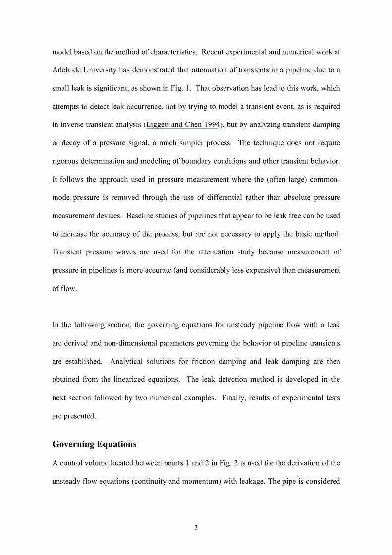
model based on the method of characteristics. Recent experimental and numerical work at

Adelaide University has demonstrated that attenuation of transients in a pipeline due to a

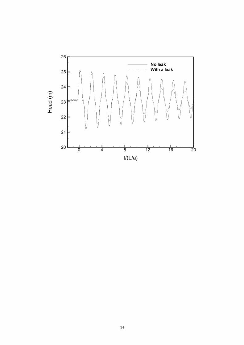
small leak is significant, as shown in Fig. 1. That observation has lead to this work, which

attempts to detect leak occurrence, not by trying to model a transient event, as is required

in inverse transient analysis (Liggett and Chen 1994), but by analyzing transient damping

or decay of a pressure signal, a much simpler process. The technique does not require

rigorous determination and modeling of boundary conditions and other transient behavior.

It follows the approach used in pressure measurement where the (often large) common-

mode pressure is removed through the use of differential rather than absolute pressure

measurement devices. Baseline studies of pipelines that appear to be leak free can be used

to increase the accuracy of the process, but are not necessary to apply the basic method.

Transient pressure waves are used for the attenuation study because measurement of

pressure in pipelines is more accurate (and considerably less expensive) than measurement

of flow.

In the following section, the governing equations for unsteady pipeline flow with a leak

are derived and non-dimensional parameters governing the behavior of pipeline transients

are established. Analytical solutions for friction damping and leak damping are then

obtained from the linearized equations. The leak detection method is developed in the

next section followed by two numerical examples. Finally, results of experimental tests

are presented.

Governing Equations

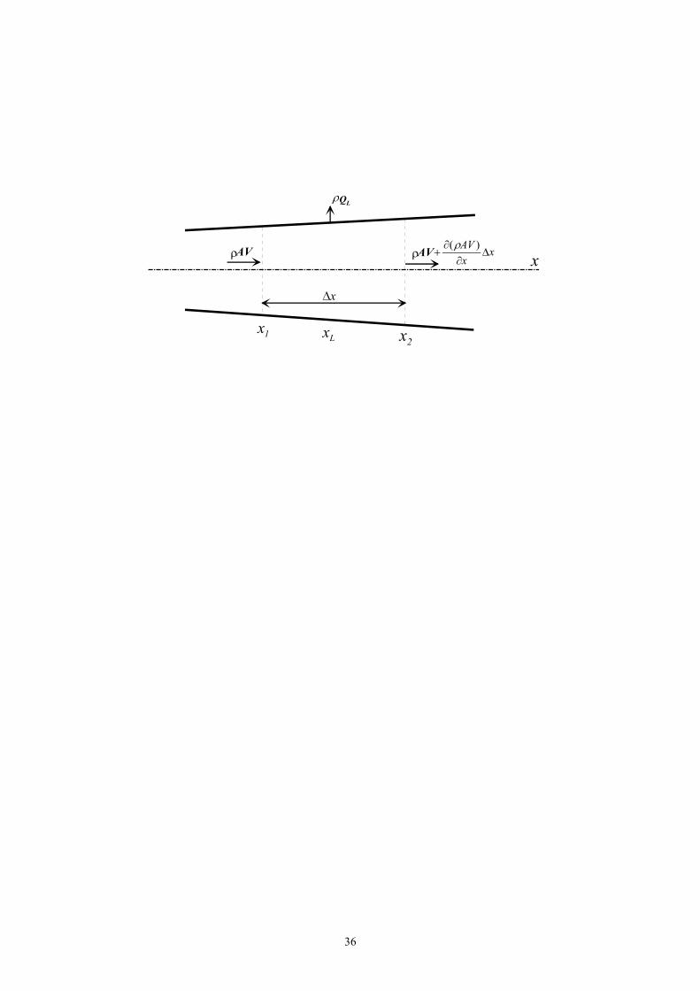
A control volume located between points 1 and 2 in Fig. 2 is used for the derivation of the

unsteady flow equations (continuity and momentum) with leakage. The pipe is considered

4

to be horizontal with a leak located as shown in Fig. 2, where QL is the total discharge out

of the leak located at x = xL.

Adapting the non-leak equation of Wylie and Streeter (1993), conservation of mass in the

control volume gives

LQxAVx

xAt

��� ����

���

�

� )()( (1)

where x = distance along the pipeline, t = time, � = fluid density, A = cross-sectional area

of the pipe, and V = velocity of flow. Dividing (1) throughout by �x and letting �x

approach zero gives

)()()( LL xxQAVx

At

����

��

�

����� (2)

The Dirac delta function is defined as

��

��

� ��

��

otherwise0

if)(

L

L

xxxx� , and �

�

��

��

�

��

�L

L

x

x L dxxx 1)(lim0

(3)

where � = a small distance on the either side of the leak. Note that �(x-xL) has dimension

of length-1. Considering the compressibility of the water and the elasticity of the pipe wall

with some simplifications (Wylie and Streeter 1993), Eq. (2) is expressed in the more

usual water-hammer-equation form,

0)(22

����

��

�

��

�

�

LL xxQgAa

xQ

gAa

xH

AQ

tH

� (4)

in which H = piezometric head, Q = flow rate in the pipeline, a = wave speed in the fluid,

and g = gravitational acceleration. Similarly, conservation of momentum for a leak

perpendicular to the pipe axis is

0)(

21

22

2

2 ��

���

��

�

��

�

�

gAxxQQ

DgAfQ

xQ

gAQ

tQ

gAxH LL� (5)

5

where f = friction factor and D = pipe diameter. The last term in (5) is caused by the mass

flow discontinuity at the leak in the pipeline. Eq. (5) assumes that pipe friction during a

transient event is described by a constant steady-state Darcy-Weisbach friction factor,

which is a common assumption. However, pipe friction during unsteady events can be

significantly larger than that predicted by the Darcy-Weisbach equation. The effects of

unsteady friction are considered later in the paper.

Leak discharge is a function of pressure in a pipe and size of a leak and is expressed by the

orifice equation

LLdL HgACQ �� 2 (6)

where LH� = HL-zL = pressure head at a leak (assuming pressure outside of the pipe is

atmospheric), HL = piezometric head in the pipeline at the leak, Lz = pipe elevation at the

leak, Cd = leak discharge coefficient, and AL = leak area. The following dimensionless

quantities are used to non-dimensionalize (4), (5) and (6):

1

*

HHH � ,

aLtt/

*� ,

Lxx �

* , 0

*

QQQ � , and Lxxxx LL )()( **

��� �� (7)

in which H1 = reference piezometric head (e.g., the head at a tank), L = pipe length, and

Q0 = reference flow rate. Substituting (6) and applying the dimensionless quantities in (7)

to (4) and (5) gives

0)(2 ***1

01

0

*

*

1

0*

**0

*

*

���

��

��

�

��

�

�

LLLd xxHgH

QAC

gAHaQ

xQ

gAHaQ

xHQ

aV

tH

�

(8)

� �

� � 02

2

****

0

10

2*0*

**0

*

*

*

*

0

1

�����

��

��

�

��

�

�

LLLd xxHQQ

gHACa

V

QDAafLQ

xQQ

aV

tQ

xH

aQgAH

(9)

6

Because V0/a is normally small, the second term in (8) and the third and the last terms in

(9) can be neglected. The dimensionless equations become

0)(1 ****

*

*

*

�����

��

�

�LL xxHM

xQ

FtH

� (10)

02**

*

*

*

���

��

�

� RQtQ

xHF (11)

where aDAfLQR

20

� , 12

2gHa

AAC

M Ld� ,

JHH

F 1� and

gaV

H J0

� is the Joukowsky

pressure head rise, resulting from an instantaneous reduction of velocity V0 to zero. The

dimensionless quantities R, M and F are used to characterize the leak problem.

Linearized Solutions

Expressing H* and Q* as steady-state values plus small transient quantities gives

**0

* hHH �� , **0

* qQQ �� (12)

where h* = non-dimensional head deviation, *0H = non-dimensional steady head, q* =

non-dimensional flow deviation and *0Q = non-dimensional steady flow. When only linear

terms are retained, the square root in (10) is expressed as

**0

***0

*** hHzhHzHH LLLLLL ���������

= )1)(2

(*

0

**

0 T

L

L eH

hH �

�

�� (13)

where

*0

**

0

*0

**

0*

2

)2

(

L

L

L

LL

T

HhH

HhHH

e

���

�����

� is the truncation error in the Taylor

expansion, *LH� = HL

*-zL* = dimensionless pressure head at the leak, HL

* = dimensionless

piezometric head in the pipeline at the leak, Lz * = dimensionless elevation at the leak, and

7

HL0* = dimensionless steady-state piezometric head at the leak. Substituting (12) and (13)

into (10) and (11) and neglecting Te and (q*)2 terms yields

0)(2

1 **

*0

*

*

*

*

*

��

�

��

��

�

�L

L

xxH

hMxq

Fth

� (14)

02 **

*

*

*

���

��

�

� Rqtq

xhF (15)

Applying the operation � � ��

���

�

�

��

�

�

Fxt)Eq.(15)Eq.(14 ** and using

)(2

1 **

*0

*

*

*

*

*

L

L

xxH

hMth

xq

F�

�

��

���

�

�� (16)

from the continuity equation, Eq. (14), results in

*0

***

*

*

*0

**

2*

*2

2*

*2

2

)(2

2

)(2

L

L

L

L

H

xxhRM

th

H

xxMR

th

xh

�

��

�

�

��

�

�

�

�

���

�

��

�

� ��(17)

Eq. (17) simplifies to

****

***

2*

*2

2*

*2

)(2)](2[ hxxRFthxxFR

th

xh

LLLL ���

����

�

��

�

��� (18)

in which *

02 L

LH

MF�

� is the leak parameter. Since 1

0*0 H

zHH LL

L�

�� , if zL= 0, the leak

parameter is

0

1

0

1

22

22

L

Ld

L

Ld

L gHa

AAC

HH

gHa

AAC

F �� (19)

where HL0 = steady-state piezometric head at the leak.

Consider a pipeline connecting two reservoirs with constant water elevations. The

boundary conditions are

8

h*(0, t*) = 0 and h*(1, t*) = 0 (20)

Alternatively, the problem of a pipeline connecting an upstream reservoir and a

downstream valve can be considered by using a mirrored imaginary pipeline. The

application of this technique is presented in the second numerical example later in the

paper.

If a known transient is initiated in the pipeline, the initial conditions are given as

)()0,( *** xfxh � and )()0,( **

**

xgtxh

��

� (21)

in which f(x*) and g(x*) are known piecewise continuous functions in the range of 0�x*� 1.

The head variation in the pipeline is obtained by solving (18) subject to the boundary and

initial conditions of (20) and (21). By applying a Fourier expansion, the solution to (18) is

� �

� �)sin()(4)(sin

)(4)(cos),(

**22

1

*22)(*** *

xntRRRRnB

tRRRRnAetxh

nLnLn

nnLnLn

tRR nL

��

�

���

������

�

��

(22)

in which )(sin *2LLnL xnFR ��

or )(sin2

*2

0L

L

LdnL xn

gHa

AAC

R �� (n = 1, 2, 3,…) (23)

RnL is the leak-induced damping factor for component n, where xL* is the dimensionless

location of the leak along the pipeline. Since values of R and RnL are normally much

smaller than unity, Eq. (22) is approximated as

� � � �)sin()sin()cos(),( **

1

*)(*** *

xntnBtnAetxh nn

ntRR nL

�����

�

��

�� (24)

The Fourier coefficients, An and Bn, are

��

1

0

*** )sin()(2 dxxnxfAn � (n = 1, 2, 3,...) (25)

9

�

�

� nARR

dxxnxgn

B nnLn

)()sin()(2 1

0

*** �

�� � (n = 1, 2, 3,...) (26)

Note that the friction damping coefficient, R (= fLQ0/2aDA), of (24) does not depend on n

provided f is constant. For this case, the Fourier components are damped exponentially by

friction, and that damping for all components is equal. In fact, *Rte� can be taken outside

of the summation in (24). In contrast, the leak-induced damping factor, RnL of (24),

depends on n and is different for each component; it cannot be removed from the

summation sign in (24). A separate analysis, not reported in this paper, found that leak

damping is approximately exponential when applied to the entire transient. Eq. (24)

indicates that leak damping is exactly exponential when applied to a distinct Fourier

component.

Application to Leak Detection

The solution in (24) shows that any measured pipeline transient is the summation of a

series of harmonic components that are each exponentially damped with damping rate

R+RnL (n = 1, 2, 3,…). If unsteady friction effects are negligible, the friction damping

factor, R, is a function of steady flow conditions only and, its value is known.

Alternatively, the value can also be experimentally determined by measuring the damping

rate of a transient in a leak-free pipeline. Therefore, for a measured pipeline transient, if

the damping rate R+RnL for an individual component can be obtained, the leak-induced

damping factor RnL can be found by subtracting R from R+RnL.

Two types of measurement data, space-domain data and time-domain data, can be used for

calculation of the damping coefficient R + RnL. Space-domain data are obtained by

measuring the transient pressure head at a number of locations along the pipeline at a

10

single time (in (24) t* = constant and 0< x*< 1). Time-domain data are obtained by

measuring the transient pressure history at a single pipeline location (in (24) x* = constant

and t*> 0). Since measurement of pressure history at a specific location is easier, time-

domain data are used for calculation of damping rates. A separate study has shown that

the damping rates of the harmonic components obtained using both space-domain data and

time-domain data are identical. The feasibility of analyzing pipeline transient period by

period is presented in Appendix B.

In (23) the leak-induced damping coefficient, RnL, depends on leak size (CdAL), location of

a leak (xL*) and component, n. An algorithm is developed in this section to locate a leak

utilizing the different damping of separate harmonics and to quantify a leak using the

magnitude of damping. The process of leak detection, location and quantification is as

follows:

1. Set up steady flow in the pipeline and then introduce a transient event.

2. Measure the variation of pressure head with time at one or more points along the pipe.

3. Divide the pressure trace into separate periods (Period 1, Period 2, etc. as shown in

Fig. B1 of Appendix B) so that each can be analyzed individually.

4. Using a Fourier transformation, such as the Discrete or Fast Fourier Transforms (Press

et al. 1992), decompose one period of the transient into its separate harmonic

components and calculate the amplitude of each component. The amplitude En(i) of the

nth harmonic for the ith period is expressed as

*)1)(()1()( TiRRn

in

nLeEE ���

� (27)

11

where 22**

)(*))(()1( )sin(

)(

*0

*0

nnnL

tRRTtRR

n BAxnTRR

eeEnLnL

�

��

��

�����

� = amplitude of nth harmonic

component at the first period, t0* = dimensionless starting time of the analysis and T* =

dimensionless period defined as T* = T/(L/a), in which T = natural period of the

pipeline. For the reservoir-pipeline-reservoir problem T* = 2.0, and for the reservoir-

pipeline-valve problem, T* = 4.0. Details of derivation of (27) are given in Appendix

B.

5. Repeat step 4 period by period along the pressure trace.

6. For each component n, plot the amplitude En(i) expressed in (27) versus period in terms

of L/a. Compute the damping coefficient R + RnL from the plotted data using an

exponential fitting function in form of (27) where both initial amplitude En(1) and the

damping coefficient R+RnL can be calculated.

7. Analyze the damping rates of the separate components to determine occurrence,

location and magnitude of the leak.

Determining existence, location and size of a leak using damping rates of separate

components is now considered in detail.

Presence of a Leak

For a pipeline without a leak, CdAL = 0 in (23) and hence RnL = 0; damping of each

component is independent of component number, n, and is only dependent on friction

damping factor, R. Therefore, given the same steady flow conditions followed by a

transient event, presence of a leak is indicated by:

a. the damping rates R+RnL of the decomposed harmonic components, determined in step

6, are significantly different from each other, and

12

b. the damping rates for some components are larger than the friction-damping factor R.

Leak-induced damping depends strongly on the position of a leak and on n through a sine

squared function in (23). Different components have different responses to a leak. For

example, for a leak located in the middle of a pipeline (xL* = 0.5), components n = 1 and 3

have the maximum response whereas the response of component n = 2 is zero. Therefore,

in practice more than one harmonic component should be used to detect a leak. Fig. 3

shows the relative response of the first three harmonics (n = 1, 2 and 3) to the different

leak locations along the pipeline.

Location of a Leak

Applying a Fourier transform to a measured pipeline transient, leak location is calculated

from the ratios of the different damping rates of a pair of harmonic components. Consider

n = n1 and n = n2, for which leak damping factors are

)(sin2

*1

2

01 L

L

LdLn xn

gHAaAC

R �� and )(sin2

*2

2

02 L

L

LdLn xn

gHAaAC

R �� (28)

The ratio of these two terms is

)(sin)(sin

*1

2

*2

2

1

2

L

L

Ln

Ln

xnxn

RR

�

�

� (29)

which is a function of only leak location xL* and not a function of the leak size CdAL.

For a measured pipeline transient, the damping rate R+RnL for each harmonic component n

can be calculated from its amplitude En(i) by analyzing each period. Since friction

damping factor can be calculated from steady flow conditions, which are normally known,

leak-induced damping RnL for any component n is easily obtained by subtraction, giving

the ratio of any two leak-induced damping rates as in (29). Solution of (29) for xL* yields

13

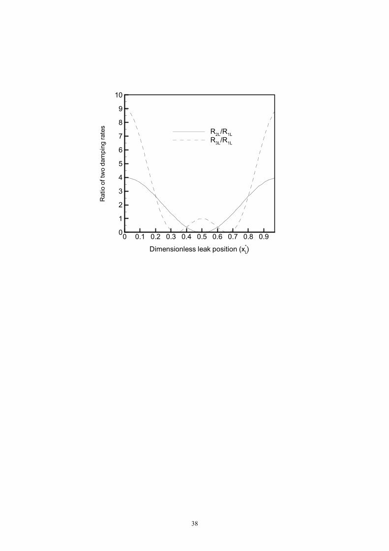
leak location. Fig. 4 is a plot of the theoretical relationship between the damping ratios of

harmonic components n2 = 2, n1 = 1 and harmonic components n2 = 3, n1 = 1 with the

corresponding leak locations in a pipeline.

Due to the symmetric nature of the sine squared function, the relationship between the

damping ratio of two harmonic components and leak location is not unique. Two leak

locations correspond to one value of the damping ratio R2L/R1L except for xL* = 0.5. For

damping ratios of higher harmonic components, one damping ratio may correspond to a

greater number of possible leak locations. For example, a damping ratio of R3L/R1L < 1.0

corresponds to four possible leak locations. Therefore, only harmonic components of n =

1, 2, 3 are used for leak detection analysis in this study.

Size of a Leak

Once the position of a leak has been determined, the magnitude of a leak can be easily

calculated using (28). It is

)(sin2

*20

L

LnLLd xna

gHARAC

�

� (n = 1, 2, 3,…) (30)

where n is any one of the components. Theoretically, leak magnitude calculated using

different components should be the same. Different measurement positions and different

forms of transients can be used for added confirmation and to increase accuracy if

necessary.

Sensitivity analysis

In the initial derivation, q*2 was neglected and the orifice equation was linearized in (13)

in arriving at the (14) and (15). Reconsidering the equations without linearization gives

14

)]()('2)]('2[ *****'*

***'

2*

*2

2*

*2

LLLLL xxExxhFRthxxFR

th

xh

�����

����

�

��

�

���� (31)

where )1('TLL eFF �� , R' = R(1+q*), and *

0'2 LT HMReE � . Assuming a constant q*, an

approximate solution for (31) is

� � � �)sin()sin()cos(),( **

1

*)'(*** *'

xntnBtnAetxh nn

ntRR nL

�����

�

��

�� (32)

in which nLTLLnL RexnFR )1()(sin *2''��� � . From (32), leak damping is only influenced

by the value of Te , which is the linearization error of the orifice equation. Neglecting q*2

has no direct influence on the location and quantification of a leak. Noticing that the ratio

of any two leak damping coefficients of nLR' is independent of parameter Te , then the

location of a leak is not affected by the error in the linearization of orifice equation. The

error of leak size induced by the orifice linearization is defined as

realLd

apparentLdrealLds AC

ACAC)(

)()( �

�� (33)

Substituting (30) into (33) gives

*0

*

*0

**0

*

/1

)/5.01(/1)1(

L

LLT

nL

nLTnLs

Hh

HhHhe

RReR

�

���

����

��

�� (34)

Variation of relative leak size error with parameter of *0

* / LHh is plotted in Fig. 5. To

avoid negative pressure in a pipeline, *0

* / LHh must be less than 1.0. Within this range,

the error in the size of a leak caused by the orifice linearization is less than 6% and thus

not significant.

Neglecting the q*2 term has no direct influence on location and quantification of a leak, but

it does affect friction damping. Because leak damping may be obtained by measuring total

damping and subtracting friction damping, linearization may indirectly lead to an

15

experimental error in leak damping. That error shows up in the ratio of the Fourier

components and thus influences the calculation of leak location.

By including the term of q*2, the total damping is RnL + R(1+ *q ). If leak damping is

obtained by subtracting friction damping R that is calculated from the steady state, the

calculated leak damping coefficient is RnL + Rq*, in which RnL is the real leak damping.

Then the ratio of leak damping of any two Fourier components is

)]([sin)]([sin

*1

2

*2

2

*

*

1

2

LL

LL

Ln

Ln

xnxn

RqRRqR

��

��

�

�

�

�

�

(35)

in which L� = dimensionless distance away from a real leak location. Substituting

)(sin)(sin

*1

2

*2

2

1

2

L

L

Ln

Ln

xnxn

RR

�

�

� into (35) and rearranging gives

)]([sin)]([sin

1)(sin)(sin

*1

2

*2

2*1

2

*2

2

LL

LLL

L

xnxn

T

Txnxn

��

���

�

�

�

�

�

�

(36)

where LnR

RqT1

*

� . The leak location error, L� , is a function of parameter T and real leak

location, xL*. Variation of L� with parameter T and leak location xL

* is presented in Fig. 6

if the first two Fourier components, n1 = 1 and n2 = 2, are used. Due to symmetry, only

half of the pipeline is plotted. Fig. 6 indicates that large values of parameter T cause large

errors in the location of leak, and leaks at different locations have different sensitivities to

the parameter T. Leaks close to xL* = 0.33 are least influenced by error in the friction

damping when the first two harmonics are used.

Leak size error, assuming that pressure at the leak is little influenced by leak location

error, gives

16

)]([sin)(sin)1(

1)(

)()(*2

*2

LL

L

realLd

apprarentLdrealLds xn

xnTAC

ACAC��

�

�

�

�

��

�

� (37)

Variation of relative leak size error s� with parameter T and leak location xL* is presented

in Fig. 7. Since leaks close to the ends of the pipeline cause less damping, a small error in

the value of leak damping can cause a large error in the calculation of the leak size despite

small T. In the application of the proposed leak detection method, small values of

parameter T can be achieved by using small magnitudes of pipeline transient or small

values of friction damping. The latter is achieved by using a low steady–state flow rate in

the pipeline. Alternatively, friction damping can be obtained from a test in a leak-free

pipeline or calculated using a numerical model. An example for such a situation is given

in the second numerical application later in the paper.

Unsteady Friction Damping

In the derivation of (5), friction loss was assumed to be represented by a steady-state

friction relationship. For rapidly varying flow, experiments have shown that damping of

transients is greater than that predicted by the Darcy-Weisbach head loss equation. This

difference can be addressed using unsteady friction models such as those by Zielke (1968),

Brunone et al. (1991), Vardy and Hwang (1991), and Bergant et al. (2001). Applying an

unsteady friction model, the total friction factor f is expressed as

us fff �� (38)

where fs represents the quasi-steady contribution and fu is an additional contribution due to

unsteadiness. To account for the unsteady friction damping, the friction-damping factor R

in (24) is replaced by

R = Rs+ Ru (39)

17

in which Rs represents damping by steady friction, and Ru represents damping by unsteady

friction. In contrast to steady friction damping, Rs, the value of unsteady friction damping,

Ru, is not constant, and is different for different Fourier components. For this case, the

*Rte� term in (24) can not be taken outside the summation sign. The value of Ru (and hence

R) can be determined by experimental tests or by a numerical model that incorporates an

appropriate unsteady friction model, e.g. the modified Brunone model (Vitkovský, 2001).

Numerical Verification

The leak detection method discussed above is tested numerically in an artificial pipeline,

shown in Fig. 8, using the results of simulated transients calculated from the method of

characteristics (MOC). Two types of problems, a reservoir-pipeline-reservoir system and

a reservoir-pipeline-valve system, are considered.

Reservoir-Pipeline-Reservoir Problem

In this case a transient in the pipeline is initiated by closing a side-discharge valve located

750m (x* = 0.75) away from the upstream reservoir as shown in Fig. 8, while the valve

adjoint to the downstream reservoir is fully open with negligible head loss. The magnitude

of the side-discharge valve coefficient is CdAS/A = 0.001 where AS = area of the side-

discharge valve. Closing time of the valve is 0.05s. For the first test (case 1) the leak at

xL* = 0.25 is removed (CdAL/A = 0) while for case 2 a leak of relative size of CdAL/A =

0.001 is assumed. The transient head in the pipeline is calculated numerically by a

standard method-of-characteristics program using 16 pipe reaches. The calculations are

started from steady state. The Darcy-Weisbach friction factor is calculated as f = 0.015

using the Swamee-Jain formula. The steady state friction-damping factor is R = 0.0742

(also Rs) with a steady-flow Reynolds number of 3.96�105. The sensitivity parameter, T,

18

is calculated as 0.0063. Based on previous sensitivity analysis, the leak location error, �L,

and leak size error, �s, are both less than 1%.

Fig. 9 presents the leak detection analysis using the “measured” transient. Measured

pressures at x* = 0.75 are shown in Fig. 9(a) for cases of no leak (case 1) and with a leak

(case 2). The amplitudes for separate components, n, are obtained by applying a discrete

Fourier transform algorithm to analyze the measured data in Fig. 9(a), the results of which

are presented in Fig. 9(b) for the first period signal (t* = 0.0 ~ 2.0). The transient signals

were analyzed period by period with an interval of t* = 2.0. Fig. 9(c) shows computed

amplitudes of the Fourier series of the first three harmonic components plotted against

period in terms of L/a. In Fig. 9(c1)—the no leak case—the damping rate R+RnL for all

three harmonic components is determined to be R = 0.0742 by fitting (27) to the decaying

amplitudes. In Fig. 9(c2)—in which a leak was present—the damping rates R+RnL are

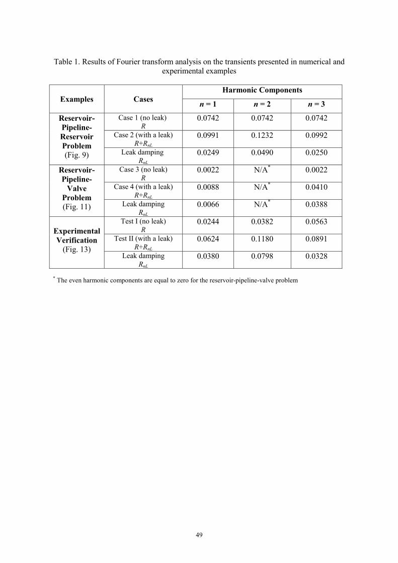
0.0991, 0.1232, 0.0992 for the first three components. The second value is significantly

different from the first and third and all are larger than the friction-damping factor. The

leak-induced damping rates RnL for components n = 1, 2 and 3 are 0.0249, 0.0490 and

0.0250, which are obtained by subtracting R from R+RnL (see Table 1). The ratios of two

leak-induced damping rates defined in (29) are R2L/R1L = 1.97 and R3L/R1L = 1.00. Using

these two ratios in Fig. 4, corresponding leak locations are either xL* = 0.25 or xL

* = 0.75,

the former being the real leak location. Applying (30) based on either of the calculated

leak locations and R1L = 0.0249, the calculated leak size is CdAL/A = 0.001, which is

identical to the real magnitude of the leak used to generate the MOC transient data.

Following the same procedure, transient damping, measured at different pipeline positions,

x* = 0.375, 0.5, and 0.625, was analyzed. Damping rates for separate harmonic

19

components are presented in Table 2. The Fourier transform analysis of transients

measured at different locations give almost identical results for the damping rate for each

component except for R2L at x*= 0.5, where a large error is introduced since the amplitude

of the component n = 2 is close to zero.

The results in Table 2 for R1L and R3L show that the analysis can be performed for the

measurement site located anywhere (0<x*<1) along the pipeline. The results of the Fourier

series analysis of numerical and experimental verifications presented in Figures 9, 12 and

13 are included in Table 1.

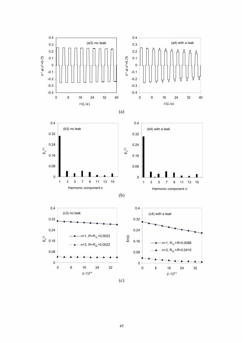
Reservoir-Pipeline-Valve Problem

A reservoir-pipeline-valve case provides an additional numerical example. For the

pipeline of 1000m (between x* = 0.0 and 1.0) in Fig. 10, a transient is initiated by closing

the downstream valve. The initial steady flow in the pipeline is Q0 = 2.0 L/s, which can be

achieved by a partially opened downstream valve. The Reynolds number of the flow in

pipeline is 11,160. The Darcy-Weisbach friction factor is calculated as f = 0.0302 using

the Swamee-Jain formula and the friction damping factor Rs = 0.0048. The leak detection

method presented earlier in the paper was developed from the general solution presented

in (24) based on boundary conditions of two constant-head reservoirs. Thus, it cannot be

directly applied to this particular example; however, it can be applied by adding an

imaginary symmetric section (dashed portion) to the original pipeline as shown in Fig. 10.

Two cases, referred to as case 3 and case 4, are considered. In case 3, no leak is present in

the pipeline, and in case 4, a leak of CdAL/A = 0.001 is present at x* = 0.25. The transient

pressures, generated by MOC for the original pipeline, are measured at x* = 0.75 for the

20

two cases that are presented in Fig. 11(a). The presence of the leak has very obvious

effects on the transient damping and shape. Note that the period of the transients is 4L/a

for cases 3 and 4, while for cases 1 and 2 the transient period is 2L/a.

The amplitudes of different harmonic components of the first period transient (t* = 0.0 ~

4.0) are given in Fig. 11(b) for cases 3 and 4 respectively. Amplitudes of all even

harmonic components (n = 2, 4, 6,…) are close to zero. Damping of the first two odd

harmonics, fitted using (27), are presented in Fig. 11(c). Due to the large magnitude of q*

(q* = 1.0) in this case, sensitivity parameter T is calculated as 0.35. Therefore, as stated in

the sensitivity analysis, the accuracy of leak detection will be significantly affected if the

value used for friction damping is incorrect. As a result, the accurate value of the friction

damping is obtained from a test in a leak-free pipeline (see case 3). For case 3, the friction

damping rates determined from a leak-free pipeline are R = 0.0022 for harmonic

components n = 1 and 3. For case 4, friction plus leak-induced damping rates for n = 1

and 3 are R+R1L = 0.0088 and R+R3L = 0.0410. Therefore, leak-induced damping for

harmonic components n = 1 and 3 are R1L = 0.0066 and R3L = 0.0386 (see Table 1), and

the damping ratio for the first and the third harmonics is R3L/R1L = 5.879. The

corresponding leak positions are determined using Fig. 4 as *1x̂ = 0.124 or *

2x̂ = 0.876.

Applied to the real pipeline, the leak position of *1x̂ = 0.124 becomes x* = 0.248, which is

close to the real leak location of x* = 0.25. The other possible leak is located in the

imaginary symmetric section. As a result, the location detected using this type of transient

system is unique. Applying R1L = 0.0066 and xL* = 0.124 in (30), the magnitude of the

leak is calculated as CdAL/A = 0.0010, which is identical to the actual leak size CdAL/A =

0.001.

21

Experimental Verification

Experimental tests were conducted in a single pipeline in the Robin Hydraulics Laboratory

at Adelaide University. The pipeline is a straight 37.2m copper pipe with inner diameter

of 22mm between two pressurized tanks as shown in Fig. 12. Five pressure transducers

are located at equidistant points along the pipeline and two one-quarter-turn ball valves are

installed at both ends for flow control. A side-discharge orifice, used to simulate a leak, is

installed at the one-quarter position (point B) with exchangeable leak orifice sizes of 1mm,

1.5mm and 2mm diameter. To initiate a transient, another side-discharge valve is installed

at point D. More details of this experimental apparatus are found in Vítkovský (2001).

Two tests were conducted. Test I is a no–leak case and in Test II a 1mm leak is located at

point B (Fig. 12). The flow conditions are as follows: wave speed a = 1320m/s, head at

tank 1 H1 = 23.6m, head at Tank 2 H2 = 22.8m and lumped leak parameter CdAL =

5.00�10-7 m2. The steady flow velocity in the pipeline is V0 = 0.567m/s, and the steady

friction damping factor is calculated as Rs = 0.0109.

In Test I, the valves at locations A and E and the side-discharge valve at D are opened and

steady state achieved. The side-discharge valve at D is then closed quickly. In Test II,

valves at locations A and E, the leak at B and the side-discharge valve at D are open until

steady state is obtained. The side-discharge valve at D is then sharply closed. During the

tests, pressure was measured by five pressure transducers at points A, B, C, D, and E.

Only the measured pressures at point D (x* = 0.75) for Test I and Test II are used for leak

detection analysis and they are plotted in Fig. 13(a). The leak-induced damping of Test II

is obvious compared to the transient in Test I that has no leak.

22

Fig. 13(b) shows the computed amplitudes of different harmonic components for the first

period of the transient. The amplitude of each component is less in Test II than in Test I

because the magnitude of the transient in test II is less than that in Test I due to the energy

loss at the leak.

Friction damping factors obtained from the no-leak case (Test I) are presented in Fig.

13(c). Damping factors of the first three harmonic components (n = 1, 2, 3) are R1 =

0.0244, R2 = 0.0382, R3 = 0.0563 (see Table 1), all being larger than the steady friction

damping factor Rs = 0.0109, calculated using steady state friction. The differences

between the measured and the calculated damping values are due to unsteady friction. It

accounts for 50%, 71% and 80% of the total for the first three components. As a result,

despite a small value of sensitivity parameter T (T = 0.00036), the friction damping in this

case cannot be calculated from the steady state conditions, and must be obtained either

from a leak-free measurement or from numerical analysis. As previously indicated, values

of unsteady friction damping are different for different Fourier components. In Fig. 13(c),

regression coefficients of the fitted curves of the damping factors are larger than 0.99,

experimentally confirming the analysis that damping for each component is exponential.

In Tests I and II, since the steady flow conditions were similar and both the transients were

initiated by closing the side-discharge valve at approximately the same speed, steady and

unsteady friction effects are similar. Leak-induced damping rates for the first three

harmonic components (n = 1, 2, 3) are R1L = 0.0380, R2L = 0.0798, R3L = 0.0328 (see Table

1). The ratios of damping rates R2L and R1L, and R3L and R1L are 10.21

2�

L

L

RR

, and

23

863.01

3�

L

L

RR

. Corresponding leak locations for these damping ratios are xL* = 0.242 (or

xL* = 0.758) and xL

* = 0.255 (or xL* = 0.745 ) by applying these two ratios in Fig. 4.

Averaging of these results gives the location as xL* = 0.249, almost the exact real location

of the leak. Using R1L = 0.0380, R2L = 0.0801 and leak location xL* = 0.242 and xL

* =

0.255, the magnitude of the leak is calculated, from (30), as CdAL = 4.912�10-7 and CdAL =

4.917�10-7 m2, which are about 1.7% smaller than the real leak size of CdAL = 5.00�10-7

m2.

Conclusions

Transients in pipelines are damped by both pipe friction and leaks. Steady state friction

damping is independent of the harmonic component of the transient, but leak damping is

different for different Fourier components. This fact can be used successfully to detect

presence of leaks, to compute their location, and to find their size. The damping rate is

useful for finding the quantity of leak discharge and the ratio of damping rates between

different harmonic components is used to find leak location. Leaks of 0.1% of a pipeline’s

cross-sectional area or smaller can be detected and located.

A linearized analysis of the governing equations indicates that steady Darcy-Weisbach

friction damping is exactly exponential, and leak damping is exponential for each of the

individual harmonic components but only approximately exponential for an entire

transient. Sensitivity analysis shows that linearization generates an insignificant error in

both leak location and quantification. Inaccurate steady-state friction determination (if it

is used to find the leak damping by subtraction from total damping), on the other hand,

may or may not be significant, depending on the parameters of the pipeline and flow and

24

the location of a leak. Also, if subtraction is used to find leak damping, the added

damping caused by unsteady flow may become important. Both nonlinear numerical

analyses using the method of characteristics and laboratory experiments have verified the

accuracy of the linearized solution in specific cases. The analysis of a linearized set of

equations has provided significant insight into a leak detection technique.

Leak detection techniques based on analyzing pressure measurement during transient

events in a pipe network have the obvious advantage of being orders of magnitude less

expensive than field investigations. Although the leak detection technique presented in

this paper does not have the generality of some other methods (e.g., the inverse transient

method), and is not generally applicable to complex systems such as pipe networks, it is

simple to use and apply.

Acknowledgements

The authors thank Prof. E. O. Tuck of the Department of Applied Mathematics, Adelaide

University for the valuable discussion on the mathematical approach for the Dirac delta

function. Financial support from the Australian Research Council to the second, third, and

fourth authors and scholarships provided by the Australian Government and Adelaide

University to the first author are gratefully acknowledged.

25

References

Abramowitz, M., and Stegun, I. A. (1972). Handbook of Mathematical Functions withFormulas, Graphs, and Mathematical Tables, National Bureau of Standards, Washington,USA.

Bergant, T., Simpson, A. R., and Vítkovský, J. (2001). “Developments in unsteady pipefriction modelling.” J. Hydr. Res., IAHR, 39(3), 249-257.

Black, P. (1992). “A review of pipeline leak detection technology.” Pipeline Systems, B.Coulbeck and E. Evans eds., Kluwer Academic Publishers, 287-297.

Brunone, B., Golia, U. M., and Greco, M. (1991). “Modelling of fast transients bynumerical methods.” Int. Meeting on Hydr. Transients with Column Separation, IAHR,Valencia, Spain, 201-209.

Brunone, B. (1999). "Transient test-based technique for leak detection in outfall pipes," J.Water Resour. Plng. and Mgmt., ASCE, Vol. 125, No. 5, 302-306.

Covas, D., and Romas, H. (1999). “Leakage detection in single pipeline using pressurewave behaviour.” Water Industry System: modelling and optimization application,Baldock, Hertfordshire, England, 287-299.

Fuchs, H. V., and Riehle, R. (1991). “Ten years of experience with leak detection byacoustic signal analysis.” Applied Acoustics, 33(1), 1-19.

Furness, R. A., and Reet, J. D. (1998). “Pipe line leak detection techniques.” Pipe LineRules of Thumb Handbook, E. W. McAllister, ed., Gulf Publishing Company, Houston,Texas, USA, 476-484.

Griebenow, G., and Mears, M. (1989). “Leak detection implementation: modeling andtuning methods.” J. Energ. Resour. Tech., ASME, 111, 66-71.

Hovey, D. J., and Farmer, E. J. (1999). “DOT states indicate need to refocus pipelineaccident prevention.” Oil & Gas J., 97(11), 52-53.

Jönsson, L., and Larson, M. (1992). “Leak detection through hydraulic transient analysis.”Pipeline Systems, B. Coulbeck and E. Evans, eds., Kluwer Academic Publishers, 273-286.

Liggett, J. A., and Chen, L.-C. (1994). “Inverse transient analysis in pipe networks.” J.Hydr. Engrg., ASCE, 120(8), 934-955.

Liou, C. P. (1994). “Mass imbalance error of waterhammer equations and leak detection.”J. Fluids Engrg., ASME, 116, 103-109.

Liou, C. P., and Tian, J. (1995). “Leak detection-transient flow simulation approaches.” J.Energ. Resour. Tech., ASME, 117, 243-248.

Liou, C. P. (1998). “Pipeline Leak Detection by Impulse Response Extraction.” J. FluidsEngrg., ASME, 120, 833-838.

26

McInnis, D., and Karney, B. (1995). “Transients in distribution networks: field tests anddemand models.” J. Hydr. Engrg., ASCE, 121(3), 218-231.

Mpesha, W., Gassman, S. L., and Chaudhry, M. H. (2001). “Leak detection in pipes byfrequency response method.” J. Hydr. Engrg., ASCE, 127(2), 134-147.

Press, W.H., Teukolsky, S.A., Vetterling, W.T., and Flannery, B.P. (1992). NumericalRecipes: The Art of Scientific Computing. Cambridge University Press, Cambridge, U.K.

Pudar, R. S., and Liggett, J. A. (1992). “Leaks in pipe networks.” J. Hydr. Engrg., ASCE,118(7), 1031-1046.

Vardy, A. E., and Hwang, K.-L. (1991). “A characteristics model of transient friction inpipes.” J. Hydr. Res., IAHR, 29(5), 669-684.

Wiggert, D. C. (1968). “Unsteady flows in lines with distributed leakage.” J. Hydr. Div.,ASCE, 94(HY1), 143-162

Vítkovský, J., Simpson, A. R., and Lambert, M. F. (2000). “Leak detection and calibrationusing transients and genetic algorithms.” J. Water Resour. Plng. and Mgmt., ASCE,126(4), 262-265.

Vítkovský, J. (2001). “Inverse Analysis and Modelling of Unsteady Pipe Flow: Theory,Applications and Experimental Verification,” Ph.D. Thesis, Department of Civil &Environmental Engineering, Adelaide University, Adelaide, Australia.

Weil, G. J., Graf, R. J., and Forister, L. M. (1994). “Remote sensing pipeline rehabilitationmethodologies based upon the utilization of infrared thermography.” Proc. of UrbanDrainage Rehabilitation Programs and Techniques, ASCE, 173-181.

Wylie, E. B., and Streeter, S. L. (1993). Fluid Transients in Systems, Prentice-Hall Inc.,Englewood Cliffs, N. J., USA.

Zielke, W. (1968). “Frequency-dependent friction in transient pipe flow.” J. Basic Engrg.,ASME, 90, 109-115.

27

Appendix A: Notation

A = inner pipe cross-sectional area;

AL = leak area;

AS = area of side-discharge valve;

An, Bn = Fourier coefficients;

a = wave speed;

C = constant;

C0(i) = Fourier coefficient of ith period transient;

)()( , im

im DC = Fourier coefficients of ith period transient;

Cd = leak orifice discharge coefficient;

D = diameter of the pipe;

E = a parameter defined as *0'2 LT HMReE � ;

En(1) = amplitude of nth harmonic component of the first period transient;

En(i) = amplitude of nth harmonic component of the ith period transient;

Te = truncation error in Taylor expansion;

F = a dimensionless head;

FL, 'LF = leak parameter;

f = friction factor;

fs = Darcy-Weisbach steady friction factor;

fu = unsteady friction factor;

g = gravitational acceleration;

H = piezometric head;

H0 = steady state piezometric head;

28

H1 = a reference head in the pipeline;

HJ = Joukowsky head rise;

HL = piezometric head at leak;

HL0 = steady piezometric head at leak;

H* = dimensionless head =H/H1;

HL0* = dimensionless steady head at leak = HL0/H1;

h* = dimensionless head disturbance;

L = length of pipeline;

M = leak parameter;

m, n = component number in a Fourier series;

Pn = nth period of a transient;

p = pressure;

Q = flow rate;

Q0 = steady state flow rate;

QL = flow rate through leak;

Q* = dimensionless flow rate =Q/Q0;

q* = dimensionless flow rate disturbance;

R, R' = pipeline friction damping factor;

Rs = steady friction damping factor;

Ru = unsteady friction damping factor;

Re = Reynolds number;

RnL, 'nLR = leak damping factor for nth harmonic (n = 1,2,3,…);

T = natural period of pipeline; parameter used in sensitivity analysis;

T* = dimensionless period of transient = T/(L/a);

t = time;

29

t0* = dimensionless reference time;

t* = dimensionless time = t/(L/a);

V = flow velocity in the pipe;

V0 = steady flow velocity in pipe;

x = distance along pipeline;

x* = dimensionless distance = x/L;

xL = position of leak;

*Lx = dimensionless leak position = xL/L;

*2

*1 ˆ,ˆ xx ..= dimensionless leak position in the combined real and imaginary pipeline;

�HL = pressure head at the leak = HL-zL;

�HL* = dimensionless pressure head at the leak = HL

*-zL*;

�x = distance interval;

� = Dirac delta function;

� = roughness height for pipe wall; a small distance from the leak;

L� = dimensionless leak location error;

S� = dimensionless leak size error;

� = density of fluid;

Appendix B: Fourier analysis of the time-domain pressure variation data

When a time-domain transient (measured at a particular location x*) is divided into

sections period by period as shown in Fig. B1, each transient period can be expressed as a

Fourier series based on (24).

For the first period P1:

30

� �� ���

�

��

��

1

***)(*** )sin()sin()cos(),(*

nnn

tRR xntnBtnAetxh nL��� (t0

*< t*< t0*+T*) (B1)

where t0* = starting time of analysis, and T* = dimensionless period defined as T* =

T/(L/a), in which T = natural period of pipeline. For the case in Fig. B1, T* = 2.0.

For the second period P2:

��

� � **0

*2

**0

*2

1

*2

)(*2

**

2*)sin()sin(

)cos(),(*2

TttTtxntnB

tnAetxh

n

nn

tRR nL

�����

���

�

��

��

�

(B2)

Setting ***2 Ttt �� and noticing the periodic property of the sinusoid functions give

��� � **

0**

0**

1

*)(*)(****

)sin()sin(

)cos(),(*

TtttxntnB

tnAeeTtxh

n

nn

tRRTRR nLnL

����

�� ��

�

����

��

�

(B3)

For the ith period Pi

��

� � **0

***0

**1

*)(***

)1()sin()sin(

)cos(),(*

iTttTitxntnB

tnAetxh

iin

nin

tRRi

inL

������

���

�

��

��

�

(B4)

Setting *** )1( Titti ��� gives

��� � **

0**

0**

1

*)(*)1)((****

)sin()sin(

)cos())1(,(*

TtttxntnB

tnAeeTitxh

n

nn

tRRTiRR nLnL

����

��� ��

�

�����

��

�

(B5)

A similar Fourier series is now fitted period by period to the “measured” transient data

given in Fig. B1 (created by MOC). For the ith period transient the fitted Fourier series is

31

� � )()sin()cos())1(,( **0

**0

1

*)(*)()(0

**** TttttmDtmCCTitxhm

im

im

i��������� �

�

�

�� (B6)

The Fourier coefficients )(0

iC , )(imC and )(i

mD are defined as

** *****

)(0

*0

*0

))1(,(1 dtTitxhT

CTt

t

i�

�

��� (B7)

** ******

)(*0

*0

)cos())1(,(2 tdtmTitxhT

CTt

t

im �

�

��� � (B8)

��

���

* *******

)(*0

*0

)sin())1(,(2 Tt

t

im dttmTitxh

TD � (B9)

Substituting the theoretical solution of h*(x*, t*+(i-1)T*) from (B5) into (B7) gives

)(0

iC = � �� �� ��

�

�

�����

�

* *

1

***)()1)((*

*0

*0

**

)sin()sin()cos(1 Tt

tn

nntRRTiRR dtxntnBtnAee

TnLnL

��� (B10)

)(0

iC = � �� � *

1

**)(*)1)((** )sin()cos()sin(1 *

*0

*0

*

dttnBtnAeexnT n

nntRRTt

t

TiRR nLnL� ��

�

���

���

� ��� (B11)

The integral term in (B11) is zero (Abramowitz and Stegun 1972). Therefore,

)(0

iC = 0 (B12)

Substituting the theoretical solution of h*(x*, t*) from (B5) into (B8) gives

��

� � ****

*

1

*)()1)((*

)(

)cos()sin()sin(

)cos(2 *0

*0

**

dttmxntnB

tnAeeT

C

n

Tt

tn

ntRRTiRRi

mnLnL

���

�

�

� � ��

�

�

�����

(B13)

��

� � ***

* *)(

1

)1)((**

)(

)cos()sin(

)cos()sin(2 *0

*0

**

dttmtnB

tnAeexnT

C

n

Tt

t ntRR

n

TiRRim

nLnL

��

��

�

� ���

��

�

�

���

(B14)

32

The integral term in (B14) is zero except when n = m (Abramowitz and Stegun 1972).

Then (B14) is expressed as

**0

*0

)1)((**

)(*))(()( )sin(

)(TiRR

nnL

tRRTtRRi

nnL

nLnL

eAxnTRR

eeC ���

�����

��

�� � (B15)

Similarly by substituting (B5) into (B9) the Fourier coefficient Dm(i) is expressed as

**0

*0

)1)((**

)(*))(()( )sin(

)(TiRR

nnL

tRRTtRRi

nnL

nLnL

eBxnTRR

eeD ���

�����

��

�� � (B16)

The amplitude En(i) for a component n at the ith period Pi is

**0

*0

)1)((22**

)(*))(()( )sin(

)(TiRR

nnnL

tRRTtRRi

nnL

nLnL

eBAxnTRR

eeE ���

�����

�

��

�� � (B17)

or *)1)(()1()( TiRR

ni

nnLeEE ���

� (B18)

where 22**

)(*))(()1( )sin(

)(

*0

*0

nnnL

tRRTtRR

n BAxnTRR

eeEnLnL

�

��

��

�����

� is the amplitude of the

component n at the first period.

Each Fourier component is exponentially damped in time. The damping rate of

component n is (R + RnL), which is the parameter to be determined.

33

Fig. 1. Damping caused by presence of a leak on the pipeline transients in a laboratory test.

Fig. 2. A pipe section with a leak

Fig. 3. Sensitivity of the leak position on the different harmonic components

Fig. 4. Damping ratios (Eq. (29)) of harmonic components

Fig. 5. Influence of linearization of orifice equation on the leak size

Fig. 6. Sensitivity of leak location on the sensitivity parameter T

Fig. 7. Sensitivity of leak size on the sensitivity parameter T

Fig. 8. A pipeline connected with two reservoirs

Fig. 9. Fourier series analysis of the transients measured from a pipeline without a leak(case 1) and with a leak (case 2) of CdAL/A = 0.1% at xL

* = 0.25 (T* = 2.0): (a) time historyof the measured pipeline transients (MOC); (b) Fourier series analysis of the first periodtransient (0< t*< 2.0); and (c) damping of harmonic components with periods

34

Fig. 10. A pipeline connecting an upstream reservoir and downstream valve, and the addedimaginary symmetric pipeline (D = 0.2m, a = 1000m/s, � = 0.023mm).

Fig. 11. Fourier series analysis of the transients measured from a pipeline without a leak(case 3) and with a leak (case 4) of CdAL/A = 0.1% at xL

* = 0.25 by closing a downstreamvalve (T* = 4.0): (a) time history of the measured pipeline transients (MOC); (b) Fourierseries analysis of the first period transient (0< t*< 4.0); and (c) damping of harmoniccomponents with periods

Fig. 12. Experimental pipeline apparatus

Fig. 13. Experimental transients and Fourier series analysis results: (a) time history of theexperimental transients; (b) Fourier series analysis results of the first period transient (0<t* < 2); and (c) damping of harmonic components with periods (T* = 2.0, and periodnumber i =1, 2, 3,…)

Fig. B1. A time-domain pipeline transient (generated by MOC)

35

0 4 8 12 16 20

t/(L/a)

20

21

22

23

24

25

26H

ead

(m)

No leakWith a leak

36

�AV �AV xxAV

��

��

)(�

x1 x2

x�

x

QL

xL

�

37

0 0.1 0.2 0.3 0.4 0.5 0.6 0.7 0.8 0.9

Dimensionless leak position (xL*)

0

0.2

0.4

0.6

0.8

1

1.2

1.4si

n(n�

x L* )n = 1n = 2n = 3

38

0 0.1 0.2 0.3 0.4 0.5 0.6 0.7 0.8 0.9

Dimensionless leak position (xL*)

0

1

2

3

4

5

6

7

8

9

10R

atio

oftw

oda

mpi

ngra

tes

R2L/R1LR3L/R1L

39

-1

0

1

2

3

4

5

6

7

0 0.2 0.4 0.6 0.8 1

�s(%

)

h*/HL*

40

-20

-10

0

10

20

0 0.1 0.2 0.3 0.4 0.5

T = 0.001T = 0.01T = 0.1T = 0.5T = 1.0

�L(%

)

xL *

41

-150

-100

-50

0

50

100

150

0 0.1 0.2 0.3 0.4 0.5

T = 0.001T = 0.01T = 0.1T = 0.5T = 1.0

�s(%

)

xL*

42

H1=25mH2=10m

L = Pipe length=1000mD = Pipe diameter=0.2m = Pipe roughness=0.023mma = Wave speed=1000m/sV0= Steady velocity=1.98m/s

V0

�

Leak Side dischargeCdAL/A= 0.002, xL = 250m CdAS/A= 0.001 xS = 750m

43

(a)

(b)

(c)

(c2) with a leak

0

0.005

0.01

0.015

0.02

0.025

0 2 4 6 8 10 12 14 16

(i -1)T *

E n(i)

n=1, R+R1L=0.0991

n=2, R+R2L=0.1232

n=3, R+R3L=0.0992

(c1) no leak

0

0.005

0.01

0.015

0.02

0.025

0 2 4 6 8 10 12 14 16(i - 1)T*

E n(i)

n=1, R+R1L=0.0742

n=2, R+R2L=0.0742

n=3, R+R3L=0.0742

(a1) no leak

-0.04

-0.02

0

0.02

0.04

0 4 8 12 16 20

t /(L /a )

h* a

t x*=

0.75

(a2) with a leak

-0.04

-0.02

0

0.02

0.04

0 4 8 12 16 20t /(L /a )

h* a

t x*=

0.75

(b1) no leak

0

0.005

0.01

0.015

0.02

0.025

1 3 5 7 9 11 13 15Harmonic component n

E n(1

)

(b2) with a leak

0

0.005

0.01

0.015

0.02

0.025

1 3 5 7 9 11 13 15Harmonic component n

E n(1

)

44

H1=25m H'1=25m

= 0.0 = 0.5 = 1.0

Q0=2.0 L/s Q0=2.0 L/s

2Q0

L=1000m L=1000m

x*=0.0 x*=1.0x*=0.5

*x̂ *x̂ *x̂

CdAL/A= 0.001 CdAL/A= 0.001

45

(a)

(b)

(c)

(a3) no leak

-0.4

-0.3

-0.2

-0.1

0

0.1

0.2

0.3

0.4

0 8 16 24 32 40

t /(L /a )

h* a

t x*=

0.75

(a4) with a leak

-0.4

-0.3

-0.2

-0.1

0

0.1

0.2

0.3

0.4

0 8 16 24 32 40

t /(L /a )

h* a

t x*=

0.75

(b3) no leak

0

0.08

0.16

0.24

0.32

0.4

1 3 5 7 9 11 13 15

Harmonic component n

E n(1

)

(b4) with a leak

0

0.08

0.16

0.24

0.32

0.4

1 3 5 7 9 11 13 15

Harmonic component n

E n(1

)

(c4) with a leak

0

0.08

0.16

0.24

0.32

0.4

0 8 16 24 32

(i -1)T *

En(i)

n=1, R1L+R=0.0088

n=3, R3L+R=0.0410

(c3) no leak

0

0.08

0.16

0.24

0.32

0.4

0 8 16 24 32

(i -1)T *

E n(i) n=1, R+R1L=0.0022

n=3, R+R3L=0.0022

46

Data aquisition and processing

EL=0.0

EL=2.0

Pressure Regulation

Tank 1

Tank 2

Pipeline

Valve1

Valve2

Leak

A

DC

B

E

Side discharge

47

(a)

(b)

(c)

(Test II) with a leak

0

0.01

0.02

0.03

0.04

0.05

0.06

0 2 4 6 8 10 12 14 16

(i -1)T *

E n(i)

n=1 R + R1L =0.0624n=2 R + R2L =0.1180n=3 R + R3L =0.0891

(Test I) no leak

0

0.01

0.02

0.03

0.04

0.05

0.06

0 2 4 6 8 10 12 14

(i -1)T *

E n(i)

n=1 R=0.0244n=2 R=0.0382n=3 R=0.0563

(Test I) no leak

0

0.01

0.02

0.03

0.04

0.05

0.06

1 3 5 7 9 11 13 15

Harmonic component n

E n(1

)

(Test II) with a leak

0

0.01

0.02

0.03

0.04

0.05

0.06

1 3 5 7 9 11 13 15

Harmonic component n

E n(1

)

(Test I) no leak

-0.1

-0.06

-0.02

0.02

0.06

0.1

-2 0 2 4 6 8 10 12 14 16

t /(L /a )

h* a

t poi

nt D

(Test II) with a leak

-0.1

-0.06

-0.02

0.02

0.06

0.1

-2 0 2 4 6 8 10 12 14 16

t /(L /a )

h* a

t poi

nt D

48

-0.04

-0.02

0

0.02

0.04

0 2 4 6 8 10

t /(L /a )

h*

MEASURED (MOC)

P1 P2

t0* t0

* +T* t0* +2T*

P3

t0* +3T*

49

Table 1. Results of Fourier transform analysis on the transients presented in numerical andexperimental examples

Harmonic ComponentsExamples Cases n = 1 n = 2 n = 3

Case 1 (no leak) R

0.0742 0.0742 0.0742

Case 2 (with a leak)R+RnL

0.0991 0.1232 0.0992

Reservoir-Pipeline-ReservoirProblem(Fig. 9) Leak damping

RnL

0.0249 0.0490 0.0250

Case 3 (no leak)R

0.0022 N/A* 0.0022

Case 4 (with a leak)R+RnL

0.0088 N/A* 0.0410

Reservoir-Pipeline-

ValveProblem(Fig. 11) Leak damping

RnL

0.0066 N/A* 0.0388

Test I (no leak)R

0.0244 0.0382 0.0563

Test II (with a leak)R+RnL

0.0624 0.1180 0.0891ExperimentalVerification

(Fig. 13)Leak damping

RnL

0.0380 0.0798 0.0328

* The even harmonic components are equal to zero for the reservoir-pipeline-valve problem

50

Table 2. Results using transients from the different measurementlocations (R = 0.0742)-Case 1

Measurement

position R1L R2L R3L R2L/R1L R3L/R1L

x* = 0.375 0.0248 0.0489 0.0249 1.972 1.004

x* = 0.5 0.0247 0.0314 0.0247 1.271 1.000

x* = 0.625 0.0248 0.0489 0.0251 1.972 1.012

x* = 0.75 0.0249 0.0490 0.0250 1.968 1.004