Uncertainty quantification

in the time domain pipeline

leak detection

Alireza Keramat

June 2017

Introduction

Time domain model for leak detection in a noisy environment

Cramer-Rao lower bound (CRLB)

Direct differentiation method (DDM) for numerical computation of CRLB

Case study, results and discussion

✓ Time closure

✓ Sample size

✓ Noise level

✓ Correlation between adjacent leaks, resolution in localization

• Water hammer model (continuity and momentum equations)

• Method of characteristics

Leak detection in the time domain

T

1

T T

,1 , 1, ( ,..., ), ( ,..., , ( ,..., ), )L ei M MMmi mx A h hh h n n m m

h = + n nh h h

Reservoir

Q1 Q2

Qi-

Valve

Qi+

Qi

, , , 1,...,Li ei j ejx A x A j N h h

, 1,...,ej jA N m

h = h n

ej ej jA A x

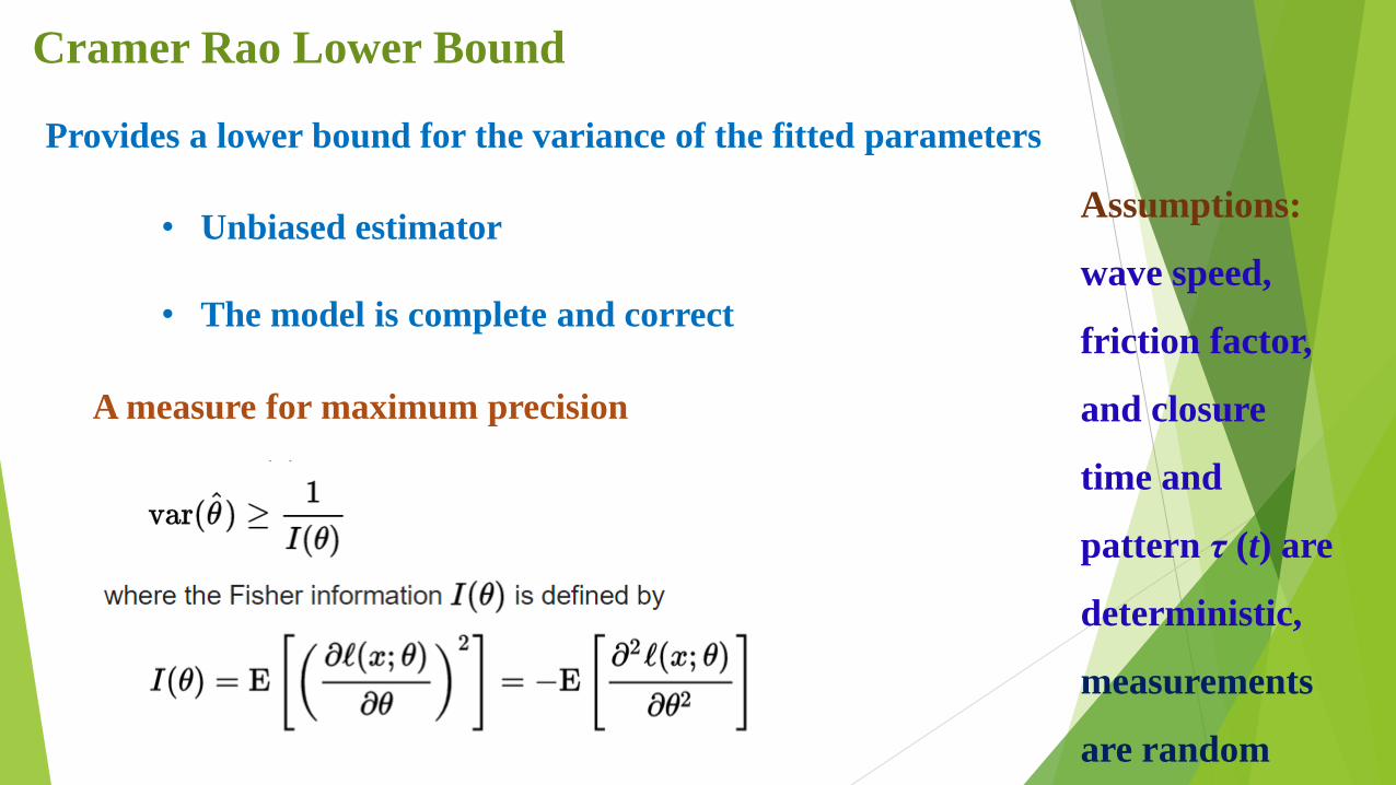
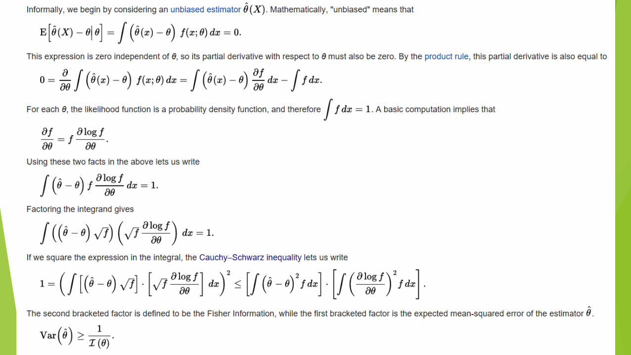
Provides a lower bound for the variance of the fitted parameters

• Unbiased estimator

• The model is complete and correct

A measure for maximum precision

Cramer Rao Lower Bound

Assumptions:

wave speed,

friction factor,

and closure

time and

pattern τ (t) are

deterministic,

measurements

are random

T 11 1( , ) exp .

22 det( )M

p

m e m mh A = h h Σ h h

Σ

2

2

1ln ( ; ) ln(2 ) ln

2 2

ML M

e m mA h = h h

1

2

,

ˆCRLB : cov( ) ( ) ,

ln ( ; )i j

ei ej

I LA A

e e

e m

A I A

A hE

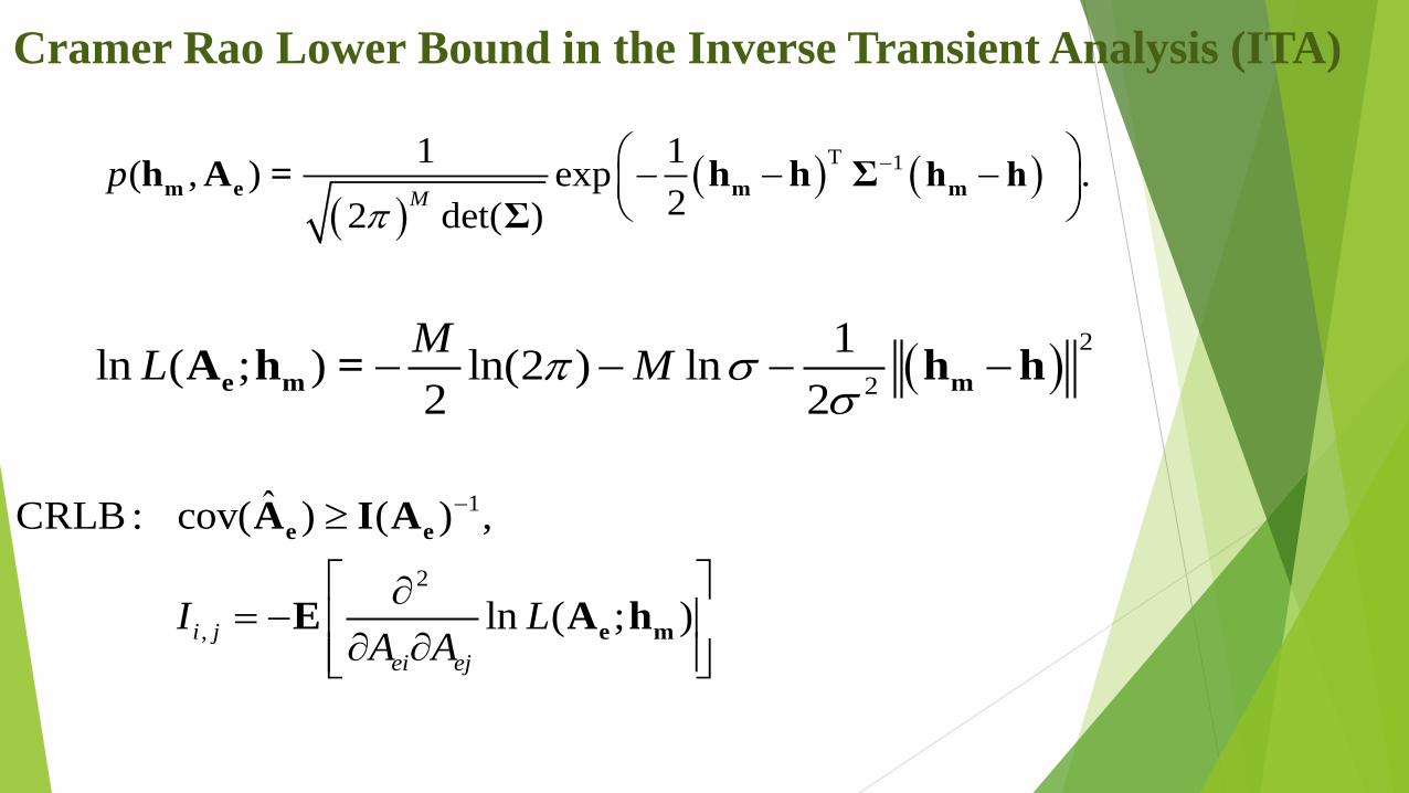
Cramer Rao Lower Bound in the Inverse Transient Analysis (ITA)

2 T

, 2

1ln ( ; ) .i j

ei ej ei ej

I LA A A A

e m

h hA hE

1? ?cov( ) ( )T

e e e e e eA A A A A I AE

1ˆcov( ) ( ) ,e e

A I A

Partial derivatives are calculated using Characteristic equations.

Cramer Rao Lower Bound in the Inverse Transient Analysis (ITA)

Each element of the Fisher Information Matrix (FIM):

h contains a, f, measurement location, time and pattern of valve closure, etc.

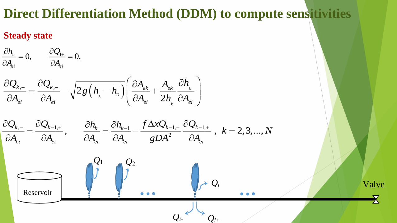
Direct Differentiation Method (DDM) to compute sensitivities

Steady state

1 10, 0,ei ei

h Q

A A

, 1, 1, 1,1

2, , 2,3,...,

k k k kk k

ei ei ei ei ei

Q Q f xQ Qh hk N

A A A A gDA A

, ,2

2

k

k

k

k k ek eko

ei ei ei ei

hQ Q A Ag h h

A A A h A

Reservoir

Q1 Q2

Qi-

Valve

Qi+

Qi

Direct Differentiation Method (DDM) to compute sensitivities

Transient state

C : ,k ap k pQ C h C

C : ,k an k nQ C h C

1 2 2 ,k k ek k oQ Q A g h h

0.5 2

2

2 2 2

 

? ? ? ? ?, with

?

2 ? ? 2 ? 2 ? 2 ? 2 ? ? ? 4 .

ek ek n an n ap p an p ap

k

an ap

an ek ap o n an n ap p an p ap an ap oo

A gA C C C C C C C Ch

C C

g C h gA C h C C C C C C C C C C h

p apk k n k k k an k

ei n ei p ei ap ei an ei ei

C Ch h C h h h C h

A C A C A C A C A A

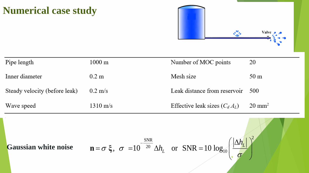
9

2SNR

2010, 10 or SNR 10 log

L

L

hh

n ξ

Numerical case study

Gaussian white noise

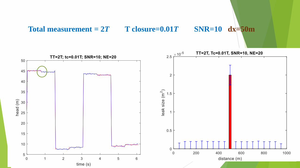
Total measurement = 2T T closure=0.01T SNR=10 dx=50m

Increase time closure to 0.1T wave front = a . Tc = 400 m

Inaccurate size detection and localization

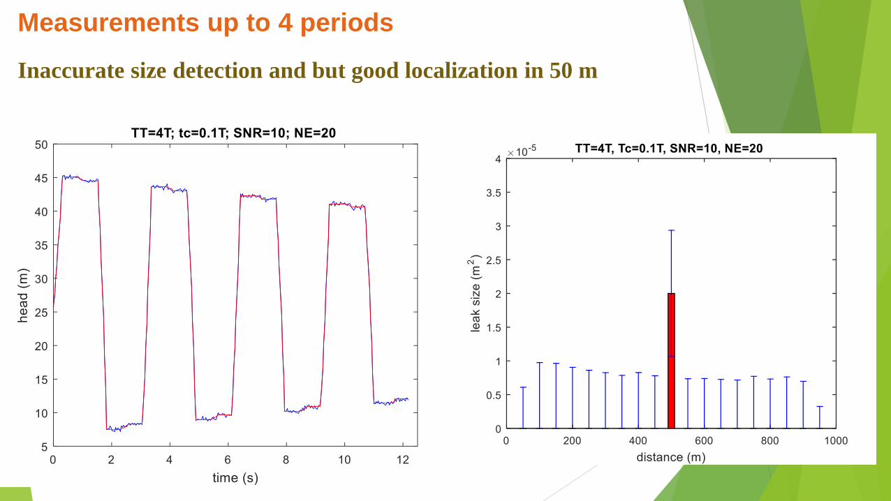
Measurements up to 4 periods

Inaccurate size detection and but good localization in 50 m

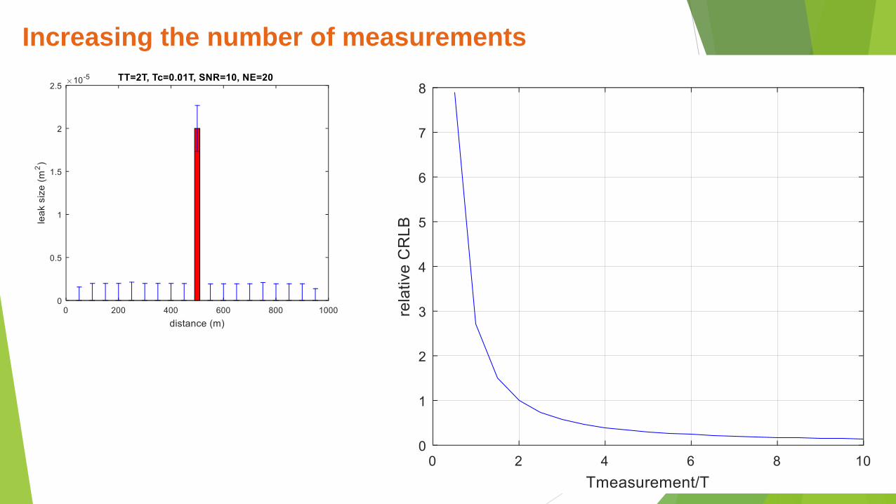
Increasing the number of measurements

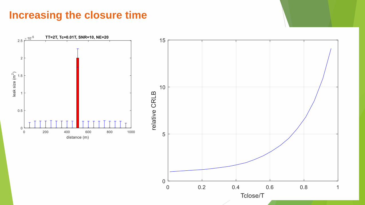
Increasing the closure time

Increasing SNR

Tc=0.06s

λ=60m

ΔxMOC>a.Tc

NE<1000/60=16

CRLB does

not change if

ΔxMOC>a.Tc

Study the number of parameters (distance between leaks)

CRLB increases with increase in parameters (MOC nodes)

if ΔxMOC<a.Tc

a.Tc = 100 m

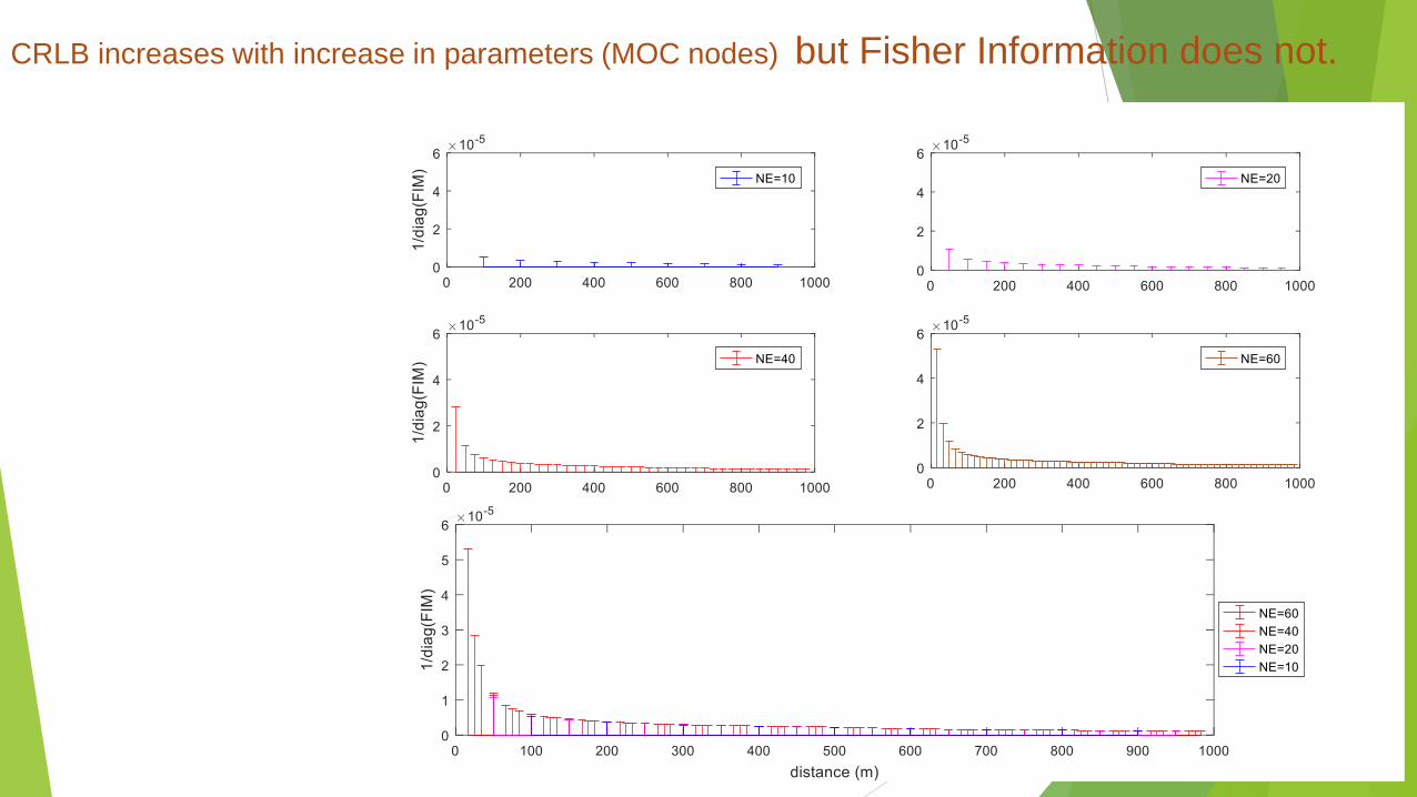
CRLB increases with increase in parameters (MOC nodes) but Fisher Information does not.

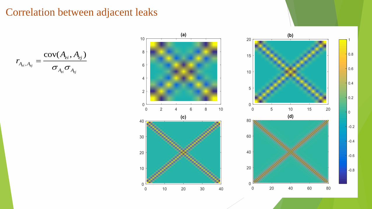
Correlation between adjacent leaks

,

cov( , )

ei ej

ei ej

ei ej

A A

A A

A Ar

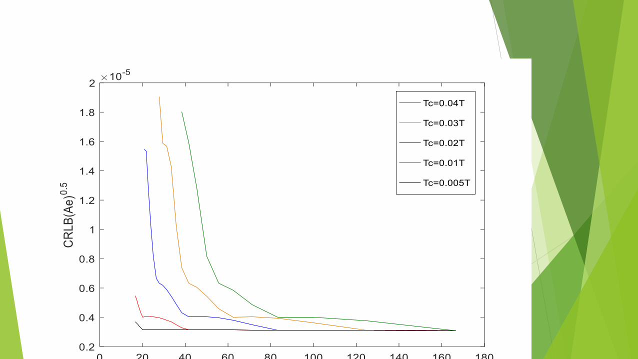
Average CRLB trend with distance between two consecutive leaks

T=4 s

λmin=160 m

λmin=120 m

λmin=80 m

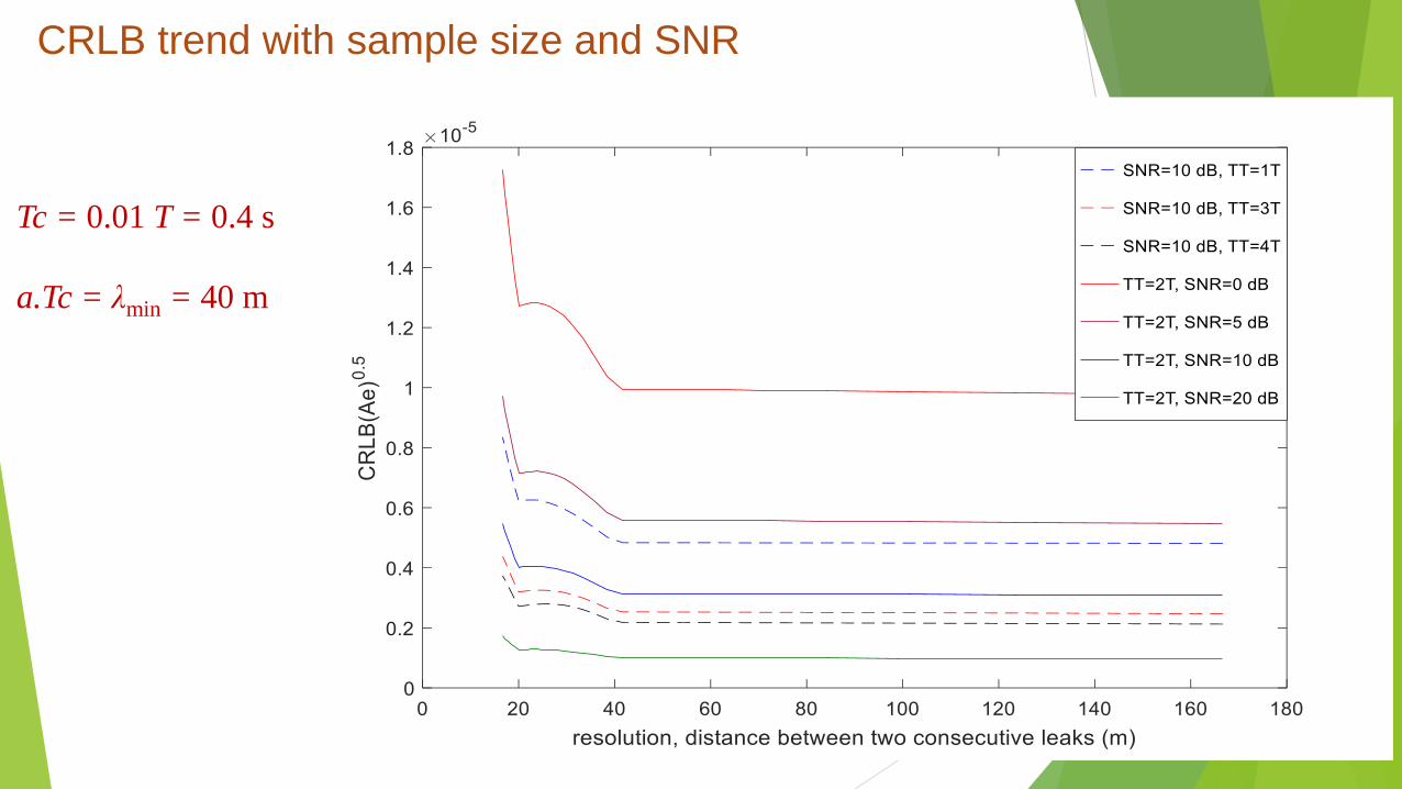
a.Tc = λmin = 40 m

CRLB trend with sample size and SNR

Tc = 0.01 T = 0.4 s

Thanks for your attention

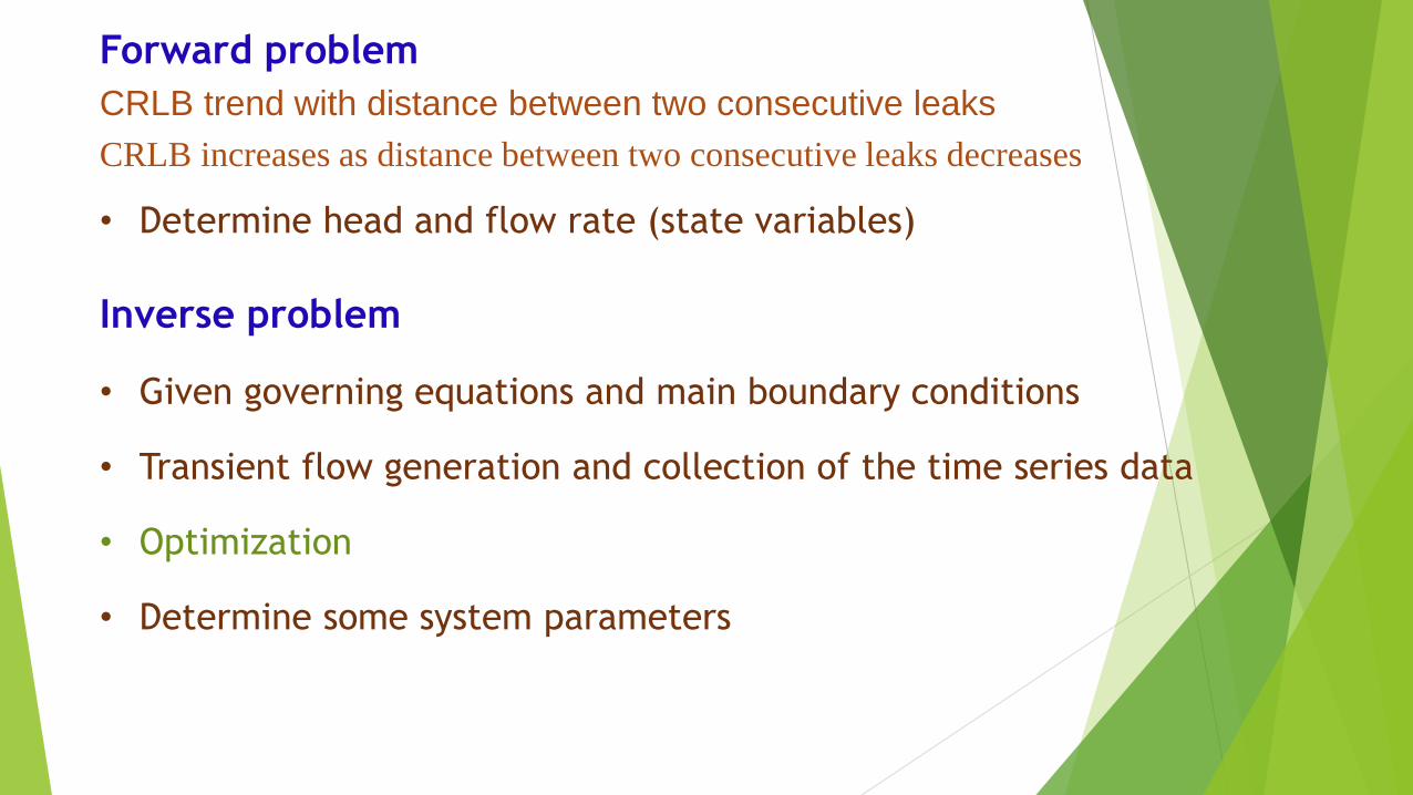
Forward problem

CRLB trend with distance between two consecutive leaks

CRLB increases as distance between two consecutive leaks decreases

• Determine head and flow rate (state variables)

Inverse problem

• Given governing equations and main boundary conditions

• Transient flow generation and collection of the time series data

• Optimization

• Determine some system parameters

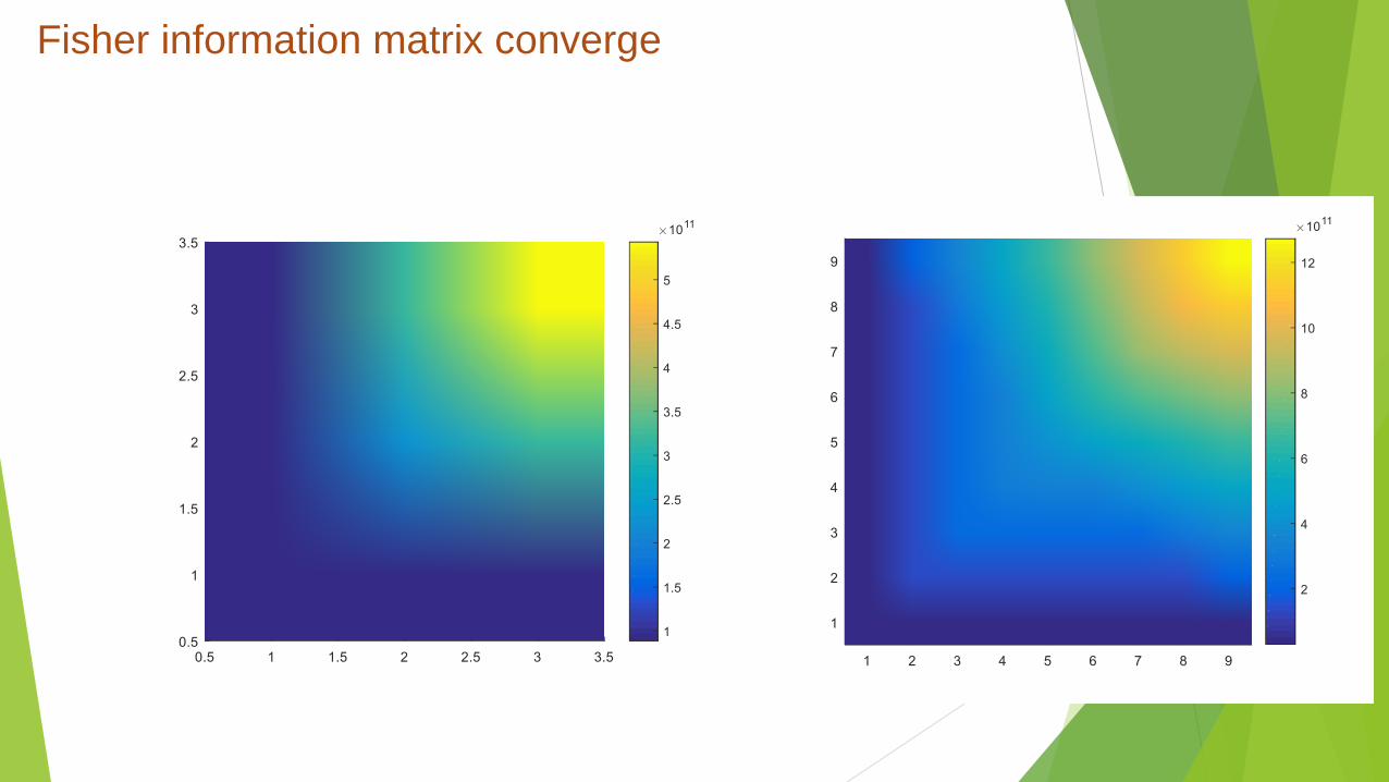
Fisher information matrix converge