Searches for gravitational waves from known pulsars with S5 LIGO data

arX

iv:0

909.

3583

v1 [

astr

o-ph

.HE

] 1

9 Se

p 20

09

Searches for gravitational waves from known pulsars with S5

LIGO data

B. P. Abbott28, R. Abbott28, F. Acernese18ac, R. Adhikari28, P. Ajith2, B. Allen2,75,

G. Allen51, M. Alshourbagy20ab, R. S. Amin33, S. B. Anderson28, W. G. Anderson75,

F. Antonucci21a, S. Aoudia42a, M. A. Arain63, M. Araya28, H. Armandula28, P. Armor75,

K. G. Arun25, Y. Aso28, S. Aston62, P. Astone21a, P. Aufmuth27, C. Aulbert2, S. Babak1,

P. Baker36, G. Ballardin11, S. Ballmer28, C. Barker29, D. Barker29, F. Barone18ac, B. Barr64,

P. Barriga74, L. Barsotti31, M. Barsuglia4, M. A. Barton28, I. Bartos10, R. Bassiri64,

M. Bastarrika64, Th. S. Bauer40a, B. Behnke1, M. Beker40, M. Benacquista58,

J. Betzwieser28, P. T. Beyersdorf47, S. Bigotta20ab, I. A. Bilenko37, G. Billingsley28,

S. Birindelli42a, R. Biswas75, M. A. Bizouard25, E. Black28, J. K. Blackburn28,

L. Blackburn31, D. Blair74, B. Bland29, C. Boccara14, T. P. Bodiya31, L. Bogue30,

F. Bondu42b, L. Bonelli20ab, R. Bork28, V. Boschi28, S. Bose76, L. Bosi19a, S. Braccini20a,

C. Bradaschia20a, P. R. Brady75, V. B. Braginsky37, J. E. Brau69, D. O. Bridges30,

A. Brillet42a, M. Brinkmann2, V. Brisson25, C. Van Den Broeck8, A. F. Brooks28,

D. A. Brown52, A. Brummit46, G. Brunet31, R. Budzynski44b, T. Bulik44cd, A. Bullington51,

H. J. Bulten40ab, A. Buonanno65, O. Burmeister2, D. Buskulic26, R. L. Byer51,

L. Cadonati66, G. Cagnoli16a, E. Calloni18ab, J. B. Camp38, E. Campagna16ac,

J. Cannizzo38, K. C. Cannon28, B. Canuel11, J. Cao31, F. Carbognani11, L. Cardenas28,

S. Caride67, G. Castaldi71, S. Caudill33, M. Cavaglia55, F. Cavalier25, R. Cavalieri11,

G. Cella20a, C. Cepeda28, E. Cesarini16c, T. Chalermsongsak28, E. Chalkley64,

P. Charlton77, E. Chassande-Mottin4, S. Chatterji28, S. Chelkowski62, Y. Chen1,7,

A. Chincarini17, N. Christensen9, C. T. Y. Chung54, D. Clark51, J. Clark8, J. H. Clayton75,

F. Cleva42a, E. Coccia22ab, T. Cokelaer8, C. N. Colacino13,20, J. Colas11, A. Colla21ab,

M. Colombini21b, R. Conte18c, D. Cook29, T. R. C. Corbitt31, C. Corda20ab, N. Cornish36,

A. Corsi21ab, J.-P. Coulon42a, D. Coward74, D. C. Coyne28, J. D. E. Creighton75,

T. D. Creighton58, A. M. Cruise62, R. M. Culter62, A. Cumming64, L. Cunningham64,

E. Cuoco11, S. L. Danilishin37, S. D’Antonio22a, K. Danzmann2,27, A. Dari19ab, V. Dattilo11,

B. Daudert28, M. Davier25, G. Davies8, E. J. Daw56, R. Day11, R. De Rosa18ab, D. DeBra51,

J. Degallaix2, M. del Prete20ac, V. Dergachev67, S. Desai53, R. DeSalvo28, S. Dhurandhar24,

L. Di Fiore18a, A. Di Lieto20ab, M. Di Paolo Emilio22ad, A. Di Virgilio20a, M. Dıaz58,

A. Dietz8,26, F. Donovan31, K. L. Dooley63, E. E. Doomes50, M. Drago43cd,

R. W. P. Drever6, J. Dueck2, I. Duke31, J.-C. Dumas74, J. G. Dwyer10, C. Echols28,

M. Edgar64, A. Effler29, P. Ehrens28, E. Espinoza28, T. Etzel28, M. Evans31, T. Evans30, V.

Fafone22ab, S. Fairhurst8, Y. Faltas63, Y. Fan74, D. Fazi28, H. Fehrmann2, I. Ferrante20ab, F.

Fidecaro20ab, L. S. Finn53, I. Fiori11, R. Flaminio32, K. Flasch75, S. Foley31, C. Forrest70,

N. Fotopoulos75, J.-D. Fournier42a, J. Franc32, A. Franzen27, S. Frasca21ab, F. Frasconi20a,

http://arxiv.org/abs/0909.3583v1

– 2 –

M. Frede2, M. Frei57, Z. Frei13, A. Freise62, R. Frey69, T. Fricke30, P. Fritschel31,

V. V. Frolov30, M. Fyffe30, V. Galdi71, L. Gammaitoni19ab, J. A. Garofoli52, F. Garufi18ab,

G. Gemme17, E. Genin11, A. Gennai20a, I. Gholami1, J. A. Giaime33,30, S. Giampanis2,

K. D. Giardina30, A. Giazotto20a, K. Goda31, E. Goetz67, L. M. Goggin75, G. Gonzalez33,

M. L. Gorodetsky37, S. Goßler2,40, R. Gouaty33, M. Granata4, V. Granata26, A. Grant64,

S. Gras74, C. Gray29, M. Gray5, R. J. S. Greenhalgh46, A. M. Gretarsson12, C. Greverie42a,

F. Grimaldi31, R. Grosso58, H. Grote2, S. Grunewald1, M. Guenther29, G. Guidi16ac,

E. K. Gustafson28, R. Gustafson67, B. Hage27, J. M. Hallam62, D. Hammer75,

G. D. Hammond64, C. Hanna28, J. Hanson30, J. Harms68, G. M. Harry31, I. W. Harry8,

E. D. Harstad69, K. Haughian64, K. Hayama58, J. Heefner28, H. Heitmann42, P. Hello25,

I. S. Heng64, A. Heptonstall28, M. Hewitson2, S. Hild62, E. Hirose52, D. Hoak30,

K. A. Hodge28, K. Holt30, D. J. Hosken61, J. Hough64, D. Hoyland74, D. Huet11,

B. Hughey31, S. H. Huttner64, D. R. Ingram29, T. Isogai9, M. Ito69, A. Ivanov28,

P. Jaranowski44e, B. Johnson29, W. W. Johnson33, D. I. Jones72, G. Jones8, R. Jones64,

L. Sancho de la Jordana60, L. Ju74, P. Kalmus28, V. Kalogera41, S. Kandhasamy68,

J. Kanner65, D. Kasprzyk62, E. Katsavounidis31, K. Kawabe29, S. Kawamura39,

F. Kawazoe2, W. Kells28, D. G. Keppel28, A. Khalaidovski2, F. Y. Khalili37, R. Khan10,

E. Khazanov23, P. King28, J. S. Kissel33, S. Klimenko63, K. Kokeyama39, V. Kondrashov28,

R. Kopparapu53, S. Koranda75, I. Kowalska44c, D. Kozak28, B. Krishnan1, A. Krolak44af ,

R. Kumar64, P. Kwee27, P. La Penna11, P. K. Lam5, M. Landry29, B. Lantz51,

A. Lazzarini28, H. Lei58, M. Lei28, N. Leindecker51, I. Leonor69, N. Leroy25, N. Letendre26,

C. Li7, H. Lin63, P. E. Lindquist28, T. B. Littenberg36, N. A. Lockerbie73, D. Lodhia62,

M. Longo71, M. Lorenzini16a, V. Loriette14, M. Lormand30, G. Losurdo16a, P. Lu51,

M. Lubinski29, A. Lucianetti63, H. Luck2,27, B. Machenschalk1, M. MacInnis31, J.-M.

Mackowski32, M. Mageswaran28, K. Mailand28, E. Majorana21a, N. Man42a, I. Mandel41,

V. Mandic68, M. Mantovani20c, F. Marchesoni19a, F. Marion26, S. Marka10, Z. Marka10,

A. Markosyan51, J. Markowitz31, E. Maros28, J. Marque11, F. Martelli16ac, I. W. Martin64,

R. M. Martin63, J. N. Marx28, K. Mason31, A. Masserot26, F. Matichard33, L. Matone10,

R. A. Matzner57, N. Mavalvala31, R. McCarthy29, D. E. McClelland5, S. C. McGuire50,

M. McHugh35, G. McIntyre28, D. J. A. McKechan8, K. McKenzie5, M. Mehmet2,

A. Melatos54, A. C. Melissinos70, G. Mendell29, D. F. Menendez53, F. Menzinger11,

R. A. Mercer75, S. Meshkov28, C. Messenger2, M. S. Meyer30, C. Michel32, L. Milano18ab,

J. Miller64, J. Minelli53, Y. Minenkov22a, Y. Mino7, V. P. Mitrofanov37, G. Mitselmakher63,

R. Mittleman31, O. Miyakawa28, B. Moe75, M. Mohan11, S. D. Mohanty58,

S. R. P. Mohapatra66, J. Moreau14, G. Moreno29, N. Morgado32, A. Morgia22ab,

T. Morioka39, K. Mors2, S. Mosca18ab, V. Moscatelli21a, K. Mossavi2, B. Mours26,

C. MowLowry5, G. Mueller63, D. Muhammad30, H. zur Muhlen27, S. Mukherjee58,

H. Mukhopadhyay24, A. Mullavey5, H. Muller-Ebhardt2, J. Munch61, P. G. Murray64,

– 3 –

E. Myers29, J. Myers29, T. Nash28, J. Nelson64, I. Neri19ab, G. Newton64, A. Nishizawa39,

F. Nocera11, K. Numata38, E. Ochsner65, J. O’Dell46, G. H. Ogin28, B. O’Reilly30,

R. O’Shaughnessy53, D. J. Ottaway61, R. S. Ottens63, H. Overmier30, B. J. Owen53,

G. Pagliaroli22ad, C. Palomba21a, Y. Pan65, C. Pankow63, F. Paoletti20a,11, M. A. Papa1,75,

V. Parameshwaraiah29, S. Pardi18ab, A. Pasqualetti11, R. Passaquieti20ab, D. Passuello20a,

P. Patel28, M. Pedraza28, S. Penn15, A. Perreca62, G. Persichetti18ab, M. Pichot42a,

F. Piergiovanni16ac, V. Pierro71, M. Pietka44e, L. Pinard32, I. M. Pinto71, M. Pitkin64,

H. J. Pletsch2, M. V. Plissi64, R. Poggiani20ab, F. Postiglione18c, M. Prato17, M. Principe71,

R. Prix2, G. A. Prodi43ab, L. Prokhorov37, O. Puncken2, M. Punturo19a, P. Puppo21a,

V. Quetschke63, F. J. Raab29, O. Rabaste4, D. S. Rabeling40ab, H. Radkins29, P. Raffai13,

Z. Raics10, N. Rainer2, M. Rakhmanov58, P. Rapagnani21ab, V. Raymond41, V. Re43ab,

C. M. Reed29, T. Reed34, T. Regimbau42a, H. Rehbein2, S. Reid64, D. H. Reitze63,

F. Ricci21ab, R. Riesen30, K. Riles67, B. Rivera29, P. Roberts3, N. A. Robertson28,64,

F. Robinet25, C. Robinson8, E. L. Robinson1, A. Rocchi22a, S. Roddy30, L. Rolland26,

J. Rollins10, J. D. Romano58, R. Romano18ac, J. H. Romie30, D. Rosinska44gd, C. Rover2,

S. Rowan64, A. Rudiger2, P. Ruggi11, P. Russell28, K. Ryan29, S. Sakata39, F. Salemi43ab,

V. Sandberg29, V. Sannibale28, L. Santamarıa1, S. Saraf48, P. Sarin31, B. Sassolas32,

B. S. Sathyaprakash8, S. Sato39, M. Satterthwaite5, P. R. Saulson52, R. Savage29, P. Savov7,

M. Scanlan34, R. Schilling2, R. Schnabel2, R. Schofield69, B. Schulz2, B. F. Schutz1,8,

P. Schwinberg29, J. Scott64, S. M. Scott5, A. C. Searle28, B. Sears28, F. Seifert2,

D. Sellers30, A. S. Sengupta28, D. Sentenac11, A. Sergeev23, B. Shapiro31, P. Shawhan65,

D. H. Shoemaker31, A. Sibley30, X. Siemens75, D. Sigg29, S. Sinha51, A. M. Sintes60,

B. J. J. Slagmolen5, J. Slutsky33, M. V. van der Sluys41, J. R. Smith52, M. R. Smith28,

N. D. Smith31, K. Somiya7, B. Sorazu64, A. Stein31, L. C. Stein31, S. Steplewski76,

A. Stochino28, R. Stone58, K. A. Strain64, S. Strigin37, A. Stroeer38, R. Sturani16ac,

A. L. Stuver30, T. Z. Summerscales3, K. -X. Sun51, M. Sung33, P. J. Sutton8, B. Swinkels11,

G. P. Szokoly13, D. Talukder76, L. Tang58, D. B. Tanner63, S. P. Tarabrin37, J. R. Taylor2,

R. Taylor28, R. Terenzi22ac, J. Thacker30, K. A. Thorne30, K. S. Thorne7, A. Thuring27,

K. V. Tokmakov64, A. Toncelli20ab, M. Tonelli20ab, C. Torres30, C. Torrie28, E. Tournefier26,

F. Travasso19ab, G. Traylor30, M. Trias60, J. Trummer26, D. Ugolini59, J. Ulmen51,

K. Urbanek51, H. Vahlbruch27, G. Vajente20ab, M. Vallisneri7, J. F. J. van den Brand40ab, S.

van der Putten40a, S. Vass28, R. Vaulin75, M. Vavoulidis25, A. Vecchio62, G. Vedovato43c,

A. A. van Veggel64, J. Veitch62, P. Veitch61, C. Veltkamp2, D. Verkindt26, F. Vetrano16ac,

A. Vicere16ac, A. Villar28, J.-Y. Vinet42a, H. Vocca19a, C. Vorvick29, S. P. Vyachanin37,

S. J. Waldman31, L. Wallace28, R. L. Ward28, M. Was25, A. Weidner2, M. Weinert2,

A. J. Weinstein28, R. Weiss31, L. Wen7,74, S. Wen33, K. Wette5, J. T. Whelan1,45,

S. E. Whitcomb28, B. F. Whiting63, C. Wilkinson29, P. A. Willems28, H. R. Williams53,

L. Williams63, B. Willke2,27, I. Wilmut46, L. Winkelmann2, W. Winkler2, C. C. Wipf31,

– 4 –

A. G. Wiseman75, G. Woan64, R. Wooley30, J. Worden29, W. Wu63, I. Yakushin30,

H. Yamamoto28, Z. Yan74, S. Yoshida49, M. Yvert26, M. Zanolin12, J. Zhang67, L. Zhang28,

C. Zhao74, N. Zotov34, M. E. Zucker31, J. Zweizig28

The LIGO Scientific Collaboration & The Virgo Collaboration

– 5 –

1Albert-Einstein-Institut, Max-Planck-Institut fur Gravitationsphysik, D-14476 Golm, Germany

2Albert-Einstein-Institut, Max-Planck-Institut fur Gravitationsphysik, D-30167 Hannover, Germany

3Andrews University, Berrien Springs, MI 49104 USA

4AstroParticule et Cosmologie (APC), CNRS: UMR7164-IN2P3-Observatoire de Paris-Universite Denis

Diderot-Paris VII - CEA : DSM/IRFU

5Australian National University, Canberra, 0200, Australia

6California Institute of Technology, Pasadena, CA 91125, USA

7Caltech-CaRT, Pasadena, CA 91125, USA

8Cardiff University, Cardiff, CF24 3AA, United Kingdom

9Carleton College, Northfield, MN 55057, USA

10Charles Sturt University, Wagga Wagga, NSW 2678, Australia

11Columbia University, New York, NY 10027, USA

12European Gravitational Observatory (EGO), I-56021 Cascina (Pi), Italy

13Embry-Riddle Aeronautical University, Prescott, AZ 86301 USA

14Eotvos University, ELTE 1053 Budapest, Hungary

15ESPCI, CNRS, F-75005 Paris, France

16Hobart and William Smith Colleges, Geneva, NY 14456, USA

17INFN, Sezione di Firenze, I-50019 Sesto Fiorentinoa; Universita degli Studi di Firenze, I-50121b, Firenze;

Universita degli Studi di Urbino ’Carlo Bo’, I-61029 Urbinoc, Italy

18INFN, Sezione di Genova; I-16146 Genova, Italy

19INFN, sezione di Napoli a; Universita di Napoli ’Federico II’b Complesso Universitario di Monte S.Angelo,

I-80126 Napoli; Universita di Salerno, Fisciano, I-84084 Salernoc, Italy

20INFN, Sezione di Perugiaa; Universita di Perugiab, I-6123 Perugia,Italy

21INFN, Sezione di Pisaa; Universita di Pisab; I-56127 Pisa; Universita di Siena, I-53100 Sienac, Italy

22INFN, Sezione di Romaa; Universita ’La Sapienza’b, I-00185 Roma, Italy

23INFN, Sezione di Roma Tor Vergataa; Universita di Roma Tor Vergatab, Istituto di Fisica dello Spazio

Interplanetario (IFSI) INAFc, I-00133 Roma; Universita dell’Aquila, I-67100 L’Aquilad, Italy

24Institute of Applied Physics, Nizhny Novgorod, 603950, Russia

25Inter-University Centre for Astronomy and Astrophysics, Pune - 411007, India

26LAL, Universite Paris-Sud, IN2P3/CNRS, F-91898 Orsay, France

27Laboratoire d’Annecy-le-Vieux de Physique des Particules (LAPP), IN2P3/CNRS, Universite de Savoie,

– 6 –

F-74941 Annecy-le-Vieux, France

28Leibniz Universitat Hannover, D-30167 Hannover, Germany

29LIGO - California Institute of Technology, Pasadena, CA 91125, USA

30LIGO - Hanford Observatory, Richland, WA 99352, USA

31LIGO - Livingston Observatory, Livingston, LA 70754, USA

32LIGO - Massachusetts Institute of Technology, Cambridge, MA 02139, USA

33Laboratoire des Materiaux Avances (LMA), IN2P3/CNRS, F-69622 Villeurbanne, Lyon, France

34Louisiana State University, Baton Rouge, LA 70803, USA

35Louisiana Tech University, Ruston, LA 71272, USA

36Loyola University, New Orleans, LA 70118, USA

37Montana State University, Bozeman, MT 59717, USA

38Moscow State University, Moscow, 119992, Russia

39NASA/Goddard Space Flight Center, Greenbelt, MD 20771, USA

40National Astronomical Observatory of Japan, Tokyo 181-8588, Japan

41Nikhef, National Institute for Subatomic Physics, P.O. Box 41882, 1009 DB Amsterdam, The

Netherlandsa; VU University Amsterdam, De Boelelaan 1081, 1081 HV Amsterdam, The Netherlandsb

42Northwestern University, Evanston, IL 60208, USA

43Departement Artemis, Observatoire de la Cote d’Azur, CNRS, F-06304 Nice a; Institut de Physique de

Rennes, CNRS, Universite de Rennes 1, 35042 Rennes b; France

44INFN, Gruppo Collegato di Trentoa and Universita di Trentob, I-38050 Povo, Trento, Italy; INFN,

Sezione di Padovac and Universita di Padovad, I-35131 Padova, Italy

45IM-PAN 00-956 Warsawa; Warsaw Univ. 00-681b; Astro. Obs. Warsaw Univ. 00-478c; CAMK-PAM

00-716 Warsawd; Bialystok Univ. 15-424e; IPJ 05-400 Swierk-Otwockf ; Inst. of Astronomy 65-265 Zielona

Gora g, Poland

46Rochester Institute of Technology, Rochester, NY 14623, USA

47Rutherford Appleton Laboratory, HSIC, Chilton, Didcot, Oxon OX11 0QX United Kingdom

48San Jose State University, San Jose, CA 95192, USA

49Sonoma State University, Rohnert Park, CA 94928, USA

50Southeastern Louisiana University, Hammond, LA 70402, USA

51Southern University and A&M College, Baton Rouge, LA 70813, USA

52Stanford University, Stanford, CA 94305, USA

53Syracuse University, Syracuse, NY 13244, USA

– 7 –

S. Begin85,88, A. Corongiu82, N. D’Amico82,81, P. C. C. Freire78,89, J. Hessels79,

G. B. Hobbs80, M. Kramer86, A. G. Lyne86, R. N. Manchester80, F. E. Marshall87,

J. Middleditch83, A. Possenti82, S. M. Ransom84, I. H. Stairs85, and B. Stappers86

54The Pennsylvania State University, University Park, PA 16802, USA

55The University of Melbourne, Parkville VIC 3010, Australia

56The University of Mississippi, University, MS 38677, USA

57The University of Sheffield, Sheffield S10 2TN, United Kingdom

58The University of Texas at Austin, Austin, TX 78712, USA

59The University of Texas at Brownsville and Texas Southmost College, Brownsville, TX 78520, USA

60Trinity University, San Antonio, TX 78212, USA

61Universitat de les Illes Balears, E-07122 Palma de Mallorca, Spain

62University of Adelaide, Adelaide, SA 5005, Australia

63University of Birmingham, Birmingham, B15 2TT, United Kingdom

64University of Florida, Gainesville, FL 32611, USA

65University of Glasgow, Glasgow, G12 8QQ, United Kingdom

66University of Maryland, College Park, MD 20742 USA

67University of Massachusetts - Amherst, Amherst, MA 01003, USA

68University of Michigan, Ann Arbor, MI 48109, USA

69University of Minnesota, Minneapolis, MN 55455, USA

70University of Oregon, Eugene, OR 97403, USA

71University of Rochester, Rochester, NY 14627, USA

72University of Sannio at Benevento, I-82100 Benevento, Italy

73University of Southampton, Southampton, SO17 1BJ, United Kingdom

74University of Strathclyde, Glasgow, G1 1XQ, United Kingdom

75University of Western Australia, Crawley, WA 6009, Australia

76University of Wisconsin-Milwaukee, Milwaukee, WI 53201, USA

77Washington State University, Pullman, WA 99164, USA

– 8 –

ABSTRACT

We present a search for gravitational waves from 116 known millisecond and

young pulsars using data from the fifth science run of the LIGO detectors. For

this search ephemerides overlapping the run period were obtained for all pulsars

using radio and X-ray observations. We demonstrate an updated search method

that allows for small uncertainties in the pulsar phase parameters to be included

in the search. We report no signal detection from any of the targets and therefore

interpret our results as upper limits on the gravitational wave signal strength.

Our best (lowest) upper limit on gravitational wave amplitude is 2.3×10−26 for

J1603−7202 and our best (lowest) limit on the inferred pulsar ellipticity is 7.0×

10−8 for J2124−3358. Of the recycled millisecond pulsars several of the measured

upper limits are only about an order of magnitude above their spin-down limits.

For the young pulsars J1913+1011 and J1952+3252 we are only a factor of a

few above the spin-down limit, and for the X-ray pulsar J0537−6910 we reach

the spin-down limit under the assumption that any gravitational wave signal

from it stays phase locked to the X-ray pulses over timing glitches. We also

present updated limits on gravitational radiation from the Crab pulsar, where

the measured limit is now a factor of seven below the spin-down limit. This limits

78Arecibo Observatory, HC 3 Box 53995, Arecibo, Puerto Rico 00612, USA

79Astronomical Institute “Anton Pannekoek”, Kruislaan 403, 1098SJ, Amsterdam, The Netherlands

80Australia Telescope National Facility, CSIRO, PO Box 76, Epping NSW 1710, Australia

81Dipartimento di Fisica Universita di Cagliari, Cittadella Universitaria, I-09042 Monserrato, Italy

82INAF - Osservatorio Astronomico di Cagliari, Poggio dei Pini, 09012 Capoterra, Italy

83Modeling, Algorithms, and Informatics, CCS-3, MS B265, Computer, Computational, and Statistical

Sciences Division, Los Alamos National Laboratory, Los Alamos, NM 87545, USA

84National Radio Astronomy Observatory, Charlottesville, VA 22903, USA

85Department of Physics and Astronomy, University of British Columbia, 6224 Agricultural Road, Van-

couver, BC V6T 1Z1, Canada

86University of Manchester, Jodrell Bank Centre for Astrophysics Alan-Turing Building, Oxford Road,

Manchester M13 9PL, UK

87NASA Goddard Space Flight Center, Greenbelt, MD 20771, USA

88Departement de physique, de genie physique et d’optique, Universite Laval, Quebec, QC G1K 7P4,

Canada.

89West Virginia University, Department of Physics, PO Box 6315, Morgantown, WV 26506, USA

– 9 –

the power radiated via gravitational waves to be less than ∼2% of the available

spin-down power.

Subject headings: gravitational waves - pulsars: general

1. Introduction

Within our Galaxy some of the best targets for gravitational wave searches in the sen-

sitive frequency band of current interferometric gravitational wave detectors (∼40–2000Hz)

are millisecond and young pulsars. There are currently just over 200 known pulsars with

spin frequencies greater than 20Hz, which therefore are within this band. In this paper we

describe the latest results from the ongoing search for gravitational waves from these known

pulsars using data from the Laser Interferometric Gravitational-Wave Observatory (LIGO).

As this search looks for objects with known positions and spin-evolutions it can use long

time spans of data in a fully coherent way to dig deeply into the detector noise. Here we use

data from the entire two-year run of the three LIGO detectors, entitled Science Run 5 (S5),

during which the detectors reached their design sensitivities (Abbott et al. 2009). This run

started on 2005 November 4 and ended on 2007 October 1. The detectors (the 4 km and 2 km

detectors at LIGO Hanford Observatory, H1 and H2, and the 4 km detector at the LIGO Liv-

ingston Observatory, L1) had duty factors of 78% for H1, 79% for H2, and 66% for L1. The

GEO600 detector also participated in S5 (Grote & the LIGO Scientific Collaboration 2008),

but at lower sensitivities that meant it was not able to enhance this search. The Virgo detec-

tor also had data overlapping with S5 during Virgo Science Run 1 (VSR1) (Acernese et al.

2008). However this was also generally at a lower sensitivity than the LIGO detectors and

had an observation time of only about 4 months, meaning that no significant sensitivity

improvements could be made by including this data. Due to its multi-stage seismic isola-

tion system Virgo does have better sensitivity than the LIGO detectors below about 40Hz,

opening the possibility of searching for more young pulsars, including the Vela pulsar. These

lower frequency searches will be explored more in the future.

This search assumes that the pulsars are triaxial stars emitting gravitational waves at

precisely twice their observed spin frequencies, i.e. the emission mechanism is an ℓ = m = 2

quadrupole, and that gravitational waves are phase-locked with the electromagnetic signal.

We use the so-called spin-down limit on strain tensor amplitude hsd0 as a sensitivity target

for each pulsar in our analysis. This can be calculated, by assuming that the observed spin-

down rate of a pulsar is entirely due to energy loss through gravitational radiation from an

ℓ = m = 2 quadrupole, as

hsd0 = 8.06×10−19I38r

−1kpc(|ν|/ν)

1/2, (1)

– 10 –

where I38 is the pulsar’s principal moment of inertia (Izz) in units of 1038 kgm2, rkpc is the

pulsar distance in kpc, ν is the spin-frequency in Hz, and ν is the spin-down rate in Hz s−1.

Due to uncertainties in Izz and r, hsd0 is typically uncertain by about a factor 2. Part of

this is due to the uncertainty in Izz which, though predicted to lie roughly in the range

1–3×1038 kgm2, has not been measured for any neutron star; and the best (though still

uncertain) prospect is star A of the double pulsar system J0737-3039 with 20 years’ more

observation (Kramer & Wex 2009). Distance estimates based on dispersion measure can

also be wrong by a factor 2–3, as confirmed by recent parallax observations of the double

pulsar (Deller et al. 2009). For pulsars with measured braking indices, n = νν/ν2, the

assumption that spin-down is dominated by gravitational wave emission is known to be false

(the braking index for quadrupolar gravitational wave emission should be 5, but all measured

n’s are less than 3) and a stricter indirect limit on gravitational wave emission can be set.

A phenomenological investigation of some young pulsars (Palomba 2000) indicates that this

limit is lower than hsd0 by a factor 2.5 or more, depending on the pulsar. See Abbott et al.

(2007) and Abbott et al. (2008) for more discussion of the uncertainties in indirect limits.

The LIGO band covers the fastest (highest-ν) known pulsars, and the quadrupole for-

mula for strain tensor amplitude

h0 = 4.2 × 10−26ν2100I38ε−6r

−1kpc (2)

indicates that these pulsars are the best gravitational wave emitters for a given equatorial

ellipticity ε = (Ixx − Iyy)/Izz (here ν100 = ν/(100 Hz) and ε−6 = ε/10−6). The pulsars with

high spin-downs are almost all less than ∼ 104 years old. Usually this is interpreted as greater

electromagnetic activity (including particle winds) in younger objects, but it could also mean

that they are more active in gravitational wave emission. This is plausible on theoretical

grounds too. Strong internal magnetic fields may cause significant ellipticities (Cutler 2002)

which would then decay as the field decays or otherwise changes (Goldreich & Reisenegger

1992). The initial crust may be asymmetric if it forms on a time scale on which the neutron

star is still perturbed by its violent formation and aftermath, including a possible lengthy

perturbation due to the fluid r-modes (Lindblom et al. 2000; Wu et al. 2001), and asymme-

tries may slowly relax due to mechanisms such as viscoelastic creep. Also the fluid r-modes

may remain unstable to gravitational wave emission for up to a few thousand years after

the neutron star’s birth, depending on its composition, viscosity, and initial spin frequency

(Owen et al. 1998; Bondarescu et al. 2009). Such r-modes are expected to have a gravita-

tional wave frequency about 4/3 the spin frequency. However, we do not report on r-mode

searches in this paper.

– 11 –

1.1. Previous analyses

The first search for gravitational waves from a known pulsar using LIGO and GEO600

data came from the first science run (S1) in 2002 September. This targeted just one pulsar

in the approximately one weeks worth of data – the then fastest known pulsar J1939+2134

(Abbott et al. 2004). Data from LIGO’s second science run (S2), which spanned from 2003

February to 2003 April, was used to search for 28 isolated pulsars (i.e. those not in binary

systems) (Abbott et al. 2005). The last search for gravitational waves from multiple known

pulsars using LIGO data combined data from the third and fourth science runs and had 78

targets, including isolated pulsars and those in binary systems (Abbott et al. 2007). The

best (lowest), 95% degree-of-belief, upper limit on gravitational wave amplitude obtained

from the search was h95%0 = 2.6×10−25 for J1603−7202, and the best (smallest) limit on

ellipticity was just under 10−6 for J2124−3358. The data run used in this paper is almost

an order of magnitude longer, and has a best strain noise amplitude around a factor of two

smaller, than that used in the best previous search.

We have also previously searched the first nine months of S5 data for a signal from the

Crab pulsar (Abbott et al. 2008). That analysis used two methods to search for a signal:

one in which the signal was assumed to be precisely phase-locked with the electromagnetic

signal, and another which searched a small range of frequencies and frequency derivatives

around the electromagnetic parameters. The time span of data analysed was dictated by

a timing glitch in the pulsar on 2006 August 23, which was used as the end point of the

analysis. In that search the spin-down limit for the Crab pulsar was beaten for the first

time (indeed it was the first time a spin-down limit had been reached for any pulsar), with

a best limit of h95%0 = 2.7×10−25, or slightly below one-fifth of the spin-down limit. This

allowed the total power radiated in gravitational waves to be constrained to less than 4% of

the spin-down power. We have since discovered an error in the signal template used for the

search. We have re-analysed the data and find a new upper limit based on the early S5 data

alone at the higher value shown in Table 3, along with the smaller upper limit based on the

full S5 data.

For this analysis we have approximately 525 days of H1 data, 532 days of H2 data and

437 days of L1 data. This is using all data flagged as science mode during the run (i.e. taken

when the detector is locked in its operating condition on the dark fringe of the interference

pattern, and relatively stable), except data one minute prior to loss of lock, during which

time it is often seen to become more noisy.

– 12 –

1.2. Electromagnetic observations

The radio pulsar parameters used for our searches are based on ongoing radio pulsar

monitoring programs, using data from the Jodrell Bank Observatory (JBO), the NRAO

100m Green Bank Telescope (GBT) and the Parkes radio telescope of the Australia Telescope

National Facility. We used radio data coincident with the S5 run as these would reliably

represent the pulsars’ actual phase evolution during our searches. We obtained data for 44

pulsars from JBO (including the Crab pulsar ephemeris, Lyne et al. (1993, 2009)), 39 pulsars

within the Terzan 5 and M28 globular clusters from GBT, and 47 from Parkes, including

pulsars timed as part of the Parkes Pulsar Timing Array (Manchester 2008). For 15 of these

pulsars there were observations from more than one site, making a total of 115 radio pulsars

in the analysis (see Table 1 for list of the pulsars, including the observatory and time span of

the observations). For the pulsars observed at JBO and Parkes we have obtained parameters

fit to data overlapping with the entire S5 run. For the majority of pulsars observed at GBT

the parameters have been fit to data overlapping approximately the first quarter of S5.

Pulsars generally exhibit timing noise on long time scales. Over tens of years this can

cause correlations in the pulse time of arrivals which can give systematic errors in the pa-

rameter fits produced, by the standard pulsar timing package TEMPO90, of order 2–10 times

the regular errors that TEMPO assigns to each parameter (Verbiest et al. 2008), depending

on the amplitude of the noise. For our pulsars, with relatively short observation periods

of around two years, the long-term timing noise variations should be largely folded in to

the parameter fitting, leaving approximately white uncorrelated residuals. Also millisecond

pulsars, in general, have intrinsically low levels of timing noise, showing comparatively white

residuals. This should mean that the errors produced by TEMPO are approximately the

true 1σ errors on the fitted values.

The regular pulse timing observations of the Crab pulsar (Lyne et al. 1993, 2009) in-

dicate that the 2006 August 23 glitch was the only glitch during the S5 run. One other

radio pulsar, J1952+3252, was observed to glitch during the run (see §5.1.3.) Independent

ephemerides are available before and after each glitch.

We include one pulsar in our analysis that is not observed as a radio pulsar. This is

PSRJ0537−6910 in the Large Magellanic Cloud, for which only X-ray timings currently exist.

Data for this source come from dedicated time on the Rossi X-ray Timing Explorer (RXTE)

(Middleditch et al. 2006), giving ephemerides covering the whole of S5. These ephemerides

comprise seven inter-glitch segments, each of which produces phase-stable timing solutions.

90http://www.atnf.csiro.au/research/pulsar/tempo/

http://www.atnf.csiro.au/research/pulsar/tempo/

– 13 –

The segments are separated by times when the pulsar was observed to glitch. Due to the

complexity of the pulsar behaviour near glitches, which is not reflected in the simple model

used to predict pulse times of arrival, sometimes up to ∼ 30 days around them are not

covered by the ephemerides.

2. Gravitational wave search method

The details of the search method are discussed in Dupuis & Woan (2005) and Abbott et al.

(2007), but we will briefly review them here. Data from the gravitational wave detectors are

heterodyned using twice the known electromagnetic phase evolution of each pulsar, which

removes this rapidly varying component of the signal, leaving only the daily varying ampli-

tude modulation caused by each detector’s antenna response. Once heterodyned the (now

complex) data are low-pass filtered at 0.25Hz, and then heavily down-sampled, by averaging,

from the original sample rate of 16 384Hz to 1/60Hz. Using these down-sampled data (Bk,

where k represents the kth sample) we perform parameter estimation over the signal model

yk(a) given the unknown signal parameters a. This is done by calculating the posterior

probability distribution (Abbott et al. 2007)

p(a|{Bk}) ∝M∏

j

(

n∑

k

(ℜ{Bk} − ℜ{yk(a)})2 + (ℑ{Bk} − ℑ{yk(a)})2

)

−mj

× p(a), (3)

where the first term on the right hand side is the likelihood (marginalised over the data

variance, giving a Student’s-t-like distribution), p(a) is the prior distribution for a, M is

the number of data segments into which the Bks have been cut (we assume stationarity of

the data during each segment), mj is the number of data points in the jth segment (with a

maximum value of 30, i.e. we only assume stationarity for periods less than, or equal to, 30

minutes in length), and n =∑j

i=1mj.

We have previously (Abbott et al. 2004, 2005, 2007) performed parameter estimation

over the four unknown gravitational wave signal parameters of amplitude h0, initial phase φ0,

cosine of the orientation angle cos ι, and polarisation angle ψ, giving a = {h0, φ0, cos ι, ψ}.

Priors on each parameter are set to be uniform over their allowed ranges, with the upper end

of the range for h0 set empirically from the noise level of the data. Using a uniformly spaced

grid on this four-dimensional parameter space the posterior is calculated at each point. To

obtain a posterior for each individual parameter we marginalise over the three others. Using

the marginalised posterior on h0 we can set an upper limit by calculating the value that,

integrating up from zero, bounds the required cumulative probability (which we have taken

as 95%). We also combine the data from multiple detectors to give a joint posterior. To

– 14 –

do this we simply take the product of the likelihoods for each detector and multiply this

joint likelihood by the prior. This is possible due to the phase coherence between detectors.

Again we can marginalise to produce posteriors for individual parameters.

Below, in §2.1, we discuss exploring and expanding this parameter space to more di-

mensions using a Markov chain Monte Carlo (MCMC) technique.

2.1. MCMC parameter search

When high resolutions are needed it can be computationally time consuming to calculate

the posterior over an entire grid as described above, and redundant areas of parameter space

with very little probability are explored for a disproportionately large amount of time. A

more efficient way to carry out such a search is with a Markov chain Monte Carlo (MCMC)

technique, in which the parameter space is explored more efficiently and without spending

much time in the areas with very low probability densities.

An MCMC integration explores the parameter space by stepping from one position

in parameter space to another, comparing the posterior probability of the two points and

using a simple algorithm to determine whether the step should be accepted. If accepted

it moves to that new position and repeats; if it is rejected it stays at the current position

and repeats. Each iteration of the chain, whether it stays in the same position or not, is

recorded and the amount of time the chain spends in a particular part of parameter space is

directly proportional to the posterior probability density there. The new points are drawn

randomly from a specific proposal distribution, often given by a multivariate Gaussian with

a mean set as the current position, and a predefined covariance. For an efficient MCMC the

proposal distribution should reflect the underlying posterior it is sampling, but any proposal

(that does not explicitly exclude the posterior), given enough time, will sample the posterior

and deliver an accurate result. We use the Metropolis-Hastings (MH) algorithm to set the

acceptance/rejection ratio. Given a current position ai MH accepts the new position ai+1

with probability

α(ai+1|ai) = min

(

1,p(ai+1|d)

p(ai|d)

q(ai|ai+1)

q(ai+1|ai)

)

, (4)

where p(a|d) is the posterior value at a given data d, and q(a|b) is the proposal distribution

defining how we choose position a given a current position b. In our case we have symmet-

ric proposal distributions, so q(ai+1|a)/q(ai|ai+1) = 1 and therefore only the ratio of the

posteriors is needed.

A well-tuned MCMC will efficiently explore the parameter space and generate chains

that, in histogram form, give the marginalised posterior distribution for each parameter.

– 15 –

Defining a good set of proposal distributions for the parameters in a has been done experi-

mentally assuming that they are uncorrelated and therefore have independent distributions.

(There are in fact correlations between the h0 and cos ι parameters and the φ0 and ψ pa-

rameters, but in our studies these do not significantly alter the efficiency from assuming

independent proposals.) The posterior distributions of these parameters will also generally

not be Gaussian, especially in low SNR cases (which is the regime in which we expect to

be), but a Gaussian proposal is easiest to implement and again does not appear to sig-

nificantly affect the chain efficiency. We find that, for the angular parameters, Gaussian

proposal distributions with standard deviations of an eighth the allowed parameter range

(i.e. σφ0= π/4 rad, σcos ι = 1/4 and σψ = π/16 rad) provide a good exploration of the param-

eter space (as determined from the ratio of accepted to rejected jumps in the chain) for low

SNR signals. We can reproduce the results of the grid-based search easily with an MCMC

over those four parameters.

An MCMC integration may take time to converge on the bulk of the probability distri-

bution to be sampled, especially if the chains start a long way in parameter space from the

majority of the posterior probability. Chains are therefore allowed a burn-in phase, during

which the positions in the chain are not recorded. For low SNR signals, where the signal

amplitude is close to zero and the posteriors are reasonably broad, this burn-in time can be

short. To aid the convergence we use simulated annealing in which a temperature parame-

ter is used to flatten the posterior during burn-in to help the chain explore the space more

quickly. We do however use techniques to assess whether our chains have converged (see

Brooks & Roberts (1998) for a good overview of convergence assessment tests for MCMCs.)

We use two such tests: the Geweke test is used on individual chains to compare the means

of two independent sections of the chain; and the Gelman and Rubins test is used to com-

pare the variances between and within two or more separate chains. These tests are never

absolute indicators of convergence, so each chain also has to be examined manually. The

acceptance/rejection ratio of each chain is also looked at as another indicator of convergence.

2.2. Adding phase parameters

The heterodyne phase is calculated using the parameters measured from electromagnetic

observations, which have associated errors. These errors could mean that the heterodyne

phase will be offset, and drift away from, the true phase of the signal. Previously we have

required that our data be heterodyned with a phase that was known to match the true

signal phase over the course of the run to a few degrees. The criterion used to decide on

whether to keep, or discard, a pulsar from the analysis was that there was no more than a

– 16 –

30◦ drift of the electromagnetic phase from the signal phase over the course of a data run

(Abbott et al. 2007) (i.e. if a signal was present the phase drift would lead to a loss in SNR

of less than about 15%.) In Abbott et al. (2007) this potential phase drift was calculated

from the known uncertainties of the heterodyne phase parameters, but without taking into

account the covariance between parameters, and as such was an over-conservative estimate,

risking the possibility that some pulsars were excluded from the analysis unnecessarily.

Rather than just setting an exclusion criterion for pulsars based on the potential phase

mismatch (see §3) we can instead search over the uncertainties in the phase parameters. This

search can also be consistent with the, now provided, covariances on the phase parameters.

For pulsars that have small mismatches over the run (that would have been included in the

previous analysis), the extra search space allows these small uncertainties to be naturally

folded (via marginalisation) into the final posteriors on the four main gravitational wave pa-

rameters and our eventual upper limit. For pulsars with larger mismatches, which previously

would have been excluded, this extra search space allows us to keep them in the analysis

and again fold the phase parameter uncertainties into the final result.

We can incorporate the potential phase error into the search by including the phase

parameters, as an offset from the heterodyne phase parameters, in the parameter estimation

and marginalising over them. A pulsar with, for example, associated errors on ν, ν, right

ascension, declination, proper motion in both positional parameters and 5 orbital binary

parameters would add 11 extra parameters to the search. An MCMC is a practical way that

allows us to search over these extra parameters. It also means that we make sure we cover

enough of the parameter space so as not to miss a signal with a slight phase offset from the

heterodyne values. Examples of MCMCs being used in a similar context can be found in

Umstatter et al. (2004) and Veitch et al. (2005). However both these examples attempted

to explore far greater parameter ranges than will be applied here. We do not attempt to

use the MCMC as a parameter estimation tool for these extra parameters (i.e. due to our

expected low SNR regime we would not expect to improve on the given uncertainties of the

parameters), but just as a way of making sure we fully cover the desired parameter space,

and fold the uncertainties into our final result without excessive computational cost.

The number of extra parameters included in the search depends on how many parameters

were varied to fit the radio data. When fitting parameters with the pulsar timing packages

TEMPO, or TEMPO2 (Hobbs et al. 2006), certain values can be held fixed and others left

free to vary, so errors will only be given on those allowed to vary. The uncertainties on those

parameters that are fit will contain all the overall phase uncertainty.

– 17 –

2.3. Setting up the MCMC

In our search we have information on the likely range over which to explore each param-

eter as given by the error from the fit (which we take as being the 1σ value of a Gaussian

around the best fit value), and the associated parameter covariance matrix. We use this

information to set a prior on these parameters b given by a multivariate Gaussian

p(b) ∝ exp

{

−1

2(b − b0)

TC−1(b − b0)

}

, (5)

with a covariance matrix C. For the vast majority of pulsars we expect that the uncertainties

on the parameters are narrow enough that within their ranges they all give essentially the

same phase model (see discussion of phase mismatch in §3). In this case the posterior on

the parameters should be dominated by this prior, therefore a good proposal distribution to

efficiently explore the space with is the same multivariate Gaussian.

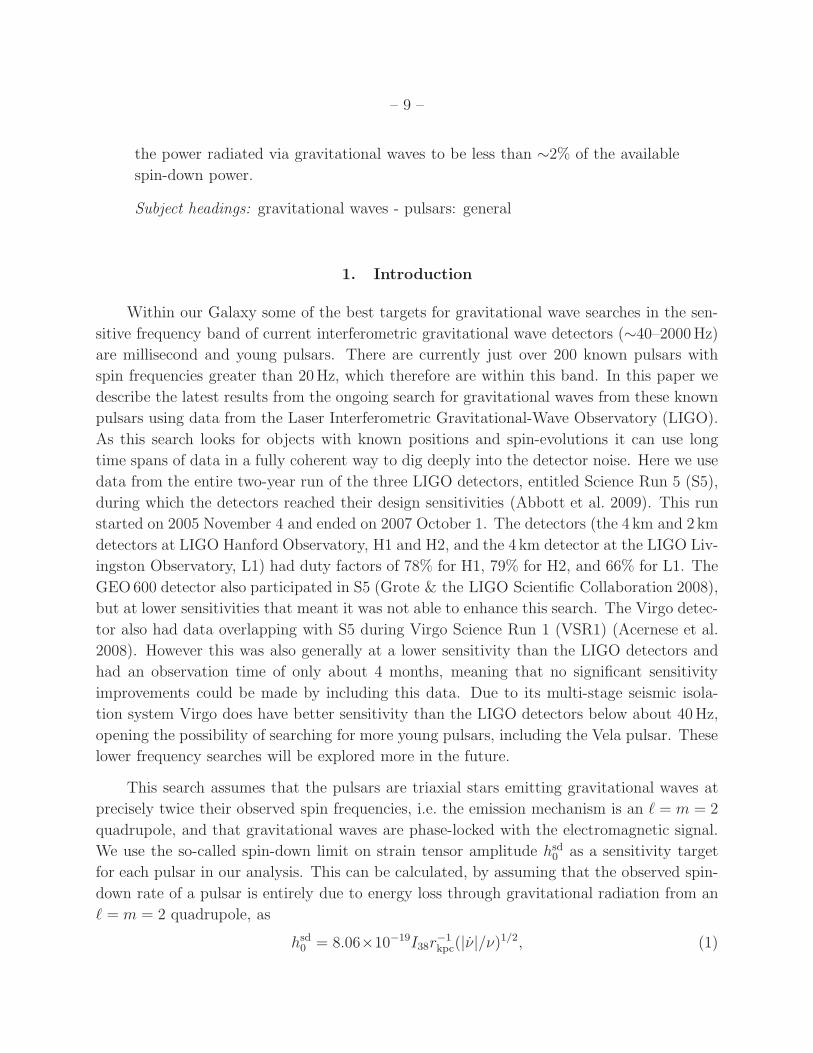
An example of the posteriors produced when searching over additional parameters (in

this case changes in declination and right ascension) can be seen in Figure 1. The figure

shows the multivariate Gaussian used as priors on the two parameters and how the posterior

is essentially identical to the prior (i.e. the data, which contains no signal, is adding no new

information on those parameters, but the full prior space is being explored).

2.4. Hardware injections

During all LIGO science runs, except the first, fake pulsar signals have been injected

into the detectors by direct actuation of the end test masses. These have provided end-to-

end validation of the analysis codes with coherence between the different detectors. During

S5, as with S3 and S4 (Abbott et al. 2007), ten signals with different source parameters

were injected into the detectors. As a demonstration of the analysis method these have been

extracted using the MCMC and all have been recovered with their known injection parameter

values. The extracted parameters for the two strongest signals are shown in Figure 2. From

these injections it can be seen that the parameters can be extracted to a high accuracy and

consistently between detectors. The offsets in the extracted values from the injected values

are within a few percent. These are well within the expected uncertainties of the detector

calibration, which are approximately 10%, 10% and 13% in amplitude, and 4.◦3 (0.08 rads),

3.◦4 (0.06 rads) and 2.◦3 (0.04 rads) in phase for H1, H2 and L1 respectively.

– 18 –

−5 0 5

x 10−6

0

1

2

3x 10

5

∆δ (rads)

prob

abili

ty d

ensi

ty

0 5 10 15

x 105

−1

−0.5

0

0.5

1x 10

−6

∆α (

rads

)

probability density

posterior

prior

∆δ (rads)

∆α (

rads

)

−5 0 5

x 10−6

−1

−0.5

0

0.5

1x 10

−6

Fig. 1.— The posteriors and priors on offsets in declination δ and right ascension α computed

from an MCMC search for PSRJ0407+1607 using a day of simulated data containing no

signal. The covariance contour plot of the MCMC chains for the two parameters is shown

and has a correlation coefficient of −0.93, which is identical to that of the multivariate

Gaussian prior distribution used in this study.

– 19 –

3. Evaluation of pulsar parameter errors

For the majority of pulsars we have parameter correlation matrices that have been

produced during the fit to the radio data, and (as discussed in §2.2) we can use these to

search over the uncertainties on the phase parameters. For some pulsars no correlation matrix

was produced with the radio observations, so for these we instead construct conservative

correlation matrices. These assume no correlations between any parameters, except in the

case of binary systems for which we assume a correlation of 1 between the angle and time of

periastron. This gives a slightly conservative over-estimate of the parameter errors, but is

still a useful approximation for our purposes. From these correlation matrices and the given

parameter standard deviations we produce a covariance matrix for each pulsar.

Using these covariance matrices we can also assess the potential phase mismatch that

might occur between the true signal and the best fit signal used in the heterodyne due to

errors in the pulsar phase parameters (as discussed in §2.2.) We take the mismatch (i.e. the

loss in signal power caused by the heterodyne phase being offset, over time, from the true

signal phase) to be

M =

∣

∣

∣

∣

∣

∣

1 −

(

∫ T

0φ(b + δb, t)dt∫ T

0φ(b, t)dt

)2∣

∣

∣

∣

∣

∣

, (6)

where φ is the phase given a vector of phase parameters b at time t, and T is the total

observation time. To get offsets in the phase parameters, δb, we draw random values from

1.6 1.7 1.8

x 10−23

0

5

10x 10

24

h0

prob

abili

ty d

ensi

ty

5.48 5.5 5.52 5.540

50

100

150

200

φ0 (rads)

−0.1 −0.08 −0.060

100

200

300

cosι

prob

abili

ty d

ensi

ty

0.43 0.44 0.45 0.46 0.470

100

200

300

ψ (rads)

H1H2L1Jointinjected

1.55 1.6 1.65 1.7

x 10−23

0

5

10

15x 10

24

h0

prob

abili

ty d

ensi

ty

5.85 5.9 5.950

50

100

150

200

φ0 (rads)

0.06 0.07 0.08 0.090

200

400

600

cosι

prob

abili

ty d

ensi

ty

0.15 0.16 0.17 0.18 0.190

200

400

ψ (rads)

H1H2L1Jointinjected

Fig. 2.— The extracted posteriors for the pulsar parameters from the two strongest hardware

injections for each detector and for a joint detector analysis. In each plot the injected

parameter value is marked by a dashed vertical line. The left pulsar injection was at a

frequency of 108.9Hz and the right pulsar was at 194.3Hz.

– 20 –

the multivariate Gaussian defined by the covariance matrix. For each pulsar we drew 100 000

random points and calculated the mean and maximum mismatch over the period of the S5

run. The mean mismatch is a good indicator of whether the given best fit parameter values

are adequate for our search, or whether the potential offset is large and a search including the

phase parameters is entirely necessary. The maximum mismatch represents a potential worst

case in which the true signal parameters are are at a point in parameter space approximately

4.5σ from the best fit values (the maximum mismatch will obviously increase if one increases

the number of randomly drawn values). Of our 113 non-glitching pulsars there are only

16 pulsars with mean mismatches greater than 1%, three of which are greater than 10%:

J0218+4232 at ∼ 43%, J0024−7204H at ∼ 15% and J1913+1011 at ∼ 37%. Given the

exclusion criterion for the S3 and S4 analyses (see §2.2) these three pulsars would have been

removed from this analysis. There are 16 pulsars with maximum mismatches greater than

10% with three of these being at almost 100%—i.e. if the signal parameters truly were offset

from their best fit values by this much, and these parameters were not searched over, then

the signal would be completely missed. This suggests that for the majority of pulsars the

search over the four main parameters of h0, φ0, cos ι and ψ is all that is necessary. But for

a few, and in particular the three with large mean mismatches (J0218+4232, J0024−7204H,

and J1913+1011), the search over the extra parameters is needed to ensure not losing signal

power.

4. Analysis

We have used the MCMC search over all phase parameters, where they have given errors,

for all but three pulsars (see below). For the majority of pulsars it is unnecessary (though

harmless) to include these extra parameters in the search as their priors are so narrow, but

it does provide an extra demonstration of the flexibility of the method. To double check, we

also produced results for each pulsar using the four dimensional grid of the earlier analyses

and found that, for pulsars with negligible mismatch, the results were consistent to within a

few percent.

For our full analysis we produced three independent MCMC chains with burn-in periods

of 100 000 iterations, followed by 100 000 iterations to sample the posterior. The three chains

were used to assess convergence using the tests discussed above in §2.1. All chains were seen

to converge and were therefore combined to give a total chain length of 300 000 iterations

from which the posteriors were generated.

For the three pulsars that glitched during S5 (the Crab, J1952+3252 and J0539−6910)

the MCMC was not used to search over the position and frequency parameters as above,

– 21 –

as the uncertainties on these parameters gave negligable potential mismatch. Our analysis

of these pulsars did however include extra parameters in the MCMC to take into account

potential uncertainties in the model caused by the glitches. We analysed the data coherently

over the full run as well as in stretches separated by the glitches that are treated separately.

We also included a model that allowed for a fixed but unknown phase jump ∆φ at the time

of each glitch, keeping other physical parameters fixed across the glitch. Results for all of

these cases are given in §5.1.

5. Results

No evidence of a gravitational wave signal was seen for any of the pulsars. In light of

this, we present joint 95% upper limits on h0 for each pulsar (see Table 1 for the results for

the non-glitching pulsars). We also interpret these as limits on the pulsar ellipticity, given

by

ε = 0.237 h−24rkpcν−2I38, (7)

where h−24 is the h0 upper limit in units of 1×10−24, I38 = 1 and rkpc pulsar distance in

kpc. For the majority of pulsars this distance is taken as the estimate value from Australia

Telescope National Facility Pulsar Catalogue91 (Manchester et al. 2005), but for others more

up-to-date distances are known. For pulsars in Terzan 5 (those with the name J1748−2446) a

distance of 5.5 kpc is used (Ortolani et al. 2007). For J1939+2134 the best estimate distance

is a highly uncertain value of ∼ 8.3 ± 5 kpc based on parallax measurements (Kaspi et al.

1994), but it is thought to be a large overestimate, so instead we use a value of 3.55 kpc de-

rived from the Cordes & Lazio (2002) NE2001 galactic electron density model. The observed

spin-down rate for globular cluster pulsars is contaminated by the accelerations within the

cluster, which can lead to some seeming to spin-up as can be seen in column four of Table 1.

For all pulsars in globular clusters, except J1824−2452A, we instead calculate a conservative

spin-down limit by assuming all pulsars have a characteristic age τ = ν/2ν of 109 years. Note

that using the characteristic age gives a spin-down limit that is independent of frequency and

only depends on τ and r. Globular cluster pulsar J1824−2452A has a large spin-down that

is well above what could be masked by cluster accelerations. Therefore, for this pulsar we

use its true spin-down for our limit calculation. For some nearby pulsars there is a small, but

measurable, Shklovskii effect which will contaminate the observed spin-down. For these if a

value of the intrinsic spin-down is known then this is used when calculating the spin-down

limit.

91http://www.atnf.csiro.au/research/pulsar/psrcat/

http://www.atnf.csiro.au/research/pulsar/psrcat/

– 22 –

The results are plotted in histogram form in Figure 3. Also shown for comparison are

the results of the previous search using combined data from the S3 and S4 science runs.

The median upper limit on h0 for this search, at 7.2×10−26, is about an order of magnitude

better than in the previous analysis (6.3×10−25). A large part of this increased sensitivity

(about a factor of 4 to 5) is due the the longer observation time. The median ellipticity is

ε = 1.1×10−6, an improvement from 9.1×10−6, and the median ratio to the spin-down limit

is 108, improved from 870. If one excludes the conservatively estimated spin-down limits for

the globular cluster pulsars, the median ratio is 73. In Figure 4 the upper limits on h0 are

also plotted overlaid onto an estimate of the search sensitivity92. The expected uncertainties

in these results due to the calibrations are given in §2.4.

The smallest upper limit on h0 for any pulsar is 2.3×10−26 for J1603−7202, which has

a gravitational wave frequency of 135Hz and is in the most sensitive part of the detectors’

bands. The lowest ellipticity upper limit is 7.0×10−8 for J2124−3358, which has a gravita-

tional wave frequency of 406Hz and a best estimate distance of 0.2 kpc. Of the millisecond

recycled pulsars this is also the closest to its spin-down limit, at a value of 9.4 times greater

than this limit. Of all pulsars which did not glitch during S5, the young pulsar J1913+1011

is the closest to its spin-down limit, at only 3.9 times greater than it.

92The upper and lower estimated sensitivity limits for the shaded band in Figure 4 come from the values

of the 95% h0 upper limits that bound 95% of total values from simulations on white noise for randomly

distributed pulsars. The band can be estimated from Figure 1 of Dupuis & Woan (2005), which gives limits

of (7 to 20)×√

Sn/T , where Sn is the single sided power spectral density and T is the total observation time

in seconds.

–23

–

Table 1. Information on the non-glitching pulsars in our search, including the start and

end times of the radio observations used in producing the parameter fits for our search, and

upper limit results.

Pulsar start – end (MJD) ν (Hz) ν (Hz s−1) distance (kpc) spin-down limit joint h95%0 ellipticity h95%

0 /hsd0

J0024−7204Ccp 48383 – 54261 173.71 1.5 × 10−15 4.9 6.55 × 10−28 5.88 × 10−25 2.26 × 10−5 898

J0024−7204Dcp 48465 – 54261 186.65 1.2 × 10−16 4.9 6.55 × 10−28 4.45 × 10−26 1.48 × 10−6 68

J0024−7204Ebcp 48465 – 54261 282.78 −7.9 × 10−15 4.9 6.55 × 10−28 9.97 × 10−26 1.44 × 10−6 152

J0024−7204Fcp 48465 – 54261 381.16 −9.4 × 10−15 4.9 6.55 × 10−28 8.76 × 10−26 6.98 × 10−7 134

J0024−7204Gcp 48600 – 54261 247.50 2.6 × 10−15 4.9 6.55 × 10−28 1.00 × 10−25 1.90 × 10−6 153

J0024−7204Hbcp 48518 – 54261 311.49 1.8 × 10−16 4.9 6.55 × 10−28 6.44 × 10−26 7.69 × 10−7 98

J0024−7204Ibcp 50684 – 54261 286.94 3.8 × 10−15 4.9 6.55 × 10−28 5.19 × 10−26 7.30 × 10−7 79

J0024−7204Jbcp 48383 – 54261 476.05 2.2 × 10−15 4.9 6.55 × 10−28 1.04 × 10−25 5.34 × 10−7 159

J0024−7204Lcp 50687 – 54261 230.09 6.5 × 10−15 4.9 6.55 × 10−28 5.82 × 10−26 1.27 × 10−6 89

J0024−7204Mcp 48495 – 54261 271.99 2.8 × 10−15 4.9 6.55 × 10−28 6.14 × 10−26 9.61 × 10−7 94

J0024−7204Ncp 48516 – 54261 327.44 2.4 × 10−15 4.9 6.55 × 10−28 8.35 × 10−26 9.02 × 10−7 128

J0024−7204Qbcp 50690 – 54261 247.94 −2.1 × 10−15 4.9 6.55 × 10−28 5.74 × 10−26 1.08 × 10−6 88

J0024−7204Rbcp 50743 – 54261 287.32 −1.2 × 10−14 4.9 6.55 × 10−28 5.53 × 10−26 7.76 × 10−7 84

J0024−7204Sbcp 50687 – 54241 353.31 1.5 × 10−14 4.9 6.55 × 10−28 6.82 × 10−26 6.33 × 10−7 104

J0024−7204Tbcp 50684 – 54261 131.78 −5.1 × 10−15 4.9 6.55 × 10−28 3.34 × 10−26 2.23 × 10−6 51

J0024−7204Ubcp 48516 – 54261 230.26 −5.0 × 10−15 4.9 6.55 × 10−28 5.63 × 10−26 1.23 × 10−6 86

J0024−7204Ybcp 51504 – 54261 455.24 7.3 × 10−15 4.9 6.55 × 10−28 9.42 × 10−26 5.26 × 10−7 144

J0218+4232bj 49092 – 54520 430.46 −1.4 × 10−14† 5.8 7.91 × 10−28 1.47 × 10−25 1.10 × 10−6 186

J0407+1607bj 52719 – 54512 38.91 −1.2 × 10−16 4.1 3.48 × 10−28 6.18 × 10−26 3.93 × 10−5 178

J0437−4715bp 53683 – 54388 173.69 −4.7 × 10−16† 0.1 8.82 × 10−27 5.73 × 10−25 6.74 × 10−7 65

J0613−0200bjp 53406 – 54520 326.60 −9.8 × 10−16† 0.5 2.91 × 10−27 1.11 × 10−25 1.18 × 10−7 38

J0621+1002bj 52571 – 54516 34.66 −5.5 × 10−17† 1.9 5.40 × 10−28 1.53 × 10−25 5.65 × 10−5 284

J0711−6830p 53687 – 54388 182.12 −2.7 × 10−16† 1.0 9.52 × 10−28 5.00 × 10−26 3.71 × 10−7 53

J0737−3039Abj 53595 – 54515 44.05 −3.4 × 10−15† 1.1 6.17 × 10−27 7.87 × 10−26 1.10 × 10−5 13

J0751+1807bj 53405 – 54529 287.46 −6.3 × 10−16† 0.6 1.92 × 10−27 1.64 × 10−25 2.91 × 10−7 85

J1012+5307bj 53403 – 54523 190.27 −4.7 × 10−16† 0.5 2.43 × 10−27 6.94 × 10−26 2.36 × 10−7 29

J1022+1001bjp 53403 – 54521 60.78 −1.6 × 10−16 0.4 3.27 × 10−27 4.44 × 10−26 1.14 × 10−6 14

J1024−0719jp 53403 – 54501 193.72 −6.9 × 10−16 0.5 2.88 × 10−27 5.01 × 10−26 1.67 × 10−7 17

J1045−4509bp 53688 – 54386 133.79 −2.0 × 10−16† 3.2 3.00 × 10−28 4.37 × 10−26 1.87 × 10−6 145

–24

–

Table 1—Continued


0 /hsd0

J1455−3330bj 52688 – 54524 125.20 −2.5 × 10−16† 0.7 1.53 × 10−27 5.15 × 10−26 5.75 × 10−7 34

J1600−3053bp 53688 – 54386 277.94 −6.5 × 10−16† 2.7 4.62 × 10−28 5.57 × 10−26 4.55 × 10−7 121

J1603−7202bp 53688 – 54385 67.38 −5.9 × 10−17† 1.6 4.62 × 10−28 2.32 × 10−26 1.98 × 10−6 50

J1623−2631bcj 53403 – 54517 90.29 −5.5 × 10−15 2.2 1.46 × 10−27 5.81 × 10−26 3.71 × 10−6 40

J1640+2224bj 53410 – 54506 316.12 −1.6 × 10−16† 1.2 4.86 × 10−28 6.65 × 10−26 1.87 × 10−7 137

J1643−1224bjp 52570 – 54517 216.37 −6.8 × 10−16† 4.9 2.94 × 10−28 4.35 × 10−26 1.07 × 10−6 148

J1701−3006Abcp 53590 – 54391 190.78 4.8 × 10−15 6.9 4.65 × 10−28 5.82 × 10−26 2.61 × 10−6 125

J1701−3006Bbcp 53650 – 54391 278.25 2.7 × 10−14 6.9 4.65 × 10−28 7.63 × 10−26 1.61 × 10−6 164

J1701−3006Cbcp 53590 – 54396 131.36 1.1 × 10−15 6.9 4.65 × 10−28 3.52 × 10−26 3.32 × 10−6 76

J1713+0747bjp 53406 – 54509 218.81 −3.8 × 10−16† 1.1 9.54 × 10−28 4.44 × 10−26 2.45 × 10−7 47

J1730−2304jp 52571 – 54519 123.11 −3.1 × 10−16 0.5 2.49 × 10−27 5.93 × 10−26 4.72 × 10−7 24

J1732−5049bp 53725 – 54386 188.23 −4.9 × 10−16 1.8 7.18 × 10−28 5.25 × 10−26 6.34 × 10−7 73

J1744−1134jp 52604 – 54519 245.43 −4.1 × 10−16† 0.5 2.18 × 10−27 1.10 × 10−25 2.07 × 10−7 50

J1748−2446Abcjg 52320 – 54453 86.48 2.2 × 10−16 5.5 5.83 × 10−28 3.89 × 10−26 6.77 × 10−6 67

J1748−2446Ccjg 53403 – 54516 118.54 8.5 × 10−15 5.5 5.83 × 10−28 5.00 × 10−26 4.63 × 10−6 86

J1748−2446Dcg 50851 – 53820 212.13 −5.7 × 10−15 5.5 5.83 × 10−28 6.78 × 10−26 1.96 × 10−6 116

J1748−2446Ebcg 53193 – 53820 455.00 3.8 × 10−15 5.5 5.83 × 10−28 8.95 × 10−26 5.62 × 10−7 153

J1748−2446Fcg 53193 – 53820 180.50 −1.3 × 10−16 5.5 5.83 × 10−28 8.37 × 10−26 3.34 × 10−6 143

J1748−2446Gcg 51884 – 53820 46.14 −8.4 × 10−16 5.5 5.83 × 10−28 5.82 × 10−26 3.56 × 10−5 100

J1748−2446Hcg 51884 – 53820 203.01 3.4 × 10−15 5.5 5.83 × 10−28 7.81 × 10−26 2.46 × 10−6 134

J1748−2446Ibcg 50851 – 54195 104.49 7.3 × 10−16 5.5 5.83 × 10−28 3.54 × 10−26 4.21 × 10−6 61

J1748−2446Kcg 51884 – 53820 336.74 1.1 × 10−14 5.5 5.83 × 10−28 6.67 × 10−26 7.65 × 10−7 114

J1748−2446Lcg 51884 – 53820 445.49 3.4 × 10−15 5.5 5.83 × 10−28 1.39 × 10−25 9.09 × 10−7 238

J1748−2446Mbcg 51884 – 53820 280.15 −3.9 × 10−14 5.5 5.83 × 10−28 1.01 × 10−25 1.68 × 10−6 173

J1748−2446Nbcg 53193 – 54195 115.38 −7.4 × 10−15 5.5 5.83 × 10−28 5.85 × 10−26 5.71 × 10−6 100

J1748−2446Obcg 52500 – 53957 596.43 2.5 × 10−14 5.5 5.83 × 10−28 2.65 × 10−25 9.68 × 10−7 454

J1748−2446Pbcg 53193 – 54557 578.50 −8.7 × 10−14 5.5 5.83 × 10−28 1.56 × 10−25 6.08 × 10−7 267

J1748−2446Qbcg 53193 – 54139 355.62 4.6 × 10−15 5.5 5.83 × 10−28 8.80 × 10−26 9.05 × 10−7 151

J1748−2446Rcg 52500 – 53820 198.86 −1.9 × 10−14 5.5 5.83 × 10−28 8.23 × 10−26 2.71 × 10−6 141

–25

–

Table 1—Continued


0 /hsd0

J1748−2446Scg 53193 – 53820 163.49 −1.7 × 10−15 5.5 5.83 × 10−28 4.46 × 10−26 2.17 × 10−6 76

J1748−2446Tcg 51884 – 53819 141.15 −6.1 × 10−15 5.5 5.83 × 10−28 5.12 × 10−26 3.34 × 10−6 88

J1748−2446Vbcg 53193 – 53820 482.51 2.2 × 10−14 5.5 5.83 × 10−28 1.26 × 10−25 7.04 × 10−7 216

J1748−2446Wbcg 52500 – 53820 237.80 −7.1 × 10−15 5.5 5.83 × 10−28 9.57 × 10−26 2.20 × 10−6 164

J1748−2446Xbcg 51884 – 54139 333.44 −6.5 × 10−15 5.5 5.83 × 10−28 8.18 × 10−26 9.57 × 10−7 140

J1748−2446Ybcg 53193 – 53820 488.24 −4.0 × 10−14 5.5 5.83 × 10−28 2.10 × 10−25 1.15 × 10−6 360

J1748−2446Zbcg 53193 – 54139 406.08 1.4 × 10−14 5.5 5.83 × 10−28 8.43 × 10−26 6.65 × 10−7 145

J1748−2446aacg 51884 – 53819 172.77 1.3 × 10−14 5.5 5.83 × 10−28 2.28 × 10−25 9.92 × 10−6 391

J1748−2446abcg 51884 – 53819 195.32 −1.6 × 10−14 5.5 5.83 × 10−28 4.67 × 10−26 1.59 × 10−6 80

J1748−2446accg 52500 – 53819 196.58 −8.8 × 10−15 5.5 5.83 × 10−28 7.19 × 10−26 2.42 × 10−6 123

J1748−2446adbcg 53204 – 54557 716.36 1.7 × 10−14 5.5 5.83 × 10−28 1.77 × 10−25 4.48 × 10−7 303

J1748−2446aebcg 53193 – 53820 273.33 4.3 × 10−14 5.5 5.83 × 10−28 6.57 × 10−26 1.14 × 10−6 113

J1748−2446afcg 53193 – 53820 302.63 2.1 × 10−14 5.5 5.83 × 10−28 1.07 × 10−25 1.52 × 10−6 183

J1748−2446agcg 53193 – 53819 224.82 −6.3 × 10−16 5.5 5.83 × 10−28 9.49 × 10−26 2.44 × 10−6 163

J1748−2446ahcg 53193 – 53819 201.40 −2.3 × 10−14 5.5 5.83 × 10−28 5.49 × 10−26 1.76 × 10−6 94

J1756−2251bj 53403 – 54530 35.14 −1.3 × 10−15 2.9 1.65 × 10−27 9.70 × 10−26 5.42 × 10−5 59

J1801−1417j 53405 – 54505 275.85 −4.0 × 10−16 1.8 5.42 × 10−28 6.15 × 10−26 3.44 × 10−7 113

J1803−30cp 53654 – 54379 140.83 −1.0 × 10−15 7.8 4.11 × 10−28 5.51 × 10−26 5.12 × 10−6 134

J1804−0735bcj 52573 – 54518 43.29 −8.8 × 10−16 8.4 3.82 × 10−28 8.44 × 10−26 8.95 × 10−5 221

J1804−2717bj 52574 – 54453 107.03 −4.7 × 10−16 1.2 1.44 × 10−27 2.40 × 10−26 5.79 × 10−7 17

J1807−2459Abcp 53621 – 54462 326.86 4.8 × 10−16 2.7 1.19 × 10−27 1.53 × 10−25 9.13 × 10−7 129

J1810−2005bj 53406 – 54508 30.47 −1.4 × 10−16 4.0 4.28 × 10−28 2.22 × 10−25 2.28 × 10−4 519

J1823−3021Acj 53403 – 54530 183.82 −1.1 × 10−13 7.9 4.06 × 10−28 3.93 × 10−26 2.17 × 10−6 97

J1824−2452Acjpg 53403 – 54509 327.41 −1.7 × 10−13 4.9 3.79 × 10−27 7.80 × 10−26 8.43 × 10−7 21

J1824−2452Bcg 53629 – 54201 152.75 5.6 × 10−15 4.9 6.55 × 10−28 4.26 × 10−26 2.11 × 10−6 65

J1824−2452Cbcg 52335 – 54202 240.48 −9.8 × 10−15 4.9 6.55 × 10−28 6.48 × 10−26 1.30 × 10−6 99

J1824−2452Ecg 53629 – 54201 184.53 3.7 × 10−15 4.9 6.55 × 10−28 7.51 × 10−26 2.55 × 10−6 115

J1824−2452Fcg 52497 – 54114 407.97 −1.6 × 10−15 4.9 6.55 × 10−28 9.74 × 10−26 6.78 × 10−7 149

J1824−2452Gbcg 53629 – 54202 169.23 −5.2 × 10−15 4.9 6.55 × 10−28 7.23 × 10−26 2.93 × 10−6 110

– 26 –

−26 −25.5 −25 −24.5 −24 −23.50

5

10

15

20

25

30

log10

h0

num

ber

of p

ulsa

rs

−8 −6 −4 −20

5

10

15

20

25

30

35

40

log10

ε0 1 2 3 4

0

5

10

15

20

25

30

log10

spin−down ratio

Fig. 3.— The solid histograms show the results of this analysis in terms of upper limits on

h0, the ellipticity ε and the ratio to the spin-down limit (excluding the glitching pulsars).

The clear histograms show the same set of values for the combined S3 and S4 analysis

(Abbott et al. 2007).

5.1. Glitching pulsars

For the three pulsars that glitched, we have chosen to take into account three different

models related to the coherence of the gravitational wave signal and the electromagnetic

signal over the glitch: i) there is coherence between them over the glitch (i.e. the glitch

causes no discontinuity between the electromagnetic and gravitational wave phases); ii) there

is decoherence (in terms of a phase jump) between them at the time of the glitch, but the

phase discontinuity is included as an extra search parameter (i.e. a ∆φ parameter is added

at the time of the glitch); and iii) the data stretches before, between and after the glitches

are treated separately and analysed independently.

5.1.1. Crab pulsar

For this search we include the three different models described above relating to the

observed glitch in the pulsar on 2006 August 3. Potentially all the four main gravitational

wave signal parameters could be changed during the glitch if it is large enough to cause major

disruption to the star, but this is not the case for the observed glitch. It had a fractional

frequency change of order ∆ν/ν ∼ 5×10−9, which is unlikely to be energetic enough to cause

changes in the gravitational wave amplitude near our current levels of sensitivity. To model

–27

–

Table 1—Continued


0 /hsd0

J1824−2452Hbcg 53629 – 54202 216.01 −3.6 × 10−15 4.9 6.55 × 10−28 8.27 × 10−26 2.05 × 10−6 126

J1824−2452Jbcg 53629 – 54201 247.54 4.7 × 10−15 4.9 6.55 × 10−28 1.07 × 10−25 2.03 × 10−6 163

J1841+0130bj 53405 – 54513 33.59 −9.2 × 10−15 3.2 4.19 × 10−27 1.65 × 10−25 1.10 × 10−4 39

J1843−1113j 53353 – 54508 541.81 −2.8 × 10−15 2.0 9.33 × 10−28 1.64 × 10−25 2.61 × 10−7 176

J1857+0943bjp 53409 – 54517 186.49 −6.0 × 10−16† 0.9 1.59 × 10−27 7.27 × 10−26 4.50 × 10−7 46

J1905+0400j 53407 – 54512 264.24 −3.4 × 10−16 1.3 6.81 × 10−28 7.40 × 10−26 3.36 × 10−7 109

J1909−3744bp 53687 – 54388 339.32 −3.1 × 10−16† 1.1 6.78 × 10−28 8.09 × 10−26 1.89 × 10−7 119

J1910−5959Abcp 53666 – 54380 306.17 −2.8 × 10−16 4.5 7.13 × 10−28 7.71 × 10−26 8.75 × 10−7 108

J1910−5959Bcp 53609 – 54473 119.65 1.1 × 10−14 4.5 7.13 × 10−28 3.81 × 10−26 2.83 × 10−6 53

J1910−5959Ccp 53666 – 54390 189.49 −7.8 × 10−17 4.5 7.13 × 10−28 4.34 × 10−26 1.29 × 10−6 61

J1910−5959Dcp 53621 – 54460 110.68 −1.2 × 10−14 4.5 7.13 × 10−28 3.03 × 10−26 2.63 × 10−6 42

J1910−5959Ecp 53610 – 54441 218.73 2.1 × 10−14 4.5 7.13 × 10−28 4.77 × 10−26 1.06 × 10−6 67

J1911+1347j 53403 – 54530 216.17 −8.0 × 10−16 1.6 9.63 × 10−28 7.00 × 10−26 5.70 × 10−7 73

J1911−1114bj 53407 – 54512 275.81 −4.8 × 10−16† 1.6 6.66 × 10−28 5.62 × 10−26 2.78 × 10−7 84

J1913+1011j 53745 – 54911 27.85 −2.6 × 10−12 4.5 5.51 × 10−26 2.14 × 10−25 2.93 × 10−4 3.9

J1939+2134jp 53407 – 54519 641.93 −4.3 × 10−14† 3.5 1.86 × 10−27 1.79 × 10−25 3.65 × 10−7 96

J1955+2908bj 53403 – 54524 163.05 −7.6 × 10−16† 5.4 3.23 × 10−28 7.07 × 10−26 3.39 × 10−6 219

J2019+2425bj 53599 – 54505 254.16 −1.7 × 10−16† 0.9 7.14 × 10−28 9.23 × 10−26 3.07 × 10−7 129

J2033+17bj 53702 – 54522 168.10 −3.1 × 10−16 1.4 7.93 × 10−28 7.49 × 10−26 8.65 × 10−7 94

J2051−0827bj 53410 – 54520 221.80 −6.1 × 10−16† 1.3 1.04 × 10−27 7.57 × 10−26 4.65 × 10−7 73

J2124−3358jp 53410 – 54510 202.79 −5.1 × 10−16† 0.2 5.13 × 10−27 4.85 × 10−26 6.96 × 10−8 9.4

J2129−5721bp 53687 – 54388 268.36 −2.0 × 10−15† 2.5 8.71 × 10−28 6.12 × 10−26 5.13 × 10−7 70

J2145−0750bjp 53409 – 54510 62.30 −1.0 × 10−16† 0.5 2.05 × 10−27 3.83 × 10−26 1.17 × 10−6 19

J2229+2643bj 53403 – 54524 335.82 −1.6 × 10−16 1.4 3.95 × 10−28 9.89 × 10−26 2.96 × 10−7 250

J2317+1439bj 53406 – 54520 290.25 −1.3 × 10−16† 1.9 2.82 × 10−28 8.83 × 10−26 4.68 × 10−7 313

J2322+2057j 53404 – 54519 207.97 −1.8 × 10−16† 0.8 9.55 × 10−28 1.12 × 10−25 4.78 × 10−7 117

bThe pulsar is within a binary system.

cThe pulsar is within a globular cluster.

gThe pulsar was observed by the Green Bank Telescope.

jThe pulsar was observed by the Jodrell Bank Observatory.

pThe pulsar was observed by the Parkes Observatory.

– 28 –

frequency (Hz)

h 0

102

103

10−26

10−25

10−24

sensitivity estimatejoint 95% upper limit (S5)joint 95% upper limit (S3/S4)

Fig. 4.— The gravitational wave amplitude upper limits are plotted over the estimated

sensitivity of the search as defined by the grey band (see text). Also plotted are the limits

from the S3/S4 search.

– 29 –

the signal phase we use the regularly updated Crab pulsar Monthly Ephemeris (Lyne et al.

1993, 2009), which is needed to take into account the phase variations caused by timing

noise.

As for the previous Crab Pulsar search (Abbott et al. 2008) we have information on the

orientation of the pulsar from the orientation of the pulsar wind nebula (PWN) (Ng & Romani

2008). We use this information to set Gaussian priors on the ψ and ι parameters of

ψ = 125.◦155 ± 1.◦355 (the ψ-dependence wraps around at ±45◦, so the actual value used

is 35.◦155) and ι = 62.◦17 ± 2.◦20.

There is reason to believe that the PWN orientation reflects that of the central pulsar,

but in case this is not an accurate description we present results using both a uniform prior

over all parameters, and using the restricted prior ranges. The MCMC only searches over

the four main parameters and does not include errors on the pulsar position, frequency

or frequency derivatives as these are negligible. The results are summarised in Table 3,

where for the ellipticity and spin-down limit calculations a distance of 2 kpc was used. The

orientation angle suggested by the restricted priors is slightly favourable in terms of the

observable gravitational wave emission it would produce, and this allows us to set a better

upper limit.

In Figure 5 we plot the result from model i), with restricted priors, as an exclusion region

on the moment of inertia–ellipticity plane. It can been seen that for all the allowed regions

in moment of inertia we beat the spin-down limit. If one assumes the Crab pulsar to have

a moment of inertia at the upper end of the allowed range our result beats the spin-down

limit by over an order of magnitude.

5.1.2. PSRJ0537−6910

For pulsar J0537−6910, which has so far been timed only in X-rays, we rely on data

from the Rossi X-ray Timing Explorer (RXTE) satellite. This pulsar is young, has a high

spin-down rate, and is a prolific glitcher, and therefore we require observations overlapping

with our data to produce a coherent template. Middleditch et al. (2006) have published

observations covering from the beginning of S5 up to 2006 August 21, during which time

the pulsar was seen to glitch three times. Further observations have been made which

span the rest of the S5 run and show another three glitches during this time. The epochs

and parameters for the seven ephemeris periods overlapping with our data run are given in

Table 2. For the first epoch there was no data for L1, so the joint result only uses H1 and

H2 data. For the analyses using all the data (models i and ii) we have 474 days of H1 data,

– 30 –

475 days of H2 data and 397 days of L1 data. Due to the glitches we perform parameter

estimation for the same three models given above.

As with the Crab Pulsar there is also information on the orientation of J0537−6910 from

model fits to its pulsar wind nebula (Ng & Romani 2008). These are used to set Gaussian

priors on ψ and ι of ψ = 131.◦0 ± 2.◦2 (equivalently 41.◦0) and ι = 92.◦8 ± 0.◦9. We again

quote results using uniform priors over all parameters and with these restricted priors. The

distance used in the ellipticity and spin-down limits for J0537−6910 is 49.4 kpc. The results

are summarised in Table 3. Using the restricted priors we obtain a worse upper limit on

h0 than for uniform priors. This is because the nebula suggests that the star has its spin

axis perpendicular to the line of sight, and therefore the gravitational radiation is linearly

polarised and the numerical strain amplitude is lower than average for a given strain tensor

amplitude h0.

In Figure 5 we again plot the result from model i), with restricted priors, on the moment

of inertia–ellipticity plane. It can be seen that the spin-down limit is beaten if we assume a

moment of inertia to be 2 × 1038 kgm2 or greater.

5.1.3. PSRJ1952+3252

PSRJ1952+3252 is another young pulsar with a high spin-down rate (although a couple

of orders of magnitude less than for the Crab pulsar and J0537−6910) – it has a spin

parameters of ν = 25.30Hz and ν = −3.73×10−12 Hz s−1. Jodrell Bank observations of

this pulsar were made over the whole of S5, but it was observed to glitch at some point

between 2007 January 1 and January 12. For both the pre and post-glitch epochs we have

coherent timing solutions and again perform analyses as above. The are no constraints on

the orientation of this pulsar, so we do not use any restricted priors. The results for this

pulsar are given in Table 3. We reach about a factor of two above the spin-down limit using

a distance of 2.5 kpc. The result from model i) is also plotted on the moment of inertia–

ellipticity plane in Figure 5. It can be seen that I38 just over over 4, which is above the

expected maximum allowable value, would be needed to beat the spin-down limit.

6. Conclusions

In this paper we have searched for continuous gravitational waves from an unprece-

dented number of pulsars with unprecedented sensitivity, using coincident electromagnetic

observations of many millisecond and young pulsars. Our direct upper limits have beaten the

– 31 –

Table 2. Ephemeris information for PSRJ0537−6910. The first four values are taken from

Middleditch et al. (2006).

start – end (MJD) ν (Hz) ν (Hz s−1) ν (Hz s−2) epoch (MJD)

1. 53551–53687 62.000663106 −1.994517×10−10 11.2×10−21 53557.044381976239

2. 53711–53859 61.996292178 −1.993782×10−10 8.1×10−21 53812.224185839386

3. 53862–53950 61.995120229 −1.994544×10−10 9.6×10−21 53881.096123033291

4. 53953–53996 61.993888026 −1.995140×10−10 9.6×10−21 53952.687378384607

5. 54003–54088 61.992869785 −1.994516×10−10 2.2×10−21 54013.061576594146

6. 54116–54273 61.990885506 −1.994577×10−10 8.1×10−21 54129.540333159754

7. 54277–54441 61.988307647 −1.994958×10−10 7.7×10−21 54280.918705402011

ellipticity

mom

ent o

f ine

rtia

(kg

m2 )

10−5

10−4

10−3

1038

1039

Crab pulsar resultCrab pulsar spin−downJ0537−6910 resultJ0537−6910 spin−downJ1952+3252 resultJ1952+3252 spin−down

Fig. 5.— The results of the Crab pulsar, J0537−6910 and J1952+3252 analyses, and the

spin-down limits, plotted on the moment of inertia–ellipticity plane. The results used are

those from model i) and with restricted priors on the angular parameters for the Crab pulsar

and J0537−6910. Areas to the right of the diagonal lines are excluded. The shaded regions

are those outside the theoretically predicted range of moments of inertia I38 =1–3.

– 32 –

Table 3. Results of the analysis for the Crab pulsar, J0537−6910 and J1952+3252.

h95%0 ellipticity h95%

0 /hsd0

epoch uniform restricted† uniform restricted† uniform restricted†

Crab pulsar

model i)a 2.6×10−25 2.0×10−25 1.4×10−4 1.1×10−4 0.18 0.14

model ii)b 2.4×10−25 1.9×10−25 1.3×10−4 9.9×10−5 0.17 0.13

1. 4.9×10−25 3.9×10−25 2.6×10−4 2.1×10−4 0.34 0.27

2. 2.4×10−25 1.9×10−25 1.3×10−4 1.0×10−4 0.15 0.13

J0537−6910

model i)a 2.9×10−26 3.9×10−26 8.9×10−5 1.2×10−4 1.0 1.3

model ii)b 4.1×10−26 4.6×10−26 1.2×10−4 1.4×10−4 1.4 1.5

1. 9.1×10−25 1.2×10−24 2.8×10−3 3.7×10−3 31.2 41.2

2. 1.2×10−25 1.5×10−25 3.6×10−4 4.6×10−4 4.1 5.2

3. 1.4×10−25 1.3×10−25 4.2×10−4 3.8×10−4 4.7 4.3

4. 8.3×10−26 1.1×10−25 2.5×10−4 3.3×10−4 2.8 3.7

5. 1.4×10−25 1.3×10−25 4.1×10−4 4.0×10−4 4.7 4.6

6. 4.4×10−26 5.8×10−26 1.3×10−4 1.8×10−4 1.5 2.0

7. 4.9×10−26 6.1×10−26 1.5×10−4 1.9×10−4 1.7 2.1

J1952+3252

model i)a 2.5×10−25 · · · 2.3×10−4 · · · 2.0 · · ·

model ii)b 3.6×10−25 · · · 3.3×10−4 · · · 2.9 · · ·

1. 4.7×10−25 · · · 4.3×10−4 · · · 3.8 · · ·

2. 4.4×10−25 · · · 4.0×10−4 · · · 3.5 · · ·

†Uses observationally restricted priors on the orientation angle and polarisation angle

aUses the full data set for a coherent analysis

bUses the full data set, but searches over an extra phase parameter at each glitch

– 33 –

indirect limits (including the spin-down limit) for the Crab Pulsar and are at the canonical

spin-down limit for J0537−6910. For several more pulsars our upper limits are within roughly

one order of magnitude of the spin-down limits, and therefore we expect a comparable search

of Advanced LIGO and Virgo data to beat the latter.

For the Crab Pulsar we improve upon the previous upper limit, which already beat the

spin-down limit and other indirect limits; and we also provide results for different scenarios

in which the signals may not be fully coherent over the run. By assuming the observationally

constrained priors on the angular parameters are correct we can limit the power output of the

pulsar (see Abbott et al. (2008)) to be less than ∼ 2% of the canonical spin-down luminosity.

Pulsar J0537−6910 is an interesting case due to its youth and glitchiness. Assuming

that the gravitational wave signal phase is coherent with the X-ray pulses over glitches, our

upper limit is within a few percent of the canonical spin-down limit for this pulsar. If we

assume that the phase is incoherent over the glitches then using the full data set our upper

limit is ∼ 1.2 times the canonical spin-down limit. Even if we assume that none of the four

main pulsar parameters remains coherent during a glitch (i.e. there is a major rearrangement

in the star’s structure) then the results from the final two epochs individually are still only

approximately two times the spin-down limit. All of these direct upper limits are within

the uncertainties of the spin-down limit, and (unlike the Crab) there is no firmly observed

braking index and thus no substantially stricter indirect limit.

Pulsar J1952+3252 gets close to its spin-down limit, but even taking into account mo-

ment of inertia and distance uncertainties, probably would still just miss beating it. It does

however make an exciting target for future runs.

Our observational upper limits on the ellipticities of the Crab and J0537−6910 are in the

vicinity of 10−4. Elastic deformations of this magnitude have been predicted as sustainable

(Owen 2005; Haskell et al. 2007; Lin 2007; Knippel & Sedrakian 2009) not for normal neu-

tron stars but only for exotic forms of crystalline quark matter (Xu 2003; Mannarelli et al.

2007). Such ellipticities could also be sustained by internal toroidal magnetic fields of or-

der 1016 G depending on the field configuration, equation of state, and superconductiv-

ity of the star (Cutler 2002; Akgun & Wasserman 2007; Haskell et al. 2008; Colaiuda et al.

2008). Therefore our observations have achieved the sensitivity to detect some of the more

extreme possibilities, and have constrained the internal magnetic fields of the Crab and

J0537−6910 to be less than of order 1016 G. However we must correct a misconception (Lin

2007; Haskell et al. 2007) which is spreading (Knippel & Sedrakian 2009): Our upper limits

do not constrain the properties of crystalline quark matter, because we constrain the true

ellipticity of a star rather than the maximum ellipticity (Owen 2005).

– 34 –

Recent work by Horowitz & Kadau (2009) suggests that the breaking strain of neutron

star crusts may be an order of magnitude higher (10−1) than the highest values (10−2)

previously used in estimates of maximum sustainable ellipticities. Their simulations are

strictly applicable only to the outer crust (i.e. no neutron drip), but since the reason for

the high breaking strain is very generic—the extreme pressure simply crushes away defects

that contribute to early fracture—it may apply to the inner crust (the major contributor to

ellipticity) as well. In that case normal neutron stars could sustain ellipticities close to 10−5,

which is beyond reach of the present search (for those stars where our results are at or near

the spin-down limit) but would be accessible with data from advanced interferometers. If

the high breaking strain holds for mixed phases in hybrid stars (which is not clear due to

the increasing importance of the strong interaction at high densities), it would bring their

maximum ellipticities estimated by Owen (2005) up an order of magnitude to about the 10−4

values achieved here.

In 2009 July the LIGO 4km detectors (featuring some upgraded systems and titled

Enhanced LIGO) and the upgraded Virgo detector began their sixth and second science

runs respectively (S6 and VSR2). These upgrades aim to provide significantly better strain

sensitivities than S5/VSR1. For LIGO these improvements will primarily be at frequencies

greater than 40Hz, but Virgo will improve at lower frequencies too and should outperform

LIGO below about 40Hz. LIGO and Virgo will closely approach and could potentially beat

the spin-down limits not only for the Crab and J0537-6910 but for six more known pul-

sars: J1952+3252, J1913+1011, J0737−3039A, J0437−471593, and the recently discovered

J1747−2809 (Camilo et al. 2009) and J1813−1749 (Gotthelf & Halpern 2009). Below 40Hz

Virgo could beat the spin-down limits for three more pulsars: the Vela pulsar, J0205+6449

and J1833−1034. Most of these eleven pulsars are young and may be prone to large levels

of timing noise and glitches. Therefore to reach the best sensitivities it is essential to have

radio and X-ray observations of these sources made in coincidence with the S6/VSR2 run.

In particular the extension of the RXTE satellite is crucial to our ability to perform targeted

searches of J0573−6910 and J1813−1749 during this time of enhanced detector performance.

On a time scale of a few years, the Advanced LIGO and Virgo interferometers are

expected to achieve strain sensitivities more than 10 times better for the pulsars in the

current band, and will extend that band downward to approximately 10Hz. Searches at

such sensitivities will beat the spin-down limits from dozens of known pulsars and also enter

the range of ellipticities predicted for normal neutron stars, improving the prospects for

direct gravitational wave observations from these objects.

93This pulsar sits on a strong LIGO spectral noise line caused by the violin mode resonance of the sus-

pension wires, so the required sensitivity may only be reachable with Virgo.

– 35 –

The authors gratefully acknowledge the support of the United States National Science

Foundation for the construction and operation of the LIGO Laboratory, the Science and

Technology Facilities Council of the United Kingdom, the Max-Planck-Society, and the State

of Niedersachsen/Germany for support of the construction and operation of the GEO600 de-

tector, and the Italian Istituto Nazionale di Fisica Nucleare and the French Centre National

de la Recherche Scientifique for the construction and operation of the Virgo detector. The

authors also gratefully acknowledge the support of the research by these agencies and by the

Australian Research Council, the Council of Scientific and Industrial Research of India, the

Istituto Nazionale di Fisica Nucleare of Italy, the Spanish Ministerio de Educacion y Ciencia,

the Conselleria d’Economia Hisenda i Innovacio of the Govern de les Illes Balears, the Foun-

dation for Fundamental Research on Matter supported by the Netherlands Organisation for

Scientific Research, the Royal Society, the Scottish Funding Council, the Polish Ministry of

Science and Higher Education, the FOCUS Programme of Foundation for Polish Science, the

Scottish Universities Physics Alliance, The National Aeronautics and Space Administration,

the Carnegie Trust, the Leverhulme Trust, the David and Lucile Packard Foundation, the

Research Corporation, and the Alfred P. Sloan Foundation. LIGO Document No. LIGO-

P080112-v5.

Pulsar research at UBC is supported by a Natural Sciences and Engineering Research

Council of Canada Discovery Grant. The Parkes radio telescope is part of the Australia

Telescope which is funded by the Commonwealth Government for operation as a National

Facility managed by CSIRO. The National Radio Astronomy Observatory is a facility of

the United States National Science Foundation operated under cooperative agreement by

Associated Universities, Inc. We thank Maura McLaughlin for useful discussions.

REFERENCES

Abbott et al., B. 2004, Phys. Rev. D, 69, 082004

—. 2005, Phys. Rev. Lett., 94, 181103

—. 2007, Phys. Rev. D, 76, 042001

—. 2008, ApJ, 683, L45

—. 2009, Rept. Prog. Phys., 72, 076901

Acernese et al., F. 2008, Classical Quantum Gravity, 25, 184001

Akgun, T. & Wasserman, I. 2007, MNRAS, 383, 1551

– 36 –

Bondarescu, R., Teukolsky, S. A., & Wasserman, I. 2009, Phys. Rev. D, 79, 104003

Brooks, S. P. & Roberts, G. O. 1998, Statistics and Computing, 8, 319

Camilo, F., Ransom, S. M., Gaensler, B. M., & Lorimer, D. R. 2009, ApJ, 700, L34

Colaiuda, A., Ferrari, V., Gualtieri, L., & Pons, J. A. 2008, MNRAS, 385, 2080

Cordes, J. M. & Lazio, T. J. W. 2002, ArXiv Astrophysics e-prints

Cutler, C. 2002, Phys. Rev. D, 66, 084025

Deller, A. T., Bailes, M., & Tingay, S. J. 2009, Science, 323, 1327

Dupuis, R. J. & Woan, G. 2005, Phys. Rev. D, 72, 102002

Goldreich, P. & Reisenegger, A. 1992, ApJ, 395, 250

Gotthelf, E. V. & Halpern, J. P. 2009, ApJ, 700, L158

Grote, H. & the LIGO Scientific Collaboration. 2008, Classical Quantum Gravity, 25, 114043

Haskell, B., Andersson, N., Jones, D. I., & Samuelsson, L. 2007, Phys. Rev. Lett., 99, 231101

Haskell, B., Samuelsson, L., Glampedakis, K., & Andersson, N. 2008, MNRAS, 385, 531

Hobbs, G. B., Edwards, R. T., & Manchester, R. N. 2006, MNRAS, 369, 655

Horowitz, C. J. & Kadau, K. 2009, Phys. Rev. Lett., 102, 191102

Kaspi, V. M., Taylor, J. H., & Ryba, M. F. 1994, ApJ, 428, 713

Knippel, B. & Sedrakian, A. 2009, Phys. Rev. D, 79, 083007

Kramer, M. & Wex, N. 2009, Classical Quantum Gravity, 26, 073001

Lin, L.-M. 2007, Phys. Rev. D, 76, 081502

Lindblom, L., Owen, B. J., & Ushomirsky, G. 2000, Phys. Rev. D, 62, 084030

Lyne, A. G., Pritchard, R. S., & Graham-Smith, F. 1993, MNRAS, 265, 1003

Lyne, A. G., Roberts, M. E., & Jordan, C. A. 2009, Jodrell Bank Crab Pulsar Monthly

Ephemeris

http://www.jb.man.ac.uk/∼pulsar/crab.html

http://www.jb.man.ac.uk/~pulsar/crab.html

– 37 –

Manchester, R. N. 2008, in American Institute of Physics Conference Series, Vol. 983, 40

Years of Pulsars: Millisecond Pulsars, Magnetars and More, ed. C. Bassa, Z. Wang,

A. Cumming, & V. M. Kaspi, 584–592

Manchester, R. N., Hobbs, G. B., Teoh, A., & Hobbs, M. 2005, AJ, 129, 1993

Mannarelli, M., Rajagopal, K., & Sharma, R. 2007, Phys. Rev. D, 76, 074026

Middleditch, J., Marshall, F. E., Wang, Q. D., Gotthelf, E. V., & Zhang, W. 2006, ApJ,

652, 1531

Ng, C.-Y. & Romani, R. W. 2008, ApJ, 673, 411

Ortolani, S., Barbuy, B., Bica, E., Zoccali, M., & Renzini, A. 2007, A&A, 470, 1043

Owen, B. J. 2005, Phys. Rev. Lett., 95, 211101

Owen, B. J., Lindblom, L., Cutler, C., Schutz, B. F., Vecchio, A., & Andersson, N. 1998,

Phys. Rev. D, 58, 084020

Palomba, C. 2000, A&A, 354, 163

Umstatter, R., Meyer, R., Dupuis, R. J., Veitch, J., Woan, G., & Christensen, N. 2004,

Classical Quantum Gravity, 21, 1655

Veitch, J., Umstatter, R., Meyer, R., Christensen, N., & Woan, G. 2005, Classical Quantum

Gravity, 22, 995

Verbiest, J. P. W., Bailes, M., van Straten, W., Hobbs, G. B., Edwards, R. T., Manchester,

R. N., Bhat, N. D. R., Sarkissian, J. M., Jacoby, B. A., & Kulkarni, S. R. 2008, ApJ,

679, 675

Wu, Y., Matzner, C. D., & Arras, P. 2001, ApJ, 549, 1011

Xu, R. X. 2003, ApJ, 596, L59

This preprint was prepared with the AAS LATEX macros v5.0.

Searches for gravitational waves from known pulsars with S5 LIGO data

Documents

Transcript of Searches for gravitational waves from known pulsars with S5 LIGO data