
Improving the sensitivity of Higgs boson searches in the golden channel
31
Improving the sensitivity of Higgs boson searches in the golden channel James S. Gainer a,b , Kunal Kumar b , Ian Low a,b , and Roberto Vega-Morales b a High Energy Physics Division, Argonne National Laboratory, Argonne, IL 60439 b Department of Physics and Astronomy, Northwestern University, Evanston, IL 60208 Abstract Leptonic decays of the Higgs boson in the ZZ (*) channel yield what is known as the golden channel due to its clean signature and good total invariant mass resolution. In addition, the full kinematic distribution of the decay products can be reconstructed, which, nonetheless, is not taken into account in traditional search strategy relying only on measurements of the total invariant mass. In this work we implement a type of multivariate analysis known as the matrix element method, which exploits differences in the full production and decay matrix elements between the Higgs boson and the dominant irreducible background from q ¯ q → ZZ (*) . Analytic expressions of the differential distributions for both the signal and the background are also presented. We perform a study for the Large Hadron Collider at √ s = 7 TeV for Higgs masses between 175 and 350 GeV. We find that, with an integrated luminosity of 2.5 fb -1 or higher, improvements in the order of 10 - 20% could be obtained for both discovery significance and exclusion limits in the high mass region, where the differences in the angular correlations between signal and background are most pronounced. 1 arXiv:1108.2274v2 [hep-ph] 6 Nov 2011
Transcript of Improving the sensitivity of Higgs boson searches in the golden channel
Improving the sensitivity of Higgs boson searches
in the golden channel
James S. Gainer a,b, Kunal Kumar b, Ian Low a,b, and Roberto Vega-Morales b
a High Energy Physics Division, Argonne National Laboratory, Argonne, IL 60439
b Department of Physics and Astronomy, Northwestern University, Evanston, IL 60208
Abstract
Leptonic decays of the Higgs boson in the ZZ(∗) channel yield what is known as the golden
channel due to its clean signature and good total invariant mass resolution. In addition, the full
kinematic distribution of the decay products can be reconstructed, which, nonetheless, is not taken
into account in traditional search strategy relying only on measurements of the total invariant
mass. In this work we implement a type of multivariate analysis known as the matrix element
method, which exploits differences in the full production and decay matrix elements between the
Higgs boson and the dominant irreducible background from qq → ZZ(∗). Analytic expressions
of the differential distributions for both the signal and the background are also presented. We
perform a study for the Large Hadron Collider at√s = 7 TeV for Higgs masses between 175 and
350 GeV. We find that, with an integrated luminosity of 2.5 fb−1 or higher, improvements in the
order of 10−20% could be obtained for both discovery significance and exclusion limits in the high
mass region, where the differences in the angular correlations between signal and background are
most pronounced.
1
arX
iv:1
108.
2274
v2 [
hep-
ph]
6 N
ov 2
011

I. INTRODUCTION
The discovery of the Higgs boson [1] would be the triumphant culmination of the exper-
imental quest to discover the particles of the Standard Model. The Tevatron has already
set interesting limits on the Standard Model (SM) Higgs boson in the intermediate mass
range [2]. At the Large Hadron Collider (LHC), with data corresponding to roughly 1 fb−1 of
integrated luminosity, the ATLAS collaboration has announced exclusions at 95% confidence
level of Higgs masses in the ranges 155 − 190 GeV and 295 − 450 GeV [3], while the CMS
collaboration’s limits are in the ranges 149 − 206 GeV and 300 − 440 GeV [4]. High mass
limits from both collaborations are driven by measurements in the ZZ(∗) channel, which is
considered the main discovery channel of the Higgs boson for masses above 200 GeV.
Among the different decay products of the Higgs into ZZ(∗) bosons, the one with both Z
bosons decaying into e+e− or µ+µ− is often referred to as “the golden channel” because of
the good invariant mass resolution and well-controlled background. The traditional search
strategy using the golden channel thus focuses on measuring the invariant mass spectrum
of the four leptons. However, given that four-momenta of all decay products can be recon-
structed with sufficient resolution, it is possible to measure more than just the total invariant
mass of the four leptons. In fact, there are a total of five angles (and two additional in-
variant masses, those of the off-shell Z bosons) that can be measured. Obviously it would
be advantageous to incorporate all available kinematic information when searching for the
Higgs boson.
Additional kinematic variables can be included in an experimental measurement by mul-
tivariate analyses [5], which already have a wide range of applications in many measurements
done at the Tevatron and the B factories. Several multivariate methods have been employed,
such as neural nets; boosted decision trees; and the Matrix Element Method (MEM) [6], the
best-known use of which has been in studying the top quark at the Tevatron [7]. Even in
some of the LHC Higgs analyses, most notably leptonic decays of Higgs to W+W− where
there are two missing neutrinos, multivariate analyses, in particular boosted decision trees,
have been used to incorporate additional kinematic observables such as the opening angle
between the two charged leptons in the final states [8]. On the other hand, it is somewhat
surprising that in the golden channel, where there is no missing particle in the final state and
all angles can be reconstructed, no experimental analysis that we are aware of has considered
2
supplementing total invariant mass with angular correlations to search for the Higgs boson.
(For recent analyses, see [3, 9].)
Angular correlations of Higgs decays in the golden channel have been studied previously,
to determine the spin and CP properties of the putative Higgs resonance [10, 11]. A par-
ticularly useful observable, the azimuthal angle between the decay planes of the two Z
bosons, was pointed out recently in Refs. [12, 13]. Subsequently, two comprehensive studies
appeared in Refs. [14, 15]. These works included the computation of the angular correla-
tions of the final state leptons resulting from the production of a resonance (with arbitrary
spin less than or equal to two) which in turn decays, via general couplings, to a pair of Z
bosons, which subsequently decay leptonically. Both analyses also implemented the MEM
in this ZZ(∗) → 4` channel, to distinguish between various hypotheses for the spin and CP
properties of the putative Higgs signal at the LHC with√s = 14 and 10 TeV, respectively.
Moreover, Ref. [15] briefly discussed using the MEM to enhance the Higgs discovery reach in
the golden channel at 10 TeV for two specific values of the Higgs mass (200 and 350 GeV).
In the present work, instead of comparing angular correlations for different spin and CP
assumptions for a singly produced resonance, we aim at distinguishing the SM Higgs boson
signal from the dominant irreducible background qq → ZZ(∗) → 4` using the MEM at the
LHC with√s = 7 TeV. The scattering amplitude for qq → ZZ(∗) → 4`, when both Z bosons
are on-shell, has been computed long ago in Refs. [16, 17]. We extend the calculation of
Ref. [17] to off-shell Z bosons and present analytic expressions for the fully differential cross
section. Then we perform a Monte Carlo study, implementing the MEM to determine the
improvement in sensitivity for Higgs boson searches in the golden channel over a significant
range of Higgs masses (between 175 and 350 GeV). We perform these analyses for several
integrated luminosities, between 1 and 7.5 fb−1. For simplicity we consider only the 0-jet
bin and assume that events have no intrinsic pT , though we expect the qualitative features
of our results to be more generally applicable.
This work is organized as follows: in Sect. II we introduce and define kinematic variables
to be used in the fully differential cross sections. In particular, Lorentz-invariant expressions
for all production and decay angles are presented, so that the kinematic distributions can
be reconstructed using measurements done in the laboratory frame. In Sect. III we com-
pute the amplitude and cross section for qq → ZZ(∗) → 4` using the technique of helicity
amplitudes introduced in Ref. [18], allowing both Z bosons to be off-shell. In Sect. IV the
3

MEM is briefly reviewed, as well as the relevant statistical procedures we employed. The
Monte Carlo study, including event generation, detector smearing effects, and construction
of pseudo-experiments is discussed in Sect. V. Then we present our results for both expected
significance and exclusion limits in Sect. VI. Finally, we close with conclusions in Sect. VII.
II. KINEMATICS
As noted above, in this study we consider events in which two Z bosons are produced,
either from the decay of a SM Higgs Boson produced in the gluon fusion channel or from
t(u)-channel qq production. Each Z boson, which could be either on or off the mass shell,
decays to a lepton (`) and an anti-lepton (¯). We do not consider events with additional
particles in the final state; thus the transverse momentum of the 4` system is assumed to
be negligible. In other words, we only consider exclusive ZZ(∗) → 4` processes.
In these events, the final state can be completely reconstructed. In general the kinematics
can be specified in terms of two production angles of the ZZ(∗) system, one of which is
irrelevant; four decay angles describing ZZ(∗) → 4`; and the invariant masses of the Z’s. In
hadron colliders it is also necessary to know the momentum fractions of the initial massless
partons, x1, and x2, in order to compute the differential cross sections. We now describe our
convention for the angles which specify the event and how to obtain them for a particular
event. In particular, we provide Lorentz-invariant definitions of all angles, allowing for their
determination from four-momenta reconstructed in the laboratory (Lab) frame.
A. Definition of angles
Let p1 and p2 be the momenta of the lepton pair coming from Z1, and p3 and p4 be
the momenta of the lepton pair from Z2, while k1,2 are the momenta of Z1,2. Our notation
is such that p1 = `1, p2 = ¯1, p3 = `2, p4 = ¯
2, i.e. p1 is the momentum of the lepton
from Z1 decay, p2 the momentum of the antilepton from Z1 decay, etc. We denote the
momenta of the incoming partons by kq and kq. The total momentum of the ZZ(∗) system
is P = kq + kq = k1 + k2 = p1 + p2 + p3 + p4, which satisfies P 2 = s ≡ M2. For Higgs
production in the gluon fusion channel, the incoming partons are self-conjugate, kq = kgluon,1,
kq = kgluon,2, and the total momentum P is the Higgs momentum.
4
(a) (b)
q(kq)
xCM xCM
zCM zCM
Z1(k1)Z2(k2) Z2(k2) Z1(k1)
!
!!1" ! !2
#1#2
$1(p1)
$1(p2)
$2(p3)
$2(p4)
q(kq)
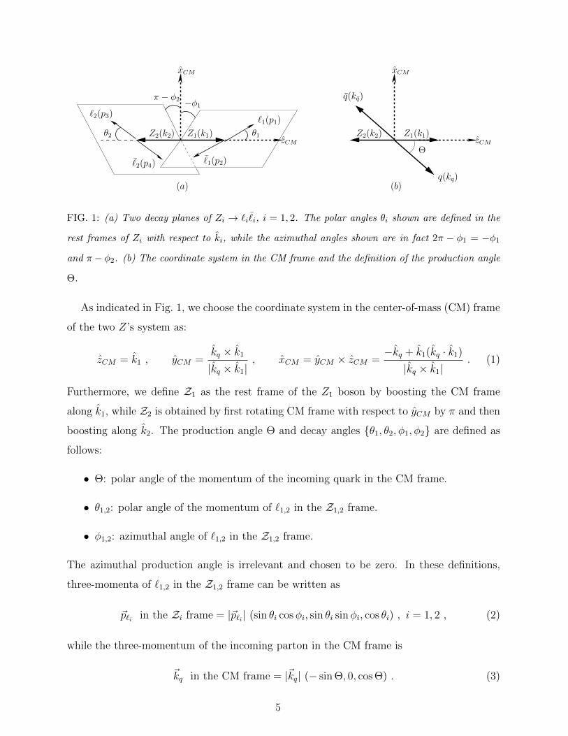
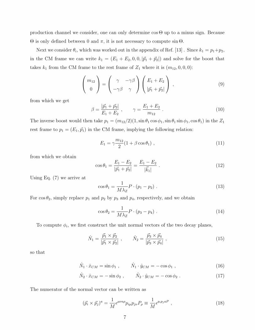
FIG. 1: (a) Two decay planes of Zi → `i ¯i, i = 1, 2. The polar angles θi shown are defined in the
rest frames of Zi with respect to ki, while the azimuthal angles shown are in fact 2π − φ1 = −φ1
and π− φ2. (b) The coordinate system in the CM frame and the definition of the production angle
Θ.
As indicated in Fig. 1, we choose the coordinate system in the center-of-mass (CM) frame
of the two Z’s system as:
zCM = k1 , yCM =kq × k1
|kq × k1|, xCM = yCM × zCM =
−kq + k1(kq · k1)
|kq × k1|. (1)
Furthermore, we define Z1 as the rest frame of the Z1 boson by boosting the CM frame
along k1, while Z2 is obtained by first rotating CM frame with respect to yCM by π and then
boosting along k2. The production angle Θ and decay angles θ1, θ2, φ1, φ2 are defined as
follows:
• Θ: polar angle of the momentum of the incoming quark in the CM frame.
• θ1,2: polar angle of the momentum of `1,2 in the Z1,2 frame.
• φ1,2: azimuthal angle of `1,2 in the Z1,2 frame.
The azimuthal production angle is irrelevant and chosen to be zero. In these definitions,
three-momenta of `1,2 in the Z1,2 frame can be written as
~p`i in the Zi frame = |~p`i | (sin θi cosφi, sin θi sinφi, cos θi) , i = 1, 2 , (2)
while the three-momentum of the incoming parton in the CM frame is
~kq in the CM frame = |~kq| (− sin Θ, 0, cos Θ) . (3)
5
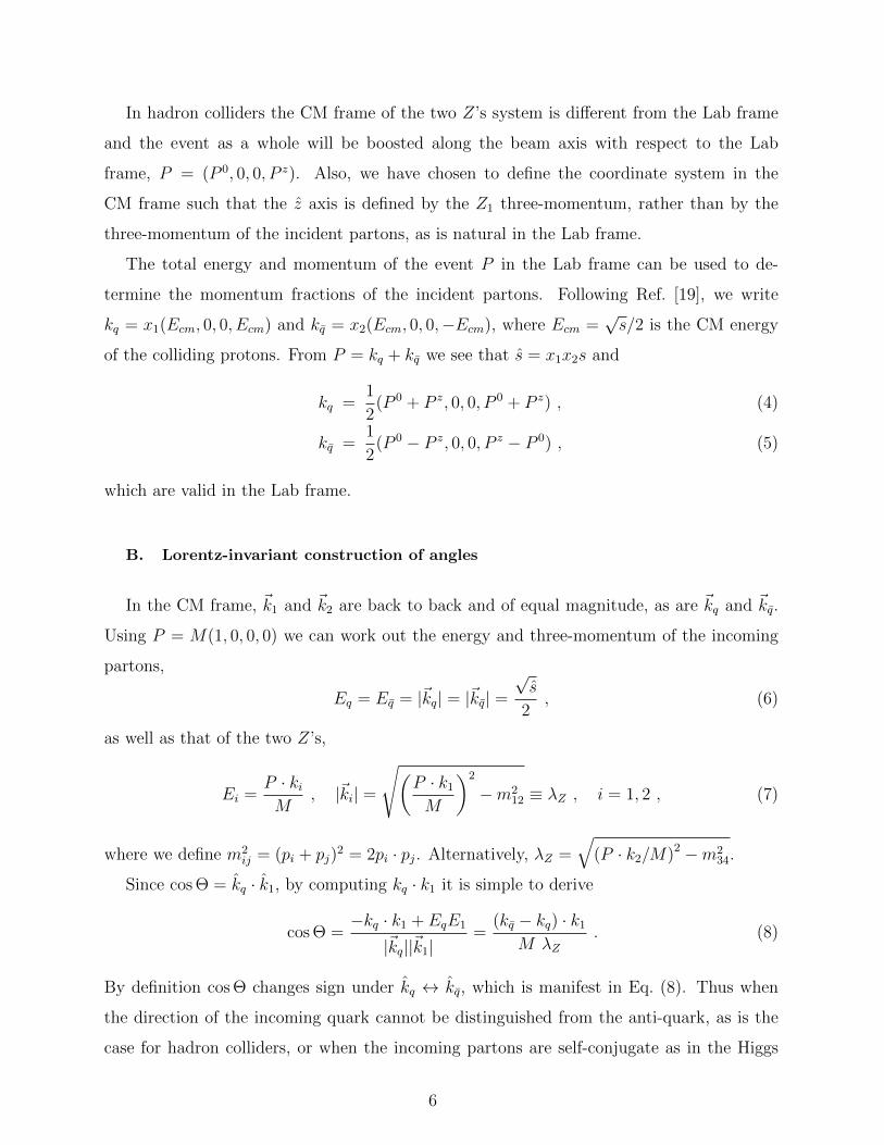
In hadron colliders the CM frame of the two Z’s system is different from the Lab frame
and the event as a whole will be boosted along the beam axis with respect to the Lab
frame, P = (P 0, 0, 0, P z). Also, we have chosen to define the coordinate system in the
CM frame such that the z axis is defined by the Z1 three-momentum, rather than by the
three-momentum of the incident partons, as is natural in the Lab frame.
The total energy and momentum of the event P in the Lab frame can be used to de-
termine the momentum fractions of the incident partons. Following Ref. [19], we write
kq = x1(Ecm, 0, 0, Ecm) and kq = x2(Ecm, 0, 0,−Ecm), where Ecm =√s/2 is the CM energy
of the colliding protons. From P = kq + kq we see that s = x1x2s and
kq =1
2(P 0 + P z, 0, 0, P 0 + P z) , (4)
kq =1
2(P 0 − P z, 0, 0, P z − P 0) , (5)
which are valid in the Lab frame.
B. Lorentz-invariant construction of angles
In the CM frame, ~k1 and ~k2 are back to back and of equal magnitude, as are ~kq and ~kq.
Using P = M(1, 0, 0, 0) we can work out the energy and three-momentum of the incoming
partons,
Eq = Eq = |~kq| = |~kq| =√s
2, (6)
as well as that of the two Z’s,
Ei =P · kiM
, |~ki| =√(
P · k1
M
)2
−m212 ≡ λZ , i = 1, 2 , (7)
where we define m2ij = (pi + pj)
2 = 2pi · pj. Alternatively, λZ =√
(P · k2/M)2 −m234.
Since cos Θ = kq · k1, by computing kq · k1 it is simple to derive
cos Θ =−kq · k1 + EqE1
|~kq||~k1|=
(kq − kq) · k1
M λZ. (8)
By definition cos Θ changes sign under kq ↔ kq, which is manifest in Eq. (8). Thus when
the direction of the incoming quark cannot be distinguished from the anti-quark, as is the
case for hadron colliders, or when the incoming partons are self-conjugate as in the Higgs
6
production channel we consider, one can only determine cos Θ up to a minus sign. Because
Θ is only defined between 0 and π, it is not necessary to compute sin Θ.
Next we consider θi, which was worked out in the appendix of Ref. [13] . Since k1 = p1+p2,
in the CM frame we can write k1 = (E1 + E2, 0, 0, |~p1 + ~p2|) and solve for the boost that
takes k1 from the CM frame to the rest frame of Z1 where it is (m12, 0, 0, 0):m12
0
=
γ −γβ−γβ γ
E1 + E2
|~p1 + ~p2|
, (9)
from which we get
β =|~p1 + ~p2|E1 + E2
, γ =E1 + E2
m12
. (10)
The inverse boost would then take p1 = (m12/2)(1, sin θ1 cosφ1, sin θ1 sinφ1, cos θ1) in the Z1
rest frame to p1 = (E1, ~p1) in the CM frame, implying the following relation:
E1 = γm12
2(1 + β cos θ1) , (11)
from which we obtain
cos θ1 =E1 − E2
|~p1 + ~p2|=E1 − E2
|~k1|. (12)
Using Eq. (7) we arrive at
cos θ1 =1
MλZP · (p1 − p2) . (13)
For cos θ2, simply replace p1 and p2 by p3 and p4, respectively, and we obtain
cos θ2 =1
MλZP · (p3 − p4) . (14)
To compute φi, we first construct the unit normal vectors of the two decay planes,
N1 =~p1 × ~p2
|~p1 × ~p2|, N2 =
~p3 × ~p4
|~p3 × ~p4|, (15)
so that
N1 · xCM = sinφ1 , N1 · yCM = − cosφ1 , (16)
N2 · xCM = − sinφ2 , N2 · yCM = − cosφ2 . (17)
The numerator of the normal vector can be written as
(~pi × ~pj)a =1
MεµνaρpiµpjνPρ ≡
1
MεpipjaP , (18)
7
where ε0123 = −ε0123 = 1. On the other hand, the Lorentz-invariant form of the numerator
can be obtained using the relations
|~pi| =1
Mpi · P , cos θij = 1− m2
ij
2|~pi||~pj|, (19)
where θij is the opening angle between ~pi and ~pj in the CM frame, so that in the end we
have
|~pi × ~pj| = |~pi||~pj| sin θij = mij
(pi · PM
pj · PM
− m2ij
4
) 12
≡ κij . (20)
One then calculates
sinφ1 = − ~p1 × ~p2
|~p1 × ~p2|· kq
sin Θ=
2
M2κ12 sin Θεp1p2kqP , (21)
cosφ1 = − ~p1 × ~p2
|~p1 × ~p2|· kq × k1
|kq × k1|= − 2
M3κ12λZ sin Θ
∣∣∣∣∣∣∣∣∣p1 · kq p1 · k1 p1 · Pp2 · kq p2 · k1 p2 · PP · kq P · k1 M2
∣∣∣∣∣∣∣∣∣ , (22)
and similarly
sinφ2 = − 2
M2κ34 sin Θεp3p4kqP , (23)
cosφ2 = − 2
M3κ34λZ sin Θ
∣∣∣∣∣∣∣∣∣p3 · kq p3 · k1 p3 · Pp4 · kq p4 · k1 p4 · PP · kq P · k1 M2
∣∣∣∣∣∣∣∣∣ . (24)
It is also worth noting that when kq → −kq, φi → π+φi. So in hadron colliders or gluon fu-
sion production we cannot distinguish between an event described by angles (Θ, θ1, θ2, φ1, φ2)
and an event described by angles (π −Θ, θ1, θ2, φ1 + π, φ2 + π).
III. DIFFERENTIAL CROSS SECTIONS
Angular distributions in ZZ(∗) → 4` provide a wealth of information on the production
mechanism of the two Z bosons [11–15, 20]. Similar angular correlations in the vector boson
fusion channel of Higgs production have also been discussed in Ref. [21]. As noted above, in
this work we focus on the search of the Higgs boson in the golden channel, h→ ZZ(∗) → 4`,
and study the possibility of differentiating the Higgs signal from the dominant irreducible
background qq → ZZ(∗) → 4` using spin correlations. In particular, we will compute the
amplitudes in a helicity basis following Ref. [17].
8
(a) (b)
q
q
q
q
Z1
Z2
Z1Z2
!1
!1
!1
!1
!2
!2
!2
!2
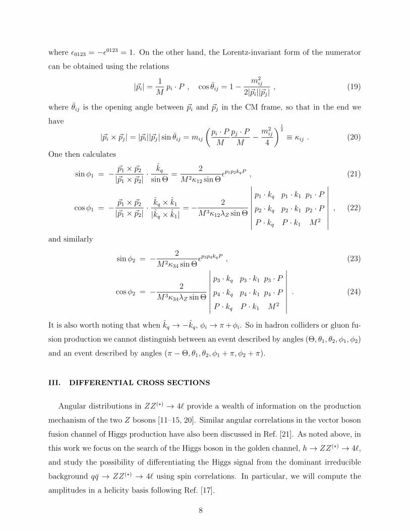
FIG. 2: Feynman diagrams contributing to qq → 4`. We only consider (a), since final states from
(b) have a total invariant mass at the Z mass.
We will present the expressions for the fully differential cross section for both the signal
and the background. Results for the Higgs production and decay have appeared in many
previous works (see, for example, Refs. [11, 13–15, 22]) and are not new. They are given
here for completeness. Earlier works on qq → ZZ(∗) → 4` include [16, 17].
Feynman diagrams contributing to qq → 4` are shown in Fig. 2. We consider only the
diagram in (a) and the corresponding u-channel diagram, as we are interested in final states
with a total invariant mass much larger than the Z mass. We will compute the amplitude
of the diagram in Fig. 2 (a) and its u-channel partner in a helicity basis, following Ref. [17].
The amplitude for the process under consideration factorizes into one production and two
decay amplitudes:
q(kq, σ) + q(kq, σ) −→ Z1(k1, λ1) + Z2(k2, λ2) , (25)
Z1(k1, λ1) −→ `1(p1, σ1) + ¯1(p2, σ2) , (26)
Z2(k2, λ2) −→ `2(p3, σ3) + ¯2(p4, σ4) , (27)
where the momentum and helicity of each particle are indicated. A similar factorization
obtains in the case of the gg → h → ZZ(∗) → 4` signal. As the production and decay
amplitudes factorize, we will consider them separately.
Before going into details of the computation, we state here the conventions we choose
for various kinematic vectors and fermion spinors. We use the explicit expressions for the
9
four-momenta and polarization vectors of the Z bosons in the CM frame:
k1 = m1γ1(1, 0, 0, β1) , (28)
k2 = m2γ2(1, 0, 0,−β2) , (29)
ε(±)1 =
1√2
(0,∓1, i, 0) , ε(0)1 = γ1(β1, 0, 0, 1) , (30)
ε(±)2 =
1√2
(0,±1, i, 0) , ε(0)2 = γ2(β2, 0, 0,−1) , (31)
where k2i = m2
i , i = 1, 2 is the invariant mass of Zi, which could be off the mass shell, and
the boost factors are
γ1 =1√
1− β21
=
√s
2m1
(1 + x) , γ2 =1√
1− β22
=
√s
2m1
(1− x) , x =m2
1 −m22
s. (32)
We will also use the explicit forms of u(p, λ) and v(p, λ) spinors:
uR =
0
0√
2E
0
, uL =
0√
2E
0
0
, vR =
√
2E
0
0
0
, vL =
0
0
0
−√
2E
, (33)
where E is the energy (or momentum) of the massless lepton. In these expressions, u(p, λ)
have been defined for p in the z direction and v(p, λ) have been defined for p in the −zdirection. Our conventions here are those in [17, 18]; these were chosen so that our qq →ZZ(∗) helicity amplitudes would reduce to those in Ref. [17] in the limit where the Z bosons
are on shell.
A. Production amplitudes for the signal
Because the Higgs is a scalar particle, the two Z bosons can only have the following three
helicity combinations: (0, 0) and (±1,±1). Since the gluon-gluon-Higgs coupling is given by
αs12πv
hGµνGµν , (34)
where v = 246 GeV is the Higgs vev, the production helicity amplitude MZZh;λ1λ2
for gg →h→ ZZ(∗) can be written as
MZZh;±1±1 =
αsm2Z s
3πv2((s−m2h)
2 +m2hΓ
2h)
1/2, (35)
MZZh;00 = γ1γ2(1 + β1β2)
αsm2Z s
3πv2((s−m2h)
2 +m2hΓ
2h)
1/2. (36)
10
This is the amplitude for a particular spin and color configuration for the initial gluons. In
the interest of clarity, we do not write the gluon helicities in the above amplitude, however
these amplitudes should be taken as the amplitude for the ++ or −− initial state gluon
helicities. For the other two helicity combinations, the amplitude vanishes. We will average
the squared sum of these amplitudes over spin and color when finding the differential cross
section. It is worth pointing out that, as one can easily see from Eq. (35), in the high energy
limit when the Higgs is heavy, the boost factor γ 1 and the amplitude for two longitudinal
Z bosons, (λ1, λ2) = (0, 0), dominate over those for the transverse Zs.
B. Production amplitudes for the background
The production helicity amplitude for qq → Z1Z2 in the CM frame reads [17]
MZZσσ;λ1λ2
= 4√
2(gZqq∆σ
)2
ε δ|∆σ|,±1
A∆σλ1λ2
(Θ) dJ0∆σ,∆λ(Θ)
4β1β2 sin2 Θ + (1− β1β2)2 − x2(1 + β1β2)2. (37)
In the above ∆σ = σ−σ, ε = ∆σ(−1)λ2 , ∆λ = λ1−λ2, and J0 = max(|∆σ|, |∆λ|). Note that
in the limit of massless quarks, which we consider in this work, the amplitude in Eq. (37)
vanishes for ∆σ = 0. The left- and right-handed coupling of quarks to the Z boson are given
by:
gZqq∆σ =|e|(T3 −Q sin2 θW )
sin θW cos θW, (38)
where T3 = 0 for right-handed quarks. Furthermore, dJ0∆σ,∆λ(Θ) is the d function in the
convention of the Particle Data Group [23]. The coefficients A∆σλ1λ2
are
∆λ = ±2 : A∆σ±∓ = −
√2(1 + β1β2) , (39)
∆λ = ±1 : A∆σ±0 =
1
γ2(1 + x)
[(∆σ∆λ)
(1 +
β21 + β2
2
2
)− 2 cos Θ
−(∆σ∆λ)(β22 − β2
1)x− 2x cos Θ− (∆σ∆λ)
(1− β2
1 + β22
2
)x2
](40)
: A∆σ0± =
1
γ1(1− x)
[(∆σ∆λ)
(1 +
β21 + β2
2
2
)− 2 cos Θ
−(∆σ∆λ)(β22 − β2
1)x+ 2x cos Θ− (∆σ∆λ)
(1− β2
1 + β22
2
)x2
](41)
∆λ = 0 : A∆σ±± = −(1− β1β2) cos Θ− λ1∆σ(1 + β1β2)x , (42)
∆λ = 0 : A∆σ00 = 2γ1γ2 cos Θ
[((1− x)β1 + (1 + x)β2)
√β1β2
1− x2− (1 + β2
1β22)
]. (43)
11
It can be checked that in the on-shell limit when x → 0, β1, β2 → β, and γ1, γ2 → γ,
the above expressions reduce to those presented in Appendix D of Ref. [17]. Moreover, in
the high energy limit when γ 1, the ∆λ = ±2 amplitudes dominate, corresponding to
(λ1, λ2) = (±,∓).
C. Amplitudes for Z boson decay to leptons
The decay helicity amplitude for the 1→ 2 process such as Z → `¯ is essentially a matrix
element of the spin-1 rotation matrix, which is the inner product between states with definite
projections of angular momenta along a chosen axis [19]. We have defined our angles, in
particular θ1, θ2, φ1, and φ2, such that we need consider only Zi(λ) → `σ(θi, φi)¯σ. That
is, the amplitude has the same form for i = 1 and for i = 2. Specifically, following the
conventions described above in Eq. (28) and (33), we find that
M(i)λi;σiσi
= ∆σi (−1)λi√
2 gZ`¯
∆σ d(∆σi, λi, θi) mi eiλiφi , (44)
where d(∆σi, λi, θi) = dmax( |∆σi|, |λi| )∆σi, λi
(θi) in the conventions of Ref. [23]. In the above, mi is
the invariant mass of Zi, λi is its helicity, ∆σi = σi − σi, and the coupling of the Z to the
lepton pair is
gZ`¯
∆σ =|e|(T3 + sin2 θW )
sin θW cos θW, (45)
where T3 = −1/2 (0) for left (right)-handed leptons. Note that the amplitude in Eq. (44)
vanishes for ∆σi = 0 in the limit of massless leptons, which is the limit taken in this work.
For ∆σi = −1, the expression in Eq. (44) reproduces Eq. (4.8a) in Ref. [17].
D. Differential cross sections for signal and background
The full amplitude of qq → Z1Z2 → (`1¯1)(`2
¯2) is then
M(σ, σ;σi) =∑λ1,λ2
MZZσσ;λ1λ2
DZ(k21)DZ(k2
2) M(1)λ1;σ1σ1
M(2)λ2;σ2σ2
, (46)
where the propagator factor for the Z boson may be taken to be
DZ(q2) =1
q2 −m2Z + imZΓZ
. (47)
12
The full differential cross section is then (using the short-hand notation Ω =
Θ, θ1, θ2, φ1, φ2 and dΩ = d cos Θ d cos θ1 d cos θ2 dφ1 dφ2)
dσ
dΩ dm21 dm
22
= 2π1
4
1
3
1
2s
β1(1 + x)
32π2
(1
32π2
)2(1
2π
)2 ∑σ,σ,σi
|M(σ, σ;σi)|2 , (48)
where 2π comes from integrating over the unobservable production azimuthal angle, 1/4
from averaging over initial spin states, 1/3 from averaging initial color states, 1/(2s) from
the incoming flux, β1(1 + x)/(32π2) from the ZZ(∗) two-body phase space, 1/(32π2) from
the phase space of each of the `¯ final states, and 1/(2π) from each dm2i integral that one
obtains when re-expressing the four particle phase space in terms of the dm2i variables (see
for example [24]).
Likewise, in the case of the gg → h→ Z1Z2 → (`1¯1)(`2
¯2) signal, the full amplitude is
M(h;σi) =∑λ1,λ2
MZZh;λ1λ2
DZ(k21)DZ(k2
2) M(1)λ1;σ1σ1
M(2)λ2;σ2σ2
, (49)
and the full differential cross section is
dσ
dΩ dm21 dm
22
= 2π1
4
1
8
1
2s
β1(1 + x)
32π2
(1
32π2
)2(1
2π
)2 (2
)∑σi
|M(h;σi)|2 . (50)
Note that the only significant difference between Eq. (48) and Eq. (50) is that color averaging
yields a factor of 13
in Eq. (48), but 18
in Eq. (50). The factor of 2 before the sum in Eq. (50)
is from summing over initial gluon helicities.
Before proceeding, we note our definitions of Z1 and Z2. When the two Z bosons decay
into 2e2µ final states, we define Z1 to be the parent particle of the electron/positron pair,
while for 4e or 4µ final states, Z1 is the Z with lower invariant mass. Technically, one
could reconstruct e.g. a 4µ final state in two ways (in terms of assigning a particular muon
and a particular antimuon to a given Z), however generally one of these reconstructions
would make the resulting Zs far off-shell. Hence we only keep the reconstruction for which
the product of the Z Breit-Wigner factors is largest. We note that the total event rate of
ZZ(∗) → 2e2µ is a factor of two larger than that of ZZ(∗) → 4e or ZZ(∗) → 4µ.
E. Angular distributions
Analytic expressions for the background and signal distributions are contained in Eqs. (48)
and (50). However, they are too long to be presented explicitly and not very illuminating.
13
0 1 2 3 4 5 60.10
0.12
0.14
0.16
0.18
0.20
Φ1
dΣN
dΦ1
s = 220 GeV
0 1 2 3 4 5 60.10
0.12
0.14
0.16
0.18
0.20
F
dΣN
dF
s = 220 GeV
-1.0 -0.5 0.0 0.5 1.00.0
0.2
0.4
0.6
0.8
1.0
cos Θ1
dΣN
dcos
Θ1
s = 220 GeV
-1.0 -0.5 0.0 0.5 1.00.0
0.2
0.4
0.6
0.8
1.0
cos Q
dΣN
dcos
Q
s = 220 GeV
0 1 2 3 4 5 60.10
0.12
0.14
0.16
0.18
0.20
Φ1
dΣN
dΦ1
s = 350 GeV
0 1 2 3 4 5 60.10
0.12
0.14
0.16
0.18
0.20
F
dΣN
dFs = 350 GeV
-1.0 -0.5 0.0 0.5 1.00.0
0.2
0.4
0.6
0.8
1.0
cos Θ1
dΣN
dcos
Θ1
s = 350 GeV
-1.0 -0.5 0.0 0.5 1.00.0
0.2
0.4
0.6
0.8
1.0
cos Q
dΣN
dcos
Q
s = 350 GeV
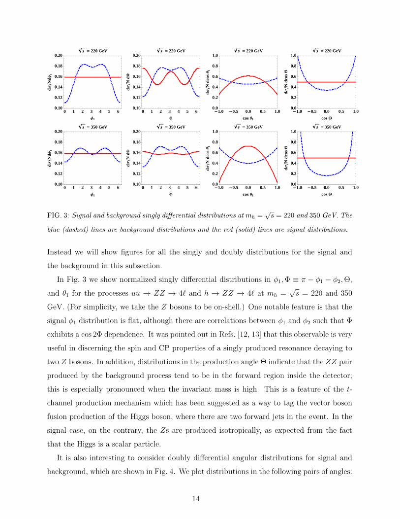
FIG. 3: Signal and background singly differential distributions at mh =√s = 220 and 350 GeV. The
blue (dashed) lines are background distributions and the red (solid) lines are signal distributions.
Instead we will show figures for all the singly and doubly distributions for the signal and
the background in this subsection.
In Fig. 3 we show normalized singly differential distributions in φ1,Φ ≡ π − φ1 − φ2,Θ,
and θ1 for the processes uu → ZZ → 4` and h → ZZ → 4` at mh =√s = 220 and 350
GeV. (For simplicity, we take the Z bosons to be on-shell.) One notable feature is that the
signal φ1 distribution is flat, although there are correlations between φ1 and φ2 such that Φ
exhibits a cos 2Φ dependence. It was pointed out in Refs. [12, 13] that this observable is very
useful in discerning the spin and CP properties of a singly produced resonance decaying to
two Z bosons. In addition, distributions in the production angle Θ indicate that the ZZ pair
produced by the background process tend to be in the forward region inside the detector;
this is especially pronounced when the invariant mass is high. This is a feature of the t-
channel production mechanism which has been suggested as a way to tag the vector boson
fusion production of the Higgs boson, where there are two forward jets in the event. In the
signal case, on the contrary, the Zs are produced isotropically, as expected from the fact
that the Higgs is a scalar particle.
It is also interesting to consider doubly differential angular distributions for signal and
background, which are shown in Fig. 4. We plot distributions in the following pairs of angles:
14
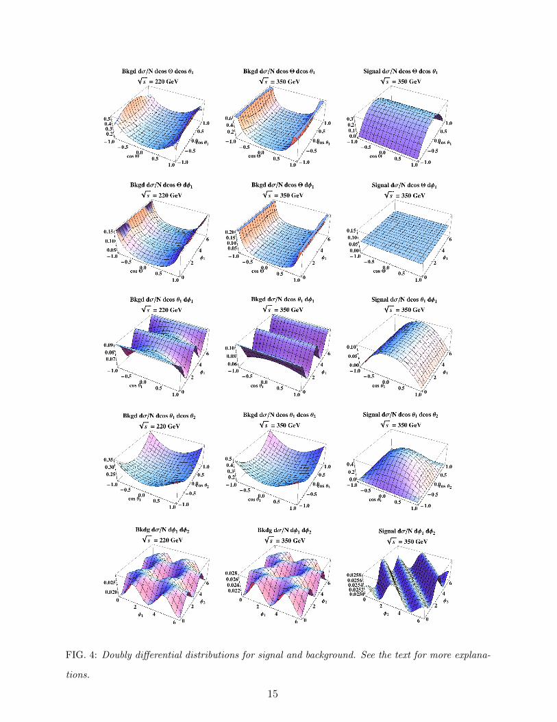
FIG. 4: Doubly differential distributions for signal and background. See the text for more explana-
tions.
15
(Θ, θ1), (Θ, φ1), (θ1, φ1), (θ1, θ2), and (φ1, φ2). The background distributions are again from
uu initial states and shown for√s = 220 and 350 GeV. We observe noticeable changes in
the distributions of the first three pairs of variables for these two different center-of-mass
energies. On the other hand, the signal distributions do not change as much when one varies
the Higgs mass, except for the (φ1, φ2) distributions, and are shown only for mh = 350 GeV.
The background exhibits strong correlations between the pairs of angles in all five cases.
IV. STATISTICAL PROCEDURES
Likelihood methods are frequently employed to establish the presence, or lack, of a signal
using kinematic distributions which discriminate signal from background. For example, if
the purpose is discovery, one considers the “null hypothesis” assuming the observed data
set is entirely due to background and an “alternative hypothesis” assuming the presence of
both signal and background. A likelihood function is defined for each hypothesis to quantify
the probability of obtaining the actual data under that particular hypothesis. In order to
accept or reject one hypothesis in favor of the other, a “test statistic” must also be defined.
In quantum field theory there is a natural object quantifying the probability of obtaining
a particular event in a given set of data: the differential cross section. This motivates the
use of the MEM, which is simply the use of likelihood methods where the probability density
function (pdf) used in the likelihood is the properly normalized differential cross section (or
“matrix element”) with respect to certain kinematic variables1. When the number of events
is small one can include every event in the evaluation of the likelihood. This “unbinned
likelihood method” is what we adopt in the following.
A. Extended maximum likelihood method
When there exist free parameters in the underlying hypothesis one wishes to test2, statis-
tically preferred values of the parameters of the underlying model are found by maximizing
the likelihood function with respect to those parameters. When the overall number of events
is not fixed but allowed to fluctuate, the normalization of the likelihood function may become
1 We use “pdf” for probability density function and “PDF” for parton distribution function.2 In such cases the hypothesis is called “composite”, while those without free parameters are called “simple”.
16

a free parameter. In this case, one is using the “extended” maximum likelihood method [25],
which we employ in this work.
To be more specific, we consider the likelihood for some collider signature with (unknown)
expected number of events µ described by kinematic information x = x1, x2, ...xN, where
the xi are kinematic variables describing event i of N total events. The unbinned likelihood
is simply
L(µ;θ) =e−µµN
N !
N∏i=1
P (θ;xi), (51)
where P (θ;x) is the pdf for the kinematic variables as a function of θ, the parameters of the
underlying model. In the MEM, P (θ, x) is the differential cross section normalized by the
total cross section, generally scaled by efficiencies and acceptances of the detector involved.
We will define Ps(mh, xi) to be the normalized pdf for the signal process, which depends
on one underlying parameter, the Higgs mass mh.3 The normalized pdf for the background
process is then given by Pb(xi); it is assumed here that the differential cross section for the
background process is known and contains no unknown parameters. The likelihood function
for the signal plus background hypothesis is then given by
Ls+b(µ, f,mh) =e−µµN
N !
N∏i=1
[fPs(mh;xi) + (1− f)Pb(xi)] , (52)
where µ = µs + µb is the sum of the expected number of signal events µs and expected
number of background events µb, while the signal fractional yield f is defined as
0 < f =µs
µs + µb< 1 . (53)
We often refer to f simply as the “yield”. For Lb, the likelihood for the background-only
hypothesis, we simply set µs = 0. When computing the likelihood for each hypothesis, we
calculate the maximum of Ls+b in µ,mh, f and Lb in µ, respectively4. In practice, since
the Poisson distribution factors in the definition of the likelihood function, the maximum of
the likelihood always occurs at µ = N . So effectively one can replace µ by N , the measured
total number of events, in the calculation.
3 We set the Higgs width to the SM value for the given Higgs mass, mh, as found by HDECAY [26].4 In our fitting procedure, we look for the local maximum closest to the true Higgs mass.
17

B. Expected significance
In determining the significance for Higgs discovery from a set of events, we are really
comparing the likelihood of two hypotheses: (i) that the events consist of signal events from
the Higgs boson at some mass, as well as events from background qq → ZZ(∗) production,
and (ii) that all the events are due to qq → ZZ(∗) production. Our choice of test statistic
for describing this relative likelihood is the likelihood ratio
Q =Ls+bLb
, (54)
from which the significance of discovery is computed
S =√
2 lnQ . (55)
This test statistic was used by the LEP experiments in their Higgs searches [27], while its use
for h→ ZZ(∗) → 4µ was studied in Ref. [28]. In our case we include the angular correlations
in the likelihood function. The expected significance S is then obtained by performing a large
number of pseudo-experiments and choosing the median value. The 1 and 2 σ spreads in Sare determined from the distribution of significances obtained from the pseudo-experiments.
C. Exclusion limit
We determine the exclusion limit, in the absence of a signal, by setting an upper limit on
the yield, f , defined in Eq. (53). For a particular choice of Higgs mass mh, we define a pdf
f by considering the likelihood Ls+b as a function of f ,
p(f) =Ls+b(N, f, mh)∫ 1
0Ls+b(N, f , mh) df
. (56)
The 95% confidence level limit on f for a given set of data is given by α as follows:∫ α
0
p(f) df = 0.95. (57)
We then translate α into a 95% confidence level upper limit on the Higgs production cross
section by unfolding with the detector acceptances and efficiencies. The expected exclusion
limit is obtained by performing a large number of pseudo-experiments.
It should be noted that the procedure above for setting the exclusion limit only takes into
account differences in the shape of kinematic distributions between signal and background.
18
In particular we are mainly interested in possible improvements by including angular distri-
bution in addition to the invariant mass spectrum. Typically experimental collaborations
set limits directly on the normalization of the signal cross section by performing counting
experiments in a particular window of total invariant mass. In comparison with the standard
CLs method employed by ATLAS and CMS collaborations, our method should be consid-
ered as a shortcut for the purpose of understanding the improvement from incorporating
the angular correlations. One would hope to incorporate both the counting experiments and
shape measurements in a more complete study.
D. Probability density functions
In this subsection we define the signal and background pdfs that enter into the likelihood
function in Eq. (52). The kinematic observables are x = Y, s,m21,m
22,Ω, where Y is the
pseudo-rapidity of the ZZ(∗) system, s is the partonic center-of-mass energy, m1(2) is the
invariant mass of the Z1(2) boson, and Ω represents the production and decay angles.
The signal pdf is
Ps(mh;x) =1
εsσs(mh)
dσs(mh;x)
dY ds dm21 dm
22 dΩ
, (58)
where σs(mh) is the total hadronic cross section, dσs is the corresponding differential cross
section, and εs is the total signal efficiency (which in principle includes geometric acceptance
as well as reconstruction efficiencies). More explicitly,
Ps(mh;x) =1
εsσs(mh)
(fg(x1)fg(x2)
s
)dσh(mh, s,m1,m2,Ω)
dm21 dm
22 dΩ
. (59)
In the above, σh is the partonic cross section, and the fg(x) is the gluon PDF.
For the background pdf we take into account the fact that, in a hadron collider, we are
unable to determine the direction of the initial quark (as opposed to the anti-quark) on an
event-by-event basis by calculating the cross section for each choice of initial quark direction
and summing the two. This may be written as
Pb(x) =1
εbσqq
((fq(x1)fq(x2)
s
)dσqq(s, m1,m2,Ω)
dm21 dm
22 dΩ
+
(fq(x1)fq(x2)
s
)dσqq(s, m1,m2,Ω
′)
dm21 dm
22 dΩ′
),
(60)
where Ω′ ≡ (π − Θ, θ1, θ2, φ1 + π, φ2 + π) is the shift in angles needed for an initial quark
in the −z direction and we have switched the quark PDF with the anti-quark PDF (or
19

-4 -2 0 2 40
500
1000
1500
2000
2500
Dm HGeVL
Nu
mb
ero
fE
ven
ts Z®Μ+Μ-
Z®e+e-
-0.04 -0.02 0.00 0.02 0.040
500
1000
1500
2000
DQ
Nu
mb
ero
fE
ven
ts
-0.04 -0.02 0.00 0.02 0.040
1000
2000
3000
4000
DΘ1
Nu
mb
ero
fE
ven
ts Z®Μ+Μ-
Z®e+e-
-0.04 -0.02 0.00 0.02 0.040
1000
2000
3000
4000
DΦ1
Nu
mb
ero
fE
ven
ts Z®Μ+Μ-
Z®e+e-
FIG. 5: Effect of detector resolution in measuring E and pT on kinematic variables. Each of the
histograms were generated using twenty thousand events. The channel used for these plots is the
background 2e2µ channel.
equivalently switched x1 and x2). The total qq → ZZ∗ → 4` cross section is given by σqq
with the function fq(q) representing the quark (anti-quark) PDF, and εb the total efficiency
for this channel. In calculating the cross section, σqq, for the qq → ZZ(∗) → 4` background,
we sum over the quark flavors, u, d, s and c. We use CTEQ5L for the PDFs indicated in
Eq. (59) and Eq. (60) as fi(x) [29].
V. MONTE CARLO SIMULATIONS
We generate the signal and background events for our analysis using Mad-
Graph/MadEvent (MG/ME) version 4.4.52 [30]. Proton-proton collisions at√s = 7 TeV
are implemented with the CTEQ5L [29] PDFs. As noted above, the main irreducible back-
ground, and the only one which we will consider in our analysis, is qq → ZZ(∗) → 4`. For
signal we consider only gg → h → ZZ(∗) → 4`, without additional jets in the final states;
effectively our analysis considers only the “0-jet bin” for the ZZ(∗) → 4` channel.
20
Detector effects are modeled by applying Gaussian smearing to the energy of electrons
according to (σE,eE
)2
=(0.036√
E
)2
+ 0.00262, (61)
and to the pT of muons according to
σpT ,µ = 0.015 pT − 5.710−6 p2T + 2.210−7 p3
T . (62)
These expressions follow the CMS TDR [31]. The value of the constant term in Eq. (61) may
be somewhat optimistic. However, we verified that our results do not change significantly
when using a value for this quantity that is twice as large. The smearing of the muon pT
is quite conservative as we have used the resolution corresponding to 1.8 < |η| < 2.0 and
assumed this to be the same for lower values of η as well. The angles measured in the lab
frame are not smeared. Nevertheless, angles which define the kinematics of the four lepton
system, as described in Sect. II, are affected by the E and pT resolution, as can be seen
in Fig. 5. A more sophisticated treatment of detector effects would include the effects of
reconstruction efficiencies, which we neglect for simplicity.
Another effect of smearing the lepton E or pT is that the four lepton system will now
have a small pT in the lab frame, even without the presence of additional jets or particles in
the final states. We simply boost away this induced pT and proceed to define angles as in
Section II.
After generating events and smearing the lepton pT , we apply the following cuts to each
of the lepton in the lab frame:
|pT | ≥ 10 GeV ,
|η| ≤ 2.5 .
Moreover, we focus on the following window for the 4` invariant mass
150 GeV ≤ s ≤ 450 GeV . (63)
The efficiency (geometric acceptance) for our selection of signal events is listed in Table I
and varies from ∼ 0.5 to ∼ 0.7 as we increase the mass of the Higgs boson from 170 GeV
to 350 GeV. The efficiency for selection of background events is 0.52. Moreover, these cuts
affect the reconstructed angular distributions. As can be seen in Fig. 6, the distributions
21
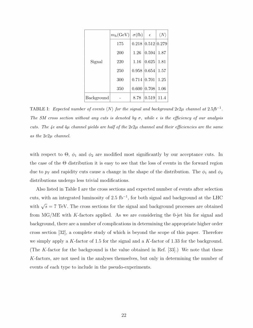
Signal
mh(GeV) σ(fb) ε 〈N〉
175 0.218 0.512 0.279
200 1.26 0.594 1.87
220 1.16 0.625 1.81
250 0.958 0.654 1.57
300 0.714 0.701 1.25
350 0.600 0.708 1.06
Background - 8.78 0.519 11.4
TABLE I: Expected number of events 〈N〉 for the signal and background 2e2µ channel at 2.5fb−1.
The SM cross section without any cuts is denoted by σ, while ε is the efficiency of our analysis
cuts. The 4e and 4µ channel yields are half of the 2e2µ channel and their efficiencies are the same
as the 2e2µ channel.
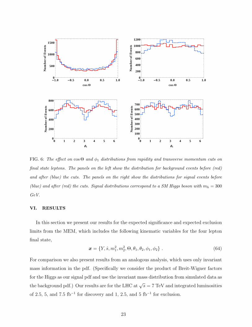
with respect to Θ, φ1 and φ2 are modified most significantly by our acceptance cuts. In
the case of the Θ distribution it is easy to see that the loss of events in the forward region
due to pT and rapidity cuts cause a change in the shape of the distribution. The φ1 and φ2
distributions undergo less trivial modifications.
Also listed in Table I are the cross sections and expected number of events after selection
cuts, with an integrated luminosity of 2.5 fb−1, for both signal and background at the LHC
with√s = 7 TeV. The cross sections for the signal and background processes are obtained
from MG/ME with K-factors applied. As we are considering the 0-jet bin for signal and
background, there are a number of complications in determining the appropriate higher order
cross section [32], a complete study of which is beyond the scope of this paper. Therefore
we simply apply a K-factor of 1.5 for the signal and a K-factor of 1.33 for the background.
(The K-factor for the background is the value obtained in Ref. [33].) We note that these
K-factors, are not used in the analyses themselves, but only in determining the number of
events of each type to include in the pseudo-experiments.
22
-1.0 -0.5 0.0 0.5 1.00
500
1000
1500
cos Q
Nu
mb
ero
fE
ven
ts
-1.0 -0.5 0.0 0.5 1.00
200
400
600
800
1000
1200
cos Q
Nu
mb
ero
fE
ven
ts
0 1 2 3 4 5 60
200
400
600
800
Φ1
Nu
mb
ero
fE
ven
ts
0 1 2 3 4 5 60
100
200
300
400
500
600
700
Φ1
Nu
mb
ero
fE
ven
ts
FIG. 6: The effect on cos Θ and φ1 distributions from rapidity and transverse momentum cuts on
final state leptons. The panels on the left show the distribution for background events before (red)
and after (blue) the cuts. The panels on the right show the distributions for signal events before
(blue) and after (red) the cuts. Signal distributions correspond to a SM Higgs boson with mh = 300
GeV.
VI. RESULTS
In this section we present our results for the expected significance and expected exclusion
limits from the MEM, which includes the following kinematic variables for the four lepton
final state,
x = Y, s,m21,m
22,Θ, θ1, θ2, φ1, φ2 . (64)
For comparison we also present results from an analogous analysis, which uses only invariant
mass information in the pdf. (Specifically we consider the product of Breit-Wigner factors
for the Higgs as our signal pdf and use the invariant mass distribution from simulated data as
the background pdf.) Our results are for the LHC at√s = 7 TeV and integrated luminosities
of 2.5, 5, and 7.5 fb−1 for discovery and 1, 2.5, and 5 fb−1 for exclusion.
23
A. Expected significance
To compute the expected significance, we perform ten thousand pseudo-experiments
(each) for Higgs masses of 175, 200, 220, 250, 300, and 350 GeV. Each pseudo-experiment
consists of signal and background events with 4µ, 2e2µ, and 4e final states; the number of
events of each type are chosen from Poisson distributions, where the expected numbers of
signal and background events are given by the product of the luminosity under considera-
tion, the theoretical cross section, and acceptance efficiencies after smearing and cuts. The
cross section after cuts is also used to normalize the signal and background pdfs Ps and
Pb in the likelihood function in Eq. (52). As we do not include the different reconstruction
efficiencies for electrons and muons in our analysis, Ps and Pb are identical for 4µ, 2e2µ, and
4e final states. However, we do consider the yields in each channel as separate parameters
when finding the significance from pseudo-experiments by maximizing the likelihood with
respect to the undetermined parameters.
The median values of significance obtained for each Higgs mass in this channel, using
both the MEM (all kinematic variables) and the likelihood method (invariant mass only),
are shown in Fig. 7. The 1σ and 2σ bands on the significance obtained from the MEM
are also shown in this figure. We do not show the corresponding bands for the invariant
mass-based analysis; the widths of the bands for this case are similar.
We note that the MEM consistently outperforms the invariant mass only method, and
that the effect is more pronounced, on the order of 10 - 20 %, at higher Higgs masses. This
is because the helicity amplitudes for h→ ZZ(∗) and qq → ZZ(∗) are increasingly different
at larger values of invariant mass. More specifically, as already pointed out in Sect. III,
the (λ1, λ2) = (±1,∓1) amplitudes dominate in the high mass case for qq, while only the
(λ1, λ2) = (0, 0) amplitude survives in the heavy Higgs limit in the h→ ZZ(∗) case.
B. Exclusion
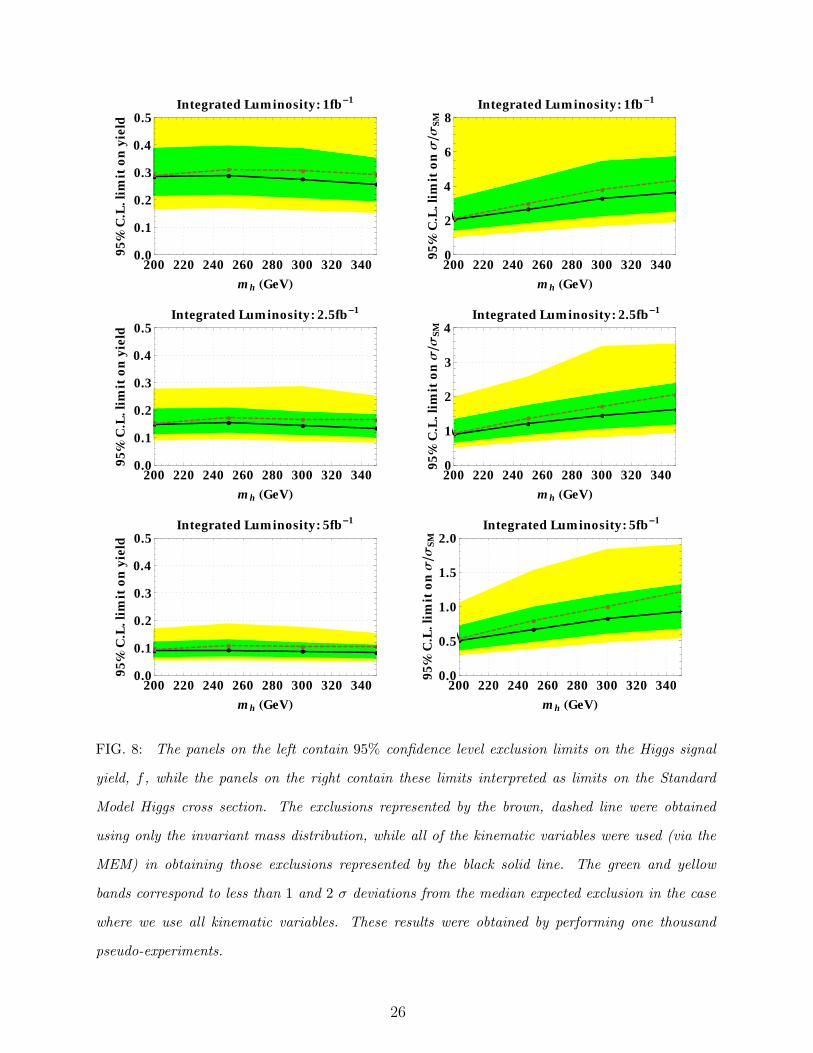
In Figure 8, we show the median 95% confidence level exclusions on the yield parameter
f , both as obtained with the MEM and as obtained with a likelihood method using only
invariant mass information. These limits were obtained using the procedure described in
Subsection IV C to find the 95% confidence limit on f in a given pseudo-experiment consist-
24

æ
ææ
ææ æ
æ
ææ
æ
æ æ
200 250 300 3500
2
4
6
8
mh HGeVL
2ln
Q
Integrated Luminosity: 2.5fb-1
æ
ææ
ææ æ
æ
ææ
æ
æ æ
200 250 300 3500
2
4
6
8
mh HGeVL
2ln
Q
Integrated Luminosity: 5fb-1
æ
ææ
æ
ææ
æ
æ
æ
æ
æ æ
200 250 300 3500
2
4
6
8
mh HGeVL
2ln
Q
Integrated Luminosity: 7.5fb-1
FIG. 7: Comparison of significance for Higgs discovery obtained from using only invariant mass
information (brown dotted line) with that obtained from all of the kinematic variables using the
MEM (black solid line) at different integrated luminosities. The green and yellow bands correspond
to less than 1 and 2 σ deviations from the median expected significance in the case where we use
all kinematic variables.
25
æ
æ ææ
æ
æ
æ
æ ææ
200 220 240 260 280 300 320 3400.0
0.1
0.2
0.3
0.4
0.5
mh HGeVL
95%
C.L
.lim
ito
nyi
eld
Integrated Luminosity: 1fb-1
æ
æ
æ
æ
ææ
æ
æ
æ
æ
200 220 240 260 280 300 320 3400
2
4
6
8
mh HGeVL
95%
C.L
.lim
ito
nΣ
Σ SM
Integrated Luminosity: 1fb-1
æ
æ ææ
æ
æ
æ
æ æ æ
200 220 240 260 280 300 320 3400.0
0.1
0.2
0.3
0.4
0.5
mh HGeVL
95%
C.L
.lim
ito
nyi
eld
Integrated Luminosity: 2.5fb-1
æ
æ
æ
æ
æ
æ
æ
æ
æ
æ
200 220 240 260 280 300 320 3400
1
2
3
4
mh HGeVL
95%
C.L
.lim
ito
nΣ
Σ SM
Integrated Luminosity: 2.5fb-1
æ
æ æ æ æ
æ
ææ æ æ
200 220 240 260 280 300 320 3400.0
0.1
0.2
0.3
0.4
0.5
mh HGeVL
95%
C.L
.lim
ito
nyi
eld
Integrated Luminosity: 5fb-1
æ
æ
æ
æ
æ
æ
æ
æ
æ
æ
200 220 240 260 280 300 320 3400.0
0.5
1.0
1.5
2.0
mh HGeVL
95%
C.L
.lim
ito
nΣ
Σ SM
Integrated Luminosity: 5fb-1
FIG. 8: The panels on the left contain 95% confidence level exclusion limits on the Higgs signal
yield, f , while the panels on the right contain these limits interpreted as limits on the Standard
Model Higgs cross section. The exclusions represented by the brown, dashed line were obtained
using only the invariant mass distribution, while all of the kinematic variables were used (via the
MEM) in obtaining those exclusions represented by the black solid line. The green and yellow
bands correspond to less than 1 and 2 σ deviations from the median expected exclusion in the case
where we use all kinematic variables. These results were obtained by performing one thousand
pseudo-experiments.
26
ing only of background events, which were generated, as in our investigation of significance,
using the method described in Section V. We note that in obtaining these limits, the yield,
f , was fixed to be the same for each of the three channels (4e, 2e2µ, and 4µ), and one
thousand pseudo-experiments were performed.
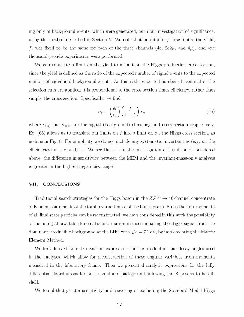
We can translate a limit on the yield to a limit on the Higgs production cross section,
since the yield is defined as the ratio of the expected number of signal events to the expected
number of signal and background events. As this is the expected number of events after the
selection cuts are applied, it is proportional to the cross section times efficiency, rather than
simply the cross section. Specifically, we find
σs =
(εbεs
)(f
1− f
)σb, (65)
where εs(b) and σs(b) are the signal (background) efficiency and cross section respectively.
Eq. (65) allows us to translate our limits on f into a limit on σs, the Higgs cross section, as
is done in Fig. 8. For simplicity we do not include any systematic uncertainties (e.g. on the
efficiencies) in the analysis. We see that, as in the investigation of significance considered
above, the difference in sensitivity between the MEM and the invariant-mass-only analysis
is greater in the higher Higgs mass range.
VII. CONCLUSIONS
Traditional search strategies for the Higgs boson in the ZZ(∗) → 4` channel concentrate
only on measurements of the total invariant mass of the four leptons. Since the four-momenta
of all final state particles can be reconstructed, we have considered in this work the possibility
of including all available kinematic information in discriminating the Higgs signal from the
dominant irreducible background at the LHC with√s = 7 TeV, by implementing the Matrix
Element Method.
We first derived Lorentz-invariant expressions for the production and decay angles used
in the analyses, which allow for reconstruction of these angular variables from momenta
measured in the laboratory frame. Then we presented analytic expressions for the fully
differential distributions for both signal and background, allowing the Z bosons to be off-
shell.
We found that greater sensitivity in discovering or excluding the Standard Model Higgs
27
boson can be achieved when including spin correlations in addition to total invariant mass
measurements. Generally, these improvements are on the order of 10 - 20 %; they are
larger for higher Higgs masses, for which the differences between signal and background
distributions are greater.
Searching for the Higgs boson is among the top priorities of the physics program at
the LHC. Our results indicate it would be worthwhile to include full angular distributions
in actual experimental searches in the golden channel through some type of multivariate
analyses. Whether a Standard Model Higgs boson will be discovered or excluded in the near
future, we eagerly await the result!
Acknowledgments
We would like to thank Johan Alwall, Pierre Artoisenet, Pushpa Bhat, Qinghong Cao,
Johannes Heinonen, Wai-Yee Keung, Jen Kile, Andrew Kobach, Andrew Kubik, Tom
LeCompte, Joe Lykken, Olivier Mattelaer, Frank Petriello, Seth Quackenbush, Heidi Schell-
man, Michael Schmitt, Shashank Shalgar, Gabe Shaughnessy, Tim Tait, and Nhan Tran for
useful conversations and/or correspondence. RVM acknowledges the support of a GAANN
fellowship. This work was supported in part by the U.S. Department of Energy under
contract numbers DE-AC02-06CH11357 and DE-FG02-91ER40684.
[1] A. Djouadi, Phys. Rept. 457, 1 (2008) [arXiv:hep-ph/0503172].
[2] The CDF, D0 Collaborations, the Tevatron New Phenomena, Higgs Working Group.
arXiv:1107.5518 [hep-ex].
[3] ATLAS Collaboration, “Combined Standard Model Higgs Boson Searches in pp Collisions at
√s = 7 TeV with the ATLAS Experiment at the LHC”, ATLAS-CONF-2011-112 (2011).
[4] CMS Collaboration, “Search for standard model Higgs boson in pp collisions at√s = 7 TeV”,
CMS-PAS-HIG-11-011 (2011).
[5] See, for example, P. C. Bhat, “Advanced analysis methods in particle physics,” FERMILAB-
PUB-10-054-E.
[6] K. Kondo, J. Phys. Soc. Jap. 57, 4126 (1988); K. Kondo, J. Phys. Soc. Jap. 60, 836 (1991);
28
K. Kondo, T. Chikamatsu and S. H. Kim, J. Phys. Soc. Jap. 62, 1177 (1993); R. H. Dalitz
and G. R. Goldstein, Phys. Rev. D 45, 1531 (1992); R. H. Dalitz and G. R. Goldstein, Phys.
Lett. B 287, 225 (1992); G. R. Goldstein, K. Sliwa and R. H. Dalitz, Phys. Rev. D 47, 967
(1993) [arXiv:hep-ph/9205246]; R. H. Dalitz and G. R. Goldstein, Int. J. Mod. Phys. A 9,
635 (1994) [arXiv:hep-ph/9308345]; M. F. Canelli, “Helicity of the W boson in single - lepton
tt events,” FERMILAB-THESIS-2003-22; K. Kondo, J. Phys. Conf. Ser. 53, 202 (2006);
P. Artoisenet and O. Mattelaer, PoS CHARGED2008, 025 (2008); J. Alwall, A. Freitas and
O. Mattelaer, AIP Conf. Proc. 1200, 442 (2010) [arXiv:0910.2522 [hep-ph]]; P. Artoisenet,
V. Lemaitre, F. Maltoni and O. Mattelaer, JHEP 1012, 068 (2010) [arXiv:1007.3300 [hep-
ph]]; J. Alwall, A. Freitas and O. Mattelaer, Phys. Rev. D 83, 074010 (2011) [arXiv:1010.2263
[hep-ph]]; C. Y. Chen and A. Freitas, JHEP 1102, 002 (2011) [arXiv:1011.5276 [hep-ph]];
I. Volobouev, arXiv:1101.2259 [physics.data-an].
[7] B. Abbott et al. [D0 Collaboration], Phys. Rev. D 60, 052001 (1999) [arXiv:hep-ex/9808029];
V. M. Abazov et al. [D0 Collaboration], Nature 429, 638 (2004) [arXiv:hep-ex/0406031];
A. Abulencia et al. [CDF Collaboration], Phys. Rev. D 74, 032009 (2006) [arXiv:hep-
ex/0605118]; V. M. Abazov et al. [D0 Collaboration], Phys. Rev. D 78, 012005 (2008)
[arXiv:0803.0739 [hep-ex]]; T. Aaltonen et al. [CDF Collaboration], Phys. Rev. Lett. 101,
252001 (2008) [arXiv:0809.2581 [hep-ex]]; F. Fiedler, A. Grohsjean, P. Haefner and P. Schiefer-
decker, Nucl. Instrum. Meth. A 624, 203 (2010) [arXiv:1003.1316 [hep-ex]]; T. Aaltonen et al.
[CDF Collaboration], arXiv:1108.1601 [hep-ex].
[8] CMS Collaboration, “Search for the Higgs Boson in the Fully Leptonic Final State”. CMS-
PAS-HIG-11-003 (2011).
[9] CMS Collaboration, “Search for a Standard Model Higgs boson in the decay channel H →
ZZ(∗) → 4`”, CMS PAS HIG-11-004 (2011).
[10] T. Matsuura and J. J. van der Bij, Z. Phys. C 51, 259 (1991); S. Y. Choi, D. J. . Miller,
M. M. Muhlleitner and P. M. Zerwas, Phys. Lett. B 553, 61 (2003) [arXiv:hep-ph/0210077].
[11] C. P. Buszello, I. Fleck, P. Marquard and J. J. van der Bij, Eur. Phys. J. C 32, 209 (2004)
[arXiv:hep-ph/0212396].
[12] W. Y. Keung, I. Low and J. Shu, Phys. Rev. Lett. 101, 091802 (2008). [arXiv:0806.2864
[hep-ph]].
[13] Q. H. Cao, C. B. Jackson, W. Y. Keung, I. Low and J. Shu, Phys. Rev. D 81, 015010 (2010)
29
[arXiv:0911.3398 [hep-ph]].
[14] Y. Gao, A. V. Gritsan, Z. Guo, K. Melnikov, M. Schulze and N. V. Tran, Phys. Rev. D 81,
075022 (2010) [arXiv:1001.3396 [hep-ph]].
[15] A. De Rujula, J. Lykken, M. Pierini, C. Rogan and M. Spiropulu, Phys. Rev. D 82, 013003
(2010) [arXiv:1001.5300 [hep-ph]].
[16] J. F. Gunion and Z. Kunszt, Phys. Rev. D 33, 665 (1986); M. J. Duncan, G. L. Kane and
W. W. Repko, Nucl. Phys. B 272, 517 (1986).
[17] K. Hagiwara, R. D. Peccei, D. Zeppenfeld and K. Hikasa, Nucl. Phys. B 282, 253 (1987).
[18] K. Hagiwara and D. Zeppenfeld, Nucl. Phys. B 274, 1 (1986).
[19] See, for example, M. E. Peskin and D. V. Schroeder, “An Introduction to quantum field
theory,” Reading, USA: Addison-Wesley (1995) 842 p
[20] B. A. Kniehl, Nucl. Phys. B 352, 1 (1991); D. Chang, W. Y. Keung and I. Phillips, Phys.
Rev. D 48, 3225 (1993). [arXiv:hep-ph/9303226]; V. D. Barger, K. M. Cheung, A. Djouadi,
B. A. Kniehl and P. M. Zerwas, Phys. Rev. D 49, 79 (1994); K. Hagiwara, S. Ishihara,
J. Kamoshita and B. A. Kniehl, Eur. Phys. J. C 14, 457 (2000) [arXiv:hep-ph/0002043];
V. Barger, T. Han, P. Langacker, B. McElrath and P. Zerwas, Phys. Rev. D 67, 115001
(2003) [arXiv:hep-ph/0301097]; R. M. Godbole, D. J. . Miller and M. M. Muhlleitner, JHEP
0712, 031 (2007) [arXiv:0708.0458 [hep-ph]]; S. Dutta, K. Hagiwara and Y. Matsumoto, Phys.
Rev. D 78, 115016 (2008) [arXiv:0808.0477 [hep-ph]].
[21] V. Hankele, G. Klamke, D. Zeppenfeld and T. Figy, Phys. Rev. D 74, 095001 (2006)
[arXiv:hep-ph/0609075]; K. Hagiwara, Q. Li and K. Mawatari, JHEP 0907, 101 (2009)
[arXiv:0905.4314 [hep-ph]].
[22] I. Low and J. Lykken, JHEP 1010, 053 (2010) [arXiv:1005.0872 [hep-ph]].
[23] K. Nakamura et al. [Particle Data Group], J. Phys. G 37, 075021 (2010).
[24] H. Muruyama. “Notes on Phase Space” Lecture notes. Accessible at
http://hitoshi.berkeley.edu/233B/phasespace.pdf.
[25] R. J. Barlow, Nucl. Instrum. Meth. A 297, 496 (1990).
[26] A. Djouadi, J. Kalinowski and M. Spira, Comput. Phys. Commun. 108, 56 (1998) [arXiv:hep-
ph/9704448].
[27] R. Barate et al. [LEP Working Group for Higgs boson searches and ALEPH Collaboration
and and], Phys. Lett. B 565, 61 (2003) [arXiv:hep-ex/0306033].
30
[28] V. Bartsch, G. Quast, “Expected signal observability at future experiments”, CMS-NOTE-
2005-004 (2005).
[29] H. L. Lai et al. [CTEQ Collaboration], Eur. Phys. J. C 12, 375 (2000) [arXiv:hep-ph/9903282].
[30] J. Alwall et al., JHEP 0709, 028 (2007) [arXiv:0706.2334 [hep-ph]].
[31] G. L. Bayatian et al. [CMS Collaboration], CMS-TDR-008-1, 2006.
[32] S. Catani, D. de Florian and M. Grazzini, JHEP 0201, 015 (2002) [arXiv:hep-ph/0111164];
C. Anastasiou, K. Melnikov and F. Petriello, Phys. Rev. Lett. 93, 262002 (2004) [arXiv:hep-
ph/0409088]; G. Davatz, F. Stockli, C. Anastasiou, G. Dissertori, M. Dittmar, K. Melnikov and
F. Petriello, JHEP 0607, 037 (2006) [arXiv:hep-ph/0604077]; C. Anastasiou, G. Dissertori and
F. Stockli, JHEP 0709, 018 (2007) [arXiv:0707.2373 [hep-ph]]; C. Anastasiou, G. Dissertori,
F. Stockli and B. R. Webber, JHEP 0803, 017 (2008) [arXiv:0801.2682 [hep-ph]]; M. Grazzini,
JHEP 0802, 043 (2008) [arXiv:0801.3232 [hep-ph]]; C. Anastasiou, G. Dissertori, M. Grazzini,
F. Stockli and B. R. Webber, JHEP 0908, 099 (2009) [arXiv:0905.3529 [hep-ph]]; E. L. Berger,
Q. H. Cao, C. B. Jackson, T. Liu and G. Shaughnessy, Phys. Rev. D 82, 053003 (2010)
[arXiv:1003.3875 [hep-ph]]; C. F. Berger, C. Marcantonini, I. W. Stewart, F. J. Tackmann
and W. J. Waalewijn, JHEP 1104, 092 (2011) [arXiv:1012.4480 [hep-ph]]; I. W. Stewart and
F. J. Tackmann, arXiv:1107.2117 [hep-ph].
[33] V. D. Barger, J. L. Lopez and W. Putikka, Int. J. Mod. Phys. A 3, 2181 (1988).
31