Journal of

Marine Science and Engineering

Article

Numerical Modeling of Marine Circulation with 4DVariational Data Assimilation

Vladimir Zalesny 1,2,*, Valeriy Agoshkov 1,3, Victor Shutyaev 1,4 , Eugene Parmuzin 1,4

and Natalia Zakharova 1

1 Marchuk Institute of Numerical Mathematics, Russian Academy of Sciences, 119333 Moscow, Russia;agoshkov@inm.ras.ru (V.A.); victor.shutyaev@mail.ru (V.S.); parm@inm.ras.ru (E.P.);zakharova_nb@inm.ras.ru (N.Z.)

2 Marine Hydrophysical Institute of RAS, 299011 Sevastopol , Russia3 Faculty of Computational Mathematics and Cybernetics, Moscow State University, 119991 Moscow, Russia4 Moscow Institute for Physics and Technology, 141701 Moscow, Russia* Correspondence: vzalesny@yandex.ru; Tel.: +7-495-984-8120

Received: 23 June 2020; Accepted: 7 July 2020; Published: 9 July 2020

Abstract: The technology is presented for modeling and prediction of marine hydrophysical fieldsbased on the 4D variational data assimilation technique developed at the Marchuk Institute ofNumerical Mathematics, Russian Academy of Sciences (INM RAS). The technology is based onsolving equations of marine hydrodynamics using multicomponent splitting, thereby solving anoptimality system that includes adjoint equations and covariance matrices of observation errors.The hydrodynamic model is described by primitive equations in the sigma-coordinate system, whichis solved by finite-difference methods. The technology includes original algorithms for solving theproblems of variational data assimilation using modern iterative processes with a special choiceof iterative parameters. The methods and technology are illustrated by the example of solvingthe problem of circulation of the Baltic Sea with 4D variational data assimilation of sea surfacetemperature information.

Keywords: sea dynamics modeling; variational data assimilation; observations; sea surface temperature

1. Introduction

Numerical models of the dynamics of oceans and seas are important components of moderntechnologies for monitoring and forecasting the global hydrosphere, oceans and inland and marginalseas. They allow one to simulate complex hydrodynamic processes, and to study the fine structure ofhydrophysical fields and their spatio-temporal variability [1–4].

In modern studies of oceanic and marine circulations, three key factors are distinguished forimproving the model performance and accuracy of numerical forecasting. The first is to increasethe spatial resolution of numerical models. It allows one to explicitly describe the mesoscale eddieswhich are often highly energetic, to improve and detail the qualitative structure of the simulatedhydrodynamic fields [5–19]. The second, one of the most interesting points, towards which scientificmodeling research is moving, is that of coupled models with a strong multidisciplinary component(atmosphere, ocean, waves, aerosol, biological component, etc.). Coupling plays an important roleboth for very small space-time scales (order of km and hours) and for very large scales (synoptic scalefor short term and climatological approaches) [20–23]. These questions are not discussed in our article.

The third factor is related to the development of observational systems and numerical techniquesfor data assimilation. This allows one to link the model trajectory to real data and increase the

J. Mar. Sci. Eng. 2020, 8, 503; doi:10.3390/jmse8070503 www.mdpi.com/journal/jmse

J. Mar. Sci. Eng. 2020, 8, 503 2 of 19

accuracy of the forecast. Especially in coastal areas, with a greater presence of data in situ, assimilationtechniques can play a fundamental role in overcoming the shortcomings of satellite data.

Currently, there is an increasing interest in computational technologies that combine the flowsof real data and hydrodynamic forecasts using mathematical models. This is especially true for4D technologies—the combination of the flows of observational data and forecasts in a certainspatio-temporal domain. These methods have received the greatest applications in meteorology andoceanography, where observations are assimilated into numerical models. The purpose of assimilationprocedures is to construct or refine the initial and boundary conditions (or other model parameters) toimprove the accuracy of a prediction model [24–34].

At present, two main approaches are well known for the assimilation of observational datain models of geophysical hydrodynamics and oceanography. The first approach is based on themethods of probability theory and mathematical statistics. Historically, it is based on the classicalleast squares method proposed by C.F. Gauss (1795) and A. Legendre (1805); its rigorous justificationand limits of applicability were given by A.A. Markov [35] and A.N. Kolmogorov [36]. From amethodological point of view, the least squares method can be considered the predecessor of themethods of optimal interpolation, the Kalman filter and their subsequent modifications, widely usedin various fields of science and technology. The method belongs to the family of error theory methodsused to estimate unknown quantities from measurement data, taking into account the random natureof measurement errors.

The second approach is based on the methods of calculus of variations, optimal control [28,37]and the theory of adjoint equations [4,27,29–31,34]. Compared to the statistical method, the variationalmethod has greater versatility. It allows, on a unified methodological basis, to solve the problemsof initializing hydrophysical fields, assessing the sensitivity of a model solution, identifying modelparameters, etc. The variational approach can be applied by assimilating information of varioustypes and measuring systems. To solve these problems, the technique of 4D variational assimilation(4DVAR) is usually used. The main idea of the method is to minimize some functional that describesthe deviation of the model solution from the observational data, and the minimum of this functional issought on the model trajectories, in other words, in the subspace of model solutions.

The problem is formulated in a four-dimensional space-time domain and requires the solution of acoupled system of direct and adjoint equations in forward and backward time, respectively. Comparedto the forecast Cauchy-type problem, the 4D data assimilation problem is much more complicatedfrom the computational point of view. First, the problem adjoint to the original nonlinear problem hasa more complex form. Secondly, when solving the adjoint problem, it is required to store a 4D array ofthe solution of the direct problem in machine memory. Third, when solving the problem of 4D dataassimilation, iterative processes are used, and their convergence in many cases is under = question.

Ocean general circulation (OGC) models are very complex systems. Their basis is nonlineardifferential equations describing the evolution of three-dimensional fields of currents, temperature,salinity, pressure and density [1–4]. In the operator of the ocean dynamics equations, two main partscan be distinguished. First, is an established classical basis—a subsystem that describes the dynamicsof a rotating fluid in the framework of the approximations traditionally used in oceanology. Secondcomes the part which includes various kinds of physical parameterizations and is changed as ourunderstanding of natural phenomena improves. In this regard, the formulation of the model andthe development of an efficient numerical method are based on the splitting into physical processes.Using physical considerations, we select the main subsystems and then carry out their numericalsolution [4,7,10].

The main feature of the INM RAS model INMOM, which distinguishes it from other well-knownocean models (see, for example, [1–3]), is that its numerical implementation is based on the methodof splitting according to physical processes and spatial coordinates [10,38]. The complex operatorof the differential problem of ocean dynamics is represented as a sum of simpler non-negativeoperators describing individual physical processes: three-dimensional transport-diffusion of moment,

J. Mar. Sci. Eng. 2020, 8, 503 3 of 19

heat and salt, adaptation of density and current fields, dynamics of external gravitational waves, etc.This representation allows us to split the complex problem operator into a number of simpler ones andsolve it in time using explicit or implicit schemes.

The aim of this paper is to present the technology for modeling and prediction of marinehydrophysical fields based on the 4D variational data assimilation technique developed at the MarchukInstitute of Numerical Mathematics, Russian Academy of Sciences (INM RAS). The technology isbased on solving equations of marine hydrodynamics using multicomponent splitting, thereby solvingan optimality system that includes adjoint equations and covariance matrices of observation errors.The hydrodynamic model is described by primitive equations in the sigma-coordinate system, whichis solved by finite-difference methods. The technology includes original algorithms for solving theproblems of variational data assimilation using modern iterative processes with a special choice ofiterative parameters. The methods and technology are illustrated by the example of solving theproblem of circulation of the Baltic Sea with the 4D variational data assimilation of sea surfacetemperature information.

2. Mathematical Model of Marine Circulation

A mathematical model of the sea dynamics is considered in geographical coordinates. Let ~U =

(u, v, w) be the velocity vector, ζ the sea surface level function, T the temperature and S the salinity.In the domain D of variables (x, y, z) for t ∈ (0, t) we consider the system of equations

of hydrothermodynamics for the functions u, v, ζ, T, S under hydrostatics and Boussinesqapproximations [39], with the Lame coefficients for a spherical coordinate system [40]:

d~udt

+

[0 − ff 0

]~u− ggradζ + Au~u + (Ak)

2~u = ~f − 1ρ0

gradPa−

− gρ0

gradz∫

0

ρ1(T, S)dz′,

∂ζ

∂t−m

∂

∂x(

H∫0

Θ(z)udz)−m∂

∂y(

H∫0

Θ(z)nm

vdz) = f3,

dTdt

+ ATT = fT ,dSdt

+ ASS = fS,

(1)

where ~u= (u, v) , ρ1 (T, S) = ρ0βT

(T − T(0)

)+ ρ0βS

(S− S(0)

)+ γρ0βTS (T, S) + fP, ~f = ( f1, f2) is

the forcing, fT , fS, fP are the functions of the “internal” sources, ρ0 = const ≈ 1 is the mean density,T(0), S(0) are the reference values of temperature and salinity, βTS (T, S) is the sum of all other termsof the expansion of the function of state ρ = ρ (T, S), f3 ≡ f3 (x, y, t) is the function related to thetide-generating forces, βT , βS, γ, g = const, Aϕ ϕ ≡ −Div

(aϕGradϕ

), Θ(z) ≡ (R− z)/R≈ 1 and R is

the Earth radius.The first equation in (1) is a two-component vector equation for horizontal velocities u and v.

The second equation describes the evolution of the sea surface level. The two last equations governthree-dimensional transport-diffusion process of heat and salt, respectively.

For system (1) in D× (0, t) the following boundary conditions [40] on the sea surface ΓS = Ωare set:

U(−)n u− ν ∂u

∂z − k33∂∂z Aku = τ

(a)x /ρ0, U(−)

n v− ν ∂v∂z − k33

∂∂z Akv = τ

(a)y /ρ0,

Aku = 0, Akv = 0,

U(−)n T − νT

∂T∂z + γT(T − Ta) = QT ,

U(−)n S− νS

∂S∂z + γS(S− Sa) = QS,

(2)

where τ(a)x , τ

(a)y , γT , γS, Ta, Sa, QT , QS are given functions, U(−)

n = (|Un| −Un)/2, Un|z=0 = −w|z=0.The first two equations in (2) define the momentum flux on the sea surface. The last two equations

J. Mar. Sci. Eng. 2020, 8, 503 4 of 19

describe heat and salt flows through the sea surface. The vertical velocity w = w(u, v) is defined bythe formula

w(x, y, z, t) =1r

m∂

∂x

H∫z

rudz′

+ m∂

∂y

nm

H∫z

rvdz′

, (x, y, t) ∈ Ω× (0, t) , (3)

where r = R− z ≈ R. Equation (3) is obtained by integrating the continuity equation with respectto depth.

In addition, boundary conditions are set on the “solid side wall” Γw,c, on the “liquid part of theside wall” Γw,op and at the bottom ΓH [33]. Thus, the normal component of the velocity vector issupposed to be zero on the solid side wall and at the bottom (the so-called “no normal flow” condition).The same is supposed for the normal components of the gradients ∇T and ∇S of temperature andsalinity, respectively (no heat and salt fluxes on these boundaries).

Initial conditions for u, v, T, S, ζ have the form

u = u0, v = v0, T = T0, S = S0, ζ = ζ0, for t = 0, (4)

where u0, v0, T0, S0, ζ0 are given functions.The problem of large-scale sea dynamics in terms of the functions u, v, ζ, T, S is formulated as

follows: find u, v, ζ, T, S, that satisfy (1)–(4). If the functions u, v, ζ, T, S are found, then the function wis determined by Equation (3).

Equations (1)–(4) are called primitive equations describing OGC. Primitive OGC models haveseveral features. These are the Boussinesq and hydrostatics approximations (since the vertical size ofthe ocean is much smaller than the horizontal size, the equation for vertical velocity is replaced bythe hydrostatics relation), the incompressibility of sea water with a free sea surface, the Coriolis force(the effect of the Earth’s rotation) and the turbulent nature of the diffusion and dissipation process,taken into account. These features are reflected in the structure of governing equations; they requirespecial physical parameterizations and searching for efficient numerical algorithms.

Note that the above boundary conditions may be modified depending on a specific physicalproblem. Problem (1)–(4) is approximated by the splitting method using the finite differences [10,38].

3. Splitting Method and Main Features of the Numerical Model

The main features of the numerical model of sea dynamics (1)–(4) are the simultaneous use ofthe splitting method [10,38] and the transition to the σ-coordinate system [7,10]. We used these twocomponents in tandem to build efficient computer technology for 4DVAR ocean data assimilation.

Let us explain the connection between these two components. The essence of the splittingmethod is that the process of solving a complex problem is divided into several steps in which simplerproblems are solved [38]. The splitting method is used to solve classical evolutionary problems,each equation involving a time derivative. However, the problems of geophysical hydrodynamicsand ocean dynamics are described by non-classical systems of equations, some of which do not havetime derivatives. Such equations are sometimes called equations of the diagnostic type. These includethe hydrostatic equation—the third momentum equation and the continuity equation. The absenceof several terms in the hydrostatic equation, including the time derivative, is due to the fact that theocean domain is quasi-two-dimensional because the ocean depth is much less than its horizontalsize [1]. The absence of a time derivative in the continuity equation is related to the incompressibilityof sea water. Another difficulty of the ocean dynamics equations is the boundary condition on the seasurface. In modern models of the ocean general circulation it is formulated on a free moving surfacethat describes sea surface. Because of this, the ocean model domain varies in time. These difficultiescan be circumvented by introducing the σ-coordinate system [7,10]. In this case, the ocean dynamicsproblem is formulated in the form of a system of evolutionary equations, and the problem solution

J. Mar. Sci. Eng. 2020, 8, 503 5 of 19

domain does not depend on time: its horizontal boundaries do not change, and the vertical coordinatechanges from zero to unity.

Let us introduce the grid on [0; t]: 0 = t0 < t1 < ... < tJ−1 < tJ = t, ∆tj = tj − tj−1 andconsider problem (1)–(4) on (tj−1, tj), assuming that the vector of the approximate solution φk ≡(uk, vk, ξk, Tk, Sk), k = 1, 2, ..., j− 1 at the previous intervals, is already defined. To approximate theproblem, we apply one of the schemes of the total approximation method [38], which consists of theimplementation of the following steps (to simplify the notation, the index j for all components of thesolutions of the subproblems is omitted at these steps).

Step 1. Consider the problem

Tt + (U, Grad) T −Div (aT ·Grad T) = fT in D×(tj−1, tj

)(5)

under corresponding boundary and initial conditions.Step 2. Solve the problem

St + (U, Grad)S−Div(aS ·Grad S) = fS in D× (tj−1, tj) (6)

under appropriate boundary and initial conditions.Step 3. The system

u(1)t +

[0 −ll 0

]u(1) − ggradξ = ggradG− 1

ρ0grad

Pa + gz∫

0

ρ1(T, S)dz′

in D× (tj−1, tj),

ξt − div

(H∫0

Θu(1)dz

)= f3 in Ω× (tj−1, tj),

u(1) = uj−1, ξ = ξ j−1 for t = tj−1, u(1)j ≡ u(1)(tj) in D

(7)

is solved under corresponding boundary conditions, and the function ξ j ≡ ξ(1) is taken as anapproximation to ξ on (tj−1, tj). Then the following problem is solved:

u(2)t +

[0 − f1(u)

f1(u) 0

]u(2) = 0 in D× (tj−1, tj),

u(2) = u(1)j for t = tj−1, u(2)

j ≡ u(2)(tj) in D,

(8)

u(3)

t + (U, Grad)u(3) −Div(au ·Grad)u(3) + (Ak)2u(3) = 0 in D×

(tj−1, tj

),

u(3) = u(2) for t = tj−1 in D,(9)

where u(3) = (u(3), v(3)), U(3) = (u(3), w(3)(u(3), v(3))). After solving (9) the vector u(3) ≡ ~uj ≡ (uj, vj)

is taken as an approximation to the exact vector ~u on D × (tj−1, tj), and the approximation wj ≡w(uj, vj

)to the vertical component of the velocity vector is calculated.

Thus, when steps 1–3 are implemented, after the first step we get an approximation to T, after thesecond an approximation to S, and after the third step we get an approximation to ~u = (u, v), ξ.Therefore, the subproblems at these steps are independent of each other and may be solved in parallel.

Note once again that for numerical solution of the complete problem (1)–(4) we use theσ-coordinate system. The transition to the σ-system can be carried out at the stage of considering thecomplete problem before applying suitable splitting schemes and other numerical procedures [41].However, the transition to σ-systems is also possible after applying splitting schemes, i.e., in our case,

J. Mar. Sci. Eng. 2020, 8, 503 6 of 19

as applied to problems (5)–(9). A number of other approaches for numerical solution of problems (5)–(9)are described, for example, in [39,41].

4. 4D Variational Assimilation of Sea Surface Temperature Data

Variational data assimilation is based on the idea of minimization of a cost functionassociated with observational data on the trajectories (solutions) of the model under consideration.Thus, the assimilation problem is formulated as an optimal control problem in order to determineunknown model parameters [28–34].

Suppose that in problem (1)–(4) an additional unknown (“control”) is the total heat flux function

Q = −νt∂T∂z

on ΓS. Let us introduce the cost function in the form

Jα(Q) =α

2

t∫0

∫Ω

|Q−Q(0)|2dΩdt +12

J

∑j=1

J0,j,

J0,j ≡tj∫

tj−1

∫Ω(T|z=0 − Tobs)R−1(T|z=0 − Tobs)dΩdt,

(10)

where Q(0) = Q(0)(x, y, t) is a given function, α = const > 0 is the regularization parameter, Tobs is thefunction of observations on the sea surface Ω andR is the observation error covariance operator.

The problem of variational data assimilation is formulated as follows: find a solution toproblem (1)–(4) and a function Q, such that functional (10) takes the minimum value.

The optimality system, which determines the solution of the formulated problem of variationaldata assimilation, includes the direct problem (1)–(4), the adjoint problem and an additional optimalitycondition of the form:

α(

Q−Q(0))+ T∗ = 0 on Ω. (11)

The last equation means that the gradient of the functional Jα(Q) with respect to Q equals zero. Here T∗

is the solution of the adjoint problem, which in the case of applying the splitting method is determinedat step 1 in the form:

− T∗t −Div (UT∗)−Div (aT ·Grad T∗) = 0 in D×(tj−1, tj

),

T∗ = 0 for t = tj,

−νT∂T∗

∂z= R−1(T|z=0 − Tobs) on Ω.

(12)

Problem (12) is adjoint with respect to (5).As shown in [42], the optimality system that determines the solution of the formulated problem of

variational data assimilation reduces to the sequential solution of some subproblems on t ∈(tj−1, tj

),

j = 1, 2, . . . , J.We formulate some of the algorithms for solving the problem under consideration.

The construction of approximate solutions of the complete numerical model with the simultaneousdetermination of Q by variational assimilation of Tobs may be carried out by the following iterativealgorithm. If Q(k) is the already constructed approximation to Q on

(tj−1, tj

), then after solving

the direct problem with Q ≡ Q(k) the corresponding adjoint problem is solved, and the followingapproximation Q(k+1) is computed by:

Q(k+1) = Q(k) − γk(α(Q(k) −Q(0)) + T∗) on Ω×(tj−1, tj

)(13)

with the parameter γk, which is chosen so that the iterative process under consideration converges [42].After computing Q(k+1) the solution of the direct and adjoint problems is repeated already with the

J. Mar. Sci. Eng. 2020, 8, 503 7 of 19

new approximation Q(k+1), and then Q(k+2) is calculated, and so on. Iterations are repeated until asuitable convergence criterion is met.

According to [42], for γk one can take the parameters

γk =12

tj∫tj−1

∫Ω

(T|z=0 − Tobs)R−1(T|z=0 − Tobs)dΩdt/ tj∫

tj−1

∫Ω

(T∗2 )2|z=0dΩdt

which may significantly accelerate the convergence of the iterative process.The above-considered variational assimilation problem belongs to the class of four-dimensional

variational data assimilation problems. The splitting method is considered here as a method ofapproximation of the original model, while the problem of variational assimilation itself is solved onthe set D× (tj−1, tj), j = 1, 2, . . . , J.

5. Implementation

A detailed description of the numerical INMOM model can be found in [41] (see also [43,44]).To illustrate the operation of variational data assimilation algorithms, we performed numerical

experiments for the problem of reconstructing the heat flux function Q in the Baltic Sea by variationalassimilation of the observed sea surface temperature (SST). The calculations were carried out on thebasis of the sigma-model of the Baltic Sea, developed at the INM RAS [13], based on the splittingmethod and supplemented by the variational assimilation of data taking into account covariancematrices of observation errors. The approximation of the model on the “grid C” [13] was used.The transport-diffusion equations were solved by splitting with respect to geometrical coordinates,using implicit schemes in time. For numerical experiments, modifications of the boundary conditionswere chosen according to [10].

The model area of the Baltic Sea is located from 9.375 E to 30.375 E and from 53.625 Nto 65.9375 N. The spatial resolution of the model is 1/16× 1/32 × 25 in longitude, latitudeand vertically. The grid area in the horizontal plane contains 336 × 394 nodes; the sigma levelsare unevenly distributed in depth. The first point of the “grid C” [41] has the coordinates 9:406

E and 53:64 N. The mesh sizes in x and y are constant and equal to 0.0625 and 0.03125 degrees,respectively. The time step is 5 min. The computational domain with the topography of the Baltic Seais presented in Figure 1. Here the section along 19 E is shown (black dashed line), which was used inthe experiments to present the depth values of temperature and salinity. The model was started fromclimatic temperature and salinity fields and zero initial velocities and ran with atmospheric forcingobtained from reanalysis until the solution reached a nearly stable, dynamically consistent regime,and after that the result of calculation was taken as an initial condition for further running of the model.The spinup time was about 1 year for the Baltic Sea. To start the 4DVAR assimilation procedure for theheat flux reconstruction, we consider the model forecast at the end of the previous time interval as aninitial condition for calculations on the current time interval.

Sea surface temperature observation data provided by Copernicus Marine Service were usedin the study. The daily mean sea surface temperature data of the Baltic Sea of the DanishMeteorological Institute, based on measurements of radiometers (AVHRR, AATSR and AMSRE)and spectroradiometers (SEVIRI and MODIS) [45], were used as Tobs. To recalculate the observationaldata on the computational grid of the numerical model of the thermodynamics of the Baltic Sea,data interpolation algorithms were used [46,47].

The diagonal elements of the covariance matrixR, recalculated based on the statistical propertiesof the observational data, were taken as weighting coefficients in the cost functional when solving thedata assimilation problem. Statistical characteristics (the mean and the variance) were computed basedon observational data for 35 years, from 1982 to 2017, separately for each day of the year.

J. Mar. Sci. Eng. 2020, 8, 503 8 of 19

Era-Interim global reanalysis data were used as a forcing. For Q(0) we used the mean climaticflux obtained according to the NCEP (National Center for Environmental Prediction) reanalysis. Notethat Q(0) has a physical meaning here; it is not only an initial guess for Q but also a parametercalculated from atmospheric data and taken in the model for temperature boundary condition on thesea surface when the model runs without the assimilation procedure. Using the presented model ofhydrothermodynamics, supplemented by the procedure of assimilation of the surface temperature Tobs,calculations were performed in the Baltic Sea, in which the assimilation algorithm worked only at sometime instants tj, with tj+1 = tj + ∆tj+1. This means that until tj the calculation was done accordingto the model without the assimilation algorithm, and starting from tj the assimilation algorithmwas turned on, and the initial assimilation field was set from the previous calculation for t = tj.When implementing the assimilation procedure at one time step (tj−1, tj) a system of the form (5)–(9)was considered, where by (5)–(9) we mean finite-dimensional analogues of the corresponding problems.The assimilation block diagram, according to the algorithm (13), is presented in Figure 2. It includesthe data assimilation module based on minimization of the cost function (10), using the observationdata Tobs.

Figure 1. Computational domain of the Baltic Sea with depth and section along 19 E.

Figure 2. Assimilation block diagram.

J. Mar. Sci. Eng. 2020, 8, 503 9 of 19

6. Results of Numerical Experiments for the Baltic Sea Circulation Model

Let us present the results of numerical experiments for the problem of reconstructing the heat fluxfunction Q in the Baltic Sea by variational assimilation of the observed sea surface temperature data.

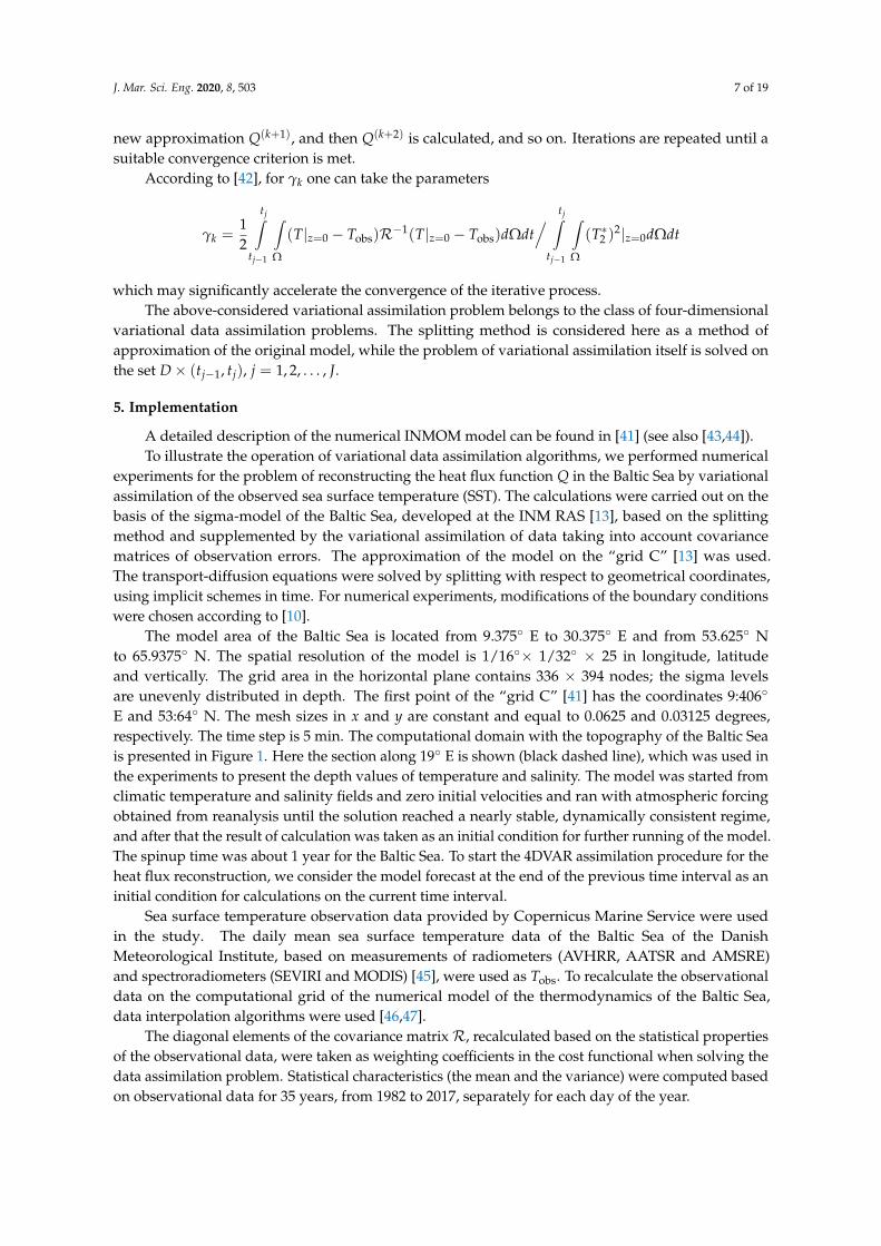
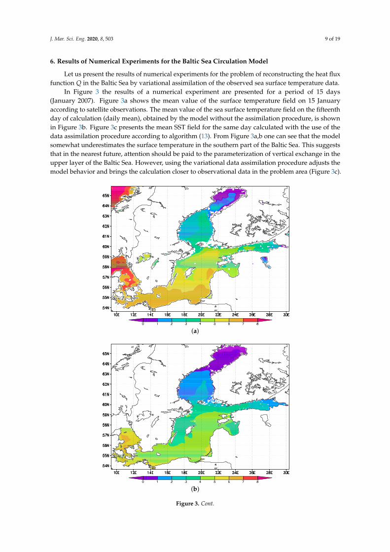
In Figure 3 the results of a numerical experiment are presented for a period of 15 days(January 2007). Figure 3a shows the mean value of the surface temperature field on 15 Januaryaccording to satellite observations. The mean value of the sea surface temperature field on the fifteenthday of calculation (daily mean), obtained by the model without the assimilation procedure, is shownin Figure 3b. Figure 3c presents the mean SST field for the same day calculated with the use of thedata assimilation procedure according to algorithm (13). From Figure 3a,b one can see that the modelsomewhat underestimates the surface temperature in the southern part of the Baltic Sea. This suggeststhat in the nearest future, attention should be paid to the parameterization of vertical exchange in theupper layer of the Baltic Sea. However, using the variational data assimilation procedure adjusts themodel behavior and brings the calculation closer to observational data in the problem area (Figure 3c).

(a)

(b)

Figure 3. Cont.

J. Mar. Sci. Eng. 2020, 8, 503 10 of 19

(c)

Figure 3. Sea surface temperature (C): (a) Observational data Tobs; (b) Model without assimilation,Tmodel; (c) Model with assimilation, Tassim.

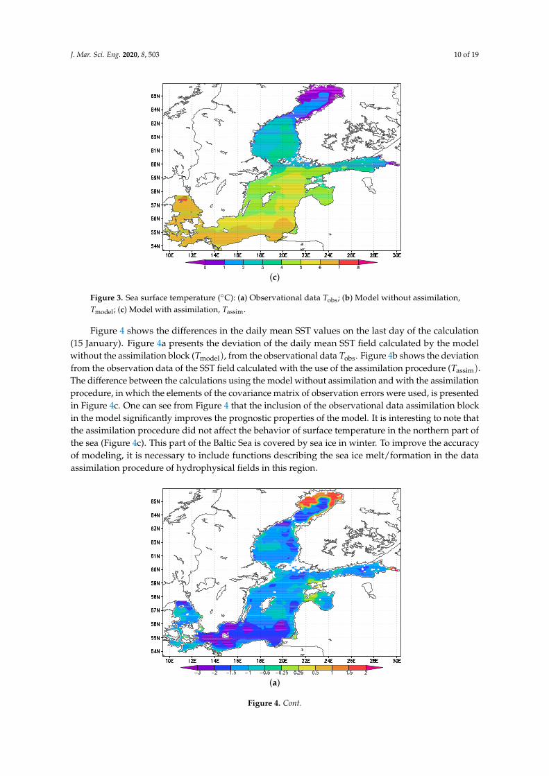
Figure 4 shows the differences in the daily mean SST values on the last day of the calculation(15 January). Figure 4a presents the deviation of the daily mean SST field calculated by the modelwithout the assimilation block (Tmodel), from the observational data Tobs. Figure 4b shows the deviationfrom the observation data of the SST field calculated with the use of the assimilation procedure (Tassim).The difference between the calculations using the model without assimilation and with the assimilationprocedure, in which the elements of the covariance matrix of observation errors were used, is presentedin Figure 4c. One can see from Figure 4 that the inclusion of the observational data assimilation blockin the model significantly improves the prognostic properties of the model. It is interesting to note thatthe assimilation procedure did not affect the behavior of surface temperature in the northern part ofthe sea (Figure 4c). This part of the Baltic Sea is covered by sea ice in winter. To improve the accuracyof modeling, it is necessary to include functions describing the sea ice melt/formation in the dataassimilation procedure of hydrophysical fields in this region.

(a)

Figure 4. Cont.

J. Mar. Sci. Eng. 2020, 8, 503 11 of 19

(b)

(c)

Figure 4. Differences in mean temperature (C): (a) Tmodel − Tobs; (b) Tassim − Tobs; (c) Tmodel − Tassim.

Figure 5 shows the daily mean temperature on the 15th day in the vertical section of the BalticSea along 19 E (this section is presented in Figure 1 by black dashed line). The differences betweenthe model runs without assimilation and with assimilation in Figure 5c show that when assimilatingSST, a change in temperature occurs only in the surface layer, and the temperature at the other levelsremains almost unchanged. Thus, we can conclude that the depth values of temperature simulatedby the model can be corrected only if in-depth observation data are available. We also note that theassimilation procedure, while adjusting the water temperature in the upper layers, makes it warmerwhen calculating in the winter period for the studied water area (Figure 5b).

J. Mar. Sci. Eng. 2020, 8, 503 12 of 19

(a)

(b)

(c)

Figure 5. Vertical section of temperature (C), along 19 E: (a) model without assimilation, Tmodel;(b) model with assimilation, Tassim; (c) difference Tmodel − Tassim.

J. Mar. Sci. Eng. 2020, 8, 503 13 of 19

The results of numerical experiments also showed that the SST assimilation procedure has a weakeffect on other components of the complete solution of the problem, such as salinity, current velocitiesand sea surface level. Figure 6 shows the daily mean salinity in the Baltic Sea on the 15th day of modelintegration. Figure 6a,b corresponds to a section along 19 E. Here Smodel is the model salinity withoutthe SST assimilation procedure, and Sassim is the model salinity obtained using the assimilation ofobservational data. Note that the salinity in the calculation (see Figure 6a) generally corresponds tothe hydrological regime of the Baltic Sea. Figure 6b demonstrates that the salinity remains almostunchanged after assimilation of sea surface temperature for 15 days. From a physical point of view,our problem is to estimate the heat flux on the sea surface using the synthesis of observational dataand model data. It is clear that surface heat flux is mainly controlled by temperature of the upperlayer and surface winds, so the observations of the SST should be taken into account first of all.Improving the simulation of other components of the marine circulation depends on the one hand onthe improvement of physical parameterizations, and on the other hand on the data of observations ofsalinity, currents and sea level. As an additional control parameter, surface wind should be includedwith the SST.

(a)

(b)

Figure 6. Vertical section of salinity S (o/oo), along 19 E: (a) Model with SST assimilation, Sassim;(b) Difference Smodel − Sassim.

J. Mar. Sci. Eng. 2020, 8, 503 14 of 19

Figure 7 shows the circulation in the Baltic Sea after 15th days of integration. For Figure 7a thecalculation was carried out without the data assimilation procedure, and in Figure 7b the results ofthe experiment are presented for the same time period, but using the procedure of assimilation ofsea surface temperature. The difference between these values is shown in Figure 7c. Note that theassimilation of only SST does not have a significant effect on the circulation of the Baltic Sea waters inshort-term calculations, and the velocities differ by less than 5 percent. Note that the model adequatelydescribes subsurface currents in the Baltic Sea (see Figure 7a), and the assimilation only slightlycorrects them. According to Figure 7c, insignificant deviations of the velocity field are observed ina small subdomain of the southern part of the Baltic Sea in the vicinity of the the point 20 E, 56 N.Namely, in this region a significant change in sea surface temperature during assimilation is observed,which possibly affects the velocity.

(a)

(b)

Figure 7. Cont.

J. Mar. Sci. Eng. 2020, 8, 503 15 of 19

(c)

Figure 7. Subsurface velocity field: (a) Model without assimilation; (b) Model with assimilation;(c) Difference in velocities, cm/s.

To give quantitative characteristics, the results of numerical experiments for temperature,salinity and velocity profiles at selected points in the Baltic Sea are shown in Tables 1–3. Table 1presents the differences in temperature, salinity and velocity values when calculating with and withoutprocedure of variational assimilation of SST on standard depth levels for the point 20 E, 63.2 N inthe Gulf of Bothnia. Similar results are given in Table 2 for the point 19.5 E, 55 N in the Gulf ofFinland and in Table 3 for the point 24.3 E, 60 N in the southern part of the Baltic Sea. From thetables it follows that during variational assimilation for 15 days, the temperature difference can reachup to 1.5 degrees on the sea surface; however, it drops with depth. Thus, the assimilation of surfacetemperature most significantly affects the upper layers of the sea; the effect on the lower layers ismostly insignificant. The effect on salinity and water circulation during the assimilation of only SST isnot significant in the case of short-term calculations.

Table 1. Differences in temperature, salinity and velocity. Point 20 E, 63.2 N.

Levels, m ∆T , C ∆S, o/oo ∆~u, cm/s

1 1.55 2.1 × 10−3 −0.452 1.479 3.1 × 10−3 −0.443 1.455 4.9 × 10−3 −0.245 1.447 5.2 × 10−3 −0.11

10 1.406 6.1 × 10−4 −0.2515 1.107 −4.2 × 10−3 0.3620 0.621 −1.0 × 10−3 0.0330 0.254 −8.5 × 10−4 0.1740 0.08 −3.6 × 10−4 −0.00350 0.034 −4.4 × 10−4 −0.00460 0.015 −8.6 × 10−4 −0.00375 0.001 −1.4 × 10−3 −0.006

J. Mar. Sci. Eng. 2020, 8, 503 16 of 19

Table 2. Differences in temperature, salinity and velocity. Point 19.5 E, 55 N.

Levels, m ∆T , C ∆S, o/oo ∆~u, cm/s

1 1.649 −6.1 × 10−3 0.052 1.585 −1.2 × 10−2 −0.063 1.554 −1.2 × 10−2 −0.145 1.537 −9.6 × 10−3 −0.17

10 1.541 −1.0 × 10−2 −0.2315 1.547 −1.0 × 10−2 −0.0320 1.545 −1.1 × 10−2 0.2130 1.465 −6.6 × 10−3 0.0640 0.967 6.8 × 10−3 −0.4150 0.772 −6.5 × 10−4 −0.6260 0.683 −8.0 × 10−3 −0.3475 0.443 1.3 × 10−2 0.008

100 0.08 1.5 × 10−2 0.003

Table 3. Differences in temperature, salinity and velocity. Point 24.3 E, 60 N.

Levels, m ∆T , C ∆S, o/oo ∆~u, cm/s

1 0.564 2.6 × 10−3 −0.112 0.523 2.6 × 10−3 −0.103 0.51 2.6 × 10−3 −0.115 0.504 2.5 × 10−3 −0.10

10 0.488 2.5 × 10−3 −0.0815 0.470 2.4 × 10−3 −0.0720 0.459 2.2 × 10−3 −0.0530 0.456 1.7 × 10−3 −0.03

7. Discussion

Let us recall that the main feature of the INMOM model is that its numerical implementationis based on the splitting according to physical processes and spatial coordinates. The splitting ofequations can be multicomponent. The principal is splitting into physical processes: transfer-diffusion,adaptation and so on. Then, a secondary splitting of the main process can be carried out, for example,into the transport-diffusion of a substance along separate coordinates. Our experience shows that thismethod gives good results in modeling the dynamics of the seas and oceans [4,10,41].

The multicomponent splitting method allows for stable calculations, and it is convenient whenwriting codes for complex hierarchically developed systems. A natural property of a split model is itsmodular principle: a separate problem is related to a separate module. Moreover, when solving 4DVARproblems, the adjoint analogue is constructed for a separate subsystem, which simplifies the process ofconstructing an optimality system. Each subsystem can have its own adjoint. The total model can be“assembled” from a different number of modules. The computational characteristics of the model canbe improved by changing individual computing modules. In the considered method of variational dataassimilation, the model is used in the calculation at each iterative step of the optimality system. Therefore,at each calculated time instant, the solution of the variational assimilation problem satisfies the boundaryand initial conditions of the model, and the numerical stability of the model is not violated.

When running the model without assimilation with real forcing, it was noted that the modelsomewhat underestimates the temperature in the southern Baltic Sea in winter. Therefore, a variationalassimilation method was proposed to correct the boundary condition for the possible improvementof the model properties. Using the algorithm proposed in the paper, it was possible to adjust themodel behavior and bring the calculation closer to the observational data not only in the problem area,but throughout the water area. Note that the method with control at the boundary, when using thesplitting method, requires less computational time-consuming compared to the more common method

J. Mar. Sci. Eng. 2020, 8, 503 17 of 19

of variational initialization, since in this case the iterative process of solving the optimality systemdoes not need to be carried out over the entire assimilation interval. We also note that it is possible tojointly use the initialization method and the method considered in the paper to improve the prognosticproperties of the model.

Numerical experiments showed that the inclusion of the data assimilation procedure increasesthe calculation time by about 10%. This is due to the fact that the splitting method is used, whichallows us to use implicit schemes and simplify the problem at each time step and thereby reduce thenumber of internal iterations of the assimilation algorithm. This gives the advantage to the variationalapproach over the statistical method, which requires ensemble calculations to construct covariancematrices at each time step.

The variational data assimilation approach has great versatility, because it is based on thefundamental principle to minimize a cost function describing the deviation of the model solution fromthe observational data, and the minimum of this functional is sought on the model trajectories. In thepaper we have demonstrated the application of this approach to the problem of reconstruction of theheat fluxes, the boundary conditions on the sea surface. However, this approach allows one, on aunified methodological basis, to solve the problem of initialization of hydrophysical fields, to assess thesensitivity of the model solution, to identify model parameters, etc. Moreover, considering the weakformulation of 4DVAR can help to take into account the model errors and uncertainties via assimilation.

8. Conclusions

In this paper the methods and technology for modeling and analysis of marine hydrophysicalfields based on 4D variational assimilation of observational data are presented. The developed methodscan be used for monitoring and predicting sea currents, for solving problems of variational dataassimilation in order to reconstruct boundary and/or initial conditions and other model parameters.The technology is based on a numerical model of marine circulation in a sigma-coordinate system,which includes a procedure of 4D variational data assimilation. Variational assimilation algorithms arebased on modern iterative processes with a special choice of iterative parameters.

The main feature of the presented algorithms is the use of the splitting method for physicalprocesses and geometric coordinates, which made it possible to simplify the problems underconsideration at each time interval and make the implementation of 4D variational assimilationalgorithms more efficient. Numerical experiments have shown the efficiency of the developedalgorithms for 4D variational assimilation of sea surface temperature data using the example forreconstruction of heat fluxes on the sea surface. When developing and testing the algorithms andcodes in this article, the Baltic Sea was chosen as a marine area for certainty. However, theoreticalresults and computational algorithms under consideration may be extended to other water areas.

Author Contributions: V.Z., V.A. and V.S. presented the theory; E.P. performed the numerical experiments;N.Z. processed the data. All authors have read and agreed to the published version of the manuscript.

Funding: This research received no external funding.

Acknowledgments: This work was supported by the Russian Science Foundation (project 17-77-30001, studiesin Sections 1–3; project 20-11-20057, studies in Sections 4 and 5); the Russian Foundation for Basic Research(project 18-01-00267, studies in Section 6); and by the Moscow Center for Fundamental and Applied Mathematics(agreement with the Ministry of Education and Science of the Russian Federation, number 075-15-2019-1624).

Conflicts of Interest: The authors declare no conflict of interest. The founding sponsors had no role in the designof the study; in the collection, analyses or interpretation of data; in the writing of the manuscript, or in the decisionto publish the results.

References

1. Sarkisyan, A.; Sündermann, J. Modelling Ocean Climate Variability; Springer: Heidelberg, Germany, 2009.2. Griffies, S.M.; Boening, C.; Bryan, F.O.; Chassignet, E.P.; Gerdes, R.; Hasumi, H.; Hirst, A.; Treguier, A.-M.;

Webb, D. Developments in ocean climate modelling. Ocean Model. 2000, 2, 123–192. [CrossRef]

J. Mar. Sci. Eng. 2020, 8, 503 18 of 19

3. Chassignet, E.P.; Verron, J. (Eds.) Ocean Weather Forecasting: An Integrated View of Oceanography; Springer:Heidelberg, Germany, 2006.

4. Dymnikov, V.P.; Zalesny, V.B. Fundamentals of Computational Geophysical Fluid Dynamics; GEOS: Moscow,Russia, 2019.

5. Druzhinin, O.A.; Ostrovsky, L.A.; Zilitinkevich, S.S. The study of the effect of small-scale turbulence oninternal gravity waves propagation in a pycnocline. Nonlinear Process. Geophys. 2013, 20, 977–986. [CrossRef]

6. Thomas, L.N.; Tandon, A.; Mahadevan, A. Submesoscale processes and dynamics. In Ocean Modeling in anEddying Regime; Hecht, M.W., Hasumi, H., Eds.; American Geophysical Union: Washington, DC, USA, 2008;pp. 17–38.

7. Zalesny, V.; Agoshkov, V.; Aps, R.; Shutyaev, V.; Zayachkovskiy, A.; Goerlandt, F.; Kujala P. Numericalmodeling of marine circulation, pollution assessment and optimal ship routes. J. Mar. Sci. Eng. 2017, 5, 27.[CrossRef]

8. Zalesny, V.; Gusev, A.; Chernobay, S.; Aps, R.; Tamsalu, R.; Kujala, P.; Rytkönen, J. The Baltic Sea circulationmodeling and assessment of marine pollution. Russ. J. Numer. Anal. Math. Model. 2014, 29, 129–138.[CrossRef]

9. Zalesny, V.B.; Gusev, A.V.; Lukyanova, A.N.; Fomin, V.V. Numerical modelling of sea currents and tidalwaves. Russ. J. Numer. Anal. Math. Model. 2016, 31, 115–125. [CrossRef]

10. Zalesny, V.B.; Marchuk, G.I.; Agoshkov, V.I.; Bagno, A.V.; Gusev, A.V.; Diansky, N.A.; Moshonkin, S.N.;Tamsalu, R.; Volodin, E.M. Numerical simulation of large-scale ocean circulation based on themulticomponent splitting method. Russ. J. Numer. Anal. Math. Model. 2010, 25, 581–609. [CrossRef]

11. Zalesny, V.B.; Tamsalu, R. High-resolution modeling of a marine ecosystem using the FRESCOhydroecological model. Izv. Atmos. Ocean. Phys. 2009, 45, 102–115. [CrossRef]

12. Leppäranta, M.; Myrberg, K. Physical Oceanography of the Baltic Sea; Springer-Praxis: Heidelberg,Germany, 2009.

13. Zalesny, V.B.; Gusev, A.V.; Ivchenko, V.O.; Tamsalu, R.; Aps, R. Numerical model of the Baltic Sea circulation.Russ. J. Numer. Anal. Math. Model. 2013, 28, 85–100. [CrossRef]

14. Chassignet, E.P.; Xu, X. Impact of horizontal resolution (1/12 to 1/50) on Gulf Stream separation,penetration, and variability. J. Phys. Oceanogr. 2017, 47, 1999–2021. [CrossRef]

15. Gusev, A.V.; Zalesny, V.B.; Fomin, V.V. Technique for simulation of Black Sea circulation with increasedresolution in the area of the IO RAS polygon. Oceanology 2017, 57, 880–891. [CrossRef]

16. Diansky, N.A.; Fomin, V.V.; Zhokhova, N.V.; Korshenko, A.N. Simulations of currents and pollution transportin the coastal waters of Big Sochi. Izv. Atmos. Ocean. Phys. 2013, 49, 611–621. [CrossRef]

17. Mizyuk, A.I.; Senderov, M.V.; Korotaev, G.K.; Sarkysyan, A.S. Features of the horizontal variability of the seasurface temperature in the Western Black Sea from high resolution modeling. Izv. Atmos. Ocean. Phys. 2016,52, 570–578. [CrossRef]

18. Su, Z.; Wang, J.; Klein, P.; Thompson, A.F.; Menemenlis, D. Ocean submesoscales as a key component of theglobal heat budget. Nat. Commun. 2018, 9, 775. [CrossRef] [PubMed]

19. Ponte, A.L.; Klein, P. Reconstruction of the upper ocean 3D dynamics from high-resolution sea surface height.Ocean Dyn. 2013, 63, 777–791. [CrossRef]

20. Varlas, G.; Katsafados, P.; Papadopoulos, A.; Korres, G. Implementation of a two-way coupledatmosphere-ocean wave modeling system for assessing air-sea interaction over the Mediterranean Sea.Atmos. Res. 2018, 208, 201–217. [CrossRef]

21. Carniel, S.; Benetazzo, A.; Bonaldo, D.; Falcieri, F.M.; Miglietta, M.M.; Ricchi, A.; Sclavo, M. Scratchingbeneath the surface while coupling atmosphere, ocean and waves: Analysis of a dense water formationevent. Ocean Model. 2016, 101, 101–112. [CrossRef]

22. Renault L.; Chiggiato J.; Warner J.C.; Gomez M.; Vizoso G.; Tintore J. Coupled atmosphere-ocean-wavesimulations of a storm event over the Gulf of Lion and Balearic Sea. J. Geophys. Res. 2012, 117, 1–25.[CrossRef]

23. Olabarrieta, M.; Warner, J.C.; Armstrong, B.; Zambon, J.B.; He, R. Ocean-atmosphere dynamics duringHurricane Ida and Nor’Ida: An application of the coupled ocean-atmosphere wave sediment transport(COAWST) modeling system. Ocean Model. 2012, 43, 112–137. [CrossRef]

24. Asch, M.; Bocquet, M.; Nodet, M. Data Assimilation: Methods, Algorithms, and Applications; SIAM: Philadelphia,PA, USA, 2016.

J. Mar. Sci. Eng. 2020, 8, 503 19 of 19

25. Fletcher, S.J. Data Assimilation for the Geosciences: From Theory to Application; Elsevier: Amsterdam,The Netherlands, 2017.

26. Carrassi, A.; Bocquet, M.; Bertino, L.; Evensen, G. Data assimilation in the geosciences: an overview ofmethods, issues, and perspectives. WIREs Clim. Chang. 2018, 9, 1–80.

27. Shutyaev, V.P. Methods for observation data assimilation in problems of physics of atmosphere and ocean.Izv. Atmos. Ocean. Phys. 2019, 55, 17–31. [CrossRef]

28. Lions, J.L. Contrôle Optimal de Systèmes Gouvernés par des Équations aux Dérivées Partielles; Dunod: Paris,France, 1968.

29. Le Dimet, F.X.; Talagrand, O. Variational algorithms for analysis and assimilation of meteorologicalobservations: theoretical aspects. Tellus A 1986, 38, 97–110. [CrossRef]

30. Marchuk, G.I. Adjoint Equations and Analysis of Complex Systems; Kluwer: Dordrecht, The Netherlands, 1995.31. Agoshkov, V.I. Methods of Optimal Control and Adjoint Equations in Problems of Mathematial Physis; INM RAS:

Moscow, Russia, 2003.32. Agoshkov, V.I.; Zalesny, V.B.; Parmuzin, E.I.; Shutyaev, V.P.; Ipatova, V.M. Problems of variational assimilation

of observational data for ocean general circulation models and methods for their solution. Izv. Atmos.Ocean. Phys. 2010, 46, 677–712. [CrossRef]

33. Agoshkov, V.I.; Parmuzin, E.I.; Zalesny, V.B.; Shutyaev, V.P.; Zakharova, N.B.; Gusev, A.V. Variationalassimilation of observation data in the mathematical model of the Baltic Sea dynamics. Russ. J. Numer. Anal.Math. Model. 2015, 30, 203–212. [CrossRef]

34. Zalesny, V.B.; Agoshkov, V.I.; Shutyaev, V.P.; Le Dimet, F.; Ivchenko, B.O. Numerical modeling of oceanhydrodynamics with variational assimilation of observational data. Izv. Atmos. Ocean. Phys. 2016, 52,431–442. [CrossRef]

35. Markov, A.A. Ischislenie Veroyatnostej; Imperial Academy of Sciences: St Petersburg, Russia, 1900.36. Kolmogorov, A.N. On the proof of the method of least squares. Uspekhi Mat. Nauk. 1946, 1, 57–70.37. Pontryagin, L.S.; Boltyansky, V.G.; Gamkrelidze, R.V.; Mishchenko, E.F. The Mathematical Theory of Optimal

Processes; International Series of Monographs in Pure and Applied Mathematics; Brown, D.E., Translator;Pergamon Press: Oxford, UK, 1964; Volume 55.

38. Marchuk, G.I. Splitting and alternating direction methods. In Handbook of Numerical Analysis; Ciarlet, P.G.,Lions, J.L., Eds.; North-Holland: Amsterdam, The Netherlands, 1990; Volume 1, pp. 197–462.

39. Marchuk, G.I.; Dymnikov, V.P.; Zalesny, V.B. Mathematical Models in Geophysical Hydrodynamics and NumericalMethods for their Implementation; Hydrometeoizdat: Leningrad, Russia, 1987.

40. Agoshkov, V.I.; Gusev, A.V.; Diansky, N.A.; Oleinikov, R.V. An algorithm for the solution of the oceanhydrothermodynamics problem with variational assimilation of the sea level function data. Russ. J. Numer.Anal. Math. Model. 2007, 22, 133–161. [CrossRef]

41. Marchuk, G.I.; Rusakov, A.S.; Zalesny, V.B.; Diansky, N.A. Splitting numerical technique with applicationto the high resolution simulation of the Indian ocean circulation. Pure Appl. Geophys. 2005, 162, 1407–1429.[CrossRef]

42. Agoshkov, V.I.; Parmuzin, E.I.; Shutyaev, V.P. Numerical algorithm for variational assimilation of sea surfacetemperature data. Comput. Math. Math. Phys. 2008, 48, 1293–1312. [CrossRef]

43. Ivchenko, V.O.; Zalesny, V.B.; Drinkwater, M.; Schroeter, J. A quick response of the equatorial ocean toAntarctic sea ice/salinity anomalies. J. Geophys. Res. 2006, 111, 1–19. [CrossRef]

44. Agoshkov, V.I.; Zalesny, V.B. Variational data assimilation technique in mathematical modeling of oceandynamics. Pure Appl. Geophys. 2012, 169, 555–578. [CrossRef]

45. Karagali, I.; Hoyer, J.; Hasager, C.B. SST diurnal variability in the North Sea and the Baltic Sea. Remote Sens.Environ. 2012, 121, 159–170. [CrossRef]

46. Zakharova, N.B.; Lebedev, S.A. ARGO floats data interpolation for data assimilation in World oceancirculation models. Curr. Probl. Remote Sens. Earth Space 2010, 7, 104–111.

47. Zakharova, N.B.; Agoshkov, V.I.; Parmuzin, E.I. The new method of ARGO buoys system observation datainterpolation. Russ. J. Numer. Anal. Math. Model. 2013, 28, 67–84. [CrossRef]

c© 2020 by the authors. Licensee MDPI, Basel, Switzerland. This article is an open accessarticle distributed under the terms and conditions of the Creative Commons Attribution(CC BY) license (http://creativecommons.org/licenses/by/4.0/).