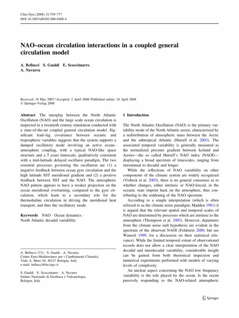
NAO–ocean circulation interactions in a coupled generalcirculation model

A. Bellucci Æ S. Gualdi Æ E. Scoccimarro ÆA. Navarra

Received: 18 May 2007 / Accepted: 2 April 2008 / Published online: 18 April 2008

� Springer-Verlag 2008

Abstract The interplay between the North Atlantic

Oscillation (NAO) and the large scale ocean circulation is

inspected in a twentieth century simulation conducted with

a state-of-the-art coupled general circulation model. Sig-

nificant lead–lag covariance between oceanic and

tropospheric variables suggests that the system supports a

damped oscillatory mode involving an active ocean–

atmosphere coupling, with a typical NAO-like space

structure and a 5 years timescale, qualitatively consistent

with a mid-latitude delayed oscillator paradigm. The two

essential processes governing the oscillation are (1) a

negative feedback between ocean gyre circulation and the

high latitude SST meridional gradient and (2) a positive

feedback between SST and the NAO. The atmospheric

NAO pattern appears to have a weaker projection on the

ocean meridional overturning, compared to the gyre cir-

culation, which leads to a secondary role for the

thermohaline circulation in driving the meridional heat

transport, and thus the oscillatory mode.

Keywords NAO � Ocean dynamics �North Atlantic decadal variability

1 Introduction

The North Atlantic Oscillation (NAO) is the primary var-

iability mode of the North Atlantic sector, characterized by

a redistribution of atmospheric mass between the Arctic

and the subtropical Atlantic (Hurrell et al. 2003). The

associated temporal variability is generally measured as

the normalized pressure gradient between Iceland and

Azores—the so called Hurrell’s NAO index (NAOI)—

displaying a broad spectrum of timescales, ranging from

interannual to decadal and longer.

While the reflections of NAO variability on other

components of the climate system are widely recognized

(Visbeck et al. 2003), there is no general consensus as to

whether changes, either intrinsic or NAO-forced, in the

oceanic state imprint back on the atmosphere, thus con-

tributing to the reddening of the NAO spectrum.

According to a simple interpretation (which is often

referred to as the climate noise paradigm; Madden 1981) it

is argued that the relevant spatial and temporal scales of

NAO are determined by processes which are intrinsic to the

atmosphere (Thompson et al. 2003). However, departures

from the climate noise null hypothesis are evident in the

spectrum of the observed NAOI (Feldstein 2000; but see

Wunsch 1999, for a discussion on their statistical rele-

vance). While the limited temporal extent of observational

records does not allow a clear interpretation of the NAO

decadal and interdecadal variability, considerable insight

can be gained from both theoretical inspection and

numerical experiments performed with models of varying

levels of complexity.

An unclear aspect concerning the NAO low frequency

variability is the role played by the ocean. Is the ocean

passively responding to the NAO-related atmospheric

A. Bellucci (&) � S. Gualdi � A. Navarra

Centro Euro-Mediterraneo per i Cambiamenti Climatici,

Viale A. Moro 44, 40127 Bologna, Italy

e-mail: bellucci@bo.ingv.it

S. Gualdi � E. Scoccimarro � A. Navarra

Istituto Nazionale di Geofisica e Vulcanologia,

Bologna, Italy

123

Clim Dyn (2008) 31:759–777

DOI 10.1007/s00382-008-0408-4

fluxes (Frankignoul and Hasselmann 1977) or does the

coupling with the overlying atmosphere determine

enhanced spectral power in both fluids at specific time-

scales? Numerical experiments performed with a hierarchy

of models with varying levels of complexity, but with

mostly idealized settings, show no unanymous answer

regarding the nature of ocean–atmosphere interactions in

the extratropical North Atlantic. Saravanan and McWil-

liams (1998) suggest that the ocean passively responds to

atmospheric variability at a preferred resonant decadal

time scale, set by a typical oceanic advective velocity and a

length scale determined by the dominant atmospheric

variability pattern. A similarly passive oceanic response to

unaltered NAO-like atmospheric fluctuations does also

emerge from Zorita and Frankignoul (1997) and Frankig-

noul et al. (2000) analyses of the low resolution flux

adjusted ECHAM1/LSG integration. Marshall et al. (2001;

hereafter M01) and Czaja and Marshall (2001; hereafter

CM01) based on a simplified theoretical model of the

extratropical North Atlantic coupled ocean–atmosphere

system, suggest that ocean dynamics introduce a significant

departure from the climate noise paradigm at decadal

timescales, with the ocean gyre circulation providing the

delay necessary to support a coupled oscillatory mode (a

mechanism which is generally referred to as the delayed

oscillator paradigm), thus extending to the Atlantic sector a

conceptual scheme widely used for ENSO studies, and also

adopted to inspect decadal variability in the North Pacific

(Latif and Barnett 1996).

Relying on a simplified numerical experimental setup is

appealing in that it allows to explore wide areas of a model

parametric space. On the other hand, the relevance to the

real system of results obtained through this approach can be

legitimately questioned. In the present study, the interplay

between ocean circulation and the NAO is addressed in a

twentieth century simulation conducted with a full-fledged

sea–ice ocean–atmosphere coupled GCM (CGCM), using

no flux corrections. The role of large scale ocean circulation

as a cross-basin heat carrier, and its impact on the low

frequency modulation of the mid-to-high latitude SST is

investigated. The relative role of the barotropic gyre versus

meridional overturning circulation in driving the poleward

heat transfer is also analysed. A mechanism governing the

oscillation is identified, bearing strong similarities with the

delayed oscillator paradigm proposed by M01.

The paper is structured as follows. In Sect. 2 we

describe the model used to perform the twentieth century

climate integration. In Sect. 3, the dominant modes of

variability of the analysed coupled system are illustrated.

In Sect. 4 we analyse the lead–lag relationships between

SST and NAOI. The NAO/ocean circulation interactions

are analysed with respect to both mass and heat transport,

in Sects. 5 and 6, respectively. A damped multiannual

oscillatory mode, and the underlying mechanism, are

skectched in Sect. 7. In Sect. 8, the magnitude of the

delayed oscillator parameters are derived from the coupled

model and compared with the estimates provided by CM01

and M01. A summary of the main results and final con-

cluding comments are reported in Sect. 9.

2 Model description and data

The model used for this study is the SINTEX-G (hereafter

SXG) coupled GCM (Gualdi et al. 2007). With respect to

the previous SINTEX and SINTEX-F versions (Gualdi

et al. 2003a; Gualdi et al. 2003b; Guiliardy et al. 2003;

Luo et al. 2003) the SXG model includes a thermo-

dynamic–dynamic snow sea–ice model (Fichefet and

Morales-Maqueda 1999), with three vertical levels (one for

snow, and two for ice).

We analyse results from a simulation of the twentieth

century, performed with forcing agents (including green-

house gases and sulfate aerosols) as specified by the IPCC

protocol for the 20C3M experiment (http://www-pcmdi.

llnl.gov/ipcc/about_ipcc.php). The main features of the

SXG 20C3M climate are documented in Gualdi et al.

(2007).

We restrict our analysis to the Atlantic sector, defined as

the [100W–0W; 0N–80N] longitude–latitude domain, with

a major focus on the boreal winter period (JFM), when the

NAO signature is expected to be more prominent (Hurrell

et al. 2003). In the present investigation, the whole length

of the 20C3M simulation, spanning the 1870–2000 period,

is used. All statistical moments have been calculated over

this time period. Winter anomalies were computed by

subtracting from each yearly JFM mean winter, the long-

term winter average computed over the whole JFM subset.

In the computation of empirical orthogonal functions

(EOF), a simple linear detrending has been applied to the

model data so as to remove the signature of the global

warming trend.

Since we are mainly interested in the coherency between

tropospheric and oceanic variables, throughout the paper

we will rely on lead–lag correlation (rather than regression)

patterns. We anticipate here that regression patterns for

several time-lags (not shown) reproduce the basic features

emerging from the correlation distributions shown.

3 Dominant patterns of oceanic and atmospheric

variability

We illustrate the temporal and spatial structure of the

model leading variability modes in the Atlantic sector by

resorting to a EOF analysis.

760 A. Bellucci et al.: NAO-ocean circulation interactions

123

The first EOF of wintertime sea level pressure (SLP;

equivalent to the model NAO) is shown in Fig. 1 (left

panel). Winter SLP variability (explaining 34% of the

variance) is dominated by a dipole structure, with a posi-

tive centre of action straddling the subtropics, and a

negative lobe approximately centred over Iceland, which is

grossly consistent with the main features of the observed

wintertime NAO (Hurrell et al. 2003).

A model NAO index is defined as the normalized dif-

ference between the JFM mean SLP spatially averaged

over two large areas, encompassing the dominant centres of

action: a northern subpolar box (50W–0W; 55–80N), and a

southern subtropical box (70W–0W; 30–55N). An NAOI

definition based on large areas averages is here preferred to

the more standard two-point approach since the former

allows a reduced dependence of the index on the migration

of the centres of actions (Stephenson et al. 2006). The

robustness of this NAOI definition has been tested against

changes in the zonal width of the (larger) southern box, by

progressively reducing the westward extent of this region,

but no relevant effects on the index were found. It is worth

to note that the model NAOI turns out to be almost

undistinguishable from the SLP leading principal compo-

nent (PC) (not shown). Similarly, the spatial pattern of

NAO obtained by linearly regressing SLP onto the NAOI,

shows negligible differences compared to SLP EOF1 (not

shown).

The model NAOI spectrum is compared with an

observed NAOI spectrum evaluated by using mean winter

(JFM) SLP station data from Iceland and Gibraltar for the

1870–2000 period (Fig. 2). We only focus on the interan-

nual-to-decadal timescale range, due to the poor resolution

of observed multi-decadal variability. The spectral power

was estimated using a Blackman–Tukey correlogram

technique (Blackman and Tukey 1958).

The model spectrum displays a bimodal structure, with a

broad-band peak around multiannual timescales (around

6 years) a narrower spectral signature around the quasi-

biennial period, and reduced power around 3–4 years. This

is fairly consistent with the power spectrum of the observed

NAO index, except that the latter shows more energy in the

near-decadal range. Also, the model appears to be sys-

tematically less energetic compared to observations, a

model bias which is shared by other state-of-the-art

CGCMs (Stephenson et al. 2006).

The leading EOF of winter SST (Fig. 1, right panel)

explains 29% of the variance and exhibits a tripole struc-

ture, with a warm anomaly in the western subtropical

Atlantic, a cold anomaly in the subpolar region and an

additional cold lobe in the tropics. Both the space structure

and amplitude of the leading SST mode are consistent with

the observed tripolar pattern dominating the wintertime

SST variability of the North Atlantic ocean (Cayan 1992).

Correlation between SST PC1 and NAOI is 0.5, statisti-

cally significant at the 95% level. A detailed lead–lag

covariance analysis between SST and NAOI is presented in

Sect. 4.

The vertical structure of the atmospheric response to a

positive phase of the NAO is diagnosed through a com-

posite analysis of winter (JFM) geopotential height (GPH)

anomalies at different pressure levels. Composites of GPH

anomalies for 850, 500 and 200 hPa keyed to the model

NAOI using a threshold of one standard deviation, are

shown in Fig. 3. The composite maps show that the 0-lag

free troposhpere response to a NAO+ event is equivalent

barotropic, with a positive (negative) GPH anomaly cor-

responding to the warm SST-high pressure (cold SST-low

pressure) NAO centre of action. This behaviour is consis-

tent with results obtained by Ferreira and Frankignoul

(2005) and D’Andrea et al. (2005) with a simple quasi-

geostrophic atmospheric model coupled to a slab ocean

mixed layer. Ferreira and Frankignoul (2005) describe the

equivalent barotropic response to a NAO-like SST anoma-

lous field as the result of transient eddy fluxes of

momentum and heat turning the initial baroclinic response

into a barotropic one.

90° W 60° W 30° W 0°

0°

15° N

30° N

45° N

60° N

75° N

SLP

90° W 60° W 30° W 0°

0°

15° N

30° N

45° N

60° N

75° N

SST

Fig. 1 (left) First EOF of boreal

winter (JFM) SLP (hPa). The

contour interval is 0.25 hPa.

(right) First EOF of boreal

winter (JFM) SST (�C). The

contour interval is 0.05�C. Solid(dashed) contours indicate

positive (negative) values. The

black thick contour indicates the

zero line

A. Bellucci et al.: NAO-ocean circulation interactions 761

123

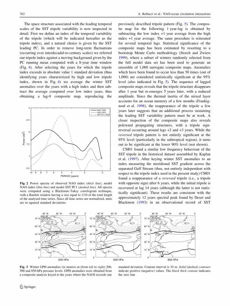
The space structure associated with the leading temporal

scales of the SST tripole variability is now inspected in

detail. First we define an index of the temporal variability

of the tripole (which will be indicated hereafter as the

tripole index), and a natural choice is given by the SST

leading PC. In order to remove long-term fluctuations

(occurring over interdecadal-to-century scales) we referred

our tripole index against a moving background given by the

PC running mean computed with a 8-year time window

(Fig. 4). After selecting the years for which the tripole

index exceeds in absolute value 1 standard deviation (thus

identifying years characterized by high and low tripole

index, shown in Fig. 4) we average the winter SST

anomalies over the years with a high index and then sub-

tract the average computed over low index years, thus

obtaining a lag-0 composite map, reproducing the

previously described tripole pattern (Fig. 5). The compos-

ite map for the following 1 year-lag is obtained by

subtracting the low index +1 year average from the high

index +1 year average. The same procedure is reiterated

for several temporal lags. Statistical significance of the

composite maps has been estimated by resorting to a

bootstrap Monte Carlo methodology (Storch and Zwiers

1999), where a subset of winters randomly selected from

the full model data set has been used to generate an

ensemble of 1,000 surrogate composite maps. Anomalies

which have been found to occur less than 50 times (out of

1,000) are considered statistically significant at the 95%

level (also indicated in Fig. 5). The sequence of lagged

composite maps reveals that the tripole structure disappears

after 1 year but re-emerges 5 years later, with a reduced

amplitude. Since the thermal inertia of the mixed layer

accounts for an ocean memory of a few months (Frankig-

noul et al. 1998), the reappearance of the tripole a few

years later suggests that an additional process sustaining

the leading SST variability pattern must be at work. A

closer inspection of the composite maps also reveals

poleward propagating structures, with a tripole sign-

reversal occurring around lags +2 and +3 years. While the

reversed tripole pattern is not entirely significant at the

95% level (particularly in the subtropical region), it turns

out to be significant at the lower 90% level (not shown).

CM01 found a similar low frequency behaviour of the

SST tripole in the historical dataset assembled by Kaplan

et al. (1997). After keying winter SST anomalies to an

index measuring the meridional SST gradient across the

separated Gulf Stream (thus, not entirely independent with

respect to the tripole index used in the present study) CM01

found a reappearance of a reversed tripole (i.e., a tripole

with opposite sign) after 6 years, while the initial tripole is

recovered at lag 14 years (although the latter is not statis-

tically significant). These results are consistent with the

approximately 12 years spectral peak found by Deser and

Blackmon (1993) in an observational record of SST

10 9 8 7 6 5 4 3 2

0.5

1

1.5

2

2.5

3

Pow

er (

std2 )

PERIOD (years)

NAO−OBSNAO−SXGSST PC1−SXG

Fig. 2 Power spectra of observed NAO index (thick line), model

NAO index (thin line) and model SST PC1 (dashed line). All spectra

were computed using a Blackman–Tukey correlogram technique,

with a Bartlett window having a size equal to 1/10 of the total length

of the analysed time series. Since all time series are normalized, units

are in squared standard deviations

90° W 60° W 30° W 0°

0°

15° N

30° N

45° N

60° N

75° N

850 hPa

90° W 60° W 30° W 0°

0°

15° N

30° N

45° N

60° N

75° N

500 hPa

90° W 60° W 30° W 0°

0°

15° N

30° N

45° N

60° N

75° N

200 hPa

Fig. 3 Winter GPH anomalies (in meters) at (from left to right) 200,

500 and 850-hPa pressure levels. GPH anomalies were obtained from

a composite analysis keyed to the years where the NAOI exceeds one

standard deviation. Contour interval is 10 m. Solid (dashed) contoursindicate positive (negative) values. The black thick contour indicates

the zero line

762 A. Bellucci et al.: NAO-ocean circulation interactions

123

spanning the 1900–1989 time period. The multiannual

memory emerging from the model composite maps is

consistent with the power spectrum of the tripole index,

showing enhanced power around the 5 years period (shown

in Fig. 2). A discussion on the possible causes underlying

this mismatch between model and observed timescales of

the SST tripole will be provided in Sect. 7.

It is important here to stress that these results are robust

with respect to changes in the time window used to define

the moving background of the tripole index. Using 5 and

10 years for the time window width provided essentially

similar results (not shown). The multiannual variability of

the tripole pattern is further discussed in the following

section.

4 NAO/SST interactions: lead–lag analysis

In the present section the coherency between NAOI and

SST is investigated. Pointwise correlation maps of NAOI

against winter SST anomalies at lags from -4 to +4 years

are shown in Fig. 6 (the NAOI leads for positive lags).

From this analysis emerges that the interaction between the

leading atmospheric variability mode and SST occurs at

spatial scales which are basin-wide. The zero lag correla-

tion map shows the well known tripole pattern (consistent

1880 1900 1920 1940 1960 1980 2000−3

−2

−1

0

1

2

3

YEAR

SST PC1

Fig. 4 First PC of SST. Circles (stars) indicate years where the PC is

larger (smaller) than +1 (-1) standard deviation

Fig. 5 Composite maps of winter SST anomalies (in �C), based on

years where the normalized SST PC1 (the tripole index; shown in

Fig. 4) is high and low, with respect to a threshold of one standard

deviation (in absolute value). At lag zero, the composite is simply the

difference between the average SST anomalies computed over high

tripole and low tripole years. At lag +1 year (and similarly for larger

lags), the composite is computed by shifting the high and low tripole

index years by 1 year. Regions featuring a 95% statistical significance

level, according to a bootstrap Monte Carlo methodology (see text for

details), are encircled with a black thick contour

A. Bellucci et al.: NAO-ocean circulation interactions 763

123

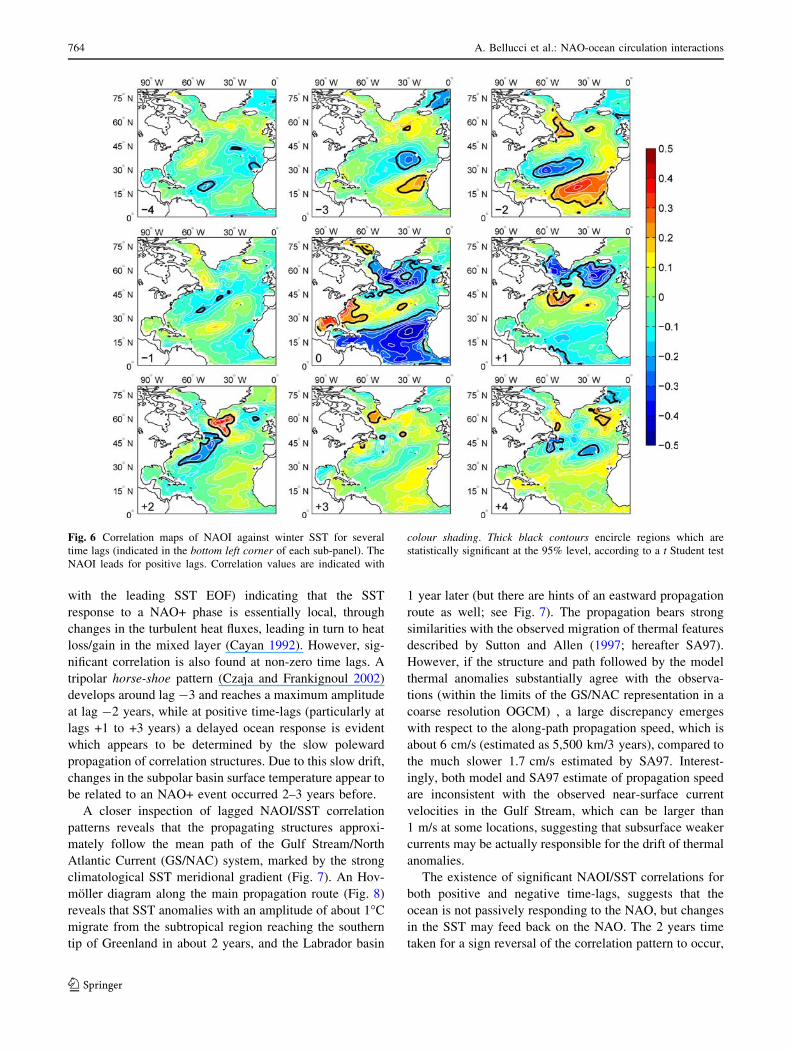
with the leading SST EOF) indicating that the SST

response to a NAO+ phase is essentially local, through

changes in the turbulent heat fluxes, leading in turn to heat

loss/gain in the mixed layer (Cayan 1992). However, sig-

nificant correlation is also found at non-zero time lags. A

tripolar horse-shoe pattern (Czaja and Frankignoul 2002)

develops around lag -3 and reaches a maximum amplitude

at lag -2 years, while at positive time-lags (particularly at

lags +1 to +3 years) a delayed ocean response is evident

which appears to be determined by the slow poleward

propagation of correlation structures. Due to this slow drift,

changes in the subpolar basin surface temperature appear to

be related to an NAO+ event occurred 2–3 years before.

A closer inspection of lagged NAOI/SST correlation

patterns reveals that the propagating structures approxi-

mately follow the mean path of the Gulf Stream/North

Atlantic Current (GS/NAC) system, marked by the strong

climatological SST meridional gradient (Fig. 7). An Hov-

moller diagram along the main propagation route (Fig. 8)

reveals that SST anomalies with an amplitude of about 1�C

migrate from the subtropical region reaching the southern

tip of Greenland in about 2 years, and the Labrador basin

1 year later (but there are hints of an eastward propagation

route as well; see Fig. 7). The propagation bears strong

similarities with the observed migration of thermal features

described by Sutton and Allen (1997; hereafter SA97).

However, if the structure and path followed by the model

thermal anomalies substantially agree with the observa-

tions (within the limits of the GS/NAC representation in a

coarse resolution OGCM) , a large discrepancy emerges

with respect to the along-path propagation speed, which is

about 6 cm/s (estimated as 5,500 km/3 years), compared to

the much slower 1.7 cm/s estimated by SA97. Interest-

ingly, both model and SA97 estimate of propagation speed

are inconsistent with the observed near-surface current

velocities in the Gulf Stream, which can be larger than

1 m/s at some locations, suggesting that subsurface weaker

currents may be actually responsible for the drift of thermal

anomalies.

The existence of significant NAOI/SST correlations for

both positive and negative time-lags, suggests that the

ocean is not passively responding to the NAO, but changes

in the SST may feed back on the NAO. The 2 years time

taken for a sign reversal of the correlation pattern to occur,

Fig. 6 Correlation maps of NAOI against winter SST for several

time lags (indicated in the bottom left corner of each sub-panel). The

NAOI leads for positive lags. Correlation values are indicated with

colour shading. Thick black contours encircle regions which are

statistically significant at the 95% level, according to a t Student test

764 A. Bellucci et al.: NAO-ocean circulation interactions

123

is consistent with the results found in the composite ana-

lysis of the SST tripole pattern. The propagation speed of

SST anomalies is consistent with an oceanic advective

mechanism (typical horizontal velocity magnitudes in the

model upper 100-m layer are of the order of 10 cm/s;not

shown). If this is the case, then the multiannual re-emer-

gence of the tripole pattern would be determined by a

typical non-local process. The relationships between the

large scale (barotropic and overturning) ocean circulation

and NAO variability are inspected in the next section.

5 The role of ocean circulation

In this section, the interactions between NAO and ocean

circulation are investigated. We ideally split the large scale

ocean mass transport into a horizontal gyre component, and

a meridional overturning component. The gyre circulation

is diagnosed via the barotropic streamfunction of the ver-

tically integrated transport (in Sv; 1 Sv = 106 m3/s),

obtained by solving the Poisson equation with an iterative

method. The meridional overturning transport (which is

often identified with the thermohaline circulation) is

defined as the zonally integrated meridional transport

above a certain geopotential level (in Sv).

5.1 Gyre circulation

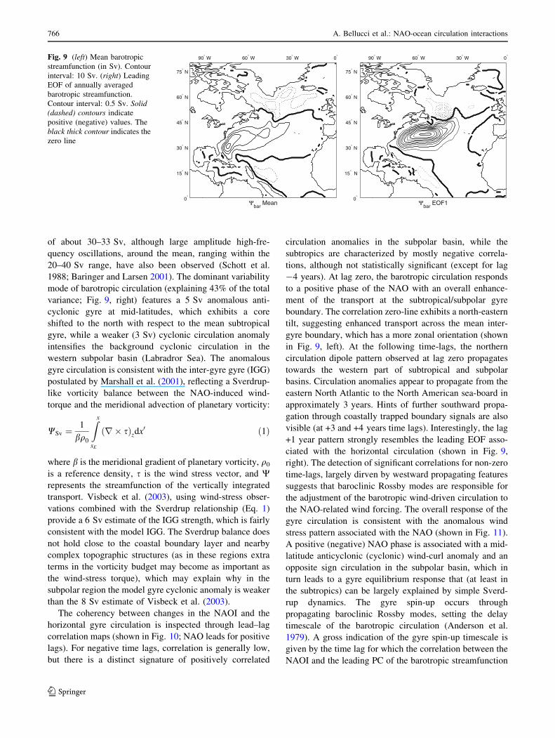
The mean horizontal circulation structure (Fig. 9, left)

reproduces in a realistic way the extratropical double-gyre

circulation pattern, with a subtropical gyre strength of

40 Sv, and a 20 Sv subpolar gyre. The barotropic circula-

tion is generally poorly observed but estimates of the

Florida Current strength (approximately coinciding with

the core of the subtropical gyre) provide a mean transport

90° W 60° W 30° W 0°

0°

15° N

30° N

45° N

60° N

75° N

LAG 0

LAG +1

LAG +2

LAG +3

0

5

10

15

20

25

30

Fig. 7 Regions of positive NAOI/winter SST correlation regions for

time-lags 0 to +3 years (white contour; statistically significant at the

95% level, according to a t Student test). Grey shading indicates the

climatological SST (in �C). The dashed white curve indicates the

dominant propagation path followed by thermal anomalies

TIM

E (

YE

AR

)

Along−track distance (km)0 1000 2000 3000 4000 5000

1870

1880

1890

1900

1910

1920

1930

TIM

E (

YE

AR

)

Along−track distance (km)0 1000 2000 3000 4000 5000

1940

1950

1960

1970

1980

1990

2000Fig. 8 Hovmoller diagram of

linearly detrended winter SST

anomalies along the track

indicated by the dashed line in

Fig. 7 (in �C). Left (right) panel

shows anomalies for the 1870–

1935 (1936–2000) time period.

Contour interval is 0.2�C. Greyshading is used for warm

anomalies

A. Bellucci et al.: NAO-ocean circulation interactions 765

123

of about 30–33 Sv, although large amplitude high-fre-

quency oscillations, around the mean, ranging within the

20–40 Sv range, have also been observed (Schott et al.

1988; Baringer and Larsen 2001). The dominant variability

mode of barotropic circulation (explaining 43% of the total

variance; Fig. 9, right) features a 5 Sv anomalous anti-

cyclonic gyre at mid-latitudes, which exhibits a core

shifted to the north with respect to the mean subtropical

gyre, while a weaker (3 Sv) cyclonic circulation anomaly

intensifies the background cyclonic circulation in the

western subpolar basin (Labradror Sea). The anomalous

gyre circulation is consistent with the inter-gyre gyre (IGG)

postulated by Marshall et al. (2001), reflecting a Sverdrup-

like vorticity balance between the NAO-induced wind-

torque and the meridional advection of planetary vorticity:

WSv ¼1

bq0

Zx

xE

ðr � sÞzdx0 ð1Þ

where b is the meridional gradient of planetary vorticity, q0

is a reference density, s is the wind stress vector, and Wrepresents the streamfunction of the vertically integrated

transport. Visbeck et al. (2003), using wind-stress obser-

vations combined with the Sverdrup relationship (Eq. 1)

provide a 6 Sv estimate of the IGG strength, which is fairly

consistent with the model IGG. The Sverdrup balance does

not hold close to the coastal boundary layer and nearby

complex topographic structures (as in these regions extra

terms in the vorticity budget may become as important as

the wind-stress torque), which may explain why in the

subpolar region the model gyre cyclonic anomaly is weaker

than the 8 Sv estimate of Visbeck et al. (2003).

The coherency between changes in the NAOI and the

horizontal gyre circulation is inspected through lead–lag

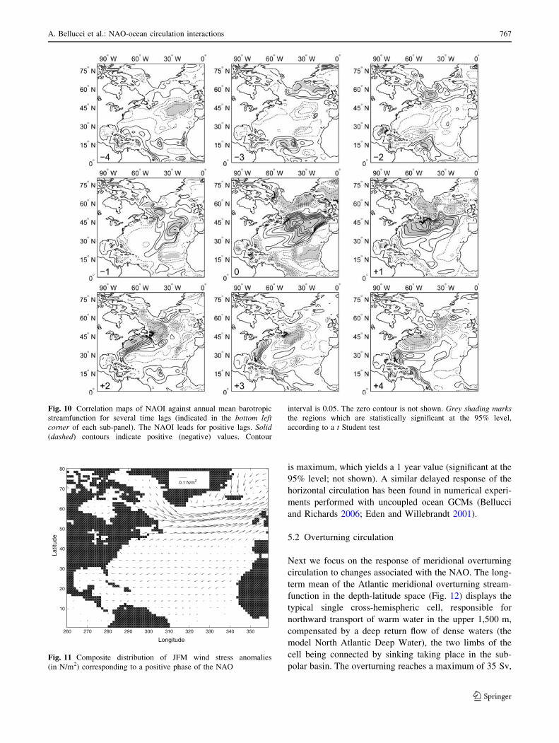
correlation maps (shown in Fig. 10; NAO leads for positive

lags). For negative time lags, correlation is generally low,

but there is a distinct signature of positively correlated

circulation anomalies in the subpolar basin, while the

subtropics are characterized by mostly negative correla-

tions, although not statistically significant (except for lag

-4 years). At lag zero, the barotropic circulation responds

to a positive phase of the NAO with an overall enhance-

ment of the transport at the subtropical/subpolar gyre

boundary. The correlation zero-line exhibits a north-eastern

tilt, suggesting enhanced transport across the mean inter-

gyre boundary, which has a more zonal orientation (shown

in Fig. 9, left). At the following time-lags, the northern

circulation dipole pattern observed at lag zero propagates

towards the western part of subtropical and subpolar

basins. Circulation anomalies appear to propagate from the

eastern North Atlantic to the North American sea-board in

approximately 3 years. Hints of further southward propa-

gation through coastally trapped boundary signals are also

visible (at +3 and +4 years time lags). Interestingly, the lag

+1 year pattern strongly resembles the leading EOF asso-

ciated with the horizontal circulation (shown in Fig. 9,

right). The detection of significant correlations for non-zero

time-lags, largely dirven by westward propagating features

suggests that baroclinic Rossby modes are responsible for

the adjustment of the barotropic wind-driven circulation to

the NAO-related wind forcing. The overall response of the

gyre circulation is consistent with the anomalous wind

stress pattern associated with the NAO (shown in Fig. 11).

A positive (negative) NAO phase is associated with a mid-

latitude anticyclonic (cyclonic) wind-curl anomaly and an

opposite sign circulation in the subpolar basin, which in

turn leads to a gyre equilibrium response that (at least in

the subtropics) can be largely explained by simple Sverd-

rup dynamics. The gyre spin-up occurs through

propagating baroclinic Rossby modes, setting the delay

timescale of the barotropic circulation (Anderson et al.

1979). A gross indication of the gyre spin-up timescale is

given by the time lag for which the correlation between the

NAOI and the leading PC of the barotropic streamfunction

90° W 60° W 30° W 0°

0°

15° N

30° N

45° N

60° N

75° N

Ψbar

EOF1

90° W 60° W 30° W 0°

0°

15° N

30° N

45° N

60° N

75° N

Ψbar

Mean

Fig. 9 (left) Mean barotropic

streamfunction (in Sv). Contour

interval: 10 Sv. (right) Leading

EOF of annually averaged

barotropic streamfunction.

Contour interval: 0.5 Sv. Solid(dashed) contours indicate

positive (negative) values. The

black thick contour indicates the

zero line

766 A. Bellucci et al.: NAO-ocean circulation interactions

123

is maximum, which yields a 1 year value (significant at the

95% level; not shown). A similar delayed response of the

horizontal circulation has been found in numerical experi-

ments performed with uncoupled ocean GCMs (Bellucci

and Richards 2006; Eden and Willebrandt 2001).

5.2 Overturning circulation

Next we focus on the response of meridional overturning

circulation to changes associated with the NAO. The long-

term mean of the Atlantic meridional overturning stream-

function in the depth-latitude space (Fig. 12) displays the

typical single cross-hemispheric cell, responsible for

northward transport of warm water in the upper 1,500 m,

compensated by a deep return flow of dense waters (the

model North Atlantic Deep Water), the two limbs of the

cell being connected by sinking taking place in the sub-

polar basin. The overturning reaches a maximum of 35 Sv,

Fig. 10 Correlation maps of NAOI against annual mean barotropic

streamfunction for several time lags (indicated in the bottom leftcorner of each sub-panel). The NAOI leads for positive lags. Solid(dashed) contours indicate positive (negative) values. Contour

interval is 0.05. The zero contour is not shown. Grey shading marksthe regions which are statistically significant at the 95% level,

according to a t Student test

260 270 280 290 300 310 320 330 340 350

10

20

30

40

50

60

70

80

0.1 N/m2

Longitude

Latit

ude

Fig. 11 Composite distribution of JFM wind stress anomalies

(in N/m2) corresponding to a positive phase of the NAO

A. Bellucci et al.: NAO-ocean circulation interactions 767

123

at a 1,500 m depth around 45�N. This is by far an over-

estimate of the available observations, indicating an

approximately 18 Sv strength for the Atlantic overturning

(Kuhlbrodt et al. 2007, and references therein), even when

the large uncertainties associated with the direct estimates

are taken into consideration. While this is a clear deficiency

of the present model, it must be emphasized that it is the

time-dependent part of the meridional overturning (and the

coherency with the NAO) to be relevant to the process

under examination, rather than the amplitude of the mean

state. Moreover, we anticipate here that the overturning

component of the large scale circulation appears to play a

relatively less significant role in orchestrating the coordi-

nated changes between NAO and ocean circulation

detected in the model.

Pointwise correlations between the NAOI and the

meridional overturning circulation are shown in Fig. 13.

Two distinct timescales govern the overturning response to

NAO. At lag zero, most of the signal is essentially deter-

mined by Ekman dynamics driving the shallow surface

flow cells associated with the NAO-related zonal wind-

stress anomalies. At non-zero time lags correlation patterns

reveal spatially coherent structures, involving changes in

the deep circulation. At lag +1 year, a dipole pattern

emerges. During a positive NAO phase, a deep clockwise

(counter-clockwise) overturning cell enhances (decreases)

the background meridional circulation in the subpolar

(subtropical) basin. The enhanced meridional overturning

and sinking in the subpolar basin points to the increased

high latitude buoyancy losses (which in turn lead to

anomalously cold SST) and convection during a positive

NAO phase as likely driving factors. For time lags +2 up to

+4 years the enhanced overturning region propagates

southward, while in the mean time a negative correlation

area (determining weaker overturning) starts to develope in

the subpolar area. At lag +4 years, the dipole initially

detected at lag +1, reappears with reversed sign. The sign

inversion of the dipole-like overturning anomalies can also

be traced for time lags -2 and +7 years (not shown),

although the associated correlations are below the 95%

statistical significance level. Thus, the overturning circu-

lation variability undergoes an oscillatory mode having a

typical 6 years period. The southward propagating over-

turning anomalies take about 4 years to reach the equator

from the subpolar generation region. This slow adjustment

of the thermohaline circulation indicates that advection of

convectively generated dense water is the primary cause of

the delayed response of the meridional overturning, in

agreement with the results shown by Marotzke and Klinger

(2000).

In general, the overturning anomalous flow does not

show any hemispheric structure, i.e., involving the whole

Atlantic conveyor, but it is rather localized in space. The

overturning dipole indicates that during a positive NAO

phase, the anomalous downward mass transport in the

northern part of the subpolar basin is compensated by

anomalous upwelling around 45�N.

The implications stemming from the differing gyre and

thermo-haline response to the NAO on the ocean meri-

dional heat transport will be discussed in the next section.

6 Meridional heat transport

In Sect. 4, we found evidence of poleward propagating

surface thermal anomalies along the path set by the model

Gulf Stream and its extension, which concurs to modulate

the northern part of the tripole over a 5 years time scale.

The slow propagation speed of SST anomalies suggests

that advection is likely to play a relevant role in this

process. As discussed in Sect. 5, both the gyre and over-

turning circulation show a lagged coherent response to the

NAO and are potentially involved in the poleward

migration of thermal anomalies. In order to elucidate the

relative importance of gyre and overturning circulation on

the meridional transfer of heat across the subtropical/

subpolar gyre boundary, we analyse the lagged correlation

between the NAOI and advective heat transport at 51�N,

grossly marking the climatological position of the high

latitude zero line in the mean gyre circulation. We

explicitly compute the total advective heat transport and

the contribution from the meridional overturning circula-

tion, while the gyre contribution is obtained as a residual

between the total transport and the overturning component

(Fig. 14).

The total and gyre heat transport reach a maximum

positive correlation at lag +1 years, whereas the

−30 −20 −10 0 10 20 30 40 50 60−4000

−3500

−3000

−2500

−2000

−1500

−1000

−500

0

0

0

0

0

0 0

3

3

3

3

333 3

6

66

6

6

66

9

9

9

9

9

99

12

12

12

12

1212

15

15

15

15

1515

18

18

18

18

1818

21

21

21

21

2121

24

24

24

24

24

2727 27

2727

27

30

30

30

30

33

33

LATITUDE

DE

PT

H

Fig. 12 Mean meridional overturning streamfunction (in Sv). Con-

tour interval is 3 Sv

768 A. Bellucci et al.: NAO-ocean circulation interactions

123

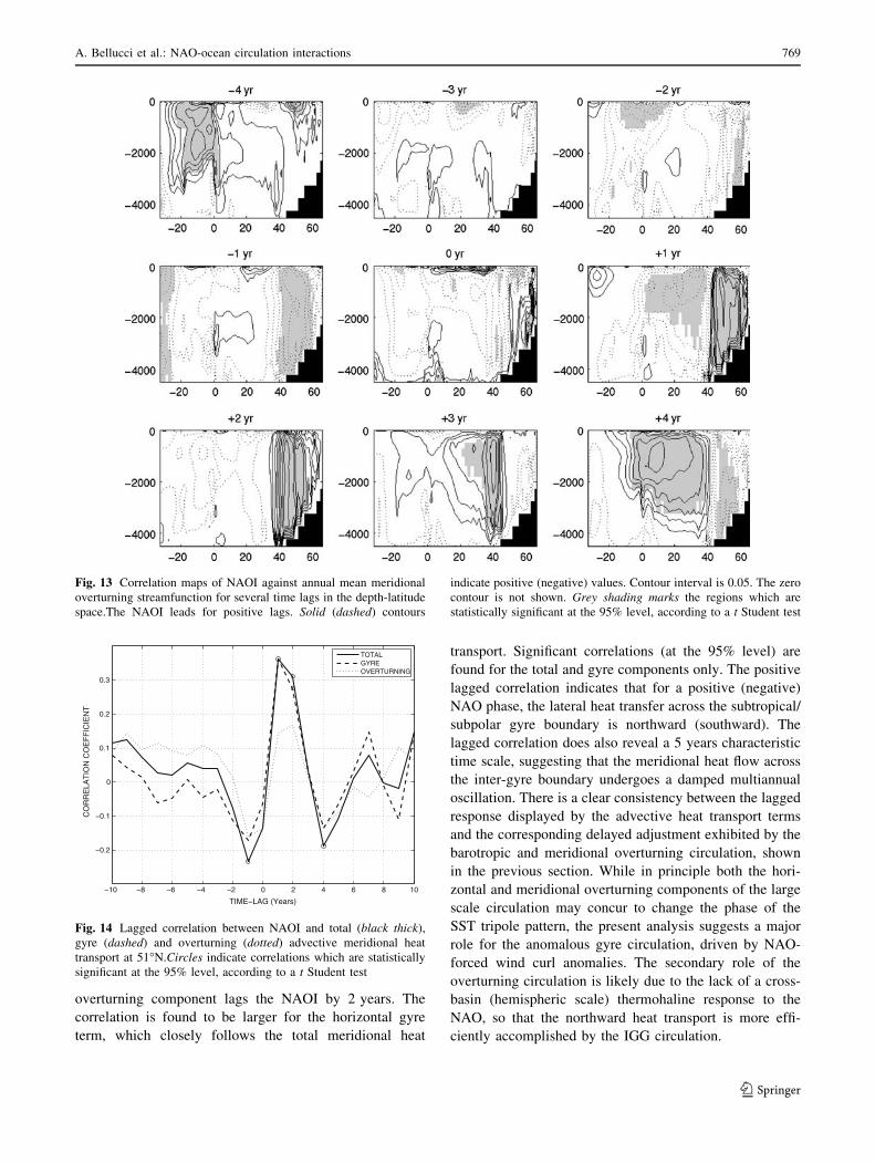
overturning component lags the NAOI by 2 years. The

correlation is found to be larger for the horizontal gyre

term, which closely follows the total meridional heat

transport. Significant correlations (at the 95% level) are

found for the total and gyre components only. The positive

lagged correlation indicates that for a positive (negative)

NAO phase, the lateral heat transfer across the subtropical/

subpolar gyre boundary is northward (southward). The

lagged correlation does also reveal a 5 years characteristic

time scale, suggesting that the meridional heat flow across

the inter-gyre boundary undergoes a damped multiannual

oscillation. There is a clear consistency between the lagged

response displayed by the advective heat transport terms

and the corresponding delayed adjustment exhibited by the

barotropic and meridional overturning circulation, shown

in the previous section. While in principle both the hori-

zontal and meridional overturning components of the large

scale circulation may concur to change the phase of the

SST tripole pattern, the present analysis suggests a major

role for the anomalous gyre circulation, driven by NAO-

forced wind curl anomalies. The secondary role of the

overturning circulation is likely due to the lack of a cross-

basin (hemispheric scale) thermohaline response to the

NAO, so that the northward heat transport is more effi-

ciently accomplished by the IGG circulation.

Fig. 13 Correlation maps of NAOI against annual mean meridional

overturning streamfunction for several time lags in the depth-latitude

space.The NAOI leads for positive lags. Solid (dashed) contours

indicate positive (negative) values. Contour interval is 0.05. The zero

contour is not shown. Grey shading marks the regions which are

statistically significant at the 95% level, according to a t Student test

−10 −8 −6 −4 −2 0 2 4 6 8 10

−0.2

−0.1

0

0.1

0.2

0.3

TIME−LAG (Years)

CO

RR

ELA

TIO

N C

OE

FF

ICIE

NT

TOTALGYREOVERTURNING

Fig. 14 Lagged correlation between NAOI and total (black thick),

gyre (dashed) and overturning (dotted) advective meridional heat

transport at 51�N.Circles indicate correlations which are statistically

significant at the 95% level, according to a t Student test

A. Bellucci et al.: NAO-ocean circulation interactions 769

123

7 Damped multiannual oscillation: a mechanism

The strong coherency characterizing several components of

the system under analysis, supports the idea that the

dynamics underlying the detected coordinated changes in

the NAO (via meridional redistribution of air mass), SST

and large scale mass and heat transport in the ocean are

essentially coupled. In the present section we sketch a

possible mechanism, favouring a scenario where the

anomalous gyre circulation (or IGG) is a preferred process

with respect to the meridional overturning.

During a positive NAO phase, enhanced surface

westerlies across the middle latitudes, combined with

stronger than average trade winds in the 10–30�N latitude

belt, determine an anticyclonic wind stress curl anomaly

straddling the extratropics between 30 and 50�N, while a

cyclonic surface circulation anomaly develops over the

subpolar region. The vorticity source associated with the

NAO wind-torque drives a Sverdrup response of the

barotropic wind driven circulation, leading to a mirror

anticyclonic IGG, enhancing the background subtropical

gyre circulation in proximity of the GS/NAC frontal sys-

tem. The IGG determines an enhanced meridional heat

transport across the subtropical/subpolar gyre boundary,

which in turn leads to the warming (cooling) of the sub-

polar (subtropical) basin. The consequent sign reversal in

the northern SST dipole, forces the NAO to enter into a

negative phase, through a positive NAO/SST feedback.

Once the NAO has stepped into a negative phase, the

previously described stages of the oscillation repeat with

reversed sign, and the oscillation completes its cycle.

According to this scheme, the gyre circulation is an

essential element of the coupled oscillatory mode, in that it

provides the delay which is crucial for sustaining the

oscillation. A combination of advective and wave dyna-

mics governs the negative feedback between the ocean

gyre circulation and NAO. The adjustment of the baro-

tropic IGG to changes in the wind stress curl occurs

through the propagation of baroclinic Rossby modes. The

gyre spin up is quite fast (order 1 year), but the lateral

transport is also affected by the (slower) advective process.

The effective timescale associated with the poleward

transport of thermal anomalies (i.e., the time taken by an

SST anomaly to propagate from the subtropical basin to the

subpolar basin) is of the order of 2–3 years.

In sketching the coupled mechanism we have assumed

that the northern SST dipole forces a NAO-like atmo-

spheric response, ultimately leading to sizeable changes in

the surface wind stress. The lead–lag correlation analysis

between NAOI and SST does indeed show significant

correlation for negative time lags, i.e., when the SST leads

the NAO. In particular, the correlation pattern emerging at

lag -2 years bears striking similarity with the so called

horse-shoe pattern described by Czaja and Frankignoul

(2002; hereafter CF) who analysed the lagged covariance

between SST and tropospheric anomalies in the NCEP-

NCAR reanalysis. In CF analysis, the horse-shoe pattern

precedes a NAO positive phase by several months. In our

analysis the intra-seasonal time scale is not considered, but

a similar covariability appears to work on the interannual

time scale. This is not entirely inconsistent with CF results,

which show that it is the long persistence (from summer to

winter) of the horse-shoe pattern to favour the onset of a

positive NAO-phase. A clear identification of causal rela-

tionships in observations as well as in CGCMs results

cannot be achieved by (even sophisticated) statistical

diagnostic tools, and further understanding of mid-latitude

SST forcing mechanisms of NAO has been gained through

numerical experiments (Peng and Whitaker 1999; Peng

et al. 2002, 2003). Rodwell et al. (1999) analyse the

response of an atmospheric GCM forced with observed

SSTs and show that SST anomalies re-enforce the thermal

and geopotential structure of the NAO, thus suggesting the

existence of a positive feedback (i.e., SSTs generated by

anomalous NAO-heat fluxes strengthen the wind stress

field which in turn feeds back on the SSTs). A potential

indicator of SST-induced atmospheric thermal heating is

provided by the 200-hPa GPH anomalies, which relate to

changes in the thickness of the troposphere. Figure 15

shows composite maps of 200-hPa GPH and SST winter

(JFM) anomalies, obtained for positive minus negative

phases of the SST tripole (as diagnosed through the pre-

viously defined tripole index). This is done at lags 0, +3

and +5 year, so that at lag 0, the composite is simply the

difference between the average SST and GPH anomalies

computed over high minus low tripole index years, while at

the following n-year lags, the composite is computed by

shifting the high and low index years by n years. The

200 hPa GPH anomalies exhibit (at lag 0) a deep low over

the subpolar region and a high over the subtropical region,

overlying cold and warm SST anomalies, respectively. The

same pattern re-emerges after 5 years with a weaker

amplitude, after going through a phase reversal at lag

+3 year. This result is consistent with Rodwell et al. (1999)

findings (see their Fig. 3e). The strong spatial and temporal

coherence displayed by these two fields suggests—with all

the due caveats concerning the identification of causality in

a CGCM—that ocean SSTs may impact, through diabatic

heating, not only on the lower troposphere, but—through

an equivalent barotropic response—on the upper tropo-

spheric layers as well.

In order to corroborate the hypothesis of a positive

feedback between mid-latitude SST anomalies and NAO,

additional AMIP-type experiments using the SXG atmo-

spheric model (ECHAM4 with T106 resolution) in stand-

alone configuration, forced with observed SSTs for the

770 A. Bellucci et al.: NAO-ocean circulation interactions

123

1956–2000 period were performed. We analysed monthly

outputs from a three-members ensemble of 44 years long

integrations to examine the atmospheric response to the

winter time (JFM) SST tripole. The model response was

calculated as differences of JFM 200 hPa GPH anomalies

between high and low extremes of a SST tripole index. The

SST index was defined as the difference between winter

anomalies in a northern subpolar and a southern subtropical

region, so as to capture the centres of action of the

observed SST tripole. The response is season dependent,

but a strong NAO pattern emerges in February-March-

April, with an amplitude of *30 m/K (Fig. 16). GPH

anomalies computed at 500 hPa (not shown) display a

*20 m/K response. These results are consistent with the

findings of Peng et al. (2002), who used a large ensemble

of experiments performed with the NCEP GCM with a T42

resolution. The fact that the same tropospheric variability

patterns found in the coupled framework were reproduced

in the uncoupled system indicates that mid-latitude SSTs

can indeed force a significant response in the present

atmospheric model.

The coupled oscillation is highly damped and this may be

due to the relatively small spatial extent of propagating

thermal anomalies in concomitance with the thermal

damping operated by turbulent air–sea fluxes. The coupled

oscillation is consistent with a stochastically forced delayed

oscillator model, with the delay essentially provided by the

gyre circulation. Marshall et al. (2001; hereafter M01)

developed a theoretical model which extends the stochastic

climate model of Frankignoul and Hasselmann (1977),

adding the effects of ocean dynamics. According to M01, a

privileged role is played by the wind-driven circulation,

with the anomalous IGG being considered a most efficient

heat carrier through the GS/NAC front, compared to the

meridional overturning. Once a feedback between SST and

wind-stress is allowed, the system behaves as a delayed

oscillator, with the delay set by the propagation of baro-

clinic Rossby waves (assumed to be of order 10 years). The

ocean–atmosphere coupling introduces enhanced power in

the surface temperature spectrum around the delay time-

scale, determining a major deviation from the essentially

red noise spectrum displayed by Frankignoul and Hassel-

mann (1977) model. Using the M01 theoretical model,

CM01 show that, when the coupling is considered, the

spectral structures found in the SST imprint on the wind

Fig. 15 Composite maps of winter 200 hPa GPH (contour) and SST

anomalies (colour shading), in m and �C, respectively, based on years

where the tripole index (shown in Fig. 4) is high, with respect to a

threshold of one standard deviation (in absolute value). At lag zero,

the composite is simply the average GPH (or SST) anomaly computed

over high tripole years. At lag +3 years (and similarly for lag

+5 years), the composite is computed by shifting the high tripole

index years by 3 years. Countour interval is 5 m. Solid (dashed) line

indicates positive (negative) values. The black thick line indicates the

0 line

Fig. 16 Composite map of February–April 200 hPa GPH (contour)

and January–March SST anomalies (grey shading), in m and �C,

respectively, computed over years where a SST tripole index exceeds

one standard deviation (high minus low index years; see text for

details). These results are from an ensemble of integrations performed

with ECHAM4 (T106) in a stand-alone configuration, forced with

observed SSTs for the 1956–2000 period. Contour interval is 5 m.

Solid black (white) contours indicate positive (negative) values. The

black thick contour indicates the 0-line

A. Bellucci et al.: NAO-ocean circulation interactions 771

123

stress power spectrum as well, showing enhanced vari-

ability over the same frequency range as for SST. The

mechanism emerging from the analysis of the SXG coupled

model qualitatively fits within the one outlined by M01. A

gross spectral consistency between the NAOI (essentially

capturing changes in the geostrophically balanced wester-

lies) and the SST leading variability mode is found in the

SXG model (Fig. 2), similar to the one shown by CM01.

Both NAOI and SST signals exhibit a bimodal spectral

structure, with enhanced power at quasi-biennial and multi-

annual periods. The broad multiannual spectral peaks

largely overlap, although the SST clearly peaks at 5 years,

while the former is centred around a slightly longer period.

Discrepancies between SXG and M01 model arise when

the essential timescales featured by the two systems are

compared. The adjustment of the IGG to changes in the

NAO (estimated as the time lag for which the correlation

between the NAOI and the barotropic streamfunction PC1

is maximum) takes place in about 1 year in the CGCM,

against the decadal timescale assumed by M01 and CM01.

However, if the time taken by gyre anomalies to propagate

across the zonal width of the Atlantic basin (as can be

inferred from Fig. 10, around 45�N) is considered, we find

a slightly longer *3 years timescale. This is still an

underestimate of the theoretical phase speed for the first

baroclinic Rossby wave, predicting a 8 years time-scale at

45�N (Killworth et al. 1997). Bellucci and Richards

(2006), using an uncoupled OGCM forced with a realistic

NAO-like wind-stress pattern, found a strong dependency

of the IGG spinup timescale on the ocean eddy mixing

strength, with a slow 4 years (fast 2 years) adjustment

under low (high) dissipative conditions. A thorough dis-

cussion on the limitations of state-of-the-art OGCMs in

correctly reproducing the planetary waves is beyond the

scopes of the present work. However, the high dissipation

which is needed to maintain the numerical stability in

coarse resolution ocean models (as in the present case) is

likely to impact on the correct representation of local

potential vorticity gradients, which may ultimately alter the

propagation speed of planetary waves.

It is interesting to contrast our results with those

obtained with experimental setup of intermediate com-

plexity (a detailed comparison between the coupled

oscillation found in SXG and the delayed oscillator

framework described by M01 and CM01 is presented in the

next section). Eden and Greatbach (2003) couple a OGCM

(having a horizontal resolution similar to the ocean model

used in SXG) to a simple stochastic atmosphere (described

in Bretherton and Battisti 2000) and find that the system

undergoes a damped decadal oscillation. However, unlike

the scenario postulated by M01 and the results from the

present analysis, the negative feedback which maintains the

oscillation is orchestrated by the overturning circulation

(providing the decadal timescale), while the IGG circula-

tion determines a positive feedback on the meridional SST

gradient, with the wind-driven circulation acting to actually

reduce the cross-gyre heat transport for a positive NAO

phase. Using a similar approach, D’Andrea et al. (2005)

analyse the impact of ocean heat transport on NAO with a

quasi-geostrophic potential vorticity atmospheric model

coupled to a mixed layer ocean model. The effects of ocean

dynamics on heat transport are parameterized so as to

mimic the M01 analytical model, with the ocean response

to changes in the NAO governed by a fixed 10 years

timescale. This highly constrained system produces an

oscillation in both atmosphere and ocean with a 15 years

period and a space structure bearing strong similarities with

the oscillation diagnosed in SXG coupled system. Differ-

ences between the dominant temporal scales in our system

and in D’Andrea et al. (2005) clearly reflect the assumption

made by the latter on the decadal adjustment of gyre cir-

culation to changes in the NAO.

8 Relationships between SXG and the delayed

oscillator model

8.1 The delayed oscillator: basic equations and scaling

factors

Here a more quantitative analysis of the mid-latitude

oscillatory mode is presented, essentially aimed to set the

coupled model behaviour within the parameter space of the

delayed oscillator framework, developed by M01 and

CM01. A complete derivation of this model can be found

in M01 and CM01. Here we will schematically refer to the

dimensional equations B.1 and B.2 in CM01 (here, Eqs. 2

and 3, respectively), in the hypothesis that the largest

contribution from ocean dynamics comes from the wind-

driven gyre circulation:

dDT

dt¼ �kDT � aN þ gwg ð2Þ

s ¼ N � f DT ð3Þ

Equations 2, 3 govern the interannual evolution of the

northern SST dipole DT (defined as the difference of SST

anomalies averaged over a northern and a southern box,

TN-TS) and the zonal wind stress anomaly s (defined as the

difference between anomalous westerlies and trade winds),

with N the stochastic component of surface wind stress, g

wg the heating rate associated with the anomalous heat

transport by the IGG, k-1 denoting a damping timescale for

DT due to air–sea interactions, and f the SST dipole

feedback on the zonal wind stress. After scaling Eqs. 2, 3

by the system relevant scales for time (td, related to the

propagation of baroclinic Rossby modes, around the IGG

772 A. Bellucci et al.: NAO-ocean circulation interactions

123

latitude), IGG strength (Wg), SST dipole ð� Þ and zonal

wind stress (swind), a new set of equations is obtained

which is formally identical to the previous one except that

now non-dimensional forms of g, f and k parameters

appear, defined as g� ¼ gtdWg��1; f � ¼ f� swind

�1 and

k* = k td. After invoking time-dependent Sverdrup

dynamics for the parameterization of wg, and neglecting

the stochastic wind forcing N in Eq. 3 (see CM01), Eqs. 2,

3, now regarded as non-dimensional, can be rephrased as a

delayed oscillator problem:

dDT

dt¼ �k�DT � f �g�DTðt � 1

2Þ ð4Þ

where the second term on the right hand side expresses the

dependency of the gyre advection term on the wind

induced by temperature anomalies during the previous

Rossby wave transit time. Equation 4 reveals that a par-

ticularly insightful parameter of the delayed oscillator is

R = f*g*/k*, weighting the efficiency of gyre dynamics in

transferring heat through the inter-gyre boundary (f*g*),

with respect to the damping of SST anomalies (k*) through

ocean–atmosphere interactions (incorporating both local

and Ekman-driven non-local processes). An estimate of R

determines whether damped (R \ 1) or growing (R [ 1)

oscillatory solutions are supported by the system. In order

to relate in a simple way the coupled model behaviour to

the simplified delayed oscillator system, we derive R from

the analysed SXG simulation, and compare it to the esti-

mates provided by CM01 and M01.

In the present study, the scale factors have been directly

estimated from the main features of the coupled model

20c3m simulation, yielding td = 3 years, Wg = 5 Sv,

swind = 0.07 Nm-2 and � ¼ 1 K: The temporal scale

factor td reflects the zonal propagation timescale detected

for horizontal circulation anomalies around the IGG lati-

tude (Fig. 10). The strength of the IGG was diagnosed

through the amplitude of the dominant variability pattern of

barotropic streamfunction (shown in Fig. 9b). For swind, an

average value of the zonal wind stress anomaly in the

westerly belt during a positive phase of the NAO, was

selected (see Fig. 11). An indicative 1 K value has been

adopted to scale DT, based on the typical north–south SST

gradient during a positive NAO phase. The boxes selected

to define DT in the model are (50�N–70�N, 60�W–30�W)

for the northern box, and (40�N–50�N,80�W–60�W) for the

southern box, and have been chosen so as to isolate the

centres of action of the NAO SST dipole.

8.2 Delayed oscillator parameters estimate

The estimate of the parameters contributing to the ampli-

tude of the R factor is performed by relying on a linear

regression approach.

Equation 2 is a linear model with one predictand _DT

(where the dot indicates the time derivative) and three

predictors DT, N and w. We assume that, over the inter-

annual timescales considered here, the stochastic

component of the surface wind stress N is instantaneously

uncorrelated with respect to the other terms in Eq. 2, as N is

by definition a white noise signal, while DT and w display a

red spectral signature. Thus, we estimate k and g by fitting

into a simplified version of Eq. 2 (i.e., after removing the

stochastic forcing term) a linear model:

Y ¼ b0 þ b1DT þ b2wg ð5Þ

with Y the predicted value for _DT ; and b1 and b2 yielding

the estimates for k and g, respectively. The left-hand side

term in Eq. 2 is evaluated using a centred finite difference

scheme, while wg is defined as the barotropic

streamfunction anomaly (i.e., obtained by removing the

long-term time-mean) area-averaged inside the core of the

IGG. The non-local nature of the dynamic (gyre) predictor

imposes to consider correlations at non-zero time lags.

Similarly, a simple lagged correlation between DT and _DT

displays an antisymmetric shape around lag 0, with

significant correlations at lags +1 and -1 year, and zero

correlation at lag 0 (not shown). We use the multiple

correlation coefficient R2 to evaluate the fit of the predicted

Y onto the observed _DT : Several predictand/predictors

time-lag relationships are considered (not shown) but a

maximum R2 = 0.5 fit is found for:

_DTn�2 ¼ �kDTn�1 þ gwn ð6Þ

where the n subscript indicates the temporal index. Thus,

the set of predictors DT and w accounts for about 50% of

the total variance of the predictand _DT ; when wg (DT) leads

the SST dipole rate of change by 2 (1) years. The corre-

sponding dimensional estimates for the gyre efficiency and

SST dipole damping rate are g = 0.025 K Sv-1 year-1 and

k = 1/(2.3 years) yielding the non-dimensional values

g� ¼ gtdWg��1 ¼ 0:38 and k* = k td = 1.3. The positive

value for g implies that an anticyclonic (cyclonic) gyre

circulation anomaly drives a positive (negative) DT thermal

contrast, i.e., the northern box becomes warmer (cooler)

compared to the southern box. The 2 years lagged corre-

lation reflects the poleward propagation time-scale

affecting surface thermal anomalies (Fig. 7).

In order to estimate the feedback of the SST dipole onto

the zonal wind stress f we make use of the AMIP set of

uncoupled atmospheric integrations, already described in

Sect. 7. Averaging over an ensemble of AMIP simulations

allows to better single out the atmospheric response forced

by the SST, from the response to the weather noise N,

different for each member, the latter approaching zero in

the limit of a large ensemble. It must be noted that a more

rigorous approach would have required the use of an AMIP

A. Bellucci et al.: NAO-ocean circulation interactions 773

123

ensemble forced with SSTs taken from the long coupled

simulation (while in the present case, an observed SST is

used). This approach, described in detail by Schneider and

Fan (2007), will not be pursued here. After linearly

regressing DT onto s (over a region in the northern North

Atlantic displaying significant cross-correlation) we obtain

an (ensemble mean) dimensional estimate f = + 0.029 N

m-2 K-1 indicating that a negative DT (colder than average

northern box and warmer than average southern box) is

consistent with a positive NAO phase (increased westerlies

and trade winds). The non-dimensional value is f � ¼f� swind

�1 ¼ 0:41: This estimate is also consistent with the

analysis performed by Neelin and Weng (1999) of the

zonal wind stress response of ECHAM2 atmospheric

model to SST anomalies in the North Atlantic (see their

Fig. 2), suggesting that f* can reach *0.4. We are now

able to estimate the parameter D = f*g* = 0.16, modulat-

ing the magnitude of the delay term (due to gyre dynamics)

in Eq. 4, and finally R = D/k* ^ 0.1.

The fairly low magnitude of D and R indicates that the

oscillatory mode detected in the coupled model is a strongly

damped one. In Table 1, we compare the parameter values

found in SXG with the estimates provided by CM01 and

M01 (where available). The coupled model parameters are

largely consistent with those provided by CM01 and M01,

except for g, which shows a considerably lower magnitude.

This leads to a consistently smaller R value, compared with

the estimates of CM01 (R = 0.4) and M01 (R = 1.6). The

scaling factors adopted to define the delayed oscillator

parameters (listed in Table 2) are clearly crucial in deter-

mining the size of R. Again, there is an overall consistency

between the scale factors diagnosed for SXG and the esti-

mates provided by CM01 and M01, except for td which in

SXG (and M01) is far shorter than in CM01. This dis-

crepancy relates to differences in the estimate of the IGG

adjustment timescale, which is in turn determined by the

phase speed of the first order baroclinic Rossby mode at a

mean IGG latitude. In CM01 an indicative 40�N latitude is

adopted, implying a *10 years propagation timescale

(Killworth et al. 1997). The rather shorter 3 years timescale

diagnosed for the SXG coupled model, despite the gross

consistency with the observed IGG structure and location

(CM01; Visbeck et al. 2003), may suggest a misrepresen-

tation of planetary waves in the coupled model.

Changes in the definition of the northern and southern

boxes appear to have a small impact on the magnitude of R.

Overall, even accounting for the uncertainties associated

with each single parameter, the resulting R = 0.1 estimate

appears to be a robust estimate. The low g magnitude is

clearly the most impacting factor, showing that the effi-

ciency of the wind-driven gyre circulation in sustaining the

oscillatory mode is strongly contrasted by the air–sea

damping of thermal anomalies.

9 Summary and conclusions

In this study the interplay between the large scale ocean

circulation and NAO was analysed with a full-fledged

CGCM. The model captures both the observed long-term

re-emergence of the SST tripole pattern (CM01) and the

propagation of surface temperature anomalies along the

path of the GS/NAC system (SA97). Based on the analysis

of the SXG 20C3M integration, it is argued that these fea-

tures of the extra-tropical North Atlantic SST variability are

strictly related to each other. The structure of the anomalous

gyre circulation suggests that the latter plays a dominant

role in the transfer of surface thermal features across the

inter-gyre boundary as well as in their following recircu-

lation within the western subpolar basin, which in turn

concurs to the low frequency changes in the northern part of

the SST tripole. On the other hand, the contribution of the

mean advection of temperature anomalies to the cross-gyre

heat transport is marginal as the mean flow acts along,

rather than across, the inter-gyre boundary, but its role is not

negligible in the subtropical gyre, where the mean flow

effects on the overall transport dominate. Significant lead–

lag covariance between oceanic and tropospheric variables

suggests that the system supports a damped oscillatory

mode involving an active ocean–atmosphere coupling, with

a typical NAO-like space structure and a 5 years timescale,

qualitatively consistent with the theoretical framework

developed by M01. The two essential processes governing

the oscillation are (1) a positive feedback between SST and

the NAO, and (2) a negative feedback between ocean gyre

circulation and the high latitude SST meridional gradient.

The existence of a significant atmospheric circulation

response to extra-tropical SST anomalies is further sup-

ported by additional AMIP-type integrations performed

with the SXG atmospheric model (ECHAM4) in stand-

alone configuration, forced with observed SSTs. The

atmospheric NAO pattern appears to have a weaker pro-

jection on the ocean meridional overturning, compared to

the gyre circulation, which leads to a secondary role for the

thermohaline circulation in driving the northward heat

transport, and thus the oscillatory mode.

A quantitative analysis of the mid-latitude oscillatory

mode, setting the coupled model behaviour within the

parameter space of the delayed oscillator framework,

shows that the efficiency of the wind-driven gyre circula-

tion is strongly contrasted by the air–sea damping of

thermal anomalies, yielding highly damped oscillations (as

quantified by a fairly low R = 0.1 factor), in accord with

the findings of CM01. The heavily damped nature of the

oscillation found in the SXG model sets a major difference

with respect to the mid-latitude unstable mode described by

Latif and Barnett (1994, 1996) for the North Pacific, and

later adapted by Grotzner et al. (1998) to the North

774 A. Bellucci et al.: NAO-ocean circulation interactions

123

Atlantic case, underlying the self-sustained decadal oscil-

lation found in an extended integration of the ECHO

coupled model.

An important consideration to be done is that, despite

the qualitative consistency with existing theoretical models

and observations, the relevant temporal scales charac-

terizing the present mechanism appear to be distorted by

deficiencies in the ocean component of the CGCM. In

particular, both the re-emergence of the tripole and the

poleward drift of SST anomalies take place over a shorter

timescale compared to the observations. This timescale

discrepancy determines enhanced coupled variability at

multiannual—rather than decadal—temporal scales. A

number of factors may contribute to this mismatch. First,

the anomalously fast gyre spin-up (with respect to what the

theory of baroclinic Rossby waves predicts at the latitudes

under exam) which is likely to be related to the relatively

high dissipation used in the OGCM. An additional reason

of concern is the oversized strength of the Atlantic con-

veyor, which may concur to enhance the background mean

flow and thus further reduce the advective time scale of the

ocean sub-system. These considerations point to the need

for including less dissipative ocean models (i.e., explicitly

resolving a larger fraction of the currently unresolved

physical processes) in next generation CGCMs, if we aim

to a proper representation of low frequency variability at

the extra-tropics. The recent availability of the AR4 IPCC

experiments makes possible to set the present results in the

wider context of a multi-model framework, and possible

extensions of this work, focusing on the impact of OGCM

horizontal resolution on the NAO/ocean circulation inter-

actions are currently under study.

Another important issue is the role of the seasonal cycle.

Throughout the paper we focused on winter time anomalies

as we were mostly interested in interannual-to-decadal

timescales, and winter is the season of the year featuring the

most powerful NAO signature, in both oceanic and tropo-

spheric variables. While an analysis taking into account the

effects associated with the seasonal variability was beyond

the scope of the present work, it is worth mentioning that the

seasonal cycle is likely to play an important role in the mid-

latitude delayed oscillator mechanism by affecting the year-

to-year persistency of surface thermal anomalies through

the winter re-emergence process described by Watanabe

and Kimoto (2000), ultimately affecting the damping rate of

SST anomalies (parameter k, in Eq. 2).

Finally, based on this set of results, we cannot rule out

other possible sources of uncoupled variability, i.e.,

involving intrinsic oceanic and atmospheric processes. A

complete assessment of the impact of ocean circulation on

the variability of the coupled system would probably

require an additional uncoupled experiment, where the

interactive ocean model is replaced with climatologically

varying SSTs. Compared to a standard AMIP type inte-

gration (where the atmospheric GCM is forced with

observed SSTs) this additional experiment would allow the

total removal not only of ocean dynamics but also of the

interannual changes of observed SSTs, which do include

the effects of ocean circulation embedded within. This will

be the subject of additional work.

Acknowledgements The authors wish to thank Riccardo Farneti

and Annalisa Cherchi for stimulating discussions and precious sup-

port. Comments from three reviewers considerably improved the

original manuscript. This work was supported by the Centro Euro-

Mediterraneo per i Cambiamenti Climatici (CMCC) Project and the

European Community ENSEMBLES Project (Contract GOCECT-

2003-505539).

References

Anderson D, Bryan K, Gill A, Pacanowski R (1979) The transient

response of the North Atlantic: some model studies. J Geophys

Res 84:4795–4815

Baringer M, Larsen J (2001) Sixteen years of florida current transport

at 27N. Geophys Res Lett 28:3179–3182

Bellucci A, Richards KJ (2006) Effects of NAO variability on the

North Atlantic Ocean circulation. Geophys Res Lett 33:L02612.

doi:10.1029/2005GL024890

Table 1 Summary of the delayed oscillator parameters in SXG, CM01 and M01

SXG CM01 M01

Dim Non-dim Dim Non-dim Dim Non-dim

k (2.3 year)-1 1.3 1 year-1 7 (1.6 year)-1 2.5

g 0.025 K Sv-1 year-1 0.38 n.a. 8 n.a. 10

f 0.029 N m-2 K-1 0.41 0.015 N m-2 K-1 0.3 n.a. 0.4

R = f*g*/k* 0.1 0.4 1.6

Table 2 Summary of the scale factors adopted to normalize the

delayed oscillator parameters in SXG, CM01 and M01

SXG CM01 M01

swind (N m-2) 0.07 0.05 0.05

� ðKÞ 1 1 1

td (year) 3 10 4

Wg (Sv) 5 10 10

A. Bellucci et al.: NAO-ocean circulation interactions 775

123

Blackman R, Tukey JW (1958) The measurement of power spectra

from the point of view of communication engineering. Dover,

Mineola

Bretherton C, Battisti D (2000) An interpretation of the results from

atmospheric general circulation models forced by the time

history of the observed sea surface temperature distribution.

Geophys Res Lett 27:767–770

Cayan D (1992) Latent and sensible heat flux anomalies over the

Northern oceans: driving the sea surface temperature. J Phys

Oceanogr 22:859–881

Czaja A, Frankignoul C (2002) Observed impact of Atlantic SST

anomalies on the North Atlantic Oscillation. J Clim 15:606–

623

Czaja A, Marshall J (2001) Observations of atmosphere ocean

coupling in the North Atlantic. J R Meteor Soc 127:1893–1916

D’Andrea F, Czaja A, Marshall J (2005) Impact of anomalous ocean

heat transport on the North Atlantic Oscillation. J Clim 18:4955–

4969

Deser C, Blackmon R (1993) Surface climate variations over the

North Atlantic during winter: 1900–1989. J Clim 10:393–408

Eden C, Greatbatch R (2003) A damped decadal oscillation in the

North Atlantic climate system. J Clim 16:4043–4060

Eden C, Willebrandt J (2001) Mechanisms of interannual to decadal

variability in the North Atlantic circulation. J Clim 14:2266–

2280

Feldstein SB (2000) The timescale, power spectra, and climate noise

properties of teleconnection patterns. J Clim 13:4430–4440

Ferreira D, Frankignoul C (2005) The transient atmospheric to

midlatitude SST anomalies. J Clim 18:1049–1067

Fichefet T, Morales-Maqueda MA (1999) Modelling the influence of

snow accumulation and snow-ice formation on the seasonal

cycle of the Antarctic sea-ice cover. Clim Dyn 15:251–268

Frankignoul C, Hasselmann K (1977) Stochastic climate models, part

II: applications to sea-surface temperature variability and

thermocline variability. Tellus 29:289–305

Frankignoul C, Czaja A, L’Heveder B (1998) Air-sea feedback in the

North Atlantic and surface boundary conditions for ocean

models. J Clim 11:2310–2324

Frankignoul C, Kestenare E, Sennechael N, de Coetlogon G,

D’Andrea F (2000) On decadal-scale ocean-atmosphere interac-

tions in the extended ECHAM1/LSG climate simulation. Clim

Dyn 16:333–354

Grotzner A, Latif M, Barnett T (1998) A decadal climate cycle in the

North Atlantic ocean as simulated by the ECHO coupled GCM. J

Clim 11:831-847

Gualdi S, Navarra A, Guilyardi E, Delecluse P (2003a) Assessment of

the tropical Indo-Pacific climate in the SINTEX CGCM. Ann

Geophys 46:1–26

Gualdi S, Guilyardi E, Navarra A, Masina S, Delecluse P (2003b) The

interannual variability in the tropical Indian Ocean as simulated

by a CGCM. Clim Dyn 20:567–582

Gualdi S, Scoccimarro E, Navarra A (2007) Changes in tropical

cyclone activity due to global warming: results from a high-

resolution coupled general circulation model. J Clim (in press)

Guilyardi E, Delecluse P, Gualdi S, Navarra A (2003) Mechanisms

for ENSO phase change in a coupled GCM. Clim Dyn 16:1141–

1158

Hurrell J, Kushnir Y, Ottersen G, Visbeck M (2003) An overview of

the North Atlantic Oscillation. In: Hurrell J , Kushnir J, Ottersen

G, Visbeck M (eds) The North Atlantic Oscillation: climatic

significance and environmental impact. American Geophysical

Union, Washington DC

Kaplan A, Kushnir Y, Cane M, Blumenthal B (1997) Reduced space

optimal analysis for historical datasets:136 years of Atlantic sea

surface temperatures. J Geophys Res 102:27835–27860

Killworth P, Chelton D, de Szoeke R (1997) The speed of observed

and theoretical long extratropical planetary waves. J Phys

Oceanogr 27:1946–1966

Kuhlbrodt T, Griesel A, Montoya M, Levermann A, Hofmann M,

Rahmstorf S (2007) On the driving processes of the Atlantic

meridional overturning circulation. Rev Geophys 45:1–32

Latif M, Barnett T (1994) Causes of decadal variability over the

North Pacific and North America. Science 266:634–637

Latif M, Barnett T (1996) Decadal climate variability over the North

Pacific and North America: dynamics and predictability. J Clim

9:2407–2423

Luo J, Masson S, Behera S, Delecluse P, Gualdi S, Navarra A,

Yamagata T (2003) South pacific origin of the decadal ENSO-

like variation as simulated by a coupled GCM. Geophys Res Lett

30, 2250. doi:10.1029/2003GL018649

Madden R (1981) A quantitative approach to long range prediction.

J Geophys Res 86:9817–9825

Marotzke J, Klinger B (2000) A study of the interaction of the North

Atlantic Oscillation with the ocean circulation. J Phys Oceanogr

30:955–970

Marshall J, Johnson H, Goodman J (2001) A study of the interaction

of the North Atlantic Oscillation with the ocean circulation.

J Clim 14:1399–1421

Neelin JD, Weng W (1999) Analytical prototypes for ocean-

atmosphere interaction at midlatitudes. Part I: coupled feedbacks

as a sea surface temperature dependent stochastic process. J Clim

12:697–721

Peng S, Whitaker JS (1999) Mechanisms determining the atmospheric

response to midlatitude SST anomalies. J Clim 12:1393–1408

Peng S, Robinson W, Li S (2002) North Atlantic SST forcing of the

NAO and relationships with intrinsic hemispheric variability.

Geophys Res Lett 29:1276. doi:10.1029/2001GL014043

Peng S, Robinson W, Li S (2003) Mechanisms for the NAO responses

to the North Atlantic SST tripole. J Clim 16:1987–2004

Rodwell M, Rowell D, Folland C (1999) Oceanic forcing of the

wintertime North Atlantic Oscillation and European climate.

Nature 398:320–323

Saravanan R, McWilliams J (1998) Advective ocean-atmosphere

interaction: an analytical stochastic model with implications for

decadal variability. J Clim 11:165–188

Schneider E, Fan M (2007) Weather noise forcing of surface climate

variability. J Atm Sci 64:3265–3280

Schott F, Lee T, Zantopp R (1988) Variability of structure and

transport of the florida current in the period range of days to

seasonal. J Phys Oceanogr 18:1209–1230

Stephenson D, Pavan V, Collins M, Junge M, Quadrelli R (2006)

North Atlantic Oscillation response to transient greenhouse gas

forcing and the impact on European winter climate: a CMIP2

multi-model assessment. Clim Dyn 27:401–420. doi:

10.1007/s00382-006-0140-x

Storch HV, Zwiers FW (1999) Statistical analysis in climate research.

Cambridge University Press, United Kingdom

Sutton RT, Allen MR (1997) Decadal predictability of North Atlantic

sea surface temperature and climate. Nature 388:563–567

Thompson D, Lee S, Baldwin M (2003) Atmospheric processes

governing the Northern Hemisphere Annular Mode/North

Atlantic Oscillation. In: Hurrell J, Kushnir J, Ottersen G,

Visbeck M (eds) The North Atlantic Oscillation: climatic

significance and environmental impact. American Geophysical

Union, Washington DC

Visbeck M, Chassignet E, Curry RG, Delworth T, Dickson R,

Krahmann G (2003) The ocean’s response to North Atlantic

Oscillation. In: Hurrell J, Kushnir J, Ottersen G, Visbeck M (eds)

The North Atlantic Oscillation: climatic significance and envi-

ronmental impact. American Geophysical Union, Washington DC

776 A. Bellucci et al.: NAO-ocean circulation interactions

123

Watanabe M, Kimoto M (2000) On the persistence of decadal SST

anomalies in the North Atlantic. J Clim 13:3017–3028

Wunsch C (1999) The interpretation of short climate records, with

comments on the North Atlantic Oscillation and Southern

Oscillations. Bull Am Meteor Soc 80:245–255

Zorita E, Frankignoul C (1997) Modes of North Atlantic decadal

variability in the ECHAM1/LSG coupled atmosphere-ocean

general circulation model. J Clim 10:183:200

A. Bellucci et al.: NAO-ocean circulation interactions 777

123