not for circulation THE MATHEMATICS STUDENT
184
Member's copy - not for circulation ISSN: 0025-5742 THE MATHEMATICS STUDENT Volume 87, Numbers 1-2, January-June (2018) (Issued: May, 2018) Editor-in-Chief J. R. PATADIA EDITORS Bruce C. Berndt George E. Andrews M. Ram Murty N. K. Thakare Satya Deo Gadadhar Misra B. Sury Kaushal Verma Krishnaswami Alladi S. K. Tomar Subhash J. Bhatt L. Sunil Chandran M. M. Shikare C. S. Aravinda A. S. Vasudeva Murthy Indranil Biswas Timothy Huber T. S. S. R. K. Rao Clare D 0 Cruz Atul Dixit PUBLISHED BY THE INDIAN MATHEMATICAL SOCIETY www.indianmathsociety.org.in
-
Upload
khangminh22 -
Category
Documents
-
view
3 -
download
0
Transcript of not for circulation THE MATHEMATICS STUDENT
Member's copy - not for circulation
ISSN: 0025-5742
THE
MATHEMATICS
STUDENTVolume 87, Numbers 1-2, January-June (2018)
(Issued: May, 2018)
Editor-in-Chief
J. R. PATADIA
EDITORS
Bruce C. Berndt George E. Andrews M. Ram Murty
N. K. Thakare Satya Deo Gadadhar Misra
B. Sury Kaushal Verma Krishnaswami Alladi
S. K. Tomar Subhash J. Bhatt L. Sunil Chandran
M. M. Shikare C. S. Aravinda A. S. Vasudeva Murthy
Indranil Biswas Timothy Huber T. S. S. R. K. Rao
Clare D′Cruz Atul Dixit
PUBLISHED BY
THE INDIAN MATHEMATICAL SOCIETY
www.indianmathsociety.org.in
Member's copy - not for circulation
THE MATHEMATICS STUDENT
Edited by J. R. PATADIA
In keeping with the current periodical policy, THE MATHEMATICS STUDENT will
seek to publish material of interest not just to mathematicians with specialized interest
but to the postgraduate students and teachers of mathematics in India. With this in
view, it will ordinarily publish material of the following type:
1. research papers,
2. the texts (written in a way accessible to students) of the Presidential Addresses, the
Plenary talks and the Award Lectures delivered at the Annual Conferences.
3. general survey articles, popular articles, expository papers, Book-Reviews.
4. problems and solutions of the problems,
5. new, clever proofs of theorems that graduate / undergraduate students might see in
their course work, and
6. articles that arouse curiosity and interest for learning mathematics among readers and
motivate them for doing mathematics.
Articles of the above type are invited for publication in THE MATHEMATICS
STUDENT. Manuscripts intended for publication should be submitted online in the
LATEX and .pdf file including figures and tables to the Editor J. R. Patadia on E-mail:
Manuscripts (including bibliographies, tables, etc.) should be typed double spaced on
A4 size paper with 1 inch (2.5 cm.) margins on all sides with font size 10 pt. in LATEX.
Sections should appear in the following order: Title Page, Abstract, Text, Notes and
References. Comments or replies to previously published articles should also follow this
format. In LATEX the following preamble be used as is required by the Press:
\ documentclass[10 pt,a4paper,twoside,reqno]amsart\ usepackage amsfonts, amssymb, amscd, amsmath, enumerate, verbatim, calc\ renewcommand\ baselinestretch1.2\ textwidth=12.5 cm
\ textheight=20 cm
\ topmargin=0.5 cm
\ oddsidemargin=1 cm
\ evensidemargin=1 cm
\ pagestyleplainThe details are available on Indian Mathematical Society website: www.indianmath
society.org.in
Authors of articles / research papers printed in the the Mathematics Student as well as in
the Journal shall be entitled to receive a soft copy (PDF file with watermarked “Author’s
copy”) of the paper published. There are no page charges. However, if author(s) (whose
paper is accepted for publication in any of the IMS periodicals) is (are) unable to send
the LATEX file of the accepted paper, then a charge Rs. 100 (US $ 10) per page will be
levied towards LATEX typesetting.
All business correspondence should be addressed to S. K. Nimbhorkar, Treasurer, Indian
Mathematical Society, Dept. of Mathematics, Dr. B. A. M. University, Aurangabad -
431 004 (Maharashtra), India. E-mail: [email protected]
Copyright of the published articles lies with the Indian Mathematical Society.
In case of any query, the Editor may be contacted.
Member's copy - not for circulation
ISSN: 0025-5742
THE
MATHEMATICS
STUDENTVolume 87, Numbers 1-2, January-June, (2018)
(Issued: May, 2018)
Editor-in-Chief
J. R. PATADIA
EDITORS
Bruce C. Berndt George E. Andrews M. Ram Murty
N. K. Thakare Satya Deo Gadadhar Misra
B. Sury Kaushal Verma Krishnaswami Alladi
S. K. Tomar Subhash J. Bhatt L. Sunil Chandran
M. M. Shikare C. S. Aravinda A. S. Vasudeva Murthy
Indranil Biswas Timothy Huber T. S. S. R. K. Rao
Clare D′Cruz Atul Dixit
PUBLISHED BY
THE INDIAN MATHEMATICAL SOCIETY
www.indianmathsociety.org.in

Member's copy - not for circulation
ISSN: 0025-5742
ii
c© THE INDIAN MATHEMATICAL SOCIETY, 2018.
This volume or any part thereof may not be
reproduced in any form without the written
permission of the publisher.
This volume is not to be sold outside the
Country to which it is consigned by the
Indian Mathematical Society.
Member’s copy is strictly for personal use.
It is not intended for sale or circular.
Published by Prof. N. K. Thakare for the Indian Mathematical Society, type set by
J. R. Patadia at 5, Arjun Park, Near Patel Colony, Behind Dinesh Mill, Shivanand
Marg, Vadodara - 390 007 and printed by Dinesh Barve at Parashuram Process,
Shed No. 1246/3, S. No. 129/5/2, Dalviwadi Road, Barangani Mala, Wadgaon
Dhayari, Pune 411 041 (India). Printed in India.

Member's copy - not for circulation
The Mathematics Student ISSN: 0025-5742Vol. 87, Nos. 1-2, January-June, (2018)
CONTENTS
1. Satya Deo Professor V. M. Shah - A remembrance 01-06
2. N. K. Thakare IMS, Pune Usniversity and Professor V. M. Shah 07-08
3. J. R. Patadia Professor V. M. Shah - My Teacher and Colleague 09-12
4. Manjul Gupta Presidential General Address 13-19
5. Manjul Gupta Some topics in Functional Analysis : 21-65our contributions with emphasis on holomorphy
6. Friedrich Ranges of functors in algebra 67-81Wehrung
7. P. V. Jain Approximation by Spline functions and its 83-105Applications
8. R. Narasimha Fluid Mathematics 107-118
9. T. Augusta Defining and computing cubic splines 119-127Mesquita
10. Ajai Choudhry A Diophantine problem on biquadrate – revisited 129-132
11. M. Narayan Some facts about Fiboncci numbers, Lucas numbers 133-144Murty and Golden ratio
12. Prakash A. A unifying multiplication on Cartesian product of 145-152Dabhi and Banach algebrasSavan K. Patel
13. R. G. Vyas and On the absolute Norlund summability of Fourier 153-160
K. N. Darji series
14. Ting-Ting The log-balancedness of generalized Motzkin 161-167Zhang and numbersFeng-Zhen Zhao
15. - Problem Section 169-173
*******

Member's copy - not for circulation
iv

Member's copy - not for circulation
The Mathematics Student ISSN: 0025-5742
Vol. 87, Nos. 1-2, January-June (2018), 01-06
PROFESSOR V. M. SHAH - A REMEMBRANCE(25-09-1929 - 03-12-2017)
SATYA DEO
Professor Vadilal Maganlal Shah (popularly known as Prof. V. M. Shah)
breathed his last very recently on Dec 3, 2017 at Vadodara. He was suffering
from chronic kidney disease and had been with his eldest daughter at Ahmedabad
where he had a mild stroke and was treated there. He did recover briefly, but
other complications cropped up leading to the end. The entire family of the Indian
Mathematical Society and his other friends came to know about this sad news with
great shock and sorrow. Prof Shah had been a great source of encouragement
for all of us in the Indian Math. Society. We lost a great educationist, a noted
mathematician, a great teacher and an extraordinary human being. He is survived
by his wife and four daughters.
A Mathematician and an Administrator
Prof Shah started his academic career as an Assistant Lecturer in the Depart-
ment of Mathematics, Faculty of Science, the M.S.University of Baroda, Vadodara,
Gujarat. He worked under the supervision of Prof U. N. Singh for his doctoral
degree at the M. S. University, became Reader and then Professor at the same
university. His field of research was Fourier Analysis and related areas, which was
a very popular topic during those days. He served the M. S. University of Baroda
with great distinction as Head of the Mathematics Department, as Dean, Faculty
of Science and with numerous administrative responsibilities. Prof V. M. Shah
was elected Fellow of the National Academy of Sciences, India in the year 1980.
He was also elected as the Sectional President (Mathematics including Statistics)
of the Indian Science Congress. He enjoyed the reputation of an excellent teacher,
a sound scholar, and a visionary educationist not only in Gujarat, but in the whole
country. He has been on several UGC committees as well as the Gujarat State level
committees to serve the cause of mathematics teaching and research. He wrote
extremely popular elementary mathematics books entitled ”Majedar Ganit” for
the benefit of students as well as teachers. This must be the case because of his
fascination for mathematics. He joined the Council of the Indian Mathematical
Society first as a Treasurer, but slowly moved upward as its General Secretary, the
most important position of the Society by its constitution.
c© Indian Mathematical Society, 2018 .
1
Member's copy - not for circulation
2 SATYA DEO
Prof Shah and the IMS
As noted earlier, Prof Shah served the Indian Mathematical Society as Trea-
surer, then as the editor of the Journal of Indian Mathematical Society and Math-
ematics Student both, also as its President, and most importantly, as its General
Secretary from 2005 until 2013. As General Secretary, he had to face a big chal-
lenge when there were some attempts by a group of people to run the Society in
their arbitrary style; it surfaced when without taking the Academic Secretary or
the General Secretary of IMS in confidence, a number of academic programmes
were formulated and even announced. This was a great surprise to the elected
office bearers of the Society who did not know what to do in a situation like this.
Prof Shah faced this challenge with great patience, took all the Council members
in confidence and proceeded to neutralize all the moves very quickly. Everything
afterwards became normal, but it took some time and determination to act the
way Prof Shah did. Later on as the General Secretary of the IMS, Prof Shah took
the Society to a great level of prestige, popularity, and academic standard. He
was not only the eldest of all but also most experienced, most patient and highly
sympathetic towards his colleagues. He would always listen to each one of us,
will appreciate opinion of everybody and will go by the consensus. I never saw
him insisting on any point or forcing his opinion on any one.The team of senior
mathematicians like Profs N. K. Thakare, Satya Deo, J. R. Patadia and other
Council members of the IMS worked under his guidance with a noble mission and
motto to strengthen the Society in the same spirit as the founding fathers of the
Society had imagined. During his tenure as the General Secretary, the working
style of the Society became more democratic; more dedicated to the development
of Mathematics in India and established remarkable traditions in its functioning.
Every Council member was there only to give his/her best to the Society and not
to get anything for himself/herself. He left the Society only when most of the
things were ideally streamlined. We never wanted that Prof Shah should retire
from the Society, but because of his health and unshakable principles he declined
our request and took retirement from the IMS in the year 2013. Nevertheless, his
style of functioning, his important actions and visionary decisions in the IMS are
permanent foot-prints for us to follow.
The Centenary Year 2007 of the IMS
I came in contact with Prof V. M. Shah in December 2005 when he was the
General Secretary of IMS and I was nominated as the Academic Secretary. It took
no time for me to realize that Prof. Shah was a great leader and totally committed
to see that the IMS becomes one of the best mathematical societies of the world
as soon as possible. He made plans, wrote letters to several government organi-
zations and leading mathematicians to seek their cooperation. The year 2007 was
the Centenary year of the Indian Mathematical Society, and under his leadership

Member's copy - not for circulation
PROFESSOR V. M. SHAH - A REMEMBRANCE 3
the society celebrated its centenary year in a big way. We invited almost all of
the Indian mathematicians within the country and abroad to come and attend the
Centenary Conference organized by the Department of Mathematics at the Pune
University, Pune. Even though Prof Shah remained in the M. S. University of Bar-
oda throughout his life, he knew almost all the leading mathematicians working
in universities, research institutes, IITs and NITs really well. Prof N. K. Thakare,
myself and J. R. Patadia were always there to offer suggestions which he accepted
with great confidence. Most of the leading mathematicians were invited to give
plenary talks, invited talks and to organize symposia on contemporary topics dur-
ing that annual session. A large number of research scholars presented their works
during the paper-reading session. Prof Thakare, working as the editor of the JIMS
put all his efforts to make the JIMS up to date with no backlog. During the cente-
nary year, special editions of the JIMS and Mathematics Student were published
and a great academic programme was chalked out and implemented. Field medal-
list Prof. S. T. Yau, Abel Laureate Prof. S. R. S. Varadhan, Richard Hamilton
(famous for his Ricci Flow ) and many other mathematicians of very high stature
came and participated in the centenary conference. Everyone who came expressed
the opinion that the conference was really a great success.
IMS stamp in 2009
When we were preparing to celebrate the centenary year of the IMS, the
Council of the IMS, under the leadership of Prof Shah, approached the Govt. of
India to issue a postal stamp honouring 100 years of the IMS. Prof Shah wrote
to various authorities giving all details about the work done by the Society. After
some correspondences and phone calls, the Central Government agreed to issue a
“five rupee postal stamp” bearing the name “Indian Mathematical Society” in Hindi
as well as English. It was during the inaugural function of the Platinum Jubilee
conference of the IMS on Dec 27, 2009 that a special commemorative stamp release
function was organized. The Department of Posts, Govt. of India issued the stamp
on completion of 100 years of IMS. It was released by Shri K. Ramchandiran, Post
Master General, Madurai and was received by the Chancellor of Kalasalingam
University - the host of the IMS session. This was indeed a historic event in the
annals of the Indian Mathematical Society and a moment of pride for all of us in
the IMS when the stamp appeared in the postal mails among the general masses.
IMS and the ICM-2010
Then came the International Congress of Mathematicians (ICM) organized by
the NBHM at Hyderabad (for the first time in India). Prof M. S. Raghunathan,
who was a member of the Executive Committee of the International Mathematical
Union, had been trying to have an ICM in India and this finally materialized in
2010. He roped in all the mathematical societies of India including the oldest
Indian Mathematical Society to join together and work for the success of the ICM

Member's copy - not for circulation
4 SATYA DEO
2010. Prof Shah lent all support to the organizers of the ICM and himself prepared
a booklet for the IMS to be distributed to the participants of the ICM. Prof
Shah had been trying hard through the IMS that the birth day of our legendary
Indian Mathematical genius Srinivasa Ramanujan should be made the National
Mathematics Day. Prof Shah regularly asked each of us, whoever became the
sectional president of the Indian Science Congress, to push for such a decision in
the Council of ISCA. We continued doing it year after year. However, it became
a reality only when the NBHM, under Prof M. S. Raghunathan, made the final
decisive effort. When the country was celebrating the 125th birthday of Srinvasa
Ramanujan in Madras University, Chennai, in 2012, the then Prime Minister of
India, Dr Manmohan Singh declared December 22 as The National Mathematics
Day and the year 2012 as the National Mathematics Year. It was a matter of great
joy for all mathematicians of India when this announcement was made. I must
remark here that the IMS, under the leadership of Prof V. M. Shah, had already
prepared a good background amongst the scientists and the govt. authorities for
this noble decision to be taken.
Digitization of IMS periodicals
Everyone in Indian Mathematical world knows that the Journal of the Indian
Mathematical Society has a glorious past in terms of its reputation ever since
late V. Ramswamy Aiyar started the Journal way back in 1907. The great genius
Srinivasa Ramanujan published five of his important research papers in this journal
besides many modern mathematicians of the world like Andre Weil, M. H. Stone
and many others of that stature. Prof Shah, along with all of us, was very clear
that our back volumes of the JIMS, which are lying in the Ramanujan Institute of
Advance Studies in Mathematics, Madras University, Chennai, must be digitized
as soon as possible. A large number of mathematicians had been requesting for the
old papers published in the JIMS. He appointed a committee under Prof Thakare
to go Chennai, see the situation of IMS library there, meet the Chairman, NBHM
and suggest as to how this can be done. We then embarked upon this great task
by contacting several publishing houses to do this job for us. This job has now
been accomplished through the Informatics Private Ltd (IPL for short) people.
Thanks to the efforts of Prof Shikare and the University of Pune, this digitization
work has moved toward its completion. Yet another important achievement in
this effort has been to publish our journal JIMS online in cooperation with IPL. I
am happy to note here that the online publication of the JIMS has been regularly
going on positively on January 1 and July 1 every year since 2013 onward.
IMS got its permanent home
In the beginning days of its establishment, the IMS had its headquarter and
library at the Fergusson College, Pune, but the Society was registered afterwards

Member's copy - not for circulation
PROFESSOR V. M. SHAH - A REMEMBRANCE 5
at Delhi. Some people pointed out that the IMS does not have even its registra-
tion number which is indeed against the rule of societies. Prof. Shah dug out
the registration number of IMS at Delhi and from that point onward made it a
point to mention the IMS registration number clearly in all our correspondences,
periodicals, newsletters etc. Prof V. M. Shah was of the firm opinion that the
IMS can become an international Mathematical Society only if we have our own
Headquarters. He worked on this mission also. The suggestions were given that
we should try to have our own land and then construct an IMS building. Since
a suitable piece of land in Pune could not be found immediately, we decided to
buy a flat in Pune until we get such a land. For this purpose alone Prof Shah
made exclusive trips to Pune a couple of times, arranged meetings with the rev-
enue registrar and an advocate and finalized the purchase deal of an IMS flat. He
got it registered in the name of the Indian Mathematical Society. This work was
completed during his tenure as the general secretary of IMS. Of course, the Pune
Council members extended all possible help in achieving this deal. As a result now
the IMS has its permanent headquarter in Pune.
As a human being
Once I visited his residence in Baroda long back when I was not in the IMS. It
was a beautiful house named “Anant” which means “infinity”. I am sure this was
named so because of his genuine love for mathematics. I was too junior to him,
but he and his wife both treated me so nicely that it became an unforgettable
meeting. I had heard about Prof. Shah at Jabalpur from my senior colleague
Prof H. P. Dikshit, but was fortunate to experience it personally. Prof Shah had
a unique way of mixing with people; he/she may be a high profile mathematician,
may be an official, a colleague, a student or a research scholar. He had absolutely
no ego of any kind, and had lot of patience to hear everyone carefully. His huge ex-
perience, always in forefront, will win over anyone he met. He treated his students
in a very friendly manner and used to help them not only in academics but also in
their personal problems. Having a photographic memory, he was always the center
of attraction in the annual sessions of the IMS. In his addresses during the annual
sessions, he always spoke with perfect clarity. He was highly organized and will
hardly forget anything at all. He would always carry a bunch of small shorthand
papers making sure that all he wanted to say has really gone out completely. Even
during the Council meetings, those papers will always be in his hands so that the
decisions are taken with full facts.
By nature he was always very fair to everyone. He took special care to make
sure that the IMS remains equally represented by all quarters of the country,
and the identity of the IMS remains highly visible. He emphasised that the annual
sessions of the IMS should be held in the remote north, south, east and west corners
of the country. He was very concerned that the colleges and universities should be

Member's copy - not for circulation
6 SATYA DEO
given more importance, but was well aware of the quality research being done by
the people working in research institutes, IITs, NITs etc. He never lost his temper
except only once when someone had exceeded all limits of non-performance, and
still continued to be an office bearer of the IMS.
Satya Deo
Harish-Chnadra Research Institute
Chhatnag Road, Jhusi, Allahabad-211 019, (UP), India
E-mail: [email protected]

Member's copy - not for circulation
The Mathematics Student ISSN: 0025-5742
Vol. 87, Nos. 1-2, January-June (2018), 07-08
IMS, PUNE UNIVERSITYAND PROFESSOR V. M. SHAH
N. K. THAKARE
It was deeply sad news that Professor Vadilal Maganlal Shah of Vodadara is no
more. It is an irreparable and great loss to the Indian Mathematical Society which
he built with the proactive support from stalwarts such as Prof. R. P. Agarwal,
H. C. Khare, M. K. Singal, D. N. Verma to name a very few. When he recused
himself from the responsibilities of the General Secretaryship of IMS after Surat
Annual Conference in December 2010, I was asked to carry out on his behalf the
duties of general secretaryship of IMS. I was happy to act like a Laxmana (of
Ramayan Epic) till 31st March 2013 when his term was to be completed. Though,
he was not physically present in the subsequent three annual conferences held
respectively at Nanded (2011-12), Varanasi (2012-13) and Cochin (2013-14), I
abided by his suggestions and desires on almost daily basis.
I have written about him earlier [see Math. Student, 82 (2013) p. 9-11]
in the context of his association with IMS while he was very much around us.
The purpose of this tribute is rather to remember his involvement in building up
the Department of Mathematics of Pune University (now Savitribai Phule Pune
University) from outside and his genuine and intense desire to have a permanent
headquarters of IMS at Pune.
In 1985, I joined the Department of Mathematics of Pune University as Profes-
sor of Mathematics (Lokmanya Tilak Chair) which was then known only as a very
good teaching department. The research component was yet to attain its right-
ful place expected of a university department. Prof. V. M. Shah, Prof. Vasanti
Bhat-Nayak were a very few good mathematicians who helped our department to
rise to that expectation in the real sense of the term. They helped the university
in selection of good and talented faculty under the DSA (Department for Special
Assistance), COSIST (Department of Science and Technology, Government. of
India) programmes leading finally to the status of Centre for Advanced Studies in
Mathematics (CAS) in 2010. They also helped the young faculty in modernizing
the syllabi. Professor V. M. Shah was a bacon light for the faculty in reaching to
that distinct position of (CAS). So much so that with positive attitudes of a few
good mathematicians like Prof. V. M. Shah, V. Kannan, S. Arumugam, the
c© Indian Mathematical Society, 2018 .
7

Member's copy - not for circulation
8 N. K. THAKARE
Department of Mathematics of Pune University received the maximum grants
from the University Grants Commission in 2016 amongst the only three Advanced
Centres of Studies in Mathematics in the Universities in India. It virtually means
that the said department is at the top of the ladder of mathematics departments in
the universities in India. It is a unique achievement, Indeed! And Prof. V. M. Shah
was directly or indirectly instrumental in that achievement.
When the Indian Mathematical Society (the original name was the Analytical
Club) came into existence in 1907, its headquarters were at Pune; and it continued
to be so till 1950. Later on the headquarters of IMS became almost mobile with no
permanent place of its own. Professor Shah was very serious about having perma-
nent premises of IMS at Pune. Being a former Treasurer of IMS he knew how to
raise and handle the finances truthfully and judiciously. It was his personal dream
that became a reality when he signed the purchase documents for the 900 sq.ft.
permanent premises on 9th September 2010 with N. K. Thakare, J. R. Patadia,
S. K. Nimbhorkar, M. M. Shikare and B. N. Waphare as witnesses. That is how,
IMS has its own permanent premises at Pune. Earlier Prof. Shah, the author of
five volumes of Mazedar Ganit in Gujarathi went into reclusion after December
2010 Surat Conference and now he went in reclusion for his permanent heavenly
abode. His passing away is a great loss to all of us Indeed!
N. K. Thakare
General Secretary, IMS. Dhule, Maharashtra, India.
E-mail: [email protected]

Member's copy - not for circulation
The Mathematics Student ISSN: 0025-5742
Vol. 87, Nos. 1-2, January-June (2018), 09-12
PROFESSOR V. M. SHAH- MY TEACHER AND COLLEAGUE
J. R. PATADIA
It was at about 11.30 am on December 03, 2017 when I received a call giving
the shocking news about the sad demise of Prof. V. M. Shah and informing that
his mortal remains will be taken to “Shmashan” for the last rituals at about
12.15 p.m. I rushed to his residence and upon reaching there learned that it will
take little more time as “his eyes are being donated”. The family had brought
him to Vadodara at about 9.00 am that morning itself from the Shalby hospital
at Ahmedabad where he was in ICU under the care of his eldest daughter Shruti
Vaidya, and he breathed his last at 10.10 am that morning at his residence in
Vadodara; and they had immediately called the doctors for donating his eyes.
Prof. V. M. Shah had been undergoing kidney dialysis, initially twice a week
and later on thrice a week. He usually was staying with one of his daughter’s place.
In that course, lastly he had been to Ahmedabad to stay with his eldest daughter
before Diwali, on October 07, 2017 and everything was going on smoothly. On
October 28, due to mild brain hemorrhage, he was admitted to ICU of Shalby
Hospitals at Ahmedabad. He recovered briefly, but other complications cropped
up and was re-admitted to ICU.
The sad news created a feeling of sort of an emptiness in me and my colleagues,
and I remembered the warmness, personal guidence and inspiration received from
him during my long association of more than 47 years as his student, colleague
and a family friend. In fact, it was during 1969-70 that I first came in contact with
him when I was in M.Sc. part-1 and he taught us a course on complex analysis
leaving a lasting impression as a sincere and excellent teacher always stressing on
the basic conceptual clarity.
I worked for my doctoral researches under his guidance. He indicated a broad
direction, suggested books and then some research papers to read. The best thing
was I never felt any pressure from him and he appreciated my pace of research
progress. The care, concern, freedom, independence and the moral support needed
at times received from him was so impressive that my contemporary research
students from other disciplines considered it extraordinary as some of them were
not that comfortable with their supervisors to frankly express their views.
c© Indian Mathematical Society, 2018 .
9

Member's copy - not for circulation
10 J. R. PATADIA
Since 1978 onwards, I was his colleague in the same department and I have
noticed in him some rare qualities which I wish to mention.
A visionary. He had a strong intuition and was able to judge persons and unfold-
ing events well in advance. Knowing well that not every master’s student opts for
research career and being aware of the need of industries around Vadodara in par-
ticular and Gujarat in general, he could forsee, in early seventies, the importance
of job oriented courses like Linear Programming, Operations Research, Computer
Programming and Numerical Analysis and he introduced these courses at gradu-
ate as well as post graduate level - our University was the first in Gujarat for such
initiative. His way of thinking used to be so balanced and objective that often
his opinion was sought on many occasions by members of even higher authorities
of the university. I remember very well he telling us once: “I suggested the Vice-
Chancellor not to open several fronts (of confrontations) simultaneously when I
met but he seems to be firm in his decisions”; and indeed the Vice-Chancellor
suffered severe consequences.
Very practical, never demanding and committed to cause. As an office
bearer of IMS, of late, he naturally had lots of on line work and correspondences
to make. He neither was well versed with using computer for it nor had necessary
computer facilities at his place. On the other hand, I had all the necessary facilities
at my place. Under the circumstances, though I always felt embarrassed as I was
much younger and was his student, for such IMS work, it was he, at the age above
80, with left leg knee problem, who used to come to my place twice a week regularly
on a two wheeler, driving almost 7 km. one way, for almost six years till he took
retirement from IMS in 2013!! He didn’t prefer autorikshaw, once he told me when
I asked, because one has to walk for some distance & often one has to wait also for
some time to pick one, and if one fixes one for regular travel then flexibility will
be lost; moreover, he continued, “I am confident I can drive scooter!” And, indeed
he never had any driving problem during those years. Of course, I very often used
to make a precautionary call on his youngest daughter to convey that ‘Pappa has
left my place’ or ‘how long back Pappa has left your home’ if he is little late in
reaching my place! All these hard work and risks he took at that age because he
wanted to set things right for IMS before he retires from IMS!
From his own observation and analysis, he felt convinced that students should
be catched very young before they develop “Math Phobia” if cause of mathematics
is to be served well by making them feel “mathematics too is very interesting”.
Out of this conviction only, he wrote five volumes of “Majedar Ganit” in Gujarati
which became very popular and several editions are already printed. However,
even I was surprised when I learned from my friend Prof. V. D. Pathak that as
late as the last week of November 2018, when he called on him to inquire about his
Member's copy - not for circulation
PROFESSOR V. M. SHAH - MY TEACHER AND COLLEAGUE 11
health (Prof. Shah was then in ICU and undergoing dialysis alternate day), he said
to him,“Pathak, the book ‘Pako Payo Ganitno’ (Strong foundation of (primary)
mathematics) is complete and I am giving final touch”. What a determination
and dedication for the task on hand for young students!!
He worked for achieving goal even if he has to go all alone. Being very op-
timistic, he always believed that there will certanly be some positive outcome if
sustained efforts are made.
I have never noticed him in indulging into “self praise” - another appreciable
characteristic of him.
Wishful Donor. When I learned about the donation of eyes of Prof. Shah, I
immediately remembered that he often talked to me about Shri Deepchand Gardi,
a silent donor basically from Padadhari, Rajkot, Gujarat (later based in Bombay,
died in 2014, at the age of 99) fondly called Modern day Daanveer Bhamasha
who has donated crores for the cause of education and health with number of
educational institutions and hospitals comming up from his donations. (In fact,
Gardiji had started donating at least Rs. 1000/- per day from the age of 45). I
understand Prof. Shah greatly appreciated Gardiji because he himself strongly
belived in donating for social cause and had donated, as per his financial ability,
for the cause of education (refer my article on him: The Math. Student, 82, 1-4
(2013)). Apart from this, I am unable to resist my temptation to mention the
following of his unfulfilled desires.
Since 2012, he repeatedly told me and conveyed to the Head, Dept. of Mathe-
matics as well that he wishes to donate a corpus fund of Rs. 15 lakh, through the
“Prof. (Dr.) V. M. Shah Charitable Trust”, to institute two scholarships in each
semester (totally ten scholarships), in the Department of Mathematics, Faculty
of Science of his alma mater, for F.Y.B.Sc. through M.Sc.(Final) students taking
mathematics as principal subject - one for the topper from general category stu-
dents and one for the topper from reserved category students. He several times
reminded me whether I have framed the rules as requested by him. Initially, I
did prepare rough draft of rules, then didn’t get time and later on knowing that
he has to spend a lot every month towards his dialysis and not aware of his real
financial position, I remained cool. I am not sure whether I did right or wrong,
but sometimes I do feel sorry that his desire remained unfulfilled may be because
of me.
Also, in 2014, he purchased a piece of land in the vicinity of his native village
in Vadodara district and invited us all there for an inaugural party (insisting that
I must go, though I could not). He later declared and got the resolution passed in
the Trust Meeting about two years before to spend Rs. 50 lakh to build a hospital
building on this purchased land with an intension to start an eye hospital in due

Member's copy - not for circulation
12 J. R. PATADIA
course for the benefit of the rural people of the area there with management under
the control of the Trust. The land is already purchased, fund is there, the Trust
(and all his family members) in its last meeting on December 31, 2017 did resolve
to make all the efforts for this, but all the concerned people are full time busy and
the absence of the driving force was strongly felt!!
J. R. Patadia
Editor, The Mathematics Student.
(Dept. of Mathematics, Faculty of Science, The M. S. University of Baroda)
5, Arjun Park, Near Patel Colony, Behind Dinesh Mill, Shivanand Marg,
Vadodara-390 007, Gujarat, India.
Email: [email protected]
Member's copy - not for circulation
The Mathematics Student ISSN: 0025-5742
Vol. 87, Nos. 1-2, January-June (2018), 13-19
PRESIDENTIAL GENERAL ADDRESS*
MANJUL GUPTA
Hon’ble Chief Guest and Vice-Chancellor Prof. A. Damodaram of Sri Venkate-
swara University, Prof. S. Sreenath, Local Organizing Secretary, Prof. N. K.
Thakare, General Secretary, IMS, other dignataries sitting on the dias, fellow
mathematicians, young researchers, ladies and gentlemen:
It gives me a great pleasure to welcome all of you to the 83rd Annual Confer-
ence of the Indian Mathematical Society which has grown to be an International
Meet from this year. This conference is being held at Tirupati which is referred to
as the “Spiritual Capital of Andhra Pardesh” and is the holiest Hindu privileged
city because of Tirumala Venkateswara temple. Indeed, “Tiru” means “sacred”
in Dravidian translation and also referred to Goddess Lakshmi and “Pati” means
“husband” and so it is known as the sacred abode of Lord Vishnu. The idols of
the incarnations of Lord Vishnu, namely Shri Rama and Krishna find their place
in the sanctum sanctorium of the temple. According to Varha Purana, during
Treta Yugam, Shri Rama resided here along with Sita Devi and Lakshmana on his
return from Lankapuri.
I also take this opportunity to express my gratitude to the members of the
Indian Mathematical Society for electing me the President of the Society for the
year 2017-2018 in which I have such a distinguished line of predecessors. It is
indeed a great honor and privilege for me to address this august gathering of
mathematicians and invited guests today.
From distinguished line of my predecessors, I would like to name late Prof.
H. P. Dikshit whom I met when I was a research scholar and later also when he
visited IIT Kanpur. We have lost him this year in April 2017. He was a distin-
guished mathematician having experience in the formal and distance education
system, besides being an able administrator. I am also deeply pained to add one
more name of late Prof. V. M. Shah who breathed his last almost a week back on
December 3, 2017. He had served the Society in different capacities for 26 years.
He was a soft spoken person with cognitive personality.
* The text of the Presidential Address (general) delivered at the 83rd Annual Conference of the
Indian Mathematical Society - An International Meet, held at Sri Venkateswara University, Tir-
upati - 517 502, Andhra Pradesh, India during December 12 - 15, 2017.
c© Indian Mathematical Society, 2018 .
13
Member's copy - not for circulation
14 MANJUL GUPTA
Being a lady, I can not stop recalling the name of the woman who won the
‘Nobel Prize’ of mathematics, that is, ‘The Field Medal Award’ in 2014. This
award is given in every four years since 1936 to mathematicians under the age
of 40 for their outstanding contribution in the subject. Her name is Maryam
Mirzakhani from Iran, whose untimely demise this year at the age of forty has
created a vaccum in the realm of mathematics. She was professor at the Stanford
University, USA and was given this award for her contribution to “Dynamics
and Geometry of Riemann Surfaces and Modulii Spaces” along with three other
mathematicians including Prof. Manjul Bhargava. As the number of women
scientists and mathematicians are limited, she said, “I will be happy if this award
encourages young female scientists and mathematicians. I am sure there will be
many more women winning this kind of award in coming years.”
I pay my homage to these mathematicians - Prof. H. P. Dikshit, Prof. V. M.
Shah and Prof. Maryam Mirzakhani.
As Tirupati is an ancient city having a vibrant historical heritage, similar is
the case with mathematics. Its historical development in India is as old as the civ-
ilization of its people. Indeed, history of mathematics is the common heritage of
mankind, irrespective of any particular nation, race or country. However, math-
ematics being the mirror of civilization, its development from prehistoric time
has been affected by place , time and sociological requirements. Accordingly, we
have prehistoric mathematics (time before the invention of writing system, stone
age etc.), Sumerian mathematics (2000-1500 BC), Babylonian mathematics (3000
BC), Egyptian mathematics (2000 to 1800 BC), Greek mathematics (700-450 BC),
Roman mathematics (middle of first century BC), Mayan mathematics (250 to 900
CE), Chinese mathematics (2000 BC), Indian mathematics (sutras from early vedic
period 1000 BC), Islamic mathematics (9th to 15th century), Medieval Europian
mathematics (12th to 15th century) and then came the period of 16th, 17th, 18th
19th and 20th century mathematics. I won’t go into the details of evolution of
mathematics as many articles and books are available on this topic. Besides many
societies, like - Indian Society of History of Mathematics (ISHM), The British
Society of History of Mathematics, Canadian Society of the History and Philos-
ophy of Mathematics, International Commission of the History of Mathematics
etc., have been formed in order to promote this area and are holding conferences
all over the world. Recently, “International Conference on Exploring the History
of Indian Mathematics” was held about a week back at IIT Gandhinagar from
December 04 to December 06, 2017.
With the women empowerment in all fields of our society at present, I was
curious to know whether women had a role to play in the development of math-
ematics in olden days. While tracing the history of Indian mathematics, I came
Member's copy - not for circulation
PRESIDENTIAL GENERAL ADDRESS 15
across with the name “Lilavati” which means playful or one possessing play (from
Sanskrit, ‘Lila’ means ‘play’ and ‘vati’ means ‘female’). Indeed, it is the book writ-
ten by the great Indian mathematician Bhaskaracharya II, around 1150 AD, in the
name of his daughter who must have been a very bright young woman. Quoting
[2], about Lilavati, it is said that she was destined to pass her life unmarried and
without children. To avoid this fate, Bhaskaracharya II ascertained a lucky hour
for contracting her in a marriage, but the destiny had a role to play. Inspite of
his best efforts, the lucky hour passed away and marriage could not be performed.
Disappointed father said to his daughter that he would write a book which shall
remain to the latest times - for a good name is a second life, and the ground work
of the eternal existence. Thus the motivation for writing this book came from a
young girl who happened to be the daughter of a great mathematician.
This book deals with arithmetic and geometry through sutras (aphormisms),
many of these are addressed to Lilavati. The sutras are original thoughts spoken
or written in a concise and memorable form and come from our civilization. In-
deed, our sages passed on their collected work orally from one generation to other
using codes which unlock various layers of meaning. This system was lost to the
world until it was discovered by a scholar “Swami Trithaji” (Jagadguru Swami Sri
Bharati Krsna Tirthaji Maharaja, 1884 -1960) in the last century and so it can
be thought as twentieth century mathematics. The mathematics sutras hold the
power to speed up your calculation, give you confidence and make mathematics
fun and interesting, as suggested by the name Lilavati.
Let us now consider two sutras with their applications.
1. Nikhilam Navatascaraman Dasatah (All from nine and the last from
ten): For applying this sutra, powers of 10 are taken as base. Let us apply this
sutra to multiplication and division.
(a) Multiplication:
Let us multiply 997 by 985 and 115 by 107 in (i) and (ii) respectively. For
(i) the nearest base is 1000 whereas for (ii) it is 100. Subtract base from these
numbers and write the remainders on the right of the corresponding numbers with
appropriate sign and separated by a vertical line. Cross add and put them below
these numbers (as shown in the diagram). Multiply the remainders vertically and
write below on the right side of the vertical line with 0 preceding the multiplication
(having the same number of digits as the number of zeros in the base). In (ii) the
multiplication is three digit number, so 1 is carried to the left and added as shown.

Member's copy - not for circulation
16 MANJUL GUPTA
(i)
1000
997 −3
985 −15
982 045
(ii)
100
115 15
107 07
122 05
1
123 05
Thus for (i) and (ii), the answers are 982045 and 12305 respectively.
In case both the multiplicand and multiplier are not near to a convenient base,
we apply the subsutra (or subformula) “Anurupyena” which means “proportion-
ality”, e.g., in examples (iii) and (iv) our bases are 10 × 5 = 50 and 10004 = 250
respectively.
Let us now begin as above with the following diagrams for the multiplication
of the numbers 48 with 47 and 249 with 245.
(iii)
50
48 −2
47 −3
45 6
5
225 6
(iv)
250
249 −1
245 −5
4)244 005
4
61 005
In case of (iii) we multiply 45 by 5 in order to get the answer 2256, whereas
in case of (iv) we divide 244 by 4 and we get the answer as 61005.
(b) Division
When we divide 115 by 58, our working base is 100, which we write as in the
diagram (i) below. Here divisor is 58, dividend is 115, quotient is 1 and remainder
is 57. Indeed, we subtract 58 from 100 to get 42 and put a line between 1 and 15
as shown. We multiply 42 with 1 and put the product below 15 and add to get the
remainder as 57. We follow the same procedure for (ii), where we divide 20137 by
9819. Here the working base is 10000, quotient is 2 and remainder is 499. While
multiplying 8 with 2, we get 16 which is written and added as shown in (ii).
(i)
100
58 1/15
42 42
1/57
(ii)
10000
9819 2/0137
0181 02162
2/0499
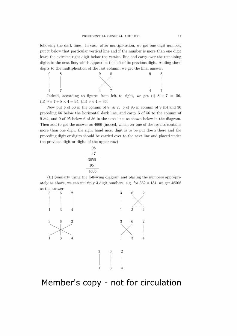
2. Urdhva Tiryagbhyam (vertically and crosswise)
As the name suggests, we multiply vertically and crosswise while applying this
sutra, illustrated in the following examples:
(I) Let us multiply 98 by 47 using the following diagram:
Let us place the digits of the numbers to be multiplied at the points on the up-
per and lower line. Now perform the multiplication of the corresponding numbers
Member's copy - not for circulation
PRESIDENTIAL GENERAL ADDRESS 17
following the dark lines. In case, after multiplication, we get one digit number,
put it below that particular vertical line and if the number is more than one digit
leave the extreme right digit below the vertical line and carry over the remaining
digits to the next line, which appear on the left of its previous digit. Adding these
digits to the multiplication of the last column, we get the final answer.
4
9
7
8
4
8
7
9
4
9
7
8
Indeed, according to figures from left to right, we get (i) 8 × 7 = 56,
(ii) 9 × 7 + 8 × 4 = 95, (iii) 9 × 4 = 36.
Now put 6 of 56 in the column of 8 & 7, 5 of 95 in column of 9 &4 and 36
preceding 56 below the horizontal dark line, and carry 5 of 56 to the column of
9 &4, and 9 of 95 below 6 of 36 in the next line, as shown below in the diagram.
Then add to get the answer as 4606 (indeed, whenever one of the results contains
more than one digit, the right hand most digit is to be put down there and the
preceding digit or digits should be carried over to the next line and placed under
the previous digit or digits of the upper row)
98
47
3656
95
4606
(II) Similarly using the following diagram and placing the numbers appropri-
ately as above, we can multiply 3 digit numbers, e.g. for 362 × 134, we get 48508
as the answer
1
3
3
6
4
2
1
3
3
2
4
6
1
2
4
3
3
6
1
6
3
3
4
2
1
3
3
6
4
2

Member's copy - not for circulation
18 MANJUL GUPTA
Indeed, figures, (i) 2×4 = 8, (ii) 6×4+2×3 = 30, (iii) 2×1+4×3+6×3 = 32,
(iv) 3 × 3 + 6 × 1 = 15 and (v) 3 × 1 = 3 yield
362
134
35208
133
48508
(III) For four digit numbers we follow the following diagram, for example, we get
1121 × 1132 = 1268972.
1
1
1
1
3
2
2
1
1
1
1
1
3
1
2
2
1
1
1
11
23
2
1
11
21
2
3
1
1
21
31
1
2
1
1
11
1 3
2
2
1
1
1
1
1
3
2
2
1
One may proceed like this for multiplying higher digit numbers using these sutras.
There are sixteen sutras and thirteen subsutras discovered by Swami Tirthaji
which deal with basic arithmetic operations, decimal/fraction, conversions etc.
The purpose of these sutras is to evolve a method which makes calculations easy
and short. In case one sutra does not help , other one is used; for instance Nikhilam
does not help when divisors are small digit numbers, then sutras like- Paravartya
Yojayet (transpose and adjust), Dhvajanka (flag method) may apply. I urge the
audience to enjoy the basic mathematics with sutras and teach children to learn
the same. One may refer to [1, 3].

Member's copy - not for circulation
PRESIDENTIAL GENERAL ADDRESS 19
Finally, I sum up with the note that mathematics has shaped our lives and
moulded our civilization through ages and still the process is on with more vigour
and passion.
Thank You.
References
[1] Glover, J. T., Vedic Mathematics For Schools, Books 1 & 2, Motilal Banarasidass Publishers
Private Limited, 1995 & 1999.
[2] Taylor, John, Lilawati: or A Treatise on Arithmetic or Geometry by Bhascara Acharya,
1816.
[3] Tirthaji Maharaja, Jagadguru Swami Sri Bharati Krisna, Vedic Mathematics, Motilal Ba-
narasidass Publishers Private Limited, 1965.
Manjul Gupta
Department of Mathematics and Statistics
IIT Kanpur, Kanpur - 208 016, India.
E-mail: [email protected]

Member's copy - not for circulation
20

Member's copy - not for circulation
The Mathematics Student ISSN: 0025-5742
Vol. 87, Nos. 1-2, January-June (2018), 21-65
SOME TOPICS IN FUNCTIONAL ANALYSIS:
OUR CONTRIBUTIONS WITH EMPHASISON HOLOMORPHY
MANJUL GUPTA
Abstract. In this talk, I shall give a brief description of our work carried
out by me with my group of co-researchers during a period of almost forty
five years. I shall pay more attention to the study of the spaces of holomor-
phic functions defined on open subsets of a finite/infinite dimensional locally
convex space.
1. INTRODUCTION
After the birth of a basis in a Banach space by J. Schauder around the year
1927, notion of a general topological space by F. Hausdorff in 1904, and that of
a locally convex space by John von Neumann in the year 1935, mathematicians
working in Functional Analysis got interested to consider all spaces of importance
for finding the structural properties of these spaces vis-a-vis basis and their rela-
tionships. Among such spaces, the class of entire functions occupy a privileged
position because of its vast applications in the theory of distributions, theory of
locally convex spaces etc, as well as providing examples for various concepts being
studied in several off-shoots of Functional Analysis, for instance, nuclear locally
convex spaces, hypercyclicity of linear operators, different types of bases etc.
I started my research career with the spaces of analytic/entire functions of two
variables, which played an important role in motivating me to carry out researches
in several topics of Functional Analysis and Operator Theory, namely, Schauder
basis and decompositions, scalar and vector valued sequence spaces, nuclearity of
spaces and operators, bi-locally convex spaces/mixed convergence, ordered gen-
eralized sequence spaces and ordered decompositions, approximation quantities
and ideals of linear operators, dynamics of linear operators and currently pursuing
researches in infinite dimensional holomorphy. All these topics which are interre-
lated in one way or the other involve the spaces of entire and analytic functions
except possibly our study of order structures; for this study is usually carried out
for the vector spaces defined over the real field.
* The text of the Presidential Address (technical) delivered at the 83rd Annual Conference of
the Indian Mathematical Society - An International Meet, held at Sri Venkateswara University,
Tirupati - 517 502, Andhra Pradesh, India during December 12 - 15, 2017.
c© Indian Mathematical Society, 2018 .
21

Member's copy - not for circulation
22 MANJUL GUPTA
Before passing on to describing the salient features of our contributions in
these topics, let us familiarize ourselves with the basics of locally convex spaces
and the spaces of entire functions of one complex variable.
1.1. Locally Convex Spaces. For a subset A of a vector space X over a vector
field K = R (reals) or C (complex numbers), its Minkowski’s functional or gauge
pA is defined as
pA(x) = infρ > 0 : x ∈ ρA, x ∈ X.
If A is balanced, convex and absorbing subset of X, then pA is a semi-norm on X.
A topological vector space (TVS) is a vector space equipped with a topol-
ogy T for which the vector operations are jointly continuous. A locally convex
space(LCS) (X,T ) is a TVS for which there exists a fundamental neighborhood
system UX at origin consisting of absorbing, balanced and convex sets or equiv-
alently the topology T is generated by the family DT = pU : U ∈ UX of
continuous semi-norms. We assume throughout that (X,T ) is a Hausdorff LCS,
which means that p(x) = 0, ∀ p ∈ DT yields x = 0. A subset B of X is bounded
if it is absorbed by each member U ∈ UX , that is, there exists a λ > 0 such that
B ⊂ λU ; and is said to be bornivorous if it absorbs every bounded subset of X.
A net xα in X tends to x ∈ X with respect to the topology T if and only if
p(xα − x) → 0,∀ p ∈ DT . A LCS (X,T ) is said to be complete (sequentially
complete) if every net xα (sequence xn) converges in (X,T ); and it is called
a barrelled (infrabarrelled) space if every barrel (bornivorous barrel) in (X,T ) is
a neighborhood of origin in (X,T ) where a barrel in (X,T ) means an absorbing,
balanced, convex and T -closed set. A complete metrizable locally convex space is
called a Frechet space. A LCS (X,T ) is said to be a semi-Montel space if every
bounded subset of X is relatively compact. An infrabarrelled semi-Montel space
is said to be a Montel space.
Let us now recall polar topologies defined corresponding to a dual pair <
E,F > of vector spaces E and F with respect to a bilinear form < ·, · >. For a
given subset A of E, the polar of A is the set A = y ∈ F : | < x, y > | ≤ 1, ∀x ∈A. The weak, Mackey and strong topologies on E are respectively the topologies
σ(E,F ), τ(E,F ) and β(E,F ) generated by the family pA : A ∈ S, where S is
respectively the collection of finite or singleton subsets of F ; all balanced, convex,
σ(F,E)-compact subsets of F ; and all σ(F,E)-bounded subsets of F . Similarly,
one can have the topologies σ(F,E), τ(F,E) and β(F,E) on F . A set B ⊂ X∗ is
said to be equicontinuous if B ⊂ U for some U ∈ UX .
For a LCS (X,T ), < X,X∗ > forms a dual pair with respect to the bi-linear
form < x, f >= f(x), x ∈ X, f ∈ X∗, topological dual of X. We call a LCS (X,T )
a Mackey space if T ≈ τ(X,X∗) and an S-space if (X∗, σ(X∗, X)) is sequentially
complete. It is known that every barrelled space is a Mackey S-space.

Member's copy - not for circulation
SOME TOPICS IN ..... WITH EMPHASIS ON HOLOMORPHY 23
The generalization of normed linear spaces (nls) is two fold, namely, locally
convex spaces and locally bounded spaces (a TVS is locally bounded if there exists
a bounded neighborhood at 0). Among locally convex spaces, the class which
is much closer to finite dimensional space as compared to the Hilbert spaces, is
the class of nuclear locally convex spaces. These spaces were introduced by A.
Grothendieck [39] around the year 1953, where he studied these spaces using the
technique of tensor products. To have an appreciative idea of what these spaces
are, let us recall that a linear map A : (X,TX) → (Y, TY ) where (X,TX) and
(Y, TY ) are two LCS, is said to be nuclear if there exist αn in `1 (the class of
all absolutely summable sequences), an equicontinuous sequence fn in X∗ and
a bounded sequence yn in Y with
A(x) =∑n≥1
αnfn(x)yn, ∀ x ∈ X.
A LCS (X,TX) is said to be nuclear (resp. Schwartz ) if for each U ∈ UX ,
there exits V ∈ UX such that V is absorbed by U , i.e. V ⊂ αU for some α > 0,
and the mapping KVU : XV → XU with KV
U (xV ) = xU is nuclear (precompact),
where XV = X/kerpV and XU = X/kerpU are the normed spaces w.r.to the
quotient norm pV and pU respectively, and kerpV = x ∈ X : pV (x) = 0,kerpU = x ∈ X : pU (x) = 0. The references for the detailed theory of locally
convex as well as nuclear spaces are [83, 114].
1.2. Spaces of Entire Functions of One Variable. The rudimentary theory of
the spaces of entire and analytic functions dates back to eighteenth century in the
investigations of L. Euler and J.R. d’Alembert; however, the full following of the
subject was possible only after the publications of the fundamental works of A. L.
Cauchy, B. Riemann and K. Weierstrass in the nineteenth century. Its methods
are widely used in many branches of mathematics and engineering. The literature
on the structural study of spaces of analytic/entire functions of one variable is too
vast to be elaborated here; but for our work I would like to mention the names
of early contributors, namely, A. I. Markusevich, V. G. Iyer, M. G. Arsove, V.
Krishnamurthy etc.
All of us know that a function f : C → C is said to be entire if it has the
expansion
f(z) =
∞∑n=0
f(n)zn, z ∈ C, (1.1)
where |f(n)| 1n → 0 as n→∞.
Let us denote byH(C) the class of all entire functions and equip this space with
the compact open topology τ generated by the family of semi-norms ‖·‖n : n ∈ Nwhere
‖f‖n = sup|z|≤n
|f(z)|, f ∈ H(C).

Member's copy - not for circulation
24 MANJUL GUPTA
The translation invariant metric d on H(C), which also generates τ , is defined as
d(f, g) =∑n≥1
1
2n‖f − g‖n
1 + ‖f − g‖n, f, g ∈ H(C).
The space (H(C), τ) is a nuclear Frechet space, cf. [114]; and a sequence fnconverges to f in (H(C), τ) if and only if fn(z) → f(z) uniformly on all compact
subsets of C.
For an entire function f and r > 0, define M(r) = sup|z|=r |f(z)|. Then f is
said to be of finite order if there exists a positive number µ such that
M(r) < erµ
(1.2)
for all sufficiently large r. The number ρ = inf µ, infimum being considered over
such µ’s for which (1.2) holds, is called the order of an entire function f . Given
an entire function f of order ρ, suppose there exists a positive number k such that
M(r) < ekrρ
(1.3)
for all sufficiently large r. Then f is said to be of finite type and σ = inf k, over
those values of k for which (1.3) holds, is called the type of f .
An element γ of H(C) with γ(z) =∑∞n=0 γnz
n, γn > 0 for each n ∈ N0 is
called a comparison function if the sequence of ratios γn+1
γndecreases to zero as n
increases to ∞, where N is the set of all natural numbers and N0 = N ∪ 0. In
addition, if the sequence wn, wn = nγnγn−1
is also monotonically decreasing, we
call γ an admissible comparison function.
The differential and translation operators on the space H(C), which are re-
spectively denoted by D and Ta, 0 6= a ∈ C, are defined as Df(z) = f ′(z) and
Taf(z) = f(z + a), for f ∈ H(C) and z ∈ C.Using the function γ and results on sequence spaces, various subspaces of the
space H(C) have been defined, which we shall consider in due course.
Hardy space defined on the open unit disc D of C as
H2(D) = f : D→ C, f(z) =∑n≥0
anzn : ‖f‖2 =
∞∑n=0
|an|2 <∞
is a Hilbert space with orthonormal basis δn(z) = zn, n ∈ N0 and the inner product
is given by < f, g >=∑n≥0 anbn for f(z) =
∑n≥0 anz
n and g(z) =∑n≥0 bnz
n.
For the theory of holomorphic/entire functions, we refer to [103].
2. Salient Features of Our Research Contributions
In this section we mention briefly, the salient features of our contributions.
Let us begin with
(a) Spaces of Analytic Functions of Two Variables: Let us denote by
X the space of all entire functions of two variables z1, z2 ∈ C, equipped with
the topology T of uniform convergence on compact sets in C2 = C × C. In other
words, f ∈ X if and only if

Member's copy - not for circulation
SOME TOPICS IN ..... WITH EMPHASIS ON HOLOMORPHY 25
f(z1, z2) =∑m
∑n
m+n≥0
amnzm1 z
n2 , z1, z2 ∈ C
withlim supm+n→∞
|amn|1
m+n = 0.
If M(f ; r1, r2) = sup|z|≤rii=1,2
|f(z1, z2)| for r1, r2 > 0, then the topology T is generated
by the family of semi-norms M(f ; r1, r2) : r1 > 0, r2 > 0.The space (X,T ) is known to be a non-normed nuclear Frechet space, cf. [114].
In the papers [41, 85, 87], we were interested in studying the topological aspects of
certain subspaces X1 and X2 of the space X and the problem of characterizing the
proper bases (those bases equivalent or similar to δmn(z1, z2) = zm1 zn2 ) in them.
Indeed, for given finite positive numbers ρ1, ρ2;σ1, σ2, we define X1 ≡ X(ρ1, ρ2)
and X2 ≡ X(ρ1, ρ2;σ1, σ2) as follows
X1 ≡ f ∈ X : for ε > 0, M(f ; r1, r2) ≤ exp[rρ1+ε1 + rρ2+ε
2 ],
for all sufficiently large r1, r2 ≥ 0and
X2 ≡ f ∈ X : for ε > 0, M(f ; r1, r2;σ1, σ2) ≤ exp[(σ1 + ε)rρ11
+(σ2 + ε)rρ22 ] valid for all large r1, r2.(2.1)
In the terminology of entire functions of several complex variables, an f in X1 is
said to possess an order point at best equal to (ρ1, ρ2) and an f ∈ X2 is said to
possess a type at best equal to (σ1, σ2) relative to the order point (ρ1, ρ2). Clearly,
X2 ⊂ X1 ⊂ X.
Making use of a characterization of Fred Gross [29] for members of X2, namely-
“an f in X belongs to X2 if and only if
|amn| < [eρ1(σ1 + ε)
m]mρ1 [
eρ2(σ2 + ε)
n]nρ2
for all sufficiently large m+n and arbitrary ε > 0; in [85], we topologize the space
X2 by the family of semi-norms ‖·;σ1 + δ, σ2 + δ‖ : δ > 0, where
‖f ;σ1 + δ, σ2 + δ‖ = |a00|+∑n
∑m
m+n≥1
|amn|[m
(σ1 + δ)eρ1]mρ1 [
n
(σ2 + δ)eρ2]nρ2
and show that the sequence δmn, δmn(z1, z2) = zm1 zn2 , z1, z2 ∈ C, m,n ∈ N,
forms a Schauder base for X2 with respect to the topology T2 which makes X2
a Frechet space. Further, we use the series representation of members of X2 to
characterize its topological dual and continuous linear operators from X2 into
itself. We also deal with the problem of proper bases in X2.
However, for members of X1, the characterization of Fred Gross in terms of
Taylor coefficients doesn’t help in getting the topological structure of X1; and so
Member's copy - not for circulation
26 MANJUL GUPTA
in [87] we first characterize the members of X1 in the form which may be suitable
to topologize this space; indeed, we prove
Theorem 2.1. An f in X belongs to X1 if and only if for each δ > 0, there exists
an integer N0 ≡ N0(δ) such that
|amn| ≤ m−m
ρ1+δ n−n
ρ2+δ
for all m+ n ≥ N0.
This characterization gives rise to a family of norms ‖·; ρ1 +δ, ρ2 +δ‖ : δ > 0on X1, where for f ∈ X1
‖f ;σ1 + δ, σ2 + δ‖ = |a00|+∑m
∑n
m+n≥1
|amn|mm
ρ1+δ nn
ρ2+δ .
The topology T1 generated by this family of norms is a Frechet topology on X1,
which is stronger than the induced topology from X. The problems tackled in this
paper [87], as well as in the papers [86, 88] where we consider functions analytic
in a bicylinder, are similar in nature as mentioned above and so we shall not
elaborate them. In [41], we show that the space (X1, T1) is a Montel space. In
subsequent work [44], certain simultaneous automorphism on X and a subspace
Y of it, bearing a topology stronger than the induced one, have been constructed
(simultaneous automorphism on X and Y means a mapping f such that f is an
automorphism on X and f |Y is an automorphism on Y ).
Our paper [60] deals with the space K < x1, x2 > of entire functions of two
variables x1, x2 ∈ K which is a non-archimedean valued field complete under the
metric of valuation of rank 1 or real valuation (a non-archimedean valuation of
rank 1 is a real-valued function φ defined on the field satisfying the properties:
φ(a) > 0 for a 6= 0, φ(0) = 0; φ(ab) = φ(a)φ(b) and φ(a + b) ≤ maxφ(a), φ(b)for a, b ∈ K, cf. [16]). We introduce a complete linear metrizable topology on
K < x1, x2 >, which makes it a totally disconnected space. We characterize
continuous linear functionals on K < x1, x2 > and show that its dual is not a
topological vector space. For the subject matter of this section, one may refer to
any elementary book on functions of several complex variables, for instance, [30].
(b) Schauder Bases and Decompositions:
The theory of Schauder bases plays an important role for various investiga-
tions in the theory of sequence spaces, theory of nuclear spaces, theory of ordered
topological vector spaces etc. For the study of these topics in Banach spaces, we
refer to the books [101, 104, 127]. However, our major contributions in this direc-
tion are the monographs [91, 92, 93] which contain almost all our researches on
this topic carried out till the time of their publications. To have the glimpse of
some important contributions and later publications, let us first consider Schauder
bases and then Schauder decompositions.

Member's copy - not for circulation
SOME TOPICS IN ..... WITH EMPHASIS ON HOLOMORPHY 27
(I) Schauder Bases: A topological base or just a base in a TVS (X,T ) is
a pair xn, fn of sequences xn ⊂ X, fn ⊂ X ′ (algebraic dual of X) with
fi(xj) = δij where δij is the Kronecker delta such that each x ∈ X has the form
x =∞∑i=1
fi(x)xi,
where the convergence of the series is considered in the linear topology T of X.
If fn ⊂ X∗, the base xn, fn is said to be a Schauder base for X. A base
xn, fn forming a Schauder base for the topology σ(X,X∗) of a TVS is called a
weak Schauder base.
Depending on the types of convergence and properties of the components
comprising a base, one can define various types of Schauder bases in a TVS. Before
we pass on to various notions of Schauder bases, let us consider the following from
[91].
Definition 2.2. A formal series∑n≥1 xn in a LCS (X,T ) is said to be (i) con-
vergent if the sequence n∑i=1
xi converges in X, (ii) absolutely convergent if for
each p ∈ DT ,∑n≥1 p(xn) <∞, (iii) weakly convergent if there exists x ∈ X such
that∑i≥1 f(xi) converges to f(x), for each f ∈ X∗, (iv) bounded multiplier con-
vergent if for each b = bi ∈ `∞ (the space of all scalar bounded sequences), the
series∑i≥1 bixi converges in (X,T ), (v) subseries convergent if for any increasing
sequence J in N, the series∑i∈J xi converges in (X,T ), and (vi) unconditionally
or reordered convergent if for any σ ∈ Π (the set of all permutations of N), the
series∑i≥1 xσ(i) converges to the same element x in X.
It is known that in a sequentially complete LCS (X,T ), every absolutely con-
vergent series is convergent, but converse holds in a metrizable LCS (X,T ), i.e.,
in that case (X,T ) becomes a Frechet space, cf. [91], p.142.
In our work, the following notions of Schauder bases are of particular interest.
Definition 2.3. A Schauder base xn, fn in a LCS (X,T ) is said to be un-
conditional (subseries, bounded multiplier) convergent if the series∑n≥1
fn(x)xn
is convergent unconditionally (subseries, bounded multiplier) in (X,T ) for each
x ∈ X, (ii) semi-absolute if the series∑n≥1 fn(x)xn is absolutely convergent or
equivalently,∑n≥1 |fn(x)|p(xn) < ∞, ∀x ∈ X and p ∈ DT , (iii) absolute if it
is semi-absolute and whenever∑n≥1 |αn|p(xn) < ∞ for some sequence αn of
scalars and ∀ p ∈ DT , then∑n≥1 αnxn converges in (X,T ), (iv) fully absolute if
it is semi-absolute and T ≈ TQ where TQ is the locally convex topology generated
by the family Q of semi-norms Qp on X, where Qp(x) =∑n≥1 |fn(x)|p(xn), (v)
shrinking (almost shrinking) if fn,Ψ(xn) is a Schauder basis for (X∗, β(X∗, X))
(resp. (X∗, τ(X∗, X))), where Ψ is the usual canonical embedding from X into
X∗∗ = (X∗, β(X∗, X))∗, (vi) boundedly complete if the series∑i≥1 αixi converges

Member's copy - not for circulation
28 MANJUL GUPTA
in X whenever the sequence ∑ni=1 αixi is bounded in X, where αn ⊂ K,
and (vii) symmetric if for each pair (ρ, σ) in Π × Π and x ∈ X, the series∑n≥1 fρ(n)(x)xσ(n) converges in (X,T ).
For the historical briefing of the developments of these types of Schauder bases,
we refer to [93], p.35, and the references given therein. Shrinking and boundedly
complete bases/decompositions have been found useful by R. C. James and T. A.
Cook in characterizing the semi-reflexivity of the space in which they are present,
cf. [92], p.133, 144 and [93], p.190. The notions of shrinking and almost shrinking
bases are enveloped in the definition of S-uniform basis which were introduced in
[89]; indeed
Definition 2.4. Corresponding to a collection S of bounded subsets in a LCS
(X,T ) such that S covers X, a Schauder base xn, fn is said to be S-uniform
if limn→∞
supx∈B|f(x − Sn(x))| = 0 for each f ∈ X∗ and each B ∈ S, where Sn(x) =
n∑i=1
fi(x)xi.
Concerning such bases, we prove in [89]
Theorem 2.5. In a LCS (X,T ), a Schauder base xn, fn is S-uniform if and
only if fn, ψ(xn) is a base for X∗ for the topology of S-convergence. In ad-
dition, if every S-bounded sequence in X∗ is equicontinuous and if xn, fn is
S-uniform, then fn, ψ(xn) is a boundedly complete base for X∗ in the topology
of S-convergence.
Note that S-uniform base is a shrinking base (almost shrinking base) if S is
the collection of all bounded subsets of X (of all balanced convex and σ(X,X∗)-
compact subsets of X).
The importance of a weak Schauder base in asserting the completeness of the
space or its dual containing the base was also proved by us, cf. [92], p.39.
The notion of an absolute base was used for the first time by Karlin [96] in
proving a result that a Banach space having an absolute Schauder base is isomet-
rically isomorphic to l1. This led to many generalizations, especially replacing the
Banach space by more general LCS and dissecting an absolute Schauder base into
various components in order to see their effect on the structure of the underlying
LCS (some of these have already been defined in Definition 2.3). We show the
independence of several notions of absolute Schauder bases defined by Kalton [95]
in a LCS, which lie in the lumped form of absolute Schauder base in a Frechet
space, cf. [93], p.63. We also obtain some interesting applications of fully absolute
base in the form of
Theorem 2.6. Let (X,T ) be a locally convex space containing a fully absolute
Schauder base xn, fn. Then T and σ(X,X∗) define the same convergent and
Member's copy - not for circulation
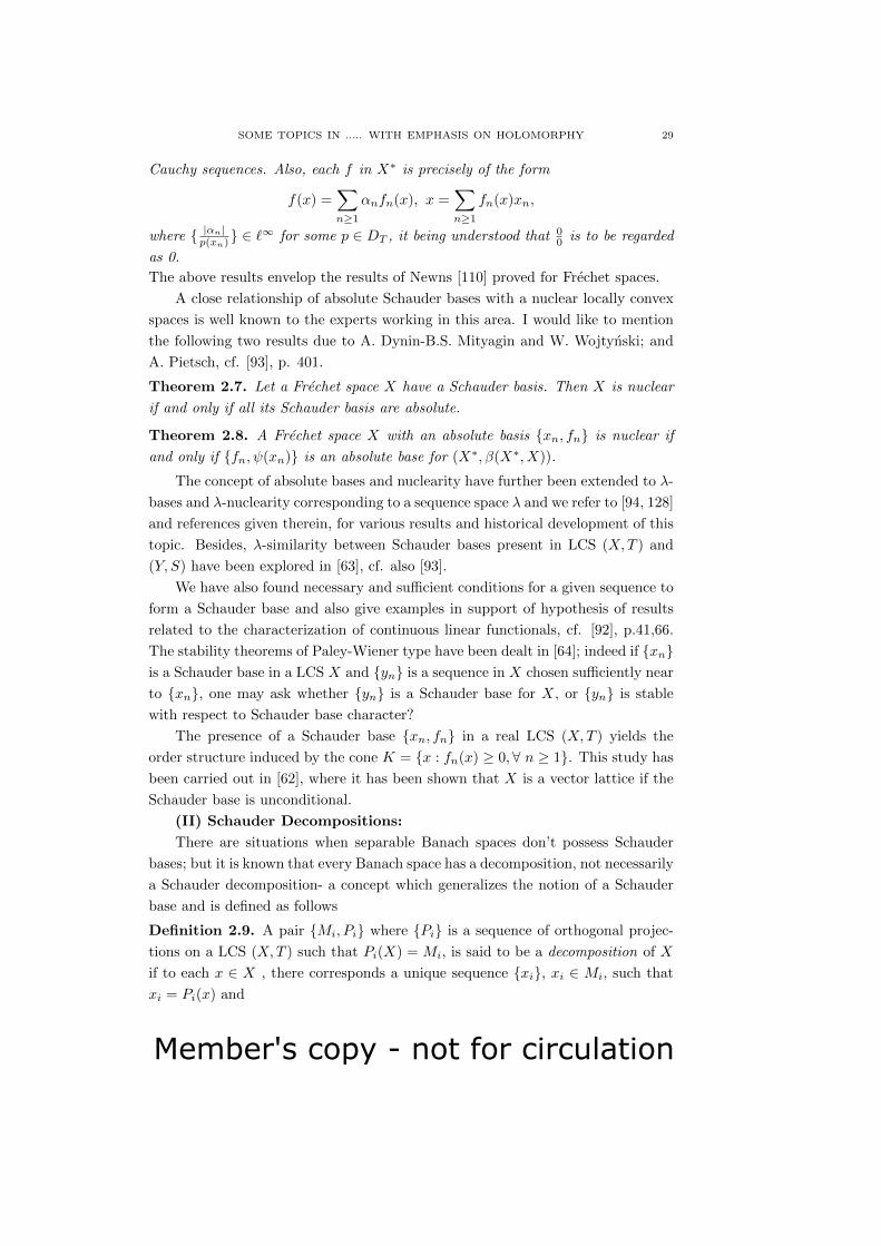
SOME TOPICS IN ..... WITH EMPHASIS ON HOLOMORPHY 29
Cauchy sequences. Also, each f in X∗ is precisely of the form
f(x) =∑n≥1
αnfn(x), x =∑n≥1
fn(x)xn,
where |αn|p(xn) ∈ `∞ for some p ∈ DT , it being understood that 0
0 is to be regarded
as 0.
The above results envelop the results of Newns [110] proved for Frechet spaces.
A close relationship of absolute Schauder bases with a nuclear locally convex
spaces is well known to the experts working in this area. I would like to mention
the following two results due to A. Dynin-B.S. Mityagin and W. Wojtynski; and
A. Pietsch, cf. [93], p. 401.
Theorem 2.7. Let a Frechet space X have a Schauder basis. Then X is nuclear
if and only if all its Schauder basis are absolute.
Theorem 2.8. A Frechet space X with an absolute basis xn, fn is nuclear if
and only if fn, ψ(xn) is an absolute base for (X∗, β(X∗, X)).
The concept of absolute bases and nuclearity have further been extended to λ-
bases and λ-nuclearity corresponding to a sequence space λ and we refer to [94, 128]
and references given therein, for various results and historical development of this
topic. Besides, λ-similarity between Schauder bases present in LCS (X,T ) and
(Y, S) have been explored in [63], cf. also [93].
We have also found necessary and sufficient conditions for a given sequence to
form a Schauder base and also give examples in support of hypothesis of results
related to the characterization of continuous linear functionals, cf. [92], p.41,66.
The stability theorems of Paley-Wiener type have been dealt in [64]; indeed if xnis a Schauder base in a LCS X and yn is a sequence in X chosen sufficiently near
to xn, one may ask whether yn is a Schauder base for X, or yn is stable
with respect to Schauder base character?
The presence of a Schauder base xn, fn in a real LCS (X,T ) yields the
order structure induced by the cone K = x : fn(x) ≥ 0,∀ n ≥ 1. This study has
been carried out in [62], where it has been shown that X is a vector lattice if the
Schauder base is unconditional.
(II) Schauder Decompositions:
There are situations when separable Banach spaces don’t possess Schauder
bases; but it is known that every Banach space has a decomposition, not necessarily
a Schauder decomposition- a concept which generalizes the notion of a Schauder
base and is defined as follows
Definition 2.9. A pair Mi, Pi where Pi is a sequence of orthogonal projec-
tions on a LCS (X,T ) such that Pi(X) = Mi, is said to be a decomposition of X
if to each x ∈ X , there corresponds a unique sequence xi, xi ∈ Mi, such that
xi = Pi(x) and

Member's copy - not for circulation
30 MANJUL GUPTA
x = limn→∞
n∑i=1
xi =∑i≥1
xi =∑i≥1
Pi(x),
where the convergence of the infinite series being with respect to topology T of X.
In case, each Pi is continuous, the decomposition Mi, Pi is known as a Schauder
decomposition.
Clearly, if each Mi is one dimensional, we get the notion of a Schauder base. As
in the case of Schauder basis, we have different types of Schauder decompositions,
like, unconditional, absolute, bounded multiplier, subseries, boundedly complete,
shrinking etc. A notion useful for our study on infinite dimensional holomorphy
is S-absolute decomposition which is defined as
Definition 2.10. Corresponding to a sequence space S = (βn)∞n=1 : βn ⊂C with lim sup
n→∞|βn|
1n ≤ 1, a Schauder decomposition Mi, Pi is said to be S-
absolute if for each β = (βj) ∈ S, x =∞∑j=1
xj ∈ X, xj ∈Mj , β · x =∞∑j=1
βjxj ∈ X;
and pβ(x) =∞∑j=1
|βj |pβ(xj) defines a continuous semi-norm on X for each p ∈ DT .
Like Schauder basis, various type of Schauder decompositions help charac-
terizing the structure of space in which they are present, cf. [42] and reference
given therein. In our first contribution [80] in this direction, we have interrelated
Schauder decompositions in X, X∗ and X∗∗ when they are equipped with various
polar topologies. The applications of Schauder decompositions in asserting the
continuity of linear operators and semi-norms have been obtained, cf. [92], p.43.
The problem concerning the existence of a Schauder decomposition for a subspace
of the whole space has also been tackled, cf [92], p.115.
For the historical developments of Schauder bases and decompositions, we
refer to the theses [40, 121] and the references given therein.
We will see in the next subsection that whereas Schauder bases have close con-
nections with scalar valued sequence spaces, Schauder decompositions correspond
to vector valued sequence spaces. Both these concepts play an important role in
the structural study of locally convex spaces via their relationships with sequence
spaces.
(c) Scalar and Vector Valued Sequence Spaces:
The theory of scalar valued sequence spaces (SVSS) was founded by G. Kothe
and O. Toeplitz around the year 1935 and the vector valued sequence spaces
(VVSS) emerged as generalizations of SVSS by Phoung Cac [119], though these
were earlier used by A. Grothendieck in the form of tensor product of `p with a
Banach space for developing the theory of nuclear spaces and later studied exten-
sively by A. Pietsch in his book [113]. For historical development of these two
theories, we refer to [97, 111].

Member's copy - not for circulation
SOME TOPICS IN ..... WITH EMPHASIS ON HOLOMORPHY 31
Corresponding to a vector space X, let us write Ω(X) and Φ(X) respectively
for the vector space of all sequences formed by the elements of X and the subspace
of Ω(X) consisting of all finitely non-zero sequences. A vector valued sequence space
(VVSS) or a generalized sequence space Λ(X) is a subspace of Ω(X) containing
Φ(X). Members of Λ(X) are denoted by x = xn, y = yn etc. where xn, yn ∈X for each n ∈ N. The symbols δxn for x ∈ X and n ∈ N stands for the sequence
0, 0, . . . , x, 0, . . . , where x is placed at the nth-coordinate. The nth-section of
x = xn in Λ(X) is written as x(n) = x1, x2, . . . , xn, 0, 0, . . . =n∑i=1
δxii . A VVSS
Λ(X) is said to be (i) symmetric if xσ = xσ(n) ∈ Λ(X) whenever x = xn ∈Λ(X) and σ ∈ Π, the set of all permutations of N; (ii)monotone if m0Λ(X) ⊂Λ(X), where m0 = spanA, A being the set of all sequences of zeros and ones; (iii)
normal if for x = xn ∈ Λ(X) and α = αn ⊂ K with |αn| ≤ 1 for every n ∈ N,
the sequence αx = αnxn ∈ Λ(X), or equivalently `∞Λ(X) ⊂ Λ(X), where `∞
is the sequence space of all bounded sequences in K.
Corresponding to a dual pair < X,Y > of vector spaces, the generalized Kothe
dual Λ×(Y ), the generalized β-dual Λβ(Y ) and the generalized δ-dual Λδ(Y ) of
Λ(X) are the spaces defined as
Λ×(Y ) = y = yn ⊂ Y :∑n≥1
| < xn, yn > | <∞, ∀ x = xn ∈ Λ(X),
Λβ(Y ) = y = yn ⊂ Y :∑n≥1
< xn, yn > converges ∀ x = xn ∈ Λ(X), and
Λδ(Y )=y = yn ⊂ Y :∑n≥1
| < xn, yσn > | <∞, ∀ x = xn ∈ Λ(X) & σ ∈ Π.
Clearly, Λδ(Y ) ⊂ Λ×(Y ) ⊂ Λβ(Y ).
A VVSS is said to be perfect if Λ(X) = Λ××(X) = (Λ×(Y ))×. Every perfect
VVSS is normal and every normal VVSS is monotone.
In case X = K, the field of scalars, we get results on SVSS. We write Ω(K) = ω,
Φ(K) = φ and Λ(K) = λ, a SVSS containing φ. If en = δnj, δnj denoting the
Kronecker delta, is the n-th unit vector in ω, one can easily see that φ = spanen :
n ≥ 1. The members of λ are written as α = αn, β = βn etc. and the nth-
section of α = αn ∈ λ as α(n) =∑ni=1 αie
i. A sequence α > 0 means αn > 0 for
each n ∈ N. Symmetric, monotone, normal or solid SVSS are defined analogously.
Also, α− or Kothe, β− and δ− duals in case of SVSS λ are denoted by λ× or λα,
λβ and λδ respectively. A SVSS λ is perfect if λ = λ××.
Let (X,T ) be a Hausdorff LCS. Then a VVSS Λ(X) equipped with a locally
convex topology τ is said to be a GK-space if the maps Pi : Λ(X)→ X, Pi(x) = xi,
i ≥ 1 are continuous. A GK-space is said to be a GAD-space if Φ(X) is dense in
Λ(X); and a GAK-space if for each x = xi ∈ Λ(X), x(n) → x in τ . A VVSS
(Λ(X), τ) is said to be a GC -space (GSC-space) if the maps Ri : X → Λ(X),

Member's copy - not for circulation
32 MANJUL GUPTA
Ri(x) = δxi , i ≥ 1 and x ∈ X are continuous (sequentially) continuous.
For SVSS, the concepts GK-, GAK- and GAD- defined above are referred in
the literature as K-, AK- and AD- respectively. Relating the topological dual with
the Kothe dual of a sequence space, we have [91], p.59, 60.
Theorem 2.11. Let (λ, τ) be an AK-space. Then λ∗ can be identified as λs =
f(en) : f ∈ λ∗ and λ∗ ⊂ λβ. If (λ, τ) is also barrelled, then λ∗ = λβ and
additionally if λ is monotone, then λ∗ = λ×.
If λ, µ are sequence spaces such that µ ⊂ λβ , then < λ, µ > forms a dual system
and as such we can define topologies σ(λ, µ), τ(λ, µ) and β(λ, µ) on λ (similarly
on µ by interchanging the roles of λ and µ). In addition, there is a natural
locally convex topology on λ, the normal or solid topology generated by the family
pβ : β ∈ λ× of semi-norms defined as pβ(α) =∑i≥1 |αiβi|, ∀ α = αi ∈ λ.
Note that the topology σ(λ, λ×) is generated by qβ : β ∈ λ×, where qβ(α) =
|∑i≥1 αiβi|. A subset B of a SVSS λ is said to be normal if α = αn ∈ B
whenever |αn| ≤ |βn|, n ≥ 1, for some β = βn ∈ B; and a semi-norm p on λ
is called solid if p(α) ≤ p(β) for α, β ∈ λ with |αn| ≤ |βn| for n ≥ 1. Thus the
normal topology is generated by the family of solid semi-norms. Relating these
topologies, we have
Proposition 2.12. For any sequence space λ, σ(λ, λ×) ⊂ η(λ, λ×) ⊂ τ(λ, λ×);
in particular
(λ, σ(λ, λ×))∗ = (λ, η(λ, λ×))∗ = (λ, τ(λ, λ×))∗ = λ∗.
Proposition 2.13. If λ is monotone, then (λ×, σ(λ×, λ)) is sequentially complete
and α(n) → α in τ(λ, λ×) as n→∞ , ∀ α ∈ λ.Thus we have
Proposition 2.14. Let λ be a sequence space and µ be a subspace of λ containing
φ. Then en, en is a Schauder basis for (λ, σ(λ, µ)) and (λ, η(λ, µ)). If λ is
monotone, then en, en is a Schauder basis for (λ, τ(λ, λ×)).
Proposition 2.15. A sequence space (λ, η(λ, λ×)) is nuclear (resp. Schwartz)
space if for 0 < α ∈ λ×, there corresponds a sequence 0 < β ∈ λ× such that
α ≤ β, that is αn ≤ βn for each n ∈ N and αnβn ∈ `1 (resp. c0).A sequence space (λ, τ) is said to be simple if every bounded set is dominated
by a member in λ. It is shown in [84] that each perfect nuclear space is simple.
Particular type of sequence spaces which have played a vital role in our re-
searches are Orlicz, Lorentz and Musielak-Orlicz sequence spaces. I shall present
here only Orlicz sequence spaces. An Orlicz function M is a continuous convex
function from [0,∞) to itself such that M(0) = 0, M(r) > 0 for r > 0. An Orlicz
function M is always increasing and M(r)→∞ as r →∞. Such function M has
the integral representation
M(r) =
∫ r
0
p(t)dt,

Member's copy - not for circulation
SOME TOPICS IN ..... WITH EMPHASIS ON HOLOMORPHY 33
where p(t), known as the kernel of M , is right continuous, non-decreasing function
for t > 0. Also, tp(t) → ∞ as t → ∞ and tp(t) = 0 for t = 0. However p(t) > 0
for t = 0 is equivalent to the fact that the Orlicz sequence space `M is isomorphic
to `1, cf. [91], p.309. Hence we assume that p(0) = 0 and p(t)→∞ as t→∞.
For a given Orlicz function M with kernel p, the function N defined as N(s) =s∫0
q(t)dt, where q(s) = supt : p(t) ≤ s for s ≥ 0 is also an Orlicz function. The
functions M and N are called mutually complementary Orlicz functions and satisfy
the following conditions
(i) For s, t ≥ 0, st ≤ M(s) + N(t) (Young’s inequality), (ii) For s ≥ 0,
sp(s) = M(s) +N(p(s)); and (iii) M(αs) ≤ αM(s) for s ≥ 0 and 0 < α < 1.
An Orlicz function M is said to satisfy the ∆2-condition for small t or at ’0’
if for each k > 0, there exists Rk > 1 and tk > 0 such that M(kt) ≤ RkM(t),
∀t ∈ (0, tk], or equivalently, limt→0
M(2t)M(t) <∞. The Orlicz sequence space `M defined
by the Orlicz function M is given by
`M = α = αn :∑n≥1
M(|αn|ρ
) <∞, for some ρ > 0.
An equivalent definition of this space is also given in terms of complementary
Orlicz function. In this case if we denote by ˜N the sequence class
˜N = α = αn : δ(α, N) =
∑N≥1
N(|αn|) <∞
we have
`M = α = αn :∑n≥1
αnβn converges ∀ β = βn ∈ ˜N
Thus on `M , we have two equivalent norms given by
‖α‖M=infρ > 0 :∑n≥1
M(|αn|ρ
) ≤ 1 & ‖α‖(M) = sup|∑n≥1
αnβn| : δ(β, N) ≤ 1;
indeed, ‖α‖M ≤ ‖α‖(M) ≤ 2‖α‖M , for α = αn ∈ `M .
The space `M is BK (Banach K-) space when it is equipped with either of the
above two norms. An AK-, BK- subspace of `M is hM defined as
hM = α = αn :∑n≥1
M(|αn|ρ
) <∞,∀ρ > 0.
We have
Theorem 2.16. For an Orlicz function M , following is true:
M satisfies ∆2-condition at ’0’ ⇔ hM = `M ⇔ `M is an AK space.
Theorem 2.17. If M and N are mutually complimentary Orlicz functions and
M satisfies ∆2-condition at 0, then `×M = `βM = `∗M = `N . Indeed, if both M and
N satisfy ∆2-condition at 0, then the spaces `M and `N are perfect.

Member's copy - not for circulation
34 MANJUL GUPTA
All the above results on SVSS are contained in [91] and I refer to this book
for the detailed theory of SVSS. However, for brief history on Orlicz and modular
sequence spaces, the reference is [118].
In the following few pages, we shall see that there is a close connection between
spaces having Schauder basis (Schauder decompositions) and the theory of SVSS
(VVSS), cf. [91, 92, 93, 120]. Let us first consider Schauder basis. In case (X,T )
is a LCS having a Schauder basis xn, fn, let us define the following sequence
spacesδ ≡ δxn,fn = fn(x) : x ∈ X
andµ ≡ µxn,fn = fn(x) : f ∈ X∗.
The spaces δ and µ form a dual system corresponding to the bilinear form < ·, · >on δ × µ given by
< fn(x), f(xn) > =∑n≥1
fn(x)f(xn), x ∈ X, f ∈ X∗.
Let F : δ → X and G : X∗ → µ be defined by F (fn(x)) = x and G(f) =
f(xn), then both F and G are bijective and one has
Proposition 2.18. (X,σ(X,X∗)) ∼= (δ, σ(δ, µ)) under F−1 and (X∗, σ(X∗, X)) ∼=(µ, σ(µ, δ)) under G, where the symbol ∼= denotes the topological isomorphism.
Let us note that
Proposition 2.19. If a LCS (X,T ) has an absolute base xn, fn, then δ is
perfect. In addition, if (X,T ) is an S-space, then µ = δ×.
All the above results are used in proving [90]
Theorem 2.20. If (X,T ) is a barrelled space possessing an absolute Schauder
base xn, fn, then (X,T ) is complete.
Various other connections between types of a Schauder base in a LCS and the
structure of δ have been established in [62, 81] etc. For instance, we have
Proposition 2.21. A Schauder base xn, fn for a LCS (X,T ) is bounded mul-
tiplier (resp. subseries) base if and only if δ is normal (resp. monotone).
Theorem 2.22. A Schauder base xn, fn for a barrelled space (X,T ) is sym-
metric if and only δ is symmetric.
As mentioned in the beginning of this subsection, there are basically two di-
rections to study the topological properties of a VVSS Λ(X), namely, (i) when no
restriction is placed on the structure of Λ(X) relative to a given SVSS λ and (ii)
when members of Λ(X) are chosen corresponding to a given SVSS λ. In case (i)
the topology on Λ(X) is obtained as a consequence of its dual relationship with
Λ×(X∗), and in case (ii) the topology of Λ(X) is introduced with the help of the
topologies of the parent SVSS λ and the topology of LCS (X,T ). For (i) we refer
to [35, 111, 119, 120] and the references for (ii) are [98, 113, 123]. Whereas the

Member's copy - not for circulation
SOME TOPICS IN ..... WITH EMPHASIS ON HOLOMORPHY 35
importance of VVSS of type (ii) lies in the study of nuclear spaces, λ-compact op-
erators etc. [10, 114], the methods developed by the duality of Λ(X) and Λ×(X∗)
has immediate applications in Schauder decomposition theory; indeed, it is shown
that every VVSS equipped with the weak topology σ(Λ(X),Λ×(X∗)) has an un-
conditional Schauder decomposition, and various results interrelating the types of
Schauder decompositions with the properties of the space Λ(X) have also been
proved, cf. [42, 120]. Generalizing the Schur’s property of `1 following has been
proved in [43]
Theorem 2.23. Let (X,T ) be a reflexive LCS. Then σ(`1(X), `∞(X∗))− and
β(`1(X), `∞(X∗))-convergent sequences in `1(X) are the same if and only if
σ(X,X∗) and β(X,X∗)-convergent sequences are same, where `1(X) = xi :
xi ∈ X ∀i ≥ 1 and∑i≥1 p(xi) < ∞, ∀ p ∈ DT and `∞(X∗) = fi : fi ∈
X∗, ∀i ≥ 1 and fi is β(X∗, X)− bounded.In the paper [79], we deal with the generalized µ-dual of a VVSS Λ(X), defined
corresponding to an SVSS µ and the dual pair < X,Y > of vector spaces as follows
Λ(X)µ = Λµ(Y ) = y ∈ Ω(Y ) : < xi, yi > ∈ µ, ∀ x ∈ Λ(X).For µ = `1, cs (the class of scalar sequences for which series converges) and bs
(the class of scalar sequences for which partial sums of the series are bounded),
cf. [91, 100], the corresponding µ-duals are generalized Kothe, β− and γ-duals.
ClearlyΛδ(Y ) ⊂ Λ×(Y ) ⊂ Λβ(Y ) ⊂ Λγ(Y ).
It is shown in [79] that (i) Λβ(Y ) = Λ×(Y ) if Λ(X) is monotone, (ii) Λγ(Y ) =
Λ×(Y ) if Λ(X) is normal, (iii) Λδ(Y ) = Λ×(Y ) if Λ(X) is symmetric. Also,
the topological dual of a barrelled GAK- and GC- vector valued sequence space
(Λ(X), τ) is Λβ(X∗), i.e. Λβ(X∗) = Λ(X)∗. This generalizes Theorem 2.11. If µ
is a SVSS equipped with a Hausdorff locally convex topology Tµ generated by the
family Dµ of Tµ continuous semi-norms, then we can topologize the space Λ(X)
with a locally convex topology , which we refer to σµ-topology and is generated by
the family of semi-norms py : p ∈ Dµ, y ∈ Λ(X)µ, where py(x) = p(< xi, yi >
) for x = xi ∈ Λ(X) and p ∈ Dµ. Various results involving the structural
properties of (µ, Tµ) and (Λ(X), σµ) have been proved in [79].
In case of SVSS, for a given sequence α = αn in ω and a sequence space
µ; in [78], we consider αµ-duals which as a particular case includes the notions of
Kothe, β−, γ- and the other duals studied in [15, 91]. Indeed, we have
Definition 2.24. For a given sequence α = αn and a sequence space µ, the
αµ-dual of a sequence space λ is the subspace λµα of ω defined as
λµα = b = bn ∈ ω : αab = αnanbn ∈ µ, ∀ a = an ∈ λ.If (µ, Tµ) is a locally convex sequence space with Tµ being generated by a family
Dµ of semi-norms, then we can topologize either of the spaces λ and λµα with the
corresponding locally convex topologies Tα,µ and T ∗α,µ, respectively generated by

Member's copy - not for circulation
36 MANJUL GUPTA
the families pαb : p ∈ Dµ, b ∈ λµα and pαa : p ∈ Dµ, a ∈ λ of semi-norms where
for a ∈ λ, b ∈ λµα and p ∈ Dµ,
pαb (a) = pαa (b) = p(αnanbn).
A SVSS λ is said to be αµ-perfect if λ = λµµαα, where λµµαα = (λµα)µα = c = cn ∈ω : αbc ∈ µ, for each b = bn ∈ λµα, the αµ-dual of λµα. Invoking the structural
properties of these spaces in relation to µ, we prove several results which have
been used in the structural study of several subspaces of the space of holomorphic
mappings, cf. [78].
Coming back to our study of VVSS, A. Pietsch, R. C. Rosier, N. De Grande
- De Kimpe and others studied the spaces of the following type
λ[X] = xi : xi ∈ X, i ≥ 1, and f(xi) ∈ λ, ∀ f ∈ X∗,
λ(X) = xi : xi ∈ X, i ≥ 1, and p(xi) ∈ λ, ∀ p ∈ DT and
λ < X > = xi : xi ∈ X, i ≥ 1, and ‖xi‖B ∈ λ, for some closed
absolutely convex, bounded subset B of X,where λ is a perfect SVSS, (X,T ) is a LCS and ‖ · ‖B denotes the norm generated
by the Minkowski functional of B on the space XB = ∪n∈NnB. Pietsch [114]
proved that a LCS X is nuclear if and only if `1(X) = `1[X]. It was shown by
Kimpe that a Frechet space X is nuclear if and only if `p(X) = `p[X] for some p,
1 ≤ p < ∞, cf. [98], p.144, and a barrelled space X possessing an absolute base
is nuclear if and only if `1 < X∗β >= `1[X∗β ], where X∗β = (X∗, β(X∗, X)). On the
other hand, it is proved in [57] that for a Banach space X, `1[X] is a GAK-space
if and only if X does not contain a copy of c0. Also, for 1 < p <∞ and a reflexive
Banach space X, `p[X∗] is a GAK-space if and only if each member of L(X∗, `p)
is a compact linear operator.
As in the case of Schauder basis, we can define a VVSS through a Schauder
decomposition Mn, Pn present in a LCS (X,T ), indeed, we have, cf. [42, 120]
Λ(X) = x : x = Pn(x), x ∈ X and
∆(X∗) = f : f = P ∗n(f), f ∈ X∗.
Then using the duality between Λ(X) and ∆(X∗), we have proved
Theorem 2.25. If Λ(X) and ∆(X∗) are as defined above for a LCS (X,T ) with
a Schauder decomposition Mn, Pn and if Λ×(X) = ∆(X∗), then Λ(X) is perfect
if Mn is a boundedly complete Schauder decomposition and it is normal if Mnis bounded multiplier Schauder decomposition.
Matrix Transformations between Sequence Spaces:
The theory of matrix transformations on scalar-valued sequence spaces dates
back to the beginning of the last century; indeed it was shown by G. Kothe and O.
Toeplitz that a linear transformation A from a SSVS λ to another SSVS µ, where
λ is monotone, is a matrix transformation if and only if it is σ(λ, λ×) − σ(µ, µ×)
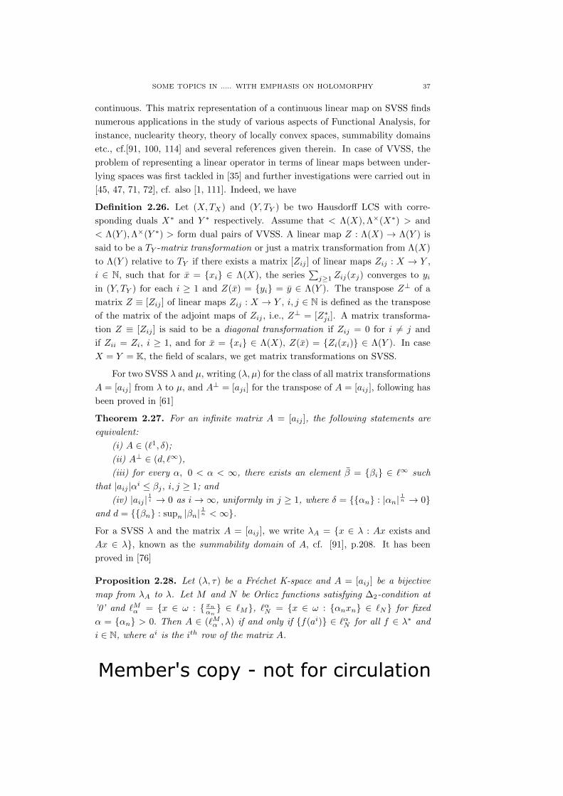
Member's copy - not for circulation
SOME TOPICS IN ..... WITH EMPHASIS ON HOLOMORPHY 37
continuous. This matrix representation of a continuous linear map on SVSS finds
numerous applications in the study of various aspects of Functional Analysis, for
instance, nuclearity theory, theory of locally convex spaces, summability domains
etc., cf.[91, 100, 114] and several references given therein. In case of VVSS, the
problem of representing a linear operator in terms of linear maps between under-
lying spaces was first tackled in [35] and further investigations were carried out in
[45, 47, 71, 72], cf. also [1, 111]. Indeed, we have
Definition 2.26. Let (X,TX) and (Y, TY ) be two Hausdorff LCS with corre-
sponding duals X∗ and Y ∗ respectively. Assume that < Λ(X),Λ×(X∗) > and
< Λ(Y ),Λ×(Y ∗) > form dual pairs of VVSS. A linear map Z : Λ(X) → Λ(Y ) is
said to be a TY -matrix transformation or just a matrix transformation from Λ(X)
to Λ(Y ) relative to TY if there exists a matrix [Zij ] of linear maps Zij : X → Y ,
i ∈ N, such that for x = xi ∈ Λ(X), the series∑j≥1 Zij(xj) converges to yi
in (Y, TY ) for each i ≥ 1 and Z(x) = yi = y ∈ Λ(Y ). The transpose Z⊥ of a
matrix Z ≡ [Zij ] of linear maps Zij : X → Y , i, j ∈ N is defined as the transpose
of the matrix of the adjoint maps of Zij , i.e., Z⊥ = [Z∗ji]. A matrix transforma-
tion Z ≡ [Zij ] is said to be a diagonal transformation if Zij = 0 for i 6= j and
if Zii = Zi, i ≥ 1, and for x = xi ∈ Λ(X), Z(x) = Zi(xi) ∈ Λ(Y ). In case
X = Y = K, the field of scalars, we get matrix transformations on SVSS.
For two SVSS λ and µ, writing (λ, µ) for the class of all matrix transformations
A = [aij ] from λ to µ, and A⊥ = [aji] for the transpose of A = [aij ], following has
been proved in [61]
Theorem 2.27. For an infinite matrix A = [aij ], the following statements are
equivalent:
(i) A ∈ (`1, δ);
(ii) A⊥ ∈ (d, `∞),
(iii) for every α, 0 < α < ∞, there exists an element β = βi ∈ `∞ such
that |aij |αi ≤ βj , i, j ≥ 1; and
(iv) |aij |1i → 0 as i→∞, uniformly in j ≥ 1, where δ = αn : |αn|
1n → 0
and d = βn : supn |βn|1n <∞.
For a SVSS λ and the matrix A = [aij ], we write λA = x ∈ λ : Ax exists and
Ax ∈ λ, known as the summability domain of A, cf. [91], p.208. It has been
proved in [76]
Proposition 2.28. Let (λ, τ) be a Frechet K-space and A = [aij ] be a bijective
map from λA to λ. Let M and N be Orlicz functions satisfying ∆2-condition at
’0’ and `Mα = x ∈ ω : xnαn ∈ `M, `αN = x ∈ ω : αnxn ∈ `N for fixed
α = αn > 0. Then A ∈ (`Mα , λ) if and only if f(ai) ∈ `αN for all f ∈ λ∗ and
i ∈ N, where ai is the ith row of the matrix A.

Member's copy - not for circulation
38 MANJUL GUPTA
Besides proving the general representation results on matrix transformations,
we initiate the study of precompactness and nuclearity of diagonal operators on
VVSS in [72]. In our subsequent work [47, 71], we introduce the notion of gener-
alized simple sequence spaces and characterize matrix transformations on these as
well as nuclear VVSS.
In [45, 47], we consider VVSS of type λ(X) = x = xi : xi ∈ X, ∀ i ∈N and ‖xi‖X ∈ λ, where (X, ‖·‖X) is a Banach space and (λ, ‖·‖λ) is a Banach
sequence space, and characterize the compact and approximable diagonal opera-
tors defined on λ(X) using Kolomogrov and approximation numbers respectively.
Indeed, for Banach spaces X,Y with closed unit balls BX and BY respectively
and S ∈ L(X,Y ) and n ∈ N, the nth-Kolomogrov numbers and nth-approximation
numbers of S are respectively given by
dn(S) = infδ > 0 : S(BX) ⊂ Nδ + δBY ; Nδ is a subspace of Y with dimNδ < n
and
an(S) = inf‖S −A‖ : A ∈ L(X,Y ), rankA < n.An operator S ∈ L(X,Y ) is said to be approximable if an(S) → 0 as n → ∞. It
has been shown in [47] (resp. in [45]) that for a suitably restricted Banach SVSS
λ, the diagonal operator Z : λ(X)→ λ(Y ) is approximable (resp. compact) if and
only if Zii is approximable (resp. compact) for each i ∈ N and ‖Zii‖ → 0 as i→∞.
Also, in [47], the approximation numbers of the inclusion maps between the spaces
of the type `p(X), 1 ≤ p ≤ ∞, have been computed. In case of the inclusion map
I : `1(X) → `∞(X), it is shown that 12 ≤ an(I) ≤ 1, n ≥ 2, n ∈ N; further
an(I) = 1, ∀n ∈ N if dim X = ∞; and if dim X = k, then an(I) = 1, 1 ≤ n ≤ k
and an(I) = 12 , ∀n > k. This shows how the dimension of the underlying space
affects the value of the approximation number of the inclusion map.
For the historical development of the theories of SVSS and VVSS, I would like
to refer to the theses [1, 111, 120] and the books [91, 100, 124] on SVSS.
(d) Bi-locally Convex Spaces/Mixed Structure:
While studying topological vector spaces, one usually encounters with several
linear topologies on a vector space and sometimes two Hausdorff linear topolo-
gies give rise to a mixed structure which finds its applications in the theory of
summability, theory of sequence spaces, theory of Schauder decompositions etc.
Motivated by the earlier work of G. Fichtenholz, A. Alexiewicz introduced the
concept of a two-norm space which was systematically developed by himself in
collaboration with Z. Semadeni and later utilized by P. K. Subramanian and R.
Rothman for Banach spaces having Schauder decompositions, cf. [22] for refer-
ences. Having observed these contributions, an initiative to develop the structural
study for vector spaces equipped with two Hausdorff locally convex topologies was
taken in [58]; indeed, a bi-locally convex space (bi-LCS) is a triplet (X,T1, T2)

Member's copy - not for circulation
SOME TOPICS IN ..... WITH EMPHASIS ON HOLOMORPHY 39
denoted by Xb where T1 and T2 are Hausdorff locally convex topologies on X such
that T1 is finer than T2; and a net xα in a bi-LCS Xb is said to be γ-convergent
if xα is T1-bounded and converges to x in T2. Depending on γ-convergence,
various notions like γ-completeness, γ-boundedness, γ-compactness, γ-reflexivity
etc. have been defined and studied in this paper. In our subsequent work [77],
it has been shown that a LCS with a Schauder decomposition yields a bi-LCS
which is termed as canonical bi-LCS and of which the structural properties could
be related with types of Schauder decompositions. This study is continued in
[59], where k-reflexive bi-LCS are introduced and characterized in terms of the
subspaces forming the Schauder decomposition. Also, the γ-completion of such a
bi-LCS is identified as a VVSS and the relationship between k- and γ-reflexivity
of a canonical bi-LCS has been established. For chronological development of this
theory and results, I refer to [21, 22].
(e) Ordered Generalized Sequence Spaces:
The theory of VVSS of which we have seen the importance in earlier subsec-
tions, poses a natural question regarding the impact of ordering of the underlying
space X on Λ(X) and vice-versa, in case X is assumed to be an ordered vector
space (OVS). Indeed, the real SVSS are OVS in a natural way with respect to
the co-ordinatewise ordering. Motivated by the work of J. Dieduonne on function
spaces which are clearly partially ordered spaces, A. L. Peressini tried to relate the
ordering and topological structure of SVSS, and proved several results, cf. [112]
and references given therein. For detailed developments of results on OVS, Riesz
spaces, VVSS and linear operators on Riesz spaces, one is referred to Chapter 2
of the doctoral dissertation [97].
With the rich literature of ordered vector spaces and locally convex lattices in
hand [2, 102, 112, 129], one may possibly think of tackling problem in the following
three directions involving VVSS, namely (i) the impact of ordering and duality of
underlying space with its order dual, on the VVSS and the matrix transformations
defined thereof, (ii) combined effect of ordering and topological properties of the
underlying space on VVSS; and (iii) the applications of the ordered VVSS in the
study of positive absolutely summing and majoring operators with domain and
range contained in vector or locally convex vector lattices. An attempt in the
direction of attacking problems related to (ii) and (iii) was made by Walsh [130]
who introduced ordered VVSS analogous to c0, `1 and `∞ and used them in the
study of K-absolutely summing and majorizing operators introduced for Banach
lattices, cf. [2, 126]. However, the problems related to (i) have been considered
by us , cf. [97]. Besides, various polar topologies which involve the concepts of
ordering as well as duality theory of LCS, have been considered in [65]. It is known
that every order complete Riesz space has an order decomposition, cf. [129], but

Member's copy - not for circulation
40 MANJUL GUPTA
the indexing set for the family of bands (order closed ideals) constituting the order
decomposition is not necessarily countable. However, in case of ordered VVSS
which are Riesz spaces, it is possible to find countable ordered decompositions
in a natural way, cf. [97]. In [66], the concept of o-similarity between countable
order decompositions has been introduced and the results proved for ordered VVSS
associated with countable order decomposition in a Riesz space and its sequential
order dual, have been employed to characterize the o-similarity of countable order
decompositions.
(f) Operator Ideals and Approximation Quantities:
Sequence spaces have played a significant role in the study of operator ideals
which has its origin in the work of J. W. Calkin, R. Schatten and J. von Neumann
on the rings of operators defined on Hilbert spaces. On the other hand, approxima-
tion quantities which yield the measure of compactness for linear operators defined
on Banach or Hilbert spaces, appeared for the first time in the work of E. Schmidt,
L. S. Pontrjagin and L. G. Schnirelman. Indeed, motivated by the work of Pontr-
jagin and Schnirelman for classifying massiveness of sets in metric spaces, involv-
ing the least number of coverings with radii tending to zero, A. N. Kolomogorov
invented the idea of metric entropy or ε-entropy to characterize compact sets ac-
cording to their massivity. Besides, eigenvalues of a compact operator defined on a
Hilbert space form a member of c0. This observation led researchers to introduce
the concept of s-numbers of operators on Hilbert spaces; indeed, these are defined
as the eigenvalues of the positive operator (T ∗T )12 , arranged in decreasing order,
for a bounded linear operator T defined on a Hilbert space H into itself. In 1957,
D. Eh. Allakhverdiev proved that the nth s-number of such an operator T is given
by sn(T ) = inf‖T − S‖ : S is a finite rank operator on H with rank(T) < n.Motivated by this result, A. Pietsch introduced the concept of approximation num-
bers an(T ) for a bounded linear operator defined on a Banach space in 1963.
Indeed, various kinds of geometric quantities like Kolomogrov numbers, Gelfand
numbers for such operators were presented by B. S. Mitiagin and A. Peleczynski
in “Proc. Internat. Cong. Math (Moscow) 1966; Izdat ’Mir’, Moscow, 51, (1968),
366–372” of which the unified study was carried out by A. Pietsch [117] under
the nomenclature of s-numbers of operators. Using these numbers and sequence
spaces, different types of operator ideals have been introduced and studied. Let
us now considerDefinition 2.29. Let L be the class of bounded linear operators between any
pair of Banach spaces and A ⊂ L and A(X,Y ) = A ∩ L(X,Y ) for Banach spaces
X and Y . Then the collection A is said to be an operator ideal if it satisfies the
conditions (i) all finite rank operators are contained in A; (ii) T + S ∈ A(X,Y )
for T, S ∈ A(X,Y ) and (iii) if T ∈ A(X,Y ) and S ∈ L(Y, Z), then ST ∈ A(X,Z)
and also if T ∈ L(X,Y ) and S ∈ A(Y,Z), then ST ∈ A(X,Z).
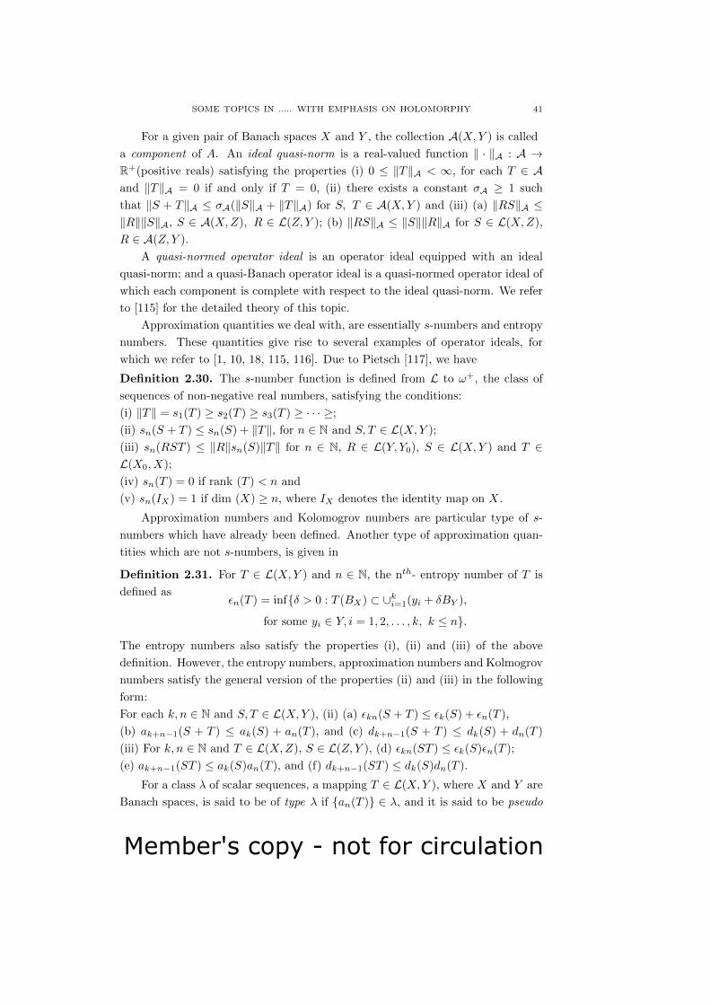
Member's copy - not for circulation
SOME TOPICS IN ..... WITH EMPHASIS ON HOLOMORPHY 41
For a given pair of Banach spaces X and Y , the collection A(X,Y ) is called
a component of A. An ideal quasi-norm is a real-valued function ‖ · ‖A : A →R+(positive reals) satisfying the properties (i) 0 ≤ ‖T‖A < ∞, for each T ∈ Aand ‖T‖A = 0 if and only if T = 0, (ii) there exists a constant σA ≥ 1 such
that ‖S + T‖A ≤ σA(‖S‖A + ‖T‖A) for S, T ∈ A(X,Y ) and (iii) (a) ‖RS‖A ≤‖R‖‖S‖A, S ∈ A(X,Z), R ∈ L(Z, Y ); (b) ‖RS‖A ≤ ‖S‖‖R‖A for S ∈ L(X,Z),
R ∈ A(Z, Y ).
A quasi-normed operator ideal is an operator ideal equipped with an ideal
quasi-norm; and a quasi-Banach operator ideal is a quasi-normed operator ideal of
which each component is complete with respect to the ideal quasi-norm. We refer
to [115] for the detailed theory of this topic.
Approximation quantities we deal with, are essentially s-numbers and entropy
numbers. These quantities give rise to several examples of operator ideals, for
which we refer to [1, 10, 18, 115, 116]. Due to Pietsch [117], we have
Definition 2.30. The s-number function is defined from L to ω+, the class of
sequences of non-negative real numbers, satisfying the conditions:
(i) ‖T‖ = s1(T ) ≥ s2(T ) ≥ s3(T ) ≥ · · · ≥;
(ii) sn(S + T ) ≤ sn(S) + ‖T‖, for n ∈ N and S, T ∈ L(X,Y );
(iii) sn(RST ) ≤ ‖R‖sn(S)‖T‖ for n ∈ N, R ∈ L(Y, Y0), S ∈ L(X,Y ) and T ∈L(X0, X);
(iv) sn(T ) = 0 if rank (T ) < n and
(v) sn(IX) = 1 if dim (X) ≥ n, where IX denotes the identity map on X.
Approximation numbers and Kolomogrov numbers are particular type of s-
numbers which have already been defined. Another type of approximation quan-
tities which are not s-numbers, is given in
Definition 2.31. For T ∈ L(X,Y ) and n ∈ N, the nth- entropy number of T is
defined asεn(T ) = infδ > 0 : T (BX) ⊂ ∪ki=1(yi + δBY ),
for some yi ∈ Y, i = 1, 2, . . . , k, k ≤ n.
The entropy numbers also satisfy the properties (i), (ii) and (iii) of the above
definition. However, the entropy numbers, approximation numbers and Kolmogrov
numbers satisfy the general version of the properties (ii) and (iii) in the following
form:
For each k, n ∈ N and S, T ∈ L(X,Y ), (ii) (a) εkn(S + T ) ≤ εk(S) + εn(T ),
(b) ak+n−1(S + T ) ≤ ak(S) + an(T ), and (c) dk+n−1(S + T ) ≤ dk(S) + dn(T )
(iii) For k, n ∈ N and T ∈ L(X,Z), S ∈ L(Z, Y ), (d) εkn(ST ) ≤ εk(S)εn(T );
(e) ak+n−1(ST ) ≤ ak(S)an(T ), and (f) dk+n−1(ST ) ≤ dk(S)dn(T ).
For a class λ of scalar sequences, a mapping T ∈ L(X,Y ), where X and Y are
Banach spaces, is said to be of type λ if an(T ) ∈ λ, and it is said to be pseudo

Member's copy - not for circulation
42 MANJUL GUPTA
λ-nuclear if there exist sequences λn ∈ λ, fn ⊂ X∗ and yn ⊂ Y such that
‖fn‖ ≤ 1, ‖yn‖ ≤ 1, n ∈ N and T has the representation: T (x) =∑n≥1
λnfn(x)yn,
x ∈ X, cf. [93].
If the class λ contains φ, finite rank operators are of type λ. If λ = `p,
0 < p < ∞, mappings of type λ are known as the mappings of type `p, and
for λ = `1, these are nuclear mappings, cf. [114]. These mappings are compact
and characterize nuclear spaces. Moreover, all such operators of the same type
constitute an ideal in the class of all bounded linear operators. Whereas in [46]
representation theorems for operators of type `v,w,ψp,q and Sw,ψ in terms of finite
rank operators have been obtained, where 0 < p < q ≤ ∞, ψ : [0,∞) → [0,∞)
a continuous, strictly sub-additive function satisfying ψ(0) = 0, and v = vn,w = wn sequences of positive numbers; the paper [48] incorporates results on
the Orlicz type operators (λ = `M ), indeed, it is shown that the space LM of all
such operators T between arbitrary Banach spaces such that an(T ) ∈ `M , for
a fixed Orlicz function M , is an operator ideal; and also its component `M (X,Y )
is a Kothe sequence space of linear operators. Further generalizations of these
operators which form an operator ideals have been studied in [55, 56].
In the paper [54], the concept of λ-compact operator has been introduced and
it is shown that such operators form a quasi-normed operator ideal under suitable
restriction on λ; a set K is said to be λ-compact if there exists xn ⊂ X with
‖xn‖ ∈ λ such that K ⊂ ∑n≥1
αnxn : α = αn ∈ Bλ×, and T ∈ L(X,Y ) is a
λ-compact operator if T maps bounded sets to λ-compact sets, where X, Y and λ
are Banach spaces. Equipping λ with the normal topology η(λ, λ×), the notion of
λη-compact sets has been introduced and studied in [10] and it is proved that the
collection of all λη-compact operators form an operator ideal.
For the theories and historical development of these topics, I refer to [1, 10,
18, 115, 116].
(g) Dynamics of Linear Operators:
Linear Dynamics or dynamics of linear operators deals with chaos and related
properties of linear systems. Indeed, it is mainly concerned with the behavior of
orbits generated by operators defined on topological vector spaces. This subject
lies at the intersection of several domains of mathematics such as operator theory,
topological dynamics, universality and ergodic theory. The main theme in linear
dynamics is hypercyclicity which comes from the operator theory via cyclicity- a
notion related to the famous invariant subspace problem. In topological dynamics,
hypercyclicity is related to the topological transitivity via the Birkhoff’s transi-
tivity theorem which states that if f is continuous map on a separable complete
metric space X with no isolated points, then there exists an x ∈ X such that the
orbit x, f(x), f2(x), . . . is dense in X if and only if for every pair of non-empty

Member's copy - not for circulation
SOME TOPICS IN ..... WITH EMPHASIS ON HOLOMORPHY 43
open sets U and V , we have fn(U)∩V 6= φ for some n ∈ N. Also, hypercyclicity is
a particular case of universality, where a family fα of maps between topological
spaces X and Y is said to be universal if fα(x) is dense in Y for some x ∈ X. An
operator f from a TVS X into itself is said to be hypercyclic if its orbit is dense
in X It was S. Rolewicz [122] who initiated the study of hypercyclic operators
in the Banach space setting, though the translation and differentiation operators
were known to be hypercyclic on the space (H(C), τ) of entire functions in the
work of G. D. Birkhoff and G. R. MacLane . The concept of supercyclicity of
operators was introduced by H. M. Hilden and L. J. Wallen, but the researches on
these topics gained momentum after C. Kitai presented a detailed and systematic
study of hypercyclic and supercyclic operators in her Ph.D thesis [99]. On the
other hand, motivated by the contributions in ergodic theory, especially Birkhoff’s
ergodic theorem, cf. [38]; in 2006, F. Bayart and S. Grivaux [7] introduced the con-
cept of frequent-hypercyclicity of operators, a notion stronger than hypercyclicity.
A good account of these results are given in survey articles [26, 36, 37] and the
theses [108, 118].
Motivated by the study of the frequently hypercyclic operators, for a given
natural number q, we have introduced the concept of q-frequent hypercyclic oper-
ator in [68]; indeed, we define the q-lower density of a subset A of N asq − denA = lim inf
N→∞(n ∈ A : n ≤ Nq/Nq).
A continuous linear operator T on a separable topological vector space X is said
to be q-frequent hypercyclic if there exist x ∈ X such that for any non-empty open
subset U of X, the set N(x, U) = x ∈ N : Tn(x) ∈ U has positive q-lower
density. Such a vector x is called a q-frequent hypercyclic vector for T . Since the
notion of 1-lower density and lower density coincides, frequent hypercyclicity of
an operator is the same as its 1-frequent hypercyclicity. In general the following
implications are true:
frequent hypercyclicity ⇒ q − frequent hypercyclicity ⇒ hypercyclicity,
for all q ∈ N. In [68], examples have been given in order to show that none of
the converse implications is true. Besides obtaining the sufficient criterion, it is
shown that the non- convolution operator Tµ on (H(C), τ), Tµ(f)(z) = f ′(µz) is
frequently hypercyclic for |µ| ≥ 1. In [67], we modify the sufficient criterion for
q-hypercyclicity and study the conditions for a linear map of the form CR,T (S) =
RST to be q-frequently hypercyclic defined on algebras of operators on separable
Banach spaces. Also, the frequent hypercyclicity of the operators CM∗φ ,Mψon
the spaces Sp(H2(D)), ‖ · ‖p) and K(H2(D), ‖ · ‖p) have been characterized, where
φ, ψ are non-zero, bounded, analytic functions on D (open unit disc in C) with
one of them being non-constant and Mφ is the multiplication operator associated
to φ, Sp(H2(D)) = T ∈ L(H2(D)) : αn(T ) ∈ `p, 1 ≤ p < ∞ (the pth
Schatten von-Neumann class) equipped with the norm ‖T‖p = (∑an(T )p)
1p and
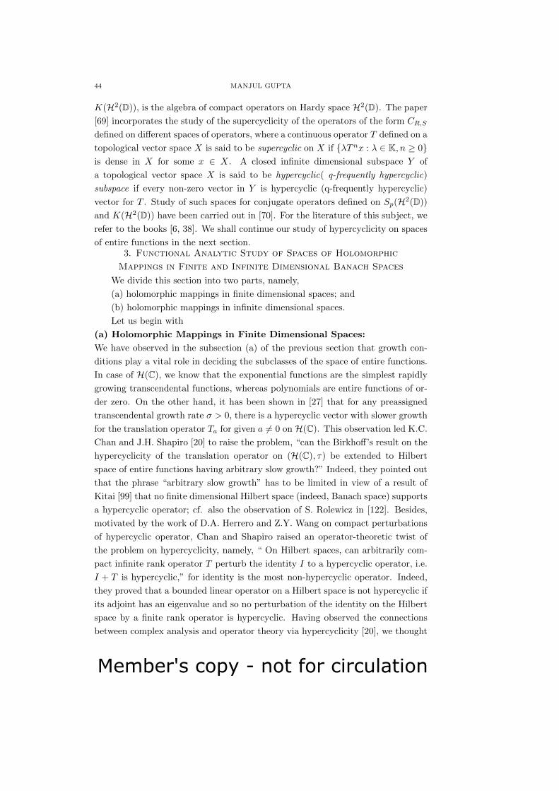
Member's copy - not for circulation
44 MANJUL GUPTA
K(H2(D)), is the algebra of compact operators on Hardy space H2(D). The paper
[69] incorporates the study of the supercyclicity of the operators of the form CR,S
defined on different spaces of operators, where a continuous operator T defined on a
topological vector space X is said to be supercyclic on X if λTnx : λ ∈ K, n ≥ 0is dense in X for some x ∈ X. A closed infinite dimensional subspace Y of
a topological vector space X is said to be hypercyclic( q-frequently hypercyclic)
subspace if every non-zero vector in Y is hypercyclic (q-frequently hypercyclic)
vector for T . Study of such spaces for conjugate operators defined on Sp(H2(D))
and K(H2(D)) have been carried out in [70]. For the literature of this subject, we
refer to the books [6, 38]. We shall continue our study of hypercyclicity on spaces
of entire functions in the next section.3. Functional Analytic Study of Spaces of Holomorphic
Mappings in Finite and Infinite Dimensional Banach Spaces
We divide this section into two parts, namely,
(a) holomorphic mappings in finite dimensional spaces; and
(b) holomorphic mappings in infinite dimensional spaces.
Let us begin with
(a) Holomorphic Mappings in Finite Dimensional Spaces:
We have observed in the subsection (a) of the previous section that growth con-
ditions play a vital role in deciding the subclasses of the space of entire functions.
In case of H(C), we know that the exponential functions are the simplest rapidly
growing transcendental functions, whereas polynomials are entire functions of or-
der zero. On the other hand, it has been shown in [27] that for any preassigned
transcendental growth rate σ > 0, there is a hypercyclic vector with slower growth
for the translation operator Ta for given a 6= 0 on H(C). This observation led K.C.
Chan and J.H. Shapiro [20] to raise the problem, “can the Birkhoff’s result on the
hypercyclicity of the translation operator on (H(C), τ) be extended to Hilbert
space of entire functions having arbitrary slow growth?” Indeed, they pointed out
that the phrase “arbitrary slow growth” has to be limited in view of a result of
Kitai [99] that no finite dimensional Hilbert space (indeed, Banach space) supports
a hypercyclic operator; cf. also the observation of S. Rolewicz in [122]. Besides,
motivated by the work of D.A. Herrero and Z.Y. Wang on compact perturbations
of hypercyclic operator, Chan and Shapiro raised an operator-theoretic twist of
the problem on hypercyclicity, namely, “ On Hilbert spaces, can arbitrarily com-
pact infinite rank operator T perturb the identity I to a hypercyclic operator, i.e.
I + T is hypercyclic,” for identity is the most non-hypercyclic operator. Indeed,
they proved that a bounded linear operator on a Hilbert space is not hypercyclic if
its adjoint has an eigenvalue and so no perturbation of the identity on the Hilbert
space by a finite rank operator is hypercyclic. Having observed the connections
between complex analysis and operator theory via hypercyclicity [20], we thought

Member's copy - not for circulation
SOME TOPICS IN ..... WITH EMPHASIS ON HOLOMORPHY 45
of carrying out researches on the subspaces of the space of entire functions, which
are defined with the help of Orlicz sequence spaces and the comparison function
γ, thus involving the sequence space theory and growth properties. Indeed, in the
paper [73], using the representation (1.1) for f ∈ H(C) and recalling the definitions
of M , N , ˜`M and γ, we introduce
EM (γ) = f ∈ H(C) :∞∑n=0
f(n)
γnβn converges for all β = βn ∈ ˜
N.
For f ∈ EM (γ), we write
‖f‖M,γ = sup|∞∑n=0
f(n)
γnβn| : δ(β;N) ≤ 1 and
‖f‖(M),γ = infρ > 0 :∞∑n=0
M(f(n)
γnρ) ≤ 1.
The space EM (γ) equipped with the any of the above equivalent norms, is a
Banach space and the subspace topology on EM (γ) induced from the compact
open topology τ is weaker than the norm topology. If we write un(z) = γnzn, for
z ∈ C and n ∈ N0, we prove
Theorem 3.1. Let the Orlicz function M satisfy ∆2-condition at ’0’ and the
complimentary Orlicz function N be such that N(1) = 1. Then the sequence unforms a normalized Schauder base for EM (γ) with ‖un‖M,γ = 1, for each n ∈ N;
and a fortiori, the space EM (γ) is separable.
We also introduce the Banach subspaces `∞(γ) and E∞(γ) as follows:
`∞(γ) = f ∈ H(C) : ‖f‖∞,γ = sup |(f(n)/γn)| <∞;
E∞(γ) = f ∈ H(C) : ‖f‖∞γ = sup(|f(z)|/γ(|z|) : z ∈ C <∞and prove
Proposition 3.2. If M is an Orlicz function such that M(1) = 1, then EM (γ) ⊂`∞(γ) ⊂ E∞(γ) and the inclusion map from EM (γ) to `∞(γ), and to E∞(γ) are
continuous.
In the process of finding whether the inclusions in the above proposition are
strict, surprisingly it turns out that these spaces are almost the same as shown in
Proposition 3.3. If the comparison function γ is such that the sequence nγnγn−1
is bounded, and γ(z) = a0 + a1z + a2z2 + z3γ(z) (where a0, a1 and a2 are chosen
appropriately so that γ(z) becomes a comparison function), then E∞(γ) ⊂ EM (γ)
and ‖f‖M,γ ≤ B‖f‖∞γ for some B > 0.
Corresponding to two Orlicz functions M and N , we define multiplier between
the spaces EM (γ) and EN (γ) as a sequence α = αn of scalars such that for
each f ∈ EM (γ), αf ∈ EN (γ) where (αf)(z) =∑∞n=0 f(n)αnz
n. Clearly, for
αn ∈ `∞ and f ∈ EM (γ), the function g defined on C as g(z) =∑∞n=0 f(n)αnz
n,
is an entire function. Using this fact and the Orlicz function M∗N (s) defined with
the help of two Orlicz funtions M and N as
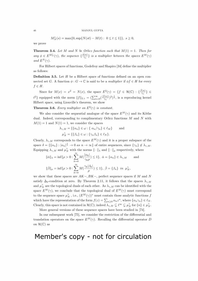
Member's copy - not for circulation
46 MANJUL GUPTA
M∗N (s) = max0, supN(st)−M(t) : 0 ≤ t ≤ 1, s ≥ 0,
we prove
Theorem 3.4. Let M and N be Orlicz function such that M(1) = 1. Then for
any φ ∈ EM∗N (γ), the sequence φ(n)γn is a multiplier between the spaces EM (γ)
and EN (γ).
For Hilbert spaces of functions, Godefroy and Shapiro [34] define the multiplier
as follows:
Definition 3.5. Let H be a Hilbert space of functions defined on an open con-
nected set G. A function φ : G→ C is said to be a multiplier if φf ∈ H for every
f ∈ H.
Since for M(x) = x2 = N(x), the space E2(γ) = f ∈ H(C) : f(n)γn ∈
`2 equipped with the norm ‖f‖2,γ = (∑∞n=0( |f(n)|
γn)2)
12 , is a reproducing kernel
Hilbert space, using Liouville’s theorem, we show
Theorem 3.6. Every multiplier on E2(γ) is constant.
We also consider the sequential analogue of the space EM (γ) and its Kothe
dual. Indeed, corresponding to complimentary Orlicz functions M and N with
M(1) = 1 and N(1) = 1, we consider the spaces
λγ,M = αn ∈ ω : αn/γn ∈ `M and
µγN = βn ∈ ω : γnβn ∈ `N.
Clearly, λγ,M corresponds to the space EM (γ) and it is a proper subspace of the
space δ = αn : |αn|1n → 0 as n → ∞ of entire sequences, since γn 6∈ λγ,M .
Equipping λγ,M and µγN with the norms ‖ · ‖λ and ‖ · ‖µ respectively, where
‖α‖λ = infρ > 0 :∞∑k=0
M(|αk|γkρ
) ≤ 1, α = αn ∈ λγ,M and
‖β‖µ = infρ > 0 :∞∑k=0
M(γk|βk|ρ
) ≤ 1, β = βn in µγN ,
we show that these spaces are AK−, BK−, perfect sequence spaces if M and N
satisfy ∆2-condition at zero. By Theorem 2.11, it follows that the spaces λγ,M
and µγN are the topological duals of each other. As λγ,M can be identified with the
space EM (γ), we conclude that the topological dual of EM (γ) must correspond
to the sequence space µγN , i.e., (EM (γ))∗ must contain those analytic functions f
which have the representation of the form f(z) =∑n≥0 αnz
n, where αnγn ∈ `N .
Clearly, this space is not contained inH(C); indeed λγ,M ( `∞ ( µγN for n ∈ µγN .
More general versions of these sequence spaces have been studied in [74].
In our subsequent work [75], we consider the restriction of the differential and
translation operators on the space EM (γ). Recalling the differential operator D
on H(C) as

Member's copy - not for circulation
SOME TOPICS IN ..... WITH EMPHASIS ON HOLOMORPHY 47
Df(z) =∞∑n=1
nf(n)zn−1, z ∈ C
for f(z) =∑∞n=1 f(n)zn; when it is restricted to EM (γ), we prove
Theorem 3.7. Let M and N be complementary Orlicz functions such that M
satisfies ∆2-condition at ’0’ and N(1) = 1. If γ is a comparison function with
wn = nγnγn−1
, then we have (i) The operator D is a bounded linear operator from
(EM (γ), ‖ · ‖M,γ) to itself if and only if wn is a bounded sequence.
(ii) D is compact on (EM (γ), ‖ · ‖M,γ) if wn → 0 as n→∞. Converse holds
if γ is an admissible comparison function, and both the Orlicz functions M and N
satisfy ∆2-condition at ‘0’.
(iii) D from EM (γ) to itself is nuclear if wn ∈ `1.
Relating the approximation number αn(D) of the differential operator D with
the sequence wn, we have
Proposition 3.8. Let γ be an admissible comparison function. Then αn(D) ≤wn+1.
The above result immediately yields that for an admissible comparison func-
tion γ, D is of type `p if wn ∈ `p, p ≥ 1. Let us note that an admissible
comparison function γ with limn→∞
wn = τ , is an entire function of order 1 and type
τ , cf. [20]. For such a comparison function, we prove that the spectrum σ(D)
of D|EM (γ) is the closed unit disc Bτ = z : |z| ≤ τ. Also, we show that if
G(z) =∑∞n=0 anz
n, is an analytic function in a neighborhood of Bτ , then the
series∑∞n=0 anD
n converges to a bounded linear operator, say G(D), in the Ba-
nach space L(EM (γ), EM (γ)) equipped with the usual operator norm; further,
if a0 6= 0, then G(D) is invertible. Concerning the restriction of the translation
operator Ta, a 6= 0 on EM (γ), we prove
Proposition 3.9. If the sequence nγnγn−1 = wn is bounded, then the operator Ta,
a 6= 0, is a bounded linear operator on EM (γ) and has the following representation
Ta =∞∑n=0
an
n!Dn
in the operator norm topology of L(EM (γ), EM (γ)), where D is the differential
operator.
Theorem 3.10. Let γ be an admissible comparison function and a(6= 0) ∈ C,
then the translation operator Ta on EM (γ) is hypercyclic.
Generalizations of some of the above results will be considered in the next
subsection.
(b) Holomorhic Functions in Infinite Dimensional Spaces:
Infinite dimensional holomorphy is a branch of Functional Analysis which deals

Member's copy - not for circulation
48 MANJUL GUPTA
with the study of holomorphic functions defined on open, or compact or more
general subsets of complex locally convex spaces. This theory has its origin in the
work of V. Volterra around the year 1887; but Gateaux’s work [32, 33] published
posthumously, in 1919 and 1922 comprised the study of holomorphic mappings
defined through the complex polynomials or Gateaux differentials. However, it
was L. Nachbin [109] who developed the present theory of infinite dimensional
holomorphy. In 1968, he noticed the existence of a holomorphic function on an
infinite dimensional space, which takes a bounded set to unbounded set (a distinc-
tive feature from the finite dimensional case). which motivated him to define the
class Hb(E,F ) of holomorphic mappings of bounded type, i.e., the holomorphic
mappings taking bounded subsets of E to bounded subsets of F , where E and F
are complex Banach spaces, cf. [19], p.218. This class has an analogy with the
class of holomorphic mappings defined on an open subset of a finite dimensional
space. This theory is now developed extensively and we have several books avail-
able on this topic, cf. [5, 19, 24, 25, 106, 109]. For historical development of this
subject, I refer to the doctoral thesis [23] and books [24, 25, 106].
Before proceeding further for our contributions on this topic, we first consider
some basic notions and results in infinite dimensional holomorphy.
For each m ∈ N,L(mE;F ) is the Banach space of all continuous m-linear
mappings from E to F endowed with its natural sup norm, namely
‖ A ‖= supxi 6=0
i=1,2,...,m
‖ A(x1, ..., xm) ‖‖ x1 ‖ ... ‖ xm ‖
.
The closed subspace of L(mE;F ) consisting of all continuous symmetric m-linear
mappings A, i.e., A(x1, ..., xm) = A(xσ(1), ..., xσ(m)) for each σ ∈ πm, the class of
all permutations of 1, 2, ...,m, is denoted by Ls(mE;F ). For all x, y ∈ E, each
A in Ls(mE;F ) satisfies the Newton Binomial formula
A(x+ y)m =m∑k=0
(m
k
)A(xm−k, yk).
A continuous m-homogeneous polynomial P is a mapping from E to F defined
asP (x) = A(x, ..., x), x ∈ E,
where A ∈ Ls(mE;F ). In this case, we also write P = A. The space of all m-
homogeneous continuous polynomials from E to F is denoted by P(mE;F ) which
is a Banach space endowed with the norm
‖ P ‖= supx6=0
‖ P (x) ‖‖ x ‖m
.
A continuous polynomial P is a mapping from E into F which can be represented
as a sum P = P0 + P1 + · · · + Pk with Pm ∈ P(mE;F ), m = 0, 1, ..., k. The
vector space of continuous polynomials from E into F is denoted by P(E;F ).
The subspace of P(mE) ≡ P(mE;C) spanned by the collection φm : φ ∈ E∗,

Member's copy - not for circulation
SOME TOPICS IN ..... WITH EMPHASIS ON HOLOMORPHY 49
is denoted by Pf (mE) and each member of Pf (mE) is known as a polynomial of
finite type. Other than the subspace norm, we have a stronger norm ‖ · ‖N known
as the nuclear norm defined as
‖P‖N = infm∑i=1
‖φi‖m : P =m∑i=1
φmi , φ ∈ E∗,
where the infimum is taken over all possible representations of P .
Definition 3.11. A mapping f : U → F is said to be holomorphic at ξ ∈ U , if
there exists a sequence of polynomials Pm ∈ P(mE;F ) such that
f(x) =∞∑m=0
Pm(x− ξ), (3.1)
where the series converges uniformly in some ball Bρ(ξ) = x : ‖x− ξ‖ < ρ ⊂ U .
The series (3.1) is called the Taylor series of f at ξ and in analogy with the complex
case, Pm is written as 1m! d
mf(ξ), i.e.,
f(x) =∞∑m=0
Pm(x− ξ) =∞∑m=0
1
m!dmf(ξ)(x− ξ). (3.2)
If f is holomorphic at each ξ ∈ U , then f is said to be holomorphic from
U to F . The space of all holomorphic mappings from U to F is denoted by
H(U ;F ). In case U = E, the class H(E,F ) is the space of entire mappings from
E into F . An entire mapping f : E → F is said to be of bounded type if f is
bounded on all bounded subsets of E. The space of entire mappings of bounded
type is denoted by Hb(E;F ) which is a Frechet space when endowed with the
topology τb of the uniform convergence on bounded sets. We write H(E), Hb(E),
P(E), P(mE), L(mE) and Ls(mE) respectively for H(E;C), Hb(E;C), P(E;C),
P (mE;C), L(mE;C) and Ls(mE;C).
If (3.2) is the Taylor series expansion of f ∈ H(U ;F ) at ξ, then the Taylor
series expansion of dif(x) at ξ is
dif(x) =∞∑k=0
diPk+i(x− ξ). (3.3)
For f ∈ H(U ;F ) and ξ ∈ U , the inequalities
‖ 1
i!dif(ξ)‖ ≤ 1
ρisup
‖x−ξ‖=ρ‖f(x)‖, i = 0, 1, 2, ... (3.4)
are known as the Cauchy inequalities, where Bρ(ξ) = x : ‖x − ξ‖ ≤ ρ ⊂ U,
for some ρ > 0. Following [13, 14], in case of a Hausdorff TVS (X,T ) and a
sequentially complete LCS (Y, S), let us write Pa(mX;Y ) and P(mX;Y ) for the
class of algebraic and continuous m-homogeneous polynomials from X to Y . For
an open subset U of (X,T ), we have

Member's copy - not for circulation
50 MANJUL GUPTA
Definition 3.12. (i) A function f : U → Y is said to be G-holomorphic (holo-
morphic) if for every x ∈ U , there exists a series∑n≥1 fn, fn ∈ Pa(mX;Y ) (resp.
P(mX;Y )) such that
f(x+ h) =∑n≥1
fn(h)
for all h in a neighborhood of 0 in X.
(ii) A mapping f : U → Y is known as hypoanalytic if it is G-holomorphic and
is continuous on compact sets.
As mentioned above H(U) denotes the class of all holomorphic mappings from
U to C and by Hhy(U) we denote the class of all hypoanalytic mappings from U
to C. Clearly H(U) ⊂ Hhy(U).
For considering subspaces of H(E), let us denote by µ a normal sequence space
equipped with a Hausdorff locally convex topology Tµ generated by the family Dµ
of solid semi-norms; α = αn, a sequence in ω with αn 6= 0, n ≥ 0, and λ a
sequence space. In [78], we introduce the spaces
Hµ(E) = f ∈ H(E) : dnf(0) ∈ P(nE) with (‖dnf(0)‖n!
)1n ∈ µ (3.5)
HµN (E) = f ∈ H(E) : dnf(0) ∈ P(mE) with (‖dnf(0)‖Nn!
)1n ∈ µ (3.6)
Hµα(E, λ) = f ∈ Hµ(E) : ‖dnf(0)‖ 1n ∈ λµα and (3.7)
HµN,α(E, λ) = f ∈ HµN (E) : ‖dnf(0)‖1n
N ∈ λµα (3.8)
Clearly HµN (E) ⊂ Hµ(E) and HµN,α(E, λ) = Hµα(E, λ) ∩ HµN (E). These spaces
(3.5-3.8) are respectively equipped with the Hausdorff locally convex topologies
Th, TNh , Th,α and TNh,α generated by the families Dh = Qp : p ∈ Dµ, DN
h =
QNp : p ∈ Dµ, Dλh = Qap : p ∈ Dµ, a ∈ λ and DN λ
h = QNp,a : p ∈ Dµ, a ∈ λ,where for p ∈ Dµ and a ∈ λ
Qp(f) = p((‖dnf(0)‖
n!)
1n ), f ∈ Hµ(E)
QNp (f) = p((‖dnf(0)‖N
n!)
1n ), f ∈ HµN (E)
Qp,a(f) = p(‖dnf(0)‖ 1nαnan), f ∈ Hµα(E;λ) and
QNp,a(f) = p(‖dnf(0)‖1n
Nαnan), f ∈ HµN,α(E;λ).
We prove
Proposition 3.13. Let (µ, Tµ) be a complete K-space such that p0(en) = 1, for
each n ≥ 0 and some p0 ∈ Dµ. Then the spaces (Hµ(E), Th) and (HµN (E), TNh )
are quasi-complete. In addition, if λ contains an element b = bn satisfying
the condition |bn| > 1
|αn|n!1n
, ∀n ≥ 0, then the spaces (HµN,α(E;λ), TNh,α) and
(Hµα(E;λ), Th,α) are quasi-complete.
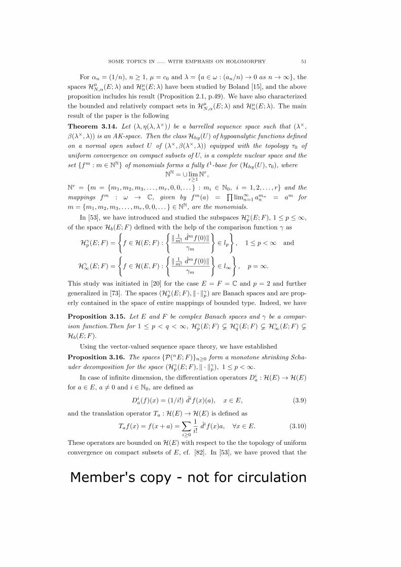
Member's copy - not for circulation
SOME TOPICS IN ..... WITH EMPHASIS ON HOLOMORPHY 51
For αn = (1/n), n ≥ 1, µ = c0 and λ = a ∈ ω : (an/n)→ 0 as n→∞, the
spaces HµN,α(E;λ) and Hµα(E;λ) have been studied by Boland [15], and the above
proposition includes his result (Proposition 2.1, p.49). We have also characterized
the bounded and relatively compact sets in HµN,α(E;λ) and Hµα(E;λ). The main
result of the paper is the following
Theorem 3.14. Let (λ, η(λ, λ×)) be a barrelled sequence space such that (λ×,
β(λ×, λ)) is an AK-space. Then the class Hhy(U) of hypoanalytic functions defined
on a normal open subset U of (λ×, β(λ×, λ)) equipped with the topology τ0 of
uniform convergence on compact subsets of U, is a complete nuclear space and the
set fm : m ∈ NN of monomials forms a fully `1-base for (Hhy(U), τ0), where
NN = ∪ limr≥1
Nr,
Nr = m = m1,m2,m3, . . . ,mr, 0, 0, . . . : mi ∈ N0, i = 1, 2, . . . , r and the
mappings fm : ω → C, given by fm(a) =∏
lim∞n=1 amnn = am for
m = m1,m2,m3, . . . ,mr, 0, 0, . . . ∈ NN, are the monomials.
In [53], we have introduced and studied the subspaces Hγp(E;F ), 1 ≤ p ≤ ∞,
of the space Hb(E;F ) defined with the help of the comparison function γ as
Hγp(E;F ) =
f ∈ H(E;F ) :
‖ 1m! d
mf(0)‖γm
∈ lp
, 1 ≤ p <∞ and
Hγ∞(E;F ) =
f ∈ H(E,F ) :
‖ 1m! d
mf(0)‖γm
∈ l∞
, p =∞.
This study was initiated in [20] for the case E = F = C and p = 2 and further
generalized in [73]. The spaces (Hγp(E;F ), ‖ · ‖γp) are Banach spaces and are prop-
erly contained in the space of entire mappings of bounded type. Indeed, we have
Proposition 3.15. Let E and F be complex Banach spaces and γ be a compar-
ison function.Then for 1 ≤ p < q < ∞, Hγp(E;F ) Hγq (E;F ) Hγ∞(E;F ) Hb(E;F ).
Using the vector-valued sequence space theory, we have established
Proposition 3.16. The spaces P(nE;F )n≥0 form a monotone shrinking Scha-
uder decomposition for the space (Hγp(E;F ), ‖ · ‖γp), 1 ≤ p <∞.
In case of infinite dimension, the differentiation operators Dia : H(E)→ H(E)
for a ∈ E, a 6= 0 and i ∈ N0, are defined as
Dia(f)(x) = (1/i!) dif(x)(a), x ∈ E, (3.9)
and the translation operator Ta : H(E)→ H(E) is defined as
Taf(x) = f(x+ a) =∑i≥0
1
i!dif(x)a, ∀x ∈ E. (3.10)
These operators are bounded on H(E) with respect to the the topology of uniform
convergence on compact subsets of E, cf. [82]. In [53], we have proved that the
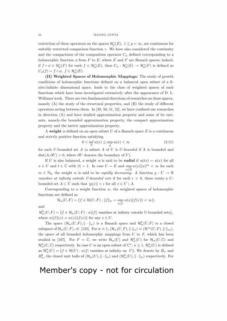
Member's copy - not for circulation
52 MANJUL GUPTA
restriction of these operators on the spaces Hγp(E), 1 ≤ p <∞, are continuous for
suitably restricted comparison function γ. We have also considered the continuity
and the compactness of the composition operator Cφ defined corresponding to a
holomorphic function φ from F to E, where E and F are Banach spaces; indeed,
if f φ ∈ Hγp(F ) for each f ∈ Hγp(E), then Cφ : Hγp(E) → Hγp(F ) is defined as
Cφ(f) = f φ, f ∈ Hγp(E).
(II) Weighted Spaces of Holomorphic Mappings: The study of growth
conditions of holomorphic functions defined on a balanced open subset of a fi-
nite/infinite dimensional space, leads to the class of weighted spaces of such
functions which have been investigated extensively after the appearance of D. L.
Williams’work. There are two fundamental directions of researches on these spaces,
namely (A) the study of the structural properties, and (B) the study of different
operators acting between them. In [49, 50, 51, 52], we have confined our researches
in direction (A) and have studied approximation property and some of its vari-
ants, namely-the bounded approximation property, the compact approximation
property and the metric approximation property.
A weight w defined on an open subset U of a Banach space E is a continuous
and strictly positive function satisfying
0 < infA
w(x) ≤ supA
w(x) <∞ (3.11)
for each U -bounded set A (a subset A of U is U -bounded if A is bounded and
dist(A, ∂U) > 0, where ∂U denotes the boundary of U).
If U is also balanced, a weight w is said to be radial if w(tx) = w(x) for all
x ∈ U and t ∈ C with |t| = 1. In case U = E and supx∈E
w(x)‖x‖m < ∞ for each
m ∈ N0, the weight w is said to be rapidly decreasing. A function g : U → Rvanishes at infinity outside U-bounded sets if for each ε > 0, there exists a U -
bounded set A ⊂ U such that |g(x)| < ε for all x ∈ U \A.
Corresponding to a weight function w , the weighted spaces of holomorphic
functions are defined as
Hw(U,F ) = f ∈ H(U ;F ) : ‖f‖w = supx∈U
w(x)‖f(x)‖ <∞;and
H0w(U,F ) = f ∈ Hw(U ;F ) : w‖f‖ vanishes at infinity outside U-bounded sets,
where w‖f‖(x) = w(x)‖f(x)‖ for any x ∈ U .
The space (Hw(U,F ), ‖ · ‖w) is a Banach space and H0w(U,F ) is a closed
subspace ofHw(U,F ), cf. [125]. For w ≡ 1, (Hw(U,F ), ‖·‖w) ≡ (H∞(U,F ), ‖·‖∞),
the space of all bounded holomorphic mappings from U to F, which has been
studied in [107]. For F = C, we write Hw(U) and H0w(U) for Hw(U,C) and
H0w(U,C) respectively. In case U is an open subset of Cn, n ≥ 1, H0
w(U) is defined
as H0w(U) = f ∈ H(U) : w|f | vanishes at infinity on U. We denote by Bw and
B0w, the closed unit balls of (Hw(U), ‖ · ‖w) and (H0
w(U), ‖ · ‖w) respectively. For

Member's copy - not for circulation
SOME TOPICS IN ..... WITH EMPHASIS ON HOLOMORPHY 53
the weight w given by an entire function γ with positive coefficients, i.e., w(x) =1
γ(‖x‖) , we write Hγ for Hw. Since each compact subset K of U is U -bounded, and
for each U -bounded set A we have supx∈A ‖f(x)‖ ≤ 1infx∈A
w(x)‖f‖w <∞, it follows
that τ0 ≤ τ‖·‖w ≤ τb and so the following inclusions are continuous
(Hw(U ;F ), ‖ · ‖w) → (Hb(U ;F ), τb) → (H(U ;F ), τ0).
The evaluation map δx : H(U) → C defined as δx(f) = f(x), f ∈ Hw(U) is τ0-
continuous. Consequently, the closed unit ball Bw of Hw(U) which can be written
as Bw =⋂δ−1x (B(0, 1
w(x) ), is τ0-closed. Hence Bw is τ0-compact and by Ng’s
Theorem (namely-if τ is a Hausdorff locally convex topology on a Banach space E
weaker than the norm topology, such that BE is τ -compact, then E is isometrically
isomorphic to a dual space), we have
Proposition 3.17. For a weight w on an open subset U of a Banach space E,
Hw(U) is a dual Banach space and its predual is given by
Gw(U) = φ ∈ Hw(U)′ : φ|Bw is τ0 − continuous.Further, the evaluation mapping JwU : Hw(U) → Gw(U)∗, JwU (f) = f with f(h) =
h(f), f ∈ Hw(U) and h ∈ Gw(U), is an isometric isomorphism.
In our paper [49], we have proved the following linearization theorem for the
space Hw(U ;F ).
Theorem 3.18. (Linearization Theorem) For an open subset U of a Banach
space E and a weight w on U , there exists a Banach space Gw(U) and a mapping
∆w ∈ Hw(U ;Gw(U)) with the following property: for each Banach space F and
each mapping f ∈ Hw(U ;F ), there is a unique operator Tf ∈ L(Gw(U);F ) such
that Tf ∆w = f . The correspondence Ψ between Hw(U ;F ) and L(Gw(U);F )
given by Ψ(f) = Tf , is an isometric isomorphism. The space Gw(U) is uniquely
determined up to an isometric isomorphism by these properties.
In case, the weight w being given by an entire function γ with positive coeffi-
cients, i.e., w(x) = 1γ(‖x‖) , we write Hγ for Hw, Gγ for Gw, ∆w = ∆γ , and in that
case ‖∆γ‖ = 1. As an application of linearization theorem, we have
Proposition 3.19. Let w be a weight defined on an open subset U of a Banach
space E such that P(E) ⊂ Hw(U). Then E is topologically isomorphic to a com-
plemented subspace of Gw(U). In case U = E and w is a radial rapidly decreasing
weight on E, E is topologically isomorphic to a 1-complemented subspace of Gw(U).
Proposition 3.20. The space Q(mE) is topologically isomorphic to a comple-
mented subspace of Gw(U), where Q(mE) is the predual of P(mE) defined as
Q(mE) = φ ∈ P(mE)′ : φ|Bm is τ0 − continuous.For our study of the approximation property in weighted spaces of holomor-
phic mappings, linearization theorems play a vital role. This property, appeared

Member's copy - not for circulation
54 MANJUL GUPTA
for the first time in Banach’s book [4] in 1932, has been found useful in the struc-
tural study of Banach spaces. A systematic treatment of this property along with
its variants was carried out by Grothendieck [39] in 1955. As a Banach space
with a Schauder basis has the approximation property and the spaces of holo-
morphic mappings on infinite dimensional spaces do not possess Schauder basis,
it becomes all the more interesting to study this property in these spaces. This
study is possible either by using the technique of linearization or a representation
of holomorphic mappings as an infinite sum of homogeneous polynomials. The
approximation property for spaces of holomorphic mappings was first considered
by R. Aron and M. Schottenloher [3] in the year 1976 and further continued by
several mathematicians for various classes of holomorphic mappings.
A locally convex space X is said to have (i) the approximation property (AP)
if for every compact set K of X, p a continuous semi-norm on X and ε > 0, there
exists a finite rank operator T = Tε,K such that supx∈K p(T (x)−x) < ε and (ii) the
compact approximation property (CAP) if there is a compact linear operator T such
that supx∈K
p(T (x)−x) < ε. If Tε,K : ε > 0 and K varies over compact subsets ofX
is an equicontinuous subset of F(X,X), class of all finite rank operators on X,
X is said to have the bounded approximation property (BAP). When X is normed
and above T can be chosen with ‖T‖ ≤ λ, we say X has the λ-bounded approx-
imation property. In case λ = 1, X is said to have the metric approximation
property(MAP).
In order to study the approximation property for the weighted spaces, in
[49] we have introduced a locally convex topology τM on Hw(U ;F ) of which the
particular cases have been considered in [107, 125]. For a finite set A and r > 0,
we define N(A, r) = f ∈ Hw(U ;F ) : infx∈A
w(x) supy∈A‖f(y)‖ ≤ r and consider the
class
U = ∩∞
limj=1
N(Aj , rj) : (Aj) varies over all sequences of finite subsets of Uand
(rj) varies over all positive sequences diverging to infinity.
Each member of U is balanced, convex and absorbing. Thus it forms a fundamental
neighborhood system at 0 for a locally convex topology which is denoted by τM.
Equivalently, this topology is generated by the family pα,A : α = (αj) ∈ c+0 , A =
(Aj), Ajbeing finite subset of U for each j of semi-norms given by
pα,A(f) = supj∈N
(αj infx∈Aj
w(x) supy∈Aj
‖f(y)‖)
These are the Minkowski functionals of members in U . For F = C, τM = τbc,
cf. [125].
Relating τM with τ0 and τ‖.‖w , and bounded sets with respect to these topolo-
gies, we have

Member's copy - not for circulation
SOME TOPICS IN ..... WITH EMPHASIS ON HOLOMORPHY 55
Proposition 3.21. For a weight w on an open subset U of a Banach space E,
the following hold:
(i) τ0 ≤ τM ≤ τ‖.‖w on Hw(U ;F ).
(ii) τM and ‖.‖w-bounded sets are the same.
(iii) τM|B = τ0|B for any ‖ · ‖w- bounded set B.
Proposition 3.22. Let E and F be Banach spaces. For a radial weight w on a
balanced open subset U of E with P(E) ⊂ Hw(U), the space P(E;F ) is τM-dense
in Hw(U ;F ).
The following result which identifies the class of holomorphic mappings with
the class of linear operators is useful for our study on approximation properties.
Theorem 3.23. Let E and F be Banach spaces, and w be a weight on an open
subset U of E. Then the mapping Ψ : (Hw(U ;F ), τM) → (L(Gw(U);F ), τc) is a
topological isomorphism.
We write
Hw(U)⊗ F = f ∈ Hw(U ;F ) : f has finite dimensional rangeand
Hcw(U ;F ) = f ∈ Hw(U ;F ) : wf has a relatively compact range.The interplay between the properties of a mapping f ∈ Hw(U ;F ) and the corre-
sponding operator Tf ∈ L(Gw(U);F ) is established as follows
Proposition 3.24. Let U be an open subset of a Banach space E and w be a
weight on U . Then for any Banach space F ,
(a) f ∈ Hw(U)⊗ F if and only if Tf ∈ F(Gw(U);F ), and
(b) f ∈ Hcw(U ;F ) if and only if Tf ∈ K(Gw(U);F ).
Proposition 3.25. Let w be a weight on an open subset U of a Banach space E.
Then F(Gw(U);F )‖·‖
= K(Gw(U);F ) if and only if Hw(U)⊗ F‖·‖w
= Hcw(U ;F )
for each Banach space F .
Proposition 3.26. Let w be a weight on an open subset U of a Banach space E.
Then F(Gw(U);F )τc
= L(Gw(U);F ) if and only if Hw(U)⊗ FτM
= Hw(U ;F ) for
each Banach space F .
Using the above results, we have established the following holomorphic ana-
logues of Grothendieck’s characterization of the approximation property for a Ba-
nach space E.
Theorem 3.27. Let E be a Banach space. Then for each Banach space F , the
following are equivalent:
(i) E has the approximation property.
(ii) Hw(V )⊗ EτM
= Hw(V ;E), for each open subset V of F and weight w on V .
(iii) Hw(V )⊗ E‖·‖w
=Hcw(V ;E), for each open subset V of F and weight w on V .

Member's copy - not for circulation
56 MANJUL GUPTA
Next, we characterize the approximation property for the weighted space
Hw(U).
Theorem 3.28. For an open subset U of a Banach space E, Hw(U) has the
approximation property if and only if Hw(U)⊗ F is ‖ · ‖w-dense in Hcw(U ;F ) for
each Banach space F .
Theorem 3.29. Let E be a Banach space and w be a radial weight on a balanced
open subset U of E such that Hw(U) contains all the polynomials. Then the
following assertions are equivalent:
(i) E has the approximation property.
(ii) Pf (E;F )τM
= Hw(U ;F ) for each Banach space F .
(iii) Hw(U)⊗ FτM
= Hw(U ;F ), for each Banach space F .
(iv) Gw(U) has the approximation property.
Every Banach space with the approximation property also has the compact
approximation property. However, the converse implication is not true, cf. [131].
In [51], we have studied the compact approximation property for the weighted
spaces and their preduals and have obtained the analogous results.
In [51], we have also defined the locally convex topology τ ′M on Hw(U,F ) gen-
erated by the family qα,A : α = (αj) ∈ c+0 , A = (Aj), Aj being finite subset of U
for each j of semi-norms given by
qα,A(f) = supj∈N
(αj supx∈Aj
w(x)‖f(x)‖),
Clearly τM ≤ τ ′M. Equipping Hw(U,F ) with τ ′M, we prove
Theorem 3.30. Let w be a radial weight on a balanced open subset U of a Banach
space E such that P(E) ⊂ Hw(U). Then for each Banach space F , the following
assertions are equivalent:
(a) w1i−1IU ∈ Hcw(U ;E)
τ ′Mfor each i ∈ N, where IU : U → E is the inclusion
mapping.
(b) Hcw(U ;F )τ ′M
= Hw(U,F ).
For studying the metric approximation property in [50], we have proved the
following representation theorem for members of Gw(U).
Theorem 3.31. Let w be a weight on an open subset U of a Banach space E.
Then each u in Gw(U) has a representation of the form
u =∑n≥1
αnw(xn)∆w(xn) (3.12)
for α = (αn) ∈ l1 and (xn) ⊂ U . Also,
‖u‖ = inf‖α‖1 : α varies over all represtations of u in (3.12).It is proved in [50]
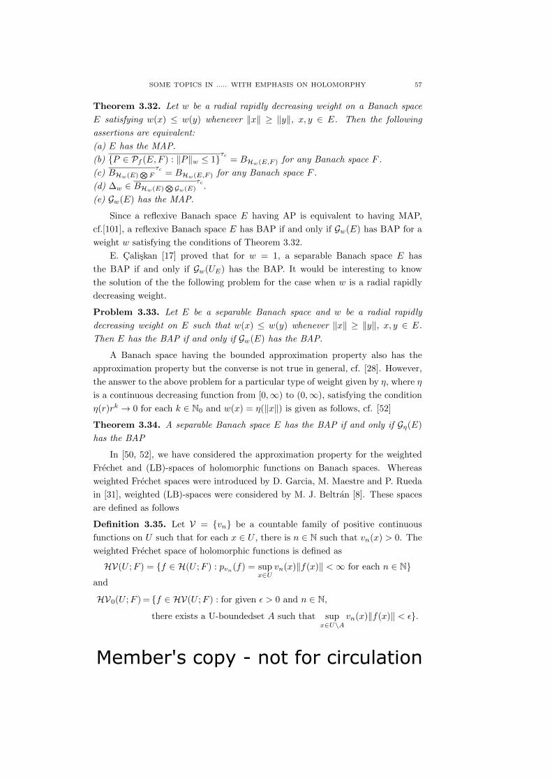
Member's copy - not for circulation
SOME TOPICS IN ..... WITH EMPHASIS ON HOLOMORPHY 57
Theorem 3.32. Let w be a radial rapidly decreasing weight on a Banach space
E satisfying w(x) ≤ w(y) whenever ‖x‖ ≥ ‖y‖, x, y ∈ E. Then the following
assertions are equivalent:
(a) E has the MAP.
(b) P ∈ Pf (E,F ) : ‖P‖w ≤ 1τc
= BHw(E,F ) for any Banach space F .
(c) BHw(E)⊗Fτc
= BHw(E,F ) for any Banach space F .
(d) ∆w ∈ BHw(E)⊗Gw(E)
τc.
(e) Gw(E) has the MAP.
Since a reflexive Banach space E having AP is equivalent to having MAP,
cf.[101], a reflexive Banach space E has BAP if and only if Gw(E) has BAP for a
weight w satisfying the conditions of Theorem 3.32.
E. Caliskan [17] proved that for w = 1, a separable Banach space E has
the BAP if and only if Gw(UE) has the BAP. It would be interesting to know
the solution of the the following problem for the case when w is a radial rapidly
decreasing weight.
Problem 3.33. Let E be a separable Banach space and w be a radial rapidly
decreasing weight on E such that w(x) ≤ w(y) whenever ‖x‖ ≥ ‖y‖, x, y ∈ E.
Then E has the BAP if and only if Gw(E) has the BAP.
A Banach space having the bounded approximation property also has the
approximation property but the converse is not true in general, cf. [28]. However,
the answer to the above problem for a particular type of weight given by η, where η
is a continuous decreasing function from [0,∞) to (0,∞), satisfying the condition
η(r)rk → 0 for each k ∈ N0 and w(x) = η(‖x‖) is given as follows, cf. [52]
Theorem 3.34. A separable Banach space E has the BAP if and only if Gη(E)
has the BAP
In [50, 52], we have considered the approximation property for the weighted
Frechet and (LB)-spaces of holomorphic functions on Banach spaces. Whereas
weighted Frechet spaces were introduced by D. Garcia, M. Maestre and P. Rueda
in [31], weighted (LB)-spaces were considered by M. J. Beltran [8]. These spaces
are defined as follows
Definition 3.35. Let V = vn be a countable family of positive continuous
functions on U such that for each x ∈ U , there is n ∈ N such that vn(x) > 0. The
weighted Frechet space of holomorphic functions is defined as
HV(U ;F ) = f ∈ H(U ;F ) : pvn(f) = supx∈U
vn(x)‖f(x)‖ <∞ for each n ∈ N
and
HV0(U ;F ) = f ∈ HV(U ;F ) : for given ε > 0 and n ∈ N,
there exists a U-boundedset A such that supx∈U\A
vn(x)‖f(x)‖ < ε.

Member's copy - not for circulation
58 MANJUL GUPTA
For F = C, we write HV(U) and HV0(U) instead of HV(U,F ) and HV0(U,F ).
The space HV(U) and HV0(U) are endowed with the topology τV generated by
the family of semi-norms pvn : n ∈ N.
A family V of weights satisfies condition I if for each U -bounded set A there
exists n ∈ N such that infx∈A
vn(x) > 0 and, V satisfies condition II if for each n ∈ N,
there exist R > 1 and m ∈ N such that
pvn(P jf(0)) ≤ 1
Rjpvm(f)
for each j ∈ N and f ∈ HV(U).
For α = αn∞n=1, a sequence of strictly positive numbers, define Dα = f ∈HV(U) : pvn(f) ≤ αn for each n. Clearly Dα is a τV -bounded set. Also, Dαα is
a fundamental system of absolutely convex τV -bounded sets which are τ0-compact.
Further, it can be easily seen that Vn,ε : n ∈ N, ε > 0, where Vn,ε = f ∈ HV(U) :
pvn(f) ≤ ε, is a fundamental 0-neighborhood system consisting of absolutely
convex τ0-closed sets. Then the space
GV(U) = φ ∈ HV(U)′ : φ|Dα is τ0 − continuousis a complete barrelled DF-space(see [100], p.396 for definition of DF-space) whose
strong dual is topologically isomorphic to HV(U), cf. [11].
In the finite dimensional case, K.D. Bierstedt, J. Bonet and A. Galbis in [12]
considered the bounded approximation property(BAP) for the weighted spaces of
holomorphic mappings containing polynomials; indeed, in this case Cesaro mean
operators Cn are the finite rank operators converging uniformly on compact sets
to the identity operator. For weighted spaces of holomorphic mappings defined on
an open balanced subset of a Banach space, the techniques involving S-absolute
decompositions come to our rescue to establish results for the BAP. In our paper
[50], we have shown
Theorem 3.36. Let V be a family of weights satisfying the conditions I and II,
and HV(U) contain all the polynomials. Then
(i) the sequence of spaces Q(nE)∞n=0 is an S−absolute decomposition for GV(U),
and
(ii) the sequence P(nE)∞n=0 is an S−absolute decomposition for HV(U).
Consequently, using a general result of E. Caliskan, namely- “if Xn∞n=1 is
an S-absolute decomposition of a locally convex space X, then X has the BAP if
and only if each Xn has the BAP” and the above result, we derive
Theorem 3.37. Let V be a family of weights defined on an open balanced subset U
of a Banach space E. Assume that V satisfies the conditions I and II, and HV(U)
contains all the polynomials. Then the following are equivalent:
(a) E has the BAP.

Member's copy - not for circulation
SOME TOPICS IN ..... WITH EMPHASIS ON HOLOMORPHY 59
(b) Q(mE) has the BAP for each m ∈ N.
(c) GV(U) has the BAP.
We now consider weighted (LB)-spaces defined corresponding to a countable
decreasing family V = vn of weights (vn+1 ≤ vn) for each n ∈ N as
V H(E) =⋃n≥1
Hvn(X) and V H0(E) =⋃n≥1
H0vn(X).
These spaces are endowed with the locally convex inductive topologies τI and
τ ′I respectively. Since the closed unit ball Bvn of each Hvn(E) is τ0-compact, it
follows by Mujica’s completeness Theorem, cf. [105], V H(E) is complete and its
predual
V G(E) = φ ∈ V H(E)′ : φ|Bvn is τ0 − continuous for each n ∈ Nis endowed with the topology of uniform convergence on the sets Bvn . In case V
consists of a single weight v, V G(E) is written as Gv(E).
Analogous to condition (II), Beltran [8] introduced a condition for a decreasing
family V ; indeed, a decreasing family V of weights satisfies condition (A) if for
each m ∈ N, there exist D > 0, R > 1 and n ∈ N, n ≥ m such that
‖P jf(0)‖vn ≤D
Rj‖f‖vm
for each j ∈ N and f ∈ Hvm(E).
In [52], we have proved results analogous to Theorem 3.36 for a a decreasing
family of radial rapidly decreasing weights satisfying condition (A) and derive
Theorem 3.38. Let V be a decreasing family of radial rapidly decreasing weights
satisfying condition (A). Then the following are equivalent:
(a). E has the BAP(AP).
(b). Q(mE) has the BAP(AP)for each m ∈ N.
(c). V G(E) has the BAP(AP).
Concerning the BAP for the dual of E, we prove
Theorem 3.39. Let E be a Banach space with P(mE) = Pw(mE), for each
m ∈ N. Then, for a decreasing family V of radial rapidly decreasing weights on E
satisfying condition (A), the following are equivalent:
(a). E∗ has the BAP.
(b). P(mE) has the BAP for each m ∈ N.
(c). V H(E) has the BAP.
Remark 3.40. We would like to point out that Theorem 3.34 is not a particular
case of Theorem 3.38 as the family V consisting of a single weight v never satisfies
condition (A); indeed, if there exists some D > 0 and R > 1 such that for each
j ∈ N and f ∈ Hv(U)
‖P jf(0)‖v ≤D
Rj‖P jf(0)‖v
would yield Rj ≤ D for each j, which is not possible.

Member's copy - not for circulation
60 MANJUL GUPTA
Illustrating the above results, we consider the Hormander algebra Ap(E) of
entire functions defined on a Banach space E, cf. [9]. This algebra is defined with
the help of the family V = vn of weights being given by vn(x) = e−np(‖x‖), x ∈ E,
where a growth condition p is an increasing continuous function p : [0,∞)→ [0,∞)
with the following properties:
(a) φ : r → p(er) is convex.
(b) log(1 + r2) = o(p(r)) as r →∞.
(c) there exists λ ≥ 0 such that p(2r) ≤ λ(p(r) + 1) for each r ≥ 0.
Then V = vn is a family of rapidly decreasing weights satisfying condition (A),
cf. [9]. Consequently
Example 3.41. Under the hypothesis of Theorem 3.39 for E, i.e., P(mE) =
Pw(mE), for each m ∈ N, Ap(E) has the BAP whenever E∗ has the BAP. In
particular, Ap(CN ) has the BAP for each growth condition p and N ∈ N.
References
[1] Acharya, L., Linear Operators and Approximation Quantities, Ph.D. Thesis, IIT Kanpur,
2008.
[2] Aliprantis, C. D. and Burkinshaw, O., Locally Solid Riesz Spaces, Academic Press, New
York, 1978.
[3] Aron, R. and Schottenloher, M., Compact holomorphic mappings on Banach spaces and the
aproximation property, J. Funct. Anal., 21 (1976), 7–30.
[4] Banach, S., Theorie des Operations Lineaires, Warszawa, 1932.
[5] Barroso, J. A., Introduction to Holomorphy, North-Holland Math. Studies, 106, 1985.
[6] Bayart, F. and E. Matheron, E., Dynamics of Linear Operators, Camb. Univ. Press. 179,
2009.
[7] Bayart, F. and Grivaux, S., Frequently Hypercyclic Operators. Trans. Amer. Math. Soc.,
358 (2006), 5083–5117.
[8] Beltran, M. J., Linearization of weighted (LB)-spaces of entire functions on Banach spaces,
Rev. R. Acad. Cienc. Exactas Fis. Nat. Ser. A Mat., RACSAM, 106 (1) (2012), 275–286.
[9] Beltran, M. J., Spectra of weighted (LB)-algebras of entire functions on Banach spaces, J.
Math. Anal. Appl. 387 (2) (2012), 604–617.
[10] Bhar, A., Generalized Orlicz-Lorentz Bounded Families, λ-compactness and Linear Opera-
tors, Ph. D. Thesis, IIT Kanpur, India, 2014.
[11] Bierstedt, K. D. and Bonet, J., Biduality in Frechet and (LB)-spaces, in: Progress in Func-
tional Anlysis, K. D. Bierstedt et. al.(eds.), North Holland Math. Stud., 170 (1992), 113–
133.
[12] Bierstedt, K. D., Bonet, J. and Galbis, A., Weighted spaces of holomorphic functions on
Balanced domains, Michigan Math. J., 40 (1993), 271–297.
[13] Bochnak, J. and Siciak, J., Polynomials and multilinear mappings in topological vector
spaces, Studia Math., 39 (1971), 59–76.
[14] Bochnak, J. and Siciak, J., Analytic functions in topological vector spaces, Studia Math.,
39 (1971), 77–112.
[15] Boland, P. J., Some spaces of entire and nuclearly entire functions on a Banach space. I, J.
Reine Angew. Math., 270 (1974), 38–60.

Member's copy - not for circulation
SOME TOPICS IN ..... WITH EMPHASIS ON HOLOMORPHY 61
[16] Bruhat, F., Lectures on Some Aspects of p-adic Analysis, Tata Institute of Fundamental
Research, Bombay, 1963.
[17] Caliskan, E., The bounded approximation property for the predual of the space of bounded
holomorphic mappings, Studia Math., 177 (2006), 225–233.
[18] Carl, B. and Stephani, I., Entropy, Compactness and the Approximation of Operators,
Cambridge Univ. Press, Cambridge, 1990.
[19] Chae, S. B., Holomorpgy and Calculas in Normed Spaces, Monographs and Textbooks in
Pure and Applied Mathematics, Marcel Dekker, 1985.
[20] Chan, K. C. and Shapiro, J. H., The cyclic behaviour of translation operators on Hilbert
spaces of entire functions. Indiana University Mathematics Journal, 40 (1991), 1421–1449.
[21] Cooper, J. B., Saks Spaces and Applications to Functional Analysis, Notas de Matematica
[Mathematical Notes], 64, North-Holland Publishing Co., Amsterdam-New York, 1978.
[22] Das, N. R., Bi-Locally Convex Spaces and Schauder Decompositions, Ph.D Thesis, IIT
Kanpur, 1982.
[23] Deheri, G. M., Finite and Infinite Dimensional Holomorphy, Ph.D. Thesis, IIT Kanpur,
India, 1985.
[24] Dineen, S., Complex Analysis in Locally Convex Spaces, North-Holland Math. Studies, 57,
North-Holland, Amsterdam, 1981.
[25] Dineen, S., Complex Analysis in Infinite Dimensional Spaces, Springer-Verlag, London,
1999.
[26] Dodson, C. J., A review of some recent work on hypercyclicity, Balkan J. Geom. Appl., 19
(2014), 22–41.
[27] Duyos-Ruiz, S. M., On the existence of universal functions, Soviet Math. Dokl., 27 (1983),
9–13.
[28] Figiel, T. and Johnson W. B., The approximation property does not imply the bounded
approximation property, Proc. Amer. Math. Soc., 41 (1973), 197–200.
[29] Fred Gross, Generalized Taylor series and orders and types of entire functions of several
complex variables, Trans. Amer. Math. Soc., 120 (1965), 124–144.
[30] Fuks, B. A., Introduction to the Theory of Analytic Functions of Several Complex Variables,
American Mathematical Society, Providence, R. I., 1963.
[31] Garcia, D., Maestre, M. and Rueda, P., Weighted spaces of holomorphic functions on Banach
spaces, Studia Math., 138 (1) (2000), 1–24.
[32] Gateaux, R., Fonctions d’une infinite des variables independantes, Bull. Soc. Math. France,
47 (1919), 70–96.
[33] Gateaux, R., Sur diverses questions de calcul functionnel, Bull. Soc. Math. France, 50
(1922), 1–37.
[34] Godefroy, G. and Shapiro, J. H., Operators with dense, invariant, cyclic vector manifolds,
J. Funct. Anal., 98 (1991), 229–269.
[35] Gregory, D. A., Vector-Valued Sequence Spaces, Dissertation, University of Michigan, Ann.
Arbor, 1967.
[36] Grosse-Erdman, K. -G., Universal families and hypercyclic operators, Bull. Amer. Math.
Soc., 36 (1999), 345–381.
[37] Grosse-Erdman, K. -G., Recent developments in hypercyclicity, RACSAM, 97 (2003), 273–
286.
[38] Grosse-Erdman, K. -G. and Peris, A., Linear Chaos, Springer Universitext, 2011.
[39] Grothendieck, A., Produits tensoriels topologiques et especas nucleaires, Memo. Amer.
Math. Soc., 16, 1955.

Member's copy - not for circulation
62 MANJUL GUPTA
[40] Gupta, M., A topological Study of Spaces of Analytic Functions of Several Variables, Ph.D.
Thesis, IIT Kanpur, 1973.
[41] On the class of entire functions of several complex variables having finite order point,
J. Korean Math. Soc., 13 (1976), 19–25.
[42] Schauder decompositions and their applications, Aligarh Bull. Math., 7 (1977), 43–
51.
[43] The generalized spaces l1(X) and m0(X), J. Math. Anal. Appl., 78 (1980), 357–366.
[44] Simultaneous automorphisms on the space of analytic functions of several complex
variables Portugal. Math., 46 (1989), 195–208.
[45] Gupta, M. and Acharya, L. R., On Kolmogorov numbers of matrix transformations, Banach
spaces and their applications in Analysis, 219–227, Walter de Gruyter, Berlin, 2007.
[46] Representation theorems for operators of type lv,ω,ψp,q and Sω,ψ , Glas. Mat. Ser. III,
43 no. 2 (2008), 423–437.
[47] Approximation numbers of matrix transformations and inclusion maps, Tamkang J.
Math., 42 (2011), 193–203.
[48] On the ideals of Orlicz type operators, Oper. Matrices, 6 no.2 (2012), 327–337.
[49] Gupta, M. and Baweja, D., Weighted spaces of holomorphic functions on Banach spaces and
the approximation property,Extracta Math., 31 no. 2 (2016), 123–144.
[50] The Bounded approximation property for the weighted spaces of holomorphic func-
tions on Banach spaces, Glasgow Math. J., (2017), 1–14.
[51] The Compact Approximation Property for Weighted Spaces of Holomorphic Map-
pings. In: Ruzhansky, M., Cho, Y., Agarwal, P., Area I. (eds), Advances in Real and Complex
Analysis with Applications, Trends in Mathematics, Birkhauser, Singapore, 33–47, 2017.
[52] The Bounded Approximation Property for the Weighted (LB)-Spaces of Holomorphic
Mappings on Banach Spaces, Note di Matematica, 37 (1) (2017), 53–68.
[53] Certain Subspaces of the Space of Holomorphic Functions of Bounded Type and
Composition Operators, (Communicated).
[54] Gupta, M. and Bhar, A., On λ-compact operators, Indian J. Pure Appl. Math., 44 no. 3
(2013), 355–374.
[55] Generalized Orlicz-Lorentz sequence spaces and corresponding operator ideals, Math.
Slovaca 64 no. 6 (2014), 1475–1496.
[56] On Lorentz and Orlicz-Lorentz subspaces of bounded families and approximation
type operators, Rev. R. Acad. Cienc. Exactas Fs. Nat. Ser. A Math. RACSAM, 108 (2014),
733–755.
[57] Gupta, M. and Bu, Q., On Banach-valued GAK-sequence spaces lp[X], J. Math. Anal., 2
(1994), 103–113.
[58] Gupta, M. and Das, N. R., Bi-locally convex spaces, Portugal. Math., 42, (1983/84), 417–
433.
[59] k-reflexivity and canonical γ-completion, Collect. Math., 34 (1983), 169–195.
[60] Gupta, M. and Kamthan, P. K., Space of entire functions of several variables in a non-
Archimedean field, Acta Mexicana Ci. Tecn., 8 (1974), 19–33.
[61] On matrix transformations, Period. Math. Hungar., 13 (1982), 325–328.
[62] Unconditional bases and the order structure, Period. Math. Hungar., 17, (1986),
279–294.
[63] λ-similar bases, Internat. J. Math. and Math. Sci., 10 (2) (1987), 227–232.
[64] Paley-Wiener type stability theorems in locally convex spaces, The Bulletin, GUMA,
1 (1994), 11–29.
Member's copy - not for circulation
SOME TOPICS IN ..... WITH EMPHASIS ON HOLOMORPHY 63
[65] Gupta, M. and Kaushal, K., Order polar topologies, Note Mat., 13 (1993), 87–98.
[66] o-similarity, J. Indian Math. Soc. , 63 (1997), 45–52.
[67] Gupta, M. and Mundayadan, A., q-frequent hypercyclicity in spaces of operators, Monatsh.
Math., 183 no. 2 (2017), 251–268.
[68] q-frequently hypercyclic operators, Banach J. Math. Anal., 9 no. 2 (2015), 114–126.
[69] Supercyclicity in spaces of operators. Results Math., 70 no. 1-2 (2016), 95–107.
[70] Hypercyclic and q-frequently hypercyclic subspaces of conjugate operators, preprint.
[71] Gupta, M. and Patterson, J., Generalized sequence spaces and matrix transformations,
Houston J. Math., 10 (1984), 387–398.
[72] Matrix transformations on generalized sequence spaces, J. Math. Anal. Appl., 106
(1985), 54–68.
[73] Gupta, M. and Pradhan, S., On Orlicz spaces of entire functions,Indian J. pure appl. Math.,
39 (2008), 123–135.
[74] On certain type of modular sequence spaces, Turkish J. Math., 32 (2008), 293–303.
[75] Differential operators on the Orlicz spaces of entire functions, Ganita, 61 (2010),
7–18.
[76] On matrix transformations and multilpliers, Ganita, 62 (2011), 1–13.
[77] Gupta, M., Kamthan, P. K. and Das, N. R., Bi-locally convex spaces and Schauder decom-
positions, Ann. Mat. Pura Appl., 133 (1983), 267–284.
[78] Gupta, M., Kamthan, P. K. and Deheri, G. M., αµ-duals and holomorphic (nuclear) map-
pings, Collect. Math., 36 (1985), 33–71.
[79] Gupta, M., Kamthan, P. K. and Patterson, J., Duals of generalized sequence spaces, J.
Math. Anal. Appl., 82 no. 1 (1981), 152–168.
[80] Gupta, M., Kamthan, P. K. and Ray S. K., Schauder decompositions in dual and bidual
spaces, Colloq. Math., 36 (1976), 109–115.
[81] Gupta, M., Kamthan, P. K. and Ruckle, W. H, Symmetric sequence spaces, bases, and
applications, J. Math. Anal. Appl., 113 (1986), 210–229.
[82] Gupta, C. P., Malgrange Theorem for Nuclearly Entire Functions of Bounded Type on a
Banach space, Thesis, University of Rochester, 1966.
[83] Horvath, J., Topological Vector Spaces and Distributions, Addison- Wesley, London, 1966.
[84] Kamthan, P. K., The behaviour of transformations on sequence spaces, Collect. Math., 33
(1982), 77– 87.
[85] Kamthan, P. K. and Gupta, M., Expansion of entire functions of several complex variables
having finite growth, Trans. Amer. Math. Soc., 192 (1974), 371–382.
[86] Analytic functions in bicylinders, Indian J. Pure Appl. Math., 5 (1974), 1119–1126.
[87] Space of entire functions of several complex variables having finite order point, Math.
Japon., 20 (1975), 7–19.
[88] Linear homeomorphisms in the space of analytic functions in bicylinders, Riv. Mat.
Univ. Parma, 2 (1976), 69–75.
[89] Uniform bases in locally convex spaces, J. Reine Angew. Math., 295 (1977), 208–213.
[90] Several notions of absolute bases, J. Reine Angew. Math., 307/308 (1979), 160–165.
[91] Sequence Spaces and Series, 65, Marcel Dekker, Inc., New York, 1981.
[92] Theory of Bases and Cones, Research Notes in Mathematics, 117, Pitman (Advanced
Publishing Program), Boston, 1985.
[93] Schauder Bases: Behaviour and Stability, Pitman Monographs and Surveys in Pure
and Applied Mathematics, 42, Longman Scientific & Technical, Harlow; Inc., New York,
1988.

Member's copy - not for circulation
64 MANJUL GUPTA
[94] Kamthan, P. K., Gupta, M. and Sofi, M. A., λ-bases and their applications. J. Math. Anal.
Appl., 88 (1982), 76–99.
[95] Kalton, N. J., On absolute bases, Math. Ann., 200 (1973), 209–225.
[96] Karlin, S., Bases in Banach spaces, Duke Math. J., 15 (1973), 971–985.
[97] Kaushal, K., Ordered Generalized Sequence Spaces, o-Matix Transformations and Order
Decompositons, Ph.D. Thesis, IIT Kanpur, 1992.
[98] Kimpe N. De Grande-De, Generalized sequence spaces, Bull. Soc. Math. Belgique, 23 (1971),
123–166.
[99] Kitai, C., Invariant closed sets for linear operators, Ph.D thesis, University of Toronto,
Toronto, 1982.
[100] Kothe, G., Topological Vector Spaces I, Springer-Verlag, Berlin-Heidelberg-NewYork, 1969.
[101] Lindenstrauss, J. and Tzafriri, L., Classical Banach Spaces, Springer-Verlag, 1997.
[102] Luxemberg, W. A. J. and Zaanen, A. C., Riesz Spaces, Vol. 1, North Holland, Amsterdam,
1971.
[103] Markushevich, A. I., Theory of Functions of a Complex Variable. Vol. I, II, III. Translated
and edited by Richard A. Silverman, Second English edition, Chelsea Publishing Co., New
York, 1977.
[104] Marti, J. T., Introduction to the Theory of Bases, Springer-Verlag, 1969.
[105] Mujica, J., A completeness criteria for inductive limits of Banach spaces, In Functional
Analysis: Holomorphy and Approximation Theory II, North Holland Math. Studies, 86
(1984), 319–329.
[106] Complex Analysis in Banach Spaces, North-Holland Math. Studies, 120, North
Holland, Amestardam, 1986.
[107] Linearization of bounded holomorphic mappings on Banach spaces, Trans. Amer.
Math. Soc., 324 2 (1991), 867–887.
[108] Mundayadan, A., q-Frequent Hypercyclicity and Supercyclicity in Spaces of Operators,
Ph.D Thesis, IIT Kanpur, 2015.
[109] Nachbin, L., Topology on Spaces of Holomorphic Mappings, Springer-Verlag, Berlin, 1969.
[110] Newns, W. F., On the representation of analytic functions by infinite series, Philos. Trans.
Roy. Soc. London. Ser. A, 245 (1953), 429–468.
[111] Patterson, J., Generalized Sequence Spaces and Matrix Transformations, Ph.D. Thesis,
IIT Kanpur, 1980.
[112] Peressini, A. L., Ordered Topological Vector Spaces, Harper and Row, New York, 1967.
[113] Pietsch, A., Verallgemeinerte Vollkommene Folgenraum, Akademi-Verlag, East Berlin,
1962.
[114] Nuclear Locally Convex Spaces, London, Springer-Verlag, 1972.
[115] Operator Ideals, North Holland Mathematical Libraray, 20, North Holland Publish-
ing Co., Amsterdam-New York, 1980.
[116] Eigenvalues and s-Numbers, Cambridge Studies in Advanced Mathematics, 13,
Cambridge University Press, Cambridge, 1987.
[117] s-numbers of operators in Banach spaces, Studia Math., 51 (1974), 201–223.
[118] Pradhan, S., Orlicz Spaces of Entire Functions and Modular Sequence Spaces. Ph.D. The-
sis, IIT Kanpur, 2008.
[119] Phoung Cac, N., Sur les espaces porfait de suites generalises, Math. Ann., 171 (1967),
131–143.
[120] Rao, K. L. N., Generalized Kothe Sequence Spaces and Decompositions, Ph.D. Thesis, IIT
Kanpur, 1976.
Member's copy - not for circulation
SOME TOPICS IN ..... WITH EMPHASIS ON HOLOMORPHY 65
[121] Ray, S. K., Decomposition of Topological Vector Spaces, Ph.D. Thesis, IIT Kanpur, 1974.
[122] Rolewicz, S., On orbits of elements, Studia Math., 32 (1969), 17–22.
[123] Rosier, R. C., Generalized Sequence Spaces, Dissertation, of Maryland, U.S.A., 1970.
[124] Ruckle, W. H., Sequence Spaces, Research Notes in Mathematics, 49, Pitman (Advanced
Publishing Program), Boston, 1981.
[125] Rueda, P., On the Banach Dieudonne theorem for spaces of holomorphic functions, Quaest.
Math., 19 (1996), 341–352.
[126] Schaefer, H. H., Banach Lattices and Positive Operators, Springer-Verlag, New York-
Berlin, 1974.
[127] Singer, I., Bases in Banach spaces I & II, Springer-Verlag, Berlin, New York, 1970 & 1981.
[128] Sofi, M. A., λ-Bases and λ -Nuclearity, Ph.D. Thesis, IIT Kanpur, 1981.
[129] Vulikh, B. Z., Introduction to the Theory of Partially Ordered Vector Spaces, Wolters
Noordhoff, Groningen, 1967.
[130] Walsh, B., Ordered vector spaces and related class of linear operators, Math. Ann., 206
(1973), 89–138.
[131] Willis, G., The compact approximation property does not imply the approximation prop-
erty, Studia Math., 103 (1992), 99–108.
Manjul Gupta
Department of Mathematics and Statistics
I I T Kanpur, Kanpur-208 016, UP, India.
E-mail: [email protected]

Member's copy - not for circulation
66
Member's copy - not for circulation
The Mathematics Student ISSN: 0025-5742
Vol. 87, Nos. 1-2, January-June (2018), 67-81
RANGES OF FUNCTORS IN ALGEBRA*
FRIEDRICH WEHRUNG
Abstract. The problem of determining the range of a given functor arises
in various parts of mathematics. We present a sample of such problems, with
focus on various functors, arising in the contexts of nonstable K0-theory of
rings, congruence lattices of universal algebras, spectral spaces of ring-like
objects. We also sketch some of the ideas involved in the solutions of those
problems.
1. Introduction
The present short survey paper deals with the following kind of problem. We
are given classes A and B, together with a map Ψ: A→ B. We would like to find
a way to recognize the members of the range Ψ[A] =defΨ(A) | A ∈ A of Ψ. That
is, we would like to find simple criteria for a given B ∈ B to be Ψ(A) for some
A ∈ A.
Our main line of argument is that in many situations, if there exists a solu-
tion A, then there exists a “nice” solution Anice, where “nice” means that part of
the structure of B can be read on the construction of Anice.
In most of those situations, A and B are classes of structures: groups, rings,
modules, lattices (which are all particular instances of so-called universal algebras),
but also topological spaces. In all those instances, both A and B afford a notion of
isomorphism, which enables us to state that two structures, although not identical
in the set-theoretical sense, share all the properties that matter (e.g., isomorphic
groups, homeomorphic topological spaces).
The relevant context, for this kind of problem, is thus category theory. Now A
and B are both categories and Ψ is a functor from A to B. Moreover, instead of
* This article is based on the text of the Plenary Talk delivered at the 83rd Annual Confere-
nce of the Indian Mathematical Society - An international Meet held at Sri Venkateswara Univ-
ersity, Tirupati - 517 502, Andhra Pradesh, India during December 12 - 15, 2017.
The author expresses his deepest thanks to the organizers of the Conference for their invitation
and outstanding hospitality, which resulted in a week full of sunshine in both physical and met-
aphorical sense, with special thanks to S. Sreenadh and N. K. Thakare.
2010 Mathematics Subject Classification: 18A25; 18A20; 18A35; 03E05; 05D10; 06A07;
06A12; 06F20; 06F25; 08B10; 08A30.
Key words and phrases: Category; functor; diagram; condensate; spectrum; sober space; sp-
ectral space; Stone duality; congruence; lattice; distributive; Murray - von Neumann equivalen-
ce; nonstable K-theory.
c© Indian Mathematical Society, 2018 .
67

Member's copy - not for circulation
68 FRIEDRICH WEHRUNG
asking for Ψ(A) = B, we only ask for Ψ(A) ∼= B (say that A lifts B with respect
to Ψ), and the “range” of Ψ is the class of all B that are isomorphic to Ψ(A) for
some object A of A: in formula,
Ψ[A] =defB ∈ B | (∃A ∈ A)(Ψ(A) ∼= B) . (1.1)
Observe right away that (1.1) already involves a quite common abuse of notation,
used there for simplicity’s sake: “B ∈ B” should be “B is an object of B”, and,
similarly, “A ∈ A” should be “A is an object of A”. Calling the right hand side
of (1.1) the “range” of Ψ is a similar abuse of terminology, as the Ψ[A] of (1.1)
usually properly contains the set-theoretical range of Ψ.
“Niceness” of the solution A means that if B is obtained as a colimit of (usually
simpler) structures Bi , then A is also the colimit of suitably chosen structures Ai
with each Ψ(Ai) ∼= Bi . Thinking of the Bi as all the “finitely generated” sub-
structures of B, we would like to lift (with respect to Ψ) not only the object B,
but the diagram formed by all the Bi and the inclusion maps between them. We
are thus trying to lift the slice category B ↓B of all arrows from some object of B
to B.
Now it is often the case that we are only trying to lift a subdiagram of B ↓B.
A “diagram” in B is, really, a functor Φ: I→ B, for some category I. Our initial
problem can thus be recast as follows: we are given categories I, A, B together
with functors Φ: I → B and Ψ: A → B. We are asking whether there exists a
functor Γ: I→ A such that the functors Φ and Ψ Γ are isomorphic, in notation
Φ ∼= Ψ Γ (two functors are isomorphic if there exists a natural transformation
from one to the other all of whose components are isomorphisms; the relation
Φ ∼= Ψ Γ could be paraphrased as “Φ = Ψ Γ up to isomorphism”).
The monograph Gillibert and Wehrung [12] deals extensively with this kind
of problem, in situations arising from algebra. It is articulated around a technical
statement called there the Condensate Lifting Lemma (CLL for short, Lemma 3.4.2
in [12]). This statement makes it possible, in many situations, to reduce the
liftability of a diagram ~B of B to the liftability of a suitable object B of B, called a
condensate of ~B. Even for diagrams indexed by a finite partially ordered set (poset
for short) P , the construction of a condensate can be a difficult matter, relying on
objects called lifters of P and whose existence follows from statements of infinite
combinatorics based on Kuratowski’s Free Set Theorem (cf. Kuratowski [21], Erdos
et al. [10, Theorem 46.1]). The “size” (often defined as cardinality) of a condensate
may be (strictly) larger than the size of the diagram ~B: even in case ~B is a
diagram of finite structures, indexed by a finite poset P , the condensate B may
have transfinite cardinality, often ℵn−1 where n is nothing else than the order-
dimension of the poset P (cf. Gillibert and Wehrung [13]). In addition, this
construction works if P is a finite lattice, but may fail for general finite posets.
Member's copy - not for circulation
RANGES OF FUNCTORS IN ALGEBRA 69
Many readers would object that this is sounding a bit abstract. Hence, let us
now inch away from category theory and present some more specific situations.
2. Spectral spaces: Stone duality and Hochster’s Theorem
For more details and references about the present section, we refer the reader
to Gratzer [15, § 2.5], Hochster [17], Johnstone [18, § II.3 and Ch. V], Stone [27].
2.1. Hochster’s Theorem. The Zariski spectrum of a commutative unital ringA,
is a topological space, fundamental in algebraic geometry. Let us recall the defini-
tion of that space. An ideal P of A is prime if it is proper (i.e., P 6= A, equivalently
1 /∈ P ) and the quotient ring A/P is a domain (equivalently, xy ∈ P implies that
either x ∈ P or y ∈ P , whenever x, y ∈ A). We denote by SpecA the set of all
prime ideals of A, endowed with the topology whose closed sets are exactly those
of the formSpec(A,X) =
defP ∈ SpecA | X ⊆ P , (2.1)
for X ⊆ A. This is a so-called hull-kernel topology.
The assignment A 7→ SpecA can be extended to a (contravariant) functor, by
sending any homomorphism f : A → B of commutative unital rings to the map
Spec f : SpecB → SpecA, Q 7→ f−1[Q] =defx ∈ A | f(x) ∈ Q. This map is easily
seen to be continuous (this is not the best possible guess, but it will do for now).
Hence, Spec defines a contravariant functor, from the category of all commutative
unital rings, with unital ring homomorphisms, to the category of all topological
spaces, with continuous maps.
What kind of topological space is SpecA? Easy examples show that it may
not be Hausdorff. However, other easy examples show that not every topological
space is the Zariski spectrum of a commutative unital ring, even in the finite case.
Let us now prepare for the definition of the relevant topological spaces.
Definition 2.1. A nonempty closed set F in a topological space X is irreducible
if F = A ∪ B implies that either F = A or F = B, for all closed sets A and B.
We say that X is sober if every irreducible closed set is the closure of a unique
singleton1.
Definition 2.1 can be paraphrased by saying that a topological space is sober if
it has as few points as possible with respect to the lattice structure of its collection
of open sets.
For a topological space X, we shall denote byK(X) the set of all open and
compact2 subsets of X, partially ordered under set inclusion. In general, for ar-
bitrary U, V ∈K(X), the union U ∪ V always belongs to
K(X). However, the
intersection U ∩ V may not belong toK(X).
1Due to the uniqueness, every sober space is T0 (not all references assume this).2Throughout the paper, “compact” means what some other references call “quasicompact”
(i.e., every open cover has a finite subcover); in particular, it does not imply Hausdorff.

Member's copy - not for circulation
70 FRIEDRICH WEHRUNG
Definition 2.2. A topological space X is spectral if it is sober andK(X) is a
basis of the topology of X, closed under finite intersection.
Defining the empty intersection as the whole space X, this shows that a spec-
tral space is always compact.
It is well know, and easy to verify, that the Zariski spectrum of any commuta-
tive unital ring is a spectral space. The converse is given by the following theorem
of Hochster [17].
Theorem 2.3 (Hochster). Every spectral space is homeomorphic to the Zariski
spectrum of some commutative unital ring.
Hochster’s construction, that assigns, to any spectral topological space X,
a commutative unital ring AX such that X ∼= SpecAX , is functorial, from the
category of all commutative unital rings with unital ring embeddings, to spectral
spaces with spectral maps. By definition, for spectral spaces X and Y , a map
ϕ : X → Y is spectral if ϕ−1[V ] is compact open whenever V is a compact open
subset of Y ; every spectral map is continuous, but not every continuous map is
spectral.
In particular, Hochster’s Theorem implies that the range of the Zariski spec-
trum functor is completely described: it is the class of all spectral topological
spaces.
2.2. Stone duality. The construction of the Zariski spectrum, for commutative
unital rings, can be extended to bounded distributive lattices, in the following
way. Recall that a lattice is a structure (L,∨,∧), where ∨ and ∧ are both binary
operations on a set L such that there is a partial ordering ≤ for which x ∨ y =
sup(x, y) (the join of x, y) and x ∧ y = inf(x, y) (the meet of x, y) whenever
x, y ∈ L. Necessarily, x ≤ y ⇔ x ∨ y = y ⇔ x ∧ y = x whenever x, y ∈ L, so the
partial ordering ≤ is uniquely determined by either ∨ or ∧. We say that L is
• distributive if x ∧ (y ∨ z) = (x ∧ y) ∨ (x ∧ z) whenever x, y, z ∈ L;
• bounded if ≤ has a smallest element (then denoted by 0) and a largest
element (then denoted by 1).
An ideal P , in a bounded distributive lattice D, is prime if it is proper (i.e.,
P 6= D, equivalently 1 /∈ P ) and x ∧ y ∈ P implies that either x ∈ P or y ∈ P ,
whenever x, y ∈ D.
The remainder of the definition of the spectrum, of a bounded distributive
lattice, follows the one for commutative unital rings. We denote by SpecD the set
of all prime ideals of D, endowed with the topology whose closed sets are exactly
those of the form
Spec(D,X) =defP ∈ SpecD | X ⊆ P ,
for X ⊆ D. It can be easily seen that SpecD is a spectral space.

Member's copy - not for circulation
RANGES OF FUNCTORS IN ALGEBRA 71
The assignment D 7→ SpecD can be extended to a (contravariant) functor, by
sending any 0, 1-lattice homomorphism f : D → E to the map Spec f : SpecE →SpecD, Q 7→ f−1[Q]. This map is easily seen to be continuous, and even spectral
(cf. Section 2.1). Hence, Spec defines a contravariant functor, from the category
of all bounded distributive lattices, with 0, 1-lattice homomorphisms, to spectral
spaces, with spectral maps.
Stone duality [27] is contained in the following theorem and the subsequent
comments.
Theorem 2.4 (Stone). The pair (Spec,K) induces a (categorical) duality, between
bounded distributive lattices with 0, 1-lattice homomorphisms and spectral spaces
with spectral maps.
The dual of a bounded distributive lattice D is its spectrum SpecD, and the
dual of a spectral space X is the latticeK(X) of all its compact open subsets.
The dual of a spectral map ϕ : X → Y , between spectral spaces, is the 0, 1-lattice
homomorphismK(ϕ) :
K(Y ) →
K(X), V 7→ ϕ−1[V ]. For a bounded distributive
lattice D, the assignment a 7→ P ∈ SpecD | a /∈ P defines a lattice isomorphism
εD : D →K(SpecD), and the assignment D 7→ εD defines a natural transforma-
tion from the identity functor, on bounded distributive lattices, to the functorK Spec. For a spectral space X, the assignment x 7→ U ∈
K(X) | x /∈ U
defines a homeomorphism ηX : X → SpecK(X), and the assignment X 7→ ηX
is a natural transformation from the identity functor, on spectral spaces, to the
functor Spec K.
The duality described above restricts to the classical Stone duality between
Boolean algebras and zero-dimensional compact Hausdorff spaces. It can also be
extended, mutatis mutandis, to what should be called Stone duality between dis-
tributive lattices with zero, with cofinal3 zero-preserving lattice homomorphisms,
and so-called “generalized spectral spaces” with spectral maps (cf. Rump and
Yang [26, page 63], Johnstone [18, § II.3], Gratzer [15, § II.5]).
While Stone’s Theorem and Hochster’s Theorem both characterize spectral
spaces as spectra of commutative rings and bounded distributive lattices, respec-
tively, the former result achieves one more feature: since we are dealing with a
duality, every spectral space is the spectrum of a unique (up to isomorphism)
bounded distributive lattice, while a commutative unital ring is usually not de-
termined by its Zariski spectrum (e.g., the Zariski spectrum of any field is the
one-point topological space).
3For posets P and Q, a map f : P → Q is cofinal if for every q ∈ Q there exists p ∈ P such
that q ≤ f(p).

Member's copy - not for circulation
72 FRIEDRICH WEHRUNG
Something can still be said about the interaction between Stone duality and
Hochster’s Theorem. For a subset X in a commutative unital ring A, the Zariski-
closed set Spec(A,X) introduced in (2.1) depends only on the ideal I generated
by X: namely, Spec(A,X) = Spec(A, I). This can be even made more precise, by
observing that Spec(A, I) = Spec(A,√I), where
√I, the radical of I, is defined
as x ∈ A | xn ∈ I for some positive integer n. Now this is as precise as it can
get, as by Krull’s Theorem, every radical ideal (an ideal I is radical if I =√I) is
the intersection of all the prime ideals containing it. Building on that observation,
it is easy to verify that the Stone dual of SpecA is isomorphic to the (bounded,
distributive) lattice IdrcA of all radicals of finitely generated ideals4 (beware the
ambiguity about the “finitely generated radical ideal” terminology!) of A. Hence,
by applying Stone duality to Theorem 2.3, we obtain the following.
Corollary 2.5. Every bounded distributive lattice with zero is isomorphic to IdrcA
for some commutative unital ring A.
3. Congruence lattices
For more detail and references about this section, we refer the reader to Weh-
rung [36, 37, 38].
3.1. The Congruence Lattice Problem. A congruence of a lattice (L,∨,∧)
is an equivalence relation θ on L such that x1 ≡θ y1 and x2 ≡θ y2 implies both
x1∨x2 ≡θ y1∨y2 and x1∧x2 ≡θ y1∧y2 , whenever x1, x2, y1, y2 ∈ L (we say that θ
is compatible with the operations ∨ and ∧). Here, x ≡θ y is short for (x, y) ∈ θ.The set ConL of all congruences of a lattice L, partially ordered under ⊆, is
a complete lattice, in which∧i∈I
θi =⋂i∈I
θi and∨i∈I
θi = congruence generated by⋃i∈I
θi
for every collection θi | i ∈ I of congruences of L.
A congruence θ is finitely generated if it is the least one such that x1 ≡θ y1and · · · and xn ≡θ yn, for some xi, yi ∈ L (1 ≤ i ≤ n). A congruence θ is finitely
generated iff it is a compact element of ConL, that is, whenever θ ⊆∨i∈I θi , there
exists a finite subset J of I such that θ ⊆∨i∈J θi .
The lattice ConL is algebraic, that is, it is complete and every congruence can
be written in the form∨i∈I θi with all θi compact.
Up to this point, there is nothing special about the structure of lattice and the
concept of congruence can be extended to any “universal algebra” (i.e., nonempty
set A with a [possibly infinite] collection of operations An → A for various n). For
example, the congruences of a group G are in one-to-one correspondence with the
normal subgroups of G. However, the congruences of a lattice L are, usually, not
in any natural one-to-one correspondence with subsets of L.
4The letter “r” stands for “radical” while the letter “c” stands for “compact”, which is the
lattice-theoretical counterpart of “finitely generated”.

Member's copy - not for circulation
RANGES OF FUNCTORS IN ALGEBRA 73
The congruence lattice of any universal algebra is an algebraic lattice. The
converse, stating that every algebraic lattice arises as the congruence lattice of
some universal algebra, is a deep theorem of Gratzer and Schmidt [16].
A large part of what makes lattices so special is the following fundamental
result, established in Funayama and Nakayama [11]. We show a proof for conve-
nience.
Theorem 3.1 (Funayama and Nakayama). The congruence lattice of every lattice
is distributive.
Proof. Define the lower median operation on a lattice L by setting m(x, y, z) =def
(x∧y)∨ (x∧z)∨ (y∧z), whenever x, y, z ∈ L. The map m is a majority operation,
that is, m(x, x, y) = m(x, y, x) = m(y, x, x) = x whenever x, y ∈ L. Now let
α, β, γ ∈ ConL and let (x, y) ∈ α∩(β∨γ). Since (x, y) belongs to β∨γ, which is the
transitive closure of β∪γ, there exists a finite sequence (z0, . . . , zn) of elements of L
such that z0 = x, zn = y, and each (zi, zi+1) ∈ β ∪ γ. Since m is a composition of
the fundamental operations ∨ and ∧, every congruence of L is compatible with m.
Setting ti =def
m(x, y, zi) for each i, it follows that each (ti, ti+1) ∈ β∪γ. Moreover,
since m is a majority operation, t0 = x and tn = y. From x ≡α y it follows that
each ti ≡α m(x, x, zi) = x, thus each (ti, ti+1) ∈ α ∩ (β ∪ γ) = (α ∩ β) ∪ (α ∩ γ).
Therefore, (x, y) ∈ (α∩ β)∨ (α∩ γ), thus completing the proof that α∩ (β ∨ γ) ⊆(α ∩ β) ∨ (α ∩ γ). The converse containment is trivial.
Theorem 3.1 is quite lattice-specific, in the sense that it does not extend to
groups, modules, rings. . . For example, usually A ∩ (B + C) 6= (A ∩B) + (A ∩ C)
for submodules A, B, C of a given module.
In the 1940’s, Dilworth proved that conversely, every finite distributive lattice
is the congruence lattice of a (finite) lattice. Then he asked whether this could be
extended to the infinite case:
The Congruence Lattice Problem (CLP), ∼ 1940. Is every distributive al-
gebraic lattice the congruence lattice of a lattice?
CLP initiated a considerable amount of work, leading to a host of positive
results. All those results are more conveniently stated in terms of the set Conc L
of all compact (i.e., finitely generated) congruences of L, partially ordered under
set inclusion. It should be noted that Conc L is not a lattice as a rule: for compact
congruences α and β, the join α ∨ β is compact, but the meet α ∩ β may not be
compact. Hence, Conc L is a (∨, 0)-semilattice5. It is distributive, that is, whenever
α ⊆ β1 ∨ β2 in Conc L, there are αi ⊆ βi in Conc L such that α = α1 ∨ α2 .
Moreover, one can go naturally from ConL to Conc L (the latter is the semilattice
5Or, equivalently, a commutative, idempotent monoid, endowed with the partial ordering ≤given by x ≤ y ⇔ x ∨ y = y.

Member's copy - not for circulation
74 FRIEDRICH WEHRUNG
of all compact elements of the former) and back (the former is isomorphic to the
ideal lattice of the latter), and this functorially. We thus reach the following
Semilattice formulation of CLP. Is every distributive (∨, 0)-semilattice repre-
sentable, that is, isomorphic to Conc L for some lattice L?
Some known positive instances of CLP are given by the following result:
Theorem 3.2. Let S be a distributive (∨, 0)-semilattice. In each of the following
cases, S is representable:
(i) S is countable (Bauer ∼ 1980);
(ii) cardS ≤ ℵ1 (Huhn 1989);
(iii) S is a lattice (Schmidt 1981);
(iv) S = lim−→n<ωSn, with all transition maps Sn → Sn+1 (∨, 0)-homomor-
phisms and all Sn distributive lattices (Wehrung 2003).
In any of those cases, a representing lattice L (such that Conc L ∼= S) can be
taken sectionally complemented (a lattice L with zero is sectionally complemented
if whenever a ≤ b in L, there exists x ∈ L such that a∨ x = b and a∧ x = 0). The
following result was established in Wehrung [30, 31].
Theorem 3.3. For every cardinal number κ ≥ ℵ2 , there exists a distributive
(∨, 0, 1)-semilattice Sκ , of cardinality κ, not isomorphic to Conc L for any sec-
tionally complemented lattice L.
The task of removing “sectionally complemented” from the statement of The-
orem 3.3 was completed nearly ten years later in Wehrung [32], thus yielding a
negative solution of CLP, using the class of counterexamples constructed for The-
orem 3.3 (with a far more elaborate proof):
Theorem 3.4. The distributive (∨, 0, 1)-semilattice Sℵω+1 is not representable.
The optimal cardinality bound was subsequently obtained by Ruzicka in [24]:
Theorem 3.5 (Ruzicka). The distributive (∨, 0, 1)-semilattice Sℵ2 is not repre-
sentable.
Those results, together with the proof of Theorem 3.1, shift the original Con-
gruence Lattice Problem to the following (still unsolved) problem: is every dis-
tributive algebraic lattice the congruence lattice of a majority algebra? By def-
inition, a majority algebra is a pair (A,m), where m : A3 → A is a majority
operation. The proof of Theorem 3.1 shows that the congruence lattice of any
majority algebra is distributive.
3.2. A heavy cube, and congruence-permutable algebras. Referring to the
terminology “lifting” (with respect to a functor) from Section 1, “heavy” is in-
tended to mean “hard to lift”.
We consider the diagram Dc of (∨, 0)-semilattices and (∨, 0)-homomorphisms
represented in Figure 3.1, where e(x) = (x, x), p(x, y) = x∨ y, and s(x, y) = (y, x)
whenever x, y ∈ 0, 1. This diagram is obviously commutative.
The following result was established in Tuma and Wehrung [28].

Member's copy - not for circulation
RANGES OF FUNCTORS IN ALGEBRA 75
0, 1
0, 12
p::
0, 12
p
OO
0, 12
pdd
0, 12 0, 12
sdd
0, 12
0, 1e
dd
e
OO
e
::
Figure 3.1. The heavy cube Dc
Theorem 3.6. The cube Dc cannot be lifted (with respect to the functor Conc),
by any cube of sectionally complemented lattices and lattice homomorphisms.
In fact, it turns out that Theorem 3.6 can be extended to a much broader
algebraic context; in particular, it is not lattice-specific. For binary relations α
and β on a set A, we set αβ =def(x, y) ∈ A×A | (∃z ∈ A)((x, z) ∈ α and (z, y) ∈
β). We say that an algebra A is congruence-permutable if α β = β α for all
congruences α and β of A. For example, groups, modules, rings are all congruence-
permutable (e.g., HK = KH for normal subgroups in a group). However, not
every lattice is congruence-permutable (e.g., consider the three-element chain).
The following result was established in Ruzicka, Tuma, and Wehrung [25].
Theorem 3.7. The cube Dc cannot be lifted (with respect to the functor Conc), by
any cube of congruence-permutable (universal) algebras. In particular, it cannot
be lifted by groups, rings, or modules.
It is still unknown whether every diagram of finite Boolean (∨, 0)-semilattices
and (∨, 0)-homomorphisms, indexed by a finite lattice, can be lifted with respect
to the functor Conc on lattices.
The proof of Theorem 3.7 (i.e., non-liftability of Dc by congruence-permutable
algebras), yielded the construction of a distributive (∨, 0)-semilattice that cannot
be lifted by congruence-permutable algebras, in Ruzicka, Tuma, and Wehrung [25].
Theorem 3.8. For every cardinal number κ ≥ ℵ2 , the distributive (∨, 0, 1)-semi-
lattice Sκ is not isomorphic to ConcA for any congruence-permutable algebra A.
In particular, Sℵ2 is not isomorphic to ConcA whenever A is a sectionally comple-
mented lattice, a group, a module, or a ring. Moreover, in the case of sectionally
complemented lattices, groups, modules, rings, the cardinality bound ℵ2 is optimal.
Since congruences of a module are identified with submodules, it follows, for
example, that Sℵ2 is not isomorphic to the submodule lattice of any module.
Similarly, it is not isomorphic to the normal subgroup lattice of any group.

Member's copy - not for circulation
76 FRIEDRICH WEHRUNG
In all the results described in this section, the unliftability statements about
cubes (of order-dimension n = 3) always parallel unliftability statements about
objects of cardinality ℵn−1 = ℵ2 . General principles explaining this correspon-
dence are developed in the monograph Gillibert and Wehrung [12]. Nonetheless,
the constructions described in the present section predate the monograph.
4. Nonstable K0-theory
For further details and references about this section, see Ara [2], Goodearl [14],
Wehrung [33].
Two idempotent matrices a and b over a (not necessarily commutative or
unital) ring R are Murray - von Neumann equivalent, in symbol a ∼ b, if there are
matrices x and y such that a = xy and b = yx. For square matrices x and y over R,
we set x⊕ y =def
(x 0
0 y
). If x1 ∼ y1 and x2 ∼ y2 , then x1 ⊕ x2 ∼ y1 ⊕ y2 , for all
square matrices (not necessarily of the same dimension) x1 , x2 , y1 , y2 . Hence,
Murray - von Neumann equivalence classes [a] =defx | a ∼ x, for idempotent
matrices a over R, can be added, via the rule [a] + [b] =def
[a ⊕ b]. The monoid
V(R) =def[a] | a idempotent matrix on R is commutative (x + y = y + x) and
conical (x+ y = 0 ⇒ x = y = 0). It encodes the nonstable K0-theory of R.
If R is unital, then V(R) is isomorphic to the monoid of isomorphism classes
of all finitely generated projective right (or, equivalently, left) R-modules, and the
enveloping group (also called Grothendieck group) of V(R) is the group usually
denoted by K0(R).
For example, if R is a field, or more generally a division ring, then the finitely
generated right R-modules are exactly the finite-dimensional right R-vector spaces,
which are classified by dimension. Hence, V(R) is isomorphic to the monoid N0 =def
0, 1, 2, . . . of nonnegative integers.
The following result was established in Bergman [4], Bergman and Dicks [5]:
Theorem 4.1 (Bergman and Dicks). Every commutative conical monoid M is
isomorphic to V(RM ) for some ring RM .
To my knowledge, the functoriality of the assignment M 7→ RM has not yet
been studied.
Further restrictions on the ring R are usually met with restrictions on the
nonstable K0-theory. An important class of rings for which this occurs is the
following. It was introduced by Warfield [29] in the unital case, Ara [1] in the
general case.
Definition 4.2. A ring R is an exchange ring if for all x ∈ R, there are an
idempotent e ∈ R and r, s ∈ R such that e = rx = x+ s− sx.
It can be established (and this is not trivial) that this condition is left-right
symmetric. Every von Neumann regular ring (i.e., satisfying (∀x)(∃y)(xyx = x))
Member's copy - not for circulation
RANGES OF FUNCTORS IN ALGEBRA 77
is an exchange ring, and a C*-algebra is an exchange ring iff it has real rank zero
(Ara et al. [3], Ara [1]).
Extending earlier results about von Neumann regular rings and C*-algebras
of real rank zero, Ara established in [1] the following result, in full generality.
Theorem 4.3 (Ara). Let R be an exchange ring. Then V(R) is a refinement
monoid, that is, for all a0, a1, b0, b1 ∈ V(R) such that a0 + a1 = b0 + b1 , there are
ci,j ∈ V(R), for i, j ∈ 0, 1, such that each ai = ci,0 + ci,1 and bi = c0,i + c1,i .
It is not known whether every conical refinement monoid M arises in this
way, that is, M ∼= V(R) for some exchange ring R. Nevertheless, it is known since
Wehrung [30] that the answer to that problem is negative for von Neumann regular
rings (with counterexamples of cardinality ℵ2), and it is known since Wehrung [33]
that the answer is negative for C*-algebras of real rank zero (with counterexamples
of cardinality ℵ3 , using the CLL tool from Gillibert and Wehrung [12]).
Say that a monoid is simplicial if it is isomorphic to a finite power of the ad-
ditive monoid N0 of all nonnegative integers. The following result was established
in Wehrung [33]:
Theorem 4.4. There is a commutative cube, of simplicial monoids and monoid
homomorphisms, that can be lifted, with respect to the functor V, by exchange rings
and by C*-algebras of real rank 1, but not by semiprimitive exchange rings, thus
neither by von Neumann regular rings nor by C*-algebras of real rank 0.
The cube of Theorem 4.4 is obtained from the one of Figure 3.1 by replac-
ing 0, 1 by N0 and setting e(x) = (x, x), p(x, y) = x + y, and s(x, y) = (y, x)
whenever x, y ∈ N0 .
Theorem 4.4 could be paraphrased by saying that at diagram level, the non-
stable K0-theory of exchange rings properly contains both the one of von Neumann
regular rings and the one of C*-algebras of real rank zero. By using again the tools
of Gillibert and Wehrung [12], this result is extended to objects in [33].
Theorem 4.5. There exists a unital exchange ring of cardinality ℵ3 (resp., an
ℵ3-separable unital C*-algebra of real rank 1) R such that V(R) is not isomor-
phic to V(B) for any ring B which is either a C*-algebra of real rank 0 or a
von Neumann regular ring.
5. Back to spectral spaces
For more details and references about the present section, we refer the reader
to Delzell and Madden [8], Gratzer [15, § 2.5], Johnstone [18, § II.3 and Ch. V],
Keimel [20], Coste and Roy [6], Dickmann [9, Ch. 6], Wehrung [34, 35].
The Zariski spectrum construction can be extended to various contexts, such
as Abelian `-groups (yielding the `-spectrum) and partially ordered, commutative
unital rings (yielding the real spectrum). Tailoring the methods above (in partic-
ular, CLL) to that new context, further results can be obtained on `-spectra and
real spectra. Let us give a short summary of such results.

Member's copy - not for circulation
78 FRIEDRICH WEHRUNG
5.1. The `-spectrum of an Abelian `-group. An `-group is a group G endowed
with a translation-invariant lattice ordering. An `-ideal of G is an order-convex
normal subgroup of G, closed under the lattice operations. An `-ideal P of an
Abelian `-group G is prime if it is proper (i.e., P 6= G) and x∧ y ∈ P implies that
either x ∈ P or y ∈ P , whenever x, y ∈ G. The `-spectrum of G, denoted Spec`G,
is the set of all prime `-ideals of G, endowed with the topology whose closed sets
are exactly those of the form
Spec`(G,X) =defP ∈ Spec`G | X ⊆ P , (5.1)
for X ⊆ G. An order-unit of G is an element e of the positive cone G+ of G
such that every element of G+ lies below an integer multiple of e. To ease the
presentation, let us deal only with Abelian `-groups with order-unit. For those
`-groups, Spec`G is a spectral space. (If G has no order-unit, then Spec`G is only
a generalized spectral space.)
A spectral space X is completely normal if for all z ∈ X and all x, y in the
closure of z, either x belongs to the closure of y or y belongs to the closure
of x. It is known since Keimel [19] that the `-spectrum of any Abelian `-group
with unit is completely normal. The characterization problem of all `-spectra of
Abelian `-groups with unit has been open since then, sometimes under equivalent
names (mostly Mundici’s MV-spectrum problem, see [23]). The countable case was
recently solved in Wehrung [34]:
Theorem 5.1. Every second countable, completely normal spectral space is home-
omorphic to the `-spectrum of an Abelian `-group with order-unit.
Due to a counterexample by Delzell and Madden [7], Theorem 5.1 cannot be
extended to spectral spaces that fail to be second countable. In fact, due to the
results of [34], the class of all Stone duals of `-spectra of Abelian `-groups with
unit cannot be characterized by any class of L∞,ω-formulas (thus, in particular,
it is not first-order).
5.2. The real spectrum of a commutative unital ring. Let A be a com-
mutative unital ring. A subset C of A is a cone if it is both an additive and a
multiplicative submonoid of A, containing all squares in A. A cone P of A is prime
if A = P ∪ (−P ) and the support P ∩ (−P ) is a prime ideal of A. For a prime
cone P , −1 /∈ P (otherwise 1 ∈ P ∩ (−P ), thus P ∩ (−P ) = A, a contradiction).
We denote by SpecrA the set of all prime cones of A, endowed with the topology
generated by all subsets of the form P ∈ SpecrA | a /∈ P, for a ∈ A, and we
call SpecrA the real spectrum of A. The real spectrum of A is always a completely
normal spectral space. Delzell and Madden [7] established that not every com-
pletely normal spectral space arises in this way. Mellor and Tressl [22] extended
that result by proving that for any infinite cardinal number λ, the class of Stone
duals of all real spectra cannot be defined by any class of L∞,λ-formulas.
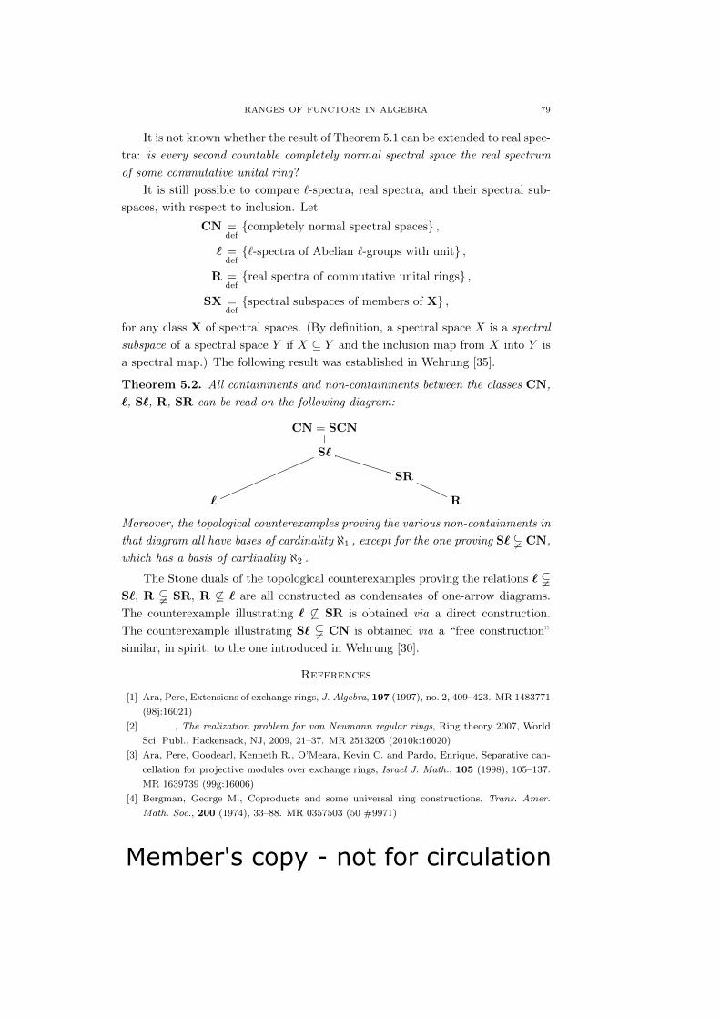
Member's copy - not for circulation
RANGES OF FUNCTORS IN ALGEBRA 79
It is not known whether the result of Theorem 5.1 can be extended to real spec-
tra: is every second countable completely normal spectral space the real spectrum
of some commutative unital ring?
It is still possible to compare `-spectra, real spectra, and their spectral sub-
spaces, with respect to inclusion. Let
CN =defcompletely normal spectral spaces ,
` =def`-spectra of Abelian `-groups with unit ,
R =defreal spectra of commutative unital rings ,
SX =defspectral subspaces of members of X ,
for any class X of spectral spaces. (By definition, a spectral space X is a spectral
subspace of a spectral space Y if X ⊆ Y and the inclusion map from X into Y is
a spectral map.) The following result was established in Wehrung [35].
Theorem 5.2. All containments and non-containments between the classes CN,
`, S`, R, SR can be read on the following diagram:
CN = SCN
S`
SR
` R
Moreover, the topological counterexamples proving the various non-containments in
that diagram all have bases of cardinality ℵ1 , except for the one proving S` $ CN,
which has a basis of cardinality ℵ2 .
The Stone duals of the topological counterexamples proving the relations ` $S`, R $ SR, R 6⊆ ` are all constructed as condensates of one-arrow diagrams.
The counterexample illustrating ` 6⊆ SR is obtained via a direct construction.
The counterexample illustrating S` $ CN is obtained via a “free construction”
similar, in spirit, to the one introduced in Wehrung [30].
References
[1] Ara, Pere, Extensions of exchange rings, J. Algebra, 197 (1997), no. 2, 409–423. MR 1483771
(98j:16021)
[2] , The realization problem for von Neumann regular rings, Ring theory 2007, World
Sci. Publ., Hackensack, NJ, 2009, 21–37. MR 2513205 (2010k:16020)
[3] Ara, Pere, Goodearl, Kenneth R., O’Meara, Kevin C. and Pardo, Enrique, Separative can-
cellation for projective modules over exchange rings, Israel J. Math., 105 (1998), 105–137.
MR 1639739 (99g:16006)
[4] Bergman, George M., Coproducts and some universal ring constructions, Trans. Amer.
Math. Soc., 200 (1974), 33–88. MR 0357503 (50 #9971)
Member's copy - not for circulation
80 FRIEDRICH WEHRUNG
[5] Bergman, George M. and Dicks, Warren, Universal derivations and universal ring construc-
tions, Pacific J. Math., 79 (1978), no. 2, 293–337. MR 531320 (81b:16024)
[6] Coste, Michel and Roy, Marie-Francoise, La topologie du spectre reel, Ordered fields and
real algebraic geometry (San Francisco, Calif., 1981), Contemp. Math., Vol. 8, Amer. Math.
Soc., Providence, R. I., 1982, 27–59. MR 653174
[7] Delzell, Charles N. and Madden, James J., A completely normal spectral space that is not
a real spectrum, J. Algebra 169 (1994), no. 1, 71–77. MR 1296582
[8] , Lattice-ordered rings and semialgebraic geometry. I, Real analytic and algebraic
geometry (Trento, 1992), de Gruyter, Berlin, 1995, 103–129. MR 1320313
[9] Dickmann, Maximo A., Applications of model theory to real algebraic geometry. A survey,
Methods in mathematical logic (Caracas, 1983), Lecture Notes in Math., Vol. 1130, Springer,
Berlin, 1985, 76–150. MR 799038
[10] Erdos, Paul, Hajnal, Andras, Mate, Attila and Rado, Richard, Combinatorial Set Theory:
Partition Relations for Cardinals, Studies in Logic and the Foundations of Mathematics,
Vol. 106, North-Holland Publishing Co., Amsterdam, 1984. MR 795592
[11] Funayama, Nenosuke and Nakayama, Tadasi, On the distributivity of a lattice of lattice-
congruences, Proc. Imp. Acad. Tokyo, 18 (1942), 553–554. MR 0014065
[12] Gillibert, Pierre and Wehrung, Friedrich, From Objects to Diagrams for Ranges of Func-
tors, Lecture Notes in Mathematics, Vol. 2029, Springer, Heidelberg, 2011. MR 2828735
(2012i:18001)
[13] , An infinite combinatorial statement with a poset parameter, Combinatorica, 31
(2011), no. 2, 183–200. MR 2848250
[14] Goodearl, Kenneth R., Von Neumann regular rings and direct sum decomposition problems,
Abelian groups and modules (Padova, 1994), Math. Appl., Vol. 343, Kluwer Acad. Publ.,
Dordrecht, 1995, 249–255. MR 1378203
[15] Gratzer, George, Lattice Theory: Foundation, Birkhauser/Springer Basel AG, Basel, 2011.
MR 2768581 (2012f:06001)
[16] Gratzer, George and Schmidt, E. Tamas, Characterizations of congruence lattices of abstract
algebras, Acta Sci. Math. (Szeged), 24 (1963), 34–59. MR 0151406 (27 #1391)
[17] Hochster, Melvin, Prime ideal structure in commutative rings, Trans. Amer. Math. Soc.
142 (1969), 43–60. MR 0251026
[18] Johnstone, Peter T., Stone Spaces, Cambridge Studies in Advanced Mathematics, Vol. 3,
Cambridge University Press, Cambridge, 1982. MR 698074
[19] Keimel, Klaus, The representation of lattice-ordered groups and rings by sections in sheaves,
(1971), 1–98. Lecture Notes in Math., Vol. 248. MR 0422107
[20] , Some trends in lattice-ordered groups and rings, Lattice theory and its applica-
tions (Darmstadt, 1991), Res. Exp. Math., Vol. 23, Heldermann, Lemgo, 1995, 131–161.
MR 1366870
[21] Kuratowski, Casimir, Sur une caracterisation des alephs, Fund. Math., 38 (1951), 14–17.
MR 0048518
[22] Mellor, Timothy and Tressl, Marcus, Non-axiomatizability of real spectra in L∞λ, Ann.
Fac. Sci. Toulouse Math., (6) 21 (2012), no. 2, 343–358. MR 2978098
[23] Mundici, Daniele, Advanced Lukasiewicz Calculus and MV-Algebras, Trends in Logic–Studia
Logica Library, Vol. 35, Springer, Dordrecht, 2011. MR 2815182
[24] Ruzicka, Pavel, Free trees and the optimal bound in Wehrung’s theorem, Fund. Math., 198
(2008), no. 3, 217–228. MR 2391012

Member's copy - not for circulation
RANGES OF FUNCTORS IN ALGEBRA 81
[25] Ruzicka, Pavel, Tuma, Jirı and Wehrung, Friedrich, Distributive congruence lattices of
congruence-permutable algebras, J. Algebra, 311 (2007), no. 1, 96–116. MR 2309879
[26] Rump, Wolfgang and Yang, Yi Chuan, The essential cover and the absolute cover of a
schematic space, Colloq. Math. 114 (2009), no. 1, 53–75. MR 2457279
[27] Stone, Marshall H., Topological representations of distributive lattices and Brouwerian log-
ics, Cas. Mat. Fys. 67 (1938), no. 1, 1–25.
[28] Tuma, Jirı and Wehrung, Friedrich, Simultaneous representations of semilattices by lattices
with permutable congruences, Internat. J. Algebra Comput., 11 (2001), no. 2, 217–246.
MR 1829051
[29] Warfield, Jr., Robert B., Exchange rings and decompositions of modules, Math. Ann., 199
(1972), 31–36. MR 0332893
[30] Wehrung, Friedrich, Non-measurability properties of interpolation vector spaces, Israel J.
Math. 103 (1998), 177–206. MR 1613568 (99g:06023)
[31] , A uniform refinement property for congruence lattices, Proc. Amer. Math. Soc.,
127 (1999), no. 2, 363–370. MR 1468207
[32] , A solution to Dilworth’s congruence lattice problem, Adv. Math., 216 (2007), no. 2,
610–625. MR 2351371
[33] , Lifting defects for nonstable K0-theory of exchange rings and C∗-algebras, Algebr.
Represent. Theory 16 (2013), no. 2, 553–589. MR 3036005
[34] , Spectral spaces of countable Abelian lattice-ordered groups, hal-01431444, preprint,
February 2017.
[35] , Real spectrum versus `-spectrum via Brumfiel spectrum, hal-01550450, preprint,
July 2017.
[36] , Schmidt and Pudlak’s Approaches to CLP, Lattice Theory: Special Topics and
Applications. Vol. 1, Birkhauser/Springer, Cham, 2014, 235–296. MR 3330600
[37] , Congruences of Lattices and Ideals of Rings, Lattice Theory: Special Topics and
Applications. Vol. 1, Birkhauser/Springer, Cham, 2014, 297–335. MR 3330601
[38] , Liftable and Unliftable Diagrams, Lattice Theory: Special Topics and Applications.,
Vol. 1, Birkhauser/Springer, Cham, (2014), 337–392. MR 3330602
Friedrich Wehrung
LMNO, CNRS UMR 6139
Departement de Mathematiques, BP 5186
Universite de Caen, Campus 2 , 14032 Caen cedex, France.
E-mail: [email protected]
URL: http://wehrungf.users.lmno.cnrs.fr

Member's copy - not for circulation
82

Member's copy - not for circulation
The Mathematics Student ISSN: 0025-5742
Vol. 87, Nos. 1-2, January-June (2018), 83-105
APPROXIMATION BY SPLINE FUNCTIONSAND ITS APPLICATIONS*
P. V. JAIN
Abstract. In this article, the historical background and motivation for the
definition of spline functions initiated by I. J. Schoenberg have been discussed
along with the basis functions for linear and higher degree spline space. The
concept of discrete splines introduced by Mangasarian and Schumaker has
been also presented.
After bivariate splines, the idea of Finite Elements has been elaborated.
Using an interesting result of geometry, Wachspress has initiated the rational
basis functions on convex polygons and polycons. The constructive aspects
of these basis functions have been introduced.
The applications of spline functions to Civil Engineering and One-Dimensi-
onal Cutting Stock Problems are highlighted in the concluding part of the
article.
1. Introduction and Motivation
The numerical solution to a problem is in general expressed in terms of an
approximation U(x) to the true solution u(x) for x in some prescribed region D. A
norm ||.||may be defined and U may be chosen as function which best approximates
u over some approximation space A in the sense that U(x) = U(x, a0), where
H = ||U(x, a0)− u(x)|| = minU(x,a)∈A
||U(x, a)− u(x)||.
Questions of existence and uniqueness of a0, and of convergence of H to zero as
the dimension of A is increased some how, are considered in many research papers.
This is a central problem in approximation theory (cf. [68]).
With the advancement of computer technology, function which can be easily
stored in computer and which have nice mathematical properties such as:• Strong approximation power
• Computational convenience
* This is the text of the 13th Ganesh Prasad Memorial Award Lecture delivered at the 83rd
Annual Conference of the Indian Mathematical Society - An international Meet held at Sri
Venkateswara University, Tirupati - 517 502, Andhra Pradesh, India during December 12 - 15,
2017.
2010 Mathematics Subject Classification : 97N50, 57R12, 41A52, 41A50, 42A10, 65L60,
74S05.
Key words and phrases: Univariate Spline, Bivariate Spline, Finite Element Methods,
Sustainable Trim, CSP, SYI, CN.
c© Indian Mathematical Society, 2018 .
83

Member's copy - not for circulation
84 P. V. JAIN
• Sufficient degree of smoothnessplay a significant role in the field of approximation theory.
At the early stage, the process of approximation was quite crude; like if two
values are available corresponding to two distinct points of the domain, the ap-
proximate value in between the two points used to be a constant function obtained
by computing the average of two values (refer Figure 1.1).
Later, it was noticed that the polynomials are most suitable functions for
approximation as they can be evaluated, differentiated and integrated easily. The
simple theorem of polynomial interpolation upon which much practical numerical
analysis rests states as:
Figure 1.1. Crude Approximation
Theorem 1.1 ([8], p.24). Given (n+1) distinct points (real or complex) z0, z1, . . . ,
zn and n+1 (real or complex) values w0, w1, . . . , wn. There exists polynomial pn(z)
(of degree n or less) ∈ Pn for which
pn(zi) = wi i = 0, 1, . . . , n
Figure 1.2. Polynomial interpolation of degree 3
Please refer Figure 1.2 for polynomial interpolation of degree 3.
The major problem with the polynomial approximation was the complexity of
computation for sufficiently large number of data.
We now state the second fundamental theorem due to Weierstrass [8] which
was very strong and popular during 1885.

Member's copy - not for circulation
APPROXIMATION BY SPLINE FUNCTIONS AND ITS APPLICATIONS 85
Theorem 1.2. Let f(x) ∈ C[a, b], given an ε > 0, we can find a polynomial pn(x)
(of sufficiently high degree) for which
|f(x)− pn(x)| ≤ ε a ≤ x ≤ bWeierstrass theorem asserts the possibility of uniform approximation by polyno-
mials to continuous functions over a closed interval (see Figure 1.3).
Multivariate analogue of the foregoing theorem is also known for a continuous
function defined on a compact subset of Rn (the n-dimensional Euclidean space).
A constructive and elegant proof of this theorem depends on the Bernstein
polynomials Bn(f) associated with f , which are defined in terms of Bernstein
basis polynomials (see [11]);
Figure 1.3. Polynomial Approximation of continuous function
For a given positive integer n and x ∈ [0, 1]
Bnj (x) =
(n
j
)(1− x)n−jxj j = 0, 1, . . . , n;
B00 ≡ 1,
Bnj ≡ 0 for n < j or j < 0.
The Bernstein polynomial associated with a given function f defined over [0, 1]
is given by
Bn(f)(x) =n∑
k=0
f(
(k
n
))Bn
k (x)
In fact for each f ∈ C[a, b] (space of all continuous functions defined over
[a, b]), we have||f − Bn(f)|| → 0 as n → ∞
One of the most surprising facts in the theory of interpolation and approxima-
tion is that the simplest and most natural approach to synthesis leads to failure or
rather to an impossibility. Referring Weierstrass theorem of 1885, given a function
of class C[a, b], what is more natural than to think that if a sequence of polynomi-
als pn(f, x) is set up that duplicates the function at n+ 1 points of interval, then

Member's copy - not for circulation
86 P. V. JAIN
as n → ∞, the question is whether pn(f, x) will converge to f(x) or not? The
answer is quite disappointing, pn(f, x) may not converge to f in general.
Runge ([64], p. 102) looks at the function f(x) = 11+x2 out of several mero-
morphic functions and found the following to be true:
If pn(f, x) interpolates to f at n+ 1 equidistant points of the interval |x| ≤ 5,
pn converges to f only in the interval |x| ≤ 3.63... and diverges out side this
interval (see Figure 1.4). In 1912, Bernstein proved that equidistant interpolation
over |x| ≤ 1 to the function y = |x| diverges for 0 < |x| < 1.
Figure 1.4. Lagrange Interpolation of 11+x2 at 15 equidistant
points on [−5, 5]
These results relate to equidistant points of interpolation. The space was still
open for different choices of interpolatory points. The hopes for this idea vanished
when Bernstein and Faber in 1914 simultaneously discovered the following:
Theorem 1.3 (cf. [8]). Let
−1 ≤ x0n < x1n < · · · < xnn ≤ 1 n = 1, 2, . . . (1.1)
be any prescribed triangular system of interpolation points. Then for each sequence
of interpolation sets (1.1), there exists f ∈ C[−1, 1] for which its n − th degree
interpolating polynomials pnf , matching f at xin i = 0, 1, . . . , n do not converge
uniformly to f .
In view of these results, it was quite natural to search for some other approx-
imants which can overcome these deficiencies.
The beginning of one such major approach could be traced back to the pio-
neering work of I. J. Schoenberg [62](see also [63]). The basic idea is to employ
piecewise polynomial functions (pp functions) with certain degree of smoothness
at the joints which are termed as splines. Basically, SPLINE is a French word.
Its meaning is a device of small pieces of curves which are used by architects to
design a railway track. One apparent advantage in the use of pp functions instead
of polynomials is that a higher degree of flexibility is achieved through splines
without paying for additional computational complexities inherent in dealing with
polynomials of higher degree. A formal definition of spline is as follows [10]:
Member's copy - not for circulation
APPROXIMATION BY SPLINE FUNCTIONS AND ITS APPLICATIONS 87
Consider a closed interval [a, b] on R and define a partition P as
P : a = τ0 < τ1 < · · · < τn = b
where τi’s are distinct points of the interval [a, b] and are called as knots or nodal
points. A class of mth degree splines with respect to partition P is denoted by
Sm(p); s ∈ Sm(p) if
• its restriction on each subinterval [τi−1, τi] (i = 1, 2, . . . , n) is a polynomial
of degree m or less,
• at each nodal point τi (i = 1, 2, . . . , n− 1), s ∈ Cm−1[a, b].
We next consider interpolation of derivatives also. Let τ1, τ2, . . . , τr be given
distinct real points which are associated with multiplicities mj (positive integers),
j = 1, 2, . . . , r, such that m1 +m2 + · · ·+mr = n+1. Under Hermite interpolation
by mth degree polynomial pm, we expect it to satisfy the following conditions:
plm(τj) = cj,l, l = 0, 1, . . . ,mj − 1; j = 1, 2, . . . , r. (1.2)
If cj,l = f l(τj), we say that polynomial pm = pmf is the Hermite interpolant
of the function f . If mj = 1 for every j, r = n + 1, we call pm the Lagrange
interpolant of f at τ0, τ1, . . . , τn. It may be checked easily that there is a unique
polynomial satisfying the interpolatory conditions (1.2).
A common technique of computing approximants is to use the approximation
space
A = U(x; a) =
n∑i=1
aiwi(x), (1.3)
where wi are known basis functions and the ai’s are combining coefficients.
2. Univariate Splines
Basis for Linear Approximation. We denote the piecewise linear or broken line
interpolant (cf. [10]) to g at points τ1, . . . , τn with a = τ1 < τ2 < · · · < τn = b by
I2g. Let S2 denotes the linear space of all continuous broken lines on [τ1, τn] with
breaks at τ2, . . . , τn−1.
The convenient basis for S2 is
Hi(x) =
(x− τi−1)/(τi − τi−1), τi−1 < x ≤ τi;(τi+1 − x)/(τi+1 − τi), τi ≤ x < τi+1;
0, otherwise.
It is easy to verify that Hi(x) are linearly independent functions. Hi(x) are called
Hat functions (cf. Figure 2.1 on the next page).
We now define the space of splines of degree k and smoothness of order r.
Let P : a = x0 < x1 < · · · < xn = b be a partition of an interval [a, b] and
k > r ≥ 0 be given integers. Then define
Srk(p) = s ∈ Cr[a, b] : s is a polynomial of degree ≤ k
on each subinterval [xi−1, xi], i = 1, 2, . . . , n
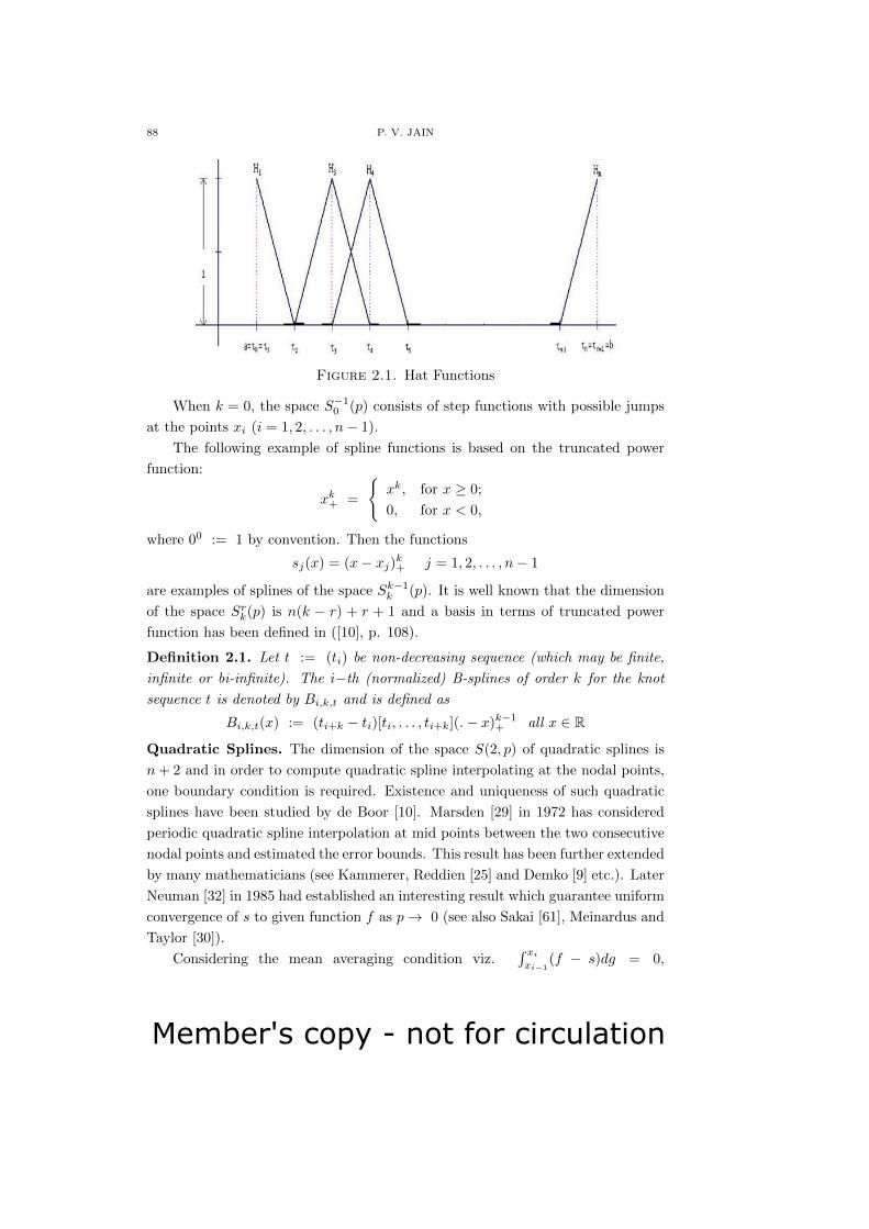
Member's copy - not for circulation
88 P. V. JAIN
Figure 2.1. Hat Functions
When k = 0, the space S−10 (p) consists of step functions with possible jumps
at the points xi (i = 1, 2, . . . , n− 1).
The following example of spline functions is based on the truncated power
function:
xk+ =
xk, for x ≥ 0;
0, for x < 0,
where 00 := 1 by convention. Then the functions
sj(x) = (x− xj)k+ j = 1, 2, . . . , n− 1
are examples of splines of the space Sk−1k (p). It is well known that the dimension
of the space Srk(p) is n(k − r) + r + 1 and a basis in terms of truncated power
function has been defined in ([10], p. 108).
Definition 2.1. Let t := (ti) be non-decreasing sequence (which may be finite,
infinite or bi-infinite). The i−th (normalized) B-splines of order k for the knot
sequence t is denoted by Bi,k,t and is defined as
Bi,k,t(x) := (ti+k − ti)[ti, . . . , ti+k](.− x)k−1+ all x ∈ R
Quadratic Splines. The dimension of the space S(2, p) of quadratic splines is
n+ 2 and in order to compute quadratic spline interpolating at the nodal points,
one boundary condition is required. Existence and uniqueness of such quadratic
splines have been studied by de Boor [10]. Marsden [29] in 1972 has considered
periodic quadratic spline interpolation at mid points between the two consecutive
nodal points and estimated the error bounds. This result has been further extended
by many mathematicians (see Kammerer, Reddien [25] and Demko [9] etc.). Later
Neuman [32] in 1985 had established an interesting result which guarantee uniform
convergence of s to given function f as p→ 0 (see also Sakai [61], Meinardus and
Taylor [30]).
Considering the mean averaging condition viz.∫ xi
xi−1(f − s)dg = 0,

Member's copy - not for circulation
APPROXIMATION BY SPLINE FUNCTIONS AND ITS APPLICATIONS 89
i = 1, 2, . . . , n. Sharma and Tzimbalario [66] have established the existence and
uniqueness theorems for 1-periodic function which is locally integrable along with
non-negative measure dg.
Some interesting studies concerning monotonicity of spline interpolant of mono-
tone data have been also made (see [33]).
Piecewise Cubic Interpolation. Broken lines are neither very smooth nor very
efficient approximators. Both for a smoother approximation and for more effi-
cient approximation, one has to go to piecewise polynomial approximation with
higher order pieces. The most popular choice continue to be a piecewise cubic
approximating function.
We shall be highlighting some major contribution. Applying the technique of
matching of integral means of Sharma and Tzimbalario [66], Dikshit [12] in 1978
established the following result:
Theorem 2.1. Let f ∈ C2[0, 1] be a 1-periodic locally integrable function with
respect to a non-negative measure dµ satisfying µ(x+h)−µ(x) = κ Suppose
further that either∫ h
0α(x)dµ > 0 or
∫ h
0α(h−x)dµ > 0, where α(x) = 3x3−6hx2+
h3 and h = xi+1 − xi. Then there exists a unique s(x) ∈ S0p(3,∆) satisfying the
following conditions:∫ xi
xi−1
f(x)− s(x)dµ = 0 i = 1, 2, . . . , n
Sr(0) = Sr(1) r = 0, 1, 2
[ Dimension : 4n − (n − 1)3 = n + 3 n interpolatory conditions and 3
boundary conditions.]
The above theorem has been proved for two different cases viz. (i) n even (ii)
n odd with different choice of α(x)
Theorem 2.2 (cf. [12]). The following error bound holds:
||e′′|| ≤ [1 + (9H + 12B(1) + 4B(3))/δ]ω(f ;h)
where δ =∫ h
0α(x)dµ or
∫ h
0α(h− x)dµ according as∫ h
0
α(x)dµ > 0 or
∫ h
0
α(h− x)dµ > 0
where e(x) = s(x)− f(x).
By making less restrictive continuity requirements at the joints and having
two interpolatory conditions, Dikshit and Powar [13] (see also [15]) had posed the
following problem:
Problem 2.1. Let f be a 1-periodic locally integrable function with respect to a
positive measure dg, where g satisfies:
• g(x+ h)− g(x) = a constant k′
• g(x) = k (0 ≤ x < mh, 2/9 ≤ m < 1/2)
Member's copy - not for circulation
90 P. V. JAIN
• g(x) = k (mh ≤ x ≤ h, 1/2 ≤ m ≤ 7/9)
Find 1-periodic s(x) ∈ S(3,∆) satisfying the conditions:
f(θi) = s(θi),
∫ xi
xi−1
(f − s)(x)dg = 0, i = 1, 2, . . . , n,
where θi = xi−1 +mh.
The answer to this Problem was given in the following Theorem;
Theorem 2.3. There exists a unique s(x) ∈ S(3,∆) which satisfies the conditions
of Problem 2.1 provided that g(x) does not have just one jump in [0, h] at the point
mh, 0 ≤ m ≤ 1.
The following error estimate was also computed in [13].
Theorem 2.4. Suppose s(x) is the deficient cubic spline of Theorem 2.3 interpo-
lating f(x) and f(x) ∈ C1[0, 1]. Then
maxx|s(x)− f(x)| ≤ κ(m)ω(f ;h) and
maxx|s′(x)− f ′(x)| ≤ κ′(m)ω(f ;h) + κ′′(m)ω1(f ;h),
where κ(m), κ′(m) and κ′′(m) are functions only depending on m.
Several such results on existence and uniqueness had been explored (see [61],
[62], [63], [64] etc.). The problems of computation of error bounds and the refine-
ment of the bounds which are already available have been also studied extensively
(see [6], [11]).
Discrete Splines. Mangasarian and Schumaker [28] in 1973 introduced discrete
splines as solutions of certain minimization problems involving differences. Exis-
tence, uniqueness and error bounds for discrete cubic splines interpolating at the
knots are due to Lyche [27].
In order to achieve the desired order of continuity, instead of derivatives, the
following differences have been matched at the nodal points.
D1hf(x) =
f(x+ h)− f(x)
h, D2
hf(x) =f(x+ 2h)− 2f(x+ h) + f(x)
h2, etc.
By simply letting h → 0 in the above formulae, Classical splines as a special
case of discrete splines are obtained.
The existence, uniqueness and convergence of discrete cubic splines which
interpolate to a given function at one interior point of each mesh interval had
been studied in [14] (see also [37]).
Considering αi = xi+1 + αp (p = xi − xi−1) with 0 ≤ α ≤ 1 and the
interpolatory condition
(f − s)(αi) = 0 i = 1, 2, . . . , n (2.1)
for given functional value, following problem was proposed in [14]:
Problem 2.2. Given h > 0 for what choice of α, does the interpolatory problem
(2.1) admit unique solutions for splines of class D1(3, p, h) or class D2(3, p, h)?

Member's copy - not for circulation
APPROXIMATION BY SPLINE FUNCTIONS AND ITS APPLICATIONS 91
The answer to the above problem was given in the form of following theorem:
Theorem 2.5. [14] Suppose 0 < h ≤ p and (i) 0 ≤ α ≤ 13 or (ii) 2
3 ≤α ≤ 1. The interpolation problem (2.1) admits a unique solution in D1(3, p, h),
if f is periodic with period b − a. (2.1) admits a unique solution in D2(3, p, h) if
(s− f)(b) = 0 when (i) holds or if (s− f)(a) = 0 when (ii) holds.
Many more results dealing with error bounds have been explored in [14].
3. Bivariate Splines
The domain under consideration is simply connected region for which a dis-
cretization is considered (see Figure 3.1).
Figure 3.1. Discretization of the domain
On each member of the partition, a bivariate polynomial of degree m is defined
and the inter-element continuity is imposed. Polynomial of degree m in n variables
have(m+nn
)= (m+n)!
m!n! free parameters. Many of the mathematicians (see [1], [2],
[3], [7] etc.) worked on bivariate splines. Due to discretization of the domain and
complexity in bivariate polynomial pieces, it was difficult to handle and settle the
dimension problem, ultimately the field reached to the stagnation.
4. Finite Element Method
Given a simply connected domain, the discretization of the domain into finite
number of sub-domains (polygons/polycons) is considered. Each sub-domain is
called the FINITE ELEMENT (cf. [5]). The discretization (see Figure 4.1 on the
next page) has been done in such a way that between two adjacent elements, only
two vertices and a side is common.
Triangular Element.
• Basis for the linear approximation over triangular element
For the triangle in Figure 4.2 on the next page, a linear approximation
U(x, y) (cf. [68]) is given by
U(x, y) =3∑
i=1
u(xi, yi)ωi(x, y) (4.1)
where ωi(x, y) (i = 1, 2, 3) are defined as follows:

Member's copy - not for circulation
92 P. V. JAIN
Figure 4.1. Discretizations
Let L1(x, y) be the linear function (polynomial of degree one) which
vanishes on side (2,3) of the triangle (Figure 4.2). Then, we have
ω1(x, y) = L1(x, y)/L1(x1, y1),
where (x1, y1) is a coordinate of the vertex 1.
Figure 4.2. Triangular Finite Element
This wedge basis function is associated with the node 1 of the triangle
(1,2,3) (see Figure 4.3).
ω1(1) =
1, at the vertex 1;
linear, on the sides (1,2) and (1,3);
0, on (2,3) and otherwise
The other wedges are defined similarly. It follows directly by construc-
tion that the collection ωi(x, y)3i=1 is linearly independent. U(x, y) (cf.
relation (4.1)) is a linear approximation by Finite Element Method.
Figure 4.3. Wedge construction at the vertex 1
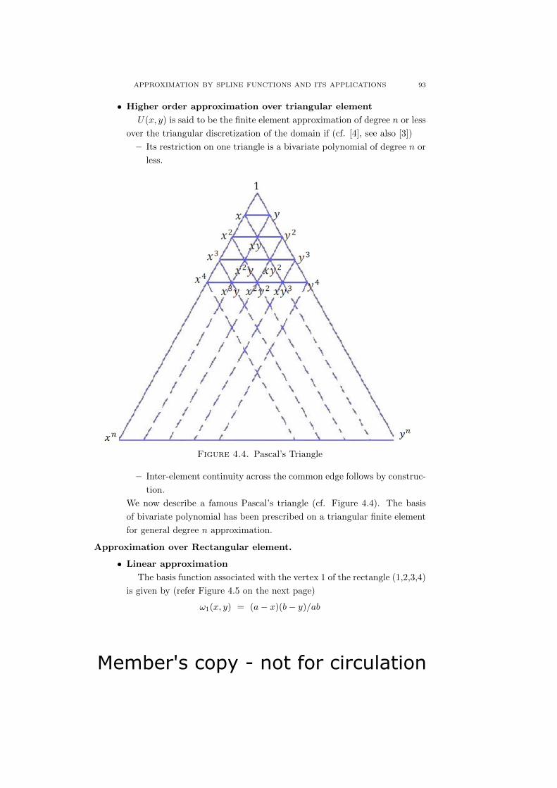
Member's copy - not for circulation
APPROXIMATION BY SPLINE FUNCTIONS AND ITS APPLICATIONS 93
• Higher order approximation over triangular element
U(x, y) is said to be the finite element approximation of degree n or less
over the triangular discretization of the domain if (cf. [4], see also [3])
– Its restriction on one triangle is a bivariate polynomial of degree n or
less.
Figure 4.4. Pascal’s Triangle
– Inter-element continuity across the common edge follows by construc-
tion.
We now describe a famous Pascal’s triangle (cf. Figure 4.4). The basis
of bivariate polynomial has been prescribed on a triangular finite element
for general degree n approximation.
Approximation over Rectangular element.
• Linear approximation
The basis function associated with the vertex 1 of the rectangle (1,2,3,4)
is given by (refer Figure 4.5 on the next page)
ω1(x, y) = (a− x)(b− y)/ab

Member's copy - not for circulation
94 P. V. JAIN
Figure 4.5. Rectangular element
ω1(1) =
1, at the vertex 1;
Linear, on the adjacent sides (1,2) and (1,4);
0, on (3,4) and (2,3).
Other wedges may be defined similarly. It is easy to verify that the collec-
tion ωi4i=1 is linearly independent and U(x, y) =∑4
i=1 u(xi, yi)ωi(x, y)
is a linear approximation over a rectangular element.
• Higher order approximation over rectangular element
The basis of bivariate monomial has been prescribed on a rectangular
element for general n−degree approximation (cf. Figure 4.6).
Figure 4.6. Monomials
Approximation over parallelogram element. Consider the parallelogram
(1, 2, 3, 4) (cf. Figure 4.7 on the next page). The basis functions for nodes 1
and 2 are given by
ω1(x, y) = (2; 3)(3; 4)/[(2; 3)(3; 4)|1]; ω2(x, y) = (3; 4)(4; 1)/[(3; 4)(4; 1)|2]
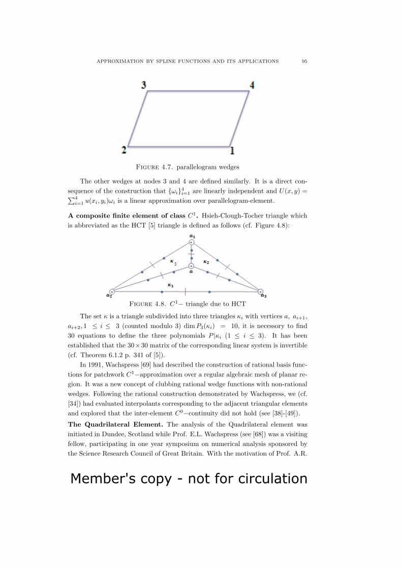
Member's copy - not for circulation
APPROXIMATION BY SPLINE FUNCTIONS AND ITS APPLICATIONS 95
Figure 4.7. parallelogram wedges
The other wedges at nodes 3 and 4 are defined similarly. It is a direct con-
sequence of the construction that ωi4i=1 are linearly independent and U(x, y) =∑4i=1 u(xi, yi)ωi is a linear approximation over parallelogram-element.
A composite finite element of class C1. Hsieh-Clough-Tocher triangle which
is abbreviated as the HCT [5] triangle is defined as follows (cf. Figure 4.8):
Figure 4.8. C1− triangle due to HCT
The set κ is a triangle subdivided into three triangles κi with vertices a, ai+1,
ai+2, 1 ≤ i ≤ 3 (counted modulo 3) dimP3(κi) = 10, it is necessory to find
30 equations to define the three polynomials P |κi (1 ≤ i ≤ 3). It has been
established that the 30×30 matrix of the corresponding linear system is invertible
(cf. Theorem 6.1.2 p. 341 of [5]).
In 1991, Wachspress [69] had described the construction of rational basis func-
tions for patchwork C1−approximation over a regular algebraic mesh of planar re-
gion. It was a new concept of clubbing rational wedge functions with non-rational
wedges. Following the rational construction demonstrated by Wachspress, we (cf.
[34]) had evaluated interpolants corresponding to the adjacent triangular elements
and explored that the inter-element C0−continuity did not hold (see [38]-[49]).
The Quadrilateral Element. The analysis of the Quadrilateral element was
initiated in Dundee, Scotland while Prof. E.L. Wachspress (see [68]) was a visiting
fellow, participating in one year symposium on numerical analysis sponsored by
the Science Research Council of Great Britain. With the motivation of Prof. A.R.

Member's copy - not for circulation
96 P. V. JAIN
Mitchell, the general quadrilateral element was reported at the Dundee conference
of Application of Numerical Analysis held in April, 1971.
Having demonstrated the inadequacy of polynomials as quadrilateral wedges,
the rational form of the basis function was investigated after going through several
exercises. The choice of the denominator function is based on a following lemma
which plays a key role in defining the rational form.
Lemma 4.1 (Lemma 2.1, p.34 [68]). If three lines intersect at a point, then the
ratio of linear forms which vanish on any two of these lines is constant on the
third line.
• Wedge construction for linear approximation
It has been noticed that the polynomials and the monomials are inad-
equate to define wedge functions over quadrilateral element.
Thus, the rational function of least degree in numerator and denomina-
tor which can be a candidate for the wedge is (cf. Figure 4.9):
ω1(x, y) =Q1
(2, 3)(3, 4)|1
(2, 3)(3, 4)
Q1(4.2)
Hence, the linear form Q1 should be such that
(a): Q1 6= 0 within the quadrilateral.
(b): (2,3)(3,4)Q1
should be linear on both (4, 1) and (1, 2).
Figure 4.9. Quadrilateral element
In view of Lemma 4.1, the exact choice of Q1 is the exterior diagonal (5, 6)
obtained by joining exterior intersection points 5 and 6 (cf. Figure 4.9)
which satisfies both the conditions (a) and (b).
Wedge functions ω2, ω3 and ω4 at the vertices 2, 3, 4 may be defined
similarly.
Thus, U(x, y) =∑4
i=1 u(xi, yi)ωi is a rational linear approximation over
the quadrilateral element.
• Wedge construction for quadratic approximation
Consider a quadrilateral (1, 2, 3, 4) (cf. Figure 4.10 on the next page)
with mid points 5, 6, 7, 8 on the sides (1, 4), (1, 2), (2, 3) and (3, 4) respec-
tively. The linear forms li (i = 1, 2, . . . , 8) joining two points have been

Member's copy - not for circulation
APPROXIMATION BY SPLINE FUNCTIONS AND ITS APPLICATIONS 97
displayed in Figure 4.10. The basis functions associated with nodes 1, 2
and 5 are as follows:
ω1 = κ1(l2l3l7/Q), ω2 = κ2(l3l4l6/Q), . . . , ω5 = κ5(l1l2l3/Q), . . . , ω8
Figure 4.10. Quadratic approximation over quadrilateral element
The other wedges may be defined similarly. Applying Lemma 4.1, it
may be verified easily that the restriction of each wedge on the adja-
cent sides is quadratic and zero on the opposite sides. Thus, U(x, y) =∑8i=1 u(xi, yi)ωi is a rational quadratic approximation over the quadrilat-
eral element.
Similar wedges can be constructed for higher degree approximation over
convex quadrilateral.
Wedge construction on convex polygons of order n and some polycons
has been discussed in details in [68] (see also [38]-[50])
5. Triangulation Methods
The Local Optimization Procedure (LOP) for constructing a locally optimal
triangulation is widely used in many cases to get an optimal triangulation of a
general point set U = ui = (xi, yi)N1 . In the local procedure, we need to
consider the sets of four points (see Figure 5.1) that form convex quadrilaterals.
The only two possible triangulations of convex quadrilateral are those which are
Figure 5.1

Member's copy - not for circulation
98 P. V. JAIN
obtained by adjoining two different diagonals of it. In order to satisfy the criterion,
choosing a diagonal is called the Local Optimization Procedure.
The problem of Minimal roughness property of the Delaunay triangulation
has been discussed in [60] which is based on a lemma involving the circle criterion.
The proof of the lemma was quite lengthy and complex.
We [35] have redefined the circle criterion in terms of power of a point and
established a very short and elegant proof of the lemma which states as follows:
Lemma 5.1. Let sT ∈ S01(T ) and sT∗ ∈ S0
1(T ) be the interpolators to the data
vector f on triangulations T and T ∗ respectively. Then
|sT∗ |2 − |sT |2 = φ(f, r, s)µ(r, s)/β(r, s) (5.1)
where
φ(f, r, s) = f2(rq − ps) + sf4 − qf32,
µ(r, s) = qr2 + qs2 − rq + (p− p2 − q2)s/q,
β(r, s) = s(rq − ps)q(r − 1)− s(p− 1)Hansford [24] has investigated an interesting construction of a neutral set for
the min-max angle criterion. The technique described by her requires three data
points to obtain the locus of the fourth point. We [36] have noticed that the min-
max neutral set may be obtain even with two data set points and a given angle.
6. Applications
• Civil Engineering
• One-Dimensional Cutting Stock Problem
Civil Engineering. Watershed management is one of the key branch of Civil
Engineering. Soil, water and vegetation are natural resources, and their manage-
ment is fundamental to the maintenance of ecosystem and economic development.
In India, about 175 M/ha area which constitutes about 53 % of the aggregate
geographical area, is subjected to land degradation due to soil erosion. It is esti-
mated that 5334 million tons of soil is eroded annually, which is a matter of serious
concern for agricultural productivity (cf. [65]).
Our study is focused on soil erosion from watershed. This work was carried
over in collaboration with Prof. V. P. Singh (see [67]), Department of Biological
and Agricultural Engineering, Texas A & M University, College Station, USA and
Dr. Sarita Gajbhiye Meshram, Dr. D.S. Kothari Fellow.
The method is illustrated with a case study of one watershed of Narmada
Basin located in Mandala district, Madhya Pradesh (cf. [31], see also [56]).
On the basis of the data extracted from satellite, the Sediment Yield Index
(SYI) for fourteen sub-watersheds (corresponding to their Curve Number (CN))
have been computed by using following formula:
SY I =
∑ni=1Ai ∗Wi ∗DR
Aw∗ 100

Member's copy - not for circulation
APPROXIMATION BY SPLINE FUNCTIONS AND ITS APPLICATIONS 99
where
Ai − The area of the i− th unit in km2
Wi − The weightage value of the i− th unit (Dimension less unit)
n − The number of mapping units
DR − Delivery ratio (Dimension less) (without units)
Aw − The sub watershed area in km2
For developing relationship between SYI and CN, the proposed procedure is as
follows:
(1) Estimation of sub watershed wise Sediment Yield Index (SYI) and curve
number
(2) CN of different watersheds are arranged in increasing order with respect
to the magnitude which will determine the interval of CN as the domain
of cubic spline interpolation.
(3) For our analysis fourteen watersheds were considered out of which seven
were selected for the construction of cubic splines (see Figure 6.1) and the
remaining were used for the validation of the result.
(4) Referring the cubic spline curve, compute Sediment Yield Index corre-
sponding to CN’s of remaining seven watersheds (see Figure 6.1).
(5) The computed SYI (SYIc) was compared with the observed SYI (SYIo)
computed as per the guide lines of All India Soil and Land Use Survey
(AISLUS, 1991).
Figure 6.1. Cubic spline approximation for soil erosion
Remark: It has been observed that the approximate SYI’s were quite close to
the actual SYI’s. Computation of SYI is quite tedious and lengthy process. With

Member's copy - not for circulation
100 P. V. JAIN
the information of curve number (which is easily available) for any watershed, the
approximate SYI can be predicted immediately and accordingly some preventive
steps can be taken to control the soil erosion. For those curve numbers lying out
side the domain, some extrapolation methods can be applied.
One-Dimensional Cutting Stock Problem. Kantarovich [26] is the first known
Soviet Mathematician and economist who formulated the cutting stock problem
in the year 1939. In 1961, Gilmore and Gomory [16] (see also [17] - [19]) proposed
the first solution methodology for cutting stock problem by applying some tech-
niques of Operations Research (see [20]-[23]). During last two decade this problem
become very popular and many mathematicians, economists, computer scientists
and engineers suggested several cutting plans by taking in consideration space
constraint, time constraint, cost minimization, trim loss minimization etc.
Our study is focused on transmission tower manufacturing industry. One of
the major component for the viability of any industry dealing with Cutting Stock
Problem (CSP) is based on the scrap or the trim loss.
We have suggested (cf. [51]-[57]) the environment friendly cutting plan which
may be easily acceptable by any industry as it resolves the following problems
up-to some extent:
Figure 6.2. Linear spline interpolation for 1D-CSP
• The cutting plan consists of cutting of at most two order lengths at a time
out of the required n order lengths from a given set of m stock lengths.
This consideration requires minimum working space, even one person can
carry out the sorting process conveniently.
• The next set of two order lengths has been considered for cutting, only
when the demand of first set of two order lengths is completed.

Member's copy - not for circulation
APPROXIMATION BY SPLINE FUNCTIONS AND ITS APPLICATIONS 101
• Using the techniques of summability methods, sustainable trims of differ-
ent orders have been defined in terms of order lengths and corresponding
required number of pieces.
• Corresponding to sustainable trim as nodal point on the interval of the
domain and data as total trim loss, the linear (cubic) (cf. Figure 6.2
(on previous page) and Figure 6.3) approximation has been computed (cf.
[54]).
• Extracting the data from KEC international (transmission tower manu-
facturing industry), the complete data analysis has been carried out.
• The mathematical model for the cutting plan has been designed by con-
sidering the nature of the data.
• Writing algorithm and the programming was the most tedious job of this
work (see also [57]-[59]).
Figure 6.3. Cubic spline interpolation for 1D-CSP
Acknowledgement. On this occasion of my professional carrier, I propose my
indebtedness to my teacher Late Prof. H. P. Dikshit, (former Professor at R. D.
University, Jabalpur and Jiwaji University, Gwalior; former Vice-Chancellor, R. D.
University, Jabalpur; Himachal Pradesh University, Shimla; IGNOU, New Delhi
and Bhoj University, Bhopal) for initiating me to the interesting area of research
in Spline Theory.
Prof. E. L. Wachspress took me one step ahead and very kindly guided me
to understand the concept of Finite Element Methods. I shall never forget his
generosity and selfless help.
References
[1] Alfeld, P., On the dimension of multivariate piecewise polynomials, Proc. Biennial Dundee
conference on Numer. Anal. Pitman, 1985.
[2] Alfeld, P. and Shumaker, L. L., The dimension of bivariate spline spaces of smoothness r for
degree d ≥ 4r + 1, Construct. Approx., 3 (1987), 189–197.

Member's copy - not for circulation
102 P. V. JAIN
[3] Alfeld, P. and Shumaker, L. L., On the dimension of bivariate space, spaces of smoothness
r and degree d = 3r + 1, Numer. Math., 57 (1990), 651–661.
[4] Ciarlet, P. G. and Raviart, P. A., General Lagrange and Hermite interpolation in Rn with
applications to finite element methods, Arch. Rat. Mech. Anal., 46 (1972), 177–199.
[5] Ciarlet, P. G., Finite Element Method for Elliptic Problems, North Holland, 1978.
[6] Dahmen, W., Dyn, N. and Levin, D., On the convergence rates of subdivision algorithms
for box spline surfaces, Constructive Approximation, 1 (1985), 305–322.
[7] Dahmen, W., Dress, A. and Miccheli, C. A., On multivariate splines, matroids and functor,
Adv. in Appl. Maths, 17 (3) (1996), 251–307.
[8] Davis, P. J., Interpolation and approximation, Blaisdell Publishing Company, New York,
1963.
[9] Demko, S., Interpolation by quadratic splines, J. Approx. Theory, 23 (1978), 392–400.
[10] De Boor, C., A Practical Guide to Splines, Springer-Verlag, New York, 1978.
[11] De Vore, R. A. and Lorentz, G. G., Constructive approximation, Springer-Verlag, 1991.
[12] Dikshit, H. P., On cubic interpolatory splines, J. Approx. Theory, 22 (1978), 105–111.
[13] Dikshit, H. P. and Powar, P. L., On deficient cubic spline interpolation, J. Approx. Theory,
31 (1981), 99–106.
[14] Dikshit, H. P. and Powar, P. L., Discrete cubic spline interpolation, Numer. Math., 40
(1982), 71–78.
[15] Dikshit, H. P. and Rana, S. S., Cubic interpolation splines with non uniform meshes, J.
Approx. Theory, 45(1985), 350–357.
[16] Gilmore, P. C. and Gomory, R. E., A linear programming approach to the cutting stock
problem, Operations Research, 9 (1961), 848–859.
[17] Gilmore, P. C. and Gomory, R. E., A linear programming approach to the cutting stock
problem part-II, Operations Research, 11 (1963), 863–888.
[18] Gilmore, P. C. and Gomory, R. E., Multistage cutting stock problems of two and more
dimensions, Operations Research, 13 (1) (1965), 94–120.
[19] Gilmore P. C., Cutting stock, linear programming, knapsacking, dynamic programming and
integer programming; some interconnections, Annals of Discrete Mathematics, 4 (1979),
217–235.
[20] Gradisar, M., Jesenko, J. and Resinovic, G., Optimization of roll cutting in clothing industry,
Computer & Operations Research, 24 (1997), 945–953.
[21] Gradisar, M., Kljajic, M., Resinovic, G. and Jesenko J., A sequential heuristic procedure for
one-dimensional cutting, European Journal of Operational Research, 114 (1999), 557–568.
[22] Gradisar, M., Resinovic, G. and Kljajic, M., Evaluation of algorithms of one-dimensional
cutting, Computer & Operations Research, 29 (2002), 1207–1220.
[23] Gradisar, M., Erjavec, J. and Tomat, L., One-dimensional cutting stock optimization with
usable leftover: a case study of low stock-to-order ratio, International Journal of Decision
Support System Technology, 3 (2011), 54–66.
[24] Hansford, D., The neutral case for the min-max triangulation, Computer Aided Geometric
Design, 7 (1990), 43–438.
[25] Kammerer, W. J., Reddien, G. W. and Verga, R. S., Quadratic interpolatory splines, Numer.
Math., 22 (1974), 241–259.
[26] Kantorovich, L. V., Mathematical methods of organizing and planning production, Man-
agement Science, 6 (1960), 363–422.
[27] Lyche, T., Discrete cubic spline interpolation, BIT, 16 (1976), 281–290.

Member's copy - not for circulation
APPROXIMATION BY SPLINE FUNCTIONS AND ITS APPLICATIONS 103
[28] Mangasarian, O. L. and Schumaker, L. L., Discrete spline via. mathematical programming,
SIAMJ, Numer. Anal., 10 (1973), 448–459.
[29] Marsden, M. J., Quadratic spline interpolation, Bull. Amer. Math. Soc., 80 (1974), 903–906.
[30] Meinardus, G. and Taylor, G. D., Periodic quadratic spline interpolant of minimal norm, J.
Approx. Theory, 23 (1978), 137–141.
[31] Meshram, S. G., Powar, P. L. and Singh, V. P., Modelling soil erosion from a watershed
using cubic splines, Arab J Geo Sci., 10:155 (2017), 1–13.
[32] Neuman, E., Determination of quadratic spline function with given values of the integrals
in subintervals, Zastor, Math., 16 (1980), 681–689.
[33] Passow, E., Monotone quadratic spline interpolation, J. Approx. Theory, 19 (1977), 143–
147.
[34] Powar, P. L. and Rao, R., A counter example of the construction of C1-rational finite element
due to Wachspress, Computers Math. Applic., 22 (3) (1991), 17–22.
[35] Powar, P. L., Minimal roughness property of the Delaunay triangulation: a shorter approach,
Computer Aided Geometric Design, 9 (1992), 491–494.
[36] Powar, P. L., The neutral case for the min-max angle criterion : a generalized concept,
Computer Aided Geometric Design, 9 (1992), 413–418.
[37] Powar, P. L. and Dikshit, H. P., Area matching interpolation by discrete cubic splines,
Approximation Theory and Applications, Proc. Conf. St. Jons New Foundland, 35–45, 1984.
[38] Powar, P. L., A shorter approach to the construction of Hermit rational Wachspress Type
finite element, Proceedings of the Mathematical Society, 8 (1993), 7–12.
[39] Powar, P. L. and Rana S. S., Construction of Wachspress Type: rational basis functions
over rectangles, Proc. Ind. Acad. Sci., 110 (1999), 69–77.
[40] Powar, P. L., C1 approximation on triangles, Approximation Theory and its Applications,
(1996), 99–106.
[41] Powar, P. L. and Jain V., Higher degree approximation through polynomial bases, Approx-
imation Theory and its Applications, (1996), 107–119.
[42] Powar, P. L. and Rana S. S., Construction of “Wachspress type” rational basis functions
over rectangles, Proc. Indian Acad. Sci. (Math. Sci.), 110 (1) (2000), 69–77.
[43] Powar, P. L., Construction of Hermit Rational Finite Element over the Convex Polygon for
Quadratic Approximation, Vislesana, 8 (1) (2003), 138–143.
[44] Powar, P. L., The theorem on optimal triangulation: a counterexample, International Jour-
nal of Mathematical Sciences, 3 (1) (2004), 157–160.
[45] Powar, P. L., On Ck triangle, Varahmihir Jour. of Mathematical Sciences, 4 (2) (2004),
499–510.
[46] Powar, P. L., Constructions of Hermit rational finite element over the convex polygon for
quadratic approximation, Vislesana, 8 (1) (2004), 138–14.
[47] Powar, P. L., Constructive aspects of the Hermit rational finite element over the convex
polygon for cubic approximation, Acta Ciencia, XXXM (4) (2004), 679–682.
[48] Powar, P. L., C1- finite element over the convex quadrilateral, Vislesana, 9 (2) (2005),
109–114.
[49] Powar, P. L., Rana, S. S. and Chaudhary, P. R. S., Construction of Hermite rational finite
element with the new basis functions over the rectangle, Vislesana, 10 (2) (2006), 101–108.
[50] Powar, P. L., Mean value coordinates due to Floater, Proc. National Conference on Advance
Computing and Communication, 12–17, 2009.

Member's copy - not for circulation
104 P. V. JAIN
[51] Powar, P. L., Jain, V., Saraf, M. and Vishwakarma, R., One-dimensional cutting stock
problem (1D-CSP): A new approach, International Journal of Advanced Computing, 46 (2)
(2013), 1223–1228.
[52] Powar, P. L., Jain, V., Saraf, M. and Vishwakarma, R., One-Dimensional Cutting Stock
Problem (1D-CSP) with First Order Sustainable Trim: A Practical Approach, Interna-
tional Journal of Computer Science Engineering and Information Technology Research
(IJCSEITR), 3 (3) (2013), 227–240.
[53] Powar, P. L., Jain, V., Saraf, M. and Vishwakarma, R., One-Dimensional Cutting Stock
Problem (1D-CSP) with Second Order Sustainable Trim: A Comparative Study With First
Order Sustainable Trim, International Journal of Computer Engineering and Technology
(IJCET), 4 (4) (2013), 136–149.
[54] Powar, P. L., Jain, V., Saraf, M. and Vishwakarma, R., Application of Spline Approxi-
mation Method to Obtain Locally Minimal Approximate Trim Loss for One-Dimensional
Cutting Stock Problem (1D-CSP), International Journal of Computer Science Engineering
and Information Technology Research (IJCSEITR), 3 (4) (2013), 19–36.
[55] Powar, P. L., Jain, V., Saraf, M. and Vishwakarma, R., One-Dimensional Cutting Stock
Problem (1D-CSP): A Study on Data Dependent Trim Loss, International Journal of Com-
puter Engineering & Technology (IJCET), 4 (4) (2013), 524–538.
[56] Powar, P. L. and Meshram S. G., Piecewise Regression Using Cubic Spline: A Case Study,
International Journal of Hybrid Information Technology, 10 (1) (2017), 75–84.
[57] Powar, P. L., Vishwakarma, R. and Meshram, C., Effective Mathematical Simulation for
One-Dimensional Cutting Stock Problem using Heuristics Approach, International Journal
of Hybrid Information Technology, 10(1) (2017), 111–124.
[58] Powar, P. L. and Samuel, S., Comparative Study of Various Algorithms dealing with Com-
putational Aspects of One-Dimensional Cutting Stock Problem, Advances in Computational
Sciences and Technology, 10 (3) (2017), 409–422.
[59] Powar, P. L. and Vishwakarma R., Modified FFD Algorithm for One-Dimensional Cutting
Stock Problem, International Journal of Computer and Mathematical Sciences, 6 (7) (2017),
66–72.
[60] Rippa, S., Minimal roughness property of the Delaunay triangulation, Computer Aided
Geometric Design, 7 (1990), 489–497.
[61] Sakai, M., Some new consistency relations connecting spline values at mesh and mid points,
BIT, 23 (1983), 543–544.
[62] Schoenberg, I. J., Contribution to the problem of approximation of equidistant data by
analytic functions, Quaterly Applied Math., 4 (1946), 45–99(part A), 112–141 (part B).
[63] Schoenberg, I. J., On interpolation by spline functions and its minimal properties in P.L.
Butzer and J. Kprevaar (eds). On approximation Theory ISNM, 5(1964), Birkhauser, 109–
129.
[64] Schumaker, L. L., Spline Functions: Basic Theory, A Wiley-Interscience Publication, New
York, 1981.
[65] Sebestian, M., Jayaraman, V. and Chandrashekhar, M. G., Space technology application for
development of watershed, Technical report, ISRO-HQ-TR-104-95, ISRO, Banglore, 1–41,
1995.
[66] Sharma, A. and Tzimbalario, J., Quadratic splines, J. Approx. Theory, 19 (1977), 183–193.
[67] Singh, V. P. and Yadava, R. N., Watershed Management, Allied publisher private limited
ISBN 81-7464-545-5, 2003.
[68] Wachspress, E. L., A rational finite element basis, Academic Press, 1975.

Member's copy - not for circulation
APPROXIMATION BY SPLINE FUNCTIONS AND ITS APPLICATIONS 105
[69] Wachspress, E. L., C1- rational finite elements, Computers and Mathematics with applica-
tions, 22 (3) (1991), 11–16.
P. V. Jain
Department of Mathematics and Computer Science
Rani Durgavati University, Jabalpur-482 001, M.P., India
E-mail: [email protected]

Member's copy - not for circulation
106
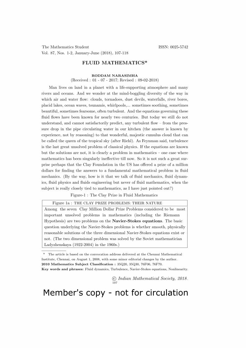
Member's copy - not for circulation
The Mathematics Student ISSN: 0025-5742
Vol. 87, Nos. 1-2, January-June (2018), 107-118
FLUID MATHEMATICS*
RODDAM NARASIMHA
(Received : 01 - 07 - 2017; Revised : 09-02-2018)
Man lives on land in a planet with a life-supporting atmosphere and many
rivers and oceans. And we wonder at the mind-boggling diversity of the way in
which air and water flow: clouds, tornadoes, dust devils, waterfalls, river bores,
placid lakes, ocean waves, tsunamis, whirlpools,... sometimes soothing, sometimes
beautiful, sometimes fearsome, often turbulent. And the equations governing these
fluid flows have been known for nearly two centuries. But today we still do not
understand, and cannot satisfactorily predict, any turbulent flow – from the pres-
sure drop in the pipe circulating water in our kitchen (the answer is known by
experience, not by reasoning) to that wonderful, majestic cumulus cloud that can
be called the queen of the tropical sky (after Riehl). As Feynman said, turbulence
is the last great unsolved problem of classical physics. If the equations are known
but the solutions are not, it is clearly a problem in mathematics – one case where
mathematics has been singularly ineffective till now. So it is not such a great sur-
prise perhaps that the Clay Foundation in the US has offered a prize of a million
dollars for finding the answers to a fundamental mathematical problem in fluid
mechanics. (By the way, how is it that we talk of fluid mechanics, fluid dynam-
ics, fluid physics and fluids engineering but never of fluid mathematics, when the
subject is really closely tied to mathematics, as I have just pointed out?)
Figure-1 : The Clay Prize in Fluid Mathematics
Figure 1a : THE CLAY PRIZE PROBLEMS: THEIR NATURE
Among the seven Clay Million Dollar Prize Problems considered to be most
important unsolved problems in mathematics (including the Riemann
Hypothesis) are two problems on the Navier-Stokes equations. The basic
question underlying the Navier-Stokes problems is whether smooth, physically
reasonable solutions of the three dimensional Navier-Stokes equations exist or
not. (The two dimensional problem was solved by the Soviet mathematician
Ladyzhenskaya (1922-2004) in the 1960s.)
* The article is based on the convocation address delivered at the Chennai Mathematical
Institute, Chennai, on August 1, 2008, with some minor editorial changes by the author.
2010 Mathematics Subject Classification : 35Q20, 35Q30, 76F06, 76F70.
Key words and phrases: Fluid dynamics, Turbulence, Navier-Stokes equations, Nonlinearity.
c© Indian Mathematical Society, 2018 .107

Member's copy - not for circulation
108 RODDAM NARASIMHA
Figure 1b: THE CLAY PRIZE PROBLEMS: THEIR ESSENCE
As solution of the problem, proof is demanded of one of four statements. The
flavour of these statements is conveyed by the following question. If the
initial velocity field is sufficiently smooth everywhere, and the forcing
function F(x, t) is also similarly sufficiently smooth everywhere and at all
times, does the Navier-Stokes solution for the velocity field remain smooth
with finite energy, or can it blow up?
Figure 1c: THE CLAY PRIZE PROBLEMS:MORE PRECISELY STATED
1. Let ν > 0 and n = 3. Let uo(x) be a given smooth vector-valued function
with divuo = 0, satisfying a given decay relation at ∞. Let F(x, t)≡ 0. Prove
that there exists a physically reasonable solution to the Navier-Stokes
equations such that u(x,0) = uo(x).
2. Let ν > 0 and n = 3. Find a smooth vector-valued function uo, with
divuo = 0, and a smooth function F(x, t) satisfying (specified) decay condit-
ions for which there is no physically reasonable solution to the Navier-
Stokes equations satisfying u(x,0) = uo(x).
The Prize is about limiting solutions of the Navier-Stokes equations
(Figure 1abc), which govern the flow of common fluids like air and water: mun-
dane, classical, perhaps prosaic, you may think. Not so – as I hope to show you:
for behind the mundane in this case lurks the arcane, in Michael Berry’s phrase
about a certain kind of science.Figures 2, 3
The equations were first written down by the French engineer Louis Navier
(Figure 2) in 1822, with a molecular argument that led to a momentum diffu-
sion term. According to Navier this had nothing to do with viscosity. But in
1845 George Stokes (also in Figure 2) derived the same partial differential equa-
tions as Navier did but appealing explicitly to viscosity, and to linear relations
between stress and strain rate in an isotropic medium – very much as we would do
it today. Between Navier and Stokes there were others who contributed; at any

Member's copy - not for circulation
FLUID MATHEMATICS 109
rate the equations had a fairly long gestation period of 23 years before acceptance
(Figure 3). Finding the right boundary conditions took a little longer.
A solution to the Clay mathematical problem is actually going to help in
engineering at some stage or the other. The reason is that the limit ν → 0
(vanishing viscosity) is very important for engineers. To see this, we must first
realize that the relevant value of ν is not what you get for any fluid in the hand
books of physics: it is the value relevant to the flow problem, i.e., it should be
expressed in the natural flow units velocity (U , say) × length (L, say), not in
meters and seconds. That is, as the British engineer Osborne Reynolds figured
out in 1883, we really want the handbook value divided by UL, which gives us the
reciprocal of what came to be called the Reynolds number. Using a flow-scaled ν,
a mainline Boeing aircraft would fly around ν ∼ 10−7, birds at about 10−4, the
smallest insects at around 1. It is legitimate to ask: Is 10−7, or 10−4 (or even 1)
close to zero? (Equivalently, is the reciprocal, the Reynolds number, close to the
limit of infinity at 107?)
But the answer is not obvious. To see this, look at how crazy and long the
crooked road to ν = 0 is for one particular fluid-dynamical parameter, namely the
base pressure (more precisely, the nondimensionalized pressure coefficient at the
rear stagnation point) on a perfect, smooth circular cylinder in a stream of given
velocity. Who would have thought that the path from 10−1 to 10−7 (meticulously
surveyed by Anatol Roshko in 1993) could be so full of ups and downs, zigs and
zags (Figure 4)?
Why is this so? The chief reason is: Because the non-linearity in the Navier-
Stokes equations becomes more important as ν → 0 (the other limit ν → ∞ is
linear and boring (I am exaggerating)), and because the road is strewn with rocks
known as regime transitions, some of them big boulders causing huge changes, and
some little pebbles causing tiny kinks. Almost all of the nine transitions shown
in the figure (labelled A to J) come from experimental data (acquired in several
different labs across the world). Apart from the relatively smooth curve at the
boring end of ν there are no theories, and only one or two transitions at the same
end of ν can be computed at present. Here, incidentally, is the challenge to Fluid
Mathematics and to computer science.
The most famous transition is from laminar to turbulent flow. This, by the
way, was the main subject of that 1883 paper by Reynolds: transition to turbulence
in pipe flow. (His paper on the subject began by pointing out that the problem
was of both practical and philosophical interest; we could say the same thing today,
more than a century later.) He showed that transition – and, as it turned out, the
whole character of any flow – depended only on the Reynolds number combination,
not on the fluid itself; thus a dust particle in air may behave like a marble in honey,
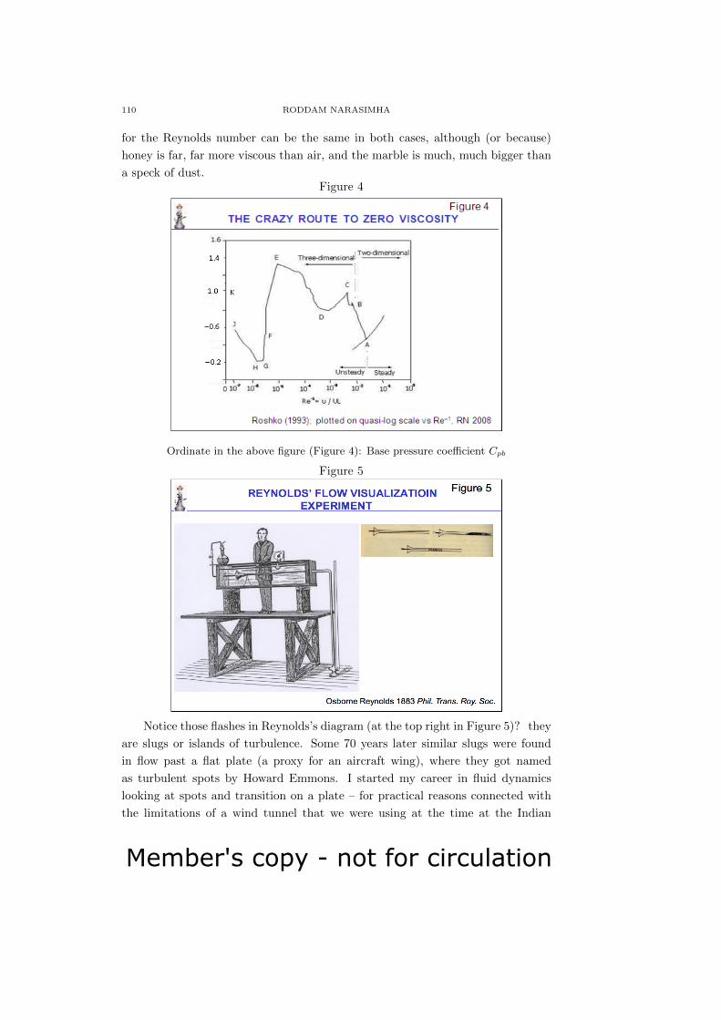
Member's copy - not for circulation
110 RODDAM NARASIMHA
for the Reynolds number can be the same in both cases, although (or because)
honey is far, far more viscous than air, and the marble is much, much bigger than
a speck of dust.Figure 4
Ordinate in the above figure (Figure 4): Base pressure coefficient Cpb
Figure 5
Notice those flashes in Reynolds’s diagram (at the top right in Figure 5)? they
are slugs or islands of turbulence. Some 70 years later similar slugs were found
in flow past a flat plate (a proxy for an aircraft wing), where they got named
as turbulent spots by Howard Emmons. I started my career in fluid dynamics
looking at spots and transition on a plate – for practical reasons connected with
the limitations of a wind tunnel that we were using at the time at the Indian

Member's copy - not for circulation
FLUID MATHEMATICS 111
Institute of Science. (Mundane and arcane again!) I had the great good fortune
of having as my adviser Satish Dhawan, who combined many worlds in himself
beginning with degrees in Mathematics and Physics and in Engineering (not to
mention English literature). I got some results that pleased me (Figure 6), and
in 1956/57 had an unexpected opportunity to tell Kurt Friedrichs about them
when he visited Bangalore. He was the first real mathematician I had ever met.
(I was familiar with his name as co-author, with Courant, of the famous book
Supersonic Flow and Shock Waves, a mathematical treatise that engineers of the
time used to decorate their book-shelves with.) For the first 15 minutes I told
him what I was doing, going through all the different stages of the transition
process: smooth laminar flow near the leading edge, appearance of instability,
breakdown into turbulence at points along an ‘onset’ line in the form of tiny spots
of turbulence, and their eventual growth and merger leading to fully turbulent
flow (Figure 6). Friedrichs seemed fascinated (he had clearly not heard anything
about ‘spots’ in boundary layer transition before), and I was pleased. For the next
half-hour however he kept shooting ideas at me about why I might be seeing what I
saw, and I had great difficulty keeping up with his agile mind as he kept firing new
proposals at me, quickly modifying them if I should so much as utter a mild word
of doubt about any of them. So I saw at first-hand how a great mathematician
thinks about fluid flow problems.
Figure 6
We return to the long sequence of transitions seen in the base pressure on the
cylinder, ranging over some six decades in the Reynolds number. Such transitions
are due not only to the non-linearity of the Navier-Stokes equations, but also to
their three-dimensionality. Nonlinearity is writ large over most interesting fluid
dynamics: let us look at some other examples.
One consequence of nonlinearity is non-uniqueness of a certain kind in the
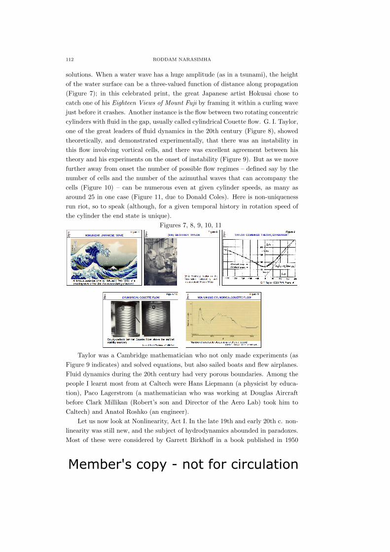
Member's copy - not for circulation
112 RODDAM NARASIMHA
solutions. When a water wave has a huge amplitude (as in a tsunami), the height
of the water surface can be a three-valued function of distance along propagation
(Figure 7); in this celebrated print, the great Japanese artist Hokusai chose to
catch one of his Eighteen Views of Mount Fuji by framing it within a curling wave
just before it crashes. Another instance is the flow between two rotating concentric
cylinders with fluid in the gap, usually called cylindrical Couette flow. G. I. Taylor,
one of the great leaders of fluid dynamics in the 20th century (Figure 8), showed
theoretically, and demonstrated experimentally, that there was an instability in
this flow involving vortical cells, and there was excellent agreement between his
theory and his experiments on the onset of instability (Figure 9). But as we move
further away from onset the number of possible flow regimes – defined say by the
number of cells and the number of the azimuthal waves that can accompany the
cells (Figure 10) – can be numerous even at given cylinder speeds, as many as
around 25 in one case (Figure 11, due to Donald Coles). Here is non-uniqueness
run riot, so to speak (although, for a given temporal history in rotation speed of
the cylinder the end state is unique).
Figures 7, 8, 9, 10, 11
Taylor was a Cambridge mathematician who not only made experiments (as
Figure 9 indicates) and solved equations, but also sailed boats and flew airplanes.
Fluid dynamics during the 20th century had very porous boundaries. Among the
people I learnt most from at Caltech were Hans Liepmann (a physicist by educa-
tion), Paco Lagerstrom (a mathematician who was working at Douglas Aircraft
before Clark Millikan (Robert’s son and Director of the Aero Lab) took him to
Caltech) and Anatol Roshko (an engineer).
Let us now look at Nonlinearity, Act I. In the late 19th and early 20th c. non-
linearity was still new, and the subject of hydrodynamics abounded in paradoxes.
Most of these were considered by Garrett Birkhoff in a book published in 1950

Member's copy - not for circulation
FLUID MATHEMATICS 113
(Figure 12; his definition of paradox was that it represented an apparent inconsis-
tency between fact and plausible argument). The subtitle of Birkhoffs book tells
us about the mathematical mystery surrounding fluid flows. The frontispiece to
the book (Figure 13) showed a supersonic flow with shock waves, which Birkhoff
considered at the time an instance of common sense contradicted, because it in-
volved so many virtually discontinuous solutions. But today such pictures are
daily fare for space scientists and missile engineers.
The grand-father of all these paradoxes is the one due to d’Alembert, who in
1768 proved (assuming zero viscosity, among other things) that the drag of a finite
body in steady motion was zero. (His ‘proof’ implied that at ν = 0 the flow should
plot at +1 (point K) on the ordinate in Figure 4 - i. e., steeply up the scale in the
diagram.) Of course we know that drag is not zero in real life, hence the paradox.
D’Alembert knew this too, but he left it ‘to future Geometers for elucidation’ (he
must have been a Greek at heart, for mathematics meant geometry in classical
Greece). The prize that was promised by the Berlin Academy on the subject was
not awarded, because they had (wisely) demanded experimental evidence in sup-
port of the analytical ‘proof’. (So we can wonder whether mathematics is here
seeking to provide the ‘proof’ for the experiment, or experiment to provide the
‘proof’ for the mathematics, but at any rate the Clay Prize of today continues an
old fluid-dynamical tradition of problem-solving awards.) This ‘d’Alembert para-
dox’ was one of the many instances that led to the Hydraulics-Hydrodynamics
wars, fought because it was said that the former (created and exploited by engi-
neers) observed things which could not be explained, whereas the latter (pursued
by ‘geometers’, i.e. mathematicians) explained things that could not be observed.
(The word hydrodynamics was invented by Daniel Bernoulli, who confused the
issue by using it as the title of a book he wrote on hydraulics.)
Figures 12, 13
The paradoxes slowly got resolved in the first half of the 20th century, largely
through the change in thinking wrought by one man, the German engineer Lud-
wig Prandtl (Figure 14), who successfully bridged the epistemological gulf with the
mathematicians. (The portrait of Prandtl is a copy of one painted by his student V.

Member's copy - not for circulation
114 RODDAM NARASIMHA
M. Ghatage, who got his PhD on an atmospheric problem, but went on to become
India’s first professor in aeronautics – at IISc – and India’s first aircraft designer
as well, retiring as Managing Director at Hindustan Aircraft (now Aeronautics),
Bangalore.) Prandtl was working in industry when the famous mathematician
Felix Klein persuaded him to move to Gottingen as a professor of applied me-
chanics – surely one of the most inspired appointments ever made in the history
of fluid dynamics. In 1903 Prandtl read a paper at the 3rd International Con-
gress of Mathematics at Heidelberg (porous borders again!), and introduced a new
mathematical method of handling nonlinearity – chiefly in laminar flow problems
– by creating the concept of boundary or singular layers – small regions within
which the nonlinearity and viscous effects were concentrated and could by clever
approximations be managed. This approach yielded interesting asymptotic solu-
tions in the ν → 0 limit. We could in fact truthfully say that this particular page
in Prandtl’s paper of 1904 (Figure 15) gave birth to modern fluid dynamics, and
resolved d’Alembert’s paradox.
Prandtl’s method was later codified into singular perturbation theory by
(among others) the same Friedrichs I had met in Bangalore, and in particular
by Paco Lagerstrom, developing what came to be called the method of matched
asymptotic expansions (MAX for short). Many paradoxes dissolved under the ap-
propriate MAX attack. One of the most dramatic uses of MAX (not so called at
the time) was the demonstration of the instability of Prandtl’s boundary layer by
his student Tollmien (1929). It took more than a decade before this instability was
observed experimentally, in contrast with Taylor’s almost instantaneously success-
ful comparison of theory and experiment (shown in Figure 9). This led to some
controversies between the two leaders in 1938, although each of them respected
the other greatly. (G I Taylor proposed Prandtl for the Nobel Prize, even calling
Prandtl his ‘chief’; but next year their two countries were at war with each other,
and the Nobel Prize was forgotten.)Figures 14, 15
The whole area of hydrodynamic instability has been the joint enterprise of

Member's copy - not for circulation
FLUID MATHEMATICS 115
physicists (Sommerfeld, Rayleigh, Heisenberg), mathematicians (Orr, Taylor), en-
gineers (Reynolds, Prandtl, Tollmien, Schubauer) (porous borders again). The
subject is important because many flows crumple into some form of instability or
other at the slightest excuse, making them prone to turbulence.
But even MAX cannot handle what (Sir) Horace Lamb, in his ever-enduring
treatise called Hydrodynamics that summarised pre-modern fluid dynamics, called
‘the chief outstanding difficulty of our subject’, namely turbulence – the apparently
random/irregular/chaotic/intermittent vortical motion that is the natural state of
most air and water flows we observe.Figure 16
That brings us back to turbulence and pipe flow, and how our Indus valley
ancestors who pushed water through their cities more than 4000 years ago clearly
knew things that as mathematicians we still cannot explain. In nearly 135 years
since Reynolds made his famous experiments we have learnt a lot about turbulent
flows. For example, engineers can predict not only the pressure loss in a pipe,
but also the drag of an aircraft or the trajectory of a satellite launch vehicle with
considerable confidence – but not starting from first principles, and not without
appealing to experimental data at some stage or the other. All we can say is that
a lot of clever analysis has gone into reducing the amount of data that needs to be
acquired, but the problem of getting it all from first principles remains unsolved.
So the chief outstanding difficulty of Horace Lamb remains just that to this day.
Before I close however I want to show you some flow pictures, for fluid dy-
namics is nothing if it is not photogenic. (As John Ruskin said, nature produces
its most beautiful inorganic forms in water flow.) Prandtl’s path-breaking paper
at the International Congress of Mathematics contained numerous flow pictures at
the end. The pictures I now show (following his example) were all taken in Ban-
galore. The first (Figure 17 on the next page) shows how flows can be generated
in the laboratory to look like clouds in the atmosphere. As the fake clouds are

Member's copy - not for circulation
116 RODDAM NARASIMHA
generated in a water tank the great resemblance we see with real clouds shows the
extraordinary power of the idea of dynamical similarity: isn’t it amazing that a
cloud made by the motion of moist air over a height of several kilometers in the
atmosphere can be mimicked in a plume generated in a little water tank that is a
cube of about 1 m side if only we put the right amount of heat at the right place
and right time into the laboratory plume?
Figure 17
Figure 18
(Left: Raw image. Right: Wavelet transform,
revealing a fluted vortex ring at a particular
value of the wavelet length scale.)
One of the intriguing things about turbulence is that a flow we consider random
or chaotic may actually possess concealed order. This was convincingly demon-
strated by Brown and Roshko in the 1970s. Figure 18 shows an instance where
the order concealed in a plume can be revealed by its wavelet transform.

Member's copy - not for circulation
FLUID MATHEMATICS 117
I have already mentioned the phenomenon of transitions from laminar to tur-
bulent flow but reverse transitions from turbulent to laminar flow are also possible.
Here is one instance (Figure 19) where that happens in a rather dramatic way, by
the simple expedient of bending the tube carrying turbulent flow (red, diffused
in the picture) into a coil (leading to the green, non-diffusing filament of laminar
flow at the third coil). This phenomenon can be seen as the anti of that studied
in Reynolds’s experiment.Figure 19
So the big question is: What is the mathematics that can handle all these
phenomena? In a well known lecture given at the Courant Institute, Eugene
Wigner once spoke eloquently about the unreasonable effectiveness of mathemat-
ics. But for all those who have been collectively wrestling with turbulence for more
than a century, what seems striking is the singular ineffectiveness of mathematics
in handling the highly nonlinear Navier-Stokes equations (hence the Clay prize).
Fluid flow has always been a complex problem. The Yoga-Vasis. tha (6th / 7th c.?)
drew parallels between the richly diverse ways in which water flows and the human
mind works. Galileo said he knew more about the motion of heavenly bodies than
about the flow of water under his very eyes. Echoing this thought more than three
centuries later, Feynman pointed out that we can follow the evolution of a star till
convection starts, but thereafter we can no longer deduce what should happen. ‘A
few million years later the star explodes, but we cannot figure out the reason’ –
thus his conclusion that turbulence was the greatest unsolved problem in classical
physics. After writing down his equations in 1757 (basically Navier-Stokes without
the viscous terms), Euler declared that the difficulty with fluid flows was not the
sufficiency of the principles of mechanics but the fact that ‘analysis abandons us
here’. But the man who saw most clearly the fundamentally mathematical nature
of the problem was von Neumann. He thought that if the turbulence problem were
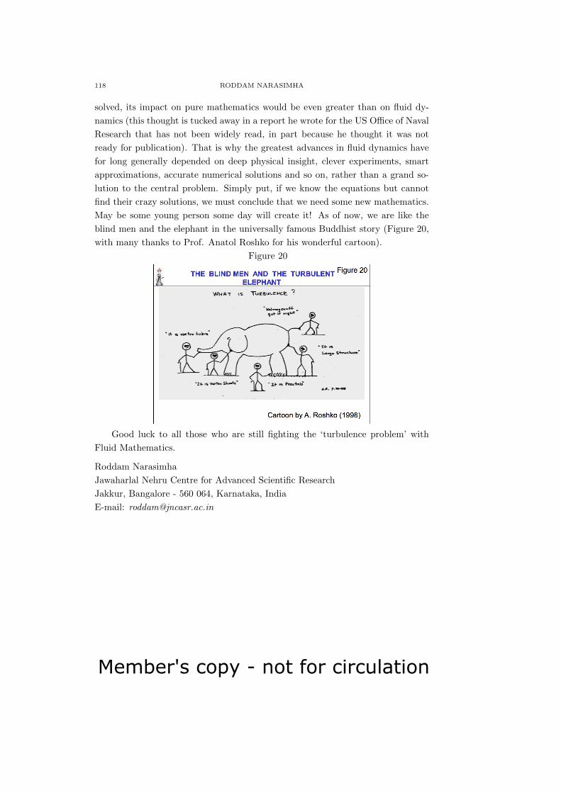
Member's copy - not for circulation
118 RODDAM NARASIMHA
solved, its impact on pure mathematics would be even greater than on fluid dy-
namics (this thought is tucked away in a report he wrote for the US Office of Naval
Research that has not been widely read, in part because he thought it was not
ready for publication). That is why the greatest advances in fluid dynamics have
for long generally depended on deep physical insight, clever experiments, smart
approximations, accurate numerical solutions and so on, rather than a grand so-
lution to the central problem. Simply put, if we know the equations but cannot
find their crazy solutions, we must conclude that we need some new mathematics.
May be some young person some day will create it! As of now, we are like the
blind men and the elephant in the universally famous Buddhist story (Figure 20,
with many thanks to Prof. Anatol Roshko for his wonderful cartoon).
Figure 20
Good luck to all those who are still fighting the ‘turbulence problem’ with
Fluid Mathematics.
Roddam Narasimha
Jawaharlal Nehru Centre for Advanced Scientific Research
Jakkur, Bangalore - 560 064, Karnataka, India
E-mail: [email protected]

Member's copy - not for circulation
The Mathematics Student ISSN: 0025-5742
Vol. 87, Nos. 1-2, January-June (2018), 119-127
DEFINING AND COMPUTING CUBIC SPLINES
T. AUGUSTA MESQUITA
(Received : 25 - 04 - 2017)
Abstract. In this note we address the students’ usual misperception of the
cubic spline definition and construction within an undergraduate numerical
course in order to present an alternative initial approach. We describe suc-
cinctly the standard path from the interpolating polynomial towards a smooth
piecewise interpolation model and we focus on a simpler, though unstable,
cubic spline structure. This less common choice aims to promote a more
comprehensible dialogue between the notion of cubic spline functions and the
numerical (in)adequacy of different methods for computing such functions.
1. IntroductionThe construction of real valued functions working as models of empirical data
is a classical topic in numerical analysis courses. In such first approach to data
fitting, we typically face the solution given by polynomial interpolation if we are
searching for a model that totally replicates the numerical observations. If we
assume differently by aiming to find a function not reproducing the entire set of
data but reasonably adjusting into it, the solution is usually provided by the least-
square method. Persevering on the interpolation option, we commonly point to
the direction of a piecewise polynomial function, more precisely, we address the
construction of the spline functions of order m. Their definition is motivated by
the rigidity of polynomials phenomenon and can be accompanied with enlightening
sketches for the first, second and third order (m = 1, m = 2 and m = 3). Nonethe-
less, the prompt construction of such functions - provided by several branches -
constitutes many times a great challenge to students, in particular for the cubic
case m = 3. The cubic spline is a versatile and smooth function that appears often
in a diverse number of engineering applications, though its derivation starts usu-
ally with two integrations. This initial part transmits an extra level of difficulty
from which emerges the questions: why do we need to follow that algorithm? Are
there other possibilities? In order to answer these questions and simultaneously
provide students with means to exercise their numerical sensibility while working
with unstable solutions, we explore here an alternative approach to the presen-
tation of the spline functions in an undergraduate numerical analysis classroom.
2010 Mathematics Subject Classification: 97D70; 97N50; 97D80.
Key words and phrases : Curve fitting; polynomial rigidity; piecewise interpolation; numeri-
cal stability; cubic splines; Octave 4.0.0.
c© Indian Mathematical Society, 2018 .
119

Member's copy - not for circulation
120 T. AUGUSTA MESQUITA
2. From the interpolating polynomial to the cubic spline
The polynomial interpolation is a classical method which aim is to create a
continuous function acting as a precise model of a given set of numerical data.
Although easy to construct and unique when the given numerical information has
the form(xi, yi), i = 0, . . . , n, a = x0 < x1 < · · · < xn−1 < xn = b, (2.1)
it becomes easily an unsuitable solution, such as when the dependent variable y
has sudden changes. A data set (2.1) with n + 1 points allows the definition of a
polynomial p(x) of degree n (or lower) such that p (xi) = yi, i = 0, . . . , n. Even
knowing that theoretically the increase of data points, and thus the increase of the
degree of the correspondent polynomial, shall give place to a better description
of the underlying function y(x), the implementation shows us that the provided
model has undesirable fluctuations. In fact, a larger number of interpolating points
implies a higher degree of the interpolating polynomial which augments the abso-
lute values of the coefficients of its derivatives, indicating bigger oscillations. As
an example, let us take the numerical data of Table 1, where the variable y equals
the mean variation of the annual temperature in different latitudes (x), when we
x 65 55 45 35 25 15
y -3.1 -3.22 -3.3 -3.32 -3.17 -3.07
x 5 -5 -15 -25 -35 -45 -55
y -3.02 -3.02 -3.12 -3.2 -3.35 -3.37 -3.25
Table 1. Data from Philosophical Magazine 41, 237 (1896) re-
ferred in [1, p. 76]
Figure 1. An example of the rigidity of an higher-order interpo-
latory polynomial.
consider a fixed concentration of carbonic acid [1]. The unique polynomial (of
degree 12) that interpolates the entire table is depicted in Figure 1.
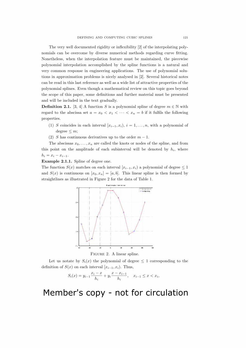
Member's copy - not for circulation
DEFINING AND COMPUTING CUBIC SPLINES 121
The very well documented rigidity or inflexibility [2] of the interpolating poly-
nomials can be overcome by diverse numerical methods regarding curve fitting.
Nonetheless, when the interpolation feature must be maintained, the piecewise
polynomial interpolation accomplished by the spline functions is a natural and
very common response in engineering applications. The use of polynomial solu-
tions in approximation problems is nicely analysed in [2]. Several historical notes
can be read in this last reference as well as a wide list of attractive properties of the
polynomial splines. Even though a mathematical review on this topic goes beyond
the scope of this paper, some definitions and further material must be presented
and will be included in the text gradually.
Definition 2.1. [3, 4] A function S is a polynomial spline of degree m ∈ N with
regard to the abscissa set a = x0 < x1 < · · · < xn = b if it fulfils the following
properties.
(1) S coincides in each interval [xi−1, xi), i = 1, . . . , n, with a polynomial of
degree ≤ m;
(2) S has continuous derivatives up to the order m− 1.
The abscissas x0, . . . , xn are called the knots or nodes of the spline, and from
this point on the amplitude of each subinterval will be denoted by hi, where
hi = xi − xi−1.Example 2.1.1. Spline of degree one.
The function S(x) matches on each interval [xi−1, xi) a polynomial of degree ≤ 1
and S(x) is continuous on [x0, xn] = [a, b]. This linear spline is then formed by
straightlines as illustrated in Figure 2 for the data of Table 1.
Figure 2. A linear spline.
Let us notate by Si(x) the polynomial of degree ≤ 1 corresponding to the
definition of S(x) on each interval [xi−1, xi). Thus,
Si(x) = yi−1xi − xhi
+ yix− xi−1
hi, xi−1 ≤ x < xi,

Member's copy - not for circulation
122 T. AUGUSTA MESQUITA
where yi = f(xi). It is obvious that S(x) is continuous on [a, b].
Example 2.1.2. Spline of second degree.
If m = 2, then S(x) coincides with a polynomial of degree ≤ 2 on each subinterval
[xi−1, xi) and S(x) is a continuous function with derivative function S′(x) also
continuous on [a, b].
3. Cubic Splines
When we choose m = 3 in Definition 2.1, we get a function S(x) that on each
subinterval [xi−1, xi) coincides with a polynomial of degree ≤ 3 and has derivative
functions of first and second order, S′(x) and S′′(x), continuous on [a, b].
For a given set of numerical data, the construction of an interpolating cubic
spline usually starts in the numerical methods textbooks by considering the second
derivative of each branch of S(x) (e.g. [5, 3, 4]). Let us denote the i-th branch of
S(x) by Si(x), with i = 1, . . . , n. It is then easy to note that the second derivative
of each branch must be a polynomial of degree ≤ 1 defined on an interval [xi−1, xi).
The construction of S(x) is therefore redirected to the computation of the values
of S′′(x) in the knots x0, x1, . . . , xn, notated as Mi, i = 1, . . . , n. In other words,
when we take the linear interpolation of the two points (xi−1,Mi−1) and (xi,Mi),
where Mi = S′′i (xi) = S′′(xi), as follows
S′′i (x) = Mi−1xi − xhi
+Mix− xi−1
hi, (3.1)
it becomes immediately assured the continuity of the second derivative. Then, we
have to integrate twice both sides of the equation (3.1) to obtain the expression
of Si(x), yielding:
Si(x) = Mi−1(xi − x)
3
6hi+Mi
(x− xi−1)3
6hi+ αi
xi − xhi
+ βix− xi−1
hi, αi, βi ∈ R.
Taking into account the interpolating conditions Si(xi−1) = yi−1, Si(xi) = yi, i =
0, . . . , n, the constants of integration αi, βi are easily calculated and we finally get:
Si(x) = Mi−1(xi − x)
3
6hi+Mi
(x− xi−1)3
6hi(3.2)
+
(yi−1 −Mi−1
(hi)2
6
)xi − xhi
+
(yi −Mi
(hi)2
6
)x− xi−1
hi.
The full numerical definition of S(x) is now reduced to the computation of the
constants M0,M1, . . . ,Mn. Differentiating (3.2) we get S′i(x) and the continuity of
S′(x) at the interior knots x1, . . . , xn−1 justify the next list of n−1 linear equations
(i = 1, 2, . . . , n− 1).
hi6Mi−1 +
hi + hi+1
3Mi +
hi+1
6Mi+1 =
yi+1 − yihi+1
− yi − yi−1hi
Recalling that we have n + 1 unknowns (M0, . . . ,Mn), we get two degrees of
freedom requiring additional input. Depending on the context of application, we
encounter more frequently the following designations or definitions [6, 7].
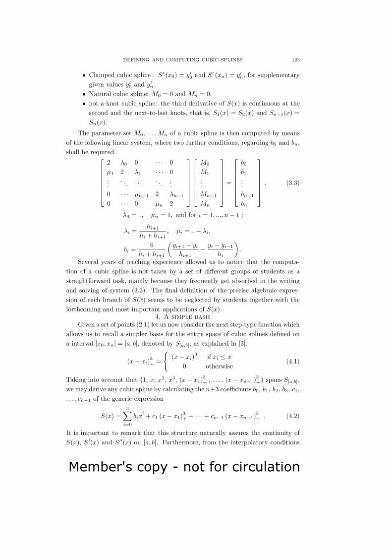
Member's copy - not for circulation
DEFINING AND COMPUTING CUBIC SPLINES 123
• Clamped cubic spline : S′ (x0) = y′0 and S′ (xn) = y′n, for supplementary
given values y′0 and y′n.
• Natural cubic spline: M0 = 0 and Mn = 0.
• not-a-knot cubic spline: the third derivative of S(x) is continuous at the
second and the next-to-last knots, that is, S1(x) = S2(x) and Sn−1(x) =
Sn(x).
The parameter set M0, . . . ,Mn of a cubic spline is then computed by means
of the following linear system, where two further conditions, regarding b0 and bn,
shall be required.
2 λ0 0 · · · 0
µ1 2 λ1 · · · 0...
. . .. . .
. . ....
0 · · · µn−1 2 λn−1
0 · · · 0 µn 2
M0
M1
...
Mn−1
Mn
=
b0
b1...
bn−1
bn
, (3.3)
λ0 = 1, µn = 1, and for i = 1, ..., n− 1 :
λi =hi+1
hi + hi+1, µi = 1− λi,
bi =6
hi + hi+1
(yi+1 − yihi+1
− yi − yi−1hi
).
Several years of teaching experience allowed us to notice that the computa-
tion of a cubic spline is not taken by a set of different groups of students as a
straightforward task, mainly because they frequently get absorbed in the writing
and solving of system (3.3). The final definition of the precise algebraic expres-
sion of each branch of S(x) seems to be neglected by students together with the
forthcoming and most important applications of S(x).4. A simple basis
Given a set of points (2.1) let us now consider the next step-type function which
allows us to recall a simpler basis for the entire space of cubic splines defined on
a interval [x0, xn] = [a, b], denoted by S[a,b], as explained in [3].
(x− xi)3+ =
(x− xi)3 if xi ≤ x
0 otherwise(4.1)
Taking into account that 1, x, x2, x3, (x− x1)3+ , . . . , (x− xn−1)
3+ spans S[a,b],
we may derive any cubic spline by calculating the n+3 coefficients b0, b1, b2, b3, c1,
. . . , cn−1 of the generic expression
S(x) =3∑
i=0
bixi + c1 (x− x1)
3+ + · · ·+ cn−1 (x− xn−1)
3+ . (4.2)
It is important to remark that this structure naturally assures the continuity of
S(x), S′(x) and S′′(x) on [a, b]. Furthermore, from the interpolatory conditions

Member's copy - not for circulation
124 T. AUGUSTA MESQUITA
S (xi) = yi, i = 0, . . . , n, we obtain n + 1 linear equations for the unknowns
b0, b1, b2, b3, c1, . . . , cn−1. The additional two conditions again reflect an option as
before recalled through the clamped or natural cubic spline, among other possible
choices. For example, the coefficients of a natural cubic spline can be obtained by
means of the following linear system.
1 x0 x20 x301 x1 x21 x311 x2 x22 x32 (x2 − x1)
3
1 x3 x23 x33 (x3 − x1)3
......
......
1 xn x2n x3n (xn − x1)3 · · · (xn − xn−1)
3
0 0 2 6x0 0 · · · 0
0 0 2 6xn 6 (xn − x1) · · · 6 (xn − xn−1)
b0
b1
b2
b3
c1
c2...
cn−1
=
y0
y1
y2
y3...
yn
0
0
(4.3)
Replacing in (4.2) the complete polynomial of degree three∑3
i=0 bixi by
y0+d1 (x− x0)3+, we can define the following particular model.
S(x) = y0 + d1 (x− x0)3+ + · · ·+ dn (x− xn−1)
3+ (4.4)
We have lost the generality of function (4.2) in the sense that we cannot derive
all functions of S[a,b] through expression (4.4), nevertheless the interpolatory con-
ditions and the continuity of S(x) allow an iterative computation of d1, . . . , dn,
and a straightforward verification clarifies that S′(x) and S′′(x) are continuous.
In other words, function (4.4) allows us to quickly confirm all items of Definition
2.1 with m = 3 and furnishes a simple instrument for constructing analytically a
cubic spline function which interpolates a small set of points.
The next section proposes a small classroom project focused on the computation
of (4.4), when given a numerical table, with potential to be resized if other related
numerical discussions are to be included.
5. A short assignment
The particular structure of a cubic spline given by equation (4.4) was proposed
in a self contained worksheet to a classroom of a numerical methods short course
attended by eight Civil Engineering students to be solved with the help of the
software Octave [8], in its 4.0.0 version. We remark that the definition of the
function (x− xi)3+ demands a step function. The Octave’s symbolic package has a
built-in function Heaviside [9]. Let us recall that the Heaviside function is defined
as
Heaviside(x) =
1 , x > 0
0.5 , x = 0
0 , x < 0
.
From our standpoint we should use the syntax heaviside(x,zero_value) with
zero_value=1, so that the value at x = 0 is changed to 1. Since the symbolic
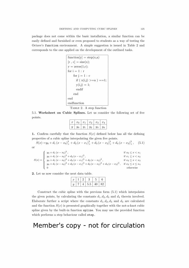
Member's copy - not for circulation
DEFINING AND COMPUTING CUBIC SPLINES 125
package does not come within the basic installation, a similar function can be
easily defined and furnished or even proposed to students as a way of testing the
Octave’s function environment. A simple suggestion is issued in Table 2 and
corresponds to the one applied on the development of the outlined tasks.
function[y] = step(x,a)
[r , c] = size(x);
y = zeros(1,c);
for i = 1 : r
for j = 1 : c
if ( x(i,j) >=a ) ==1;
y(i,j) = 1;
endif
end
end
endfunction
Table 2. A step function
5.1. Worksheet on Cubic Splines. Let us consider the following set of five
points.
x x0 x1 x2 x3 x4
y y0 y1 y2 y3 y4
1. Confirm carefully that the function S(x) defined below has all the defining
properties of a cubic spline interpolating the given five points.
S(x) =y0 + d1 (x− x0)3+ + d2 (x− x1)
3+ + d3 (x− x2)
3+ + d4 (x− x3)
3+ , (5.1)
or
S(x) =
y0 + d1 (x− x0)3 , if x0 ≤ x < x1
y0 + d1 (x− x0)3 + d2 (x− x1)3 , if x1 ≤ x < x2
y0 + d1 (x− x0)3 + d2 (x− x1)3 + d3 (x− x2)3 , if x2 ≤ x < x3
y0 + d1 (x− x0)3 + d2 (x− x1)3 + d3 (x− x2)3 + d4 (x− x3)3 , if x3 ≤ x ≤ x4
0 otherwise
2. Let us now consider the next data table.
x 1 2 3 5 6
y 7 4 5.5 40 82
Construct the cubic spline with the previous form (5.1) which interpolates
the given points, by calculating the constants d1, d2, d3 and d4 therein involved.
Elaborate further a script where the constants d1, d2, d3 and d4 are calculated
and the function S(x) is presented graphically together with the not-a-knot cubic
spline given by the built-in function spline. You may use the provided function
which performs a step behaviour called step.

Member's copy - not for circulation
126 T. AUGUSTA MESQUITA
5.2. Discussion and Final Remarks. A possible layout for a straightforward
resolution of the proposed second task of subsection 5.1 can be read in Table 3.
clear all
x = [1 2 3 5 6];
y = [7 4 5.5 40 82];
d1 = (y(2)-y(1))(x(2)-x(1)) 3;
d2 = (y(3)-y(1)-d1?(x(3)-x(1)) 3) (x(3)-x(2)) 3;
d3 = (y(4)-y(1)-d1(x(4)-x(1)) 3-d2?(x(4)-x(2)) ˆ 3)(x(4)-x(3)) 3;
d4 = (y(5)-y(1)-d1?(x(5)-x(1)) 3-d2 ?(x(5)-x(2)) 3-d3 ?(x(5)-x(3)) 3)(x(5)-x(4)) ˆ 3;
xx = linspace(x(1),x(end));
yy = y(1)+d1 .?(xx-x(1)). 3.? step(xx,x(1))+d2.?(xx-x(2)) . 3 .?step(xx,x(2))
+ d3.?(xx-x(3)). 3 .? step(xx,x(3))+d4.?(xx-x(4)). 3 .? step(xx,x(4));
zz = spline (x, y, xx);
plot(xx,yy, x,y,’o’, xx, zz, ’- -’)
grid on
Table 3. A possible script for item 2. of the proposed worksheet.
Figure 3. The not-a-knot cubic spline versus a trivial cubic
spline of Table of item 2. of the proposed worksheet
The software Octave [8], as any other algebra manipulator, has built-in func-
tions for many interpolation methods. In particular, the function spline imple-
ments by default a not-a-knot cubic spline based on the first described method of
derivation whose main expression is given by (3.2). By means of a few instructions,
a student can visualize the graph of a smooth piecewise polynomial fit.
The graphical comparison between both cubic spline functions is shown in
Fig.3 and is the output of the latest steps of the script of Table 3. In other words,
the very simple cubic structure chosen does not provide a suitable model, show-
ing instability, whereas the more theoretically demanding option avoids unstable
operations.
Other concepts strictly related to linear algebra can be explored, as for
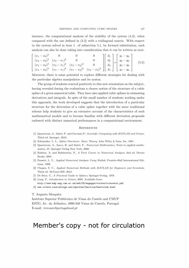
Member's copy - not for circulation
DEFINING AND COMPUTING CUBIC SPLINES 127
instance, the computational analysis of the stability of the system (4.3), when
compared with the one defined in (3.3) with a tridiagonal matrix. With respect
to the system solved in item 1. of subsection 5.1, by forward substitution, such
analysis can also be done taking into consideration that it can be written as next.(x1 − x0)3 0 0 0
(x2 − x0)3 (x2 − x1)3 0 0
(x3 − x0)3 (x3 − x1)3 (x3 − x2)3 0
(x4 − x0)3 (x4 − x1)3 (x4 − x2)3 (x4 − x3)3
d1
d2
d3
d4
=y1 − y0y2 − y0y3 − y0y4 − y0
(5.2)
Moreover, there is some potential to explore different strategies for dealing with
the particular algebra manipulator and its syntax.
The group of students reacted positively to this new orientation on the subject,
having revealed during the evaluations a clearer notion of the structure of a cubic
spline of a given numerical table. They have also applied cubic splines in estimating
derivatives and integrals. In spite of the small number of students working under
this approach, the work developed suggests that the introduction of a particular
structure for the derivation of a cubic spline together with the more traditional
scheme help students to give an extensive account of the characteristics of such
mathematical models and to become familiar with different derivation proposals
endowed with distinct numerical performances in a computational environment.
References
[1] Quarteroni, A., Saleri, F. and Gervasio P., Scientific Computing with MATLAB and Octave,
Third ed. Springer, 2010.
[2] Schumaker, L. L., Spline Functions: Basic Theory, John Wiley & Sons, Inc, 1981.
[3] Quarteroni, A., Sacco, R. and Saleri, F., Numerical Mathematics, Texts in applied mathe-
matics, 37, Springer-Verlag New York, 2000.
[4] Ralston, A. and Rabinowitz, P., A First Course in Numerical Analysis, 2nd ed. Dovers
Books, 2001.
[5] Fausett, L. V., Applied Numerical Analysis Using Matlab, Prentice-Hall International Edi-
tions, 1999.
[6] Chapra, S. C., Applied Numerical Methods with MATLAB for Engineers and Scientists,
Third ed. McGraw-Hill, 2012.
[7] De Boor, C., A Practical Guide to Splines, Springer-Verlag, 1978.
[8] Long, P., Introduction to Octave, 2005. Available from:
http://www-mdp.eng.cam.ac.uk/web/CD/engapps/octave/octavetut.pdf.
[9] www.octave.sourceforge.net/specfun/function/heaviside.html
T. Augusta Mesquita
Instituto Superior Politecnico de Viana do Castelo and CMUP
ESTG, Av. do Atlantico, 4900-348 Viana do Castelo, Portugal
E-mail: [email protected]

Member's copy - not for circulation
128
Member's copy - not for circulation
The Mathematics Student ISSN: 0025-5742
Vol. 87, Nos. 1-2, January-June (2018), 129-132
A DIOPHANTINE PROBLEM ON BIQUADRATESREVISITED
AJAI CHOUDHRY
(Received : 01 - 08 - 2017; Revised : 05-02-2018)
Abstract. In this paper we obtain a new parametric solution of the problem
of finding two triads of biquadrates with equal sums and equal products.
This paper is a sequel to my earlier paper [2] concerning the problem of finding
two triads of biquadrates with equal sums and equal products. The problem is
mentioned in [6, p. 214], and thirty numerical solutions, obtained by computer
search, were presented in [2]. Subsequently, a method of obtaining infinitely many
numerical examples of such triads was given in [4, pp. 346–47]. In this paper we
obtain a parametric solution of the problem. The triads of biquadrates are given
by the following theorem.
Theorem: A parametric solution of the simultaneous diophantine equations,
X41 +X4
2 +X43 = Y 4
1 + Y 42 + Y 4
3 , X1X2X3 = Y1Y2Y3, (1)
is given by
X1 = (2a− b)(a2 − ab+ b2)(5a3 − 7a2b+ 4ab2 − b3),
X2 = (a3 − 3a2b+ 2ab2 − b3)(5a3 − 8a2b+ 5ab2 − b3),
X3 = (a3 − ab2 + b3)(3a2 − 3ab+ b2)b,
Y1 = (2a− b)(a2 − ab+ b2)(5a3 − 8a2b+ 5ab2 − b3),
Y2 = (a3 − 3a2b+ 2ab2 − b3)(3a2 − 3ab+ b2)b,
Y3 = (a3 − ab2 + b3)(5a3 − 7a2b+ 4ab2 − b3),
(2)
where a and b are arbitrary parameters.
Proof: To obtain a solution of the simultaneous equations (1), we will first obtain
a parametric solution of the simultaneous diophantine equations,
x21 + x22 + x23 = y21 + y22 + y23 , (3)
x1x2x3 = y1y2y3, (4)
and then choose the parameters such that xi, yi, i = 1, 2, 3, become perfect
squares. The complete solution of Eqs. (3) and (4) is already known ([1], [7]).
2010 Mathematics Subject Classification: 11D25
Key words and phrases : Biquadrates; Equal sums and equal products of integers.
c© Indian Mathematical Society, 2018 .
129

Member's copy - not for circulation
130 AJAI CHOUDHRY
Since we need to ensure that xi, yi, i = 1, 2, 3 eventually become perfect squares,
instead of using the solutions given in ([1], [7]), we will solve Eqs. (3) and (4)
directly by writing,
x1 = (tu+ 1)p2, x2 = (u+ 1)q2, x3 = r2,
y1 = (u+ 1)p2, y2 = q2, y3 = (tu+ 1)r2,(5)
where p, q, r, t and u are arbitrary nonzero parameters.
With the values of xi, yi, i = 1, 2, 3 given by (5), Eq. (4) is identically
satisfied while Eq. (3) reduces to a linear equation in u which is readily solved,
and we thus obtain a parametric solution of the simultaneous equations (3) and
(4). Since both these equations are homogeneous in the variables xi, yi, we obtain
the following solution of Eqs. (3) and (4) after appropriate scaling:
x1 = (p4 − r4)t2 − 2(p4 − q4)t+ p4 − q4p2k,
x2 = (p4 − r4)t2 − 2(p4 − r4)t+ p4 − q4q2k,
x3 = (p4 − r4)t2 − (p4 − q4)r2k,
y1 = (p4 − r4)t2 − 2(p4 − r4)t+ p4 − q4p2k,
y2 = (p4 − r4)t2 − (p4 − q4)q2k,
y3 = (p4 − r4)t2 − 2(p4 − q4)t+ p4 − q4r2k,
(6)
where p, q, r, t and k are arbitrary parameters.
To ensure that xi, yi, i = 1, 2, 3, are all perfect squares, we note that since
the ratios y1/x2, y2/x3 and y3/x1 are perfect squares, it suffices to ensure that
xi, i = 1, 2, 3, are all perfect squares. We will first make the products x1x3 and
x2x3 simultaneously perfect squares by choice of the parameters p, q, r and then
choose k suitably such that x1, x2 and x3 become perfect squares simultaneously.
Now x1x3 and x2x3 may be considered as two quartic polynomials in t with
coefficients in terms of the parameters p, q, r, and we need to choose a suitable
value of t such that both of these quartic polynomials become perfect squares.
The problem of making two quartic polynomials perfect squares simultaneously is
a very difficult diophantine problem and there is no general method of finding a
solution. Here we will solve the problem by finding different values of t that make
each quartic a perfect square separately, and we will equate two such values of t
to obtain a condition that must be satisfied by the parameters p, q, r. Finally, to
obtain a solution, we will find suitable values of p, q, r that satisfy the condition
just obtained.
We note that the coefficient of t4 in both of our quartic polynomials are perfect
squares. Accordingly, we may divide each quartic polynomial by the respective
coefficient of t4 to obtain two monic quartic polynomials both of which must be
made perfect squares simultaneously. Thus, we must find a common value of t
that satisfies both of the following two diophantine equations for suitably chosen

Member's copy - not for circulation
A DIOPHANTINE PROBLEM ON BIQUADRATES REVISITED 131
values of p, q and r:
ξ21 = t4 − 2(p4 − q4)t3/(p4 − r4) + 2(p4 − q4)2t/(p4 − r4)2
− (p4 − q4)2/(p4 − r4)2, (7)
ξ22 = t4 − 2t3 + 2(p4 − q4)t/(p4 − r4)− (p4 − q4)2/(p4 − r4)2. (8)
A method of obtaining values of t that make a monic quartic polynomial of t a
perfect square has been given by Fermat [5, p. 639]. This method, however, leads
to very cumbersome solutions of (7) and (8). To obtain relatively simpler solutions
of (7) and (8), we will apply a theorem given in [3, Theorem 4.1, p. 789-90] by
which we can use two known solutions of a quartic equation of type (7) to obtain
a new solution.
It is readily verified that two solutions of Eq. (7) are given by
(t, ξ1) =(1, (q4 − r4)/(p4 − r4)
)and
(t, ξ1) =((p2 + q2)/(p2 + r2), 2pq(p2 + q2)(q2 − r2)/(p2 − r2)(p2 + r2)2
),
and on applying the aforementioned theorem, we get the following value of t that
provides a solution of Eq. (7):
(p2 + q2)(p4 + 2p3q − 2p2r2 − 2pq3 − 4pqr2 + q4 + 2q2r2 + 2r4)
(p2 − r2)(p4 + 2p3q − 2p2r2 + 2pq3 + q4 − 2q2r2 − 2r4). (9)
Similarly, two solutions of Eq. (8) are given by
(t, ξ2) =((p4 − q4)/(p4 − r4), −(p4 − q4)(q4 − r4)/(p4 − r4)2
)and (t, ξ2) =
((p2 − q2)/(p2 − r2), 2pr(p2 − q2)(q2 − r2)/(p2 − r2)2(p2 + r2)
),
and using these solutions, we get the following value of t that provides a solution
of Eq. (8):
(p2 + q2)(p4 − 2p3r − 2p2q2 + 4pq2r + 2pr3 + 2q4 + 2q2r2 + r4)
(p2 − r2)(p4 − 2p3r − 2p2q2 − 2pr3 − 2q4 − 2q2r2 + r4). (10)
On equating the two values of t given by (9) and (10), we get the following
condition:
(q + r)(p2 + q2)(q2 + r2)(p2 + pq − pr + q2 − qr + r2)
× (p3 − pq2 + pqr − pr2 + q3 − r3) = 0. (11)
On equating to 0 any of the factors on the left-hand side of Eq. (11), except the
last, we get a trivial result. When, however, we equate to 0 the last factor, we get
a cubic equation in p, q, r which represents a curve of genus 0 in the projective
plane with a singularity at (−1, −1, 1). On drawing an arbitrary straight line
through the singular point and taking its intersection with the cubic curve, we get
a rational point which immediately yields the following solution for p, q, r:
p = 2a3 − 3a2b+ 3ab2 − b3, q = −a3 + 3a2b− 2ab2 + b3, r = a3 − ab2 + b3, (12)
where a and b are arbitrary parameters. With these values of p, q, r, the two
values of t given by (9) and (10) coincide and are given by
Member's copy - not for circulation
132 AJAI CHOUDHRY
−(5a4 − 8a3b+ 8a2b2 − 4ab3 + b4)/a(a− b)(5a2 − 5ab+ 2b2). (13)
On substituting the values of p, q, r given by (12) and the value of t given by (13)
in (6) and choosing k suitably, we obtain a parametric solution of Eqs. (3) and
(4) in which xi, yi, i = 1, 2, 3, are all perfect squares. This immediately gives the
solution (2) of the simultaneous equations (1) stated in the theorem.
As a numerical example, when a = 1, b = −1, we get the two triads of bi-
quadrates 74, 1334, 1534 and 174, 494, 1714 with equal sums and equal prod-
ucts.
Acknowledgment. I wish to thank the Harish-Chandra Research Institute,
Allahabad for providing me with all the necessary facilities that have helped me
to pursue my research work in mathematics.
References
[1] Choudhry, A., On triads of squares with equal sums and equal products, Ganita, 49 (1998),
101–106.
[2] Choudhry, A., Triads of biquadrates with equal sums and equal products, The Math. Student,
70 (2001), 149–152.
[3] Choudhry, A., Quadratic diophantine equations with applications to quartic equations, Rocky
Mountain Journal of Mathematics, 46 (2016), 769–799.
[4] Choudhry, A. and Wroblewski, J., Quartic Diophantine Chains, Acta Arithmetica, 128,
(2007), 339–348.
[5] Dickson, L. E., History of theory of numbers, Vol.2, Chelsea Publishing Company, New York,
1992, reprint.
[6] Guy, R. K., Unsolved problems in number theory, third edition, Springer-Verlag (2004).
[7] Kelly, J. B., Two equal sums of three squares with equal products, Amer. Math. Monthly,
98 (1991), 527–529.
Ajai Choudhry,
13/4 A Clay Square,
Lucknow - 226001, UP, India
E-mail: [email protected]

Member's copy - not for circulation
The Mathematics Student ISSN: 0025-5742
Vol. 87, Nos. 1-2, January-June (2018), 133-144
SOME FACTS ABOUT FIBONACCI NUMBERS,LUCAS NUMBERS AND GOLDEN RATIO
M. NARAYAN MURTY
(Received : 15 - 09 - 2017, Revised : 02 - 01 - 2018)
Abstract. In this article, some facts about Fibonacci numbers, Lucas num-
bers and golden ratio are presented. Fibonacci numbers and Fibonacci curve
occur in nature. Lucas numbers are related to Fibonacci numbers and both
sequences are related. Electrical energy can be produced with more efficiency
using solar panels when arranged in Fibonacci sequence. The golden ratio
comes from Fibonacci numbers. The concept of golden ratio finds application
in architecture.
1. Introduction
The sequence of numbers introduced by famous Italian mathematician Leonardo
Pisano (1170 -1250) is known as Fibonacci sequence. Fibonacci was his nickname.
He was born in Pisa, Italy. Fibonacci sequence first appeared in his book ‘Liber
Abaci’ in the year 1202. Fibonacci day is observed on November 23, as it has
digits ‘1, 1, 2, 3′, which is a part of Fibonacci sequence. Fibonacci introduced the
sequence of numbers by considering the growth of an idealized rabbit population,
shown in Figure 1. Starting with a male and female rabbit, he has calculated the
number of pairs of rabbits born in a year as per the following steps.
• Begin with one male rabbit and one female rabbit that have just been
born. After one month, this pair is not at sexual maturity and cant mate.
• Let the rabbits reach sexual maturity after one month. So, at the end of
two months, the rabbits have mated after reaching sexual maturity but
not yet given birth. That is, at the end of two months, there is only one
pair of rabbits.
• Let the gestation period of a female rabbit is one month. At the end of
three months, the female rabbit gave birth to another pair. Now there are
two pairs of rabbits.
• At the end of four months, the original pair gives birth to another pair.
The second pair reaches sexual maturity and mates, but does not give
2010 Mathematics Subject Classification: 11B39
Keywords and Phrases: Fibonacci numbers, Fibonacci curve, Lucas numbers, Golden secti-
on, Golden ratio.
c© Indian Mathematical Society, 2018 .
133

Member's copy - not for circulation
134 M. NARAYAN MURTY
birth. That is, there are three pairs of rabbits at the end of four months.
Continuing the above steps, there will be 144 pairs of rabbits at the end of one
year. The pairs of rabbits at the end of every month form the Fibonacci sequence.
Figure 1. Growth of rabbit population
The Fibonacci sequence is given by
1, 1, 2, 3, 5, 8, 13, 21, 34, 55, 89, 144, 233, · · · (1.1)
Each term in the sequence after the first two is the sum of the immediately pre-
ceeding two terms. The nth term, denoted by Fn, is called the nth Fibonacci
number. Note that F3 = F2 + F1 = 1 + 1 = 2; F6 = F5 + F4 = 5 + 3 = 8. In
general we can writeFn = Fn−1 + Fn−2, (n ≥ 3), (1.2)
which is known as the recurrence relation for the Fibonacci sequence. We observe
the following properties of the Fibonacci sequence.
(1) Every third number, (2, 8, 34, 144, 610, .....), is a multiple of 2. Every fourth
number, (3, 21, 144, 987, ....), is a multiple of 3. Also, every fifth num-
ber, (5, 55, 610, 6765, ...), is a multiple of 5 and so on. These multiples,
2, 3, 5, ...., again form Fibonacci sequence.
(2) Fibonacci numbers grow rapidly. Their order in the sequence indicates
that
F5n+2 > 10n for n ≥ 1. (1.3)
Thus, F7 > 10, F12 > 100, F17 > 1000, · · ·(3) Any positive integer can be written as a sum of Fibonacci numbers. For
example, 4 = 1+1+2 or 4 = 2+2, 6 = 1+2+3 or 6 = 3+3, 7 = 2+5,
9 = 1 + 8.
There is another sequence of natural numbers, called Lucas numbers. This se-
quence was introduced by Edouard Lucas (1842-1891). He was a French math-
ematician who taught at the Lycee Charlemagne (a secondary school) in Paris.
The sequence of Lucas numbers is given by

Member's copy - not for circulation
SOME FACTS ABOUT ........ GOLDEN RATIO 135
1, 3, 4, 7, 11, 18, 29, 47, 76, 123, 199, 322, · · · (1.4)
In the above sequence, from the third term onwards, each term is the sum
of its immediate two predecessors as in Fibonacci sequence (1.1). Denoting the
nth term, called the nth Lucas number, by Ln, from (1.4) we have its recurrence
relation given byLn = Ln−1 + Ln−2, (n ≥ 3). (1.5)
Thus, for example, L7 = L6 +L5 = 18 + 11 = 29. The Lucas numbers L4, L8, L16,
L32, ..all have 7 as the final digit.
Now to define golden ratio, consider the quadratic equation x2 − x − 1 = 0.
The roots of this equation are φ = (1 +√
5)/2 and ψ = (1−√
5)/2. The constant
φ, having approximate value 1.618, is known as golden ratio. In the twentieth
century, American mathematician, Mark Barr, began using the Greek letter φ to
represent the golden ratio.
The rest of the article is organized as follows. Some facts about Fibonacci
numbers are given in Section 2 and some facts about Lucas numbers are described
in Section 3. The Section 4 deals golden ratio.
2. Some facts about Fibonacci numbers2.1. Terms below zero. In modern usage, 0 is taken as the initial number of
Fibonacci sequence. This sequence also works below zero as shown in the following
Table 1. The sequence below zero has the same numbers as the sequence above
zero, except they follow + - + - + -....pattern.
Table 1: Fibonacci numbers below zero.
n ... -6 -5 -4 -3 -2 -1 0 1 2 3 4 5 6 ...
Fn ... -8 5 -3 2 -1 1 0 1 1 2 3 5 8 ...
It can be written that
F−n = (−1)n+1Fn (2.1)
Any number below zero is the sum of two integers immediately following it in the
sequence. For example, 2 = −3 + 5 and −3 = 5 + (−8).
2.2. Fibonacci primes. A prime number which occurs in Fibonacci sequence is
a Fibonacci prime. The first few such primes in the sequence are 2, 3, 5, 13, 89, 233,
1597.... Till date Fibonacci primes with thousands of digits have been found.
2.3. Generating function. The generating function g(x) of Fibonacci sequence
is a power series given by
g(x) =∑
n≥1Fnx
n. (2.2)
Taking x = 0.1, this gives
g(0.1) =∑n≥1 Fn(0.1)n = 0.1 + 0.01 + 0.002 + 0.0003 + 0.00005 + 0.000008 +
0.0000013 + 0.000000021 + ... = 0.11235955... = 10/89. Hence∑n≥1
(Fn/10n+1) = 1/89. (2.3)
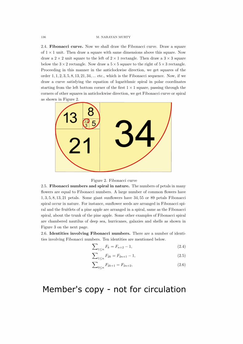
Member's copy - not for circulation
136 M. NARAYAN MURTY
2.4. Fibonacci curve. Now we shall draw the Fibonacci curve. Draw a square
of 1× 1 unit. Then draw a square with same dimensions above this square. Now
draw a 2× 2 unit square to the left of 2× 1 rectangle. Then draw a 3× 3 square
below the 3× 2 rectangle. Now draw a 5× 5 square to the right of 5× 3 rectangle.
Proceeding in this manner in the anticlockwise direction, we get squares of the
order 1, 1, 2, 3, 5, 8, 13, 21, 34, ... etc., which is the Fibonacci sequence. Now, if we
draw a curve satisfying the equation of logarithmic spiral in polar coordinates
starting from the left bottom corner of the first 1× 1 square, passing through the
corners of other squares in anticlockwise direction, we get Fibonacci curve or spiral
as shown in Figure 2.
Figure 2. Fibonacci curve
2.5. Fibonacci numbers and spiral in nature. The numbers of petals in many
flowers are equal to Fibonacci numbers. A large number of common flowers have
1, 3, 5, 8, 13, 21 petals. Some giant sunflowers have 34, 55 or 89 petals Fibonacci
spiral occur in nature. For instance, sunflower seeds are arranged in Fibonacci spi-
ral and the fruitlets of a pine apple are arranged in a spiral, same as the Fibonacci
spiral, about the trunk of the pine apple. Some other examples of Fibonacci spiral
are chambered nautilus of deep sea, hurricanes, galaxies and shells as shown in
Figure 3 on the next page.
2.6. Identities involving Fibonacci numbers. There are a number of identi-
ties involving Fibonacci numbers. Ten identities are mentioned below.∑1≤n
Fk = Fn+2 − 1, (2.4)∑1≤n
F2k = F2n+1 − 1, (2.5)∑0≤n
F2k+1 = F2n+2, (2.6)

Member's copy - not for circulation
SOME FACTS ABOUT ........ GOLDEN RATIO 137
(a) (b) (c)
(d) (e) (f)
Figure 3. Fibonacci spiral in nature
(a) Sunflower seeds (b) Spiral galaxy (c) Hurricane
(d) Nautilus (e) Fruit lets of pine apple (f) Shell.∑1≤n
F3k = (F3n+2 − 1)/2, (2.7)
Fm+n = Fm+1Fn + FmFn−1, (2.8)
F2n+1 = F 2n+1 + F 2
n , (2.9)
F2n = F 2n+1 − F 2
n−1, (n ≥ 2) (2.10)
Fn−1Fn+1 − F 2n = (−1)n, (2.11)
F2k+1F2k−1 − 1 = F 22k. (2.12)
The last identity (2.12) can be described geometrically as per the following exam-
ple. Taking k = 3, we obtain F2k = F6 = 8, F2k+1 = F7 = 13 and F2k−1 = F5 = 5.
A square is shown in Figure 4 with it side equal to the Fibonacci number F2k = 8.
The area of this square is F 22k = 64. This Square is partitioned into two right an-
gled triangles (A and B) of equal area and two quadrilaterals (C and D) of equal
area. A rectangle with Fibonacci numbers F2k+1 = 13 and F2k−1 = 5 as its sides
is shown in Figure 5. The area of this rectangle is F2k+1F2k−1 = 65. Within this
rectangle, the geometrical figures A, B, C and D along with one parallelogram E of
unit area can be adjusted. Because, according to the identity (2.12), 65− 1 = 64.
Hence, this identity indicates that the area of the rectangle minus the area of the
parallelogram is equal to the area of the square.
2.7. Expression for finding Fibonacci numbers. Fibonacci numbers can be
found using the expression

Member's copy - not for circulation
138 M. NARAYAN MURTY
Fn =1√5
(1 +√
5
2
)n−(
2
1 +√
5
)ncosnπ
. (2.13)
For example, since cos3π = −1, we get F3 = 1√5
(1+√5
2
)3−(
21+√5
)3(−1)
=
2, as can be easily shown.
2.8. Pascal’s triangle. This triangle is named after French mathematician Blaise
Pascal (1623 -1662). The description about the triangle is found in his mathemat-
ical treatise Traite du triangle arithmatique (1653). Pascal’s triangle is formed by
the binomial coefficients in binomial expansions. If we expand algebraic expression
(x+ y)n for n = 1, 2, 3, · · · , etc., we obtain
(x+ y)1 = 1x+ 1y,
(x+ y)2 = 1x2 + 2xy + 1y2,
(x+ y)3 = 1x3 + 3x2y + 3xy2 + 1y3,
(x+ y)4 = 1x4 + 4x3y + 6x2y2 + 4xy3 + 1y4,
(x+ y)5 = 1x5 + 5x4y + 10x3y2 + 10x2y3 + 5xy4 + 1y5,
(x+ y)6 = 1x6 + 6x5y + 15x4y2 + 20x3y3 + 15x2y4 + 6xy5 + 1y6,
(x+ y)7 = 1x7 + 7x6y + 21x5y2 + 35x4y3 + 35x3y4 + 21x2y5 + 7xy6 + 1y7,
.... .... .... .... .... .... .... .... .... .... ....
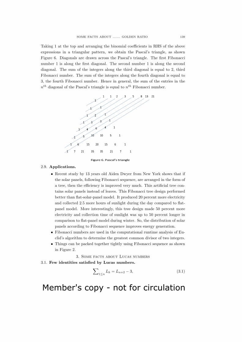
Member's copy - not for circulation
SOME FACTS ABOUT ........ GOLDEN RATIO 139
Taking 1 at the top and arranging the binomial coefficients in RHS of the above
expressions in a triangular pattern, we obtain the Pascal’s triangle, as shown
Figure 6. Diagonals are drawn across the Pascal’s triangle. The first Fibonacci
number 1 is along the first diagonal. The second number 1 is along the second
diagonal. The sum of the integers along the third diagonal is equal to 2, third
Fibonacci number. The sum of the integers along the fourth diagonal is equal to
3, the fourth Fibonacci number. Hence in general, the sum of the entries in the
nth diagonal of the Pascal’s triangle is equal to nth Fibonacci number.
2.9. Applications.
• Recent study by 13 years old Aiden Dwyer from New York shows that if
the solar panels, following Fibonacci sequence, are arranged in the form of
a tree, then the efficiency is improved very much. This artificial tree con-
tains solar panels instead of leaves. This Fibonacci tree design performed
better than flat-solar-panel model. It produced 20 percent more electricity
and collected 2.5 more hours of sunlight during the day compared to flat-
panel model. More interestingly, this tree design made 50 percent more
electricity and collection time of sunlight was up to 50 percent longer in
comparison to flat-panel model during winter. So, the distribution of solar
panels according to Fibonacci sequence improves energy generation.
• Fibonacci numbers are used in the computational runtime analysis of Eu-
clid’s algorithm to determine the greatest common divisor of two integers.
• Things can be packed together tightly using Fibonacci sequence as shown
in Figure 2.
3. Some facts about Lucas numbers
3.1. Few identities satisfied by Lucas numbers.∑1≤n
Lk = Ln+2 − 3, (3.1)

Member's copy - not for circulation
140 M. NARAYAN MURTY∑1≤n
L2k = L2n+1 − 1, (3.2)∑0≤n−1
L2k+1 = L2n − 2, (3.3)
L2n = L2n − 2(−1)n, (3.4)
L2n+1 = LnLn+1 + (−1)n+1, (3.5)
Ln−1Ln+1 − L2n = 5(−1)n+1, (n ≥ 2) (3.6)
Lm+n + (−1)nLm−n = LmLn. (3.7)
L2n = L2n + 2(−1)n. (3.8)
3.2. Some relations between Lucas numbers and Fibonacci numbers.
Lucas numbers are related to Fibonacci numbers. Some relations between Lucas
numbers and Fibonacci numbers are given below.
Ln = Fn+1 + Fn−1 = Fn + 2Fn−1, (n ≥ 2) (3.9)
Ln+1 + Ln−1 = 5Fn, (n ≥ 2) (3.10)
F2n = FnLn, (n ≥ 1) (3.11)
L2n − 5F 2
n = 4(−1)n, (n ≥ 1) (3.12)
2Lm+n = LmLn + 5FmFn, (m ≥ 1, n ≥ 1) (3.13)
2Fm+n = FmLn + FnLm, (m ≥ 1, n ≥ 1) (3.14)
Ln = Fn+2 − Fn−2, (n ≥ 3) (3.15)
L2n = F 2
n + 4Fn+1Fn−1, (n ≥ 2) (3.16)
L2n+1 = 5FnFn+1 + (−1)n, (n ≥ 1) (3.17)
L2n − F 2
n = 4Fn−1Fn+1, (n ≥ 2) (3.18)
4. Golden ratio
4.1. Relation between Fibonacci numbers and golden ratio. We know the
roots of the quadratic equation x2 = x+1 are φ = (1+√
5)/2 and ψ = (1−√
5)/2,
where the constant φ, having approximate value 1.618, is the golden ratio. We can
write the Fibonacci numbers in terms of golden ratio. In fact, we observe that
F1 = 1 = φ−ψφ−ψ , F2 = 1 = (φ + ψ) = φ2−ψ2
φ−ψ , and similarly, the nth Fibonacci
number can be expressed as
Fn = (φn − ψn)/(φ− ψ). (4.1)
Since (i) ψ = 1− φ, (ii) φ− ψ =√
5 and using the value of φ = 1.61803398 . . . in
ψ, one gets (iii) ψ = 1− φ = −0.61803398 . . . ≈ − 1φ , it follows that
Fn = (φn − (1− φ)n)/√
5 = (φn − (−φ)−n)/√
5. (4.2)
Using this any Fibonacci number can be calculated from the golden ratio. For ex-
ample, for n = 6, one gets F6 = ((1.618034)6−(−0.618034)6)/√
5 = 8.000001073 ≈8. Any two successive Fibonacci numbers have a ratio close to the golden ratio.
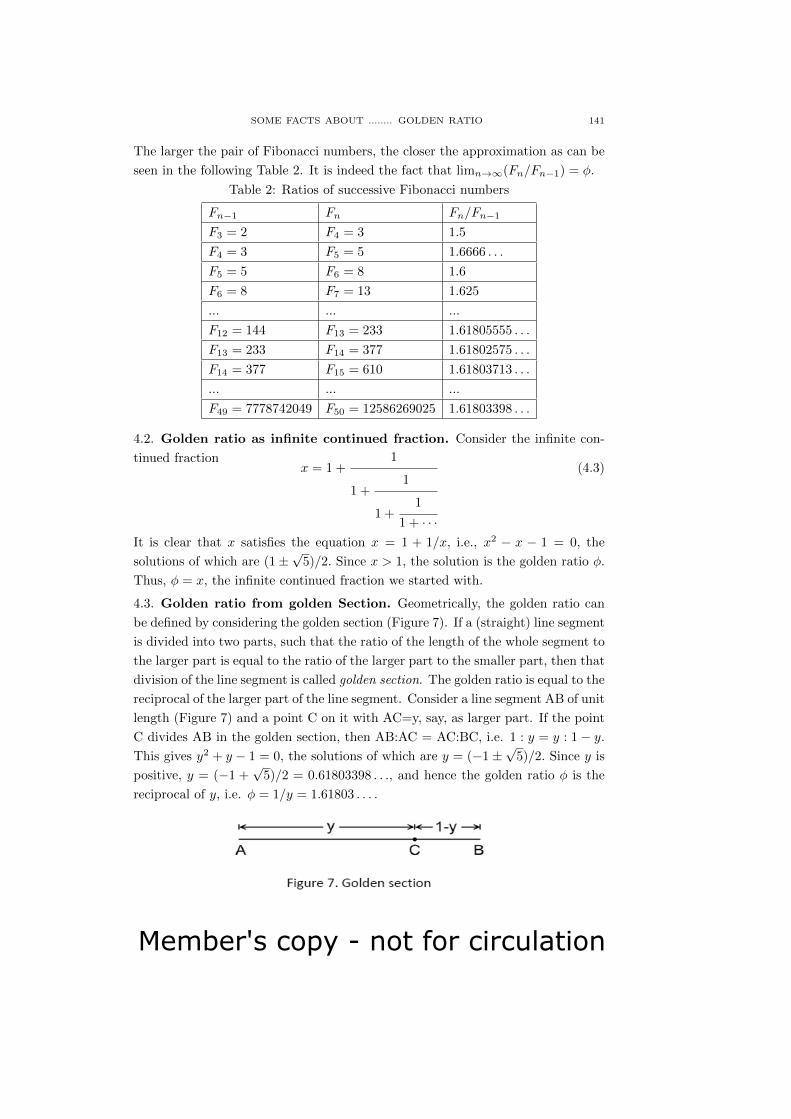
Member's copy - not for circulation
SOME FACTS ABOUT ........ GOLDEN RATIO 141
The larger the pair of Fibonacci numbers, the closer the approximation as can be
seen in the following Table 2. It is indeed the fact that limn→∞(Fn/Fn−1) = φ.
Table 2: Ratios of successive Fibonacci numbers
Fn−1 Fn Fn/Fn−1
F3 = 2 F4 = 3 1.5
F4 = 3 F5 = 5 1.6666 . . .
F5 = 5 F6 = 8 1.6
F6 = 8 F7 = 13 1.625
... ... ...
F12 = 144 F13 = 233 1.61805555 . . .
F13 = 233 F14 = 377 1.61802575 . . .
F14 = 377 F15 = 610 1.61803713 . . .
... ... ...
F49 = 7778742049 F50 = 12586269025 1.61803398 . . .
4.2. Golden ratio as infinite continued fraction. Consider the infinite con-
tinued fractionx = 1 +
1
1 +1
1 +1
1 + · · ·
(4.3)
It is clear that x satisfies the equation x = 1 + 1/x, i.e., x2 − x − 1 = 0, the
solutions of which are (1±√
5)/2. Since x > 1, the solution is the golden ratio φ.
Thus, φ = x, the infinite continued fraction we started with.
4.3. Golden ratio from golden Section. Geometrically, the golden ratio can
be defined by considering the golden section (Figure 7). If a (straight) line segment
is divided into two parts, such that the ratio of the length of the whole segment to
the larger part is equal to the ratio of the larger part to the smaller part, then that
division of the line segment is called golden section. The golden ratio is equal to the
reciprocal of the larger part of the line segment. Consider a line segment AB of unit
length (Figure 7) and a point C on it with AC=y, say, as larger part. If the point
C divides AB in the golden section, then AB:AC = AC:BC, i.e. 1 : y = y : 1− y.This gives y2 + y − 1 = 0, the solutions of which are y = (−1±
√5)/2. Since y is
positive, y = (−1 +√
5)/2 = 0.61803398 . . ., and hence the golden ratio φ is the
reciprocal of y, i.e. φ = 1/y = 1.61803 . . . .
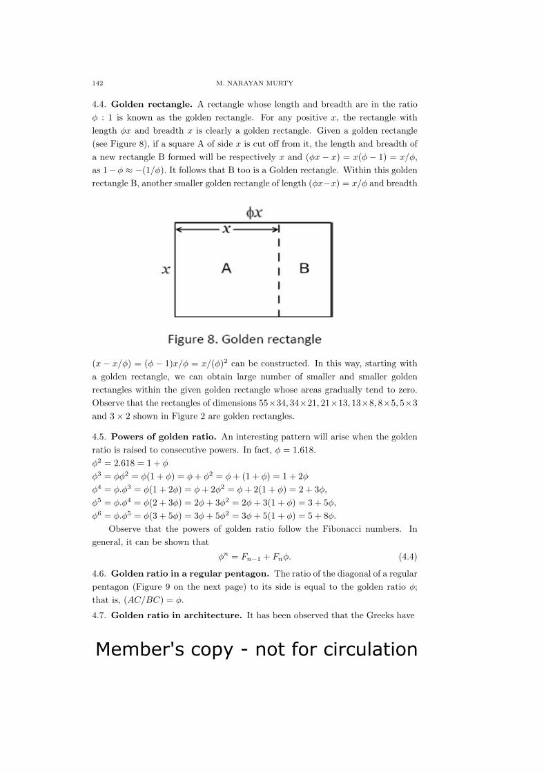
Member's copy - not for circulation
142 M. NARAYAN MURTY
4.4. Golden rectangle. A rectangle whose length and breadth are in the ratio
φ : 1 is known as the golden rectangle. For any positive x, the rectangle with
length φx and breadth x is clearly a golden rectangle. Given a golden rectangle
(see Figure 8), if a square A of side x is cut off from it, the length and breadth of
a new rectangle B formed will be respectively x and (φx − x) = x(φ − 1) = x/φ,
as 1−φ ≈ −(1/φ). It follows that B too is a Golden rectangle. Within this golden
rectangle B, another smaller golden rectangle of length (φx−x) = x/φ and breadth
(x − x/φ) = (φ − 1)x/φ = x/(φ)2 can be constructed. In this way, starting with
a golden rectangle, we can obtain large number of smaller and smaller golden
rectangles within the given golden rectangle whose areas gradually tend to zero.
Observe that the rectangles of dimensions 55×34, 34×21, 21×13, 13×8, 8×5, 5×3
and 3× 2 shown in Figure 2 are golden rectangles.
4.5. Powers of golden ratio. An interesting pattern will arise when the golden
ratio is raised to consecutive powers. In fact, φ = 1.618.
φ2 = 2.618 = 1 + φ
φ3 = φφ2 = φ(1 + φ) = φ+ φ2 = φ+ (1 + φ) = 1 + 2φ
φ4 = φ.φ3 = φ(1 + 2φ) = φ+ 2φ2 = φ+ 2(1 + φ) = 2 + 3φ,
φ5 = φ.φ4 = φ(2 + 3φ) = 2φ+ 3φ2 = 2φ+ 3(1 + φ) = 3 + 5φ,
φ6 = φ.φ5 = φ(3 + 5φ) = 3φ+ 5φ2 = 3φ+ 5(1 + φ) = 5 + 8φ.
Observe that the powers of golden ratio follow the Fibonacci numbers. In
general, it can be shown that
φn = Fn−1 + Fnφ. (4.4)
4.6. Golden ratio in a regular pentagon. The ratio of the diagonal of a regular
pentagon (Figure 9 on the next page) to its side is equal to the golden ratio φ;
that is, (AC/BC) = φ.
4.7. Golden ratio in architecture. It has been observed that the Greeks have

Member's copy - not for circulation
SOME FACTS ABOUT ........ GOLDEN RATIO 143
used the concept of golden ratio in the construction of temples. The Parthenon
in Athens is the classic example of the golden ratio being used in architecture. It
was constructed between 448-432 BC as a temple for the Goddess Athena. This
structure contains a multitude of golden rectangles. The great pyramid in Giza,
Egypt, is another example of an ancient structure where golden ratio is used in
its design. The ratio of the height of its triangular face to half of the side of its
square base approximates to golden ratio φ.
4.8. Illustrations of golden ratio in human body. According to the book by
Samuel Obara [6], the following ratios in the human body are very close to golden
ratio.
• Height of a person to the distance between the naval point and the foot.
• Separation between the pupils of the eyes to the average length between
the eyebrows.
• Width of the nose to the length between the nostrils.
• Length of the shoulder line to the length of the head.
• Distance from the ground to the naval point to the distance from the
ground to the knee.
• Length of the hand to the distance from wrist to the elbow.
If the above ratios in human body are close to golden ratio, the body appears
beautiful.
References
[1] Abbas, S., Golden Ratio - a measure of physical beauty, Resonance, Indian Academy of
Sciences, 22 No.1 (2017), 51 – 60.

Member's copy - not for circulation
144 M. NARAYAN MURTY
[2] Burton, David M., Elementary Number Theory, Tata McGraw Hill Publishing Company
Ltd. (2007).
[3] Mallik, A. K., From natural numbers to numbers and curves in nature - I, Resonance, Indian
Academy of Sciences, 9 No. 9 (2004), 29 – 37.
[4] Mallik, A. K., From natural numbers to numbers and curves in nature - II, Resonance,
Indian Academy of Sciences, 9 No. 10 (2004), 34 – 40.
[5] Mukhopadhyay, U., Logarithmic spiral - a splendid curve, Resonance, Indian Academy of
Sciences, 9, No.11 (2004), 39 – 45.
[6] Obara, Samuel, The Golden Ratio in Art and Architecture, University of Goergia, Depart-
ment of Mathematics Education.
[7] Robbins, Neville, Beginning Number Theory, Narosa Publishing House (2007).
[8] Shanks, Daniel, Solved and unsolved problems in Number Theory, AMS Chelsea Publishing,
American Mathematical Society (2003).
M. Narayan Murty
Department of Physics
Raghu Institute of Technology
Visakhapatnam - 531162, Andhra Pradesh, India.
Email: [email protected]

Member's copy - not for circulation
The Mathematics Student ISSN: 0025-5742
Vol. 87, Nos. 1-2, January-June (2018), 145-152
A UNIFYING MULTIPLICATION ONCARTESIAN PRODUCT OF BANACH ALGEBRAS*
PRAKASH A. DABHI AND SAVAN K. PATEL
(Received : 26 - 09 - 2017; Revised : 06-12-2017)
Abstract. Let C and B be Banach algebras, A be a closed subalgebra of
C, T : B → C be an algebra homomorphism with ‖T‖ ≤ 1, and let P :
C → A be linear with ‖P‖ ≤ 1. We define a Banach algebra product on
the Cartesian product of A and B, which we shall denote by A ×PT B. This
product simultaneously generalizes several multiplications on A × B like θ-
Lau product, T - product, semidirect product, generalized semidirect product
and the pointwise product. When A×PT B is a commutative Banach algebra,
we characterize the Gelfand space and multipliers.
1. IntroductionGiven commutative Banach algebras A and B, the Cartesian product space
A× B can be endowed with several multiplications making it a linear associative
algebra with suitable norms. These include the standard coordinatewise product,
θ- Lau product [7, 8], defined with the help of a multiplicative linear functional θ
on B, the semidirect product and its generalization [1, 2, 3, 10], a product recently
introduced in [9]. There is also a product introduced in [4] that eventually turns
out to be isomorphic to the pointwise product [5]. Computing Gelfand spaces
and multipliers of a Banach algebra have been an important aspect of Banach
algebra theory. For the product considered above, some aspects of these have
been discussed in [6, 8, 9].
In the present note, given linear associative algebras A and B, we consider a
fairly general framework to define an associative product on A×B incorporating all
these different multiplications; and when A×B is a commutative Banach algebra
with this multiplication, we compute the Gelfand space and multipliers.
2. Generalized Product A×PT BLet C and B be linear associative algebras, and let A be a subalgebra of C.
Let T : B → C be an algebra homomorphism, and P : C → A be a linear map. For
* The work has been supported by the UGC-SAP-DRS-III provided to the Department of
Mathematics, Sardar Patel University, Vallabh Vidyanagar - 388120, India.
The second author gratefully acknowledges Junior Research Fellowship from UGC, India.
2010 Mathematics Subject Classification: 46J05
Key words and phrases: Lau product, perturbed product, semidirect product, Gelfand spa-
ce, multiplier algebra.
c© Indian Mathematical Society, 2018 .
145
Member's copy - not for circulation
146 PRAKASH A. DABHI AND SAVAN K. PATEL
(a, b), (c, d) ∈ A× B, we introduce the multiplication
(a, b)(c, d) = (P (ac+ T (b)c+ aT (d)), bd). (2.1)
Lemma 2.1. The product defined by equation (2.1) on A×B is associative if and
only if the following equations hold for all a, c, e ∈ A and b, d, f ∈ B.
(i) P(aP(ce))=P(P(ac)e) (v) P(T(b)P(cT(f)))=P(P(T(b)c)T(f))
(ii) P(aP(T(d)e))=P(P(aT(d))e) (vi) P(T(b)P(T(d)e))=P(T(b)T(d)e)
(iii) P(aP(cT(f)))=P(P(ac)T(f)) (vii) P(P(aT(d))T(f))=P(aT(d)T(f))
(iv) P(T(b)P(ce))=P(P(T(b)c)e)
Proof. Let (a, b), (c, d), (e, f) ∈ A× B. Then (a, b)((c, d)(e, f))
= (a, b)(P (ce+ T (d)e+ cT (f)), df)
= (P (aP (ce+ T (d)e+ cT (f)) + aT (df) + T (b)P (ce+ T (d)e+ cT (f)), bdf)
=(P (aP (ce)) + aP (T (d)e) + aP (cT (f)) + aT (df) + T (b)P (ce)
+T (b)P (T (d)e) + T (b)P (cT (f)), bdf),
=(P (aP (ce)) + P (aP (T (d)e)) + P (aP (cT (f))) + P (aT (df))
+P (T (b)P (ce)) + P (T (b)P (T (d)e)) + P (T (b)P (cT (f))), bdf).(2.2)
Also, ((a, b)(c, d))(e, f)
= (P (ac+ T (b)c+ aT (d)), bd)(e, f)
= (P (P (ac+ T (b)c+ aT (d))e+ P (ac+ T (b)c+ aT (d))T (f) + T (bd)e), bdf)
=(P (P (ac)e) + P (T (b)c)e+ P (aT (d))e+ P (ac)T (f)
+P (T (b)c)T (f) + P (aT (d))T (f) + T (bd)e), bdf)
=(P (P (ac)e) + P (P (T (b)c)e) + P (P (aT (d))e) + P (P (ac)T (f))
+P (P (T (b)c)T (f)) + P (P (aT (d))T (f)) + P (T (bd)e), bdf).(2.3)
It follows that the product is associative if and only if (i)-(vii) hold.
We shall denote the multiplication in (2.1) by ×PT , and A × B by A ×PT B.
Throughout we assume that the map P : A → C is such that A×PT B is associative.
Now, let C and B be a Banach algebras, A be a closed subalgebra of C, T :
B → C be an algebra homomorphism with ‖T‖ ≤ 1, and let P : C → A be a linear
map with ‖P‖ ≤ 1. For (a, b) ∈ A×PT B, let
‖(a, b)‖1 = ‖a‖+ ‖b‖.If (a, b), (c, d) ∈ A× B, then
‖(a, b)(c, d)‖1=‖(P (ac+ aTd+ T (b)c), bd)‖1 = ‖P (ac+ aTd+ T (b)c)‖+ ‖bd‖
≤ ‖ac+ aTd+ T (b)c‖+ ‖bd‖
≤ ‖a‖‖c‖+‖a‖‖d‖+‖b‖‖c‖+‖b‖‖d‖
= (‖a‖+ ‖b‖)(‖c‖+ ‖d‖)
= ‖(a, b)‖1‖(c, d)‖1.
Member's copy - not for circulation
A UNIFYING MULTIPLICATION ON .... BANACH ALGEBRAS 147
Therefore A×PT B is a Banach algebra.
We show below that certain standard multiplications considered in the litera-
ture are special cases of A×PT B.
(1) T - product [4]: Let A and B be Banach algebras. Let P : A → A be the
identity map, i.e., P (a) = a (a ∈ A), and let T : B → A be a homomorphism with
‖T‖ ≤ 1. If (a, b), (c, d) ∈ A× B, then
(a, b)(c, d) = (P (ac+ T (b)c+ aT (d)), bd) = (ac+ T (b)c+ aT (d), bd).
It follows that A×PT B = A×T B.
In particular, if T is a zero map, then we get the usual Cartesian product of Aand B. It should be noted that as recently shown in [5] that A×T B is isomorphic
to the Cartesian product space A × B via the map (a, b) 7→ (a + T (b), b) from
A×T B to A× B.
(2) Semidirect product [1, 2, 3, 6, 10]: Suppose that A is a Banach algebra such
that it can be written as a direct sum of a closed ideal I and a closed subalgebra
B, i.e., A = I ⊕B, and that ‖a+ b‖ = ‖a‖+ ‖b‖ for all a+ b ∈ A. Let T : B → Abe an algebra homomorphism with ‖T‖ ≤ 1, and let P : A → I be the projection
on I, i.e., P (i+ b) = i (i+ b ∈ A). If (i, b), (j, d) ∈ I ⊕ B = A, then
(i, b)(j, d) = (P (ij + T (b)j + iT (d)), bd) = (ij + T (b)j + iT (d), bd).
In particular, if we take T (b) = b (b ∈ B), then we get the semidirect product.
Therefore generalized semidirect product is a particular case of I ×PT B.
(3) θ- Lau Product [7]: Let A and B be Banach algebra, and let θ be a multi-
plicative linear functional on B. For (a, b), (c, d) ∈ A× B, let
(a, b)(c, d) = (ac+ θ(b)c+ θ(d)a, bd).
Then A×B is a Banach algebra with this multiplication, called the θ- Lau product,
and the norm ‖(a, b)‖ = ‖a‖ + ‖b‖ ((a, b) ∈ A × B). The Banach algebra A × Bwith this multiplication is denoted by A×θ B.
Take C = Ae, the unitization of A. Let T : B → C be T (b) = θ(b)e (b ∈ B),
where e is the identity in C. Let P : C → A be P (a+ λe) = a (a+ λ ∈ C).If (a, b), (c, d) ∈ A× B, then
(a, b)(c, d) = (P (ac+ T (b)c+ aT (d)), bd)
= (P (ac+ θ(b)c+ aθ(d)), bd) = (ac+ θ(b)c+ θ(d)a, bd).
It follows that A×PT B = A×θ B.
This product was introduced by Lau [7] for certain class of Banach algebras
and was extended by Sangani Monfared [8] for the general case.
(4) [9] Let A be a commutative Banach algebra. A bounded linear map T : A → Ais a multiplier if T (ab) = aT (b) = T (a)b (a, b ∈ A). Let M(A) be the collection
of all multipliers on A. Then M(A) is a unital commutative Banach algebra with
composition as multiplication and with the norm ‖T‖ = sup‖Ta‖ : ‖a‖ ≤ 1.

Member's copy - not for circulation
148 PRAKASH A. DABHI AND SAVAN K. PATEL
Let C = A⊕M(A). Then C is a commutative Banach algebra with the product
(a, F )(b,G) = (ab+G(a) + F (b), FG) ((a, F ), (b,G) ∈ C)and the norm
‖(a, F )‖ = ‖a‖+ ‖F‖ ((a, F ) ∈ C).Then both A and M(A) are closed subalgebras of C. We shall identify element
of A and element of M(A) with elements of C by a ↔ (a, 0) and F ↔ (0, F )
respectively. Thus if a ∈ A and F ∈M(A), then Fa = aF = F (a) = (F (a), 0).
Let B be a Banach algebra, and let T ′ : B → M(A) be a homomorphism
with ‖T ′‖ ≤ 1. Define T : B → C by T (b) = (0, T ′(b)) (b ∈ B). Then T is a
homomorphism with ‖T‖ = ‖T ′‖ ≤ 1. Let P : C → A be P ((a, F )) = a ((a, F ) ∈C). Then P is linear and ‖P‖ ≤ 1. If (a, b), (c, d) ∈ A× B, then
(a, b)(c, d)=((a, 0), b)((c, 0), d) = (P ((a, 0)(c, 0)+(a, 0)T (d)+T (b)(c, 0)), bd)
= (P ((ac, 0)+(a, 0)(0, T ′(d))+(0, T ′(b))(c, 0)), bd)
= (P ((ac, 0) + (T ′(d)(a), 0) + (T ′(b)(c), 0)), bd)
= (ac+ T ′(d)(a) + T ′(b)c, bd).
Thus in this case the product on A×PT B is product defined in [9].
All these make the multiplication ×PT on A×B exciting and interesting. The
present note is aimed at describing the Gelfand space and multipliers of A×PT B in
the commutative case. Notice that recently there has been considerable interest
in special cases discussed above [1, 2, 4, 6, 7, 9].
A Banach algebraA is without order if a = 0 whenever a ∈ A and aA = 0. It
is easy to see that θ- product (T -product, semidirect product) of Banach algebras
A and B is without order if and only if both A and B are without order. The
product ×PT defined using P and T described below is not covered in the particular
cases described above.
Example 2.2. Let A = C = Cb([0, 1)∪ (1, 2]) = the set of all bounded continuous
functions on [0, 1) ∪ (1, 2], B = C[0, 2], both with the sup norm ‖ · ‖∞. Define
T : B → A and P : A → A by T (f) = fχ[0,1) for all f ∈ B and P (f) = fχ[0,1) for
all f ∈ A, where χ[0,1) is the characteristic function on [0, 1). If (f1, g1), (f2, g2) ∈A×PT B, then
(f1, g1)(f2, g2) = (P (f1f2 + T (g1)f2 + f1T (g2)), g1g2)
= (P (f1f2 + g1χ[0,1)f2 + f1g2χ[0,1)), g1g2)
= (f1f2χ[0,1) + g1f2χ[0,1) + f1g2χ[0,1), g1g1).
Take an element (χ(1,2], 0) ∈ A ×PT B. Then (χ(1,2], 0) 6= 0. If (f, g) ∈ A ×PT B,
then
(χ(1,2], 0)(f, g) = (P (χ(1,2]f+χ(1,2]T (g)), 0)=((χ(1,2]f + χ(1,2]T (g))χ[1,0), 0
)=
((f + T (g))χ(1,2]χ[1,0), 0
)= (0, 0).
Hence A×PT B is not without order even though both A and B are without order.
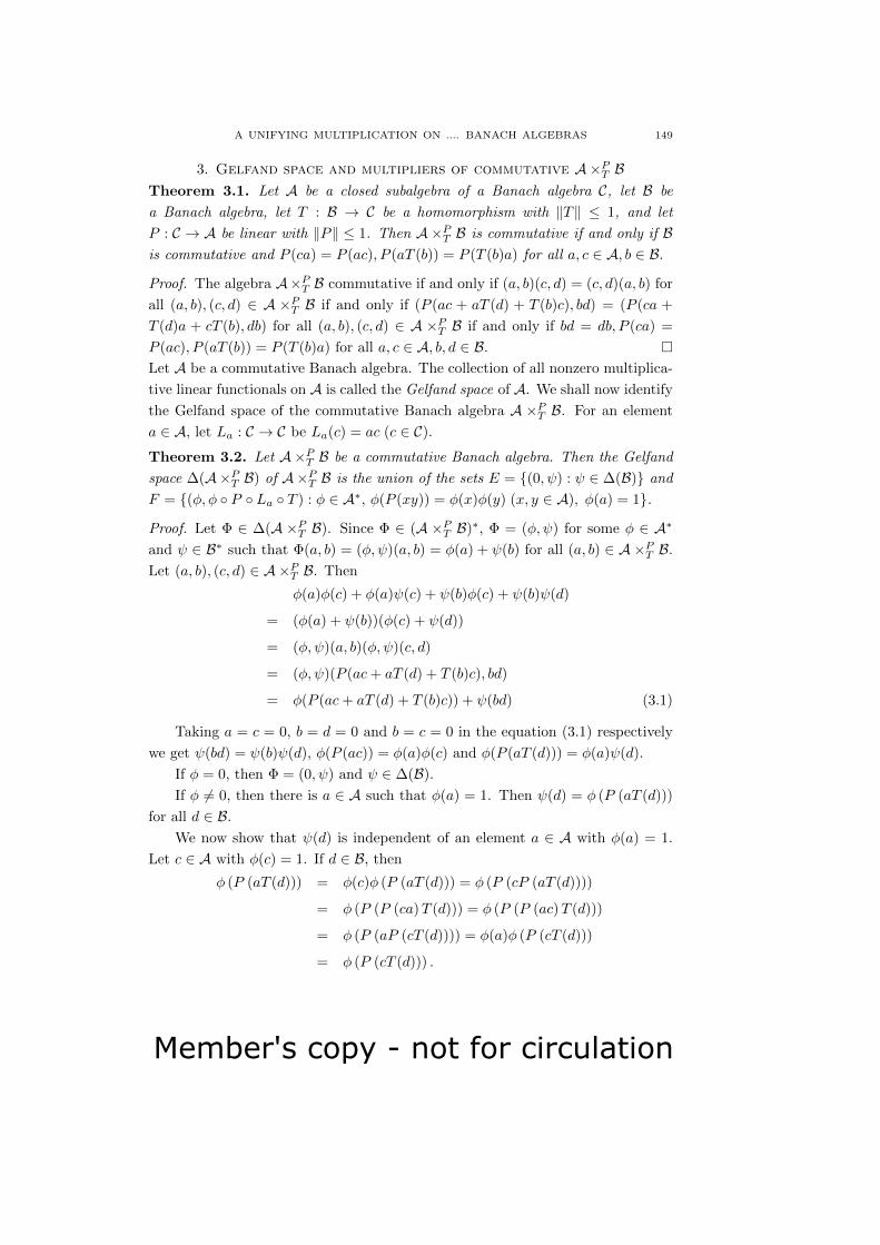
Member's copy - not for circulation
A UNIFYING MULTIPLICATION ON .... BANACH ALGEBRAS 149
3. Gelfand space and multipliers of commutative A×PT BTheorem 3.1. Let A be a closed subalgebra of a Banach algebra C, let B be
a Banach algebra, let T : B → C be a homomorphism with ‖T‖ ≤ 1, and let
P : C → A be linear with ‖P‖ ≤ 1. Then A×PT B is commutative if and only if Bis commutative and P (ca) = P (ac), P (aT (b)) = P (T (b)a) for all a, c ∈ A, b ∈ B.
Proof. The algebra A×PT B commutative if and only if (a, b)(c, d) = (c, d)(a, b) for
all (a, b), (c, d) ∈ A ×PT B if and only if (P (ac + aT (d) + T (b)c), bd) = (P (ca +
T (d)a + cT (b), db) for all (a, b), (c, d) ∈ A ×PT B if and only if bd = db, P (ca) =
P (ac), P (aT (b)) = P (T (b)a) for all a, c ∈ A, b, d ∈ B.
Let A be a commutative Banach algebra. The collection of all nonzero multiplica-
tive linear functionals on A is called the Gelfand space of A. We shall now identify
the Gelfand space of the commutative Banach algebra A ×PT B. For an element
a ∈ A, let La : C → C be La(c) = ac (c ∈ C).Theorem 3.2. Let A×PT B be a commutative Banach algebra. Then the Gelfand
space ∆(A×PT B) of A×PT B is the union of the sets E = (0, ψ) : ψ ∈ ∆(B) and
F = (φ, φ P La T ) : φ ∈ A∗, φ(P (xy)) = φ(x)φ(y) (x, y ∈ A), φ(a) = 1.
Proof. Let Φ ∈ ∆(A ×PT B). Since Φ ∈ (A ×PT B)∗, Φ = (φ, ψ) for some φ ∈ A∗
and ψ ∈ B∗ such that Φ(a, b) = (φ, ψ)(a, b) = φ(a) + ψ(b) for all (a, b) ∈ A ×PT B.
Let (a, b), (c, d) ∈ A×PT B. Then
φ(a)φ(c) + φ(a)ψ(c) + ψ(b)φ(c) + ψ(b)ψ(d)
= (φ(a) + ψ(b))(φ(c) + ψ(d))
= (φ, ψ)(a, b)(φ, ψ)(c, d)
= (φ, ψ)(P (ac+ aT (d) + T (b)c), bd)
= φ(P (ac+ aT (d) + T (b)c)) + ψ(bd) (3.1)
Taking a = c = 0, b = d = 0 and b = c = 0 in the equation (3.1) respectively
we get ψ(bd) = ψ(b)ψ(d), φ(P (ac)) = φ(a)φ(c) and φ(P (aT (d))) = φ(a)ψ(d).
If φ = 0, then Φ = (0, ψ) and ψ ∈ ∆(B).
If φ 6= 0, then there is a ∈ A such that φ(a) = 1. Then ψ(d) = φ (P (aT (d)))
for all d ∈ B.
We now show that ψ(d) is independent of an element a ∈ A with φ(a) = 1.
Let c ∈ A with φ(c) = 1. If d ∈ B, then
φ (P (aT (d))) = φ(c)φ (P (aT (d))) = φ (P (cP (aT (d))))
= φ (P (P (ca)T (d))) = φ (P (P (ac)T (d)))
= φ (P (aP (cT (d)))) = φ(a)φ (P (cT (d)))
= φ (P (cT (d))) .
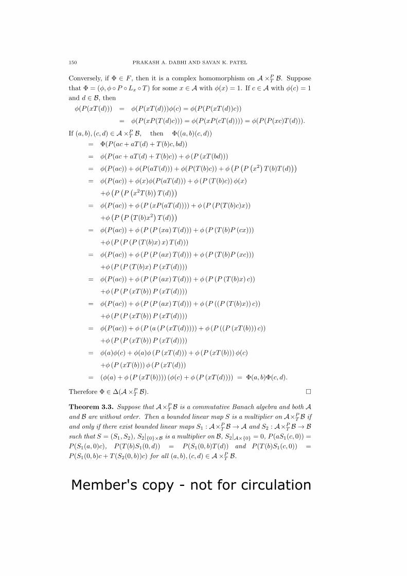
Member's copy - not for circulation
150 PRAKASH A. DABHI AND SAVAN K. PATEL
Conversely, if Φ ∈ F , then it is a complex homomorphism on A ×PT B. Suppose
that Φ = (φ, φ P Lx T ) for some x ∈ A with φ(x) = 1. If c ∈ A with φ(c) = 1
and d ∈ B, then
φ(P (xT (d))) = φ(P (xT (d)))φ(c) = φ(P (P (xT (d))c))
= φ(P (xP (T (d)c))) = φ(P (xP (cT (d)))) = φ(P (P (xc)T (d))).
If (a, b), (c, d) ∈ A×PT B, then Φ((a, b)(c, d))
= Φ(P (ac+ aT (d) + T (b)c, bd))
= φ(P (ac+ aT (d) + T (b)c)) + φ (P (xT (bd)))
= φ(P (ac)) + φ(P (aT (d))) + φ(P (T (b)c)) + φ(P(P(x2
)T (b)T (d)
))= φ(P (ac)) + φ(x)φ(P (aT (d))) + φ (P (T (b)c))φ(x)
+φ(P(P(x2T (b)
)T (d)
))= φ(P (ac)) + φ (P (xP (aT (d)))) + φ (P (P (T (b)c)x))
+φ(P(P(T (b)x2
)T (d)
))= φ(P (ac)) + φ (P (P (xa)T (d))) + φ (P (T (b)P (cx)))
+φ (P (P (P (T (b)x)x)T (d)))
= φ(P (ac)) + φ (P (P (ax)T (d))) + φ (P (T (b)P (xc)))
+φ (P (P (T (b)x)P (xT (d))))
= φ(P (ac)) + φ (P (P (ax)T (d))) + φ (P (P (T (b)x) c))
+φ (P (P (xT (b))P (xT (d))))
= φ(P (ac)) + φ (P (P (ax)T (d))) + φ (P ((P (T (b)x)) c))
+φ (P (P (xT (b))P (xT (d))))
= φ(P (ac)) + φ (P (a (P (xT (d))))) + φ (P ((P (xT (b))) c))
+φ (P (P (xT (b))P (xT (d))))
= φ(a)φ(c) + φ(a)φ (P (xT (d))) + φ (P (xT (b)))φ(c)
+φ (P (xT (b)))φ (P (xT (d)))
= (φ(a) + φ (P (xT (b)))) (φ(c) + φ (P (xT (d)))) = Φ(a, b)Φ(c, d).
Therefore Φ ∈ ∆(A×PT B).
Theorem 3.3. Suppose that A×PT B is a commutative Banach algebra and both Aand B are without order. Then a bounded linear map S is a multiplier on A×PT B if
and only if there exist bounded linear maps S1 : A×PT B → A and S2 : A×PT B → Bsuch that S = (S1, S2), S2|0×B is a multiplier on B, S2|A×0 = 0, P (aS1(c, 0)) =
P (S1(a, 0)c), P (T (b)S1(0, d)) = P (S1(0, b)T (d)) and P (T (b)S1(c, 0)) =
P (S1(0, b)c+ T (S2(0, b))c) for all (a, b), (c, d) ∈ A×PT B.
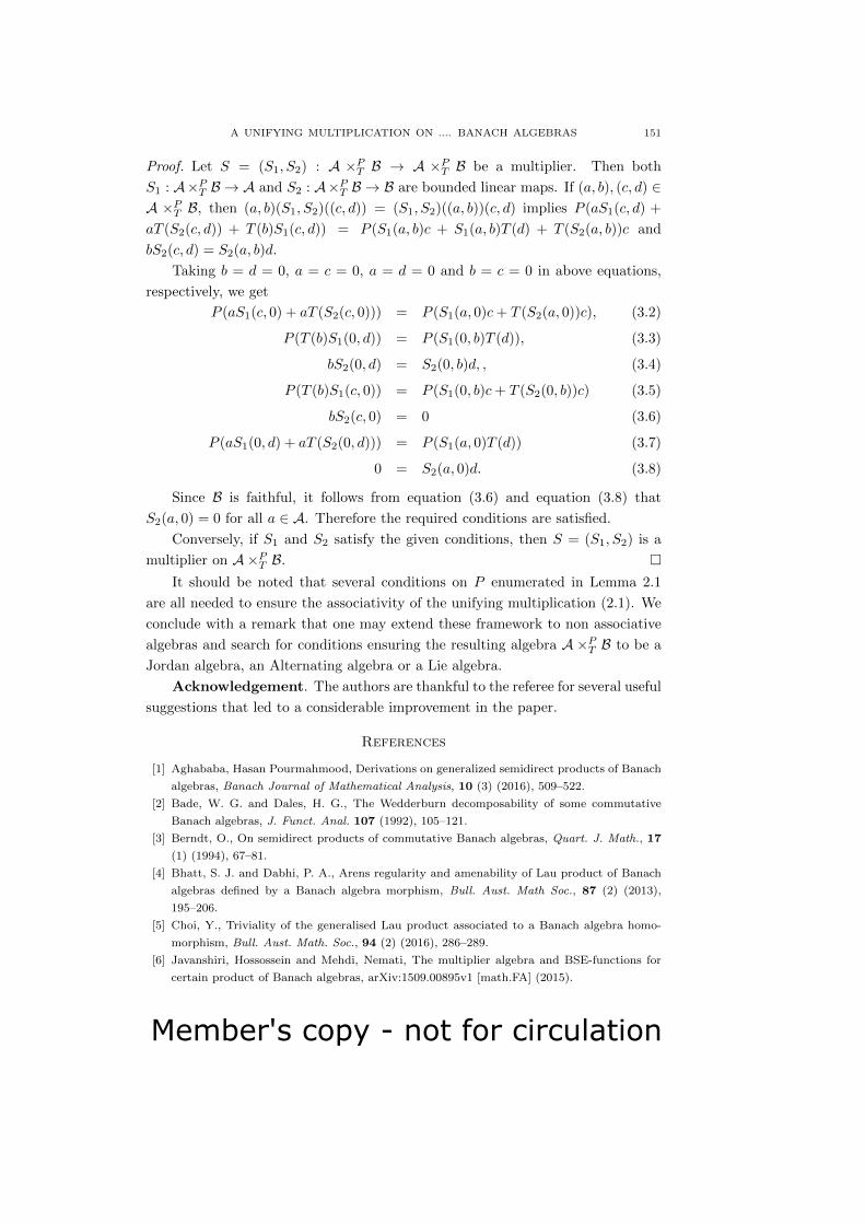
Member's copy - not for circulation
A UNIFYING MULTIPLICATION ON .... BANACH ALGEBRAS 151
Proof. Let S = (S1, S2) : A ×PT B → A ×PT B be a multiplier. Then both
S1 : A×PT B → A and S2 : A×PT B → B are bounded linear maps. If (a, b), (c, d) ∈A ×PT B, then (a, b)(S1, S2)((c, d)) = (S1, S2)((a, b))(c, d) implies P (aS1(c, d) +
aT (S2(c, d)) + T (b)S1(c, d)) = P (S1(a, b)c + S1(a, b)T (d) + T (S2(a, b))c and
bS2(c, d) = S2(a, b)d.
Taking b = d = 0, a = c = 0, a = d = 0 and b = c = 0 in above equations,
respectively, we get
P (aS1(c, 0) + aT (S2(c, 0))) = P (S1(a, 0)c+ T (S2(a, 0))c), (3.2)
P (T (b)S1(0, d)) = P (S1(0, b)T (d)), (3.3)
bS2(0, d) = S2(0, b)d, , (3.4)
P (T (b)S1(c, 0)) = P (S1(0, b)c+ T (S2(0, b))c) (3.5)
bS2(c, 0) = 0 (3.6)
P (aS1(0, d) + aT (S2(0, d))) = P (S1(a, 0)T (d)) (3.7)
0 = S2(a, 0)d. (3.8)
Since B is faithful, it follows from equation (3.6) and equation (3.8) that
S2(a, 0) = 0 for all a ∈ A. Therefore the required conditions are satisfied.
Conversely, if S1 and S2 satisfy the given conditions, then S = (S1, S2) is a
multiplier on A×PT B.
It should be noted that several conditions on P enumerated in Lemma 2.1
are all needed to ensure the associativity of the unifying multiplication (2.1). We
conclude with a remark that one may extend these framework to non associative
algebras and search for conditions ensuring the resulting algebra A×PT B to be a
Jordan algebra, an Alternating algebra or a Lie algebra.
Acknowledgement. The authors are thankful to the referee for several useful
suggestions that led to a considerable improvement in the paper.
References
[1] Aghababa, Hasan Pourmahmood, Derivations on generalized semidirect products of Banach
algebras, Banach Journal of Mathematical Analysis, 10 (3) (2016), 509–522.
[2] Bade, W. G. and Dales, H. G., The Wedderburn decomposability of some commutative
Banach algebras, J. Funct. Anal. 107 (1992), 105–121.
[3] Berndt, O., On semidirect products of commutative Banach algebras, Quart. J. Math., 17
(1) (1994), 67–81.
[4] Bhatt, S. J. and Dabhi, P. A., Arens regularity and amenability of Lau product of Banach
algebras defined by a Banach algebra morphism, Bull. Aust. Math Soc., 87 (2) (2013),
195–206.
[5] Choi, Y., Triviality of the generalised Lau product associated to a Banach algebra homo-
morphism, Bull. Aust. Math. Soc., 94 (2) (2016), 286–289.
[6] Javanshiri, Hossossein and Mehdi, Nemati, The multiplier algebra and BSE-functions for
certain product of Banach algebras, arXiv:1509.00895v1 [math.FA] (2015).

Member's copy - not for circulation
152 PRAKASH A. DABHI AND SAVAN K. PATEL
[7] Lau, A. T., Analysis on a class of Banach algebras with applications to harmonic analysis
on locally compact groups and semigroups, Fund. Math., 118 (3)(1983), 161–175.
[8] Sangani, Monfared, On certain products of Banach algebras with applications to harmonic
analysis, Studia Math., 178 (3) (2007), 277–294.
[9] Sin-Ei, Takahasi, Hiroyuki, Takagi and Takeshi, Miura, A Characterization of multipliers of
a Lau algebra constructed by semisimple commutative Banach algebras, Taiwanese Journal
of Mathematics, 20 (6) (2016), 1401–1415.
[10] Thomas, P. Marc, Principal ideals and semi-direct products in commutative Banach alge-
bras, J. Funct. Anal., 101 (2) (1991), 312–328.
Prakash A. Dabhi Department of Mathematics, Sardar Patel University
Vallabh Vidyanagar - 388120, Gujarat, India
E-mail: [email protected]
Savan K. Patel Department of Mathematics, Sardar Patel University
Vallabh Vidyanagar - 388120, Gujarat, India
E-mail: [email protected]
Member's copy - not for circulation
The Mathematics Student ISSN: 0025-5742
Vol. 87, Nos. 1-2, January-June (2018), 153-160
ON THE ABSOLUTE NORLUNDSUMMABILITY OF FOURIER SERIES
R. G. VYAS AND K. N. DARJI
(Received : 02 - 11 - 2017 ; Revised : 12 - 02 - 2018)
Abstract. In this paper we study the absolute Norlund summability of
Fourier series of functions of the classes ΛBV ([0, 2π]) and ΛBV (r)([0, 2π]).
1. Introduction
Absolute summability is a generalization of the concept of the absolute con-
vergence just as the summability is an extension of the concept of the convergence.
The absolute convergence of Fourier series is closely related to the variation and
the modulus of continuity of functions. Since there are several classical criteria
for the absolute convergence of Fourier series (see e.g., [8, 9]), one can extend the
concept of the absolute convergence of Fourier series to absolute summability just
as we can do with the convergence of Fourier series by the summability. Sev-
eral results have been obtained for the absolute summability of Fourier series by
Norlund means (see, [1, 2, 3, 4, 5]). Hyslop [2] extended Bernstein’s theorem by
using absolute Cesaro summability. This theorem was extended by McFadden [6]
applying absolute Norlund summability, but the final result in the same direction
is due to M. Izumi and I. Izumi [3] and S. N. Lal [4]. In 1970, by applying abso-
lute Norlund summability, S. M. Shah [7] obtained an analog of Zygmund’s result
for the class of functions of bounded variation. Shah observes that his theorem
supplements an earlier result of S. N. Lal [4]. Later in 1977, the study of the ab-
solute Norlund summability of Fourier series of functions of r−bounded variation
(r ≥ 1) was done by S. N. Lal and S. Ram [5]. Here, generalizing these results,
we study the absolute Norlund summability of Fourier series of functions of the
classes ΛBV ([0, 2π]) and ΛBV (r)([0, 2π]) (r ≥ 1).
2. Notations and Definitions
Let pn be a sequence of nonnegative numbers and write
Pn =n∑v=0
pv (P−1 = p−1 = 0).
The sequence to sequence transformation
2010 Mathematics Subject Classification: 42A24, 40G05, 26A45
Key words and phrases: Functions of the classes ΛBV ([0, 2π]) and ΛBV (r)([0, 2π]), |N, pn|summability, modulus of continuity, integral modulus of continuity.
c© Indian Mathematical Society, 2018 .
153

Member's copy - not for circulation
154 R. G. VYAS AND K. N. DARJI
tn =1
Pn
n∑v=0
pn−v Sv (Pn > 0)
defines the sequence tn of Norlund means of the sequence Sn generated by
the sequence of coefficients pn.Definition 2.1. The series
∑an with the sequence of partial sums Sn is said to
be absolutely summable (N, pn), or summable |N, pn|, if∞∑n=1
|tn − tn−1| <∞.
In particular, when p0 = 1 and pn = 0, for n > 0, the summability |N, pn| reduces
to the absolute convergence of the series∑an.
The notion of bounded variation is generalized in many ways and many different
notions of generalized bounded variations are introduced. One of such generaliza-
tion is as follows.
In the sequel T = [0, 2π), L is a class of non-decreasing sequences Λ = λn∞n=1
of positive numbers such that∑n
1λn
diverges, Λn =∑nk=1
1λk
, P (t) = P[t], where
[t] denotes the integer part of t, and C denotes a positive constant not necessarily
the same at each occurrence.
Definition 2.2. Given sequence Λ = λn∞n=1 ∈ L and r ≥ 1, a function f defined
on the interval T is said to be of r−Λ−bounded variation (that is, f ∈ ΛBV (r)(T))
if
VΛr(f,T) = sup
T
(∑
i
|∆f(xi)|r
λi
) 1r
<∞,
where T : 0 = x1 < x2 < · · · < xn = 2π and ∆f(xi) = f(xi+1)− f(xi).
In the above Definition 2.2, for Λ = 1 (that is, λn = 1, for all n) and r = 1
one gets the class BV (T) of functions of bounded variation; for r = 1 one gets the
class ΛBV (T) of functions of Λ−bounded variation; and for Λ = 1 one gets the
class BV (r)(T) of functions of r−bounded variation.
Note that for any f ∈ ΛBV (r)(T), we have
|f(x)| ≤ (λ1)1r
(|f(x)− f(0)|r
λ1
) 1r
+ |f(0)| ≤ (λ1)1r VΛr
(f,T) + |f(0)| <∞.
Thus, f ∈ ΛBV (r)(T) is bounded on T. In particular, when r = 1, f ∈ ΛBV (T)
is bounded on T.
Definition 2.3. The modulus of continuity of a function f is defined as
ω(δ) ≡ ω(f ; δ) = sup |f(x+ h)− f(x)| : 0 ≤ h < δand the p−integral modulus of continuity of an f ∈ Lp(T) (p ≥ 1) is defined as
ω(p)(δ) ≡ ω(p)(f ; δ) = sup
(∫T|f(x+ h)− f(x)|p dx
) 1p
: 0 ≤ h < δ
.
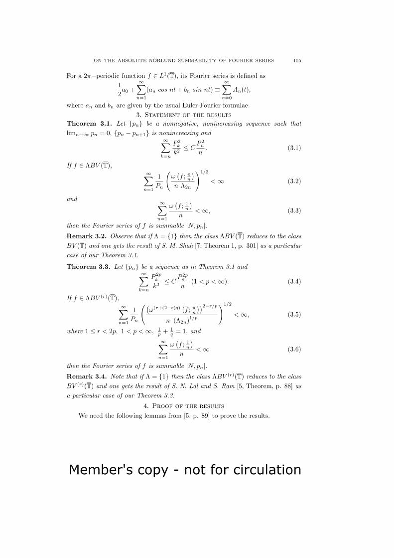
Member's copy - not for circulation
ON THE ABSOLUTE NORLUND SUMMABILITY OF FOURIER SERIES 155
For a 2π−periodic function f ∈ L1(T), its Fourier series is defined as
1
2a0 +
∞∑n=1
(an cos nt+ bn sin nt) ≡∞∑n=0
An(t),
where an and bn are given by the usual Euler-Fourier formulae.
3. Statement of the results
Theorem 3.1. Let pn be a nonnegative, nonincreasing sequence such that
limn→∞ pn = 0, pn − pn+1 is nonincreasing and∞∑k=n
P 2k
k2≤ CP
2n
n. (3.1)
If f ∈ ΛBV (T),∞∑n=1
1
Pn
(ω(f ; πn
)n Λ2n
)1/2
<∞ (3.2)
and∞∑n=1
ω(f ; 1
n
)n
<∞, (3.3)
then the Fourier series of f is summable |N, pn|.Remark 3.2. Observe that if Λ = 1 then the class ΛBV (T) reduces to the class
BV (T) and one gets the result of S. M. Shah [7, Theorem 1, p. 301] as a particular
case of our Theorem 3.1.
Theorem 3.3. Let pn be a sequence as in Theorem 3.1 and∞∑k=n
P 2pk
k2≤ CP
2pn
n(1 < p <∞). (3.4)
If f ∈ ΛBV (r)(T),∞∑n=1
1
Pn
((ω(r+(2−r)q) (f ; πn
))2−r/pn (Λ2n)
1/p
)1/2
<∞, (3.5)
where 1 ≤ r < 2p, 1 < p <∞, 1p + 1
q = 1, and
∞∑n=1
ω(f ; 1
n
)n
<∞ (3.6)
then the Fourier series of f is summable |N, pn|.Remark 3.4. Note that if Λ = 1 then the class ΛBV (r)(T) reduces to the class
BV (r)(T) and one gets the result of S. N. Lal and S. Ram [5, Theorem, p. 88] as
a particular case of our Theorem 3.3.
4. Proof of the results
We need the following lemmas from [5, p. 89] to prove the results.
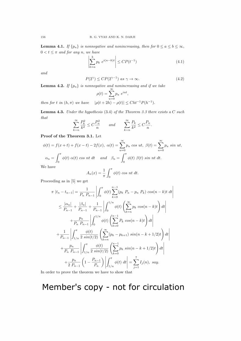
Member's copy - not for circulation
156 R. G. VYAS AND K. N. DARJI
Lemma 4.1. If pn is nonnegative and nonincreasing, then for 0 ≤ a ≤ b ≤ ∞,0 < t ≤ π and for any n, we have∣∣∣∣∣
b∑k=a
pk ei(n−k)t
∣∣∣∣∣ ≤ CP (t−1) (4.1)
and
P (2γ) ≤ CP (2γ−1) as γ →∞. (4.2)
Lemma 4.2. If pn is nonnegative and nonincreasing and if we take
ρ(t) =∞∑u=0
pu eiut,
then for t in (h, π) we have |ρ(t+ 2h)− ρ(t)| ≤ Cht−1P (h−1).
Lemma 4.3. Under the hypothesis (3.4) of the Theorem 3.3 there exists a C such
that∞∑k=n
P 2k
k2≤ CP
2n
nand
∞∑k=n
Pkk2≤ CPn
n.
Proof of the Theorem 3.1. Let
φ(t) = f(x+ t) + f(x− t)− 2f(x), α(t) =
∞∑u=0
pu cos ut, β(t) =
∞∑u=0
pu sin ut,
αn =
∫ π
0
φ(t) α(t) cos nt dt and βn =
∫ π
0
φ(t) β(t) sin nt dt.
We have
An(x) =1
π
∫ π
0
φ(t) cos nt dt.
Proceeding as in [5] we get
π |tn − tn−1| =1
Pn Pn−1
∣∣∣∣∣∫ π
0
φ(t)n−1∑k=0
(pk Pn − pn Pk) cos(n− k)t dt
∣∣∣∣∣≤ |αn|Pn−1
+|βn|Pn−1
+1
Pn−1
∣∣∣∣∣∫ 1/n
0
φ(t)
( ∞∑k=n
pk cos(n− k)t
)dt
∣∣∣∣∣+
pnPn Pn−1
∣∣∣∣∣∫ 1/n
0
φ(t)
(n−1∑k=0
Pk cos(n− k)t
)dt
∣∣∣∣∣+
1
Pn−1
∣∣∣∣∣∫ π
1/n
φ(t)
2 sin(t/2)
( ∞∑k=n
(pk − pk+1) sin(n− k + 1/2)t
)dt
∣∣∣∣∣+
pnPn Pn−1
∣∣∣∣∣∫ π
1/n
φ(t)
2 sin(t/2)
(n−1∑k=0
pk sin(n− k + 1/2)t
)dt
∣∣∣∣∣+
pn2 Pn−1
(1− Pn−1
Pn
) ∣∣∣∣∣∫ π
1/n
φ(t) dt
∣∣∣∣∣ =7∑j=1
Ij(n), say.
In order to prove the theorem we have to show that

Member's copy - not for circulation
ON THE ABSOLUTE NORLUND SUMMABILITY OF FOURIER SERIES 157
∞∑n=2
Ij(n) <∞, for j = 1 to 7.
Under the hypotheses of the theorem α(t) ∈ L2 and as f ∈ ΛBV (T) is bounded,
φ is bounded, and hence φ(t)α(t) ∈ L2.
Since the Fourier series of φ(t+ h)α(t+ h)− φ(t− h)α(t− h) is
− 4
π
∞∑n=1
αn sin nt sin nh,
in view of Parseval’s formula we get
∞∑n=1
|αn sin nh|2 ≤ C∫ π
0
|φ(t+ h)α(t+ h)− φ(t− h)α(t− h)|2dt
≤ C∫ π
0
α2(t+ h)|φ(t+ h)− φ(t− h)|2dt+ C
∫ h
−hφ2(t)α2(t+ 2h) dt
+ C
∫ h
−hφ2(t)α2(t) dt+ C
∫ π
h
φ2(t)|α(t+ 2h)− α(t)|2dt
=4∑j=1
Tj(h), say. (4.3)
Take
∆φk = φ
(t+
kπ
N
)− φ
(t+
(k − 1)π
N
).
Now (cf, [5, p. 92]) we get∫ π
0
α2(t+
π
2N
) ∣∣∣φ(t+π
2N
)− φ
(t− π
2N
)∣∣∣2 dt=
∫ π
0
α2(t+
π
N
) ∣∣∣φ(t+π
N
)− φ (t)
∣∣∣2 dt
≤ ω(f ;
π
N
)∫ π
0
α2(t+
π
N
) ∣∣∣φ(t+π
N
)− φ (t)
∣∣∣ dt=
(ω(f ; πN
)Λ2N
)2N∑k=1
1
λk
∫ π
0
α2
(t+
kπ
N
)|∆φk| dt
≤ C
(ω(f ; πN
)Λ2N
)[1 +
∞∑k=1
P 2k
k2
].
Thus,T1
( π
2N
)≤ C
(ω(f ; πN
)Λ2N
).
By Lemma 4.1,
T2(h) ≤ C∫ h
−hω2(t)P 2
(1
t+ 2h
)dt ≤ Chω2(h)P 2(h−1), (4.4)

Member's copy - not for circulation
158 R. G. VYAS AND K. N. DARJI
and
T3(h) ≤ Cω2(h)
∫ ∞1/h
P 2(t)
t2dt ≤ Chω2(h)P 2(h−1), (4.5)
in view of (3.1). By Lemma 4.2,
T4(h) ≤ Ch2P 2(h−1)
∫ 1/h
1/π
ω2(t−1)dt. (4.6)
Taking h = π2N in (4.3), we have∞∑n=1
|αn|2 ≤ C[(ω (f ; πN
)Λ2N
)+N−1ω2
( π
2N
)P 2
(2N
π
)
+N−2P 2
(2N
π
)∫ 2N/π
1/π
ω2(t−1) dt].
Putting N = 2u, we get 2u∑n=2u−1+1
|αn|21/2
≤ C
(ω (f ; π2u
)Λ2u+1
)1/2
+ C
2−uP
(2u+1
π
)(∫ 2u+1/π
1/π
ω2(t−1) dt
)1/2 .
Now, by Holder’s inequality and making use of (4.2) of Lemma 4.1, we get
2u∑n=2u−1+1
|αn|Pn−1
≤
2u∑n=2u−1+1
|αn|21/2 2u∑
n=2u−1+1
P−2n−1
1/2
≤ C
2u/2
P (2u)
(ω(f ; π
2u
)Λ2u+1
)1/2
+ 2−u/2
(∫ 2u+1/π
1/π
ω2(t−1) dt
)1/2
and therefore∞∑n=2
I1(n) =∞∑u=1
2u∑n=2u−1+1
|αn|Pn−1
≤ C∞∑u=1
2u/2
P (2u)
(ω(f ; π
2u
)Λ2u+1
)1/2
+ C∞∑u=1
2−u/2
(∫ 2u+1/π
1/π
ω2(t−1) dt
)1/2
≤ C∞∑n=1
1
Pn
(ω(f ; πn
)n Λ2n
)1/2
+ C
∞∑u=1
2−u/2 + C
∞∑u=1
2−u/2
(2u∑k=2
ω2(k−1)
)1/2
≤ C + C∞∑u=1
2−u/2u∑
m=1
2m∑n=2m−1+1
ω2(k−1)
1/2
≤ C + C
∞∑m=1
2m/2ω(1/2m)
∞∑u=m
2−u/2 ≤ C + C
∞∑m=1
ω(1/2m) <∞,

Member's copy - not for circulation
ON THE ABSOLUTE NORLUND SUMMABILITY OF FOURIER SERIES 159
by the hypothesis (3.2) and (3.3) of the theorem. Similarly we can prove that∑∞n=2 I2(n) <∞. Finally,
∞∑n=2
Ij(n) <∞ (j = 3 to 7)
follows from the proof of [5, Theorem] and hence the result follows.
Proof of the Theorem 3.3: Since f ∈ ΛBV (r)(T) is bounded implies φ is
bounded and hence φ ∈ L2. Proceeding as in the proof of the Theorem 3.1, we
get (4.3). Take
∆φk = φ(t+ kπ/N)− φ(t+ (k − 1)π/N).
Since
2 = ((2− r)q + r)/q + r/p,
by using Holder’s inequality, we obtain∫ π
0
α2(t+
π
2N
) ∣∣∣φ(t+π
2N
)− φ
(t− π
2N
)∣∣∣2 dt=
∫ π
0
α2(t+
π
N
) ∣∣∣φ(t+π
N
)− φ (t)
∣∣∣2 dt=
∫ π
0
α2
(t+
kπ
N
)|∆φk|2 dt
≤(∫ π
0
α2p
(t+
kπ
N
)|∆φk|r dt
)1/p
×(∫ π
0
|∆φk|(2−r)q+r dt)1/q
≤(ω((2−r)q+r)
(f ;
π
N
))2−r/p(∫ π
0
α2p
(t+
kπ
N
)|∆φk|r dt
)1/p
=(ω((2−r)q+r)
(f ;
π
N
))2−r/p∑2N
k=11λk
(∫ π0α2p
(t+ kπ
N
)|∆φk|r dt
)1/pΛ2N
≤(ω((2−r)q+r)
(f ;
π
N
))2−r/p×
(∑2Nk=1
1λk
∫ π0α2p
(t+ kπ
N
)|∆φk|r dt
)1/p
(Λ2N )1−1/p
Λ2N
≤(ω((2−r)q+r) (f ; πN
))2−r/p(Λ2N )1/p
( 2N∑k=1
1
λk
∫ π
0
α2p
(t+
kπ
N
)|∆φk|r dt
)1/p
≤ C(ω((2−r)q+r) (f ; πN
))2−r/p(Λ2N )1/p
[1 +
∞∑k=1
P 2pk
k2
]1/p
.
Thus,
I1
( π
2N
)≤ C
(ω((2−r)q+r) (f ; πN
))2−r/p(Λ2N )1/p
.

Member's copy - not for circulation
160 R. G. VYAS AND K. N. DARJI
Now, proceeding as in the proof of the Theorem 3.1 (from (4.4) onward), we obtain
the theorem.
References
[1] Dikshit, H. P., Absolute summability of a Fourier series by Norlund means, Mathematische
Zeitschrift, 102 (2) (1967), 166–170.
[2] Hyslop, J. M., On the absolute summability of Fourier series, Proc. London Math. Soc., 43
(1937), 475–483.
[3] Izumi, M. and Izumi, I., Norlund summability of Fourier series, Pacific J. Math., 26 (1968),
289–301.
[4] Lal, S. N., On the theorem of M. Izumi and S. Izumi, Pacific J. Math., 35 (1970), 661–667.
[5] Lal, S. N. and Ram, S., The absolute summability of Fourier series of a function of Wiener’s
class by Norlund means, Proc. Amer. Math. Soc., 67 (1) (1977), 87–94.
[6] McFadden, L., Absolute Norlund summability, Duke Math. J., 9 (1942), 168–207.
[7] Shah, S. M., Absolute Norlund summability of Fourier series, Tuhoku Math. J., 24 (1972),
309–318.
[8] Vyas, R. G., On the absolute convergence of Fourier series of functions of ΛBV (p) and
ϕΛBV , Georgian Math. J., 14 (4) (2007), 769–774.
[9] Vyas, R. G. and Patadia, J. R., On the absolute convergence of Fourier series of functions
of generalized bounded variations, J. Indian Math. Soc., 62 (1- 4) (1996), 129–136.
R. G. Vyas
Department of Mathematics, Faculty of Science,
The Maharaja Sayajirao University of Baroda
Vadodara-390 002, Gujarat, India.
Email :[email protected]
K. N. Darji
Department of Science and Humanities,
Tatva Institute of Technological Studies
Modasa-, Aravalli, Gujarat, India.
Email: [email protected]
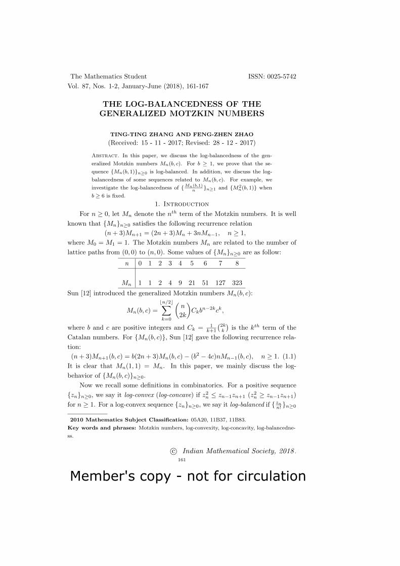
Member's copy - not for circulation
The Mathematics Student ISSN: 0025-5742
Vol. 87, Nos. 1-2, January-June (2018), 161-167
THE LOG-BALANCEDNESS OF THEGENERALIZED MOTZKIN NUMBERS
TING-TING ZHANG AND FENG-ZHEN ZHAO
(Received: 15 - 11 - 2017; Revised: 28 - 12 - 2017)
Abstract. In this paper, we discuss the log-balancedness of the gen-
eralized Motzkin numbers Mn(b, c). For b ≥ 1, we prove that the se-
quence Mn(b, 1)n≥0 is log-balanced. In addition, we discuss the log-
balancedness of some sequences related to Mn(b, c). For example, we
investigate the log-balancedness of Mn(b,1)nn≥1 and M2
n(b, 1) when
b ≥ 6 is fixed.
1. Introduction
For n ≥ 0, let Mn denote the nth term of the Motzkin numbers. It is well
known that Mnn≥0 satisfies the following recurrence relation
(n+ 3)Mn+1 = (2n+ 3)Mn + 3nMn−1, n ≥ 1,
where M0 = M1 = 1. The Motzkin numbers Mn are related to the number of
lattice paths from (0, 0) to (n, 0). Some values of Mnn≥0 are as follow:
n 0 1 2 3 4 5 6 7 8
Mn 1 1 2 4 9 21 51 127 323
Sun [12] introduced the generalized Motzkin numbers Mn(b, c):
Mn(b, c) =
bn/2c∑k=0
(n
2k
)Ckb
n−2kck,
where b and c are positive integers and Ck = 1k+1
(2kk
)is the kth term of the
Catalan numbers. For Mn(b, c), Sun [12] gave the following recurrence rela-
tion:
(n+ 3)Mn+1(b, c) = b(2n+ 3)Mn(b, c)− (b2 − 4c)nMn−1(b, c), n ≥ 1. (1.1)
It is clear that Mn(1, 1) = Mn. In this paper, we mainly discuss the log-
behavior of Mn(b, c)n≥0.
Now we recall some definitions in combinatorics. For a positive sequence
znn≥0, we say it log-convex (log-concave) if z2n ≤ zn−1zn+1 (z2n ≥ zn−1zn+1)
for n ≥ 1. For a log-convex sequence znn≥0, we say it log-balanced if znn! n≥0
2010 Mathematics Subject Classification: 05A20, 11B37, 11B83.
Key words and phrases: Motzkin numbers, log-convexity, log-concavity, log-balancedne-
ss.
c© Indian Mathematical Society, 2018 .
161

Member's copy - not for circulation
162 TING-TING ZHANG AND FENG-ZHEN ZHAO
is log-concave (Doslic [3] gave this definition). It is well known that znn≥0 is
log-convex (log-concave) if and only if its quotient sequence zn+1
znn≥0 is non-
decreasing (nonincreasing) and a log-convex sequence znn≥0 is log-balanced
if and only if (n+1)znzn−1
≥ nzn+1
znfor each n ≥ 1. It is clear that log-balancedness
is a special case of log-convexity and the quotient sequence of a log-balanced
sequence does not grow too fast. Log-behavior is not only one of the sources for
inequalities, but also plays an important role in many disciplines. Log-concave
sequences often occur in combinatorics, algebra, and geometry. For instance,
the binomial coefficient(nk
)is log-concave for k when n ≥ 2 is fixed. See [2]
for various results of log-concavity. Log-convexity of sequences and functions
is relevant in many subjects such as combinatorics, economics, mathematical
biology, and physics. Many famous combinatorial sequences including Catalan
numbers, Motzkin numbers, Fine numbers, large Schroder numbers, and cen-
tral Delannoy numbers, are log-convex. Log-convexity of a bond price means
that the relative decline is decreasing when the interest rate grows. In finance,
it was found that log-convexity of the discount function is equivalent to the de-
creased impatience. Log-convex sequences arise as the enumerating sequences
of secondary structures of certain biopolymers. For various applications of
log-behavior, see [1, 2, 4, 5, 6, 7, 8, 9, 10, 11]. We note that log-balanced se-
quences are suitable for providing important examples in white noise theory
(See [7] for more details). In addition, since log-balancedness is related to log-
convexity and log-concavity, it can help us to obtain more inequalities. Hence,
log-balancedness of sequences deserves to be studied. Doslic [3] gave several
sufficient conditions for log-balancedness and proved log-balancedness of many
sequences including Motzkin numbers, Fine numbers, large Schroder numbers,
central Delannoy numbers, and so on.
Some recurrences of general secondary structure numbers are analogous to
those for the Motzkin numbers (See Doslic [6] for more details). From the log-
balancedness of Motzkin numbers, we can know properties for the growth rate
of secondary structure numbers. Hence, it is useful studying log-balancedness of
Motzkin numbers. Doslic [3] showed that Mnn≥0 is log-balanced. Motivated
by the article Doslic [3], we consider log-balancedness of Mn(b, c)n≥0. In the
next section, we discuss log-balancedness of Mn(b, 1)n≥0. In addition, we
also investigate log-balancedness of some sequences related to Mn(b, 1)n≥0.
2. The log-balancedness of Mn(b, 1)n≥0Doslic [3] proved that the sequence Mnn≥0 is log-balanced. In this sec-
tion, we discuss the log-balancedness of Mn(b, 1)n≥0. The following lemmas
will be used.
Lemma 2.1. Assume that b ≥ 1. For n ≥ 0, let xn = Mn+1(b,1)Mn(b,1)
. When b ≥ 3,
we have
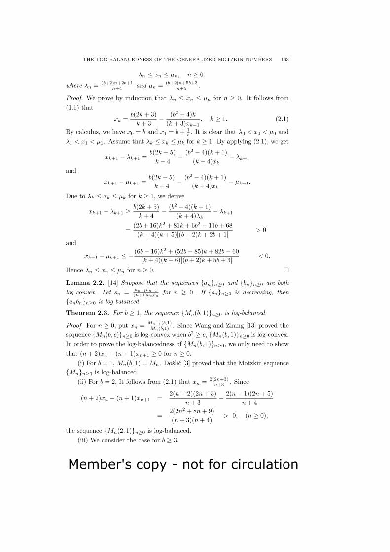
Member's copy - not for circulation
THE LOG-BALANCEDNESS OF THE GENERALIZED MOTZKIN NUMBERS 163
λn ≤ xn ≤ µn, n ≥ 0
where λn = (b+2)n+2b+1n+4 and µn = (b+2)n+5b+3
n+5 .
Proof. We prove by induction that λn ≤ xn ≤ µn for n ≥ 0. It follows from
(1.1) that
xk =b(2k + 3)
k + 3− (b2 − 4)k
(k + 3)xk−1, k ≥ 1. (2.1)
By calculus, we have x0 = b and x1 = b+ 1b . It is clear that λ0 < x0 < µ0 and
λ1 < x1 < µ1. Assume that λk ≤ xk ≤ µk for k ≥ 1. By applying (2.1), we get
xk+1 − λk+1 =b(2k + 5)
k + 4− (b2 − 4)(k + 1)
(k + 4)xk− λk+1
and
xk+1 − µk+1 =b(2k + 5)
k + 4− (b2 − 4)(k + 1)
(k + 4)xk− µk+1.
Due to λk ≤ xk ≤ µk for k ≥ 1, we derive
xk+1 − λk+1 ≥b(2k + 5)
k + 4− (b2 − 4)(k + 1)
(k + 4)λk− λk+1
=(2b+ 16)k2 + 81k + 6b2 − 11b+ 68
(k + 4)(k + 5)[(b+ 2)k + 2b+ 1]> 0
and
xk+1 − µk+1 ≤ −(6b− 16)k2 + (52b− 85)k + 82b− 60
(k + 4)(k + 6)[(b+ 2)k + 5b+ 3]< 0.
Hence λn ≤ xn ≤ µn for n ≥ 0.
Lemma 2.2. [14] Suppose that the sequences ann≥0 and bnn≥0 are both
log-convex. Let sn = an+1bn+1
(n+1)anbnfor n ≥ 0. If snn≥0 is decreasing, then
anbnn≥0 is log-balanced.
Theorem 2.3. For b ≥ 1, the sequence Mn(b, 1)n≥0 is log-balanced.
Proof. For n ≥ 0, put xn = Mn+1(b,1)Mn(b,1)
. Since Wang and Zhang [13] proved the
sequence Mn(b, c)n≥0 is log-convex when b2 ≥ c, Mn(b, 1)n≥0 is log-convex.
In order to prove the log-balancedness of Mn(b, 1)n≥0, we only need to show
that (n+ 2)xn − (n+ 1)xn+1 ≥ 0 for n ≥ 0.
(i) For b = 1, Mn(b, 1) = Mn. Doslic [3] proved that the Motzkin sequence
Mnn≥0 is log-balanced.
(ii) For b = 2, It follows from (2.1) that xn = 2(2n+3)n+3 . Since
(n+ 2)xn − (n+ 1)xn+1 =2(n+ 2)(2n+ 3)
n+ 3− 2(n+ 1)(2n+ 5)
n+ 4
=2(2n2 + 8n+ 9)
(n+ 3)(n+ 4)> 0, (n ≥ 0),
the sequence Mn(2, 1)n≥0 is log-balanced.
(iii) We consider the case for b ≥ 3.

Member's copy - not for circulation
164 TING-TING ZHANG AND FENG-ZHEN ZHAO
It follows from (2.1) that
(n+ 2)xn − (n+ 1)xn+1
=(n+ 2)(n+ 4)x2n − b(n+ 1)(2n+ 5)xn + (b2 − 4)(n+ 1)2
(n+ 4)xn.
For any real number t, define a function
f(t) = (n+ 2)(n+ 4)t2 − b(n+ 1)(2n+ 5)t+ (b2 − 4)(n+ 1)2.
It is evident that
(n+ 2)xn − (n+ 1)xn+1 = f(xn)/((n+ 2)xn).
Since f ′(t) > 0 for t > ρn, where ρn = b(n+1)(2n+5)2(n+2)(n+4) , f(t) is increasing on
[ρn,+∞). It follows from Lemma 2.1 that xn ≥ λn, where λn = (b+2)n+2b+1n+4 .
Since λn ≥ ρn, f(t) is increasing on [λn,+∞). We note that
f(λn) =(n+ 2)[(b+ 2)n+ 2b+ 1]2 − b(n+ 1)(2n+ 5)[(b+ 2)n+ 2b+ 1]
n+ 4
+(b2 − 4)(n+ 1)2
=(b2 + 2b− 12)n2 + (2b2 + 7b− 27)n+ 2b2 + 3b− 14
n+ 4> 0.
Since f(xn) ≥ f(λn), f(xn) > 0. This implies that (n+2)xn−(n+1)xn+1 > 0.
Hence the sequence Mn(b, 1)n≥0 is log-balanced.
Zhao [15] proved that the sequence Mn
n n≥4 is log-balanced. Zhang and
Zhao [14] showed that M2nn≥2 is also log-balanced. Now we discuss the log-
balancedness of Mn(b,1)n n≥1 and M2
n(b, 1)n≥0 by Lemma 2.2.
Theorem 2.4. Suppose that b ≥ 1 is fixed.
(i) For b ≥ 3, there exists a positive integer Lb such that Mn(b,1)n n≥Lb
is
log-balanced.
(ii) For b ≥ 6, there exists a positive integer Nb such that the sequence
M2n(b, 1)n≥Nb
is log-balanced.
Proof. For n ≥ 0, let xn = Mn+1(b,1)Mn(b,1)
and yn = nxn
(n+1)2 (n ≥ 1). It is clear that
the sequences 1nn≥1 and Mn(b, 1)n≥0 (b ≥ 1) are both log-convex. In order
to prove the log-concavity of Mn(b,1)nn! n≥1 and M
2n(b,1)n! n≥0, it is sufficient to
show that ynn≥1 is decreasing and (n + 2)x2n − (n + 1)x2n+1 ≥ 0 holds for
n ≥ 0.
(i) It is clear that
yn − yn+1 =n(n+ 2)2xn − (n+ 1)3xn+1
(n+ 1)2(n+ 2)2.
It follows from (2.1) that
n(n+ 2)2xn − (n+ 1)3xn+1
= n(n+ 2)2xn − (n+ 1)3b(2n+ 5)xn − (b2 − 4)(n+ 1)
(n+ 4)xn
=n(n+ 4)(n+ 2)2x2n − b(2n+ 5)(n+ 1)3xn + (b2 − 4)(n+ 1)4
(n+ 4)xn.
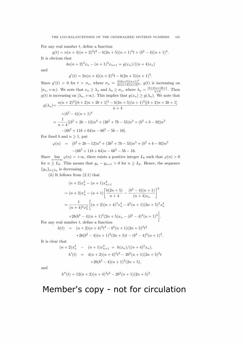
Member's copy - not for circulation
THE LOG-BALANCEDNESS OF THE GENERALIZED MOTZKIN NUMBERS 165
For any real number t, define a function
g(t) = n(n+ 4)(n+ 2)2t2 − b(2n+ 5)(n+ 1)3t+ (b2 − 4)(n+ 1)4.
It is obvious that
4n(n+ 2)2xn − (n+ 1)3xn+1 = g(xn)/((n+ 4)xn)
and
g′(t) = 2n(n+ 4)(n+ 2)2t− b(2n+ 5)(n+ 1)3.
Since g′(t) > 0 for t > σn, where σn = b(2n+5)(n+1)3
2n(n+4)(n+2)2 , g(t) is increasing on
[σn,+∞). We note that xn ≥ λn and λn ≥ σn, where λn = (b+2)n+2b+1n+4 . Then
g(t) is increasing on [λn,+∞). This implies that g(xn) ≥ g(λn). We note that
g(λn)=n(n+ 2)2[(b+ 2)n+ 2b+ 1]2 − b(2n+ 5)(n+ 1)3[(b+ 2)n+ 2b+ 1]
n+ 4
+(b2 − 4)(n+ 1)4
=1
n+ 4[(b2 + 2b− 12)n4 + (3b2 + 7b− 55)n3 + (b2 + b− 92)n2
−(6b2 + 11b+ 64)n− 6b2 − 5b− 16].
For fixed b and n ≥ 1, put
ϕ(n) = (b2 + 2b− 12)n4 + (3b2 + 7b− 55)n3 + (b2 + b− 92)n2
−(6b2 + 11b+ 64)n− 6b2 − 5b− 16.
Since limn→+∞
ϕ(n) = +∞, there exists a positive integer Lb such that ϕ(n) > 0
for n ≥ Lb. This means that yn − yn+1 > 0 for n ≥ Lb. Hence, the sequence
ynn≥Lbis decreasing.
(ii) It follows from (2.1) that
(n+ 2)x2n − (n+ 1)x2n+1
= (n+ 2)x2n − (n+ 1)
[b(2n+ 5)
n+ 4− (b2 − 4)(n+ 1)
(n+ 4)xn
]2=
1
(n+ 4)2x2n
[(n+ 2)(n+ 4)2x4n − b2(n+ 1)(2n+ 5)2x2n
+2b(b2 − 4)(n+ 1)2(2n+ 5)xn − (b2 − 4)2(n+ 1)3].
For any real number t, define a function
h(t) = (n+ 2)(n+ 4)2t4 − b2(n+ 1)(2n+ 5)2t2
+2b(b2 − 4)(n+ 1)2(2n+ 5)t− (b2 − 4)2(n+ 1)3.
It is clear that
(n+ 2)x2n − (n+ 1)x2n+1 = h(xn)/((n+ 4)2xn),
h′(t) = 4(n+ 2)(n+ 4)2t3 − 2b2(n+ 1)(2n+ 5)2t
+2b(b2 − 4)(n+ 1)2(2n+ 5),
and
h′′(t) = 12(n+ 2)(n+ 4)2t2 − 2b2(n+ 1)(2n+ 5)2.
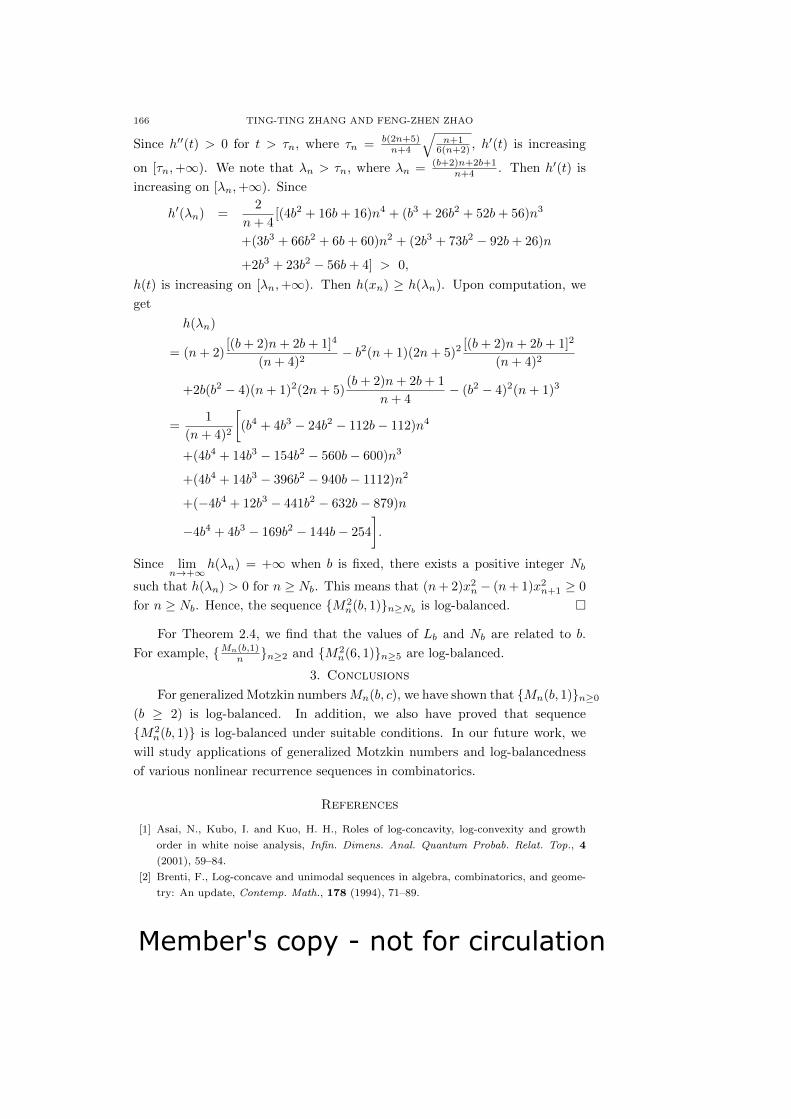
Member's copy - not for circulation
166 TING-TING ZHANG AND FENG-ZHEN ZHAO
Since h′′(t) > 0 for t > τn, where τn = b(2n+5)n+4
√n+1
6(n+2) , h′(t) is increasing
on [τn,+∞). We note that λn > τn, where λn = (b+2)n+2b+1n+4 . Then h′(t) is
increasing on [λn,+∞). Since
h′(λn) =2
n+ 4[(4b2 + 16b+ 16)n4 + (b3 + 26b2 + 52b+ 56)n3
+(3b3 + 66b2 + 6b+ 60)n2 + (2b3 + 73b2 − 92b+ 26)n
+2b3 + 23b2 − 56b+ 4] > 0,
h(t) is increasing on [λn,+∞). Then h(xn) ≥ h(λn). Upon computation, we
get
h(λn)
= (n+ 2)[(b+ 2)n+ 2b+ 1]4
(n+ 4)2− b2(n+ 1)(2n+ 5)2
[(b+ 2)n+ 2b+ 1]2
(n+ 4)2
+2b(b2 − 4)(n+ 1)2(2n+ 5)(b+ 2)n+ 2b+ 1
n+ 4− (b2 − 4)2(n+ 1)3
=1
(n+ 4)2
[(b4 + 4b3 − 24b2 − 112b− 112)n4
+(4b4 + 14b3 − 154b2 − 560b− 600)n3
+(4b4 + 14b3 − 396b2 − 940b− 1112)n2
+(−4b4 + 12b3 − 441b2 − 632b− 879)n
−4b4 + 4b3 − 169b2 − 144b− 254
].
Since limn→+∞
h(λn) = +∞ when b is fixed, there exists a positive integer Nb
such that h(λn) > 0 for n ≥ Nb. This means that (n+ 2)x2n − (n+ 1)x2n+1 ≥ 0
for n ≥ Nb. Hence, the sequence M2n(b, 1)n≥Nb
is log-balanced.
For Theorem 2.4, we find that the values of Lb and Nb are related to b.
For example, Mn(b,1)n n≥2 and M2
n(6, 1)n≥5 are log-balanced.
3. Conclusions
For generalized Motzkin numbersMn(b, c), we have shown that Mn(b, 1)n≥0(b ≥ 2) is log-balanced. In addition, we also have proved that sequence
M2n(b, 1) is log-balanced under suitable conditions. In our future work, we
will study applications of generalized Motzkin numbers and log-balancedness
of various nonlinear recurrence sequences in combinatorics.
References
[1] Asai, N., Kubo, I. and Kuo, H. H., Roles of log-concavity, log-convexity and growth
order in white noise analysis, Infin. Dimens. Anal. Quantum Probab. Relat. Top., 4
(2001), 59–84.
[2] Brenti, F., Log-concave and unimodal sequences in algebra, combinatorics, and geome-
try: An update, Contemp. Math., 178 (1994), 71–89.
Member's copy - not for circulation
THE LOG-BALANCEDNESS OF THE GENERALIZED MOTZKIN NUMBERS 167
[3] Doslic, T., Log-balanced combinatorial sequences, Int. J. Math. Math. Sci., 4 (2005),
507–522.
[4] Doslic, T., Seven (lattice) paths to log-convexity, Acta Appl. Math., 110 (2010), 1373–
1392.
[5] Doslic, T., Svrtan, D. and Veljan, D., Enumerative aspects of secondary structures,
Discrete Math., 285 (2004), 67–82.
[6] Doslic, T. and Veljan, D., Logarithmic behavior of some combinatorial sequences, Dis-
crete Math., 308 (2008), 2182–2212.
[7] Kuo, H. H., White Noise Distribution Theory, CRC Press, 1996.
[8] Milenkovic, O. and Compton, K. J., Probabilistic transforms for combinatorial urn mod-
els, Combin. Probab. Comput., 13 (2004), 645–675.
[9] Prelec, D., Decreasing impatience: A criterion for non-stationary time preference and
“hyperbolic” discounting, Scand. J. Econ., 106 (2004), 511–532.
[10] Stanley, R. P., Enumerative Combinatorics, Vol. 2, Cambridge University Press, 1999.
[11] Stanley, R. P., Log-concave and unimodal sequences in algebra, combinatorics, and
geometry, Ann.New York Acad. Sci., 576 (1989), 500–535.
[12] Sun, Z. W., Congruences involving generalized central trinomial coefficients, Sci. China.
Math., 57 (2014), 1375–1400.
[13] Wang, Y. and Zhang, Z. H., Combinatorics of generalized Motzkin numbers, J. Integer
Seq., 18 (2015), Article 15.2.4.
[14] Zhang, T. T. and Zhao, F. Z., Some sufficient conditions for log-balancedness of combi-
natorial sequences, J. Integer Seq., 19 (2015), Article 16.6.8.
[15] Zhao, F. Z., The log-balancedness of combinatorial sequences, Sarajevo J. Math., 11
(2015), 141–154.
Ting-Ting Zhang
Department of Mathematics, Shanghai University
Shanghai 200444, P. R. China.
E-mail: [email protected]
Feng-Zhen Zhao
Department of Mathematics, Shanghai University
Shanghai 200444, P. R. China.
E-mail: [email protected]

Member's copy - not for circulation
168

Member's copy - not for circulation
The Mathematics Student ISSN: 0025-5742
Vol. 87, Nos. 1-2, January-June, (2018), 169-173
PROBLEM SECTION
In the last issue of the Math. Student Vol. 86, Nos. 3-4, July-December
(2017), we had invited solutions from the floor to the remaining problems 2 and
5 of the MS, 86, 1-2, 2017 as well as to the seven new problems 6, 7, 8, 9, 10, 11
and 12 presented therein till April 30, 2018.
No solution was received from the floor to the remaining problems 2 and 5 of
the MS, 86, 1-2, 2017 and hence we provide in this issue the Proposer’s solution
to these problems.
The status regarding the problems of MS, 86, 3-4, 2017 is as under.
1. We received from the floor four correct solutions to problem 7 and publish
here the solution from the floor which also states and proves a generalized version
of the problem;
2. We received from the floor one incorrect solution to the Problems 8 and
10; and two comments correctly pointing out that “some extra condition is required
in Pr-10 ”, and hence we now provide here the corrected version of Pr-10. Readers
can try their hand on both these problems till April 30, 2018.
3. We received from the floor one incomplete solution to problem 11. Read-
ers can try their hand on this till April 30, 2018.
4. We also received two correct solutions to the problem 12 and publish here
one of them.
5. No solutions were received from the floor to the remaining problems 6
and 9. Readers can try their hand on these till April 30, 2018.
In this issue we first present six new problems. Solutions to these problems as
also to the remaining problems 6, 8, 9, 10, and 11 of MS, 86, 3-4, 2017, received
from the floor till October 31, 2018, if approved by the Editorial Board, will be
published in the MS, 87, 3-4, 2018.
Problems proposed by B. Sury
MS-2018, Nos. 1-2: Problem-1:
Find the largest possible diameter of a circular hole that can be covered
by two square boards of unit area.
MS-2018, Nos. 1-2: Problem-2:
Find a characterization of the positive integers m such that Sn has an
element of order m.
© Indian Mathematical Society, 2018 .
169

Member's copy - not for circulation
170 PROBLEM SECTION
MS-2018, Nos. 1-2: Problem-3:
Consider a convex polygon of n sides. Draw n − 3 diagonals which do
not intersect inside. Then, the polygon is broken into n − 2 triangles. Let
ai be the number of those triangles formed which have Pi as vertex. For
instance, for n = 6, one may draw diagonals P1P3, P1P4 and P1P5. in this
case, (a1, a2, a3, a4, a5, a6) = (4, 1, 2, 2, 2, 1). Notice that 4 − 11− 1
2− 12− 1
2
= 0.
Prove that in general,
a1 −1
a2 − 1a3− 1
···− 1an−1
= 0.
MS-2018, Nos. 1-2: Problem-4:
Find with proof, the unique solution to the following multiplication table
where each digit 0 to 9 is repeated twice :
∗ ∗ ∗× ∗ ∗ ∗
∗ ∗ ∗∗ ∗ ∗
∗ ∗ ∗
∗ ∗ ∗ ∗ ∗
MS-2018, Nos. 1-2: Problem-5:
A spider starts crawling along an elastic rope at the rate of 1 foot per
second. Initially, the elastic rope is f feet long and at the end of each second,
it is stretched uniformly by f feet. Does the spider ever reach the other end
of the rope?
MS-2018, Nos. 1-2: Problem-6: Proposed by George E. Andrews.
Prove that PO2(n), the number of partitions of n in which each odd part
appears at most twice, must be even if n ≡ 2 or 3(mod4). For example, there
are 8 such partitions of 6, namely, 6, 5 + 1, 4 + 2, 4 + 1 + 1, 3 + 3, 3 + 2 +
1, 2 + 2 + 2, 2 + 2 + 1 + 1; and 6 ≡ 2(mod4).
MS-2017, Nos. 3-4: Problem-10. (corrected version):
Show that there does not exist a symmetric matrix over rational numbers
whose characteristic polynomial is X2 − 3.

Member's copy - not for circulation
PROBLEM SECTION 171
Solution from the floor: MS-2017, Nos. 3-4: Problem 7: Evaluate∫ π/2
0
dx
1 + (tanx)√3.
(Solution submitted on 30-11-2017 by Dasari Naga Vijay Krishna, Machilipat-
nam, Andhra Pradesh-521001; [email protected]).
Solution. Denote the given integral by I. Using∫ baf(x)dx =
∫ baf(a + b − x)dx,
we get
I =
∫ π/2
0
(tanx)√3dx
1 + (tanx)√3.
Adding this to given integral we obtain 2I = π/2. Hence I = π/4.
Actually the given integral is a particular case of the following general fact:
Let a < b and f : [a, b] → R be a continuous fucntion such that f(a + b − x) =
1/f(x), f(x) 6= 0, for all x in (a, b). Then for all real exponents k, we have∫ b
a
dx
1 + f(x)k=b− a
2.
Here a = 0, b = π/2, f(x) = tanx and k =√
3; hence I=π/4.
Correct solution was also received from the floor from:
Subhash Chand Bhoriya.; (Village & Post Office - Bakali-136132, near Ladwa,
Kurukshetra, Haryana, India; E-mail: [email protected], received on 29-11-
2017)
R. Mabel Lizzy.; (Research Scholar, Dept. of Mathematics, Bharathiar Univer-
sity, Coimbatore-641046, India; E-mail: [email protected], received on
02-12-2017).
Prajnanaswroopa S. (Bangalore, Karnataka, India; [email protected], re-
ceived on 30-04-18).
Solution from the floor: MS-2017, Nos. 3-4: Problem 12: Show that∏n≥2
((1− 1
n2
)2(n2−1)(1 + 1/n
1− 1/n
)n)= π.
(Solution submitted on 01-12-2017 by Subhash Chand Bhoriya.; Village &
Post Office - Bakali-136132, near Ladwa, Kurukshetra, Haryana, India; E-mail:
Solution. Let FP=∏mn≥2
((1− 1
n2
)2(n2−1)(1+1/n1−1/n
)n), the finite product. Then
FP =m∏n≥2
((1− 1
n
)2n2−n−2(1 +
1
n
)2n2+n−2)
=m∏n≥2
(1− 1
n
)2n2−n−2 m∏n≥2
(1 +
1
n
)2n2+n−2
.

Member's copy - not for circulation
172 PROBLEM SECTION
We re-index the first product in the last step by changing n into n+ 1 and obtain
FP =m−1∏n≥1
(n
n+ 1
)2n2+3n−1 m∏n≥2
(n+ 1
n
)2n2+n−2
=1
2
(m+ 1
m
)2m2+3m−1 m∏n≥1
((n
n+ 1
)2n2+3n−1(n+ 1
n
)2n2+n−2)
=1
2
(m+ 1
m
)2m2+3m−1 m∏n≥1
(n
n+ 1
)2n+1
=1
2
(m+ 1
m
)2m2+3m−113
23.25
35.37
47...
(m− 1)2m−1
m2m−1 .m2m+1
(m+ 1)2m+1,
and after some cancellation in the last step we obtain
FP =1
2
(m+ 1
m
)2m2+3m−1(m!)2
(m+ 1)2m+1=
1
2
(m+ 1
m
)2m2+m−2(m!)2
m2m+1.
Multiplying and dividing the last expression of right side by e2m
2π we arrive at
FP =1
2
(m+ 1
m
)2m2+m−2(m!)2e2m
2πm2m+1× 2π
e2m.
Now taking limit as m→∞ on both sides we see that
given product = π limm→∞Am × 1, where Am = 1e2m .
(m+1m
)2m2+m−2
, as
limm→∞(m!)2e2m
2πm2m+1 = 1 in view of the well known Stirling Approximation. Let
us now show that limm→∞Am = 1.
Observe that logAm = (2m2 + m − 2)(
log(m + 1) − logm)− 2m. Putting
m = 1/p in the last equality and taking p→ 0 we get,
limp→0
logA1/p = limp→0
(2
p2+
1
p− 2
)(log
(1
p+ 1
)− log
1
p
)− 2
p
= limp→0
(2 + p− 2p2) log(p+ 1)− 2p
p2. (0/0 form)
Applying L’Hospital’s Rule we get,
log limp→0
A1/p = limp→0
−p− 2p2 + (1− 4p)(p+ 1) log(p+ 1)
2p(p+ 1). (0/0 form)
Again applying L’Hospital’s Rule we obtain,
log limp→0
A1/p = limp→0
−8p+ (1− 4p) log(p+ 1)− 4(p+ 1) log(p+ 1)
2(2p+ 1)= 0.
It follows that limp→0A1/p = 1, that is, limm→∞Am = 1. This completes the
proof of our desired equality.

Member's copy - not for circulation
PROBLEM SECTION 173
Correct solution was also received from the floor from:
Dasari Naga Vijay Krishna (Machilipatnam-521 001, Andhra Pradesh, India;
E-mail: [email protected], received on 01-12-2017)
Solution by the Proposer B. Sury: MS-2017, Nos. 1-2: Problem 2:
Let n be a positive integer and d1, · · · , dr be certain divisors of n (not necessarily
all and not necessarily distinct). Let a1, · · · , ar, b be arbitrary integers. Determine
the number of solutions of the congruence
a1x1 + · · ·+ arxr ≡ b mod nfor integers xi satisfying (xi, n) = di.
Solution. Attempted answers to this question over the years had gaps or they
proved partial cases. Finally, now this has appeared as a theorem by Bibak,
Khodakhast; Kapron, Bruce M.; Srinivasan, Venkatesh; Tauraso, Roberto; Toth,
Laszlo in a paper titled ”Restricted linear congruences”, J. Number Theory 171
(2017), 128-144. The readers are invited to look at that paper for a wealth of
results of this kind. We just recall the expression that gives the number we seek.
Recall the Ramanujan sums defined by cn(m) =∑
(r,n)=1 exp(2irπ/n) which can
also be expressed as∑d|(m,n) dµ(n/d). Then, the number of solutions of the
congruence is1
n(∏i
φ(n/di))∑d|n
cd(b)∏i
µ(d/(aidi, d))
φ(d/(aidi, d)).
Solution by the Proposer B. Sury: MS-2017, Nos. 3-4: Problem 5:
Prove that∑nk=1
1kr =
∑I
(nir
) (−1)r−1
i1i2···ir where I = (i1, · · · , ir) runs through r-tuples
satisfying 1 ≤ i1 ≤ i2 ≤ · · · ≤ ir ≤ n.
Solution. For each k ≥ 1, consider
I(k, r) :=
∫ 1
0
1
x1
∫ x1
0
1
x2· · ·∫ xr−1
0
xk−1r dxr · · · dx1
Note that only the last integrand is xk−1r ; others are 1xi
. Simplification leads to
I(k, r) = 1kr easily which gives
∑nk=1 I(k, r) =
∑nk=1
1kr .
On the other hand, rewrite I(k, r) with the variable xr changed to yr = 1 − xr.Summing over all k from 1 to n, we have∑
k
I(k, r) =
∫ 1
0
1
x1· · ·∫ 1
1−xr−1
1− (1− yr)n
yrdyr · · · dx1
=∑lr≥1
(−1)lr−1(n
lr
)∫ 1
0
1
x1· · ·∫ 1
1−xr−1
ylr−1r dyr · · · dx1
Simplification gives us the RHS∑
1≤i1≤≤···≤ir≤n(nir
) (−1)ir−1
i1i2···ir of our assertion.
———–

Member's copy - not for circulation
174

Member's copy - not for circulation
Member's copy - not for circulation
FORM IV(See Rule 8)
1. Place of Publication: PUNE
2. Periodicity of publica-tion:
QUARTERLY
3. Printer’s Name: DINESH BARVENationality: INDIANAddress: PARASURAM PROCESS
38/8, ERANDWANEPUNE-411 004, INDIA
4. Publisher’s Name: N. K. THAKARENationality: INDIANAddress: GENERAL SECRETARY
THE INDIAN MATHEMATICAL SOCIETYc/o:CENTER FOR ADVANCED STUDY INMATHEMATICS, S. P. PUNE UNIVERSITYPUNE-400 007, MAHARASHTRA, INDIA
5. Editor’s Name: J. R. PATADIANationality: INDIANAddress: (DEPARTMENT OF MATHEMATICS,
THE M. S.UNIVERSITY OF BARODA)5 , ARJUN PARK, NEAR PATEL COLONYBEHIND DINESH MILL, SHIVANAND MARGVADODARA - 390 007, GUJARAT, INDIA
6. Names and addresses of THE INDIAN MATHEMATICAL SOCIETYindividuals who own thenewspaper and partnersor shareholders holdingmore than 1% of thetotal capital:
I, N. K. Thakare, hereby declare that the particulars given above are true to thebest of my knowledge and belief.
N. K. THAKAREDated: 03rd May 2018 Signature of the Publisher
Published by Prof. N. K. Thakare for the Indian Mathematical Society, type set byJ. R. Patadia at 5, Arjun Park, Near Patel Colony, Behind Dinesh Mill, ShivanandMarg, Vadodara - 390 007 and printed by Dinesh Barve at Parashuram Process,Shed No. 1246/3, S. No. 129/5/2, Dalviwadi Road, Barangani Mala, WadgaonDhayari, Pune 411 041 (India). Printed in India
Member's copy - not for circulation
The Mathematics Student ISSN: 0025-5742Vol. 87, Nos. 1-2, January-June, (2018)
EDITORIAL BOARDJ. R. Patadia (Editor-in-Chief)
5, Arjun Park, Near Patel Colony, Behind Dinesh MillShivanand Marg, Vadodara-390007, Gujarat, India
E-mail : [email protected]
Bruce C. Berndt George E. AndrewsDept. of Mathematics, University Dept. of Mathematics, The Pennsylvaniaof Illinois 1409 West Green St. State University, University ParkUrbana, IL 61801, USA PA 16802, USAE −mail : [email protected] E −mail : [email protected]
M. Ram Murty N. K. Thakare
Queens Research Chair and Head C/o :Dept. of Mathematics and Statistics Center for Advanced StudyJeffery Hall, Queens University in Mathematics, Savitribai PhuleKingston, Ontario, K7L3N6, Canada Pune University, Pune− 411007, IndiaE −mail : [email protected] E −mail : [email protected]
Satya Deo Gadadhar MisraHarish− Chandra Research Institute Dept. of MathematicsChhatnag Road, Jhusi Indian Institute of ScienceAllahabad− 211019, India Bangalore− 560012, IndiaE −mail : [email protected] E −mail : [email protected]
B. Sury A. S. Vasudeva MurthyTheoretical Stat. and Math. Unit TIFR Centre for Applicable MathematicsIndian Statistical Institute P. B. No. 6503, GKV K Post SharadanagaraBangalore− 560059, India Chikkabommasandra,Bangalore− 560065, IndiaE −mail : [email protected] E −mail : [email protected]
S. K. Tomar Krishnaswami AlladiDept. of Mathematics, Panjab University Dept. of Mathematics, University ofSector − 4, Chandigarh− 160014, India F lorida, Gainesville, FL32611, USAE −mail : [email protected] E −mail : [email protected]
Subhash J. Bhatt L. Sunil ChandranDept. of Mathematics Dept. of Computer Science&AutomationSardar Patel University Indian Institute of ScienceV. V. Nagar − 388120, India Bangalore− 560012, IndiaE −mail : [email protected] E −mail : [email protected]
M. M. Shikare T. S. S. R. K. RaoCenter for Advanced Studyin Theoretical Stat. and Math. UnitMathematics, Savitribai Phule Pune Indian Statistical InstituteUniversity, Pune− 411007, India Bangalore− 560059, IndiaE −mail : [email protected] E −mail : [email protected]
Kaushal Verma C. S. AravindaDept. of Mathematics TIFR Centre for Applicable MathematicsIndian Institute of Science P. B. No. 6503, GKV K Post SharadanagaraBangalore− 560012, India Chikkabommasandra,Bangalore− 560065, IndiaE −mail : [email protected] E −mail : [email protected]
Indranil Biswas Timothy HuberSchool of Mathematics, Tata Institute School of Mathematics and statistical Sciencesof Fundamental Research, Homi Bhabha University of Texas Rio Grande V alley, 1201Rd., Mumbai− 400005, India West Univ. Avenue,Edinburg, TX78539 USAE −mail : [email protected] E −mail : [email protected]
Clare D′Cruz Atul Dixit
Dept. of Mathematics, CMI, H1, SIPCOT AB 5/340, Dept. of MathematicsIT Park, Padur P.O., Siruseri IIT Gandhinagar, Palaj, Gandhinagar−Kelambakkam− 603103, Tamilnadu, India 382355, Gujarat, IndiaE −mail : [email protected] E −mail : [email protected]

Member's copy - not for circulation
THE INDIAN MATHEMATICAL SOCIETYFounded in 1907
Registered Office: Center for Advanced Study in MathematicsSavitribai Phule Pune University, Pune - 411 007
COUNCIL FOR THE SESSION 2018-2019
PRESIDENT: Sudhir Ghorpade, Department of Mathematics, I. I. T. Bombay-400 056, Powai, Mumbai (MS), India
IMMEDIATE PAST PRESIDENT: Manjul Gupta, Department of Mathematics& Statistics, I. I. T. Kanpur-208 016, Kanpur (UP), India
GENERAL SECRETARY: N. K. Thakare, C/o. Center for Advanced Study inMathematics, S. P. Pune University, Pune-411 007, Maharashtra, India
ACADEMIC SECRETARY: Peeyush Chandra, Department of Mathematics &Statistics, I. I. T. Kanpur-208 016, Kanpur (UP), India
ADMINISTRATIVE SECRETARY: M. M. Shikare, Center for Advanced Study inMathematics, S. P. Pune University, Pune-411 007, Maharashtra, India
TREASURER: S. K. Nimbhorkar, Dept. of Mathematics, Dr. Babasaheb AmbedkarMarathwada University, Aurangabad-431 004, Maharashtra, India
EDITOR: J. Indian Math. Society: Satya Deo, Harish-Chandra ResearchInstitute, Chhatnag Road, Jhusi, Allahabad-211 019, UP, India
EDITOR: The Math. Student: J. R. Patadia, (Dept. of Mathematics, The M. S.University of Baroda), 5, Arjun Park, Near Patel Colony, Behind Dinesh MillShivananda Marg, Vadodara-390 007, Gujarat, India
LIBRARIAN: G. P. Youvaraj, Director, Ramanujan Inst. for Advanced Study inMathematics, University of Madras, Chennai-600 005, Tamil Nadu, India
OTHER MEMBERS OF THE COUNCIL
S. P. Tiwari: Dept. of Applied Mathematics, I. S. M. , Dhanbad - 226 007, Jharkhand, India
Veermani, P.: Dept. of Mathematics, I. I. T. Madras, Chennai-600 036, TN, India
G. P. Singh: Dept. of Mathematics, V.N.I.T., Nagpur-440 010, Maharashtra, India
S. S. Khare: 521, Meerapur, Allahabad-211003, Uttar Pradesh, India
P. Rajasekhar Reddy: Sri Venkateswara University, Tirupati-517 502, A.P., India
Asma Ali: Dept. of Mathematics, Aligarh Muslim University, Aligarh-200 202, UP, India
G. P. Rajasekhar: Dept. of Maths., IIT Kharagpur. Kharagpur-700 019, WB, India
Sanjib Kumar Datta: Dept. of Mathematics, Univ. of Kalyani, Kalyani-741 235, WB, India
Back volumes of our periodicals, except for a few numbers out of stock, are available.
Edited by J. R. Patadia and published by N. K. Thakarefor the Indian Mathematical Society.
Type set by J. R. Patadia at 5, Arjun Park, Near Patel Colony, Behind Dinesh Mill,Shivanand Marg, Vadodara-390 007 and printed by Dinesh Barve at ParashuramProcess, Shed No. 1246/3, S. No.129/5/2, Dalviwadi Road, Barangani Mala, WadgaonDhayari, Pune – 411 041, Maharashtra, India. Printed in India
Copyright c©The Indian Mathematical Society, 2018