International-A-Level-Mathematics-Statistics-1-Student-Book ...

PEARSON EDEXCEL INTERNATIONAL A LEVEL

STATISTICS 1Student Book

Series Editors: Joe Skrakowski and Harry SmithAuthors: Greg Attwood, Ian Bettison, Alan Clegg, Ali Datoo, Gill Dyer, Jane Dyer, Keith Gallick, Susan Hooker, Michael Jennings, John Kinoulty, Mohammed Ladak, Jean Littlewood, Bronwen Moran, James Nicholson, Su Nicholson, Laurence Pateman, Keith Pledger, Joe Skrakowski, Harry Smith

F01_IAL_S1_45140_PRE_i-x.indd 1 08/02/2019 09:47

Unc

orre

cted

pro

of, a

ll co

nten

t sub

ject

to c

hang

e at

pub

lishe

r dis

cret

ion.

Not

for r

esal

e, c

ircul

atio

n or

dis

tribu

tion

in w

hole

or i

n pa

rt. ©

Pea

rson

201

9

SAMPLE

Published by Pearson Education Limited, 80 Strand, London, WC2R 0RL.

www.pearsonglobalschools.com

Copies of official specifications for all Pearson qualifications may be found on the website: https://qualifications.pearson.com

Text © Pearson Education Limited 2019 Edited by Eric PradelTypeset by Tech-Set Ltd, Gateshead, UKOriginal illustrations © Pearson Education Limited 2019Illustrated by © Tech-Set Ltd, Gateshead, UKCover design by © Pearson Education Limited 2019

The rights of Greg Attwood, Ian Bettison, Alan Clegg, Ali Datoo, Gill Dyer, Jane Dyer, Keith Gallick, Susan Hooker, Michael Jennings, John Kinoulty, Mohammed Ladak, Jean Littlewood, Bronwen Moran, James Nicholson, Su Nicholson, Laurence Pateman, Keith Pledger, Joe Skrakowski and Harry Smith to be identified as the authors of this work have been asserted by them in accordance with the Copyright, Designs and Patents Act 1988.

First published 2019

22 21 20 1910 9 8 7 6 5 4 3 2 1

British Library Cataloguing in Publication DataA catalogue record for this book is available from the British Library

ISBN 978 1 292245 14 0

Copyright noticeAll rights reserved. No part of this may be reproduced in any form or by any means (including photocopying or storing it in any medium by electronic means and whether or not transiently or incidentally to some other use of this publication) without the written permission of the copyright owner, except in accordance with the provisions of the Copyright, Designs and Patents Act 1988 or under the terms of a licence issued by the Copyright Licensing Agency, Barnard's Inn, 86 Fetter Lane, London, EC4A 1EN (www.cla.co.uk). Applications for the copyright owner’s written permission should be addressed to the publisher.

Printed in Slovakia by Neografia

Picture CreditsThe authors and publisher would like to thank the following individuals and organisations for permission to reproduce photographs:

Alamy Stock Photo: Mark Levy 1, Cosmo Condina Stock Market 124; Getty Images: Billie Weiss/Boston Red Sox 54; Shutterstock.com: ifong 29, Anette Holmberg 95, Jeremy Richards 151, Stephen Marques 3, istidesign 3, Ecuadorpostales 5

Cover images: Front: Getty Images: Werner Van SteenInside front cover: Shutterstock.com: Dmitry Lobanov

All other images © Pearson Education Limited 2019All artwork © Pearson Education Limited 2019

Endorsement StatementIn order to ensure that this resource offers high-quality support for the associated Pearson qualification, it has been through a review process by the awarding body. This process confirms that this resource fully covers the teaching and learning content of the specification or part of a specification at which it is aimed. It also confirms that it demonstrates an appropriate balance between the development of subject skills, knowledge and understanding, in addition to preparation for assessment.

Endorsement does not cover any guidance on assessment activities or processes (e.g. practice questions or advice on how to answer assessment questions) included in the resource, nor does it prescribe any particular approach to the teaching or delivery of a related course.

While the publishers have made every attempt to ensure that advice on the qualification and its assessment is accurate, the official specification and associated assessment guidance materials are the only authoritative source of information and should always be referred to for definitive guidance.

Pearson examiners have not contributed to any sections in this resource relevant to examination papers for which they have responsibility.

Examiners will not use endorsed resources as a source of material for any assessment set by Pearson. Endorsement of a resource does not mean that the resource is required to achieve this Pearson qualification, nor does it mean that it is the only suitable material available to support the qualification, and any resource lists produced by the awarding body shall include this and other appropriate resources.

F01_IAL_S1_45140_PRE_i-x.indd 2 08/02/2019 09:47

Unc

orre

cted

pro

of, a

ll co

nten

t sub

ject

to c

hang

e at

pub

lishe

r dis

cret

ion.

Not

for r

esal

e, c

ircul

atio

n or

dis

tribu

tion

in w

hole

or i

n pa

rt. ©

Pea

rson

201

9

SAMPLE

iiiCONTENTS

COURSE STRUCTURE iv

ABOUT THIS BOOK vi

QUALIFICATION AND ASSESSMENT OVERVIEW viii

EXTRA ONLINE CONTENT x

1 MATHEMATICAL MODELLING 1

2 MEASURES OF LOCATION AND SPREAD 5

3 REPRESENTATIONS OF DATA 29

4 PROBABILITY 54

REVIEW EXERCISE 1 88

5 CORRELATION AND REGRESSION 95

6 DISCRETE RANDOM VARIABLES 124

7 THE NORMAL DISTRIBUTION 151


EXAM PRACTICE 179

NORMAL DISTRIBUTION TABLES 183

GLOSSARY 185

ANSWERS 187

INDEX 207

F01_IAL_S1_45140_PRE_i-x.indd 3 08/02/2019 09:47

Unc

orre

cted

pro

of, a

ll co

nten

t sub

ject

to c

hang

e at

pub

lishe

r dis

cret

ion.

Not

for r

esal

e, c

ircul

atio

n or

dis

tribu

tion

in w

hole

or i

n pa

rt. ©

Pea

rson

201

9

SAMPLE

iv COURSE STRUCTURE

CHAPTER 1 MATHEMATICAL MODELLING 1

1.1 MATHEMATICAL MODELS 21.2 DESIGNING A MODEL 3CHAPTER REVIEW 1 4

CHAPTER 2 MEASURES OF LOCATION AND SPREAD 5

2.1 TYPES OF DATA 62.2 MEASURES OF CENTRAL

TENDENCY 92.3 OTHER MEASURES OF LOCATION 132.4 MEASURES OF SPREAD 162.5 VARIANCE AND STANDARD

DEVIATION 182.6 CODING 21CHAPTER REVIEW 2 25

CHAPTER 3 REPRESENTATIONS OF DATA 29

3.1 HISTOGRAMS 303.2 OUTLIERS 353.3 BOX PLOTS 383.4 STEM AND LEAF DIAGRAMS 403.5 SKEWNESS 443.6 COMPARING DATA 48CHAPTER REVIEW 3 49

CHAPTER 4 PROBABILITY 544.1 UNDERSTANDING THE VOCABULARY

USED IN PROBABILITY 554.2 VENN DIAGRAMS 574.3 MUTUALLY EXCLUSIVE AND

INDEPENDENT EVENTS 604.4 SET NOTATION 634.5 CONDITIONAL PROBABILITY 684.6 CONDITIONAL PROBABILITIES

IN VENN DIAGRAMS 714.7 PROBABILITY FORMULAE 744.8 TREE DIAGRAMS 77CHAPTER REVIEW 4 82


CHAPTER 5 CORRELATION AND REGRESSION 95

5.1 SCATTER DIAGRAMS 965.2 LINEAR REGRESSION 995.3 CALCULATING LEAST SQUARES

LINEAR REGRESSION 1035.4 THE PRODUCT MOMENT

CORRELATION COEFFICIENT 112CHAPTER REVIEW 5 118

F01_IAL_S1_45140_PRE_i-x.indd 4 08/02/2019 09:47

Unc

orre

cted

pro

of, a

ll co

nten

t sub

ject

to c

hang

e at

pub

lishe

r dis

cret

ion.

Not

for r

esal

e, c

ircul

atio

n or

dis

tribu

tion

in w

hole

or i

n pa

rt. ©

Pea

rson

201

9

SAMPLE

vCOURSE STRUCTURE

CHAPTER 6 DISCRETE RANDOM VARIABLES 124

6.1 DISCRETE RANDOM VARIABLES 1256.2 FINDING THE CUMULATIVE

DISTRIBUTION FUNCTION FOR A DISCRETE RANDOM VARIABLE 130

6.3 EXPECTED VALUE OF A DISCRETE RANDOM VARIABLE 133

6.4 VARIANCE OF A DISCRETE RANDOM VARIABLE 136

6.5 EXPECTED VALUE AND VARIANCE OF A FUNCTION OF X 138

6.6 SOLVING PROBLEMS INVOLVING RANDOM VARIABLES 142

6.7 USING DISCRETE UNIFORM DISTRIBUTION AS A MODEL FOR THE PROBABILITY DISTRIBUTION OF THE OUTCOMES OF CERTAIN EXPERIMENTS 144

CHAPTER REVIEW 6 146

CHAPTER 7 THE NORMAL DISTRIBUTION 151

7.1 THE NORMAL DISTRIBUTION 1527.2 USING TABLES TO FIND

PROBABILITIES OF THE STANDARD NORMAL DISTRIBUTION Z 155

7.3 USING TABLES TO FIND THE VALUE OF z GIVEN A PROBABILITY 158

7.4 THE STANDARD NORMAL DISTRIBUTION 161

7.5 FINDING μ AND σ 164CHAPTER REVIEW 7 168


EXAM PRACTICE 179

NORMAL DISTRIBUTION TABLES 183

GLOSSARY 185

ANSWERS 187

INDEX 207

F01_IAL_S1_45140_PRE_i-x.indd 5 08/02/2019 09:47

Unc

orre

cted

pro

of, a

ll co

nten

t sub

ject

to c

hang

e at

pub

lishe

r dis

cret

ion.

Not

for r

esal

e, c

ircul

atio

n or

dis

tribu

tion

in w

hole

or i

n pa

rt. ©

Pea

rson

201

9

SAMPLE

The following three themes have been fully integrated throughout the Pearson Edexcel International Advanced Level in Mathematics series, so they can be applied alongside your learning.

1. Mathematical argument, language and proof

• Rigorous and consistent approach throughout

• Notation boxes explain key mathematical language and symbols

2. Mathematical problem-solving

• Hundreds of problem-solving questions, fully integrated into the main exercises

• Problem-solving boxes provide tips and strategies

• Challenge questions provide extra stretch

3. Transferable skills

• Transferable skills are embedded throughout this book, in the exercises and in some examples

• These skills are signposted to show students which skills they are using and developing

The Mathematical Problem-Solving Cycle

specify the problem

interpret resultscollect information

process andrepresent information

vi ABOUT THIS BOOK

ABOUT THIS BOOK

Each chapter starts with a list of Learning objectives

The Prior knowledge check helps make sure you are ready to start the chapter

Glossary terms will be identifi ed by bold blue text on their fi rst appearance.

The real world applications of the maths you are about to learn are highlighted at the start of the chapter.

Finding your way around the book

Each chapter is mapped to the specifi cation content for easy reference

F01_IAL_S1_45140_PRE_i-x.indd 6 08/02/2019 09:47

Unc

orre

cted

pro

of, a

ll co

nten

t sub

ject

to c

hang

e at

pub

lishe

r dis

cret

ion.

Not

for r

esal

e, c

ircul

atio

n or

dis

tribu

tion

in w

hole

or i

n pa

rt. ©

Pea

rson

201

9

SAMPLE

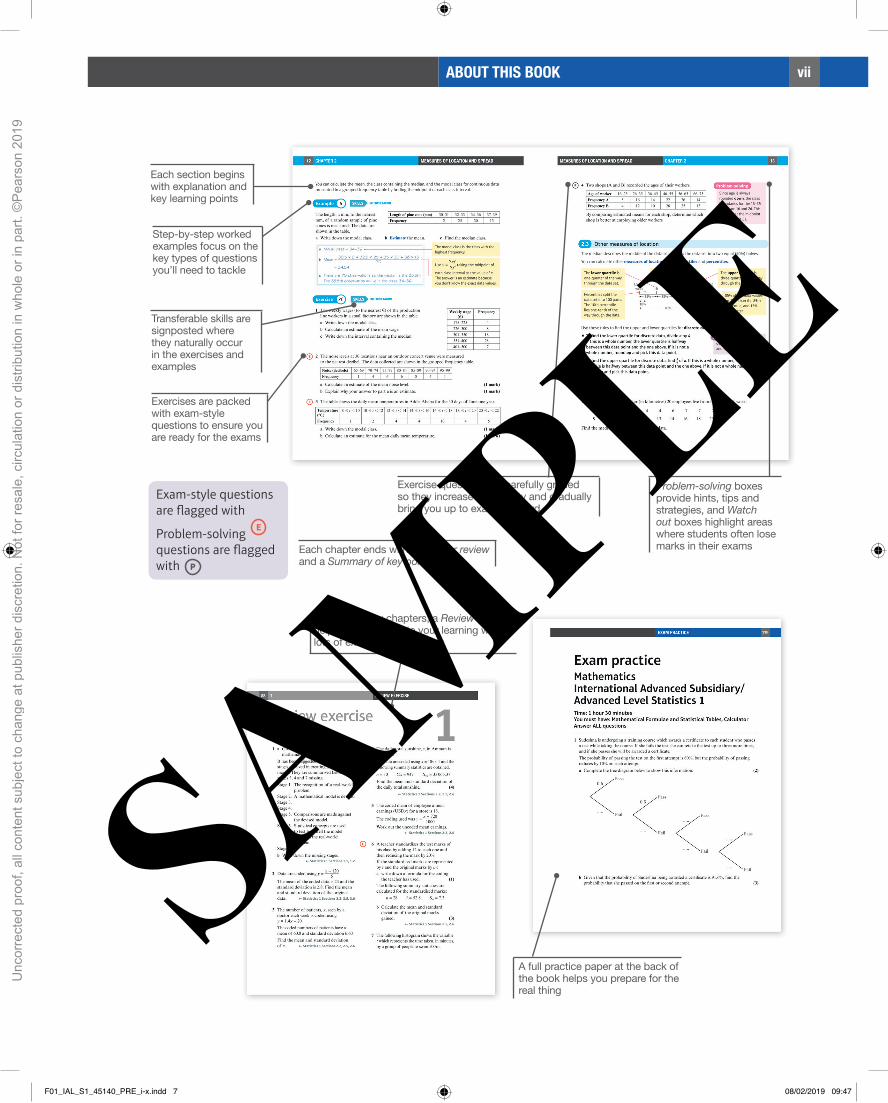
viiABOUT THIS BOOK

Exercise questions are carefully graded so they increase in diffi culty and gradually bring you up to exam standard

Transferable skills are signposted where they naturally occur in the exercises and examples

Each section begins with explanation and key learning points

Problem-solving boxes provide hints, tips and strategies, and Watch out boxes highlight areas where students often lose marks in their examsEach chapter ends with a Chapter review

and a Summary of key points

Exercises are packed with exam-style questions to ensure you are ready for the exams

Exam-style questions are fl agged with

Problem-solving questions are fl agged with

E

P

A full practice paper at the back of the book helps you prepare for the real thing

After every few chapters, a Review exercise helps you consolidate your learning with lots of exam-style questions

Step-by-step worked examples focus on the key types of questions you’ll need to tackle

F01_IAL_S1_45140_PRE_i-x.indd 7 08/02/2019 09:47

Unc

orre

cted

pro

of, a

ll co

nten

t sub

ject

to c

hang

e at

pub

lishe

r dis

cret

ion.

Not

for r

esal

e, c

ircul

atio

n or

dis

tribu

tion

in w

hole

or i

n pa

rt. ©

Pea

rson

201

9

SAMPLE

viii QUALIFICATION AND ASSESSMENT OVERVIEW

QUALIFICATION AND ASSESSMENT OVERVIEWQualification and content overviewStatistics 1 (S1) is an optional unit in the following qualifications:

International Advanced Subsidiary in Mathematics

International Advanced Subsidiary in Further Mathematics

International Advanced Level in Mathematics

International Advanced Level in Further Mathematics

Assessment overviewThe following table gives an overview of the assessment for this unit.

We recommend that you study this information closely to help ensure that you are fully prepared for this course and know exactly what to expect in the assessment.

Unit Percentage Mark Time Availability

S1: Statistics 1

Paper code WST01/01

33 1 _ 3 % of IAS

16 2 _ 3 % of IAL

75 1 hour 30 min January, June and October

First assessment June 2019

IAS: International Advanced Subsidiary, IAL: International Advanced A Level.

Assessment objectives and weightings Minimum weighting in IAS and IAL

AO1Recall, select and use their knowledge of mathematical facts, concepts and techniques in a variety of contexts.

30%

AO2

Construct rigorous mathematical arguments and proofs through use of precise statements, logical deduction and inference and by the manipulation of mathematical expressions, including the construction of extended arguments for handling substantial problems presented in unstructured form.

30%

AO3

Recall, select and use their knowledge of standard mathematical models to represent situations in the real world; recognise and understand given representations involving standard models; present and interpret results from such models in terms of the original situation, including discussion of the assumptions made and refinement of such models.

10%

AO4Comprehend translations of common realistic contexts into mathematics; use the results of calculations to make predictions, or comment on the context; and, where appropriate, read critically and comprehend longer mathematical arguments or examples of applications.

5%

AO5Use contemporary calculator technology and other permitted resources (such as formulae booklets or statistical tables) accurately and efficiently; understand when not to use such technology, and its limitations. Give answers to appropriate accuracy.

5%

F01_IAL_S1_45140_PRE_i-x.indd 8 08/02/2019 09:47

Unc

orre

cted

pro

of, a

ll co

nten

t sub

ject

to c

hang

e at

pub

lishe

r dis

cret

ion.

Not

for r

esal

e, c

ircul

atio

n or

dis

tribu

tion

in w

hole

or i

n pa

rt. ©

Pea

rson

201

9

SAMPLE

ixQUALIFICATION AND ASSESSMENT OVERVIEW

Relationship of assessment objectives to units

S1

Assessment objective

AO1 AO2 AO3 AO4 AO5

Marks out of 75 20–25 20–25 15–20 5–10 5–10

% 26 2 _ 3 –33 1 _ 3 26 2 _ 3 –33 1

_ 3 20–26 2 _ 3 6 2 _ 3 –13 1 _ 3 6 2 _ 3 –13 1 _ 3

CalculatorsStudents may use a calculator in assessments for these qualifications. Centres are responsible for making sure that calculators used by their students meet the requirements given in the table below.

Students are expected to have available a calculator with at least the following keys: +, –, ×, ÷, π, x2,

√ __

x , 1 __ x , xy, ln x, ex, x!, sine, cosine and tangent and their inverses in degrees and decimals of a degree,

and in radians; memory.

ProhibitionsCalculators with any of the following facilities are prohibited in all examinations:

• databanks

• retrieval of text or formulae

• built-in symbolic algebra manipulations

• symbolic differentiation and/or integration

• language translators

• communication with other machines or the internet

F01_IAL_S1_45140_PRE_i-x.indd 9 08/02/2019 09:47

Unc

orre

cted

pro

of, a

ll co

nten

t sub

ject

to c

hang

e at

pub

lishe

r dis

cret

ion.

Not

for r

esal

e, c

ircul

atio

n or

dis

tribu

tion

in w

hole

or i

n pa

rt. ©

Pea

rson

201

9

SAMPLE

x EXTRA ONLINE CONTENT

Whenever you see an Online box, it means that there is extra online content available to support you.

Extra online content

SolutionBankSolutionBank provides worked solutions for questions in the book. Download the solutions as a PDF or quickly fi nd the solution you need online.

Use of technology Explore topics in more detail, visualise problems and consolidate your understanding. Use pre-made GeoGebra activities or Casio resources for a graphic calculator.

Find the point of intersection graphically using technology.

Onlinex

y

GeoGebra-powered interactives Graphic calculator interactives

Interact with the maths you are learning using GeoGebra's easy-to-use tools

Explore the mathematics you are learning and gain confi dence in using a graphic calculator

Interact with the mathematics you are learning using GeoGebra's easy-to-use tools

Calculator tutorialsOur helpful video tutorials will guide you through how to use your calculator in the exams. They cover both Casio's scientifi c and colour graphic calculators.

Step-by-step guide with audio instructions on exactly which buttons to press and what should appear on your calculator's screen

Work out each coeffi cient quickly using the nCr and power functions on your calculator.

Online

F01_IAL_S1_45140_PRE_i-x.indd 10 08/02/2019 09:47

Unc

orre

cted

pro

of, a

ll co

nten

t sub

ject

to c

hang

e at

pub

lishe

r dis

cret

ion.

Not

for r

esal

e, c

ircul

atio

n or

dis

tribu

tion

in w

hole

or i

n pa

rt. ©

Pea

rson

201

9

SAMPLE

1CHAPTER 1MATHEMATICAL MODELLING

1 MATHEMATICALMODELLING

Imagine that a scientist discovers that the number of leopards in Sri Lanka changes from year to year, and she wants to investigate these changes. Instead of tracking every leopard, she can create a mathematical model. By using a mathematical model, the investigation becomes more manageable, less time-consuming and cheaper. It also enables the scientist to make predictions.

A� er completing this chapter you should be able to:

● Understand what mathematical modelling is → page 2

● Design a simple mathematical model → pages 3–4

1.1

1 Write down the defi nition for qualitative and quantitative data. ← International GCSE Mathematics

2 List three areas outside of mathematics where statistics can be used. ← International GCSE Mathematics

Prior knowledge check

Learning objectives

M01_IAL_S1_45140_U01_001-004.indd 1 04/02/2019 08:53

Unc

orre

cted

pro

of, a

ll co

nten

t sub

ject

to c

hang

e at

pub

lishe

r dis

cret

ion.

Not

for r

esal

e, c

ircul

atio

n or

dis

tribu

tion

in w

hole

or i

n pa

rt. ©

Pea

rson

201

9

SAMPLE

MATHEMATICAL MODELLING 2 CHAPTER 1

1.1 Mathematical models

A mathematical model is a simplification of a real-world situation. It can be used to make predictions and forecasts about real-world situations. This helps solve and improve the understanding of real-world situations by analysing the results and the model.

The model will aim to include all the main features of the real-world situation but, given the difficulties of the real world, the model may have to be based on certain assumptions. As a result, these assumptions will need to be taken into consideration when analysing the results.

There are many advantages of mathematical models, and these include (but are not limited to):

■ they are relatively quick and easy to produce

■ they are usually a much more cost-effective way of analysing the real-world situation

■ they enable predictions to be made

■ they help improve the understanding of our world

■ they help show how certain changes in variables will affect the outcomes

■ they help simplify complex situations.

However, mathematical models do have disadvantages, and these include:

■ simplification of the real-world situation can cause errors, as the model does not include all aspects of the problem and may have included some assumptions

■ the model may work only in certain conditions that are difficult or expensive to fulfil in the real world.

Example 1

Give two advantages and disadvantages of using a mathematical model:

Advantages Disadvantages

They are relatively quick and easy to produce Simplification of a real-world situation may cause errors as the model is too simplistic

They help enable predictions to be made The model may work only in certain conditions

SKILLS ANALYSIS

M01_IAL_S1_45140_U01_001-004.indd 2 04/02/2019 08:53

Unc

orre

cted

pro

of, a

ll co

nten

t sub

ject

to c

hang

e at

pub

lishe

r dis

cret

ion.

Not

for r

esal

e, c

ircul

atio

n or

dis

tribu

tion

in w

hole

or i

n pa

rt. ©

Pea

rson

201

9

SAMPLE

3CHAPTER 1MATHEMATICAL MODELLING

1.2 Designing a model

The process of designing a model generally involves seven stages, outlined below.

Stage 1: The recognition of a real-world problem

Stage 2: A mathematical model is devised

Stage 3: Model used to make predictions about the behaviour of the real-world problem

Stage 4: Experimental data are collected from the real world

Stage 5: Comparisons are made against the devised model

Stage 6: Statistical concepts are used to test how well the model describes the real-world problem

Stage 7: Model is refined

Example 2

A scientist is investigating the population of owls and notices that the population varies year to year. Give a summary of the stages that are needed to create a mathematical model for this population variation.1 Some assumptions need to be made to ensure the model is manageable. Birth and death rates of

owls should be included, but food supply and environment changes should not. 2 Plan a mathematical model which will include diagrams. 3 Use this model to predict the population of the owls over a period of years. 4 Include and collect fresh data that match the conditions of the predicted values. You may also

use historical data from the previous years.5 Analyse the data using techniques you will meet in this course to compare the predicted data

with the experimental data.6 Use statistical tests that will provide an objective means of deciding if the differences between

the model’s predictions and experimental data are within acceptable limits. If the predicted values do not match the experimental data closely enough, then the model can be refined. This will involve repeating and refining steps 2 –6. This model is then constantly refined making the model more and more accurate.

SKILLS EXECUTIVE FUNCTION

1 Briefly explain the role of statistical tests in the process of mathematical modelling. 2 Describe how to refine the process of designing a mathematical model.

Exercise 1A SKILLS ANALYSIS; EXECUTIVE FUNCTION

M01_IAL_S1_45140_U01_001-004.indd 3 04/02/2019 08:54

Unc

orre

cted

pro

of, a

ll co

nten

t sub

ject

to c

hang

e at

pub

lishe

r dis

cret

ion.

Not

for r

esal

e, c

ircul

atio

n or

dis

tribu

tion

in w

hole

or i

n pa

rt. ©

Pea

rson

201

9

SAMPLE

MATHEMATICAL MODELLING 4 CHAPTER 1

3 It is generally accepted that there are seven stages involved in creating a mathematical model. They are summarised below. Write down the missing stages. Stage 1: Stage 2: A mathematical model is devised Stage 3: Model used to make predictions Stage 4: Stage 5: Comparisons are made against the devised model Stage 6: Stage 7: Model is refined

1 Mathematical models can simplify real-world problems and are a quick way to describe a real-world situation. Give two other reasons why mathematical models are used.

2 Give two advantages and two disadvantages of the use of mathematical models. 3 Explain how mathematical modelling can be used to investigate climate change. 4 A statistician is investigating population growth in Southeast Asia. Give a summary of the

stages that are needed to create a mathematical model for this investigation.

1 A mathematical model is a simplification of a real-world situation.

2 It is generally accepted that there are seven stages involved in creating a mathematical model.

• Stage 1: The recognition of a real-world problem

• Stage 2: A mathematical model is devised

• Stage 3: Model used to make predictions

• Stage 4: Experimental data collected

• Stage 5: Comparisons are made against the devised model

• Stage 6: Statistical concepts are used to test how well the model describes the real-world problem

• Stage 7: Model is refined

3 There are advantages and disadvantages to mathematical models. Some of these are:

Advantages Disadvantages

They are relatively quick and easy to produce Simplification of a real-world situation may cause

errors as the model is too simplistic

They help enable predictions to be made The model may work only in certain conditions

Summary of key points

Chapter review 1 SKILLS ANALYSIS; EXECUTIVE FUNCTION

M01_IAL_S1_45140_U01_001-004.indd 4 04/02/2019 08:54

Unc

orre

cted

pro

of, a

ll co

nten

t sub

ject

to c

hang

e at

pub

lishe

r dis

cret

ion.

Not

for r

esal

e, c

ircul

atio

n or

dis

tribu

tion

in w

hole

or i

n pa

rt. ©

Pea

rson

201

9

SAMPLE

2 MEASURES OF LOCATION AND SPREAD

Wildlife biologists use statistics such as mean wingspan and standard deviation to compare populations of endangered birds in diff erent habitats.

Aft er completing this chapter you should be able to:

● Recognise diff erent types of data → pages 6−8

● Calculate measures of central tendency such as the mean, median and mode → pages 9−12

● Calculate measures of location such as percentiles → pages 13−15

● Calculate measures of spread such as range, interquartile range and interpercentile range → pages 16−17

● Calculate variance and standard deviation → pages 18−21

● Understand and use coding → pages 21−25

1 Calculate the mean, mode and median of the following data:

10, 12, 38, 23, 38, 23, 21, 27, 38 ← International GCSE Mathematics

2 A train runs for 3 hours at a speed of 65 km per hour, and for the next 2 hours at a speed of 55 km per hour. Find the mean speed of the train for the 5 hour journey. ← International GCSE Mathematics

3 Find the mean, median, mode and range of the data shown in this frequency table.

Number of peas in a pod

3 4 5 6 7

Frequency 4 7 11 18 6

← International GCSE Mathematics

2.22.3


Learning objectives

M02_IAL_S1_45140_U02_005-028.indd 5 04/02/2019 08:55

Unc

orre

cted

pro

of, a

ll co

nten

t sub

ject

to c

hang

e at

pub

lishe

r dis

cret

ion.

Not

for r

esal

e, c

ircul

atio

n or

dis

tribu

tion

in w

hole

or i

n pa

rt. ©

Pea

rson

201

9

SAMPLE

MEASURES OF LOCATION AND SPREAD6 CHAPTER 2

2.1 Types of data

In statistics, we collect observations or measurements of some variables. These observations are known as data. Variables associated with non-numerical data are qualitative variables, and variables associated with numerical data are quantitative variables. The flowchart below shows different types of data in more detail.

Types of data

Examples includefavourite colour orfavourite animal

Discrete data -Takes specific values

in a given range

Continous data -Takes any value in

a given range

Examples includenumber of girls in

a family or numberof bowling pins le�

standing

Examples includea person's weight

or the distancebetween two points

Qualitative(Non-numerical data)

Quantitative(Numerical data)

A variable that can take only specific values in a given range is a discrete variable.

Hint

A variable that can take any value in a given range is a continuous variable.

Hint

Example 1

State whether each of the following variables is continuous or discrete. a Sprint times for a 100 m raceb Length c Number of 10 cent coins in a bag d Number of boys in a family

a Sprint times are continuous

b Length is continuous

c Number of 10 cent coins is discrete

d Number of boys in a family is discrete

Time can take any value, as determined by the accuracy of the measuring device. For example: 9 seconds, 9.1 seconds, 9.08 seconds, 9.076 seconds, etc.

You can’t have 2.45 boys in a family.

You can’t have 5.62 coins.

M02_IAL_S1_45140_U02_005-028.indd 6 04/02/2019 08:55

Unc

orre

cted

pro

of, a

ll co

nten

t sub

ject

to c

hang

e at

pub

lishe

r dis

cret

ion.

Not

for r

esal

e, c

ircul

atio

n or

dis

tribu

tion

in w

hole

or i

n pa

rt. ©

Pea

rson

201

9

SAMPLE

7CHAPTER 2MEASURES OF LOCATION AND SPREAD

The time, x seconds, taken by a random sample of females to run 400 m is measured and is shown in two different tables.a Write down the class boundaries for the first row of each table. b Find the midpoint and class width for the first row for each table.

Large amounts of discrete data can be written as a frequency table or as grouped data. For example, the table below shows the number of students with a specific shoe size.

Shoe size( x ) Number of students, f

39 3

40 17

41 29

42 34

43 12

Data can also be presented as a grouped frequency table. The specific data values are not included in the table, instead they are grouped. You will need to know:

■ the groups are commonly known as classes

■ how to find the class boundaries

■ how to find the midpoint of a class

■ how to find the class width.

The number of anything is called its frequency, where f stands for frequency.

A frequency table is a quick way of writing a long list of numbers. For instance, this table tells us that 3 students have a shoe size of 39, and 17 students have a shoe size of 40, etc.

Example 2 SKILLS INTERPRETATION

Table 1 Table 2Time to run

400 m (s)Number of

females fTime to run

400 m (s)Number of

females f55–65 2 55–65 265–70 25 66–70 2570–75 30 71–75 3075–90 13 76–90 13

It may seem that the classes overlap. However, this is not the case, as 55–65 is the shorthand form of writing 55 < x , 65

The data has gaps and therefore the class boundaries are halfway between 55 and 65.

a The class boundaries for Table 1 are 55 s, 65 s as the data has no gaps and therefore the class boundaries are the numbers of the class. The class boundaries for Table 2 are 54.5 s, 65.5 s because the data has gaps.

b The midpoint for Table 1 is 1 __ 2 (55 + 65) = 60 The midpoint for Table 2 is 1 __ 2 (54.5 + 65.5) = 60The class width for Table 1 is 65 − 55 = 10 The class width for Table 2 is 65.5 − 54.5 = 11

M02_IAL_S1_45140_U02_005-028.indd 7 04/02/2019 08:55

Unc

orre

cted

pro

of, a

ll co

nten

t sub

ject

to c

hang

e at

pub

lishe

r dis

cret

ion.

Not

for r

esal

e, c

ircul

atio

n or

dis

tribu

tion

in w

hole

or i

n pa

rt. ©

Pea

rson

201

9

SAMPLE


1 State whether each of the following variables is qualitative or quantitative:a The height of a building b The colour of a jumperc Time spent waiting in a queued Shoe size e Names of students in a school

2 State which of the following statements are true:a The weight of apples is discrete data. b The number of apples on the trees in an orchard is discrete data. c The amount of time it takes a train to make a journey is continuous data.d Simhal collected data on car colours by standing at the end of her road and writing down

the car colours. The data she collected is quantitative.

3 The distribution of the lifetimes of torch batteries are shown in the grouped frequency table below. a Write down the class boundaries for the second group. b Work out the midpoint of the fifth group.

Lifetime (Nearest 0.1 of an hour)

Frequency

5.0–5.9 56.0–6.9 87.0–7.9 10

8.0–8.9 229.0–9.9 10

10.0–10.9 2

4 The grouped frequency table below shows the distributions of the weights of 16-week-old kittens. a Write down the class boundaries for the third group. b Work out the midpoint of the second group.

Weight (kg) Frequency1.2–1.3 81.3–1.4 281.4–1.5 321.5–1.6 22

Sometimes it is not possible or practical to count the number of all the objects in a set, but that number is still discrete. For example, counting the number of apples on all the trees in an orchard or the number of bricks in a multi-storey building might not be possible (or desirable!) but nonetheless these are still discrete numbers.

Hint

Exercise 2A SKILLS INTERPRETATION

M02_IAL_S1_45140_U02_005-028.indd 8 04/02/2019 08:55

Unc

orre

cted

pro

of, a

ll co

nten

t sub

ject

to c

hang

e at

pub

lishe

r dis

cret

ion.

Not

for r

esal

e, c

ircul

atio

n or

dis

tribu

tion

in w

hole

or i

n pa

rt. ©

Pea

rson

201

9

SAMPLE


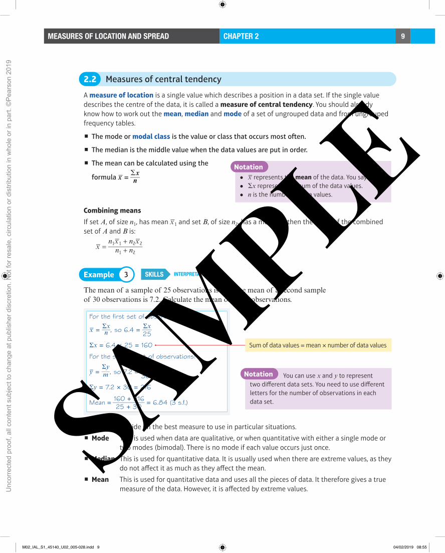
2.2 Measures of central tendency

A measure of location is a single value which describes a position in a data set. If the single value describes the centre of the data, it is called a measure of central tendency. You should already know how to work out the mean, median and mode of a set of ungrouped data and from ungrouped frequency tables.

■ The mode or modal class is the value or class that occurs most often.

■ The median is the middle value when the data values are put in order.

■ The mean can be calculated using the

formula x = Sx ___ n

Combining means

If set A, of size n1, has mean x 1 and set B, of size n 2, has a mean x 2, then the mean of the combined set of A and B is:

x = n1 x 1 + n2 x 2 __________ n1 + n2

● x represents the mean of the data. You say ‘x bar’.● Sx represents the sum of the data values.● n is the number of data values.

Notation

The mean of a sample of 25 observations is 6.4. The mean of a second sample of 30 observations is 7.2. Calculate the mean of all 55 observations.

For the first set of observations:

x = Σx ___ n , so 6.4 = Σx ___ 25

Σx = 6.4 × 25 = 160

For the second set of observations:

y = Σy

___ m , so 7.2 = Σy

___ 30

Σy = 7.2 × 30 = 216

Mean = 160 + 216 __________ 25 + 30

= 6.84 (3 s.f.)

Sum of data values = mean × number of data values

You can use x and y to represent two different data sets. You need to use different letters for the number of observations in each data set.

Notation

You need to decide on the best measure to use in particular situations.

■ Mode This is used when data are qualitative, or when quantitative with either a single mode or two modes (bimodal). There is no mode if each value occurs just once.

■ Median This is used for quantitative data. It is usually used when there are extreme values, as they do not affect it as much as they affect the mean.

■ Mean This is used for quantitative data and uses all the pieces of data. It therefore gives a true measure of the data. However, it is affected by extreme values.


M02_IAL_S1_45140_U02_005-028.indd 9 04/02/2019 08:55

Unc

orre

cted

pro

of, a

ll co

nten

t sub

ject

to c

hang

e at

pub

lishe

r dis

cret

ion.

Not

for r

esal

e, c

ircul

atio

n or

dis

tribu

tion

in w

hole

or i

n pa

rt. ©

Pea

rson

201

9

SAMPLE


You can calculate the mean and median for discrete data presented in a frequency table.

■ For data given in a frequency table, the mean can be calculated using the formula

x = Sxf

____ Sf

● Sxf is the sum of the products of the

data values and their frequencies.● Sf is the sum of the frequencies.

Notation

Li Wei records the shirt collar size, x, Shirt collar size 15 15.5 16 16.5 17Frequency 3 17 29 34 12

of the male students in his year. The results are shown in the table.

For these data, find:a the mode b the median c the mean.d Explain why a shirt manufacturer might use the mode when planning production numbers.

1 Priyanka collected wild mushrooms every day for a week. When she got home each day she weighed them to the nearest 100 g. The weights are shown below:

500 700 400 300 900 700 700a Write down the mode for these data.b Calculate the mean for these data.c Find the median for these data.On the next day, Priyanka collected 650 g of wild mushrooms.d Write down the effect this will have

on the mean, the mode and the median.

Try to answer part d without recalculating the averages. You could recalculate to check your answer.

Hint

Example 4 SKILLS REASONING/ARGUMENTATION

a Mode = 16.5

b There are 95 observations

so the median is the 95 + 1 _______ 2

= 48th.

There are 20 observations up to 15.5 and 49 observations up to 16.

Median = 16

c x = 15 × 3 + 15.5 × 17 + 16 × 29 + 16.5 × 34 + 17 × 12 _________________________________________________ 95

= 45 + 263.5 + 464 + 561 + 204 ______________________________ 95

= 1537.5 _______ 95

= 16.2

d The mode is an actual data value and gives the manufacturer information on the most common size worn/purchased.

16.5 is the collar size with the highest frequency.

The 48th observation is therefore 16.

The mean is not one of the data values and the median is not necessarily indicative of the most popular collar size.

Exercise 2B SKILLS REASONING/ARGUMENTATION

M02_IAL_S1_45140_U02_005-028.indd 10 04/02/2019 08:55

Unc

orre

cted

pro

of, a

ll co

nten

t sub

ject

to c

hang

e at

pub

lishe

r dis

cret

ion.

Not

for r

esal

e, c

ircul

atio

n or

dis

tribu

tion

in w

hole

or i

n pa

rt. ©

Pea

rson

201

9

SAMPLE


2 Taha collects six pieces of data, x1, x2, x3, x4, x5 and x6. He works out that Sx is 256.2a Calculate the mean for these data.Taha collects another piece of data. It is 52.b Write down the effect this piece of data will have on the mean.

3 The daily mean visibility, v metres, for Kuala Lumpur in May and June was recorded each day. The data are summarised as follows:

May: n = 31, Sv = 724 000June: n = 30, Sv = 632 000

a Calculate the mean visibility in each month.b Calculate the mean visibility for the total recording period.

4 A small workshop records how long it takes, in minutes, for each of their workers to make a certain item. The times are shown in the table.

Worker A B C D E F G H I JTime in minutes 7 12 10 8 6 8 5 26 11 9

a Write down the mode for these data.b Calculate the mean for these data.c Find the median for these data.d The manager wants to give the workers an idea of the average time they took.

Write down, with a reason, which of the answers to a, b and c she should use.

5 The frequency table shows the number of Breakdowns 0 1 2 3 4 5Frequency 8 11 12 3 1 1

breakdowns, b, per month recorded by a lorry firm over a certain period of time.a Write down the modal number of breakdowns.b Find the median number of breakdowns.c Calculate the mean number of breakdowns.d In a brochure about how many loads reach their destination on time, the firm quotes

one of the answers to a, b or c as the number of breakdowns per month for its vehicles. Write down which of the three answers the firm should quote in the brochure.

6 The table shows the frequency distribution for Number of petals 5 6 7 8 9Frequency 8 57 29 3 1

the number of petals in the flowers of a group of celandines.Calculate the mean number of petals.

7 A scientist is investigating how many eggs the endangered kakapo bird lays in each brood cycle. The results are given in this frequency table.

Number of eggs 1 2 3Frequency 7 p 2

If the mean number of eggs is 1.5, find the value of p.

P

Use the formula for the mean of an ungrouped frequency table to write an equation involving p.

Problem-solving

M02_IAL_S1_45140_U02_005-028.indd 11 04/02/2019 08:55

Unc

orre

cted

pro

of, a

ll co

nten

t sub

ject

to c

hang

e at

pub

lishe

r dis

cret

ion.

Not

for r

esal

e, c

ircul

atio

n or

dis

tribu

tion

in w

hole

or i

n pa

rt. ©

Pea

rson

201

9

SAMPLE


You can calculate the mean, the class containing the median, and the modal class for continuous data presented in a grouped frequency table by finding the midpoint of each class interval.

The length, x mm, to the nearest Length of pine cone (mm) 30–31 32–33 34–36 37–39Frequency 2 25 30 13

mm, of a random sample of pine cones is measured. The data are shown in the table.a Write down the modal class. b Estimate the mean. c Find the median class.

a Modal class = 34–36

b Mean = 30.5 × 2 + 32.5 × 25 + 35 × 30 + 38 × 13 _________________________________________ 70

= 34.54

c There are 70 observations so the median is the 35.5th. The 35.5th observation will lie in the class 34–36.

The modal class is the class with the highest frequency.

Use x = Sxf

____ Sf

, taking the midpoint of

each class interval as the value of x. The answer is an estimate because you don’t know the exact data values.

1 The weekly wages (to the nearest €) of the production Weekly wage (€)

Frequency

175–225 4226–300 8301–350 18351–400 28401–500 7

line workers in a small factory are shown in the table.a Write down the modal class.b Calculate an estimate of the mean wage.c Write down the interval containing the median.

2 The noise levels at 30 locations near an outdoor concert venue were measured to the nearest decibel. The data collected are shown in the grouped frequency table.

Noise (decibels) 65–69 70–74 75–79 80–84 85–89 90–94 95–99Frequency 1 4 6 6 8 4 1

a Calculate an estimate of the mean noise level. (1 mark)b Explain why your answer to part a is an estimate. (1 mark)

3 The table shows the daily mean temperatures in Addis Ababa for the 30 days of June one year.

Temperature (°C)

8 < t , 10 10 < t , 12 12 < t , 14 14 < t , 16 16 < t , 18 18 < t , 20 20 < t , 22

Frequency 1 2 4 4 10 4 5

a Write down the modal class. (1 mark)b Calculate an estimate for the mean daily mean temperature. (1 mark)

E

E


Exercise 2C SKILLS INTERPRETATION

M02_IAL_S1_45140_U02_005-028.indd 12 04/02/2019 08:55

Unc

orre

cted

pro

of, a

ll co

nten

t sub

ject

to c

hang

e at

pub

lishe

r dis

cret

ion.

Not

for r

esal

e, c

ircul

atio

n or

dis

tribu

tion

in w

hole

or i

n pa

rt. ©

Pea

rson

201

9

SAMPLE


4 Two shops (A and B) recorded the ages of their workers.

Since age is always rounded down, the class boundaries for the 16–25 group are 16 and 26. This means that the midpoint of the class is 21.

Problem-solving

Age of worker 16–25 26–35 36–45 46–55 56–65 66–75Frequency A 5 16 14 22 26 14Frequency B 4 12 10 28 25 13

By comparing estimated means for each shop, determine which shop is better at employing older workers.

P

2.3 Other measures of location

The median describes the middle of the data set. It splits the data set into two equal (50%) halves.

You can calculate other measures of location such as quartiles and percentiles.

The data below shows how far (in kilometres) 20 employees live from their place of work.

1 3 3 3 4 4 6 7 7 7

9 10 11 11 12 13 14 16 18 23

Find the median and quartiles for these data.

Example 6

Use these rules to find the upper and lower quartiles for discrete data.

■ To find the lower quartile for discrete data, divide n by 4. If this is a whole number, the lower quartile is halfway between this data point and the one above. If it is not a whole number, round up and pick this data point.

■ To find the upper quartile for discrete data, find 3 _ 4 of n. If this is a whole number, the upper quartile is halfway between this data point and the one above. If it is not a whole number, round up and pick this data point.

Q1 is the lower quartile, Q2 is the median and Q3 is the upper quartile.

Notation

Lowestvalue

HighestvalueQ1 Q2 Q3

10%85%

25% 25% 25% 25%

The lower quartile is one-quarter of the way through the data set.

Percentiles split the data set into 100 parts. The 10th percentile lies one-tenth of the way through the data.

This is the median value. The upper quartile is three-quarters of the way through the data set.

85% of the data values are less than the 85th percentile, and 15% are greater.

M02_IAL_S1_45140_U02_005-028.indd 13 04/02/2019 08:55

Unc

orre

cted

pro

of, a

ll co

nten

t sub

ject

to c

hang

e at

pub

lishe

r dis

cret

ion.

Not

for r

esal

e, c

ircul

atio

n or

dis

tribu

tion

in w

hole

or i

n pa

rt. ©

Pea

rson

201

9

SAMPLE


For grouped continuous data, or data presented in a cumulative frequency table:

Q1 = n __ 4

th data value

Q2 = n __ 2

th data value

Q3 = 3n ___ 4

th data value

Watch out

Q2 = 20 + 1 _______ 2

th value = 10.5th value

Q2 = 7 + 9 ______ 2

= 8 km

Q1 = 5.5th value

Q1 = 4 km

Q3 = 15.5th value

Q3 = 12.5 km

Q2 is the median. It lies halfway between the 10th and 11th data values (7 km and 9 km respectively).

20 ___ 4

= 5 so the lower quartile is halfway between

the 5th and 6th data values.

3 × 20 ______ 4

= 15 so the upper quartile is halfway

between the 15th and 16th data values.

The length of time (to the nearest minute) Time spent on the internet (minutes) 30–31 32–33 34–36 37–39

Frequency 2 25 30 13

spent on the internet each evening by a group of students is shown in the table.

a Find an estimate for the upper quartile. b Find an estimate for the 10th percentile.

When data are presented in a grouped frequency table you can use a technique called interpolation to estimate the median, quartiles and percentiles. When you use interpolation, you are assuming that the data values are evenly distributed within each class.

a Upper quartile: 3 × 70 _______ 4 = 52.5th value

Using interpolation:

33.5 36.5Q3

27 5752.5

Q3 − 33.5

____________ 36.5 − 33.5

= 52.5 − 27 __________ 57 − 27

Q3 − 33.5 __________

3 = 25.5 _____

30

Q3 = 36.05

b The 10th percentile is the 7th data value.

P10 − 31.5

___________ 33.5 − 31.5

= 7 − 2 _______ 27 − 2

P10 − 31.5 __________

2 = 5 ___

25

P10 = 31.9

The endpoints on the line represent the class boundaries.

Use proportion to estimate Q3. The 52.5th value

lies 52.5 − 27 ________ 57 − 27

of the way into the class, so Q3 lies

Q3 − 33.5

__________ 36.5 − 33.5

of the way between the class

boundaries. Equate these two fractions to form an equation and solve to find Q3.

Problem-solving

The values on the bottom are the cumulative frequencies for the previous classes and this class.

You can write the 10th percentile as P10.Notation


M02_IAL_S1_45140_U02_005-028.indd 14 04/02/2019 08:55

Unc

orre

cted

pro

of, a

ll co

nten

t sub

ject

to c

hang

e at

pub

lishe

r dis

cret

ion.

Not

for r

esal

e, c

ircul

atio

n or

dis

tribu

tion

in w

hole

or i

n pa

rt. ©

Pea

rson

201

9

SAMPLE


1 The daily mean pressure (hPa) during the last 16 days of July in Perth is recorded. The data are given below:

1024 1022 1021 1013 1009 1018 1017 10241027 1029 1031 1025 1017 1019 1017 1014

a Find the median pressure for that period.b Find the lower and upper quartiles.

2 Zaynep records the number of books in the collections of students in her year. The results are in the table below.

Number of books 35 36 37 38 39Frequency 3 17 29 34 12

Find Q1, Q2 and Q3.

3 A hotel is worried about the reliability of its lift. Number of breakdowns

Frequency

0–1 182–3 74–5 1

It keeps a weekly record of the number of times it breaks down over a period of 26 weeks. The data collected are summarised in the table opposite.Use interpolation to estimate the median number of breakdowns. (2 marks)

4 The weights of 31 cows were recorded to the nearest kilogram. The weights are shown in the table.a Find an estimate for the Weight of

cow (kg) 300–349 350–399 400–449 450–499 500–549

Frequency 3 6 10 7 5

median weight.

b Find the lower quartile, Q1.c Find the upper quartile, Q3.d Interpret the meaning of the value you have found for the upper quartile in part c.

5 A roadside assistance company kept a record over a week of the amount of time, in minutes, people were kept waiting for assistance. The times are shown below.

Time waiting, t (minutes) 20 < t , 30 30 < t , 40 40 < t , 50 50 < t , 60 60 < t , 70Frequency 6 10 18 13 2

a Find an estimate for the mean time spent waiting. (1 mark)b Calculate the 65th percentile. (2 marks)

The firm writes the following statement for an advertisement:

Only 10% of our customers have to wait longer than 56 minutes.

c By calculating a suitable percentile, comment on the validity of this claim. (3 marks)

This is an ungrouped frequency table so you do not need to use interpolation. Use the rules for finding the median and quartiles of discrete data.

Hint

E

E

Exercise 2D SKILLS INTERPRETATION

hPa (hectopascal) is the SI unit used to measure atmospheric pressure in weather and meteorology.

Notation

M02_IAL_S1_45140_U02_005-028.indd 15 04/02/2019 08:55

Unc

orre

cted

pro

of, a

ll co

nten

t sub

ject

to c

hang

e at

pub

lishe

r dis

cret

ion.

Not

for r

esal

e, c

ircul

atio

n or

dis

tribu

tion

in w

hole

or i

n pa

rt. ©

Pea

rson

201

9

SAMPLE


6 The table shows the recorded wingspans, in metres, of 100 endangered California condor birds.

Wingspan, w (m) 1.0 < w , 1.5 1.5 < w , 2.0 2.0 < w , 2.5 2.5 < w , 3.0 3.0 < wFrequency 4 20 37 28 11

a Estimate the 80th percentile and interpret the value. (3 marks)b State why it is not possible to estimate the 90th percentile. (1 mark)

E

2.4 Measures of spread

A measure of spread is a measure of how spread out the data are. Here are two simple measures of spread.

■ The range is the difference between the largest and smallest values in the data set.

■ The interquartile range (IQR) is the difference between the upper quartile and the lower quartile, Q3 − Q1.

The range takes into account all of the data but can be affected by extreme values. The interquartile range is not affected by extreme values but only considers the spread of the middle 50% of the data.

■ The interpercentile range is the difference between the values for two given percentiles.

The 10th to 90th interpercentile range is often used since it is not affected by extreme values but still considers 80% of the data in its calculation.

Measures of spread are sometimes called measures of dispersion or measures of variation.

Notation

The table shows the masses, in tonnes, of 120 African bush elephants.

Mass, m (tonnes) 4.0 < m , 4.5 4.5 < m , 5.0 5.0 < m , 5.5 5.5 < m , 6.0 6.0 < m , 6.5Frequency 13 23 31 34 19

Find estimates for:a the range b the interquartile range c the 10th to 90th interpercentile range.

a Range is 6.5 − 4.0 = 2.5 tonnes

b Q1 = 30th data value: 4.87 tonnesQ3 = 90th data value: 5.84 tonnesThe interquartile range is therefore 5.84 − 4.87 = 0.97 tonnes

c 10th percentile = 12th data value: 4.46 tonnes90th percentile = 108th data value: 6.18 tonnesThe 10th to 90th interpercentile range is therefore 6.18 − 4.46 = 1.72 tonnes

Use interpolation: Q1 − 4.5

________ 5.0 − 4.5

= 30 − 13 _______ 23

Use interpolation: Q3 − 5.5

________ 6.0 − 5.5

= 90 − 67 _______ 34

Use interpolation to find the 10th and 90th percentiles, then work out the difference between them.

The largest possible value is 6.5 and the smallest possible value is 4.0.


M02_IAL_S1_45140_U02_005-028.indd 16 04/02/2019 08:55

Unc

orre

cted

pro

of, a

ll co

nten

t sub

ject

to c

hang

e at

pub

lishe

r dis

cret

ion.

Not

for r

esal

e, c

ircul

atio

n or

dis

tribu

tion

in w

hole

or i

n pa

rt. ©

Pea

rson

201

9

SAMPLE


1 The lengths of a number of slow worms were measured, to the nearest mm. The results are shown in the table.a Work out how many slow worms were

measured. b Estimate the interquartile range for the

lengths of the slow worms.c Calculate an estimate for the mean length

of the slow worms.d Estimate the number of slow worms

whose length is more than one interquartile range above the mean.

2 The table shows the monthly income for workers in a factory.

Monthly income, x ($) 900 < x , 1000 1000 < x , 1100 1100 < x , 1200 1200 < x , 1300Frequency 3 24 28 15

a Calculate the 34% to 66% interpercentile range. (3 marks)b Estimate the number of data values that fall within this range. (2 marks)

3 A train travelled from Manchester to Liverpool. The times, to the nearest minute, it took for the journey were recorded over a certain period. The times are shown in the table.

Journey time (minutes) 15–16 17–18 19–20 21–22Frequency 5 10 35 10

a Calculate the 5% to 95% interpercentile range. (3 marks)b Estimate the number of data values that fall within this range. (1 mark)

4 The daily mean temperature (°C) in Santiago for each of the first ten days of June is given below: 14.3 12.7 12.4 10.9 9.4 13.2 12.1 10.3 10.3 10.6

a Calculate the median and interquartile range. (2 marks)The median daily mean temperature in Santiago during the first 10 days of May was 9.9 °C and the interquartile range was 3.9 °C.b Compare the data for May with the data for June. (2 marks)The 10% to 90% interpercentile range for the daily mean temperature in Santiago during July was 5.4 °C.c Estimate the number of days in July on which the daily mean temperature fell

within this range. (1 mark)

P

For part d, work out x + IQR, and determine which class interval it falls in. Then use proportion to work out how many slow worms from that class interval you need to include in your estimate.

Problem-solving

E

E

E/P

Length of slow worms (mm)

Frequency

125–139 4140–154 4155–169 2170–184 7185–199 20200–214 24215–229 10

Exercise 2E SKILLS INTERPRETATION

M02_IAL_S1_45140_U02_005-028.indd 17 04/02/2019 08:55

Unc

orre

cted

pro

of, a

ll co

nten

t sub

ject

to c

hang

e at

pub

lishe

r dis

cret

ion.

Not

for r

esal

e, c

ircul

atio

n or

dis

tribu

tion

in w

hole

or i

n pa

rt. ©

Pea

rson

201

9

SAMPLE


2.5 Variance and standard deviation

Another measure that can be used to work out the spread of a data set is the variance. This makes use of the fact that each data point deviates from the mean by the amount x − x .

■ Variance = S(x − x )2

_________ n = Sx2

____ n − ( Sx ___ n )

2

= Sxx ___ n

where Sxx = S(x − x )2 = Sx2 − (Sx)2

_____ n

The second version of the formula, Sx2

____ n − ( Sx ___ n )

2

, is easier to work with when given raw data.

It can be thought of as ‘the mean of the squares minus the square of the mean’.

The third version, Sxx ___ n , is easier to use if you can use your calculator to find Sxx quickly.

The units of the variance are the units of the data squared. You can find a related measure of spread that has the same units as the data.

■ The standard deviation is the square root of the variance:

σ = √

_________

S(x − x )2

_________ n = √

___________

Sx2

____ n − ( Sx ___ n )

2 = √

___

Sxx ___ n

Sxx is a summary statistic, which is used to make formulae easier to use and learn.

Notation

σ is the symbol we use for the standard deviation of a data set. Hence σ2 is used for the variance.

Notation

The marks gained in a test by seven randomly selected students are:3 4 6 2 8 8 5

Find the variance and standard deviation of the marks of the seven students.

Sx = 3 + 4 + 6 + 2 + 8 + 8 + 5 = 36

Sx2 = 9 + 16 + 36 + 4 + 64 + 64 + 25 = 218

variance, σ2 = 218 ____ 7

− ( 36 ___ 7 )

2 = 4.69

standard deviation, σ = √ _____

4.69 = 2.17

■ You can use these versions of the formulae for variance and standard deviation for grouped data that is presented in a frequency table:

● σ2 = S f (x − x )2

__________ S f

= S fx2

_____ S f

− ( S fx

____ S f

) 2

● σ = √

__________

S f (x − x )2

__________ S f

= √

______________

S fx2

_____ S f

− ( S fx

____ S f

) 2

where f is the frequency for each group and S f is the total frequency.

Use the ‘mean of the squares minus the square of the mean’:

σ2 = Sx2

____ n − ( Sx ___ n )

2

Example 9 SKILLS EXECUTIVE FUNCTION

M02_IAL_S1_45140_U02_005-028.indd 18 04/02/2019 08:55

Unc

orre

cted

pro

of, a

ll co

nten

t sub

ject

to c

hang

e at

pub

lishe

r dis

cret

ion.

Not

for r

esal

e, c

ircul

atio

n or

dis

tribu

tion

in w

hole

or i

n pa

rt. ©

Pea

rson

201

9

SAMPLE


Shamsa records the time spent out of school Time spent out of school, x (min) 35 36 37 38Frequency 3 17 29 34

during the lunch hour to the nearest minute, x, of the students in her year. The results are shown in the table.

Calculate the standard deviation of the time spent out of school.

Example 10

If the data are given in a grouped frequency table, you can calculate estimates for the variance and standard deviation of the data using the midpoint of each class interval.

Akira recorded the length, in minutes, of each phone call she made for a month. The data are summarised in the table below.

Length of phone call, l (min) 0 , l < 5 5 , l < 10 10 , l < 15 15 , l < 20 20 , l < 60 60 , l < 70Frequency 4 15 5 2 0 1

Calculate an estimate of the standard deviation of the length of Akira’s phone calls.

Length of phone call,

l (min)

Frequency Midpoint x

fx fx2

0 , l < 5 4 2.5 4 × 2.5 = 10 4 × 6.25 = 25

5 , l < 10 15 7.5 112.5 843.75

10 , l < 15 5 12.5 62.5 781.25

15 , l < 20 2 17.5 35 612.5

20 , l < 60 0 40 0 0

60 , l < 70 1 65 65 4225

total 27 285 6487.5

S fx2 = 6487.5 S fx = 285 S f = 27

σ2 = 6487.5 ________ 27

− ( 285 _____ 27

) 2 = 128.858 02

σ = √ ___________

128.858 02 = 11.4 (3 s.f.)

You can use a table like this to keep track of your working.

S fx2 = 3 × 352 + 17 × 362 + 29 × 372 + 34 × 382 = 114 504

S fx = 3 × 35 + 17 × 36 + 29 × 37 + 34 × 38 = 3082

S f = 3 + 17 + 29 + 34 = 83

σ2 = 114 504 ________ 83

− ( 3082 ______ 83

) 2 = 0.741 47…

σ = √ ___________

0.741 47… = 0.861 (3 s.f.)

σ2 is the variance, and σ is the standard deviation.

Use σ2 = S fx2

_____ S f

− ( S fx

____ S f

) 2

The values of S fx2, S fx and S f are sometimes given with the question.

Hint

Example 11 SKILLS EXECUTIVE FUNCTION

M02_IAL_S1_45140_U02_005-028.indd 19 04/02/2019 08:55

Unc

orre

cted

pro

of, a

ll co

nten

t sub

ject

to c

hang

e at

pub

lishe

r dis

cret

ion.

Not

for r

esal

e, c

ircul

atio

n or

dis

tribu

tion

in w

hole

or i

n pa

rt. ©

Pea

rson

201

9

SAMPLE


1 The summary data for a variable x are: Sx = 24 Sx2 = 78 n = 8Find:a the meanb the variance σ2

c the standard deviation σ.

2 Ten collie dogs are weighed (w kg). The summary data for the weights are:Sw = 241 Sw2 = 5905

Use this summary data to find the standard deviation of the collies’ weights. (2 marks)

3 Eight students’ heights (h cm) are measured. They are as follows:165 170 190 180 175 185 176 184

a Work out the mean height of the students.b Given Sh2 = 254 307, work out the variance. Show all your working.c Work out the standard deviation.

4 For a set of 10 numbers: Sx = 50 Sx2 = 310For a different set of 15 numbers: Sx = 86 Sx2 = 568Find the mean and the standard deviation of the combined set of 25 numbers.

5 Nahab asks the students in his year group how much allowance they get per week. The results, rounded to the nearest Omani Riyals, are shown in the table.

Number of OMR 8 9 10 11 12Frequency 14 8 28 15 20

a Work out the mean and standard deviation of the allowance. Give units with your answer. (3 marks)

b How many students received an allowance amount more than one standard deviation above the mean? (2 marks)

6 In a student group, a record was kept of the number of days of absence each student had over one particular term. The results are shown in the table.

Number of days absent 0 1 2 3 4Frequency 12 20 10 7 5

Work out the standard deviation of the number of days absent. (2 marks)

E

P

E

E

Exercise 2F SKILLS EXECUTIVE FUNCTION

M02_IAL_S1_45140_U02_005-028.indd 20 04/02/2019 08:55

Unc

orre

cted

pro

of, a

ll co

nten

t sub

ject

to c

hang

e at

pub

lishe

r dis

cret

ion.

Not

for r

esal

e, c

ircul

atio

n or

dis

tribu

tion

in w

hole

or i

n pa

rt. ©

Pea

rson

201

9

SAMPLE


7 A certain type of machine contained a part that tended to wear out after different amounts of time. The time it took for 50 of the parts to wear out was recorded. The results are shown in the table.

Lifetime, h (hours) 5 , h < 10 10 , h < 15 15 , h < 20 20 , h < 25 25 , h < 30Frequency 5 14 23 6 2

The manufacturer makes the following claim:

90% of the parts tested lasted longer than one standard deviation below the mean.

Comment on the accuracy of the manufacturer’s claim, giving relevant numerical evidence. (5 marks)

8 The daily mean wind speed, x (knots) in Chicago is recorded. The summary data are:Sx = 243 Sx2 = 2317

a Work out the mean and the standard deviation of the daily mean wind speed. (2 marks)The highest recorded wind speed was 17 knots and the lowest recorded wind speed was 4 knots.b Estimate the number of days in which the wind speed was greater than one

standard deviation above the mean. (2 marks)c State one assumption you have made in making this estimate. (1 mark)

E/P

You need to calculate estimates for the mean and the standard deviation, then estimate the number of parts that lasted longer than one standard deviation below the mean.

Problem-solving

E

2.6 Coding

Coding is a way of simplifying statistical calculations. Each data value is coded to make a new set of data values which are easier to work with.

In your exam, you will usually have to code values using a formula like this: y = x − a _____ b

where a and b are constants that you have to choose, or are given with the question.

When data are coded, different statistics change in different ways.

■ If data are coded using the formula y = x − a _____ b

● the mean of the coded data is given by y = x − a _____ b

● the standard deviation of the coded data is given

by σy = σx ___ b , where σx is the standard deviation

of the original data.

You usually need to find the mean and standard deviation of the original data given the statistics for the coded data. You can rearrange the formulae as:

● x = b y + a● σx = bσy

Hint

The manager at a local bakery calculates the mean and standard deviation of the number of loaves of bread bought per person in a random sample of her customers as 0.787 and 0.99 respectively. If each loaf costs $1.04, calculate the mean and standard deviation of the amount spent on loaves per person.

Challenge

M02_IAL_S1_45140_U02_005-028.indd 21 04/02/2019 08:55

Unc

orre

cted

pro

of, a

ll co

nten

t sub

ject

to c

hang

e at

pub

lishe

r dis

cret

ion.

Not

for r

esal

e, c

ircul

atio

n or

dis

tribu

tion

in w

hole

or i

n pa

rt. ©

Pea

rson

201

9

SAMPLE


a Original data, x 332 355 306 317 340

Coded data, y 3.2 5.5 0.6 1.7 4.0

b Sy = 15, Sy2 = 59.74

y = 15 ___ 5 = 3

σy2 = 59.74 ______

5 − (

15 ___ 5 )

2

= 2.948

σy = √ ______

2.948 = 1.72 (3 s.f.)

c 3 = x − 300 ________ 10

so x = 30 + 300 = 330 °C

1.72 = σx ___ 10

so σx = 17.2 °C (3 s.f.)

When x = 332, y = 332 − 300 _________ 10

= 3.2

Substitute into y = x − a _____ b and solve to find x .

You could also use x = b y + a with a = 300, b = 10 and y = 3.

Substitute into σy = σx ___ b and solve to find σx .

You could also use σx = b σy with σy = 1.72 and b = 10.

Data on the maximum gust, g knots, are recorded in Chicago during May and June.

The data were coded using h = g − 5

_____ 10 and the following statistics found:

Shh = 43.58 h = 2 n = 61

Calculate the mean and standard deviation of the maximum gust in knots.

2 = g − 5 ______

10

g = 2 × 10 + 5 = 25 knots

σh = √

_______

43.58 ______ 61

= 0.845…

σh = σg

___ 10

σg = σh × 10 = 8.45 knots (3 s.f.)

Use the formula for the mean of a coded variable:

h = g − a

_____ b with a = 5 and b = 10.

Calculate the standard deviation of the coded

data using σh = √

___

Shh ___ n , then use the formula for

the standard deviation of a coded variable:

σh = σg

__ b with b = 10.

A scientist measures the temperature, x °C, at five different points in a nuclear reactor. Her results are given below:

332 °C 355 °C 306 °C 317 °C 340 °C

a Use the coding y = x − 300 _______ 10 to code these data.

b Calculate the mean and standard deviation of the coded data.c Use your answer to part b to calculate the mean and standard deviation of the original data.



M02_IAL_S1_45140_U02_005-028.indd 22 04/02/2019 08:55

Unc

orre

cted

pro

of, a

ll co

nten

t sub

ject

to c

hang

e at

pub

lishe

r dis

cret

ion.

Not

for r

esal

e, c

ircul

atio

n or

dis

tribu

tion

in w

hole

or i

n pa

rt. ©

Pea

rson

201

9

SAMPLE


As seen in Example 11, Akira recorded the length, in minutes, of each phone call she made for a month, as summarised in the table below. This example will now show you how to solve this type of question with a different method.

Use y = x − 7.5 _______ 5 to calculate an

estimate for:

a the mean b the standard deviation.

Length of phone call Number of occasions0 , l < 5 4

5 , l < 10 15

10 , l < 15 5

15 , l < 20 2

20 , l < 60 0

60 , l < 70 1

Example 14

a Length of phone call

Number of occasions

Midpoint x y = x − 7.5 ________

5

0 , l < 5 4 2.5 −1

5 , l < 10 15 7.5 0

10 , l < 15 5 12.5 1

15 , l < 20 2 17.5 2

20 , l < 60 0 40 6.5

60 , l < 70 1 65 11.5

Total 27

Mean of coded data:

= 16.5 _____ 27

= 0.6111

Mean of original data

= 0.6111 = x − 7.5 _______ 5

0.6111 × 5 = x − 7.5x = 10.56

b Length of phone call

Number of occasions

Midpoint x y = x − 7.5 ________

5 fy fy2

0 , l < 5 4 2.5 −1 −4 4

5 , l < 10 15 7.5 0 0 0

10 , l < 15 5 12.5 1 5 5

15 , l < 20 2 17.5 2 4 8

20 , l < 60 0 40 6.5 0 0

60 , l < 70 1 65 11.5 11.5 132.25

Total 27 16.5 149.25

Standard deviation of coded data = √

_________________

149.25 _______ 27

− ( 16.5 _____ 27

) 2 = 2.27

Standard deviation of original data = 2.27 × 5 = 11.35

M02_IAL_S1_45140_U02_005-028.indd 23 04/02/2019 08:55

Unc

orre

cted

pro

of, a

ll co

nten

t sub

ject

to c

hang

e at

pub

lishe

r dis

cret

ion.

Not

for r

esal

e, c

ircul

atio

n or

dis

tribu

tion

in w

hole

or i

n pa

rt. ©

Pea

rson

201

9

SAMPLE


1 A set of data values, x, is shown below: 110 90 50 80 30 70 60

a Code the data using the coding y = x ___ 10

b Calculate the mean of the coded data values.c Use your answer to part b to calculate the mean of the original data.

2 A set of data values, x, is shown below: 52 73 31 73 38 80 17 24

a Code the data using the coding y = x − 3 _____ 7


3 The coded mean price of televisions in a shop was worked out. Using the coding y = x − 65 ______ 200

the mean price was 1.5. Find the true mean price of the televisions. (2 marks)

4 The coding y = x − 40 gives a standard deviation for y of 2.34

Write down the standard deviation of x.

5 A study was performed to investigate how long a mobile phone battery lasts if the phone is not used. The grouped frequency table shows the battery life (b hours) of a random sample of 100 different mobile phones.

Battery life (b hours)

Frequency ( f )

Midpoint (x) y = x − 14 ______ 2

11–21 1121–27 2427–31 2731–37 2637–43 12

a Copy and complete the table.

b Use the coding y = x − 14 ______ 2 to calculate an estimate of the mean battery life.

6 The lifetime, x, in hours, of 70 light bulbs is shown in the table below.

Lifetime, x (hours) 20 , x < 22 22 , x < 24 24 , x < 26 26 , x < 28 28 , x < 30Frequency 3 12 40 10 5

The data are coded using y = x − 1 _____ 20 Code the midpoints of each class interval. The midpoint of the 22 , x < 24 class interval is 23, so the coded midpoint will

be 23 − 1 ______ 20

= 1.1

Problem-solving

a Estimate the mean of the coded values y . b Hence find an estimate for the mean lifetime

of the light bulbs, x .c Estimate the standard deviation of the lifetimes

of the light bulbs.

E

Adding or subtracting constants does not affect how spread out the data are, so you can ignore the ‘−40’ when finding the standard deviation for x.

Watch out

P

P

Exercise 2G SKILLS INTERPRETATION

M02_IAL_S1_45140_U02_005-028.indd 24 04/02/2019 08:55

Unc

orre

cted

pro

of, a

ll co

nten

t sub

ject

to c

hang

e at

pub

lishe

r dis

cret

ion.

Not

for r

esal

e, c

ircul

atio

n or

dis

tribu

tion

in w

hole

or i

n pa

rt. ©

Pea

rson

201

9

SAMPLE


7 The weekly income, i, of 100 workers was recorded.

The data were coded using y = i − 90 _____ 100 and the following summations were obtained:

Sy = 131, Sy2 = 176.84Estimate the standard deviation of the actual workers’ weekly income. (2 marks)

8 A meteorologist collected data on the annual rainfall, x mm, at six randomly selected places.

The data were coded using s = 0.01x − 10 and the following summations were obtained:

Ss = 16.1, Ss2 = 147.03

Work out an estimate for the standard deviation of the actual annual rainfall. (2 marks)

9 The daily mean pressure, p hPa, in Accra during August is recorded.

The data are coded using c = p __ 2 − 500 and the following

summary statistics were obtained:

n = 30 c = 10.15 Scc = 296.4

Find the mean and standard deviation of the daily mean pressure. (4 marks)

E

E

E/P

1 On a science test, the mean mark for a group of eight students is 65. The mean mark for a second group of 12 students is 72. Calculate the mean mark for the combined group of 20 students.

2 The data set below shows the prices (x) of six shares on a particular day in the year 2007:

807 967 727 167 207 767

a Code the data using the coding y = x − 7 _____ 80


3 Different teachers using different methods taught two groups of students. Both groups of students took the same examination at the end of the course. The students’ marks are shown in the grouped frequency table.

Exam mark 20–29 30–39 40–49 50–59 60–69 70–79 80–89Frequency group A 1 3 6 6 11 10 8Frequency group B 1 2 4 13 15 6 3

a Work out an estimate of the mean mark for group A and an estimate of the mean mark for group B.

b Write down whether or not the answer to a suggests that one method of teaching is better than the other. Give a reason for your answer.

Chapter review 2 SKILLS PROBLEM-SOLVING

M02_IAL_S1_45140_U02_005-028.indd 25 04/02/2019 08:55

Unc

orre

cted

pro

of, a

ll co

nten

t sub

ject

to c

hang

e at

pub

lishe

r dis

cret

ion.

Not

for r

esal

e, c

ircul

atio

n or

dis

tribu

tion

in w

hole

or i

n pa

rt. ©

Pea

rson

201

9

SAMPLE


4 The lifetimes of 80 batteries, to the nearest hour, are shown in the table below.

Lifetime (hours) 6–10 11–15 16–20 21–25 26–30Frequency 2 10 18 45 5

a Write down the modal class for the lifetime of the batteries.b Use interpolation to find the median lifetime of the batteries.

The midpoint of each class is represented by x and its corresponding frequency by f, giving S fx = 1645.c Calculate an estimate of the mean lifetime of the batteries.

Another batch of 12 batteries is found to have an estimated mean lifetime of 22.3 hours.d Estimate the mean lifetime for all 92 batteries.

5 A frequency distribution is shown below.

Class interval 1–20 21–40 41–60 61–80 81–100Frequency 5 10 15 12 8

Use interpolation to find an estimate for the interquartile range.

6 A frequency distribution is shown below.

Class interval 1–10 11–20 21–30 31–40 41–50Frequency 10 20 30 24 16

a Use interpolation to estimate the value of the 30th percentile.b Use interpolation to estimate the value of the 70th percentile.c Hence estimate the 30% to 70% interpercentile range.

7 The times it took a random sample of runners to complete a race are summarised in the table.

Time taken, t (minutes) 20–29 30–39 40–49 50–59 60–69Frequency 5 10 36 20 9

a Use interpolation to estimate the interquartile range. (3 marks)

The midpoint of each class was represented by x and its corresponding frequency by f giving:

S fx = 3740 S fx2 = 183 040

b Estimate the variance and standard deviation for these data. (3 marks)

8 The heights of 50 clover flowers are summarised in the table.

Height, x (mm) 90 < x , 95 95 < x , 100 100 < x , 105 105 < x , 110 110 < x , 115Frequency 5 10 26 8 1

a Find Q1.b Find Q2.c Find the interquartile range.d Use S fx = 5075 and S fx2 = 516 112.5 to find the standard deviation.

E

M02_IAL_S1_45140_U02_005-028.indd 26 04/02/2019 08:55

Unc

orre

cted

pro

of, a

ll co

nten

t sub

ject

to c

hang

e at

pub

lishe

r dis

cret

ion.

Not

for r

esal

e, c

ircul

atio

n or

dis

tribu

tion

in w

hole

or i

n pa

rt. ©

Pea

rson

201

9

SAMPLE


9 The daily mean temperatures recorded in Dakar, Senegal, during September are shown in the table below.

Temp (°C) 25 < t , 27 27 < t , 29 29 < t , 31Frequency 12 14 4

a Estimate the mean and standard deviation of the temperatures. (3 marks)b Use linear interpolation to find an estimate for the 10% to 90%

interpercentile range. (3 marks) c Estimate the number of days in September when the daily mean temperature

in Dakar is more than one standard deviation greater than the mean. (2 marks)

10 The daily mean wind speed, w knots, was recorded at Toronto Pearson International Airport,

during May. The data were coded using z = w − 3 _____ 2

Summary statistics were calculated for the coded data:n = 31 Sz = 106 Szz = 80.55

a Find the mean and standard deviation of the coded data. (2 marks)b Work out the mean and standard deviation of the daily mean wind speed at

Toronto Pearson International Airport during May. (2 marks)

11 20 endangered owls were caught for ringing (wrapping a label around their legs to help identify them). Their wingspans (x cm) were measured to the nearest centimetre.The following summary statistics were worked out:

Sx = 316 Sx2 = 5078

a Work out the mean and the standard deviation of the wingspans of the 20 birds. (3 marks)One more bird was caught. It had a wingspan of 13 centimetres.b Without doing any further calculation, say how you think this extra wingspan

will affect the mean wingspan. (1 mark)

20 eagles were also caught for ringing. Their wingspans ( y cm) were also measured to the

nearest centimetre and the data coded using z = y − 5

_____ 10

The following summary statistics were obtained from the coded data:Sz = 104 Szz = 1.8

c Work out the mean and standard deviation of the wingspans of the eagles. (5 marks)

E/P

E

E

A biologist recorded the heights, x cm, of 20 plant seedlings. She calculated the mean and standard deviation of her results:

x = 3.1 cm σ = 1.4 cm

The biologist subsequently discovered she had written down one value incorrectly. She replaced a value of 2.3 cm with a value of 3.2 cm.

Calculate the new mean and standard deviation of her data.

Challenge

M02_IAL_S1_45140_U02_005-028.indd 27 04/02/2019 08:55

Unc

orre

cted

pro

of, a

ll co

nten

t sub

ject

to c

hang

e at

pub

lishe

r dis

cret

ion.

Not

for r

esal

e, c

ircul

atio

n or

dis

tribu

tion

in w

hole

or i

n pa

rt. ©

Pea

rson

201

9

SAMPLE


1 The mode or modal class is the value or class that occurs most often.

2 The median is the middle value when the data values are put in order.

3 The mean can be calculated using the formula x = Sx ___ n

4 For data given in a frequency table, the mean can be calculated using the formula x = Sxf

____ S f

5 To find the lower quartile for discrete data, divide n by 4. If this is a whole number, the lower quartile is halfway between this data point and the one above. If it is not a whole number, round up and pick this data point.

6 To find the upper quartile for discrete data, find 3 _ 4 of n. If this is a whole number, the upper quartile is halfway between this data point and the one above. If it is not a whole number, round up and pick this data point.

7 The range is the difference between the largest and smallest values in a data set.

8 The interquartile range (IQR) is the difference between the upper quartile and the lower quartile, Q3 − Q1.

9 The interpercentile range is the difference between the values for two given percentiles.

10 Variance = S(x − x )2

________ n = Sx2

____ n − ( Sx ___ n )

2

= Sxx ___ n , where Sxx = S(x − x )2 = Sx2 −

(Sx)2

_____ n

11 The standard deviation is the square root of the variance:

σ = √

_________

S(x − x )2

________ n = √

___________

Sx2

____ n − ( Sx

___ n ) 2

= √

____

Sxx ___ n

12 You can use these versions of the formulae for variance and standard deviation for grouped data that is presented in a frequency table:

σ2 = S f (x − x )2

_________ S f

= S fx2

_____ S f

− ( S fx

____ S f

) 2

σ = √

_________

S f (x − x )2

_________ S f

= √

_____________

S fx2

_____ S f

− ( S fx

____ S f

) 2

where f is the frequency for each group and S f is the total frequency.

13 If data are coded using the formula y = x − a _____ b

• the mean of the coded data is given by y = x − a _____ b

• the standard deviation of the coded data is given by σy = σx ___ b where σx is the standard

deviation of the original data.

14 If set A, of size n1, has mean x 1, and set B, of size n2, has a mean x 2, then the mean of the combined set of A and B is:

x = n1 x 1 + n2 x 2 _____________ n1 + n2


M02_IAL_S1_45140_U02_005-028.indd 28 04/02/2019 08:55

Unc

orre

cted

pro

of, a

ll co

nten

t sub

ject

to c

hang

e at

pub

lishe

r dis

cret

ion.

Not

for r

esal

e, c

ircul

atio

n or

dis

tribu

tion

in w

hole

or i

n pa

rt. ©

Pea

rson

201

9

SAMPLE

2929

Visual representations can help to illustrate the key features of a data set without the need for complicated calculations. Graphs and charts are vital in many industries, from the fi nancial sector to journalism. Graphs sector to journalism. Graphs and charts help you to and charts help you to visualise complicated data, visualise complicated data, here for example showing the here for example showing the diff erent food groups.diff erent food groups.

1 The table shows the number of siblings for 60 students:

Number of siblings Frequency0 5

1 8

2 29

3 15

4 3

Draw a pie chart to show the data. ← International GCSE Mathematics

2 Work out the interquartile range for this set of data:

3, 5, 8, 8, 9, 11, 14, 15, 18, 20, 21, 24 ← Statistics 1 Section 2.4

3 Work out the mean and standard deviation for this set of data:

17, 19, 20, 25, 28, 31, 32, 32, 35, 37, 38 ← Statistics 1 Sections 2.2, 2.5

2.12.4

3 REPRESENTATIONS OF DATA

Aft er completing this chapter you should be able to:

● Draw and interpret histograms → pages 30–34

● Identify outliers in data sets → pages 35–37

● Draw and interpret box plots → pages 38–40

● Draw and interpret stem and leaf diagrams → pages 40–44

● Work out whether or not data are skewed → pages 44–47

● Compare two data sets → pages 48–49


Learning objectives

M03_IAL_S1_45140_U03_029-053.indd 29 04/02/2019 08:57

Unc

orre

cted

pro

of, a

ll co

nten

t sub

ject

to c

hang

e at

pub

lishe

r dis

cret

ion.

Not

for r

esal

e, c

ircul

atio

n or

dis

tribu

tion

in w

hole

or i

n pa

rt. ©

Pea

rson

201

9

SAMPLE

REPRESENTATIONS OF DATA30 CHAPTER 3

3.1 Histograms

Grouped continuous data can be represented in a histogram.

Generally, a histogram gives a good picture of how the data are distributed. It enables you to see a rough location, the general shape and how spread out the data are.

In a histogram, the area of the bar is proportional (related in size) to the frequency in each class. This allows you to use a histogram to represent grouped data with unequal class intervals.

■ In a histogram, to calculate the

0

10

20

30

40

50

60

70

80

90

Freq

uenc

y de

nsity

Length0 1 2 3 4 5 6 7 8 9 10 11 12 13 14 15 16

height of each bar (the frequency density) use the formula:

area of bar = k × frequency.

k = 1 is the easiest value to use when drawing a histogram.

If k = 1, then

frequency density = frequency

___________ class width

■ Joining the middle of the top of each bar in a histogram forms a frequency polygon.

Example 1

In a random sample, 200 students were asked how long it took them to complete their homework the previous night. The times were recorded and summarised in the table below.

Time, t (minutes) 25 < t , 30 30 < t , 35 35 < t , 40 40 < t , 50 50 < t , 80Frequency 55 39 68 32 6

a Draw a histogram and a frequency polygon to represent the data.b Estimate how many students took between 36 and 45 minutes to complete their homework.

a Time, t (minutes)

FrequencyClass width

Frequency density

25 < t , 30 55 5 11

30 < t , 35 39 5 7.8

35 < t , 40 68 5 13.6

40 < t , 50 32 10 3.2

50 < t , 80 6 30 0.2

Frequency density = 55 __ 5 = 11

Class width = 30 − 25 = 5

SKILLS INTERPRETATION

M03_IAL_S1_45140_U03_029-053.indd 30 04/02/2019 08:57

Unc

orre

cted

pro

of, a

ll co

nten

t sub

ject

to c

hang

e at

pub

lishe

r dis

cret

ion.

Not

for r

esal

e, c

ircul

atio

n or

dis

tribu

tion

in w

hole

or i

n pa

rt. ©

Pea

rson

201

9

SAMPLE

31CHAPTER 3REPRESENTATIONS OF DATA

0

2

4

6

8

10

12

14Fr

eque

ncy

dens

ity

Time, (min)20 30 40

36 45

50 60 70 80t

b Shaded area = (40 − 36) × 13.6 + (45 − 40) × 3.2 = 70.4 students

To draw the frequency polygon, join the middle of the top of each bar of the histogram.

To estimate the number of students who spent between 36 and 45 minutes, you need to find the area between 36 and 45.

The histogram below displays the information gathered from 100 people, regarding how long, in minutes, they took to complete a word puzzle.

Time (minutes)

Freq

uenc

y de

nsity

0 1 2 3 4 5 6 7 8 9 10

a Why should a histogram be used to represent these data? b Write down the underlying feature associated with each of the bars in a histogram.c Given that 5 people completed the puzzle between 2 and 3 minutes, find the number

of people who completed the puzzle between 0 and 2 minutes.


M03_IAL_S1_45140_U03_029-053.indd 31 04/02/2019 08:57

Unc

orre

cted

pro

of, a

ll co

nten

t sub

ject

to c

hang

e at

pub

lishe

r dis

cret

ion.

Not

for r

esal

e, c

ircul

atio

n or

dis

tribu

tion

in w

hole

or i

n pa

rt. ©

Pea

rson

201

9

SAMPLE


a Time is continuous, and continuous data can be represented in a histogram.

b The area of the bar is proportional to the frequency.

c There are 25 small squares between 2 and 3 minutes. Therefore, 25 small squares represents 5 people. 1 small square represents 1 __ 5 of a person. There are 20 small squares between 0 and 2 minutes. Thus, 20 × 1 __ 5 = 4 people.

1 The data in the table show the mass, in kilograms, of 50 adult puffer fish.a Draw a histogram for these data.b On the same set of axes, draw a frequency polygon.

2 Some students took part in an

40 50 60 70Time (seconds)

Freq

uenc

y de

nsity

80 90 100 110 120

2

0

4

6

8

10

12

14

16

obstacle race. The time for each student to complete the race was noted. The results are shown in the histogram. a Give a reason to justify the

use of a histogram to represent these data.

90 students took between 60 and 70 seconds to complete the race.b Find the number of students

who took between 40 and 60 seconds.

c Find the number of students who took 80 seconds or less.

d Calculate the total number of students who took part in the race.

Mass, m (kg) Frequency10 < m , 15 415 < m , 20 1220 < m , 25 2325 < m , 30 830 < m , 35 3

P

Frequency density × class width is always proportional to frequency in a histogram, but not necessarily equal to frequency.

Watch out

Exercise 3A SKILLS PROBLEM-SOLVING; INTERPRETATION

M03_IAL_S1_45140_U03_029-053.indd 32 04/02/2019 08:57

Unc

orre

cted

pro

of, a

ll co

nten

t sub

ject

to c

hang

e at

pub

lishe

r dis

cret

ion.

Not

for r

esal

e, c

ircul

atio

n or

dis

tribu

tion

in w

hole

or i

n pa

rt. ©

Pea

rson

201

9

SAMPLE


3 A Fun Day committee at a local sports

0 10 20 30Distance (metres)

Freq

uenc

y de

nsity

40 50 60

2

0

4

6

8

10

centre organised a tennis ball throwing competition. The distance thrown by every competitor was recorded and the data is shown in the histogram. Forty people threw the ball less than 20 m.a Why is a histogram a suitable

diagram to represent these data?b How many people entered the

competition?c Estimate how many people threw

between 30 and 40 metres.d How many people threw between

45 and 65 metres?e Estimate how many people threw less than 25 metres.

4 A farmer found the masses of a random

20 22 24 26Mass, m

Freq

uenc

y de

nsity

28 30 32 340

sample of lambs. The masses were summarised in a grouped frequency table and represented by a histogram. The frequency for the class 28 < m , 32 was 32.a Show that 25 small squares on the

histogram represents 8 lambs.b Find the frequency of the

24 < m , 26 class.c How many lambs did the farmer

weigh in total?d Estimate the number of lambs that

had masses between 25 and 29 kg.

PP

P

You can use area to solve histogram problems where no vertical scale is given. You could also use the information given in the question to work out a suitable scale for the vertical axis.

Problem-solving

M03_IAL_S1_45140_U03_029-053.indd 33 04/02/2019 08:57

Unc

orre

cted

pro

of, a

ll co

nten

t sub

ject

to c

hang

e at

pub

lishe

r dis

cret

ion.

Not

for r

esal

e, c

ircul

atio

n or

dis

tribu

tion

in w

hole

or i

n pa

rt. ©

Pea

rson

201

9

SAMPLE


5 The partially (not entirely) completed histogram shows the time, in minutes, that passengers were delayed at an airport.

a i Copy and complete the table.

Time, t (min) Frequency 0 < t , 20 420 < t , 3030 < t , 35 1535 < t , 40 2540 < t , 5050 < t , 70

ii Copy and complete the histogram. (4 marks)

b Estimate how many passengers were delayed between 25 and 38 minutes. (2 marks)

6 The variable y was measured to the nearest whole number. 60 observations were taken and are recorded in the table below.

y 10–12 13–14 15–17 18–25Frequency 6 24 18 12

a Write down the class boundaries for the 13–14 class. (1 mark)

A histogram was drawn and the bar representing the 13–14 class had a width of 4 cm and a height of 6 cm.

For the bar representing the 15–17 class, find:

b i the width (1 mark) ii the height. (2 marks)

7 The table here shows the hourly wage in euros for 31 employees working at a retail store. A histogram was drawn using this data. The 8 < w , 10 group was represented by a bar of width 1 cm and a height of 8 cm.

a Find the width and height of the bar representing the 10 < w , 11 group. (2 marks)

b Estimate the mean and standard deviation of the employees working at the store. (3 marks)

c Use linear interpolation to find an estimate for the lower quartile of wages. (2 marks)

d Estimate how many employees had an hourly wage higher than the mean plus one standard deviation. (2 marks)

E/P

0 10 20 30Time, t (minutes)

Freq

uenc

y de

nsity

40 50 60 700

1

2

3

4

E/P

Remember that area is proportional to frequency.

Problem-solving

E/P Hourly wage, w (C) Frequency 4 < w , 8 4 8 < w , 10 810 < w , 11 611 < w , 12 712 < w , 15 515 < w , 16 1

The table below shows the lengths of 108 fish in an aquarium.

Length (cm) 5–10 10–20 20–25 25–30 30–40 40–60 60–90

Frequency 8 16 20 18 20 14 12

If the data were represented by a histogram, what would be the ratio of the heights of the shortest and highest bars?

M03_IAL_S1_45140_U03_029-053.indd 34 04/02/2019 08:57

Unc

orre

cted

pro

of, a

ll co

nten

t sub

ject

to c

hang

e at

pub

lishe

r dis

cret

ion.

Not

for r

esal

e, c

ircul

atio

n or

dis

tribu

tion

in w

hole

or i

n pa

rt. ©

Pea

rson

201

9

SAMPLE


3.2 Outliers

An outlier is an extreme value that lies outside the overall pattern of the data.

There are a number of different ways of calculating outliers, depending on the nature of the data and the calculations that you are asked to carry out.

■ A common definition of an outlier is any value that is:

● either greater than Q3 + k(Q3 − Q1)

● or less than Q1 − k(Q3 − Q1)

In the exam, you will be told which method to use to identify outliers in data sets, including the value of k.

Q1 and Q3 are the first and third quartiles.

Notation

Example 3

The blood glucose levels of 30 females are recorded. The results, in mmol/litre, are shown below: 1.7, 2.2, 2.3, 2.3, 2.5, 2.7, 3.1, 3.2, 3.6, 3.7, 3.7, 3.7, 3.8, 3.8, 3.8,3.8, 3.9, 3.9, 3.9, 4.0, 4.0, 4.0, 4.0, 4.4, 4.5, 4.6, 4.7, 4.8, 5.0, 5.1

An outlier is an observation that falls either 1.5 × the interquartile range above the upper quartile, or 1.5 × the interquartile range below the lower quartile.a Find the quartiles. b Find any outliers.

a Q1: 30 ___ 4

= 7.5; pick the 8th term = 3.2

Q3: 3(30) ______

4 = 22.5; pick the 23rd term = 4.0

Q2: 30 ___ 2 = 15; pick the 15.5th term = 3.8

b Interquartile range = 4.0 − 3.2 = 0.8Outliers are values less than 3.2 − 1.5 × 0.8 = 2or greater than 4.0 + 1.5 × 0.8 = 5.2Therefore 1.7 is the only outlier.

Work out n ÷ 4 and round up.

Work out 3n ÷ 4 and round up.

Use the definition of an outlier given in the question.

Work out n ÷ 2 and go halfway to the next term.

1.7 < 2, so it is an outlier.

SKILLS ANALYSIS

The table below shows the lengths of 108 fish in an aquarium.

Length (cm) 5–10 10–20 20–25 25–30 30–40 40–60 60–90

Frequency 8 16 20 18 20 14 12

If the data were represented by a histogram, what would be the ratio of the heights of the shortest and highest bars?

Challenge

M03_IAL_S1_45140_U03_029-053.indd 35 04/02/2019 08:57

Unc

orre

cted

pro

of, a

ll co

nten

t sub

ject

to c

hang

e at

pub

lishe

r dis

cret

ion.

Not

for r

esal

e, c

ircul

atio

n or

dis

tribu

tion

in w

hole

or i

n pa

rt. ©

Pea

rson

201

9

SAMPLE


a Mean = Σx ___ n = 252 _____ 12

= 21 cm

Variance = Σx2 ____ n − x 2 = 5468 ______

12 − 212

= 14.666…

Standard deviation = √ _________

14.666… = 3.83 (3 s.f.)

b Mean − 2 × standard deviation = 21 − 2 × 3.83 = 13.34

Mean + 2 × standard deviation = 21 + 2 × 3.83 = 28.66

32 cm is an outlier.

Use the definition of an outlier given in the question.

Use the summary statistics given to work out the mean and standard deviation quickly.

Different questions might use different definitions of outliers. Read the question carefully before finding any outliers.

Watch out

Sometimes outliers are legitimate values (values that are acceptable according to the rules) which could be correct. For example, there really could be a giant African land snail 32 cm long.

However, there are occasions when an outlier should be removed from the data since it is clearly an error and it would be misleading to keep it in. These data values are known as anomalies (values that are different from what is normal or expected).

■ The process of removing anomalies from a data set is known as cleaning the data.

Anomalies can be the result of experimental or recording error, or could be data values which are not relevant to the investigation.

Here is an example where there is a clear anomaly:

Ages of people at a birthday party: 12, 17, 21, 33, 34, 37, 42, 62, 165

x = 47 σ = 44.02 x + 2σ = 135.04

The data value recorded as 165 is significantly higher than x + 2σ, so it can be considered an outlier. An age of 165 is impossible, so this value must be an error. You can clean the data by removing this value before carrying out any analysis.

Be careful not to remove data values just because they do not fit the pattern of the data. You must justify why a value is being removed.

Watch out

You can write 165 ≫ 135.04 where ≫ is used to denote ‘much greater than’.Similarly you can use ≪ to denote ‘much less than’.

Notation

The lengths, in cm, of 12 giant African land snails are given below:17, 18, 18, 19, 20, 20, 20, 20, 21, 23, 24, 32

a Calculate the mean and standard deviation, given that Σx = 252 and Σx2 = 5468.

b An outlier is an observation which lies ±2 standard deviations from the mean. Identify any outliers for these data.

Σx is the sum of the data and Σx2 is the sum of the square of each value.

Notation

Example 4 SKILLS ANALYSIS

M03_IAL_S1_45140_U03_029-053.indd 36 04/02/2019 08:57

Unc

orre

cted

pro

of, a

ll co

nten

t sub

ject

to c

hang

e at

pub

lishe

r dis

cret

ion.

Not

for r

esal

e, c

ircul

atio

n or

dis

tribu

tion

in w

hole

or i

n pa

rt. ©

Pea

rson

201

9

SAMPLE


1 Some data are collected. Q1 = 46 and Q3 = 68.

A value greater than Q3 + 1.5 × (Q3 − Q1) or less than Q1 − 1.5 × (Q3 − Q1) is defined as an outlier.

Using this rule, work out whether or not the following are outliers:

a 7 b 88 c 105

2 The masses of male and female turtles are given in grams. For males, the lower quartile was 400 g and the upper quartile was 580 g. For females, the lower quartile was 260 g and the upper quartile was 340 g.

An outlier is an observation that falls either 1 × the interquartile range above the upper quartile or 1 × the interquartile range below the lower quartile.

a Which of these male turtle masses would be outliers?

400 g 260 g 550 g 640 g

b Which of these female turtle masses would be outliers?

170 g 300 g 340 g 440 g

c What is the largest mass a male turtle can be without being an outlier?

3 The masses of arctic foxes are found and the mean mass was 6.1 kg. The variance was 4.2.

An outlier is an observation which lies ±2 standard deviations from the mean.

a Which of these arctic fox masses are outliers?

2.4 kg 10.1 kg 3.7 kg 11.5 kg

b What are the smallest and largest masses that an arctic fox can be without being an outlier?

4 The ages of nine people at a children’s birthday party are recorded. Σx = 92 and Σx2 = 1428.

a Calculate the mean and standard deviation of the ages. (3 marks)

An outlier is an observation which lies ±2 standard deviations from the mean.

One of the ages is recorded as 30.

b State, with a reason, whether or not this is an outlier. (2 marks)

c Suggest a reason why this age could be a legitimate data value. (1 mark)

d Given that all nine people were children, clean the data and recalculate the mean and standard deviation. (3 marks)

The definition of an outlier here is different from that in question 1. You will be told which rule to use in the exam.

Hint

E

After you clean the data you will need to find the new values for n, Σx and Σx2.

Problem-solving

Exercise 3B SKILLS EXECUTIVE FUNCTION; ANALYSIS

M03_IAL_S1_45140_U03_029-053.indd 37 04/02/2019 08:57

Unc

orre

cted

pro

of, a

ll co

nten

t sub

ject

to c

hang

e at

pub

lishe

r dis

cret

ion.

Not

for r

esal

e, c

ircul

atio

n or

dis

tribu

tion

in w

hole

or i

n pa

rt. ©

Pea

rson

201

9

SAMPLE


a Draw a box plot for the data on blood glucose levels of females from Example 3.Lower quartile = 3.2Upper quartile = 4.0Median = 3.8Outlier = 1.7Lowest value = 2.2Highest value = 5.1

The blood glucose levels of 30 males are recorded. The results are summarised below:Lower quartile = 3.6Upper quartile = 4.7Median = 4.0Lowest value = 1.4Highest value = 5.2

An outlier is an observation that falls either 1.5 × the interquartile range above the upper quartile or 1.5 × the interquartile range below the lower quartile.

b Given that there is only one outlier for the males, draw a box plot for these data on the same diagram as the one for females.

c Compare the blood glucose levels for males and females.


3.3 Box plots

A box plot can be drawn to represent important features of the data. It shows the quartiles, maximum and minimum values and any outliers.

A box plot looks like this:

Median

marks100 20 30 40 50 60

Lower quartile

Upper quartile

Highest value that is not an outlier, or the boundary for outliers

Outlier

Lowest value that is not an outlier, or the boundary for outliers

Two sets of data can be compared using box plots.

M03_IAL_S1_45140_U03_029-053.indd 38 04/02/2019 08:57

Unc

orre

cted

pro

of, a

ll co

nten

t sub

ject

to c

hang

e at

pub

lishe

r dis

cret

ion.

Not

for r

esal

e, c

ircul

atio

n or

dis

tribu

tion

in w

hole

or i

n pa

rt. ©

Pea

rson

201

9

SAMPLE


a

0 1 2 3Blood glucose level (mmol/litre)

4 5 6

Females

b Outliers are values less than 3.6 − 1.5 × 1.1 = 1.95

or values greater than 4.7 + 1.5 × 1.1 = 6.35

There is one outlier, which is 1.4

0 1 2 3Blood glucose level (mmol/litre)

4 5 6

Females

Males

c The median blood glucose level for females is lower than the median blood glucose level for males.The interquartile range (the width of the box) and range for blood glucose levels are smaller for the females.

When comparing data you should compare a measure of location and a measure of spread. You should also write your interpretation in the context of the question.

The end of the box plot is plotted at the outlier boundary (in this case 1.95) as we do not know the actual figure.

When drawing two box plots, use the same scale so they can be compared. Remember to give each a title and label the axis.

Problem-solving

1 A group of students took a test. The summary data are shown in the table.

Lowest mark Lower quartile Median Upper quartile Highest mark5 21 28 36 58

Given that there were no outliers, draw a box plot to illustrate these data.

2 Here is a box plot of marks in an examination.

10 20 30Marks

40 50 60 70 80

a Write down the upper and lower quartiles.b Write down the median.c Work out the interquartile range.d Work out the range.

Exercise 3C SKILLS INTERPRETATION

The quartiles and outliers were found in Example 3.

The outlier is marked with a cross. The lowest value which is not an outlier is 2.2.

Always use a scale and label it. Remember to give your box plot a title.

M03_IAL_S1_45140_U03_029-053.indd 39 04/02/2019 08:57

Unc

orre

cted

pro

of, a

ll co

nten

t sub

ject

to c

hang

e at

pub

lishe

r dis

cret

ion.

Not

for r

esal

e, c

ircul

atio

n or

dis

tribu

tion

in w

hole

or i

n pa

rt. ©

Pea

rson

201

9

SAMPLE


3 The masses of male and female turtles are

0 100 200 300 400Mass (g)

500 600 700

Males

Females

given in grams. The data are summarised in the box plots.a Compare and contrast the masses of the

male and female turtles.b A turtle was found to have a mass of 330 grams.

State whether it is likely to be a male or a female. Give a reason for your answer.

c Write down the size of the largest female turtle.

4 The average weight (in kg) for 30 different breeds of dog are shown below. 13 15 16 19 2021 22 22 24 2425 25 26 26 2627 29 29 30 3033 33 38 46 48

a Calculate Q1, Q2 and Q3. (3 marks)

An outlier is defined as a value which lies either 1.5 × the interquartile range above the upper quartile, or 1.5 × the interquartile range below the lower quartile. b Show that 46 kg and 48 kg are outliers. (1 mark)c Draw a box plot for this data. (3 marks)

P

E

3.4 Stem and leaf diagrams

■ A stem and leaf diagram is used to order and present data given to 2 or 3 significant figures. Each number is first split into its stem and leaf. For example, take the number 42:

42

2 is the leaf4 is the stem

■ It enables the shape of the distribution of the data to be revealed, and quartiles can easily be found from the diagram.

■ Two sets of data can be compared using back to back stem and leaf diagrams.

The blood glucose levels of 30 males are recorded. The results, in mmol/litre, are given below. 4.4 2.4 5.1 3.7 4.7 2.2 3.8 4.2 5.0 4.7 4.1 4.6 4.7 3.7 3.62.1 2.5 3.8 4.2 4.0 3.5 4.8 5.1 4.5 3.6 1.4 3.2 4.7 3.6 5.2

a Draw a stem and leaf diagram to represent the data. b Find:

i the mode ii the lower quartileiii the upper quartile iv the median.

Example 6 SKILLS INTERPRETATION; EXECUTIVE FUNCTION

M03_IAL_S1_45140_U03_029-053.indd 40 04/02/2019 08:57

Unc

orre

cted

pro

of, a

ll co

nten

t sub

ject

to c

hang

e at

pub

lishe

r dis

cret

ion.

Not

for r

esal

e, c

ircul

atio

n or

dis

tribu

tion

in w

hole

or i

n pa

rt. ©

Pea

rson

201

9

SAMPLE


a Step 1: Rearrange the numbers in ascending order. 1.4 2.1 2.2 2.4 2.5 3.2 3.5 3.6 3.6 3.6 3.7 3.7 3.8 3.8 4.04.1 4.2 4.2 4.4 4.5 4.6 4.7 4.7 4.7 4.7 4.8 5.0 5.1 5.1 5.2

Step 2: Choose an appropriate stem and leaf for the data. For these data, the whole number part is chosen as the stem and the decimal part is chosen as the leaf.

Step 3: Draw the stem and leaf diagram.

Stem Leaf1 42 1 2 4 53 2 5 6 6 6 7 7 8 84 0 1 2 2 4 5 6 7 7 7 7 85 0 1 1 2

Step 4: Include a key.

Stem Leaf Key: 1 | 4 = 1.41 42 1 2 4 53 2 5 6 6 6 7 7 8 84 0 1 2 2 4 5 6 7 7 7 7 85 0 1 1 2

b Stem Leaf Key: 1 | 4 = 1.41 4 (1)2 1 2 4 5 (4)3 2 5 6 6 6 7 7 8 8 (9)4 0 1 2 2 4 5 6 7 7 7 7 8 (12)5 0 1 1 2 (4)

i From the diagram, you can see the mode is 4.7 as it occurs the most frequently.

ii Lower quartile: 30 ___ 4 = 7.5, so pick the 8th term which is 3.6

iii Upper quartile 3(30) ____ 4 = 22.5, so pick the 23rd term which is 4.7

iv Median 30 ___ 2 = 15, so pick the 15.5th term which is 40.5 (halfway between 4.0 and 4.1)

This row contains all the numbers between 5.0 and 5.2

This row contains all the numbers between 2.0 and 2.5

This is the number of pieces of data in the row.

M03_IAL_S1_45140_U03_029-053.indd 41 04/02/2019 08:57

Unc

orre

cted

pro

of, a

ll co

nten

t sub

ject

to c

hang

e at

pub

lishe

r dis

cret

ion.

Not

for r

esal

e, c

ircul

atio

n or

dis

tribu

tion

in w

hole

or i

n pa

rt. ©

Pea

rson

201

9

SAMPLE


Achara recorded the resting pulse rate for the 16 boys and 23 girls in her year at school. The results were as follows:

Girls Boys55 80 84 91 80 92 80 60 91 6598 40 60 64 66 72 67 59 75 4696 85 88 90 76 54 72 71 74 5758 92 78 80 79 64 60 50 68

a Construct a back to back stem and leaf diagram to represent these data.b Comment on your results.

Example 7 SKILLS INTERPRETATION; EXECUTIVE FUNCTION

The blood glucose levels of 30 females are recorded. The results, in mmol/litre, are shown in the stem and leaf diagram below:

Stem Leaf Key: 2 | 1 = 2.12 2 2 3 3 5 7 (6)3 1 2 6 7 7 7 8 8 8 8 9 9 9 (13)4 0 0 0 0 4 5 6 7 8 (9)5 1 5 (2)

An outlier is an observation that falls either 1.5 × the interquartile range above the upper quartile or 1.5 × the interquartile range below the lower quartile.a Find the quartiles. b Find any outliers.


a Use the steps outlined in Example 6 to complete the stem and leaf diagram. The lowest value always goes next to the stem when ordering.

Girls Boys0 4 6

8 5 4 5 0 7 96 4 0 6 0 0 4 5 7 8

9 8 6 2 7 1 2 4 58 5 4 0 0 0 8 08 6 2 2 1 0 9 1

b The back to back stem and leaf diagram shows that the resting pulse rate for the boys tends to be lower than that for the girls.

Key: 0 | 4 | 6 means40 for the girls and 46 for the boys

a Lower quartile: 30 ___ 4 = 7.5, so pick the 8th term = 3.2

Upper quartile: 3(30) ____ 4 = 22.5, so pick the 23rd term = 4.0

Median: 30 ___ 2 = 15, so pick the 15.5th term = 3.8

M03_IAL_S1_45140_U03_029-053.indd 42 04/02/2019 08:57

Unc

orre

cted

pro

of, a

ll co

nten

t sub

ject

to c

hang

e at

pub

lishe

r dis

cret

ion.

Not

for r

esal

e, c

ircul

atio

n or

dis

tribu

tion

in w

hole

or i

n pa

rt. ©

Pea

rson

201

9

SAMPLE


b Interquartile range = 4.0 − 3.2 = 0.8Outliers are values less than 3.2 − (1.5 × 0.8) = 2 or values greater than 4.0 + (1.5 × 0.8) = 5.2 Therefore 5.5 is an outlier.

1 Thirty college students were asked how many movies they had in their collection. The results are as follows:

12 25 34 17 12 18 29 34 45 6 15 9 25 3 2922 20 32 15 15 19 12 26 27 27 32 35 42 26 25

Draw a stem and leaf diagram to represent these data.a Find the median. b Find the lower quartile. c Find the upper quartile.

2 The following stem and leaf diagram shows some information about the marks gained by a group of students in a statistics test.Stem Leaf Key: 2 | 3 means 23 marks

0 8 9 (2)1 2 5 5 9 (4)2 3 6 6 6 7 (5)3 4 4 5 7 7 7 7 7 9 (9)4 5 8 8 9 (4)

a Write down the highest mark. b Write down the lowest mark. c How many students scored 26 marks?d What is the modal mark?e Find the median.f Find the lower quartile. g Find the upper quartile.

3 A class of 16 boys and 13 girls completed a Physics test. The test was marked out of 60. Their marks are shown below:

Boys Girls45 54 32 60 26 54 47 3228 34 54 56 34 34 45 4632 29 47 48 39 52 24 2844 45 56 57 33

a Draw back to back stem and leaf diagrams to represent these data. b Comment on your results.

Exercise 3D SKILLS INTERPRETATION; EXECUTIVE FUNCTION

M03_IAL_S1_45140_U03_029-053.indd 43 04/02/2019 08:57

Unc

orre

cted

pro

of, a

ll co

nten

t sub

ject

to c

hang

e at

pub

lishe

r dis

cret

ion.

Not

for r

esal

e, c

ircul

atio

n or

dis

tribu

tion

in w

hole

or i

n pa

rt. ©

Pea

rson

201

9

SAMPLE


3.5 Skewness

The shape (skewness) of a data set can be described using diagrams, measures of location and measures of spread.

■ A distribution can be symmetrical, have a positive skew or have a negative skew.

0

10

20

30

40

50

60

70

0 1 2 3 4 5 6 7 8 90

10

20

30

40

50

60

70

0 1 2 3 4 5 6 7 8 90

10

20

30

40

50

60

70

0 1 2 3 4 5 6 7 8 9

This distribution is said to be symmetrical

This distribution is said to have a positive skew

This distribution is said to have a negative skew

■ Data which are spread evenly are symmetrical.

■ Data which are mostly at lower values have a positive skew.

■ Data which are mostly at higher values have a negative skew.

There are several ways of comparing skewness. Sometimes you will be told which to use, and sometimes you will have to choose one depending on what data you have available.

You can see the shape of the data from a box plot. You can also look at the quartiles.

Q1 Q2 Q3

Q1 Q2 Q3

Q1 Q2 Q3

Symmetrical

Positive Skew

Negative Skew

Q2 − Q1 = Q3 − Q2

Q2 − Q1 < Q3 − Q2

Q2 − Q1 > Q3 − Q2

4 The stem and leaf diagram below shows the median age, in years, of a selection of African elephants in Tanzania.Stem Leaf

1 5 6 6 6 7 7 7 7 7 7 8 8 8 8 8 8 8 8 8 9 9 9 9 9 9 9 9 9 9 92 0 0 0 0 0 0 0 1 1 1 1 1 3 3 3 4 5 73 4 44 1

Find: Key: 1 | 8 = 18 yearsa the median b the interquartile range and any outliers.

M03_IAL_S1_45140_U03_029-053.indd 44 04/02/2019 08:57

Unc

orre

cted

pro

of, a

ll co

nten

t sub

ject

to c

hang

e at

pub

lishe

r dis

cret

ion.

Not

for r

esal

e, c

ircul

atio

n or

dis

tribu

tion

in w

hole

or i

n pa

rt. ©

Pea

rson

201

9

SAMPLE


Another test uses the measures of location:

■ Mode = median = mean describes a distribution which is symmetrical

■ Mode < median < mean describes a distribution with a positive skew

■ Mode > median > mean describes a distribution with a negative skew

You can also calculate 3(mean – median)

________________ standard deviation

which tells you how skewed the data are.

Negative skew Symmetrical0

Positive skew

■ A value of 0 implies that the mean = median and the distribution is symmetrical

■ A positive value implies that the median < mean and the distribution is positively skewed

■ A negative value implies that median > mean and the distribution is negatively skewed

The further from 0 the value is, the more likely the data will be skewed.

The following stem and leaf diagram shows the scores obtained by a group of students in a test.

Score Key: 6 | 1 means 612 1 2 8 (3)3 3 4 7 8 9 (5)4 1 2 3 5 6 7 9 (7)5 0 2 3 3 5 5 6 8 9 9 (10)6 1 2 2 3 4 4 5 6 6 8 8 8 9 9 (14)7 0 2 3 4 5 7 8 9 (8)8 0 1 4 (3)

The modal value is 68, the mean is 57.46 and the standard deviation is 15.7 for these data.

a Find the three quartiles for this data set.

b Calculate the value of 3(mean – median)

_________________ standard deviation and comment on the skewness.

c Use two further methods to show that the data are negatively skewed.


M03_IAL_S1_45140_U03_029-053.indd 45 04/02/2019 08:57

Unc

orre

cted

pro

of, a

ll co

nten

t sub

ject

to c

hang

e at

pub

lishe

r dis

cret

ion.

Not

for r

esal

e, c

ircul

atio

n or

dis

tribu

tion

in w

hole

or i

n pa

rt. ©

Pea

rson

201

9

SAMPLE


1 In a survey of the earnings of some college students who worked weekend jobs, the median wage was $36.50. The 75th percentile was $45.75 and the interquartile range was $30.50. Use the quartiles to describe the skewness of the distributions.

2 A group of estate agents recorded the time spent on the first meeting with a random sample of 120 of their clients. The mean time spent with their clients is 31.1 minutes and the variance is 78.05. The median time is 29.7 minutes and Q1 and Q3 values are 25.8 minutes and 34.8 minutes.

One measure of skewness is found using 3(mean – median)

_________________ standard deviation

a Evaluate this measure and describe the skewness of the data

The estate agents are undecided whether to use the median and quartiles, or the mean and standard deviation to summarise the data.

b State, giving a reason, which you would recommend for them to use.

Exercise 3E SKILLS ANALYSIS

a Q1: 50 ___ 4

= 12.5, therefore we use the 13th term = 46

Q2: 50 ___ 2 = 25, therefore we use the mean of the 25th

and 26th terms = 60

Q3: 3(50) ______

4 = 37.5, therefore we use the 38th term = 69

b 3(mean − median)

_________________ standard deviation

= 3(57.46 − 60)

______________ 15.7

= −0.486

Therefore the data are negatively skewed.

c (Q3 – Q2) < (Q2 – Q1) 9 < 14Therefore negatively skewed

Mean < median < mode57.46 < 60 < 68Therefore negatively skewed

M03_IAL_S1_45140_U03_029-053.indd 46 04/02/2019 08:57

Unc

orre

cted

pro

of, a

ll co

nten

t sub

ject

to c

hang

e at

pub

lishe

r dis

cret

ion.

Not

for r

esal

e, c

ircul

atio

n or

dis

tribu

tion

in w

hole

or i

n pa

rt. ©

Pea

rson

201

9

SAMPLE


3 The following stem and leaf diagram summarises the wing length, to the nearest mm, of a random sample of 67 birds.

Wing length Key: 5 | 0 means 50 mm5 0 0 0 1 1 2 2 3 3 3 4 4 (12)5 5 5 6 6 6 7 8 8 9 9 (10)6 0 1 1 1 3 3 4 4 4 4 (10)6 5 5 6 7 8 9 9 (7)7 1 1 2 2 3 3 (6)7 5 7 9 9 (4)8 1 1 1 2 2 3 3 4 (8)8 7 8 9 (3)9 0 1 1 2 (4)9 5 7 9 (3)

a Write down the mode. b Find the median and quartiles of the data. c Construct a box plot to represent the data. d Comment on the skewness of the distribution. e Calculate the mean and standard deviation for the data. f Use another method to shows that the data is skewed.g State, giving a reason, which of b or e would you

recommend using to summarise the data in the diagram.

An orange farmer randomly selects 120 oranges from her farm. The histogram below shows the diameters (in mm) of the oranges.

Diameter (mm)

Freq

uenc

y de

nsity

60 70 80 90 100

1

2

3

4

5

6

00

Calculate an estimate of the mean and standard deviation. Comment on why the mean is only an estimate, whether there any outliers, and the type of skewness displayed by the histogram.

Challenge

M03_IAL_S1_45140_U03_029-053.indd 47 04/02/2019 08:57

Unc

orre

cted

pro

of, a

ll co

nten

t sub

ject

to c

hang

e at

pub

lishe

r dis

cret

ion.

Not

for r

esal

e, c

ircul

atio

n or

dis

tribu

tion

in w

hole

or i

n pa

rt. ©

Pea

rson

201

9

SAMPLE


3.6 Comparing data

■ When comparing data sets you can comment on:● a measure of location ● a measure of spread

You can compare data by using the mean and standard deviation or by using the median and interquartile range. If the data set contains extreme values, then the median and interquartile range are more appropriate statistics to use.

Do not use the median with the standard deviation or the mean with the interquartile range.

Watch out

Example 10

The daily mean temperature (°C) during August is recorded at London Heathrow Airport and Dubai International Airport.

For London Heathrow, Σx = 562.0 and Σx2 = 10 301.2

a Calculate the mean and standard deviation for London Heathrow.

For Dubai International, the mean temperature was 31 °C with a standard deviation of 1.35 °C.

b Compare the data for the two airports using the information given.

SKILLS ANALYSIS

1 The box plots below show the distribution of speeds of cars on two motorways.

55 60 65 70 75 80 85Speed (kilometres per hour)

90

Motorway B

Motorway A

Compare the distributions of the speeds on the two motorways.

P

Exercise 3F SKILLS EXECUTIVE FUNCTION; ANALYSIS

a x = 562.0 ÷ 31 = 18.12… = 18.1 °C (3 s.f.)

= √

____________________

10 301.2 ________ 31

− ( 562.0 ______

31 )

2

= 1.906…

= 1.91 °C (3 s.f.)

b The mean daily temperature at Dubai International is significantly higher and the spread of temperatures is lower than at London Heathrow.

Use x = Σx ___ n . There are 31 days in August, so n = 31.

Use your calculator to do this calculation in one step. Round your final answer to 3 significant figures.

Compare the mean and standard deviation as a measure of location and a measure of spread.

M03_IAL_S1_45140_U03_029-053.indd 48 04/02/2019 08:57

Unc

orre

cted

pro

of, a

ll co

nten

t sub

ject

to c

hang

e at

pub

lishe

r dis

cret

ion.

Not

for r

esal

e, c

ircul

atio

n or

dis

tribu

tion

in w

hole

or i

n pa

rt. ©

Pea

rson

201

9

SAMPLE


2 Two classes of primary school children complete a puzzle. Summary statistics for the times the children took, in minutes, are shown in the table.

n Σx Σx2

Class 2B 20 650 22 000Class 2F 22 598 19 100

Calculate the mean and standard deviation of the times and compare the distributions.

3 The stem and leaf diagram below shows the age, in years, of the members of a sports club. Male Female

Key: 1 | 4 | 0 represents a male aged 41 and a female aged 40

8 8 7 6 1 6 6 6 7 7 8 8 97 6 5 5 3 3 2 1 2 1 3 3 4 5 7 8 8 9 9

9 8 4 4 3 3 2 3 3 4 75 2 1 4 0 1 8

9 0 5 0

a Find the median and interquartile range for the males. b The median and interquartile ranges for the females are 27 and 15 respectively.

Make two comparisons between the ages of the males and females.

4 In the box plots here, the marks for a group of students taking their Mathematics exam for the first time are shown on the top. The marks for a group of students who are retaking their Mathematics exam are shown on the bottom.Compare and contrast the marks between the two groups taking the exam. (3 marks)

P

E/P

10 1009080706050403020

Students taking the exam for the �rst time

Students retaking their exam

1 Aroon and Bassam decided to go on a touring holiday in Europe for the whole of July. They recorded the distance they drove, in kilometres, each day:

155, 164, 168, 169, 173, 175, 177, 178, 178, 178, 179, 179, 179, 184, 184, 185, 185, 188, 192, 193, 194, 195, 195, 196, 204, 207, 208, 209, 211, 212, 226

a Draw a stem and leaf diagram and find Q1, Q2 and Q3. Outliers are values that lie below Q1 − 1.5(Q3 − Q1) or above Q3 + 1.5(Q3 − Q1).b Find any outliers.c Draw a box plot of these data.d Comment on the skewness of the distribution.

Chapter review 3 SKILLS PROBLEM-SOLVING; ANALYSIS

M03_IAL_S1_45140_U03_029-053.indd 49 04/02/2019 08:57

Unc

orre

cted

pro

of, a

ll co

nten

t sub

ject

to c

hang

e at

pub

lishe

r dis

cret

ion.

Not

for r

esal

e, c

ircul

atio

n or

dis

tribu

tion

in w

hole

or i

n pa

rt. ©

Pea

rson

201

9

SAMPLE


2 Cross-country runners from the Marathon Club and the Runners Club were keen to see which club had the faster runners overall. They decided that all the members from both clubs would take part in a cross-country run. The time each runner took to complete the run was recorded.The results are summarised in the box plots.

25 30 35 40Time (min)

45 50 55 60 65 70 75 80

Marathon Club

Runners Club

a Write down the time by which 50% of the Marathon Club runners had completed the run.b Write down the time by which 75% of the Runners Club runners had completed the run.c Explain what is meant by the cross (×) on the Marathon Club box plot.d Compare and contrast these two box plots.e What conclusions can you draw from this information about which club has the faster runners?f Give one advantage and one disadvantage of comparing distributions using box plots.

3 Random samples of 35 tortoises were taken from two different zoos and their ages were recorded. The results are summarised in the back to back stem and leaf diagram below.

Zoo 1 Zoo 28 7 2 5 5 6 7 8 8 9

9 8 7 3 1 1 1 2 3 4 4 5 6 7 94 4 4 0 4 0 1 2 4 7

6 6 5 2 2 5 0 0 5 5 58 6 5 4 2 1 1 6 2 5 6 6

8 6 6 6 4 3 1 1 7 0 59 8 4 3 2 8

4 9 9

a The lower quartile, median and upper quartile for Zoo 1 are 44, 64 and 76 years respectively. Find the median and the quartiles for Zoo 2.

b An outlier is a value that falls either:more than 1.5 × (Q3 − Q1) above Q3 or more than 1.5 × (Q3 − Q1) below Q1

State any outliers in the above data for Zoo 2.c State the skewness of each distribution. Justify your answer.

P

Key: 7 | 3 | 1 means 37-year-olds for Zoo 1 and 31-year-olds for Zoo 2

M03_IAL_S1_45140_U03_029-053.indd 50 04/02/2019 08:57

Unc

orre

cted

pro

of, a

ll co

nten

t sub

ject

to c

hang

e at

pub

lishe

r dis

cret

ion.

Not

for r

esal

e, c

ircul

atio

n or

dis

tribu

tion

in w

hole

or i

n pa

rt. ©

Pea

rson

201

9

SAMPLE


4 The histogram shows the time taken by a group of 58 girls

50 52 54 56Time (seconds)

Freq

uenc

y de

nsity

58 60 62 64

0.50

11.5

22.5

33.5

44.5

55.5

to run a measured distance.a Work out the number of girls who took longer than

56 seconds.b Estimate the number of girls who took between

52 and 55 seconds.

5 The table gives the distances travelled to school, in km, of the population of children in a particular region of the United Kingdom.

Distance, d (km) 0 < d , 1 1 < d , 2 2 < d , 3 3 < d , 5 5 < d , 10 10 < dNumber 2565 1784 1170 756 630 135

A histogram of these data was drawn with distance along the horizontal axis. A bar of horizontal width 1.5 cm and height 5.7 cm represented the 0 –1 km group.Find the widths and heights, in cm, to 1 decimal place, of the bars representing the following groups:a 2 < d , 3 b 5 < d , 10 (5 marks)

6 The labelling on bags of garden compost indicates Mass, m (kg) Frequency14.6 < m , 14.8 114.8 < m , 18.0 018.0 < m , 18.5 518.5 < m , 20.0 620.0 < m , 20.2 2220.2 < m , 20.4 1520.4 < m , 21.0 1

that the bags have a mass of 20 kg. The actual masses of a random sample of 50 bags are summarised in the table opposite.a On graph paper, draw a histogram of these data.b Estimate the mean and standard deviation of the

mass of a bag of compost.(You may use Σfy = 988.85, Σfy2 = 19 602.84)

c Using linear interpolation, estimate the median.

d One measure of skewness is given by 3(mean – median)

_________________ standard deviation . Evaluate this coefficient for the data.

e Comment on the skewness of the distribution of the weights of bags of compost.

P

E/P

M03_IAL_S1_45140_U03_029-053.indd 51 04/02/2019 08:57

Unc

orre

cted

pro

of, a

ll co

nten

t sub

ject

to c

hang

e at

pub

lishe

r dis

cret

ion.

Not

for r

esal

e, c

ircul

atio

n or

dis

tribu

tion

in w

hole

or i

n pa

rt. ©

Pea

rson

201

9

SAMPLE


7 The number of bags of potato crisps sold per day in a coffee shop was recorded over a two-week period. The results are shown below.

20 15 10 30 33 40 5 11 13 20 25 42 31 17a Calculate the mean of these data.b Draw a stem and leaf diagram and find the median and quartiles for these data.

An outlier is an observation that falls either 1.5 × the interquartile range above the upper quartile or 1.5 × the interquartile range below the lower quartile.c Determine whether or not any items of data are outliers.d On graph paper, draw a box plot to represent these data. Show your scale clearly.e Comment on the skewness of the distribution of bags of crisps sold per day.

Justify your answer.

8 For three weeks, Suha and Jameela each count the number of bicycles they see on their routes to school. The data they collected are summarised in this back to back stem and leaf diagram.

Suha Jameela

Key: 5 | 0 | 6 means Suha counts 5 bicycles and Jameela counts 6 bicycles

9 9 7 5 0 6 67 6 5 3 3 2 2 2 1 1 1 1 1 5

5 3 3 2 2 2 1 2 2 2 3 7 7 8 92 1 3 2 3 4 7 7 8

4 2

a Write down the modal number of bicycles Jameela counts on her route.

The quartiles are summarised in the table below:

Suha Jameela

Lower quartile X 21Median 13 Y

Upper quartile Z 33

b Find the values of X, Y, and Z.

9 The table shows summary statistics of the mean daily temperature in Toronto in April 1987 and April 2015.

a Calculate the mean of the mean daily temperatures in each of the two years. (2 marks)b In 2015, the standard deviation was 1.02. Compare the mean daily temperatures in

the two years. (2 marks)c A recorded temperature is considered ‘normal’ for the time of year if it is within one

standard deviation of the mean. Estimate for how many days in April 2015 a ‘normal’ mean daily temperature was recorded. State one assumption you have made in making the estimate. (3 marks)

E Min Max Median Σx Σx2

1987 7.0 17.0 11.85 356.1 4408.92015 10.1 14.1 12.0 364.1 4450.2

M03_IAL_S1_45140_U03_029-053.indd 52 04/02/2019 08:57

Unc

orre

cted

pro

of, a

ll co

nten

t sub

ject

to c

hang

e at

pub

lishe

r dis

cret

ion.

Not

for r

esal

e, c

ircul

atio

n or

dis

tribu

tion

in w

hole

or i

n pa

rt. ©

Pea

rson

201

9

SAMPLE


The table shows the lengths of the films in a film festival, to the nearest minute.

Length (min) Frequency

70–89 4

90–99 17

100–109 20

110–139 9

140–179 2

A histogram is drawn to represent the data, and the bar representing the 90–99 class is 3 cm higher than the bar representing the 70–89 class.

Find the height of the bar chart representing the 110–139 class.

Challenge

1 A common definition of an outlier is any value that is:• greater than Q3 + k(Q3 − Q1)• or less than Q1 − k(Q3 − Q1)

2 The process of removing anomalies from a data set is known as cleaning the data.

3 On a histogram, to calculate the height of each bar (the frequency density) use the formula:

area of bar = k × frequency

4 Joining the middle of the top of each bar in a histogram forms a frequency polygon.

5 When comparing data sets you can comment on:• a measure of location• a measure of spread

6 A stem and leaf diagram reveals the shape of the data and enables quartiles to be found.

7 Two sets of data can be compared using back to back stem and leaf diagrams.

8 A box plot represents important features of the data. It shows quartiles, maximum and minimum values, and any outliers.

9 Box plots can be used to compare two sets of data.

10 Diagrams, measures of location, and measures of spread can be used to describe the shape (skewness) of a data set.

11 You can describe whether a distribution is skewed using

• quartiles

• shape from box plots

• measures of location

• the formula 3(mean – median)

________________ standard deviation

, where a larger value means greater skew.


M03_IAL_S1_45140_U03_029-053.indd 53 04/02/2019 08:57

Unc

orre

cted

pro

of, a

ll co

nten

t sub

ject

to c

hang

e at

pub

lishe

r dis

cret

ion.

Not

for r

esal

e, c

ircul

atio

n or

dis

tribu

tion

in w

hole

or i

n pa

rt. ©

Pea

rson

201

9

SAMPLE

International-A-Level-Mathematics-Statistics-1-Student-Book ...

Documents

Transcript of International-A-Level-Mathematics-Statistics-1-Student-Book ...