I YEAR DJB1C - BUSINESS MATHEMATICS & STATISTICS ...
159
MANONMANIAM SUNDARANAR UNIVERSITY DIRECTORATE OF DISTANCE & CONTINUING EDUCATION TIRUNELVELI 627012, TAMIL NADU B.B.A. - I YEAR DJB1C - BUSINESS MATHEMATICS & STATISTICS (From the academic year 2016-17) Most Student friendly University - Strive to Study and Learn to Excel For more information visit: http://www.msuniv.ac.in
-
Upload
khangminh22 -
Category
Documents
-
view
0 -
download
0
Transcript of I YEAR DJB1C - BUSINESS MATHEMATICS & STATISTICS ...

MANONMANIAM SUNDARANAR UNIVERSITY
DIRECTORATE OF DISTANCE & CONTINUING EDUCATION
TIRUNELVELI 627012, TAMIL NADU
B.B.A. - I YEAR
DJB1C - BUSINESS MATHEMATICS & STATISTICS (From the academic year 2016-17)
Most Student friendly University - Strive to Study and Learn to Excel
For more information visit: http://www.msuniv.ac.in

Manonmaniam Sundaranar University, Directorate of Distance & Continuing Education, Tirunelveli.
1
BBA - I YEAR
DJB1C : BUSINESS MATHEMATICS AND STATISTICS
SYLLABUS
UNIT – I:
Measures of centraltendency – Mean, Median, Mode, G.M. and H.M. Dispersion – Range
– Q.D. – M.D. – S.D. – C.V.
UNIT – II:
Simple Correlation and Regression – Index numbers – Time series – Components –
Estimating Trend.
UNIT – III:
Differential Calculus – Sum, Product, Quotient Rules, Maximum and Minimum.
UNIT – IV:
Integral Calculus – Rules of Integration – Definite integral – Area interpretation.
UNIT – V:
Matrices – Inversion – Solving system of equations.
References:
1. Statistics Theoryand Practice – R.S.N. Pillaiand V. Bagavathi.
2. An introduction to Business Mathematics – V. Sundaresan and S.D. Jeyaseelan.

Manonmaniam Sundaranar University, Directorate of Distance & Continuing Education, Tirunelveli.
2
INDEX
Unit Title Page Number
I 1.1. Measures of Central Tendency 3
1.2. Dispersion 39
II 2.1. Correlation 59
2.2. Regression 68
2.3. Index Numbers 79
2.4. Analysis of Time Series 91
III 3.1. Differential Calculus 105
IV 4.1. Integral Calculus 119
V 5.1. Matrices 135

Manonmaniam Sundaranar University, Directorate of Distance & Continuing Education, Tirunelveli.
3
UNIT - I:
Measures of centraltendency – Mean, Median, Mode, G.M. and H.M. Dispersion – Range – Q.D.
– M.D. – S.D. – C.V.
MEASURES OF CENTRAL TENDENCY (AVERAGES)
INTRODUCTION
Condensation of data is necessary in statistical analysis. This is because a large number
of big figures are not only confusing but also difficult to analyse. Therefore, in order to reduce
the complexity of data and to make them comparable it is necessary that various phenomena,
which are being compared, are reduced to a single figure. The first of such measures is averages
or measures of central tendency. Measures of central tendency are a typical value of the entire
group or data. It describes the characteristics of the entire mass of data. It reduces the complexity
of data and makes them to compare. According to Prof. R. A. Fisher, “The inherent inability of
the human mind to grasp in it‟s entirely a large body of numerical data compels us to seek
relatively few constants that will adequately describe the data.” Human mind is incapable of
remembering the entire mass of unwieldy data. So a simple figure is used to describe the series
which must be a representative number.
Meaning:
A central tendency is a central or typical value for a probability distribution. It may also
be called a center or location of the distribution. Colloquially, measures of central tendency are
often called averages. The term central tendency dates from the late 1920s. If a large volume of
data is summarized and given is one simple term. Then it is called as the „Central Value‟ or an
„average‟. In other words an average is a single value that represents group of values.
Definitions:
Various statisticians have defined the word average differently. Some of the important
definitions are given below:

Manonmaniam Sundaranar University, Directorate of Distance & Continuing Education, Tirunelveli.
4
According to Clark, "Average is an attempt to find one single figure describe whole of
figures."
According to Croxton and Cowdon, "An average value is a single value with'' the range
of the data that is used to represent all of the values in the series. Since an average is somewhere
within the range of the data, it is also called the measure of central value."
According to Murry R. Speigal, “Average is a value which is typical or representative of
a set of data”
It is clear from the above definition that average is called a „type‟ as it is a typical value
of the entire data and is a measure of central tendency.
Objectives or Functions of an average
Averages occupy a prime place in the theory of statistical methods. That is why Bowley
remarked, "Statistics is a science of averages." The following are the objectives of an average:
1. Facilitates Comparison:
The foremost purpose of average is that it facilitates comparison. For instance, a
comparison of the production of jute in Maharashtra a Punjab shows that production of jute in
Maharashtra is much more as compared Punjab.
2. Formulation of Policies:
Averages are of great use in the formulation of various policy measures. For instance,
when the Government, finds that there is a fear of low product of sugar, it can formulate various
policies to compensate the same.
3. Short Description:
Averages help to present the raw data in a brief a systematic manner.

Manonmaniam Sundaranar University, Directorate of Distance & Continuing Education, Tirunelveli.
5
4. Representation of Universe:
Average represents universe. According conclusions can be drawn in respect of the
universe as a whole.
Characteristics of a Typical Average
A measure of central tendency is a typical value around which other figures congregate.
Average condenses a frequency distribution in one figure. According to the statisticians Yule and
Kendall, an average will be termed good or efficient if possesses the following characteristics:
1. It should be easily understandable.
2. It should be rigidly defined. It means that the definition should be so clear that the
interpretation of the definition does not differ from person to person.
3. The average should be such that it can be easily determined.
4. The average of a variable should be based on all the values of the variable. This
means that in the formula for average all the values of the variable should be
incorporated
5. The value of average should not change significantly along with the change in
sample. This means that the values of the averages of different samples of the same
size drawn from the same population should have small variations. In other words, an
average should possess sampling stability
6. It should be amenable to algebraic treatment
7. The average should be unduly affected by extreme values. i.e, the formula for average
should be such that it does not show large due to the presence of one or two very
large or very small values of the variable.
Qualities of Good Averages
The qualities of good averages are as follows:

Manonmaniam Sundaranar University, Directorate of Distance & Continuing Education, Tirunelveli.
6
1. It should be properly defined, preferably by a mathematical formula, so that different
individuals working with the same data should get the same answer unless there are
mistakes in calculations.
2. It should be simple to understand and easy to calculate.
3. It should be based on all the observations so that if we change the value of any
observation, the value of the average should also be changed.
4. It should not be unduly affected by extremely large or extremely small values.
5. It should be capable of algebraic manipulation. By this we mean that if we are given
the average heights for different groups, then the average should be such that we can
find the combined average of all groups taken together.
6. It should have quality of sampling stability. That is, it should not be affected by the
fluctuations of sampling.
For example, if we take ten or twelve samples of twenty students‟ each and find
the average height for each sample, we should get approximately the same average height
for each sample.
Kinds of Averages
The following are the important types of averages:
1. Arithmetic mean
i) Simple and
ii) Weighted
2. Median
3. Mode
4. Geometric mean and
5. Harmonic Mean
MEAN
Mean is one of the types of averages. Mean is further divided into three kinds, which are
the arithmetic mean, the geometric mean and the harmonic mean. These kinds are explained as
follows;

Manonmaniam Sundaranar University, Directorate of Distance & Continuing Education, Tirunelveli.
7
i) Arithmetic Mean: Simple Arithmetic Average:
A. Individual Observation: Direct Method:
The arithmetic mean is most commonly used average. It is generally referred as the
average or simply mean. The arithmetic mean or simply mean is defined as the value obtained by
dividing the sum of values by their number or quantity. It is denoted as 𝐗 (read as X-bar).
Therefore, the mean for the values X1, X2, X3,………..,Xn shall be denoted by 𝐗 . Following is
the mathematical representation for the formula for the arithmetic mean or simply, the mean.
𝑿 =𝐗𝟏+𝐗𝟐+𝐗𝟑+⋯+𝐗𝐧
𝐍=
𝚺𝐗
𝐍
Where, 𝑋 = Arithmetic Mean
Σx = Sum of all the values of the variables i.e., X1 + X2 + X3+ … + Xn
N = Number of observations.
Illustration 1: Calculate mean from the following data:
Roll Numbers 1 2 3 4 5 6 7 8 9 10
Marks 40 50 55 78 58 60 73 35 43 48
Solution: Calculation of mean
Roll Numbers Marks (x)
1
2
3
4
5
6
7
40
50
55
78
58
60
73
Manonmaniam Sundaranar University, Directorate of Distance & Continuing Education, Tirunelveli.
8
8
9
10
35
43
48
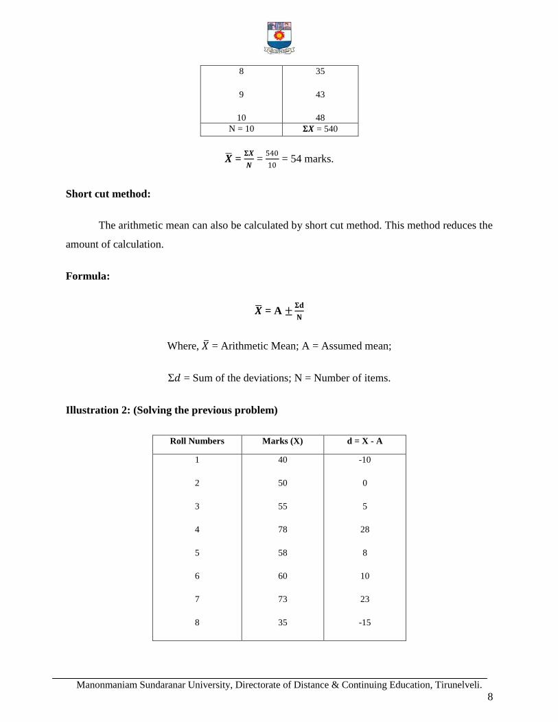
N = 10 𝚺𝑿 = 540
𝑿 = 𝚺𝑿
𝑵 =
540
10 = 54 marks.
Short cut method:
The arithmetic mean can also be calculated by short cut method. This method reduces the
amount of calculation.
Formula:
𝑿 = A ±𝚺𝐝
𝐍
Where, 𝑋 = Arithmetic Mean; A = Assumed mean;
Σ𝑑 = Sum of the deviations; N = Number of items.
Illustration 2: (Solving the previous problem)
Roll Numbers Marks (X) d = X - A
1
2
3
4
5
6
7
8
40
50
55
78
58
60
73
35
-10
0
5
28
8
10
23
-15

Manonmaniam Sundaranar University, Directorate of Distance & Continuing Education, Tirunelveli.
9
9
10
43
48
-7
-2
N = 10 𝚺𝒅 = 40
Let the assumed mean, A = 50
𝑋 = A ±Σd
N= 50 +
40
10 = 54 marks.
B. Discrete Series: Direct Method:
To find out the total of items in discrete series, frequency of each value is multiplied with
the respective size. The values so obtained are totaled up. This total is then divided by the total
number of frequencies to obtain the arithmetic mean. The formula is
𝐗 =𝚺𝒇𝒙
𝑵
Where, 𝑋 = Arithmetic Mean;Σf𝑥 = the sum of products;N = Total frequency.
Illustration 3: Calculate mean from the following data:
Value 1 2 3 4 5 6 7 8 9 10
Frequency 21 30 28 40 26 34 40 9 15 57
Solution: Calculation of mean
x f fx
1
2
3
4
5
6
7
21
30
28
40
26
34
40
21
60
84
160
130
204
280

Manonmaniam Sundaranar University, Directorate of Distance & Continuing Education, Tirunelveli.
10
8
9
10
9
15
57
72
135
570
𝚺𝒇 = 𝐍 = 𝟑𝟎𝟎 𝚺𝐟𝐱 = 1716
𝑋 = Σfx
𝑁 =
1716
300 = 5.72.
Short cut Method
Formula:
𝑿 = A ±𝚺𝐟𝐝
𝐍
Where, 𝑋 = Arithmetic Mean; A = Assumed mean
Σf𝑑 = Sum of total deviations; N = Total frequency.
Illustration: 4 (Solving the previous problem)
X f d = X - A fd
1
2
3
4
5
6
7
8
9
10
21
30
28
40
26
34
40
9
15
57
-4
-3
-2
-1
0
1
2
3
4
5
-84
-90
-56
-40
0
34
80
27
60
285
𝚺𝐟 = N = 40 𝚺𝐟𝐝 = + 216

Manonmaniam Sundaranar University, Directorate of Distance & Continuing Education, Tirunelveli.
11
Let the assumed mean, A = 5
𝑋 = A ±Σfd
N
𝑋 = 5 + 216
300
= 5.72.
C. Continuous Series
In continuous frequency distribution, the value of each individual frequency distribution
is unknown. Therefore an assumption is made to make them precise or on the assumption that
the frequency of the class intervals is concentrated at the centre that the midpoint of each class
interval has to be found out. In continuous frequency distribution, the mean can be calculated by
any of the following methods:
1. Direct Method
2. Short cut method
3. Step Deviation Method
1. Direct Method
The formula is 𝑿 = 𝚺𝒇𝒎
𝑵
Where, 𝑋 = Arithmetic Mean; Σf𝑚 = Sum of the product of f & m; N = Total frequency.
Illustration 5: From the following find out the mean:
Class Interval 0 – 10 10 – 20 20 – 30 30 – 40 40 - 50
Frequency 6 5 8 15 7
Solution: Calculation of Mean
Class Interval Mid Point (m) Frequency (f) fm
0 – 10 0 + 10
2= 5
6 30

Manonmaniam Sundaranar University, Directorate of Distance & Continuing Education, Tirunelveli.
12
10 – 20 10 + 20
2= 15
5 75
20 – 30 20 + 30
2= 25
8 200
30 – 40 30 + 40
2= 35
15 525
40 - 50 40 + 50
2= 45
7 315
𝚺𝐟 = N = 41 𝚺𝐟𝐦 = 1145
𝑿 = 𝚺𝒇𝒎
𝑵 =
1145
41= 27.93
2. Short cut method
Formula:
𝑿 = A ±𝚺𝐟𝐝
𝐍
Where, 𝑋 = Arithmetic Mean; A = Assumed mean
Σf𝑑 = Sum of total deviations; N = Total frequency.
Illustration: 6 (Solving the previous problem)
Class Interval Mid Point (m) d = m - A Frequency (f) fd
0 – 10 0 + 10
2= 5
5 – 25 = -20 6 -120
10 – 20 10 + 20
2= 15
15 – 25 = - 10 5 -50
20 – 30 20 + 30
2= 25
25 – 25 = 0 8 0
30 – 40 30 + 40
2= 35
35 – 25 = 10 15 150
40 - 50 40 + 50
2= 45
45 – 25 = 20 7 140
𝚺𝐟 = N = 41 𝚺𝐟𝐦 = +120
d = m – A; here A = 25

Manonmaniam Sundaranar University, Directorate of Distance & Continuing Education, Tirunelveli.
13
𝑿 = A ±𝚺𝐟𝐝
𝐍 = 25 +
120
41 = 25 + 2.93 = 27.93
3. Step Deviation Method
Formula:
𝑿 = A ±𝚺𝐟𝐝′
𝐍 x C
Where, 𝑋 = Arithmetic Mean; A = Assumed mean; N
Σf𝑑′ = Sum of total deviations;N = Total frequency; C = Common Factor
Illustration: 7 (Solving the previous problem)
Class Interval Mid-Point (m) Frequency (f) d = m - A d' = 𝒎−𝑨
𝑪 fd‟
0 – 10 0 + 10
2= 5
6 5 – 25 = -20 -2 -12
10 – 20 10 + 20
2= 15
5 15 – 25 = -
10
-1 -5
20 – 30 20 + 30
2= 25
8 25 – 25 = 0 0 0
30 – 40 30 + 40
2= 35
15 35 – 25 = 10 1 15
40 - 50 40 + 50
2= 45
7 45 – 25 = 20 2 14
𝚺𝐟 = N = 41 𝚺𝐟𝐝′ = +12
Here A = 25; C = 10
𝑿 = A ±𝚺𝐟𝐝′
𝐍 x C
= 25 + 12
41 x 10= 25 +
120
41
= 25 + 2.93= 27.93

Manonmaniam Sundaranar University, Directorate of Distance & Continuing Education, Tirunelveli.
14
WEIGHTED ARITHMETIC MEAN
When the values are not of equal importance, we assign them certain numerical values to
express their relative importance. These numerical values are called weights. If X1, X2,.., Xk
have weights W1, W2, ……., W3, then the weighted arithmetic mean or the weighted mean,
which is denoted as𝑋 𝑤, is calculated by the following formula;
𝑿 𝐰 =𝑾𝟏𝑿𝟏+ 𝑾𝟐𝑿𝟐
+ …….+𝑾𝒌𝑾𝒌
𝑾𝟏+𝑾𝟐+ ⋯+𝑾𝒌
=𝚺𝑾𝑿
𝚺𝑾
Thus the mean of grouped data may be regarded as the weighted mean of the values of
the values X1, X2, ……,Xk whose weights are the respective class frequencies f1, f2, ….., fk.
Illustration 8:The marks obtained by a student in English, Urdu and Statistics were 70, 76,
and 82 respectively. Find the appropriate average if weights of 5, 4 and 3 are assigned to these
subjects.
We will use the weighted mean, the weights attached to the marks being 5, 4 and 3. Thus,
𝑿 𝐰 =𝑾𝟏𝑿𝟏+ 𝑾𝟐𝑿𝟐
+ …….+𝑾𝒌𝑾𝒌
𝑾𝟏+𝑾𝟐+ ⋯+𝑾𝒌
=𝚺𝑾𝑿
𝚺𝑾
= 5 70 + 4 76 + 3(82)
5+4+3
=350+304+246
12 =
900
12 = 75 pounds
Illustration 9: A contractor employs three types of workers, male, female and children. To a
male he pays Rs.40 per days. To a female worker Rs.32 per day and to a child worker Rs.15 per
day. The number of male, female and children workers employed is 20, 15 and 15 respectively.
Find out the weighted Arithmetic means.

Manonmaniam Sundaranar University, Directorate of Distance & Continuing Education, Tirunelveli.
15
Solution: Calculation of Weighted Arithmetic Mean
Daily wages in Rs. (X) No. of workers (W) WX
40 2 800
32 15 480
15 15 225
∑W = 50 ∑WX = 1505
Weighted Arithmetic Average 𝑋 w = Σ𝑊𝑋
Σ𝑊 =
1505
50 = 30.10
Illustration 10: A train runs 25 miles at a speed of 30 mph another 50 miles at a speed of 40
mph; then due to repairs of the track travels for 6 minutes at a speed of 10 m.p.h and finally
covers the remaining distance of 24 miles at a speed of 24 mph. What is the average speed in
miles per hour?
Solution:
Time for 25 miles at a speed of 30 m.p.h = 25
30 x 60 = 50 minutes
For 50 miles at a speed of 40 m.p.h. = 50
40x 60 = 75 minutes
For 24 miles at a speed of 25 m.p.h = 24
24 x 60 = 60 minutes
Take the time as weights
Speed in miles per hour (X) Time taken W WX
30 50 1500
40 75 3000
10 6 60
24 60 1440
Average speed 𝑋 𝑤 = Σ𝑊𝑋
Σ𝑊 =
6000
191 = 31.41 miles per hour.

Manonmaniam Sundaranar University, Directorate of Distance & Continuing Education, Tirunelveli.
16
MEDIAN
Median is the value of item that goes to divide the series into equal parts. It may be
defined as the value of that item which divides the series into equal parts, one half containing
values greater that it and the other half containing values less than it. Therefore, the series has to
be arranged in ascending or descending order, before finding the median. If the items of a series
are arranged in ascending or descending order of magnitude, the item which falls in the middle
of it is called median. Hence it is the “middle most” or “most central” value of a set of number.
Definitions
According to L. R. Connor, “The median is that value of the variable which divides the
group into two equal parts, one part comprising all values greater and the other, all values less
than median”.
According to YauLun Chou, “The median, as its name indicates, is the value f the middle
item in a series, when items are arranged according to magnitude”.
Calculation of Median – Individual Series
Illustration 1: Find out the median of the following items
X: 10, 15, 9, 25, 19.
Solution: Computation of Median
S. No. Size of ascending order Size of descending order
1
2
3
4
5
9
10
15
19
25
25
19
15
10
9
Median = Size of 𝑁+1
2
th item
= Size of 5+1
2
thitem = 3
rd item = 15.

Manonmaniam Sundaranar University, Directorate of Distance & Continuing Education, Tirunelveli.
17
Illustration 2: Find out the median of the following items
X: 8, 10, 5, 9, 12, 11.
Solution: Computation of Median
S. No. X
1
2
3
4
5
6
5
8
9
10
11
12
Median = Size of 𝑁+1
2
th item
= Size of 6+1
2
thitem = Size of 3.5
th item
= Size of (3rd item +4th item )
2 =
9+10
2 = 9.5
Calculation of Median - Discrete Series
Illustration 3: Locate median from the following:
Size of shoes 5 5.5 6 6.5 7 7.5 8
Frequency 10 16 28 15 30 40 34
Solution: Computation of Median
Size of shoes f c.f
5
5.5
6
6.5
7
7.5
8
10
16
28
15
30
40
34
10
26
54
69
99
139
173

Manonmaniam Sundaranar University, Directorate of Distance & Continuing Education, Tirunelveli.
18
Median = Size of 𝑁+1
2
th item
= Size of 173+1
2
thitem
= Size of 87th
item= 7
Calculation of Median - Continuous Series
Illustration 4: Calculate the median of the following table:
Marks 10 – 25 25 - 40 40 – 55 55 - 70 70 – 85 85 - 100
Frequency 6 20 44 26 3 1
Solution: Computation of Median
x f c.f
10 – 25 6 6
25 – 40 20 26
40 – 55 44 70
55 – 70 26 96
70 – 85 3 99
85 - 100 1 100
Median = L +
N
2− cf
f x i
N
2 =
100
2 = 50; L = 40; f = 44; cf = 26; i = 15
Median = 40 + 50−26
44 x 15 = 40 + 8.18
= 48. 18 marks
Merits:
1. It is easy to compute and understand.

Manonmaniam Sundaranar University, Directorate of Distance & Continuing Education, Tirunelveli.
19
2. It eliminates the effect of extreme items.
3. The value of median can be located graphically.
4. It is amenable to further algebraic process as it is used in the measurement of dispersion.
5. It can be computed even if the items at the extremes are unknown.
Demerits:
1. For calculating median, it is necessary to arrange the data; other averages do not
need any arrangement.
2. Typical representative of the observations cannot be computed if the distribution
of item is irregular.
3. It is affected more by fluctuation of sampling than the arithmetic mean.
MODE
Mode is the value which occur the greatest number of frequency in a series. It is derived
from the French word „La mode‟ meaning the fashion. It is the most fashionable or typical value
of a distribution, because it is repeated the highest number of times in the series.
Mode or the modal value is defined as the value of the variable which occur more number
of times or most frequently in a distribution.
Definition
According to Croxton and Cowden, “The mode of a distribution is the value at the point
around which the items tend to be most heavily concentrated.”
Types of Mode
i) Unimodal: If there is only one mode in series, it is called unimodal.
Eg., 10, 15, 20, 25, 18, 12, 15 (Mode is 15)

Manonmaniam Sundaranar University, Directorate of Distance & Continuing Education, Tirunelveli.
20
ii) Bi - modal: If there are two modes in the series, it is called bi - modal.
Eg., 20, 25, 30, 30, 15, 10, 25 (Modes are 25, 30)
iii) Tri - modal: If there are three modes in the series, it is called Tri - modal.
Eg., 60, 40, 85, 30, 85, 45, 80, 80, 55, 50, 60 (Modes are 60, 80, 85)
iv) Multi – modal: If there are more than three modes in the series it is called multi-modal.
Merits:
1. It can be easily ascertained without much mathematical calculation.
2. It is not essential to know all the items in a series to compute mode.
1. Open – end classes do not disturb the position of the mode.
2. Its values can be ascertained graphically as well as empirically.
3. It may be very well applied to qualitative as well quantitative data.
4. It is not affected by extreme values as in the average.
Demerits:
1. The mode becomes less useful as an average which the distribution is bi-modal.
2. It is not suitable for further mathematical treatment.
3. It is stable only when the sample is large.
4. Mode is influenced by magnitude of the class-intervals.
Mode - Individual Series
Illustration : 1. Calculate the mode from the following data of the marks obtain by 10 students.
Serial No. 1 2 3 4 5 6 7 8 9 1
Marks obtained 60 77 74 62 77 77 70 68 65 80
Solution:
Marks obtained by 10 students 60, 77, 74, 62, 77, 77, 70, 68, 65, and 80.

Manonmaniam Sundaranar University, Directorate of Distance & Continuing Education, Tirunelveli.
21
Here 77 is repeated three times.
∴The Mode mark is 77.
DISCRETE SERIES
A grouping Table has six columns
Column 1: In column 1 rite the actual frequencies and mark the highest frequency.
Column 2: Frequencies are grouped in twos, adding frequencies of items 1 and 2; 3 and 4; 5 and
6; and so on.
Column 3: Leave the first frequency and then add the remaining in twos.
Column 4: Group of frequencies in threes.
Column 5: Leave the first frequency and group the remaining in threes.
Column 6: Leave the first two frequencies and then group the remaining the threes.
The maximum frequencies in all six columns are marked with a circle and an analysis table is
prepared as follows:
1. Put column number on the left – hand side
2. Put the various probable values of mode on the right – hand side.
3. Enter the highest marked frequencies by means of a bar in the relevant box corresponding
to the values they represent.
Illustration: 2. Calculate the mode from the following:
Size 10 11 12 13 14 15 16 17 18
Frequency 10 12 15 19 20 8 4 3 2

Manonmaniam Sundaranar University, Directorate of Distance & Continuing Education, Tirunelveli.
22
Solution: Grouping Table
Size Frequency
1 2 3 4 5 6
10
11
12
13
14
15
16
17
18
10
12
15
19
20
8
4
3
2
22
34
28
7
27
39
12
5
37
47
9
46
32
54
15
Analysis Table
Column No. Size of item containing maximum frequency
11 12 13 14 15
1
2
3
1
1
1
1

Manonmaniam Sundaranar University, Directorate of Distance & Continuing Education, Tirunelveli.
23
4
5
6
1
1
1
1
1
1
1
1
1
1
1 3 5 4 1
The mode is 13, as the size of item repeats 5 times. But through inspection, we say the mode is
14, because the size 14 occurs 20 times. But this wrong decision is revealed by analysis table.
Calculation of Mode - Continuous Series
Z = L1 + 𝐟𝟏−𝐟𝟎
𝟐𝐟𝟏−𝐟𝟎−𝐟𝟐 x i
Where, Z = Mode;
L1 = Lower limit of the modal class; f1 = Frequency of the modal;
f0 = Frequency of the class preceding the modal class;
f2 = Frequency of the class succeeding the modal class; i = Class interval
Illustration: 3. Calculate the mode from the following:
Size of item Frequency
0 – 5
5 – 10
10 – 15
15 – 20
20 – 25
25 – 30
30 – 35
35 – 40
40 – 45
20
24
32
28
20
16
34
10
8

Manonmaniam Sundaranar University, Directorate of Distance & Continuing Education, Tirunelveli.
24
Solution: Grouping Table
Size of item Frequency
1 2 3 4 5 6
0 - 5
5 – 10
10 - 15
15 - 20
20 - 25
25 - 30
30 - 35
35 - 40
40 - 45
20
24
32
28
20
16
34
10
8
44
60
36
44
56
48
50
18
76
64
52
84
70
80
60

Manonmaniam Sundaranar University, Directorate of Distance & Continuing Education, Tirunelveli.
25
Analysis Table
Column No. Size of item containing maximum frequency
0 - 5 5 - 10 10 - 15 15 - 20 20 - 25 30 - 35
1
2
3
4
5
6
1
1
1
1
1
1
1
1
1
1
1
1
1
1
1 3 5 3 1 1
Z = L1 + 𝐟𝟏−𝐟𝟎
𝟐𝐟𝟏−𝐟𝟎−𝐟𝟐 x i
L1 = 10; f1 = 32; f0 = 24; f2 = 28; i = 5
Z = 10 + 32−24
2 𝑥 32−24−28 x 5
= 10 + 40
12= 10 + 3. 33
∴ The Mode is = 13. 33
The relationship among mean, median and mode:
The three averages (mean, median and mode) are identical, when the distribution is
symmetrical. In an asymmetrical distribution, the values of mean, median and mode are not
equal. In a moderately asymmetrical distribution the distance between the mean and median is
about one-third of the distance between mean and mode.
Mean - Median = 1/3 (Mean - Mode)
Mode = 3 Median - 2 Mean
Median = Mode + 2/3 (Mean - Mode)

Manonmaniam Sundaranar University, Directorate of Distance & Continuing Education, Tirunelveli.
26
Mode = Mean - 3 (Mean - Mode)
Mean - Mode = 3 (Mean - Median)
Illustration 1: The value of mode and median for a moderately skewed distribution are 64.2 and
68.6 respectively. Find the value of the mean.
Solution:
Mean = Mode + (3/2) (Median – Mode)
Mean = 64.2 + (3/2) (68.6 – 64.2)
= 64.2 + (3/2) (68.6 – 64.2)= 64.2 + 6.6 = 70.8
∴The value of the mean is 70.8
Illustration 2: In a moderately asymmetrical distribution, the values of mode and mean are 32.1
and 35.4 respectively. Find the median value.
Solution:
Median = 1/3 (2 Median + Mode)
Median = 1/3 (2 x 35.4 + 32.1)
= 1/3 x 102.9 = 34.3
∴The median value is 34. 3
Illustration 3: In a frequency distribution, the values of arithmetic mean and median are 68 and
66 respectively. Estimate the value of the mode.
Solution:
Mode = 3 Median – 2 Mean
Given: Mean = 68, Median = 66

Manonmaniam Sundaranar University, Directorate of Distance & Continuing Education, Tirunelveli.
27
Mode = 3 (66) – 2 (68) = 198 – 136 = 62
∴The value of the Mode is 62.
GEOMETRIC MEAN
The geometric mean, G, of a set of n positive values X1, X2, ……,Xn is the Nth root of
the product of N items. Mathematically the formula for geometric mean will be as follows;
G. M = 𝑿𝟏,𝑿𝟐, … , 𝑿𝒏𝒏 = (𝑿𝟏, 𝑿𝟐, … … , 𝑿𝒏
𝟏/𝒏
G.M = Geometric Mean; n = number of items; X1, X2, X3,….. = are various values
Illustration1: The geometric mean of the values 2, 4 and 8 is the cubic root of 2 x 4 x 8 or
2x4x83
= 643
= 4
In practice, it is difficult to extract higher roots. The geometric mean is, therefore,
computed using logarithms. Mathematically, it will be represented as follows;
Geometric Mean = Antilog of 𝐥𝐨𝐠 𝐗𝟏+𝐥𝐨𝐠𝐗𝟐+𝐥𝐨𝐠𝐗𝟑….𝐥𝐨𝐠 𝐗𝐧
𝐍orG. M. = Antilog of
𝐥𝐨𝐠 𝐗
𝐍
Here we assume that all the values are positive, otherwise the logarithms will be not defined.
Geometric Mean – Individual Series
Illustration 2: Calculate the geometric mean of the following:
50 72 54 82 93
Solution: Calculation of Geometric Mean
X log of X
50 1.6990
72 1.8573

Manonmaniam Sundaranar University, Directorate of Distance & Continuing Education, Tirunelveli.
28
54 1.7324
82 1.9138
93 1.9685
N = 5 ∑ 𝐥𝐨𝐠𝑿 = 𝟗. 𝟏𝟕𝟏𝟎
G.M. = 50 × 72 × 54 × 82 × 93 or
G. M. = Antilog of log X
N
G.M = Antilog of 9.1710
5
= Antilog of 1.8342
= 68.26
Geometric Mean – Discrete Series
G.M. = antilog of ∑𝒇𝒍𝒐𝒈𝑿
𝑵
Where, f = frequency value; log x = logarithm of each value; N = Total frequencies
Illustration 3: The following table gives the weight of 31 persons in a sample survey. Calculate
geometric mean.
Weight (lbs) 130 135 140 145 146 148 149 150 157
No. of persons 3 4 6 6 3 5 2 1 1

Manonmaniam Sundaranar University, Directorate of Distance & Continuing Education, Tirunelveli.
29
Solution: Calculation of Geometric Mean
Size of item (X) Frequency (f) log X f log X
130
135
140
145
146
148
149
150
157
3
4
6
6
3
5
2
1
1
2.1139
2.1303
2.1461
2.1614
2.1644
2.1703
2.1732
2.1761
2.1959
6.3417
8.5212
12.8766
12.9684
6.4932
10.8515
4.3464
2.1761
2.1959
N = ∑𝐟 = 𝟑𝟏 ∑𝐟𝐥𝐨𝐠𝐗 = 𝟔𝟔. 𝟕𝟕𝟏𝟎
G.M. = antilog of ∑𝒇𝒍𝒐𝒈𝑿
𝑵
G.M. = antilog of 66.7710
31= antilog of 2.1539
G.M. Weight = 142.5 lbs
Geometric Mean – Continuous Series
G.M. = antilog of ∑𝐟 𝐥𝐨𝐠 𝐦
𝐍
Where, f = frequency; m = midvalue; log m = logarithm of each midvalue; N = Total frequencies
Illustration 4: Find out the geometric mean:
Yield of wheat (mounds) No. of farms
7.5 – 10.5
10.5 – 13.5
5
9

Manonmaniam Sundaranar University, Directorate of Distance & Continuing Education, Tirunelveli.
30
13.5 – 16.5
16.5 – 19.5
19.5 – 22.5
22.5 – 25.5
25.5 – 28.5
19
23
7
4
1
Solution: Calculation of Geometric Mean
Yield of wheat
(mounds)
No. of farms (f) m log m f log m
7.5 – 10.5
10.5 – 13.5
13.5 – 16.5
16.5 – 19.5
19.5 – 22.5
22.5 – 25.5
25.5 – 28.5
5
9
19
23
7
4
1
9
12
15
18
21
24
27
0.9542
1.0792
1.1761
1.2553
1.3222
1.3802
1.4314
4.7710
9.7128
22.3459
28.8719
9.2554
5.5208
1.4314
N = ∑𝐟 = 𝟔𝟖 ∑𝐟𝐥𝐨𝐠𝐦 = 𝟖𝟏. 𝟗𝟎𝟗𝟐
G.M. = antilog of ∑𝒇𝒍𝒐𝒈𝒎
𝑵
G.M. = antilog of 81.9092
68 = antilog of 1.2045
= 16.02 maunds
Uses:
1. Geometric mean is highly useful in averaging ratios, percentages and rate of
increase between two periods.
2. Geometric mean is important in the construction of index numbers.
3. In economic and social sciences, where we want to give more weight to smaller
items and smaller weight to large items, geometric mean is appropriate.

Manonmaniam Sundaranar University, Directorate of Distance & Continuing Education, Tirunelveli.
31
4. It is the only useful average that can be employed to indicate rate of change.
Merits:
1. Every item in the distribution is included in the calculation.
2. It can be calculated with mathematical exactness, provided that all the quantities are
greater than zero and positive.
3. Large items have less effect on it than the arithmetic average.
4. It is amenable to further algebraic manipulation.
Demerits:
1. It is very difficult to calculate.
2. It is impossible to use it when any item is zero or negative.
3. The value of the geometric mean may not correspond with any actual value in the
distribution.
4. If cannot be used in the series in which the end values of the classes are left open.
HARMONIC MEAN
Harmonic Mean, like geometric mean is a measure of central tendency in solving special
types of problems. Harmonic Mean is the reciprocal of the arithmetic average of the reciprocal of
values of various items in the variable. The reciprocal of a number is that value, which is
obtained dividing one by the value.
For example, the reciprocal of 5 is 1/5. The reciprocal can be obtained from logarithm tables.
Harmonic Mean – Individual Series
H.M. = 𝐍
𝟏
𝐗𝟏+
𝟏
𝐗𝟐+
𝟏
𝐗𝟑+⋯
𝟏
𝐗𝐧
or H.M. = 𝑵
∑𝟏
𝑿
X1, X2, X3…….. Xn, refer to the various in the observations

Manonmaniam Sundaranar University, Directorate of Distance & Continuing Education, Tirunelveli.
32
Illustration 5: The monthly incomes of 10 families in rupees are given below:
Family: 1 2 3 4 5 6 7 8 9 10
Income: 85 70 10 75 500 8 42 250 40 36
Solution: Calculation of Harmonic Mean
Family Income (x) Reciprocals(𝟏
𝑿)
1
2
3
4
5
6
7
8
9
10
85
70
10
75
500
8
42
250
40
36
1/85 = 0. 0118
1/70 = 0. 0143
1/10 = 0. 1000
1/75 = 0. 0133
1/500 = 0. 0020
1/8 = 0. 1250
1/42 = 0. 0232
1/250 = 0. 0040
1/40 = 0. 0250
1/36 = 0. 0278
N =10 ∑
𝟏
𝑿= 𝟎. 𝟑𝟒𝟔𝟒
H.M. = 𝑁
∑1
𝑋
=10
0.3464
= Rs. 28.87/-
Harmonic Mean – Discrete Series
H.M. = 𝐍
∑𝐟(𝟏
𝐗)

Manonmaniam Sundaranar University, Directorate of Distance & Continuing Education, Tirunelveli.
33
Illustration 6: Calculate harmonic mean from the following data.
Size of items: 6 7 8 9 10 11
Frequency: 4 6 9 5 2 8
Solution: Calculation of harmonic mean
Size of items (x) Frequency (f) Reciprocal (𝟏
𝑿) (𝒇
𝟏
𝑿)
6
7
8
9
10
11
4
6
9
5
2
8
0.1667
0.1429
0.1250
0.1111
0.1000
0.0909
0.6668
0.8574
1.1250
0.5555
0.2000
0.7272
N = ∑𝐟 = 𝟑𝟒 ∑𝐟(𝟏
𝐗) = 4.1319
H.M. = 𝐍
∑𝐟(𝟏
𝐗)=
34
4.1319 = 8.23
Harmonic Mean - Continuous Series
H.M. = 𝐍
∑𝐟(𝟏
𝐦)
Illustration 7: Calculate H.M. of the following data:
Size: 0 – 10 10 – 20 20 – 30 30 – 40 40 – 50
Frequency: 5 8 12 6 4
Solution:
Calculation of Harmonic Mean
Size (x) Frequency (f) Mid Value (m) (
𝟏
𝐦) 𝐟(
𝟏
𝐦)
0 – 10 5 5 1/5 = 0.2000 1.0000

Manonmaniam Sundaranar University, Directorate of Distance & Continuing Education, Tirunelveli.
34
10 – 20
20 – 30
30 – 40
40 - 50
8
12
6
4
15
25
35
45
1/15 = 0.0667
1/25 = 0.0400
1/35 = 0.0286
1/45 = 0.0222
0.5336
0.4800
0.1716
0.0888
N = ∑𝐟 = 𝟑𝟓 ∑𝐟 𝟏
𝐦 = 2.274
H.M. = 𝐍
∑𝐟(𝟏
𝐦) =
35
2.274 = 15.39
Relationship between Arithmetic mean, Geometric mean and Harmonic mean.
1. If all the items in a distribution have the same, then,
A.M = G.M. = H.M
For example, we take two positive items 5 and 5
A.M = 5+5
2=
10
2= 5
G.M. = 5 × 5 = 5
H.M = 2
1
5+
1
5
= 21
5
= 2×5
2= 5
Thus A.M = G.M. = H.M
2. But if the size vary, as will generally be the case,
A.M > G.M > H.M.
For example, we take two positive items 4 and 9
A.M = 4+9
2=
13
2= 6.5
G.M. = 4 × 9 = 6

Manonmaniam Sundaranar University, Directorate of Distance & Continuing Education, Tirunelveli.
35
H.M = 2
1
4+
1
9
= 2
13
36
= 2×36
13= 5.54
Thus A.M > G.M > H.M.
Merits:
1. It utilizes all values of a variable.
2. It is very important to small values.
3. It is amenable to further algebraic manipulation.
4. If provides consistent results in problems relating to time and rates than similar averages.
Demerits:
1. It is not very easy t understand.
2. The method of calculation is difficult.
3. The presence of both positive and negative items in a series makes it impossible
to compute its value. The same difficulty is felt if one or more items are zero.
4. It is only a summary figure and may not be the actual item in the series.
*****
Theoretical Questions
1. Define and explain the objectives of averages.
2. What are the functions of averages?
3. Explain the characteristics of typical average.
4. Give the qualities of good average.
5. What are the kinds of averages? Explain in detail.
6. Write a note on weighted arithmetic mean. How do you calculate it?
7. Discuss the merits and demerits of median.
8. What is mode? Explain its types.
9. Discuss the merits and demerits of modes.
10. Explain the procedure to compute mode for discrete and continuous series.

Manonmaniam Sundaranar University, Directorate of Distance & Continuing Education, Tirunelveli.
36
11. What is G.M? Explain its uses
12. Discuss the merits and demerits of G.M.
13. Describe the relationship between A.M, G.M & H.M. with suitable examples.
Practical Problems
1. The monthly income of 10 families of a certain locality is given in rupees as below.
Calculate the arithmetic average.
Families A B C D E F G H I J
Income in rupees 85 70 10 75 500 8 42 250 40 36
(Mean = Rs. 111. 60)
2. The coins are tossed 1024 times. The theoretical frequencies of 10 heads to 0 head are
given below. Calculate the mean number of heads per tossing.
(Mean = Rs. 5)
3. Find mean from the following frequency distribution:
(Mean = Rs. 40. 2)
4. The following are the marks scored by 7 students; find out the median marks:
Roll Numbers 1 2 3 4 5 6 7
Marks 45 32 18 57 65 28 46
(Median marks = 45)
5. Find out the median from the following:
57 58 61 42 38 65 72 66
(Median = 59.5)
6. Find the median
x 13 14 15 16 17 18 19 20 21 22 23 24 25
f 37 162 343 390 256 433 161 355 65 85 49 46 40
(Median = 18)
No. of heads 0 1 2 3 4 5 6 7 8 9 10
Frequency 1 10 45 120 210 252 210 120 45 10 1
Class Interval 15 – 25 25 – 35 35 – 45 45 – 55 55 – 65 65 - 75
Frequency 4 11 19 14 0 2

Manonmaniam Sundaranar University, Directorate of Distance & Continuing Education, Tirunelveli.
37
7. Find the median:
Wages Rs. 60 – 70 50 – 60 40 – 50 30 – 40 20 - 30
No. of labourers 5 10 20 5 3
(Median = 46.75)
8. 10 persons have the following income:
Rs. 850 750 600 825 850 725 600 850 640 530
(Mode = 850)
9. Calculate the mode from the following series:
Size 4 5 6 7 8 9 10 11 12 13 14 15 16 17 18 19
Frequency 40 48 52 57 60 63 57 55 50 52 41 57 63 52 48 40
(Mode = 9)
10. Find the mode:
Size 0 – 10 10 – 20 20 – 30 30 – 40 40 – 50 50 – 60 60 – 70
Frequency 5 7 12 18 16 10 5
(Mode = 37.5)
11. Calculate mean, median and mode form the following frequency distribution of marks at
a test in statistics:
Marks 5 10 15 20 25 30 40 45 50
No. of students 20 43 75 76 72 45 9 8 50
(Mean = 22. 16; Median = 20; mode = 20)
12. Calculate the mean, median and mode for the following data.
(Mean = 28; Median = 27.4; mode = 25.62)
13. Calculate the geometric mean of the following series:
2000 35 400 15 40 1500 300 6 90 250 20
(G.M = 55.35)
Profits per shop 0 – 10 10 – 20 20 – 30 30 – 40 40 – 50 50 - 60
No. of shops 12 18 27 20 17 6

Manonmaniam Sundaranar University, Directorate of Distance & Continuing Education, Tirunelveli.
38
14. Calculate G.M from the following series:
Weekly wages (in Rs.) 13 18.5 20.5 22 23 24
No. of workers 8 10 14 6 7 3
(G.M = 19.05)
15. Compute the geometric mean of the following series.
Marks 0 – 10 10 – 20 20 – 30 30 – 40 40 – 50
No. of students 5 7 15 25 8
(G.M = 25. 63)
16. Calculate the H.M of the following series of monthly expenditure of a batch students:
Rs. 125 130 75 10 45 0.5 0.40 500 150 5
(H.M = 2. 06)
17. From the following distribution, calculate H.M.
Marks 50 40 25 20 10
No. of Students 10 20 50 30 20
(H.M = 20. 97)
18. Find the harmonic mean from the data given below:
Class boundaries 15 – 25 25 – 35 35 – 45 45 – 55 55 – 65 65 – 75
Frequency 4 11 19 14 0 2
(H.M = 37. 04)
19. The monthly income of 8 families in rupees in a certain locality is given below. Calculate
the A.M, the G.M and the H.M and confirm the relationship A.M<G.M<H.M. holds true.
Family: A B C D E F G H
Income Rs.: 70 10 500 75 8 250 8 42
(A.M = Rs. 120.37, G.M = Rs. 45. 27, H.M = 19. 635)
*****

Manonmaniam Sundaranar University, Directorate of Distance & Continuing Education, Tirunelveli.
39
DISPERSION
Dispersion is studied to have an idea of the homogeneity or heterogeneity of the
distribution. Measures of dispersion are the measures of scatter or spread about an average.
Measures of dispersion are called the averages of the second order.
Definitions:
According to A.L. Bowley, “Dispersion is the measure of the variation of the items”.
According to L.R. Connor, “Dispersion is a measure of extent to which the individual
items vary”.
According to Simpson and Kafka, “The measurement of the scatterness of the mass of
figures in a series about an average is called measure of variation or dispersion”.
According to Spiegel, “The degree to which numerical data tend to spread about an
average value is called the variation dispersion of the data”.
Importance of Dispersion
Measures of Dispersion are important in:
1. Testing the reliability of the measures of central tendency.
2. Comparing two or more series on the basis of their variability and deciding the
consistency of performance.
3. Enabling to control the variability, in quality of products.
Characteristics of Dispersion
1. It is easy to understand.
2. It is easy to compute.
3. It should be based on all observations and it should not be affected by extreme
observations.
4. It should be amenable to further algebraic treatment.

Manonmaniam Sundaranar University, Directorate of Distance & Continuing Education, Tirunelveli.
40
Methods of Measuring Dispersion
There are various methods of studying variation or dispersion important methods
studying dispersion are as follows:
1. Range
2. Inter - quartile range
3. Mean Deviation
4. Standard Deviation
5. Lorenz curve
1. Range
Range is the simplest and crudest measure of dispersion. It is a rough measure of
dispersion. It is the difference between the highest and the lowest value in the distribution.
Range = L – S
Where, L = Largest Value; S = Smallest Value.
The Relative measure of range is called as the Co – efficient of Range.
Co - efficient of Range = 𝐋−𝐒
𝐋+𝐒
Illustration1: Find the range of weights of 7 students from the following
27, 30, 35, 36, 38, 40, 43
Solution:
Range = L – S
Here L = 43; S = 27
∴ Range = 43 – 27 = 16

Manonmaniam Sundaranar University, Directorate of Distance & Continuing Education, Tirunelveli.
41
Co – efficient of Range = 𝐋−𝐒
𝐋+𝐒=
43−27
43+27 =
16
70= 0.23
Practical utility of Range
1. It is used in industries for the statistical quality control of the manufactured product.
2. It is used to study the variations such as stock, shares and other commodities.
3. It facilitates the use of other statistical measures.
Advantages
1. It is the simplest method
2. It is easy to understand and the easiest to compute.
3. It takes minimum time to calculate and accurate.
Disadvantages
1. Range is completely dependent on the two extreme values.
2. It is subject to fluctuations of considerable magnitude from sample to sample.
3. Range cannot tell us anything about the character of the distribution.
2. Quartile Deviation
Quartile deviation is an absolute measure of dispersion. Co-efficient of quartile deviation
is known as relative measure of dispersion.
In the series, four quartiles are there. By eliminating the lowest items (25%) and the
highest items (25%) of a series we can obtain a measure of dispersion and can find out the half of
the distance between the first and the third quartiles. That is, [Q3 (third quartiles) – Q1 (first
quartiles). The inter-quartile range is reduced to the form of the semi – inter quartile range (or)
quartile deviation by dividing it by 2.
Inter quartile range = Q3 – Q1
Inter quartile range or Quartile deviation =𝐐𝟑−𝐐𝟏
𝟐

Manonmaniam Sundaranar University, Directorate of Distance & Continuing Education, Tirunelveli.
42
Coefficient of Quartile deviation =𝐐𝟑−𝐐𝟏
𝐐𝟑+𝐐𝟏
Quartile Deviation – Individual Series
Illustration 2: Find out the value of Quartile Deviation and its coefficient from the following
data:
Roll No. 1 2 3 4 5 6 7
Marks 20 28 40 30 50 60 52
Solution: Calculation of Q.D.
Marks arranged in ascending order: 20 28 30 40 50 52 60
Q1 = Size of 𝑵+𝟏
𝟒
th item
Q1 = size of 7+1
4
thitem
= size of 8
4
th item
= size of 2nd
item = 28
Q3 = Size of 3( 𝑵+𝟏
𝟒)th
item
Q3= Size of 3( 7+1
4)th
item
= Size of 3( 8
4)th
item= size of24
4
th item
= size of 6th
item = 52
Q. D. =𝐐𝟑−𝐐𝟏
𝟐 =
52−28
2=
24
2= 12
Coefficient of Q.D =𝐐𝟑−𝐐𝟏
𝐐𝟑+𝐐𝟏=
52−28
52+28 =
24
80 = 0.3

Manonmaniam Sundaranar University, Directorate of Distance & Continuing Education, Tirunelveli.
43
Quartile Deviation – Discrete Series
Illustration 3: Find out the value of Quartile Deviation and its coefficient from the following
data:
Age in years 20 30 40 50 60 70 80
No. of members 3 61 132 153 140 51 3
Solution: Calculation of Q.D.
Age in years (x) No. of members (f) c.f.
20
30
40
50
60
70
80
3
61
132
153
140
51
3
3
64
196
349
489
540
543
Q1 = Value of 𝑵+𝟏
𝟒
th item
Q1 = value of 543+1
4
thitem = value of
544
4
th item
= value of 136th
item = 40 years
Q3 = Value of 3( 𝑵+𝟏
𝟒)th
item
Q3= value of 3( 543+1
4)th
item= value of 3( 544
4)th
item
= value of 3(136)th
item= value of 408th
item = 60 years
Q. D. =𝐐𝟑−𝐐𝟏
𝟐 =
60−40
2=
20
2= 10 years

Manonmaniam Sundaranar University, Directorate of Distance & Continuing Education, Tirunelveli.
44
Coefficient of Q.D =𝐐𝟑−𝐐𝟏
𝐐𝟑+𝐐𝟏=
60−40
60+40 =
20
100 = 0.2
Quartile Deviation – Continuous Series
Illustration 4: Find out the value of Quartile Deviation and its coefficient from the following
data:
Wages (Rs.) 30 – 32 32 – 34 34 - 36 36 - 38 38 - 40 40 - 42 42 - 44
Labourers 12 18 16 14 12 8 6
Solution: Calculation of Q.D.
Wages (x) Labourers (f) c.f.
30 – 32
32 – 34
34 – 36
36 – 38
38 – 40
40 – 42
42 – 44
12
18
16
14
12
8
6
12
30
46
60
72
80
86
Q1 = size of 𝑵
𝟒
th item= size of
86
4
th item = 21.5
th item
∴ Q1 lies in the group 32 - 34
Q1 = L +
𝐍
𝟐− 𝐜𝐟
𝐟𝐱𝐢
= 32 + 21.5−12
18 x 2= 32 +
9.5
18 x 2
Q1= 32 + 19
18 = 32 + 1.06= 33.06
Q1 = size of 𝟑𝑵
𝟒
th item

Manonmaniam Sundaranar University, Directorate of Distance & Continuing Education, Tirunelveli.
45
= size of 3 𝑋 86
4
th item = 64.5 th item
∴ Q3 lies in the group 38 – 40.
Q3 = L +
𝟑𝐍
𝟐− 𝐜𝐟
𝐟𝐱𝐢
= 38 + 64.5−60
12 x 2= 32 +
4.5
12 x 2
Q3= 32 + 9
12 = 32 + 0.75= 38.75
Q. D. =𝐐𝟑−𝐐𝟏
𝟐=
38.75−33.06
2=
5.69
2= 2.85
Coefficient of Q.D =𝐐𝟑−𝐐𝟏
𝐐𝟑+𝐐𝟏=
38.75−33.06
38.75+33.06 =
5.69
71.81 = 0.08
Merits:
1. It is simple to calculate.
2. It is easy to understand.
3. Risk of excrement item variation is eliminated, as it depends upon the central 50
percent items.
Demerits
1. Items below Q1 and above Q3 are ignored.
2. It is not capable of further mathematical treatment.
3. It is affected much by the fluctuations of sampling.
4. It is not calculated from a computed average, but from a positional average.
3. Mean Deviation The mean deviation is also known as the average deviation. It is the average
difference between the items in a distribution computed from the mean, median or mode of that
series counting all such deviation as positive. Median is preferred to the average because the
sum of deviation of items from median is minimum when signs are ignored. But, the arithmetic

Manonmaniam Sundaranar University, Directorate of Distance & Continuing Education, Tirunelveli.
46
mean is more frequently used in calculating the value of average deviation. Hence, it is
commonly called Mean deviation.
Mean Deviation – Individual Series
M. D. (mean or median or mode) = ∑│𝑫│
𝑵
Coefficient of Mean Deviation:𝐌𝐞𝐚𝐧𝐃𝐞𝐯𝐢𝐚𝐭𝐢𝐨𝐧
𝐌𝐞𝐚𝐧𝐨𝐫𝐦𝐞𝐝𝐢𝐚𝐧𝐨𝐫𝐦𝐨𝐝𝐞
Illustration 5: Calculate mean deviation from mean and median for the following data:
100 150 200 250 360 490 500 600 671
Solution: Calculation of Mean Deviation
X │D│= X - 𝐗 ; X – 369 │D│= X – median; X - 360
100
150
200
250
360
490
500
600
671
269
219
169
119
9
121
131
231
302
260
210
160
110
0
130
140
240
311
∑X = 3321 ∑│D│= 1570 ∑│D│= 1561
Mean 𝐗 = ∑𝐗
𝐍 Median = Value of
(𝑁+1)
2th item
= 3321
9 = 369 = Value of
(9+1)
2th item
= Value of 5th item = 360

Manonmaniam Sundaranar University, Directorate of Distance & Continuing Education, Tirunelveli.
47
M.D. from mean = ∑│𝑫│
𝑵 M.D. from mean =
∑│𝑫│
𝑵
= 1570
9 = 174.44 =
1561
9 = 173.44
Coefficient of M.D. = 𝐌.𝐃.
𝐗 Coefficient of M.D. =
𝐌.𝐃.
𝐌𝐞𝐝𝐢𝐚𝐧
= 174.44
369 = 0.47 =
173.44
369 = 0.48
Mean Deviation – Discrete Series
M. D. = ∑𝒇│𝑫│
𝑵
Illustration 6: Calculate mean deviation from mean from the following data:
x 2 4 6 8 10
f 1 4 6 4 1
Solution: Calculation of Mean Deviation
x f fx │𝑫│ = 𝒙 − 𝐗 𝒇│𝑫│
2
4
6
8
10
1
4
6
4
1
2
16
36
32
10
4
2
0
2
4
4
8
0
8
4
N = ∑f = 16 ∑fx = 96 ∑𝒇│𝑫│ = 𝟐𝟒
Mean 𝐗 = ∑𝐟𝐗
𝐍 =
96
16 = 6
M.D. from mean = ∑𝒇│𝑫│
𝑵 =
24
16 = 1.5
Coefficient of M.D. = 𝐌.𝐃.
𝐗 =
1.5
6 = 0.25

Manonmaniam Sundaranar University, Directorate of Distance & Continuing Education, Tirunelveli.
48
Mean Deviation - Continuous Series
M. D. = ∑𝒇│𝑫│
𝑵
Illustration 7: Calculate mean deviation from mean from the following data:
Class interval 2 - 4 4 - 6 6 - 8 8 - 10
Frequency 3 4 2 1
Solution: Calculation of Mean Deviation
Class
Interval (x)
Mid value
(m)
f fm │𝑫│ = 𝒎 − 𝐗 𝒇│𝑫│
2 – 4
4 – 6
6 – 8
8 - 10
3
5
7
9
3
4
2
1
9
20
14
9
2.2
0.2
1.8
3.8
6.6
0.8
3.6
3.8
N = ∑f = 10 ∑fm = 52 ∑𝒇│𝑫│ = 𝟏𝟒. 𝟖
Mean 𝐗 = ∑𝐟𝐦
𝐍 =
52
10 = 5.2
M.D. from mean = ∑𝒇│𝑫│
𝑵 =
14.8
10 = 1.48
Coefficient of M.D. = 𝐌.𝐃.
𝐗 =
1.48
10 = 0.148
Merits
1. It is clear and easy to understand.
2. It is based on each and every item of the data.
3. It can be calculated from any measure of central tendency and as such is flexible too.
4. It is not disturbed by the values of extreme items as in the case of range.
Demerits:
1. It is not suitable for further mathematical processing.
2. It is rarely used in sociological studies.

Manonmaniam Sundaranar University, Directorate of Distance & Continuing Education, Tirunelveli.
49
4. Standard Deviation
Karl Pearson introduced the concept of Standard deviation in 1893. Standard deviation is
the square root of the means of the squared deviation from the arithmetic mean. So, it is called
as Root - Mean Square Deviation or Mean Error or Mean Square Error. The Standard deviation
is denoted by the small Greek letter „𝜎‟ (read as sigma)
Standard Deviation – Individual Observation
Deviation taken from Actual Mean
𝛔 = ∑𝐱𝟐
𝐍 or 𝛔 =
∑(𝐗−𝐗 )𝟐
𝐍 or 𝛔 =
∑𝐗𝟐
𝐍− (
∑𝐗
𝐍)𝟐
Illustration 8: Calculate the standard deviation from the following data;
14, 22, 9, 15, 20, 17, 12, 11
Solution: Calculation of standard deviation from actual mean
Values (X) X2 X - 𝐗 ; (X - 15) (X - 𝐗 )
2
14
22
9
15
20
17
12
11
196
484
81
225
400
289
144
121
-1
7
-6
0
5
2
-3
-4
1
49
36
0
25
4
9
16
N = 8; ∑X = 120 ∑X2 = 1940 ∑(X - 𝐗 )
2 = 140
𝐗 = ∑𝐗
𝐍=
𝟏𝟐𝟎
𝟖 = 15

Manonmaniam Sundaranar University, Directorate of Distance & Continuing Education, Tirunelveli.
50
𝛔 = ∑𝐱𝟐
𝐍 or 𝛔 =
∑(𝐗−𝐗 )𝟐
𝐍 =
𝟏𝟒𝟎
𝟖= 17.5 = 4.18
Alternatively
We can find out standard deviation by using variables directly, i.e., no deviation is found
out.
𝛔 = ∑𝐗𝟐
𝐍− (
∑𝐗
𝐍)𝟐 =
1940
8− (
120
8)2 = 242.5 − 225 = 17.5 = 4.18
Deviation taken from Assumed Mean
𝛔 = ∑𝐝𝟐
𝐍− (
∑𝐝
𝐍)𝟐
Where d = X – A
Illustration 9: Calculate the standard deviation from the following data;
30, 43, 45, 55, 68, 69, 75.
Solution: Calculation of standard deviation from assumed mean
X d = X – A= X - 55 d2
30
43
45
55
68
69
75
-25
-12
-10
0
13
14
20
625
144
100
0
169
196
400
N = 7 ∑d = 0 ∑d2 = 1634
𝛔 = ∑𝐝𝟐
𝐍− (
∑𝐝
𝐍)𝟐
Manonmaniam Sundaranar University, Directorate of Distance & Continuing Education, Tirunelveli.
51
= 1634
7− (
0
7)2= 233.429 = 15.28
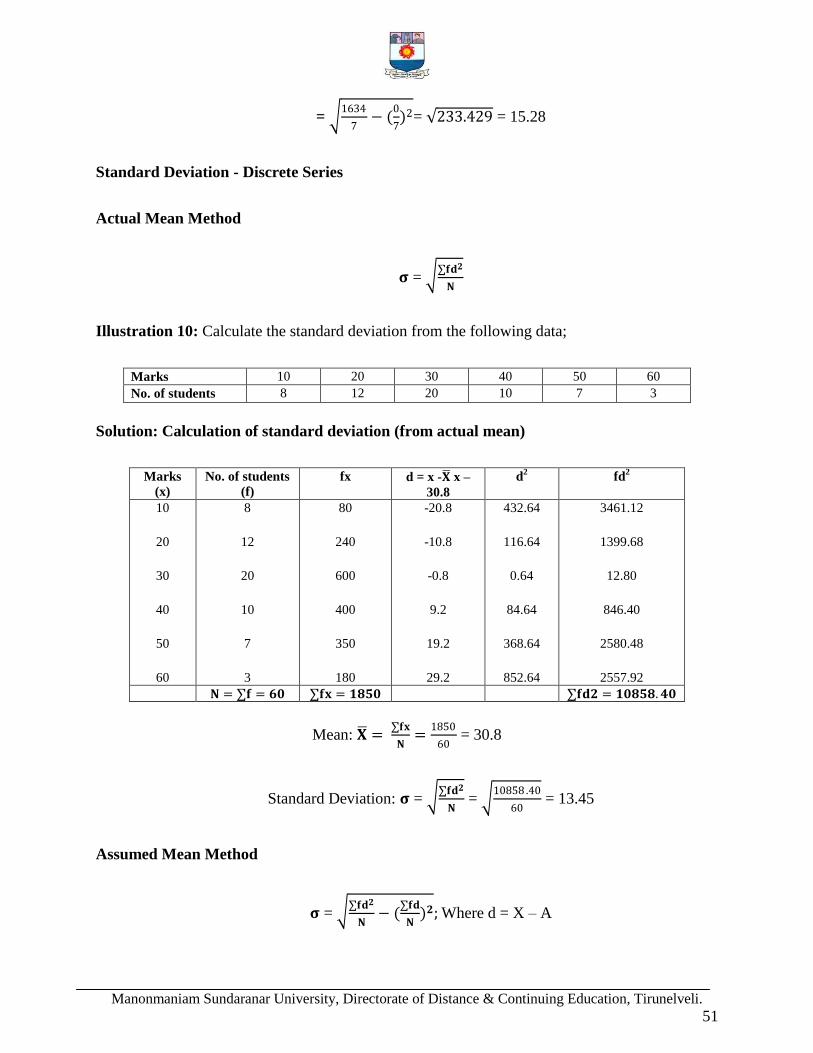
Standard Deviation - Discrete Series
Actual Mean Method
𝛔 = ∑𝐟𝐝𝟐
𝐍
Illustration 10: Calculate the standard deviation from the following data;
Marks 10 20 30 40 50 60
No. of students 8 12 20 10 7 3
Solution: Calculation of standard deviation (from actual mean)
Marks
(x)
No. of students
(f)
fx d = x -𝐗 x –
30.8
d2 fd
2
10
20
30
40
50
60
8
12
20
10
7
3
80
240
600
400
350
180
-20.8
-10.8
-0.8
9.2
19.2
29.2
432.64
116.64
0.64
84.64
368.64
852.64
3461.12
1399.68
12.80
846.40
2580.48
2557.92
𝐍 = ∑𝐟 = 𝟔𝟎 ∑𝐟𝐱 = 𝟏𝟖𝟓𝟎 ∑𝐟𝐝𝟐 = 𝟏𝟎𝟖𝟓𝟖. 𝟒𝟎
Mean: 𝐗 = ∑𝐟𝐱
𝐍=
1850
60 = 30.8
Standard Deviation: 𝛔 = ∑𝐟𝐝𝟐
𝐍 =
10858 .40
60 = 13.45
Assumed Mean Method
𝛔 = ∑𝐟𝐝𝟐
𝐍− (
∑𝐟𝐝
𝐍)𝟐; Where d = X – A

Manonmaniam Sundaranar University, Directorate of Distance & Continuing Education, Tirunelveli.
52
Illustration 11: (Solving the previous problem)
Solution: Calculation of standard deviation (from assumed mean)
x f d = x -𝟑𝟎 fd fd2
10
20
30
40
50
60
8
12
20
10
7
3
-20
-10
0
10
20
30
-160
-120
0
100
140
90
3200
1200
0
1000
2800
2700
𝐍 = ∑𝐟 = 𝟔𝟎 ∑fd = 50 ∑𝐟d2 = 10900
𝛔 = ∑𝐟𝐝𝟐
𝐍− (
∑𝐟𝐝
𝐍)𝟐
𝛔 = 𝟏𝟎𝟗𝟎𝟎
𝟔𝟎− (
𝟓𝟎
𝟔𝟎)𝟐 = 181.67 − 0.69 = 180.98 = 𝟏𝟑. 𝟒𝟓
Step Deviation Method
𝛔 = ∑𝐟𝐝𝟐
𝐍− (
∑𝐟𝐝
𝐍)𝟐 x C
Where d‟ = X − A
C; C = Common Factor
Illustration 12: (Solving the previous problem)
Solution: Calculation of standard deviation (from step deviation)
x f d' = 𝑿−𝟑𝟎
𝟏𝟎 fd' fd'
2
10
20
30
8
12
20
-2
-1
0
-16
-12
0
32
12
0

Manonmaniam Sundaranar University, Directorate of Distance & Continuing Education, Tirunelveli.
53
40
50
60
10
7
3
1
2
3
10
14
9
10
28
27
𝐍 = ∑𝐟 = 𝟔𝟎 ∑fd‟ = 5 ∑𝐟d‟2 = 109
𝛔 = ∑𝐟𝐝𝟐
𝐍− (
∑𝐟𝐝
𝐍)𝟐 x C
𝛔 = 109
60− (
5
60)2 x 10= 1.817 − 0.0069 x 10
= 1.81 x 10 = 1.345 x 10 = 13.45
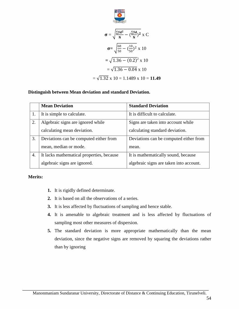
Standard Deviation - Continuous Series
𝛔 = ∑𝐟𝐝𝟐
𝐍− (
∑𝐟𝐝
𝐍)𝟐 x C
Where d = m − A
𝐶; C = Common Factor
Illustration13: Compute the standard deviation from the following data:
Class 0 - 10 10 - 20 20 - 30 30 - 40 40-50
Frequency 5 8 15 16 6
Solution:
Computation of standard deviation
x m f d = 𝒎−𝟐𝟓
𝟏𝟎 d
2 fd fd
2
0 - 10
10 - 20
20 - 30
30 - 40
40 - 50
5
15
25
35
45
5
8
15
16
6
-2
-1
0
1
2
4
1
0
1
4
-10
-8
0
16
12
20
8
0
16
24
𝐍 = ∑𝐟 = 𝟓𝟎 ∑fd = 10 ∑𝐟d2 = 68
Manonmaniam Sundaranar University, Directorate of Distance & Continuing Education, Tirunelveli.
54
𝛔 = ∑𝐟𝐝𝟐
𝐍− (
∑𝐟𝐝
𝐍)𝟐 x C
𝛔= 68
50− (
10
50)2 x 10
= 1.36 − 0.2 2 x 10
= 1.36 − 0.04 x 10
= 1.32 x 10 = 1.1489 x 10 = 11.49
Distinguish between Mean deviation and standard Deviation.
Mean Deviation Standard Deviation
1. It is simple to calculate. It is difficult to calculate.
2. Algebraic signs are ignored while
calculating mean deviation.
Signs are taken into account while
calculating standard deviation.
3. Deviations can be computed either from
mean, median or mode.
Deviations can be computed either from
mean.
4. It lacks mathematical properties, because
algebraic signs are ignored.
It is mathematically sound, because
algebraic signs are taken into account.
Merits:
1. It is rigidly defined determinate.
2. It is based on all the observations of a series.
3. It is less affected by fluctuations of sampling and hence stable.
4. It is amenable to algebraic treatment and is less affected by fluctuations of
sampling most other measures of dispersion.
5. The standard deviation is more appropriate mathematically than the mean
deviation, since the negative signs are removed by squaring the deviations rather
than by ignoring

Manonmaniam Sundaranar University, Directorate of Distance & Continuing Education, Tirunelveli.
55
Demerits:
1. It lacks wide popularity as it is often difficult to compute, when big numbers are
involved, the process of squaring and extracting root becomes tedious.
2. It attaches more weight to extreme items by squaring them.
3. It is difficult to calculate accurately when a grouped frequency distribution has
extreme groups with no definite range.
Uses:
1. Standard deviation is the best measure of dispersion.
2. It is widely used in statistics because it possesses most of the characteristics of an
ideal measure of dispersion.
3. It is widely used in sampling theory and by biologists.
4. It is used in coefficient of correlation and in the study of symmetrical frequency
distribution.
Co - efficient of variation (Relative Standard Deviation)
The Standard deviation is an absolute measure of dispersion. The corresponding relative
measure is known as the co - efficient of variation. It is used to compare the variability of two or
more than two series. The series for which co-efficient or variation is more is said to be more
variable or conversely less consistent, less uniform less table or less homogeneous.
Variance:
Square of standard deviation is called variance.
Variance = σ2;σ = 𝐕𝐚𝐫𝐢𝐚𝐧𝐜𝐞
Co – efficient of standard deviation = 𝛔
𝐗
Co – efficient of variation (C.V.) = 𝛔
𝐗 x 100

Manonmaniam Sundaranar University, Directorate of Distance & Continuing Education, Tirunelveli.
56
Illustration 14: The following are the runs scored by two batsmen A and B in ten innings:
A 101 27 0 36 82 45 7 13 65 14
B 97 12 40 96 13 8 85 8 56 15
Who is the more consistent batsman?
Solution:
Batsman A Batsman B
Runs Scored X dx = X - 𝑿 dx2 Runs Scored Y dx = Y - 𝒀 dy
2
101
27
0
36
82
45
7
13
65
14
62
-12
-39
-3
43
6
-32
-26
26
-25
3844
144
1521
9
1849
36
1024
676
676
625
97
12
40
96
13
8
85
8
56
15
54
-31
-3
53
-30
-35
42
-35
13
-28
2916
961
9
2809
900
1225
1764
1225
169
784
∑X = 390 ∑ dx2= 10404 ∑Y = 430 ∑ dy
2 = 12762
Batsman A Batsman B ∑𝐗
𝐍=
390
10 = 39 𝐘 =
∑𝐘
𝐍=
430
10 = 43
𝛔X = ∑𝐝𝐱𝟐
𝐍=
𝟏𝟎𝟒𝟎𝟒
𝟏𝟎 = 32.26𝛔Y =
∑𝐝𝐲𝟐
𝐍=
𝟏𝟐𝟕𝟔𝟐
𝟏𝟎 = 35.72
C.V. = 𝛔
𝐗 x 100 =
𝟑𝟐.𝟐𝟔
𝟑𝟗 x 100 C.V. =
𝛔
𝐘 x 100 =
𝟑𝟓.𝟕𝟐
𝟒𝟑 x 100
= 82.72% = 83.07%

Manonmaniam Sundaranar University, Directorate of Distance & Continuing Education, Tirunelveli.
57
Batsman A is more consistent in his batting, because the co-efficient of variation of runs
is less for him.
Theoretical Questions
1. Define and explain characteristics of dispersion.
2. Give the importance dispersion.
3. Elucidate the methods of measuring dispersion.
4. What is the practical utility of range?
5. Explain its merits & demerits of range.
6. Distinguish between Mean deviation and standard Deviation.
7. What are the uses of S.D?
Practical Problems
1. Calculate Range, Q.D, M.D (from mean), S.D and C.V of the marks obtained by 10
students given below:
50 55 57 49 54 61 64 59 59 56
(Range = 15, Q.D = 2.75, M. D = 3.6, S.D = 4.43 and C.V = 7.85%)
2. Compute Q.D from the following data:
Height in inches 58 59 60 61 62 63 64 65 66
No. of students 15 20 32 35 33 22 20 10 8
(Q.D = 1.5)
3. Compute quartile deviation from the following data.
x: 4 – 8 8 – 12 12 - 16 16 - 20 20 - 24 24 - 28 28 - 32 32 – 36 36 - 40
f: 6 10 18 30 15 12 10 6 2
(Q.D = 5.21)
4. Calculate mean deviation (from mean) from the following data:
x: 2 4 6 8 10
f: 1 4 6 4 1
(M.D = 1.5)

Manonmaniam Sundaranar University, Directorate of Distance & Continuing Education, Tirunelveli.
58
5. Calculate the mean deviation from the following data.
x: 0 - 5 5 - 10 10 - 15 15 - 20 20 - 25 25 - 30 30 - 35 35 - 40
f: 449 705 507 281 109 52 16 4
(M.D = 5.25)
6. Calculate the S.D of the following:
Size of the item 6 7 8 9 10 11 12
Frequency 3 6 9 13 8 5 4
(S.D = 1.6)
7. Compute standard deviation of the following data:
Wages(Rs. Per day) 1 – 3 3 – 5 5 – 7 7 – 9 9 – 11
No. of workmen 15 18 27 10 6
(S.D = 2.33)
8. Two cricketers scored the following runs in the several innings. Find who is a better run
getter and who more consistent player is?
A: 42 17 83 59 72 76 64 45 40 32
B: 28 70 31 0 59 108 82 14 3 95
(C.V (A) = 38% and C.V (B) = 75.6%)
9. Two brands of types are tested with the following results:
Life („000 miles) 20 – 25 25 – 30 30 – 35 35 – 40 40 – 45 45 – 50
Brand X 8 15 12 18 13 9
Brand Y 6 20 32 30 12 0
(C.V (X) = 21.82% and C.V (Y) = 16.11%)
*****

Manonmaniam Sundaranar University, Directorate of Distance & Continuing Education, Tirunelveli.
59
UNIT – II:
Simple Correlation and Regression - Index numbers - Time series - Components - Estimating
Trend.
CORRELATION ANALYSIS
Correlation refers to the relationship of two or more variables. For example, there exists
some relationship between the height of a mother and the height of a daughter, sales and cost and
so on. Hence, it should be noted that the detection and analysis of correlation between two
statistical variables requires relationship of some sort which associates the observation in pairs,
one of each pair being a value of the two variables. The word „relationship‟ is of important and
indicates that there is some connection between the variables under observation. Thus, the
association of any two variates is known as correlation.
Definitions:
According to YaLun Chou, “Correlation analysis attempts to determine the degree of
relationship between variables”.
According to L.R.Connon “If two or more quantities vary in sympathy so that
movements in one tend to be accompanied by corresponding movements in the other(s), then
they are said to be correlated.”
Uses of correlation
1. Correlation is very useful in physical and social sciences, business and economics.
2. Correlation analysis is very useful to economists to study the relationship between
variables like price and quantity demanded.
3. It helps for businessmen to estimate costs, sales, price and other related variables.
4. Correlation is the basis of the concept of regression and ratio of variation.
5. Correlation analysis helps in calculating the sampling error.

Manonmaniam Sundaranar University, Directorate of Distance & Continuing Education, Tirunelveli.
60
Types of Correlation
1. Positive and Negative correlation
2. Simple and Multiple correlations
3. Partial and total correlation
4. Linear and Non-linear correlation.
1. Positive and Negative Correlation :
The correlation is said to be positive when the values of two variables move in the same
direction, so that an increase in the value of one variable is accompanied by an increase in the
value of the other variable or a decrease in the value of one variable is followed by a decrease in
the value of the other variable.
The correlation is said to be negative when the values of two variables move in opposite
direction, so that an increase or decrease in the values of one variable is followed by a decrease
or increase in the value of the other.
2. Simple and multiple Correlation :
When only two variables are studied then the correlation is said to be simple correlation.
Example: The study of price and demand of an article.
When more than two variables are studied simultaneously, the correlation is said to be
multiple correlation.
Example: the study of price, demand and supply.
3. Partial and total Correlation:
Partial correlation coefficient provides a measure of relationship between a dependent
variable and a particular independent variable when all other variables involved are kept
constant. i.e., when the effect of all other variables are removed.

Manonmaniam Sundaranar University, Directorate of Distance & Continuing Education, Tirunelveli.
61
Example: When we study the relationship between the yield of rice per acre and both the
amount of rainfall and the amount of fertilizers used. In these relationship if we limit our
correlation analysis to yield and rainfall. It becomes a problem relating to simple correlation.
4. Linear and Non-linear Correlation :
The correlation is said to be linear, if the amount of change in one variable tends to bear a
constant ratio to the amount of change in the other variable.
The correlation is non-linear, if the amount of change in one variable does not bear a
constant ratio to the amount of change in the other related variable.
Methods of studying correlation
The following correlation methods are used to find out the relationship between two
variables.
A. Graphic Method :
i. Scatter diagram (or) Scattergram method.
ii. Simple Graph or Correlogram method.
B. Mathematical Method :
i. Karl Pearson‟s Coefficient of Correlation.
ii. Spearman‟s Rank Correlation of Coefficient
iii. Coefficient of Concurrent Deviation
iv. Method of least squares.
C. Graphic Method
i. Scatter diagram method of correlation
This is the simplest method of finding out whether there is any relationship present
between two variables by plotting the values on a chart, known as scatter diagram. In this
method, the given data are plotted on a graph paper in the form of dots. X variables are plotted
on the horizontal axis and Y variables on the vertical axis. Thus we have the dots and we can
know the scatter or concentration of various points.

Manonmaniam Sundaranar University, Directorate of Distance & Continuing Education, Tirunelveli.
62
If the plotted dots fall in a narrow band and the dots are rising from the lower left hand
corner to the upper right-hand corner it is called high degree of positive correlation.
If the plotted dots fall in a narrow band from the upper left hand corner to the lower right
hand corner it is called a high degree of negative correlation.
If the plotted dots line scattered all over the diagram, there is no correlation between the
two variables.
Merits:
1. It is easy to plot even by beginner.
2. It is simple to understand.
3. Abnormal values in a sample can be easily detected.
4. Values of some dependent variables can be found out.
Demerits:
1. Degree of correlation cannot be predicted.
2. It gives only a rough idea.
3. The method is useful only when number of terms is small.
ii. Simple Graph method of correlation
In this method separate curves are drawn for separate series on a graph paper. By
examining the direction and closeness of the two curves we can infer whether or not variables are
related. If both the curves are moving in the same direction correlation is said to be positive. On
the other hand, if the curves are moving in the opposite directions is said to be negative.
Merits:
1. It is easy to plot
2. Simple to understand
3. Abnormal values can easily be deducted.

Manonmaniam Sundaranar University, Directorate of Distance & Continuing Education, Tirunelveli.
63
Demerits
1. This method is useless when number of terms is very big.
2. Degree of correlation cannot be predicted.
B. Mathematical Method:
i. Karl Pearson‟s Coefficient of Correlation.
Karl Pearson, a great biometrician and statistician, introduced a mathematical method for
measuring the magnitude of linear relationship between two variables. This method is most
widely used in practice. This method is known as Pearsonian Coefficient of Correlation. It is
denoted by the symbol ′𝑟′; the formula for calculating Pearsonian r is:
(i) r = 𝑪𝒐𝒗𝒂𝒓𝒊𝒂𝒏𝒄𝒆𝒐𝒇𝒙𝒚
𝝈𝒙 ×𝝈𝒚, (ii) r =
𝚺𝒙𝒚
𝑵𝝈𝒙 ×𝝈𝒚, (iii) r =
𝚺𝒙𝒚
𝚺𝒙𝟐𝚺𝒚𝟐
𝒙 = (𝒙 − 𝑿) , 𝒚 = (𝒚 − 𝒀)
𝝈𝒙 = 𝑺𝒕𝒂𝒏𝒅𝒂𝒓𝒅𝒅𝒆𝒗𝒊𝒂𝒕𝒊𝒐𝒏𝒐𝒇𝒔𝒆𝒓𝒊𝒆𝒔𝒙
𝝈𝒚 = 𝑺𝒕𝒂𝒏𝒅𝒂𝒓𝒅𝒅𝒆𝒗𝒊𝒂𝒕𝒊𝒐𝒏𝒐𝒇𝒔𝒆𝒓𝒊𝒆𝒔𝒚
The value of the coefficient of correlation shall always lie between +1 and -1.
When r = +1, then there is perfect positive correlation between the variables.
When r = -1, then there is perfect negative correlation between the variables.
When r = 0, then there is no relationship between the variables.
Illustration 1: Calculate Karl Pearson coefficient of correlation from the following data:
X 100 101 102 102 100 99 97 98 96 95
Y 98 99 99 97 95 92 95 94 90 91

Manonmaniam Sundaranar University, Directorate of Distance & Continuing Education, Tirunelveli.
64
Solution: Calculation of coefficient of correlation
X x = X - 𝑿
=X – 99
x2 Y y = Y - 𝒀
=Y - 95
y2 xy
100
101
102
102
100
99
97
98
96
95
1
2
3
3
1
0
-2
-1
-3
-4
1
4
9
9
1
0
4
1
9
16
98
99
99
97
95
92
95
94
90
91
3
4
4
2
0
-3
0
-1
-5
-4
9
16
16
4
0
9
0
1
25
16
3
8
12
6
0
0
0
1
15
16
∑ X = 990 ∑ x2 = 54 ∑ Y = 950 ∑ y
2 = 96 ∑ xy = 61
𝑿 = 𝚺𝑿
𝑵=
𝟗𝟗𝟎
𝟏𝟎= 𝟗𝟗; 𝒀 = 𝚺𝒀
𝑵= 𝟗𝟓𝟎
𝟏𝟎= 𝟗𝟓;
r = 𝚺𝒙𝒚
𝚺𝒙𝟐𝚺𝒚𝟐=
61
54 ×96 =
61
5184 =
61
72= + 0.85
Illustration 2: Calculate Karl Pearson coefficient of correlation from the following data:
X: 6 2 10 4 8
Y: 9 11 5 8 7
Solution: Calculation of coefficient of correlation
X X2 Y Y
2 XY
6
2
10
4
36
4
100
16
9
11
5
8
81
121
25
64
54
22
50
32

Manonmaniam Sundaranar University, Directorate of Distance & Continuing Education, Tirunelveli.
65
8 64 7 49 56
∑ X = 30 ∑ X2 = 220 ∑ Y = 40 ∑ Y
2 = 340 ∑ XY = 214
r = 𝐍𝚺𝐗𝐘−(𝚺𝐗.𝚺𝐘)
𝐍𝚺𝑿𝟐−(𝚺𝑿)𝟐𝐱 𝐍𝚺𝒀𝟐−(𝚺𝒀)𝟐
= (5 x 214)−(30 x 40)
5 x 220−(30)2 x 5 x 340−(40)2
= 1070−1200
1100−900 x 1700−1600
= −130
200 x 100
r= - 0.92
*****
RANK CORRELATION COEFFICIENT
Spearman‟s rank correlation co-efficient.
In 1904, a famous British psychologist Charles Edward Spearman found out the method
of ascertaining the coefficient of correlation by ranks. This method is based on rank. Rank
correlation is applicable only to individual observations. This measure is useful in dealing with
qualitative characteristics such as intelligence, beauty, morality, character, etc.,
The formula for Spearman‟s rank correlation which is denoted by P is;
P = 1- 𝟔𝚺𝑫𝟐
𝑵(𝑵𝟐−𝟏) or P = 1-
𝟔𝚺𝑫𝟐
(𝑵𝟑−𝑵)
Where, P = Rank co-efficient of correlation
D = Difference of the two ranks
∑D2 = Sum of squares of the difference of two ranks

Manonmaniam Sundaranar University, Directorate of Distance & Continuing Education, Tirunelveli.
66
N = Number of paired observations
Like the Karl Pearson‟s coefficient of correlation, the value of P lies between + 1 and – 1.
Where ranks are given
Illustration 3: Following are the rank obtained by 10 students in two subjects, Statistics and
Mathematics. To what extent the knowledge of the students in the two subjects is related?
Statistics 1 2 3 4 5 6 7 8 9 10
Mathematics 2 4 1 5 3 9 7 10 6 8
Solution: Calculation of Pearman‟s rank correlation coefficient
Rank of Statistics
(x)
Rank of Mathematics
(y)
D = x – y D2
1
2
3
4
5
6
7
8
9
10
2
4
1
5
3
9
7
10
6
8
-1
-2
+2
-1
+2
-3
0
-2
+3
+2
1
4
4
1
4
9
0
4
9
4
N = 10 𝚺𝑫𝟐 = 𝟒𝟎
P = 1- 𝟔𝚺𝑫𝟐
𝑵(𝑵𝟐−𝟏)
P = 1- 6 x 40
10(102−1)

Manonmaniam Sundaranar University, Directorate of Distance & Continuing Education, Tirunelveli.
67
= 1- 240
10(100 −1)
P = 1- 240
990 = 1 – 0.24= + 0.76
Where ranks are not given
Illustration 4: A random sample of 5 college students is selected and their grades in
Mathematics and Statistics are found to be:
Mathematics 85 60 73 40 90
Statistics 93 75 65 50 80
Solution: Calculation of Pearman‟s rank correlation coefficient
Marks in
Mathematics (x)
Rank x Marks in
Statistics (y)
Rank y D = x – y D2
85
60
73
40
90
2
4
3
5
1
93
75
65
50
80
1
3
4
5
2
+1
+1
-1
0
-1
1
1
1
0
1
𝚺𝑫𝟐 = 𝟒
P = 1- 𝟔𝚺𝑫𝟐
𝑵(𝑵𝟐−𝟏)
P = 1- 6 x 4
5(52−1) = 1-
24
5(25 −1) = 1-
24
5(24)
= 1- 1
5 = 1 – 0.2 = + 0. 8
Equal or Repeated Ranks
When two or more items have equal values, it is difficult to give ranks to them. In that
case the items are given the average of the ranks they would have received, if they are not tied. A
slightly different formula is used when there is more than one item having the same value.

Manonmaniam Sundaranar University, Directorate of Distance & Continuing Education, Tirunelveli.
68
P = 1 – 6{𝚺𝑫𝟐+
𝟏
𝟏𝟐 𝒎𝟑− 𝒎 +
𝟏
𝟏𝟐 𝒎𝟑− 𝒎 +⋯
𝑵𝟑 − 𝑵}
m = the number of items whose ranks are common
Illustration 5: From the following data calculate the rank correlation coefficient after making
adjustment for tied ranks.
X 48 33 40 9 16 16 65 24 16 57
Y 13 13 24 6 15 4 20 9 6 19
Solution: Calculation of Pearman‟s rank correlation coefficient
X Rank x Y Rank y D =R(x) – R(y) D2
48
33
40
9
16
16
65
24
16
57
8
6
7
1
3
3
10
5
3
9
13
13
24
6
15
4
20
9
6
19
5.5
5.5
10
2.5
7
1
9
4
2.5
8
2.5
0.5
-3.0
-1.5
4.0
2.0
1.0
1.0
0.5
1.0
6.25
0.25
9.00
2.25
16.00
4.00
1.00
1.00
025
1.00
𝚺𝑫𝟐 = 𝟒𝟏
P = 1 – 6{𝚺𝑫𝟐+
𝟏
𝟏𝟐 𝒎𝟑− 𝒎 +
𝟏
𝟏𝟐 𝒎𝟑− 𝒎 +
𝟏
𝟏𝟐 𝒎𝟑− 𝒎 …
𝑵𝟑 − 𝑵}
= 1 – 6{41+
1
12 33− 3 +
1
12 23− 2 +
1
12 23− 2 …
103 − 10}= 1 – {
6 41+2+0.5+05
990}
= 1 – { 264
990} = 1 – 0.267 = + 0. 733

Manonmaniam Sundaranar University, Directorate of Distance & Continuing Education, Tirunelveli.
69
Merits:
1. It is simple to understand and easier to apply.
2. It can be used to any type of data, qualitative or quantitative.
3. It is the only method that can be used where we are given the ranks and not the actual
data.
4. Even where actual data are given, rank method can be applied for ascertaining correlation
by assigning the ranks to each data.
Demerits:
1. This method is not useful to find out correlation in a grouped frequency distribution.
2. For large samples it is not convenient method. If the items exceed 30 the calculations
become quite tedious and require a lot of time.
3. It is only an approximately calculated measure as actual values are not used for
calculations.
CONCURRENT DEVIATION METHOD
The method of studying correlation is the simplest of all the methods. The only thing that
is required under this method is to find out the direction of change of X variable and Y variable.
This is based on the signs of deviations; for each term the change is the value of the variable
from its preceding or previous value which may be plus (+) or minus (-).
The formula is:
r(c) = ± 𝟐𝑪−𝑵
𝑵
Where, r(c) = Coefficient of correlation by the concurrent deviation method
C = Number of concurrent deviations (C = ∑dxdy)
N = Number of pairs of deviation compared

Manonmaniam Sundaranar University, Directorate of Distance & Continuing Education, Tirunelveli.
70
Illustration 6: Calculate the coefficient of concurrent deviations from the data given below:
Month Jan. Feb. Mar. Apr. May. June July Aug. Sep.
Supply 160 164 172 182 166 170 178 192 186
Price 292 280 260 234 266 254 230 190 200
Solution: Calculation of coefficient of concurrent deviations
Month Supply x dx Price y dy dxdy
Jan.
Feb.
Mar.
Apr.
May
June
July
Aug.
Sept.
160
164
172
182
166
170
178
192
186
+
+
+
-
+
+
+
-
292
280
260
234
266
254
230
190
200
-
-
-
+
-
-
-
+
-
-
-
-
-
-
-
-
N = 8 C =∑dxdy = 0
r(c) = ± 𝟐𝑪−𝑵
𝑵
= ± 2 x 0−8
8
= ± −8
8 = ±
−1
1
= ± −(−1)
= ± (+1)= - 1
*****

Manonmaniam Sundaranar University, Directorate of Distance & Continuing Education, Tirunelveli.
71
REGRESSION
The statistical method which helps us to estimate the unknown value of one variable from
the known value of the related variable is called Regression. The dictionary meaning of the word
regression is „return‟ or „going back‟. In 1877, Sir Francis Galton, first introduced the word
„regression‟. The tendency to regression or going back was called by Galton as the „Line of
Regression‟. The line describing the average relationship between two variables is known as the
line of regression. The regression analysis confined to the study of only two variables at a time is
termed as simple regression. The regression analysis for studying more than two variables at a
time is known as multiple regressions.
Definitions
According to Blair, “Regression is the measure of the average relationship between two
or more variables in terms of the original units of the data”.
According to Taro Yamane, “One of the most frequently used techniques in economics
and business research, to find a relation between two or more variables that are related causally,
is regression analysis”.
Uses of Regression Analysis
The following are the uses of regression analysis
1. It is useful to estimate the relationship between two variables.
2. It is useful for prediction of unknown value.
3. It is widely used in social sciences like economics, natural and physical sciences.
4. It is useful to forecast the business situations.
5. It is useful o estimate thereof in sampling.
6. It is useful to calculate correlation co-efficient and co-efficient of determination.

Manonmaniam Sundaranar University, Directorate of Distance & Continuing Education, Tirunelveli.
72
Differentiate Correlation from Regression.
Correlation Regression
It is the relationship between two or more
variable.
It is a mathematical measure showing the
average relationship between two
variables.
Both x and y are random variables. Here x is a random variable and y is a
fixed variable.
It gives limited information after verifying
the relationship between the variables
It is used for the prediction of one value,
in relationship to the other given value.
The range of relationship between -1 and
+1.
Regression value is an absolute figure.
It studies linear relationship between the
variables.
It studies linear and non-linear
relationship between the variables.
If the coefficient of correlation is positive,
then the two variables are positively
correlated and vice versa.
The regression coefficient explains that
the decrease in one variable is associated
with the increase in the other variable.
Regression lines
If we take two variables X and Y we have two regression lines:
i) Regression of X on Y and
ii) Regression of Y on X
The regression line of X on Y gives the most probable value of X for any given value of
Y. The regression of Y on X gives the most probable value of Y for any given value of X. There
are two regression lines in the case of two variables.
Regression Equations
The algebraic expressions of the two regression lines are called regression equations.

Manonmaniam Sundaranar University, Directorate of Distance & Continuing Education, Tirunelveli.
73
Regression Equation of X on Y:
Xc = a + by
To determine the values of „a‟ and „b‟, the following two normal equations are to be
solved simultaneously.
∑X = Na + b∑Y
∑XY = a∑Y + b∑Y2
Regression Equation of Y on X:
Yc = a + bx
To determine the value of „a‟ and „b‟, the following two normal equations are to be
solved simultaneously.
∑Y = Na + b∑X
∑XY = a∑X + b∑X2
We can call these equations as normal equations.
Illustration 1: Determine the two regression equations of a straight line which best fits the data.
X 10 12 13 16 17 20 25
Y 10 22 24 27 29 33 37
Solution: Calculation of Regression
X X2 Y Y
2 XY
0
12
13
16
17
100
144
169
256
289
10
22
24
27
29
100
484
576
729
841
100
264
312
432
493

Manonmaniam Sundaranar University, Directorate of Distance & Continuing Education, Tirunelveli.
74
20
25
400
625
33
37
1089
1369
660
925
∑X = 113 ∑ X2
= 1983 ∑Y = 182 ∑ Y2
= 5188 ∑ XY = 3186
Regression Equation of Y on X:
The two normal equations are:
∑Y = Na + b∑X
∑XY = a∑X + b∑X2
Substituting the values,
N = 7; ∑X = 113; ∑ X2
= 1983; ∑Y = 182; ∑ XY = 3186;
7a + 113b = 182 …(1)
113a + 1983b = 3186 …(2)
Multiplying (1), by 113,
791a + 12769b = 20566 …(3)
Multiplying (2), by 7,
791a + 13881b = 22302 …(4)
Subtracting (4) from (3)
- 1112 b = - 1736
b = −1736
−1112 =>b = 1.56
Put b = 1.56 in (1) we get
7a + 113(1.56)b = 182
7a + 176.28 = 182 => 7a =5.72

Manonmaniam Sundaranar University, Directorate of Distance & Continuing Education, Tirunelveli.
75
a = 5.72
7 =>a = 0.82
The equation of straight line is Yc = a + bX
Put a = 0.82, b = 1.56
∴The equation of the required straight line is Yc = 0.82 + 1.56 X
This is called regression of y on x
Regression Equation of X on Y:
The two normal equations are:
∑X = Na + b∑Y
∑XY = a∑Y + b∑Y2
Substituting the values,
N = 7; ∑X = 113; ∑ Y2
= 5188; ∑Y = 182; ∑ XY = 3186;
7a + 182b = 113 …(1)
182a + 5188b = 3186 …(2)
Multiplying (1), by 182,
1274a + 33124b = 20566 …(3)
Multiplying (2), by 7,
1274a + 36316b = 22302 …(4)
Subtracting (4) from (3)
3192 b = 1736
b = 1736
3192 =>b = 0.54

Manonmaniam Sundaranar University, Directorate of Distance & Continuing Education, Tirunelveli.
76
Put b = 0.54 in (1) we get
7a + 182(0.54)b = 113
7a + 98.28 = 113 => 7a = 14.72
a = 14.72
7 =>a = 2.1
The equation of straight line is Xc = a + bY
Put a = 2.1, b = 0.54
∴The equation of the required straight line is Xc = 2.1 + 0.54 Y
This is called regression of x on y
Deviation taken from Actual Means:
Regression equation of X on Y:
X - 𝑿 = r𝜎𝑥
𝜎𝑦 (𝐘 − 𝒀 )
Where, X = the value of x to be estimated for the given y value. 𝑿 = Mean value of X
variable. Y = the value of y given in the problem; 𝒀 = Mean value of y variables.
r𝜎𝑥
𝜎𝑦 =
∑𝑥𝑦
∑𝑦2 = Regression co - efficient of X on Y.
x = X - 𝑿 ; y = Y- 𝒀
Regression equation of Y on X:
Y- 𝒀 = r𝜎𝑥
𝜎𝑦 (X –𝑿 )
r𝜎𝑥
𝜎𝑦 =
∑𝑥𝑦
∑𝑦2 = Regression co-efficient of Y on X.

Manonmaniam Sundaranar University, Directorate of Distance & Continuing Education, Tirunelveli.
77
Illustration 2: Find regression lines from the following data:
X 3 5 6 8 9 11
Y 2 3 4 6 5 10
And also estimate Y when X is 15.
Solution: Calculation of Regression Equations (by actual mean)
X x = X - 𝑿 x2 Y y = 𝐘 − 𝒀 y
2 xy
3
5
6
8
9
11
-4
-2
-1
1
2
4
16
4
1
1
4
16
2
3
4
6
5
10
-3
-2
-1
1
0
5
9
4
1
1
0
25
12
4
1
1
0
20
∑X = 42 ∑x = 0 ∑ x2 = 42 ∑Y = 30 ∑y = 0 ∑ y
2 = 40 ∑xy = 38
𝑿 = 𝚺𝑿
𝑵=
42
6= 7 𝒀 =
𝚺𝒀
𝑵=
30
6= 5
Regression equation of X on Y: Regression equation of Y on X:
X - 𝑿 = r𝜎𝑥
𝜎𝑦 (𝐘 − 𝒀 ) Y- 𝒀 = r
𝜎𝑥
𝜎𝑦 (X –𝑿 )
r𝜎𝑥
𝜎𝑦 =
∑𝑥𝑦
∑𝑦2 =
38
40 = 0.95 r
𝜎𝑥
𝜎𝑦 =
∑𝑥𝑦
∑𝑦2 =
38
42 = 0.90
X – 7 = 0.95(Y – 5) Y – 5 = 0.90(X – 7)
X – 7 = 0.95Y – 4.75 Y – 5 = 0.90X – 6.30
X = 0.95Y + 2.25 Y = 0.90X – 1.30
When X is 15, Y will be,Y = 0.90 x 15 – 1.30
= 13.5 – 1.30

Manonmaniam Sundaranar University, Directorate of Distance & Continuing Education, Tirunelveli.
78
Y = 14.8
Deviation taken from the Assumed Mean:
Regression equation of X on Y:
X - 𝑿 = r𝜎𝑥
𝜎𝑦 (Y -𝒀 )
Where, r𝜎𝑥
𝜎𝑦 =
𝑁Σ𝑑𝑥𝑑𝑦 − Σ𝑑𝑥 (Σ𝑑𝑦 )
𝑁Σ𝑑𝑦2−(Σ𝑑𝑦 )2
dx = X - A; dy = Y - A; ( A = assumed mean)
Regression equation of Y on X :
Y – 𝒀 = r𝜎𝑦
𝜎𝑥 (X -𝑿 )
r𝜎𝑥
𝜎𝑦 =
𝑁Σ𝑑𝑥𝑑𝑦 − Σ𝑑𝑥 (Σ𝑑𝑦 )
𝑁Σ𝑑𝑥2−(Σ𝑑𝑥 )2
Illustration: 3. Find regression lines from the following data:
X 40 38 35 42 30
Y 30 35 40 36 29
Also calculate Karl Pearson‟s coefficient of correlation.
Solution: Calculation of Regression Equations (by assumed mean)
X dx = X – A dx2 Y dy= Y – A dy
2 dx.dy
40
38
35
42
30
5
3
0
7
-5
25
9
0
49
25
30
35
40
36
29
0
5
10
6
-1
0
25
100
36
1
0
15
0
42
5
∑ dx = 10 ∑ dx2=108 ∑ dy=1020 ∑ dy
2=162 dx.dy = 62
𝑿 = 𝑨 ±𝚺𝐝𝒙
𝑵= 35 ±
10
5= 37 𝒀 = 𝑨 ±
𝚺𝐝𝒚
𝑵= 30 ±
20
5= 34

Manonmaniam Sundaranar University, Directorate of Distance & Continuing Education, Tirunelveli.
79
Regression equation of X on Y Regression equation of Y on X
X - 𝑿 = bxy (Y -𝒀 ) Y – 𝒀 = byx (X - 𝑿 ))
bxy = 𝑁Σ𝑑𝑥𝑑𝑦 − Σ𝑑𝑥 (Σ𝑑𝑦 )
𝑁Σ𝑑𝑦2−(Σ𝑑𝑦 )2 byx = 𝑁Σ𝑑𝑥𝑑𝑦 − Σ𝑑𝑥 (Σ𝑑𝑦 )
𝑁Σ𝑑𝑥2−(Σ𝑑𝑥 )2
= 5 𝐱 62− 10 (20)
5 x 162 −(20)2 = 5 𝐱 62− 10 (20)
5 x 10⁸ −(10)2
= 310−200
810−400 =
110
410 =
310−200
540−100 =
110
440
bxy = 0.27 byx = 0.25
X – 37 = 0.27(Y – 34) Y – 34 = 0.25(X – 37)
X – 37 = 0.27Y – 9.18 Y – 34 = 0.25X – 9.25
X = 0.27Y + 27.82 Y = 0.25X + 24.75
r = 𝑏𝑥𝑦 𝑥 𝑏𝑦𝑥
= 2.2 x 0.37 = 0.814= 0.9
Illustration 4: Given the following data, calculate the expected value of Y when X = 12.
X Y
Arithmetic Mean (X ) 7.6 14.8
Standard Deviation (σ) 3.6 2.5
Coefficient of correlation(r) = 0.99
Solution:
Regression of Y on X
Y- 𝒀 = r𝜎𝑥
𝜎𝑦 (X –𝑿 )
Y – 14.8 = 0.99 x 2.5
3.6 (X – 7.6)
Y – 14.8 = 0.688 (X – 7.6)
Y – 14.8 = 0.688 X – 5.23
Y = 0.688 X – 5.23 + 14.8

Manonmaniam Sundaranar University, Directorate of Distance & Continuing Education, Tirunelveli.
80
Y = 0.688 X + 9.57
When X = 12 => Y = 0.688 (12) + 9.57 = 17.826
Hence the expected value of Y is 17.83.
*****
Theoretical Questions
1. Define and explain the uses of correlation.
2. Define and explain the merits & demerits of correlation.
3. Explain the types of correlation.
4. Describe the methods of correlation with relative merits and demerits.
5. Define and explain the uses of Regression.
6. Define and explain the merits & demerits of Regression.
7. Explain the types of Regression.
8. Differences between Correlation and Regression.
Practical Problems
1. Calculate Pearson‟s coefficient of correlation between advertisement cost and sales
from the following data:
Advertisement Cost(„000) Rs. 39 65 62 90 82 75 25 98 36 78
Sales (‟00,000) 47 53 58 86 62 68 60 91 51 84
(r = + 0.78)
2. Compute the coefficient of correlation of the following score of A and B.
A: 5 10 5 11 12 4 3 2 7 1
B: 1 6 2 8 5 1 4 6 5 2
(r = + 0.58)
3. Ten competitors in a voice contest are ranked by 3 judges in the following orders:
I Judge 1 6 5 10 3 2 4 9 7 8
II Judge 3 5 8 4 7 10 2 1 6 9
III Judge 6 4 9 8 1 2 3 10 5 7

Manonmaniam Sundaranar University, Directorate of Distance & Continuing Education, Tirunelveli.
81
Use the rank correlation to gauge which pair of judges have the nearest approach
to common likings in voice.
(I & II = - 0.212; II & III = - 0.297; I & III = + 0.636)
4. Calculate the rank correlation coefficient for the following table of marks of students
in two subjects:
Major I 80 64 54 49 48 35 32 29 20 18 15 10
Major II 36 38 39 41 27 43 45 52 51 42 40 52
(r = - 0.685)
5. The following table gives the score obtained by 11 students in Mathematics and
Statistics. Find the rank correlation coefficient.
Mathematics 40 46 54 60 70 80 82 85 85 90 95
Statistics 45 45 50 43 40 75 55 72 65 42 70
(r = + 0.36)
6. Calculate the coefficient of concurrent deviation from the data given below:
Year 1976 1977 1978 1979 1980 1981 1982 1983 1984
Supply 160 164 172 182 166 170 178 192 186
Price 292 290 260 234 266 254 230 130 200
(r = -1)
7. Obtain the equations of lines of regression between the indices.
X: 78 77 85 88 87 82 81 77 76 83 97 93
Y: 84 82 82 85 89 90 88 92 83 89 98 99
(X = 0.79 Y + 13.82; Y = 0.59 X + 39.05)
8. Calculate the two regression equations of X on Y and Y on X from the data given
below, taking deviations from actual means of X and Y.
Price (Rs.) 10 12 13 12 16 15
Amount demanded 40 38 43 45 37 43
Estimate the likely demand when the price is Rs. 20.
(X = -0.12 Y + 17.92; Y = -0.25 X + 44.25; Y = 39.25)
9. The correlation coefficient between two variable X and Y is r = 0.6. If σx = 1.5 σy=
2.0, 𝑋 = 10 and 𝑌 = 20, find the regression lines of Y on X and X on Y.
(X = 0.45 Y + 1; Y = 0.8 X + 12)

Manonmaniam Sundaranar University, Directorate of Distance & Continuing Education, Tirunelveli.
82
10. By using the following data. Find out the two lines regression and from them
compute the Karl Pearson‟s Coefficient of Correlation:
∑X = 250; ∑Y = 300; ∑XY = 7900; ∑X2 = 6500; ∑Y
2 = 10,000; N -= 10.
(r = - 0.8)
11. Given the following data, estimate the marks in mathematics obtained by a student
who has scored 60 marks in statistics.
Mean marks of mathematics 80
Mean marks of statistics 50
S.D marks in mathematics 15
S.D marks in statistics 10
Coefficient of correlation 0.4
(X = 0.6 Y + 50; X = 86.)
*****
INDEX NUMBERS
An index number is a number which is used to measure the level of a certain
phenomenon as compared to the level of the same phenomenon at some standard period. It is a
statistical device for comparing the general level of magnitude of a group of related variables in
two or more situations. It is a number which indicates the change in magnitude.
Definitions
According to Croxton and Cowden, “Index numbers are devices for measuring
differences in the magnitude of a group of related variables”.
According to Spiegal, “An index number is a statistical measure designed to show
changes in a variable or a group of related variables with respect to time, geographic location or
other characteristics”.
According to Maslow, “It is a numerical value characterizing the change in complex
economic phenomena over a period of time or space”.

Manonmaniam Sundaranar University, Directorate of Distance & Continuing Education, Tirunelveli.
83
Characteristics of Index numbers
1. Index numbers are specialized averages.
2. Index numbers measure the net change in a group of related variables.
3. Index numbers measure changes not capable of direct measurement.
4. Index numbers are for comparison.
5. Index numbers are expressed in terms of percentages so as to show the extent of
change. However, percentage sign (%) is never used.
Uses of Index Numbers
1. Index numbers are most widely used statistical devices.
2. Index numbers are used to measure the relative changes.
3. Index numbers widely used in the evaluation of business and economic conditions.
4. Index numbers are useful for better standard of living comparison.
5. Index numbers help in framing suitable policies
6. Index numbers are useful to know trends and tendencies.
7. Index numbers measure the purchasing power of money.
8. Index numbers are the wage adjuster.
9. Index numbers are useful in deflation.
10. Index numbers are used as guides.
Types of Index Numbers
There are various types of index numbers. Some of which are follows.
1. Price Index:
It is used for measuring the value of money. It is an index number which
compares the prices for a group of commodities at a certain time or at a place with prices
of a base period.
There are two types of price index namely,
i. Wholesale Price index numbers and
ii. Retail Price index numbers.

Manonmaniam Sundaranar University, Directorate of Distance & Continuing Education, Tirunelveli.
84
The changes in the general price level of a country are called wholesale price
index.
The changes in the retail prices of commodities such as, consumption goods, bank
deposits, bonds, etc., are called retail price index.
2. Quantity Index:
The changes in the volume of goods produced or consumed are studied in
quantity index numbers.
3. Value Index:
The total value of a certain period is compared with the total value of the base
period is called value index numbers.
Methods of construction of index numbers
The various methods of construction of index numbers are as follows:
I. Unweighted Index Numbers.
1. Simple Aggregative method
This is the simplest method of constructing the index numbers. The prices of the
different commodities of the current year are added and the total is divided by the sum of the
prices of base year commodity and multiplied by 100:
P01=𝚺𝑷𝟏
𝚺𝑷𝟎𝐱𝟏𝟎𝟎
Illustration 1: Construct an index number for 2016 taking 2015 as base from the following data.
Commodity Price in 2015 (Rs.) Price in 2016 (Rs.)
A 50 60
B 40 80
C 70 110
D 90 70
E 50 40

Manonmaniam Sundaranar University, Directorate of Distance & Continuing Education, Tirunelveli.
85
Solution: Calculation of index number
Commodity Price in 2015 (Rs.) Price in 2016 (Rs.)
A 50 60
B 40 80
C 70 110
D 90 70
E 50 40
∑P0 = 300 ∑P1=360
Price Index, P01 =Σ𝑃1
Σ𝑃0 x 100 =
360
300 x 100 = 120
This means that as compared to 2015, in 2016 there is a net increase in the prices of
commodities to the extent of 20%.
2. Simple Average of Price relative method:
In this method, the price relative of each item is calculated separately and then averaged.
Arithmetic Mean of Price Relatives: P01 = 𝚺𝑷
𝑵
Geometric Mean of Price Relatives: P01 = antilog ∑𝒍𝒐𝒈𝑷
𝑵
Where, P = 𝑃1
𝑃0x 100; N = Number of items.
Illustration 2: Compute a price index for the following by using both arithmetic mean and
geometric mean:
Commodity A B C D E F
Price in 2014 (Rs.) 20 30 10 25 40 50
Price in 2015 (Rs.) 25 30 15 35 45 55

Manonmaniam Sundaranar University, Directorate of Distance & Continuing Education, Tirunelveli.
86
Solution: Calculation for Price Index
Commodity Price in 2014
P0
Price in 2015
P0
Price Relative
P = 𝑷𝟏
𝑷𝟎 x 100
Log P
A
B
C
D
E
F
20
30
10
25
40
50
25
30
15
35
45
55
125
100
150
140
112.5
110
2.0960
2.0000
2.1761
2.1461
2.0511
2.0414
N = 6 ∑P = 737.5 ∑log P =12.5116
Arithmetic Mean of Price Relatives: P01 = 𝚺𝑷
𝑵=
737.5
6 = 122.92
Geometric Mean of Price Relatives: P01 = Antilog ∑𝒍𝒐𝒈𝑷
𝑵
=Antilog 12.5116
6
= Antilog 2.0853
= 121.7.
II. Weighted Index Number
Weighted Aggregative Index Numbers: Under this method weights are assigned to
various items and a number of formulae have been used. The following are some of the
methods, generally used.
A. Laspeyre‟s method: In this method, the base year quantities are taken as weights:
P01 (La) =𝚺𝑷𝟏𝒒𝟎
𝚺𝑷𝟎𝒒𝟎𝐱𝟏𝟎𝟎
B. Paasche‟s method: In this method, current year quantities are taken as weights:
P01 (Pa) =𝚺𝑷𝟏𝒒𝟎
𝚺𝑷𝟎𝒒𝟎𝐱𝟏𝟎𝟎

Manonmaniam Sundaranar University, Directorate of Distance & Continuing Education, Tirunelveli.
87
C. BowleyDorfish method: This is an index number got by the arithmetic mean of
Laspeyre‟s and Paasche‟s methods. This method takes into account both the current and
the base periods.
P01 (B) = 𝐋+𝐏
𝟐
Where,L = Laspeyre‟s method; P = Paasche‟s method
D. Fisher‟s ideal Method: Fisher‟s price index number is given by the geometric mean of
Laspeyre‟s and Paasche‟s formula;
P01 (F) = 𝐋𝐱𝐏
E. Marshal Edge worth Method: Under this method, the arithmetic mean of base year and
current year quantities are taken as weights (𝑤 =𝑞0+ 𝑞1
2)
P01 (Ma) = 𝚺𝒑𝟏𝒒𝟎
𝚺𝒑𝟎𝒒𝟎+
𝚺𝒑𝟏𝒒𝟏
𝚺𝒑𝟎𝒒𝟏x 100
F. Kelly‟s method: Kelly‟s method number uses quantities of some period (which is neither
the base period nor the current period) as weights. This weight is kept constant for all
periods. If we denote it by q, then Kelly‟s method number is given by
P01 (K) =𝚺𝑷𝟏𝒒
𝚺𝑷𝟎𝒒𝐱𝟏𝟎𝟎
G. Walsch‟s method: Under this method, the geometric mean of the base year and current
year quantities as weights.
P01 (Wa) = 𝚺𝑷𝟏 𝒒𝟎𝒒𝟏
𝚺𝑷𝟎 𝒒𝟎𝒒𝟏 x 100
Illustration 3: Calculate index number from the following data through a) Laspeyre‟s method b)
Paasche‟s method c) Bowley‟s method d) Fisher‟s ideal formula method and e) Marshall Edge
worth method:
Base Year Current Year
Kilo Rate (Rs.) Kilo Rate (Rs.)
Bread
Meat
Tea
10
20
2
3
15
25
8
15
3
3.25
20
23

Manonmaniam Sundaranar University, Directorate of Distance & Continuing Education, Tirunelveli.
88
Solution: Calculation of Index Numbers
Base Year Current Year p1q0 p0q0 p1q1 p0q1
Kilo Rate Kilo Rate
q0 p0 q1 p1
Bread
Meat
Tea
10
20
2
3
15
25
8
15
3
3.25
20
23
32.50
400.00
46.00
30
300
50
26
300
69
24
225
75
Total ∑ p1q0 =
478.50
∑ p0q0 =
380
∑ p1q1 =
395
∑ p0q1 =
324
a) Laspeyre‟s method: P01 (La) = 𝚺𝑷𝟏𝒒𝟎
𝚺𝑷𝟎𝒒𝟎𝐱𝟏𝟎𝟎=
478.50
380x 100 = 125.9
b) Paasche‟s method: P01 (Pa) = 𝚺𝑷𝟏𝒒𝟎
𝚺𝑷𝟎𝒒𝟎𝐱𝟏𝟎𝟎=
395
324 x 100= 121.9
c) BowleyDorfish method: P01 (B) = 𝐋+𝐏
𝟐 =
125.9+121.9
2 = 123.9
d) Fisher‟s ideal Method: P01 (F) = 𝐋𝐱𝐏= 125.9 x 121.9
= 15347.21 = 123.9
e)Marshal Edge worth Method: P01 (Ma) = 𝚺𝒑𝟏𝒒𝟎
𝚺𝒑𝟎𝒒𝟎+
𝚺𝒑𝟏𝒒𝟏
𝚺𝒑𝟎𝒒𝟏x 100
= 478.5
380+
395
324x 100 =
873.5
704x 100 = 1.24 x 100 = 124.
2. Weighted average of price relative.
P01 = ∑𝑷𝑽
∑𝑽 ; P01 =Antilog
∑𝑽𝒍𝒐𝒈𝑷
∑𝑽

Manonmaniam Sundaranar University, Directorate of Distance & Continuing Education, Tirunelveli.
89
Illustration 4: Compute a price index for the following by using both arithmetic mean and
geometric mean:
Item Price in 1976 Price in 1977 Quantity in 1976
Wheat
Sugar
Milk
2
3
1.50
2.50
3.25
1.75
40 kg
20 kg
10 lit.
Solution: Construction of Index
Item p0 p1 q0 V = P0q0 P = p1/p0 x
100
PV Log P Log PV
Wheat
Sugar
Milk
2
3
1.50
2.50
3.25
1.75
40
20
10
80
60
15
125
108.33
116.67
10000
6499.8
1750.05
2.0969
2.0346
2.0669
167.7520
122.0760
31.0065
Total ∑V= 155 ∑PV =
18249.85
∑ Log PV
=320.8345
P01 = ∑𝑷𝑽
∑𝑽=
𝟏𝟖𝟐𝟒𝟗.𝟖𝟓
𝟏𝟓𝟓 = 117.74
P01 = Antilog ∑𝑽𝒍𝒐𝒈𝑷
∑𝑽= Antilog
𝟑𝟐𝟎.𝟖𝟑𝟒𝟓
𝟏𝟓𝟓
= Antilog 2.0699 = 111.4
Test of consistency of Index Numbers
1. Time Reversal Test
P01 = 𝚺𝑷𝟏𝒒𝟎
𝚺𝑷𝟎𝒒𝟎𝐱
𝚺𝑷𝟏𝒒𝟏
𝚺𝑷𝟎𝒒𝟏; P10 =
𝚺𝑷𝟎𝒒𝟏
𝚺𝑷𝟏𝒒𝟏𝐱
𝚺𝑷𝟎𝒒𝟎
𝚺𝑷𝟏𝒒𝟎
P01 x P10 = 𝚺𝑷𝟏𝒒𝟎
𝚺𝑷𝟎𝒒𝟎𝐱
𝚺𝑷𝟏𝒒𝟏
𝚺𝑷𝟎𝒒𝟏𝐱
𝚺𝑷𝟎𝒒𝟏
𝚺𝑷𝟏𝒒𝟏𝐱
𝚺𝑷𝟎𝒒𝟎
𝚺𝑷𝟏𝒒𝟎= 𝟏 = 𝟏
It shows that the Time Reversal Test is satisfied
2. Factor Reversal Test
P01 = 𝚺𝐩𝟏𝐪𝟎
𝚺𝐩𝟎𝐪𝟎𝐱
𝚺𝐩𝟏𝐪𝟏
𝚺𝐩𝟎𝐪𝟏; Q01 =
𝚺𝐪𝟏𝐩𝟎
𝚺𝐪𝟎𝐩𝟎𝐱
𝚺𝐩𝟎𝐪𝟎
𝚺𝐪𝟎𝐩𝟏

Manonmaniam Sundaranar University, Directorate of Distance & Continuing Education, Tirunelveli.
90
P01 x Q01 = 𝚺𝐩𝟏𝐪𝟎
𝚺𝐩𝟎𝐪𝟎𝐱
𝚺𝐩𝟏𝐪𝟏
𝚺𝐩𝟎𝐪𝟏𝐱
𝚺𝐪𝟏𝐩𝟎
𝚺𝐪𝟎𝐩𝟎𝐱
𝚺𝐪𝟏𝐩𝟏
𝚺𝐪𝟎𝐏𝟏
= 𝚺𝐩𝟏𝐪𝟏
𝚺𝐩𝟎𝐪𝟎𝐱
𝚺𝐩𝟏𝐪𝟏
𝚺𝐩𝟎𝐪𝟎 =
𝚺𝐩𝟏𝐪𝟏
𝚺𝐩𝟎𝐪𝟎
Illustration 5: Compute Index Number, using Fishers Ideal Formula and show that it satisfies
time – reversal test and factor – reversal test.
Commodity Quantity Base Year
Price
Quantity Current Year
Price
A
B
C
D
12
15
24
5
10
7
5
16
15
20
20
5
12
5
9
14
Solution: Computation of Index Number
Commodity q0 p0 q1 p1 p1q0 p0q0 p1q1 p0q1
A
B
C
D
12
15
24
5
10
7
5
16
15
20
20
5
12
5
9
14
144
75
216
70
120
105
120
80
180
100
180
70
150
140
100
80
∑ p1q0 =
505
∑ p0q0 =
425
∑ p1q1 =
530
∑ p0q1 =
470
P01 = 𝚺𝑷𝟏𝒒𝟎
𝚺𝑷𝟎𝒒𝟎𝐱
𝚺𝑷𝟏𝒒𝟏
𝚺𝑷𝟎𝒒𝟏x 100 =
505
425 x
530
470x 100 = 1.188 x 1.128x 100= 115.8
Test of consistency of Index Numbers
1. Time Reversal Test
Time Reversal Test is satisfied when P01 x P10= 1 = 1
P01 x P10 = 𝚺𝐩𝟏𝐪𝟎
𝚺𝐩𝟎𝐪𝟎𝐱
𝚺𝐩𝟏𝐪𝟏
𝚺𝐩𝟎𝐪𝟏𝐱
𝚺𝐩𝟎𝐪𝟏
𝚺𝐩𝟏𝐪𝟏𝐱
𝚺𝐩𝟎𝐪𝟎
𝚺𝐩𝟏𝐪𝟎 = 𝟏 = 𝟏
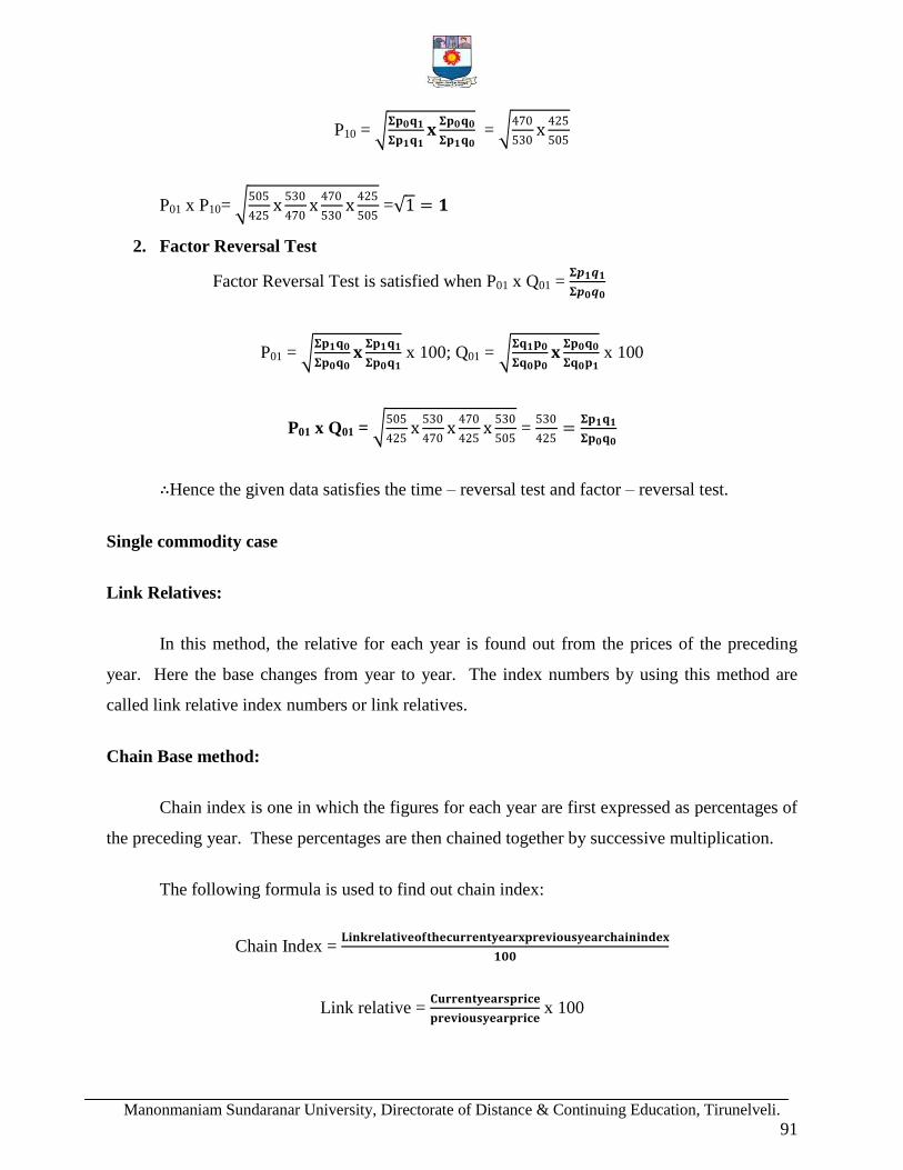
Manonmaniam Sundaranar University, Directorate of Distance & Continuing Education, Tirunelveli.
91
P10 = 𝚺𝐩𝟎𝐪𝟏
𝚺𝐩𝟏𝐪𝟏𝐱
𝚺𝐩𝟎𝐪𝟎
𝚺𝐩𝟏𝐪𝟎 =
470
530x
425
505
P01 x P10= 505
425x
530
470x
470
530x
425
505 = 1 = 𝟏
2. Factor Reversal Test
Factor Reversal Test is satisfied when P01 x Q01 = 𝚺𝒑𝟏𝒒𝟏
𝚺𝒑𝟎𝒒𝟎
P01 = 𝚺𝐩𝟏𝐪𝟎
𝚺𝐩𝟎𝐪𝟎𝐱
𝚺𝐩𝟏𝐪𝟏
𝚺𝐩𝟎𝐪𝟏 x 100; Q01 =
𝚺𝐪𝟏𝐩𝟎
𝚺𝐪𝟎𝐩𝟎𝐱
𝚺𝐩𝟎𝐪𝟎
𝚺𝐪𝟎𝐩𝟏 x 100
P01 x Q01 = 505
425x
530
470x
470
425x
530
505 =
530
425=
𝚺𝐩𝟏𝐪𝟏
𝚺𝐩𝟎𝐪𝟎
∴Hence the given data satisfies the time – reversal test and factor – reversal test.
Single commodity case
Link Relatives:
In this method, the relative for each year is found out from the prices of the preceding
year. Here the base changes from year to year. The index numbers by using this method are
called link relative index numbers or link relatives.
Chain Base method:
Chain index is one in which the figures for each year are first expressed as percentages of
the preceding year. These percentages are then chained together by successive multiplication.
The following formula is used to find out chain index:
Chain Index = 𝐋𝐢𝐧𝐤𝐫𝐞𝐥𝐚𝐭𝐢𝐯𝐞𝐨𝐟𝐭𝐡𝐞𝐜𝐮𝐫𝐫𝐞𝐧𝐭𝐲𝐞𝐚𝐫𝐱𝐩𝐫𝐞𝐯𝐢𝐨𝐮𝐬𝐲𝐞𝐚𝐫𝐜𝐡𝐚𝐢𝐧𝐢𝐧𝐝𝐞𝐱
𝟏𝟎𝟎
Link relative = 𝐂𝐮𝐫𝐫𝐞𝐧𝐭𝐲𝐞𝐚𝐫𝐬𝐩𝐫𝐢𝐜𝐞
𝐩𝐫𝐞𝐯𝐢𝐨𝐮𝐬𝐲𝐞𝐚𝐫𝐩𝐫𝐢𝐜𝐞 x 100

Manonmaniam Sundaranar University, Directorate of Distance & Continuing Education, Tirunelveli.
92
Advantages of chain base index
1. It is a great advantage to economists and businessmen.
2. Without any recalculation we can omit old items and introduce new items.
3. Weights can be adjusted as frequently as possible.
4. It is free from seasonal variations.
Fixed Base index
In this method, no link relative method is used. Weights cannot be adjusted frequently.
The base year does not change and it is suitable for long period only.
How would you convert the Chain Base index to fixed base index?
The following steps are to be followed to convert the chain base index to fixed base index
1. First year is fixed as the chain base index and the same will be taken as the base
which is 100.
2. For other years to find out the index numbers the following formula is used.
Current year FBI = 𝐂𝐮𝐫𝐫𝐞𝐧𝐭𝐲𝐞𝐚𝐫𝐂.𝐁.𝐈
𝐏𝐫𝐞𝐯𝐢𝐨𝐮𝐬𝐲𝐞𝐚𝐫’𝐬𝐅𝐁𝐈 x 100
Base shifting
The change of reference base period is called shifting the base. For comparison, it is
necessary to shift the base from one period to another period. We can express the series in terms
of a recent period. It is called base shifting
Index number = 𝐂𝐮𝐫𝐫𝐞𝐧𝐭𝐲𝐞𝐚𝐫’𝐬𝐨𝐥𝐝𝐢𝐧𝐝𝐞𝐱𝐧𝐮𝐦𝐛𝐞𝐫
𝐍𝐞𝐰𝐛𝐚𝐬𝐞𝐲𝐞𝐚𝐫’𝐬𝐨𝐥𝐝𝐢𝐧𝐝𝐞𝐱𝐧𝐮𝐦𝐛𝐞𝐫 x 100
Differentiate chain base and fixed base.
Chain Base Fixed Base
1. The base year changes. The base year does not change.

Manonmaniam Sundaranar University, Directorate of Distance & Continuing Education, Tirunelveli.
93
2. Here the link relative method is used. No such link relative method is used.
3. Introduction and deletion of items are
easy to calculate without
recalculation of the entire series.
Any change in the commodities, will
involve the entire index number to be
recast.
4. It cannot be computed if data for any
one year is missing.
There is no such problem.
5. It is suitable for short period only. It is suitable for long periods only.
6. Index number wrong if an error is
committed in the calculation of any
link index number.
This is not so, the error is confined to
the index of that year only.
Consumer price index (or) Cost of living index.
Consumer price index is designed to measure the change in the cost of living of workers
due to change in the retail price. A change in the price level affects the cost of living of the
people. People consume different types of commodities. So there is need to construct consumer‟s
price index. Consumer price index can be used in different places for many purposes.
Methods of construction of consumer price index.
a) Aggregate Expenditure method
b) Family Budget method.
a) Aggregate expenditure method: P01 = 𝚺𝑷𝟏𝒒𝟎
𝚺𝑷𝟎𝒒𝟎x 100
This method is based upon the Laspeyre‟s method.
b) Family Budget method: P01 = 𝚺𝑷𝑽
𝚺𝑽
Where; P = P1
P0 x 100; V = p0q0 (value weight)

Manonmaniam Sundaranar University, Directorate of Distance & Continuing Education, Tirunelveli.
94
Uses of cost of living index
The following are the main uses of cost of live index:
1. It is useful or fixing the wages.
2. It is useful to know the purchasing power of money.
3. By using the cost of living index the Government decides about the price and other
variables.
4. Dearness Allowances and Bonus are regulated with the help of this index.
5. It is useful for the analysis of price situation.
Limitations of index numbers
1. If the chosen base year is not a normal one, all the purpose is lost.
2. Every index number has its own purpose. No index number can serve all the purpose.
3. These are only approximate indications of the relative level.
*****
ANALYSIS OF TIME SERIES
An arrangement of statistical data in accordance with time of occurrence or in
chronological order is called a time series. Thus when we observe numerical data at regular
intervals of time the set of observation is known as time series. The regular intervals may be an
hour, a day, a week a month, a year, a decade etc.,
Definitions
According to Wessel and Welelt, “When quantitative data are arranged in the order of
their occurrence, the resulting statistical series is called a time series”.
According to Morris Hamburg, “A time series is a set of observations arranged in
chronological order”.

Manonmaniam Sundaranar University, Directorate of Distance & Continuing Education, Tirunelveli.
95
According to Cecil H. Maers, “A time series may be defined as a sequence or repeated
measurements of a variable made periodically through time”.
According to Patterson, “A time series consist of statistical data which are collected,
recorded or observed over successive increments”.
According to Ya-Luh-Chou, “A time series may be defined as a collection of magnitudes
belonging to different time periods, of some variable or composite of variables, such as
production of steel, per capital income, gross national product, price of tobacco or index of
industrial production”.
Uses of time series
Time series analysis is useful indifferent fields like economics, science, research work,
etc because of the following reasons.
1. It helps in understanding the past behavior.
2. It helps in planning and forecasting the future operations.
3. It facilitates comparison between data of one period with another period.
4. It is useful not only to economists but also to the businessman.
5. It helps in evaluating current accomplishments.
6. It is useful for forecasting the trade cycles.
Types of variations or components or elements of time series.
There are four basic types of variations and these are called the components or elements
of time series.
(i) Secular trend (ii) Seasonal variation (iii) Cyclical variations (iv) Irregular variation.

Manonmaniam Sundaranar University, Directorate of Distance & Continuing Education, Tirunelveli.
96
i) Secular Trend:
A secular or long-term trend refers to the movement of a series reflecting continuous
growth or decline over a long period of time. There are many types of trend. Some trend rise
upward and some trend fall downward.
The following are the types of trend.
i. Linear (or) Straight Line Trend.
ii. Non-Linear (or) Curvilinear Trend
If the values of time series are plotted on a graph and if it forms a straight line then it is
called Linear (or) Straight Line Trend.
If the values of time series are plotted on a graph an if it forms a curve then it is called
Non-linear (or) Curvilinear Trend.
ii) Seasonal variation:
Seasonal variations are those periodic movements in business activities within the year,
recurring periodically year after year. Generally, seasons variations appear at weekly, monthly
or quarterly intervals.
Causes:
Seasonal variation may occur due to climate, weather conditions, customs, habits and
traditions.
Uses:
Seasonal variation analysis is used to formulate correct policy decisions and of planning
future operations. It is useful to businessmen, producers, agriculturist etc., to study effects of
seasonal variations and to isolate them from the trend.

Manonmaniam Sundaranar University, Directorate of Distance & Continuing Education, Tirunelveli.
97
Cyclical variation:
According to Linecoin L. Chou, “Up and down movements are different from seasonal
fluctuations, in that they extend over longer period of time - usually two or more years”.
Business time series is influenced by the wave-like change of prosperity and depression.
This up and down movement is known as cyclical variation. Cyclical variation analysis is helpful
to businessmen for stabilizing the level of business activities and also useful to the economist for
formulating suitable policies.
Irregular variation:
Irregular variations refer to such variations in business activities which do not repeat in a
definite pattern. They are also called „erratic‟ accidental or random variations which are
generally non-recurring and unpredictable. Irregular variations of time series are either random
or caused by some sporadic forces such as war, flood, revolution, etc. It is usually a short-term
one, but it will affect all the components of time series.
Methods of estimating the trend components
There are four methods of estimating trend.
1. The free hand Graphic method.
In this method we must plot the original data on the graph. Draw a smooth curve
carefully which will show the direction of the trend.
2. Semi - Averages
In this method the original data are divided into two equal parts and averages are
calculated for both the parts. These averages are called Semi –Averages. Trend line is
drawn with the help of this average.
3. Moving average method :
In this method, the average value for a number of years or months or weeks is
taken into an account and placing it at the centre of the time span (period of moving
average) and it is the normal or trend value for the middle period.
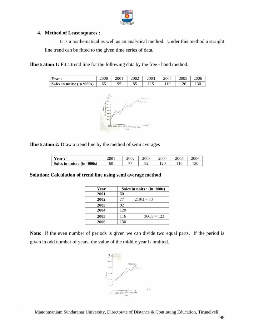
Manonmaniam Sundaranar University, Directorate of Distance & Continuing Education, Tirunelveli.
98
4. Method of Least squares :
It is a mathematical as well as an analytical method. Under this method a straight
line trend can be fitted to the given time series of data.
Illustration 1: Fit a trend line for the following data by the free - hand method.
Year : 2000 2001 2002 2003 2004 2005 2006
Sales in units: (in „000s) 65 95 85 115 110 120 130
Illustration 2: Draw a trend line by the method of semi averages
Year : ` 2001 2002 2003 2004 2005 2006
Sales in units : (in „000s) 60 77 82 120 116 130
Solution: Calculation of trend line using semi average method
Year Sales in units : (in „000s)
2001 60
2002 77 219/3 = 73
2003 82
2004 120
2005 116 366/3 = 122
2006 130
Note: If the even number of periods is given we can divide two equal parts. If the period is
given in odd number of years, the value of the middle year is omitted.

Manonmaniam Sundaranar University, Directorate of Distance & Continuing Education, Tirunelveli.
99
Illustration 3: Draw a trend line by the method of semi-averages
Year : 2000 2001 2002 2003 2004 2005 2006
Sales in units : (in „000s) 100 110 120 115 130 135 140
Solution:
Calculation of trend line using semi average method
Year Sales in units : (in „000s)
2000 100
2001 330/3 = 110
2002 120
2003 115 Left out the middle item
2004 130
2005 405/3 = 135
2006 140
3. Moving average method
In this method the average value for a number of years or months or weeks is taken into
account. It is placed at the centre of the time - span. It is the normal or trend value for the
middle period.
Calculation of moving averages:
The formula for calculating 3 yearly moving averages is
𝒂+𝒃+𝒄
𝟑,𝒃+𝒄+𝒅
𝟑,
𝒄+𝒅+𝒆
𝟑
The formula for 4 yearly moving averages is

Manonmaniam Sundaranar University, Directorate of Distance & Continuing Education, Tirunelveli.
100
𝒂+𝒃+𝒄+𝒅
𝟒 ,
𝒃+𝒄+𝒅+𝒆
𝟒,𝒄+𝒅+𝒆+𝒇
𝟒
The formula for 5 yearly moving averages is
𝒂+𝒃+𝒄+𝒅+𝒆
𝟓,𝒃+𝒄+𝒅+𝒆+𝒇
𝟓,
𝒄+𝒅+𝒆+𝒇+𝒈
𝟓
Steps to calculate 3 yearly moving averages:
1. Compute the value of first three years and place the three year total against the middle
year.
2. Leave the first year‟s value and compute the value of next three years and place the total
against the middle year ie., against 3rd
year.
3. This process should be continued until the last year‟s value is taken for calculation.
4. The three yearly total values are divided by 3 and the value placed in the next column.
This value is called the Trend value of moving average.
Steps for calculating of 4yearly moving average (or) Even period of moving average:
1. Computer the value of first four years and place the total value in between second and
the third year.
2. Leave the first year‟s value and compute the value of next four years and place the
total in between third and fourth year.
3. This process must be continued until the last year‟s value is taken for calculation.
4. Computer the first two four year totals and place the value against the middle of two
four years totals.
5. Leave the first four years total and compute the next two four year‟s totals and place
it against the middle of next four year.
6. This method must be continued until all the four year totals.
7. The two four yearly totals is divided by 8 and put the value in the next column. This
value is called Trend value.

Manonmaniam Sundaranar University, Directorate of Distance & Continuing Education, Tirunelveli.
101
Illustration 4: Find the 3-yearly moving average from the following time series data.
Year : 1998 1999 2000 2001 2002 2003 2004 2005
Sales in units : (in tones) 30.1 45.4 39.3 41.4 42.2 46.4 46.6 49.2
Solution:
Calculation of 3 yearly moving average method
Year Sales (in
tons)
3 yearly
moving total
3 yearly
moving value
1998 30.1 - -
1999 45.4 114.8 38.27
2000 39.3 126.1 42.03
2001 41.4 122.9 40.97
2002 42.2 130.0 43.33
2003 46.4 135.2 45.07
2004 46.6 142.2 47.40
2005 49.2 - -
Illustration 5: Calculate the trend value by using three yearly moving averages of the following
data.
Year : 1990 1991 1992 1993 1994 1995 1996 1997 1998 1999
Production (in „000 tons) 21 22 23 25 24 22 25 26 27 26
Solution: Calculation of trend value by using 3 yearly moving averages
Year Production (in
„000 tons)
3 yearly
moving total
3 yearly moving Average
(Trend value)
1990 21 - -
1991 22 66 22.00
1992 23 70 23.33
1993 25 72 24.00
1994 24 71 23.67
1995 22 71 23.67
1996 25 73 24.33
1997 26 78 26.00
1998 27 79 26.33
1999 26 - -

Manonmaniam Sundaranar University, Directorate of Distance & Continuing Education, Tirunelveli.
102
Illustration 6: Calculate the 5 yearly moving averages from the following data:
Year : 1997 1998 1999 2000 2001 2002 2003 2004 2005 2006
No. of Students: 705 685 703 687 705 689 715 685 725 730
Solution: Calculation of 5 yearly moving average method
Year No. of students 5 yearly moving total Moving Value
1997 705
1998 683
1999 703 3485 697.0
2000 687 3469 693.8
2001 705 3499 699.8
2002 689 3481 696.2
2003 715 3519 703.8
2004 685 3544 708.8
2005 725
2006 730
Illustration 7: Calculate the four – yearly moving average for the following data
Year : 1994 1995 1996 1997 1998 1999 2000 2001 2002 2003
Production : (in „000 tons) 464 515 518 467 502 540 557 571 586 612
Solution: Calculation of 4 yearly moving average method
Year Production 4 Yearly Moving Combined Total Moving Average
1994 464
1995 515
1964
1996 518 3966 3966/8 = 495.75
2002
1997 467 4029 4029/8 = 503.63
2027
1998 502 4093 4093/8 = 511.63
2066
1999 540 4236 4236/8 = 529.50
2170
2000 557 4424 4424/8 = 553.00
2254
2001 571 4580 4580/8 = 572.50
2326
2002 586
2003 612

Manonmaniam Sundaranar University, Directorate of Distance & Continuing Education, Tirunelveli.
103
4. Methods of least square
A Straight line trend can be fitted from the time series of given data. The trend line is
called the line of best fit.
The sum of deviations of the actual values of Y and the trend value (Yc) is zero. And the
sum of squares of deviations of actual value of Y and the trend value (Yc) is the least.
i.e. (Y-Yc) = 0 and (Y-Yc)2
= least value
This method is called the method of least square (or) the line of best fit. The method of
least square can be used in the liner and non-linear trend
Yc = a + bx;
Yc = required trend value; X = unit of time; a and be are constants
The constants a and b are calculated from the following two normal equations.
𝚺𝐘 = 𝐍𝐚 + 𝐛𝚺𝐗_______ (1)
𝚺𝐗𝐘 = 𝐚𝚺𝐗 + 𝐛𝚺𝐗𝟐_______(2)
Where N = Number of years or months
When x = 0 (middle year taken as origin)
𝚺𝐗 = 𝟎
𝐛𝚺𝐗 = 𝟎 and 𝐚𝚺𝐗 = 𝟎
From (1),𝚺𝐘 = 𝐍𝐚 + 𝟎 → 𝐚 = 𝚺𝐘
𝐍or 𝐘
From (2),𝚺𝐗𝐘 = 𝟎 + 𝐛𝚺𝐗𝟐 → 𝐛 = 𝚺𝐗𝐘
𝚺𝐗𝟐
a = 𝚺𝐘
𝐍 and 𝐛 =
𝚺𝐗𝐘
𝚺𝐘𝟐

Manonmaniam Sundaranar University, Directorate of Distance & Continuing Education, Tirunelveli.
104
Illustration 8: Compute the trend from the following by the method of least squares:
Year : 2000 2001 2002 2003 2004
Population (in Lakhs ) 830 920 710 900 1690
Solution: Computation of trend values
Year Production (in lakhs)
(Y)
Deviation from
2002 (X)
XY X2
2000 830 2000-2002=-2 -1660 4
2001 920 2001-2002=-1 -920 1
2002 710 2002-2002=0 0 0
2003 900 2003-2002=1 900 1
2004 1690 2004-2002=2 3380 4
𝚺y = 5050 𝚺x = 0 𝚺xy = 1700 𝚺x2=10
Since ∑x =0, a = ∑y
N = 5050/5 = 1010
b = ΣXY
ΣX2 = 1700 / 10 = 170
Yc = a + bx = 1010 + 170 x
Yc = 1010 + 170 x
When X = -2, Y2000 = 1010 + 170(-2) = 1010 – 340 = 670
When X = -1, Y2001 = 1010 + 170 (-1) = 1010 - 170 = 840
When X = 0, Y2002 = 1010+170(0) = 1010 – 0 = 1010
When x = 1, Y 2003 = 1010 + 170(1) = 1010 + 170 = 1180
When x = 2, Y2004 = 1010 + 170 (2) = 1010 + 340 = 1350

Manonmaniam Sundaranar University, Directorate of Distance & Continuing Education, Tirunelveli.
105
Illustration 9: Fit a straight line trend by the method of least squares from the following data
and estimate the earnings for the year 2008:
Year : 1999 2000 2001 2002 2003 2004 2005 2006
Earnings (in Lakhs ) 38 40 65 72 69 60 87 95
Solution: Computation of trend values
Year Earnings (Rs. in
lakhs) (Y)
Deviation from 2002.5
(X)
XY X2
1999 38 1999 - 2002.5 = -3.5 -133.0 12.25
2000 40 2000 - 2002.5 = -2.5 -100.0 6.25
2001 65 2001 - 2002.5 = -1.5 -97.5 2.25
2002 72 2002 - 2002.5 = -0.5 -36.0 0.25
2003 69 2003 - 2002.5 = 0.5 34.5 0.25
2004 60 2004 - 2002.5 = 1.5 90.0 2.25
2005 87 2005 - 2002.5 = 2.5 217.5 6.25
2006 95 2006 - 2002.5 = 3.5 332.5 12.25
N = 8 𝚺y = 526 𝚺x = 0 𝚺xy = 308 𝚺x2 = 42
Yc = a + bx
a = ∑y
N = 526/8 = 65.75
b = ΣXY
ΣX2 = 308 / 42 = 7.33
That is Yc = 65.75 + 7.33 x
In the year 2008, the value of x is 5.5 that is (2008 – 2002.5)
∴ The earnings for the year 2008 will be
Y2008 = 65.75 + 7.33(5.5) = 65.75 + 40.31 = 106.06
*****

Manonmaniam Sundaranar University, Directorate of Distance & Continuing Education, Tirunelveli.
106
Theoretical Questions
1. Explain the characteristics of index numbers.
2. What are the uses of index numbers?
3. Discuss the types of index numbers in detail.
4. Describe the various methods of construction of index numbers.
5. Define and explain the advantages of chain base index.
6. How would you convert the Chain Base index to fixed base index?
7. Differentiate chain base and fixed base.
8. Explain the methods of construction of consumer price index.
9. What are uses of cost of living index?
10. Give the limitations of index numbers.
11. Define and explain the types of time series.
12. Describe the components of time series.
13. Explain the uses and causes of time series.
14. What are the steps to calculate 3 yearly moving averages?
15. Explain the steps for calculating of 4yearly moving average.
Practical Problems
1. Construct an index number for 2016 taking 2015 as base from the following data.
Commodity Price in 1984 (Rs.) Price in 1985 (Rs.)
A 90 95
B 40 60
C 90 110
D 30 35
(P01 = 120)

Manonmaniam Sundaranar University, Directorate of Distance & Continuing Education, Tirunelveli.
107
2. Compute a price index for the following by average of price relative method.
Commodity A B C D E F
Price in 2005 (Rs.) 10 25 30 20 40 50
Price in 2006 (Rs.) 15 30 40 30 50 55
(P01 = 131.39)
3. Compute Index Number, using Fishers Ideal Formula and show that it satisfies time –
reversal test and factor – reversal test.
Commodity Quantity Base Year Price Quantity Current Year Price
A
B
C
D
E
50
100
60
30
40
6
2
4
10
8
56
120
60
24
36
10
2
6
12
12
(P01 = 139.8)
4. Calculate a) Paasche‟s index, b) Laspeyre‟s index and c) Fisher‟s index numbers for
the following data:
Commodity P0 q0 P1 q1
A
B
C
D
E
12
10
15
60
3
20
8
2
1
2
15
16
12
65
10
25
10
1
1
1
(Ans. a) 130.13; b) 129.09; and c) 129.60)
5. Compute the trend from the following by the method of least squares:
Year : 1976 1977 1978 1979 1980 1981
Population (in Lakhs ) 24 25 29 26 22 24
Estimate the likely production for 1984.
(Ans. 23.119)

Manonmaniam Sundaranar University, Directorate of Distance & Continuing Education, Tirunelveli.
108
6. The following table gives the price per egg on the first of each month.
Year Jan. Feb. Mar. Apr. May June July Aug. Sep. Oct. Nov. Dec.
1988 18 19 20 21 23 24 26 26 28 25 23 29
1989 18 21 21 21 22 24 25 26 27 24 23 21
1990 19 17 20 22 23 25 25 26 26 24 22 20
Calculate the seasonal variations for each of the months Jan. to Dec.
(Ans. 80.9; 83.9; 89.7; 94.2; 100; 107.5; 111.9; 114.9; 119.3; 107.5; 100.9; 89.8)
*****
Manonmaniam Sundaranar University, Directorate of Distance & Continuing Education, Tirunelveli.
109
UNIT - III:
Differential Calculus - Sum, Product, Quotient Rules, Maximum and Minimum.
DIFFERENTIAL CALCULUS
INTRODUCTION
Sir Isacc Newton of England and Gottfried Wilhelm Leibnitz of Germany invented
calculus in the 17th
century, independently.
Leibniz‟s calculus originated from his attempts to solve some problems in geometry.
Newton‟s calculus originated from his attempts to solve some problems in physics and
astronomy.
CALCULUS
Origin
„Calculus‟ is a Latin word which means a „pebble‟ or a „small stone‟. In ancient times,
pebbles were used as for calculations.
Meaning
Calculus is the mathematics of motion and change. When increasing or decreasing
quantities are made the subject of mathematical investigation, it frequently becomes necessary to
estimate their rate of growth or decay.
BASIC OPERATIONS OF CALCULUS
The basic operations of calculus are divided into two main parts. They are:
I. Differential Calculus and II. Integral calculus
DIFFERENTIAL CALCULUS
Differential calculus deals with the rate of change of one quantity with respect to another.

Manonmaniam Sundaranar University, Directorate of Distance & Continuing Education, Tirunelveli.
110
USES OF DIFFERENTIAL CALCULUS
i) It is used in calculating the rate of change of velocity of a vehicle with respect to time.
ii) It is used in calculating the rate of change of growth of population with respect to time.
iii) Differential calculus is also a method by which maxima and minima of functions are
obtained.
iv) Marginal analysis is one of the important applications of calculus in business and economics.
v) The problems of maximizing profit and minimizing cost under various assumptions can be
solved.
OBJECTIVES OF THE DIFFERENTIAL CALCULUS
The main objective of the differential calculus is to describe an instrument for the
measurement of such rates to frame rules for its formation and use.
RULES OF DIFFERENTIATION
Constant Rules
The derivative of a constant is zero
If y = c (constant)
Then, 𝑑𝑦
𝑑𝑥=
𝑑𝑐
𝑑𝑥= 0
Power Function Rule
The derivative of a power function: xnis nx
n-1
If y = xn
Then, 𝑑𝑦
𝑑𝑥 = nx
n-1

Manonmaniam Sundaranar University, Directorate of Distance & Continuing Education, Tirunelveli.
111
For Example,
Y = x6 then
𝑑𝑦
𝑑𝑥=
𝑑
𝑑𝑥(x
6)= 6x
6-1 = 6x
5
Y = x then 𝑑𝑦
𝑑𝑥=
𝑑
𝑑𝑥(x)= 1x
1-1 = 1x
0 = 1
Sum Rule:
The derivative of a sum of two functions is the sum of the derivatives of the two
functions.
If y = u + v
Then, 𝑑𝑦
𝑑𝑥=
𝑑𝑢
𝑑𝑥+
𝑑𝑣
𝑑𝑥
Illustration 1: Differentiate: y = 3x2 + 5x
4
Solution:
𝑑𝑦
𝑑𝑥 =
𝑑
𝑑𝑥 (3x
2) +
𝑑
𝑑𝑥 (5x
4)
= 6x + 20x3
Difference Rule:
The derivative of difference of two functions is the difference of the derivatives of the
two functions.
If y = u – v
Then, 𝑑𝑦
𝑑𝑥=
𝑑𝑢
𝑑𝑥 -
𝑑𝑣
𝑑𝑥

Manonmaniam Sundaranar University, Directorate of Distance & Continuing Education, Tirunelveli.
112
Illustration 3: Differentiate: y = 2x2 – 5x
3 + 5
Solution:
𝑑𝑦
𝑑𝑥 =
𝑑
𝑑𝑥 (2x
2) -
𝑑
𝑑𝑥(5x
3) +
𝑑
𝑑𝑥 (5)
= 4x – 15x2
Product Rule:
The derivative of the product of two functions is equal to the first function times the
derivative of the second function plus the second function times the derivative of the first
function.
y = uv
𝑑𝑦
𝑑𝑥= u
𝑑𝑣
𝑑𝑥 + v
𝑑𝑢
𝑑𝑥
Illustration 4: Differentiate: y = (4x + 8) (4x3)
Solution:
u = 4x + 8; v = 4x3
𝑑𝑦
𝑑𝑥 =
𝑑(𝑢𝑣)
𝑑𝑥 (4x + 8)
𝑑
𝑑𝑥 (4x
3) + (4x
3)
𝑑
𝑑𝑥 (4x + 8)
= (4x + 8) 12 x2 + (4x
3) (4)
= 48x3 + 96x
2 + 16x
3
= 64x3 + 96x
2
Quotient Rule:
The derivative of the quotient of two functions is given by the following formula.

Manonmaniam Sundaranar University, Directorate of Distance & Continuing Education, Tirunelveli.
113
If u and v are differential function and if v(x) ≠ 0,
Then, y = 𝑢𝑣
𝑑𝑦
𝑑𝑥 =
𝑣𝑑𝑢
𝑑𝑥−
𝑢𝑑𝑣
𝑑𝑥
𝑣2
Illustration: 5. Differentiate: y = 2𝑥+1
𝑥
Solution:
𝑑𝑦
𝑑𝑥 =
𝑣𝑑𝑢
𝑑𝑥−
𝑢𝑑𝑣
𝑑𝑥
𝑣2
y =𝑢
𝑣; u = 2x + 1; v = x
𝑑𝑦
𝑑𝑥 =
𝑑(𝑢
𝑣)
𝑑𝑥=
𝑥𝑑 2
𝑑𝑥− 2𝑥+1 .
𝑑 1
𝑑𝑥
𝑥2
= 𝑥 .2− 2𝑥+1 .1
𝑥2 =
2𝑥−2𝑥−1
𝑥2 =
−1
𝑥2
Function of a Function Rule:
If we have a function y = f(x) where x is in turn a function of another variable, u, then the
derivative of y with respect to u is equal to the derivative of y with respect to x times in the
derivative of x with respect to u.
If y = f(x) and x = g(u)
Then 𝑑𝑦
𝑑𝑥=
𝑑𝑦
𝑑𝑢.𝑑𝑢
𝑑𝑥
Illustration 6: Differentiate y = (x2 + 8x – 8)
16 with respect to x.
Solution:
Let y = (x2 + 8x – 8)
16 and u = x
2 + 8x – 8

Manonmaniam Sundaranar University, Directorate of Distance & Continuing Education, Tirunelveli.
114
Then y = u16
and u = (x2 + 8x – 8)
𝑑𝑦
𝑑𝑥=
𝑑
𝑑𝑥 𝑢16 .
𝑑
𝑑𝑥(𝑥2 + 8𝑥 − 8) = 16u
15 (2x + 8)=
16(x2+8x-8)
15. (2x+8)
Function of a Function Rule or Chain Rule of Differentiation
y 𝒅𝒚
𝒅𝒙
f(x) 𝒅𝒚
𝒅𝒖.𝒅𝒖
𝒅𝒙
Illustration 7: Find 𝒅
𝒅𝒙𝒆𝒂𝒙
Solution:
Let u = ax y = eu
du
dx= a,
dy
du= eu = 𝑒𝑎𝑥
dy
d𝑥=
dy
du.du
d𝑥
∴dy
d𝑥= aeax
So if y = 𝑒3𝑥 , 𝑑𝑦
𝑑𝑥= 3𝑒3𝑥
y = 𝑒−5𝑥 ,𝑑𝑦
𝑑𝑥= −5𝑒−5𝑥
y = 𝑒−𝑥 , 𝑑𝑦
𝑑𝑥= −𝑒−𝑥
y = 1/𝑒4𝑥 = 𝑒−4𝑥 , 𝑑𝑦
𝑑𝑥= −4𝑒−4𝑥
= −4/𝑒4𝑥

Manonmaniam Sundaranar University, Directorate of Distance & Continuing Education, Tirunelveli.
115
Some other Important Rules
Sometimes we have to differentiate logarithmic and exponential functions. Their
derivatives are:
Logarithmic function
If y = log x then 𝑑𝑦
𝑑𝑥=
1
𝑥
Exponential function
If y = ex then
𝑑𝑦
𝑑𝑥= 𝑒𝑥
Higher Order Derivatives:
𝑑
𝑑𝑥(𝑑𝑦
𝑑𝑥) is denoted by
𝑑2𝑦
𝑑𝑥2 read as: “d – squared y by dx squared”. This is called the second
order differential coefficient of y with respect to x. Various symbols used are y2, y‟‟, y‟‟(x), f
2(x),
D2y.
Similarly 𝑑3𝑦
𝑑𝑥 3 is the third order differential coefficient of y with respect x and so on..
Illustration 8.Consider the function y = x5
Solution:
𝑑𝑦
𝑑𝑥 = 5x
4
𝑑2𝑦
𝑑𝑥 2 = 20 x3
𝑑3𝑦
𝑑𝑥 3 = 60 x 2
𝑑4𝑦
𝑑𝑥 4 = 120 x

Manonmaniam Sundaranar University, Directorate of Distance & Continuing Education, Tirunelveli.
116
Simple applications to Economics
Elasticity of the function:
The elasticity of a function y = f(x) at the point x is the rate of proportional change in y
per unit proportional change in x.
𝑬𝒚
𝑬𝒙=
𝒙
𝒚 .
𝒅𝒚
𝒅𝒙
Illustration 9: Let y = 3x – 6. Find i) elasticity and ii) the elasticity if x = 8.
Solution:
𝑬𝒚
𝑬𝒙=
𝒙
𝒚 .
𝒅𝒚
𝒅𝒙 =
𝑥
3𝑥−6.𝑑(3𝑥 – 6)
𝑑𝑥 =
𝑥
3𝑥−6(3) =
3𝑥
3(𝑥−2) =
𝑥
𝑥−2
When x = 8, 𝑬𝒚
𝑬𝒙=
𝟖
𝟖−𝟐 =
𝟖
𝟔 =
𝟒
𝟑
Elasticity of Demand
The elasticity of demand denoted by ή is defined by ή = −𝑝
𝑞.𝑑𝑞
𝑑𝑝
Illustration 10: q = 32 – 4p – p2. Find ή when p = 3.
Solution:
ή = −𝑝
𝑞.𝑑𝑞
𝑑𝑝
= - 3
32 – 4 3 –(3)2.𝑑(32 – 4p – p2)
𝑑𝑝
= - 3
11(−4 − 2𝑝) = -
3
11(−4 − 2(3) =
30
11
ή = 30
11 or 2.727.

Manonmaniam Sundaranar University, Directorate of Distance & Continuing Education, Tirunelveli.
117
Marginal Revenue:
It is defined as 𝑑𝑅
𝑑𝑞
𝑑𝑅
𝑑𝑞= 𝑝(1 −
1
ή )
Illustration 11: If p = 3 and ή = 30
11 . Find
𝑑𝑅
𝑑𝑞.
Solution:
𝑑𝑅
𝑑𝑞= 𝑝(1 −
1
ή ) = 3(1-
30
11) = 3(
19
30) =
19
10 = 1.9
Illustration 12: The total cost, C, of making x units of a product is, C = 0.00003x3 –
0.045x2+8x+25000. Find the marginal cost at 1000 units out-put.
Solution:
C = 0.00003x3 –0.045x
2+8x+25,000 ………………….(1)
Marginal Cost at the level x is 𝑑𝐶
𝑑𝑥
Differentiating both sides of with respect to ‘x’
𝑑𝐶
𝑑𝑥= 0.00009 x
2 - 0.09 x + 8
Marginal Cost at x = 1000 is 𝑑𝐶
𝑑𝑥 at x = 1000.
When x = 1000 =>𝑑𝐶
𝑑𝑥= 0.00009 (1000)
2 - 0.09(1000) + 8 = 90 - 90 + 9 = 8
∴Marginal Cost at x = 1000 is 8.

Manonmaniam Sundaranar University, Directorate of Distance & Continuing Education, Tirunelveli.
118
CRITERIA FOR MINIMA
Consider the curve y=f(x) given in the below figure. From the figure we see that V is the
lowest point of the curve and so the y - coordinate of V is the minimum value that y can take.
From Figure we see that the ordinates at the points on either side of V are all greater than the
ordinate of V.
Definition
A function y = f (x) is said to have a minimum at x = a if f (a + h) – f (a) ≥ 0, for
sufficiently small h, positive or negative. So, we find that the function y = f (x) decreases as x
increases upto V and then increases as x increases after crossing V.
It is clear that the value of 𝑑𝑦
𝑑𝑥 will be negative upto V, becomes zero at V and will be
positive after crossing V. Therefore its differential coefficient 𝑑2𝑦
𝑑𝑥 2should be positive at V.
Thus we have, 𝑑𝑦
𝑑𝑥 = y‟ = 0 and
𝑑2𝑦
𝑑𝑥 2 is positive at a point where y is minimum.
CRITERIA FOR MAXIMA
Consider the curve y = f(x) given in the below Fig. From the figure we see that V is the
highest point of the curve and so the y co - ordinate of V is the maximum value that y can take.
The ordinates of the points on either side of V are all less than the ordinate of V.

Manonmaniam Sundaranar University, Directorate of Distance & Continuing Education, Tirunelveli.
119
Definition A function y = f (x) is said to have a maximum at x = a if f (a + h) – f (a) ≤ 0 for
sufficiently small h positive or negative. So, we find that the function y = f (x) increases as x
increases upto V, and then decreases as x increases after crossing V. It is clear from figure that
the value of 𝑑𝑦
𝑑𝑥will be positive up to V, becomes zero at V and will be negative after crossing V.
Therefore its differential coefficient 𝑑2𝑦
𝑑𝑥 2 should be negative at V.
Thus we have, 𝑑𝑦
𝑑𝑥= 𝑦′ = 0 and
𝑑2𝑦
𝑑𝑥 2is negative at a point where y is maximum.
Points of inflexion
Consider the below figure. Here at the point V the tangent is parallel to the x - axis and
therefore𝑑𝑦
𝑑𝑥= 0. But V gives neither a maximum point nor a minimum point. Actually the
tangent crosses the curve here. At such a point 𝑑2𝑦
𝑑𝑥 2 = 0 and such points are called points of
inflexion.
Extreme Values:
The maximum and minimum values of a function are called the extreme values of the
function.

Manonmaniam Sundaranar University, Directorate of Distance & Continuing Education, Tirunelveli.
120
Step by Step Procedure to find Maxima and Minima of a Function of one Variable
1. Find 𝑑𝑦
𝑑𝑥 for the given function y = f(x)
2. Find the value or values of x which make 𝑑𝑦
𝑑𝑥 zero. Let these be x1, x2, x3,….
3. Find 𝑑2𝑦
𝑑𝑥 2 .
4. Find the sign of 𝑑2𝑦
𝑑𝑥 2 at x = x1, x2,… And hence decide which of these x1,
x2,…..maximize or minimize the function.
5. Find the maximum and minimum values of the function by substituting for x in y
= f(x) by choosing the suitable value of x from x1, x2, x3,….
Sometimes, by the very nature of the problem, it will be clear whether the value of x
which makes 𝑑𝑦
𝑑𝑥 zero maximizes y or minimizes y. In such cases there is no need for the second
derivative test.
We tabulate the result as:
Maximum Minimum
Necessary condition dy
dx = 0
dy
dx = 0
Sufficient condition 𝑑𝑦
𝑑𝑥=0;
𝑑2𝑦
𝑑𝑥 2 < 0, 𝑑𝑦
𝑑𝑥=0,
𝑑2𝑦
𝑑𝑥 2 > 0
Illustration: 13. Examine the cost function, y = 40 – 4x + x2 for maximum or minimum.
Solution:
y = 40 – 4x + x2
……(1)
𝑑𝑦
𝑑𝑥= −4 + 2𝑥 ..…..(2)

Manonmaniam Sundaranar University, Directorate of Distance & Continuing Education, Tirunelveli.
121
𝑑𝑦
𝑑𝑥 = 0 if - 4 + 2x = 0 =>x = 2
Differentiating (2), with respect to x,
d2y
d𝑥2= 2 > 0 always
∴x = 2 makes y, a minimum and this minimum value of y is got by putting x = 2 in (1).
y = 40 – 4 x 2 + 22 = 40 – 8 + 4 = 36.
Illustration 14: Examine the function, y = 2x2 – x
3 + 5for maximum and minimum.
Solution:
y = 2x2 – x
3 + 5
……(1)
𝑑𝑦
𝑑𝑥= 4𝑥 + 3𝑥2
..…..(2)
𝑑𝑦
𝑑𝑥 = 0 gives, 4x + 3x
2 = 0 =>x = 0 or
4
3.
Differentiating (2), with respect to x,
d2y
d𝑥2= 4 − 6𝑥
At x = 0, d2y
d𝑥2 = 4 – 0 = 4 > 0
∴x = 0 makes y, a minimum and this minimum value of y is got by putting x = 0 in (1) is 5.
At x= 4
3,
d2y
d𝑥2 = 4 – 6(
4
3) = - 4 < 0
∴x = 4
3 makes y, a maximum and this maximum value of y is got by putting x =
4
3 in (1) is
167
27.

Manonmaniam Sundaranar University, Directorate of Distance & Continuing Education, Tirunelveli.
122
Illustration 15: Examine for extrema, if any, for the function y = x5 – 5x
3 + 6. (x is real).
Solution:
y = x5 – 5x
3 + 6
𝑑𝑦
𝑑𝑥= 5x
4 + 15 x
2 ..…..(2)
𝑑𝑦
𝑑𝑥 = 0 gives, 5x4 + 15 x
2= 0 =>x = 0.
Since x is real x2 + 3 ≠ 0
d2y
d𝑥2 = 20x3 + 30 x
When x = 0, d2y
d𝑥2=0
d2y
d𝑥2= x(20x2 + 30) and is less than zero if x is less than zero.
Also d2y
d𝑥2 is 0 > if x> 0
d2y
d𝑥2changes sign when it passes through x = 0
Hence x = 0 is a point of inflexion.
*****
Practical Problems:
1. Differentiate the following with respect to „x‟:
a. –x2
b. 2ex
c.x5.e
x d. e
xlog x e.
2𝑥+1
3𝑥−2
2. Find d2y
d𝑥2 and d3y
d𝑥3 if y = 5x2 – 7x. (Ans. 30)

Manonmaniam Sundaranar University, Directorate of Distance & Continuing Education, Tirunelveli.
123
3. The total cost C of making x units of product is C = 50 + 3x + 𝑥. Find the marginal cost
at 100 units output. (Ans. 3.05)
4. Find the minimum of the function 3x4 – 8x
3 – 90x
2.(Ans. -1375 at x = -5, -351 at x = 3)
5. Find the maximum of the function 3x4 – 10x
3 + 3x
2 + 12x + K.(Ans. 8 + K)
6. Find the maximum or minimum for the function y = x2
-6x.[Ans. (3, -9), minimum]
7. Find the maximum and minimum of 2x3 – 3x
2 – 36x + 10.
(x = 3 min y = -71 &x = -2 max y = -54)
8. Find the point of inflexion, of the function y = 3x3
– 6x2
(No point of inflexion)
9. Find the point of inflexion, of the function y = x4
– 6x3(Ans. 0, 0)
10. Find the point of inflexion, of the function y = ce−𝑥3
2(1,
𝑐
𝑒), (-1,
𝑐
𝑒)

Manonmaniam Sundaranar University, Directorate of Distance & Continuing Education, Tirunelveli.
124
UNIT - IV:
Integral Calculus - Rules of Integration - Definite integral - Area interpretation.
INTEGRAL CALCULUS
Integral:
The technique of finding the functional relationship is called “Integration”. It is the
reverse or inverse of differentiation.
Integral calculus:
Integral calculus deals with finding a function when its rate of change is known.
Constant:
A constant is a quantity which has only one value throughout a particular investigation.
The constant can be classified into two classes. They are: i) Absolute constant and ii) Arbitrary
constants
Absolute constant:
It is constant whose value never changes.
Arbitrary constants:
It is a constant whose value may change from problem to problem but remains fixed in a
single problem.
For example : a, b, c, …. etc.
Definition:
A function F(x) is called as anti-derivative or integral of a function f(x) on an interval I if,
F‟(x) = f(x) for every value of x in I

Manonmaniam Sundaranar University, Directorate of Distance & Continuing Education, Tirunelveli.
125
If the differential coefficient of F(x) with respect x is f(x), then the integral of f(x) with
respect to x is F(x), in symbols.
If dF (x)
dx= f(x)
Then, f x dx = F(x)
is used to denote summation. The differential dx tells us that we have to integrate with respect
to x. The variable x in dx is called variable of integration or integrator. The function f(x) is called
integrand. The process of finding the integral is called integration.
Constant of Integration
Consider the following examples.
i. ) 5 𝑑𝑥 = 5𝑥 + 𝑐
ii.) 2𝑥𝑑𝑥 = 𝑥2 + 𝑐
c in the present case is called the constant of integration. Since c can take any constant
value, the integral is called indefinite integral. If c assumes particular values then the integral
becomes definite integral.
Some Standard Results
a.) xn dx =xn +1
n+1+ c (n ≠ −1)
b.) 1
𝑥𝑑𝑥 = log 𝑥 + 𝑐
c.) 𝑒𝑥 𝑑𝑥 = 𝑒𝑥 + 𝑐
d.) 𝑒−𝑥 𝑑𝑥 = −𝑒𝑥 + 𝑐
e.) 𝑒𝑎𝑥 𝑑𝑥 =𝑒𝑎𝑥
𝑎+ 𝑐
f.) 𝑑𝑥 = 𝑥 + 𝑐

Manonmaniam Sundaranar University, Directorate of Distance & Continuing Education, Tirunelveli.
126
g.) 𝑎𝑥 𝑑𝑥 =𝑎𝑥
𝑙𝑜𝑔𝑎+ 𝑐
Illustration: 1: Evaluate the following
a.) 𝑥𝑑𝑥 = 𝑥1+1
1+1+ 𝑐 =
𝑥2
2+ 𝑐
b.) 𝑥2𝑑𝑥 = 𝑥2+1
2+1+ 𝑐 =
𝑥3
3+ 𝑐
c.) 1
𝑥3 𝑑𝑥 = 𝑥−3𝑑𝑥 = 𝑥−3+1
−3+1 + 𝑐 =
𝑥−2
−2+ 𝑐 =
−1
2𝑥2 + 𝑐
d.) 𝑥𝑑𝑥= 𝑥1/2 𝑑𝑥 = 𝑥
12
+1
1
2+ 1
+ 𝑐 = 𝑥
32
3
2
+ 𝑐 = 2𝑥3/2
3+ 𝑐
e.) 𝑥−4 𝑑𝑥 = 𝑥−4+1
−4+1+ 𝑐 =
𝑥−3
−3+ 𝑐 =
−1
3𝑥3 + 𝑐
f.) 4𝑥3𝑑𝑥 = 4 𝑥3𝑑𝑥 = 4 𝑥3+1
3+1 + 𝑐 =
4𝑥4
4+ 𝑐 = 𝑥4 + 𝑐
g.) 1
𝑥+5𝑑𝑥 = log( 𝑥 + 5) + 𝑐
h.) 𝑒2𝑥 𝑑𝑥 =𝑒2𝑥
2+ 𝑐
Illustration 2: Let 𝑥 represent the investment in rupees and g 𝑥 =𝑥
20 be the marginal out-put
of paddy. Find the total out-put function denoted by 𝑓(𝑥) when no paddy can be produced with-
out any investment. What will be the out-put function if the land is in such a bad condition that
only after spending Rs. 1000 for clearing it, one can start farming?
g 𝑥 =𝑥
20
𝑓 𝑥 = 𝑥
20𝑑𝑥 =
𝑥2
40+ 𝑐
𝑓 𝑥 = 𝑥2
40+ 𝑐 .... (1)
(i) Given that when 𝑥 = 0, 𝑓 𝑥 = 0. Using this in (1) we have
0 = 0 + 𝑐𝑖. 𝑒 𝑐 = 0
Hence 𝑓 𝑥 =𝑥2
40

Manonmaniam Sundaranar University, Directorate of Distance & Continuing Education, Tirunelveli.
127
(ii) Given that when 𝑥 = 1000, 𝑓 𝑥 = 0
Using this in (1) we have
0 = 1000 2
40+ 𝑐
𝑐 = −1000 2
40= −25000
𝑓 𝑥 = 𝑥2
40− 25,000
Integration is inherently more difficult than differentiation. As we have done in
differentiation we will have lists of standard forms and certain rules of integration using which
we shall be in a position to integrate functions which normally arise in business situations.
Standard Forms List I
(1) 𝑥𝑛𝑑𝑥 =𝑥𝑛+1
𝑛+1+ 𝑐
Where 𝑛 is any constant other than −1
For, 𝑑
𝑑𝑥
𝑥𝑛+1
𝑛+1+ 𝑐 =
1
𝑛+1
𝑑
𝑑𝑥𝑥𝑛+1
=1
𝑛+1 𝑛 + 1 𝑥𝑛+1−1 = 𝑥𝑛
(2) If 𝑛 = −1,
𝑥𝑛𝑑𝑥 = 𝑥−1𝑑𝑥 = 1
𝑥𝑑𝑥
= log 𝑥 + 𝑐
since 𝑑
𝑑𝑥 log 𝑥 + 𝑐 =
1
𝑥

Manonmaniam Sundaranar University, Directorate of Distance & Continuing Education, Tirunelveli.
128
(3) 𝑒𝑘𝑥 𝑑𝑥 =𝑒𝑘𝑥
𝑘+ 𝑐 where k is any constant
For, 𝑑
𝑑𝑥
𝑒𝑘𝑥
𝑘+ 𝑐 =
1
𝑘
𝑑
𝑑𝑥𝑒𝑘𝑥
=1
𝑘× 𝑘𝑒𝑘𝑥 = 𝑒𝑥
∴ 𝑒𝑘𝑥 𝑑𝑥 =𝑒𝑘𝑥
𝑘+ 𝑐
(4) 𝑎𝑘𝑥 𝑑𝑥 =𝑎𝑘𝑥
𝑘 log 𝑎+ 𝑐
Where, „k‟ and „a‟ are constants
For, 𝑑
𝑑𝑥
𝑎𝑘𝑥
𝑘 log 𝑎 =
1
𝑘 log 𝑎
𝑑
𝑑𝑥𝑎𝑘𝑥
= 1
𝑘 log 𝑎𝑎𝑘𝑥 𝑘 log 𝑎 = 𝑎𝑘𝑥
∴ 𝑎𝑘𝑥 𝑑𝑥 =𝑒𝑘𝑥
𝑘𝑙𝑜𝑔𝑎+ 𝑐
Particular useful cases of these standard forms:
𝑑𝑥 = 1 𝑑𝑥 = 𝑥𝑜 𝑑𝑥
=𝑥𝑜+1
𝑜+1+ 𝑐 = 𝑥 + 𝑐
This is a particular case of the standard form (1) when, 𝑛 = 0. Even direct method of
evaluation is very simple once we observe that
(a) 𝑑𝑥 = 1. 𝑑𝑥𝑎𝑛𝑑𝑑
𝑑𝑥 𝑥 = 1
(b) 𝑒𝑥 𝑑𝑥 = 𝑒𝑥 + 𝑐

Manonmaniam Sundaranar University, Directorate of Distance & Continuing Education, Tirunelveli.
129
particular case of the standard form (3) when k = 1
(c) 𝑎𝑥 𝑑𝑥 =𝑎𝑥
𝑙𝑜𝑔 𝑎+ 𝑐is also a particular case of (4)
when k = 1
Some Rules of Integration
(1) 𝑓1 𝑥 + 𝑓2 𝑥 𝑑𝑥 = 𝑓1 𝑥 𝑑𝑥 + 𝑓2 𝑥 𝑑𝑥
This can be extended to a sum of any finite number of functions. This rule states that
integral of a sum of any finite number of functions is equal to the sum of the integrals of the
individual functions.
Similarly we have
𝑓1 𝑥 − 𝑓2(𝑥) 𝑑𝑥
= 𝑓1 𝑥 𝑑𝑥 − 𝑓2 𝑥 𝑑𝑥
and 𝑓1 𝑥 = 𝑓2 𝑥 + 𝑓3(𝑥)} 𝑑𝑥
= 𝑓1 𝑥 𝑑𝑥 − 𝑓2 𝑥 𝑑𝑥 + 𝑓3 𝑥 𝑑𝑥
and so on.
(2) 𝑘𝑓 𝑥 𝑑𝑥 = 𝑘 𝑓 𝑥 𝑑𝑥Where k is any constant.
(Proofs can be supplied by using the corresponding rules we have in differentiation)
Illustration 3: Evaluate 𝑥1/2𝑑𝑥
Solution:
We know that 𝑥𝑛 𝑑𝑥 = 𝑥𝑛+1
𝑛+1+ 𝑥𝑖𝑓𝑛 ≠ −1

Manonmaniam Sundaranar University, Directorate of Distance & Continuing Education, Tirunelveli.
130
𝑥1 2 𝑑𝑥 =𝑥1/2+1
1
2+1
+ 𝑐
= 𝑥3 2
3
2
+ 𝑐 =2
3− 𝑥3 2 + 𝑐
Illustration 4: Evaluate 𝑥3 + 4𝑥2 − 5𝑥 − 6 𝑑𝑥
Solution:
𝑥3 + 4𝑥2 − 5𝑥 − 6 𝑑𝑥 = 𝑥3𝑑𝑥 + 4𝑥2𝑑𝑥 − 5𝑥𝑑𝑥 − 6𝑑𝑥
=𝑥3+1
3+1+ 4 𝑥2𝑑𝑥 − 5 𝑥𝑑𝑥 − 6 𝑑𝑥 + 𝑐
= 𝑥4
4+ 4
𝑥2+1
2+1− 5
𝑥1+1
1+1− 6𝑥 + 𝑐
= 𝑥4
4+
4
3𝑥3 − 5
𝑥2
2− 6𝑥 + 𝑐
Illustration 5: Evaluate 𝑥3 2 −1
𝑥2 +5
𝑥− 7 𝑑𝑥
Solution:
𝑥3 2 −1
𝑥2 +5
𝑥− 7 𝑑𝑥 = 𝑥3 2 𝑑𝑥 − 𝑥−2𝑑𝑥 +
5
𝑥𝑑𝑥 − 7𝑑𝑥
=𝑥3 2+1
3
2+1
− 𝑥2𝑑𝑥 + 5 1
𝑥𝑑𝑥 − 7 𝑑𝑥 + 𝑐
=𝑥5 2
5
2
−𝑥−2+1
−2+1+ 5 𝑙𝑜𝑔𝑥 − 7𝑥 + 𝑐
=2
5𝑥5 2 + 𝑥−1 + 5 𝑙𝑜𝑔𝑥 − 7𝑥 + 𝑐

Manonmaniam Sundaranar University, Directorate of Distance & Continuing Education, Tirunelveli.
131
Illustration 6: Evaluate 3𝑥 + 𝑒𝑥 + 𝑥−7 2 𝑑𝑥
Solution:
3𝑥 + 𝑒𝑥 + 𝑥−7 2 𝑑𝑥 = 3𝑥 𝑑𝑥 + 𝑒𝑥𝑑𝑥 + 𝑥−7/2𝑑𝑥
=3𝑥
𝑙𝑜𝑔 3+ 𝑒𝑥 +
𝑥−7 2+1
−7
2+1
+ 𝑐 =𝑥
𝑙𝑜𝑔 3+ 𝑒𝑥 −
2
5𝑥−5 2 + 𝑐
Illustration 7: Evaluate 4𝑥7+3𝑥3−5𝑥2
𝑥4 𝑑𝑥
Solution:
4𝑥7+3𝑥3−5𝑥2
𝑥4 𝑑𝑥 = 4𝑥7
𝑥4 𝑑𝑥 + 3𝑥3𝑑𝑥
𝑥4 − 5𝑥2𝑑𝑥
𝑥4
= 4𝑥3 𝑑𝑥 + 3
𝑥𝑑𝑥 −
5
𝑥2 𝑑𝑥
= 4𝑥4
4+ 3 𝑙𝑜𝑔𝑥 − 5 𝑥−2𝑑𝑥 + 𝑐
= 𝑥4 + 3 𝑙𝑜𝑔𝑥 − 5 𝑥−2+1
−2+1+ 𝑐
= 𝑥4 + 3 𝑙𝑜𝑔𝑥 + 5𝑥−1 + 𝑥
Illustration 8: Evaluate 𝑥 +1
𝑥
2
𝑑𝑥
Solution:
𝑥 +1
𝑥
2
𝑑𝑥 = 𝑥2 + 2 +1
𝑥2 𝑑𝑥
= 𝑥2𝑑𝑥 + 2 𝑑𝑥 + 𝑥−2 𝑑𝑥
=𝑥2+1
2+1+ 2𝑥 +
𝑥−2+1
−2+1+ 𝑐 =
𝑥3
3+ 2𝑥 − 𝑥−1 + 𝑐

Manonmaniam Sundaranar University, Directorate of Distance & Continuing Education, Tirunelveli.
132
Illustration 9: Evaluate 𝑒2𝑥 − 5𝑥−1 𝑑𝑥
Solution:
𝑒2𝑥 − 5𝑥−1 𝑑𝑥 = 𝑒2𝑥 𝑑𝑥 − 5 𝑥−1𝑑𝑥 =𝑒2𝑥
2− 5 𝑙𝑜𝑔𝑥 + 𝑐
Definite Integral
Consider the integral 3𝑥2 𝑑𝑥
We know that 3𝑥2𝑑𝑥 = 𝑥3 + 𝑐
When 𝑥 = 4, the value of the integral is 43 + 𝑥 = 64 + 𝑐
When 𝑥 = 2, the value of the integral is 23 + 𝑥 = 8 + 𝑐
(The value of the integral 3𝑥2 𝑑𝑥 when 𝑥 = 4) - (The value of the integral 3𝑥2 𝑑𝑥
when 𝑥 = 2)
= 64 + 𝑐 − 8 + 𝑐 = 64 − 8 = 56
We say that we have integrated the function 3𝑥2 with respect to 𝑥 from 𝑥 = 2 to 𝑥 = 4
and we denote the whole thing as
3𝑥2𝑑𝑥 = 56
4
2
3𝑥2𝑑𝑥 = value of 3𝑥2𝑑𝑥𝑎𝑡𝑥 = 4
4
2
= value of 3𝑥2 𝑑𝑥 𝑎𝑡 𝑥 = 2

Manonmaniam Sundaranar University, Directorate of Distance & Continuing Education, Tirunelveli.
133
2 and 4 are called limits of integration. 2 is called the lower limit of the integral and 4 is
called the upper limit of the integral and 3𝑥2 𝑑𝑥4
2 is called the “Definite Integral” of 3𝑥2
integrated from 𝑥 = 2 to 𝑥 = 4. Notice that in the value of the definite integral, C, the arbitrary
constant of integration disappears. That is, the integral has no arbitrariness. It has got a definite
value and hence the name definite integral.
Definition
If 𝑓 𝑥 𝑑𝑥 = 𝑔 𝑥 + 𝑐,then 𝑓 𝑥 𝑑𝑥 = 𝑔 𝑏 − 𝑔(𝑎)𝑏
𝑎 is called the Definite Integral
of 𝑓(𝑥) with respect to 𝑥 integrated from 𝑥 = 𝑎 to 𝑥 = 𝑏, „a‟ and „b‟ are called the lower and
upper limits of integration respectively.
We denote g b − g a by 𝑔(𝑥) 𝑎𝑏
∴ 𝑓 𝑥 𝑑𝑥 =𝑏
𝑎 𝑔(𝑥) 𝑎
𝑏
It is easy to verify the following facts
𝑖 𝑓 𝑥 𝑑𝑥
𝑏
𝑎
= − 𝑓 𝑥 𝑑𝑥
𝑎
𝑏
𝑖𝑖 𝑓 𝑥 𝑑𝑥
𝑏
𝑎
= 𝑓 𝑥 𝑑𝑥
𝑐
𝑎
+ 𝑓 𝑥 𝑑𝑥, 𝑎 < 𝑐 < 𝑏
𝑏
𝑐
= 𝑓 𝑥 𝑑𝑥
𝑐1
𝑎
+ 𝑓 𝑥 𝑑𝑥
𝑐2
𝑐1
+ ⋯ + 𝑓 𝑥 𝑑𝑥
𝑏
𝑐𝑛−1
Where 𝑎 < 𝑐1 < 𝑐2 … … < 𝑐𝑛−1 < 𝑏
Proofs follow at once from the definition of the definite integral.

Manonmaniam Sundaranar University, Directorate of Distance & Continuing Education, Tirunelveli.
134
Meaning of a Definite Integral
Consider 4𝑥𝑑𝑥
4
2
4𝑥𝑑𝑥
4
2
= 2𝑥2 24 = 32 − 8 = 24
Has the number 24 any significance? Consider the graph of the integrand𝑖. 𝑒. , 4𝑥.
Let𝑦 = 4𝑥. We know that the graph of 𝑦 = 4𝑥 is a straight line. Consider the portion of the
graph lying between 𝑥 = 2 (the lower limit of the integral) and 𝑥 = 4 (the upper limit of the
integral).
Consider the area included by the part of this line bounded by the ordinates at 𝑥 = 2 (the
lower limit of the definite integral) and at 𝑥 = 4 (the upper limit of the definite integral) and the
part of the 𝑥 - axis lying between these ordinates as shown in Fig. 1.
The area bounded by the stated lines is the trapezium AMNBA. We know that the area of
AMNB
=1
2 𝐴𝑀 + 𝐵𝑁 𝑀𝑁
=1
2 8 + 16 × 2 = 24
Thus we notice that 4𝑥 𝑑𝑥 = 244
2, is the area bounded by 𝑦 = 4𝑥, the ordinates at
𝑥 = 2, 𝑥 = 4, and the part of the 𝑥 − axis lying between them.This is not a coincidence. This is
in fact generally true. The definite integral 𝑓 𝑥 𝑑𝑥𝑏
𝑎 is the area bounded by the curve 𝑦 =
𝑓(𝑥), the ordinates at 𝑥 = 𝑎, 𝑥 = 𝑏 and the 𝑥 - axis cut off by these ordinates.

Manonmaniam Sundaranar University, Directorate of Distance & Continuing Education, Tirunelveli.
135
Area under a Curve
Let us find the area below the curve 𝑦 = 𝑓(𝑥), bounded by the 𝑥 − axis and the lines
𝑥 = 𝑎, 𝑥 = 𝑏.
Divide the length 𝑀𝑁(= 𝑏 − 𝑎) into 𝑛 equal parts each of length ∆𝑥.
Then ∆𝑥=𝑏−𝑎
𝑛
The points of subdivision are
𝑥0 = 𝑎
𝑥1 = 𝑎 + ∆𝑥
𝑥2 = 𝑎 + 2∆𝑥
𝑥3 = 𝑎 + 3∆𝑥
𝑥𝑛 = 𝑎 + 𝑛∆𝑥
Let the area of AMNB be A.
The area AMNB to be found out can be approximated by the sum of the areas of 𝑛
rectangles as follows.
𝐴 = 𝑓 𝑥1 ∆𝑥 + 𝑓 𝑥2 ∆𝑥 + 𝑓 𝑥3 ∆𝑥 + ⋯ + 𝑓 𝑥𝑛 . ∆𝑥 nearly
𝑖. 𝑒. , 𝐴 = 𝑓 𝑥𝑖 ∆𝑥
𝑛
𝑖=1
nearly

Manonmaniam Sundaranar University, Directorate of Distance & Continuing Education, Tirunelveli.
136
We will have better approximation if we have finer subdivisions i.e., more rectangles
with still smaller width and thus,
𝐴 =𝐿𝑡
𝑛 → ∞ 𝑓 𝑥𝑖 ∆𝑥
𝑛
𝑖=1
Area by Integration: The Definite Integral
The limit of the sum of areas can be evaluated by integration. Let us find the area
bounded by the curve𝑦 = 𝑓(𝑥), the lines 𝑥 = 𝑎, 𝑥 = 𝑏 and the 𝑥 − axis as shown in the figure.
(We take the curve to be a straight line for simplicity sake) We can consider the area
PQRS as that traced out by moving PQ parallel to itself in such a way that P moves along the
curve 𝑦 = 𝑓(𝑥) and Q moves along the 𝑥 − axis starting from the position PQ marked in the
figure to the position RS. Let TU be the position of PQ at some general stage. Let 𝑥1 be the
𝑥 −coordinate of T and therefore 𝑇𝑈 = 𝑓 𝑥1 . Let the area PQTU be A and let VW be another
position of PQ such that it is very close to TU. Let 𝑇𝑉 = ∆𝑥 and the area UTVW be ∆𝐴. It is
clear that the area is a function of 𝑥1 for if we vary 𝑥1 the area A will vary in general and ∆𝐴 is
nothing but the increase in area A as 𝑥1 increases by ∆𝑥to𝑥1 + ∆𝑥. Apparently ∆𝐴 is larger than
the rectangle which is determined by the base ∆𝑥 times the height 𝑓 𝑥1 and smaller than the
rectangle determined by ∆𝑥times𝑓 𝑥1 + ∆𝑥 .
i.e., 𝑓 𝑥1 ∆𝑥 < ∆𝐴 < 𝑓 𝑥1 + ∆𝑥 ∆𝑥
Dividing this inequality throughout by ∆𝑥 and noting that ∆𝑥 is positive we have
𝑓 𝑥1 <∆𝐴
∆𝑥< 𝑓 𝑥1 + ∆𝑥 ....(1)

Manonmaniam Sundaranar University, Directorate of Distance & Continuing Education, Tirunelveli.
137
Since we consider continuous function only
𝑓 𝑥1 + ∆𝑥 → 𝑓 𝑥1 as ∆𝑥 → 0
and also 𝐿𝑡
∆𝑥 → 0∆𝐴
∆𝑥=
𝑑𝐴
𝑑𝑥
Taking limit as ∆𝑥 → 0 of (1)
𝑓 𝑥1 <𝐿𝑡
∆𝑥 → 0∆𝐴
∆𝑥< 𝑓 𝑥1
𝐿𝑡
∆𝑥 → 0∆𝐴
∆𝑥= 𝑓 𝑥1
i.e., 𝑑𝐴
𝑑𝑥= 𝑓 𝑥1
Since 𝑥1 is a general value of x which can be anywhere between a and b we can write
𝑑𝐴
𝑑𝑥= 𝑓 𝑥
𝑑𝐴 = 𝑓 𝑥 𝑑𝑥
𝐴 = 𝑓 𝑥 𝑑𝑥 + 𝑐
Let 𝑓 𝑥 𝑑𝑥 = 𝑔(𝑥)
Then 𝐴 = 𝑔 𝑥 + 𝑐 ....(2)
From the diagram we see that A represents the area under the curve 𝑦 = 𝑓 𝑥 and
between the lines 𝑥 = 𝑎 and 𝑥 − 𝑥1.
When 𝑥1 = 𝑎 (its initial value), A = 0 trivially.
(2) becomes 0 = g(a) + c
c = -g(a) ....(3)

Manonmaniam Sundaranar University, Directorate of Distance & Continuing Education, Tirunelveli.
138
Using (3) in (2) we have
𝐴 = 𝑔 𝑥 − 𝑔 𝑎 = 𝑓 𝑥 𝑑𝑥
𝑥
𝑎
… . (4)
When x = b we get the whole area PQRS. From (2) we have
A = g(b) + c = g(b) - g(a) using (3).
∴ Reqd. area 𝑃𝑄𝑅𝑆 = 𝐴 = 𝑓 𝑥 𝑑𝑥
𝑏
𝑎
.
Combining the results in this and the previous articles we have the following important
result which illustrates the fact that integration is „after all‟ an „infinite summation‟
𝐴 =𝐿𝑡
𝑛 → ∞ 𝑓 𝑥4 ∆𝑥
𝑛
𝑖=1
= 𝑓 𝑥 𝑑𝑥
𝑏
𝑎
Illustration 10: Evaluate 𝑒2𝑥𝑑𝑥2
0
Solution:
𝑒2𝑥𝑑𝑥
2
0
= 𝑒2𝑥
2
0
2
=𝑒4
2−
𝑒0
2
=𝑒4
2−
1
2=
1
2 𝑒4 − 1

Manonmaniam Sundaranar University, Directorate of Distance & Continuing Education, Tirunelveli.
139
Illustration 11: Evaluate 𝑥 −2
𝑥 𝑑𝑥
5
1
Solution:
𝑥 −2
𝑥 𝑑𝑥
5
1
= 𝑥2
2− 2 log𝑒𝑥
1
5
= 25
2− 2 𝑙𝑜𝑔𝑒 5 −
1
2− 2 𝑙𝑜𝑔 1
=25
2− 2 𝑙𝑜𝑔𝑒 5 −
1
2
=24
2− 2𝑙𝑜𝑔𝑒5
= 12 − 2 𝑙𝑜𝑔𝑒 5
Practical Problems:
1. Evaluate the following integrals
(i) 𝑥 +1
𝑥 𝑑𝑥 (ii) 𝑥3 2 + 2𝑥2 − 4 𝑑𝑥
(iii) 2𝑥−3
6𝑥2 𝑑𝑥 (iv) 2𝑥 +3
𝑥
2
𝑑𝑥
(v) 2𝑥3−5𝑥2+7
𝑥𝑑𝑥 (vi) 4𝑒𝑥 +
5
𝑥−
1
𝑥2 𝑑𝑥
2. Find the approximate values of the area bounded by the line 𝑦 = 4𝑥 and the ordinates
at 𝑥 = 2, 𝑥 = 4 and the x - axis considering the sum of the rectangles by taking
(a) Δx = 1, ordinates at x = 3, 4
(b) Δx = 0.5, ordinates at x = 2.5, 3.0, 3.5, 4
(c) Δx = 0.25, ordinates at x = 2.25, 2.5, 2.75, 3.00, 3.25, 3.5, 3.75, 4.
Compare these approximations with the actual area got by integration.

Manonmaniam Sundaranar University, Directorate of Distance & Continuing Education, Tirunelveli.
140
3. Evaluate the following:
i. 𝑒−0.5𝑥𝑑𝑥
2
0
ii. 6𝑥𝑑𝑥
4
2
iii. 1
𝑥𝑑𝑥
25
0
iv. 𝑥1 2 − 1 𝑑𝑥
1 4
0
4. Find the area included between the curvy 𝑦 = 9 − 𝑥2, the x - axis and the lines x=0
and x = 3.
5. Find the area under 𝑦 = 5𝑥 over the interval from x = 0 to x = 2.
6. Find the area under 𝑥𝑦 = 10 over the interval from x = 2 to x = 3.

Manonmaniam Sundaranar University, Directorate of Distance & Continuing Education, Tirunelveli.
141
UNIT - V:
Matrices - Inversion - Solving system of equations.
MATRICES
Definition
A matrix is a rectangular array consists of elements arranged in rows and columns
enclosed by a pair of brackets.
Order of Matrix
A rectangular arrangement of elements in „m‟ rows and n columns is called a matrix of
order m x n.
General format of a matrix
The general format of a matrix having „m‟ rows and „n‟ columns is
A =
𝑎11𝑎12 𝑎13 … . . 𝑎1𝑛
𝑎21𝑎22𝑎23……. 𝑎2𝑛..
𝑎𝑚1𝑎𝑚2𝑎𝑚3 …… 𝑎𝑚𝑛
Notations:
Every matrix is denoting by capital letters and its elements by corresponding small
letters.
Types of Matrices:
The following are the types of matrix
1. Row matrix:
A matrix that consists of only one row is called a row matrix.
m x n

Manonmaniam Sundaranar University, Directorate of Distance & Continuing Education, Tirunelveli.
142
For example: B = 1 2 3 4
2. Column matrix:
A matrix consists of only one column is called a column matrix.
For example: 𝑎𝑏𝑐
3. Square matrix:
A matrix, in which the number of rows is equal to the number of columns, is called
square matrix.
For example: X = 1 2 34 5 67 8 9
4. Zero matrix or Null matrix:
A matrix in which all the elements are zero is called a null matrix.
For example: 0 0 00 0 00 0 0
5. Diagonal Matrix:
A square matrix in which all the elements are zero, except the leading diagonal elements.
For example: A = 1 0 00 5 00 0 9
6. Scalar Matrix:
A diagonal matrix in which all the diagonal elements are equal is called a scalar matrix.

Manonmaniam Sundaranar University, Directorate of Distance & Continuing Education, Tirunelveli.
143
For example: A = 2 0 00 2 00 0 2
7. Identity / Unit Matrix:
A square matrix is said to be unit matrix if all the elements are zero expect diagonal
elements and diagonal elements are equal to 1. It is denoted by 1.
For example: A = 1 0 00 1 00 0 1
8. Triangular Matrix:
A square matrix in which all the elements below the leading diagonal elements are zero,
it is called Upper Triangular Matrix.
For example: A = 13 50 5 40 0 9
9. Lower Triangular Matrix:
A square matrix in which all the elements above the leading diagonal elements are zero is
called a lower triangular matrix.
For example: A = −1 0 0 8 1 4 3 − 4 2
10. Singular and Nonsingular Matrices:
A square matrix A is said to be singular if its determinant is zero. A = 0
A square matrix A is said to be non-singular if its determinant is not equal to zero. A ≠ 0

Manonmaniam Sundaranar University, Directorate of Distance & Continuing Education, Tirunelveli.
144
11. Transpose Matrix:
The matrix obtained by interchanging rows and column of the matrix A is called the
transpose of Matrix A. It is denoted by AT (read as A transpose).
If A = 1 2 34 5 6
Then AT =
1 42 53 6
12. Symmetric Matrix:
A square matrix is called a symmetric matrix. If aij = aji for all i and j.
For example: A = 1 − 5 3−5 − 2 4
3 4 2 and B =
x a ba y cb c z
13. Skew–symmetric Matrix:
A square matrix is said to be skew symmetric if for all I and j and a
For example: X = 0 − 3 2 3 0 4 −3 4 2
14. Equal Matrix:
Two matrices are said to be equal if and only if they are comparable and each element of,
one is equal to the corresponding element of the other.
For example: If A = 1 2 34 −5 6
and B = 1 2 34 −5 6
15. Orthogonal Matrix:
A square matrix A is said to be orthogonal if AAT = AT
A = I

Manonmaniam Sundaranar University, Directorate of Distance & Continuing Education, Tirunelveli.
145
16. Sub – Matrix:
Let A be a given matrix. By deleting a few rows and columns we get a new matrix called
the sub matrix of A and A is also a sub matrix of itself.
For example: If A = 1 2 34 5 6
The sub – matrices
are 1 2 34 5 6
, 1 2 3 , 4 5 6 , 1 24 5
, 1 34 6
, 2 35 6
, 14 ,
25 ,
36 ,
1 2 , 1 3 , 2 3 , 4 6 , 5 6 , 1 , 2 , 3 , 4 , 5 , 6 .
17. Scalar Multiplication:
Multiplication of every element in a matrix by a constant is called scalar multiplication.
For example: A = 2 56 8
Then 2A = 2 2 56 8
= 4 10
12 16
Properties of a Matrix
i) If A and B are two matrices of order „m‟ and ‟n‟ then A + B = B + A.
ii) (A +B) + C = A + (B + C)
iii) K (A + B) = KA + KB.
iv) Existence of additive identity, that is, A + 0 = 0 + A = A
v) Existence of additive inverse, that is, A + (-A) = (-A) + A = 0
vi) Cancellation law A + C = B + C => A = B
vii) Multiplication is distributive over addition, that is A (B + C) = AB + AC.
viii) Matrix multiplication is associative that is, (AB) C = A (BC)

Manonmaniam Sundaranar University, Directorate of Distance & Continuing Education, Tirunelveli.
146
ix) If matrices A and O are of the order m x n, then AO = O = OA.
x) Multiplication of a matrix by unit matrix is that matrix itself AI = IA = A.
Product of Matrices
Two matrices A and B can be multiplied if and only if the number of columns in A is
equal to the number of rows in B. The product matrix is denoted by AB. In these case we say
matrices A and B are compatible for multiplication and the product matrix AB has the same
number of rows as A and the same number of columns as B. Thus if A is a m x n matrix and B is
a n x p matrix then AB is a m x p matrix.
Multiplication of Matrices
Two matrices A and B can be multiplied if and only if the number of column in A is
equal to the number of rows in B. The resultant matrix AB will have the same number of rows
as A and the same number of columns as B.
A = [ ] m x n B = [ ] n x p
∴ AB = [ ] m x p
Illustration 1: If A = 3 4 21 2 5
and B = 4 12 05 3
find AB
Solution:
Here, columns of A = 3 and rows B is also 3. Hence matrix multiplication is possible.
AB = 3 4 21 2 5
2 x 3 4 12 05 3
2 x 2
= 3 x 4) + 4 x 2 + (2 x 5 3x 1 + 4 x 0 + (2 x 3) 1 x 4 + 2 x 2 + (5 x 5) 1 x 1 + 2 x 0 + (5 x 3)

Manonmaniam Sundaranar University, Directorate of Distance & Continuing Education, Tirunelveli.
147
= 12 + 8 + 10 (3 + 0 + 6)(4 + 4 + 25) (1 + 0 + 15)
= 30 933 16
2 x 2
Illustration 2: If A = [5 2 8] and B = 427 find AB.
Solution:
Here, columns of A = 3 and rows of B = 3. Hence matrix multiplication is possible
AB = [5 2 8] 1 x 3 427 3 x 1
= [(5x4) + (2x2) + (8x7)] = [(20 + 4 + 56) = [80]
Illustration 3: If A = 2 3
−1 4 B =
5 −2−1 6
then verify whether AB = BA.
Solution:
AB = 2 3
−1 4
5 −2−1 6
= 2 x 5 + (3 x (−1)) 2 x (−2 ) + (3 x 6)
−1 x 5 + (4 x (−1)) ( −1 x −2 ) + (4 x 6)
= 10 − 3 −4 + 18−5 − 4 2 + 24
= 7 14
−9 26 …. (1)
BA = 5 −2
−1 6
2 3−1 4
= 5 x 2 + ((−2) x (−1)) 5 x 3 + ((−2) x 4)
−1 x 2 + (6 x (−1)) ( −1 x 3) + (6 x 4)
= 10 + 2 15 − 8−2 − 6 −3 + 24
= 12 7−8 21
…. (2)
From (1) and (2) we get AB ≠ BA
Thus it verified.

Manonmaniam Sundaranar University, Directorate of Distance & Continuing Education, Tirunelveli.
148
Illustration 4 : If A = 17 514 6
and B = 1 02 −2
then find the value of x if 5x + 2B = A.
Solution:
5x + 2B = A
5x = A – 2B
2B = 2 1 02 −2
= 2 04 −4
5x = A – 2B = 17 514 6
- 2 04 −4
= 17 − 2 5 − 014 − 4 6 − (−4)
= 15 510 10
∴x = 1
5 15 510 10
=
15
5
5
510
5
10
5
= 3 12 2
∴ The value of x = 3 12 2
Illustration 5 : Show that A = 1 2 2 2 1 2 2 2 1
satisfies the equation A2 – 4A – 5I = 0.
Solution:
A2
=AA = 1 2 2 2 1 2 2 2 1
1 2 2 2 1 2 2 2 1
= 9 8 8 8 9 8 8 8 9
4A = 4 1 2 2 2 1 2 2 2 1
= 4 8 8 8 4 8 8 8 4
5I = 5 1 0 00 1 00 0 1
= 5 0 00 5 00 0 5

Manonmaniam Sundaranar University, Directorate of Distance & Continuing Education, Tirunelveli.
149
A2 – 4A =
9 8 8 8 9 8 8 8 9
- 4 8 8 8 4 8 8 8 4
= 5 0 00 5 00 0 5
A2 – 4A – 5I =
5 0 00 5 00 0 5
- 5 0 00 5 00 0 5
= 0 0 00 0 00 0 0
= 0
∴A2 – 4A – 5I = 0.Thus it showed that A satisfied the equation.
Inverse of a Matrix
Finding the Inverse by Adjoint Matrix Method
A-1
= 𝟏
𝐀 𝐚𝐝𝐣𝐀
An Important Fact.
A-1
exists if and only if 𝐴 ≠ 0.
Illustration 6: Find the inverse of 2 23 5
Solution:
A-1
= 𝟏
𝐀 𝐚𝐝𝐣𝐀
A = 2 23 5
= 2 x 5 – 2 x 3 = 10 – 6 = 4 ≠ 0
∴ A-1
exists.
Adj A = (Cofactor of A)‟
Cofactor of A:
C11 = (-1) 1 + 1
5 = 5

Manonmaniam Sundaranar University, Directorate of Distance & Continuing Education, Tirunelveli.
150
C12 = (-1) 1 + 2
3 = -3
C21 = (-1) 2 + 1
2= -2
C22 = (-1) 2 + 2
2 =2
∴ Cofactor of A 5 −3
−2 2
Adj A = (Cofactor of A)‟ = 5 −2−3 2
A-1
= 𝟏
𝐀 𝐚𝐝𝐣𝐀
A-1
= 𝟏
𝟒 5 −2−3 2
=
5
4
−2
4−3
4
2
4
=
5
4
−1
2−3
4
1
2
Illustration 7: Find the inverse of 4 0 2
2 10 23 9 1
Solution:
A-1
= 𝟏
𝐀 𝐚𝐝𝐣𝐀
A = 4 0 2 2 10 2
3 9 1 = 4
10 29 1
- 0 2 23 1
+ 2 2 103 9
= 4[(10 x 1) – (9 x 2)] – 0 + 2[(2 x 9) – (3 x 10)]
= 4(10 – 18) + 2(18 – 30) = 4(- 8) + 2(-12) = –32 – 24 = -56 ≠ 0
∴ A-1
exists.
Adj A = (Cofactor of A)‟

Manonmaniam Sundaranar University, Directorate of Distance & Continuing Education, Tirunelveli.
151
Cofactor of A:
C11 = (-1)1+1
10 2 9 1
= 10 – 18 = - 8
C12 = (-1)1+2
2 23 1
= - (2 – 6) = + 4
C13 = (-1)1+3
2 103 9
= 18 – 30 = - 12
C21 = (-1)2+1
0 29 1
= - (0 – 18) = +18
C22 = (-1)2+2
4 23 1
= 4 – 6 = - 2
C23 = (-1)2+3
4 03 9
= - (36 – 0) = - 36
C31 = (-1)3+1
0 210 2
= 0 – 20 = - 20
C32 = (-1)3+2
4 22 2
= - (8 – 4) = - 4
C33 = (-1)3+3
4 02 10
= 40 – 0 = + 40
Cofactor of A = −8 4 − 12
18 −2 − 36 −20 − 4 40
Adj A = (Cofactor of A)‟ = −8 18 20 4 −2 − 4 −12 − 36 40
A-1
= 𝟏
−𝟓𝟔 −8 18 20 4 −2 − 4 −12 − 36 40
=
−8
−56
18
−56
20
−564
−56
−2
−56
−4
−56−12
−56
−36
−56
40
−56
=
1
7
−9
28
5
14−1
14
1
28
1
143
14
9
14
−5
7

Manonmaniam Sundaranar University, Directorate of Distance & Continuing Education, Tirunelveli.
152
Solution of a System of Linear Equations
By Matrix Inversion Technique
AX = B
X = A-1
B
Illustration 8: Solve:
2x1+ 3x2 – x3 = 9; x1 +x2 + x3 = 9; 3x1 – x2 – x3 = -1
Solution:
AX = B
A = 2 3 − 11 1 13 − 1 − 1
X =
𝑥1
𝑥2
𝑥3
B = 99
−1
X = A-1
B
A-1
= 𝟏
𝐀 𝐚𝐝𝐣𝐀
A = 2 3 − 1 1 1 1 3 − 1 − 1
= 2 1 1−1 − 1
- 3 1 13 −1
- 1 1 13 −1
= 2[(1 x -1) – (-1 x 1)] – 3[(1 x -1) – (3 x 1)] -1[(1 x -1) – (3 x 1)]
= 2(-1 + 1) – 3 (-1 - 3) -1(-1 – 3) = 2(0) -3(-4) -1(-4)
= 0 + 12 + 4 = 16 ≠ 0
∴ A-1
exists.
Adj A = (Cofactor of A)‟

Manonmaniam Sundaranar University, Directorate of Distance & Continuing Education, Tirunelveli.
153
Cofactor of A:
C11 = (-1)1+1
1 1−1 −1
= 0
C12 = (-1)1+2
1 1 3 −1
= +4
C13 = (-1)1+3
1 1 3 −1
= -4
C21 = (-1)2+1
3 −1−1 −1
= +4
C22 = (-1)2+2
2 −1 3 −1
= +1
C23 = (-1)2+3
2 33 −1
= +11
C31 = (-1)3+1
3 −11 1
= +4
C32 = (-1)3+2
2 −31 1
= -3
C33 = (-1)3+3
2 31 1
= -1
Cofactor of A = 0 4 − 44 1 114 − 3 − 1
∴Adj A = (Cofactor of A)‟ = 0 4 4 4 1 − 3−4 11 − 1
A-1
= 𝟏
𝟏𝟔
0 4 4 4 1 − 3−4 11 − 1

Manonmaniam Sundaranar University, Directorate of Distance & Continuing Education, Tirunelveli.
154
A-1
B = 𝟏
𝟏𝟔
0 4 4 4 1 − 3−4 11 − 1
9 9−1
= 𝟏
𝟏𝟔 324864
=
32
1648
1664
16
But X = A-1
B. i.e.,
𝑥1
𝑥2
𝑥3
= 2 3 4
x1 = 2, x2 = 3 and x3 = 4.
Substitute these values of x1, x2, and x3 in the equations and see whether they are satisfied to ensure that the
solution is correct.
*****
Practical Problems:
1. Find A+ B and A – B if
A = 1 2 32 4 6
3 6 9 ; B =
−1 −2 − 4−1 −2 − 4
1 2 4
2. Find AB and BA when
A = 2 −1 1
−1 2 − 1 1 − 1 2
B = −1 −2 − 1 6 12 6
5 10 5
3. If A = 2 5 − 13 −1 2
7 2 − 3 find A
-1
4. Solve by using matrix inversion method.
2x – y + 3z = 1;
x + y + z = 2;
x - y + z = 4.
*****

Manonmaniam Sundaranar University, Directorate of Distance & Continuing Education, Tirunelveli.
155
Sub. Code: DB 1 C/ DNB 1 C
BBA DEGREE EXAMINATION, MAY 2016.
First Year/Non-Semester
Business Administration - Main (DD & CE)
QUANTITATIVE METHODS/ BUSINESS MATHEMATICS AND STATISTICS
Time: Three hours Maximum: 100 marks
PART A – (5 x 5 = 25 marks)
Answer any FIVE questions out of Eight.
1. Define. What are the various methods of measuring dispersion?
2. Why are there in general two regression equations?
3. Evaluatelim𝑥→3 𝑥2−9
𝑥−3
4. Find 1
(1 cos 𝑥)𝑑𝑥.
5. Is AB = BA? (Where A and B are 3 x 3 matrices). Exemplify you answer.
6. Calculate the S.D. for the data 9, 27, 18, 54, 45, 72, 36, 63, 87.
7. Find out the regression equation of sales on profit from the given data:
Average S.D.
Sales (in „000) 33 8.6
Profit (in „000) 12 17.4
8. Evaluate: lim𝑛→∞1+2+⋯+𝑛
𝑛2 .
PART B – (5 x 15 = 75 marks)
Answer any FIVE questions out of Eight.
9. The co – efficient of Q.D. in a symmetric distribution is 0.7. The first and 3rd
quartiles
are 21 and 42. Calculate the value of median.

Manonmaniam Sundaranar University, Directorate of Distance & Continuing Education, Tirunelveli.
156
10. For two variables x and y the equation of regression lines are 9y – x – 288 = 0 and x – 4y
+ 38 = 0, find
(a) 𝑥 and 𝑦
(b) The coefficient of correlation between x and y
(c) The ration of the S.D. of y to that of x.
11. If y = (log x) 2
show that x2y2 + xy1 = 2.
12. Integrate 1
𝑥(log 𝑥)𝑛 w.r.t.x.
13. Solve for X and Y if 3X + 2Y = I and 2X – Y = 0 where I, 0 are unit and null matrix of
order three.
14. Calculate MD and its co-efficient from the data given below:
X 10 20 30 40 50 60 70 80 90
F 35 47 52 69 78 57 43 32 15
15. Given data: variance of x = 25; y on x→ 5x – y = 28; y on 64x – 45y = 24. Find mean
value of x and y; coefficients of correlation between x and y, and standard deviation of y.
Assume other data if required.
16. If x = a (cost + t. sin t), y = a (sin t – t.cos t) find𝑑2𝑦
𝑑𝑥 2 = ?
*****

Manonmaniam Sundaranar University, Directorate of Distance & Continuing Education, Tirunelveli.
157
Sub. Code: DB 1 C/ DNB 1 C
BBA DEGREE EXAMINATION, DECEMBER 2016.
First Year/Non-Semester
Business Administration – Main (DD & CE)
QUANTITATIVE METHODS/BUSINESS MATHEMATICS AND STATISTICS
Time: Three hours Maximum: 100 marks
PART A – (5 x 5 = 25 marks)
Answer any FIVE questions out of Eight.
1. Define G.M. Calculate the G.M. for 25, 37, 356, 545, 976, 500, 750.
2. Calculate the S. D. for the data: 9, 27, 18, 54, 45, 72, 36, 63, 87.
3. What is correlation analysis? Name the types of correlation.
4. Distinguish between correlation and regression.
5. Prove: 𝑑(𝑥𝑛 )
𝑑𝑥 = nx
n-1
6. Find: 𝑑𝑦
𝑑𝑥 = y
2 = ax.
7. Integrate the following with respect to x: 𝑥 +1
3
3
8. If X = 1 2 33 2 1
Y = 4 22 41 1
: find X, Y.
PART B – (5 x 15 = 75 marks)
Answer any FIVE questions out of Eight.
9. Briefly explain the various measures of control tendency.
10. Calculate the G.M. from the following data:

Manonmaniam Sundaranar University, Directorate of Distance & Continuing Education, Tirunelveli.
158
Income (Rs.) : 45 52 59 62 75 80
No. of families : 3 9 6 5 2 1
11. Calculate Co – efficient of Q.D. for the following data:
Wages ( per
week)
No. of wage
earners
Less than 349 14
350 – 379 62
380 – 409 99
410 – 430 18
Over 430 7
12. Find the rank correlation coefficient for the following data:
x: 92 89 87 86 86 77 71 63 53 50
y: 86 83 91 77 68 85 52 82 37 57
13. Find the coefficient of correlation between x and y from the following data:
x: 15 20 25 30 35 40
y: 90.5 100.8 120.7 140.9 160.1 170.8
14. What are the various properties of limits?
15. Find matrices M and G of order 2 such that2M – 3G = 2 53 1
: 2M + 3G = 7 14 5
.
16. If K = 5 4 − 2 4 5 − 2 −2 − 2 2
then, show that (A – 10I) (A – I) = 0.
*****
Prepared by
Miss. K. MEENA, MBA, M.Phil., UGC-NET-MGT.,
Assistant Professor, Department of Business Administration,
Manonmaniam Sundaranar University Constituent College of Arts and Science,
Sathankulam - 628 704, Thoothukudi - District.